Simplified coupling power model for fibers fusion

A Simplified coupling power model for fibersfusion

1Saktioto, 2Jalil Ali, 2Rosly Abdulrahman, 3Mohamed Fadhali, 2Jasman

Zainal1Physics Dept., Math and Sciences Faculty,University of Riau

Panam Pekanbaru, Tel.+62 761 63273, Indonesia, email:[email protected]

2Institute of Advanced Photonics ScienceScience Faculty, Universiti Teknologi Malaysia (UTM)

81310 Skudai, Johor Bahru, Malaysia, Tel.07-5534110, Fax 07-5566162

3Physics Dept, Faculty of Science, Ibb University, Yemen

ABSTRACT

Coupled fibers are successfully fabricated by injecting hydrogen flow at 1bar andfused slightly by unstable torch flame in the range of 800-1350oC. Opticalparameters may vary significantly over wide range physical properties. Couplingcoefficient and refractive index are estimated from the experimental result ofthe coupling ratio distribution from 1% to 75%. The change of structural andgeometrical fiber affects the normalized frequency (V) even for single modefibers. Coupling ratio as a function of coupling coefficient and separation offiber axis changes with respect to V at coupling region. V is derived fromradius, wavelength and refractive index parameters. Parametric variations areperformed on the left and right hand side of the coupling region. At the centerof the coupling region V is assumed constant. A partial power is modeled andderived using V, normalized lateral phase constant (u), and normalized lateralattenuation constant, (w) through the second kind of modified Bessel function ofthe l order, which obeys the normal mode, LP01 and normalized propagation constant(b). Total power is maintained constant in order to comply with the energyconservation law. The power is integrated through V, u and w over the pullinglength range of 7500-9500μm for 1-D where radial and angle directions areignored. The core radius of fiber significantly affects V and power partially atcoupling region rather than wavelength and refractive index of core and cladding.This model has power phenomena in transmission and reflection for industrialapplication of coupled fibers.

Keywords: single mode fiber, coupling ratio, coupling coefficient, normalizedfrequency, power

1

1. INTRODUCTION

The waveguide carrying electric field, a single mode fiber (SMF-28e®) has beensuccessfully fabricated using two fibers with the same geometry. In 1X2configuration it splits one power source to become two transmission lines as Yjunction. The fibers are heated with a slightly unstable torch within atemperature range of 800-1350C. A laser diode source λ =1310nm is used toguide a complete power transfer over a distance of z. The coupling ratio setcannot determine that the cladding diameter is constant even though the LP01

diameter position has been achieved. The decrease of the refractive index at thejunction fibers is due to structural and geometrical change to the fiber bypulling them at a coupling region, with the 2 cores distance is closer than theradius of those two claddings [1,2]. The SMF-28e® core after fusion is reducedfrom 80.5% to 94% [3]. A half distance of pulling length of fiber couplerincreases significantly over the coupling ratio. The coupling length alsoincreases over coupling ratio due to the longer time taken at the coupling regionby a few milliseconds to attain a complete coupling power.

During fusion, the power transmission and coupling coefficient are fluctuatedslightly due to the effects of twisting fibers, fibers heating, and refractiveindex changes [3,4] which cannot be easily controlled. However, experimentallythe coupling coefficient is in the range of 0.9-0.6/mm corresponding torefractive index of the core and cladding at values of is n1=1.4640-1.4623 andn2=1.4577-1.4556 respectively for coupling ratio of 1-75%. The separation offibers between the two cores is obtained at a mean value of 10-10.86μm [3]. Inorder to obtain a higher coupling power, the experimental result should meet thepower transmits at the coupling region for a larger coupling length.

The fusion process will change the structures and geometries of coupled fibers atthe coupling region. These changes are complicated as the refractive indices andfiber geometries are made uncertain due to the slightly unstable torch flame andcoupling ratio effect [5,6]. However, they tend to decrease along the fibers fromone edge to the center of the coupling region and again increase to the other. Italso occurs to the wave and power propagation partially but total power obeys theenergy conservation law [7,8]. The coupling region itself has three regions basedon the core and cladding geometry which is situated at the left, center andright. At the center of the coupling region, the main coupling occurs where bythe power propagation splits from one core to another through the cladding.

Although the coupling ratio research has shown good progress in the experimentaland theoretical calculation, coupled waveguide fibers still have reflection andpower losses due to effects of fabrication. Coupling fiber fabrications do notonly take into account the source and waveguide but also involves some parametricfunction that emerges along the process when information transfer to fibers

2

occurs [9,10]. This results in a complicated problem, particularly at thejunction as the electric field and power are affected by the waveguide, thestructure and the geometry of the fiber itself. The loss of transmission andcoupling power is significant especially in delivering the power ratio.

To investigate the coupling region, the power is simply derived and modeled. Thepower propagates along SMF-28e® depending on the normalized frequency. Thisnormalized frequency is a function of the core radius, wavelength, and therefractive index of core and cladding. The partial power change and itsdependence on normalized frequency parameters are studied. This paper describespower gradient and its integration as computed from coupling coefficient rangeand coupling region data which is experimentally obtained from the coupling ratiodistribution.

2. PARTIAL POWER GRADIENT MODEL

Wave propagation in cylindrical waveguide for medium is assumed isotropic,linear, non-conducting, non-magnetic but inhomogeneous. The wave equation is asfollows [11]

2E + { (1/εr)( εr) . E} - μoεo ∂2E/ t∂ 2 = 0

The wave equation of electric field vector E, where n=√εr, is similarly formagnetic field H, where it changes to scalar Ψ as

2Ψ = εoμo n2 ∂2Ψ/ t∂ 2

Solving this equation for an ideal step-index fiber under the weakly guidingapproximation, gives a set of solutions [12],

Ψ(r,φ,z,t)= R(r) eilφ ei(ωt – βz)

A Jl (ur/a) cos(l φ) ; r<awhere R(r) = sin(l φ) ; r<a

B Kl (wr/a) cos(l φ) ; r>a sin(l φ) ; r>a

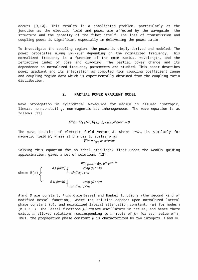
A and B are constant, Jl and Kl are Bessel and Hankel functions (the second kind ofmodified Bessel function), where the solution depends upon normalized lateralphase constant (u), and normalized lateral attenuation constant, (w) for modes l(0,1,2,…). The Bessel functions Jl (ur/a) are oscillatory in nature, and hence thereexists m allowed solutions (corresponding to m roots of J1) for each value of l.Thus, the propagation phase constant β is characterized by two integers, l and m.

3

Single mode fiber (SMF) has dominant mode, LP01 with normalized frequency,V=2.405. It has two radii with two refractive indices n1 n≈ 2 where n1 and n2 arecore and cladding respectively, and the radius is discontinuous at r=a. When twocoupled fibers are being fused and pulled, the value changes depending on thewavelength source and material of the fibers. At coupling region the changes ofsome optical parameters are due to the structural and geometrical properties ofthe fibers. Fiber sizes are decreased and increased on the left and rightcoupling region. At the center of the coupling region it is assumed to beconstant. Consider the pulling length of fibers as follows,

PL= PL1 + PL2 + PL3,

where PL1 = PL3 and PL2=CL (CL is coupling length).Power propagation (P) along coupling region can be reflected and transmitted as anormalized frequency. The total power input and output must however beconservative. Total scalar power for core and cladding power can be defined asfollows [12],

P = Pcore + Pcladding

P = (constant) [ |Ψ (r,φ)|2r dr dφ + |Ψ (r,φ)|2r dr dφ ]

then, P = C π a2 [{ 1 - } + { - 1}]

P = C π a2 (V2/u2) [ ] (1)

where C is constant of A and B, a is core radius, u is normalized lateral phaseconstant, w is the normalized lateral attenuation constant, K is the second kindof modified Bessel function of order l. For a k range species of coupling region,total power can be written as a sum of partial power,

P =

The subscript of k is (+), (0) or (-) and then, the value of

is a

function of P = P(a,V,u,w), resulting in a set of equations in z direction,

= {C π a2 (V2/u2) [ ]}

4

= { C π [a2 V2 (1/u2) + (a2/u2) (V2) + (V2/u2) (a2)] }

x { } + {C π a 2 (V2/u2) [

]} (2)

For simplicity, the first, second and third term of the Equation (2) will benoted as the following,

= {[A] x [B]} – [C]

(3) Firstly, consider {[A] x [B]} as a function of u, V, and a, where

u2 (k≡ 2n12 - βlm

2)a2

w2 (β≡ lm2 - k2n2

2)a2; β1= kn1 ; β2= kn2 (4)V = (u2 + w2)1/2 = (2πa/λ) (n1

2 – n22)1/2

where l and m are the number of modes, β is the propagation constant and k is thewave number. The left hand side of Equation (4) have parametric values dependenton the values of u=u(a,k,n1,βlm), w=w(a,k,n2,βlm), and V=V(a,n1,n2,λ) [12]. The value of βlm iscalculated from the normalized propagation constant b, which is equal to (β2

lm- β2)/(β1- β2). Since w is a part of K function, then it can be derived by the K functionitself. Evaluating these functions separately over z direction we find,

u = [(ak2n12da/dz + ka2n1

2dk/dz + n1k2a2 dn1/dz) – (aβlm2da/dz + βlm a2dβlm/dz)] / (u)

βlm = [ β2(dβ2/dz) + blm( β1 dβ1/dz - β2 dβ2/dz)] / (βlm) V = 2{(π/λ)(n1

2– n22)1/2da/dz + πa(n1

2–n22)1/2[d(1/λ)/dz] dλ/dz

(5) + (2πa/λ) [½ (n1

2 –n22)-1/2] (n1dn1/dz - n2 dn2/dz)}

where dblm/dz is expected to be zero, and thus can be ignored. The first andsecond terms of Equation (3) can be rewritten by combining Equation (5) asfollows:

{[A] x [B]} = { 2C π [- u-3 a2 V2 + V (a2/u2) + a (V2/u2) ] }

x { } (6)

The K function can be derived by the first order resulting in,

[C] = C π a2 (V2/u2)

5

x { }(7)

Equations (6) and (7) are then combined to have a solution of Equation (3). Inorder to obtain a complete solution, the second kind of modified Bessel functionof order l is substituted by a recurrence relation for a given function as

Then it is finally given by, (I)

= [ 2C π {- u-3 a2 V2 + V (a2/u2) + a (V2/u2) }

(II) (III) х { } ] - [ C π a2 (V2/u2) х

(IV) (V)(VI) (VII)

{

(VIII)

} ]

(8)

Equation (8) can be computed by setting a number of known parameters andevaluated within the boundary conditions of coupling region as defined byEquation (3). Since the total power obeys the energy conservation law, then P=0. It can then be applied for each k region as

= P|+ + P|0 + P|- = 0

The value of P|+ corresponds to positive gradient where the radius of fibers isdecreased and negative gradient when the radius of fibers is increased at P|- .At PL2, it is assumed that P|0 0. ≈ For a simplified partial power model, the fibersare set by a certain temperature and the change of fiber properties asinhomogeneous. At PL1 the value of a linearly changes as same as n1 and n2 towardsthe temperature. Meanwhile, the wavelength linearly depends upon n1 and n2. These

6

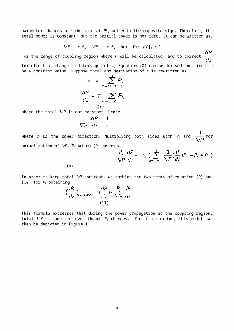
parameter changes are the same at PL3 but with the opposite sign. Therefore, thetotal power is constant, but the partial power is not zero. It can be written as,

P|+ ≠ 0, P|- ≠ 0, but for P|0 0 ≈

For the range of coupling region where P will be calculated, and to correct

for effect of change in fibers geometry, Equation (8) can be derived and fixed tobe a constant value. Suppose total and derivation of P is rewritten as

P =

=

(9)where the total P is not constant. Hence

=

where z is the power direction. Multiplying both sides with Pk and for

normalization of P, Equation (9) becomes

= Pk

(10)

In order to keep total P constant, we combine the two terms of equation (9) and(10) for Pk obtaining

(11)

This formula expresses that during the power propagation at the coupling region,total P is constant even though Pk changes. For illustration, this model canthen be depicted in Figure 1.

7

Torch Flame

Pa

Pb

Po P1 P|+= P1+(dP1 /dz) z P|0=P2 P|-=P2+(dP2 /dz)z P1 z

Core Cladding PL1 PL2 PL3

Figure 1. SMF-28e® coupler fiber is heated by H2 gas at the temperature of 800-1350C. The core and cladding reduce 75-90% in size after fusion. Total pulling offibers to the left and right side is in the range of 7500-9500μm with a velocity of≈100μm/s. Pulling is stopped subject to the coupling ratio achieving a pre-setvalue.

3. INTEGRATION OF POWER AND DISCUSSION

The values of P partially change at the coupling region are integrated over zdirection of core radius and a half pulling length. It is run in Ode45 Matlabplatform with a set of input data for refractive index of core and cladding, wavelength and initial P. For the given values of equation (4), it shows that at PL1 ,the result is as follows:

( a)|+ = 1044.3864 to 796.8127 x 10-6,( λ)|+n1 = -0.0006542 to -0.0010101 x 10-9, ( λ)|+n2 = -0.0008376 to -0.0012823 x 10-9, (n1)|+ = 1.05 to 1.65 x 10-6, (n2)|+ = 1.35 to 2.05 x 10-6, (12) da/dz = 7.9681 to 9.0039 x 10-4, dk/dz = 2.3952 to 3.6983,

8

dn1/dz = 1.05 to 1.65 x 10-6, dn2/dz = 1.35 to 2.05 x10-6

dβ1/dz = 8.5516 to 13.3419, dβ2/dz = 9.9779 to 15.2409, dβlm/dz = 9.2064 to 14.2137, u = 322.5195 to 364.4422, V = 475.5291 to 537.3407

These parametric values exist as a result of the coupling ratio in the range of 1to 75%. It has a function of coupling coefficient and produces the parametricvalues gradients existing in that number range. The value of λo/λ=n moves todecrease along PL1 until it meets the coupling length and inversely increasesalong PL3. The equation (12) is similar to PL3 but the gradient is in the oppositesign.

The graph of P at PL1, as calculated from Equation (11) is the power gradient atthe first and end of the coupling region as depicted in Figure 2.

Figure 2. P along coupling region;P =1.18 at first of PL1 and 1.26 at end of PL1 at coupling region z = 3.75x10-3m

Comparing the two curves, it shows that the change of partial P is slightlydifferent rather than that shown at end of PL1. It shows that end of PL1 hasdecreased slightly due to the fact of pulling length and heating of fibers at endof PL1. It also meant that the higher gradient to reach coupling length hasresulted in the more reflection of power to the source fiber and crosstalk fiberdue to the refractive indices gradient and more loss of power from the core to

9

the cladding and to the edge cladding due to the radius gradient. This resulthas the same values for PL3 but in the negative gradient.

If we assume that partial P is not linear and exponentially decreasing orincreasing. Suppose it is affected by the function factor P=P(1+e-α) then theradius is not proportional to the speed of pulling length. The function factorP=P(1-e-α) suggests that the fibers are not precisely heated at the center of fibersand the gradient of refractive indices will be close to factor 10-3. However,these reasons are negligible, since the mechanical process of the fabrication isfixed and the radius change is much more significant than the other parameters.

Table I. Calculation of partial P in each term of Equation (8)No. Calculation Result Term1 (0.2857 – 0.0546i) to (0.3229 –

0.006171i)I

2 (0.9899 + 0.5456i) II3 (-7.3511 x 10-4 + 1.45057 x 10-4i) III4 (0.1154 – 0.1875i) IV,VII5 (-0.3056-0.2007i) V,VII6 (0.0177 + 0.6021i) VI7 (0.1154 – 0.1876i) V,VI,VII8 (-0.2169 + 0.4334i) VIII9 (0.3126 + 0.10181i) to (0.3533 +

0.1150i)I and II

10 (-1.847 x10-5 – 4.0113 x 10-5i) III toVIII

11 (0.3126 + 0.1018i) to (0.3533 +0.1150i)

I toVIII

Based on Table I, the results are significantly affected by multiplication ofterm I and II by a factor of 10-1 rather than multiplication of term III untilterm VIII. Before being derived, term II is comparable to term I in contributingthe power. In fact, the order of l deserves to the balancing of term I, but termIII is too high a factor by the order of 10-4, then the effect of power gradientis seemingly contributed by term I. The main influence of term III is the valueof core radius by factor of a2 which similarly occurs in term I. However, sinceterm I is a summation operation ultimately it will diminished. Therefore,partialP is reduced by the value of a and otherwise increased by K function of lorder in term II. In other words, in summation operation, K function is dominantbut in reduced operation, the value of a becomes significant. The partial powergradient at PL1 and PL3 results in parametric changes to reduce or to add powersignificantly along coupling region. This calculation can be seen in Figure 3(a)and Figure 3(b) as illustration.

10

As shown by the straight lines in Figure 3, when power gradient is integrated, itdescribes the first PL1 as higher than that of end PL1. The left coupling regionis set at z=0 and let the power curves move from P input to the output at 3.75 x10-3mm. This phenomena expresses the change of each parameter of P is set nearlylinear although the actual changes are not obvious. One of the parametric valuesof P is evaluated in linear assumption that gives a significant dependence inchanging to both gradient and integral of P is radius of core by order 10-3.Refractive indices and wavelength do not necessarily have linear relationshipsince refractive indices and wavelength difference are by the order of 10-6 and10-9 respectively. Therefore the linear effect is maintained to retain the modeat LP01. The P input value changes at coupling length position from 1 mW to 0.31mWfor one core and 0.62mW for two cores. Implicitly it shows that the partial powertransmission will reduce along the coupling region as a result of refractiveindices, core geometry and separation of fiber axis between the cores. Thispartial power results seem to be very significant, but actually it decreases orincreases partially from one core source radiates to its cladding and also toanother core and cladding when coupled.

Figure 3 (a)

1mW z

1 cladding

dP/dz 1 cladding

0.62mW (2 cores)

11

Power

Power in Power out

From first of PL1 to end of PL3

Power of two

0.31mW (1core) Coupling length

Figure 3 (b)

Figure 3. P integration over coupling region (power source of one core); 3(a) and Illustration of power propagation; 3(b)

Table 2 describes the details of parametric value changes along the couplingregion. A validation of code results is maintained by the initial and final P,while at the coupling region (excluding coupling length) it is assumed to changelinearly.

Table 2. Power parameters of coupled SMF-28e® Paramete

r at first of

PL1

at end ofPL1

atPL2

at first ofPL3

at end ofPL3

z

position

0 3.75x10-3

5.42x10-3 7.5x10-3mm

λ 0 to 4.5x10-9

(+)

0 to 7x10-9

(+)

0 0 to -7x10-9

(-)

0 to -4.5x10-

9 (-)

a 0 to 1.5

(+)

0 to 2

(+)

0 0 to -2

(-)

0 to -1.5

(-)n1,n2 0 to -

2.55x10-7 (-)

0 to -

3.48x10-7(-)

0 0 to

3.48x10-7(+)

0 to

2.55x10-7(+)

βlm 0 to 0.035

(+)

0 to 0.054

(+)

0 0 to 0.054

(-)

0 to 0.035

(-)u 0 to 1.2

(+)

0 to 1.38

(+)

0 0 to 1.38

(-)

0 to 1.2

(-)V 0 to 1.8

(+)

0 to 2

(+)

0 0 to -2

(-)

0 to -1.8

(-) Initial SMF-28e® V= V1 = 2.4506; n1=1.4677 and n2=1.4624; and a= 4.1 x 10-6m The initial core and cladding diameter are respectively 8.2μm and 125μm C = 6.4032x106 – 1.2245x106i, P=1mW; Pcladding/Ptotal = 0.1702, Pcore/Ptotal = 0.8298, After Fusion: V= V2 = 0.9761- 0.3353; n1=1.4623-1.4640; n2=1.4556-1.4577; and a= 0.5-1.5

x 10-6m (V, V1 and V2 values are calculated from refractive indices known. The symbol of(+) and (-) indicates positive and negative gradient respectively and deal with along each z direction 0 to 3.75x 10-3mm).

12

4. CONCLUSION

Coupling ratio range of 1 to 75% with coupling coefficient at 0.6-0.9/mm ofcoupled fibers has successfully been derived for partial power gradient and itsintegration along the coupling region. Normalized frequency and power gradientgive significant parametric changes over power transmission into fiber atcoupling region from the power source of one core. The core radius is much moreaffected to P rather than the refractive indices and wavelength although theychange linearly.

ACKNOWLEDGMENT

We would like to thank the Government of Malaysia, Universiti Teknologi Malaysia,University of Riau, Indonesia and International Development Bank (IDB) for theirgenerous support in this research.

REFERENCES

1. L.B. Jeunhomme, M Dekker, Single Mode Fiber Optics. Principles and Applications, MarcelDekker Inc., New York, 1990.

2. E. Pone, X. Daxhelet and S. Lacroix, “Refractive Index Profile of Fused-Tapered Fiber Couplers”, Optic Express 12(13), 2909-2918, (2004).

3. Saktioto. A. Jalil, R.A. Rosly, M Fadhali, Z. Jasman, “Coupling Ratioand Power Transmission to Core and Cladding Structure for a FusedSingle Mode Fiber”, J.Komunikasi Fisika Indonesia, 5(11), 209-212, (2007).

4. J. M. Senior, Optical Fiber Communications, Principles and Practice. 2nd edition, PrenticeHall of India, New Delhi,1996.

5. B. Ortega and L. Dong, “Selective Fused Couplers Consisting of a MismatchedTwin-Core Fiber and a Standard Optical Fiber”, J.Lightwave Tech. 17(1), 123-128(1999).

6. N. Kashima, Passive Optical Components for Optical Fiber Transmission,: British LibraryCataloging in – Publication Data. Artech House Inc., London, 1995.

7. H. A. Hauss, Waves and Fields in Optoelectronics, Prentice-Hall Inc., Series inSolid State Physics Electronics. Holonyak. N. Jr. Editor, Nee York, 1984.

8. A. Yariv and P. Yeh, Optical Waves in Crystals, Propagation and Control of LaserRadiation, John Wiley and Sons, Hoboken, New Jersey, 2003.

9. A. Sharma, J Kompella and P.K. Mishra, “Analysis of Fiber DirectionalCouplers and Coupler Half-Block Using a New Simple Model for Single-ModeFiber”, J.Lightwave Technology, 8(2), 143-151, (1990).

13

10. I. Yokohama, J. Noda and K Okamoto, Fiber-Coupler Fabrication with AutomaticFusion-Elongation Processes for Low Excess Loss and High Coupling-RatioAccuracy, J.Lightwave Technology, 5(7), 910-915, (1987).

11. A. D.Yablon, Optical Fiber Fusion Splicing, Springer-Verlag Berlin, Heidelberg,Germany, 2005.

12. R. P. Khare, Fiber Optics and Optoelectronics, Oxford University Press, New Delhi,India, 2004.

14