Simple models for dynamic hysteresis loop calculations of ...

Simple models for dynamic hysteresis loop calculations of magneticsingle-domain nanoparticles: Application to magnetic hyperthermiaoptimization

J. Carrey,a) B. Mehdaoui, and M. RespaudUniversite de Toulouse, INSA, UPS, Laboratoire de Physique et Chimie des Nano-Objets (LPCNO), 135Avenue de Rangueil, F-31077 Toulouse, France and CNRS, UMR 5215, LPCNO, F-31077 Toulouse, France

(Received 12 July 2010; accepted 31 December 2010; published online 21 April 2011; publisher

error corrected 26 April 2011)

To optimize the heating properties of magnetic nanoparticles (MNPs) in magnetic hyperthermia

applications, it is necessary to calculate the area of their hysteresis loops in an alternating magnetic

field. The separation between “relaxation losses” and “hysteresis losses” presented in several articles is

artificial and criticized here. The three types of theories suitable for describing hysteresis loops of

MNPs are presented and compared to numerical simulations: equilibrium functions, Stoner–Wohlfarth

model based theories (SWMBTs), and a linear response theory (LRT) using the Neel–Brown

relaxation time. The configuration where the easy axis of the MNPs is aligned with respect to the

magnetic field and the configuration of a random orientation of the easy axis are both studied. Suitable

formulas to calculate the hysteresis areas of major cycles are deduced from SWMBTs and from

numerical simulations; the domain of validity of the analytical formula is explicitly studied. In the case

of minor cycles, the hysteresis area calculations are based on the LRT. A perfect agreement between

the LRT and numerical simulations of hysteresis loops is obtained. The domain of validity of the LRT

is explicitly studied. Formulas are proposed to calculate the hysteresis area at low field that are valid for

any anisotropy of the MNP. The magnetic field dependence of the area is studied using numerical

simulations: it follows power laws with a large range of exponents. Then analytical expressions derived

from the LRT and SWMBTs are used in their domains of validity for a theoretical study of magnetic

hyperthermia. It is shown that LRT is only pertinent for MNPs with strong anisotropy and that

SWMBTs should be used for weakly anisotropic MNPs. The optimum volume of MNPs for magnetic

hyperthermia is derived as a function of material and experimental parameters. Formulas are proposed

to allow to the calculation of the optimum volume for any anisotropy. The maximum achievable

specific absorption rate (SAR) is calculated as a function of the MNP anisotropy. It is shown that an

optimum anisotropy increases the SAR and reduces the detrimental effects of the size distribution of

the MNPs. The optimum anisotropy is simple to calculate; it depends only on the magnetic field used in

the hyperthermia experiments and the MNP magnetization. The theoretical optimum parameters are

compared to those of several magnetic materials. A brief review of experimental results as well as a

method to analyze them is proposed. This study helps in the determination of suitable and unsuitable

materials for magnetic hyperthermia and provides accurate formulas to analyze experimental data. It is

also aimed at providing a better understanding of magnetic hyperthermia to researchers working on this

subject. VC 2011 American Institute of Physics. [doi:10.1063/1.3551582]

I. INTRODUCTION

Magnetic hyperthermia is a promising cancer treatment

technique that is based on the fact that magnetic nanoparticles

(MNPs) placed in an alternating magnetic field release heat.

Active research is being done to improve the specific absorp-

tion rate (SAR) of MNPs, which could permit the treatment of

tumors of a smaller size1 and could reduce the amount of ma-

terial that must be injected to treat a tumor of a given size.

If an assembly of MNPs is put into an alternating mag-

netic field of frequency f and amplitude l0Hmax, the amount

of heat A released by the MNPs during one cycle of the mag-

netic field simply equals the area of their hysteresis loop,

which can be expressed as

A ¼ðþHmax

�Hmax

l0MðHÞdH; (1)

where M(H) is the NP magnetization. Then the SAR is:

SAR ¼ Af : (2)

As will be described in more detail in the following text, Adepends, in a very complex manner, on the characteristics of

the NPs: A depends on the NPs’ effective anisotropy Keff,

their volume V, the temperature T, the frequency and ampli-

tude of the magnetic field, and eventually magnetic interac-

tions between NPs. It is thus crucial to be able to evaluate Aas precisely as possible as a function of these parameters to

target the optimum parameters for the required application.

a)Author to whom correspondence should be addressed. Electronic mail:

[email protected].

0021-8979/2011/109(8)/083921/17/$30.00 VC 2011 American Institute of Physics109, 083921-1

JOURNAL OF APPLIED PHYSICS 109, 083921 (2011)

Downloaded 22 May 2011 to 195.83.11.66. Redistribution subject to AIP license or copyright; see http://jap.aip.org/about/rights_and_permissions

http://dx.doi.org/10.1063/1.3551582

http://dx.doi.org/10.1063/1.3551582

http://dx.doi.org/10.1063/1.3551582

http://dx.doi.org/10.1063/1.3551582

The theoretical literature on the properties of MNPs is

very large. Of this large number of articles, those related to

the evolution of the hysteresis area with the intrinsic parame-

ters of the MNPs are of interest for magnetic hyperthermia

applications.2–8 A few theoretical papers have also been

devoted specifically to the problem of magnetic hyperther-

mia.1,9–14 However, the articles published on this subject are

not complete and are sometimes inaccurate. First, the major-

ity of the articles are mainly based on the linear response

theory (LRT), which, as will be shown later, is not the most

useful for magnetic hyperthermia. Second, when using theo-

ries derived from the Stoner–Wohlfarth model, the domain

of validity is not taken into account, and, more importantly,

central conclusions that could be derived from them are

missing. Third, in articles published by Hergt et al., an artifi-

cial separation of the mechanisms responsible for the heating

is made between “hysteresis losses” and “relaxation losses.”

This separation is improper or at least very confusing; in our

opinion, it is detrimental to a deep understanding of mag-

netic hyperthermia and to correct usage of the models to cal-

culate SARs. Unfortunately, the paradigmatic presentation of

magnetic hyperthermia by a large number of experimental

articles still follows this separation. Finally, a recent article

by N. A. Usov has used numerical simulations of hysteresis

loops to study hyperthermia.14 Although this article draws

qualitatively correct conclusions, it is based on the study of

examples and does not provide a generalization and a quanti-

tative approach to the problem.

The present article aims to give a complete and rigorous

presentation of the theory of magnetic hyperthermia. First, in

Sec. II, we will provide a global view of the three types of

theories suitable for the calculation of the hysteresis loop

areas of MNPs, and we will give simple analytical formulas

for this purpose; this will include a precise determination of

their domain of validity using numerical calculations. A clar-

ification of the issue concerning hysteresis vs relaxation

losses will also be done in this section. Numerical simula-

tions will be used to illustrate the variety of curves that could

be obtained experimentally when measuring the magnetic

field dependence of the SAR. In Sec. III, the previous results

will be used for a specific study of magnetic hyperthermia. It

will be shown that the LRT is only pertinent for strongly ani-

sotropic MNPs; for weakly anisotropic MNPs, theories

derived from the Stoner–Wohlfarth model should be used

instead. Formulas that predict the optimum volume of MNPs

as a function of material and experimental parameters will

be provided. Additionally, it will be shown that the anisot-

ropy of the MNPs is the central parameter for the optimiza-

tion of magnetic hyperthermia because it determines both

the maximum achievable SAR and controls the influence of

the size distribution of MNPs on the SAR. A simple formula

to determine the optimum anisotropy for magnetic hyper-

thermia will be proposed, and a comparison with the parame-

ters of bulk magnetic materials will be done. This study

should help to determine suitable and unsuitable materials

for magnetic hyperthermia, and it will provide accurate for-

mulas to analyze experimental data. We also hope it will

lead to a better understanding of magnetic hyperthermia for

researchers in this field.

II. NUMERICAL CALCULATIONS AND ANALYTICALEXPRESSIONS OF HYSTERESIS LOOPS

A. Single-domain uniaxial nanoparticles in a magneticfield

Let us consider a MNP of volume V composed of a fer-

romagnetic material having a spontaneous magnetization MS

and a magnetocrystalline anisotropy. Below a critical vol-

ume, the MNP becomes single domain to minimize its mag-

netic energy. Because all the spins are parallel to one

another, one can model the magnetization as a single giant

magnetic moment l¼MSV, the amplitude of which does not

depend on its spatial orientation; these are the so-called

“macrospin” and coherent rotation approximations. As a

result of magnetic anisotropy, l is generally pinned along

well-defined directions, that is, along its magnetic anisotropy

axis. As a result of several contributions, among them the

magnetocrystalline, shape, and surface contributions that

arise from spherical deviations, the anisotropy can be very

complex. Indeed these numerous contributions have neither

the same symmetries (cubic versus uniaxial) nor the same

directions. Nevertheless one of these contributions domi-

nates and determines the main first-order contribution. From

a practical point of view, one generally concludes from the

experimental studies that the anisotropy displays a first-

order-dominant uniaxial character. Thus considering the

macrospin approximation and an effective uniaxial anisot-

ropy (Keff), the energy of a MNP placed in an external mag-

netic field (l0Hmax) is given by the following:2

Eðh;/Þ ¼ KeffV sin2ðhÞ � l0MSVHmax cosðh� /Þ; (3)

where h is the angle between the easy axis and the magnetiza-

tion and / is the angle between the easy axis and the magnetic

field [see Fig. 1(a)]. In the following, we will use the dimen-

sionless parameters r¼KeffV/kBT and n¼ l0MSVHmax/kBT.

The reduced magnetic energy normalized to the thermal energy

is

Eðh;/ÞkBT

¼ r sin2ðhÞ � n cosðh� /Þ: (4)

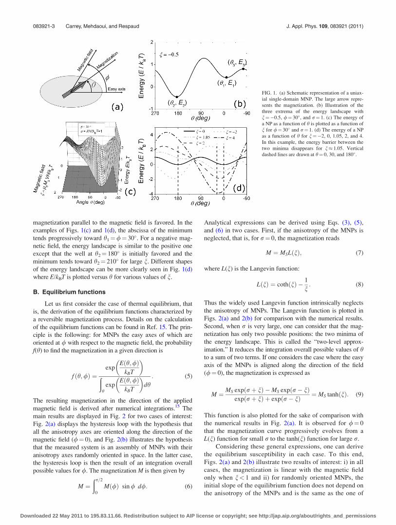
Figure 1(c) displays the reduced magnetic energy as a func-

tion of the normalized magnetic field (n varies between 0

and 2) and the angle h for a given particle orientation,

/¼ 30� and r¼ 1. Two different shapes are noticeable.

When l0Hmax is greater than the anisotropy field

l0HK¼ 2Keff/MS, the energy landscape displays only one

minimum, which defines the equilibrium position, that is,

along the anisotropy axis direction. Conversely, when

l0Hmax is less than l0HK, the energy profile as a function of

h displays two minima at the coordinates (h1, E1) and (h2,

E2) and two maxima. We will refer to (h3, E3) as the saddle

point, i.e., the smaller maximum [see Fig. 1(b)]. For n¼ 0

(in the absence of magnetic fields), the magnetization can

take two equivalent equilibrium values at h1¼ 0� and

h2¼ 180�, that is, along its easy axis [see Figs. 1(c) and

1(d)]. For a finite positive n, the magnetic field favors one of

the two minima (here, the one initially at h1¼ 0�). Increasing

n moves the abscissa of this minimum progressively so that a

083921-2 Carrey, Mehdaoui, and Respaud J. Appl. Phys. 109, 083921 (2011)


magnetization parallel to the magnetic field is favored. In the

examples of Figs. 1(c) and 1(d), the abscissa of the minimum

tends progressively toward h1¼/¼ 30�. For a negative mag-

netic field, the energy landscape is similar to the positive one

except that the well at h2¼ 180� is initially favored and the

minimum tends toward h2¼ 210� for large n. Different shapes

of the energy landscape can be more clearly seen in Fig. 1(d)

where E/kBT is plotted versus h for various values of n.

B. Equilibrium functions

Let us first consider the case of thermal equilibrium, that

is, the derivation of the equilibrium functions characterized by

a reversible magnetization process. Details on the calculation

of the equilibrium functions can be found in Ref. 15. The prin-

ciple is the following: for MNPs the easy axes of which are

oriented at / with respect to the magnetic field, the probability

f(h) to find the magnetization in a given direction is

f ðh;/Þ ¼exp

Eðh;/ÞkBT

� �ð

hexp

Eðh;/ÞkBT

� �dh: (5)

The resulting magnetization in the direction of the applied

magnetic field is derived after numerical integrations.15 The

main results are displayed in Fig. 2 for two cases of interest:

Fig. 2(a) displays the hysteresis loop with the hypothesis that

all the anisotropy axes are oriented along the direction of the

magnetic field (/¼ 0), and Fig. 2(b) illustrates the hypothesis

that the measured system is an assembly of MNPs with their

anisotropy axes randomly oriented in space. In the latter case,

the hysteresis loop is then the result of an integration overall

possible values for /. The magnetization M is then given by

M ¼ðp=2

0

M /ð Þ sin / d/: (6)

Analytical expressions can be derived using Eqs. (3), (5),

and (6) in two cases. First, if the anisotropy of the MNPs is

neglected, that is, for r¼ 0, the magnetization reads

M ¼ MSLðnÞ; (7)

where L(n) is the Langevin function:

LðnÞ ¼ cothðnÞ � 1

n: (8)

Thus the widely used Langevin function intrinsically neglects

the anisotropy of MNPs. The Langevin function is plotted in

Figs. 2(a) and 2(b) for comparison with the numerical results.

Second, when r is very large, one can consider that the mag-

netization has only two possible positions: the two minima of

the energy landscape. This is called the “two-level approx-

imation.” It reduces the integration overall possible values of hto a sum of two terms. If one considers the case where the easy

axis of the MNPs is aligned along the direction of the field

(/¼ 0), the magnetization is expressed as

M ¼ MS expðrþ nÞ �MS expðr� nÞexpðrþ nÞ þ expðr� nÞ ¼ MS tanhðnÞ: (9)

This function is also plotted for the sake of comparison with

the numerical results in Fig. 2(a). It is observed for /¼ 0

that the magnetization curve progressively evolves from a

L(n) function for small r to the tanh(n) function for large r.

Considering these general expressions, one can derive

the equilibrium susceptibility in each case. To this end,

Figs. 2(a) and 2(b) illustrate two results of interest: i) in all

cases, the magnetization is linear with the magnetic field

only when n< 1 and ii) for randomly oriented MNPs, the

initial slope of the equilibrium function does not depend on

the anisotropy of the MNPs and is the same as the one of

FIG. 1. (a) Schematic representation of a uniax-

ial single-domain MNP. The large arrow repre-

sents the magnetization. (b) Illustration of the

three extrema of the energy landscape with

n¼�0.5, /¼ 30�, and r¼ 1. (c) The energy of

a NP as a function of h is plotted as a function of

n for /¼ 30� and r¼ 1. (d) The energy of a NP

as a function of h for n¼�2, 0, 1.05, 2, and 4.

In this example, the energy barrier between the

two minima disappears for n� 1.05. Vertical

dashed lines are drawn at h¼ 0, 30, and 180�.



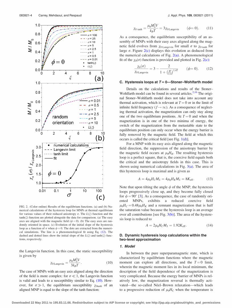
the Langevin function. In this case, the static susceptibility

is given by

v0 Langevin ¼l0M2

SV

3kBT: (10)

The case of MNPs with an easy axis aligned along the direction

of the field is more complex: for r� 1, the Langevin function

is valid and leads to a susceptibility similar to Eq. (10). How-

ever, for r� 1, the equilibrium susceptibility v0tanh of an

aligned MNP is equal to the slope of the tanh function:

v0 tanh ¼l0M2

SV

kBT¼ 3v0 Langevin ð/¼ 0Þ: (11)

As a consequence, the equilibrium susceptibility of an as-

sembly of MNPs with their easy axes aligned along the mag-

netic field evolves from v0 Langevin for small r to v0 tanh for

large r. Figure 2(c) displays this evolution as deduced from

the numerical calculations of Fig. 2(a). A phenomenological

fit of the v0(r) function is provided and plotted in Fig. 2(c):

v0ðrÞv0 Langevin

¼ 3� 2

1þ r3:4

� �1:47ð/¼ 0Þ: (12)

C. Hysteresis loops at T 5 0—Stoner–Wohlfarth model

Details on the calculations and results of the Stoner–

Wohlfarth model can be found in several articles.2,16 The origi-

nal Stoner–Wohlfarth model does not take into account any

thermal activation, which is relevant at T¼ 0 or in the limit of

infinite field frequency ( f!1). As a consequence of neglect-

ing thermal activation, the magnetization can only stay along

one of the two equilibrium positions. At T¼ 0 and when the

magnetization is in one of the two minima of energy, the

switch of the magnetization from the metastable state to the

equilibrium position can only occur when the energy barrier is

fully removed by the magnetic field. The field at which this

occurs is called the critical field [see Fig. 1(d)].

For a MNP with its easy axis aligned along the magnetic

field direction, the suppression of the anisotropy barrier by

the magnetic field occurs at l0HK. The resulting hysteresis

loop is a perfect square, that is, the coercive field equals both

the critical and the anisotropy fields in this case. This is

shown using numerical calculations in Fig. 3(a). The area of

this hysteresis loop is maximal and is given as

A ¼ 4l0HCMS ¼ 4l0HKMS ¼ 8Keff : (13)

Note that upon tilting the angle / of the MNP, the hysteresis

loops progressively close up, and they become fully closed

for /¼ 90� [3]. As a consequence, the case of randomly ori-

ented MNPs, exhibits a reduced coercive field

l0HC¼ 0.48l0HK and a remnant magnetization that is half

the saturation value because the hysteresis loop is an average

over all contributions [see Fig. 3(b)]. The area of the hystere-

sis loop is reduced to

A ¼ 2l0HCMS ¼ 1:92Keff : (14)

D. Dynamic hysteresis loop calculations within thetwo-level approximation

1. Model

In between the pure superparamagnetic state, which is

characterized by equilibrium functions where the magnetic

moment can explore all directions, and the T¼ 0 limit,

wherein the magnetic moment lies in its local minimum, the

description of the field dependence of the magnetization is

very complicated. Because the energy barrier of MNPs is rel-

atively low, the magnetization reversal is thermally acti-

vated—the so-called Neel–Brown relaxation—which leads

to a progressive reduction of l0HC when the temperature is

FIG. 2. (Color online) Results of the equilibrium functions. (a) and (b) Nu-

merical calculations of the hysteresis loop for MNPs at thermal equilibrium

for various values of their reduced anisotropy r. The L(n) function and the

tanh(n) function are plotted alongside the data for comparison. (a) The easy

axes are aligned with the magnetic field (/¼ 0). (b) The easy axes are ran-

domly oriented in space. (c) Evolution of the initial slope of the hysteresis

loop as a function of r when /¼ 0. The dots are extracted from the numeri-

cal simulations. The line is a phenomenological fit using Eq. (12). The

dashed and dotted lines show the initial slope of the L(n) and tanh(n) func-

tions, respectively.



raised. Decreasing the sweeping rate of the magnetic field

has similar consequences.3–5,8 The incorporation of these

effects in a model is far from easy. Within the two-level

approximation, one neglects excited states inside each well

so that dynamic loop calculations only depend on the two

minima (h1, E1) and (h2, E2) and on the saddle point (h3, E3).

When the applied magnetic field is below l0HK, the magnet-

ization can switch from the h1 to the h2 direction at a rate m1

given by

v1 ¼ v01 exp �E3 � E1

kBT

� �: (15)

Similarly, the switching rate m2 from the h2 to the h1 direc-

tion is given by

v2 ¼ v02 exp �E3 � E2

kBT

� �: (16)

The attempt frequencies v01 and v0

2 are complex functions of

the material parameters (gyromagnetic ratio, damping, MS

and Keff) and experimental conditions (temperature and

magnetic field).17,18 For the sake of simplicity, we will keep

these frequencies constant and equal to 1010 Hz.

In the various theoretical articles dealing with the influ-

ence of a finite temperature and frequency in the Stoner–

Wohlfarth model, the numerical methods and approxima-

tions to include these thermally activated jumps vary. In their

numerical simulations, Garcia-Otero et al. have taken the

crude approximation that the switching occurs as soon as

DE(l0Hmax,/)¼ (E3�Ei)¼ kBT where i identifies the start-

ing well.5 Pfeiffer et al. assumed that the switch from one

well to the other occurs when the relaxation time over the

barrier matches a “measurement time” sm.4 In both articles,

the final results for the variation of the coercive field with

temperature and frequency depends on this sm parameter.

However, trying to define the value of sm has necessarily

unphysical consequences. Indeed the coercive field mainly

depends on the sweeping rate of the magnetic field. In a

superconducting quantum interference device measurement,

one could simply take the “measurement time” as the time to

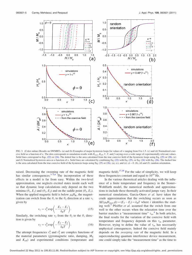
FIG. 3. (Color online) Results on SWMBTs. (a) and (b) Examples of major hysteresis loops for values of j ranging from 0 to 1.5. (c) and (d) Normalized coer-

cive field as a function of j. The dots corresponds to simulation results with Hmax, Keff, V, T, and f varying over a wide range of experimentally relevant values.

Solid lines correspond to Eqs. (22) or (24). The dotted line is the area calculated from the true coercive field of the hysteresis loops using Eq. (25) or (26). (e)

and (f) Normalized hysteresis area as a function of j. Solid lines are calculated by combining Eq. (22) with Eq. (25), or Eq. (24) with Eq. (26). The dashed line

is the area calculated from the true coercive field of the hysteresis loops using Eq. (25) or (26). (a), (c), and (e): /¼ 0. (b), (d) and (f): random orientation.



measure one point, which corresponds to Pfeiffer et al.’s cri-

teria. However, the coercive field would vary as a function

of the step value. Alternatively, one could take the time of a

complete cycle. In this case, the coercive field would vary

with the maximum applied magnetic field.

The principle of our calculation is more rigorous and is

similar to the one used by Lu et al.3 and Usov et al.8,14 A time-

dependent magnetic field H(t)¼Hmaxcos(xt) is applied to the

MNP along a direction that makes an angle / with respect to

the easy axis. To compute the magnetization, one has to calcu-

late the time dependence of p1 and p2¼ (1� p1), the probabil-

ity of finding the magnetization in the first and second

potential wells, respectively. The time evolution of p1 reads

@p1

@t¼ ð1� p1Þm2 � p1m1: (17)

Knowing the occupation probabilities, one can calculate the

magnetization according to

M ¼ MS p1 cos h1 þ ð1� p1Þ cos h2ð Þ: (18)

The resolution of the time evolution of p1 is performed using

an explicit Runge–Kutta2,3 method. With this method, the

time step is not constant but becomes shorter when p1 varies

more, which ensures an optimum compromise between cal-

culation time and precision. When there is only one mini-

mum, p1 is simply set equal to either zero or unity.

To calculate hysteresis loops for a random orientation of

MNPs, 50 cycles with / ranging from 0 to p/2 are calculated.

Then the magnetization is calculated according to Eq. (6).

We will show that using this single model, one can simulate

major and minor hysteresis loops and the behavior in the

framework of the LRT. For the latter cases, the initial condi-

tions are set to p1¼ p2¼ 0.5, and several successive hystere-

sis loops are performed until the curve converges and

becomes symmetrical with respect to the abscissa axis.

Under most conditions, only two or three cycles are neces-

sary to achieve convergence. Typical examples of the hyster-

esis loops generated will be shown in the following sections.

2. Temperature and frequency dependence of thecoercive field

Historically, the first analytical expressions for the tem-

perature dependence of the coercive field were based on the

approximation of the “measurement time” previously

described. In the /¼ 0 case, the expression of the coercive

field reads4

l0HC ¼ l0HK 1� kBT

KeffVln

sm

s0

� �� 12

" #; ð/¼ 0Þ; (19)

where s0 is the frequency factor of the Neel–Brown relaxa-

tion time defined as (see Sec. II E)

s0 ¼1

2m01

¼ 1

2m02

: (20)

In the case of randomly oriented NPs, the following analyti-

cal expression was obtained by Garcia-Otero et al.:5

l0HC � 0:48l0HK 1� kBT

KeffVln

sm

s0

� �� 34

" #:

ðrandom orientationÞ ð21Þ

We previously used the latter equation to interpret hyperther-

mia experiments with FeCo MNPs by stating that sm¼ (1/f).19

However, as mentioned in the preceding text, these analytical

formulas do not depend on the sweeping rate of the magnetic

field 4Hmaxf but on this undefined sm parameter. Recently,

Usov et al.8 proposed a novel dimensionless parameter j for

the variation of the coercive field that takes into account the

sweeping rate. In the /¼ 0 case, the coercive field is

l0HC ¼ l0HK 1� j12

� �ð/¼ 0Þ (22)

with

j ¼ kBT

KeffVln

kBT

4l0HmaxMSVf s0

� �: (23)

In Fig. 3(c), numerical calculations of hysteresis loops are

compared to Eq. (22). To achieve this, a large number of

simulations were performed with parameters varying over

a wide range of values: f (10–400 kHz), l0Hmax (0.05–5 T),

Keff (103–106 J m�3), T (0.5–500 K), and the spherical radii

of the nanoparticles (1.5–30 nm). The normalized coercive

field extracted from the hysteresis loop is then plotted as a

function of j. The fact that all the data fall onto a single mas-

ter curve confirms the relevance of the dimensionless param-

eter proposed by Usov et al.8 Our simulations are in good

agreement with the analytical expressions (22) and (23)

derived by Usov et al. as long as j is below roughly 0.5.

For the random orientation case, Usov et al. derived an

expression for the coercive field from the phenomenological

fit of their numerical simulations. However, the authors

made the assumption that the coercive field equals the criti-

cal field, which is not rigorously true for NPs with a large /,

and performed a fit over a large range of temperatures. In

Fig. 3(d), our simulations for the coercive field in the random

orientation case are shown. From the best fit of these data at

low values of j, the following formula is obtained:

l0HC ¼ 0:48l0HK b� jnð Þðrandom orientationÞ; (24)

where b¼ 1 and n¼ 0.8 6 0.05. Usov et al. found slightly

different coefficients of b¼ 0.9 and n¼ 1. The domain of va-

lidity is roughly the same as for the aligned case: Eq. (24) is

roughly valid up to j¼ 0.5. In the remainder of this article,

our own values for b and n will be used.

3. Temperature and frequency dependence of thehysteresis loop area

The aim of this subsection is to study the frequency and

temperature dependencies of the hysteresis area and to derive

general analytical expressions in the case of aligned and ran-

domly oriented MNPs. This topic has not been addressed in

the publications mentioned in the preceding text. At T¼ 0,

the area is proportional to the coercive field as given by



Eqs. (13) and (14), and the question is whether these expres-

sions are still valid when T= 0. Similar to the study of the

coercive field dependence, we estimated from numerical hys-

teresis calculations the associated area for the aligned and

randomly oriented cases; these are displayed in Figs. 3(e)

and 3(f), respectively. Examples of these hysteresis loops are

shown in Figs. 3(a) and 3(b). These data are then compared

to those calculated using the analytical expressions

AðTÞ � 4l0HCðTÞMS ð/¼ 0Þ; (25)

and

AðTÞ � 2l0HCðTÞMS ðrandom orientationÞ: (26)

The area A(T) has been calculated by using i) HC deduced

from the simulated hysteresis loops (shown as a dashed line)

and ii) HC calculated using Eqs. (22) and (24) (shown as a

solid line). The A(T) curves calculated according to the first

procedure match the exact values of the area except at large

j values (above 1). This difference is due to the reduced

squareness of the hysteresis loops. From the close compari-

son between the dots and the dashed line, it can be observed

that Eqs. (25) and (26) slightly overestimate the hysteresis

area for large j. This overestimation partially compensates

for the underestimation of the coercive field by Eqs. (22) and

(24) at high j. As a consequence, the combination of Eqs.

(22) and (24) with Eqs. (25) and (26) gives an acceptable

value of the area at higher j values than Eqs. (22) and (24)

do for the coercive field. To provide a numerical limit that

can be used later in the article, Figs. 3(e) and 3(f) show that

the area is calculated with less than 10% error when j< 0.7.

Finally, the transition toward reversible hysteresis loops

can also be deduced from this figure. If we state that the re-

versibility occurs when HC� 0.01HK, this transition can be

estimated to occur when j� 1.6.

E. Minor hysteresis loops and linear response theory

The LRT has been previously reported in several

articles.1,7,9,10 The presentation here will be slightly different

from that of other articles and will aim to explicitly illustrate

the fact that the LRT is also a model to calculate the hystere-

sis area, a point that was not always developed in previous

works. The results for MNPs aligned with the magnetic field,

not derived in previous articles, will also be given.

The LRT is a model that aims to describe the dynamic

response of an assembly of MNPs using the Neel–Brown

relaxation time. The starting assumption of this model is that

the magnetic system responds linearly with the magnetic

field and its magnetization can be put in the form

MðtÞ ¼ ~vHðtÞ; (27)

where ~v is the complex susceptibility and reads

~v ¼ v0

1

1þ ixsR: (28)

v0 is the static susceptibility defined in Sec. II B, and sR

is the time it takes for the system to relax back to equilibrium

after a small step in the magnetic field. The results of Sec. II

B showed that the magnetization is linear with the magnetic

field approximately for the condition when n< 1. A small

value of n is thus the first criterion for the validity of the

LRT; it will be more precisely studied in the following text.

Moreover, in Eq. (28), sR is a variable independent of the

magnetic field, which is only true for small deformations of

the barrier between the two equilibrium positions, i.e., when

l0Hmax� l0HK. At the magnetic field frequencies used in

hyperthermia or magnetic measurements, it can be shown

that the second condition is always verified when the first

one is (see following text). The relaxation time of the mag-

netization sR when the MNPs cannot move physically equals

the Neel–Brown relaxation time sN, which reads

sR ¼ sN ¼1

2m01

expKeffV

kBT

� �¼ s0 exp

KeffV

kBT

� �: (29)

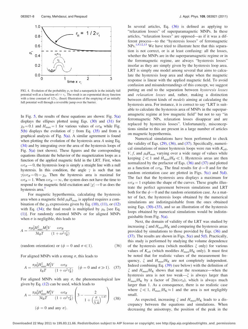
The fact that there is a factor 1/2 between s0 and the attempt

frequency m01 comes from the fact that we are dealing with a re-

versible jump in a system with two potential wells. If this point

is unclear to the reader, it is illustrated in Fig. 4. Figure 4 dis-

plays an imaginary case in which all of the MNPs are first mag-

netized in one direction and then relax at zero magnetic field

through a reversible jump over an energy barrier at a rate m1.

The probability p1 to find the MNPs in this well drops exponen-

tially to 0.5 with a time constant of 1/(2m1). Thus the relaxation

time of the magnetization is half the mean time taken by the

magnetization to reverse spontaneously. This explains the fac-

tor of 1/2 between s0 and the attempt frequency m01.

In the LRT, the response of the system to an alternating

magnetic field

HðtÞ ¼ Hmax cosðxtÞ (30)is

MðtÞ ¼ vj jHmax cosðxtþ uÞ; (31)

where u is the phase delay between the magnetization and

the magnetic field. From Eq. (28), it is straightforward to

show that

vj j ¼ v0ffiffiffiffiffiffiffiffiffiffiffiffiffiffiffiffiffiffiffi1þ x2s2

R

p ; (32)

sin u ¼ xsRffiffiffiffiffiffiffiffiffiffiffiffiffiffiffiffiffiffiffi1þ x2s2

R

p or cos u ¼ 1ffiffiffiffiffiffiffiffiffiffiffiffiffiffiffiffiffiffiffi1þ x2s2

R

p : (33)

Basic mathematics indicates that Eqs. (30) and (31) corre-

spond to the parametric equation of an ellipse in the (H, M)

plane. The area Aellipse of this ellipse and the angle c between

its long axis and the abscise axis are given by

Aellipse ¼ pH2max vj j sin u ¼ pH2

maxv0

xsR

1þ x2s2R

; (34)

and

tan 2c ¼ 2H2max vj j cos u

H2max � H2

max vj j2¼ 2v0

1þ x2s2R � v2

0

: (35)



In Fig. 5, the results of these equations are shown: Fig. 5(a)

displays the ellipses plotted using Eqs. (30) and (31) for

v0¼ 0.1 and Hmax¼ 1 for various values of xsR while Fig.

5(b) displays the evolution of c from Eq. (35) and from a

graphical analysis of Fig. 5(a). A similar agreement is found

when plotting the evolution of the hysteresis area A using Eq.

(34) and by integrating over the area of the hysteresis loops of

Fig. 5(a) (not shown). These figures and the corresponding

equations illustrate the behavior of the magnetization loops as a

function of the applied magnetic field in the LRT. First, when

xsR! 0, the hysteresis loop is simply a straight line with a null

hysteresis. In this condition, the angle c is such that tan

c(xsR¼ 0)¼ v0. Then the hysteresis area is maximal for

xsR¼ 1. When xsR!1, the system does not have the time to

respond to the magnetic field excitation and jvj! 0 as does the

hysteresis area.7

For magnetic hyperthermia, calculating the hysteresis

area when a magnetic field l0Hmax is applied requires a com-

bination of the v0 expressions given by Eq. (10), (11), or (12)

with Eq. (34); the final result is multiplied by l0 [see Eq.

(1)]. For randomly oriented MNPs or for aligned MNPs

when r is negligible, this leads to

A ¼ pl20H2

maxM2SV

3kBT

xsR

1þ x2s2Rð Þ

(random orientation) or (/ ¼ 0 and r�1Þ: ð36Þ

For aligned MNPs with a strong r, this leads to

A ¼ pl20H2

maxM2SV

kBT

xsR

1þ x2s2Rð Þ ð/ ¼ 0 and r�1Þ: (37)

For aligned MNPs with any r, the phenomenological law

given by Eq. (12) can be used, which leads to

A ¼ pl20H2

maxM2SV

3kBT

xsR

1þ x2s2Rð Þ 3� 2

1þ r3:4

� �1:47

0B@

1CA

ð/ ¼ 0 and any rÞ:

(38)

In several articles, Eq. (36) is defined as applying to

“relaxation losses” of superparamagnetic MNPs. In these

articles, “relaxation losses” are opposed—as if it was a dif-

ferent process—to the “hysteresis losses” of ferromagnetic

NPs.1,9,12,13 We have tried to illustrate here that this separa-

tion is not correct, or is at least confusing: all the losses,

whether the MNPs are in the superparamagnetic regime or in

the ferromagnetic regime, are always “hysteresis losses”

insofar as they are simply given by the hysteresis loop area.

LRT is simply one model among several that aims to calcu-

late the hysteresis loop area and shape when the magnetic

response is linear with the applied magnetic field. To avoid

confusion and misunderstandings of this concept, we suggest

putting an end to the separation between hysteresis lossesand relaxation losses and, rather, making a distinction

between different kinds of models aiming at calculating the

hysteresis area. For instance, it is correct to say “LRT is suit-

able to calculate the hysteresis area of MNPs in the superpar-

amagnetic regime at low magnetic field” but not to say “in

ferromagnetic NPs, relaxation losses disappear and are

replaced by hysteresis losses”. Unfortunately, misconcep-

tions similar to this are present in a large number of articles

on magnetic hyperthermia.

Numerical simulations have been performed to check

the validity of Eqs. (29), (36), and (37). Specifically, numeri-

cal simulations of minor hysteresis loops were run with Keff,

V, f, and l0Hmax varying over a wide range of values while

keeping n� 1 and Hmax/HK� 1. Hysteresis areas are then

normalized by the prefactor of Eqs. (36) and (37) and plotted

as a function of xsR. The final results for /¼ 0 and for the

random orientation case are plotted in Figs. 5(c) and 5(d).

The fact that the hysteresis area displays a maximum for

xsR¼ 1 explains the shape of the curves. These graphs illus-

trate the perfect agreement between simulations and LRT

both for the /¼ 0 and the random orientation case. As a mat-

ter of fact, the hysteresis loops obtained by the numerical

simulations are indistinguishable from the ones obtained

using Eqs. (30)–(33), and so an illustration of the hysteresis

loops obtained by numerical simulations would be indistin-

guishable from Fig. 5(a).

Next, the domain of validity of the LRT was studied by

increasing n and Hmax/HK and comparing the hysteresis areas

provided by simulations to those provided by Eqs. (36) and

(37). The results are shown in Figs. 5(e) and 5(f). Practically,

this study is performed by studying the volume dependence

of the hysteresis area (which modifies n only) for various

values of Keff (which modifies Hmax/HK only). It must first

be noted that for realistic values of the measurement fre-

quency, n and Hmax/HK are not completely independent.

Indeed combining Eq. (39) (see below) with the definition of

n and Hmax/HK shows that near the resonance—when the

hysteresis area is not too weak—n is always larger than

Hmax/HK by a factor of 2ln(xs0), which is always much

larger than 1. As a consequence, there is no realistic case

where n� 1, Hmax /HK� 1 and the area is not negligibly

small.

As expected, increasing n and Hmax/HK leads to a dis-

crepancy between the equations and simulations. When

decreasing the anisotropy, the position of the peak in the

FIG. 4. Evolution of the probability p1 to find a nanoparticle in the initially full

potential well as a function of t� m1. The result is an exponential decay function

with a time constant of 1/2m1. (Inset) Illustration of the emptying of an initially

full potential well through a reversible jump over the barrier.



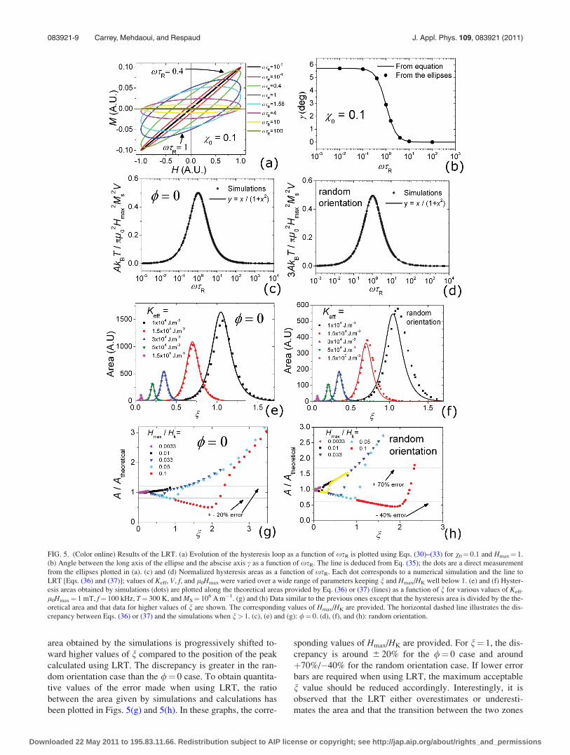
area obtained by the simulations is progressively shifted to-

ward higher values of n compared to the position of the peak

calculated using LRT. The discrepancy is greater in the ran-

dom orientation case than the /¼ 0 case. To obtain quantita-

tive values of the error made when using LRT, the ratio

between the area given by simulations and calculations has

been plotted in Figs. 5(g) and 5(h). In these graphs, the corre-

sponding values of Hmax/HK are provided. For n¼ 1, the dis-

crepancy is around 6 20% for the /¼ 0 case and around

þ70%/�40% for the random orientation case. If lower error

bars are required when using LRT, the maximum acceptable

n value should be reduced accordingly. Interestingly, it is

observed that the LRT either overestimates or underesti-

mates the area and that the transition between the two zones

FIG. 5. (Color online) Results of the LRT. (a) Evolution of the hysteresis loop as a function of xsR is plotted using Eqs. (30)–(33) for v0¼ 0.1 and Hmax¼ 1.

(b) Angle between the long axis of the ellipse and the abscise axis c as a function of xsR. The line is deduced from Eq. (35); the dots are a direct measurement

from the ellipses plotted in (a). (c) and (d) Normalized hysteresis areas as a function of xsR. Each dot corresponds to a numerical simulation and the line to

LRT [Eqs. (36) and (37)]; values of Keff, V, f, and l0Hmax were varied over a wide range of parameters keeping n and Hmax/HK well below 1. (e) and (f) Hyster-

esis areas obtained by simulations (dots) are plotted along the theoretical areas provided by Eq. (36) or (37) (lines) as a function of n for various values of Keff.

l0Hmax¼ 1 mT, f¼ 100 kHz, T¼ 300 K, and MS¼ 106 A m�1. (g) and (h) Data similar to the previous ones except that the hysteresis area is divided by the the-

oretical area and that data for higher values of n are shown. The corresponding values of Hmax/HK are provided. The horizontal dashed line illustrates the dis-

crepancy between Eqs. (36) or (37) and the simulations when n> 1. (c), (e) and (g): /¼ 0. (d), (f), and (h): random orientation.



is approximately localized around the peak in the area [see

Figs. 5(e) and 5(f)]. Therefore if we identify the zone to the

left of the peak as a “superparamagnetic regime” and the

zone to the right of the peak as a “ferromagnetic regime,”

these data can be summarized this way: for values of n above

1, the LRT overestimates the hysteresis area in the superpar-

amagnetic regime and underestimates it in the ferromagnetic

regime. Another conclusion, which will be developed later in

this article but is also visible in Figs. 5(e) and 5(f), is that

LRT is mainly useful for highly anisotropic NPs.

F. Dynamic hysteresis loops and areain the general case

We have just seen that the LRT allows one to calculate

the hysteresis area when n< 1. Similarly, SWMBTs can be

used when j< 0.7 and when the hysteresis loop is a major

hysteresis loop, that is, when the NPs are saturated by the

magnetic field. In all other cases, these theories cannot be

used, and numerical simulations are the only way to calcu-

late the hysteresis area. In this subsection, we will present

results for the hysteresis area provided completely by numer-

ical simulations. In particular, numerical simulations give us

the opportunity to study the magnetic field dependence of

the hysteresis area, which is accessible in hyperthermia

experiments by performing measurements as a function of

the magnetic field. Because the results depend on all the

external and structural parameters, there is no universal

curve or pertinent dimensionless parameters. Thus we have

only used as an illustration the magnetic parameters of bulk

magnetite and external parameters typical of hyperthermia.

When they are not being varied, the parameter values in this

section are Keff¼ 13 000 J m�3, MS¼ 106 A m�1, f¼ 100

kHz, l0Hmax¼ 20 mT, T¼ 300 K, and m10¼ 1010 Hz.

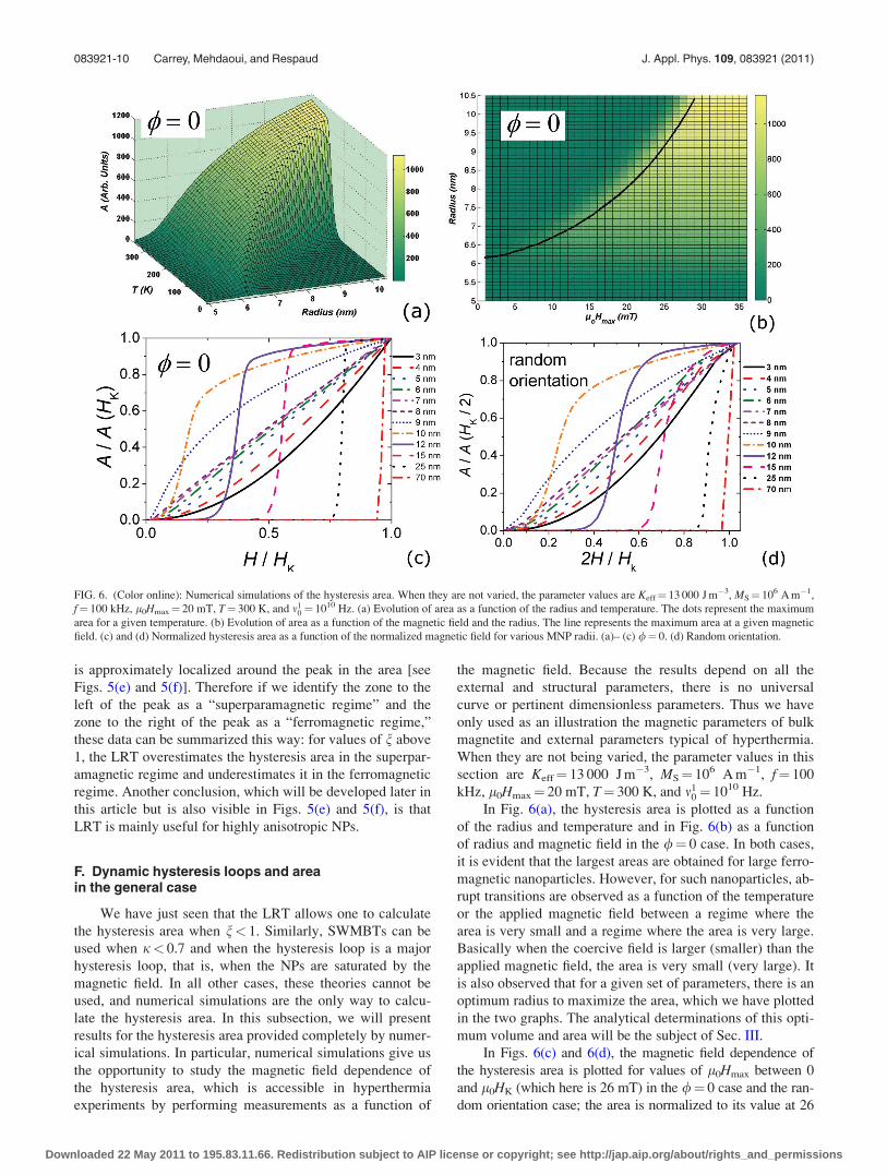
In Fig. 6(a), the hysteresis area is plotted as a function

of the radius and temperature and in Fig. 6(b) as a function

of radius and magnetic field in the /¼ 0 case. In both cases,

it is evident that the largest areas are obtained for large ferro-

magnetic nanoparticles. However, for such nanoparticles, ab-

rupt transitions are observed as a function of the temperature

or the applied magnetic field between a regime where the

area is very small and a regime where the area is very large.

Basically when the coercive field is larger (smaller) than the

applied magnetic field, the area is very small (very large). It

is also observed that for a given set of parameters, there is an

optimum radius to maximize the area, which we have plotted

in the two graphs. The analytical determinations of this opti-

mum volume and area will be the subject of Sec. III.

In Figs. 6(c) and 6(d), the magnetic field dependence of

the hysteresis area is plotted for values of l0Hmax between 0

and l0HK (which here is 26 mT) in the /¼ 0 case and the ran-

dom orientation case; the area is normalized to its value at 26

FIG. 6. (Color online): Numerical simulations of the hysteresis area. When they are not varied, the parameter values are Keff¼ 13 000 J m�3, MS¼ 106 A m�1,

f¼ 100 kHz, l0Hmax¼ 20 mT, T¼ 300 K, and m10¼ 1010 Hz. (a) Evolution of area as a function of the radius and temperature. The dots represent the maximum

area for a given temperature. (b) Evolution of area as a function of the magnetic field and the radius. The line represents the maximum area at a given magnetic

field. (c) and (d) Normalized hysteresis area as a function of the normalized magnetic field for various MNP radii. (a)– (c) /¼ 0. (d) Random orientation.



mT. For very small NPs, the LRT is valid and predicts a square

dependence of the hysteresis loop area [see Eqs. (36)–(38)],

which has been verified in a large number of experimental

works (e.g., Refs. 20, 21, or 22) and is also observed here. For

large NPs in the ferromagnetic regime, the magnetic field de-

pendence displays a very abrupt jump with a null hysteresis

area below the critical fields and a sharp increase followed by

a plateau. For NPs with intermediate sizes, the transition

between these two regimes is progressive and the curves dis-

play a large variety of shapes. These curves were fitted by a

power law in a range where the fit is acceptable. The corre-

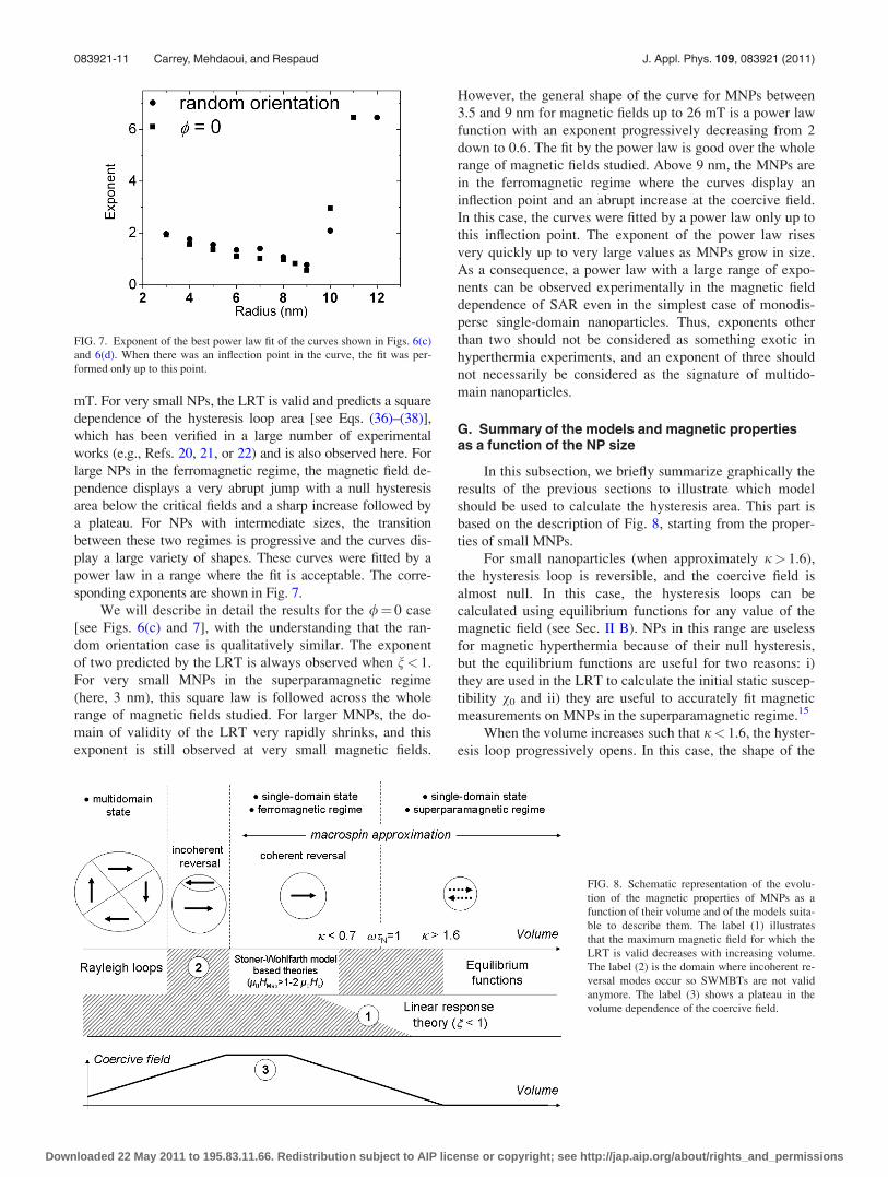
sponding exponents are shown in Fig. 7.

We will describe in detail the results for the /¼ 0 case

[see Figs. 6(c) and 7], with the understanding that the ran-

dom orientation case is qualitatively similar. The exponent

of two predicted by the LRT is always observed when n< 1.

For very small MNPs in the superparamagnetic regime

(here, 3 nm), this square law is followed across the whole

range of magnetic fields studied. For larger MNPs, the do-

main of validity of the LRT very rapidly shrinks, and this

exponent is still observed at very small magnetic fields.

However, the general shape of the curve for MNPs between

3.5 and 9 nm for magnetic fields up to 26 mT is a power law

function with an exponent progressively decreasing from 2

down to 0.6. The fit by the power law is good over the whole

range of magnetic fields studied. Above 9 nm, the MNPs are

in the ferromagnetic regime where the curves display an

inflection point and an abrupt increase at the coercive field.

In this case, the curves were fitted by a power law only up to

this inflection point. The exponent of the power law rises

very quickly up to very large values as MNPs grow in size.

As a consequence, a power law with a large range of expo-

nents can be observed experimentally in the magnetic field

dependence of SAR even in the simplest case of monodis-

perse single-domain nanoparticles. Thus, exponents other

than two should not be considered as something exotic in

hyperthermia experiments, and an exponent of three should

not necessarily be considered as the signature of multido-

main nanoparticles.

G. Summary of the models and magnetic propertiesas a function of the NP size

In this subsection, we briefly summarize graphically the

results of the previous sections to illustrate which model

should be used to calculate the hysteresis area. This part is

based on the description of Fig. 8, starting from the proper-

ties of small MNPs.

For small nanoparticles (when approximately j> 1.6),

the hysteresis loop is reversible, and the coercive field is

almost null. In this case, the hysteresis loops can be

calculated using equilibrium functions for any value of the

magnetic field (see Sec. II B). NPs in this range are useless

for magnetic hyperthermia because of their null hysteresis,

but the equilibrium functions are useful for two reasons: i)

they are used in the LRT to calculate the initial static suscep-

tibility v0 and ii) they are useful to accurately fit magnetic

measurements on MNPs in the superparamagnetic regime.15

When the volume increases such that j< 1.6, the hyster-

esis loop progressively opens. In this case, the shape of the

FIG. 7. Exponent of the best power law fit of the curves shown in Figs. 6(c)

and 6(d). When there was an inflection point in the curve, the fit was per-

formed only up to this point.

FIG. 8. Schematic representation of the evolu-

tion of the magnetic properties of MNPs as a

function of their volume and of the models suita-

ble to describe them. The label (1) illustrates

that the maximum magnetic field for which the

LRT is valid decreases with increasing volume.

The label (2) is the domain where incoherent re-

versal modes occur so SWMBTs are not valid

anymore. The label (3) shows a plateau in the

volume dependence of the coercive field.



hysteresis loop cannot be calculated simply for any value of

l0Hmax. However, the LRT allows one to calculate the hys-

teresis loop shape if n< 1 or n� 1 depending on the accu-

racy required (see Sec. II E). The fact that the magnetic field

value for which the LRT is valid progressively reduces

as the NP volume increases is schematized at Label (1) in

Fig. 8.

The formal transition between the superparamagnetic

regime (xsN< 1) and the ferromagnetic regime (xsN> 1)

occurs at xsN¼ 1. Precisely at this transition, the hysteresis

loop area for small magnetic fields displays a maximum (see

Sec. II E). However, we emphasize that nothing special

occurs at this transition with respect to the hysteresis loop

shape and area at high magnetic field: the coercive field has

started to grow well before the transition and keeps increas-

ing after the transition. This means that the hysteresis loop

area at high magnetic fields does not display a maximum

here but continues to increase with an increase in the volume.

For xsN> 1, the MNPs are in the ferromagnetic regime

where they display a more and more open hysteresis loop as

their volume increases. In the ferromagnetic regime, the

SWMBTs are suitable to describe the NP hysteresis loops if

the NPs are not too close to the superparamagnetic-ferro-

magnetic transition, i.e., for j< 0.7. Using SWMBTs to cal-

culate the area supposes also that the MNPs are saturated,

which is true for approximately l0Hmax>l0HC in the /¼ 0

case and l0Hmax> 2l0HC in the random orientation case.

The LRT is still valid in this region and can be used to calcu-

late minor hysteresis loop area at very low fields.

In larger MNPs, incoherent reversal modes start to

occur, which leads to a decrease of the coercive field. This

is where the theories used in this article cease to be valid.

For large MNPs, SWMBTs predict for the coercive field a

value independent of the NP volume, which is the value

of the coercive field at T¼ 0. As a consequence, if the

volume at which this phenomenon occurs is smaller than

the one at which incoherent reversal modes start, a plateau

in the evolution of the coercive field with the volume

might in principle be observed. We made this assumption

in Fig. 8, and the plateau is labeled as (3). If incoherent

reversal modes began before this plateau, a peak in the co-

ercive field value should be observed instead of a plateau.

Finally, the largest MNPs are composed of a vortex23 or

of several magnetic domains separated by magnetic walls.

In the latter case, the process leading to their magnetiza-

tion is the growth of one or several domains in the direc-

tion of the field at the expense of the others. In this case,

their hysteresis loops at very small magnetic fields are

described by “Rayleigh loops.”24

III. OPTIMUM PARAMETERS FOR MAGNETICHYPERTHERMIA

In this section, the models presented in the preceding

text are used to calculate the optimum parameters of MNPs

for magnetic hyperthermia. The domain of validity of each

model will be taken into account. The case of MNPs aligned

with the magnetic field (/¼ 0) as well as the case of a ran-

dom orientation will both be treated.

A. Optimum size as a function of the anisotropy

In this part, the optimum volume of MNPs for mag-

netic hyperthermia will be calculated as a function of their

anisotropy. In the figures, specific values of the external

parameters have been used: f¼ 100 kHz, l0Hmax¼ 20 mT,

T¼ 300 K, and m10 ¼ m2

0 ¼ 1010 Hz. These f and l0Hmax

values are the ones used in clinical applications at the

Charite Hospital, Berlin.25 In addition, results for three dif-

ferent values of MS (M1¼ 0.4� 106 A m�1, M2¼ 106

A m�1, and M3¼ 1.7� 106 A m�1) will be shown. They

correspond to the magnetizations of CoFe2O4, magnetite,

and iron, respectively. Equivalent graphs for any value of

the external and magnetic parameters can be plotted with

the condition to resolve one equation numerically (see fol-

lowing text).

In the LRT, even though the hysteresis area is different

for /¼ 0 and for a random orientation of NPs, Eqs. (36)–(38)

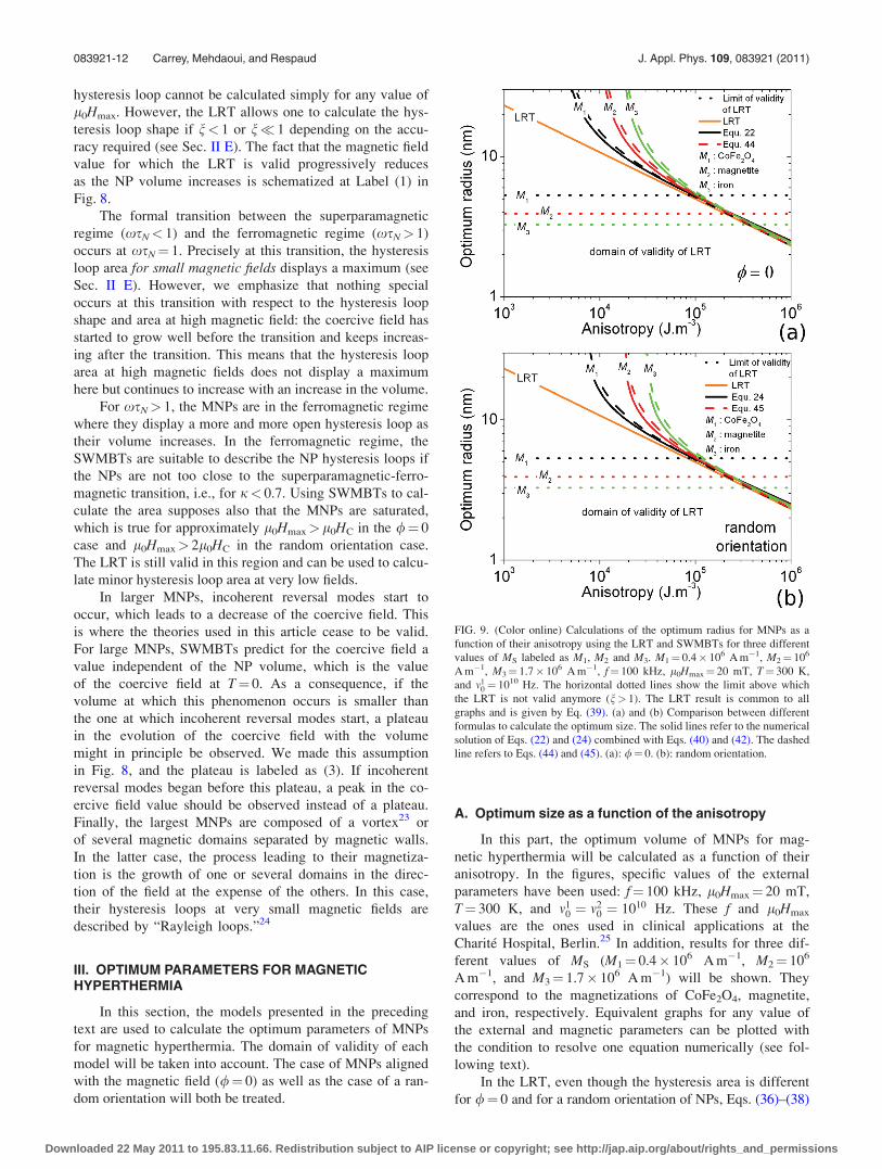
FIG. 9. (Color online) Calculations of the optimum radius for MNPs as a

function of their anisotropy using the LRT and SWMBTs for three different

values of MS labeled as M1, M2 and M3. M1¼ 0.4� 106 A m�1, M2¼ 106

A m�1, M3¼ 1.7� 106 A m�1, f¼ 100 kHz, l0Hmax¼ 20 mT, T¼ 300 K,

and m10¼ 1010 Hz. The horizontal dotted lines show the limit above which

the LRT is not valid anymore (n> 1). The LRT result is common to all

graphs and is given by Eq. (39). (a) and (b) Comparison between different

formulas to calculate the optimum size. The solid lines refer to the numerical

solution of Eqs. (22) and (24) combined with Eqs. (40) and (42). The dashed

line refers to Eqs. (44) and (45). (a): /¼ 0. (b): random orientation.



show that the maximum of this area always occurs for

xsN¼ 1. This means that the optimum volume is given by

the following equation, which is plotted in the two graphs of

Fig. 9:

Vopt ¼kBT

Keff

lnðpf s0Þ: (39)

Because the LRT is valid when n< 1, this condition is plot-

ted in the graphs of Fig. 9: it appears as horizontal lines

above which the LRT is no longer valid. It is evident from

this graph that the LRT is mainly useful for strongly aniso-

tropic NPs. For instance, it is deduced from the intersection

between Eq. (39) and the function n¼ 1 that for MS¼ 106

A m�1, Eq. (39) is no longer valid for MNPs with an anisot-

ropy below 2� 105 J m�3.

We now consider the optimum sizes predicted by the

SWMDTs starting with the formula derived by Pfeiffer et al.and Garcia-Otero et al. [Eqs. (19) and (21)]. First, sm must

be replaced by an expression depending on experimental pa-

rameters. For reasons that will be clear later, we arbitrarily

state sm¼ (1/2pf). Then it should be decided what the opti-

mum coercive field of the MNPs is when a given magnetic

field is applied. In the case of MNPs aligned with the field

(/¼ 0) and due to the fact that the hysteresis loop is approxi-

mately square,

l0HC � l0Hmax ð/¼ 0Þ (40)

is taken. This leads to an optimum area Adopt given by

Aopt � 4l0MSHmax ð/¼ 0Þ: (41)

In the random orientation case, the magnetic field necessary

to saturate an assembly of MNPs is approximately twice its

coercive field. As a consequence, a coercive field of half the

applied magnetic field could be targeted. Eq. (26) shows this

would lead to an optimum area Aopt¼l0MSHmax. However,

numerical calculations show that it is better to target a coer-

cive field slightly higher than this: the increase in area due to

the increase in coercive field compensates for the fact that

some of the MNPs are not switched by the applied magnetic

field. The best compromise is found to depend slightly on

the exact shape of the hysteresis loop and is given by

l0HC � 0:81 6 0:04l0Hmax ðrandom orientationÞ: (42)

With this optimum coercive field, the optimum area is

Aopt � 1:5660:08l0MSHmax ðrandom orientationÞ: (43)

Combining Eqs. (40) and (42) with Eqs. (19) and (21) allows

one to calculate the optimum volume Vopt. For NPs aligned

with the magnetic field, this leads to

Vopt ¼�kBT lnðpf s0Þ

Keff 1� l0HmaxMS

2Keff

� �2ð/¼ 0Þ: (44)

In the random case, this leads to

Vopt¼�kBT lnðpf s0Þ

Keff 1�1:69l0HmaxMS

2Keff

� �43

ðrandom orientationÞ:

(45)

These two functions are plotted in Figs. 9(a) and 9(b) in

dashed lines.

Equations (22) and (24) are more rigorous methods to

calculate the coercive field and thus the optimum volume. In

these equations, a numerical solution is required to extract

the volume corresponding to a given coercive field, the result

of which is plotted in Figs. 9(a) and 9(b) in solid lines. The dif-

ference between the results provided by Eqs. (44) and (45) and

the numerical solution of Eqs. (22) and (24) can reach up to

3 nm for the set of parameters we used, which is not negligible.

Figures 9(a) and 9(b) give evidence that the optimum

volume obtained using SWMBTs deviates from the LRT

results for small anisotropies, i.e., precisely in the domain

where the LRT is not valid anymore. Thus in this domain,

SWMBTs should be used instead of LRT to calculate the op-

timum size. For strong anisotropies, the optimum volumes

given by Eqs. (44) and (45) tend toward the one deduced

from LRT because of the assumption we made; that is, that

sm¼ (1/2pf). The numerical solutions of Eqs. (22) and (24)

also leads to an optimum volume very close to the one pre-

dicted by the LRT for strong anisotropy; the difference

between the two predictions never exceeds 1 nm over a wide

range of parameters: f (5–500 kHz), MS (0.4–1.7� 106

A m�1), s0 (10�9–10�12 s), and l0Hmax (0–80 mT). Strictly

speaking, there is a zone where none of the models used is

valid because just above the LRT limit (when n> 1), j is not

immediately smaller than 0.7. This point will be more clearly

evidenced in the next section. However, because the

SWMBT results approximately tend toward the LRT results

at high anisotropy, it can be reasonably assumed that the

transition between the two models is also acceptably repro-

duced by SWMBTs.

As a conclusion, Eqs. (44) and (45) can be used to give

an approximate value of the optimum size of MNPs, but the

error for weakly anisotropic MNPs can be significant. The

numerical solution of Eqs. (22) and (24) can safely be used

to calculate the optimum size of MNPs for magnetic hyper-

thermia over a wide range of anisotropies without caring too

much about which is the most suitable model to describe

their behavior. However, the most rigorous approach consists

of calculating n and j and using LRT when n< 1, Eqs. (22)

and (24) when j< 0.7 and numerical simulations otherwise.

B. Optimum anisotropy

In the previous section, the optimum size for MNPs with

a given anisotropy was derived. However, the question of

whether there is an optimum anisotropy was not addressed;

this important point is treated now. To solve this problem,

the SAR of a MNP with an optimum size was calculated ver-

sus the anisotropy. The calculations were performed for

MS¼M2¼ 106 Am�1 (magnetite value) and with the same

values as given previously for the other parameters. To

express the result in W/g, which is the usual unity for SARs,



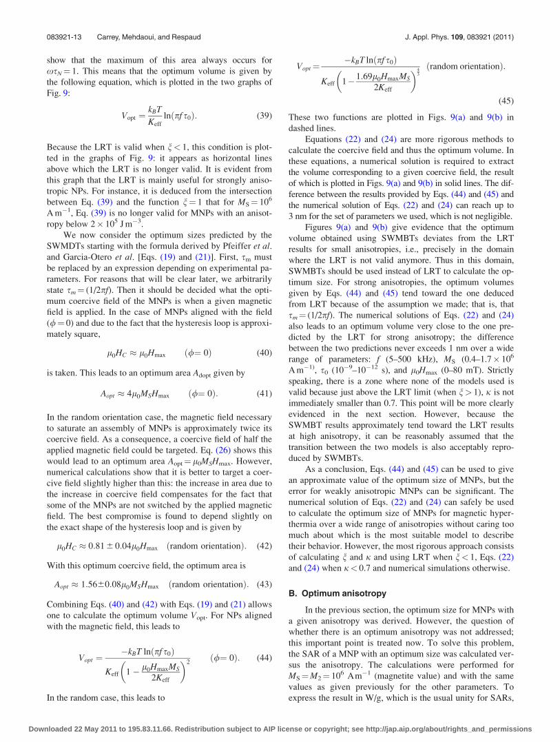
a density of q¼ 5.2� 106 kg.m�3 (magnetite value) is

assumed. The results of the LRT for the /¼ 0 and random

orientation case were obtained using Eqs. (36), (38), and

(39). They are plotted in Fig. 10 as solid lines. The data are

not plotted outside the domain of validity of the LRT, i.e.,

when n> 1. The calculations in the ferromagnetic regime

were performed for simplicity without numerical solutions

using Eqs. (19), (21), and (40)–(45). This simplification does

not change the main conclusions of this part. Data are plotted

in Fig. 10 as solid lines and are not plotted outside the do-

main of validity of the SWMBTs, that is, when j> 0.7.

A very important point to consider in a discussion of the

optimum parameters for magnetic hyperthermia is the influ-

ence of the size distribution on the final SAR value. To illus-

trate this, the SAR value for a MNP with a volume 30%

below the optimum volume was calculated in each case. The

results illustrate the loss of SAR due to the size distribution

of MNPs. The results are plotted as dashed lines along with

the previous data.

Figure 10 displays an essential result for magnetic

hyperthermia and is worth a detailed comment beginning

with the high anisotropy MNPs described by the LRT. First,

the LRT shows that the maximum achievable SAR increases

with a reduction in anisotropy. This is obvious from Eqs.

(36)–(39): for a MNP with the optimum size, the resonating

term xsR

ð1þx2s2RÞ

is maximal and always equals 1/2. Because

A!V [see Eqs. (36)–(38)] and because the optimum volume

is inversely proportional to the anisotropy [see Eq. (39)], the

maximal SAR value increases with decreasing anisotropy. In

this regime, the effect of the size distribution is dramatic: the

SAR decreases by more than one order of magnitude for

nonoptimum NPs.

After passing the blank space to the left of these curves

where the transition between the two regimes is out of

the domain of validity of both models used here, the SAR of

the optimum NPs displays a plateau: in this region, the SAR

can be maximized by tuning the NP volume to adjust their co-

ercive fields because an optimum volume satisfying Eqs. (40)

and (42) always exists. With absolutely no size distribution,

all of the MNPs in this anisotropy range could be perfect can-

didates for magnetic hyperthermia. However, it is observed

that the NPs with a weak anisotropy are less sensitive to size

distribution effects. At the left extremity of this plateau, the

size distribution effects are canceled. For /¼ 0, this occurs

when l0Hmax�l0HK, and for the random orientation case it

occurs when 0.81 l0Hmax� 0.48 l0HK, that is, when the tar-

geted coercive field equals the low temperature coercive field

of the material. Therefore, the relation giving the optimum

anisotropy for MNPs with a known magnetization is

Kopt ¼ Cl0HmaxMS

2; (46)

with C¼ 1 for /¼ 0 and C¼ 1.69 for the random orientation

case

At the left of this plateau, a decrease of the SAR is

observed. This occurs when the anisotropy field of the NP is

so weak that there is no solution to Eqs. (40) and (42). In this

case, the coercive field of the NPs is l0HK for /¼ 0 and

0.48 HK for a random orientation. Then the SAR calculated

using Eqs. (25) and (26) leads to the observed decrease.

At the optimum anisotropy, the optimum volume of the

MNPs diverges and tends toward infinity [see Figs. 9(a) and

9(b)]. This means that, in principle, a large single-domain

MNP with the optimum anisotropy would be the perfect

object. However, increasing the size of the NPs too much

leads to several problems: i) It leads to the transition toward

multidomain NPs. They might be interesting objects for

magnetic hyperthermia because the coercive field value is

also influenced by the size near this transition (see Fig. 8).26

However, there is no simple way to calculate the optimum

size and the hysteresis area for such nano-objects. ii) Dis-

persing and stabilizing NPs in a colloidal solution is all the

more difficult if they have a large diameter. iii) A larger size

favors recognition by the phagocytosis system after intrave-

nous administration.

The optimum volume of the MNPs and the optimum an-

isotropy thus result from a compromise between the effi-

ciency of magnetic hyperthermia, which requires large NPs

with an anisotropy given by Eq. (46), and other factors for

which a large size could be detrimental. If for any reason the

volume of the MNPs needs to be limited to a maximum

value, the equations used so far allow one to deduce easily

what would be the optimum anisotropy for a given volume.

In any case, Eq. (46) provides the approximate target anisot-

ropy to optimize the SAR of MNPs.

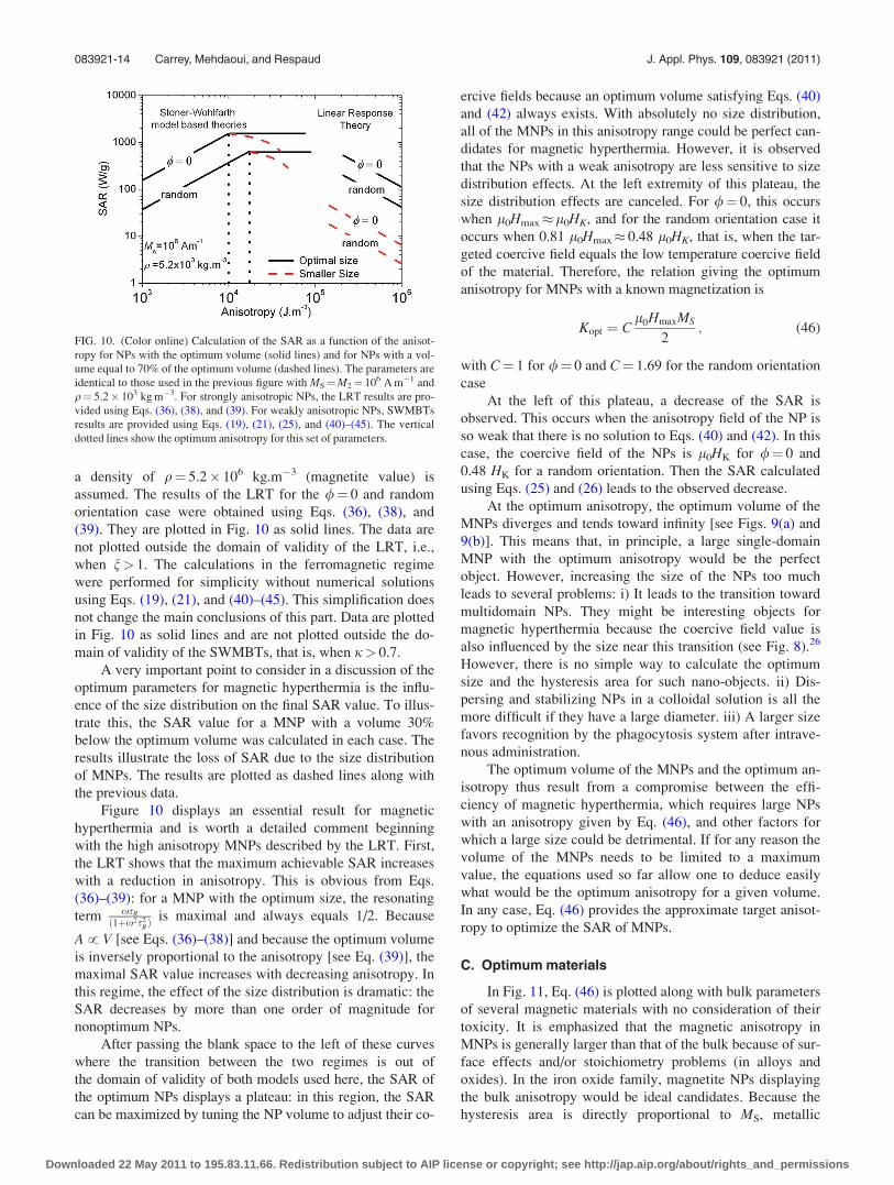
C. Optimum materials

In Fig. 11, Eq. (46) is plotted along with bulk parameters

of several magnetic materials with no consideration of their

toxicity. It is emphasized that the magnetic anisotropy in

MNPs is generally larger than that of the bulk because of sur-

face effects and/or stoichiometry problems (in alloys and

oxides). In the iron oxide family, magnetite NPs displaying

the bulk anisotropy would be ideal candidates. Because the

hysteresis area is directly proportional to MS, metallic

FIG. 10. (Color online) Calculation of the SAR as a function of the anisot-

ropy for NPs with the optimum volume (solid lines) and for NPs with a vol-

ume equal to 70% of the optimum volume (dashed lines). The parameters are

identical to those used in the previous figure with MS¼M2¼ 106 A m�1 and

q¼ 5.2� 103 kg m�3. For strongly anisotropic NPs, the LRT results are pro-

vided using Eqs. (36), (38), and (39). For weakly anisotropic NPs, SWMBTs

results are provided using Eqs. (19), (21), (25), and (40)–(45). The vertical

dotted lines show the optimum anisotropy for this set of parameters.



materials with high magnetization are required to reach the

highest SARs. In this case, FeCo alloys would be perfect, but

their probable toxicity could be a severe problem. Iron,

which is not intrinsically toxic, could be a good candidate

but presents in its crystalline form an anisotropy value too

large for 20 mT applications. Fe1-xSix alloys have both a

reduced anisotropy and magnetization and could represent

an interesting compromise. Also amorphous iron should dis-

play a reduced anisotropy. However, the possibility of creat-

ing MNPs with a reduced anisotropy using amorphous iron

or Fe1-xSix alloys still needs to be demonstrated.

D. The Brownian motion

1. Influence of Brownian motion on hyperthermiaproperties

When MNPs are in a fluid, they can rotate physically

under the influence of the magnetic fluid, similarly to a com-

pass, until the magnetization is aligned with the magnetic

field. This is known as relaxation by Brownian motion. In a

standard hyperthermia experiment, the relaxation by Brown-

ian motion and the relaxation by magnetization reversal

described in the preceding text are both possible, which leads

to a global hysteresis loop resulting from the two mecha-

nisms. Whether the relaxation occurs only by Brownian

motion or by both mechanisms, the heating during one cycle

still simply equals the hysteresis loop area A. The influence

of Brownian motion can be easily incorporated into the

LRT.10 A Brownian relaxation time is defined as

sB ¼3gVH

kBT; (47)

where g is the viscosity of the solvent and VH is the hydrody-

namic volume of the MNPs. The relaxation time sR, which

includes the Neel and Brownian relaxation times, is then

defined as

1

sR¼ 1

sNþ 1

sB: (48)

Here again, it must be kept in mind that the LRT including

Brownian motion has a restricted domain of validity, which

is discussed in detail in Ref. 11: the LRT is valid for small

magnetic fields, i.e., for n< x with x depending on the value

of xsB/n. For any value of the parameters, numerical results

have been obtained by Raiker et al. with the restrictive hy-

pothesis that the relaxation by magnetization reversal is not

possible.11 The hysteresis loop of a MNP in a magnetic fluid

when both magnetization reversal and Brownian motion are

allowed has to our knowledge not been solved in the most

general case.

2. Optimum volume calculation

In a situation where only reversal by Brownian motion

would occur, the LRT indicates that the optimum volume is

the one for which xsB¼ 1. For an applied frequency of 100

kHz and the viscosity of water, this leads to an optimum ra-

dius of around 15.5 nm independently of any magnetic pa-

rameters. However, there are some ranges of parameters

(MNP magnetization, magnetic field amplitude, and fre-

quency) for which the optimum size given by this simple

equation is not correct because it is out of the domain of va-

lidity of the LRT; the only way to know it is to use numerical

calculations.11 In the case of relaxation by Brownian motion,

there is so far no equivalent to the simple analytical formula

we used in the case of relaxation by magnetization reversal,

which would be valid over a wide range of parameters. The-

oretical progress is required on this point.

3. Why Brownian motion is not the way to optimizethermal effects

Progress in the development of analytical formulas and/

or the use of numerical simulations could lead to progress in

the determination of the optimum parameters of MNP heat-

ing through their Brownian motion. One can imagine that

eventually MNPs with such optimum magnetic properties

could be synthesized. However, we think that this method is

less promising than the one consisting of optimizing the

SAR and using heating by magnetization reversal. The main

reason is the following: the Brownian motion depends

strongly on the environment and the aggregation state of the

MNPs because the hydrodynamic volume of the MNP is the

main parameter governing the Brownian motion. Thus two

aggregated MNPs or a MNP functionalized and linked to a

tumor cell would display SAR values very different to that

of a free MNP. Moreover, the application of an alternating

magnetic field can lead to the formation of chains or columns

of MNPs with very different Brownian properties.27,28

We think that the ideal objects for magnetic hyperthermia

should display a SAR that is as independent as possible from

such phenomena. This requires that the physical rotation of

the MNP in the alternating field is blocked for all MNPs,

FIG. 11. (Color online) Comparison between theoretical optimum parame-

ters and experimental bulk parameters of several magnetic materials. Equa-

tion (46) is plotted for l0Hmax¼ 20 mT (dotted lines) and 50 mT (dashed

lines). In each case, the upper curve represents the random orientation case,

and the lower one represents the /¼ 0 case. Label (a): for the FeCo alloy,

the anisotropy of 15 nm MNPs estimated in Ref. 19 is provided. Reprinted

with permission from L.-M. Lacroix, R. Bel-Malaki, J. Carrey, S. Lachaize,

G. F. Goya, B. Chaudret, and M. Respaud, J. Appl. Phys. 105, 023911

(2009). Copyright VC 2009 American Institute of Physics.



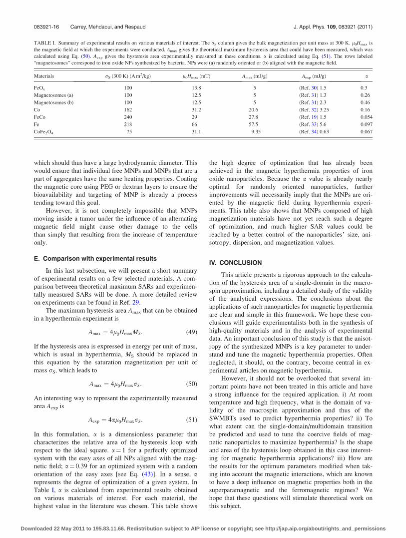
which should thus have a large hydrodynamic diameter. This

would ensure that individual free MNPs and MNPs that are a

part of aggregates have the same heating properties. Coating

the magnetic core using PEG or dextran layers to ensure the

bioavailability and targeting of MNP is already a process

tending toward this goal.

However, it is not completely impossible that MNPs

moving inside a tumor under the influence of an alternating

magnetic field might cause other damage to the cells

than simply that resulting from the increase of temperature

only.

E. Comparison with experimental results

In this last subsection, we will present a short summary

of experimental results on a few selected materials. A com-

parison between theoretical maximum SARs and experimen-

tally measured SARs will be done. A more detailed review

on experiments can be found in Ref. 29.

The maximum hysteresis area Amax that can be obtained

in a hyperthermia experiment is

Amax ¼ 4l0HmaxMS: (49)

If the hysteresis area is expressed in energy per unit of mass,

which is usual in hyperthermia, MS should be replaced in

this equation by the saturation magnetization per unit of

mass rS, which leads to

Amax ¼ 4l0HmaxrS: (50)

An interesting way to represent the experimentally measured

area Aexp is

Aexp ¼ 4al0HmaxrS: (51)

In this formulation, a is a dimensionless parameter that

characterizes the relative area of the hysteresis loop with

respect to the ideal square. a¼ 1 for a perfectly optimized

system with the easy axes of all NPs aligned with the mag-

netic field; a¼ 0.39 for an optimized system with a random

orientation of the easy axes [see Eq. (43)]. In a sense, arepresents the degree of optimization of a given system. In

Table I, a is calculated from experimental results obtained

on various materials of interest. For each material, the

highest value in the literature was chosen. This table shows

the high degree of optimization that has already been

achieved in the magnetic hyperthermia properties of iron

oxide nanoparticles. Because the a value is already nearly

optimal for randomly oriented nanoparticles, further

improvements will necessarily imply that the MNPs are ori-

ented by the magnetic field during hyperthermia experi-

ments. This table also shows that MNPs composed of high

magnetization materials have not yet reach such a degree

of optimization, and much higher SAR values could be

reached by a better control of the nanoparticles’ size, ani-

sotropy, dispersion, and magnetization values.

IV. CONCLUSION

This article presents a rigorous approach to the calcula-

tion of the hysteresis area of a single-domain in the macro-

spin approximation, including a detailed study of the validity

of the analytical expressions. The conclusions about the

applications of such nanoparticles for magnetic hyperthermia

are clear and simple in this framework. We hope these con-

clusions will guide experimentalists both in the synthesis of

high-quality materials and in the analysis of experimental

data. An important conclusion of this study is that the anisot-

ropy of the synthesized MNPs is a key parameter to under-

stand and tune the magnetic hyperthermia properties. Often

neglected, it should, on the contrary, become central in ex-

perimental articles on magnetic hyperthermia.

However, it should not be overlooked that several im-

portant points have not been treated in this article and have

a strong influence for the required application. i) At room

temperature and high frequency, what is the domain of va-

lidity of the macrospin approximation and thus of the

SWMBTs used to predict hyperthermia properties? ii) To

what extent can the single-domain/multidomain transition

be predicted and used to tune the coercive fields of mag-

netic nanoparticles to maximize hyperthermia? Is the shape

and area of the hysteresis loop obtained in this case interest-

ing for magnetic hyperthermia applications? iii) How are

the results for the optimum parameters modified when tak-

ing into account the magnetic interactions, which are known

to have a deep influence on magnetic properties both in the

superparamagnetic and the ferromagnetic regimes? We

hope that these questions will stimulate theoretical work on

this subject.

TABLE I. Summary of experimental results on various materials of interest. The rS column gives the bulk magnetization per unit mass at 300 K. l0Hmax is

the magnetic field at which the experiments were conducted. Amax gives the theoretical maximum hysteresis area that could have been measured, which was

calculated using Eq. (50). Aexp gives the hysteresis area experimentally measured in these conditions. a is calculated using Eq. (51). The rows labeled

“magnetosomes” correspond to iron oxide NPs synthesized by bacteria. NPs were (a) randomly oriented or (b) aligned with the magnetic field.

Materials rS (300 K) (A m2/kg) l0Hmax (mT) Amax (mJ/g) Aexp (mJ/g) a

FeOx 100 13.8 5 (Ref. 30) 1.5 0.3

Magnetosomes (a) 100 12.5 5 (Ref. 31) 1.3 0.26

Magnetosomes (b) 100 12.5 5 (Ref. 31) 2.3 0.46

Co 162 31.2 20.6 (Ref. 32) 3.25 0.16

FeCo 240 29 27.8 (Ref. 19) 1.5 0.054

Fe 218 66 57.5 (Ref. 33) 5.6 0.097

CoFe2O4 75 31.1 9.35 (Ref. 34) 0.63 0.067



ACKNOWLEDGMENTS

We acknowledge L.-M. Lacroix, S. Lachaize, and Y.

Raikher for fruitful discussions. This work was supported by

the InNaBioSante Foundation.

1R. Hergt and S. Dutz, J. Magn. Magn. Mater. 311, 187 (2007).2E. C. Stoner and E. P. Wohlfarth, Philos. Trans. R. Soc. London, Ser. A

240, 599 (1948).3J. J. Lu, H. L. Huang, and I. Klik, J. Appl. Phys. 76, 1726 (1994).4H. Pfeiffer, Phys. Status Solidi A 120, 233 (1990)5J. Garcia-Otero, A. J. Garcia-Bastida, and J. Rivas, J. Magn. Magn. Mater.

189, 377 (1998).6D. Kechrakos and K. N. Trohidou, Phys. Rev. B 58, 12169 (1998).7Y. L. Raikher, V. I. Stepanov, and R. Perzynski, Physica B 343, 262

(2004).8N. A. Usov and Y. B. Grebenshchikov, J. Appl. Phys. 106, 023917

(2009).9R. Hergt, W. Andra, C. G. d’Ambly, I. Hilger, W. A. Kaiser, U. Richter,

and H.-G. Schmidt, IEEE Trans. Magn. 34, 3745 (1998).10R. E. Rosensweig, J. Magn. Magn. Mater. 252, 370 (2002).11Y. L. Raikher and V. I. Stepanov, J. Magn. Magn. Mater 320, 2692

(2008).12R. Hergt, S. Dutz and M. Roder, J. Phys. Condens. Matter. 20, 385214

(2008).13R. Hergt, S. Dutz and M. Zeisberger, Nanotechnology 21, 015706 (2010).14N. A. Usov, J. Appl. Phys. 107, 123909 (2010).15M. Respaud, J. Appl. Phys. 86, 556 (1999).16C Tannous and J Gieraltowski, Eur. J. Phys. 29, 475-487 (2008)17W. T. Coffey, D. S. F. Crothers, J. L. Dormann, Yu. P. Kalmykov, E. C.

Kennedy, and W. Wernsdorfer, Phys. Rev. Lett. 80, 5655 (1998).

18Y. P. Kalmykov, J. Appl. Phys. 96, 1138 (2004).19L.-M. Lacroix, R. Bel-Malaki, J. Carrey, S. Lachaize, G. F. Goya, B.

Chaudret, and M. Respaud, J. Appl. Phys. 105, 023911 (2009).20R. Hiergeist, W. Andra, N. Buske, R. Hergt, I. Hilger, U. Richter, and W.

Kaiser, J. Magn. Magn. Mater. 201, 420 (1999).21X. Wang, H. Gub, and Z. Yang, J. Magn. Magn. Mater. 293, 334 (2005).22B. Mehdaoui, A. Meffre, L.-M. Lacroix, J. Carrey, S. Lachaize, M. Respaud,

M. Gougeon, and B. Chaudret, J. Appl. Phys. 107, 09A324 (2010)23E. Snoeck, C. Gatel, L. M. Lacroix, T. Blon, S. Lachaize, J. Carrey, M.

Respaud, and B. Chaudret, Nanoletters 8, 4293 (2008)24B. D. Cullity and C. D. Graham, Introduction to Magnetic Materials, 2nd

ed. (Wiley, Hokoben, 2009), p. 321.25A. Jordan, R. Scholz, K. Maier-Hauff, M. Johannsen, P. Wust, J. Nadobny,

H. Schirra, H. Schmidt, S. Deger, S. Loening, W. Lanksch, and R. Felix, J.

Magn. Magn. Mater. 225, 118 (2001).26M. Andres Verges, R. Costo, A. G. Roca, J. F. Marco, G. F. Goya, C. J.

Serna, and M. P. Morales, J. Phys. D:Appl. Phys. 41, 134003 (2008).27M. Klokkenburg, B. H. Erne, J. D. Meeldijk, A. Wiedenmann, A. V.

Petukhov, R. P. A. Dullens, and A. P. Philipse, Phys. Rev. Lett. 97,

185702 (2006).28B. Mehdaoui, A. Meffre, L.-M. Lacroix, J. Carrey, S. Lachaize, M. Gou-

jeon, M. Respaud, and B. Chaudret, J. Magn. Magn. Mat. 322, L49 (2010).29L.-M. Lacroix, D. Ho, and S. Sun, Curr. Top. Med. Chem. 10, 1184 (2010)30R. Hergt, R. Hiergeist, I. Hilger, W.A. Kaiser, Y. Lapatnikov, S. Margel,

and U. Richter, J. Magn. Magn. Mater. 270, 345 (2004).31R. Hergt, R. Hiergeist, M. Zeisberger, D. Schuler, U. Heyen, I. Hilger, and

W. A. Kaiser, J. Magn. Magn. Mater. 293, 80 (2005).32M. Zeisberger S. Dutz, R. Muller, R. Hergt, N. Matoussevitch, and H.

Bonnemann, J. Magn. Magn. Mater. 311, 224 (2007).33B. Mehdaoui, A. Meffre, L.-M. Lacroix, J. Carrey, S. Lachaize, M. Gou-

jeon, M. Respaud, and B. Chaudret, J. Magn. Magn. Mat. 322, L49 (2010).34J.-P. Fortin, F. Gazeau, and C. Wilhelm, Eur. Biophys. J. 37, 223 (2008)



http://dx.doi.org/10.1016/j.jmmm.2006.10.1156

http://dx.doi.org/

http://dx.doi.org/10.1063/1.358424

http://dx.doi.org/10.1002/pssa.v120:1

http://dx.doi.org/10.1016/S0304-8853(98)00243-1

http://dx.doi.org/10.1103/PhysRevB.58.12169

http://dx.doi.org/10.1016/j.physb.2003.08.105

http://dx.doi.org/10.1063/1.3173280

http://dx.doi.org/10.1109/20.718537

http://dx.doi.org/10.1016/S0304-8853(02)00706-0


http://dx.doi.org/10.1088/0953-8984/20/38/385214

http://dx.doi.org/10.1088/0957-4484/21/1/015706

http://dx.doi.org/10.1063/1.3445879

http://dx.doi.org/10.1063/1.370765

http://dx.doi.org/10.1088/0143-0807/29/3/008

http://dx.doi.org/10.1103/PhysRevLett.80.5655

http://dx.doi.org/10.1063/1.1760839

http://dx.doi.org/10.1063/1.3068195

http://dx.doi.org/10.1016/S0304-8853(99)00145-6


http://dx.doi.org/10.1063/1.3348795

http://dx.doi.org/

http://dx.doi.org/10.1016/S0304-8853(00)01239-7

http://dx.doi.org/10.1016/S0304-8853(00)01239-7

http://dx.doi.org/10.1088/0022-3727/41/13/134003

http://dx.doi.org/10.1103/PhysRevLett.97.185702


http://dx.doi.org/10.2174/156802610791384207





http://dx.doi.org/10.1007/s00249-007-0197-4

Simple models for dynamic hysteresis loop calculations of ...

Documents