Simple Modeling of Approximate Turning Characteristics of Tracked Mobile Vehicles in Steady State Condition (2)

Proceeding of the 2013

RSI/ISM International Conference on Robotics and Mechatronics

February 13-15, 2013, Tehran, Iran

978-1-4673-5811-8/13/$31.00 ©2013 IEEE

Simple Modeling of Approximate Turning

Characteristics of Tracked Mobile Vehicles in Steady

State Condition

Majid M. Moghadam

Tarbiat Modares University

Tehran, Iran

[email protected]

Ramin Mardani

Islamic Azad University Of Central

Tehran,Iran

[email protected]

Moosa Daryanavard

Tarbiat Modares University

Tehran, Iran

[email protected]

Abstract— To investigate the behavior of tracked mobile robots

or vehicles, first a mathematical model is developed to describe

the physics of tracked vehicles. Then, the equations of motion

are solved for radius of rotation in steady state condition using a

numerical method. Results are compared with an ideal

differentially-driven vehicle and notable similarities are

observed. Further, few mathematical functions are developed to

approximate turning characteristics of the vehicle in steady state

condition on rigid ground. Forms of these functions are simple

and can be used in real time control and motion planning of

tracked vehicles. Finally, the results are compared with similar works in the area.

Key words— Tracked mobile vehicle, kinematic robot control,

motion planning, turning characteristics.

I. INTRODUCTION

Despite obvious control similarities, motion control

methods used for differential wheel robots and its results

cannot be directly used for tracked vehicles [1]. However in

this research a simple formulation is proposed to use these

results and methods for tracked vehicles. Moreover, results of this work can improve the speed of calculations in autonomous

control and motion planning of tracked robots.

Tracked mobile vehicles and robots have more advantages comparing with wheeled vehicles on rough terrain, and that is

why they are used vastly in the fields like agricultural, military,

mining, and even city services and rescue assistance [2].

Using of tracked vehicles continued for a long period

without feeling any necessity to autonomous control and

motion planning of these vehicles. Until last decay when more

serious works done in this area. Due to the sophisticated

behavior of tracked mobile vehicles, improvements advanced

with a substantial delay compared with other types of vehicles

[3]. Complication rises from the geometry of track, sinkage and

slippage phenomena and soil behaviors, and moving in such

unprepared terrain has its own difficulties [4].

Control and motion planning of tracked vehicles have been

more successful on rigid grounds and in steady state condition; however, good works are done in different conditions and

useful reviews have been published to gather the works done in

this field [5].

A kinematic approach for tracked mobile robots is

proposed in order to improve motion control and pose

estimation [6]. The proposed solution is based on the fact that

the instantaneous centers of rotation (ICRs) of treads on the

motion plane with respect to the vehicle are dynamics-

dependent, but they lie within a bounded area.

Numerical analysis is developed here to calculate the

steering properties of a rigid suspension tracked vehicle turning

on soft terrain [7]. The developed numerical analysis is based

on a method to solve a set of non-linear equations. The

comparison between measured and calculated values shows

that the numerical analysis can predict sinkage, slip ratios and

turning radius within an error amount of 15% .

A three-dimensional multi-body simulation model for

simulating the dynamic behavior of tracked off-road vehicles

was developed using the LMS-DADS simulation program [8].

The normal and tangential forces are calculated using classical soil mechanics equations, it was concluded that the influence of

the track dynamics and the soil–link interaction on the vehicle

dynamics can be better predicted with the newly developed

model.

II. NOMENCLATURE

d width of vehicle, normal distance between the left and the right wheels or tracks. (m)

ax x component of Acceleration of C.G of vehicle in local frame. (m/sec2)

ay y component of Acceleration of C.G of vehicle in local frame. (m/sec2)

b Length of vehicle, distance between the first and the last

axes. (m)

c1 constant coefficient


mailto:[email protected]






978-1-4673-5811-8/13/$31.00 ©2013 IEEE



DDV Differentially Driven Vehicle

f friction force acting on wheels (N)

Ic instantaneous center of rotation

k number of total axes

m mass of vehicle (kg)

MG resultant moments about C.O.M (N.m)

MWD Multiple Wheels Drive model

N normal force acting on a wheel (N)

d width of vehicle, normal distance between the left and the

right wheels or tracks. (m)

r radius of each wheel, Radius of Driver sprocket or pulley (m)

V linear velocity of chain or belt relative to track. (m/sec)

Vx x component of absolute velocity of vehicle at wheel contact point (m/sec)

Vy y component of absolute velocity of vehicle at wheel contact point (m/sec)

x x position of a wheel contact point (m)

y y position of a wheel contact point (m)

angle between a line tangent to path at origin, and x direction (deg)

angular velocity of driver pulley. (rad/sec)

r angular velocity of right track driver pulley(rad/sec)

l angular velocity of left track driver pulley(rad/sec)

U lr /

V lr (rad/sec)

z angular velocity MWD vehicle. (rad/sec)

zdd angular velocity DDV vehicle. (rad/sec)

coefficient of friction.

III. THE MODEL

A tracked mobile vehicle has a special chain or belt which

is lying over ground and has a large contact area in contrast with wheeled vehicles like differentially drive robots which

theoretically touch the ground at only two points. Tracks have

a driver sprocket and some contact areas encounter greater

forces (Fig. 1).

The linear velocity of chain or belt relative to the track can

be calculated as follows:

rv (1)

Figure 1: schematic of a tracked mobile vehicle and its high pressure contacts

area.

Where:

v: is the linear velocity of chain or belt relative to track.

r: is the radios of drive sprocket and pulley

: is the angular velocity of sprocket or pulley.

High pressure points in a tracked mobile robot provide an

insight to replace the track with a wheeled drive vehicle which

has many driver wheels (and axes for each pair)(Fig 2).

Figure 2: Multiple Wheels Drive Model (MWD).

Let name the model “Multiple Wheels Drive” (MWD). It

is assumed that all wheels (or axes) are driver and rotate with

same angular velocity. Number of total axes in the model is

defined by k. for k=1 the model changes to be a “differentially

drive Vehicle” (DDV), and its behaviour must approach to

DDV when solving equations. Another way for the behaviour

of MWD to be approached to DDV; is to decrease distance

between first and last axes near to zero. This is checked later in

the paper.

Geometrical properties of model:

Geometrical properties of model can be defined with four

parameters which are represented in Fig. 3.

d: width of vehicle, Normal distance between left and right

wheels or tracks.

b: length of vehicle, Distance between first and last axes.

k: Number of total axes.

r: radios of each wheel, radios of the driver sprocket or

pulley.

Numerical values of each parameter, in the calculations,

can be read from the table below:

Table 1: Numerical values of parameters.

Param.

Name d b r k N

Value 0.5m 0.7m 0.05m 8 600 N 0.6

In table 1 N is the vehicle weight and is the effective

kinematic coefficient of friction.

Geometrical parameters of motion:




978-1-4673-5811-8/13/$31.00 ©2013 IEEE

Figure 4: Geometrical parameters of motion.

In Fig. 4 the robot is moving in a circle with the center

specified by “Instantaneous center of rotation” in a steady state

manner. The direction is C.C.W and is positive so that

Angular velocity of right track sprocket is more than the left

one. That is:

lr (2)

IV. EQUATIONS OF MOTION

It is assumed that each wheel encounters a different normal

force with a horizontal force due to friction. The friction is in

the opposite direction of relative velocity between the track and

the ground and obeys coulomb’s law of friction. Figure 5

shows a wheel for which equations (3) to (6) is written.

Figure 5: friction forces acting on a wheel.

rel

rel

V

VNf

(3)

jVirVV yxrelˆˆ)(

(4)

In equation 4 is alternatively and for right and left tracks.

Also we have:

)2

(d

RV yzx (5)

)( xRV yzy (6)

xV and yV are components of absolute velocity of vehicle

at contact points as the vehicle is considered as a rigid body.

We have 3 equilibrium equations for plane motion and here

regarding figure 4 we can write:

2

zxxx mRmaf (7)

2

zyyy mRmaf (8)

0GM (9)

The force components xf and yf (and its moments) are

summed over wheels from wheel number 1 to wheel number

2k.

Unknown parameters in the figure 4 are ,,, yx RRR

and z which are related by two equations:

222

yx RRR (10)

y

x

R

Rtan (11)

So 3 unknown parameters remain to be solved using 3

equations of motion. After properly substituting equations (3)

to (6) into equations of motion (7 to 9), the system of equations

can be solved with some numerical methods to obtain yx RR ,

and z , taking r and l

as inputs or known parameters.

It also means that yx RR , and z are functions of two

variable namely ),( lrxx RR , ),( lryy RR

and ),( lrzz ; But it is shown later in this paper that

new variables can be defined instead of r and l

to make

these functions to be only of one variable.

Equations of motion are described in equations 7 to 9 and is

solved with “fsolve” command of “MATLAB” software.




978-1-4673-5811-8/13/$31.00 ©2013 IEEE

“fsolve” command solves a system of nonlinear equations

based on Gauss-Newton, Levenberg-Marquardt, and large

scale method [8]. A simple program was written to solve these

equations using “fsolve”.

V. VALIDATION OF MODEL AND SOLVING METHOD

Two check points are available to make sure that the model

and the method of solving equations works properly and gives

reasonable answers. First it is tested that when b approaches to

zero, the MWD behaviour becomes similar to DDV. For the

second it is tested that the answers converge by increasing k.

These are shown in Figures 6 and 7.

Results shown in figures 6 and 7 give a relatively good

validation for the method of solving problem but for more

validation some experiments can be performed;

Another conclusion which can be made from fig 7 is that

picking k=8 is enough for our calculations. That is the case for

rest of graphs in this paper.

Figure 1: Ry of MWD model approaches to Rydd (in DDV model) as b

approach to zero.

Figure 2: Ry converges when k is increased.

VI. BEHAVIOUR OF DDV

In the case of k=1 or b=0, MWD’s behaviour converges

to DDV. Exact solution of DDV can be found analytically.

Considering Fig. 6 parameters yddR , xddR and zdd can be

written as functions of r and l

as follows (assuming no slip

condition):

lzddydd rd

R )2

( (12)

rzddydd rd

R )2

( (13)

Solving for yddR and zdd gives:

)( lrzddd

r (14)

2)1(

ddR

l

r

ydd

(15)

Figure 3: motion geometry of DDV.

Equations (14) and (15) shows that although zdd and

yddR are two variable functions but new variables like u and v

can be defined to make them functions of only one variable.

(Equations 16 and 17: )

l

ru

(16)

lrv (17)

Substituting into (14) and (15) gives:




978-1-4673-5811-8/13/$31.00 ©2013 IEEE

vd

rzdd (18)

2)1(

d

u

dRydd

(19)

Figures 9 to 12 plots graph of equations 14, 15, 18 and 19.

These graphs are considered as ideal behavior and will be

compared with actual behavior of tracked vehicle or MWD.

The angular velocities of tracks are ranged from 1 to 20

rad/s resulting in a linear velocity ranged from 0.05 to 1 m/s

which is our actual robot velocity range. And also note that

calculations are done only where lr (Eq. 2).

Graph in figure 9 plots Rydd as a function of r and l

..

Figure 4: Rydd as a function of r and l

. See Eq. 15. The graph is valid

for lr . See Eq. 2.

Figure 5:

zdd as a function of r and

l . See Eq. 14. The graph is valid

forlr . See Eq. 2.

Figure 6: Rydd as a function of u. See Eq. 19.

Figure 7: zdd as a function of v. See Eq. 18.

Rydd approaches to infinity when r approaches to l

or u

in equation 16 approaches to one. Also in this condition (or when

v approaches to zero) zdd approaches to zero, this is the case

when robot moves on a straight line.

VII. COMPARISON OF IDEAL AND ACTUAL MODELS

Results of solving equations of motion for MWD model are plotted in figures 13 to 16. Compare these figures with the

exact solution for DDV represented in figures 9 to 12.




978-1-4673-5811-8/13/$31.00 ©2013 IEEE

Figure 8: Ry as a function of

r and

l . It is qualitatively comparable with

figure 9.

Figure 9:

z as a function of r and

l . It is qualitatively comparable

with figure 10.

By comparing Fig. 13 with Fig. 9 it is concluded that Ry

behaves very similar to Rydd described with the equations 15

and 19. This tends us to use data in Fig 14 to plot Ry as a

function of u and then compare it with Fig.11. This is done in

Fig 15:

Figure 10: Ry behaves very similar to Rydd.

Direct and important conclusion taken from Fig. 15 is that

equation 19 can be used to approximate Ry adding some

constant to it. Two general suggestions are given in equations

20 and 21:

2)1(

111

ac

u

acRcR yddy

(20)

211

212)1(

cac

u

accRcR yddy

(21)

Equation 21 gives more accurate results for Ry.

Also in a same way by comparing Fig. 14 with Fig. 10 it

is concluded that z behaves very similar to zdd described

with the equations 14 and 18. The comparison is made Fig 16:

Figure 11: z behaves very similar to zdd .

The direct conclusion taken from Fig. 16 is that equation

18 can be used to approximate z adding some constant to it.

A suggestion is given in equations 22:

vcd

rc zddz 33 (22)

Note that Ry in Fig 15 is larger than Rydd everywhere in

the graph and z in Fig 16 is smaller than zdd every where too,

This is physically reasonable because frictional forces in a

tracked mobile vehicle make the act of turning more difficult

for it, and namely we can say:

11 c (23)

02 c (24)

13 c (25)




978-1-4673-5811-8/13/$31.00 ©2013 IEEE

For the model solved here, numerical values for constants

defined in equations 21 and 22 obtained as follows:

c1=1.60

c2=0.50 (26)

c3=0.63

Compatibility of results in Eq 26 with Eqs 23 to 25 is

another qualitative validation for the model and method of

solving equation used here.

The other unknown parameter which is remained to be

solved is . is zero for ideal DDV model and so

approximate formula for it, can not be obtained in the same

way we done for Ry and z . But naturally we can guess that

is a function of u or v just like Ry and z , so it is plotted

versus u and v in Figs 17 and 18 respectively.

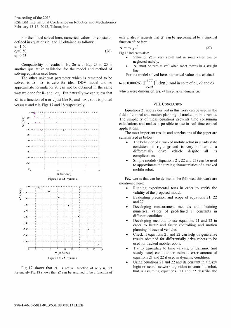
Figure 12: versus u.

Figure 13: versus v.

Fig 17 shows that is not a function of only u, but

fortunately Fig 18 shows that can be assumed to be a function of

only v, also it suggests that can be approximated by a binomial

function of the form: 2

4vc (27)

Fig 18 indicates also:

Value of is very small and in some cases can be

neglected entirely.

must be zero at v=0 when robot moves in a straight

line.

For the model solved here, numerical value of c4 obtained

to be 0.000263 ( deg.]sec

[ 2

rad). And in spite of c1, c2 and c3

which were dimensionless, c4 has physical dimension.

VIII. CONCLUSION

Equations 21 and 22 derived in this work can be used in the

field of control and motion planning of tracked mobile robots.

The simplicity of these equations prevents time consuming

calculations and makes it possible to use in real time control

applications.

The most important results and conclusions of the paper are

summarized as below:

The behavior of a tracked mobile robot in steady state

condition on rigid ground is very similar to a

differentially drive vehicle despite all its

complications.

Simple models (Equations 21, 22 and 27) can be used

to approximate the turning characteristics of a tracked

mobile robot.

Few works that can be defined to be followed this work are

mentioned here:

Running experimental tests in order to verify the

validity of the proposed model.

Evaluating precision and scope of equations 21, 22

and 27.

Developing measurement methods and obtaining

numerical values of predefined ci constants in

different conditions.

Developing methods to use equations 21 and 22 in

order to better and faster controlling and motion

planning of tracked vehicles.

Check if equations 21 and 22 can help us generalize

results obtained for differentially drive robots to be

used for tracked mobile robots.

Try to generalize to time varying or dynamic (not

steady state) condition or estimate error amount of

equations 21 and 22 if used in dynamic condition.

Using equations 21 and 22 and its constant in a fuzzy

logic or neural network algorithm to control a robot,

that is assuming equations 21 and 22 describe the




978-1-4673-5811-8/13/$31.00 ©2013 IEEE

motion of robot but, ci coefficient are dynamically

varying as robot moves.

REFERENCES

[1] Ramnَ Gonzalez , Mirko Fiacchini , José Luis Guzmin,

Teodoro ilamo, Francisco Rodriguez , Robust tube-based

predictive control for mobile robots in off-road conditions ,

Robotics and Autonomous Systems 59 (2011) 711–726

[2] Liang Ding, Haibo Gao , Zongquan Deng , Keiji

Nagatani , Kazuya Yoshida , Experimental study and analysis

on driving wheels’ performance for planetary exploration

rovers moving in deformable soil , Journal of Terramechanics

48 (2011) 27–45

[3] Alireza Pazooki a,n, SubhashRakheja a, DongpuCao ,

Modeling and validation of off-road vehicle ride dynamics ,

Mechanical Systems and Signal Processing 28 (2012) 679–695

[4] R.A. Irani , R.J. Bauer, A. Warkentin , A dynamic

terramechanic model for small lightweight vehicles with

rigid wheels and grousers operating in sandy soil , Journal

of Terramechanics 48 (2011) 307–318

[5] J.Y. Wong a,*, Wei Huang , ‘‘Wheels vs. tracks’’ – A

fundamental evaluation from the traction perspective , Journal

of Terramechanics 43 (2006) 27–42

[6] J. L. Martínez, A. Mandow, J. Morales, S. Pedraza, A.

García-Cerezo, Approximating Kinematics for Tracked Mobile

Robots, International Journal of Robotics Research, Vol. 24,

No. 10, 2005,867-878.

[7] J.Y. Wong, Wei Huang, “Wheels vs. Track” – A Fundumental Evaluation from the Traction Perspective,

Journal of Terramechanics, 43, 2006, 27–42.

[8] MATLAB (TR) R14 help file – optimization tool box,

Math Works INC, 1984-2012.

Simple Modeling of Approximate Turning Characteristics of Tracked Mobile Vehicles in Steady State Condition (2)

Documents