Simple Fiscal Policy Rules: Two Cheers for a Debt Brake! · automatic stabilization according to a counter-cyclical spending rule following the idea of the debt brake results to perform

Simple Fiscal Policy Rules: Two Cheers for a Debt

Brake!

Eric Mayer∗ and Nikolai Stahler†‡

October 30, 2008

(Long) First Draft Version – with mathematical derivations

Abstract

In a New Keynesian DSGE model with non-Ricardian consumers, we show thatautomatic stabilization according to a counter-cyclical spending rule following the ideaof the debt brake results to perform quite well to steer the economy and in termsof welfare. However, it is essential to design the debt brake such that lapses in thespending scheme due to estimation errors in trend output or discretionary fiscal policyactions are booked on an adjustment account and cut future government spending,where discretionary lapses should be corrected faster than lapses due to estimationerrors.

Keywords: fiscal policy, debt brake, welfare, dsge.

JEL code: E 32, G 61, E 62.

∗University of Wurzburg, Department of Economics, Sanderring 2, 97070 Wurzburg, Germany, e-mail:[email protected].

†Deutsche Bundesbank, Department of Economics, Wilhelm-Epstein-Str. 14, 60431 Frankfurt a.M., Ger-many, e-mail: [email protected].

‡We would like to thank Johannes Clemens, Jurgen Hamker, Jana Kremer, Thomas Laubach, Dan Ste-garescu and Karsten Wendorff for their helpful comments. The opinions expressed in this paper do notnecessarily reflect the opinions of the Deutsche Bundesbank or of its staff. Any errors are ours alone.

1

1 Introduction

In the political debate, the stabilizing and potentially welfare enhancing effects of counter-cyclical fiscal policy are attracting more and more attention. The International MonetaryFund (IMF) has just recently identified a possible role for such fiscal stimuli in phases ofeconomic downturns. In its World Economic Outlook, it is, however, found that the effects ofcounter-cyclical fiscal policy are complicated and highly dependent on the characteristics ofthe economy and the fiscal stimulus itself. Special emphasis is laid on the question whetherdiscretionary policy measures should be taken, or whether automatic stabilizers are a betterinstrument. In a cautious conclusion, the IMF states that automatic stabilizers may be amore adequate instrument to “fine tune” the economy as their responses to cyclical changesof the economy can be expected to be more on time, and the danger of a deficit bias presentwith discretionary policy is diminished.1 In case discretionary policy to steer the economyacross cyclical fluctuations is not abolished, the IMF suggests a “fiscal watchdog” – chargedwith identifying changes in the cyclical states of economy, assessing the extent to whichfiscal policy is consistent with medium-term objectives, and providing advice on variouspolicy measures – to to bolster the credibility of discretionary policy actions and reduce thedeficit bias. It is adumbrated that simple fiscal rules, including sustainable and counter-cyclical elements, may be advantageous instruments (see IMF, 2008; chapter 5). In thispaper, we will resume this issue and analyze current proposals in this vein.

The discussion is not as new as it might seem at first sight. Already Allsopp and Vines(2005) and Solow (2005) have noticed that, after quite a time in which the stabilizing roleof fiscal policy has been widely neglected because of the basically disappointing experiencesin the 1970s, there seems to arise somewhat of a consensus that fiscal policy could, however,be an appropriate instrument to steer the economy. In Europe, a potential role of fiscalstabilization has been more or less seriously discussed since the start of this decade (seee.g. European Commission, 2001). The Stability and Growth Pact of the European Union,adopted in 1997 and amended in 2005, allows member countries for some (sustainable)stabilization by demanding budgets to be ‘close to balance or in surplus’ without actuallycalling for corrective means if the corresponding member state does not systematically violatethe 3% deficit ceiling.

Since rather recently, a fiscal regime called “debt brake” is being discussed, which isaiming at strengthening the sustainable stabilizing role of fiscal policy. The debt brake is

1The deficit bias can be explained by arguments from the political economy as e.g. fiscal illusion of eco-nomic subjects (i.e. while citizens fully appreciate the benefits of credit-financed spending and/or tax relief,the same cannot always be said for the associated financing burden), intergenerational income distribution,social polarization (i.e. largely different opinions what governments should spend their money on; see Woo,2005) or that an incumbent government may also be motivated to raise the debt level so as to restrict thenew government’s leeway (see Alesina Tabellini, 1990). Those issues are, however, not addressed in moredetail within this paper. Nevertheless, Cournede (2007) shows that these mechanisms seem to determinepolitical spending behavior and – allegedly necessary – fiscal consolidation has been delayed exactly becauseof such reasons.

2

a proposal to steer fiscal policy according to a simple fiscal rule, i.e., in principle, it followsthe quest to find a “Taylor rule” for fiscal policy. The basic idea is that real governmentexpenditures in a certain period, including interest on outstanding debt, should be equalto real trend revenues raised by the government and not fluctuate with cyclical revenuedeviations. In principle, this means that in “good times”, i.e. in times of output abovetrend, expenditures should fall short of revenues and, thus, the government should save. In“bad times”, i.e. when output is below trend, the government is allowed to deficit-financesome of its expenditures. Actual (discretionary) lapses in this pre-determined spending andpotential deficits/surpluses resulting from cyclical revenue fluctuations are memorized onwhat is called “adjustment account”. A positive balance of the adjustment account thenforces governments to cut future spending. Hence, this spending rule is supposed to bewelfare enhancing due to its counter-cyclical behavior and sustainable as it diminishes thedeficit bias and should, for symmetric shocks, have a determined (fixed) level of debt in thelong run (see Danninger, 2002; Muller, 2006; German Council of Economic Experts, 2007;Kastrop and Snelting, 2008; and Kremer and Stegarescu, 2008; for a discussion). Rules inthis vein have already been implemented in Switzerland in 2001 and it is currently discussedto implement such rules in Germany.

In the present paper, we will analyze the business cycle dynamics and welfare effectsof a debt brake and compare them to a balance budget rule and a debt brake augmentedby an additional component which move counter-cyclical to GDP (see e.g. Taylor, 2000) –in the following simply referred to as automatic stabilizer – and optimal discretion.2 Wefurther analyze which are important setscrews of the debt brake and how recent proposalsdeal with them in the debt brake design. In order to analyze these questions, we construct aconventional DSGE model in the manner of Gali et al. (2007), Leith and Wren-Lewis (2007)and Linnemann and Schabert (2003) with Ricardian and non-Ricardian households, a firmsector with staggered price setting as in Calvo (1983), a monetary authority, for which weassume that it follows a simple Taylor rule, and a fiscal authority that implements a debtbrake, automatic stabilizer or a balanced budget rule.

We find that none of the rules currently in the political debate can be considered as the“new Taylor rule” of fiscal policy. All rules reviewed perform significantly worse than optimaldiscretion. Fundamentally, the Taylor rule is advisable because the “Taylor principle” fits toall shocks. Unfortunately, none of the proposed policy rules embeds such a principle whichfits to all shocks. Therefore, our general finding is that a rule which steers fiscal expendituresalong the trend path and abstains from activism is preferable. We find that the balance

2Note that, in the public discussion, an automatic stabilizer is usually defined to have a constant govern-ment spending path tied to the evolution of trend revenues like the debt brake. In the economic literature,reactions of government spending are often modelled to (additionally) depend negatively on deviations ofoutput from trend, which gives government spending a more active role. In this paper, we term the latter“automatic stabilizer” referring to the literature (basically starting with e.g. Taylor, 2000), while this obvi-ously does not fully correspond to the term used politically. The difference will become clearer when settingup the model. However, the reader is urged to keep this difference in mind.

3

budget rule potentially destabilizes the economy and gives rise to sunspot equilibria. Due toerratic spending schemes, the balanced budget regime destabilizes the economy as it triggersboom-bust cycles in consumption among non-Ricardian households. As monetary authoritiesdo not have a leverage on these hand-to-mouth consumers, such a fiscal policy stance maygive rise to sunspot equilibria, even if the central bank adopts the Taylor principle (see alsoGali, 2004). Accordingly, the overall welfare loss would increase by 11% if fiscal authoritieswould switch from a debt brake to a balanced budget regime. The debt brake, in principle,ties real government spending to real government trend revenue. However, it also acts mildlypro-cyclical, which can be attributed to the interest payments on outstanding debt and to thecommitment to keep overall debt constant over time. For a shock positively influencing actualreal government revenue, this implies that these additional funds are gradually spend overtime. The conventional automatic stabilizer basically augments the debt brake by explicitlynecessitating stabilization in output. This, indeed, generates, in principle, a counter-cyclicalresponse to any economic shock. Note, however, as the government equally has to redeeminterest on debt and is committed towards a constant level of real debt in the long run, theoverall fiscal stance does not necessarily move counter-cyclical to GDP, but depends on thesize of the different effects. A distinct difference to the two previous rules stems from theneed to design a feedback from tax rates to changes in government debt in order to attaina stable equilibrium. Without this feedback, the adaption of government spending due tothe adjustment account to real government expenditures would not suffice to stabilize debt.In terms of welfare, calculated as an average consumer loss function, a conventional debtbrake and a debt brake augmented by an automatic stabilizer are very comparable as thewelfare difference is 4%. Fundamentally, the automatic stabilizer wins the DSGE horse racebecause it keeps expenditures itself closer to real trend than the debt brake itself. Thereforeit attenuates the adverse effects of government spending on wages, in particular, in the caseof cost-push shock, as it does not crowd in private consumption as much as the debt brakedoes.

Regarding the design of a debt brake, we find that the feedback of the adjustment accountto real government spending should ideally differ with the shock. Discretionary governmentspending shocks should be corrected as soon as possible and, thus, have a higher feedback,while all the other shocks (generating expectation errors) should fade out slowly over timein order to keep fluctuations actively introduced into the system low (see also Kremer andStegarescu, 2008; who find the same result in an empirical analysis using German data). Debtbrakes already in action or proposed have the problem that trend estimation is a difficulttask. Therefore, we analyze the effects if fiscal authorities persistently over- or underestimatethe growth trend. We find that our preferred design of a debt brake is well suited to scopewith this problem. In detail, we show that, if trend is over- (under)-estimated, governmentspending tends to be too high (low). Whenever the feedback from the adjustment account isset equal to the values proposed, it is well suited to prevent debt from dramatically increasing,while equally stabilizing inflation and output. If the feedback of the adjustment account istoo low, debt dramatically increases nd the economy is subject to more pronounced cycles

4

in GDP and inflation. Thus, we conclude that the problem of trend mis-estimation gives astrong motive for the installation of an adjustment account.

Debt brakes in place tie government spending to projected revenues and correct thisby a counter-cyclical component to reduce (augment) spending in “good” (“bad”) times.Constructing the debt brake like this, one has to be very careful to adapt the reaction ofgovernment spending to the elasticities of revenues and output correctly, as the latter tendsto be lower than the first, differing in shocks, however). If this adaption is not done correctly,one easily generates a strong pro-cyclical feedback of the debt brake, which is, in terms ofwelfare, not quite as bad as the balanced budget rule, but far from the performance of thebasic idea of a debt brake.

Related literature: As already mentioned earlier, the focus of economic stabilization has,for quite a while, been devoted to monetary policy alone (see e.g. Clarida et al., 1999; andWoodford, 2003; for an overview). One reason may have been that, in the classical theory,Ricardian equivalence dominated the scientific arena. Ricardian equivalence means that, ashouseholds know that higher (potentially deficit-financed) government spending today meanshigher taxes tomorrow, the fiscal multiplier is zero (under the assumption of distortionarytaxation, it may even become negative, see Sutherland, 1997; and Hemming et al., 2002).However, challenging the assumption of full Ricardian equivalence, already Auerbach andKotlikoff (1987) pointed out that, if the crowding-out effects resulting from a fiscal stimulusneed more time to die out than the impulse to affect economic behavior, positive multiplierscan be expected in the short or middle run. The extension of conventional models by shortertime horizons and non- (or only partly) altruistic behavior of economic subjects in e.g.overlapping generation models further pointed in the direction that fiscal policy was, mostlikely, influential (see e.g. Blanchard, 1985; and Mankiw, 2000). The fact that, empirically,there was and is large evidence suggesting that, indeed, fiscal multipliers with respect toGDP are significantly different from zero (see e.g. Baxter and King, 1993; Fatas and Mihov,2001; Blanchard and Perotti, 2002; Perotti, 2005; Heppke-Falk et al., 2006), has led tothe development of models incorporating such features. The first wave of DSGE-papersstudied fiscal policy alongside monetary policy and focussed on how the stability propertiesof monetary policy rules are influenced by fiscal policy, basically building on Leeper’s (1991)active and passive monetary policy (see e.g. Lubik, 2003; Kremer, 2004; Railavo, 2004;Schmitt-Grohe and Uribe, 2007; Leith and von Thadden, 2008; and Stehn and Vines, 2008).Only a little later, Gali et al. (2007) showed that the reactions of macroeconomic variablesto a fiscal policy shock found empirically can (only) be reconciled in DSGE models withrule-of-thumb consumers as well as sticky prices and deficit financing. Going a step further,Straub and Tchakarov (2007), Leith and Wren-Lewis (2007) and Gali and Monacelli (2008)show that, indeed, counter-cyclical fiscal policy may be welfare enhancing in such setups.The main reason – in short – is that such fiscal actions help to at least partly internalizethe externalities caused by the implemented rigidities and market imperfection and keepfluctuations in inflation and disutility of labor smaller than without stabilization. Mayer and

5

Grimm (2008) approve that counter-cyclical tax rules can also improve welfare for supply-side shocks. They show that this even holds for balanced budget rules if the tax rule iscontingent on the observed welfare gap or on the shock. The latest public discussion isfocussing on which fiscal rule should be followed. In this paper, we will contribute to thediscussion by comparing the debt brake, an automatic stabilizer and a balanced budget ruleboth in terms of their effect on macroeconomic variables and in terms of welfare and pointout which are important setscrews to be taken into account.

We will proceed as follows. Section 2 introduces the model used and derives the log-linearized version. In section 3, we analyze the impulse responses of our model, while section4 contains some welfare considerations. In section 5, we have a look at what are importantissues to deal with when constructing a debt brake in reality. Section 6 concludes. A detailedmathematical appendix is added.

2 The model

In this section, we present a New Keynesian DSGE model with firms, households as wellas monetary and fiscal authorities. As standard, firms are categorized into the final goodsector and a continuum of intermediate good producers. Intermediate good producers havesome monopoly power over prices that are set in a staggered way following Calvo (1983).Households obtain utility from consumption, public goods and leisure, and further invest instate contingent securities. The household sector is partitioned into so called Ricardian andNon-Ricardian Households. The Ricardian households, with share (1−λ), own the firms andare able to save, i.e. invest in bonds and state contingent securities, whereas Non-Ricardianhouseholds, with share λ, are hand to mouth consumers in the sense that they spend eachperiod their total labor income. Monetary policy is assumed to be given by a standardTaylor rule. Government expenditures are financed by distortionary taxes levied on wagesand consumption. Fiscal policy is implemented by a spending rule incorporating the debtbrake or the balance budget rule. The model is built on the framework of Gali, Lopez-Salidoand Valles (2007), Leith and Wren-Lewis (2007), and Mayer and Grimm (2008).

In what follows, any aggregated variable Xt is defined by a weighted average of thecorresponding variables for each consumer type, i.e.

Xt = λXrt + (1 − λ)Xo

t , (1)

where the superscripts o and r stand for optimizing Ricardian consumers and rule-of-thumbconsumers, respectively. Further, variables with a “bar” (as in X) indicate the deterministicsteady-state value of the variable X, while variables with a “hat” (as in X) denote percentagedeviations from the steady-state value of this variable X as given by

Xt = log

(Xt

X

)

≈(Xt − X)

X. (2)

6

2.1 Firms and Price Setting

2.1.1 Final good producers

The final good is bundled by a representative firm which operates under perfect competition.The technology available to the firm is

Yt =

[∫ 1

0

Qt(j)ǫt−1

ǫt dj

] ǫtǫt−1

, (3)

where Yt is the final good, Qt(j) are the quantities of intermediate goods, indexed by j ∈(0, 1), and ǫt > 1 is the time-varying elasticity of substitution in period t. Profit maximizationimplies the following demand schedule for all j ∈ (0, 1)

Qt(j) =

(Pt(j)

Pt

)−ǫt

Yt. (4)

The zero-profit theorem implies Pt =[∫ 1

0Pt(j)

(1−ǫt)dj] 1

(1−ǫt)

, where Pt(j) is the price of the

intermediate good j ∈ (0, 1). In a similar way to Smets and Wouters (2003), we assumethat ǫt is a stochastic parameter. This implies that Φt = ǫt

(1−ǫt)reflects the time-varying

markup in the goods market. We get Φt = Φ + Φt, where we assume that Φt is i.i.d. normaldistributed. Then, Φ = ǫ

(1−ǫ)is the deterministic markup which holds in the long-run flexible

price steady state.

2.1.2 Intermediate good producers and prices

The intermediate good sector behaves in the usual manner. Profit by firm j at time t isgiven by

Πt(j) = Pt(j)Qt(j) − Wt(1 + τwt )Nt(j), (5)

where Wt denotes the nominal wage rate, Nt are labor services rented and τwt are social

security contributions of firms. The production technology available to firms is given by

Qt(j) = At · Nt(j), (6)

in which labor is the sole input. For analytical simplicity, it is linear in the shock, whereEt{At} = 1. Real marginal costs per firm can, thus, be represented by

mct(i) =Wt(1 + τw

t )Nt(j)

PtQt(j)= A−1

t︸︷︷︸

=Nt/Qt

[(1 + τw)wt]. (7)

Using equation (5), we can state real profits to be

Πt(j)

Pt=

[Pt(j)

Pt− mct(j)

]

Yt(j). (8)

7

Hence, a firm resetting its price in period t will seek to maximize

Et

∞∑

k=0

(βθp)kΛt,t+k

[Pt(j)

Pt+k

− mct+k(j)

]

Qt+k(j), (9)

with respect to Pt(j) and Qt+k(j), where θp is the exogenous Calvo probability that prices re-main unchanged (see Calvo, 1983). The product demand constraint Qt+k(j) is given by equa-tion (4), which is the isoelastic demand function. Λt,t+k denotes the stochastic discount factorof shareholders, to whom profits are redeemed. It is defined as Λt,t+k = (UC(Ct+k)/UC(Ct)).β denotes a discount factor with β ∈ (0, 1). The corresponding Lagrangian is thus given by

Et

∞∑

k=0

(βθp)kΛt,t+k

{[

Pt(j)

Pt+k− mct+k(j)

]

Qt+k(j) − ϑjt+k

[

Qt+k(j) −

(

Pt(i)

Pt

)−ǫ

Yt+k

]}

,

where Pt(i) is the optimal reset price and ϑjt denotes the Lagrangian multiplier. The combi-

nation of the resulting first-order conditions yields (see Appendix B)

Et

{∞∑

k=0

(βθp)kΛt,t+k

(

Pt(i)

Pt+k

)−ǫ

Yt+k

[1

Pt+k− ǫ

(1

Pt+k−

mct+k(j)

Pt+k(j)

)]}

= 0. (10)

2.2 The Household Sector

We assume a continuum of households indexed by j ∈ (0, 1) of which (1 − λ) householdsare assumed to own the assets such as contingent claims, i.e. they are Ricardian consumers,whereas the rest λ has a consumption ratio of one, i.e. they are Non-Ricardian consumers,rule-of-thumb consumers or liquidity-constraint consumers. Let us assume that any house-hold j is characterized by the following lifetime utility

E0

∞∑

t=0

βtU it

(Ci

t(j), Lit(j)), (11)

where i = o, r indicates optimizing and rule-of-thumb households, respectively.In what follows, we will first describe the optimizing households’ behavior and, then,

turn to the rule-of-thumb consumers.

2.2.1 Optimizing Households

The per-period utility function for optimizing households is given by

Uot (j) = ζt [(1 − χ)log (Co

t (j)) + χlog (Gt) + υtlog (Lot (j))] , (12)

where ζt is a common preference shock to all optimizing households, with E{ζt} = ζ = 1.Lo

t (j) is household j’s leisure, where Not (j) = 1−Lo

t (j) gives the corresponding labor supply

8

of household j. υt > 0, with Et{υt} = υ, measures how leisure is valued compared toconsumption Co

j (j). χ ∈ (0, 1) measures the relative weight of public goods consumption Gt.The flow budget constraint of optimizing households in real terms is given by

(1 + τCt )Co

t (j) +Bo

t+1(j)

PtRt≤ (1 − τd

t )Wt

PtNo

t (j) +Πo

t (j)

Pt+

Bot (j)

Pt, (13)

where Bt is a bond issued by the government. The bond pays a gross interest equal to therisk free nominal rate Rt, which is assumed to be the monetary authority’s policy instrument.Wt is the nominal wage rate. As we assume that the productivity of Ricardian and Non-Ricardian consumers is identical and that their labor services offered to firms are perfectsubstitutes we can drop the superscript o and r in the following regarding wages. Πo

t (j)are nominal profits from the intermediate good sector, which implies that we assume thatthose firms are owned by the optimizing households. τd

t is a distortionary tax rate levied onnominal labor income, while τC

t is a consumption (quasi value added) tax.Each optimizing household now maximizes his utility, equation (11) – given equation

(12) – with respect to consumption, leisure and bond holdings subject to the intertemporalversion of the budget constraint, equation (13). We find that (see Appendix C)

ζt

Cot (j)

= βRtEt

{1 + τC

t

1 + τCt+1

·ζt+1

Cot+1(j)

·Pt

Pt+1

}

(14)

is the consumption Euler equation for optimizing households and derive

Lot (j)

Cot (j)

=υt

(1 − χ)·(1 + τC

t )

(1 − τdt )

· wt (15)

as the labor supply schedule of optimizing households expressed in terms of leisure, wherewt = Wt

Ptand Lo

t (j) = [1 − Not (j)].

2.2.2 Rule-of-Thumb Consumers

Turning to the non-optimizing, i.e. the rule-of-thumb households, who do not have access tocapital markets, we assume that their per-period utility function is also given by an equationanalogue to equation (12), i.e.

U rt (j) = ζt [(1 − χ)log (Cr

t (j)) + χlog (Gt) + υtlog (Lrt (j))] , (16)

where only the superscript o has to be substituted by r. Their lifetime utility is given byequation (11). However, as they do not have access to the capital market, their budgetconstraint becomes static and is given by

(1 + τCt )Cr

t (j) = (1 − τdt )

Wt

PtN r

t (j), (17)

9

which implies that they spend all their per-period income. Note further, that N rt = 1 − Lr

t

also applies. Hence, rule-of-thumb consumers maximize equation (11) – given equation (16)– with respect to Cr

t (j) and Lrt (j) subject to the intertemporal version of the static budget

constraint, equation (17). We get (see Appendix C)

Crt (j)

Lrt (j)

=(1 − τd

t )

(1 + τCt )

(1 − χ)

υt

wt, (18)

which, substituted in equation (17) and remembering that N rt = 1 − Lr

t yields

N rt (j) =

(1 − χ)

(1 − χ) + υt⇔ Lr

t (j) =υt

(1 − χ) + υt. (19)

Hence, labor supply by rule-of-thumb consumers is exogenously fixed by the shock parameterυt, which values leisure compared to consumption, where Et{υt} = υ. Further, it is deter-mined by (1 − χ), which gives the relative weight of private consumption. Using equation(19) and equation (18), we find that

Crt (j) =

(1 − χ)

(1 − χ) + υt· wt ·

(1 − τdt )

(1 + τCt )

. (20)

2.3 Fiscal Authorities

The government issues bonds Bt+1 each period (which have to be repaid with interest in thefollowing period), and collects consumption taxes τC

t PtCt and labor income taxes τLt WtNt,

where τLt = τw

t + τdt . The receipts are used to finance government expenditure PtGt and

interest on outstanding debt Rt−1Bt of the previous period (where in Rt−1, the re-paymentis included). Hence, the government’s flow budget constraint reads

Bt+1 + τLt WtNt + τC

t PtCt = Rt−1Bt + PtGt. (21)

Expressing equation (21) in real terms implies dividing it by Pt. Further, we normalizeequation (21) by dividing it by Y , where Y is the steady-state output of the economy, i.e.the trend-output within our model. This yields

Bt+1

PtY+

τLt wtNt

Y+

τCt Ct

Y=

Rt−1Bt

Pt−1Y

Pt−1

Pt+

Gt

Y. (22)

Defining bt = Bt

Pt−1Yas the cyclically adjusted debt, and government tax revenues as Ψt =

τLt WtNt + τC

t PtCt, whereΨt

PtY=

τLt wtNt

Y+

τCt Ct

Y, (23)

equation (22) rewrites to

bt+1 +Ψt

PtY= Rt−1bt

Pt−1

Pt+

Gt

Y. (24)

10

For later use, we will further define

bt = bt − b =Bt

Pt−1Y−

B

P Y(25)

as the deviation of the percentage of the cyclically adjusted debt from its steady-state ratio.In what follows, we will describe the different fiscal spending rules in more detail.

2.3.1 Balanced Budget Rule

As a benchmark for a sustainable spending rule, we introduce a balanced budget rule, whichimplies that – as government spending is usually planned at least one period in advance– the government is not allowed to spend more than the projected funds raised by thegovernment. Any expectation errors, i.e. differences between projected and actual fundsraised by the government, and (active) discretionary spending shocks νt are booked on anadjustment account ACt to memorize lapses in the spending behavior. Thus, (ex-ante)spending according to the balance budget rule is determined by projected revenues minusprevious balances booked on the adjustment account, i.e. Et−1{Ψt} − ρ · ACt−1, where ρis a parameter indicating how much effect earlier lapses in the spending behavior have oncurrent spending. It can be interpreted as the speed of adjustment. This implies, actual(ex-post) spending is given by

(Rt−1 − 1)Bt + PtGt = Et−1{Ψt} − ρACt−1︸︷︷︸

=Rule based spending

+νt. (26)

The adjustment account for the balanced budget rule reads

ACt = (1 − ρ)ACt−1 + νt + Et−1{Ψt} − Ψt︸︷︷︸

Expectation error

. (27)

In normalized real terms, this reads

(Rt−1 − 1)bt +Gt

Y= Et−1

{Ψt

PtY

}

− ρ ·Pt−1

Pt· act−1 +

νt

PtY(28)

and

act = (1 − ρ)Pt−1

Pt

· act−1 +νt

PtY+ Et−1

{Ψt

PtY

}

−Ψt

PtY, (29)

where act = ACt

PtY.

2.3.2 Debt Brake and Automatic Stabilizer

In the political debate – summarized under the heading “debt brake” –, there is quite adiscussion to implement simple spending rules that give counter-cyclical impulses to the

11

economy as pointed out in the introduction. The main idea is that real spending, includinginterest on outstanding real debt, should be equal to real trend revenues, i.e. Ψ

Pin our

model (see Danninger, 2002; German Council of Economic Experts, 2007; Kastrop andSnelting, 2008; and Kremer and Stegarescu, 2008 for a discussion). It is counter-cyclicalbecause, whenever output/revenue is above trend, the government saves, while in times ofoutput/revenue above trend, the government deficit-finances part of its expenditures.

An automatic stabilizer as it is usually modelled is a public revenue and spending mech-anism that automatically and more actively than the debt brake just described gives acounter-cyclical fiscal impulse to the economy on the demand side (see Taylor, 2000; Artisand Buti, 2000; or Buti et al., 2001). Classical examples for such automatic stabilizers areincome taxation (on the revenue side) and unemployment insurance (on the expenditureside). In principle, the debt brake and the automatic stabilizer are rather similar. How-ever, for a conventional automatic stabilizer, real government expenditures, which are stillbasically restricted by the revenue side, have to be augmented by a more active counter-cyclical component compared to the debt brake. The counter-cyclical component is given by(Y /Yt

)α, which actively diminishes spending for Y < Yt and vice versa, where α > 0 cap-

tures the magnitude of the automatic reaction of government spending to output deviationsfrom trend.

Regarding the adjustment account, we have to differentiate between the two rules. Forboth rules, we know that we have to book (active) discretionary spending shocks νt as theyare never part of the spending rule and, hence, have to be corrected in future periods.However, the rule-based spending differs in both cases and, hence, what has to be booked onthe account differs. First, for the debt brake, i.e. α = 0, we only have to book the differencebetween real normalized trend revenue and real normalized true revenue, i.e. Ψ

P Y− Ψt

PtYt

as debt accumulates whenever trend exceeds true revenue. Second, for the convectionalautomatic stabilizer, i.e. α > 0, we only have to book expectation errors regarding thecyclical situation of the economy, i.e. Et−1

{(Y /Yt

)α}−(Y /Yt

)αas such errors generate

spending that does not conform with the rule.This discussion can be summarized formally (in normalized terms, i.e. divided by Y ) by

(Rt−1 − 1)bt +Gt

Y=

Ψ

P Y· Et−1

{(Y

Yt

)α}

− ρ ·Pt−1

Pt

act−1

︸︷︷︸


+νt

PtY, (30)

where νt is a (discretionary) government spending shock and act = ACt

PtY. Because the budget

plans are usually made at least one period ahead, in the case of the automatic stabilizer,the government sets spending in t according to the projected cyclical situation in t at time(t− 1). Note further that, for α = 0, we have the spending rule according to the debt brake,while for α > 0, the conventional automatic stabilizer applies. For the adjustment account,

12

it holds that

act = (1 − ρ) ·Pt−1

Pt· act−1 +

νt

PtY+

Ψ

P Y·

[

Et−1

{(Y

Yt

)α}

−

(Y

Yt

)α]

︸︷︷︸

=Automatic Stabilizer; α>0, =0

+

[Ψ

P Y−

Ψt

PtY

]

︸︷︷︸

Debt Brake; α=0, =1

, (31)

where α = 0 and = 1 for the debt brake, and α > 0 and = 0 for the automaticstabilizer. Note that, as the government is committed towards keeping real debt constant inthe long run, debt services and the adjustment account can almost chancel out the automaticstabilizer component such that the fiscal stance might only move mildly counter-cyclical toGDP.

2.4 Market Clearance

In clearing of factor and goods markets, the following conditions are satisfied

Yt = Ct + Gt, (32)

where Ct = λCrt + (1 − λ)Co

t is aggregated consumption.3 Further,

Yt(j) = Qt(j) (33)

and

Nt =

∫ λ

0

N rt (j)dj +

∫ 1

λ

Not (j)dj. (34)

2.5 Linearized Equilibrium Conditions

In this section, we summarize the model by taking a log-linear approximation of the keyequations around a symmetric equilibrium steady state.

Firms: Log-linearizing the marginal cost function, equation (7), yields

mct(i) = −At + wt + ιw τwt , (35)

where ιw = τw

(1+τw). From the production technology, equation (6), we know that

Nt = Yt − At. (36)

3Note that, within each group i = o, r each household consumes the same due to constant labor supplyfor rule-of-thumb consumers and state-contingent claims for optimizing consumers (see also Woodford, 2003;and Appendix C for details).

13

Solving the firm’s optimality condition for the optimal reset price Pt(j) and following Galiet al. (2001), we can derive the Phillips curve (see Appendix B)

πt = β · Et {πt+1} + κ · mct + ǫt, (37)

where

κ =(1 − θp)(1 − βθp)

θp.

Note that we defined πt = Pt − Pt−1.

Households: The consumption Euler equation expressed in aggregated variables and deepparameters reads (see Appendix C)

Ct = EtCt+1−ΘnEt∆Nt+1 +ιCEt∆τCt+1−Et[Rt− πt+1]+ΘυEt[υt− υt+1]+Et[ζt− ζt+1], (38)

where Θn = λγrϕ(1−γrλ)

, Θυ = γrλ(1−χ)(1−χ+υ)(1−γrλ)

, ιC ≡ τC

(1+τC ), ϕ = N

1−N, γr = υ

1−χ+υ1

1−N, and we

have used the fact that, in the steady-state, R = β−1. Note that ∆Nt+1 = Nt+1 − Nt and soon. Under perfectly competitive labor markets, the wage evolution (labor supply schedule)is given by

wt = Ct + ϕNt + ιdτdt + ιC τC

t + υt, (39)

where ιd ≡ τd

(1−τd). Calculations can also be retraced in Appendix C.

Fiscal authorities: Log-linearizing the normalized budget constraint, equation (24) aroundits steady-state yields

bt+1 − β−1bt = γG

[

Gt − (Ψt − Pt)]

︸︷︷︸

=Primary Deficit

+¯b(1 − β−1

)

︸︷︷︸

<0

[

Ψt − Pt

]

+¯bβ−1

[

Rt−1 − πt

]

. (40)

Equation (40) determines the evolution of the level of debt after a deviation of other theparameters. Real government revenues evolve according to

Ψt − Pt =τLW N

Ψ︸︷︷︸

=RevL

(

τLt + Wt + Nt

)

+τC P C

Ψ︸︷︷︸

=RevV AT

(

τCt + Ct

)

, (41)

where

RevL =τL(ǫ − 1)

ǫ(1 + τw)[γG − (1 − β−1)¯b]

is the percentage of labor tax revenue and

RevV AT =τC

γC [γG − (1 − β−1)¯b]

14

the percentage of value added tax revenue calculated in deep parameters, with RevL +RevV AT = 1 (see Appendix E for more details). Equation (41) determines the deviation ofgovernment revenue from its steady-state value.

Log-linearized government spending is given by

Gt =(1 − β−1)

γGbt −

ρ

γG· act−1 +

1

γGP Y· νt +

¯b(1 − β−1)

γGπt − β−1

¯b

γGRt−1

+γG − (1 − β−1)¯b

γG

ø1 · Et−1

{

Ψt − Pt

}

︸︷︷︸

Balanced Budget

−α · Et−1

{

Yt

}

︸︷︷︸

Automatic Stabilizer

︸︷︷︸

=0 for Debt Brake

, (42)

while the log-linearized adjustment account is given by

act = (1 − ρ)act−1 +νt

P Y+(

γG − (1 − β−1)¯b) [(

ø1 · Et−1

{

Ψt

}

− Ψt

)

−(

ø1 · Et−1

{

Pt

}

− Pt

)

− α(

Et−1

{

Yt

}

− Yt

)]

, (43)

where ø1 = α = 0 and = 1 for the debt brake, ø1 = = 0 and α > 0 for the automaticstabilizer and ø1 = = 1 and α = 0 for the balanced budget rule for both equations (42)and (43). Note, again, that πt = Pt − Pt−1. All the calculations regarding fiscal authoritiescan be retraced in Appendix D.

Monetary authorities: We assume that monetary authority acts as (exogenously) givenby the following simple Taylor rule,

Rt = (1 − µ)[

φππt + φY Yt

]

+ µRt−1 + zt, (44)

where φπ and φY denote the reaction coefficients towards inflation and output deviations,respectively. µ denotes the degree of interest rate smoothing. zt defines the monetary shock.

Market clearing: Market clearing implies that

Yt = γCCt + γGGt, (45)

where γC and γG are the shares of output devoted to private and public consumption, re-spectively. They can be expressed in terms of deep parameters (see Appendix E).

Additional feedback and shocks: We further assume that there may exist an additionalfeedback of debt to tax rates in order to generate existence. This implies that we assumeτCt = χCbt, τw

t = χwbt and τdt = χdbt. Note that, except for the automatic stabilizer, we

15

are able to set χk = 0, where k = C, w, d (see section 3 for a more detailed discussion).For the shocks we assume autocorrelation implying ζt = ρζ · ζt−1 + ζt, At = ρA · At−1 + At,ǫt = ρǫ · ǫt−1 + ǫt, υt = ρυ ·υt−1 + υt, zt = ρz · zt−1 + zt, νt = ρν ·νt−1 + νt and ξt = ρξ · ξt−1 + ξt,where ζt, At, ǫt, υt, zt, νt and ξt are random i.i.d. shocks.

Proposition 1. All endogenous macro-variables and, thus, welfare can be expressed by deepparameters and fixed levels of tax rates τw, τd and τC in the steady-state and are identicalacross all fiscal regimes considered.

Proof. See Appendix E.

Proposition 1 states that the steady-state levels of all variables are identical across fiscalregimes. This is of utmost importance for our welfare exercise as it allows us to focus on thebusiness cycle implications of fiscal policy, whereas we do not need to adjust our conclusionsfor differences in the steady-states.

3 Calibration and Impulse Response Analysis

In this section we provide details on the business cycle dynamics if fiscal authorities imple-ment the fiscal rules discussed above.

3.1 Calibration Strategy

While conducting the calibration exercise of the deep parameters we rely on parameter valuestypically recommended to describe the euro area.

For fiscal authorities we set in particular tax rates such that they reflect average taxrates on labor and value added typically reported. The labor tax rate was set to τd = 0.125,which includes labor income tax and the social security contributions of households. Thesteady-state rate of social security contributions of firms was set equal to τw = 0.125. Theconsumption tax rate is calibrated to be τC = 0.183. This endogenously determines theprivate consumption to output ratio and the government consumption to output ratio whichare equal to γC = 0.67 and γG = 0.33.4

For the fraction of liquidity constraint consumers we choose λ = 0.33, which engineers amore moderate crowding out of private consumption to a highly autocorrelated exogenousexpenditure shock on impact. For moderately autocorrelated spending shocks, it is able toreplicate a crowding-in of private consumption, which is in line line with evidence reportedfrom a VAR by Gali et al. (2007). For lower values of λ as, for instance, proposed byCoenen et al. (2008), our model would still predict a substantial crowding out in private

4Coenen et al. (2008) propose instead to set tax rates equal to marginal rates. Although appealing atfirst sight this would inflate the endogenously determined government to output ratio beyond 0.4 in ourmodel.

16

consumption which might be considered as counterfactual (see Figure 1 which pictures theimpulse responses for a fiscal spending shock with parameters set according to the baselinecalibration and autocorrelation coefficient for the shock set equal to ρν = 0.5).

4 8−0.2

0

0.2

0.4

0.6

0.8GDP

Quarters

λ=0.00λ==0.33

4 8−0.2

−0.1

0

0.1

0.2Consumption

Quarters

4 8−1

0

1

2

3Government

Quarters4 8

0

0.02

0.04

0.06Interest Rate

Quarters

4 8−0.05

0

0.05

0.1

0.15Inflation

Quarters4 8

−0.5

0

0.5

1Real Wage

Quarters

Figure 1: Government expenditure shock

Since we do not have a distinctive imagination for appropriate numerical values for ρ,which governs the partial feedback from the adjustment account to expenditures and for χj,where j = C, d, w, which governs the feedback from changes in public debt to tax rates, wechoose the parameters such that our welfare metric was minimized. We find in particularthat for all shocks except government expenditure shocks the algorithm preferred rathersmall parameters for ρ and χj . Accordingly, we set ρ = 0.05, which generates a uniqueand determined rational expectations equilibrium. In section 5.1, we provide some furtherdiscussion on the role of ρ for a welfare enhancing design of a debt brake. We are ableto set χj = 0. This is advisable as it allows us to eliminate movements in distortionarytaxes on labor and value added at the business cycle frequency. Note however, as we willdiscuss below, we need some moderate feedback of taxes to changes in debt for an automaticstabilizer to output to prevent the equilibrium to be non-unique.

For the supply side of the model to imply a substantial degree of nominal rigidities we setθp = 0.75, which implies that prices are fixed on average for four quarters. This is calibratedsomehow in the middle of the range typically reported in literature. Coenen et al (2008) andSmets and Wouters (2004) estimate an average price duration for optimal price setting of tenquarters using full information Baysian estimation techniques, while Del Negro et al. (2005)

17

only report an average price duration of three quarters. Micro-data for the euro-area on pricesetting report low price durations with a median of around 3.5 quarters (see Alvaraez et al.,2006 for a summary of recent micro-evidence). The steady-state mark-up of intermediategood producers over marginal cost is set at 10 per cent, implying that ǫ = 11.

As we have modelled the household sector by a log-log specification for analytical con-venience, the implied intertemporal elasticity of substitution is equal to σ = 1. FollowingGali et al. (2004), who specify the household sector in a similar setting, we calibrate theinverse of the Frisch elasticity of labor supply equal to ϕ = 1. This, in turn, implies thatthe steady-state per capita consumption ratio of liquidity constraint to average consumersis equal to γr = Cr/C = 0.8. The discount factor is fixed to β = 0.99, implying a 4%steady-state real interest rate.

The Taylor-rule coefficients display the familiar values. The inflation coefficient on theinflation rate was set to φπ = 1.9 while for the output gap coefficient we opt for φY = 0.25(see Del Negro et al., 2005; Coenen et al., 2008; and Smets and Wouters, 2003). FollowingGali et al. (2004), we set the inflation coefficient to a somewhat higher value than originallyproposed by Taylor (1993) as, in the light of rule-of-thumb consumers, the central bank isforced to follow a more anti-inflationary policy. The interest rate smoothing coefficient wasset to µ = 0.85.

The exogenous driving forces ζt, At and ǫt are assumed to follow a univariate autoregres-sive process where the first order coefficients where set as follows: ρζ = 0.882, ρǫ = 0.890and ρA = 0.822. These values reflect coefficients found in Coenen et al. (2006) and Smetsand Wouters (2003, 2007). For the case of the exogenous fiscal spending shock, the recentliterature has not yet found a clear cut consensus. While some authors report evidencefor highly auto-correlated fiscal expenditure shocks such as Smets and Wouters (2004) withρυ = 0.956 among others. Chari et al. (2007) attribute only little role to fiscal expenditureshocks at all. Still, others estimate DSGE models and remain tacit whether there is any rolefor fiscal expenditure shocks by not specifying them (Coenen at al., 2008).

3.2 Impulse Response Analysis

Given the above calibration we kick off to analyze the different sets of fiscal policy rules. Inthis section the emphasis is on the identification of distinct differences across fiscal regimesfollowing a shock to consumer preferences and to a price mark-up shock. In section 4, wewill draw welfare conclusions.

Shock to consumer preferences

Figure 2 portrays the dynamic response of selected variables to a shock to consumerpreferences if fiscal policy follows a debt brake.

Due to the additional demand posted to firms those firms that are allowed to reset pricesincrease prices to cushion the increasing marginal cost pressure stemming from higher wages

18

0 4 80

0.1

0.2

0.3

0.4

0.5

0.6GDP

Quarters

GovernmentConsumption

0 4 80

0.2

0.4

0.6

0.8

1Consumption

Quarters

Non−RicardianRicardian

0 4 8−0.1

−0.05

0

0.05

0.1Tax Wedge

Quarters

Value Added TaxEmployers TaxEmployees Tax

0 4 80

0.5

1

1.5

2Tax Revenues

Quarters

Labor TaxesValue Added Tax

0 4 8−2

−1.5

−1

−0.5

0

0.5Expenditures

Quarters

PurchasesDebt ServicesAdjustment Account

0 4 8−1.5

−1

−0.5

0Debt

Quarters

Primary DeficitRevolving Debt

0 4 80

0.05

0.1

Interest Rate

Quarters0 4 8

0

0.05

0.1

0.15

0.2

0.25

0.3Inflation

Quarters0 4 8

0

0.5

1

1.5Wages

Quarters

Figure 2: Debt Brake and Consumer Preference Shock

19

to incite households to work more in order to satisfy the additional demand. The increasein real wages, in turn, encourages Non-Ricardian consumers to increase their consumptionexpenditures. Although they only account for one third of the household sector they drive, onimpact, almost 50% in the consumption dynamics and start to dominate the picture onward.As monetary authorities are determined to dampen inflation variability they increase realinterest rates and slowdown consumption expenditures such that inflation falls quickly. Thesomewhat tough stance on inflation and the implied high interest rate along the adjustmentpath almost completely wipes out the positive impact of the consumer preference shockfor Ricardian households from quarter three onwards. The impulse responses portray thatfiscal authorities keep expenditures largely stable over the cycle. In particular the additionalfunds raised due to an increase in labor and consumption taxes are not spent but pathedthrough to debt. Thus the debt brake embodies automatic stabilization on the revenue sideas government expenditures are decoupled from cyclical movements in revenues and keptat trend. The mildly pro-cyclical movement in government expenditures can be attributedto interest rate payments on outstanding debt and the commitment of fiscal authorities tokeep overall debt constant in the long run, which means that the additional funds are spentgradually over time. This is engineered by a low feedback from the adjustment account togovernment expenditures.

Figure 3 depicts the business cycle dynamics if fiscal authorities are determined to bal-ance the budget in each period. Due to the planning horizon of one period the budget willnot balanced in the first period as the unexpected tax revenues are not accounted for inthe predetermined government expenditure plans. The regime shift leads to a number ofremarkable changes in the business cycle. First, government expenditures become quanti-tatively the driving component of GDP, whereas for the debt brake, private consumptionexpenditures dominated the picture over the first five quarters. From period two onward,the government spends the additional tax revenues which has two effects on the economy.On the one hand, firms have to pay significantly higher wages to optimizing households toextent their hours worked, while, on the other hand, the significantly higher wages lead toa boom in consumption among liquidity constraint consumers. Accordingly, compared toa debt brake, we observe a somewhat higher inflation rate and higher interest rates, whichalmost completely crowd out the consumption expenditures of Ricardian households. Thelow feedback running from the partial adjustment account to expenditures gradually reducesthe debt accumulated in the first period due to the expectations error.

Figure 4 illustrates the response to a consumer- preference shock if the government triesto implement a debt brake but explicitly allows for automatic stabilization in output (whichwe have termed “automatic stabilizer”). In the upper panel, we plot the tax wedge. It servesas a measure for the cumulative distortions imposed on the economy due to movements intax rates at the business cycle frequency. Following Coenen et. al (2007), it is measured as

follows: Define the real effective wage income of households as(1−τd

t )

(1+τCt )

Wt

Ptand the effective

labor cost of firms as (1+ τwt )W−t

Pt. In an undistorted equilibrium, the ratio of the two would

20

0 4 80

0.5

1

1.5GDP

Quarters


0 4 80

0.2

0.4

0.6

0.8

1Consumption

Quarters


0 4 8−0.1

−0.05

0

0.05

0.1Tax Wedge

Quarters


0 4 80

0.5

1

1.5

2

2.5

3Tax Revenues

Quarters


0 4 8−4

−3

−2

−1

0

1

2

3Expenditures

Quarters


0 4 8

−0.5

−0.4

−0.3

−0.2

−0.1

0

0.1Debt

Quarters


0 4 80

0.05

0.1

0.15

0.2Interest Rate

Quarters0 4 8

0

0.05

0.1

0.15

0.2

0.25

0.3Inflation

Quarters

0 4 80

0.5

1

1.5

2Wages

Quarters

Figure 3: Balanced Budget and Consumer Preference Shock

21

0 4 8−0.2

0

0.2

0.4

0.6

0.8GDP

Quarters


0 4 80

0.2

0.4

0.6

0.8

1Consumption

Quarters


0 4 8−0.015

−0.01

−0.005

0Tax Wedge

Quarters


0 4 80

0.5

1

1.5

2Tax Revenues

Quarters


0 4 8

−0.1

−0.05

0

0.05Expenditures

Quarters


0 4 8−2

−1.5

−1

−0.5

0Debt

Quarters


0 4 80

0.05

0.1

Interest Rate

Quarters0 4 8

0

0.05

0.1

0.15

0.2

0.25

0.3Inflation

Quarters0 4 8

0

0.5

1

1.5

2Wages

Quarters

Figure 4: Automatic Stabilizer and Consumer Preference Shock

22

be one. Accordingly,

τwedget = 1 −

(1 − τdt )

(1 + τCt )(1 + τw

t )

serves as a summary statistic to measure the evolution of the tax wedge over the cycle. Adistinct difference of the automatic stabilizer regime to the two previous regimes stems fromthe need to design a feedback from tax rates to changes in government debt. Without thisfeedback, the moderate cut in government spending due to the feedback from the adjustmentaccount to real government expenditures would not be sufficient to stabilize the net presentvalue of outstanding real government liabilities and, thus, generate explosive equilibria. Asfor the case of a debt brake, the additional revenues are not spent but passed through todebt. Because the government needs to rely on pro-cyclical taxation, the surpluses in rev-enues quickly vanish and debt starts to return gradually to its initial steady state. Generally,the effects are very similar to those of the debt brake. However, note that, for the auto-matic stabilizer, government spending acts very mildly counter-cyclical (or, basically, staysconstant), while it is mildly pro-cyclical for the debt brake.

Shock to price mark-up

Figure 5 illustrates the course of business cycle dynamics if the economy is hit by apersistent shock to the price mark-up. Those firms who can reset prices adjusts prices upwardas market power has risen. Monetary authorities increase real interest rates to set incentivesto Ricardian households to reallocate planned consumption expenditures into the future.This depresses contemporaneous aggregate demand such that firms have to engineer cutsin production by offering lower real wages. As consumption expenditures of Non-Ricardianhouseholds are driven by real wages, the downturn of the economy is accelerated.

If fiscal authority’s implement a debt brake, the basic operating principles are identicalto those observed for the case of a demand shock. The cyclical shortfall in revenues does nottrigger cuts in government expenditures but is absorbed by debt. This builds in an auto-matic stabilization mechanism for the evolution of GDP as government expenditures movemildly but persistently pro-cyclical. This pro-cyclical behavior stems from debt services andmore moderate fiscal expenditure from quarter two onward as the government is committedtowards keeping the steady state debt to GDP ratio constant over time.

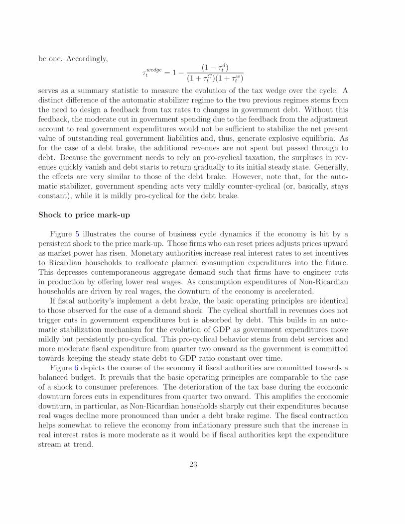
Figure 6 depicts the course of the economy if fiscal authorities are committed towards abalanced budget. It prevails that the basic operating principles are comparable to the caseof a shock to consumer preferences. The deterioration of the tax base during the economicdownturn forces cuts in expenditures from quarter two onward. This amplifies the economicdownturn, in particular, as Non-Ricardian households sharply cut their expenditures becausereal wages decline more pronounced than under a debt brake regime. The fiscal contractionhelps somewhat to relieve the economy from inflationary pressure such that the increase inreal interest rates is more moderate as it would be if fiscal authorities kept the expenditurestream at trend.

23

0 4 8 12 16

−0.5

−0.4

−0.3

−0.2

−0.1

0GDP

Quarters


0 4 8 12 16

−0.5

−0.4

−0.3

−0.2

−0.1

0Consumption

Quarters


0 4 8 12 16−0.1

−0.05

0

0.05

0.1Tax Wedge

Quarters


0 4 8 12 16−1.2

−1

−0.8

−0.6

−0.4

−0.2

0Tax Revenues

Quarters


0 4 8 12 16

−2

−1

0

1

2

Expenditures

Quarters


0 4 8 12 160

0.5

1

1.5

2

2.5

3

3.5Debt

Quarters


0 4 8 12 160

0.05

0.1

0.15

0.2Interest Rate

Quarters0 4 8 12 16

0

0.1

0.2

0.3

0.4Inflation

Quarters0 4 8 12 16

−1

−0.8

−0.6

−0.4

−0.2

0Wages

Quarters

Figure 5: Debt Brake and Price Mark-Up Shock

24

0 4 8 12 16

−0.6

−0.4

−0.2

0

GDP

Quarters


0 4 8 12 16

−0.5

−0.4

−0.3

−0.2

−0.1

0

0.1

Consumption

Quarters


0 4 8 12 16−0.1

−0.05

0

0.05

0.1Tax Wedge

Quarters


0 4 8 12 16−1.5

−1

−0.5

0

Tax Revenues

Quarters


0 4 8 12 16−2

−1.5

−1

−0.5

0

Expenditures

Quarters


0 4 8 12 16−0.06

−0.04

−0.02

0

0.02

0.04Debt

Quarters


0 4 8 12 160

0.05

0.1

Interest Rate

Quarters0 4 8 12 16

0

0.1

0.2

0.3

0.4Inflation

Quarters0 4 8 12 16

−1.5

−1

−0.5

0

0.5Wages

Quarters

Figure 6: Balanced Budget and Price Mark-Up Shock

25

Figure 7 portrays the dynamics of the business cycle if fiscal authorities implement anautomatic stabilizer. For the case of a price mark-up shock, this regimes turns out to be themost passive one in terms of fiscal expenditures because the counter-cyclical stance due toautomatic stabilization in output and the need to bring back real debt in the medium termchancel out. Hence, government expenditures are effectively kept constant. Consequently,fiscal authorities are less ambitious to reverse debt dynamic which prevail more persistence.As beforehand a sufficiently strong pro-cyclical movement in tax rates is a necessary conditionto revert debt dynamics and anchor the outstanding real government liabilities. As tax ratesare increased, tax revenues are at their trend level after four quarters. The dynamics of theinflation rate and wage dynamics are similar as those observed under a debt break.

0 4 8 12 16−0.4

−0.3

−0.2

−0.1

0

0.1GDP

Quarters


0 4 8 12 16−0.8

−0.6

−0.4

−0.2

0Consumption

Quarters


0 4 8 12 16−0.01

0

0.01

0.02

0.03

0.04

0.05Tax Wedge

Quarters


0 4 8 12 16−1.5

−1

−0.5

0Tax Revenues

Quarters


0 4 8 12 16

−0.2

−0.1

0

0.1

0.2Expenditures

Quarters


0 4 8 12 160

1

2

3

4Debt

Quarters


0 4 8 12 160

0.05

0.1

Interest Rate

Quarters0 4 8 12 16

0

0.05

0.1

0.15

0.2

0.25

Inflation

Quarters0 4 8 12 16

−1

−0.8

−0.6

−0.4

−0.2

0Wages

Quarters

Figure 7: Automatic Stabilizer and Price Mark-Up Shock

Shock to technology

Figure 8 portrays the course of the business cycle dynamics if the economy is hit by atechnology shock under a fiscal debt brake regime. The technology shock augments produc-tivity and, thus, cuts marginal costs of firms. For a given level of output, this allows firms

26

to cut employment or augment production for a given level of employment. In order to cutemployment, firms reduce wages, which decreases labor supply and consumption of Ricar-dian households. As marginal costs and wage costs decrease, those firms that can reset theirprices to a lower level, which decreases inflation. The fall in inflation makes the central bankcut interest rates, which, in turn, augments consumption of Ricardian households. In total,consumption rises. Higher demand for goods implies that additional production is neededand, therefore, firms raise wages from period three onward to also make Non-Ricardianhouseholds supply more labor, which, then, increases their consumption level. The rise inconsumption and output then drive inflation back to its original level. Following the debtbrake, the government basically keeps expenditures fixed to trend revenues and passes thefall in true revenues to debt, which, as in the other cases, yields a very mild counter-cyclicalspending behavior due to the interest payments.

0 4 8 12−0.1

0

0.1

0.2

0.3GDP

Quarters


0 4 8 12−0.2

0

0.2

0.4

0.6Consumption

Quarters


0 4 8 12−0.1

−0.05

0

0.05

0.1Tax Wedge

Quarters


0 4 8 12−0.8

−0.6

−0.4

−0.2

0

0.2Tax Revenues

Quarters


0 4 8 12−0.4

−0.3

−0.2

−0.1

0

0.1

0.2

Expenditures

Quarters


0 4 8 12−0.2

−0.1

0

0.1

0.2

0.3Debt

Quarters


0 4 8 12−0.1

−0.08

−0.06

−0.04

−0.02

0Interest Rate

Quarters0 4 8 12

−0.25

−0.2

−0.15

−0.1

−0.05

0Inflation

Quarters0 4 8 12

−0.6

−0.4

−0.2

0

0.2Wages

Quarters

Figure 8: Debt Brake and Technology Shock

In figure 9, we see how the business cycle dynamics change whenever the government fol-lows a balance budget rule. In the first period, the decrease in revenues, mainly due to labortaxes because of lower wages and less labor supply, is not anticipated by the government

27

and passed though to debt because of the planning horizon. However, in the second period,we see, in contrast to the debt brake regime, a sharp decrease in government expendituremainly resulting from the balanced budget requirement. As the demand from the govern-ment decreases, this dampens GDP and yields a further decrease in wages, again, loweringconsumption of Non-Ricardian households. In a certain way, this could be interpreted as anegative government spending shock. This is, in total, not able to compensate for the in-crease in consumption of Ricardian households resulting from the interest rate decrease dueto less inflation. From period three onward, tax revenues increase due to higher value addedtaxes from more aggregated consumption, which boosts government expenditure and output.Due to the rise in output, wages have to rise in order to augment labor supply. In total,we see that the balanced budget regime generates much more fluctuations in governmentspending and also other macroeconomic variables.

0 4 8 12−0.4

−0.2

0

0.2

0.4

0.6GDP

Quarters


0 4 8 12−0.4

−0.2

0

0.2

0.4

0.6Consumption

Quarters


0 4 8 12−0.1

−0.05

0

0.05

0.1Tax Wedge

Quarters


0 4 8 12−1

−0.5

0

0.5Tax Revenues

Quarters


0 4 8 12−1

−0.5

0

0.5Expenditures

Quarters


0 4 8 12−0.2

−0.1

0

0.1

0.2

0.3Debt

Quarters


0 4 8 12

−0.1

−0.05

0Interest Rate

Quarters0 4 8 12

−0.25

−0.2

−0.15

−0.1

−0.05

0Inflation

Quarters0 4 8 12

−1

−0.5

0

0.5Wages

Quarters

Figure 9: Balanced Budget and Technology Shock

Figure 10 illustrates the business cycle dynamics under an automatic stabilizer regime.We see that, in principle, it is quite similar to the debt brake regime. However, the counter-cyclical government expenditure reaction is more pronounced and, as for the other regimes,

28

we need a small feedback between taxes and debt to achieve a stable equilibrium. Gov-ernment expenditures move slightly counter-cyclical, mainly driven by the counter-cyclicalcomponent of the debt brake as hardly anything that is booked on the adjustment accountaffects government spending. From period three onward, the higher demand for goods andoutput makes firms rise wages to generate higher labor supply, which augment governmentrevenue. These extra revenues are, basically, fully passed into debt which falls stronger thanin the case of the debt brake. Still, government spending stays low as the counter-cyclicalcomponent is not compensated by the reduced debt services (more precisely, the additionalincome resulting from negative levels of debt).

0 4 8 12−0.1

0

0.1

0.2

0.3GDP

Quarters


0 4 8 12−0.2

0

0.2

0.4

0.6Consumption

Quarters


0 4 8 12−4

−2

0

2

4

6

8x 10

−3 Tax Wedge

Quarters


0 4 8 12−0.8

−0.6

−0.4

−0.2

0

0.2Tax Revenues

Quarters


0 4 8 12

−0.1

−0.05

0

Expenditures

Quarters


0 4 8 12−0.2

−0.1

0

0.1

0.2

0.3Debt

Quarters


0 4 8 12−0.1

−0.08

−0.06

−0.04

−0.02

0Interest Rate

Quarters0 4 8 12

−0.25

−0.2

−0.15

−0.1

−0.05

0Inflation

Quarters0 4 8 12

−0.6

−0.4

−0.2

0

0.2Wages

Quarters

Figure 10: Automatic Stabilizer and Technology Shock

29

4 Welfare

As shown in Appendix F, the welfare criterion is derived by a second-order approximationof the average utility of a household around the deterministic long-run steady state. Thewelfare function can be written as follows (see also Erceg, Henderson, and Levine, 2000; Galiand Monacelli, 2007; and Woodford 2003)

W0 = E0

∞∑

t=0

Ut =

∞∑

t=0

((1 + A1)

2

[

(1 + Yt)2 − (Yt − ζt)

2]

−ϕ

2γo

[

Y 2t − (Yt − υt)

2])

−A1 ·ǫ

κ

∞∑

t=0

βtπ2t , (46)

where −1 < A1 =(

(1 − γG)λ 1−γr

1−γrλϕ − υ

γoϕ)

< 0. Next, we characterize the welfare impli-

cations of the different fiscal policy regimes by means of numerical analysis for five typesof shocks, namely shocks to consumer preferences, shocks to the price mark-up, transitorytechnology shocks, monetary shocks and fiscal spending shocks. For the baseline calibration,more than 90% of the welfare losses are driven by technology, cost-push and consumer pref-erence shocks, as shown in Figure 17. Therefore, we only discuss these three shocks in turnbefore presenting the overall welfare statistics.

Figures 11 to 13 plot the adjustment path of the inflation rate (which dominates thewelfare metric in the upper panel) for the different fiscal policy regimes under considerationand the response of fiscal authorities under the different regimes in the lower panel for aconsumer preference shock, a cost push shock and a technology shock, respectively. As areference point we additionally report how a discretionary optimizing fiscal authority thatresponds to the predetermined state variables ζt, ǫt, At and bt+1 behaves by implementingthe following rules

Gt = −13.44(6.23) · ζt−1 − 0.34(0.07) · bt, (47)

Gt = −60.56(7.03) · ǫt−1 − 0.33(0.05) · bt (48)

andGt = −7.71(0.41) · At−1 − 0.31(0.03) · bt, (49)

where the coefficients are chosen such that the welfare loss function, equation (46), is mini-mized. In order to give a fair comparison, we assume informational symmetry. This meansthat the optimizing fiscal policymaker can only observe the predetermined state variableswith one period delay such that public expenditures are predetermined in the first quarteracross all considered regimes. The following remarks summarize the main findings.

Remark 1. All proposed simple fiscal policy regimes perform remarkably worse than anoptimal discretionary fiscal policymaker that implements rules (47) to (49).

30

The impulse responses illustrate that an optimal discretionary fiscal policymaker designsa negative correlation between the inflation rate and government expenditures. Such acontractionary policy stance is welfare enhancing. Accordingly, any policy measure whichcontributes to inflation stabilization increases welfare (see also the description of the businesscycle dynamics in section 3.2). The reasons become obvious by inspection of equation (46),which states that inflation is the main contributor to aggregated welfare losses.

4−0.4

−0.2

0

0.2

0.4

0.6

0.8

1

1.2Inflation

Quarters

Balanced BudgetAutomatic StabilizerDebt BrakeOptimal Discretion

4−4

−3

−2

−1

0

1

2

3Government Expenditures

Quarters

Figure 11: Shock to consumer preferences and welfare

Remark 2. In particular, a balanced budget rule moves government expenditures pro-cyclicalto inflation which aggravates the adverse welfare affects of price dispersion as it promotes aboom in overall consumption and (relatively) boosts inflation.

In presence of the balanced budget rule, government spending, in principle, moves pro-cyclically with inflation, whereas the optimal response would be to move exactly in theopposite direction. An exception is the presence of a cost-push shock. In this case, asdescribed in detail in Figure 6, tax revenues fall, which implies a fall in government spendingwhen adapting the balanced budget rule (while the other rules imply a rather fixed spendingpath, see Figure 12). Note, however, that this is the only type of shock in which the balancedbudget rule moves government spending in the right direction.

Remark 3. The debt brake and the automatic stabilizer generally keep government spendingstable and, thus, avoid to be a source of economic disturbance. They do a lot better thanthe balanced budget rule, namely 15.4% for the automatic stabilizer and 11.4% for the debtbrake.

31

4−0.5

0

0.5

1

1.5Inflation

Quarters

4−10

−8

−6

−4

−2

0


Quarters

Balanced BudgetAutomatic StabilizerBalanced BudgetOptimal Discretion

Figure 12: Cost push shock and welfare

As becomes clear by the description in section 3.2, government spending is more or lesskept constant according to the debt brake and the automatic stabilizer (which is nothingbut the debt brake with active built-in stabilization). Hence, the inflation dynamics arequite similar. Inspection of Figure 11 shows that, for a consumer preference shock, inflationdynamics are, on impact, a little lower for the debt brake than for the automatic stabilizer,while the opposite holds for the cost-push shock.

Is this evidence gained from Figures 11 to 13 robust? To discuss this issue we conducta simple robustness exercise. Precisely speaking, we compute the expected value of the lossfunction, equation (46), for the debt brake and for a regime with automatic stabilizationand the balanced budget and take the ratio of the two. If the ratio takes a value one, thenthe loss under a debt brake and the two alternative fiscal policy regimes would be identical.If the value of the ratio is above (below) one, then the loss under a debt brake is smaller(larger) than the loss under the alternative fiscal policy regimes. The two lines in Figure ??indicate for a consumer preference shock, how the ratio changes when the deep parametersdisplayed at the top of the figure is altered, while the other parameters remain fixed at theirbaseline values.

The following results stand out. While the relative performance of the debt brake incomparison to a debt brake which builds-in an automatic stabilization remains somewhatconstant over a wide range of parameters the relative performance of a balanced budget quitecritically hinges on the concrete parameter constellation. It prevails in particular that foran increasing share of Non-Ricardian households the balanced budget regime does poorly

32

4−1.2

−1

−0.8

−0.6

−0.4

−0.2

0

0.2

0.4Inflation

Quarters

4−1

0

1

2

3

4


Quarters

Balanced BudgetAutomatic StabilizerDebt BrakeOptimal Discretion

Figure 13: Shock to technology and welfare

and ultimately fails to generate a determinate equilibrium. With an increasing share ofNon-Ricardian households monetary authorities loose their leverage on the intertemporalconsumption decision of the average household, as documented by Gali et al. (2004). As abalanced budget regime generates larger amplitude in real wages this promotes a boom inconsumption for rule of thumb consumers. If their share increases this will offset the dropin consumption of Ricardian households and ultimately destabilize the economy.

The robustness exercise indicates that the relative performance of the debt brake and theautomatic stabilizer remain almost constant for increasing values of φπ, while the balancebudget still performs poorly. This reflects that a stronger stance on inflation generateshigher real interest rates along the adjustment path such that given a constant share ofNon-Ricardian consumer’s consumption returns faster towards its steady state. This in turnmoderates real wage claims and consumer spending among Non-Ricardian households suchthat the cycle will be less pronounced irrespectively of the fiscal policy regime.

Comparing the results for a cost push shock, we observe that the automatic stabilizerdoes better than the debt brake. This can be explained as follows: We observe in quarterone that consumption over both consumer types drops faster for the case of the automaticstabilizer. Accordingly, we observe a more pronounced cut in real wages which moderatesthe increase of the inflation rate and is thus welfare enhancing. Therefore inflation on impactis 10 percent lower than under a debt brake regime.

The economic mechanism which drives the result for a debt brake is explained by themild but highly persistent movement in government expenditures. As we have shown be-

33

0 0.1 0.2 0.3 0.4 0.51

1.05

1.1

1.15

1.2

1.25

1.3

1.35

1.4

ζt

W(AS)/W(DB)

W(BB)/W(DB)

0 0.1 0.2 0.3 0.4 0.50.95

1

1.05

1.1

At

W(AS)/W(DB)

W(BB)/W(DB)

0 0.1 0.2 0.3 0.40.75

0.8

0.85

0.9

0.95

1

εt

W(AS)/W(DB)

W(BB)/W(DB)

Figure 14: Robustness λ

1.1 1.25 1.50 1.75 2.0 2.251

1.1

1.2

1.3

1.4

1.5

1.6

1.7

1.8

ζt

W(AS)/W(DB)

W(BB)/W(DB)

1.1 1.25 1.50 1.75 2.0 2.250.96

0.98

1

1.02

1.04

1.06

1.08

1.1

1.12

1.14

1.16

At

W(AS)/W(DB)

W(BB)/W(DB)

1.1 1.25 1.50 1.75 2.0 2.250.75

0.8

0.85

0.9

0.95

1

1.05

1.1

1.15

εt

W(AS)/W(DB)

W(BB)/W(DB)

Figure 15: Robustness φπ

34

fore, for the case of highly correlated shocks, movements in public expenditures lead tosignificant crowding out effects. Therefore the anticipation of a highly persistent cut ingovernment expenditures crowds in consumption as the drop of consumption among non-Ricardian households is only moderate. The crowding in effect is driven by expectations ofhigher interest rates along the adjustment path on the behalf of monetary authorities. Thesecrowding in effects retard the drops in GDP and accordingly of wages on impact. Only fromperiod three onward, when the cuts in government expenditures actually materialize, theimpulse responses among the two regimes start to converge.

In sum, the anticipation effect of highly correlated government expenditures, which onlymaterialize in later periods, drive the differences in welfare results for a debt brake and anautomatic stabilizer regime. As the anticipation of highly correlated government expendi-tures promotes a more moderate drop in wages this supports higher inflation rates and is inturn welfare reducing.

Welfare under the complete set of shocks: While we have focussed in the previoussections on the individual shocks and the economic mechanisms which drive the welfareresults we now present as a summary statistic the overall welfare implications. Assumingthat the economy is driven by a set of orthogonal shocks we can compute the welfare figuresbased on the findings for the individual shocks by just summing up the numbers.

As a summary statistic we find that the part of the welfare function that can be manipu-lated by fiscal authorities would increase by 11.42% if fiscal policy would switch from a debtbrake towards a regime of a balanced budget. With respect to the automatic stabilizer itprevails that the overall welfare could be enhanced by 3.98%.

5 Design and stress testing

In this section, we will refer to some important issues that may arise when designing a debtbrake. We do not claim completeness, however, think that the issues addressed below are ofgreat importance.

5.1 How to set the feedback of the adjustment account

Thorough the last sections we have set ρ = 0.05, claiming that such a value is roughly welfareoptimal. In this section we will verify this claim and make a proposition to install a twotired adjustment account framework as the fiscal shock calls for a rather high value of ρ,while for all other shocks it is advisable to set ρ to a small number, which still supportsa determinate rational expectations equilibrium and anchors the real value of outstandinggovernment liabilities.

Figure 16 illustrates which value of ρ would be optimal from a welfare perspective if itwould be possible to fine tune ρ towards a specific shock. Precisely speaking we compute the

35

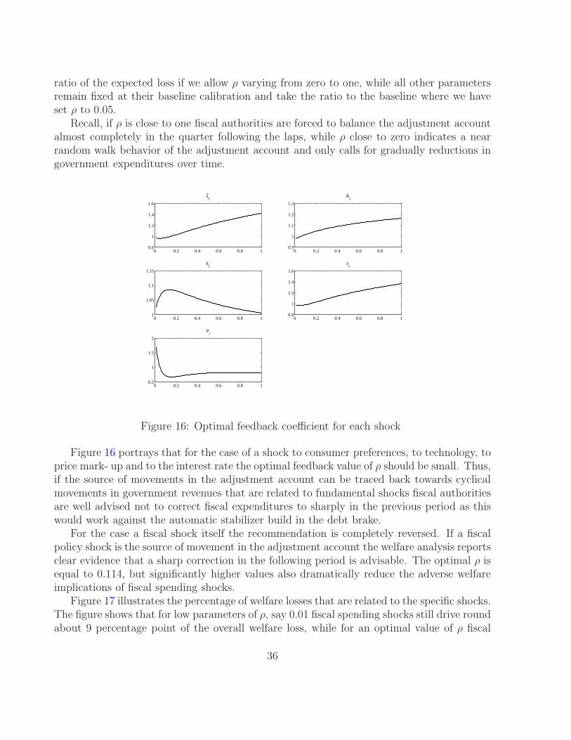
ratio of the expected loss if we allow ρ varying from zero to one, while all other parametersremain fixed at their baseline calibration and take the ratio to the baseline where we haveset ρ to 0.05.

Recall, if ρ is close to one fiscal authorities are forced to balance the adjustment accountalmost completely in the quarter following the laps, while ρ close to zero indicates a nearrandom walk behavior of the adjustment account and only calls for gradually reductions ingovernment expenditures over time.

0 0.2 0.4 0.6 0.8 10.8

1

1.2

1.4

1.6

ζt

0 0.2 0.4 0.6 0.8 10.9

1

1.1

1.2

1.3

At

0 0.2 0.4 0.6 0.8 11

1.05

1.1

1.15

εt

0 0.2 0.4 0.6 0.8 10.8

1

1.2

1.4

1.6

zt

0 0.2 0.4 0.6 0.8 10.5

1

1.5

2

νt

Figure 16: Optimal feedback coefficient for each shock

Figure 16 portrays that for the case of a shock to consumer preferences, to technology, toprice mark- up and to the interest rate the optimal feedback value of ρ should be small. Thus,if the source of movements in the adjustment account can be traced back towards cyclicalmovements in government revenues that are related to fundamental shocks fiscal authoritiesare well advised not to correct fiscal expenditures to sharply in the previous period as thiswould work against the automatic stabilizer build in the debt brake.

For the case a fiscal shock itself the recommendation is completely reversed. If a fiscalpolicy shock is the source of movement in the adjustment account the welfare analysis reportsclear evidence that a sharp correction in the following period is advisable. The optimal ρ isequal to 0.114, but significantly higher values also dramatically reduce the adverse welfareimplications of fiscal spending shocks.

Figure 17 illustrates the percentage of welfare losses that are related to the specific shocks.The figure shows that for low parameters of ρ, say 0.01 fiscal spending shocks still drive roundabout 9 percentage point of the overall welfare loss, while for an optimal value of ρ fiscal

36

Figure 17: Loss decomposition

policy could be almost eliminated as a source of economic disturbances as only 1.88% of theoverall welfare loss could then be traced back towards fiscal policy. Based on this analysis atwo tired adjustment account system seems advisable. In one account the fiscal lapses wouldbe booked while the other account would keep track of the rest. Such a system would allowdesigning a high feedback towards the adjustment account related to fiscal spending shocksand simultaneously a low feedback for the rest. This setting requires to be safeguarded byan institutional arrangement where a fiscal watchdog analysis and separates the lapses intime such that an appropriate feedback would materialize in the following period.

5.2 Trend estimation errors

In this section, we extent the setting derived in the previous parts of the paper to allow formeasurement error on trend output on behalf of fiscal authorities. In practice, it prevailsthat governments are often subject to persistent measurement errors in trend output. Ad-ditionally, estimations vary according to who estimates the trend; further, there is quite ahigh frequency of trend revisions as time moves on.5 For analytical simplicity and without

loss of generality, we assume that¯b = 0, i.e. we consider a zero debt economy. Reverting to

equations (30) and (31), we can express the debt brake in presence of trend mis-estimationsas

(Rt−1 − 1)bt +Gt

Y=

Ψ

P Y· Et−1 {at} − ρ ·

Pt−1

Ptact−1

︸︷︷︸


+νt

PtY,

5As Fritsche and Dopke (2006) put it, “it [may] not always [be] advisable to listen to the majority offorecasters”. The issue of trend mis-estimation and its implications are briefly addressed within this section,but not in a very sophisticated manner as it is not the primary focus of this analysis. However, it is certainlyan important point for further research.

37

where Et−1 {at} denotes an estimation error in trend output. Whenever it is greater one,trend is overestimated and vice versa. The adjustment account is then given by

act = (1 − ρ) ·Pt−1

Pt· act−1 +

νt

PtY+

[Ψ

P YEt−1 {at} −

Ψt

PtY

]

.

In log-linearized terms, this is translates into

Gt =(1 − β−1)

γG

bt +νt

P Y+ Et−1 {at} − ρact−1 (50)

where we assume that Et−1 {at} in the following experiment and


P Y+ γG

[

Et−1 {at} −(

Ψt − Pt

)]

. (51)

We see from equation (50) that overestimating trend revenues, i.e. Et−1 {at} > 0, unambigu-ously increases government spending. Although this is booked on the adjustment accountand partly repaid in future periods, it is straightforward to see that government spendingwill remain high for quite some periods, even when the estimation error is corrected im-mediately in the next period as the adjustment account does only partially feed back ongovernment spending. Because trend mis-estimations are usually correlated over time dueto the available time series-estimation methods, and it take quite a while to realize thatEt−1 {at} > 0 was wrong, things may even get worse. As Brunez (2003) has shown, a biasin trend estimations cannot be neglected. Kremer and Stegarescu (2008) show with Germandata that trend tends to be over-estimated in booms and under-estimated in downturns,while, on average, there seems to be an over-estimation. Furthermore, there may also be apositive political economic bias as suggested by Heinemann (2006).

In Figure 18, we report evidence from the following case study. We assume that the gov-ernment falls prey to estimation errors for 16 quarters in a row as trend output is estimatedone percentage point higher than it actually is. Each period, the government is surprisedto learn that output is lower than initially expected. Nevertheless, it escribes this to someother source but trend mis-estimation.

From quarter 16 to 17, the government then realizes that trend was wrongly estimatedand adjusts its expenditures accordingly. The green (high feedback, ρ = 0.99), black (lowfeedback, ρ = 0.01) and red (optimal baseline feedback, ρ = 0.05) lines report how theeconomy evolves under the different feedbacks. The following differences prevail.

First, the higher the feedback to the adjustment account, the lower the increase in debt.Second, from quarter 16 to 17, the economy goes into a deeper recession if fiscal expendituresare corrected sharply as, in particular, Non-Ricaridan households reduce consumption ex-penditures. Third, the inflation response for the optimal baseline feedback evolves smootherthan the others.

We conclude that the installation of an adjustment account is able to balance the desire tokeep the debt bounded, while equally not irritating the economy at large, if fiscal authoritiesfall prey to measurement errors.

38

0 4 8 12 16 20 24 28−0.4

−0.2

0

0.2

0.4

0.6GDP

Quarters0 4 8 12 16 20 24 28

−0.2

−0.1

0

0.1

0.2Consumption

Quarters0 4 8 12 16 20 24 28

−0.5

0

0.5

1

1.5Error in Trend Estimation

Quarters

0 4 8 12 16 20 24 28−0.5

0

0.5

1Tax Revenues

Quarters0 4 8 12 16 20 24 28

−1

−0.5

0

0.5

1Expenditures

Quarters0 4 8 12 16 20 24 28

−1

0

1

2

3Debt

Quarters

0 4 8 12 16 20 24 28−0.4

−0.2

0

0.2

0.4

0.6Interest Rate

Quarters0 4 8 12 16 20 24 28

−0.04

−0.02

0

0.02

0.04Inflation

Quarters0 4 8 12 16 20 24 28

−0.5

0

0.5

1Wages

Quarters

Intermediate FeedbackLow FeedbackHigh Feedback

Figure 18: Trend estimation errors

5.3 Elasticities

Under current time-series estimation methods, debt brakes in action in Switzerland or pro-posed for Germany tie government spending to real trend revenue by estimating futurerevenue and correct this by a cyclical component similar to the automatic stabilizer derivedin section 2.3.2 in order to boost spending in “bad times” and diminish spending in “goodtimes” (see Colombier, 2004, 2006; Danninger, 2002; German Council of Economic Experts,2007; for a description about the debt brake in Switzerland and the proposals in Germany).This approach may, however, result in a pro-cyclical tool which is, in terms of our model,more (but not yet fully) a balanced budget rule than an automatic stabilizer even whenabstracting from estimation errors.

To make the argument clearer, let us step back to describe existing or proposed rules interms of our model (referring also to section 2.3). Government spending, including intereston outstanding debt, according to the debt brake design just described, should be tied toprojected funds raised by the government, i.e. Et−1 {Ψt}. This is augmented by projectedcounter-cyclical component Et−1

{Y /Yt

}. Hence, ex-post government spending is given by

(Rt−1 − 1)Bt + PtGt = Et−1

{

Ψt ·

(Y

Yt

)α}

− ρACt−1

︸︷︷︸


+νt,

39

where, as in section 2.3.2, α > 0 is the magnitude how much revenues react in expecteddeviations from (estimated) trend output and the adjustment account evolves according to

ACt = (1 − ρ)ACt−1 + νt + Et−1

{

Ψt ·

(Y

Yt

)α}

−

(

Ψt ·

(Y

Yt

)α)

︸︷︷︸

Expectation error

.

Expressing these equations in real terms (i.e. dividing by Pt), normalizing (i.e. dividing

by Y ), assuming a zero debt economy for analytical convenience (i.e.¯b = 0 without loss of

generality) and log-linearization (i.e. following the same procedure as presented in AppendixD), we find that

Gt =(1 − β−1)

γGbt +

νt

P Y+ Et−1

{

Ψt − Pt

}

− α · Et−1

{

Yt

}

︸︷︷︸


−ρact−1 (52)

and


P Y+[

Et−1

{

Ψt − Pt

}

−(

Ψt − Pt

)]

− α[

Et−1

{

Yt

}

− Yt

]

︸︷︷︸

Expectation error

. (53)

Taking the descriptions of the rules literally, the rules seem to imply α = 1. However, in thiscase, it is a straightforward to show that, referring to equation (52), Rule based spending >0, which means that government spending reacts pro-cyclically to exogenous shocks. Thereason for this is that the elasticity of real government revenues to any shock is larger thanthe elasticity of output to the same shock. This implies that, given any positive shock,government real revenues increase by more than the counter-cyclical component to dampenspending. In total, spending rises with any positive shock, while the idea of the debt brakesays that it should not react (see section 2.3.2). Girouard and Andre (2005) have shownempirically that the elasticity relation in our model appears to hold. To solve this problem,it seems natural to set α > 1 such that Rule based spending = 0, which corresponds withthe basic idea of the rule. However, this may be quite a challenging task as it can be shownthat the optimal α differs according to the shock.

6 Conclusion

In this paper, we have analyzed the effects of simple government spending rules that whichaim at stabilizing the economy in a sustainable way. We used a conventional New KeynesianDSGE model to implement the idea of a balanced budget rule, a debt brake and a debtbrake augmented by an additional component which moves counter-cyclical to GDP, whichwe termed automatic stabilizer as this is how automatic stabilizers are typically modelled

40

in the literature. The debt brake, which is currently in action in Switzerland and proposedto be implemented in Germany, is a rule tying government spending to real trend revenues.Primary surpluses and deficits are booked on an adjustment account. The (positive) balanceof the account cuts future government spending in order to keep debt at a constant level inthe long run.

We find that, not surprisingly, the balanced budget rule gives pro-cyclical impulses tothe economy as it directly moves with (projected) government revenues. The debt brakeand the automatic stabilizer have very similar business cycle effects. However, the debtbrake still acts mildly pro-cyclical which can be attributed to the interest payments onoutstanding debt and to the commitment to keep overall debt stable in the long run, whilethe automatic stabilizer indeed acts mildly counter-cyclical. In terms of welfare, calculatedas an average consumer loss function, the debt brake and the automatic stabilizer are verysimilar. Nevertheless, on an aggregated level, the automatic stabilizer seems to generateslightly smaller a welfare loss of 4% for our baseline calibration. This can be explained bythe anticipation effect of highly correlated government expenditures, which only materializein later periods and drive the differences in welfare results for a debt brake and an automaticstabilizer regime.

We can keep hold of the fact that, generally, attention should be devoted to the feedback ofthe adjustment account to real government spending. Only for discretionary spending shocks,this feedback should be relatively stronger, while adjustment of debt due to other economicshocks should die out slowly. Additionally, it is important to take into account potentialestimation errors, especially, regarding trend output. Overestimating trend generates toohigh government spending. We conclude that the installation of an adjustment account isable to balance the desire to keep debt bounded, while not irritation the economy at large,if fiscal authorities fall prey to measurement errors.

The debt brake in action (and proposed) do not ty expenditures to expected trend rev-enues directly but to projected funds raised by the government in the following period aug-mented by a cyclical factor which is supposed to add out the cyclical fluctuations. However,in such a case, one has to carefully consider the fact that elasticities to a shock generallydiffer for government revenues and for output. Even without trend mis-estimation, one maygenerate strong pro-cyclical spending behavior if the reaction of government spending is notcorrectly adapted to these elasticities (which, to make things worse, differ across shocks).Then, the idea of the debt brake may be foiled and welfare implication go more in thedirection of a balanced budget rule.

41

Appendix

A Baseline Calibration

Parameter Symbol Value

Discount factor β 0.990Elasticity of demand in intermediate good sector ǫ 11.000Taylor rule coefficient: inflation φπ 1.900Taylor rule coefficient: output φY 0.250Taylor rule coefficient: interest rate smoothing µ 0.850Feed back of adjustment account to spending ρ 0.150Fraction of firms that leave their price unchanged θp 0.750Fraction of firms that do price indexation ωp 0.000Share of liquidity constraint consumers λ 0.330Steady state rate of employee wage taxes τd 0.125Steady state rate of employer wage taxes τw 0.125Steady state rate of consumption taxes τC 0.183Feedback of debt to taxes χd, χw, χC 0.000Autoregressive parameter for consumer preference shock ρζ 0.822Autoregressive parameter for technology shock ρA 0.828Autoregressive parameter for supply shock ρǫ 0.890Autoregressive parameter for monetary policy shock ρz 0.150Autoregressive parameter for government spending shock ρν 0.956Autoregressive parameter for government revenue shock ρχ 0.500Relative weight of leisure to consumption υ 0.761

Table 1: Baseline Calibrationn

Shock type Standard deviations

Consumer preferences 0.324Technology 0.628Supply 0.140Monetary policy 0.240Government expenditure 0.331Government revenue 0.329

Table 2: Standard Deviations of Shocks

42

B Optimal Firms’ Price Setting and the Phillips Curve

The relevant first-order conditions of the firm’s maximization problem are given by

∂(.)

∂Qt(j)= θpβΛt

[

Pt(j)

Pt+k

− mct+k(j) − ϑjt

]

≡ 0 (54)

and

∂(.)

∂Pt(j)= Et

{∞∑

k=0

(βθp)kΛt,t+k

[

Qt+k(j)

Pt+k− ϑt+k · ǫ

(

Pt(i)

Pt+k

)−ǫ

Pt+k

Pt+k(j)

1

Pt+kYt+k

]}

≡ 0.

(55)Using equations (4) and (54) to substitute into equation (55), we get equation (10),

Et

{∞∑

k=0

(βθp)kΛt,t+k

(

Pt(i)

Pt+k

)−ǫ

Yt+k

[1

Pt+k− ǫ

(1

Pt+k−

mct+k(j)

Pt+k(j)

)]}

= 0.

⇒ (ǫ − 1)Et

{∞∑

k=0

(βθp)kΛt,t+k

(

Pt(i)

Pt+k

)−ǫ

Yt+k

Pt+k

}

= ǫEt

{∞∑

k=0

(βθp)kΛt,t+k

(

Pt(i)

Pt+k

)−ǫ

Yt+kmct+k(j)

Pt+k(j)

}

⇒ P−ǫt (j)(ǫ − 1)Et

{∞∑

k=0

(βθp)kΛt,t+kP

ǫ−1t+k Yt+k

}

= P−ǫ−1t (j)ǫEt

{∞∑

k=0

(βθp)kΛt,t+kP

ǫt+kYt+kmct+k(j)

}

.

Solving for Pt(j) yields

Pt(j) =ǫ

ǫ − 1·Et

{∑∞

k=0(βθp)kΛt,t+kP

ǫt+kYt+kmct+k(j)

}

Et

{∑∞

k=0(βθp)kΛt,t+kPǫ−1t+k Yt+k

} (56)

as the optimal reset price for firm j that is able to reset prices. Note that if all firms wereallowed to reset prices (i.e. θp = 0), we would get

Pt(j) =ǫ

ǫ − 1· Et{mcflex

t · P flext } = P flex

t . (57)

Equation (57) implies that, in the flexible price equilibrium, in steady-state, mc = Φ = ǫǫ−1

(see also section 2.1.1), which will become handy to remember for later use.

43

Pt(j)Et

{∑∞

k=0(βθp)kΛt,t+kP

ǫ−1t+k Yt+k

}= ǫ

ǫ−1Et

{∑∞

k=0(βθp)kΛt,t+kP

ǫt+kYt+kmct+k(j)

}is the

rearranged equation (56), which, log-linearized, gives

ΛP ǫ−1Y ¯P (j)Et

{

1

1 − βθp

ˆPt(j) +

∞∑

k=0

(βθp)k(

Λt+k + Yt+k + (ǫ − 1)Pt+k

)}

=ǫ

ǫ − 1ΛP ǫY mcEt

{∞∑

k=0

(βθp)k(

Λt+k + Yt+k + ǫPt+k + mct+k

)}

,

where we have used∑

∞

k=0(βθp)k = 1

1−βθp. Further, we know from equation (56) that ¯P =

ǫǫ−1

mcP which allows us to simplify the previous equations as

ˆPt(j) = (1 − βθp)Et

{∞∑

k=0

(βθp)k(

Pt+k + mct+k

)}

,

which can also be written as

ˆPt(j) = (1 − βθp){(

Pt + mct

)

+ βθpˆPt+1(j)

}

. (58)

The aggregated price index Pt evolves as P(1−ǫ)t = (1 − θp)(P

∗

t )(1−ǫ) + θpP(1−ǫ)t−1 (see Gali

et al., 2001), which, in log-linearized form, yields Pt = (1 − θp)P∗

t + θpPt−1. We furtherassume that the group of price setters is subdivided into optimizers, with share (1 − ωp),

and those who index their prices, with share ωp. Hence, P ∗

t = (1 − ωp)ˆPt(j) + ωpP

bt , where

the indexation rule is conducted according to P bt = P ∗

t−1 + πt−1. Making use of this set ofequations, it holds that

ˆPt(j) =1

1 − ωp

P ∗

t −ωp

1 − ωp

[P ∗

t−1 + πt−1]

and we further know that

P ∗

t =1

1 − θpPt −

θp

1 − θpPt−1,

which yields (combining these two equations and rearranging)

ˆPt(j) =Pt + [θpωp − 2ωp − θp]Pt−1 + ωpPt−2

(1 − ωp)(1 − θp).

Substituting the previous expression into equation (58) yields

Pt + [θpωp − 2ωp − θp]Pt−1 + ωpPt−2

(1 − ωp)(1 − θp)= (1 − βθp)

(

Pt + mct

)

+βθpPt+1 + [θpωp − 2ωp − θp]Pt + ωpPt−1

(1 − ωp)(1 − θp),

44

which we can rearrange to

[1 − (1 − ωp)(1 − θp)(1 − βθp) − βθp(θpωp − 2ωP − θp)]Pt

= βθpPt+1 + [−(θpωp − 2ωP − θp) + βθpωp]Pt−1 − ωpPt−2

+(1 − ωp)(1 − θp)(1 − βθp)mct.

Using that πt = Pt − Pt−1, this can be written as

[θp + ωp(1 − θp(1 − β))]πt = βθpπt+1 + ωpπt−1 + (1 − ωp)(1 − θp)(1 − βθp)mct,

which yields

πt =βθp

[θp + ωp(1 − θp(1 − β))]πt+1 +

ωp

[θp + ωp(1 − θp(1 − β))]πt−1

+(1 − ωp)(1 − θp)(1 − βθp)

[θp + ωp(1 − θp(1 − β))]mct,

which is equation (37). Note that in the main text, we will set ωp = 0.

C Aggregation of Household Sector

The first-order conditions for optimizing households are

∂(.)

∂Cot (j)

=(1 − χ)ζt

Cot (j)

− λot (1 + τC

t ) = 0, (59)

∂(.)

∂Lot (j)

=υtζt

Lot (j)

− λot (1 − τd

t )wt = 0, (60)

and∂(.)

∂Bot+1(j)

= −1

RtPtλo

t + βEt

{

λot+1

1

Pt+1

}

= 0, (61)

where λot is the Lagrangian multiplier associated with the budget constraint, equation (13).

From equation (61), we know that

R−1t = βEt

{λo

1,t+1

λo1,t

Pt

Pt+1

}

, (62)

which is the stochastic discount factor. Using equation (59) yields equations (14) and (15).The first-order conditions for rule-of-thumb consumers are given by

∂(.)

∂Crt (j)

=(1 − χ)ζt

Crt (j)

− λrt (1 + τC

t ) = 0 (63)

45

and∂(.)

∂Lrt (j)

=υtζt

Lrt (j)

− λrt (1 − τd

t )wt = 0, (64)

where λrt is the Lagrangian multiplier associated with the corresponding budget constraint.

From equations (63) and (64), we derive equation (18).The aim of the rest of this section is to derive an aggregated consumption Euler equation

(in log-linearized terms) expressed only in aggregated variables and deep parameters. Toachieve this, we revert to the households’ consumption decisions derived in subsections 2.2.1and 2.2.2. This means that we have to back-step every now and then to simplify the resultingequations. The principle of aggregation follows what we have stated in equation (1).

Using the principle of equation (1), we know with the help of equation (19) that

Nt = λN rt + (1 − λ)No

t =λ · (1 − χ)

(1 − χ) + υt

+ (1 − λ)Not (65)

and that

Ct = λCrt + (1 − λ)Co

t

= λ

[(1 − χ)

υt

wt(1 − τd

t )

(1 + τCt )

Lrt

]

+ (1 − λ)

[(1 − χ)

υt

wt(1 − τd

t )

(1 + τCt )

Lot

]

=

[(1 − χ)

υtwt

(1 − τdt )

(1 + τCt )

]

[λLrt + (1 − λ)Lo

t ]︸︷︷︸

≡Lt

, (66)

where the index j has been dropped for notational convenience6, while Crt is given by equation

(18) and Cot by equation (15). Log-linearization of equation (66) yields

Ct − Lt = wt − ιdτdt − ιC τC

t − υt,

where ιd ≡ τd

(1−τd)and ιC ≡ τC

(1+τC). We know that Lt = − N

1−NNt = −ϕNt from log-linearizing

Lt = 1−Nt, where ϕ = N1−N

is the inverse of the Fisher labor supply elasticity. Substituting

Lt and rearranging thus gives

wt = Ct + ϕNt + ιdτdt + ιC τC

t + υt, (67)

which is equation (39) of the main text.We now come to some side-steps to derive be able to derive the aggregated Consumption-

Euler equation. From equation (20) we know that, in steady-state, Cr = (1−τd)(1−χ)((1−χ)+υ)(1+τC )

w,

6Note that, due to state-contingent claims available for optimizing households, which is generally assumedin this type of model, and the fact that rule-of-thumb consumers consume all of their income, each individualhousehold’s consumption in i = o, r is equal anyway (see Woodford, 2003, chapter 2).

46

while, from equation (66) and L = 1 − N , it is clear that C = (1 − N) (1−τd)(1−χ)υ(1+τC )

w, whichyields

Cr

C=

υ

1 − χ + υ·

1

1 − N≡ γr, (68)

where γr is, thus, the per-head consumption share of rule-of-thumb households relative tototal per-head consumption. As we further know from equation (66) that C = λCr + (1 −λ)Co, we find that 1 = λ Cr

C+ (1 − λ) Co

C, which, using equation (68) can be reformulated as

Co

C=

1

1 − λ−

λ

1 − λ

υ

1 − χ + υ

1

1 − N︸︷︷︸

=γr

=1 − γrλ

1 − λ≡ γo, (69)

which, equivalently, gives the per-head consumption share of optimizing households relativeto total per-head consumption. (Note that, whenever optimizing households consume morethan rule-of-thumb households, γo > 1 may well be possible and vice versa). Using L =λLr + (1 − λ)Lo = λ(1 − N r) + (1 − λ)Lo, where N r is given by equation (19), we know

that L = λ(

1 − (1−χ)1−χ+υ

)

+ (1 − λ)Lo, which, dividing both sides by L = (1 − N) yields

1 = γrλ + (1 − λ) Lo

L, where γr is given by equation (68). Thus,

Lo

L=

1 − γrλ

1 − λ= γo (70)

is also the per-head leisure of optimizing households relative to total per-head leisure.From equation (14), we know that, for the optimizing households, it holds that

ζt

Cot · (1 + τC

t )= βRtEt

{ζt+1

Cot+1 · (1 + τC

t+1)·

Pt

Pt+1

}

. (71)

A Taylor expansion and use of Etrt = Et

{

Rt ·Pt

Pt+1

}

yields

ζ

Co · (1 + τC)

[

−(Co

t − Co)

C

C

Co+

(ζt − ζ)

ζ−

τC

1 + τC

(τCt − τC)

τw

]

= βrζ

Co · (1 + τC)Et

[

−(Co

t+1 − Co)

C

C

Co+

(ζt+1 − ζ)

ζ−

τC

1 + τC

(τCt+1 − τC)

τw+

1

r(rt − r)

]

.

We now define Cot ≡

(Cot −Co)

Cand Lo

t ≡(Lo

t−Lo)

Land note that C

Co = LLo = 1

γo(see equations

(69) and (70))7 as well as r = β−1. Substitution and rearranging yields[

−Cot

1

γo+ ζt − ιC τC

t

]

= Et

[

−Cot+1

1

γo+ ζt+1 − ιC τC

t+1 + rt

]

,

7Note that this is, then, the deviation of Cot or Lo

t from its steady-state value evaluated at the steady-state value of total consumption/leisure. This is corrected for by dividing this term by γo in the followingequation. The slightly different definition from the standard definition will be useful for further calculations.

47

where ιC = τC

1+τC . Rearranging gives

Cot = EtC

ot+1 + γo

{

ιCEt[τCt+1 − τC

t ] + Et[ζt − ζt+1] − rt

}

. (72)

We define ∆Lot+1 = [Lo

t+1 − Lot ] and ∆τC

t+1 = [τCt+1 − τC

t ] for later use.

From equation (65), we know that Nt

N= λ·(1−χ)

N((1−χ)+υt)+ (1 − λ)

Not

N. A first-order Taylor

expansion implies that

Not =

Nt

1 − λ+

λ

(1 − λ)N

(1 − χ)υ

(1 − χ + υ)2υt ⇒ Lo

t = −ϕ

1 − λNt−

λϕ

(1 − λ)N

(1 − χ)υ

(1 − χ + υ)2υt (73)

because Lt = − N1−N

Nt = −ϕNt, where we have defined Not =

Not −No

N. From equation (20)

and (66), it must hold thatCr

t

C= Ct

Cυt

(1−χ)+υt

11−Nt

, where a first-order Taylor expansion yields

Crt = γrCt + ϕγrNt + γr

(1 − χ)

1 − χ + υυt, (74)

where we have used the definition for γr (see equation (68)), ϕ = N/(1 − N) and defined

Crt =

Crt −Cr

C. Log-linearizing aggregated consumption Ct = λCr

t + (1 − λ)Cot yields Ct =

λCrt + (1 − λ)Co

t . Solving this for Cot and using equation (74) yields

Cot =

1 − γrλ

1 − λ︸︷︷︸

=γo

Ct −λγrϕ

1 − λNt −

γrλ(1 − χ)

(1 − χ + υ)(1 − λ)υt. (75)

From equation (73), we know that ∆Lot+1 = − ϕ

(1−λ)∆Nt+1 must hold. Substituting this and

equation (75) into equation (72) we get

γoCt −λγrϕ

(1 − λ)Nt −

γrλ(1 − χ)

(1 − χ + υ)(1 − λ)υt − γoζt = γoEtCt+1 −

λγrϕ

(1 − λ)EtNt+1

−γrλ(1 − χ)

(1 − χ + υ)(1 − λ)Et[υt+1] + γo

{

ιCEt∆τCt+1 − Et[ζt+1] − Et[Rt − πt+1]

}

,

where we have used that rt = [Rt − πt+1], with πt+1 ≈ Pt+1 − Pt. Dividing by γo, i.e.

multiplying by (1−λ)1−γrλ

, we get equation (72). Equation (38) is the standard aggregated con-sumption Euler equation expressed in aggregated variables and deep parameters only. In-dividual steady-state relations have been substituted out but, of course, still drive equation(38) through the “correct” substitution.

48

D The Fiscal Spending Rule

Before deriving the spending rule in log-linearized terms, it seems appropriate to have somesteady-state considerations regarding the spending rule, equations (28) and (30), and theadjustment account, equations (29) and (31). From these equations, we see that, in steady-state,

(R − 1)¯b +G

Y=

Ψ

P Y− ρ · ac (76)

and

ac = (1 − ρ)ac +Ψ

P Y−

Ψ

P Y⇒ ρ · ac = 0. (77)

As we know that ρ > 0 if the adjustment account feeds back on government spending, ac = 0

has to hold in steady-state. Then, from equation (76), we know that ΨP Y

= γG − (1− β−1)¯b,

where we have used the definition γG = GY

and the fact that R = β−1 in steady-state. Notethat these conditions correspond to the evolution of debt in steady-state, given by equation

(24) in steady-state, which also gives ΨP Y

= γG − (1 − β−1)¯b, but where the adjustmentaccount has not yet been taken into account. Hence, the fact that ac = 0 in steady-state isconsistent with the model.

A first-order Taylor expansion of equation (24) yields

[

¯b +

Ψ

P Y

]

︸︷︷︸

=γG+β−1¯b

+ (bt+1 − b)︸︷︷︸

=bt+1

+1

P Y

(Ψt − Ψ

)−

Ψ

P 2Y

(Pt − P

)

=

[

R¯b +

G

Y

]

︸︷︷︸

=γG+β−1¯b

+¯b(Rt−1 − R

)+ R

(

bt − b)

︸︷︷︸

=bt

+R¯b

P

(Pt−1 − P

)

−R¯bP

P 2

(Pt − P

)+

1

Y

(Gt − G

),

where use has been made of equations (25) and (76) to derive the terms in the under-braces. Using the definition for any variable’s deviation around its steady-state, equa-tion (2), as well as equation (76) and R = β−1, we can rearrange the above equation to

bt+1 +[

γG − ¯b(1 − β−1)](

Ψt − Pt

)

= β−1bt + β−1¯b(

Rt−1 + Pt−1 − Pt

)

+ γGGt.8 Using the

definition πt ≈ Pt − Pt−1, rearranging yields equation (40).

8Remember that Ψ/(P Y ) = γG −¯b(1 − β−1).

49

A first-order Taylor expansion of the spending rule, equation (30), yields[

(R − 1)b +G

Y

]

︸︷︷︸

=γG−(1−β−1)¯b

+(R − 1) (bt − b)︸︷︷︸

=bt

+¯b(Rt−1 − R

)+

(R − 1)¯b

P

(Pt−1 − P

)

−(R − 1)¯bP

P 2

(Pt − P

)+

1

Y

(Gt − G

)

=

[Ψ

P Y

]

︸︷︷︸

=γG−(1−β−1)¯b

−

[Ψ

P Y

]

︸︷︷︸

=γG−(1−β−1)¯b

·α · Et−1

{

Yt

}

+νt

P Y− ρ · act−1,

whereas a first-order Taylor expansion of equation (28) yields[

(R − 1)b +G

Y

]

︸︷︷︸

=γG−(1−β−1)¯b

+(R − 1) (bt − b)︸︷︷︸

=bt

+¯b(Rt−1 − R

)+

(R − 1)¯b

P

(Pt−1 − P

)

−(R − 1)

¯bP

P 2

(Pt − P

)+

1

Y

(Gt − G

)

=

[Ψ

P Y

]

︸︷︷︸

=γG−(1−β−1)¯b

+

[Ψ

P Y

]

︸︷︷︸

=γG−(1−β−1)¯b

·Et−1

{

Ψt − Pt

}

+νt

P Y− ρ · act−1.

where we have already used the fact that ac = ν = 0 and we used the definition of equation(25) and and the steady-state condition (76). Solving for Gt, and combining the two previousequations yields equation (42).

A first-order Taylor expansion of equation (31) yields

(act − ac) = (1 − ρ)(act−1 − ac) +ac

P(Pt−1 − P ) −

ac

P 2(Pt − P )

︸︷︷︸

=0

+νt

P Y

−Ψ

P Y︸︷︷︸

=γG−(1−β−1)¯b

·[

α(

Et−1

{

Yt

}

− Yt

)

+ (

Ψt − Pt

)]

,

while a fist-order Taylor expansion of equation (29) is given by

(act − ac) = (1 − ρ)(act−1 − ac) +ac

P(Pt−1 − P ) −

ac

P 2(Pt − P )

︸︷︷︸

=0

+νt

P Y

+Ψ

P Y︸︷︷︸

=γG−(1−β−1)¯b

·[(

Et−1

{

Ψt

}

− Ψt

)

−(

Et−1

{

Pt

}

− Pt

)]

,

50

which can be combined to equation (43).

E Steady-state considerations

We know that, in the long-run, equilibrium prices will be equal to the flex-price equilibrium.Then, we know that it holds that (see also equation (57))

mc =ǫ − 1

ǫ, (78)

where we have used that Pt(i) = P flext holds in the long-run steady-state. Additionally, we

know from the cost minimization problem of a representative firm that (see equation (7))

w = ·mcY

N

1

(1 + τw). (79)

From equation (66), we know that w = υ(1−χ)

C1−N

(1+τC)(1−τd)

, which, in combination with equation

(79) yields

υ

(1 − χ)

C

1 − N

(1 + τC)

(1 − τd)= mc ·

Y

N

1

(1 + τw)

⇒N

1 − N= mc

(1 − τd)

(1 + τw)(1 + τC)

υ

(1 − χ)

Y

C

⇒N

1 − N=

ǫ − 1

ǫ

(1 − τd)

(1 + τw)(1 + τC)

υ

(1 − χ)

1

γC︸︷︷︸

=ϕ

, (80)

where we have used equation (78) and defined γC = CY

. Hence, we know that N = ϕ1+ϕ

. This

implies that N can be expressed in exogenous parameters if we are able to find a solutionfor γC which we will derive now.

Note that, from steady-state condition resulting from equation (76), we know that ΨP Y

=

γG − (1− β−1)¯b holds, where

¯b = 0 in the zero steady-state debt case. Further, it holds that

(see equation (23))Ψ

P Y= τLw

N

Y+ τC C

Y,

where τL = τw + τd. Using equations (78) and (79), the definition γC = CY

and combiningthe last two equations yields

γG − (1 − β−1)¯b = τL ǫ − 1

ǫ

1

(1 + τw)+ τCγC. (81)

51

From the resource constraint, Y = C + G, we know that 1 = CY

+ GY

= γC + γG. Using thisand equation (81), we then find that

G

Y= γG =

1

(1 + τC)

{

(1 − β−1)¯b +ǫ − 1

ǫτL 1

(1 + τw)+ τC

}

(82)

is determined by exogenous parameters. Hence, from the resource constraint, we know that,then

C

Y≡ γC = 1 − γG. (83)

From the first-order condition of the cost minimizing problem of the firm, we know thatmc = N

Y[(1 + τw)w] (see equation (7)), where N

Y= 1

A= 1 as A = 1 (see equation (6)),

which, using equation (78) and rearranging yields

w =1

(1 + τw)

ǫ − 1

ǫ. (84)

From equation (66) we can then calculate

C =(1 − χ)

υ·

1 − τd

1 + τC(1 − N)w =

(1 − χ)

υ·

(1 − τd)(1 − N)

(1 + τC)(1 + τw)

ǫ − 1

ǫ, (85)

where w is given by equation (84) and N by equation (80). Using equation (85) and γC = CY

,where γC is given by equation (83), we can calculate

Y =C

γC. (86)

An analogous proceeding allows us – using equations (82) and (86) – to derive

G = γGY = CγG

γC

. (87)

Further, we know, using equation (81), that

1 =τL(ǫ − 1)

ǫ(1 + τw)[γG − (1 − β−1)¯b]︸︷︷︸

=RevL

+τC

γC [γG − (1 − β−1)¯b]︸︷︷︸

=RevV at

, (88)

where all parameters are know following the calculation above. This implies that we areable to express all aggregated variables in terms of exogenous parameters. Note that theseaggregated variables in steady-state are independent of the implemented government spend-ing policy regime, i.e. they are independent of whether automatic stabilizers, the debt brakeor no restriction on government spending apply. Note further that χ = γG following froman “optimal planner’s solution” (see Gali and Monacelli, 2008; who apply exactly the samecalculation procedure that is necessary here).

52

F Welfare Approximation

We know that per-period utility of household j of type i is given by

ζt

[(1 − χ)log

(Ci

t(j))

+ χlog(Gt)]

︸︷︷︸

=ui

+ ζtυtlog(Li

t(j))

︸︷︷︸

=V i

, (89)

where i = o, r (see also equations (12) and (16)). In what follows, we will derive the second-order Taylor approximation of the consumption part of this equation (indicated by ui) andthe leisure part (indicated by V i) separately for convenience. For consumption, we then get

uit ≈ ui + ui

Ci

(Ci

t − Ci)

+1

2ui

CiCi

(Ci

t − Ci)2

+ uiG

(Gt − G

)+

1

2ui

GG

(Gt − G

)2

+uiCiζ

(Ci

t − Ci) (

ζt − ζ)

+ uiGζ

(Gt − G

) (ζt − ζ

)

= ui + (1 − χ)

(Ci

t − Ci)

Ci− (1 − χ)

1

2

(Ci

t − Ci)2

(Ci)2+ χ

(Gt − G

)

G− χ

1

2

(Gt − G

)2

G2

+

(ζt − ζ

)

ζ

[

(1 + χ)

(Ci

t − Ci)

Ci+ χ

(Gt − G

)

G

]

= ui + (1 + ζt)

{

(1 − χ)

[

Cit

γi−

1

2

(Cit)

2

γ2i

+1

2

(Cit)

2

γ2i

]

+ χ

[

Gt −1

2(Gt)

2 +1

2(Gt)

2

]}

= ui + (1 + ζt)

{

(1 − χ)Ci

t

γi+ χGt

}

, (90)

where we have used the fact that we defined Cit =

(Cit−Ci)

Cearlier, used the definitions for

γr and γo (see equations (68) and (69), respectively) and made use of the commonly knownfact that, for any variable X, it holds that (Xt − X) ≈ X[Xt + 1

2X2

t ] and (Xt − X)2 ≈ 12X2

t

when approximating second order. Further, we have neglected the individual householdparameter j for notational convenience and remembered that ζ = 1. Remembering thatEt{υt} = υ = υ, we get in an analogous proceeding for the disutility of labor (utility of

53

leisure, respectively)

V it ≈ V i + V i

Li

(Li

t − Li)

+1

2V i

LiLi

(Li

t − Li)2

+ V iLiζ

(Li

t − Li) (

ζt − ζ)

+V iLiυ

(Li

t − Li)(υt − υ)

= V i + υ

(Li

t − Li)

Li− υ

1

2

(Li

t − Li)2

(Li)2+ υ

(Li

t − Li)(ζt − 1)

Li

+

(Li

t − Li)(υt − υ)

Li

= V i + υ

{[

Lit

γi−

1

2

(Lit)

2

γ2i

+1

2

(Lit)

2

γi

]}

+Li

t

γi

(

υζt + υt

)

= V i + (1 + ζt)υLi

t

γi

+ υtLi

t

γi

= V i +(

(1 + ζt)υ + υt

) Lit

γi

. (91)

Combining the utility of consumption and disutility of labor, we get for household j of typei = o, r that

U it (j) = ui(j) + V i(j)

︸︷︷︸

U i

+(1 + ζt)

{

(1 − χ)Ci

t(j)

γi+ χGt

}

+(

(1 + ζt)υ + υt

) Lit(j)

γi. (92)

Noting that individuals of type r have a constant (potentially disturbed by common pref-erence shocks, but always equal within the group) consumption pattern due to constant(potentially disturbed by common preference shocks, but always equal within the group) la-bor supply (see equations (19) and (20)), we know that Cr

t (j) = Crt , where the latter is given

by equation (74). Due to the assumption of complete markets and state-contingent claimsthat can be purchased by households of type o, we know that Co

t (j) = Cot (see Woodford,

2003, chapter 2 for more details), where the latter is given by equation (75). Unfortunately,this does not hold for the labor supply (i.e. leisure) except for households of type r. We willcome back to this in a second. As we further know that a share λ of households is of typer, while the remaining ones, i.e. (1 − λ), are of type o, aggregated per-period utility can beexpressed through the second-order Taylor approximation

Ut = λU r + (1 − λ)Uo + (1 + ζt)

{

(1 − χ)

[

λCr

t

γr+ (1 − λ)

Cot

γo

]

+ χGt

}

+(

(1 + ζt)υ + υt

)[

λ1λ

∫ λ

0Lr

t (j)dj

γr

+ (1 − λ)

1(1−λ)

∫ 1

λLo

t (j)dj

γo

]

(93)

We can use equation (19) to substitute Lrt (j) = (1−χ)

(1−χ+υ)21Lυt, equation (74) to substitute Cr

t

and equation (75) to substitute Cot . Further, we know that Lt =

∫ 1

oLt(j)dj =

∫ λ

oLr

t (j)dj +

54

∫ 1

λLo

t (j)dj, which implies

∫ 1

λ

Lot (j)dj = Lt −

∫ λ

0

Lrt (j)dj

= Lt − λ(1 − χ)

(1 − χ + υ)2

1

Lυt

= −ϕNt − λ(1 − χ)

(1 − χ + υ)2

1

Lυt. (94)

Substitution into equation (93) and rearranging gives

Ut = λU r + (1 − λ)Uo +(

(1 + ζt)υ + υt

)[

λ(1 − γr)

γr(1 − λγr)

(1 − χ)

(1 − χ + υ)2(1 − N)υt −

1

γo

ϕNt

]

+(1 + ζt)

{

(1 − χ)

[

λ

(

Ct + ϕNt +(1 − χ)

1 − χ + υυt

)

+(1 − λ)

(

Ct −λ

1 − λ

γr

γoϕNt −

λ

1 − λ

(1 − χ)γr

(1 − χ + υ)γoυt

)]

+ χGt

}

From the analysis of an efficient steady-state, we know that χ = γG is set by a socialplanner to ensure efficiency. We assume this to hold henceforth. As usual, we define termsindependent of the policy (regime) chosen as tip. So far, those are given as

tip = λU r + (1 − λ)Uo +(

(1 + ζt)υ + υt

)[

λ(1 − γr)

γr(1 − λγr)

(1 − γG)

(1 − γG + υ)2(1 − N)υt

]

+(1 + ζt)(1 − γG)λ

(1 − γr

1 − γrλ

)(1 − γG)

1 − χ + υυt

The previous considerations allow us to write equation (93) as

Ut = (1+ζt)[

(1 − γG)Ct + γGGt

]

︸︷︷︸

=Yt

+ϕNt

(1 + ζt)(1 − γG)λ1 − γr

1 − γrλ−

(

(1 + ζt)υ + υt

)

γo

+tip.

(95)Note that from the resource constraint, we know that Y = C + G must holds. Dividing byY , this implies 1 = γC + γG, which yields γC = (1 − γG). Hence, (1 − γG)Ct + γGGt = Yt.Further, we can use

Nt =

∫ 1

0

Nt(j)dj =

∫ 1

o

Yt(j)

At

dj =Yt

At

∫ 1

o

Yt(j)

Yt

dj

=Yt

At

∫ 1

o

(Pt(j)

Pt

)−ǫ

dj

55

and log-linearize which yields Nt = Yt − At + qt, where qt = log

(∫ 1

o

[Pt(j)Pt

]−ǫ

dj

)

. Using

standard results as in Woodford (2003), we know that qt = ǫ2σ2

t , where σ2t =

∫ 1

0[pt(j)−pt]

2dj(where lower case letters p denote second-order log-deviations). Substituting into equation(95), we get

Ut =

(1 + ζt)

(

1 + (1 − γG)λ1 − γr

1 − γrλϕ

)

−

(

(1 + ζt)υ + υt

)

ϕ

γo

Yt

−

(1 + ζt)(1 − γG)λ1 − γr

1 − γrλ−

(

(1 + ζt)υ + υt

)

γo

ϕ(

At −ǫ

2σ2

t

)

+ tip.

=

[

(1 + ζt)

(

1 + (1 − γG)λ1 − γr

1 − γrλϕ −

υ

γoϕ

)

−υtϕ

γo

]

Yt

−

[

(1 + ζt)

(

(1 − γG)λ1 − γr

1 − γrλϕ −

υ

γoϕ

)

−υt

γoϕ

](

At −ǫ

2σ2

t

)

+ tip. (96)

Let us define A1 =(

(1 − γG)λ 1−γr

1−γrλϕ − υ

γoϕ)

, where −1 < A1 < 0. This allows us to re-write

equation (96) as

Ut =

[

(1 + ζt)(1 + A1) −ϕ

γo

υt

]

Yt −

[

(1 + ζt)A1 −ϕ

γo

υt

](

At +ǫ

2σ2

t

)

+ tip.

Noting that ζtYt = 12

[

ζ2t + Y 2

t − (Yt − ζt)2]

and υtYt = 12

[

υ2t + Y 2

t − (Yt − υt)2]

, we are able

to rearrange this to

Ut =(1 + A1)

2

[

(1 + Yt)2 − (Yt − ζt)

2]

−ϕ

2γo

[

Y 2t − (Yt − υt)

2]

+

[

(1 + ζt)A1 −υtϕ

γo

]ǫ

2σ2

t + tip, (97)

where

tip = tip −

[

(1 + ζt)A1 −υtϕ

γo

]

At +(1 + A1)

2ζt −

υtϕ

2γo−

(1 + A1)

2

is the full set of variables independent of policy. Noting that 12

∑∞

t=0 βtσ2t = ǫ

κ

∑∞

t=0 βtπ2t (see

Woodford, 2003) and taking conditional expectations at date zero, the discounted sum ofutility streams can be written as equation (46). Note that shock variables multiplied withthe inflation deviations are terms of higher order than 2 and are, therefore, neglected.

56

References

Alesina, A. and R. Tabellini [1990], “A Positive Theory of Fiscal Deficits,” Review ofEconomic Studies, 57, pp. 403–414.

Allsopp, C. and D. Vines [2005], “The Macroeconomic Role of Fiscal Policy,” OxfordReview of Economic Policy, 21, pp. 485–508.

Artis, M. J. and M. Buti [2000], “‘Close to Balance or in Surplus’ – A Policy Maker’sGuide to the Implementation of the Stability and Growth Pact,” Journal of CommonMarket Studies, 38, pp. 563–592.

Auerbach, A. J. and L. J. Kotlikoff [1987], “Dynamic Fiscal Policy,” CambridgeUniversity Press: New York.

Baxter, M. and R. G. King [1993], “Fiscal Policy in General Equilibrium,” AmericanEconomic Review, 83, pp. 315–334.

Blanchard, O. [1985], “Debt, Deficits, and the Finite Horizon,” Journal of Political Econ-omy, 93, pp. 223–247.

Blanchard, O. and R. Perotti [2002], “An Empirical Characterization of the DynamicEffects of Changes in Government Spending and Taxes on Output,” Quarterly Journalof Economics, 117, pp. 1329–1368.

Brunez, P. A. [2003], “A Modification of the HP Filter Aiming at Reducing the End-PointBias,” Eidgenossische Finanzverwaltung, Working Paper No. 18, Bern.

Buti, M., W. Roeger and J. in’t Veld [2001], “Stabilising Output and Inflation: PolicyConflicts and Coordination under a Stability Pact,” Journal of Common Market Studies,39, pp. 801–821.

Calvo, G. [1983], “Staggered Prices in a Utility-maximizing Framework,” Journal of Mon-etary Economics, 12, pp. 383–398.

Clarida, R., J. Gali and M. Gertler [1999], “The Science of Monetary Policy: A NewKeynesian Perspective,” Journal of Economic Literature, 37, pp. 1661–1707.

Coenen, G., P. McAdam and R. Straub [2008], “Tax Reform and Labour-MarketPerformance in the Euro Area: A Simulation-Based Analysis Using the New Area-WideModel,” Journal of Economic Dynamics and Control, 32, pp. 2543–2583.

Colombier, C. [2004], “Eine Neubewertung der Schuldenbremse,” Eidgenossische Fi-nanzverwaltung, Working Paper No. 2, Bern.

Colombier, C. [2006], “Die Schweizer Schuldenbremse – nachhaltiger und konjunktur-gerechter als der neue Stabilitats- und Wachstumspakt?,” Schmollers Jahrbuch, 126, pp.521–533.

Cournede, B. [2007], “The Political Economy of Delaying Fiscal Consolidation,” OECDEconomics Department Working Papers, No. 548, OECD Publishing.

Danninger, S. [2002], “The Swiss Debt Brake,” IMF Working Paper, No. WP/02/18.Erceg, D., D. Henderson and A. Levin [2000], “Optimal Monetary Policy with Stag-

gered Wage and Price Contracts,” Journal of Monetary Economics, 46, pp. 281–313.

57

European Commission [2001], “European Economy – Public Finances in EMU 2001,”European Commission, Directorate-General for Economic and Financial Affairs, Brussels.

European Commission [2008], “European Economy – Public Finances in EMU 2008,”European Commission, Directorate-General for Economic and Financial Affairs, Brussels.

Fatas, A. and I. Mihov [2001], “The Effects of Fiscal Policy on Consumption and Em-ployment: Theory and Evidence,” CEPR Discussion Paper, No. 2760.

Fritsche, U. and J. Dopke [2006], “Growth and Inflation Forecasts for Germany,” Em-pirical Economics, 31, pp. 777–798.

Gali, J., M. Gertler and D. Lopez-Salido [2001], “European Inflation Dynamics,”European Economic Review, 45, pp. 1237–1270.

Gali, J., D. Lopez-Salido and J. Valles [2004], “Rule of Thumb Consumers andthe Design of Interest Rate Rules,” Journal of Money, Credit and Banking, 36(4), pp.739–763.

Gali, J., D. Lopez-Salido and J. Valles [2007], “Understanding the Effects of Gov-ernment Spending on Consumption,” Journal of the European Economics Association,5(1), pp. 227–270.

Gali, J. and T. Monacelli [2008], “Optimal Monetary and Fiscal Policy in a CurrencyUnion,” Economics Working Paper, No. 909, Department of Economics and Business,Universitat Pompeu Fabra, Barcelona.

German Council of Economic Experts [2007], “Staatsverschuldung wirksam begren-zen,” Expertise im Auftrag des Bundesministers fur Wirtschaft und Technologie, ElsevierGroup, Reutlingen.

Girouard, N. and C. Andre [2005], “Measuring Cyclically-adjusted Budget Balancesfor OECD Countries,” OECD Economics Department Working Papers, No. 434, OECDPublishing.

Heinemann, F. [2006], “Planning or Propaganda? An Evaluation of Germany’s Medium-term Budgetary Planning,” FinanzArchiv, 62, pp. 551–578.

Hemming, R., M. Kell and S. Mahfouz [2002], “The Effectiveness of Fiscal Policyin Stimulating Economic Activity: A Review of Literature,” IMF Working Paper, No.WP/02/208.

Heppke-Falk, K., J. Tennhofen and G. B. Wolff [2006], “The Macroeconomic Ef-fects of Exogenous Fiscal Policy Shocks in Germany: A Disaggregated SVAR Analysis,”Discussion Paper, Deutsche Bundesbank, Series 1: Economic Studies, No. 41/2006,Frankfurt am Main.

IMF [2008], “World Economic Outlook: Financial Stress, Downturns, and Recoveries,”International Monetary Fund, October 2008, Washington, D.C..

Kastrop, C. and M. Snelting [2008], “Das Modell des Bundesfinanzministeriums fureine neue Schuldenregel,” Wirtschaftsdienst, 88(6), pp. 375–382.

Kremer, J. [2004], “Fiscal Rules and Monetary Policy in a Dynamic Stochastic GeneralEquilibrium Model,” Discussion Paper, Deutsche Bundesbank, Series 1: Economic Stud-ies, No. 35/2004, Frankfurt am Main.

58

Kremer, J. and D. Stegarescu [2008], “Eine strenge und mittelfristig stabilisierendeHaushaltsregel,” Wirtschaftsdienst, 88(3), pp. 181–187.

Leeper, E. M. [1991], “Equilibria under ‘active’ and ‘passive’ Monetary and Fiscal Poli-cies,” Journal of Monetary Economics, 27, pp. 129–147.

Leith, C. and L. von Thadden [2008], “Monetary and fiscal policy interactions in a NewKeynesian model with capital accumulation and non-Ricardian consumers,” ,” Journalof Economic Theory, 140, pp. 279–313.

Leith, C. and S. Wren-Lewis [2007], “Counter Cyclical Fiscal Policy: Which Instrumentis Best?,” Working Paper, University of Glasgow, Department Working Papers, No.2005/03, extended version of The Cost of Fiscal Inflexibility.

Linnemann, L. and A. Schabert [2003], “Fiscal Policy in the New Neoclassical Synthe-sis,” Journal of Money, Credit, and Banking, 35, pp. 911–928.

Linnemann, L. and A. Schabert [2006], “Productive Government Expenditure,” ScottishJournal of Political Economy, 53, pp. 28–46.

Lubik, T. A. [2003], “Investment Spending, Equilibrium Intedeterminacy, and the Interac-tions of Monetary and Fiscal Policy,” Working Paper, Department of Economics, JohnHopkins University.

Mankiw, G. N. [2000], “The Savers-Spenders Theory of Fiscal Policy,” American EconomicReview, 90, pp. 120–125.

Mayer, E. and O. Grimm [2008], “Countercyclical Taxation and Price Dispersion,”Wurzburg Economic Papers No. 78, University of Wurzburg, Wurzburg.

Muller, C. [2006], “The Swiss Debt Brake - Lessons for EMU?,” Working Paper, ETHZurich, Zurich.

Perotti, R. [2005], “Estimating the Effects of Fiscal Policy in OECD Countries,” CEPRDiscussion paper, No. 4842.

Railavo, J. [2004], “Stability Consequences of Fiscal Policy Rules,” Discussion Paper, No.01/2004, Bank of Finland.

Schmitt-Grohe, S. and M. Uribe [2006], “Optimal Fiscal and Monetary Policy in aMedium-Scale Macroeconomic Model,” ECB Working Paper Series, No. 612.

Schmitt-Grohe, S. and M. Uribe [2007], “Optimal Simple and Implementable Monetaryand Fiscal Rules,” Journal of Monetary Economics, 54, pp. 1702–1725.

Schweizerischer Bundesrat [2000], “Botschaft zur Schuldenbremse,” available on in-ternet under www.admin.ch/ch/ff/2000/4653.pdf.

Smets, F. and R. Wouters [2003], “An Estimated Stochastic Dynamic General Equi-librium Model of the Euro Area,” Journal of the European Economics Association, 1(5),pp. 1123–1175.

Solow, R. M. [2005], “Rethinking Fiscal Policy,” Oxford Review of Economic Policy, 21,pp. 509–514.

Stehn, S. J. and D. Vines [2008], “Debt Stabilization Bias and the Taylor Principle:Optimal Policy in a New Keynesian Model with Government Debt and Inflation Persis-tence,” CEPR Discussion paper Series, No. 6696.

59

Straub, R. and I. Tschakarov [2007], “Assessing the Impact of a Change in the Com-position of Public Spending: A DSGE Approach,” ECB Working Paper Series, No. 795,Frankfurt am Main.

Sutherland, A. [1997], “Fiscal Crisis and Aggregated Demand: Can high Public DebtReverse the Effects of Fiscal Policy,” Journal of Public Economics, 65, pp. 147–162.

Taylor, J. B. [2000], “Recessing Discretionary Fiscal Policy,” Journal of Economic Per-spectives, 14, 21–36.

Woo, J. [2005], “Social Polarization, Fiscal Instability, and Growth,” European EconomicReview, 49, 1451–1477.

Woodford, M. [2003], “Interest and Prices: Foundations of a Theory of Monetary Policy,”Princeton University Press, Princeton and Oxford.

60

Simple Fiscal Policy Rules: Two Cheers for a Debt Brake! · automatic stabilization according to a counter-cyclical spending rule following the idea of the debt brake results to perform

Documents