Similarity solutions for the Wheeler–DeWitt equation in f (R)

Eur. Phys. J. C (2019) 79:1031https://doi.org/10.1140/epjc/s10052-019-7553-2

Regular Article - Theoretical Physics

Similarity solutions for the Wheeler–DeWitt equation inf (R)-cosmology

Andronikos Paliathanasisa

Institute of Systems Science, Durban University of Technology, PO Box 1334, Durban 4000, Republic of South Africa

Received: 8 October 2019 / Accepted: 10 December 2019 / Published online: 26 December 2019© The Author(s) 2019

Abstract In the case of a spatially flat Friedmann–Lemaître–Robertson–Walker Universe in f (R)-gravity we write theWheeler–DeWitt equation of quantum cosmology. The equa-tion depends upon the functional form of f (R). We chooseto work with four specific functions of f (R) in which thefield equations for the classical models are integrable andsolvable through quadratures. For these models we deter-mine similarity solutions for the Wheeler–DeWitt equationby determining Lie–Bäcklund transformations. In additionwe show how the classical limit is recovered by the similar-ity solutions of the Wheeler–DeWitt equation.

1 Introduction

Modified theories of gravity [1,2] are an alternate approach tothe dark energy models to explain recent observational phe-nomena [3–6]. The common characteristic of the modifiedtheories of gravity is the modification of the Einstein-HilbertAction by adding new invariant terms to the gravitationalAction. The novelty of that approach is that new geometro-dynamical components are introduced into the field equationswhich drive the dynamics to explain the observations.

In the literature there have been proposed a plethora of dif-ferent modified theories of gravity. A specific class of modelswhich have drawn the attention are the so-called f -theories.In f -theories of gravity a function f (Q) is introduced intothe Einstein-Hilbert Action, where Q is an invariant func-tion. Some theories which belong to that class of models

are the: f (R)-gravity in the metric formalism [7], f(R)

-

gravity in the Palatini formalism [8], f (G)-Gauss Bonnettheory [9], while in the Teleparallel formalism of gravity thef (T )-theory has been widely studied the last decade [10–13]. For other modified theories which belong to that classwe referee the reader to [14–28] and references therein.

a e-mail: [email protected]

In this work we are interested in f (R)-gravity in themetric formalism [29], where Action Integral in a four-dimensional manifold is given by the expression S =∫dx4√−g f (R). In this theory, variable R corresponds to

the Ricci scalar of the underlying geometry with line ele-ment gμν ; consequently, General Relativity with or with-out the cosmological constant is fully recovered when f (R)

is a linear function. Various specific functional forms off (R)-theory have been proposed in the literature in orderto describe the various phases of the universe. The quadraticmodel f (R) = R + αR2 can describe well the inflationaryera of our universe [30,31]. The natural extension of the latterinflationary model is the f (R) = R+αRn model [32] whichprovides power-law attractors. For other f (R)-models withapplications in the late acceleration phase of the universe see[33–36] and references therein.

f (R)-theory is a fourth-order theory and it is dynamicalequivalent to the Brans–Dicke theory with zero value for theBrans–Dicke parameter. The scalar field attributes the extradegree of freedom such that the theory is written as a second-order theory but with extra dependent variables so that thetotal degrees of freedom are the same. The theory is nonlin-ear and there are few exact solutions, either for spacetimeswith one free function such as the Friedmann–Lemaître–Robertson–Walker metric (FLRW) which is usually appliedin modern cosmology. Indeed, in the case of a spatially flatFLRW spacetime the de Sitter solution, R = R0, is recov-ered when there exists a solution to the algebraic equationR0 f ′ (R0) = 2 f (R0) [31]. In addition, power law solutions,which describe an ideal gas with constant equation parameter,are recovered when f (R) = f0Rn , n �= 0, 1, 2. However,the latter exact solutions do not describe the generic analyticsolution for the corresponding field equations because theyare valid only for specific initial conditions. Some analyticsolutions have been found by searching for conservation lawsfor the field equations and making a conclusion about theintegrability of the gravitational model by writing the ana-

123

1031 Page 2 of 12 Eur. Phys. J. C (2019) 79 :1031

lytic solution with the use of closed-form functions or makinguse of theorems from the theory of Analytic Mechanics, forinstance see [37–40].

We focus on the determination of exact solutions of theWheeler–DeWitt (WdW) equation [41] in f (R)-cosmology.The WdW equation is mainly applied in quantum cosmol-ogy. Recall that in modern cosmology we assume that thespacetime is described by the FLRW metric with zero spatialcurvature. WdW is an equation of Klein–Gordon type, wherethe dependent variable is denoted to describe the wavefunc-tion of the universe and the independent variables are thedynamical variables of the classical system. There are var-ious issues such that there is not a unique way for one todefine probability [42,43]. Also there is the so-called prob-lem of time, because time is involved in the wavefunctionthrough the dynamical variables [44–47].

A previous analysis of the exact solutions of WdW inf (R)-cosmology was published in [48–50]. Specifically in[48] there was found that for the special power-law theory

f (R) = R32 , the classical solution can be recovered from

the solution of the WdW equation. The case f (R) = R32

describes an integrable cosmological model which admitsa conservation law linear in the momentum. That approachhas been extended and applied in other gravitational models,such as anisotropic universes [43], static spherical symmet-ric spacetimes [51–53], inhomogeneous spacetimes [54] andelectromagnetic three-dimensional pp-wave spacetimes [55].

In our consideration we determine a family of Lie–Bäcklund transformations for the WdW equation for somespecific models of f (R)-cosmology. The models of f (R)-cosmology that we study form integrable dynamical systemswhere the conservation laws which ensure the integrabilityare constructed by point transformations which leave the vari-ational integral invariant. The plan of the paper is as follows.

In Sect. 2 we present the basic equations of f (R)-cosmology. The main mathematical materials necessary forthe analysis of the present work are given in Sect. 3. Specif-ically, we show how Lie–Bäcklund transformations canbe constructed for the conformally invariant Klein–Gordonequation by using the point symmetries of the classicalHamiltonian system. In addition we show how the Lie–Bäcklund operators are applied in order to determine similar-ity solutions for the WdW equation. The context of the one-dimensional optimal system is discussed. Section 4 includesthe main material of our analysis. For four integrable classi-cal models of f (R)-cosmology we write the WdW equationand we determine the infinitesimal generators of the pointtransformations where the WdW equation is invariant. Fromthe infinitesimal generators we construct the Lie–Bäcklundoperators and we find the similarity solutions. In order ourresults to be completed the one-dimensional optimal systemis determined for each model. For the models of our study we

observe that the classical limit is always recovered. Finally inSect. 5, we discuss our results and we draw our conclusions.

2 f (R)-cosmology

For a spatially flat FLRW background space with line element

ds2 = −dt2 + a2 (t)(dx2 + dy2 + dz2

), (1)

and Ricciscalar

R = 6(H + 2H

), (2)

the gravitational field equations of f (R)-gravity are calcu-lated to be [7]

3 f ′H2 = f ′R − f

2− 3H f ′′ R, (3)

2 f ′ H+3 f ′H2= − 2H f ′′ R −(f ′′′ R2+ f ′′ R

)− f − R f ′

2,

(4)

where H (t) is the Hubble function, H (t) = a(t)a(t) , dot indi-

cates derivative with respect to the independent variable “t”;and a prime denotes derivative with respect to the Ricciscalar,that is, f ′ (R) = d f (R)

dR .The latter field equations can be written in an equivalently

form as follows [7]

Gμν = kef f T

μf ν (5)

where now Gμν , is the Einstein tensor, kef f is a varying

“Einstein-constant” defined as kef f = 1f ′(R)

, and Tμf ν is

the effective energy momentum tensor which attributes thegeometrodynamical degrees of freedom of the higher-orderof gravity. Indeed, the energy–momentum tensor Tμ

f ν isdefined as

Tμν = (ρ f + p f

)uμν + p f gμν,

where the energy density ρ f and pressure term p f are definedas [7]

ρ f = f ′R − f

2− 3H f ′′ R, (6)

p f = 2H f ′′ R +(f ′′′ R2 + f ′′ R

)+ f − R f ′

2. (7)

Hence, the field equations are

3H2 = kef f ρ f , 2H + 3H2 = −ke f f p f , (8)

while the equation of state parameter for the effective fluid

w f = p f

ρ f= −

(f − R f ′) + 4H f ′′ R + 2

(f ′′′ R2 + f ′′ R

)

( f − R f ′) + 6H f ′′ R,

(9)

123

Eur. Phys. J. C (2019) 79 :1031 Page 3 of 12 1031

Note that the latter expression for f (R) = R − 2� givesw f = −1 which means that the theory of General Relativitywith the cosmological constant is recovered.

2.1 Minisuperspace approach

The gravitational field equations (2), (3) and (4) can bederived by a variation principle of the Action integral

A =∫

L(N , a, a, R, R

)dadRdN (10)

where L(N , a, a, R, R

)is defined as [38]

L(N , a, a, R, R

) = 1

N

(6a f ′a2 + 6a2 f ′′a R

)

+Na3 (f ′R − f

)(11)

where N (t) is a generic lapse function for the FLRW met-ric, such that the Hubble function is defined H (t) = 1

Naa .

We note that Lagrangian (11) is a singular Lagrangian since∂L∂ N

= 0. Lagrangian (11) defines a constraint system, with

constraint equation ∂L∂N = 0. The two-second order differ-

ential equations follow by the variation with respect to thevariables {a, R}, that is, d

dt∂L∂ a − ∂L

∂a = 0 and ddt

∂L∂ R

− ∂L∂R = 0.

Lagrangian (11) is of the form

L(N , a, a, R, R

) = 1

2NGAB

dq A

dt

dqB

dt− NU(qC ) (12)

where q A = (a, R), U(qC

) = −a3(f ′R − f

)and GAB is

the minisuperspace defined as

GAB =(

12a f ′ 6a2 f ′′6a2 f ′′ 0

). (13)

The second-rank tensor GAB defines the space where thedynamical variables {a, R} evolve.

We can define a canonical momenta for the variable {a, R},and write the point-like Lagrangian (11) as a Hamiltoniansystem. It follows that the two momentum pa = ∂L

∂a , andpR = ∂L

∂ Rare

Npa = 12a f ′a + 6a2 f ′′ R, NpR = 6a2 f ′′a (14)

so the Hamiltonian function is

H = N

[pa pR6a2 − f ′ p2

R

6a3 − a3 (f ′R − f

)]

, (15)

or equivalently

H = N

(1

2GAB PAPB + U(qC )

). (16)

where PA = (pa, pR) is the canonical momentum.

Hence, the constraint equation provides

H (a, R, pa, pR) ≡ 0, (17)

while the rest of the field equations are given by the Hamiltonequations

a = ∂H∂pa

, R = ∂H∂pR

, (18)

pa = −∂H∂a

, pR = −∂H∂R

, (19)

that is

1

Na = pR

6a2 ,1

NR = pa

6a2 − f ′ pR3a3 (20)

1

Npa = − pa pR

3a3 + f ′ p2R

2a4 + 3a2 (f ′R − f

), (21)

and

1

NpR = f ′′ p2

R

6a3 + a3 f ′′R. (22)

2.2 Wheeler–DeWitt equation

Constraint Eq. (17) yields the WdW equation H�(q) = 0,where H is the Hamiltonian operator under canonical quan-tization, PA = 1√

G∂

∂q A .

The operator H is defined as [56]

H�(q) =(

1

2�L + U(q)

)�(q) ≡ 0, (23)

in which �L is the conformal Laplace operator defined as

�L = � + n − 2

4(n − 1)R, (24)

where R is the Ricciscalar of the minisuperspace GAB andn = dim GAB and � is the Laplace operator, that is,

� = 1√−G ∂A

(√−GGAB∂B

). (25)

For the second-rank tensor (13) we calculate n = 2, whichmeans that �L = �. The conformal Laplace operator �L

has the property that it is invariant under conformal trans-formations, such a requirement it is necessary in the caseof quantum cosmology since the theory should be confor-mal invariant because of the arbitance of the lapse functionN (t). While in the case where n = 2 operator �L followsfrom the canonical quantization PA � 1√

G∂

∂q A , for higher-dimensional spaces, n ≥ 3, the conformal Laplace operator�L follows from the canonical quantization only for confor-mally flat spaces, and in general the term n−2

4(n−1)R should be

added by hand. However, which quantization process whichprovides the operator �L for n ≥ 3 from a point-Lie Hamil-tonian function is still an open problem.

123

1031 Page 4 of 12 Eur. Phys. J. C (2019) 79 :1031

In general and in terms of the 1+3 decomposition notationof GR the WdW equation it follows from the Hamiltonianconstraint

H� =[−4κ2Gi jkl

δ2

δhi j δhkl+

√h

4κ2

(−R+2� + 4κ2T 00

)]�=0,

(26)

where Gi jkl is defined as

Gi jkl = 1

2√h

(hikh jl + hilh jk − hi j hkl

), (27)

is the metric of superspace, the space of all 3-geometries withmetric hi j and Ricci scalar R, and the matter configuration.

We note that in general the WdW equation (26) is a hyper-bolic functional differential equation on superspace, wherein the case of the minisuperspace approximation it is reducedto a single equation for all the points of the superspace.

As far as our model of f (R)-cosmology is concerned,with constraint equation (15), the WdW equation in the min-isuperspace approach is found to be

1

a2 f ′′ �,aR − f ′

a3 ( f ′′)2 �,RR +(

f ′ f ′′′

a3 ( f ′′)3 − 1

a3 f ′′

)�,R

−6a3 (f ′R − f

)� = 0. (28)

For the latter linear second-order partial differential equa-tion we shall determine exact solutions for specific formsof f (R) function. In the following section we present themain mathematical tools which will be applied in order todetermine solutions for Eq. (28).

3 Constructing similarity solutions

Consider the partial differential equation H(q A, �,�,A,

�,AB, . . .) ≡ 0 where q A = (

q1, q2, . . . , qn)

denotes then-independent variables and � = �

(q A

)is the dependent

variable. Let the differential equation H(q A, �,�,A, �,AB ,

. . .) be invariant under the infinitesimal one-parameter pointtransformation qn → qn + ε, then the differential equa-tion can be rewritten as H

(qα,�,�,α,�,αβ, . . .

), where

� = � (qα) and qa = (q1, q2, . . . , qn−1

). This process

is called similarity transformation or similarity reduction,while the solutions which follow by that kind of transforma-tions are called similarity solutions.

When the differential equation H(q A, �,�,A, �,AB, . . .

)is invariant under the infinitesimal one-parameter point trans-formation qn → qn+ε, then we shall say that the differentialequation admits the Lie point symmetry X = ∂qn and viceversa.

In general, the differential equation H(q A, �,�,A,

�,AB, . . .)

is invariant under the infinitesimal one-parameterpoint transformation

q A → q A + εξ A(qB, �

), � → � + εη

(qB, �

)(29)

if and only if there exists a function λ(qB, �

)such that ξ

[X [k], H

]= λH, (30)

where X [k] is the kth extension of the vector field X =ξ A∂A + η∂� in the jet-space

{q A, �,�,A, �,AB, . . .

}. The

transformation q A → q A(qB

)which transforms the generic

field X = ξ A(qB, �

)∂A + η

(qB, �

)∂� in the form X =

∂qn is called canonical transformation.The Lie symmetries for the conformal invariant Klein–

Gordon equation (23) have been studied before in [57].Specifically it has been found that the generic Lie symmetryhas the form

X = ξ A(qB

)∂A +

(2 − n

2ψ

(q A

)� + a0� + b

(q A

))∂�,

(31)

in which a0 is a constant, b(q A

)is a solution of the origi-

nal Eq. (23) and represents the infinity number of solutions,since the equation is linear, and ξ A

(q A

)is a conformal vec-

tor field for the minisuperspace GAB(qC

), with conformal

factor ψ(qB

), that is,

LξGAB

(qC

)= 2ψ

(qC

)GAB

(qC

),

Lξ denotes the Lie derivative with respect to the vector fieldξ .

In addition, the conformal vector field and the potentialU(qC ) satisfy the constraint condition

LξU(qC ) + 2ψ(qC

)U(qC ) = 0. (32)

By definition, if X = ξ A(qB , �

)∂A + η

(qB, �

)∂� is a

Lie point symmetry for the differential equation H(q A, �,

�,A, �,AB, . . .), the symmetry vector X = (

η(qB, �

) −ξ A

(qB, �

)�,A

)∂� is a Lie–Bäcklund symmetry. Vector

field X is the canonical form of the vector field X .A Lie–Bäcklund symmetry preserves the set of solutions

for the differential equation, that is,

X (�) = λ0�, λ0 = cons � t. (33)

Condition (33) provides a constraint equation which will beused in the following to solve the WdW equation (28).

The symmetry condition (32) where ξ A(qB

)is a con-

formal vector field of the minisuperspace has been foundbefore in [37] for the variational symmetries for singularLagrangians of the form of (11). Indeed, for every variationalsymmetry of (11) a Lie point symmetry and consequently aLie–Bäcklund can be constructed for the WdW equation (28).However, that it is not the only relation between variationalsymmetries of classical Lagrangians and Lie symmetries ofthe WdW equation.

123

Eur. Phys. J. C (2019) 79 :1031 Page 5 of 12 1031

If we consider that the lapse-function N (t) in theLagrangian (11) is fixed, then we can apply the results forthe variational symmetries of regular Lagrangians [38]. Aswe shall see for the f (R)-theory we recover the results of[58] while also we found new Lie–Bäcklund operators whichwill be used to determine new similarity solutions for equa-tion (28).

However, the Lie point symmetries of regular systemscan be time-dependent, something which is not true for theWdW equation. Below we show two cases of important inter-est where we show how Lie–Bäcklund operators are con-structed by using the time-dependent symmetries of the reg-ular Lagrangian.

3.1 Higher-order Lie–Bäcklund operators

We show, for two models of special interest, how to constructLie–Bäcklund operators for the conformal Laplace equation(23) by using time-dependent point symmetries of regularLagrangians.

3.1.1 Oscillator

Consider the point-like regular Lagrangian

L = 1

2

(x2 + hAB

(yC

)y A yB

)+ 1

2μ2x2 + F

(yC

). (34)

where hAB(yC

)and F

(yC

)are arbitrary functions.

Lagrangian (34) admits the variational symmetries, ∂t ande±μt∂x , with respective gauge function f

(t, x, yA

) =μe±x . Consequently, from the two-latter variational sym-metries for the dynamical system with Lagrangian (34) wecan construct the time-dependent conservation laws

I± = e±μt x ∓ μe±μt x . (35)

It is easy to show that the combined integral I0 = I+ I− istime independent and equals

I0 = x2 − μ2x2. (36)

The corresponding conformal invariant Klein–Gordonequation is

�xx + hAB(yC

)�A�B − �A

(yC

)�A

+ n − 2

4 (n − 1)R

(yC

)� − μ2x2� − F

(yC

)� = 0.

(37)

Equation (37) does not admit any Lie point symmetry forgeneral hAB, F

(yC

)while R

(yC

)is the Ricciscalar for the

metric hAB .We observe that Eq. (37) is separable with respect to x .

Indeed the solution can be written in the form �(x, yA

) =

w (x) S(yA

). This implies that the operator

I = Dx Dx − μ2x2 − I0 (38)

satisfies I� = I0�, where Di is the operator Di = ∂A +�A∂� + �AB∂�A + · · · .

From the latter it follows that the Klein Gordon equation(37) possesses a Lie–Bäcklund symmetry with generatingvector

X =(�xx − μ2x2�

)∂�. (39)

3.1.2 Ermakov–Pinney system

The second case we consider is that of the Ermakov–Pinneysystem. Let us assume the generic regular Lagrangian func-tion

L = 1

2

(r2 + r2hAB

(yC

)y A yB

)+ 1

2μ2r2 − F

(yC

)

r2

(40)

where hAB(yC

)and F

(yC

)are arbitrary functions.

The dynamical system described by the Lagrangian (40)admits the time-dependent conservation laws

I+ = h

μe2μt − e2μsr r + μe2μt r2 (41)

I− = h

μe−2μt + e−2μt r r + μe−2μt r2. (42)

where h is the value for the integral of motion described bythe Hamiltonian for Lagrangian (40).

In a similar way as before we construct the autonomousfirst integral [59]

�0 = h2 − I+ I−, (43)

which equals

�0 = r4hDB yA yB + 2F

(yC

). (44)

This is the well known Ermakov invariant, also known asLewis invariant.

Consider now the conformal invariant Klein–Gordonequation

�rr + 1

r2 hAB�AB + n − 1

r�r − 1

r2 �A�A

+ n − 2

4 (n − 1)

1

r2 R(yC

)�+μ2r2�+ 1

r2 F(yC

)� = 0,

(45)

where R(yC

)is the Ricciscalar of the metric hAB

(yC

). The

latter equation does not have any Lie point symmetries.However, the latter Klein–Gordon equation is separable,

in the sense that �(r, yC

) = w (r) S(yC

). Then we shall

say that the operator

123

1031 Page 6 of 12 Eur. Phys. J. C (2019) 79 :1031

� = hABDADB−�ADA+F(yC

)+ n−2

4 (n−1)R

(yC

)−�0,

(46)

satisfies the equation �� = 0 which means that the KleinGordon equation (45) admits the Lie–Bäcklund symmetrywith generator

X =(hABDADB� − �ADA� + F

(yC

)�

+ n − 2

4 (n − 1)R

(yC

)�

)∂�. (47)

3.2 One-dimensional optimal system

However, Lie symmetries are used to find new similarity solu-tions for other similarity solutions by applying the adjointrepresentation of the admitted Lie group for the given dif-ferential equations. Hence, it is important to determine theone-dimensional optimal system for the admitted Lie algebrafor the equation of our study. In that case we will determineall the unique similarity solutions which can not derived byadjoint transformation. In the following we give the definitionof the adjoint operator as also when two Lie point symmetriesare connected through the adjoint representation.

Let a given differential equation H(q A, �,�,A, �,AB ,

. . .) to admit a n-dimensional Lie algebra Gn with elementsX1, X2, . . . , Xn . Then we shall say that the two vector fields[60,61]

Z =n∑

i=1

ai Xi , W =n∑

i=1

bi Xi , ai , bi are constants,

(48)

are equivalent if and only if W = limnj=i Ad (exp (εi Xi )) Z

or biai

= c, c = const, in which Ad (exp (εi Xi )) is theadjoint operator defined as

Ad (exp (εXi )) X j = X j − ε[Xi , X j

]

+1

2ε2 [

Xi ,[Xi , X j

]] + · · · . (49)

4 Similarity solutions of the Wheeler–DeWitt equation

As we discussed before, in order to solve the WdW equa-tion (28) we will construct differential operators by usingthe variational symmetries for the classical system. Such ananalysis was performed before in [38] where the unknownfunction f (R) which defines the theory is constrained by therequirement the field equations in f (R)-cosmology to admitconservation laws generated by point symmetries.

In Lagrangian (11) we assume that N (t) = 1. There-fore, for arbitrary function f (R) the dynamical system isautonomous and admits the point symmetry ∂t . However ,the

latter symmetry does not provide any differential operator forthe WdW equation (28).

In addition, there are four specific functions of f (R)-function where Lagrangian (11) is transformed such that thevariation of the Action Integral (10) to be invariant. Specif-

ically, the cases we shall study are (A) f (R) = R32 ; (B)

f (R) = R78 ; (C) f (R) = (R − 2�)

32 and (D) f (R) =

(R − 2�)78 . The first two models are power-law models;

however models D and E, belong to a family of models whichare called �bcCDM with general form f (R) = (

Rb − 2�)c

[14]. Indeed, model D is the �1 32CDM while model E cor-

responds to the �1 78CDM.

At this point it is important to mention that because theWdW equation (28) is a linear second-order partial differen-tial equation, it admits for arbitrary function f (R) the twosymmetry vectors X� = �∂� and Xb = b (a, R) ∂� , inwhich b (a, R) is a solution of (28). Symmetry Xb denotesthe infinity number of solutions for the partial differentialequations. However, Xb plays no role in the derivation ofsimilarity solutions and for that reason we will omit it.

4.1 Case A: power law model R32

For the first model of our consideration, with f (R) = R32 ,

the point-like Lagrangian of the classical field equationsbecomes

L(a, a, R, R

) = 9a√Ra2 + 9a2

2√Ra R + a3

2R

32 . (50)

However, under the change of coordinates {a, R} → {z, w}with the relation a = ( 9

2

)− 13√z , R = w2

z the point-likeLagrangian (50) is simplified as follows,

L (z, w, z, w) = zw + 1

9w3 (51)

Consequently, the field equations in the Hamiltonian for-malism become

H = pz pw − 1

9w3 ≡ 0 (52)

z = pw, w = pz, pz = 0, pw = 1

3w2. (53)

The latter system can be easily integrated and the exact solu-tion is presented in [38].

From the Hamiltonian (52) results the WdW equation

�zw − 1

9w3� = 0. (54)

which admit the Lie point symmetries

X1 = ∂z, X2 = 1

w3 ∂w, X3 = z∂z − w

4∂w, X� = �∂�,

(55)

123

Eur. Phys. J. C (2019) 79 :1031 Page 7 of 12 1031

Table 1 Commutators of the admitted Lie point symmetries for theWdW equation (54)

[ , ] X1 X2 X3 X4

X1 0 0 X1 0

X2 0 0 −X2 0

X3 −X1 X2 0 0

X4 0 0 0 0

Table 2 Adjoint representation of the admitted Lie point symmetriesfor the WdW equation (54)

Ad(e(εXi )

)X j X1 X2 X3 X4

X1 X1 X2 −εX1 + X3 X4

X2 X1 X2 εX2 + X3 X4

X3 eεX1 e−εX2 X3 X4

X4 X1 X2 X3 X4

or in canonical form the Lie–Bäcklund operators

X1 = �z∂�, X2 = 1

w3 �w∂�,

X3 =(z�z − w

4�w

)∂�, X� = �∂� (56)

The commutators and the Adjoint representation of theadmitted Lie algebra are presented in Tables 1 and 2.

Therefore, from the Adjoint representation we determinethe one-dimensional optimal system

{X1} , {X2} , {X3} , {X1 + γ X2} , {X1 + δX�} ,

{X2 + δX�} , {X3 + δX�} and {X1 + γ X2 + δX�} .

Hence, we shall determine seven invariant solutions for theWdW equations (54) which are not related through adjointtransformation

By using {X1} and X2 we infer that � (z, w) = 0, whichis a trivial solution. On the other hand by using {X3} we find

�3 (z, w) = �03(1) I0

(w2√z

3

)+ �0

3(2)K0

(w2√z

3

),

(57)

where I0 (x) , K0 (x) are the modified Bessel functions and�0

3(1), �03(2) are constants.

In addition, from the symmetry vector {X1 + γ X2} wecalculate the travel-wave like wavefunction

�12 (z, w) = �012(1) exp

(iw4 − 4γ z

12√

γ

)

+�012(1) exp

(−i

w4 − 4γ z

12√

γ

). (58)

In a similar way, the rest of the similarity solutions aredetermined to be

{X1 + δX�} : �1 (z, w) = �01 exp

(δz + w4

36δ

)(59)

{X2 + δX�} : �2 (z, w) = �02 exp

(z

9δ+ w4δ

4

)(60)

{X3 + δX�} : �3 (z, w) =(w−2δz

δ2

) (�0

3(1) Iδ

(w2√z

3

)

+�03(2)Kδ

(w2√z

3

))(61)

and

{X1 + γ X2 + δX� } : �4 (z, w)

= �012(1) exp

⎛⎝

(3δ + i

√4γ − 9δ2

) (w4 − 4γ z

)

24γ+ δz

⎞⎠

+ �012(2) exp

⎛⎝

(3δ − i

√4γ − 9δ2

) (w4 − 4γ z

)

24γ+ δz

⎞⎠ .

(62)

We observe that solutions �1 (z, w) , �2 (z, w) and�12 (z, w) are equivalent, hence we have found in total fiveindependent similarity solutions. Because the WdW equationis linear the generic similarity solution by point transforma-tions is written as

� (z, w) =∑

α1�1 (z, w) +∑

α3�3 (z, w)

+∑

a3�3 (z, w) +∑

a4�4 (z, w) , (63)

where the sum is on all the free parameters of the solutions.Recall that no boundary conditions have been applied to con-strain the similarity solutions. The boundary conditions inquantum cosmology is still an open problem.

However, for the classical system and specifically from(52) the Hamilton–Jacobi equation follows ∂S

∂z∂S∂w

− w3

9 =0 with the constraint equation ∂S

∂z = S0, which is nothingelse than the conservation law pz = 0. Consequently, thegeneric solution of the Hamilton–Jacobi equation is

S (z, w) = S0z + w4

36S0(64)

which is nothing else than the exponent function of the sim-ilarity solution �1 (z, w). Therefore, we can infer that solu-tion �1 (z, w) is the one which recovers the classical solu-tion where parameter δ is related with the conservation lawpz = S0.

In addition, we observe that the solution of the Hamilton–Jacobi equation is included in solution �4 (z, w), but not inthe rest of the solutions, namely �3 (z, w) and �3 (z, w).

123

1031 Page 8 of 12 Eur. Phys. J. C (2019) 79 :1031

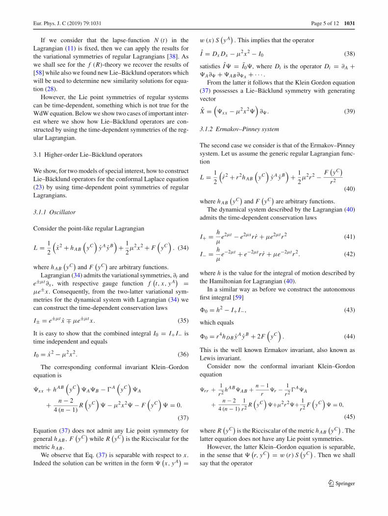
Fig. 1 Qualitative evolution of the wavefunction Im(�1 (a, R)

)for

δ = i10 , that is, Im

(�1 (a, R)

) ∼ sin (S (a, R)) with S (a, R) be thesolution of the Hamilton–Jacobi equation

In Fig. 1 we give the qualitative evolution of the wavefunc-tion Im

(�1 (a, R)

)for δ = i

10 , that is, Im(�1 (a, R)

) ∼sin (S (a, R)) where S (a, R) is the solution of the Hamilton–Jacobi equation.

4.2 Case B: power law model R78

For the power-law model f (R) = R78 we prefer to work on

the new coordinates {ρ, σ }

a =(

21

4

)− 13 √

ρeσ , R = e12σ

ρ4 , (65)

where the point-like Lagrangian takes the simple form

L (ρ, ρ, σ, σ ) = 1

2ρ2 − 1

2ρ2σ 2 + V0

e12σ

ρ2 . (66)

The latter Lagrangian describes the two-dimensional Erm-akov–Pinney system without the oscillatory term, while con-stant V0 has the value V0 = − 1

42 .The Hamiltonian constraint is

H = 1

2p2ρ − 1

2ρ2

(p2σ − 2V0e

12σ)

≡ 0, (67)

where

�0 =(p2σ − 2V0e

12σ)

, (68)

is the Ermakov–Pinney invariant, also known as Lewis invari-ant.

Table 3 Commutators of the admitted Lie point symmetries for theWdW equation (69)

[ , ] Y1 Y2 Y3 Y4

Y1 0 −6Y2 6Y3 0

Y2 6Y2 0 0 0

Y3 −6Y3 0 0 0

Y4 0 0 0 0

Table 4 Adjoint representation of the admitted Lie point symmetriesfor the WdW equation (69)

Ad(e(εYi )

)Y j Y1 Y2 Y3 Y4

Y1 Y1 e6εY2 e−6εY3 Y4

Y2 Y1 − 6εY2 Y2 Y3 Y4

Y3 Y1 + 6εY3 Y2 Y3 Y4

Y4 Y1 Y2 Y3 Y4

As far as the WdW equation (28) is concerned it is calcu-lated to be

�ρρ − 1

ρ2 �σσ + 1

ρ�ρ − 2V0

e12σ

ρ2 � = 0. (69)

The later partial differential equation is invariant under theone-parameter point transformations with generators the vec-tor fields

Y1 = ρ∂ρ, Y2 = ρ−5e−6σ ∂ρ + ρ−6e−6σ ∂σ ,

Y3 = ρ7e−6σ ∂ρ − ρ6e−6σ ∂σ , Y� = �∂�.

where in the canonical forms are

Y1 = ρ�ρ∂�, Y2 = ρ−5e−6σ(�ρ + �σ

)∂� + ρ−6e−6σ ∂σ ,

Y3 = ρ6e−6σ(ρ�ρ − �σ

)∂�, Y� = �∂�.

In Tables 3 and 4 we present the commutators and theadjoint representation of the admitted point symmetries.From Table 4 we find that the one-dimensional optimal sys-tem to be

{Y1} , {Y2} , {Y3} , {Y2 − γY3} , {Y1 + δY4} ,

{Y2 + δY4} , {Y3 + δY4} , {Y2 − γY3 + δY4} .

From the one-dimensional algebras {Y2} and {Y3} we findthe trivial solutions � (ρ, σ ) = 0. From the other one-dimensional algebras it follows

{Y1} : �1 (ρ, σ ) = �01(1) I0

(√21

126e6σ

)

+�01(2)K0

(√21

126e6σ

)(70)

123

Eur. Phys. J. C (2019) 79 :1031 Page 9 of 12 1031

{Y2 − γY3} : �23 (ρ, σ ) = �023(1) sin

( √21

252√

γe6ζ

)

+�023(2) sin

( √21

252√

γe6ζ

),

ζ = y + 1

6ln

⎛⎝

(γρ12 − 1

)

ρ6

⎞⎠ (71)

{Y1 + δY4} : �1 (ρ, σ ) = ρδ

(�0

1(1) I δ6

(√21

126e6σ

)

+�01(2)K δ

6

(√21

126e6σ

))(72)

{Y2 + δY4} : �2 (ρ, σ ) = �02 exp

(δ

12ρ6e6y + 1

252δρ−6e6y

), (73)

{Y3 + δY4} : �3 (ρ, σ ) = �02 exp

(− δ

12ρ−6e6y − 1

252δρ6e6y

),

(74)

while from {Y3 + δY4} we get the solution of �23 (ρ, σ ) mul-

tiplied by the function exp(

δ12γ

ρ−6e6y)

.

However as we discussed in the previous section for theErmakov–Pinney system the Lewis invariant (68) can be usedto construct the Lie–Bäcklund operator

�σσ + 2V0e12� = (cJ )

2 � (75)

By using the later constraint we find the wavefunction

�LB (ρ, σ ) = (a1ρ

cJ + a2ρ−cJ

) ([b1 JcJ

6

(1

6

√2V0e

6σ

)

+b2YcJ6

(1

6

√2V0e

6σ

)])(76)

where a1, a2, b1 and b2 are integration constants and Ji (x) ,

Yi (x) are the Bessel functions. We observe that solutions�1 (ρ, σ ) and �1 (ρ, σ ) are included in the latter genericsolution. In total we have found four different solutions,hence, the generic wavefunction is expressed as

� (ρ, σ ) =∑

α1�LB +∑

α23�23 (ρ, σ )

+∑

a2�2 +∑

α23�23 (ρ, σ ) . (77)

In order to relate any quantum solution with the classicaluniverse, we should solve the Hamilton–Jacobi equation (67)with the use of the constraint (68) where pρ = ∂S

∂ρand pσ =

∂S∂σ

. We find that

S (ρ, σ ) = √�0 ln ρ + 1

6

√2V0e12σ + �0

+�0

6arctan h

(√2V0e12σ + �0

�0

),

�0 �= 0, (78)

or

S (ρ, σ ) = −√

2V0

6e6σ , �0 = 0. (79)

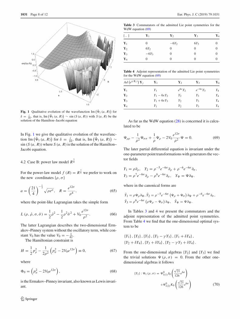
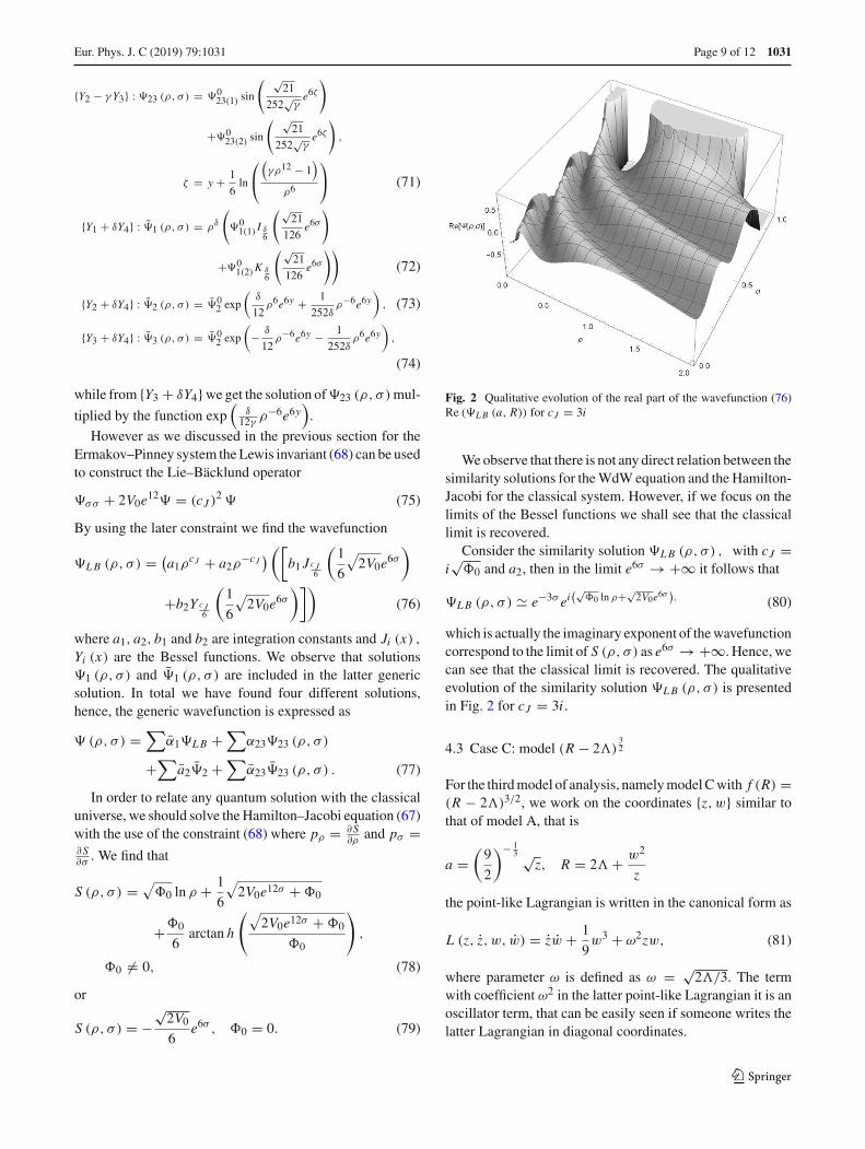
Fig. 2 Qualitative evolution of the real part of the wavefunction (76)Re (�LB (a, R)) for cJ = 3i

We observe that there is not any direct relation between thesimilarity solutions for the WdW equation and the Hamilton-Jacobi for the classical system. However, if we focus on thelimits of the Bessel functions we shall see that the classicallimit is recovered.

Consider the similarity solution �LB (ρ, σ ) , with cJ =i√

�0 and a2, then in the limit e6σ → +∞ it follows that

�LB (ρ, σ ) � e−3σ ei(√

�0 ln ρ+√2V0e6σ

). (80)

which is actually the imaginary exponent of the wavefunctioncorrespond to the limit of S (ρ, σ ) as e6σ → +∞. Hence, wecan see that the classical limit is recovered. The qualitativeevolution of the similarity solution �LB (ρ, σ ) is presentedin Fig. 2 for cJ = 3i .

4.3 Case C: model (R − 2�)32

For the third model of analysis, namely model C with f (R) =(R − 2�)3/2, we work on the coordinates {z, w} similar tothat of model A, that is

a =(

9

2

)− 13 √

z, R = 2� + w2

z

the point-like Lagrangian is written in the canonical form as

L (z, z, w, w) = zw + 1

9w3 + ω2zw, (81)

where parameter ω is defined as ω = √2�/3. The term

with coefficient ω2 in the latter point-like Lagrangian it is anoscillator term, that can be easily seen if someone writes thelatter Lagrangian in diagonal coordinates.

123

1031 Page 10 of 12 Eur. Phys. J. C (2019) 79 :1031

Hence, from (81) it follows that the Hamiltonian constraintis

H = pz pw − 1

9w3 − ω2zw ≡ 0, (82)

while the field equations are

z = pw, w = pz, (83)

pz = ω2w, pw = 1

3w2 + ω2z. (84)

From the latter system we construct the quadratic conserva-tion law I0 = p2

z − ω2w2.

The solution of the Hamilton–Jacobi equation by usingthe quadratic conservation law I0 is found to be

S (z, w) =√I0 + ω2w2

ω4

(ω2w2 + 27ω4z − 2I0

)(85)

The WdW equation for this specific model is written inthe coordinates {z, w} as

�zw −(

1

9w3 + ω2zw

)� = 0. (86)

The linear partial differential equation (86) is invariant underthe point transformations with infinitesimal generators thevector fields

Z1 = 2∂z − 9

wω2∂w, Z� = �∂�.

The one-dimensional optimal system consists of by the vectorfields {Z1} , {Z1 + δZ�}. In canonical form the vector fieldZ1 is written as Z1 = (

2�z − 9w

ω2�w

)∂� .

From the point transformation {Z1 + δZ�} the similaritysolution follows

�1 (z, w) = exp

(δ

4z − δ

36ω2 w2) (

�01(1)Ai (ζ ) + �0

1(2)Bi (ζ ))

,

(87)

where Ai (ζ ) , Bi (ζ ) are the Airy functions and ζ =− 6

23

288ω83

(1 + √

3i) (

δ2 + 72ω4z + 8ω2w2). It is not a sur-

prise that the wavefunction is expressed by the Airy func-tions. Recall that the Airy functions solve the Schrödingerequation for a particle confined by a triangular well [62].

However, by using the differential operator generated bythe quadratic conservation law I0, that is,

I0� ≡ �zz − ω2w2� + cJ� (88)

we find the similarity solution

�LB (z, w) = �0LB(1) sin (ξ) + �0

LB(2) cos (ξ) (89)

where parameter ξ is defined as

ξ =√cJ − ω2w2

ω4

(ω2w2 + 27ω4z + 2cJ

). (90)

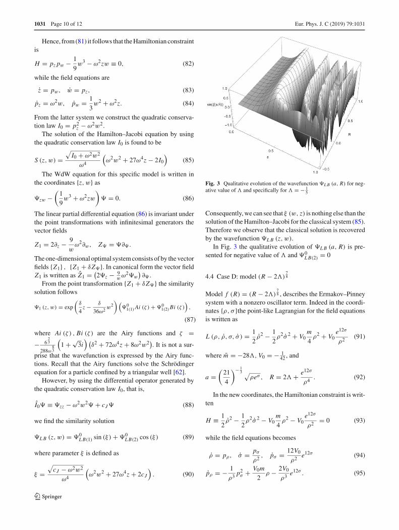
Fig. 3 Qualitative evolution of the wavefunction �LB (a, R) for neg-ative value of � and specifically for � = − 1

5

Consequently, we can see that ξ (w, z) is nothing else than thesolution of the Hamilton–Jacobi for the classical system (85).Therefore we observe that the classical solution is recoveredby the wavefunction �LB (z, w).

In Fig. 3 the qualitative evolution of �LB (a, R) is pre-sented for negative value of � and �0

LB(2) = 0

4.4 Case D: model (R − 2�)78

Model f (R) = (R − 2�)78 , describes the Ermakov–Pinney

system with a nonzero oscillator term. Indeed in the coordi-nates {ρ, σ }the point-like Lagrangian for the field equationsis written as

L (ρ, ρ, σ, σ ) = 1

2ρ2 − 1

2ρ2σ 2 + V0

m

4ρ2 + V0

e12σ

ρ2 (91)

where m = −28�, V0 = − 142 , and

a =(

21

4

)− 13 √

ρeσ , R = 2� + e12σ

ρ4 . (92)

In the new coordinates, the Hamiltonian constraint is writ-ten

H ≡ 1

2ρ2 − 1

2ρ2σ 2 − V0

m

4ρ2 − V0

e12σ

ρ2 = 0 (93)

while the field equations becomes

ρ = pρ, σ = pσ

ρ2 , pσ = 12V0

ρ2 e12σ (94)

pρ = − 1

ρ3 p2σ + V0m

2ρ − 2V0

ρ3 e12σ . (95)

123

Eur. Phys. J. C (2019) 79 :1031 Page 11 of 12 1031

Finally, the field equations admit the Lewis invariant whichis written as

� = σ 2 + V0e12σ . (96)

The WdW equation (28) is written as follows

�ρρ − 1

ρ2 �σσ + 1ρ�ρ − 2

(V0

m

4ρ2 + V0

e12σ

ρ2

)� = 0,

(97)

and has no other point symmetries except the trivial ones.However, as we discussed in Sect. 3 from the Lewis-invariantwe construct the differential operator

�� ≡ �σσ + V0e12σ � − �0�. (98)

Hence from (97) and (98), with �� = 0 we find thesimilarity solution

�LB (ρ, σ )

=(

�0LB(1) I

√�06

(√42

252e6σ

)+�0

LB(2)K√

�06

(√42

252e6σ

))

× J√�02

(√−6�

12ρ2

)+

(�0LB(3) I

√�06

(√42

252e6σ

)

+�0LB(4)K

√�06

(√42

252e6σ

))Y√

�02

(√−6�

12ρ2

)(99)

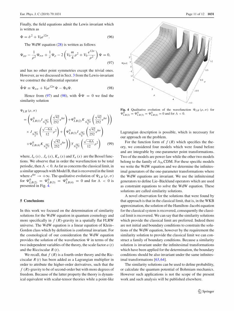
where, Ia (x) , Ja (x), Ka (x) and Ya (x) are the Bessel func-tions. We observe that in order the wavefunction to be totalperiodic, then � < 0. As far as concerns the classical limit, ina similar approach with Model B, that is recovered in the limitwhere e6σ → +∞. The qualitative evolution of �LB (ρ, σ )

for �0LB(2) = �0

LB(3) = �0LB(4) = 0 and for � < 0 is

presented in Fig. 4.

5 Conclusions

In this work we focused on the determination of similaritysolutions for the WdW equation in quantum cosmology andmore specifically in f (R)-gravity in a spatially flat FLRWuniverse. The WdW equation is a linear equation of Klein–Gordon class which by definition is conformal invariant. Forthe cosmological of our consideration the WdW equationprovides the solution of the wavefunction � in terms of thetwo independent variables of the theory, the scale factor a (t)and the Ricciscalar R (t).

We recall, that f (R) is a fourth-order theory and the Ric-ciscalar R (t) has been added as a Lagrangian multiplier inorder to attribute the higher-order derivatives, such that thef (R)-gravity to be of second-order but with more degrees offreedom. Because of the latter property the theory is dynam-ical equivalent with scalar-tensor theories while a point-like

Fig. 4 Qualitative evolution of the wavefunction �LB (ρ, σ ) for�0

LB(2) = �0LB(3) = �0

LB(4) = 0 and for � < 0.

Lagrangian description is possible, which is necessary forour approach on the problem.

For the function form of f (R) which specifies the the-ory, we considered four models which were found beforeand are integrable by one-parameter point transformations.Two of the models are power-law while the other two modelsbelong to the family of �bcCDM. For these specific modelswe write the WdW equation and we determine the infinites-imal generators of the one-parameter transformations wherethe WdW equations are invariant. We use the infinitesimalgenerators to define Lie–Bäcklund operators which are usedas constraint equations to solve the WdW equation. Thesesolutions are called similarity solutions.

A novel observation for the solutions that were found bythat approach is that in the classical limit, that is, in the WKBapproximation, the solution of the Hamilton–Jacobi equationfor the classical system is recovered, consequently the classi-cal limit is recovered. We can say that the similarity solutionswhich provide the classical limit are preferred. Indeed thereare not initial and boundary conditions to constrain the solu-tions of the WdW equation, however by the requirement thesimilarity solution to provide the classical limit we can con-struct a family of boundary conditions. Because a similaritysolution is invariant under the infinitesimal transformationswhich have been applied for the determination, the boundaryconditions should be also invariant under the same infinites-imal transformations [63,64].

The similarity solutions can be used to define probability,or calculate the quantum potential of Bohmiam mechanics.However such applications is not the scope of the presentwork and such analysis will be published elsewhere.

123

1031 Page 12 of 12 Eur. Phys. J. C (2019) 79 :1031

Acknowledgements The author acknowledges Marianthi Paliathanasifor continuous support.

Data Availability Statement This manuscript has no associated dataor the data will not be deposited. [Authors’ comment: The work istheoretical.]

Open Access This article is licensed under a Creative Commons Attri-bution 4.0 International License, which permits use, sharing, adaptation,distribution and reproduction in any medium or format, as long as yougive appropriate credit to the original author(s) and the source, pro-vide a link to the Creative Commons licence, and indicate if changeswere made. The images or other third party material in this articleare included in the article’s Creative Commons licence, unless indi-cated otherwise in a credit line to the material. If material is notincluded in the article’s Creative Commons licence and your intendeduse is not permitted by statutory regulation or exceeds the permit-ted use, you will need to obtain permission directly from the copy-right holder. To view a copy of this licence, visit http://creativecommons.org/licenses/by/4.0/.Funded by SCOAP3.

References

1. T. Clifton, P.G. Ferreira, A. Padilla, C. Skordis, Phys. Rep. 513, 1(2012)

2. S. Nojiri, S.D. Odintsov, V.K. Oikonomou, Phys. Rep.692, 1 (2017)3. M. Tegmark et al., Astrophys. J. 606, 702 (2004)4. M. Kowalski et al., Astrophys. J. 686, 749 (2008)5. E. Komatsu et al., Astrophys. J. Suppl. Ser. 180, 330 (2009)6. P.A.R. Ade et al., Astron. Astrophys. 571, A15 (2014)7. A. De Felice, S. Tsujikawa, Living Rev. Relativ. 13, 3 (2010)8. G.J. Olmo, Int. J. Mod. Phys. D 20, 413 (2011)9. B. Li, J.D. Barrow, D.F. Mota, Phys. Rev. D 76, 044027 (2007)

10. R. Ferraro, M.J. Guzman, Phys. Rev. D 97, 104028 (2018)11. A. Paliathanasis, J.D. Barrow, P.G.L. Leach, Phys. Rev. D 94,

023525 (2016)12. R.C. Nunes, S. Pan, E.N. Saridakis, Phys. Rev. D 98, 104055 (2018)13. A. Paliathanasis, S. Basilakos, E.N. Saridakis, S. Capozziello, K.

Atazadeh, F. Darabi, M. Tsamparlis, Phys. Rev. D 89, 104042(2014)

14. L. Amendola, S. Tsujikawa,DarkEnergy Theory andObservations(Cambridge University Press, Cambridge, 2010)

15. T. Harko, F.S.N. Lobo, G. Otalor, E.N. Saridakis, JCAP 1412, 021(2014)

16. A. Paliathanasis, Phys. Rev. D 95, 064062 (2017)17. S.D. Odintsov, V.K. Oikonomou, S. Banrajee, Nucl. Phys. B 938,

935 (2019)18. C. Erics, E. Papantonopoulos, E.N. Saridakis, Phys. Rev. D 99,

123527 (2019)19. X. Liu, P. Channuie, D. Samart, Phys. Dark Univ. 17, 52 (2017)20. R. Ferrraro, Proc. AIP. Conf. 1471, 103 (2012)21. K. Bamba, M. Ilyas, M.Z. Bhatti, Z. Yousaf, Gen. Relativ. Gravit.

49, 112 (2017)22. S. Nojiri, S.D. Odintsov, MPLA 29, 1450211 (2014)23. R. Myrzakulov, L. Sebastiani, Astrophys. Space Sci. 361, 188

(2016)24. S. Chakrabati, J.Levi Said, G. Farrugia, EPJC 77, 815 (2017)25. S. Pan, MPLA A33, 1850003 (2018)26. S. Carloni, J.P. Mimoso, EPJC 77, 547 (2017)27. R. Kase, S. Tsujikawa, JCAP 1909, 054 (2019)

28. J.B. Jimenez, L. Heisenberg, T.S. Koivisto, S. Pekar,arXiv:1906.10027

29. H.A. Buchdahl, Mon. Not. R. Astron. Soc. 150, 1 (1970)30. A.A. Starobinsky, Phys. Lett. B 91, 99 (1980)31. J.D. Barrow, A.C. Ottewill, J. Phys. A 16, 2757 (1983)32. S.M. Carroll, V. Duvvuri, M. Trodden, M.S. Turner, Phys. Rev. D

70, 043528 (2004)33. A. Alho, S. Carloni, C. Uggla, JCAP 08, 064 (2016)34. T.B. Vasilev, M. Bouhmadi-Lopez, P. Martin-Moruno. Phys. Rev.

D 100, 084016 (2019)35. R.C. Nunes, S. Pan, E.N. Saridakis, E.M.C. Abreu, JCAP 1701,

005 (2017)36. T. Inagaki, H. Sakamoto, arXiv:1909.0763837. A. Paliathanasis, Class. Quantum Gravity 33, 075012 (2016)38. A. Paliathanasis, M. Tsamparlis, S. Basilakos, Phys. Rev. D 84,

123514 (2011)39. S. Domazet, V. Radovanovic, M. Simonovic, H. Stefancic, Int. J.

Mod. Phys. D 22, 1350006 (2013)40. A. Paliathanasis, EPJC 77, 438 (2017)41. B.S. De Witt, Phys. Rev. 160, 1113 (1967)42. A. Barvinsky, Phys. Rep. 230, 237 (1993)43. A. Zampeli, T. Pailas, P.A. Terzis, T. Christodoulakis, JCAP 1605,

066 (2016)44. A. Peres, Critique of the Wheeler–DeWitt equation, in On Ein-

stein’s Path ed. by A. Harvey (Springer, New York, 1999)45. N.P. Landsman, Class. Quantum Gravity 12, L119 (1995)46. A. Yu Kamenshchik, A. Tronconi, T. Vardanyan, G. Venturi, Int. J.

Mod. Phys. D 28, 1950073 (2019)47. T.P. Shestakova, Int. J. Mod. Phys. D 27, 1841004 (2018)48. B. Vakili, Phys. Lett. B 669, 211 (2008)49. V. Vázquez-Báez, C. Ramírez, Adv. Math. Phys. 2017, 1056514

(2017). https://doi.org/10.1155/2017/105651450. A. Alonso-Serrano, M. Bouhmadi-Lopez, P. Martin-Moruno, Phys.

Rev. D 98, 104004 (2018)51. B. Vakili, Int. J. Theor. Phys. 51, 133 (2012)52. T. Christodoulakis, N. Dimakis, P.A. Terzis, G. Doulis, Th Gram-

menos, E. Melas, A. Spanou, J. Geom. Phys. 71, 127 (2013)53. A. Karagiorgos, T. Pailas, N. Dimakis, G.O. Papadopoulos, P.A.

Terzis, T. Christodoulakis, JCAP 1904, 006 (2019)54. A. Paliathanasis, A. Zampeli, T. Christodoulakis, M.T. Mustafa,

Class. Quantum Gravity 35, 125005 (2018)55. T. Pailas, N. Dimakis, A. Karagiorgos, P.A. Terzis, G.O.

Papadopoulos, T. Christodoulakis, Class. Quantum Gravity 36,135010 (2019)

56. D. Wiltshire, An introduction to quantum cosmology, Cosmology:the Physics of the Universe ed. by B. Robson, N. Visvanathan andW.S. Woolcock (World Scientific, Singapore, 1996)

57. A. Paliathanasis, M. Tsamparlis, Int. J. Geom. Methods Mod. Phys.11, 1450037 (2014)

58. N. Dimakis, T. Christodoulakis, P.A. Terzis, J. Geom. Phys. 77, 97(2014)

59. M. Tsamparlis, A. Paliathanasis, J. Phys. A Math. Theor. 45,275202 (2012)

60. P.J. Olver, Applications of Lie Groups to Differential Equations(Springer, New York, 1993)

61. G.W. Bluman, S. Kumei, Symmetries and Differential Equations(Springer, New York, 1989)

62. L.F. Matin, H.H. Bouzari, F. Ahmadi, J. Theor. Appl. Phys. 8, 140(2014)

63. R. Cherniha, S. Kovalenko, Commun. Nonlinear Sci. Numer.Simul. 17, 71 (2012)

64. I.T. Habibulin, Nonlinear Math. Phys. 3, 147 (1996)

123