Similarity Search in Mass Spectra Databases

Charles University in Prague

Faculty of Mathematics and Physics

DOCTORAL THESIS

Ing. Jirı Novak

Similarity Search in Mass SpectraDatabases

Department of Software Engineering

Supervisor of the doctoral thesis: doc. RNDr. Tomas Skopal, Ph.D.

Study programme: Computer Science

Specialization: Software Systems

Prague 2013

I would like to thank my supervisor doc. RNDr. Tomas Skopal, Ph.D. andmy consultant RNDr. David Hoksza, Ph.D. for many valuable advices during myPh.D. study. I would like to also express deep gratitude to my family for havingthe patience with me, especially to my wife MUDr. Lucia Novakova, my funnyson Jirı, and my parents Miroslava Novakova and Jirı Novak.

I declare that I carried out this doctoral thesis independently, and only with thecited sources, literature and other professional sources.

I understand that my work relates to the rights and obligations under the ActNo. 121/2000 Coll., the Copyright Act, as amended, in particular the fact thatthe Charles University in Prague has the right to conclude a license agreementon the use of this work as a school work pursuant to Section 60 paragraph 1 ofthe Copyright Act.

In Prague date April 22nd, 2013 Signature of the author

Annotation

Title:Similarity Search in Mass Spectra Databases

Author:Ing. Jirı Novakemail: [email protected]

Department:Department of Software EngineeringFaculty of Mathematics and PhysicsCharles University in Prague

Supervisor:doc. RNDr. Tomas Skopal, Ph.D.email: [email protected]

Abstract:Shotgun proteomics is a widely known technique for identification of pro-tein and peptide sequences from an ”in vitro” sample. A tandem massspectrometer generates tens of thousands of mass spectra which must beannotated with peptide sequences. For this purpose, the similarity search ina database of theoretical spectra generated from a database of known pro-tein sequences can be utilized. Since the sizes of databases grow rapidly inrecent years, there is a demand for utilization of various database indexingtechniques. We investigate the capabilities of (non)metric access methodsas the database indexing techniques for fast and approximate similarity re-trieval in mass spectra databases. We show that the method for peptidesequences identification is more than 100× faster than a sequential scan overthe entire database while more than 90% of spectra are correctly annotatedwith peptide sequences. Since the method is currently suitable for smallmixtures of proteins, we also utilize a precursor mass filter as the databaseindexing technique for complex mixtures of proteins. The precursor massfilter followed by ranking of spectra by a modification of the parametrizedHausdorff distance outperforms state-of-the-art tools in the number of iden-tified peptide sequences and the speed of search. The proposed methodsare implemented in the peptide identification engine SimTandem which canbe used for a batch analysis in the framework TOPP based on OpenMS.

Keywords:tandem mass spectrometry, peptide identification, metric and non-metricaccess methods, similarity search, bioinformatics

Anotace

Nazev prace:Podobnostnı vyhledavanı v databazıch hmotnostnıch spekter

Autor:Ing. Jirı Novakemail: [email protected]

Katedra:Katedra softwaroveho inzenyrstvıMatematicko-fyzikalnı fakultaUniverzita Karlova v Praze

Skolitel:doc. RNDr. Tomas Skopal, Ph.D.email: [email protected]

Abstrakt:Tandemova hmotnostnı spektrometrie je znama metoda pro identifikaci pro-teinovych a peptidovych sekvencı ze vzorku biologickeho materialu. Hmot-nostnı spektrometr generuje desetitisıce spekter, ktera musı byt nasledneanotovana peptidovymi sekvencemi. Za tımto ucelem lze vyuzıt podobnos-tnı vyhledavanı v databazıch teoretickych spekter generovanych z databazıznamych proteinovych sekvencı. Vzhledem k tomu, ze objem techto databazıkazdorocne narusta temer exponencialnım tempem, je zapotrebı hledat novezpusoby pro jejich indexovanı. V teto praci se zamerujeme na vyuzitı(ne)metrickych prıstupovych metod jako databazovych indexu pro rychlea aproximativnı podobnostnı vyhledavanı v databazıch spekter. Navrzenametoda identifikace peptidovych sekvencı dosahuje vıce nez 100-nasobnehozrychlenı oproti sekvencnımu pruchodu cele databaze, pricemz je spravneanotovano pres 90% spekter. V soucasnosti je metoda vhodna zejmenapro male smesi proteinu. Pro komplexnı smesi proteinu vyuzıvame in-dexovacı metodu zalozenou na prekurzorovem hmotnostnım filtru, kterama pri pouzitı s modifikacı parametrizovane Hausdorffovy vzdalenosti vyssırychlost i presnost vyhledavanı nez bezne pouzıvane metody. Navrzenemetody jsou implementovany v aplikaci SimTandem, kterou lze pouzıt prodavkove zpracovanı ve frameworku TOPP zalozenem na knihovne OpenMS.

Klıcova slova:tandemova hmotnostnı spektrometrie, identifikace peptidu, metricke a ne-metricke prıstupove metody, podobnostnı vyhledavanı, bioinformatika

Contents

Preface 5Summary of Contributions . . . . . . . . . . . . . . . . . . . . . . . . . 5Structure of Thesis . . . . . . . . . . . . . . . . . . . . . . . . . . . . . 5

1 Introduction 7

2 Mass Spectrometry Fundamentals 92.1 Protein Digestion . . . . . . . . . . . . . . . . . . . . . . . . . . . 92.2 High-pressure Liquid Chromatography . . . . . . . . . . . . . . . 92.3 Mass Spectrometry . . . . . . . . . . . . . . . . . . . . . . . . . . 10

2.3.1 Ionization Techniques . . . . . . . . . . . . . . . . . . . . . 102.3.2 Mass Analyzers . . . . . . . . . . . . . . . . . . . . . . . . 12

2.4 Tandem Mass Spectrometry . . . . . . . . . . . . . . . . . . . . . 142.4.1 Tandem Mass Spectrum . . . . . . . . . . . . . . . . . . . 142.4.2 Modifications in Tandem Mass Spectra . . . . . . . . . . . 17

3 Algorithms for Processing of Mass Spectra 193.1 Preprocessing of Spectra . . . . . . . . . . . . . . . . . . . . . . . 19

3.1.1 Peak Selection Heuristics . . . . . . . . . . . . . . . . . . . 203.1.2 Spectrum Quality Filtering . . . . . . . . . . . . . . . . . . 203.1.3 Spectrum Clustering . . . . . . . . . . . . . . . . . . . . . 21

3.2 Identification of Peptides . . . . . . . . . . . . . . . . . . . . . . . 223.2.1 Similarity Search . . . . . . . . . . . . . . . . . . . . . . . 223.2.2 De Novo Peptide Sequencing . . . . . . . . . . . . . . . . . 263.2.3 Statistical Evaluation . . . . . . . . . . . . . . . . . . . . . 273.2.4 Probabilistic Consensus Scoring . . . . . . . . . . . . . . . 28

3.3 Identification of Proteins . . . . . . . . . . . . . . . . . . . . . . . 303.3.1 Bottom-up Proteomics . . . . . . . . . . . . . . . . . . . . 303.3.2 Top-down Proteomics . . . . . . . . . . . . . . . . . . . . . 33

3.4 Quantification of Peptides and Proteins . . . . . . . . . . . . . . . 343.4.1 Label-based Quantification . . . . . . . . . . . . . . . . . . 343.4.2 Label-free Quantification . . . . . . . . . . . . . . . . . . . 35

3.5 Frameworks for Shotgun Proteomics . . . . . . . . . . . . . . . . . 37

4 Speeding up the Mass Spectra Database Search 414.1 Precursor Mass Filter . . . . . . . . . . . . . . . . . . . . . . . . . 424.2 Peptide Sequence Tags . . . . . . . . . . . . . . . . . . . . . . . . 424.3 Fuzzy and Tandem Cosine Distance . . . . . . . . . . . . . . . . . 43

4.3.1 Fuzzy Cosine Distance . . . . . . . . . . . . . . . . . . . . 43

1

4.3.2 Tandem Cosine Distance . . . . . . . . . . . . . . . . . . . 444.3.3 MVP-tree . . . . . . . . . . . . . . . . . . . . . . . . . . . 454.3.4 Semi-metric Search . . . . . . . . . . . . . . . . . . . . . . 45

4.4 Locality Sensitive Hashing . . . . . . . . . . . . . . . . . . . . . . 454.4.1 Family of Hash Functions . . . . . . . . . . . . . . . . . . 464.4.2 Data Structure and Query Processing . . . . . . . . . . . . 46

4.5 Inverted Files . . . . . . . . . . . . . . . . . . . . . . . . . . . . . 474.6 Other approaches . . . . . . . . . . . . . . . . . . . . . . . . . . . 49

5 Metric and Non-metric Access Methods 515.1 Metric Access Methods . . . . . . . . . . . . . . . . . . . . . . . . 51

5.1.1 Metric Space and Metric Distance . . . . . . . . . . . . . . 515.1.2 Minkowski Distances . . . . . . . . . . . . . . . . . . . . . 525.1.3 Cosine Similarity . . . . . . . . . . . . . . . . . . . . . . . 525.1.4 Hausdorff Distance . . . . . . . . . . . . . . . . . . . . . . 535.1.5 Similarity Queries . . . . . . . . . . . . . . . . . . . . . . . 535.1.6 LAESA . . . . . . . . . . . . . . . . . . . . . . . . . . . . 545.1.7 M-tree . . . . . . . . . . . . . . . . . . . . . . . . . . . . . 575.1.8 Performance Estimation . . . . . . . . . . . . . . . . . . . 645.1.9 Cost Measures . . . . . . . . . . . . . . . . . . . . . . . . . 65

5.2 Non-Metric Access Methods . . . . . . . . . . . . . . . . . . . . . 655.2.1 Enforcement of Metric Postulates . . . . . . . . . . . . . . 665.2.2 T-error . . . . . . . . . . . . . . . . . . . . . . . . . . . . . 665.2.3 T-modifiers and T-bases . . . . . . . . . . . . . . . . . . . 675.2.4 TriGen . . . . . . . . . . . . . . . . . . . . . . . . . . . . . 675.2.5 NM-Tree . . . . . . . . . . . . . . . . . . . . . . . . . . . . 69

6 Non-metric Similarity Search in Mass Spectra Databases 736.1 Similarity Functions for MAMs . . . . . . . . . . . . . . . . . . . 73

6.1.1 Angle Distance . . . . . . . . . . . . . . . . . . . . . . . . 736.1.2 Logarithmic Distance . . . . . . . . . . . . . . . . . . . . . 746.1.3 Parameterized Hausdorff Distance . . . . . . . . . . . . . . 756.1.4 Modification of Parameterized Hausdorff Distance . . . . . 786.1.5 Angle Distance with Precursor . . . . . . . . . . . . . . . . 786.1.6 Parameterized Hausdorff Distance with Precursor . . . . . 78

6.2 Identification of Peptide Sequences . . . . . . . . . . . . . . . . . 786.2.1 Indexing . . . . . . . . . . . . . . . . . . . . . . . . . . . . 796.2.2 Querying . . . . . . . . . . . . . . . . . . . . . . . . . . . . 80

6.3 Dealing with Modifications in Spectra . . . . . . . . . . . . . . . . 816.4 Clustering and Sequential Scan of Protein Sequence Candidates . 83

6.4.1 Pre-processing . . . . . . . . . . . . . . . . . . . . . . . . . 836.4.2 Query phase . . . . . . . . . . . . . . . . . . . . . . . . . . 846.4.3 Post-processing . . . . . . . . . . . . . . . . . . . . . . . . 84

7 Experiments 877.1 Measured Quantities . . . . . . . . . . . . . . . . . . . . . . . . . 877.2 Data Sets . . . . . . . . . . . . . . . . . . . . . . . . . . . . . . . 88

7.2.1 Amethyst and Opal . . . . . . . . . . . . . . . . . . . . . . 887.2.2 Keller 1 . . . . . . . . . . . . . . . . . . . . . . . . . . . . 88

2

7.2.3 Keller 2 . . . . . . . . . . . . . . . . . . . . . . . . . . . . 897.2.4 E. coli and Human . . . . . . . . . . . . . . . . . . . . . . 89

7.3 TriGen-based Modifications . . . . . . . . . . . . . . . . . . . . . 907.3.1 FP-bases for Amethyst and Opal . . . . . . . . . . . . . . 907.3.2 FP-bases and RBQ-bases for Keller 1 . . . . . . . . . . . . 90

7.4 Effectiveness and Efficiency of Non-metric Similarity Search . . . 917.4.1 Sequential Scan . . . . . . . . . . . . . . . . . . . . . . . . 917.4.2 Improving the Indexability . . . . . . . . . . . . . . . . . . 927.4.3 Speeding-up using M-tree . . . . . . . . . . . . . . . . . . 92

7.5 Dealing with Modifications in Spectra . . . . . . . . . . . . . . . . 937.5.1 Sequential Scan . . . . . . . . . . . . . . . . . . . . . . . . 937.5.2 Speeding-up using M-tree . . . . . . . . . . . . . . . . . . 93

7.6 Advanced Analysis of Non-metric Similarity Search . . . . . . . . 947.6.1 Comparison of dHP , d′HP , dA and d′A . . . . . . . . . . . . . 947.6.2 Comparison of M-tree with LAESA . . . . . . . . . . . . . 957.6.3 k in kNN queries . . . . . . . . . . . . . . . . . . . . . . . 967.6.4 Comparison of a set of M-trees with NM-tree . . . . . . . 96

7.7 Clustering and Sequential Scan of Protein Sequence Candidates . 977.7.1 Clustering of Spectra from Two Spectrometer Runs . . . . 987.7.2 Effectiveness and Efficiency of Identification . . . . . . . . 987.7.3 Clustering of Spectra Appended from More Runs . . . . . 997.7.4 Impact of Distance Threshold on Clustering . . . . . . . . 100

7.8 Utilization of Precursor Mass Filter . . . . . . . . . . . . . . . . . 1017.8.1 State-of-the-Art Tools . . . . . . . . . . . . . . . . . . . . 1017.8.2 SimTandem . . . . . . . . . . . . . . . . . . . . . . . . . . 1027.8.3 Efficiency of Precursor Mass Filter . . . . . . . . . . . . . 103

8 Implementation 1058.1 Web Interface . . . . . . . . . . . . . . . . . . . . . . . . . . . . . 1058.2 TOPP Tool . . . . . . . . . . . . . . . . . . . . . . . . . . . . . . 109

8.2.1 Installation Instructions . . . . . . . . . . . . . . . . . . . 109

9 Conclusion 113

List of Figures 130

List of Tables 131

List of Algorithms 133

List of Abbreviations 136

3

4

Preface

Proteins are the basis of all living organisms while the tandem mass spectrometryis a widely used technique for identification and quantification of peptides andproteins from an ”in vitro” sample. A mass spectrometer produces tens of thou-sands of mass spectra which must be annotated with peptide sequences. One ofthe commonly used approaches for annotation of spectra is the similarity searchin a database of theoretical spectra generated from a database of known proteinsequences. Since the sizes of databases grow rapidly in recent years, there is ademand for fast similarity search in these databases. A way how to speed-upthe search in a database is to utilize an indexing technique. The (non)metricaccess methods are database indexing techniques which are based on propertiesof (non)metric spaces and they are suitable for various kinds of multimedia data.

Summary of Contributions

In this thesis, we investigate the utilization of database indexing techniques formass spectra databases. We map the recently proposed techniques and analyzethe capabilities of (non)metric access methods for fast and approximate similaritysearch in mass spectra databases. The proposed method has been successfullytested on small mixtures of purified proteins (up to tens of proteins). However,due to a rapid development of new and very accurate instruments, the utiliza-tion of (non)metric access methods on complex mixtures of proteins (containingthousands of proteins) is a non-trivial task. From this reason, we also investigatethe utilization of a precursor mass filter followed by a ranking of theoretical spec-tra by a modification of the parameterized Hausdorff distance originally designedfor (non)metric indexes. We show that the method outperforms state-of-the arttools on complex mixtures of proteins in both – the number of identified peptidesequences and the speed of the search. The proposed algorithms have been im-plemented in the application SimTandem which can be used for a batch analysisin the framework TOPP based on OpenMS.

Structure of Thesis

The thesis is organized as follows. In Chap. 1, proteins are briefly introducedand an overview of amino acids is proposed. In Chap. 2, the basic physical andchemical principles of mass spectrometry are described. The Chap. 3 gives anoverview of existing algorithmic techniques for identification and quantificationof peptides/proteins from databases of theoretical mass spectra, and for statistical

5

evaluation of peptide-spectrum matches. Since the thesis is focused on the index-ing of mass spectra, the Chap. 4 maps the existing approaches which speed-up thesearch in mass spectra databases. In Chap. 5, the metric and non-metric accessmethods are described. The approach for identification of peptides by non-metricaccess methods is proposed in Chap. 6. In experimental Chap. 7, the efficiencyand effectiveness of the algorithm for identification of peptide sequences by non-metric access methods are studied, and a statistical comparison of precursor massfilter with state-of-the art tools is proposed. In Chap. 8, the implementation ofSimTandem is described.

6

Chapter 1

Introduction

The genetic information of prokaryotes and eukaryotes is encoded in DNA (de-oxyribonucleic acid) which determines their characteristics. The DNA is orga-nized as a double helix having two complementary strands. A strand of the helixcan be represented by a linear sequence over the alphabet of four bases – adenine,cytosine, guanine and thymine (A, C, G and T). While adenines in one strandare paired with thymines in the other strand, the cytosines are coupled with gua-nines. A triplet of bases (or codon) encodes an amino acid. Even though thereare 43 = 64 different triplets of bases, they encode only 20 amino acids becausesome amino acids are encoded by more triplets and because some triplets serve asstop codons. As defined by the central dogma of molecular biology, the DNA istranscripted into RNA (ribonucleic acid) and the RNA is translated into proteins.

Proteins are linear chains of amino acids which are connected by peptide bonds(Fig. 2.7). Proteins are the basis of all living organisms and they are essential forcorrect construction of cells and for their proper functioning [1]. In terms ofcomputer science, a protein can be understood as a linear sequence over 20-lettersubset of the English alphabet where each letter corresponds to an amino acid.

Figure 1.1: Basic types of amino acids

7

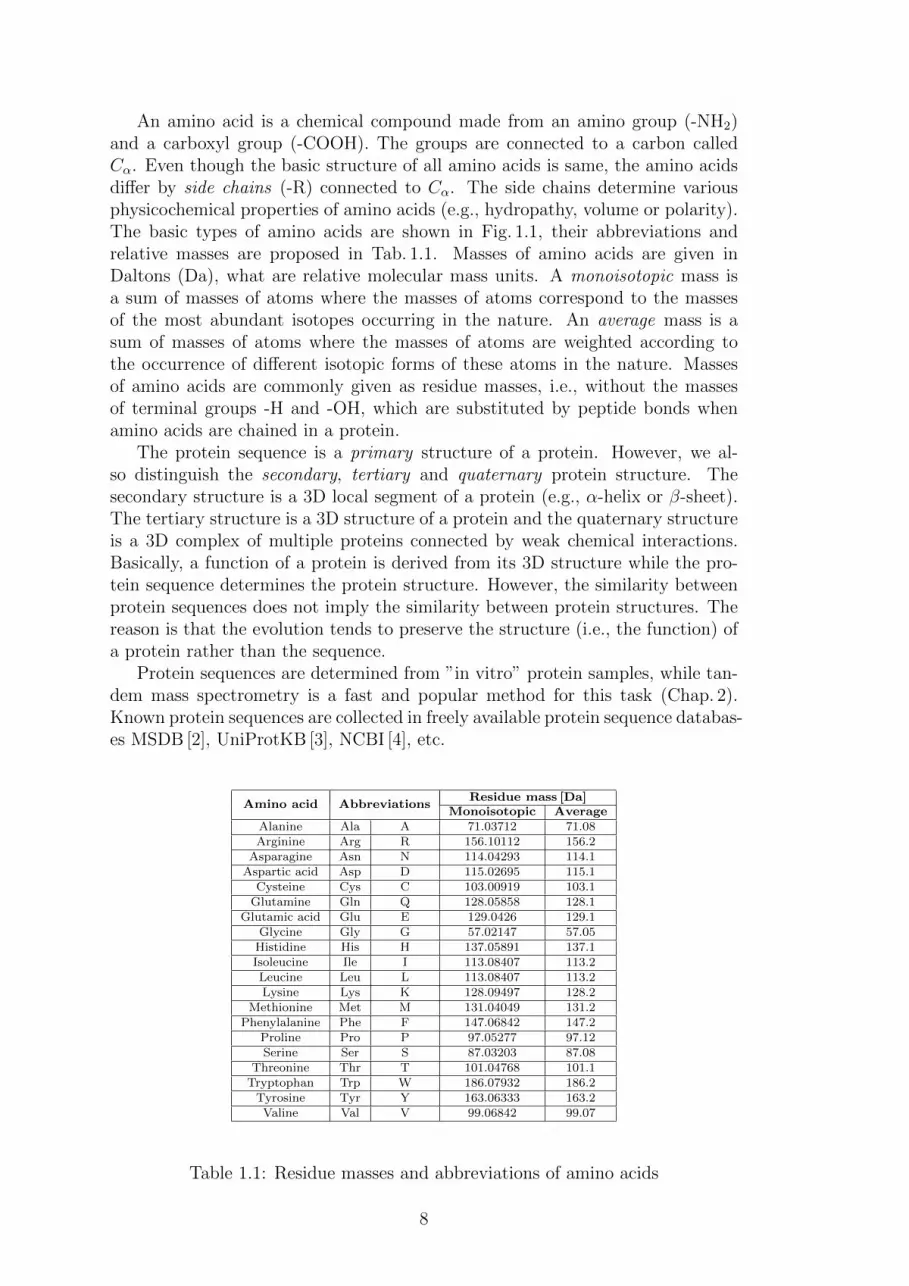
An amino acid is a chemical compound made from an amino group (-NH2)and a carboxyl group (-COOH). The groups are connected to a carbon calledCα. Even though the basic structure of all amino acids is same, the amino acidsdiffer by side chains (-R) connected to Cα. The side chains determine variousphysicochemical properties of amino acids (e.g., hydropathy, volume or polarity).The basic types of amino acids are shown in Fig. 1.1, their abbreviations andrelative masses are proposed in Tab. 1.1. Masses of amino acids are given inDaltons (Da), what are relative molecular mass units. A monoisotopic mass isa sum of masses of atoms where the masses of atoms correspond to the massesof the most abundant isotopes occurring in the nature. An average mass is asum of masses of atoms where the masses of atoms are weighted according tothe occurrence of different isotopic forms of these atoms in the nature. Massesof amino acids are commonly given as residue masses, i.e., without the massesof terminal groups -H and -OH, which are substituted by peptide bonds whenamino acids are chained in a protein.

The protein sequence is a primary structure of a protein. However, we al-so distinguish the secondary, tertiary and quaternary protein structure. Thesecondary structure is a 3D local segment of a protein (e.g., α-helix or β-sheet).The tertiary structure is a 3D structure of a protein and the quaternary structureis a 3D complex of multiple proteins connected by weak chemical interactions.Basically, a function of a protein is derived from its 3D structure while the pro-tein sequence determines the protein structure. However, the similarity betweenprotein sequences does not imply the similarity between protein structures. Thereason is that the evolution tends to preserve the structure (i.e., the function) ofa protein rather than the sequence.

Protein sequences are determined from ”in vitro” protein samples, while tan-dem mass spectrometry is a fast and popular method for this task (Chap. 2).Known protein sequences are collected in freely available protein sequence databas-es MSDB [2], UniProtKB [3], NCBI [4], etc.

Amino acid AbbreviationsResidue mass [Da]

Monoisotopic AverageAlanine Ala A 71.03712 71.08Arginine Arg R 156.10112 156.2

Asparagine Asn N 114.04293 114.1Aspartic acid Asp D 115.02695 115.1

Cysteine Cys C 103.00919 103.1Glutamine Gln Q 128.05858 128.1

Glutamic acid Glu E 129.0426 129.1Glycine Gly G 57.02147 57.05

Histidine His H 137.05891 137.1Isoleucine Ile I 113.08407 113.2Leucine Leu L 113.08407 113.2Lysine Lys K 128.09497 128.2

Methionine Met M 131.04049 131.2Phenylalanine Phe F 147.06842 147.2

Proline Pro P 97.05277 97.12Serine Ser S 87.03203 87.08

Threonine Thr T 101.04768 101.1Tryptophan Trp W 186.07932 186.2

Tyrosine Tyr Y 163.06333 163.2Valine Val V 99.06842 99.07

Table 1.1: Residue masses and abbreviations of amino acids

8

Chapter 2

Mass SpectrometryFundamentals

Tandem mass spectrometry combined with high-pressure liquid chromatography(HPLC-MS/MS) is a widely used technique for identification and quantificationof proteins and peptides [5] [6] [7] [8].

We can easily analyze small mixtures of purified proteins as well as complexmixtures of proteins obtained by a cell lysis containing thousands of proteins. Atandem mass spectrometer commonly generates tens of thousands of mass spectracorresponding to peptides (i.e., small pieces of proteins). In this chapter, webriefly describe the basic physical and chemical principles of mass spectrometry.The understanding of these principles is important for further computationalprocessing of mass spectra.

2.1 Protein Digestion

In the bottom-up proteomics (Sec. 3.3.1), the proteins are commonly digested intopeptides by an enzyme before the analysis by a spectrometer. The most commonand cheap enzyme is trypsin which splits proteins after each amino acid lysine (K)and arginine (R) if they are not followed by proline (P) [9] [10]. Since the digestionis not perfect in practice, the tools for identification of peptides commonly allowto set up a maximum number of missed cleavage sites. For example, assume apeptide sequence ”GHPETLEKFDK”. Since the peptide is not digested afterthe first ”K”, the number of missed cleavage sites is equal to 1. An overview ofdigestion enzymes is presented in Tab. 2.1 [11].

2.2 High-pressure Liquid Chromatography

In general, the chromatography is a technique for separation of mixtures. A mix-ture is dissolved in a liquid called the mobile phase which carries the mixturethrough an immobilized porous substance denoted the stationary phase. Thehigh-pressure liquid chromatography (HPLC) is a technique which is common-ly used in proteomics for separation of peptides before the analysis by a massspectrometer. The mobile phase passes through a column and carries separatedpeptides out of the column [5]. Originally, the liquid chromatography (LC) used

9

Enzyme Cleaves at: Except if:

arg C after R before Pasp N before D

chymotrypsin after F, (L, M,) W or Y before P; after PYcyanogen bromide after M

Glu C (basic) after E before P or EGlu C (acidic) after D or E before D or E

Lys C after Kpepsin (high acidity) after F or Lpepsin (low acidity) after A, E, F, L, Q, W or Y

proteinase K after A, C, F, G, M, S, W or Ytrypsin after K or R before P

Table 2.1: Protein digestion enzymes

the gravity force to pass the mobile phase through the stationary phase. Howev-er, in modern HPLC techniques, high-pressure pumps are used to get reasonableflow rates.

Commonly, a detector is placed at the outlet of the column which detectscomponents as they pass out of the column. Then a chromatogram is captured byan interconnected computer. The chromatogram is a 2D graph, having retentiontime along the horizontal axis and the intensities of eluted components alongthe vertical axis. The retention time determines when specified peptides elutefrom the column. Since the retention time can be also predicted from peptidesequences (usually, by methods based on the machine learning), it can be usedas an auxiliary information when mass spectra are being annotated with peptidesequences [12].

2.3 Mass Spectrometry

In principle, a mass spectrometer consists of three parts – an ion source, a massanalyzer and a detector. The ion source charges neutral molecules which becomeions. The mass analyzer separates charged ions by m

zratios where m is the mass

of a ion and z is the charge of the ion. The mz

ratio can be calculated as shownin Eq. 2.1 [13], where Mr is the molecular relative mass of a neutral moleculeand Ar(H) = 1.00794 is the relative atom mass of the hydrogen. The detectormeasures the intensities of ions with specific m

zratios and forms mass spectra.

m

z=Mr + zAr(H)

|z|(2.1)

2.3.1 Ionization Techniques

Since mass analyzers are unable to detect neural molecules, the molecules mustbe charged by an ion source before the mass analysis. In practice, two mainionization techniques are utilized for biomolecules – MALDI and ESI [14]. Thesetechniques are also known as soft because ions are not fragmented during theionization.

10

MALDI

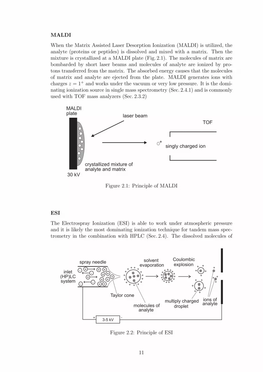
When the Matrix Assisted Laser Desorption Ionization (MALDI) is utilized, theanalyte (proteins or peptides) is dissolved and mixed with a matrix. Then themixture is crystallized at a MALDI plate (Fig. 2.1). The molecules of matrix arebombarded by short laser beams and molecules of analyte are ionized by pro-tons transferred from the matrix. The absorbed energy causes that the moleculesof matrix and analyte are ejected from the plate. MALDI generates ions withcharges z = 1+ and works under the vacuum or very low pressure. It is the domi-nating ionization source in single mass spectrometry (Sec. 2.4.1) and is commonlyused with TOF mass analyzers (Sec. 2.3.2)

Figure 2.1: Principle of MALDI

ESI

The Electrospray Ionization (ESI) is able to work under atmospheric pressureand it is likely the most dominating ionization technique for tandem mass spec-trometry in the combination with HPLC (Sec. 2.4). The dissolved molecules of

Figure 2.2: Principle of ESI

11

analyte are brought through a spray needle into the ionization source (Fig. 2.2).In the ion source, small droplets are arising because of a torrent of nitrogen. Thedroplets carry many charges what is caused by high voltage in the spray needle(3-5 kV). The evaporation of solvent causes that droplets become smaller andthat electrostatic charge densities are higher. When a critical density is reached,a droplet is broken into smaller droplets. This effect is known as the Coulombicexplosion. The Coulombic explosions are repeated until charged ions are releasedfrom droplets.

The released ions are commonly multiply charged what is advantageous fortandem mass spectrometry because both types of fragment ions can be cap-tured when a multiply charged peptide ion (i.e., z ≥ 2+) is being fragmented(Fig. 2.7). In top-down proteomics (Sec. 3.3.2), the ESI enables the identificationof big proteins because high charges cause that these proteins can be detectedby a mass analyzer. For example, assume a mass analyzer having the range ofmeasured m

zvalues up to 3,000 Da. When a protein ion having mass 10,000 Da

carries the charge 4+, it generates the mz

value of 2,501 Da (Eq. 2.1) and thusthe ion is in the range of the mass analyzer. On the other hand, the multiplycharged ions commonly complicate the identification of proteins because a massspectrum contains more peaks having different charges but corresponding to thesame molecule. Thus a deconvolution of spectra must performed which detectsand eliminates these peaks.

2.3.2 Mass Analyzers

A mass analyzer is the main part of a mass spectrometer which separates chargedions by m

zvalues [5] [14] [13]. The analyzers are based on different physical prin-

ciples. We briefly describe several most common types of analyzers.

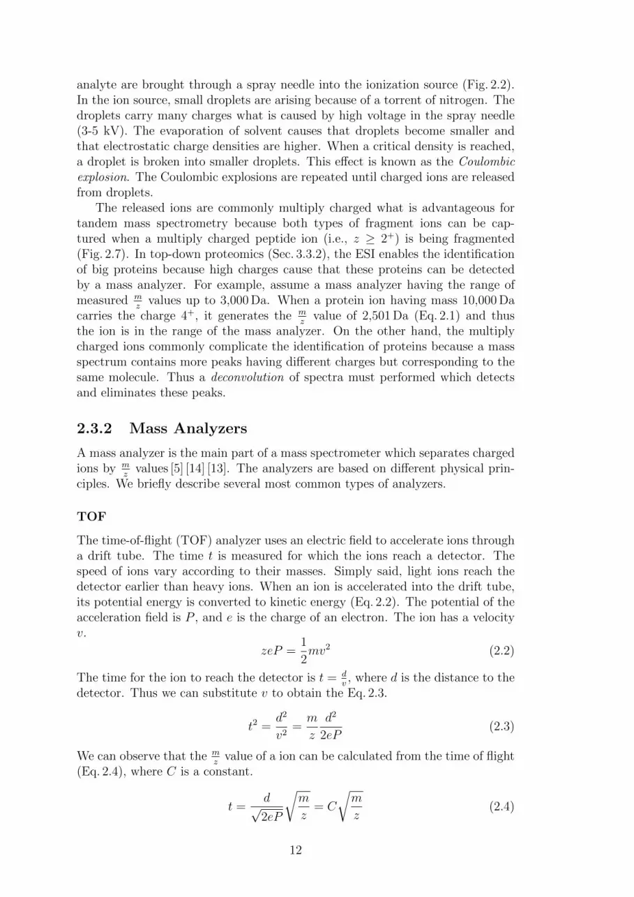
TOF

The time-of-flight (TOF) analyzer uses an electric field to accelerate ions througha drift tube. The time t is measured for which the ions reach a detector. Thespeed of ions vary according to their masses. Simply said, light ions reach thedetector earlier than heavy ions. When an ion is accelerated into the drift tube,its potential energy is converted to kinetic energy (Eq. 2.2). The potential of theacceleration field is P , and e is the charge of an electron. The ion has a velocityv.

zeP =1

2mv2 (2.2)

The time for the ion to reach the detector is t = dv, where d is the distance to the

detector. Thus we can substitute v to obtain the Eq. 2.3.

t2 =d2

v2=m

z

d2

2eP(2.3)

We can observe that the mz

value of a ion can be calculated from the time of flight(Eq. 2.4), where C is a constant.

t =d√2eP

√m

z= C

√m

z(2.4)

12

Quadrupole

Another common mass analyzer is the quadrupole formed from four parallelmetabolic rods which are passed through by ions (Fig. 2.3) [15]. The quadrupoleanalyzer stabilizes paths of ions with a specific m

zvalue using oscillating electri-

cal field while the other ions collide with the rods. By changing the oscillationfrequency, ions with all m

zvalues can be passed through the rods and a mass

spectrum is captured.

Figure 2.3: Principle of quadrupole

Ion Trap

Ion traps are based on the same physical principles like the quadrupole withthe difference that all ions are trapped and only ions with a specific m

zvalue

are ejected sequentially. The basic kinds of ion traps are 3D ion trap, linearion trap and orbitrap [5]. For example, the orbitrap (Fig. 2.4) [16] consists of aninner and an outer electrode which form an electrostatic field. The ions performan orbitally harmonic oscillation along the axis of the electrostatic field. Thefrequency of oscillation is inversely proportional to m

zvalues of ions. Orbitraps

have high accuracies and they are patented by Thermo Scientific [17].

Figure 2.4: Principle of orbitrap

13

2.4 Tandem Mass Spectrometry

The tandem mass spectrometry (MS/MS, MS2) is based on a concatenation oftwo mass analyzers to obtain more accurate results. Let’s assume that a massanalyzer is replaced by a chain mass analyzer 1, collision chamber and massanalyzer 2 (Fig. 2.5).

The first analyzer separates peptide ions by mz

values. In the collision chamber,peptide ions collide with molecules of an inert gas (e.g., argon or xenon) andthe ions are fragmented into peptide fragment ions. The second mass analyzerseparates peptide fragment ions by m

zvalues. Finally, a mass spectrum of peptide

fragment ions is generated for each peptide ion.In principle, any analyzers described in Sec. 2.3.2 can be used while a tan-

dem mass spectrometer can be constructed from different types of analyzers.We can meet with analyzers TOF-TOF, Q-TOF (Quadrupole TOF), Q-Trap(Quadrupole Ion Trap) or QQQ (Quadrupole-Quadrupole-Quadrupole; the sec-ond quadrupole plays the role of a collision chamber), etc. Generally, combina-tions of analyzers impact the accuracy of the machine and its price. Moreover,different instruments are more or less suitable for different experimental setups [5].Even though it is not very common, more than two mass analyzers can be concate-nated to generate MSn spectra where n is the number of concatenated analyzers.

2.4.1 Tandem Mass Spectrum

In shotgun proteomics (Sec. 3.3.1), peptides are subjected to a mass spectrometerafter a chromatographic separation. The peptides are charged and separated bytheir m

zratios. Intensities of peptides are detected and thus a mass spectrum is

obtained. The mass spectrum is a list of peaks where each peak is representedby a pair (m

zratio, intensity) corresponding to a peptide ion.

Figure 2.5: Differences between MS and MS/MS

14

For a small mixture of purified proteins, one spectrum can be generated whereeach peak corresponds to a peptide ion. This kind of mass spectrometry is knownas the single mass spectrometry (MS). The identification of protein sequences iscommonly realized by a comparison of an experimentally taken spectrum with alibrary of known spectra. The method is known as the peptide mass fingerprint-ing [18].

In case of MS/MS, a set of spectra is generated where each spectrum corre-sponds to a peptide ion (Fig. 2.5). In contrast to MS, each peak is represented bythe pair (m

zratio, intensity) corresponding to a peptide fragment ion. The mass

corresponding to the mz

value of a peptide ion being split into fragments is calledthe peptide precursor mass. The tandem mass spectrometer estimates the chargeof the precursor ion from m

zvalues of fragment ions. For each precursor ion, the

retention time is also determined.

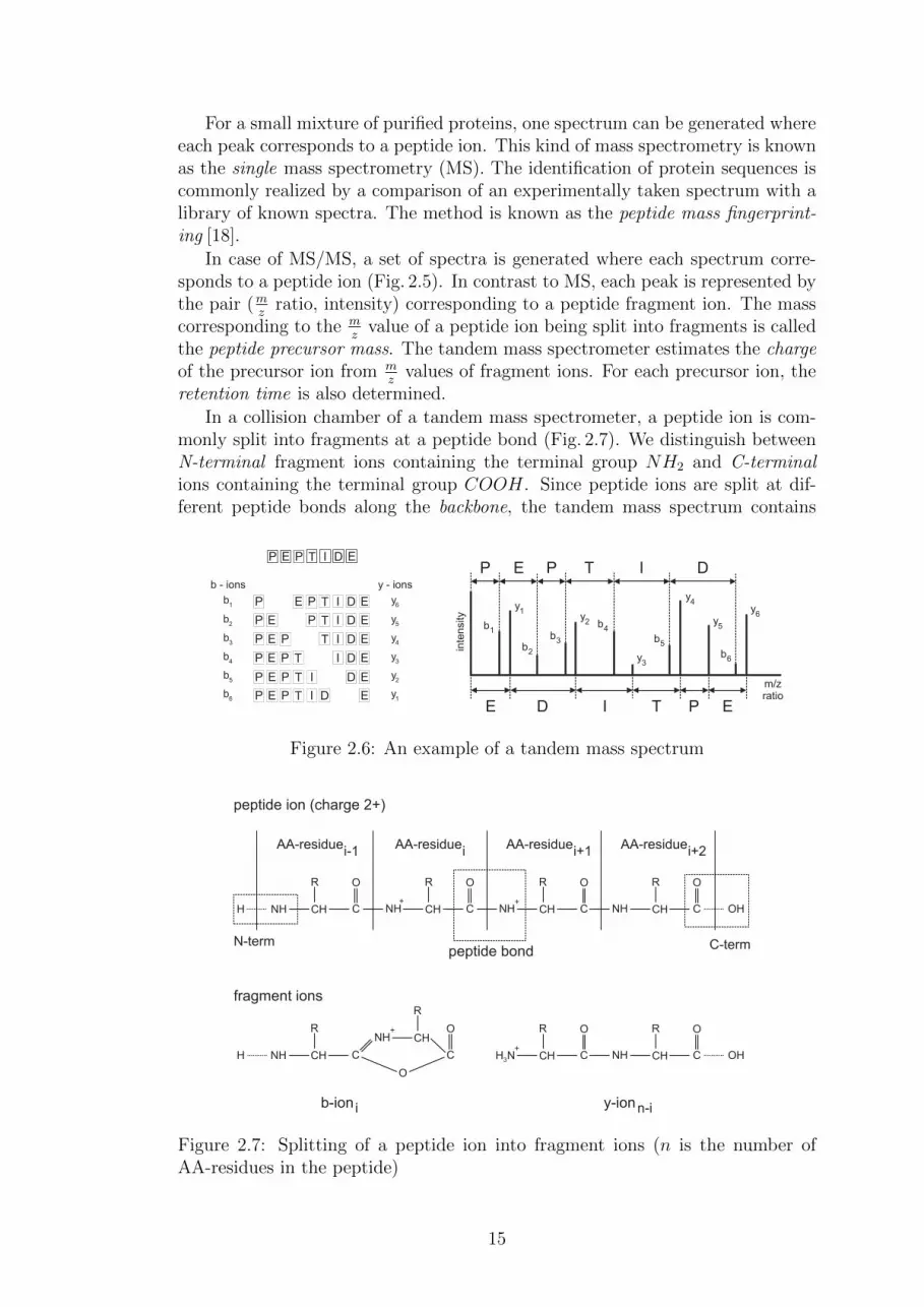
In a collision chamber of a tandem mass spectrometer, a peptide ion is com-monly split into fragments at a peptide bond (Fig. 2.7). We distinguish betweenN-terminal fragment ions containing the terminal group NH2 and C-terminalions containing the terminal group COOH. Since peptide ions are split at dif-ferent peptide bonds along the backbone, the tandem mass spectrum contains

Figure 2.6: An example of a tandem mass spectrum

Figure 2.7: Splitting of a peptide ion into fragment ions (n is the number ofAA-residues in the peptide)

15

Figure 2.8: Other types of fragment ions

complementary fragment ion series with well predictable structure. The mostknown types of fragment ions are b-ions (N-terminal) and y-ions (C-terminal)which are commonly the most important for correct identification of a peptidesequence corresponding to the spectrum (Fig. 2.6). The fragment ions form serieswhere the difference between any two neighboring ions in a series correspondsto a mass of an amino acid residue (AA-residue). However, a peptide ion doesnot have to be split exactly at a peptide bond (Fig. 2.8). In these cases, othertypes of fragment ions can arise like a-ions/c-ions (N-terminal), or x-ions/z-ions(C-terminal). An overview of fragment ions is proposed in Tab. 2.2 [11].

Note that a mass spectrometer detects only charged ions. When the charge ofa peptide ion is at least 2+, it is likely that both types of fragment ions (e.g., b-ion and y-ion) arise from a single peptide ion (Fig. 2.7). This is advantageous foridentification of peptide sequences because of higher completeness of fragment ionseries, and it happens when ESI is used as the ionization technique (Sec. 2.3.1).

The identification of peptide sequences from spectra is often complicated be-cause many fragment ions with unpredictable structure may arise. These frag-

Fragment ion type Composition mz

value Frequency

a Σ +H − CO Mr(Σ)− 27.00216 quite commonb Σ +H Mr(Σ) + 1.00794 commonc Σ +H +NH +H +H Mr(Σ) + 18.0385 rarex Σ +OH + CO Mr(Σ) + 45.01744 rarey Σ +OH +H +H Mr(Σ) + 19.02322 very commonz Σ +OH −NH Mr(Σ) + 1.99266 very raredoubly charged ion ion + H (m

zof ion + 1.00794)/2 very common

triply charged ion ion + H +H (mz

of ion + 2.01588)/3 rare

a∗, b∗, y∗ ion − NH3mz

of ion − 17.03056 w.r.t. ion type

ao, bo, yo ion − H2Omz

of ion − 18.01528 w.r.t. ion type

di ai+1 − part of the sideways chain - -v y − sideways chain - -w z − part of the sideways chain - -

Table 2.2: Fragment ions compositions and mz

values (Σ is the sum of amino acidresidues; Mr(Σ) is the relative molecular mass of amino acid residues)

16

ment ions are regarded as a noise and they form up to 80% of all peaks in aspectrum. The intensity may help to differentiate between more and less signif-icant peaks in a spectrum. However, it is not fully guaranteed that a peak withlow intensity must be a noise one, and the peak with high intensity must be asignal peak. Another problem is the incompleteness of the y-ion and b-ion serieswhich causes a loss of information about the order of amino acids.

2.4.2 Modifications in Tandem Mass Spectra

The identification of peptides is often complicated due to modifications in themass spectra which change masses of amino acids and thus cause shifts of m

z

values (Fig. 6.5) [19]. Modifications can be artificially added to an ”in vitro”sample because they enable more precise analysis (e.g., carbamidomethylation ofcysteine). They can arise during the sample preparation or during the mass analy-sis. A special group of modifications are post-translational modifications (PTMs)which arise during the lifetime of a protein molecule and they give new proper-ties to proteins, make stable conformations of proteins, regulate protein functions,etc. We distinguish two kinds of modifications – fixed and variable. Fixed mod-ifications change all amino acids of the same type, e.g., carbamidomethylationof cysteine. Variable modifications do not have to change all amino acids of thesame type, e.g., oxidation of methionine.

The database UNIMOD gathers discovered protein modifications for the massspectrometry [20]. At the time of writing this thesis, there was about a thousandof known modifications.

17

18

Chapter 3

Algorithms for Processing ofMass Spectra

Because of many inaccuracies in mass spectra, the identification of peptides andproteins is a non-trivial task. In this chapter, the methods used for a preprocess-ing of spectra prior to identification are briefly mentioned. Then the commonlyused approaches for identification and quantification of peptides/proteins, and ap-proaches for a statistical evaluation of results produced by different search enginesare described. Finally, the existing frameworks for complex (HP)LC-MS/MS dataanalysis and management are briefly introduced.

3.1 Preprocessing of Spectra

Raw spectra produced by a spectrometer contain many noise peaks and theyresemble an analog signal, thus a preprocessing of spectra is commonly appliedbefore peptides and proteins can be identified from the spectra [13]. The peakpicking is commonly used to recognize signal peaks (i.e., peaks corresponding toy-ions and b-ions) in raw data and to form peak lists [21] [22]. The peak picking isoften done by vendor software bundled with the machine. However, the processis imperfect in practice and preprocessed peak lists commonly contain tens tohundreds of peaks.

Once the peak lists are formed from raw data, the deisotoping is commonlyused to reduce peaks belonging to the same fragment ions [5]. For example, peakshaving the difference of m

zvalues equals to 1 Da are very likely different isotopic

forms of the same fragment ion and can be represented by one peak.

Before the identification of peptide sequences from the mass spectra, it isadvantageous to utilize advanced methods eliminating noise peaks from massspectra and methods eliminating low-quality and redundant spectra from sets ofspectra. The peak selection heuristics can be used to eliminate noise peaks in thespectra. The spectrum quality filtering eliminates the low-quality spectra, andthe clustering of spectra can be used to remove low-quality spectra and spectracorresponding to the same peptides [23] [24].

19

3.1.1 Peak Selection Heuristics

Two simple heuristics based on a selection of a specified number of peaks withhighest intensities are described below. More sophisticated heuristics for thedenoising of mass spectra were proposed, e.g., in [25] [26].

Peaks with Highest Intensities

The heuristic consists in a selection of p peaks which correspond to peaks withhighest intensities in a query spectrum. The heuristic is not very good in practicebecause the highest intensity peaks are not distributed evenly.

Peaks with Highest Intensities in a Window

A more sophisticated heuristic which splits the range of mz

values in a query massspectrum into windows of specified size w (e.g., w = 50 Da). The p peaks withhighest intensities are selected from each window, e.g., p = 5. Finally, m peakswith highest intensities are chosen from all pre-selected peaks to limit the numberof peaks in the query spectrum (e.g., m = 50).

3.1.2 Spectrum Quality Filtering

The spectrum quality filtering is a way how to remove low-quality spectra fromthe set of spectra produced by a spectrometer [27] [28] [5]. Reasons why low-quality (i.e., uninterpretable) spectra are presented in the query sets of spectraare different. For example, many y-ions and b-ions in a spectrum are missing,the fragmented precursor ion does not have to be a peptide, the peptide may bemodified in a way that is not taken into account by the search engine, or thepeptide is missing in the searched database.

The quality filtering analyzes many parameters of spectra (the number ofpeaks, the number of peaks with relative intensity > 0.1, the intensity differ-ence between top two peaks, the precursor mass, the charge of precursor ion, thenumber of complementary y-ions and b-ions, etc.) and assigns a score to eachspectrum. Only spectra exceeding a score threshold are further analyzed whilethe other spectra are ignored. Since mass spectrometers from different manu-facturers use different physical principles, the significance of parameters differsfrom instrument to instrument. Thus, the score heavily depends on the massspectrometer which was used to capture the spectra [27].

A machine learning technique (i.e., a classifier) is commonly used to makea decision whether a spectrum is a ”good” or ”bad” quality one. The classifierrequires a set of parameters and a training set of spectra for which the qualitiesare known. Once the classifier is trained, it can be used on a testing set. Thecommonly used classifiers are, e.g., Bayesian classifiers, support vector machines,neural networks, quadratic discriminant analysis or decision trees. However, theclassification is not perfect in practice and thus some low-quality spectra maybe classified as ”good” and vice versa. An advantage is that proteins commonlycontain many peptides and thus wrong classifications of some spectra do not haveto significantly impact the identified protein sequences.

20

3.1.3 Spectrum Clustering

The spectrum clustering is another way how to remove low-quality spectra. More-over, since a mass spectrometer generates multiple spectra corresponding to apeptide sequence, the clustering can be also used to eliminate the spectra cor-responding to the same peptide (i.e., sibling spectra) [29] [30] [31] [32] [33]. Anadvantage is that the clustering is independent on the properties of different in-struments because the spectra from different sources are processed the same way,i.e., without the knowledge of significance of particular parameters.

To form the clusters, a pairwise similarity or distance function between thespectra must be defined. Suitable similarity functions are, e.g., the cosine similar-ity (Sec. 6.1.1), the parameterized Hausdorff distance (Sec. 6.1.3) or the sigmoidsimilarity (Eq. 3.3) [29]. In Eq. 3.1, the variables l and p impact the locationand the pivot of the sigmoid curve. In Eq. 3.2 and Eq. 3.3, ai ∈ A and bj ∈ Bare peaks of spectra A and B, dist(ai, bj) computes the absolute m

zdifference of

peaks, I(ai) is the intensity of the peak ai, f(·, ·) and g(·, ·) can be substitutedwith the minimum, maximum or average.

sigm(x) =1

1 + ex−lp

(3.1)

s(A,B) =m∑i=1

n∑j=1

sigm(dist(ai, bj))g(I(ai), I(bj)) (3.2)

S(A,B) =s(A,B)

f(s(A,A), s(B,B))(3.3)

Since the spectra corresponding to a peptide sequence are similar, they forma cluster. When a cluster contains only one spectrum, it is called the singleton.Spectra in singletons can be regarded as noise. However, a set of spectra from aMS/MS run contains also many spectra which form singletons but they can beassigned to peptides. A disadvantage in these cases is that the clustering maycause a loss of some interpretable spectra.

One of the best-known clustering algorithms is the K-means algorithm [34].This algorithm is not very suitable for clustering of mass spectra because wecannot predict the number of clusters K before the clustering [30]. Moreover,its time complexity is O(NKd), where N is the number of spectra in the queryset and d is the dimensionality. The K-means is not suitable for large querysets and high-dimensional data what is exactly the case of mass spectra (usuallycontaining many peaks/dimensions).

A better clustering algorithm for mass spectra is the hierarchical cluster-ing [30] [34]. The hierarchical clustering can be based on complete linkage whereall spectra in a cluster are pairwise similar. When an object in a cluster is similarto at least one other object, the clustering is called single linkage. A disadvan-tage of single linkage is that ”chains” of similar objects may arise among theclusters. On the other hand, the single linkage is less space-consuming becausenot all pairwise distances need to be accessible simultaneously. An intermediatecriterion can be also employed when an object in a cluster must be similar to atleast k other objects. A disadvantage of the hierarchical clustering on large querysets of spectra is the time complexity O(N2). An example of a bit more efficient

21

algorithm is the density clustering (DENCLUE) [35] with the time complexityO(N logN), which is capable of tackling high-dimensional data (what is exactlythe case of mass spectra) and which is robust when dealing with noise data.

Once the spectra are clustered, it is suitable to let one spectrum represent acluster. In general, two ways can be used to obtain a representative spectrum ofa cluster. First, the best (e.g., the most intense) spectrum in the cluster can beselected. Second, a representative spectrum can be obtained by aggregating allspectra in a cluster. In practice, none of these methods has significant advantagesover the other method.

3.2 Identification of Peptides

The annotation of query mass spectra with peptide sequences is often realizedby means of a similarity search in databases of theoretical spectra generatedfrom databases of known protein sequences [36], by means of a similarity searchin libraries of annotated experimental spectra [37] [38] [39] [40] [41] or by de novopeptide sequencing (Sec. 3.2.2).

3.2.1 Similarity Search

When the similarity search in a database of theoretical spectra is employed, aquery spectrum is compared with all theoretical spectra (i.e., a sequential scan ofthe database is performed) using a similarity function [42] [43] [44]. The theoret-ical spectrum with the best score is selected to form a PSM (peptide-spectrummatch). In further sections, we describe the similarities used in state-of-the-arttools SEQUEST, MASCOT MS/MS Ions Search, OMSSA and X!Tandem. Apartfrom these tools, there are also MyriMatch [45], ProteinProspector MS-Tag [46],Morpheus [47] (designed for high-resolution data), and a vast number of othertools [48] [36].

Commonly, the user must select PTMs which will be supported during thesimilarity search in a database. In this case, theoretical spectra of modifiedpeptides are generated and compared with query spectra. However, there are alsoapproaches supporting the blind search of spectra with modifications like spectralconvolution or spectral alignment [49] [19], InsPecT [50] and others [51] [52] [53]. Anovel approach is based on a detection of possible modifications in a query set ofspectra from differences of m

zvalues of precursor ions in a query set [54].

SEQUEST

SEQUEST [55] [5] employs two types of scores – the preliminary score Sp and thecross-correlation score Xcorr. Since Xcorr is computationally more time consumingthan Sp, Sp is used to filter out the theoretical spectra which cannot match aquery spectrum and then Xcorr is computed for remaining theoretical spectra.The preliminary score Sp is defined by Eq. 3.4 where ni is the number of m

zvalues

in a query spectrum which are paired with mz

values in a theoretical spectrum,∑ni

m=0 im is the sum of their intensities and nt is the total number of predictedmz

values in the theoretical spectrum. The division by nt prevents Sp from anexcessive increase for long peptide sequences from which some theoretical spectra

22

are generated. The continuity of a matched ion series is taken into considerationby β. The initial value β = 0 is increased by 0.075 for each matched consecutivefragment ions. ρ = 0 is increased by 0.15 when an immonium ion of the aminoacids histidine, tyrosine, tryptophan, methionine and phenylalanine occurs in thequery spectrum.

Sp =

(ni∑m=0

im

)(nint

)(1 + β) (1 + ρ) , (3.4)

The cross-correlation score Xcorr (Eq. 3.6) is computed using the correlation func-tion Corr(t) (Eq. 3.5) what is the dot product of vectors ~x and ~y where ~y is shiftedby t (by default, t = 75). ~x corresponds to a query spectrum and ~y to a theoreticalspectrum. The vectors contain m

zvalues rounded to integers. The function avg

computes an average of the values in the interval 〈Corr (~x, ~y,−t) , Corr (~x, ~y, t)〉.

Corr(~x, ~y, t) =n∑i=1

~xi~yi+t (3.5)

Xcorr(~x, ~y) = Corr (~x, ~y, 0)− avg (〈Corr (~x, ~y,−t) , Corr (~x, ~y, t)〉) (3.6)

The PSMs with highest Sp and Xcorr are preferred in the output. However,SEQUEST uses following additional values to score PSMs.

• ∆Cn = Xcross1−Xcross2

Xcross1where Xcross1 and Xcross2 are the first and the second

highest correlation values.

• RSp is the rank got in the preliminary scoring by Sp.

• Ions is the number of matched mz

values divided by the number of mz

valuesin the theoretical spectrum.

• dM is the difference between the precursor mass of the query spectrum andprecursor mass of the theoretical spectrum.

Several approaches exist which combine these different components into a singlescore [56] [57]. There are also re-implementations of SEQUEST like Crux [58] andothers [59].

MASCOT

MASCOT [60] is a popular commercial software for identification of peptide se-quences. The details of its probability scoring algorithm for MS/MS spectra werenot published. However, the algorithm for MS/MS spectra is based on the al-gorithm MOWSE (MOlecular Weight SEarch) for single MS spectra. MOWSEis based on a frequency factor matrix F where each row represents an intervalof 100 Da of peptide mass and each column represents an interval of 10 kDa ofprotein mass. A reason for the construction of F is that peptides with low massesoccur more frequently than peptides with high masses. Moreover, the frequenciesof occurrence depend on the lengths of protein sequences from which the peptidesoriginate.

To determine the frequency factors, the protein sequence database is tra-versed while the ”in silico” digestion of protein sequences into peptide sequences

23

is performed. Let F be initialized with zeros. When a peptide sequence is beinggenerated, the corresponding item fi,j in F is incremented. When all peptideshave been generated, items in each column are transformed to the probability oftheir occurrence f ′i,j (Eq. 3.7).

f ′i,j =fi,j∑i

fi,j(3.7)

Then the items in a column are normalized by the maximum value in the col-umn (Eq. 3.8). By the normalization, we get the items mi,j of a new matrix M(MOWSE factor matrix).

mi,j =f ′i,j

maxi

f ′i,j(3.8)

Finally, the score of a protein is determined by Eq. 3.9 where Mprot is the massof a protein, n number of peaks in the spectrum which correspond to peptidesincluded in the protein and the normalization value 50 kDa is used to protect thescore from a large increase for long protein sequences.

score =50, 000

Mprot ×∏n

mi,j

(3.9)

OMSSA

The Open Mass Spectrometry Search Algorithm (OMSSA) calculates the E-valueas a scoring function of PSMs [61]. The calculation of E-value is based on char-acteristics of random matches of m

zvalues between a query and a theoretical

spectrum. The distribution of random matches allows to determine the signifi-cance of a PSM as the probability that the PSM is random. A low probabilityimplies that the PSM is a significant hit. The distribution of matches of m

zvalues

is fit by the Poisson distribution and is calculated separately for different chargestates of fragment ions.

Let’s assume the charge state 1+. Let o be the smallest measured mz

valueand r be the highest measured m

zvalue. When t is the m

zerror tolerance, the

maximum possible number of matches of mz

values is r−o2t

. If m is the neutral

mass of the precursor, we are trying to match h (r−o)m

theoretical mz

values to vexperimental where t is the total number of theoretical m

zvalues. A mean is then

calculated as shown in Eq. 3.10 for the Poisson distribution (Eq. 3.11) where x isthe number of matched m

zvalues between a query and a theoretical spectrum.

µ1 =

(2t

r − o

)(h(r − o)

m

)v =

2thv

m(3.10)

P (x, µ) =µx

x!e−µ (3.11)

When singly and doubly charged fragment ions (i.e., 1+ and 2+) occur inquery spectra and are generated into the theoretical spectra, then two separateranges of m

zvalues are used to calculate the mean. The m

zrange A above m

2which

24

contains only charge 1+ fragment ions and the range B below m2

which containsfragment ions with both charges 1+ and 2+.

In the range A, the number of possible matches isr−m

2

2tand we are trying to

match hr−m

2

mtheoretical m

zvalues to v

r−m2

r−o experimental mz

values. The mean µAis calculated by Eq. 3.12.

µA =

(2t

r − m2

)(h(r − m

2)

m

)(v(r − m

2)

r − o

)=

2thv

m

r − m2

r − o(3.12)

In the range B, the number of possible matches ism2−o

2tand we are trying to

match hm2−om

singly charged fragment ions and hm2−om2

doubly charged fragment

ions to vm2−o

r−o experimental mz

values. The mean µB is calculated by Eq. 3.13.

µB =

(2t

m2− o

)(h(m

2− o)m

+h(m

2− o)m2

)(v(m

2− o)

r − o

)=

6thv

m

m2− o

r − o(3.13)

The resulting mean µ2 for charge states 1+ and 2+ is defined by Eq. 3.14.

µ2 = µA + µB =2thv

m

r +m− 3o

r − o= µ1

r +m− 3o

r − o(3.14)

The OMSSA further increases sensitivity and efficiency using the followingidea – at least one m

zvalue in a theoretical spectrum must match one of the n

peaks with highest intensity in a query spectrum (n = 3, by default). This ideachanges the probability distribution. Let q = n

vbe the probability of a match of

mz

values between a theoretical and query mass spectrum, then the probabilitydistribution P ′ is defined by Eq. 3.15 where the normalization factor Q is definedby Eq. 3.16.

P ′(x, µ) =1

Q(1− (1− q)x)P (x, µ) (3.15)

Q =∑x

(1− (1− q)x)P (x, µ) (3.16)

The probability that a PSM is not random is defined by Eq. 3.17, where yis the number of matches of m

zvalues between the theoretical and query mass

spectrum, and z = 1 or z = 2 depending on the fragment ion series employed.

y−1∑x=0

P ′(x, µz) (3.17)

When the query spectrum is compared against N theoretical spectra, the proba-bility that a PSM is random is defined by Eq. 3.18.

1−

(y−1∑x=0

P ′(x, µz)

)N

(3.18)

Finally, the E-value is calculated using Eq. 3.19. For example, E-value equals to1.0 means that one hit with a score equal to or better than the hit being scoredwould be expected at random when a query spectrum is compared against Ntheoretical spectra.

E(y, µ) = N

1−

(y−1∑x=0

P ′(x, µz)

)N (3.19)

25

X!Tandem

The X!Tandem [62] implements the hyperscoreHS as a similarity between a queryand theoretical mass spectrum (Eq. 3.20). Ii is the intensity of a peak in a queryspectrum and Pi ∈ {0, 1} says whether the peak is predicted in a theoreticalspectrum or not. The hypergeometric distribution of matched m

zvalues is as-

sumed and thus factorials of the number of matched b-ions Nb and the numberof matched y-ions Ny are used.

HS =

(n∑i=0

IiPi

)Nb!Ny! (3.20)

3.2.2 De Novo Peptide Sequencing

Query mass spectra can be interpreted also using graph algorithms (withoutany reference database). Such approaches are called de novo peptide sequenc-ing [63] [64] and they are based primarily on the detection of y-ions and b-ionsseries. A graph is constructed over a query spectrum where a node correspondsto a peak (its m

zvalue) and an edge is ranked with the m

zdifference between two

mz

values corresponding to connected nodes. The paths in the graph with mostedges are selected whose weights best fit the masses of amino acids. In Fig. 3.1a,edges corresponding to amino acids and pairs of amino acids are shown for a peakwith m

zvalue equals to 260. The complete graph created over the query spectrum

is shown in Fig. 3.1b.A drawback is that many paths and thus many peptide sequences can be

assigned to a query spectrum and the number of identified peptide sequences canbe low. This is due to noise peaks, modifications of amino acids, substitutions ofamino acids with equal or similar masses (also substitutions of pairs or triplets ofamino acids), and the fact that some of y-ions or b-ions may never arise. Examplesof amino acids and pairs of amino acids with equal or similar masses are shownin Tab. 3.1. Note that masses are equal when the numbers and types of atomsoccurring in the amino acids are equal.

The completeness of y-ions or b-ions series impacts the number of identifiedpeptides because the difference between two neighboring peaks in one series cor-responds to the mass of an amino acid. For example, when peaks y3 and b4 are

Amino acid(s) Residue mass [Da] Amino Acid(s) Residue mass [Da]L 113.08407 ⇔ I 113.08407Q 128.05858 ↔ K 128.09497

A + G 128.05858 ⇔ Q 128.05858A + G 128.05858 ↔ K 128.09497G + G 114.04294 ↔ N 114.04293G + V 156.08989 ↔ R 156.10112A + D 186.06407 ⇔ E + G 186.06407A + D 186.06407 ↔ W 186.07932E + G 186.06407 ↔ W 186.07932S + V 186.10045 ↔ W 186.07932S + S 174.06406 ↔ C (+5H+3C+O+N) 174.04629

F 147.06842 ↔ M (+O) 147.03539

Table 3.1: Amino acids and pairs of amino acids with equal/similar masses (equalmasses are denoted by ⇔ and similar masses by ↔)

26

Figure 3.1: De novo peptide sequencing

missing in Fig. 2.6, we lose the information about the order of the letters T andI. The letters can be determined from the difference of m

zvalues between peaks

y2 and y4 (or b3 and b5) but more candidate pairs of amino acids having similaraggregate m

zvalues can be selected from 202 possible pairs of amino acids.

Tools based on de novo peptide sequencing are, e.g., PEAKS [65], PepNovo [66]and Lutefisk [67]. Instead of the de novo, a novel idea is to use hybrid approachescombined with the database search. Examples of these approaches are sequencetag methods (Sec. 4.2) or lookup peaks [68].

3.2.3 Statistical Evaluation

The output of an engine for identification of peptides is a list of PSMs. Eventhough there is a score for each PSM, a common problem is a substantial overlapbetween scores between correct and incorrect peptide sequence identifications. Asolution consists in the statistical evaluation of PSMs [69].

The most common significance measure in statistics is the p-value. Let a nullhypothesis be that a PSM is incorrect. For example, a p-value of 0.01 meansthat there is a 1% chance that the null hypothesis is correct, i.e., that the PSMis incorrect. To determine the p-value of a PSM, we have to know which PSMsare correct and which are incorrect. A widely accepted technique is to apply atarget-decoy approach [69] [70]. The protein sequences in the database are markedas target. The decoy sequences are generated by reversing or shuffling of targetsequences. Another way is to generate random sequences using a Markov modelwith parameters derived from target sequences. Finally, the decoy sequences areappended to target sequences.

The query spectra are searched against the database of target and decoysequences. In an ideal case, there should not be an overlap between target anddecoy peptide sequences. The p-value is the percentage of decoy peptide sequenceswhich receive a score x or lower (we assume a distance as a scoring function thusthe lower score is better). For example, when the score below a threshold t ≤ 0.3is assigned to 30 decoy PSMs and 6000 target PSMs, the p-value is 0.005.

A disadvantage of the p-value is a lack of the multiple testing correction. Let’sassume a query set containing 30,000 spectra. Ideally, the list generated by anengine should contain 30,000 PSMs. However, for the p-value less or equals to

27

0.005, 0.005× 30,000 = 150 PSMs are obtained at random. A widely acceptedmethod for multiple testing correction is the false discovery rate FDR. For a givenscore threshold t, the FDR is a ratio of the number of decoy PSMs to the numberof all PSMs having score equals to or better than t (Eq. 3.21).

FDR =#decoy

#decoy + #target(3.21)

However, an alternative calculation of FDR was suggested in [69] where FDR iscalculated as the ratio of the number of decoy PSMs to the number of targetPSMs (Eq. 3.22).

FDR =#decoy

#target(3.22)

Since FDR is a property of a set of PSMs, the q-value is used as a property ofa single PSM. The q-value is defined as the minimum FDR threshold at which agiven PSM is accepted as correct [69].

Let’s assume a pair-wise distance function d. When a query set of spectrais compared against theoretical spectra, a set of PSMs is obtained where di isthe distance between ith spectrum in the query set and its nearest theoreticalspectrum. Let t be a threshold of d and S be a set of PSMs such that S ={PSMi ∈ S, di ≤ t}. Now assume the following example – when t = 0.6 and Scontains 5 decoy and 500 target PSMs, the FDR = 0.01; when t = 0.65 and Scontains 5 decoy and 1000 target PSMs, the FDR = 0.005. Since the numbersof decoy PSMs are equal in both cases, the q-value is 0.005 for target PSMs.

An alternative to the q-value is the posterior error probability PEP what isthe probability that a single PSM is incorrect [71]. The difference between FDRand PEP is shown in Fig. 3.2, where A and B are areas of the distributions forcorrect and incorrect PSMs. While FDR is the ratio of the number of incorrectPSMs with score ≤ t (B) to the total number of PSMs with score ≤ t (A + B),the PEP is the ratio of corresponding heights of the distribution, i.e., the numberb of incorrect PSMs with score equal to t is divided by the total number of PSMswith score equal to t (a+ b).

Commonly, statistical or machine learning approaches are used to estimatethe PEP. The probability model is learned from a set of annotated training dataand used to predict PEPs of all future test data. When this approach is used,the PEP of a PSM having score t is always the same, regardless the query setin which the PSM occurs. On the other hand, the q-value and FDR are alwaysdependent on the query set.

The q-value and PEP are useful in different scenarios. When proteins ex-pressed in a certain type of cells are investigated (i.e., a group of PSMs is an-alyzed), the q-value is more suitable measure. When the presence of a specificpeptide or protein is analyzed, the PEP is more relevant.

3.2.4 Probabilistic Consensus Scoring

It has been shown that different search engines like X!Tandem, OMSSA or MAS-COT assign different peptide sequences to query spectra in many cases. Anotherwords, the first sequence in the list of peptide sequences assigned to a queryspectrum does not have to correspond to the correct sequence, or the correct

28

Figure 3.2: Distributions of scores for correct and incorrect PSMs

sequence is missing in the list. The overlap of identified peptide sequences amongthe engines is usually poor.

When only peptide sequences identified by more than one engine are taken in-to account, the reliability of identification increases but the sensitivity decreases.When peptide sequences identified by at least one engine are chosen, the sensitiv-ity of identification increases but the reliability is lower. To address this problem,several methods have been developed which combine scores from different enginesinto one score. Probabilistic consensus scoring is a framework which combinesscores from different engines into a joint consensus score [72]. The algorithmworks in three steps as follows.

1. The mixture modeling of score distributions is applied to convert scores ofpeptide sequences from different search engines into probabilities. The dis-tribution of scores is modeled by a two-component mixture model, where adensity of incorrectly assigned sequences is modeled as a density of a Gum-bel distribution and a density of correctly assigned sequences is modeled asa density of Gaussian distribution.

2. For each peptide sequence p missing in the output of an engine e, the corre-sponding probability score is estimated. The peptide sequence p′ the mostsimilar to p is selected from the output of the engine e. The probabili-ty score of p′ is assigned to p and weighted by the similarity to p′. Thesimilarity between peptide sequences is computed using global alignmentcomputed by Needleman-Wunsch algorithm [49].

3. A joint consensus score is calculated for each peptide sequence from theprobabilities.

When three engines are used, the consensus score is computed as shown inEq. 3.23. Let s1 be a probability score of a peptide sequence p matched by enginee1. Since the most similar peptide sequence to p in the result set of e1 is p itself,the weight of s1 is equal to 1. s2 and s3 are probabilities of the most similarpeptide sequences to p in the result sets of engines e2 and e3. The weights α andβ are similarities between p and the most similar peptide sequences in the resultsets of e2 and e3.

consensus score =s1 + αs2 + βs3

(1 + α + β)2(3.23)

29

Other methods based on the combining of scores from multiple engines are,e.g., Scaffold [73], MSblender [74], iProphet [75] or PepArML[76].

3.3 Identification of Proteins

The identification of protein sequences by MS/MS can be performed by two dif-ferent approaches – by bottom-up or top-down proteomics [77]. Below, we brieflydescribe these two approaches.

3.3.1 Bottom-up Proteomics

The bottom-up proteomics (or shotgun proteomics) can be used for identificationof small mixtures of purified proteins (up to tens of proteins) as well as for iden-tification of complex protein mixtures (several thousands of proteins) obtainedby cell lysis. In the bottom-up proteomics, proteins are enzymatically digestedinto peptides which are analyzed by LC-MS/MS. The mass spectra are then com-pared with a database of theoretical peptide spectra generated from a databaseof protein sequences or analyzed by de novo to determine PSMs. Finally, thePSMs are mapped into protein sequences.

Figure 3.3: Basic scenarios of mapping peptides into proteins

A drawback is that identified peptide sequences commonly do not cover wholeprotein sequences. Some peptides are too short or too long for detection. Howev-er, a major problem are the ionization techniques (Sec. 2.3.1), because peptidesmust compete for available charges. Properties of peptides and ionization tech-niques determine whether the peptides are charged or not.

Other problems are caused by non-unique peptides which originate from manyproteins. Moreover, the uniqueness of peptides depends on the database of proteinsequences from which the peptide sequences are generated, and on the length ofpeptide sequences because longer sequences become more likely unique.

When protein sequences corresponding to a set of PSMs are being deter-mined, we can look for a maximal or for a minimal explanatory set of proteinsequences [5]. The maximal explanatory set can be easily determined by map-ping all PSMs into proteins sequences. Since a protein sequence can be identifiedby a single PSM, some protein sequences can be identified incorrectly by incor-rect PSMs. Moreover, some proteins can be identified even though they are notpresented in the analyzed mixture of proteins. The Fig. 3.3 shows possible sce-narios when peptide sequences are being mapped into protein sequences. Distinctproteins do not share any peptide. Differentiable proteins can be distinguishedby at least one peptide. Indistinguishable proteins share all detected peptides.Subset protein contains only peptides which are occurring in another protein.Subsumable protein contains only peptides which are occurring in other proteins.

30

The maximal explanatory set can contain indistinguishable, subset or subsumableproteins even though they are not present in the analyzed mixture [78].

To address this problem, the minimal explanatory set of proteins can be deter-mined using the maximum parsimony inference. The idea is to find the smallestset of protein sequences which explain all observed peptides. Thus all indis-tinguishable, subset and subsumable protein sequences are not included in theexplanatory set. However, it may not be necessarily the truth that protein se-quences, which are not included in the explanatory set, are not presented inthe analyzed mixture. Thus sets of proteins sharing one or more peptides arecommonly reported as protein ambiguity groups.

Informations about the quantities of peptides (Sec. 3.4) can be also used toprove the presence of a specific protein in the mixture. Let’s assume that aprotein contains only one peptide which is also included in another protein havingassigned more peptides. When the abundance of this peptide is low, the proteinmatch of the former protein is likely random.

Protein Probability Estimates

ProteinProphet is a tool which estimates the probability that a protein sequence iscorrectly identified or not [79] [36]. The algorithm is based on the maximum par-simony while protein ambiguity groups are reported. To estimate that a proteinis correctly identified, peptide probability estimates (PPEs) are utilized. PPEsof PSMs are computed by PeptideProphet [56] which converts scores of searchengines into probabilities (say, 1-PEP ; Sec. 3.2.3).

The idea of PPEs is to use Bayes’ Law to compute the probability p(+|D) todetermine whether a PSM is correct or not (Eq. 3.24). For each PSM, the observeddata D includes a score or a set of scores generated by some engine(s). p(D|+)and p(D|−) are the probabilities that a PSM is among correctly or incorrectlyassigned PSMs, what is determined from the score or the set of scores included inD. The prior probabilities p(+) and p(−) are the overall proportions of correctand incorrect PSMs in the dataset. To compute the probability p(+|D) usingEq. 3.24, a probability distribution of scores generated by the engine(s) must bederived from training data with peptide assignments of known validity or learnedfrom the data itself [56].

p(+|D) =p(D|+)p(+)

p(D|+)p(+) + p(D|−)p(−)(3.24)

Let’s assume that all peptides are unique. The probability P , that a proteinidentification is correct, can be computed using a sum of probabilities of correctpeptide identifications (Eq. 3.25), where p(+|Di) is a probability of correct peptideidentification of a peptide i.

P = 1−∏i

(1− p(+|Di)) (3.25)

However, we have to consider that the same peptide sequences can be identifiedby many spectra. The modification of P is shown in Eq. 3.26, where p(+|Dj

i ) isthe probability that a peptide identification of a peptide i based on a spectrumj is correct.

31

P = 1−∏i

∏j

(1− p(+|Dji )) (3.26)

A problem with Eq. 3.26 is that PSMs are not independent. When a desiredpeptide sequence is not presented in the database (e.g., because spectra corre-sponding to a peptide are modified by a PTM), the spectra corresponding tothis peptide sequence will likely hit the same but incorrect peptide sequence. Asimple solution how to deal with this issue is to include each peptide just once,i.e., from the set of PSMs corresponding to a peptide, only one PSM with thehighest probability being correct is used (Eq. 3.27).

P = 1−∏i

(1−maxjp(+|Dj

i )) (3.27)

Correct PSMs tend to group into a small set of correct proteins while incorrectPSMs are spread over the entire protein sequence database. ProteinProphet usesthe number of sibling peptides (NSP) to correct the probabilities of PSMs toaddress this problem. In this notion, the sibling peptides are those matching thesame protein. Peptide identifications with high NSPs are more trustworthy thanidentifications with low NSPs. NSPi for the peptide i is the sum of probabilitiesof correct PSMs of other peptides matching the same protein (Eq. 3.28). m isanother distinct peptide matching the same protein and p(+|Dm) is the maximumprobability from all PSMs corresponding to the peptide m.

NSPi =∑

{m|m6=i}

p(+|Dm) (3.28)

Now, we can refine PPEs as shown in Eq. 3.29, where p(NSP |+) and p(NSP |−)are the probabilities of having a particular NSP for correct and incorrect PSMs.p(+|D) and p(−|D) are the uncorrected probabilities for the PSMs being correctand incorrect.

p(+|D,NSP ) =p(+|D)p(NSP |+)

p(+|D)p(NSP |+) + p(−|D)p(NSP |−)(3.29)

p(NSP |+) and p(NSP |−) are computed for the whole dataset (Eq. 3.30), whereN is the total number of peptide assignments and p(+) is the prior probabilityof a peptide identification being correct. NSP values are computed by binning.The probability that a correct peptide assignment has the NSP value in the bink is computed as a sum over peptides with NSP value in the bin k. p(+) canbe computed as a sum over all peptides in the dataset (Eq. 3.31). The NSPdistribution for incorrect peptide assignments is computed analogically.

p(NSP |+) =1

Np(+)

∑{i|NSPi∈k}

p(+|Di, NSPi) (3.30)

p(+) =1

N

∑i

p(+|Di, NSPi) (3.31)

ProteinProphet considers also degenerate peptides, i.e., peptides which canbe found in many protein sequences forming protein ambiguity groups. When a

32

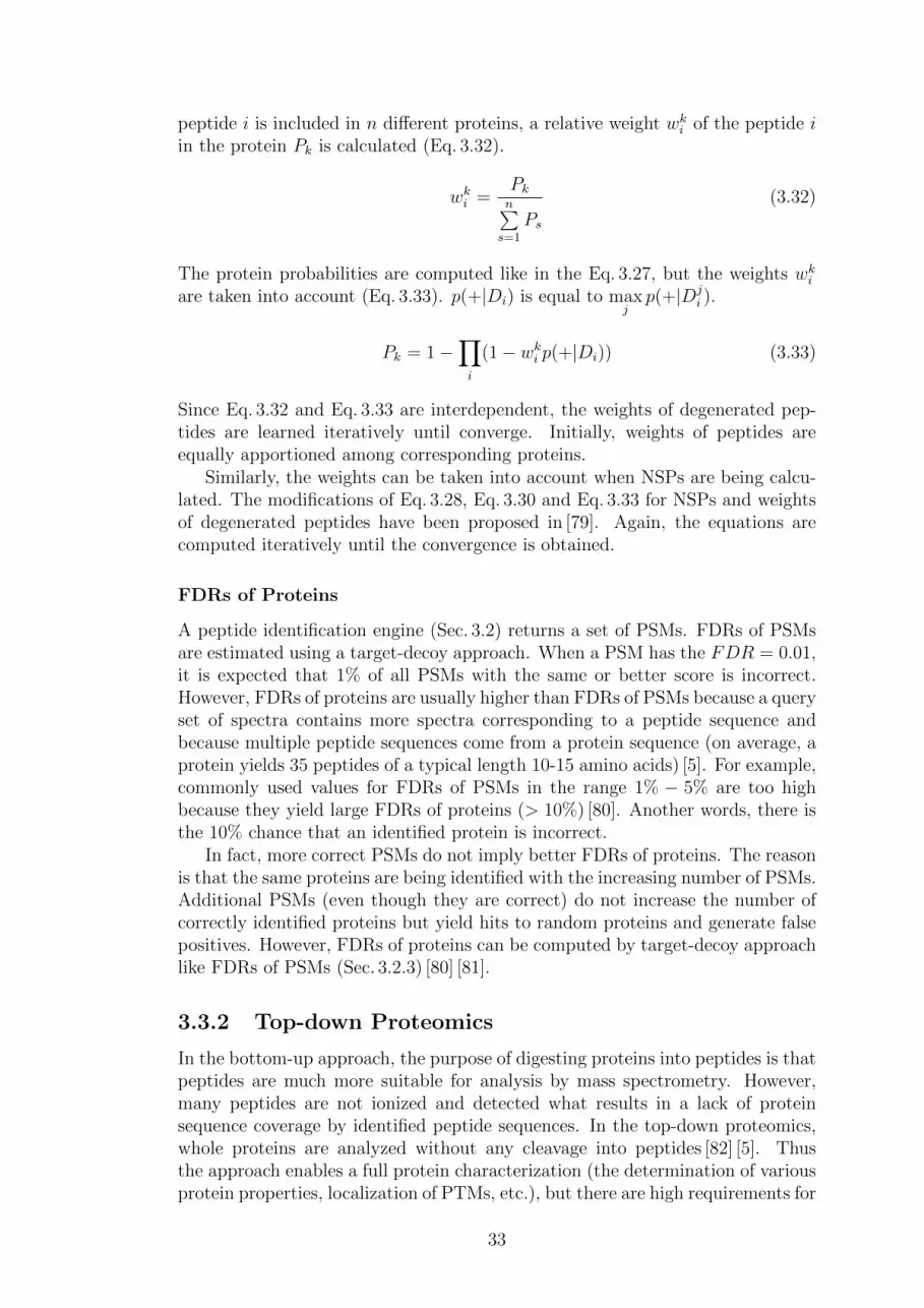
peptide i is included in n different proteins, a relative weight wki of the peptide iin the protein Pk is calculated (Eq. 3.32).

wki =Pkn∑s=1

Ps

(3.32)

The protein probabilities are computed like in the Eq. 3.27, but the weights wkiare taken into account (Eq. 3.33). p(+|Di) is equal to max

jp(+|Dj

i ).

Pk = 1−∏i

(1− wki p(+|Di)) (3.33)

Since Eq. 3.32 and Eq. 3.33 are interdependent, the weights of degenerated pep-tides are learned iteratively until converge. Initially, weights of peptides areequally apportioned among corresponding proteins.

Similarly, the weights can be taken into account when NSPs are being calcu-lated. The modifications of Eq. 3.28, Eq. 3.30 and Eq. 3.33 for NSPs and weightsof degenerated peptides have been proposed in [79]. Again, the equations arecomputed iteratively until the convergence is obtained.

FDRs of Proteins

A peptide identification engine (Sec. 3.2) returns a set of PSMs. FDRs of PSMsare estimated using a target-decoy approach. When a PSM has the FDR = 0.01,it is expected that 1% of all PSMs with the same or better score is incorrect.However, FDRs of proteins are usually higher than FDRs of PSMs because a queryset of spectra contains more spectra corresponding to a peptide sequence andbecause multiple peptide sequences come from a protein sequence (on average, aprotein yields 35 peptides of a typical length 10-15 amino acids) [5]. For example,commonly used values for FDRs of PSMs in the range 1% − 5% are too highbecause they yield large FDRs of proteins (> 10%) [80]. Another words, there isthe 10% chance that an identified protein is incorrect.

In fact, more correct PSMs do not imply better FDRs of proteins. The reasonis that the same proteins are being identified with the increasing number of PSMs.Additional PSMs (even though they are correct) do not increase the number ofcorrectly identified proteins but yield hits to random proteins and generate falsepositives. However, FDRs of proteins can be computed by target-decoy approachlike FDRs of PSMs (Sec. 3.2.3) [80] [81].

3.3.2 Top-down Proteomics

In the bottom-up approach, the purpose of digesting proteins into peptides is thatpeptides are much more suitable for analysis by mass spectrometry. However,many peptides are not ionized and detected what results in a lack of proteinsequence coverage by identified peptide sequences. In the top-down proteomics,whole proteins are analyzed without any cleavage into peptides [82] [5]. Thusthe approach enables a full protein characterization (the determination of variousprotein properties, localization of PTMs, etc.), but there are high requirements for

33

the resolution and accuracy of spectrometers. Moreover, prices and maintenancecosts of such machines are high.

The proteins are separated and ionized commonly by ESI (Sec. 2.3.1). Becauseof ESI, protein ions are usually highly charged (say, up to charge 30+). Then theprotein ions are fragmented into multiply charged b-ions and y-ions. A drawbackof this approach is that a deconvolution of spectra must be performed. Sincethere are many peaks corresponding the same b-ion or y-ion having differentcharges, these peaks must be detected and removed. For example, for a proteinhaving mass 20,000 Da, the peaks having m

zvalues 667, 691 and 715 can occur

for fragment ions having charges 30+, 29+ and 28+ (Eq. 2.1). A drawback is thata reasonable deconvolution is possible only for small mixtures of proteins whatlimits the high-throughput capabilities of top-down proteomics.

After the deconvolution, the spectra can be analyzed by database search al-gorithms, de novo or sequence tag methods (Sec. 4.2) [82]. An advantage of thetop-down approach is that it yields better characterization of proteins modifiedby PTMs. Since peaks corresponding to either modified or unmodified fragmentions can be found in a spectrum after its deconvolution, a localization of PTMsin a protein sequence is more straightforward than in the bottom-up approach.

3.4 Quantification of Peptides and Proteins

The quantification of peptides and proteins is an important task in computation-al proteomics [83] [84] [85] [86]. The quantification is either relative or absolute.Let’s have n samples, each containing a set of components (peptides or proteins).The task is to determine the abundance of components across the samples. Whenthe relative quantification is utilized, the relative changes of intensities of peptideions are calculated. In case of absolute quantification, a reference additive ofknown concentration must be available for every analyte to determine the abun-dance of components from their intensities, thus the absolute quantification ismore difficult and less common than relative. The techniques for the relativequantification can be split into label-based and label-free methods. However, anyof these methods can be also adopted for the absolute quantification.

3.4.1 Label-based Quantification

Label-based quantification (LBQ) methods are based on labeling of selectedamino acids using stable isotopes of these amino acids. LBQ techniques canbe split into chemical labeling performed ”in vitro” and metabolic labeling per-formed ”in vivo”. Examples of chemical labeling are ICAT (isotope-coded affinitytags) [87], iTRAQ (isobaric tags for relative and absolute quantification) [88] orlabeling by heavy isotopes of oxygen 16O/18O [89]. Examples of metabolic la-beling are stable isotope labeling by amino acids in cell culture (SILAC) [90] orlabeling by heavy isotopes of nitrogen 14N/15N.

An example of labeling by SILAC is shown in Fig. 3.4 [91]. Two samples areanalyzed, where the first sample contains the ”light” arginine and the secondcontains the ”heavy” arginine. Another words, cell cultures in the samples are”feeded” by different forms of arginine. The light arginine contains carbons 12C6,while its heavy form contains carbons 13C6. Since the arginine has six carbons, the

34

mass difference between its light and heavy form is 6 Da. The samples are mixedbefore LC-MS/MS analysis. After the analysis, the query set contains spectra ofheavy and light peptide ions whose precursor masses and peaks corresponding tofragment ions are shifted by 6 Da. From the differences of intensities of shiftedpeaks, the abundances of peptides in the samples are calculated. Instead ofarginine, the lysine can be used as well. The utilization of these amino acids isadvantageous because the trypsin digests proteins into peptides after these twoamino acids. In an ideal case, each peptide contains at most one arginine orlysine. The quantification of peptides/proteins from SILAC data is supported,e.g., by MaxQuant [92] and OpenMS [93].

Figure 3.4: Principle of labeling

3.4.2 Label-free Quantification

The label-free quantification (LFQ) does not use any kind of labeling and thusthe samples must be analyzed separately, i.e., a LC-MS/MS run is performed foreach sample [94] [95]. An overview of tools for label-free quantification is proposedin [96].

The mz

values and retention times of peptide precursor ions obtained in a runform a map. An example of a map is shown in Fig. 3.6. Note that not all precursorions in the map were analyzed by the spectrometer to obtain the fragmentationspectra. Precursor ions within tight intervals of m

zvalues and retention times in

the map commonly correspond to a peptide. Such a two-dimensional region inthe map corresponding to a single charge variant of a peptide is called a feature.The feature has several attributes – an average m

zratio, a centroid retention time,

an intensity, and a quality value.The basic principle of LFQ can be summarized as follows:

1. Find features in all maps.

2. Align maps.

3. Link corresponding features.

4. Identify features.

5. Quantify features.

35

Since more maps are generated from more LC-MS/MS runs, the first step isto determine features in all the maps. In the second step, the maps must bealigned because retention times between any two maps can be shifted. Once thefeatures are determined and maps are aligned, corresponding features across themaps are linked. In the fourth step, the identification of peptides from spectracorresponding to features is performed by peptide identification engines describedin Sec. 3.2.

Instead of the fourth step, the identification of peptides can be also performedin the first step – independently and in parallel to the feature finding. Thisslows down the algorithm because many more spectra must be analyzed by apeptide identification engine. On the other hand, the sensitivity of quantificationincreases because some peptides can be lost when features are determined withoutthe knowledge of peptides corresponding to the features.

Finally, the peptides/proteins occurring in the samples are quantified. Thiscan be done by computing differences in intensities of features across the maps.The spectral counting is another way how to quantify the results, where thespectra corresponding to a peptide/protein are summed [97].

Since the feature finding and maps alignment are crucial parts of LFQ, theyare briefly described below.

Feature Detection

The identification of a feature corresponds to the detection of all peaks of precur-sor ions in the map belonging to a peptide [86] [98]. The main idea is to determinesuspicious regions in the map and to fit two-dimensional models to that regions.The algorithm for feature finding can be summarized as follows:

1. Seeding. Peaks with highest intensities in the map are selected as ”seeds”,because they are very likely in features.

2. Extension. The peaks around the seeds are conservatively appended tothe seeds and create regions. A region grows in all directions simultaneouslywhile the points in its neighborhood with highest priorities are appended.The priority cannot be represented directly by the peak intensity becauseit must be smaller with increasing distance from the region and missingpeaks must be also considered. When a point is appended to a region, aboundary of the region is updated. The extension of the region stops whenthe priority of neighboring data points is below a certain threshold.

3. Modeling. A two-dimensional statistical model is fit to each region to forma peptide feature. The model is based on the Gaussian elution profile [99] inthe dimension of the retention time and on the averagine isotope model [100]in the dimension of m

zvalues.

4. Adjusting. The peaks, which do not fit the model of its feature, areremoved. A variant of the priority from the extension phase is used for thispurpose but the statistical model is also taken into account. The steps 3and 4 are repeated, until the models of features converge.

36

Maps Alignment

The optimal alignment between any two maps can be computed by a linear align-ment algorithm under the assumption that shifts of retention times between tworuns are linear [101]. The alignment of u maps can be performed simply by ap-plying u− 1 linear alignments onto one reference map.

The reference (or model) map is commonly the map with the most features.Let scene be a map which is being aligned with the model. The goal is to deter-mine an affine transformation t(x) = ax+b, which maps the points {s1, s2, . . . , sk}of a scene onto their nearest neighbors {m1,m2, . . . ,ml} in the model. a is thescale and b is the shift of the mapping. This problem is also known as the su-perposition. The parameters a and b can be recovered from the data using thealgorithm called pose clustering. The optimal affine transformation t is unique-ly determined when each map contains only two points. Then a and b can becomputed using the equations a = m1−m2

s1−s2 and b = s1m2−s2m1

s1−s2 , where t(s1) = m1,t(s2) = m2 and s1 6= s2.

For large sets of points {s1, s2, . . . , sk} and {m1,m2, . . . ,ml}, the system ofequations is overdetermined and thus approximate values for a and b must becomputed. The best approximate solution is such that maps most points fromthe scene to their nearest neighbors in the model. Another problem is thatassignments of matching points between scene and model are not considered bythe algorithm. Both problems are solved by a voting scheme. Let assume a setof pairs of parameters a and b where each pair corresponds to pairs of objects(s1,m1) and (s2,m2), we obtain a set T of affine transformations t1, t2, . . . , tn.When the set T is applied on a set of pairs of objects (s′1,m

′1) and (s′2,m

′2), a

”correct” transformation generates clusters of points while other transformationsgenerate randomly distributed points over the plane (a, b). The centroid of acluster is then used to estimate the optimal transformation.

The voting scheme can iterate over all possible pairs of objects (s′1,m′1) and

(s′2,m′2). However, the time complexity of the algorithm is O(k2l2) what leads to

a very slow solution for typical values of k, l > 1000. Fortunately, the typical mz

error tolerance ξ is small ξ ∈ 〈0.5, 2〉 Da, thus ranges of mz

values of comparedpairs of objects are tight and the algorithm is efficient.

In practice, shifts of retention times between two maps do not have to belinear, thus an alternative linear alignment and its extension to a non-linearalignment have been proposed. The idea of non-linear alignment is to computethe linear alignment using the pose clustering and then compute more accuratelocal alignments between small windows of points using local linear regressionmethod (loess) [102].

3.5 Frameworks for Shotgun Proteomics

The processing of data from shotgun proteomics is a non-trivial task which re-quires many steps like preprocessing of spectra, identification of peptides, statis-tical evaluation of results, detection of features, quantification of peptides andproteins, etc. To address this problem, a couple of software solutions has beenproposed which separate each step into a specialized tool and which allow a cre-ation of complex pipelines from these tools. Since standardized formats of input

37

and output files of the tools are used, the tools can be easily interconnected withrespect to users’ requirements.

For example, the Trans-Proteomic Pipeline (TPP) is a freely available open-source proteomics data analysis pipeline developed at the Institute for SystemsBiology at the Seattle Proteome Center [103]. Another framework is The OpenMSProteomics Pipeline (TOPP) [104] based on OpenMS [93]. OpenMS [93] is anopen-source C++ library for LC-MS/MS data management and analyses. Sincethe application SimTandem proposed in Sec. 8.2 has been designed for TOPP, webriefly describe this framework.

The TOPP contains a set of tools which can be combined into pipelines. Thetools cover a wide range of areas, for example, there are tools for file formatconversions, generating of decoy databases, preprocessing of spectra, digestingof protein sequences into peptide sequences, retention time prediction, wrappingof the commonly used tools for peptide identification (e.g., MASCOT, OMSSA,X!Tandem), statistical evaluation of PSMs, label-free and label-based quantifica-tion and many others. One of the tools is also The OpenMS Proteomics PipelineASsistant (TOPPAS) what is a GUI for a graphical composition of pipelines ofvarious tools [105]. An example of a simple peptide identification pipeline withstatistical evaluation of results is shown in Fig. 8.6.

A more complex pipeline for label-free quantification is shown in Fig. 3.5. In-put files in the node 1 are query sets of mass spectra (*.mzML). Input file in thenode 4 is the database of protein sequences (*.fasta). The pipeline uses wrappersfor three different peptide identification tools MASCOTAdapterOnline, XTande-mAdapter and OMSSAAdapter. The lists of PSMs produced by the engines areconverted to posterior error probabilities (Sec. 3.2.3). Then IDMerger mergeslists of PSMs and ConsensusID computes consensus scores. PeptideIndexer an-notates for each search result whether it is a target or a decoy hit, FalseDiscov-eryRate computes q-values and IDFilter selects only those PSMs with q-valuesless or equal the specified tolerance. In parallel to the identification part of theworkflow, FeatureFinderCentroided detects features in the input maps. IDMap-per assigns peptide identifications to the features. When all maps are collected,MapAlignerPoseClustering aligns the maps and FeatureLinkerUnlabeled groupscorresponding features in multiple runs of label-free experiments. Finally, peptideand protein abundances are computed from annotated maps by ProteinQuantifi-er.

Another graphical tool is TOPPView [106], which enables visualizations of 2Dand 3D maps of mass spectra query sets, visualizations of fragmentation spec-tra of peptides, annotations of query sets (*.mzML) with identified sequences(*.idXML), etc. The 2D map of the E. coli query set described in Sec. 7.2.4is shown in Fig. 3.6, where the axes represent m

zvalues of peptide precursor

ions and their retention times. Each horizontal ”smudge” corresponds to a fea-ture/peptide. The 3D map of the same query set is shown in Fig. 3.7, where thethird axis represents intensities of peptide precursor ions.

38

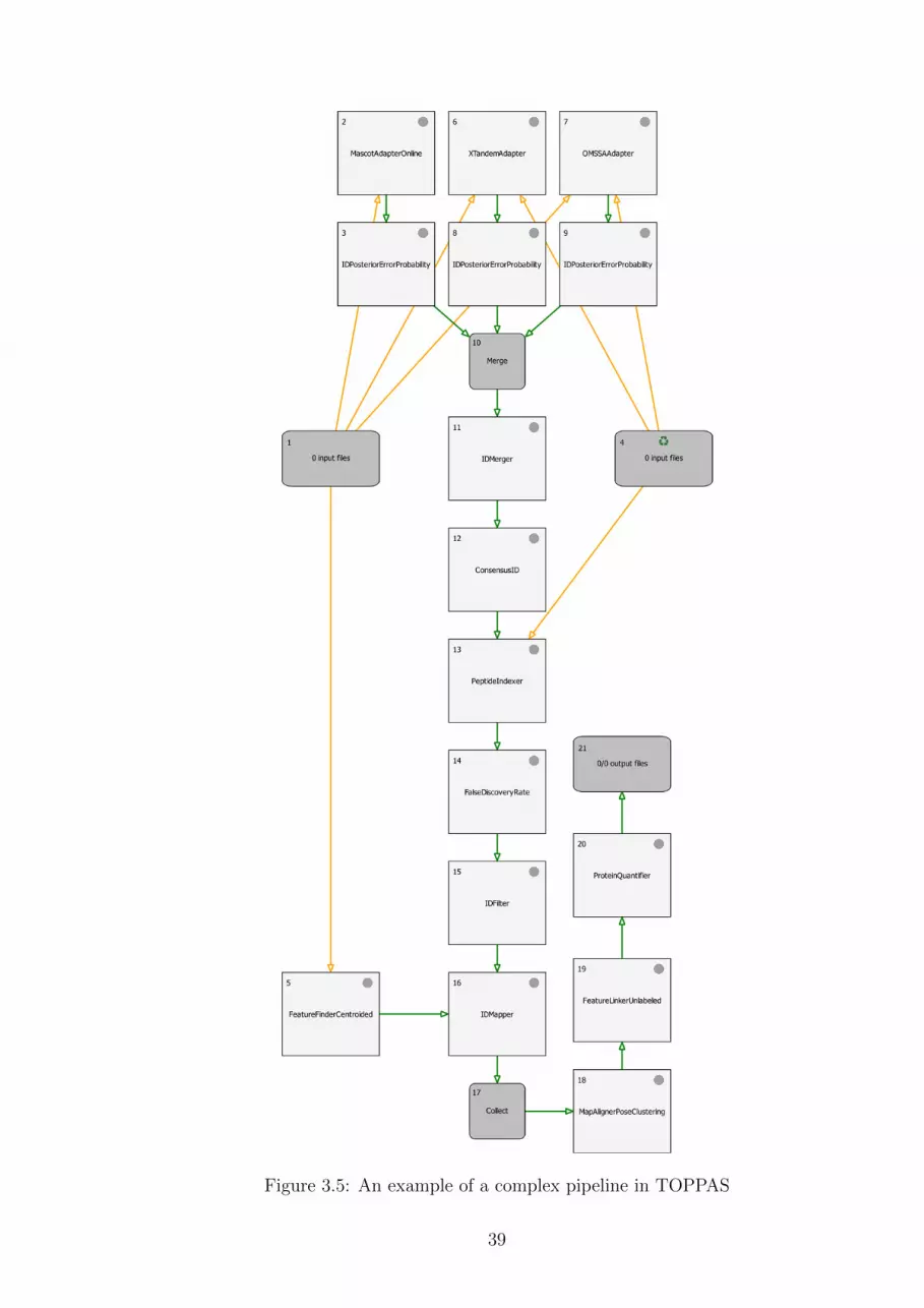
Figure 3.5: An example of a complex pipeline in TOPPAS

39

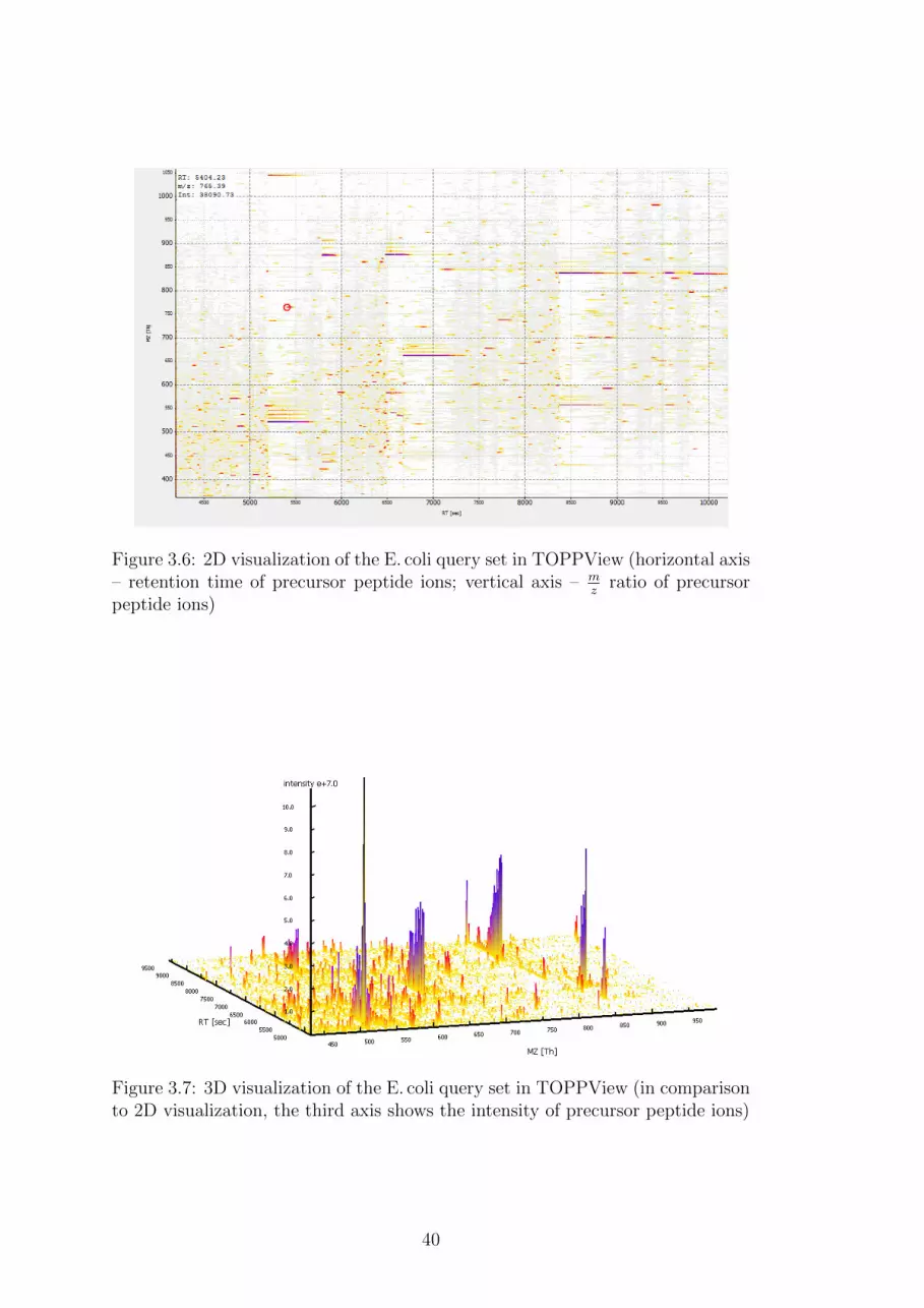
Figure 3.6: 2D visualization of the E. coli query set in TOPPView (horizontal axis– retention time of precursor peptide ions; vertical axis – m

zratio of precursor

peptide ions)

Figure 3.7: 3D visualization of the E. coli query set in TOPPView (in comparisonto 2D visualization, the third axis shows the intensity of precursor peptide ions)

40

Chapter 4

Speeding up the Mass SpectraDatabase Search

The number of protein sequences in public-available databases grows almost ex-ponentially in recent years (Fig. 4.1). Since large query sets containing tens ofthousands of query mass spectra are compared with tens to hundreds of millionsof theoretical spectra generated from a database of protein sequences, a sequentialscan of the database becomes inefficient. When a query spectrum is comparedwith n theoretical spectra generated from the database of protein sequences, thetime complexity of one-to-all comparisons is linear with the size of the databaseO(n). When a query set contains m spectra, the time complexity of all-to-allcomparisons is O(nm). A solution is to avoid one-to-all comparisons and to findan approach with sub-linear time complexity, i.e., there is a need for utilizationof database index structures. In practice, the modeling of an index structure isa non-trivial task due to the noise, modifications and inaccuracies in the massspectra.

Figure 4.1: Numbers of protein sequences in UniProtKB/Swiss-Prot in years [107]

Several approaches have been proposed which try to avoid one-to-all compar-isons. We describe the precursor mass filter, sequence tags, and two approachesbased on the properties of metric spaces (Chap. 5) – the tandem cosine distanceutilized by MVP-tree and the locality sensitive hashing. We also mention an

41

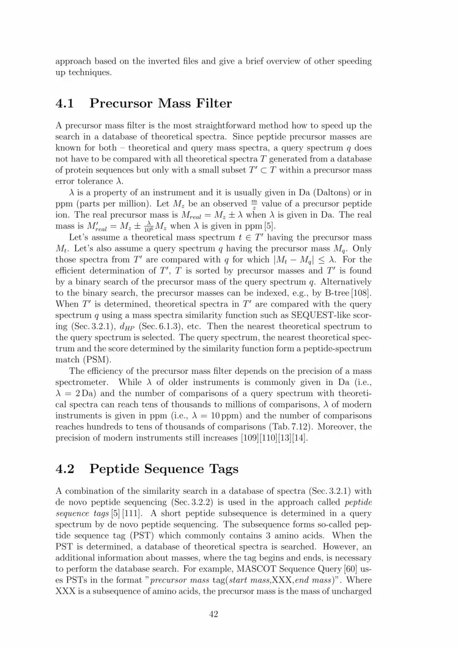
approach based on the inverted files and give a brief overview of other speedingup techniques.

4.1 Precursor Mass Filter

A precursor mass filter is the most straightforward method how to speed up thesearch in a database of theoretical spectra. Since peptide precursor masses areknown for both – theoretical and query mass spectra, a query spectrum q doesnot have to be compared with all theoretical spectra T generated from a databaseof protein sequences but only with a small subset T ′ ⊂ T within a precursor masserror tolerance λ.

λ is a property of an instrument and it is usually given in Da (Daltons) or inppm (parts per million). Let Mz be an observed m

zvalue of a precursor peptide

ion. The real precursor mass is Mreal = Mz ± λ when λ is given in Da. The realmass is M ′

real = Mz ± λ106Mz when λ is given in ppm [5].

Let’s assume a theoretical mass spectrum t ∈ T ′ having the precursor massMt. Let’s also assume a query spectrum q having the precursor mass Mq. Onlythose spectra from T ′ are compared with q for which |Mt −Mq| ≤ λ. For theefficient determination of T ′, T is sorted by precursor masses and T ′ is foundby a binary search of the precursor mass of the query spectrum q. Alternativelyto the binary search, the precursor masses can be indexed, e.g., by B-tree [108].When T ′ is determined, theoretical spectra in T ′ are compared with the queryspectrum q using a mass spectra similarity function such as SEQUEST-like scor-ing (Sec. 3.2.1), dHP (Sec. 6.1.3), etc. Then the nearest theoretical spectrum tothe query spectrum is selected. The query spectrum, the nearest theoretical spec-trum and the score determined by the similarity function form a peptide-spectrummatch (PSM).

The efficiency of the precursor mass filter depends on the precision of a massspectrometer. While λ of older instruments is commonly given in Da (i.e.,λ = 2 Da) and the number of comparisons of a query spectrum with theoreti-cal spectra can reach tens of thousands to millions of comparisons, λ of moderninstruments is given in ppm (i.e., λ = 10 ppm) and the number of comparisonsreaches hundreds to tens of thousands of comparisons (Tab. 7.12). Moreover, theprecision of modern instruments still increases [109][110][13][14].

4.2 Peptide Sequence Tags

A combination of the similarity search in a database of spectra (Sec. 3.2.1) withde novo peptide sequencing (Sec. 3.2.2) is used in the approach called peptidesequence tags [5] [111]. A short peptide subsequence is determined in a queryspectrum by de novo peptide sequencing. The subsequence forms so-called pep-tide sequence tag (PST) which commonly contains 3 amino acids. When thePST is determined, a database of theoretical spectra is searched. However, anadditional information about masses, where the tag begins and ends, is necessaryto perform the database search. For example, MASCOT Sequence Query [60] us-es PSTs in the format ”precursor mass tag(start mass,XXX,end mass)”. WhereXXX is a subsequence of amino acids, the precursor mass is the mass of uncharged

42

peptide, the start mass is the mass where the subsequence begins, and the endmass is the mass where the subsequence ends. For example, the query spectrumcorresponding to the peptide sequence ”GHPETLEK” in Fig. 4.2 has the tag ofthe form ”909.99 tag(195.20,PET,522.54)”.

Figure 4.2: Example of a peptide sequence tag in a query spectrum

To speed up the comparisons PSTs with the database of theoretical spectra,an index table can be constructed. The table contains entries for all combinationsof amino acids in the sequence tags (e.g., 203 entries for tags of the length 3). Eachentry has assigned a list of positions of peptide sequences (theoretical spectra) inthe database where the entry tag occurs. Drawbacks are that the index must berecomputed when the database is changed, and that the number of PSTs selectedfrom the database grows exponentially with the number of modifications allowedin query spectra. Among others, peptide sequence tags are implemented in Pep-tideSearch [112], ProteinProspector MS-Seq [46], GutenTag [113] or Inspect [50].Inspect employs also a trie constructed from tags of multiple query spectra tospeed up the database search. The trie is a tree data structure which stores a setof strings. A node in the trie corresponds to a prefix of one or multiple strings.

4.3 Fuzzy and Tandem Cosine Distance

An approach was proposed where a semi-metric search (Chap. 5) using the MVP-tree was employed to speed up the search in a database of theoretical spectra [114].Two variants of cosine distance were used as mass spectra similarity functions –the fuzzy cosine distance and tandem cosine distance. The approach is imple-mented in the application MSFound as a part of the framework MoBIoS [115].

4.3.1 Fuzzy Cosine Distance

The definition of the fuzzy cosine distance requires a high-dimensional booleanrepresentation of mass spectra (Fig. 6.1). For example, let the range of m

zvalues

in a mass spectrum be 0-2,000 Da and let it be divided in subintervals of 0.1 Da.Then the spectrum is represented by a 20,000-dimensional boolean feature vector

43

having ones at places corresponding to intervals for which the mz

value is nonzeroin the spectrum.

Given two boolean vectors ~A, ~B and the mz

error peak tolerance τ , the sharedpeak count (SPC) is defined by Eq. 4.1.

SPCτ ( ~A, ~B) =∑i

match(ai, bj); j ∈ [i− τ, i+ τ ]; ai ∈ ~A; bj ∈ ~B (4.1)

match(ai, bj) =

{1; ai = bj = 1;match(am, bj) = 0,m ∈ [1, i)0; otherwise

(4.2)

The Eq. 4.2 counts two peaks as equal when they lie within ±τ bins of each other.The condition match(am, bj) = 0,m ∈ [1, i) ensures that each peak is matchedwith another peak exactly once, i.e., multiple matches of the same peak withother peaks are not counted. When τ = 0, the Eq. 4.1 is reduced to the dotproduct on boolean vectors ~A and ~B (Eq. 4.3).

SPCτ=0( ~A, ~B) =∑i

match(ai, bi) = ~A · ~B (4.3)

The cosine similarity is defined as the normalized dot product between two vectors(Eq. 5.9). The fuzzy cosine similarity cosτ is defined as the normalized SPCτ(Eq. 4.4), where ‖. . .‖ is the L2 norm of a vector, ai ∈ ~A and bi ∈ ~B.

cosτ ( ~A, ~B) =SPCτ ( ~A, ~B)∥∥∥ ~A∥∥∥∥∥∥ ~B∥∥∥ (4.4)

Finally, the fuzzy cosine distance is defined as the inverse of cosτ (Eq. 4.5).

dfuzzy( ~A, ~B) = arccos(cosτ ( ~A, ~B)) (4.5)

dfuzzy is a semi-pseudometric because it violates the reflexivity and triangle in-equality (Sec. 5.1.1), what is caused by the m

zerror tolerance τ > 0. The dfuzzy

has high intrinsic dimensionality ρ (Sec. 5.1.8) and it cannot be efficiently utilizedby metric access methods (MAMs).

4.3.2 Tandem Cosine Distance

Let SA = { ~A,MA} be a mass spectrum where ~A is the high-dimensional booleanvector and MA is the precursor mass of the spectrum SA. The tandem cosinedistance dtandem is defined by Eq. 4.7. dtandem is a linear combination of dfuzzywith the difference of precursor masses dprecursor of compared spectra (Eq. 4.6).λ is the precursor mass error tolerance. c1 and c2 are weights of the membersin the equation (e.g., c1 = c2 = 1). Since dprecursor is the L1 distance computedover one-dimensional vectors and dtandem is a linear combination of dfuzzy withdprecursor, dtandem is also a semi-pseudometric. dtandem has very low ρ and it canbe efficiently utilized by MAMs. A disadvantage of dtandem is that the support ofmodifications in query mass spectra has not been discussed.

dprecursor(MA,MB) =

{0; |MA −MB| ≤ λ|MA −MB|; otherwise

(4.6)

dtandem(SA, SB) = c1dfuzzy( ~A, ~B) + c2dprecursor(MA,MB) (4.7)

44

4.3.3 MVP-tree

The vantage point tree (VP-tree) is a simple metric access method (say, a pre-decessor of M-tree (Sec. 5.1.7)) which splits indexed objects into subsets prunedduring the searching [116] [117]. In a binary VP-tree, each internal node has theform of (V, dM , Lptr, Rptr) where V is a vantage point (pivot), dM is a mediandistance among the distances from V to all objects indexed below this node, Lptrand Rptr are pointers to the subtrees. The multi vantage point tree (MVP-tree)is an extension of the VP-tree. In contrast to the VP-tree, the MVP-tree usestwo pivots in each node. Every node of the MVP-tree can be seen as two levelsof the VP-tree where all the children nodes at the lower level use the same pivot.Thus the MVP-tree stores less pivots in non-leaf levels than the VP-tree.

4.3.4 Semi-metric Search

Even though dtandem violates the triangle inequality and the search using MVP-tree is approximate, the violation of the triangle inequality can be controlled.Lets assume a metric distance d, a query object q, a pivot p and a databaseobject o. The triangle inequality is violated when d(q, p) + d(o, p) < d(q, o). Ifthere is a κ such that d(q, p) + d(o, p) +κ ≥ d(q, o), we say d violates the triangleinequality by this amount κ. Let κu be an upper bound on κ, a pruning conditionin a metric range query with a radius r can be adjusted or fixed to return exactresults by κu (Eq. 4.8) [114][118].

|d(q, p)− d(o, p)| > r + κu (4.8)

4.4 Locality Sensitive Hashing

An approach for speeding up the search in theoretical mass spectra databasesbased on the locality sensitive hashing (LSH) was also proposed [119][120][121].The LSH is an approximate algorithm which uses a hash-based indexing structureand the properties of metric spaces (Chap. 5) to obtain fast search times despitethe high intrinsic dimensionality ρ (Sec. 5.1.8). The method provides good prob-abilistic bounds on the error of returned results [122][123][124].

The basic idea is to design a set of hash functions to pre-process the theoreticalspectra in the database so that for each query spectrum the set of hash functionscan be used to find theoretical spectra closest to the query spectrum. Let’sassume a random spectrum and the cosine similarity (Eq. 5.9) as a hash function.Any query spectrum which is similar to the theoretical spectrum will have similarscore to the random spectrum.

To implement this idea, a spectrum must be represented as a high-dimensionalboolean vector (Fig. 6.1). An efficient filtering can be then achieved by ANN (ap-proximate nearest neighbor) [125] queries but the efficiency is guaranteed onlywhen L1 (Eq. 5.6) or L2 (Eq. 5.7) distances are used. The approach approximates

the cosine distance by L2 distance under the assumption that 1 − cos( ~A, ~B) ≈L2( ~A, ~B) for small angles where ~A, ~B are high-dimensional boolean vectors.A drawback of LSH is that a method for identification of peptide sequences fromspectra containing modifications has not been proposed.

45

4.4.1 Family of Hash Functions

A family H of functions h : Rn → U is called (p1, p2, r, cr)-sensitive, if for any

high-dimensional object ~O and query ~Q:

• if∥∥∥ ~O − ~Q

∥∥∥ ≤ r then Pr[h( ~O) = h( ~Q)] ≥ p1

• if∥∥∥ ~O − ~Q

∥∥∥ ≥ cr then Pr[h( ~O) = h( ~Q)] ≤ p2

where p1 > p2, r is the query radius, n is the dimension of space, U is the universeand c > 1 is the approximation factor [122].

Given a family H of hash functions, the LSH chooses t of them and concate-nates them into a t-dimensional hash function ~gj( ~A) = (h1,j( ~A), . . . , ht,j( ~A)) todecrease the frequency of collisions. L different groups of hash functions are cho-sen uniformly and independently at random, i.e., ~g1, . . . , ~gL. The parameters nand L are crucial to tune LSH because they amplify the gap between P1 and P2.

The LSH family (Eq. 4.9) has been proposed for the Euclidean space [126].A random projection of Rn onto a 1-dimensional line is assumed. The line ischopped into segments of length w and shifted by a random value b ∈ [0, w). The

projection vector ~P ∈ Rn is constructed by picking coordinates of ~P from theGaussian distribution.

h( ~A) =

⌊~P · ~A+ b

w

⌋(4.9)

4.4.2 Data Structure and Query Processing

The data structure is constructed by placing each point ~O from the database intobuckets ~gj( ~O) where j = 1, . . . , L. When a query ~Q is being processed, all the

buckets ~g1( ~Q), . . . , ~gL( ~Q) are scanned and all the points from them are retrieved.

Afterwards, their distances to ~Q are computed and any point is reported that isa valid answer to ~Q (Alg. 1) [122].

Algorithm 1: Locality Sensitive Hashing

Preprocessing:begin

1 Choose L functions ~gj, j = 1, . . . , L, by setting ~gj = (h1,j, h2,j, . . . ht,j)where h1,j, . . . , ht,j are chosen at random from the LSH family H;

2 Construct L hash tables, where for each j = 1, . . . , L, the jth hash tablecontains the dataset points hashed using the function ~gj;

Range Query:begin

3 for j = 1 to L do

4 Retrieve the points from the bucket ~gj( ~Q) in the jth hash table;

5 For each of the retrieved points, compute the distance from ~Q to itand report the point if it is a correct answer;

46

4.5 Inverted Files

Several approaches have been proposed where inverted files are utilized to indexa database of theoretical spectra [127][128][129][130]. The inverted index takesthe advantage of the high sparsity of high-dimensional boolean vectors generatedfrom the mass spectra (Fig. 6.1). Instead of storing a high-dimensional sparseboolean vector, a compact representation can be used where the positions of ones(i.e., dimensions in which the values are nonzero) are substituted with values ofthe compact vector. For example, the compact representation of the vector inFig. 6.1 is ~x = 〈7, 13, 18, 23, 27, 34〉.

Figure 4.3: Inverted index

For each value in the compact representation, an inverted index stores a list ofspectra where the value occurs (Fig. 4.3). When a query is being processed, thelists of the index are scanned in parallel. Each list has its own cursor pointing toan identifier of a spectrum. Only the cursor pointing to the smallest identifier canmove forward. When the cursors are aligned, various boolean operations can berealized, e.g., an intersection (AND), a union (OR) or a complement (NOT). Acommon mass spectra similarity is the normalized dot product which is computedusing the operation AND (Eq. 5.9). A problem can arise because lengths of thelists are not distributed evenly and the lists tend to be very long. Therefore, thehigh sparsity of boolean vectors is crucial for the efficiency of the inverted index.

A support of modifications in query mass spectra is not commonly mentionedin approaches based on the inverted index. However, recently, an approachhas been proposed which supports also spectra with modifications [130]. LetS = {a1, a2, . . . , an} be a list of m

zvalues where an is the precursor mass of the

Algorithm 2: Index Match Algorithm

Input: A spectrum S = {a1, a2, . . . , an} and a set of spectraτ = {T1, T2, . . . , Tk} represented as a set of linked lists L1, L2, . . . , LM ;Output: A spectrum T in τ with the best mass counting score with S;

begin1 Initialize score pj = 0 for each spectra Tj ∈ τ ;2 for each mass ai in S do3 for each non-null node Tj in the linked list Lai do4 Increase pj by 1 ;

5 Output spectrum Tj with the highest score pj;

47

Algorithm 3: Index Diagonal Algorithm

Input: A spectrum S = {a1, a2, . . . , an} and a set of spectraτ = {T1, T2, . . . , Tk}. All sub-vectors of the spectra in τ are represented asa set of linked lists L1, L2, . . . , LM ;Output: A spectrum T in τ with the best diagonal score with S;

begin1 for each sub-vector S[i..n] of S, i = 1, . . . , n− 2 do2 Use Alg. 2 to find the best scoring sub-vector from τ (the sub-vector

and S[i..n] have the best mass counting score);

3 Compare the best scoring sub-vectors for S[1..n], . . . , S[n− 2..n] andoutput the best one and its corresponding spectrum;

Algorithm 4: Two-Index Diagonal Algorithm

Input: A spectrum S = {a1, a2, . . . , an} and a set of spectraτ = {T1, T2, . . . , Tk}. All left sub-vectors and right sub-vectors of thespectra in τ are represented as two sets of linked lists;Output: A spectrum T in τ with the best diagonal score with S;

begin1 for i = 1 to n− 1 do2 Use Alg. 2 to find the sub-vector pair T[j..0] and T[j..m] such that

C(S[i..0],T[j..0]) + C(S[i..n],T[j..m]) is maximized;

3 Compare the best scoring sub-vector pairs for i = 1, . . . , n− 1 andoutput the best scoring one and its corresponding spectrum;

spectrum. Let s1s2 . . . sN be a high-dimensional boolean representation of thespectrum S where N = an. If there is a mass i in the spectrum S and i 6= n,si = 1; otherwise, si = 0. For example, a spectrum {2, 4, 7, 10} is represented bya vector 0101001000.

For a pair of spectra S = {a1, a2, . . . , an} and T = {b1, b2, . . . , bm}, a masspair (ai, bj) is matched if ai = bj, ai 6= an and bj 6= bm. The number of matchedmass pairs (i.e., the dot product over the high-dimensional vectors) is called masscounting score and denoted C(S, T ).

Let τ = {T1, T2, . . . , Tk} be a set of theoretical mass spectra. For simplicity,let’s assume that all the spectra in τ have the same precursor mass M . A linkedlist is generated for each column of aligned high-dimensional boolean vectors(Fig. 4.3). Having a set of linked lists L1, L2, . . . , LM , the index match algorithmis proposed to find a pair of spectra (S, T ) with the maximum C(S, T ) whereT ∈ τ (Alg. 2).

The diagonal score D(S, T ) has been proposed for spectra with modifications.When a spectrum contains a modification, m

zvalues are shifted and thus ones in

its high-dimensional representation are also shifted. Let T (u) be a spectrum gen-erated by shifting each mass in T by u, that is T (u) = {b1 +u, b2 +u, . . . , bm+u}.The diagonal score D(S, T ) = maxuC(S, T (u)) is the maximum mass countingscore among all shift values.

48

The index diagonal algorithm has been proposed to compute the diagonalscore (Alg. 3). The sub-vectors of theoretical spectra in τ and sub-vectors of thequery spectrum S are generated for this purpose. For example, for each ’1’ in thehigh-dimensional boolean representation of S except the last, all elements left tothe ’1’ are removed (including itself) from the vector to generate a sub-vector ofS. The sub-vector generated from the ith ’1’ is denoted S[i..n]. In total, n − 2sub-vectors are generated from S. For example, the spectrum {2, 4, 7, 10} havingthe boolean representation 0101001000 has two sub-vectors 01001000 and 001000.The sub-vectors of S and linked lists formed from sub-vectors of spectra in τ areused in Alg. 3 to compute the diagonal scores. A prove that Alg. 3 reports thediagonal scores correctly is shown in [130].

A modification of the diagonal algorithm has been also proposed where twoinverted indexes are used – one for left sub-vectors of spectra in τ and the otherfor right sub-vectors of spectra in τ (Alg. 4). The right sub-vectors are the sameas above defined sub-vectors. A left sub-vector is the reverse of the sub-vector leftto the element ’1’. For example, the spectrum {2, 4, 7, 10} having the booleanrepresentation 0101001000 is split by third ’1’ into a left (reversed) sub-vector’001010’ and a right sub-vector ’000’. In total, the spectrum has three (in general,n−1) different pairs of sub-vectors (0,01001000), (010,001000) and (001010,000).

4.6 Other approaches

A vast number of approaches have been proposed to speed up the search in massspectra databases. For example, there is an approach based on the hashing ofsimilar spectra into 64-bit integers [131]. A group of approaches has been proposedwhere the machine learning techniques like support vector machines or neuralnetworks are utilized [132] [133] [134]. For example, the neural network approachis based on a self-organizing map (SOM). The theoretical spectra are converted tohigh-dimensional vectors and the SOM is trained. For a query spectrum, a multi-point range query is performed using SOM, a candidate set of peptide sequencesis obtained and then a scoring function is applied.

There is also an approach which indexes the database of protein/peptide se-quences by suffix trees [135] [136]. On the other hand, a graph algorithm is usedto pre-process a query mass spectrum. The suffix tree is then searched for candi-date peptide sequences against the spectrum graph. The correct peptide sequenceis then selected by a scoring/similarity function. Another approach is based onlongest common prefixes and suffix arrays [137].

Other approaches are based on parallelization [138], GPU processing [139] orhardware acceleration of previously proposed methods [140]. Some approacheshave been proposed which utilize a combination of algorithmic and software engi-neering techniques (say, a set of cheats) to speed up the identification of peptidesusing SEQUEST-like scoring [58][59]. An overview of other methods based onthe database indexing, database reduction and database splitting has been alsoproposed in [121].

49

50

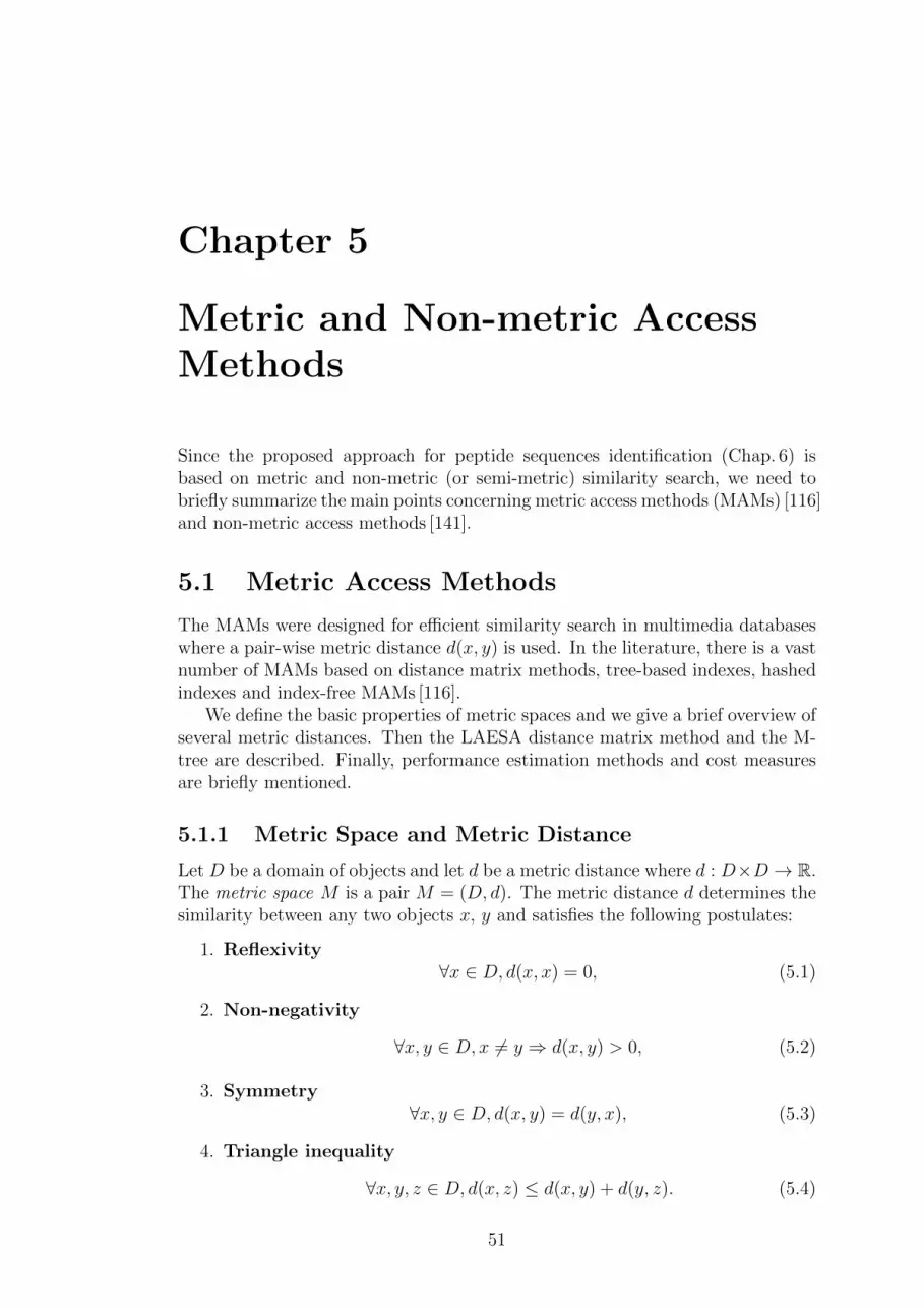
Chapter 5

Metric and Non-metric AccessMethods

Since the proposed approach for peptide sequences identification (Chap. 6) isbased on metric and non-metric (or semi-metric) similarity search, we need tobriefly summarize the main points concerning metric access methods (MAMs) [116]and non-metric access methods [141].

5.1 Metric Access Methods

The MAMs were designed for efficient similarity search in multimedia databaseswhere a pair-wise metric distance d(x, y) is used. In the literature, there is a vastnumber of MAMs based on distance matrix methods, tree-based indexes, hashedindexes and index-free MAMs [116].

We define the basic properties of metric spaces and we give a brief overview ofseveral metric distances. Then the LAESA distance matrix method and the M-tree are described. Finally, performance estimation methods and cost measuresare briefly mentioned.

5.1.1 Metric Space and Metric Distance

Let D be a domain of objects and let d be a metric distance where d : D×D → R.The metric space M is a pair M = (D, d). The metric distance d determines thesimilarity between any two objects x, y and satisfies the following postulates:

1. Reflexivity∀x ∈ D, d(x, x) = 0, (5.1)

2. Non-negativity

∀x, y ∈ D, x 6= y ⇒ d(x, y) > 0, (5.2)

3. Symmetry∀x, y ∈ D, d(x, y) = d(y, x), (5.3)

4. Triangle inequality

∀x, y, z ∈ D, d(x, z) ≤ d(x, y) + d(y, z). (5.4)

51

The metric postulates (especially the triangle inequality) are crucial to or-ganize database objects within metric regions of MAMs and to prune irrelevantregions of MAMs while searching [116]. In case the triangle inequality is partiallyviolated, the distance d is called the semi-metric distance. When the reflexivityis not satisfied the d is called pseudo-metric.

5.1.2 Minkowski Distances

The well known group of metric distances are Minkowski distances Lp whichare suitable when objects are represented by vectors of constant sizes. The Lpdistances can be summarized by Eq. 5.5 where ~x = (x1, ..., xn) and ~y = (y1, ..., yn).

Lp (~x, ~y) = p

√√√√ n∑i=1

|xi − yi|p; p ≥ 1;xi, yi ∈ R (5.5)

Manhattan Distance

Manhattan distance L1 is a special case of the Lp distance where p = 1 and isdefined by Eq. 5.6.

L1 (~x, ~y) =n∑i=1

|xi − yi| (5.6)

Euclidean Distance

Likely, the most known metric distance from the group of Minkowski distances isthe Euclidean distance L2 which is defined by Eq. 5.7.

L2 (~x, ~y) =

√√√√ n∑i=1

(xi − yi)2 (5.7)

Maximum Distance

The maximum distance L∞ is a variant of the Lp distance where p =∞ (Eq. 5.8).L∞ is used in LAESA metric access method to determine a lower-bound of adistance between a query object and a database object (Sec. 5.1.6).

L∞ (~x, ~y) =n

maxi=1|xi − yi| (5.8)

5.1.3 Cosine Similarity

Cosine similarity (or normalized dot product) determines the cosine of an angle ϕbetween vectors ~x and ~y in the n-dimensional space (Eq. 5.9), where ‖. . .‖ is theEuclidean L2 norm. The cosine similarity satisfies only the symmetry. Since thesimilarity between objects is bigger with bigger cosϕ, the cosine similarity doesnot satisfy the reflexivity. Since cosϕ ∈ 〈−1, 1〉 the postulate of non-negativityis not satisfied. The triangle inequality is also violated what can be proven by acounterexample. Let’s assume ~x = {0, 1, 1}, ~y = {0, 1, 0} and ~z = {1, 0, 0}, then

52

cos(~x, ~y) = 1√2, cos(~x, ~z) = 0 and cos(~y, ~z) = 0. Since 0 + 0 � 1√

2, the triangle

inequality is violated.

cosϕ = cos(~x, ~y) =~x~y

‖~x‖ ‖~y‖=

n∑i=1

xiyi√n∑i=1

x2i

√n∑i=1

y2i

(5.9)

The cosine similarity can be turned into the angle distance dangle(~x, ~y) by thearccos function (Eq. 5.10). The angle distance is a pseudo-metric what meansthat the metric postulates are satisfied, but it may happen that dangle(~x, ~y) = 0for ~x 6= ~y. dangle gives the size of an angle ϕ between the vectors ~x and ~y whereϕ ∈

⟨0, π

2

⟩.

dangle(~x, ~y) = ϕ = arccos

(~x~y

‖~x‖ ‖~y‖

)(5.10)

5.1.4 Hausdorff Distance

The Hausdorff distance dH [116] is a metric distance defined on sets of objects Aand B (Eq. 5.12). The dH is computed as follows:

1. For each object in the set A, the distance to its nearest neighbor in the setB is determined.

2. The maximum distance from the distances to the nearest neighbors is se-lected.

3. The steps 1 and 2 are repeated with the A and B switched.

4. The maximum distance from the two maximum distances forms the result.

The ground distance dX operating on the objects of A,B can be any otherdistance (e.g., L2 in case of point sets). If dX is a metric distance then dH is alsoa metric distance. The time complexity to compute the dH is O(nm)·O(dX(·, ·))where n and m are the numbers of objects in A and B, and O(dX(·, ·)) is thetime complexity of the ground distance dX .

h(A,B) = maxa∈A

{minb∈B{dX(a, b)}

}(5.11)

dH(A,B) = max(h(A,B), h(B,A)) (5.12)

5.1.5 Similarity Queries

The most common types of similarity queries are range queries R(q, r) and knearest neighbor queries kNN(q, k) where q is a query object and r is a queryradius (Fig. 5.1). When a sequential scan of a database DB ⊆ D is employed, thedistance d(q, o) must be computed between the query object q and any databaseobject o ∈ DB.

In case of the range query, the sequential scan of the database is performedwhile the objects for which d(q, o) ≤ r are appended to a result set (Eq. 5.13).

53

In case of the kNN query, a priority queue PQ of k nearest neighbors is updatedwhile d(q, o) are being computed (Eq. 5.14). The result of the kNN query maydepend on the order of objects in DB and on the implementation of the kNNquery when more objects are exactly in the same distance. For example, in Fig. 5.1observe that the kth and (k + 1)th objects are in the same distance (k = 3).

MAMs employ the metric postulates (especially the triangle inequality) toorganize the objects in DB into metric regions and to prune these regions whilesearching. When the range and kNN queries are performed on a MAM, many ofthe distances d(q, o) are not computed and thus the search is significantly faster.

R(q, r) = {o ∈ DB, d(o, q) ≤ r} (5.13)

kNN(q, k) = {PQ ⊆ DB, |PQ| = k∧∀x∈PQ, y∈DB−PQ : d(q, x) ≤ d(q, y)} (5.14)

Figure 5.1: Similarity queries – (a) range query and (b) kNN query

5.1.6 LAESA

Pivot tables (or distance matrix methods) represent a simple but efficient solu-tion to the similarity search. A representative of pivot tables is LAESA (LinearApproximating and Eliminating Search Algorithm) [142] [143] what is an improve-ment of AESA [144]. While AESA has quadratic space-complexity, LAESA hasthe complexity only linear.

In general, a set P of objects (so-called pivots) is selected from the database. Avector of distances between a database object oi ∈ DB and all the pivots pj ∈ Pis pre-computed {d(oi, p1), . . . , d(oi, pj), . . . , d(oi, pl)} where l is the number ofpivots. The vectors of all database objects form a distance matrix – the pivottable.

When performing a query q, a vector of distances between q and the piv-ots is pre-computed the same way as for a database object oi, i.e., {d(q, p1), . . . ,d(q, pj), . . . , d(q, pl)}. A query corresponds to the sequential scan of the entiredatabase with the difference that a lower-bound lb of a distance between q and oi isdetermined from the precomputed distances as lb = maxpj∈P{|d(q, pj)− d(oi, pj)|}.In fact, the max says that L∞ distance (Eq. 5.8) is computed. The lb allows to

54

prune irrelevant objects while the distance d(q, oi) is not computed in many casesand thus the search is faster than the sequential scan.

To show the advantage of LAESA, the d(·, ·) must be a time-consuming dis-tance. Since L∞ is used to determine the lb, the LAESA is not efficient with Lpdistances. When n-dimensional objects are indexed and l ≥ n, a computation oflb between the query q and any database object oi is more time-consuming thena direct computation of d(q, oi).

Another drawback is that the entire matrix is scanned during the query pro-cessing and thus the LAESA is efficient only when the entire matrix is stored inthe main memory. The problem is that the matrix may be very space-consuming(depending on the number of pivots l and the number of object in DB).

Figure 5.2: LAESA – filtering using the lower-bound

Range Query

The range query algorithm R(q, r) on LAESA is shown in Alg. 5. In fact, thesequential scan of the database is performed while for each database object oi, the

Algorithm 5: LAESA – range query

1 Input:2 Database of objects oi ∈ DB, query object q, radius r, set of pivots pj ∈ P,

metric distance d, matrix of pre-computed distances d(oi, pj).

3 Output:4 Set of objects S ⊆ DB where ∀o′i∈S : d(q, o′i) ≤ r.

5 begin6 S = ∅;7 for all pj ∈ P do8 compute d(q, pj);

9 for all oi ∈ DB do10 lb = maxpj∈P

{∣∣d(q, pj)− d(oi, pj)

∣∣};11 if lb ≤ r then12 compute d(q, oi);13 if d(q, oi) ≤ r then14 append oi to S;

15 return S;

55

lb is computed. When lb ≤ r, the d(q, oi) must be computed. When d(q, oi) ≤ r,the oi is appended to a result set. The principle of the filtering using the lower-bound is shown in Fig. 5.2. The task is to determine whether the oi is inside thequery ball (q, r). The d(q, pj) is known because it is computed when the rangequery is initialized. The d(oi, pj) is known because the value is stored in thepivot table. The d(q, oi) is unknown. The d(q, oi) does not have to be computedbecause its lower-bound |d(q, pj)− d(oi, pj)| is larger than r. So, the oi surelycannot be in the query ball (q, r) and thus oi is ignored.

kNN Query

The k nearest neighbor query kNN(q, k) on LAESA is shown in Alg. 6. First,the lb is computed for all objects in the database. Second, the database is sortedin ascending order w.r.t. lb. Third, the database sorted by lb is scanned and

Algorithm 6: LAESA – kNN query

1 Input:2 Database of objects oi ∈ DB, query object q, number of nearest neighborsk, set of pivots pj ∈ P, metric distance d, matrix of pre-computed distancesd(oi, pj).

3 Output:4 Priority queue PQ of k nearest neighbors (priority is determined by d(·, ·)).5 begin6 PQ = ∅;7 for all pj ∈ P do8 compute d(q, pj);

9 for all oi ∈ DB do10 lb(q,oi) = maxpj∈P

{∣∣d(q, pj)− d(oi, pj)

∣∣};11 for all oi ∈ DB sorted in ascending order w.r.t. lb(q,oi) do12 if number of objects in PQ < k then13 compute d(q, oi);14 insert oi with d(q, oi) into PQ;

else15 /* d(q, ok) is the distance between q and object in PQ

with the smallest priority (kth nearest neighbor)

*/

16 if d(q, ok) < lb(q,oi) then17 return PQ;

18 compute d(q, oi);19 if d(q, oi) < d(q, ok) then20 insert oi with d(q, oi) into PQ;21 remove the object with the smallest priority from PQ to

keep only the k nearest neighbors;

22 return PQ;

56

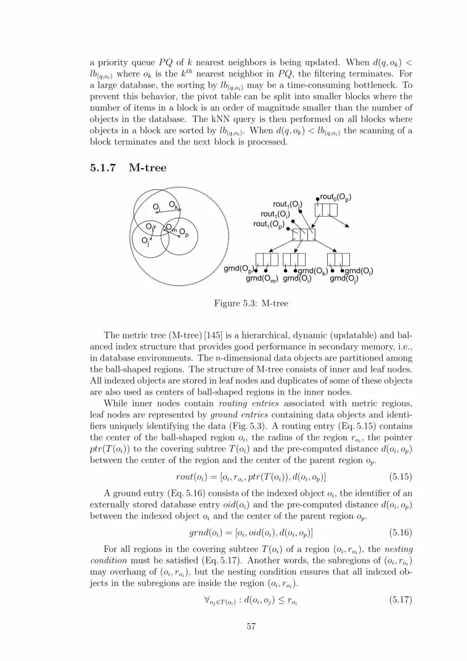
a priority queue PQ of k nearest neighbors is being updated. When d(q, ok) <lb(q,oi) where ok is the kth nearest neighbor in PQ, the filtering terminates. Fora large database, the sorting by lb(q,oi) may be a time-consuming bottleneck. Toprevent this behavior, the pivot table can be split into smaller blocks where thenumber of items in a block is an order of magnitude smaller than the number ofobjects in the database. The kNN query is then performed on all blocks whereobjects in a block are sorted by lb(q,oi). When d(q, ok) < lb(q,oi) the scanning of ablock terminates and the next block is processed.

5.1.7 M-tree

Figure 5.3: M-tree

The metric tree (M-tree) [145] is a hierarchical, dynamic (updatable) and bal-anced index structure that provides good performance in secondary memory, i.e.,in database environments. The n-dimensional data objects are partitioned amongthe ball-shaped regions. The structure of M-tree consists of inner and leaf nodes.All indexed objects are stored in leaf nodes and duplicates of some of these objectsare also used as centers of ball-shaped regions in the inner nodes.

While inner nodes contain routing entries associated with metric regions,leaf nodes are represented by ground entries containing data objects and identi-fiers uniquely identifying the data (Fig. 5.3). A routing entry (Eq. 5.15) containsthe center of the ball-shaped region oi, the radius of the region roi , the pointerptr(T (oi)) to the covering subtree T (oi) and the pre-computed distance d(oi, op)between the center of the region and the center of the parent region op.

rout(oi) = [oi, roi , ptr(T (oi)), d(oi, op)] (5.15)

A ground entry (Eq. 5.16) consists of the indexed object oi, the identifier of anexternally stored database entry oid(oi) and the pre-computed distance d(oi, op)between the indexed object oi and the center of the parent region op.

grnd(oi) = [oi, oid(oi), d(oi, op)] (5.16)

For all regions in the covering subtree T (oi) of a region (oi, roi), the nestingcondition must be satisfied (Eq. 5.17). Another words, the subregions of (oi, roi)may overhang of (oi, roi), but the nesting condition ensures that all indexed ob-jects in the subregions are inside the region (oi, roi).

∀oj∈T (oi) : d(oi, oj) ≤ roi (5.17)

57

Pruning Conditions

The M-tree employs two pruning conditions to filter out the irrelevant regionsduring the searching. Let (q, rq) be a query region, the following conditions areused to prune irrelevant regions of M-tree.

1. Basic filtering. When d(oi, q) > roi + rq then for each oj ∈ T (oi) :d(oj, q) > rq and thus the covering subtree T (oi) does not have to besearched (Fig. 5.4a).

2. Parent filtering. When |d(op, q)− d(op, oi)| > roi + rq where op is thecenter of the parent region of oi, then d(oi, q) > roi + rq and thus thecovering subtree T (oi) does not have to be searched (Fig. 5.4b).

Figure 5.4: Pruning conditions in M-tree

Construction

The M-tree can be constructed by a statical or dynamical way. The statical way(so-called bulk-loading) is suitable when a large collection of objects is available inthe time of construction. The algorithm clusters similar objects and then createsthe tree hierarchy. The details of this approach are proposed in [116] [146].

When a large collection of objects is not available in the time of constructionor when the database is frequently updated, the M-tree can be constructed dy-namically by the insertion of single objects into an existing tree hierarchy. Webriefly describe the dynamical construction of M-tree.

Algorithm 7: M-tree – construction (part 1)

1 Function InsertObject(T, oi)2 Input:3 Root node of M-tree T, inserted object oi.4 Output:5 None.6 begin7 N = FindLeaf(T, oi);8 if N is not full then9 store oi in the leaf node N;

else10 SplitNode(N, oi);

58

Algorithm 8: M-tree – construction (part 2)

1 Function FindLeaf(N, oi)2 Input:3 Node N, inserted object oi.4 Output:5 Leaf node N.6 begin7 if N is a leaf node then8 return N;

9 N′ = {∀rout(oj)∈N : d(oi, oj) ≤ roj};

10 if N′ 6= ∅ then11 select o∗j such that rout(o∗j) ∈ N′ : min{d

(o∗j , oi

)};

else12 select o∗j such that rout(o∗j) ∈ N : min{d

(o∗j , oi

)− ro∗j};

13 ro∗j = d(o∗j , oi);

14 return FindLeaf(ptr(T(o∗j)), oi);

15 Function SplitNode(N, oi)16 Input:17 Node N, inserted object oi.18 Output:19 None.20 begin21 Nall = {∀oj

: oj ∈ N} ∪ {oi};22 /* Select centers op1 , op2 of 2 new routing items from Nall */

23 Promote(Nall, op1 , op2);24 /* Split objects from Nall to Np1 ,Np2 w.r.t. op1 , op2 */

25 Partition(Nall, op1 , op2 ,Np1 ,Np2);26 allocate a new node N’;27 store entries from Np1 into N and entries from Np2 into N’;28 if N is the root node then29 allocate a new root node Np;30 store rout(op1) and rout(op2) in Np;

else31 let rout(op) be the routing entry of N stored in the parent node Np;32 replace the entry rout(op) with rout(op1) in Np;33 if Np is full then34 SplitNode(Np, op2);

else35 store rout(op2) in Np;

59

The M-tree structure can be constructed by insertions of single objects usingthe function InsertObject (Alg. 7). The function FindLeaf (Alg. 8) selects a leafnode in which a new object oi will be stored. The leaf is selected whose centerobject oj in its routing entry is closest to oi. The entry is preferred for which anextension of roj is not necessary. When such a region does not exist, the entry isselected for which a minimum extension of roj must be done.

When the leaf node is selected, the object oi (ground entry, respectively) isinserted into the leaf. In case the leaf node is overfilled, the node is split into twonew nodes by the function SplitNode (Alg. 8). Two functions are called inside theSplitNode – Promote and Partition. The function Promote selects two centersop1 and op2 of newly created routing entries from the set of objects Nall. Afew heuristics for an optimal selection of the centers are proposed in [116]. Thefunction Partition splits the set of objects between the two newly created nodes.Again, a couple of heuristics have been developed for an optimal partitioning, e.g.,an object can be inserted into the node whose center is closest to the object [116].

When the centers are selected and when the objects are partitioned, objectsbelonging to the center op1 are stored in the old node N and objects belongingto the center op2 are stored in a newly allocated node N ′. When the old node Nis the root of the M-tree, a new root must be allocated and routing items of op1and op2 are stored in the newly allocated root. In case the old node N is not theroot, the routing entry in its parent node Np must be replaced with the routingentry of op1 . The routing entry of op2 must be also inserted into Np. When op2cannot be inserted into Np because Np is overfilled, the function SplitNode iscalled recursively on the parent node Np.

The described algorithm is also known as the single-way. When an objectis being inserted, the M-tree is traversed along exactly one branch and the firstsuitable leaf node is selected. A better resulting indexing structure (i.e., less andmore tight clusters) can be achieved by the multi-way [116] [147]. Before insertinga new object oi, a point query R(oi, 0) is performed. For all visited leaves, thedistances between oi and the centers of their ball regions are computed. The leafnode whose pivot is the closest to oi is then chosen to store the new object. If nosuch leaf is found, the single-way insertion is employed. This happens when noleaf node covers the area of oi and the search algorithm terminates empty beforereaching a leaf. A drawback is that the multi-way is more time-consuming thanthe single-way.

Range Query

When performing a range query (Alg. 9), the M-tree is scanned from the root,while the subtrees of the regions which overlap the query region must be searchedas well, recursively. When a non-leaf node is processed, the pruning condition|d(op, q)− d(oi, op)| ≤ r + roi is used for a cheap elimination of regions which donot have to be scanned. d(oi, op) is stored in each routing entry and the value ofd(op, q) has been precomputed as d(oi, q) in the previous call of RangeQueryIter.When a region is not pruned by this condition, d(oi, q) must be computed andthe overlap of the region (oi, roi) with the query region (q, r) is tested. When theregion (oi, roi) overlaps (q, r), the RangeQueryIter is called recursively.

When a leaf node is processed, a simpler condition |d(op, q)− d(oi, op)| ≤ r isused to filter out the objects which do not belong to a result set S. When an

60

object oi is not eliminated by the condition, d(oi, q) must be computed and itspresence in the query region (q, r) is tested. When the object oi occurs in (q, r),oi is appended to the result set S.

Algorithm 9: M-tree – range query

1 Function RangeQueryIter(N, q, r, S)2 Input:3 Node N, query object q, radius r, set of objects S.4 Output:5 Set of objects S.6 begin7 let op be the parent object of node N;8 if N is not a leaf node then9 for each rout(oi) ∈ N do

10 if |d(op, q)− d(oi, op)| ≤ r + roithen

11 compute d(oi, q);12 if d(oi, q) ≤ r + roi

then13 RangeQueryIter(ptr(T(oi)), q, r, S);

else14 for each grnd(oi) ∈ N do15 if |d(op, q)− d(oi, op)| ≤ r then16 compute d(oi, q);17 if d(oi, q) ≤ r then18 append oi into S;

19 return S;

20 Function RangeQuery(T, q, r)21 Input:22 Root node of M-tree T, query object q, radius r.23 Output:24 Set of objects S where ∀oi∈S : d(q, oi) ≤ r.

25 begin26 S = ∅;27 RangeQueryIter(T, q, r, S);28 return S;

kNN Query

The implementation of the kNN query (Alg. 10 and Alg. 11) is not so straight-forward as the implementation of the range query because the radius r is notknown. At the beginning, the dynamic radius r is set to∞ and during the queryprocessing r is being reduced. At the end of the kNN query, r corresponds tothe distance of kth nearest neighbor. However, both kind of queries are processedwith equal I/O costs (numbers of accessed nodes).

61

Algorithm 10: M-tree – kNN query (part 1)

1 Function kNNQuery(T, q, k)2 Input:3 Root node of M-tree T, query object q, number of nearest neighbors k.4 Output:5 Queue NN of k nearest neighbors.6 begin7 insert [T,−] into PR;8 r =∞;9 for i = 1 to k do

10 NN[i] = [−,∞];

11 while PR 6= ∅ do12 nextnode = ChooseNode(PR);13 kNNSearchNode(nextnode, q, k,NN,PR, r);

14 return NN;

The kNN algorithm employs a priority queue PR (pending requests) to storeunprocessed nodes and an array NN (nearest neighbors) of the length k. PR con-tains requests [ptr(T (oi)), dmin(T (oi))] where ptr(T (oi)) refers to an unprocessedsubregion which cannot be pruned because it overlaps the dynamic query region(q, r). The priority of requests in PR is given by dmin(T (oi)) what is a distancebetween a query q and a ball region (oi, roi) (Eq. 5.18). When the dynamic radiusr is reduced during the query processing, the items for which dmin(T (oi)) > r areremoved from PR.

dmin(T (oi)) = max{0, d(oi, q)− roi} (5.18)

The array NN contains items [oi, d(q, oi)] or [−, dmax(T (oi))] which are sortedaccording to their distances from q. The items [−, dmax(T (oi))] are presentedin NN until k objects from leaves are revealed. dmax(T (oi)) is the maximumdistance between q and any object in the region (oi, roi) (Eq. 5.19). The functionNNUpdate updates the sorted array NN and returns a new value of r whichcorresponds to NN [k].dmax.

dmax(T (oi)) = d(oi, q) + roi (5.19)

At the beginning of the KNN query, the PR is initialized with a request ofthe root node T . The PR is being processed in a loop until it is empty. In eachiteration, a node with the minimum dmin(T (oi)) is selected by ChooseNode andthe node is processed by kNNSearchNode.

When a non-leaf node is being processed, the condition |d(op, q)− d(oi, op)| ≤r + roi is used to eliminate regions which do not have to be scanned. The valueof d(op, q) is known because it is computed as d(oi, q) when the parent node isbeing processed. When a region is not pruned by this condition, d(oi, q) must becomputed and the overlap of the region (oi, roi) with the dynamic query region(q, r) is tested. When the region (oi, roi) overlaps (q, r), NN and r are updated.When r is updated, all requests such that dmin(T (oi)) > r are removed from PR.

62

Algorithm 11: M-tree – kNN query (part 2)

1 Function ChooseNode(PR)2 Input:3 Priority queue of unprocessed nodes PR.4 Output:5 Node which will be processed.6 begin7 let dmin(T(o′i)) = min{∀dmin(T(oi)) ∈ PR};8 remove entry [ptr(T(o′i)), dmin(T(o′i))] from PR;9 return ptr(T(oi′));

10 Function kNNSearchNode(N, q, k,NN,PR, r)11 Input:12 Node N, query object q, number of nearest neighbors k, queue of nearest

neighbors NN, priority queue of unprocessed nodes PR, radius r.13 Output:14 None (NN, PR and r are updated).15 begin16 let op be the parent object of node N;17 if N is not a leaf node then18 for each rout(oi) ∈ N do19 if |d(op, q)− d(oi, op)| ≤ r + roi

then20 compute d(oi, q);21 if dmin(T(oi)) ≤ r then22 append [ptr(T(oi)), dmin(T(oi))] to PR;23 if dmax(T(oi)) ≤ r then24 r = NNUpdate(NN, [−, dmax(T(oi))]);25 remove from PR all entries for which dmin(T(oi)) > r;

else26 for each grnd(oi) ∈ N do27 if |d(op, q)− d(oi, op)| ≤ r then28 compute d(oi, q);29 if d(oi, q) ≤ r then30 r = NNUpdate(NN, [oi, d(oi, q)]);31 remove from PR all entries for which dmin(T(oi)) > r;

63

When a leaf node is being processed, the condition |d(op, q)− d(oi, op)| ≤ ris used to filter out the objects which are not inside the dynamic query region(q, r). When an object oi is not eliminated by the condition, d(oi, q) must becomputed and its presence in (q, r) is tested. When oi occurs in (q, r), NN andr are updated. Afterwards, unnecessary pending requests are removed from PR.

In the literature, many improvements of the M-tree have been proposed, e.g.,the PM-tree (pivoting metric tree) which employs a global array of pivots to cropthe regions of M-tree and to minimize the overlap of the regions with the queryregion [148] [149].

5.1.8 Performance Estimation

The requirement on metric postulates is crucial to index a database by MAMs.However, the postulates alone do not guarantee an efficient query processing. Afew performance estimation methods have been proposed to estimate the effi-ciency of MAMs while any MAM implementation is not necessary for this pur-pose [141].

Intrinsic Dimensionality

The efficiency limits of any MAM heavily depend on the distance distribution ina database S, and can be formalized by the concept of intrinsic dimensionality ρ(Eq. 5.20), where µ is the mean and σ2 is the variance of the distance distribution,di is the distance between any two objects in the database and n is the numberof pairs of objects in the database [150].

ρ(S, d(·, ·)) =µ2

2σ2, µ =

n∑i=1

di(·, ·)n

, σ2 =n∑i=1

(µ− di(·, ·))2

n(5.20)

ρ is low (say, ρ < 3) if the data forms tight clusters. Hence, the databasecan be efficiently searched by a MAM, because a query region overlaps only asmall number of clusters (we say that the indexability by MAMs is good). Onthe other hand, the high intrinsic dimensionality (say, ρ > 10) indicates thatmost of data objects are more or less equally far from each other. Hence, inintrinsically high-dimensional database there do not exist clusters and the searchdeteriorates to the sequential scan of the database (we say that the indexabilityis bad). The problem of high intrinsic dimensionality is, in fact, a generalizationof the well-known curse of dimensionality into metric spaces [141] [150].

Distance Distribution Histogram

Beside ρ, a distance distribution histogram (DDH) [141] is commonly used as anindicator of the low or high intrinsic dimensionality (Fig. 5.5). The DDH showsa distribution of distances between any two objects in the database. For eachdistance d± δ where δ is an error caused by rounding, the distance frequency isplotted. d+ is a maximum distance between objects. When a substantial part ofthe distribution is behind d+

2(say, on the right side of the DDH), the high ρ is

indicated and thus the indexability by MAMs is bad. On the other hand, whenthe substantial part is in front of d+

2(say, on the left side), the low ρ is indicated

and the indexability is good.

64

Figure 5.5: Distance distribution histograms

5.1.9 Cost Measures

When a MAM has been implemented, the following quantities can be used toevaluate the efficiency of the querying:

1. Real time. The time of a range or a kNN query is commonly compared tothe time of the sequential scan of entire database to determine the speed upof querying on the MAM. A drawback is that the real time can be distorteddepending on the implementation of the MAM.

2. Number of distance computations. The number of calls of the distancefunction d is counted. The number of distance computations is comparedto the number of objects in the database (i.e., the number of distance com-putations of the sequential scan) to obtain the speed up. A disadvantageis that the measure is suitable only when d is a time-consuming distance,otherwise the results may be misleading.

3. I/O costs. The number of accessed nodes/blocks of a MAM is counted.The measure is suitable when the MAM cannot fit into the main memoryand its blocks are transfered between the main memory and a HDD/SSDdrive.

4. Internal costs. The number of any implementation-dependent operationsis counted, e.g., when various auxiliary main-memory structures are used.

5.2 Non-Metric Access Methods

The metric postulates are commonly a restrictive criterion in general domains.However, a general similarity function can be converted to a distance and the ful-fillment of metric postulates can be enforced to the distance. Hence, the MAMscan be correctly used to index and to search the database using the metric mod-ification of the distance.

On the other hand, when a distance satisfies the metric postulates but theintrinsic dimensionality ρ is high, the triangle inequality can be partially violatedand MAMs can be employed for fast but approximate search.

65

We briefly describe the enforcement of metric postulates into a non-metricdistance. We define T-bases which control the enforcement of the triangle in-equality and the retrieval error. Then the TriGen algorithm is described whichautomates a selection of the best T-base for a specified retrieval error. Finally,the NM-tree is defined as an extension of the M-tree for non-metric distances.

5.2.1 Enforcement of Metric Postulates

In many practical applications, a general similarity function is used but such asimilarity cannot be commonly utilized by MAMs. Let’s assume a bounded andnormalized similarity function s(·, ·) ∈ 〈0, 1〉 where a big value means that twocompared objects are more similar than when s is a small value. The similaritys can be turned to a distance d by d(·, ·) = 1 − s(·, ·). Even though d does notfulfill the metric postulates, their fulfillment can be fixed as follows [141] [151]:

1. Reflexivity. The reflexivity is not satisfied when d(x, y) = 0 where x 6= y.The problem can be fixed when a distance dR(x, y) = d(x, y) + ε is usedinstead of d(x, y) when x 6= y where ε is a small positive constant.

2. Non-negativity. The non-negativity is satisfied because we assume thatd(x, y) ∈ 〈0, 1〉.

3. Symmetry. The symmetry can be fixed, e.g., when a distance dS(x, y) =max(d(x, y), d(y, x)) is used instead of d(x, y).

4. Triangle inequality. The triangle inequality can be added to the distanceby utilization of a T-base (Sec. 5.2.3).

5.2.2 T-error

T-error =# of non-triangular triplets

# all triplets(5.21)

Let’s assume a semi-metric distance d (i.e., only the triangle inequality is vio-lated) and let 〈d(oa, ob), d(oa, oc), d(ob, oc)〉 be a triangle triplet among the objectsoa, ob, oc, where d(x, z) ≤ d(x, y) + d(y, z), x, y, z ∈ {oa, ob, oc}, x 6= y 6= z. TheT-error (triangle error) is a ratio of triplets, which do not satisfy the triangleinequality, to all triplets in the database (Eq. 5.21).

Figure 5.6: An example of TG-modifier and TV-modifier

66

Figure 5.7: The FP-base and an RBQ(a,b)-base

5.2.3 T-modifiers and T-bases

A T-modifier (triangle modifier) is a function f(d(·, ·)), which is able to controlthe metricity (T-error, respectively) of the distance d. The T-modifier must notchange the order of objects determined by d what is guaranteed when f is amonotonous function. A triangle generating modifier (TG-modifier) is a concaveT-modifier which lowers the T-error (e.g., f(x) =

√x). A triangle violating

modifier (TV-modifier) is a convex T-modifier which increases the T-error (e.g.,f(x) = x2). A simple example is shown in Fig. 5.6.

A T-base f(d(·, ·), w) is a T-modifier with an additional parameter w, thataims to control the convexity or concavity of f . When w > 0, f gets more concave(a TG-modifier is used). When w < 0, f gets more convex (a TV-modifier isused). When w = 0, we get the identity f(d(·, ·), 0) = d(·, ·). A simple T-baseis the Fractional-Power base (FP-base) (Eq. 5.22), while a more sophisticated T-base is the Rational-Bezier-Quadratic base (RBQ-base) (Eq. 5.23). The behaviorof the T-bases for different w is shown in Fig. 5.7. For a detailed description ofthe rbq function, see [141].

FP(d(·, ·), w) =

{d(·, ·)

11+w for w > 0

d(·, ·)1−w for w ≤ 0(5.22)

RBQ(a,b)(d(·, ·), w) =

{rbq(d(·, ·), w, a, b) for w > 0rbq(d(·, ·),−w, b, a) for w ≤ 0

(5.23)

5.2.4 TriGen

The TriGen algorithm was proposed to automate the search for an optimal weightw of a T-base [141]. The TriGen searches for a T-base f for which the ρ isminimized, while the T-error does not exceed a user-specified T-error toleranceθ. The modified distance f(d(·, ·), w) can be employed by any MAM for an exactbut slower (T-error tolerance is zero, so ρ gets higher) or only an approximatebut fast (T-error tolerance is positive, so ρ gets smaller) similarity search (metricor non-metric).

The TriGen algorithm is described in Alg. 12. A set τ of t triangle triplets issampled from a sample of database objects S. For a T-base f ∗, the T-error is

67

Algorithm 12: TriGen algorithm

1 Function TriGen(d,F, θ, S, iterLimit, t)2 Input:3 (Semi-)metric d, pool F of T-bases, T-error tolerance θ, database sample S,

iteration limit iterLimit, number of sampled triplets t.4 Output:5 An optimal T-base f ∈ F and weight w.6 begin7 f = null;8 w = 0;9 maxIndexability = −∞;

10 τ = SampleTriplets(S, t, d);11 for each f∗ ∈ F do12 w∗ = 0;13 wbest = null;14 terror = ComputeTriangleError(f∗,w∗, τ);15 /* TV- or TG- modification is selected */

16 if terror < θ then17 wlb = −∞;18 wub = 0;19 w∗ = −1;

else20 wlb = 0;21 wub =∞;22 w∗ = 1;

23 /* find the optimal weight wbest for a T-base f ∗ */

24 for i = 1 to iterLimit do25 terror = ComputeTriangleError(f∗,w∗, τ);26 if terror ≤ θ then27 wbest = w∗;28 wub = w∗;

else29 wlb = w∗;

30 if wlb = −∞ or wub =∞ then31 w∗ = 2w∗;

else32 w∗ = (wlb + wub)/2;

33 /* among the candidate T-bases, choose the one with the

best ρ */

34 if wbest 6= null then35 indexability = ComputeIndexability(f∗,wbest, τ);36 if indexability > maxIndexability then37 f = f ∗;38 w = wbest;39 maxIndexability = indexability;

40 return f and w;

68

computed using w∗ = 0. If the T-error < θ, a TV-modifier is searched. Otherwise,we are looking for a TG-modifier. Weights wlb, wub and w∗ are initialized. Ina number of iterations specified by iterLimit, the T-error is computed and theweights are updated. If wlb = −∞ or wub = ∞, the weight w∗ is doubled.When wlb 6= −∞ and wub 6= ∞, the interval between wlb and wub is halved andan optimal w∗ is searched. Finally, the T-base f with the best indexability isselected from a set of T-bases.

Although the TriGen algorithm allows to use MAMs also with non-metric dis-tances, it does not guarantee that a particular non-metric distance modified intometric will be suitable for indexing by MAMs. In particular, a highly non-metricdistance (exhibiting a high T-error) is modified by TriGen very aggressively toachieve the zero T-error, what means the resulting metric will imply high intrin-sic dimensionality ρ making the database not indexable. Hence, when designinga new similarity that has to be indexable by MAMs, the attention should begiven not only to the semantics of the similarity/effectiveness, but also to itsindexability/efficiency (low both, the T-error and ρ).

5.2.5 NM-Tree

The NM-tree (non-metric tree) [152] is a modification of the M-tree which nativelyaggregates the TriGen algorithm to support the flexible approximate or exactsearch using an arbitrary (non)metric distance function. In the NM-tree, aninput distance d is supposed to be a semi-metric (i.e., the triangle inequality isviolated), while TriGen is applied before indexing in order to turn d into a metricdfM (i.e, θ = 0). Distances stored in the NM-tree are always metric ones (i.e.,dfM (·, ·)). When a query (e.g., k-NN or range) is performed and the approximatesearch is required (i.e., θ > 0), the distance dfM is by definition modified inverselyby f−1

M and then another modifier f ′ is applied, i.e., f ′(f−1M (dfM (·, ·))) is computed

instead of f ′(d(·, ·)). However, only distances at the pre-leaf and leaf level aredynamically modified by f−1

M and f ′ (Fig. 5.8). The upper levels are not modifiedbecause the NM-tree stores not only direct distances between two objects (theto-parent distances) but also radii, which consist of aggregations.

Figure 5.8: Dynamically modified distances in NM-tree

69

Construction

The construction of NM-tree is, in fact, the same as the construction of M-treewith the difference that T-bases for different θ must be determined from a sampleof objects by TriGen before an object can be inserted into the NM-tree (Alg. 13).For this purpose, objects are stored in a sequential file until a sufficient numberof objects is obtained. Then the TriGen is processed, T-bases are determined andobjects from the sequential file are seriously inserted into the NM-tree using theoriginal M-tree insertion algorithm (Alg. 7) under dfM .

Algorithm 13: NM-tree – construction

1 Function InsertObjectIntoNMTree(onew)2 Input:3 Inserted object onew.4 Output:5 None.6 begin7 if database size ≤ smallDBlimit then8 store onew into a sequential file;

else9 insert onew into the NM-tree using the original M-tree insertion

algorithm under dfM ;

10 if database size = smallDBlimit then11 run the TriGen algorithm on the database, having θM = 0 and

θ1, θ2, . . . , θk > 0 and obtaining T-bases fM , fe1 , fe2 , . . . , fek withweights wM , w1, w2, . . . , wk;

12 for each oi in the sequential file do13 insert oi into the NM-tree using the original M-tree insertion

algorithm under dfM ;

14 empty the sequential file;

Range and kNN Queries

The range query on the NM-tree is similar to the range query on the M-treewith the difference that each pruning condition must be correctly changed. Theconditions are also a bit different for non-leaf and pre-leaf nodes. A modificationof the function RangeQueryIter for the NM-tree is shown in Alg. 14. The kNNquery can be modified the same way, see [152] for details.

70

Algorithm 14: NM-tree – range query

1 Function RangeQueryIter(N, q, r, S, ek)2 Input:3 Node N, query object q, radius r, set of objects S, retrieval error ek.4 Output:5 Set of objects S.6 begin7 let op be the parent object of node N;8 if N is not a leaf node then9 if N is at pre-leaf level then

10 for each rout(oi) ∈ N do11 if∣∣∣fek(d(op, q))− fek(f−1

M (dfM (oi, op)))∣∣∣ ≤ fek(r) + fek(f−1

M (rfMoi))

then12 compute d(oi, q);

13 if fek(d(oi, q)) ≤ fek(r) + fek(f−1M (rfMoi

)) then14 RangeQueryIter(ptr(T(oi)), q, r, S, ek);

else15 for each rout(oi) ∈ N do

16 if∣∣∣fM(d(op, q))− dfM (oi, op)

∣∣∣ ≤ fM(r) + rfMoithen

17 compute d(oi, q);

18 if fM(d(oi, q)) ≤ fM(r) + rfMoithen

19 RangeQueryIter(ptr(T(oi)), q, r, S, ek);

else20 for each grnd(oi) ∈ N do

21 if∣∣∣fek(d(op, q))− fek(f−1

M (dfM (oi, op)))∣∣∣ ≤ fek(r) then

22 compute d(oi, q);23 if d(oi, q) ≤ r then24 append oi into S;

25 return S;

71

72

Chapter 6

Non-metric Similarity Search inMass Spectra Databases

In this chapter, an approach for identification of peptide sequences from HPLC-MS/MS spectra based on fast and approximate non-metric similarity search in adatabase of theoretical spectra generated from a database of known protein se-quences is proposed [153] [154]. We describe the mass spectra similarity functionsutilized by MAMs, the method how we speed up the identification of peptidesequences and the possibility how to deal with modifications in query mass spec-tra. Finally, an improvement is proposed which speeds up the search by clusteringof query mass spectra and which increases the number of identified peptide se-quences by a sequential scan of protein sequence candidates [155]. The approachhas been successfully tested on query sets containing small mixtures of purifiedproteins (Sec. 7.7). But the utilization of MAMs on complex mixtures containingthousands of proteins is a non-trivial task. However, when the precursor massfilter is utilized instead of MAMs and when it is followed by a ranking of spec-tra by a modification of parameterized Hausdorff distance (originally designedfor MAMs), we outperform several state-of-the-art tools on complex mixturesof proteins in both – the speed of search and the number of identified peptides(Sec. 7.8).

6.1 Similarity Functions for MAMs

When the similarity search in a database of theoretical spectra is used for the iden-tification of peptide sequences, a pair-wise mass spectra similarity (or distance)function is a crucial component of each search engine. Below, the distances usedby MAMs for fast and approximate search are defined.

6.1.1 Angle Distance

Using variants of cosine similarity (Eq. 5.9) and representation of mass spectra ashigh-dimensional boolean vectors (Fig. 6.1) is a common idea in mass spectrom-etry literature [114][119][156][53][33][157]. Here, the fuzzy cosine distance dfuzzy(Eq. 4.5) is redefined in a simple notation as the angle distance dA (Eq. 6.3).

In the high-dimensional representation of mass spectra (Fig. 6.1), the range ofmz

values in a spectrum is split into subintervals. A width of a subinterval is deter-

73

b1

b2

b3

b4

b5

b6

10 1 1 11 100000 00000 0000 0000 000 000 000 0

Figure 6.1: High-dimensional boolean representation of a mass spectrum

mined by mz

error tolerance ξ (e.g., ξ = 0.5 Da). When a peak falls into a subinter-val, a boolean vector contains 1 at the position corresponding to the subinterval,otherwise it contains 0. Instead of storing high-dimensional sparse boolean vec-tors, we use directly the vectors of m

zvalues ~x and ~y (say, a low-dimensional

representation of vectors). Considering the low-dimensional representation, twomz

values between compared spectra are matched when da(~xi, ~yj) ≤ ξ. When themz

values are matched, the 1 is added to a sum. The max is used to prevent du-plicate matches of the same m

zvalue in one spectrum with more m

zvalues in the

other spectrum, i.e., every match of an mz

value is counted only once. dim(~x) isthe dimension of ~x. Note that subintervals are not bounded as shown in Fig. 6.1because the differences between m

zvalues are computed.

da(~xi, ~yj) =

{0, if |~xi − ~yj| > ξ1, else

(6.1)

a(~x, ~y) =∑xi∈~x

maxyj∈~y{da(~xi, ~yj)} (6.2)

dA(~x, ~y) = arccos

(a(~x, ~y)√

dim(~x)dim(~y)

)(6.3)

6.1.2 Logarithmic Distance

The logarithmic distance dL (Eq. 6.5) has been proposed in [158]. The dL iscomputed between short vectors of m

zvalues ~x and ~y of the same dimension dim

(say, dim ∈ 〈3, 8〉). For this purpose, the vectors of mz

values are split by asliding window to many shorter vectors of a constant size (Fig. 6.2). For examplea sorted vector of 12 m

zvalues is generated from the sequence PEPTIDE. These

values correspond to y and b-ions (Fig. 2.6). The (l−1)∗2−dim+1 = 10 vectorsare created for one peptide sequence of length l = 7 and for vectors having thedimension dim = 3.

dl (~xi, ~yi) =

{log |~xi − ~yi|, if |~xi − ~yi| > 10, else

(6.4)

dL (~x, ~y) =∑i

dl(~xi, ~yi) (6.5)

The motivation for the definition of dL is that the logarithmic distance is morerobust than the Euclidean distance L2 (Eq. 5.7) when short vectors of m

zvalues of a

constant size are used. A distance between mass spectra is robust if two vectors ~xand ~y are closer if there are great differences in a small number of their components

74

than if there are small differences in a large number of their components. Forexample, let’s assume vectors ~x = 〈200, 300, 400, 500〉, ~y1 = 〈200, 300, 460, 500〉and ~y2 = 〈210, 305, 420, 475〉. The missing number 400 in ~y1 with respect to~x means that the corresponding peak in the mass spectrum is missing. Thesuperfluous number 460 in ~y1 refers to a noise peak, so the vectors ~x and ~y1

should be closer than ~x and ~y2. However, the L2 distance between the vectors~x and ~y1 is higher. The dL distance is lower and thus it models the similarityamong mass spectra better (dL(~x, ~y1)

.= 1.8, dL(~x, ~y2)

.= 4.4, L2(~x, ~y1) = 60,

L2(~x, ~y2).= 33.9).

In the approach for identification of peptide sequences from mass spectraproposed in [158], the short vectors of a constant size are used instead of vectorsof m

zvalues in order to increase the number of identified peptide sequences. To

speed-up the search, the database of short vectors is indexed by M-tree. Thespeed up is about 1000× w.r.t. the sequential scan of the database of shortvectors generated from theoretical spectra. However, the number of correctlyassigned peptide sequences to the mass spectra by dL is only 48%.

Figure 6.2: Generation of vectors of a constant size from vectors of mz

values

6.1.3 Parameterized Hausdorff Distance

An advantage of the Hausdorff distance dH (Eq. 5.12) is that components on dif-ferent positions in two vectors can be compared. Another advantage is that dHallows a comparison of vectors of different sizes what is a valuable property forpeptide sequence identification because the mass spectra (theoretical or experi-mentally obtained) have usually different numbers of peaks. The advantage oflogarithmic distance dL (Eq. 6.5) is that two vectors ~x and ~y are closer consid-ering peptide identification if there are great differences in a small number oftheir components than if there are small differences in a large number of theircomponents.

The parameterized Hausdorff distance dHP (Eq. 6.8) [159] combines the ad-vantages of dH and dL while the logarithm is replaced by the nth-root to increasethe number of identified peptide sequences. The dHP is a semi-metric and it

75

Algorithm 15: Parameterized Hausdorff Distance

1 Function ComputeAsymmetric(x, y, ξ, n)2 Input:

Sorted vectors of mz

values x and y;precursor mass error tolerance ξ;index of the root n.

3 Output:h(~x, ~y) (Eq. 6.7).

4 begin5 sum = 0;6 memj = 0;7 for i = 0 to x.size()− 1 do8 /* j in the current iteration is ≥ j in the previous

iteration (memj) because x and y are sorted */

9 min = |x[i]− y[memj]|;10 for j = memj + 1 to y.size()− 1 do11 if |x[i]− y[j]| < min then12 min = |x[i]− y[j]|;13 memj = j;14 /* a better result cannot be found */

15 else break;

16 if min > ξ then sum += n√min− ξ;

17 return sumx.size() ;

18 Function Compute(x, y, ξ, n)19 Input:

Sorted vectors of mz

values x and y;precursor mass error tolerance ξ;index of the root n.

20 Output:dHP between vectors x and y (Eq. 6.8).

21 begin22 left = ComputeAsymmetric(x, y, ξ, n);23 right = ComputeAsymmetric(y, x, ξ, n);24 if left > right then return left;25 return right;

76

works as follows (Fig. 6.3). First, a mz

value in the minimum distance in the vec-tor/spectrum ~y is found for each peak in ~x. Then the nth-root is applied on eachof the minimum distances and a sum of roots is computed. The nth-root causesthat pairs of noise peaks in small distances (exceeding a small error tolerance ξ)have big contributions in the sum and that pairs of noise peaks in big distanceshave small contributions in the sum (in order to decrease their impact on thesum). Since numbers of peaks in compared spectra may be different, an averageis computed. The process is repeated with vectors ~x and ~y switched and themaximum value is selected to obtain a symmetric measure. The dim(x) is thedimension of ~x.

dh(~xi, ~yj) =

{|~xi − ~yj|, if |~xi − ~yj| > ξ0, else

(6.6)

h(~x, ~y) =

∑~xi∈~x

n√

min~yj∈~y {dh(~xi, ~yj)}dim(~x)

(6.7)

dHP (~x, ~y) = max(h(~x, ~y), h(~y, ~x)) (6.8)

Another improvement is a significant reduction of the number of vectors thatare generated from protein sequences. Only one vector of m

zvalues represents a

peptide sequence (theoretical spectrum) what makes this method more practicallyusable. This is not possible when the dL is utilized because the splitting ofvectors of m

zvalues is required to achieve a sufficient number of identified peptide

sequences.The dHP outperforms dA in the number of identified peptides and in the index-

ability by MAMs. The number of identified peptide sequences by dHP increaseswith increasing n (Sec. 7.4.1 and Sec. 7.8.3). For n→∞, the nth-root converges to1. A drawback is that the intrinsic dimensionality ρ also increases with increasingn (Sec. 7.4.2).

Since ~x and ~y are implicitly sorted, the dHP can be computed in linear timecomplexity O(dim(~x) + dim(~y)) unlike the general Hausdorff distance dH [116].The asymmetric part of dHP can be computed using two nested loops (Alg. 15,line 1). The inner loop (line 10) is broken when the minimum distance between

x

y

farawaynoise peak

reducednoise

min {| |}x -yi j

n

min {| |}x -yi j

noise

difference

closenoise peak

big impact small impact

Figure 6.3: The principle of dHP (the dashed arrows indicates the closest peaksin ~y to the peaks in ~x).

77

mz

values in the vectors ~x and ~y is found. The position of the minimum is storedin memj and is used as a starting value of the inner cycle in the next outercycle. The time-consuming computation of the nth-root function does not causeany problem because the range of masses corresponding to generated peptidesequences is limited and thus a table of all possible roots having limited precisionup to several decimal places can be precomputed to speed up the search.

6.1.4 Modification of Parameterized Hausdorff Distance

A semi-metric modification of dHP called dmatchHP (Eq. 6.10) is also proposed whichincreases the number of identified peptides [160]. In contrast to dHP , the sum ofmz

ratios in dmatchHP is divided by the number of matches of peaks in a theoreticalspectrum with peaks in a query spectrum, i.e., a(~x, ~y) (Eq. 6.2). The 1 is addedto a(~x, ~y) to prevent the division by zero when a(~x, ~y) = 0.

hmatch(~x, ~y) =

∑~xi∈~x

n√

min~yj∈~y {dh(~xi, ~yj)}dim(~x)(a(~x, ~y) + 1)

(6.9)

dmatchHP (~x, ~y) = max(hmatch(~x, ~y), hmatch(~y, ~x)) (6.10)

6.1.5 Angle Distance with Precursor

Since dA has high intrinsic dimensionality ρ, the tandem cosine distance dtandem isdefined in Eq. 4.7 to decrease the ρ by combining dfuzzy with dprecursor (Eq. 4.6).Here, dtandem is re-defined as d′A (Eq. 6.11) which utilizes dA. Let sx = {~x,Mx} bea mass spectrum where ~x is the vector of m

zvalues and Mx is the precursor mass

of the spectrum sx. The higher the c2, the lower the ρ. For c1 = 0, the distancecorresponds to the precursor mass filter. For c2 = 0, the distance corresponds todA.

d′A(sx, sy) = c1dA(~x, ~y) + c2dprecursor(Mx,My) (6.11)

6.1.6 Parameterized Hausdorff Distance with Precursor

The dHP can be combined with dprecursor as well as the d′A (Eq. 6.12). In fact,this approach can be applied to any distance function to reduce the high intrinsicdimensionality ρ.

d′HP (sx, sy) = c1dHP (~x, ~y) + c2dprecursor(Mx,My) (6.12)

6.2 Identification of Peptide Sequences

In this section, the method for fast and approximative identification of peptidesequences from HPLC-MS/MS spectra is proposed, where (non)metric accessmethods are utilized as database indexing techniques to speed up the searchin databases of theoretical mass spectra [154] [153]. The entire process of peptidesequences identification, incorporating the previously defined measures (Sec. 6.1),can be split into two phases – indexing the database of theoretical mass spectra

78

and querying the database with a set of query spectra. A simple identificationworkflow is shown in Fig. 6.4. First, an index is created to speed-up the searchin the database of theoretical mass spectra generated from a database of knownprotein sequences. Second, the index is queried with the set of experimental (orquery) spectra while peptide sequences are being identified.

6.2.1 Indexing

The indexing phase can be formalized as follows:

1. Protein sequences in the database are split to peptide sequences ”in silico”.The splitting rules are determined by the digestion enzyme (Tab. 2.1). Acommonly used enzyme is the trypsin which splits the protein chains aftereach amino acid lysine (K) and arginine (R) if they are not followed byproline (P) [9]. However, even though the splitting sites are well predictable,the process is not perfect in practice and some missed cleavage sites canoccur. Thus the maximum number of missed cleavage sites is adjusted asa parameter what is a common option in any search engine for peptidesequences identification.

2. The theoretical mass spectra are generated from the peptide sequences. Themz

values of fragment ions commonly occurring in the experimental spectraare generated from each peptide sequence, e.g., y, b-ions or y, b, y2+-ions(Tab. 2.2). A vector of m

zvalues formed from the peptide sequence of a

length l has the dimension n(l − 1) where n is the number of generatedfragment ion series, e.g., n = 2 when y-ions and b-ions are generated in atheoretical spectrum (Fig. 2.6). Each theoretical spectrum corresponds toone indexed vector. The vectors of m

zvalues are sorted in ascending order.

3. The vectors of mz

values are indexed by a MAM (e.g., by M-tree or LAESA)under a given distance (e.g., dHP or dA) modified by TriGen (Sec. 5.2.4).Note that any non-metric function (e.g., SEQUEST-like scoring (Sec. 3.2.1))might be turned into a metric by the TriGen algorithm. A drawback is thatits efficiency is not guaranteed and likely the intrinsic dimensionality ρ will

Figure 6.4: Workflow of peptide sequences identification by MAMs

79

be high. Since the dHP is almost the metric (θ.= 0) the TriGen is not

necessary in the indexing phase.

To decrease the main memory requirements and to ensure the constant size ofitems indexed by a MAM, an indexed object does not store a vector of m

zvalues

but it stores two pointers into a database of protein sequences which is entireloaded in the main memory. The pointers refer to the begin and to the end of apeptide sequence. The sorted vector of m

zvalues is generated from the peptide

sequence when the dHP is called. This approach slows down the search up to 25%– 33% but the savings of the main memory are essential when large databases ofprotein sequences are being processed. The approach can be further optimizedwhen the length of a peptide sequence is stored instead of the pointer to the endof the peptide sequence.

6.2.2 Querying

During the indexing phase, a MAM is created which indexes a virtual database oftheoretical mass spectra generated from a database of protein sequences. Peptidesequences corresponding to the query mass spectra are determined by queryingthe MAM as follows:

1. In order to increase both the efficiency and effectiveness, the query spectraare preprocessed by a heuristic before the MAM is queried. Simple heuris-tics are described in Sec. 3.1.1. The peak selection heuristic impacts both –the effectiveness and efficiency of the search. The effectiveness is impactedby the way how the peaks are being selected. A good heuristic should selectsuch peaks from query spectra which correspond to the peaks generated intheoretical spectra. The efficiency of the search is impacted by the numberof selected peaks because the intrinsic dimensionality ρ increases with thenumber of peaks.

2. When the query spectra contain modifications, an additional pre-processingmust be performed (Sec. 6.3). During the pre-processing, shifts of m

zvalues

corresponding to the modifications are generated into the query spectra.A disadvantage is that a selection of a high number of modifications to besupported may lower the number of identified peptide sequences and slowdown the search because the intrinsic dimensionality ρ increases with thenumber of peaks in a query spectrum.

3. A kNN query is performed on the MAM for each query spectrum, thus knearest peptide sequences (theoretical mass spectra, respectively) are se-lected for each query spectrum.

4. Even though the correct peptide sequence corresponding to the spectrum isobtained as the nearest neighbor (k = 1) in many cases, the set of returnedpeptide sequences (when k > 1) can be re-ranked using a more sophisticatedsimilarity function, for which satisfying of the metric postulates and low ρare not required (e.g., SEQUEST-like scoring (Sec. 3.2.1)).

We assume that a query spectrum is successfully interpreted when the correctpeptide sequence is among the k nearest neighbors (regardless of its position

80

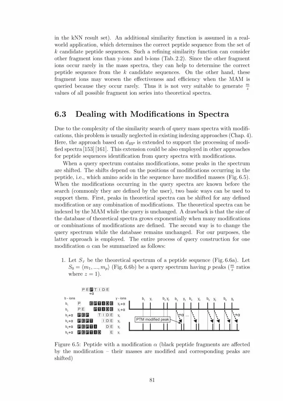
in the kNN result set). An additional similarity function is assumed in a real-world application, which determines the correct peptide sequence from the set ofk candidate peptide sequences. Such a refining similarity function can considerother fragment ions than y-ions and b-ions (Tab. 2.2). Since the other fragmentions occur rarely in the mass spectra, they can help to determine the correctpeptide sequence from the k candidate sequences. On the other hand, thesefragment ions may worsen the effectiveness and efficiency when the MAM isqueried because they occur rarely. Thus it is not very suitable to generate m

z

values of all possible fragment ion series into theoretical spectra.

6.3 Dealing with Modifications in Spectra

Due to the complexity of the similarity search of query mass spectra with modifi-cations, this problem is usually neglected in existing indexing approaches (Chap. 4).Here, the approach based on dHP is extended to support the processing of modi-fied spectra [153] [161]. This extension could be also employed in other approachesfor peptide sequences identification from query spectra with modifications.

When a query spectrum contains modifications, some peaks in the spectrumare shifted. The shifts depend on the positions of modifications occurring in thepeptide, i.e., which amino acids in the sequence have modified masses (Fig. 6.5).When the modifications occurring in the query spectra are known before thesearch (commonly they are defined by the user), two basic ways can be used tosupport them. First, peaks in theoretical spectra can be shifted for any definedmodification or any combination of modifications. The theoretical spectra can beindexed by the MAM while the query is unchanged. A drawback is that the size ofthe database of theoretical spectra grows exponentially when many modificationsor combinations of modifications are defined. The second way is to change thequery spectrum while the database remains unchanged. For our purposes, thelatter approach is employed. The entire process of query construction for onemodification α can be summarized as follows:

1. Let ST be the theoretical spectrum of a peptide sequence (Fig. 6.6a). LetS0 = 〈m1, ...,mp〉 (Fig. 6.6b) be a query spectrum having p peaks (m

zratios

where z = 1).

P

P E

T I D E

I D E

D E

E

E T I D EP+α

+α ... +αPTM modified peak

+α

+α

+α

+α

+α

+α

Figure 6.5: Peptide with a modification α (black peptide fragments are affectedby the modification – their masses are modified and corresponding peaks areshifted)

81

2. When a modification α (e.g., α = 57) happens at an unknown position i inthe peptide, only mi and some of the following peaks are shifted. Since wecannot predict this position, the entire spectrum is shifted by −α. A shiftedvector of the spectrum S0 for the modification α is Sα = 〈m1−α, ...,mp−α〉(Fig. 6.6c). Thus peaks shifted by α in S0 have their ”unshifted” counter-parts in Sα.

3. S0 and Sα are appended (Fig. 6.6d), where the union of spectra S0 ∪ Sα isa sorted vector of all peaks in the spectra S0 and Sα.

4. While S0 forms the query for an unmodified spectrum, the query for thespectrum with the modification α is SI = S0 ∪ Sα.

A disadvantage is that two other types of noise peaks occur in queries. First,the peaks shifted ”in vitro” in S0 which are superfluous in the union S0 ∪ Sα.Second, the artificial noise peaks computed in Sα, which were not modified andthey should not have been shifted in Sα. These two types of noise peaks cannotbe removed, because we are not able to recognize them. Since mass spectracontain many noise peaks and dHP is able to reduce them, the other noise peaksare partially reduced as well.

In case of two modifications α and β, the query is represented by spectrumSII = S0 ∪ Sα ∪ Sβ ∪ Sα+β, where α + β are peaks shifted by both modificationsat once. In case of three modifications α, β and γ, the query is representedby spectrum SIII = S0 ∪ Sα ∪ Sβ ∪ Sγ ∪ Sα+β ∪ Sα+γ ∪ Sβ+γ ∪ Sα+β+γ, etc.Since lengths of peptide sequences are limited, the number of modifications perspectrum usually does not exceed 2 or 3 (Tab. 7.1). Therefore the maximumnumber of shifted spectra unified in the query, which might be up to

∑ni=0

(ni

)for n different modifications, is not reached in practice.

Figure 6.6: Dealing with modifications (ST corresponds to S0 with the modifica-tion α happened at position 3 in the respective peptide sequence)

82

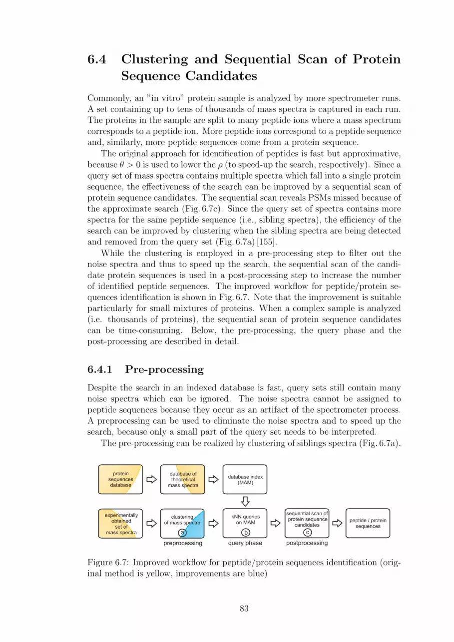
6.4 Clustering and Sequential Scan of Protein

Sequence Candidates

Commonly, an ”in vitro” protein sample is analyzed by more spectrometer runs.A set containing up to tens of thousands of mass spectra is captured in each run.The proteins in the sample are split to many peptide ions where a mass spectrumcorresponds to a peptide ion. More peptide ions correspond to a peptide sequenceand, similarly, more peptide sequences come from a protein sequence.

The original approach for identification of peptides is fast but approximative,because θ > 0 is used to lower the ρ (to speed-up the search, respectively). Since aquery set of mass spectra contains multiple spectra which fall into a single proteinsequence, the effectiveness of the search can be improved by a sequential scan ofprotein sequence candidates. The sequential scan reveals PSMs missed because ofthe approximate search (Fig. 6.7c). Since the query set of spectra contains morespectra for the same peptide sequence (i.e., sibling spectra), the efficiency of thesearch can be improved by clustering when the sibling spectra are being detectedand removed from the query set (Fig. 6.7a) [155].

While the clustering is employed in a pre-processing step to filter out thenoise spectra and thus to speed up the search, the sequential scan of the candi-date protein sequences is used in a post-processing step to increase the numberof identified peptide sequences. The improved workflow for peptide/protein se-quences identification is shown in Fig. 6.7. Note that the improvement is suitableparticularly for small mixtures of proteins. When a complex sample is analyzed(i.e. thousands of proteins), the sequential scan of protein sequence candidatescan be time-consuming. Below, the pre-processing, the query phase and thepost-processing are described in detail.

6.4.1 Pre-processing

Despite the search in an indexed database is fast, query sets still contain manynoise spectra which can be ignored. The noise spectra cannot be assigned topeptide sequences because they occur as an artifact of the spectrometer process.A preprocessing can be used to eliminate the noise spectra and to speed up thesearch, because only a small part of the query set needs to be interpreted.

The pre-processing can be realized by clustering of siblings spectra (Fig. 6.7a).

Figure 6.7: Improved workflow for peptide/protein sequences identification (orig-inal method is yellow, improvements are blue)

83

Even though a set of query spectra commonly contains more spectra correspond-ing to a peptide sequence, it is advantageous when query sets from more spec-trometer runs can be appended. Hence, many interpretable spectra which arecaptured only once per a spectrometer run have a sibling spectrum in the queryset and they are not eliminated by the clustering. On the other hand, the noisespectra are successfully cleared away and thus many spectra do not have to besearched in the query phase (Fig. 6.7b), making the search significantly faster.

We use a simple hierarchical clustering based on the complete linkage (Alg. 16),i.e., all spectra in a cluster are similar to each other. The algorithm requires a setof clusters C initialized with one mass spectrum per cluster. Then two phases arerepeated in w cycles. First, pairs of clusters in the minimum dHP (ci,0, cj,0) suchthat dHP (ci,0, cj,0) ≤ t are merged, where t is a threshold of the dHP and ci,0, cj,0are the centroids of clusters ci, cj (Alg. 17). The threshold t determines whetherthe spectra in a cluster are similar or not. Moreover, it determines the numberof clusters. If t is too low, each spectrum forms a singleton (a cluster containingone spectrum). If t is too high, all spectra form one big cluster.

Second, the spectra are rearranged among the clusters (Alg. 19). A spectrumis moved to another cluster, if the dHP between the query spectrum and anyspectrum in the target cluster is less or equal t and the difference of precursormasses is less or equal λ. In case that more clusters are selected, the cluster ispicked where the dHP between its centroid and the moved object is minimal.

New centroids of clusters are selected after each phase (Alg. 18). Finally,the centroids of clusters containing at least two spectra form the queries, whichare processed by the MAM. Another way consists in putting all peaks from allthe spectra in the cluster into a representative spectrum. The intensities of theclosest peaks are counted up and their m

zvalues are averaged. Since the increasing

number of peaks in a spectrum worsens the efficiency of MAMs because of highintrinsic dimensionality ρ, this alternative needs to be a bit of improved. Forexample, a specified number of peaks with the highest intensity might be selectedfrom the representative spectrum.

6.4.2 Query phase

The query phase (Fig. 6.7b) corresponds to the original idea proposed in Sec. 6.2.2,where a kNN query is performed by a MAM for each query spectrum selectedin the pre-processing step. The k nearest neighbor peptide sequences to eachquery spectrum are assigned to the protein sequences of their origin. The proteinsequences containing at least one ”good” peptide sequence hit (e.g., dHP ≤ 0.65)form the protein sequence candidates.

6.4.3 Post-processing

The post-processing is a sequential scan of protein sequence candidates (Fig. 6.7c),which significantly improves the number of identified peptide sequences becausemore peptide sequences in a protein sequence correspond to the mass spectra inthe query set [162] [23]. The protein sequence candidates (i.e., a small subset ofthe database sequences selected in the query phase) are split to peptide sequencesand their theoretical spectra are compared to the entire set of input query spectra

84

(as it was before the clustering phase). Many spectra previously missed duringthe pre-processing or during the query phase are assigned to peptide sequences.The newly identified peptide sequences are assigned to the protein sequences oftheir origin. Finally, the peptide (or protein, respectively) sequences identified inthe query phase and refined in the post-processing phase form the result. Notethat some peptide sequences are lost during the clustering because their spectraare present only once in the query set. Some peptide sequences are lost duringthe query phase because the search is only approximative (non-metric). Thesequential scan of protein sequence candidates helps to reveal a peptide sequencein case it forms a part of a candidate protein sequence which is hit by anotherpeptide sequence.

Algorithm 16: Clustering of query mass spectra (main function)

1 Function Clustering(C, t,w)2 Input:

A set of clusters C initialized with one query mass spectrum per cluster;a threshold t;a number of clustering cycles w.

3 Output:The set of clusters C.

4 begin5 for i = 1 to w do6 MergeClusters(C, t);7 SelectCentroids(C);8 RearrangeClusters(C, t);9 SelectCentroids(C);

Algorithm 17: Clustering of query mass spectra (MergeClusters)

1 Function MergeClusters(C, t)2 Input:

A set of clusters C;a threshold t.

3 Output:The set of clusters C.

4 begin5 for all clusters ci ∈ C do6 for all clusters cj ∈ C do7 if i 6= j then8 /* a centroid of the cluster ci is stored at ci,0 */

9 if all spectra cj,k in the cluster cj have dHP (ci,0, cj,k) ≤ tthen

10 store the position j of the cluster cj in the minimumdHP (ci,0, cj,0) into p;

11 merge the clusters ci and cp;

85

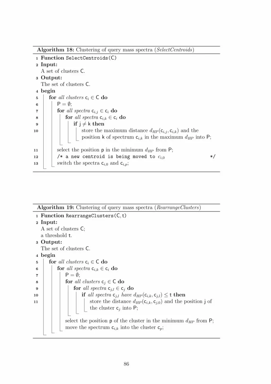
Algorithm 18: Clustering of query mass spectra (SelectCentroids)

1 Function SelectCentroids(C)2 Input:

A set of clusters C.3 Output:

The set of clusters C.4 begin5 for all clusters ci ∈ C do6 P = ∅;7 for all spectra ci,j ∈ ci do8 for all spectra ci,k ∈ ci do9 if j 6= k then

10 store the maximum distance dHP (ci,j, ci,k) and theposition k of spectrum ci,k in the maximum dHP into P;

11 select the position p in the minimum dHP from P;12 /* a new centroid is being moved to ci,0 */

13 switch the spectra ci,0 and ci,p;

Algorithm 19: Clustering of query mass spectra (RearrangeClusters)

1 Function RearrangeClusters(C, t)2 Input:

A set of clusters C;a threshold t.

3 Output:The set of clusters C.

4 begin5 for all clusters ci ∈ C do6 for all spectra ci,k ∈ ci do7 P = ∅;8 for all clusters cj ∈ C do9 for all spectra cj,l ∈ cj do

10 if all spectra cj,l have dHP (ci,k, cj,l) ≤ t then11 store the distance dHP (ci,k, cj,0) and the position j of

the cluster cj into P;

select the position p of the cluster in the minimum dHP from P;move the spectrum ci,k into the cluster cp;

86

Chapter 7

Experiments

In this chapter, an experimental evaluation of the methods described in Chap. 6 isproposed. First, the quantities measured in the experiments and the data sets aredescribed. Then the T-bases for dHP and dA determined by the TriGen algorithmare proposed. The T-bases enable the utilization of the distances for fast andapproximate search by MAMs.

The efficiency and effectiveness of peptide sequences identification by non-metric access methods are studied without and with the support of modifica-tions [153]. The utilization of different indexing structures is analyzed (M-tree,LAESA and NM-tree) [154] [163]. An improvement of this approach is also testedwhere a pre-processing by clustering is employed to speed up the search and apost-processing by a sequential scan of protein sequence candidates is used toincrease the number of identified peptide sequences [155].

Finally, a comparison of the state-of-the-art tools with the parameterizedHausdorff distance dHP and with the modification of the parameterized Hausdorffdistance dmatchHP is proposed where the precursor mass filter is utilized instead ofMAMs [160].

7.1 Measured Quantities

The following quantities were measured in the experiments utilizing MAMs:

1. The correctness of mass spectra interpretation (correctness/quality of pep-tide sequences identification or ratio of identified spectra) as a ratio of massspectra correctly annotated with peptide sequences to all spectra in thequery set (i.e., to a ground truth determined by another peptide identifi-cation engine). We assume that a peptide sequence is correctly annotatedwhen the correct peptide sequence is among the k nearest neighbors to thequery spectrum.

2. The distance computations ratio as a ratio of the average number of distancecomputations (the number of calls of a pair-wise distance function, e.g.,dHP ) per one mass spectrum interpretation to the cost of the sequentialscan.

3. The average query time per one mass spectrum interpretation.

87

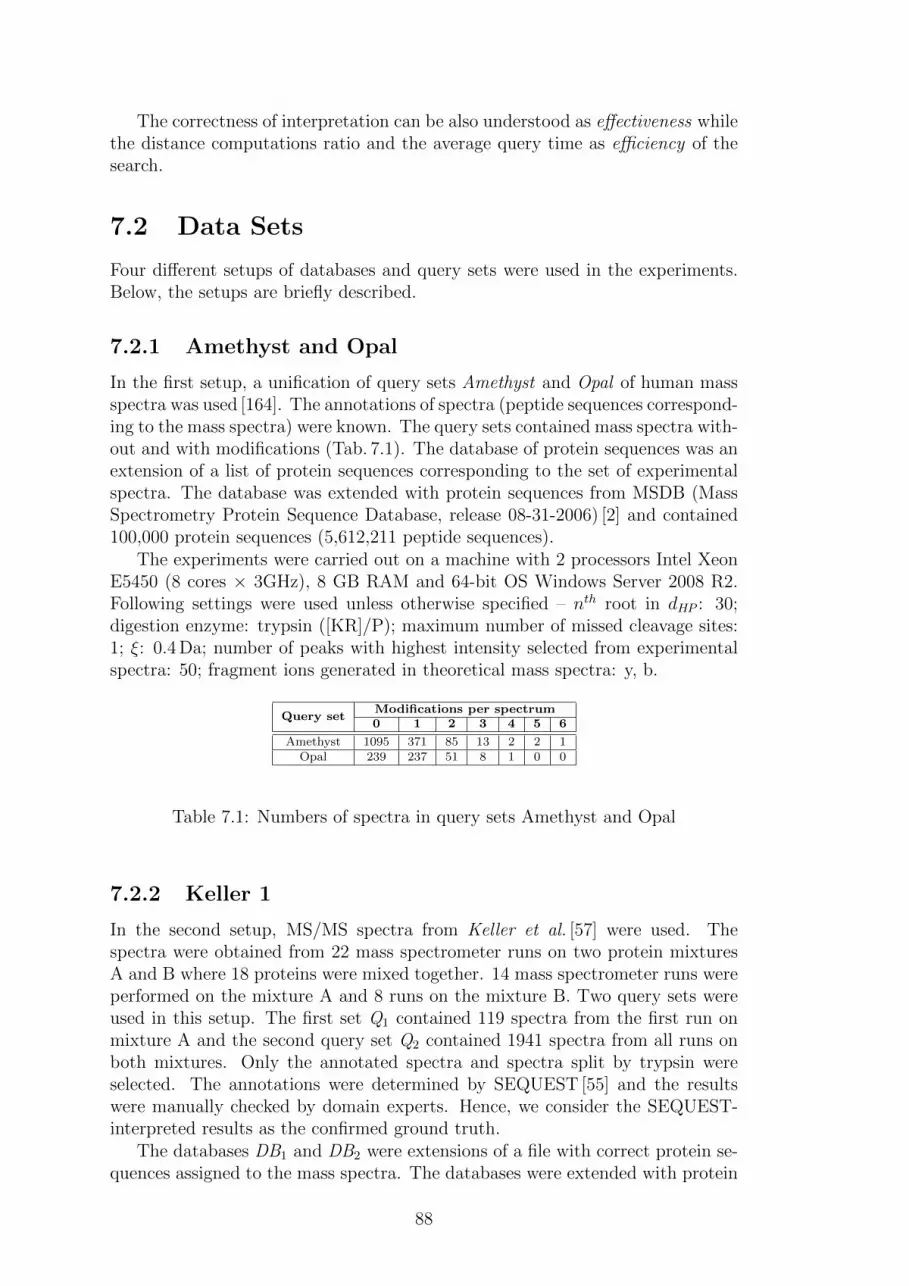
The correctness of interpretation can be also understood as effectiveness whilethe distance computations ratio and the average query time as efficiency of thesearch.

7.2 Data Sets

Four different setups of databases and query sets were used in the experiments.Below, the setups are briefly described.

7.2.1 Amethyst and Opal

In the first setup, a unification of query sets Amethyst and Opal of human massspectra was used [164]. The annotations of spectra (peptide sequences correspond-ing to the mass spectra) were known. The query sets contained mass spectra with-out and with modifications (Tab. 7.1). The database of protein sequences was anextension of a list of protein sequences corresponding to the set of experimentalspectra. The database was extended with protein sequences from MSDB (MassSpectrometry Protein Sequence Database, release 08-31-2006) [2] and contained100,000 protein sequences (5,612,211 peptide sequences).

The experiments were carried out on a machine with 2 processors Intel XeonE5450 (8 cores × 3GHz), 8 GB RAM and 64-bit OS Windows Server 2008 R2.Following settings were used unless otherwise specified – nth root in dHP : 30;digestion enzyme: trypsin ([KR]/P); maximum number of missed cleavage sites:1; ξ: 0.4 Da; number of peaks with highest intensity selected from experimentalspectra: 50; fragment ions generated in theoretical mass spectra: y, b.

Query setModifications per spectrum0 1 2 3 4 5 6

Amethyst 1095 371 85 13 2 2 1Opal 239 237 51 8 1 0 0

Table 7.1: Numbers of spectra in query sets Amethyst and Opal

7.2.2 Keller 1

In the second setup, MS/MS spectra from Keller et al. [57] were used. Thespectra were obtained from 22 mass spectrometer runs on two protein mixturesA and B where 18 proteins were mixed together. 14 mass spectrometer runs wereperformed on the mixture A and 8 runs on the mixture B. Two query sets wereused in this setup. The first set Q1 contained 119 spectra from the first run onmixture A and the second query set Q2 contained 1941 spectra from all runs onboth mixtures. Only the annotated spectra and spectra split by trypsin wereselected. The annotations were determined by SEQUEST [55] and the resultswere manually checked by domain experts. Hence, we consider the SEQUEST-interpreted results as the confirmed ground truth.

The databases DB1 and DB2 were extensions of a file with correct protein se-quences assigned to the mass spectra. The databases were extended with protein

88

sequences from MSDB (release 08-31-2006) [2]. The DB1 contained 100,000 pro-tein sequences (5,600,747 peptide sequences) and DB2 contained 500,000 proteinsequences (29,460,880 peptide sequences).

The experiments were carried out on a machine with 2 processors Intel XeonE5450 (8 cores × 3GHz) with 8 GB RAM and 64-bit OS Windows Server 2008R2. By default, the average query time per one mass spectrum interpretation wasmeasured on 8 processor cores. The following settings were used unless otherwisespecified – nth root in dHP : 50; digestion enzyme: trypsin ([KR]/P); maximumnumber of missed cleavage sites: 1; ξ: 0.4 Da; precursor mass error tolerance (λ):2 Da; number of peaks with highest intensity selected from experimental spectra:100; fragment ions generated in theoretical mass spectra: y, b.

7.2.3 Keller 2

In the third setup, MS/MS spectra fromKeller et al. [57] were also used. Thespectra from the first 6 runs on mixture A and from all runs on mixture B wereused. The query spectra were searched against the database DB1 (Sec 7.2.2).

The experiments were carried out on a machine with 2 processors Intel XeonX5660 (24 cores, 2.8 GHz) with 24 GB RAM and 64-bit OS Windows Server2008 R2. The stated average query times of clustering and peptide sequencesidentification are measured on one core. If not otherwise stated, the followingsettings were used – digestion enzyme: trypsin ([KR]/P); maximum number ofmissed cleavage sites: 1; mass range of peptide ions generated from the database:500-5,000 Da; fragment ions generated in hypothetical mass spectra: y-ions andb-ions; mass range of generated fragment ions: 300-2,000; m

zerror tolerance (ξ):

0.4 Da; number of peaks with highest intensity used in a query: 50; distancemeasure: dHP (with n = 30); clustering threshold (t): 0.65 (values returned bydHP were normalized to 〈0, 1〉), T-error tolerance θ: 0.1.

7.2.4 E. coli and Human

HPLC-MS/MS spectra from E. coli and human were used in the last setup. Sep-aration of the E. coli digest was performed using an easyLC HPLC system (Prox-ean) with a 2 h segmented gradient. Peptides eluting from the column were on-lineinjected into an LTQ-Orbitrap XL instrument (Thermo Fisher Scientific), withtop 10 selection of the most abundant ions for further fragmentation. A dynamicexclusion list of 500 masses and exclusion time of 90 seconds was used to avoidrepeated fragmentation of the same ions. The query set E.coli contained 30,358tandem mass spectra. Human spectra were taken from 2 runs from a label-freehuman data set [165] – the query set Hum48 contained 26,417 spectra and Hum49contained 24,537 spectra. The query sets are also available at [166] or [167].

The manually curated database containing 8,272 protein (332,862 peptide) se-quences was used with E.coli. The database of 173,450 human protein (9,567,012peptide) sequences from UniProtKB/Swiss-Prot (v. 07/2012) [3] was used withhuman query sets. Decoy protein sequences were included in both databases.Theoretical spectra were generated with following settings – digestion enzyme:trypsin ([KR]/P); maximum number of missed cleavage sites: 1; length of peptidesequences: 7-50 amino acids; precursor mass of peptides: 500-5,000 Da; fragment

89

ions types: y, b, y2+; mz

ratios of fragment ions: 200-2,000 Da. Query spectra wereprocessed as follows – minimum number of peaks in a spectrum to be processed:30; peak selection heuristic: the range of m

zvalues was split by 50 Da, 5 most

intense peaks were selected in each window and 50 most intense peaks were se-lected from the unification of the most intense peaks in the windows. λ = 10 ppm,ξ = 0.5 Da and n = 30 (in dHP and dmatchHP ). A machine with Windows 7 x64,Intel Core i7 2GHz, 8 GB RAM and 5400 rpm HDD was used.

7.3 TriGen-based Modifications

Even though the dHP (Sec. 6.1.3) and dA (Sec. 6.1.1) are semi-metric distances,the T-error of each of them is very low (below 0.001) but the intrinsic dimen-sionality ρ is very high (ρ = 88.5 for dHP and ρ = 158.1 for dA). Thus, theTriGen algorithm (Sec. 5.2.4) was used to improve ρ. The dA and dHP must benormalized to 〈0, 1〉 in order to employ the TriGen. The dA is normalized by π

2,

while dHP is normalized by n√dmaxh , where dmaxh is the maximum mass of theoret-

ically generated peptides (e.g., 5000 Da). The modifications of dHP and dA weredetermined for the experimental setups proposed in Sec. 7.2.1 and Sec. 7.2.2.

7.3.1 FP-bases for Amethyst and Opal

The TriGen was used on a sample of the database from Sec. 7.2.1 to improve theintrinsic dimensionality ρ, setting the T-error tolerances θ to the range 0 – 0.1.The FP-base was used. For all θ, the TriGen found convex T-modifiers (w < 0),so ρ was reduced (down to 2.3 for θ = 0.1). The resulting FP-bases determinedby TriGen for dHP (n = 30) and dA are shown in Tab. 7.2.

dHP dAT-error ρ w ρ w

0 88.5 -0.17 158.1 -0.840.01 5.2 -4.44 11.1 -7.430.02 4.0 -5.23 8.5 -8.940.03 3.5 -5.71 7.1 -10.010.04 3.2 -6.08 6.3 -10.920.05 2.9 -6.40 5.7 -11.650.06 2.8 -6.64 5.2 -12.340.07 2.6 -6.87 4.8 -13.000.08 2.5 -7.06 4.5 -13.630.09 2.4 -7.25 4.2 -14.280.1 2.3 -7.42 3.9 -14.92

Table 7.2: ρ and empirically determined FP-bases for dHP (n = 30) and dA

7.3.2 FP-bases and RBQ-bases for Keller 1

The TriGen was used on a sample of the database DB1 from Sec. 7.2.2, settingθ to the range 0.001 – 0.2. The FP-base and 454 different RBQ-bases (differentpoints (a, b)) were used. For all θ the TriGen found convex T-modifiers (w < 0),so the intrinsic dimensionality ρ was reduced (down to 2.1 for θ = 0.2). Theresulting T-bases with smallest ρ determined by the TriGen for dHP (n = 50)

90

FP(v,w) RBQ(a,b)(v,w)

T-err.tol. ρ T-err. w ρ T-err. a b w0.001 18.6 0.001 -2.6 15.7 0.001 0.22 0.82 -3.10.01 7.6 0.013 -5.0 6.8 0.013 0.22 0.82 -11.30.02 6.0 0.023 -5.9 5.7 0.020 0.22 0.82 -20.50.04 4.5 0.042 -7.0 4.6 0.042 0.13 0.83 -7.60.06 3.8 0.062 -7.9 3.7 0.061 0.13 0.83 -10.40.08 3.3 0.082 -8.6 3.1 0.081 0.13 0.83 -15.30.1 3.0 0.102 -9.2 2.8 0.092 0.13 0.83 -20.40.12 2.8 0.120 -9.6 2.3 0.112 0.13 0.83 -54.90.14 2.6 0.138 -10.1 2.7 0.140 0.05 0.85 -6.40.16 2.4 0.154 -10.5 2.5 0.160 0.05 0.85 -7.10.18 2.3 0.173 -10.9 2.3 0.174 0.05 0.85 -7.50.2 2.2 0.191 -11.3 2.1 0.196 0.05 0.85 -8.4

Table 7.3: ρ and empirically determined FP and RBQ-bases for dHP (n = 50)

are shown in Tab. 7.3. ρ is slightly better when RBQ-bases are used than whenFP-base is used, however, testing many RBQ-bases is time-consuming.

7.4 Effectiveness and Efficiency of Non-metric

Similarity Search

The algorithm for identification of peptide sequences using the approximate sim-ilarity search by MAMs (Sec. 6.2) was tested on query sets Amethyst and Opal(Sec. 7.2.1) [153]. First, the correctness of interpretation using dHP was testedwhen the sequential scan of entire database was employed. Second, the impactof T-bases determined by TriGen on the indexability by MAMs was analyzed.Finally, the speed up and correctness of interpretation on M-tree with TriGenmodified dHP were studied.

7.4.1 Sequential Scan

Figure 7.1: Sequential scan – correctness of interpretation (dHP )

The sequential scan of entire database of theoretical spectra was performedwhile dHP was utilized. The correctness of interpretation and average query timewere measured lacking spectra with modifications. The correctness of interpreta-tion was bigger with increasing index of the root n (Fig. 7.1). It was up to 98.3%when n = 30 and 10 NN queries were used. The average query time was 14.4 s.The correctness of interpretation was 95.7% and the average query time was 9.8 swhen dA and 10 NN queries were used.

91

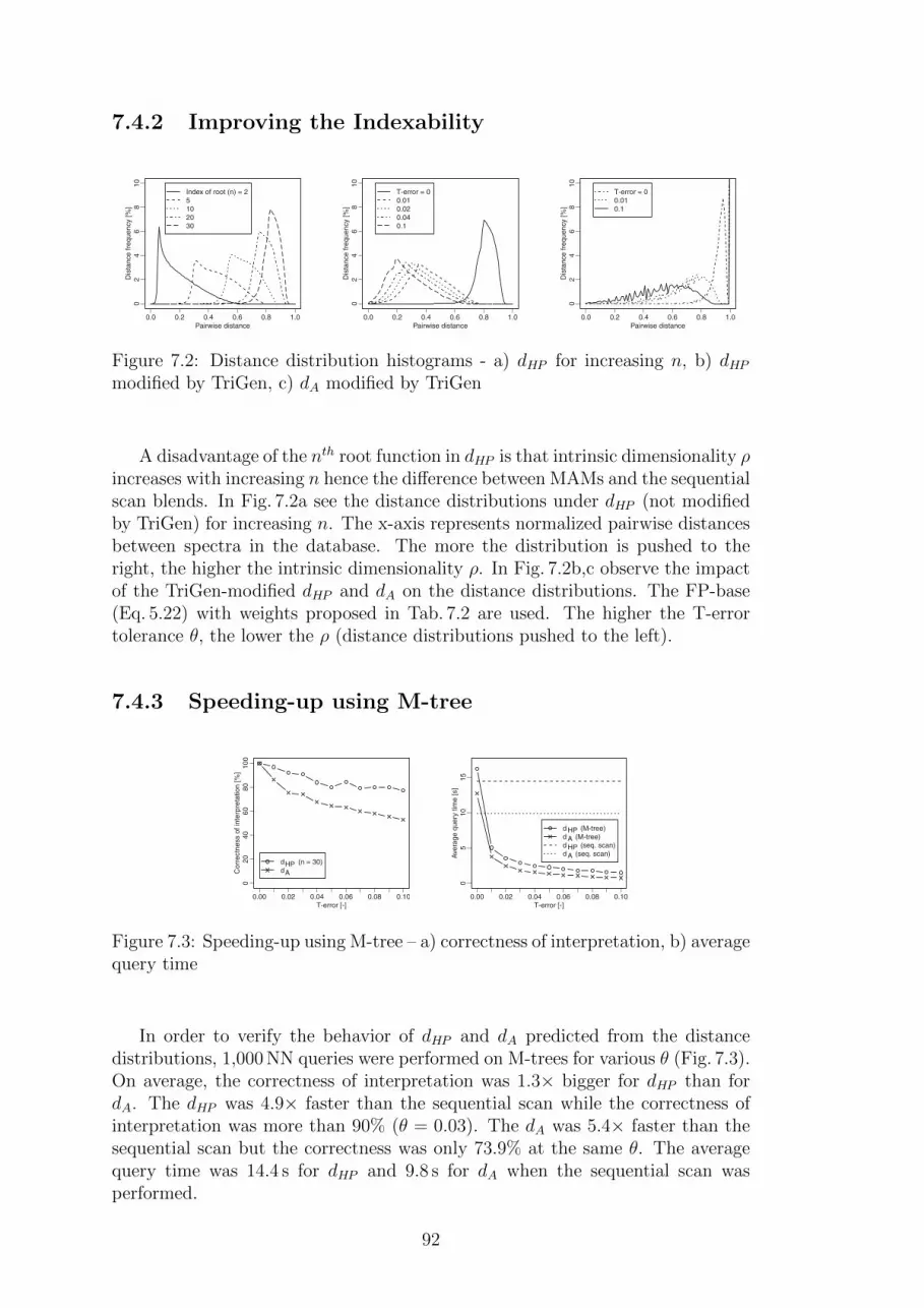
7.4.2 Improving the Indexability

Figure 7.2: Distance distribution histograms - a) dHP for increasing n, b) dHPmodified by TriGen, c) dA modified by TriGen

A disadvantage of the nth root function in dHP is that intrinsic dimensionality ρincreases with increasing n hence the difference between MAMs and the sequentialscan blends. In Fig. 7.2a see the distance distributions under dHP (not modifiedby TriGen) for increasing n. The x-axis represents normalized pairwise distancesbetween spectra in the database. The more the distribution is pushed to theright, the higher the intrinsic dimensionality ρ. In Fig. 7.2b,c observe the impactof the TriGen-modified dHP and dA on the distance distributions. The FP-base(Eq. 5.22) with weights proposed in Tab. 7.2 are used. The higher the T-errortolerance θ, the lower the ρ (distance distributions pushed to the left).

7.4.3 Speeding-up using M-tree

Figure 7.3: Speeding-up using M-tree – a) correctness of interpretation, b) averagequery time

In order to verify the behavior of dHP and dA predicted from the distancedistributions, 1,000 NN queries were performed on M-trees for various θ (Fig. 7.3).On average, the correctness of interpretation was 1.3× bigger for dHP than fordA. The dHP was 4.9× faster than the sequential scan while the correctness ofinterpretation was more than 90% (θ = 0.03). The dA was 5.4× faster than thesequential scan but the correctness was only 73.9% at the same θ. The averagequery time was 14.4 s for dHP and 9.8 s for dA when the sequential scan wasperformed.

92

7.5 Dealing with Modifications in Spectra

The identification of peptide sequences from query spectra with modificationshas been tested on query sets Amethyst and Opal (Sec. 7.2.1). A modified queryspectrum was generated for each query spectrum (Sec. 6.3).

7.5.1 Sequential Scan

Modifications Correctness of interpretation [%]per spectrum 1 NN 10 NN 100 NN 1,000 NN

without the support of modifications1 20.0 41.0 61.7 75.02 9.3 18.6 28.7 65.83 0 0 0 0

with the support of modifications1 69.9 84.0 94.3 98.92 24.8 55.1 76.8 90.83 31.0 54.8 61.9 100.0

Table 7.4: Correctness of interpretation without and with the support of modifi-cations

The correctness of interpretation was measured without and with the sup-port of modifications (Tab. 7.4). 467 spectra containing one modification, 77spectra containing two modifications and 10 spectra containing three modifica-tions were used. The following modifications α∈{−28, −17, −14, 1, 14, 16, 28,57}, pairs of modifications {α, β}∈ {{−17, 57} , {57, 57}} and triplets of modi-fications {α, β, γ}∈ {{−17, 57, 57} , {57, 57, 57}} were searched. The queries SIwere performed for spectra with one modification, SII for spectra containing twomodifications and SIII for spectra containing three modifications (Sec. 6.3).

Since modifications commonly do not shift all peaks in the query spectra, thedHP is partially able to determine correct peptide sequences when modificationsin the query spectra are not supported. The correctness of interpretation is morethan 90% in all cases when modifications are supported (1,000 NN queries). Itdecreases with increasing number of modifications per spectrum when smallerkNN queries are used.

The number of peaks in a query and the average query time increase withincreasing number of supported modifications. The average query time is 18.9 sfor spectra with one modification, 24.2 s for spectra with two modifications and35.6 s for spectra with three modifications.

7.5.2 Speeding-up using M-tree

A set of 1,000 NN queries was processed on M-trees for different θ when the dHPwas employed. Results for spectra with one and two modifications are shownin Fig. 7.4. The M-tree was 3.3× faster for spectra with one modification and2.5× faster for spectra with two modifications than the sequential scan (T-error= 0.06) while the correctness of interpretation was still about 90%.

93

Figure 7.4: Speeding-up using M-tree (spectra with modifications) – a) correct-ness of interpretation and b) average query time

7.6 Advanced Analysis of Non-metric Similarity

Search

The algorithm for identification of peptide sequences using the approximate sim-ilarity search by MAMs (Sec. 6.2) was additionally tested using the setup Keller 1(Sec. 7.2.2) [154]. The dHP , d′HP , dA and d′A were compared, the M-tree was com-pared with LAESA and NM-tree, and the impact of different k in kNN querieson the efficiency and effectiveness of the search was also studied.

7.6.1 Comparison of dHP , d′HP , dA and d′A

The indexability of dHP (n = 50) was analyzed when FP-bases and RBQ-basesproposed in Tab. 7.3 were used. In Fig. 7.5a,b observe the impact of T-errortolerance θ on the distance distributions obtained using the TriGen-modified dHP ,considering either FP-base or RBQ-bases. Obviously, a higher θ leads to a moreconvex T-modifier, and so to lower ρ (distance distribution pushed to the left).In Fig. 7.5c, see the same for the angle distance dA. In fact, about 35% of allpairwise distances are in the maximum distance dA = 1 (not shown for all T-error tolerances in Fig. 7.5c for better readability). These 35% distances cannotbe fixed by the TriGen algorithm because they are indistinguishable.

In Fig. 7.5a,c, the distances d′HP (Eq. 6.12) and d′A (Eq. 6.11) are shown for acomparison with dHP and dA (the TriGen was not employed because T-error

.= 0;

c1 = 1, c2 = 1 for both d′HP and d′A). Since the indexability of d′HP and d′A isgood, the average query time and the correctness of interpretation were measuredon DB2 indexed by M-tree where 1000NN queries and Q2 were used. The average

0

2

4

6

8

10

0 25 50 75 100Pairwise distance [%]

Dis

tance

frequency

[%]

T-error tolerance = 00.040.120.2d’HP (precursor mass)

0

2

4

6

8

10

0 25 50 75 100Pairwise distance [%]

Dis

tance

frequency

[%]

T-error tolerance = 00.040.120.2

0

5

10

15

0 25 50 75 100Pairwise distance [%]

Dis

tance

frequency

[%]

T-error tolerance = 00.040.120.2d’A (precursor mass)

Figure 7.5: Distance distribution histograms – a) dHP with FP-base and d′HP , b)dHP with RBQ-bases, c) dA with FP-base and d′A

94

query time was only 0.4 s for d′A and d′HP . The d′HP with the M-tree was 33×faster than the sequential scan. It was also 14.9× faster than dHP with M-treewhen θ = 0.1 (see the curve for 103NN in Fig. 7.9a for a comparison with dHP fordifferent θ).

The correctness of interpretation was 89.6% for d′A and 85.7% for d′HP . Sincethe search is approximate, the correctness was only 57.8% for dHP when θ = 0.1(see the curve for 103NN in Fig. 7.8a for a comparison with dHP for different θ).Although the indexability, the correctness of identification and the speed up ofd′HP were good on the M-tree, an extension of d′HP (and d′A) for the identificationof peptides from query spectra containing modifications might be limited becaused′HP aggregates dHP with the difference of precursor masses of compared spectra.

7.6.2 Comparison of M-tree with LAESA

The M-tree and LAESA (pivot table) utilizing the dHP with FP-base were com-pared to the sequential scan of entire database. The experiments were performedon DB1 and Q1, 2000NN queries were used, and 8 processor cores were employed.The LAESA was constructed for 40 randomly selected pivots. The distance com-putations ratio got lower (w.r.t. seq. scan) when the T-error tolerance θ washigher. The lowest numbers of distance computations were obtained using LAE-SA for θ = 0.04 and higher (Fig. 7.6c). However, the best average query time wasobtained using M-tree (Fig. 7.6b). Since LAESA was stored in the main memory,it was also fast, but the size of the pivot table was almost 2 GB. The correctnessof interpretation was lower with increasing T-error tolerance θ for both – M-treeand LAESA (Fig. 7.6a).

The performance of M-tree and LAESA (having 50 pivots) with dHP wasalso tested on databases of different sizes generated from DB1 (from 10 to 100thousands of proteins; from 650 thousands to 5.6 millions of peptides or indexedvectors). The Fig. 7.7a shows the impact of the database size on the averagequery time, while θ = 0.1. The LAESA is faster than the M-tree as long as all itsblocks are stored in the main memory. If the main memory size is exceeded, theLAESA becomes inefficient. A 600 MB buffer was allocated in the main memoryand it was exceeded when 25 thousands of protein sequences (1.5 millions ofpeptides) were indexed by LAESA. Moreover, for more than 40 thousands ofprotein sequences (2.4 millions of peptides) the sequential scan outperformed theLAESA. Fig. 7.7b shows that distance computations are misleading for LAESAwhen the size of the main memory is exceeded.

0

20

40

60

80

100

0 0.04 0.08 0.12 0.16 0.2T-error tolerance

Corr

ectn

ess

ofin

terp

reta

tion

[%]

Pivot tableM-treesequential

0

0.5

1

1.5

2

2.5

3

0 0.04 0.08 0.12 0.16 0.2T-error tolerance

Avera

ge

query

tim

e[s

]

Pivot tableM-treesequential

0

20

40

60

80

100

0 0.04 0.08 0.12 0.16 0.2T-error tolerance

Dis

tance

com

puta

tions

ratio

[%]

Pivot tableM-tree

Figure 7.6: Comparison of M-tree and LAESA – a) correctness of interpretation,b) average query time, c) distance computations ratio

95

0

2

4

6

8

10

1.3 2.4 3.7 4.5 5.6Database size [millions of peptides]

Avera

ge

query

tim

e[s

]

Pivot tableM-treesequential

0

5

10

15

20

25

1.3 2.4 3.7 4.5 5.6Database size [millions of peptides]

Dis

tance

com

puta

tions

ratio

[%]

Pivot tableM-tree

Figure 7.7: Database size – a) average query time, b) distance computations ratio

7.6.3 k in kNN queries

The following experiments were performed on M-tree while DB2 and Q2 wereutilized. The correctness of mass spectra interpretation is lower with increasingT-error tolerance θ. However, the kNN queries with higher k can be used to avoidthis problem (Fig. 7.8a). The correct peptide sequences are not spread uniformlyover all interval 〈1..k〉 of a kNN query result set but they are cumulated amonga few nearest neighbors in many cases. As shown in Fig. 7.8b, the first nearestneighbor taken from the 100NN result was more likely to be correct than whentaking the first nearest neighbor from 10NN result. The average query time of akNN query and its distance computations ratio (w.r.t. sequential scan) increaseswith k (Fig. 7.9).

0

20

40

60

80

100

0.04 0.08 0.12 0.16 0.2

+ 1NN

+ 10NN

+ 102NN+ 103NN

T-error tolerance

Corr

ectn

ess

ofin

terp

reta

tion

[%]

Seq.scan

[kN

N]

1NN10NN102NN103NN

0

20

40

60

80

100

0.04 0.08 0.12 0.16 0.2

+ 1NN

+ 10NN

+ 102NN+ 103NN

T-error tolerance

Corr

ectn

ess

ofin

terp

reta

tion

[%]

Seq.scan

[kN

N]

1NN of 10NN1NN of 102NN1NN of 103NN10NN of 102NN10NN of 103NN

Figure 7.8: k in kNN queries – correctness of interpretation (dHP )

0

5

10

15

20

25

0.04 0.08 0.12 0.16 0.2T-error tolerance

Avera

ge

query

tim

e[s

]

1NN10NN102NN103NNsequential

0

5

10

15

20

25

0.04 0.08 0.12 0.16 0.2T-error tolerance

Dis

tance

com

puta

tions

ratio

[%]

1NN10NN102NN103NN

Figure 7.9: kNN queries – a) average query time, b) distance computations ratio

7.6.4 Comparison of a set of M-trees with NM-tree

Since a new M-tree structure must created for each T-error tolerance θ, the uti-lization of NM-tree was tested [163]. The NM-tree has been designed to be able

96

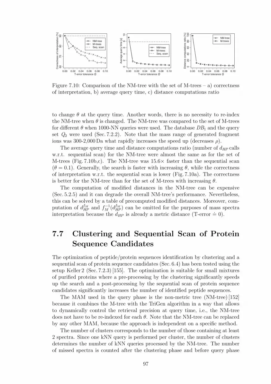
Figure 7.10: Comparison of the NM-tree with the set of M-trees – a) correctnessof interpretation, b) average query time, c) distance computations ratio

to change θ at the query time. Another words, there is no necessity to re-indexthe NM-tree when θ is changed. The NM-tree was compared to the set of M-treesfor different θ when 1000-NN queries were used. The database DB1 and the queryset Q2 were used (Sec. 7.2.2). Note that the mass range of generated fragmentions was 300-2,000 Da what rapidly increases the speed up (decreases ρ).

The average query time and distance computations ratio (number of dHP callsw.r.t. sequential scan) for the NM-tree were almost the same as for the set ofM-trees (Fig. 7.10b,c). The NM-tree was 15.6× faster than the sequential scan(θ = 0.1). Generally, the search is faster with increasing θ, while the correctnessof interpretation w.r.t. the sequential scan is lower (Fig. 7.10a). The correctnessis better for the NM-tree than for the set of M-trees with increasing θ.

The computation of modified distances in the NM-tree can be expensive(Sec. 5.2.5) and it can degrade the overall NM-tree’s performance. Nevertheless,this can be solved by a table of precomputed modified distances. Moreover, com-putation of dfMHP and f−1

M (dfMHP ) can be omitted for the purposes of mass spectrainterpretation because the dHP is already a metric distance (T-error

.= 0).

7.7 Clustering and Sequential Scan of Protein

Sequence Candidates

The optimization of peptide/protein sequences identification by clustering and asequential scan of protein sequence candidates (Sec. 6.4) has been tested using thesetup Keller 2 (Sec. 7.2.3) [155]. The optimization is suitable for small mixturesof purified proteins where a pre-processing by the clustering significantly speedsup the search and a post-processing by the sequential scan of protein sequencecandidates significantly increases the number of identified peptide sequences.

The MAM used in the query phase is the non-metric tree (NM-tree) [152]because it combines the M-tree with the TriGen algorithm in a way that allowsto dynamically control the retrieval precision at query time, i.e., the NM-treedoes not have to be re-indexed for each θ. Note that the NM-tree can be replacedby any other MAM, because the approach is independent on a specific method.

The number of clusters corresponds to the number of those containing at least2 spectra. Since one kNN query is performed per cluster, the number of clustersdetermines the number of kNN queries processed by the NM-tree. The numberof missed spectra is counted after the clustering phase and before query phase

97

(Fig. 6.7). It corresponds to the number of annotated spectra in clusters withsingle objects and thus missed by clustering.

Single runs means that query sets of spectra from more spectrometer runswere processed separately and the results were summed (the number of clusters,the number of missed spectra, the time of clustering and the ratio of identifiedspectra to annotated spectra) or averaged (the time of identification per spec-trum). Appended runs means that query sets of spectra from more spectrometerruns were processed together.

7.7.1 Clustering of Spectra from Two Spectrometer Runs

The clusters formed from appended query sets of spectra from two spectrometerruns contain many more annotated spectra than clusters formed from the querysets which are processed separately (Tab. 7.5). On average, the clusters formedfrom spectra from two spectrometer runs contain about 40.7% more annotatedspectra than clusters formed from a single spectrometer run. Since one kNN queryis performed per cluster containing at least 2 spectra, up to 79% of all kNN queriesare not performed for the clusters formed from the spectra appended from tworuns. For clusters formed from the spectra from single runs, up to 87% of allkNN queries are not performed but there are many missed annotated spectra.

Num. of Num. of Single runs Appended runsQuery set all annotated Num. of Spectra Clustering Num. of Spectra Clustering

spectra spectra clusters missed time [s] clusters missed time [s]

A1-2 2213 215 321 92 7.9 397 16 16.3A3-4 1858 158 304 69 5.3 400 25 10.4A5-6 2021 164 306 49 6.5 385 18 13.7B1-2 618 121 49 87 0.5 113 33 1.0B3-4 902 155 86 104 1.1 203 9 2.2B5-6 1418 208 185 122 3.0 313 23 5.8B7-8 1661 223 212 123 4.2 365 13 8.0

Table 7.5: Clustering of spectra from single runs and from two appended runs

7.7.2 Effectiveness and Efficiency of Identification

The impact of the clustering of query spectra on the number of finally identifiedpeptide sequences (i.e., after the post-processing) and on the average time ofidentification per spectrum was tested. The sequential scan of the entire databaseand the NM-tree were compared in 3 different ways – without the clustering, withthe clustering of two query sets processed separately and with the clustering of aquery set appended from two query sets. When the clustering and/or the NM-treewere employed, the post-processing was used.

The most peptide sequences (on average 94.6%) were identified when thesequential scan was performed without the clustering (Tab. 7.6). On average93.8% peptide sequences were identified when the NM-tree was employed withoutthe clustering. The ratio of identified peptides was noticeably worse when theclustering was applied on the query sets from single runs – about 75.3% forthe sequential scan and only 65.4% for the NM-tree. When the clustering wasapplied on the query sets appended from two spectrometer runs, the ratio of

98

Without clusteringWith clustering

Query set Single runs Appended runsSeq. scan NM-tree Seq. scan NM-tree Seq. scan NM-tree

A1-2 96.7 96.7 74.0 72.6 95.8 95.8A3-4 91.1 90.5 69.6 59.5 88.6 81.6A5-6 93.3 92.7 81.1 78.7 93.3 87.2B1-2 98.3 95.9 59.5 28.9 97.5 87.6B3-4 97.4 96.8 81.3 71.0 97.4 96.8B5-6 91.8 90.9 87.0 78.8 90.9 90.9B7-8 93.3 93.3 74.4 68.2 91.9 91.0

Table 7.6: The ratio of identified spectra to annotated spectra [%]

Without clusteringWith clustering

Query set Single runs Appended runsSeq. scan NM-tree Seq. scan NM-tree Seq. scan NM-tree

A1-2 7.36 0.33 1.13 0.05 1.42 0.08A3-4 7.09 0.30 1.27 0.05 1.63 0.08A5-6 7.28 0.30 1.17 0.05 1.53 0.07B1-2 6.75 0.23 0.59 0.02 1.38 0.06B3-4 6.92 0.24 0.73 0.03 1.75 0.07B5-6 6.94 0.27 0.99 0.04 1.70 0.08B7-8 7.20 0.30 0.97 0.04 1.73 0.08

Table 7.7: Average time of identification per spectrum [s]

identified peptides was almost the same like when no clustering was employed.On average, it was about 93.6% for the sequential scan and 90.1% for the NM-tree. The clustering of query sets appended from 2 runs worsened the ratio ofidentified peptides about 1% when the sequential scan was performed over theentire database and about 3.7% when the NM-tree was employed.

The slowest method was the sequential scan without the clustering wherethe average time of identification per spectrum was 7.04 s (Tab. 7.7). The NM-tree without the clustering took 0.28 s thus the speed-up was 25.1×. When theclustering was applied on the query sets from single runs, the average time was0.98 s (speed-up 7.2×) for the sequential scan and 0.04 s (speed-up 176.0×) for theNM-tree. When query sets from two spectrometer runs were appended and theclustering was applied, the average time was 1.59 s for the sequential scan (speed-up 4.4×) and 0.07 s for the NM-tree (speed-up 100.6×). When the NM-treewas employed with the clustering, the average speed-up was 4× w.r.t. NM-treewithout the clustering.

7.7.3 Clustering of Spectra Appended from More Runs

The impact of the increasing number of spectra from more spectrometer runsin a query set on the number of annotated mass spectra missed by clusteringand on the time of clustering (Tab. 7.8) was analyzed. We can observe that thenumber of missed annotated spectra is almost the same when spectra from two ormore spectrometer runs are appended, thus appending spectra from more thantwo spectrometer runs does not significantly improve the effectiveness of peptidesequences identification. Since we employ a simple clustering algorithm (Alg. 16),a disadvantage of appending spectra from too many spectrometer runs is that thetime of clustering increases with the quadratic time complexity.

99

QueryNum. Num. of Num. Ratio of

SpectraClustering Ratio of Avg. time

setof all annotated of clust. to all

missedtime identified of ident.

spectra spectra clusters spectra [%] [s] spectra [%] [s]

A1 1122 119 157 14.0 49 4.0 76.5 0.05A1-2 2213 215 397 17.9 16 16.3 95.8 0.08A1-3 3038 274 540 17.8 15 30.6 96.0 0.08A1-4 4071 373 706 17.3 15 61.2 94.4 0.09A1-5 5071 451 839 16.5 16 106.4 94.9 0.09A1-6 6092 537 943 15.5 17 148.3 94.0 0.09

Table 7.8: Clustering of spectra appended from more spectrometer runs

The ratio of identified to annotated spectra and the average time of identifi-cation per spectrum were also measured on the NM-tree. The ratio of identifiedspectra is almost the same when spectra from two or more spectrometer runsare appended (on average 95%). The time of identification a bit increases withincreasing number of spectra because of the quadratic time complexity of clus-tering.

We can observe that the ratio of the number of clusters to the number of allspectra in a query set is lower with the increasing number of spectra. This couldbe an advantage for large query sets of mass spectra because only a small numberof the spectra is queried and thus the search is significantly faster. When spectrafrom 14 spectrometer runs on mixture A were appended, 14365 spectra formed1188 clusters with more than one spectrum. Thus only 8.3% of all queries wereperformed on the NM-tree. When spectra from 8 spectrometer runs on mixtureB were appended, 4599 spectra formed 711 clusters thus only 15.5% of all querieswere performed.

7.7.4 Impact of Distance Threshold on Clustering

The impact of the threshold t of dHP on the number of clusters, on the numberof spectra missed by the clustering and on the time of clustering was tested(Tab. 7.9). The dataset A1-2 with 2213 spectra appended from two spectrometerruns from the setup Keller 2 (Sec. 7.2.3) was used. The number of clusters is biggerwith increasing t while the number of spectra missed by clustering is smaller. Theoptimal t seems to be about 0.65 when the number of clusters (or kNN queriesperformed, respectively) is only 17.9% w.r.t. the number of kNN queries whichmust be performed when the clustering is not employed. Moreover, there are only16 missed spectra. For t < 0.65, the number of spectra missed by clustering growsbecause there are less hits among the theoretical and the query spectra. The ratioof identified to annotated spectra is still more than 95% because the sequentialscan of protein sequence candidates is employed. For t > 0.65, the number ofclusters increases (up to t = 0.75) and the number of missed spectra is almostzero. A disadvantage is that high t may form clusters of spectra not coming fromthe same peptide. In practice, the optimal t depends on the number of peaksin query spectra. The optimal t may be higher than 0.65 when the support ofmodifications is implemented as described in Sec. 6.3. The time of identificationa bit increases with the increasing t – this corresponds to the increasing numberof clusters.

100

tNum. of Spectra Clustering Ratio of ident. Avg. time ofclusters missed time [s] spectra [%] ident. [s]

0.3 162 93 16.6 93.0 0.040.4 242 69 16.3 95.3 0.050.5 312 49 16.9 95.3 0.060.6 368 31 16.0 95.8 0.070.65 397 16 16.3 95.8 0.080.7 562 4 17.0 95.8 0.110.75 633 0 18.0 95.8 0.120.8 318 0 24.8 49.8 0.07

Table 7.9: Impact of distance threshold t on clustering

7.8 Utilization of Precursor Mass Filter

Even though the identification of peptide sequences by non-metric access methodshas been successfully tested on query sets containing small mixtures of purifiedproteins (Sec. 7.7), their utilization on query sets of complex protein mixturescontaining thousands of proteins is a non-trivial task. Thus the precursor massfilter (Sec. 4.1) has been also implemented as a database indexing technique tosupport complex query sets [160]. When the precursor mass filter is used, dmatchHP

outperforms several state-of-art tools for peptide sequences identification fromHPLC-MS/MS spectra in both – the number of identified peptides and in thespeed of search.

The identification of peptide sequences using the precursor mass filter followedby a ranking of theoretical spectra by dA, dHP and dmatchHP (Eq. 6.10) was testedin the following experiments (i.e., MAMs were not employed). The setups E. coliand Human were used for this purpose (Sec. 7.2.4). The results were comparedwith state-of-the-art tools OMSSA [61] and X!Tandem [62]. Peptide identifica-tions from all engines were statistically evaluated by OpenMS v. 1.9 [93]. Whena fixed modification was searched, the mass of an amino acid was changed whentheoretical spectra were generated, e.g., the mass of cysteine was increased byapprox. 57.02 Da. When a variable modification was searched, theoretical spec-tra with all possible shifts of m

zvalues were generated, compared with the query

spectrum and the theoretical spectrum with the best score was selected to forma PSM.

7.8.1 State-of-the-Art Tools

First of all, a comparison of the state-of-the-art tools was performed. The num-bers of identified peptides for different q-values (Sec. 3.2.3) and search timeswere measured using the freely available tools OMSSA (v. 2.1.8) and X!Tandem(v. 2011.12.01.1). The refinement mode in X!Tandem was not used becauseit impacted the statistical evaluation. The comparison was made using Open-MS (v. 1.9). Simple pipelines in TOPPAS were created for this purpose (e.g.,OMSSAAdapter → PeptideIndexer → FalseDiscoveryRate → IDFilter, whereOMSSAAdapter calls OMSSA search engine, PeptideIndexer annotates for eachsearch result whether it is a target or a decoy hit, FalseDiscoveryRate computes q-values and IDFilter selects only those PSMs with q-values less or equal a specifiedtolerance). Pipelines were processed without and with the support of modifica-tions (carbamidomethylation of cysteine was used as a fixed modification and

101

OMSSA X!Tandemq-value

Timeq-value

Time0.05 0.01 0.001 0.05 0.01 0.001

E.coli11,729 10,301 7,989 03:40 10,277 8,518 6,398 03:35

mod. 13,008 11,435 9,123 05:00 11,612 9,813 7,487 04:36

Hum486,893 6,147 5,439 27:42 7,330 5,902 4,239 40:03

mod. 9,430 8,508 7,229 27:42 10,494 8,524 5,411 51:20

Hum498,118 7,119 5,392 24:03 7,728 6,085 4,673 37:07

mod. 11,465 10,333 8,601 25:10 11,695 9,712 6,119 53:30

dA dHP

q-valueTime

q-valueTime

0.05 0.01 0.001 0.05 0.01 0.001

E.coli12,846 10,404 1,785 00:40 13,004 11,200 8,307 00:44

mod. 14,554 11,587 1,948 01:26 14,576 12,556 9,288 01:33

Hum486,205 3,717 773 03:19 7,162 5,863 4,225 03:53

mod. 8,615 4,845 934 06:06 9,882 8,108 6,119 06:29

Hum497,859 5,186 2,512 03:05 8,347 6,888 5,329 03:44

mod. 11,244 6,944 3,291 05:12 12,002 10,011 8,120 06:46

dmatchHP

q-valueTime

0.05 0.01 0.001

E.coli13,373 11,668 9,402 00:43

mod. 14,969 13,113 10,005 01:30

Hum487,461 6,230 4,497 03:42

mod. 10,305 8,680 7,109 06:34

Hum498,760 7,512 5,311 03:57

mod. 12,531 10,816 8,689 06:15

Table 7.10: Numbers of identified peptides and search times [min:sec]. In acell with a number of identified peptides, the best result among all engines ishighlighted.

oxidation of methionine as a variable modification). The results are shown inTab. 7.10. OMSSA identified more peptides than X!Tandem in all query sets andthe search was 1.5× - 2.1× faster on human query sets.

7.8.2 SimTandem

Numbers of peptides identified by SimTandem (i.e., by precursor filter followedby a ranking of theoretical spectra by dA, dHP and dmatchHP ) and search timesare shown in Tab. 7.10. The most peptides are identified when dmatchHP is used.However, when q = 0.001, OMSSA identifies more peptides in three cases. Whenq = 0.05, X!Tandem identifies the most peptides in one case. dmatchHP identifiesmore peptide sequences than dHP in almost all cases. The number of identifiedpeptides is bigger for dHP than for X!Tandem when E.coli and Hum49 are used.OMSSA outperforms dHP on human query sets when q ≤ 0.01 is used. Thenumber of identified peptides is significantly smaller for dA than for other engines.

SimTandem is 5.0×-7.1× faster than OMSSA without the support of modifi-cations and 3.2×-4.3× faster with the support of modifications. It is also 4.9×-10.3× faster than X!Tandem without modifications and 3.0×-7.9× faster withmodifications. The speed up is almost the same when dmatchHP is used.

A graphical comparison of numbers of identified peptides with state-of-the-arttools is shown in Fig. 7.11. The overlap of identified peptides between SimTandemand OMSSA is bigger than the overlap between SimTandem and X!Tandem andalso bigger than the overlap between OMSSA and X!Tandem on all query sets.

102

Figure 7.11: Comparison of dHP with state-of-the-art tools (q = 0.05)

We have tested the impact of the index of the root n in dHP and dmatchHP onthe number of identified peptides. Results are shown in Tab. 7.11. The numberis bigger with bigger n. However, when n is too big, the number of identifiedpeptides is smaller. The optimal n depends on the data sets and should bedetermined empirically.

7.8.3 Efficiency of Precursor Mass Filter

The efficiency of the precursor mass filter was also studied when different pre-cursor mass error tolerances λ and different protein sequence databases wereutilized. Since the number of comparisons of a query spectrum with theoreti-cal spectra is crucial for the efficiency of the precursor mass filter, an averagenumber of comparisons was measured in protein sequence databases Swiss-Prot(v. 07/2012) (human sequences only and all sequences) [3], MSDB [2] and NCBIRefSeq (v. 55) [4]. The query set Hum48 was used and modifications were notsupported. The results are shown in Tab. 7.12. Since an organism is usuallyknown for a query set of spectra (e.g., E. coli or human) and the precision ofmodern spectrometers increases, the number of spectra compared with a query

ndHP dmatch

HPE.coli Hum48 Hum49 E.coli Hum48 Hum49

5 4,237 1,605 2,321 8,307 3,283 4,64610 6,288 2,590 4,167 9,165 4,194 5,51720 8,101 3,773 5,160 9,360 4,440 5,22030 8,307 4,225 5,329 9,402 4,497 5,31150 8,370 4,343 5,144 9,427 4,530 5,268100 8,415 4,447 5,579 9,453 4,560 5,295∞ 8,348 3,928 5,023 9,332 3,988 5,110

Table 7.11: Numbers of identified peptides by dHP and dmatchHP for different n(q = 0.001, modifications in query spectra were not supported). The best resultin each column is highlighted.

103

spectrum is small and thus the precursor filter is efficient. For example, 409 spec-tra are compared with a query spectrum when human sequences from Swiss-Protare used and when λ = 10 ppm. When the NCBI database is used, the numberof comparisons is 60,638. For a mass spectrometer with a low precision λ = 2 Da,the number of comparisons is significantly bigger. For example, 15,564 spectraare compared when human sequences from Swiss-Prot are used and 2,451,235comparisons are made when the NCBI database is used.

DatabaseNumber of Number of λ

proteins peptides 5 ppm 10 ppm 15 ppm 0.5 Da 1 Da 2 Da

Swiss-Prot173,450 9,567,012 206 409 613 3,892 7,792 15,564

(human)Swiss-Prot

1,073,578 52,361,610 1,056 2,091 3,135 21,261 42,645 85,141(complete)

MSDB 6,478,158 281,767,270 5,756 11,369 17,042 113,272 227,017 453,153NCBI 34,737,538 1,533,987,691 30,606 60,638 91,004 612,225 1,227,339 2,451,235

Table 7.12: Average numbers of comparisons of a query spectrum with theoreticalspectra for different protein sequence databases and different precursor mass errortolerances λ. Numbers of protein and peptide sequences in databases are alsoproposed (decoy sequences are included in the databases).

104

Chapter 8

Implementation

SimTandem is a freely available tool for identification of peptides from HPLC-MS/MS spectra. It is based on the similarity search of query mass spectra in adatabase of theoretical spectra generated from a database of known protein se-quences. SimTandem employs the parameterized Hausdorff distance as the massspectra similarity function. SimTandem has been implemented in two alterna-tives. First, it has been implemented as the on-line web application to demon-strate the utilization of non-metric access methods for the fast and approximatesimilarity search in a database of theoretical tandem mass spectra. Second, Sim-Tandem has been implemented as a peptide identification tool which can be usedin the framework TOPP [104] based on OpenMS [93]. The advantages of theTOPP tool are that the results can be statistically evaluated, easily comparedwith other state-of-the-art tools, and that many other tools for processing of massspectra can be used as SimTandem’s predecessors or successors. The TOPP toolsupports the precursor mass filter next to the approach based on (non)metricaccess methods. The SimTandem is freely available at [166].

8.1 Web Interface

The on-line version of SimTandem demonstrates the utilization of MAMs asdatabase indexing techniques for identification of peptide/protein sequences fromHPLC-MS/MS spectra [166]. The index is created over theoretical spectra gener-ated from a database of protein sequences. The core of the application is imple-mented in C++ and it employs the Siret Object Library (SOL) – a framework for

Figure 8.1: SimTandem (on-line version) – architecture

105

Figure 8.2: SimTandem (on-line version) – general settings

Figure 8.3: SimTandem (on-line version) – advanced options

106

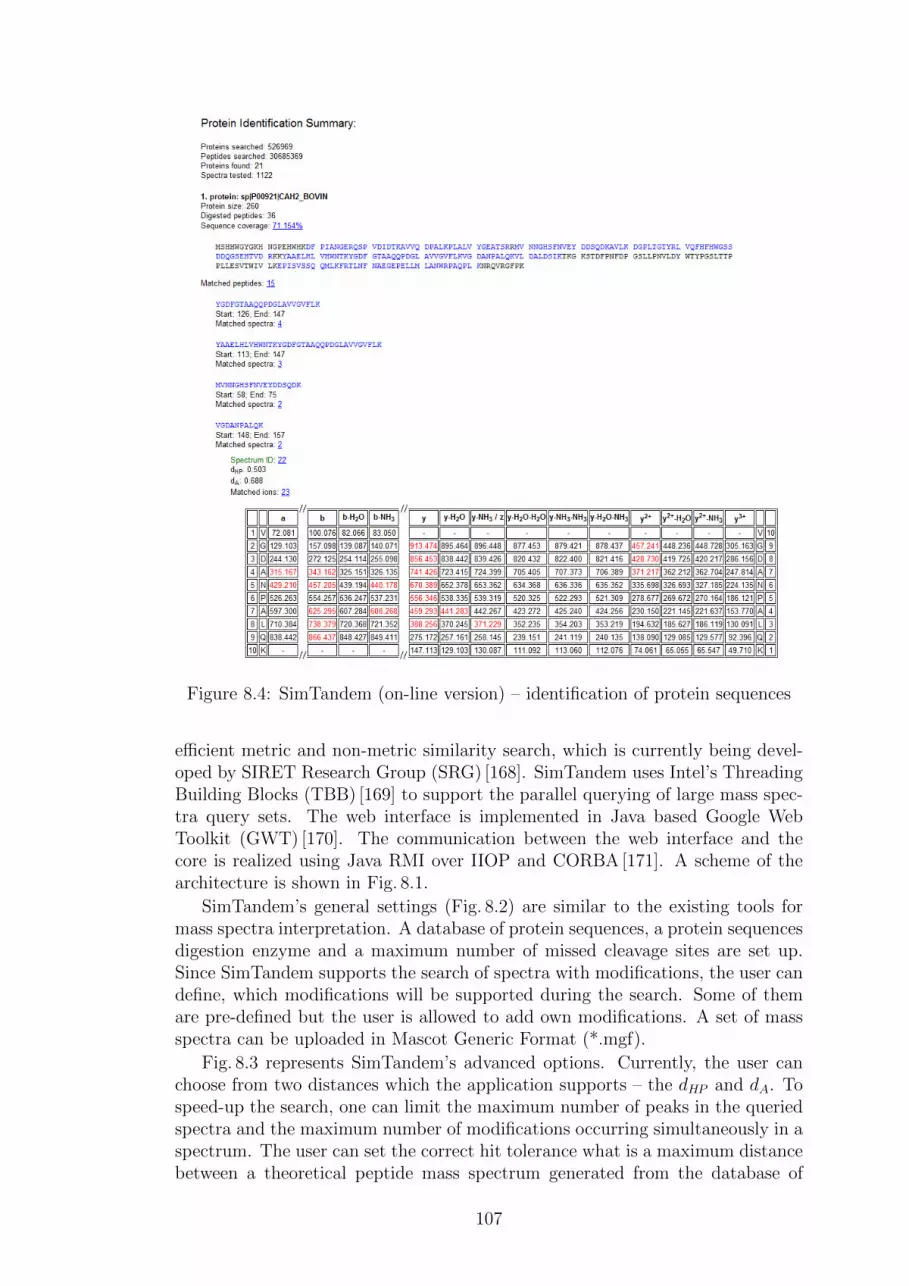
Figure 8.4: SimTandem (on-line version) – identification of protein sequences

efficient metric and non-metric similarity search, which is currently being devel-oped by SIRET Research Group (SRG) [168]. SimTandem uses Intel’s ThreadingBuilding Blocks (TBB) [169] to support the parallel querying of large mass spec-tra query sets. The web interface is implemented in Java based Google WebToolkit (GWT) [170]. The communication between the web interface and thecore is realized using Java RMI over IIOP and CORBA [171]. A scheme of thearchitecture is shown in Fig. 8.1.

SimTandem’s general settings (Fig. 8.2) are similar to the existing tools formass spectra interpretation. A database of protein sequences, a protein sequencesdigestion enzyme and a maximum number of missed cleavage sites are set up.Since SimTandem supports the search of spectra with modifications, the user candefine, which modifications will be supported during the search. Some of themare pre-defined but the user is allowed to add own modifications. A set of massspectra can be uploaded in Mascot Generic Format (*.mgf).

Fig. 8.3 represents SimTandem’s advanced options. Currently, the user canchoose from two distances which the application supports – the dHP and dA. Tospeed-up the search, one can limit the maximum number of peaks in the queriedspectra and the maximum number of modifications occurring simultaneously in aspectrum. The user can set the correct hit tolerance what is a maximum distancebetween a theoretical peptide mass spectrum generated from the database of

107

Figure 8.5: SimTandem (on-line version) – search of with modifications

protein sequences and a spectrum captured by a spectrometer. If a distancebetween the mass spectra is less or equal the correct hit tolerance, a hit betweenthe peptide sequence and the mass spectrum is assumed.

The user can also customize the output report (Fig. 8.4). One can choosewhether the query mass spectra will be reported independently or whether thespectra (peptide sequences, respectively) will be grouped into protein sequences.The user can set the minimum number of peptide sequence hits in a proteinsequence and the minimum protein sequence coverage. Only the protein sequencesachieving the both values are reported. The minimum number of peptide sequencehits can be determined as a sum of different peptide sequence hits in a proteinsequence or as a sum of all peptide sequence hits (more spectra can match thesame peptide sequence). The protein sequence coverage is the percentage ofamino acids in the protein sequence, which are covered by peptide sequence hits.Finally, one can set the number of peptide sequences (k nearest neighbors), whichwill be reported for a spectrum.

In an output report, a table of fragment ions predicted from a peptide sequenceis shown for a hit between a theoretical spectrum and a query spectrum. Fragmentions matched in the query spectrum (within a specified m

zerror tolerance ξ) and

ions shifted by modifications are highlighted (Fig. 8.5).

108

Figure 8.6: A simple identification pipeline in TOPPAS with SimTandem

8.2 TOPP Tool

SimTandem has been also implemented as a peptide identification tool which canbe used by the framework TOPP [104] based on OpenMS [93]. Currently, thetool supports the precursor mass filter as a database indexing technique next toMAMs, thus complex mixtures containing thousands of proteins can be easilyprocessed. The advantages of the TOPP tool are that:

• TOPP contains tools for statistical evaluation of PSMs and thus results canbe easily evaluated and compared with other peptide identification tools likeOMSSA [61], X!Tandem [62], MASCOT [60], MyriMatch [45], etc.;

• since pipelines formed from different tools can be created in TOPP, oth-er tools in TOPP (or any executable file) can be used as SimTandem’spredecessors or successors;

• since SimTandem is a stand-alone application, query sets from shotgunproteomics having sizes of hundreds of megabytes can be easily processed;

• SimTandem can be easily offered to end users via OpenMS.

A basic pipeline in TOPP, where SimTandem is utilized as a peptide sequencesidentification engine, is shown in Fig. 8.6. SimTandem requires an input *.mgf filewith the query set of mass spectra and a *.fasta file with the database of proteinsequences. The output is generated in the standardized *.IdXML file format.The configuration properties of SimTandem are shown in Fig. 8.7.

8.2.1 Installation Instructions

Below, the system requirements of the tool, the installation instructions for Win-dows x64 and an example of use are proposed.

109

System requirements Any 64-bit Windows system is suitable (Windows 7,Windows Server 2008, etc.). Other requirements are just recommended and de-pends on the sizes of the protein sequence databases and the sizes of query sets.Say, at least 4 to 8 GB RAM and a few GB of free disk space for temporary indexfiles.

Installation

1. Download and install ”OpenMS-1.9.0-Win 64bit setup.exe” from the Open-MS website [93].

2. Download and unzip the lastest release of SimTandem from [166].

3. Put the file ”SimTandem.ttd” into”../OpenMS-1.9/share/OpenMS/TOOLS/EXTERNAL”.

4. Restart your computer.

Usage

1. Run TOPPAS.

2. SimTandem is available in the left menu ”TOPP tools”in ”EXTERNAL/GenericWrapper/SimTandem”.

3. Drag & Drop SimTandem to the workspace.

4. Click with the right mouse button on the SimTandem’s box and select ”editparameters”.

5. Set the correct location of ”simtandem openms.exe” in the option ”exe-cutable”.

6. Optionally, the path in ”indexDir” can be changed where the indexed filesare stored (make sure that the path is writable).

7. Connect input files *.mgf and *.fasta with SimTandem and connect also theoutput *.IdXML file with an output box or with another tool.

8. If you have another input file than *.mgf, the tool”File Handling/FileConverter” can be used as SimTandem’s predecessor.

110

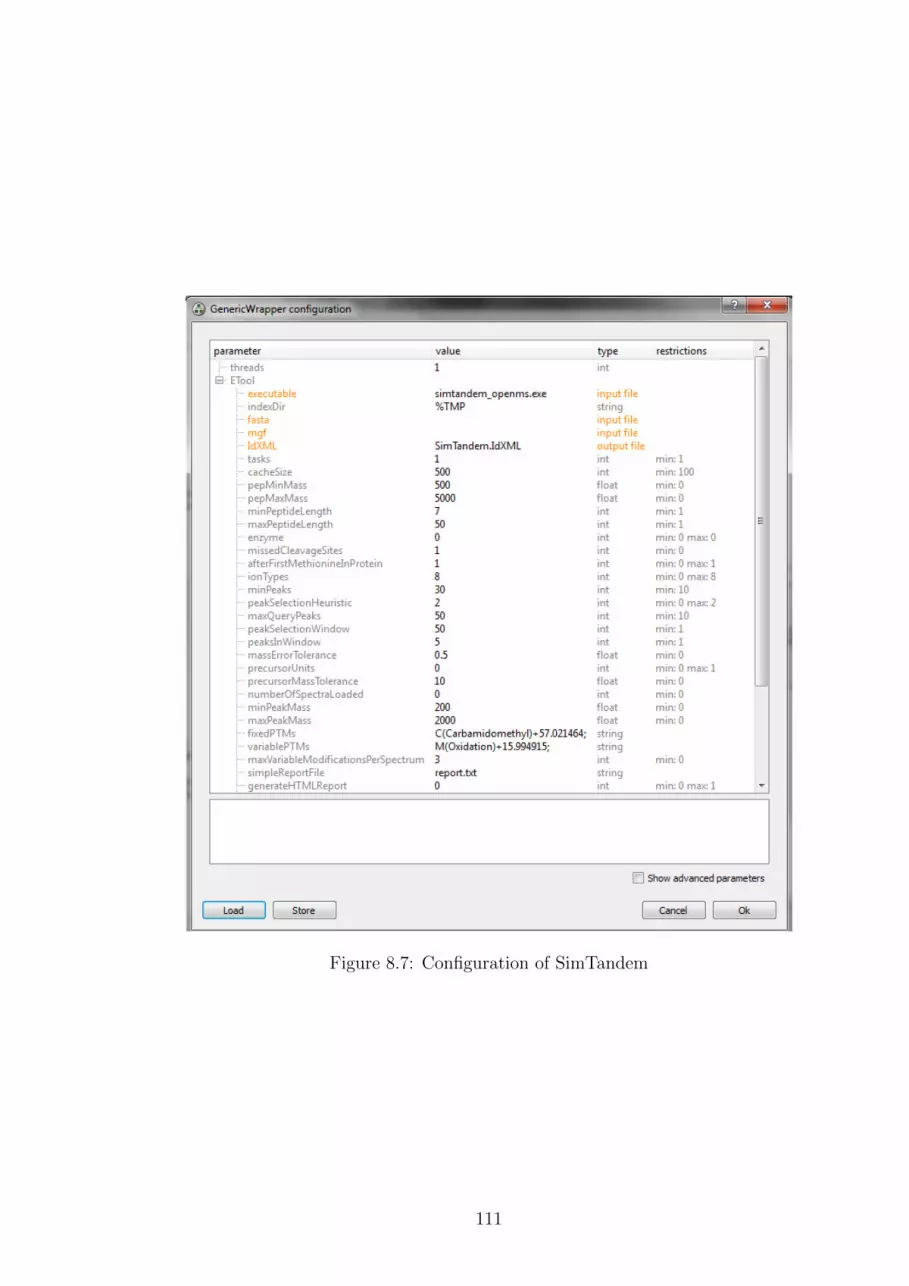
Figure 8.7: Configuration of SimTandem

111

112

Chapter 9

Conclusion

In this thesis, we studied the methods for identification of peptide sequences fromtandem mass spectra based on the similarity search in databases of theoreticalmass spectra generated from databases of known protein sequences. Since thesizes of protein sequence databases grow rapidly in recent years, we were focusedon the database indexing techniques which can be employed to speed-up thesearch in databases of theoretical mass spectra.

We have shown that non-metric access methods can be used as the databaseindexing techniques for fast and approximate similarity search in databases oftheoretical mass spectra. Currently, the proposed method is suitable for smallmixtures of purified proteins (several tens of proteins). The method for peptidesequences identification is more than 100× faster than a sequential scan over theentire database of theoretical mass spectra while more than 90% of spectra (w.r.t.a ground truth determined by a state-of-the-art search engine) are correctly as-signed to peptide sequences.

However, the utilization of non-metric access methods on complex mixturesof proteins obtained by a cell lysis (i.e., containing thousands of proteins) is anon-trivial task. To support the complex mixtures of proteins, we have alsoimplemented the precursor mass filter as the database indexing technique. Whenthe precursor mass filter is followed by a ranking of theoretical mass spectra usinga modification of the parameterized Hausdorff distance (originally designed fornon-metric indexes), our method outperforms state-of-the-art tools in both – thenumber of identified peptide sequences and the speed of search. The proposedmethods have been implemented in the application SimTandem which can beused for a batch analysis in the framework TOPP based on OpenMS.

113

114

Bibliography

[1] Gregory Petsko and Dagmar Ringe. Protein Structure and Function(Primers in Biology). New Science Press Ltd, London, UK, 2004.

[2] MSDB.http://www.proteomics.leeds.ac.uk/bioinf/.

[3] UniProtKB/Swiss-Prot.http://www.uniprot.org/.

[4] NCBI RefSeq.http://www.ncbi.nlm.nih.gov/RefSeq/.

[5] Ingvar Eidhammer, Kristian Flikka, Lennart Martens, and Svein-OleMikalsen. Computational Methods for Mass Spectrometry Proteomics. JohnWiley & Sons, England, 2007.

[6] Donald F. Hunt and et al. Protein Sequencing by Tandem Mass Spectrom-etry. In Proc. Nati. Acad. Sci. USA, volume 83, pages 6233–6237, 1986.

[7] Rune Matthiesen. Mass Spectrometry Data Analysis in Proteomics (Meth-ods in Molecular Biology). Humana Press, Totowa, New Jersey, 2007.

[8] Edmond de Hoffmann and Vincent Stroobant. Mass Spectrometry: Princi-ples and Applications. John Wiley & Sons, England, 2007.

[9] Jesper V. Olsen, Shao-En Ong, and Matthias Mann. Trypsin Cleaves Exclu-sively C-terminal to Arginine and Lysine Residues. Molecular and CellularProteomics, 3:608–614, 2004.

[10] Linda Switzar, Martin Giera, and Wilfried M. A. Niessen. Protein Diges-tion: An Overview of the Available Techniques and Recent Developments.Journal of Proteome Research, 12(3):1067–1077, 2013.

[11] Peptide Mass Spectrum Interpretation.http://www.weddslist.com/ms/.

[12] Nico Pfeifer, Andreas Leinenbach, Christian G. Huber, and OliverKohlbacher. Improving Peptide Identification in Proteome Analysis by aTwo-Dimensional Retention Time Filtering Approach. Journal of ProteomeResearch, 8(8):4109–4115, 2009.

[13] Beata Reiz, Attila Kertesz-Farkas, Sandor Pongor, and Michael P. Myers.Data Preprocessing and Filtering in Mass Spectrometry Based Proteomics.Current Bioinformatics, 7(2):212–220, 2012.

115

[14] John R. Yates III. Mass Spectral Analysis in Proteomics. Annual Reviewof Biophysics and Biomolecular Structure, 33:297–316, 2004.

[15] Quadrupole on Wikipedia.http://en.wikipedia.org/wiki/Quadrupole_mass_analyzer.

[16] Orbitrap on Wikipedia.http://en.wikipedia.org/wiki/Orbitrap.

[17] Thermo Scientific.http://www.thermoscientific.com.

[18] William J. Henzela, Colin Watanabea, and John T. Stults. Protein Identi-fication: the Origins of Peptide Mass Fingerprinting. Journal of the Amer-ican Society for Mass Spectrometry, 14(9):931–942, 2003.

[19] Pavel A. Pevzner and et al. Efficiency of Database Search for Identifica-tion of Mutated and Modified Proteins via Mass Spectrometry. GenomeResearch, 11(2):290–299, 2001.

[20] UNIMOD.http://www.unimod.org/.

[21] Chris Bauer, Rainer Cramer, and Johannes Schuchhardt. Evaluation ofPeak-Picking Algorithms for Protein Mass Spectrometry. In Data Miningin Proteomics, volume 696 of Methods in Molecular Biology, pages 341–352.2011.

[22] Eva Lange, Clemens Gropl, Knut Reinert, Oliver Kohlbacher, and An-dreas Hildebrandt. High-Accuracy Peak Picking of Proteomics Data UsingWavelet Techniques. In Pac Symp Biocomput., pages 243–254, 2006.

[23] Jussi Salmi, Tuula A. Nyman, Olli S. Nevalainen, and Tero Aittokallio.Filtering Strategies for Improving Protein Identification in High-throughputMS/MS Studies. Proteomics, 9:848–860, 2009.

[24] Bernhard Y. Renard and et al. When Less Can Yield More - ComputationalPreprocessing of MS/MS Spectra for Peptide Identification. Proteomics,9:4978–4984, 2009.

[25] Wenjun Lin and et al. An Adaptive Approach to Denoising Tandem MassSpectra. In IEEE Bioinformatics and Biomedicine Workshops, pages 89–94,2010.

[26] Wenjun Lin, Fang-Xiang Wu, Jinhong Shi, Jiarui Ding, and Wenjun Zhang.An adaptive approach to denoising tandem mass spectra. Proteomics,11(19):3773–3778, 2011.

[27] Kristian Flikka and et al. Improving the Reliability and Throughput of MassSpectrometry-based Proteomics by Spectrum Quality Filtering. Proteomics,6:2086–2094, 2006.

116

[28] Alexey I. Nesvizhskii and et al. Dynamic Spectrum Quality Assessment andIterative Computational Analysis of Shotgun Proteomic Data. Molecularand Cellular Proteomics, 5:652–670, 2006.

[29] Kristian Flikka and et al. Implementation and Application of a VersatileClustering Tool for Tandem Mass Spectrometry Data. Proteomics, 7:3245–3258, 2007.

[30] Ari M. Frank and et al. Clustering Millions of Tandem Mass Spectra.Journal of Proteome Research, 7(1):113–122, 2008.

[31] Jayson A. Falkner, Jarret W. Falkner, Anastasia K. Yocum, and Philip C.Andrews. A Spectral Clustering Approach to MS/MS Identification of Post-translational Modifications. Journal of Proteome research, 7(11):4614–4622,2008.

[32] Ilan Beer, Eilon Barnea, Tamar Ziv, and Arie Admon. Improving Large-scale Proteomics by Clustering of Mass Spectrometry Data. Proteomics,4:950–960, 2004.

[33] David L. Tabb and et al. Similarity among Tandem Mass Spectra fromProteomic Experiments: Detection, Significance and Utility. Anal. Chem.,75(10), 2003.

[34] Rui Xu and Donald Wunsch. Survey of Clustering Algorithms. IEEETransactions on neural networks, 16(3):645–678, 2005.

[35] Alexander Hinneburg and Daniel A. Keim. An Efficient Approach to Clus-tering in Large Multimedia Databases with Noise. In Proc. of KDD’98,pages 58–65, 1998.

[36] Alexey I. Nesvizhskii. A Survey of Computational Methods and Error RateEstimation Procedures for Peptide and Protein Identification in ShotgunProteomics. Journal of Proteomics, 73(11):2092–2123, 2010.

[37] Henry Lam and Ruedi Aebersold. Building and Searching Tandem Mass(MS/MS) Spectral Libraries for Peptide Identification in Proteomics. Meth-ods, 54(4):424–431, 2011.

[38] R. Craig, J. C. Cortens, D. Fenyo, and R. C. Beavis. Using AnnotatedPeptide Mass Spectrum Libraries for Protein Identification. Journal ofProteome Research, 5(8):1843–1849, 2006.

[39] Henry Lam, Eric W. Deutsch, James S. Eddes, Jimmy K. Eng, NicholeKing, Stephen E. Stein, and Ruedi Aebersold. Development and Validationof a Spectral Library Searching Method for Peptide Identification fromMS/MS. Proteomics, 7(5):655–667, 2007.

[40] Barbara E. Frewen, Gennifer E. Merrihew, Christine C. Wu,William Stafford Noble, and Michael J. MacCoss. Analysis of PeptideMS/MS Spectra from Large-Scale Proteomics Experiments Using SpectrumLibraries. Analytical Chemistry, 78(16):5678–5684, 2006.

117

[41] William R. Cannon, Mitchell M. Rawlins, Douglas J. Baxter, Stephen J.Callister, Mary S. Lipton, and Donald A. Bryant. Large Improvementsin MS/MS-Based Peptide Identification Rates using a Hybrid Analysis.Journal of Proteome Research, 10(5):2306–2317, 2011.

[42] Attila Kertesz-Farkas, Beata Reiz, Michael P. Myers, and Sandor Pon-gor. Database Searching in Mass Spectrometry Based Proteomics. CurrentBioinformatics, 7(2):221–230, 2012.

[43] Michael Kinter and Nicholas E. Sherman. Protein Sequencing and Identifi-cation Using Tandem Mass Spectrometry. John Wiley & Sons, New York,USA, 2000.

[44] Rovshan G. Sadygov, Daniel Cociorva, and John R. Yates III. Large-scaleDatabase Searching Using Tandem Mass Spectra: Looking up the Answerin the Back of the Book. Nature Met., 1(3):195–202, 2004.

[45] David L. Tabb, Christopher G. Fernando, and Matthew C. Chambers.MyriMatch: Highly Accurate Tandem Mass Spectral Peptide Identificationby Multivariate Hypergeometric Analysis. Journal of Proteome Research,6(2):654–661, 2007.

[46] ProteinProspector.http://prospector.ucsf.edu/.

[47] Craig D. Wenger and Joshua J. Coon. A Proteomics Search AlgorithmSpecifically Designed for High-Resolution Tandem Mass Spectra. Journalof Proteome Research, 12(3):1377–1386, 2013.

[48] Mass Spectrometry Software.http://en.wikipedia.org/wiki/Mass_spectrometry_software.

[49] Neil C. Jones and Pavel A. Pevzner. An Introduction to BioinformaticsAlgorithms. MIT Press, Cambridge, Massachusetts, 2004.

[50] Stephen Tanner and et al. InsPecT: Identification of Posttranslational-ly Modified Peptides from Tandem Mass Spectra. Analytical Chemistry,77(14):4626–4639, 2005.

[51] Dekel Tsur, Stephen Tanner, Ebrahim Zandi, Vineet Bafna, and Pavel A.Pevzner. Identification of Post-translational Modifications by Blind Searchof Mass Spectra. In Nature Biotechnology, volume 23, pages 1562–1567,2005.

[52] Kang Ning, Hoong K. Ng, and Hon W. Leong. An Accurate and EfficientAlgorithm for Peptide and PTM Identification by Tandem Mass Spectrom-etry. In Genome Informatics, volume 19, pages 119–130, 2007.

[53] Jian Liu and et al. Methods for Peptide Identification by Spectral Com-parison. Proteome Science, 5(3), 2007.

118

[54] Sven Nahnsen, Timo Sachsenberg, and Oliver Kohlbacher. PTMeta: In-creasing Identification Rates of Modified Peptides using Modification Pres-canning and Meta-analysis. Proteomics, 13(6):1042–1051, 2013.

[55] Jimmy Eng, Ashley L. McCormack, and John R. Yates III. An Approachto Correlate Tandem Mass Spectral Data of Peptides with Amino AcidSequences in a Protein Database. J. of the Am. Soc. for Mass Spec., 5:976–989, 1994.http://fields.scripps.edu/sequest/.

[56] Andrew Keller, Alexey I. Nesvizhskii, Eugene Kolker, and Ruedi Aebersold.Empirical Statistical Model To Estimate the Accuracy of Peptide Identi-fications Made by MS/MS and Database Search. Analytical Chemistry,74(20):5383–5392, 2002.http://peptideprophet.sourceforge.net/.

[57] Andrew Keller and et al. Experimental Protein Mixture for ValidatingTandem Mass Spectral Analysis. OMICS: A Journal of Integrative Biology,6(2):207–212, 2002.

[58] Christopher Y. Park and et al. Rapid and Accurate Peptide Identificationfrom Tandem Mass Spectra. Journal of Proteome research, 7(7):3022–3027,2008.

[59] Benjamin J. Diament and William S. Noble. Faster SEQUEST Searchingfor Peptide Identification from Tandem Mass Spectra. Journal of ProteomeResearch, 10(9):3871–3879, 2011.

[60] David N. Perkins, Darryl J. C. Pappin, David M. Creasy, and John S.Cottrell. Probability-based Protein Identification by Searching SequenceDatabases using Mass Spectrometry Data. Electrophoresis, 20(18):3551–3567, 1999.http://www.matrixscience.com/.

[61] Lewis Y. Geer and et al. Open Mass Spectrometry Search Algorithm.Journal of Proteome Research, 3(5):958–964, 2004.

[62] Robertson Craig and Ronald C. Beavis. TANDEM: Matching Proteins withTandem Mass Spectra. Bioinformatics, 20(9):1466–1467, 2004.http://www.thegpm.org/TANDEM/.

[63] Vlado Dancık and et al. De Novo Peptide Sequencing via Tandem MassSpectrometry. Journal of Computational Biology, 6(3):327–342, 1999.

[64] Sangtae Kim, Nuno Bandeira, and Pavel A. Pevzner. Spectral Profiles,a Novel Representation of Tandem Mass Spectra and Their Applicationsfor de Novo Peptide Sequencing and Identification. Molecular and CellularProteomics, 8(6):1391–1400, 2009.

[65] Bin Ma and et al. PEAKS: powerful software for peptide de novo sequencingby tandem mass spectrometry. Rapid Communications in Mass Spectrom-etry, 17(20):2337–2342, 2003.

119

[66] Ari Frank and Pavel Pevzner. PepNovo: De Novo Peptide Sequencingvia Probabilistic Network Modeling. Analytical Chemistry, 77(4):964–973,2005.

[67] Richard S. Johnson and J. Alex Taylor. Searching Sequence Databases viaDe Novo Peptide Sequencing by Tandem Mass Spectrometry. MolecularBiotechnology, 22:301–315, 2002.

[68] Marshall Bern, Yuhan Cai, and David Goldberg. Lookup Peaks: A Hybridof de Novo Sequencing and Database Search for Protein Identification byTandem Mass Spectrometry. Analytical Chemistry, 79(4):1393–1400, 2007.

[69] Lukas Kall and et al. Assigning Significance to Peptides Identified by Tan-dem Mass Spectrometry Using Decoy Databases. Journal of Proteome Re-search, 7(1):29–34, 2008.

[70] Joshua E. Elias and Steven P. Gygi. Target-Decoy Search Strategy for MassSpectrometry-Based Proteomics. In Proteome Bioinformatics, volume 604,pages 55–71. 2010.

[71] Lukas Kall, John D. Storey, Michael J. MacCoss, and William StaffordNoble. Posterior Error Probabilities and False Discovery Rates: Two Sidesof the Same Coin. Journal of Proteome Research, 7(1):40–44, 2008.

[72] Sven Nahnsen, Andreas Bertsch, Jorg Rahnenfuhrer, Alfred Nordheim,and Oliver Kohlbacher. Probabilistic Consensus Scoring Improves TandemMass Spectrometry Peptide Identification. Journal of Proteome Research,10(8):3332–3343, 2011.

[73] Brian C. Searle, Mark Turner, and Alexey I. Nesvizhskii. Improving Sensi-tivity by Probabilistically Combining Results from Multiple MS/MS SearchMethodologies. Journal of Proteome Research, 7(1):245–253, 2008.http://www.proteomesoftware.com.

[74] Taejoon Kwon, Hyungwon Choi, Christine Vogel, Alexey I. Nesvizhskii, andEdward M. Marcotte. MSblender: A Probabilistic Approach for IntegratingPeptide Identifications from Multiple Database Search Engines. Journal ofProteome Research, 10(7):2949–2958, 2011.

[75] David Shteynberg and et al. iProphet: Multi-level Integrative Analysis ofShotgun Proteomic Data Improves Peptide and Protein Identification Ratesand Error Estimates. Molecular and Cellular Proteomics, 10(12), 2011.

[76] Nathan Edwards, Xue Wu, and Chau-Wen Tseng. An Unsupervised,Model-Free, Machine-Learning Combiner for Peptide Identifications fromTandem Mass Spectra. Clinical Proteomics, 5:23–36, 2009.

[77] Neil L. Kelleher, Hong Y. Lin, Gary A. Valaskovic, David J. Aaserud,Einar K. Fridriksson, and Fred W. McLafferty. Top Down versus Bottom UpProtein Characterization by Tandem High-Resolution Mass Spectrometry.Journal of the American Chemical Society, 121(4):806–812, 1999.

120

[78] Alexey I. Nesvizhskii and Ruedi Aebersold. Interpretation of Shotgun Pro-teomic Data: The Protein Inference Problem. Molecular and Cellular Pro-teomics, 4(10):1419–1440, 2005.

[79] Alexey I. Nesvizhskii, Andrew Keller, Eugene Kolker, and Ruedi Aebersold.A Statistical Model for Identifying Proteins by Tandem Mass Spectrometry.Analytical Chemistry, 75(17):4646–4658, 2003.http://proteinprophet.sourceforge.net.

[80] Lukas Reiter and et al. Protein Identification False Discovery Rates for VeryLarge Proteomics Data Sets Generated by Tandem Mass Spectrometry.Molecular and Cellular Proteomics, 8(11):2405–2417, 2009.

[81] Manfred Claassen, Lukas Reiter, Michael O. Hengartner, Joachim M. Buh-mann, and Ruedi Aebersold. Generic Comparison of Protein Inference En-gines. Molecular and Cellular Proteomics, 2011.

[82] Gavin E. Reid and Scott A. McLuckey. ’Top Down’ Protein Character-ization via Tandem Mass Spectrometry. Journal of Mass Spectrometry,37(7):663–675, 2002.

[83] Marcus Bantscheff, Markus Schirle, Gavain Sweetman, Jens Rick, and Bern-hard Kuster. Quantitative Mass Spectrometry in Proteomics: a CriticalReview. Analytical and Bioanalytical Chemistry, 389:1017–1031, 2007.

[84] Marcus Bantscheff, Simone Lemeer, MikhailM. Savitski, and BernhardKuster. Quantitative Mass Spectrometry in Proteomics: Critical ReviewUpdate from 2007 to the Present. Analytical and Bioanalytical Chemistry,404:939–965, 2012.

[85] Jeffrey C. Silva, Marc V. Gorenstein, Guo-Zhong Li, Johannes P. C. Vissers,and Scott J. Geromanos. Absolute Quantification of Proteins by LCMSE:A Virtue of Parallel ms Acquisition. Molecular and Cellular Proteomics,5(1):144–156, 2006.

[86] Clemens Gropl and et al. Algorithms for the Automated Absolute Quantifi-cation of Diagnostic Markers in Complex Proteomics Samples. In Proceed-ings of the First international conference on Computational Life Sciences,CompLife’05, pages 151–162, 2005.

[87] Steven P. Gygi, Beate Rist, Scott A. Gerber, Frantisek Turecek, Michael H.Gelb, and Ruedi Aebersold. Quantitative Analysis of Complex ProteinMixtures using Isotope-coded Affinity Tags. Nat Biotech, 17:994–999, 1999.

[88] Philip L. Ross, Yulin N. Huang, and et al. Multiplexed Protein Quanti-tation in Saccharomyces cerevisiae Using Amine-reactive Isobaric TaggingReagents. Molecular and Cellular Proteomics, 3(12):1154–1169, 2004.

[89] Ian I. Stewart, T. Thomson, and D. Figeys. 18O Labeling: a Tool forProteomics. Rapid Communications in Mass Spectrometry, 15(24):2456–2465, 2001.

121

[90] Shao-En Ong, Blagoy Blagoev, Irina Kratchmarova, Dan Bach Kristensen,Hanno Steen, Akhilesh Pandey, and Matthias Mann. Stable Isotope La-beling by Amino Acids in Cell Culture, SILAC, as a Simple and AccurateApproach to Expression Proteomics. Molecular and Cellular Proteomics,1(5):376–386, 2002.

[91] SILAC on Wikipedia.http://en.wikipedia.org/wiki/Stable_isotope_labeling_by_

amino_acids_in_cell_culture.

[92] Jurgen Cox and Matthias Mann. MaxQuant Enables High Peptide Identi-fication Rates, Individualized p.p.b.-range Mass Accuracies and Proteome-wide Protein Quantification. Nat Biotech, 26:1367–1372, 2008.

[93] Marc Sturm and et al. OpenMS – An Open-source Software Framework forMass Spectrometry. BMC Bioinformatics, 9(163), 2008.http://www.open-ms.de/.

[94] Matthew C. Wiener, Jeffrey R. Sachs, Ekaterina G. Deyanova, andNathan A. Yates. Differential Mass Spectrometry: A Label-Free LC-MSMethod for Finding Significant Differences in Complex Peptide and Pro-tein Mixtures. Analytical Chemistry, 76(20):6085–6096, 2004.

[95] Weixun Wang, Haihong Zhou, Hua Lin, Sushmita Roy, Thomas A. Shaler,Lander R. Hill, Scott Norton, Praveen Kumar, Markus Anderle, andChristopher H. Becker. Quantification of Proteins and Metabolites by MassSpectrometry without Isotopic Labeling or Spiked Standards. AnalyticalChemistry, 75(18):4818–4826, 2003.

[96] Sven Nahnsen, Chris Bielow, Knut Reinert, and Oliver Kohlbacher. Toolsfor Label-free Peptide Quantification. Molecular and Cellular Proteomics,2012.

[97] Deborah H. Lundgren, Sun-Il Hwang, Linfeng Wu, and David K. Han.Role of Spectral Counting in Quantitative Proteomics. Expert Review ofProteomics, 7(1):39–53, 2010.

[98] Marc Sturm. OpenMS – A Framework for Computational Mass Spectrom-etry. PhD thesis, Universitat Tubingen, 2010.

[99] Valerio B. Di Marco and G. Giorgio Bombi. Mathematical Functions forthe Representation of Chromatographic Peaks. Journal of ChromatographyA, 931(1–2):1–30, 2001.

[100] Michael W. Senko, Steven C. Beu, and Fred W. McLaffertycor. Determi-nation of Monoisotopic Masses and Ion Populations for Large Biomoleculesfrom Resolved Isotopic Distributions. Journal of the American Society forMass Spectrometry, 6:229–233, 1995.

[101] Eva Lange, Clemens Gropl, Ole Schulz-Trieglaff, Andreas Leinenbach,Christian Huber, and Knut Reinert. A Geometric Approach for the Align-ment of Liquid Chromatography – Mass Spectrometry Data. Bioinformat-ics, 23(13):i273–i281, 2007.

122

[102] Katharina Podwojski and et al. Retention Time Alignment Algorithms forLC/MS Data Must Consider Non-linear Shifts. Bioinformatics, 25(6):758–764, 2009.

[103] Eric W. Deutsch and et al. A guided tour of the Trans-Proteomic Pipeline.Proteomics, 10(6):1150–1159, 2010.

[104] Oliver Kohlbacher and et al. TOPP – the OpenMS Proteomics Pipeline.Bioinformatics, 23(2):e191–e197, 2007.

[105] Johannes Junker, Chris Bielow, Andreas Bertsch, Marc Sturm, Knut Rein-ert, and Oliver Kohlbacher. TOPPAS: A Graphical Workflow Editor forthe Analysis of High-Throughput Proteomics Data. Journal of ProteomeResearch, 11(7):3914–3920, 2012.

[106] Marc Sturm and Oliver Kohlbacher. TOPPView: An Open-Source Viewerfor Mass Spectrometry Data. Journal of Proteome Research, 8(7):3760–3763, 2009.

[107] UniProtKB/Swiss-Prot Statistics.http://web.expasy.org/docs/relnotes/relstat.html.

[108] R. Bayer and E. M. McCreight. Organization and Maintenance of LargeOrdered Indices. In Acta Inf., volume 1, pages 173–189, 1972.

[109] Karl R. Clauser, Peter Baker, and Alma L. Burlingame. Role of AccurateMass Measurement (±10 ppm) in Protein Identification Strategies Em-ploying MS or MS/MS and Database Searching. Analytical Chemistry,71(14):2871–2882, 1999.

[110] Jesper V. Olsen and et al. Parts per Million Mass Accuracy on an OrbitrapMass Spectrometer via Lock Mass Injection into a C-trap. Molecular andCellular Proteomics, 4(12):2010–2021, 2005.

[111] Ejvind Mørtz and et al. Sequence Tag Identification of Intact Proteins byMatching Tandem Mass Spectral Data Against Sequence Databases. InProc. Nati. Acad. Sci. USA, volume 93, pages 8264–8267, 1996.

[112] M. Mann and M. Wilm. Error-tolerant Identification of Peptides in Se-quence Databases by Peptide Sequence Tags. Analytical chemistry, 66:4390–4399, 1994.

[113] David L. Tabb, Anita Saraf, and John R. Yates III. GutenTag: High-Throughput Sequence Tagging via an Empirically Derived FragmentationModel. Analytical Chemistry, 75(23):6415–6421, 2003.

[114] Smriti R. Ramakrishnan and et al. A Fast Coarse Filtering Method forPeptide Identification by Mass Spectrometry. Bioinformatics, 22(12):1524–1531, 2006.

[115] Daniel Miranker, Weijia Xu, and Rui Mao. MoBIoS: a Metric-Space DBMSto Support Biological Discovery. In Proc. of the Int. Conf. on Scientific andStatistical Database Management Systems, pages 241–244, 2003.

123

[116] Pavel Zezula, Giuseppe Amato, Vlastislav Dohnal, and Michal Batko. Simi-larity Search: The Metric Space Approach (Advances in Database Systems).Springer, USA, 2006.

[117] Tolga Bozkaya and Meral Ozsoyoglu. Distance-based Indexing for High-dimensional Metric Spaces. In Proceedings of the 1997 ACM SIGMODinternational conference on Management of data, pages 357–368, 1997.

[118] S. Cenk Sahinalp, Murat Tasan, Jai Macker, and Z. Meral Ozsoyoglu. Dis-tance Based Indexing for String Proximity Search. In Proc. of 19th Inter-national Conference on Data Engineering, pages 125–136, 2003.

[119] Debojyoti Dutta and Ting Chen. Speeding up Tandem Mass Spectrome-try Database Search: Metric Embeddings and Fast Near Neighbor Search.Bioinformatics, 23(5):612–618, 2007.

[120] Søren Besenbacher, Benno Schwikowski, and Jens Stoye. Indexing andSearching a Mass Spectrometry Database. In Algorithms and Applications,volume 6060 of Lecture Notes in Computer Science, pages 62–76. 2010.

[121] Mohamed Helmy, Masaru Tomita, and Yasushi Ishihama. Peptide Iden-tification by Searching Large-scale Tandem Mass Spectra against LargeDatabases: Bioinformatics Methods in Proteogenomics. Genes GenomeGenomics, 6:76–85, 2012.

[122] Alexandr Andoni and Piotr Indyk. Near-optimal Hashing Algorithms forApproximate Nearest Neighbor in High Dimensions. Commun. ACM,51(1):117–122, 2008.

[123] Loıc Pauleve, Herve Jegou, and Laurent Amsaleg. Locality Sensitive Hash-ing: a Comparison of Hash Function Types and Querying Mechanisms.Pattern Recognition Letters, 31(11):1348–1358, 2010.

[124] David Novak, Martin Kyselak, and Pavel Zezula. On Locality-sensitiveIndexing in Generic Metric Spaces. In SISAP ’10, pages 67–74, 2010.

[125] Piotr Indyk and Rajeev Motwani. Approximate Nearest Neighbors: To-wards Removing the Curse of Dimensionality. In Proceedings of the thirtiethannual ACM symposium on Theory of computing, pages 604–613, 1998.

[126] Mayur Datar, Nicole Immorlica, Piotr Indyk, and Vahab S. Mirrokni.Locality-sensitive Hashing Scheme Based on P-stable Distributions. In SCG’04, pages 253–262, 2004.

[127] Rui Mao, Smriti R. Ramakrishnan, Glen Nuckolls, and Daniel P. Miranker.An Inverted Index for Mass Spectra Similarity Query and Comparison witha Metric-space Method: Case Study. In SISAP ’10, pages 93–99, 2010.

[128] Houjun Tang and et al. An Inverted Index Method for Mass SpectraK-Nearest Neighbor Queries. Lecture Notes in Information Technology,10:115–122, 2012.

124

[129] You Li and et al. Speeding up Tandem Mass Spectrometry Based DatabaseSearching by Peptide and Spectrum Indexing. Rapid Comm. Mass Spec.,24(6):807–814, 2010.

[130] Xiaowen Liu, Alessandro Mammana, and Vineet Bafna. Speeding upTandem Mass Spectral Identification using Indexes. Bioinformatics,28(13):1692–1697, 2012.

[131] Zhan Wu, Gilles Lajoie, and Bin Ma. MSDASH: Mass SpectrometryDatabase and Search. Proc. LSS Comput. Syst. Bioinform. Conf., 7:63–71, 2008.

[132] Peter J. Ulintz, Ji Zhu, Zhaohui S. Qin, and Philip C. Andrews. ImprovedClassification of Mass Spectrometry Database Search Results Using NewerMachine Learning Approaches. Molecular and Cellular Proteomics, 5:497–509, 2006.

[133] D. C. Anderson, Weiqun Li, Donald G. Payan, and William S. Noble. ANew Algorithm for the Evaluation of Shotgun Peptide Sequencing in Pro-teomics: Support Vector Machine Classification of Peptide MS/MS Spectraand SEQUEST Scores. Journal of Proteome Research, 2(2):137–146, 2003.

[134] Kang Ning, Hoong K. Ng, and Hon W. Leong. PepSOM: An Algorithm forPeptide Identification by Tandem Mass Spectrometry based on SOM. InGenome Informatics, volume 17, pages 194–205, 2006.

[135] Bingwen Lu and Ting Chen. A Suffix Tree Approach to the Interpretation ofTandem Mass Spectra: Applications to Peptides of Non-specific Digestionand Post-translational Modifications. In Bioinformatics, volume 19, pagesSuppl. 2:ii113–21, 2003.

[136] Esko Ukkonen. On-line Construction of Suffix Trees. Algorithmica, 14:249–260, 1995.

[137] Chen Zhou and et al. Speeding up Tandem Mass Spectrometry-basedDatabase Searching by Longest Common Prefix. BMC Bioinformatics,11:1–11, 2010.

[138] Leheng Wang and et al. An Efficient Parallelization of PhosphorylatedPeptide and Protein Identification. Rapid Communications in Mass Spec-trometry, 24(12):1791–1798, 2010.

[139] You Li and Xiaowen Chu. Speeding up Scoring Module of Mass Spec-trometry Based Protein Identification by GPU. In 2012 IEEE 14th Inter-national Conference on High Performance Computing and Communication2012 IEEE 9th International Conference on Embedded Software and Sys-tems (HPCC-ICESS), pages 1315–1320, 2012.

[140] Istvan Bogdan, Daniel Coca, Jenny Rivers, and Robert J. Beynon. Hard-ware Acceleration of Processing of Mass Spectrometric Data for Proteomics.Bioinformatics, 23(6):724–731, 2007.

125

[141] Tomas Skopal. Unified Framework for Fast Exact and Approximate Searchin Dissimilarity Spaces. ACM Transactions on Database Systems, 32(4):29,2007.

[142] Marıa Luisa Mico, Jose Oncina, and Enrique Vidal. A New Version of theNearest-neighbour Approximating and Eliminating Search Algorithm (AE-SA) with Linear Preprocessing Time and Memory requirements. PatternRecogn. Lett., 15(1):9–17, 1994.

[143] Francisco Moreno-Seco, Luisa Mico, and Jose Oncina. Extending LAESAFast Nearest Neighbour Algorithm to Find the k Nearest Neighbours. Struc-tural, Syntactic, and Statistical Pattern Recognition, LNCS 2396:718–724,2002.

[144] Enrique Vidal. New Formulation and Improvements of the Nearest-neighbour Approximating and Eliminating Search Algorithm (AESA). Pat-tern Recogn. Lett., 15(1):1–7, 1994.

[145] Paolo Ciaccia, Marco Patella, and Pavel Zezula. M-tree: An Efficient AccessMethod for Similarity Search in Metric Spaces. In VLDB, pages 426–435,1997.

[146] Marco Patella. Similarity Search in Multimedia Databases. Dipartimentodi Elettronica Informatica e Sistemistica, Bologna, 1999.http://www-db.deis.unibo.it/Mtree/index.html.

[147] Jakub Lokoc. Parallel Dynamic Batch Loading in the M-tree. In SISAP2009, IEEE, pages 117–123, 2009.

[148] Tomas Skopal, Jaroslav Pokorny, and Vaclav Snasel. PM-tree: PivotingMetric Tree for Similarity Search in Multimedia Databases. In ADBIS,pages 99–114, 2004.

[149] Jakub Lokoc, Premysl Cech, Jirı Novak, and Tomas Skopal. Cut-Region:A Compact Building Block for Hierarchical Metric Indexing. SimilaritySearch and Applications, LNCS 7404:85–100, 2012.

[150] Edgar Chavez and Gonzalo Navarro. A Probabilistic Spell for the Curseof Dimensionality. In ALENEX’01, LNCS 2153, pages 147–160. Springer,2001.

[151] Tomas Skopal and Benjamin Bustos. On Nonmetric Similarity Search Prob-lems in Complex Domains. ACM Computing Surveys, 43(4), 2011.

[152] Tomas Skopal and Jakub Lokoc. NM-Tree: Flexible Approximate SimilaritySearch in Metric and Non-metric Spaces. In DEXA ’08, pages 312–325,2008.

[153] Jirı Novak, Tomas Skopal, David Hoksza, and Jakub Lokoc. Non-metricSimilarity Search of Tandem Mass Spectra Including PosttranslationalModifications. Journal of Discrete Algorithms, 13:19–31, 2012.

126

[154] Jirı Novak, Tomas Skopal, David Hoksza, and Jakub Lokoc. Improving theSimilarity Search of Tandem Mass Spectra using Metric Access Methods.In SISAP ’10, pages 85–92, 2010.

[155] Jirı Novak, David Hoksza, Jakub Lokoc, and Tomas Skopal. On Optimizingthe Non-metric Similarity Search in Tandem Mass Spectra by Clustering.Bioinformatics Research and Applications, LNBI 7292:189–200, 2012.

[156] Katty X. Wan, Ilan Vidavsky, and Michael L. Gross. Comparing SimilarSpectra: From Similarity Index to Spectral Contrast Angle. Journal of theAmerican Society for Mass Spectrometry, 13(1):85–88, 2002.

[157] Z. B. Alfassi. On the Normalization of a Mass Spectrum for Comparison ofTwo Spectra. Journal of the Am. Soc. for Mass Spec., 15(3):385–387, 2004.

[158] Jirı Novak and David Hoksza. An Application of the Metric Access Methodsto the Mass Spectrometry Data. In CIBCB 2009, IEEE, pages 220–227,2009.

[159] Jirı Novak and David Hoksza. Parametrised Hausdorff Distance as a Non-Metric Similarity Model for Tandem Mass Spectrometry. In CEUR Proc.DATESO, pages 1–12, 2010.

[160] Jirı Novak, Timo Sachsenberg, David Hoksza, Tomas Skopal, and OliverKohlbacher. A Statistical Comparison of SimTandem with State-of-the-ArtPeptide Identification Tools. In 7th International Conference on PracticalApplications of Computational Biology and Bioinformatics, accepted, 2013.

[161] Jirı Novak and David Hoksza. Similarity Search and Posttranslation-al Modifications in Tandem Mass Spectra. In IEEE Bioinformatics andBiomedicine Workshops, pages 845–846, 2010.

[162] Jian Wang and et al. Peptide Identification from Mixture Tandem MassSpectra. Molecular and Cellular Proteomics, 9(7):1476–1485, 2010.

[163] Jirı Novak, Tomas Skopal, David Hoksza, Jakub Lokoc, and Jakub Galgo-nek. Protein Sequences Identification using NM-tree. In SISAP ’11, pages125–126, 2011.

[164] The Global Proteome Machine Organization (GPM).http://www.thegpm.org/quartz/.

[165] Martin Beck and et al. The Quantitative Proteome of a Human Cell Line.Molecular Systems Biology, 7(549), 2011.

[166] Jirı Novak, Jakub Galgonek, David Hoksza, and Tomas Skopal. SimTan-dem: Similarity Search in Tandem Mass Spectra. Similarity Search andApplications, LNCS 7404:242–243, 2012.http://www.simtandem.org,http://siret.cz/simtandem.

127

[167] E. coli and Human Data Sets.E. colihttp://www-bs2.informatik.uni-tuebingen.de/services/sachsenb/

data/20100219_SvNa_SA_Ecoli.mzML,Hum48http://www-bs2.informatik.uni-tuebingen.de/services/sachsenb/

data/A10-07048.mzXML,Hum49http://www-bs2.informatik.uni-tuebingen.de/services/sachsenb/

data/A10-07049.mzXML.

[168] SImilarity RETrieval Research Group (SIRET).http://www.siret.cz/.

[169] Threading Building Blocks.http://www.threadingbuildingblocks.org/.

[170] Google Web Toolkit (GWT).http://developers.google.com/web-toolkit/.

[171] omniORB : Free CORBA ORB.http://omniorb.sourceforge.net/.

128

List of Figures

1.1 Basic types of amino acids . . . . . . . . . . . . . . . . . . . . . . 7

2.1 Principle of MALDI . . . . . . . . . . . . . . . . . . . . . . . . . . 112.2 Principle of ESI . . . . . . . . . . . . . . . . . . . . . . . . . . . . 112.3 Principle of quadrupole . . . . . . . . . . . . . . . . . . . . . . . . 132.4 Principle of orbitrap . . . . . . . . . . . . . . . . . . . . . . . . . 132.5 Differences between MS and MS/MS . . . . . . . . . . . . . . . . 142.6 An example of a tandem mass spectrum . . . . . . . . . . . . . . 152.7 Splitting of a peptide ion into fragment ions . . . . . . . . . . . . 152.8 Other types of fragment ions . . . . . . . . . . . . . . . . . . . . . 16

3.1 De novo peptide sequencing . . . . . . . . . . . . . . . . . . . . . 273.2 Distributions of scores for correct and incorrect PSMs . . . . . . . 293.3 Basic scenarios of mapping peptides into proteins . . . . . . . . . 303.4 Principle of labeling . . . . . . . . . . . . . . . . . . . . . . . . . . 353.5 An example of a complex pipeline in TOPPAS . . . . . . . . . . . 393.6 2D visualization of the E. coli query set in TOPPView . . . . . . . 403.7 3D visualization of the E. coli query set in TOPPView . . . . . . . 40

4.1 Numbers of protein sequences in UniProtKB/Swiss-Prot . . . . . 414.2 Example of a peptide sequence tag in a query spectrum . . . . . . 434.3 Inverted index . . . . . . . . . . . . . . . . . . . . . . . . . . . . . 47

5.1 Similarity queries . . . . . . . . . . . . . . . . . . . . . . . . . . . 545.2 LAESA – filtering using the lower-bound . . . . . . . . . . . . . . 555.3 M-tree . . . . . . . . . . . . . . . . . . . . . . . . . . . . . . . . . 575.4 Pruning conditions in M-tree . . . . . . . . . . . . . . . . . . . . . 585.5 Distance distribution histograms . . . . . . . . . . . . . . . . . . 655.6 An example of TG-modifier and TV-modifier . . . . . . . . . . . . 665.7 The FP-base and an RBQ(a,b)-base . . . . . . . . . . . . . . . . . 675.8 Dynamically modified distances in NM-tree . . . . . . . . . . . . . 69

6.1 High-dimensional boolean representation of a mass spectrum . . . 746.2 Generation of vectors of a constant size from vectors of m

zvalues . 75

6.3 The principle of dHP . . . . . . . . . . . . . . . . . . . . . . . . . 776.4 Workflow of peptide sequences identification by MAMs . . . . . . 796.5 Peptide with a modification α . . . . . . . . . . . . . . . . . . . . 816.6 Dealing with modifications . . . . . . . . . . . . . . . . . . . . . . 826.7 Improved workflow for peptide/protein sequences identification . . 83

7.1 Sequential scan – correctness of interpretation (dHP ) . . . . . . . . 91

129

7.2 Distance distribution histograms - dHP and dA . . . . . . . . . . . 927.3 Speeding-up using M-tree . . . . . . . . . . . . . . . . . . . . . . 927.4 Speeding-up using M-tree (spectra with modifications) . . . . . . 947.5 Distance distribution histograms – FP and RBQ-bases . . . . . . 947.6 Comparison of M-tree and LAESA . . . . . . . . . . . . . . . . . 957.7 Database size . . . . . . . . . . . . . . . . . . . . . . . . . . . . . 967.8 k in kNN queries . . . . . . . . . . . . . . . . . . . . . . . . . . . 967.9 kNN queries . . . . . . . . . . . . . . . . . . . . . . . . . . . . . . 967.10 Comparison of the NM-tree with the set of M-trees . . . . . . . . 977.11 Comparison of dHP with state-of-the-art tools . . . . . . . . . . . 103

8.1 SimTandem (on-line version) – architecture . . . . . . . . . . . . . 1058.2 SimTandem (on-line version) – general settings . . . . . . . . . . . 1068.3 SimTandem (on-line version) – advanced options . . . . . . . . . . 1068.4 SimTandem (on-line version) – identification of protein sequences 1078.5 SimTandem (on-line version) – search of with modifications . . . . 1088.6 A simple identification pipeline in TOPPAS with SimTandem . . 1098.7 Configuration of SimTandem . . . . . . . . . . . . . . . . . . . . . 111

130

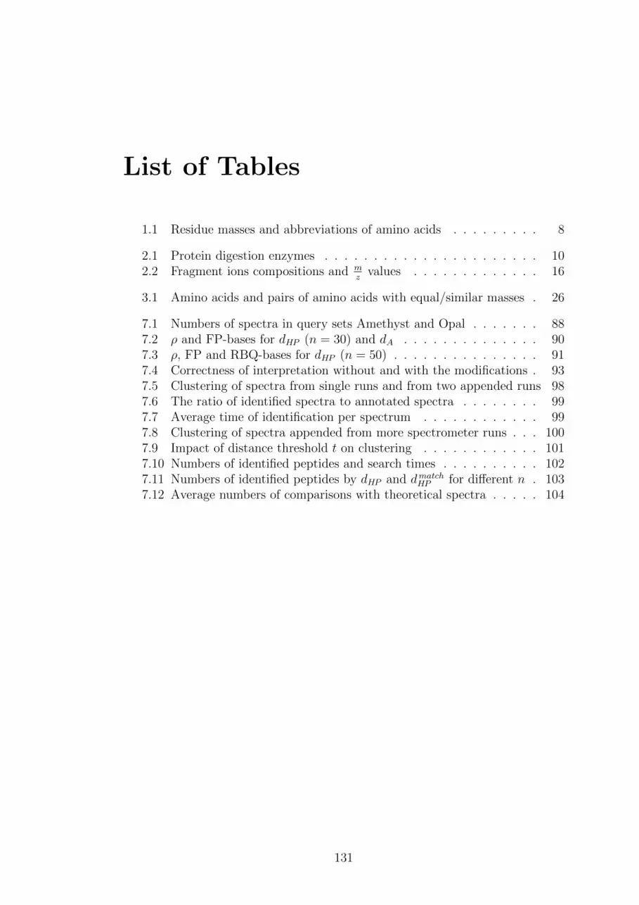
List of Tables

1.1 Residue masses and abbreviations of amino acids . . . . . . . . . 8

2.1 Protein digestion enzymes . . . . . . . . . . . . . . . . . . . . . . 102.2 Fragment ions compositions and m

zvalues . . . . . . . . . . . . . 16

3.1 Amino acids and pairs of amino acids with equal/similar masses . 26

7.1 Numbers of spectra in query sets Amethyst and Opal . . . . . . . 887.2 ρ and FP-bases for dHP (n = 30) and dA . . . . . . . . . . . . . . 907.3 ρ, FP and RBQ-bases for dHP (n = 50) . . . . . . . . . . . . . . . 917.4 Correctness of interpretation without and with the modifications . 937.5 Clustering of spectra from single runs and from two appended runs 987.6 The ratio of identified spectra to annotated spectra . . . . . . . . 997.7 Average time of identification per spectrum . . . . . . . . . . . . 997.8 Clustering of spectra appended from more spectrometer runs . . . 1007.9 Impact of distance threshold t on clustering . . . . . . . . . . . . 1017.10 Numbers of identified peptides and search times . . . . . . . . . . 1027.11 Numbers of identified peptides by dHP and dmatchHP for different n . 1037.12 Average numbers of comparisons with theoretical spectra . . . . . 104

131

132

List of Algorithms

1 Locality Sensitive Hashing . . . . . . . . . . . . . . . . . . . . . . . 462 Index Match Algorithm . . . . . . . . . . . . . . . . . . . . . . . . 473 Index Diagonal Algorithm . . . . . . . . . . . . . . . . . . . . . . . 484 Two-Index Diagonal Algorithm . . . . . . . . . . . . . . . . . . . . 48

5 LAESA – range query . . . . . . . . . . . . . . . . . . . . . . . . . 556 LAESA – kNN query . . . . . . . . . . . . . . . . . . . . . . . . . 567 M-tree – construction (part 1) . . . . . . . . . . . . . . . . . . . . . 588 M-tree – construction (part 2) . . . . . . . . . . . . . . . . . . . . . 599 M-tree – range query . . . . . . . . . . . . . . . . . . . . . . . . . . 6110 M-tree – kNN query (part 1) . . . . . . . . . . . . . . . . . . . . . 6211 M-tree – kNN query (part 2) . . . . . . . . . . . . . . . . . . . . . 6312 TriGen algorithm . . . . . . . . . . . . . . . . . . . . . . . . . . . . 6813 NM-tree – construction . . . . . . . . . . . . . . . . . . . . . . . . 7014 NM-tree – range query . . . . . . . . . . . . . . . . . . . . . . . . . 71

15 Parameterized Hausdorff Distance . . . . . . . . . . . . . . . . . . 7616 Clustering of query mass spectra (main function) . . . . . . . . . . 8517 Clustering of query mass spectra (MergeClusters) . . . . . . . . . . 8518 Clustering of query mass spectra (SelectCentroids) . . . . . . . . . 8619 Clustering of query mass spectra (RearrangeClusters) . . . . . . . . 86

133

134

List of Abbreviations

AA-residue Amino Acid ResidueAESA Approximating and Eliminating Search AlgorithmANN Approximate Nearest NeighborDa DaltonDDH Distance Distribution HistogramDNA Deoxyribonucleic AcidESI Electrospray IonizationFDR False Discovery RateFP-modifier Fractional-Power ModifierGPU Graphic Processing UnitHDD Hard Disk DriveHPLC High-pressure Liquid ChromatographyICAT Isotope-coded Affinity TagsiTRAQ Isobaric Tags for Relative an Absolute QuantificationkNN k Nearest NeighborsLAESA Linear Approximating and Eliminating Search AlgorithmLBQ Label-based QuantificationLFQ Label-free QuantificationLSH Locality Sensitive HashingM-tree Metric TreeMALDI Matrix Assisted Laser Desorption IonizationMAM Metric Access MethodMOWSE MOlecular Weight SEarchMS Mass SpectrometryMS/MS, MS2 Tandem Mass SpectrometryMSDB Mass Spectrometry Protein Sequence DatabaseMVP-tree Multi Vantage Point TreeNAM Non-metric Access MethodNM-tree Non-metric TreeNSP Number of Sibling PeptidesOMSSA Open Mass Spectrometry Search AlgorithmPEP Posterior Error ProbabilityPM-tree Pivoting Metric TreePPE Peptide Probability Estimateppm Parts per Million

135

PSM Peptide-spectrum MatchPST Peptide Sequence TagPTM Post-translational ModificationRBQ-modifier Rational-Bezier-Quadratic ModifierRNA Ribonucleic AcidSILAC Stable Isotope Labeling by Amino Acids in Cell CultureSOM Self-organizing MapSP-modifier Similarity Preserving ModifierSPC Shared Peak CountSSD Solid-state DriveT-error Triangle ErrorT-modifier Triangle ModifierTG-modifier Triangle Generating ModifierTOF Time of FlightTOPP The OpenMS Proteomics PipelineTOPPAS The OpenMS Proteomics Pipeline ASsistantTPP Trans-Proteomic PipelineTriGen Triangle Generating AlgorithmTV-modifier Triangle Violating ModifierVP-tree Vantage Point Tree

136