Simcenter 3D Low Frequency EM User Guide Version: Simcenter 3D 2019.2

Welcome message from author
This document is posted to help you gain knowledge. Please leave a comment to let me know what you think about it! Share it to your friends and learn new things together.
Transcript
Simcenter 3D Low Frequency EM User Guide
Version: Simcenter 3D 2019.2
Table of Contents 1 Introduction .......................................................................................................................................................... 1
2 Simcenter 3D Low Frequency EM environment ................................................................................................... 2
3 Workflow .............................................................................................................................................................. 3
4 Air and Remesh regions ........................................................................................................................................ 4
Air Region ........................................................................................................................................................ 4
Remesh Region ................................................................................................................................................ 4
5 Meshing ................................................................................................................................................................ 5
Stitching (2D models) ...................................................................................................................................... 5
Mesh Mating Conditions (3D models) ............................................................................................................. 5
6 Materials ............................................................................................................................................................... 6
7 Constraint Types ................................................................................................................................................... 7
Defining the outer boundary ........................................................................................................................... 7
Periodic ............................................................................................................................................................ 8
7.2.1 Even Periodic constraint ...................................................................................................................... 8
7.2.2 Odd Periodic constraint ....................................................................................................................... 9
Flux Tangential – Electromagnetic .................................................................................................................. 9
Field Normal – Electromagnetic ...................................................................................................................... 9
Surface Impedance (3D only) – Electromagnetic .......................................................................................... 10
7.5.1 Surface Loss Density .......................................................................................................................... 10
Thin Plate (3D only) – Electromagnetic ......................................................................................................... 11
7.6.1 Fields ................................................................................................................................................. 11
7.6.2 Forces ................................................................................................................................................ 11
Perfect Electric Insulator – Electromagnetic ................................................................................................. 11
Perfect Thermal Insulator – Thermal ............................................................................................................ 12
Specified Temperature – Thermal ................................................................................................................. 12
Thermal Environmental Conditions – Thermal .......................................................................................... 12
Thin Thermal Layer (3D only) – Thermal ................................................................................................... 12
8 Simulation Object Types ..................................................................................................................................... 13
Coils ............................................................................................................................................................... 13
8.1.1 Face Coil (Simple) .............................................................................................................................. 13
8.1.2 Body Coil (Current Flow Surface ‐ CFS) .............................................................................................. 13
8.1.3 Face/Body coil Properties .................................................................................................................. 13
8.1.4 Conductor Area Per Turn ................................................................................................................... 14
Stranded coils ................................................................................................................................................ 15
8.2.1 Current‐driven Stranded coils ........................................................................................................... 15
8.2.2 Voltage‐driven Stranded coils ........................................................................................................... 16
8.2.3 Litz wire Stranded coils ...................................................................................................................... 17
Motion component ....................................................................................................................................... 18
8.3.1 Velocity‐driven motion ...................................................................................................................... 18
8.3.2 Load‐driven motion ........................................................................................................................... 18
8.3.3 Bumpers ............................................................................................................................................ 18
8.3.4 Springs ............................................................................................................................................... 19
8.3.5 Damping ............................................................................................................................................ 19
8.3.6 Setting up Motion Simulations with Multiple Degrees of Freedom .................................................. 19
8.3.7 Meshing tips: Setting up motion models........................................................................................... 22
8.3.8 Current limitations for 3D motion: .................................................................................................... 23
8.3.9 Remesh regions ................................................................................................................................. 23
8.3.10 Guidelines .......................................................................................................................................... 24
8.3.11 Modeling Tips for a motion component ............................................................................................ 24
8.3.12 Devices with periodic constraints:..................................................................................................... 24
9 Modeling Objects ................................................................................................................................................ 25
Circuits ........................................................................................................................................................... 25
Circuit Components in Motion solving .......................................................................................................... 26
Coil excitation ................................................................................................................................................ 27
9.3.1 Options (Transient solution only) ...................................................................................................... 27
9.3.2 Waveform parameters (Transient solution only) .............................................................................. 27
Parameterization Attribute ........................................................................................................................... 29
10 Circuit Editor ....................................................................................................................................................... 30
11 Simcenter 3D Low Frequency EM Solvers ........................................................................................................... 31
Static........................................................................................................................................................... 31
Time‐harmonic ........................................................................................................................................... 31
Transient .................................................................................................................................................... 32
Solution Attributes ..................................................................................................................................... 32
11.4.1 General .............................................................................................................................................. 32
11.4.2 Convergence ...................................................................................................................................... 32
11.4.3 Adaption ............................................................................................................................................ 33
11.4.4 Coupled ............................................................................................................................................. 34
11.4.5 Time Steps (Transient only) ............................................................................................................... 35
11.4.6 Solution Storage (Transient only) ...................................................................................................... 36
11.4.7 Average Power Loss (Transient only) ................................................................................................ 36
11.4.8 Motion (Transient only) ..................................................................................................................... 36
11.4.9 Parameterization ............................................................................................................................... 36
11.4.10 Advanced ........................................................................................................................................... 37
12 About increasing solution accuracy .................................................................................................................... 40
Mesh refinement ....................................................................................................................................... 40
Coil mesh refinement ................................................................................................................................. 40
Polynomial order ........................................................................................................................................ 40
Constraints ................................................................................................................................................. 40
Linear Solver Tolerance .............................................................................................................................. 41
Maximum Newton iterations ..................................................................................................................... 41
Newton tolerance ...................................................................................................................................... 41
Error estimation ......................................................................................................................................... 41
Adaption ..................................................................................................................................................... 41
Using the magnetostatic solver for time‐harmonic problems ................................................................... 42
12.10.1 DC limit .............................................................................................................................................. 42
12.10.2 High Frequency Limit ......................................................................................................................... 42
13 Results ................................................................................................................................................................. 43
Simcenter 3D Low Frequency EM Results Viewer ...................................................................................... 44
13.1.1 Data Sets ............................................................................................................................................ 45
13.1.2 Filters ................................................................................................................................................. 47
Examples of multi layers of fields and filters ............................................................................................. 64
Plane and 3D views (Field View) ................................................................................................................ 67
14 Procedures .......................................................................................................................................................... 69
Stage 1 ........................................................................................................................................................ 69
14.1.1 Create new FEM and Simulation files ................................................................................................ 69
Stage 2 ........................................................................................................................................................ 70
14.2.1 Create a remesh region for a motion component ............................................................................. 70
14.2.2 Create air regions .............................................................................................................................. 72
Stage 3 ........................................................................................................................................................ 73
14.3.1 Make groups ...................................................................................................................................... 73
14.3.2 Matching boundaries prior to applying periodic conditions to a 3D model ...................................... 74
14.3.3 Matching boundaries prior to applying periodic conditions to a 2D model ...................................... 77
14.3.4 Preparing the 3D model before assigning meshes ............................................................................ 78
14.3.5 Verifying the Mesh Mating Conditions .............................................................................................. 78
14.3.6 Assigning a mesh ............................................................................................................................... 79
14.3.7 Assigning materials ............................................................................................................................ 79
14.3.8 Assigning direction to a permanent magnet (Uniform direction only) ............................................. 80
14.3.9 Assigning direction to a material (permanent magnet or anisotropic material) ............................... 81
Stage 4 ........................................................................................................................................................ 83
14.4.1 Assigning Periodic Constraints .......................................................................................................... 83
14.4.2 Assigning constraints ......................................................................................................................... 84
14.4.3 Create a motion component ............................................................................................................. 85
14.4.4 Create multiple coils .......................................................................................................................... 86
14.4.5 Create a single coil ............................................................................................................................. 88
14.4.6 Creating a circuit................................................................................................................................ 89
14.4.7 Creating a winding component ......................................................................................................... 91
14.4.8 Circuit Editor features: Add component ........................................................................................... 92
14.4.9 Circuit Editor features: Add connection ............................................................................................ 94
14.4.10 Circuit Editor features: Add to Report ............................................................................................... 95
14.4.11 Circuit Editor features: Align ............................................................................................................. 96
14.4.12 Circuit Editor features: Connection Line Bridging ............................................................................. 97
14.4.13 Circuit Editor features: Delete ........................................................................................................... 98
14.4.14 Circuit Editor features: Export ........................................................................................................... 99
14.4.15 Circuit Editor features: Grid ............................................................................................................. 100
14.4.16 Circuit Editor features: Nudge ......................................................................................................... 101
14.4.17 Circuit Editor features: Pan ............................................................................................................. 102
14.4.18 Circuit Editor features: Print/Print Preview/Print Setup ................................................................. 103
14.4.19 Circuit Editor features: Properties ................................................................................................... 104
14.4.20 Circuit Editor features: Rotate ......................................................................................................... 105
14.4.21 Circuit Editor features: Scroll ........................................................................................................... 105
14.4.22 Parameterizing the model ............................................................................................................... 106
Stage 5 ...................................................................................................................................................... 113
14.5.1 Solving a solution ............................................................................................................................. 113
14.5.2 Viewing results ................................................................................................................................ 113
14.5.3 Manipulating the viewing mode in the Field view .......................................................................... 114
14.5.4 Manipulating the display properties ............................................................................................... 115
14.5.5 Modifying the Colormap ................................................................................................................. 120
14.5.6 Accessing the display properties ..................................................................................................... 120
14.5.7 Modifying the color of the Label and Title ...................................................................................... 121
14.5.8 Modifying the Data Range ............................................................................................................... 121
14.5.9 Moving the Colormap around the Field view .................................................................................. 122
14.5.10 Re‐sizing the Colormap .................................................................................................................... 122
14.5.11 Camera and Actor mode example ................................................................................................... 123
14.5.12 Manipulating the Clip/Slice mesh filter widget ............................................................................... 124
14.5.13 Activating the widget ...................................................................................................................... 124
14.5.14 Setting up “Data Sets and Views” (Selecting mesh, quantities and fields)...................................... 126
14.5.15 Copy a Data Set or Filter .................................................................................................................. 127
14.5.16 Activating or de‐activating a data set .............................................................................................. 127
Simcenter 3D Low Frequency EM User Guide 2019.2
Restricted © Siemens AG 2019 Page 1 Siemens PLM Software
1 Introduction
Simcenter 3D Low Frequency EM is designed for solving low frequency electromagnetic (EM) problems that can involve static magnetic fields, time-varying fields and eddy-currents, and transient conditions with motion of parts of the device. In addition to these analyses, an option is available for providing static or transient coupled thermal solutions of EM problems. Many devices can be represented very well by 2D models, with a substantial saving in computing resources and solution time.
Simcenter 3D Low Frequency EM provides a “virtual laboratory” in which a user can create models from magnetic materials and coils, view displays in the form of field plots and graphs, and get numerical values for quantities such as flux linkage and force.
A feature of Simcenter 3D Low Frequency EM is its use of the latest methods of solving the field equations and calculating quantities such as force and torque. To get reliable results, the user does not need to be an expert in electromagnetic theory or numerical analysis. Nevertheless, the user does need to be aware of the factors that govern the accuracy of the solution.
Simcenter 3D Low Frequency EM User Guide 2019.2
Restricted © Siemens AG 2019 Page 2 Siemens PLM Software
2 Simcenter 3D Low Frequency EM environment
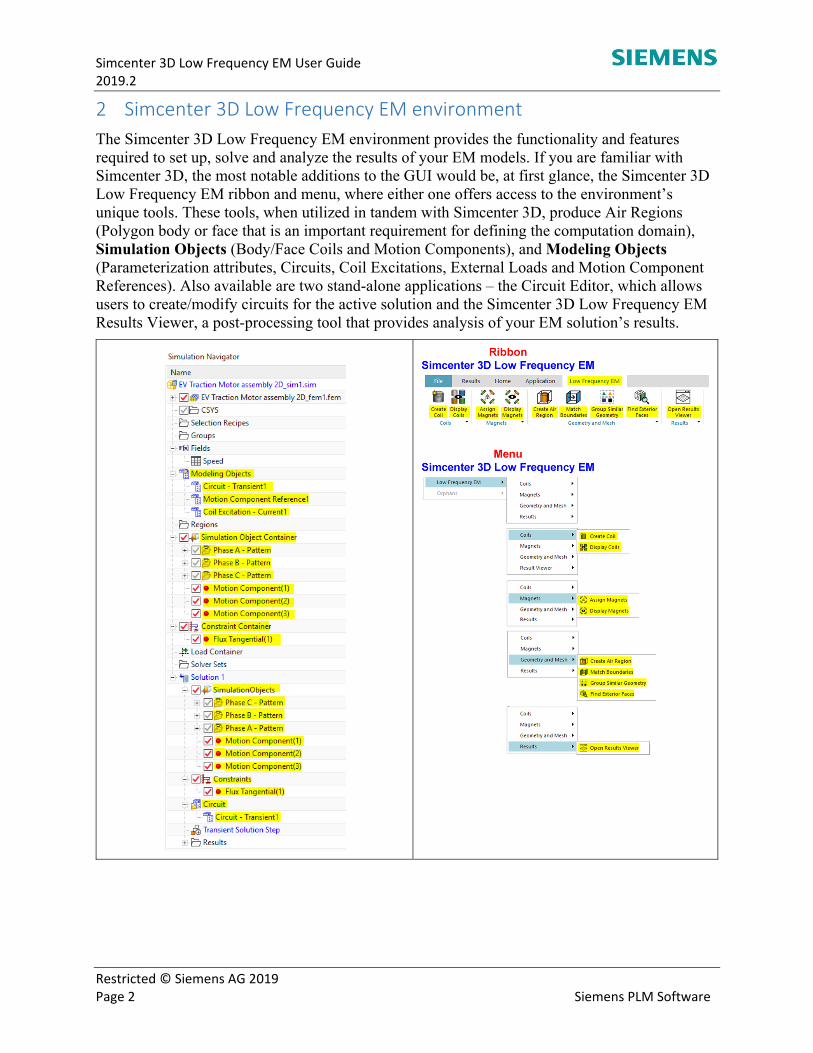
The Simcenter 3D Low Frequency EM environment provides the functionality and features required to set up, solve and analyze the results of your EM models. If you are familiar with Simcenter 3D, the most notable additions to the GUI would be, at first glance, the Simcenter 3D Low Frequency EM ribbon and menu, where either one offers access to the environment’s unique tools. These tools, when utilized in tandem with Simcenter 3D, produce Air Regions (Polygon body or face that is an important requirement for defining the computation domain), Simulation Objects (Body/Face Coils and Motion Components), and Modeling Objects (Parameterization attributes, Circuits, Coil Excitations, External Loads and Motion Component References). Also available are two stand-alone applications – the Circuit Editor, which allows users to create/modify circuits for the active solution and the Simcenter 3D Low Frequency EM Results Viewer, a post-processing tool that provides analysis of your EM solution’s results.
Simcenter 3D Low Frequency EM User Guide 2019.2
Restricted © Siemens AG 2019 Page 3 Siemens PLM Software
3 Workflow
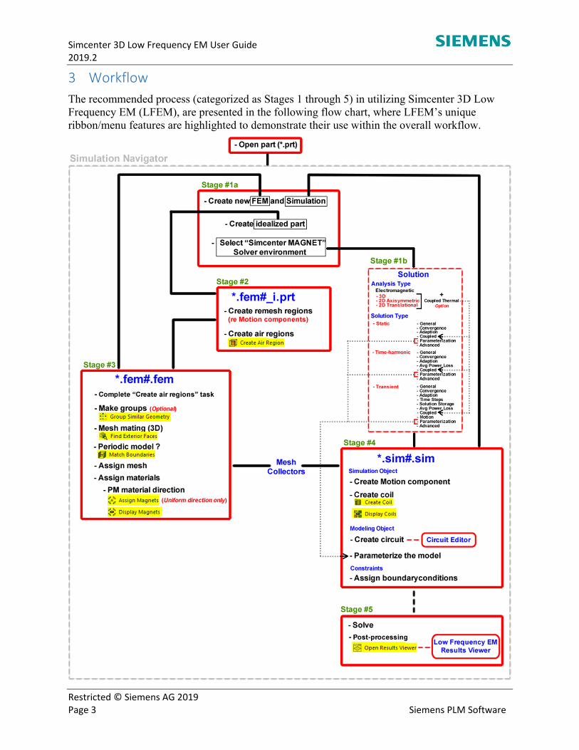
The recommended process (categorized as Stages 1 through 5) in utilizing Simcenter 3D Low Frequency EM (LFEM), are presented in the following flow chart, where LFEM’s unique ribbon/menu features are highlighted to demonstrate their use within the overall workflow.

Simcenter 3D Low Frequency EM User Guide 2019.2
Restricted © Siemens AG 2019 Page 4 Siemens PLM Software
4 Air and Remesh regions Air Region
In EM analysis, air regions are needed to define the computation domain. With the proper constraints, it provides a unique solution for the analysis model. Simcenter 3D Low Frequency EM provides an easy solution for creating an air region around the model that only requires a few steps to complete.
Remesh Region
In analyses where electric machine applications have moving components, two air boxes enclosing both stationary and rotary/linear motion parts are necessary, with the latter referred to as the remesh region.
Please refer to “Create Air Regions” and “Remesh Regions” for more information.
3D Sphere 3D Cylinder 3D Box
Simcenter 3D Low Frequency EM User Guide 2019.2
Restricted © Siemens AG 2019 Page 5 Siemens PLM Software
5 Meshing
In the finite element method of analysis, the model is divided into a mesh of elements. The field inside each element is represented by a polynomial with unknown coefficients. The finite element analysis is the solution of the set of equations for the unknown coefficients.
In 2D, the elements are shaped like triangles defined by three vertices (nodes). In 3D, the elements are shaped like tetrahedra. Each tetrahedral element is defined by four vertices.
The accuracy of the solution depends upon the nature of the field and the size of the mesh elements. In regions where the direction or magnitude of the field is changing rapidly, high accuracy requires small elements or high polynomial orders (or a combination of both).
Simcenter 3D Low Frequency EM provides you with control over the size of the mesh elements. You can change the size of the elements for the entire model, or only in areas of interest.
Stitching (2D models)
For 2D models, the “Create Air Region” procedure automatically performs the stitching process, which eliminates the need for any further action from the user on this matter.
Mesh Mating Conditions (3D models)
For purposes of obtaining a valid mesh for Finite Element Analysis, it is critical, for any source and target faces that are geometrically identical, that a single face is shared by the two bodies. To ensure the integrity of the mesh, the recommended method is to use the Mesh Mating condition with the Glue Coincident mesh mating type, selecting all faces or bodies in the model. Please refer to Simcenter documentation if you unfamiliar with this procedure.
Simcenter 3D Low Frequency EM User Guide 2019.2
Restricted © Siemens AG 2019 Page 6 Siemens PLM Software
6 Materials
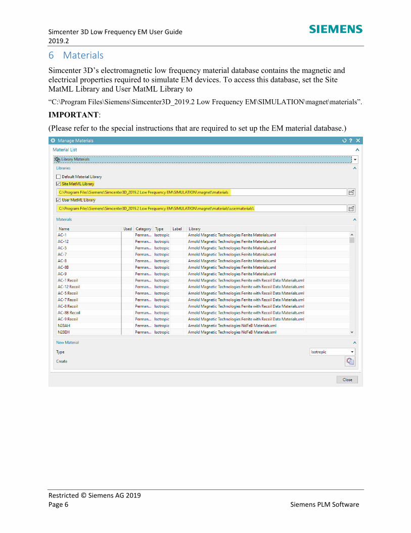
Simcenter 3D’s electromagnetic low frequency material database contains the magnetic and electrical properties required to simulate EM devices. To access this database, set the Site MatML Library and User MatML Library to
“C:\Program Files\Siemens\Simcenter3D_2019.2 Low Frequency EM\SIMULATION\magnet\materials”.
IMPORTANT:
(Please refer to the special instructions that are required to set up the EM material database.)
Simcenter 3D Low Frequency EM User Guide 2019.2
Restricted © Siemens AG 2019 Page 7 Siemens PLM Software
7 Constraint Types
Constraints define the behavior of the magnetic or thermal fields at the boundaries of the model. Constraints are applied to surfaces of the model, or to surfaces of an air box that represents an artificial outer boundary that surrounds the model. Conditions of symmetry can also be implied by using the appropriate constraint.
Simcenter 3D Low Frequency EM provides the following constraints:
Electromagnetic Thermal
Periodic (Odd/Even)
Flux Tangential
Field Normal
Surface Impedance
Thin Plate (3D only)
Perfect Electric Insulator (3D only)
Periodic (Odd/Even)
Perfect Thermal Insulator
Specified Temperature
Thermal Environmental Conditions
Thin Thermal Layer
Note The Flux Tangential constraint is applied, by default, to all outer surfaces of the model that are not assigned the Field Normal, Surface Impedance, or one of the Periodic constraints.
Note The Perfect Thermal Insulator constraint is applied, by default, to all outer surfaces of the model that have no other explicitly assigned constraints.
Defining the outer boundary Many problems in magnetics involve fields that decay far from the model. The magnetic field at these distances may be quite weak and of little interest. These spaces where the field is weak need not be modeled in any great detail because they do not have a substantial effect on the solution. However, at least part of the space needs to be modeled. The placement of an artificial boundary wall surrounding the model limits the extent of the field to be solved.
The distance that the outer boundary should be placed is often a matter of guesswork. Two general rules can aid in determining the best placement of the boundary.
1. Only the immediate area of interest needs to be modeled.
Many magnetic problems only require that the correct solution be produced in an area of particular interest. For example, in a model of a recording head, the area of prime interest is the magnetic field in the recording film near the head gap. This area is unlikely to be significantly affected by whether the leakage field is modeled at any great distance.
2. The field of a closed set of currents decays rapidly.
Every magnetics problem contains a closed set of currents, so that the field at a sufficient distance is similar to that of a dipole. The field of a dipole decays rapidly with distance and, in most cases, it is not necessary to model beyond a distance of one or two times the major dimension of interest.

Simcenter 3D Low Frequency EM User Guide 2019.2
Restricted © Siemens AG 2019 Page 8 Siemens PLM Software
Periodic
If a model has a structure where the geometry and the field repeat in intervals (e.g. in linear or rotary machines), then it is only necessary to model one of the repeating sections. The mesh nodes on one line of symmetry are related to the mesh nodes on the other side.
Simcenter 3D Low Frequency EM has two periodic constraints:
Even Periodic: Used when there are an even number of poles in the model.
Odd Periodic: Used when there are an odd number of poles in the model.
7.2.1 Even Periodic constraint
If symmetry conditions exist, you can use the Even Periodic constraint to model sections of linear or rotary machines that have an even number of poles. The mesh nodes on one plane of symmetry are related to the mesh nodes on the other side.
For example, if two poles of a multi-polar motor are modeled, then the field or temperature on one plane of symmetry is in the opposite direction to the field or temperature on the other plane of symmetry. The symmetry conditions are specified by defining a periodic constraint on each plane of symmetry.
Four-pole model Half the four-pole model with Even Periodic constraint applied to two surfaces
Matched nodes of the Even Periodic constraint
Simcenter 3D Low Frequency EM User Guide 2019.2
Restricted © Siemens AG 2019 Page 9 Siemens PLM Software
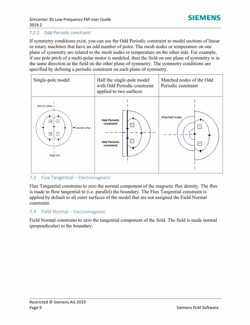
7.2.2 Odd Periodic constraint
If symmetry conditions exist, you can use the Odd Periodic constraint to model sections of linear or rotary machines that have an odd number of poles. The mesh nodes or temperature on one plane of symmetry are related to the mesh nodes or temperature on the other side. For example, if one pole pitch of a multi-polar motor is modeled, then the field on one plane of symmetry is in the same direction as the field on the other plane of symmetry. The symmetry conditions are specified by defining a periodic constraint on each plane of symmetry.
Single-pole model Half the single-pole model with Odd Periodic constraint applied to two surfaces
Matched nodes of the Odd Periodic constraint
Flux Tangential – Electromagnetic
Flux Tangential constrains to zero the normal component of the magnetic flux density. The flux is made to flow tangential to (i.e. parallel) the boundary. The Flux Tangential constraint is applied by default to all outer surfaces of the model that are not assigned the Field Normal constraint.
Field Normal – Electromagnetic
Field Normal constrains to zero the tangential component of the field. The field is made normal (perpendicular) to the boundary.
Simcenter 3D Low Frequency EM User Guide 2019.2
Restricted © Siemens AG 2019 Page 10 Siemens PLM Software
Surface Impedance (3D only) – Electromagnetic
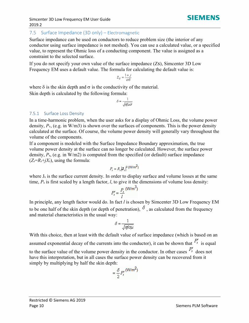
Surface impedance can be used on conductors to reduce problem size (the interior of any conductor using surface impedance is not meshed). You can use a calculated value, or a specified value, to represent the Ohmic loss of a conducting component. The value is assigned as a constraint to the selected surface.
If you do not specify your own value of the surface impedance (Zs), Simcenter 3D Low Frequency EM uses a default value. The formula for calculating the default value is:
where is the skin depth and is the conductivity of the material. Skin depth is calculated by the following formula:
7.5.1 Surface Loss Density
In a time-harmonic problem, when the user asks for a display of Ohmic Loss, the volume power density, Pv, (e.g. in W/m3) is shown over the surfaces of components. This is the power density calculated at the surface. Of course, the volume power density will generally vary throughout the volume of the components. If a component is modeled with the Surface Impedance Boundary approximation, the true volume power density at the surface can no longer be calculated. However, the surface power density, Ps, (e.g. in W/m2) is computed from the specified (or default) surface impedance (Zs=Rs+jXs), using the formula:
where Js is the surface current density. In order to display surface and volume losses at the same time, Ps is first scaled by a length factor, l, to give it the dimensions of volume loss density:
In principle, any length factor would do. In fact l is chosen by Simcenter 3D Low Frequency EM
to be one half of the skin depth (or depth of penetration), , as calculated from the frequency and material characteristics in the usual way:
With this choice, then at least with the default value of surface impedance (which is based on an
assumed exponential decay of the currents into the conductor), it can be shown that is equal
to the surface value of the volume power density in the conductor. In other cases does not have this interpretation, but in all cases the surface power density can be recovered from it simply by multiplying by half the skin depth:
Simcenter 3D Low Frequency EM User Guide 2019.2
Restricted © Siemens AG 2019 Page 11 Siemens PLM Software
Thin Plate (3D only) – Electromagnetic
Thin plates are implemented in Simcenter 3D Low Frequency EM as a surface property. The user can assign a surface property to the face(s) of component(s).
Thin plates have two properties that the user can specify:
The thickness of the plate The material
From the results point of view, two things are very important.
(1) Displaying fields on thin plates (2) Obtaining forces on thin plates
The size of the mesh elements that surround the face that the constraint has been applied to must be larger than the thickness of the plate for the approximation to work.
Since field plates have 0 thickness in the view, displaying fields is a bit tricky. For instance, if on one side of the plate, the field is very low and on the other, it is very high, the plate has to choose one field to display. The field it will choose to display is the same as the face it is applied to.
7.6.1 Fields
The field display shows the user what the field is on the thin plate. The field may be different depending on which side of the thin plate is being viewed. As for fields on slices, thin plates are ignored when extracting fields over slices. In effect, the field on thin plates only exists on shells.
7.6.2 Forces
Thin plates, like components, make up bodies, and the Electromagnetic 3D solver determines the bodies by examining how the surfaces are connected to each other.
Perfect Electric Insulator – Electromagnetic
The Perfect Electric Insulator (PEI) constraint can be applied to one common face of adjacent, or touching, components to prevent current from flowing through a conducting body. An example of its application would be when one is modelling laminations. Typically, laminations are insulated from each other by a thin layer of non-conducting material (e.g. glue). Meshing such a structure in 3D can become very expensive in processing time, so the use of the PEI constraint to simulate this behavior provides an economical alternative. Another example of the PEI constraint would be in cases where PEI is applied to a face which also has a periodic (i.e. binary) constraint.
Simcenter 3D Low Frequency EM User Guide 2019.2
Restricted © Siemens AG 2019 Page 12 Siemens PLM Software
Perfect Thermal Insulator – Thermal
With this condition, no heat is permitted to flow through the boundary. (Default setting)
Specified Temperature – Thermal
The temperature on the boundary is fixed to a value defined by the user.
Thermal Environmental Conditions – Thermal
This condition, defined by the convective heat transfer coefficient (hc), the radiation heat transfer coefficient (hr), and the environmental temperature outside (Te), specifies the way heat flows through the boundary:
q = hc*(T-Te) + hr*(T4 - Te4)
where T is the temperature at a point on the boundary, and q the heat flux through it.
Note The radiative heat transfer coefficient is related to emissivity by the Stefan–Boltzmann constant:
hr = emissivity x 5.6697e-8
The emissivity is a number between 0 and 1 (1 corresponds to the ideal, black-body emitter). No area is involved.
Note Any part of a Thermal Environment constraint which is on an interior surface will be ignored.
Thin Thermal Layer (3D only) – Thermal
This constraint is for modeling interference gaps between components and is implemented in Simcenter 3D Low Frequency EM as a surface property in a coupled thermal solution.
Simcenter 3D Low Frequency EM User Guide 2019.2
Restricted © Siemens AG 2019 Page 13 Siemens PLM Software
8 Simulation Object Types
Two important components of EM simulations are the coils and, in cases that consists of moving parts within an assembly, a motion component or components (i.e. for multiple degrees of freedom analysis).
Coils
Electromagnetic coils in Simcenter 3D Low Frequency EM can be configured as a Face Coil (2D or 3D) or as a Body Coil (3D only) and can either be solid or stranded, with a current or voltage source.
8.1.1 Face Coil (Simple)
Each coil has a start and end terminal. The direction of positive current flow is from the start terminal (F in) to the end terminal (F out).
8.1.2 Body Coil (Current Flow Surface ‐ CFS)
A coil defined by a cut plane.
The point and normal define a "current loop cut plane".
The CFS is the surface of intersection between the conductor and the plane defined by the point & normal which contains the point.
The current flow in a coil side can be reversed by pressing the Reverse Direction button.
8.1.3 Face/Body coil Properties Type Solid
A solid coil is a solid piece of conductor, in which the current is free to flow where it wants. For example, in a solid copper wire carrying 60 Hz current, the skin effect dictates that most of the current will flow near the surface of the wire.
Solid coils have 1 turn.
Stranded A stranded coil is a conductor made up of many fine wires. These wires are assumed to be uniformly distributed over the cross-section, and insulated from one another. Furthermore, they are assumed to be in series.
Simcenter 3D Low Frequency EM User Guide 2019.2
Restricted © Siemens AG 2019 Page 14 Siemens PLM Software
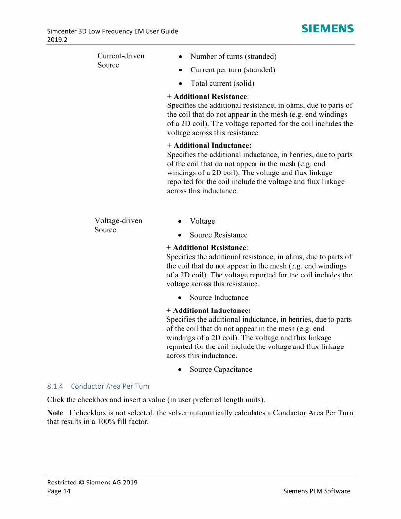
Current-driven Source
Number of turns (stranded)
Current per turn (stranded)
Total current (solid)
+ Additional Resistance: Specifies the additional resistance, in ohms, due to parts of the coil that do not appear in the mesh (e.g. end windings of a 2D coil). The voltage reported for the coil includes the voltage across this resistance.
+ Additional Inductance: Specifies the additional inductance, in henries, due to parts of the coil that do not appear in the mesh (e.g. end windings of a 2D coil). The voltage and flux linkage reported for the coil include the voltage and flux linkage across this inductance.
Voltage-driven Source
Voltage
Source Resistance
+ Additional Resistance: Specifies the additional resistance, in ohms, due to parts of the coil that do not appear in the mesh (e.g. end windings of a 2D coil). The voltage reported for the coil includes the voltage across this resistance.
Source Inductance
+ Additional Inductance: Specifies the additional inductance, in henries, due to parts of the coil that do not appear in the mesh (e.g. end windings of a 2D coil). The voltage and flux linkage reported for the coil include the voltage and flux linkage across this inductance.
Source Capacitance
8.1.4 Conductor Area Per Turn
Click the checkbox and insert a value (in user preferred length units).
Note If checkbox is not selected, the solver automatically calculates a Conductor Area Per Turn that results in a 100% fill factor.
Simcenter 3D Low Frequency EM User Guide 2019.2
Restricted © Siemens AG 2019 Page 15 Siemens PLM Software
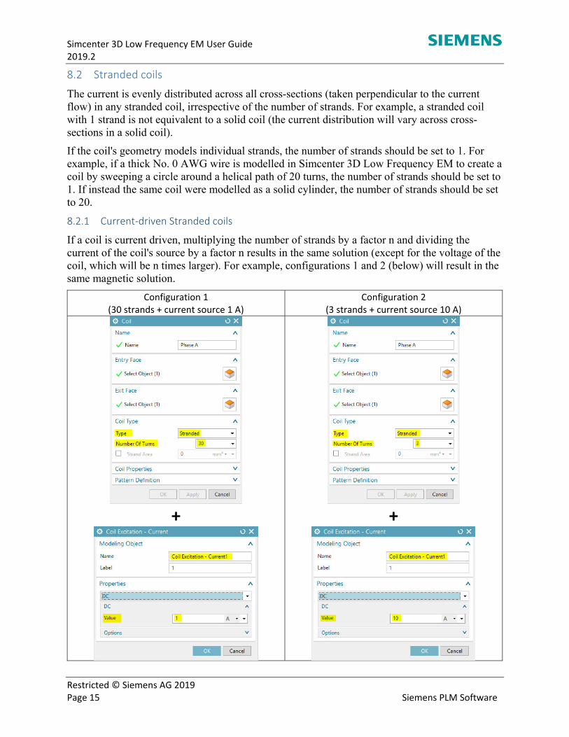
Stranded coils
The current is evenly distributed across all cross-sections (taken perpendicular to the current flow) in any stranded coil, irrespective of the number of strands. For example, a stranded coil with 1 strand is not equivalent to a solid coil (the current distribution will vary across cross-sections in a solid coil).
If the coil's geometry models individual strands, the number of strands should be set to 1. For example, if a thick No. 0 AWG wire is modelled in Simcenter 3D Low Frequency EM to create a coil by sweeping a circle around a helical path of 20 turns, the number of strands should be set to 1. If instead the same coil were modelled as a solid cylinder, the number of strands should be set to 20.
8.2.1 Current‐driven Stranded coils
If a coil is current driven, multiplying the number of strands by a factor n and dividing the current of the coil's source by a factor n results in the same solution (except for the voltage of the coil, which will be n times larger). For example, configurations 1 and 2 (below) will result in the same magnetic solution.
Configuration 1 (30 strands + current source 1 A)
Configuration 2 (3 strands + current source 10 A)
+
+
Simcenter 3D Low Frequency EM User Guide 2019.2
Restricted © Siemens AG 2019 Page 16 Siemens PLM Software
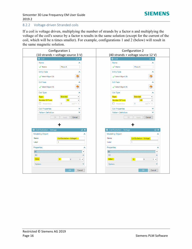
8.2.2 Voltage‐driven Stranded coils
If a coil is voltage driven, multiplying the number of strands by a factor n and multiplying the voltage of the coil's source by a factor n results in the same solution (except for the current of the coil, which will be n times smaller). For example, configurations 1 and 2 (below) will result in the same magnetic solution.
Configuration 1 (10 strands + voltage source 3 V)
Configuration 2 (40 strands + voltage source 12 V)
+
+
Simcenter 3D Low Frequency EM User Guide 2019.2
Restricted © Siemens AG 2019 Page 17 Siemens PLM Software
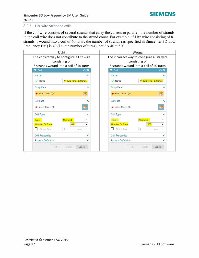
8.2.3 Litz wire Stranded coils
If the coil wire consists of several strands that carry the current in parallel, the number of strands in the coil wire does not contribute to the strand count. For example, if Litz wire consisting of 8 strands is wound into a coil of 40 turns, the number of strands (as specified in Simcenter 3D Low Frequency EM) is 40 (i.e. the number of turns), not 8 x 40 = 320.
Right Wrong
The correct way to configure a Litz wire consisting of
8 strands wound into a coil of 40 turns
The incorrect way to configure a Litz wire consisting of
8 strands wound into a coil of 40 turns
Simcenter 3D Low Frequency EM User Guide 2019.2
Restricted © Siemens AG 2019 Page 18 Siemens PLM Software
Motion component
A Motion Component is the nomenclature Simcenter 3D Low Frequency EM uses to identify the moving part or parts within an assembly. This component also requires an air region (i.e. remesh region).
8.3.1 Velocity‐driven motion
The movement of the motion component is specified through a user-defined waveform of component position versus time.
8.3.2 Load‐driven motion
The equations of motion are solved to find the movement of the motion component.
The following applies:
Component is given an initial position and velocity
Mass, center of gravity and moment of inertia automatically calculated
Time, position or speed-dependent loads (e.g. spring forces, damping)
Magnetic force/torque automatically calculated and added as a load
A positive load acts in the negative direction of motion and a negative load acts in the direction of motion (e.g. a spring)
A position dependent load should be defined for the complete range of motion, otherwise Simcenter 3D Low Frequency EM will extrapolate in a way that might not correspond to what the user wants
In a load driven problem, the position vs. time and speed vs. time curves of the motion Component/Load page are ignored. In a velocity driven problem, position of the motion component vs. time can be specified in the motion Component/Position page, by selecting Position based in the drop-down list. If position vs. time is specified, a piece-wise constant (PWC) speed vs. time curve will result that might introduce high frequency noise in the field solutions. A way to prevent this is to specify instead the speed vs. time curve as a PWL (by selecting Speed based in the drop-down list), which can be calculated from the position vs. time data and as result, the position computed by the motion solver will be smooth (i.e. continuous with continuous first derivative)
8.3.3 Bumpers
Bumpers can be defined to limit motion. Collisions with bumpers are, by default, perfectly elastic and bounce off at the same velocity at which it hit in the first place
Simcenter 3D Low Frequency EM User Guide 2019.2
Restricted © Siemens AG 2019 Page 19 Siemens PLM Software
8.3.4 Springs
Springs, tied to the inertia center of the motion component, can be defined. The spring parameters are the following:
Spring Constant: spring constant (N/m)
Spring Rest Position: equilibrium position (zero elongation) with respect to the zero displacement position of the motion component. The default value for Spring Rest Position is 0.0 (therefore corresponding to the zero displacement position of the motion component).
8.3.5 Damping
If no damping is specified, the natural mechanical oscillations of the model will not be attenuated. In order to damp the motion, one can apply a Friction Viscous Coefficient in the Motion Component dialog. One can then enter any non-negative number in order to lessen the bouncing that is observed at the bumpers
8.3.6 Setting up Motion Simulations with Multiple Degrees of Freedom
If a moving body is not constrained to pivot about an axis or move along a line, then that body has multiple degrees of freedoms. A rigid body whose motion is constrained to be planar has three degrees of freedom; a rotation in the plane and translation in two directions. This is the case for an unconstrained body in a 2D solve. In 3D, an unconstrained body has six degrees of freedom: three rotations (roll, yaw, and pitch), and translation in three possible directions (up-down, left-right, forward-backward).
In most cases of practical interest, the motion is, in fact, not completely unconstrained. For example, a top spinning about a fixed pivot has only three degrees of freedom. The usual way of applying constraints to a dynamical system is to use state variables to define what kinds of motion are possible. For example, the motion of the rotor of a machine that is constrained to pivot about an axis, has only one degree of freedom and is described with just one state variable: the angle of the rotor from its initial position. The motion of the top, mentioned previously, can be described by the standard spin, precession and nutation state variables.
Most motion that is constrained by mechanical linkages can be naturally described using state variables, which control a sequence of shifts and rotations that are applied cumulatively. Simcenter 3D Low Frequency EM is limited to constraints that can be described in this way. An example of a constraint that cannot be simulated in Simcenter 3D Low Frequency EM is a coin rolling on the floor which is wobbling as it rolls, since the constraint at the contact point is more complex that a simple rotation or sliding constraint. The state variables chosen to describe the motion depend on the dynamical system being simulated. Once the state variables have been selected, setting up the Simcenter 3D Low Frequency EM simulation is straightforward.
Simcenter 3D Low Frequency EM User Guide 2019.2
Restricted © Siemens AG 2019 Page 20 Siemens PLM Software
Simcenter 3D Low Frequency EM uses a hierarchical approach that is a simple extension of the single degree of freedom case, where one motion component is created for each state variable. Thus, there will be as many motion components as degrees of freedom. The parameters of each motion component apply to the associated degree of freedom, and the global quantities report position, speed, and other parameters of the motion for that state variable. However, it is important to understand that the dynamical equations are solved simultaneously, so the interactions between degrees of freedom are modeled correctly. For example, a spinning top simulated in Simcenter 3D Low Frequency EM will show all the familiar characteristics such as precession.
The motion components are created in an order that unwinds the sequence of cumulative shifts and rotations represented by each state variable, starting with the last one. In other words, each motion component describes a motion relative to the moving coordinate frame described by the subsequent motion components. Each of these subsequent motion components are created by selecting the previous motion component and then clicking on "Make Motion Component" from the "Model" menu. Therefore, each motion component describes the motion of the reference frame for the motion component inside it.
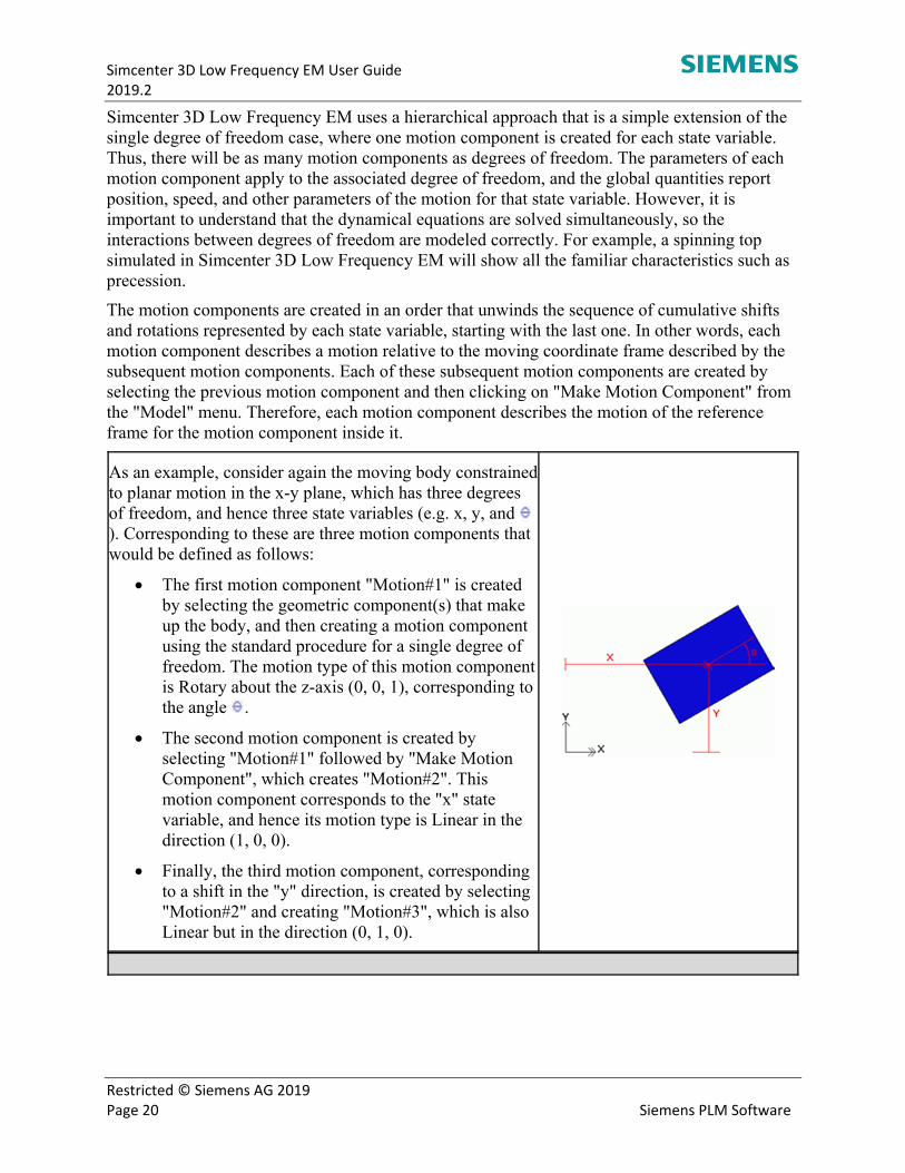
As an example, consider again the moving body constrained to planar motion in the x-y plane, which has three degrees of freedom, and hence three state variables (e.g. x, y, and ). Corresponding to these are three motion components that would be defined as follows:
The first motion component "Motion#1" is created by selecting the geometric component(s) that make up the body, and then creating a motion component using the standard procedure for a single degree of freedom. The motion type of this motion component is Rotary about the z-axis (0, 0, 1), corresponding to the angle .
The second motion component is created by selecting "Motion#1" followed by "Make Motion Component", which creates "Motion#2". This motion component corresponds to the "x" state variable, and hence its motion type is Linear in the direction (1, 0, 0).
Finally, the third motion component, corresponding to a shift in the "y" direction, is created by selecting "Motion#2" and creating "Motion#3", which is also Linear but in the direction (0, 1, 0).
Simcenter 3D Low Frequency EM User Guide 2019.2
Restricted © Siemens AG 2019 Page 21 Siemens PLM Software
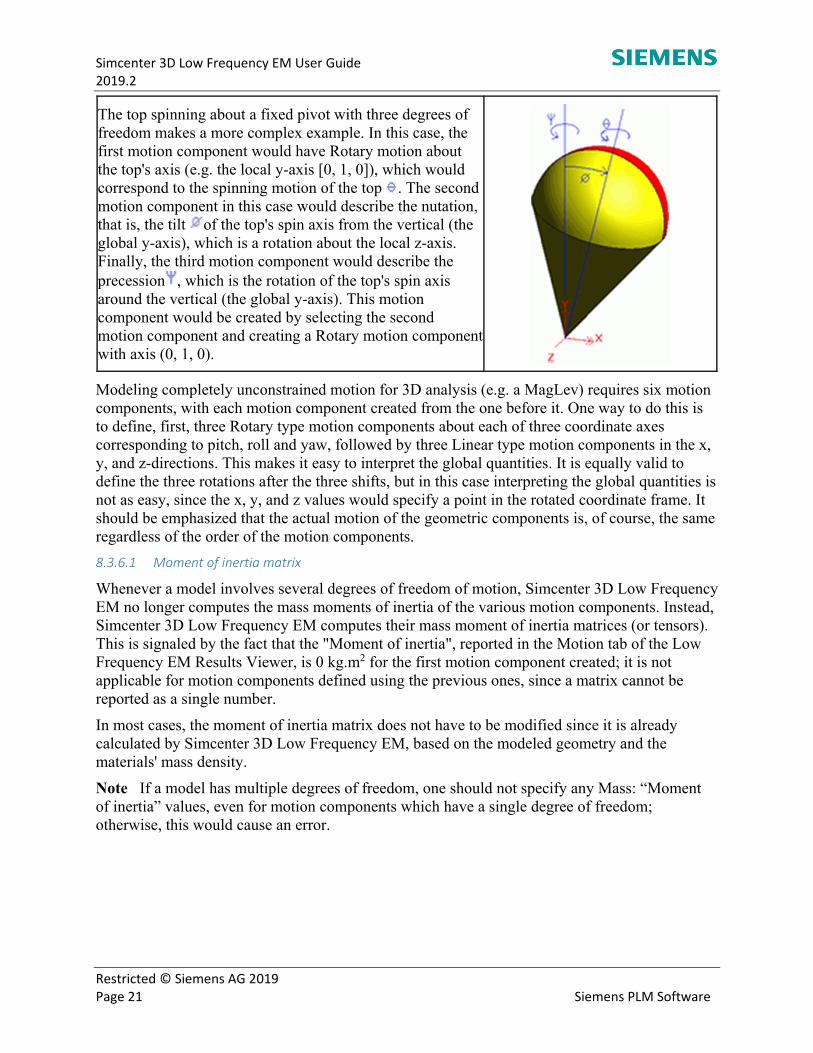
The top spinning about a fixed pivot with three degrees of freedom makes a more complex example. In this case, the first motion component would have Rotary motion about the top's axis (e.g. the local y-axis [0, 1, 0]), which would correspond to the spinning motion of the top . The second motion component in this case would describe the nutation, that is, the tilt of the top's spin axis from the vertical (the global y-axis), which is a rotation about the local z-axis. Finally, the third motion component would describe the precession , which is the rotation of the top's spin axis around the vertical (the global y-axis). This motion component would be created by selecting the second motion component and creating a Rotary motion component with axis (0, 1, 0).
Modeling completely unconstrained motion for 3D analysis (e.g. a MagLev) requires six motion components, with each motion component created from the one before it. One way to do this is to define, first, three Rotary type motion components about each of three coordinate axes corresponding to pitch, roll and yaw, followed by three Linear type motion components in the x, y, and z-directions. This makes it easy to interpret the global quantities. It is equally valid to define the three rotations after the three shifts, but in this case interpreting the global quantities is not as easy, since the x, y, and z values would specify a point in the rotated coordinate frame. It should be emphasized that the actual motion of the geometric components is, of course, the same regardless of the order of the motion components.
8.3.6.1 Moment of inertia matrix
Whenever a model involves several degrees of freedom of motion, Simcenter 3D Low Frequency EM no longer computes the mass moments of inertia of the various motion components. Instead, Simcenter 3D Low Frequency EM computes their mass moment of inertia matrices (or tensors). This is signaled by the fact that the "Moment of inertia", reported in the Motion tab of the Low Frequency EM Results Viewer, is 0 kg.m2 for the first motion component created; it is not applicable for motion components defined using the previous ones, since a matrix cannot be reported as a single number.
In most cases, the moment of inertia matrix does not have to be modified since it is already calculated by Simcenter 3D Low Frequency EM, based on the modeled geometry and the materials' mass density.
Note If a model has multiple degrees of freedom, one should not specify any Mass: “Moment of inertia” values, even for motion components which have a single degree of freedom; otherwise, this would cause an error.
Simcenter 3D Low Frequency EM User Guide 2019.2
Restricted © Siemens AG 2019 Page 22 Siemens PLM Software
8.3.7 Meshing tips: Setting up motion models
Certain rules must be obeyed in order to model motion problems correctly and to solve them efficiently. Here is a short summary that can be used as a guide for setting up motion models.
A valid motion model can be classified into one of the following types:
Type A. The motion component is completely enclosed by a single remesh region. No part of the moving body may intersect the remesh region's boundary.
Type B. The motion component is completely enclosed by a single remesh region, but some of its faces are coplanar with faces of the remesh region. These faces must be on the exterior boundary of the model (usually, they are planes of symmetry).
Type C. The outer shell of the motion component is on the exterior of the model except for a "motion interface" face, which connects it to the stationary part of the model. In this case, there are two remesh regions adjacent to the motion interface face: one connected to the stationary part of the mesh, and one that is part of the motion component. The motion is strictly rotary or linear for this case since the moving object "slides" against the stationary part of the model. The motion interface must be simple in nature -- that is, it must be a single model face with no interior edges or loops. Most models of this type have periodic constraints.
All remesh regions can be assigned the material AIR or any of the fluid materials (i.e. Coolants in material database).
For type C, if the model has periodic constraints, there is no need to add the extra constraint on the motion interface. The condition will be applied automatically by getting the periodic information from the explicitly defined constraints.
Limit the size and simplify the geometric structure of the remesh region(s) as much as possible. This will speed up the remeshing operation at each time step and have a significant impact on overall solution time. A motion object with a complicated exterior structure will incur significant remeshing time because its outer boundary is also part of the remesh boundary. However, enclosing the object with a simple region composed of planar or cylindrical faces isolates the motion object's complexity since the outer boundary adjacent to the remesh region is now much simpler. Of course, the enclosing dummy region should be assigned the appropriate material (i.e. AIR or a fluid) and must be part of the motion component definition.
Simcenter 3D Low Frequency EM User Guide 2019.2
Restricted © Siemens AG 2019 Page 23 Siemens PLM Software
8.3.8 Current limitations for 3D motion:
The motion object cannot be made up of disjoint pieces.
For types A and B, there can be only one remesh region.
For types A and B, all objects occupying the interior of the remesh region must be motion components.
Tip If one or more stationary bodies can’t be excluded from the remesh region without some difficulty, make each one a motion component and specify each source type to be "Velocity Driven". By default, these objects will have 0 velocity.
No other components may occupy the interior of any remesh region (except for the motion component for types A and B).
For Type C, the device must be modeled in the aligned position.
For Type C, there can be only one motion interface.
8.3.9 Remesh regions
In order to simulate motion problems correctly, a remesh region component is required to create an air region between the moving and stationary components of the model. Creating this component remeshes the region surrounding the moving component. Remeshing this relatively small and simple region is quick, and with this approach, no additional constraint equations need to be solved, which keeps solution times short and memory requirements low.
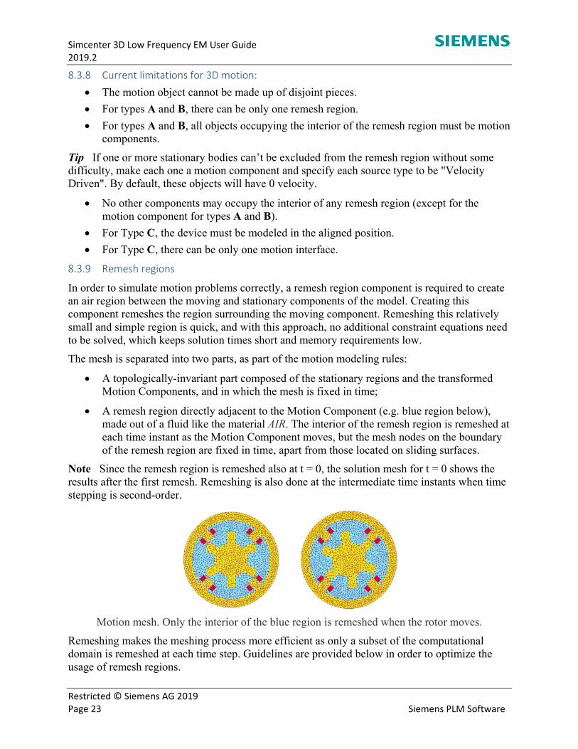
The mesh is separated into two parts, as part of the motion modeling rules:
A topologically-invariant part composed of the stationary regions and the transformed Motion Components, and in which the mesh is fixed in time;
A remesh region directly adjacent to the Motion Component (e.g. blue region below), made out of a fluid like the material AIR. The interior of the remesh region is remeshed at each time instant as the Motion Component moves, but the mesh nodes on the boundary of the remesh region are fixed in time, apart from those located on sliding surfaces.
Note Since the remesh region is remeshed also at t = 0, the solution mesh for t = 0 shows the results after the first remesh. Remeshing is also done at the intermediate time instants when time stepping is second-order.
Motion mesh. Only the interior of the blue region is remeshed when the rotor moves.
Remeshing makes the meshing process more efficient as only a subset of the computational domain is remeshed at each time step. Guidelines are provided below in order to optimize the usage of remesh regions.
Simcenter 3D Low Frequency EM User Guide 2019.2
Restricted © Siemens AG 2019 Page 24 Siemens PLM Software
8.3.10 Guidelines
Problem size: as motion meshing is a computationally expensive process, especially in 3D, the model should be reduced to the minimal size possible (e.g. by invoking symmetry or periodicity considerations).
Remesh regions
o Refine the remesh regions to improve force calculations.
o A complicated remesh region incurs significant remeshing time. Limit the size and simplify the structure of the remesh region(s) as much as possible, while keeping it large enough so that its boundaries do not come in contact with the Motion Component at any time. This will speed up the remeshing operation at each time step and have a significant impact on the overall solution time.
8.3.11 Modeling Tips for a motion component
All regions adjacent to a motion component must be assigned the material AIR.
Try to minimize the size of the air region(s) surrounding the motion component(s). This will speed up the remesh operation for every time step since there are a smaller number of elements to replace.
When you create a new material, if you do not specify a value for mass density, Simcenter 3D Low Frequency EM will assign a default value of zero (0). If the material is assigned to a motion component, give it a positive mass density -- otherwise, the solver will report that the component has zero (0) inertia.
To improve force calculations, make sure the air region surrounding the motion components is sufficiently refined.
It may be necessary to lower the linear solver tolerance or use a higher polynomial order to get accurate results when solving motion problems.
8.3.12 Devices with periodic constraints:
Always model the device in the aligned position (i.e. the symmetry faces of the rotor and stator are aligned). This enables Simcenter 3D Low Frequency EM to automatically determine the areas it must remesh as parts of the mesh are transformed by the effects of motion. Incorrect solutions will result if this rule is not followed. Note This limitation applies to 3D only.
The air region between the stationary and moving components must be modeled as two volumes. In addition, the air region adjacent to the moving part must be included as part of the motion component definition. It is not necessary to define a periodic constraint on the interface surface between the two air regions – the system will automatically impose the correct constraints as the two volumes move against each together.
There can only be one motion component when using periodic constraints.
For rotary motion, explicitly set the motion component mass property "Center of gravity". The value calculated by Simcenter 3D Low Frequency EM will be incorrect since the entire device is not being modeled.

Simcenter 3D Low Frequency EM User Guide 2019.2
Restricted © Siemens AG 2019 Page 25 Siemens PLM Software
9 Modeling Objects
Simcenter 3D Low Frequency EM provides several modeling objects that are instrumental to the EM simulation environment of Simcenter 3D. These objects can be created in two ways; one as a by-product of utilizing Simcenter 3D Low Frequency EM’s Circuit Editor, Coil Excitation dialog or Motion Component dialog, the other is to create them from the Modeling Objects Manager. Either way is acceptable and depends on the user’s preference.
Circuits
Various circuit components are available through the Circuit Editor to create an external electric circuit that connects to the coil(s). The complexity of a circuit can range from a simple configuration, with a current or voltage driven source or a more elaborate one containing any combination of the following:
Current/Voltage Source
Windings
Resistors
Capacitors
Inductors
Diodes
Switches (+ Current/Voltage)
Ground
Voltmeters
Ammeters
Position Switch (Motion components only – see below for more information)
Commutator (Motion components only – see below for more information)
Simcenter 3D Low Frequency EM User Guide 2019.2
Restricted © Siemens AG 2019 Page 26 Siemens PLM Software
Circuit Components in Motion solving
A motion component must already exist before placing a Position Switch and Commutator in a circuit; they must be linked to a specific motion component, since their operation is based on its position:
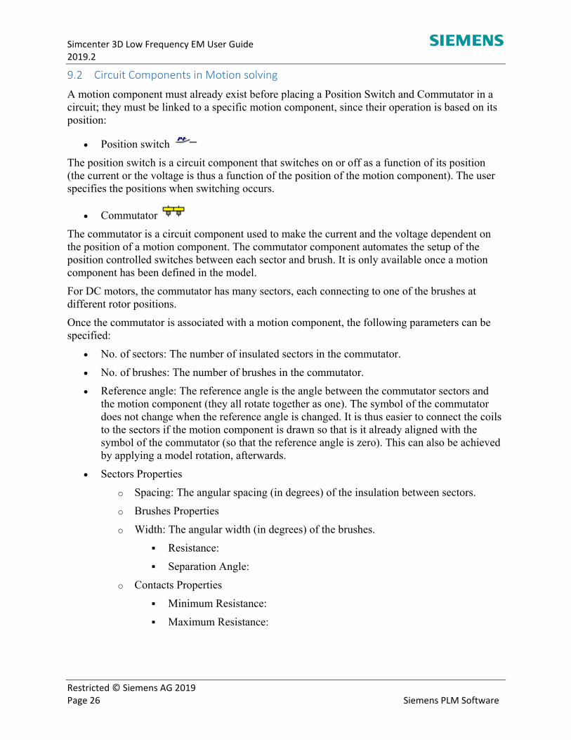
Position switch
The position switch is a circuit component that switches on or off as a function of its position (the current or the voltage is thus a function of the position of the motion component). The user specifies the positions when switching occurs.
Commutator
The commutator is a circuit component used to make the current and the voltage dependent on the position of a motion component. The commutator component automates the setup of the position controlled switches between each sector and brush. It is only available once a motion component has been defined in the model.
For DC motors, the commutator has many sectors, each connecting to one of the brushes at different rotor positions.
Once the commutator is associated with a motion component, the following parameters can be specified:
No. of sectors: The number of insulated sectors in the commutator.
No. of brushes: The number of brushes in the commutator.
Reference angle: The reference angle is the angle between the commutator sectors and the motion component (they all rotate together as one). The symbol of the commutator does not change when the reference angle is changed. It is thus easier to connect the coils to the sectors if the motion component is drawn so that is it already aligned with the symbol of the commutator (so that the reference angle is zero). This can also be achieved by applying a model rotation, afterwards.
Sectors Properties
o Spacing: The angular spacing (in degrees) of the insulation between sectors.
o Brushes Properties
o Width: The angular width (in degrees) of the brushes.
Resistance:
Separation Angle:
o Contacts Properties
Minimum Resistance:
Maximum Resistance:

Simcenter 3D Low Frequency EM User Guide 2019.2
Restricted © Siemens AG 2019 Page 27 Siemens PLM Software
Coil excitation
The Coil Excitation dialog allows you to define the properties that will drive the coils. The available source types differ for each solution:
Static Time Harmonic Transient
9.3.1 Options (Transient solution only)
Current Driven Voltage Driven
Negative Voltage Limit: Limits the voltage of the coil to be greater than the specified value (any number <= 0), if the coil is current-driven.
Positive Voltage Limit: Limits the voltage of the coil to be less than the specified value (any number >= 0), if the coil is current-driven.
Initial Current: If specified, the current at the initial time step will be constrained to be equal to this value.
Current On At Transient Start: If checked, it indicates that the current source was on before the Transient solver started. If not, it’s turned on at the start time.
Negative Current Limit: Limits the current of the coil to be greater than the specified value (any number <= 0), if the coil is voltage-driven.
Positive Current Limit: Limits the current of the coil to be less than the specified value (any number >= 0), if the coil is voltage-driven.
Initial Current: If specified, the current at the initial time step will be constrained to be equal to this value.
Voltage On At Transient Start: If checked, it indicates that the voltage source was on before the Transient solver started. If not, it’s turned on at the start time.
9.3.2 Waveform parameters (Transient solution only)
The different waveform types are defined in the Coil Excitation Properties group:
Simcenter 3D Low Frequency EM User Guide 2019.2
Restricted © Siemens AG 2019 Page 28 Siemens PLM Software
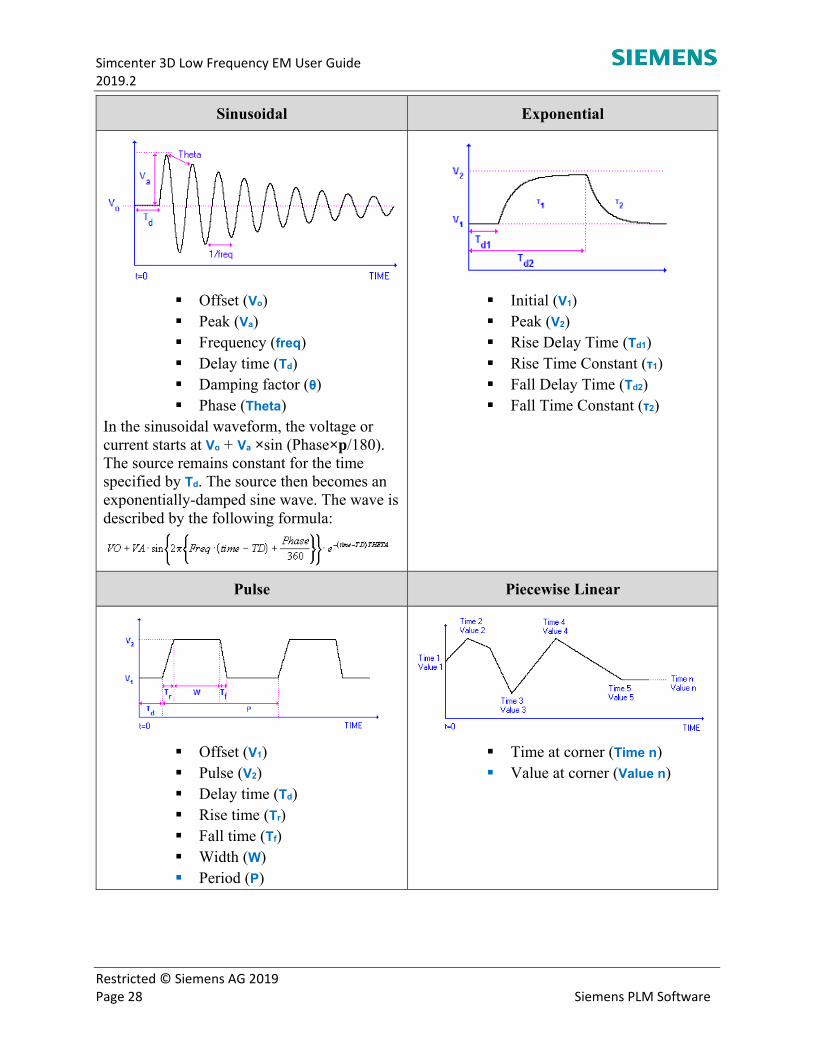
Sinusoidal Exponential
Offset (Vo) Peak (Va) Frequency (freq) Delay time (Td) Damping factor (θ) Phase (Theta)
In the sinusoidal waveform, the voltage or current starts at Vo + Va ×sin (Phase×p/180). The source remains constant for the time specified by Td. The source then becomes an exponentially-damped sine wave. The wave is described by the following formula:
Initial (V1) Peak (V2) Rise Delay Time (Td1) Rise Time Constant (τ1) Fall Delay Time (Td2) Fall Time Constant (τ2)
Pulse Piecewise Linear
Offset (V1) Pulse (V2) Delay time (Td) Rise time (Tr) Fall time (Tf) Width (W) Period (P)
Time at corner (Time n) Value at corner (Value n)

Simcenter 3D Low Frequency EM User Guide 2019.2
Restricted © Siemens AG 2019 Page 29 Siemens PLM Software
Parameterization Attribute
You can define a parameterization attribute by using an expression that was previously created for the model or by using an NX software expression, if any exist. The attribute can contain one or more values. Once completed, the resulting modeling object is then ready to be partnered with a solution, creating a step for each one of the values. When solved, results will be generated for each solution step (i.e. # of values = # of steps = # of problems solved).
Note The parameterization attribute is used exclusively with Simcenter 3D Low Frequency EM’s parameterization feature.
Define the Parameterization attribute Partner the attribute with a solution
Note the steps listed under the solution Note the equal number of solutions
Simcenter 3D Low Frequency EM User Guide 2019.2
Restricted © Siemens AG 2019 Page 30 Siemens PLM Software
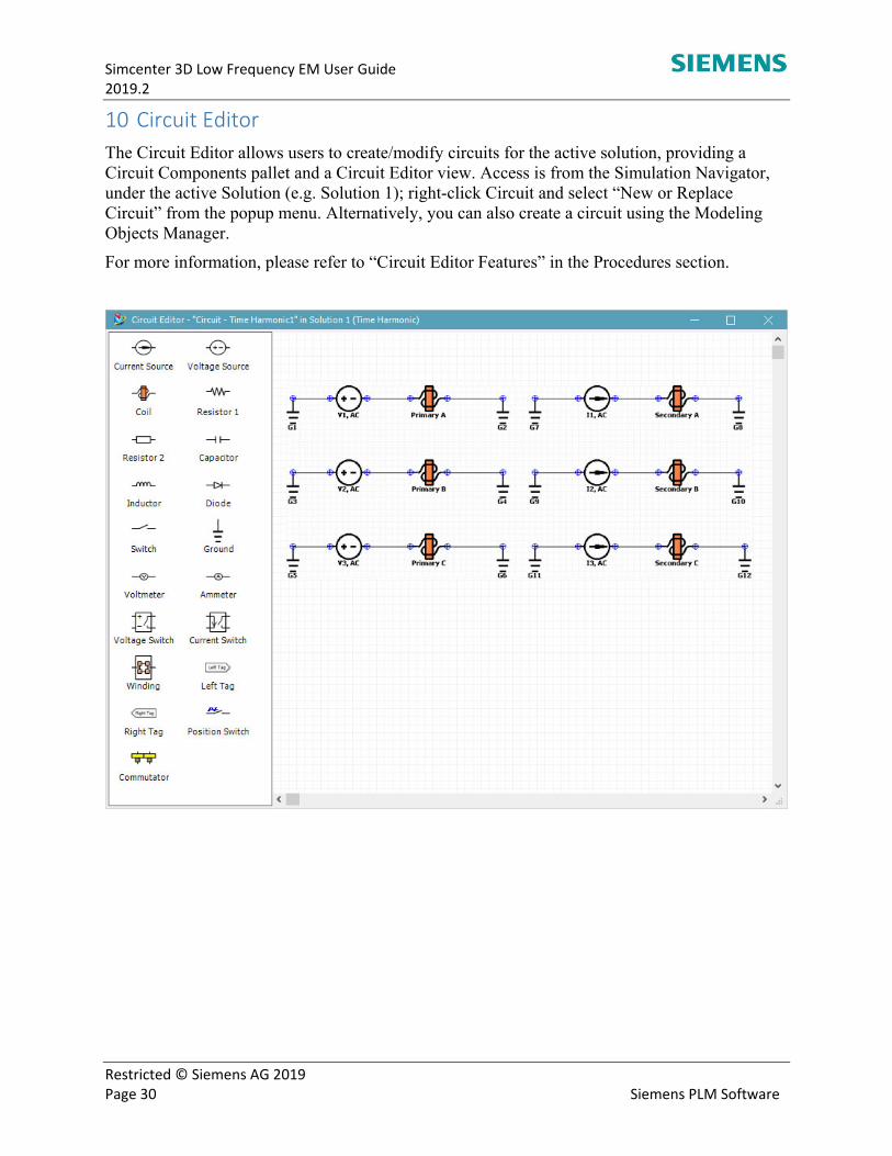
10 Circuit Editor The Circuit Editor allows users to create/modify circuits for the active solution, providing a Circuit Components pallet and a Circuit Editor view. Access is from the Simulation Navigator, under the active Solution (e.g. Solution 1); right-click Circuit and select “New or Replace Circuit” from the popup menu. Alternatively, you can also create a circuit using the Modeling Objects Manager.
For more information, please refer to “Circuit Editor Features” in the Procedures section.

Simcenter 3D Low Frequency EM User Guide 2019.2
Restricted © Siemens AG 2019 Page 31 Siemens PLM Software
11 Simcenter 3D Low Frequency EM Solvers
Simcenter 3D Low Frequency EM provides three types of solvers for electromagnetic analysis and two thermal solution types, which perform two-way coupling between the thermal and EM solvers.
Note
All solvers are categorized under Simcenter MAGNET.
The selection of the thermal solution type is made from the Coupled folder of the Solution dialog.
Static
Simcenter 3D Low Frequency EM static solver finds the magnetostatic field in and around specified current distributions in the presence of magnetic materials that may be linear or nonlinear, and isotropic or anisotropic.
In addition, each material may have a specified coercivity and direction of magnetization, thus allowing for the modeling of permanent magnets. The specified currents may flow through any type of conducting material, including magnetic materials.
In calculating the magnetostatic field, Simcenter 3D Low Frequency EM assumes that the specified currents are unchanging in time.
Time‐harmonic
Simcenter 3D Low Frequency EM's time-harmonic solver finds the time-harmonic magnetic field in and around current-carrying conductors, in the presence of materials that can be conducting, magnetic, or both. The conducting materials can be isotropic or anisotropic. The magnetic materials can be linear and isotropic or anisotropic.
Time-harmonic analysis is analysis at one specified frequency. Sources and fields are represented by complex phasors.
Theoretically, time-harmonic analysis is only possible when all the materials in the problem are linear. If they are nonlinear, sinusoidal-varying sources will not give rise to sinusoidal-varying fields, and time-harmonic analysis is not possible. However, Simcenter 3D Low Frequency EM’s time-harmonic 2D and 3D solvers are actually quasi nonlinear solvers, taking into account the approximate material nonlinearities by trying to find the operation point on a nonlinear B-H curve, using its first few data points.
The time-harmonic solver can handle two types of conductors, solid and stranded . It can also solve problems at a frequency of zero.
Note The time-harmonic solver can only model linear magnetic materials.
Simcenter 3D Low Frequency EM User Guide 2019.2
Restricted © Siemens AG 2019 Page 32 Siemens PLM Software
Transient
Simcenter 3D Low Frequency EM's transient solvers find the time-varying magnetic field in and around current-carrying conductors, in the presence of materials that may be conducting, magnetic, or both. The conducting materials can be isotropic or anisotropic. The magnetic materials may be linear (isotropic or anisotropic) or nonlinear (isotropic).
In addition, each material can have a specified coercivity and direction of magnetization, thus allowing for the modeling of permanent magnets. The currents may flow through any type of material, including magnetic materials.
The transient solver can handle two types of coils: solid and stranded .
Note The transient solver begins by finding a static solution; that is, the fields that would exist in the device assuming the conditions at the start time had held unchanged for all earlier times. The transient solution develops in time from this starting condition.
Displacement current is neglected and, so, wave phenomena are not modeled.
Solution Attributes
11.4.1 General
Description (optional):
Initial Temperature: Specifies the temperature for all components.
Default Source Frequency (TH/Transient only): Specifies the source frequency, in Hz (also expressed in multiples), used for all sources.
Effective Length (2D Translational only): Specifies the sweep distance applied to all volumes for calculating global quantities in a 2D Translational solution.
11.4.2 Convergence
Polynomial Order: Specifies the polynomial order used for all components.
Note
For 2D models, the value can be 1, 2, 3, or 4.
For 3D models, the value can be 1, 2, or 3
(Order 4 is treated as order 3 for 3D solutions).
Default (Depends on the model type):
2D Translational (default is 1)
2D Axisymmetric (default is 2)
3D (default is 1)

Simcenter 3D Low Frequency EM User Guide 2019.2
Restricted © Siemens AG 2019 Page 33 Siemens PLM Software
Nonlinear Method (3D only):
Newton-Raphson: this method is used for nonlinear solution types. Each step of the method solves a set of linear equations by the Conjugate Gradient (CG) method.
Successive Substitution: If a nonlinear problem has difficulty converging with the Newton-Raphson method, the Successive Substitution method can be used instead. This method is slower than the Newton-Raphson method, but is generally more certain to reach convergence.
Linear Solver Tolerance (%): Sets the maximum percentage of allowable change from one Conjugate Gradient (CG) step to the next. The iterative solution process ends when the tolerance is met. The default of 0.01% is generally acceptable. If necessary, the tolerance can be reduced to obtain a more accurate solution, but this will increase solving time.
Nonlinear Convergence Tolerance (%): Sets the maximum percentage of allowable change in the field from one Newton step to the next. The iterative solution process ends when the tolerance is met. The default of 1% is generally acceptable. If necessary, the tolerance can be reduced to obtain a more accurate solution, but this will increase solving time.
Maximum Nonlinear Iterations (TH only): Sets a limit for the number of iterations of a nonlinear solution.
Force All Materials to Be Linear: When checked, sets the material type to linear.
11.4.3 Adaption
Enable H-Adaption (2D only): When checked, uses H-Adaption when solving.
Enable P-Adaption (3D only): When checked, uses P-Adaption when solving.
Percentage of Elements to Refine: Specifies the percentage of elements to refine at each H-adaptive or P-Adaptive step.
Convergence Tolerance (%): Specifies the adaption tolerance.
Maximum Number of Steps: Specifies the maximum number of adaptive steps.
Simcenter 3D Low Frequency EM User Guide 2019.2
Restricted © Siemens AG 2019 Page 34 Siemens PLM Software
11.4.4 Coupled
11.4.4.1 Solving Sequence (Thermal – Static)
Solve EM Problem First -- This is the default mode. The events are as follows:
1. On the basis of the components' initial temperatures, an EM solution is computed. 2. On the basis of the time-averaged losses from this EM solution (plus any specified thermal
heat sources), a steady-state thermal solution is computed. This completes the first iteration. 3. On the basis of the temperatures from the latter thermal solution, an updated EM solution is
computed. 4. On the basis of the time-averaged losses from the latter EM solution (plus any specified
thermal heat sources), a new steady-state thermal solution is computed. This completes an additional iteration.
5. Steps 3 and 4 are repeated for each subsequent iteration.
Reuse Existing EM Solution -- If the model already has an EM solution (corresponding to the components' initial temperatures), this option instructs the thermal solver to fetch that solution instead of regenerating it from scratch in Step 1 above. If no EM solution is available, the coupled solve is aborted with this validation error:
“Cannot reuse electromagnetic solution. The electromagnetic solution does not exist.” If applicable, the Reuse option saves the effort of one full EM solve and is, therefore, automatically favored over the other two options.
Solve Thermal Problem First -- The events are as follows:
1. On the basis of only the specified thermal heat sources, a steady-state thermal solution is computed.
2. On the basis of the temperatures from this thermal solution, an EM solution is computed. This completes the first iteration.
3. On the basis of the time-averaged losses from the latter EM solution (plus any specified thermal heat sources), a new steady-state thermal solution is computed.
4. On the basis of the temperatures from the latter thermal solution, a new EM solution is computed. This completes an additional iteration.
5. Steps 3 and 4 are repeated for each subsequent iteration. Note This option cannot reuse an existing EM solution because the first EM solution it uses is computed from new temperatures. “Solve Thermal Problem First” is the preferred option if all of these conditions apply: There is no EM solution that could be reused; One is primarily interested in the EM quantities; When the EM losses are ignored, the thermal solution is still closer to the correct one
than are the components' initial temperatures. In that case, the option “Solve Thermal Problem First” yields a better estimate of the EM solution after the first iteration than the option “Solve EM Problem First” because it obtains its estimate from temperatures that were improved over the components' initial ones. Thus, the EM solution has a better start, and that advantage is retained over subsequent iterations.
Simcenter 3D Low Frequency EM User Guide 2019.2
Restricted © Siemens AG 2019 Page 35 Siemens PLM Software
11.4.4.2 Solving Sequence (Thermal – Static)
Solve EM Problem at Every Step --
Solve EM Problem Only Once at Start --
Solve EM Problem at Specified Interval --
Reuse Existing EM Solution -- If the model already has an EM solution (corresponding to the components' initial temperatures), this option instructs the thermal solver to fetch that solution instead of regenerating it from scratch in Step 1 above. If no EM solution is available, the coupled solve is aborted with this validation error: Cannot reuse electromagnetic solution. The electromagnetic solution does not exist. If applicable, the Reuse option saves the effort of one full EM solve and is, therefore, automatically favored over the other two options.
11.4.5 Time Steps (Transient only)
Time Step Method There are three methods by which the time steps for a transient solution are determined:
Fixed Interval (Default)
Adaptive
User Defined
The time stepping method must be set before you initiate the transient solution process.
Fixed Interval In the Fixed Interval time stepping method, each time step is of an equal length. The following options must be set for the fixed interval method.
o Start time: The first time instant
o Stop time: The last time instant
o Time Step: The interval between each time instant
o Advanced Time Step Options
Time Step Order: Polynomial adaption (First or Second order)
Adaptive In the Adaptive time stepping method, Simcenter 3D Low Frequency EM finds the appropriate time step length for the solution. The following options must be set for the adaptive method:
o Start time: The first time instant
o Stop time: The last time instant
o Initial Step: The interval between the first time instant and the second time instant
o Maximum Step: The maximum step length
o Minimum Step: The minimum step length
o Time Step Tolerance (%): Specifies the time adaption tolerance. Note Valid only for adaptive transient problems.
o Advanced Time Step Options
Time Step Order: Polynomial adaption (First or Second order)
Simcenter 3D Low Frequency EM User Guide 2019.2
Restricted © Siemens AG 2019 Page 36 Siemens PLM Software
User Defined In the User Defined time stepping method, each time instant is defined in the text pad provided, in the time units designated by the user.
11.4.6 Solution Storage (Transient only)
Solution Storage Method: You can choose to save all of the solutions, only the last solution, or a specific distribution of the solutions. (Default = Store All Solutions)
11.4.7 Average Power Loss (Transient only)
Specify Average Power Loss Start Time: Specifies the start time (in seconds) that is used to calculate the average power loss in the transient solution.
Specify Average Power Loss End Time: Specifies the end time (in seconds) that is used to calculate the average power loss in the transient solution.
11.4.8 Motion (Transient only)
Specify Gravitational Acceleration: Specifies the gravitational acceleration, in meters/second squared.
11.4.9 Parameterization
When simulating an electromagnetic device with software, it is useful to perform multiple experiments with one model. Unlike laboratory testing, one single model in Simcenter 3D Low Frequency EM can simulate a complete range of physical models, by using the parameterization feature.
Geometric features, materials, constraint types, simulation object types and mesh values can be varied through a user-specified range of values, and the results used to generate a family of performance curves for making design decisions. By automating much of this process, Simcenter 3D Low Frequency EM increases the throughput of the software, enabling more design possibilities to be tested with less computer time and less user time.
Material changes use either the built-in library, or a user-specified material. Geometric changes can be used for two functions: for position changes and for shape changes. Various shapes can be tested by inputting a range of dimensions, for example, when varying the shape of a pole face to minimize fringing. Similarly, the effect of a range of positions of one piece of the model versus the other can be examined for example, the position of one coil relative to another.
Presently, only the Single Parameter option is available as a parameterization method. More information on this feature can be found in “Modeling Objects – Parameterization Attribute” and “Parameterizing the model”.
Simcenter 3D Low Frequency EM User Guide 2019.2
Restricted © Siemens AG 2019 Page 37 Siemens PLM Software
11.4.10 Advanced
Convergence
o Linear Solver Technique (2D only): Specifies which solver technique (Direct/Iterative) to use.
Note The following only applies to 2D Transient solves.
If no Linear Solver Technique is specified, and a Direct solve fails, then Iterative solves will be attempted for all subsequent Newton steps within that Newton loop.
If more than 2/3 of all completed Newton solves are failed Direct solves, only then will subsequent time steps remain as Iterative solves.
If less than 2/3 of all completed Newton solves are failed Direct solves, a Direct solve will again be attempted during subsequent time steps.
If the Linear Solver Technique is specified as Direct, and the Direct solver fails for whatever reason, the solve will stop.
o Polynomial Order Is Minimized: If checked, it determines the polynomial order on the face between two components with different orders.
o Polynomial Order Augmented Layers: Determines how many layers of tetrahedrals, at the interface of faces of differing orders, augment to the higher order. Note In order to use this parameter, “Polynomial Order Is Minimized” must be unchecked.
0 = only faces will be augmented
1 = 1 layer of tetrahedrals touching the boundary
2 = 2 layers of tetrahedrals touching the boundary plus the tetrahedrals touching the first layer, etc.
o Maximum Nonlinear Iterations: Sets a limit for the number of iterations of a nonlinear solution. (Default = 50 iterations) Note Only applies to nonlinear problems. The 2D and 3D solvers will abort if a solution does not converge within the maximum number of Newton steps.
o Minimum Nonlinear Iterations: Sets a minimum number of iterations for a nonlinear solution. (Default = 0 iterations)
o Excess Nonlinear Iterations: Specifies how many additional Newton steps are required after convergence is satisfied.
o Excess Converged Nonlinear Iterations: Specifies how many additional converged Newton steps are required for convergence to be satisfied.
o Newton Iteration Scheme:
o Newton Search Iterations: Sets a limit for the number of iterations of a nonlinear solution.
o Newton Search Tolerance (%): Sets the maximum percentage of allowable change in the field from one Newton step to the next. The iterative solution process ends when the tolerance is met.
Simcenter 3D Low Frequency EM User Guide 2019.2
Restricted © Siemens AG 2019 Page 38 Siemens PLM Software
Coil Configuration (3D only)
o Create Implicit Coils: When checked, implicit coils are created automatically.
o Current Flow CG Tolerance: Conjugate gradient tolerance used when solving for the current distribution in a 3D coil. (Default = 1e-07)
o Solver Ignores Redundant Coils: Allows the solve to proceed if redundant coils are detected by replacing them with a short-circuit.
Solver Behaviour
o Solver Hysteresis Method (Transient only): Specifies the hysteresis modeling method to use.
None (default) -- Hysteresis is ignored
Jiles-Atherton -- Uses Jiles-Atherton hysteresis model
Jiles-Atherton (JA) model: a physics-based hysteresis model, explains the hysteresis loss mechanism with the theory of domain wall motion. The two modes of domain wall transitions (both the bending and translational motions) in a magnetic material result in a reversible and an irreversible component of magnetization, respectively. The total magnetization of material is computed using the following equation:
Where, Man(Ms, a) is the anhysteretic magnetization, Ms is the saturation magnetization, is the inter-domain coupling coefficient, a is a parameter that determines the shape of the anhysteretic curve and has the units of the magnetic field, k is the pinning coefficient, and c is the domain wall flexibility coefficient. These are known as the JA model parameters.
o Solver Ignores Eddy Currents (TH/Transient only): If set to:
Yes: component will have the DC steady-state current distribution if it is part of a coil; otherwise, it will have zero current. (Default for components of a stranded coil)
No: eddy currents will redistribute the current even if it is part of a stranded coil. (Default for all other conducting components)
o Solver Ignores Demagnetization: If checked, the solver will use the reversible model. If unchecked, the solver will follow the recoil curves, once the permanent magnet is demagnetized. (Applies only if the assigned material is a nonlinear permanent magnet)
Simcenter 3D Low Frequency EM User Guide 2019.2
Restricted © Siemens AG 2019 Page 39 Siemens PLM Software
Material Property Configuration
o Conductivity Scale Factor: Specifies the scale factor for the material conductivity.
o Iron Loss Adjustment Factor: Specifies the factor to scale the Kh and Ke loss coefficients.
o Magnetization Scale Factor: Specifies the scale factor for the material magnetization.
o Stacking Factor: Specifies the factor to adjust permeabilities, loss coefficients and mass densities to account for laminations.
o Include Rayleigh Region: When checked, it models the Rayleigh region for material curves.
o Reverse Magnetization Direction: When checked, the direction of every component's magnetization is reversed.
o BHAC Option (TH only): Specifies how the B-H curve is interpreted, and possibly transformed, for time-harmonic solves with in-phase AC sources.
The options “Transform for Equal RMS” and “Transform for Best Fit” transform the curve so that the sinusoidal waveform has either the same RMS value as, or is the best fit to, the transient waveform.
o BHAC Interpolation Factor (TH only): In a nonlinear periodic solution, both B and H cannot be sinusoidal. If this parameter is set to 0, then the solver will assume B is sinusoidal. If set to 1, it will assume H is sinusoidal. A value in between will result in interpolation. This applies to iron loss calculation, to instantaneous fields, and to the material curves when BHAC Option is either “Transform for Equal RMS” or “Transform for Best Fit”.
Transient Initial Conditions
o Zero Initial Solution: When checked, it overrides “Current/Voltage On At Transient Start”. Note Useful when the zero field is a closer approximation to the steady-state field than the default field obtained from a Static solution.
o Current On At Transient Start: If checked, it indicates that the current source was on before the Transient solver started. If not, it’s turned on at the start time.
o Voltage On At Transient Start: If checked, it indicates that the voltage source was on before the Transient solver started. If not, it’s turned on at the start time.
Simcenter 3D Low Frequency EM User Guide 2019.2
Restricted © Siemens AG 2019 Page 40 Siemens PLM Software
12 About increasing solution accuracy Solution accuracy is influenced by the following factors.
Mesh refinement
Smaller mesh elements increase the accuracy of the solution in two ways: modeling of the field and shape modeling.
Modeling of the field: Smaller elements allow the true field to be better approximated. Since smaller elements also increase the problem size and solution time, this effect is usually only used in specific areas of interest.
Shape modeling: Smaller elements may allow device shapes to be approximated more accurately. This effect is more evident when modeling circular components.
Coil mesh refinement
In general, refining the coil mesh will not improve solution accuracy. It is only necessary to refine the coil mesh with regard to improving the shape of the coil (see Shape modeling above).
Polynomial order
The potential in each tetrahedron of the mesh is modeled as a polynomial in the spatial coordinates (x, y, and z). The polynomial order can be specified individually for each component of the problem, or for the model as a whole. The polynomial order can be 1, 2, 3, 4 (Note: Order 4 is treated as order 3 for 3D solutions) or default. In general, higher orders give greater accuracy, but involve longer solution times. Where solution time is an issue, the polynomial order should be increased only in the areas of interest.
Constraints
Constraints define the limits of the field surrounding the model. Since the fields vary far less rapidly far away from the sources, a relatively coarse mesh can be used near the outer boundary. Consequently, the outer boundary can be placed quite far away without greatly increasing the number of elements of the mesh.
If you are concerned that the boundary has not been placed at a great enough distance, you can place an additional boundary to create an extra layer or two of elements. Differences in the solutions will indicate any increase in accuracy.
Simcenter 3D Low Frequency EM User Guide 2019.2
Restricted © Siemens AG 2019 Page 41 Siemens PLM Software
Linear Solver Tolerance
This method is an iterative solving method for the large set of linear simultaneous equations generated by the finite element analysis of the model. The linear solver tolerance is used for both linear and non-linear problems.
The linear solver tolerance is set in the Solution dialog. The default of 0.01% is generally acceptable. If necessary, the tolerance can be reduced to obtain a more accurate solution, but this will increase solving time.
Maximum Newton iterations
For nonlinear problems, Simcenter 3D Low Frequency EM uses a Newton-Raphson algorithm. Each step of the algorithm involves the solution of a set of linear equations by the linear solver method. When the change in the solution from one step to the next is smaller than the Newton tolerance, the iteration stops.
Note The 2D and 3D solvers will abort if a solution does not converge within the maximum number of Newton steps.
Newton tolerance
The Newton tolerance is set in the Solution dialog. The default of 1% is generally acceptable. If necessary, the tolerance can be reduced to obtain a more accurate solution, but this will increase solving time.
Error estimation
The error field for the model can be viewed as a shaded plot in the Simcenter 3D Low Frequency EM’s Results Viewer. A large difference in the magnitude or direction of the computed field between adjoining finite elements within the same material indicates a large error.
Note In some cases, the flux density may be perfectly continuous, yet errors may exist in that area. Changing the mesh in the area, or increasing the polynomial order, and comparing solution results will indicate any increase in accuracy.
Adaption
Simcenter 3D Low Frequency EM's analysis of magnetic models is based upon the finite element method. This method requires a finite element mesh. The quality of the results obtained from a finite element solution depends largely on the quality of the mesh. In regions where the direction or magnitude of the field is changing rapidly, high accuracy requires small elements. Simcenter 3D Low Frequency EM's adaption process automatically identifies and refines the areas of the mesh most in need of refinement to improve the quality of the solution.
Simcenter 3D Low Frequency EM User Guide 2019.2
Restricted © Siemens AG 2019 Page 42 Siemens PLM Software
Using the magnetostatic solver for time‐harmonic problems
Time-harmonic solutions are more computationally expensive than magnetostatic solutions. When possible, you can run the magnetostatic solver to save solving time. Two cases are listed below in which the magnetostatic solver could solve problems where the fields are time-harmonic.
12.10.1 DC limit
If the skin-depth in the conductors is very large compared to the size of the conductors, the currents are distributed more-or-less as they would be at DC. This can happen because:
The frequency is low, or zero.
The conductivities are low, or zero.
The model is small.
If the DC current distribution is fairly uniform, it can be modeled with coil meshes. The coil should be made stranded, with one turn, and the magnetic field calculated with the magnetostatic solver.
If the DC current distribution is not uniform, the problem can still be solved by the magnetostatic solver. In this case, the coil should be left as solid to allow for redistribution of the uniform coil current.
12.10.2 High Frequency Limit
If the skin-depth in the conductors is very small compared to the size of the conductors, the currents are distributed more-or-less in an infinitely-thin skin on the surface. The reasons for this occurrence are as follows:
The frequency is high
The conductivities are high
The model is large
The magnetostatic solver can be used with the Flux Tangential constraint on the surface of the conductors. Alternatively, the time-harmonic solver can be used with a surface impedance approximation on the surface of the conductors. This is a little more computationally expensive, but more accurate.
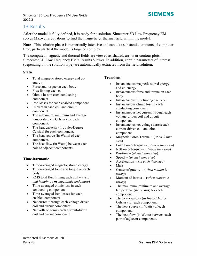
Simcenter 3D Low Frequency EM User Guide 2019.2
Restricted © Siemens AG 2019 Page 43 Siemens PLM Software
13 Results After the model is fully defined, it is ready for a solution. Simcenter 3D Low Frequency EM solves Maxwell's equations to find the magnetic or thermal field within the model.
Note This solution phase is numerically intensive and can take substantial amounts of computer time, particularly if the model is large or complex.
The computed magnetic and thermal fields are viewed as shaded, arrow or contour plots in Simcenter 3D Low Frequency EM’s Results Viewer. In addition, certain parameters of interest (depending on the solution type) are automatically extracted from the field solution:
Static
Total magnetic stored energy and co-energy
Force and torque on each body Flux linking each coil Ohmic loss in each conducting
component Iron losses for each enabled component Current in each coil and circuit
component The maximum, minimum and average
temperature (in Celsius) for each component.
The heat capacity (in Joules/Degree Celsius) for each component.
The heat source (in Watts) of each component.
The heat flow (in Watts) between each pair of adjacent components.
Time-harmonic
Time-averaged magnetic stored energy Time-averaged force and torque on each
body RMS total flux linking each coil -- (real
and imaginary or magnitude and phase) Time-averaged ohmic loss in each
conducting component Time-averaged iron losses for each
enabled component Net current through each voltage-driven
coil and circuit component Net voltage across each current-driven
coil and circuit component
Transient
Instantaneous magnetic stored energy and co-energy
Instantaneous force and torque on each body
Instantaneous flux linking each coil Instantaneous ohmic loss in each
conducting component Instantaneous net current through each
voltage-driven coil and circuit component
Instantaneous net voltage across each current-driven coil and circuit component
Magnetic Force/Torque -- (at each time step)
Load Force/Torque -- (at each time step) NetForce/Torque -- (at each time step) Position -- (at each time step) Speed -- (at each time step) Acceleration -- (at each time step) Mass Center of gravity -- (when motion is
rotary) Moment of Inertia -- (when motion is
rotary) The maximum, minimum and average
temperature (in Celsius) for each component.
The heat capacity (in Joules/Degree Celsius) for each component.
The heat source (in Watts) of each component.
The heat flow (in Watts) between each pair of adjacent components.
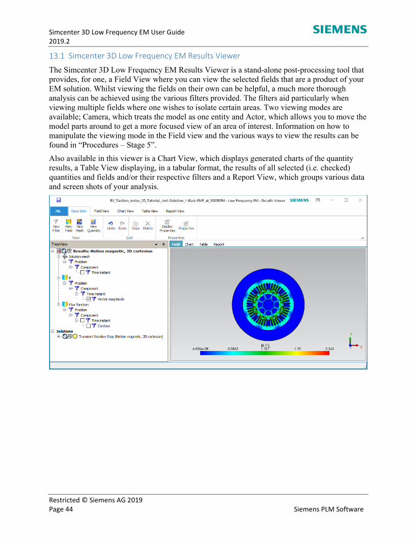
Simcenter 3D Low Frequency EM User Guide 2019.2
Restricted © Siemens AG 2019 Page 44 Siemens PLM Software
Simcenter 3D Low Frequency EM Results Viewer
The Simcenter 3D Low Frequency EM Results Viewer is a stand-alone post-processing tool that provides, for one, a Field View where you can view the selected fields that are a product of your EM solution. Whilst viewing the fields on their own can be helpful, a much more thorough analysis can be achieved using the various filters provided. The filters aid particularly when viewing multiple fields where one wishes to isolate certain areas. Two viewing modes are available; Camera, which treats the model as one entity and Actor, which allows you to move the model parts around to get a more focused view of an area of interest. Information on how to manipulate the viewing mode in the Field view and the various ways to view the results can be found in “Procedures – Stage 5”.
Also available in this viewer is a Chart View, which displays generated charts of the quantity results, a Table View displaying, in a tabular format, the results of all selected (i.e. checked) quantities and fields and/or their respective filters and a Report View, which groups various data and screen shots of your analysis.
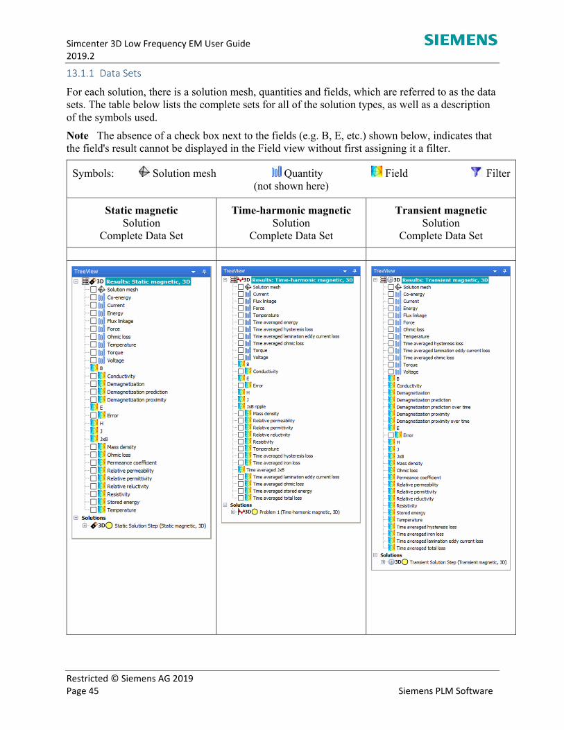
Simcenter 3D Low Frequency EM User Guide 2019.2
Restricted © Siemens AG 2019 Page 45 Siemens PLM Software
13.1.1 Data Sets
For each solution, there is a solution mesh, quantities and fields, which are referred to as the data sets. The table below lists the complete sets for all of the solution types, as well as a description of the symbols used.
Note The absence of a check box next to the fields (e.g. B, E, etc.) shown below, indicates that the field's result cannot be displayed in the Field view without first assigning it a filter.
Symbols: Solution mesh Quantity Field Filter (not shown here)
Static magnetic Solution
Complete Data Set
Time-harmonic magnetic Solution
Complete Data Set
Transient magnetic Solution
Complete Data Set
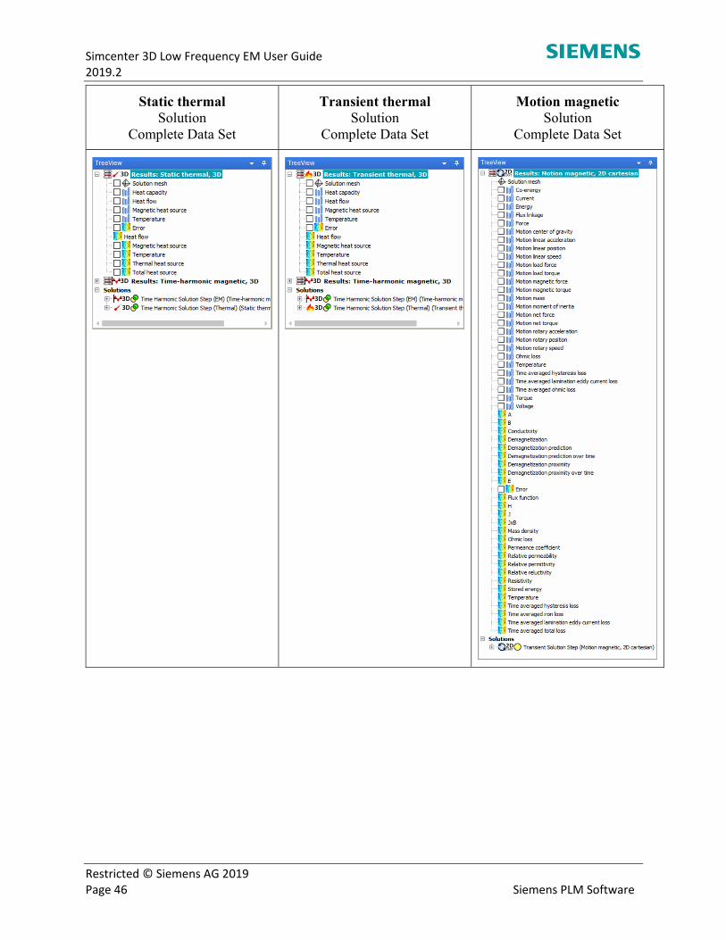
Simcenter 3D Low Frequency EM User Guide 2019.2
Restricted © Siemens AG 2019 Page 46 Siemens PLM Software
Static thermal Solution
Complete Data Set
Transient thermal Solution
Complete Data Set
Motion magnetic Solution
Complete Data Set
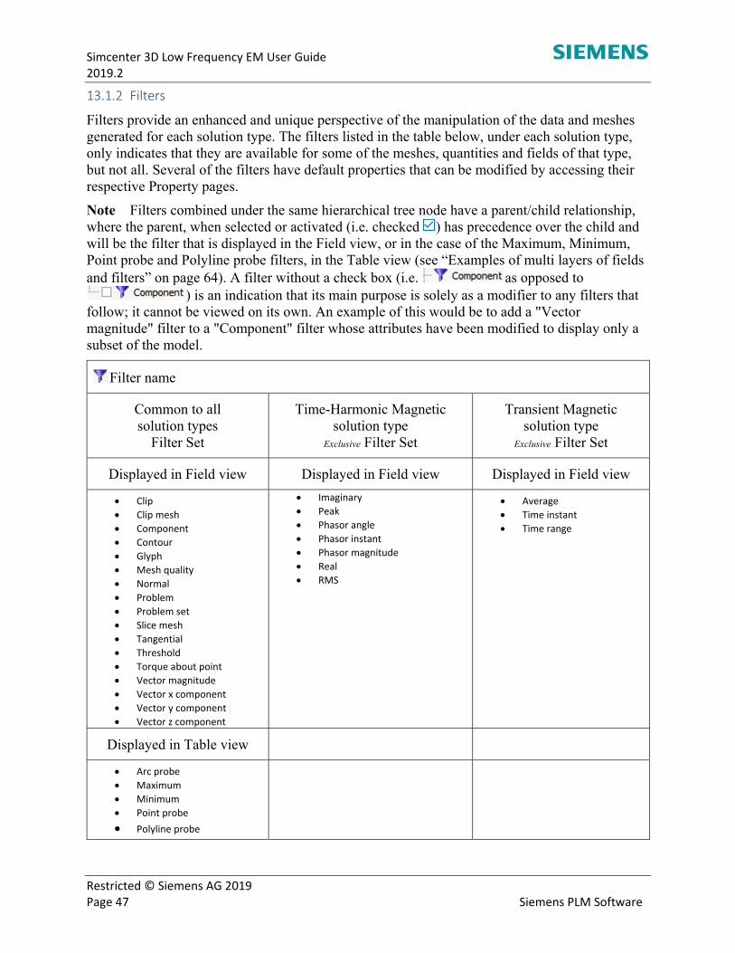
Simcenter 3D Low Frequency EM User Guide 2019.2
Restricted © Siemens AG 2019 Page 47 Siemens PLM Software
13.1.2 Filters
Filters provide an enhanced and unique perspective of the manipulation of the data and meshes generated for each solution type. The filters listed in the table below, under each solution type, only indicates that they are available for some of the meshes, quantities and fields of that type, but not all. Several of the filters have default properties that can be modified by accessing their respective Property pages.
Note Filters combined under the same hierarchical tree node have a parent/child relationship, where the parent, when selected or activated (i.e. checked ) has precedence over the child and will be the filter that is displayed in the Field view, or in the case of the Maximum, Minimum, Point probe and Polyline probe filters, in the Table view (see “Examples of multi layers of fields and filters” on page 64). A filter without a check box (i.e. as opposed to
) is an indication that its main purpose is solely as a modifier to any filters that follow; it cannot be viewed on its own. An example of this would be to add a "Vector magnitude" filter to a "Component" filter whose attributes have been modified to display only a subset of the model.
Filter name
Common to all solution types
Filter Set
Time-Harmonic Magnetic solution type
Exclusive Filter Set
Transient Magnetic solution type
Exclusive Filter Set
Displayed in Field view Displayed in Field view Displayed in Field view
Clip
Clip mesh
Component
Contour
Glyph
Mesh quality
Normal
Problem
Problem set
Slice mesh
Tangential
Threshold
Torque about point
Vector magnitude
Vector x component
Vector y component
Vector z component
Imaginary
Peak
Phasor angle
Phasor instant
Phasor magnitude
Real
RMS
Average
Time instant
Time range
Displayed in Table view
Arc probe
Maximum
Minimum
Point probe
Polyline probe
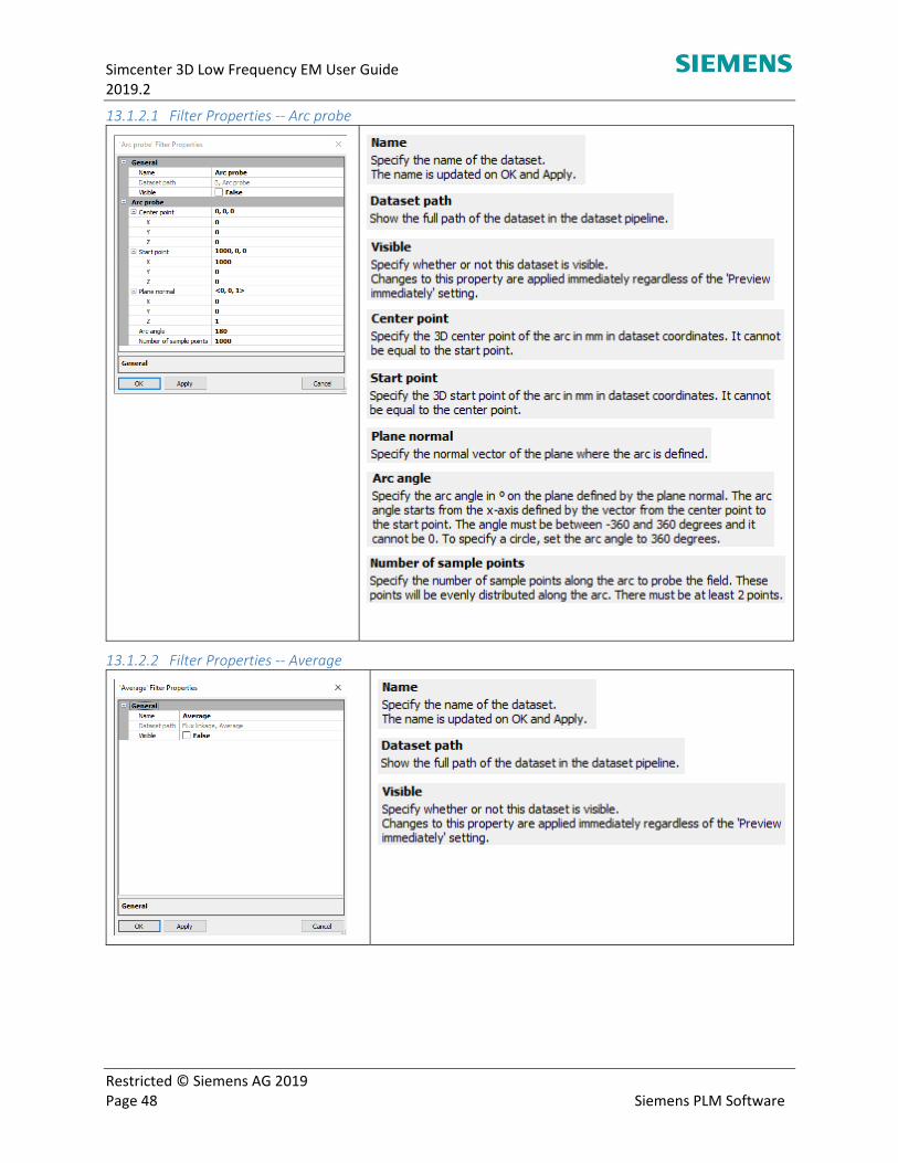
Simcenter 3D Low Frequency EM User Guide 2019.2
Restricted © Siemens AG 2019 Page 48 Siemens PLM Software
13.1.2.1 Filter Properties ‐‐ Arc probe
13.1.2.2 Filter Properties ‐‐ Average
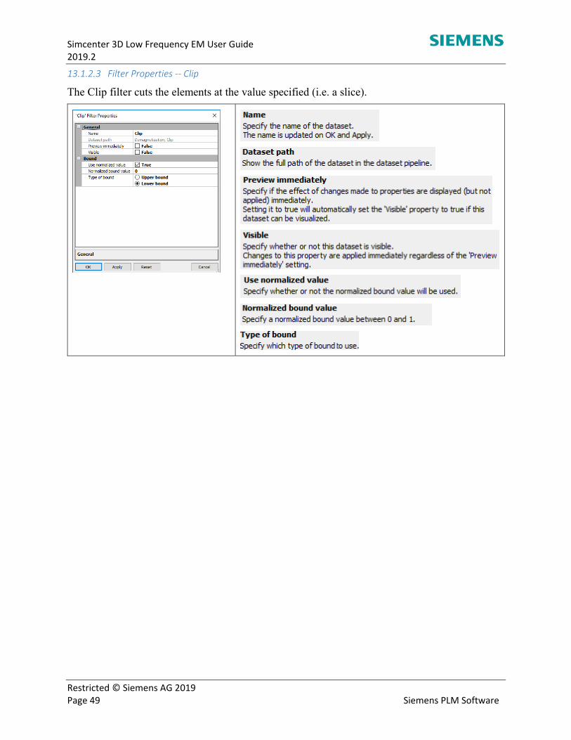
Simcenter 3D Low Frequency EM User Guide 2019.2
Restricted © Siemens AG 2019 Page 49 Siemens PLM Software
13.1.2.3 Filter Properties ‐‐ Clip
The Clip filter cuts the elements at the value specified (i.e. a slice).
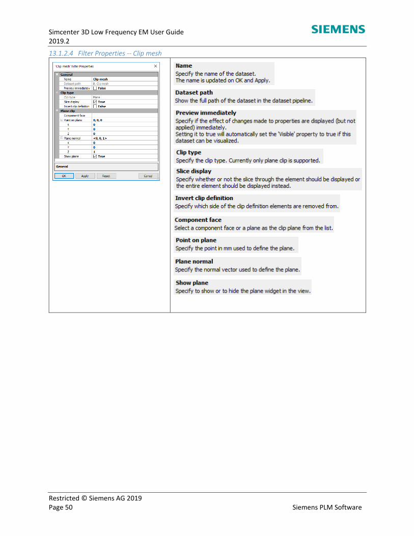
Simcenter 3D Low Frequency EM User Guide 2019.2
Restricted © Siemens AG 2019 Page 50 Siemens PLM Software
13.1.2.4 Filter Properties ‐‐ Clip mesh

Simcenter 3D Low Frequency EM User Guide 2019.2
Restricted © Siemens AG 2019 Page 51 Siemens PLM Software
13.1.2.5 Filter Properties ‐‐ Component
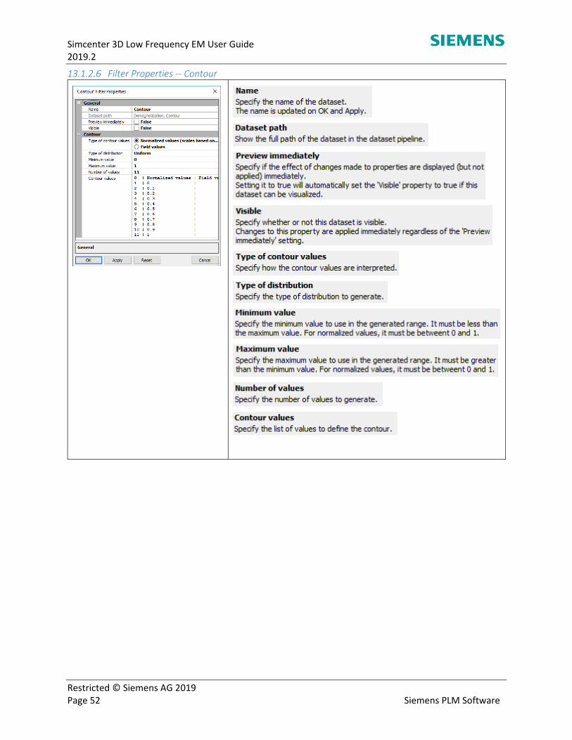
Simcenter 3D Low Frequency EM User Guide 2019.2
Restricted © Siemens AG 2019 Page 52 Siemens PLM Software
13.1.2.6 Filter Properties ‐‐ Contour
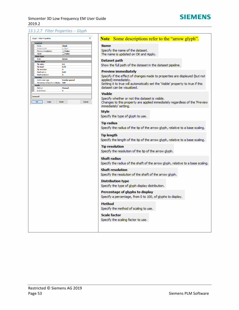
Simcenter 3D Low Frequency EM User Guide 2019.2
Restricted © Siemens AG 2019 Page 53 Siemens PLM Software
13.1.2.7 Filter Properties ‐‐ Glyph
Note Some descriptions refer to the “arrow glyph”.

Simcenter 3D Low Frequency EM User Guide 2019.2
Restricted © Siemens AG 2019 Page 54 Siemens PLM Software
13.1.2.8 Filter Properties ‐‐ Imaginary
13.1.2.9 Filter Properties – Maximum/Minimum
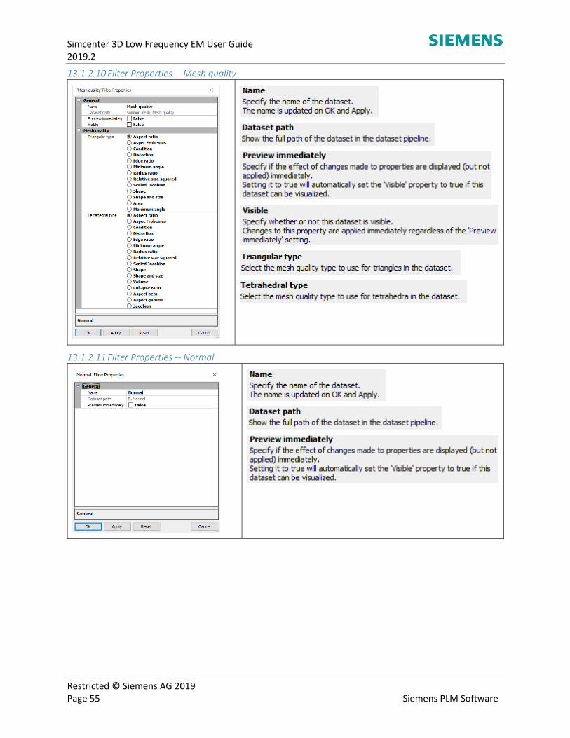
Simcenter 3D Low Frequency EM User Guide 2019.2
Restricted © Siemens AG 2019 Page 55 Siemens PLM Software
13.1.2.10 Filter Properties ‐‐ Mesh quality
13.1.2.11 Filter Properties ‐‐ Normal
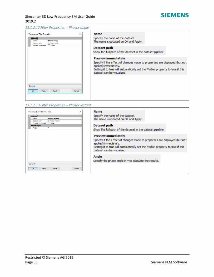
Simcenter 3D Low Frequency EM User Guide 2019.2
Restricted © Siemens AG 2019 Page 56 Siemens PLM Software
13.1.2.12 Filter Properties ‐‐ Phasor angle
13.1.2.13 Filter Properties ‐‐ Phasor instant
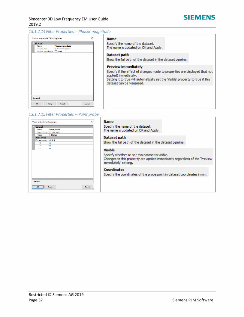
Simcenter 3D Low Frequency EM User Guide 2019.2
Restricted © Siemens AG 2019 Page 57 Siemens PLM Software
13.1.2.14 Filter Properties ‐‐ Phasor magnitude
13.1.2.15 Filter Properties ‐‐ Point probe
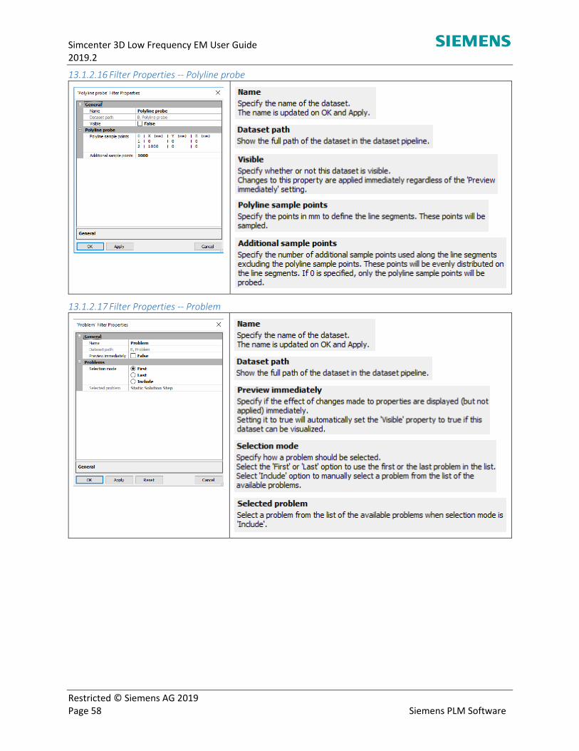
Simcenter 3D Low Frequency EM User Guide 2019.2
Restricted © Siemens AG 2019 Page 58 Siemens PLM Software
13.1.2.16 Filter Properties ‐‐ Polyline probe
13.1.2.17 Filter Properties ‐‐ Problem
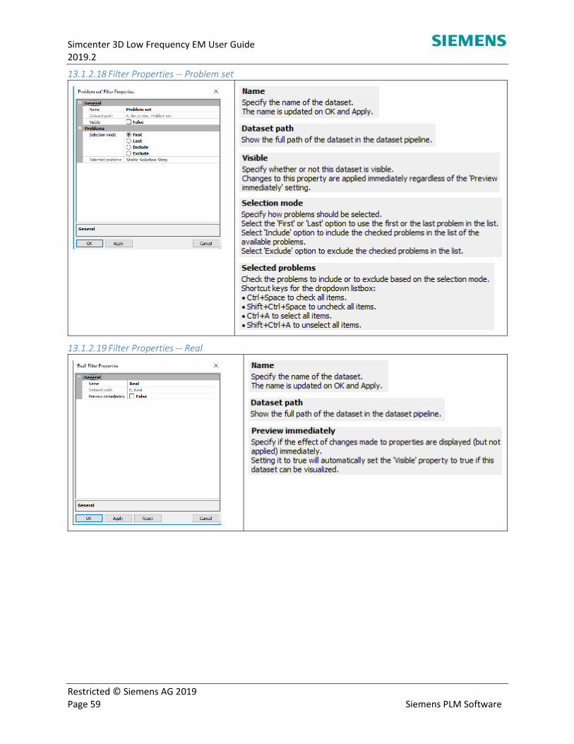
Simcenter 3D Low Frequency EM User Guide 2019.2
Restricted © Siemens AG 2019 Page 59 Siemens PLM Software
13.1.2.18 Filter Properties ‐‐ Problem set
13.1.2.19 Filter Properties ‐‐ Real
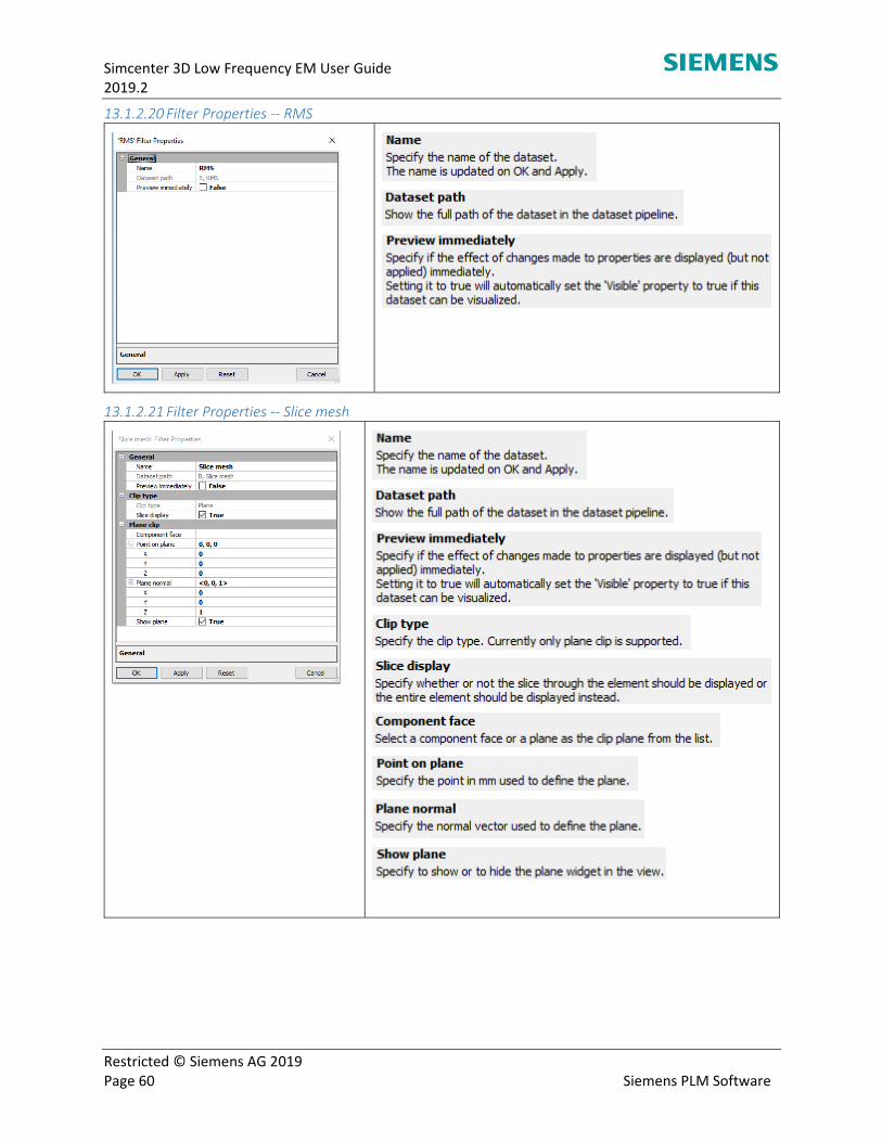
Simcenter 3D Low Frequency EM User Guide 2019.2
Restricted © Siemens AG 2019 Page 60 Siemens PLM Software
13.1.2.20 Filter Properties ‐‐ RMS
13.1.2.21 Filter Properties ‐‐ Slice mesh
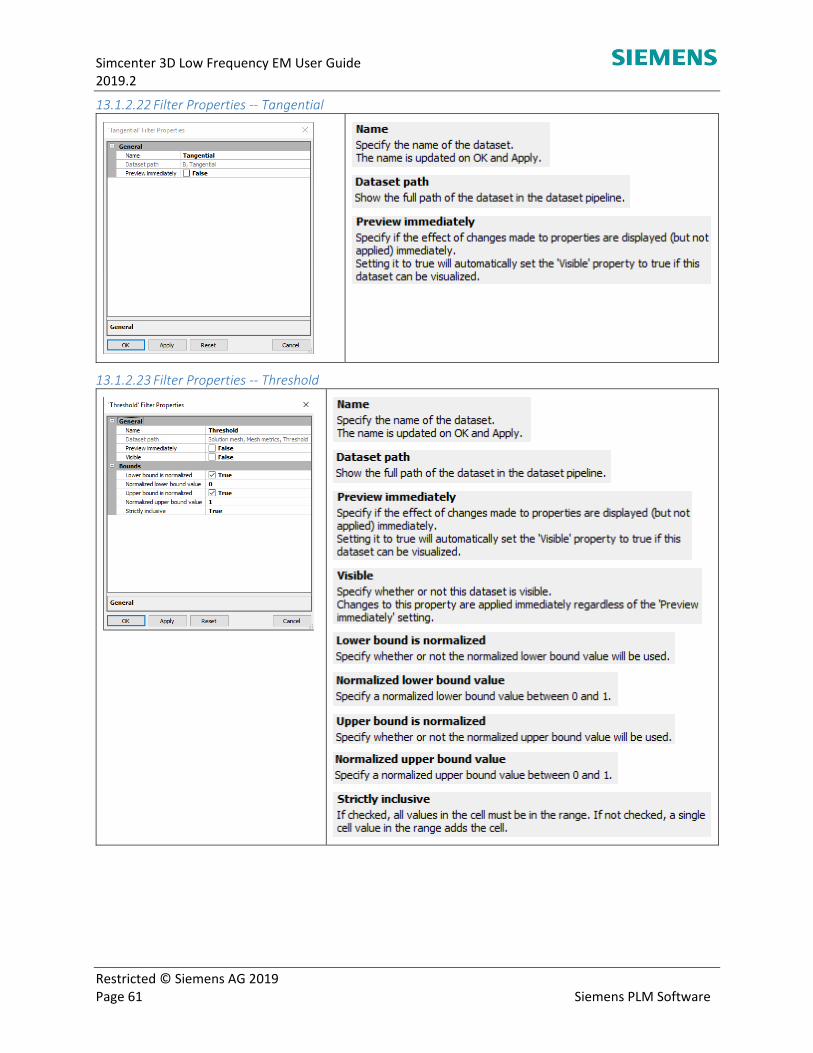
Simcenter 3D Low Frequency EM User Guide 2019.2
Restricted © Siemens AG 2019 Page 61 Siemens PLM Software
13.1.2.22 Filter Properties ‐‐ Tangential
13.1.2.23 Filter Properties ‐‐ Threshold
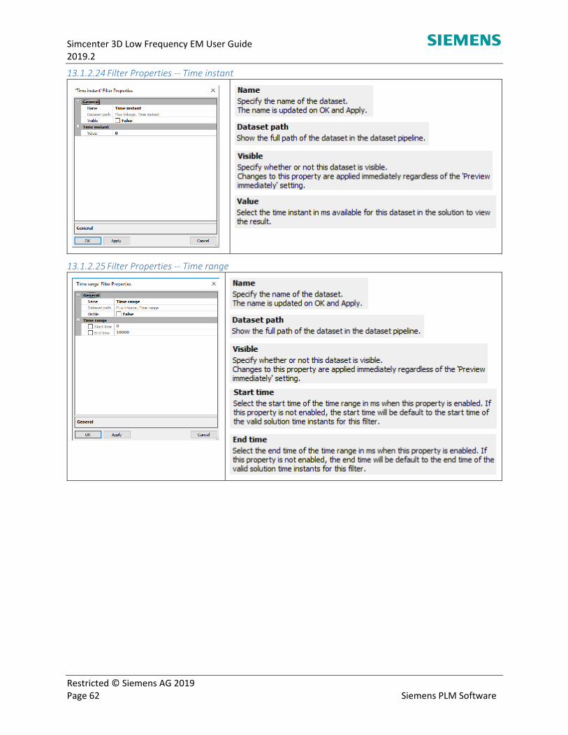
Simcenter 3D Low Frequency EM User Guide 2019.2
Restricted © Siemens AG 2019 Page 62 Siemens PLM Software
13.1.2.24 Filter Properties ‐‐ Time instant
13.1.2.25 Filter Properties ‐‐ Time range
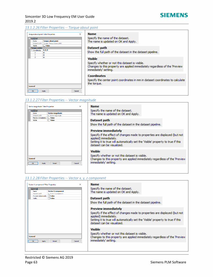
Simcenter 3D Low Frequency EM User Guide 2019.2
Restricted © Siemens AG 2019 Page 63 Siemens PLM Software
13.1.2.26 Filter Properties ‐‐ Torque about point
13.1.2.27 Filter Properties ‐‐ Vector magnitude
13.1.2.28 Filter Properties ‐‐ Vector x, y, z component
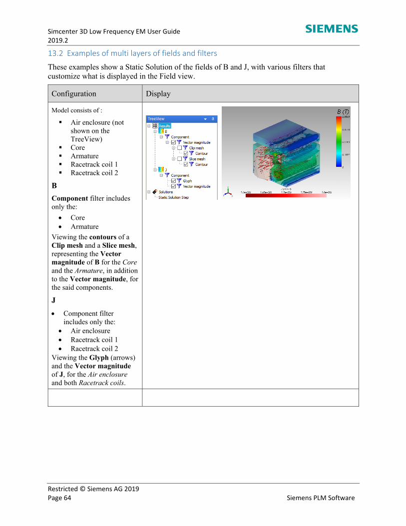
Simcenter 3D Low Frequency EM User Guide 2019.2
Restricted © Siemens AG 2019 Page 64 Siemens PLM Software
Examples of multi layers of fields and filters
These examples show a Static Solution of the fields of B and J, with various filters that customize what is displayed in the Field view.
Configuration Display
Model consists of :
Air enclosure (not shown on the TreeView)
Core Armature Racetrack coil 1 Racetrack coil 2
B
Component filter includes only the:
Core Armature
Viewing the contours of a Clip mesh and a Slice mesh, representing the Vector magnitude of B for the Core and the Armature, in addition to the Vector magnitude, for the said components.
J
Component filter includes only the:
Air enclosure Racetrack coil 1 Racetrack coil 2
Viewing the Glyph (arrows) and the Vector magnitude of J, for the Air enclosure and both Racetrack coils.
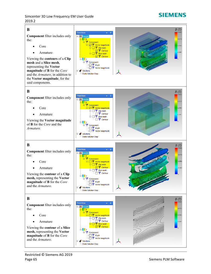
Simcenter 3D Low Frequency EM User Guide 2019.2
Restricted © Siemens AG 2019 Page 65 Siemens PLM Software
B
Component filter includes only the:
Core
Armature
Viewing the contours of a Clip mesh and a Slice mesh, representing the Vector magnitude of B for the Core and the Armature, in addition to the Vector magnitude, for the said components.
B
Component filter includes only the:
Core
Armature
Viewing the Vector magnitude of B for the Core and the Armature.
B
Component filter includes only the:
Core
Armature
Viewing the contour of a Clip mesh, representing the Vector magnitude of B for the Core and the Armature.
B
Component filter includes only the:
Core
Armature
Viewing the contour of a Slice mesh, representing the Vector magnitude of B for the Core and the Armature.
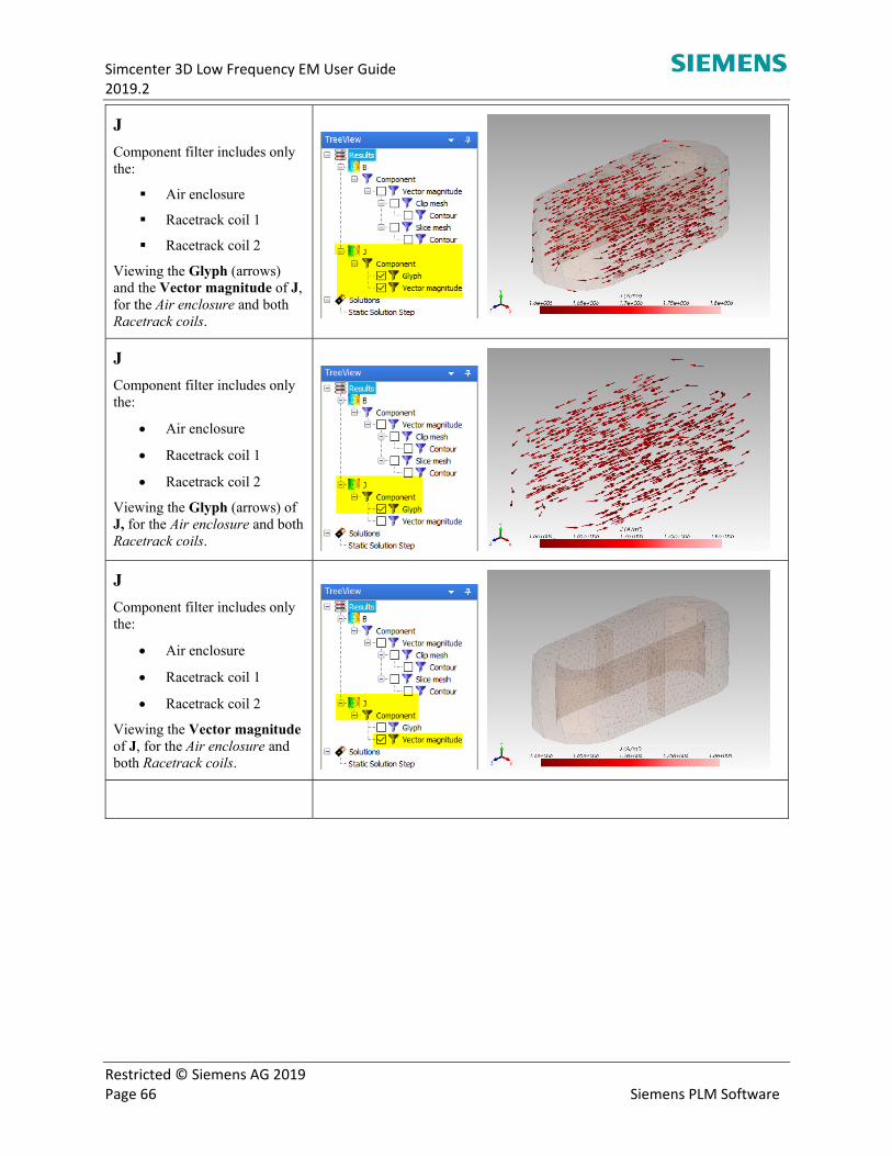
Simcenter 3D Low Frequency EM User Guide 2019.2
Restricted © Siemens AG 2019 Page 66 Siemens PLM Software
J
Component filter includes only the:
Air enclosure
Racetrack coil 1
Racetrack coil 2
Viewing the Glyph (arrows) and the Vector magnitude of J, for the Air enclosure and both Racetrack coils.
J
Component filter includes only the:
Air enclosure
Racetrack coil 1
Racetrack coil 2
Viewing the Glyph (arrows) of J, for the Air enclosure and both Racetrack coils.
J
Component filter includes only the:
Air enclosure
Racetrack coil 1
Racetrack coil 2
Viewing the Vector magnitude of J, for the Air enclosure and both Racetrack coils.
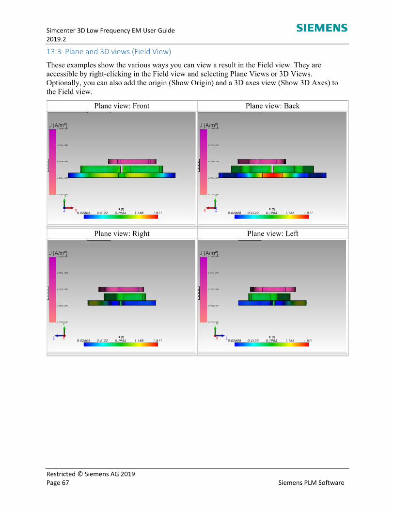
Simcenter 3D Low Frequency EM User Guide 2019.2
Restricted © Siemens AG 2019 Page 67 Siemens PLM Software
Plane and 3D views (Field View)
These examples show the various ways you can view a result in the Field view. They are accessible by right-clicking in the Field view and selecting Plane Views or 3D Views. Optionally, you can also add the origin (Show Origin) and a 3D axes view (Show 3D Axes) to the Field view.
Plane view: Front Plane view: Back
Plane view: Right Plane view: Left
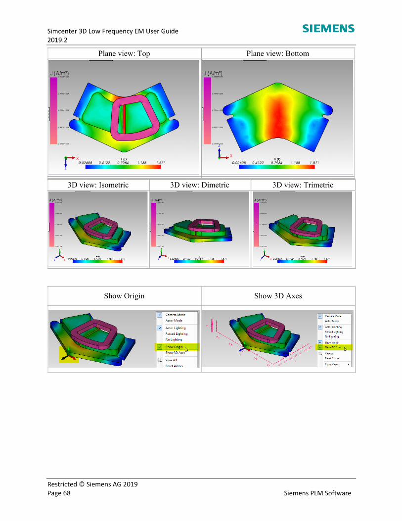
Simcenter 3D Low Frequency EM User Guide 2019.2
Restricted © Siemens AG 2019 Page 68 Siemens PLM Software
Plane view: Top Plane view: Bottom
3D view: Isometric 3D view: Dimetric 3D view: Trimetric
Show Origin Show 3D Axes
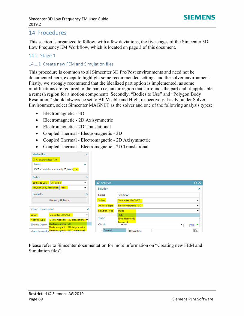
Simcenter 3D Low Frequency EM User Guide 2019.2
Restricted © Siemens AG 2019 Page 69 Siemens PLM Software
14 Procedures This section is organized to follow, with a few deviations, the five stages of the Simcenter 3D Low Frequency EM Workflow, which is located on page 3 of this document.
Stage 1
14.1.1 Create new FEM and Simulation files
This procedure is common to all Simcenter 3D Pre/Post environments and need not be documented here, except to highlight some recommended settings and the solver environment. Firstly, we strongly recommend that the idealized part option is implemented, as some modifications are required to the part (i.e. an air region that surrounds the part and, if applicable, a remesh region for a motion component). Secondly, “Bodies to Use” and “Polygon Body Resolution” should always be set to All Visible and High, respectively. Lastly, under Solver Environment, select Simcenter MAGNET as the solver and one of the following analysis types:
Electromagnetic - 3D
Electromagnetic - 2D Axisymmetric
Electromagnetic - 2D Translational
Coupled Thermal - Electromagnetic - 3D
Coupled Thermal - Electromagnetic - 2D Axisymmetric
Coupled Thermal - Electromagnetic - 2D Translational
Please refer to Simcenter documentation for more information on “Creating new FEM and Simulation files”.
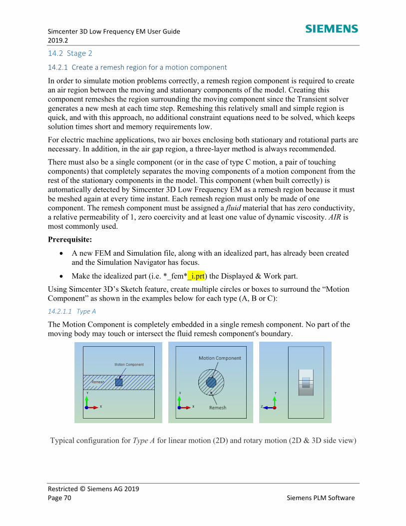
Simcenter 3D Low Frequency EM User Guide 2019.2
Restricted © Siemens AG 2019 Page 70 Siemens PLM Software
Stage 2
14.2.1 Create a remesh region for a motion component
In order to simulate motion problems correctly, a remesh region component is required to create an air region between the moving and stationary components of the model. Creating this component remeshes the region surrounding the moving component since the Transient solver generates a new mesh at each time step. Remeshing this relatively small and simple region is quick, and with this approach, no additional constraint equations need to be solved, which keeps solution times short and memory requirements low.
For electric machine applications, two air boxes enclosing both stationary and rotational parts are necessary. In addition, in the air gap region, a three-layer method is always recommended.
There must also be a single component (or in the case of type C motion, a pair of touching components) that completely separates the moving components of a motion component from the rest of the stationary components in the model. This component (when built correctly) is automatically detected by Simcenter 3D Low Frequency EM as a remesh region because it must be meshed again at every time instant. Each remesh region must only be made of one component. The remesh component must be assigned a fluid material that has zero conductivity, a relative permeability of 1, zero coercivity and at least one value of dynamic viscosity. AIR is most commonly used.
Prerequisite:
A new FEM and Simulation file, along with an idealized part, has already been created and the Simulation Navigator has focus.
Make the idealized part (i.e. *_fem*_i.prt) the Displayed & Work part.
Using Simcenter 3D’s Sketch feature, create multiple circles or boxes to surround the “Motion Component” as shown in the examples below for each type (A, B or C):
14.2.1.1 Type A
The Motion Component is completely embedded in a single remesh component. No part of the moving body may touch or intersect the fluid remesh component's boundary.
Typical configuration for Type A for linear motion (2D) and rotary motion (2D & 3D side view)
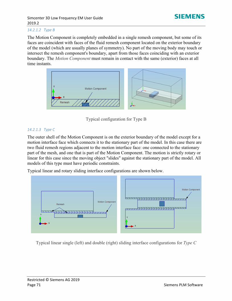
Simcenter 3D Low Frequency EM User Guide 2019.2
Restricted © Siemens AG 2019 Page 71 Siemens PLM Software
14.2.1.2 Type B
The Motion Component is completely embedded in a single remesh component, but some of its faces are coincident with faces of the fluid remesh component located on the exterior boundary of the model (which are usually planes of symmetry). No part of the moving body may touch or intersect the remesh component's boundary, apart from those faces coinciding with an exterior boundary. The Motion Component must remain in contact with the same (exterior) faces at all time instants.
Typical configuration for Type B
14.2.1.3 Type C
The outer shell of the Motion Component is on the exterior boundary of the model except for a motion interface face which connects it to the stationary part of the model. In this case there are two fluid remesh regions adjacent to the motion interface face: one connected to the stationary part of the mesh, and one that is part of the Motion Component. The motion is strictly rotary or linear for this case since the moving object "slides" against the stationary part of the model. All models of this type must have periodic constraints.
Typical linear and rotary sliding interface configurations are shown below.
Typical linear single (left) and double (right) sliding interface configurations for Type C
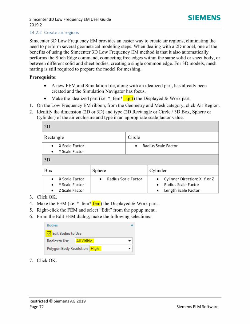
Simcenter 3D Low Frequency EM User Guide 2019.2
Restricted © Siemens AG 2019 Page 72 Siemens PLM Software
14.2.2 Create air regions
Simcenter 3D Low Frequency EM provides an easier way to create air regions, eliminating the need to perform several geometrical modeling steps. When dealing with a 2D model, one of the benefits of using the Simcenter 3D Low Frequency EM method is that it also automatically performs the Stich Edge command, connecting free edges within the same solid or sheet body, or between different solid and sheet bodies, creating a single common edge. For 3D models, mesh mating is still required to prepare the model for meshing.
Prerequisite:
A new FEM and Simulation file, along with an idealized part, has already been created and the Simulation Navigator has focus.
Make the idealized part (i.e. *_fem*_i.prt) the Displayed & Work part.
1. On the Low Frequency EM ribbon, from the Geometry and Mesh category, click Air Region. 2. Identify the dimension (2D or 3D) and type (2D Rectangle or Circle / 3D Box, Sphere or
Cylinder) of the air enclosure and type in an appropriate scale factor value.
2D
Rectangle Circle
X Scale Factor
Y Scale Factor
Radius Scale Factor
3D
Box Sphere Cylinder
X Scale Factor
Y Scale Factor
Z Scale Factor
Radius Scale Factor Cylinder Direction: X, Y or Z
Radius Scale Factor
Length Scale Factor
3. Click OK. 4. Make the FEM (i.e. *_fem*.fem) the Displayed & Work part. 5. Right-click the FEM and select “Edit” from the popup menu. 6. From the Edit FEM dialog, make the following selections:
7. Click OK.
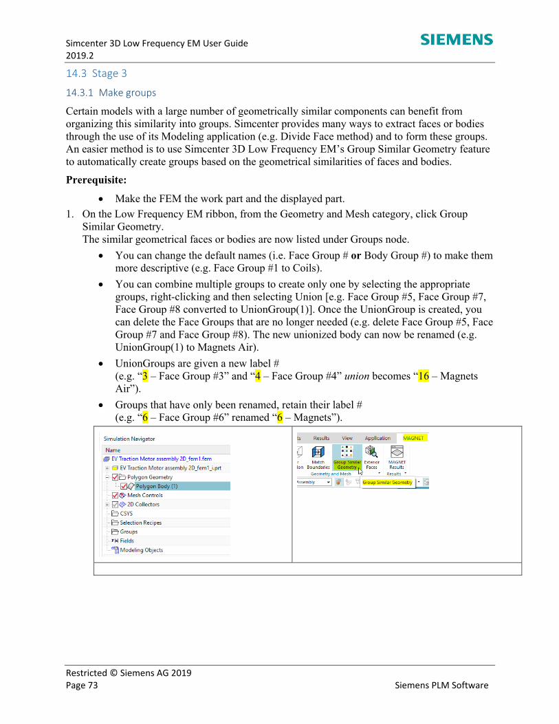
Simcenter 3D Low Frequency EM User Guide 2019.2
Restricted © Siemens AG 2019 Page 73 Siemens PLM Software
Stage 3
14.3.1 Make groups
Certain models with a large number of geometrically similar components can benefit from organizing this similarity into groups. Simcenter provides many ways to extract faces or bodies through the use of its Modeling application (e.g. Divide Face method) and to form these groups. An easier method is to use Simcenter 3D Low Frequency EM’s Group Similar Geometry feature to automatically create groups based on the geometrical similarities of faces and bodies.
Prerequisite:
Make the FEM the work part and the displayed part.
1. On the Low Frequency EM ribbon, from the Geometry and Mesh category, click Group Similar Geometry. The similar geometrical faces or bodies are now listed under Groups node.
You can change the default names (i.e. Face Group # or Body Group #) to make them more descriptive (e.g. Face Group #1 to Coils).
You can combine multiple groups to create only one by selecting the appropriate groups, right-clicking and then selecting Union [e.g. Face Group #5, Face Group #7, Face Group #8 converted to UnionGroup(1)]. Once the UnionGroup is created, you can delete the Face Groups that are no longer needed (e.g. delete Face Group #5, Face Group #7 and Face Group #8). The new unionized body can now be renamed (e.g. UnionGroup(1) to Magnets Air).
UnionGroups are given a new label # (e.g. “3 – Face Group #3” and “4 – Face Group #4” union becomes “16 – Magnets Air”).
Groups that have only been renamed, retain their label # (e.g. “6 – Face Group #6” renamed “6 – Magnets”).
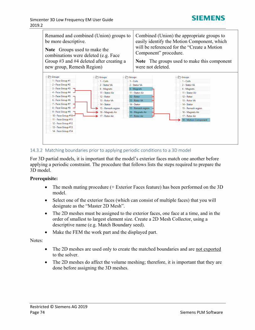
Simcenter 3D Low Frequency EM User Guide 2019.2
Restricted © Siemens AG 2019 Page 74 Siemens PLM Software
Renamed and combined (Union) groups to be more descriptive.
Note Groups used to make the combinations were deleted (e.g. Face Group #3 and #4 deleted after creating a new group, Remesh Region)
Combined (Union) the appropriate groups to easily identify the Motion Component, which will be referenced for the “Create a Motion Component” procedure.
Note The groups used to make this component were not deleted.
14.3.2 Matching boundaries prior to applying periodic conditions to a 3D model
For 3D partial models, it is important that the model’s exterior faces match one another before applying a periodic constraint. The procedure that follows lists the steps required to prepare the 3D model.
Prerequisite:
The mesh mating procedure (+ Exterior Faces feature) has been performed on the 3D model.
Select one of the exterior faces (which can consist of multiple faces) that you will designate as the “Master 2D Mesh”.
The 2D meshes must be assigned to the exterior faces, one face at a time, and in the order of smallest to largest element size. Create a 2D Mesh Collector, using a descriptive name (e.g. Match Boundary seed).
Make the FEM the work part and the displayed part.
Notes:
The 2D meshes are used only to create the matched boundaries and are not exported to the solver.
The 2D meshes do affect the volume meshing; therefore, it is important that they are done before assigning the 3D meshes.
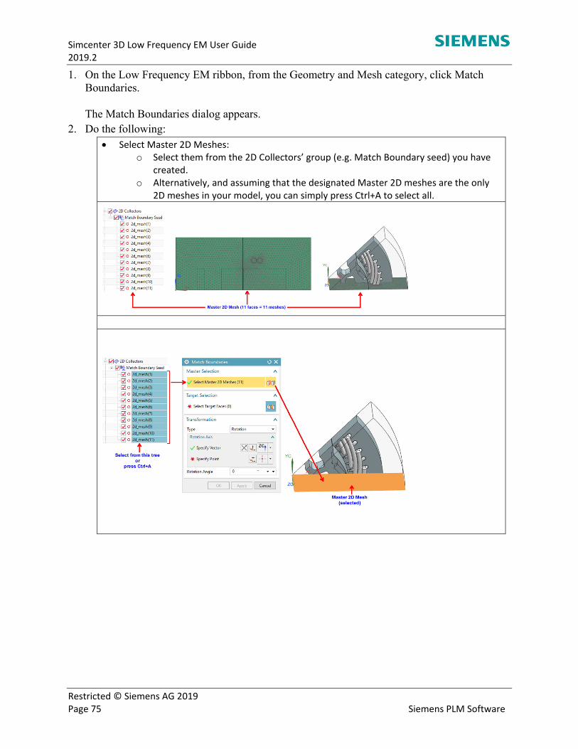
Simcenter 3D Low Frequency EM User Guide 2019.2
Restricted © Siemens AG 2019 Page 75 Siemens PLM Software
1. On the Low Frequency EM ribbon, from the Geometry and Mesh category, click Match Boundaries. The Match Boundaries dialog appears.
2. Do the following: Select Master 2D Meshes:
o Select them from the 2D Collectors’ group (e.g. Match Boundary seed) you have created.
o Alternatively, and assuming that the designated Master 2D meshes are the only 2D meshes in your model, you can simply press Ctrl+A to select all.
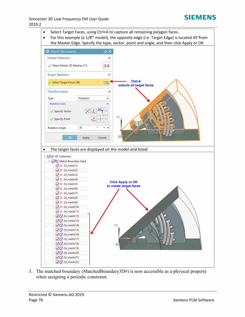
Simcenter 3D Low Frequency EM User Guide 2019.2
Restricted © Siemens AG 2019 Page 76 Siemens PLM Software
Select Target Faces, using Ctrl+A to capture all remaining polygon faces.
For this example (a 1/8th model), the opposite edge (i.e. Target Edge) is located 45°from the Master Edge. Specify the type, vector, point and angle, and then click Apply or OK.
The target faces are displayed on the model and listed
3. The matched boundary (MatchedBoundary3D#) is now accessible as a physical property when assigning a periodic constraint.

Simcenter 3D Low Frequency EM User Guide 2019.2
Restricted © Siemens AG 2019 Page 77 Siemens PLM Software
14.3.3 Matching boundaries prior to applying periodic conditions to a 2D model
For 2D partial models, it is important that the model’s exterior edges match one another before applying a periodic constraint. The procedure that follows lists the steps required to prepare the 2D model.
Prerequisite:
Make the FEM the work part and the displayed part.
1. On the Low Frequency EM ribbon, from the Geometry and Mesh category, click Match Boundaries. The Match Boundaries dialog appears.
2. Do the following: Select Master Edges, using the cursor (left‐click) to capture the edge, designating it the
Master Edge.
Select Target Edges, using Ctrl+A to capture all remaining polygon edges.
For this example (a 1/8th model), the opposite edge (i.e. Target Edge) is located 45°from the Master Edge. Specify the type, vector, point and angle, and then click Apply or OK.
The matching Edge density symbols are displayed along the master and target edges.
3. The matched boundary (MatchedBoundary2D#) is now accessible as a physical property when assigning a periodic constraint.

Simcenter 3D Low Frequency EM User Guide 2019.2
Restricted © Siemens AG 2019 Page 78 Siemens PLM Software
14.3.4 Preparing the 3D model before assigning meshes
To prepare the 3D model and ensure the integrity of its mesh, the recommended method is to use the Mesh Mating condition with the Glue Coincident mesh mating type, selecting all faces or bodies in the model.
Please refer to Simcenter documentation for information on “Mesh Mating Conditions”.
14.3.5 Verifying the Mesh Mating Conditions
Once the mesh mating procedure is complete, the Simulation Navigator is seeded with a MMC Collection node that lists the information on the merged nodes. Simcenter 3D Low Frequency EM provides a tool that helps verify that the mesh mating was successful.
Prerequisite:
Make the FEM the work part and the displayed part.
1. On the Low Frequency EM ribbon, from the Geometry and Mesh category, click Exterior Faces. Exterior Faces is now listed under Groups node.
2. Right-click “Exterior Faces” and select Show Only.
3. Examine the model in the view and verify that only the exterior faces are displayed (e.g. if
the model has an air region surrounding it, only the faces of the air region should be visible). 4. If more than just the exterior faces are displayed, do one or more of the following:
Keep the MMC Collectors and run the mesh mating procedure again, retaining the same settings as before
If only a few interior faces still exist, it may be faster to use the Manual Creation setting on these faces
Refine the Search Distance
5. Repeat these steps until only exterior faces are displayed.
Simcenter 3D Low Frequency EM User Guide 2019.2
Restricted © Siemens AG 2019 Page 79 Siemens PLM Software
14.3.6 Assigning a mesh
Creating a good finite element mesh is a critical step in the analysis process, as the accuracy of your finite element results depends partly on the quality of the mesh. In the finite element method of analysis, spatial discretization of the computational domain is accomplished through the division of the model into a mesh of elements. The field inside each element is represented by a set of polynomial base functions with unknown coefficients. The finite element analysis is the solution of the set of equations for the unknown coefficients. Simcenter 3D Low Frequency EM provides the following element property types:
3D Models
3D Tetrahedral -- Element Properties Type:
o Linear Tetrahedron
2D Mesh -- Element Properties Type:
o Linear Triangle 2D Seed (Note This 2D mesh is applied only to a face and is never exported to the Solver. It is used to seed the tetrahedral mesh or to create a Matched Boundary for periodic constraints)
2D Models
2D Mesh -- Element Properties Type:
o Linear Triangle – 2D Translational
o Linear Triangle – 2D Axisymmetrical
Prerequisite:
Make the FEM the work part and the displayed part.
Recommended: Use Simcenter 3D Low Frequency EM’s Group Similar Geometry feature to automatically create groups based on the geometrical similarities of faces and bodies.
Recommended: Before assigning meshes, determine the order of assignment, beginning with the smallest element size to the largest. This is especially important when components share a face or an edge.
Apply the 3D Tetrahedral or 2D Mesh, creating the appropriate 2D/3D Collectors, as per the procedures laid out for meshing in the Simcenter documentation.
14.3.7 Assigning materials
Simcenter 3D’s electromagnetic low frequency material database contains the magnetic and electrical properties required to simulate EM devices. To access this database, set the Site MatML Library and User MatML Library to: “C:\Program Files\Siemens\Simcenter3D\simulation\magnet\”.
Simcenter 3D Low Frequency EM User Guide 2019.2
Restricted © Siemens AG 2019 Page 80 Siemens PLM Software
14.3.8 Assigning direction to a permanent magnet (Uniform direction only)
For models that have a large number of magnets with uniform direction, Simcenter 3D Low Frequency EM can expedite the process by combining the magnet uniform orientation with Simcenter 3D’s pattern definition option.
Prerequisite:
Make the FEM the work part and the displayed part.
1. Uncheck the Polygon Geometry and from the mesh collector node, ensure that only the magnets are displayed in the view window.
2. On the Low Frequency EM ribbon, from the Magnets category, click Assign Magnets. The Assign Magnets Orientation dialog appears.
3. Using the cursor, first select a mesh and then do the following:
For the Material Orientation, specify the vector’s direction. To reverse the direction, click . (Please refer to Simcenter documentation for information on “Vector tool dialog box”)
For the Pattern Definition, select a type:
Circular (specify the vector’s direction and the point of origin of the circle of the selected mesh)
Linear (specify the vector’s direction of the selected mesh)
Determine the spacing, using the combination of any two of Count, Pitch and Span
(Please refer to Simcenter documentation for information on “Vector tool dialog box”, “Point tool dialog box” and “Pattern Part – Spacing Options”)
Enable “Alternate Orientation” to change the direction of every second magnet in the Count.
Click Preview Pattern to verify that the direction of the magnets are defined properly.
4. If another set of magnets (i.e. the opposite pair) require orientation, click Apply and repeat Step #3.
5. Click OK to save the assignments. 6. If there is more than one set of magnets, you can verify the proper uniform orientation
assignments for each magnet of the model by clicking Display Magnets from the Magnets category of the Low Frequency EM ribbon. Arrows, indicating the direction, accompanied by annotations identifying the Material Orientation Method (i.e. Uniform) will be displayed.
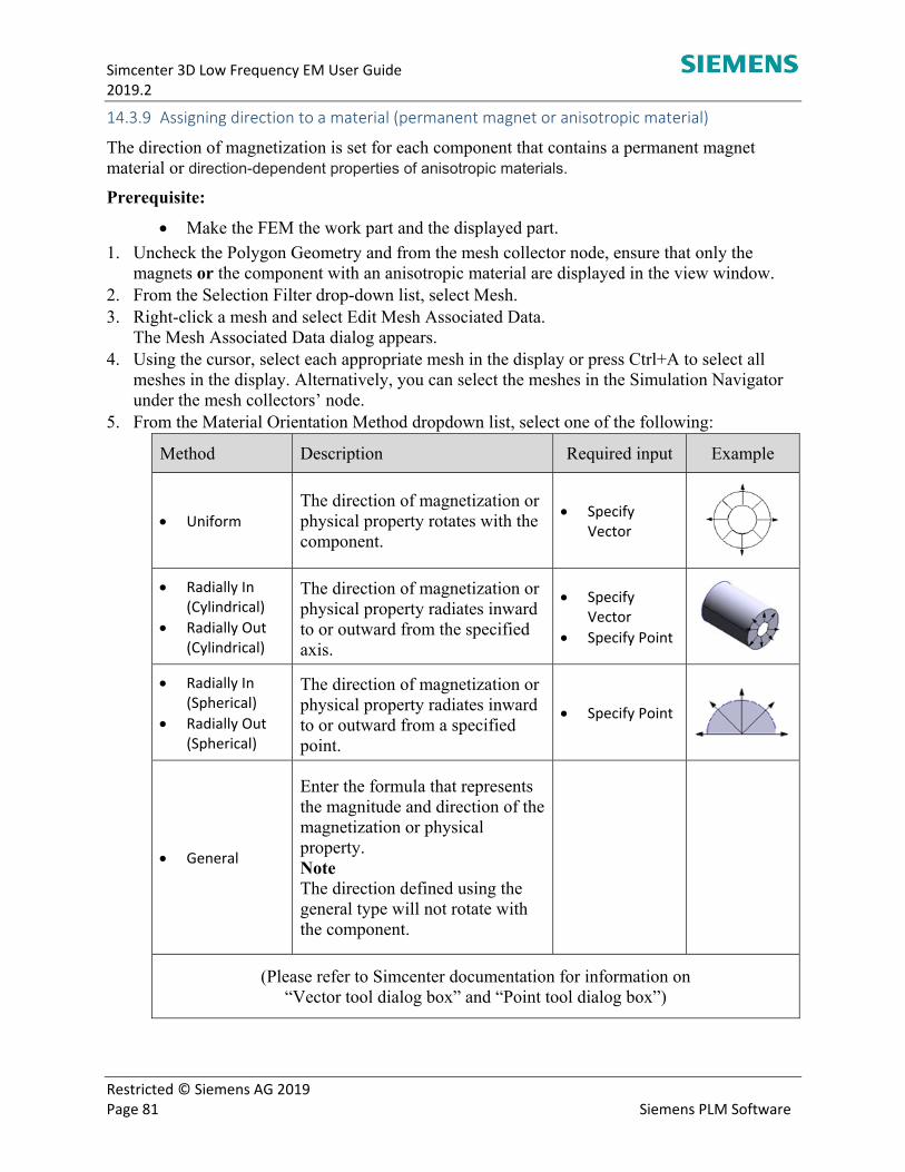
Simcenter 3D Low Frequency EM User Guide 2019.2
Restricted © Siemens AG 2019 Page 81 Siemens PLM Software
14.3.9 Assigning direction to a material (permanent magnet or anisotropic material)
The direction of magnetization is set for each component that contains a permanent magnet material or direction-dependent properties of anisotropic materials.
Prerequisite:
Make the FEM the work part and the displayed part.
1. Uncheck the Polygon Geometry and from the mesh collector node, ensure that only the magnets or the component with an anisotropic material are displayed in the view window.
2. From the Selection Filter drop-down list, select Mesh. 3. Right-click a mesh and select Edit Mesh Associated Data.
The Mesh Associated Data dialog appears. 4. Using the cursor, select each appropriate mesh in the display or press Ctrl+A to select all
meshes in the display. Alternatively, you can select the meshes in the Simulation Navigator under the mesh collectors’ node.
5. From the Material Orientation Method dropdown list, select one of the following:
Method Description Required input Example
Uniform The direction of magnetization or physical property rotates with the component.
Specify Vector
Radially In (Cylindrical)
Radially Out (Cylindrical)
The direction of magnetization or physical property radiates inward to or outward from the specified axis.
Specify Vector
Specify Point
Radially In (Spherical)
Radially Out (Spherical)
The direction of magnetization or physical property radiates inward to or outward from a specified point.
Specify Point
General
Enter the formula that represents the magnitude and direction of the magnetization or physical property. Note The direction defined using the general type will not rotate with the component.
(Please refer to Simcenter documentation for information on “Vector tool dialog box” and “Point tool dialog box”)
Simcenter 3D Low Frequency EM User Guide 2019.2
Restricted © Siemens AG 2019 Page 82 Siemens PLM Software
6. For 3D meshes, it is important that the “Export Mesh to Solver” checkbox is always selected.
7. Click OK. 8. Magnets only - Verify the proper orientation assignments for each magnet of the model by
clicking Display Magnets from the Magnets category of the Low Frequency EM ribbon. Arrows, indicating the direction or location, accompanied by annotations identifying the Material Orientation Method (i.e. Uniform) will be displayed.
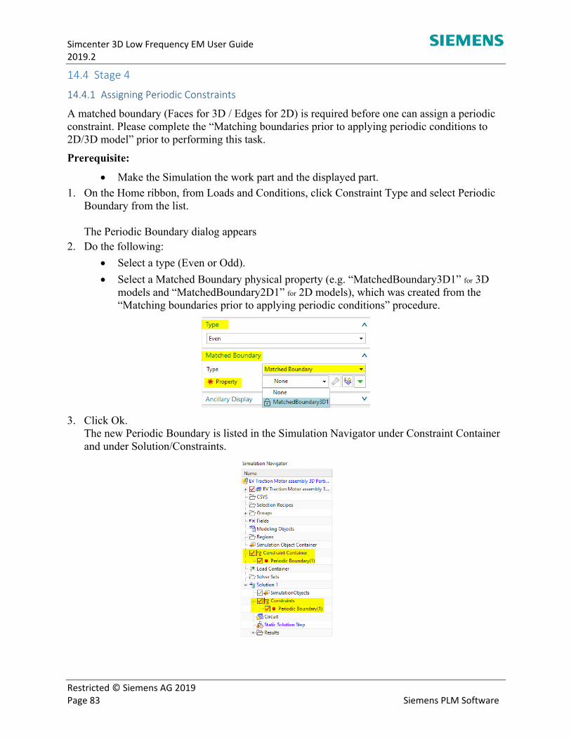
Simcenter 3D Low Frequency EM User Guide 2019.2
Restricted © Siemens AG 2019 Page 83 Siemens PLM Software
Stage 4
14.4.1 Assigning Periodic Constraints
A matched boundary (Faces for 3D / Edges for 2D) is required before one can assign a periodic constraint. Please complete the “Matching boundaries prior to applying periodic conditions to 2D/3D model” prior to performing this task.
Prerequisite:
Make the Simulation the work part and the displayed part.
1. On the Home ribbon, from Loads and Conditions, click Constraint Type and select Periodic Boundary from the list. The Periodic Boundary dialog appears
2. Do the following:
Select a type (Even or Odd).
Select a Matched Boundary physical property (e.g. “MatchedBoundary3D1” for 3D models and “MatchedBoundary2D1” for 2D models), which was created from the “Matching boundaries prior to applying periodic conditions” procedure.
3. Click Ok. The new Periodic Boundary is listed in the Simulation Navigator under Constraint Container and under Solution/Constraints.

Simcenter 3D Low Frequency EM User Guide 2019.2
Restricted © Siemens AG 2019 Page 84 Siemens PLM Software
14.4.2 Assigning constraints
Prerequisite:
Make the Simulation the work part and the displayed part.
1. On the Home ribbon, from Loads and Conditions, click Constraint Type and select one of the following :
Periodic Boundary (please refer to “Assigning Periodic Constraints” procedure)
Flux Tangential Boundary
Field Normal Boundary
Surface Impedance Boundary (Time Harmonic 3D only)
Thin Plate Boundary (3D only)
Perfect Electric Insulator Boundary (3D only)
2. Use the cursor to select the object.
If constraint is Surface Impedance, select Calculated Value or insert a Specified Value for Resistance and Reactance. Either option represents the ohmic loss of the conducting component and assigns the value as a constraint to the selected surface.
If constraint is Thin Plate, select a thickness and a material that is different from the body or face’s material.
3. Click OK.

Simcenter 3D Low Frequency EM User Guide 2019.2
Restricted © Siemens AG 2019 Page 85 Siemens PLM Software
14.4.3 Create a motion component
If a motion component consists of multiple components, using the Make Group feature to combine these components beforehand is highly recommended. This procedure will assume that this has been done.
Prerequisite:
Make the Simulation the work part and the displayed part.
1. If Motion Component was previously identified in Groups, select it now. 2. On the Home ribbon, from Loads and Conditions, click Simulation Object Type and select
Motion Component. The Motion Component dialog appears.
3. Select a type (Rotary/Linear Component). 4. Under Components, Select Object will indicate the number of components that make up the
Motion Component. 5. (Optional) If the motion problem is a multiple degrees of freedom one, select a modeling
object from the Motion Component Reference dropdown list. 6. Do one of the following:
If type is Rotary, specify the axis of rotation (Vector and Point)
If type is Linear, specify the direction (Vector)
(Please refer to Simcenter documentation for information on “Vector tool dialog box” and “Point tool dialog box”)
7. Select a Source type (Load Driven/Velocity Driven).
Load Select External Load from drop down list or create a new Modeling Object. (see External Load –dialog)
Position Load Driven o Position at Startup o Speed at Startup
Velocity Driven o Position Based – Specify Field o Speed Based – Specify Field
Mass Insert a value for Mass
Enable Center of gravity and select a point (Rotary Component type only)
Insert a value for Moment of inertia (Rotary Component type only)
Limits Bumpers (Load Driven only) o Lower Position o Upper Position
Positions to Stop Solver o Lower Position o Upper Position
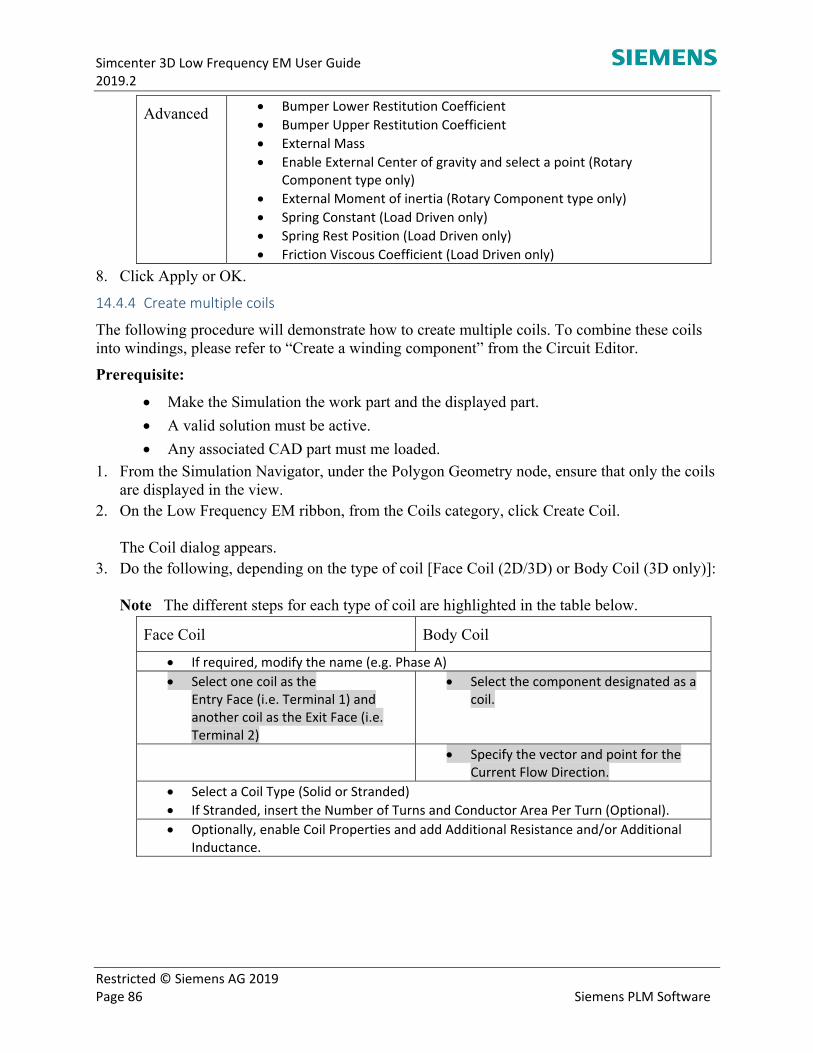
Simcenter 3D Low Frequency EM User Guide 2019.2
Restricted © Siemens AG 2019 Page 86 Siemens PLM Software
Advanced Bumper Lower Restitution Coefficient
Bumper Upper Restitution Coefficient
External Mass
Enable External Center of gravity and select a point (Rotary Component type only)
External Moment of inertia (Rotary Component type only)
Spring Constant (Load Driven only)
Spring Rest Position (Load Driven only)
Friction Viscous Coefficient (Load Driven only)
8. Click Apply or OK.
14.4.4 Create multiple coils
The following procedure will demonstrate how to create multiple coils. To combine these coils into windings, please refer to “Create a winding component” from the Circuit Editor.
Prerequisite:
Make the Simulation the work part and the displayed part.
A valid solution must be active.
Any associated CAD part must me loaded.
1. From the Simulation Navigator, under the Polygon Geometry node, ensure that only the coils are displayed in the view.
2. On the Low Frequency EM ribbon, from the Coils category, click Create Coil. The Coil dialog appears.
3. Do the following, depending on the type of coil [Face Coil (2D/3D) or Body Coil (3D only)]: Note The different steps for each type of coil are highlighted in the table below.
Face Coil Body Coil
If required, modify the name (e.g. Phase A)
Select one coil as the Entry Face (i.e. Terminal 1) and another coil as the Exit Face (i.e. Terminal 2)
Select the component designated as a coil.
Specify the vector and point for the Current Flow Direction.
Select a Coil Type (Solid or Stranded)
If Stranded, insert the Number of Turns and Conductor Area Per Turn (Optional).
Optionally, enable Coil Properties and add Additional Resistance and/or Additional Inductance.
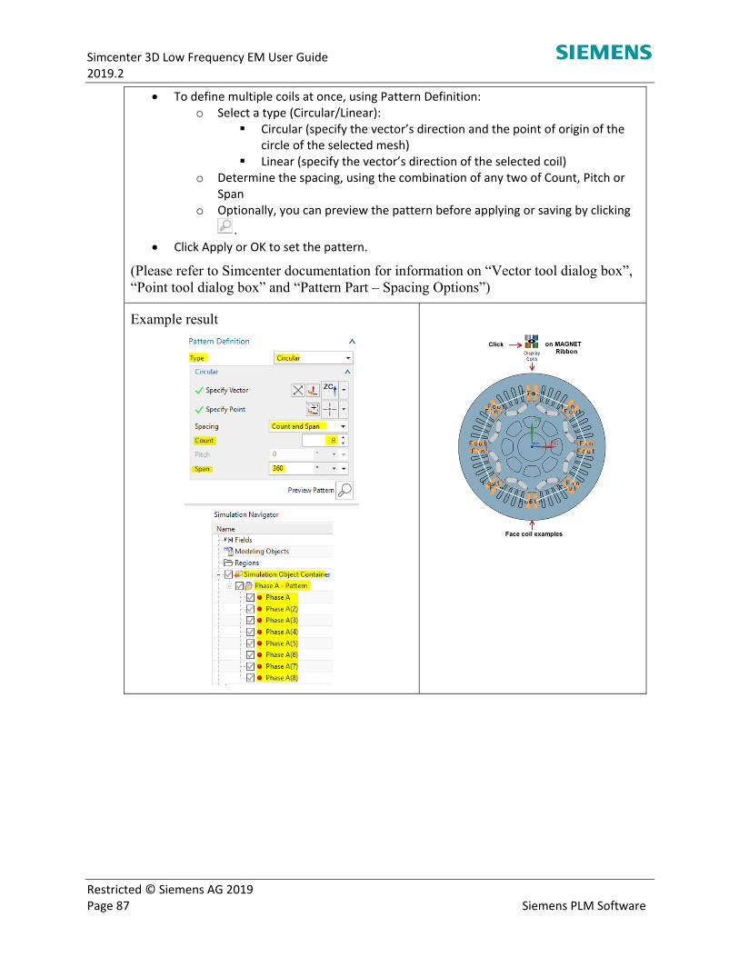
Simcenter 3D Low Frequency EM User Guide 2019.2
Restricted © Siemens AG 2019 Page 87 Siemens PLM Software
To define multiple coils at once, using Pattern Definition: o Select a type (Circular/Linear):
Circular (specify the vector’s direction and the point of origin of the circle of the selected mesh)
Linear (specify the vector’s direction of the selected coil) o Determine the spacing, using the combination of any two of Count, Pitch or
Span o Optionally, you can preview the pattern before applying or saving by clicking
.
Click Apply or OK to set the pattern.
(Please refer to Simcenter documentation for information on “Vector tool dialog box”, “Point tool dialog box” and “Pattern Part – Spacing Options”)
Example result
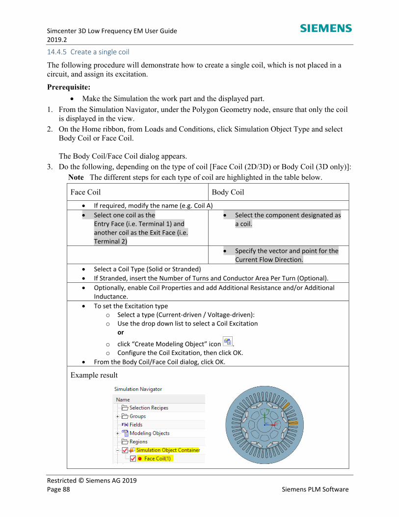
Simcenter 3D Low Frequency EM User Guide 2019.2
Restricted © Siemens AG 2019 Page 88 Siemens PLM Software
14.4.5 Create a single coil
The following procedure will demonstrate how to create a single coil, which is not placed in a circuit, and assign its excitation.
Prerequisite:
Make the Simulation the work part and the displayed part.
1. From the Simulation Navigator, under the Polygon Geometry node, ensure that only the coil is displayed in the view.
2. On the Home ribbon, from Loads and Conditions, click Simulation Object Type and select Body Coil or Face Coil. The Body Coil/Face Coil dialog appears.
3. Do the following, depending on the type of coil [Face Coil (2D/3D) or Body Coil (3D only)]: Note The different steps for each type of coil are highlighted in the table below.
Face Coil Body Coil
If required, modify the name (e.g. Coil A)
Select one coil as the Entry Face (i.e. Terminal 1) and another coil as the Exit Face (i.e. Terminal 2)
Select the component designated as a coil.
Specify the vector and point for the Current Flow Direction.
Select a Coil Type (Solid or Stranded)
If Stranded, insert the Number of Turns and Conductor Area Per Turn (Optional).
Optionally, enable Coil Properties and add Additional Resistance and/or Additional Inductance.
To set the Excitation type o Select a type (Current‐driven / Voltage‐driven): o Use the drop down list to select a Coil Excitation
or
o click “Create Modeling Object” icon . o Configure the Coil Excitation, then click OK.
From the Body Coil/Face Coil dialog, click OK.
Example result
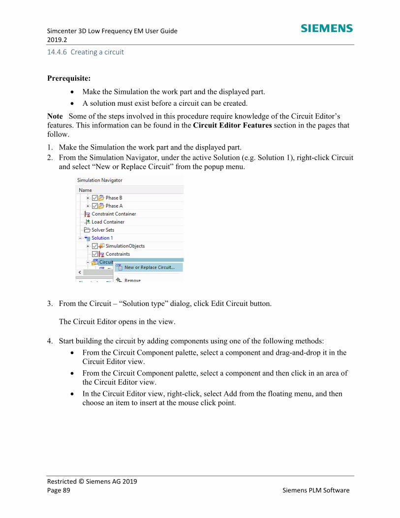
Simcenter 3D Low Frequency EM User Guide 2019.2
Restricted © Siemens AG 2019 Page 89 Siemens PLM Software
14.4.6 Creating a circuit
Prerequisite:
Make the Simulation the work part and the displayed part.
A solution must exist before a circuit can be created.
Note Some of the steps involved in this procedure require knowledge of the Circuit Editor’s features. This information can be found in the Circuit Editor Features section in the pages that follow.
1. Make the Simulation the work part and the displayed part. 2. From the Simulation Navigator, under the active Solution (e.g. Solution 1), right-click Circuit
and select “New or Replace Circuit” from the popup menu.
3. From the Circuit – “Solution type” dialog, click Edit Circuit button. The Circuit Editor opens in the view.
4. Start building the circuit by adding components using one of the following methods:
From the Circuit Component palette, select a component and drag-and-drop it in the Circuit Editor view.
From the Circuit Component palette, select a component and then click in an area of the Circuit Editor view.
In the Circuit Editor view, right-click, select Add from the floating menu, and then choose an item to insert at the mouse click point.
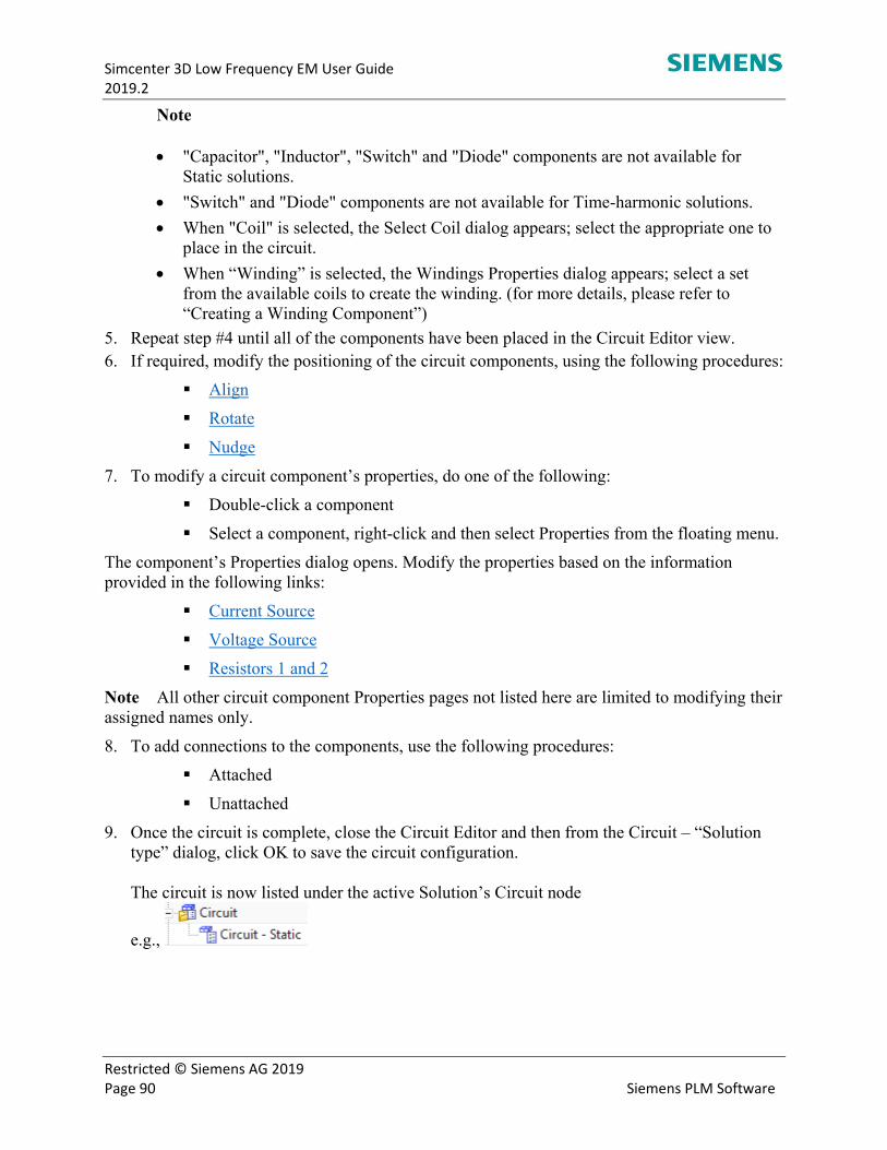
Simcenter 3D Low Frequency EM User Guide 2019.2
Restricted © Siemens AG 2019 Page 90 Siemens PLM Software
Note
"Capacitor", "Inductor", "Switch" and "Diode" components are not available for Static solutions.
"Switch" and "Diode" components are not available for Time-harmonic solutions.
When "Coil" is selected, the Select Coil dialog appears; select the appropriate one to place in the circuit.
When “Winding” is selected, the Windings Properties dialog appears; select a set from the available coils to create the winding. (for more details, please refer to “Creating a Winding Component”)
5. Repeat step #4 until all of the components have been placed in the Circuit Editor view. 6. If required, modify the positioning of the circuit components, using the following procedures:
Align
Rotate
Nudge
7. To modify a circuit component’s properties, do one of the following:
Double-click a component
Select a component, right-click and then select Properties from the floating menu.
The component’s Properties dialog opens. Modify the properties based on the information provided in the following links:
Current Source
Voltage Source
Resistors 1 and 2
Note All other circuit component Properties pages not listed here are limited to modifying their assigned names only.
8. To add connections to the components, use the following procedures:
Attached
Unattached
9. Once the circuit is complete, close the Circuit Editor and then from the Circuit – “Solution type” dialog, click OK to save the circuit configuration. The circuit is now listed under the active Solution’s Circuit node
e.g.,
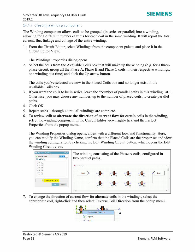
Simcenter 3D Low Frequency EM User Guide 2019.2
Restricted © Siemens AG 2019 Page 91 Siemens PLM Software
14.4.7 Creating a winding component
The Winding component allows coils to be grouped (in series or parallel) into a winding, allowing for a different number of turns for each coil in the same winding. It will report the total current, flux linkage and voltage of the entire winding.
1. From the Circuit Editor, select Windings from the component palette and place it in the Circuit Editor View. The Windings Properties dialog opens.
2. Select the coils from the Available Coils box that will make up the winding (e.g. for a three-phase circuit, group all the Phase A, Phase B and Phase C coils in their respective windings, one winding at a time) and click the Up arrow button. The coils you’ve selected are now in the Placed Coils box and no longer exist in the Available Coils box.
3. If you want the coils to be in series, leave the “Number of parallel paths in this winding” at 1. Otherwise, you may choose any number, up to the number of placed coils, to create parallel paths.
4. Click OK. 5. Repeat steps 1 through 4 until all windings are complete. 6. To review, edit or alternate the direction of current flow for certain coils in the winding,
select the winding component in the Circuit Editor view, right-click and then select Properties from the popup menu. The Winding Properties dialog opens, albeit with a different look and functionality. Here, you can modify the Winding Name, confirm that the Placed Coils are the proper set and view the winding configuration by clicking the Edit Winding Circuit button, which opens the Edit Winding Circuit view.
The winding consisting of the Phase A coils, configured in two parallel paths.
7. To change the direction of current flow for alternate coils in the windings, select the appropriate coil, right-click and then select Reverse Coil Direction from the popup menu.
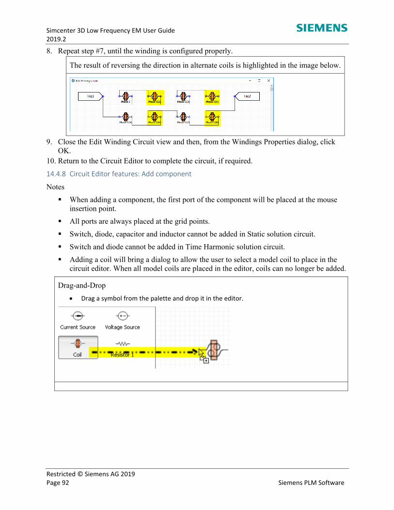
Simcenter 3D Low Frequency EM User Guide 2019.2
Restricted © Siemens AG 2019 Page 92 Siemens PLM Software
8. Repeat step #7, until the winding is configured properly.
The result of reversing the direction in alternate coils is highlighted in the image below.
9. Close the Edit Winding Circuit view and then, from the Windings Properties dialog, click OK.
10. Return to the Circuit Editor to complete the circuit, if required.
14.4.8 Circuit Editor features: Add component
Notes
When adding a component, the first port of the component will be placed at the mouse insertion point.
All ports are always placed at the grid points.
Switch, diode, capacitor and inductor cannot be added in Static solution circuit.
Switch and diode cannot be added in Time Harmonic solution circuit.
Adding a coil will bring a dialog to allow the user to select a model coil to place in the circuit editor. When all model coils are placed in the editor, coils can no longer be added.
Drag-and-Drop
Drag a symbol from the palette and drop it in the editor.
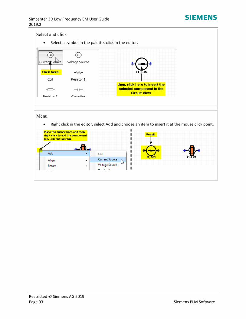
Simcenter 3D Low Frequency EM User Guide 2019.2
Restricted © Siemens AG 2019 Page 93 Siemens PLM Software
Select and click
Select a symbol in the palette, click in the editor.
Menu
Right click in the editor, select Add and choose an item to insert it at the mouse click point.
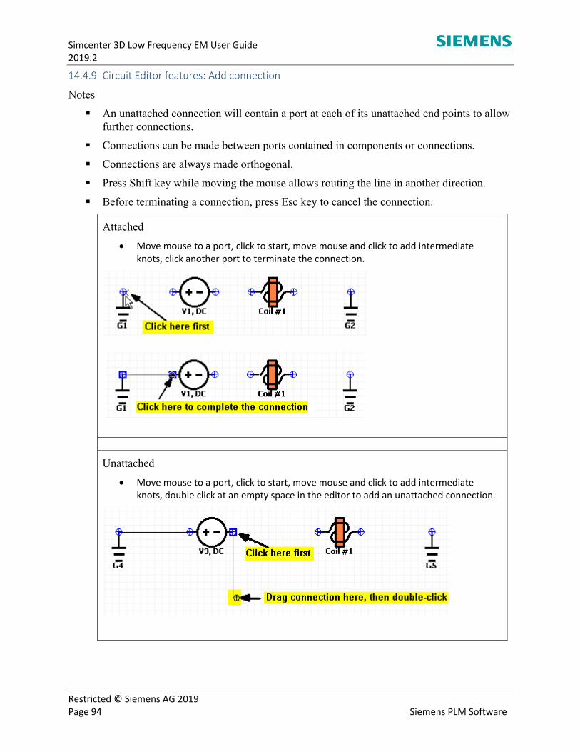
Simcenter 3D Low Frequency EM User Guide 2019.2
Restricted © Siemens AG 2019 Page 94 Siemens PLM Software
14.4.9 Circuit Editor features: Add connection
Notes
An unattached connection will contain a port at each of its unattached end points to allow further connections.
Connections can be made between ports contained in components or connections.
Connections are always made orthogonal.
Press Shift key while moving the mouse allows routing the line in another direction.
Before terminating a connection, press Esc key to cancel the connection.
Attached
Move mouse to a port, click to start, move mouse and click to add intermediate knots, click another port to terminate the connection.
Unattached
Move mouse to a port, click to start, move mouse and click to add intermediate knots, double click at an empty space in the editor to add an unattached connection.
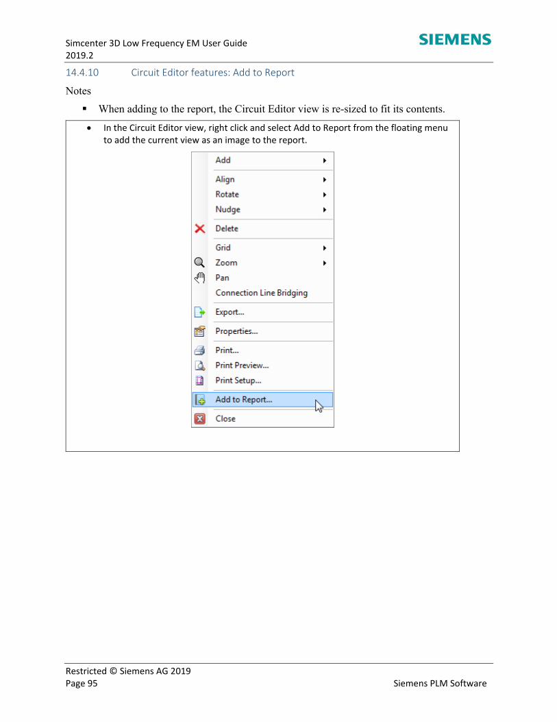
Simcenter 3D Low Frequency EM User Guide 2019.2
Restricted © Siemens AG 2019 Page 95 Siemens PLM Software
14.4.10 Circuit Editor features: Add to Report
Notes
When adding to the report, the Circuit Editor view is re-sized to fit its contents.
In the Circuit Editor view, right click and select Add to Report from the floating menu to add the current view as an image to the report.
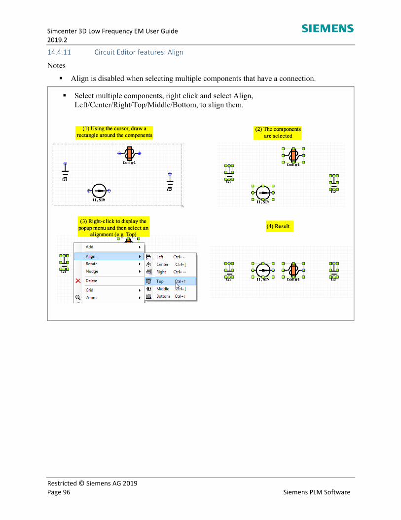
Simcenter 3D Low Frequency EM User Guide 2019.2
Restricted © Siemens AG 2019 Page 96 Siemens PLM Software
14.4.11 Circuit Editor features: Align
Notes
Align is disabled when selecting multiple components that have a connection.
Select multiple components, right click and select Align, Left/Center/Right/Top/Middle/Bottom, to align them.
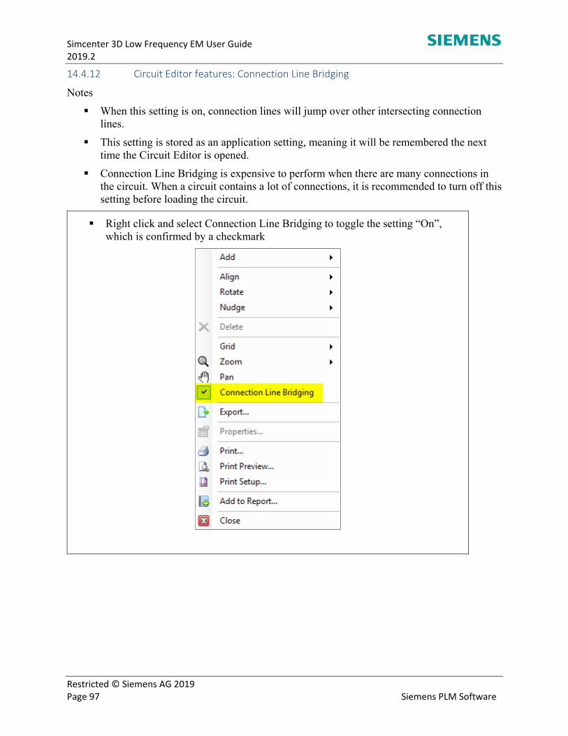
Simcenter 3D Low Frequency EM User Guide 2019.2
Restricted © Siemens AG 2019 Page 97 Siemens PLM Software
14.4.12 Circuit Editor features: Connection Line Bridging
Notes
When this setting is on, connection lines will jump over other intersecting connection lines.
This setting is stored as an application setting, meaning it will be remembered the next time the Circuit Editor is opened.
Connection Line Bridging is expensive to perform when there are many connections in the circuit. When a circuit contains a lot of connections, it is recommended to turn off this setting before loading the circuit.
Right click and select Connection Line Bridging to toggle the setting “On”, which is confirmed by a checkmark
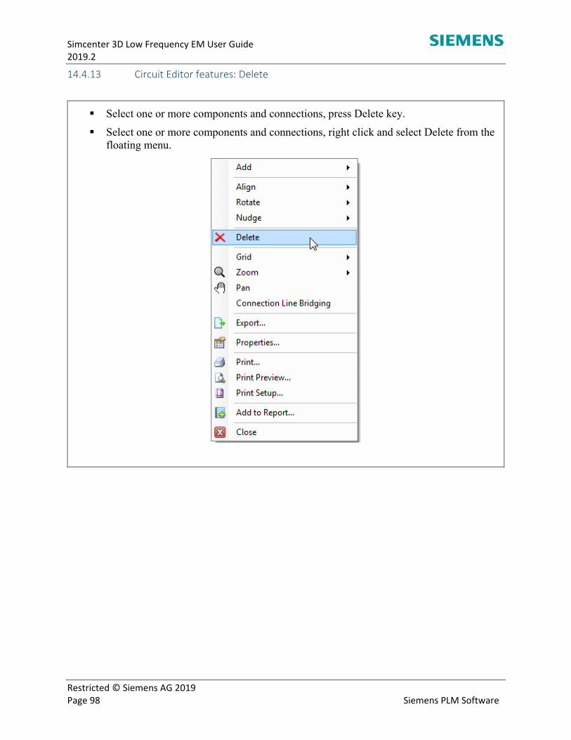
Simcenter 3D Low Frequency EM User Guide 2019.2
Restricted © Siemens AG 2019 Page 98 Siemens PLM Software
14.4.13 Circuit Editor features: Delete
Select one or more components and connections, press Delete key.
Select one or more components and connections, right click and select Delete from the floating menu.
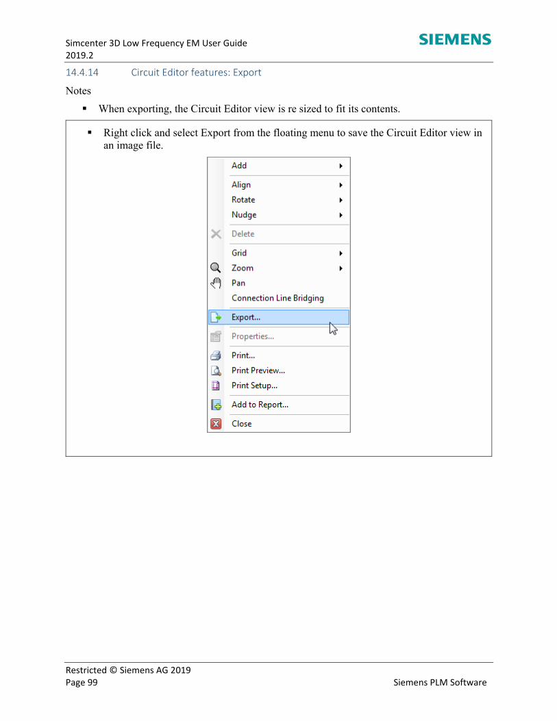
Simcenter 3D Low Frequency EM User Guide 2019.2
Restricted © Siemens AG 2019 Page 99 Siemens PLM Software
14.4.14 Circuit Editor features: Export
Notes
When exporting, the Circuit Editor view is re sized to fit its contents.
Right click and select Export from the floating menu to save the Circuit Editor view in an image file.
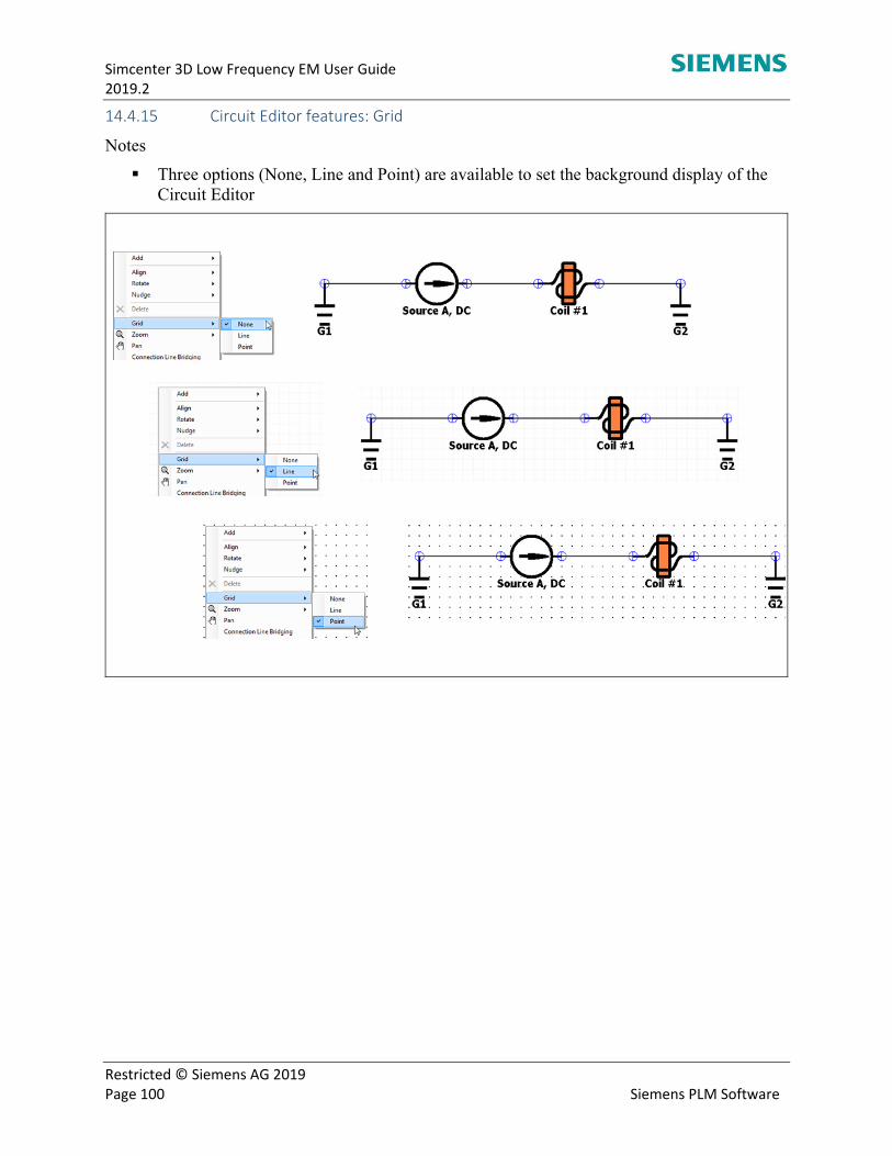
Simcenter 3D Low Frequency EM User Guide 2019.2
Restricted © Siemens AG 2019 Page 100 Siemens PLM Software
14.4.15 Circuit Editor features: Grid
Notes
Three options (None, Line and Point) are available to set the background display of the Circuit Editor
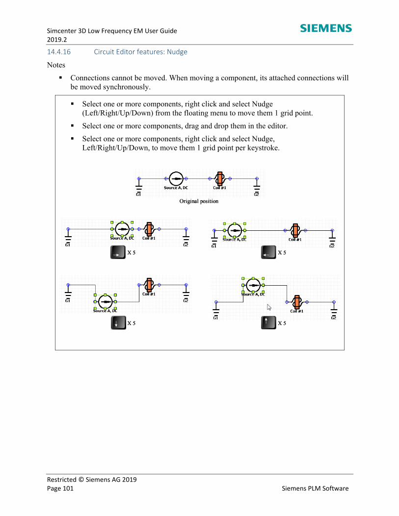
Simcenter 3D Low Frequency EM User Guide 2019.2
Restricted © Siemens AG 2019 Page 101 Siemens PLM Software
14.4.16 Circuit Editor features: Nudge
Notes
Connections cannot be moved. When moving a component, its attached connections will be moved synchronously.
Select one or more components, right click and select Nudge (Left/Right/Up/Down) from the floating menu to move them 1 grid point.
Select one or more components, drag and drop them in the editor.
Select one or more components, right click and select Nudge, Left/Right/Up/Down, to move them 1 grid point per keystroke.
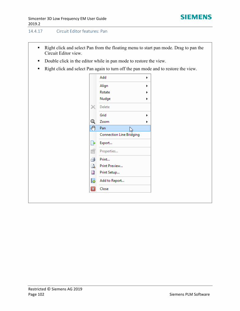
Simcenter 3D Low Frequency EM User Guide 2019.2
Restricted © Siemens AG 2019 Page 102 Siemens PLM Software
14.4.17 Circuit Editor features: Pan
Right click and select Pan from the floating menu to start pan mode. Drag to pan the Circuit Editor view.
Double click in the editor while in pan mode to restore the view.
Right click and select Pan again to turn off the pan mode and to restore the view.
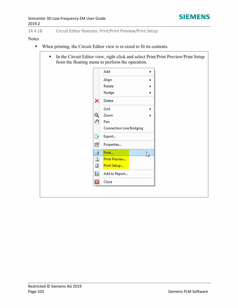
Simcenter 3D Low Frequency EM User Guide 2019.2
Restricted © Siemens AG 2019 Page 103 Siemens PLM Software
14.4.18 Circuit Editor features: Print/Print Preview/Print Setup
Notes
When printing, the Circuit Editor view is re-sized to fit its contents.
In the Circuit Editor view, right click and select Print/Print Preview/Print Setup from the floating menu to perform the operation.
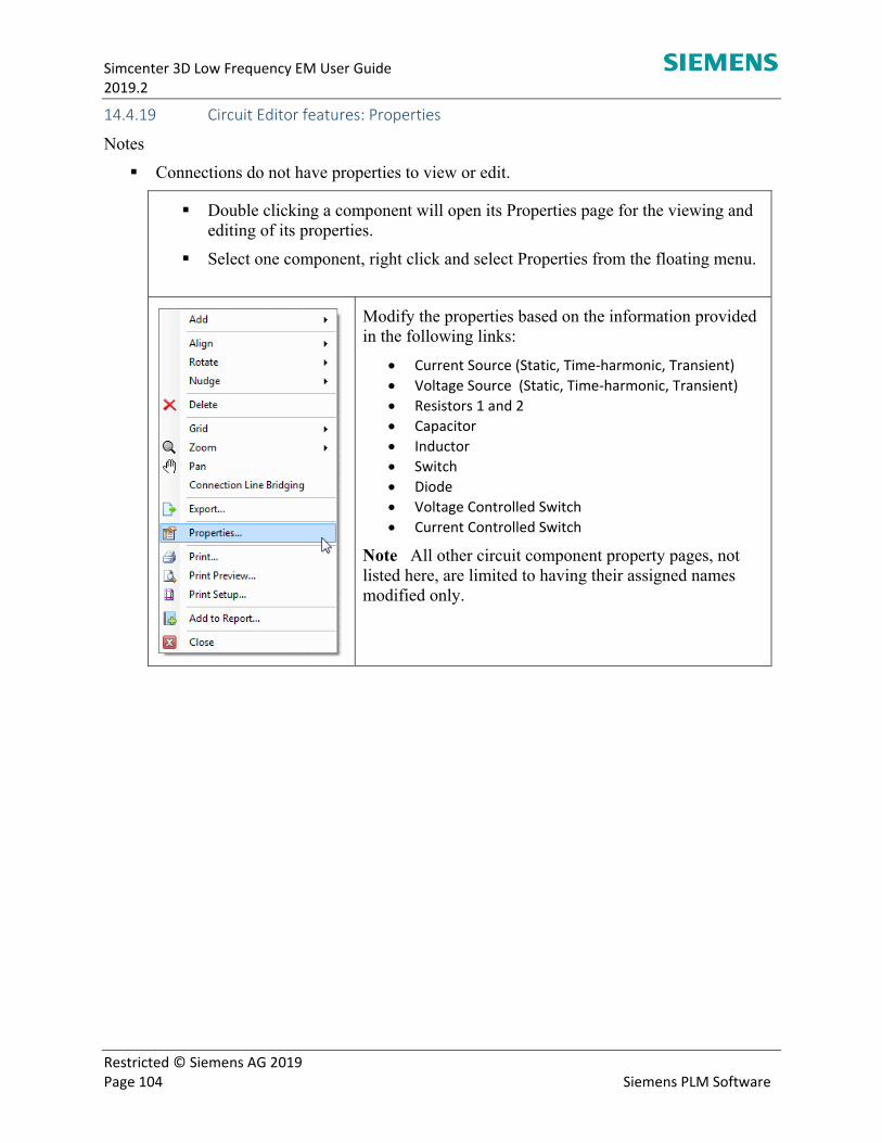
Simcenter 3D Low Frequency EM User Guide 2019.2
Restricted © Siemens AG 2019 Page 104 Siemens PLM Software
14.4.19 Circuit Editor features: Properties
Notes
Connections do not have properties to view or edit.
Double clicking a component will open its Properties page for the viewing and editing of its properties.
Select one component, right click and select Properties from the floating menu.
Modify the properties based on the information provided in the following links:
Current Source (Static, Time‐harmonic, Transient)
Voltage Source (Static, Time‐harmonic, Transient)
Resistors 1 and 2
Capacitor
Inductor
Switch
Diode
Voltage Controlled Switch
Current Controlled Switch
Note All other circuit component property pages, not listed here, are limited to having their assigned names modified only.
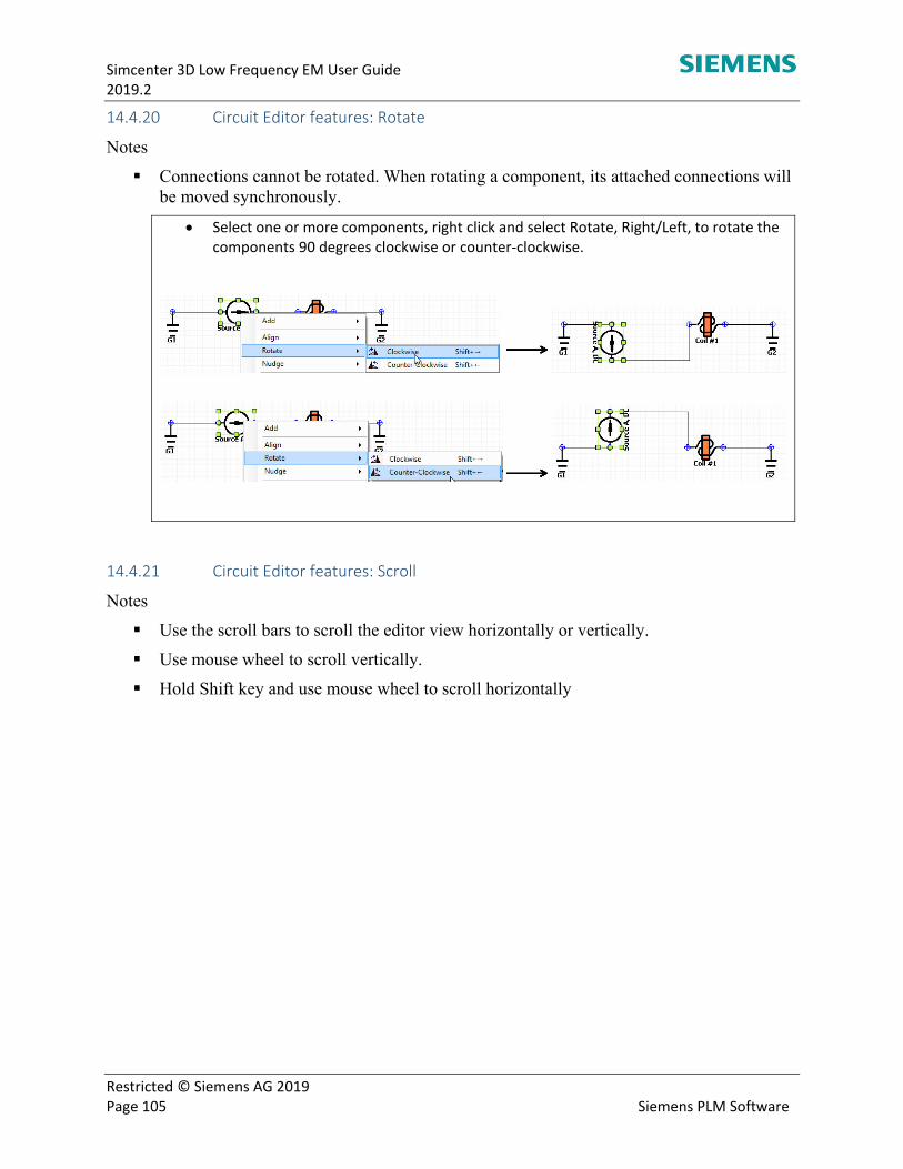
Simcenter 3D Low Frequency EM User Guide 2019.2
Restricted © Siemens AG 2019 Page 105 Siemens PLM Software
14.4.20 Circuit Editor features: Rotate
Notes
Connections cannot be rotated. When rotating a component, its attached connections will be moved synchronously.
Select one or more components, right click and select Rotate, Right/Left, to rotate the components 90 degrees clockwise or counter‐clockwise.
14.4.21 Circuit Editor features: Scroll
Notes
Use the scroll bars to scroll the editor view horizontally or vertically.
Use mouse wheel to scroll vertically.
Hold Shift key and use mouse wheel to scroll horizontally
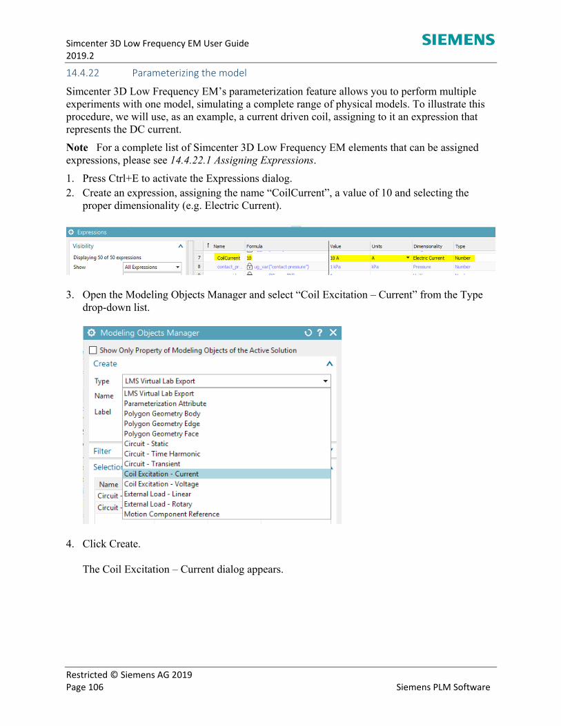
Simcenter 3D Low Frequency EM User Guide 2019.2
Restricted © Siemens AG 2019 Page 106 Siemens PLM Software
14.4.22 Parameterizing the model
Simcenter 3D Low Frequency EM’s parameterization feature allows you to perform multiple experiments with one model, simulating a complete range of physical models. To illustrate this procedure, we will use, as an example, a current driven coil, assigning to it an expression that represents the DC current.
Note For a complete list of Simcenter 3D Low Frequency EM elements that can be assigned expressions, please see 14.4.22.1 Assigning Expressions.
1. Press Ctrl+E to activate the Expressions dialog. 2. Create an expression, assigning the name “CoilCurrent”, a value of 10 and selecting the
proper dimensionality (e.g. Electric Current).
3. Open the Modeling Objects Manager and select “Coil Excitation – Current” from the Type drop-down list.
4. Click Create.
The Coil Excitation – Current dialog appears.
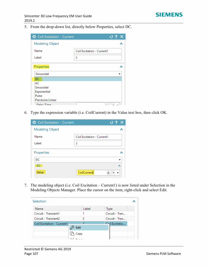
Simcenter 3D Low Frequency EM User Guide 2019.2
Restricted © Siemens AG 2019 Page 107 Siemens PLM Software
5. From the drop-down list, directly below Properties, select DC.
6. Type the expression variable (i.e. CoilCurrent) in the Value text box, then click OK.
7. The modeling object (i.e. Coil Excitation – Current1) is now listed under Selection in the Modeling Objects Manager. Place the cursor on the item, right-click and select Edit.
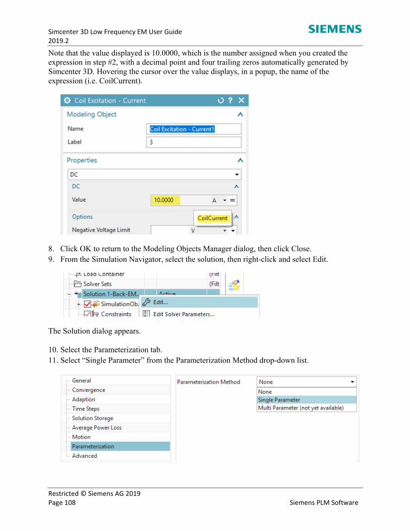
Simcenter 3D Low Frequency EM User Guide 2019.2
Restricted © Siemens AG 2019 Page 108 Siemens PLM Software
Note that the value displayed is 10.0000, which is the number assigned when you created the expression in step #2, with a decimal point and four trailing zeros automatically generated by Simcenter 3D. Hovering the cursor over the value displays, in a popup, the name of the expression (i.e. CoilCurrent).
8. Click OK to return to the Modeling Objects Manager dialog, then click Close. 9. From the Simulation Navigator, select the solution, then right-click and select Edit.
The Solution dialog appears.
10. Select the Parameterization tab. 11. Select “Single Parameter” from the Parameterization Method drop-down list.
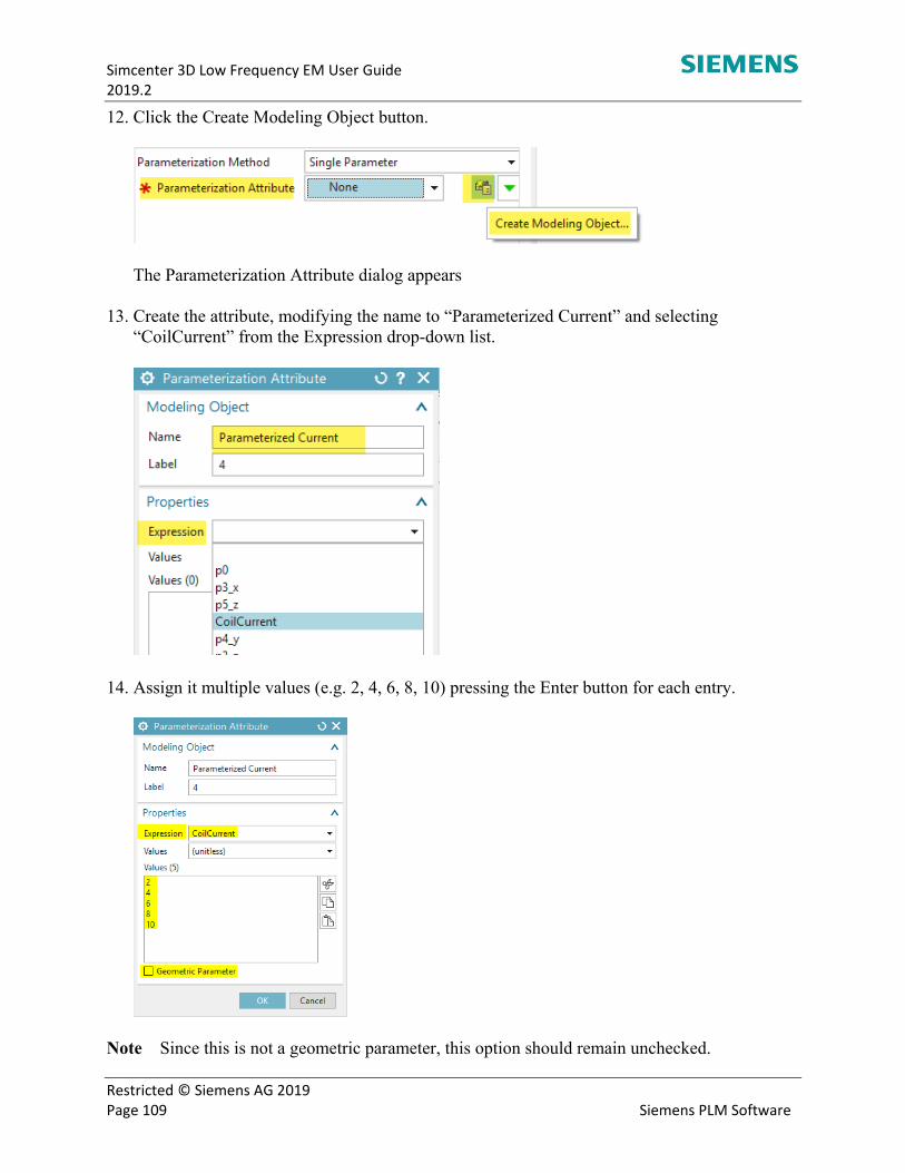
Simcenter 3D Low Frequency EM User Guide 2019.2
Restricted © Siemens AG 2019 Page 109 Siemens PLM Software
12. Click the Create Modeling Object button.
The Parameterization Attribute dialog appears
13. Create the attribute, modifying the name to “Parameterized Current” and selecting “CoilCurrent” from the Expression drop-down list.
14. Assign it multiple values (e.g. 2, 4, 6, 8, 10) pressing the Enter button for each entry.
Note Since this is not a geometric parameter, this option should remain unchecked.
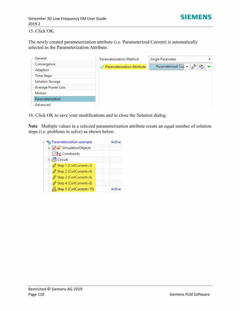
Simcenter 3D Low Frequency EM User Guide 2019.2
Restricted © Siemens AG 2019 Page 110 Siemens PLM Software
15. Click OK.
The newly created parameterization attribute (i.e. Parameterized Current) is automatically selected as the Parameterization Attribute.
16. Click OK to save your modifications and to close the Solution dialog.
Note Multiple values in a selected parameterization attribute create an equal number of solution steps (i.e. problems to solve) as shown below.

Simcenter 3D Low Frequency EM User Guide 2019.2
Restricted © Siemens AG 2019 Page 111 Siemens PLM Software
14.4.22.1 Assigning expressions
In addition to being assigned to various NX environments, expressions can also be applied, as non-geometrical parameters, to the following Simcenter 3D Low Frequency EM elements:
Coil dialog
Number of Turns o Conductor Area per Turn
Additional Resistance
Additional Inductance
Pattern Definition o Pitch o Span
Coil Excitation dialog
Options o Negative Voltage/Current Limit o Positive Voltage/Current Limit o Initial Current
DC o Value
AC o Magnitude (RMS) o Phase
Sinusoidal o Offset o Peak o Frequency o Delay Time o Damping Factor o Phase
Exponential o Initial o Peak o Rise Delay Time o Rise Time o Fall Delay Time o Fall Time Constant
Pulse o Offset o Pulse o Delay Time o Rise Time o Fall Time o Width o Period
Circuit Components dialog
Resistor o Resistor Value
Capacitor o Capacitor Value
Inductor o Inductor Value o Initial Current
Diode o Junction Voltage o On Resistance o Off Resistance o Resistance Ratio
Voltage Switch Properties o Voltage Threshold o Voltage Hysteresis
Current Switch Properties o Current Threshold o Current Hysteresis
Commutator o Reference Angle o Spacing o Brush
Width Resistance Separation Angle
o Contacts Minimum Resistance Maximum Resistance
Motion Component dialog
Position o Position at Startup o Speed at Startup
Mass o Mass
Limits o Bumpers
Lower Position Bumper Upper Position Bumper
o Positions to Stop Solver Lower Position to Stop Solver Upper Position to Stop Solver
Advanced o Bumper Lower Restitution Coefficient o Bumper Upper Restitution Coefficient o External Mass o Spring Constant o Spring Rest Position o Friction Viscous Coefficient
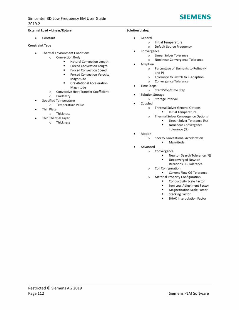
Simcenter 3D Low Frequency EM User Guide 2019.2
Restricted © Siemens AG 2019 Page 112 Siemens PLM Software
External Load – Linear/Rotary
Constant
Constraint Type
Thermal Environment Conditions o Convection Body
Natural Convection Length Forced Convection Length Forced Convection Speed Forced Convection Velocity
Magnitude Gravitational Acceleration
Magnitude o Convective Heat Transfer Coefficient o Emissivity
Specified Temperature o Temperature Value
Thin Plate o Thickness
Thin Thermal Layer o Thickness
Solution dialog
General o Initial Temperature o Default Source Frequency
Convergence o Linear Solver Tolerance o Nonlinear Convergence Tolerance
Adaption o Percentage of Elements to Refine (H
and P) o Tolerance to Switch to P‐Adaption o Convergence Tolerance
Time Steps o Start/Stop/Time Step
Solution Storage o Storage Interval
Coupled o Thermal Solver General Options
Initial Temperature o Thermal Solver Convergence Options
Linear Solver Tolerance (%) Nonlinear Convergence
Tolerance (%)
Motion o Specify Gravitational Acceleration
Magnitude
Advanced o Convergence
Newton Search Tolerance (%) Unconverged Newton
Iterations CG Tolerance o Coil Configuration
Current Flow CG Tolerance o Material Property Configuration
Conductivity Scale Factor Iron Loss Adjustment Factor Magnetization Scale Factor Stacking Factor BHAC Interpolation Factor
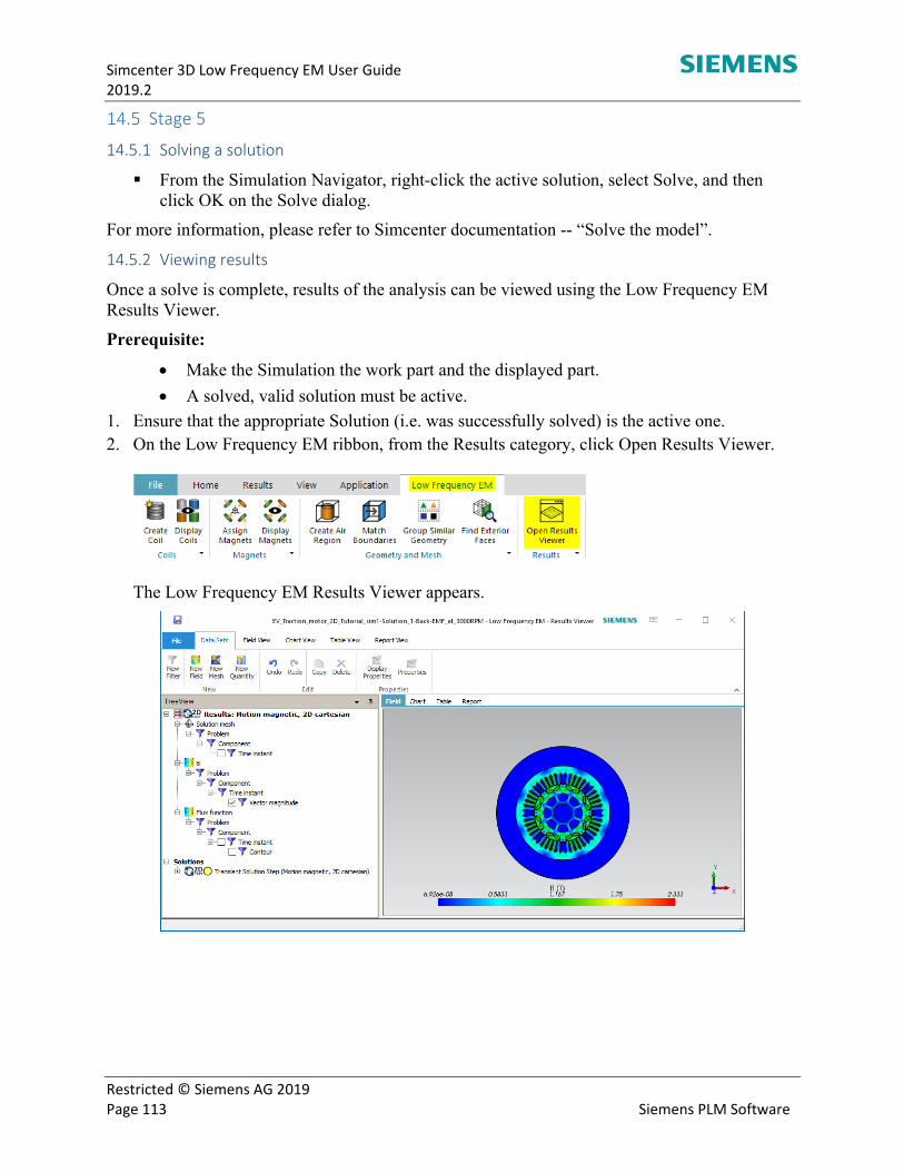
Simcenter 3D Low Frequency EM User Guide 2019.2
Restricted © Siemens AG 2019 Page 113 Siemens PLM Software
Stage 5
14.5.1 Solving a solution
From the Simulation Navigator, right-click the active solution, select Solve, and then click OK on the Solve dialog.
For more information, please refer to Simcenter documentation -- “Solve the model”.
14.5.2 Viewing results
Once a solve is complete, results of the analysis can be viewed using the Low Frequency EM Results Viewer.
Prerequisite:
Make the Simulation the work part and the displayed part.
A solved, valid solution must be active.
1. Ensure that the appropriate Solution (i.e. was successfully solved) is the active one. 2. On the Low Frequency EM ribbon, from the Results category, click Open Results Viewer.
The Low Frequency EM Results Viewer appears.
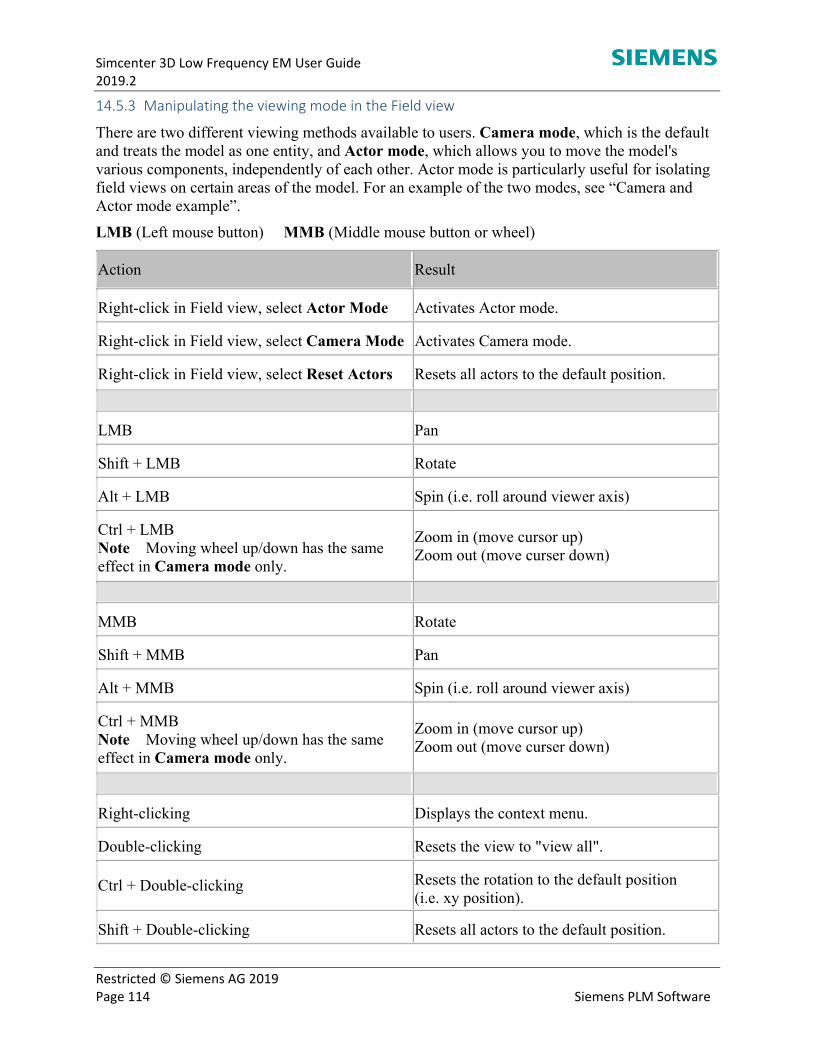
Simcenter 3D Low Frequency EM User Guide 2019.2
Restricted © Siemens AG 2019 Page 114 Siemens PLM Software
14.5.3 Manipulating the viewing mode in the Field view
There are two different viewing methods available to users. Camera mode, which is the default and treats the model as one entity, and Actor mode, which allows you to move the model's various components, independently of each other. Actor mode is particularly useful for isolating field views on certain areas of the model. For an example of the two modes, see “Camera and Actor mode example”.
LMB (Left mouse button) MMB (Middle mouse button or wheel)
Action Result
Right-click in Field view, select Actor Mode Activates Actor mode.
Right-click in Field view, select Camera Mode Activates Camera mode.
Right-click in Field view, select Reset Actors Resets all actors to the default position.
LMB Pan
Shift + LMB Rotate
Alt + LMB Spin (i.e. roll around viewer axis)
Ctrl + LMB Note Moving wheel up/down has the same effect in Camera mode only.
Zoom in (move cursor up) Zoom out (move curser down)
MMB Rotate
Shift + MMB Pan
Alt + MMB Spin (i.e. roll around viewer axis)
Ctrl + MMB Note Moving wheel up/down has the same effect in Camera mode only.
Zoom in (move cursor up) Zoom out (move curser down)
Right-clicking Displays the context menu.
Double-clicking Resets the view to "view all".
Ctrl + Double-clicking Resets the rotation to the default position (i.e. xy position).
Shift + Double-clicking Resets all actors to the default position.
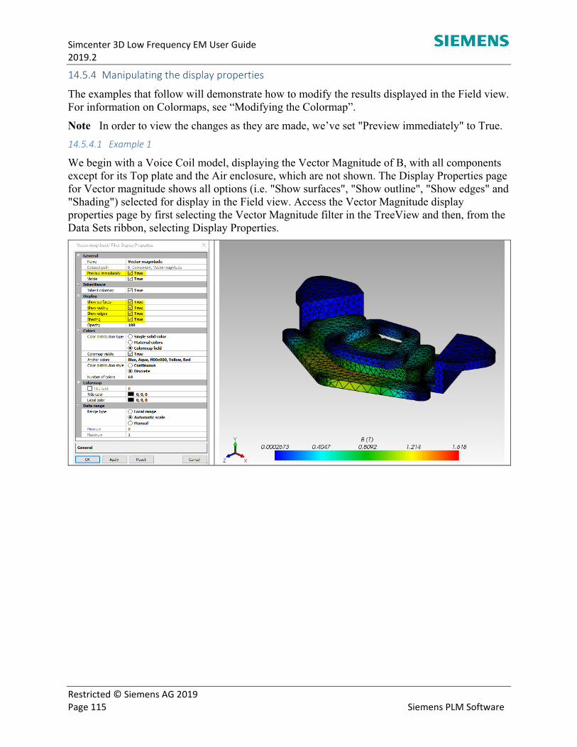
Simcenter 3D Low Frequency EM User Guide 2019.2
Restricted © Siemens AG 2019 Page 115 Siemens PLM Software
14.5.4 Manipulating the display properties
The examples that follow will demonstrate how to modify the results displayed in the Field view. For information on Colormaps, see “Modifying the Colormap”.
Note In order to view the changes as they are made, we’ve set "Preview immediately" to True.
14.5.4.1 Example 1
We begin with a Voice Coil model, displaying the Vector Magnitude of B, with all components except for its Top plate and the Air enclosure, which are not shown. The Display Properties page for Vector magnitude shows all options (i.e. "Show surfaces", "Show outline", "Show edges" and "Shading") selected for display in the Field view. Access the Vector Magnitude display properties page by first selecting the Vector Magnitude filter in the TreeView and then, from the Data Sets ribbon, selecting Display Properties.
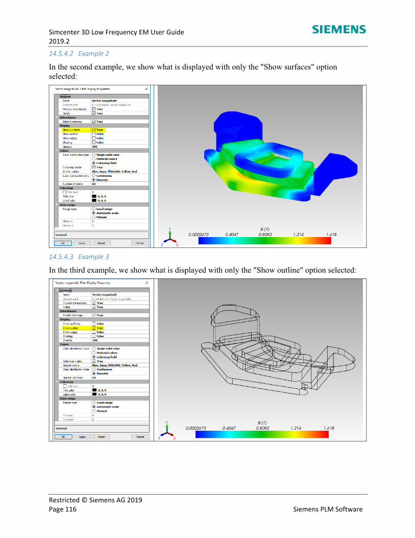
Simcenter 3D Low Frequency EM User Guide 2019.2
Restricted © Siemens AG 2019 Page 116 Siemens PLM Software
14.5.4.2 Example 2
In the second example, we show what is displayed with only the "Show surfaces" option selected:
14.5.4.3 Example 3
In the third example, we show what is displayed with only the "Show outline" option selected:
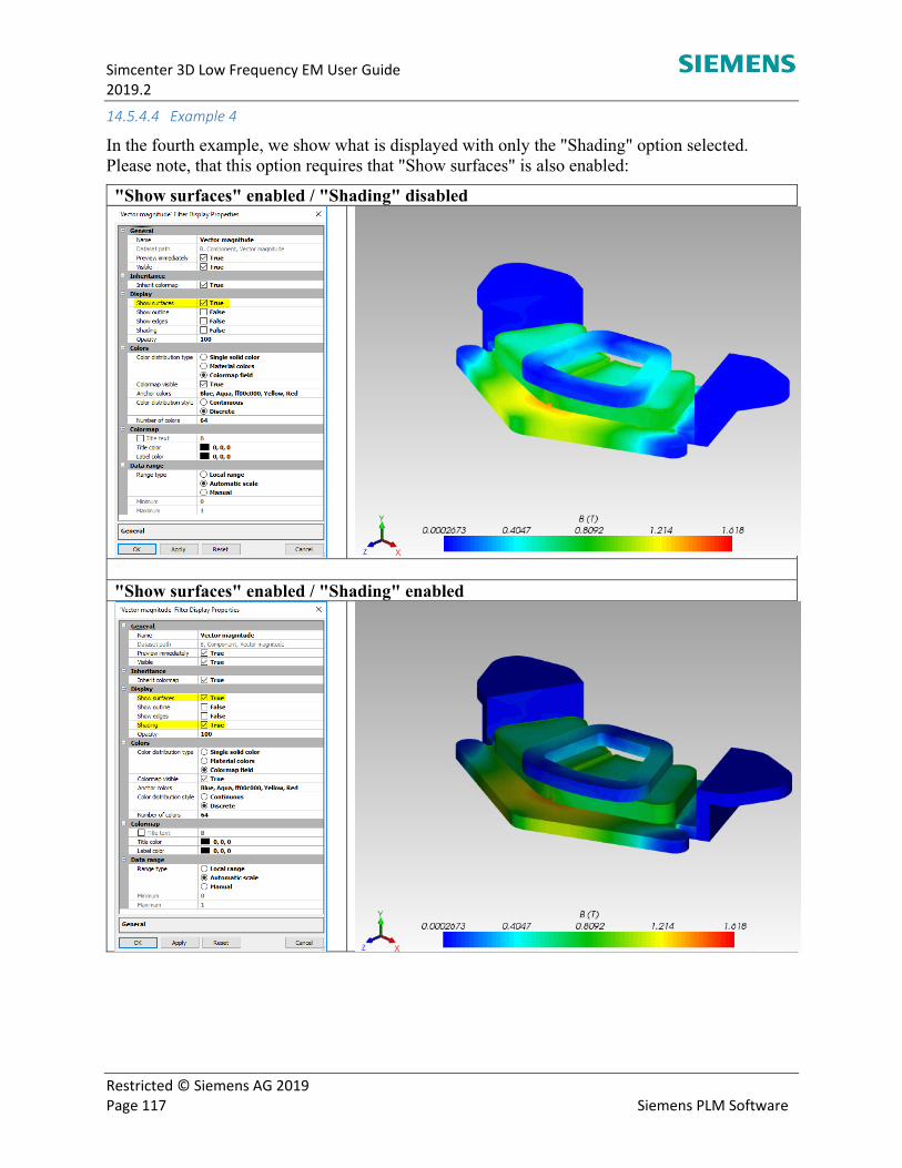
Simcenter 3D Low Frequency EM User Guide 2019.2
Restricted © Siemens AG 2019 Page 117 Siemens PLM Software
14.5.4.4 Example 4
In the fourth example, we show what is displayed with only the "Shading" option selected. Please note, that this option requires that "Show surfaces" is also enabled:
"Show surfaces" enabled / "Shading" disabled
"Show surfaces" enabled / "Shading" enabled
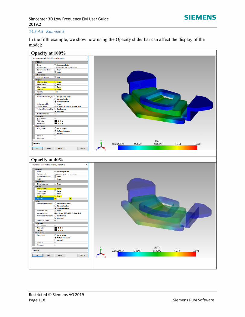
Simcenter 3D Low Frequency EM User Guide 2019.2
Restricted © Siemens AG 2019 Page 118 Siemens PLM Software
14.5.4.5 Example 5
In the fifth example, we show how using the Opacity slider bar can affect the display of the model:
Opacity at 100%
Opacity at 40%
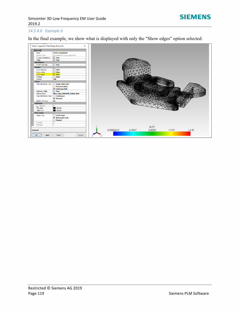
Simcenter 3D Low Frequency EM User Guide 2019.2
Restricted © Siemens AG 2019 Page 119 Siemens PLM Software
14.5.4.6 Example 6
In the final example, we show what is displayed with only the "Show edges" option selected:
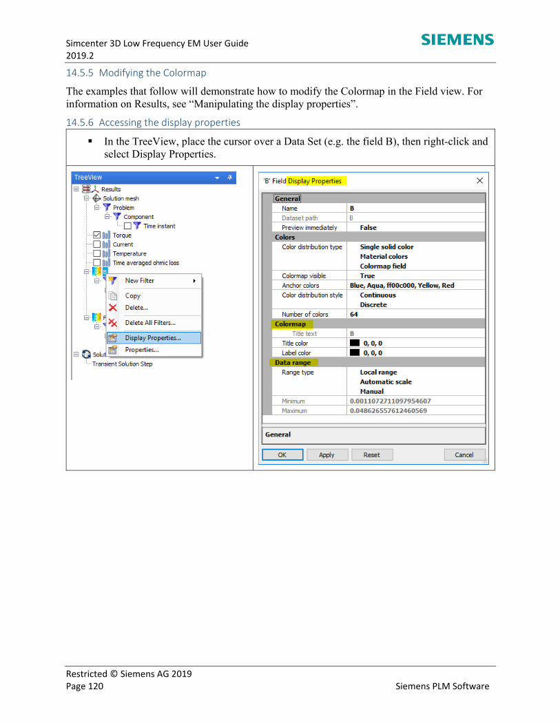
Simcenter 3D Low Frequency EM User Guide 2019.2
Restricted © Siemens AG 2019 Page 120 Siemens PLM Software
14.5.5 Modifying the Colormap
The examples that follow will demonstrate how to modify the Colormap in the Field view. For information on Results, see “Manipulating the display properties”.
14.5.6 Accessing the display properties
In the TreeView, place the cursor over a Data Set (e.g. the field B), then right-click and select Display Properties.
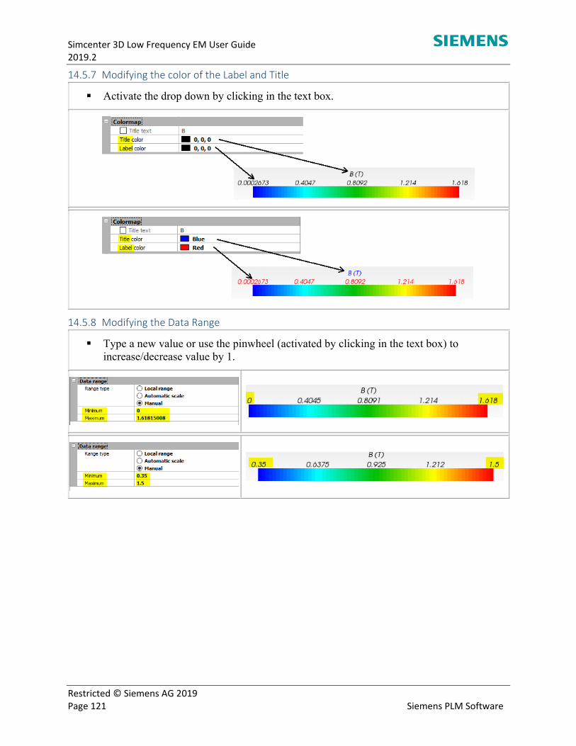
Simcenter 3D Low Frequency EM User Guide 2019.2
Restricted © Siemens AG 2019 Page 121 Siemens PLM Software
14.5.7 Modifying the color of the Label and Title
Activate the drop down by clicking in the text box.
14.5.8 Modifying the Data Range
Type a new value or use the pinwheel (activated by clicking in the text box) to increase/decrease value by 1.
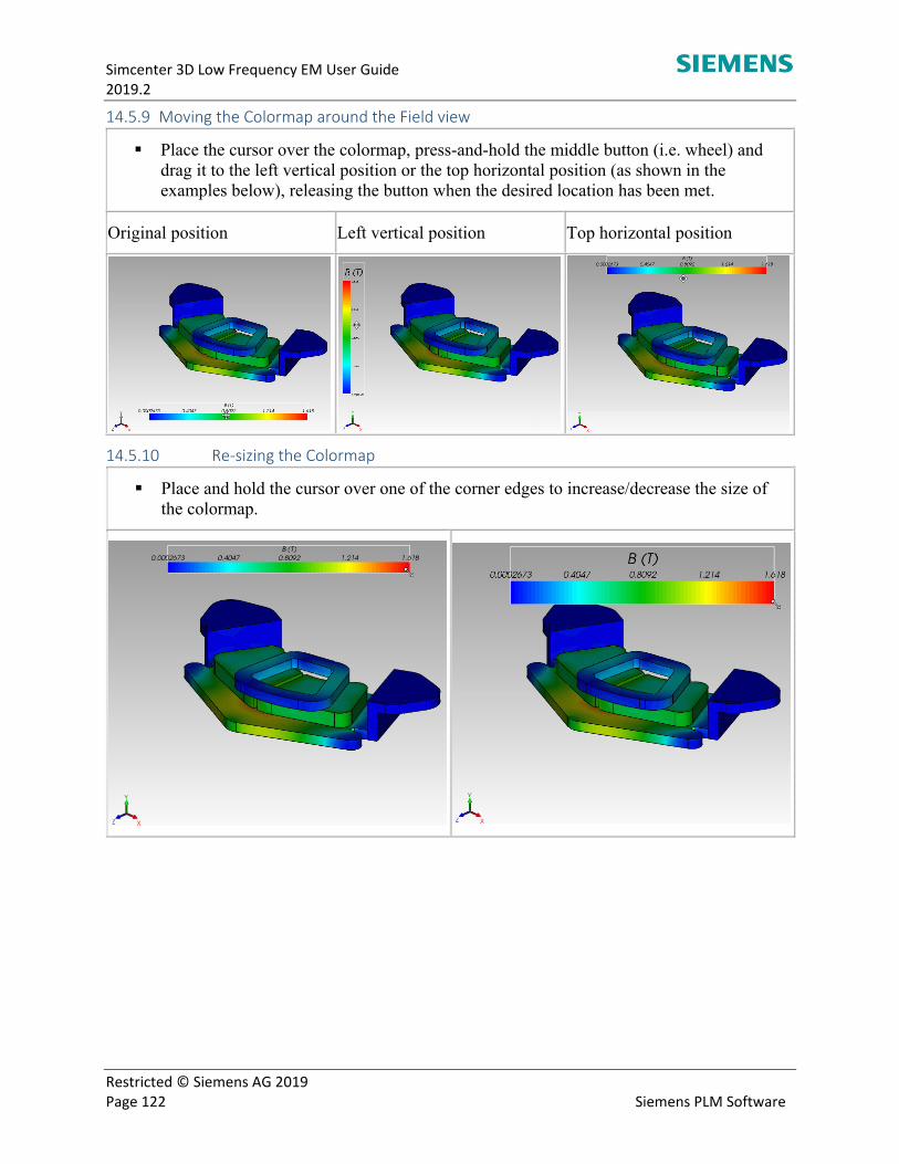
Simcenter 3D Low Frequency EM User Guide 2019.2
Restricted © Siemens AG 2019 Page 122 Siemens PLM Software
14.5.9 Moving the Colormap around the Field view
Place the cursor over the colormap, press-and-hold the middle button (i.e. wheel) and drag it to the left vertical position or the top horizontal position (as shown in the examples below), releasing the button when the desired location has been met.
Original position Left vertical position Top horizontal position
14.5.10 Re‐sizing the Colormap
Place and hold the cursor over one of the corner edges to increase/decrease the size of the colormap.
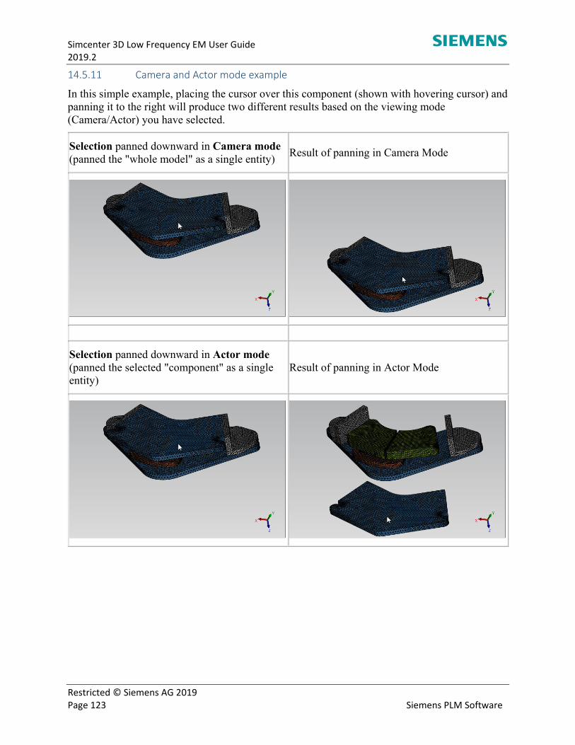
Simcenter 3D Low Frequency EM User Guide 2019.2
Restricted © Siemens AG 2019 Page 123 Siemens PLM Software
14.5.11 Camera and Actor mode example
In this simple example, placing the cursor over this component (shown with hovering cursor) and panning it to the right will produce two different results based on the viewing mode (Camera/Actor) you have selected.
Selection panned downward in Camera mode (panned the "whole model" as a single entity)
Result of panning in Camera Mode
Selection panned downward in Actor mode (panned the selected "component" as a single entity)
Result of panning in Actor Mode
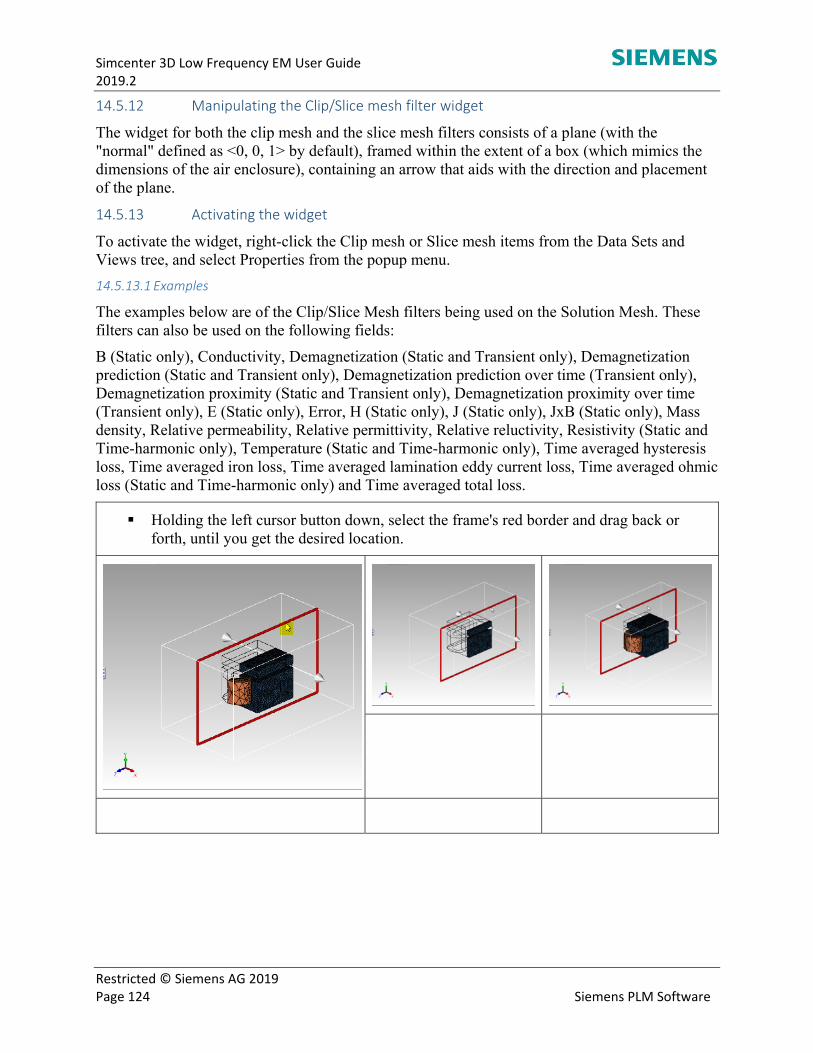
Simcenter 3D Low Frequency EM User Guide 2019.2
Restricted © Siemens AG 2019 Page 124 Siemens PLM Software
14.5.12 Manipulating the Clip/Slice mesh filter widget
The widget for both the clip mesh and the slice mesh filters consists of a plane (with the "normal" defined as <0, 0, 1> by default), framed within the extent of a box (which mimics the dimensions of the air enclosure), containing an arrow that aids with the direction and placement of the plane.
14.5.13 Activating the widget
To activate the widget, right-click the Clip mesh or Slice mesh items from the Data Sets and Views tree, and select Properties from the popup menu.
14.5.13.1 Examples
The examples below are of the Clip/Slice Mesh filters being used on the Solution Mesh. These filters can also be used on the following fields:
B (Static only), Conductivity, Demagnetization (Static and Transient only), Demagnetization prediction (Static and Transient only), Demagnetization prediction over time (Transient only), Demagnetization proximity (Static and Transient only), Demagnetization proximity over time (Transient only), E (Static only), Error, H (Static only), J (Static only), JxB (Static only), Mass density, Relative permeability, Relative permittivity, Relative reluctivity, Resistivity (Static and Time-harmonic only), Temperature (Static and Time-harmonic only), Time averaged hysteresis loss, Time averaged iron loss, Time averaged lamination eddy current loss, Time averaged ohmic loss (Static and Time-harmonic only) and Time averaged total loss.
Holding the left cursor button down, select the frame's red border and drag back or forth, until you get the desired location.
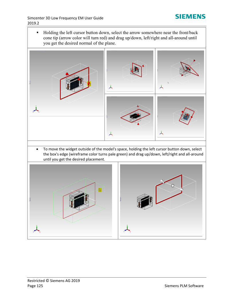
Simcenter 3D Low Frequency EM User Guide 2019.2
Restricted © Siemens AG 2019 Page 125 Siemens PLM Software
Holding the left cursor button down, select the arrow somewhere near the front/back cone tip (arrow color will turn red) and drag up/down, left/right and all-around until you get the desired normal of the plane.
To move the widget outside of the model's space, holding the left cursor button down, select the box's edge (wireframe color turns pale green) and drag up/down, left/right and all‐around until you get the desired placement.
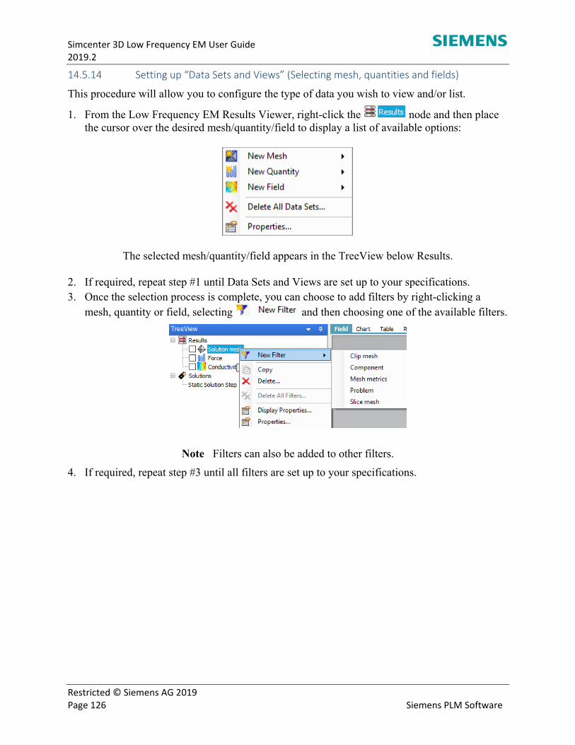
Simcenter 3D Low Frequency EM User Guide 2019.2
Restricted © Siemens AG 2019 Page 126 Siemens PLM Software
14.5.14 Setting up “Data Sets and Views” (Selecting mesh, quantities and fields)
This procedure will allow you to configure the type of data you wish to view and/or list.
1. From the Low Frequency EM Results Viewer, right-click the node and then place the cursor over the desired mesh/quantity/field to display a list of available options:
The selected mesh/quantity/field appears in the TreeView below Results.
2. If required, repeat step #1 until Data Sets and Views are set up to your specifications. 3. Once the selection process is complete, you can choose to add filters by right-clicking a
mesh, quantity or field, selecting and then choosing one of the available filters.
Note Filters can also be added to other filters.
4. If required, repeat step #3 until all filters are set up to your specifications.
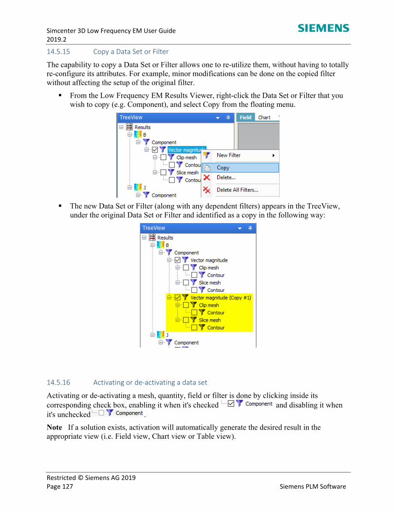
Simcenter 3D Low Frequency EM User Guide 2019.2
Restricted © Siemens AG 2019 Page 127 Siemens PLM Software
14.5.15 Copy a Data Set or Filter
The capability to copy a Data Set or Filter allows one to re-utilize them, without having to totally re-configure its attributes. For example, minor modifications can be done on the copied filter without affecting the setup of the original filter.
From the Low Frequency EM Results Viewer, right-click the Data Set or Filter that you wish to copy (e.g. Component), and select Copy from the floating menu.
The new Data Set or Filter (along with any dependent filters) appears in the TreeView, under the original Data Set or Filter and identified as a copy in the following way:
14.5.16 Activating or de‐activating a data set
Activating or de-activating a mesh, quantity, field or filter is done by clicking inside its corresponding check box, enabling it when it's checked and disabling it when it's unchecked .
Note If a solution exists, activation will automatically generate the desired result in the appropriate view (i.e. Field view, Chart view or Table view).
Related Documents