Silicon isotope fractionation at low temperatures in the presence of Aluminum: An experimental approach and application to di↵erent weathering regimes Dissertation zur Erlangung des Grades eines Doktors der Naturwissenschaften (doctor rerum naturalium) am Fachbereich Geowissenschaften der Freien Universit¨ at Berlin vorgelegt von: Marcus Oelze Berlin 2015

Welcome message from author
This document is posted to help you gain knowledge. Please leave a comment to let me know what you think about it! Share it to your friends and learn new things together.
Transcript
Silicon isotope fractionation at lowtemperatures in the presence of
Aluminum:
An experimental approach andapplication to di↵erent weathering
regimes
Dissertation
zur Erlangung des Grades eines
Doktors der Naturwissenschaften (doctor rerum naturalium)
am Fachbereich Geowissenschaften
der Freien Universitat Berlin
vorgelegt von:
Marcus Oelze
Berlin 2015

Erstgutachter: Prof. Friedhelm von BlanckenburgZweitgutachter: Prof. Martin Dietzel
Tag der Disputation: 04. Marz 2015
(I was not able to decide which citation describes me and my work best,therefore I decided to give two citations here!)
Our whole universe was in a hot dense state,Then nearly fourteen billion years ago expansion started. Wait...The Earth began to cool,The autotrophs began to drool,Neanderthals developed tools,We built a wall (we built the pyramids),Math, science, history, unraveling the mysteries,That all started with the big bang!
“Since the dawn of man” is really not that long,As every galaxy was formed in less time than it takes to sing this song.A fraction of a second and the elements were made.The bipeds stood up straight,The dinosaurs all met their fate,They tried to leap but they were lateAnd they all died (they froze their asses o↵)The oceans and pangeaSee ya, wouldn’t wanna be yaSet in motion by the same big bang!
It all started with the big BANG!
It’s expanding ever outward but one dayIt will cause the stars to go the other way,Collapsing ever inward, we won’t be here, it wont be hurtOur best and brightest figure that it’ll make an even bigger bang!
Australopithecus would really have been sick of usDebating out while here they’re catching deer (we’re catching viruses)Religion or astronomy, Encarta, DeuteronomyIt all started with the big bang!
Music and mythology, Einstein and astrologyIt all started with the big bang!It all started with the big BANG!
(This nerdy song describes my nerdy universe!)
It’s been a long roadGetting from there to hereIt’s been a long timeBut my time is finally nearAnd I can feel the change in the wind right nowNothing’s in my wayAnd they’re not gonna hold me down no moreNo they’re not gonna hold me down
‘Cause I’ve got faith of the heartI’m going where my heart will take meI’ve got faith to believe, I can do anythingI’ve got strength of the soulAnd no one’s gonna bend or break meI can reach any star, I’ve got faithI’ve got faith, faith of the heart
It’s been a long nightTrying to find my wayBeen through the darknessNow I finally have my dayAnd I will see my dream come alive at lastI will touch the skyAnd they’re not gonna hold me down no moreNo they’re not gonna change my mind
‘Cause I’ve got faith of the heartI’m going where my heart will take meI’ve got faith to believe, I can do anythingI’ve got strength of the soulAnd no one’s gonna bend or break meI can reach any star, I’ve got faithFaith of the heart
I’ve known a wind so cold and seen the darkest daysBut now the winds I feel are only winds of changeI’ve been through the fire and I’ve been through the rain but I’ll be fine
‘Cause I’ve got faith of the heartI’m going where my heart will take meI’ve got faith to believe, I can do anythingI’ve got strength of the soulAnd no one’s gonna bend or break meI can reach any star, I’ve got faithFaith of the
Faith of the heartI’m going where my heart will take meI’ve got faith to believeThat no one’s gonna bend or break me
I can reach any star‘Cause I’ve got faith‘Cause I’ve got faithFaith of the heart
It’s been a long road
(and this one my long road!)
Eidesstattliche Erklarung
Ich versichere hiermit an Eides Statt, dass diese Arbeit von niemand anderem als meinerPerson verfasst worden ist. Alle verwendeten Hilfsmittel wie Berichte, Bucher, Inter-netseiten oder ahnliches sind im Literaturverzeichnis angegeben, Zitate aus fremden Ar-beiten sind als solche kenntlich gemacht. Die Arbeit wurde bisher in gleicher oder ahn-licher Form keiner anderen Prufungskommission vorgelegt. Die Teile der Arbeit die schonvero↵entlicht oder eingereicht wurden, sind im Vorwort (“Preface”) kenntlich gemacht.Weiterhin ist im Vorwort (“Preface”) dargelegt, zu welchem Teil der Arbeit andere Wis-senschaftler beigetragen haben.
April 3, 2015
Marcus Oelze
Danksagung
Als erstes danke ich naturlich Prof. Friedhelm von Blanckenburg, fur die immerwahrendeUnterstutzung, Fuhrung und die Moglichkeit, diese Arbeit durchzufuhren. Seine fachlicheKompetenz und Rat sind immer eine große Hilfe gewesen. Auch mochte ich ihm fur dasVertrauen danken, mich diese Arbeit eigenstandig gestalten zu lassen.Mein weiterer Dank gilt Prof. Martin Dietzel (TU Graz), erstens fur die Bereitschaftals zweiter Gutachter meine Dissertation zu bewerten, im Besonderen fur die Umset-zung der Adsorptions- und Ausfallungsexperimente und naturlich fur alle Diskussionen,Verbesserungen und sonstigen Kleinigkeiten die beim Schreiben der schon vero↵entlichenTeile auftraten. Hier gilt es auch Daniel Hollen (Montanuniversitat Leoben) zu danken derdie Experimente durchgefuhrt hat und bei Fragen und Diskussionen stets schnell bereitwar, zu antworten. Danke dafur. Ich danke auch dem PromotionsausschussvorsitzendenProf. Harry Becker fur die freundliche Ubernahme des Vorsitzes, sowie Prof. Timm John,Prof. Anna Gorbushina und Uwe Wiechert fur die Bereitschaft im Promotionsausschussmitzuwirken.Ein ganz großer Dank geht an die Mitarbeiter des GFZ, besonders an die Sektion 3.4:Oberflachennahe Geochemie, die mir mit vielen anregenden Diskussionen immer wiedergute Impulse gegeben haben, durch die ich viel gelernt habe.Ein ganz großes Dankeschon geht an: To my friend Julien Bouchez for the great o�cecommunity, his willingness for endless stimulating discussions and for his willingness toshare his mathematical expertise with me (and never forget: “L´equipe tricolore ne vaisjamais gagner vers Allemagne”...oder so!).Meiner ehemaligen Kollegin und guten Freundin Grit Steinhofel danke ich fur die tolleBurogemeinschaft, die vielen Diskussion und die immer guten Ratschlage.Jan Schussler danke ich fur seine immerwahrende Arbeit damit die “Maschine” (die Nep-tune, d. Red) auch lauft. Fur seine Bereitschaft zur Diskussion bei allen massenspek-trometrischen oder analytischen Problemen, fur die Einrichtung der “FONSI” Arbeits-gruppe (“Friends Of Novel Stable Isotopes”) sowie fur seine große Mitarbeit am GFZ-ESG-DR danke ich ihm.Thanks to Jean Dixon for sharing her geomorphic knowledge, for being a nice colleagueand for becoming a good friend.Der leider viel zu fruh verstorbenen Carola Ocholt danke ich fur ihre aufopferungsvolleArbeit, fur ihre nie nachlassende Hilfsbereitschaft (”Frag doch mal Carola!!”) und furjedes liebe Wort. DANKE Carola!!!Der lieben Conny Dettla↵ danke ich fur die vielen Aufgaben, die sie uns abnimmt, undder immer freundlichen Stimmung im Sekretariat.Allen weiteren Mit-Doktoranden (David Uhlig, Ricarda Maekeler jetzt Behrens, HannaHaedke, Nadine Dannhaus, Michael Tatzel) und allen “Hiwis” (Manuel Quiring, ReneKapannusch) in der Sektion danke ich fur die vielen Diskussionen und Gesprache.Herausheben mochte ich aus der Riege der Doktoranden noch zwei Personen die ammeisten unter meinem unermudlichen Wissensdrang ”leiden” mussten.Zum einen Hanna die gerade in der letzten Zeit meinen immerwahrenden Fragen bezuglichder angewandten Statistik sowie zu Scriptproblemen in Matlab/R ertragen musste unddie mir eine gute Freundin geworden ist.Ein ganz besonderer Dank geht aber an den ”Tatzel” (Michael Tatzel, die Red.) der mitmir und ich mit ihm viele Stunden diskutierend bei Ka↵ee und Wasser verbracht hat,und wir dabei die Systematik der Si Isotope beginnend von Fraktionierungsexperimenten
bis hin zu prakambrischen Ablagerungen beleuchtet haben. Fur seine nicht abnehmendeBereitschaft, meinen kritischen Fragen zu trotzen und fur seine Freundschaft danke ichihm.Ich danke auch unseren technischen Mitarbeiterinnen Jutta Bartel, Josefine Buhk sowieCathrin Schulz fur die Unterstutzung im Labor, denn ohne sie wurden die Arbeiten imLabor sehr viel langsamer von der Hand gehen.Last but not least mochte ich meiner Familie danken, die mir durch finanzielle Un-terstutzung mein Studium erst ermoglicht und mir immer mit Rat und Tat zu Seitegestanden hat. Meiner “Exfreundin” (und jetzigen Frau) Hella Wittmann-Oelze und un-serem Sohn Marten danke ich, weil sie mir Kraft gegeben haben, mich immer geduldig(zumindest meistens) unterstutzt haben, und Hella fur die vielen, vielen Stunden desKorrekturlesens, der vielen kritischen Fragen und Anmerkungen und der standigen Bere-itschaft zur Diskussion.Abschließen mochte ich meine Danksagung mit einem Zitat aus Friedrich Schiller’s “DieGlocke”, welches ich immer vor Augen und im Kopf habe, da es an meinem Elternhausverewigt ist.
Arbeit ist des Burgers Zierde,Segen ist der Muhe Preis,
Ehrt den Konig seine Wurde,Ehret uns der Hande Fleiß.
“Das Lied von der Glocke”von Friedrich Schiller
(hier in etwas abgewandelter Form:Publizieren ist des Wissenschaftlers Zierde,
Zitate sind der Muhe Preis,Ehrt den Professor seine Wurde,Ehret uns des Geistes Fleiss.)
Summary
During the weathering of minerals and rocks elements are released into the ambient so-lution. In the last 10 years stable Si isotope ratios have emerged as a powerful proxy forthe quantification of this release, and to disclose the associated low-temperature water-mineral and water-rock interactions. The isotope ratios potentially trace the way Si isreleased from Si-bearing solids into soil and (diagenetic) interstitial solutions. They alsotrace how silica is precipitated into secondary solids from these solutions. Given the use-ful information Si stable isotopes provide along this pathway, the resulting isotope ratioshave been increasingly explored as a tool to trace silicate weathering, sediment diagenesisand the associated silicification, precipitation of siliceous sediments from hydrothermalvents, and the genesis of Precambrian cherts and banded iron formation. In general,dissolved silica in soil and in river waters is enriched in the heavy isotopes as comparedto the primary silicate minerals where Si is sourced from. In siliceous precipitates fromhydrothermal solutions, the common picture emerging is one of preferential incorporationof light isotopes in the precipitates. To date, only a few notable studies have exploredSi isotope fractionation during fixation of Si from solution under controlled experimentalconditions.In particular, the partitioning of Si isotopes in the presence of Al has not been exploredin detail under controlled laboratory conditions and the related Si isotope fractionationfactors need to be determined. The determination of these fractionation factors is so im-portant as in virtually all Earth surface reactions, Si being released from primary silicatesis accompanied by variable amounts of Al. Crucial in the understanding of Si isotopefractionation in the presence of Al are two processes: 1.) Si isotope fractionation duringadsorption onto Al precipitates and 2.) Si isotope fractionation during Si precipitationfrom solutions in the presence of variable Al concentrations.To better understand Si isotope fractionation during secondary precipitate formation pro-cesses (adsorption and precipitation), I conducted Si isotope fractionation experimentsduring the adsorption of Si onto gibbsite at three di↵erent initial Si concentrations. Toexplore Si isotope fractionation during precipitation of Si from the solution, a new ex-perimental approach was used. In this approach alternating dissolution-precipitation,implying depolymerization-polymerization of silica, is induced by freezing and thawingfor predefined cycle length over a long run duration. This experimental setup allowed meto analyze the temporal change in the Si isotope fractionation factor as the system evolvesfrom a state that is characterized by high net Si removal rates (dominated by unidirec-tional kinetic isotope fractionation), to a state where the net change for precipitation anddissolution is close to zero (Si isotope fractionation closer to equilibrium). Si precipitationexperiments reveal that during cyclic freeze-thaw of dissolved Si-containing solutions, Siis removed from the solution. In the absence of appreciable amounts of Al this removalis not accompanied by a fractionation of Si isotopes. In contrast if Al is present in thesesolutions at high concentrations (here 1 mmol/l), Si removal is faster and accompaniedby strong Si isotope fractionation favoring the light isotopes in the solids. For these high-Al experiments I calculate a fractionation factor of up to ↵30/28Si
solid/solution
=0.9950(103ln↵
solid/solution
= -5h) for the first 20 days of the experiment. With ongoing run-time the early formed precipitates are reorganized wholesale, and ↵30/28Si
solid/solution
ap-proaches 1 (103ln↵
solid/solution
= 0h). The presence of Al increases the precipitation rateand therefore Si isotopes will fractionate according to the Al/Si ratio. The di↵erence be-tween the rapidly precipitating Al-containing phase compared to the slowly precipitating
Al-free phase can then be predicted to be mirrored in the Si isotope composition of thesetwo phases, with the higher enrichment of 28Si in the Al-containing phase.The conducted adsorption experiments presented in Chapter 3 reveal that adsorption ofmonomeric silicic acid onto gibbsite is accompanied by a significant kinetic Si isotopefractionation and that light Si isotopes are preferentially adsorbed. The calculated Siisotope fractionation factors are dependent on the initial Si concentration. High initial Siconcentrations result in a strong kinetic Si isotope fractionation during adsorption. Thisinitial kinetic signature begins to re-equilibrate only after ca. two months. This behavioris compatible with a change from high net adsorption rates to low net adsorption rates(almost constant Si concentration at the end of experiments).Having established the principle fractionation factors in these experiments I explored theSi isotopic composition of natural samples to investigate the dependence of Si isotopefractionation related to soil processes under di↵erent kinetic regimes. To be able to pre-cisely and accurately analyze the natural samples I also extended the established digestionmethod for natural samples by a removal step of organic carbon from solid and water sam-ples (Chapter 2). I show further how external Mg addition improves the accuracy andstability of Si isotope measurements under dry plasma conditions in comparison to wetplasma measurements without Mg addition.After extending the digestion method, the goal here was to study the influence of parame-ters like soil residence time, denudation rate (erosion and weathering rate) and elementalchemical depletion on Si isotope fractionation in settings that are steadily eroding. Theserelations can only be studied when comparing di↵erent weathering regimes. Here I exploreSi isotopes in di↵erent weathering regimes that range from highly weathered thick tropicalsoils in the tectonically inactive mountain range of the Highlands of Sri Lanka representingsupply limited conditions where the weathering erosion relationship is mainly dominatedby chemical dissolution, to the rapidly uplifting Swiss Alps. There the sampling site islocated in the upper Rhone valley, representing the kinetically limited counterpart wherephysical erosion dominates. The intermediate weathering regime is located in the south-ern Sierra Nevada mountain range, California, where chemical weathering and physicalerosion are balanced. The Si isotope measurements of the amorphous and clay fractionextracted from soils and saprolites reveal that a strong relationship between the Si iso-topic composition of these pools and the regolith residence time of the three di↵erentweathering regimes exists. An increase in regolith residence time leads to lower 30Si/28Siratios for secondary silicates formed in di↵erent weathering regimes. In Sri Lanka, thesetting with the longest regolith residence time, the lowest 30Si/28Si ratios for the amor-phous and clay phase are measured. Extracted phases of the Sierra Nevada samplingsite, where regolith residence time are shorter than in Sri Lanka, show relative higher30Si/28Si ratios for the amorphous and clay phase. Amorphous and clay fractions of theSwiss Alps sampling site (lowest regolith residence time of all settings) show the highest30Si/28Si ratios of three sampled weathering regimes. An isotope mass balance modelreveal that the proportion of particulate export flux increases over the dissolved importSi flux according to the decrease in regolith residence time. This change is mirrored inthe 30Si/28Si ratios of secondary precipitates.
Zusammenfassung
Wahrend der chemischen Verwitterung von gesteinsbildenden Mineralen und anstehen-dem Festgestein werden Elemente in die umgebene Bodenlosung abgegeben. In den let-zten 10 Jahren wurden Si Isotope benutzt, um solche Reaktionen zwischen primarenMineralen bzw. dem anstehenden Festgestein und den sie umgebenen Fluiden zu un-tersuchen. Verhaltnisse der stabilen Si Isotope zeigen dabei den moglichen Pfad von Sivon der Freisetzung bei der Verwitterung von primaren Mineralen und anstehenden Fest-gestein bis zum anschließenden Einbau in sekundare Minerale auf. Weiterhin wurdenstabile Si Isotope eingesetzt, um die Ausfallung von hydrothermalem Si, die Genese vonpra-Kambrischem Cherts und von gebanderten Eisenerz–Formationen besser zu verstehen.Die generelle Beobachtung ist, dass das geloste Si im Boden oder Flusswasser isotopischschwerer ist im Vergleich zu dem in gesteinsbildenden Mineralen gebundenem Si. Dasdazugehorige Reservoir von leichten Si Isotopen findet sich in den sekundaren Si Phasen.Auch Neubildungen aus hydrothermalen Losungen zeigen einen bevorzugten Einbau vonleichten Si Isotopen.Trotz der konsistenten Beobachtung, dass leichte Si Isotope bevorzugt in sekundare Min-erale eingebaut werden, wurde die Isotopenfraktionierung von Si im System Si-Al nochnicht im Detail unter kontrollierten Laborbedingungen untersucht. Dabei ist die Bes-timmung von Si Isotopenfraktionierungsfaktoren von Reaktionen zwischen Al und Si vongrundlegender Bedeutung, da es sich mit hoher Wahrscheinlichkeit um die ersten Reak-tionen nach der Freisetzung der beiden Elemente handelt. Bei Reaktionen von Al und Sinehmen zwei wesentliche Prozesse eine fuhrende Rolle ein: 1.) Si Isotopenfraktionierungbei der Adsorption von Si an Al Ausfallungen und 2.) Si Isotopenfraktionierung bei derAusfallung von Si aus wassrigen Losungen in An- und Abwesenheit von Aluminium.Um die Si Isotopenmuster wahrend der Verwitterung von Gestein und der einhergehen-den Neubildung von sekundaren Silikaten erklaren zu konnen, ist die Kenntnis der SiIsotopenfraktionierung bei der Bildung von sekundaren Silikaten durch Adsorption undAusfallung von Si notwendig. Aus diesem Grund wurden in einem ersten experimentellenAnsatz die Si Isotopenfraktionierungsfaktoren bei der Adsorption von Si an Gibbsit beiunterschiedlichen Si Konzentrationen untersucht. Um die Isotopenfraktionierung bei derAusfallung von Si aus wassrigen Losungen zu untersuchen, wurde ein neuartiger experi-menteller Ansatz gewahlt, bei dem die Ausfallung von Si durch ein alternierendes Auflosenund Ausfallen von Si erzwungen wird. Dieses alternierende Auflosen und Ausfallen wurdeinduziert durch einen kontinuierlichen Wechsel von Gefrier- und Tauzyklen uber einen lan-gen Zeitraum hinweg, was zu einer Polymerisierung und Depolymerisierung von Si fuhrt.Dieser neuartige experimentelle Ansatz erlaubt die Umsetzung des zeitlichen Verlaufs vonWechsel zwischen hohen Si Ausfallungsraten (und damit einhergehender ausgepragterkinetischer Si Isotopenfraktionierung) hin zu einem Systemzustand von annahrend aus-geglichen Ausfallungs- und Auflosungsraten (und damit moglicher Si Gleichgewichts–Isotopenfraktionierung). Die durchgefuhrten Si Ausfallungsexperimete zeigen, dass esbeim zyklischen Gefrieren und Auftauen von Si enthaltenen Losungen zur Ausfallung vonSi kommt (Kapitel 4). Wenn es sich dabei um reine Si Losungen (ohne Zugabe von Al)handelt, dann findet bei der Ausfallung keine Si Isotopenfraktionierung statt. Im Gegen-satz zu den Al freien Si Ausfallungsexperimenten ist die Si Ausfallung bei der Zugabevon Al (hier 1 mmol/l) schneller und geht mit einer Si Isotopenfraktionierung einher,bei der bevorzugt leichtes Si in die Ausfallungen eingebaut wird. Fur die Si Ausfallung-sexperimente mit hohen Al Konzentrationen wurden Si Isotopenfraktionierungsfaktoren
von bis zu 103ln↵solid/solution
= -5h fur die ersten 20 Tage des Experimentes ermittelt.Mit zunehmender Laufzeit der Experimente findet eine Reorganisation der anfanglichgebildeten Si Ausfallungen statt, wobei sich ein Si Isotopenfraktionierungsfaktor von103ln↵
solid/solution
= 0h einstellt. Nach Erreichen eines gleichgewichtsahnlichen Zustandes(Si Konzentration annahernd konstant) findet bei der Reorganisation der Si Ausfallungenkeine Isotopenfraktionierung mehr statt. Demzufolge wird durch die Anwesenheit von Aldie Si Ausfallungsraten erhoht und daraus resultiert eine Beziehung zwischen der Si Iso-topenfraktionierung und dem Al/Si Verhaltnis. Der Unterschied zwischen den sich schnellbildenden Al enthaltenen Si Phasen und den sich langsam bildenden Al freien Phasen wirddaher in den resultierenden Si Isotopenverhaltnissen abgebildet.Die in Kapitel 3 gezeigten Si Adsorptionsexperimente zeigen, dass es bei der Adsorptionvon Monokieselsaure an Gibbsit zu einer signifikanten Si Isotopenfraktionierung kommt,wobei die leichten Si Isotope bevorzugt adsorbiert werden. Die von mir bestimmten SiIsotopenfraktionierungsfaktoren sind stark abhangig von der initialen Si Konzentration.Hohe initiale Si Konzentrationen resultieren in einer starkeren kinetischen Si Isotopenfrak-tionierung wahrend der Adsorption. Die initiale kinetische Si Isotopensignatur zeigt Anze-ichen einer Reequilibrierung erst nach ca. zwei Monaten Versuchsdauer. Dieses Verhaltengeht einher mit einem Wechsel von hoher netto–Adsorptionsrate hin zu langsamen netto–Adsorptionsraten (d.h. die Si Konzentration am Ende der Experimente ist annaherndkonstant).Weiterhin habe ich die Isotopenzusammensetzung von naturlichen Proben und den Zusam-menhang zwischen Si Isotopensignatur und Bodenbildungsprozessen in unterschiedlichenVerwitterungsregimen untersucht.Um die Si Isotopie an naturlichen Proben richtig und prazise zu bestimmen, habe ichzunachst die Methodik des Probenaufschlusses und der Messung der Si Isotope an natur-lichen Proben um einen weiteren Arbeitsschritt erweitert, in dem in den Proben enthal-tener organischer Kohlensto↵ entfernt wird. Weiterhin zeige ich, wie der Zusatz von Mgdie Richtigkeit und Prazision der Si Isotopenmessungen erheblich verbessert (Kapitel 2).Meine Arbeit an naturlichen Proben hatte das Ziel den Einfluss von Bodenbildungsparam-etern wie Bodenverweilzeit, Denudationsrate (Erosions- und Verwitterungsrate), sowiedie Abreicherung von Elementen auf die Si Isotopenfraktionierung in verschieden Ver-witterungsregimen zu untersuchen. Diese Zusammenhange konnen nur untersucht wer-den wenn verschiedene Verwitterungsregime miteinander verglichen werden. Ein unter-suchtes Verwitterungsregime ist das von machtigen, stark verwitterten Boden gezeich-nete, tektonisch inaktive Hochland von Sri Lanka, welches das Nachlieferungs–limitierteVerwitterungsregime (“supply-limited”) reprasentiert. In Sri Lanka ist der Zusammen-hang zwischen Verwitterung und Erosion dominiert von der chemischer Auflosung derGesteine. Das kinetisch limitierte Verwitterungsregime liegt im oberen Rhone Tal inden tektonisch aktiven Schweizer Alpen. Im Gegensatz zu dem in Sri Lanka beprobtenVerwitterungsregime dominiert hier physikalische Erosion den Denudationsprozess. DerGebirgszug der sudlichen Sierra Nevada, USA, reprasentiert das Verwitterungsregime indem chemische Verwitterung und physikalische Erosion ausgeglichen sind.Resultate der Si Isotopenmessungen der amorphen Si Fraktion und der Tonfraktion vonBoden und Saprolit zeigen, dass es einen starken Zusammenhang zwischen der Si Isotopen-zusammensetzung dieser Phasen und der Verweilzeit im Regolith in den unterschiedlichenVerwitterungsregimen gibt (Kapitel 5). Langere Regolith–Verweilzeiten fuhren zu niedri-geren 30Si/28Si Verhaltnissen in den sekundar gebildeten Si Ausfallungen. Die niedrigsten30Si/28Si Verhaltnisse wurden in Sri Lanka gemessen, dem Verwitterungsregime mit der

langsten Regolith Verweilzeit. Die extrahierten Fraktionen aus den Proben der SierraNevada, wo die Regolith Verweilzeit kurzer als in Sri Lanka ist, zeigen relativ hohere30Si/28Si Verhaltnisse fur die amorphe Si Fraktion und die Tonfraktion. Die amorpheSi Fraktion sowie die Tonfraktion der Schweizer Alpen, dem Beprobungsstandort mit derkurzesten Regolith Verweilzeit, zeigt die hochsten 30Si/28Si Verhaltnisse der drei beprobtenVerwitterungsregime. Ein Isotopen–Massenbilanzmodel zeigt, dass das Verhaltnis vonpartikularen Export von Si enthalten in sekundaren Phasen zu dem Import von gelostenSi in die Verwitterungszone ansteigt, wenn die Regolith–Verweilzeit abnimmt. DieserWechsel wird in den 30Si/28Si Verhaltnissen der sekundar gebildeten Si Ausfallungen abge-bildet.
Preface
This thesis is composed of several Chapters. Here I will declare which parts of the in-dividual chapters are my work and which parts of the chapter is work from colleaguesthat I collaborated with on these projects. Further will I provide a short summary ofthe content of the individual chapters. All Chapters are prepared in a way that they canbe read individually. Therefore some introductory material is repeated in the individualChapters.
Chapter 1 summarizes the chemical characteristics of Si and its isotopes and furtherprovides a short summary of isotope fractionation processes.
In Chapter 2 an extension of the established digestion method for natural samples is de-scribed. Further it is shown how external Mg doping improves the accuracy and stabilityof Si isotope measurements by multi-collector inductively coupled plasma mass spectrom-eters (MC-ICP-MS). All performed experiments, measurements, data evaluation and datainterpretation were conducted by me and I also wrote the manuscript. The idea to removeorganic carbon from natural solid and water samples was developed jointly by me andGrit Steinhoefel. Most of the tests to establish this “carbon burning” technique wereconducted by Grit Steinhoefel.
Chapter 3 has been published in Chemical Geology (Marcus Oelze, Friedhelm von Blanck-enburg, Daniel Hoellen, Martin Dietzel, Julien Bouchez 2014; DOI: 10.1016/ j.chemgeo.2014.04.027). Adsorption experiments were carried out at pH 7 with di↵erent initial Siconcentrations of 0.36, 0.71 and 1.42 mmol/l Si starting concentrations. As Al-hydroxideadsorbent, 30 g/l crystalline gibbsite were used to provide equal surface area in all ex-periments. Adsorption rates are higher with higher initial Si concentration. At the sametime, calculated apparent isotope fractionation factors 103ln↵adsorbed/solution decrease from-1.8 to -3 h with increasing initial Si concentration. These observations may provide anexplanation for the light Si isotope signature that clay minerals formed during weatheringcarry: the light Si isotope composition is being inherited early on during Si adsorptiononto amorphous Al-hydroxides and is potentially carried over during all further stages oftransformation.Martin Dietzel and Daniel Hoellen conducted the adsorption experiments. I conductedall isotope measurements, performed data evaluation and data interpretation and wrotethe manuscript. Julien Bouchez, Friedhelm von Blanckenburg, Martin Dietzel and DanielHoellen contributed to data interpretation, writing and discussion.
Chapter 4 is submitted to Chemical Geology and is accepted pending minor revisions.A series of precipitation experiments in which continuous precipitation and dissolutionof Si solids is forced by daily cyclic freezing (solid formation) and thawing (solid re-dissolution) was conducted. Six Si precipitation experiments, lasting for about 120 dayswere conducted, with constant initial Si concentrations and varying amounts of Al . No Siisotope fractionation occurs during formation of almost pure Si solids, which is interpretedto show the absence of Si isotope fractionation during polymerization of silicic acid. Siisotope fractionation occurs only in the high-Al concentration experiments, characterizedby an enrichment of the light Si isotopes in the solids forming early. With ongoing runtimere-dissolution of these solids is indicated by the Si isotope value of the complementarysolution that shifts to lighter values and eventually reaches near-starting compositions.
The results of the experiments suggest that the enrichment of light Si isotopes foundin natural environments is caused exclusively by an unidirectional kinetic isotope e↵ectduring fast precipitation of solids, aided by co-precipitation of Al phases or other carrierphases. In contrast, during slow precipitation, or in the absence of a carrier phase like Al,no Si isotope fractionation is expected and solids obtain the composition of the ambientfluid.Martin Dietzel and Daniel Hoellen conducted the freeze-thaw experiments. I conductedall isotope measurements, performed data evaluation and data interpretation and wrotethe manuscript. Julien Bouchez, Friedhelm von Blanckenburg, Martin Dietzel and DanielHoellen contributed to data interpretation, writing and discussion.
In Chapter 5 it is tested whether the kinetic isotope e↵ect explored in controlled labora-tory experiments in Chapter 3 and Chapter 4 is also expressed during natural weatheringreactions. Three di↵erent study sites were chosen, representing di↵erent weathering anderosional regimes. Si isotopes are used to trace di↵erences in these di↵erent weatheringregimes, ranging from highly weathered thick tropical soil-mantled hillslopes, present inthe tectonically inactive mountain range of the Highlands of Sri Lanka. This settingrepresents supply limited conditions, where primary mineral dissolution is almost com-plete. The rapidly uplifting Swiss Alps sampling site located in the upper Rhone valleyrepresents the kinetically limited counterpart where physical erosion dominates. An in-termediate weathering regime is located in the southern Sierra Nevada mountain range,California, where chemical weathering and physical erosion are balanced. The goal is tostudy the influence of parameters like soil residence time, denudation rate (erosion andweathering rate), elemental chemical depletion, and their influence on Si isotope fraction-ation.The sampling and further the generation of background data (XRF bulk soil data, majorelement concentration in river water) of the described samples were conducted during anongoing project of the Earth Surface Geochemistry Group at GFZ Potsdam. Some resultsof these measurements are shown in the Appendix of this Chapter (XRF bulk soil data,major element concentration in river water) to provide a complete picture of the sam-pled sites and are taken from the GFZ-ESG-DR (GFZ-Earth Surface Geochemistry-DataRepository) or from already published literature. I conducted the sample processing for Siisotope measurements, Si isotope measurements, data evaluation and data interpretation.
Contents
1 Introduction 11.1 Background on Si and on stable Si isotopes . . . . . . . . . . . . . . . . . . 11.2 Isotope fractionation processes . . . . . . . . . . . . . . . . . . . . . . . . . 51.3 Appendix Chapter 1 . . . . . . . . . . . . . . . . . . . . . . . . . . . . . . 8
1.3.1 Tables . . . . . . . . . . . . . . . . . . . . . . . . . . . . . . . . . . 8
2 Si stable isotope ratio determination of natural samples by MC-ICP-MS 92.1 Abstract . . . . . . . . . . . . . . . . . . . . . . . . . . . . . . . . . . . . . 92.2 Introduction . . . . . . . . . . . . . . . . . . . . . . . . . . . . . . . . . . . 92.3 Sample digestion . . . . . . . . . . . . . . . . . . . . . . . . . . . . . . . . 11
2.3.1 Solid samples . . . . . . . . . . . . . . . . . . . . . . . . . . . . . . 112.3.2 Water samples . . . . . . . . . . . . . . . . . . . . . . . . . . . . . . 12
2.4 Column chemistry and preparation of Mg addition solution . . . . . . . . . 122.5 MC-ICP-MS analysis . . . . . . . . . . . . . . . . . . . . . . . . . . . . . . 13
2.5.1 Wet plasma conditions without Mg addition . . . . . . . . . . . . . 132.5.2 Dry plasma conditions with Mg addition . . . . . . . . . . . . . . . 132.5.3 Reporting Si isotope ratios . . . . . . . . . . . . . . . . . . . . . . . 142.5.4 Results of measured Si isotope reference materials . . . . . . . . . . 14
2.6 Tests conducted under wet and dry plasma conditions . . . . . . . . . . . . 222.6.1 Si concentration matching for dry plasma conditions . . . . . . . . . 222.6.2 Mg concentration matching for dry plasma conditions . . . . . . . . 232.6.3 Molarity matching for wet and dry plasma conditions . . . . . . . . 252.6.4 Column fractionation . . . . . . . . . . . . . . . . . . . . . . . . . . 262.6.5 Anion contamination . . . . . . . . . . . . . . . . . . . . . . . . . . 27
2.7 Summary . . . . . . . . . . . . . . . . . . . . . . . . . . . . . . . . . . . . 322.8 Appendix Chapter 2 . . . . . . . . . . . . . . . . . . . . . . . . . . . . . . 33
2.8.1 Tables . . . . . . . . . . . . . . . . . . . . . . . . . . . . . . . . . . 33
3 Si stable isotope fractionation during adsorption and the competitionbetween kinetic and equilibrium isotope fractionation: implications forweathering systems1 363.1 Abstract . . . . . . . . . . . . . . . . . . . . . . . . . . . . . . . . . . . . . 363.2 Introduction . . . . . . . . . . . . . . . . . . . . . . . . . . . . . . . . . . . 373.3 Materials and Methods . . . . . . . . . . . . . . . . . . . . . . . . . . . . . 37
3.3.1 Si source for adsorption experiments . . . . . . . . . . . . . . . . . 373.3.2 Adsorption experiments . . . . . . . . . . . . . . . . . . . . . . . . 38
1This Chapter is published in Chemical Geology : Oelze et al. (2014);http://dx.doi.org/10.1016/j.chemgeo.2014.04.027
xiv
3.3.3 Chemical separation and purification . . . . . . . . . . . . . . . . . 383.3.4 Mass spectrometry . . . . . . . . . . . . . . . . . . . . . . . . . . . 383.3.5 Analytical tests . . . . . . . . . . . . . . . . . . . . . . . . . . . . . 39
3.4 Results . . . . . . . . . . . . . . . . . . . . . . . . . . . . . . . . . . . . . . 403.4.1 Evolution of Si concentration . . . . . . . . . . . . . . . . . . . . . 403.4.2 Silicon isotopes . . . . . . . . . . . . . . . . . . . . . . . . . . . . . 42
3.5 Discussion . . . . . . . . . . . . . . . . . . . . . . . . . . . . . . . . . . . . 453.5.1 Si isotope fractionation during Si adsorption . . . . . . . . . . . . . 453.5.2 Kinetics of Si adsorption . . . . . . . . . . . . . . . . . . . . . . . . 453.5.3 The change of the isotope fractionation regime . . . . . . . . . . . . 473.5.4 Si adsorption in natural systems . . . . . . . . . . . . . . . . . . . . 493.5.5 Comparison to adsorption of transition metals . . . . . . . . . . . . 503.5.6 Implications for silicate weathering environments . . . . . . . . . . 50
3.6 Summary . . . . . . . . . . . . . . . . . . . . . . . . . . . . . . . . . . . . 513.7 Appendix Chapter 3 . . . . . . . . . . . . . . . . . . . . . . . . . . . . . . 53
3.7.1 Tables . . . . . . . . . . . . . . . . . . . . . . . . . . . . . . . . . . 533.7.2 Determination of monosilicic acid using
�-silicomolybdate method . . . . . . . . . . . . . . . . . . . . . . . 543.7.3 Chemical kinetic rate laws applied to Si adsorption on gibbsite . . . 55
4 The e↵ect of Al on Si isotope fractionation investigated by silica precip-itation experiments2 584.1 Abstract . . . . . . . . . . . . . . . . . . . . . . . . . . . . . . . . . . . . . 584.2 Introduction . . . . . . . . . . . . . . . . . . . . . . . . . . . . . . . . . . . 594.3 Framework for isotope fractionation during precipitation . . . . . . . . . . 614.4 Materials and Methods . . . . . . . . . . . . . . . . . . . . . . . . . . . . . 62
4.4.1 Description of Experiments . . . . . . . . . . . . . . . . . . . . . . 624.4.2 Requirements for Si precipitation experiments . . . . . . . . . . . . 634.4.3 Filtration of solutions and chemical separation for Si isotope analyses 644.4.4 Mass spectrometry . . . . . . . . . . . . . . . . . . . . . . . . . . . 64
4.5 Results . . . . . . . . . . . . . . . . . . . . . . . . . . . . . . . . . . . . . . 654.5.1 Si and Al concentrations . . . . . . . . . . . . . . . . . . . . . . . . 654.5.2 Silicon isotopes . . . . . . . . . . . . . . . . . . . . . . . . . . . . . 68
4.6 Discussion . . . . . . . . . . . . . . . . . . . . . . . . . . . . . . . . . . . . 734.6.1 Potential removal processes . . . . . . . . . . . . . . . . . . . . . . 734.6.2 Isotope fractionation associated with Si removal . . . . . . . . . . . 744.6.3 Rate dependence of Si isotope fractionation . . . . . . . . . . . . . 75
4.7 Summary and implications . . . . . . . . . . . . . . . . . . . . . . . . . . . 784.8 Appendix 4 . . . . . . . . . . . . . . . . . . . . . . . . . . . . . . . . . . . 79
4.8.1 Tables . . . . . . . . . . . . . . . . . . . . . . . . . . . . . . . . . . 794.8.2 Determination of mono-and polysilicic acid using the �-silicomolybdate
method . . . . . . . . . . . . . . . . . . . . . . . . . . . . . . . . . 824.8.3 Modeling a net precipitation-dissolution process associated with iso-
tope fractionation . . . . . . . . . . . . . . . . . . . . . . . . . . . . 84
2This Chapter is published in Chemical Geology : Oelze et al. (2015);http://dx.doi.org/10.1016/j.chemgeo.2015.01.002
5 The Si isotope record of di↵erent weathering regimes 915.1 Abstract . . . . . . . . . . . . . . . . . . . . . . . . . . . . . . . . . . . . . 915.2 Introduction . . . . . . . . . . . . . . . . . . . . . . . . . . . . . . . . . . . 91
5.2.1 Sri Lankan Highland study site . . . . . . . . . . . . . . . . . . . . 935.2.2 Swiss Alps study site . . . . . . . . . . . . . . . . . . . . . . . . . . 955.2.3 Sierra Nevada study sites . . . . . . . . . . . . . . . . . . . . . . . . 97
5.3 Methods and Materials . . . . . . . . . . . . . . . . . . . . . . . . . . . . . 995.3.1 Sampling . . . . . . . . . . . . . . . . . . . . . . . . . . . . . . . . 995.3.2 Sample preparation for Si isotope measurements . . . . . . . . . . . 1005.3.3 Extraction procedures for di↵erent Si fractions . . . . . . . . . . . . 1005.3.4 Element concentration measurements . . . . . . . . . . . . . . . . . 102
5.4 Isotope results . . . . . . . . . . . . . . . . . . . . . . . . . . . . . . . . . . 1035.4.1 Isotope Results - Sri Lanka . . . . . . . . . . . . . . . . . . . . . . . 1035.4.2 Isotope Results - Swiss Alps . . . . . . . . . . . . . . . . . . . . . . 1045.4.3 Isotope Results - Sierra Nevada . . . . . . . . . . . . . . . . . . . . 105
5.5 Discussion . . . . . . . . . . . . . . . . . . . . . . . . . . . . . . . . . . . . 1075.5.1 Control of the export- to import flux ratio of Si in the weathering
zone on the Si isotopic composition of secondary weathering products1075.6 Summary . . . . . . . . . . . . . . . . . . . . . . . . . . . . . . . . . . . . 1145.7 Appendix Chapter 5 . . . . . . . . . . . . . . . . . . . . . . . . . . . . . . 115
5.7.1 Background data . . . . . . . . . . . . . . . . . . . . . . . . . . . . 1155.7.2 Si isotope depth profiles . . . . . . . . . . . . . . . . . . . . . . . . 1315.7.3 Combining the findings of the individual sampling sites . . . . . . . 1405.7.4 Tables . . . . . . . . . . . . . . . . . . . . . . . . . . . . . . . . . . 144
Chapter 1
Introduction
1.1 Background on Si and on stable Si isotopes
Silicon has been under geological investigation since its discovery in the 18th centuryas it is the second most abundant element in the earth crust. Being a constituent ofalmost all geological processes from mountain building to core formation, its chemicalbehavior has been thoroughly investigated. With the developing ability to measure theabundance of the stable isotopes of the elements and to explore the processes leading totheir fractionation in the mid 20th century, also the stable isotopes of Si became a fieldof interest in geochemistry research. Silicon has three stable isotopes with the relativeabundances 28Si = 92.23 %, 29Si = 4.67 % and 30Si = 3.10 %. Si isotope data is reportedrelative to the standard reference material NBS28 (quartz sand) in the delta notationaccording to Coplen (2011) as �(29/28Si)NBS28 and �(30/28Si)NBS28 expressed in per mill(h) by multiplication of Equation 1.1 and Equation 1.2 with a factor of 103:
�(29/28Si)NBS28 =
0
B@
⇣29Si28Si
⌘
sample� 29Si28Si
�NBS28
� 1
1
CA (1.1)
�(30/28Si)NBS28 =
0
B@
⇣30Si28Si
⌘
sample� 30Si28Si
�NBS28
� 1
1
CA (1.2)
To complete the isotopic terminology further used in this thesis definitions for isotopefractionation factors and isotopic di↵erences are also given here:
↵A�B
=R
A
RB
=1000 + �
A
1000 + �B
(1.3)
Where ↵A�B
denotes the isotopic fractionation factor between substance A and B. RA
andR
B
denote the isotope ratios of substance A and B, respectively. The isotopic fractionationfactor can also be expressed in permil (h) by:
�A�B
' 1000 ⇤ ln(↵A�B
) (1.4)
The isotopic di↵erence between two substances A and B is defined as:
1
Chapter 1. Introduction Marcus Oelze
�A�B
= �A
� �B
(1.5)
The isotopic composition of Si-containing materials has been measured first by Reynoldsand Verhoogen (1953) by converting Si into SiF4 and measuring gaseous SiF4 by gas massspectrometry. Before the development of multi-collector inductively coupled plasma massspectrometers (MC-ICP-MS) in the early 2000’s, Si has been measured as SiF4 by gasmass spectrometry. The ability to measure Si isotopes on a MC-ICP-MS resulted in theopportunity to distinguish between reservoirs with only small isotopic variation, due tothe much higher precision of the isotope ratios determined by MC-ICP-MS compared toconventional gas mass spectrometers. Cardinal et al. (2003) carried out the first precisemeasurements of stable Si isotopes. Since then many studies have been published thatreport Si stable isotope compositions of a whole variety of compartments of the Earth,from mantle rocks and minerals to the foliage of trees.According to Iler (1979) is the term “silicon” used for the element Silicon (Si) and theterm “silica” is used as a short form of “silicon dioxide”. Si can be found in a variety ofbonding environments (silicate minerals) but only rarely in elemental form at the Earth’ssurface due to the high a�nity to binding with oxygen. In bonding environments, Siusually has the oxidation state 4+. Si and also the oxide SiO2 are almost insoluble in allacids, except for HF-HNO4 mixtures. Si has a high solubility in hot bases but SiO2 reactsslowly in aqueous bases. To digest Si oxides, the most common way is to use alkalinefusion techniques, where an alkaline flux (e.g. NaOH) is added to the sample. During themelting process at temperatures between 600 and 800�, easily soluble alkaline silicatesare formed.Caused by the low solubility of Si and SiO2, only small amounts of Si can be found asmonosilicic acid (H4SiO4) in natural waters (<100 mg/l). In dilute solutions monosilicicacid is only a weak acid and and does not dissociate below neutral pH. This causes theconstant solubility of Si below pH 7. At low pH the dissociation can be described by thefollowing reaction:
SiO2(solid) +H2O ⌦ H4SiO4
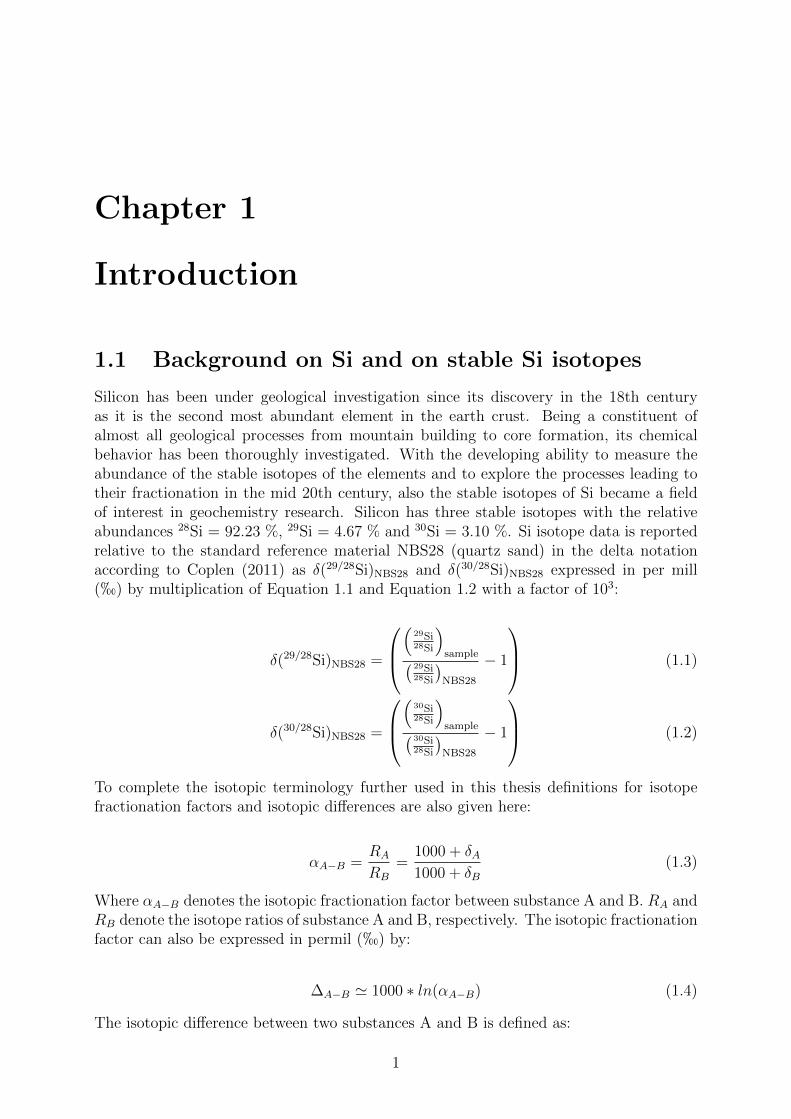
With increasing pH the weak diprotonic monosilicic acid starts to dissociate, which causesthe increase in solubility (see Figure 1.1) according to the following reactions:
H4SiO4 ⌦ H3SiO�4 +H+
H3SiO�4 ⌦ H2SiO
2�4 +H+
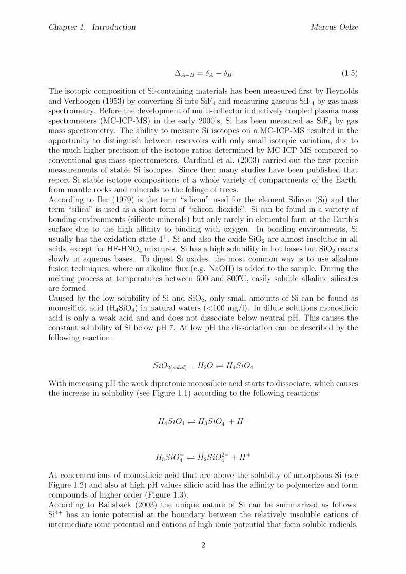
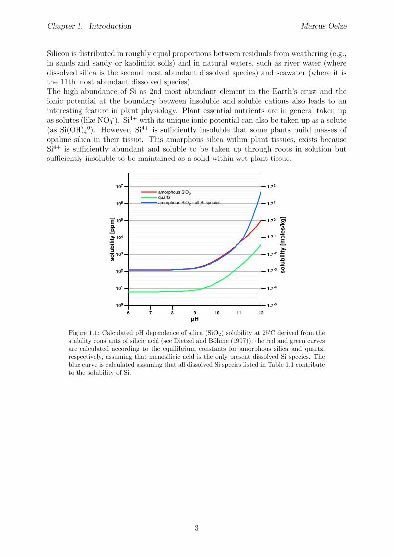
At concentrations of monosilicic acid that are above the solubilty of amorphous Si (seeFigure 1.2) and also at high pH values silicic acid has the a�nity to polymerize and formcompounds of higher order (Figure 1.3).According to Railsback (2003) the unique nature of Si can be summarized as follows:Si4+ has an ionic potential at the boundary between the relatively insoluble cations ofintermediate ionic potential and cations of high ionic potential that form soluble radicals.
2
Chapter 1. Introduction Marcus Oelze
Silicon is distributed in roughly equal proportions between residuals from weathering (e.g.,in sands and sandy or kaolinitic soils) and in natural waters, such as river water (wheredissolved silica is the second most abundant dissolved species) and seawater (where it isthe 11th most abundant dissolved species).The high abundance of Si as 2nd most abundant element in the Earth’s crust and theionic potential at the boundary between insoluble and soluble cations also leads to aninteresting feature in plant physiology. Plant essential nutrients are in general taken upas solutes (like NO3
-). Si4+ with its unique ionic potential can also be taken up as a solute(as Si(OH)40). However, Si4+ is su�ciently insoluble that some plants build masses ofopaline silica in their tissue. This amorphous silica within plant tissues, exists becauseSi4+ is su�ciently abundant and soluble to be taken up through roots in solution butsu�ciently insoluble to be maintained as a solid within wet plant tissue.
6 7 8 9 10 11 12
pH
100
101
102
103
104
105
106
107
so
lub
ilit
y [
pp
m]
amorphous SiO2
quartz
amorphous SiO2 - all Si species
1.7-5
1.7-4
1.7-3
1.7-2
1.7-1
1.70
1.71
1.72
so
lub
ilit
y [
mo
les/k
g]
Figure 1.1: Calculated pH dependence of silica (SiO2
) solubility at 25� derived from thestability constants of silicic acid (see Dietzel and Bohme (1997)); the red and green curvesare calculated according to the equilibrium constants for amorphous silica and quartz,respectively, assuming that monosilicic acid is the only present dissolved Si species. Theblue curve is calculated assuming that all dissolved Si species listed in Table 1.1 contributeto the solubility of Si.
3
Chapter 1. Introduction Marcus Oelze
010
020
030
0
temperature [°C]
0.0000.0050.0100.0150.0200.0250.030
solu
bilit
y [m
oles
/kg]
010
020
030
0
temperature [°C]
0
500
1000
1500
solu
bilit
y [p
pm]
0 5 10 15 20temperature [°C]
20
25
30
35
40
45
50
solu
bilit
y [p
pm]
Si [mg/Kg] Rimstedt & Barnes (1980)Si [mg/Kg] Fournier & Rowe (1977)Si [mg/Kg] Gunnarson & Arnorson (1999)
3.3-4
4.2-4
5.0-4
5.8-4
6.7-4
7.5-4
8.3-4
solu
bilit
y [m
oles
/kg]
Figure 1.2: Solubility curves for amorphous Si in the temperature range from 0 to 20�using the empirical relationships of Fournier and Rowe (1977), Rimstidt and Barnes (1980)and Gunnarsson and Arnorsson (2000). The upper left panel shows the solubilities in[moles/kg] of amorphous silica (black) and quartz (orange) in the temperature range from 0to 350�, calculated using the empirical relationship of Gunnarsson and Arnorsson (2000).The upper right panel shows the solubilities in [ppm] of amorphous Si (solid black) andquartz as Si (solid orange) and of amorphous SiO
2
(stippled black) and quartz as SiO2
(stippled orange)
6 7 8 9 10 11 12pH
0
10
20
30
40
50
60
70
80
90
100
mol
% S
iO2
Si(OH)4SiO(OH)3-SiO2(OH)22-Si2O2(OH)5-Si2O3(OH)42-Si3O5(OH)53-Si4O6(OH)62-Si4O4(OH)124-
Figure 1.3: Calculated mol% SiO2
concentration of silica contained in monomeric or poly-meric form at 25� as a function of pH, derived from stability constants of silicic acid (seeDietzel and Bohme (1997)) using all Si species shown in Table 1.
4
Chapter 1. Introduction Marcus Oelze
1.2 Isotope fractionation processes
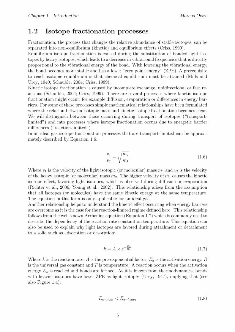
Fractionation, the process that changes the relative abundance of stable isotopes, can beseparated into non-equilibrium (kinetic) and equilibrium e↵ects (Criss, 1999).Equilibrium isotope fractionation is caused during the substitution of bonded light iso-topes by heavy isotopes, which leads to a decrease in vibrational frequencies that is directlyproportional to the vibrational energy of the bond. With lowering the vibrational energy,the bond becomes more stable and has a lower “zero point energy” (ZPE). A prerequisiteto reach isotopic equilibrium is that chemical equilibrium must be attained (Mills andUrey, 1940; Schauble, 2004; Criss, 1999).Kinetic isotope fractionation is caused by incomplete exchange, unidirectional or fast re-actions (Schauble, 2004; Criss, 1999). There are several processes where kinetic isotopefractionation might occur, for example di↵usion, evaporation or di↵erences in energy bar-riers. For some of these processes simple mathematical relationships have been formulatedwhere the relation between isotopic mass and kinetic isotope fractionation becomes clear.We will distinguish between those occurring during transport of isotopes (“transport-limited”) and into processes where isotope fractionation occurs due to energetic barrierdi↵erences (“reaction-limited”).In an ideal gas isotope fractionation processes that are transport-limited can be approxi-mately described by Equation 1.6.
v1v2
=
rm2
m1
(1.6)
Where v1 is the velocity of the light isotopic (or molecular) mass m1 and v2 is the velocityof the heavy isotopic (or molecular) mass m2. The higher velocity of m1 causes the kineticisotope e↵ect, favoring light isotopes, which is observed during di↵usion or evaporation(Richter et al., 2006; Young et al., 2002). This relationship arises from the assumptionthat all isotopes (or molecules) have the same kinetic energy at the same temperature.The equation in this form is only applicable for an ideal gas.Another relationship helps to understand the kinetic e↵ect occurring when energy barriersare overcome as it is the case for the reaction-limited regime defined here. This relationshipfollows from the well-known Arrhenius equation (Equation 1.7) which is commonly used todescribe the dependency of the reaction rate constant on temperature. This equation canalso be used to explain why light isotopes are favored during attachment or detachmentto a solid such as adsorption or desorption:
k = A⇥ e�EaRT (1.7)
Where k is the reaction rate, A is the pre-exponential factor, Ea
is the activation energy, Ris the universal gas constant and T is temperature. A reaction occurs when the activationenergy E
a
is reached and bonds are formed. As it is known from thermodynamics, bondswith heavier isotopes have lower ZPE as light isotopes (Urey, 1947), implying that (seealso Figure 1.4):
Ea�light
< Ea�heavy
(1.8)
5
Chapter 1. Introduction Marcus Oelze
From Equation 1.7 and Equation 1.8, it follows that the reaction rate constant k of lightisotopes is larger. The larger reaction rate constant leads to a higher reaction rate oflight isotopes compared to heavy isotopes. The e↵ect of slight di↵erences in the energyat the transition state occurs during all chemical reactions when evolving from educt toproduct (“forward reaction”) as well as when evolving from product to educt (“backwardreaction”).
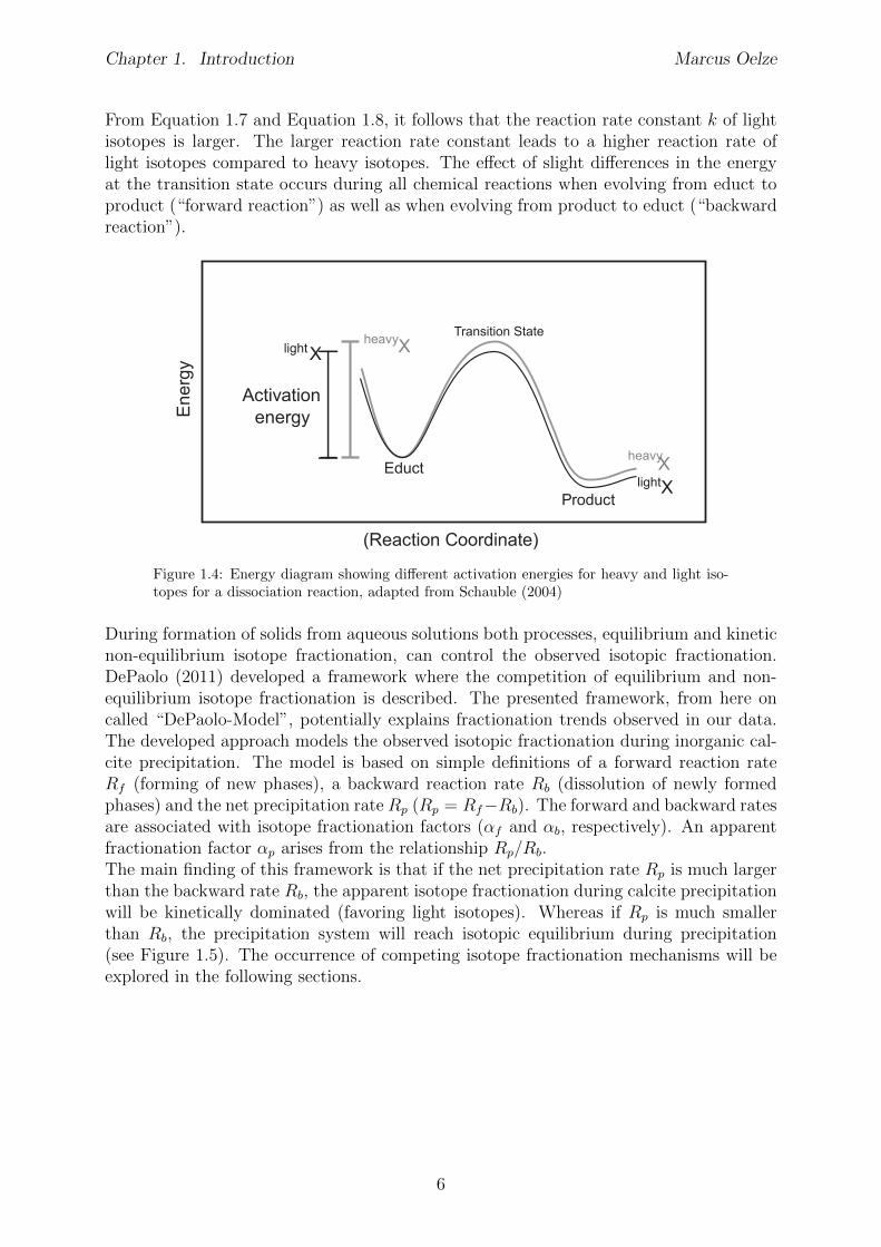
(Reaction Coordinate)
Ene
rgy
Activationenergy
Transition State
Educt
Product
XX
heavyXlightX
light
heavy
Figure 1.4: Energy diagram showing di↵erent activation energies for heavy and light iso-topes for a dissociation reaction, adapted from Schauble (2004)
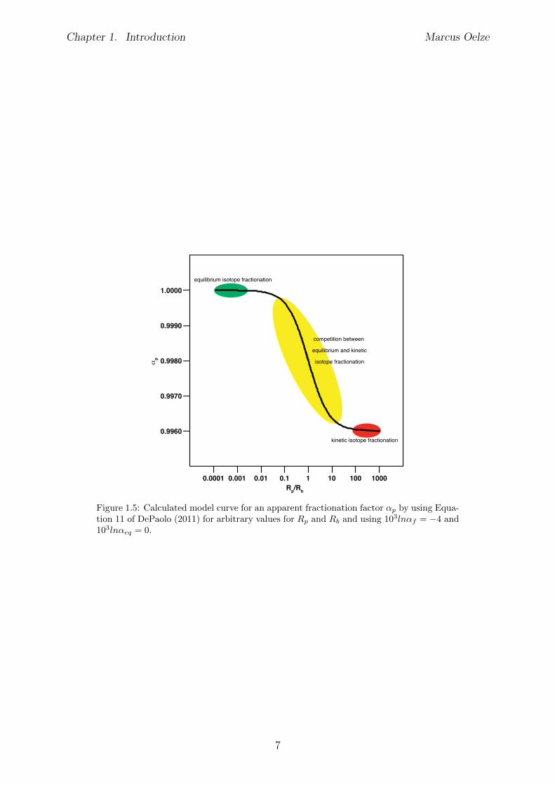
During formation of solids from aqueous solutions both processes, equilibrium and kineticnon-equilibrium isotope fractionation, can control the observed isotopic fractionation.DePaolo (2011) developed a framework where the competition of equilibrium and non-equilibrium isotope fractionation is described. The presented framework, from here oncalled “DePaolo-Model”, potentially explains fractionation trends observed in our data.The developed approach models the observed isotopic fractionation during inorganic cal-cite precipitation. The model is based on simple definitions of a forward reaction rateR
f
(forming of new phases), a backward reaction rate Rb
(dissolution of newly formedphases) and the net precipitation rate R
p
(Rp
= Rf
�Rb
). The forward and backward ratesare associated with isotope fractionation factors (↵
f
and ↵b
, respectively). An apparentfractionation factor ↵
p
arises from the relationship Rp
/Rb
.The main finding of this framework is that if the net precipitation rate R
p
is much largerthan the backward rate R
b
, the apparent isotope fractionation during calcite precipitationwill be kinetically dominated (favoring light isotopes). Whereas if R
p
is much smallerthan R
b
, the precipitation system will reach isotopic equilibrium during precipitation(see Figure 1.5). The occurrence of competing isotope fractionation mechanisms will beexplored in the following sections.
6
Chapter 1. Introduction Marcus Oelze
0.0001 0.001 0.01 0.1 1 10 100 1000Rp/Rb
0.9960
0.9970
0.9980
0.9990
1.0000
αp
equilibrium isotope fractionation
kinetic isotope fractionation
competition between
equilibrium and kinetic
isotope fractionation
Figure 1.5: Calculated model curve for an apparent fractionation factor ↵p
by using Equa-tion 11 of DePaolo (2011) for arbitrary values for R
p
and Rb
and using 103ln↵f
= �4 and103ln↵
eq
= 0.
7
Chapter 1. Introduction Marcus Oelze
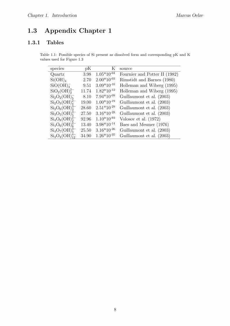
1.3 Appendix Chapter 1
1.3.1 Tables
Table 1.1: Possible species of Si present as dissolved form and corresponding pK and Kvalues used for Figure 1.3
species pK K sourceQuartz 3.98 1.05*10-04 Fournier and Potter II (1982)Si(OH)4 2.70 2.00*10-03 Rimstidt and Barnes (1980)SiO(OH)�3 9.51 3.09*10-10 Holleman and Wiberg (1995)SiO2(OH)2�2 11.74 1.82*10-12 Holleman and Wiberg (1995)Si2O2(OH)�5 8.10 7.94*10-09 Guillaumont et al. (2003)Si2O3(OH)2�4 19.00 1.00*10-19 Guillaumont et al. (2003)Si3O6(OH)3�3 28.60 2.51*10-29 Guillaumont et al. (2003)Si3O5(OH)3�5 27.50 3.16*10-28 Guillaumont et al. (2003)Si4O8(OH)2�2 92.96 1.10*10-93 Volosov et al. (1972)Si4O6(OH)2�6 13.40 3.98*10-14 Baes and Mesmer (1976)Si4O7(OH)3�5 25.50 3.16*10-26 Guillaumont et al. (2003)Si4O4(OH)4�12 34.90 1.26*10-35 Guillaumont et al. (2003)
8
Chapter 2
Si stable isotope ratio determinationof natural samples by MC-ICP-MS
2.1 Abstract
It is shown how Mg addition improves the measurement repeatability of Si isotope de-termination under dry plasma conditions. Several tests were conducted to show how Mgaddition helps to circumvent non-spectral matrix e↵ects when measuring Si stable iso-topes using a desolvation unit. These tests show that the use of Mg as “matrix modifier”has several benefits when measuring Si stable isotopes under dry plasma conditions. Ingeneral, the addition of Mg reduces variations in the instrumental mass bias between sam-ple and standards. Conducted tests reveal that: 1) Mg addition increases the sensitivityby up to a factor of 3 compared to Mg free solutions. 2) Given a mismatch of Si and Mgconcentration between samples and bracketing standards, this mismatch may vary of upto ±50% with no visible e↵ect observed on instrumental mass bias. 3) Given a molar-ity mismatch between samples and standard in the range of 0.05 to 0.2 mol/l measuredagainst a 0.1 mol/l bracketing standard solution does not result in observable changes inthe instrumental mass bias. 4) Also, remaining anionic impurities (SO4, PO4, NO3) showno e↵ect on mass bias if the ratio of [anion] to Si is lower than 1. Therefore, the additionof Mg is highly recommended when measuring Si isotopes under dry plasma conditions.
2.2 Introduction
In this Chapter a description is provided of the analytical procedures and digestion stepsconducted to measure Si isotopes on natural samples using multi-collector inductively cou-pled plasma mass spectrometers (MC-ICP-MS). Results of conducted tests (concentrationmatching, molarity matching, anion contamination with SO4, PO4 and NO3) show theinfluence of di↵erent sample matrices on the mass bias (instrumental mass fractionation)when measuring Si stable isotopes. When measuring Si stable isotopes in wet plasmamode which is liquid sample nebulization into a glass spray chamber before introductioninto the plasma, both accuracy and precision are limited by the resulting low intensityfor the individual isotopes (highly likely that counting statistics of 30Si is the limitingfactor). Therefore often a desolvation unit (here: ESI Apex Sample Inlet System) is usedto introduce the samples dissolved in acids into the plasma (dry plasma mode) as thisusually increases sensitivity. This increase in sensitivity is caused by the reduction of wa-
9
Chapter 2. Analytical improvements Marcus Oelze
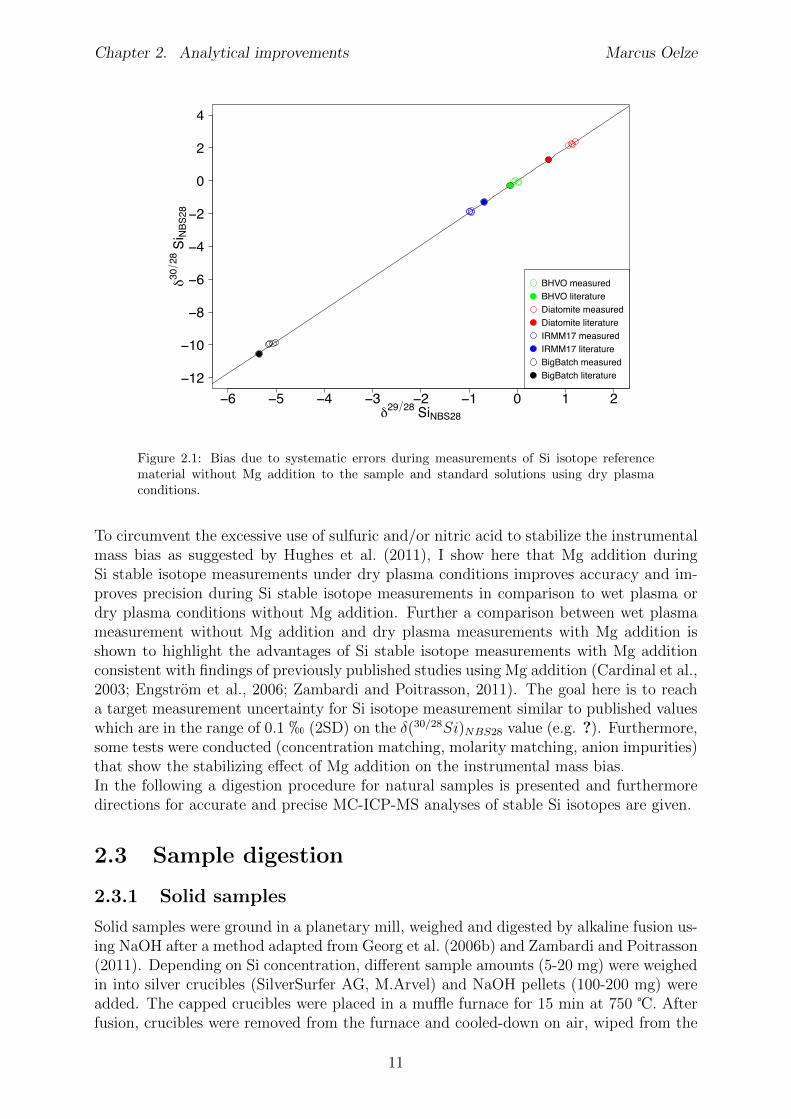
ter matrix load delivered to the plasma (Gray, 1986). The reduction of water load furtherdecreases the amount of oxides and hydroxides formed within the plasma (Tsukahara andKubota, 1990; Lam and McLaren, 1990).One disadvantage of the overall reduced matrix load is the increased sensitivity to remain-ing impurities in samples that have previously been chemically purified. Such impuritiesinduce a di↵erent matrix load between samples and standards. These di↵erences in ma-trix load cause di↵erent mass bias e↵ects for samples and standards, respectively. Thise↵ect is often called non-spectral matrix e↵ect. Therefore the use of a standard - sample- bracketing (SSB) method to correct for mass bias is questionable. This e↵ect has beenobserved for measurements of Si stable isotopes where the change in instrumental massbias is induced by sulfur remaining after column purification (van den Boorn et al., 2009).Hughes et al. (2011) suggested to maintain the mass-bias constant during SSB by meansof excessive addition of sulfuric and/or nitric acid, i.e. matrix matching between samplesand standards used for calibration.The need to control mass bias during Si measurements under dry plasma conditionsseems necessary as test measurements of Si reference materials (BHVO–2G, Diatomite,BigBatch, IRMM-17) measured without matrix matching between samples and standardused for calibration during SSB resulted in an o↵set from the reference values (Figure 2.1).These test measurements of Si stable isotopes using a desolvation unit without samplematrix modification results in good measurement repeatability of isotope ratios but badaccuracy. Systematic errors probably by non-identical matrices during SSB, di↵er in thedirection and magnitude of the bias (Figure 2.1). It is most likely that space charge e↵ectswithin the plasma or di↵erent fluid properties during nebulization are generating thesebias which are probably caused by anionic remaining’s in the purified sample solutions.However, also other factors like concentration or molarity mismatch between samplesand standards as well as high DOC contents in the sample might be responsible for theobserved bias. As all measured isotope ratios plot on the terrestrial fractionation line(Figure 2.1), isobaric interferences on Si during measurements can be excluded.
10
Chapter 2. Analytical improvements Marcus Oelze
δ29 28 SiNBS28
δ3028
Si N
BS28
−12
−10
−8
−6
−4
−2
0
2
4
−6 −5 −4 −3 −2 −1 0 1 2
BHVO measuredBHVO literatureDiatomite measuredDiatomite literatureIRMM17 measuredIRMM17 literatureBigBatch measuredBigBatch literature
Figure 2.1: Bias due to systematic errors during measurements of Si isotope referencematerial without Mg addition to the sample and standard solutions using dry plasmaconditions.
To circumvent the excessive use of sulfuric and/or nitric acid to stabilize the instrumentalmass bias as suggested by Hughes et al. (2011), I show here that Mg addition duringSi stable isotope measurements under dry plasma conditions improves accuracy and im-proves precision during Si stable isotope measurements in comparison to wet plasma ordry plasma conditions without Mg addition. Further a comparison between wet plasmameasurement without Mg addition and dry plasma measurements with Mg addition isshown to highlight the advantages of Si stable isotope measurements with Mg additionconsistent with findings of previously published studies using Mg addition (Cardinal et al.,2003; Engstrom et al., 2006; Zambardi and Poitrasson, 2011). The goal here is to reacha target measurement uncertainty for Si isotope measurement similar to published valueswhich are in the range of 0.1 h (2SD) on the �(30/28Si)
NBS28 value (e.g. ?). Furthermore,some tests were conducted (concentration matching, molarity matching, anion impurities)that show the stabilizing e↵ect of Mg addition on the instrumental mass bias.In the following a digestion procedure for natural samples is presented and furthermoredirections for accurate and precise MC-ICP-MS analyses of stable Si isotopes are given.
2.3 Sample digestion
2.3.1 Solid samples
Solid samples were ground in a planetary mill, weighed and digested by alkaline fusion us-ing NaOH after a method adapted from Georg et al. (2006b) and Zambardi and Poitrasson(2011). Depending on Si concentration, di↵erent sample amounts (5-20 mg) were weighedin into silver crucibles (SilverSurfer AG, M.Arvel) and NaOH pellets (100-200 mg) wereadded. The capped crucibles were placed in a mu✏e furnace for 15 min at 750 �. Afterfusion, crucibles were removed from the furnace and cooled-down on air, wiped from the
11
Chapter 2. Analytical improvements Marcus Oelze
outside and placed into PTFE beakers. Depending on beaker size di↵erent amounts ofMilli-Q water were added and beakers were stored in darkness for 24 hours. Afterwardsthe sample solution was transferred into pre-cleaned PE bottles. More Milli-Q water wasadded while the crucibles were remaining in PTFE beakers. Milli-Q water was then acid-ified with a calculated amount of HCl to reach a pH of 1.5. The beakers were then storedfor additional 6 hours, sonicated and slightly shaken in between. This second solution wasthen added to the first solution into the PE bottle. The total solution was then acidifiedwith a calculated amount of HCl to a final pH of 1.5. Due to the low solubility of Siin acidic solutions (Gunnarsson and Arnorsson, 2000), the concentration of Si should bebelow ⇠50 ppm to avoid silica precipitation during sample storage. Si blanks of the fusionprocedure are in general below 1 µg.
2.3.2 Water samples
The extraction of silicon from natural water samples is complicated by occasional highconcentration of dissolved organic carbon (DOC). To ensure absence of the organic com-pounds in solution, water samples were treated before column purification. To digest DOCin water samples a fusion method was developed. Water samples were pre–concentrated(if necessary) by evaporation in PTFE beakers to a final amount of Si processed of ⇠100µg. After pre–concentration the remaining samples were transferred into silver cruciblesand finally evaporated to dryness. The silver crucibles were then placed in a mu✏e fur-nace and heated to 750 � to incinerate the organic carbon. Depending on the initial DOCcontent, the carbon incineration time had to be adjusted (depending on visual inspectionafter carbon incineration). To redissolve samples, 5 ml 1M NaOH were added to silvercrucibles and evaporated to dryness. The crucibles were then placed a second time intoa mu✏e furnace, using the alkaline fusion method described above for solid samples toredissolve the “carbon free” water samples. The re-dissolution of the fusion cake is thenhandled in the same way as for solid samples.If high amounts of anions were present in the sample solutions a co–precipitation step isconducted prior to DOC decomposition. Iron as Fe(NO3)3 in 0.3 M HNO3 is added to thesample solution to reach a final Fe:Si ratio by mass of 100:1. This solution is then well-mixed and precipitation of Fe(III)OOH is forced by addition of NH4(OH) to attain a pHof ⇡10. During Fe precipitation Si will be scavenged by the Fe precipitates and separatedfrom the anions. The samples were then centrifuged and the supernatant was decanted.The precipitate was redissolved in 0.1 M HCl and transferred into silver crucibles andtreated in the same way as common water samples. Several tests were conducted, whereBHVO - 2G solution (digested using the above outlined method) was treated as watersolution. No Si isotope fractionation was observed when using this method. Si blanks ofthe fusion and column separation procedure are in general below 1 µg which is less than1 % of the total amount Si processed.
2.4 Column chemistry and preparation of Mg addi-tion solution
Digested solid samples and pre - treated water samples are further purified using a cationexchange resin (Method adapted from Georg et al. (2006b)). This method uses 1.8 mlresin of Dowex 50 WX8 (200-400 mesh) filled into polypropylen columns (resin bed area
12
Chapter 2. Analytical improvements Marcus Oelze
8 x 10 x 16 mm (IDxODxlength)). The resin was cleaned and conditioned with 3M and6M HCl and 7M HNO3 before samples were loaded. Depending on Si concentrations upto 20 ml of samples were loaded. The eluate was collected in pre-cleaned PE tubes andfully removed from resin with 5 ml Milli-Q water. Si concentration and purity of samplesafter column chemistry was checked on an ICP-OES.The Mg solution was prepared from a 10000 ppm Mg standard solution in 0.5 M HNO3acquired from Merck. This solution (0.3 ml) was evaporated to dryness, re-dissolved inMilli-Q water, evaporated again to dryness and again re-dissolved in Milli-Q water. Thefinal solution was then transferred into a pre-cleaned PE bottle and diluted to a Mgconcentration of ⇠50 ppm Mg in H2O.
2.5 MC-ICP-MS analysis
Determination of the Si isotope composition was performed in medium or high massresolution on a Thermo Neptune MC-ICP-MS equipped with an H-skimmer cone andthe Thermor Jet-interface using a normal sample cone (wet plasma) or a Jet cone (dryplasma). Si stable isotopes have been measured under wet plasma conditions withoutMg addition and under dry plasma conditions with Mg addition. Here the instrumentalsettings for both measuring conditions are summarized.
2.5.1 Wet plasma conditions without Mg addition
The purified sample solutions were introduced into the plasma using the Thermo stable in-troduction system (SIS) glass spray chamber (wet-plasma) equipped with a self–aspirating120 µl/min nebulizer. Samples measured in wet plasma conditions were diluted to 2.5 ppmin 0.1 M HCl which typically resulted in an intensity of 2 V/ppm on 28Si (1011 ⌦ resistor).Si stable isotope measurements were conducted in static mode on the interference-free low-mass side of the three Si isotopes. Si isotopes were collected in L4 (28Si), L1 (29Si) andC (30Si) cups, respectively. To correct for instrumental mass bias, we used a standard-sample-bracketing procedure. Samples and Si isotope reference material were measuredat least 4 times during a sequence; each sample or standard was measured for 30 cycleswith an integration time for each cycle of 4 s. Pure 0.1 M HCl solutions were measuredbefore and after each standard-sample-standard block and were used for on-peak zerocorrection. Typical intensities of 28Si in blank solutions were below 5 mV.
2.5.2 Dry plasma conditions with Mg addition
The sample solutions were introduced into the plasma via a desolvation unit for dryplasma conditions (Apex, ESIr) equipped with a 100 µl/ min nebulizer. Measurementswere conducted on the interference-free low-mass side of the three Si isotopes. Si stableisotope measurements were conducted in dynamic magnet switching mode and the Siisotopes were collected in L4 (28Si), L1 (29Si) and C (30Si) cups, respectively. Aftermagnet switching (idle time 3 s), Mg isotopes are collected in L2 (24Mg), center cup(25Mg) and H3 (26Mg). Samples and Si isotope reference material were measured at least4 times during a sequence; each sample or standard was measured for 30 cycles with anintegration time for each cycle of 4 s for Si as well as for Mg in dynamic mode. PureHCl solutions (0.1 M) were repeatedly measured during a sequence and typical intensitiesof 28Si in blank solutions were below 15 mV. To correct for instrumental mass bias an
13
Chapter 2. Analytical improvements Marcus Oelze
external normalization scheme using Mg - addition is applied. Here we combine standard- sample - bracketing with an exponential mass bias law (Cardinal et al., 2003) and correctthe measured Si isotope ratios using:
✓30Si28Si
◆
corrected
=
✓30Si28Si
◆
measured
⇥✓Mass30Si
Mass28Si
◆f
(2.1)
The Si isotope ratios are corrected for instrumental mass bias using an instrumentalfractionation factor f determined from simultaneous measurements of Mg isotope ratios:
f = ln
⇣26Mg
24Mg
⌘
corrected⇣26Mg
24Mg
⌘
measured
/lnMass26Mg
Mass24Mg(2.2)
A positive side e↵ect of the matrix modification by Mg addition is that the Si sensitivityis enhanced when measuring under dry plasma conditions, as it boosts signal intensity.We observed an increase in intensity by up to a factor of 3 between solutions withoutMg addition and solutions with Mg addition, respectively. Sample solutions measuredwithout Mg addition resulted in intensities of ⇠6 V/ ppm on 28Si (using a 1011 ⌦ resistor)in 0.1 M HCl. Solutions with Mg added ([Si]/[Mg] = 1) typically result in an intensity of⇠15 V/ ppm on 28Si (using a 1011 ⌦ resistor) in 0.1 M HCl. Typical Si concentrations inmeasurement ready solutions are in the range of 0.8 to 1 ppm, which results in typical Siintensities on 28Si of 12 to 15 V (using a 1011 ⌦ resistor).
2.5.3 Reporting Si isotope ratios
We report Si isotope values in the delta notation (�) according to Coplen (2011) as�(29/28Si)
NBS28 and �(30/28Si)NBS28 relative to the international isotope measurement
standard NBS28 (quartz sand) in per mill (h) by multiplying Equation 2.3 and Equa-tion 2.4 with a factor of 103:
�(29/28Si)NBS28 =
✓(29Si/28Si)
sample
(29Si/28Si)NBS28
� 1
◆(2.3)
�(30/28Si)NBS28 =
✓(30Si/28Si)
sample
(30Si/28Si)NBS28
� 1
◆(2.4)
Reported uncertainties on delta values are the 95% confidence interval (CI) calculatedaccording to Equation 2.5 where �(30/28Si) is the mean of the measured delta values forsamples or standards (at least n= 4 mass spectrometric repeats), t
n�1 is a critical valuefrom tables of the Student-t distribution and SE is the standard error of the mean:
CI = �(30/28Si)NBS28 ± t
n�1 ⇤ SE (2.5)
2.5.4 Results of measured Si isotope reference materials
Literature values of Si isotope reference materials
The well defined Si isotope reference material BHVO–2G, a basalt standard, was usuallymeasured as control standard during measured sequences for wet plasma and dry plasmameasurements. Further the pure Si metal standard IRMM-17, the Diatomite (natural
14
Chapter 2. Analytical improvements Marcus Oelze
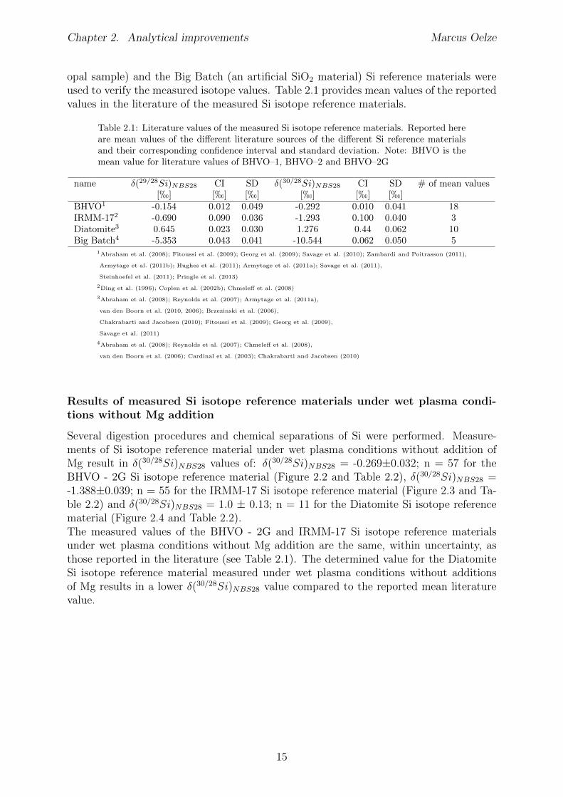
opal sample) and the Big Batch (an artificial SiO2 material) Si reference materials wereused to verify the measured isotope values. Table 2.1 provides mean values of the reportedvalues in the literature of the measured Si isotope reference materials.
Table 2.1: Literature values of the measured Si isotope reference materials. Reported hereare mean values of the di↵erent literature sources of the di↵erent Si reference materialsand their corresponding confidence interval and standard deviation. Note: BHVO is themean value for literature values of BHVO–1, BHVO–2 and BHVO–2G
name �(29/28Si)NBS28
CI SD �(30/28Si)NBS28
CI SD # of mean values[h] [h] [h] [h] [h] [h]
BHVO1 -0.154 0.012 0.049 -0.292 0.010 0.041 18IRMM-172 -0.690 0.090 0.036 -1.293 0.100 0.040 3Diatomite3 0.645 0.023 0.030 1.276 0.44 0.062 10Big Batch4 -5.353 0.043 0.041 -10.544 0.062 0.050 5
1Abraham et al. (2008); Fitoussi et al. (2009); Georg et al. (2009); Savage et al. (2010); Zambardi and Poitrasson (2011),
Armytage et al. (2011b); Hughes et al. (2011); Armytage et al. (2011a); Savage et al. (2011),
Steinhoefel et al. (2011); Pringle et al. (2013)
2Ding et al. (1996); Coplen et al. (2002b); Chmele↵ et al. (2008)
3Abraham et al. (2008); Reynolds et al. (2007); Armytage et al. (2011a),
van den Boorn et al. (2010, 2006); Brzezinski et al. (2006),
Chakrabarti and Jacobsen (2010); Fitoussi et al. (2009); Georg et al. (2009),
Savage et al. (2011)
4Abraham et al. (2008); Reynolds et al. (2007); Chmele↵ et al. (2008),
van den Boorn et al. (2006); Cardinal et al. (2003); Chakrabarti and Jacobsen (2010)
Results of measured Si isotope reference materials under wet plasma condi-tions without Mg addition
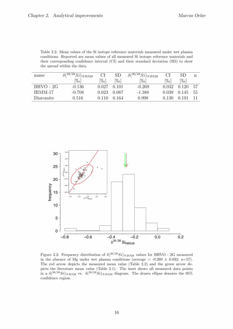
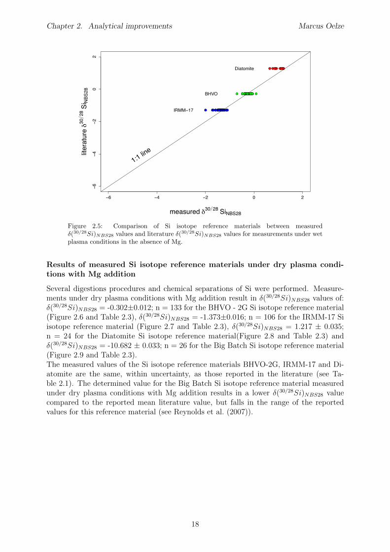
Several digestion procedures and chemical separations of Si were performed. Measure-ments of Si isotope reference material under wet plasma conditions without addition ofMg result in �(30/28Si)
NBS28 values of: �(30/28Si)NBS28 = -0.269±0.032; n = 57 for the
BHVO - 2G Si isotope reference material (Figure 2.2 and Table 2.2), �(30/28Si)NBS28 =
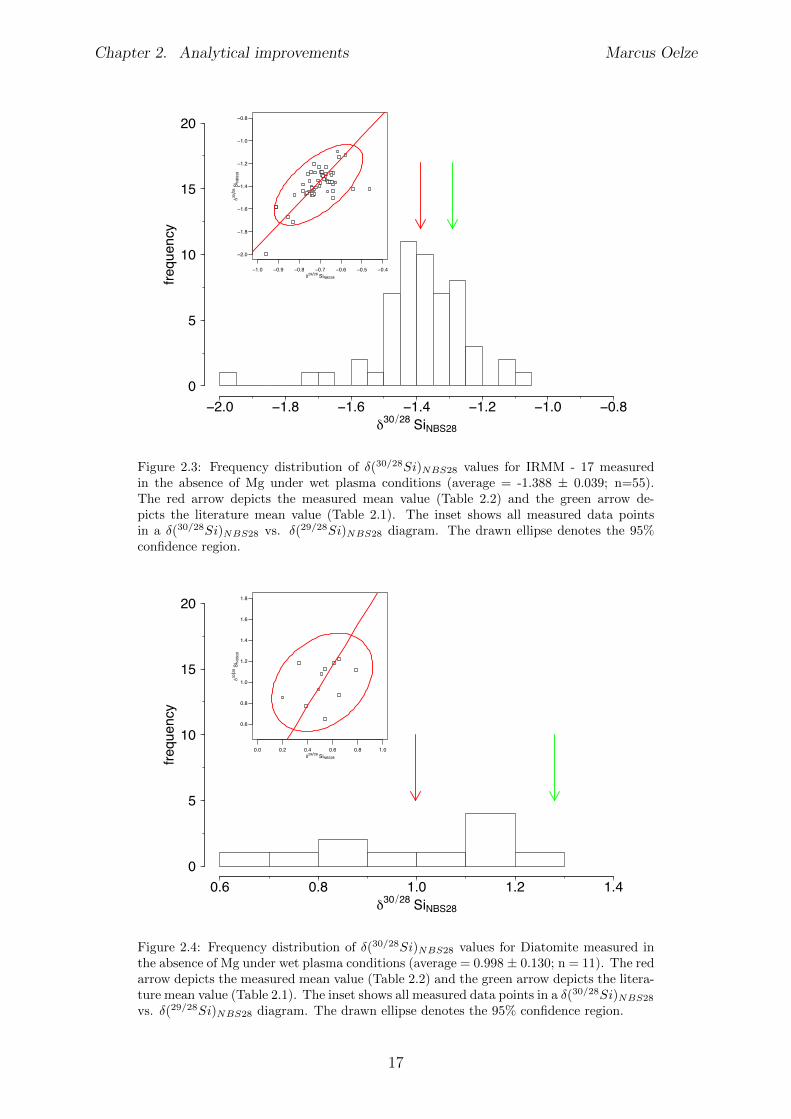
-1.388±0.039; n = 55 for the IRMM-17 Si isotope reference material (Figure 2.3 and Ta-ble 2.2) and �(30/28Si)
NBS28 = 1.0 ± 0.13; n = 11 for the Diatomite Si isotope referencematerial (Figure 2.4 and Table 2.2).The measured values of the BHVO - 2G and IRMM-17 Si isotope reference materialsunder wet plasma conditions without Mg addition are the same, within uncertainty, asthose reported in the literature (see Table 2.1). The determined value for the DiatomiteSi isotope reference material measured under wet plasma conditions without additionsof Mg results in a lower �(30/28Si)
NBS28 value compared to the reported mean literaturevalue.
15
Chapter 2. Analytical improvements Marcus Oelze
Table 2.2: Mean values of the Si isotope reference materials measured under wet plasmaconditions. Reported are mean values of all measured Si isotope reference materials andtheir corresponding confidence interval (CI) and their standard deviation (SD) to showthe spread within the data.
name �(29/28Si)NBS28 CI SD �(30/28Si)
NBS28 CI SD n[h] [h] [h] [h] [h] [h]
BHVO - 2G -0.136 0.027 0.101 -0.269 0.032 0.120 57IRMM-17 -0.708 0.023 0.087 -1.388 0.039 0.145 55Diatomite 0.516 0.110 0.164 0.998 0.130 0.191 11
δ30 28 SiNBS28
frequency
−0.8 −0.6 −0.4 −0.2 0.0 0.20
5
10
15
20
25
30
−0.4 −0.2 0.0 0.2 0.4
−0.8
−0.6
−0.4
−0.2
0.0
0.2
0.4
δ29 28 SiNBS28
δ3028
Si NB
S28
Figure 2.2: Frequency distribution of �(30/28Si)NBS28
values for BHVO - 2G measuredin the absence of Mg under wet plasma conditions (average = -0.269 ± 0.032; n=57).The red arrow depicts the measured mean value (Table 2.2) and the green arrow de-picts the literature mean value (Table 2.1). The inset shows all measured data pointsin a �(30/28Si)
NBS28
vs. �(29/28Si)NBS28
diagram. The drawn ellipse denotes the 95%confidence region.
16
Chapter 2. Analytical improvements Marcus Oelze
δ30 28 SiNBS28
frequency
−2.0 −1.8 −1.6 −1.4 −1.2 −1.0 −0.80
5
10
15
20
−1.0 −0.9 −0.8 −0.7 −0.6 −0.5 −0.4
−2.0
−1.8
−1.6
−1.4
−1.2
−1.0
−0.8
δ29 28 SiNBS28
δ3028
Si NB
S28
Figure 2.3: Frequency distribution of �(30/28Si)NBS28
values for IRMM - 17 measuredin the absence of Mg under wet plasma conditions (average = -1.388 ± 0.039; n=55).The red arrow depicts the measured mean value (Table 2.2) and the green arrow de-picts the literature mean value (Table 2.1). The inset shows all measured data pointsin a �(30/28Si)
NBS28
vs. �(29/28Si)NBS28
diagram. The drawn ellipse denotes the 95%confidence region.
δ30 28 SiNBS28
frequency
0.6 0.8 1.0 1.2 1.40
5
10
15
20
0.0 0.2 0.4 0.6 0.8 1.0
0.6
0.8
1.0
1.2
1.4
1.6
1.8
δ29 28 SiNBS28
δ3028
Si NB
S28
Figure 2.4: Frequency distribution of �(30/28Si)NBS28
values for Diatomite measured inthe absence of Mg under wet plasma conditions (average = 0.998 ± 0.130; n = 11). The redarrow depicts the measured mean value (Table 2.2) and the green arrow depicts the litera-ture mean value (Table 2.1). The inset shows all measured data points in a �(30/28Si)
NBS28
vs. �(29/28Si)NBS28
diagram. The drawn ellipse denotes the 95% confidence region.
17
Chapter 2. Analytical improvements Marcus Oelze
−6 −4 −2 0 2
−6−4
−20
2
measured δ30 28 SiNBS28
litera
ture
δ30
28 S
i NBS2
8
1:1 line
BHVO
IRMM−17
Diatomite
Figure 2.5: Comparison of Si isotope reference materials between measured�(30/28Si)
NBS28
values and literature �(30/28Si)NBS28
values for measurements under wetplasma conditions in the absence of Mg.
Results of measured Si isotope reference materials under dry plasma condi-tions with Mg addition
Several digestions procedures and chemical separations of Si were performed. Measure-ments under dry plasma conditions with Mg addition result in �(30/28Si)
NBS28 values of:�(30/28Si)
NBS28 = -0.302±0.012; n = 133 for the BHVO - 2G Si isotope reference material(Figure 2.6 and Table 2.3), �(30/28Si)
NBS28 = -1.373±0.016; n = 106 for the IRMM-17 Siisotope reference material (Figure 2.7 and Table 2.3), �(30/28Si)
NBS28 = 1.217 ± 0.035;n = 24 for the Diatomite Si isotope reference material(Figure 2.8 and Table 2.3) and�(30/28Si)
NBS28 = -10.682 ± 0.033; n = 26 for the Big Batch Si isotope reference material(Figure 2.9 and Table 2.3).The measured values of the Si isotope reference materials BHVO-2G, IRMM-17 and Di-atomite are the same, within uncertainty, as those reported in the literature (see Ta-ble 2.1). The determined value for the Big Batch Si isotope reference material measuredunder dry plasma conditions with Mg addition results in a lower �(30/28Si)
NBS28 valuecompared to the reported mean literature value, but falls in the range of the reportedvalues for this reference material (see Reynolds et al. (2007)).
18
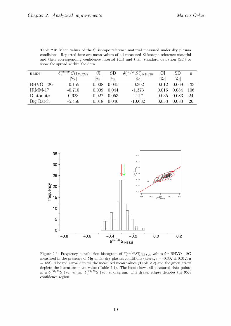
Chapter 2. Analytical improvements Marcus Oelze
Table 2.3: Mean values of the Si isotope reference material measured under dry plasmaconditions. Reported here are mean values of all measured Si isotope reference materialand their corresponding confidence interval (CI) and their standard deviation (SD) toshow the spread within the data.
name �(29/28Si)NBS28 CI SD �(30/28Si)
NBS28 CI SD n[h] [h] [h] [h] [h] [h]
BHVO - 2G -0.155 0.008 0.045 -0.302 0.012 0.069 133IRMM-17 -0.710 0.009 0.044 -1.373 0.016 0.084 106Diatomite 0.623 0.022 0.053 1.217 0.035 0.083 24Big Batch -5.456 0.018 0.046 -10.682 0.033 0.083 26
δ30 28 SiNBS28
frequency
−0.8 −0.6 −0.4 −0.2 0.0 0.20
5
10
15
20
25
30
35
−0.4 −0.3 −0.2 −0.1 0.0
−0.8
−0.6
−0.4
−0.2
0.0
0.2
0.4
δ29 28 SiNBS28
δ3028
Si NB
S28
Figure 2.6: Frequency distribution histogram of �(30/28Si)NBS28
values for BHVO - 2Gmeasured in the presence of Mg under dry plasma conditions (average = -0.302 ± 0.012; n= 133). The red arrow depicts the measured mean values (Table 2.2) and the green arrowdepicts the literature mean value (Table 2.1). The inset shows all measured data pointsin a �(30/28Si)
NBS28
vs. �(29/28Si)NBS28
diagram. The drawn ellipse denotes the 95%confidence region.
19
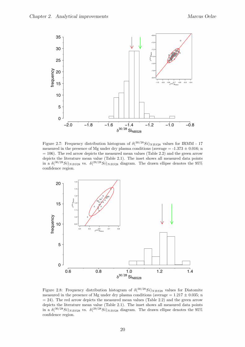
Chapter 2. Analytical improvements Marcus Oelze
δ30 28 SiNBS28
frequency
−2.0 −1.8 −1.6 −1.4 −1.2 −1.0 −0.80
5
10
15
20
25
30
35
−1.0 −0.9 −0.8 −0.7 −0.6 −0.5 −0.4
−2.0
−1.8
−1.6
−1.4
−1.2
−1.0
−0.8
δ29 28 SiNBS28
δ3028
Si NB
S28
Figure 2.7: Frequency distribution histogram of �(30/28Si)NBS28
values for IRMM - 17measured in the presence of Mg under dry plasma conditions (average = -1.373 ± 0.016; n= 106). The red arrow depicts the measured mean values (Table 2.2) and the green arrowdepicts the literature mean value (Table 2.1). The inset shows all measured data pointsin a �(30/28Si)
NBS28
vs. �(29/28Si)NBS28
diagram. The drawn ellipse denotes the 95%confidence region.
δ30 28 SiNBS28
frequency
0.6 0.8 1.0 1.2 1.40
5
10
15
20
0.4 0.5 0.6 0.7 0.8
0.9
1.0
1.1
1.2
1.3
1.4
1.5
δ29 28 SiNBS28
δ3028
Si NB
S28
Figure 2.8: Frequency distribution histogram of �(30/28Si)NBS28
values for Diatomitemeasured in the presence of Mg under dry plasma conditions (average = 1.217 ± 0.035; n= 24). The red arrow depicts the measured mean values (Table 2.2) and the green arrowdepicts the literature mean value (Table 2.1). The inset shows all measured data pointsin a �(30/28Si)
NBS28
vs. �(29/28Si)NBS28
diagram. The drawn ellipse denotes the 95%confidence region.
20
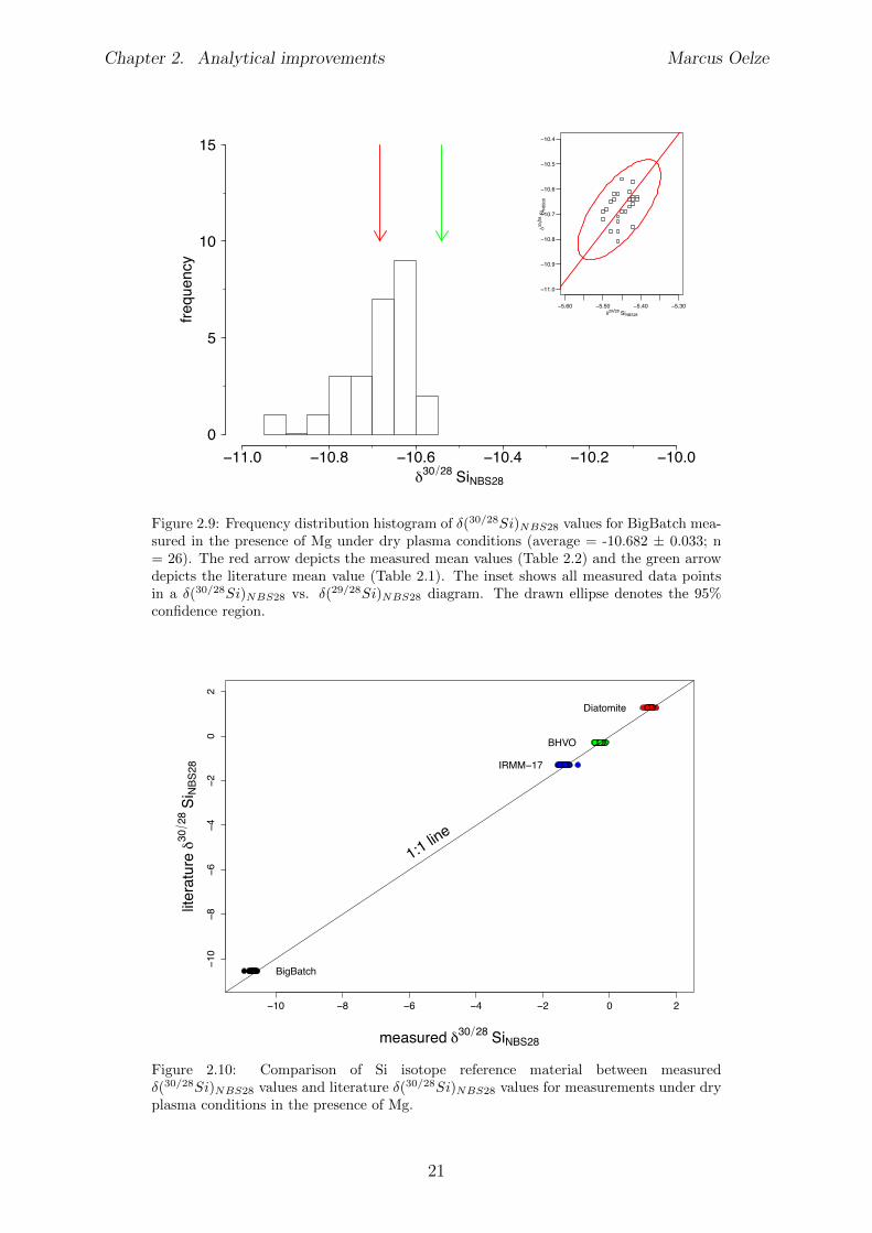
Chapter 2. Analytical improvements Marcus Oelze
δ30 28 SiNBS28
frequency
−11.0 −10.8 −10.6 −10.4 −10.2 −10.00
5
10
15
−5.60 −5.50 −5.40 −5.30
−11.0
−10.9
−10.8
−10.7
−10.6
−10.5
−10.4
δ29 28 SiNBS28
δ3028
Si NB
S28
Figure 2.9: Frequency distribution histogram of �(30/28Si)NBS28
values for BigBatch mea-sured in the presence of Mg under dry plasma conditions (average = -10.682 ± 0.033; n= 26). The red arrow depicts the measured mean values (Table 2.2) and the green arrowdepicts the literature mean value (Table 2.1). The inset shows all measured data pointsin a �(30/28Si)
NBS28
vs. �(29/28Si)NBS28
diagram. The drawn ellipse denotes the 95%confidence region.
−10 −8 −6 −4 −2 0 2
−10
−8−6
−4−2
02
measured δ30 28 SiNBS28
literature
δ30
28 Si NB
S28
1:1 line
BHVO
IRMM−17
Diatomite
BigBatch
Figure 2.10: Comparison of Si isotope reference material between measured�(30/28Si)
NBS28
values and literature �(30/28Si)NBS28
values for measurements under dryplasma conditions in the presence of Mg.
21
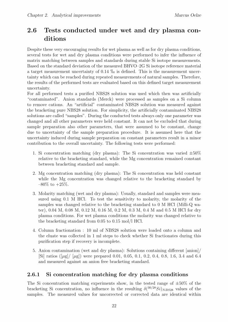
Chapter 2. Analytical improvements Marcus Oelze
2.6 Tests conducted under wet and dry plasma con-ditions
Despite these very encouraging results for wet plasma as well as for dry plasma conditions,several tests for wet and dry plasma conditions were performed to infer the influence ofmatrix matching between samples and standards during stable Si isotope measurements.Based on the standard deviation of the measured BHVO–2G Si isotope reference materiala target measurement uncertainty of 0.14 h is defined. This is the measurement uncer-tainty which can be reached during repeated measurements of natural samples. Therefore,the results of the performed tests are evaluated based on this defined target measurementuncertainty.For all performed tests a purified NBS28 solution was used which then was artificially“contaminated”. Anion standards (Merck) were processed as samples on a Si columnto remove cations. An “artificial” contaminated NBS28 solution was measured againstthe bracketing pure NBS28 solution. For simplicity, the artificially contaminated NBS28solutions are called “samples”. During the conducted tests always only one parameter waschanged and all other parameters were held constant. It can not be excluded that duringsample preparation also other parameters, that were assumed to be constant, changedue to uncertainty of the sample preparation procedure. It is assumed here that theuncertainty induced during sample preparation on constant parameters result in a minorcontribution to the overall uncertainty. The following tests were performed:
1. Si concentration matching (dry plasma): The Si concentration was varied ±50%relative to the bracketing standard, while the Mg concentration remained constantbetween bracketing standard and sample.
2. Mg concentration matching (dry plasma): The Si concentration was held constantwhile the Mg concentration was changed relative to the bracketing standard by–80% to +25%.
3. Molarity matching (wet and dry plasma): Usually, standard and samples were mea-sured using 0.1 M HCl. To test the sensitivity to molarity, the molarity of thesamples was changed relative to the bracketing standard to 0 M HCl (Milli-Q wa-ter), 0.04 M, 0.08 M, 0.12 M, 0.16 M, 0.2 M, 0.3 M, 0.4 M and 0.5 M HCl for dryplasma conditions. For wet plasma conditions the molarity was changed relative tothe bracketing standard from 0.05 to 0.15 mol/l HCl.
4. Column fractionation : 10 ml of NBS28 solution were loaded onto a column andthe eluate was collected in 1 ml steps to check whether Si fractionates during thispurification step if recovery is incomplete.
5. Anion contamination (wet and dry plasma): Solutions containing di↵erent [anion]/[Si] ratios ([µg]/ [µg]) were prepared 0.01, 0.05, 0.1, 0.2, 0.4, 0.8, 1.6, 3.4 and 6.4and measured against an anion free bracketing standard.
2.6.1 Si concentration matching for dry plasma conditions
The Si concentration matching experiments show, in the tested range of ±50% of thebracketing Si concentration, no influence in the resulting �(30/28Si)
NBS28 values of thesamples. The measured values for uncorrected or corrected data are identical within
22
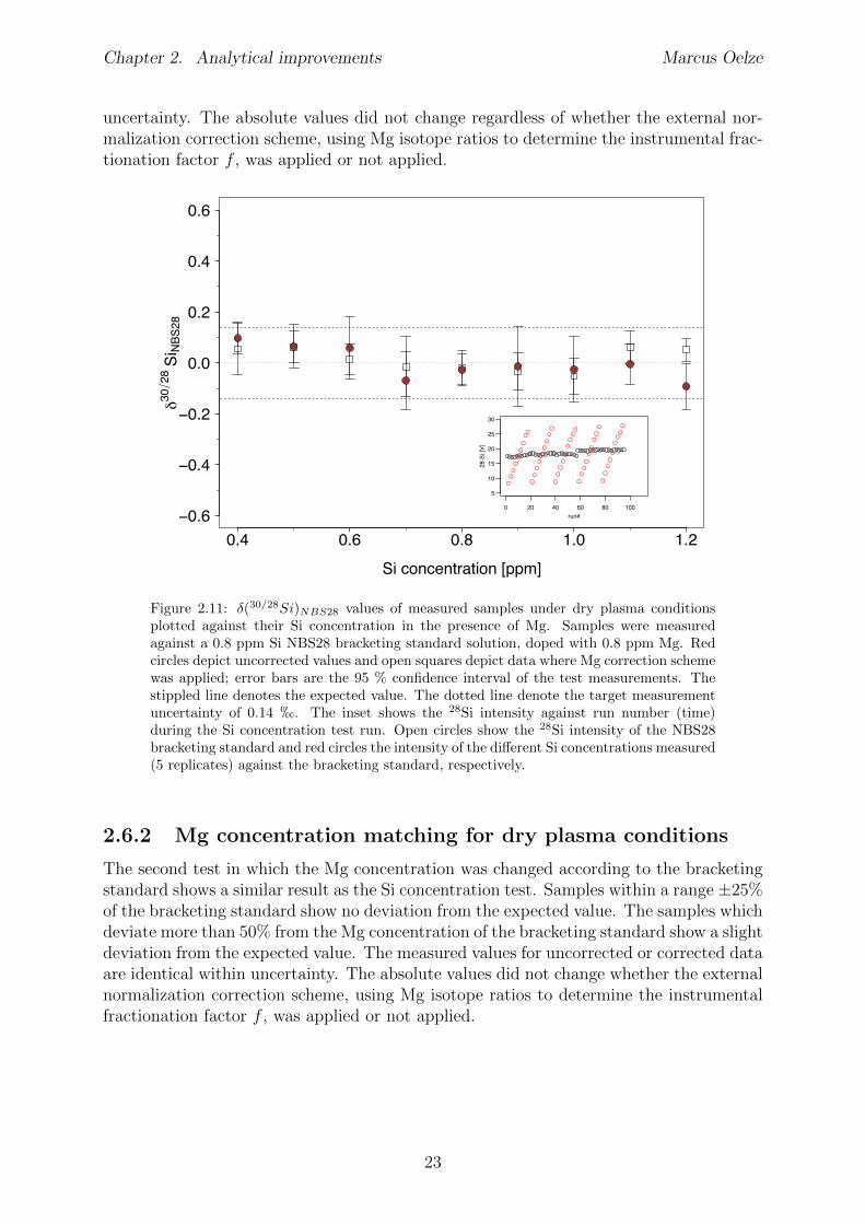
Chapter 2. Analytical improvements Marcus Oelze
uncertainty. The absolute values did not change regardless of whether the external nor-malization correction scheme, using Mg isotope ratios to determine the instrumental frac-tionation factor f , was applied or not applied.
0.4 0.6 0.8 1.0 1.2−0.6
−0.4
−0.2
0.0
0.2
0.4
0.6
Si concentration [ppm]
δ3028
Si N
BS28
0 20 40 60 80 100
5
10
15
20
25
30
run#
28 S
i [V]
Figure 2.11: �(30/28Si)NBS28
values of measured samples under dry plasma conditionsplotted against their Si concentration in the presence of Mg. Samples were measuredagainst a 0.8 ppm Si NBS28 bracketing standard solution, doped with 0.8 ppm Mg. Redcircles depict uncorrected values and open squares depict data where Mg correction schemewas applied; error bars are the 95 % confidence interval of the test measurements. Thestippled line denotes the expected value. The dotted line denote the target measurementuncertainty of 0.14 h. The inset shows the 28Si intensity against run number (time)during the Si concentration test run. Open circles show the 28Si intensity of the NBS28bracketing standard and red circles the intensity of the di↵erent Si concentrations measured(5 replicates) against the bracketing standard, respectively.
2.6.2 Mg concentration matching for dry plasma conditions
The second test in which the Mg concentration was changed according to the bracketingstandard shows a similar result as the Si concentration test. Samples within a range ±25%of the bracketing standard show no deviation from the expected value. The samples whichdeviate more than 50% from the Mg concentration of the bracketing standard show a slightdeviation from the expected value. The measured values for uncorrected or corrected dataare identical within uncertainty. The absolute values did not change whether the externalnormalization correction scheme, using Mg isotope ratios to determine the instrumentalfractionation factor f , was applied or not applied.
23
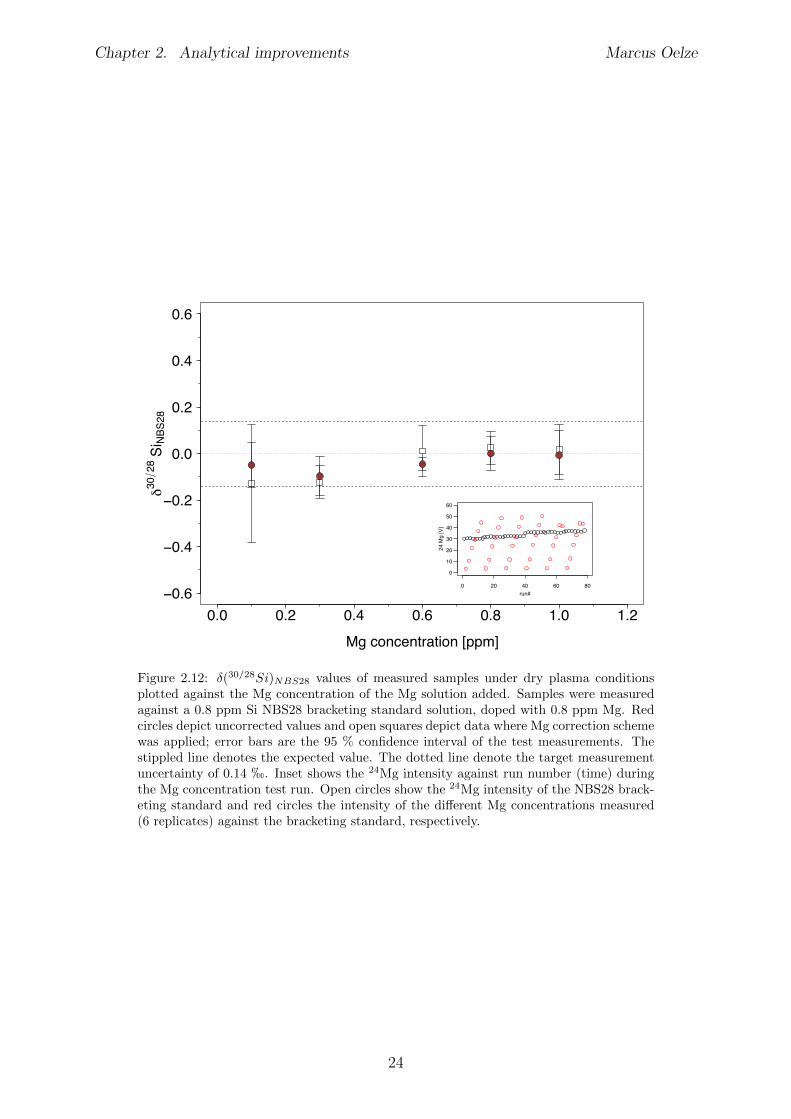
Chapter 2. Analytical improvements Marcus Oelze
0.0 0.2 0.4 0.6 0.8 1.0 1.2−0.6
−0.4
−0.2
0.0
0.2
0.4
0.6
Mg concentration [ppm]
δ3028
Si N
BS28
0 20 40 60 80
0
10
20
30
40
50
60
run#
24 M
g [V
]
Figure 2.12: �(30/28Si)NBS28
values of measured samples under dry plasma conditionsplotted against the Mg concentration of the Mg solution added. Samples were measuredagainst a 0.8 ppm Si NBS28 bracketing standard solution, doped with 0.8 ppm Mg. Redcircles depict uncorrected values and open squares depict data where Mg correction schemewas applied; error bars are the 95 % confidence interval of the test measurements. Thestippled line denotes the expected value. The dotted line denote the target measurementuncertainty of 0.14 h. Inset shows the 24Mg intensity against run number (time) duringthe Mg concentration test run. Open circles show the 24Mg intensity of the NBS28 brack-eting standard and red circles the intensity of the di↵erent Mg concentrations measured(6 replicates) against the bracketing standard, respectively.
24
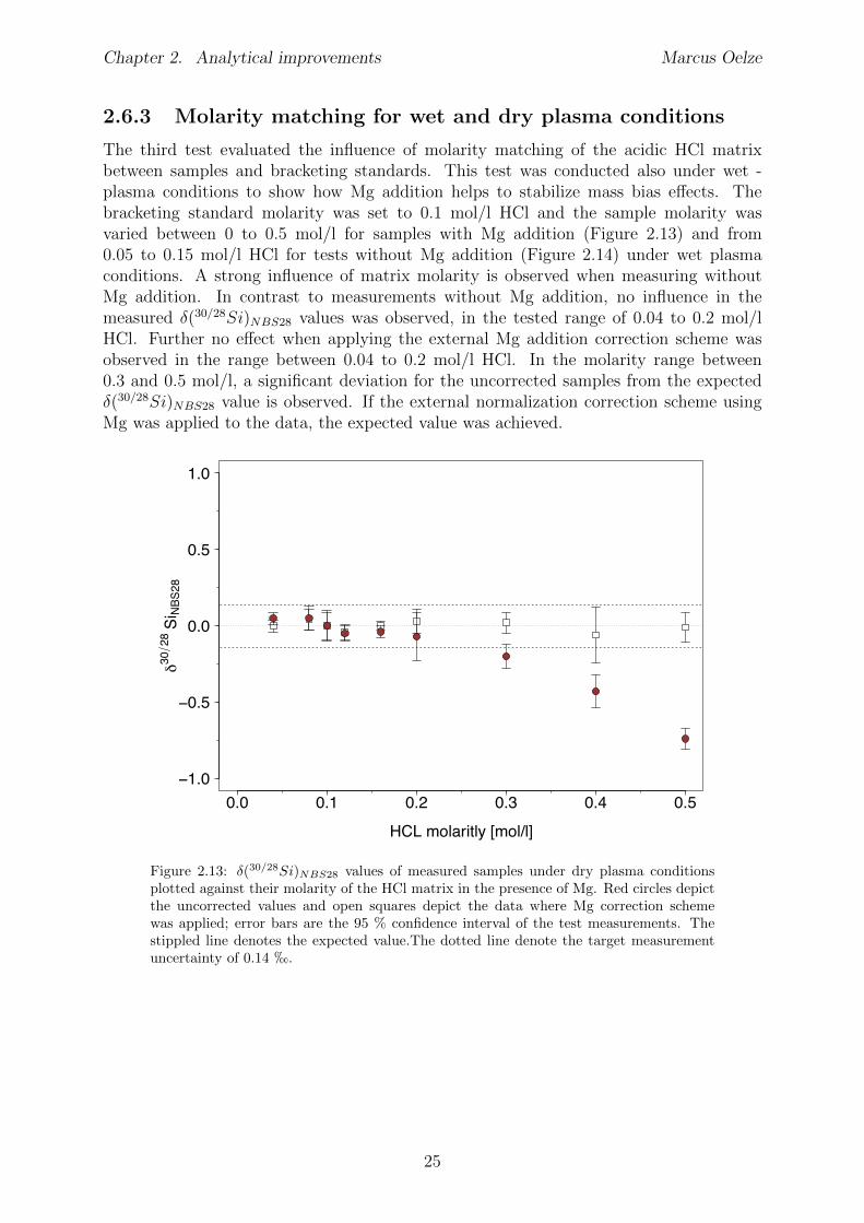
Chapter 2. Analytical improvements Marcus Oelze
2.6.3 Molarity matching for wet and dry plasma conditions
The third test evaluated the influence of molarity matching of the acidic HCl matrixbetween samples and bracketing standards. This test was conducted also under wet -plasma conditions to show how Mg addition helps to stabilize mass bias e↵ects. Thebracketing standard molarity was set to 0.1 mol/l HCl and the sample molarity wasvaried between 0 to 0.5 mol/l for samples with Mg addition (Figure 2.13) and from0.05 to 0.15 mol/l HCl for tests without Mg addition (Figure 2.14) under wet plasmaconditions. A strong influence of matrix molarity is observed when measuring withoutMg addition. In contrast to measurements without Mg addition, no influence in themeasured �(30/28Si)
NBS28 values was observed, in the tested range of 0.04 to 0.2 mol/lHCl. Further no e↵ect when applying the external Mg addition correction scheme wasobserved in the range between 0.04 to 0.2 mol/l HCl. In the molarity range between0.3 and 0.5 mol/l, a significant deviation for the uncorrected samples from the expected�(30/28Si)
NBS28 value is observed. If the external normalization correction scheme usingMg was applied to the data, the expected value was achieved.
0.0 0.1 0.2 0.3 0.4 0.5−1.0
−0.5
0.0
0.5
1.0
HCL molaritly [mol/l]
δ3028
Si N
BS28
Figure 2.13: �(30/28Si)NBS28
values of measured samples under dry plasma conditionsplotted against their molarity of the HCl matrix in the presence of Mg. Red circles depictthe uncorrected values and open squares depict the data where Mg correction schemewas applied; error bars are the 95 % confidence interval of the test measurements. Thestippled line denotes the expected value.The dotted line denote the target measurementuncertainty of 0.14 h.
25
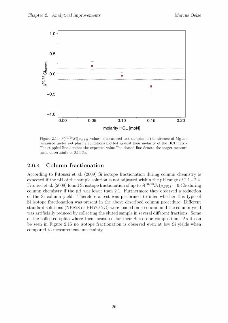
Chapter 2. Analytical improvements Marcus Oelze
0.00 0.05 0.10 0.15 0.20−1.0
−0.5
0.0
0.5
1.0
molarity HCL [mol/l]
δ3028
Si N
BS28
Figure 2.14: �(30/28Si)NBS28
values of measured test samples in the absence of Mg andmeasured under wet plasma conditions plotted against their molarity of the HCl matrix.The stippled line denotes the expected value.The dotted line denote the target measure-ment uncertainty of 0.14 h.
2.6.4 Column fractionation
According to Fitoussi et al. (2009) Si isotope fractionation during column chemistry isexpected if the pH of the sample solution is not adjusted within the pH range of 2.1 - 2.4.Fitoussi et al. (2009) found Si isotope fractionation of up to �(30/28Si)
NBS28 = 0.4h duringcolumn chemistry if the pH was lower than 2.1. Furthermore they observed a reductionof the Si column yield. Therefore a test was performed to infer whether this type ofSi isotope fractionation was present in the above described column procedure. Di↵erentstandard solutions (NBS28 or BHVO-2G) were loaded on a column and the column yieldwas artificially reduced by collecting the eluted sample in several di↵erent fractions. Someof the collected splits where then measured for their Si isotope composition. As it canbe seen in Figure 2.15 no isotope fractionation is observed even at low Si yields whencompared to measurement uncertainty.
26
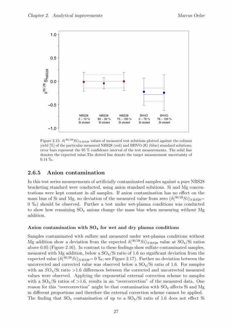
Chapter 2. Analytical improvements Marcus Oelze
−1.0
−0.5
0.0
0.5
1.0
δ3028
Si N
BS28
NBS28 2 − 12 % Si eluted
NBS28 82 − 92 % Si eluted
NBS28 75 − 100 %
Si eluted
BHVO 0 − 76 % Si eluted
BHVO 76 − 100 %
Si eluted
Figure 2.15: �(30/28Si)NBS28
values of measured test solutions plotted against the columnyield [%] of the particular measured NBS28 (red) and BHVO-2G (blue) standard solutions;error bars represent the 95 % confidence interval of the test measurements. The solid linedenotes the expected value.The dotted line denote the target measurement uncertainty of0.14 h.
2.6.5 Anion contamination
In this test series measurements of artificially contaminated samples against a pure NBS28bracketing standard were conducted, using anion standard solutions. Si and Mg concen-trations were kept constant in all samples. If anion contamination has no e↵ect on themass bias of Si and Mg, no deviation of the measured value from zero (�(30/28Si)
NBS28=0 h) should be observed. Further a test under wet-plasma conditions was conductedto show how remaining SO4 anions change the mass bias when measuring without Mgaddition.
Anion contamination with SO4
for wet and dry plasma conditions
Samples contaminated with sulfate and measured under wet-plasma conditions withoutMg addition show a deviation from the expected �(30/28Si)
NBS28 value at SO4/Si ratiosabove 0.05 (Figure 2.16). In contrast to these findings show sulfate contaminated samples,measured with Mg addition, below a SO4/Si ratio of 1.6 no significant deviation from theexpected value (�(30/28Si)
NBS28= 0 h; see Figure 2.17). Further no deviation between theuncorrected and corrected value was observed below a SO4/Si ratio of 1.6. For sampleswith an SO4/Si ratio >1.6 di↵erences between the corrected and uncorrected measuredvalues were observed. Applying the exponential external correction scheme to sampleswith a SO4/Si ratios of >1.6, results in an “overcorrection” of the measured data. Onereason for this “overcorrection” might be that contamination with SO4 a↵ects Si and Mgin di↵erent proportions and therefore the external correction scheme cannot be applied.The finding that SO4 contamination of up to a SO4/Si ratio of 1.6 does not e↵ect Si
27
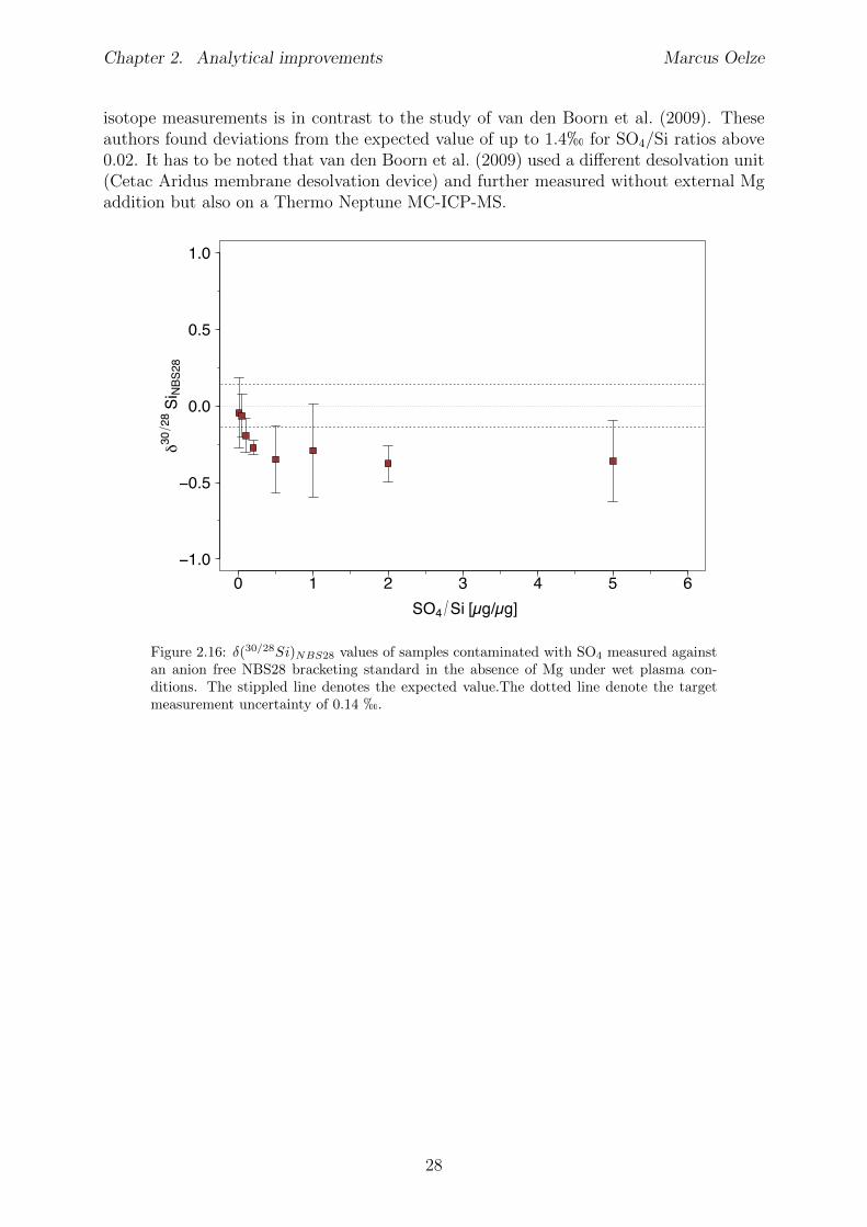
Chapter 2. Analytical improvements Marcus Oelze
isotope measurements is in contrast to the study of van den Boorn et al. (2009). Theseauthors found deviations from the expected value of up to 1.4h for SO4/Si ratios above0.02. It has to be noted that van den Boorn et al. (2009) used a di↵erent desolvation unit(Cetac Aridus membrane desolvation device) and further measured without external Mgaddition but also on a Thermo Neptune MC-ICP-MS.
0 1 2 3 4 5 6−1.0
−0.5
0.0
0.5
1.0
SO4 Si [µg/µg]
δ3028
Si NBS
28
Figure 2.16: �(30/28Si)NBS28
values of samples contaminated with SO4
measured againstan anion free NBS28 bracketing standard in the absence of Mg under wet plasma con-ditions. The stippled line denotes the expected value.The dotted line denote the targetmeasurement uncertainty of 0.14 h.
28
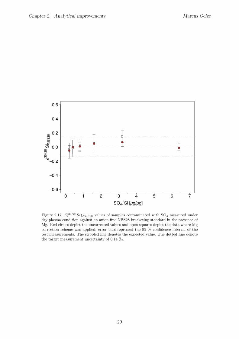
Chapter 2. Analytical improvements Marcus Oelze
0 1 2 3 4 5 6 7−0.6
−0.4
−0.2
0.0
0.2
0.4
0.6
SO4 Si [µg/µg]
δ3028
Si NBS
28
Figure 2.17: �(30/28Si)NBS28
values of samples contaminated with SO4
measured underdry plasma condition against an anion free NBS28 bracketing standard in the presence ofMg. Red circles depict the uncorrected values and open squares depict the data where Mgcorrection scheme was applied; error bars represent the 95 % confidence interval of thetest measurements. The stippled line denotes the expected value. The dotted line denotethe target measurement uncertainty of 0.14 h.
29
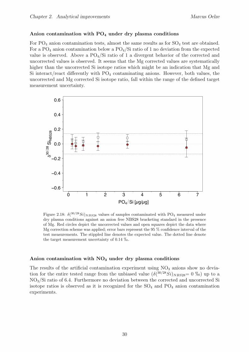
Chapter 2. Analytical improvements Marcus Oelze
Anion contamination with PO4
under dry plasma conditions
For PO4 anion contamination tests, almost the same results as for SO4 test are obtained.For a PO4 anion contamination below a PO4/Si ratio of 1 no deviation from the expectedvalue is observed. Above a PO4/Si ratio of 1 a divergent behavior of the corrected anduncorrected values is observed. It seems that the Mg corrected values are systematicallyhigher than the uncorrected Si isotope ratios which might be an indication that Mg andSi interact/react di↵erently with PO4 contaminating anions. However, both values, theuncorrected and Mg corrected Si isotope ratio, fall within the range of the defined targetmeasurement uncertainty.
0 1 2 3 4 5 6 7−0.6
−0.4
−0.2
0.0
0.2
0.4
0.6
PO4 Si [µg/µg]
δ3028
Si NBS
28
Figure 2.18: �(30/28Si)NBS28
values of samples contaminated with PO4
measured underdry plasma conditions against an anion free NBS28 bracketing standard in the presenceof Mg. Red circles depict the uncorrected values and open squares depict the data whereMg correction scheme was applied; error bars represent the 95 % confidence interval of thetest measurements. The stippled line denotes the expected value. The dotted line denotethe target measurement uncertainty of 0.14 h.
Anion contamination with NO3
under dry plasma conditions
The results of the artificial contamination experiment using NO3 anions show no devia-tion for the entire tested range from the unbiased value (�(30/28Si)
NBS28= 0 h) up to aNO3/Si ratio of 6.4. Furthermore no deviation between the corrected and uncorrected Siisotope ratios is observed as it is recognized for the SO4 and PO4 anion contaminationexperiments.
30
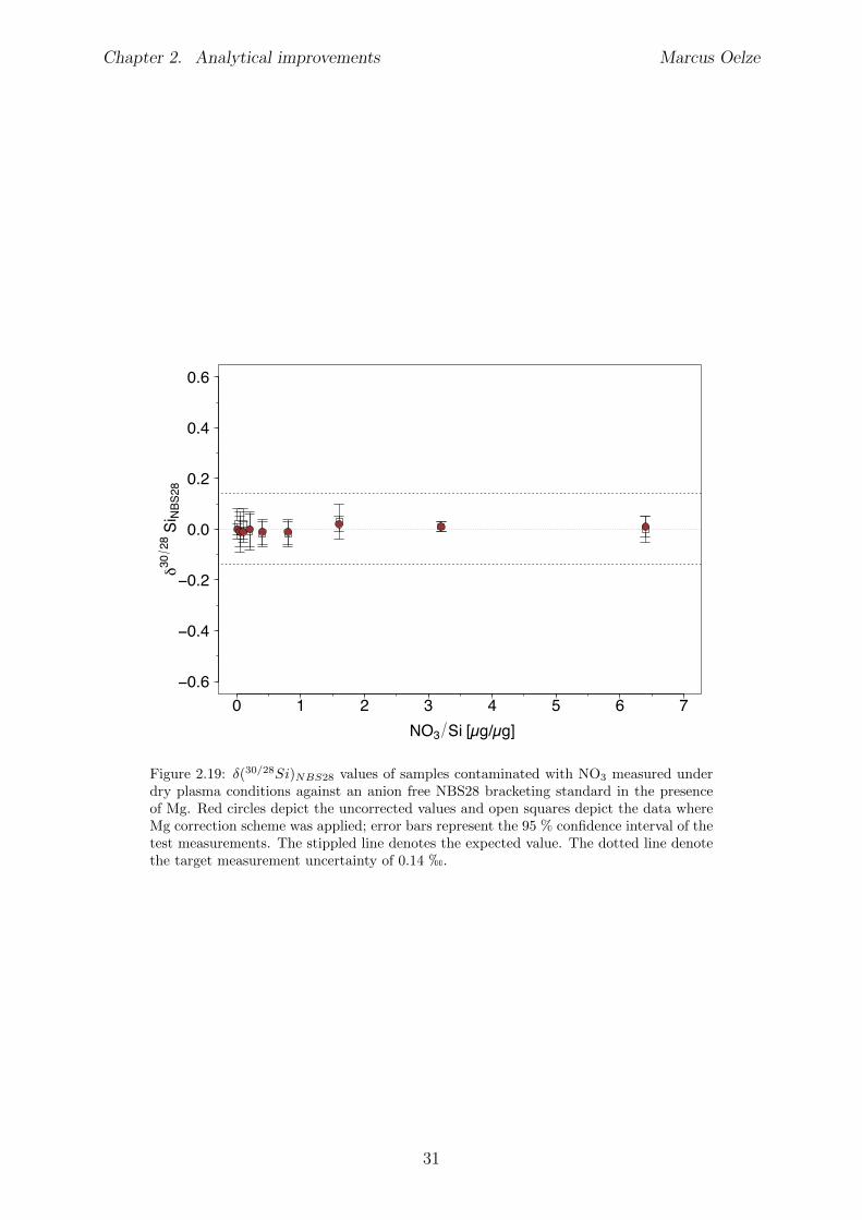
Chapter 2. Analytical improvements Marcus Oelze
0 1 2 3 4 5 6 7−0.6
−0.4
−0.2
0.0
0.2
0.4
0.6
NO3 Si [µg/µg]
δ3028
Si NBS
28
Figure 2.19: �(30/28Si)NBS28
values of samples contaminated with NO3
measured underdry plasma conditions against an anion free NBS28 bracketing standard in the presenceof Mg. Red circles depict the uncorrected values and open squares depict the data whereMg correction scheme was applied; error bars represent the 95 % confidence interval of thetest measurements. The stippled line denotes the expected value. The dotted line denotethe target measurement uncertainty of 0.14 h.
31
Chapter 2. Analytical improvements Marcus Oelze
2.7 Summary
An extension of the established digestion method for natural samples by an organic re-moval step for solid and water samples is described in detail. Further it is shown howexternal Mg additions improves the accuracy and stability of Si isotope measurementsunder dry plasma conditions in comparison to wet plasma measurements without Mg ad-dition (see Table 2.2 and Table 2.3 and Figures 2.2 to 2.9). Measurements of Si referencematerial under dry plasma conditions with Mg addition compared to wet plasma condi-tions without Mg addition show lower SD values, respectively (Table 2.2 and Table 2.3).The use of Mg as “matrix modifier” to improve the measurement repeatability of isotopemeasurements has been also shown for measurements of Pb by Barling and Weis (2008)and is also e↵ective for Si. The use of external Mg addition further helps to circumventseveral known issues when measuring stable isotopes using a desolvation unit. The use ofMg as “matrix modifier” has several benefits when measuring Si stable isotope under dryplasma conditions:
1. The addition of Mg increases the sensitivity by up to a factor of 3 when measuringunder dry plasma conditions.
2. The addition of Mg reduces variations in mass bias between sample and standardsinduced by di↵erent sample standards matrices:
(a) Concentration matching: Si and Mg concentration can vary between samplesand bracketing standards of up to ±50% with no visible e↵ect observed oninstrumental mass bias.
(b) Molarity matching: A molarity mismatch between samples and standard inthe range of 0.05 to 0.2 mol/l measured against a 0.1 mol/l bracketing stan-dards does not result in observable changes. For a sample-standard molar-ity mismatch above 0.2 mol/l to 0.5 mol/l Si isotope fractionation of up to�(30/28Si)
NBS28= -0.7 h occurs for the uncorrected values. When applyingthe external Mg correction scheme, no deviation from the expected value isobserved.
(c) Anion contamination: No e↵ect on mass bias is observed for anion contami-nations with SO4 and PO4 below an [anion]/Si ratio of 1. For an anion con-tamination with NO3 no change in mass bias is observable below an [anion]/Siratio of 6.4.
When using Mg as matrix modifier, the solution matrix is dominated by the high amountof Mg added and not by remaining impurities or sample standard mismatch (e.g. anions,discrepancies in Si concentration or molarity mismatching between sample and bracketingstandard). One possible reason for this increased performance when using Mg addition isthe low ionization potential of Mg (Mg = 7.65 eV). Therefore when Mg is introduced intothe ICP, Mg will ionize more e�ciently and therefore dominate the plasma environment.Small changes in the ionization environment due to anion contamination or concentra-tion/molarity mismatching will be retained by the dominating Mg ions and will not a↵ectthe Si ionization e�ciency. Several tests reveal that Si isotope measurements conductedwith external Mg addition are less sensitive to sample and standard matrix mismatchas expected from measurements under wet plasma conditions without Mg addition. Afurther test of potential Si isotope fractionation during Si column separation procedurereveal that no Si isotope fractionation occurs.
32
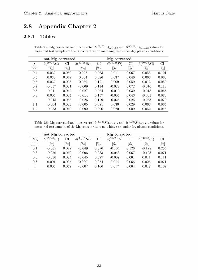
Chapter 2. Analytical improvements Marcus Oelze
2.8 Appendix Chapter 2
2.8.1 Tables
Table 2.4: Mg corrected and uncorrected �(29/28Si)NBS28
and �(30/28Si)NBS28
values formeasured test samples of the Si concentration matching test under dry plasma conditions.
not Mg corrected Mg corrected
[Si] �(29/28Si) CI �(30/28Si) CI �(29/28Si) CI �(30/28Si) CI[ppm] [h] [h] [h] [h] [h] [h] [h] [h]0.4 0.032 0.060 0.097 0.063 0.011 0.067 0.055 0.1010.5 0.038 0.042 0.064 0.086 0.037 0.046 0.063 0.0630.6 0.032 0.098 0.059 0.121 0.009 0.059 0.013 0.0590.7 -0.057 0.061 -0.069 0.114 -0.029 0.072 -0.016 0.1180.8 -0.011 0.042 -0.027 0.064 -0.010 0.039 -0.018 0.0680.9 0.005 0.084 -0.014 0.157 -0.004 0.043 -0.033 0.0731 -0.015 0.058 -0.026 0.129 -0.025 0.026 -0.053 0.0701.1 -0.004 0.033 -0.005 0.081 0.030 0.029 0.063 0.0651.2 -0.053 0.040 -0.092 0.090 0.020 0.009 0.052 0.045
Table 2.5: Mg corrected and uncorrected �(29/28Si)NBS28
and �(30/28Si)NBS28
values formeasured test samples of the Mg concentration matching test under dry plasma conditions.
not Mg corrected Mg corrected
[Mg] �(29/28Si) CI �(30/28Si) CI �(29/28Si) CI �(30/28Si) CI[ppm] [h] [h] [h] [h] [h] [h] [h] [h]0.1 -0.065 0.027 -0.049 0.096 -0.104 0.126 -0.128 0.2540.3 -0.050 0.050 -0.096 0.083 -0.063 0.067 -0.123 0.0710.6 -0.036 0.034 -0.045 0.027 -0.007 0.061 0.011 0.1110.8 0.001 0.095 0.000 0.074 0.014 0.066 0.025 0.0711 0.005 0.052 -0.007 0.106 0.017 0.064 0.017 0.107
33
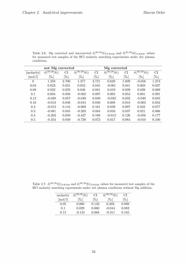
Chapter 2. Analytical improvements Marcus Oelze
Table 2.6: Mg corrected and uncorrected �(29/28Si)NBS28
and �(30/28Si)NBS28
valuesfor measured test samples of the HCl molarity matching experiments under dry plasmaconditions.
not Mg corrected Mg corrected
[molarity] �(29/28Si) CI �(30/28Si) CI �(29/28Si) CI �(30/28Si) CI[mol/l] [h] [h] [h] [h] [h] [h] [h] [h]
0 1.358 2.700 1.377 2.721 0.628 1.809 -0.056 1.2730.04 0.023 0.021 0.052 0.045 -0.001 0.041 0.003 0.0370.08 0.022 0.035 0.046 0.081 0.019 0.039 0.039 0.0690.1 0.004 0.056 -0.002 0.097 0.005 0.053 0.001 0.0910.12 -0.038 0.057 -0.049 0.049 -0.033 0.032 -0.040 0.0450.16 -0.013 0.046 -0.044 0.040 0.008 0.044 -0.003 0.0340.2 -0.012 0.144 -0.069 0.161 0.039 0.097 0.032 0.0770.3 -0.081 0.045 -0.203 0.084 0.033 0.037 0.021 0.0660.4 -0.202 0.059 -0.427 0.108 -0.013 0.126 -0.056 0.1770.5 -0.354 0.049 -0.738 0.073 0.017 0.084 -0.010 0.100
Table 2.7: �(29/28Si)NBS28
and �(30/28Si)NBS28
values for measured test samples of theHCl molarity matching experiments under wet plasma conditions without Mg addition.
molarity �(29/28Si) CI �(30/28Si) CI[mol/l] [h] [h] [h] [h]0.05 0.060 0.133 0.203 0.0980.1 0.029 0.060 -0.044 0.0820.15 -0.131 0.068 -0.311 0.185
34
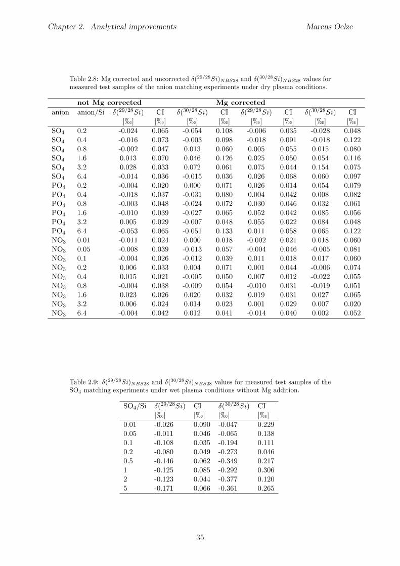
Chapter 2. Analytical improvements Marcus Oelze
Table 2.8: Mg corrected and uncorrected �(29/28Si)NBS28
and �(30/28Si)NBS28
values formeasured test samples of the anion matching experiments under dry plasma conditions.
not Mg corrected Mg corrected
anion anion/Si �(29/28Si) CI �(30/28Si) CI �(29/28Si) CI �(30/28Si) CI[h] [h] [h] [h] [h] [h] [h] [h]
SO4 0.2 -0.024 0.065 -0.054 0.108 -0.006 0.035 -0.028 0.048SO4 0.4 -0.016 0.073 -0.003 0.098 -0.018 0.091 -0.018 0.122SO4 0.8 -0.002 0.047 0.013 0.060 0.005 0.055 0.015 0.080SO4 1.6 0.013 0.070 0.046 0.126 0.025 0.050 0.054 0.116SO4 3.2 0.028 0.033 0.072 0.061 0.075 0.044 0.154 0.075SO4 6.4 -0.014 0.036 -0.015 0.036 0.026 0.068 0.060 0.097PO4 0.2 -0.004 0.020 0.000 0.071 0.026 0.014 0.054 0.079PO4 0.4 -0.018 0.037 -0.031 0.080 0.004 0.042 0.008 0.082PO4 0.8 -0.003 0.048 -0.024 0.072 0.030 0.046 0.032 0.061PO4 1.6 -0.010 0.039 -0.027 0.065 0.052 0.042 0.085 0.056PO4 3.2 0.005 0.029 -0.007 0.048 0.055 0.022 0.084 0.048PO4 6.4 -0.053 0.065 -0.051 0.133 0.011 0.058 0.065 0.122NO3 0.01 -0.011 0.024 0.000 0.018 -0.002 0.021 0.018 0.060NO3 0.05 -0.008 0.039 -0.013 0.057 -0.004 0.046 -0.005 0.081NO3 0.1 -0.004 0.026 -0.012 0.039 0.011 0.018 0.017 0.060NO3 0.2 0.006 0.033 0.004 0.071 0.001 0.044 -0.006 0.074NO3 0.4 0.015 0.021 -0.005 0.050 0.007 0.012 -0.022 0.055NO3 0.8 -0.004 0.038 -0.009 0.054 -0.010 0.031 -0.019 0.051NO3 1.6 0.023 0.026 0.020 0.032 0.019 0.031 0.027 0.065NO3 3.2 0.006 0.024 0.014 0.023 0.001 0.029 0.007 0.020NO3 6.4 -0.004 0.042 0.012 0.041 -0.014 0.040 0.002 0.052
Table 2.9: �(29/28Si)NBS28
and �(30/28Si)NBS28
values for measured test samples of theSO
4
matching experiments under wet plasma conditions without Mg addition.
SO4/Si �(29/28Si) CI �(30/28Si) CI[h] [h] [h] [h]
0.01 -0.026 0.090 -0.047 0.2290.05 -0.011 0.046 -0.065 0.1380.1 -0.108 0.035 -0.194 0.1110.2 -0.080 0.049 -0.273 0.0460.5 -0.146 0.062 -0.349 0.2171 -0.125 0.085 -0.292 0.3062 -0.123 0.044 -0.377 0.1205 -0.171 0.066 -0.361 0.265
35
Chapter 3
Si stable isotope fractionation duringadsorption and the competitionbetween kinetic and equilibriumisotope fractionation: implicationsfor weathering systems1
3.1 Abstract
The adsorption of Si onto amorphous Al-hydroxides is the cause for the light Si isotopesignature that secondary crystalline clay minerals in weathering systems carry. We pro-pose this hypothesis from a series of adsorption experiments in which the light isotopes arebeing favored during Si adsorption onto crystalline gibbsite and in which the associatedfractionation factor depends on the solution’s initial Si concentration.Three adsorption experiments were carried out at pH 7 with di↵erent initial Si concentra-tions of 0.36, 0.71 and 1.42 mmol/l Si start concentrations. As Al-hydroxide adsorbent,30 g/l crystalline gibbsite were used to provide equal surface area in all experiments.Adsorption rates are higher with higher initial Si concentration. At the same time, cal-culated apparent isotope fractionation factors 103ln↵adsorbed/solution decrease from -1.8 to-3 h with increasing initial Si concentration. As care was taken to avoid isotope frac-tionation during transport of dissolved Si to the gibbsite surface, the mass dependence ofthe activation energy barrier at the interface is causing the kinetic isotope fractionation.Within the mass balance framework of DePaolo (2011) the shift in Si isotope fractiona-tion with initial Si concentration is interpreted to be induced by di↵erent kinetic isotopefractionation factors associated with the forward reaction. Only after ca. two months dothe isotope ratios begin to adjust to an equilibrium isotope fractionation factor that isclose to 0 h. With such slow re-equilibration Si adsorption di↵ers fundamentally fromtransition metals that re-equilibrate isotopically within hours after adsorption onto Feand Mn oxide surfaces.These observations may provide an explanation for the light Si isotope signature clay min-erals formed during weathering carry: the light Si isotope composition is being inherited
1This Chapter is published in Chemical Geology : Oelze et al. (2014);http://dx.doi.org/10.1016/j.chemgeo.2014.04.027
36
Chapter 3. Si stable isotope fractionation during adsorption Marcus Oelze
early on during Si adsorption onto amorphous Al-hydroxides and is potentially carriedover during all further stages of transformation.
3.2 Introduction
Weathering of minerals and rocks releases elements into the ambient solution. Si and Albeing the second and third most abundant elements in the Earth’s crust, respectively,are both key players during weathering of silicates. While Al is almost insoluble undernear neutral pH conditions and low dissolved organic carbon contents (Sposito, 1996), Siis partitioned in roughly equal proportions between the dissolved phase and into a solidsecondary mineral phase during the dissolution of primary silicate minerals. In the lastdecade Si stable isotopes have been increasingly used to trace weathering processes.One major finding of these Si isotopes studies is the relative enrichment of heavy Siisotopes in the ambient soil solution. The isotopically lighter counterpart is found in sec-ondary siliceous solid phases (Ziegler et al., 2005a,b; Georg et al., 2006a, 2007b; Opfergeltet al., 2009; Bern et al., 2010; Opfergelt et al., 2011). Despite this consistent picture, thepartitioning of Si isotopes in the presence of Al has not been explored in detail undercontrolled laboratory conditions. Determining the related isotope fractionation factors iscritical as the reaction of Si and Al is likely to be the first crucial reaction occurring inweathering environments after releasing Al and Si from primary silicates.In the present study, we explore Si isotope fractionation during adsorption of Si ontogibbsite at three di↵erent initial Si concentrations. We explain the resulting dependenceof the Si isotope fractionation factor on adsorption rate within the conceptual mass balanceframework of DePaolo (2011).
3.3 Materials and Methods
3.3.1 Si source for adsorption experiments
Dietzel (1993, 2002) showed that only monomeric silicic acid (H4SiO4) is formed whentetraethylorthosilicate (TEOS; (C2H5O)4Si) is used as Si source and that its behaviorin adsorption experiments is identical to that found in monomeric silicic acid solutionsprepared by alternative means. The advantage of using TEOS as Si source is that neitherassociated cations nor minor elemental amounts (released during the dissolution of silicates(e.g. Na2SiO3) or from alkaline standard solutions (SiO2 in 2% NaOH)) are present inthe solution, which then have to be removed to obtain pure silicic acid for experiments.Further monomeric silicic acid can be produced easily by a simple addition of smallvolumes of TEOS to aqueous solutions where TEOS converts to silicic acid via a hydrolysisreaction. The side product of TEOS hydrolysis is ethanol (a concentration of 296 ppm iscalculated). The Si stock solution was prepared by adding 5.9 g (6 ml) TEOS (Merck®)to 20 l Milli-Q water (1.42 mmol/l Si).To avoid formation of polysilicic acid the prepared starting solution was held below thesolubility of amorphous silica. In addition, before using the starting solution we first ana-lyzed the solution for the degree of polymerization of dissolved silicic acid and the presenceof colloidal silica using the �-silicomolybdate method (for details see subsection 3.7.2 andIler (1979) and Dietzel (2000)). The amount of colloidal silica is determined by measur-ing the total Si concentration using ICP-OES minus the concentration of monosilicic acid
37
Chapter 3. Si stable isotope fractionation during adsorption Marcus Oelze
determined by the �-silicomolybdate method. For all experiments both Si concentrationsshow that within the analytical precision of 5% no colloidal Si was present in the experi-ments. Furthermore, the reaction rate constant for the formation of the �-silicomolybdatecomplex can be used to evaluate the average polymerization degree of dissolved silicic acid.For the present stock solution a value of 2 min-1 was calculated, which clearly indicatesthe sole presence of monomeric silicic acid.
3.3.2 Adsorption experiments
Adsorption experiments were carried out following a method adapted from Dietzel andBohme (1997). The experimental solutions were prepared from a TEOS stock solution.Three distinct adsorption experiments were performed with initial Si concentrations of0.36, 0.71 and 1.42 mmol/l Si corresponding to concentrations of 10, 20 and 40 ppm,respectively. All experimental solutions were adjusted to 0.1 M NaCl by addition of NaCl(p.a. grade Merck®). Si concentrations were below the solubility limit of amorphoussilica which is 2.14 mmol/l Si at 25�C and pH <8 (Gunnarsson and Arnorsson, 2000), toprevent polymerization and precipitation of amorphous silica.In each experimental run 30 g of gibbsite (�-Al(OH)3; p.a. grade Merck®) with a givenspecific surface area of 1.18 m2/g (BET, N2-adsorption) was suspended in 1 l of theexperimental solution containing Si in PE bottles. The pH of 7.0 was adjusted and keptconstant during the experiment by the addition of diluted HCl or NaOH solution (pHwere measured with pH meter WTW 330 and pH electrode WTW SenTix 41, calibratedusing pH 4.0 and 7.0 WTW standard bu↵er solutions). The variability of the pH valuesthroughout the whole experimental runtime were ± 0.1 pH units. During the first 6 hoursof the experiment, the gibbsite suspension was heavily agitated using a IKA RW 20 DZMstirrer at 500 rpm with a Teflon stirring sta↵. A parafilm cover prevented evaporationof the solution. Subsequently the closed PE bottles were placed in an overhead shaker.Experimental suspensions (15 ml) were sampled with a syringe and filtered (0.45 µmporosity, cellulose acetate) at several intervals; total maximum experimental run time was1536 hours (64 days). The sampled solutions were split: 10 ml were used for ICP-OESanalyses (Varian 720-ES) and Si isotope measurements (Thermo Scientific NEPTUNE).The remaining solutions of 5 ml were immediately analyzed by UV-Vis (UV-VIS 641 Cary100, Varian).
3.3.3 Chemical separation and purification
Chemical separation of Si was done following the method from Georg et al. (2006b). Thefiltered solutions were loaded onto pre-cleaned columns (1.5 ml of BioRad DOWEX 50W-X8; 200-400 mesh) and Si was eluted with 5 ml Milli-Q water and stored in pre-cleanedcentrifuge tubes. It was assured for all samples that the Si yield was >95%, which waschecked by ICP-OES (Varian 720-ES).
3.3.4 Mass spectrometry
Silicon isotope composition was measured on a Thermo Neptune multi-collector induc-tively coupled mass spectrometer (MC-ICP-MS) equipped with an H-skimmer cone andthe newly developed Thermo Scientific® Jet - interface in high-resolution mode (m/�m> 5000). The purified sample solutions were introduced into the plasma via a desolva-
38
Chapter 3. Si stable isotope fractionation during adsorption Marcus Oelze
tion unit for dry plasma conditions (Apex, ESI®, no N2 addition, no further membranedesolvation) equipped with a 120 µl/min nebulizer.We used Mg doping combined with standard-sample-bracketing to correct for mass biasduring measurements by using an exponential mass bias law (Cardinal et al., 2003). Amagnesium solution was added to samples and standards to yield a final concentration of1 ppm Mg. Sample solutions were diluted to 1 ppm Si concentration in 0.1 M HCl, whichtypically resulted in an intensity of ⇠15 V/ppm on 28Si (using a 1011⌦ resistor).Measurements were conducted on the interference-free low-mass side of the three Si iso-topes. The most critical interference, caused by 14N16O on the 30Si signal, is usually below5V which is resolvable from the 30Si signal in the high-resolution mode used. Each sampleand standard was measured at least 4 times during a sequence; each sample or standardwas measured in dynamic mode for 30 cycles with an integration time for each cycle of4 s for Si as well as for Mg with an idle time of 3 s after magnet switching. Pure 0.1M HCl solutions were measured before and after each standard-sample-standard blockand were used for on-peak zero correction. Typical intensities of 28Si in blank solutionswere below 5 mV. We report Si isotope data relative to the standard reference materialNBS28 (quartz sand) in the delta notation according to Coplen (2011) as �(29/28Si)NBS28
and �(30/28Si)NBS28 expressed in per mill (h) by multiplication of Equation 3.1 and Equa-tion 3.2 with a factor of 103:
�(29/28Si)NBS28 =
0
B@
⇣29Si28Si
⌘
sample� 29Si28Si
�NBS28
� 1
1
CA (3.1)
�(30/28Si)NBS28 =
0
B@
⇣30Si28Si
⌘
sample� 30Si28Si
�NBS28
� 1
1
CA (3.2)
All reported errors on delta values are the 95% confidence interval (CI) calculated accord-ing to Equation 3.3 where �(30/28Si)NBS28 is the mean of the measured delta values for thesample or standard (at least n=4), tn-1 is a critical value from tables of the Student0s t-lawand SE is the standard error of the mean.
CI = �(30/28Si)NBS28 ± tn-1 ⇥ SE (3.3)
The well-defined Si isotope reference material BHVO-2g, a basalt standard (measuredover a 12 months period of analysis ; including several individual chemical separations aswell as several digestions procedures; �(30/28Si)NBS28 = �0.27± 0.02; n=73), was usuallymeasured as control standard during measured sequences.
3.3.5 Analytical tests
As it is mentioned in subsection 3.3.1 the side product during monomeric silicic acidpreparation using TEOS is ethanol. In a separate experiment using similar starting ma-terial (Oelze et al., 2015) it has been tested whether the remaining ethanol in the preparedsolutions induces analytical artifacts during the preparation and measurement of Si iso-topes. Pairs of solutions and the formed solid counterparts were measured. Applying a
39
Chapter 3. Si stable isotope fractionation during adsorption Marcus Oelze
mass balance approach showed that all fluid-solid pairs gave the isotopic composition ofthe starting solution. Hence no mass-spectrometric artifact was induced from the releaseof ethanol during preparation of Si-containing solutions using TEOS.A known limitation using the sample purification method of Georg et al. (2006b) is thatanions present in the samples remain in the purified Si solutions. As the Si adsorptionexperiments were conducted in the presence of 0.1 M NaCl and further HCl has beenused to adjust the pH, Cl� anions might have been present after purification and po-tentially might have caused matrix e↵ects as their amounts are di↵erent between sampleand bracketing standards. Therefore we tested whether di↵erent amounts of Cl� anionsin sample and bracketing standard causes matrix e↵ects by measuring a “Cl�-doped”standard against “pure” bracketing standards. In the estimated range of di↵erent Cl�
anion concentrations (di↵erence between “doped” and “pure” of up to 20 %) no bias hasbeen found.
3.4 Results
Si concentrations as well as �(29/28Si)solution and �(30/28Si)solution values are reported in theAppendix Table 3.2.
3.4.1 Evolution of Si concentration
During the adsorption experiments, a continuous decrease in Si concentration with timeis observed (Figure 3.1). In all experiments (0.36, 0.71 and 1.42 mmol/l Si startingconcentration) the major change of Si concentration occurs during the first 50 hours,and subsequently the changes slow down continuously. Over 60% of the total adsorptiontakes place during the first 24 hours. Si adsorption rates (Figure 3.2) at the beginningof the experiments di↵er strongly between the conducted experiments. Adsorption ratesfor experiments with an initial Si concentration of 1.42 mmol/l are up to four timeshigher compared to solutions with an initial concentration of 0.36 mmol/l Si; the 0.71mmol/l Si solution experiment yields intermediate adsorption rates. Using estimates fromKaramalidis and Dzombak (2011) of 8 - 8.8 adsorption surface sites/nm2 on gibbsite andthe measured BET surface area of 1.18 m2/g a maximum possible amount of adsorbedSi of 440 - 484 µg/g (470 - 520 µmol Si total) can be calculated. As the maximum Siamounts adsorbed (definded by the equilibrium constant of the adsorption reaction) wereca. 130, 200, and 250 µmol for the 0.36, 0.71, and 1.42 mmol/l experiment, respectively,in all adsorption experiments an excess of free adsorption surface sites was still availableat the end of the experiments.
40
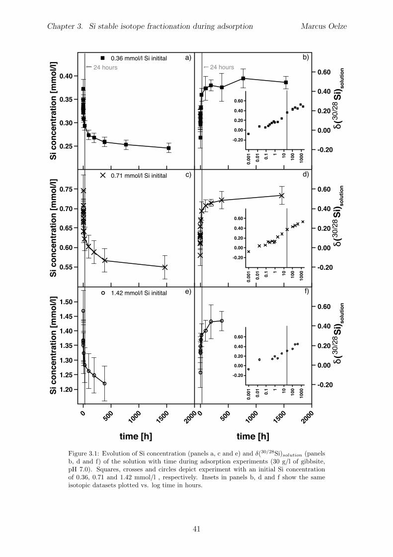
Chapter 3. Si stable isotope fractionation during adsorption Marcus Oelze
24 hours24 hours
0.25
0.30
0.35
0.40
Si c
once
ntra
tion
[mm
ol/l]
0.36 mmol/l Si initital
0.55
0.60
0.65
0.70
0.75
Si c
once
ntra
tion
[mm
ol/l]
0.71 mmol/l Si initital
050
010
0015
0020
00
time [h]
1.20
1.25
1.30
1.35
1.40
1.45
1.50
Si c
once
ntra
tion
[mm
ol/l]
1.42 mmol/l Si initital
-0.20
0.00
0.20
0.40
0.60
30/2
8(
Si) so
lutio
n
-0.20
0.00
0.20
0.40
0.60
30/2
8(
Si) so
lutio
n
050
010
0015
0020
00
time [h]
-0.20
0.00
0.20
0.40
0.60
30/2
8(
Si) so
lutio
n
0.00
1
0.01 0.
1 1 10 100
1000
-0.20
0.00
0.20
0.40
0.60
0.00
1
0.01 0.
1 1 10 100
1000
-0.20
0.00
0.20
0.40
0.60
0.00
1
0.01 0.
1 1 10 100
1000
-0.20
0.00
0.20
0.40
0.60
a)
c)
e)
b)
d)
f)
Figure 3.1: Evolution of Si concentration (panels a, c and e) and �(30/28Si)solution
(panelsb, d and f) of the solution with time during adsorption experiments (30 g/l of gibbsite,pH 7.0). Squares, crosses and circles depict experiment with an initial Si concentrationof 0.36, 0.71 and 1.42 mmol/l , respectively. Insets in panels b, d and f show the sameisotopic datasets plotted vs. log time in hours.
41
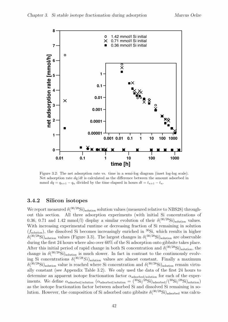
Chapter 3. Si stable isotope fractionation during adsorption Marcus Oelze
0.01 0.1 1 10 100 1000time [h]
0
1
2
3
4
5
6
7
8
net a
dsor
ptio
n ra
te [m
mol
/h]
0.36 mmol/l Si initial0.71 mmol/l Si initial1.42 mmol/l Si initial
0.001 0.01 0.1 1 10 100 10000.00001
0.0001
0.001
0.01
0.1
1
Figure 3.2: The net adsorption rate vs. time in a semi-log diagram (inset log-log scale).Net adsorption rate dq/dt is calculated as the di↵erence between the amount adsorbed inmmol dq = q
n+1
� qn
divided by the time elapsed in hours dt = tn+1
� tn
.
3.4.2 Silicon isotopes
We report measured �(30/28Si)solution solution values (measured relative to NBS28) through-out this section. All three adsorption experiments (with initial Si concentrations of0.36, 0.71 and 1.42 mmol/l) display a similar evolution of their �(30/28Si)solution values.With increasing experimental runtime or decreasing fraction of Si remaining in solution(fsolution), the dissolved Si becomes increasingly enriched in 30Si, which results in higher�(30/28Si)solution values (Figure 3.3). The largest changes in �(30/28Si)solution are observableduring the first 24 hours where also over 60% of the Si adsorption onto gibbsite takes place.After this initial period of rapid change in both Si concentration and �(30/28Si)solution, thechange in �(30/28Si)solution is much slower. In fact in contrast to the continuously evolv-ing Si concentrations �(30/28Si)solution values are almost constant. Finally a maximum�(30/28Si)solution value is reached where Si concentration and �(30/28Si)solution remain virtu-ally constant (see Appendix Table 3.2). We only used the data of the first 24 hours todetermine an apparent isotope fractionation factor ↵adsorbed/solution for each of the exper-iments. We define ↵adsorbed/solution (↵adsorbed/solution = (30Si/28Si)adsorbed/(30Si/28Si)solution)as the isotope fractionation factor between adsorbed Si and dissolved Si remaining in so-lution. However, the composition of Si adsorbed onto gibbsite �(30/28Si)adsorbed was calcu-
42
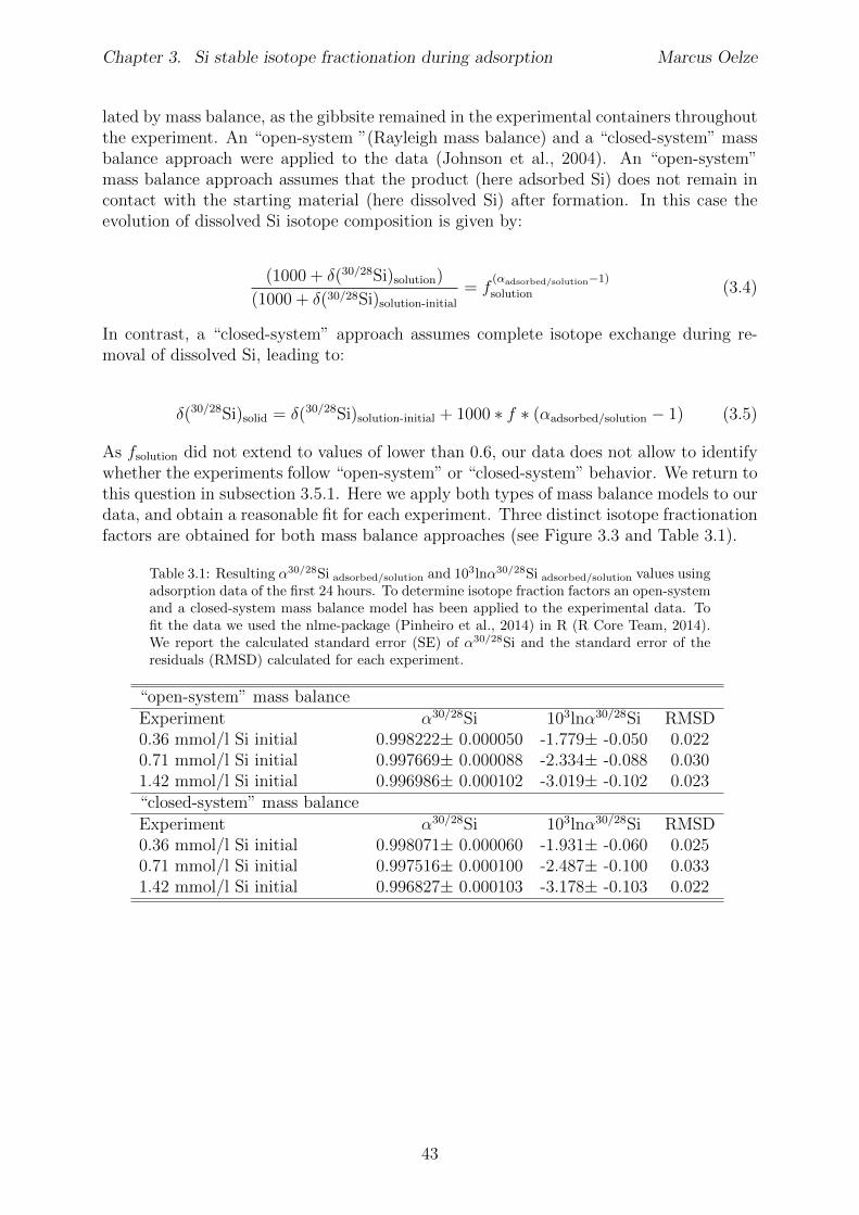
Chapter 3. Si stable isotope fractionation during adsorption Marcus Oelze
lated by mass balance, as the gibbsite remained in the experimental containers throughoutthe experiment. An “open-system ”(Rayleigh mass balance) and a “closed-system” massbalance approach were applied to the data (Johnson et al., 2004). An “open-system”mass balance approach assumes that the product (here adsorbed Si) does not remain incontact with the starting material (here dissolved Si) after formation. In this case theevolution of dissolved Si isotope composition is given by:
(1000 + �(30/28Si)solution)
(1000 + �(30/28Si)solution-initial= f
(↵adsorbed/solution�1)
solution (3.4)
In contrast, a “closed-system” approach assumes complete isotope exchange during re-moval of dissolved Si, leading to:
�(30/28Si)solid = �(30/28Si)solution-initial + 1000 ⇤ f ⇤ (↵adsorbed/solution � 1) (3.5)
As fsolution did not extend to values of lower than 0.6, our data does not allow to identifywhether the experiments follow “open-system” or “closed-system” behavior. We return tothis question in subsection 3.5.1. Here we apply both types of mass balance models to ourdata, and obtain a reasonable fit for each experiment. Three distinct isotope fractionationfactors are obtained for both mass balance approaches (see Figure 3.3 and Table 3.1).
Table 3.1: Resulting ↵30/28Siadsorbed/solution
and 103ln↵30/28Siadsorbed/solution
values usingadsorption data of the first 24 hours. To determine isotope fraction factors an open-systemand a closed-system mass balance model has been applied to the experimental data. Tofit the data we used the nlme-package (Pinheiro et al., 2014) in R (R Core Team, 2014).We report the calculated standard error (SE) of ↵30/28Si and the standard error of theresiduals (RMSD) calculated for each experiment.
“open-system” mass balanceExperiment ↵30/28Si 103ln↵30/28Si RMSD0.36 mmol/l Si initial 0.998222± 0.000050 -1.779± -0.050 0.0220.71 mmol/l Si initial 0.997669± 0.000088 -2.334± -0.088 0.0301.42 mmol/l Si initial 0.996986± 0.000102 -3.019± -0.102 0.023“closed-system” mass balanceExperiment ↵30/28Si 103ln↵30/28Si RMSD0.36 mmol/l Si initial 0.998071± 0.000060 -1.931± -0.060 0.0250.71 mmol/l Si initial 0.997516± 0.000100 -2.487± -0.100 0.0331.42 mmol/l Si initial 0.996827± 0.000103 -3.178± -0.103 0.022
43
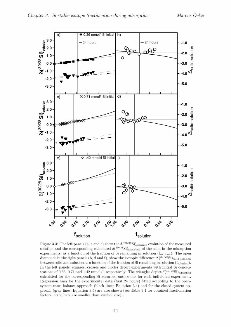
Chapter 3. Si stable isotope fractionation during adsorption Marcus Oelze
24 hours
-3.0
-2.0
-1.0
0.0
1.0
2.0
3.00.36 mmol/l Si initial
-3.0
-2.0
-1.0
0.0
1.0
2.0
3.00.71 mmol/l Si initial
0.50
0.60
0.70
0.80
0.90
1.00
fsolution
-3.0
-2.0
-1.0
0.0
1.0
2.0
3.0
30/2
8(
Si) so
lutio
n
1.42 mmol/l Si initial
-5.0
-4.0
-3.0
-2.0
-1.0
solid
-sol
utio
n
-5.0
-4.0
-3.0
-2.0
-1.0
solid
-sol
utio
n
0.50
0.60
0.70
0.80
0.90
1.00
fsolution
-5.0
-4.0
-3.0
-2.0
-1.0
solid
-sol
utio
n
24 hours
a)
c)
e)
b)
d)
f)
30/2
8(
Si) so
lutio
n30
/28
(
Si
) solu
tion
Figure 3.3: The left panels (a, c and e) show the �(30/28Si)solution
evolution of the measuredsolution and the corresponding calculated �(30/28Si)
adsorbed
of the solid in the adsorptionexperiments, as a function of the fraction of Si remaining in solution (f
solution
). The opendiamonds in the right panels (b, d and f), show the isotopic di↵erence�(30/28Si)
solid-solution
between solid and solution as a function of the fraction of Si remaining in solution (fsolution
).In the left panels, squares, crosses and circles depict experiments with initial Si concen-trations of 0.36, 0.71 and 1.42 mmol/l, respectively. The triangles depict �(30/28Si)
adsorbed
calculated for the corresponding Si adsorbed onto solids for each individual experiment.Regression lines for the experimental data (first 24 hours) fitted according to the open-system mass balance approach (black lines; Equation 3.4) and for the closed-system ap-proach (gray lines; Equation 3.5) are also shown (see Table 3.1 for obtained fractionationfactors; error bars are smaller than symbol size).
44
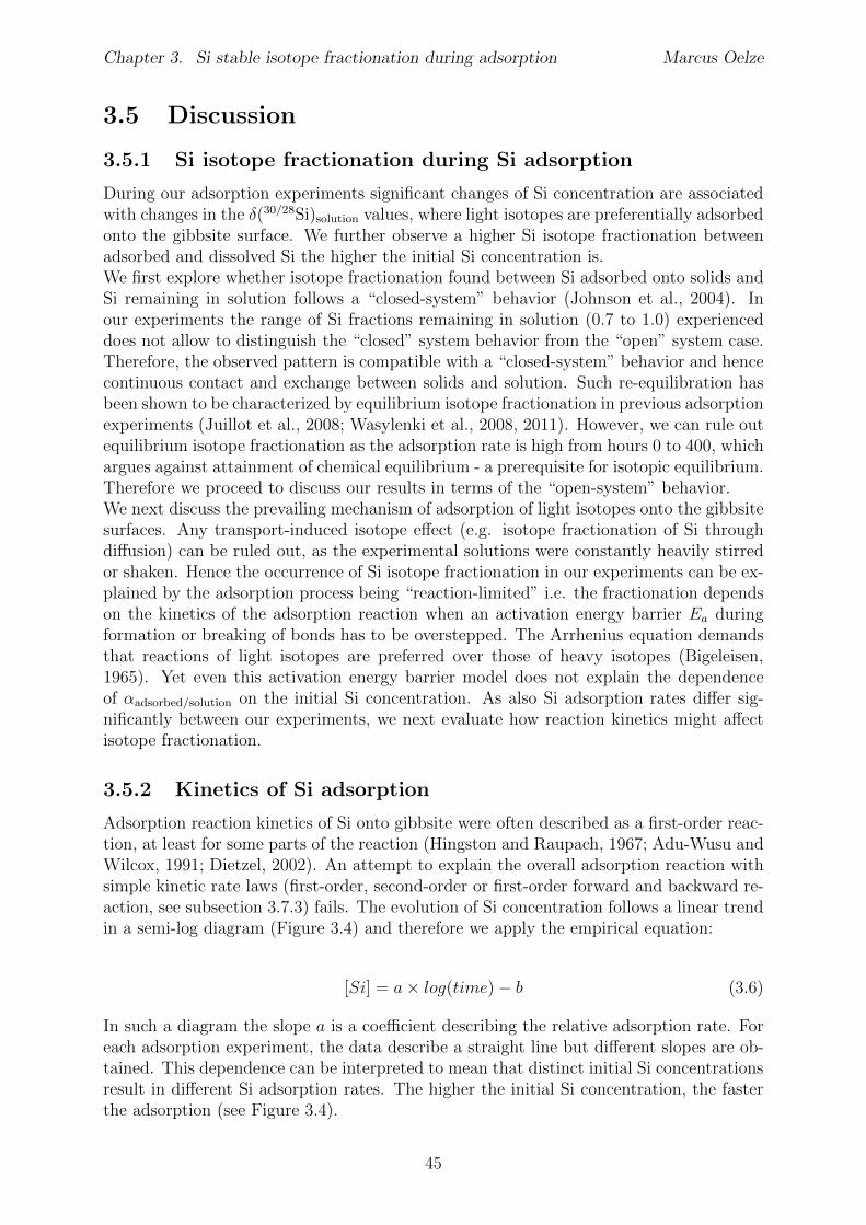
Chapter 3. Si stable isotope fractionation during adsorption Marcus Oelze
3.5 Discussion
3.5.1 Si isotope fractionation during Si adsorption
During our adsorption experiments significant changes of Si concentration are associatedwith changes in the �(30/28Si)solution values, where light isotopes are preferentially adsorbedonto the gibbsite surface. We further observe a higher Si isotope fractionation betweenadsorbed and dissolved Si the higher the initial Si concentration is.We first explore whether isotope fractionation found between Si adsorbed onto solids andSi remaining in solution follows a “closed-system” behavior (Johnson et al., 2004). Inour experiments the range of Si fractions remaining in solution (0.7 to 1.0) experienceddoes not allow to distinguish the “closed” system behavior from the “open” system case.Therefore, the observed pattern is compatible with a “closed-system” behavior and hencecontinuous contact and exchange between solids and solution. Such re-equilibration hasbeen shown to be characterized by equilibrium isotope fractionation in previous adsorptionexperiments (Juillot et al., 2008; Wasylenki et al., 2008, 2011). However, we can rule outequilibrium isotope fractionation as the adsorption rate is high from hours 0 to 400, whichargues against attainment of chemical equilibrium - a prerequisite for isotopic equilibrium.Therefore we proceed to discuss our results in terms of the “open-system” behavior.We next discuss the prevailing mechanism of adsorption of light isotopes onto the gibbsitesurfaces. Any transport-induced isotope e↵ect (e.g. isotope fractionation of Si throughdi↵usion) can be ruled out, as the experimental solutions were constantly heavily stirredor shaken. Hence the occurrence of Si isotope fractionation in our experiments can be ex-plained by the adsorption process being “reaction-limited” i.e. the fractionation dependson the kinetics of the adsorption reaction when an activation energy barrier E
a
duringformation or breaking of bonds has to be overstepped. The Arrhenius equation demandsthat reactions of light isotopes are preferred over those of heavy isotopes (Bigeleisen,1965). Yet even this activation energy barrier model does not explain the dependenceof ↵adsorbed/solution on the initial Si concentration. As also Si adsorption rates di↵er sig-nificantly between our experiments, we next evaluate how reaction kinetics might a↵ectisotope fractionation.
3.5.2 Kinetics of Si adsorption
Adsorption reaction kinetics of Si onto gibbsite were often described as a first-order reac-tion, at least for some parts of the reaction (Hingston and Raupach, 1967; Adu-Wusu andWilcox, 1991; Dietzel, 2002). An attempt to explain the overall adsorption reaction withsimple kinetic rate laws (first-order, second-order or first-order forward and backward re-action, see subsection 3.7.3) fails. The evolution of Si concentration follows a linear trendin a semi-log diagram (Figure 3.4) and therefore we apply the empirical equation:
[Si] = a⇥ log(time)� b (3.6)
In such a diagram the slope a is a coe�cient describing the relative adsorption rate. Foreach adsorption experiment, the data describe a straight line but di↵erent slopes are ob-tained. This dependence can be interpreted to mean that distinct initial Si concentrationsresult in di↵erent Si adsorption rates. The higher the initial Si concentration, the fasterthe adsorption (see Figure 3.4).
45
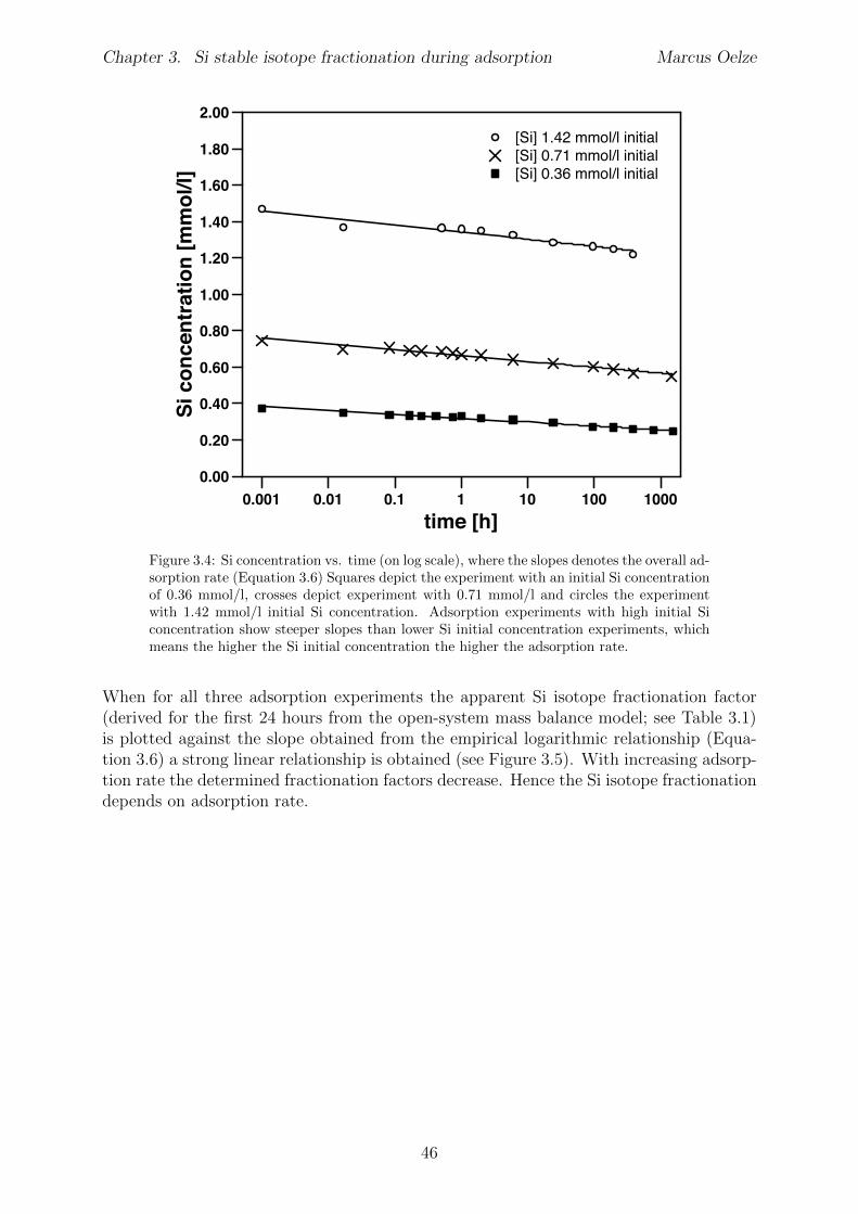
Chapter 3. Si stable isotope fractionation during adsorption Marcus Oelze
0.001 0.01 0.1 1 10 100 1000time [h]
0.00
0.20
0.40
0.60
0.80
1.00
1.20
1.40
1.60
1.80
2.00
Si c
once
ntra
tion
[mm
ol/l]
[Si] 1.42 mmol/l initial[Si] 0.71 mmol/l initial[Si] 0.36 mmol/l initial
Figure 3.4: Si concentration vs. time (on log scale), where the slopes denotes the overall ad-sorption rate (Equation 3.6) Squares depict the experiment with an initial Si concentrationof 0.36 mmol/l, crosses depict experiment with 0.71 mmol/l and circles the experimentwith 1.42 mmol/l initial Si concentration. Adsorption experiments with high initial Siconcentration show steeper slopes than lower Si initial concentration experiments, whichmeans the higher the Si initial concentration the higher the adsorption rate.
When for all three adsorption experiments the apparent Si isotope fractionation factor(derived for the first 24 hours from the open-system mass balance model; see Table 3.1)is plotted against the slope obtained from the empirical logarithmic relationship (Equa-tion 3.6) a strong linear relationship is obtained (see Figure 3.5). With increasing adsorp-tion rate the determined fractionation factors decrease. Hence the Si isotope fractionationdepends on adsorption rate.
46
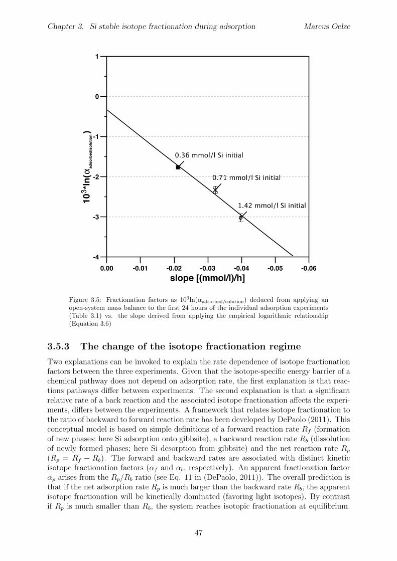
Chapter 3. Si stable isotope fractionation during adsorption Marcus Oelze
-0.06-0.05-0.04-0.03-0.02-0.010.00slope [(mmol/l)/h]
-4
-3
-2
-1
0
1
103 *
ln(
adso
rbed
/sol
utio
n
)
0.36 mmol/l Si initial
0.71 mmol/l Si initial
1.42 mmol/l Si initial
Figure 3.5: Fractionation factors as 103ln(↵adsorbed/solution
) deduced from applying anopen-system mass balance to the first 24 hours of the individual adsorption experiments(Table 3.1) vs. the slope derived from applying the empirical logarithmic relationship(Equation 3.6)
3.5.3 The change of the isotope fractionation regime
Two explanations can be invoked to explain the rate dependence of isotope fractionationfactors between the three experiments. Given that the isotope-specific energy barrier of achemical pathway does not depend on adsorption rate, the first explanation is that reac-tions pathways di↵er between experiments. The second explanation is that a significantrelative rate of a back reaction and the associated isotope fractionation a↵ects the experi-ments, di↵ers between the experiments. A framework that relates isotope fractionation tothe ratio of backward to forward reaction rate has been developed by DePaolo (2011). Thisconceptual model is based on simple definitions of a forward reaction rate R
f
(formationof new phases; here Si adsorption onto gibbsite), a backward reaction rate R
b
(dissolutionof newly formed phases; here Si desorption from gibbsite) and the net reaction rate R
p
(Rp
= Rf
� Rb
). The forward and backward rates are associated with distinct kineticisotope fractionation factors (↵
f
and ↵b
, respectively). An apparent fractionation factor↵p
arises from the Rp
/Rb
ratio (see Eq. 11 in (DePaolo, 2011)). The overall prediction isthat if the net adsorption rate R
p
is much larger than the backward rate Rb
, the apparentisotope fractionation will be kinetically dominated (favoring light isotopes). By contrastif R
p
is much smaller than Rb
, the system reaches isotopic fractionation at equilibrium.
47
Chapter 3. Si stable isotope fractionation during adsorption Marcus Oelze
While at intermediate regimes ↵p
depends on the values of ↵f
, ↵b
and Rp
/Rb
. On thelow and on the high end of the R
p
/Rb
axis (Figure 3.6) plateaus in ↵p
emerge. We canevaluate whether the dependence of the fractionation factor on adsorption rate can beinterpreted within this framework.First, for a given experiment, net adsorption rates decrease abruptly over the first 24 hours,hence it is most likely that the R
p
/Rb
ratio changes. However, ↵30/28Siadsorbed/solution (↵p
in DePaolo (2011)’s terminology) remains constant. This means that the early stage ofour experiments cannot be interpreted as being located at intermediate R
p
/Rb
valueswhere ↵
p
is expected to be strongly dependent on adsorption rate (Figure 3.6). Second,as there is net adsorption during this early stage, the experiments cannot be interpretedas operating near chemical and isotopic equilibrium, hence they are likely not locatedon the low end of the R
p
/Rb
axis (Figure 3.6). Therefore, for the first 24 hours in eachexperiment, the constant ↵
p
value while Rp
/Rb
ratios change means that the experimentsare located, on the “kinetic plateau”. There, at the high end of R
p
/Rb
values, ↵p
⇠ ↵f
.The di↵erence between the apparent isotope fractionation factors then reflects di↵erentvalues of the kinetic isotope fractionation factors associated with the forward reaction.We therefore conclude that the observed dependence of Si isotope fractionation on theinitial Si concentration can only be explained within the DePaolo framework if ↵
f
valuesdi↵er between the three experiments (Figure 3.6).After 24 hours �(30/28Si)solution and hence ↵30/28Siadsorbed/solution changes. We can interpretthis second stage of the experiments within the DePaolo framework as only then R
b
increases at the cost of Rf
and hence ↵p
departs from the kinetic plateau and evolvestowards equilibrium. We can estimate the equilibrium isotope fractionation factor fromthe linear correlation of the overall net adsorption rate and the determined closed-systemisotope fractionation factors (see Figure 3.5). Extrapolated to a zero net adsorption rate,an equilibrium isotope fractionation factor of ↵30/28Si adsorbed/solution =0.9997 (103ln↵30/28Si
adsorbed/solution = -0.3 h) results.That ↵
f
values depend on Si concentrations is an unexpected conclusion that warrantsan explanation. At the early stage of this finding we can only speculate on its cause.We can exclude that our high-concentration experiments were limited in adsorption sites,such that the removal mechanism shifted from one of adsorption to one for example ofprecipitation (see subsection 3.4.1). The most likely process is hence adsorption ontomonolayers in all three experiments. It is conceivable that a shift in surface complexationoccurs with increasing Si concentration and that di↵erent complexes di↵er by the strengthof their adsorption site and are hence associated with di↵erent ↵
f
values (Lemarchandet al., 2007). However, this assumption is not supported by surface complexation modelswhich are able to reconcile the evolution of Si adsorption onto gibbsite using only onesurface complex (Karamalidis and Dzombak, 2011). We note that the poor fit and thesmall amount of usable data of that study does not allow to fully rule out this explanationeither. A second possible explanation is the polymerization of silicic acid at the gibbsitesurface and therefore the formation of Si-O-Si bonds that are probably associated withdi↵erent isotope fractionation factors. Yokoyama et al. (1982) reported the polymerizationof Si at the surface of Al-hydroxides but only for much higher concentrations of dissolvedSi. However, in a precipitation experiment Oelze et al. (2015) observed a fractionationfactor ↵
p
= 1 for polymerization of silicic acid. Therefore further studies on the exactadsorption process of Si onto Al-hydroxides are needed to resolves this issue.
48
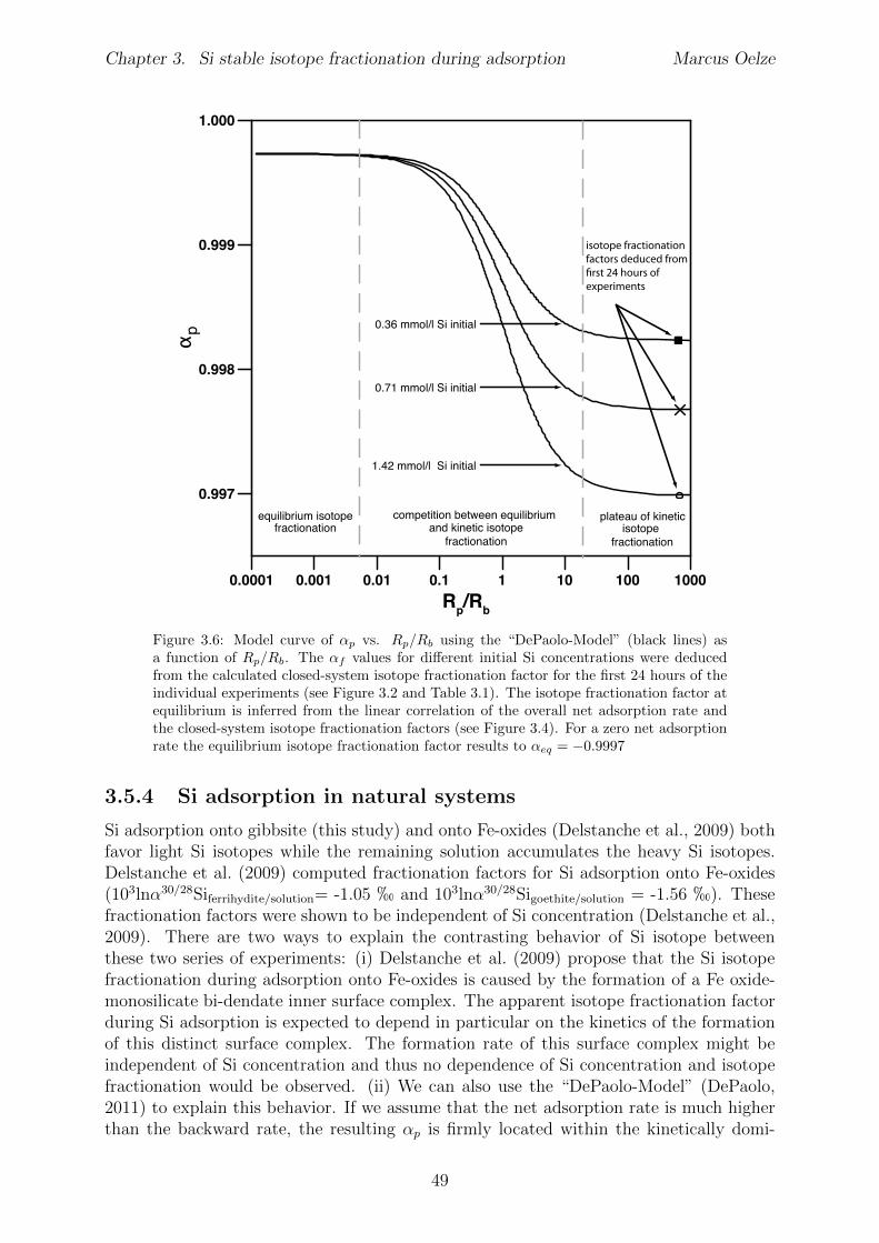
Chapter 3. Si stable isotope fractionation during adsorption Marcus Oelze
0.0001 0.001 0.01 0.1 1 10 100 1000Rp/Rb
0.997
0.998
0.999
1.000
p
equilibrium isotope fractionation
competition between equilibrium and kinetic isotope
fractionation
plateau of kinetic isotope
fractionation
isotope fractionationfactors deduced from
experiments
0.36 mmol/l Si initial
0.71 mmol/l Si initial
1.42 mmol/l Si initial
Figure 3.6: Model curve of ↵p
vs. Rp
/Rb
using the “DePaolo-Model” (black lines) asa function of R
p
/Rb
. The ↵f
values for di↵erent initial Si concentrations were deducedfrom the calculated closed-system isotope fractionation factor for the first 24 hours of theindividual experiments (see Figure 3.2 and Table 3.1). The isotope fractionation factor atequilibrium is inferred from the linear correlation of the overall net adsorption rate andthe closed-system isotope fractionation factors (see Figure 3.4). For a zero net adsorptionrate the equilibrium isotope fractionation factor results to ↵
eq
= �0.9997
3.5.4 Si adsorption in natural systems
Si adsorption onto gibbsite (this study) and onto Fe-oxides (Delstanche et al., 2009) bothfavor light Si isotopes while the remaining solution accumulates the heavy Si isotopes.Delstanche et al. (2009) computed fractionation factors for Si adsorption onto Fe-oxides(103ln↵30/28Siferrihydite/solution= -1.05 h and 103ln↵30/28Sigoethite/solution = -1.56 h). Thesefractionation factors were shown to be independent of Si concentration (Delstanche et al.,2009). There are two ways to explain the contrasting behavior of Si isotope betweenthese two series of experiments: (i) Delstanche et al. (2009) propose that the Si isotopefractionation during adsorption onto Fe-oxides is caused by the formation of a Fe oxide-monosilicate bi-dendate inner surface complex. The apparent isotope fractionation factorduring Si adsorption is expected to depend in particular on the kinetics of the formationof this distinct surface complex. The formation rate of this surface complex might beindependent of Si concentration and thus no dependence of Si concentration and isotopefractionation would be observed. (ii) We can also use the “DePaolo-Model” (DePaolo,2011) to explain this behavior. If we assume that the net adsorption rate is much higherthan the backward rate, the resulting ↵
p
is firmly located within the kinetically domi-
49
Chapter 3. Si stable isotope fractionation during adsorption Marcus Oelze
nated regime and is thus independent of small changes of Rp
/Rb
(see Figure 3.6). Bothexplanations are conceivable.
3.5.5 Comparison to adsorption of transition metals
The isotopic behavior of Si during adsorption di↵ers fundamentally from that observed instudies of transition metals. The adsorption of molybdenum onto Mn-Oxide surfaces wasshown to attain equilibrium within <10 hours (Wasylenki et al., 2008). Adsorption ofzinc onto ferryhydrite and goethite surfaces attained isotopic equilibrium after <20 hours(Juillot et al., 2008). Adsorption of ferrous iron to surfaces of goethite, quartz, goethite-loaded quartz, and aluminium oxide resulted in attainment of equilibrium within <72hours (Mikutta et al., 2008). Given such rapid equilibration time scales and the observed“closed-system” behavior, in natural environmental systems such transition metal resultscan be interpreted in terms of equilibrium isotope fractionation. The opposite is observedfor silica. The strong kinetic isotope fractionation accompanying Si adsorption and itssluggish re-equilibration, even after several months of experimental runtime, makes itlikely that natural systems are dominated by kinetic isotope e↵ects. This conclusionbears important implications for weathering systems that we explore in the next section.
3.5.6 Implications for silicate weathering environments
Many recent studies attribute the heavy Si isotopic signature of soil and stream waterto the formation of secondary minerals containing the complementary reservoir of lightSi isotopes (Douthitt, 1982; de La Rocha et al., 2000; Basile-Doelsch et al., 2005; Ziegleret al., 2005a; Basile-Doelsch, 2006; Georg et al., 2006a, 2009; Opfergelt et al., 2011). How-ever, the formation of secondary silicate minerals is su�ciently slow so that equilibriumisotope fractionation can be expected (Iler, 1979; Sposito, 1996). The Si isotope fraction-ation factors inferred from ab initio calculations (Meheut et al., 2009) and experimentalstudies (Oelze et al., 2015) show that 28Si will not be preferentially incorporated into theclay fraction if dissolved Si and crystalline silicates are in isotopic equilibrium. How thencan the enrichment of 28Si in clays found in weathering systems be explained?With increasing age and/or stage of silicate weathering the composition of secondarysolids changes from one dominated by amorphous solids to one dominated by crystallineclay minerals (Ziegler et al., 2003; Joussein et al., 2005). For instance, a known transfor-mation path is the reaction of plagioclase to amorphous alumosilicates such as allophane,subsequently e.g. to halloysite, and finally to clay minerals such as kaolinite. It is indeedmore likely that kaolinite is formed via thermodynamically less stable phases which actas precursor such as allophane and halloysite (Steefel and Van Cappellen, 1990).In any case, the first step is the release of Al and Si from primary minerals such asplagioclase. At pH values between 5 and 7 and at the low dissolved organic carbonconcentrations typically prevailing in soils or in interstitial solutions, the solubility ofAl(OH)3 is extremely low (Sposito, 1996). Accordingly, Al precipitates as amorphousAl(OH)3 or as crystalline solids such as gibbsite. The a�nity of Si to adsorb onto theseprecipitated Al-hydroxides is high (Hingston and Raupach, 1967; Adu-Wusu and Wilcox,1991; Dietzel, 2002). As we have shown in this study, Si adsorption onto Al-hydroxides isassociated with rather strong Si isotope fractionation, favoring light Si isotopes adsorbedonto the solid surface. In the next step, amorphous alumosilicates like siliceous gelsor colloids such as hydroxyaluminosilicate (HAS) are formed. Accordingly, Strekopytov
50
Chapter 3. Si stable isotope fractionation during adsorption Marcus Oelze
et al. (2006) suggested that, for HAS formation, the reaction of Si with Al-hydroxides is aprerequisite. Such amorphous Al-Si phases can be re-arranged to structures with higherdegrees of order, similar to allophane or imogolite (Sposito, 1996; Doucet et al., 2001). Ifthe transformation from amorphous Al-Si phases without any short range order to phaseswith distinct short range order like HAS or allophane takes place without substantialexchange of Si, the Si isotope signature of HAS/allophane will be inherited from the initialfast adsorption process of Si. With ongoing weathering, the halloysite content in the soildecreases, whereas the kaolinite content increases (Papoulis et al., 2004). As halloysitehas the same structure and chemical compositions as kaolinite except for the higher watercontent in halloysite (Joussein et al., 2005), we can assume that during the transformationof halloysite to kaolinite no shift in Si isotope composition occurs, as Si will be neitherlost nor added. Therefore, we suggest that the Si isotopic signature of crystalline clayminerals, such as kaolinite, is inherited from the kinetically-dominated process occurringduring adsorption of Si onto a previously formed amorphous Al-hydroxide.Our model of inherited isotope signals has important implications for interpreting ele-ment cycles in the di↵erent weathering regimes observed at the Earth surface. In thekinetically limited weathering regime (where supply into and erosion from the weatheringzone is so fast that not all primary minerals are dissolved (West et al., 2005; Ferrier andKirchner, 2008; Dixon et al., 2012) and solutions are at equilibrium concentrations (Ma-her, 2011)), the Si isotopic signature of soil or stream water will inevitably show heavy Siisotopic values, as in such regimes only fast processes like adsorption of Si occur and nolight Si will be released from secondary minerals due to their short residence time in theweathering zone. In the supply-limited weathering regime (where supply and erosion ofprimary minerals is so slow that most primary minerals are exhausted (West et al., 2005;Ferrier and Kirchner, 2008; Dixon et al., 2012) and solutions are diluted with respect toequilibrium concentrations (Maher, 2011)), the Si isotopic signature of the soil or streamwater will be characterized by the degree of weathering, ranging from heavy Si isotopicsignatures, where kinetically dominated Si adsorption is the major process, to light Siisotopic signatures where the system is governed by dissolution of clay minerals. This hasbeen already shown for tropical supply-limited settings in the black-water rivers of theAmazon and Congo basin (Cardinal et al., 2010; Hughes et al., 2013). Where erosion ratesof secondary minerals are low, it is also conceivable that adsorption of Si and dissolution ofsecondary minerals are balanced out which results then in an isotopic signature of soil andstream water indistinguishable from the parent material. The dissolution of previouslyformed secondary precipitates dominates and these minerals release their inherited light Si(Bouchez et al., 2013). Such temporal evolution has been observed from chronosequencesin Hawaii (Ziegler et al., 2005a). These authors measured the isotopic signature of thesoil solutions and observed an enrichment of heavy Si in solution with increasing age ofthe soil. In analogy, Opfergelt et al. (2011) clearly showed from allophane sequences involcanic soils that the more weathered the soil, the older the allophane and the lighterthe Si isotope signature is.
3.6 Summary
The adsorption of monomeric silicic acid onto gibbsite is accompanied by a significantkinetic Si isotope fractionation. In all adsorption experiments, light Si isotopes are pref-erentially adsorbed. By applying a closed-system mass balance model we calculate Siisotope fractionation factors that are dependent on the initial Si concentration. High ini-
51
Chapter 3. Si stable isotope fractionation during adsorption Marcus Oelze
tial Si concentrations result in a strong kinetic Si isotope fractionation during adsorption.This initial kinetic signature does begin to re-equilibrate only after ca. 2 months. Withthis sluggish behavior Si behaves fundamentally di↵erent from transition metals (e.g. Fe,Mo, Zn) that equilibrate isotopically within hours.Application of the mass balance model of DePaolo (2011) requires the assumption of dif-ferent isotope fractionation factors (↵
f
) associated with the forward reaction at di↵erentinitial Si concentrations, rather than changes in forward to backward reaction rate. Aminor shift in isotope ratios after 24 hours of Si adsorption is explained by a change inthe isotope fractionation regime from kinetically dominated to dominated by equilibriumisotope fractionation. This behavior is compatible with a change from high net adsorp-tion rates to low net adsorption rates (almost constant Si concentration at the end ofexperiments).Our findings have major relevance for explaining Si isotope systematics during silicateweathering. We hypothesize that the light Si isotopes signatures commonly found insecondary siliceous minerals and amorphous solids are obtained from adsorption of Sionto Al-hydroxides during the early stages of weathering. When these amorphous phasesslowly age to ordered structures and clay minerals, the low isotope ratio is passed onfrom the amorphous precursors. The light isotope composition found in clays is thereforeinherited from the early stages of primary mineral decomposition.
52
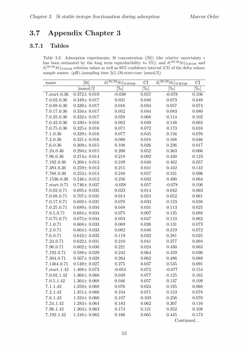
Chapter 3. Si stable isotope fractionation during adsorption Marcus Oelze
3.7 Appendix Chapter 3
3.7.1 Tables
Table 3.2: Adsorption experiments; Si concentration ([Si]) (the relative uncertainty ✏has been estimated by the long term reproducibility to 5%); and �(29/28Si)
NBS28
and�(30/28Si)
NBS28
solution values as well as 95% confidence interval (CI) of the delta values;sample names: (pH) (sampling time [h]) (Si-start-conc [mmol/l])
name [Si] �(29/28Si)NBS28 CI �(30/28Si)
NBS28 CI[mmol/l] [h] [h] [h] [h]
7 start 0.36 0.372± 0.019 -0.038 0.057 -0.078 0.1067 0.02 0.36 0.349± 0.017 0.031 0.040 0.073 0.0487 0.08 0.36 0.339± 0.017 0.016 0.034 0.057 0.0747 0.17 0.36 0.334± 0.017 0.052 0.044 0.083 0.0807 0.25 0.36 0.332± 0.017 0.058 0.068 0.114 0.1027 0.42 0.36 0.330± 0.016 0.082 0.049 0.148 0.0637 0.75 0.36 0.325± 0.016 0.071 0.072 0.173 0.0167 1 0.36 0.329± 0.016 0.077 0.045 0.156 0.0767 2 0.36 0.321± 0.016 0.080 0.018 0.168 0.0467 6 0.36 0.309± 0.015 0.108 0.026 0.236 0.0177 24 0.36 0.294± 0.015 0.206 0.052 0.363 0.0667 96 0.36 0.274± 0.014 0.218 0.092 0.430 0.1237 192 0.36 0.268± 0.013 0.249 0.040 0.462 0.0577 384 0.36 0.259± 0.013 0.215 0.041 0.442 0.1427 768 0.36 0.253± 0.013 0.248 0.057 0.531 0.0967 1536 0.36 0.246± 0.012 0.256 0.032 0.490 0.0647 start 0.71 0.746± 0.037 -0.038 0.057 -0.078 0.1067 0.02 0.71 0.695± 0.035 0.023 0.014 0.042 0.0637 0.08 0.71 0.707± 0.035 0.014 0.024 0.052 0.0617 0.17 0.71 0.692± 0.035 0.070 0.033 0.123 0.0387 0.25 0.71 0.689± 0.034 0.048 0.031 0.113 0.0257 0.5 0.71 0.684± 0.034 0.075 0.007 0.135 0.0887 0.75 0.71 0.675± 0.034 0.053 0.047 0.110 0.0627 1 0.71 0.668± 0.033 0.069 0.026 0.131 0.0737 2 0.71 0.664± 0.033 0.082 0.040 0.219 0.0727 6 0.71 0.642± 0.032 0.119 0.032 0.281 0.0257 24 0.71 0.622± 0.031 0.210 0.041 0.377 0.0947 96 0.71 0.602± 0.030 0.221 0.024 0.430 0.0637 192 0.71 0.588± 0.029 0.242 0.064 0.459 0.0367 384 0.71 0.567± 0.028 0.264 0.062 0.486 0.0887 1464 0.71 0.549± 0.027 0.275 0.037 0.535 0.0917 start 1.42 1.468± 0.073 -0.054 0.072 -0.077 0.1547 0.02 1.42 1.368± 0.068 0.049 0.077 0.125 0.1657 0.5 1.42 1.364± 0.068 0.046 0.057 0.137 0.1097 1 1.42 1.359± 0.068 0.076 0.024 0.195 0.0687 2 1.42 1.351± 0.068 0.104 0.071 0.153 0.0787 6 1.42 1.324± 0.066 0.107 0.103 0.256 0.0707 24 1.42 1.283± 0.064 0.183 0.062 0.307 0.1167 96 1.42 1.263± 0.063 0.174 0.121 0.352 0.1087 192 1.42 1.248± 0.062 0.166 0.065 0.445 0.173
Continued. . .
53
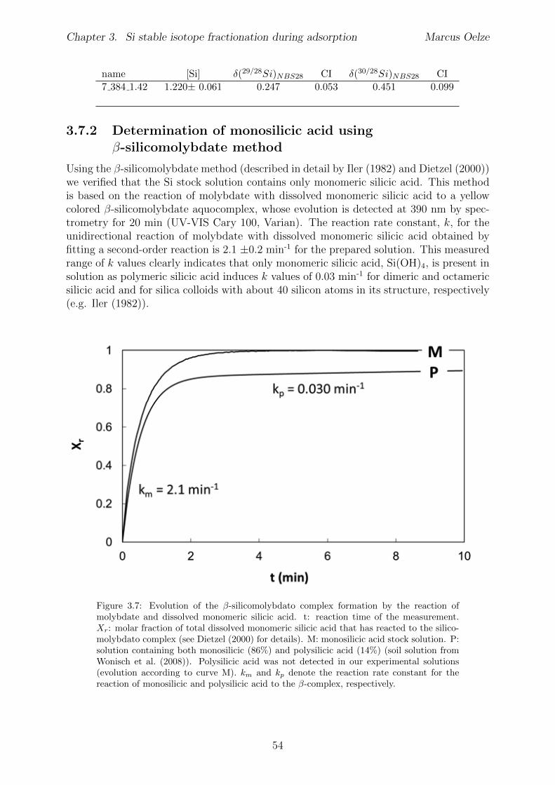
Chapter 3. Si stable isotope fractionation during adsorption Marcus Oelze
name [Si] �(29/28Si)NBS28 CI �(30/28Si)
NBS28 CI7 384 1.42 1.220± 0.061 0.247 0.053 0.451 0.099
3.7.2 Determination of monosilicic acid using�-silicomolybdate method
Using the �-silicomolybdate method (described in detail by Iler (1982) and Dietzel (2000))we verified that the Si stock solution contains only monomeric silicic acid. This methodis based on the reaction of molybdate with dissolved monomeric silicic acid to a yellowcolored �-silicomolybdate aquocomplex, whose evolution is detected at 390 nm by spec-trometry for 20 min (UV-VIS Cary 100, Varian). The reaction rate constant, k, for theunidirectional reaction of molybdate with dissolved monomeric silicic acid obtained byfitting a second-order reaction is 2.1 ±0.2 min-1 for the prepared solution. This measuredrange of k values clearly indicates that only monomeric silicic acid, Si(OH)4, is present insolution as polymeric silicic acid induces k values of 0.03 min-1 for dimeric and octamericsilicic acid and for silica colloids with about 40 silicon atoms in its structure, respectively(e.g. Iler (1982)).
Figure 3.7: Evolution of the �-silicomolybdato complex formation by the reaction ofmolybdate and dissolved monomeric silicic acid. t: reaction time of the measurement.X
r
: molar fraction of total dissolved monomeric silicic acid that has reacted to the silico-molybdato complex (see Dietzel (2000) for details). M: monosilicic acid stock solution. P:solution containing both monosilicic (86%) and polysilicic acid (14%) (soil solution fromWonisch et al. (2008)). Polysilicic acid was not detected in our experimental solutions(evolution according to curve M). k
m
and kp
denote the reaction rate constant for thereaction of monosilicic and polysilicic acid to the �-complex, respectively.
54
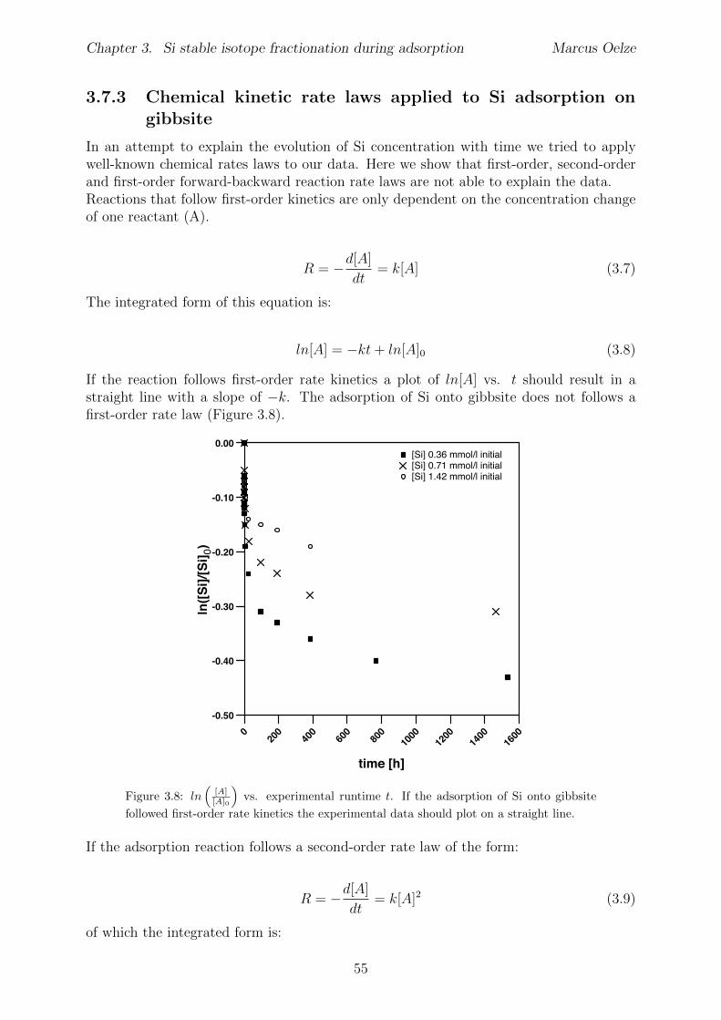
Chapter 3. Si stable isotope fractionation during adsorption Marcus Oelze
3.7.3 Chemical kinetic rate laws applied to Si adsorption ongibbsite
In an attempt to explain the evolution of Si concentration with time we tried to applywell-known chemical rates laws to our data. Here we show that first-order, second-orderand first-order forward-backward reaction rate laws are not able to explain the data.Reactions that follow first-order kinetics are only dependent on the concentration changeof one reactant (A).
R = �d[A]
dt= k[A] (3.7)
The integrated form of this equation is:
ln[A] = �kt+ ln[A]0 (3.8)
If the reaction follows first-order rate kinetics a plot of ln[A] vs. t should result in astraight line with a slope of �k. The adsorption of Si onto gibbsite does not follows afirst-order rate law (Figure 3.8).
020
040
060
080
010
0012
0014
0016
00
time [h]
-0.50
-0.40
-0.30
-0.20
-0.10
0.00
ln([S
i]/[S
i] 0)
[Si] 0.36 mmol/l initial[Si] 0.71 mmol/l initial[Si] 1.42 mmol/l initial
Figure 3.8: ln⇣
[A]
[A]0
⌘vs. experimental runtime t. If the adsorption of Si onto gibbsite
followed first-order rate kinetics the experimental data should plot on a straight line.
If the adsorption reaction follows a second-order rate law of the form:
R = �d[A]
dt= k[A]2 (3.9)
of which the integrated form is:
55
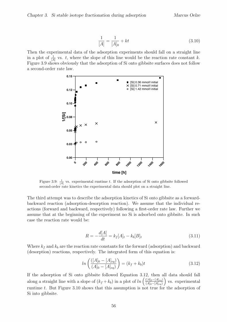
Chapter 3. Si stable isotope fractionation during adsorption Marcus Oelze
1
[A]=
1
[A]0+ kt (3.10)
Then the experimental data of the adsorption experiments should fall on a straight linein a plot of 1
[A]vs. t, where the slope of this line would be the reaction rate constant k.
Figure 3.9 shows obviously that the adsorption of Si onto gibbsite surfaces does not followa second-order rate law.
020
040
060
080
010
0012
0014
0016
00
time [h]
0.00
0.03
0.05
0.08
0.10
0.12
0.15
1/[S
i]
[Si] 0.36 mmol/l initial[Si] 0.71 mmol/l initial[Si] 1.42 mmol/l initial
Figure 3.9: 1
[A]
vs. experimental runtime t. If the adsorption of Si onto gibbsite followedsecond-order rate kinetics the experimental data should plot on a straight line.
The third attempt was to describe the adsorption kinetics of Si onto gibbsite as a forward-backward reaction (adsorption-desorption reaction). We assume that the individual re-actions (forward and backward, respectively) following a first-order rate law. Further weassume that at the beginning of the experiment no Si is adsorbed onto gibbsite. In suchcase the reaction rate would be:
R = �d[A]
dt= k
f
[A]t
� kb
[B]t
(3.11)
Where kf
and kb
are the reaction rate constants for the forward (adsorption) and backward(desorption) reactions, respectively. The integrated form of this equation is:
ln
✓([A]0 � [A]
eq
)
(A]0 � [A]eq
)
◆= (k
f
+ kb
)t (3.12)
If the adsorption of Si onto gibbsite followed Equation 3.12, then all data should fall
along a straight line with a slope of (kf
+kb
) in a plot of ln⇣
([A]0�[A]eq)
(A]0�[A]eq)
⌘vs. experimental
runtime t. But Figure 3.10 shows that this assumption is not true for the adsorption ofSi into gibbsite.
56
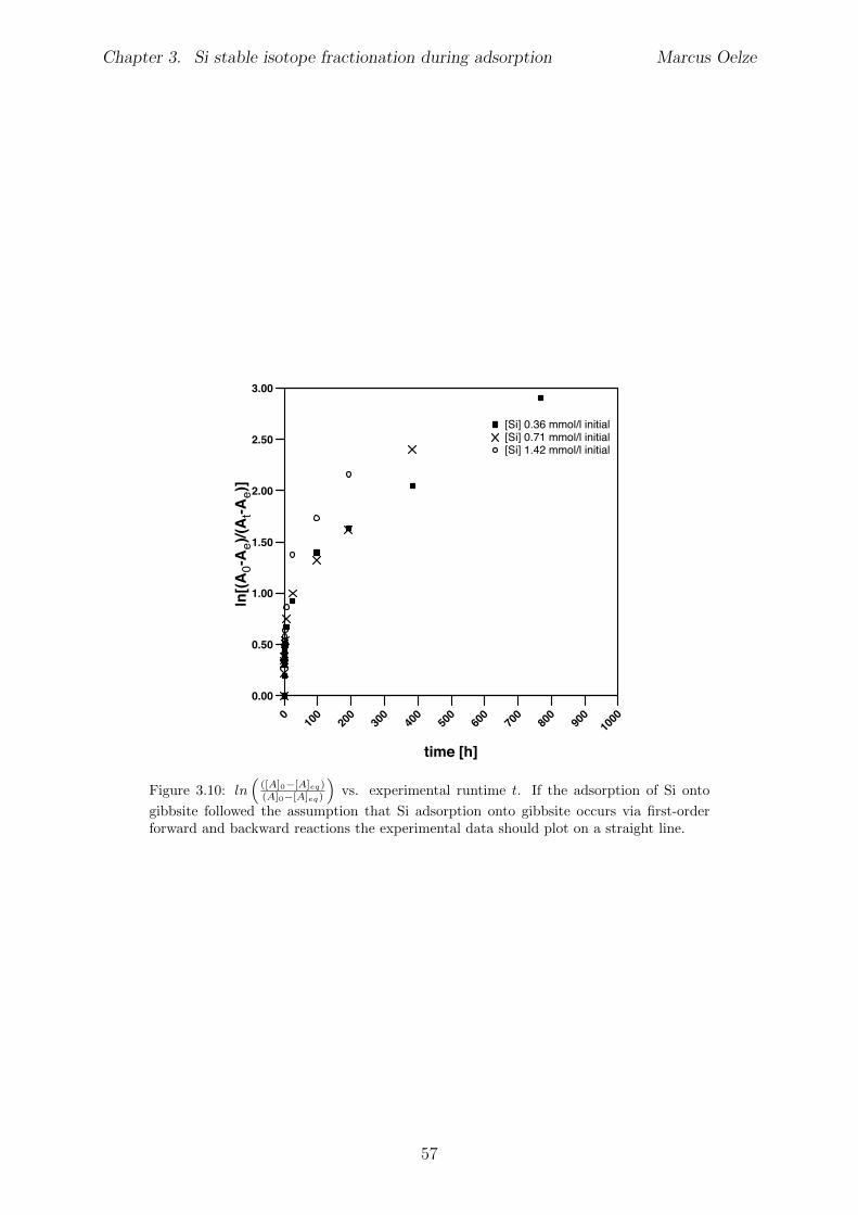
Chapter 3. Si stable isotope fractionation during adsorption Marcus Oelze
010
020
030
040
050
060
070
080
090
010
00
time [h]
0.00
0.50
1.00
1.50
2.00
2.50
3.00
ln[(A
0-A
e)/(A
t-Ae)
]
[Si] 0.36 mmol/l initial[Si] 0.71 mmol/l initial[Si] 1.42 mmol/l initial
Figure 3.10: ln⇣
([A]0�[A]eq)
(A]0�[A]eq)
⌘vs. experimental runtime t. If the adsorption of Si onto
gibbsite followed the assumption that Si adsorption onto gibbsite occurs via first-orderforward and backward reactions the experimental data should plot on a straight line.
57
Chapter 4
The e↵ect of Al on Si isotopefractionation investigated by silicaprecipitation experiments1
4.1 Abstract
Mass-dependent isotope fractionation occurring during precipitation of solids in low-temperature environments often depends on precipitation rate. Using a series of pre-cipitation experiments in which continuous precipitation and dissolution of Si solids isforced by daily cyclic freezing (solid formation) and thawing (solid re-dissolution), weshow this dependence. We conducted six Si precipitation experiments for about 120 dayswith initial dissolved Si concentration of 1.6 mmol/l Si, at pH values between 4.5 and7, with additions of 0.1 – 1 mM of dissolved aluminum (Al), and in the absence of Al.During all experiments increasing amounts of an X-ray amorphous silica-containing solidare formed. No Si isotope fractionation occurs during formation of almost pure Si solids,interpreted as an absence of Si isotope fractionation during polymerization of silicic acid.Si isotope fractionation occurs only in the high-Al concentration experiments, character-ized by an enrichment of the light Si isotopes in the solids formed early. With ongoingduration of the experiments, a re-dissolution of these solids is indicated as the Si isotopevalue of the complementary solution shifts to lighter values and eventually reaches near-initial compositions. Hence, our high-Al experiments are characterized by a gradual shiftfrom a regime that is dominated by unidirectional kinetic isotope fractionation with solidsformed that are up to 5h lighter in their 30Si/28Si ratio than the corresponding solution,to one of steady-state between dissolution and precipitation with the 30Si/28Si ratio ofthe solid being almost identical to the solution (�solid-solution ⇡ 0h). This suggests thatthe enrichment of light Si isotopes found in natural environments is caused exclusivelyby a unidirectional kinetic isotope e↵ect during fast precipitation of solids, aided by co-precipitation with Al phases or other carrier phases (e.g. Fe(III)). By contrast, duringslow precipitation, or in the absence of a carrier phase like Al, no Si isotope fractionationis expected and solids obtain the composition of the ambient fluid.
1This Chapter is published in Chemical Geology : Oelze et al. (2015);http://dx.doi.org/10.1016/j.chemgeo.2015.01.002
58
Chapter 4. Al determines the Si isotope fractionation Marcus Oelze
4.2 Introduction
Ratios of stable isotopes of Si have emerged as a powerful proxy to distinguish the reac-tions involved in low-temperature water-mineral and water- rock interaction. The isotoperatios potentially trace the way Si is released from Si-bearing solids into soil and (diage-netic) interstitial solutions. Si isotopes also trace how silica is precipitated into secondarysolids from these solutions. Given the useful information Si stable isotopes provide alongthis pathway, the resulting isotope ratios have been increasingly explored as a tool to tracesilicate weathering, sediment diagenesis and the associated silicification, precipitation ofsiliceous sediments from hydrothermal vents, and the genesis of Precambrian cherts andbanded iron formation (e.g. Ziegler et al. (2005a); Robert and Chaussidon (2006); Stein-hoefel et al. (2009); van den Boorn et al. (2010); Chakrabarti et al. (2012)). In general,dissolved Si in soil and in river waters is enriched in the heavy isotopes as compared tothe primary silicate minerals where Si is sourced from. The corresponding isotopicallylight reservoir is found in secondary siliceous solid phases (Ziegler et al., 2005a,b; Georget al., 2007a; Opfergelt et al., 2009; Bern et al., 2010; Steinhoefel et al., 2011). Fur-thermore, siliceous precipitates from hydrothermal solutions enriched in dissolved Si alsoshow the common picture of preferential incorporation of light isotopes in the precipitates(Douthitt, 1982; Ding et al., 1996; de La Rocha et al., 2000). This pictures is also inferredfrom the prevalence of low isotope ratios in Precambrian cherts (Andre et al., 2006; Stein-hoefel et al., 2009, 2010; van den Boorn et al., 2010). However, for chert formation, theway in which diagenetic silicification modifies the Si isotope composition from that of theoriginal deposits is far from understood. Basile-Doelsch et al. (2005) found some of thelowest Si isotope ratios in Aptian siliceous cements. Chen et al. (2007) also reported lowisotope ratios in Anabarites celoms (tubular small shelly fossil), and in quartz ocurring ingranular phosphates. In contrast, Robert and Chaussidon (2006), Abraham et al. (2011)and Chakrabarti et al. (2012) reported Archean cherts enriched in heavy Si isotopes.Converting these observations into a quantitative understanding of the movement of silicain low-temperature environments requires knowledge of the isotope fractionation factorsassociated with precipitation and recrystallization of siliceous solids. However, not onlydo we lack even first–order experimental estimates of equilibrium isotope fractionationfactors, but probably the formation of many siliceous secondary minerals and chemicaldeposits is a↵ected by non-equilibrium processes, as they are often enriched in light Siisotopes which suggest that the origin of the Si isotope fractionation is mostly kinetic(see e.g. Ziegler et al. (2005a); Georg et al. (2009); DePaolo (2011)). In these conditions,the relative importance of the forward (precipitation) and backward (dissolution) reac-tion rates determine the net solid formation rate and the associated isotope fractionationfactor (DePaolo, 2011). In addition, sedimentary silicates usually do not directly precip-itate from aqueous solutions, as documented by the large number of known amorphoussilica precursor phases (e.g. Iler (1979)). Therefore the generation of surface area dur-ing nucleation, growth and dissolution, and precursor replacement is important as theprocesses and rates at the mineral-water interface control the isotope composition of thesolid material during mineral growth (Cole et al., 1983; Criss et al., 1987; Steefel andVan Cappellen, 1990; Nielsen et al., 2012; Druhan et al., 2013).To date, only a few notable studies have explored Si isotope fractionation during thefixation of Si from solution under controlled experimental conditions. The Si isotopefractionation during adsorption of Si onto Fe-oxides, the Si isotopic evolution duringallophane- and gel-like solid formation and the Si isotope fractionation during abiotic
59
Chapter 4. Al determines the Si isotope fractionation Marcus Oelze
silica precipitation at low temperatures have been experimentally investigated (Li et al.,1995; Ziegler et al., 2005a; Delstanche et al., 2009; Opfergelt et al., 2009; Geilert et al.,2014). Recently, silicon isotope fractionation during adsorption of Si onto Al-hydroxideshas been shown to result in a strong rate dependence of silicon isotope fractionation (Oelzeet al., 2014). All these studies demonstrate the preferential incorporation of 28Si into thesolid, most likely during Si adsorption onto the solid phase. Isotope fractionation factors103ln↵solid/solution range from -1.0h to -1.6h for adsorption of Si onto Fe-oxides, -1.8hup to -3h for adsorption of Si onto Al-hydroxides and up to ⇡ -3.0h for precipitation ofallophane- and gel-like solid phases. First-principle calculations predict an enrichment of30Si in the higher-ordered solid at equilibrium conditions (Ding et al., 1996; Meheut et al.,2007, 2009). However, these predictions suggest that the Si isotope fractionation of theaforementioned experimental studies are dominated by a kinetic isotope e↵ect. Indeed,attaining Si isotopic equilibrium in experimental settings is virtually impossible due tothe extremely low exchange rates between solids and fluids in low-temperature processes,especially in the SiO2-H2O system. Li et al. (2011) suggested that recrystallization (or re-organization) induced by “Ostwald ripening”, the dissolution of small particles and the re-deposition of the dissolved species on the surfaces of larger particles in a saturated solution,is the only way to induce an isotope exchange at low temperature that is not overprinted bykinetic processes. To test whether equilibrium has indeed been attained, experimentalistsuse the addition of isotopically-enriched species in one of the two compartments (Johnsonet al., 2002; Welch et al., 2003; Schuessler et al., 2007). However, this approach is notpossible if, as is the case here, Si is precipitated from a homogeneous solution.A possible experimental approach in which dissolution-precipitation reactions take place isa batch reactor in which solid precipitation is driven by evaporation of the fluid, and soliddissolution driven by dilution of the fluid. However, the slow evaporation rates involvedin such an experiment would result in excessively long experimental runtimes. For Si-containing solids, once precipitated, isotopic equilibration times will exceed any feasibleexperimental runtime due the slow exchange rates. It is most likely that dissolution isthe limiting step to reach full exchange between formed solid products and solution. Thelow dissolution rate for amorphous silica (⇡ 1 ⇤ 10�12 mol⇤m-2⇤sec-1 at 20�; Icenhowerand Dove (2000)) will likely impair attainment of equilibrium as in experiments of CaCO3
precipitation (Tang et al., 2008).To circumvent these di�culties we designed a novel approach. Alternating dissolution-precipitation, implying depolymerization-polymerization of silica, is induced by freezingand thawing for predefined cycle length over a long run duration (Dietzel, 2005). Duringfreezing, only H2O molecules are captured in the ice lattice and the remaining solutionbecomes supersaturated in Si and precipitation of solids from the remaining solution oc-curs as soon as a critical supersaturation is reached. At the end of the freezing time span,temperatures are increased and the ice previously formed melts. Hence the solution isthen undersaturated with respect to the formed solids, leading to their partial dissolutionduring thawing. By continuing these freeze-thaw cycles steady-state conditions betweensilica precipitation and dissolution are reached, meaning that the dissolution and precip-itation fluxes compensate each other at the scale of a freeze-thaw cycle. At this stageconcentrations of dissolved Si do not change from a freeze-thaw cycle to the next. Oursetup allows us to explore the temporal change in the Si isotope fractionation factor asthe system evolves from a state that is characterized by high net Si removal rates (domi-nated by unidirectional kinetic isotope fractionation), to a state where the net change forprecipitation and dissolution is close to zero.
60
Chapter 4. Al determines the Si isotope fractionation Marcus Oelze
The rationale for this approach becomes apparent from fundamental experimental studieson dissolution-precipitation kinetics of SiO2 polymorphs. The process of dissolution andprecipitation of SiO2 polymorphs has been described as fully reversible (Rimstidt andBarnes, 1980; Renders et al., 1995; Carroll et al., 1998). Using the empirical relationshipsof Rimstidt and Barnes (1980) and Dove et al. (2008) for the dependence of the dissolutionrate on temperature and saturation state we can estimate the dissolution rate for anexperiment maintained far from equilibrium. The dissolution rate and therefore the timeneeded to reach full exchange is accelerated by a factor of 60 in comparison to experimentsclose to equilibrium conditions.Our experimental approach also provides insight into the numerous geological processesassociated with water-solid interaction that involve repeated dissolution-precipitating cy-cles of silica at the water-solid interface, such as for example during mineral replacementin weathering reactions, diagenesis, silicification, or biogenic ooze maturation. In addi-tion, this experimental approach of repeated freeze-thaw cycles can give insights into theformation process of authigenic silicates in polar regions (Tedrow, 1966; Dickinson andGrapes, 1997).However, in virtually all Earth surface reactions will Si release from primary silicates beaccompanied by variable amounts of Al. Reactions between Si and Al are hence likely thefirst crucial reactions. Aluminum in the system not only reduces the solubility of Si inaqueous solutions (Dixit et al., 2001; Van Cappellen et al., 2002), it also further providessurface area for fast adsorption of Si (Hingston and Raupach, 1967; Dietzel and Bohme,1997). In addition, pH will exert a first-order control over the precipitation kinetics ofboth elements as the solubility of Al and Si are both “pH dependent”. Therefore, weperformed experiments of Si precipitation from solutions in the presence of variable Alconcentrations and di↵erent pH.In the present study, we conducted six Si precipitation experiments for about 120 dayswith initial dissolved Si concentration of 1.6 mmol/l Si, with additions of di↵erent amountsof Al (0, 0.1, 1 mmol/l dissolved Al) and explored the evolution of the dissolved siliconisotope composition. In all experiments increasing amounts of an X-ray amorphous silica-containing solids are formed. The evolution of the dissolved silicon isotope compositioncan be explained by the presence or absence of dissolved Al.
4.3 Framework for isotope fractionation during pre-cipitation
Because of the diversity of isotope fractionation mechanisms encountered in our experi-ments, we first review the framework of definitions of these processes. There are severalprocesses during which kinetic isotope fractionation might occur, for example di↵usion,evaporation, or due to di↵erences in energy barriers. In the literature, the term “kinetic”actually serves as an umbrella for two fundamentally di↵erent processes generating iso-tope fractionation: (1) di↵erential transport velocity of isotopes over a given distance forexample during di↵usion (“transport-limited”) and (2) di↵erences in the energetic barrierassociated with chemical reactions (“reaction-limited”).In “transport-limited” regimes, kinetic isotope fractionation arises from di↵erent trans-port velocities (e.g. di↵erent di↵usion coe�cients) resulting from the mass di↵erences ofisotopes (Richter et al., 2006). This regime will not be further discussed in this paper,as under our experimental conditions this e↵ect will be small (see Table 1 in Richter
61
Chapter 4. Al determines the Si isotope fractionation Marcus Oelze
et al. (2006)). In addition to isotope fractionation due to di↵erent di↵usion coe�cientsfor isotopes, the influence of a chemical gradient in solution without su�cient stirringmust be considered possible (Gislason and Oelkers, 2003). Such an e↵ect is also describedas “transport-limited”. The observed precipitation and dissolution rates and further themeasured isotope fractionation are then influenced by the evolution of a chemical gradientand are no longer dependent on the bulk fluid chemistry but rather on the evolution ofthe chemical gradient. It is assumed here that mixing of the solution due to ice movementand climate cabinet vibrations will preclude the e↵ects of chemical gradients and can betherefore considered as subordinate.In the “reaction-limited” case the kinetic e↵ect arises because an activation energy has tobe overstepped to form or break bonds. The activation energy is likely to di↵er betweenisotopes of an element, as bonds with heavier isotopes have lower zero point energiesthan light isotopes (Urey, 1947). For example, during ion desolvation kinetic isotopefractionation has been documented to be induced by the di↵erence in activation energy(Hofmann et al., 2012). The Arrhenius equation indicates that at a given temperature, thereaction rate constant of light isotopes is higher than that of heavy isotopes. Importantly,during a reversible reaction the light isotope will be favored in both directions of thereaction. Therefore it follows that the overall isotope fractionation is governed by therelative magnitudes of forward and backward reaction rates, and by the individual isotopefractionation factors for these reactions (DePaolo, 2011).
4.4 Materials and Methods
4.4.1 Description of Experiments
Freeze-thaw experiments were conducted following a method adapted from Dietzel (2005).All experiments were carried out at similar initial Si concentrations and at two pH con-ditions (near neutral: pH 7 and acidic: pH 4.5 or 5) to mimic typical soil pH values(Schwertmann and Fischer, 1982). Three experimental series were conducted: the firstseries (a) was carried out without Al addition, the second series (b) with low amountsAl added (low: 0.1 mmol/l Al) and the third series (c) with high Al amounts added(high: 1 mmol/l Al), respectively. All reagent solutions were at least of analytical grade,and Milli-Q water (18.2 M⌦) was used. The pH of the initial solutions was adjustedwith diluted HCl and NaOH. Initial solutions of 1.6 mmol/l Si were prepared from atetraethylorthosilicate (TEOS) solution acquired from Merck. Aluminum was added asAlNO3⇤9H2O and 100 ml of these initial solutions were then evenly distributed into eachof several 100 ml polyethylene (PE) bottles. One separate bottle was prepared for eachexperimental runtime (each data point in Figures 4.1, 4.2, 4.5 and 4.6 is an individualbottle; see also Tables 4.1, 4.2 and 4.3) and was removed for analyses after a given ofruntime.We conducted the cyclic freeze-thaw experiments in a climate cabinet where temperaturewas changed over 24 hour-cycles from 20� to -20� (6 h from 20� to -20�, 6 h at -20�,6 h from -20� to 20�, 6h at 20�; heating and cooling rate: 0.11� min-1). About 4 hafter reaching 0� visual inspection showed that the experimental solution was completelyfrozen or thawed, respectively, but nevertheless small amounts of unfrozen water mightstill be present even at -20� (e.g. Anderson and Tice (1973); Anderson (1981)). Duringfreezing, the formation of ice crystals results in a decrease of the remaining volume of thesolution and therefore an elevated concentration of dissolved Si in the solution. Further
62
Chapter 4. Al determines the Si isotope fractionation Marcus Oelze
the decrease in temperature leads to a decrease in the amorphous Si solubility (Rimstidtand Barnes, 1980). Both e↵ects induce supersaturation with respect to amorphous silicaso that precipitation of amorphous silica can occur. During warming of the solution andsubsequent thawing of ice crystals, the solution becomes undersaturated with respect tothe formed Si-containing solids which are expected to partly redissolve. The amountof silica that is precipitated from solution at a given time interval depends on the rateof ice formation and the kinetics of silica precipitation (see Dietzel (2005) and referencestherein). Temperature limits, rates of cooling and warming, total solution volume and theinitial concentration of dissolved Si are decisive experimental parameters. We performedseveral pre-experiments to find these parameters. The cooling and thawing rates were setto 0.11� min-1, a rate at which we observed that precipitation of Si starts ca. 0.5 hoursbefore the solution is completely frozen.Freeze-thaw cycles were repeated up to 130 times. Although the solutions were not stirredor shaken, we assume that the solution was su�ciently well mixed through the motions ofthe ice crystals. During the thawing period, the melt water accumulated at the bottom ofthe bottles and the residual ice at the top. Additionally, vibration of the climate cabinetdue to ventilation enhanced mixing. Therefore isotope fractionation due to di↵usion(Richter et al., 2006) can be regarded as negligible. We cannot fully exclude the e↵ectof “transport-limitation” that arises from a chemical gradient (surrounding the particlesformed; see Gislason and Oelkers (2003) and Section 4.3). This e↵ect will only a↵ect thereaction rates and therefore the resulting isotope fractionation factors but will not changethe reaction mechanism itself. Therefore the derived isotope fractionation mechanisms donot depend on this.
4.4.2 Requirements for Si precipitation experiments
Si initial concentration
The precipitation of amorphous silica requires high concentrations of dissolved Si (� 2mmol/l Si at 25�, the solubility of amorphous silica (Gunnarsson and Arnorsson, 2000)).In addition, as we aimed to analyze both the dissolved Si and the precipitated silica fortheir Si isotope composition, a significant amount of solid Si has to be formed. There-fore the dissolved Si has to be prepared with even higher Si concentrations than requiredfor the first nucleation. However, it is a requirement that no polymeric Si is present inthe experimental initial solution, as its presence would render isotope data interpretationunnecessarily complex. To avoid formation of polysilicic acid, the Si concentration of theinitial solution was kept below the solubility of amorphous silica. An initial Si concen-tration of 1.6 mmol/l was deemed su�cient to meet this requirement. Initial solutionswere analyzed for the polymerization degree of dissolved Si (�-silicomolybdate method;see 4.8.2 and for further details Iler (1979) and Dietzel (2000)) by measuring the totalSi concentration using ICP-OES and subtracting the concentration of monosilicic aciddetermined by the �-silicomolybdate method. The results showed that no colloidal Si waspresent in the initial solution in any of the experiments.
Si source
We used tetraethylorthosilicate (TEOS) as a Si source. Dietzel (1993, 2002) showedthat when using TEOS as Si source only monomeric silicic acid is formed below thesolubility of amorphous silica and that the behavior of dissolved Si in experiments is
63
Chapter 4. Al determines the Si isotope fractionation Marcus Oelze
identical to monomeric silicic acid solutions that were prepared by alternative means (e.g.dissolution of silicates). One further advantage of TEOS is that no associated cations ofother minor elements (that would be released during the dissolution of other Si sources,such as silicates (e.g. Na2SiO3) or alkaline standard solutions (SiO2 in 2% NaOH)) arepresent in the solution. These elements would then have to be removed to obtain puresilicic acid for the experiments. Further the solution can be easily produced by addingsmall volumes of TEOS to water where it converts into silicic acid via a hydrolysis reaction.However, the side product of this reaction is ethanol that we estimate to be presentin our experimental solution at a concentration of 6.4 mmol/l. We explored whetherthe ethanol potentially remaining in the purified mass spectrometric solutions inducesanalytical artifacts during the preparation and measurement of Si isotopes by measuringthe purified solutions and the precipitated solid counterpart of the conducted experiments(see Table 4.3). Mass balance shows that each fluid-solid pair yields a calculated bulkisotopic composition that is identical to that of the initial solution. The fact that thecalculated bulk isotope composition of the system at di↵erent fluid-solid ratios (massdissolved Si/mass of precipitated silica) is similar to the composition of the initial solutiondemonstrates the absence of analytical artifacts induced by the release of ethanol duringpreparation of Si-containing solutions using TEOS.
4.4.3 Filtration of solutions and chemical separation for Si iso-tope analyses
The precipitate was separated from the solution by using cellulose acetate filters (0.1 µm).Where su�cient amounts of precipitate were obtained, the precipitate was rinsed o↵ fromthe filter and dried at 40�. The filtered precipitates of freeze-thawing experiments weredigested (⇡ 2 mg sample) using 200 µl 1M NaOH (analytical grade; Si concentration<1 ppb) in Teflon beakers. After digestion, samples were taken up in Milli-Q water forcolumn chemistry. Si was separated from the matrix following the method of Georg et al.(2006b): the filtered solutions and the digested precipitates were loaded onto pre-cleanedcolumns (1.5 ml of BioRad DOWEX 50W-X8; 200-400 mesh) and Si was eluted with 5 mlMilli-Q water and stored in pre-cleaned centrifuge tubes. It was assured for all samplesthat the Si yield was >95%, which was checked by ICP-OES (Varian 720-ES).
4.4.4 Mass spectrometry
Determination of Si isotopic composition was usually done in medium resolution modeon a Thermo Neptune multi-collector inductively coupled mass spectrometer (MC-ICP-MS). The purified sample solutions were introduced into the plasma using the Thermostable introduction system (SIS) glass spray chamber (wet-plasma) equipped with a 120µl/min nebulizer. Samples measured in wet plasma conditions were diluted to 2.5 ppmin 0.1 M HCl which typically resulted in an intensity of 5 V/ppm on 28Si (1011 ⌦ re-sistor). To correct for instrumental mass bias, we used a standard-sample-bracketingprocedure. Measurements were conducted on the interference-free low-mass side of thethree Si isotopes. Samples and secondary standards were measured at least 4 times dur-ing a sequence; each sample or standard was measured for 30 cycles with an integrationtime for each cycle of 4 s. Pure 0.1 M HCl solutions were measured before and aftereach standard-sample-standard block and were used for on-peak zero correction. Typicalintensities of 28Si in blank solutions were below 5 mV. We report Si isotope data relative
64
Chapter 4. Al determines the Si isotope fractionation Marcus Oelze
to the standard reference material NBS28 (quartz sand) in the delta notation accord-ing to Coplen (2011) as �(29/28Si)NBS28 and �(30/28Si)NBS28 expressed in per mill (h) bymultiplication of Equation 4.1 and 4.2 with a factor of 103:
�(29/28Si)NBS28 =
0
B@
⇣29Si28Si
⌘
sample� 29Si28Si
�NBS28
� 1
1
CA (4.1)
�(30/28Si)NBS28 =
0
B@
⇣30Si28Si
⌘
sample� 30Si28Si
�NBS28
� 1
1
CA (4.2)
Reported errors on delta values are the 95% confidence interval (CI) were calculatedaccording to Equation 4.3:
CI = �(x/28Si)NBS28 ± tn-1 ⇥ SE (4.3)
where �(x/28Si)NBS28 is the mean of the measured delta values with x= 29Si or 30Si for thesample or standard (at least n=4), tn-1 is a critical value from tables of the Student0s t-law and SE is the standard error of the mean. Two reference materials (BHVO-2 andIRMM-017) were used to control accuracy of our measurements. These two standardsmeasured over 12 months and after several individual digestion and chemical separationprocedures (digestion and Si separation procedure adapted from Georg et al. (2006b) andZambardi and Poitrasson (2011)) yielded for BHVO-2g: �(30/28Si)NBS28 = 0.27 ± 0.02 h(n=73) and for IRMM-017 �(30/28Si)NBS28 = 1.36 ± 0.03 h (n=53). The obtained valuesof both secondary standards are comparable, within uncertainty, to those reported in theliterature for BHVO-2g �(30/28Si)NBS28 = 0.28 ± 0.02 h (Reynolds et al., 2007; Fitoussiet al., 2009; Savage et al., 2010; Zambardi and Poitrasson, 2011; Armytage et al., 2011a)and IRMM-017 �(30/28Si)NBS28 = 1.29 ± 0.10 h (Ding et al., 1996; Coplen et al., 2002a;Chmele↵ et al., 2008).
4.5 Results
Si and Al concentration as well as �(29/28Si)NBS28 and �(30/28Si)NBS28 values for the freeze-thaw experiments are reported in Tables 4.1, 4.2 and 4.3.
4.5.1 Si and Al concentrations
The evolution of dissolved Si and Al concentrations with time is displayed in Figures4.1 and 4.2, respectively. X-ray di↵raction patterns (XRD, Panalytical X’Pert Pro, Co-K↵) show that the formed precipitates are not crystalline (Figure 4.3). Si concentrationdecreases with runtime in all experiments. In the zero-Al experimental series (a) a pureSi-containing solid is formed. In the low-Al experimental series (b) (0.1 mmol/l Al) and inthe high-Al experimental series (c) (1 mmol/l Al), a Si and Al-containing solid is formed(see Figures 4.1, 4.2 and 4.4).The zero-Al experimental series (a) shows low Si removal rates and low amounts of solidprecipitated. The low-Al experimental series (b) (0.1 mmol/l Al) shows lower removal
65
Chapter 4. Al determines the Si isotope fractionation Marcus Oelze
rates of dissolved Si than the high-Al experimental series (c) (1 mmol/l Al). At acidicconditions, the zero-Al experimental series (a) shows higher Si removal rates from solutionand larger amounts of Si precipitated than at neutral pH conditions. In the low-Alexperimental series (b) (0.1 mmol/l Al), the removal of Si is instead more pronouncedand rapid at neutral pH conditions. The highest removal rates are observed in the high-Alexperimental series (c) (1 mmol/l Al), for the experiments at pH 7, where almost all Si(>95%) is removed during the first 10 days (see Figures 4.1 and 4.2). For comparison, inthe low-Al experiment (0.1 mmol/l Al) conducted at pH 4.5 only minor amounts (<5%)of Si were removed from the solution during the first 60 days. The high-Al experiments(1 mmol/l Al) at pH 4.5 and the low-Al experiment (0.1 mmol/l Al) at pH 7 show similarbehavior in the evolution of their Si concentrations. After 50 days, more than 50% of theinitial amount of dissolved Si was removed from solution. Finally, the low-Al experiment(0.1 mmol/l Al) at pH 7 shows an increase in dissolved Si concentration between day 80and 100. As each data point corresponds to an individual experiment, irregularities inthe preparation of a particular sample might have resulted in such a deviation.Dissolved Al concentrations decrease with time in most Al-containing experiments, exceptfor the low-Al experiment at pH 4.5. The evolution of Al concentration strongly dependson the pH value and the initial Al concentration (Figure 4.2). In the low-Al experiment(0.1 mmol/l Al; series (b)) at pH 4.5, the Al concentration remains constant during theentire experiment (see Figure 4.2). This contrasts with the low-Al experiment (0.1 mmol/lAl; series (b)) at pH 7, where the Al concentration declines continuously during the first50 days, until all Al is completely removed from solution. For the high-Al experiment (1mmol/l Al; series (c)) at pH 4.5, the Al concentration declines during the first 20 daysto 0.6 mmol/l and stabilizes around this concentration for the remaining experimentalruntime. At pH 7 in the high-Al experiment (1 mmol/l Al; series (c)), all Al was almostquantitatively removed from the solution.Analysis of dissolved Al concentrations of the respective initial solutions for the high-Al experiment at pH 7 (1 mmol/l Al) at 25� indicates substantial precipitation of Alimmediately after adding Al even before starting the freeze-thaw cycles. This can beexplained by Al(OH)3 formation due to high supersaturation with respect to amorphousAl(OH)3.To confirm this hypothesis we used the computer code PHREEQC (with database, Parkhurstand Appelo, 1999) to model saturation indices (SI) with respect to amorphous Al(OH)3.The saturation index is calculated by dividing the chemical activities of the dissolved ionsof the mineral (ion activity product, IAP) by their solubility product (Ksp), such thatS.I. = log(IAP/Ksp). The calculated saturation indexes (S.I.(amorphous Al(OH)3)) forthe low-Al experimental series (b) (0.1 mmol/l Al) are -2.12 and 0.73 (for the referencesolutions at 25�) at a pH of 4.5 and 7, respectively. For the high-Al experimental se-ries (c) (1 mmol/l Al) saturation indexes S.I.(amorphous Al(OH)3) of -1.13 and 1.73 arepredicted for the reference solutions at 25� at a pH of 4.5 and 7, respectively. Precipita-tion of Al (and Si) prior to cyclic freezing is only observed for the high-Al experiment (1mmol/l Al) at pH 7. For the low-Al experiment (0.1 mmol/l Al) at pH 7 the calculationsuggests that the solution is also supersaturated with respect to amorphous Al(OH)3, butno precipitation occurs at room temperature.We calculated the evolution of the Si/Al ratio of the solid (Si/Alsolid) with time (Figure4.2). The Si/Alsolid ratio remains constant at ⇡1.5 throughout the experimental runtimefor the high-Al experiment (1 mmol/l Al; series (c)) conducted at pH 7. For the high-Al experiment (1 mmol/l Al; series (c)) conducted at pH 4.5, Si/Alsolid evolves from
66
Chapter 4. Al determines the Si isotope fractionation Marcus Oelze
0.0
0.5
1.0
1.5
2.0Si
con
cent
ratio
n [m
mol
/l]
0.0
0.5
1.0
1.5
2.0
Si c
once
ntra
tion
[mm
ol/l]
0 50 100 150time [days]
0.0
0.5
1.0
1.5
2.0
Si c
once
ntra
tion
[mm
ol/l]
0 50 100 150time [days]
pH=4.5 concAl=1 mmol/l
pH=4.5 concAl=0.1 mmol/l
pH=7.0 concAl=1 mmol/l
series (b)
pH=7.0 concAl=0.1 mmol/l
pH=5 concAl= no Al pH=7 conc
Al= no Al
series (a) series (a)
series (b)
series (c) series (c)
Figure 4.1: Evolution of Si concentration in solutions during freeze-thaw experiments.Open symbols depict experiments at pH 4.5 or pH 5 and solid symbols those at pH 7.Triangles represent zero-Al experiments, circles represent low-Al experiments (0.1 mmol/lAl) and squares high-Al experiments (1 mmol/l Al), respectively (an error of 5% wasestimated for concentration measurements)
67
Chapter 4. Al determines the Si isotope fractionation Marcus Oelze
⇡1 to ⇡2.5. For the low-Al experiments (0.1 mmol/l Al; series (b)), Si/Alsolid shows apronounced increase with time from ratios of ⇡0.1 to ⇡15.
0.0
0.2
0.4
0.6
0.8
1.0
Al c
once
ntra
tion
[mm
ol/l]
0
5
10
15
20
25
Si/A
l sol
id
0 50 100 150time [days]
0.0
0.2
0.4
0.6
0.8
1.0
Al c
once
ntra
tion
[mm
ol/l]
0 50 100 150time [days]
0.0
0.6
1.2
1.8
2.4
3.0
Si/A
l sol
id
pH=4.5 concAl=0.1 mmol/l pH=7.0 conc
Al=0.1 mmol/l
pH=4.5 concAl=1 mmol/l pH=7.0 conc
Al=1 mmol/l
Figure 4.2: Evolution of Al concentration in solutions (left axis; open and solid black sym-bols) and evolution of Si/Al
solid
ratios (right axis; grey symbols) in solids. Open symbolsdepict experiments at pH 4.5 and solid those at pH 7. Circles represent experiments low-Alexperiments (0.1 mmol/l Al) and squares high-Al experiments (1 mmol/l Al), respectively(an error of 5% was estimated for concentration measurements).
4.5.2 Silicon isotopes
We present Si isotope ratios measured in solution reported as �(30/28Si)solution
=�(30/28Si)
solution(t)� �(30/28Si)solution(initial) (see Figure 4.5 and Figure 4.6). Corresponding
precipitates were also analyzed for the high-Al experiment (1 mmol/l Al; series (c)) atpH 4.5 (see Table 4.3). Mass balance shows that precipitates yield the complementaryisotope reservoir to the dissolved phase.For the zero- and low-Al experimental series (a) and (b), at both pH values the�(30/28Si)
solution
values are stable (within the error of analyses) and remain close to theinitial value of the solution of �(30/28Si)
solution
⇡ 0h. This observation remains valideven after significant precipitation of silica has occurred, in particular at acidic conditionsin series (a) and at neutral conditions in series (b) (see Figure 4.1).
68
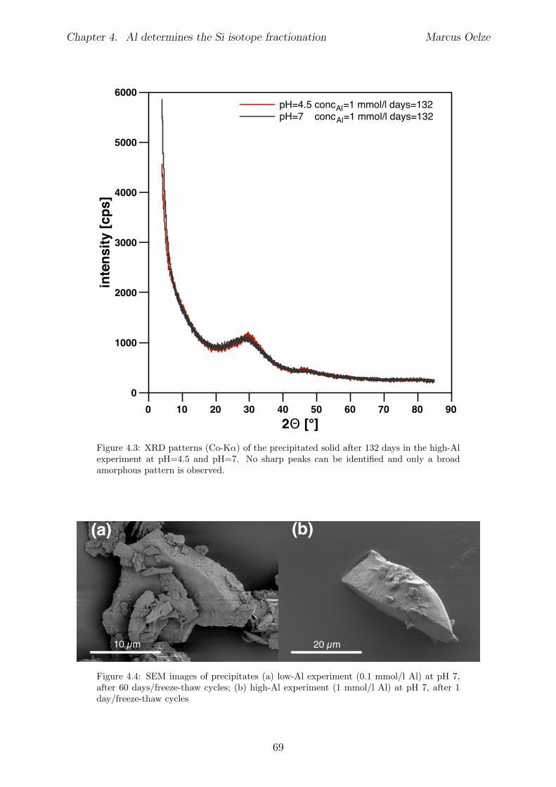
Chapter 4. Al determines the Si isotope fractionation Marcus Oelze
0 10 20 30 40 50 60 70 80 902 [°]
0
1000
2000
3000
4000
5000
6000in
tens
ity [c
ps]
pH=4.5 concAl
=1 mmol/l days=132
pH=7 concAl
=1 mmol/l days=132
Figure 4.3: XRD patterns (Co-K↵) of the precipitated solid after 132 days in the high-Alexperiment at pH=4.5 and pH=7. No sharp peaks can be identified and only a broadamorphous pattern is observed.
20 µm
(b)(a)
10 µm
Figure 4.4: SEM images of precipitates (a) low-Al experiment (0.1 mmol/l Al) at pH 7,after 60 days/freeze-thaw cycles; (b) high-Al experiment (1 mmol/l Al) at pH 7, after 1day/freeze-thaw cycles
69
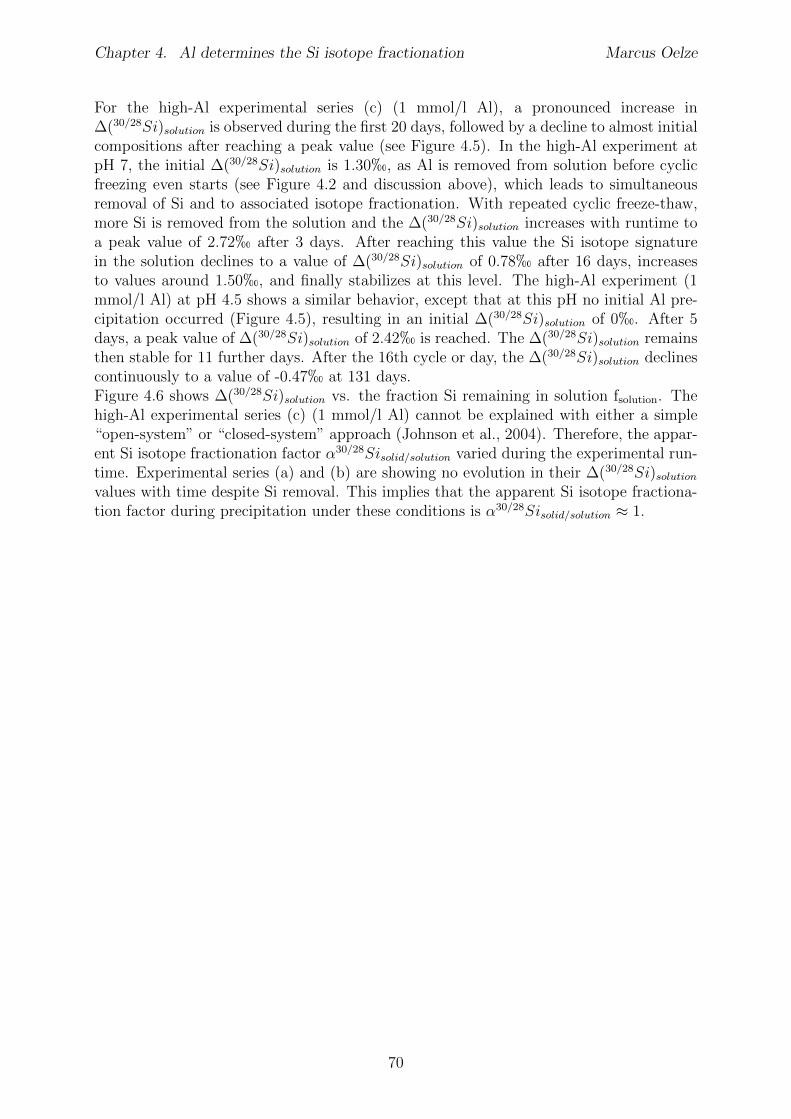
Chapter 4. Al determines the Si isotope fractionation Marcus Oelze
For the high-Al experimental series (c) (1 mmol/l Al), a pronounced increase in�(30/28Si)
solution
is observed during the first 20 days, followed by a decline to almost initialcompositions after reaching a peak value (see Figure 4.5). In the high-Al experiment atpH 7, the initial �(30/28Si)
solution
is 1.30h, as Al is removed from solution before cyclicfreezing even starts (see Figure 4.2 and discussion above), which leads to simultaneousremoval of Si and to associated isotope fractionation. With repeated cyclic freeze-thaw,more Si is removed from the solution and the �(30/28Si)
solution
increases with runtime toa peak value of 2.72h after 3 days. After reaching this value the Si isotope signaturein the solution declines to a value of �(30/28Si)
solution
of 0.78h after 16 days, increasesto values around 1.50h, and finally stabilizes at this level. The high-Al experiment (1mmol/l Al) at pH 4.5 shows a similar behavior, except that at this pH no initial Al pre-cipitation occurred (Figure 4.5), resulting in an initial �(30/28Si)
solution
of 0h. After 5days, a peak value of �(30/28Si)
solution
of 2.42h is reached. The �(30/28Si)solution
remainsthen stable for 11 further days. After the 16th cycle or day, the �(30/28Si)
solution
declinescontinuously to a value of -0.47h at 131 days.Figure 4.6 shows �(30/28Si)
solution
vs. the fraction Si remaining in solution fsolution. Thehigh-Al experimental series (c) (1 mmol/l Al) cannot be explained with either a simple“open-system” or “closed-system” approach (Johnson et al., 2004). Therefore, the appar-ent Si isotope fractionation factor ↵30/28Si
solid/solution
varied during the experimental run-time. Experimental series (a) and (b) are showing no evolution in their �(30/28Si)
solution
values with time despite Si removal. This implies that the apparent Si isotope fractiona-tion factor during precipitation under these conditions is ↵30/28Si
solid/solution
⇡ 1.
70
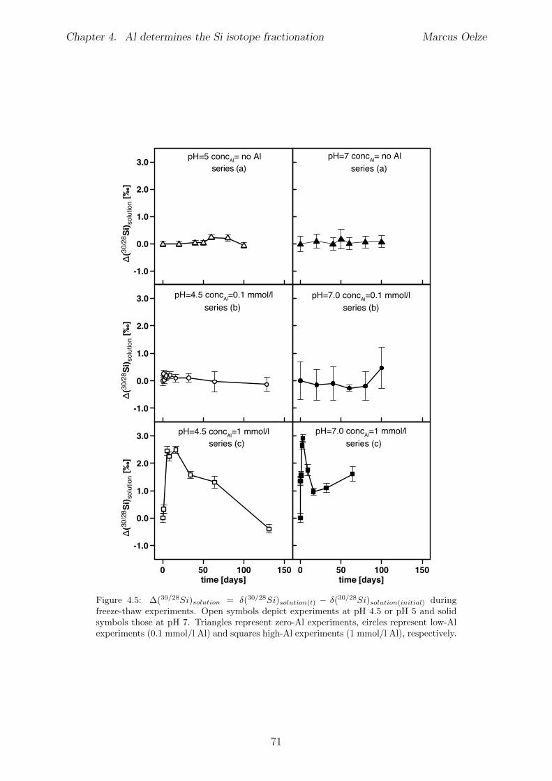
Chapter 4. Al determines the Si isotope fractionation Marcus Oelze
-1.0
0.0
1.0
2.0
3.0
(30
/28Si
) so
lutio
n [‰
]
-1.0
0.0
1.0
2.0
3.0
(30
/28Si
) so
lutio
n [‰
]
0 50 100 150time [days]
-1.0
0.0
1.0
2.0
3.0
(30
/28Si
) so
lutio
n [‰
]
0 50 100 150time [days]
pH=4.5 concAl=1 mmol/l
pH=4.5 concAl=0.1 mmol/l
pH=7.0 concAl=1 mmol/l
pH=7.0 concAl=0.1 mmol/l
pH=5 concAl= no Al pH=7 conc
Al= no Al
series (b)
series (a) series (a)
series (b)
series (c) series (c)
Figure 4.5: �(30/28Si)solution
= �(30/28Si)solution(t)
� �(30/28Si)solution(initial)
duringfreeze-thaw experiments. Open symbols depict experiments at pH 4.5 or pH 5 and solidsymbols those at pH 7. Triangles represent zero-Al experiments, circles represent low-Alexperiments (0.1 mmol/l Al) and squares high-Al experiments (1 mmol/l Al), respectively.
71
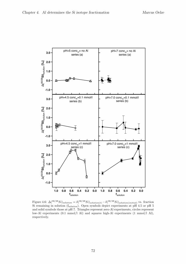
Chapter 4. Al determines the Si isotope fractionation Marcus Oelze
-1.0
0.0
1.0
2.0
3.0
(30
/28Si
) so
lutio
n [‰
]
-1.0
0.0
1.0
2.0
3.0
(30
/28Si
) so
lutio
n [‰
]
0.00.20.40.60.81.0fsolution
-1.0
0.0
1.0
2.0
3.0
(30
/28Si
) so
lutio
n [‰
]
0.00.20.40.60.81.0fsolution
pH=4.5 concAl=1 mmol/l
pH=4.5 concAl=0.1 mmol/l
pH=7.0 concAl=1 mmol/l
pH=7.0 concAl=0.1 mmol/l
pH=5 concAl= no Al pH=7 conc
Al= no Al
series (b)
series (a) series (a)
series (b)
series (c) series (c)
Figure 4.6: �(30/28Si)solution
= �(30/28Si)solution(t)
��(30/28Si)solution(initial)
vs. fractionSi remaining in solution (f
solution
). Open symbols depict experiments at pH 4.5 or pH 5and solid symbols those at pH 7. Triangles represent zero-Al experiments, circles representlow-Al experiments (0.1 mmol/l Al) and squares high-Al experiments (1 mmol/l Al),respectively.
72
Chapter 4. Al determines the Si isotope fractionation Marcus Oelze
4.6 Discussion
4.6.1 Potential removal processes
During freezing, four main processes govern the removal of Si from solution (Dietzel,2005): (i) The solubility of Si decreases with decreasing temperature in pure Si-containingsolutions (Rimstidt and Barnes, 1980). (ii) During ice formation, the total amount ofliquid H2O decreases and the remaining solution becomes supersaturated with respectto amorphous silica. (iii) Al-hydroxide can precipitate from solution as the solution getssupersaturated with respect to amorphous Al(OH)3 or gibbsite. Dissolved Si can thensorb onto Al-hydroxide particles. As a result hydroxyaluminosilicates (HAS), gel- orallophane-like solids that incorporate both Si and Al can form.The removal of Si by precipitation of amorphous silica, HAS, gel or allophane-like solidsfrom a solution that contains monosilicic acid involves polymerization of monosilicic acidto polysilicic acid. During this so-called condensation process, the reaction of monosilicicacid molecules forms disilicic acid. Disilicic acid reacts further with monosilicic acidto form trisilicic acid and tetrasilicic acid (Iler, 1979). With ongoing oligomerizationcyclic tetramers form and higher orders of polymerized silicic acid, silica colloids, gel andparticles form (Greenberg and Sinclair, 1955; Iler, 1979; Tarutani, 1989). In the zero-Al experimental series (a) and the low-Al experimental series (b) the removal of Si fromsolution is only induced by polymerization of monosilicic acid, which leads to the formationof the solid. In contrast, the removal of Si in experimental series (c) is probably forcedby the formation of Al-hydroxides with which monomeric Si can co-precipitate or ontowhich monosilicic acid will adsorb. As a result HAS phases might form. Precipitation ofAl from solution provides ⌘Al-OH surface sites which are known to be highly attractivefor Si(OH)4 to form Al-O-Si bonds (see Dietzel (2002) and references therein). Thisprocess ultimately leads to the formation of crystalline silicate phases such as halloysiteor kaolinite (Exley et al., 2002). Therefore the presence of Al (and other ions, see e.g.Marshall and Warakomski (1980); Marshall (1980b,a)) in the system can significantlydecrease the solubility of silica (Dixit et al., 2001; Van Cappellen et al., 2002). Hence inprecipitation experiments Si removal is usually accelerated by the presence of Al (Willey,1975a,b; Wada and Kubo, 1975).We compared the number of adsorption sites available for Si fixation in our high-Alexperiments to the amount of Si removed. We therefore compare the amount of Al thatis precipitated (0.05 mmol Al) to the precipitated amount of Si (1.2 mmol Si; both valuesfor the high-Al experiment (1m mmol/l Al) pH 4.5, measured after 131 days). Assumingthat only monosilicic acid is adsorbed (assumption: 1 mol Al binds 1 mol Si), the amountof Al precipitated is insu�cient to fixate all Si removed from solution. We thereforesuggest that the high degree of supersaturation attained already during the first freeze-thaw cycles leads to the formation of negatively charged polysilicic acid molecules (seesubsection 4.8.2 Figure 4.9). These polysilicic acid molecules have a much higher a�nityfor Al precipitates surfaces, as shown experimentally (Dietzel and Bohme, 1997; Tayloret al., 1997). Furthermore polysilicic acid molecules form at the surface of Al-hydroxides,which provides an important mechanism to fixate Si onto Al-hydroxides (Jepson et al.,1976; Yokoyama et al., 1982; Dietzel, 2002). Therefore, the adsorption of polysilicic acidcan account for the relatively large amount of Si adsorbed/precipitated in our high-Alexperiments.
73
Chapter 4. Al determines the Si isotope fractionation Marcus Oelze
4.6.2 Isotope fractionation associated with Si removal
Our experimental design does not allow us to determine Si removal rates and the isotopiccomposition under constant conditions. Parameters like temperature, Si saturation index,Si solubility and ionic strength change during freeze-thaw cycles. However, the systemdoes evolve into a state where Si concentration and therefore the net solid formation rateis constant. To illustrate these di↵erent stages we next explore the kinetics and theirchange during a freeze-thaw experiment.The kinetics of monosilicic acid removal from solution, as observed in our zero- and low-Alseries (a) and (b), has been investigated over decades. A range of possible kinetic mod-els have been derived from measurements of the time-dependent decrease of monosilicicacid in solution (see summary in Tobler et al. (2009)). Icopini et al. (2005) suggestedthat during the formation of di- and trisilicic acid an equilibrium is immediately attainedand that further oligomerization of silicic acid is a fast process (Conrad et al., 2007).The ongoing formation from nanocolloidal silica to a solid precipitate in contrast is aslow process (Conrad et al., 2007). Given these previous findings we suggest that for theexperimental series (a) and (b) the mechanisms responsible for the potentially entailingisotope fractionation (Si isotope fractionation during the formation of di-, tri and tetrasili-cic acid; as no Al is involved) occur rapidly. One possible explanation for the stable Siisotopic composition of the solution despite fast reaction rates in the zero-Al and low-Alexperimental series (a) and (b) is that the a net isotope fractionation between the originalSi in solution, the polymerized form of silicic acid and the solid that eventually forms is↵30/28Si
solid/solution
= 1. During reactions of tetrasilicic acids to higher polymerized silicicacid no further isotope fractionation is expected due to the high mass of these molecules(molecular mass > 120). We therefore suggest that in the absence of Al the rate at whichpure Si precipitates are formed does not impact the resulting isotope fractionation.In contrast to series (a) and (b) a strong initial Si isotope fractionation accompanies Siremoval from solution in the high-Al series (c). We tested di↵erent kinetic rate laws(zeroth-order, first-order, second-order) for unidirectional precipitation only to explainthe evolution of Si concentration with time. Only an irreversible second-order kineticrate law, assuming a net rate constant, is able to fit the measured evolution of Si con-centration with time assuming irreversible precipitation (see subsection 4.8.3). We usethe Si isotope results to further evaluate this description whether the governing processof net solid formation is a unidirectional and irreversible precipitation reaction. In thiscase an open-system type isotope mass balance fractionation model should be applicable(Johnson et al., 2004). For the first freeze-thaw cycles such precipitation results in areasonable fractionation factor (�(30/28Si)
solid�solution
⇡ �4.3h, subsection 4.8.3). How-ever this mass balance approach fails with ongoing experimental runtime, as unusuallylarge Si isotope fractionation between solid and solution result for the later stages of theexperiment (�(30/28Si)
solid�solution
⇡ +8h, subsection 4.8.3). Such large enrichment ofheavy 30Si within a solid product has never been observed nor predicted by first princi-ple equilibrium isotope fractionation calculations (Meheut et al., 2007, 2009; Meheut andSchauble, 2014; Opfergelt and Delmelle, 2012). Hence we conclude that solely unidirec-tional precipitation is not a process in operation in these experiments.We propose instead that the evolution of dissolved Si is governed by the alternationbetween precipitation (freezing-stage) and dissolution of the precipitated solid (thawing-stage). We propose further that net precipitation and net dissolution both follow a first-order rate law, as shown for quartz dissolution-precipitation reactions (Dove and Rimstidt(1994); see subsection 4.8.3). An important prerequisite of this model is that the Si
74
Chapter 4. Al determines the Si isotope fractionation Marcus Oelze
fixated during freezing can dissolve rapidly during thawing. Dietzel (2005) showed thatup to 95% of the fixated Si during freezing-thawing experiments is released into solutionwithin 3 days. This release translates into rates of ⇡1⇤10�10 mol*m�2⇤sec�1 (assuminga surface area of hydrated amorphous silica of ⇡1000 m2⇤g�1; Iler (1979)). This rateis much faster than dissolution rates for amorphous silica determined experimentally atconstant temperature (1⇤10�12 mol⇤m�2⇤sec�1 at 20�; e.g. Icenhower and Dove (2000)).The reason for such high dissolution rates observed in our experiments might be themetastability of the amorphous silica formed or its small particle size, where surface areasmight be much higher than the assumed 1000 m2⇤g�1.Using this framework of precipitation and dissolution reactions, results from the high-Alexperimental series (c) (1 mmol/l Al) can be described as follows:(1.) The increase of �(30/28Si)
solution
during the first 20 days can be attributed to kineticisotope fractionation during unidirectional attachment of Si onto Al-hydroxides (precip-itation dominates over dissolution). As a result, the precipitate is strongly enriched in28Si (Oelze et al., 2014).(2.) In the second phase of the experiment, �(30/28Si)
solution
values return to the initialisotopic composition (close to 0h for the experiment at pH 4.5 and close to 1.30h for theexperiment pH 7). Although the dissolved Si concentrations do not change, solids haveto undergo dissolution-reprecipitation cycles for their isotope composition to change.At the end of the experiments, concentrations are at steady-state. Therefore the�(30/28Si)
solution
value at the end of the experiment reflects what we call here dynamicsteady-state isotope fractionation. It is di�cult to attribute this steady-state isotopefractionation to either equilibrium or kinetic e↵ects, as we lack independent estimatesof the equilibrium fractionation factor. Theoretical calculations predict that the phasewith the higher degree of polymerization should be enriched in 30Si (Ding et al., 1996;Meheut et al., 2007). Further calculations of Meheut et al. (2009), Polyakov and Mineev(2000) and Schauble (2001) show that in a covalent bonding environment heavy isotopesare favored, because they lower the zero-point energy and therefore stronger bonds areformed. Considering these previous studies we expect that at equilibrium either no iso-tope fractionation or preferential incorporation of heavy Si isotopes into the formed solidsoccurs. Therefore it seems that our experimental results are consistent with theoreticalpredictions of isotopic equilibrium, although the system does not reach thermodynamicor isotopic equilibrium.
4.6.3 Rate dependence of Si isotope fractionation
We suggest that both precipitation and dissolution reactions are accompanied by Si iso-tope fractionation. The change of the net precipitation and net dissolution rates throughtime, combined with two associated isotope fractionation factors, leads to a change inthe bulk fractionation factor due to simple mass balance e↵ects. Figure 4.7 shows howthe measured net solid formation rate changes along with the relative isotopic di↵erencebetween solid and solution.It is possible that a change in surface area of the solids influences the apparent fraction-ation factor, as it will a↵ect the exchange flux. Unfortunately the determination of theactual surface area of the formed reactive solids is virtually impossible, as the area willbe altered once the solids are removed from the ambient solution.Regardless of this e↵ect, we can infer that the isotopic di↵erence between solid and solution�(30/28Si)
solid�solution
changes with time from a kinetically dominated regime at high net
75
Chapter 4. Al determines the Si isotope fractionation Marcus Oelze
solid formation rates, where light Si isotopes are rapidly withdrawn from the solutioninto the solid, to a dynamic steady-state regime, where the Si concentration is nearlyconstant between cycles. In this regime the isotopic di↵erence between solid and solution,compared to the kinetic regime, is very small. We show a model of this evolution in Figure4.7 for the high-Al experiment at pH 4.5 (1 mmol/l Al) (see Model 3 in subsection 4.8.3).We model continuous precipitation and dissolution assuming two opposing first-orderreactions, which are associated with respective isotope fractionation factors ↵30/28Si
prec
and ↵30/28Sidiss
. We find that for the high Al experiments the most likely case is one wherethe major part of the formed solid redissolves and exchanges with the solution at eachcycle. The best fit values of the developed isotope mass balance model (see Figure 4.11 inthe subsection 4.8.3) yields isotope fractionation factors for precipitation and dissolutionof ↵30/28Si
prec
=0.9953 (103ln↵prec
= -4.7h) and ↵30/28Sidiss
=0.9947 (103ln↵diss
= -5.3h) for the experiment at pH 4.5 and ↵30/28Si
prec
=0.9989 to 0.9991 (103ln↵prec
=-1.1 to -0.9h) and ↵30/28Si
diss
=0.9992 to 0.9994 (103ln↵diss
= -0.8 to -0.6h) for theexperiment at pH 7, respectively.The initial kinetic isotope fractionation factor, where net-precipitation dominates, is likelygoverned by chemisorption processes. These values are similar to the fractionation factorsfound in the Oelze et al. (2014) adsorption experiments (-1.8h to -3h, depending on Siconcentration). This initial Si isotope fractionation factor, probably reaches the kineticlimit of Si isotope fractionation (Nielsen et al., 2012; Druhan et al., 2013). Thereforeit might represent the absolute maximum kinetic Si isotope fractionation factor for Siduring precipitation. Above this kinetic limit an increase of the precipitation rate is notaccompanied by a further increase in the isotope fractionation factor (see Figure 8 inNielsen et al. (2012)).In the zero-Al and low-Al experimental series (a) and (b), the initial phase involvingkinetic isotope fractionation is not encountered, and the system evolves with an apparentisotope fractionation factor of ↵30/28Si
solid/solution
=1 (103ln↵solid/solution
= 0h). In allhigh-Al experiments, towards the end the Si isotope fractionation at steady-state is alsoclose to ↵30/28Si
solid/solution
=1 (103ln↵solid/solution
= 0h).
76
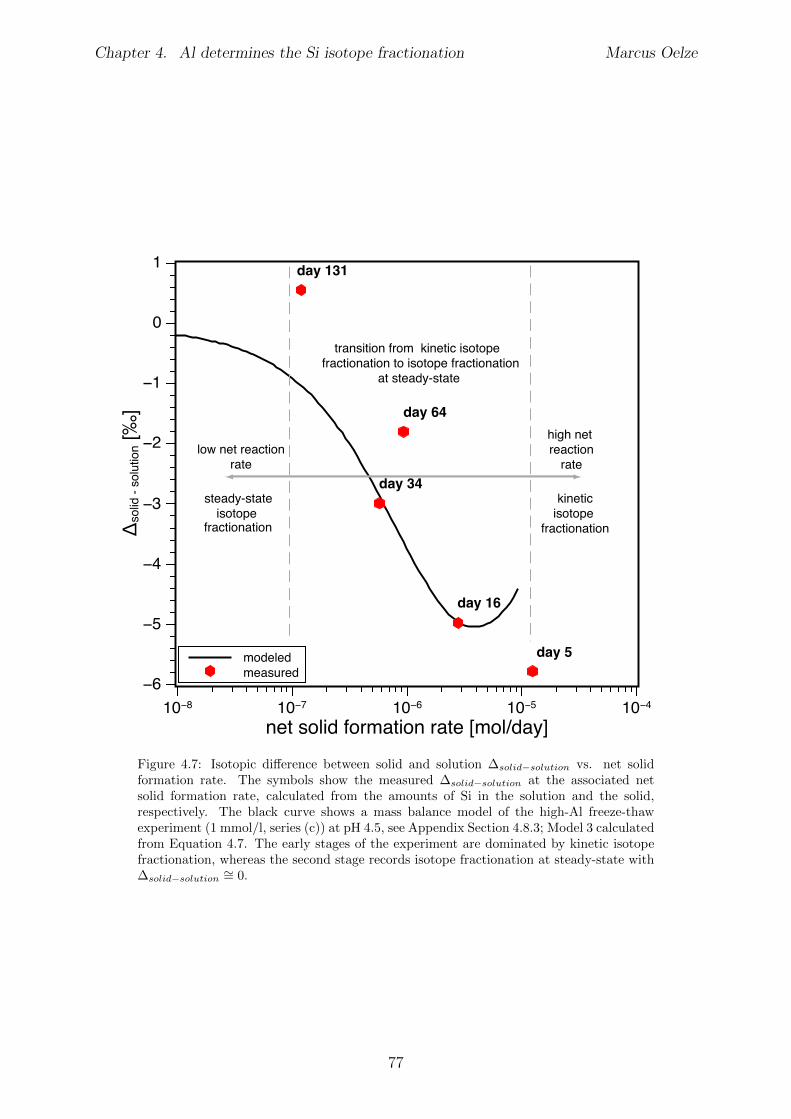
Chapter 4. Al determines the Si isotope fractionation Marcus Oelze
steady-stateisotope
fractionation
transition from kinetic isotope fractionation to isotope fractionation
at steady-state
kineticisotope
fractionation
high net reaction
ratelow net reaction
rate
modeled measured
Figure 4.7: Isotopic di↵erence between solid and solution �solid�solution
vs. net solidformation rate. The symbols show the measured �
solid�solution
at the associated netsolid formation rate, calculated from the amounts of Si in the solution and the solid,respectively. The black curve shows a mass balance model of the high-Al freeze-thawexperiment (1 mmol/l, series (c)) at pH 4.5, see Appendix Section 4.8.3; Model 3 calculatedfrom Equation 4.7. The early stages of the experiment are dominated by kinetic isotopefractionation, whereas the second stage records isotope fractionation at steady-state with�
solid�solution
⇠= 0.
77
Chapter 4. Al determines the Si isotope fractionation Marcus Oelze
4.7 Summary and implications
We have demonstrated that, during cyclic freeze-thaw of dissolved Si-containing solu-tions, Si is removed from the solution. In the absence of appreciable amounts of Althis removal is not accompanied by the fractionation of Si isotopes. The formation ofdi-, tri- and tetrasilicic acid apparently proceeds with a Si isotope fractionation factor↵30/28Si
solid/solution
=1 (103ln↵solid/solution
= 0h). With subsequent oligomerization andformation of almost pure Si solids no further Si isotope fractionation is expected due tothe high molecular masses involved. To conclude, the precipitation of pure Si solids doesnot lead to any Si isotope fractionation.In contrast if Al is present in these solutions at high concentrations (i.e. here 1 mmol/l),Si removal is faster and accompanied by strong Si isotope fractionation favoring the lightisotopes in the solids. For these high Al experiments we calculate a fractionation factor ofup to ↵30/28Si
solid/solution
=0.9950 (103ln↵solid/solution
= -5h) for the first 20 days of theexperiment . This strong initial isotope fractionation occurs during adsorption or bindingof Si onto Al-hydroxide (Oelze et al., 2014). With ongoing runtime the early formedprecipitates are reorganized wholesale, such that ↵30/28Si
solid/solution
=1 (103ln↵solid/solution
= 0h). Hence after attaining steady-state conditions no Si isotope fractionation duringsolid reorganization occurs. It is likely that the zero fractionation factor observed in thefinal phase of the high-Al experimental series (c) and in the low- and zero-Al experimentsrepresents the equilibrium isotope fractionation factor of silica precipitation.Regarding silicate weathering this study implies that where secondary precipitates (such asmetastable silica-containing solids) are formed, kinetic isotope e↵ects will be dominating.Secondary minerals formed with high Al/Si ratios, will be enriched in 28Si (see Savageet al. (2013); Cornelis et al. (2014)). This conclusion is supported by the observation thatSi measured in river water is enriched in 30Si over the host rock (e.g. Ziegler et al. (2005b);Georg et al. (2006a); Opfergelt et al. (2009); Bern et al. (2010); Steinhoefel et al. (2011),while secondary soil minerals are mostly depleted in 30Si. Moreover, this study suggeststhat slowly re-organization or recrystallization of these solids is likely accompanied bynegligible Si isotope fractionation.During silicification of sediments a variety of isotope fractionation factors are likely to bein operation, depending on individual environmental conditions. If solutions are supersat-urated with respect to opal-A or opal-CT and free of “impurities” (no Al or other carrierphases present) they will probably precipitate with an Si isotope fractionation factor of↵30/28Si
solid/solution
=1 (103ln↵30/28Sisolid/solution
of 0h). In contrast, the presence of Alin the system increases the precipitation rate (Wada and Kubo, 1975; Willey, 1975b) andtherefore Si isotopes will fractionate according to the Al/Si ratio. The di↵erence betweenthe rapidly precipitating Al-containing phase compared to the slowly precipitating Al-freephase is then reflected in the Si isotope composition of these two phases, with the higherenrichment of 28Si in the Al-containing phase.The inferred absence of any ↵30/28Si
solid/solution
>1 (103ln↵30/28Sisolid/solution
> 0h) be-tween solid and solution implies that in the geologic record Si isotope ratios exceedingthat of their source materials are likely to be a mass balance e↵ect stemming from fastprecipitation of solids enriched in light Si isotope.To conclude, the enrichment of light Si isotopes in geologic low-temperature processesis related to fast precipitation of secondary solids as induced by co-precipitation of Alphases or another carrier phase (e.g. Fe(III)). In contrast no Si isotope fractionationcan be expected between solid and solution during slow precipitation under equilibrium
78
Chapter 4. Al determines the Si isotope fractionation Marcus Oelze
conditions.
4.8 Appendix Chapter 4
4.8.1 Tables
Table 4.1: Freeze-thaw experiments series (a), Si concentration values and �(29/28Si)NBS28
and �(30/28Si)NBS28
values as well as 95% confidence interval (CI) for experiments withno Al.
name pH sampling time Al Si �(29/28Si) CI �(30/28Si) CI[day] [mmol/l] [ppm] [h] [h] [h] [h]
5 0 0 s 5.0 0 - 1.77 0.01 0.07 -0.04 0.075 20 0 s 5.0 20 - 1.28 -0.02 0.12 -0.05 0.075 40 0 s 5.0 40 - 1.22 0.01 0.04 -0.01 0.025 50 0 s 5.0 50 - 1.30 0.03 0.04 -0.01 0.055 60 0 s 5.0 60 - 1.13 0.08 0.01 0.20 0.065 80 0 s 5.0 80 - 0.95 0.08 0.07 0.17 0.085 100 0 s 5.0 100 - 0.20 -0.01 0.10 -0.10 0.087 0 0 s 7.0 0 - 1.75 0.00 0.06 -0.13 0.207 20 0 s 7.0 20 - 1.79 -0.01 0.03 -0.04 0.177 40 0 s 7.0 40 - 1.40 -0.08 0.05 -0.13 0.147 50 0 s 7.0 50 - 1.50 0.01 0.07 0.05 0.317 60 0 s 7.0 60 - 1.41 -0.07 0.06 -0.12 0.087 80 0 s 7.0 80 - 1.46 -0.05 0.07 -0.08 0.117 100 0 s 7.0 100 - 1.49 -0.06 0.12 -0.05 0.09
* sample names: (pH) (day) (Al-start-conc[mmol/l]) (solution[s]
79
Chapter 4. Al determines the Si isotope fractionation Marcus Oelze
Table 4.2: Freeze-thaw experiments series (b), Si concentration values and �(29/28Si)NBS28
and �(30/28Si)NBS28
values as well as 95% confidence interval (CI) for experiments with0.1 mmol/l initial Al concentration.
name pH sampling time Al Si �(29/28Si) CI �(30/28Si) CI[day] [mmol/l] [ppm] [h] [h] [h] [h]
4.5 start 0.1 s 4.5 start 0.08 1.42 -0.05 0.02 -0.12 0.134.5 1 0.1 s 4.5 1 0.09 1.42 -0.01 0.07 0.14 0.024.5 2 0.1 s 4.5 2 0.09 1.42 0.00 0.24 -0.09 0.034.5 3 0.1 s 4.5 3 0.08 1.40 0.00 0.04 0.02 0.034.5 4 0.1 s 4.5 4 0.08 1.39 0.05 0.00 0.07 0.054.5 9 0.1 s 4.5 9 0.05 1.29 0.05 0.08 0.09 0.044.5 16 0.1 s 4.5 16 0.08 1.36 0.00 0.05 -0.03 0.054.5 32 0.1 s 4.5 32 0.10 1.35 0.01 0.04 -0.02 0.094.5 64 0.1 s 4.5 64 0.10 1.40 -0.05 0.13 -0.14 0.344.5 128 0.1 s 4.5 128 0.06 0.71 -0.12 0.13 -0.24 0.217 0 0.1 s 7.0 0 0.10 1.71 0.04 0.78 0.03 0.677 20 0.1 s 7.0 20 0.02 1.08 -0.19 0.26 -0.12 0.547 40 0.1 s 7.0 40 0.01 0.71 -0.27 1.14 -0.08 0.607 60 0.1 s 7.0 60 0.02 0.24 -0.05 1.22 -0.25 0.017 80 0.1 s 7.0 80 0.00 0.10 -0.18 0.88 -0.16 0.507 100 0.1 s 7.0 100 0.01 0.79 0.19 0.06 0.50 0.74
* sample names: (pH) (day) (Al-start-conc[mmol/l]) (solution[s]
80
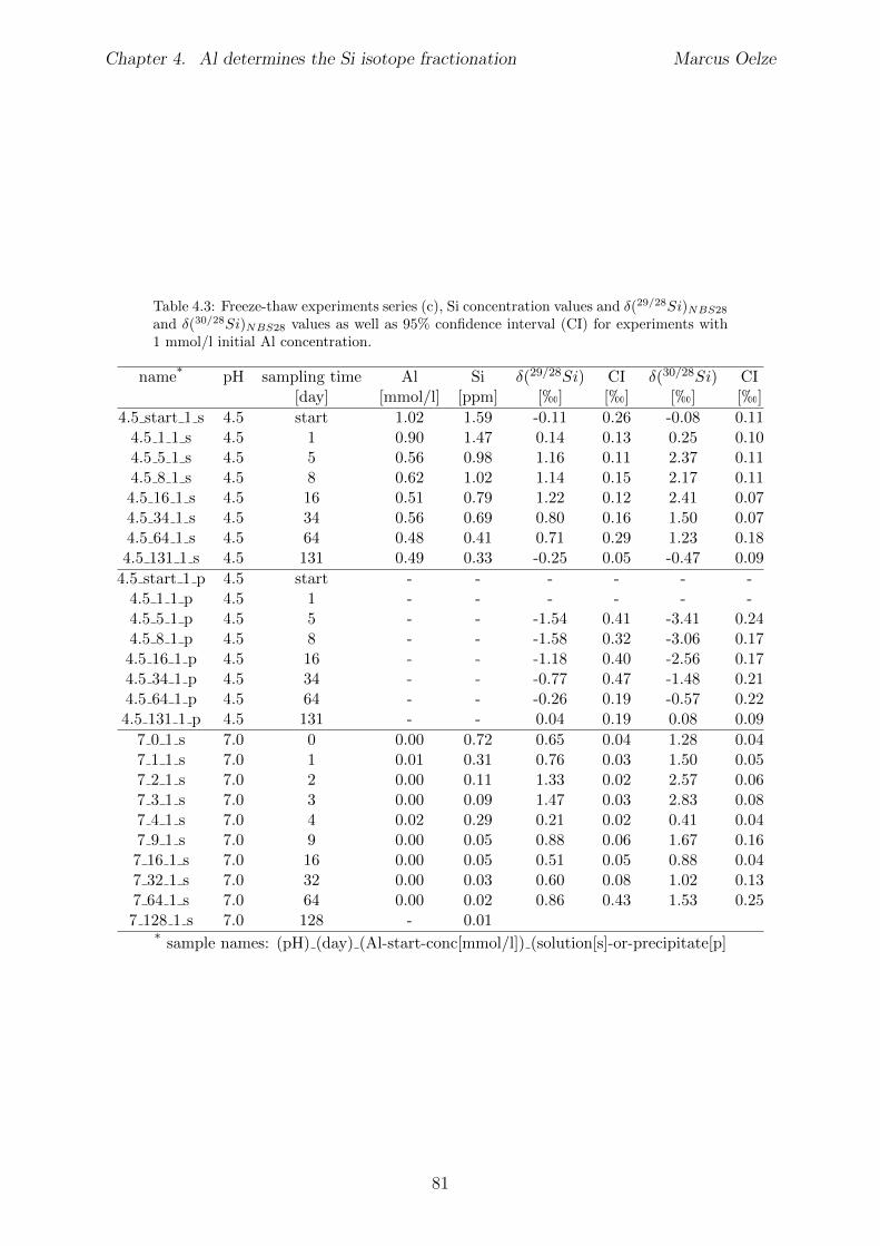
Chapter 4. Al determines the Si isotope fractionation Marcus Oelze
Table 4.3: Freeze-thaw experiments series (c), Si concentration values and �(29/28Si)NBS28
and �(30/28Si)NBS28
values as well as 95% confidence interval (CI) for experiments with1 mmol/l initial Al concentration.
name* pH sampling time Al Si �(29/28Si) CI �(30/28Si) CI[day] [mmol/l] [ppm] [h] [h] [h] [h]
4.5 start 1 s 4.5 start 1.02 1.59 -0.11 0.26 -0.08 0.114.5 1 1 s 4.5 1 0.90 1.47 0.14 0.13 0.25 0.104.5 5 1 s 4.5 5 0.56 0.98 1.16 0.11 2.37 0.114.5 8 1 s 4.5 8 0.62 1.02 1.14 0.15 2.17 0.114.5 16 1 s 4.5 16 0.51 0.79 1.22 0.12 2.41 0.074.5 34 1 s 4.5 34 0.56 0.69 0.80 0.16 1.50 0.074.5 64 1 s 4.5 64 0.48 0.41 0.71 0.29 1.23 0.184.5 131 1 s 4.5 131 0.49 0.33 -0.25 0.05 -0.47 0.094.5 start 1 p 4.5 start - - - - - -4.5 1 1 p 4.5 1 - - - - - -4.5 5 1 p 4.5 5 - - -1.54 0.41 -3.41 0.244.5 8 1 p 4.5 8 - - -1.58 0.32 -3.06 0.174.5 16 1 p 4.5 16 - - -1.18 0.40 -2.56 0.174.5 34 1 p 4.5 34 - - -0.77 0.47 -1.48 0.214.5 64 1 p 4.5 64 - - -0.26 0.19 -0.57 0.224.5 131 1 p 4.5 131 - - 0.04 0.19 0.08 0.097 0 1 s 7.0 0 0.00 0.72 0.65 0.04 1.28 0.047 1 1 s 7.0 1 0.01 0.31 0.76 0.03 1.50 0.057 2 1 s 7.0 2 0.00 0.11 1.33 0.02 2.57 0.067 3 1 s 7.0 3 0.00 0.09 1.47 0.03 2.83 0.087 4 1 s 7.0 4 0.02 0.29 0.21 0.02 0.41 0.047 9 1 s 7.0 9 0.00 0.05 0.88 0.06 1.67 0.167 16 1 s 7.0 16 0.00 0.05 0.51 0.05 0.88 0.047 32 1 s 7.0 32 0.00 0.03 0.60 0.08 1.02 0.137 64 1 s 7.0 64 0.00 0.02 0.86 0.43 1.53 0.257 128 1 s 7.0 128 - 0.01
* sample names: (pH) (day) (Al-start-conc[mmol/l]) (solution[s]-or-precipitate[p]
81
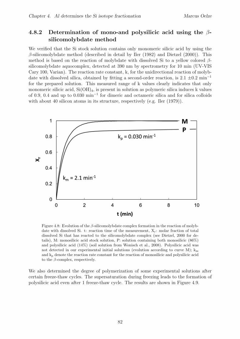
Chapter 4. Al determines the Si isotope fractionation Marcus Oelze
4.8.2 Determination of mono-and polysilicic acid using the �-silicomolybdate method
We verified that the Si stock solution contains only monomeric silicic acid by using the�-silicomolybdate method (described in detail by Iler (1982) and Dietzel (2000)). Thismethod is based on the reaction of molybdate with dissolved Si to a yellow colored �-silicomolybdate aquocomplex, detected at 390 nm by spectrometry for 10 min (UV-VISCary 100, Varian). The reaction rate constant, k, for the unidirectional reaction of molyb-date with dissolved silica, obtained by fitting a second-order reaction, is 2.1 ±0.2 min�1
for the prepared solution. This measured range of k values clearly indicates that onlymonomeric silicic acid, Si(OH)4, is present in solution as polymeric silica induces k valuesof 0.9, 0.4 and up to 0.030 min�1 for dimeric and octameric silica and for silica colloidswith about 40 silicon atoms in its structure, respectively (e.g. Iler (1979)).
Figure 4.8: Evolution of the �-silicomolybdate complex formation in the reaction of molyb-date with dissolved Si. t: reaction time of the measurement, X
r
: molar fraction of totaldissolved Si that has reacted to the silicomolybdate complex (see Dietzel, 2000 for de-tails), M: monosilicic acid stock solution, P: solution containing both monosilicic (86%)and polysilicic acid (14%) (soil solution from Wonisch et al., 2008). Polysilicic acid wasnot detected in our experimental initial solutions (evolution according to curve M); k
m
and kp
denote the reaction rate constant for the reaction of monosilicic and polysilicic acidto the �-complex, respectively.
We also determined the degree of polymerization of some experimental solutions aftercertain freeze-thaw cycles. The supersaturation during freezing leads to the formation ofpolysilicic acid even after 1 freeze-thaw cycle. The results are shown in Figure 4.9.
82
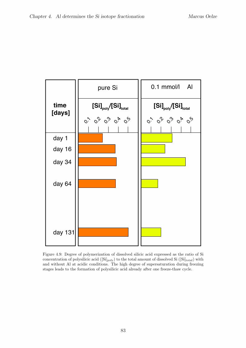
Chapter 4. Al determines the Si isotope fractionation Marcus Oelze
day 1
day 16
day 34
day 64
day 131
time [days]
pure Si
0.1 0.2 0.3 0.4 0.5
0.1 mmol/l Al
0.1 0.2 0.3 0.4 0.5
[Si]poly/[Si]total [Si]poly/[Si]total
Figure 4.9: Degree of polymerization of dissolved silicic acid expressed as the ratio of Siconcentration of polysilicic acid ([Si]
poly
) to the total amount of dissolved Si ([Si]total
) withand without Al at acidic conditions. The high degree of supersaturation during freezingstages leads to the formation of polysilicic acid already after one freeze-thaw cycle.
83
Chapter 4. Al determines the Si isotope fractionation Marcus Oelze
4.8.3 Modeling a net precipitation-dissolution process associ-ated with isotope fractionation
The aim of this modeling approach is not to determine exact rates or rate constants for at-tachment or detachment of Si. Determining rate constants would require that conditions(temperature, degree of under- and oversaturation, etc.) and solid properties (surfacearea) were constant during our experiments. This is not the case here. We rather intendto narrow the range of possible parameters that potentially explain the observed isotopicevolution of Si during our experiments. In order to test whether the experimental kineticsof the freezing-thawing approach can be described as two opposing first-order reactionsfor net precipitation and net dissolution, we tested several di↵erent kinetic rate models(zeroth-order, first-order, second-order, etc.) for the high-Al experiments. The net reac-tion rate constants used represent parameters that integrate over the changing conditionsduring the experiments.First we modeled the evolution of Si concentration. A pure precipitation mechanism fol-lowing a kinetic rate law of zeroth-order can be dismissed, as the evolution of Si concentra-tion with time clearly shows no linear dependence (see Figure 4.10). A pure precipitationmechanism following a first-order kinetic rate law (Equation 4.4) can neither be reconciledwith the measured Si concentration data for a best fit through the measured data (seeFigure 4.10 Model A) nor when we force the model to fit the Si concentration at t=131days (see Figure 4.10 Model B).
d
dt(M
d
) = Fprec
= �p⇥Md
(4.4)
Where Md
is the mass of dissolved Si in the experiment, Fprec
is the net precipitation ofSi and p is the rate constant.Assuming a second-order kinetic rate law (Equation 4.5) results in a reasonable fit to themeasured Si concentration data (see Model C in Figure 4.10).
d
dt(M
d
) = Fprec
= �p⇥M2d
(4.5)
We next explored whether this second-order precipitation model is compatible with themeasured isotope ratios. Unidirectional precipitation without back reaction can be quan-tified with an open-system mass balance model (Johnson et al., 2004). For the high-Alexperiment (1mmol/l Al) at pH 4.5, the open-system model was applied incrementallyfrom sampling point to sampling point. The initial Si concentration and initial isotopecomposition �(30/28Si)
initial
in solution were those of the previous step. This mass balancecalculation shows that the isotope fractionation factors change with each time-step. Theseisotope fractionation factors 103ln↵
solid/solution
are: day0-1: -4.3h, day1-5: -5.2h, day8-16: -1.0h, day16-34: 6.4h, day34-64: 0.5h, day64-131: 7.8h). Isotope fractionationfactors for Si as high as 7.8h calculated for the final steps have never been observed forSi isotope, and are regarded as highly unlikely. We therefore conclude that unidirectionalprecipitation is not a feasible mechanism to explain the observed Si isotopic evolution.Therefore we assume that two opposing reactions are in operation, and model these witha first-order kinetic rate law for precipitation and a first-order kinetic rate law for disso-lution. In the mass balance equation (Equation 4.6), M
d
is the total mass of Si dissolved
84
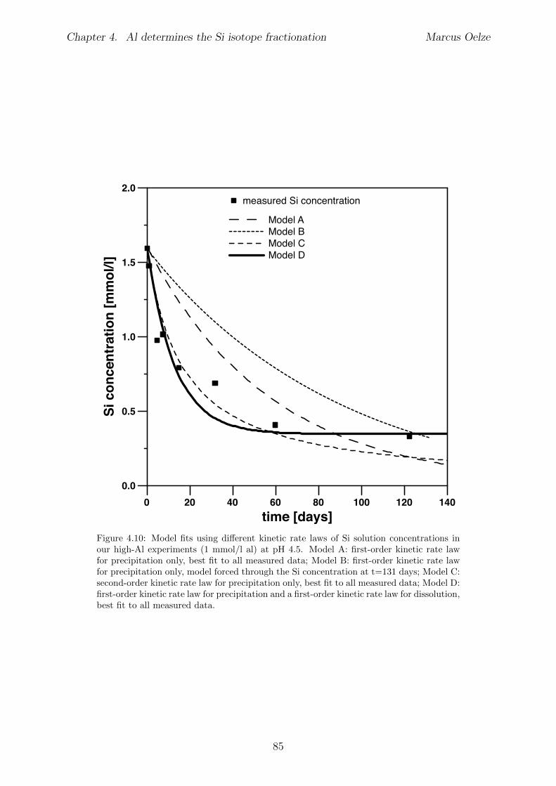
Chapter 4. Al determines the Si isotope fractionation Marcus Oelze
0 20 40 60 80 100 120 140time [days]
0.0
0.5
1.0
1.5
2.0
Si c
once
ntra
tion
[mm
ol/l]
Model AModel BModel CModel D
measured Si concentration
Figure 4.10: Model fits using di↵erent kinetic rate laws of Si solution concentrations inour high-Al experiments (1 mmol/l al) at pH 4.5. Model A: first-order kinetic rate lawfor precipitation only, best fit to all measured data; Model B: first-order kinetic rate lawfor precipitation only, model forced through the Si concentration at t=131 days; Model C:second-order kinetic rate law for precipitation only, best fit to all measured data; Model D:first-order kinetic rate law for precipitation and a first-order kinetic rate law for dissolution,best fit to all measured data.
85
Chapter 4. Al determines the Si isotope fractionation Marcus Oelze
in solution, Ms
is the total mass of Si solid and p and d are net reaction rate constants,p for precipitation and d for dissolution, respectively.
d
dt(M
d
) = Fdiss
� Fprec
= d⇥Ms
� p⇥Md
(4.6)
Assuming that the dissolved Si concentration at the end of the experiments reflects thesteady-state concentration, we can use the steady-state ratio (M
d
/Ms
)steady�state
) whichequals the d/p ratio (Table 4.4), Which reduces the number of adjustable parameters toone.
d = p⇥✓M
d
Ms
◆
steady�state
(4.7)
The evolution of Md
(and hence of dissolved Si concentration) was then numericallymodeled and fitted to the measured data according to Equation 4.8, using M
s
= Mtotal
�M
d
with Mtotal
being the total mass of Si to determine a value for p (Table 4.4).
d
dt(M
d
) = p⇥✓M
d
Ms
◆
steady�state
⇥ (Mtotal
�Md
)� p⇥Md
(4.8)
This assumption yields a reasonable fit to the measured Si concentration data (see ModelD in Figure 4.10).Next we develop an isotope mass balance model based on these simultaneous first-orderkinetic rate laws for precipitation as well as for dissolution. The basic approach is thesame for all scenarios explored. First, the evolution of dissolved Si concentration wasmodeled by using simple first-order irreversible kinetic descriptions of precipitation aswell as for dissolution (Equation 4.6). The evolution of the Si isotopic signature wasmodeled as follows:
d
dt(M
d
�d
) = Flast
⇥ (�l
+�diss
) + Fcumulative
⇥ (�c
+�diss
)
� Fprec
⇥ (�d
+�prec
) (4.9)
where �diss
(�diss
⇡ 103ln↵diss
) is the kinetic isotope fractionation factor during disso-lution and �
prec
(�prec
⇡ 103ln↵prec
) is the kinetic isotope fractionation factor duringprecipitation. Here, the solid dissolution flux F
diss
(Equation 4.4) has been separatedinto two components: the mass supplied by the outermost layer that precipitated at theprevious step F
last
and the mass from the cumulative solid Fcumulative
(formed since thebeginning of the experiment). Therefore we also make a distinction between the isotopicsignature of the outermost (“last”) layer �
l
and the isotopic signature of the cumulativesolid �
c
. The use of Equation 4.9 allows us to treat the solid as zoned or unzoned. Tosimplify Equation 4.9 we assume that the end of the experiments represents steady-state.Equation 4.9 dictates that at steady-state (�
s
� �d
)steady�state
= �prec
��diss
, regardlessof the value of F
diss
vs. Fcumulative
. Therefore we constrain the di↵erence �prec
� �diss
from the isotope data obtained at the end of our experiment (Table 4.4). We calculatethe relative contribution of the cumulative solid f
cumulative
to the total dissolution as:
86
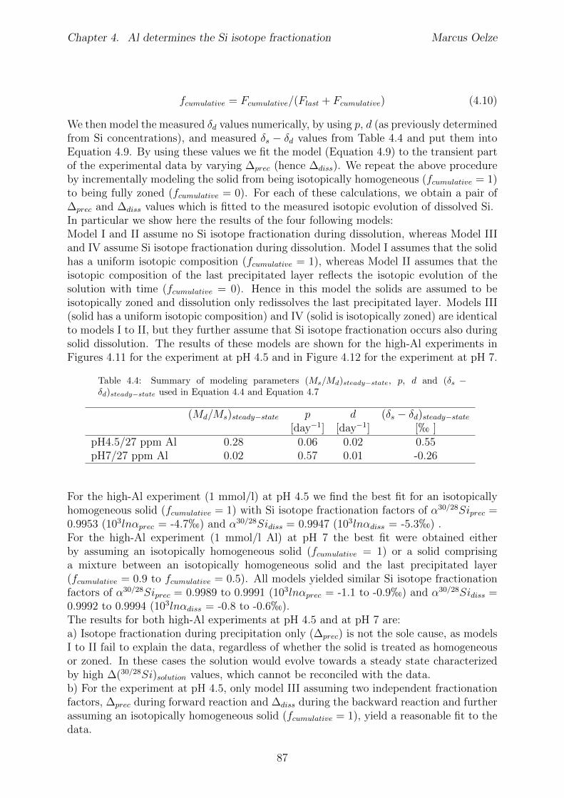
Chapter 4. Al determines the Si isotope fractionation Marcus Oelze
fcumulative
= Fcumulative
/(Flast
+ Fcumulative
) (4.10)
We then model the measured �d
values numerically, by using p, d (as previously determinedfrom Si concentrations), and measured �
s
� �d
values from Table 4.4 and put them intoEquation 4.9. By using these values we fit the model (Equation 4.9) to the transient partof the experimental data by varying �
prec
(hence �diss
). We repeat the above procedureby incrementally modeling the solid from being isotopically homogeneous (f
cumulative
= 1)to being fully zoned (f
cumulative
= 0). For each of these calculations, we obtain a pair of�
prec
and �diss
values which is fitted to the measured isotopic evolution of dissolved Si.In particular we show here the results of the four following models:Model I and II assume no Si isotope fractionation during dissolution, whereas Model IIIand IV assume Si isotope fractionation during dissolution. Model I assumes that the solidhas a uniform isotopic composition (f
cumulative
= 1), whereas Model II assumes that theisotopic composition of the last precipitated layer reflects the isotopic evolution of thesolution with time (f
cumulative
= 0). Hence in this model the solids are assumed to beisotopically zoned and dissolution only redissolves the last precipitated layer. Models III(solid has a uniform isotopic composition) and IV (solid is isotopically zoned) are identicalto models I to II, but they further assume that Si isotope fractionation occurs also duringsolid dissolution. The results of these models are shown for the high-Al experiments inFigures 4.11 for the experiment at pH 4.5 and in Figure 4.12 for the experiment at pH 7.
Table 4.4: Summary of modeling parameters (Ms
/Md
)steady�state
, p, d and (�s
��d
)steady�state
used in Equation 4.4 and Equation 4.7
(Md
/Ms
)steady�state
p d (�s
� �d
)steady�state
[day�1] [day�1] [h ]pH4.5/27 ppm Al 0.28 0.06 0.02 0.55pH7/27 ppm Al 0.02 0.57 0.01 -0.26
For the high-Al experiment (1 mmol/l) at pH 4.5 we find the best fit for an isotopicallyhomogeneous solid (f
cumulative
= 1) with Si isotope fractionation factors of ↵30/28Siprec
=0.9953 (103ln↵
prec
= -4.7h) and ↵30/28Sidiss
= 0.9947 (103ln↵diss
= -5.3h) .For the high-Al experiment (1 mmol/l Al) at pH 7 the best fit were obtained eitherby assuming an isotopically homogeneous solid (f
cumulative
= 1) or a solid comprisinga mixture between an isotopically homogeneous solid and the last precipitated layer(f
cumulative
= 0.9 to fcumulative
= 0.5). All models yielded similar Si isotope fractionationfactors of ↵30/28Si
prec
= 0.9989 to 0.9991 (103ln↵prec
= -1.1 to -0.9h) and ↵30/28Sidiss
=0.9992 to 0.9994 (103ln↵
diss
= -0.8 to -0.6h).The results for both high-Al experiments at pH 4.5 and at pH 7 are:a) Isotope fractionation during precipitation only (�
prec
) is not the sole cause, as modelsI to II fail to explain the data, regardless of whether the solid is treated as homogeneousor zoned. In these cases the solution would evolve towards a steady state characterizedby high �(30/28Si)
solution
values, which cannot be reconciled with the data.b) For the experiment at pH 4.5, only model III assuming two independent fractionationfactors, �
prec
during forward reaction and �diss
during the backward reaction and furtherassuming an isotopically homogeneous solid (f
cumulative
= 1), yield a reasonable fit to thedata.
87
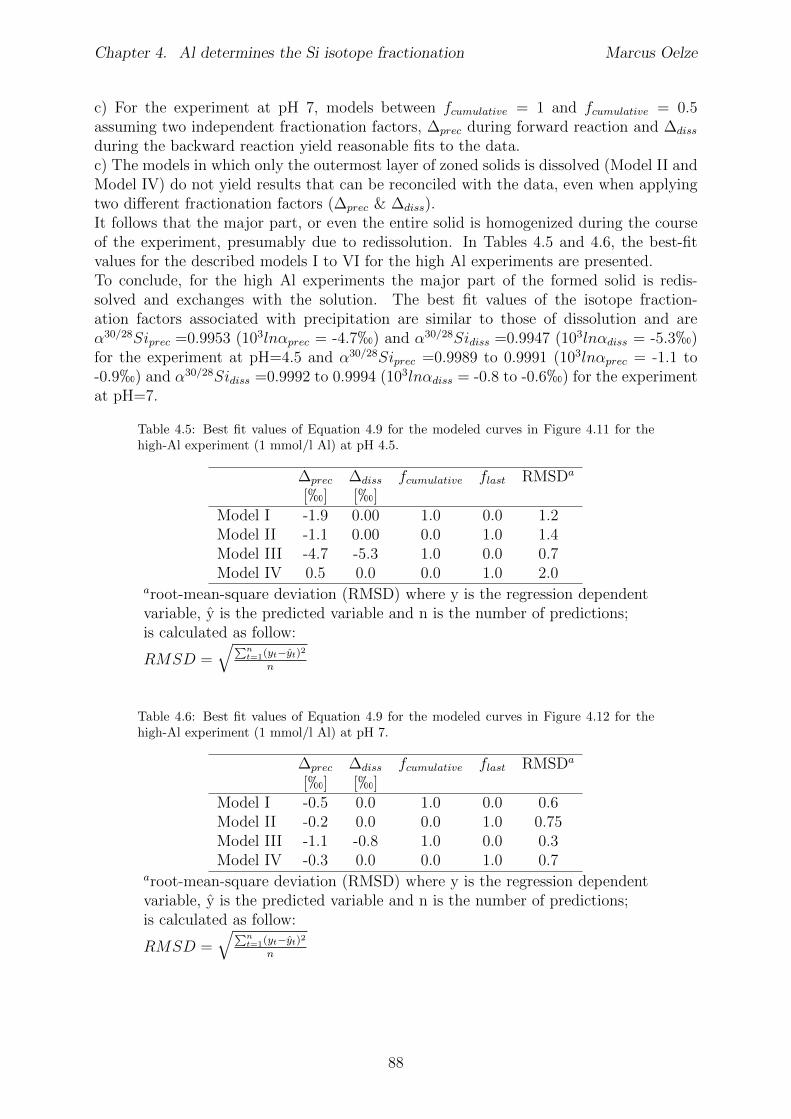
Chapter 4. Al determines the Si isotope fractionation Marcus Oelze
c) For the experiment at pH 7, models between fcumulative
= 1 and fcumulative
= 0.5assuming two independent fractionation factors, �
prec
during forward reaction and �diss
during the backward reaction yield reasonable fits to the data.c) The models in which only the outermost layer of zoned solids is dissolved (Model II andModel IV) do not yield results that can be reconciled with the data, even when applyingtwo di↵erent fractionation factors (�
prec
& �diss
).It follows that the major part, or even the entire solid is homogenized during the courseof the experiment, presumably due to redissolution. In Tables 4.5 and 4.6, the best-fitvalues for the described models I to VI for the high Al experiments are presented.To conclude, for the high Al experiments the major part of the formed solid is redis-solved and exchanges with the solution. The best fit values of the isotope fraction-ation factors associated with precipitation are similar to those of dissolution and are↵30/28Si
prec
=0.9953 (103ln↵prec
= -4.7h) and ↵30/28Sidiss
=0.9947 (103ln↵diss
= -5.3h)for the experiment at pH=4.5 and ↵30/28Si
prec
=0.9989 to 0.9991 (103ln↵prec
= -1.1 to-0.9h) and ↵30/28Si
diss
=0.9992 to 0.9994 (103ln↵diss
= -0.8 to -0.6h) for the experimentat pH=7.
Table 4.5: Best fit values of Equation 4.9 for the modeled curves in Figure 4.11 for thehigh-Al experiment (1 mmol/l Al) at pH 4.5.
�prec
�diss
fcumulative
flast
RMSDa
[h] [h]Model I -1.9 0.00 1.0 0.0 1.2Model II -1.1 0.00 0.0 1.0 1.4Model III -4.7 -5.3 1.0 0.0 0.7Model IV 0.5 0.0 0.0 1.0 2.0
aroot-mean-square deviation (RMSD) where y is the regression dependentvariable, y is the predicted variable and n is the number of predictions;is calculated as follow:
RMSD =qPn
t=1(yt�yt)2
n
Table 4.6: Best fit values of Equation 4.9 for the modeled curves in Figure 4.12 for thehigh-Al experiment (1 mmol/l Al) at pH 7.
�prec
�diss
fcumulative
flast
RMSDa
[h] [h]Model I -0.5 0.0 1.0 0.0 0.6Model II -0.2 0.0 0.0 1.0 0.75Model III -1.1 -0.8 1.0 0.0 0.3Model IV -0.3 0.0 0.0 1.0 0.7
aroot-mean-square deviation (RMSD) where y is the regression dependentvariable, y is the predicted variable and n is the number of predictions;is calculated as follow:
RMSD =qPn
t=1(yt�yt)2
n
88
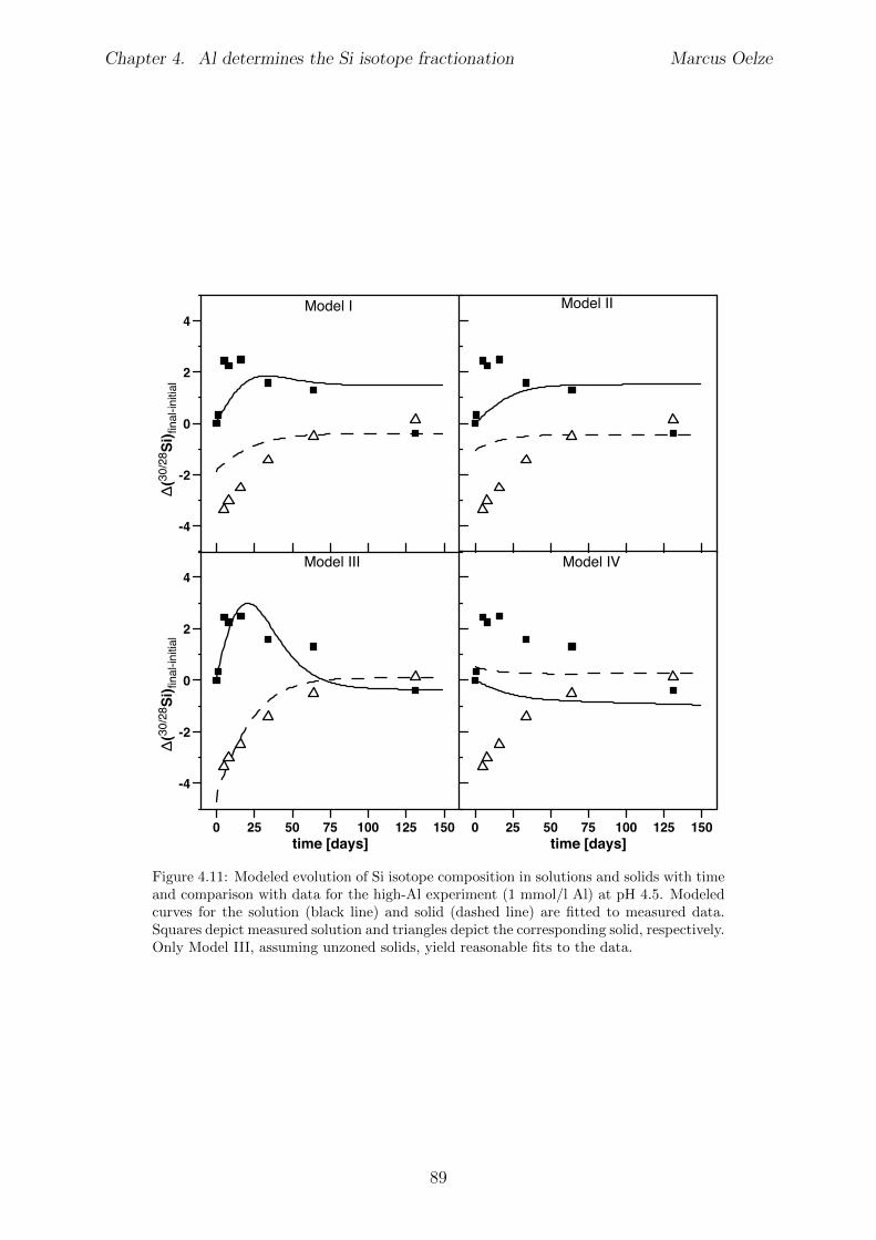
Chapter 4. Al determines the Si isotope fractionation Marcus Oelze
-4
-2
0
2
4
(30/28
Si) fi
nal-i
nitia
l
0 25 50 75 100 125 150time [days]
-4
-2
0
2
4
(30/28
Si) fi
nal-i
nitia
l
0 25 50 75 100 125 150time [days]
Model I Model II
Model IVModel III
Figure 4.11: Modeled evolution of Si isotope composition in solutions and solids with timeand comparison with data for the high-Al experiment (1 mmol/l Al) at pH 4.5. Modeledcurves for the solution (black line) and solid (dashed line) are fitted to measured data.Squares depict measured solution and triangles depict the corresponding solid, respectively.Only Model III, assuming unzoned solids, yield reasonable fits to the data.
89
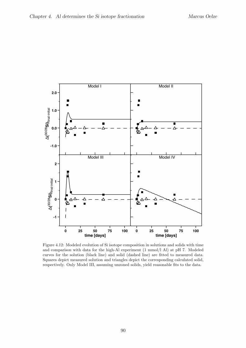
Chapter 4. Al determines the Si isotope fractionation Marcus Oelze
-1.0
0.0
1.0
2.0
(30/28
Si) fi
nal-i
nitia
l
0 25 50 75 100time [days]
-1
0
1
2
(30/28
Si) fi
nal-i
nitia
l
0 25 50 75 100time [days]
Model I Model II
Model IVModel III
Figure 4.12: Modeled evolution of Si isotope composition in solutions and solids with timeand comparison with data for the high-Al experiment (1 mmol/l Al) at pH 7. Modeledcurves for the solution (black line) and solid (dashed line) are fitted to measured data.Squares depict measured solution and triangles depict the corresponding calculated solid,respectively. Only Model III, assuming unzoned solids, yield reasonable fits to the data.
90
Chapter 5
The Si isotope record of di↵erentweathering regimes
5.1 Abstract
Si stable isotopes measured in secondary precipitates of soils and saprolite reflect thechange in the ratio of particulate export flux over the dissolved import Si flux and thustrace a change in weathering regime. Si isotope ratios measured on extracted amorphousand clay phases from soils and saprolites of three di↵erent weathering regimes (Sri Lanka,Sierra Nevada, Swiss Alps) show that the longer the regolith residence time (e.g. as in SriLanka), the lower are �(30/28Si)
NBS28 values for the amorphous and clay phase. Thus, ingeneral, a decrease in regolith residence time leads to an increase in the �(30/28Si)
NBS28
values for the secondary silicates formed.
5.2 Introduction
The formation of soils and the sculpturing of landscapes is strongly related to the inter-play between chemical weathering and physical erosion. Many studies showed that a closerelationship between physical erosion and chemical weathering exists. Natural settingswith very low total denudation rates, usually associated with low relief terrains and lowdenudation rates, show mineral supply rates into the weathering zone that are much lowerthan the rate at which minerals can be dissolved. In this case, the weathering regime iscalled “supply-limited” (or “transport-limited”), and all easily weatherable minerals aredissolved (Stallard, 1995; Riebe et al., 2004; West et al., 2005). In contrast, naturalsettings with very high denudation rates, where material is easily removed by physicalprocesses, are usually associated with steep terrains and high tectonic activity. In thesesettings fresh unweathered rocks/ minerals are transported fast through the weatheringzone, and mineral dissolution cannot follow pace. In this case, the weathering regime iscalled “kinetically - limited” (or “weathering - limited”) (Stallard, 1995; Riebe et al., 2004;West et al., 2005). The objective of this Chapter is to use the Si isotopic composition ofnatural samples to gain insight into the dependence of Si isotope fractionation related tosoil processes under di↵erent kinetic regimes. This can be studied by comparing di↵erentweathering regimes. Therefore the study of Si isotopes in di↵erent erosional regimes isfavored over the “chronosequence” approach. Chronosequences are space for time substi-tutions and are often a necessary tool to study soil development, where all soil forming
91
Chapter 5. The Si isotope record of di↵erent weathering regimes Marcus Oelze
factors remain constant except time (Walker et al., 2010).During the weathering of silicates minerals, the Si flux of the dissolved minerals is par-titioned in roughly equal proportions between the dissolved phase and a solid secondarymineral phase. From recent studies on natural samples the main findings are that theisotopically light Si is found in secondary siliceous solid phases and the heavy Si isotopesare relatively enriched in the ambient soil solution and river water (Ziegler et al., 2005a,b;Georg et al., 2006a, 2007b; Opfergelt et al., 2009; Bern et al., 2010; Opfergelt et al., 2011).Processes that fractionate Si isotopes within soils by taking up preferentially 28Si, there-fore leading to an enrichment of 30Si in the soil solution are a) the formation of secondarysilicates (including adsorption of Si onto soil particles) and b) Si uptake by plants. Ex-perimental studies reveal that during Si adsorption experiments onto gibbsite (Chapter 3,also Oelze et al. (2014)) and Si-Al solid formation experiments (Chapter 4 also Oelze et al.(2015)), kinetically driven Si isotope fractionation is taking place. A strong enrichmentof 28Si in the solid phase during higher solid formation rates was found. Under theseprerequisites it is tested whether the kinetic isotope e↵ect explored in controlled labora-tory experiments (Oelze et al. (2014) and Oelze et al. (2015)) is also visible from naturalweathering reactions.The goal here is to study the influence of parameters like soil residence time, denudationrate (erosion and weathering rate), elemental chemical depletion on Si isotope fractiona-tion in settings that are steadily eroding. Isotope mass balance models of the weatheringzone predict that the weathering regime, in particular the ratio of erosional export flux todissolved import flux, controls the extent of isotope fractionation (Bouchez et al., 2013).A prerequisite for such a study is the ability to separate and isotopically characterize thevarious Si pools in the weathering zone. Sauer et al. (2006) have developed operationallydefined separation techniques of these di↵erent Si pools (Figure 1 in Sauer et al. (2006)).These Si fractions are divided into the liquid phase (Si dissolved in soil solution), theadsorbed phase and the solid phase. The solid phase can be further subdivided into anamorphous pool, a poorly/ micro crystalline pool and the crystalline pool. The amorphouspool consist of a biogenic and a minerogenic pool and the crystalline pool is divided intoprimary and secondary silicates. The role of plants on Si isotopes has been investigatedin detail by Ding et al. (2005, 2008a) and Opfergelt et al. (2006a,b, 2008). In this study,the focus is therefore on the inorganic Si pool, both for the adsorbed and solid phases andthe potential formation path from amorphous Si precipitates to poorly crystalline solidsto crystalline solids. Work by Georgiadis (2011) shows that the second largest fractionafter the clay fraction is the minerogenic amorphous Si pool (excluding the organic richtop layer, where biogenic amorphous Si is present as phytoliths). Therefore, to revealinformation about a potential Si isotope pathway, a sequential extraction procedure wasemployed to extract these Si pools. The most two important fractions are defined here as1.) the amorphous Si fraction and 2.) the clay fraction.Here I explore Si isotopes in di↵erent weathering regimes that range from highly weath-ered thick tropical soils in the tectonically inactive mountain range of the Highlands ofSri Lanka representing supply–limited conditions (von Blanckenburg et al., 2004), wherethe weathering erosion relationship is strongly controlled by chemical dissolution, to therapidly uplifting Swiss Alps (Wittmann et al., 2007). There the sampling site is locatedin the upper Rhone valley, representing the kinetically limited counterpart where phys-ical erosion dominates (Norton and von Blanckenburg, 2010; Norton et al., 2010). Theintermediate weathering regime is located in the southern Sierra Nevada mountain range,California, where chemical weathering and physical erosion are roughly equal Dixon et al.
92
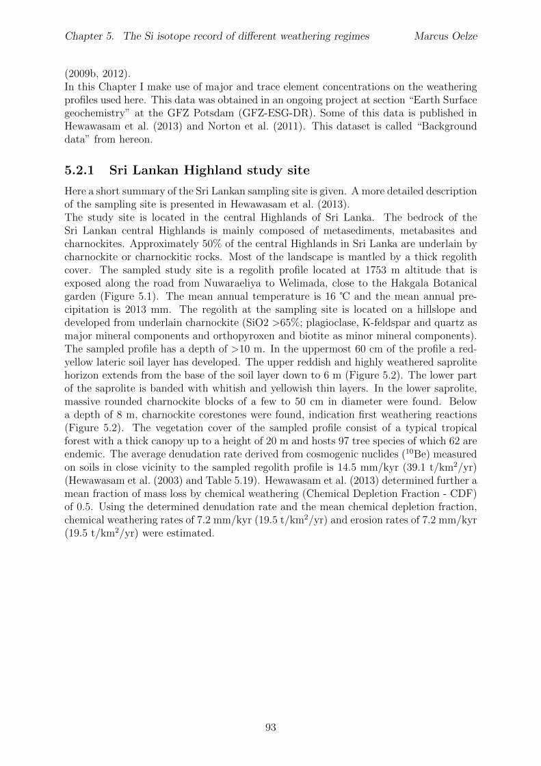
Chapter 5. The Si isotope record of di↵erent weathering regimes Marcus Oelze
(2009b, 2012).In this Chapter I make use of major and trace element concentrations on the weatheringprofiles used here. This data was obtained in an ongoing project at section “Earth Surfacegeochemistry” at the GFZ Potsdam (GFZ-ESG-DR). Some of this data is published inHewawasam et al. (2013) and Norton et al. (2011). This dataset is called “Backgrounddata” from hereon.
5.2.1 Sri Lankan Highland study site
Here a short summary of the Sri Lankan sampling site is given. A more detailed descriptionof the sampling site is presented in Hewawasam et al. (2013).The study site is located in the central Highlands of Sri Lanka. The bedrock of theSri Lankan central Highlands is mainly composed of metasediments, metabasites andcharnockites. Approximately 50% of the central Highlands in Sri Lanka are underlain bycharnockite or charnockitic rocks. Most of the landscape is mantled by a thick regolithcover. The sampled study site is a regolith profile located at 1753 m altitude that isexposed along the road from Nuwaraeliya to Welimada, close to the Hakgala Botanicalgarden (Figure 5.1). The mean annual temperature is 16 � and the mean annual pre-cipitation is 2013 mm. The regolith at the sampling site is located on a hillslope anddeveloped from underlain charnockite (SiO2 >65%; plagioclase, K-feldspar and quartz asmajor mineral components and orthopyroxen and biotite as minor mineral components).The sampled profile has a depth of >10 m. In the uppermost 60 cm of the profile a red-yellow lateric soil layer has developed. The upper reddish and highly weathered saprolitehorizon extends from the base of the soil layer down to 6 m (Figure 5.2). The lower partof the saprolite is banded with whitish and yellowish thin layers. In the lower saprolite,massive rounded charnockite blocks of a few to 50 cm in diameter were found. Belowa depth of 8 m, charnockite corestones were found, indication first weathering reactions(Figure 5.2). The vegetation cover of the sampled profile consist of a typical tropicalforest with a thick canopy up to a height of 20 m and hosts 97 tree species of which 62 areendemic. The average denudation rate derived from cosmogenic nuclides (10Be) measuredon soils in close vicinity to the sampled regolith profile is 14.5 mm/kyr (39.1 t/km2/yr)(Hewawasam et al. (2003) and Table 5.19). Hewawasam et al. (2013) determined further amean fraction of mass loss by chemical weathering (Chemical Depletion Fraction - CDF)of 0.5. Using the determined denudation rate and the mean chemical depletion fraction,chemical weathering rates of 7.2 mm/kyr (19.5 t/km2/yr) and erosion rates of 7.2 mm/kyr(19.5 t/km2/yr) were estimated.
93
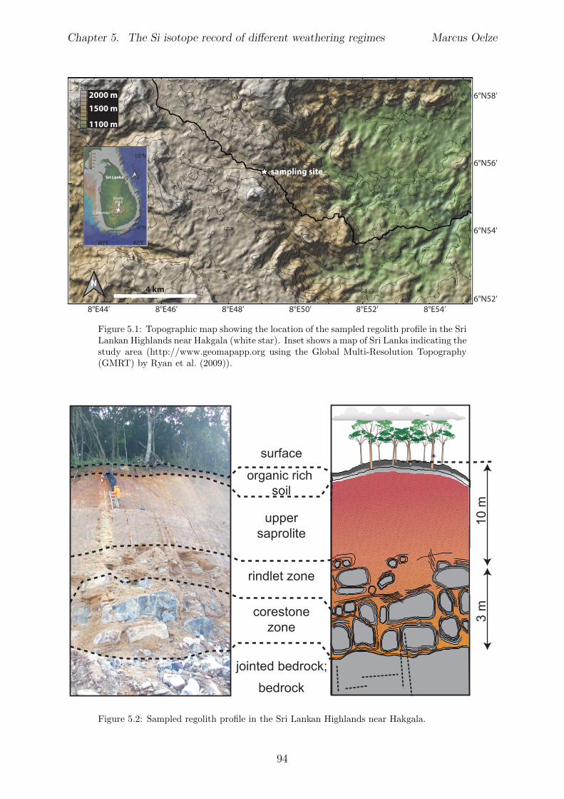
Chapter 5. The Si isotope record of di↵erent weathering regimes Marcus Oelze
8°E44’ 8°E46’ 8°E48’ 8°E50’ 8°E52’ 8°E54’
6°N58’
6°N56’
6°N54’
6°N52’4 km
sampling site
N
10°N
6°N
80°E 82°E
study area
Colombo
N
2000 m1500 m
1100 m
Sri Lanka
Figure 5.1: Topographic map showing the location of the sampled regolith profile in the SriLankan Highlands near Hakgala (white star). Inset shows a map of Sri Lanka indicating thestudy area (http://www.geomapapp.org using the Global Multi-Resolution Topography(GMRT) by Ryan et al. (2009)).
jointed bedrock;
rindlet zone
corestonezone
uppersaprolite
organic rich soil
surface
bedrock
10 m
3 m
Figure 5.2: Sampled regolith profile in the Sri Lankan Highlands near Hakgala.
94
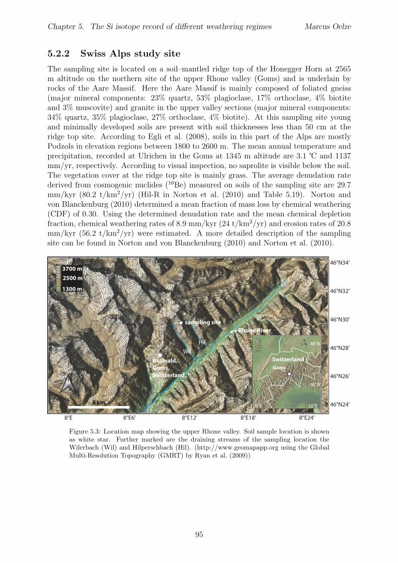
Chapter 5. The Si isotope record of di↵erent weathering regimes Marcus Oelze
5.2.2 Swiss Alps study site
The sampling site is located on a soil–mantled ridge top of the Honegger Horn at 2565m altitude on the northern site of the upper Rhone valley (Goms) and is underlain byrocks of the Aare Massif. Here the Aare Massif is mainly composed of foliated gneiss(major mineral components: 23% quartz, 53% plagioclase, 17% orthoclase, 4% biotiteand 3% muscovite) and granite in the upper valley sections (major mineral components:34% quartz, 35% plagioclase, 27% orthoclase, 4% biotite). At this sampling site youngand minimally developed soils are present with soil thicknesses less than 50 cm at theridge top site. According to Egli et al. (2008), soils in this part of the Alps are mostlyPodzols in elevation regions between 1800 to 2600 m. The mean annual temperature andprecipitation, recorded at Ulrichen in the Goms at 1345 m altitude are 3.1 � and 1137mm/yr, respectively. According to visual inspection, no saprolite is visible below the soil.The vegetation cover at the ridge top site is mainly grass. The average denudation ratederived from cosmogenic nuclides (10Be) measured on soils of the sampling site are 29.7mm/kyr (80.2 t/km2/yr) (Hil-R in Norton et al. (2010) and Table 5.19). Norton andvon Blanckenburg (2010) determined a mean fraction of mass loss by chemical weathering(CDF) of 0.30. Using the determined denudation rate and the mean chemical depletionfraction, chemical weathering rates of 8.9 mm/kyr (24 t/km2/yr) and erosion rates of 20.8mm/kyr (56.2 t/km2/yr) were estimated. A more detailed description of the samplingsite can be found in Norton and von Blanckenburg (2010) and Norton et al. (2010).
8°E 8°E6’ 8°E12’ 8°E18’ 8°E24’
46°N34’
46°N32’
46°N30’
46°N28’
46°N26’
46°N24’
Bellwald,Goms,Switzerland
Rhone River
8 km
N
SwitzerlandGoms
6°E 10°E
46°N
48°N
3700 m2500 m
1300 m
N
WilHil
sampling site
Figure 5.3: Location map showing the upper Rhone valley. Soil sample location is shownas white star. Further marked are the draining streams of the sampling location theWilerbach (Wil) and Hilperschbach (Hil). (http://www.geomapapp.org using the GlobalMulti-Resolution Topography (GMRT) by Ryan et al. (2009))
95
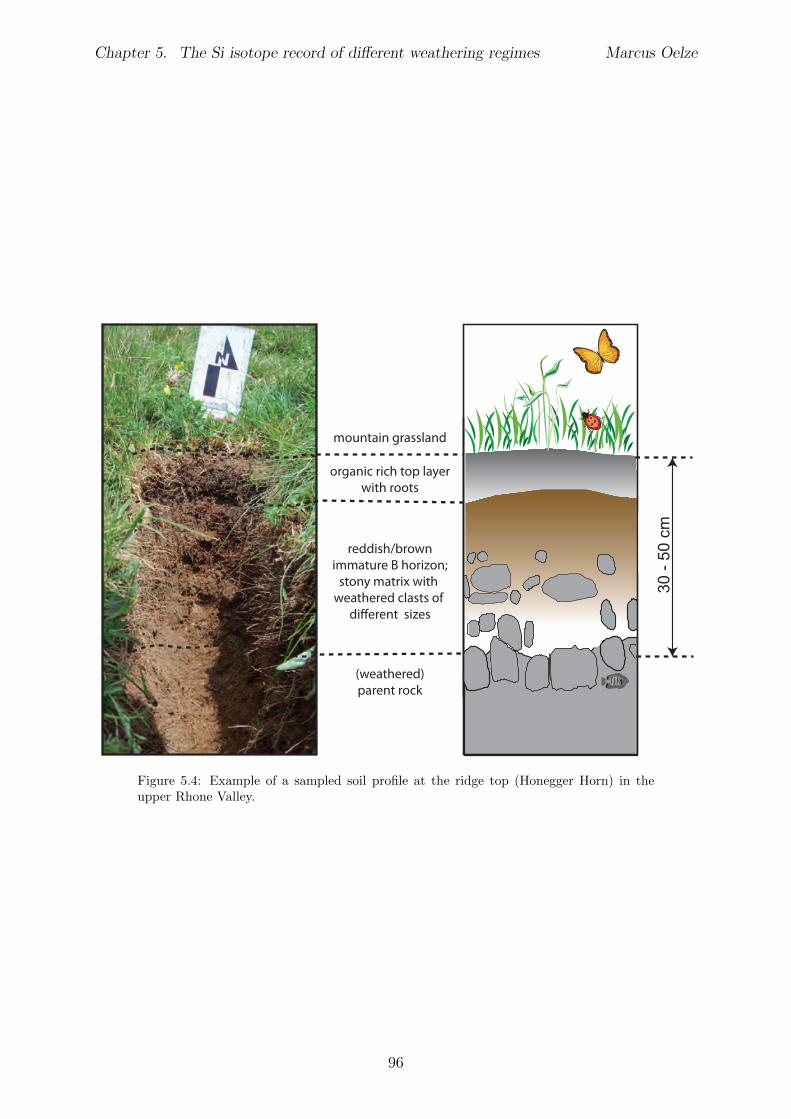
Chapter 5. The Si isotope record of di↵erent weathering regimes Marcus Oelze
organic rich top layerwith roots
reddish/brownimmature B horizon;
stony matrix with weathered clasts of
(weathered)parent rock
mountain grassland
30 -
50 c
m
Figure 5.4: Example of a sampled soil profile at the ridge top (Honegger Horn) in theupper Rhone Valley.
96
Chapter 5. The Si isotope record of di↵erent weathering regimes Marcus Oelze
5.2.3 Sierra Nevada study sites
The sampled soil profiles are located in the Kings River experimental watersheds (“KREW”)in the southern Sierra Nevada (USA) mountain range (Figure 5.5 and Figure 5.6). Withinthis critical zone observatory (CZO) soil profiles were sampled within catchments locatedat the Providence Creek (PC) site. Associated PC catchments (P301, P303, P304) rangein size between 0.49 to 1.32 km2 at an elevation between 1479 to 2113 m, with an annualprecipitation of 750 - 2000 mm (Hunsaker and Neary, 2012) and a mean annual air tem-perature of 7.8 � (Liu et al., 2012). The soils in these catchments are well–drained andare mainly underlain by granitic rocks.The sampled regolith profile is located NE of shaver lake exposed along the TollhouseRoad (168) (Figure 5.6). The bedrock at both locations is dominated by the “DinkyCreek Granodiorite” a medium, grained, equigranular, strongly foliated biotite-hornblendegranodiorite/tonalite with sphene, plagioclas and opaque minerals (Bateman and Wones,1972). It further contains abundant disc-shaped mafic inclusions (Bateman and Wones,1972). Further a quartz rich diorite is present at the PC sites (“Quartz diorite of BlueCanyon”). This rock is equigranular and well–foliated and contains conspicuous euhedralhornblende prisms and biotite plates of uniform size (Bateman and Wones, 1972).The well developed soils at the PC sites are dominated by the “Shaver soil series”, acoarse-loamy, mixed soil. This soil series has a balanced supply of moisture, is free ofcarbonates and has an organic rich surface soil horizon (Soil Survey Sta↵, 1998). Furthersoil types are from the “Gerle-Cagwin soil series”, with a coarse-loamy to fine sand orcoarser texture, mixed, superactive to frigid soil with less than 35 % (by volume) rockfragments (Soil Survey Sta↵, 1998). Dahlgren et al. (1997) described these soil types to bedominated by hydroxyl-Al interlayered vermiculite and gibbsite. The intense weatheringof feldspar and plagioclase under these environmental conditions promotes the formationof kaolinite.The vegetation cover mainly consist of conifer forest with some chaparral, barren andmeadow. More detailed description of the sampling sites can be found in Johnson et al.(2011), Bales et al. (2011), Liu et al. (2012) and Hunsaker and Neary (2012). The averagedenudation rate derived from cosmogenic nuclides (10Be) measured on soils of the samplingsite is 81.5 mm/kyr (220 t/km2/yr) (Dixon et al. (2009a) and and Table 5.19). Dixon et al.(2009a) determined a mean fraction of mass loss by chemical weathering (CDF) of 0.58.Using the determined denudation rate and the mean chemical depletion fraction, chemicalweathering rates of 47.4 mm/kyr (128.1 t/km2/yr) and erosion rates of 34 mm/kyr (91.9t/km2/yr) were estimated.
97
Chapter 5. The Si isotope record of di↵erent weathering regimes Marcus Oelze
sampling site“Balsam- profile”
sampling site“providence”
P301P303P304
119°W 24’ 119°W 15’ 119°W 6’
37°N10’
37°N6’
37°N2’
California
sampling site
124°W 119°W33°N
37°N
41°N
2900 m1800 m
700 m
N
N
4 km
Shaver Lake
Figure 5.5: Location map of the sampled regolith profile (“Balsam-profile”)and the Providence Creek (PC) site, southern Sierra Nevada, California, USA(http://www.geomapapp.org using the Global Multi-Resolution Topography (GMRT) byRyan et al. (2009)).
!R
!(!(
#*#*
#*
#*
")
")
")
")
McKinley
Dinkey
Grove Road
Deer
Providence
Creek
Duff
Creek
Creek
Creek BullCr
Providence
Wishon R
eservoir
Deer
Creek
Bull
2 41i r
!R
!(
!(
")
")
")
")
303600 304000 304400 30480 305200 305600 306800
4102
200
4102
600
4103
000
4103
400
4103
800
4104
200
4104
600
0 500 1,000250Meters
Kings River Experimental Watersheds (KREW)Providence
Road 10S17
Providence Waters
P301
P303
P304
Project Vicinity
Sierra NationalForest
KREWFresno
Providence WatershedBoundaries
CA
1:85,000
.
McKinleyGrove
Road 10S24
Road 10S17
Road 10S17
. .
Dinkey Creek Road
Shaver Lake - ca. 14.5 km
Fresno - ca. 80 km
306000 306400
Figure 5.6: Location and topographic map of the Kings River experimental watershed(KREW) at the Providence Creek (PC) site, southern Sierra Nevada, California, USA(modified from http://www.fs.fed.us/psw/topics/water/kingsriver/).
98
Chapter 5. The Si isotope record of di↵erent weathering regimes Marcus Oelze
bedrock:weatherd; partial
coherent
upper Saprolite:rock chips preserved
lower Saprolite:big corestones
present
organic rich soil
7 m
clear saprolite - rock boundary
clear soil - saproliteboundary
Figure 5.7: Sampled saprolite profile (“Balsam-Profile”) in the southern Sierra Nevada,California, USA. Field picture with isotope geochemist for scale (left) and schematic profile(right).
5.3 Methods and Materials
5.3.1 Sampling
Sri Lankan Highlands
Samples were taken on a field campaign taking place in October 2010 and described indetail in Hewawasam et al. (2013). The soil and saprolith samples were collected froma vertical section of a regolith profile (samples SL6 to SL29), exposed as a fresh roadcut during ongoing construction works. Five horizontal density cores (15 cm - long and4.6 cm - diameter plastic core sleeves) were taken throughout the saprolite for densitymeasurement. Approximately 10 m upslope from the regolith profile, nine additional soilsamples were collected at three parallel sub-sections within the 60 cm thick soil zone usinga soil corer, integrating over depth intervals from 0 to 20 cm, 20 to 40 cm, and 40 to 60 cm.The soil subsections were located about 1.5 m apart from each other in order to accountfor potential lateral variability. These soil samples were afterwards combined to producean average soil sample for each depth interval (Hakgala combined soil SL88, SL89 andSL90, respectively). Further, nine unweathered bedrock samples (SL61 and SL63-SL71)were taken beneath the regolith profile to determine source rock element concentrationand Si isotope composition (SL61, SL64, SL66, SL68 and SL70).
European Swiss Alps
The samples were taken during a field campaign in July 2010; 6 (B1 to B6) soil depthprofiles were sampled on a soil-mantled ridge top using a soil corer. Soil samples were
99
Chapter 5. The Si isotope record of di↵erent weathering regimes Marcus Oelze
taken from the soil surface down to ⇠30 cm depending on soil thickness.
Southern Sierra Nevada
The samples were taken during a field campaign in May 2010. Several soils were sampledat the PC CZO and a deep saprolith profile (“Balsam-profile”) located further away nearthe NE of Shaver Lake (Figure 5.5 and Figure 5.6). The soil samples were taken as depthprofiles using a soil corer for shallow soil horizons and using an auger for deeper soilhorizons. A soil depth profile was sampled in catchment P301 from surface down to adepth of ⇠120 cm (samples SN1 to SN10). Further soil depth profiles were sampled inPC catchments P303 (samples SN21 to SN23) and P304 (samples SN24 to SN26) fromthe surface down to 30 cm depth using a soil corer. The individual soil core samplesor augered soil samples were afterwards mixed and represent therefore an average of thesampled depth.At the “Balsam” study site the first sample was taken at ⇠180 cm below the soil surface.Several samples were taken down to a depth of ⇠800 cm below the surface. The surfaceof the exposed saprolite was scraped of and samples were taken from the “fresh” saprolitesurface with a soil corer where possible. The sampled profile starts at the soil/saproliteborder, includes the whole saprolite and extends down to the source-rock/saprolite border(samples SN11 to SN20). The soil on top of the sampled saprolite profile was not sampled.Also, bedload sediments of the stream draining catchment P301 (SN27) and at the outletof the stream integrating over the whole PC site (PIG; SN28) were sampled.
5.3.2 Sample preparation for Si isotope measurements
Rock samples were crushed < 68 µm and digested using alkaline fusion with NaOH fol-lowing methods adapted from Georg et al. (2006b) and Zambardi and Poitrasson (2011).Samples of the soil/ saprolite compartment were sieved < 2 mm and treated according tothe used Si extraction procedure (subsection 5.3.3).
5.3.3 Extraction procedures for di↵erent Si fractions
To determine the Si isotope composition of di↵erent reservoirs in the weathering zonea sequential extraction procedure developed in detail by Georgiadis (2011) was used.This extraction method targeted the following operationally defined Si pools: dissolvedand easily soluble silicic acid, adsorbed silicic acid, organically bounded silicic acid,sesquioxide–bounded silicic acid, bioopal(phytolits) and amorphous silicic acid. Herethe focus is on the major Si reservoirs in weathering environments. These are pri-mary rocks, secondary amorphous Si precipitates and secondary clays. Therefore theextraction procedure developed for amorphous Si precipitates is applied to all processedsamples (Georgiadis, 2011) followed by a clay separation procedure (USGS OFR01–041;http://pubs.usgs.gov/of/2001/of01-041/htmldocs/methods/centrifu.htm). The clay sep-aration procedure employed here di↵ers in an important way from the original method. Asthe aim here is to obtain the isotope composition of the clay fraction, rather than obtainits full mass. Therefore clay extractions was applied only once. Thus pure end-memberisotope composition were obtained, but not complete mass of the clay fraction.Soil and saprolite samples were weighed in (⇠500 mg) into 15 ml centrifuge tubes and 10ml Milli-Q water was added. To disperse clay minerals, an ultrasonic treatment procedurewas applied (comprising a 12 h treatment in the ultrasonic bath; Schmidt et al. (2008)).
100
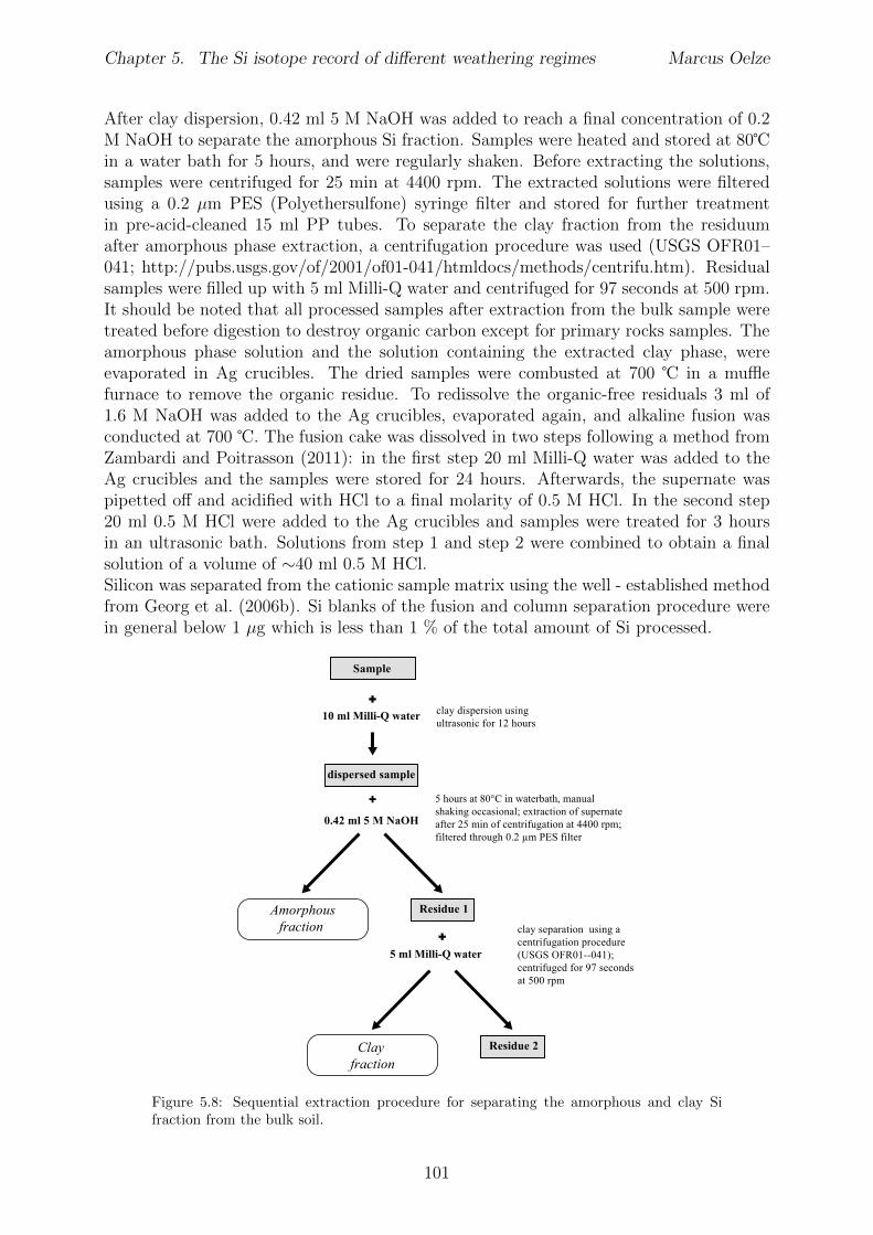
Chapter 5. The Si isotope record of di↵erent weathering regimes Marcus Oelze
After clay dispersion, 0.42 ml 5 M NaOH was added to reach a final concentration of 0.2M NaOH to separate the amorphous Si fraction. Samples were heated and stored at 80�in a water bath for 5 hours, and were regularly shaken. Before extracting the solutions,samples were centrifuged for 25 min at 4400 rpm. The extracted solutions were filteredusing a 0.2 µm PES (Polyethersulfone) syringe filter and stored for further treatmentin pre-acid-cleaned 15 ml PP tubes. To separate the clay fraction from the residuumafter amorphous phase extraction, a centrifugation procedure was used (USGS OFR01–041; http://pubs.usgs.gov/of/2001/of01-041/htmldocs/methods/centrifu.htm). Residualsamples were filled up with 5 ml Milli-Q water and centrifuged for 97 seconds at 500 rpm.It should be noted that all processed samples after extraction from the bulk sample weretreated before digestion to destroy organic carbon except for primary rocks samples. Theamorphous phase solution and the solution containing the extracted clay phase, wereevaporated in Ag crucibles. The dried samples were combusted at 700 � in a mu✏efurnace to remove the organic residue. To redissolve the organic-free residuals 3 ml of1.6 M NaOH was added to the Ag crucibles, evaporated again, and alkaline fusion wasconducted at 700 �. The fusion cake was dissolved in two steps following a method fromZambardi and Poitrasson (2011): in the first step 20 ml Milli-Q water was added to theAg crucibles and the samples were stored for 24 hours. Afterwards, the supernate waspipetted o↵ and acidified with HCl to a final molarity of 0.5 M HCl. In the second step20 ml 0.5 M HCl were added to the Ag crucibles and samples were treated for 3 hoursin an ultrasonic bath. Solutions from step 1 and step 2 were combined to obtain a finalsolution of a volume of ⇠40 ml 0.5 M HCl.Silicon was separated from the cationic sample matrix using the well - established methodfrom Georg et al. (2006b). Si blanks of the fusion and column separation procedure werein general below 1 µg which is less than 1 % of the total amount of Si processed.
10 ml Milli-Q water
0.42 ml 5 M NaOH
Amorphousfraction
+
Residue 1
+
Sample
+
dispersed sample
Residue 2
clay dispersion using
ultrasonic for 12 hours
5 hours at 80°C in waterbath, manual
shaking occasional; extraction of supernate
after 25 min of centrifugation at 4400 rpm;
filtered through 0.2 µm PES filter
clay separation using a
centrifugation procedure
(USGS OFR01--041);
centrifuged for 97 seconds
at 500 rpm
5 ml Milli-Q water
Clay fraction
Figure 5.8: Sequential extraction procedure for separating the amorphous and clay Sifraction from the bulk soil.
101
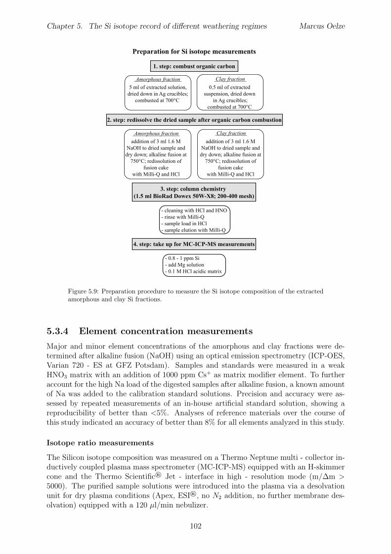
Chapter 5. The Si isotope record of di↵erent weathering regimes Marcus Oelze
5 ml of extracted solution,dried down in Ag crucibles;
combusted at 700°C
1. step: combust organic carbon
0.5 ml of extracted suspension, dried down
in Ag crucibles;combusted at 700°C
Preparation for Si isotope measurements
2. step: redissolve the dried sample after organic carbon combustion
Amorphous fraction Clay fraction
addition of 3 ml 1.6 M NaOH to dried sample and dry down; alkaline fusion at
750°C; redissolution of fusion cake
with Milli-Q and HCl
addition of 3 ml 1.6 M NaOH to dried sample and dry down; alkaline fusion at
750°C; redissolution of fusion cake
with Milli-Q and HCl
Amorphous fraction Clay fraction
3. step: column chemistry (1.5 ml BioRad Dowex 50W-X8; 200-400 mesh)
- cleaning with HCl and HNO- rinse with Milli-Q- sample load in HCl- sample elution with Milli-Q
4. step: take up for MC-ICP-MS measurements
- 0.8 - 1 ppm Si - add Mg solution- 0.1 M HCl acidic matrix
Figure 5.9: Preparation procedure to measure the Si isotope composition of the extractedamorphous and clay Si fractions.
5.3.4 Element concentration measurements
Major and minor element concentrations of the amorphous and clay fractions were de-termined after alkaline fusion (NaOH) using an optical emission spectrometry (ICP-OES,Varian 720 - ES at GFZ Potsdam). Samples and standards were measured in a weakHNO3 matrix with an addition of 1000 ppm Cs+ as matrix modifier element. To furtheraccount for the high Na load of the digested samples after alkaline fusion, a known amountof Na was added to the calibration standard solutions. Precision and accuracy were as-sessed by repeated measurements of an in-house artificial standard solution, showing areproducibility of better than <5%. Analyses of reference materials over the course ofthis study indicated an accuracy of better than 8% for all elements analyzed in this study.
Isotope ratio measurements
The Silicon isotope composition was measured on a Thermo Neptune multi - collector in-ductively coupled plasma mass spectrometer (MC-ICP-MS) equipped with an H-skimmercone and the Thermo Scientific® Jet - interface in high - resolution mode (m/�m >5000). The purified sample solutions were introduced into the plasma via a desolvationunit for dry plasma conditions (Apex, ESI®, no N2 addition, no further membrane des-olvation) equipped with a 120 µl/min nebulizer.
102
Chapter 5. The Si isotope record of di↵erent weathering regimes Marcus Oelze
We used Mg doping combined with standard-sample-bracketing to correct for mass biasduring measurements by using an exponential mass bias law (Cardinal et al. (2003) andsee Chapter 2). A magnesium solution was added to samples and standards to yield a finalconcentration of 1 ppm Mg. Sample solutions were diluted to 1 ppm Si concentration in0.1 M HCl, which typically resulted in an intensity of ⇠15 V/ppm on 28Si (using a 1011⌦resistor).Measurements were conducted on the interference-free low-mass side of the three Si iso-topes. The most critical interference, caused by 14N16O on the 30Si signal, is usually below5V which is resolvable from the 30Si signal in the high-resolution mode used. Each sampleand standard was measured at least 4 times during a sequence; each sample or standardwas measured in dynamic mode for 30 cycles with an integration time for each cycle of4 s for Si as well as for Mg with an idle time of 3 s after magnet switching. Pure 0.1M HCl solutions were measured before and after each standard-sample-standard blockand were used for on-peak zero correction. Typical intensities of 28Si in blank solutionswere below 10 mV. We report Si isotope data relative to the standard reference materialNBS28 (quartz sand) in the delta notation according to Coplen (2011) as �(29/28Si)NBS28
and �(30/28Si)NBS28 expressed in per mill (h) by multiplication of Equation 5.1 and 5.2with a factor of 103:
�(29/28Si)NBS28 =
0
B@
⇣29Si28Si
⌘
sample� 29Si28Si
�NBS28
� 1
1
CA (5.1)
�(30/28Si)NBS28 =
0
B@
⇣30Si28Si
⌘
sample� 30Si28Si
�NBS28
� 1
1
CA (5.2)
All reported errors on delta values are the 95% confidence interval (CI) calculated accord-ing to Eq.5.3 where �(30/28Si)NBS28 is the mean of the measured delta values for the sampleor standard (at least n=4), tn-1 is a critical value from tables of the Student0s t-law andSE is the standard error of the mean.
CI = �(30/28Si)NBS28 ± tn-1 ⇥ SE (5.3)
The well-defined Si isotope reference material BHVO-2g, a basalt standard (measuredover a 12 months period of analysis ; including several individual chemical separations aswell as several digestions procedures; �(30/28Si)NBS28 = �0.27± 0.02; n=73), was usuallymeasured as control standard during measured sequences.
5.4 Isotope results
5.4.1 Isotope Results - Sri Lanka
The bulk isotope composition of the source rock is �(30/28Si)bedrock
: average= -0.11 h (seeFigure 5.10 and Table 5.1) which is within the expected range of granitic rocks (Savageet al. (2012); �(30/28Si)
granite
= -0.23 ± 0.15 h). The amorphous fraction in the saproliteyields in general heavier Si isotopic values than the clay fraction, whereas in the soil
103
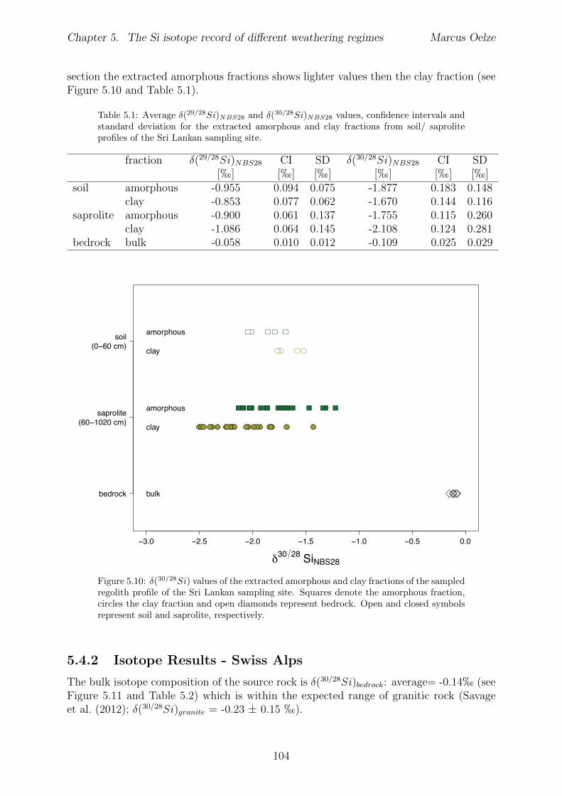
Chapter 5. The Si isotope record of di↵erent weathering regimes Marcus Oelze
section the extracted amorphous fractions shows lighter values then the clay fraction (seeFigure 5.10 and Table 5.1).
Table 5.1: Average �(29/28Si)NBS28
and �(30/28Si)NBS28
values, confidence intervals andstandard deviation for the extracted amorphous and clay fractions from soil/ saproliteprofiles of the Sri Lankan sampling site.
fraction �(29/28Si)NBS28 CI SD �(30/28Si)
NBS28 CI SD[h] [h] [h] [h] [h] [h]
soil amorphous -0.955 0.094 0.075 -1.877 0.183 0.148clay -0.853 0.077 0.062 -1.670 0.144 0.116
saprolite amorphous -0.900 0.061 0.137 -1.755 0.115 0.260clay -1.086 0.064 0.145 -2.108 0.124 0.281
bedrock bulk -0.058 0.010 0.012 -0.109 0.025 0.029
−3.0 −2.5 −2.0 −1.5 −1.0 −0.5 0.0
bedrock
saprolite(60−1020 cm)
soil(0−60 cm)
δ30 28 SiNBS28
amorphous
clay
amorphous
clay
bulk
Figure 5.10: �(30/28Si) values of the extracted amorphous and clay fractions of the sampledregolith profile of the Sri Lankan sampling site. Squares denote the amorphous fraction,circles the clay fraction and open diamonds represent bedrock. Open and closed symbolsrepresent soil and saprolite, respectively.
5.4.2 Isotope Results - Swiss Alps
The bulk isotope composition of the source rock is �(30/28Si)bedrock
: average= -0.14h (seeFigure 5.11 and Table 5.2) which is within the expected range of granitic rock (Savageet al. (2012); �(30/28Si)
granite
= -0.23 ± 0.15 h).
104
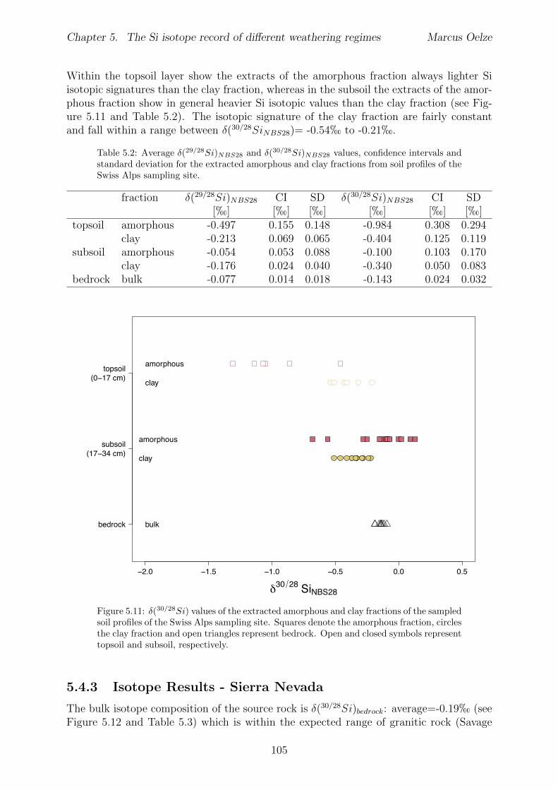
Chapter 5. The Si isotope record of di↵erent weathering regimes Marcus Oelze
Within the topsoil layer show the extracts of the amorphous fraction always lighter Siisotopic signatures than the clay fraction, whereas in the subsoil the extracts of the amor-phous fraction show in general heavier Si isotopic values than the clay fraction (see Fig-ure 5.11 and Table 5.2). The isotopic signature of the clay fraction are fairly constantand fall within a range between �(30/28Si
NBS28)= -0.54h to -0.21h.
Table 5.2: Average �(29/28Si)NBS28
and �(30/28Si)NBS28
values, confidence intervals andstandard deviation for the extracted amorphous and clay fractions from soil profiles of theSwiss Alps sampling site.
fraction �(29/28Si)NBS28 CI SD �(30/28Si)
NBS28 CI SD[h] [h] [h] [h] [h] [h]
topsoil amorphous -0.497 0.155 0.148 -0.984 0.308 0.294clay -0.213 0.069 0.065 -0.404 0.125 0.119
subsoil amorphous -0.054 0.053 0.088 -0.100 0.103 0.170clay -0.176 0.024 0.040 -0.340 0.050 0.083
bedrock bulk -0.077 0.014 0.018 -0.143 0.024 0.032
−2.0 −1.5 −1.0 −0.5 0.0 0.5
bedrock
subsoil (17−34 cm)
topsoil(0−17 cm)
δ30 28 SiNBS28
amorphous
clay
amorphous
clay
bulk
Figure 5.11: �(30/28Si) values of the extracted amorphous and clay fractions of the sampledsoil profiles of the Swiss Alps sampling site. Squares denote the amorphous fraction, circlesthe clay fraction and open triangles represent bedrock. Open and closed symbols representtopsoil and subsoil, respectively.
5.4.3 Isotope Results - Sierra Nevada
The bulk isotope composition of the source rock is �(30/28Si)bedrock
: average=-0.19h (seeFigure 5.12 and Table 5.3) which is within the expected range of granitic rock (Savage
105
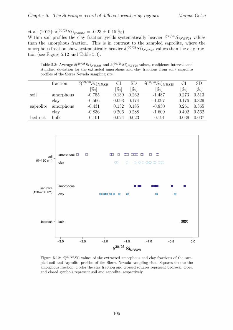
Chapter 5. The Si isotope record of di↵erent weathering regimes Marcus Oelze
et al. (2012); �(30/28Si)granite
= -0.23 ± 0.15 h).Within soil profiles the clay fraction yields systematically heavier �30/28Si
NBS28 valuesthan the amorphous fraction. This is in contrast to the sampled saprolite, where theamorphous fraction show systematically heavier �(30/28Si)
NBS28 values than the clay frac-tion (see Figure 5.12 and Table 5.3).
Table 5.3: Average �(29/28Si)NBS28
and �(30/28Si)NBS28
values, confidence intervals andstandard deviation for the extracted amorphous and clay fractions from soil/ saproliteprofiles of the Sierra Nevada sampling site.
fraction �(29/28Si)NBS28 CI SD �(30/28Si)
NBS28 CI SD[h] [h] [h] [h] [h] [h]
soil amorphous -0.755 0.139 0.262 -1.487 0.273 0.513clay -0.566 0.093 0.174 -1.097 0.176 0.329
saprolite amorphous -0.431 0.132 0.185 -0.830 0.261 0.365clay -0.836 0.206 0.288 -1.609 0.402 0.562
bedrock bulk -0.101 0.024 0.023 -0.191 0.039 0.037
−3.0 −2.5 −2.0 −1.5 −1.0 −0.5 0.0
bedrock
saprolite(120−700 cm)
soil(0−120 cm)
δ30 28 SiNBS28
amorphous
clay
amorphous
clay
bulk
Figure 5.12: �(30/28Si) values of the extracted amorphous and clay fractions of the sam-pled soil and saprolite profiles of the Sierra Nevada sampling site. Squares denote theamorphous fraction, circles the clay fraction and crossed squares represent bedrock. Openand closed symbols represent soil and saprolite, respectively.
106
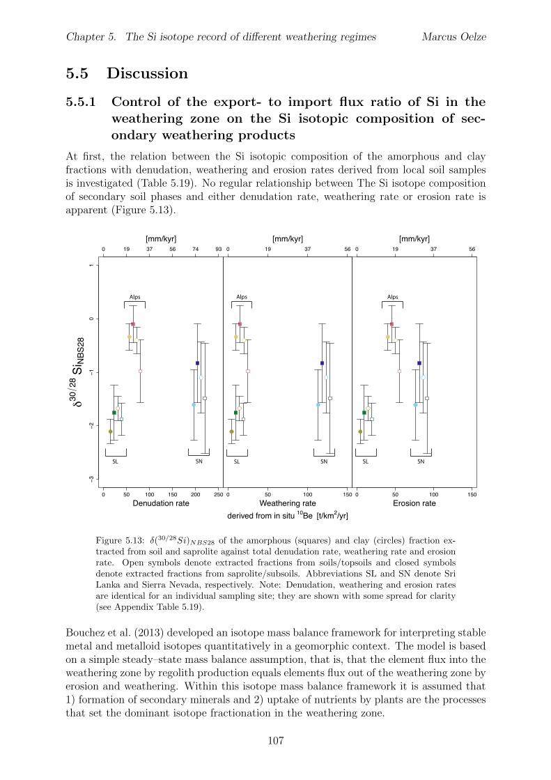
Chapter 5. The Si isotope record of di↵erent weathering regimes Marcus Oelze
5.5 Discussion
5.5.1 Control of the export- to import flux ratio of Si in theweathering zone on the Si isotopic composition of sec-ondary weathering products
At first, the relation between the Si isotopic composition of the amorphous and clayfractions with denudation, weathering and erosion rates derived from local soil samplesis investigated (Table 5.19). No regular relationship between The Si isotope compositionof secondary soil phases and either denudation rate, weathering rate or erosion rate isapparent (Figure 5.13).
0 50 100 150 200 250
−3−2
−10
1
Denudation rate
1
0 19 37 56 74 93
δ30
28 S
i NBS
28
[mm/kyr]
0 50 100 150
Weathering rate
0 19 37 56
derived from in situ 10Be [t/km2/yr]
[mm/kyr]
0 50 100 150
Erosion rate
n
0 19 37 56
[mm/kyr]
AlpsAlps Alps
SL SN SL SN SL SN
Figure 5.13: �(30/28Si)NBS28
of the amorphous (squares) and clay (circles) fraction ex-tracted from soil and saprolite against total denudation rate, weathering rate and erosionrate. Open symbols denote extracted fractions from soils/topsoils and closed symbolsdenote extracted fractions from saprolite/subsoils. Abbreviations SL and SN denote SriLanka and Sierra Nevada, respectively. Note: Denudation, weathering and erosion ratesare identical for an individual sampling site; they are shown with some spread for clarity(see Appendix Table 5.19).
Bouchez et al. (2013) developed an isotope mass balance framework for interpreting stablemetal and metalloid isotopes quantitatively in a geomorphic context. The model is basedon a simple steady–state mass balance assumption, that is, that the element flux into theweathering zone by regolith production equals elements flux out of the weathering zone byerosion and weathering. Within this isotope mass balance framework it is assumed that1) formation of secondary minerals and 2) uptake of nutrients by plants are the processesthat set the dominant isotope fractionation in the weathering zone.
107
Chapter 5. The Si isotope record of di↵erent weathering regimes Marcus Oelze
I use this model to quantitatively explain the pattern found in Figure 5.13.In the following the notation of Bouchez et al. (2013) is used for isotopic compositions,isotope fractionation factors and elemental fluxes of Si. The isotopic composition ofsecondary precipitates �Si
sec
can be predicted using Equation 5.4:
�Sisec
= �Sidiss
+�Si
prec
(5.4)
where �Sidiss
denotes the Si isotopic composition of the dissolved fraction of Si and �Si
prec
denotes the Si isotope fractionation factor of secondary silicate formation. CombiningEquation 5.4 with Equation 5e from Bouchez et al. (2013) results in:
�Sisec
= �Sirock
�ESi
sec
⇤�Si
prec
+ ESi
org
⇤�Si
upt
SSi
rock
+ SSi
prim
+�Si
prec
(5.5)
where �Sirock
denotes the Si isotopic composition of the bedrock, ESi
sec
and ESi
org
are exportfluxes of Si (mol
Si
⇤ m�2 ⇤ yr�1) by particulate erosion of Si contained in secondarysilicates and in biogenic products such as phytoliths, respectively. SSi
rock
and SSi
prim
arethe import fluxes of dissolved Si (mol
Si
⇤m�2 ⇤ yr�1) into the weathering zone resultingfrom the dissolution of bedrock and from primary minerals, respectively. �Si
upt
denotesthe Si isotope fractionation factor during Si uptake by plants. Following the approachof Bouchez et al. (2013) and normalizing a given element flux F Si (ESi
sec
, ESi
org
, SSi
rock
andSSi
prim
; capital letters) to the flux of matter crossing the weathering front (SSi
rock
+RP Si
prim
),where RP Si
prim
denotes the Regolith production rate:
fSi =F Si
SSi
rock
+RP Si
prim
(5.6)
results in non - dimensional fluxes fSi (eSisec
, eSiorg
, sSirock
and sSiprim
; lower case letters). A
flux - weighted isotope fractionation factor �Si can be calculated comprising both �Si
prec
and �Si
upt
:
�Si =ESi
sec
⇤�Si
prec
+ ESi
org
⇤�Si
upt
ESi
sec
+ ESi
org
(5.7)
Combining Equation 5.5, 5.6 and 5.7 results in:
�Sisec
� �Sirock
��Si
prec
�Si
= �eSisec
+ eSiorg
sSirock
+ sSiprim
(5.8)
where eSisec
and eSiorg
are the normalized, non - dimensional export fluxes of Si by particulateerosion of Si contained in secondary silicates and in organic matter, respectively. sSi
rock
and sSiprim
are the normalized, non - dimensional dissolved Si import fluxes resulting fromthe dissolution of bedrock and from primary minerals, respectively. Experiments and fieldstudies show that the direction and magnitude of �Si
prec
and �Si
upt
can be assumed to besimilar (Opfergelt et al., 2006a; Ding et al., 2008b; Georg et al., 2009; Oelze et al., 2014,2015) and therefore Equation 5.8 can be simplified to:
1� �Sisec
� �Sirock
�Si
=eSisec
+ eSiorg
sSirock
+ sSiprim
(5.9)
As �Sirock
is rather uniform between these three sites, the di↵erence �Sisec
� �Sirock
is onlycontrolled by �Si
sec
. Hence Equation 5.9 results in a positive linear relationship between
108
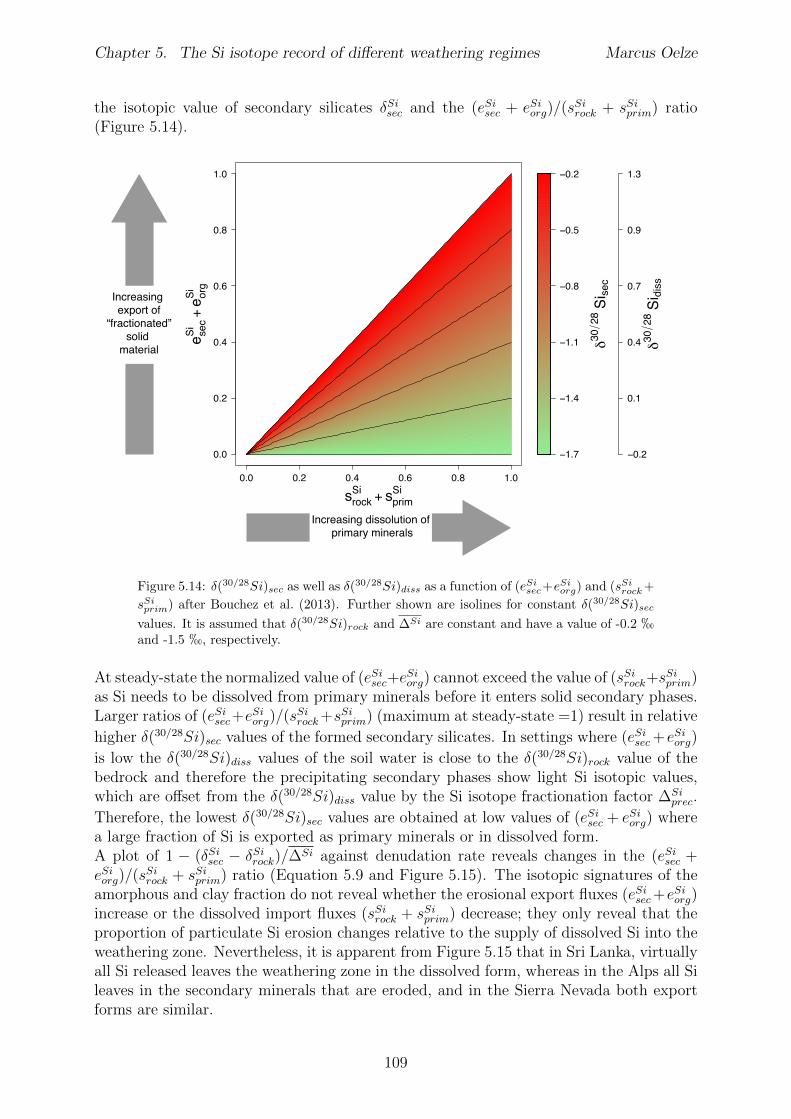
Chapter 5. The Si isotope record of di↵erent weathering regimes Marcus Oelze
the isotopic value of secondary silicates �Sisec
and the (eSisec
+ eSiorg
)/(sSirock
+ sSiprim
) ratio(Figure 5.14).
0.0 0.2 0.4 0.6 0.8 1.0
0.0
0.2
0.4
0.6
0.8
1.0
−1.7
−1.4
−1.1
−0.8
−0.5
−0.2
−0.2
0.1
0.4
0.7
0.9
1.3
δ3028
Si se
c
δ3028
Si di
ss
e sec
Si+
e org
Si
srockSi + sprim
Si
Increasing export of
“fractionated” solid
material
Increasing dissolution of primary minerals
Figure 5.14: �(30/28Si)sec
as well as �(30/28Si)diss
as a function of (eSi
sec
+eSi
org
) and (sSi
rock
+
sSi
prim
) after Bouchez et al. (2013). Further shown are isolines for constant �(30/28Si)sec
values. It is assumed that �(30/28Si)rock
and �Si are constant and have a value of -0.2 hand -1.5 h, respectively.
At steady-state the normalized value of (eSisec
+eSiorg
) cannot exceed the value of (sSirock
+sSiprim
)as Si needs to be dissolved from primary minerals before it enters solid secondary phases.Larger ratios of (eSi
sec
+eSiorg
)/(sSirock
+sSiprim
) (maximum at steady-state =1) result in relativehigher �(30/28Si)
sec
values of the formed secondary silicates. In settings where (eSisec
+eSiorg
)is low the �(30/28Si)
diss
values of the soil water is close to the �(30/28Si)rock
value of thebedrock and therefore the precipitating secondary phases show light Si isotopic values,which are o↵set from the �(30/28Si)
diss
value by the Si isotope fractionation factor �Si
prec
.Therefore, the lowest �(30/28Si)
sec
values are obtained at low values of (eSisec
+ eSiorg
) wherea large fraction of Si is exported as primary minerals or in dissolved form.A plot of 1 � (�Si
sec
� �Sirock
)/�Si against denudation rate reveals changes in the (eSisec
+eSiorg
)/(sSirock
+ sSiprim
) ratio (Equation 5.9 and Figure 5.15). The isotopic signatures of theamorphous and clay fraction do not reveal whether the erosional export fluxes (eSi
sec
+eSiorg
)increase or the dissolved import fluxes (sSi
rock
+ sSiprim
) decrease; they only reveal that theproportion of particulate Si erosion changes relative to the supply of dissolved Si into theweathering zone. Nevertheless, it is apparent from Figure 5.15 that in Sri Lanka, virtuallyall Si released leaves the weathering zone in the dissolved form, whereas in the Alps all Sileaves in the secondary minerals that are eroded, and in the Sierra Nevada both exportforms are similar.
109
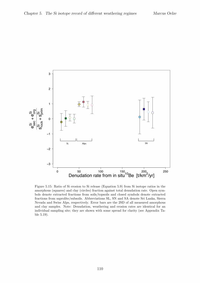
Chapter 5. The Si isotope record of di↵erent weathering regimes Marcus Oelze
0 50 100 150 200 250
−3
−2
−1
0
1
2
3
Denudation rate from in situ 10Be [t/km2/yr]
e sec
Si+
e org
Si
s roc
kSi
+s p
rimSi
SL SNAlps
Figure 5.15: Ratio of Si erosion to Si release (Equation 5.9) from Si isotope ratios in theamorphous (squares) and clay (circles) fraction against total denudation rate. Open sym-bols denote extracted fractions from soils/topsoils and closed symbols denote extractedfractions from saprolite/subsoils. Abbreviations SL, SN and SA denote Sri Lanka, SierraNevada and Swiss Alps, respectively. Error bars are the 2SD of all measured amorphousand clay samples. Note: Denudation, weathering and erosion rates are identical for anindividual sampling site; they are shown with some spread for clarity (see Appendix Ta-ble 5.19).
110
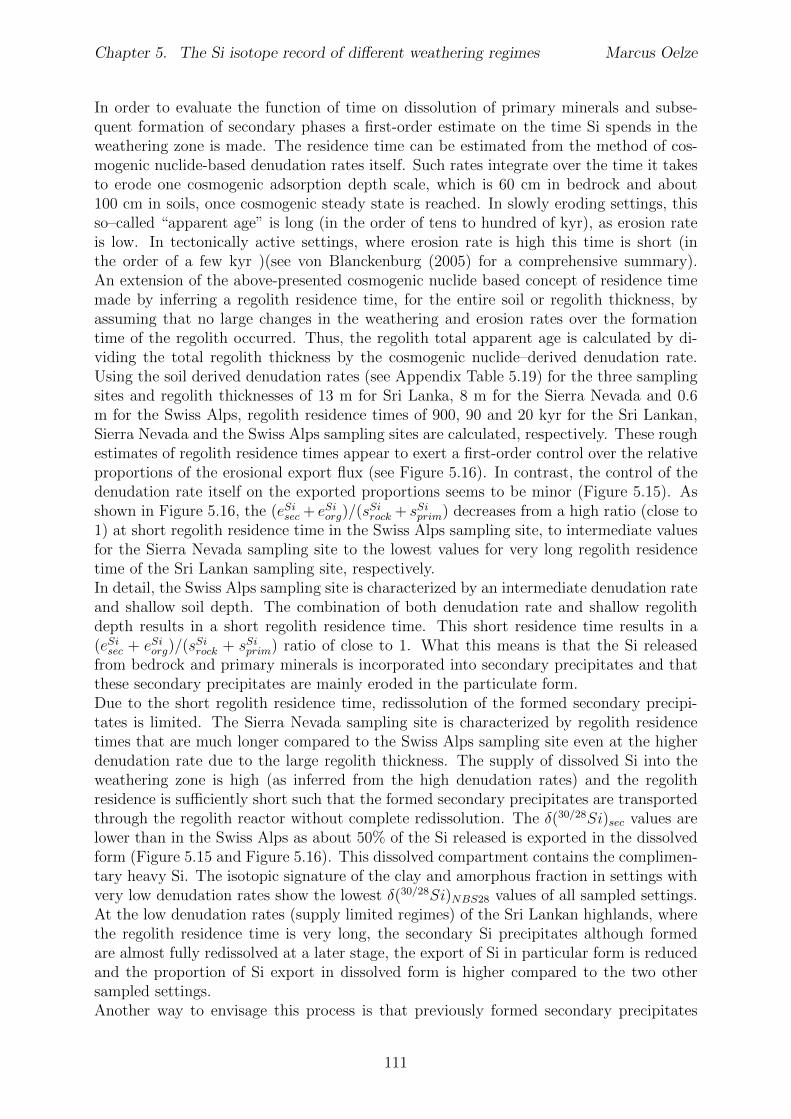
Chapter 5. The Si isotope record of di↵erent weathering regimes Marcus Oelze
In order to evaluate the function of time on dissolution of primary minerals and subse-quent formation of secondary phases a first-order estimate on the time Si spends in theweathering zone is made. The residence time can be estimated from the method of cos-mogenic nuclide-based denudation rates itself. Such rates integrate over the time it takesto erode one cosmogenic adsorption depth scale, which is 60 cm in bedrock and about100 cm in soils, once cosmogenic steady state is reached. In slowly eroding settings, thisso–called “apparent age” is long (in the order of tens to hundred of kyr), as erosion rateis low. In tectonically active settings, where erosion rate is high this time is short (inthe order of a few kyr )(see von Blanckenburg (2005) for a comprehensive summary).An extension of the above-presented cosmogenic nuclide based concept of residence timemade by inferring a regolith residence time, for the entire soil or regolith thickness, byassuming that no large changes in the weathering and erosion rates over the formationtime of the regolith occurred. Thus, the regolith total apparent age is calculated by di-viding the total regolith thickness by the cosmogenic nuclide–derived denudation rate.Using the soil derived denudation rates (see Appendix Table 5.19) for the three samplingsites and regolith thicknesses of 13 m for Sri Lanka, 8 m for the Sierra Nevada and 0.6m for the Swiss Alps, regolith residence times of 900, 90 and 20 kyr for the Sri Lankan,Sierra Nevada and the Swiss Alps sampling sites are calculated, respectively. These roughestimates of regolith residence times appear to exert a first-order control over the relativeproportions of the erosional export flux (see Figure 5.16). In contrast, the control of thedenudation rate itself on the exported proportions seems to be minor (Figure 5.15). Asshown in Figure 5.16, the (eSi
sec
+ eSiorg
)/(sSirock
+ sSiprim
) decreases from a high ratio (close to1) at short regolith residence time in the Swiss Alps sampling site, to intermediate valuesfor the Sierra Nevada sampling site to the lowest values for very long regolith residencetime of the Sri Lankan sampling site, respectively.In detail, the Swiss Alps sampling site is characterized by an intermediate denudation rateand shallow soil depth. The combination of both denudation rate and shallow regolithdepth results in a short regolith residence time. This short residence time results in a(eSi
sec
+ eSiorg
)/(sSirock
+ sSiprim
) ratio of close to 1. What this means is that the Si releasedfrom bedrock and primary minerals is incorporated into secondary precipitates and thatthese secondary precipitates are mainly eroded in the particulate form.Due to the short regolith residence time, redissolution of the formed secondary precipi-tates is limited. The Sierra Nevada sampling site is characterized by regolith residencetimes that are much longer compared to the Swiss Alps sampling site even at the higherdenudation rate due to the large regolith thickness. The supply of dissolved Si into theweathering zone is high (as inferred from the high denudation rates) and the regolithresidence is su�ciently short such that the formed secondary precipitates are transportedthrough the regolith reactor without complete redissolution. The �(30/28Si)
sec
values arelower than in the Swiss Alps as about 50% of the Si released is exported in the dissolvedform (Figure 5.15 and Figure 5.16). This dissolved compartment contains the complimen-tary heavy Si. The isotopic signature of the clay and amorphous fraction in settings withvery low denudation rates show the lowest �(30/28Si)
NBS28 values of all sampled settings.At the low denudation rates (supply limited regimes) of the Sri Lankan highlands, wherethe regolith residence time is very long, the secondary Si precipitates although formedare almost fully redissolved at a later stage, the export of Si in particular form is reducedand the proportion of Si export in dissolved form is higher compared to the two othersampled settings.Another way to envisage this process is that previously formed secondary precipitates
111
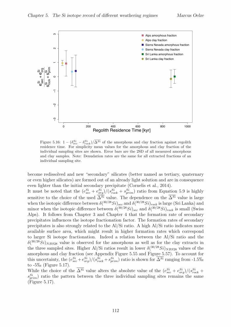
Chapter 5. The Si isotope record of di↵erent weathering regimes Marcus Oelze
−3−2
−10
12
3
Regolith Residence Time [kyr]0 200 400 600 800 1000
Alps amorphous fractionAlps clay fractionSierra Nevada amorphous fractionSierra Nevada clay fractionSri Lanka amorphous fractionSri Lanka clay fraction
e sec
Si+
e org
Si
s roc
kSi
+s p
rimSi
Figure 5.16: 1 � (�Si
sec
� �Si
rock
)/�Si of the amorphous and clay fraction against regolithresidence time. For simplicity mean values for the amorphous and clay fraction of theindividual sampling sites are shown. Error bars are the 2SD of all measured amorphousand clay samples. Note: Denudation rates are the same for all extracted fractions of anindividual sampling site.
become redissolved and new “secondary” silicates (better named as tertiary, quaternaryor even higher silicates) are formed out of an already light solution and are in consequenceeven lighter than the initial secondary precipitate (Cornelis et al., 2014).It must be noted that the (eSi
sec
+ eSiorg
)/(sSirock
+ sSiprim
) ratio from Equation 5.9 is highly
sensitive to the choice of the used �Si value. The dependence on the �Si value is largewhen the isotopic di↵erence between �(30/28Si)
sec
and �(30/28Si)rock
is large (Sri Lanka) andminor when the isotopic di↵erence between �(30/28Si)
sec
and �(30/28Si)rock
is small (SwissAlps). It follows from Chapter 3 and Chapter 4 that the formation rate of secondaryprecipitates influences the isotope fractionation factor. The formation rates of secondaryprecipitates is also strongly related to the Al/Si ratio. A high Al/Si ratio indicates moreavailable surface area, which might result in higher formation rates which correspondto larger Si isotope fractionation. Indeed a relation between the Al/Si ratio and the�(30/28Si)
NBS28 value is observed for the amorphous as well as for the clay extracts inthe three sampled sites. Higher Al/Si ratios result in lower �(30/28Si)
NBS28 values of theamorphous and clay fraction (see Appendix Figure 5.55 and Figure 5.57). To account forthis uncertainty, the (eSi
sec
+eSiorg
)/(sSirock
+sSiprim
) ratio is shown for �Si ranging from -1.5hto -5h (Figure 5.17).While the choice of the �Si value alters the absolute value of the (eSi
sec
+ eSiorg
)/(sSirock
+sSiprim
) ratio the pattern between the three individual sampling sites remains the same(Figure 5.17).
112
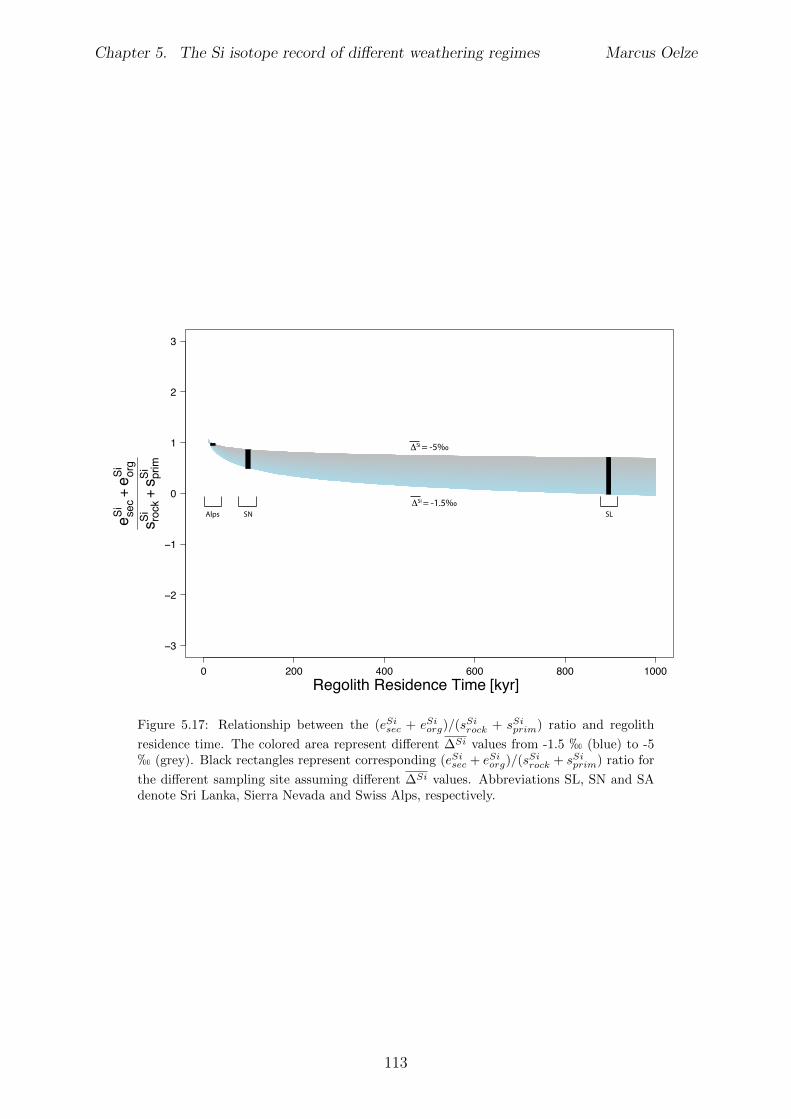
Chapter 5. The Si isotope record of di↵erent weathering regimes Marcus Oelze
−3
−2
−1
0
1
2
3
Regolith Residence Time [kyr]0 200 400 600 800 1000
e sec
Si+
e org
Si
s roc
kSi
+s p
rimSi
Alps SLSN
ΔSi = -5‰
ΔSi = -1.5‰
Figure 5.17: Relationship between the (eSi
sec
+ eSi
org
)/(sSi
rock
+ sSi
prim
) ratio and regolith
residence time. The colored area represent di↵erent �Si values from -1.5 h (blue) to -5h (grey). Black rectangles represent corresponding (eSi
sec
+ eSi
org
)/(sSi
rock
+ sSi
prim
) ratio for
the di↵erent sampling site assuming di↵erent �Si values. Abbreviations SL, SN and SAdenote Sri Lanka, Sierra Nevada and Swiss Alps, respectively.
113
Chapter 5. The Si isotope record of di↵erent weathering regimes Marcus Oelze
5.6 Summary
This chapter summarizes �(30/28Si)NBS28 values derived from three di↵erent weathering
regimes of extracted amorphous and clay phases from soils and saprolites. A method wasderived to sequentially extract the amorphous and clay phase and subsequently measurethem for their �(30/28Si)
NBS28 values.It is shown here for the first time that a strong relationship between Si isotopic compo-sition of amorphous and clay phases extracted from soils and saprolites and the regolithresidence time of the three di↵erent weathering regimes exists. An increase in regolithresidence time leads to lower �(30/28Si)
NBS28 values for secondary silicates formed. InSri Lanka, the setting with the longest regolith residence time, the lowest �(30/28Si)
NBS28
values for the amorphous and clay phase are measured. Extracted phases of the SierraNevada sampling site, where regolith residence time are shorter, show relative higher�(30/28Si)
NBS28 values for the amorphous and clay phase. Amorphous and clay fractionsof the Swiss Alps sampling site (lowest regolith residence time of all settings) show thehighest �(30/28Si)
NBS28 values of three sampled weathering regimes. An isotope mass bal-ance model (Bouchez et al., 2013) reveal that the proportion of particulate export fluxincreases over the dissolved import Si flux according to the decrease in regolith residencetime. This proportion is reflected in the �(30/28Si)
NBS28 values of secondary precipitates.
114
Chapter 5. The Si isotope record of di↵erent weathering regimes Marcus Oelze
5.7 Appendix Chapter 5
5.7.1 Background data
In this section all available data for the three described sites is provided to get a fulloverview of all settings. Most of the background data results from an ongoing “Section 3.4- Earth Surface Geochemistry” project with the focus to better understand the processesof soil and saprolite formation in these three sites. The background data presented hereare stored in the GFZ-EarthSurfaceGeochemistry-DataRepository (GFZ-ESG-DR).Total element concentrations (see subsection 5.7.1 and subsection 5.7.4) were analyzed onbulk samples using X-ray fluorescence spectrometry (XRF, Panalytical Axios Advancedat German Research Center for Geosciences (GFZ)). All samples (bedrock, saprolite andsoil) were oven dried at 60 �, and representative aliquots of the samples were pulverizedin an agate mill to <60 µm grain size. Sample powders were weighed before and aftertreating them for 5 h at 600 � to determine the loss on ignition (LOI). The remainingpowder was then used for alkali fusion using Li-metaborate to produce glass beads thatwere analyzed for bulk chemical composition. Relative analytical uncertainties on thereported XRF data are about 5% for major elements and about 10% on trace elements.
Calculation of element concentrations and elemental chemical depletion
In the weathering literature a series of measurable parameters, such as the chemicaldepletion fraction (CDF) or the elemental mass transfer coe�cient (⌧), are used to describethe weathering regime of the sampled setting. The fraction of mass that is lost in theirdissolved form due to chemical weathering has been termed by Riebe et al. (2001) as thechemical depletion fraction (CDF; Equation 5.10).
CDF = 1� [Zr]rock
[Zr]weathered
(5.10)
where [Zr]rock
and [Zr]weathered
represent Zr concentrations in the parent bedrock and inthe weathered material, respectively. When CDF = 0, no loss of soluble elements hasoccurred from saprolite or soil as compared to the parent material. A value of CDF > 0quantifies the fraction of total mass lost during chemical weathering. In many lithologiesthe CDF value will not be >0.5. One reason for this is the large fraction of the primarySiO2 that is locked in insoluble quartz. Another reason is the formation of secondaryminerals and therefore the retention of Si, Fe, and Al released from primary minerals(Dixon and von Blanckenburg, 2012). Critical for the correct calculation of CDF values area homogeneous and known concentrations of Zr in the parent material. Reported relativeuncertainties of calculated CDF values are about 14% and result from error propagationof element concentration measured by XRF (relative uncertainty: major elements 5% andtrace elements 10%).The mass change of an element (X) in the soil/saprolite relative to the parent bedrock isdefined as the dimensionless element-mass-transfer coe�cient ⌧
X
:
⌧X
=[X]
weathered
[X]rock
� [Zr]rock
[Zr]weathered
� 1 (5.11)
where [X]weathered
and [X]rock
represent concentrations of an element X in the weatheredand parent bedrock material, respectively. When ⌧
X
= 0, X has not been lost as comparedto the parent material; when ⌧
X
< 0 or ⌧X
> 0, there is elemental loss or gain of element
115
Chapter 5. The Si isotope record of di↵erent weathering regimes Marcus Oelze
X during weathering, respectively; ⌧X
= -1 means 100% loss of the element from parentbedrock to weathered material. It seems justified to use Zr as immobile element tocalculate CDF and ⌧
X
values in all sampled settings, see details in Hewawasam et al.(2013), Dixon et al. (2009a) and Norton and von Blanckenburg (2010).Reported major element composition and Zr concentration of bulk samples in Table 5.8,Table 5.13 and Table 5.18 are derived from XRF analyses and are corrected for LOI. Usingthis LOI corrected element composition, CDF values as well as element-mass-transfercoe�cient ⌧
X
are calculated.
Background data - Sri Lanka
The presented background data for the Sri Lankan sampling site is discussed and describedin detail in Hewawasam et al. (2013). Here only the main findings are summarized:Element concentrations of the bulk soil samples of the sampled regolith profile show theexpected picture of a soil developed over a Charnockite bedrock where Si, Al, Fe, K, Na,Fe and Ca are the dominant major elements (Figure 5.18). The dominating elements inthe extracted amorphous fraction are Al and Si (see Figure 5.19 and Table 5.17). Theelement pattern of the clay fraction shows a clear enrichment of Al, Si and Fe comparedthe bulk soil (see Figure 5.20 and Table 5.17).A significant variability in CDF is observed (using Zr as immobile element) within theregolith profile. The chemical depletion fractions (CDF; Equation 5.10) vary significantlywithin the sampled regolith profile. The upward gradual increase of CDF values from0.1 to 0.6 from the saprolite bedrock interface at 10 m to the soil - saprolite boundaryat a depth of 0.6 m indicates increasing chemical mass loss during bedrock to saproliteconversion (Figure 5.21). Chemical depletion fraction values of 0.6 within the saproliteindicate that up to 60% of the original rock mass is lost through chemical weathering.Using again Zr as immobile element, element depletion profiles (⌧ -plots; Equation 5.11)were calculated for the entire profile (Figure 5.22). Depletion of Ca and Na throughout thewhole regolith section can be observed (Figure 5.22). Mg, K, P, and Si show a depletiontrend towards the surface of the regolith. Within the saprolite only Al shows no strongelemental depletion, but exhibits ⌧ -values of -0.5 in the soil, indication Al loss in thisupper zone. The element depletion profile for Mn shows a broad pattern from -0.5 at thesaprolite-corestone zone boundary to values > 0.5 in 250 cm depth, to again depletionvalues of 0.5 at the saprolite - soil boundary. Only Fe and Ti show an enrichment withinthe saprolite and the soil relative to bedrock.Large di↵erences are observed for the evolution of the Al/Si ratio with depth of thedi↵erent extracted fractions (Figure 5.23). The amorphous fraction always shows largerAl/Si ratios than the clay fraction. At the saprolite - soil boundary, at the saprolite- corestone zone boundary and within the corestone zone, large di↵erence between theAl/Si ratios of the amorphous and clay fraction are observed. In contrast, di↵erencesin the Al/Si ratios of the amorphous and clay fractions between the two boundaries areminor. The Al/Si ratios of the clay fraction stay nearly constant over the whole regolithprofile.
116
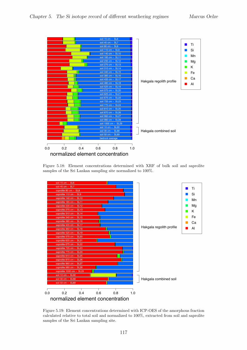
Chapter 5. The Si isotope record of di↵erent weathering regimes Marcus Oelze
normalized element concentration
0.0 0.2 0.4 0.6 0.8 1.0
Ti
Si
Mn
Mg
K
Fe
Ca
Al
soil 15 cm − SL6soil 45 cm − SL7soil 80 cm − SL8soil 110 cm − SL9soil 140 cm − SL10soil 185 cm − SL11soil 235 cm − SL12soil 275 cm − SL13soil 310 cm − SL14soil 340 cm − SL15soil 385 cm − SL16soil 435 cm − SL17soil 480 cm − SL18soil 525 cm − SL19soil 575 cm − SL20soil 625 cm − SL21soil 675 cm − SL22soil 725 cm − SL23soil 775 cm − SL24soil 810 cm − SL25soil 870 cm − SL26soil 960 cm − SL27soil 980 cm − SL28soil 1000 cm − SL29
Hakgala regolith profile
soil 10 cm − SL90soil 30 cm − SL88soil 50 cm − SL89bedrock average
Hakgala combined soil
Figure 5.18: Element concentrations determined with XRF of bulk soil and saprolitesamples of the Sri Lankan sampling site normalized to 100%.
normalized element concentration
0.0 0.2 0.4 0.6 0.8 1.0
Ti
Si
Mn
Mg
K
Fe
Ca
Al
soil 15 cm − SL6soil 45 cm − SL7saprolite 80 cm − SL8saprolite 110 cm − SL9saprolite 140 cm − SL10saprolite 185 cm − SL11saprolite 235 cm − SL12saprolite 275 cm − SL13saprolite 310 cm − SL14saprolite 340 cm − SL15saprolite 385 cm − SL16saprolite 435 cm − SL17saprolite 480 cm − SL18saprolite 525 cm − SL19saprolite 575 cm − SL20saprolite 625 cm − SL21saprolite 675 cm − SL22saprolite 725 cm − SL23saprolite 775 cm − SL24saprolite 810 cm − SL25saprolite 870 cm − SL26saprolite 960 cm − SL27saprolite 980 cm − SL28saprolite 1000 cm − SL29
Hakgala regolith profile
soil 10 cm − SL90soil 30 cm − SL88soil 50 cm − SL89
Hakgala combined soil
Figure 5.19: Element concentrations determined with ICP-OES of the amorphous fractioncalculated relative to total soil and normalized to 100%, extracted from soil and saprolitesamples of the Sri Lankan sampling site.
117
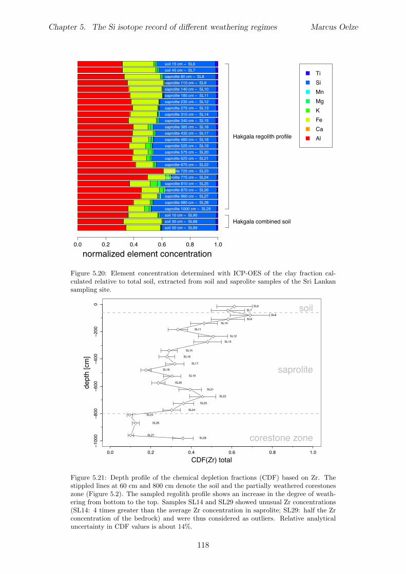
Chapter 5. The Si isotope record of di↵erent weathering regimes Marcus Oelze
normalized element concentration
0.0 0.2 0.4 0.6 0.8 1.0
Ti
Si
Mn
Mg
K
Fe
Ca
Al
soil 15 cm − SL6soil 45 cm − SL7saprolite 80 cm − SL8saprolite 110 cm − SL9saprolite 140 cm − SL10saprolite 185 cm − SL11saprolite 235 cm − SL12saprolite 275 cm − SL13saprolite 310 cm − SL14saprolite 340 cm − SL15saprolite 385 cm − SL16saprolite 435 cm − SL17saprolite 480 cm − SL18saprolite 525 cm − SL19saprolite 575 cm − SL20saprolite 625 cm − SL21saprolite 675 cm − SL22saprolite 725 cm − SL23saprolite 775 cm − SL24saprolite 810 cm − SL25saprolite 870 cm − SL26saprolite 960 cm − SL27saprolite 980 cm − SL28saprolite 1000 cm − SL29
Hakgala regolith profile
soil 10 cm − SL90soil 30 cm − SL88soil 50 cm − SL89
Hakgala combined soil
Figure 5.20: Element concentration determined with ICP-OES of the clay fraction cal-culated relative to total soil, extracted from soil and saprolite samples of the Sri Lankansampling site.
0.0 0.2 0.4 0.6 0.8 1.0
−1000
−800
−600
−400
−200
0
CDF(Zr) total
dept
h [c
m]
SL6SL7
SL8SL9
SL10
SL11
SL12
SL13
SL15
SL16
SL17
SL18
SL19
SL20
SL21
SL22
SL23
SL24SL25
SL26
SL27SL28
soil
saprolite
corestone zone
Figure 5.21: Depth profile of the chemical depletion fractions (CDF) based on Zr. Thestippled lines at 60 cm and 800 cm denote the soil and the partially weathered corestoneszone (Figure 5.2). The sampled regolith profile shows an increase in the degree of weath-ering from bottom to the top. Samples SL14 and SL29 showed unusual Zr concentrations(SL14: 4 times greater than the average Zr concentration in saprolite; SL29: half the Zrconcentration of the bedrock) and were thus considered as outliers. Relative analyticaluncertainty in CDF values is about 14%.
118
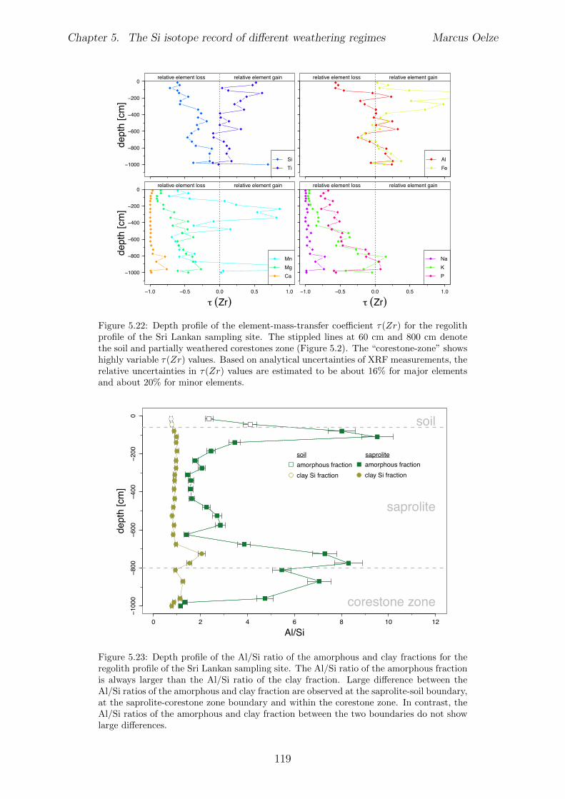
Chapter 5. The Si isotope record of di↵erent weathering regimes Marcus Oelze
−1000
−800
−600
−400
−200
0
dept
h [c
m]
relative element loss relative element gain
SiTi
relative element loss relative element gain
AlFe
−1000
−800
−600
−400
−200
0
−1.0 −0.5 0.0 0.5 1.0
dept
h [c
m]
τ (Zr)
relative element loss relative element gain
MnMgCa
dept
h [c
m]
−1.0 −0.5 0.0 0.5 1.0
τ (Zr)
relative element loss relative element gain
NaKP
Figure 5.22: Depth profile of the element-mass-transfer coe�cient ⌧(Zr) for the regolithprofile of the Sri Lankan sampling site. The stippled lines at 60 cm and 800 cm denotethe soil and partially weathered corestones zone (Figure 5.2). The “corestone-zone” showshighly variable ⌧(Zr) values. Based on analytical uncertainties of XRF measurements, therelative uncertainties in ⌧(Zr) values are estimated to be about 16% for major elementsand about 20% for minor elements.
0 2 4 6 8 10 12
−1000
−800
−600
−400
−200
0
Al/Si
dept
h [c
m]
amorphous fractionclay Si fraction
soil
saprolite
corestone zone
amorphous fractionclay Si fraction
soil saprolite
Figure 5.23: Depth profile of the Al/Si ratio of the amorphous and clay fractions for theregolith profile of the Sri Lankan sampling site. The Al/Si ratio of the amorphous fractionis always larger than the Al/Si ratio of the clay fraction. Large di↵erence between theAl/Si ratios of the amorphous and clay fraction are observed at the saprolite-soil boundary,at the saprolite-corestone zone boundary and within the corestone zone. In contrast, theAl/Si ratios of the amorphous and clay fraction between the two boundaries do not showlarge di↵erences.
119
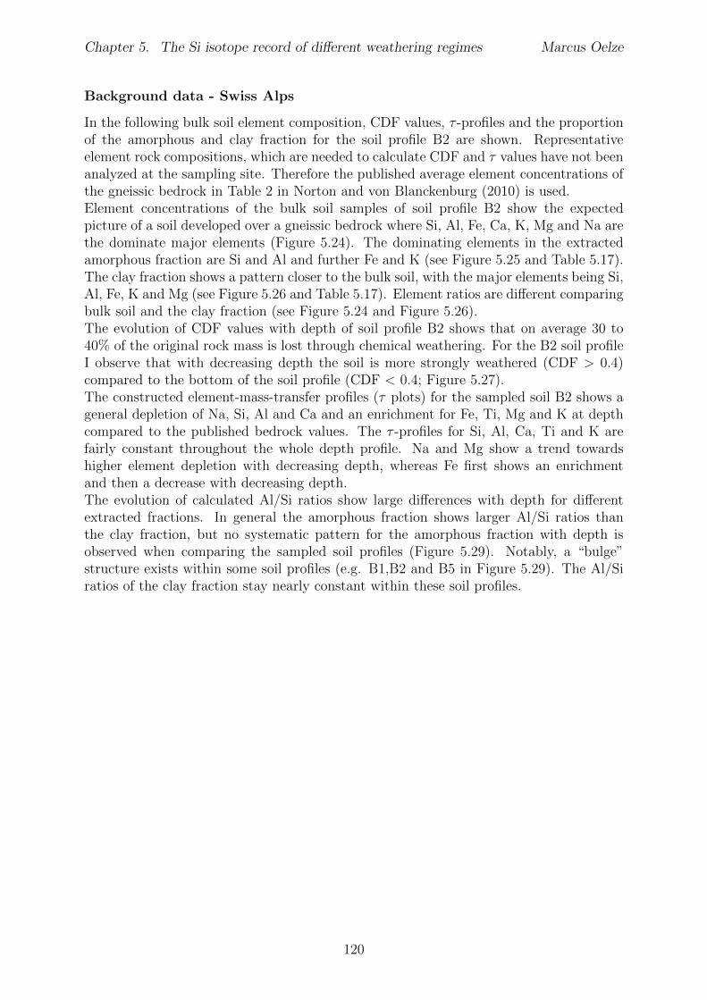
Chapter 5. The Si isotope record of di↵erent weathering regimes Marcus Oelze
Background data - Swiss Alps
In the following bulk soil element composition, CDF values, ⌧ -profiles and the proportionof the amorphous and clay fraction for the soil profile B2 are shown. Representativeelement rock compositions, which are needed to calculate CDF and ⌧ values have not beenanalyzed at the sampling site. Therefore the published average element concentrations ofthe gneissic bedrock in Table 2 in Norton and von Blanckenburg (2010) is used.Element concentrations of the bulk soil samples of soil profile B2 show the expectedpicture of a soil developed over a gneissic bedrock where Si, Al, Fe, Ca, K, Mg and Na arethe dominate major elements (Figure 5.24). The dominating elements in the extractedamorphous fraction are Si and Al and further Fe and K (see Figure 5.25 and Table 5.17).The clay fraction shows a pattern closer to the bulk soil, with the major elements being Si,Al, Fe, K and Mg (see Figure 5.26 and Table 5.17). Element ratios are di↵erent comparingbulk soil and the clay fraction (see Figure 5.24 and Figure 5.26).The evolution of CDF values with depth of soil profile B2 shows that on average 30 to40% of the original rock mass is lost through chemical weathering. For the B2 soil profileI observe that with decreasing depth the soil is more strongly weathered (CDF > 0.4)compared to the bottom of the soil profile (CDF < 0.4; Figure 5.27).The constructed element-mass-transfer profiles (⌧ plots) for the sampled soil B2 shows ageneral depletion of Na, Si, Al and Ca and an enrichment for Fe, Ti, Mg and K at depthcompared to the published bedrock values. The ⌧ -profiles for Si, Al, Ca, Ti and K arefairly constant throughout the whole depth profile. Na and Mg show a trend towardshigher element depletion with decreasing depth, whereas Fe first shows an enrichmentand then a decrease with decreasing depth.The evolution of calculated Al/Si ratios show large di↵erences with depth for di↵erentextracted fractions. In general the amorphous fraction shows larger Al/Si ratios thanthe clay fraction, but no systematic pattern for the amorphous fraction with depth isobserved when comparing the sampled soil profiles (Figure 5.29). Notably, a “bulge”structure exists within some soil profiles (e.g. B1,B2 and B5 in Figure 5.29). The Al/Siratios of the clay fraction stay nearly constant within these soil profiles.
120
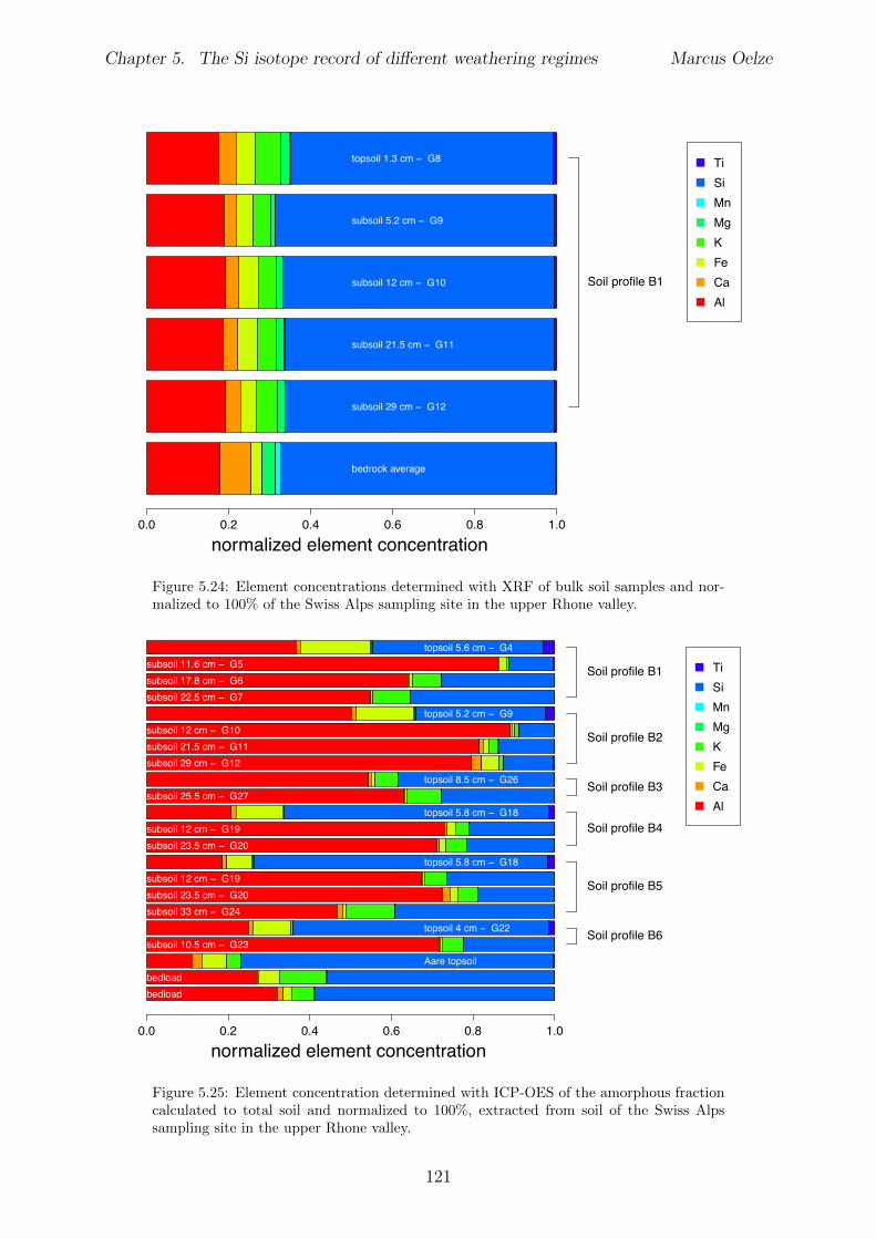
Chapter 5. The Si isotope record of di↵erent weathering regimes Marcus Oelze
normalized element concentration0.0 0.2 0.4 0.6 0.8 1.0
topsoil 1.3 cm − G8
subsoil 5.2 cm − G9
subsoil 12 cm − G10
subsoil 21.5 cm − G11
subsoil 29 cm − G12
bedrock average
Soil profile B1
TiSiMnMgKFeCaAl
Figure 5.24: Element concentrations determined with XRF of bulk soil samples and nor-malized to 100% of the Swiss Alps sampling site in the upper Rhone valley.
normalized element concentration0.0 0.2 0.4 0.6 0.8 1.0
topsoil 5.6 cm − G4subsoil 11.6 cm − G5subsoil 17.8 cm − G6subsoil 22.5 cm − G7
Soil profile B1
topsoil 5.2 cm − G9subsoil 12 cm − G10subsoil 21.5 cm − G11subsoil 29 cm − G12
Soil profile B2
topsoil 8.5 cm − G26subsoil 25.5 cm − G27
Soil profile B3
topsoil 5.8 cm − G18subsoil 12 cm − G19subsoil 23.5 cm − G20
Soil profile B4
topsoil 5.8 cm − G18subsoil 12 cm − G19subsoil 23.5 cm − G20subsoil 33 cm − G24
Soil profile B5
topsoil 4 cm − G22subsoil 10.5 cm − G23
Soil profile B6
Aare topsoilbedloadbedload
TiSiMnMgKFeCaAl
Figure 5.25: Element concentration determined with ICP-OES of the amorphous fractioncalculated to total soil and normalized to 100%, extracted from soil of the Swiss Alpssampling site in the upper Rhone valley.
121
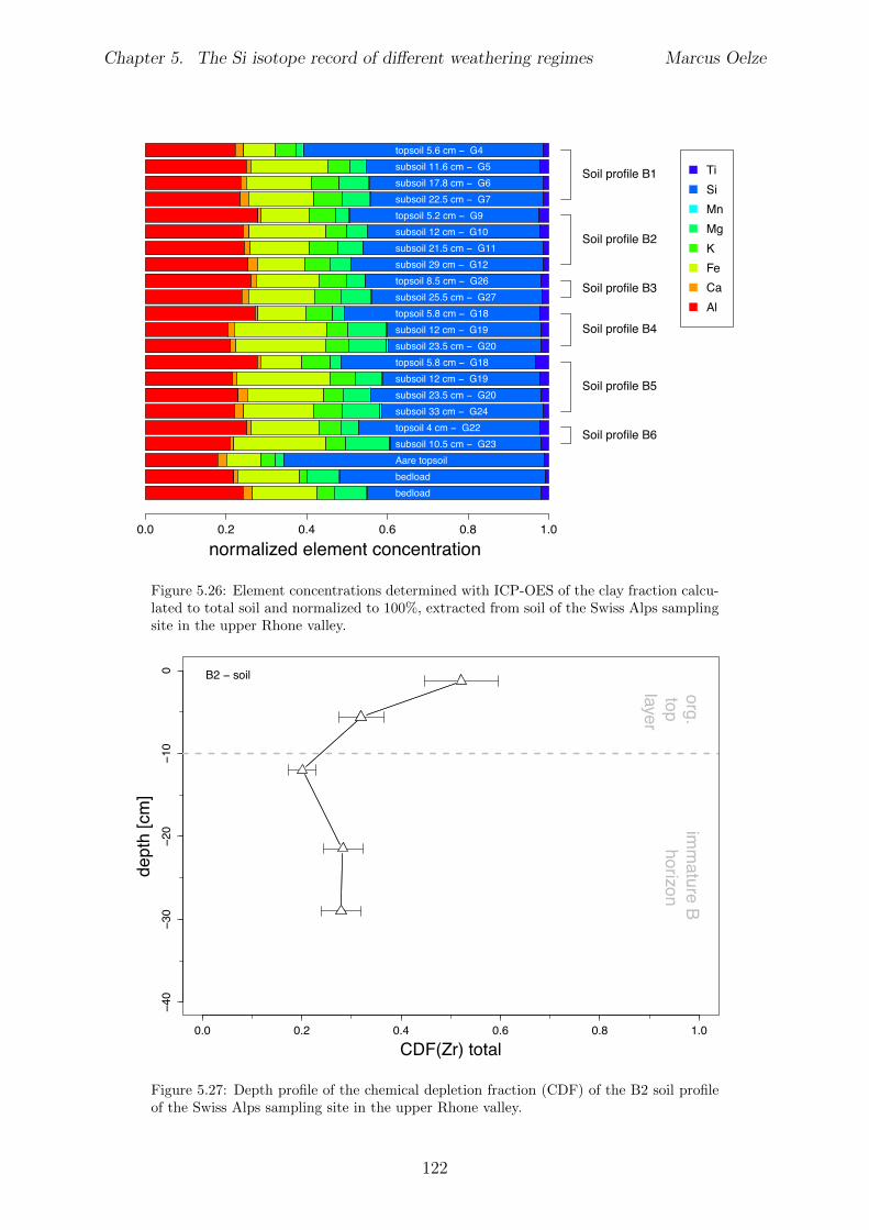
Chapter 5. The Si isotope record of di↵erent weathering regimes Marcus Oelze
normalized element concentration0.0 0.2 0.4 0.6 0.8 1.0
topsoil 5.6 cm − G4subsoil 11.6 cm − G5subsoil 17.8 cm − G6subsoil 22.5 cm − G7
Soil profile B1
topsoil 5.2 cm − G9subsoil 12 cm − G10subsoil 21.5 cm − G11subsoil 29 cm − G12
Soil profile B2
topsoil 8.5 cm − G26subsoil 25.5 cm − G27
Soil profile B3
topsoil 5.8 cm − G18subsoil 12 cm − G19subsoil 23.5 cm − G20
Soil profile B4
topsoil 5.8 cm − G18subsoil 12 cm − G19subsoil 23.5 cm − G20subsoil 33 cm − G24
Soil profile B5
topsoil 4 cm − G22subsoil 10.5 cm − G23
Soil profile B6
Aare topsoilbedloadbedload
TiSiMnMgKFeCaAl
Figure 5.26: Element concentrations determined with ICP-OES of the clay fraction calcu-lated to total soil and normalized to 100%, extracted from soil of the Swiss Alps samplingsite in the upper Rhone valley.
0.0 0.2 0.4 0.6 0.8 1.0
−40
−30
−20
−10
0
CDF(Zr) total
dept
h [c
m]
org. top layer
imm
ature B horizon
B2 − soil
Figure 5.27: Depth profile of the chemical depletion fraction (CDF) of the B2 soil profileof the Swiss Alps sampling site in the upper Rhone valley.
122
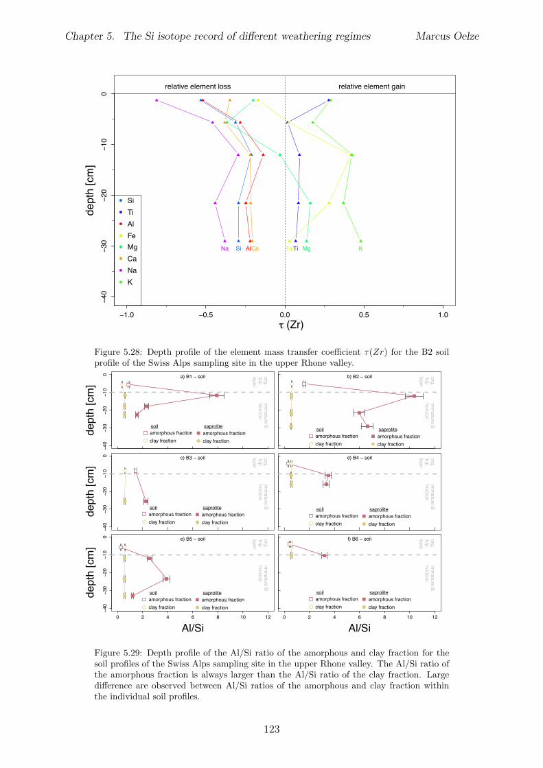
Chapter 5. The Si isotope record of di↵erent weathering regimes Marcus Oelze
−40
−30
−20
−10
0
τ (Zr)
dept
h [c
m]
−1.0 −0.5 0.0 0.5 1.0
relative element loss relative element gain
Si TiAl Fe MgCaNa K
SiTiAlFeMgCaNaK
Figure 5.28: Depth profile of the element mass transfer coe�cient ⌧(Zr) for the B2 soilprofile of the Swiss Alps sampling site in the upper Rhone valley.
−40
−30
−20
−10
0
dept
h [c
m]
amorphous fractionclay fraction
org.toplayer
imm
ature B horizon
a) B1 − soil org.toplayer
imm
ature B horizon
b) B2 − soil
−40
−30
−20
−10
0
dept
h [c
m]
org.toplayer
imm
ature B horizon
c) B3 − soil org.toplayer
imm
ature B horizon
d) B4 − soil
0 2 4 6 8 10 12
−40
−30
−20
−10
0
Al/Si
dept
h [c
m]
org.toplayer
imm
ature B horizon
e) B5 − soil
0 2 4 6 8 10 12
Al/Si
org.toplayer
imm
ature B horizon
f) B6 − soil
amorphous fractionclay fraction
soil saprolite
amorphous fractionclay fraction
amorphous fractionclay fraction
soil saprolite
amorphous fractionclay fraction
amorphous fractionclay fraction
soil saproliteamorphous fractionclay fraction
amorphous fractionclay fraction
soil saprolite
amorphous fractionclay fraction
amorphous fractionclay fraction
soil saprolite
amorphous fractionclay fraction
amorphous fractionclay fraction
soil saprolite
Figure 5.29: Depth profile of the Al/Si ratio of the amorphous and clay fraction for thesoil profiles of the Swiss Alps sampling site in the upper Rhone valley. The Al/Si ratio ofthe amorphous fraction is always larger than the Al/Si ratio of the clay fraction. Largedi↵erence are observed between Al/Si ratios of the amorphous and clay fraction withinthe individual soil profiles.
123
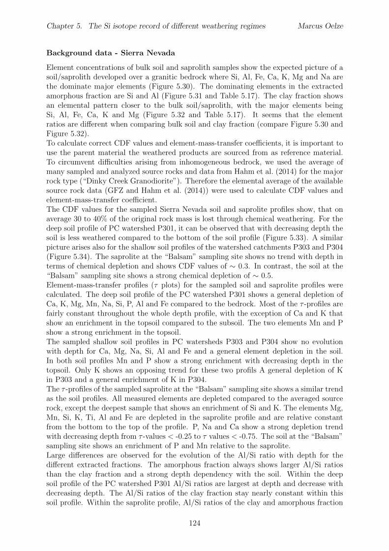
Chapter 5. The Si isotope record of di↵erent weathering regimes Marcus Oelze
Background data - Sierra Nevada
Element concentrations of bulk soil and saprolith samples show the expected picture of asoil/saprolith developed over a granitic bedrock where Si, Al, Fe, Ca, K, Mg and Na arethe dominate major elements (Figure 5.30). The dominating elements in the extractedamorphous fraction are Si and Al (Figure 5.31 and Table 5.17). The clay fraction showsan elemental pattern closer to the bulk soil/saprolith, with the major elements beingSi, Al, Fe, Ca, K and Mg (Figure 5.32 and Table 5.17). It seems that the elementratios are di↵erent when comparing bulk soil and clay fraction (compare Figure 5.30 andFigure 5.32).To calculate correct CDF values and element-mass-transfer coe�cients, it is important touse the parent material the weathered products are sourced from as reference material.To circumvent di�culties arising from inhomogeneous bedrock, we used the average ofmany sampled and analyzed source rocks and data from Hahm et al. (2014) for the majorrock type (“Dinky Creek Granodiorite”). Therefore the elemental average of the availablesource rock data (GFZ and Hahm et al. (2014)) were used to calculate CDF values andelement-mass-transfer coe�cient.The CDF values for the sampled Sierra Nevada soil and saprolite profiles show, that onaverage 30 to 40% of the original rock mass is lost through chemical weathering. For thedeep soil profile of PC watershed P301, it can be observed that with decreasing depth thesoil is less weathered compared to the bottom of the soil profile (Figure 5.33). A similarpicture arises also for the shallow soil profiles of the watershed catchments P303 and P304(Figure 5.34). The saprolite at the “Balsam” sampling site shows no trend with depth interms of chemical depletion and shows CDF values of ⇠ 0.3. In contrast, the soil at the“Balsam” sampling site shows a strong chemical depletion of ⇠ 0.5.Element-mass-transfer profiles (⌧ plots) for the sampled soil and saprolite profiles werecalculated. The deep soil profile of the PC watershed P301 shows a general depletion ofCa, K, Mg, Mn, Na, Si, P, Al and Fe compared to the bedrock. Most of the ⌧ -profiles arefairly constant throughout the whole depth profile, with the exception of Ca and K thatshow an enrichment in the topsoil compared to the subsoil. The two elements Mn and Pshow a strong enrichment in the topsoil.The sampled shallow soil profiles in PC watersheds P303 and P304 show no evolutionwith depth for Ca, Mg, Na, Si, Al and Fe and a general element depletion in the soil.In both soil profiles Mn and P show a strong enrichment with decreasing depth in thetopsoil. Only K shows an opposing trend for these two profils A general depletion of Kin P303 and a general enrichment of K in P304.The ⌧ -profiles of the sampled saprolite at the “Balsam” sampling site shows a similar trendas the soil profiles. All measured elements are depleted compared to the averaged sourcerock, except the deepest sample that shows an enrichment of Si and K. The elements Mg,Mn, Si, K, Ti, Al and Fe are depleted in the saprolite profile and are relative constantfrom the bottom to the top of the profile. P, Na and Ca show a strong depletion trendwith decreasing depth from ⌧ -values < -0.25 to ⌧ values < -0.75. The soil at the “Balsam”sampling site shows an enrichment of P and Mn relative to the saprolite.Large di↵erences are observed for the evolution of the Al/Si ratio with depth for thedi↵erent extracted fractions. The amorphous fraction always shows larger Al/Si ratiosthan the clay fraction and a strong depth dependency with the soil. Within the deepsoil profile of the PC watershed P301 Al/Si ratios are largest at depth and decrease withdecreasing depth. The Al/Si ratios of the clay fraction stay nearly constant within thissoil profile. Within the saprolite profile, Al/Si ratios of the clay and amorphous fraction
124
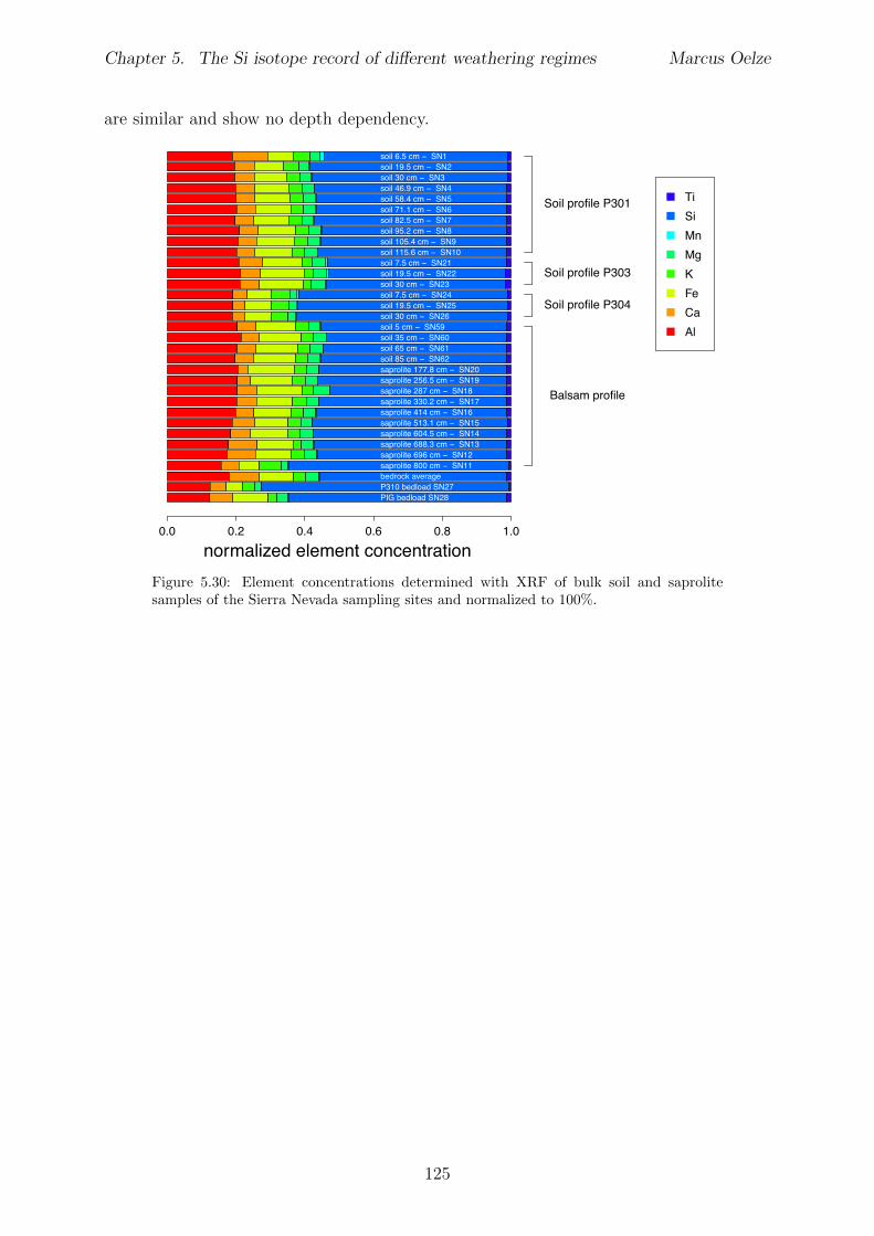
Chapter 5. The Si isotope record of di↵erent weathering regimes Marcus Oelze
are similar and show no depth dependency.
normalized element concentration0.0 0.2 0.4 0.6 0.8 1.0
TiSiMnMgKFeCaAl
soil 6.5 cm − SN1soil 19.5 cm − SN2soil 30 cm − SN3soil 46.9 cm − SN4soil 58.4 cm − SN5soil 71.1 cm − SN6soil 82.5 cm − SN7soil 95.2 cm − SN8soil 105.4 cm − SN9soil 115.6 cm − SN10
Soil profile P301
soil 7.5 cm − SN21soil 19.5 cm − SN22soil 30 cm − SN23
Soil profile P303
soil 7.5 cm − SN24soil 19.5 cm − SN25soil 30 cm − SN26
Soil profile P304
soil 5 cm − SN59soil 35 cm − SN60soil 65 cm − SN61soil 85 cm − SN62saprolite 177.8 cm − SN20saprolite 256.5 cm − SN19saprolite 287 cm − SN18saprolite 330.2 cm − SN17saprolite 414 cm − SN16saprolite 513.1 cm − SN15saprolite 604.5 cm − SN14saprolite 688.3 cm − SN13saprolite 696 cm − SN12saprolite 800 cm − SN11
Balsam profile
bedrock averageP310 bedload SN27PIG bedload SN28
Figure 5.30: Element concentrations determined with XRF of bulk soil and saprolitesamples of the Sierra Nevada sampling sites and normalized to 100%.
125
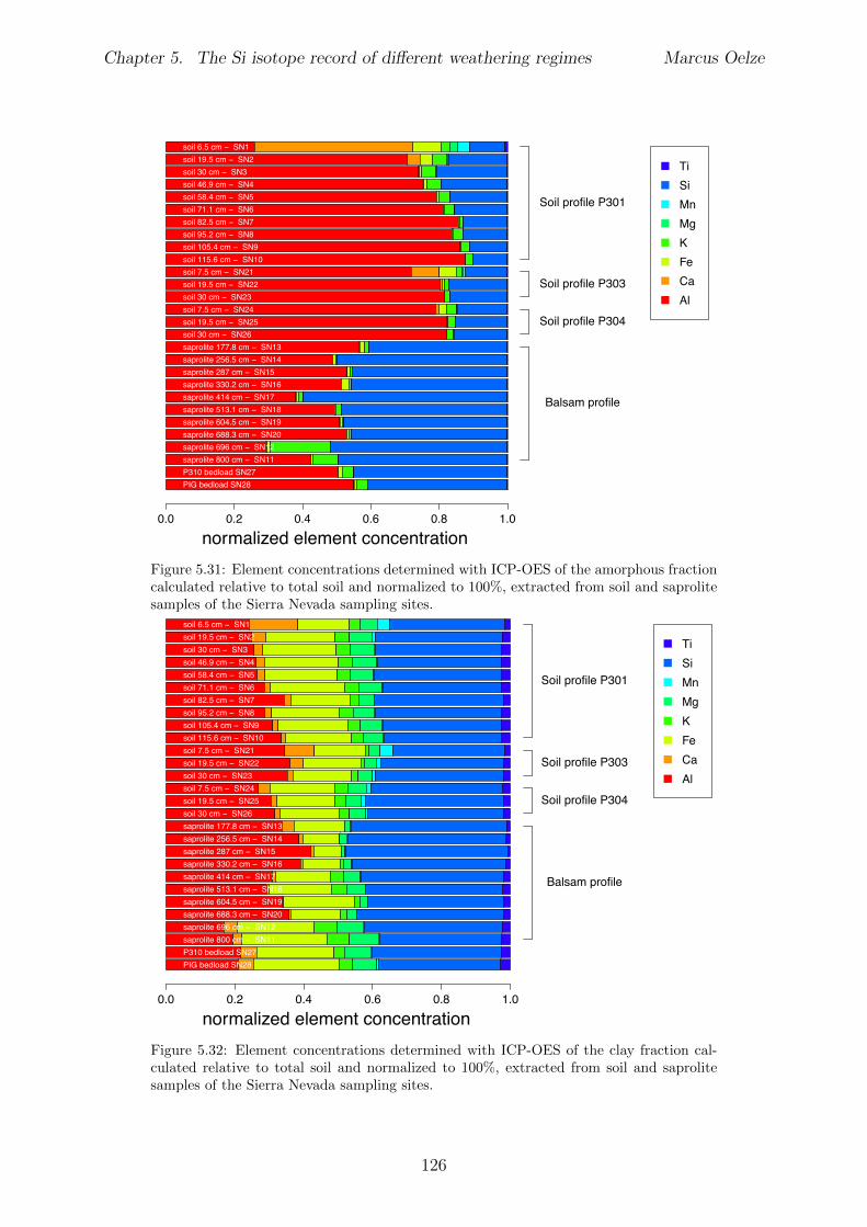
Chapter 5. The Si isotope record of di↵erent weathering regimes Marcus Oelze
normalized element concentration0.0 0.2 0.4 0.6 0.8 1.0
TiSiMnMgKFeCaAl
soil 6.5 cm − SN1soil 19.5 cm − SN2soil 30 cm − SN3soil 46.9 cm − SN4soil 58.4 cm − SN5soil 71.1 cm − SN6soil 82.5 cm − SN7soil 95.2 cm − SN8soil 105.4 cm − SN9soil 115.6 cm − SN10
Soil profile P301
soil 7.5 cm − SN21soil 19.5 cm − SN22soil 30 cm − SN23
Soil profile P303
soil 7.5 cm − SN24soil 19.5 cm − SN25soil 30 cm − SN26
Soil profile P304
saprolite 177.8 cm − SN13saprolite 256.5 cm − SN14saprolite 287 cm − SN15saprolite 330.2 cm − SN16saprolite 414 cm − SN17saprolite 513.1 cm − SN18saprolite 604.5 cm − SN19saprolite 688.3 cm − SN20saprolite 696 cm − SN12saprolite 800 cm − SN11
Balsam profile
P310 bedload SN27PIG bedload SN28
Figure 5.31: Element concentrations determined with ICP-OES of the amorphous fractioncalculated relative to total soil and normalized to 100%, extracted from soil and saprolitesamples of the Sierra Nevada sampling sites.
normalized element concentration0.0 0.2 0.4 0.6 0.8 1.0
TiSiMnMgKFeCaAl
soil 6.5 cm − SN1soil 19.5 cm − SN2soil 30 cm − SN3soil 46.9 cm − SN4soil 58.4 cm − SN5soil 71.1 cm − SN6soil 82.5 cm − SN7soil 95.2 cm − SN8soil 105.4 cm − SN9soil 115.6 cm − SN10
Soil profile P301
soil 7.5 cm − SN21soil 19.5 cm − SN22soil 30 cm − SN23
Soil profile P303
soil 7.5 cm − SN24soil 19.5 cm − SN25soil 30 cm − SN26
Soil profile P304
saprolite 177.8 cm − SN13saprolite 256.5 cm − SN14saprolite 287 cm − SN15saprolite 330.2 cm − SN16saprolite 414 cm − SN17saprolite 513.1 cm − SN18saprolite 604.5 cm − SN19saprolite 688.3 cm − SN20saprolite 696 cm − SN12saprolite 800 cm − SN11
Balsam profile
P310 bedload SN27PIG bedload SN28
Figure 5.32: Element concentrations determined with ICP-OES of the clay fraction cal-culated relative to total soil and normalized to 100%, extracted from soil and saprolitesamples of the Sierra Nevada sampling sites.
126
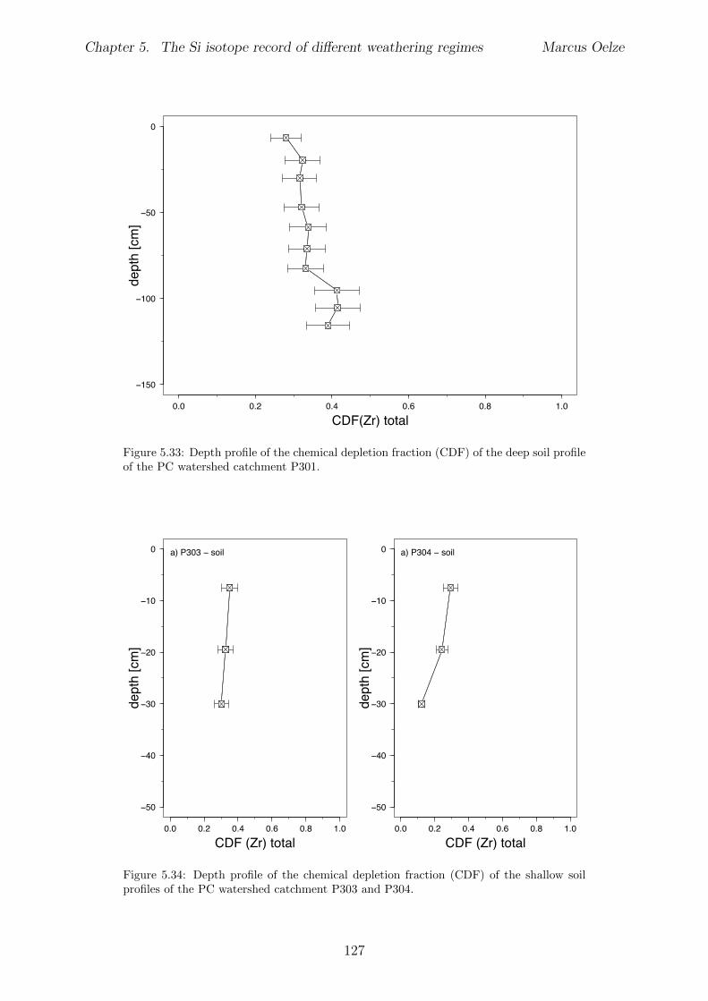
Chapter 5. The Si isotope record of di↵erent weathering regimes Marcus Oelze
0.0 0.2 0.4 0.6 0.8 1.0
−150
−100
−50
0
CDF(Zr) total
dept
h [c
m]
Figure 5.33: Depth profile of the chemical depletion fraction (CDF) of the deep soil profileof the PC watershed catchment P301.
0.0 0.2 0.4 0.6 0.8 1.0
−50
−40
−30
−20
−10
0
CDF (Zr) total
dept
h [c
m]
a) P303 − soil
0.0 0.2 0.4 0.6 0.8 1.0
−50
−40
−30
−20
−10
0
CDF (Zr) total
dept
h [c
m]
a) P304 − soil
Figure 5.34: Depth profile of the chemical depletion fraction (CDF) of the shallow soilprofiles of the PC watershed catchment P303 and P304.
127
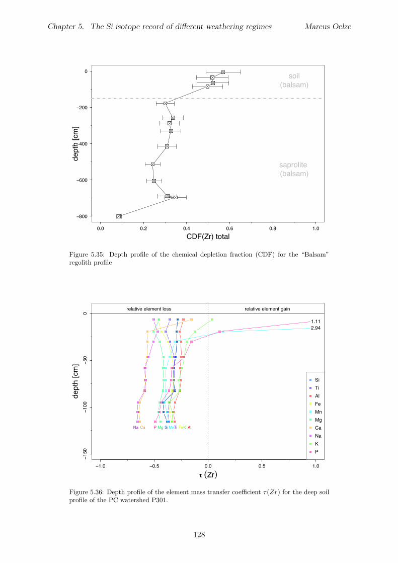
Chapter 5. The Si isotope record of di↵erent weathering regimes Marcus Oelze
0.0 0.2 0.4 0.6 0.8 1.0
−800
−600
−400
−200
0
CDF(Zr) total
dept
h [c
m]
soil(balsam)
saprolite (balsam)
Figure 5.35: Depth profile of the chemical depletion fraction (CDF) for the “Balsam”regolith profile
−1.0 −0.5 0.0 0.5 1.0
−150
−100
−50
0
τ (Zr)
dept
h [c
m]
1.112.94
relative element loss relative element gain
Si Ti AlFeMnMgCaNa KP
SiTiAlFeMnMgCaNaKP
Figure 5.36: Depth profile of the element mass transfer coe�cient ⌧(Zr) for the deep soilprofile of the PC watershed P301.
128
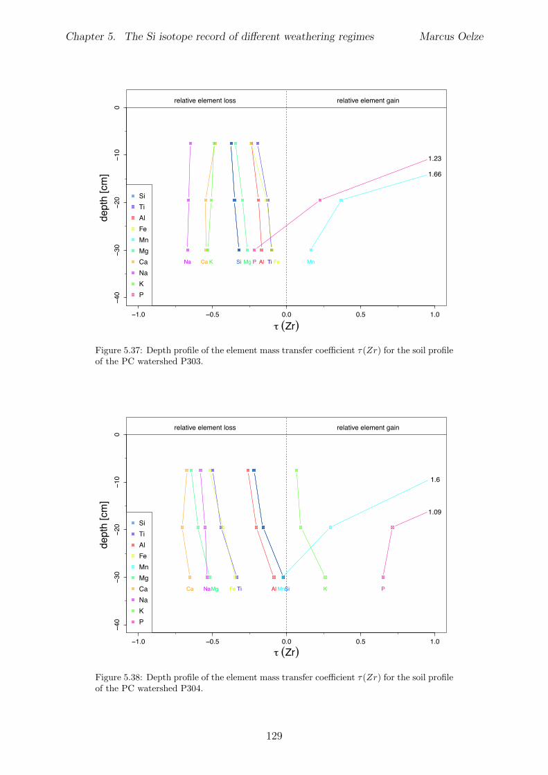
Chapter 5. The Si isotope record of di↵erent weathering regimes Marcus Oelze
−1.0 −0.5 0.0 0.5 1.0
−40
−30
−20
−10
0
τ (Zr)
dept
h [c
m]
relative element loss relative element gain
1.23
1.66
Si TiAl Fe MnMgCaNa K P
SiTiAlFeMnMgCaNaKP
Figure 5.37: Depth profile of the element mass transfer coe�cient ⌧(Zr) for the soil profileof the PC watershed P303.
−1.0 −0.5 0.0 0.5 1.0
−40
−30
−20
−10
0
τ (Zr)
dept
h [c
m]
relative element loss relative element gain
1.6
1.09
SiTi AlFe MnMgCa Na K P
SiTiAlFeMnMgCaNaKP
Figure 5.38: Depth profile of the element mass transfer coe�cient ⌧(Zr) for the soil profileof the PC watershed P304.
129
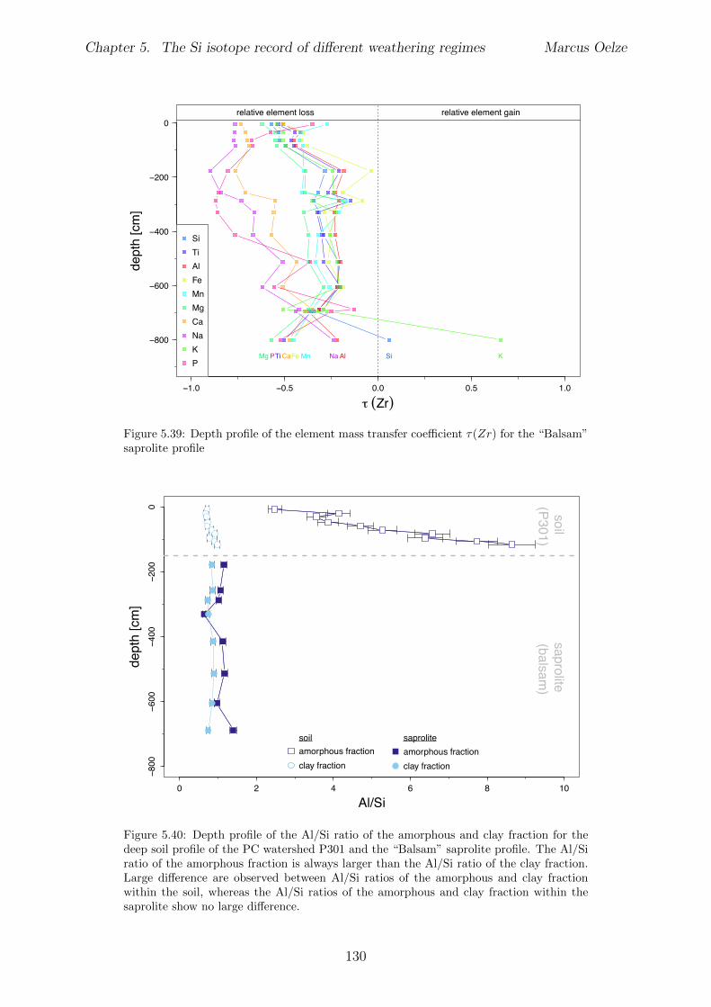
Chapter 5. The Si isotope record of di↵erent weathering regimes Marcus Oelze
−1.0 −0.5 0.0 0.5 1.0
−800
−600
−400
−200
0
τ (Zr)
dept
h [c
m]
relative element loss relative element gain
SiTi AlFe MnMg Ca Na KP
SiTiAlFeMnMgCaNaKP
Figure 5.39: Depth profile of the element mass transfer coe�cient ⌧(Zr) for the “Balsam”saprolite profile
0 2 4 6 8 10
−800
−600
−400
−200
0
Al/Si
dept
h [c
m]
amorphous fractionclay fraction
soil(P301)
saprolite(balsam
)
amorphous fractionclay fraction
soil saprolite
Figure 5.40: Depth profile of the Al/Si ratio of the amorphous and clay fraction for thedeep soil profile of the PC watershed P301 and the “Balsam” saprolite profile. The Al/Siratio of the amorphous fraction is always larger than the Al/Si ratio of the clay fraction.Large di↵erence are observed between Al/Si ratios of the amorphous and clay fractionwithin the soil, whereas the Al/Si ratios of the amorphous and clay fraction within thesaprolite show no large di↵erence.
130
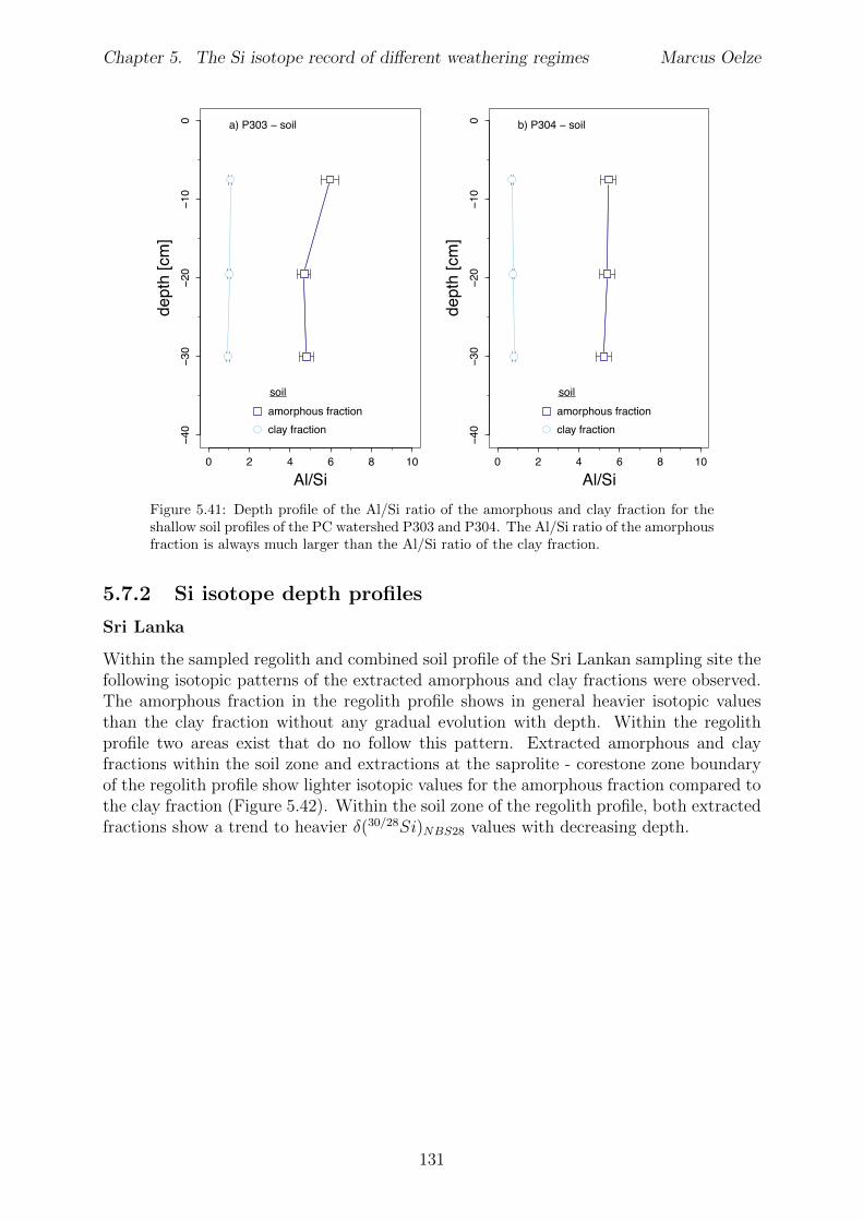
Chapter 5. The Si isotope record of di↵erent weathering regimes Marcus Oelze
0 2 4 6 8 10
−40
−30
−20
−10
0
Al/Si
dept
h [c
m]
amorphous fractionclay fraction
a) P303 − soil
0 2 4 6 8 10−4
0−3
0−2
0−1
00
Al/Si
dept
h [c
m]
amorphous fractionclay fraction
b) P304 − soil
soil soil
Figure 5.41: Depth profile of the Al/Si ratio of the amorphous and clay fraction for theshallow soil profiles of the PC watershed P303 and P304. The Al/Si ratio of the amorphousfraction is always much larger than the Al/Si ratio of the clay fraction.
5.7.2 Si isotope depth profiles
Sri Lanka
Within the sampled regolith and combined soil profile of the Sri Lankan sampling site thefollowing isotopic patterns of the extracted amorphous and clay fractions were observed.The amorphous fraction in the regolith profile shows in general heavier isotopic valuesthan the clay fraction without any gradual evolution with depth. Within the regolithprofile two areas exist that do no follow this pattern. Extracted amorphous and clayfractions within the soil zone and extractions at the saprolite - corestone zone boundaryof the regolith profile show lighter isotopic values for the amorphous fraction compared tothe clay fraction (Figure 5.42). Within the soil zone of the regolith profile, both extractedfractions show a trend to heavier �(30/28Si)
NBS28 values with decreasing depth.
131
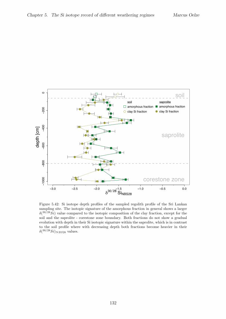
Chapter 5. The Si isotope record of di↵erent weathering regimes Marcus Oelze
−3.0 −2.5 −2.0 −1.5 −1.0 −0.5 0.0
−1000
−800
−600
−400
−200
0
δ30 28 SiNBS28
dept
h [c
m]
soil
saprolite
corestone zone
amorphous fractionclay Si fraction
amorphous fractionclay Si fraction
soil saprolite
Figure 5.42: Si isotope depth profiles of the sampled regolith profile of the Sri Lankansampling site. The isotopic signature of the amorphous fraction in general shows a larger�(30/28Si) value compared to the isotopic composition of the clay fraction, except for thesoil and the saprolite - corestone zone boundary. Both fractions do not show a gradualevolution with depth in their Si isotopic signature within the saprolite, which is in contrastto the soil profile where with decreasing depth both fractions become heavier in their�(30/28Si)
NBS28
values.
132
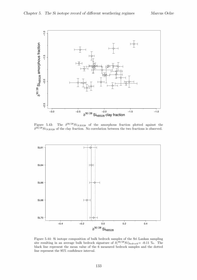
Chapter 5. The Si isotope record of di↵erent weathering regimes Marcus Oelze
−3.0 −2.5 −2.0 −1.5 −1.0
−2.5
−2.0
−1.5
−1.0
δ30 28 SiNBS28 clay fraction
δ3028
Si N
BS28
am
orph
ous
fract
ion
Figure 5.43: The �30/28SiNBS28
of the amorphous fraction plotted against the�30/28Si
NBS28
of the clay fraction. No correlation between the two fractions is observed.
−0.4 −0.2 0.0 0.2 0.4
δ30 28 SiNBS28
SL70
SL68
SL66
SL64
SL61
Figure 5.44: Si isotope composition of bulk bedrock samples of the Sri Lankan samplingsite resulting in an average bulk bedrock signature of �(30/28Si)
bedrock
= -0.11 h. Theblack line represent the mean value of the 6 measured bedrock samples and the dottedline represent the 95% confidence interval.
133
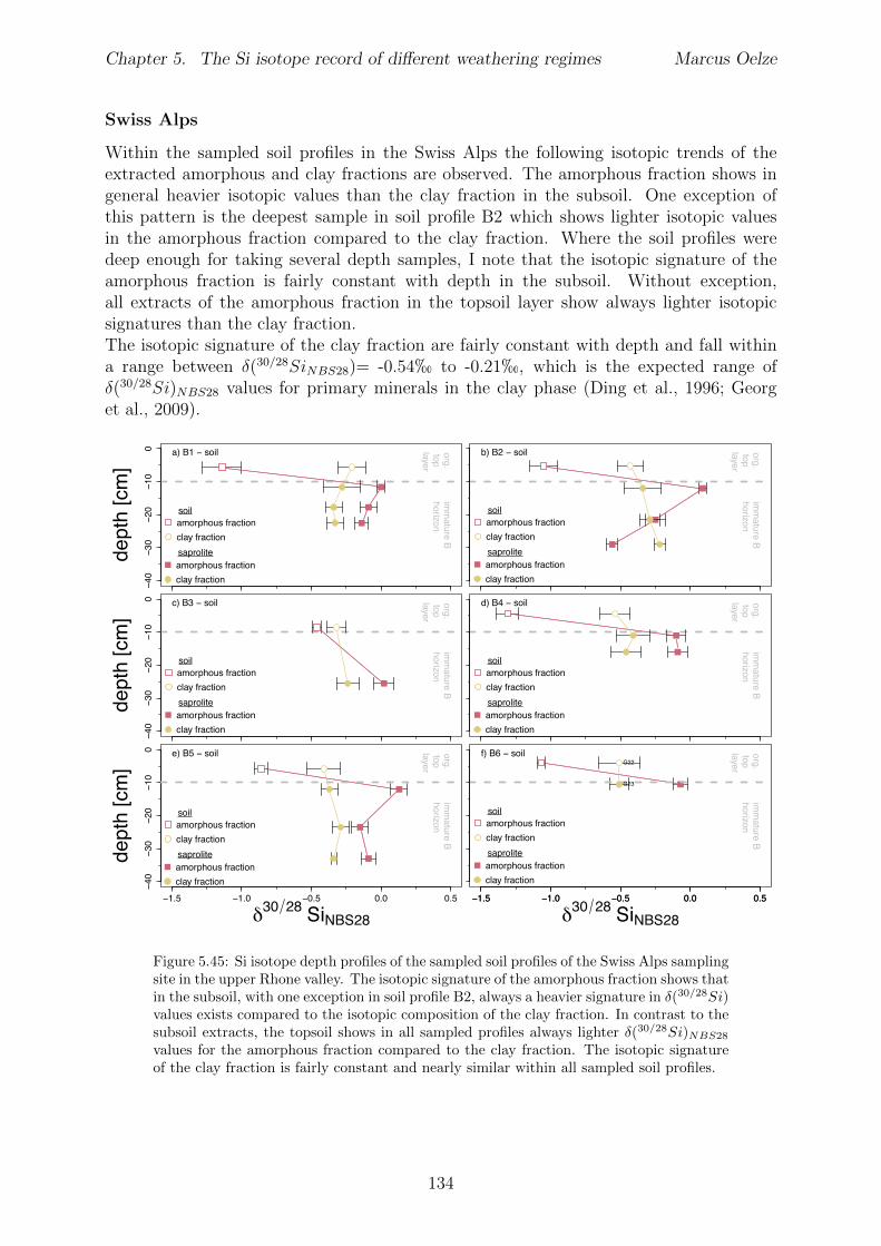
Chapter 5. The Si isotope record of di↵erent weathering regimes Marcus Oelze
Swiss Alps
Within the sampled soil profiles in the Swiss Alps the following isotopic trends of theextracted amorphous and clay fractions are observed. The amorphous fraction shows ingeneral heavier isotopic values than the clay fraction in the subsoil. One exception ofthis pattern is the deepest sample in soil profile B2 which shows lighter isotopic valuesin the amorphous fraction compared to the clay fraction. Where the soil profiles weredeep enough for taking several depth samples, I note that the isotopic signature of theamorphous fraction is fairly constant with depth in the subsoil. Without exception,all extracts of the amorphous fraction in the topsoil layer show always lighter isotopicsignatures than the clay fraction.The isotopic signature of the clay fraction are fairly constant with depth and fall withina range between �(30/28Si
NBS28)= -0.54h to -0.21h, which is the expected range of�(30/28Si)
NBS28 values for primary minerals in the clay phase (Ding et al., 1996; Georget al., 2009).
−40
−30
−20
−10
0
dept
h [c
m]
org.toplayer
imm
ature B horizon
a) B1 − soil org.toplayer
imm
ature B horizon
b) B2 − soil
−40
−30
−20
−10
0
dept
h [c
m]
org.toplayer
imm
ature B horizon
c) B3 − soil org.toplayer
imm
ature B horizon
d) B4 − soil
−40
−30
−20
−10
0
−1.5 −1.0 −0.5 0.0 0.5
δ30 28 SiNBS28
dept
h [c
m]
org.toplayer
imm
ature B horizon
e) B5 − soil
−1.5 −1.0 −0.5 0.0 0.5−1.5 −1.0 −0.5 0.0 0.5
G22
G23
δ30 28 SiNBS28
org.toplayer
imm
ature B horizon
f) B6 − soil
amorphous fractionclay fraction
amorphous fractionclay fraction
soil
saproliteamorphous fractionclay fraction
amorphous fractionclay fraction
soil
saprolite
amorphous fractionclay fraction
amorphous fractionclay fraction
soil
saprolite
amorphous fractionclay fraction
amorphous fractionclay fraction
soil
saproliteamorphous fractionclay fraction
amorphous fractionclay fraction
soil
saprolite
amorphous fractionclay fraction
amorphous fractionclay fraction
soil
saprolite
Figure 5.45: Si isotope depth profiles of the sampled soil profiles of the Swiss Alps samplingsite in the upper Rhone valley. The isotopic signature of the amorphous fraction shows thatin the subsoil, with one exception in soil profile B2, always a heavier signature in �(30/28Si)values exists compared to the isotopic composition of the clay fraction. In contrast to thesubsoil extracts, the topsoil shows in all sampled profiles always lighter �(30/28Si)
NBS28
values for the amorphous fraction compared to the clay fraction. The isotopic signatureof the clay fraction is fairly constant and nearly similar within all sampled soil profiles.
134
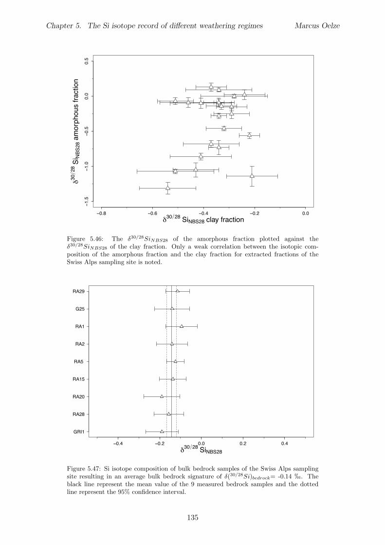
Chapter 5. The Si isotope record of di↵erent weathering regimes Marcus Oelze
−0.8 −0.6 −0.4 −0.2 0.0
−1.5
−1.0
−0.5
0.0
0.5
δ30 28 SiNBS28 clay fraction
δ3028
Si N
BS28
am
orph
ous
fract
ion
Figure 5.46: The �30/28SiNBS28
of the amorphous fraction plotted against the�30/28Si
NBS28
of the clay fraction. Only a weak correlation between the isotopic com-position of the amorphous fraction and the clay fraction for extracted fractions of theSwiss Alps sampling site is noted.
−0.4 −0.2 0.0 0.2 0.4δ30 28 SiNBS28
GRI1
RA28
RA20
RA15
RA5
RA2
RA1
G25
RA29
Figure 5.47: Si isotope composition of bulk bedrock samples of the Swiss Alps samplingsite resulting in an average bulk bedrock signature of �(30/28Si)
bedrock
= -0.14 h. Theblack line represent the mean value of the 9 measured bedrock samples and the dottedline represent the 95% confidence interval.
135
Chapter 5. The Si isotope record of di↵erent weathering regimes Marcus Oelze
Sierra Nevada
The isotopic composition of the amorphous and clay fractions of the deep (0-120 cm)soil profile P301 show a strong dependency with depth (Figure 5.48): The amorphousfraction shows Si isotope signatures �(30/28Si)
amorphous
from -0.8h at the surface, to -1.9h in 120 cm depth (Figure 5.48). The clay fraction of this soil profile shows Si isotopesignatures �(30/28Si)
clay
from -0.7h at the surface, to -1.3h in 120 cm depth (Figure 5.48).The shallow soil profiles of the PC watersheds P303 and P304 show in general also anenrichment of 28Si in the amorphous fraction, with one exception: For the upper mostsample in the soil profile in watershed P303, the �30/28Si
NBS28 value for the amorphousfraction is indistinguishable from the clay fraction within uncertainty. Both soil profilesin these catchment show a depth dependency, where both profiles show much lighter�30/28Si
NBS28 values at depth compared to the top soil for the amorphous fraction, andslightly lighter �30/28Si
NBS28 values at depth compared to the top soil for the clay fraction.I further observe a strong linear correlation between �(30/28Si)
amorphous
and �(30/28Si)clay
for all soil profiles (Figure 5.51). Within the deep “Balsam” saprolite profile a di↵erentpicture emerges. Here I observe an enrichment of 28Si in the clay fraction compared tothe amorphous fraction. The amorphous fractionation does not show an evolution withdepth, but a large spread in their isotopic composition (�(30/28Si)
amorphous
: average=-0.9h, sd=0.3h, ul=-1.3h, ll=-0.5h). The clay fraction also does not show an evolutionwith depth and a slightly smaller variation in their isotopic composition compared to theamorphous fraction (�(30/28Si)
clay
: average=-1.9h, sd=0.2h, ul=-2.1h, ll=-1.5h).No correlation between the isotopic composition of the amorphous fraction �(30/28Si)
amorphous
and the clay fraction �(30/28Si)clay
is observed in the “Balsam” saprolite profile (Fig-ure 5.51).
136
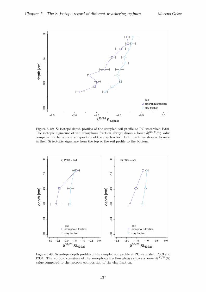
Chapter 5. The Si isotope record of di↵erent weathering regimes Marcus Oelze
−2.5 −2.0 −1.5 −1.0 −0.5 0.0
−150
−100
−50
0
δ30 28 SiNBS28
dept
h [c
m]
amorphous fractionclay fraction
soil
Figure 5.48: Si isotope depth profiles of the sampled soil profile at PC watershed P301.The isotopic signature of the amorphous fraction always shows a lower �(30/28Si) valuecompared to the isotopic composition of the clay fraction. Both fractions show a decreasein their Si isotopic signature from the top of the soil profile to the bottom.
−3.0 −2.5 −2.0 −1.5 −1.0 −0.5 0.0
−50
−40
−30
−20
−10
0
δ30 28 SiNBS28
dept
h [c
m]
a) P303 − soil
amorphous fractionclay fraction
−2.5 −2.0 −1.5 −1.0 −0.5 0.0
−50
−40
−30
−20
−10
0
δ30 28 SiNBS28
dept
h [c
m]
b) P304 − soil
amorphous fractionclay fraction
soil soil
Figure 5.49: Si isotope depth profiles of the sampled soil profile at PC watershed P303 andP304. The isotopic signature of the amorphous fraction always shows a lower �(30/28Si)value compared to the isotopic composition of the clay fraction.
137
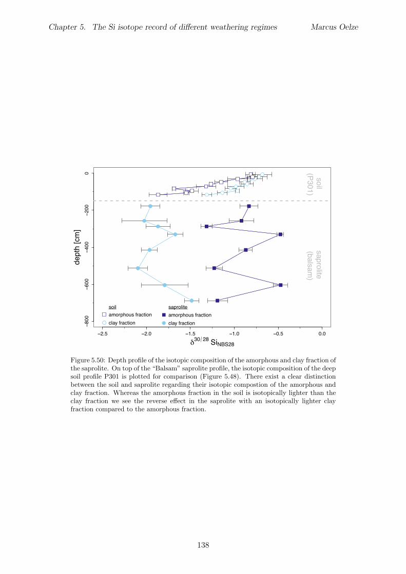
Chapter 5. The Si isotope record of di↵erent weathering regimes Marcus Oelze
−2.5 −2.0 −1.5 −1.0 −0.5 0.0
−800
−600
−400
−200
0
δ30 28 SiNBS28
dept
h [c
m]
soil(P301)
saprolite(balsam
)
amorphous fractionclay fraction
amorphous fractionclay fraction
soil saprolite
Figure 5.50: Depth profile of the isotopic composition of the amorphous and clay fraction ofthe saprolite. On top of the “Balsam” saprolite profile, the isotopic composition of the deepsoil profile P301 is plotted for comparison (Figure 5.48). There exist a clear distinctionbetween the soil and saprolite regarding their isotopic compostion of the amorphous andclay fraction. Whereas the amorphous fraction in the soil is isotopically lighter than theclay fraction we see the reverse e↵ect in the saprolite with an isotopically lighter clayfraction compared to the amorphous fraction.
138
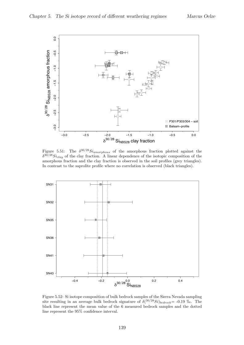
Chapter 5. The Si isotope record of di↵erent weathering regimes Marcus Oelze
−3.0 −2.5 −2.0 −1.5 −1.0 −0.5 0.0
−3.0
−2.5
−2.0
−1.5
−1.0
−0.5
0.0
δ30 28 SiNBS28 clay fraction
δ3028
Si N
BS28
am
orph
ous
fract
ion
P301/P303/304 − soilBalsam−profile
Figure 5.51: The �30/28Siamorphous
of the amorphous fraction plotted against the�30/28Si
clay
of the clay fraction. A linear dependence of the isotopic composition of theamorphous fraction and the clay fraction is observed in the soil profiles (grey triangles).In contrast to the saprolite profile where no correlation is observed (black triangles).
−0.4 −0.2 0.0 0.2 0.4δ30 28 SiNBS28
SN43
SN41
SN36
SN35
SN32
SN31
Figure 5.52: Si isotope composition of bulk bedrock samples of the Sierra Nevada samplingsite resulting in an average bulk bedrock signature of �(30/28Si)
bedrock
= -0.19 h. Theblack line represent the mean value of the 6 measured bedrock samples and the dottedline represent the 95% confidence interval.
139
Chapter 5. The Si isotope record of di↵erent weathering regimes Marcus Oelze
5.7.3 Combining the findings of the individual sampling sites
In this section the results of the former separately treated weathering regimes are com-bined to better understand the behavior of Si isotopes in di↵erent weathering regimes.Figure 5.53 shows the distribution of the chemical depletion fraction for the di↵erentsampling sites. More intense weathering takes place in the tropical regolith profile in SriLanka where up to 60% of the initial rock mass is lost through chemical weathering. Aless intense chemical depletion in the Sierra Nevada sampling site is noted by CDF valuesin the range of 0.3 to 0.4. The kinetically limited weathering regime in the Swiss Alpsshows the lowest chemical depletion fractions.In Chapter 3 and Chapter 4 a strong dependency of Si isotope fractionation with solidformation rate is noted. The observation is made that the rate of solid formation is depen-dent on the Al/Si ratio. Therefore it is straightforward to plot the isotopic compositionof the extracted amorphous and clay fractions against the measured Al/Si ratio.All three settings show the same range of Al/Si ratios from 0.5 to up to 10. Threeareas are distinguishable in Figure 5.54 for the three sampled settings in the Swiss Alps,Sierra Nevada and Sri Lanka, respectively. However, no general relationship betweenthe isotopic composition and the Al/Si ratio of the amorphous fractions extracted fromsoil and saprolite seem to exists (Figure 5.54). If only the isotopic composition of theamorphous fraction extracted from soils is plotted against their corresponding Al/Si, ratioa significant general relationship exist (Figure 5.55), whereas the isotopic composition ofthe amorphous fraction extracted from saprolite does not show any relation with theircorresponding Al/Si ratio (Figure 5.56). The amorphous fraction extracted from soilsevidently becomes lower in their �(30/28Si)
NBS28 ratios with increasing Al/Si ratio.In contrast to the observation made for the amorphous fraction, the clay fraction showsa general trend between the isotopic composition and the corresponding Al/Si ratio (Fig-ure 5.57). An increase in the Al/Si ratio is accompanied by lower �(30/28Si)
NBS28 ratiosin the clay fraction.This trend, that lower �(30/28Si)
NBS28 ratios are accompanied with an increase in theAl/Si ratio, is also observed for bulk rocks of the upper continental crust (Savage et al.,2013). However, this relationship becomes less apparent if we focus on the individual sites.For the Sierra Nevada and the Sri Lankan sampling sites this relationship still holds, butfor the Swiss Alps no relationship exists. Further a much narrower range of Al/Si ratios(< 2.5) for the clay fraction compared to the amorphous fraction (< 12) is observed inthe three sampled settings (Sri Lanka, Sierra Nevada, Swiss Alps).
140
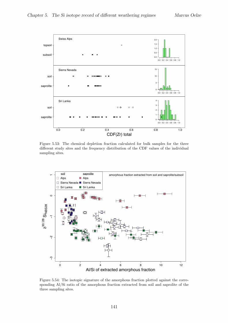
Chapter 5. The Si isotope record of di↵erent weathering regimes Marcus Oelze
elementRatiosXRF_swissAlps[c(3), "cdf.total"]
subsoil
topsoil
Swiss Alps
elementRatiosXRF_sierraNevada[c(1:10, 19:21, 22:24), "cdf.total"]
saprolite
soil
Sierra Nevada
0.0 0.2 0.4 0.6 0.8 1.0elementRatiosXRF_sriLanka[c(1, 2, 25:27), "CDF.total"]
saprolite
soil
Sri Lanka
CDF(Zr) total
0.0 0.2 0.4 0.6 0.8 1.00.0
0.5
1.0
1.5
2.0
0.0 0.2 0.4 0.6 0.8 1.0
0
5
10
15
0.0 0.2 0.4 0.6 0.8 1.00
1
2
3
4
Figure 5.53: The chemical depletion fraction calculated for bulk samples for the threedi↵erent study sites and the frequency distribution of the CDF values of the individualsampling sites.
0 2 4 6 8 10 12
−3−2
−10
1
Al/Si of extracted amorphous fraction
δ30
28 S
i NBS
28
amorphous fraction extracted from soil and saprolite/subsoilAlpsSierra NevadaSri Lanka
AlpsSierra NevadaSri Lanka
soil saprolite
Figure 5.54: The isotopic signature of the amorphous fraction plotted against the corre-sponding Al/Si ratio of the amorphous fraction extracted from soil and saprolite of thethree sampling sites.
141
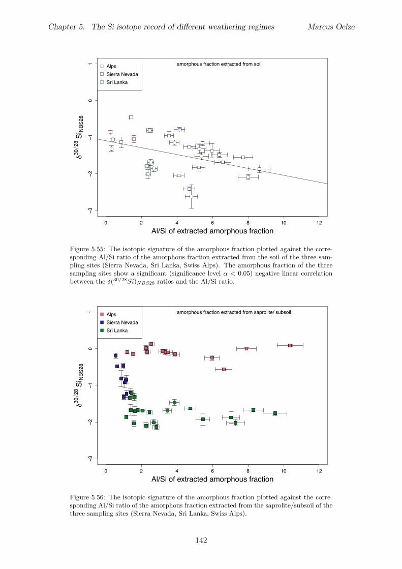
Chapter 5. The Si isotope record of di↵erent weathering regimes Marcus Oelze
0 2 4 6 8 10 12
−3−2
−10
1
Al/Si of extracted amorphous fraction
δ3028
Si N
BS28
amorphous fraction extracted from soilAlpsSierra NevadaSri Lanka
Figure 5.55: The isotopic signature of the amorphous fraction plotted against the corre-sponding Al/Si ratio of the amorphous fraction extracted from the soil of the three sam-pling sites (Sierra Nevada, Sri Lanka, Swiss Alps). The amorphous fraction of the threesampling sites show a significant (significance level ↵ < 0.05) negative linear correlationbetween the �(30/28Si)
NBS28
ratios and the Al/Si ratio.
0 2 4 6 8 10 12
−3−2
−10
1
Al/Si of extracted amorphous fraction
δ3028
Si N
BS28
amorphous fraction extracted from saprolite/ subsoilAlpsSierra NevadaSri Lanka
AlpsSierra NevadaSri Lanka
Figure 5.56: The isotopic signature of the amorphous fraction plotted against the corre-sponding Al/Si ratio of the amorphous fraction extracted from the saprolite/subsoil of thethree sampling sites (Sierra Nevada, Sri Lanka, Swiss Alps).
142
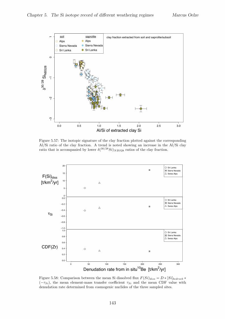
Chapter 5. The Si isotope record of di↵erent weathering regimes Marcus Oelze
0.0 0.5 1.0 1.5 2.0 2.5 3.0
−3−2
−10
1
Al/Si of extracted clay Si
δ3028
Si N
BS28
AlpsSierra NevadaSri Lanka
AlpsSierra NevadaSri Lanka
soil saprolite clay fraction extracted from soil and saprolite/subsoil
Figure 5.57: The isotopic signature of the clay fraction plotted against the correspondingAl/Si ratio of the clay fraction. A trend is noted showing an increase in the Al/Si clayratio that is accompanied by lower �(30/28Si)
NBS28
ratios of the clay fraction.
0
5
10
15
20Sri LankaSierra NevadaSwiss Alps
−1.0
−0.8
−0.6
−0.4
−0.2
0.0Sri LankaSierra NevadaSwiss Alps
0 50 100 150 200 250 300
0.0
0.2
0.4
0.6
0.8
1.0
Denudation rate from in situ 10Be [t/km2/yr]
Sri LankaSierra NevadaSwiss Alps
F(Si)diss [t/km2/yr]
τSi
CDF(Zr)
Figure 5.58: Comparison between the mean Si dissolved flux F (Si)diss
= D ⇤ [Si]bedrock
⇤(�⌧
Si
), the mean element-mass transfer coe�cient ⌧Si
and the mean CDF value withdenudation rate determined from cosmogenic nuclides of the three sampled sites.
143
Chapter 5. The Si isotope record of di↵erent weathering regimes Marcus Oelze
5.7.4 Tables
Tables Sri Lanka
This page is intentionally left blank.
144
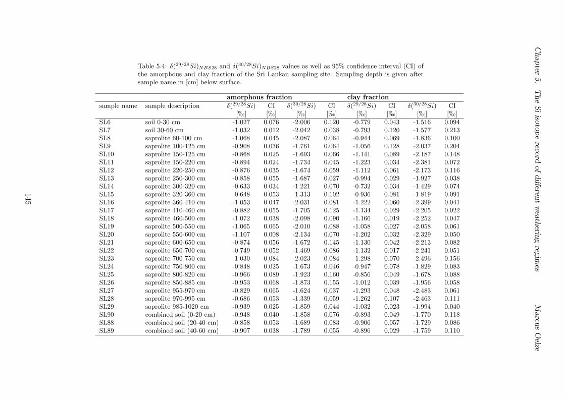
Chap
ter5.
TheSiisotop
erecord
ofdi↵eren
tweath
eringregim
esMarcu
sOelze
Table 5.4: �(29/28Si)NBS28
and �(30/28Si)NBS28
values as well as 95% confidence interval (CI) ofthe amorphous and clay fraction of the Sri Lankan sampling site. Sampling depth is given aftersample name in [cm] below surface.
amorphous fraction clay fraction
sample name sample description �(29/28Si) CI �(30/28Si) CI �(29/28Si) CI �(30/28Si) CI[h] [h] [h] [h] [h] [h] [h] [h]
SL6 soil 0-30 cm -1.027 0.076 -2.006 0.120 -0.779 0.043 -1.516 0.094SL7 soil 30-60 cm -1.032 0.012 -2.042 0.038 -0.793 0.120 -1.577 0.213SL8 saprolite 60-100 cm -1.068 0.045 -2.087 0.064 -0.944 0.069 -1.836 0.100SL9 saprolite 100-125 cm -0.908 0.036 -1.761 0.064 -1.056 0.128 -2.037 0.204SL10 saprolite 150-125 cm -0.868 0.025 -1.693 0.066 -1.141 0.089 -2.187 0.148SL11 saprolite 150-220 cm -0.894 0.024 -1.734 0.045 -1.223 0.034 -2.381 0.072SL12 saprolite 220-250 cm -0.876 0.035 -1.674 0.059 -1.112 0.061 -2.173 0.116SL13 saprolite 250-300 cm -0.858 0.055 -1.687 0.027 -0.994 0.029 -1.927 0.038SL14 saprolite 300-320 cm -0.633 0.034 -1.221 0.070 -0.732 0.034 -1.429 0.074SL15 saprolite 320-360 cm -0.648 0.053 -1.313 0.102 -0.936 0.081 -1.819 0.091SL16 saprolite 360-410 cm -1.053 0.047 -2.031 0.081 -1.222 0.060 -2.399 0.041SL17 saprolite 410-460 cm -0.882 0.055 -1.705 0.125 -1.134 0.029 -2.205 0.022SL18 saprolite 460-500 cm -1.072 0.038 -2.098 0.090 -1.166 0.019 -2.252 0.047SL19 saprolite 500-550 cm -1.065 0.065 -2.010 0.088 -1.058 0.027 -2.058 0.061SL20 saprolite 550-600 cm -1.107 0.008 -2.134 0.070 -1.202 0.032 -2.329 0.050SL21 saprolite 600-650 cm -0.874 0.056 -1.672 0.145 -1.130 0.042 -2.213 0.082SL22 saprolite 650-700 cm -0.749 0.052 -1.469 0.086 -1.132 0.017 -2.241 0.051SL23 saprolite 700-750 cm -1.030 0.084 -2.023 0.084 -1.298 0.070 -2.496 0.156SL24 saprolite 750-800 cm -0.848 0.025 -1.673 0.046 -0.947 0.078 -1.829 0.083SL25 saprolite 800-820 cm -0.966 0.089 -1.923 0.160 -0.856 0.049 -1.678 0.088SL26 saprolite 850-885 cm -0.953 0.068 -1.873 0.155 -1.012 0.039 -1.956 0.058SL27 saprolite 955-970 cm -0.829 0.065 -1.624 0.037 -1.293 0.048 -2.483 0.061SL28 saprolite 970-995 cm -0.686 0.053 -1.339 0.059 -1.262 0.107 -2.463 0.111SL29 saprolite 985-1020 cm -0.939 0.025 -1.859 0.044 -1.032 0.023 -1.994 0.040SL90 combined soil (0-20 cm) -0.948 0.040 -1.858 0.076 -0.893 0.049 -1.770 0.118SL88 combined soil (20-40 cm) -0.858 0.053 -1.689 0.083 -0.906 0.057 -1.729 0.086SL89 combined soil (40-60 cm) -0.907 0.038 -1.789 0.055 -0.896 0.029 -1.759 0.110
145
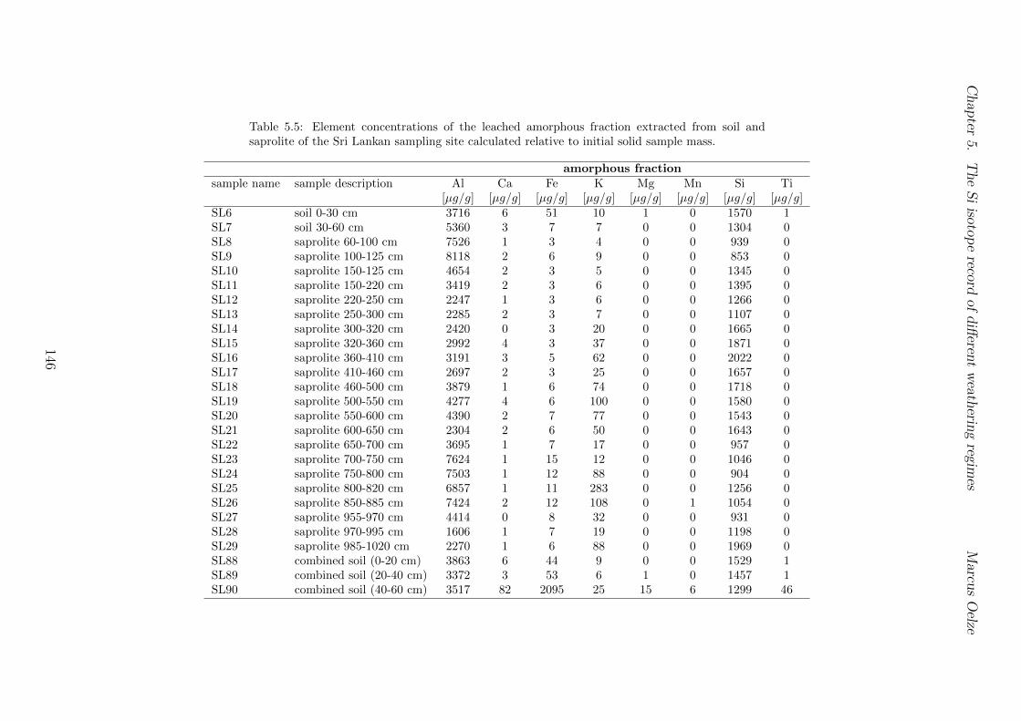
Chap
ter5.
TheSiisotop
erecord
ofdi↵eren
tweath
eringregim
esMarcu
sOelze
Table 5.5: Element concentrations of the leached amorphous fraction extracted from soil andsaprolite of the Sri Lankan sampling site calculated relative to initial solid sample mass.
amorphous fraction
sample name sample description Al Ca Fe K Mg Mn Si Ti[µg/g] [µg/g] [µg/g] [µg/g] [µg/g] [µg/g] [µg/g] [µg/g]
SL6 soil 0-30 cm 3716 6 51 10 1 0 1570 1SL7 soil 30-60 cm 5360 3 7 7 0 0 1304 0SL8 saprolite 60-100 cm 7526 1 3 4 0 0 939 0SL9 saprolite 100-125 cm 8118 2 6 9 0 0 853 0SL10 saprolite 150-125 cm 4654 2 3 5 0 0 1345 0SL11 saprolite 150-220 cm 3419 2 3 6 0 0 1395 0SL12 saprolite 220-250 cm 2247 1 3 6 0 0 1266 0SL13 saprolite 250-300 cm 2285 2 3 7 0 0 1107 0SL14 saprolite 300-320 cm 2420 0 3 20 0 0 1665 0SL15 saprolite 320-360 cm 2992 4 3 37 0 0 1871 0SL16 saprolite 360-410 cm 3191 3 5 62 0 0 2022 0SL17 saprolite 410-460 cm 2697 2 3 25 0 0 1657 0SL18 saprolite 460-500 cm 3879 1 6 74 0 0 1718 0SL19 saprolite 500-550 cm 4277 4 6 100 0 0 1580 0SL20 saprolite 550-600 cm 4390 2 7 77 0 0 1543 0SL21 saprolite 600-650 cm 2304 2 6 50 0 0 1643 0SL22 saprolite 650-700 cm 3695 1 7 17 0 0 957 0SL23 saprolite 700-750 cm 7624 1 15 12 0 0 1046 0SL24 saprolite 750-800 cm 7503 1 12 88 0 0 904 0SL25 saprolite 800-820 cm 6857 1 11 283 0 0 1256 0SL26 saprolite 850-885 cm 7424 2 12 108 0 1 1054 0SL27 saprolite 955-970 cm 4414 0 8 32 0 0 931 0SL28 saprolite 970-995 cm 1606 1 7 19 0 0 1198 0SL29 saprolite 985-1020 cm 2270 1 6 88 0 0 1969 0SL88 combined soil (0-20 cm) 3863 6 44 9 0 0 1529 1SL89 combined soil (20-40 cm) 3372 3 53 6 1 0 1457 1SL90 combined soil (40-60 cm) 3517 82 2095 25 15 6 1299 46
146
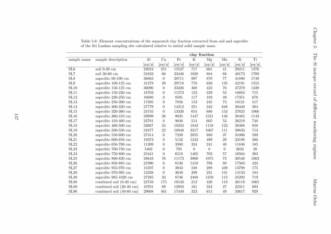
Chap
ter5.
TheSiisotop
erecord
ofdi↵eren
tweath
eringregim
esMarcu
sOelze
Table 5.6: Element concentrations of the separated clay fraction extracted from soil and saproliteof the Sri Lankan sampling site calculated relative to initial solid sample mass.
clay fraction
sample name sample description Al Ca Fe K Mg Mn Si Ti[µg/g] [µg/g] [µg/g] [µg/g] [µg/g] [µg/g] [µg/g] [µg/g]
SL6 soil 0-30 cm 22024 251 15527 717 661 41 29211 1276SL7 soil 30-60 cm 31633 66 23446 1028 884 68 40173 1709SL8 saprolite 60-100 cm 36862 0 28711 997 870 77 41890 1749SL9 saprolite 100-125 cm 41278 29 29718 778 656 135 42191 1555SL10 saprolite 150-125 cm 36090 0 23326 468 423 76 37279 1339SL11 saprolite 150-220 cm 18703 0 11573 123 229 52 18682 715SL12 saprolite 220-250 cm 16680 0 8591 117 193 49 17351 678SL13 saprolite 250-300 cm 17395 0 7856 153 245 73 18121 517SL14 saprolite 300-320 cm 27779 0 14212 251 342 648 30440 384SL15 saprolite 320-360 cm 24745 0 13326 654 680 153 27625 1066SL16 saprolite 360-410 cm 33999 38 9035 1447 1521 146 38485 1143SL17 saprolite 410-460 cm 23781 0 9040 514 605 53 26219 740SL18 saprolite 460-500 cm 32667 24 10234 1843 1158 122 38388 858SL19 saprolite 500-550 cm 31677 22 10048 3217 1067 111 39833 713SL20 saprolite 550-600 cm 27314 0 7239 2055 880 37 31006 599SL21 saprolite 600-650 cm 19373 0 5132 1242 499 29 23198 380SL22 saprolite 650-700 cm 11309 0 3380 334 241 40 11846 185SL23 saprolite 700-750 cm 5402 0 795 0 0 0 2633 28SL24 saprolite 750-800 cm 25441 0 6518 1465 703 57 16564 383SL25 saprolite 800-820 cm 28643 76 11173 3900 1975 73 30546 1063SL26 saprolite 850-885 cm 21990 6 6130 1410 798 80 17563 423SL27 saprolite 955-970 cm 15597 0 3943 248 288 439 13798 175SL28 saprolite 970-995 cm 12338 0 3649 299 231 131 14133 184SL29 saprolite 985-1020 cm 27285 33 8746 2488 1259 112 35292 719SL88 combined soil (0-20 cm) 22733 175 19133 212 420 118 26119 1065SL89 combined soil (20-40 cm) 19701 89 13958 161 334 27 22311 693SL90 combined soil (40-60 cm) 29608 461 17440 323 615 49 33617 929
147

Chapter 5. The Si isotope record of di↵erent weathering regimes Marcus Oelze
Table 5.7: Average elemental composition of the amorphous and clay fractions extractedfrom soil and saprolite of the Sri Lankan sampling site normalized to 1 mol Si.
fraction Al Ca Fe K Mg Mn Si Ti[mol] [mol] [mol] [mol] [mol] [mol] [mol] [mol]
soil amorphous 2.92 0.01 0.17 0.01 2.94E-03 5.97E-04 1.00 4.43E-03clay 0.87 0.00 0.30 0.01 2.17E-02 1.05E-03 1.00 2.18E-02
saprolite amorphous 3.88 0.00 0.00 0.03 1.87E-04 1.16E-04 1.00 5.50E-05clay 1.05 0.00 0.20 0.03 2.81E-02 2.69E-03 1.00 1.49E-02
bedrock bulk 0.27 0.04 0.04 0.08 2.72E-02 5.37E-04 1.00 5.93E-03
148
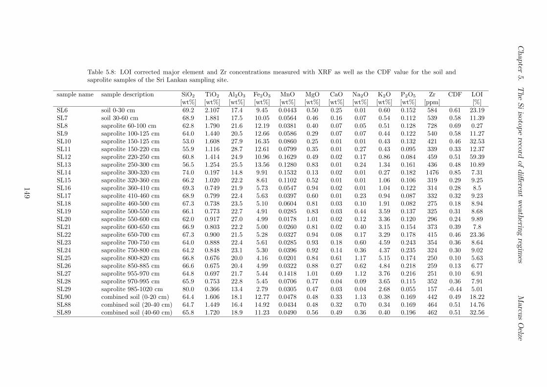
Chap
ter5.
TheSiisotop
erecord
ofdi↵eren
tweath
eringregim
esMarcu
sOelze
Table 5.8: LOI corrected major element and Zr concentrations measured with XRF as well as the CDF value for the soil andsaprolite samples of the Sri Lankan sampling site.
sample name sample description SiO2
TiO2
Al2
O3
Fe2
O3
MnO MgO CaO Na2
O K2
O P2
O5
Zr CDF LOI[wt%] [wt%] [wt%] [wt%] [wt%] [wt%] [wt%] [wt%] [wt%] [wt%] [ppm] [%]
SL6 soil 0-30 cm 69.2 2.107 17.4 9.45 0.0443 0.50 0.25 0.01 0.60 0.152 584 0.61 23.19SL7 soil 30-60 cm 68.9 1.881 17.5 10.05 0.0564 0.46 0.16 0.07 0.54 0.112 539 0.58 11.39SL8 saprolite 60-100 cm 62.8 1.790 21.6 12.19 0.0381 0.40 0.07 0.05 0.51 0.128 728 0.69 0.27SL9 saprolite 100-125 cm 64.0 1.440 20.5 12.66 0.0586 0.29 0.07 0.07 0.44 0.122 540 0.58 11.27SL10 saprolite 150-125 cm 53.0 1.608 27.9 16.35 0.0860 0.25 0.01 0.01 0.43 0.132 421 0.46 32.53SL11 saprolite 150-220 cm 55.9 1.116 28.7 12.61 0.0799 0.35 0.01 0.27 0.43 0.095 339 0.33 12.37SL12 saprolite 220-250 cm 60.8 1.414 24.9 10.96 0.1629 0.49 0.02 0.17 0.86 0.084 459 0.51 59.39SL13 saprolite 250-300 cm 56.5 1.254 25.5 13.56 0.1280 0.83 0.01 0.24 1.34 0.161 436 0.48 10.89SL14 saprolite 300-320 cm 74.0 0.197 14.8 9.91 0.1532 0.13 0.02 0.01 0.27 0.182 1476 0.85 7.31SL15 saprolite 320-360 cm 66.2 1.020 22.2 8.61 0.1102 0.52 0.01 0.01 1.06 0.106 319 0.29 9.25SL16 saprolite 360-410 cm 69.3 0.749 21.9 5.73 0.0547 0.94 0.02 0.01 1.04 0.122 314 0.28 8.5SL17 saprolite 410-460 cm 68.9 0.799 22.4 5.63 0.0397 0.60 0.01 0.23 0.94 0.087 332 0.32 9.23SL18 saprolite 460-500 cm 67.3 0.738 23.5 5.10 0.0604 0.81 0.03 0.10 1.91 0.082 275 0.18 8.94SL19 saprolite 500-550 cm 66.1 0.773 22.7 4.91 0.0285 0.83 0.03 0.44 3.59 0.137 325 0.31 8.68SL20 saprolite 550-600 cm 62.0 0.917 27.0 4.99 0.0178 1.01 0.02 0.12 3.36 0.120 296 0.24 9.89SL21 saprolite 600-650 cm 66.9 0.803 22.2 5.00 0.0260 0.81 0.02 0.40 3.15 0.154 373 0.39 7.8SL22 saprolite 650-700 cm 67.3 0.900 21.5 5.28 0.0327 0.94 0.08 0.17 3.29 0.178 415 0.46 23.36SL23 saprolite 700-750 cm 64.0 0.888 22.4 5.61 0.0285 0.93 0.18 0.60 4.59 0.243 354 0.36 8.64SL24 saprolite 750-800 cm 64.2 0.848 23.1 5.30 0.0396 0.92 0.14 0.36 4.37 0.235 324 0.30 9.02SL25 saprolite 800-820 cm 66.8 0.676 20.0 4.16 0.0201 0.84 0.61 1.17 5.15 0.174 250 0.10 5.63SL26 saprolite 850-885 cm 66.6 0.675 20.4 4.99 0.0322 0.88 0.27 0.62 4.84 0.218 259 0.13 6.77SL27 saprolite 955-970 cm 64.8 0.697 21.7 5.44 0.1418 1.01 0.69 1.12 3.76 0.216 251 0.10 6.91SL28 saprolite 970-995 cm 65.9 0.753 22.8 5.45 0.0706 0.77 0.04 0.09 3.65 0.115 352 0.36 7.91SL29 saprolite 985-1020 cm 80.0 0.366 13.4 2.79 0.0305 0.47 0.03 0.04 2.68 0.055 157 -0.44 5.01SL90 combined soil (0-20 cm) 64.4 1.606 18.1 12.77 0.0478 0.48 0.33 1.13 0.38 0.169 442 0.49 18.22SL88 combined soil (20-40 cm) 64.7 1.449 16.4 14.92 0.0434 0.48 0.32 0.70 0.34 0.169 464 0.51 14.76SL89 combined soil (40-60 cm) 65.8 1.720 18.9 11.23 0.0490 0.56 0.49 0.36 0.40 0.196 462 0.51 32.56
149

Chapter 5. The Si isotope record of di↵erent weathering regimes Marcus Oelze
Tables Swiss Alps
This page is intentionally left blank.
150
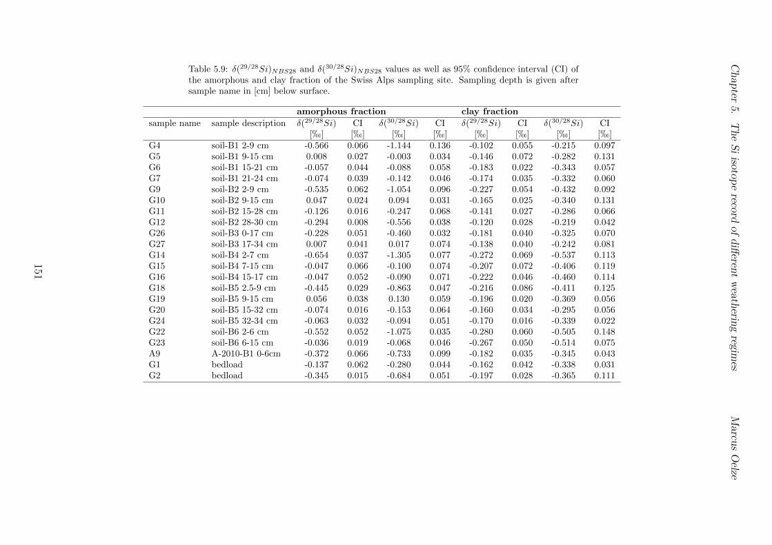
Chap
ter5.
TheSiisotop
erecord
ofdi↵eren
tweath
eringregim
esMarcu
sOelze
Table 5.9: �(29/28Si)NBS28
and �(30/28Si)NBS28
values as well as 95% confidence interval (CI) ofthe amorphous and clay fraction of the Swiss Alps sampling site. Sampling depth is given aftersample name in [cm] below surface.
amorphous fraction clay fraction
sample name sample description �(29/28Si) CI �(30/28Si) CI �(29/28Si) CI �(30/28Si) CI[h] [h] [h] [h] [h] [h] [h] [h]
G4 soil-B1 2-9 cm -0.566 0.066 -1.144 0.136 -0.102 0.055 -0.215 0.097G5 soil-B1 9-15 cm 0.008 0.027 -0.003 0.034 -0.146 0.072 -0.282 0.131G6 soil-B1 15-21 cm -0.057 0.044 -0.088 0.058 -0.183 0.022 -0.343 0.057G7 soil-B1 21-24 cm -0.074 0.039 -0.142 0.046 -0.174 0.035 -0.332 0.060G9 soil-B2 2-9 cm -0.535 0.062 -1.054 0.096 -0.227 0.054 -0.432 0.092G10 soil-B2 9-15 cm 0.047 0.024 0.094 0.031 -0.165 0.025 -0.340 0.131G11 soil-B2 15-28 cm -0.126 0.016 -0.247 0.068 -0.141 0.027 -0.286 0.066G12 soil-B2 28-30 cm -0.294 0.008 -0.556 0.038 -0.120 0.028 -0.219 0.042G26 soil-B3 0-17 cm -0.228 0.051 -0.460 0.032 -0.181 0.040 -0.325 0.070G27 soil-B3 17-34 cm 0.007 0.041 0.017 0.074 -0.138 0.040 -0.242 0.081G14 soil-B4 2-7 cm -0.654 0.037 -1.305 0.077 -0.272 0.069 -0.537 0.113G15 soil-B4 7-15 cm -0.047 0.066 -0.100 0.074 -0.207 0.072 -0.406 0.119G16 soil-B4 15-17 cm -0.047 0.052 -0.090 0.071 -0.222 0.046 -0.460 0.114G18 soil-B5 2.5-9 cm -0.445 0.029 -0.863 0.047 -0.216 0.086 -0.411 0.125G19 soil-B5 9-15 cm 0.056 0.038 0.130 0.059 -0.196 0.020 -0.369 0.056G20 soil-B5 15-32 cm -0.074 0.016 -0.153 0.064 -0.160 0.034 -0.295 0.056G24 soil-B5 32-34 cm -0.063 0.032 -0.094 0.051 -0.170 0.016 -0.339 0.022G22 soil-B6 2-6 cm -0.552 0.052 -1.075 0.035 -0.280 0.060 -0.505 0.148G23 soil-B6 6-15 cm -0.036 0.019 -0.068 0.046 -0.267 0.050 -0.514 0.075A9 A-2010-B1 0-6cm -0.372 0.066 -0.733 0.099 -0.182 0.035 -0.345 0.043G1 bedload -0.137 0.062 -0.280 0.044 -0.162 0.042 -0.338 0.031G2 bedload -0.345 0.015 -0.684 0.051 -0.197 0.028 -0.365 0.111
151
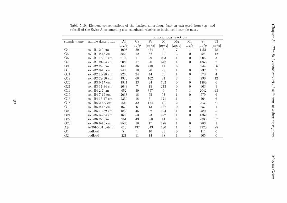
Chap
ter5.
TheSiisotop
erecord
ofdi↵eren
tweath
eringregim
esMarcu
sOelze
Table 5.10: Element concentrations of the leached amorphous fraction extracted from top- andsubsoil of the Swiss Alps sampling site calculated relative to initial solid sample mass.
amorphous fraction
sample name sample description Al Ca Fe K Mg Mn Si Ti[µg/g] [µg/g] [µg/g] [µg/g] [µg/g] [µg/g] [µg/g] [µg/g]
G4 soil-B1 2-9 cm 1008 29 474 5 7 1 1151 78G5 soil-B1 9-15 cm 3829 12 82 30 3 0 484 12G6 soil-B1 15-21 cm 2102 11 29 233 1 0 905 3G7 soil-B1 21-24 cm 2088 17 20 347 1 0 1353 2G9 soil-B2 2-9 cm 1493 36 418 11 6 1 944 66G10 soil-B2 9-15 cm 2408 10 20 29 1 0 232 2G11 soil-B2 15-28 cm 2260 24 44 60 1 0 378 4G12 soil-B2 28-30 cm 1920 60 102 24 2 1 290 12G26 soil-B3 0-17 cm 1841 23 34 192 0 0 1289 6G27 soil-B3 17-34 cm 2043 7 15 273 0 0 903 1G14 soil-B4 2-7 cm 652 39 357 9 5 1 2042 43G15 soil-B4 7-15 cm 2033 18 55 93 1 0 579 6G16 soil-B4 15-17 cm 2350 18 51 171 1 1 704 6G18 soil-B5 2.5-9 cm 524 32 174 10 2 1 2033 51G19 soil-B5 9-15 cm 1679 6 13 137 0 0 657 1G20 soil-B5 15-32 cm 1868 46 52 124 1 0 480 5G24 soil-B5 32-34 cm 1630 53 23 422 1 0 1362 2G22 soil-B6 2-6 cm 951 43 358 14 4 1 2388 57G23 soil-B6 6-15 cm 2505 10 17 178 1 0 783 1A9 A-2010-B1 0-6cm 613 132 343 190 1 1 4220 25G1 bedload 54 1 10 23 0 0 111 0G2 bedload 221 11 14 38 1 1 405 0
152
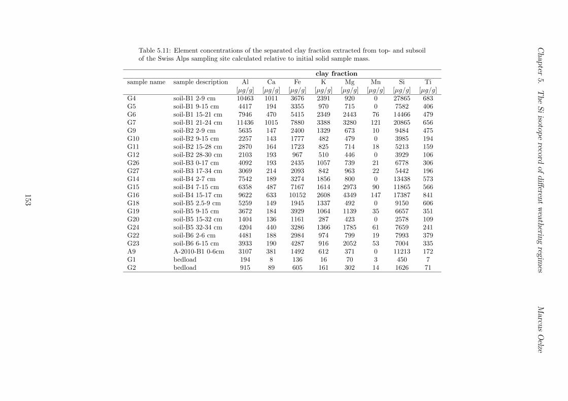
Chap
ter5.
TheSiisotop
erecord
ofdi↵eren
tweath
eringregim
esMarcu
sOelze
Table 5.11: Element concentrations of the separated clay fraction extracted from top- and subsoilof the Swiss Alps sampling site calculated relative to initial solid sample mass.
clay fraction
sample name sample description Al Ca Fe K Mg Mn Si Ti[µg/g] [µg/g] [µg/g] [µg/g] [µg/g] [µg/g] [µg/g] [µg/g]
G4 soil-B1 2-9 cm 10463 1011 3676 2391 920 0 27865 683G5 soil-B1 9-15 cm 4417 194 3355 970 715 0 7582 406G6 soil-B1 15-21 cm 7946 470 5415 2349 2443 76 14466 479G7 soil-B1 21-24 cm 11436 1015 7880 3388 3280 121 20865 656G9 soil-B2 2-9 cm 5635 147 2400 1329 673 10 9484 475G10 soil-B2 9-15 cm 2257 143 1777 482 479 0 3985 194G11 soil-B2 15-28 cm 2870 164 1723 825 714 18 5213 159G12 soil-B2 28-30 cm 2103 193 967 510 446 0 3929 106G26 soil-B3 0-17 cm 4092 193 2435 1057 739 21 6778 306G27 soil-B3 17-34 cm 3069 214 2093 842 963 22 5442 196G14 soil-B4 2-7 cm 7542 189 3274 1856 800 0 13438 573G15 soil-B4 7-15 cm 6358 487 7167 1614 2973 90 11865 566G16 soil-B4 15-17 cm 9622 633 10152 2608 4349 147 17387 841G18 soil-B5 2.5-9 cm 5259 149 1945 1337 492 0 9150 606G19 soil-B5 9-15 cm 3672 184 3929 1064 1139 35 6657 351G20 soil-B5 15-32 cm 1404 136 1161 287 423 0 2578 109G24 soil-B5 32-34 cm 4204 440 3286 1366 1785 61 7659 241G22 soil-B6 2-6 cm 4481 188 2984 974 799 19 7993 379G23 soil-B6 6-15 cm 3933 190 4287 916 2052 53 7004 335A9 A-2010-B1 0-6cm 3107 381 1492 612 371 0 11213 172G1 bedload 194 8 136 16 70 3 450 7G2 bedload 915 89 605 161 302 14 1626 71
153
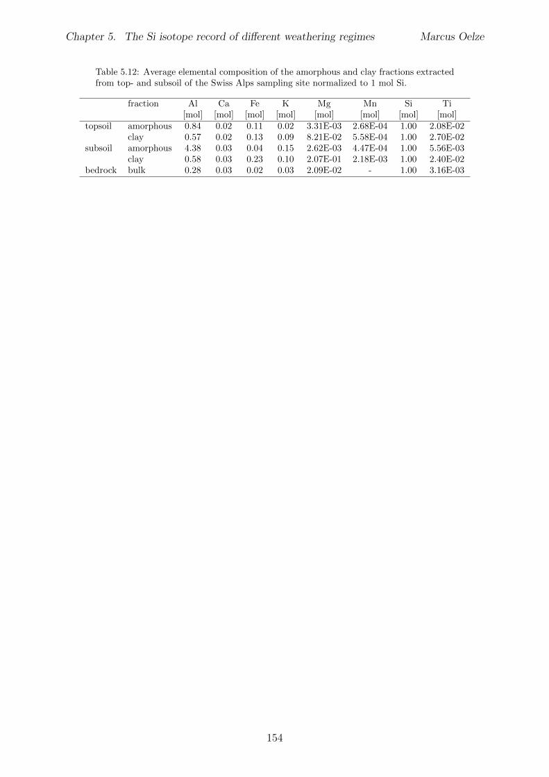
Chapter 5. The Si isotope record of di↵erent weathering regimes Marcus Oelze
Table 5.12: Average elemental composition of the amorphous and clay fractions extractedfrom top- and subsoil of the Swiss Alps sampling site normalized to 1 mol Si.
fraction Al Ca Fe K Mg Mn Si Ti[mol] [mol] [mol] [mol] [mol] [mol] [mol] [mol]
topsoil amorphous 0.84 0.02 0.11 0.02 3.31E-03 2.68E-04 1.00 2.08E-02clay 0.57 0.02 0.13 0.09 8.21E-02 5.58E-04 1.00 2.70E-02
subsoil amorphous 4.38 0.03 0.04 0.15 2.62E-03 4.47E-04 1.00 5.56E-03clay 0.58 0.03 0.23 0.10 2.07E-01 2.18E-03 1.00 2.40E-02
bedrock bulk 0.28 0.03 0.02 0.03 2.09E-02 - 1.00 3.16E-03
154
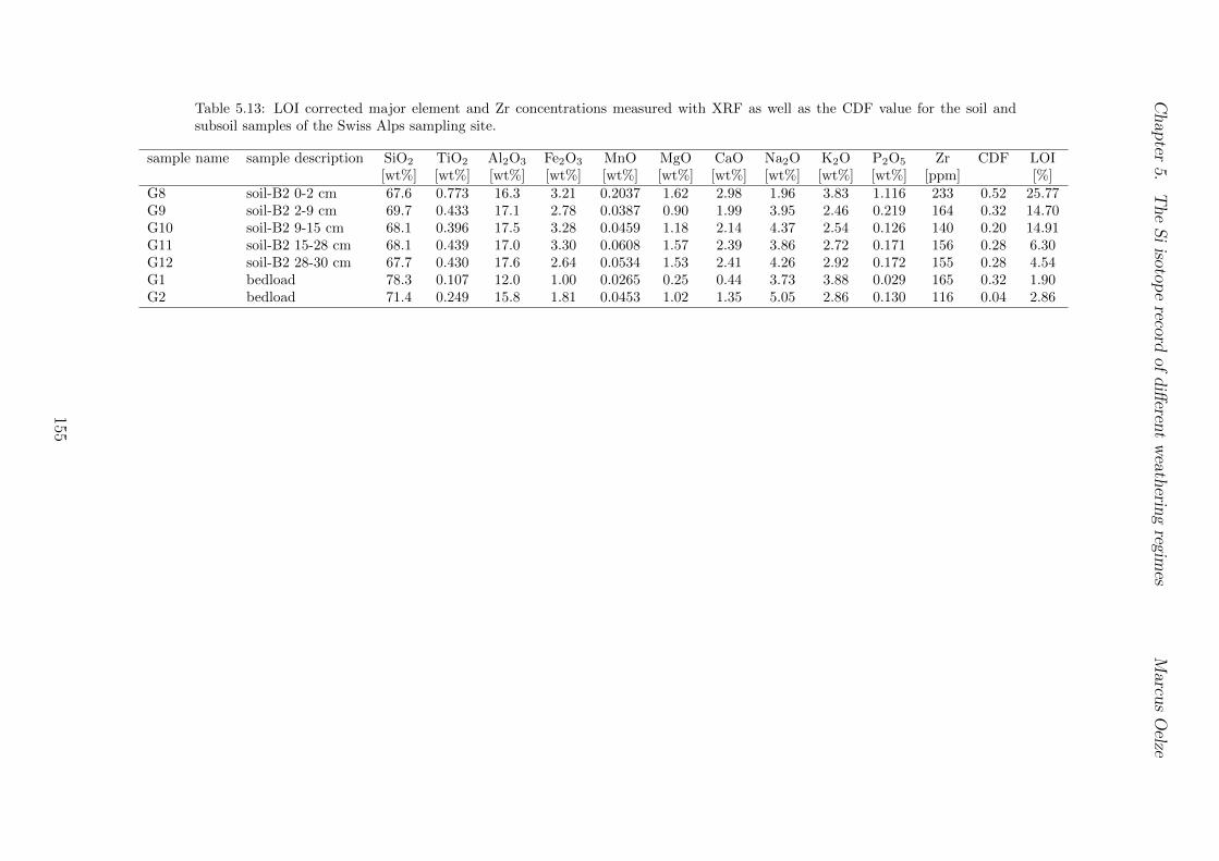
Chap
ter5.
TheSiisotop
erecord
ofdi↵eren
tweath
eringregim
esMarcu
sOelze
Table 5.13: LOI corrected major element and Zr concentrations measured with XRF as well as the CDF value for the soil andsubsoil samples of the Swiss Alps sampling site.
sample name sample description SiO2
TiO2
Al2
O3
Fe2
O3
MnO MgO CaO Na2
O K2
O P2
O5
Zr CDF LOI[wt%] [wt%] [wt%] [wt%] [wt%] [wt%] [wt%] [wt%] [wt%] [wt%] [ppm] [%]
G8 soil-B2 0-2 cm 67.6 0.773 16.3 3.21 0.2037 1.62 2.98 1.96 3.83 1.116 233 0.52 25.77G9 soil-B2 2-9 cm 69.7 0.433 17.1 2.78 0.0387 0.90 1.99 3.95 2.46 0.219 164 0.32 14.70G10 soil-B2 9-15 cm 68.1 0.396 17.5 3.28 0.0459 1.18 2.14 4.37 2.54 0.126 140 0.20 14.91G11 soil-B2 15-28 cm 68.1 0.439 17.0 3.30 0.0608 1.57 2.39 3.86 2.72 0.171 156 0.28 6.30G12 soil-B2 28-30 cm 67.7 0.430 17.6 2.64 0.0534 1.53 2.41 4.26 2.92 0.172 155 0.28 4.54G1 bedload 78.3 0.107 12.0 1.00 0.0265 0.25 0.44 3.73 3.88 0.029 165 0.32 1.90G2 bedload 71.4 0.249 15.8 1.81 0.0453 1.02 1.35 5.05 2.86 0.130 116 0.04 2.86
155

Chapter 5. The Si isotope record of di↵erent weathering regimes Marcus Oelze
Tables Sierra Nevada
This page is intentionally left blank.
156
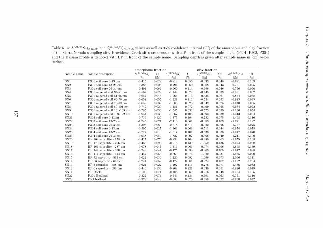
Chap
ter5.
TheSiisotop
erecord
ofdi↵eren
tweath
eringregim
esMarcu
sOelze
Table 5.14: �(29/28Si)NBS28
and �(30/28Si)NBS28
values as well as 95% confidence interval (CI) of the amorphous and clay fractionof the Sierra Nevada sampling site. Providence Creek sites are denoted with a P in front of the samples name (P301, P303, P304)and the Balsam profile is denoted with BP in front of the sample name. Sampling depth is given after sample name in [cm] belowsurface.
amorphous fraction clay fraction
sample name sample description �(29/28Si) CI �(30/28Si) CI �(29/28Si) CI �(30/28Si) CI[h] [h] [h] [h] [h] [h] [h] [h]
SN1 P301 soil core 0-13 cm -0.415 0.029 -0.814 0.056 -0.333 0.048 -0.681 0.109SN2 P301 soil core 13-26 cm -0.388 0.025 -0.794 0.060 -0.368 0.043 -0.721 0.095SN3 P301 soil core 26-34 cm -0.491 0.065 -0.960 0.114 -0.396 0.046 -0.766 0.090SN4 P301 augered soil 34-51 cm -0.567 0.029 -1.149 0.074 -0.445 0.039 -0.881 0.062SN5 P301 augered soil 51-66 cm -0.657 0.046 -1.265 0.013 -0.435 0.061 -0.854 0.068SN6 P301 augered soil 66-76 cm -0.658 0.055 -1.321 0.112 -0.524 0.052 -0.983 0.095SN7 P301 augered soil 76-89 cm -0.852 0.032 -1.686 0.023 -0.542 0.025 -1.040 0.065SN8 P301 augered soil 89-101 cm -0.742 0.029 -1.481 0.072 -0.499 0.028 -0.964 0.022SN9 P301 augered soil 101-109 cm -0.785 0.030 -1.545 0.032 -0.573 0.029 -1.136 0.054SN10 P301 augered soil 109-122 cm -0.954 0.036 -1.867 0.103 -0.693 0.039 -1.313 0.054SN21 P303 soil core 0-13cm -0.716 0.120 -1.375 0.194 -0.782 0.075 -1.498 0.116SN22 P303 soil core 13-26cm -1.245 0.071 -2.410 0.061 -0.883 0.109 -1.721 0.197SN23 P303 soil core 26-34cm -1.303 0.080 -2.618 0.315 -0.922 0.026 -1.757 0.075SN24 P304 soil core 0-13cm -0.595 0.027 -1.163 0.063 -0.511 0.044 -0.974 0.078SN25 P304 soil core 13-26cm -0.777 0.018 -1.517 0.101 -0.538 0.038 -1.047 0.070SN26 P304 soil core 26-34cm -0.938 0.059 -1.822 0.097 -0.606 0.049 -1.211 0.100SN20 BP 204 saprolite - 178 cm -0.427 0.076 -0.833 0.104 -0.989 0.063 -1.955 0.108SN19 BP 173 saprolite - 256 cm -0.466 0.095 -0.918 0.139 -1.052 0.136 -2.024 0.258SN18 BP 161 saprolite - 287 cm -0.678 0.047 -1.316 0.066 -0.974 0.096 -1.868 0.139SN17 BP 144 saprolite - 330 cm -0.249 0.044 -0.475 0.038 -0.869 0.105 -1.672 0.088SN16 BP 111 saprolite - 414 cm -0.447 0.063 -0.869 0.076 -1.020 0.031 -1.965 0.090SN15 BP 72 saprolite - 513 cm -0.622 0.030 -1.229 0.092 -1.096 0.073 -2.096 0.111SN14 BP 36 saprolite - 605 cm -0.241 0.052 -0.472 0.081 -0.924 0.107 -1.792 0.264SN13 BP 3 saprolite - 688 cm -0.621 0.022 -1.192 0.115 -0.776 0.071 -1.486 0.082SN12 BP 0 saprolite - 696 cm -0.446 0.133 -0.808 0.221 -0.439 0.051 -0.826 0.079SN11 BP Rock -0.109 0.071 -0.188 0.069 -0.216 0.048 -0.404 0.105SN27 P301 Bedload -0.322 0.074 -0.644 0.134 -0.391 0.063 -0.761 0.110SN28 PIG bedload -0.378 0.048 -0.688 0.076 -0.459 0.022 -0.900 0.042
157
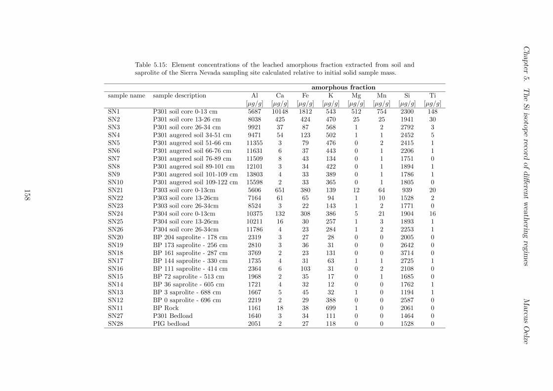
Chap
ter5.
TheSiisotop
erecord
ofdi↵eren
tweath
eringregim
esMarcu
sOelze
Table 5.15: Element concentrations of the leached amorphous fraction extracted from soil andsaprolite of the Sierra Nevada sampling site calculated relative to initial solid sample mass.
amorphous fraction
sample name sample description Al Ca Fe K Mg Mn Si Ti[µg/g] [µg/g] [µg/g] [µg/g] [µg/g] [µg/g] [µg/g] [µg/g]
SN1 P301 soil core 0-13 cm 5687 10148 1812 543 512 754 2300 148SN2 P301 soil core 13-26 cm 8038 425 424 470 25 25 1941 30SN3 P301 soil core 26-34 cm 9921 37 87 568 1 2 2792 3SN4 P301 augered soil 34-51 cm 9471 54 123 502 1 1 2452 5SN5 P301 augered soil 51-66 cm 11355 3 79 476 0 2 2415 1SN6 P301 augered soil 66-76 cm 11631 6 37 443 0 1 2206 1SN7 P301 augered soil 76-89 cm 11509 8 43 134 0 1 1751 0SN8 P301 augered soil 89-101 cm 12101 3 34 422 0 1 1894 1SN9 P301 augered soil 101-109 cm 13803 4 33 389 0 1 1786 1SN10 P301 augered soil 109-122 cm 15598 2 33 365 0 1 1805 0SN21 P303 soil core 0-13cm 5606 651 380 139 12 64 939 20SN22 P303 soil core 13-26cm 7164 61 65 94 1 10 1528 2SN23 P303 soil core 26-34cm 8524 3 22 143 1 2 1771 0SN24 P304 soil core 0-13cm 10375 132 308 386 5 21 1904 16SN25 P304 soil core 13-26cm 10211 16 30 257 1 3 1893 1SN26 P304 soil core 26-34cm 11786 4 23 284 1 2 2253 1SN20 BP 204 saprolite - 178 cm 2319 3 27 28 0 0 2005 0SN19 BP 173 saprolite - 256 cm 2810 3 36 31 0 0 2642 0SN18 BP 161 saprolite - 287 cm 3769 2 23 131 0 0 3714 0SN17 BP 144 saprolite - 330 cm 1735 4 31 63 1 1 2725 1SN16 BP 111 saprolite - 414 cm 2364 6 103 31 0 2 2108 0SN15 BP 72 saprolite - 513 cm 1968 2 35 17 0 1 1685 0SN14 BP 36 saprolite - 605 cm 1721 4 32 12 0 0 1762 1SN13 BP 3 saprolite - 688 cm 1667 5 45 32 1 0 1194 1SN12 BP 0 saprolite - 696 cm 2219 2 29 388 0 0 2587 0SN11 BP Rock 1161 18 38 699 1 0 2061 0SN27 P301 Bedload 1640 3 34 111 0 0 1464 0SN28 PIG bedload 2051 2 27 118 0 0 1528 0
158
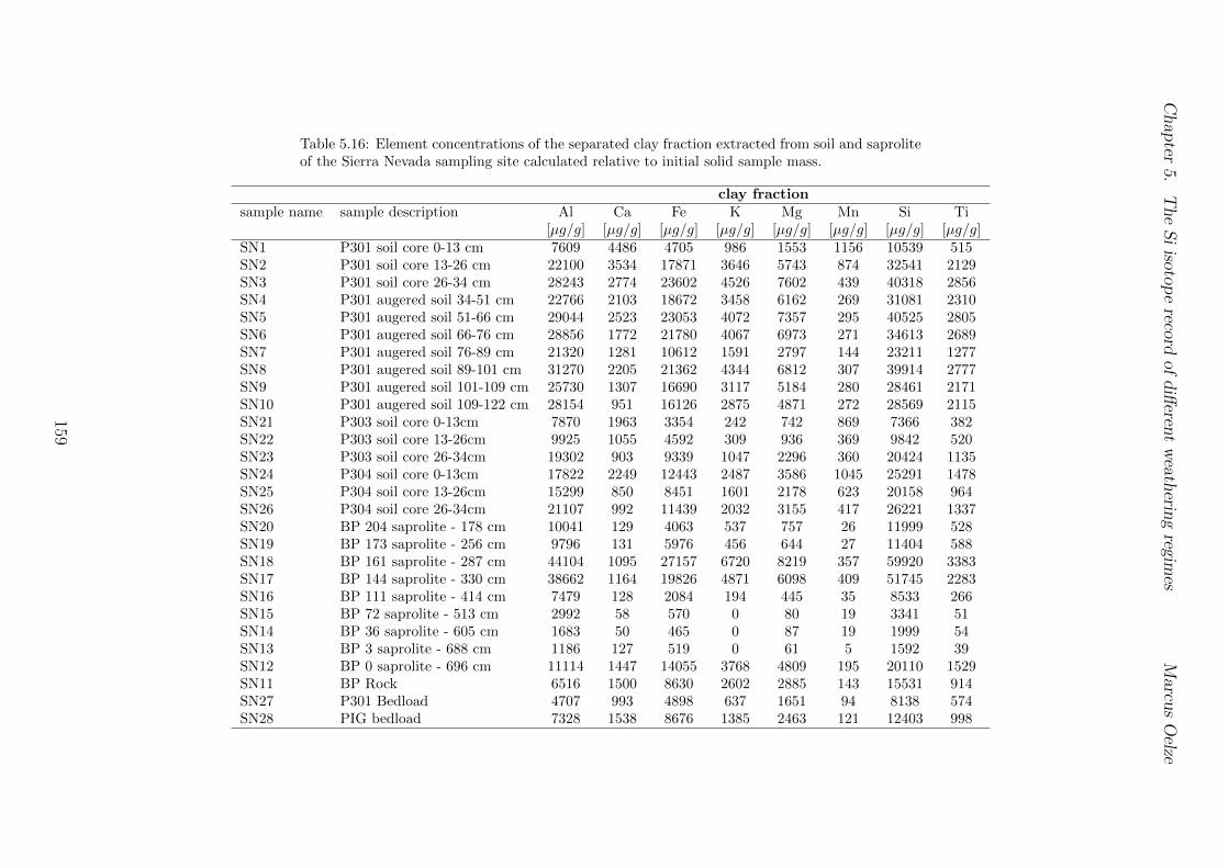
Chap
ter5.
TheSiisotop
erecord
ofdi↵eren
tweath
eringregim
esMarcu
sOelze
Table 5.16: Element concentrations of the separated clay fraction extracted from soil and saproliteof the Sierra Nevada sampling site calculated relative to initial solid sample mass.
clay fraction
sample name sample description Al Ca Fe K Mg Mn Si Ti[µg/g] [µg/g] [µg/g] [µg/g] [µg/g] [µg/g] [µg/g] [µg/g]
SN1 P301 soil core 0-13 cm 7609 4486 4705 986 1553 1156 10539 515SN2 P301 soil core 13-26 cm 22100 3534 17871 3646 5743 874 32541 2129SN3 P301 soil core 26-34 cm 28243 2774 23602 4526 7602 439 40318 2856SN4 P301 augered soil 34-51 cm 22766 2103 18672 3458 6162 269 31081 2310SN5 P301 augered soil 51-66 cm 29044 2523 23053 4072 7357 295 40525 2805SN6 P301 augered soil 66-76 cm 28856 1772 21780 4067 6973 271 34613 2689SN7 P301 augered soil 76-89 cm 21320 1281 10612 1591 2797 144 23211 1277SN8 P301 augered soil 89-101 cm 31270 2205 21362 4344 6812 307 39914 2777SN9 P301 augered soil 101-109 cm 25730 1307 16690 3117 5184 280 28461 2171SN10 P301 augered soil 109-122 cm 28154 951 16126 2875 4871 272 28569 2115SN21 P303 soil core 0-13cm 7870 1963 3354 242 742 869 7366 382SN22 P303 soil core 13-26cm 9925 1055 4592 309 936 369 9842 520SN23 P303 soil core 26-34cm 19302 903 9339 1047 2296 360 20424 1135SN24 P304 soil core 0-13cm 17822 2249 12443 2487 3586 1045 25291 1478SN25 P304 soil core 13-26cm 15299 850 8451 1601 2178 623 20158 964SN26 P304 soil core 26-34cm 21107 992 11439 2032 3155 417 26221 1337SN20 BP 204 saprolite - 178 cm 10041 129 4063 537 757 26 11999 528SN19 BP 173 saprolite - 256 cm 9796 131 5976 456 644 27 11404 588SN18 BP 161 saprolite - 287 cm 44104 1095 27157 6720 8219 357 59920 3383SN17 BP 144 saprolite - 330 cm 38662 1164 19826 4871 6098 409 51745 2283SN16 BP 111 saprolite - 414 cm 7479 128 2084 194 445 35 8533 266SN15 BP 72 saprolite - 513 cm 2992 58 570 0 80 19 3341 51SN14 BP 36 saprolite - 605 cm 1683 50 465 0 87 19 1999 54SN13 BP 3 saprolite - 688 cm 1186 127 519 0 61 5 1592 39SN12 BP 0 saprolite - 696 cm 11114 1447 14055 3768 4809 195 20110 1529SN11 BP Rock 6516 1500 8630 2602 2885 143 15531 914SN27 P301 Bedload 4707 993 4898 637 1651 94 8138 574SN28 PIG bedload 7328 1538 8676 1385 2463 121 12403 998
159

Chapter 5. The Si isotope record of di↵erent weathering regimes Marcus Oelze
Table 5.17: Average elemental composition of the amorphous and clay fractions extractedfrom soil and saprolite of the Sierra Nevada sampling site normalized to 1 mol Si.
fraction Al Ca Fe K Mg Mn Si Ti[mol] [mol] [mol] [mol] [mol] [mol] [mol] [mol]
soil amorphous 5.72 0.05 0.04 0.12 2.53E-03 3.63E-03 1.00 2.04E-03clay 0.87 0.05 0.26 0.06 1.75E-01 1.21E-02 1.00 3.72E-02
saprolite amorphous 1.04 0.00 0.01 0.05 3.00E-04 1.41E-04 1.00 1.65E-04clay 0.78 0.03 0.20 0.05 1.11E-01 3.06E-03 1.00 2.52E-02
bedrock bulk 0.34 0.11 0.09 0.05 8.35E-02 1.77E-03 1.00 1.27E-02
160
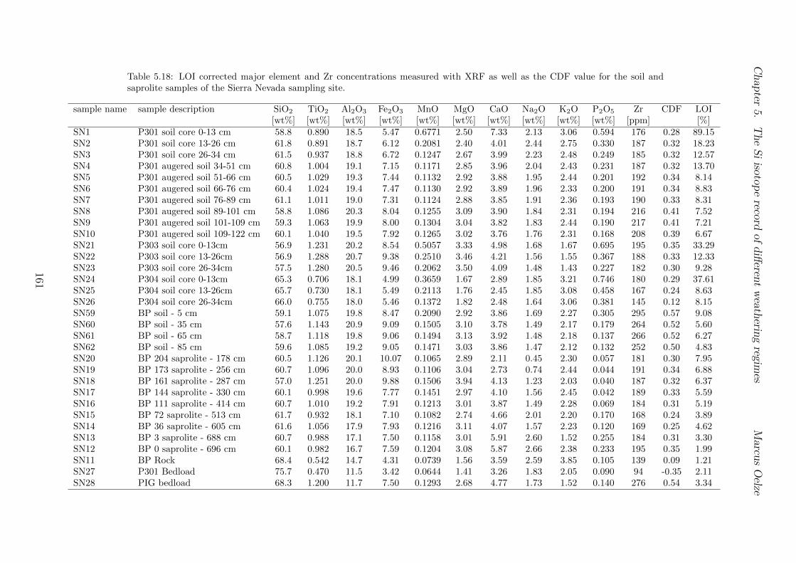
Chap
ter5.
TheSiisotop
erecord
ofdi↵eren
tweath
eringregim
esMarcu
sOelze
Table 5.18: LOI corrected major element and Zr concentrations measured with XRF as well as the CDF value for the soil andsaprolite samples of the Sierra Nevada sampling site.
sample name sample description SiO2
TiO2
Al2
O3
Fe2
O3
MnO MgO CaO Na2
O K2
O P2
O5
Zr CDF LOI[wt%] [wt%] [wt%] [wt%] [wt%] [wt%] [wt%] [wt%] [wt%] [wt%] [ppm] [%]
SN1 P301 soil core 0-13 cm 58.8 0.890 18.5 5.47 0.6771 2.50 7.33 2.13 3.06 0.594 176 0.28 89.15SN2 P301 soil core 13-26 cm 61.8 0.891 18.7 6.12 0.2081 2.40 4.01 2.44 2.75 0.330 187 0.32 18.23SN3 P301 soil core 26-34 cm 61.5 0.937 18.8 6.72 0.1247 2.67 3.99 2.23 2.48 0.249 185 0.32 12.57SN4 P301 augered soil 34-51 cm 60.8 1.004 19.1 7.15 0.1171 2.85 3.96 2.04 2.43 0.231 187 0.32 13.70SN5 P301 augered soil 51-66 cm 60.5 1.029 19.3 7.44 0.1132 2.92 3.88 1.95 2.44 0.201 192 0.34 8.14SN6 P301 augered soil 66-76 cm 60.4 1.024 19.4 7.47 0.1130 2.92 3.89 1.96 2.33 0.200 191 0.34 8.83SN7 P301 augered soil 76-89 cm 61.1 1.011 19.0 7.31 0.1124 2.88 3.85 1.91 2.36 0.193 190 0.33 8.31SN8 P301 augered soil 89-101 cm 58.8 1.086 20.3 8.04 0.1255 3.09 3.90 1.84 2.31 0.194 216 0.41 7.52SN9 P301 augered soil 101-109 cm 59.3 1.063 19.9 8.00 0.1304 3.04 3.82 1.83 2.44 0.190 217 0.41 7.21SN10 P301 augered soil 109-122 cm 60.1 1.040 19.5 7.92 0.1265 3.02 3.76 1.76 2.31 0.168 208 0.39 6.67SN21 P303 soil core 0-13cm 56.9 1.231 20.2 8.54 0.5057 3.33 4.98 1.68 1.67 0.695 195 0.35 33.29SN22 P303 soil core 13-26cm 56.9 1.288 20.7 9.38 0.2510 3.46 4.21 1.56 1.55 0.367 188 0.33 12.33SN23 P303 soil core 26-34cm 57.5 1.280 20.5 9.46 0.2062 3.50 4.09 1.48 1.43 0.227 182 0.30 9.28SN24 P304 soil core 0-13cm 65.3 0.706 18.1 4.99 0.3659 1.67 2.89 1.85 3.21 0.746 180 0.29 37.61SN25 P304 soil core 13-26cm 65.7 0.730 18.1 5.49 0.2113 1.76 2.45 1.85 3.08 0.458 167 0.24 8.63SN26 P304 soil core 26-34cm 66.0 0.755 18.0 5.46 0.1372 1.82 2.48 1.64 3.06 0.381 145 0.12 8.15SN59 BP soil - 5 cm 59.1 1.075 19.8 8.47 0.2090 2.92 3.86 1.69 2.27 0.305 295 0.57 9.08SN60 BP soil - 35 cm 57.6 1.143 20.9 9.09 0.1505 3.10 3.78 1.49 2.17 0.179 264 0.52 5.60SN61 BP soil - 65 cm 58.7 1.118 19.8 9.06 0.1494 3.13 3.92 1.48 2.18 0.137 266 0.52 6.27SN62 BP soil - 85 cm 59.6 1.085 19.2 9.05 0.1471 3.03 3.86 1.47 2.12 0.132 252 0.50 4.83SN20 BP 204 saprolite - 178 cm 60.5 1.126 20.1 10.07 0.1065 2.89 2.11 0.45 2.30 0.057 181 0.30 7.95SN19 BP 173 saprolite - 256 cm 60.7 1.096 20.0 8.93 0.1106 3.04 2.73 0.74 2.44 0.044 191 0.34 6.88SN18 BP 161 saprolite - 287 cm 57.0 1.251 20.0 9.88 0.1506 3.94 4.13 1.23 2.03 0.040 187 0.32 6.37SN17 BP 144 saprolite - 330 cm 60.1 0.998 19.6 7.77 0.1451 2.97 4.10 1.56 2.45 0.042 189 0.33 5.59SN16 BP 111 saprolite - 414 cm 60.7 1.010 19.2 7.91 0.1213 3.01 3.87 1.49 2.28 0.069 184 0.31 5.19SN15 BP 72 saprolite - 513 cm 61.7 0.932 18.1 7.10 0.1082 2.74 4.66 2.01 2.20 0.170 168 0.24 3.89SN14 BP 36 saprolite - 605 cm 61.6 1.056 17.9 7.93 0.1216 3.11 4.07 1.57 2.23 0.120 169 0.25 4.62SN13 BP 3 saprolite - 688 cm 60.7 0.988 17.1 7.50 0.1158 3.01 5.91 2.60 1.52 0.255 184 0.31 3.30SN12 BP 0 saprolite - 696 cm 60.1 0.982 16.7 7.59 0.1204 3.08 5.87 2.66 2.38 0.233 195 0.35 1.99SN11 BP Rock 68.4 0.542 14.7 4.31 0.0739 1.56 3.59 2.59 3.85 0.105 139 0.09 1.21SN27 P301 Bedload 75.7 0.470 11.5 3.42 0.0644 1.41 3.26 1.83 2.05 0.090 94 -0.35 2.11SN28 PIG bedload 68.3 1.200 11.7 7.50 0.1293 2.68 4.77 1.73 1.52 0.140 276 0.54 3.34
161

Chapter 5. The Si isotope record of di↵erent weathering regimes Marcus Oelze
Denudation, weathering and erosion rates
This page is intentionally left blank.
162
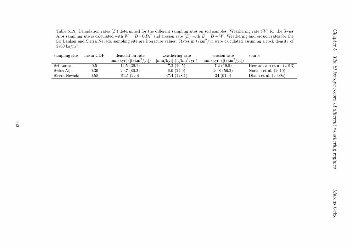
Chap
ter5.
TheSiisotop
erecord
ofdi↵eren
tweath
eringregim
esMarcu
sOelze
Table 5.19: Denudation rates (D) determined for the di↵erent sampling sites on soil samples. Weathering rate (W ) for the SwissAlps sampling site is calculated with W = D ⇤CDF and erosion rate (E) with E = D �W . Weathering and erosion rates for theSri Lankan and Sierra Nevada sampling site are literature values. Rates in t/km2/yr were calculated assuming a rock density of2700 kg/m3.
sampling site mean CDF denudation rate weathering rate erosion rate source[mm/kyr] ([t/km2/yr]) [mm/kyr] ([t/km2/yr]) [mm/kyr] ([t/km2/yr])
Sri Lanka 0.5 14.5 (39.1) 7.2 (19.5) 7.2 (19.5) Hewawasam et al. (2013)Swiss Alps 0.30 29.7 (80.2) 8.9 (24.0) 20.8 (56.2) Norton et al. (2010)Sierra Nevada 0.58 81.5 (220) 47.4 (128.1) 34 (91.9) Dixon et al. (2009a)
163
Bibliography
Abraham, K., Cardinal, D., Hofmann, A., Foley, S. F., Harris, C., Barth, M. G., andAndre, L. (2011). Coupled silicon–oxygen isotope fractionation traces Archaean silici-fication. Earth and Planetary Science Letters, 301(1-2):222–230.
Abraham, K., Opfergelt, S., and Fripiat, F. (2008). �30Si and �29Si Determinations onUSGS BHVO-1 and BHVO-2 Reference Materials with a New Configuration on a NuPlasma Multi-Collector ICP-MS. Geostandards and Geoanalytical Research.
Adu-Wusu, K. and Wilcox, W. R. (1991). Kinetics of silicate reaction with gibbsite.Journal of Colloid and Interface Science, 143(1):127–138.
Anderson, D. M. (1981). Some thermodynamic relationships governing the behavior ofpermafrost and patterned ground. Technical Report NASA TM-84211.
Anderson, D. M. and Tice, A. R. (1973). The Unfrozen Interfacial Phase in Frozen SoilWater Systems. In Physical Aspects of Soil Water and Salts in Ecosystems, pages107–124. Springer Berlin Heidelberg, Berlin, Heidelberg.
Andre, L., Cardinal, D., Alleman, L. Y., and Moorbath, S. (2006). Silicon isotopes in 3.8Ga West Greenland rocks as clues to the Eoarchaean supracrustal Si cycle. Earth andPlanetary Science Letters, 245(1-2):162–173.
Armytage, R. M. G., Georg, R. B., Savage, P. S., Williams, H. M., and Halliday, A. N.(2011a). Silicon isotopes in meteorites and planetary core formation. Geochimica etCosmochimica Acta, 75(13):3662–3676.
Armytage, R. M. G., Georg, R. B., Williams, H. M., and Halliday, A. N. (2011b). Siliconisotopes in lunar rocks: Implications for the Moon’s formation and the early history ofthe Earth. Geochimica et Cosmochimica Acta, 77:504–514.
Baes, C. F. and Mesmer, R. E. . j. a. (1976). The Hydrolysis of Cations. New York :Wiley.
Bales, R. C., Hopmans, J. W., O’Geen, A. T., Meadows, M., Hartsough, P. C., Kirchner,P., Hunsaker, C. T., and Beaudette, D. (2011). Soil Moisture Response to Snowmelt andRainfall in a Sierra Nevada Mixed-Conifer Forest. Vadose Zone Journal, 10(3):786–799.
Barling, J. and Weis, D. (2008). Influence of non-spectral matrix e↵ects on the accuracyof Pb isotope ratio measurement by MC-ICP-MS: implications for the external nor-malization method of instrumental mass bias correction. Journal of Analytical AtomicSpectrometry, 23(7):1017–1025.
164
Bibliography Marcus Oelze
Basile-Doelsch, I. (2006). Si stable isotopes in the Earth’s surface: A review. Journal ofGeochemical Exploration, 88(1-3):252–256.
Basile-Doelsch, I., Meunier, J. D., and Parron, C. (2005). Another continental pool inthe terrestrial silicon cycle. Nature, 433(7024):399–402.
Bateman, P. C. and Wones, D. R. (1972). Geologic map of the Huntington Lake quad-rangle, central Sierra Nevada, California. USGS Numbered Series, page 1 map.
Bern, C. R., Brzezinski, M. A., Beucher, C., Ziegler, K., and Chadwick, O. A. (2010).Weathering, dust, and biocycling e↵ects on soil silicon isotope ratios. Geochimica etCosmochimica Acta, 74(3):876–889.
Bigeleisen, J. (1965). Chemistry of Isotopes: Isotope chemistry has opened new areas ofchemical physics, geochemistry, and molecular biology. Science, 147(3657):463–471.
Bouchez, J., von Blanckenburg, F., and Schuessler, J. A. (2013). Modeling novel stableisotope ratios in the weathering zone. American Journal Of Science, 313(4):267–308.
Brzezinski, M. A., Jones, J. L., Beucher, C. P., Demarest, M. S., and Berg, H. L. (2006).Automated determination of silicon isotope natural abundance by the acid decomposi-tion of cesium hexafluosilicate. Analytical Chemistry, 78(17):6109–6114.
Cardinal, D., Alleman, L., de Jong, J., Ziegler, K., and Andre, L. (2003). Isotopic com-position of silicon measured by multicollector plasma source mass spectrometry in dryplasma mode. Journal of Analytical Atomic Spectrometry, 18(3):213–218.
Cardinal, D., Gaillardet, J., Hughes, H. J., Opfergelt, S., and Andre, L. (2010). Contrast-ing silicon isotope signatures in rivers from the Congo Basin and the specific behaviourof organic-rich waters. Geophysical Research Letters, 37(12):L12403.
Carroll, S., Mroczek, E., Alai, M., and Ebert, M. (1998). Amorphous silica precipitation(60 to 120°C): Comparison of laboratory and field rates. Geochimica et CosmochimicaActa, 62(8):1379–1396.
Chakrabarti, R. and Jacobsen, S. B. (2010). Silicon isotopes in the inner Solar System:Implications for core formation, solar nebular processes and partial melting. Geochimicaet Cosmochimica Acta, 74(23):6921–6933.
Chakrabarti, R., Knoll, A. H., Jacobsen, S. B., and Fischer, W. W. (2012). Si isotopevariability in Proterozoic cherts. Geochimica et Cosmochimica Acta, 91:187–201.
Chen, Y., Jiang, S., Ling, H., Yang, J., and Wan, D. (2007). Isotopic compositions of smallshelly fossil Anabarites from Lower Cambrian in Yangtze Platform of South China:Implications for palaeocean temperature. Progress in Natural Science, 17(10):1185–1191.
Chmele↵, J., Horn, I., Steinhoefel, G., and von Blanckenburg, F. (2008). In situ determina-tion of precise stable Si isotope ratios by UV-femtosecond laser ablation high-resolutionmulti-collector ICP-MS. Chemical Geology, 249(1-2):155–166.
Cole, D. R., Ohmoto, H., and Lasaga, A. C. (1983). Isotopic exchange in mineral-fluidsystems. I. Theoretical evaluation of oxygen isotopic exchange accompanying surfacereactions and di↵usion. Geochimica et Cosmochimica Acta, 47(10):1681–1693.
165
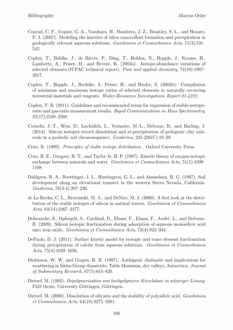
Bibliography Marcus Oelze
Conrad, C. F., Icopini, G. A., Yasuhara, H., Bandstra, J. Z., Brantley, S. L., and Heaney,P. J. (2007). Modeling the kinetics of silica nanocolloid formation and precipitation ingeologically relevant aqueous solutions. Geochimica et Cosmochimica Acta, 71(3):531–542.
Coplen, T., Bohlke, J., de Bievre, P., Ding, T., Holden, N., Hopple, J., Krouse, H.,Lamberty, A., Peiser, H., and Revesz, K. (2002a). Isotope-abundance variations ofselected elements:(IUPAC technical report). Pure and applied chemistry, 74(10):1987–2017.
Coplen, T., Hopple, J., Boehike, J., Peiser, H., and Rieder, S. (2002b). Compilationof minimum and maximum isotope ratios of selected elements in naturally occurringterrestrial materials and reagents. Water-Resources Investigations Report 01-4222.
Coplen, T. B. (2011). Guidelines and recommended terms for expression of stable-isotope-ratio and gas-ratio measurement results. Rapid Communications in Mass Spectrometry,25(17):2538–2560.
Cornelis, J.-T., Weis, D., Lavkulich, L., Vermeire, M.-L., Delvaux, B., and Barling, J.(2014). Silicon isotopes record dissolution and re-precipitation of pedogenic clay min-erals in a podzolic soil chronosequence. Geoderma, 235-236(C):19–29.
Criss, R. (1999). Principles of stable isotope distribution . Oxford University Press.
Criss, R. E., Gregory, R. T., and Taylor Jr, H. P. (1987). Kinetic theory of oxygen isotopicexchange between minerals and water. Geochimica et Cosmochimica Acta, 51(5):1099–1108.
Dahlgren, R. A., Boettinger, J. L., Huntington, G. L., and Amundson, R. G. (1997). Soildevelopment along an elevational transect in the western Sierra Nevada, California.Geoderma, 78(3-4):207–236.
de La Rocha, C. L., Brzezinski, M. A., and DeNiro, M. J. (2000). A first look at the distri-bution of the stable isotopes of silicon in natural waters. Geochimica et CosmochimicaActa, 64(14):2467–2477.
Delstanche, S., Opfergelt, S., Cardinal, D., Elsass, F., Elsass, F., Andre, L., and Delvaux,B. (2009). Silicon isotopic fractionation during adsorption of aqueous monosilicic acidonto iron oxide. Geochimica et Cosmochimica Acta, 73(4):923–934.
DePaolo, D. J. (2011). Surface kinetic model for isotopic and trace element fractionationduring precipitation of calcite from aqueous solutions. Geochimica et CosmochimicaActa, 75(4):1039–1056.
Dickinson, W. W. and Grapes, R. H. (1997). Authigenic chabazite and implications forweathering in Sirius Group diamictite, Table Mountain, dry valleys, Antarctica. Journalof Sedimentary Research, 67(5):815–820.
Dietzel, M. (1993). Depolymerisation von hochpolymerer Kieselsaure in wassriger Losung.PhD thesis, University Gottingen, Gottingen.
Dietzel, M. (2000). Dissolution of silicates and the stability of polysilicic acid. Geochimicaet Cosmochimica Acta, 64(19):3275–3281.
166
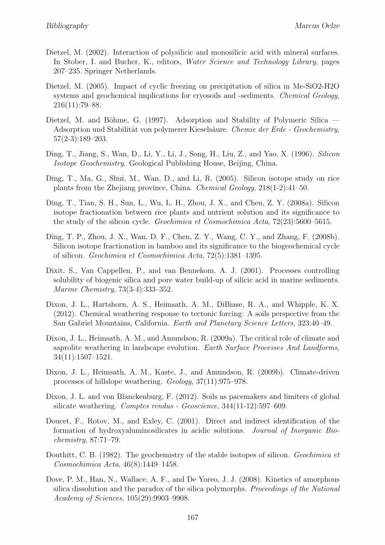
Bibliography Marcus Oelze
Dietzel, M. (2002). Interaction of polysilicic and monosilicic acid with mineral surfaces.In Stober, I. and Bucher, K., editors, Water Science and Technology Library, pages207–235. Springer Netherlands.
Dietzel, M. (2005). Impact of cyclic freezing on precipitation of silica in Me-SiO2-H2Osystems and geochemical implications for cryosoils and -sediments. Chemical Geology,216(11):79–88.
Dietzel, M. and Bohme, G. (1997). Adsorption and Stability of Polymeric Silica —Adsorption und Stabilitat von polymerer Kieselsaure. Chemie der Erde - Geochemistry,57(2-3):189–203.
Ding, T., Jiang, S., Wan, D., Li, Y., Li, J., Song, H., Liu, Z., and Yao, X. (1996). SiliconIsotope Geochemistry. Geological Publishing House, Beijing, China.
Ding, T., Ma, G., Shui, M., Wan, D., and Li, R. (2005). Silicon isotope study on riceplants from the Zhejiang province, China. Chemical Geology, 218(1-2):41–50.
Ding, T., Tian, S. H., Sun, L., Wu, L. H., Zhou, J. X., and Chen, Z. Y. (2008a). Siliconisotope fractionation between rice plants and nutrient solution and its significance tothe study of the silicon cycle. Geochimica et Cosmochimica Acta, 72(23):5600–5615.
Ding, T. P., Zhou, J. X., Wan, D. F., Chen, Z. Y., Wang, C. Y., and Zhang, F. (2008b).Silicon isotope fractionation in bamboo and its significance to the biogeochemical cycleof silicon. Geochimica et Cosmochimica Acta, 72(5):1381–1395.
Dixit, S., Van Cappellen, P., and van Bennekom, A. J. (2001). Processes controllingsolubility of biogenic silica and pore water build-up of silicic acid in marine sediments.Marine Chemistry, 73(3-4):333–352.
Dixon, J. L., Hartshorn, A. S., Heimsath, A. M., DiBiase, R. A., and Whipple, K. X.(2012). Chemical weathering response to tectonic forcing: A soils perspective from theSan Gabriel Mountains, California. Earth and Planetary Science Letters, 323:40–49.
Dixon, J. L., Heimsath, A. M., and Amundson, R. (2009a). The critical role of climate andsaprolite weathering in landscape evolution. Earth Surface Processes And Landforms,34(11):1507–1521.
Dixon, J. L., Heimsath, A. M., Kaste, J., and Amundson, R. (2009b). Climate-drivenprocesses of hillslope weathering. Geology, 37(11):975–978.
Dixon, J. L. and von Blanckenburg, F. (2012). Soils as pacemakers and limiters of globalsilicate weathering. Comptes rendus - Geoscience, 344(11-12):597–609.
Doucet, F., Rotov, M., and Exley, C. (2001). Direct and indirect identification of theformation of hydroxyaluminosilicates in acidic solutions. Journal of Inorganic Bio-chemistry, 87:71–79.
Douthitt, C. B. (1982). The geochemistry of the stable isotopes of silicon. Geochimica etCosmochimica Acta, 46(8):1449–1458.
Dove, P. M., Han, N., Wallace, A. F., and De Yoreo, J. J. (2008). Kinetics of amorphoussilica dissolution and the paradox of the silica polymorphs. Proceedings of the NationalAcademy of Sciences, 105(29):9903–9908.
167
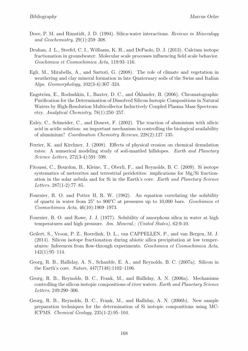
Bibliography Marcus Oelze
Dove, P. M. and Rimstidt, J. D. (1994). Silica-water interactions. Reviews in Mineralogyand Geochemistry, 29(1):259–308.
Druhan, J. L., Steefel, C. I., Williams, K. H., and DePaolo, D. J. (2013). Calcium isotopefractionation in groundwater: Molecular scale processes influencing field scale behavior.Geochimica et Cosmochimica Acta, 119:93–116.
Egli, M., Mirabella, A., and Sartori, G. (2008). The role of climate and vegetation inweathering and clay mineral formation in late Quaternary soils of the Swiss and ItalianAlps. Geomorphology, 102(3-4):307–324.
Engstrom, E., Rodushkin, I., Baxter, D. C., and Ohlander, B. (2006). ChromatographicPurification for the Determination of Dissolved Silicon Isotopic Compositions in NaturalWaters by High-Resolution Multicollector Inductively Coupled Plasma Mass Spectrom-etry. Analytical Chemistry, 78(1):250–257.
Exley, C., Schneider, C., and Doucet, F. (2002). The reaction of aluminium with silicicacid in acidic solution: an important mechanism in controlling the biological availabilityof aluminium? Coordination Chemistry Reviews, 228(2):127–135.
Ferrier, K. and Kirchner, J. (2008). E↵ects of physical erosion on chemical denudationrates: A numerical modeling study of soil-mantled hillslopes. Earth and PlanetaryScience Letters, 272(3-4):591–599.
Fitoussi, C., Bourdon, B., Kleine, T., Oberli, F., and Reynolds, B. C. (2009). Si isotopesystematics of meteorites and terrestrial peridotites: implications for Mg/Si fraction-ation in the solar nebula and for Si in the Earth’s core. Earth and Planetary ScienceLetters, 287(1-2):77–85.
Fournier, R. O. and Potter II, R. W. (1982). An equation correlating the solubilityof quartz in water from 25° to 900°C at pressures up to 10,000 bars. Geochimica etCosmochimica Acta, 46(10):1969–1973.
Fournier, R. O. and Rowe, J. J. (1977). Solubility of amorphous silica in water at hightemperatures and high pressure. Am. Mineral.; (United States), 62:9-10.
Geilert, S., Vroon, P. Z., Roerdink, D. L., van CAPPELLEN, P., and van Bergen, M. J.(2014). Silicon isotope fractionation during abiotic silica precipitation at low temper-atures: Inferences from flow-through experiments. Geochimica et Cosmochimica Acta,142(1):95–114.
Georg, R. B., Halliday, A. N., Schauble, E. A., and Reynolds, B. C. (2007a). Silicon inthe Earth’s core. Nature, 447(7148):1102–1106.
Georg, R. B., Reynolds, B. C., Frank, M., and Halliday, A. N. (2006a). Mechanismscontrolling the silicon isotopic compositions of river waters. Earth and Planetary ScienceLetters, 249:290–306.
Georg, R. B., Reynolds, B. C., Frank, M., and Halliday, A. N. (2006b). New samplepreparation techniques for the determination of Si isotopic compositions using MC-ICPMS. Chemical Geology, 235(1-2):95–104.
168
Bibliography Marcus Oelze
Georg, R. B., Reynolds, B. C., West, A. J., Burton, K. W., and Halliday, A. N. (2007b).Silicon isotope variations accompanying basalt weathering in Iceland. Earth and Plan-etary Science Letters, 261:476–490.
Georg, R. B., Zhu, C., Reynolds, B. C., and Halliday, A. N. (2009). Stable silicon isotopesof groundwater, feldspars, and clay coatings in the Navajo Sandstone aquifer, BlackMesa, Arizona, USA. Geochimica et Cosmochimica Acta, 73(8):2229–2241.
Georgiadis, A. (2011). Entwicklung einer Methode zur fraktionierten Si-Bestimmung inBoden des feucht-gemaßigten Klimas. PhD thesis, Universitat Hohenheim.
Gislason, S. R. and Oelkers, E. (2003). Mechanism, rates, and consequences of basalticglass dissolution: II. An experimental study of the dissolution rates of basaltic glass as afunction of pH and temperature. Geochimica et Cosmochimica Acta, 67(20):3817–3832.
Gray, A. L. (1986). Mass spectrometry with an inductively coupled plasma as an ionsource: the influence on ultratrace analysis of background and matrix response. Spec-trochimica Acta Part B-Atomic Spectroscopy, 41(1-2):151–167.
Greenberg, S. A. and Sinclair, D. (1955). The polymerization of silicic acid. Journal ofPhysical Chemistry, 59(5):435–440.
Guillaumont, R., Fanghanel, T., Neck, V., Fuger, J., Palmer, D. A., Grenthe, I., andRand, M. H. (2003). Update on the Chemical Thermodynamics of Uranium, Neptunium,Plutonium, Americium and Technetium. Elsevier Science Limited.
Gunnarsson, I. and Arnorsson, S. (2000). Amorphous silica solubility and the thermo-dynamic properties of H4SiO°4 the range of 0° to 350°C at P
sat
. Geochimica et Cos-mochimica Acta, 64(13):2295–2307.
Hahm, W. J., Riebe, C. S., Lukens, C. E., and Araki, S. (2014). Bedrock compositionregulates mountain ecosystems and landscape evolution. Proceedings of the NationalAcademy of Sciences, 111(9):3338–3343.
Hewawasam, T., von Blanckenburg, F., Bouchez, J., Dixon, J. L., Schuessler, J. A., andMaekeler, R. (2013). Slow advance of the weathering front during deep, supply-limitedsaprolite formation in the tropical Highlands of Sri Lanka. Geochimica et CosmochimicaActa, 118:202–230.
Hewawasam, T., von Blanckenburg, F., Schaller, M., and Kubik, P. (2003). Increaseof human over natural erosion rates in tropical highlands constrained by cosmogenicnuclides. Geology, 31(7):597–600.
Hingston, F. and Raupach, M. (1967). The reaction between monosilicic acid and alu-minium hydroxide. I. Kinetics of adsorption of silicic acid by aluminium hydroxide.Australian Journal of Soil Research, 5(2):295–309.
Hofmann, A. E., Bourg, I. C., and DePaolo, D. J. (2012). Ion desolvation as a mecha-nism for kinetic isotope fractionation in aqueous systems. Proceedings of the NationalAcademy of Sciences, 109(46):18689–18694.
Holleman, A. F. and Wiberg, N. (1995). Lehrbuch der anorganischen Chemie. Berlin.
169
Bibliography Marcus Oelze
Hughes, H. J., Delvigne, C., Korntheuer, M., de Jong, J., Andre, L., and Cardinal, D.(2011). Controlling the mass bias introduced by anionic and organic matrices in siliconisotopic measurements by MC-ICP-MS. Journal of Analytical Atomic Spectrometry,26(9):1892–1896.
Hughes, H. J., Sondag, F., Santos, R. V., Andre, L., and Cardinal, D. (2013). The riverinesilicon isotope composition of the Amazon Basin. Geochimica et Cosmochimica Acta,121:637–651.
Hunsaker, C. T. and Neary, D. G. (2012). Sediment loads and erosion in forest headwaterstreams of the Sierra Nevada, California. Notes.
Icenhower, J. and Dove, P. M. (2000). The dissolution kinetics of amorphous silica intosodium chloride solutions: E↵ects of temperature and ionic strength. Geochimica etCosmochimica Acta, 64(24):4193–4203.
Icopini, G., Brantley, S. L., and Heaney, P. (2005). Kinetics of silica oligomerization andnanocolloid formation as a function of pH and ionic strength at 25°C. Geochimica etCosmochimica Acta, 69(2):293–303.
Iler, R. K. (1979). The chemistry of silica: solubility, polymerization, colloid and surfaceproperties, and biochemistry. John Wiley & Sons, Inc., New York.
Iler, R. K. (1982). Colloidal Components in Solutions of Sodium Silicate. In Falcone,J. S., editor, Soluble Silicates, pages 95–114. American Chemical Society.
Jepson, W., Je↵s, D., and Ferris, A. (1976). The adsorption of silica on gibbsite and itsrelevance to the kaolinite surface. Journal of Colloid and Interface Science, 55(2):454–461.
Johnson, C. M., Beard, B. L., and Albarede, F. (2004). Overview and general concepts.Reviews in Mineralogy and Geochemistry, 55:1–24.
Johnson, C. M., Skulan, J., Beard, B., Sun, H., Nealson, K., and Braterman, P. (2002).Isotopic fractionation between Fe(III) and Fe(II) in aqueous solutions. Earth and Plan-etary Science Letters, 195:141–153.
Johnson, D. W., Hunsaker, C. T., Glass, D. W., Rau, B. M., and Roath, B. A. (2011).Carbon and nutrient contents in soils from the Kings River Experimental Watersheds,Sierra Nevada Mountains, California. Geoderma, 160(3-4):490–502.
Joussein, E., Petit, S., Churchman, J., Theng, B., Righi, D., and Delvaux, B. (2005).Halloysite clay minerals—a review. Clay Minerals, 40(4):383–426.
Juillot, F., Marechal, C., Ponthieu, M., Cacaly, S., Morin, G., Benedetti, M., Hazemann,J. L., Proux, O., and Guyot, F. (2008). Zn isotopic fractionation caused by sorption ongoethite and 2-Lines ferrihydrite. Geochimica et Cosmochimica Acta, 72(19):4886–4900.
Karamalidis, A. K. and Dzombak, D. A. (2011). Surface Complexation Modeling: Gibbsite.John Wiley & Sons, Inc., Hoboken, New Jersey.
Lam, J. W. and McLaren, J. W. (1990). Use of aerosol processing and nitrogen-argonplasmas for reduction of oxide interference in inductively coupled plasma mass spec-trometry. Journal of Analytical Atomic Spectrometry, 5(6):419–424.
170
Bibliography Marcus Oelze
Lemarchand, E., Schott, J., and Gaillardet, J. (2007). How surface complexes impactboron isotope fractionation: Evidence from Fe and Mn oxides sorption experiments.Earth and Planetary Science Letters, 260(1-2):277–296.
Li, W., Beard, B. L., and Johnson, C. M. (2011). Exchange and fractionation of Mgisotopes between epsomite and saturated MgSO4 solution. Geochimica et CosmochimicaActa, 75(7):1814–1828.
Li, Y., Ding, T., and Wan, D. (1995). Experimental study of silicon isotope dynamic frac-tionation and its application in geology. Chinese Journal of Geochemistry, 14(3):212–219.
Liu, F., Hunsaker, C., and Bales, R. C. (2012). Controls of streamflow generation in smallcatchments across the snow-rain transition in the Southern Sierra Nevada, California.Hydrological Processes, pages n/a–n/a.
Maher, K. (2011). The role of fluid residence time and topographic scales in determiningchemical fluxes from landscapes. Earth and Planetary Science Letters, 312(1-2):48–58.
Marshall, W. L. (1980a). Amorphous silica solubilities—I. Behavior in aqueous sodiumnitrate solutions; 25–300°C, 0–6 molal. Geochimica et Cosmochimica Acta, 44(7):907–913.
Marshall, W. L. (1980b). Amorphous silica solubilities—III. Activity coe�cient relationsand predictions of solubility behavior in salt solutions, 0–350°C. Geochimica et Cos-mochimica Acta, 44(7):925–931.
Marshall, W. L. and Warakomski, J. M. (1980). Amorphous silica solubilities—II. E↵ectof aqueous salt solutions at 25°C. Geochimica et Cosmochimica Acta, 44(7):915–924.
Meheut, M., Lazzeri, M., Balan, E., and Mauri, F. (2007). Equilibrium isotopic fraction-ation in the kaolinite, quartz, water system: Prediction from first-principles density-functional theory. Geochimica et Cosmochimica Acta, 71(13):3170–3181.
Meheut, M., Lazzeri, M., Balan, E., and Mauri, F. (2009). Structural control over equi-librium silicon and oxygen isotopic fractionation: A first-principles density-functionaltheory study. Chemical Geology, 258(1-2):28–37.
Meheut, M. and Schauble, E. A. (2014). Silicon isotope fractionation in silicate minerals:Insights from first-principles models of phyllosilicates, albite and pyrope. Geochimicaet Cosmochimica Acta, 134:137–154.
Mikutta, C., Wiederhold, J. G., Hofstetter, T. B., Cirpka, O. A., Bourdon, B., and vonGunten, U. (2008). Iron isotope fractionation during Fe(II) sorption to mineral surfaces.Geochimica et Cosmochimica Acta, 72(12):A627–A627.
Mills, G. A. and Urey, H. C. (1940). The Kinetics of Isotopic Exchange between Car-bon Dioxide, Bicarbonate Ion, Carbonate Ion and Water1. Journal of the AmericanChemical Society, 62(5):1019–1026.
Nielsen, L. C., DePaolo, D. J., and de Yoreo, J. J. (2012). Self-consistent ion-by-iongrowth model for kinetic isotopic fractionation during calcite precipitation. Geochimicaet Cosmochimica Acta, 86:166–181.
171
Bibliography Marcus Oelze
Norton, K. P. and von Blanckenburg, F. (2010). Silicate weathering of soil-mantled slopesin an active Alpine landscape. Geochimica et Cosmochimica Acta.
Norton, K. P., von Blanckenburg, F., DiBiase, R., Schlunegger, F., and Kubik, P. W.(2011). Cosmogenic Be-10-derived denudation rates of the Eastern and Southern Eu-ropean Alps. International Journal of Earth Sciences, 100(5):1163–1179.
Norton, K. P., von Blanckenburg, F., and Kubik, P. W. (2010). Cosmogenic nuclide-derived rates of di↵usive and episodic erosion in the glacially sculpted upper RhoneValley, Swiss Alps. Earth Surface Processes And Landforms, 35(6):651–662.
Oelze, M., von Blanckenburg, F., Bouchez, J., Hoellen, D., and Dietzel, M. (2015). Thee↵ect of Al on Si isotope fractionation investigated by silica precipitation experiments.Chemical Geology, 397:94–105.
Oelze, M., von Blanckenburg, F., Hoellen, D., Dietzel, M., and Bouchez, J. (2014). Sistable isotope fractionation during adsorption and the competition between kineticand equilibrium isotope fractionation: Implications for weathering systems. ChemicalGeology, 380:161–171.
Opfergelt, S., Cardinal, D., Delvaux, B., and Andre, L. (2008). Plant silicon isotopicsignature might reflect soil weathering degree. Biogeochemistry, 91(2-3):163–175.
Opfergelt, S., Cardinal, D., Henriet, C., Andre, L., and Delvaux, B. (2006a). Siliconisotope fractionation between plant parts in banana: In situ vs. in vitro. Journal ofGeochemical Exploration, 88(1-3):224–227.
Opfergelt, S., Cardinal, D., Henriet, C., Draye, X., Andre, L., and Delvaux, B. (2006b).Silicon Isotopic Fractionation by Banana (Musa spp.) Grown in a Continuous NutrientFlow Device. Plant And Soil, 285(1-2):333–345.
Opfergelt, S., de Bournonville, G., Cardinal, D., Andre, L., Delstanche, S., and Delvaux,B. (2009). Impact of soil weathering degree on silicon isotopic fractionation during ad-sorption onto iron oxides in basaltic ash soils, Cameroon. Geochimica et CosmochimicaActa, 73(24):7226–7240.
Opfergelt, S. and Delmelle, P. (2012). Silicon isotopes and continental weathering pro-cesses: Assessing controls on Si transfer to the ocean. Comptes rendus - Geoscience,344(11-12):723–738.
Opfergelt, S., Georg, R. B., Burton, K. W., Guicharnaud, R., Siebert, C., Gislason,S. R., and Halliday, A. N. (2011). Silicon isotopes in allophane as a proxy for mineralformation in volcanic soils. Applied Geochemistry, 26:S115–S118.
Papoulis, D., Tsolis-Katagas, P., and Katagas, C. (2004). Progressive stages in the forma-tion of kaolin minerals of di↵erent morphologies in the weathering of plagioclase. Claysand clay minerals, 52(3):275–286.
Pinheiro, J., Bates, D., DebRoy, S., Sarkar, D., and R Core Team (2014). nlme: Linearand Nonlinear Mixed E↵ects Models.
Polyakov, V. B. and Mineev, S. D. (2000). The use of Mossbauer spectroscopy in stableisotope geochemistry. Geochimica et Cosmochimica Acta, 64(5):849–865.
172
Bibliography Marcus Oelze
Pringle, E. A., Savage, P. S., Badro, J., Barrat, J.-A., and Moynier, F. (2013). Redoxstate during core formation on asteroid 4-Vesta. Earth and Planetary Science Letters,373:75–82.
R Core Team (2014). R: A Language and Environment for Statistical Computing. RFoundation for Statistical Computing, Vienna, Austria.
Railsback, L. B. (2003). An earth scientist’s periodic table of the elements and their ions.Geology, 31(9):737.
Renders, P. J. N., Gammons, C. H., and Barnes, H. L. (1995). Precipitation and disso-lution rate constants for cristobalite from 150 to 300°C. Geochimica et CosmochimicaActa, 59(1):77–85.
Reynolds, B. C., Aggarwal, J., Andre, L., Baxter, D., Beucher, C., Brzezinski, M. A.,Engstrom, E., Georg, R. B., Land, M., Leng, M. J., Opfergelt, S., Rodushkin, I.,Sloane, H. J., van den Boorn, S. H. J. M., Vroon, P. Z., and Cardinal, D. (2007). Aninter-laboratory comparison of Si isotope reference materials. Journal of AnalyticalAtomic Spectrometry, 22(5):561–568.
Reynolds, J. and Verhoogen, J. (1953). Natural variations in the isotopic constitution ofsilicon. Geochimica et Cosmochimica Acta, 3(5):224–234.
Richter, F. M., Mendybaev, R., Christensen, J., Hutcheon, I., Williams, R., Sturchio, N.,and Beloso, A. (2006). Kinetic isotopic fractionation during di↵usion of ionic speciesin water. Geochimica et Cosmochimica Acta, 70(2):277–289.
Riebe, C. S., Kirchner, J., and Finkel, R. (2004). Erosional and climatic e↵ects on long-term chemical weathering rates in granitic landscapes spanning diverse climate regimes.Earth and Planetary Science Letters, 224(3-4):547–562.
Riebe, C. S., Kirchner, J. W., Granger, D. E., and Finkel, R. C. (2001). Strong tectonicand weak climatic control of long-term chemical weathering rates. Geology, 29(6):511–514.
Rimstidt, J. D. and Barnes, H. L. (1980). The kinetics of silica-water reactions. Geochimicaet Cosmochimica Acta, 44(11):1683–1699.
Robert, F. and Chaussidon, M. (2006). A palaeotemperature curve for the Precambrianoceans based on silicon isotopes in cherts. Nature, 443(7114):969–972.
Ryan, W. B. F., Carbotte, S. M., Coplan, J. O., O’Hara, S., Melkonian, A., Arko, R.,Weissel, R. A., Ferrini, V., Goodwillie, A., Nitsche, F., Bonczkowski, J., and Zemsky,R. (2009). Global Multi-Resolution Topography synthesis. Geochemistry GeophysicsGeosystems, 10(3):n/a–n/a.
Sauer, D., Saccone, L., Conley, D. J., Herrmann, L., and Sommer, M. (2006). Review ofmethodologies for extracting plant-available and amorphous Si from soils and aquaticsediments. Biogeochemistry, 80(1):89–108.
Savage, P. S., Georg, R. B., Armytage, R. M. G., Williams, H. M., and Halliday, A. N.(2010). Silicon isotope homogeneity in the mantle. Earth and Planetary Science Letters,295(1-2):139–146.
173
Bibliography Marcus Oelze
Savage, P. S., Georg, R. B., Williams, H. M., Burton, K. W., and Halliday, A. N. (2011).Silicon Isotope Fractionation During Magmatic Di↵erentiation. Geochimica et Cos-mochimica Acta.
Savage, P. S., Georg, R. B., Williams, H. M., and Halliday, A. N. (2013). The siliconisotope composition of the upper continental crust. Geochimica et Cosmochimica Acta,109:384–399.
Savage, P. S., Georg, R. B., Williams, H. M., Turner, S., Halliday, A. N., and Chappell,B. W. (2012). The Silicon Isotope Composition of Granites. Geochimica et Cosmochim-ica Acta.
Schauble, E. (2001). Theoretical estimates of equilibrium Fe-isotope fractionations fromvibrational spectroscopy. Geochimica et Cosmochimica Acta, 65(15):2487–2497.
Schauble, E. A. (2004). Applying Stable Isotope Fractionation Theory to New Systems.Reviews in Mineralogy and Geochemistry, 55(1):65–111.
Schmidt, M., Rumpel, C., and Kogel Knabner, I. (2008). Evaluation of an ultrasonicdispersion procedure to isolate primary organomineral complexes from soils. Journalof Soil Science, 50(1):87–94.
Schuessler, J. A., Schoenberg, R., Behrens, H., and von Blanckenburg, F. (2007). Theexperimental calibration of the iron isotope fractionation factor between pyrrhotite andperalkaline rhyolitic melt. Geochimica et Cosmochimica Acta, 71(2):417–433.
Schwertmann, U. and Fischer, W. R. (1982). PH-Verteilung und Pu↵erung von Boden.Zeitschrift fur Pflanzenernahrung und Bodenkunde, 145(2):221–223.
Soil Survey Sta↵ (1998). Soil Survey Sta↵, Natural Resources Conservation Service,United States Department of Agriculture.
Sposito, G. (1996). The Environmental Chemistry of Aluminum. CRC Press.
Stallard, R. F. (1995). Tectonic, environmental, and human aspects of weathering anderosion: a global review from a steady-state perspective. Annual Review of Earth andPlanetary Sciences.
Steefel, C. I. and Van Cappellen, P. (1990). A new kinetic approach to modeling water-rock interaction: The role of nucleation, precursors, and Ostwald ripening. Geochimicaet Cosmochimica Acta, 54(10):2657–2677.
Steinhoefel, G., Breuer, J., von Blanckenburg, F., Horn, I., Kaczorek, D., and Sommer,M. (2011). Micrometer silicon isotope diagnostics of soils by UV femtosecond laserablation. Chemical Geology, 286(3-4):280–289.
Steinhoefel, G., Horn, I., and von Blanckenburg, F. (2009). Micro-scale tracing of Feand Si isotope signatures in banded iron formation using femtosecond laser ablation.Geochimica et Cosmochimica Acta, 73(18):5343–5360.
Steinhoefel, G., von Blanckenburg, F., Horn, I., Konhauser, K. O., Beukes, N. J., andGutzmer, J. (2010). Deciphering formation processes of banded iron formations fromthe Transvaal and the Hamersley successions by combined Si and Fe isotope analysis
174
Bibliography Marcus Oelze
using UV femtosecond laser ablation. Geochimica et Cosmochimica Acta, 74(9):2677–2696.
Strekopytov, S., Jarry, E., and Exley, C. (2006). Further insight into the mechanism offormation of hydroxyaluminosilicates. Polyhedron, 25(17):3399–3404.
Tang, J., Dietzel, M., Bohm, F., Kohler, S. J., and Eisenhauer, A. (2008). Sr2+/Ca2+ and44Ca/40Ca fractionation during inorganic calcite formation: II. Ca isotopes. Geochimicaet Cosmochimica Acta, 72(15):3733–3745.
Tarutani, T. (1989). Polymerization of Silicic Acid A Review. Analytical Sciences,5(3):245–253.
Taylor, P. D., Jugdaohsingh, R., and Powell, J. J. (1997). Soluble Silica with High A�nityfor Aluminum under Physiological and Natural Conditions. Journal of the AmericanChemical Society, 119(38):8852–8856.
Tedrow, J. C. F. (1966). Polar Desert Soils. Soil Science Society of America Journal,30(3):381.
Tobler, D. J., Shaw, S., and Benning, L. G. (2009). Quantification of initial steps of nucle-ation and growth of silica nanoparticles: An in-situ SAXS and DLS study. Geochimicaet Cosmochimica Acta, 73(18):5377–5393.
Tsukahara, R. and Kubota, M. (1990). Studies with desolvation in inductively cou-pled plasma-mass spectrometry. Spectrochimica Acta Part B-Atomic Spectroscopy,45(6):581–589.
Urey, H. C. (1947). The thermodynamic properties of isotopic substances. . Journal ofthe Chemical Society, pages 562–581.
Van Cappellen, P., Dixit, S., and van Beusekom, J. (2002). Biogenic silica dissolution inthe oceans: Reconciling experimental and field-based dissolution rates. Global Biogeo-chemical Cycles, 16(4):23–1–23–10.
van den Boorn, S. H. J. M., van Bergen, M. J., Vroon, P. Z., de Vries, S. T., and Nijman,W. (2010). Silicon isotope and trace element constraints on the origin of similar to3.5 Ga cherts: Implications for Early Archaean marine environments. Geochimica etCosmochimica Acta, 74(3):1077–1103.
van den Boorn, S. H. J. M., Vroon, P. Z., van Belle, C. C., van der Wagt, B., Schwieters,J., and van Bergen, M. J. (2006). Determination of silicon isotope ratios in silicatematerials by high-resolution MC-ICP-MS using a sodium hydroxide sample digestionmethod. Journal of Analytical Atomic Spectrometry, 21(8):734–742.
van den Boorn, S. H. J. M., Vroon, P. Z., and van Bergen, M. J. (2009). Sulfur-inducedo↵sets in MC-ICP-MS silicon-isotope measurements. Journal of Analytical AtomicSpectrometry, 24(8):1111–1114.
Volosov, A. G., Khodakovskiy, I. L., and N, R. B. (1972). Equilibria in the system SiO2-H2O at elevated temperatures along the lower three-phase curve. Geochem. Internat.,pages 362–377.
175
Bibliography Marcus Oelze
von Blanckenburg, F. (2005). The control mechanisms of erosion and weathering at basinscale from cosmogenic nuclides in river sediment. Earth and Planetary Science Letters,237(3-4):462–479.
von Blanckenburg, F., Hewawasam, T., and Kubik, P. (2004). Cosmogenic nuclide evi-dence for low weathering and denudation in the wet, tropical highlands of Sri Lanka.Journal of Geophysical Research-Earth Surface, 109(F3).
Wada, K. and Kubo, H. (1975). Precipitation of amorphous aluminosilicates from so-lutions containing monomeric silica and aluminium ions. Journal of Soil Science,26(2):100–111.
Walker, L. R., Wardle, D. A., Bardgett, R. D., and Clarkson, B. D. (2010). The use ofchronosequences in studies of ecological succession and soil development. Journal ofEcology, 98(4):725–736.
Wasylenki, L. E., Rolfe, B. A., Weeks, C. L., Spiro, T. G., and Anbar, A. D. (2008). Ex-perimental investigation of the e↵ects of temperatureand ionic strength on Mo isotopefractionation during adsorption to manganese oxides. Geochimica et CosmochimicaActa, 72(24):5997–6005.
Wasylenki, L. E., Weeks, C. L., Bargar, J. R., Spiro, T. G., Hein, J. R., and Anbar, A. D.(2011). The molecular mechanism of Mo isotope fractionation during adsorption tobirnessite. Geochimica et Cosmochimica Acta, 75(17):5019–5031.
Welch, S., Beard, B., Johnson, C. M., and Braterman, P. (2003). Kinetic and equi-librium Fe isotope fractionation between aqueous Fe(II) and Fe(III). Geochimica etCosmochimica Acta, 67(22):4231–4250.
West, A. J., Galy, A., and Bickle, M. (2005). Tectonic and climatic controls on silicateweathering. Earth and Planetary Science Letters, 235(1-2):211–228.
Willey, J. (1975a). Silica-alumina interactions in seawater. Marine Chemistry, 3(3):241–251.
Willey, J. D. (1975b). Reactions which remove dissolved alumina from seawater. MarineChemistry, 3(3):227–240.
Wittmann, H., von Blanckenburg, F., Kruesmann, T., Norton, K. P., and Kubik, P. W.(2007). Relation between rock uplift and denudation from cosmogenic nuclides in riversediment in the Central Alps of Switzerland. Journal of Geophysical Research-EarthSurface, 112:–.
Wonisch, H., Gerard, F., Dietzel, M., Ja↵rain, J., Nestroy, O., and Boudot, J. P. (2008).Occurrence of polymerized silicic acid and aluminum species in two forest soil solutionswith di↵erent acidity. Geoderma, 144(3-4):435–445.
Yokoyama, T., Nakamura, O., and Tarutani, T. (1982). Polymerization of silicic acid ad-sorbed on aluminium hydroxide. Bulletin of the Chemical Society of Japan, 55(4):975–978.
176
Bibliography Marcus Oelze
Young, E. D., Galy, A., and Nagahara, H. (2002). Kinetic and equilibrium mass-dependentisotope fractionation laws in nature and their geochemical and cosmochemical signifi-cance. Geochimica et Cosmochimica Acta, 66(6):1095–1104.
Zambardi, T. and Poitrasson, F. (2011). Precise Determination of Silicon Isotopes inSilicate Rock Reference Materials by MC-ICP-MS. Geostandards and GeoanalyticalResearch, 35(1):89–99.
Ziegler, K., Chadwick, O. A., Brzezinski, M. A., and Kelly, E. (2005a). Natural variationsof delta Si-30 ratios during progressive basalt weathering, Hawaiian Islands. Geochimicaet Cosmochimica Acta, 69(19):4597–4610.
Ziegler, K., Chadwick, O. A., White, A. F., and Brzezinski, M. A. (2005b). (DSi)-Si-30systematics in a granitic saprolite, Puerto Rico. Geology, 33(10):817–820.
Ziegler, K., Hsieh, J. C., Chadwick, O. A., Kelly, E. F., Hendricks, D. M., and Savin,S. M. (2003). Halloysite as a kinetically controlled end product of arid-zone basaltweathering. Chemical Geology, 202(3–4):461–478.
177
Related Documents