Silhouette Coherence for Camera Calibration under Circular Motion

DRAFT 1

Silhouette Coherence for Camera Calibration

under Circular Motion

Carlos Hernandez, Francis Schmitt and Roberto Cipolla

Abstract

We present a new approach to camera calibration as a part of a complete and practical system to

recover digital copies of sculpture from uncalibrated image sequences taken under turntable motion. In

this paper we introduce the concept of thesilhouette coherenceof a set of silhouettes generated by a

3D object. We show how the maximization of the silhouette coherence can be exploited to recover the

camera poses and focal length.

Silhouette coherence can be considered as a generalizationof the well known epipolar tangency

constraint for calculating motion from silhouettes or outlines alone. Further, silhouette coherence exploits

all the information in the silhouette (not just at epipolar tangency points) and can be used in many

practical situations where point correspondences or outerepipolar tangents are unavailable.

We present an algorithm for exploiting silhouette coherence to efficiently and reliably estimate

camera motion. We use this algorithm to reconstruct very high quality 3D models from uncalibrated

circular motion sequences, even when epipolar tangency points are not available or the silhouettes are

truncated. The algorithm has been integrated into a practical system and has been tested on over 50

uncalibrated sequences to produce high quality photo-realistic models. Three illustrative examples are

included in this paper. The algorithm is also evaluated quantitatively by comparing it to a state-of-the-art

system that exploits only epipolar tangents.

Index Terms

Silhouette coherence, epipolar tangency, image-based visual hull, camera motion and focal length

estimation, circular motion, 3d modeling.

DRAFT

DRAFT 2

I. I NTRODUCTION

Computer vision techniques are becoming increasingly popular for the acquisition of high

quality 3D models from image sequences. This is particularly true for the digital archiving of

cultural heritage, such as museum objects and their 3D visualization, making them available to

people without physical access.

Recently, a number of promising multi-view stereo reconstruction techniques have been pre-

sented that are now able to produce very dense and textured 3Dmodels from calibrated images.

These are typically optimized to be consistent with stereo cues in multiple images by using

space carving [1], deformable meshes [2], volumetric optimization [3], or depth maps [4].

The key to making these systems practical is that they shouldbe usable by a non-expert in

computer vision such as a museum photographer, who is only required to take a sequence of high

quality still photographs. In practice, a particularly convenient way to acquire the photographs

is to use a circular motion or turntable setup (see Fig. 1 for two examples), where the object is

rotated in front of a fixed, but uncalibrated camera. Camera calibration is thus a major obstacle

in the model acquisition pipeline. For many museum objects,between 12 and 72 images are

typically acquired and automatic camera calibration is essential.

Among all the available camera calibration techniques, point-based methods are the most

popular (see [5] for a review and [6] for a state-of-the-art implementation). These rely on the

presence of feature points on the object surface and can provide very accurate camera estimation

results. Unfortunately, especially in case of man-made objects and museum artifacts, feature

points are not always available or reliable (see the examplein Fig. 1b). For such sequences,

there exist alternative algorithms that use the object outline or silhouette as the only reliable

image feature, exploiting the notion of epipolar tangents and frontier points [7]–[9] (see [10] for

a review). In order to give accurate results, these methods require very good quality silhouettes,

making their integration in a practical system difficult. For the particular case of turntable motion,

the silhouette segmentation bottleneck is the separation of the object from the turntable. A

common solution is to clip the silhouettes (see example in Fig. 1b). Another instance of truncated

silhouettes occurs when acquiring a small region of a biggerobject (see Fig. 1a).

We present a new approach to silhouette-based camera motionand focal length estimation that

exploits the notion of multi-viewsilhouette coherence. In brief, we exploit the rigidity property

DRAFT

DRAFT 3

of 3D objects to impose the key geometric constraint on theirsilhouettes, namely that there

must exist a 3D object that could have generated these silhouettes. For a given set of silhouettes

and camera projection matrices, we are able to quantify the agreement of both the silhouettes

and the projection matrices, i.e, how much of the silhouettes could have been generated by a

real object given those projection matrices. Camera estimation is then seen as an optimization

step where silhouette coherence is treated as a function of the camera matrices that has to be

maximized. The proposed technique extends previous silhouette-based methods and can deal

with partial or truncated silhouettes, where the estimation and matching of epipolar tangents

can be very difficult or noisy. It also exploits more information than is available just at epipolar

tangency points. It is especially convenient when combinedwith 3D object modeling techniques

that already fuse silhouettes with additional cues, as in [2], [3], [11].

This paper is organized as follows: in Section II we review the literature. In Section III we

state our problem formulation. In Section IV we introduce the concept of silhouette coherence.

In Section V we describe the actual algorithm for camera calibration. In Section VI we illustrate

the accuracy of the method and show some high quality reconstructions.

II. PREVIOUS WORK

Many algorithms for camera motion estimation and auto-calibration have been reported [5].

They typically rely on correspondences between the same features detected in different images.

For the particular case of circular motion, the methods of [12] and [13] work well when the

images contain enough texture to allow a robust detection oftheir features. An alternative is

to exploit silhouettes. Silhouettes have already been usedfor camera motion estimation using

the notion ofepipolar tangency points[7], [8], [14], i.e., points on the silhouette contours in

which the tangent to the silhouette is an epipolar line. A rich literature exists on exploiting

epipolar tangents, both for orthographic cameras [7], [9],[15], [16] and perspective cameras

[17]–[20]. In particular, the works of [18] and [19] use onlythe two outermost epipolar tangents,

which eliminates the need for matching corresponding epipolar tangents across different images.

Although these methods have given good results, their main drawback is the limited number

of epipolar tangency points per pair of images, generally only two: one at the top and one at

the bottom of the silhouette. When additional epipolar tangency points are available, the goal is

to match them across different views and handle their visibility, as proposed in [16] and [20].

DRAFT

DRAFT 4

(a)

(b)

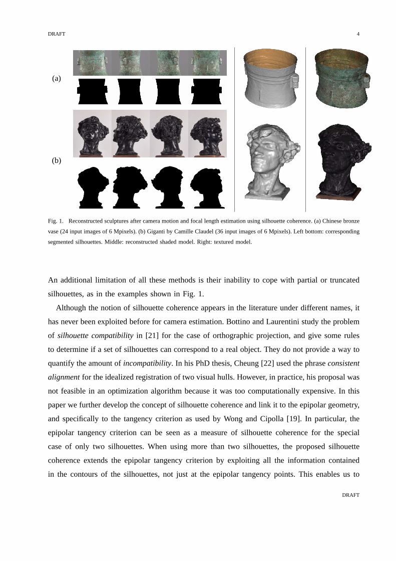
Fig. 1. Reconstructed sculptures after camera motion and focal length estimation using silhouette coherence. (a) Chinese bronze

vase (24 input images of 6 Mpixels). (b) Giganti by Camille Claudel (36 input images of 6 Mpixels). Left bottom: corresponding

segmented silhouettes. Middle: reconstructed shaded model. Right: textured model.

An additional limitation of all these methods is their inability to cope with partial or truncated

silhouettes, as in the examples shown in Fig. 1.

Although the notion of silhouette coherence appears in the literature under different names, it

has never been exploited before for camera estimation. Bottino and Laurentini study the problem

of silhouette compatibilityin [21] for the case of orthographic projection, and give some rules

to determine if a set of silhouettes can correspond to a real object. They do not provide a way to

quantify the amount ofincompatibility. In his PhD thesis, Cheung [22] used the phraseconsistent

alignmentfor the idealized registration of two visual hulls. However, in practice, his proposal was

not feasible in an optimization algorithm because it was toocomputationally expensive. In this

paper we further develop the concept of silhouette coherence and link it to the epipolar geometry,

and specifically to the tangency criterion as used by Wong andCipolla [19]. In particular, the

epipolar tangency criterion can be seen as a measure of silhouette coherence for the special

case of only two silhouettes. When using more than two silhouettes, the proposed silhouette

coherence extends the epipolar tangency criterion by exploiting all the information contained

in the contours of the silhouettes, not just at the epipolar tangency points. This enables us to

DRAFT

DRAFT 5

estimate the motion and the focal length correctly even if there are no epipolar tangents available

(see Fig. 1a). The proposed silhouette coherence criterionis also related to [23], where silhouette

coherence is used to register a laser model with a set of images. The main difference with this

paper is that we do not require a 3D representation of the object in order to perform camera

calibration. The object isimplicitly reconstructed from the silhouettes by a visual hull method

at the same time as the cameras are calibrated.

III. PROBLEM FORMULATION

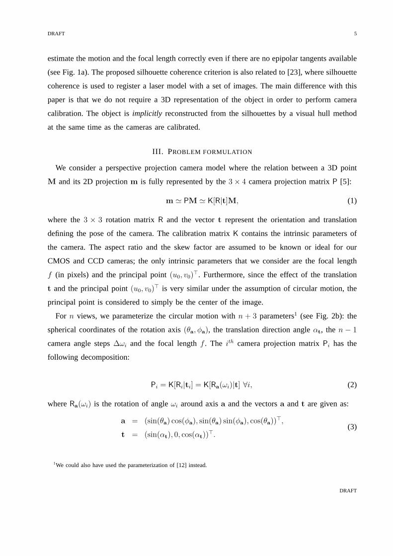
We consider a perspective projection camera model where therelation between a 3D point

M and its 2D projectionm is fully represented by the3 × 4 camera projection matrixP [5]:

m ≃ PM ≃ K[R|t]M, (1)

where the3 × 3 rotation matrixR and the vectort represent the orientation and translation

defining the pose of the camera. The calibration matrixK contains the intrinsic parameters of

the camera. The aspect ratio and the skew factor are assumed to be known or ideal for our

CMOS and CCD cameras; the only intrinsic parameters that we consider are the focal length

f (in pixels) and the principal point(u0, v0)⊤. Furthermore, since the effect of the translation

t and the principal point(u0, v0)⊤ is very similar under the assumption of circular motion, the

principal point is considered to simply be the center of the image.

For n views, we parameterize the circular motion withn + 3 parameters1 (see Fig. 2b): the

spherical coordinates of the rotation axis(θa, φa), the translation direction angleαt, the n − 1

camera angle steps∆ωi and the focal lengthf . The ith camera projection matrixPi has the

following decomposition:

Pi = K[Ri|ti] = K[Ra(ωi)|t] ∀i, (2)

whereRa(ωi) is the rotation of angleωi around axisa and the vectorsa andt are given as:

a = (sin(θa) cos(φa), sin(θa) sin(φa), cos(θa))⊤,

t = (sin(αt), 0, cos(αt))⊤.

(3)

1We could also have used the parameterization of [12] instead.

DRAFT

DRAFT 6

(a)

(b) �!i�af

a

Pi

(u0; v0)�t�a

Fig. 2. Circular motion parameterization. (a) Set of input silhouettesSi. (b) Parameterization of the projection matricesPi as

a function of the spherical coordinates of the rotation axis(θa, φa), the translation directionαt, the camera angle steps∆ωi

and the focal lengthf .

Given a set of silhouettesSi of a rigid object taken under circular motion (see Fig. 2a),

our goal is to recover the corresponding projection matrices Pi as the set ofn + 3 parameters

v = (θa, φa, αt, ∆ωi, f) (see Fig. 2b).

IV. SILHOUETTE COHERENCE

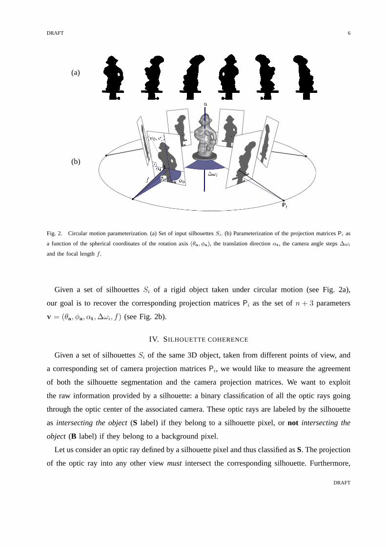
Given a set of silhouettesSi of the same 3D object, taken from different points of view, and

a corresponding set of camera projection matricesPi, we would like to measure the agreement

of both the silhouette segmentation and the camera projection matrices. We want to exploit

the raw information provided by a silhouette: a binary classification of all the optic rays going

through the optic center of the associated camera. These optic rays are labeled by the silhouette

as intersecting the object(S label) if they belong to a silhouette pixel, ornot intersecting the

object (B label) if they belong to a background pixel.

Let us consider an optic ray defined by a silhouette pixel and thus classified asS. The projection

of the optic ray into any other viewmust intersect the corresponding silhouette. Furthermore,

DRAFT

DRAFT 7

(a) (b)

Fig. 3. Two examples of different degrees of silhouette coherence. The reconstructed visual hullV is shown by the gray 3D

object. (a) A perfectly coherent silhouette set. (b) Same set of silhouettes with a different pose and low silhouette coherence.

The red area shows non-coherent silhouette pixels. In this paper we minimize the red area as a criterion for camera calibration

(see video in supplemental material).

the back projection of all these 2D intersection intervals onto the optic raymustbe coherent,

meaning that their intersection must have non-zero length.The intersection interval will contain

the exact position where the optic ray touches or intersectsthe object.

Due to noisy silhouettes or incorrect camera projection matrices, the above statement may not

be satisfied,i.e., even if a silhouette has labeled an optic ray asS, its depth interval might be

empty. In the case of only two views, the corresponding silhouettes will not be coherent if there

exists at leastoneoptic ray classified asS by one of the silhouettes whose projection does not

intersect the other silhouette. In the case ofn views, the lack of coherence is defined by the

existence of at least one optic ray where the depth intervalsdefined by then−1 other silhouettes

have an empty intersection. This lack of coherence can be measured simply by counting how

many optic rays in each silhouette are not coherent with the other silhouettes. Two examples

of coherent and non-coherent silhouettes are shown in Fig. 3. The silhouette pixels that are not

coherent with the other silhouettes are shown in red in Fig. 3b.

A simple way of measuring the silhouette coherence using theconcept of visual hull [24] is

as follows:

• compute the reconstructed visual hull defined by the silhouettes and the projection matrices,

• project the reconstructed visual hull back into the cameras, and

DRAFT

DRAFT 8

• compare the reconstructed visual hull silhouettes with theoriginal silhouettes.

In the situation of ideal data,i.e., perfect segmentation and exact projection matrices, the

reconstructed visual hull silhouettes and the original silhouettes will be exactly the same (see

Fig. 3a). With real data, both the silhouettes and the projection matrices will be imperfect. As

a consequence, the original silhouettes and the reconstructed visual hull silhouettes will not be

the same, the latter silhouettes beingalways contained in the original ones (see Fig. 3b).

A. A robust measure of silhouette coherence

Let V be the visual hull defined by the set of silhouettesSi and the set of projection matrices

Pi, andSVi its projection into theith image. A choice must be made about how to measure the

similarity C between the silhouetteSi and the projection of the reconstructed visual hullSVi . A

quick answer would be to use the ratio of areas between these two silhouettes as in [23]:

C(Si, SVi ) =

∫SV

i∫Si

=

∫(Si ∩ SV

i )∫Si

∈ [0, 1]. (4)

However, this measure has the major disadvantage of a very high computation cost, as mentioned

by [22]. To address this important issue, we propose a simplereplacement in (4) of the silhouette

Si by its contour,Ci:

C(Si, SVi ) =

∫(Ci ∩ SV

i )∫Ci

∈ [0, 1]. (5)

This new measure is much faster than (4) since, as discussed in Section V, we propose to

discretize the evaluation of the measure. Hence, the computation time of (5) is proportional

to the length term (Ci ∩ SVi ), while the computation time of (4) is proportional to thearea

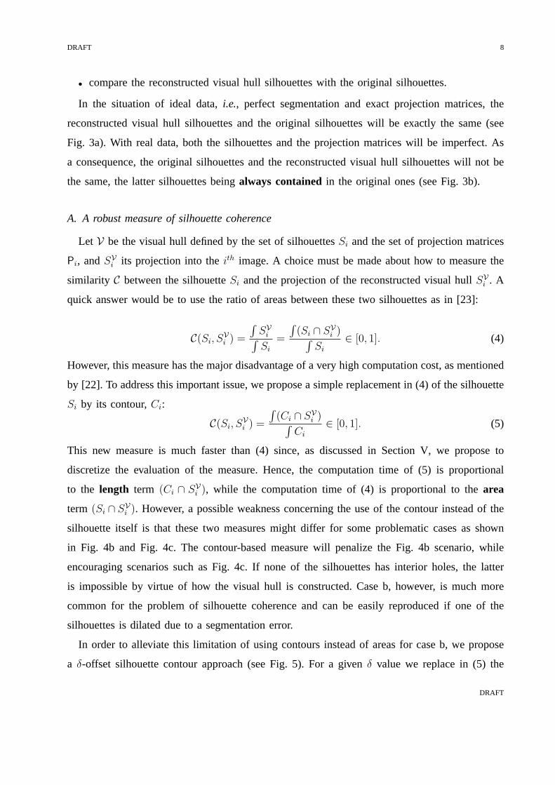
term (Si ∩ SVi ). However, a possible weakness concerning the use of the contour instead of the

silhouette itself is that these two measures might differ for some problematic cases as shown

in Fig. 4b and Fig. 4c. The contour-based measure will penalize the Fig. 4b scenario, while

encouraging scenarios such as Fig. 4c. If none of the silhouettes has interior holes, the latter

is impossible by virtue of how the visual hull is constructed. Case b, however, is much more

common for the problem of silhouette coherence and can be easily reproduced if one of the

silhouettes is dilated due to a segmentation error.

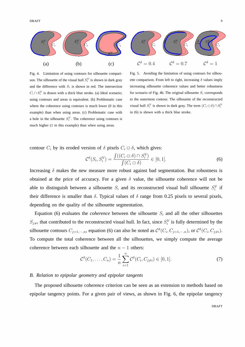
In order to alleviate this limitation of using contours instead of areas for case b, we propose

a δ-offset silhouette contour approach (see Fig. 5). For a given δ value we replace in (5) the

DRAFT

DRAFT 9

Ci

SVi

Ci

SVi

Ci

SVi

(a) (b) (c)

Fig. 4. Limitation of using contours for silhouette compari-

son. The silhouette of the visual hullSVi is shown in dark gray

and the difference withSi is shown in red. The intersection

Ci ∩SVi is drawn with a thick blue stroke. (a) Ideal scenario;

using contours and areas is equivalent. (b) Problematic case

where the coherence using contours is much lower (0 in this

example) than when using areas. (c) Problematic case with

a hole in the silhouetteSVi . The coherence using contours is

much higher (1 in this example) than when using areas.

Ci

SVi

Ci

SVi

δCi

SVi

δ

Cδ = 0.4 Cδ = 0.7 Cδ = 1

Fig. 5. Avoiding the limitation of using contours for silhou-

ette comparison. From left to right, increasingδ values imply

increasing silhouette coherence values and better robustness

for scenario of Fig. 4b. The original silhouetteSi corresponds

to the outermost contour. The silhouette of the reconstructed

visual hullSVi is shown in dark gray. The term(Ci⊖δ)∩SV

i

in (6) is shown with a thick blue stroke.

contourCi by its eroded version ofδ pixels Ci ⊖ δ, which gives:

Cδ(Si, SVi ) =

∫((Ci ⊖ δ) ∩ SV

i )∫(Ci ⊖ δ)

∈ [0, 1]. (6)

Increasingδ makes the new measure more robust against bad segmentation.But robustness is

obtained at the price of accuracy. For a givenδ value, the silhouette coherence will not be

able to distinguish between a silhouetteSi and its reconstructed visual hull silhouetteSVi if

their difference is smaller thanδ. Typical values ofδ range from 0.25 pixels to several pixels,

depending on the quality of the silhouette segmentation.

Equation (6) evaluates thecoherencebetween the silhouetteSi and all the other silhouettes

Sj 6=i that contributed to the reconstructed visual hull. In fact,sinceSVi is fully determined by the

silhouette contoursCj=1,··· ,n, equation (6) can also be noted asCδ(Ci, Cj=1,··· ,n), or Cδ(Ci, Cj 6=i).

To compute the total coherence between all the silhouettes,we simply compute the average

coherence between each silhouette and then − 1 others:

Cδ(C1, . . . , Cn) =1

n

n∑

i=1

Cδ(Ci, Cj 6=i) ∈ [0, 1]. (7)

B. Relation to epipolar geometry and epipolar tangents

The proposed silhouette coherence criterion can be seen as an extension to methods based on

epipolar tangency points. For a given pair of views, as shownin Fig. 6, the epipolar tangency

DRAFT

DRAFT 10

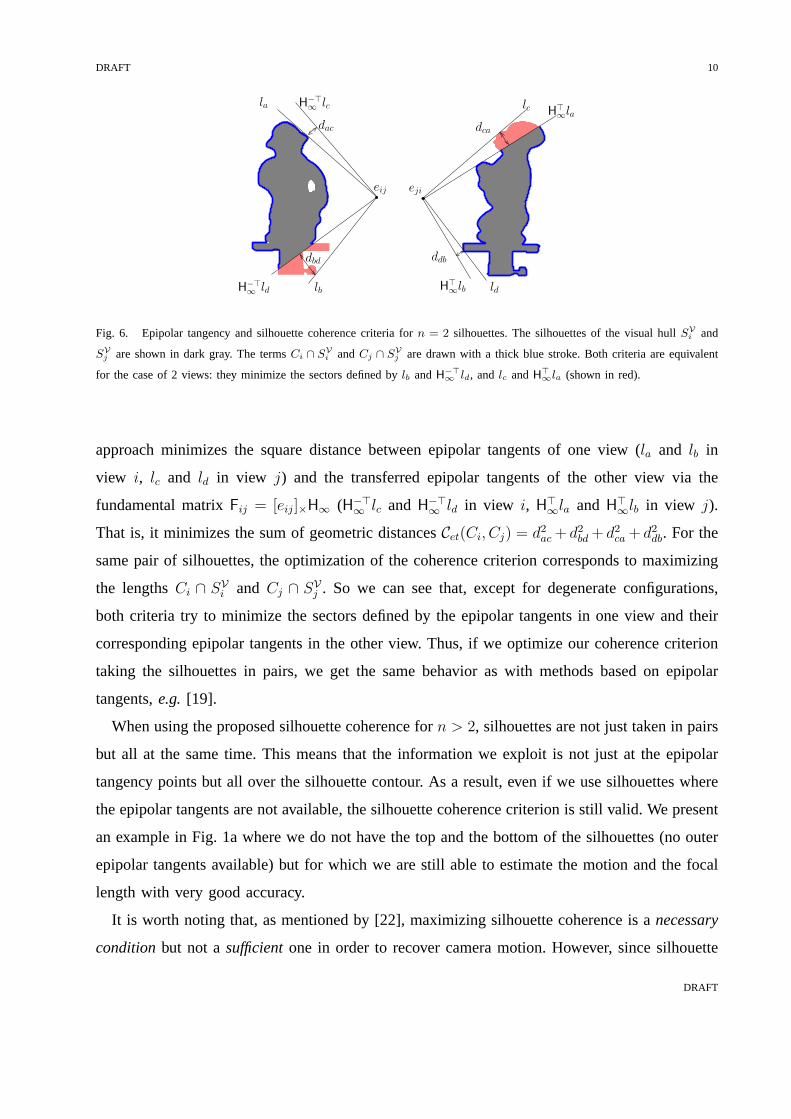
eji

dac

H⊤∞la

dca

la H−⊤∞ lc lc

ldlb

eij

ddbdbd

H⊤∞lbH

−⊤∞ ld

Fig. 6. Epipolar tangency and silhouette coherence criteria forn = 2 silhouettes. The silhouettes of the visual hullSVi and

SVj are shown in dark gray. The termsCi ∩ SV

i andCj ∩ SVj are drawn with a thick blue stroke. Both criteria are equivalent

for the case of 2 views: they minimize the sectors defined bylb andH−⊤∞ ld, and lc andH

⊤∞la (shown in red).

approach minimizes the square distance between epipolar tangents of one view (la and lb in

view i, lc and ld in view j) and the transferred epipolar tangents of the other view viathe

fundamental matrixFij = [eij]×H∞ (H−⊤∞ lc and H

−⊤∞ ld in view i, H

⊤∞la and H

⊤∞lb in view j).

That is, it minimizes the sum of geometric distancesCet(Ci, Cj) = d2

ac + d2

bd + d2

ca + d2

db. For the

same pair of silhouettes, the optimization of the coherencecriterion corresponds to maximizing

the lengthsCi ∩ SVi and Cj ∩ SV

j . So we can see that, except for degenerate configurations,

both criteria try to minimize the sectors defined by the epipolar tangents in one view and their

corresponding epipolar tangents in the other view. Thus, ifwe optimize our coherence criterion

taking the silhouettes in pairs, we get the same behavior as with methods based on epipolar

tangents,e.g. [19].

When using the proposed silhouette coherence forn > 2, silhouettes are not just taken in pairs

but all at the same time. This means that the information we exploit is not just at the epipolar

tangency points but all over the silhouette contour. As a result, even if we use silhouettes where

the epipolar tangents are not available, the silhouette coherence criterion is still valid. We present

an example in Fig. 1a where we do not have the top and the bottomof the silhouettes (no outer

epipolar tangents available) but for which we are still ableto estimate the motion and the focal

length with very good accuracy.

It is worth noting that, as mentioned by [22], maximizing silhouette coherence is anecessary

conditionbut not asufficientone in order to recover camera motion. However, since silhouette

DRAFT

DRAFT 11

coherence is an extension of epipolar tangency criteria, the same limitation applies to previous

methods using epipolar tangency points. If silhouette coherence is optimized, so is the epipolar

tangency criterion. This can be checked easily in Fig. 6. In practice, maximizing silhouette coher-

ence is sufficient and can be used for camera calibration, as demonstrated by the reconstruction

of more than 50 sequences (available for download at [25]) obtained using the 3D modeling

technique described in [2]. In order to use the modeling algorithm, cameras were calibrated

using the technique described in this paper.

V. OVERVIEW OF THE CAMERA ESTIMATION ALGORITHM

We now present a practical implementation of the silhouettecoherence criterionCδ, achieved

by discretizing the contourCi ⊖ δ into a number of equally spaced sample points. The term

(Ci⊖δ)∩SVi is evaluated by testing, for each sample point, if its associated optic ray intersects the

reconstructed visual hull using a ray casting technique [26]. A simplified version of this algorithm

is used, where we do not take into account contours inside thesilhouettes. Furthermore, we do

not compute all the depth intervals for a given optic ray. We just compute the minimum and

maximum of the interval intersection with each silhouette.This is a conservative approximation

of the real coherence,i.e., the coherence score that we obtain by storing only the minimum and

maximum depths is always equal or greater than the real one. However, in practice, the deviation

from the coherence computed with all the intervals is small.

The algorithm describing the silhouette coherenceCδ(Ci, Cj 6=i) between a given silhouette

contourCi and the remaining silhouette contoursCj 6=i is shown in Algorithm 1. IfN is the

number of sample points per silhouette, andn is the number of silhouettes, the complexity of

Cδ(Ci, Cj 6=i) is O(nN log(N)). The total silhouette coherenceCδ(Ci, . . . , Cn) in (7) is shown in

Algorithm 2 and its complexity isO(n2N log(N)). As an example, the computation time of one

evaluation of (7) on an Athlon 1.5 GHz processor is 750 ms for the Pitcher example of Fig. 7

(n = 18, N ≈ 6000).

In order to exploit silhouette coherence for camera motion and focal length estimation under

circular motion, thekey is to use the silhouette coherence as thecost in an optimization

procedure. Equation 7 can be seen as a “black box” that takes as input a set of silhouettes and

projection matrices, and gives as output a scalar value of silhouette coherence. We use Powell’s

derivative-free optimization algorithm [27] to maximize (7). Several hundred cost evaluations

DRAFT

DRAFT 12

Algorithm 1 Silhouette coherenceCδ(Ci, Cj 6=i)

Require: Projection matricesPi ∀i, reference contour

Ci, contour list Cj 6=i, contour offsetδ, number of

samples per contourN

Build point listm(k), samplingN points alongCi⊖δ

for all m(k) do

Initialize 3D intervalI3D = [0,∞]

Initialize counterN ′ = 0

for all Cj 6=i do

Project optic rayl = PjP−1i m

(k)

Compute 2D intersection intervalI2D = l ∩ Cj

Back project 2D intervalI3D = I3D ∩ P−1j I2D

end for

if I3D 6= ∅ then

N ′ = N ′ + 1

end if

end for

Return N′

N

Algorithm 2 Total silhouette coherenceCδ(Ci=1,··· ,n)

Require: Sequence of contoursCi=1,··· ,n, camera parameters

v = (θa, φa, αt, ∆ωi, f)

ComputePi from v using (2) and (3).

Return average1n

Pn

i=1 Cδ(Ci, Cj 6=i) {Algorithm 1}

Algorithm 3 Motion and focal length estimation

Require: Sequence of imagesIi=1,··· ,n

Extract contoursCi from Ii (e.g. [28]),

Initialize v = (θa, φa, αt, ∆ωi, f)=(π2, π

2, 0, 2π

n, f0),

Initialize Powell’s derivative-free algorithm [27]

repeat {see [27] for details}

v′ = v

v = Powell(v′) {Single Powell iteration with Algorithm 2}

until ||v − v′|| < ǫ

are typically required before convergence.

The system is always initialized with the same default circular motion: the rotation axis

a = (0, 1, 0)⊤ (θa = π2, φa = π

2), the translationt = (0, 0, 1)⊤ (αt = 0) and the initial guess of

the camera angles (e.g., ∆ωi = 2πn

). The initial guess of the focal lengthf0 is directly computed

from typical values of the field of view,e.g., 20 degrees. The principal point is considered

constant and equal to the center of the image. The complete algorithm for motion and focal

length estimation is described in Algorithm 3. Because circular motion is a very constrained

motion, we have found that the initial values for the rotation axis, the translation direction

and the focal length do not need to be very close to the actual solution. The only source of

convergence problems is the initial camera angles, but the algorithm has proven to have good

convergence properties for camera angle errors of up to 15 degrees.

VI. EXPERIMENTAL RESULTS

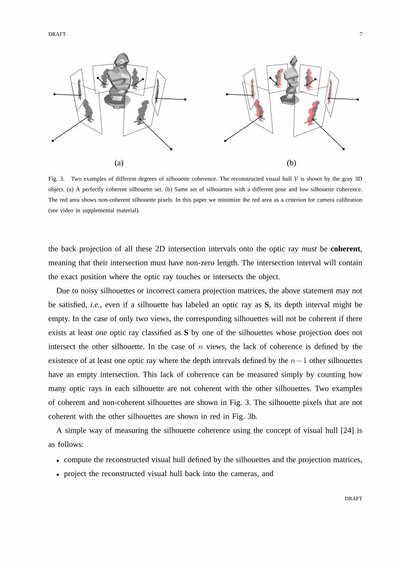
We present an experiment using a Pitcher sequence with 18 color images of 2008x3040 pixels

acquired with a computer controlled turntable. The images have been segmented by an automatic

procedure [28] (see Fig. 7). For evaluation we also use a sequence of a calibration pattern in

DRAFT

DRAFT 13

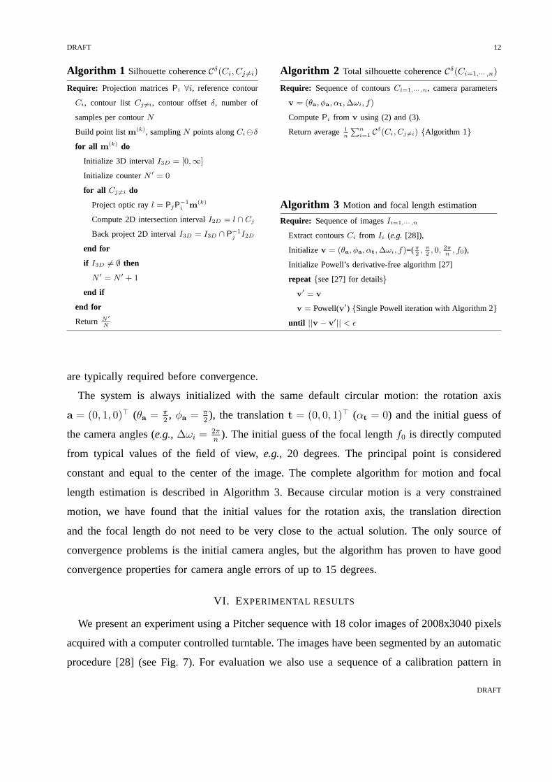
Fig. 7. Pitcher sequence. Some of the original images superimposed withthe extracted smooth polygon contours (in black).

rotation axis translation focalPitcher (degrees) (degrees) (pixels)

θa φa αt f

initial 90.0000 90.0000 0.0000 5000calibrated 99.671 90.3431 0.4266 6606

Cetrecovered99.6345 90.3050 0.4314 6576error 0.0364 0.0381 0.0049 30

Crecovered99.6861 90.3419 0.4239 6635error 0.0152 0.0011 0.0026 29 1 2 3 4 5 6 7 8 9 10 11 12 13 14 15 16 17

−0.5

−0.4

−0.3

−0.2

−0.1

0

0.1

0.2

0.3

0.4

0.5

Camera number

Deg

rees

Camera angle step error

epipolar tangency criterionsilhouette coherence criterion

TABLE I

CAMERA ESTIMATION FOR THE PITCHER SEQUENCE. MEAN CAMERA ANGLE STEP ERROR OF0.11DEGREES USING

EPIPOLAR TANGENCY POINTS(Cet) AND 0.06DEGREES USING SILHOUETTE COHERENCE(C). NOTE THAT THE AXIS ERROR

IS REDUCED BY A FACTOR OF3, THE TRANSLATION ERROR BY A FACTOR OF2, AND THE STEP ERROR BY A FACTOR OF2.

order to accurately recover the intrinsic parameters and the circular motion using [29]. Theδ-

offset used for the silhouette coherence criterion isδ = 0.25 pixels due to the sub-pixel accuracy

of the silhouette extraction. The camera angles are initialized with a uniform random noise

in the interval [−15, 15] degrees around the true angles. We show in the supplemental video

the initialization used in this example and how the different parameters are optimized by the

silhouette coherence.

Table I contains the results for the camera motion (rotationaxis, translation direction and

camera angles) and focal length estimation problem. A totalof 21 parameters are recovered. We

compare the proposed silhouette coherence with the state-of-the-art method described in [19].

The silhouette coherence clearly outperforms [19] by reducing the rotation axis error by a factor

of 3, the translation error by a factor of 2 and the camera angles error by a factor of 2. Both

criteria recover the focal length with the same accuracy (∼ 0.5%).

The same camera estimation algorithm has been repeatedly tested successfully on over 50

DRAFT

DRAFT 14

uncalibrated sequences. We illustrate in Fig. 1 two of thesesequences that are particularly

interesting. For the Chinese bronze vase (Fig. 1a) the two outermost epipolar tangents are not

available, since the tops and bottoms of the silhouettes aretruncated. For the Giganti sculpture

(Fig. 1b) just the bottom has been truncated. Problems with correctly extracting the bottom

of an object are common under turntable motion. In general, it is easy to extract the top of

an object, but it is much more difficult to separate the bottomfrom the turntable. We validate

the motion and calibration results by the quality of the finalreconstructions, generated using

an implementation of the algorithm described in [2]. Note that the Giganti sculpture (Fig. 1b)

would be very difficult to calibrate using point-based techniques, its surface being very specular,

while the Chinese vase (Fig. 1a) is impossible for epipolar tangent algorithms.

Two additional experiments ara available as supplemental material in appendix I. In the first

experiment we compare the accuracy of the silhouette coherence and the epipolar tangency

criteria as a function of silhouette noise. In the second experiment we show that silhouette

coherence exploits more information that epipolar tangency points alone by showing that it can

calibrate the cameras even when no epipolar tangency pointsare available.

VII. C ONCLUSIONS AND FUTURE WORK

A new approach to silhouette-based camera estimation has been developed. It is built on the

concept of silhouette coherence, defined as a similarity between a set of silhouettes and the

silhouettes of their visual hull. This approach has been successfully tested for the problem of

circular motion. The high accuracy of the estimation results is due to the use of the full silhouette

contour in the computation, whereas previous silhouette-based methods just use epipolar tangency

points. The proposed method eliminates the need for epipolar tangency points and naturally copes

with truncated silhouettes. Previous algorithms are completely dependant on clean silhouettes

and epipolar tangency points. We have validated the proposed approach both qualitatively and

quantitatively.

A limitation of our current silhouette coherence implementation is the discretization of the

silhouette contours. To remove this source of sampling noise, a solution would compute the exact

visual hull silhouettes as polygons and compare them with the original silhouettes. To compute

the exact silhouette of the visual hull, we can proceed as in [30], using a ray casting technique.

We are currently extending the proposed approach to roughlycircular motion and general

DRAFT

DRAFT 15

motion, but special attention has to be paid to the initialization process to avoid local minima,

less important for the case of circular motion.

REFERENCES

[1] K. N. Kutulakos and S. M. Seitz, “A theory of shape by spacecarving,” IJCV, vol. 38, no. 3, pp. 199–218, 2000.

[2] C. Hernandez and F. Schmitt, “Silhouette and stereo fusion for 3d object modeling,”CVIU, vol. 96, no. 3, pp. 367–392, 2004.

[3] G. Vogiatzis, P. Torr, and R. Cipolla, “Multi-view stereo via volumetric graph-cuts,” inCVPR, 2005.

[4] P. Gargallo and P. Sturm, “Bayesian 3d modeling from images using multiple depth maps,” inCVPR, vol. II, 2005, pp. 885–891.

[5] R. I. Hartley and A. Zisserman,Multiple View Geometry in Computer Vision. Cambridge University Press, ISBN: 0521623049, 2000.

[6] D. Nister, “An efficient solution to the five-point relative pose problem,” IEEE Trans. on PAMI, vol. 26, no. 6, pp. 756–770, June 2004.

[7] J. H. Rieger, “Three dimensional motion from fixed points ofa deforming profile curve,”Optics Letters, vol. 11, no. 3, pp. 123–125,

1986.

[8] J. Porrill and S. B. Pollard, “Curve matching and stereo calibration,” Image and Vision Computing, vol. 9, no. 1, pp. 45–50, 1991.

[9] P. Giblin, F. Pollick, and J. Rycroft, “Recovery of an unknown axis of rotation from the profiles of a rotating surface,” J.Optical Soc.

America, vol. 11A, pp. 1976–1984, 1994.

[10] R. Cipolla and P. Giblin,Visual Motion of Curves and Surfaces. Cambridge University Press, 2000.

[11] M. Lhuillier and L. Quan, “Surface reconstruction by integrating 3d and 2d data of multiple views,” inICCV, 2003, pp. 1313–1320.

[12] A. W. Fitzgibbon, G. Cross, and A. Zisserman, “Automatic 3D model construction for turn-table sequences,” in3D SMILE, June 1998,

pp. 155–170.

[13] G. Jiang, H. Tsui, L. Quan, and A. Zisserman, “Single axisgeometry by fitting conics,” inECCV, vol. 1, 2002, pp. 537–550.

[14] R. Cipolla, K. Astrom, and P. Giblin, “Motion from the frontier of curved surfaces,” in ICCV, Cambridge, June 1995, pp. 269–275.

[15] B. Vijayakumar, D. Kriegman, and J. Ponce, “Structure andmotion of curved 3d objects from monocular silhouettes,” inCVPR, 1996,

pp. 327–334.

[16] Y. Furukawa, A. Sethi, J. Ponce, and D. Kriegman, “Structure and motion from images of smooth textureless objects,” inECCV 2004,

vol. 2, Prague, Czech Republic, May 2004, pp. 287–298.

[17] K. Astrom, R. Cipolla, and P. Giblin, “Generalized epipolar constraints,” IJCV, vol. 33, no. 1, pp. 51–72, 1999.

[18] P. R. S. Mendonca, K.-Y. K. Wong, and R. Cipolla, “Epipolar geometry from profiles under circular motion,”IEEE Trans. on PAMI,

vol. 23, no. 6, pp. 604–616, June 2001.

[19] K.-Y. K. Wong and R. Cipolla, “Reconstruction of sculpture from its profiles with unknown camera positions,”IEEE Trans. on Image

Processing, vol. 13, no. 3, pp. 381 – 389, 2004.

[20] S. N. Sinha, M. Pollefeys, and L. McMillan, “Camera network calibration from dynamic silhouettes,” inCVPR, vol. 1, 2004, pp. 195–202.

[21] A. Bottino and A. Laurentini, “Introducing a new problem: Shape-from-silhouette when the relative positions of the viewpoints is unknown,”

IEEE Trans. on PAMI, vol. 25, no. 11, pp. 1484–1493, 2003.

[22] K. Cheung, “Visual hull construction, alignment and refinement for human kinematic modeling, motion tracking and rendering,” Ph.D.

dissertation, Carnegie Mellon University, 2003.

[23] H. Lensch, W. Heidrich, and H. P. Seidel, “A silhouette-based algorithm for texture registration and stitching,”J. of Graphical Models,

pp. 245–262, 2001.

[24] A. Laurentini, “The visual hull concept for silhouettebased image understanding,”IEEE Trans. on PAMI, vol. 16, no. 2, 1994.

[25] http://www.tsi.enst.fr/3dmodels/.

[26] W. Matusik, C. Buehler, R. Raskar, S. Gortler, and L. McMillan, “Image-based visual hulls,” inSIGGRAPH 2000, 2000, pp. 369–374.

[27] M. Powell, “An efficient method for finding the minimum of a function of several variables without calculating derivatives,” Computer

Journal, vol. 17, pp. 155–162, 1964.

[28] C. Xu and J. L. Prince, “Snakes, shapes, and gradient vector flow,” IEEE Trans. on Image Processing, pp. 359–369, 1998.

[29] J. M. Lavest, M. Viala, and M. Dhome, “Do we really need an accurate calibration pattern to achieve a reliable camera calibration?” in

ECCV, vol. 1, 1998, pp. 158–174.

[30] J.-S. Franco and E. Boyer, “Exact polyhedral visual hulls,” in BMVC, September 2003, pp. 329–338.

DRAFT