Silesian University Clausthal University of Technology of Technology Faculty of Energy Faculty of Energy and Environmental Engineering and Management Institute of Thermal Technology Institute of Energy Process Engineering and Fuel Technology Ph.D. thesis Ecological evaluation of the pulverized coal combustion in HTAC technology Natalia SCHAFFEL-MANCINI This thesis was realized in the frame of the agreement between Silesian University of Technology and Clausthal University of Technology for Ph.D. projects Gliwice - Clausthal-Zellerfeld 2009

Welcome message from author
This document is posted to help you gain knowledge. Please leave a comment to let me know what you think about it! Share it to your friends and learn new things together.
Transcript
Silesian University Clausthal Universityof Technology of TechnologyFaculty of Energy Faculty of Energy
and Environmental Engineering and ManagementInstitute of Thermal Technology Institute of Energy Process Engineering
and Fuel Technology
Ph.D. thesis
Ecological evaluation
of the pulverized coal combustion
in HTAC technology
Natalia SCHAFFEL-MANCINI
This thesis was realized in the frame of the agreement between
Silesian University of Technology and Clausthal University of Technology
for Ph.D. projects
Gliwice - Clausthal-Zellerfeld 2009

ii
Politechnika Śląska Uniwersytet Technicznyw Gliwicach w Clausthal
Wydział Inżynierii Środowiska Wydział Energiii Energetyki i Nauk Ekonomicznych
Instytut Techniki Cieplnej Instytut Energetycznej Inżynierii Procesowej
i Technologii Paliw
Praca doktorska
Ocena ekologiczna
procesu spalania pyłu węglowego
w technologii HTAC
Natalia SCHAFFEL-MANCINI
Praca doktorska powstała w ramach umowy o podwójnym doktoracie zawartej pomiędzy
Politechniką Śląską w Gliwicach i Uniwersytetem Technicznym w Clausthal
Gliwice - Clausthal-Zellerfeld 2009

iv
Schlesische Technische Universität Technische Universitätin Gliwice Clausthal
Fakultät für Energie Fakultät für Energie-und Umwelttechnik und Wirtschaftswissenschaften
Institut für Hochtemperaturtechnik Institut für Energieverfahrenstechnik
und Brennstofftechnik
Dissertation
Ökologische Bewertung
der HTAC-Kohlestaubverbrennungsmethode
Natalia SCHAFFEL-MANCINI
Diese Dissertation wurde im Rahmen der Doppelpromotionsvereinbarung zwischen
der Schlesischen Technischen Universität und der Technischen Universität Clausthal
ausgefertigt
Gliwice - Clausthal-Zellerfeld 2009
Author:
Mgr inż. Natalia Schaffel-Mancini Dipl.-Ing. Natalia Schaffel-Mancini
Silesian University of Technology Clausthal University of Technology
Faculty of Energy Faculty of Energy
and Environmental Engineering and Management
Institute of Thermal Technology Institute of Energy Process Engineering
and Fuel Technology
ul. Konarskiego 22 Agricolastr. 4
PL-44 100 Gliwice, Poland D-38 678 Clausthal-Zellerfeld, Germany
e-mail: [email protected] e-mail: [email protected]
Supervisors:
Prof. dr hab. inż. Andrzej Szlęk Prof. Dr.-Ing. Roman Weber
Silesian University of Technology Clausthal University of Technology
Faculty of Energy Faculty of Energy
and Environmental Engineering and Management
Institute of Thermal Technology Institute of Energy Process Engineering
and Fuel Technology
ul. Konarskiego 22 Agricolastr. 4
PL-44 100 Gliwice, Poland D-38 678 Clausthal-Zellerfeld, Germany
e-mail: [email protected] e-mail: [email protected]
Reviewers:
Prof. dr hab. inż. Marek Pronobis D. Sc. (Tech.), Professor Antti Oksanen
Silesian University of Technology Tampere University of Technology
Faculty of Energy Faculty of Science
and Environmental Engineering and Environmental Engineering
Institute of Power Engineering Department of Energy
and Turbomachinery and Process Engineering
ul. Konarskiego 20 PO Box 589
PL-44 100 Gliwice, Poland FIN-33 101 Tampere, Finland
e-mail: [email protected] e-mail: [email protected]
vi
Contents
Abstract . . . . . . . . . . . . . . . . . . . . . . . . . . . . . . . . . . . . . . . xix
Streszczenie . . . . . . . . . . . . . . . . . . . . . . . . . . . . . . . . . . . . . xxi
Kurzfassung . . . . . . . . . . . . . . . . . . . . . . . . . . . . . . . . . . . . . xxiii
Acknowledgments . . . . . . . . . . . . . . . . . . . . . . . . . . . . . . . . . . xxv
Introduction . . . . . . . . . . . . . . . . . . . . . . . . . . . . . . . . . . . . . xxvii
Motivation . . . . . . . . . . . . . . . . . . . . . . . . . . . . . . . . . . . . . . xxvii
Objectives . . . . . . . . . . . . . . . . . . . . . . . . . . . . . . . . . . . . . . xxviii
1 Coal in power generation 1
1.1 Overview of coal utilities . . . . . . . . . . . . . . . . . . . . . . . . . . . 1
1.2 Environmental issues of coal utilization . . . . . . . . . . . . . . . . . . . 3
1.3 Coal based technologies for power generation . . . . . . . . . . . . . . . . 5
1.3.1 Pulverized coal (PC) combustion systems . . . . . . . . . . . . . . 6
1.3.2 Fluidized bed combustion (FBC) systems . . . . . . . . . . . . . . 7
1.3.3 Combustion under O2/CO2 atmosphere . . . . . . . . . . . . . . . 8
1.3.4 Coal gasification (CG) technology . . . . . . . . . . . . . . . . . . 9
1.3.5 Integrated Gasification Combined-Cycle (IGCC) systems . . . . . 11
1.3.6 Integrated Gasification Fuel Cells (IGFC) systems . . . . . . . . . 11
1.4 Pulverized coal fired power plants . . . . . . . . . . . . . . . . . . . . . . 12
1.4.1 Subcritical installations . . . . . . . . . . . . . . . . . . . . . . . . 14
1.4.2 Supercritical installations . . . . . . . . . . . . . . . . . . . . . . 14
1.4.3 Ultra-supercritical installations . . . . . . . . . . . . . . . . . . . 15
1.5 High temperature materials for steam power plants . . . . . . . . . . . . 15
1.6 Rankine cycle . . . . . . . . . . . . . . . . . . . . . . . . . . . . . . . . . 17
1.7 Issues for higher efficiency . . . . . . . . . . . . . . . . . . . . . . . . . . 18
1.7.1 Steam pressure . . . . . . . . . . . . . . . . . . . . . . . . . . . . 18
1.7.2 Steam temperature . . . . . . . . . . . . . . . . . . . . . . . . . . 19
1.7.3 Exit gas temperature . . . . . . . . . . . . . . . . . . . . . . . . . 19
1.7.4 Excess air ratio . . . . . . . . . . . . . . . . . . . . . . . . . . . . 19
vii
1.7.5 Unburned carbon . . . . . . . . . . . . . . . . . . . . . . . . . . . 20
1.8 Pulverized coal (PC) boilers for power generation . . . . . . . . . . . . . 20
1.8.1 Drum type boilers . . . . . . . . . . . . . . . . . . . . . . . . . . 21
1.8.2 Once-through type boilers . . . . . . . . . . . . . . . . . . . . . . 22
2 Overview of HTAC technology 27
2.1 Development of HTAC technology . . . . . . . . . . . . . . . . . . . . . . 27
2.2 Current investigations and challenges of HTAC technology . . . . . . . . 30
2.3 Modeling of HTAC technology . . . . . . . . . . . . . . . . . . . . . . . . 34
2.4 Basic implementations of HTAC technology . . . . . . . . . . . . . . . . 39
2.5 Application of HTAC technology in furnaces . . . . . . . . . . . . . . . . 41
2.6 Application of HTAC technology in boilers . . . . . . . . . . . . . . . . . 42
3 Mathematical model 45
3.1 The governing partial differential equations . . . . . . . . . . . . . . . . . 45
3.1.1 The continuity equation . . . . . . . . . . . . . . . . . . . . . . . 46
3.1.2 The Navier-Stokes equation . . . . . . . . . . . . . . . . . . . . . 46
3.1.3 The conservation equation of chemical species . . . . . . . . . . . 46
3.1.4 The energy equation . . . . . . . . . . . . . . . . . . . . . . . . . 47
3.1.5 The equation of state . . . . . . . . . . . . . . . . . . . . . . . . . 47
3.1.6 The general governing differential equation . . . . . . . . . . . . . 47
3.2 Averaging of the governing partial differential equations . . . . . . . . . . 48
3.2.1 Reynolds averaging . . . . . . . . . . . . . . . . . . . . . . . . . . 49
3.2.2 Favre averaging . . . . . . . . . . . . . . . . . . . . . . . . . . . . 49
3.3 Set of the mathematical sub-models . . . . . . . . . . . . . . . . . . . . . 51
3.4 Turbulence . . . . . . . . . . . . . . . . . . . . . . . . . . . . . . . . . . . 51
3.5 Turbulent gas combustion . . . . . . . . . . . . . . . . . . . . . . . . . . 52
3.5.1 Turbulence-chemistry interaction models . . . . . . . . . . . . . . 54
3.5.2 Eddy Break Up Model . . . . . . . . . . . . . . . . . . . . . . . . 54
3.5.3 Eddy Dissipation Model . . . . . . . . . . . . . . . . . . . . . . . 55
3.5.4 Eddy Dissipation Concept . . . . . . . . . . . . . . . . . . . . . . 56
3.6 Particle behavior . . . . . . . . . . . . . . . . . . . . . . . . . . . . . . . 56
3.6.1 Trajectory calculations . . . . . . . . . . . . . . . . . . . . . . . . 57
3.6.2 Heat and mass transfer calculations . . . . . . . . . . . . . . . . . 58
3.7 Pulverized coal combustion . . . . . . . . . . . . . . . . . . . . . . . . . . 60
3.7.1 Coal devolatilization . . . . . . . . . . . . . . . . . . . . . . . . . 60
3.7.2 Combustion of volatiles . . . . . . . . . . . . . . . . . . . . . . . . 65
viii
3.7.3 Char combustion . . . . . . . . . . . . . . . . . . . . . . . . . . . 65
3.8 Radiative heat transfer . . . . . . . . . . . . . . . . . . . . . . . . . . . . 68
3.9 Nitric oxides . . . . . . . . . . . . . . . . . . . . . . . . . . . . . . . . . . 68
4 Model validation 73
4.1 Experimental equipment . . . . . . . . . . . . . . . . . . . . . . . . . . . 73
4.1.1 Furnace . . . . . . . . . . . . . . . . . . . . . . . . . . . . . . . . 73
4.1.2 Precombustor . . . . . . . . . . . . . . . . . . . . . . . . . . . . . 74
4.1.3 Burner block . . . . . . . . . . . . . . . . . . . . . . . . . . . . . 75
4.2 Measurements . . . . . . . . . . . . . . . . . . . . . . . . . . . . . . . . . 75
4.3 Coal characterization . . . . . . . . . . . . . . . . . . . . . . . . . . . . . 76
4.4 Numerical modeling . . . . . . . . . . . . . . . . . . . . . . . . . . . . . . 80
4.4.1 Model geometry and calculation procedure . . . . . . . . . . . . . 80
4.4.2 Flow field and recirculation . . . . . . . . . . . . . . . . . . . . . 82
4.4.3 Temperature field and radiative heat fluxes . . . . . . . . . . . . . 82
4.4.4 Oxygen and carbon dioxide concentrations . . . . . . . . . . . . . 83
4.4.5 Carbon monoxide concentration . . . . . . . . . . . . . . . . . . . 84
4.4.6 Volatiles concentration . . . . . . . . . . . . . . . . . . . . . . . . 85
4.4.7 Nitric oxide concentration . . . . . . . . . . . . . . . . . . . . . . 86
4.4.8 Char burnout . . . . . . . . . . . . . . . . . . . . . . . . . . . . . 88
4.4.9 Furnace outlet . . . . . . . . . . . . . . . . . . . . . . . . . . . . . 88
4.5 Findings . . . . . . . . . . . . . . . . . . . . . . . . . . . . . . . . . . . . 89
5 Design of the HTAC boiler 91
5.1 Shape of the HTAC boiler . . . . . . . . . . . . . . . . . . . . . . . . . . 91
5.1.1 Results and discussion . . . . . . . . . . . . . . . . . . . . . . . . 93
5.1.2 Findings . . . . . . . . . . . . . . . . . . . . . . . . . . . . . . . . 95
5.2 Distance between individual burners . . . . . . . . . . . . . . . . . . . . 96
5.2.1 Results and discussion . . . . . . . . . . . . . . . . . . . . . . . . 97
5.2.2 Findings . . . . . . . . . . . . . . . . . . . . . . . . . . . . . . . . 99
5.3 Location of the burner block . . . . . . . . . . . . . . . . . . . . . . . . . 100
5.3.1 Results and discussion . . . . . . . . . . . . . . . . . . . . . . . . 101
5.3.2 Findings . . . . . . . . . . . . . . . . . . . . . . . . . . . . . . . . 103
5.4 Dimensions of the HTAC boiler . . . . . . . . . . . . . . . . . . . . . . . 104
5.4.1 Results and discussion . . . . . . . . . . . . . . . . . . . . . . . . 104
5.4.2 Findings . . . . . . . . . . . . . . . . . . . . . . . . . . . . . . . . 106
ix
6 Final HTAC boiler design 107
6.1 Results and discussion . . . . . . . . . . . . . . . . . . . . . . . . . . . . 109
6.1.1 Velocity and recirculation . . . . . . . . . . . . . . . . . . . . . . 109
6.1.2 Temperature . . . . . . . . . . . . . . . . . . . . . . . . . . . . . . 111
6.1.3 Oxygen concentration . . . . . . . . . . . . . . . . . . . . . . . . 111
6.1.4 Coal particles behavior . . . . . . . . . . . . . . . . . . . . . . . . 113
6.1.5 Heat transfer . . . . . . . . . . . . . . . . . . . . . . . . . . . . . 115
6.2 Findings . . . . . . . . . . . . . . . . . . . . . . . . . . . . . . . . . . . . 116
7 Evaluation of the grid sensitivity 117
7.1 Grid independence . . . . . . . . . . . . . . . . . . . . . . . . . . . . . . 118
7.2 Grid quality . . . . . . . . . . . . . . . . . . . . . . . . . . . . . . . . . . 119
7.2.1 Node-point distribution . . . . . . . . . . . . . . . . . . . . . . . . 120
7.2.2 Smoothness . . . . . . . . . . . . . . . . . . . . . . . . . . . . . . 120
7.2.3 Cell shape . . . . . . . . . . . . . . . . . . . . . . . . . . . . . . . 121
8 Environmental issues 123
8.1 Nitric oxides emissions . . . . . . . . . . . . . . . . . . . . . . . . . . . . 123
8.2 Carbon monoxide and volatiles emissions . . . . . . . . . . . . . . . . . . 126
8.3 Char burnout . . . . . . . . . . . . . . . . . . . . . . . . . . . . . . . . . 127
8.4 Findings . . . . . . . . . . . . . . . . . . . . . . . . . . . . . . . . . . . . 127
9 Effects of selected operating parameters 129
9.1 Impact of the combustion air preheat . . . . . . . . . . . . . . . . . . . . 129
9.1.1 Results and discussion . . . . . . . . . . . . . . . . . . . . . . . . 130
9.1.2 Findings . . . . . . . . . . . . . . . . . . . . . . . . . . . . . . . . 134
9.2 The HTAC boiler equipped with low-momentum burners . . . . . . . . . 134
9.2.1 Results and discussion . . . . . . . . . . . . . . . . . . . . . . . . 135
9.2.2 Findings . . . . . . . . . . . . . . . . . . . . . . . . . . . . . . . . 138
9.3 The HTAC boiler operated at nearly stoichiometric conditions . . . . . . 139
9.3.1 Results and discussion . . . . . . . . . . . . . . . . . . . . . . . . 139
9.3.2 Findings . . . . . . . . . . . . . . . . . . . . . . . . . . . . . . . . 141
10 Coupling between the HTAC boiler and the steam cycle 143
10.1 Results and discussion . . . . . . . . . . . . . . . . . . . . . . . . . . . . 146
10.2 Cycle efficiency . . . . . . . . . . . . . . . . . . . . . . . . . . . . . . . . 150
10.3 Findings . . . . . . . . . . . . . . . . . . . . . . . . . . . . . . . . . . . . 151
x

11 Conclusions and future works 153
Nomenclature 156
Bibliography 163
Extended abstract . . . . . . . . . . . . . . . . . . . . . . . . . . . . . . . . . 179
Obszerne streszczenie . . . . . . . . . . . . . . . . . . . . . . . . . . . . . . . . 184
Zusammenfassung . . . . . . . . . . . . . . . . . . . . . . . . . . . . . . . . . . 189
xi

xii
List of Tables
1.1 Emission limit values for NOx, SO2 and dust . . . . . . . . . . . . . . . 4
3.1 Comburent composition and properties . . . . . . . . . . . . . . . . . . . 48
3.2 k − ε model constants . . . . . . . . . . . . . . . . . . . . . . . . . . . . 52
3.3 k − ε model Prandtl numbers . . . . . . . . . . . . . . . . . . . . . . . . 52
4.1 Comburent composition and properties . . . . . . . . . . . . . . . . . . . 74
4.2 Guasare coal proximate analysis . . . . . . . . . . . . . . . . . . . . . . . 76
4.3 Guasare coal ultimate analysis . . . . . . . . . . . . . . . . . . . . . . . . 76
4.4 The parameters for the CPD devolatilization model of Guasare coal . . . 78
4.5 The parameters for the intrinsic char combustion model of Guasare coal . 79
4.6 Boundary conditions in the numerical simulations . . . . . . . . . . . . . 80
4.7 Mass balance of NO . . . . . . . . . . . . . . . . . . . . . . . . . . . . . 88
4.8 Computed and measured values at the furnace exit . . . . . . . . . . . . 89
5.1 Boiler dimensions and firing density . . . . . . . . . . . . . . . . . . . . . 105
6.1 Boundary conditions of the boiler simulation . . . . . . . . . . . . . . . . 109
6.2 Components of the boiler energy balance . . . . . . . . . . . . . . . . . . 111
8.1 Nitric oxide formation paths . . . . . . . . . . . . . . . . . . . . . . . . . 125
10.1 Calculated steam temperatures . . . . . . . . . . . . . . . . . . . . . . . 149
10.2 Parameters for the Rankine cycle efficiency calculations . . . . . . . . . . 151
xiii

xiv
List of Figures
1.1 PC power plant installation . . . . . . . . . . . . . . . . . . . . . . . . . 6
1.2 Types of fluidized bed arrangement . . . . . . . . . . . . . . . . . . . . . 7
1.3 Oxygen/flue gas recycle combustion technology . . . . . . . . . . . . . . 9
1.4 Coal gasifier types . . . . . . . . . . . . . . . . . . . . . . . . . . . . . . 10
1.5 IGCC concept . . . . . . . . . . . . . . . . . . . . . . . . . . . . . . . . . 11
1.6 IGFC concept . . . . . . . . . . . . . . . . . . . . . . . . . . . . . . . . . 12
1.7 Steel barrier in recent years and prediction for future . . . . . . . . . . . 16
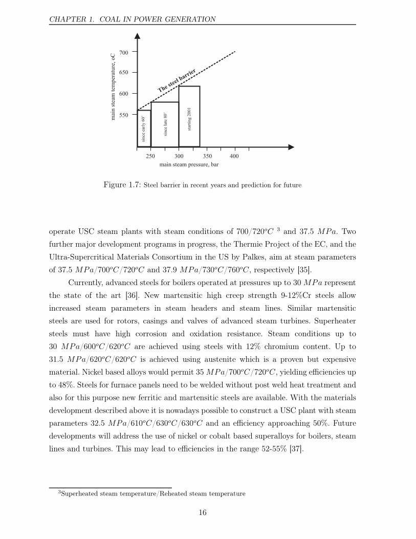
1.8 Illustration of the Rankine cycle . . . . . . . . . . . . . . . . . . . . . . . 17
1.9 Configuration of the heat transfer surfaces in the standard PC boiler . . 21
1.10 Typical burner location in the standard PC boiler . . . . . . . . . . . . . 22
1.11 Types of the water circulation installation in the boiler . . . . . . . . . . 23
1.12 Types of tube designs in the boiler combustion chamber . . . . . . . . . . 24
1.13 Configurations of the once-through boiler . . . . . . . . . . . . . . . . . . 25
2.1 Types of HTAC burners . . . . . . . . . . . . . . . . . . . . . . . . . . . 40
2.2 Mixing pattern in NFK/IFRF design . . . . . . . . . . . . . . . . . . . . 41
3.1 Coal combustion stages . . . . . . . . . . . . . . . . . . . . . . . . . . . . 60
3.2 Coal behavior during devolatilization process . . . . . . . . . . . . . . . . 62
3.3 Path of NO formation and reburning . . . . . . . . . . . . . . . . . . . . 69
4.1 Experimental IFRF furnace together with precombustor . . . . . . . . . 74
4.2 The detailed geometry of the burner . . . . . . . . . . . . . . . . . . . . 75
4.3 Guasare coal particle distribution and distribution parameters . . . . . . 77
4.4 Devolatilization and burnout measurements with the CPD and the intrinsic
model fittings for Guasare coal . . . . . . . . . . . . . . . . . . . . . . . . 78
4.5 The coal combustion model used in this work . . . . . . . . . . . . . . . 79
4.6 Operating conditions in the IFRF experiment . . . . . . . . . . . . . . . 80
4.7 Geometry of the simulated IFRF furnace . . . . . . . . . . . . . . . . . . 81
4.8 Velocity and temperature profiles . . . . . . . . . . . . . . . . . . . . . . 83
xv
4.9 Measured and calculated total radiation intensity . . . . . . . . . . . . . 84
4.10 Measured and calculated total incident radiative heat flux . . . . . . . . 84
4.11 Oxygen and carbon dioxide concentration profiles . . . . . . . . . . . . . 85
4.12 Carbon monoxide profiles. Measured CxHy concentrations and predicted
concentrations of volatiles . . . . . . . . . . . . . . . . . . . . . . . . . . 86
4.13 Nitric oxide concentration profiles and sources in the NO balance equation 87
4.14 Char burnout and carbon in ash along the centerline of the fuel jet . . . 89
5.1 Considered combustion chamber forms . . . . . . . . . . . . . . . . . . . 92
5.2 Recirculation inside the combustion chamber . . . . . . . . . . . . . . . . 93
5.3 Temperature field inside the combustion chamber . . . . . . . . . . . . . 94
5.4 Oxygen concentrations field inside the combustion chamber . . . . . . . . 94
5.5 Volatiles concentrations field inside the combustion chamber . . . . . . . 94
5.6 Optimized boiler shape . . . . . . . . . . . . . . . . . . . . . . . . . . . . 96
5.7 Geometry of the examined boilers . . . . . . . . . . . . . . . . . . . . . . 97
5.8 Velocity field inside the boiler . . . . . . . . . . . . . . . . . . . . . . . . 98
5.9 Oxygen concentration field inside the boiler . . . . . . . . . . . . . . . . 98
5.10 Geometry and position of the traverses . . . . . . . . . . . . . . . . . . . 100
5.11 Recirculation inside the up- and down-fired boiler . . . . . . . . . . . . . 101
5.12 Velocity and temperature profiles along traverses . . . . . . . . . . . . . . 102
5.13 Heat fluxes along the height of the boiler . . . . . . . . . . . . . . . . . . 103
5.14 Geometry of the examined boilers . . . . . . . . . . . . . . . . . . . . . . 104
5.15 Heat fluxes along height of the boilers . . . . . . . . . . . . . . . . . . . . 105
6.1 Final geometry of the HTAC boiler . . . . . . . . . . . . . . . . . . . . . 108
6.2 Operating conditions in the HTAC boiler . . . . . . . . . . . . . . . . . . 109
6.3 Recirculation inside the HTAC boiler . . . . . . . . . . . . . . . . . . . . 110
6.4 Velocity vectors inside the HTAC boiler . . . . . . . . . . . . . . . . . . . 112
6.5 Temperature fields inside the HTAC boiler . . . . . . . . . . . . . . . . . 112
6.6 Oxygen concentration fields inside the HTAC boiler . . . . . . . . . . . . 112
6.7 Particle tracking with coal combustion stages . . . . . . . . . . . . . . . 113
6.8 Mixing modes inside the HTAC boiler . . . . . . . . . . . . . . . . . . . . 114
6.9 Histogram of the particle residence time inside the HTAC boiler . . . . . 114
6.10 Heat flux along the height of different boiler types . . . . . . . . . . . . . 115
7.1 Numerical grid of the simulated boiler . . . . . . . . . . . . . . . . . . . 117
7.2 Temperature profiles for two different grids . . . . . . . . . . . . . . . . . 118
xvi
7.3 Oxygen concentration profiles for two different grids . . . . . . . . . . . . 119
7.4 Cell volume and cell specific length for the boiler grid . . . . . . . . . . . 120
7.5 Histogram and contours of the cell skewness . . . . . . . . . . . . . . . . 121
8.1 Concentrations of nitric oxide inside the HTAC boiler . . . . . . . . . . . 124
8.2 Formation rates of NOx paths . . . . . . . . . . . . . . . . . . . . . . . . 125
8.3 Devolatilization and char burnout regions inside the HTAC boiler . . . . 127
9.1 Operating conditions in the boilers . . . . . . . . . . . . . . . . . . . . . 130
9.2 Location of the traverses inside the boilers . . . . . . . . . . . . . . . . . 130
9.3 Velocity and temperature profiles along the traverses . . . . . . . . . . . 131
9.4 Velocity and temperature contours inside the examined boilers . . . . . . 131
9.5 Oxygen and volatiles concentration profiles along the traverses . . . . . . 133
9.6 Heat flux along the height of the boilers . . . . . . . . . . . . . . . . . . 133
9.7 Air inlet geometry for the boilers . . . . . . . . . . . . . . . . . . . . . . 135
9.8 Operating conditions in the boilers . . . . . . . . . . . . . . . . . . . . . 135
9.9 Velocity field inside the boilers . . . . . . . . . . . . . . . . . . . . . . . . 137
9.10 Temperature field inside the boilers . . . . . . . . . . . . . . . . . . . . . 137
9.11 Oxygen concentration field inside the boilers . . . . . . . . . . . . . . . . 137
9.12 Heat flux along the height of the boilers . . . . . . . . . . . . . . . . . . 138
9.13 Operating conditions in the boilers . . . . . . . . . . . . . . . . . . . . . 139
9.14 Location of the traverses inside the boilers . . . . . . . . . . . . . . . . . 140
9.15 Temperature profiles along the traverses . . . . . . . . . . . . . . . . . . 141
9.16 Oxygen concentration profiles along the traverses . . . . . . . . . . . . . 142
10.1 Arrangement of the tubing walls . . . . . . . . . . . . . . . . . . . . . . . 144
10.2 Construction of the enclosure walls of the boiler . . . . . . . . . . . . . . 144
10.3 Heat transfer surfaces in the boiler . . . . . . . . . . . . . . . . . . . . . 146
10.4 Algorithm of the boiler tube heat transfer . . . . . . . . . . . . . . . . . 146
10.5 Wall temperature at the side of the combustion products . . . . . . . . . 147
10.6 Wall temperature at the side of the working fluid . . . . . . . . . . . . . 147
10.7 Temperature difference for three tubes arrangements . . . . . . . . . . . 147
10.8 Temperature distribution along the tubes . . . . . . . . . . . . . . . . . . 148
10.9 Heat flux along the height of the boiler . . . . . . . . . . . . . . . . . . . 149
10.10T-s diagram of the considered Rankine cycle . . . . . . . . . . . . . . . . 150
xvii

xviii
Abstract
High Temperature Air Combustion (HTAC), named also FLameless OXidation-
FLOX or MILD (Moderate and Intensive Low-oxygen Dilution) combustion (often
written simple as mild combustion), is probably the most important achievement of
the combustion technology in recent years. In HTAC technology chemical reactions take
place in almost entire volume of the combustion chamber. Consequently, very uniform
both temperature and species concentrations fields are characteristics of this technology.
Moreover, the technology features very low NOx and CO emissions, and high and uniform
heat fluxes. So far, HTAC technology was implemented mainly in industrial furnaces fired
either with gaseous fuels or light oils. In most of industrial applications, the technology
is combined with heat recovery systems and such a combination typically results in
substantial fuel savings.
In this work, firstly, the mathematical models describing coal combustion in HTAC
technology have been validated against the data generated during an IFRF experiment
called HTAC 99. The CFD-based simulations have been performed using FLUENT code.
Prior to performing the numerical simulations of HTAC 99 trials, substantial efforts have
been allocated to an accurate modeling of combustion of Guasare coal which was used in
the IFRF experiments. Subsequently performed numerical simulations of the HTAC 99
experiments have demonstrated that the FLUENT code predicts both the in-furnace
measured data and the furnace exit parameters with good accuracy. Such a validated
model has then been used in the boiler design studies.
In the second part of the work, applications of HTAC technology to power station
boilers fired with pulverized coal have been numerically investigated. Several boiler
configurations have been analyzed with the respect to the following key points: existence
of an intensive in-furnace recirculation, uniformity of both the temperature and chemical
species fields, and of heat fluxes. Special considerations have been given to emissions of
NOx, CO and unburned hydrocarbons. Calculations of the steam cycle have been coupled
with the combustion chamber simulations.
The most important advantages of the pulverized coal fired boiler operating under
HTAC conditions are as following. Firstly, heat fluxes emitted during combustion process
are high and uniform which results in the high firing density and consequently the small
size of the boiler. Secondly, low NOx emissions in comparison with the standard PC
burners. Then, used burners have a very simple construction: without air staging, flame
stabilizer or swirl which are commonly used in the commercial pulverized coal burners.
xix

Overall, the present study confirmed that HTAC technology could be a practicable,
efficient and clean technology for pulverized coal fired boilers.
xx
Streszczenie
Technologia HTAC (High Temperature Air Combustion), znana także pod
nazwą FLameless OXidation- FLOX lub MILD (Moderate and Intensive Low-oxygen
Dilution) combustion, jest prawdopodobnie najważniejszym odkryciem w dziedzinie
spalania w przeciągu ostatnich lat. W technologii HTAC reakcje chemiczne zachodzą
w całej objętości komory spalania, czego efektem są równomierne pola temperatury
i koncentracji związków chemicznych. Ponadto technologia HTAC cechuje się niskimi
emisjami substancji szkodliwych (szczególnie NOx i CO) oraz wysokimi i wyrównanymi
strumieniami ciepła. Jak dotąd, technologia HTAC została zastosowana głównie w
piecach przemysłowych opalanych paliwami gazowymi lub lekkim olejem. W większości
zastosowań przemysłowych technologia ta jest zintegrowana z systemami odzysku ciepła
ze spalin, co pozwala na znaczne zmniejszenie zużycia paliwa.
W pierwszej części pracy sprawdzono poprawność modelu matematycznego
opisującego proces spalania pyłu węglowego w technologii HTAC. Weryfikacji modelu
dokonano w oparciu o pomiary przeprowadzone w instytucie badawczym IFRF,
podczas eksperymentu zwanego HTAC 99. Symulacje, oparte o numeryczną mechanikę
płynów, wykonano używając oprogramowania FLUENT. W rezultacie uzyskano dobrą
zgodność pomiędzy wynikami pomiarów i obliczeń numerycznych. Opracowany model
matematyczny spalania pyłu węglowego w technologii HTAC został zastosowany w
procesie projektowania kotła pracującego w tej technologii.
W drugiej części pracy, zbadano możliwość zastosowania technologii HTAC
w kotłach energetycznych opalanych pyłem węglowym. Konfigurację badanego kotła
analizowano ze względu na trzy kluczowe kwestie: intensywne recyrkulacje wewnątrz
komory spalania, wyrównane pola temperatury i koncentracji reagentów oraz
równomierne strumienie ciepła. Szczególną uwagę poświęcono zagadnieniom związanym
z ochroną środowiska: emisji tlenków azotu, tlenku węgla oraz niewypalonych części
stałych. Przetestowano także działanie kotła HTAC przy wybranych parametrach
eksploatacyjnych oraz we współpracy z układem parowym.
Najważniejszą zaletą zastosowania technologii HTAC w kotłach energetycznych
są wyrównane i wysokie wartości strumieni ciepła, a tym samym duża gęstość energii
w komorze kotła. Skutkuje to mniejszymi rozmiarami komory spalania takiego kotła.
Kolejną zaletą jest niska emisja substancji szkodliwych, głównie tlenków azotu, w
porównaniu ze standardowymi palnikami pyłowymi. Dodatkowo, zastosowane palniki
mają niezwykle prostą konstrukcję: bez stopniowania powietrza, stabilizacji płomienia
czy zawirowania, które są powszechnie stosowane w palnikach pyłowych.
xxi

Przedstawiona praca doktorska potwierdziła, że zastosowanie technologii HTAC w
kotłach energetycznych może być praktyczną, wysokoefektywną i czystą metodą spalania
pyłu węglowego w celu produkcji energii elektrycznej.
xxii
Kurzfassung
Die FLammenlose OXidation (FLOX), im englischen Sprachraum entweder als High
Temperature Air Combustion (HTAC) oder als MILD (Moderate and Intensive Low-
oxygen Dilution) Combustion bekannt, gehört zu den wichtigsten Forschungsgebieten der
Verbrennungstechnik in jüngerer Zeit. Die HTAC-Technologie zeichnet sich dadurch aus,
dass die chemischen Reaktionen nahezu im gesamten Volumen des Verbrennungsraumes
stattfinden. Dies geht sowohl mit einer sehr gleichmäßigen Temperaturverteilung als
auch einer gleichmäßigen Verteilung der chemischen Komponenten einher. Neben sehr
niedrigen NOx- wie auch CO-Emissionen ermöglicht die Anwendung dieser Technologie
hohe und gleichmäßige Wärmestromdichten. Bis heute hat die HTAC-Technologie
hauptsächlich Anwendung in Industrieöfen gefunden, die mit gasförmigen Brennstoffen
oder leichtem Heizöl befeuert werden. Zusätzlich wird bei den meisten industriellen
Anwendungen die Restwärme aus dem Prozess zurückgewonnen, was insgesamt zu
beträchtlichen Brennstoffeinsparungen führt.
Im Rahmen dieser Arbeit wird zuerst das mathematische Modell, das
die Verbrennung von Kohle unter HTAC-Bedingungen beschreibt, mit Hilfe
von Messergebnissen validiert, die aus einem IFRF-Experiment stammen, das
als HTAC-99 bekannt ist. Besonderes Augenmerk wurde auf die Modellierung
des Verbrennungsverhaltens von Guasare-Kohle gelegt, da diese auch in den
HTAC-99 Experimenten verwendet wurde. Dabei wurden alle verbrennungs- und
strömungstechnischen Untersuchungen mit der CFD-Software FLUENT durchgeführt.
Anschließend durchgeführte numerische Simulationen der HTAC-99 Experimente zeigen,
dass die Ergebnisse der Modellrechnungen sowohl mit den im Verbrennungsraum
gemessenen Daten wie auch mit den im Abgas gemessenen Daten mit guter Näherung
übereinstimmen. In den folgenden Untersuchungen zur Kesselauslegung wurde solch ein
validiertes Modell verwendet.
Im zweiten Teil werden die Anwendungsmöglichkeiten der HTAC-Technologie
in kohlestaubbefeuerten Kraftwerkskesseln numerisch untersucht. Verschiedene
Kesselkonfigurationen wurden bezüglich folgender Schlüsselfragen untersucht: Existenz
einer intensiven internen Rezirkulation; gleichmäßige Temperaturverteilung; gleichmäßige
Verteilung der chemischen Komponenten sowie gleichförmige Wärmestromdichten. Dabei
wurden die Emissionen an NOx, CO sowie unverbrannter Kohlenwasserstoffe einer
besonderen Betrachtung unterzogen. Zudem wurde die Berechnung des Dampfkreislaufes
mit den Simulationen der Verbrennungsvorgänge im Kraftwerkskessel gekoppelt.
xxiii
Zusammenfassend folgen die wichtigsten Vorteile der mit Staubkohle befeuerten
Kessel, die mit HTAC Technologie funktionieren. Da wären zuerst die hohen und
gleichmäßigen Wärmeströme, die während des Verbrennungsprozesses abgestrahlt
werden, welche ein Resultat der hohen Befeuerungsdichte und der konsequent kleinen
Bauart des Kessels sind. Als nächstes seien die, im Vergleich zu Standard-PC-Brenner,
geringen NOx-Emissionen genannt. Desweiteren sind die Brenner simpel aufgebaut:
ohne Luft Stufung, Flammenstabilisator oder Drall Erzeuge, was üblicherweise in
kommerziellen Staubkohlebrennern verwendet wird.
Insgesamt ergeben die Rechnungen, dass die HTAC-Technologie eine machbare,
effiziente und saubere Technologie für Staubkohle befeuerte Kessel ist.
xxiv

Acknowledgments
Writing this thesis has been fascinating and extremely rewarding. I would like to take
the opportunity to express my sincere appreciation to everyone that has contributed to
the final result in many different ways:
I wish to thank my supervisors Professor Andrzej Szlęk and Professor Roman Weber
for their constant availability, attention, time and insightful guidance. Their advice was
invaluable for the progress and completion of this thesis. One simply could not wish for
better or friendlier supervisors!
In particular, I wish to thank Marco Mancini for everlasting assistance in my life.
He supports all my undertakes and gives me the extra strength, motivation and love
necessary to get things done. He has always inspired me to learn, both as a researcher
and as a person. He is my mentor, my husband and my best friend. I am truly fortunate
to have been able to enjoy and benefit from such a relationship with him. His belief and
generosity are most profoundly acknowledged here with love and respect.
I would also like to thank my colleagues at ITC (Institute of Thermal Technology)
and at IEVB (Institute of Energy Process Engineering and Fuel Technology). Thank
you for a great time! Special thanks is given to Sebastian Werle for helping me with
the polish bureaucracy while I stay in Germany, Piotr Plis for the support with the
organization of my Ph.D. study in Poland, Marc Muster for the advice in German
translations and Jadwiga Wróbel for companionship not only during the coffee breaks.
I thank also all my friends for their companionship all the time.
Finally, I thank my family for their love, security, understanding and unswerving belief
in me. I am truly and deeply indebted to you!
I also must acknowledge my gratitude to God for the many opportunities. He has given
me the gifts that made those opportunities fruitful.
This research would not have been possible without the financial assistance of the Project
of Polish Ministry of Education and Science (2908/T02/2007/32) and the European
Commission Marie Curie INSPIRE Network (MRTN-CT-2005-019296). I acknowledge
with thanks the financing.
xxv

xxvi
Introduction
Combustion technology provides more than 90% of our worldwide energy
demand [1]. Severe environmental requirements and international agreements on
reduction of pollutants emissions (CO2, CO, NOx, soot, particles etc.) raise a continuous
demand for improved combustion technologies.
Coal is an abundant fuel resource in many of the developing regions and forecasts
show that it is likely to remain a dominant fuel for electricity generation in many countries
for years to come [2]. Coal-fired power plants currently generate approximately 40% of
the world electricity. Since coal dominates the energy supply in the developing countries
and still is an important fuel in the industrialized nations it will continue to play an
important role in worldwide power generation [3]. Thus the development of advanced
coal combustion technologies of a higher performance efficiency and lower pollutants
emissions is a major goal of combustion researchers.
The global demand for electricity is projected to grow at an annual rate of 2.5% [3].
In order for coal to continue to be a dominant fuel in power generation there are some
important challenges that must be addressed, and they are predominantly environmental.
The development of advanced coal fired power plants of higher performance efficiency and
lower pollutants emissions is a major goal of combustion researchers. To realize this goal
of environmentally friendly coal utilization new concepts are needed while the existing
combustion routes and processes have to be continuously improved.
Application of HTAC technology to boilers fired with pulverized coal could be one
of the future coal combustion technologies for the clean power generation. Technical and
ecological aspects of such applications are analyzed and discussed in this thesis.
Motivation
The ultimate goal of current combustion research in power generation sector is
to improve the fuel conversion efficiency and to minimize pollutants emissions. High
Temperature Air Combustion provides an opportunity to achieve this goal in certain
sectors of energy conversion. In the current situation of growing demand for electricity
there is an urgent need for development of advanced coal combustion technologies for
power generation. Therefore, it is important to assess whether and how HTAC technology
can be implemented in coal fired power station boilers.
xxvii
Objectives
The main objective of this thesis is to investigate applicability of HTAC technology
to power station boilers fired with pulverized coal for environmental friendly electricity
production. In order to achieve this main goal, several technical objectives have been
formulated.
The first objective is to examine how accurately HTAC combustion of coal can
be predicted using numerical modeling methods. To this end several sub-models have
been validated against the IFRF measurements. The mathematical model selected in the
validation and verification process is then used in all subsequent investigations.
The second objective is to develop a conceptual design of a pulverized coal fired
boiler utilizing HTAC technology. This involves determination of the combustion chamber
shape, its dimensions, distance between individual burners and positions of the burner
block. A successful implementation of HTAC technology requires the following three
key points: a strong recirculation of combustion products to fresh reactants, uniform
fields of temperature and chemical species inside the boiler, and an intensive radiative
heat transfer. These three points are carefully considered while developing of the boiler
conceptual design and they are discussed in this work.
The third objective involves examination of the environmental aspects of the HTAC
technology implementation. Here one focuses on NOx, CO and unburned hydrocarbons
emissions, as well as on char burnout.
The fourth objective is to examine the boiler operation under different operating
conditions like: low air preheat, low jet momentum and low air excess ratio.
The fifth objective is to investigate a whole steam cycle in order to estimate the
efficiency of electricity production in such a HTAC boiler.
xxviii
Chapter 1
Coal in power generation
Solid fuels are an important item in world energy balance. According to all forecasts,
this situation will remain unchanged over a foreseeable future [4]. Solid fuels will be of
special importance in the regions abundant in coal deposits. One of these regions is
the east part of Europe, including Poland, where coal is also the basic fuel in power
generation. Coal is also a significant fuel for the West-European countries and the USA
since it is an alternative to oil or natural gas which resources are located in politically
unstable regions of the world. Therefore, it is important to develop new coal combustion
technologies featuring low emissions of harmful substances and a high efficiency.
This Chapter provides a state of the art review of the coal based power generation
technologies all over the world. Special attention is given to the role of coal in the power
generation of today and tomorrow. In this Chapter the environmental concern of coal
combustion and pollutants emissions control policies are also described. Furthermore,
forthcoming coal utilization technologies are presented. Finally, current boiler designs are
briefly described in order to compare them later with the boiler concept proposed in this
thesis.
1.1 Overview of coal utilities
Coal is one of the major energy source for power generation. Coal is by far the
largest fossil fuel resource in the world with known reserves of some 1145 billion tons
which should suffice for the next 200 years [2]. In contrast, natural gas, its principal fossil
fuel competitor for power generation, is a more limited resource. Decreased availability
of natural gas is projected to occur in the forthcoming future, thus weakening its ability
to compete with coal for power generation in the world. Therefore, coal will remain an
indispensable major source of energy for power generation also in the coming decades.
1
CHAPTER 1. COAL IN POWER GENERATION
Coal is uniformly dispersed almost all over the world in contrast to oil and gas
which are situated only in few regions. Coal-exporting countries can be divided into two
classes. To the first group belong the United States, South Africa, Germany, Poland and
parts of the former Soviet Union. In these countries coal exports are a relatively small
fraction of a substantial domestic market. Other countries mine primarily for export.
The leading country in this class is Australia, with Colombia and Venezuela also rapidly
increasing coal exports. China is a special case: it is the world’s largest producer but
almost all of its coal is consumed domestically [1]. Japan is the world’s largest coal
importer while the fastest import growth is occurring in the rapidly developing Pacific
Rim countries, especially Taiwan and South Korea [5]. The European Union (EU) is
dependent on import of primary energy and the recent large increase of oil and gas prices
shows clearly this dependence. The coal prices remain more stable than gas and oil prices
which demonstrates the strategic role of coal in the EU energy mix.
The most important market for coal utilization is electricity generation. Two major
market components are: the construction of new generation capacity and the retrofit and
rehabilitation of existing plants. The current power station capacity of the EU amounts
to 600 GW [1]. At present more than 50% of these installations is more than 25 years
old and 30% of which is based on coal. Only 8% of the existing power plants show an
efficiency of 40% or higher. Assuming a lifetime of about 40 years, about 50% of presently
available capacity will have to be retired by 2030. In order to maintain at least the present
supply situation about 300 GW has to be replaced. If the expected increase in electricity
demand arises, a total capacity of approximately 500 GW will be needed by that time [1].
The sheer scale of such new plant capacity requirements will have to be met trough the
use of range of fuels and as noted above coal will be a part of that energy mix. It is
also expected that the gradual succession will be based on the most modern technology
with regard to environmental protection and cost effectiveness. Continuous efforts in
research and development are therefore necessary in order to achieve these goals [6]. The
need for coal fired capacity in China, India, South East Asia, Eastern Europe and the
USA is even bigger. So, a competitive, highly-efficient and low-emission coal fired power
technology represents an enormous industrial potential, internally in the EU and as an
export potential.
Summarizing, coal is a very important fossil fuel and it will play a significant role in
the foreseeable future. Therefore, a further development of the present coal technologies
and search for new methods are imperative.
2
1.2. ENVIRONMENTAL ISSUES OF COAL UTILIZATION
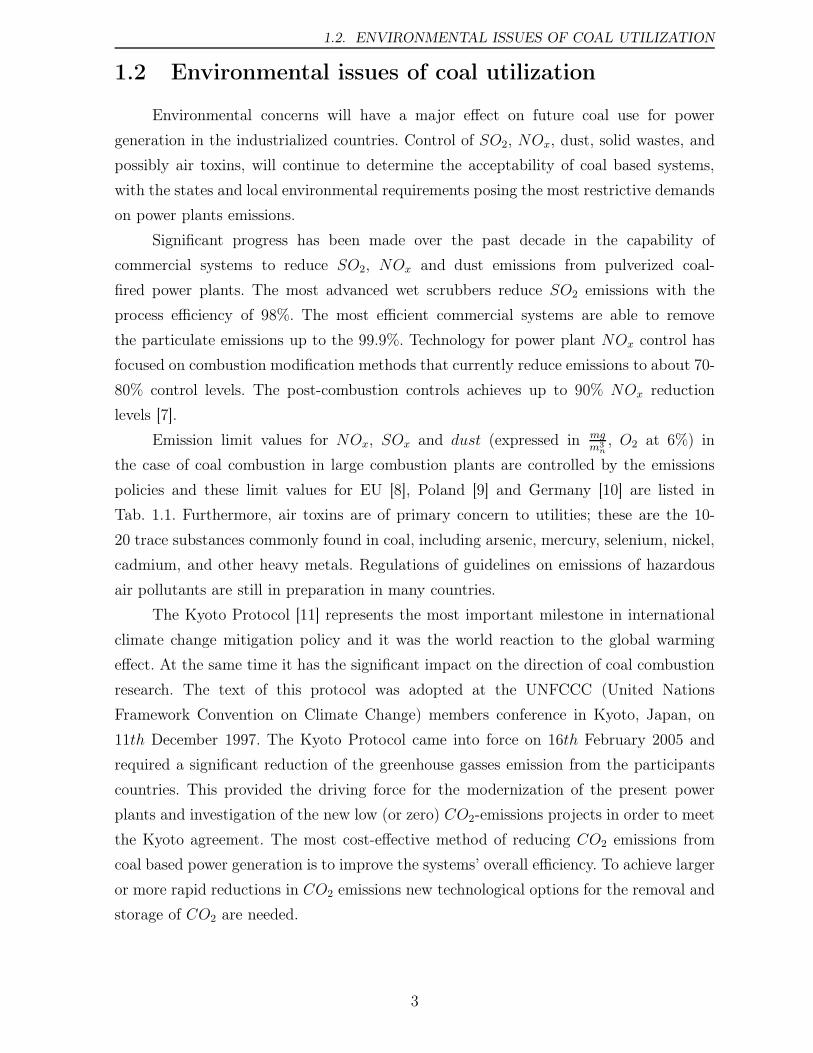
1.2 Environmental issues of coal utilization
Environmental concerns will have a major effect on future coal use for power
generation in the industrialized countries. Control of SO2, NOx, dust, solid wastes, and
possibly air toxins, will continue to determine the acceptability of coal based systems,
with the states and local environmental requirements posing the most restrictive demands
on power plants emissions.
Significant progress has been made over the past decade in the capability of
commercial systems to reduce SO2, NOx and dust emissions from pulverized coal-
fired power plants. The most advanced wet scrubbers reduce SO2 emissions with the
process efficiency of 98%. The most efficient commercial systems are able to remove
the particulate emissions up to the 99.9%. Technology for power plant NOx control has
focused on combustion modification methods that currently reduce emissions to about 70-
80% control levels. The post-combustion controls achieves up to 90% NOx reduction
levels [7].
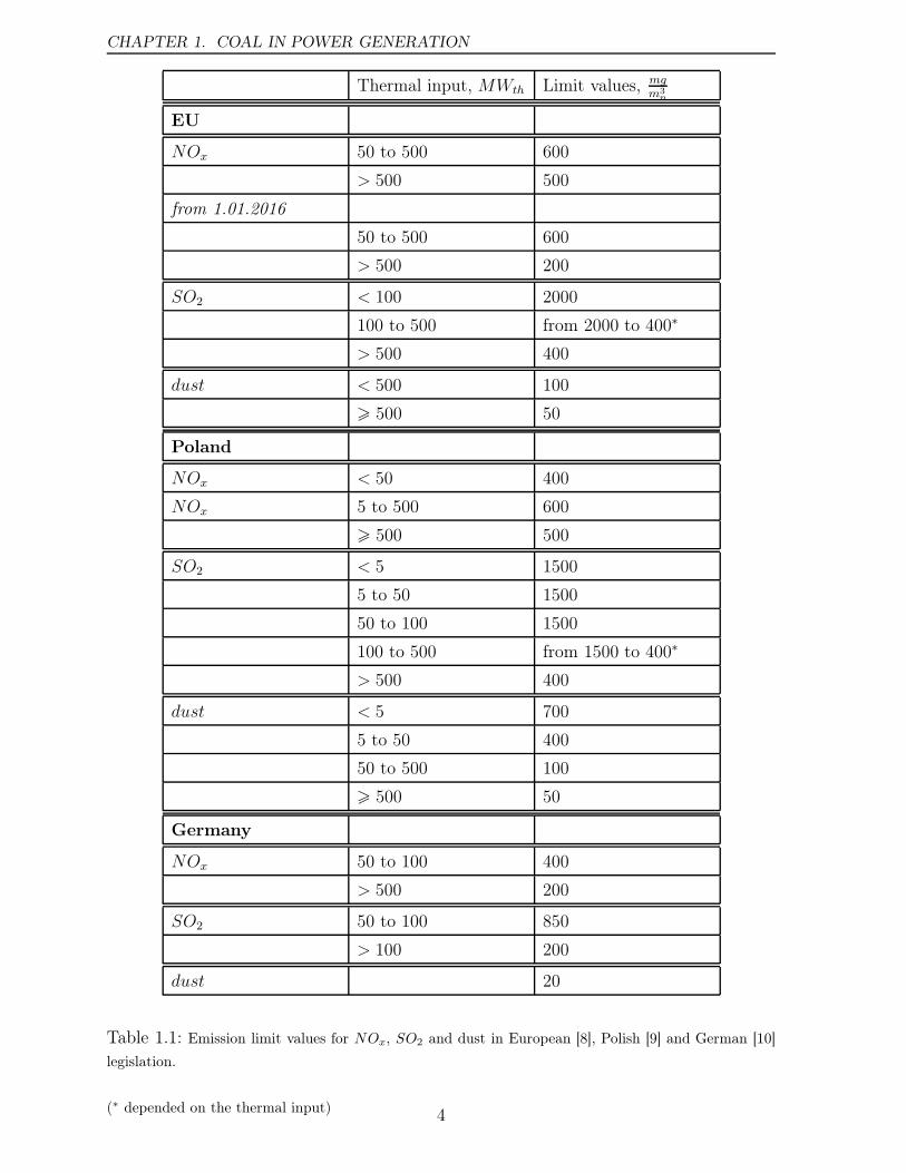
Emission limit values for NOx, SOx and dust (expressed in mgm3n
, O2 at 6%) in
the case of coal combustion in large combustion plants are controlled by the emissions
policies and these limit values for EU [8], Poland [9] and Germany [10] are listed in
Tab. 1.1. Furthermore, air toxins are of primary concern to utilities; these are the 10-
20 trace substances commonly found in coal, including arsenic, mercury, selenium, nickel,
cadmium, and other heavy metals. Regulations of guidelines on emissions of hazardous
air pollutants are still in preparation in many countries.
The Kyoto Protocol [11] represents the most important milestone in international
climate change mitigation policy and it was the world reaction to the global warming
effect. At the same time it has the significant impact on the direction of coal combustion
research. The text of this protocol was adopted at the UNFCCC (United Nations
Framework Convention on Climate Change) members conference in Kyoto, Japan, on
11th December 1997. The Kyoto Protocol came into force on 16th February 2005 and
required a significant reduction of the greenhouse gasses emission from the participants
countries. This provided the driving force for the modernization of the present power
plants and investigation of the new low (or zero) CO2-emissions projects in order to meet
the Kyoto agreement. The most cost-effective method of reducing CO2 emissions from
coal based power generation is to improve the systems’ overall efficiency. To achieve larger
or more rapid reductions in CO2 emissions new technological options for the removal and
storage of CO2 are needed.
3
CHAPTER 1. COAL IN POWER GENERATION
Thermal input, MWth Limit values, mgm3n
EU
NOx 50 to 500 600
> 500 500
from 1.01.2016
50 to 500 600
> 500 200
SO2 < 100 2000
100 to 500 from 2000 to 400∗
> 500 400
dust < 500 100
500 50
Poland
NOx < 50 400
NOx 5 to 500 600
500 500
SO2 < 5 1500
5 to 50 1500
50 to 100 1500
100 to 500 from 1500 to 400∗
> 500 400
dust < 5 700
5 to 50 400
50 to 500 100
500 50
Germany
NOx 50 to 100 400
> 500 200
SO2 50 to 100 850
> 100 200
dust 20
Table 1.1: Emission limit values for NOx, SO2 and dust in European [8], Polish [9] and German [10]
legislation.
(∗ depended on the thermal input) 4
1.3. COAL BASED TECHNOLOGIES FOR POWER GENERATION
Existing technologies for air pollutants control (SO2, NOx and particulate)
associated with pulverized coal fired power plants are capable of meeting current
or forthcoming emission reduction requirements. However, cost reduction is of the
primary concern since the cleaning flue gas installations are very expensive. Performance
improvements is required especially for NOx controls. A promising alternative to the
commonly used Selective Catalitic Reduction (SCR) de-NOx methods are low-emission
combustion technologies, such as HTAC technology which may eliminate or reduce costly
flue gas cleaning installations.
1.3 Coal based technologies for power generation
Global policies which require reduction of CO2 emission provide a strong driving
force for the development of clean and efficiently technologies for power generation,
including coal based combustion methods. High natural gas prices could also accelerate
the need for such a new capacity. Heightened concerns over global warming could
push the drive for high efficiency technology and CO2 sequestration methods to reduce
greenhouse gas emissions. Advanced power systems must not only produce significantly
lower emissions than current coal fired plants but also must compete economically with
other future options. Higher efficiencies in the new technologies will contribute not only
to lower fuel costs but also to improved environmental performance for a given power
output. To be competitive overseas, advanced technologies would require the lowest
possible capital costs accompanied by the environmental requirements. Summarizing,
efficiency, emissions, and costs are the key attributes of advanced coal based technology.
The most promising coal technologies for the power generation from thermodynamic,
environmental and economic point of view are:
• Pulverized coal (PC) combustion systems
• Fluidized bed combustion (FBC) systems
• Combustion under CO2/O2 atmosphere
• Coal gasification (CG) technology
• Integrated Gasification Combined Cycle (IGCC) systems
• Integrated Gasification Fuel Cells (IGFC) systems
5
CHAPTER 1. COAL IN POWER GENERATION
These technologies are briefly characterized in Subsections 1.3.1-1.3.6.
Magnetohydrodynamics and direct coal-fired heat engines have been omitted since
their importance is marginal.
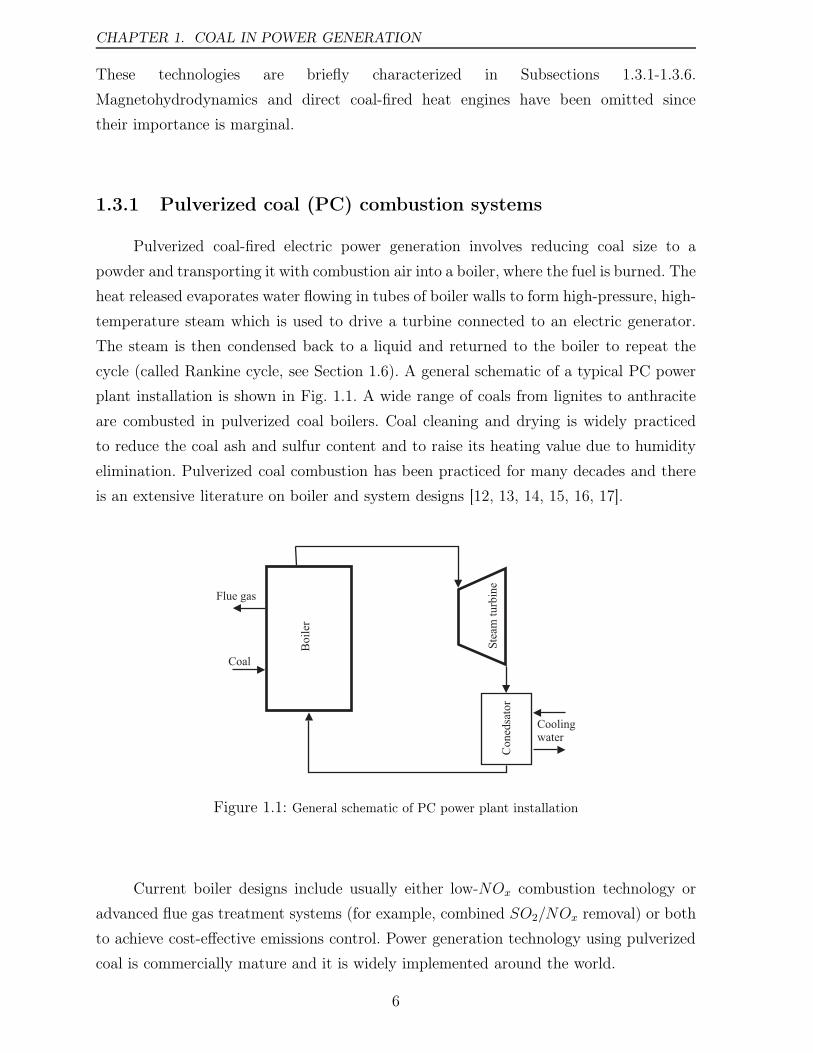
1.3.1 Pulverized coal (PC) combustion systems
Pulverized coal-fired electric power generation involves reducing coal size to a
powder and transporting it with combustion air into a boiler, where the fuel is burned. The
heat released evaporates water flowing in tubes of boiler walls to form high-pressure, high-
temperature steam which is used to drive a turbine connected to an electric generator.
The steam is then condensed back to a liquid and returned to the boiler to repeat the
cycle (called Rankine cycle, see Section 1.6). A general schematic of a typical PC power
plant installation is shown in Fig. 1.1. A wide range of coals from lignites to anthracite
are combusted in pulverized coal boilers. Coal cleaning and drying is widely practiced
to reduce the coal ash and sulfur content and to raise its heating value due to humidity
elimination. Pulverized coal combustion has been practiced for many decades and there
is an extensive literature on boiler and system designs [12, 13, 14, 15, 16, 17].
Coal
Ste
am t
urb
ine
Flue gas
Bo
iler
Co
ned
sato
r
Coolingwater
Figure 1.1: General schematic of PC power plant installation
Current boiler designs include usually either low-NOx combustion technology or
advanced flue gas treatment systems (for example, combined SO2/NOx removal) or both
to achieve cost-effective emissions control. Power generation technology using pulverized
coal is commercially mature and it is widely implemented around the world.
6
1.3. COAL BASED TECHNOLOGIES FOR POWER GENERATION
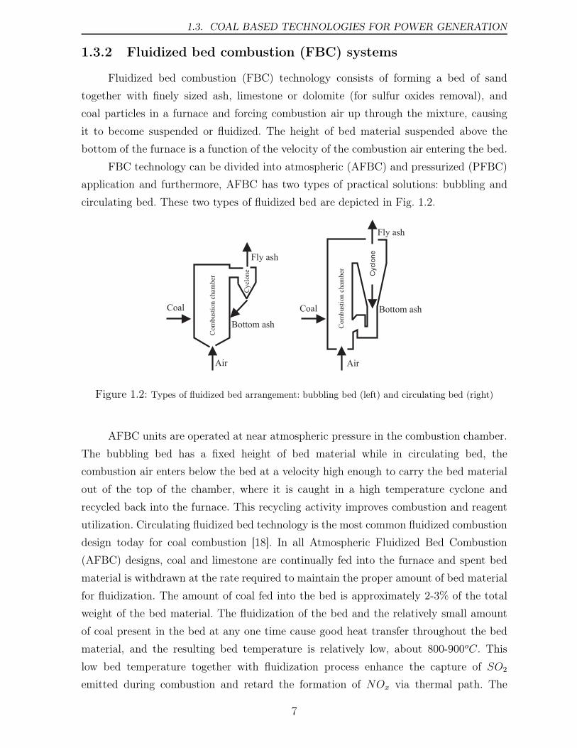
1.3.2 Fluidized bed combustion (FBC) systems
Fluidized bed combustion (FBC) technology consists of forming a bed of sand
together with finely sized ash, limestone or dolomite (for sulfur oxides removal), and
coal particles in a furnace and forcing combustion air up through the mixture, causing
it to become suspended or fluidized. The height of bed material suspended above the
bottom of the furnace is a function of the velocity of the combustion air entering the bed.
FBC technology can be divided into atmospheric (AFBC) and pressurized (PFBC)
application and furthermore, AFBC has two types of practical solutions: bubbling and
circulating bed. These two types of fluidized bed are depicted in Fig. 1.2.
Coal
Air
Fly ash
Bottom ash
Coal
Com
bust
ion c
ham
ber
Com
bust
ion c
ham
ber
Cycl
one
Cyclo
ne
Air
Fly ash
Bottom ash
Figure 1.2: Types of fluidized bed arrangement: bubbling bed (left) and circulating bed (right)
AFBC units are operated at near atmospheric pressure in the combustion chamber.
The bubbling bed has a fixed height of bed material while in circulating bed, the
combustion air enters below the bed at a velocity high enough to carry the bed material
out of the top of the chamber, where it is caught in a high temperature cyclone and
recycled back into the furnace. This recycling activity improves combustion and reagent
utilization. Circulating fluidized bed technology is the most common fluidized combustion
design today for coal combustion [18]. In all Atmospheric Fluidized Bed Combustion
(AFBC) designs, coal and limestone are continually fed into the furnace and spent bed
material is withdrawn at the rate required to maintain the proper amount of bed material
for fluidization. The amount of coal fed into the bed is approximately 2-3% of the total
weight of the bed material. The fluidization of the bed and the relatively small amount
of coal present in the bed at any one time cause good heat transfer throughout the bed
material, and the resulting bed temperature is relatively low, about 800-900oC. This
low bed temperature together with fluidization process enhance the capture of SO2
emitted during combustion and retard the formation of NOx via thermal path. The
7
CHAPTER 1. COAL IN POWER GENERATION
features of in-bed capture of SO2 and relatively low NOx emissions, plus the fluid bed’s
capacity to combust the range of different fuels, are the main attractions of FBC as power
generation technology. However, under some operating conditions, AFBC units also may
produce higher levels of organic compounds, some of which may be potential air toxic.
Current studies also indicate that AFBC units emit levels of N2O (which is classified
as a greenhouse gas), higher than other coal combustion systems [19]. AFBC technology
has been in commercial use worldwide for well over 50 years. The next generation of
FBC technology operates at pressure typically 10-15 times higher than the atmospheric
pressure. Operation in this manner allows the pressurized gas stream from a pressurized
fluidized bed combustion (PFBC) unit to be cleaned and fed to a gas turbine. The exhaust
gas from the turbine is then passed through a heat recovery boiler to produce steam. The
steam from the PFBC unit and that from the heat recovery boiler are then fed into
a steam turbine. This combined cycle mode of operation significantly increases PFBC
system efficiency over the AFBC systems. If the PFBC unit exhaust gas can be cleaned
sufficiently without reducing its temperature and as a consequence efficiencies of the
order 39-42% 1 can be achieved with PFBC designs, compared wit 34% efficiency of
AFBC. To further enhance commercial applications of FBC technologies it is a need
to achieve lower capital costs compared with modern pulverized coal (PC) boilers, to
improve environmental performance and to increase operating efficiency. Summarizing,
reduction of solids in the flue gas, high SO2 removal efficiencies and low NOx emissions
are the biggest advantages of fluidized bed boilers. Detailed analysis of this technology
applications has demonstrated that FBC power plants can be competitive to the PC
power plants when FBC power plant is located near to the mine and can utilize low rank
coals [20].
1.3.3 Combustion under O2/CO2 atmosphere
Combustion under O2/CO2 atmosphere is an advanced technology for controlling
CO2 emissions from coal-fired power plants. CO2 is regarded as the principle component of
the greenhouse gases. Therefore, controlling and decreasing CO2 emissions is an important
task for humans. Combustion under O2/CO2 atmosphere which replaces combustion
under air atmosphere (O2/N2) is considered as an advanced technology with a good
prospect of eliminating CO2 emissions from coal-fired power plants. CO2 concentrations
in a flue gas from combustion process using atmospheric air as oxidant are very low and
therefore it is difficult to separate CO2 from such a flue gas. Conversely, it is easier to
1Throughout this thesis all thermal efficiencies are based on the Low Calorific Value (LCV) of the
fuel
8
1.3. COAL BASED TECHNOLOGIES FOR POWER GENERATION
separate CO2 from the flue gas if the CO2 concentration is high (CO2 capture). Therefore,
the CO2 concentration in the flue gas should be increased. This can be achieved in
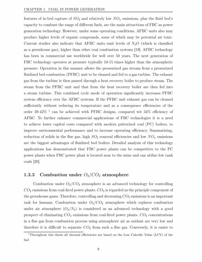
combustion under O2/CO2 atmosphere. This combustion mode has no formal name and
it is often called as: air separate/flue gas recycle technology, oxygen/flue gas recycle
combustion or oxyfuel combustion [21, 22]. The IFRF was perhaps the first institution
which carried out trials on coal combustion with recirculated flue gas enriched with
oxygen [23]. The principle of oxygen/ flue gas recycle combustion technology is shown in
Fig. 1.3.
Air
Dry recycle
Wet recycle
Separator
Fuel
BoilerO2
Water
Products
CO2
Figure 1.3: Conceptual schematic of the oxygen/flue gas recycle combustion technology
The mixture of O2 which is separated from air and recycled into flue gas is used as
oxidant in this technology. In this method, the concentration of CO2 can reach above 70%
with wet recycle, and up to 90% after dehydrator. Then, the gathering of CO2 becomes
simpler and economical [24, 25]. However, comparing both combustion under O2/CO2
and under air atmosphere, the combustion characteristics, particularly the char oxidation
of pulverized coal under O2/CO2 atmosphere change significantly [23]. In addition, the
Selective Catalytic Reduction (SCR) unit and the flue gas desulphurization unit might
be omitted in this combustion technique which results in low NOx emissions and the
remaining NOx and SO2 present in the flue gas could in principal be left for co-storage
with CO2 or could be separated easily [22]. CO2 capture reduces the net electricity
efficiency by about 10% comparing to the conventional power plants [21].
1.3.4 Coal gasification (CG) technology
Coal gasification is a method of producing a combustible gaseous fuel from almost
any type of coal. Conversion of coal to a gaseous fuel in homes and commercial
installations has been practiced for over 200 years [26]. The unstable economic and
political situation in the petroleum’s countries and predictions of impending natural gas
shortages resulted in major industry and government programs to develop gasification
9
CHAPTER 1. COAL IN POWER GENERATION
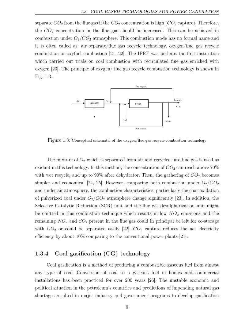
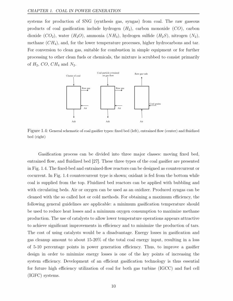
systems for production of SNG (synthesis gas, syngas) from coal. The raw gaseous
products of coal gasification include hydrogen (H2), carbon monoxide (CO), carbon
dioxide (CO2), water (H2O), ammonia (NH3), hydrogen sulfide (H2S), nitrogen (N2),
methane (CH4), and, for the lower temperature processes, higher hydrocarbons and tar.
For conversion to clean gas, suitable for combustion in simple equipment or for further
processing to other clean fuels or chemicals, the mixture is scrubbed to consist primarily
of H2, CO, CH4 and N2.
Cluster of coal
Ash
Air
Raw gas
Coal particle evtrainedon gas flow
Ash
Air
Raw gas
Raw gas+ash
Air
Coal grains
Figure 1.4: General schematic of coal gasifier types: fixed bed (left), entrained flow (center) and fluidized
bed (right)
Gasification process can be divided into three major classes: moving fixed bed,
entrained flow, and fluidized bed [27]. These three types of the coal gasifier are presented
in Fig. 1.4. The fixed-bed and entrained-flow reactors can be designed as countercurrent or
cocurrent. In Fig. 1.4 countercurrent type is shown; oxidant is fed from the bottom while
coal is supplied from the top. Fluidized bed reactors can be applied with bubbling and
with circulating beds. Air or oxygen can be used as an oxidizer. Produced syngas can be
cleaned with the so called hot or cold methods. For obtaining a maximum efficiency, the
following general guidelines are applicable: a minimum gasification temperature should
be used to reduce heat losses and a minimum oxygen consumption to maximize methane
production. The use of catalysts to allow lower temperature operations appears attractive
to achieve significant improvements in efficiency and to minimize the production of tars.
The cost of using catalysts would be a disadvantage. Energy losses in gasification and
gas cleanup amount to about 15-20% of the total coal energy input, resulting in a loss
of 5-10 percentage points in power generation efficiency. Thus, to improve a gasifier
design in order to minimize energy losses is one of the key points of increasing the
system efficiency. Development of an efficient gasification technology is thus essential
for future high efficiency utilization of coal for both gas turbine (IGCC) and fuel cell
(IGFC) systems.
10
1.3. COAL BASED TECHNOLOGIES FOR POWER GENERATION
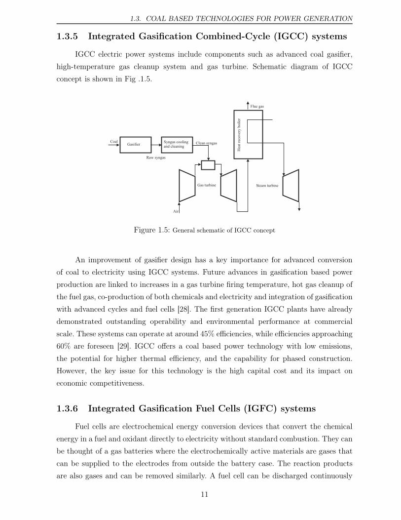
1.3.5 Integrated Gasification Combined-Cycle (IGCC) systems
IGCC electric power systems include components such as advanced coal gasifier,
high-temperature gas cleanup system and gas turbine. Schematic diagram of IGCC
concept is shown in Fig .1.5.
Coal
Air
Gas turbine Steam turbine
Flue gas
GasifierSyngas coolingand cleaning
Raw syngas
Clean syngas
Hea
t re
cover
y b
oil
er
Figure 1.5: General schematic of IGCC concept
An improvement of gasifier design has a key importance for advanced conversion
of coal to electricity using IGCC systems. Future advances in gasification based power
production are linked to increases in a gas turbine firing temperature, hot gas cleanup of
the fuel gas, co-production of both chemicals and electricity and integration of gasification
with advanced cycles and fuel cells [28]. The first generation IGCC plants have already
demonstrated outstanding operability and environmental performance at commercial
scale. These systems can operate at around 45% efficiencies, while efficiencies approaching
60% are foreseen [29]. IGCC offers a coal based power technology with low emissions,
the potential for higher thermal efficiency, and the capability for phased construction.
However, the key issue for this technology is the high capital cost and its impact on
economic competitiveness.
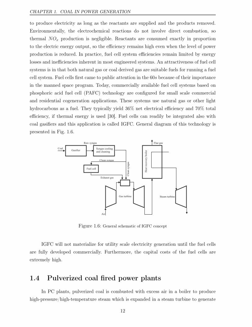
1.3.6 Integrated Gasification Fuel Cells (IGFC) systems
Fuel cells are electrochemical energy conversion devices that convert the chemical
energy in a fuel and oxidant directly to electricity without standard combustion. They can
be thought of a gas batteries where the electrochemically active materials are gases that
can be supplied to the electrodes from outside the battery case. The reaction products
are also gases and can be removed similarly. A fuel cell can be discharged continuously
11
CHAPTER 1. COAL IN POWER GENERATION
to produce electricity as long as the reactants are supplied and the products removed.
Environmentally, the electrochemical reactions do not involve direct combustion, so
thermal NOx production is negligible. Reactants are consumed exactly in proportion
to the electric energy output, so the efficiency remains high even when the level of power
production is reduced. In practice, fuel cell system efficiencies remain limited by energy
losses and inefficiencies inherent in most engineered systems. An attractiveness of fuel cell
systems is in that both natural gas or coal derived gas are suitable fuels for running a fuel
cell system. Fuel cells first came to public attention in the 60s because of their importance
in the manned space program. Today, commercially available fuel cell systems based on
phosphoric acid fuel cell (PAFC) technology are configured for small scale commercial
and residential cogeneration applications. These systems use natural gas or other light
hydrocarbons as a fuel. They typically yield 36% net electrical efficiency and 70% total
efficiency, if thermal energy is used [30]. Fuel cells can readily be integrated also with
coal gasifiers and this application is called IGFC. General diagram of this technology is
presented in Fig. 1.6.
Coal
Air
Gas turbine Steam turbine
Hea
t re
cov
ery
bo
iler
Flue gas
GasifierSyngas coolingand cleaning
Raw syngas
Clean syngas
Exhaust gas
Fuel cell
Cle
an s
yn
gas
Figure 1.6: General schematic of IGFC concept
IGFC will not materialize for utility scale electricity generation until the fuel cells
are fully developed commercially. Furthermore, the capital costs of the fuel cells are
extremely high.
1.4 Pulverized coal fired power plants
In PC plants, pulverized coal is combusted with excess air in a boiler to produce
high-pressure/high-temperature steam which is expanded in a steam turbine to generate
12
1.4. PULVERIZED COAL FIRED POWER PLANTS
electricity [7]. The major challenge facing the power generation industry based on
pulverized coal combustion over the coming decades will be to increase the efficiencies
of the power plants while also meeting more stringent environmental goals. Especially,
there is a need to reduce the emissions of NOx, SOx and CO2. At the same time,
plant reliability, availability, maintainability and operation costs, as well as the cost of
electricity, must not be compromised.
Today the total world installed capacity of coal fired boilers is of the order of
1000 GW and they generate a large majority of the electricity produced from coal which
itself is used for 38.7% of total global electricity generation [5]. In the EU old 15 countries
at present, the market for new coal fired electricity generation plants is fairly restricted.
This is mainly due to a deregulated energy market which provides utilization of natural
gas on a large scale. However, the market situation in Europe is expected to change.
Likewise, the recent enlargements of the EU with predominantly old installations will
offer considerable market opportunities in order that their capacity can approach EU
standards. Because several of the new partner states are coal producers, and so operate
coal fired power stations, the latest technologies will need to be installed to replace
the present low efficiency, environmentally unacceptable, and cost inefficient plants. The
installed capacity in the USA is approximately 830 GW , of which 40% is coal fired. In
the past Japan was strongly depended on fuel oil (together with hydro, gas and nuclear)
for electricity generation. Since the oil crises (1973 and 79), the need for diversification of
energy sources was recognized, and has given rise to increase of coal utilization and a fast
development of new more efficient technologies. Nowadays, Japan has a total installed
capacity for all energy sources of 230 GW with coal accounting for 13% [31]. Finally,
the world market, in particular in coal rich regions such as China and India with low
efficiency industrial plants, offers large additional opportunities for the modern European
technologies. The need for technological advances in these regions is strongly supported by
the increasing awareness of environment pollution and the legislative actions for emission
control in line with their national policies.
The supply of heat and electricity at competitive cost is a decisive factor for the
market penetration of new coal based conversion concepts in a liberalized energy market.
For this reason, future efforts must concentrate on reducing investment expenditure
and, in particular, operation costs. Modern coal fired power plants can achieve very
low levels of pollutants, including particulate and metals emissions. At the same time,
there is a need to continue the optimization of emissions control systems in order to
minimize any operational and capital cost issues. Furthermore, it can be expected that
future legislation for the control of emissions other than carbon dioxide will require
13
CHAPTER 1. COAL IN POWER GENERATION
compliance with more stringent limitations than are applied today. Thus, there will be a
need for environmentally more efficient and cost competitive techniques for both the fuel
conversion process and for flue gas treatment.
From the point of view of steam parameters, pulverized coal fired power plants can
be divided into [18]:
• subcritical (under critical point of water 2, usually 19 MPa and 535oC)
• supercritical (over critical point of water, usually up to 24.1 MPa and 565oC)
• ultra-supercritical (USC) (over supercritical conditions, usually 30MPa and 600oC)
1.4.1 Subcritical installations
Currently, the majority of coal-fired boilers are subcritical. Subcritical plants are
well established and relatively easy to control, with overall energy conversion efficiencies
in the range of around 30% to 40%. While the efficiencies of older power plants in
developing countries like China and India are still around 30%, modern subcritical cycles
have attained efficiencies close to 40% [18]. Further improvement in efficiency can be
achieved by using supercritical and ultra-supercritical steam conditions. One percent
increase in efficiency reduces by two percent specific emissions of CO2, NOx, SOx and
particulates [16].
In practice, up to an operating pressure of around 19MPa in the evaporator part of
the boiler, the cycle is subcritical. This means that there is a non-homogeneous mixture
of water and steam in the evaporator part of the boiler. In this case mostly a drum-type
boiler is used because the steam needs to be separated from water in the drum of the
boiler before it is superheated and led into the turbine (for details see Section 1.8).
1.4.2 Supercritical installations
In order to improve coal-fired power plant efficiency leading to a proportional
reduction in coal consumption and carbon dioxide emissions, it is widely accepted that the
power industry must move from subcritical to supercritical steam cycles. The supercritical
design not only improves efficiency by increasing the working fluid pressure but it allows
superheating of the steam to higher temperatures which provides significant steam cycle
efficiency improvement. Current supercritical coal fired power plants have efficiencies
above 45%.2The critical point of water is 22.06 MPa and t=375oC, and above these parameters, there is no
distinct water-steam phase transition [32]
14
1.5. HIGH TEMPERATURE MATERIALS FOR STEAM POWER PLANTS
The life cycle costs of supercritical coal fired power plants are lower than those of
subcritical plants. Current designs of supercritical plants have installation costs that are
only 2% higher than those of subcritical plants [13]. Fuel costs are considerably lower due
to the increased efficiency and operating costs are at the same level as subcritical plants.
The first supercritical power plants had a lot of mechanical and metallurgical problems.
Most of these were due to high thermal stresses and fatigue cracking of the heavy section
components. Today, the supercritical technology has overcome the earlier problems and
offers a more favorable cost of electricity with higher efficiency and lower emissions. Some
400 supercritical coal fired power plants are currently operating around the world [4]. The
supercritical technology plays dominant role for the newly built power plants, however
the installed technology is dominated by subcritical steam cycles.
1.4.3 Ultra-supercritical installations
As mentioned above, today state of the art in supercritical coal fired power plants
permits efficiencies that exceed 45%, depending on cooling conditions. Options to increase
the efficiency above 50% in ultra-supercritical power plants rely on elevated steam
conditions as well as on improved process and component quality. This increase of
efficiency should result in 25% reduction in CO2 and all other emissions [33]. Steam
temperatures in initial USC units was about 600oC and pressure 24.1 MPa with the
goal for future designs being 760oC and 34.5 MPa or higher [18]. USC steam plants in
service or under construction are located in Europe and in Japan. Only 13 units are in
operation [31].
1.5 High temperature materials for steam power plants
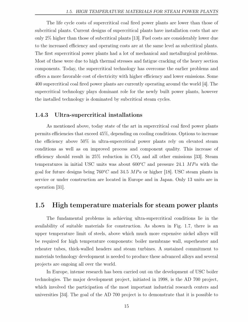
The fundamental problems in achieving ultra-supercritical conditions lie in the
availability of suitable materials for construction. As shown in Fig. 1.7, there is an
upper temperature limit of steels, above which much more expensive nickel alloys will
be required for high temperature components: boiler membrane wall, superheater and
reheater tubes, thick-walled headers and steam turbines. A sustained commitment to
materials technology development is needed to produce these advanced alloys and several
projects are ongoing all over the world.
In Europe, intense research has been carried out on the development of USC boiler
technologies. The major development project, initiated in 1998, is the AD 700 project,
which involved the participation of the most important industrial research centers and
universities [34]. The goal of the AD 700 project is to demonstrate that it is possible to
15
CHAPTER 1. COAL IN POWER GENERATION
250 300 350 400
550
600
650
700
main steam pressure, bar
mai
n s
team
tem
per
atu
re,
Co
The steel b
arrier
since
ear
ly 6
0’
since
lat
e 80’
star
ting 2
001
Figure 1.7: Steel barrier in recent years and prediction for future
operate USC steam plants with steam conditions of 700/720oC 3 and 37.5 MPa. Two
further major development programs in progress, the Thermie Project of the EC, and the
Ultra-Supercritical Materials Consortium in the US by Palkes, aim at steam parameters
of 37.5 MPa/700oC/720oC and 37.9 MPa/730oC/760oC, respectively [35].
Currently, advanced steels for boilers operated at pressures up to 30MPa represent
the state of the art [36]. New martensitic high creep strength 9-12%Cr steels allow
increased steam parameters in steam headers and steam lines. Similar martensitic
steels are used for rotors, casings and valves of advanced steam turbines. Superheater
steels must have high corrosion and oxidation resistance. Steam conditions up to
30 MPa/600oC/620oC are achieved using steels with 12% chromium content. Up to
31.5 MPa/620oC/620oC is achieved using austenite which is a proven but expensive
material. Nickel based alloys would permit 35MPa/700oC/720oC, yielding efficiencies up
to 48%. Steels for furnace panels need to be welded without post weld heat treatment and
also for this purpose new ferritic and martensitic steels are available. With the materials
development described above it is nowadays possible to construct a USC plant with steam
parameters 32.5 MPa/610oC/630oC/630oC and an efficiency approaching 50%. Future
developments will address the use of nickel or cobalt based superalloys for boilers, steam
lines and turbines. This may lead to efficiencies in the range 52-55% [37].
3Superheated steam temperature/Reheated steam temperature
16
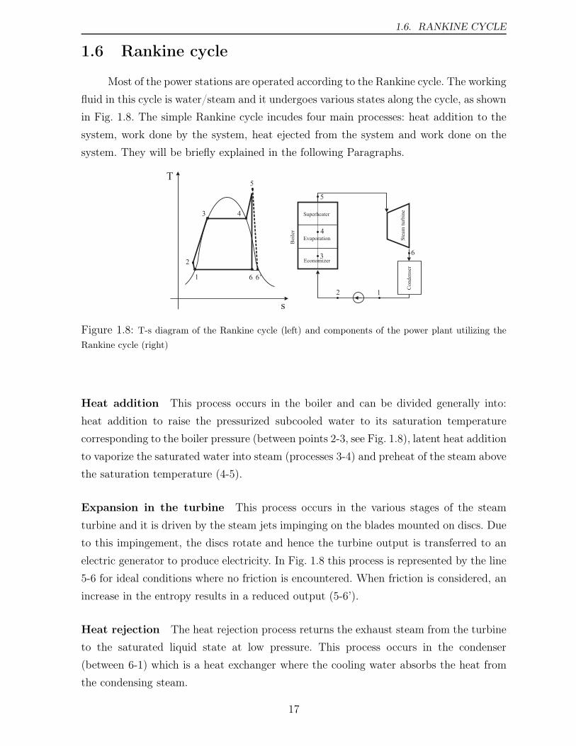
1.6. RANKINE CYCLE
1.6 Rankine cycle
Most of the power stations are operated according to the Rankine cycle. The working
fluid in this cycle is water/steam and it undergoes various states along the cycle, as shown
in Fig. 1.8. The simple Rankine cycle incudes four main processes: heat addition to the
system, work done by the system, heat ejected from the system and work done on the
system. They will be briefly explained in the following Paragraphs.
Ste
am t
urb
ine
Bo
iler
Co
nd
ense
r
Economizer
Evaporation
Superheater
12
3
4
5
6
T
s
1
2
3 4
5
6’6
Figure 1.8: T-s diagram of the Rankine cycle (left) and components of the power plant utilizing the
Rankine cycle (right)
Heat addition This process occurs in the boiler and can be divided generally into:
heat addition to raise the pressurized subcooled water to its saturation temperature
corresponding to the boiler pressure (between points 2-3, see Fig. 1.8), latent heat addition
to vaporize the saturated water into steam (processes 3-4) and preheat of the steam above
the saturation temperature (4-5).
Expansion in the turbine This process occurs in the various stages of the steam
turbine and it is driven by the steam jets impinging on the blades mounted on discs. Due
to this impingement, the discs rotate and hence the turbine output is transferred to an
electric generator to produce electricity. In Fig. 1.8 this process is represented by the line
5-6 for ideal conditions where no friction is encountered. When friction is considered, an
increase in the entropy results in a reduced output (5-6’).
Heat rejection The heat rejection process returns the exhaust steam from the turbine
to the saturated liquid state at low pressure. This process occurs in the condenser
(between 6-1) which is a heat exchanger where the cooling water absorbs the heat from
the condensing steam.
17
CHAPTER 1. COAL IN POWER GENERATION
Pumping water In order to complete the thermodynamic cycle, the water must return
to state 2. A pump is needed to raise the water temperature and pressure to state 2. In
most practical power stations calculations, pumping work can be disregarded with respect
to the turbine output [12].
Rankine cycle efficiency The Rankine cycle efficiency is proportional to the pressure
and temperature of heat addition to the cycle, and is inversely proportional to the
condenser pressure, and therefore to the temperature of the cooling medium. Based on the
nomenclature presented in Fig. 1.8, Rankine cycle thermal efficiency ηR can be described
as follows (disregarding pumping work i1 = i2):
ηR =i5 − i6i5 − i1
(1.1)
The Rankine cycle presented in Fig. 1.8 and described above is called as simple Rankine
cycle. Practically, in industrial steam power stations Rankine cycle is used with reheating
and heat regeneration in order to increase its efficiency [32] but these issues are not crucial
for this work and therefore they are not discussed here. Reheating and regeneration are
also not taken into consideration during the calculations of the steam cycle with the
HTAC boiler (see Chapter 10).
1.7 Issues for higher efficiency
The overall efficiency of a pulverized coal power generation cycle is affected by many
factors, including the thermodynamic cycle design, steam conditions (temperature and
pressure), coal grind, combustion air/fuel ratio, fuel mixing, air leakage into the system,
cooling (condenser) water temperature and parasitic energy loads for auxiliary equipment
such as grinding mills, pumps, fans, and environmental control systems [12, 17].
The most important factors for improving the pulverized coal fired power plants
efficiency are:
• increase of the steam parameters (pressure and temperature)
• increase of the boiler efficiency due to reduction of the physical and chemical losses
and they will be taken into consideration in this work.
1.7.1 Steam pressure
By increasing the final steam conditions above those developed in the condenser,
the cycle efficiency is driven higher. The obvious limit is the practical containment of
18
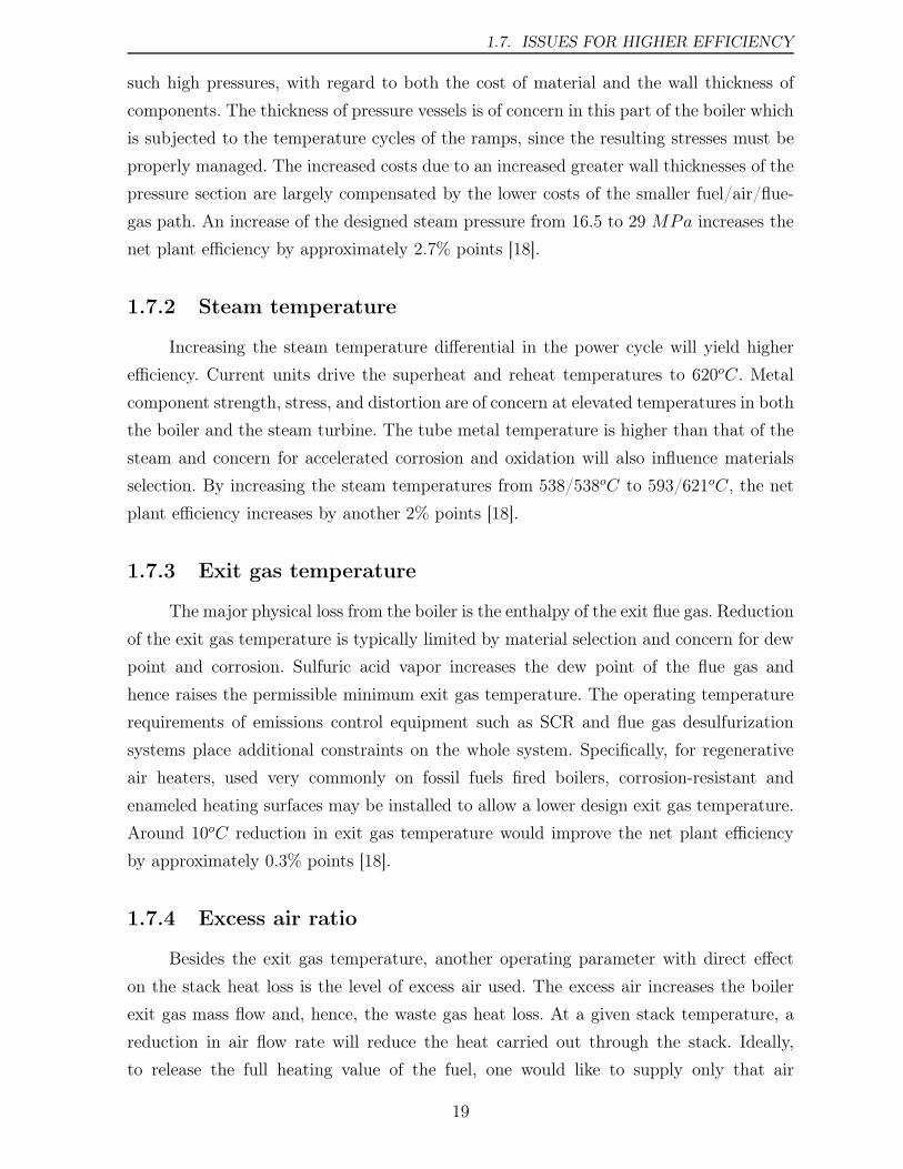
1.7. ISSUES FOR HIGHER EFFICIENCY
such high pressures, with regard to both the cost of material and the wall thickness of
components. The thickness of pressure vessels is of concern in this part of the boiler which
is subjected to the temperature cycles of the ramps, since the resulting stresses must be
properly managed. The increased costs due to an increased greater wall thicknesses of the
pressure section are largely compensated by the lower costs of the smaller fuel/air/flue-
gas path. An increase of the designed steam pressure from 16.5 to 29 MPa increases the
net plant efficiency by approximately 2.7% points [18].
1.7.2 Steam temperature
Increasing the steam temperature differential in the power cycle will yield higher
efficiency. Current units drive the superheat and reheat temperatures to 620oC. Metal
component strength, stress, and distortion are of concern at elevated temperatures in both
the boiler and the steam turbine. The tube metal temperature is higher than that of the
steam and concern for accelerated corrosion and oxidation will also influence materials
selection. By increasing the steam temperatures from 538/538oC to 593/621oC, the net
plant efficiency increases by another 2% points [18].
1.7.3 Exit gas temperature
The major physical loss from the boiler is the enthalpy of the exit flue gas. Reduction
of the exit gas temperature is typically limited by material selection and concern for dew
point and corrosion. Sulfuric acid vapor increases the dew point of the flue gas and
hence raises the permissible minimum exit gas temperature. The operating temperature
requirements of emissions control equipment such as SCR and flue gas desulfurization
systems place additional constraints on the whole system. Specifically, for regenerative
air heaters, used very commonly on fossil fuels fired boilers, corrosion-resistant and
enameled heating surfaces may be installed to allow a lower design exit gas temperature.
Around 10oC reduction in exit gas temperature would improve the net plant efficiency
by approximately 0.3% points [18].
1.7.4 Excess air ratio
Besides the exit gas temperature, another operating parameter with direct effect
on the stack heat loss is the level of excess air used. The excess air increases the boiler
exit gas mass flow and, hence, the waste gas heat loss. At a given stack temperature, a
reduction in air flow rate will reduce the heat carried out through the stack. Ideally,
to release the full heating value of the fuel, one would like to supply only that air
19
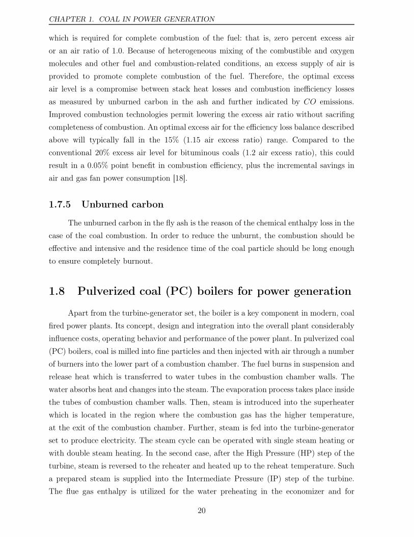
CHAPTER 1. COAL IN POWER GENERATION
which is required for complete combustion of the fuel: that is, zero percent excess air
or an air ratio of 1.0. Because of heterogeneous mixing of the combustible and oxygen
molecules and other fuel and combustion-related conditions, an excess supply of air is
provided to promote complete combustion of the fuel. Therefore, the optimal excess
air level is a compromise between stack heat losses and combustion inefficiency losses
as measured by unburned carbon in the ash and further indicated by CO emissions.
Improved combustion technologies permit lowering the excess air ratio without sacrifing
completeness of combustion. An optimal excess air for the efficiency loss balance described
above will typically fall in the 15% (1.15 air excess ratio) range. Compared to the
conventional 20% excess air level for bituminous coals (1.2 air excess ratio), this could
result in a 0.05% point benefit in combustion efficiency, plus the incremental savings in
air and gas fan power consumption [18].
1.7.5 Unburned carbon
The unburned carbon in the fly ash is the reason of the chemical enthalpy loss in the
case of the coal combustion. In order to reduce the unburnt, the combustion should be
effective and intensive and the residence time of the coal particle should be long enough
to ensure completely burnout.
1.8 Pulverized coal (PC) boilers for power generation
Apart from the turbine-generator set, the boiler is a key component in modern, coal
fired power plants. Its concept, design and integration into the overall plant considerably
influence costs, operating behavior and performance of the power plant. In pulverized coal
(PC) boilers, coal is milled into fine particles and then injected with air through a number
of burners into the lower part of a combustion chamber. The fuel burns in suspension and
release heat which is transferred to water tubes in the combustion chamber walls. The
water absorbs heat and changes into the steam. The evaporation process takes place inside
the tubes of combustion chamber walls. Then, steam is introduced into the superheater
which is located in the region where the combustion gas has the higher temperature,
at the exit of the combustion chamber. Further, steam is fed into the turbine-generator
set to produce electricity. The steam cycle can be operated with single steam heating or
with double steam heating. In the second case, after the High Pressure (HP) step of the
turbine, steam is reversed to the reheater and heated up to the reheat temperature. Such
a prepared steam is supplied into the Intermediate Pressure (IP) step of the turbine.
The flue gas enthalpy is utilized for the water preheating in the economizer and for
20
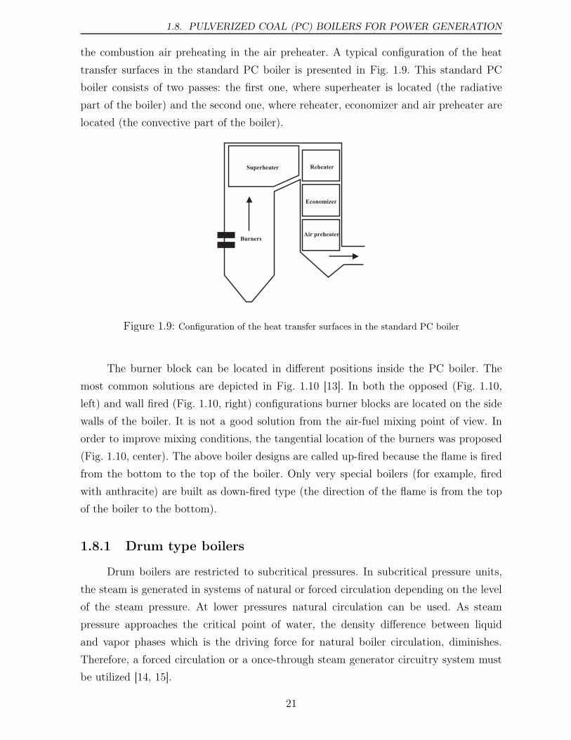
1.8. PULVERIZED COAL (PC) BOILERS FOR POWER GENERATION
the combustion air preheating in the air preheater. A typical configuration of the heat
transfer surfaces in the standard PC boiler is presented in Fig. 1.9. This standard PC
boiler consists of two passes: the first one, where superheater is located (the radiative
part of the boiler) and the second one, where reheater, economizer and air preheater are
located (the convective part of the boiler).
Burners
Superheater Reheater
Economizer
Air preheater
Figure 1.9: Configuration of the heat transfer surfaces in the standard PC boiler
The burner block can be located in different positions inside the PC boiler. The
most common solutions are depicted in Fig. 1.10 [13]. In both the opposed (Fig. 1.10,
left) and wall fired (Fig. 1.10, right) configurations burner blocks are located on the side
walls of the boiler. It is not a good solution from the air-fuel mixing point of view. In
order to improve mixing conditions, the tangential location of the burners was proposed
(Fig. 1.10, center). The above boiler designs are called up-fired because the flame is fired
from the bottom to the top of the boiler. Only very special boilers (for example, fired
with anthracite) are built as down-fired type (the direction of the flame is from the top
of the boiler to the bottom).
1.8.1 Drum type boilers
Drum boilers are restricted to subcritical pressures. In subcritical pressure units,
the steam is generated in systems of natural or forced circulation depending on the level
of the steam pressure. At lower pressures natural circulation can be used. As steam
pressure approaches the critical point of water, the density difference between liquid
and vapor phases which is the driving force for natural boiler circulation, diminishes.
Therefore, a forced circulation or a once-through steam generator circuitry system must
be utilized [14, 15].
21
CHAPTER 1. COAL IN POWER GENERATION
Figure 1.10: Typical burner location in the standard PC boiler: opposed walls (left), tangential (center)
and single wall (right) firing
Steam is separated from the water inside a drum. Water at saturation temperature
flows from the boiler-drum through unheated downcomer tubes, outside the boiler, and
steam water mixture rises to the boiler drum through steam generating tubes that cover
the fire side of furnace walls. In the drum type boilers water circulate continually inside
the installation. The drum type boiler installation is shown in Fig. 1.11, left. For many
years, the subcritical drum boiler has been the most popular boiler design worldwide. This
well proven technology is a low cost one but does not have the potential for efficiency
improvement inherent in supercritical cycles. Additionally, the drum type boilers have
long start-up time and are very responsive to the load changes [38].
1.8.2 Once-through type boilers
In high-pressure subcritical boilers and in supercritical once-through boilers there is
no boiler drum and therefore there is no water circulation. Instead the boiler consists of a
bundle of parallel tubing through which water is pumped. Along the length of the tubes
the water gradually forms steam and is getting superheated at the outlet of the tubes.
Because of the lack of circulation, the tube length participating in the heat transfer has to
be increased. The transition from evaporation to superheating is not fixed in location and
can take place at any point in the upper section of the furnace. This enables dimensioning
of the furnace without restrictions on the water/steam side [12]. The once-through type
boiler installation is shown in Fig. 1.11, right.
22
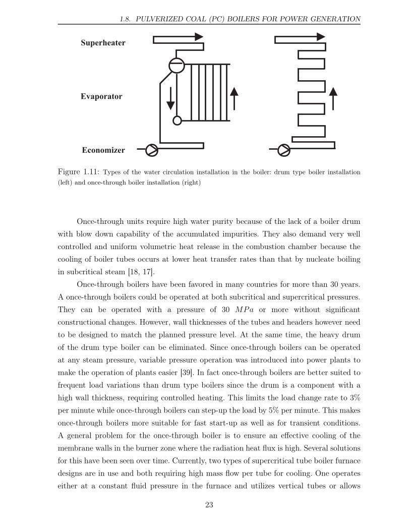
1.8. PULVERIZED COAL (PC) BOILERS FOR POWER GENERATION
Superheater
Evaporator
Economizer
Figure 1.11: Types of the water circulation installation in the boiler: drum type boiler installation
(left) and once-through boiler installation (right)
Once-through units require high water purity because of the lack of a boiler drum
with blow down capability of the accumulated impurities. They also demand very well
controlled and uniform volumetric heat release in the combustion chamber because the
cooling of boiler tubes occurs at lower heat transfer rates than that by nucleate boiling
in subcritical steam [18, 17].
Once-through boilers have been favored in many countries for more than 30 years.
A once-through boilers could be operated at both subcritical and supercritical pressures.
They can be operated with a pressure of 30 MPa or more without significant
constructional changes. However, wall thicknesses of the tubes and headers however need
to be designed to match the planned pressure level. At the same time, the heavy drum
of the drum type boiler can be eliminated. Since once-through boilers can be operated
at any steam pressure, variable pressure operation was introduced into power plants to
make the operation of plants easier [39]. In fact once-through boilers are better suited to
frequent load variations than drum type boilers since the drum is a component with a
high wall thickness, requiring controlled heating. This limits the load change rate to 3%
per minute while once-through boilers can step-up the load by 5% per minute. This makes
once-through boilers more suitable for fast start-up as well as for transient conditions.
A general problem for the once-through boiler is to ensure an effective cooling of the
membrane walls in the burner zone where the radiation heat flux is high. Several solutions
for this have been seen over time. Currently, two types of supercritical tube boiler furnace
designs are in use and both requiring high mass flow per tube for cooling. One operates
either at a constant fluid pressure in the furnace and utilizes vertical tubes or allows
23
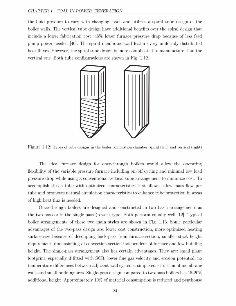
CHAPTER 1. COAL IN POWER GENERATION
the fluid pressure to vary with changing loads and utilizes a spiral tube design of the
boiler walls. The vertical tube design have additional benefits over the spiral design that
include a lower fabrication cost, 45% lower furnace pressure drop because of less feed
pump power needed [40]. The spiral membrane wall feature very uniformly distributed
heat fluxes. However, the spiral tube design is more complicated to manufacture than the
vertical one. Both tube configurations are shown in Fig. 1.12.
Figure 1.12: Types of tube designs in the boiler combustion chamber: spiral (left) and vertical (right)
The ideal furnace design for once-through boilers would allow the operating
flexibility of the variable pressure furnace including on/off cycling and minimal low load
pressure drop while using a conventional vertical tube arrangement to minimize cost. To
accomplish this a tube with optimized characteristics that allows a low mass flow per
tube and promotes natural circulation characteristics to enhance tube protection in areas
of high heat flux is needed.
Once-through boilers are designed and constructed in two basic arrangements as
the two-pass or is the single-pass (tower) type. Both perform equally well [12]. Typical
boiler arrangements of these two main styles are shown in Fig. 1.13. Some particular
advantages of the two-pass design are: lower cost construction, more optimized heating
surface size because of decoupling back-pass from furnace section, smaller stack height
requirement, dimensioning of convection section independent of furnace and low building
height. The single-pass arrangement also has certain advantages. They are: small plant
footprint, especially if fitted with SCR, lower flue gas velocity and erosion potential, no
temperature differences between adjacent wall systems, simple construction of membrane
walls and small building area. Single-pass design compared to two-pass boilers has 15-20%
additional height. Approximately 10% of material consumption is reduced and penthouse
24
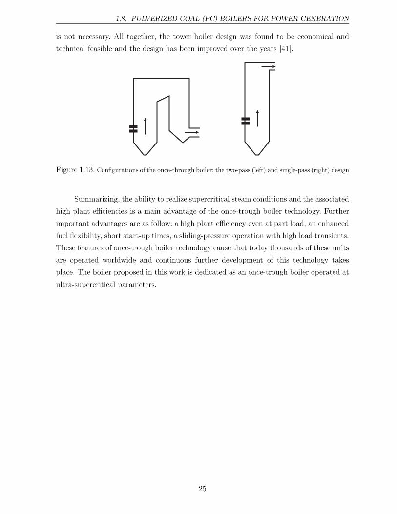
1.8. PULVERIZED COAL (PC) BOILERS FOR POWER GENERATION
is not necessary. All together, the tower boiler design was found to be economical and
technical feasible and the design has been improved over the years [41].
Figure 1.13: Configurations of the once-through boiler: the two-pass (left) and single-pass (right) design
Summarizing, the ability to realize supercritical steam conditions and the associated
high plant efficiencies is a main advantage of the once-trough boiler technology. Further
important advantages are as follow: a high plant efficiency even at part load, an enhanced
fuel flexibility, short start-up times, a sliding-pressure operation with high load transients.
These features of once-trough boiler technology cause that today thousands of these units
are operated worldwide and continuous further development of this technology takes
place. The boiler proposed in this work is dedicated as an once-trough boiler operated at
ultra-supercritical parameters.
25

CHAPTER 1. COAL IN POWER GENERATION
26
Chapter 2
Overview of HTAC technology
HTAC is a promising technology to decrease pollutants emissions and to improve
the combustion efficiency. The main feature of this technique is a combination of air
preheating and fuel dilution with combustion products to keep the oxygen concentrations
low. To achieve this goal, preheated air and fuel are gradually mixed with large amounts
of recirculated combustion products. High Temperature Air Combustion (HTAC or
HiTAC) [42] is named also as: Excess Enthalpy Combustion (EEC) [43], FLameless
OXidation (acronym FLOX)1 [44], MILD (Moderate and Intensive Low-oxygen Dilution)
combustion [45]. For the author all these names are synonym.
In this Chapter development, state of the art and challenges of HTAC technology
are reviewed. Then, progress in modeling of HTAC technology is briefly described.
Furthermore, fundamentals of this technology are explained. Additionally, there seem
to exist only two publications attempting to develop a concept for HTAC application to
boilers. These two are reviewed at the end of this Chapter.
2.1 Development of HTAC technology
Oil crisis in the 70s focused research in combustion science and technology on the
fossil fuel saving. Preheating the combustion air was found as one of the most effective
methods of achieving this goal. This principle of the technology, which later on was named
HTAC, was presented as Excess Enthalpy Combustion by Weinberg [43] in conjunction
with combustion of low calorific fuels. In EEC part of the thermal energy released during
the combustion process is fed back to the fresh reactants.
1The name FLOX is registered name by WS Wärmeprozesstechnik GmbH referring to a particular
type of burner
27
CHAPTER 2. OVERVIEW OF HTAC TECHNOLOGY
In the United Kingdom at British Gas and later at Hotwork International [46, 47]
both regenerative and recuperative systems were intensively researched as pioneering
methods of heat recovery at the burner. The recuperators were able to achieve relatively
low preheat level (the air was preheated to a temperature of about 600oC typically). The
regenerative systems were able to reach about 1200oC air preheat with an exit furnace
temperature around 1400oC. Ceramic balls were used in the regenerator to preheat
the combustion air with the gases exiting from the furnace. With the increase of air
preheat, the amount of nitric oxides emissions also increased and this tempered industrial
applications of regenerative burners.
The work on fundamentals of EEC was initiated in Japan on the initiative
of Mr. R. Tanaka at the early 90s. Efforts made by Nippon Furnace Kyogo Kaisha
Ltd. (NFK) focused on the process efficiency and minimization of pollutants emissions.
The goal was to reduce pollutants emissions, save energy and increase furnace efficiency
together with reducing the size of the equipment using Excess Enthalpy Combustion
principles. This technology, named as HTAC [42, 48], used a honeycomb regenerator to
maximize the air preheat. The honeycomb regenerator is much more compact than a
bed packed with ceramic balls and features a low pressure drop [49, 50, 51]. In relation
of ceramic honeycomb, a high cycle regenerative combustion system (HRS) burner was
developed [52]. The thermal recirculation in HRS burner provides the stable combustion
even at low oxygen concentrations, created by the exhaust gas recirculation. Furthermore,
the flame temperature is decreased due to the lower oxygen concentration which results
in low NOx emissions. The largest available HRS burners are of 6-8 MW power [53].
In all the above described developments, NFK was assisted by the University of
Maryland (USA). Gupta et al. [54, 55, 56] undertook research on the effect of combustion
air temperature and oxygen concentration on flame color, visibility and thermal emission
spectra. Gaseous fuels, such as methane, propane, LPG, carbon monoxide, hydrogen and
acetylene were used in laboratory scale experiments. Formation of pollutants, including
nitric oxide was taken into consideration.
NFK initiated also a cooperation with the Royal Institute of Technology (KTH) in
Sweden. A semi industrial furnace equipped with regenerative burners were used to run
several experiments, using liquefied propan gas (LPG). Single gas jet, as well as whole
furnace domain were researched in details. Flame size, visibility, color, lift-off distance,
flow structure were observed and measured by Lille et al. [57].
A very successful research and development program was undertaken at the
International Flame Research Foundation (IFRF). In 1991, at IFRF in IJmuiden
(Holland), a project called Scaling 400 was initiated [58, 59]. A family of burners spanning
28
2.1. DEVELOPMENT OF HTAC TECHNOLOGY
the thermal input range from 30 kW to 12MW was developed. The burners had a central
air injector and individual fuel injectors located on a circumference around the central
injector. A reduction of NOx emissions of about 80% was reported at 12 MW thermal
input. Moreover the level of NOx achieved at high fuel staging was independent of the
preheat. It was observed that in the staged flames the radiative heat flux was about 20%
higher than the heat flux of the un-staged (baseline flame). Relying on the Scaling 400
project observations and based on the promising experiments in Japan, in 1997 the IFRF
and NFK decided to test a NFK burner that used two natural gas injectors separated
from the combustion air stream. A series of experiments were performed at IFRF using
natural gas as fuel [60, 61, 62]. These trials were called HTAC 97. The success of these
experiments prompted similar experiments using light and heavy oils (HTAC 98) [63, 53]
and coal (HTAC 99) [64, 65]. Details of HTAC 99 trial are given in Chapter 4.
Independently of the Japanese investigations, Wünning [66] started investigating
possibilities of NOx reduction in natural gas firing utilizing high air preheat. In 1989, a
surprising phenomenon was observed during experiments with a self recuperative burner.
At 1000oC furnace temperatures and 650oC air preheat temperature, no flame could be
seen and no UV-signal could be detected. Despite that, the fuel was completely burnt and
the carbon-monoxide content in the exhaust was below 1 ppm. The NOx emissions were
in the single digits range what was first thought to be a malfunction of the NO-analyzer.
The combustion was stable and smooth and this condition was called flameless oxidation,
in short FLOX, and later on registered as a trade mark name [44]. Further experiments
and numerical simulations were carried out to determine the essential conditions for
FLOX [67, 68]. There are several versions of the FLOX burners commercially available
and their thermal input is typically not larger than 200-300 kW [53].
An important development, based on the Scaling 400 technology, took place in
Canada where the Canadian Gas Research Institute Burner (CGRI) was designed [69].
The idea was similar: the gas and air were injected separately so as to increase the
entrainment of inert gas.
Recently, Cavaliere et al. [45] have examined the applicability of the existing
chemical reaction schemes to combustion of hydrocarbons in high temperature air. The
authors tried to develop a definition for this new combustion mode and proposed to call
it MILD combustion.
29
CHAPTER 2. OVERVIEW OF HTAC TECHNOLOGY
2.2 Current investigations and challenges of HTAC
technology
Although HTAC is already applied commercially, research on fundamental of this
combustion method is still needed. Several companies, universities and research institutes
are continually developing HTAC technology. Most of the previous research activities
have been focused on gaseous fuels such as methane and propane. HTAC technology
has significant potential for utilizing of various kinds of gaseous fuels (biogas, syngas,
low BTU gas) as well as liquid, solid and waste fuels for applications to many technical
processes.
In 2001, a research consortium comprising the IFRF Research Station, Corus
Research Development & Technology and Gasunie Research commenced testing of HTAC
technology, internally known as High Efficiency Combustion (HEC) [70]. The objective
of this test was to enhance knowledge, gain experience and verify the potential benefits
of HEC technology for industrial application in general and steel slab reheating furnaces
in particular. The semi industrial tests with HEC technology have confirmed the high
thermal efficiency, relatively low NOx emission and high uniformity of the heat transfer.
It was decided to do the next step in this research, namely full scale industrial test.
Masson et al. [71] have carried out an experiment at a laboratory scale. The gas
burner consisted of two methane injectors and of the central air injector. Combustion
air was preheated up to 873 K using an electric heater. In a first step, the parametric
study of the air preheating temperature, the excess air ratio and combustion chamber
dimensions were performed. The input/output measurements were carried out only. In
the second step of these investigations, several in-flame measurements techniques were
applied [72]. Reaction zone structures were revealed by OH∗ chemiluminescence imaging.
Fine wire thermocouples were used to determine local temperature in the furnace, and
velocity fields were obtained by Particle Image Velocimetry (PIV). The obtained results
were similar to the previous observations [60, 61, 62].
Experimental study on HTAC combustion of natural gas was performed also by
Lupant et al. [73] and Murer et al. [74] in order to obtain more detailed information on
this combustion process. In-flame temperature and species concentration measurements
and UV-imaging were performed on a 200 kW natural gas furnace equipped with a self
regenerative burner FLOX-REGEMAT.
In parallel to the IFRF experiments on combustion of light and high oils under
HTAC conditions [63, 53], Shimo [75] and Chang et al. [76] also investigated oil
combustion. It was found that HTAC technology with oil was able to work correctly.
30
2.2. CURRENT INVESTIGATIONS AND CHALLENGES OF HTAC TECHNOLOGY
Low emission of NOx was obtained but very high emission of soot was observed. Further
investigations on HTAC application for oil combustion shown that in order to decrease
soot formation oil atomization should be improved [77]. Recently Wilk et al. [78, 79]
performed experiments on oil combustion in HTAC technology. The combustion chamber
of 100 kW was built at Silesian University of Technology. The research focused on the
oil burner construction. Measurements of the radiative heat fluxes, temperature, soot,
PAH , CO as well as NOx were conducted. It was concluded that it was possible to
operate furnaces in HTAC mode with similar effect as for the gaseous fuels.
The use of high temperature, low oxygen content air for pulverized coal combustion
was examined by Kiga et al. [80]. Laboratory scale tests were conducted in a drop tube
furnace to investigate the performance of such a combustion system. NOx formation and
combustion efficiency of the furnace were measured for various air preheat temperature,
excess air ratio and oxygen concentration. The measurements indicated that increasing air
preheat resulted in an increased combustion efficiency and reduced NOx emission whereas
decreasing the oxygen content led to a substantial reduction in combustion efficiency,
accompanied with a slight increase in NOx. It was concluded that high temperature
diluted air was not suited for pulverized coal combustion.
The International Flame Research Foundation (IFRF) carried out perhaps the first
experiment on applicability of the MILD combustion concept to pulverized coal firing [64,
65, 53]. A high volatile coal (1.4% N) was combusted with high temperature air and the
lowest NOx emissions were in the range 160-175 ppm (at 3% O2) indicating high NOx
reduction potential of this technology also for nitrogen containing fuels (for details see
Paragraph 4).
A pulverized coal FLOX burner is currently under development in the frame of an
EU project [81]. The tests have been carried out in a drop tube furnace, in a bench-scale
reactor (5-8 kW ) at the University of Stuttgart and in a pilot-scale rig (40-60 kW ) at
RWTH Aachen [82, 83]. The burner combines the FLOX technique together with air
staging. The primary air and pulverized coal are injected into the furnace via a central
pipe. The secondary air is provided through nozzles located on the circumference of the
primary jet while the tertiary (burnout) air is injected downstream. Under optimized
firing conditions, the NOx concentrations were below 200 mgm3
(at 6% O2) and the carbon
monoxide concentrations were around 30 mgm3
(at 6% O2). While firing Lausitz lignite a
high degree of burnout (carbon in ash < 0.3%) has been measured; burnout problems
have occurred for hard Budryk and Kleinkopje coals (carbon in ash < 18.9%) [82, 83].
Coal behavior under MILD combustion conditions has also being researched at the
Ruhr-University Bochum [84, 85] to gain a better understanding of NOx formation and
31
CHAPTER 2. OVERVIEW OF HTAC TECHNOLOGY
reduction mechanisms. The data on volatile matter release, volatiles composition, and
char were determined by flash pyrolysis investigations.
MILD combustion of pulverized coal was experimentally investigated by Suda et
al. [86]. Flame stability, ignition delay, char burnout, and NOx emission were examined
using a 250 kW furnace. The combustion air was preheated to a temperature of either
623 K or 1073 K. The authors concluded that the ignition delay decreased dramatically
with increasing air temperature. Stable combustion was obtained even for an anthracite.
The peak temperature of the flames remained unaltered when the air preheat was
increased from 623K to 1073K. NOx emissions of 1000 ppm and 400 ppm were measured
for the 623 K and 1073 K air temperature, respectively. Thus, a 40% NOx emissions
reduction was observed when the combustion air temperature increased. However, the
absolute NOx emissions were substantially larger than these obtained in the IFRF
experiment [64].
Gases from landfills as well as exhausts from gas purification systems often have low
calorific values (LCV) and are not anymore burnable in conventional systems. Schmid
et al. [87] tested combustion of gases with LCV below 2.5 MJm3
. It was concluded that
these gases can be burned safety even at moderate or low preheat temperatures applying
flameless oxidation (FLOX) technology. In experiment of Suphansomboon et al. [88]
low calorific value gases were burned with combustion air preheated up to 900oC. The
temperature profile and gaseous emissions were measured. The results showed that the
higher the preheated combustion air temperatures the higher average flame temperatures
and peak flame temperatures. Fuel savings were observed together with decreasing of
NOx emission.
Combustion of solid fuels like biomass and wastes in HTAC conditions has not
been investigated as comprehensively as combustion of gaseous fuels. Ponzio et al. [89]
performed experiments with wood pellets in a small scale batch reactor. Mass loss (as
function of time), ignition time and the appearance of the flame were investigated as
a function of oxidizer temperatures (600-1000oC) and oxygen concentrations (5-21%).
It was concluded that high oxidizer temperatures promoted fast mass loss. Oxygen
concentrations have limited influence on the mass loss rate. Ignition time was strongly
dependent on the oxygen concentration only at 600oC. At 800 and 1000oC, a very fast
ignition occurred at all considered oxygen concentrations.
Derudi et al. [90] concluded that HTAC combustion can be effectively used for a wide
range of low-BTU fuels with an inert gas content higher than 90%. Possibility of using
both natural gas and biogas in HTAC combustion was assessed and operative parameter
maps (in terms of average furnace temperature versus recycle ratio) were provided. It
32
2.2. CURRENT INVESTIGATIONS AND CHALLENGES OF HTAC TECHNOLOGY
was found that HTAC combustion is effective not only in reducing NOx emissions (values
larger than 15 ppm at 3% O2 have never been observed) but also in preventing soot and
PAH formation in fuel rich conditions.
Recent efforts of Gupta et al. [91, 92] have concentrated on high temperature
gasification of wastes, biomass and low grade fuels to convert them to clean fuel medium
heating value gas with high hydrogen content. High preheated air or steam were used
as an oxidizer in the gasification process. It was found that high temperature gas
generator works well for gasification of biomass or solid waste. The optimum thermal
and gas recirculation conditions were obtained together with homogenized temperature
distribution and low NOx emissions. The applications of high temperature air/steam
gasification in the various processes were studied.
The development in the conventional oxyfuel combustion led to the advent of
the new generation burners that use internal flue gas recirculation exhibit flameless
combustion and can be called flameless oxyfuel combustion- REBOX-W (Linde AG) [93].
The burner design was based on the findings of the IFRF OXYFLAME project [23]. This
burner uses oxygen as oxidizer and maintain HTAC combustion mode in the furnace.
The high velocity of oxygen at the exit of the nozzles causes excellent internal mixing and
accounting for the flameless combustion. The salient features of this burner are extremely
simple construction, operation and very small size. The NOx emissions were the lowest
for High Temperature Air Combustion with oxygen enhancement, NOx decreased with
an oxygen concentration increase (for the range of oxygen enrichment between 0-8%).
Leicher et al. [94] studied the phenomenon of HTAC combustion in order to
evaluate its applicability to gas turbine combustors. HTAC combustion process was
simulated using a chemical progress variable in conjunction with tabulated chemistry
data provided by CHEMKIN. It was investigated whether FLOX burners can be used
under gas turbine conditions with regard to flame stability and pollutant formation.
Flamme [95, 96] described the experimental project on HTAC combustion technology
which was investigated under gas turbine conditions using FLOX burner. The main
objective of the project was to show that with the new combustion systems based on
HTAC concept the following improvements can be achieved: elimination of pulsation in
gas turbine combustion chambers, increase of the stability of the combustion process
in a wide range of excess air ratio, suppression of high pollutant emissions at part load,
increase in the efficiency of gas turbines and possible use of different fuels (natural gas and
fuel oil). FLOX burner technology was investigated under gas turbine conditions also by
Wünning [96]. It was concluded that it is applicable to gas turbine conditions for example,
high pressure and overall lean conditions in conjunction with improved operational
33
CHAPTER 2. OVERVIEW OF HTAC TECHNOLOGY
performance compared to lean premixed combustion burner. Szlęk et al. [97, 98, 99, 100]
proposed completely different application of HTAC technology in gas turbines. A new
method of the isothermal expansion in a gas turbine were numerically investigated. This
isothermal expansion is achieved by continuous supply of the fuel to the expanding
oxidizer having the temperature higher than the fuel self-ignition temperature. It was
concluded that this new gas turbine cycle provides a substantial increase in turbine
performance keeping also the other advantages of HTAC technology.
2.3 Modeling of HTAC technology
The first CFD modeling of HTAC technology effort originated from Japanese
industry where Ishii et al. [101, 102, 103] carried out simulations of an experimental
continuous slab reheating furnace with emphasis on NOx formation. The authors showed
that the numerical code was able to describe the main characteristics in terms of the
flow and temperature fields and could be used to identify the best low-emissions furnace
configuration. The predicted slab temperature distribution and energy flow rates in the
experimental furnace agreed well with the experimental data. They showed that one of
the key points for this kind of combustion was the momentum of the air jets: the higher
the momentum, the lower the NO emissions. Moreover, at constant air velocity, the NOx
reduction increased with the increase of the fuel jet velocity. However, the results of their
simulations showed that their NOx models required improvements to describe properly
the NO formation under low-temperature conditions: the calculated NO level was found
to be an order of magnitude lower than the observed one during the experiments.
Also the simulations carried out by Guo et al. [104] highlighted that the combustion
in preheated air and flue gas recirculation improved the combustion efficiency and
decreased NOx emissions. Unfortunately, the simulations did not evaluate correctly the
temperature uniformity and the contributions of thermal NO and prompt NO emission
were not predicted.
Wünning [67] concluded that with the exception of the region near the burner
the temperature and the flow conditions in the combustion chamber were similar for
experiment and measurements. FLOX-A test furnace was designed and built to study
flameless oxidation and to provide data sets for comparison with result from computer
simulations. The burner was operated in lifted flame and FLOX modes. It was observed
that NOx and noise are substantially higher in flame mode compared to the FLOX mode.
CFD calculations were performed using simple sub-models: k−ε for turbulence, one step
Arrhenius approach for chemistry and a flux model for radiation.
34
2.3. MODELING OF HTAC TECHNOLOGY
In 1997 the IFRF [61, 60, 62] generated a comprehensive set of the measurement
data: the velocity, temperature field as well as main species compositions, the heat flux
and the pollutants emissions. The data were used by Orsino et al. [105] to develop and
validate models for predicting the flow field (including jet entrainment), temperature
field and chemistry field (O2, CO2, CO, H2O, unburned hydrocarbons). The authors
demonstrated that the radiative heat fluxes could be predicted with a good accuracy due
to the uniformity of both the in-furnace temperatures and CO2 and H2O concentrations.
In another publication Mancini and Weber [106] focused exclusively on predicting NOx
emissions and concluded that the NOx post-processors predicted very well the complex
dependence of NOx emissions on the temperature. A good agreement was found despite
the inability of predicting correctly the temperature and the species in the weak natural
gas jet. In more recent work Mancini et al. [107] analyzed further the IFRF experiments.
They compared several turbulence models and have shown, using also an approach based
on a network of reactors, that the failure in predicting the entrainment in the weak fuel jet
is not related to any chemistry model. Further analysis was performed by Mancini [108].
He concluded that the prompt mechanism was responsible for 60% of the NO formed
and no specific NO mechanisms were observable in HTAC flame. He pointed out that for
HTAC technology the available models for NOx formations need improvements mainly
in relation to the reburning path and to the calculation of radicals.
Coelho and Peters [109] carried out numerical simulations of FLOX burner that
operated at a 10 kW thermal input with a relatively low level of air preheat (500oC).
The experimental furnace was operated at a rather low temperature of 1000oC, resulting
in NOx emissions of around 10 ppm. Coelho and Peters argued that the steady flamelet
library was unable to correctly describe the formation of NO which is a chemically slow
process.
Laser-optical investigations of HTAC systems with strong exhaust gas recirculation
performed by Plessing et al. [110] showed that numerical models were able to predict the
flow field and the heat transfer in the furnace fired in FLOX mode. The authors found
that in order to predict HTAC combustion in a furnace environment, extinction at the
base of the flame by the shear motion of the high velocity inlet air must be modeled.
Weihong and Blasiak [111, 112, 113] studied numerically the combustion of a single
propane gas jet in the HTAC furnace of KTH. Common sub-models were used in this
work: the k−ε model for turbulence, Discrete Ordinates (DO) for radiation and the EDC
concept with multi step chemical reactions for combustion. It was found that the benefits
of HTAC technology are quantitatively demonstrated by mathematical models. They are:
a lower peak temperature, a large flame volume, uniform thermal field and higher heat
35
CHAPTER 2. OVERVIEW OF HTAC TECHNOLOGY
transfer. Mathematical modeling ofNO formation was also performed. The results showed
that NO formed by the N2O-intermediate mechanism was of paramount importance
under HTAC conditions. Finally, it was concluded that numerical simulation results were
very encouraging and could be used as an analytical or a design tool of industrial furnaces.
Dong and Blasiak [114] reported on the modeling of the IFRF experiments on natural
gas combustion with preheated air. Their numerical simulation showed globally good
results, but the need for further model improvements was highlighted. Moreover, Dong
and Blasiak [115] carried out a simulation of a single fuel jet flow in high temperature
diluted air combustion. It was found that advanced turbulent models, such as Large Eddy
Simulation (LES) and Reynolds Stress Model (RSM) gave small differences in the near
field when predicting the flow.
Pasenti et al. [116] undertook a task of simulating a 200 kW FLOX burner operated
under cyclic (unsteady state) conditions. The furnace exit temperature was varied in
the range 1090-1330oC (using a heat sink of a variable surface area) resulting in NOx
emissions that increased with the furnace exit temperature from 4 to 40 ppm (at 3% O2).
The steady state numerical simulations resulted in good quality predictions of the total
radiative heat flux. The NOx emissions were substantially under-predicted although
the dependence of the NOx emissions on the furnace exit temperature was correctly
represented in the predictions.
Tobacco et al. [117] simulated a combustion chamber equipped with a FLOX WS-
Rekumat C-150 B burner. The validation of FLUENT code sub-models was carried
out using the measurements performed at ENEA (Italian National Agency for New
Technology Energy and Environment). In the experiments three values of the air
temperature were considered: 950oC, 1050oC and 1150oC. In the calculations the
k − ε RNG model was used as the turbulence model and the following two chemical
schemes were tested: a PDF model with the chemical equilibrium assumption and an EBU
model with the one-step methane combustion. They found that the PDF method was not
able to predict correctly the ignition point for the two lower temperatures, showing a
high temperature peak just downstream the burner. The EBU 1-step model was instead
able to predict correctly the temperature in the near burner region but at the end of the
furnace the temperature was over-predicted by about 100 K.
Cavaliere and de Joannon [118] studied MILD combustion from the chemistry
point of view. They performed measurements in a well-stirred reactor at low oxygen
concentrations. The results were also numerically analyzed solving the stiff chemical
equations for complex mechanisms. The authors investigated the different paths of MILD
combustion of methane. They found that for reactor temperatures between 1000 and
36
2.3. MODELING OF HTAC TECHNOLOGY
1500 K the gas temperature reached super-adiabatic values due to the presence of
unreacted radicals. More recently [119, 120] the group analyzed the dynamic behavior
of the same well-stirred reactor. The dynamics of the reactors were also studied using
numerical methods. The authors used two reaction mechanisms and both were able to
predict the region of the flame oscillations as well as their shape but both mechanisms
failed to reproduce the amplitude and the frequency, mainly at high temperatures.
Also Porcheron et al. [121] simulated a test furnace fired using NFK burners.
They used the EBU model together with several global combustion mechanisms. They
compared this model with a model based on PDF equilibrium but they found the first
one superior. The NO furnace emissions were strongly under predicted.
Semi industrial test conducted by Corus RD&T [70] was also supported by
mathematical modeling [122, 123]. FLUENT standard sub-models were used for these
calculations. Since the average velocities were well predicted by the standard k-ε
turbulence model, and they govern the turbulent mixing, there was good confidence for the
CFD modeling of the reacting flow. Three combustion models have been analyzed in these
numerical simulations. These were the PDF (Probability Density Function)- equilibrium
model, PDF-flamelet model and the Eddy Break Up model (two equations). The radiation
has been modeled using the Discrete Ordinates radiation model. The conclusion was
drawn that all analyzed models qualitatively predicted well the air and fuel jet behavior
with the corresponding chemical reactions and diffusion processes, but quantitatively
there was room for improvements.
The experiment carried out by Lupant et al. [73] was also modeled using sub-
models available in the CFD FLUENT code. The turbulence was modeled using the
standard k−ε model, with standard wall functions. Radiative heat transfer was modeled
using the Discrete Ordinates (DO) approach. Two different models were tested for
turbulent combustion modeling: a PDF model and a Finite Rate/Eddy-Dissipation
Model. NO formation was predicted as a post-processing computation, using the standard
thermal and prompt NO models implemented in FLUENT. The models were validated
by comparison of the following computed and measured data: heat fluxes, fields of
temperature and species content and NO emission level. The numerical simulations
provided quite similar results outside the mixing zone for all the combustion models
tested. The overestimation of temperature in the near burner zone obtained with
the standard PDF was reduced with the Finite Rate/Eddy-Dissipation model. The
authors concluded that computed NO values reproduce well the measurements although
temperature field used for NO computation was substantially different from the measured
values.
37
CHAPTER 2. OVERVIEW OF HTAC TECHNOLOGY
All the papers previously reviewed were concerned with combustion of gaseous
fuels. However, CFD modeling of HTAC technology has also been applied to oil and
coal combustion. A combustion chamber fired with oil operated under HTAC conditions
was simulated by Misztal [124] using the CFD FLUENT code. Two chemical schemes
were tested by the author: a 4-steps algorithm and a 42-steps n-heptane algorithm [125]
and these were implemented in the EDC model. The standard k−ε model for turbulence
and the Discrete Ordinates (DO) model for radiation were used. Special emphasis was
given to NOx formation. It was concluded that the used models describing correctly oil
combustion under HTAC conditions. However, only the 42-steps n-heptane algorithm was
able to predict well the NOx formation.
Numerical studies of MILD coal combustion were performed by He et al. [126] who
modeled Suda’s experiments [86]. The goal was to study NOx formation and destruction
mechanisms. The free jet theory was used to describe the flow field. It was assumed
that during pyrolysis the coal nitrogen was released to volatiles as HCN or remained
in the char. The thermal mechanism of NOx formation was also considered. The model
incorporated three NO destruction paths: the reactions with HCN , char and soot. It
was concluded that 90% of the NOx emissions were formed through the fuel path and
the remaining 10% through the thermal route.
The experiment on MILD coal combustion under high pressure (3 bar) conditions
was carried out by Heil et al. [127] and modeled by Erfurth et al. [128] using the CFD
FLUENT code. Three dimensional steady-state simulations of a 1/6-sector of the furnace
were performed for lignites and bituminous coals. Standard sub-models implemented in
the FLUENT code were used; the Eddy Dissipation Concept with two global reactions
for turbulence- chemistry interaction modeling and P1 or Discrete Ordinates models for
radiation. A Lagrangian description for the solid phase was used. Very simple empirical
sub-models were used for devolatilization (constant rates) and char burnout (diffusion-
kinetics limited). This simple mathematical model was able to predict well the flow
field and the recirculation inside the combustion chamber. The temperatures were over-
predicted in comparison with the experimental data while the species concentrations
differed substantially from the measured values. Needs for detailed sub-models for
devolatilization and char burnout became apparent.
The IFRF experiments on MILD coal combustion technology [64] were simulated
by Kim et al. [129, 130]. The objective was to investigate the ability of the CFD AIOLOS
code to predict the nitrogen oxide levels. Three dimensional simulations of a quarter of the
furnace were performed under steady-state conditions. The coal combustion was modeled
including primary and secondary pyrolysis, volatile combustion, and char burnout, using
38
2.4. BASIC IMPLEMENTATIONS OF HTAC TECHNOLOGY
sub-models described by Förtsch [131, 132]. All the gas phase reactions were calculated
using global mechanisms. The pyrolysis gas was represented by CH4 while the tar
was approximated as CxHyOz. The secondary reactions of tar were modeled by three
competing reactions yielding soot, hydrogen, light hydrocarbons, and carbon monoxide.
The pyrolysis products were predicted using the Functional Group-Depolymerization
Vaporization Cross linking (FG-DVC) model [133] which allowed for predictions of both
the yield and the composition of products of primary pyrolysis. The NOx formation
modeling included fuel and thermal mechanisms. The release of volatile nitrogen was
assumed to follow the rate of primary pyrolysis and HCN and NHi were the primary
N -containing species of the pyrolysis gas. The release of char nitrogen was enhanced
in the initial stages of char combustion and char nitrogen was released not only as
intermediate NHi but also directly as NO, depending on a mechanism factor defined
by Förtsch [131]. The char-NO production was proportional to the rate of CO formation
in char oxidation. The interaction between chemistry and turbulence was modeled using
the Eddy Dissipation Concept. Turbulence was calculated using the standard k−ε model
while radiative heat transfer by a Discrete Ordinates method. An Eulerian description
for the solid phase was used. Generally, good agreement between experimental data
and simulation results was achieved. However, the carbon monoxide concentrations
were strongly over-estimated inside the combustion chamber and at the furnace exit.
Throughout the furnace and at the furnace exit too high oxygen concentrations were
computed while the carbon dioxide concentrations were under-estimated. The numerical
model slightly under-estimated the NOx values within the combustion zone. The authors
concluded that there was a need for the development of detailed coal combustion models.
2.4 Basic implementations of HTAC technology
High Temperature Air Combustion technique is probably the most important
achievement of the combustion technology in recent years. Within a decade or two, it
has been developed from laboratory tests to industrial applications which seems to be an
extraordinary fast progress as for an energy technology. In HTAC chemical reactions take
place in almost the entire volume of the combustion chamber. Consequently, very uniform
both temperature and species concentrations fields are characteristics of this technology.
Moreover, the technology features very low NOx and CO emissions and high and uniform
heat fluxes. HTAC combustion gives very high energy utilization efficiency, thus low CO2
emissions per tones of product. This combustion regime is characterized often by the lack
of a visible flame and very low emissions of flame generated noise.
39
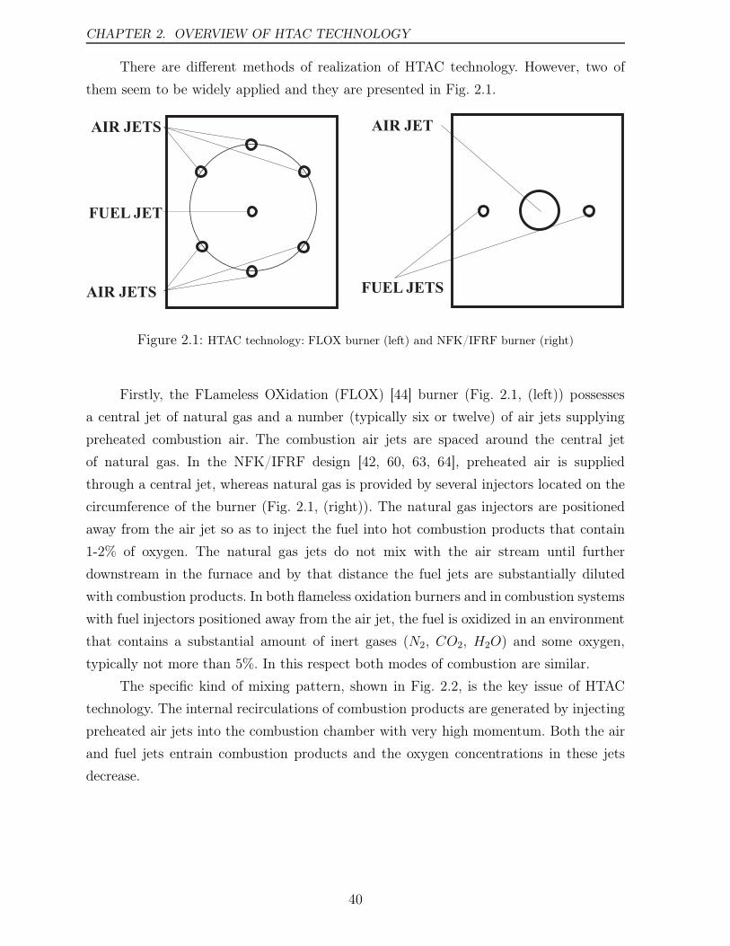
CHAPTER 2. OVERVIEW OF HTAC TECHNOLOGY
There are different methods of realization of HTAC technology. However, two of
them seem to be widely applied and they are presented in Fig. 2.1.
AIR JET
FUEL JETS
AIR JETS
FUEL JET
AIR JETS
Figure 2.1: HTAC technology: FLOX burner (left) and NFK/IFRF burner (right)
Firstly, the FLameless OXidation (FLOX) [44] burner (Fig. 2.1, (left)) possesses
a central jet of natural gas and a number (typically six or twelve) of air jets supplying
preheated combustion air. The combustion air jets are spaced around the central jet
of natural gas. In the NFK/IFRF design [42, 60, 63, 64], preheated air is supplied
through a central jet, whereas natural gas is provided by several injectors located on the
circumference of the burner (Fig. 2.1, (right)). The natural gas injectors are positioned
away from the air jet so as to inject the fuel into hot combustion products that contain
1-2% of oxygen. The natural gas jets do not mix with the air stream until further
downstream in the furnace and by that distance the fuel jets are substantially diluted
with combustion products. In both flameless oxidation burners and in combustion systems
with fuel injectors positioned away from the air jet, the fuel is oxidized in an environment
that contains a substantial amount of inert gases (N2, CO2, H2O) and some oxygen,
typically not more than 5%. In this respect both modes of combustion are similar.
The specific kind of mixing pattern, shown in Fig. 2.2, is the key issue of HTAC
technology. The internal recirculations of combustion products are generated by injecting
preheated air jets into the combustion chamber with very high momentum. Both the air
and fuel jets entrain combustion products and the oxygen concentrations in these jets
decrease.
40
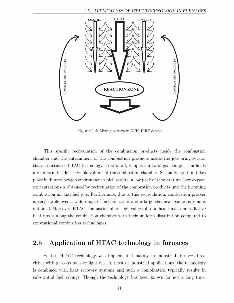
2.5. APPLICATION OF HTAC TECHNOLOGY IN FURNACES
Figure 2.2: Mixing pattern in NFK/IFRF design
This specific recirculation of the combustion products inside the combustion
chamber and the entrainment of the combustion products inside the jets bring several
characteristics of HTAC technology. First of all, temperature and gas composition fields
are uniform inside the whole volume of the combustion chamber. Secondly, ignition takes
place in diluted oxygen environment which results in low peak of temperature. Low oxygen
concentrations is obtained by recirculation of the combustion products into the incoming
combustion air and fuel jets. Furthermore, due to this recirculation, combustion process
is very stable over a wide range of fuel/air ratios and a large chemical reactions zone is
obtained. Moreover, HTAC combustion offers high values of total heat fluxes and radiative
heat fluxes along the combustion chamber with their uniform distribution compared to
conventional combustion technologies.
2.5 Application of HTAC technology in furnaces
So far, HTAC technology was implemented mainly in industrial furnaces fired
either with gaseous fuels or light oils. In most of industrial applications, the technology
is combined with heat recovery systems and such a combination typically results in
substantial fuel savings. Though the technology has been known for not a long time,
41
CHAPTER 2. OVERVIEW OF HTAC TECHNOLOGY
there are now over several hundreds of industrial furnaces all over the world which
utilize the HTAC principle. In these furnaces, combustion air is highly preheated which
leads to reduced specific fuel consumption. At the same time, high-efficiency heat
recuperators or regenerators cause that outlet physical loss is lower. As an effect, the
efficiency of HTAC furnaces is by circa 30% higher than that of conventional furnaces
with moderate recuperation temperature. Additionally, there are very low emissions of
harmful substances, including also NOx [134] although a high air preheated is used.
The conventional furnaces use either ambient temperature air or air preheated using
recuperative heat exchangers. The maximum temperature of the air in the standard
industrial furnaces is typically not higher than 500oC. The concept of HTAC is based
on a very efficient, high preheat of the combustion air to temperatures above the self-
ignition point (greater than 850oC for natural gas). The fuel consumption in industrial
furnaces represents a major amount of the operational costs of the furnaces. Significant
reductions in fuel consumption have been reported after installation of HTAC technology.
These fuel energy savings directly relate to reduction of CO2, NOx and other pollutants
emissions to the environment. Due to high heat fluxes in this combustion method the size
of the furnace can be decreased up to about 20% [135]. Several burner designs to realize
HTAC technology became a regular serial product for a variety of applications. Most of
the burners were installed in heating and heat treating furnaces of the metal and steel
industry, ceramic industry and chemical industry [136, 137, 138, 70].
2.6 Application of HTAC technology in boilers
Although most of current applications are limited to industrial furnaces, HTAC
technology is expected to provide significant advantages when applied also to the power
station boilers fired with pulverized coals. The foreseen advantages are as follows:
• An increase in radiative heat fluxes that may lead to a reduced size of the boiler
• More compact and smaller boilers can be built using a high quality steel so that
the cycle thermal efficiency is improved due to increased (superheated) steam
parameters
• A simple design of the burners and a very stable combustion process open up the
possibility of using low rank coals
• Improved mixing of the fuel and oxidizer together with uniform temperature and
oxygen concentration fields should minimize the coal burnout problems
42
2.6. APPLICATION OF HTAC TECHNOLOGY IN BOILERS
• Increased particle residence time is likely to improve char burnout
• The technology can be operated with a relatively low excess air ratio
• The technology offers low NOx emissions
In a coal or other fossil fuel fired boiler, it could be difficult to apply the conventional
honeycomb type regenerator since the ash-containing flue gas at such a high temperature
can cause plugging of the regenerator. Commercial boilers are usually of a large capacity
and thus the flow rate of combustion air is significant. Heating up a big amount of
combustion air to a high temperature in a short time period is technically not easy. Thus,
it is a need to find in the future a way to utilize the enthalpy of the boiler exhaust gas
to heat up the combustion air. A typical conventional boiler is composed of the radiative
heat transfer section and the convective heat transfer section. An air preheater and an
economizer are often used to recover the waste heat of flue gas. On the other hand, in the
high temperature air combustion boiler, the adiabatic flame temperature is much higher
than that of a conventional boiler and the heat transfer inside the boiler is dominated
by radiative heat transfer. With this feature, it is possible to design a boiler without the
convective heat transfer section and yet maintain the same thermal output. The removal
of the convective heat transfer region will certainly lead to a significant reduction of boiler
size and cost.
Several authors have postulated application of HTAC technology to power
generation [99, 100, 139] but up to now there have been only two attempts to apply
this technology to power boilers fired with pulverized coal. A new concept boiler where
fuel could be efficiently combusted in high temperature preheated air was proposed by
Kawai et al. [140]. It was perhaps the first attempt to develop a conceptual design of
HTAC boiler. It was realized that a new construction of the entire boiler was needed. The
proposed boiler was very similar to the industrial furnaces with regenerative burners. Low-
BTU syngas was combusted with high temperature preheated air and the thermal energy
contained in generated combustion gas was delivered to water/steam in boiler tubes
mainly by radiative heat transfer. Then the combustion products of 1200oC temperature
passed through a honeycomb bed to be cooled down to about 150oC and was exhausted
to atmosphere. This boiler was equipped with two burners containing each a fuel injector
and an air channel equipped with an regenerator. The first burner was located at the top
wall of the boiler and the second one at the bottom wall of the boiler. The burners
worked in a transient mode: when the first burner fired, the second worked as an
outlet of the boiler and the regenerator recovered a substantial part of the exhaust gas
energy. After the switching period (about 30 s) the role of two burners reversed. The
43
CHAPTER 2. OVERVIEW OF HTAC TECHNOLOGY
combustion air of 1000oC temperature and the fuel of 25oC were injected at a velocity
of 30 and 11 ms, respectively. The maximum thermal input examined during experiment
was equal to 120 kW . Only output and input measurements were carried out without
any detailed in-flame measurements. It was concluded that some design changes inside
the combustion zone were needed in order to improve the mixing between the gas and
the high temperature air. Finally, it was concluded that the proposed boiler was suitable
for low BTU syngas derived from gasification process of coal and wastes with no dioxin
emission and the boiler was characterized by the following features: uniform heat flux
field, augmentation of heat transfer, reduction of combustion noise level, suppression of
NOx emission and compactness.
Zhang et al. [141] proposed a boiler equipped with PRP burner (PRP stands for
primary air enrichment and preheating). The authors implemented the PRP burner as
HTAC technology because both processes were similar in their application. The PRP
burner was used to preheat the combustion air. It was equipped with a preheating chamber
with one end connected with the ambient combustion air and the other end opened to
the furnace. Inside the chamber, gas recirculation was effectively established. Low volatile
petroleum coke and an anthracite coal were used as fuels in industrial scale (12MWth) test
facility. In this approach PRP burner was installed at the side wall of the standard boiler.
Beside the new burner construction no further modifications to the boiler were required.
On the side wall of the furnace along the jet flow three rows of observation windows
were arranged. Through these windows flame appearance was recorded with a video
camera and flame brightness and temperature were measured by the color pyrometer.
Flame temperature was also measured in the furnace nearly along the centerline of the
chamber by using a S-type thermocouples with stainless steel sheath. The variations
of the temperature inside and out of chamber were used to analyze the mechanisms of
ignition, flame stabilization and NOx formation. The flue gas properties including O2,
CO, NOx, SO2 and unburned carbon were measured at the exit of the furnace. It was
concluded that the PRP burner was able to create a two-stage hot gas recirculation inside
and outside of the preheating chamber. The rapid heating of the combustible mixture in
the chamber facilitated pyrolysis, volatile matter release processes for the fuel particles,
suppressing ignition delay and enhancing combustion stability. Moreover, compared with
the results measured in the same facility but with a conventional low-NOx burner, NOx
concentrations at the furnace exit were at the same level while petroleum coke was used
as a fuel, and 50% lower while anthracite was used as a fuel.
44
Chapter 3
Mathematical model
Fluid dynamic is a field of engineering which studies the physical laws governing
the flow of fluids under various conditions. Great effort has gone into understanding the
governing laws and the nature of fluids themselves, resulting in a theoretically strong
field of research. Computational Fluid Dynamics (CFD) involves the numerical solutions
of fluid dynamic governing equations. The complex set of partial differential equations is
solved in a geometrical domain divided into small volumes. CFD methodology consists
of three main elements:
• A pre-processor which is used to create the geometry of the problem, to generate
the grid, to define the flow parameters as well as the boundary conditions
• A solver which is used to compute the governing equations of the flow
• A post-processor which is used to analyze the data and to show the results in a
graphical and easy to read format
All numerical simulations in this work were performed using GAMBIT (version 2.1) [142]
as pre-processor and FLUENT (version 6.2.16 and 6.3) [143] as solver and post-processor.
In this Chapter, both the governing differential equations for Computational Fluid
Dynamic approach and their averaging method are given. Furthermore, the set of
mathematical sub-models describing coal combustion process under HTAC conditions
is specified and finally, all used sub-models are briefly described. A specially emphasis is
given to devolatilization and char burnout models.
3.1 The governing partial differential equations
The mathematical modeling of the fluid flow is based on a set of coupled conservation
equations of mass, momentum, energy, and chemical species [144, 145]. Properties of
45
CHAPTER 3. MATHEMATICAL MODEL
fluid (the density, the viscosity, the specific heats, the molecular diffusivity, the thermal
conductivity, the radiation properties etc.) have to be given as a function of the state
variables.
3.1.1 The continuity equation
The continuity equation is a mass balance stating that the overall mass of the
gaseous phase system is conserved. The gas phase conservation equation of mass can be
written as 1:∂ρ
∂t+∂
∂xi(ρui) = Sm (3.1)
where Sm is the mass source in the system. The source term Sm accounts for the mass
transfer from solids (or liquid) phase to the gas phase.
3.1.2 The Navier-Stokes equation
The Navier-Stokes equation is the momentum conservation equation. The
conservation equation of momentum can be written as:
∂
∂t(ρui) +
∂
∂xj(ρuiuj) = −
∂p
∂xi+∂τij∂xj+ ρfi (3.2)
where fi is the sum of external forces (in our case it is only gravity) and τij is the viscous
stress tensor which is given by the Newton law:
τij = µ(∂ui∂xj+∂uj∂xi)− 23µδij∂ul∂xl
(3.3)
where the molecular viscosity µ is introduced, depending on the fluid properties and δij
is the Kronecker symbol.
3.1.3 The conservation equation of chemical species
The conservation equation of chemical species can be written as follows:
∂
∂t(ρYa) +
∂
∂xi(ρuiYa) +
∂Ja,i∂xi= Sa (3.4)
where n species have indicies a = 1, ..., n and Ja,i is the molecular diffusive flux of the
species a. Species molecular diffusivities are generally described using the Fick law:
Ja,i = −µ
Sca
∂Ya∂xj
(3.5)
1all equations are written using the Cartesian coordinate system and Einstein’s notation is apllied
46
3.1. THE GOVERNING PARTIAL DIFFERENTIAL EQUATIONS
where Sca is the Schmidt number of the species a, defined as:
Sca =µ
ρDa(3.6)
and Dk is the molecular diffusivity of the species a relative to the major species.
3.1.4 The energy equation
The conservation equation of energy can be written as:
∂
∂t(ρh) +
∂
∂xi(ρuih)− τij
∂ui∂xj+∂qi∂xi= ρuifi + Sh (3.7)
where h is the total specific enthalpy and for a multicomponent medium it takes the
following form:
h =∑
Yihi (3.8)
where Yi is the mass fraction of species i in the mixture and hi is the total enthalpy
defined by:
hi = h0Tref,i+
T∫
Tref
Cpi(T )dT (3.9)
where h0 is the enthalpy of formation, Tref is the reference temperature and Cpi(T ) is
the specific heat at a constant pressure.
3.1.5 The equation of state
The relationship between the pressure, the temperature and the fluid density is
provided through the equation of state. The perfect gas Clapeyron equation is given as:
ρ =p
R · T ·∑ YaMa
(3.10)
where R = 8.314 kJkmol·K
is the universal gas constant while Ma and Ya stand for the
molecular mass and the mass fraction of a-species, respectively.
3.1.6 The general governing differential equation
The conservation equations described in Sections 3.1.1-3.1.4 can be transformed
into a general transport equation of dependent variable φ, written as follows:
∂
∂t(ρφ)
︸ ︷︷ ︸
unsteady term
+∂
∂xj(ρφuj)
︸ ︷︷ ︸
convective term
=∂
∂xj(Γφ∂φ
∂xi)
︸ ︷︷ ︸
diffusion term
+ Sφ︸︷︷︸
source term
(3.11)
where Γφ and Sφ are the diffusion coefficient and the source term, respectively and these
are specific to a particular meaning of φ as shown in Tab. 3.1.
47
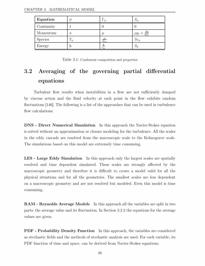
CHAPTER 3. MATHEMATICAL MODEL
Equation φ Γφ Sφ
Continuity 1 0 0
Momentum u µ ρgi +∂p∂xi
Species YaµSca
Sca
Energy h kcp
Sh
Table 3.1: Comburent composition and properties
3.2 Averaging of the governing partial differential
equations
Turbulent flow results when instabilities in a flow are not sufficiently damped
by viscous action and the fluid velocity at each point in the flow exhibits random
fluctuations [146]. The following is a list of the approaches that can be used in turbulence
flow calculations:
DNS - Direct Numerical Simulation In this approach the Navier-Stokes equation
is solved without an approximation or closure modeling for the turbulence. All the scales
in the eddy cascade are resolved from the macroscopic scale to the Kolmogorov scale.
The simulations based on this model are extremely time consuming.
LES - Large Eddy Simulation In this approach only the largest scales are spatially
resolved and time dependent simulated. These scales are strongly affected by the
macroscopic geometry and therefore it is difficult to create a model valid for all the
physical situations and for all the geometries. The smallest scales are less dependent
on a macroscopic geometry and are not resolved but modeled. Even this model is time
consuming.
RAM - Reynolds Average Models In this approach all the variables are split in two
parts: the average value and its fluctuation. In Section 3.2.2 the equations for the average
values are given.
PDF - Probability Density Function In this approach, the variables are considered
as stochastic fields and the methods of stochastic analysis are used. For each variable, its
PDF function of time and space, can be derived from Navier-Stokes equations.
48
3.2. AVERAGING OF THE GOVERNING PARTIAL DIFFERENTIAL EQUATIONS
For most engineering applications, the time-averaged or spatial filtered properties
of the flow are of interest, thus the time-averaged transport equations, such as the
Reynolds averaged Navier-Stokes (RANS) equations, are established. However, time-
averaged equations are unfortunately not closed and thus additional closure methods
corresponding to different turbulence models have to be developed. As mentioned above,
the full numerical solution of the instantaneous balance equations is possible only using
DNS but it is too computational expensive. To overcome this difficulty, an additional
term is introduced by averaging the conservation equations to describe only the mean
flow field. Local fluctuations and turbulent structures are integrated in mean quantities
and these structures have no longer to be described in the simulation.
3.2.1 Reynolds averaging
Reynolds averaging refers to the process of averaging a variable or an equation
in time [147, 148]. By using Reynolds decomposition approach, an instantaneous flow
variable φ can be decomposed into the mean value φ and the fluctuation φ′.
φ(t) = φ(t) + φ′(t) (3.12)
The mean quantity is defined as follow:
φ(t) = 〈φ(t)〉 (3.13)
where 〈〉 stands for an averaging operator. If the modeled process is stationary, it makes
sense to define the averaging operator in the following way:
〈φ(t)〉 ≡ φ(t) = 1∆t
t∫
t+∆t
φ(t)dτ (3.14)
The averaged variable is not dependent on the time t but only on the fluctuating part
φ′(t). This kind of averaging operators (called Reynolds averaging operators) are useful in
the case of constant density only. Such an averaging procedure produce new terms in the
Navier-Stokes equation. In order to achieve a closure, relations between these additional
terms have to be constructed and this process increases the complexity of the problem.
3.2.2 Favre averaging
Time averaged equations can further be simplified for compressible flows by using
Favre (density or mass) averaging procedure. In turbulent flames, fluctuations of density
are observed because of the thermal heat release, and Reynolds averaging is therefore not
49
CHAPTER 3. MATHEMATICAL MODEL
applicable. Instead, a Favre (density weighted) average is introduced. Each quantity is
decomposed into:
φ(t) = φ(t) + φ′(t) (3.15)
where the mean quantity is defined as follow:
φ(t) =〈ρφ〉ρ
(3.16)
The Favre averaging operator has slightly different properties than the Reynolds operator.
The most important one is that the Favre averaging allows for decoupling between the
average of the density and the average of the other variables. This Favre operator is
defined as below:
〈φ(t)〉 ≡ φ(t) = 1ρ〈 1∆t
t∫
t+∆t
ρφ′(t)dτ〉 (3.17)
The Favre averaged fields have no physical meaning. The Favre averaging is a
mathematical definition only that allows a more suitable formulation of the conservation
equations. In other words, Favre averaging is only a mathematical simplification. It
eliminates the density fluctuation from the time-averaged equations.
The Favre averaged conservation partial differential equations are as follow:
• The continuity equation
∂〈ρ〉∂t+∂
∂xi(〈ρ〉〈Ui〉) = 〈Sm〉 (3.18)
• The Navier-Stokes equation
∂
∂t〈ρ〉〈Ui〉+
∂
∂xj〈ρ〉〈Ui〉〈Uj〉+
∂
∂xj〈ρ〉〈UiUj〉 =
∂
∂xi〈ρ〉+ ∂
∂xj〈τij〉+ 〈ρ〉〈fi〉 (3.19)
• The conservation equation of chemical species
∂
∂t〈ρ〉〈Ya〉+
∂
∂xj〈ρ〉〈Ya〉〈Uj〉+
∂
∂xj〈ρ〉〈UjYa〉 =
∂
∂xj〈Ja,j〉+ 〈Sa〉 (3.20)
• The energy equation
∂
∂t〈ρ〉〈H〉+ ∂
∂xj〈ρ〉〈H〉〈Uj〉+
∂
∂xj〈ρ〉〈UjH〉 =
∂
∂xj〈qj〉+ρ〈Ui〉〈fi〉+ 〈
∂Ui∂xjτi,j〉+ 〈Sr〉
(3.21)
The FLUENT code uses the Favre averaged conservation equations and these equations
are closed with appropriate sub-models.
50
3.3. SET OF THE MATHEMATICAL SUB-MODELS
3.3 Set of the mathematical sub-models
Commonly used and widely accepted models available in the FLUENT code have
been applied for the description of the turbulence, the gaseous combustion and the
radiative energy exchange. In all calculations throughout this thesis the following models
have been used:
• turbulence - the k-ε model
• interaction between chemistry and turbulence - EDM (Eddy Dissipation Model)
• Lagrangian particle tracking - DPM (Discrete Phase Model)
• devolatilization - CPD (Chemical Percolation Devolatilization) model
• char burnout - intrinsic model
• radiative heat transfer - DO (Discrete Ordinates) model
3.4 Turbulence
Computations of stationary turbulent flows require that the continuity equation
(Eq. 3.1) and the momentum transport equation (Eq. 3.2) be accompanied by a model of
turbulence that relates the Reynolds stresses ρuiuj to known or calculable quantities. In all
presented simulations, the k−ε turbulence model according to Launder and Spalding [149]
is used. It is the most common model due to its simplicity and due to its capability in
predicting several turbulent flows. In the k − ε model, the turbulent stresses ρuiuj are
assumed to be proportional to the mean rate of strain.
ρuiuj = −µt(∂Ui∂xj+∂Uj∂xi) (3.22)
The eddy viscosity µt is constructed from a turbulent length scale and a turbulent velocity
scale which both are built up from the turbulent kinetic energy k and its turbulent viscous
dissipation rate ε.
µt = ρcµk2
ε(3.23)
k =1
2uiui (3.24)
ε =µ
ρ
∂ui∂xj
∂uj∂xi
(3.25)
51
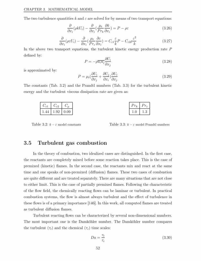
CHAPTER 3. MATHEMATICAL MODEL
The two turbulence quantities k and ε are solved for by means of two transport equations:
∂
∂xi(ρkUi)−
∂
∂xi(µtPrk
∂k
∂xi) = P − ρε (3.26)
∂
∂xi(ρεUi)−
∂
∂xi(µtPrε
∂ε
∂xi) = Cε1
ε
kP − Cε2ρ
ε2
k(3.27)
In the above two transport equations, the turbulent kinetic energy production rate P
defined by:
P = −ρuiuj∂Ui∂xj
(3.28)
is approximated by:
P = µt(∂Ui∂xj+∂Uj∂xi)∂Ui∂xj
(3.29)
The constants (Tab. 3.2) and the Prandtl numbers (Tab. 3.3) for the turbulent kinetic
energy and the turbulent viscous dissipation rate are given as:
Cε1 Cε2 Cµ
1.44 1.92 0.09
Table 3.2: k − ε model constants
Prk Prε
1.0 1.3
Table 3.3: k − ε model Prandtl numbers
3.5 Turbulent gas combustion
In the theory of combustion, two idealized cases are distinguished. In the first case,
the reactants are completely mixed before some reaction takes place. This is the case of
premixed (kinetic) flames. In the second case, the reactants mix and react at the same
time and one speaks of non-premixed (diffusion) flames. These two cases of combustion
are quite different and are treated separately. There are many situations that are not close
to either limit. This is the case of partially premixed flames. Following the characteristic
of the flow field, the chemically reacting flows can be laminar or turbulent. In practical
combustion systems, the flow is almost always turbulent and the effect of turbulence in
these flows is of a primary importance [146]. In this work, all computed flames are treated
as turbulent diffusion flames.
Turbulent reacting flows can be characterized by several non-dimensional numbers.
The most important one is the Damköhler number. The Damköhler number compares
the turbulent (τt) and the chemical (τc) time scales:
Da =τtτc
(3.30)
52
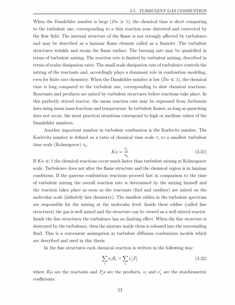
3.5. TURBULENT GAS COMBUSTION
When the Damköhler number is large (Da ≫ 1), the chemical time is short comparing
to the turbulent one, corresponding to a thin reaction zone distorted and convected by
the flow field. The internal structure of the flame is not strongly affected by turbulence
and may be described as a laminar flame element called as a flamelet. The turbulent
structures wrinkle and strain the flame surface. The burning rate may be quantified in
terms of turbulent mixing. The reaction rate is limited by turbulent mixing, described in
terms of scalar dissipation rates. The small scale dissipation rate of turbulence controls the
mixing of the reactants and, accordingly plays a dominant role in combustion modeling,
even for finite rate chemistry. When the Damköhler number is low (Da≪ 1), the chemical
time is long compared to the turbulent one, corresponding to slow chemical reactions.
Reactants and products are mixed by turbulent structures before reactions take place. In
this perfectly stirred reactor, the mean reaction rate may be expressed from Arrhenius
laws using mean mass fractions and temperature. In turbulent flames, as long as quenching
does not occur, the most practical situations correspond to high or medium values of the
Damköhler numbers.
Another important number in turbulent combustion is the Karlovitz number. The
Karlovitz number is defined as a ratio of chemical time scale τc to a smallest turbulent
time scale (Kolmogorov) τk.
Ka =τcτk
(3.31)
If Ka≪ 1 the chemical reactions occur much faster than turbulent mixing at Kolmogorov
scale. Turbulence does not alter the flame structure and the chemical region is in laminar
conditions. If the gaseous combustion reactions proceed fast in comparison to the time
of turbulent mixing the overall reaction rate is determined by the mixing himself and
the reaction takes place as soon as the reactants (fuel and oxidizer) are mixed on the
molecular scale (infinitely fast chemistry). The smallest eddies in the turbulent spectrum
are responsible for the mixing at the molecular level. Inside these eddies (called fine
structures) the gas is well mixed and the structure can be viewed as a well stirred reactor.
Inside the fine structures the turbulence has no limiting effect. When the fine structure is
destroyed by the turbulence, then the mixture inside them is released into the surrounding
fluid. This is a convenient assumption in turbulent diffusion combustion models which
are described and used in this thesis.
In the fine structures each chemical reaction is written in the following way:
∑
i
νiRi =∑
j
ν′
jPj (3.32)
where Ris are the reactants and Pjs are the products, νi and ν′
j are the stoichiometric
coefficients.
53
CHAPTER 3. MATHEMATICAL MODEL
The rate of formation or destruction of each species is :
ℜi = kf,i∏
i
[Ri]νj,i − kb,i
∏
j
[Pj ]ν′
j,i (3.33)
where kf,i and kb,i are the rate constants for the forward and backward reactions
respectively, and [Ri] and [Pj ] are mole concentration of reactants and products,
respectively. The forward and the backward reaction rate constants are linked through
the equilibrium constant:
kfkb=(P
RT
)∆ν
exp
(
∆So
R− ∆H
o
RT
)
(3.34)
where ∆ν =∑
jν′
j −∑
iνi
In chemical species equation (Eq. 3.4) the effect of the chemical reactions appears
in the source term Sa only. The part due to chemical reaction is given by:
Sa = µa∑
j
νjiRj (3.35)
The source term in the species equation takes into account the rate of formation or
destruction of each species. As discussed previously in this Chapter, the source term
has to take in consideration effects of the turbulence. This term is very complicated to
calculate and therefore sub-models are needed. Some approaches are described in the
following Sections.
3.5.1 Turbulence-chemistry interaction models
The interaction between turbulence and chemistry is assumed to be well described
using the concept of Spalding [150] - Eddy Break-Up Model (EBU), and developed further
by Magnussen and Hjertager [151] - Eddy Dissipation Model (EDM). Both models assume
that mass is exchanged between Kolmogorov eddies (fine structure) and surroundings. No
detailed chemistry can be applied and only global mechanisms are used in these models.
The Eddy Dissipation Concept (EDC) is an extension of Magnussen [152, 153, 154] to the
Eddy Dissipation Model (EDM) that include detailed chemical mechanisms occurring in
turbulent flows.
3.5.2 Eddy Break Up Model
Spalding [150] related the microscale mixing to the breakup of large eddies of
unburned fluid into successively smaller ones until the surface of the lumps becomes
significant and turbulent kinetic energy is dissipated. The model assumes that the
54
3.5. TURBULENT GAS COMBUSTION
reactions are completed at the moment of mixing, so that the reaction rate is completely
controlled by turbulent mixing. At every location, the gas mixture is supposed to comprise
fully-burned and fully-unburned gases. Combustion is then described by a single step
global chemical reaction. The reaction rate is:
ℜi = Amixρ〈ε
k〉√
Y′2F (3.36)
Amix = A〈k2
εν〉−B (3.37)
where A and B are the model parameters derived from experiments and are equal to
23.66 and 0.25, respectively. The EBU model was found attractive because the reaction
rate is simply written as a function of known quantities without an additional transport
equation. The modeled reaction rate does not depend on chemical characteristics and
assumes a homogenous and isotropic turbulence.
3.5.3 Eddy Dissipation Model
Magnussen and Hjertager derived the Eddy Dissipation Model (EDM) [151] which
is based on the EBU model. In diffusion flames both the fuel and the oxygen occur in
separate eddies. Because the chemical reactions in most cases are very fast, it can be
assumed that the rate of the combustion is determined by the rate of intermixing on the
molecular level of fuel and oxygen eddies, in other words, by the rate of dissipation of the
eddies. Because both the fuel and the oxygen appear as fluctuating intermittent quantities
there is a relationship between the fluctuations and the mean species concentration.
Consequently, the rate of dissipation can be expressed by the mean concentration of
the reacting species.
The EDM is apparently closely related to the EBU model. However, it differs from
the latter in relating the dissipation of eddies to the mean concentration of intermittent
quantities instead of the concentration fluctuations. This is a great advantage, especially
when taking into consideration the lack of the certainty with which concentration
fluctuations of reacting species can be determined. However, the simplifications of the
proposed model are only possible for quantities that appear intermittent.
Practically, the equations in both approaches are the same, but in EDM, as
mentioned above, the reaction rate (and mixing also) is not dependent on the
concentration fluctuations, hence mixing parameter Amix is not calculated. It is
empirically determined and it is a constant. The reaction rate for a single reaction is
then given by smaller of the two expressions below:
ℜi,r = ν′
i,rMw,iAρ(ε
k
)
min
(
YRν′
R,rMw,R
)
(3.38)
55
CHAPTER 3. MATHEMATICAL MODEL
ℜi,p = ν′
i,rMw,iABρ(ε
k
)
min
∑
PYP
N∑
jν′′
j,rMw,j
(3.39)
where A and B are two model constants and that are equal 4 and 0.5, respectively. YP is
the mass fraction of the product species (P ) and YR is the mass fraction of the particular
reactant (R); ν′
i,r is the stoichiometric coefficient for species i in reaction r; k and ε are
the turbulent kinetic energy and the turbulent dissipation derived from the k− ε model.
3.5.4 Eddy Dissipation Concept
The Eddy Dissipation Concept (EDC) is an extension of the EBU and EDM
models as described by Magnussen et al. [152, 153, 154]. It is a reactor concept which
identifies a reactor related to the fine structure in turbulence. This reactor is treated
as a homogeneous reactor exchanging mass and energy with the surrounding fluid, thus
allowing a complete treatment of the chemistry for the reactor. Everywhere, the gas
mixture is supposed to comprise of mean mixture and fine structures. These both (as at
the previous two models) exchange mass due to the destruction of the fine structures by
the turbulence. Chemistry reactions are active only inside the fine structures, supposed to
be mixed at the molecular level by the turbulence at the Kolmogorov scale. The reaction
rate is given by:
ℜi =γ∗
τ ∗(Y 0i − Y ∗i ) (3.40)
where γ∗ is the mass fraction of the fine structure inside the control volume and is
described as follow:
γ∗ = Cγ
(
νε
k2
3
4
)
(3.41)
where Cγ is the time scale constant and is equal 9.7687. The destruction time of the fine
structure is indicates as τ ∗ and is given as:
τ ∗ = Cτ
(
ν
ε
1
2
)
(3.42)
where Cτ is the time scale constant and is equal 0.4082. This model is more general
than the EBU and EDM because it can be coupled with detailed kinetics since the fine
structure can be considered as a well stirred reactor.
3.6 Particle behavior
Pulverized coal flame is modeled as two-phase turbulent flow system consisting of
both a gaseous and a solid phase. In discrete phase modeling, coal particles of known
56
3.6. PARTICLE BEHAVIOR
size distributions and properties are injected into the combustion chamber and tracked in
a Lagrangian fashion throughout the computational domain. Heat and mass transfer
to/from particles is calculated along each trajectory and it is used as the coupling
mechanism between the gas phase and the solid phase. In others words, discrete phase
model uses an Eulerian approach to calculate the continuous phase and a Lagrangian
particle tracking to calculate the discrete phase. The coupling between the phases and its
impact on both the discrete phase trajectories and the continuous phase flow is included.
A major assumption in the Lagrangian discrete phase model is that there is no
interaction between solid particles. As a result this approach is only applicable to dilute
fluid-particle flows where the solid phase volume fraction is low. Flows considered in this
thesis have this characteristic.
3.6.1 Trajectory calculations
The trajectory of a discrete phase particle is predicted by integrating the force
balance on the particle. The particle inertia must be equal to the forces acting on the
particle, and the resulting equation can be written for x-direction in Cartesian coordinates
in the following form:
dup,xdt= FD(u− up)︸ ︷︷ ︸
drag force
+gx(ρp − ρ)ρp
︸ ︷︷ ︸
gravity and buoancy
+ Fx︸︷︷︸
additional forces
(3.43)
where the drag force is defined:
FD =18µ
ρpd2p
CDRep24
(3.44)
All forces in the force balance equation are given per unit of particle mass. The particle
Reynolds number Rep is defined in terms of the relative velocity between solid and fluid
phase:
Rep =ρdp|up − u|µ
(3.45)
where: u- fluid phase velocity, up- particle velocity, µ- molecular viscosity of the fluid, ρ-
fluid density, ρp- density of the particle, dp- particle diameter, CD- drag coefficient. For
the two other Cartesian directions analogous equations can be written.
In turbulence flows, the effect of turbulent dispersion is taken into account. The
velocity fluctuations are assumed to be described by a Gaussian probability distribution.
When the flow is turbulent, the trajectories of particle are predicted using the mean fluid
phase velocity u. In the stochastic particle tracking in turbulent flow, the instantaneous
value of the fluctuating gas velocity u = u + u, is used to predict the dispersion of the
57
CHAPTER 3. MATHEMATICAL MODEL
particle due to turbulence. A stochastic method (in FLUENT- Discrete Random Walk
(DRW) model) is implemented to determine the instantaneous gas velocity. The particle
tracking procedure used in this work was developed at the beginning of the eighties at
the University of Sheffield [155, 156] and later on it was implemented into the FLUENT
code.
3.6.2 Heat and mass transfer calculations
The changes of momentum, mass and enthalpy during the particle trajectory
calculations is computed for every control volume and appears as a source term in the
equation for the fluid phase; this is a two way coupling between the solid and fluid phase.
The following processes are taken into account:
• inert heating/cooling
• devolatilization phase
• char burnout
and they will be explained in details in next Paragraphs.
Inert heating or cooling
The inert heating or cooling is applied when the particle temperature is lower than
the offset of devolatilization temperature (Tdev), and after the volatile fraction of a particle
(fv,0) has been released. These conditions may be written as:
• Inert heating
Tp < Tdev (3.46)
• Inert cooling
mp ¬ (1− fv,0)mp,0 (3.47)
where Tp is the particle temperature, mp,0 is the initial mass of the particle, and mp
is its current mass. During heating or cooling of particles, heat transfer is only due to
convection and radiation at the particle surface:
mpcpdTpdt= hAp(T∞ − Tp) + εpApσ(θ4R − T 4p ) (3.48)
where: mp- mass of the particle, cp- heat capacity of the particle, Ap- surface area
of the particle, T∞- local temperature of the continuous phase, h- convective heat
transfer coefficient, εp- particle emissivity, σ- Stefan-Boltzmann constant, θR- radiation
temperature. During heating and cooling, particles do not exchange mass with the
continuous phase and do not participate in any chemical reactions.
58
3.6. PARTICLE BEHAVIOR
Devolatilization phase
When the particle has reached an offset temperature for devolatilization Tdev volatile
matter release begins:
Tp Tdev (3.49)
and remains in effect untill the mass of the particle, mp, exceeds the mass of the
nonvolatiles in the particle:
mp > (1− fv,0)mp,0 (3.50)
The change of particle mass depends on the devolatilization model applied. The details
of this model are presented in Section 3.7.1.
Heat transfer to the particle during the devolatilization process includes
contributions from convection, radiation, and latent heat of devolatilization:
mpcpdTpdt= hAp(T∞ − Tp) +
dmpdthfg + Apεpσ(θR
4 − Tp4) (3.51)
Char burnout
After the volatile component of the particle is completely evolved, a surface
reaction begins which consumes the combustible fraction, fcomb, of the char particle.
Char combustion is activated after the volatiles are evolved:
mp < (1− fv,0)(1− fw,0)mp,0 (3.52)
and it remains active until the combustible fraction in the char is consumed:
mp > (1− fv,0 − fcomb)(1− fw,0)mp,0 (3.53)
When the combustible fraction, fcomb, has been consumed, the combusting particle may
contain residual ash that reverts to the inert cooling phase (described previously).
The surface reaction consumes the oxidant species in the gas phase; it supplies a
(negative) source term during the computation of the transport equation for this species.
Similarly, the surface reaction is a source of species in the gas phase: the product of the
heterogeneous surface reaction appears in the gas phase as a chemical species. The change
of the coal particle mass describes the char burnout model which is presented in details
in Section 3.7.3.
The particle heat balance during surface reaction is
mpcpdTpdt= hAp(T∞ − Tp)− fh
dmpdtHreac + Apεpσ(θR
4 − Tp4) (3.54)
where Hreac is the heat released by the surface reaction. Note that only a portion ( 1−fh)of the energy produced by the surface reaction appears as a heat source in the gas-phase
energy equation: the particle absorbs a fraction fh of this heat directly.
59
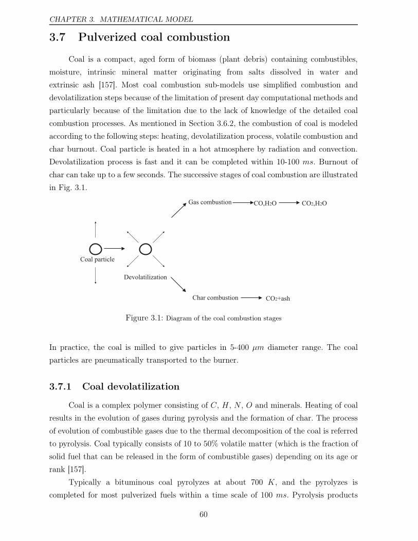
CHAPTER 3. MATHEMATICAL MODEL
3.7 Pulverized coal combustion
Coal is a compact, aged form of biomass (plant debris) containing combustibles,
moisture, intrinsic mineral matter originating from salts dissolved in water and
extrinsic ash [157]. Most coal combustion sub-models use simplified combustion and
devolatilization steps because of the limitation of present day computational methods and
particularly because of the limitation due to the lack of knowledge of the detailed coal
combustion processes. As mentioned in Section 3.6.2, the combustion of coal is modeled
according to the following steps: heating, devolatilization process, volatile combustion and
char burnout. Coal particle is heated in a hot atmosphere by radiation and convection.
Devolatilization process is fast and it can be completed within 10-100 ms. Burnout of
char can take up to a few seconds. The successive stages of coal combustion are illustrated
in Fig. 3.1.
Gas combustion
Char combustion
CO,H O2
CO +ash2
Coal particle
Devolatilization
CO ,H O2 2
Figure 3.1: Diagram of the coal combustion stages
In practice, the coal is milled to give particles in 5-400 µm diameter range. The coal
particles are pneumatically transported to the burner.
3.7.1 Coal devolatilization
Coal is a complex polymer consisting of C, H , N , O and minerals. Heating of coal
results in the evolution of gases during pyrolysis and the formation of char. The process
of evolution of combustible gases due to the thermal decomposition of the coal is referred
to pyrolysis. Coal typically consists of 10 to 50% volatile matter (which is the fraction of
solid fuel that can be released in the form of combustible gases) depending on its age or
rank [157].
Typically a bituminous coal pyrolyzes at about 700 K, and the pyrolyzes is
completed for most pulverized fuels within a time scale of 100 ms. Pyrolysis products
60
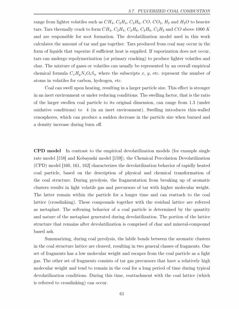
3.7. PULVERIZED COAL COMBUSTION
range from lighter volatiles such as CH4, C2H4, C2H6, CO, CO2, H2 and H2O to heavier
tars. Tars thermally crack to form CH4, C2H4, C2H6, C3H6, C2H2 and CO above 1000 K
and are responsible for soot formation. The devolatilization model used in this work
calculates the amount of tar and gas together. Tars produced from coal may occur in the
form of liquids that vaporize if sufficient heat is supplied. If vaporization does not occur,
tars can undergo repolymerization (or primary cracking) to produce lighter volatiles and
char. The mixture of gases or volatiles can usually be represented by an overall empirical
chemical formula CxHyNzOtSw where the subscripts x, y, etc. represent the number of
atoms in volatiles for carbon, hydrogen, etc.
Coal can swell upon heating, resulting in a larger particle size. This effect is stronger
in an inert environment or under reducing conditions. The swelling factor, that is the ratio
of the larger swollen coal particle to its original dimension, can range from 1.3 (under
oxidative conditions) to 4 (in an inert environment). Swelling introduces thin-walled
cenospheres, which can produce a sudden decrease in the particle size when burned and
a density increase during burn off.
CPD model In contrast to the empirical devolatilization models (for example single
rate model [158] and Kobayashi model [159]), the Chemical Percolation Devolatilization
(CPD) model [160, 161, 162] characterizes the devolatilization behavior of rapidly heated
coal particle, based on the description of physical and chemical transformation of
the coal structure. During pyrolysis, the fragmentation from breaking up of aromatic
clusters results in light volatile gas and precursors of tar with higher molecular weight.
The latter remain within the particle for a longer time and can reattach to the coal
lattice (crosslinking). These compounds together with the residual lattice are referred
as metaplast. The softening behavior of a coal particle is determined by the quantity
and nature of the metaplast generated during devolatilization. The portion of the lattice
structure that remains after devolatilization is comprised of char and mineral-compound
based ash.
Summarizing, during coal pyrolysis, the labile bonds between the aromatic clusters
in the coal structure lattice are cleaved, resulting in two general classes of fragments. One
set of fragments has a low molecular weight and escapes from the coal particle as a light
gas. The other set of fragments consists of tar gas precursors that have a relatively high
molecular weight and tend to remain in the coal for a long period of time during typical
devolatilization conditions. During this time, reattachment with the coal lattice (which
is referred to crosslinking) can occur.
61
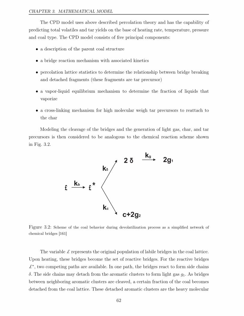
CHAPTER 3. MATHEMATICAL MODEL
The CPD model uses above described percolation theory and has the capability of
predicting total volatiles and tar yields on the base of heating rate, temperature, pressure
and coal type. The CPD model consists of five principal components:
• a description of the parent coal structure
• a bridge reaction mechanism with associated kinetics
• percolation lattice statistics to determine the relationship between bridge breaking
and detached fragments (these fragments are tar precursor)
• a vapor-liquid equilibrium mechanism to determine the fraction of liquids that
vaporize
• a cross-linking mechanism for high molecular weigh tar precursors to reattach to
the char
Modeling the cleavage of the bridges and the generation of light gas, char, and tar
precursors is then considered to be analogous to the chemical reaction scheme shown
in Fig. 3.2.
£ £ *
2 ä 2g1
c+2g2
kb
kä
kc
kg
Figure 3.2: Scheme of the coal behavior during devolatilization process as a simplified network of
chemical bridges [161]
The variable £ represents the original population of labile bridges in the coal lattice.
Upon heating, these bridges become the set of reactive bridges. For the reactive bridges
£∗, two competing paths are available. In one path, the bridges react to form side chains
δ. The side chains may detach from the aromatic clusters to form light gas g1. As bridges
between neighboring aromatic clusters are cleaved, a certain fraction of the coal becomes
detached from the coal lattice. These detached aromatic clusters are the heavy molecular
62
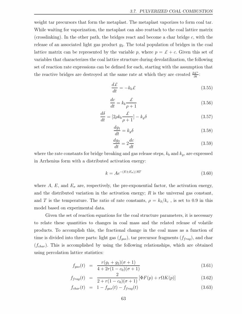
3.7. PULVERIZED COAL COMBUSTION
weight tar precursors that form the metaplast. The metaplast vaporizes to form coal tar.
While waiting for vaporization, the metaplast can also reattach to the coal lattice matrix
(crosslinking). In the other path, the bridges react and become a char bridge c, with the
release of an associated light gas product g2. The total population of bridges in the coal
lattice matrix can be represented by the variable p, where p = £ + c. Given this set of
variables that characterizes the coal lattice structure during devolatilization, the following
set of reaction rate expressions can be defined for each, starting with the assumption that
the reactive bridges are destroyed at the same rate at which they are created ∂£∗
∂t:
d£
dt= −kb£ (3.55)
dc
dt= kb
£
ρ+ 1(3.56)
dδ
dt= [2ρkb
£
ρ+ 1]− kgδ (3.57)
dg1dt= kgδ (3.58)
dg2dt= 2dc
dt(3.59)
where the rate constants for bridge breaking and gas release steps, kb and kg, are expressed
in Arrhenius form with a distributed activation energy:
k = Ae−(E±Eσ)/RT (3.60)
where A, E, and Eσ are, respectively, the pre-exponential factor, the activation energy,
and the distributed variation in the activation energy; R is the universal gas constant,
and T is the temperature. The ratio of rate constants, ρ = kδ/kc , is set to 0.9 in this
model based on experimental data.
Given the set of reaction equations for the coal structure parameters, it is necessary
to relate these quantities to changes in coal mass and the related release of volatile
products. To accomplish this, the fractional change in the coal mass as a function of
time is divided into three parts: light gas (fgas), tar precursor fragments (ffrag), and char
(fchar). This is accomplished by using the following relationships, which are obtained
using percolation lattice statistics:
fgas(t) =r(g1 + g2)(σ + 1)
4 + 2r(1− c0)(σ + 1)(3.61)
ffrag(t) =2
2 + r(1− c0)(σ + 1)[ΦF (p) + rΩK(p)] (3.62)
fchar(t) = 1− fgas(t)− ffrag(t) (3.63)
63
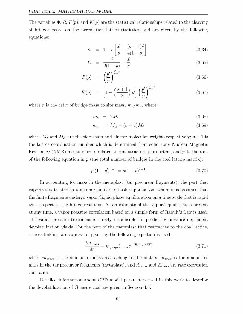
CHAPTER 3. MATHEMATICAL MODEL
The variables Φ, Ω, F (p), andK(p) are the statistical relationships related to the cleaving
of bridges based on the percolation lattice statistics, and are given by the following
equations:
Φ = 1 + r
[
£
p+(σ − 1)δ4(1− p)
]
(3.64)
Ω =δ
2(1− p) −£
p(3.65)
F (p) =
(
p′
p
)σ+1σ−1
(3.66)
K(p) =[
1−(σ + 1
2
)
p′] (
p′
p
)σ+1σ−1
(3.67)
where r is the ratio of bridge mass to site mass, mb/ma, where
mb = 2Mδ (3.68)
ma = Mcl − (σ + 1)Mδ (3.69)
where Mδ and Mcl are the side chain and cluster molecular weights respectively; σ + 1 is
the lattice coordination number which is determined from solid state Nuclear Magnetic
Resonance (NMR) measurements related to coal structure parameters, and p′ is the root
of the following equation in p (the total number of bridges in the coal lattice matrix):
p′(1− p′)σ−1 = p(1− p)σ−1 (3.70)
In accounting for mass in the metaplast (tar precursor fragments), the part that
vaporizes is treated in a manner similar to flash vaporization, where it is assumed that
the finite fragments undergo vapor/liquid phase equilibration on a time scale that is rapid
with respect to the bridge reactions. As an estimate of the vapor/liquid that is present
at any time, a vapor pressure correlation based on a simple form of Raoult’s Law is used.
The vapor pressure treatment is largely responsible for predicting pressure dependent
devolatilization yields. For the part of the metaplast that reattaches to the coal lattice,
a cross-linking rate expression given by the following equation is used:
dmcrossdt
= mfragAcrosse−(Ecross/RT ) (3.71)
where mcross is the amount of mass reattaching to the matrix, mfrag is the amount of
mass in the tar precursor fragments (metaplast), and Across and Ecross are rate expression
constants.
Detailed information about CPD model parameters used in this work to describe
the devolatilization of Guasare coal are given in Section 4.3.
64
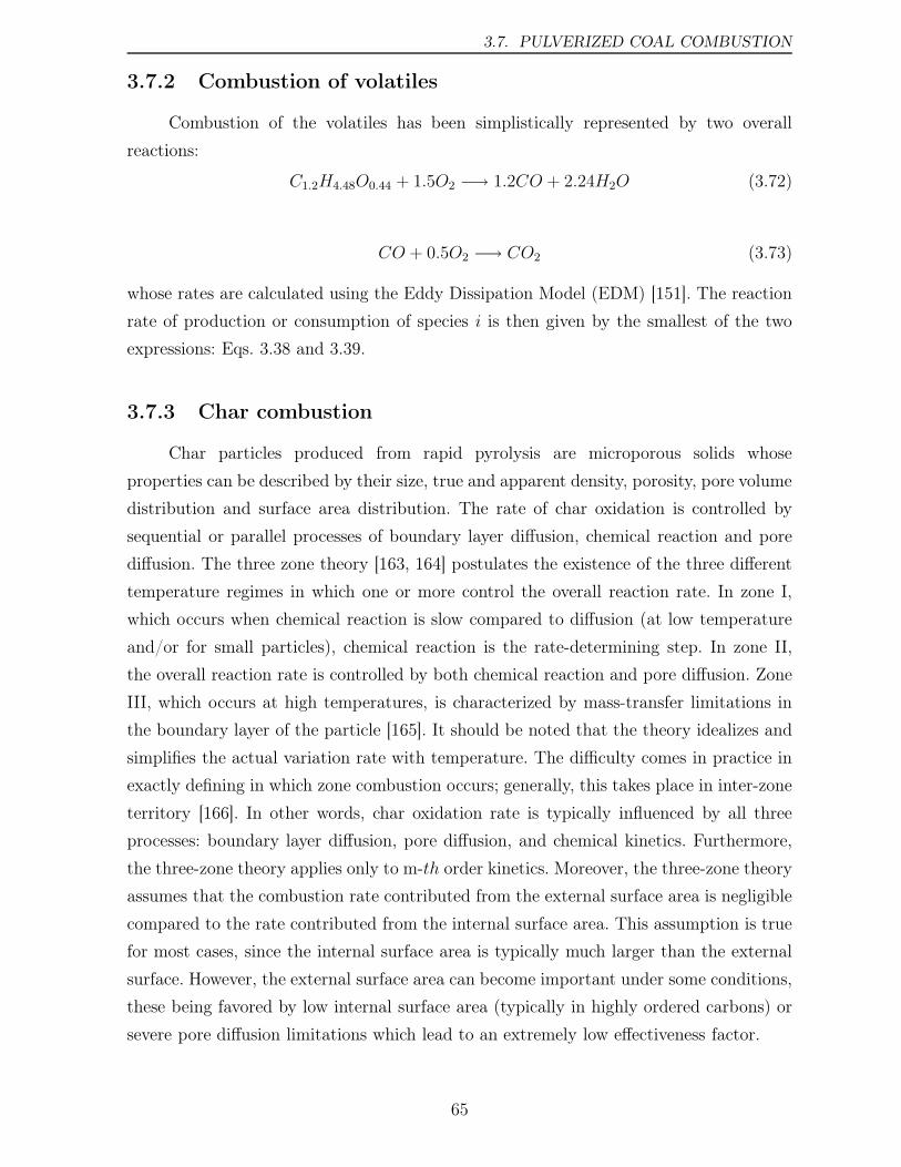
3.7. PULVERIZED COAL COMBUSTION
3.7.2 Combustion of volatiles
Combustion of the volatiles has been simplistically represented by two overall
reactions:
C1.2H4.48O0.44 + 1.5O2 −→ 1.2CO + 2.24H2O (3.72)
CO + 0.5O2 −→ CO2 (3.73)
whose rates are calculated using the Eddy Dissipation Model (EDM) [151]. The reaction
rate of production or consumption of species i is then given by the smallest of the two
expressions: Eqs. 3.38 and 3.39.
3.7.3 Char combustion
Char particles produced from rapid pyrolysis are microporous solids whose
properties can be described by their size, true and apparent density, porosity, pore volume
distribution and surface area distribution. The rate of char oxidation is controlled by
sequential or parallel processes of boundary layer diffusion, chemical reaction and pore
diffusion. The three zone theory [163, 164] postulates the existence of the three different
temperature regimes in which one or more control the overall reaction rate. In zone I,
which occurs when chemical reaction is slow compared to diffusion (at low temperature
and/or for small particles), chemical reaction is the rate-determining step. In zone II,
the overall reaction rate is controlled by both chemical reaction and pore diffusion. Zone
III, which occurs at high temperatures, is characterized by mass-transfer limitations in
the boundary layer of the particle [165]. It should be noted that the theory idealizes and
simplifies the actual variation rate with temperature. The difficulty comes in practice in
exactly defining in which zone combustion occurs; generally, this takes place in inter-zone
territory [166]. In other words, char oxidation rate is typically influenced by all three
processes: boundary layer diffusion, pore diffusion, and chemical kinetics. Furthermore,
the three-zone theory applies only to m-th order kinetics. Moreover, the three-zone theory
assumes that the combustion rate contributed from the external surface area is negligible
compared to the rate contributed from the internal surface area. This assumption is true
for most cases, since the internal surface area is typically much larger than the external
surface. However, the external surface area can become important under some conditions,
these being favored by low internal surface area (typically in highly ordered carbons) or
severe pore diffusion limitations which lead to an extremely low effectiveness factor.
65
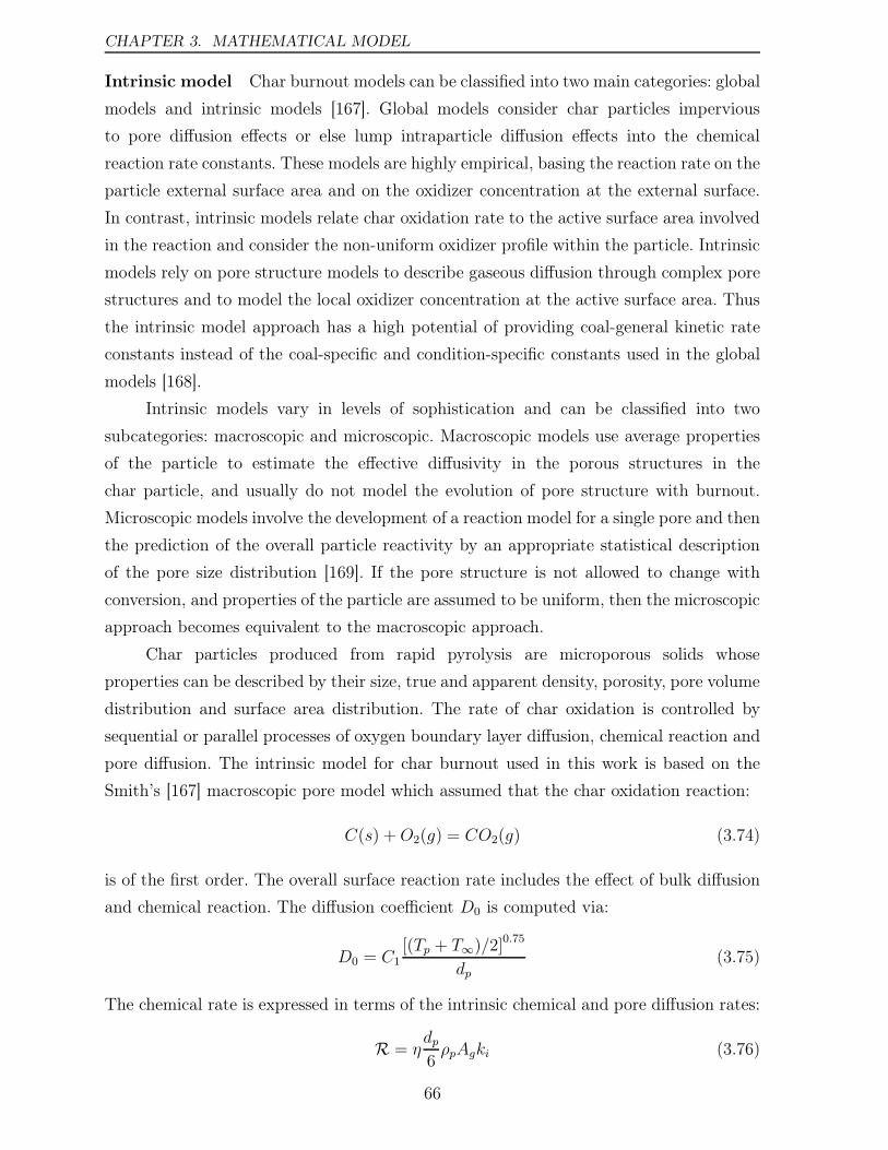
CHAPTER 3. MATHEMATICAL MODEL
Intrinsic model Char burnout models can be classified into two main categories: global
models and intrinsic models [167]. Global models consider char particles impervious
to pore diffusion effects or else lump intraparticle diffusion effects into the chemical
reaction rate constants. These models are highly empirical, basing the reaction rate on the
particle external surface area and on the oxidizer concentration at the external surface.
In contrast, intrinsic models relate char oxidation rate to the active surface area involved
in the reaction and consider the non-uniform oxidizer profile within the particle. Intrinsic
models rely on pore structure models to describe gaseous diffusion through complex pore
structures and to model the local oxidizer concentration at the active surface area. Thus
the intrinsic model approach has a high potential of providing coal-general kinetic rate
constants instead of the coal-specific and condition-specific constants used in the global
models [168].
Intrinsic models vary in levels of sophistication and can be classified into two
subcategories: macroscopic and microscopic. Macroscopic models use average properties
of the particle to estimate the effective diffusivity in the porous structures in the
char particle, and usually do not model the evolution of pore structure with burnout.
Microscopic models involve the development of a reaction model for a single pore and then
the prediction of the overall particle reactivity by an appropriate statistical description
of the pore size distribution [169]. If the pore structure is not allowed to change with
conversion, and properties of the particle are assumed to be uniform, then the microscopic
approach becomes equivalent to the macroscopic approach.
Char particles produced from rapid pyrolysis are microporous solids whose
properties can be described by their size, true and apparent density, porosity, pore volume
distribution and surface area distribution. The rate of char oxidation is controlled by
sequential or parallel processes of oxygen boundary layer diffusion, chemical reaction and
pore diffusion. The intrinsic model for char burnout used in this work is based on the
Smith’s [167] macroscopic pore model which assumed that the char oxidation reaction:
C(s) +O2(g) = CO2(g) (3.74)
is of the first order. The overall surface reaction rate includes the effect of bulk diffusion
and chemical reaction. The diffusion coefficient D0 is computed via:
D0 = C1[(Tp + T∞)/2]
0.75
dp(3.75)
The chemical rate is expressed in terms of the intrinsic chemical and pore diffusion rates:
R = ηdp6ρpAgki (3.76)
66
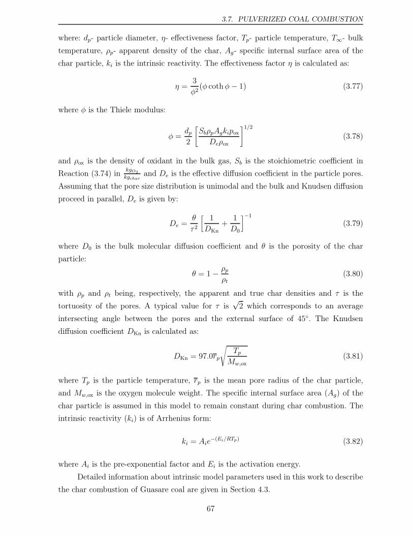
3.7. PULVERIZED COAL COMBUSTION
where: dp- particle diameter, η- effectiveness factor, Tp- particle temperature, T∞- bulk
temperature, ρp- apparent density of the char, Ag- specific internal surface area of the
char particle, ki is the intrinsic reactivity. The effectiveness factor η is calculated as:
η =3
φ2(φ cothφ− 1) (3.77)
where φ is the Thiele modulus:
φ =dp2
[
SbρpAgkipoxDeρox
]1/2
(3.78)
and ρox is the density of oxidant in the bulk gas, Sb is the stoichiometric coefficient in
Reaction (3.74) inkgO2kgchar
and De is the effective diffusion coefficient in the particle pores.
Assuming that the pore size distribution is unimodal and the bulk and Knudsen diffusion
proceed in parallel, De is given by:
De =θ
τ 2
[1
DKn+1
D0
]−1
(3.79)
where D0 is the bulk molecular diffusion coefficient and θ is the porosity of the char
particle:
θ = 1− ρpρt
(3.80)
with ρp and ρt being, respectively, the apparent and true char densities and τ is the
tortuosity of the pores. A typical value for τ is√2 which corresponds to an average
intersecting angle between the pores and the external surface of 45. The Knudsen
diffusion coefficient DKn is calculated as:
DKn = 97.0rp
√
TpMw,ox
(3.81)
where Tp is the particle temperature, rp is the mean pore radius of the char particle,
and Mw,ox is the oxygen molecule weight. The specific internal surface area (Ag) of the
char particle is assumed in this model to remain constant during char combustion. The
intrinsic reactivity (ki) is of Arrhenius form:
ki = Aie−(Ei/RTp) (3.82)
where Ai is the pre-exponential factor and Ei is the activation energy.
Detailed information about intrinsic model parameters used in this work to describe
the char combustion of Guasare coal are given in Section 4.3.
67
CHAPTER 3. MATHEMATICAL MODEL
3.8 Radiative heat transfer
Energy transfer due to radiation is taken into consideration through a source term in
the energy equation. The Radiative Transfer Equation (RTE) for an absorbing, emitting
and scattering medium at position −→r in the direction −→s is:
dI(−→r ,−→s )ds
+ (a+ σs)I(−→r ,−→s ) = an2σT
4
π+σs4π
4π∫
0
I(−→r ,−→s, )Φ(−→s · −→s, )dΩ, (3.83)
where −→r - position vector, −→s - direction vector, −→s ,- scattering direction vector, s- path
length, a- absorption coefficient, n- refractive index, σs- Stefan- Boltzmann constant,
I- radiation intensity, T - local temperature, Φ- phase function, Ω,- solid angle. If the
scattering is neglected (σs = 0) and the gas is assumed to have the refractive index
n = 1, then Eq. 3.83 simplifies notably:
dI(−→r ,−→s )ds
+ aI(−→r ,−→s ) = aσT4
π(3.84)
Discrete Ordinates (DO) [170, 171] radiation model is used to solve radiative heat transfer
equation. The DO radiation model solves the Radiative Transfer Equation (RTE) for a
finite number of discrete solid angles, each associated with a vector direction −→s fixed
in the global Cartesian system (x, y, z). The DO model solves for as many transport
equations as there are directions −→s . When the solution for the RTE is known, the energy
source term for energy equation is calculated using the radiation flux qr:
Srad = −∇qr (3.85)
The absorption coefficient in prescribed a value of 1.5 m−1, see Paragraph 4.3.
3.9 Nitric oxides
In this work the fuel, thermal, prompt and N2O paths as well as NO reburning
have been considered, as shown in Fig. 3.3. The transport equations for nitric oxide
(NO) and for intermediate species (HCN) have been solved while the N2O and N-radical
concentrations are calculated using the partial equilibrium assumption (see below). The
sources for HCN and NO have been calculated averaging the instantaneous source term
(Si = f(T )) over the temperature fluctuations:
〈Si〉 =Tmax∫
T0
P (T )Si(T )dT (3.86)
68
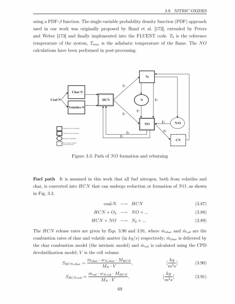
3.9. NITRIC OXIDES
using a PDF-β function. The single-variable probability density function (PDF) approach
used in our work was originally proposed by Hand et al. [172], extended by Peters
and Weber [173] and finally implemented into the FLUENT code. T0 is the reference
temperature of the system, Tmax is the adiabatic temperature of the flame. The NO
calculations have been performed in post-processing.
Figure 3.3: Path of NO formation and reburning
Fuel path It is assumed in this work that all fuel nitrogen, both from volatiles and
char, is converted into HCN that can undergo reduction or formation of NO, as shown
in Fig. 3.3.
coal-N −→ HCN (3.87)
HCN + O2 −→ NO + ... (3.88)
HCN +NO −→ N2 + ... (3.89)
The HCN release rates are given by Eqs. 3.90 and 3.91, where mchar and mvol are the
combustion rates of char and volatile matter (in kg/s) respectively; mchar is delivered by
the char combustion model (the intrinsic model) and mvol is calculated using the CPD
devolatilization model; V is the cell volume.
SHCN,char =mchar · wN,char ·MHCN
MN · V, [
kg
m3s] (3.90)
SHCN,vol =mvol · wN,vol ·MHCN
MN · V, [
kg
m3s] (3.91)
69
CHAPTER 3. MATHEMATICAL MODEL
The HCN depletion rates are given by De Soete [174] expressions:
r1 = k4XHCNXO2exp(−E4RT) · pRT, [
mole
m3s] (3.92)
r2 = k5XHCNXN2exp(−E5RT) · pRT, [
mole
m3s] (3.93)
where: k4 = 3.5 · 1010 1s , k5 = 3.01s , E4 = 280.5 kJmol , E5 = 251.2 kJmol . The instantaneous
source term SHCN reads then:
SHCN = SHCN,vol + SHCN,char − (r1 + r2) ·MHCN · 10−3, [kg
m3s] (3.94)
and is averaged over the temperature fluctuations using Eq. 3.86.
The NO source term from fuel nitrogen is expressed as follows:
SNO,fuel = (r1 − r2) ·MNO · 10−3, [kg
m3s] (3.95)
Prompt path De Soete [174] proposed a roughly estimated chemical reaction rate for
prompt NO formation:
r6 = f · A · [O2]b[N2][CxHy]exp(−EaRT) · V, [
mole
m3s] (3.96)
where the exponent b may vary between 0 and 1, and depends on the conditions in the
flame, namely the local mole fraction of oxygen [O2]:
b =
1.0, [O2] ¬ 4.1 · 10−3
−3.95− 0.9 ln [O2], 4.1 · 10−3 ¬ [O2] ¬ 1.11 · 10−2
−0.35− 0.1 ln [O2], 1.11 · 10−2 < [O2] < 0.030, [O2] 0.03
The constant A and activation energy Ea take the following values: A = 6.4 · 106(RTp)b+1,
Ea = 303.5kJmole
. The prompt factor f accounts for the type of fuel and is calculated in
the following way:
f = 4.75 + 0.0819 · c− 23.21λ+ 32
1
λ2− 12.2 1
λ3
where c is the number of carbon atoms per molecule of fuel and is assumed to be c = 1.2
for the volatile matter of the Guasare coal and λ is the air excess ratio.
The NO source term for prompt path reads then:
SNO,prompt = r6 ·MNO · 10−3, [kg
m3s] (3.97)
70
3.9. NITRIC OXIDES
Thermal path The extended Zeldovich mechanism incorporates the following
reactions:
O +N2k+1,k−1←→ NO +N (3.98)
N +O2k+2,k−2←→ NO +O (3.99)
N +OHk+3,k−3←→ NO +H (3.100)
where k+1, k+2, k+3 stand for the forward and k−1, k−2, k−3 for the backward rate
constants corresponding to Reactions 3.98, 3.99 and 3.100. Under the assumption of
partial equilibrium for N-radical, the NO formation rate can then be calculated as:
r7 = 2k+1[O][N2]1− k−1k−2[NO]2
k+1[N2]k+2[O2]
1 + k−1[NO]k+2[O2]+k+3[OH]
· V, [mole
m3s] (3.101)
The O and OH radical concentrations are calculated by assuming equilibrium of the
following reactions:
O2 +H ←→ OH +O (3.102)
O2 +M ←→ M +O +O (3.103)
Finally, the NO source term for thermal path reads:
SNO,thermal = r7 ·MNO · 10−3, [kg
m3s] (3.104)
N2O path In low temperature combustion (below 1500 K) of lean mixtures of
hydrocarbons (or at pressures higher than the atmospheric) a mechanism, in which the
N2O molecule is the intermediary, becomes important [175]. The concentration of N2O
is assumed to be in a quasi-steady state:
[N2O] =kn1[N2][O][M ] + kn2[NO]
2
(kn2 + kn3)[O] + (kn4 + kn5)[H ](3.105)
Assuming that the N2O is converted to NO the rate of NO formation is:
r8 = 2[N2O] (kn2[O] + kn4[H ]) · V, [mole
m3s] (3.106)
where
[M ] = 1.4 · [O2] + 3.0 · [CO2] + 1.7 · [N2] + 12 · [H2O]
Then, the NO source term for N2O path is calculated as:
SNO,N2O = r8 ·MNO · 10−3, [kg
m3s] (3.107)
71
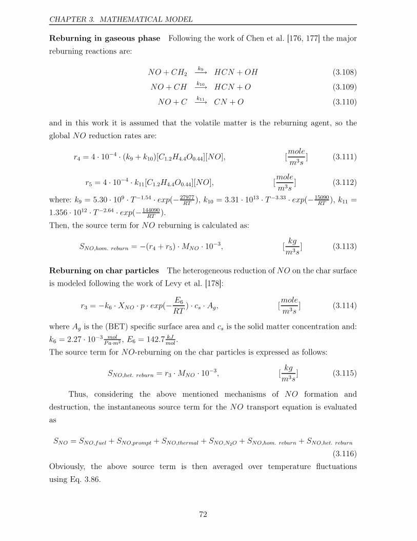
CHAPTER 3. MATHEMATICAL MODEL
Reburning in gaseous phase Following the work of Chen et al. [176, 177] the major
reburning reactions are:
NO + CH2k9−→ HCN +OH (3.108)
NO + CHk10−→ HCN +O (3.109)
NO + Ck11−→ CN +O (3.110)
and in this work it is assumed that the volatile matter is the reburning agent, so the
global NO reduction rates are:
r4 = 4 · 10−4 · (k9 + k10)[C1.2H4.4O0.44][NO], [mole
m3s] (3.111)
r5 = 4 · 10−4 · k11[C1.2H4.4O0.44][NO], [mole
m3s] (3.112)
where: k9 = 5.30 · 109 · T−1.54 · exp(−27977RT ), k10 = 3.31 · 1013 · T−3.33 · exp(−15090RT ), k11 =1.356 · 1012 · T−2.64 · exp(−144090
RT).
Then, the source term for NO reburning is calculated as:
SNO,hom. reburn = −(r4 + r5) ·MNO · 10−3, [kg
m3s] (3.113)
Reburning on char particles The heterogeneous reduction of NO on the char surface
is modeled following the work of Levy et al. [178]:
r3 = −k6 ·XNO · p · exp(−E6RT) · cs · Ag, [
mole
m3s] (3.114)
where Ag is the (BET) specific surface area and cs is the solid matter concentration and:
k6 = 2.27 · 10−3 molPa·m2, E6 = 142.7 kJmol .
The source term for NO-reburning on the char particles is expressed as follows:
SNO,het. reburn = r3 ·MNO · 10−3, [kg
m3s] (3.115)
Thus, considering the above mentioned mechanisms of NO formation and
destruction, the instantaneous source term for the NO transport equation is evaluated
as
SNO = SNO,fuel + SNO,prompt + SNO,thermal + SNO,N2O + SNO,hom. reburn + SNO,het. reburn
(3.116)
Obviously, the above source term is then averaged over temperature fluctuations
using Eq. 3.86.
72
Chapter 4
Model validation
In 1999 the IFRF (International Flame Research Foundation) carried out semi
industrial scale trials called HTAC 99 [64] that revealed a high potential for HTAC
technology also for the combustion of solid fuels. In this Chapter numerical simulations
of pulverized coal flames generated during the IFRF trials are undertaken in order to
examine if the combustion of coal under HTAC conditions can be predicted using the
numerical code. Description of the experimental setup, measurements and validation
procedure of the used sub-models against the IFRF measurements are provided in the
following Sections.
4.1 Experimental equipment
4.1.1 Furnace
The experiments were executed in a refractory lined IFRF furnace No. 1 which
is presented in Fig. 4.1. The furnace has 2 m times 2 m square cross section and its
length is 6.25 m. It consists of 11 water-cooled segments. For each segment the wall
temperatures were monitored using thermocouples located at the top wall and at the side
wall of the furnace. The furnace heat extraction was monitored measuring the volumetric
flow rate and the temperature rise of the cooling water circulating in each segment.
Measurements were carried out using the ports located on both sides of each segment.
A pressure transducer was mounted on segment five to monitor the furnace pressure. In
order to avoid air ingress, the furnace was kept in overpressure.
73
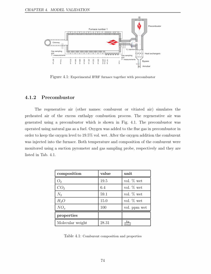
CHAPTER 4. MODEL VALIDATION
Figure 4.1: Experimental IFRF furnace together with precombustor
4.1.2 Precombustor
The regenerative air (other names: comburent or vitiated air) simulates the
preheated air of the excess enthalpy combustion process. The regenerative air was
generated using a precombustor which is shown in Fig. 4.1. The precombustor was
operated using natural gas as a fuel. Oxygen was added to the flue gas in precombustor in
order to keep the oxygen level to 19.5% vol. wet. After the oxygen addition the comburent
was injected into the furnace. Both temperature and composition of the comburent were
monitored using a suction pyrometer and gas sampling probe, respectively and they are
listed in Tab. 4.1.
composition value unit
O2 19.5 vol. % wet
CO2 6.4 vol. % wet
N2 59.1 vol. % wet
H2O 15.0 vol. % wet
NOx 100 vol. ppm wet
properties
Molecular weight 28.31 kgkmol
Table 4.1: Comburent composition and properties
74
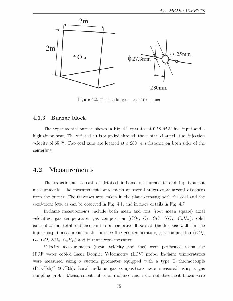
4.2. MEASUREMENTS
27.3mm
280mm
125mm2m
2m
ff
Figure 4.2: The detailed geometry of the burner
4.1.3 Burner block
The experimental burner, shown in Fig. 4.2 operates at 0.58 MW fuel input and a
high air preheat. The vitiated air is supplied through the central channel at an injection
velocity of 65 ms. Two coal guns are located at a 280 mm distance on both sides of the
centerline.
4.2 Measurements
The experiments consist of detailed in-flame measurements and input/output
measurements. The measurements were taken at several traverses at several distances
from the burner. The traverses were taken in the plane crossing both the coal and the
comburent jets, as can be observed in Fig. 4.1, and in more details in Fig. 4.7.
In-flame measurements include both mean and rms (root mean square) axial
velocities, gas temperature, gas composition (CO2, O2, CO, NOx, CnHm), solid
concentration, total radiance and total radiative fluxes at the furnace wall. In the
input/output measurements the furnace flue gas temperature, gas composition (CO2,
O2, CO, NOx, CnHm) and burnout were measured.
Velocity measurements (mean velocity and rms) were performed using the
IFRF water cooled Laser Doppler Velocimetry (LDV) probe. In-flame temperatures
were measured using a suction pyrometer equipped with a type B thermocouple
(Pt6%Rh/Pt30%Rh). Local in-flame gas compositions were measured using a gas
sampling probe. Measurements of total radiance and total radiative heat fluxes were
75
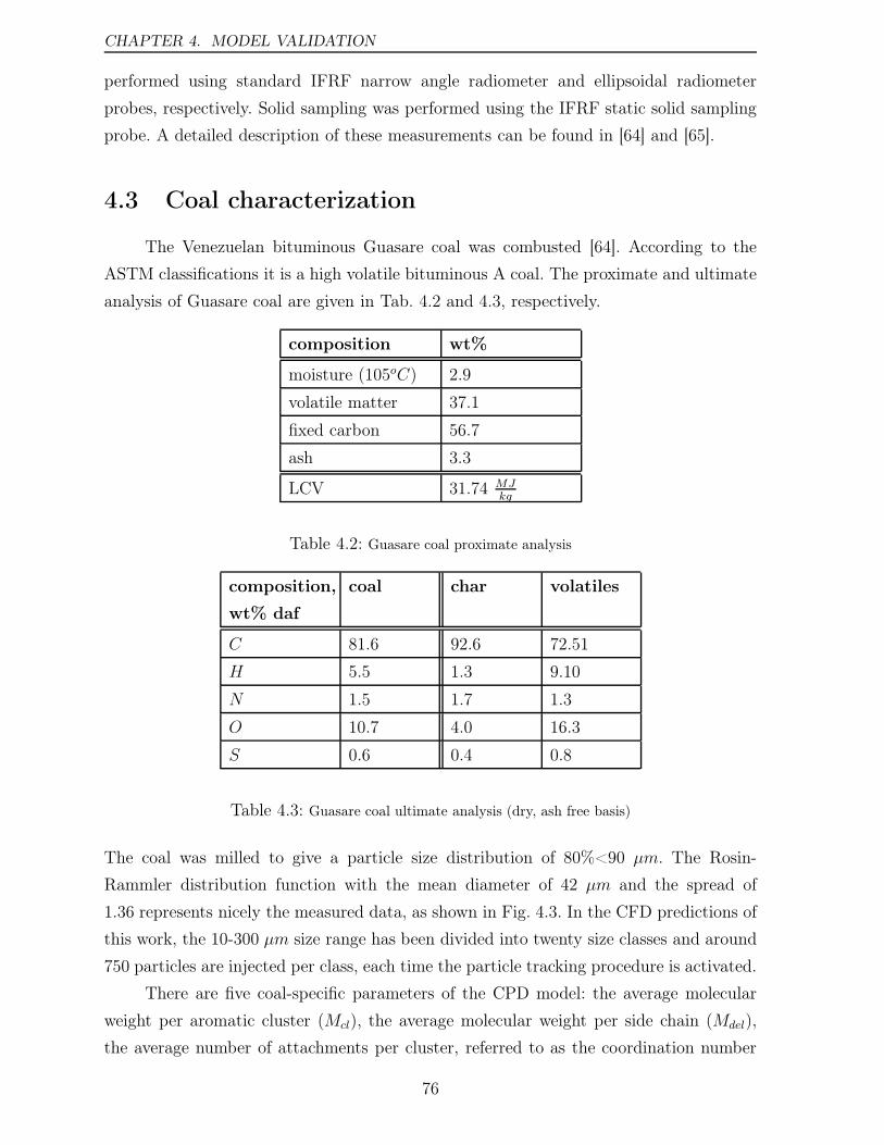
CHAPTER 4. MODEL VALIDATION
performed using standard IFRF narrow angle radiometer and ellipsoidal radiometer
probes, respectively. Solid sampling was performed using the IFRF static solid sampling
probe. A detailed description of these measurements can be found in [64] and [65].
4.3 Coal characterization
The Venezuelan bituminous Guasare coal was combusted [64]. According to the
ASTM classifications it is a high volatile bituminous A coal. The proximate and ultimate
analysis of Guasare coal are given in Tab. 4.2 and 4.3, respectively.
composition wt%
moisture (105oC) 2.9
volatile matter 37.1
fixed carbon 56.7
ash 3.3
LCV 31.74 MJkg
Table 4.2: Guasare coal proximate analysis
composition,
wt% daf
coal char volatiles
C 81.6 92.6 72.51
H 5.5 1.3 9.10
N 1.5 1.7 1.3
O 10.7 4.0 16.3
S 0.6 0.4 0.8
Table 4.3: Guasare coal ultimate analysis (dry, ash free basis)
The coal was milled to give a particle size distribution of 80%<90 µm. The Rosin-
Rammler distribution function with the mean diameter of 42 µm and the spread of
1.36 represents nicely the measured data, as shown in Fig. 4.3. In the CFD predictions of
this work, the 10-300 µm size range has been divided into twenty size classes and around
750 particles are injected per class, each time the particle tracking procedure is activated.
There are five coal-specific parameters of the CPD model: the average molecular
weight per aromatic cluster (Mcl), the average molecular weight per side chain (Mdel),
the average number of attachments per cluster, referred to as the coordination number
76
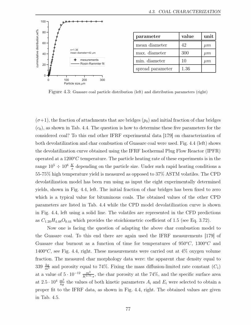
4.3. COAL CHARACTERIZATION
0 100 200 300
Particle size,mm
0
20
40
60
80
100
cum
mula
tive
dis
trib
ution,w
t%
mesurements
Rosin-Rammler fit
n=1.36
mean diameter=42 mm
parameter value unit
mean diameter 42 µm
max. diameter 300 µm
min. diameter 10 µm
spread parameter 1.36
Figure 4.3: Guasare coal particle distribution (left) and distribution parameters (right)
(σ+1), the fraction of attachments that are bridges (p0) and initial fraction of char bridges
(c0), as shown in Tab. 4.4. The question is how to determine these five parameters for the
considered coal? To this end other IFRF experimental data [179] on characterization of
both devolatilization and char combustion of Guasare coal were used. Fig. 4.4 (left) shows
the devolatilization curve obtained using the IFRF Isothermal Plug Flow Reactor (IPFR)
operated at a 1200oC temperature. The particle heating rate of these experiments is in the
range 105 ÷ 106 Ks
depending on the particle size. Under such rapid heating conditions a
55-75% high temperature yield is measured as opposed to 37% ASTM volatiles. The CPD
devolatilization model has been run using as input the eight experimentally determined
yields, shown in Fig. 4.4, left. The initial fraction of char bridges has been fixed to zero
which is a typical value for bituminous coals. The obtained values of the other CPD
parameters are listed in Tab. 4.4 while the CPD model devolatilization curve is shown
in Fig. 4.4, left using a solid line. The volatiles are represented in the CFD predictions
as C1.20H4.48O0.44 which provides the stoichiometric coefficient of 1.5 (see Eq. 3.72).
Now one is facing the question of adapting the above char combustion model to
the Guasare coal. To this end there are again used the IFRF measurements [179] of
Guasare char burnout as a function of time for temperatures of 950oC, 1300oC and
1400oC, see Fig. 4.4, right. These measurements were carried out at 4% oxygen volume
fraction. The measured char morphology data were: the apparent char density equal to
339 kgm3
and porosity equal to 74%. Fixing the mass diffusion-limited rate constant (C1)
at a value of 5 · 10−12 m3
K0.75·s, the char porosity at the 74%, and the specific surface area
at 2.5 · 104 m2kg
the values of both kinetic parameters Ai and Ei were selected to obtain a
proper fit to the IFRF data, as shown in Fig. 4.4, right. The obtained values are given
in Tab. 4.5.
77
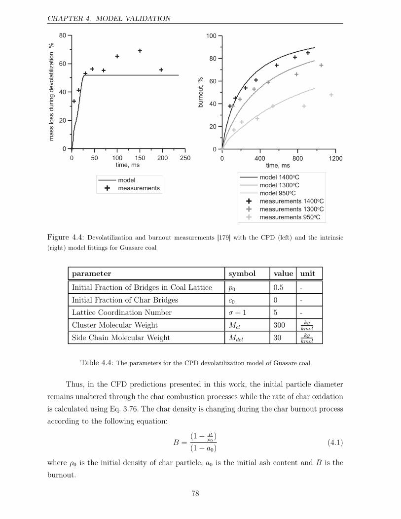
CHAPTER 4. MODEL VALIDATION
0 50 100 150 200 250time, ms
0
20
40
60
80
mass
loss
during
devola
tiliz
ation,
%
model
measurements
0 400 800 1200time, ms
0
20
40
60
80
100
burn
out,
%
model 1400oC
model 1300oC
model 950oC
measurements 1400oC
measurements 1300oC
measurements 950oC
Figure 4.4: Devolatilization and burnout measurements [179] with the CPD (left) and the intrinsic
(right) model fittings for Guasare coal
parameter symbol value unit
Initial Fraction of Bridges in Coal Lattice p0 0.5 -
Initial Fraction of Char Bridges c0 0 -
Lattice Coordination Number σ + 1 5 -
Cluster Molecular Weight Mcl 300 kgkmol
Side Chain Molecular Weight Mdel 30 kgkmol
Table 4.4: The parameters for the CPD devolatilization model of Guasare coal
Thus, in the CFD predictions presented in this work, the initial particle diameter
remains unaltered through the char combustion processes while the rate of char oxidation
is calculated using Eq. 3.76. The char density is changing during the char burnout process
according to the following equation:
B =(1− ρ
ρ0)
(1− a0)(4.1)
where ρ0 is the initial density of char particle, a0 is the initial ash content and B is the
burnout.
78
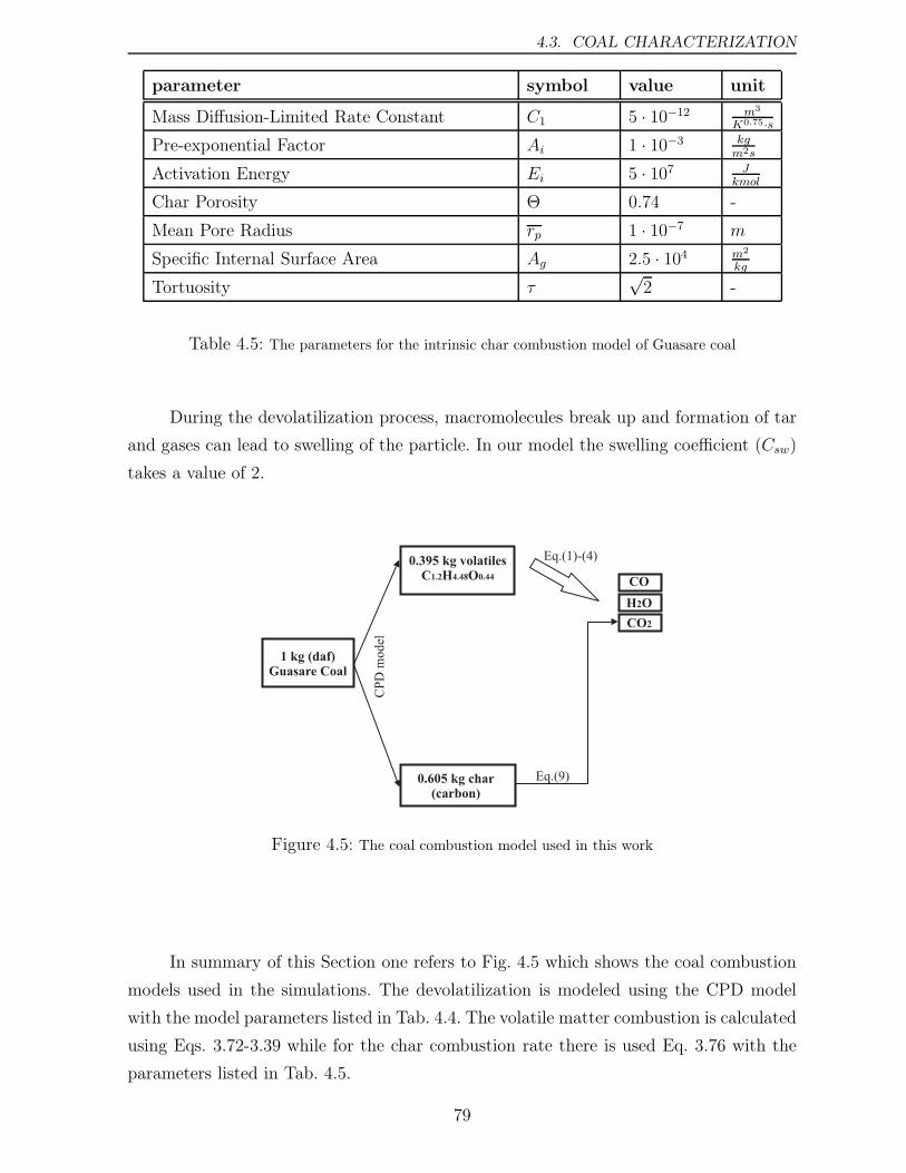
4.3. COAL CHARACTERIZATION
parameter symbol value unit
Mass Diffusion-Limited Rate Constant C1 5 · 10−12 m3
K0.75·s
Pre-exponential Factor Ai 1 · 10−3 kgm2s
Activation Energy Ei 5 · 107 Jkmol
Char Porosity Θ 0.74 -
Mean Pore Radius rp 1 · 10−7 m
Specific Internal Surface Area Ag 2.5 · 104 m2
kg
Tortuosity τ√2 -
Table 4.5: The parameters for the intrinsic char combustion model of Guasare coal
During the devolatilization process, macromolecules break up and formation of tar
and gases can lead to swelling of the particle. In our model the swelling coefficient (Csw)
takes a value of 2.
Figure 4.5: The coal combustion model used in this work
In summary of this Section one refers to Fig. 4.5 which shows the coal combustion
models used in the simulations. The devolatilization is modeled using the CPD model
with the model parameters listed in Tab. 4.4. The volatile matter combustion is calculated
using Eqs. 3.72-3.39 while for the char combustion rate there is used Eq. 3.76 with the
parameters listed in Tab. 4.5.
79
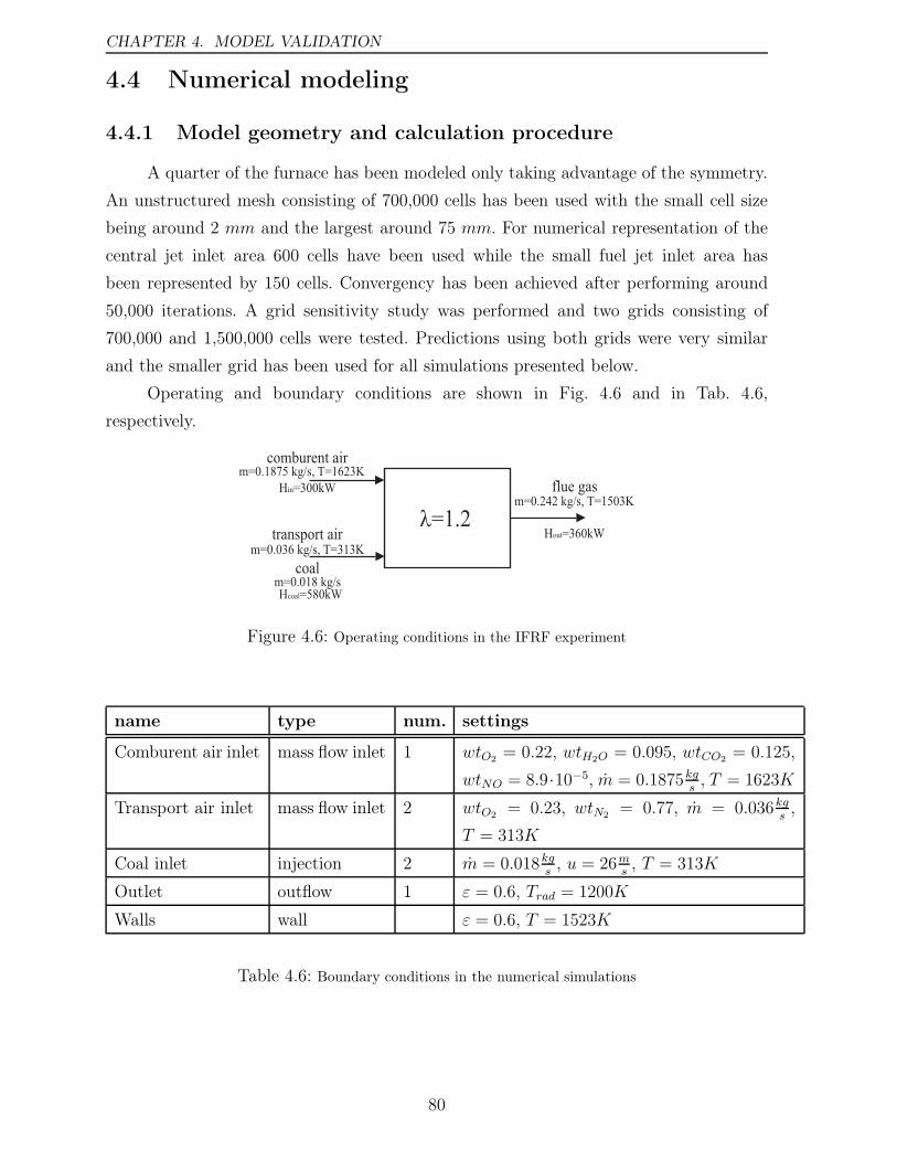
CHAPTER 4. MODEL VALIDATION
4.4 Numerical modeling
4.4.1 Model geometry and calculation procedure
A quarter of the furnace has been modeled only taking advantage of the symmetry.
An unstructured mesh consisting of 700,000 cells has been used with the small cell size
being around 2 mm and the largest around 75 mm. For numerical representation of the
central jet inlet area 600 cells have been used while the small fuel jet inlet area has
been represented by 150 cells. Convergency has been achieved after performing around
50,000 iterations. A grid sensitivity study was performed and two grids consisting of
700,000 and 1,500,000 cells were tested. Predictions using both grids were very similar
and the smaller grid has been used for all simulations presented below.
Operating and boundary conditions are shown in Fig. 4.6 and in Tab. 4.6,
respectively.
comburent air
transport air
m=0.1875 kg/s, T=1623K
coal
m=0.036 kg/s, T=313K
m=0.018 kg/s
l=1.2
flue gasH =300kWin
H =580kWcoal
m=0.242 kg/s, T=1503K
H =360kWout
Figure 4.6: Operating conditions in the IFRF experiment
name type num. settings
Comburent air inlet mass flow inlet 1 wtO2 = 0.22, wtH2O = 0.095, wtCO2 = 0.125,
wtNO = 8.9·10−5, m = 0.1875kgs , T = 1623K
Transport air inlet mass flow inlet 2 wtO2 = 0.23, wtN2 = 0.77, m = 0.036kgs,
T = 313K
Coal inlet injection 2 m = 0.018kgs, u = 26m
s, T = 313K
Outlet outflow 1 ε = 0.6, Trad = 1200K
Walls wall ε = 0.6, T = 1523K
Table 4.6: Boundary conditions in the numerical simulations
80
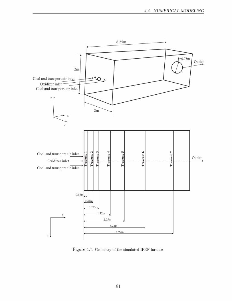
4.4. NUMERICAL MODELING
6.25m
y
x
z
2m
2m
Outlet
x
z
0.15m
0.44m
0.735m
1.32m
2.05m
3.22m
4.97m
Tra
ver
se 1
Tra
ver
se 2
Tra
ver
se 3
Tra
ver
se 4
Tra
ver
se 5
Tra
ver
se 6
Tra
ver
se 7
Outlet
Coal and transport air inlet
Oxidizer inlet
Coal and transport air inlet
Coal and transport air inlet
Oxidizer inlet
Coal and transport air inlet
f=0.75m
Figure 4.7: Geometry of the simulated IFRF furnace
81
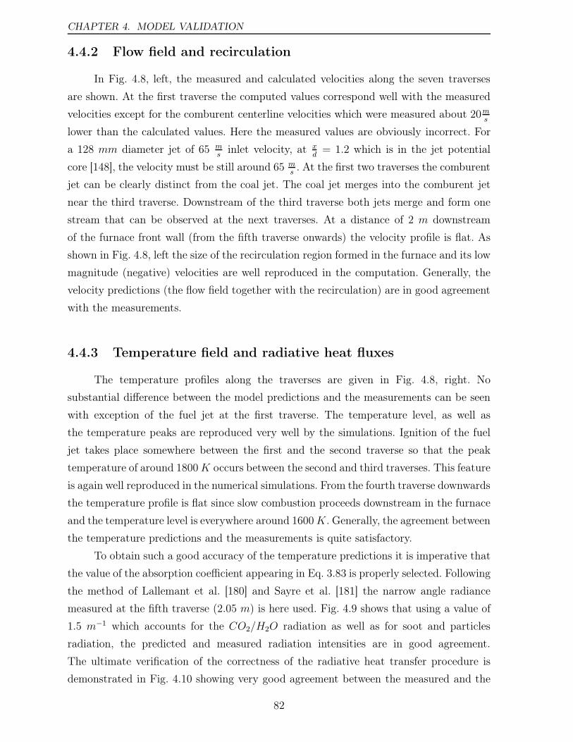
CHAPTER 4. MODEL VALIDATION
4.4.2 Flow field and recirculation
In Fig. 4.8, left, the measured and calculated velocities along the seven traverses
are shown. At the first traverse the computed values correspond well with the measured
velocities except for the comburent centerline velocities which were measured about 20ms
lower than the calculated values. Here the measured values are obviously incorrect. For
a 128 mm diameter jet of 65 ms
inlet velocity, at xd= 1.2 which is in the jet potential
core [148], the velocity must be still around 65 ms. At the first two traverses the comburent
jet can be clearly distinct from the coal jet. The coal jet merges into the comburent jet
near the third traverse. Downstream of the third traverse both jets merge and form one
stream that can be observed at the next traverses. At a distance of 2 m downstream
of the furnace front wall (from the fifth traverse onwards) the velocity profile is flat. As
shown in Fig. 4.8, left the size of the recirculation region formed in the furnace and its low
magnitude (negative) velocities are well reproduced in the computation. Generally, the
velocity predictions (the flow field together with the recirculation) are in good agreement
with the measurements.
4.4.3 Temperature field and radiative heat fluxes
The temperature profiles along the traverses are given in Fig. 4.8, right. No
substantial difference between the model predictions and the measurements can be seen
with exception of the fuel jet at the first traverse. The temperature level, as well as
the temperature peaks are reproduced very well by the simulations. Ignition of the fuel
jet takes place somewhere between the first and the second traverse so that the peak
temperature of around 1800K occurs between the second and third traverses. This feature
is again well reproduced in the numerical simulations. From the fourth traverse downwards
the temperature profile is flat since slow combustion proceeds downstream in the furnace
and the temperature level is everywhere around 1600K. Generally, the agreement between
the temperature predictions and the measurements is quite satisfactory.
To obtain such a good accuracy of the temperature predictions it is imperative that
the value of the absorption coefficient appearing in Eq. 3.83 is properly selected. Following
the method of Lallemant et al. [180] and Sayre et al. [181] the narrow angle radiance
measured at the fifth traverse (2.05 m) is here used. Fig. 4.9 shows that using a value of
1.5 m−1 which accounts for the CO2/H2O radiation as well as for soot and particles
radiation, the predicted and measured radiation intensities are in good agreement.
The ultimate verification of the correctness of the radiative heat transfer procedure is
demonstrated in Fig. 4.10 showing very good agreement between the measured and the
82
4.4. NUMERICAL MODELING
0 0.2 0.4 0.6 0.8 1
z-distance, m
0
20
40
60
velo
cit
y,m
/s
Traverse 1
0 0.2 0.4 0.6 0.8 1
0
20
40
60
velo
cit
y,m
/s
Traverse 2
0 0.2 0.4 0.6 0.8 1
0
20
40
60
velo
cit
y,m
/s
Traverse 3
measurements
simulation
0 0.2 0.4 0.6 0.8 1
0
20
40
60
velo
cit
y,m
/s
Traverse 4
0 0.2 0.4 0.6 0.8 1
z-distance, m
0
20
40
60
80
Traverse 50 0.2 0.4 0.6 0.8 1
0
20
40
60
Traverse 6
0 0.2 0.4 0.6 0.8 1
0
20
40
60
Traverse 7
0 0.2 0.4 0.6 0.8 1
z-distance, m
800
1200
1600
tem
pera
ture
,K
Traverse 1
0 0.2 0.4 0.6 0.8 1
800
1200
1600
tem
pera
ture
,K
Traverse 2
0 0.2 0.4 0.6 0.8 1
800
1200
1600
tem
pera
ture
,K
Traverse 3
measurements
simulation
0 0.2 0.4 0.6 0.8 1
800
1200
1600
tem
pera
ture
,K
Traverse 4
0 0.2 0.4 0.6 0.8 1
z-distance, m
800
1200
1600
Traverse 5
0 0.2 0.4 0.6 0.8 1
800
1200
1600
Traverse 6
0 0.2 0.4 0.6 0.8 1
800
1200
1600
Traverse 7
Figure 4.8: Velocity (left) and temperature (right) profiles along the measurement traverses. The
measured values taken from [64]. For location of the measurement traverses see Fig. 4.7
predicted total incident heat flux at the furnace wall. Flatness and high values of the
radiative heat flux are characteristics of HTAC combustion [62, 61].
4.4.4 Oxygen and carbon dioxide concentrations
In Fig. 4.11, left, the profiles of oxygen concentration are shown. No major
differences between the measurements and calculated values can be observed. However,
the oxygen concentrations near the coal nozzle are too low in comparison with the
experimental values which is consistent with the temperature predictions in this region,
see Fig. 4.8, right. It is interesting to note that the same model deficiency was already
observed in numerical simulations of the natural gas combustion [61] and it was related to
inaccurate predictions of the entrainment of the fuel jet [107]. Downstream of the fourth
traverse the oxygen concentration is uniform and practically everywhere in the furnace
83
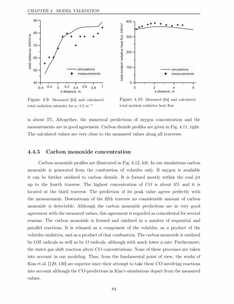
CHAPTER 4. MODEL VALIDATION
Figure 4.9: Measured [64] and calculated
total radiation intensity for a=1.5 m−1
Figure 4.10: Measured [64] and calculated
total incident radiative heat flux
is about 3%. Altogether, the numerical predictions of oxygen concentration and the
measurements are in good agreement. Carbon dioxide profiles are given in Fig. 4.11, right.
The calculated values are very close to the measured values along all traverses.
4.4.5 Carbon monoxide concentration
Carbon monoxide profiles are illustrated in Fig. 4.12, left. In our simulations carbon
monoxide is generated from the combustion of volatiles only. If oxygen is available
it can be further oxidized to carbon dioxide. It is formed mostly within the coal jet
up to the fourth traverse. The highest concentration of CO is about 6% and it is
located at the third traverse. The prediction of its peak value agrees perfectly with
the measurement. Downstream of the fifth traverse no considerable amount of carbon
monoxide is detectable. Although the carbon monoxide predictions are in very good
agreement with the measured values, this agreement is regarded as coincidental for several
reasons. The carbon monoxide is formed and oxidized in a number of sequential and
parallel reactions. It is released as a component of the volatiles, as a product of the
volatiles oxidation, and as a product of char combustion. The carbon monoxide is oxidized
by OH radicals as well as by O radicals, although with much lower a rate. Furthermore,
the water gas shift reaction alters CO concentrations. None of these processes are taken
into account in our modeling. Thus, from the fundamental point of view, the works of
Kim et al. [129, 130] are superior since their attempt to take these CO-involving reactions
into account although the CO-predictions in Kim’s simulations depart from the measured
values.
84
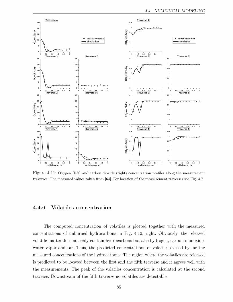
4.4. NUMERICAL MODELING
0 0.2 0.4 0.6 0.8 1
z-distance, m
0
5
10
15
20
25
O2,v
ol.
%d
ry
Traverse 10 0.2 0.4 0.6 0.8 1
0
5
10
15
20
25
O2,v
ol.
%d
ry
Traverse 20 0.2 0.4 0.6 0.8 1
0
5
10
15
20
25
O2,v
ol.
%d
ry
Traverse 3
measurements
simulation
0 0.2 0.4 0.6 0.8 1
0
5
10
15
20
25
O2,v
ol.
%d
ry
Traverse 4
0 0.2 0.4 0.6 0.8 1
z-distance, m
0
5
10
15
20
25
Traverse 50 0.2 0.4 0.6 0.8 1
0
5
10
15
20
25
Traverse 60 0.2 0.4 0.6 0.8 1
0
5
10
15
20
25
Traverse 7
0 0.2 0.4 0.6 0.8 1
z-distance, m
0
10
20
30
CO
2,v
ol.
%d
ry
Traverse 10 0.2 0.4 0.6 0.8 1
0
10
20
30
CO
2,v
ol.
%d
ry
Traverse 20 0.2 0.4 0.6 0.8 1
0
10
20
30
CO
2,v
ol.
%d
ry
Traverse 3
measurements
simulation
0 0.2 0.4 0.6 0.8 1
0
10
20
30
CO
2,v
ol.
%d
ry
Traverse 4
0 0.2 0.4 0.6 0.8 1
z-distance, m
0
10
20
30
Traverse 50 0.2 0.4 0.6 0.8 1
0
10
20
30
Traverse 60 0.2 0.4 0.6 0.8 1
0
10
20
30
Traverse 7
Figure 4.11: Oxygen (left) and carbon dioxide (right) concentration profiles along the measurement
traverses. The measured values taken from [64]. For location of the measurement traverses see Fig. 4.7
4.4.6 Volatiles concentration
The computed concentration of volatiles is plotted together with the measured
concentrations of unburned hydrocarbons in Fig. 4.12, right. Obviously, the released
volatile matter does not only contain hydrocarbons but also hydrogen, carbon monoxide,
water vapor and tar. Thus, the predicted concentrations of volatiles exceed by far the
measured concentrations of the hydrocarbons. The region where the volatiles are released
is predicted to be located between the first and the fifth traverse and it agrees well with
the measurements. The peak of the volatiles concentration is calculated at the second
traverse. Downstream of the fifth traverse no volatiles are detectable.
85
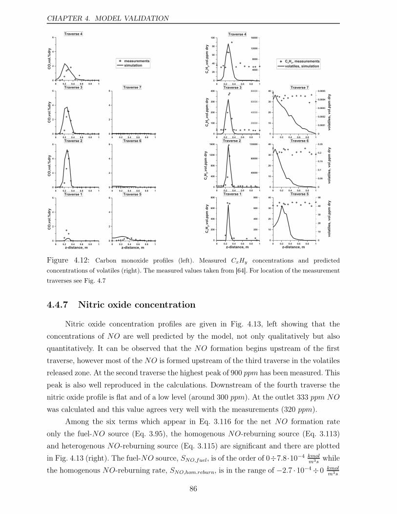
CHAPTER 4. MODEL VALIDATION
0 0.2 0.4 0.6 0.8 1
z-distance, m
0
2
4
6
CO
,vo
l.%
dry
Traverse 10 0.2 0.4 0.6 0.8 1
0
2
4
6
CO
,vo
l.%
dry
Traverse 20 0.2 0.4 0.6 0.8 1
0
2
4
6
CO
,vo
l.%
dry
Traverse 3
measurements
simulation
0 0.2 0.4 0.6 0.8 1
0
2
4
6
CO
,vo
l.%
dry
Traverse 4
0 0.2 0.4 0.6 0.8 1
z-distance, m
0
2
4
6
Traverse 50 0.2 0.4 0.6 0.8 1
0
2
4
6
Traverse 60 0.2 0.4 0.6 0.8 1
0
2
4
6
Traverse 7
Figure 4.12: Carbon monoxide profiles (left). Measured CxHy concentrations and predicted
concentrations of volatiles (right). The measured values taken from [64]. For location of the measurement
traverses see Fig. 4.7
4.4.7 Nitric oxide concentration
Nitric oxide concentration profiles are given in Fig. 4.13, left showing that the
concentrations of NO are well predicted by the model, not only qualitatively but also
quantitatively. It can be observed that the NO formation begins upstream of the first
traverse, however most of the NO is formed upstream of the third traverse in the volatiles
released zone. At the second traverse the highest peak of 900 ppm has been measured. This
peak is also well reproduced in the calculations. Downstream of the fourth traverse the
nitric oxide profile is flat and of a low level (around 300 ppm). At the outlet 333 ppm NO
was calculated and this value agrees very well with the measurements (320 ppm).
Among the six terms which appear in Eq. 3.116 for the net NO formation rate
only the fuel-NO source (Eq. 3.95), the homogenous NO-reburning source (Eq. 3.113)
and heterogenous NO-reburning source (Eq. 3.115) are significant and there are plotted
in Fig. 4.13 (right). The fuel-NO source, SNO,fuel, is of the order of 0÷7.8·10−4 kmolm3s
while
the homogenous NO-reburning rate, SNO,hom.reburn, is in the range of −2.7 · 10−4÷0 kmolm3s
86
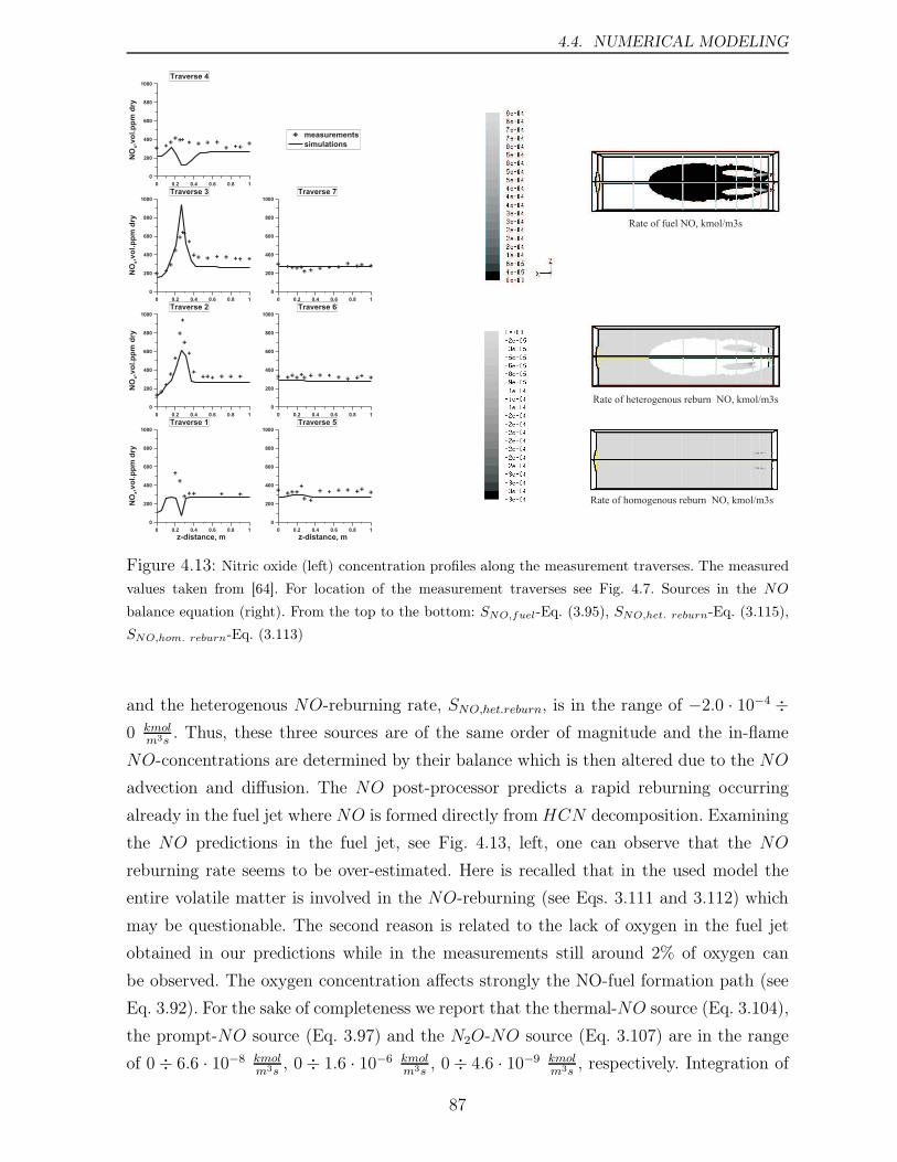
4.4. NUMERICAL MODELING
0 0.2 0.4 0.6 0.8 1
z-distance, m
0
200
400
600
800
1000
NO
x,v
ol.p
pm
dry
Traverse 10 0.2 0.4 0.6 0.8 1
0
200
400
600
800
1000
NO
x,v
ol.p
pm
dry
Traverse 20 0.2 0.4 0.6 0.8 1
0
200
400
600
800
1000
NO
x,v
ol.p
pm
dry
Traverse 3
measurements
simulations
0 0.2 0.4 0.6 0.8 1
0
200
400
600
800
1000
NO
x,v
ol.
pp
md
ry
Traverse 4
0 0.2 0.4 0.6 0.8 1
z-distance, m
0
200
400
600
800
1000
Traverse 50 0.2 0.4 0.6 0.8 1
0
200
400
600
800
1000
Traverse 60 0.2 0.4 0.6 0.8 1
0
200
400
600
800
1000
Traverse 7
Figure 4.13: Nitric oxide (left) concentration profiles along the measurement traverses. The measured
values taken from [64]. For location of the measurement traverses see Fig. 4.7. Sources in the NO
balance equation (right). From the top to the bottom: SNO,fuel-Eq. (3.95), SNO,het. reburn-Eq. (3.115),
SNO,hom. reburn-Eq. (3.113)
and the heterogenous NO-reburning rate, SNO,het.reburn, is in the range of −2.0 · 10−4 ÷0 kmolm3s
. Thus, these three sources are of the same order of magnitude and the in-flame
NO-concentrations are determined by their balance which is then altered due to the NO
advection and diffusion. The NO post-processor predicts a rapid reburning occurring
already in the fuel jet where NO is formed directly fromHCN decomposition. Examining
the NO predictions in the fuel jet, see Fig. 4.13, left, one can observe that the NO
reburning rate seems to be over-estimated. Here is recalled that in the used model the
entire volatile matter is involved in the NO-reburning (see Eqs. 3.111 and 3.112) which
may be questionable. The second reason is related to the lack of oxygen in the fuel jet
obtained in our predictions while in the measurements still around 2% of oxygen can
be observed. The oxygen concentration affects strongly the NO-fuel formation path (see
Eq. 3.92). For the sake of completeness we report that the thermal-NO source (Eq. 3.104),
the prompt-NO source (Eq. 3.97) and the N2O-NO source (Eq. 3.107) are in the range
of 0÷ 6.6 · 10−8 kmolm3s
, 0÷ 1.6 · 10−6 kmolm3s
, 0÷ 4.6 · 10−9 kmolm3s
, respectively. Integration of
87
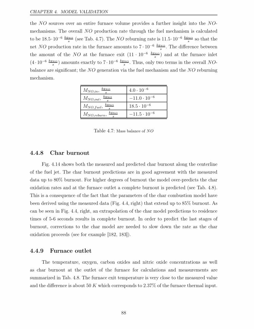
CHAPTER 4. MODEL VALIDATION
the NO sources over an entire furnace volume provides a further insight into the NO-
mechanisms. The overall NO production rate through the fuel mechanism is calculated
to be 18.5 ·10−6 kgNOs
(see Tab. 4.7). The NO reburning rate is 11.5 ·10−6 kgNOs
so that the
net NO production rate in the furnace amounts to 7 · 10−6 kgNOs
. The difference between
the amount of the NO at the furnace exit (11 · 10−6 kgNOs
) and at the furnace inlet
(4 · 10−6 kgNOs
) amounts exactly to 7 · 10−6 kgNOs
. Thus, only two terms in the overall NO-
balance are significant; the NO generation via the fuel mechanism and the NO reburning
mechanism.
MNO,in,kgNOs
4.0 · 10−6
MNO,out,kgNOs
−11.0 · 10−6
MNO,fuel,kgNOs
18.5 · 10−6
MNO,reburn,kgNOs
−11.5 · 10−6
Table 4.7: Mass balance of NO
4.4.8 Char burnout
Fig. 4.14 shows both the measured and predicted char burnout along the centerline
of the fuel jet. The char burnout predictions are in good agreement with the measured
data up to 80% burnout. For higher degrees of burnout the model over-predicts the char
oxidation rates and at the furnace outlet a complete burnout is predicted (see Tab. 4.8).
This is a consequence of the fact that the parameters of the char combustion model have
been derived using the measured data (Fig. 4.4, right) that extend up to 85% burnout. As
can be seen in Fig. 4.4, right, an extrapolation of the char model predictions to residence
times of 5-6 seconds results in complete burnout. In order to predict the last stages of
burnout, corrections to the char model are needed to slow down the rate as the char
oxidation proceeds (see for example [182, 183]).
4.4.9 Furnace outlet
The temperature, oxygen, carbon oxides and nitric oxide concentrations as well
as char burnout at the outlet of the furnace for calculations and measurements are
summarized in Tab. 4.8. The furnace exit temperature is very close to the measured value
and the difference is about 50K which corresponds to 2.37% of the furnace thermal input.
88
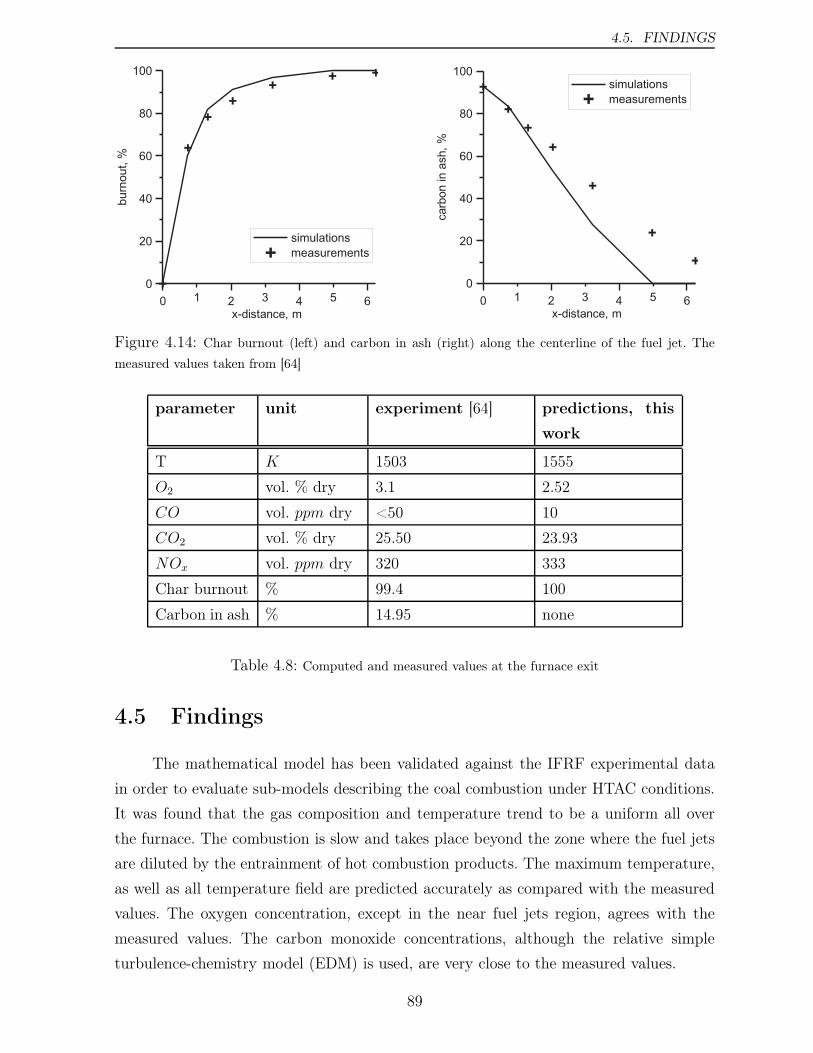
4.5. FINDINGS
Figure 4.14: Char burnout (left) and carbon in ash (right) along the centerline of the fuel jet. The
measured values taken from [64]
parameter unit experiment [64] predictions, this
work
T K 1503 1555
O2 vol. % dry 3.1 2.52
CO vol. ppm dry <50 10
CO2 vol. % dry 25.50 23.93
NOx vol. ppm dry 320 333
Char burnout % 99.4 100
Carbon in ash % 14.95 none
Table 4.8: Computed and measured values at the furnace exit
4.5 Findings
The mathematical model has been validated against the IFRF experimental data
in order to evaluate sub-models describing the coal combustion under HTAC conditions.
It was found that the gas composition and temperature trend to be a uniform all over
the furnace. The combustion is slow and takes place beyond the zone where the fuel jets
are diluted by the entrainment of hot combustion products. The maximum temperature,
as well as all temperature field are predicted accurately as compared with the measured
values. The oxygen concentration, except in the near fuel jets region, agrees with the
measured values. The carbon monoxide concentrations, although the relative simple
turbulence-chemistry model (EDM) is used, are very close to the measured values.
89
CHAPTER 4. MODEL VALIDATION
Prior to performing the numerical simulations of HTAC 99 trials, substantial efforts
have been allocated to an accurate modeling of combustion of Guasare coal which was
used in the IFRF experiments. To this end both the Chemical Percolation Devolatilization
(CPD) model and the char combustion intrinsic reactivity model have been tuned to
represent the coal in question. To ensure accurate predictions of radiative transfer an
appropriate value of the local absorption coefficient appearing in the Radiative Heat
Transfer equation has been derived using the measured data. Subsequently performed
numerical simulations of the HTAC 99 experiments have demonstrated that the CFD
FLUENT code predicted both the in-furnace measured data and the furnace exit
parameters with good accuracy. Such a validated model has then been used in the boiler
design studies.
90
Chapter 5
Design of the HTAC boiler
HTAC combustion process is different from conventional combustion. Therefore
there is a need for an innovative design of boilers utilizing this technology. Several
particular boiler concepts have been analyzed in the context of the following three
key points: existence of an intensive in-furnace recirculation, homogeneity of both the
temperature and the chemical species fields, and uniformity of heat fluxes.
The Venezuelan bituminous Guasare coal is used as fuel in all the simulations. Its
composition and parameters are reported in Tab. 4.2 and 4.3 (see Section 4.3). The set of
mathematical sub-models representing combustion of this coal is given in Chapter 4. A
hypothetical 130 MWth ultra-supercritical boiler producing 20 kgs
steam at parameters:
pressure equal to 30 MPa and temperature up to 700 oC has been developed. The
combustion air is preheated to 1200 K. The boiler is operated at air excess ratio of 1.2.
In this Chapter several simulations have been performed in order to find the shape of
the boiler and its dimensions, to optimize both the distance between burners and location
of the burner block. Results obtained by the numerical modeling of analyzed boilers are
presented and discussed in the following Sections. At the end of each Section the findings
are briefly summarized.
5.1 Shape of the HTAC boiler
To the best of author’s knowledge, no research on HTAC technology application to
power station PC boilers has been carried out, with the aim of developing a completely
new configuration of the boiler (see Section for details 2.6). In this thesis a new approach
is presented. In contrast to previous investigations on boilers operating under HTAC
conditions, in this work it is claimed that the key point of the HTAC technology
implementation in power boilers is an original construction of the entire combustion
91
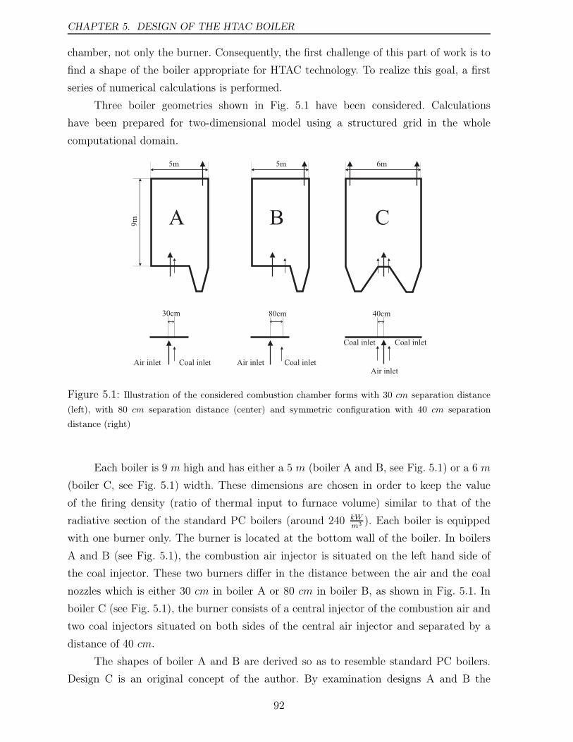
CHAPTER 5. DESIGN OF THE HTAC BOILER
chamber, not only the burner. Consequently, the first challenge of this part of work is to
find a shape of the boiler appropriate for HTAC technology. To realize this goal, a first
series of numerical calculations is performed.
Three boiler geometries shown in Fig. 5.1 have been considered. Calculations
have been prepared for two-dimensional model using a structured grid in the whole
computational domain.
Figure 5.1: Illustration of the considered combustion chamber forms with 30 cm separation distance
(left), with 80 cm separation distance (center) and symmetric configuration with 40 cm separation
distance (right)
Each boiler is 9 m high and has either a 5 m (boiler A and B, see Fig. 5.1) or a 6 m
(boiler C, see Fig. 5.1) width. These dimensions are chosen in order to keep the value
of the firing density (ratio of thermal input to furnace volume) similar to that of the
radiative section of the standard PC boilers (around 240 kWm3
). Each boiler is equipped
with one burner only. The burner is located at the bottom wall of the boiler. In boilers
A and B (see Fig. 5.1), the combustion air injector is situated on the left hand side of
the coal injector. These two burners differ in the distance between the air and the coal
nozzles which is either 30 cm in boiler A or 80 cm in boiler B, as shown in Fig. 5.1. In
boiler C (see Fig. 5.1), the burner consists of a central injector of the combustion air and
two coal injectors situated on both sides of the central air injector and separated by a
distance of 40 cm.
The shapes of boiler A and B are derived so as to resemble standard PC boilers.
Design C is an original concept of the author. By examination designs A and B the
92
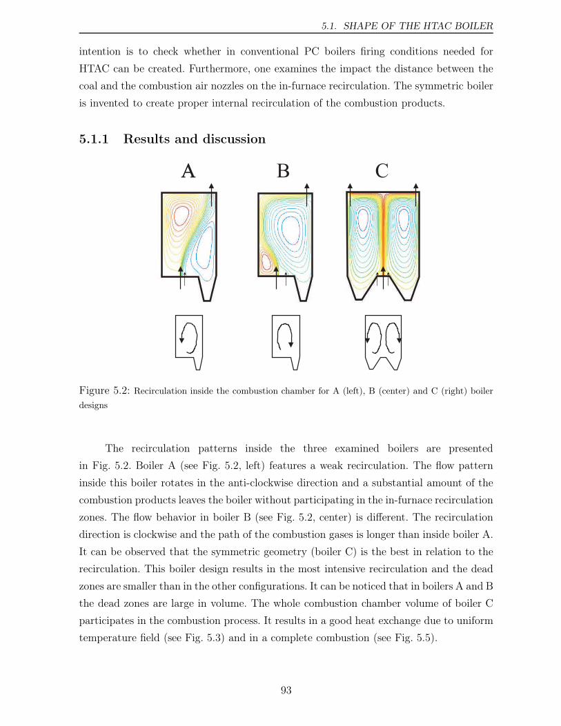
5.1. SHAPE OF THE HTAC BOILER
intention is to check whether in conventional PC boilers firing conditions needed for
HTAC can be created. Furthermore, one examines the impact the distance between the
coal and the combustion air nozzles on the in-furnace recirculation. The symmetric boiler
is invented to create proper internal recirculation of the combustion products.
5.1.1 Results and discussion
Figure 5.2: Recirculation inside the combustion chamber for A (left), B (center) and C (right) boiler
designs
The recirculation patterns inside the three examined boilers are presented
in Fig. 5.2. Boiler A (see Fig. 5.2, left) features a weak recirculation. The flow pattern
inside this boiler rotates in the anti-clockwise direction and a substantial amount of the
combustion products leaves the boiler without participating in the in-furnace recirculation
zones. The flow behavior in boiler B (see Fig. 5.2, center) is different. The recirculation
direction is clockwise and the path of the combustion gases is longer than inside boiler A.
It can be observed that the symmetric geometry (boiler C) is the best in relation to the
recirculation. This boiler design results in the most intensive recirculation and the dead
zones are smaller than in the other configurations. It can be noticed that in boilers A and B
the dead zones are large in volume. The whole combustion chamber volume of boiler C
participates in the combustion process. It results in a good heat exchange due to uniform
temperature field (see Fig. 5.3) and in a complete combustion (see Fig. 5.5).
93
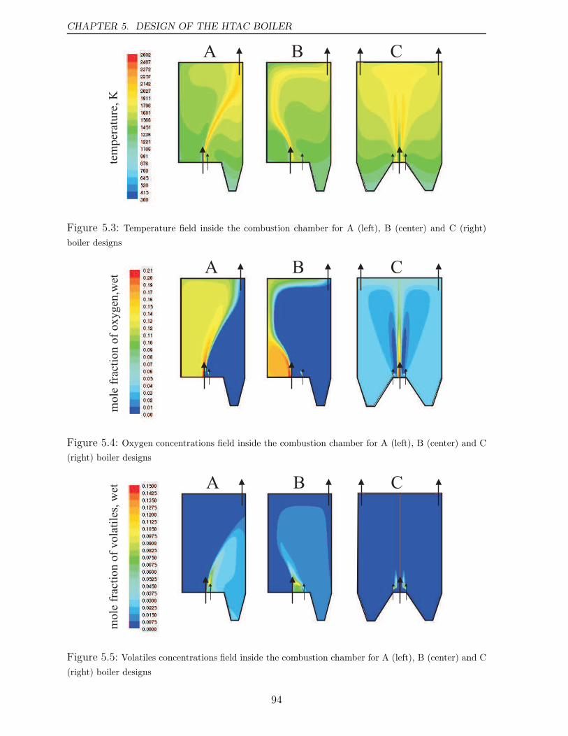
CHAPTER 5. DESIGN OF THE HTAC BOILER
Figure 5.3: Temperature field inside the combustion chamber for A (left), B (center) and C (right)
boiler designs
Figure 5.4: Oxygen concentrations field inside the combustion chamber for A (left), B (center) and C
(right) boiler designs
Figure 5.5: Volatiles concentrations field inside the combustion chamber for A (left), B (center) and C
(right) boiler designs
94
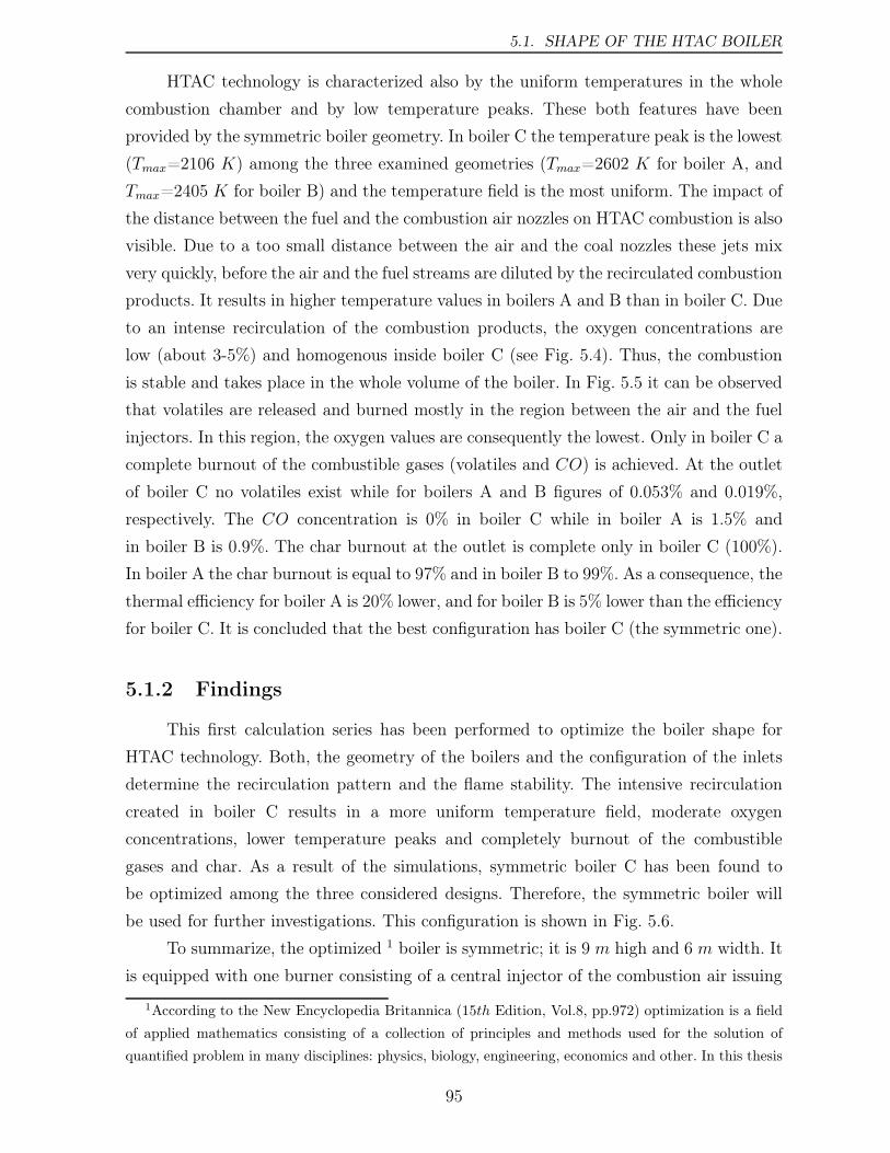
5.1. SHAPE OF THE HTAC BOILER
HTAC technology is characterized also by the uniform temperatures in the whole
combustion chamber and by low temperature peaks. These both features have been
provided by the symmetric boiler geometry. In boiler C the temperature peak is the lowest
(Tmax=2106 K) among the three examined geometries (Tmax=2602 K for boiler A, and
Tmax=2405 K for boiler B) and the temperature field is the most uniform. The impact of
the distance between the fuel and the combustion air nozzles on HTAC combustion is also
visible. Due to a too small distance between the air and the coal nozzles these jets mix
very quickly, before the air and the fuel streams are diluted by the recirculated combustion
products. It results in higher temperature values in boilers A and B than in boiler C. Due
to an intense recirculation of the combustion products, the oxygen concentrations are
low (about 3-5%) and homogenous inside boiler C (see Fig. 5.4). Thus, the combustion
is stable and takes place in the whole volume of the boiler. In Fig. 5.5 it can be observed
that volatiles are released and burned mostly in the region between the air and the fuel
injectors. In this region, the oxygen values are consequently the lowest. Only in boiler C a
complete burnout of the combustible gases (volatiles and CO) is achieved. At the outlet
of boiler C no volatiles exist while for boilers A and B figures of 0.053% and 0.019%,
respectively. The CO concentration is 0% in boiler C while in boiler A is 1.5% and
in boiler B is 0.9%. The char burnout at the outlet is complete only in boiler C (100%).
In boiler A the char burnout is equal to 97% and in boiler B to 99%. As a consequence, the
thermal efficiency for boiler A is 20% lower, and for boiler B is 5% lower than the efficiency
for boiler C. It is concluded that the best configuration has boiler C (the symmetric one).
5.1.2 Findings
This first calculation series has been performed to optimize the boiler shape for
HTAC technology. Both, the geometry of the boilers and the configuration of the inlets
determine the recirculation pattern and the flame stability. The intensive recirculation
created in boiler C results in a more uniform temperature field, moderate oxygen
concentrations, lower temperature peaks and completely burnout of the combustible
gases and char. As a result of the simulations, symmetric boiler C has been found to
be optimized among the three considered designs. Therefore, the symmetric boiler will
be used for further investigations. This configuration is shown in Fig. 5.6.
To summarize, the optimized 1 boiler is symmetric; it is 9 m high and 6 m width. It
is equipped with one burner consisting of a central injector of the combustion air issuing
1According to the New Encyclopedia Britannica (15th Edition, Vol.8, pp.972) optimization is a field
of applied mathematics consisting of a collection of principles and methods used for the solution of
quantified problem in many disciplines: physics, biology, engineering, economics and other. In this thesis
95
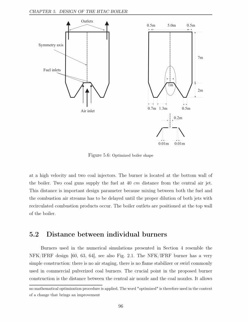
CHAPTER 5. DESIGN OF THE HTAC BOILER
0.5m 5.0m 0.5m
7m
2m
0.7m 1.3m 0.5m
0.01m
1m
0.01m
0.2m
Outlets
Symmetry axis
Fuel inlets
Air inlet
Figure 5.6: Optimized boiler shape
at a high velocity and two coal injectors. The burner is located at the bottom wall of
the boiler. Two coal guns supply the fuel at 40 cm distance from the central air jet.
This distance is important design parameter because mixing between both the fuel and
the combustion air streams has to be delayed until the proper dilution of both jets with
recirculated combustion products occur. The boiler outlets are positioned at the top wall
of the boiler.
5.2 Distance between individual burners
Burners used in the numerical simulations presented in Section 4 resemble the
NFK/IFRF design [60, 63, 64], see also Fig. 2.1. The NFK/IFRF burner has a very
simple construction: there is no air staging, there is no flame stabilizer or swirl commonly
used in commercial pulverized coal burners. The crucial point in the proposed burner
construction is the distance between the central air nozzle and the coal nozzles. It allows
no mathematical optimization procedure is applied. The word "optimized" is therefore used in the context
of a change that brings an improvement
96
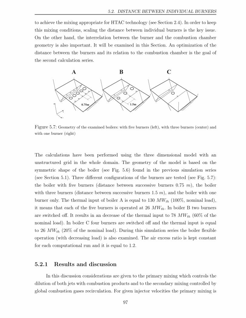
5.2. DISTANCE BETWEEN INDIVIDUAL BURNERS
to achieve the mixing appropriate for HTAC technology (see Section 2.4). In order to keep
this mixing conditions, scaling the distance between individual burners is the key issue.
On the other hand, the interrelation between the burner and the combustion chamber
geometry is also important. It will be examined in this Section. An optimization of the
distance between the burners and its relation to the combustion chamber is the goal of
the second calculation series.
Figure 5.7: Geometry of the examined boilers: with five burners (left), with three burners (center) and
with one burner (right)
The calculations have been performed using the three dimensional model with an
unstructured grid in the whole domain. The geometry of the model is based on the
symmetric shape of the boiler (see Fig. 5.6) found in the previous simulation series
(see Section 5.1). Three different configurations of the burners are tested (see Fig. 5.7):
the boiler with five burners (distance between successive burners 0.75 m), the boiler
with three burners (distance between successive burners 1.5 m), and the boiler with one
burner only. The thermal input of boiler A is equal to 130 MWth (100%, nominal load),
it means that each of the five burners is operated at 26 MWth. In boiler B two burners
are switched off. It results in an decrease of the thermal input to 78 MWth (60% of the
nominal load). In boiler C four burners are switched off and the thermal input is equal
to 26 MWth (20% of the nominal load). During this simulation series the boiler flexible
operation (with decreasing load) is also examined. The air excess ratio is kept constant
for each computational run and it is equal to 1.2.
5.2.1 Results and discussion
In this discussion considerations are given to the primary mixing which controls the
dilution of both jets with combustion products and to the secondary mixing controlled by
global combustion gases recirculation. For given injector velocities the primary mixing is
97
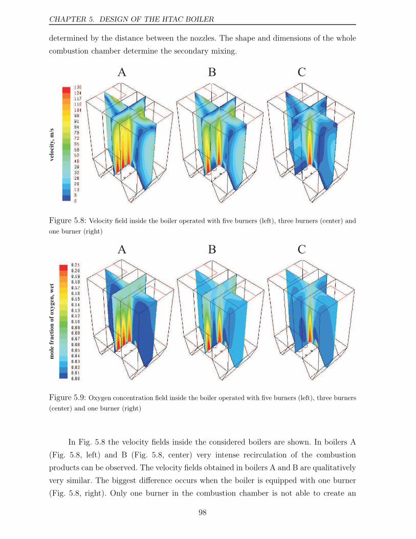
CHAPTER 5. DESIGN OF THE HTAC BOILER
determined by the distance between the nozzles. The shape and dimensions of the whole
combustion chamber determine the secondary mixing.
Figure 5.8: Velocity field inside the boiler operated with five burners (left), three burners (center) and
one burner (right)
Figure 5.9: Oxygen concentration field inside the boiler operated with five burners (left), three burners
(center) and one burner (right)
In Fig. 5.8 the velocity fields inside the considered boilers are shown. In boilers A
(Fig. 5.8, left) and B (Fig. 5.8, center) very intense recirculation of the combustion
products can be observed. The velocity fields obtained in boilers A and B are qualitatively
very similar. The biggest difference occurs when the boiler is equipped with one burner
(Fig. 5.8, right). Only one burner in the combustion chamber is not able to create an
98

5.2. DISTANCE BETWEEN INDIVIDUAL BURNERS
intense mixing conditions. There are several regions where there is almost no movement
(the velocity is zero) and the insufficient mixing of the combustion products inside the
chamber occurs. As a consequence, the uniformity of both the temperature and the species
concentration fields disappear (see Fig. 5.9, right).
Although in boilers A and B the global recirculation works correctly, problems
with the air and fuel streams dilution (and subsequently with the low and uniform
oxygen concentration) seem to occur. In boiler A there is not enough space between the
neighboring burners to ensure the correct dilution of both the air and the fuel streams
with combustion products in y-symmetry plane. The entrainment works correctly only
in the x-symmetry (due to a sufficient separation between the air and coal nozzles).
In the considered boiler, y-symmetry plane cuts through the combustion air inlets,
and x-symmetry plane cuts through the central burner, perpendicularly to the y-
symmetry plane. The oxygen concentration fields are presented in Fig. 5.9. The oxygen
concentrations in boiler A are in some regions near zero and in some regions around 12%.
These are too large variations as for HTAC technology. As mentioned above, the desired
oxygen concentration in HTAC combustion process is about 3-5% in the whole chamber.
This substantial non-uniformity in the oxygen concentration of boiler A makes this design
unsuitable for HTAC.
5.2.2 Findings
The second calculation series has been carried out in order to optimize distance
between single burners. This distance affects the mixing conditions inside the boiler,
especially of the air and the fuel jets dilution with the combustion products. The single
burner boiler produces unsatisfactory global recirculation while the boiler with five
burners features wrong entrainment conditions. Therefore for further investigations the
burner spacing of 1.5 m is chosen and five burners are still used in order to keep the
assumed thermal input of 130 MWth. This arrangement results in an increase of the
boiler depth up to 6 m. Summarizing, as a result of these calculations the optimized
distance between successive burners was found and it will be used in the forthcoming
simulations.
The performance of the HTAC boiler under partially load conditions has been also
examined. Operation with varies loads is very important for power station boilers because
of the continuously changing demand for steam. It would be optimal if the boiler could
rapidly responde to variations in power demand. In the present simulation series three
values of the load were tested: 130MWth- the nominal load (100%), 78MWth- 60% of the
nominal load and 26 MWth- 20% of the nominal load. The conclusion is that the HTAC
99
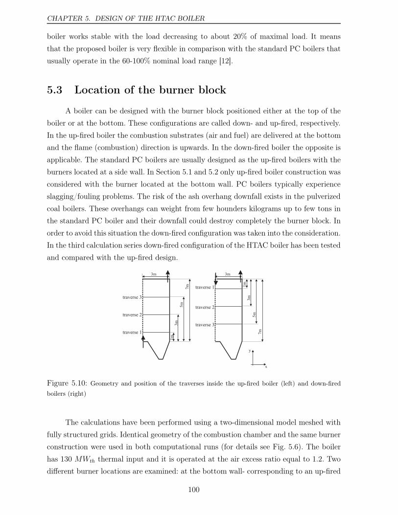
CHAPTER 5. DESIGN OF THE HTAC BOILER
boiler works stable with the load decreasing to about 20% of maximal load. It means
that the proposed boiler is very flexible in comparison with the standard PC boilers that
usually operate in the 60-100% nominal load range [12].
5.3 Location of the burner block
A boiler can be designed with the burner block positioned either at the top of the
boiler or at the bottom. These configurations are called down- and up-fired, respectively.
In the up-fired boiler the combustion substrates (air and fuel) are delivered at the bottom
and the flame (combustion) direction is upwards. In the down-fired boiler the opposite is
applicable. The standard PC boilers are usually designed as the up-fired boilers with the
burners located at a side wall. In Section 5.1 and 5.2 only up-fired boiler construction was
considered with the burner located at the bottom wall. PC boilers typically experience
slagging/fouling problems. The risk of the ash overhang downfall exists in the pulverized
coal boilers. These overhangs can weight from few hounders kilograms up to few tons in
the standard PC boiler and their downfall could destroy completely the burner block. In
order to avoid this situation the down-fired configuration was taken into the consideration.
In the third calculation series down-fired configuration of the HTAC boiler has been tested
and compared with the up-fired design.
traverse 3
traverse 1
traverse 2
3m
1m
3m
5m
7m
traverse 3
traverse 2
traverse 1
3m
7m
5m
3m
1m
y
x
Figure 5.10: Geometry and position of the traverses inside the up-fired boiler (left) and down-fired
boilers (right)
The calculations have been performed using a two-dimensional model meshed with
fully structured grids. Identical geometry of the combustion chamber and the same burner
construction were used in both computational runs (for details see Fig. 5.6). The boiler
has 130 MWth thermal input and it is operated at the air excess ratio equal to 1.2. Two
different burner locations are examined: at the bottom wall- corresponding to an up-fired
100
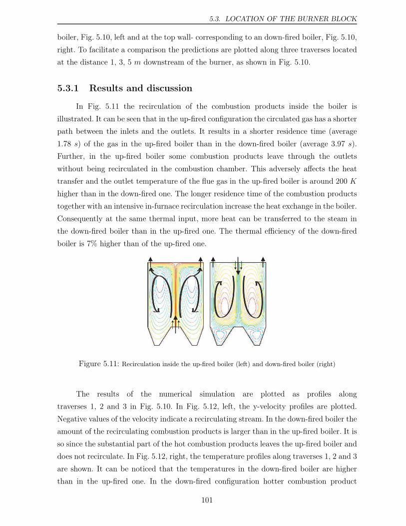
5.3. LOCATION OF THE BURNER BLOCK
boiler, Fig. 5.10, left and at the top wall- corresponding to an down-fired boiler, Fig. 5.10,
right. To facilitate a comparison the predictions are plotted along three traverses located
at the distance 1, 3, 5 m downstream of the burner, as shown in Fig. 5.10.
5.3.1 Results and discussion
In Fig. 5.11 the recirculation of the combustion products inside the boiler is
illustrated. It can be seen that in the up-fired configuration the circulated gas has a shorter
path between the inlets and the outlets. It results in a shorter residence time (average
1.78 s) of the gas in the up-fired boiler than in the down-fired boiler (average 3.97 s).
Further, in the up-fired boiler some combustion products leave through the outlets
without being recirculated in the combustion chamber. This adversely affects the heat
transfer and the outlet temperature of the flue gas in the up-fired boiler is around 200 K
higher than in the down-fired one. The longer residence time of the combustion products
together with an intensive in-furnace recirculation increase the heat exchange in the boiler.
Consequently at the same thermal input, more heat can be transferred to the steam in
the down-fired boiler than in the up-fired one. The thermal efficiency of the down-fired
boiler is 7% higher than of the up-fired one.
Figure 5.11: Recirculation inside the up-fired boiler (left) and down-fired boiler (right)
The results of the numerical simulation are plotted as profiles along
traverses 1, 2 and 3 in Fig. 5.10. In Fig. 5.12, left, the y-velocity profiles are plotted.
Negative values of the velocity indicate a recirculating stream. In the down-fired boiler the
amount of the recirculating combustion products is larger than in the up-fired boiler. It is
so since the substantial part of the hot combustion products leaves the up-fired boiler and
does not recirculate. In Fig. 5.12, right, the temperature profiles along traverses 1, 2 and 3
are shown. It can be noticed that the temperatures in the down-fired boiler are higher
than in the up-fired one. In the down-fired configuration hotter combustion product
101
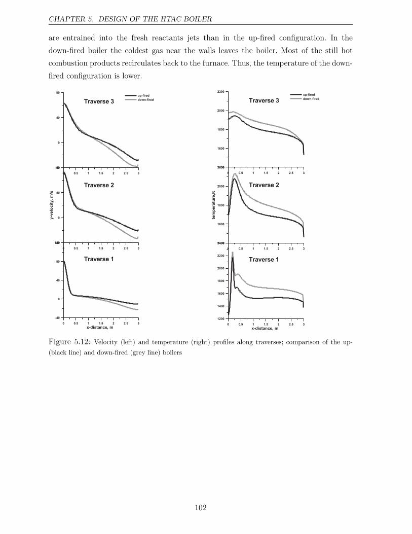
CHAPTER 5. DESIGN OF THE HTAC BOILER
are entrained into the fresh reactants jets than in the up-fired configuration. In the
down-fired boiler the coldest gas near the walls leaves the boiler. Most of the still hot
combustion products recirculates back to the furnace. Thus, the temperature of the down-
fired configuration is lower.
Figure 5.12: Velocity (left) and temperature (right) profiles along traverses; comparison of the up-
(black line) and down-fired (grey line) boilers
102
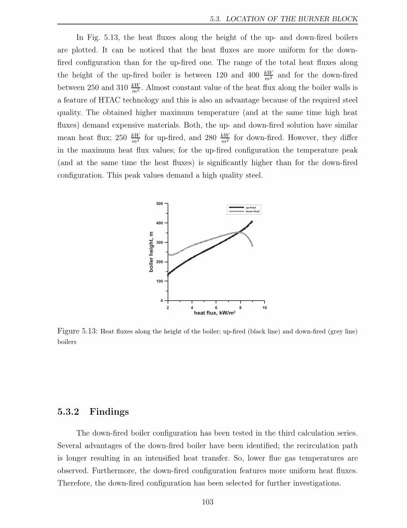
5.3. LOCATION OF THE BURNER BLOCK
In Fig. 5.13, the heat fluxes along the height of the up- and down-fired boilers
are plotted. It can be noticed that the heat fluxes are more uniform for the down-
fired configuration than for the up-fired one. The range of the total heat fluxes along
the height of the up-fired boiler is between 120 and 400 kWm2
and for the down-fired
between 250 and 310 kWm2
. Almost constant value of the heat flux along the boiler walls is
a feature of HTAC technology and this is also an advantage because of the required steel
quality. The obtained higher maximum temperature (and at the same time high heat
fluxes) demand expensive materials. Both, the up- and down-fired solution have similar
mean heat flux; 250 kWm2
for up-fired, and 280 kWm2
for down-fired. However, they differ
in the maximum heat flux values; for the up-fired configuration the temperature peak
(and at the same time the heat fluxes) is significantly higher than for the down-fired
configuration. This peak values demand a high quality steel.
Figure 5.13: Heat fluxes along the height of the boiler; up-fired (black line) and down-fired (grey line)
boilers
5.3.2 Findings
The down-fired boiler configuration has been tested in the third calculation series.
Several advantages of the down-fired boiler have been identified; the recirculation path
is longer resulting in an intensified heat transfer. So, lower flue gas temperatures are
observed. Furthermore, the down-fired configuration features more uniform heat fluxes.
Therefore, the down-fired configuration has been selected for further investigations.
103
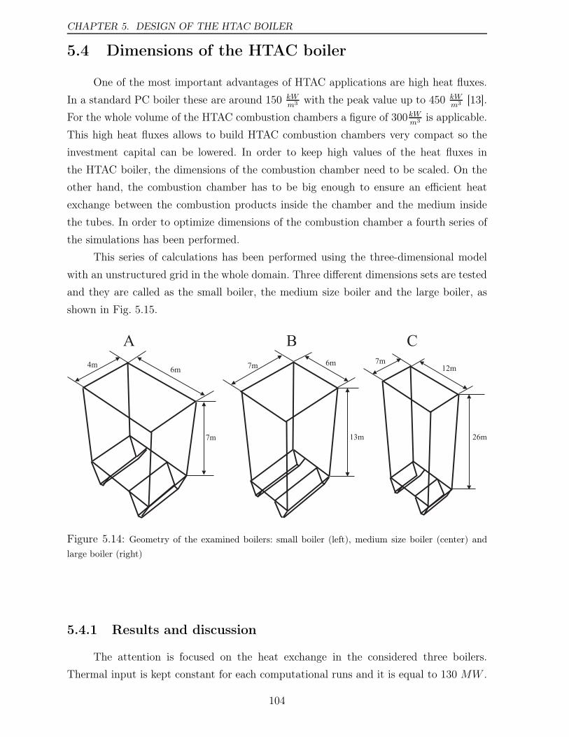
CHAPTER 5. DESIGN OF THE HTAC BOILER
5.4 Dimensions of the HTAC boiler
One of the most important advantages of HTAC applications are high heat fluxes.
In a standard PC boiler these are around 150 kWm3
with the peak value up to 450 kWm3
[13].
For the whole volume of the HTAC combustion chambers a figure of 300kWm3
is applicable.
This high heat fluxes allows to build HTAC combustion chambers very compact so the
investment capital can be lowered. In order to keep high values of the heat fluxes in
the HTAC boiler, the dimensions of the combustion chamber need to be scaled. On the
other hand, the combustion chamber has to be big enough to ensure an efficient heat
exchange between the combustion products inside the chamber and the medium inside
the tubes. In order to optimize dimensions of the combustion chamber a fourth series of
the simulations has been performed.
This series of calculations has been performed using the three-dimensional model
with an unstructured grid in the whole domain. Three different dimensions sets are tested
and they are called as the small boiler, the medium size boiler and the large boiler, as
shown in Fig. 5.15.
Figure 5.14: Geometry of the examined boilers: small boiler (left), medium size boiler (center) and
large boiler (right)
5.4.1 Results and discussion
The attention is focused on the heat exchange in the considered three boilers.
Thermal input is kept constant for each computational runs and it is equal to 130 MW .
104
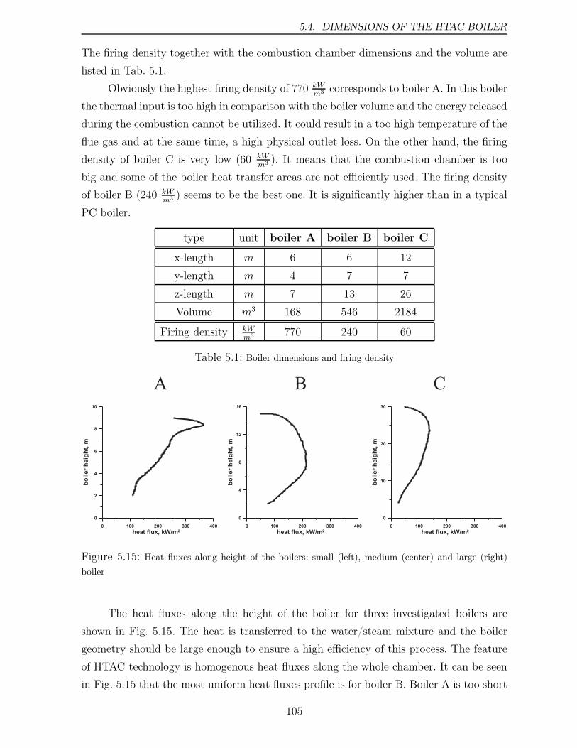
5.4. DIMENSIONS OF THE HTAC BOILER
The firing density together with the combustion chamber dimensions and the volume are
listed in Tab. 5.1.
Obviously the highest firing density of 770 kWm3
corresponds to boiler A. In this boiler
the thermal input is too high in comparison with the boiler volume and the energy released
during the combustion cannot be utilized. It could result in a too high temperature of the
flue gas and at the same time, a high physical outlet loss. On the other hand, the firing
density of boiler C is very low (60 kWm3
). It means that the combustion chamber is too
big and some of the boiler heat transfer areas are not efficiently used. The firing density
of boiler B (240 kWm3
) seems to be the best one. It is significantly higher than in a typical
PC boiler.
type unit boiler A boiler B boiler C
x-length m 6 6 12
y-length m 4 7 7
z-length m 7 13 26
Volume m3 168 546 2184
Firing density kWm3
770 240 60
Table 5.1: Boiler dimensions and firing density
Figure 5.15: Heat fluxes along height of the boilers: small (left), medium (center) and large (right)
boiler
The heat fluxes along the height of the boiler for three investigated boilers are
shown in Fig. 5.15. The heat is transferred to the water/steam mixture and the boiler
geometry should be large enough to ensure a high efficiency of this process. The feature
of HTAC technology is homogenous heat fluxes along the whole chamber. It can be seen
in Fig. 5.15 that the most uniform heat fluxes profile is for boiler B. Boiler A is too short
105
CHAPTER 5. DESIGN OF THE HTAC BOILER
and the high temperatures region occurs at the top part of this boiler. It results in the
high enthalpy of the flue gas and a decrease of the boiler efficiency. In boiler C the values
of heat fluxes are uniform but two times lower than in the medium size boiler. Extremely
low value of the firing density and the low heat fluxes show that this boiler is too big.
5.4.2 Findings
The fourth calculation series has been carried out in order to find the combustion
chamber dimensions which can, on one hand, ensure an efficient heat exchange between
the combustion products and water/steam mixture and on the other hand, provide a
high value of the firing density. Medium size boiler (boiler B) is chosen for further
investigations.
106
Chapter 6
Final HTAC boiler design
The investigations presented in Chapter 5 have been carried out to determine
the final geometry of the combustion chamber, the configuration of the burners, the
location of the burner block as well as the dimensions of the boiler. Obviously the find
design incorporates findings of the previous Chapter. In this Chapter details of the final
boiler design, as well as its operating and boundary conditions are presented. Again the
recirculation, the temperature and the chemical species concentration fields, as well as
coal particles behavior and heat transfer are analyzed.
The simulation has been performed for the three-dimensional model meshed with
an unstructured grid. Since the boiler is symmetric in two directions the calculations
have been performed for a quarter of the domain only. The boiler is 13 m high and
has 7 m times 6 m cross section, see Fig. 6.1. It is equipped with a burner block that
consists of 5 identical burners located at the top wall thus the boiler is down-fired. The
flue gas outlets are also located at the top wall of the boiler and they are symmetrically
positioned on both sides of the burner block. The outlets have a quadrate form with
lateral length of 1 m. The advantage is that the outlets are located near the burner block
and the eventual heat exchanger between flue gas and combustion air could be built
there. Each of five burners is equipped with a central injector of the hot air and two coal
guns positioned on both sides of the air injector. Pulverized coal is introduced into the
furnace by nozzles of 15mm diameter and the combustion air with nozzles of 48mm. The
boiler is equipped with two ash hoppers. This specific boiler design, derived in Chapter 5,
realizes HTAC technology. The details of the boiler construction are given in Fig. 6.1.
107
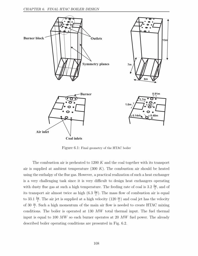
CHAPTER 6. FINAL HTAC BOILER DESIGN
Symmetry planes
OutletsBurner block
Burner
Air inlet
Coal inlets
7m
13m
6m
1.0m
1.7m
f 0.14m f 0.48m
1.5m
0.91m
Figure 6.1: Final geometry of the HTAC boiler
The combustion air is preheated to 1200 K and the coal together with its transport
air is supplied at ambient temperature (300 K). The combustion air should be heated
using the enthalpy of the flue gas. However, a practical realization of such a heat exchanger
is a very challenging task since it is very difficult to design heat exchangers operating
with dusty flue gas at such a high temperature. The feeding rate of coal is 3.2 kgs, and of
its transport air almost twice as high (6.3 kgs). The mass flow of combustion air is equal
to 33.1 kgs. The air jet is supplied at a high velocity (120 m
s) and coal jet has the velocity
of 30 ms. Such a high momentum of the main air flow is needed to create HTAC mixing
conditions. The boiler is operated at 130 MW total thermal input. The fuel thermal
input is equal to 100 MW so each burner operates at 20 MW fuel power. The already
described boiler operating conditions are presented in Fig. 6.2.
108
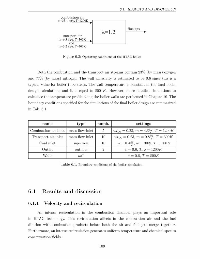
6.1. RESULTS AND DISCUSSION
combustion air
transport air
m=33.1 kg/s, T=1200K
coalm=6.3 kg/s, T=300K
m=3.2 kg/s, T=300K
l=1.2flue gas
Figure 6.2: Operating conditions of the HTAC boiler
Both the combustion and the transport air streams contain 23% (by mass) oxygen
and 77% (by mass) nitrogen. The wall emissivity is estimated to be 0.6 since this is a
typical value for boiler tube steels. The wall temperature is constant in the final boiler
design calculations and it is equal to 800 K. However, more detailed simulations to
calculate the temperature profile along the boiler walls are performed in Chapter 10. The
boundary conditions specified for the simulations of the final boiler design are summarized
in Tab. 6.1.
name type numb. settings
Combustion air inlet mass flow inlet 5 wtO2 = 0.23, m = 4.8kgs, T = 1200K
Transport air inlet mass flow inlet 10 wtO2 = 0.23, m = 0.8kgs, T = 300K
Coal inlet injection 10 m = 0.4kgs, w = 30m
s, T = 300K
Outlet outflow 2 ε = 0.6, Trad = 1200K
Walls wall ε = 0.6, T = 800K
Table 6.1: Boundary conditions of the boiler simulation
6.1 Results and discussion
6.1.1 Velocity and recirculation
An intense recirculation in the combustion chamber plays an important role
in HTAC technology. This recirculation affects in the combustion air and the fuel
dilution with combustion products before both the air and fuel jets merge together.
Furthermore, an intense recirculation generates uniform temperature and chemical species
concentration fields.
109
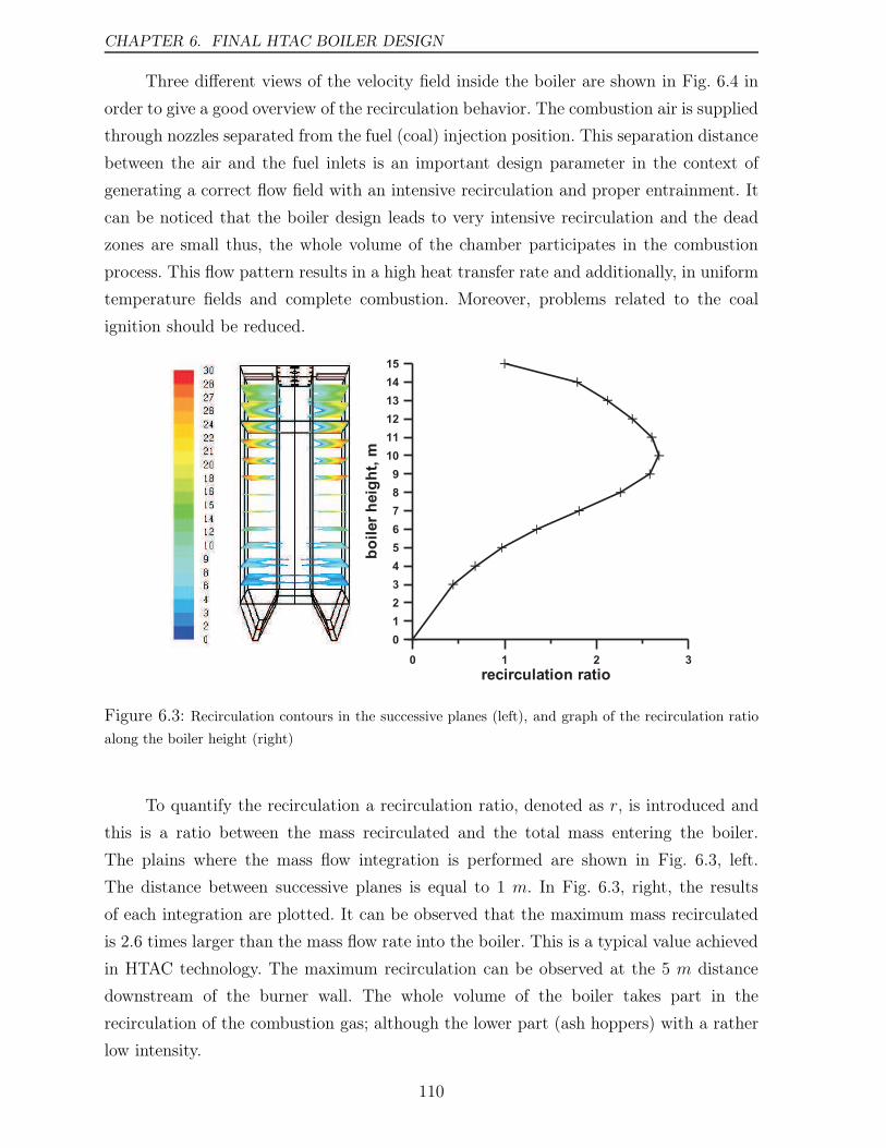
CHAPTER 6. FINAL HTAC BOILER DESIGN
Three different views of the velocity field inside the boiler are shown in Fig. 6.4 in
order to give a good overview of the recirculation behavior. The combustion air is supplied
through nozzles separated from the fuel (coal) injection position. This separation distance
between the air and the fuel inlets is an important design parameter in the context of
generating a correct flow field with an intensive recirculation and proper entrainment. It
can be noticed that the boiler design leads to very intensive recirculation and the dead
zones are small thus, the whole volume of the chamber participates in the combustion
process. This flow pattern results in a high heat transfer rate and additionally, in uniform
temperature fields and complete combustion. Moreover, problems related to the coal
ignition should be reduced.
0 1 2 3
recirculation ratio
0
1
2
3
4
5
6
7
8
9
10
11
12
13
14
15b
oil
er
heig
ht,
m
Figure 6.3: Recirculation contours in the successive planes (left), and graph of the recirculation ratio
along the boiler height (right)
To quantify the recirculation a recirculation ratio, denoted as r, is introduced and
this is a ratio between the mass recirculated and the total mass entering the boiler.
The plains where the mass flow integration is performed are shown in Fig. 6.3, left.
The distance between successive planes is equal to 1 m. In Fig. 6.3, right, the results
of each integration are plotted. It can be observed that the maximum mass recirculated
is 2.6 times larger than the mass flow rate into the boiler. This is a typical value achieved
in HTAC technology. The maximum recirculation can be observed at the 5 m distance
downstream of the burner wall. The whole volume of the boiler takes part in the
recirculation of the combustion gas; although the lower part (ash hoppers) with a rather
low intensity.
110
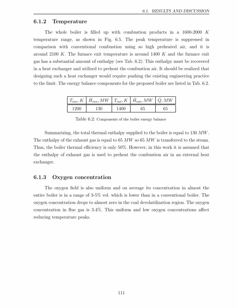
6.1. RESULTS AND DISCUSSION
6.1.2 Temperature
The whole boiler is filled up with combustion products in a 1600-2000 K
temperature range, as shown in Fig. 6.5. The peak temperature is suppressed in
comparison with conventional combustion using so high preheated air, and it is
around 2100 K. The furnace exit temperature is around 1400 K and the furnace exit
gas has a substantial amount of enthalpy (see Tab. 6.2). This enthalpy must be recovered
in a heat exchanger and utilized to preheat the combustion air. It should be realized that
designing such a heat exchanger would require pushing the existing engineering practice
to the limit. The energy balance components for the proposed boiler are listed in Tab. 6.2.
Tinn, K Hinn,MW Tout, K Hout,MW Q,MW
1200 130 1400 65 65
Table 6.2: Components of the boiler energy balance
Summarizing, the total thermal enthalpy supplied to the boiler is equal to 130MW .
The enthalpy of the exhaust gas is equal to 65MW so 65MW is transferred to the steam.
Thus, the boiler thermal efficiency is only 50%. However, in this work it is assumed that
the enthalpy of exhaust gas is used to preheat the combustion air in an external heat
exchanger.
6.1.3 Oxygen concentration
The oxygen field is also uniform and on average its concentration in almost the
entire boiler is in a range of 3-5% vol. which is lower than in a conventional boiler. The
oxygen concentration drops to almost zero in the coal devolatilization region. The oxygen
concentration in flue gas is 3.4%. This uniform and low oxygen concentrations affect
reducing temperature peaks.
111
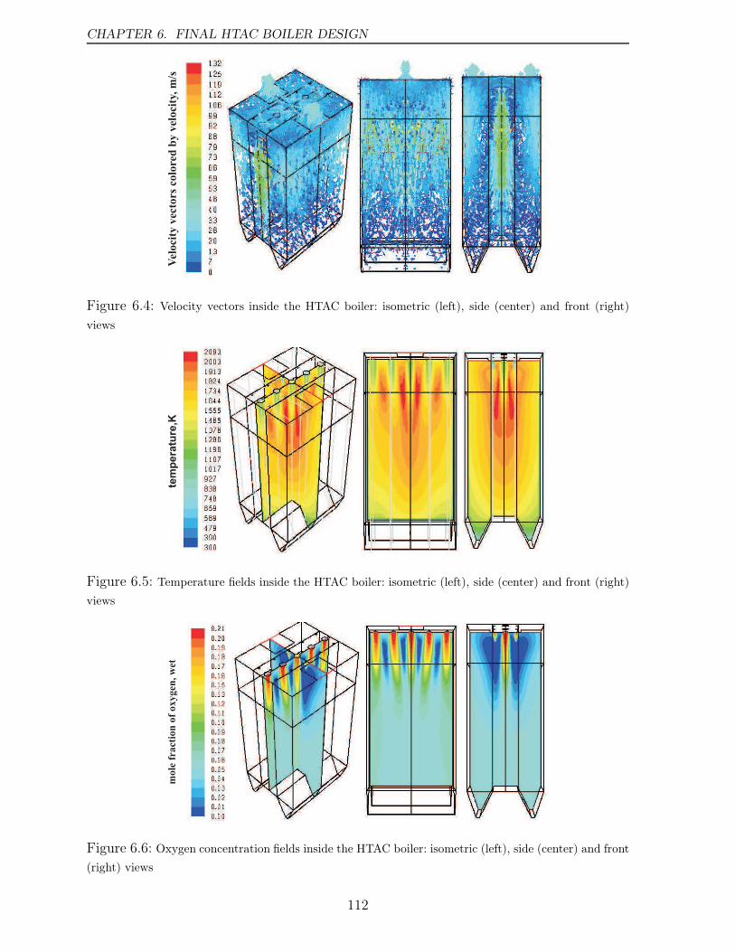
CHAPTER 6. FINAL HTAC BOILER DESIGN
Vel
oci
ty v
ecto
rs c
olo
red
by v
eloci
ty, m
/s
Figure 6.4: Velocity vectors inside the HTAC boiler: isometric (left), side (center) and front (right)
views
tem
pera
ture
,K
Figure 6.5: Temperature fields inside the HTAC boiler: isometric (left), side (center) and front (right)
views
mo
le f
ract
ion
of
ox
yg
en,
wet
Figure 6.6: Oxygen concentration fields inside the HTAC boiler: isometric (left), side (center) and front
(right) views
112
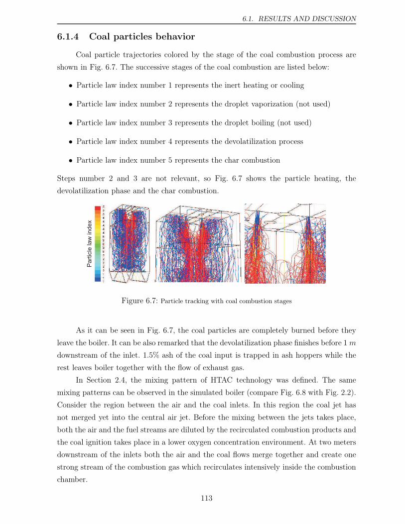
6.1. RESULTS AND DISCUSSION
6.1.4 Coal particles behavior
Coal particle trajectories colored by the stage of the coal combustion process are
shown in Fig. 6.7. The successive stages of the coal combustion are listed below:
• Particle law index number 1 represents the inert heating or cooling
• Particle law index number 2 represents the droplet vaporization (not used)
• Particle law index number 3 represents the droplet boiling (not used)
• Particle law index number 4 represents the devolatilization process
• Particle law index number 5 represents the char combustion
Steps number 2 and 3 are not relevant, so Fig. 6.7 shows the particle heating, the
devolatilization phase and the char combustion.
Pa
rtic
le la
w in
de
x
Figure 6.7: Particle tracking with coal combustion stages
As it can be seen in Fig. 6.7, the coal particles are completely burned before they
leave the boiler. It can be also remarked that the devolatilization phase finishes before 1m
downstream of the inlet. 1.5% ash of the coal input is trapped in ash hoppers while the
rest leaves boiler together with the flow of exhaust gas.
In Section 2.4, the mixing pattern of HTAC technology was defined. The same
mixing patterns can be observed in the simulated boiler (compare Fig. 6.8 with Fig. 2.2).
Consider the region between the air and the coal inlets. In this region the coal jet has
not merged yet into the central air jet. Before the mixing between the jets takes place,
both the air and the fuel streams are diluted by the recirculated combustion products and
the coal ignition takes place in a lower oxygen concentration environment. At two meters
downstream of the inlets both the air and the coal flows merge together and create one
strong stream of the combustion gas which recirculates intensively inside the combustion
chamber.
113

CHAPTER 6. FINAL HTAC BOILER DESIGN
Figure 6.8: Mixing modes inside the HTAC boiler
Due to the internal recirculation of the combustion products the residence time
of the coal particles is significantly longer in comparison with the standard PC boiler.
In Fig. 6.9 a histogram of the particle residence time inside the boiler is given. It is
depicted for 98% of the particles total mass.
Particle residence time, s
%
Figure 6.9: Histogram of the particle residence time inside the HTAC boiler
The mean residence time for the coal particles is relatively long and it is calculated
to be around 3.5 s while in a standard PC boiler it is around 1.5 s [12]. It can be also
observed that for 70% of the particles this time is much longer. Some of them stay inside
the chamber and recirculate inside the boiler even up to infinity. Only 30% of the particles
stay inside the boiler shorter than for a period of 3 s.
114
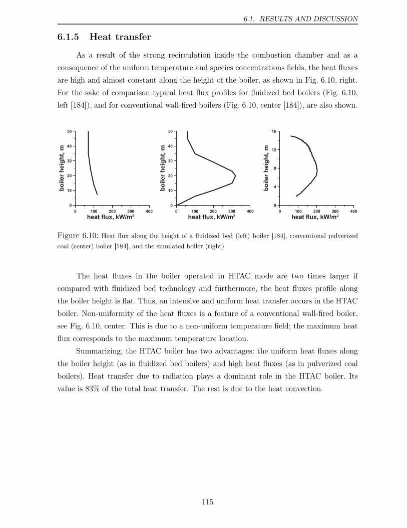
6.1. RESULTS AND DISCUSSION
6.1.5 Heat transfer
As a result of the strong recirculation inside the combustion chamber and as a
consequence of the uniform temperature and species concentrations fields, the heat fluxes
are high and almost constant along the height of the boiler, as shown in Fig. 6.10, right.
For the sake of comparison typical heat flux profiles for fluidized bed boilers (Fig. 6.10,
left [184]), and for conventional wall-fired boilers (Fig. 6.10, center [184]), are also shown.
0 100 200 300 400
heat flux, kW/m2
0
10
20
30
40
50
bo
ile
rh
eig
ht,
m
0 100 200 300 400
heat flux, kW/m2
0
10
20
30
40
50
bo
ile
rh
eig
ht,
m
0 100 200 300 400
heat flux, kW/m2
0
4
8
12
16
bo
ile
rh
eig
ht,
m
Figure 6.10: Heat flux along the height of a fluidized bed (left) boiler [184], conventional pulverized
coal (center) boiler [184], and the simulated boiler (right)
The heat fluxes in the boiler operated in HTAC mode are two times larger if
compared with fluidized bed technology and furthermore, the heat fluxes profile along
the boiler height is flat. Thus, an intensive and uniform heat transfer occurs in the HTAC
boiler. Non-uniformity of the heat fluxes is a feature of a conventional wall-fired boiler,
see Fig. 6.10, center. This is due to a non-uniform temperature field; the maximum heat
flux corresponds to the maximum temperature location.
Summarizing, the HTAC boiler has two advantages: the uniform heat fluxes along
the boiler height (as in fluidized bed boilers) and high heat fluxes (as in pulverized coal
boilers). Heat transfer due to radiation plays a dominant role in the HTAC boiler. Its
value is 83% of the total heat transfer. The rest is due to the heat convection.
115
CHAPTER 6. FINAL HTAC BOILER DESIGN
6.2 Findings
The presented final version of the boiler fired with pulverized coal possesses all the
features required for HTAC technology. First of all, an intense recirculation inside the
combustion chamber make both temperature and chemical substances concentration fields
uniform. Further, due to dilution between combustion air and fuel jets the coal ignition
takes place in low oxygen concentration environment, and therefore the temperature
peak is suppressed. Then, high and uniform heat fluxes improve heat transfer in the
boiler. Moreover, the intensification of radiative heat transfer results in an increase of
firing density, and at the same time allows to reduce the size of the boiler. It can be
economically justifiable to build this boiler from high quality steels and to increase the
steam parameters. Long particles residence time, as well as recursively recirculation of
the combustion products improve the char burnout. Very stable combustion process
and simple burner construction offer the possibility of using low rank coals. Strong
recirculation of the hot combustion products eliminates the problems related to coal
ignition. The proposed boiler has a very simple construction of the combustion chamber,
as well as of the burners in comparison with typical conventional PC boilers.
116
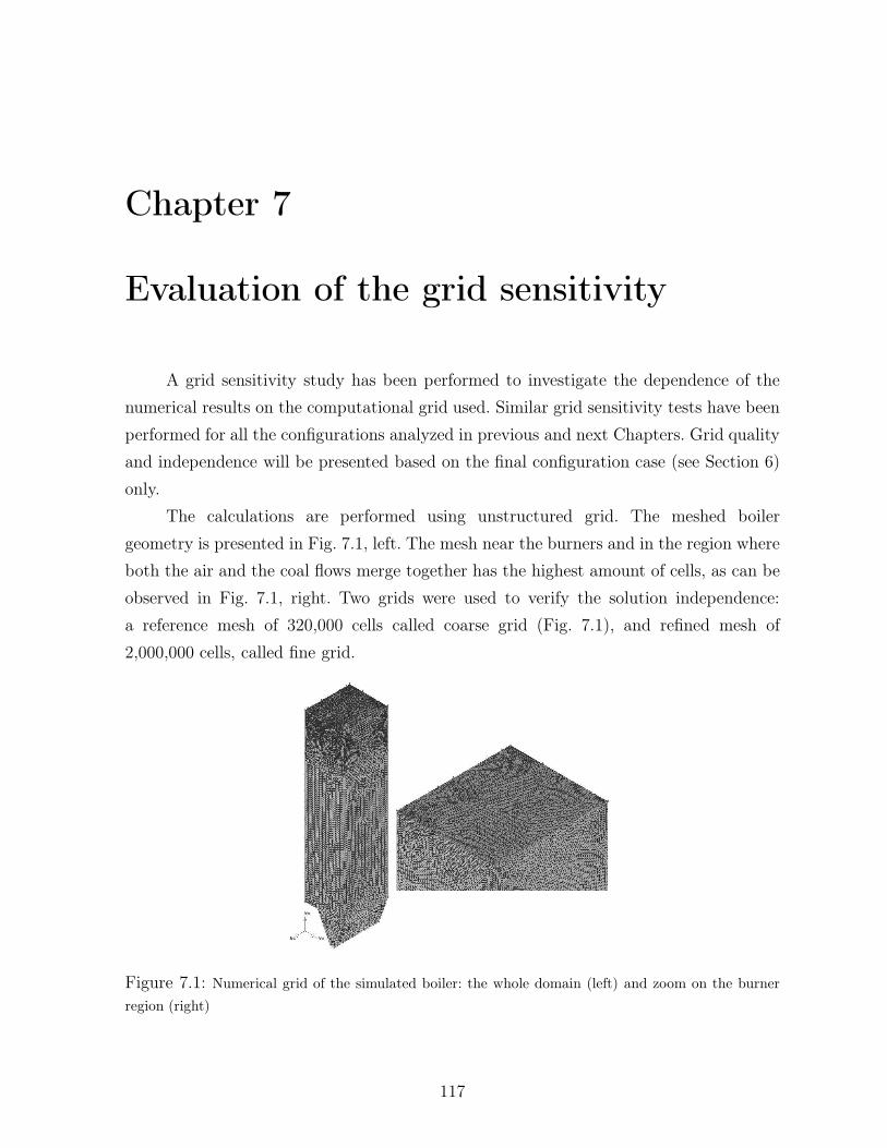
Chapter 7
Evaluation of the grid sensitivity
A grid sensitivity study has been performed to investigate the dependence of the
numerical results on the computational grid used. Similar grid sensitivity tests have been
performed for all the configurations analyzed in previous and next Chapters. Grid quality
and independence will be presented based on the final configuration case (see Section 6)
only.
The calculations are performed using unstructured grid. The meshed boiler
geometry is presented in Fig. 7.1, left. The mesh near the burners and in the region where
both the air and the coal flows merge together has the highest amount of cells, as can be
observed in Fig. 7.1, right. Two grids were used to verify the solution independence:
a reference mesh of 320,000 cells called coarse grid (Fig. 7.1), and refined mesh of
2,000,000 cells, called fine grid.
Figure 7.1: Numerical grid of the simulated boiler: the whole domain (left) and zoom on the burner
region (right)
117
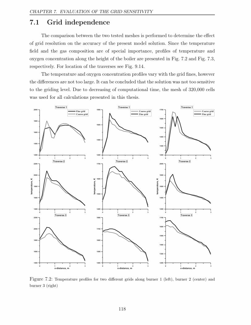
CHAPTER 7. EVALUATION OF THE GRID SENSITIVITY
7.1 Grid independence
The comparison between the two tested meshes is performed to determine the effect
of grid resolution on the accuracy of the present model solution. Since the temperature
field and the gas composition are of special importance, profiles of temperature and
oxygen concentration along the height of the boiler are presented in Fig. 7.2 and Fig. 7.3,
respectively. For location of the traverses see Fig. 9.14.
The temperature and oxygen concentration profiles vary with the grid fines, however
the differences are not too large. It can be concluded that the solution was not too sensitive
to the griding level. Due to decreasing of computational time, the mesh of 320,000 cells
was used for all calculations presented in this thesis.
0 1 2 3
x-distance, m
1400
1600
1800
2000
2200
Traverse 3
0 1 2 3
1400
1600
1800
2000
2200
tem
pera
ture
,K
Traverse 2
0 1 2 3
1200
1400
1600
1800
2000Fine grid
Coarse grid
Traverse 1
0 1 2 3
x-distance, m
1400
1500
1600
1700
1800
Traverse 3
0 1 2 3
1400
1500
1600
1700
tem
pera
ture
,K
Traverse 2
0 1 2 3
1200
1400
1600
1800Coarse grid
Fine grid
Traverse 1
0 1 2 3
x-distance, m
1200
1300
1400
1500
1600
1700
Traverse 3
0 1 2 3
1200
1400
1600
1800
2000
tem
pera
ture
,K
Traverse 2
0 1 2 3
1200
1300
1400
1500
1600
1700Coarse grid
Fine grid
Traverse 1
Figure 7.2: Temperature profiles for two different grids along burner 1 (left), burner 2 (center) and
burner 3 (right)
118
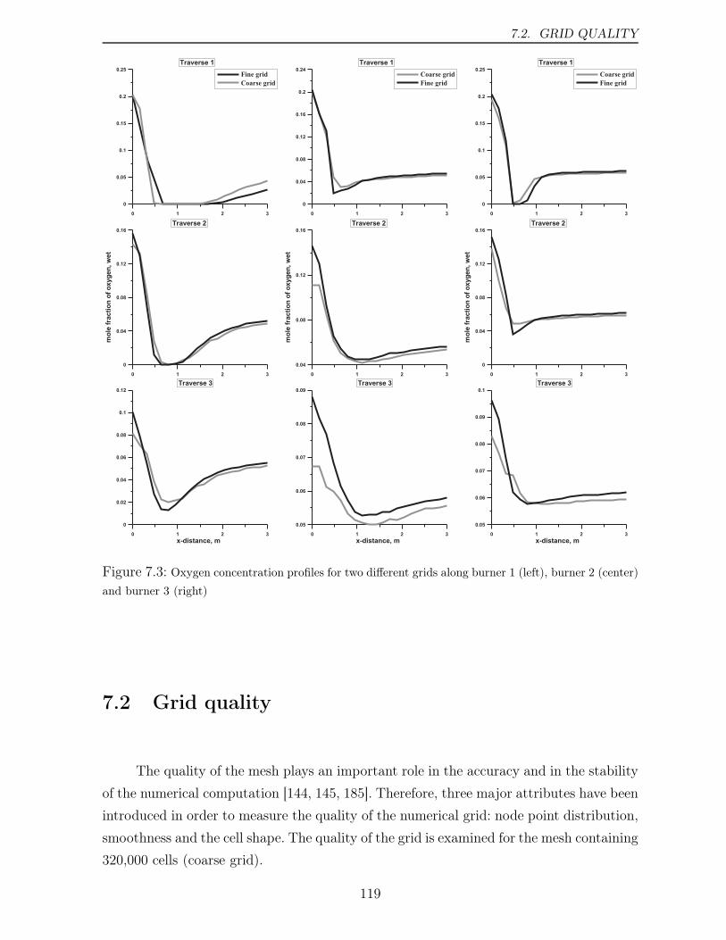
7.2. GRID QUALITY
0 1 2 3
x-distance, m
0
0.02
0.04
0.06
0.08
0.1
0.12
Traverse 3
0 1 2 3
0
0.04
0.08
0.12
0.16
mo
lefr
acti
on
of
oxyg
en
,w
et
Traverse 2
0 1 2 3
0
0.05
0.1
0.15
0.2
0.25Fine grid
Coarse grid
Traverse 1
0 1 2 3
x-distance, m
0.05
0.06
0.07
0.08
0.09
Traverse 3
0 1 2 3
0.04
0.08
0.12
0.16
mo
lefr
acti
on
of
oxyg
en
,w
et
Traverse 2
0 1 2 3
0
0.04
0.08
0.12
0.16
0.2
0.24Coarse grid
Fine grid
Traverse 1
0 1 2 3
x-distance, m
0.05
0.06
0.07
0.08
0.09
0.1
Traverse 3
0 1 2 3
0
0.04
0.08
0.12
0.16
mo
lefr
acti
on
of
oxyg
en
,w
et
Traverse 2
0 1 2 3
0
0.05
0.1
0.15
0.2
0.25Coarse grid
Fine grid
Traverse 1
Figure 7.3: Oxygen concentration profiles for two different grids along burner 1 (left), burner 2 (center)
and burner 3 (right)
7.2 Grid quality
The quality of the mesh plays an important role in the accuracy and in the stability
of the numerical computation [144, 145, 185]. Therefore, three major attributes have been
introduced in order to measure the quality of the numerical grid: node point distribution,
smoothness and the cell shape. The quality of the grid is examined for the mesh containing
320,000 cells (coarse grid).
119
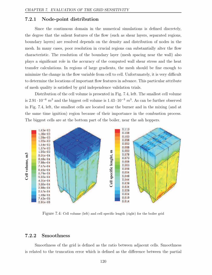
CHAPTER 7. EVALUATION OF THE GRID SENSITIVITY
7.2.1 Node-point distribution
Since the continuous domain in the numerical simulations is defined discretely,
the degree that the salient features of the flow (such as shear layers, separated regions,
boundary layers) are resolved depends on the density and distribution of nodes in the
mesh. In many cases, poor resolution in crucial regions can substantially alter the flow
characteristic. The resolution of the boundary layer (mesh spacing near the wall) also
plays a significant role in the accuracy of the computed wall shear stress and the heat
transfer calculations. In regions of large gradients, the mesh should be fine enough to
minimize the change in the flow variable from cell to cell. Unfortunately, it is very difficult
to determine the locations of important flow features in advance. This particular attribute
of mesh quality is satisfied by grid independence validation trials.
Distribution of the cell volume is presented in Fig. 7.4, left. The smallest cell volume
is 2.91 · 10−6 m3 and the biggest cell volume is 1.43 · 10−3 m3. As can be further observed
in Fig. 7.4, left, the smallest cells are located near the burner and in the mixing (and at
the same time ignition) region because of their importance in the combustion process.
The biggest cells are at the bottom part of the boiler, near the ash hoppers.
Cel
l v
olu
me,
m3
Cel
l sp
ecif
ic l
eng
ht,
m
Figure 7.4: Cell volume (left) and cell specific length (right) for the boiler grid
7.2.2 Smoothness
Smoothness of the grid is defined as the ratio between adjacent cells. Smoothness
is related to the truncation error which is defined as the difference between the partial
120
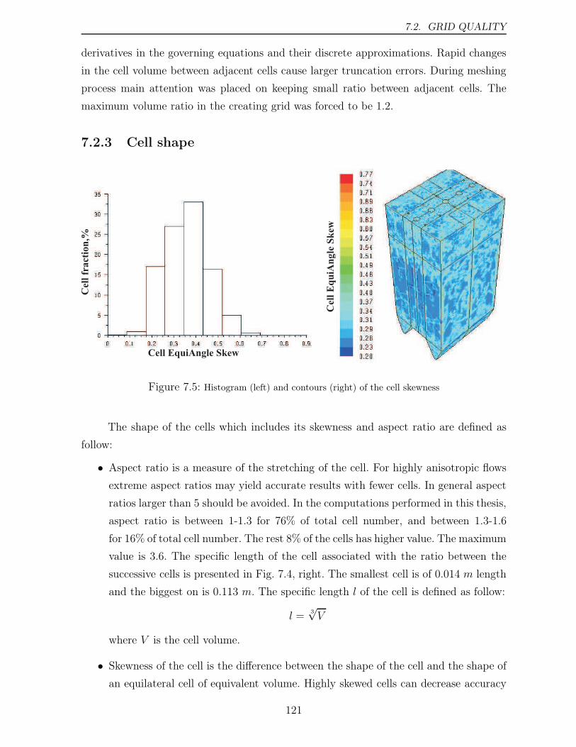
7.2. GRID QUALITY
derivatives in the governing equations and their discrete approximations. Rapid changes
in the cell volume between adjacent cells cause larger truncation errors. During meshing
process main attention was placed on keeping small ratio between adjacent cells. The
maximum volume ratio in the creating grid was forced to be 1.2.
7.2.3 Cell shape
Cell EquiAngle Skew
Cel
l fr
act
ion
,%
Cel
l E
qu
iAn
gle
Sk
ew
Figure 7.5: Histogram (left) and contours (right) of the cell skewness
The shape of the cells which includes its skewness and aspect ratio are defined as
follow:
• Aspect ratio is a measure of the stretching of the cell. For highly anisotropic flows
extreme aspect ratios may yield accurate results with fewer cells. In general aspect
ratios larger than 5 should be avoided. In the computations performed in this thesis,
aspect ratio is between 1-1.3 for 76% of total cell number, and between 1.3-1.6
for 16% of total cell number. The rest 8% of the cells has higher value. The maximum
value is 3.6. The specific length of the cell associated with the ratio between the
successive cells is presented in Fig. 7.4, right. The smallest cell is of 0.014 m length
and the biggest on is 0.113 m. The specific length l of the cell is defined as follow:
l =3√V
where V is the cell volume.
• Skewness of the cell is the difference between the shape of the cell and the shape of
an equilateral cell of equivalent volume. Highly skewed cells can decrease accuracy
121
CHAPTER 7. EVALUATION OF THE GRID SENSITIVITY
and destabilize the solution. The EquiAngle Skew method provided by the GAMBIT
package is used to examine the quality of the mesh [142]. Generally, the measure
of EquiAngle Skew (EAS) is contained between 0 and 1, where QEAS=0 describes
an equilateral element, and QEAS=1 describes a completely degenerate (poorly
shaped) element. In general, high-quality meshes contain elements that possess
average QEAS values of 0.1 (for 2-D geometry) and 0.4 (for 3-D geometry). In the
analyzed mesh, the elements with the skewness up to 0.4 are 70% of total cell
number, between 0.4 and 0.6 are 28% of total cell number. Only 2% of the cells are
between 0.6 and 0.77. The detailed distribution of the skewness is presented in the
histogram of Fig. 7.5.
Generally, it can be concluded that the meshes used in computations of this work are of
good quality.
122
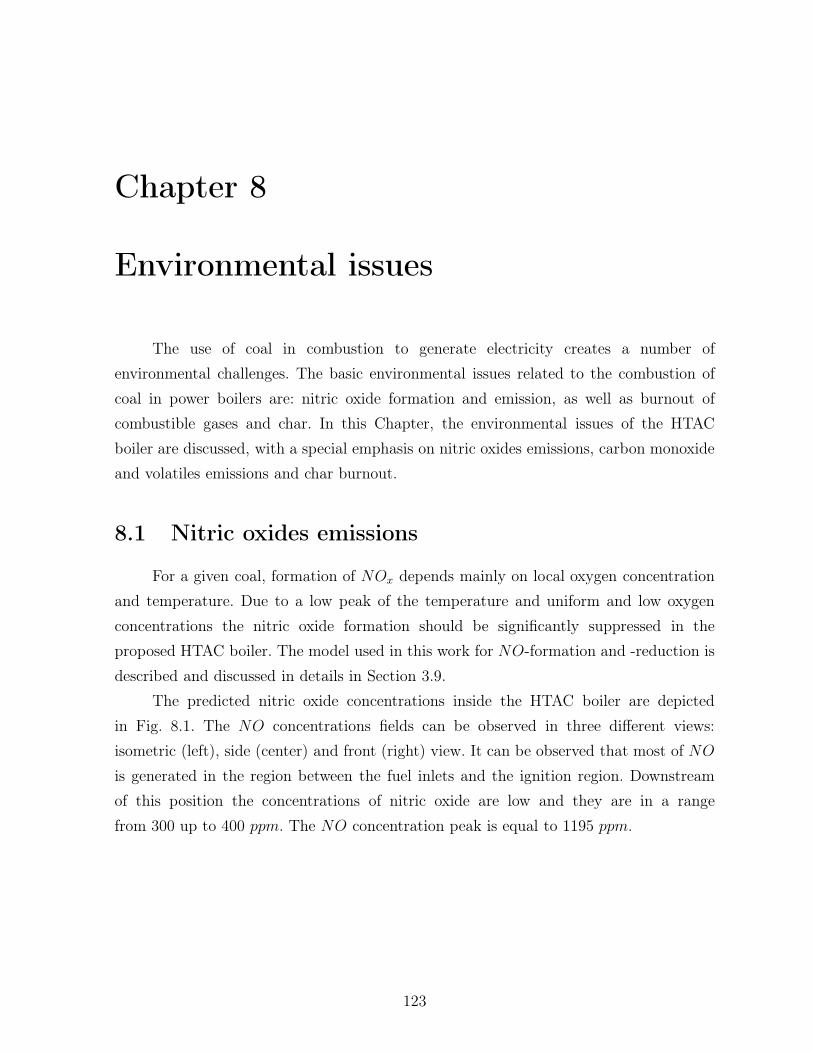
Chapter 8
Environmental issues
The use of coal in combustion to generate electricity creates a number of
environmental challenges. The basic environmental issues related to the combustion of
coal in power boilers are: nitric oxide formation and emission, as well as burnout of
combustible gases and char. In this Chapter, the environmental issues of the HTAC
boiler are discussed, with a special emphasis on nitric oxides emissions, carbon monoxide
and volatiles emissions and char burnout.
8.1 Nitric oxides emissions
For a given coal, formation of NOx depends mainly on local oxygen concentration
and temperature. Due to a low peak of the temperature and uniform and low oxygen
concentrations the nitric oxide formation should be significantly suppressed in the
proposed HTAC boiler. The model used in this work for NO-formation and -reduction is
described and discussed in details in Section 3.9.
The predicted nitric oxide concentrations inside the HTAC boiler are depicted
in Fig. 8.1. The NO concentrations fields can be observed in three different views:
isometric (left), side (center) and front (right) view. It can be observed that most of NO
is generated in the region between the fuel inlets and the ignition region. Downstream
of this position the concentrations of nitric oxide are low and they are in a range
from 300 up to 400 ppm. The NO concentration peak is equal to 1195 ppm.
123
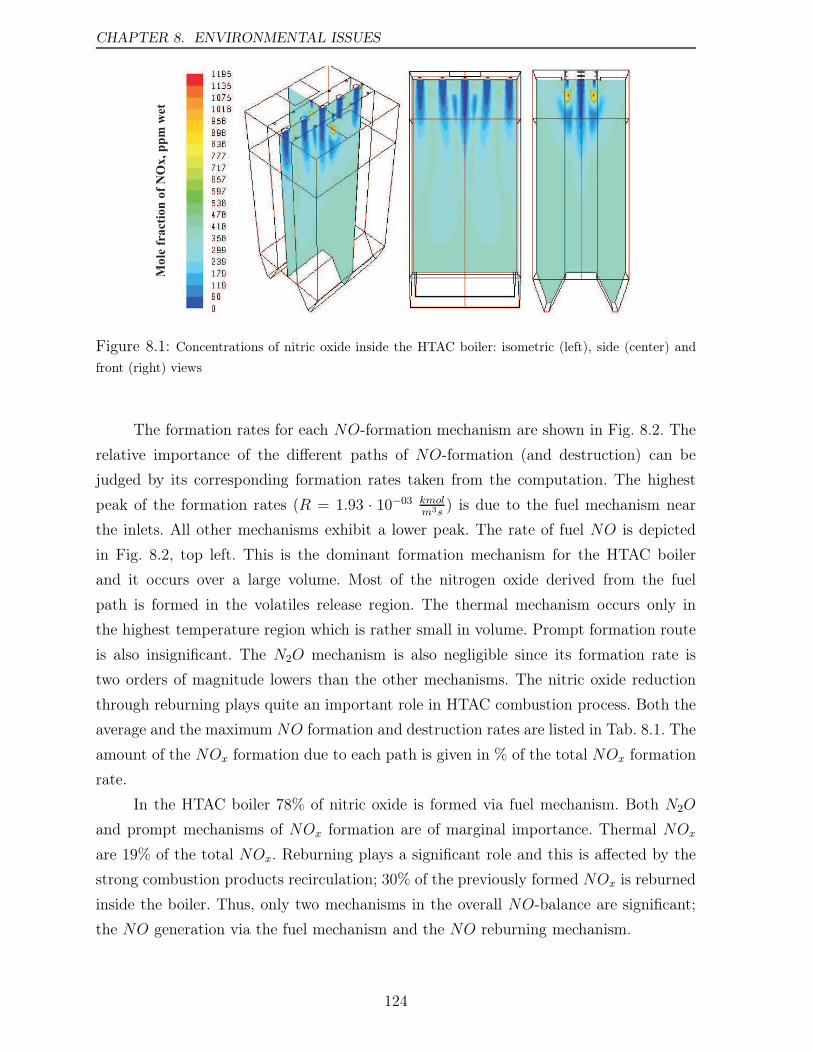
CHAPTER 8. ENVIRONMENTAL ISSUES
Mo
le f
ract
ion
of
NO
x,
wet
pp
m
Figure 8.1: Concentrations of nitric oxide inside the HTAC boiler: isometric (left), side (center) and
front (right) views
The formation rates for each NO-formation mechanism are shown in Fig. 8.2. The
relative importance of the different paths of NO-formation (and destruction) can be
judged by its corresponding formation rates taken from the computation. The highest
peak of the formation rates (R = 1.93 · 10−03 kmolm3s
) is due to the fuel mechanism near
the inlets. All other mechanisms exhibit a lower peak. The rate of fuel NO is depicted
in Fig. 8.2, top left. This is the dominant formation mechanism for the HTAC boiler
and it occurs over a large volume. Most of the nitrogen oxide derived from the fuel
path is formed in the volatiles release region. The thermal mechanism occurs only in
the highest temperature region which is rather small in volume. Prompt formation route
is also insignificant. The N2O mechanism is also negligible since its formation rate is
two orders of magnitude lowers than the other mechanisms. The nitric oxide reduction
through reburning plays quite an important role in HTAC combustion process. Both the
average and the maximum NO formation and destruction rates are listed in Tab. 8.1. The
amount of the NOx formation due to each path is given in % of the total NOx formation
rate.
In the HTAC boiler 78% of nitric oxide is formed via fuel mechanism. Both N2O
and prompt mechanisms of NOx formation are of marginal importance. Thermal NOx
are 19% of the total NOx. Reburning plays a significant role and this is affected by the
strong combustion products recirculation; 30% of the previously formed NOx is reburned
inside the boiler. Thus, only two mechanisms in the overall NO-balance are significant;
the NO generation via the fuel mechanism and the NO reburning mechanism.
124
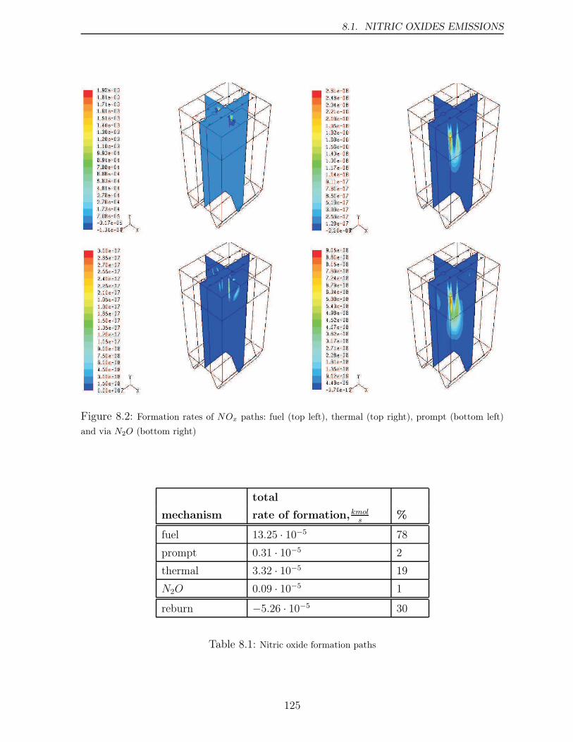
8.1. NITRIC OXIDES EMISSIONS
Figure 8.2: Formation rates of NOx paths: fuel (top left), thermal (top right), prompt (bottom left)
and via N2O (bottom right)
total
mechanism rate of formation,kmols
%
fuel 13.25 · 10−5 78
prompt 0.31 · 10−5 2
thermal 3.32 · 10−5 19
N2O 0.09 · 10−5 1
reburn −5.26 · 10−5 30
Table 8.1: Nitric oxide formation paths
125
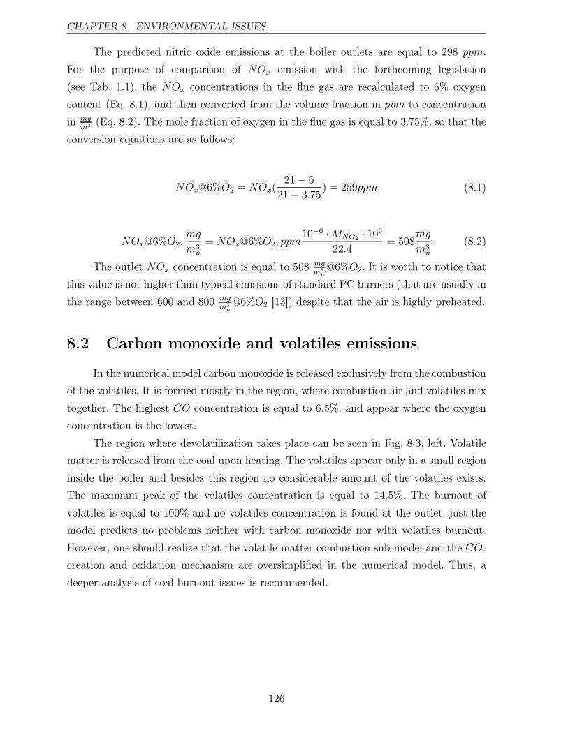
CHAPTER 8. ENVIRONMENTAL ISSUES
The predicted nitric oxide emissions at the boiler outlets are equal to 298 ppm.
For the purpose of comparison of NOx emission with the forthcoming legislation
(see Tab. 1.1), the NOx concentrations in the flue gas are recalculated to 6% oxygen
content (Eq. 8.1), and then converted from the volume fraction in ppm to concentration
in mgm3
(Eq. 8.2). The mole fraction of oxygen in the flue gas is equal to 3.75%, so that the
conversion equations are as follows:
NOx@6%O2 = NOx(21− 621− 3.75) = 259ppm (8.1)
NOx@6%O2,mg
m3n= NOx@6%O2, ppm
10−6 ·MNO2 · 10622.4
= 508mg
m3n(8.2)
The outlet NOx concentration is equal to 508 mgm3n@6%O2. It is worth to notice that
this value is not higher than typical emissions of standard PC burners (that are usually in
the range between 600 and 800 mgm3n@6%O2 [13]) despite that the air is highly preheated.
8.2 Carbon monoxide and volatiles emissions
In the numerical model carbon monoxide is released exclusively from the combustion
of the volatiles. It is formed mostly in the region, where combustion air and volatiles mix
together. The highest CO concentration is equal to 6.5%. and appear where the oxygen
concentration is the lowest.
The region where devolatilization takes place can be seen in Fig. 8.3, left. Volatile
matter is released from the coal upon heating. The volatiles appear only in a small region
inside the boiler and besides this region no considerable amount of the volatiles exists.
The maximum peak of the volatiles concentration is equal to 14.5%. The burnout of
volatiles is equal to 100% and no volatiles concentration is found at the outlet, just the
model predicts no problems neither with carbon monoxide nor with volatiles burnout.
However, one should realize that the volatile matter combustion sub-model and the CO-
creation and oxidation mechanism are oversimplified in the numerical model. Thus, a
deeper analysis of coal burnout issues is recommended.
126
8.3. CHAR BURNOUT
Figure 8.3: Devolatilization (left) and char burnout (right) regions inside the HTAC boiler
8.3 Char burnout
The char burnout is a concern of HTAC technology. The region where char burnout
takes place is shown in Fig. 8.3, right. Although the predicted value of char burnout is
equal to 99.9% at the outlet, the sub-model for char burnout used in this work is simple
(for details see Sections 3.7.3 and 4.3). However, in HTAC technology complete burnout is
expected due to intensive recirculation of the combustion gas and long particles residence
time. Char burnout process should be taken into consideration in further investigations.
8.4 Findings
In this Chapter the environmental issues related to the HTAC boiler have been
investigated. It was concluded that a low emission of NOx is achieved in this boiler
which allows to adhere to the forthcoming strict legislation of NOx emissions from power
plants without the need of a substantial capital investment. The complete burnout of
the gaseous combustibles (CO and volatiles), as well as of the char probably allows the
possibility of operating the proposed boiler at air excess ratio just a little bit higher than
stoichiometric.
127

CHAPTER 8. ENVIRONMENTAL ISSUES
128
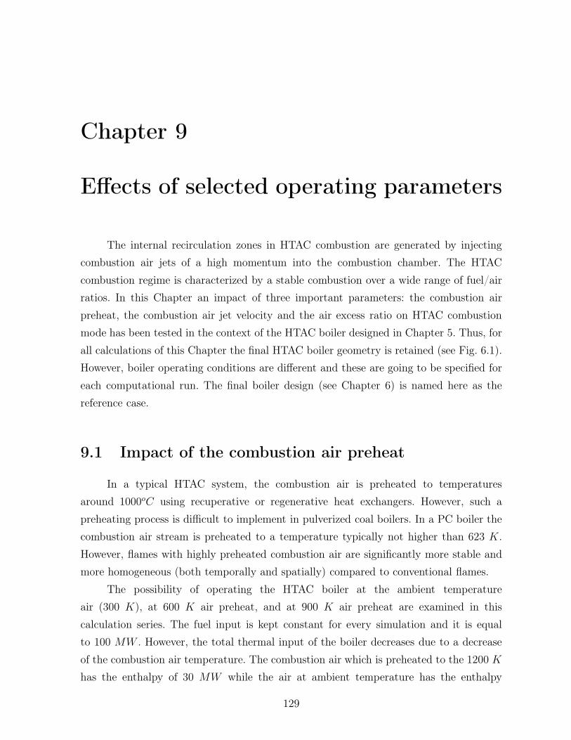
Chapter 9
Effects of selected operating parameters
The internal recirculation zones in HTAC combustion are generated by injecting
combustion air jets of a high momentum into the combustion chamber. The HTAC
combustion regime is characterized by a stable combustion over a wide range of fuel/air
ratios. In this Chapter an impact of three important parameters: the combustion air
preheat, the combustion air jet velocity and the air excess ratio on HTAC combustion
mode has been tested in the context of the HTAC boiler designed in Chapter 5. Thus, for
all calculations of this Chapter the final HTAC boiler geometry is retained (see Fig. 6.1).
However, boiler operating conditions are different and these are going to be specified for
each computational run. The final boiler design (see Chapter 6) is named here as the
reference case.
9.1 Impact of the combustion air preheat
In a typical HTAC system, the combustion air is preheated to temperatures
around 1000oC using recuperative or regenerative heat exchangers. However, such a
preheating process is difficult to implement in pulverized coal boilers. In a PC boiler the
combustion air stream is preheated to a temperature typically not higher than 623 K.
However, flames with highly preheated combustion air are significantly more stable and
more homogeneous (both temporally and spatially) compared to conventional flames.
The possibility of operating the HTAC boiler at the ambient temperature
air (300 K), at 600 K air preheat, and at 900 K air preheat are examined in this
calculation series. The fuel input is kept constant for every simulation and it is equal
to 100 MW . However, the total thermal input of the boiler decreases due to a decrease
of the combustion air temperature. The combustion air which is preheated to the 1200 K
has the enthalpy of 30 MW while the air at ambient temperature has the enthalpy
129
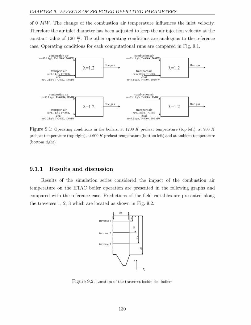
CHAPTER 9. EFFECTS OF SELECTED OPERATING PARAMETERS
of 0 MW . The change of the combustion air temperature influences the inlet velocity.
Therefore the air inlet diameter has been adjusted to keep the air injection velocity at the
constant value of 120 ms. The other operating conditions are analogous to the reference
case. Operating conditions for each computational runs are compared in Fig. 9.1.
Figure 9.1: Operating conditions in the boilers: at 1200 K preheat temperature (top left), at 900 K
preheat temperature (top right), at 600K preheat temperature (bottom left) and at ambient temperature
(bottom right)
9.1.1 Results and discussion
Results of the simulation series considered the impact of the combustion air
temperature on the HTAC boiler operation are presented in the following graphs and
compared with the reference case. Predictions of the field variables are presented along
the traverses 1, 2, 3 which are located as shown in Fig. 9.2.
traverse 3
traverse 2
traverse 1
3m
7m
5m
3m
1m
y
x
Figure 9.2: Location of the traverses inside the boilers
130
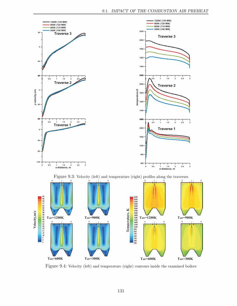
9.1. IMPACT OF THE COMBUSTION AIR PREHEAT
Figure 9.3: Velocity (left) and temperature (right) profiles along the traverses
T =1200Kair
T =600Kair T =300Kair
T =900Kair
Vel
oci
ty,m
\s
T =1200Kair
T =600Kair T =300Kair
T =900Kair
Tem
per
atu
re, K
Figure 9.4: Velocity (left) and temperature (right) contours inside the examined boilers
131
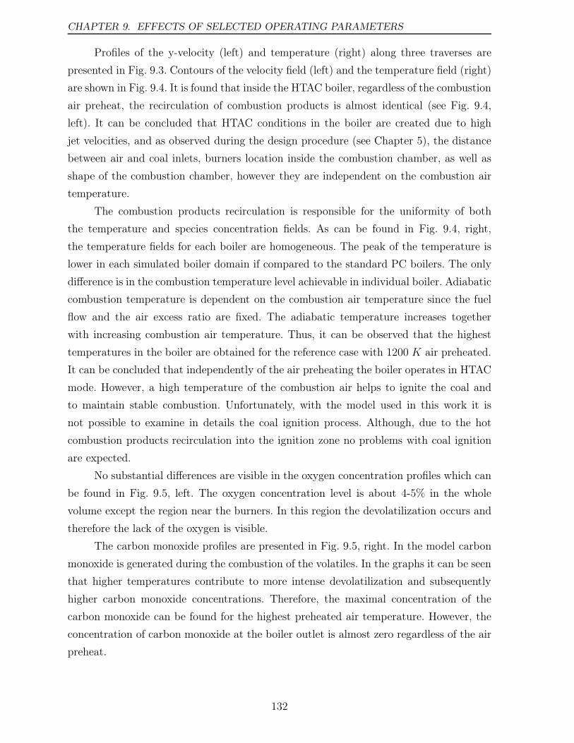
CHAPTER 9. EFFECTS OF SELECTED OPERATING PARAMETERS
Profiles of the y-velocity (left) and temperature (right) along three traverses are
presented in Fig. 9.3. Contours of the velocity field (left) and the temperature field (right)
are shown in Fig. 9.4. It is found that inside the HTAC boiler, regardless of the combustion
air preheat, the recirculation of combustion products is almost identical (see Fig. 9.4,
left). It can be concluded that HTAC conditions in the boiler are created due to high
jet velocities, and as observed during the design procedure (see Chapter 5), the distance
between air and coal inlets, burners location inside the combustion chamber, as well as
shape of the combustion chamber, however they are independent on the combustion air
temperature.
The combustion products recirculation is responsible for the uniformity of both
the temperature and species concentration fields. As can be found in Fig. 9.4, right,
the temperature fields for each boiler are homogeneous. The peak of the temperature is
lower in each simulated boiler domain if compared to the standard PC boilers. The only
difference is in the combustion temperature level achievable in individual boiler. Adiabatic
combustion temperature is dependent on the combustion air temperature since the fuel
flow and the air excess ratio are fixed. The adiabatic temperature increases together
with increasing combustion air temperature. Thus, it can be observed that the highest
temperatures in the boiler are obtained for the reference case with 1200 K air preheated.
It can be concluded that independently of the air preheating the boiler operates in HTAC
mode. However, a high temperature of the combustion air helps to ignite the coal and
to maintain stable combustion. Unfortunately, with the model used in this work it is
not possible to examine in details the coal ignition process. Although, due to the hot
combustion products recirculation into the ignition zone no problems with coal ignition
are expected.
No substantial differences are visible in the oxygen concentration profiles which can
be found in Fig. 9.5, left. The oxygen concentration level is about 4-5% in the whole
volume except the region near the burners. In this region the devolatilization occurs and
therefore the lack of the oxygen is visible.
The carbon monoxide profiles are presented in Fig. 9.5, right. In the model carbon
monoxide is generated during the combustion of the volatiles. In the graphs it can be seen
that higher temperatures contribute to more intense devolatilization and subsequently
higher carbon monoxide concentrations. Therefore, the maximal concentration of the
carbon monoxide can be found for the highest preheated air temperature. However, the
concentration of carbon monoxide at the boiler outlet is almost zero regardless of the air
preheat.
132
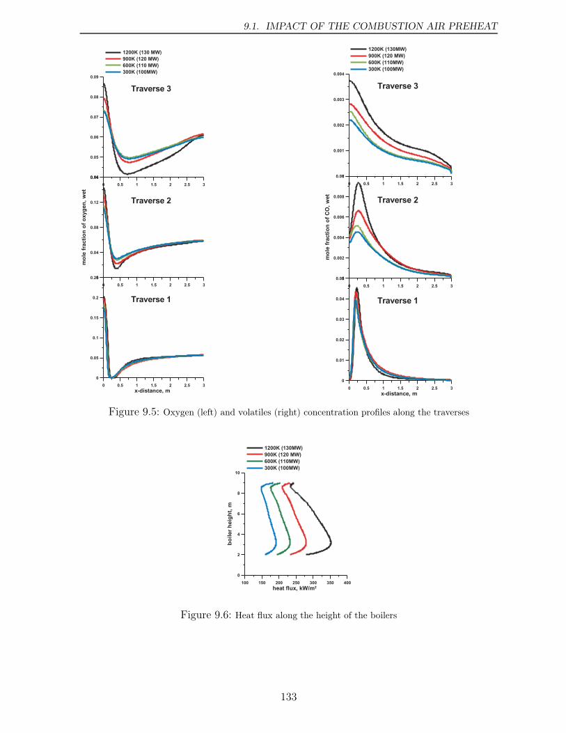
9.1. IMPACT OF THE COMBUSTION AIR PREHEAT
Figure 9.5: Oxygen (left) and volatiles (right) concentration profiles along the traverses
Figure 9.6: Heat flux along the height of the boilers
133
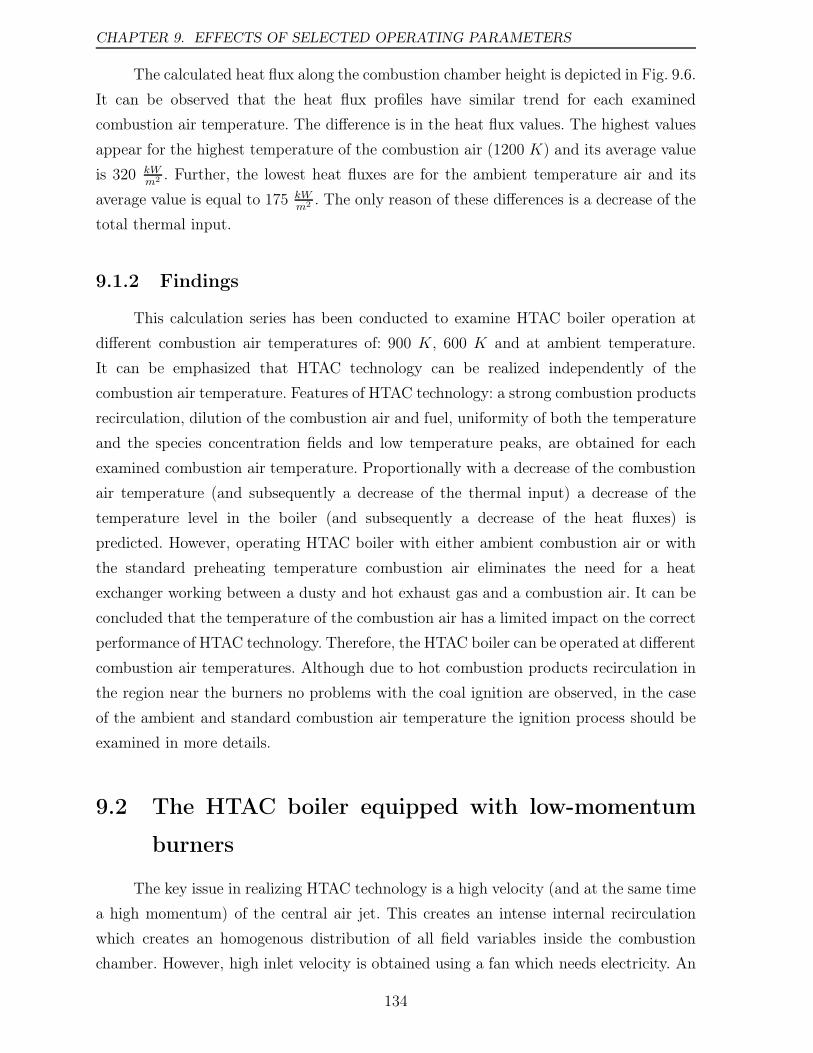
CHAPTER 9. EFFECTS OF SELECTED OPERATING PARAMETERS
The calculated heat flux along the combustion chamber height is depicted in Fig. 9.6.
It can be observed that the heat flux profiles have similar trend for each examined
combustion air temperature. The difference is in the heat flux values. The highest values
appear for the highest temperature of the combustion air (1200 K) and its average value
is 320 kWm2
. Further, the lowest heat fluxes are for the ambient temperature air and its
average value is equal to 175 kWm2
. The only reason of these differences is a decrease of the
total thermal input.
9.1.2 Findings
This calculation series has been conducted to examine HTAC boiler operation at
different combustion air temperatures of: 900 K, 600 K and at ambient temperature.
It can be emphasized that HTAC technology can be realized independently of the
combustion air temperature. Features of HTAC technology: a strong combustion products
recirculation, dilution of the combustion air and fuel, uniformity of both the temperature
and the species concentration fields and low temperature peaks, are obtained for each
examined combustion air temperature. Proportionally with a decrease of the combustion
air temperature (and subsequently a decrease of the thermal input) a decrease of the
temperature level in the boiler (and subsequently a decrease of the heat fluxes) is
predicted. However, operating HTAC boiler with either ambient combustion air or with
the standard preheating temperature combustion air eliminates the need for a heat
exchanger working between a dusty and hot exhaust gas and a combustion air. It can be
concluded that the temperature of the combustion air has a limited impact on the correct
performance of HTAC technology. Therefore, the HTAC boiler can be operated at different
combustion air temperatures. Although due to hot combustion products recirculation in
the region near the burners no problems with the coal ignition are observed, in the case
of the ambient and standard combustion air temperature the ignition process should be
examined in more details.
9.2 The HTAC boiler equipped with low-momentum
burners
The key issue in realizing HTAC technology is a high velocity (and at the same time
a high momentum) of the central air jet. This creates an intense internal recirculation
which creates an homogenous distribution of all field variables inside the combustion
chamber. However, high inlet velocity is obtained using a fan which needs electricity. An
134
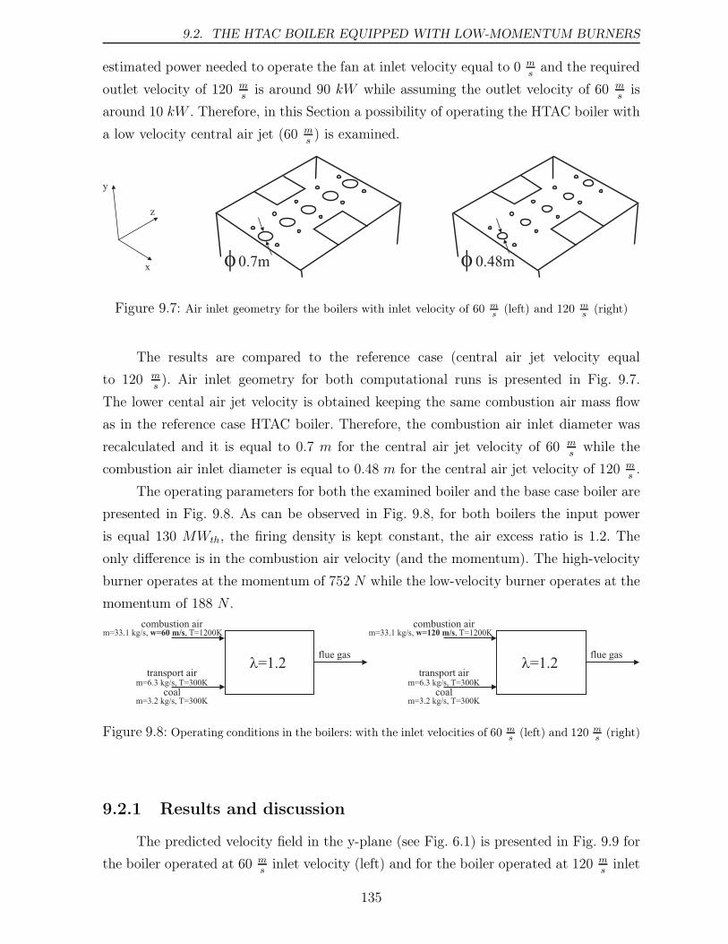
9.2. THE HTAC BOILER EQUIPPED WITH LOW-MOMENTUM BURNERS
estimated power needed to operate the fan at inlet velocity equal to 0 ms
and the required
outlet velocity of 120 ms
is around 90 kW while assuming the outlet velocity of 60 ms
is
around 10 kW . Therefore, in this Section a possibility of operating the HTAC boiler with
a low velocity central air jet (60 ms) is examined.
0.7m 0.48mx
y
z
f f
Figure 9.7: Air inlet geometry for the boilers with inlet velocity of 60 ms
(left) and 120 ms
(right)
The results are compared to the reference case (central air jet velocity equal
to 120 ms). Air inlet geometry for both computational runs is presented in Fig. 9.7.
The lower cental air jet velocity is obtained keeping the same combustion air mass flow
as in the reference case HTAC boiler. Therefore, the combustion air inlet diameter was
recalculated and it is equal to 0.7 m for the central air jet velocity of 60 ms
while the
combustion air inlet diameter is equal to 0.48 m for the central air jet velocity of 120 ms.
The operating parameters for both the examined boiler and the base case boiler are
presented in Fig. 9.8. As can be observed in Fig. 9.8, for both boilers the input power
is equal 130 MWth, the firing density is kept constant, the air excess ratio is 1.2. The
only difference is in the combustion air velocity (and the momentum). The high-velocity
burner operates at the momentum of 752 N while the low-velocity burner operates at the
momentum of 188 N .combustion air
transport air
m=33.1 kg/s, , T=1200Kw=60 m/s
coalm=6.3 kg/s, T=300K
m=3.2 kg/s, T=300K
l=1.2flue gas
combustion air
transport air
m=33.1 kg/s, w=120 m/s, T=1200K
coalm=6.3 kg/s, T=300K
m=3.2 kg/s, T=300K
l=1.2flue gas
Figure 9.8: Operating conditions in the boilers: with the inlet velocities of 60 ms
(left) and 120 ms
(right)
9.2.1 Results and discussion
The predicted velocity field in the y-plane (see Fig. 6.1) is presented in Fig. 9.9 for
the boiler operated at 60 ms
inlet velocity (left) and for the boiler operated at 120 ms
inlet
135
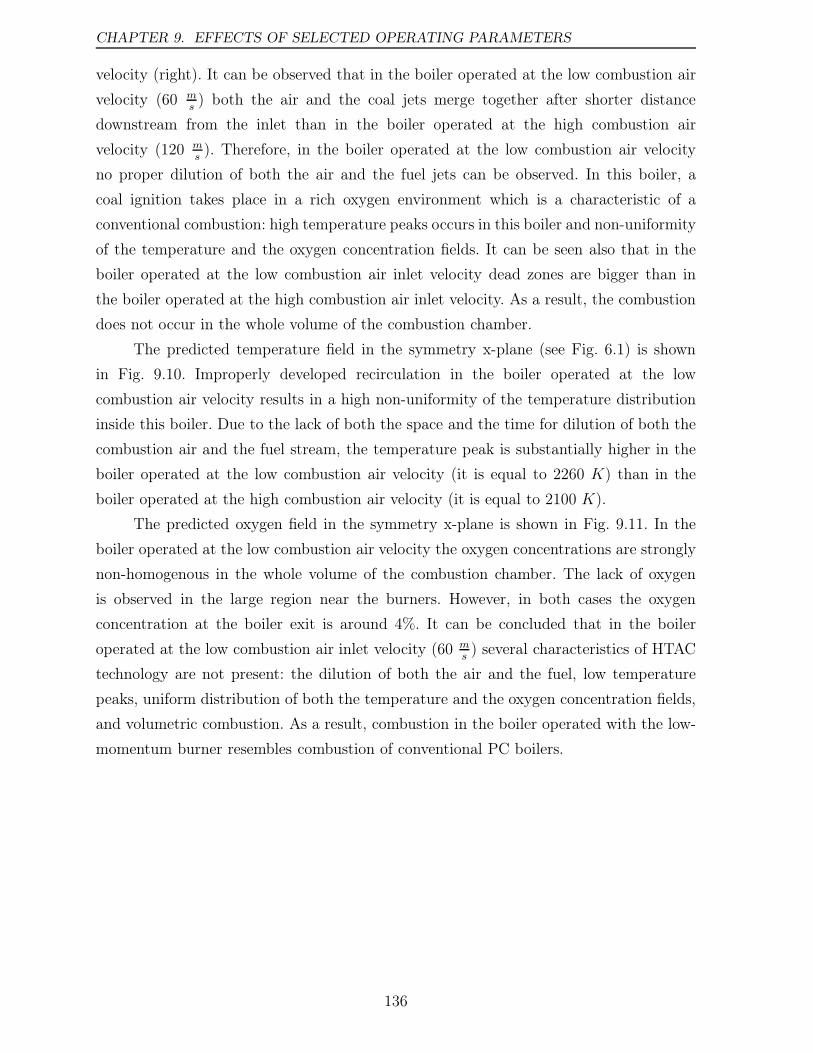
CHAPTER 9. EFFECTS OF SELECTED OPERATING PARAMETERS
velocity (right). It can be observed that in the boiler operated at the low combustion air
velocity (60 ms) both the air and the coal jets merge together after shorter distance
downstream from the inlet than in the boiler operated at the high combustion air
velocity (120 ms). Therefore, in the boiler operated at the low combustion air velocity
no proper dilution of both the air and the fuel jets can be observed. In this boiler, a
coal ignition takes place in a rich oxygen environment which is a characteristic of a
conventional combustion: high temperature peaks occurs in this boiler and non-uniformity
of the temperature and the oxygen concentration fields. It can be seen also that in the
boiler operated at the low combustion air inlet velocity dead zones are bigger than in
the boiler operated at the high combustion air inlet velocity. As a result, the combustion
does not occur in the whole volume of the combustion chamber.
The predicted temperature field in the symmetry x-plane (see Fig. 6.1) is shown
in Fig. 9.10. Improperly developed recirculation in the boiler operated at the low
combustion air velocity results in a high non-uniformity of the temperature distribution
inside this boiler. Due to the lack of both the space and the time for dilution of both the
combustion air and the fuel stream, the temperature peak is substantially higher in the
boiler operated at the low combustion air velocity (it is equal to 2260 K) than in the
boiler operated at the high combustion air velocity (it is equal to 2100 K).
The predicted oxygen field in the symmetry x-plane is shown in Fig. 9.11. In the
boiler operated at the low combustion air velocity the oxygen concentrations are strongly
non-homogenous in the whole volume of the combustion chamber. The lack of oxygen
is observed in the large region near the burners. However, in both cases the oxygen
concentration at the boiler exit is around 4%. It can be concluded that in the boiler
operated at the low combustion air inlet velocity (60 ms) several characteristics of HTAC
technology are not present: the dilution of both the air and the fuel, low temperature
peaks, uniform distribution of both the temperature and the oxygen concentration fields,
and volumetric combustion. As a result, combustion in the boiler operated with the low-
momentum burner resembles combustion of conventional PC boilers.
136
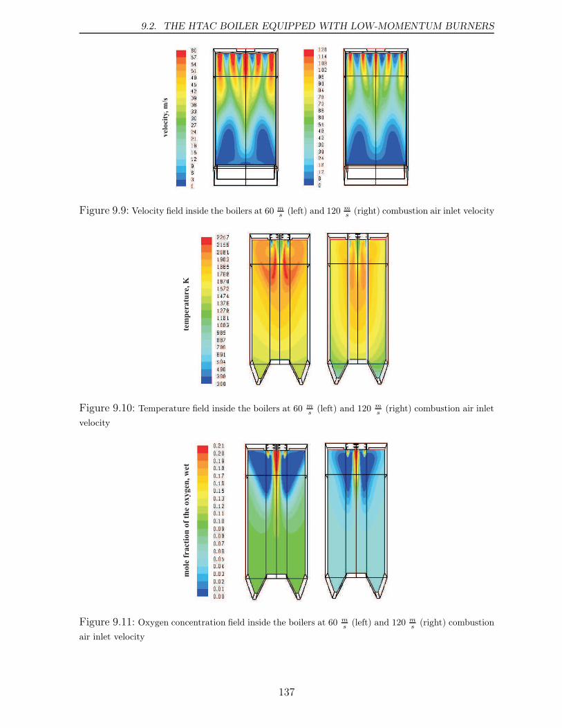
9.2. THE HTAC BOILER EQUIPPED WITH LOW-MOMENTUM BURNERS
vel
oci
ty, m
/s
Figure 9.9: Velocity field inside the boilers at 60 ms
(left) and 120 ms
(right) combustion air inlet velocity
tem
per
atu
re, K
Figure 9.10: Temperature field inside the boilers at 60 ms
(left) and 120 ms
(right) combustion air inlet
velocity
mole
fra
ctio
n o
f th
e oxygen
, w
et
Figure 9.11: Oxygen concentration field inside the boilers at 60 ms
(left) and 120 ms
(right) combustion
air inlet velocity
137
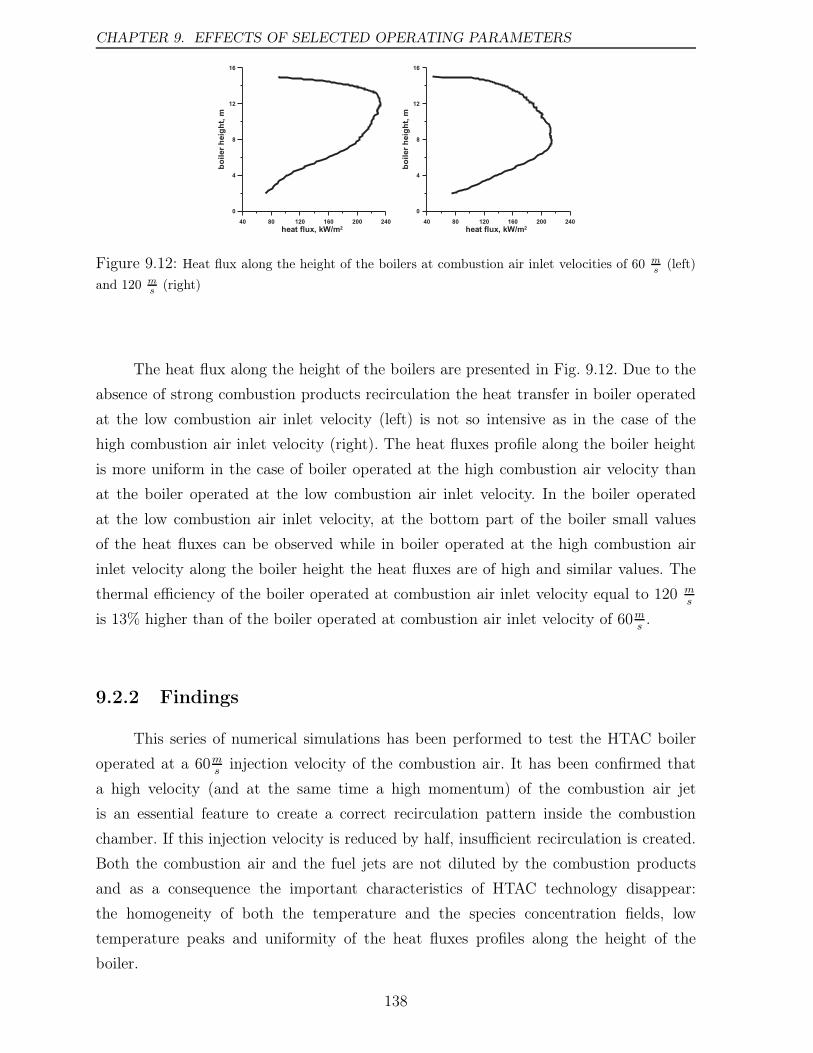
CHAPTER 9. EFFECTS OF SELECTED OPERATING PARAMETERS
40 80 120 160 200 240
heat flux, kW/m2
0
4
8
12
16
bo
iler
heig
ht,
m
40 80 120 160 200 240
heat flux, kW/m2
0
4
8
12
16
bo
iler
heig
ht,
m
Figure 9.12: Heat flux along the height of the boilers at combustion air inlet velocities of 60 ms
(left)
and 120 ms
(right)
The heat flux along the height of the boilers are presented in Fig. 9.12. Due to the
absence of strong combustion products recirculation the heat transfer in boiler operated
at the low combustion air inlet velocity (left) is not so intensive as in the case of the
high combustion air inlet velocity (right). The heat fluxes profile along the boiler height
is more uniform in the case of boiler operated at the high combustion air velocity than
at the boiler operated at the low combustion air inlet velocity. In the boiler operated
at the low combustion air inlet velocity, at the bottom part of the boiler small values
of the heat fluxes can be observed while in boiler operated at the high combustion air
inlet velocity along the boiler height the heat fluxes are of high and similar values. The
thermal efficiency of the boiler operated at combustion air inlet velocity equal to 120 ms
is 13% higher than of the boiler operated at combustion air inlet velocity of 60ms.
9.2.2 Findings
This series of numerical simulations has been performed to test the HTAC boiler
operated at a 60ms
injection velocity of the combustion air. It has been confirmed that
a high velocity (and at the same time a high momentum) of the combustion air jet
is an essential feature to create a correct recirculation pattern inside the combustion
chamber. If this injection velocity is reduced by half, insufficient recirculation is created.
Both the combustion air and the fuel jets are not diluted by the combustion products
and as a consequence the important characteristics of HTAC technology disappear:
the homogeneity of both the temperature and the species concentration fields, low
temperature peaks and uniformity of the heat fluxes profiles along the height of the
boiler.
138
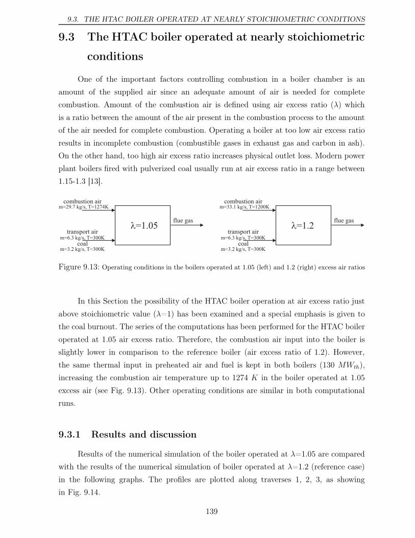
9.3. THE HTAC BOILER OPERATED AT NEARLY STOICHIOMETRIC CONDITIONS
9.3 The HTAC boiler operated at nearly stoichiometric
conditions
One of the important factors controlling combustion in a boiler chamber is an
amount of the supplied air since an adequate amount of air is needed for complete
combustion. Amount of the combustion air is defined using air excess ratio (λ) which
is a ratio between the amount of the air present in the combustion process to the amount
of the air needed for complete combustion. Operating a boiler at too low air excess ratio
results in incomplete combustion (combustible gases in exhaust gas and carbon in ash).
On the other hand, too high air excess ratio increases physical outlet loss. Modern power
plant boilers fired with pulverized coal usually run at air excess ratio in a range between
1.15-1.3 [13].
combustion air
transport air
m=33.1 kg/s, T=1200K
coalm=6.3 kg/s, T=300K
m=3.2 kg/s, T=300K
l=1.2flue gas
combustion air
transport air
m=29.7 kg/s, T=1274K
coalm=6.3 kg/s, T=300K
m=3.2 kg/s, T=300K
l=1.05flue gas
Figure 9.13: Operating conditions in the boilers operated at 1.05 (left) and 1.2 (right) excess air ratios
In this Section the possibility of the HTAC boiler operation at air excess ratio just
above stoichiometric value (λ=1) has been examined and a special emphasis is given to
the coal burnout. The series of the computations has been performed for the HTAC boiler
operated at 1.05 air excess ratio. Therefore, the combustion air input into the boiler is
slightly lower in comparison to the reference boiler (air excess ratio of 1.2). However,
the same thermal input in preheated air and fuel is kept in both boilers (130 MWth),
increasing the combustion air temperature up to 1274 K in the boiler operated at 1.05
excess air (see Fig. 9.13). Other operating conditions are similar in both computational
runs.
9.3.1 Results and discussion
Results of the numerical simulation of the boiler operated at λ=1.05 are compared
with the results of the numerical simulation of boiler operated at λ=1.2 (reference case)
in the following graphs. The profiles are plotted along traverses 1, 2, 3, as showing
in Fig. 9.14.
139
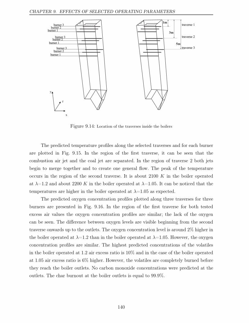
CHAPTER 9. EFFECTS OF SELECTED OPERATING PARAMETERS
1m
3m
5m
traverse 1
traverse 2
traverse 3burner 3burner 2
burner 1
x
y
z
burner 1burner 2
burner 3
burner 1burner 2
burner 3
Figure 9.14: Location of the traverses inside the boilers
The predicted temperature profiles along the selected traverses and for each burner
are plotted in Fig. 9.15. In the region of the first traverse, it can be seen that the
combustion air jet and the coal jet are separated. In the region of traverse 2 both jets
begin to merge together and to create one general flow. The peak of the temperature
occurs in the region of the second traverse. It is about 2100 K in the boiler operated
at λ=1.2 and about 2200 K in the boiler operated at λ=1.05. It can be noticed that the
temperatures are higher in the boiler operated at λ=1.05 as expected.
The predicted oxygen concentration profiles plotted along three traverses for three
burners are presented in Fig. 9.16. In the region of the first traverse for both tested
excess air values the oxygen concentration profiles are similar; the lack of the oxygen
can be seen. The difference between oxygen levels are visible beginning from the second
traverse onwards up to the outlets. The oxygen concentration level is around 2% higher in
the boiler operated at λ=1.2 than in the boiler operated at λ=1.05. However, the oxygen
concentration profiles are similar. The highest predicted concentrations of the volatiles
in the boiler operated at 1.2 air excess ratio is 10% and in the case of the boiler operated
at 1.05 air excess ratio is 6% higher. However, the volatiles are completely burned before
they reach the boiler outlets. No carbon monoxide concentrations were predicted at the
outlets. The char burnout at the boiler outlets is equal to 99.9%.
140
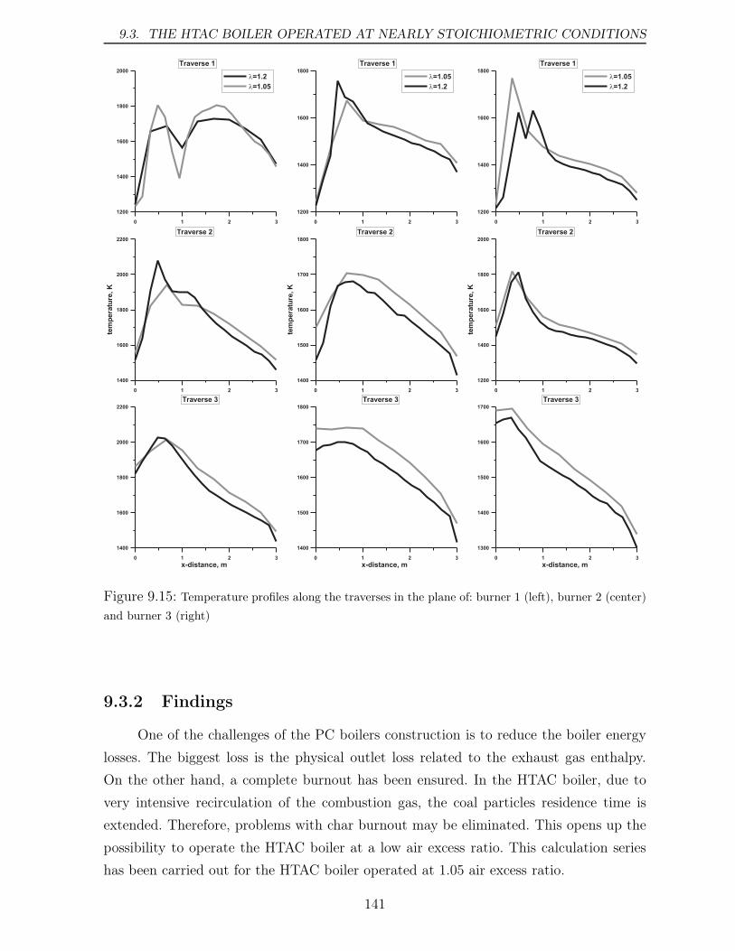
9.3. THE HTAC BOILER OPERATED AT NEARLY STOICHIOMETRIC CONDITIONS
0 1 2 3
x-distance, m
1400
1600
1800
2000
2200
Traverse 3
0 1 2 3
1400
1600
1800
2000
2200
tem
pera
ture
,K
Traverse 2
0 1 2 3
1200
1400
1600
1800
2000
l=1.2
l=1.05
Traverse 1
0 1 2 3
x-distance, m
1300
1400
1500
1600
1700
Traverse 3
0 1 2 3
1200
1400
1600
1800
2000
tem
pera
ture
,K
Traverse 2
0 1 2 3
1200
1400
1600
1800
l=1.05
l=1.2
Traverse 1
0 1 2 3
x-distance, m
1400
1500
1600
1700
1800
Traverse 3
0 1 2 3
1400
1500
1600
1700
1800
tem
pera
ture
,K
Traverse 2
0 1 2 3
1200
1400
1600
1800
l=1.05
l=1.2
Traverse 1
Figure 9.15: Temperature profiles along the traverses in the plane of: burner 1 (left), burner 2 (center)
and burner 3 (right)
9.3.2 Findings
One of the challenges of the PC boilers construction is to reduce the boiler energy
losses. The biggest loss is the physical outlet loss related to the exhaust gas enthalpy.
On the other hand, a complete burnout has been ensured. In the HTAC boiler, due to
very intensive recirculation of the combustion gas, the coal particles residence time is
extended. Therefore, problems with char burnout may be eliminated. This opens up the
possibility to operate the HTAC boiler at a low air excess ratio. This calculation series
has been carried out for the HTAC boiler operated at 1.05 air excess ratio.
141
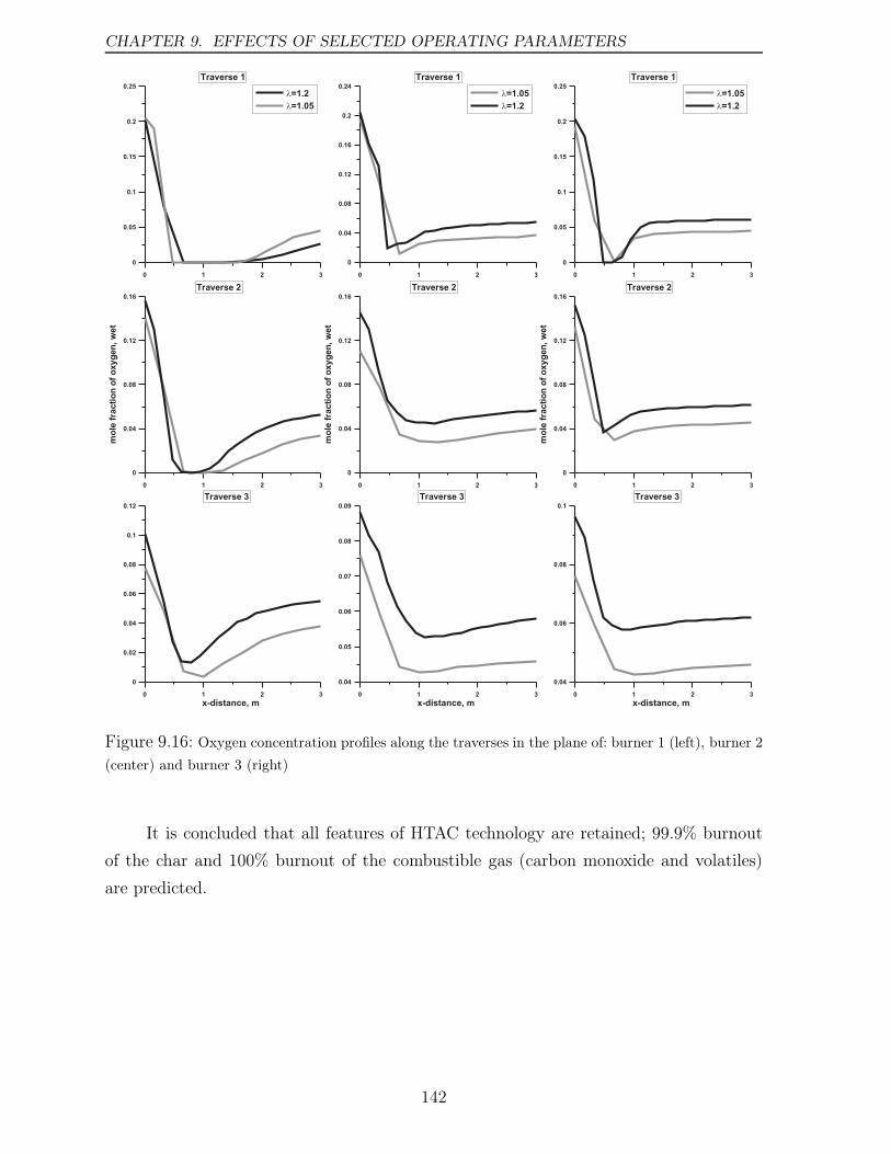
CHAPTER 9. EFFECTS OF SELECTED OPERATING PARAMETERS
0 1 2 3
x-distance, m
0.04
0.05
0.06
0.07
0.08
0.09
Traverse 3
0 1 2 3
0
0.04
0.08
0.12
0.16
mo
lefr
acti
on
of
oxyg
en
,w
et
Traverse 2
0 1 2 3
0
0.04
0.08
0.12
0.16
0.2
0.24
l=1.05
l=1.2
Traverse 1
0 1 2 3
x-distance, m
0.04
0.06
0.08
0.1
Traverse 3
0 1 2 3
0
0.04
0.08
0.12
0.16
mo
lefr
acti
on
of
oxyg
en
,w
et
Traverse 2
0 1 2 3
0
0.05
0.1
0.15
0.2
0.25
l=1.05
l=1.2
Traverse 1
0 1 2 3
x-distance, m
0
0.02
0.04
0.06
0.08
0.1
0.12
Traverse 3
0 1 2 3
0
0.04
0.08
0.12
0.16
mo
lefr
acti
on
of
oxyg
en
,w
et
Traverse 2
0 1 2 3
0
0.05
0.1
0.15
0.2
0.25
l=1.2
l=1.05
Traverse 1
Figure 9.16: Oxygen concentration profiles along the traverses in the plane of: burner 1 (left), burner 2
(center) and burner 3 (right)
It is concluded that all features of HTAC technology are retained; 99.9% burnout
of the char and 100% burnout of the combustible gas (carbon monoxide and volatiles)
are predicted.
142
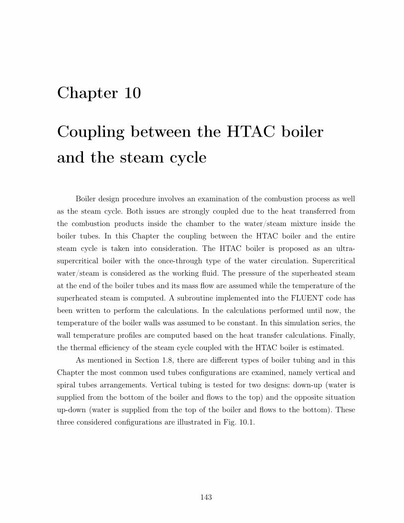
Chapter 10
Coupling between the HTAC boiler
and the steam cycle
Boiler design procedure involves an examination of the combustion process as well
as the steam cycle. Both issues are strongly coupled due to the heat transferred from
the combustion products inside the chamber to the water/steam mixture inside the
boiler tubes. In this Chapter the coupling between the HTAC boiler and the entire
steam cycle is taken into consideration. The HTAC boiler is proposed as an ultra-
supercritical boiler with the once-through type of the water circulation. Supercritical
water/steam is considered as the working fluid. The pressure of the superheated steam
at the end of the boiler tubes and its mass flow are assumed while the temperature of the
superheated steam is computed. A subroutine implemented into the FLUENT code has
been written to perform the calculations. In the calculations performed until now, the
temperature of the boiler walls was assumed to be constant. In this simulation series, the
wall temperature profiles are computed based on the heat transfer calculations. Finally,
the thermal efficiency of the steam cycle coupled with the HTAC boiler is estimated.
As mentioned in Section 1.8, there are different types of boiler tubing and in this
Chapter the most common used tubes configurations are examined, namely vertical and
spiral tubes arrangements. Vertical tubing is tested for two designs: down-up (water is
supplied from the bottom of the boiler and flows to the top) and the opposite situation
up-down (water is supplied from the top of the boiler and flows to the bottom). These
three considered configurations are illustrated in Fig. 10.1.
143
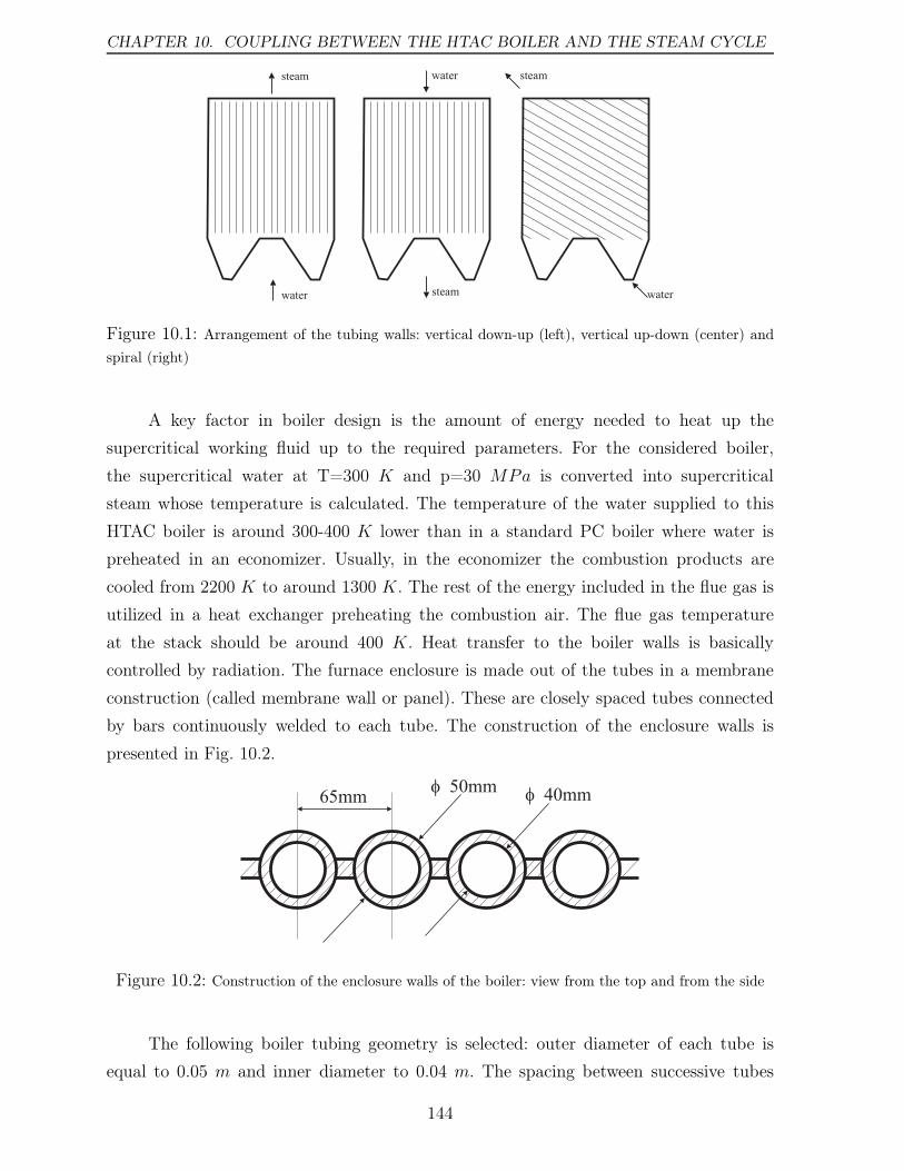
CHAPTER 10. COUPLING BETWEEN THE HTAC BOILER AND THE STEAM CYCLE
water
watersteam
steam water
steam
Figure 10.1: Arrangement of the tubing walls: vertical down-up (left), vertical up-down (center) and
spiral (right)
A key factor in boiler design is the amount of energy needed to heat up the
supercritical working fluid up to the required parameters. For the considered boiler,
the supercritical water at T=300 K and p=30 MPa is converted into supercritical
steam whose temperature is calculated. The temperature of the water supplied to this
HTAC boiler is around 300-400 K lower than in a standard PC boiler where water is
preheated in an economizer. Usually, in the economizer the combustion products are
cooled from 2200 K to around 1300 K. The rest of the energy included in the flue gas is
utilized in a heat exchanger preheating the combustion air. The flue gas temperature
at the stack should be around 400 K. Heat transfer to the boiler walls is basically
controlled by radiation. The furnace enclosure is made out of the tubes in a membrane
construction (called membrane wall or panel). These are closely spaced tubes connected
by bars continuously welded to each tube. The construction of the enclosure walls is
presented in Fig. 10.2.
65mm f 40mmf 50mm
Figure 10.2: Construction of the enclosure walls of the boiler: view from the top and from the side
The following boiler tubing geometry is selected: outer diameter of each tube is
equal to 0.05 m and inner diameter to 0.04 m. The spacing between successive tubes
144
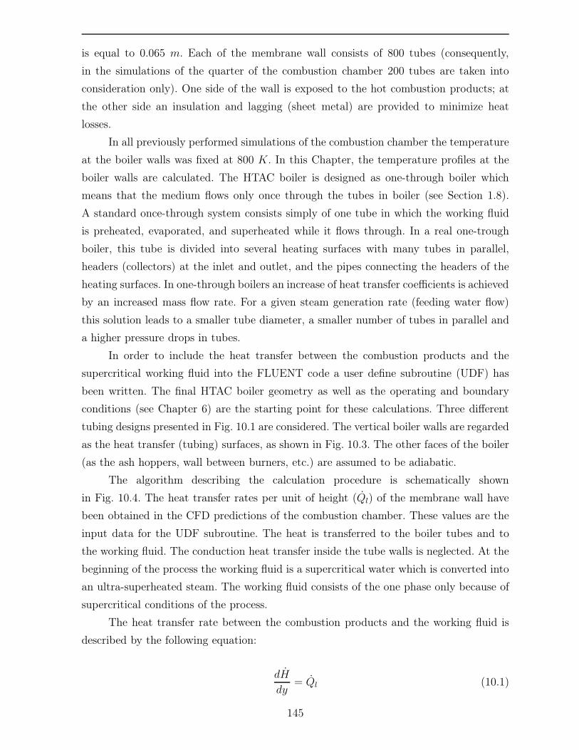
is equal to 0.065 m. Each of the membrane wall consists of 800 tubes (consequently,
in the simulations of the quarter of the combustion chamber 200 tubes are taken into
consideration only). One side of the wall is exposed to the hot combustion products; at
the other side an insulation and lagging (sheet metal) are provided to minimize heat
losses.
In all previously performed simulations of the combustion chamber the temperature
at the boiler walls was fixed at 800 K. In this Chapter, the temperature profiles at the
boiler walls are calculated. The HTAC boiler is designed as one-through boiler which
means that the medium flows only once through the tubes in boiler (see Section 1.8).
A standard once-through system consists simply of one tube in which the working fluid
is preheated, evaporated, and superheated while it flows through. In a real one-trough
boiler, this tube is divided into several heating surfaces with many tubes in parallel,
headers (collectors) at the inlet and outlet, and the pipes connecting the headers of the
heating surfaces. In one-through boilers an increase of heat transfer coefficients is achieved
by an increased mass flow rate. For a given steam generation rate (feeding water flow)
this solution leads to a smaller tube diameter, a smaller number of tubes in parallel and
a higher pressure drops in tubes.
In order to include the heat transfer between the combustion products and the
supercritical working fluid into the FLUENT code a user define subroutine (UDF) has
been written. The final HTAC boiler geometry as well as the operating and boundary
conditions (see Chapter 6) are the starting point for these calculations. Three different
tubing designs presented in Fig. 10.1 are considered. The vertical boiler walls are regarded
as the heat transfer (tubing) surfaces, as shown in Fig. 10.3. The other faces of the boiler
(as the ash hoppers, wall between burners, etc.) are assumed to be adiabatic.
The algorithm describing the calculation procedure is schematically shown
in Fig. 10.4. The heat transfer rates per unit of height (Ql) of the membrane wall have
been obtained in the CFD predictions of the combustion chamber. These values are the
input data for the UDF subroutine. The heat is transferred to the boiler tubes and to
the working fluid. The conduction heat transfer inside the tube walls is neglected. At the
beginning of the process the working fluid is a supercritical water which is converted into
an ultra-superheated steam. The working fluid consists of the one phase only because of
supercritical conditions of the process.
The heat transfer rate between the combustion products and the working fluid is
described by the following equation:
dH
dy= Ql (10.1)
145
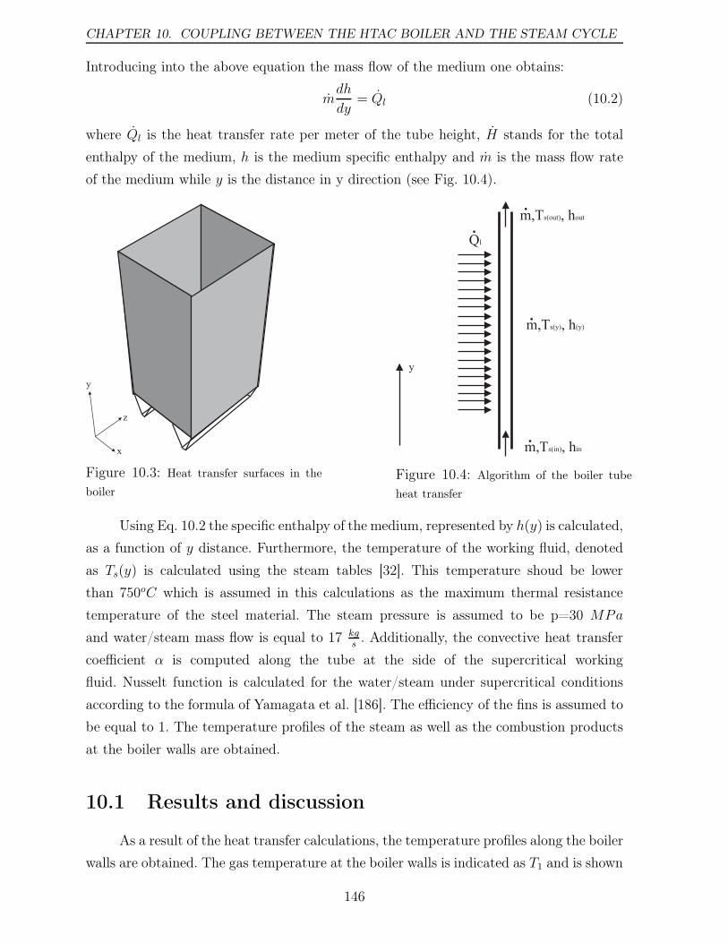
CHAPTER 10. COUPLING BETWEEN THE HTAC BOILER AND THE STEAM CYCLE
Introducing into the above equation the mass flow of the medium one obtains:
mdh
dy= Ql (10.2)
where Ql is the heat transfer rate per meter of the tube height, H stands for the total
enthalpy of the medium, h is the medium specific enthalpy and m is the mass flow rate
of the medium while y is the distance in y direction (see Fig. 10.4).
Figure 10.3: Heat transfer surfaces in the
boiler
Ql
.
m,T , hs(y) (y)
m,T , hs(out) out
m,T , hs(in) in
y
.
.
.
Figure 10.4: Algorithm of the boiler tube
heat transfer
Using Eq. 10.2 the specific enthalpy of the medium, represented by h(y) is calculated,
as a function of y distance. Furthermore, the temperature of the working fluid, denoted
as Ts(y) is calculated using the steam tables [32]. This temperature shoud be lower
than 750oC which is assumed in this calculations as the maximum thermal resistance
temperature of the steel material. The steam pressure is assumed to be p=30 MPa
and water/steam mass flow is equal to 17 kgs. Additionally, the convective heat transfer
coefficient α is computed along the tube at the side of the supercritical working
fluid. Nusselt function is calculated for the water/steam under supercritical conditions
according to the formula of Yamagata et al. [186]. The efficiency of the fins is assumed to
be equal to 1. The temperature profiles of the steam as well as the combustion products
at the boiler walls are obtained.
10.1 Results and discussion
As a result of the heat transfer calculations, the temperature profiles along the boiler
walls are obtained. The gas temperature at the boiler walls is indicated as T1 and is shown
146
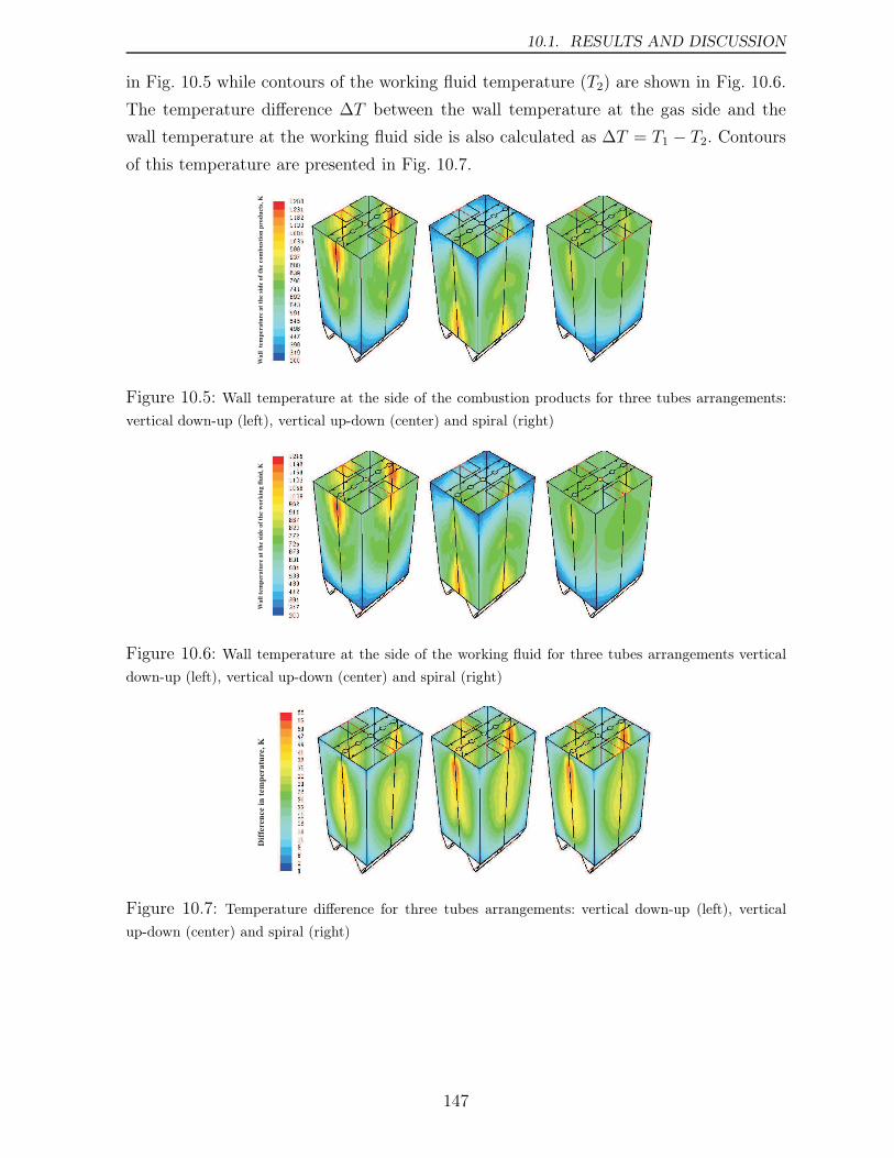
10.1. RESULTS AND DISCUSSION
in Fig. 10.5 while contours of the working fluid temperature (T2) are shown in Fig. 10.6.
The temperature difference ∆T between the wall temperature at the gas side and the
wall temperature at the working fluid side is also calculated as ∆T = T1 − T2. Contours
of this temperature are presented in Fig. 10.7.
Wall
at
the
sid
e of
the
cte
mp
eratu
re, K
om
bu
stio
n p
rod
uct
s
Figure 10.5: Wall temperature at the side of the combustion products for three tubes arrangements:
vertical down-up (left), vertical up-down (center) and spiral (right)
Wall
tem
per
atu
re a
t th
e si
de
of
the
w, K
ork
ing f
luid
Figure 10.6: Wall temperature at the side of the working fluid for three tubes arrangements vertical
down-up (left), vertical up-down (center) and spiral (right)
Dif
fere
nce
in
tem
per
atu
re, K
Figure 10.7: Temperature difference for three tubes arrangements: vertical down-up (left), vertical
up-down (center) and spiral (right)
147
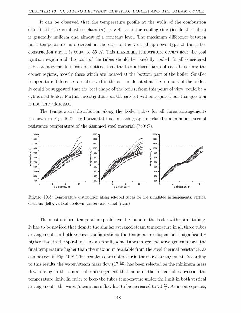
CHAPTER 10. COUPLING BETWEEN THE HTAC BOILER AND THE STEAM CYCLE
It can be observed that the temperature profile at the walls of the combustion
side (inside the combustion chamber) as well as at the cooling side (inside the tubes)
is generally uniform and almost of a constant level. The maximum difference between
both temperatures is observed in the case of the vertical up-down type of the tubes
construction and it is equal to 55 K. This maximum temperature occurs near the coal
ignition region and this part of the tubes should be carefully cooled. In all considered
tubes arrangements it can be noticed that the less utilized parts of each boiler are the
corner regions, mostly these which are located at the bottom part of the boiler. Smaller
temperature differences are observed in the corners located at the top part of the boiler.
It could be suggested that the best shape of the boiler, from this point of view, could be a
cylindrical boiler. Further investigations on the subject will be required but this question
is not here addressed.
The temperature distribution along the boiler tubes for all three arrangements
is shown in Fig. 10.8; the horizontal line in each graph marks the maximum thermal
resistance temperature of the assumed steel material (750oC).
0 4 8 12
y-distance, m
300
400
500
600
700
800
900
1000
1100
1200
1300
tem
pera
ture
,K
0 4 8 12
y-distance, m
300
400
500
600
700
800
900
1000
1100
1200
1300
tem
pera
ture
,K
0 4 8 12
y-distance, m
300
400
500
600
700
800
900
1000
1100
1200
1300
tem
pera
ture
,K
Figure 10.8: Temperature distribution along selected tubes for the simulated arrangements: vertical
down-up (left), vertical up-down (center) and spiral (right)
The most uniform temperature profile can be found in the boiler with spiral tubing.
It has to be noticed that despite the similar averaged steam temperature in all three tubes
arrangements in both vertical configurations the temperature dispersion is significantly
higher than in the spiral one. As an result, some tubes in vertical arrangements have the
final temperature higher than the maximum available from the steel thermal resistance, as
can be seen in Fig. 10.8. This problem does not occur in the spiral arrangement. According
to this results the water/steam mass flow (17 kgs) has been selected as the minimum mass
flow forcing in the spiral tube arrangement that none of the boiler tubes overrun the
temperature limit. In order to keep the tubes temperature under the limit in both vertical
arrangements, the water/steam mass flow has to be increased to 20 kgs. As a consequence,
148
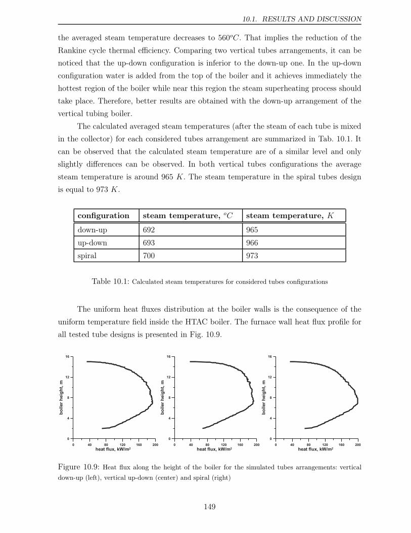
10.1. RESULTS AND DISCUSSION
the averaged steam temperature decreases to 560oC. That implies the reduction of the
Rankine cycle thermal efficiency. Comparing two vertical tubes arrangements, it can be
noticed that the up-down configuration is inferior to the down-up one. In the up-down
configuration water is added from the top of the boiler and it achieves immediately the
hottest region of the boiler while near this region the steam superheating process should
take place. Therefore, better results are obtained with the down-up arrangement of the
vertical tubing boiler.
The calculated averaged steam temperatures (after the steam of each tube is mixed
in the collector) for each considered tubes arrangement are summarized in Tab. 10.1. It
can be observed that the calculated steam temperature are of a similar level and only
slightly differences can be observed. In both vertical tubes configurations the average
steam temperature is around 965 K. The steam temperature in the spiral tubes design
is equal to 973 K.
configuration steam temperature, oC steam temperature, K
down-up 692 965
up-down 693 966
spiral 700 973
Table 10.1: Calculated steam temperatures for considered tubes configurations
The uniform heat fluxes distribution at the boiler walls is the consequence of the
uniform temperature field inside the HTAC boiler. The furnace wall heat flux profile for
all tested tube designs is presented in Fig. 10.9.
0 40 80 120 160 200
heat flux, kW/m2
0
4
8
12
16
bo
iler
heig
ht,
m
0 40 80 120 160 200
heat flux, kW/m2
0
4
8
12
16
bo
iler
heig
ht,
m
0 40 80 120 160 200
heat flux, kW/m2
0
4
8
12
16
bo
iler
heig
ht,
m
Figure 10.9: Heat flux along the height of the boiler for the simulated tubes arrangements: vertical
down-up (left), vertical up-down (center) and spiral (right)
149
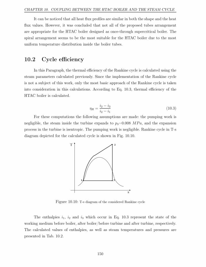
CHAPTER 10. COUPLING BETWEEN THE HTAC BOILER AND THE STEAM CYCLE
It can be noticed that all heat flux profiles are similar in both the shape and the heat
flux values. However, it was concluded that not all of the proposed tubes arrangement
are appropriate for the HTAC boiler designed as once-through supercritical boiler. The
spiral arrangement seems to be the most suitable for the HTAC boiler due to the most
uniform temperature distribution inside the boiler tubes.
10.2 Cycle efficiency
In this Paragraph, the thermal efficiency of the Rankine cycle is calculated using the
steam parameters calculated previously. Since the implementation of the Rankine cycle
is not a subject of this work, only the most basic approach of the Rankine cycle is taken
into consideration in this calculations. According to Eq. 10.3, thermal efficiency of the
HTAC boiler is calculated.
ηR =i2 − i3i2 − i1
(10.3)
For these computations the following assumptions are made: the pumping work is
negligible, the steam inside the turbine expands to p3=0.008 MPa, and the expansion
process in the turbine is isentropic. The pumping work is negligible. Rankine cycle in T-s
diagram depicted for the calculated cycle is shown in Fig. 10.10.
T
s
1 3
2
Figure 10.10: T-s diagram of the considered Rankine cycle
The enthalpies i1, i2 and i3 which occur in Eq. 10.3 represent the state of the
working medium before boiler, after boiler/before turbine and after turbine, respectively.
The calculated values of enthalpies, as well as steam temperatures and pressures are
presented in Tab. 10.2.
150
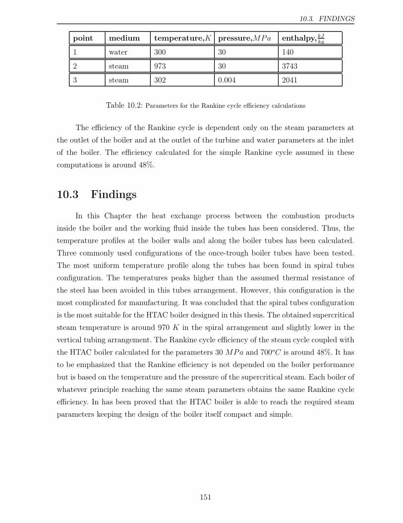
10.3. FINDINGS
point medium temperature,K pressure,MPa enthalpy,kJkg
1 water 300 30 140
2 steam 973 30 3743
3 steam 302 0.004 2041
Table 10.2: Parameters for the Rankine cycle efficiency calculations
The efficiency of the Rankine cycle is dependent only on the steam parameters at
the outlet of the boiler and at the outlet of the turbine and water parameters at the inlet
of the boiler. The efficiency calculated for the simple Rankine cycle assumed in these
computations is around 48%.
10.3 Findings
In this Chapter the heat exchange process between the combustion products
inside the boiler and the working fluid inside the tubes has been considered. Thus, the
temperature profiles at the boiler walls and along the boiler tubes has been calculated.
Three commonly used configurations of the once-trough boiler tubes have been tested.
The most uniform temperature profile along the tubes has been found in spiral tubes
configuration. The temperatures peaks higher than the assumed thermal resistance of
the steel has been avoided in this tubes arrangement. However, this configuration is the
most complicated for manufacturing. It was concluded that the spiral tubes configuration
is the most suitable for the HTAC boiler designed in this thesis. The obtained supercritical
steam temperature is around 970 K in the spiral arrangement and slightly lower in the
vertical tubing arrangement. The Rankine cycle efficiency of the steam cycle coupled with
the HTAC boiler calculated for the parameters 30MPa and 700oC is around 48%. It has
to be emphasized that the Rankine efficiency is not depended on the boiler performance
but is based on the temperature and the pressure of the supercritical steam. Each boiler of
whatever principle reaching the same steam parameters obtains the same Rankine cycle
efficiency. In has been proved that the HTAC boiler is able to reach the required steam
parameters keeping the design of the boiler itself compact and simple.
151

CHAPTER 10. COUPLING BETWEEN THE HTAC BOILER AND THE STEAM CYCLE
152
Chapter 11
Conclusions and future works
Conclusions
This thesis presents a novel boiler concept that utilizes the principle of High
Temperatures Air Combustion. Although the combustion with highly preheated air has
substantially advanced over the last decade or so, there has been relatively little work
undertaken to adapt it to coal combustion. The HTAC technology has already been
successfully applied to a number of industrial furnaces. However, such applications are
limited to either gaseous fuels or light oils. To the best of author’s knowledge this thesis
is the first attempt to design a HTAC boiler fired with pulverized coal. A hypothetical
130 MWth supercritical boiler producing 20 kgs
steam at parameters: pressure of 30 MPa
and temperature up to 700 oC has been developed.
Realizing the advantages of High Temperatures Air Combustion technology a boiler
of a high firing density has been designed with the combustion process proceeding in such
a way as to provide the highest possible uniformity of the increased heat fluxes. To this
end the NFK/IFRF burner concept which can be characterized by a central combustion
air jet and two pulverized coal jets, has been carefully tailored into the optimized boiler
shape (and volume). In order to achieve the required uniformity of the combustion process
which efficiently proceeds over the entire boiler volume a thorough optimization of the
following parameters has been carried out:
• number of burners and burner spacing
• distance between the coal jets and the central air jet
• the momentum (velocity) of the combustion air stream
• dimensions of the combustion chamber
153
CHAPTER 11. CONCLUSIONS AND FUTURE WORKS
Among the several geometries considered, the symmetrical boiler of a down-fired type
equipped with a one-trough spiral arrangement of cooling tubes has proven to be superior.
Such a design may result in the Rankine cycle efficiency exceeding 50%.
The study has indicated that such a boiler will possess several additional
characteristics as follow:
• low NOx emissions which for a coal containing around 1.5% N is
around 260 ppm at 6%O2
• flexible operation in terms of boiler turn-down
• improved fuel burnout due to enhanced coal ignition and long residence times
• simple burner constructions; without flame stabilization devices, swirl or air staging
which are commonly used in conventional pulverized coal burners
• small boiler size in comparison with standard PC boilers
Although HTAC technology seems to be attractive for power boilers fired with
pulverized coal there are still many open questions. The particulate concentration in the
flue gas for the coal flame is probably too high to use this technique in conjunction with
regenerative heat exchangers. There is a need to find a way to utilize the enthalpy of
the boiler exhaust gas. The unresolved issues of the HTAC technology application to
coal-fired boilers which have been identified in this work are:
• practical realization of preheating of combustion air using the flue gas
• the design may be prone to erosion
Overall, the present study confirmed that HTAC technology could be a practicable,
efficient and clean technology for fossil fuel fired boilers. However, it has to be pointed
out that the investigated boiler is still a concept only.
The study has been carried out for a Guasare high volatiles coal which in its
properties is similar to many hard coals of Poland. However, before proceeding further
with the boiler design optimization a comprehensive analysis of the effect of coal
properties is needed to establish a range of coals suitable for this particular design.
154
Future works
The work has demonstrated the advantages of the HTAC boiler although it is
prematurely to say that this new concept is complete. Research in the follow areas is
still required:
Optimization procedure of the boiler. The developed HTAC boiler is only a
concept; there are still several parameters which should be optimized. Probably, a
cylindrical boiler could be advantages.
Boiler fired with natural gas or oil. The major obstacle of the proposed HTAC
boiler is in the lack of a clear concept for utilization of the exhaust gas enthalpy for
air preheating. High particles concentrations of the exhaust gas cause slagging and
fouling of such devices. This problem does not occur when gaseous fuels or oils are
combusted. Boilers fired with natural gas were not investigated in this work because
of a low importance of natural gas in Poland. However, applications of HTAC technology
to boilers fired with gaseous fuels or oils are extremely attractive.
FLOX configuration. In the present work only the NFK/IFRF concept of HTAC
technology implementation has been studied. It could be interresting to examine also the
German approach, namely FLOX burner application into the proposed boiler.
HTAC combustion under O2/CO2 atmosphere. Increase interest in CO2
sequestration from large CO2 sources such as fossil fuel power plants is forced through
the anty-global warming polices. Several technologies for large scale CO2 capture are
under development. HTAC technology may be suitable for coal combustion under O2/CO2
atmosphere.
Laboratory, pilot and semi-industrial scale tests. Extra laboratory tests are
needed to enhance the understanding of both the devolatilization and the char combustion
under HTAC conditions. Furthermore, slagging, fouling, corrosion and errosion of metal
surfaces under HTAC conditions is poorly understood. Together with a basic research,
there is a need to increase the knowledge on applicability of HTAC technology to real
power plant boilers. Before an eventual industrial application of this technology takes
place, pilot tests, as well as semi industrial scale tests will be needed.
155

156
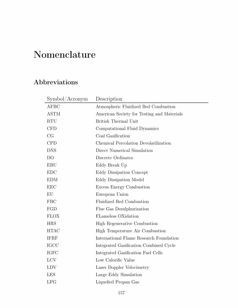
Nomenclature
Abbreviations
Symbol/Acronym DescriptionAFBC Atmospheric Fluidized Bed Combustion
ASTM American Society for Testing and Materials
BTU British Thermal Unit
CFD Computational Fluid Dynamics
CG Coal Gasification
CPD Chemical Percolation Devolatilization
DNS Direct Numerical Simulation
DO Discrete Ordinates
EBU Eddy Break Up
EDC Eddy Dissipation Concept
EDM Eddy Dissipation Model
EEC Excess Energy Combustion
EU European Union
FBC Fluidized Bed Combustion
FGD Flue Gas Desulphurization
FLOX FLameless OXidation
HRS High Regenerative Combustion
HTAC High Temperature Air Combustion
IFRF International Flame Research Foundation
IGCC Integrated Gasification Combined Cycle
IGFC Integrated Gasification Fuel Cells
LCV Low Calorific Value
LDV Laser Doppler Velocimetry
LES Large Eddy Simulation
LPG Liquefied Propan Gas
157

Symbol/Acronym DescriptionMILD Moderate and Intensive Low-oxygen Dilution
NFK Nippon Furnace Kogyo
NMR Nuclear Magnetic Resonance
PC Pulverized Coal
PFBC Pressurized Fluidized Bed Combustion
PFR Plug Flow Reactor
RAM Reynolds Avaraged Models
RANS Reynolds Avaraged Navier Stokes Equation
R&D Research and Development
SCR Selectiv Catalytic Reduction
SNG SyNtesis Gas
UNFCCC United Nations Framework Convention on Climate
Change
USA United States of America
USC Ultra Super Critical
158
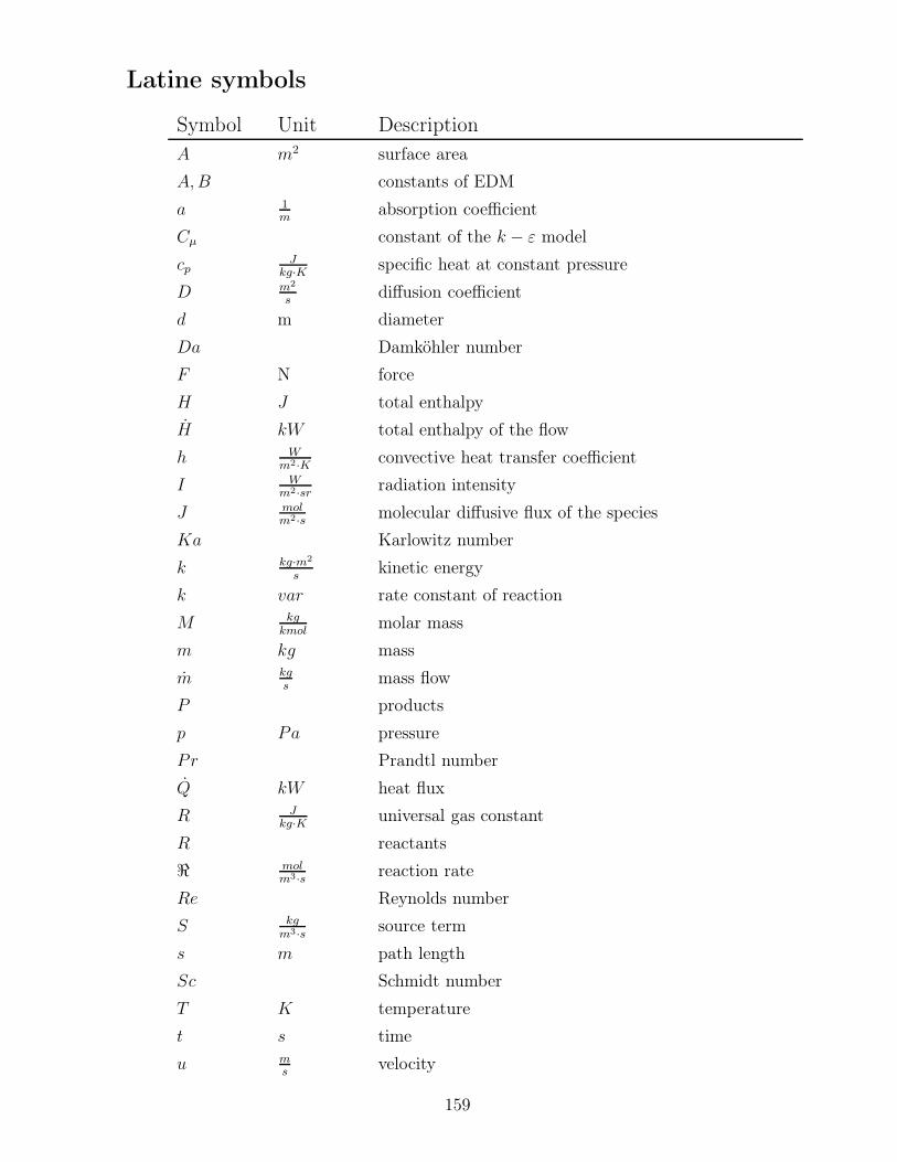
Latine symbols
Symbol Unit DescriptionA m2 surface area
A,B constants of EDM
a 1m
absorption coefficient
Cµ constant of the k − ε model
cpJkg·K
specific heat at constant pressure
D m2
sdiffusion coefficient
d m diameter
Da Damköhler number
F N force
H J total enthalpy
H kW total enthalpy of the flow
h Wm2·K
convective heat transfer coefficient
I Wm2·sr
radiation intensity
J molm2·s
molecular diffusive flux of the species
Ka Karlowitz number
k kg·m2
skinetic energy
k var rate constant of reaction
M kgkmol
molar mass
m kg mass
m kgs
mass flow
P products
p Pa pressure
Pr Prandtl number
Q kW heat flux
R Jkg·K
universal gas constant
R reactants
ℜ molm3·s
reaction rate
Re Reynolds number
S kgm3·s
source term
s m path length
Sc Schmidt number
T K temperature
t s time
u ms
velocity
159
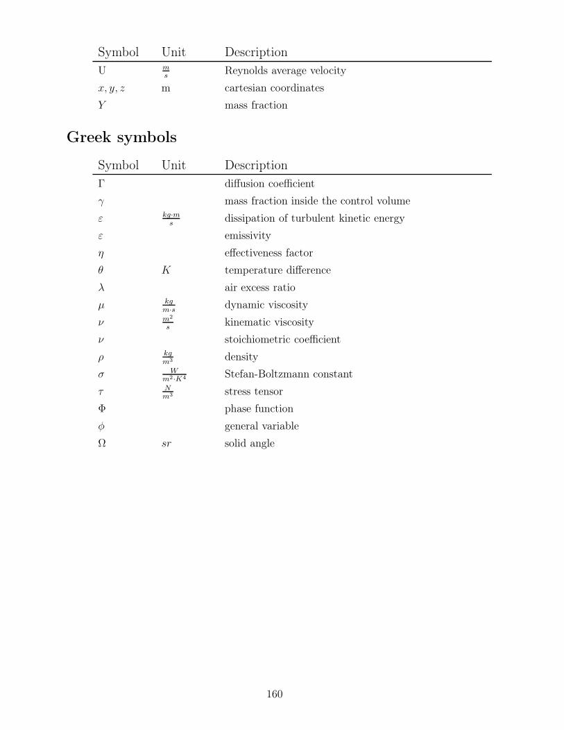
Symbol Unit DescriptionU m
sReynolds average velocity
x, y, z m cartesian coordinates
Y mass fraction
Greek symbols
Symbol Unit DescriptionΓ diffusion coefficient
γ mass fraction inside the control volume
ε kg·ms
dissipation of turbulent kinetic energy
ε emissivity
η effectiveness factor
θ K temperature difference
λ air excess ratio
µ kgm·s
dynamic viscosity
ν m2
skinematic viscosity
ν stoichiometric coefficient
ρ kgm3
density
σ Wm2·K4
Stefan-Boltzmann constant
τ Nm3
stress tensor
Φ phase function
φ general variable
Ω sr solid angle
160

Superscripts
Symbol Description⋆ fine structures
Subscripts
Symbol Descriptiona, b, .. chemical species
c chemical
comb combustion
dev devolatilization
i, j, ... variables
inn at the inlet
m mass
out at the outlet
p particle
R radiation
t turbulent
vap vaporization
∞ continuous phase
0 initial
161

162
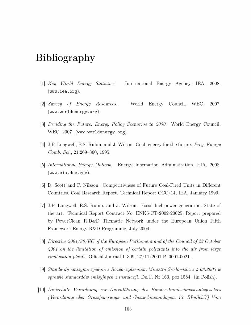
Bibliography
[1] Key World Energy Statistics. International Energy Agency, IEA, 2008.
(www.iea.org).
[2] Survey of Energy Resources. World Energy Council, WEC, 2007.
(www.worldenergy.org).
[3] Deciding the Future: Energy Policy Scenarios to 2050. World Energy Council,
WEC, 2007. (www.worldenergy.org).
[4] J.P. Longwell, E.S. Rubin, and J. Wilson. Coal: energy for the future. Prog. Energy
Comb. Sci., 21:269–360, 1995.
[5] International Energy Outlook. Energy Inormation Administration, EIA, 2008.
(www.eia.doe.gov).
[6] D. Scott and P. Nilsson. Competitivness of Future Coal-Fired Units in Different
Countries. Coal Research Report. Technical Report CCC/14, IEA, January 1999.
[7] J.P. Longwell, E.S. Rubin, and J. Wilson. Fossil fuel power generation. State of
the art. Technical Report Contract No. ENK5-CT-2002-20625, Report prepared
by PowerClean R,D&D Thematic Network under the European Union Fifth
Framework Energy R&D Programme, July 2004.
[8] Directive 2001/80/EC of the European Parliament and of the Council of 23 October
2001 on the limitation of emission of certain pollutants into the air from large
combustion plants. Official Journal L 309, 27/11/2001 P. 0001-0021.
[9] Standardy emisyjne zgodnie z Rozporządzeniem Ministra Środowiska z 4.08.2003 w
sprawie standardów emisyjnych z instalacji. Dz.U. Nr 163, poz.1584. (in Polish).
[10] Dreizehnte Verordnung zur Durchführung des Bundes-Immissionsschutzgesetzes
(Verordnung über Grossfeuerungs- und Gasturbinenanlagen, 13. BImSchV) Vom
163
BIBLIOGRAPHY
20. Juli 2004. Bundesgesetzblatt Jahrgang 2004 Teil I Nr. 37, ausgegeben zu Bonn
am 23. Juli 2004, Seite 1717. (in German).
[11] Kyoto Protocol to the United Nations Framework Convention on Climate Change.
United Nations, 1998. (www.unfccc.int).
[12] E.E. Khalil. Power Plant Design. Abacus Press/Gordon and Breach Science
Publishers, 1990.
[13] S. Kakac, editor. Boilers, evaporators and condensers. John Wiley & Sons, Inc.,
1991.
[14] P. Kiameh. Power generation handbook. Selection, Applications, Operation, and
Maintenance. McGraw-Hill, 2003.
[15] T.C Elliot, K. Chen, and R. Swanekamp. Standard Handbook of Powerplant
Engineering. McGraw-Hill, 1997.
[16] H. Termuehlen and W. Empsperger. Clean and Efficient coal fired power plants.
ASME Press, 2003.
[17] M. Pronobis. Modernizacja kotłów energetycznych. Wydawnictwa Naukowo-
Techniczne, Warszawa, 2002. (in Polish).
[18] J.M. Beer. High efficiency electric power generation: The environmental role. Prog.
Energy Comb. Sci., 33:107–134, 2007.
[19] E.S. Tavoulareas. Fluidized bed combustion technology. Annu. Rev. Energy
Environ., 16:25–57, 1991.
[20] M.L. Murphy. Fluidized Bed Technology Solution to Animal Waste Disposal. In
17th International Pittsburgh Coal Conference, Pittsburgh, USA, 2000.
[21] B.J.P. Buhre, L.K. Elliott, C.D. Sheng, R.P. Gupta, and Wall T.F. Oxy-fuel
combustion technology for coal-fired power generation. Prog. Energy Comb. Sci.,
31:283–307, 2005.
[22] K. Damen, M. van Troost, A. Faaij, and W. Turkenburg. A comparison of electricity
and hydrogen production systems with CO2 capture and storage. Part A: Review
and selection of promising conversion and capture technologies. Prog. Energy Comb.
Sci., 32:215–246, 2006.
164
BIBLIOGRAPHY
[23] D.M. Woycenko, W.L. van de Kamp, and P.A. Peters. Combustion of pulverized
coal in mixtures of oxygen and recycled flue gas. Technical Report IFRF Doc. No.
F98/y/1, IFRF Reaserch Report, IJmuiden, 1995.
[24] Y.R. Mao, M.X. Fang, and S.R. Wang. Current Development of Research on Air
Separation Flue Gas Recycle Technology. Boiler Technology J., 33:5–9, 2002.
[25] Y.R. Mao, Y.G. Zhang, and G.S. Zhang. Research on Technologies for CO2
Emission Control Sequestration and Recovery from Coal-fired Power Plant. Boiler
Manufacturing J., 1:20–22, 2003.
[26] K. Littewood. Gasification: Theory and Application. Prog. Energy Combust. Sci.,
3:35–71, 1977.
[27] X.T. Lia, J.R. Gracea, C.J. Lima, A.P. Watkinson, H.P. Chen, and J.R. Kim.
Biomass gasification in a circulating fluidized bed. Biomass and Bioenergy, 26:171–
193, 2004.
[28] R.F. Geosits and L.A. Schmoe. IGCC- the challenges of integration. In ASME
Turbo Expo 2005: Power for Land, Sea and Air, Reno-Tahoe, Nevada, USA, 2005.
[29] Gasification Plant Cost and Performance Optimization. Technical Report Contract
No. DE-AC26-99FT40342, US Department of Energy National Energy Technology
Laboratory (NETL), September 2003.
[30] R.D. Hottenshine, N.A. Phillips, and R.A. Dill. Developments plans for advanced
fossil fuel power plants. Technical Report CS-4029, EPRI, 1985.
[31] The Federation of Power Companies of Japan. Electricity Review Japan, March
2007. (www.fepc.or.jp).
[32] J. Szargut. Termodynamika. Wydawnictwo Politechniki Śląskiej, 2000. (in Polish).
[33] DTI/IEA. Supercritical Steam Cycles for Power Generation Applications, January
1999.
[34] K. Yamamoto, I. Kaijgaya, and I. Umaki. Operational Experience of USC Steam
Condition Plant and PFBC Combined Cycle System with Material Performance.
Materials at High Temperatures, 20:15–18, 2003.
[35] J.E. Oakey, L.W. Pinder, R. Vanstone, M. Henderson, and Osgerby S. Review of
status of advanced materials for power generation. Technical Report COAL R224
DTI/Pub URN 02/1509, 2003.
165
BIBLIOGRAPHY
[36] S. Kjaer. The Advanced Supercritical 700oC Pulverised Coal-Fired Power Plant.
In Power-Gen Europe 2001, Brussels, Belgium, 2001.
[37] J. Hald and B. Nath. New High Temperature Steels For Steam Power Plants. In
Power-Gen Europe 1998, Milan, Italy, 1998.
[38] K. Strauss. Kraftwerkstechnik. Springer Verlag, 2006. (in German).
[39] Z.L. Rataj and A.W. Walewski. Once-through Benson boiler system after 83 years
permament development- optimal design for supercritical CFB (OTU) boilers. In
10th International Conference on Boiler Techniology 2006, Szczyrk, Poland, 2006.
[40] D.K. Mc Donald and S.S Kim. Vertical Tube, Variable Pressure Furnace for
Supercritical Steam Boilers. In Power-Gen International, Las Vegas, Nevada, USA,
2001.
[41] H.H. Poulsen. Advantages of Ultra Super Critical Technology in Power Generation.
In International Conference on Clean Coal Technologies for our Future, Sardinia,
Italy, 2005.
[42] M. Katsuki and T. Hasegawa. The Science and Technology of in Highly Preheated
Air. Proc. Combust. Inst., 27:3135–3146, 1998.
[43] F. Weinberg and D. Hardesty. Burners producing large excess enthalpies. Combust.
Sci. Tech., 8:201–214, 1974.
[44] J. Wünning. Flammenlose Oxidation von Brennstoff mit hochvorgewärmter Luft.
Chem.-Ing.-Tech., 63:1243–1245, 1991. (in German).
[45] A. Cavaliere and M.D. de Joannon. Mild Combustion. Prog. Energy Combust. Sci.,
30:329–366, 2004.
[46] M. Gettings. The regenerative burner in the metals industry. Gaswärme
International, 35:292–296, 1986.
[47] J. Masters, R. Webb, and R. Davies. The use of modelling techniques in the design
and application of recuperative burners. J. Inst. Energy, 52:196–204, 1979.
[48] H. Tsuji, A.K. Gupta, T. Hasegawa, M. Katsuki, K. Kishimoto, and M. Morita.
High Temperature Air Combustion: from energy conservation to pollution reduction.
CRC Press, 2003.
166
BIBLIOGRAPHY
[49] T. Hasegawa. Environmentally Compatible Regenerative Combustion Heating
System. In 2nd International Seminar on High Temperature Air Combustion,
Stockholm, Sweden, 2000.
[50] T. Hasegawa and S. Mochida. Highly Preheated Air Combustion Characteristic
Development of a Combustion Diagnostic on Advanced Industrial Furnace Making.
In International Joint Power Generation Conference, San Francisco, USA, 1999.
[51] T. Hasegawa and S. Mochida. Development of a Combustion Diagnostic Method
on Advanced Industrial Furnaces Utilizing High Temperature Air Combustion. In
3rd HiTACG Symposium, Yokohama, Japan, 2000.
[52] S. Mochida and Yasuda T. Review of HiTAC Development and Future Possibility.
In 6th HiTACG Symposium, Essen, Germany, 2005.
[53] R. Weber. Combustion of Natural Gas, Oil and Coal with Air Preheated
to Temperatures in Excess of 1000oC. In 13th IFRF Members Conference,
Noordwijkerhout, The Netherlands, 2001.
[54] A.K. Gupta. Flame Characteristics and Challenges with High Temperature Air
Combustion. In International Joint Power Generation Conference, Miami Beach,
Florida, USA, 2000.
[55] A.K. Gupta. Thermal characteristics of gaseous fuel flames using high temperature
air. ASME J. Eng. Gas Turbines Power, 126:9–19, 2004.
[56] T. Hasegawa, S. Mochida, and A.K. Gupta. Development of Advanced Industrial
Furnace using Highly Preheated Air Combustion. J. Propulsion and Power, 2:233–
239, 2002.
[57] S. Lille, W. Blasiak, and M. Jewartowski. Experimental study of the fuel jet
combustion in high temperature and low oxygen content exhaust gases. Energy,
30:373–384, 2005.
[58] R. Weber, J. Driscoll, and W. Dahm. Scalling characteristic of the aerodynamics
and low NOx properties of industrial natural gas burner. Technical Report GRI-
93/0227, IFRF Reaserch Report, IJmuiden, 1993. The Scalling 400 Study.
[59] R. Weber, J. Dugué, A. Sayre, and H. Horsamnn. Scalling characteristics of the
aerodynamics and low NOx properties of industrial natural gas burner. Technical
Report IFRF Doc. No. F40/y/9, IFRF Reaserch Report, IJmuiden, 1993. The
Scalling 400 Study.
167
BIBLIOGRAPHY
[60] A. Verlaan, S. Orsino, N. Lallemant, and R. Weber. Fluid flow and mixing in
a furnace equipped with the low NOx regenerative burner of Nippon Furnace
Kyogo. Results of HTAC 97 trials. Technical Report IFRF Doc. No. F46/y/1,
IFRF Reaserch Report, IJmuiden, 1998.
[61] R. Weber, A. Verlaan, S. Orsino, and N. Lallemant. On emerging furnace design
methodology that provides substantial energy savings and drastic reductions in
CO2, CO and NOx emissions. J. Inst. Energy, 72:77–83, 1999.
[62] R. Weber, A. Verlaan, S. Orsino, and N. Lallemant. Combustion of natural gas
with high temperature air and large quantities of flue gas. Proc. Combust. Inst.,
28:1315–1321, 2000.
[63] A. Verlaan, G. Deus Vasquez, M. Kosters, S. Orsino, N. Lallemant, and R. Weber.
Excess enthalpy combustion of light and heavy fuel oils. Results of HTAC 98 trials.
Technical Report IFRF Doc. No. F46/y/2, IFRF Reaserch Report, IJmuiden, 1999.
[64] S. Orsino, M. Tamura, P. Stabat, S. Costantini, O. Prado, and R. Weber. Excess
enthalpy combustion of coal. Results of HTAC 99 trials. Technical Report IFRF
Doc. No. F46/y/3, IFRF Reaserch Report, IJmuiden, 2000.
[65] R. Weber, J. Smart, and W. Vd Kamp. On the MILD Combustion of Gaseous,
Liquid, and Solid Fuels in High Temperature Preheated Air. Proc. Combust. Inst.,
30:2623–2629, 2005.
[66] J.G. Wünning. Flammlose Oxidation von Brennstoff. PhD thesis, Aachen
University of Technology, 1996. (in German).
[67] J.A. Wünning and J.G. Wünning. Flammeless Oxidation to Reduce Thermal NO-
Formation. Prog. Energy Combust. Sci., 23:81–94, 1997.
[68] J. Wünning. Flameless Oxidation. In 6th HiTACG Symposium, Essen, Germany,
2005.
[69] A. Sobiesiak, S. Rahbar, and H.A. Becker. Performance characteristics of the new
low NOx CGRI burner for use with high air preheat. Combust. and Flame, 115:93–
125, 1998.
[70] B.T. Burggraaf, B. Lewis, P.D.J. Hoppesteyn, N. Fricker, S. Santos, and B.K.
Slim. Towards industrial application of High Efficiency Combustion. In 15th IFRF
Members Conference, Pisa, Italy, 2007.
168
BIBLIOGRAPHY
[71] E. Masson, B. Taupin, L. Dampt, A. Boukhalfa, D. Honore, R. Hauguel, and
L. Porcheron. Parametric study of flameless combustion regime in a laboratory-scale
facility. In 6th HiTACG Symposium, Essen, Germany, 2005.
[72] C. Rottier, C. Lacour, G. Godard, B. Taupin, A. Boukhalfa, D. Honore,
L. Porcheron, and R. Hauguel. Velocity and temeprature measurements in a
laboratory-scale facility operating in flameless (MILD) combustion regime. In 15th
IFRF Members Conference, Pisa, Italy, 2007.
[73] D. Lupant, B. Pesenti, P. Evrard, and P. Lybaert. Numerical and experimental
characterization of a self-regenerative flameless oxidation burner operation in pilot-
scale furnace. In 6th HiTACG Symposium, Essen, Germany, 2005.
[74] S. Murer, B. Pesenti, and P. Lybaert. CFD modeling of flameless combustion of
natural gas in a 30kW combustor. In 6th HiTACG Symposium, Essen, Germany,
2005.
[75] N. Shimo. Fundamental Research of Oil Combustion with Highly Preheated Air.
In 2nd International Seminar on High Temperature Air Combustion, Stockholm,
Sweden, 2000.
[76] R.C. Chang and W.C. Chang. Research of High Temperature Air Combustion Fired
Heavy Oil. In 2nd International Seminar on High Temperature Air Combustion,
Stockholm, Sweden, 2000.
[77] R. Wilk, K. Malczyk, T. Misztal, A. Szlęk, and A. Zajdel. Liquid Fuel Combustion
under HTAC Technology. In 4th HiTACG Symposium, Rome, Italy, 2001.
[78] R. Wilk, T. Misztal, A. Szlęk, and K. Malczyk. Investigation of the NO emission
during High Temperature Air Combustion of light oil. In 13th International
Symposium on Combustion, Chicago, USA, 2004.
[79] R. Wilk, T. Misztal, K. Malczyk, A. Szlęk, and A. Zajdel. Investigations of the
NO formation during light oil combustion in highly preheated air. In 5th HiTACG
Symposium, Tokyo, Japan, 2002.
[80] T. Kiga, K. Yoshikawa, M. Sakai, and S. Mochida. Characteristics of Pulverized
Coal Combustion in High-Temperature Preheated Air. J. of Propulsion and Power,
16:601–605, 2000.
169
BIBLIOGRAPHY
[81] FLOX-coal development of a pilot scale flameless oxidation burner for ultra low
NOx combustion of pulverized coal. European Commission (Research Fund for
Coal and Steel), RFCR-CR-2005-00010.
[82] D. Ristic, A. Schuster, G. Scheffknecht, H. Stadler, M. Foerster, Kneer R., and J.G.
Wünning. Experimental Study on Flameless Oxidation of Pulverised Coal in Bench
and Pilot Scale. In 23th German Flameday, Berlin, Germany, 2007.
[83] D. Ristic, M. Schneider, A. Schuster, G. Scheffknecht, and J.G. Wünning.
Investigation of NOx formation for flameless coal combustion. In 7th HiTACG
Symposium, Phuket, Thailand, 2008.
[84] S. Löhr, M. Kretschmann, S. Wirtz, and V. Scherer. Pyrolyse und
Flüchtigenabbrand von Kraftwerkskohlen bei niedrigen Sauerstoffkonzentrationen.
In 23th German Flameday, Berlin, Germany, 2007. (in German).
[85] Untersuchungen zur Schadstoffbildung bei der FLOX-Verbrennung von Kohlestaub.
DFG (German Research Foundation), Gz.: SCHE 322/4-2, (in German).
[86] T. Suda, M. Takafuji, T. Hirata, M. Yoshino, and J. Sato. A study of combustion
behavior of pulverized coal in high-temperature air. Proc. Combust. Inst., 29:503–
509, 2002.
[87] M.R. Schmid, J.G. Wünning, and R. Berger. New horizons for FLOX-technology
for biomass fuels. In 6th HiTACG Symposium, Essen, Germany, 2005.
[88] V. Suphansomboon, P. Suvarnakuta, S. Patumsawad, and S. Kerdsuwan.
Investigation into Low Calorific Value Gas Combustion with High Temperature and
Low-Oxygen Concentration Combustion Air. In 6th HiTACG Symposium, Essen,
Germany, 2005.
[89] A. Ponzio, S. Kalisz, J. Promelle, and W. Blasiak. Combustion of Wood Pellets in an
Oxygen Diluted and High Temperature Environment. In 6th HiTACG Symposium,
Essen, Germany, 2005.
[90] M. Derudi, A. Effuggi, A. Villani, and R. Rota. Use of Methane-derived Fuel
Mixtures, Natural Gas and Biogas, for MILD Combustion Applications. In 6th
HiTACG Symposium, Essen, Germany, 2005.
[91] A.K. Gupta and S. Mochida. Developments in High Temperature Air Combustion
(Flameless Oxidation) and Fuel Reforming. In 6th HiTACG Symposium, Essen,
Germany, 2005.
170
BIBLIOGRAPHY
[92] W. Cichonski and A.K. Gupta. Hydrogen Generation from Wastes using Ultra-High
Temperature Steam Gasification. In 6th HiTACG Symposium, Essen, Germany,
2005.
[93] N. Krishnamurthy, Y. Weihong, T. Ekman, and W. Blasiak. Combustion
Characteristics of Flameless Oxyfuel and Oxygen Enriched -High Temperature Air
Combustion. In 6th HiTACG Symposium, Essen, Germany, 2005.
[94] J. Leicher, S. Wirtz, and V. Scherer. Simulating Flameless Oxidation Using a
Progress Variable Approach. In 6th HiTACG Symposium, Essen, Germany, 2005.
[95] A. Al-Halbouni and M. Flamme. New Burner Systems for Gas Turbines. In 6th
HiTACG Symposium, Essen, Germany, 2005.
[96] M. Flamme. New combustion systems for gas turbines (NGT). Applied Thermal
Engineering, 24:1551–1559, 2004.
[97] R. Weber, A. Szlęk, and R. Wilk. A novel application of mild combustion technology
to gas turbines that results in substantial increase of cycle efficiency. In 6th HiTACG
Symposium, Essen, Germany, 2005.
[98] A. Szlęk. Combustion of methane in a compressed, preheated and expanding air. In
31st International Symposium on Combustion, Heidelberg, Germany, 2006. poster
presentation.
[99] A. Szlęk, R. Weber, and R. Wilk. High Temperature Air Combustion Technology
in Power Cycles. In ECOS Conference, Trondhaim, Norway, 2005.
[100] A. Szlęk, R. Wilk, K. Malczyk, and T. Misztal. On HTAC application in power
generation. In 5th HiTACG Symposium, Tokyo, Japan, 2002.
[101] Y. Hino, C. Zhang, and T. Ishii. Comparison of measurements and predictions of
flame structure and NOx emissions in a gas-fired furnace. In AIAA/ASME Joint
Thermophysics and Heat Transfer Conference, Albuquerque, New Mexico, USA,
1998.
[102] T. Ishii, C. Zhang, and S. Sugiyama. Numerical analysis of NOx formation rate in
a regenerative furnace. In Joint Power Generation Conference, Denver, Colorado,
USA, 1997.
171
BIBLIOGRAPHY
[103] C. Zhang, T. Ishii, and S. Sugijama. Numerical modeling of the thermal
performance of regenerative slab reheating furnaces. Num. Heat Transf., 32:613–
631, 1997.
[104] H. Guo, Y. Ju, and K. Mauta. Numerical investigations for NOx emissions in
high temperature air combustion. In First Asia-Pacific Conference on Combustion,
Nagoya, Japan, 1997.
[105] S. Orsino, R. Weber, and U. Bollettini. Numerical simulation of natural gas
combustion with high-tempeature air. Combust. Sci. Tech., 168:1–34, 2002.
[106] M. Mancini and R. Weber. Formation and destruction of nitrogen oxides in
combustion of natural gas with high temperature air. In 5th HiTACG Symposium,
Yokohama, Japan, 2002.
[107] M. Mancini, P. Schwöppe, R. Weber, and S. Orsino. On mathematical modeling of
flameless combustion. Combust. Flame, 150:54–59, 2007.
[108] M. Mancini. Analysis of mild combustion of Natural Gas with preheated air. PhD
thesis, Clausthal University of Technology, Faculty of Energy and Management,
2007.
[109] P. Coehlo and N. Peters. Numerical simulation of a MILD combustion burner.
Combust. Flame, 124:503–518, 2001.
[110] P. Coehlo and N. Peters. Laseroptical investigation of highly preheated combustion
with strong exhaust gas recirculation. Proc. Combust. Inst., 27:3197–3204, 1998.
[111] S. Yang and W. Blasiak. Numerical study of fuel temperature influence on single gas
jet combustion in highly preheated and oxygen deficient air. Energy, 30:385–398,
2005.
[112] S. Yang and W. Blasiak. Numerical simulation of properties of a LPG flme with
high-temperature air. International Journal of Thermal Sci., 44:973–985, 2005.
[113] S. Yang and W. Blasiak. Mathematical modelling of NO emissions from high-
temperature air combustion with nitrous oxide mechanism. Fuel Proc. Tech.,
86:943–957, 2005.
[114] W. Dong and W. Blasiak. Numerical modeling of highly preheated air combustion
in a 580kW testing furnace at IFRF. In 3rd CRST International Symposium,
Yokohama, Japan, 2000.
172
BIBLIOGRAPHY
[115] W. Dong and W. Blasiak. Large Eddy Simulation of a single jet flow in highly
preheated and diluted air combustion. Archivum Combustionis, 20:163, 2000.
[116] B. Pasenti, P. Evrard, and P. Lybaert. NOx production and radiative heat transfer
from an autoregenerative flameless oxidation burner. In 4th HiTACG Symposium,
Rome, Italy, 2001.
[117] D. Tobacco, C. Innarella, and C. Bruno. Theoretical and numerical investigation
on flameless combustion. Combust. Sci. Tech., 174:1–35, 2002.
[118] A. Cavaliere and M.D. de Joannon. Zero-dimensional analysis of diluted oxidation
of methane in rich conditions. Proc. Combust. Inst., 28:1639–1646, 2000.
[119] M. de Joannon, P. Saba, A. Tregrossi, and A. Cavaliere. Dynamic behavior of the
methane oxidation in premixed flow reactor. Combust. Sci. and Tech., 176:769–783,
2004.
[120] M. de Joannon, A. Cavaliere, T. Faravelli, E. Ranzi, and P. Sabia. Analysis
of process parameters for steady operation of methane MILD technology. Proc.
Combust. Inst., 30:2605–2612, 2005.
[121] L. Porcheron, L. Ferrand, E. Masson, F. Aguile, A. Quinqueneau, D. Honore, and
M. Boukhalfa. High Temperature Air Combustion burner: semi-industrial scale
experiment and CFD simulation. In 6th HiTACG Symposium, Essen, Germany,
2005.
[122] B.T. Burggraaf, B. Lewis, P.D.J. Hoppesteyn, N. Fricker, S. Santos, and B.K. Slim.
Towards industrial application of High Efficiency Combustion. IFRF Combustion
Journal, 200704, 2007.
[123] R. Hekkens and M. Mancini. CFD modeling for high efficiency combustion. In 14th
IFRF Member Conference, Noordwijkerhout, Netherlands, 2004.
[124] T. Misztal. Badanie emisji NO podczas spalania oleju w warunkach
wysokotemperaturowego podgrzewu powietrza spalania. PhD thesis, Silesian
University of Technology, Faculty of Environmental Protection Technology and
Energy, 2005. (in Polish).
[125] M. Bui Pham and K. Seshadri. Comparison between Experimental Measurements
and Numerical Calculations of the Structure of Heptane-Air Diffusion Flames.
Combust. Sci. and Tech., 79:293–310, 1991.
173
BIBLIOGRAPHY
[126] R. He, T. Suda, M. Takafuji, T. Hirata, and J. Sato. Analysis of low NO emission
in high temperature air combustion for pulverized coal. Fuel, 83:1133–1141, 2004.
[127] P. Heil, U. Renz, and R. Kneer. Experimentelle Untersuchung eines FLOX-Brenners
bei Druckkohlenstaubfeuerungsbetrieb. In 4. Druckflamm Seminar, Dortmund,
Germany, 2004. (in German).
[128] J. Erfurth, D. Toporov, S. Tschunko, C. von Petry, and R. Kneer. Modellierung
der Flammlosen Verbrennung in einer Druckkohlenstaubfeuerung. In 22th German
Flameday, Braunschweig, Germany, 2005. (in German).
[129] J.P. Kim, U. Schnell, G. Scheffknecht, and A.C. Benim. Numerical Modeling of
MILD Combustion for Coal. Prog. in Comput. Fluid Dynamics, 7:337–346, 2007.
[130] J.P. Kim. Numerical modeling of MILD combustion. PhD thesis, University
of Stuttgart, Faculty of Energy Technology, Process Engineering and Biological
Engineering, 2008.
[131] D. Förtsch. A Kinetic Model of Pulverised Coal Combustion for Computational
Fluid Dynamics. PhD thesis, University of Stuttgart, Faculty of Energy Technology,
Process Engineering and Biological Engineering, 2003.
[132] D. Förtsch, F. Kluger, U. Schnell, H. Spliethoff, and H.R.G. Klaus. A kinetic model
for the predtiction of NO emissions from staged combustion of pulverized coal. Proc.
Combust. Inst., 27:3037–3044, 1998.
[133] P.R. Solomon, T.H. Fletcher, and R.J. Pugmire. Progress in coal pyrolysis. Fuel,
72:587–597, 1993.
[134] D. Szewczyk, J. Sudoh, A. Świderski, and B. Forsberg. Over decade of the industrial
experience in high temperature air combustion applied with HRS regenerative
burners. In 6th HiTACG Symposium, Essen, Germany, 2005.
[135] M. Mörtberg, W. Blasiak, and A.K. Gupta. Flameless Combustion of Methane
Fuel Jet injected into Transverse High Temperature Air Flow. In 6th HiTACG
Symposium, Essen, Germany, 2005.
[136] J. Massingham. Evaluation of low NOx burners for steel industry applications.
In 2nd International Seminar on High Temperature Air Combustion, Stockholm,
Sweden, 2000.
174
BIBLIOGRAPHY
[137] J. Wünning. Regenerative Burner Using Flameless Oxidation. In IGRC, Cannes,
France, 1995.
[138] R. Weber, A.L. Verlaan, S. Orsino, and N. Lallemant. On emerging furnace design
methodology that provides substantial energy savings and drastic reductions in
CO2, CO and NOx emissions. In 2nd International Seminar on High Temperature
Air Combustion, Stockholm, Sweden, 2000.
[139] A. Saponaro. The Ansaldo Caldaie combustion research experience in HiTAC. In
6th HiTACG Symposium, Essen, Germany, 2005.
[140] K. Kawai, K. Yoshikawa, H. Kobayashi, J.S. Tsai, M. Matsuo, and H. Katsushima.
High temperature air combustion boiler for low BTU gas. Energy Conversion and
Management, 43:1563–1570, 2002.
[141] H. Zhang, G. Yue, J. Lu, Z. Jia, J. Mao, T. Fujimori, T. Suko, and T. Kiga.
Development of High Temperature Air Combustion technology in pulverized fossil
fuel fired boilers. Proc. Combust. Inst., 31:2779–2785, 2007.
[142] Fluent Inc. of ANSYS Inc. GAMBIT 2.2 Documentation. User’s Guide, 2006.
[143] Fluent Inc. of ANSYS Inc. FLUENT 6.3 Documentation. User’s Guide, 2006.
[144] J. Ferziger and M. Peric. Computational Methods for Fluids Dynamics. Springer
Verlag, 1999.
[145] T.J. Chung. Computational Fluid Dynamics. Cambridge University Press, 2002.
[146] S.R. Turns. An Introduction to Combustion. Concepts and applications. McGraw-
Hill, 2000.
[147] R.O. Fox. Computational Models for Turbulent Reacting Flows. Cambridge
University Press, 2003.
[148] S.B. Pope. Turbulent flows. Cambridge University Press, 2000.
[149] B.E. Launder and D.B. Spalding. The numerical computation of turbulent flows.
Computer Methods in Applied Mechanics and Engineering, 3:269–289, 1974.
[150] D.B. Spalding. Mixing and chemical reaction in steady confined turbulent flames.
Proc. Combust. Inst., 13:649–657, 1971.
175
BIBLIOGRAPHY
[151] B.F. Magnussen and B.H. Hjertager. On mathematical modeling of turbulent
combustion with special emphasis on soot formation and combustion. Proc.
Combust. Inst., 16:719–729, 1976.
[152] B.F. Magnussen. On the Structure of Turbulence and a Generalized Eddy
Dissipation Concept for Chemical Reaction in Turbulent Flow. In 19th AIAA
Meeting, St. Louis, USA, 1981.
[153] B.F. Magnussen. Modeling of NOx and Soot Formation by the Eddy Dissipation
Concept. In 1st Topic Oriented Technical Meeting, International Flame Research
Foundation, Amsterdam, Holland, 1989.
[154] I.S. Ertesvag and B.F. Magnussen. The Eddy Dissipation Turbulence Energy
Cascade Model. Combust. Sci. and Tech., 159:213–235, 2000.
[155] F. Boysan, W.H. Ayers, and J. Swithenbank. Fundamental Mathematical Modelling
Approach to Cyclone Design. Trans. I. Chem. E., 60:222–230, 1982.
[156] R. Weber, F. Boysan, W.H. Ayers, and J. Swithenbank. Simulation of Dispersion
of Heavy Particles in Confined Turbulent Flows. AICHE J., 30:490–492, 1984.
[157] K. Annamalai and I.K. Puri. Combustion Science and Engineering. CRC Press
Taylor & Francis Group, 2007.
[158] S. Badzioch and P.G.W. Hawksley. Kinetics of Thermal Decomposition of
Pulverized Coal Particles. Ind. Eng. Chem. Process Design and Development,
9:521–530, 1970.
[159] H. Kobayashi, J.B. Howard, and A.F. Sarofim. Coal Devolatilization at High
Temperatures. Proc. Combust. Inst., 16:411–425, 1976.
[160] D.M. Grant, R.J. Pugmire, T.H. Fletcher, and A.R. Kerstein. Chemical Model of
Coal Devolatilization Using Percolation Lattice Statistics. 3:175–186, 1989.
[161] T.H. Fletcher, A.R. Kerstein, R.J. Pugmire, and D.M. Grant. Chemical Percolation
Model for Devolatilization: 2. Temperature and Heating Rate Effects on Product
Yields. Energy and Fuels, 4:54–60, 1990.
[162] T.H. Fletcher and A.R. Kerstein. Chemical Percolation Model for Devolatilization:
3. Direct Use of 13C NMR Data to Predict Effects of Coal Type. Energy and Fuels,
6:414–431, 1992.
176
BIBLIOGRAPHY
[163] P.L.Jr. Walker, F.J. Rusinko, and L.G. Austin. Gas Reactions of Carbon. Advances
in Catalysis, 11:133–140, 1959.
[164] D. Gray, J.G. Cogoli, and R.H. Essenhigh. Problems in Pulverized Coal and Char
Combustion. Advances in Chemistry Series, 13:72–91, 1974.
[165] V. Banin, R. Moors, and B. Veefikind. Kinetic study of High-Pressure Pulverised
Coal Char Combustion: Experiment and Modelling. Fuel, 76:945–949, 1997.
[166] A. Williams, M. Pourkashanian, and J.M. Jones. Combustion of pulverised coal
and biomass. Prog. Energy Comb. Sci., 27:587–610, 2001.
[167] I.W. Smith. The Combustion Rates of Coal Chars: A Review. Proc. Combust.
Inst., 19:1045–1065, 1982.
[168] H.E. Klimesh and R.H. Essenhigh. Non-Dissociative and Dissociative Adsorption of
Oxygen on Carbon: A Theoretical Comparison with Prediction of Reaction Order.
Proc. Combust. Inst., 27, 1998.
[169] N.M. Laurendeau. Heterogeneous Kinetics of Coal Char Gasification and
Combustion. Prog. Energy Com. Sci., 4:221–270, 1978.
[170] W.A. Fiveland and A.S. Jamaluddin. Three-dimensional radiative heat transfer
solutions by the discrete-ordinates method. J. Thermophysics, 2:309–316, 1988.
[171] J.S. Truelove. Three-dimensional radiation in absorbing-emitting-scattering in
using the discrete-ordinates approximation. JQSRT, 39:27–31, 1988.
[172] G. Hand, M. Missaghi, M. Pourkashanian, and A. Williams. Experimental Studies
and Computer Modeling of Nitric Oxides in a Cylindrical Natural Gas Fired
Furnace. In 9th IFRF Members Conference, Noordwijkerhout, the Netherlands,
1989.
[173] A.A.F. Peters and R. Weber. Modeling of a 2.25 MWth Swirling Natural Gas
Flame. Part I: Eddy Break-up Concept for Turbulent Combustion; Probability
Density Function Approach for Nitric Oxide Formation. Combust. Sci. Tech., 110-
111:67–101, 1995.
[174] G.G. De Soete. Overall Reaction Rates of NO and N2 Formation from Fuel
Nitrogen. Proc. Combust. Inst., 15:1093–1102, 1975.
177
BIBLIOGRAPHY
[175] P. Malte and D. Pratt. Measurements of atomic oxygen and nitrogen oxides in jet
stirred combustion. Proc. Combust. Inst., 15:1061–1070, 1974.
[176] W. Chen, L.D. Smoot, T.H. Fletcher, and R.D. Boardman. Global Rate Expression
for Nitric Oxide Reburning. Part II. Energy & Fuels, 10:1046–1056, 1999.
[177] W. Chen, L.D. Smoot, S.C. Hill, and T.H. Fletcher. A Computational Method for
Determining Global Fuel-NO Rate Expressions. Part I. Energy & Fuels, 10:1036–
1046, 1999.
[178] J.M. Levy, L.K. Chen, A.F. Sarofim, and J.M. Beer. NO/Char Reactions at
Pulverized Coal Flame Conditions. Proc. Combust. Inst., 18:340–343, 1981.
[179] M. Tamura. Data on characterization of Guasare coal, 2000. (unpublished).
[180] N. Lallemant, A. Sayre, and R. Weber. Evaluation of emissivity correlations for
H2O−CO2−N2/air mixtures and coupling with solution methods of the Radiative
Transfer Equation. Prog. Energy Combust. Sci., 22:543–574, 1990.
[181] A. Sayre, N. Lallemant, J. Dugué, and R. Weber. Effect of radiation on nitrogen
emissions from non-sooty swirling flames of natural gas. Proc. Combust. Inst.,
25:235–242, 1994.
[182] A.A.F. Peters and R. Weber. Mathematical Modeling of a 2.4 MWth Swirling
Pulverized Coal Flame. Combust. Sci. and Tech., 122:131–182, 1997.
[183] J. Haas. Experimentelle Untersuchungen der Reaktivität von Kohlenkoks zur
Modellierung seines Verbrennungsverhaltens in Staubfeurungen. PhD thesis,
Clausthal University of Technology, Faculty of Energy and Management, 1999. (in
German).
[184] R. Lundquist, A. Schrief, P. Kinnunen, K. Myohanen, and M. Seshamani. A Major
Forward- The Supercritical CFB Boiler. In Power-Gen International 2003, Las
Vegas, USA, 2003.
[185] A. Saario and A. Oksanen. Effect of Computational Grid in Industrial-Scale Boiler
Modeling. Int. J. of Numerical Methods for Heat & Fluid Flow, 19:93–117, 2009.
[186] K. Yamagata, K. Nishikawa, S. Hasegawa, T. Fuji, and S. Yoshida. Forced
convective heat transfer to supercritical water flowing in tubes. Int. J. Heat Mass
Transfer, 15:2575–2593, 1972.
178
Extended abstract
High Temperature Air Combustion (HTAC or HiTAC) is named also as: Excess
Enthalpy Combustion (EEC), FLameless OXidation (acronym FLOX), MILD (Moderate
and Intensive Low-oxygen Dilution) combustion. The most important feature of HTAC
technology is an existence of an intense recirculation of combustion products inside the
chamber. This recirculation causes that both the combustion air stream and the fuel
stream being diluted before the ignition occurs. Therefore, the temperature peaks are
suppressed. The second result of these specific mixing conditions is homogeneity of both
the temperature and the species concentrations fields. Consequently, HTAC technology
features low NOx and CO emissions and high and uniform heat fluxes. So far, HTAC
technology was implemented mainly in industrial furnaces fired either with gaseous fuels
or light oils. In most of industrial applications, the technology is combined with heat
recovery systems and such a combination typically results in substantial fuel savings. In
this work, the application of HTAC technology in power boilers fired with pulverized coal
has been investigated. The following advantages are expected:
• In HTAC furnaces, the radiative heat fluxes are significantly higher than in
traditional ones. If the same could be achieved in boilers, then the size of the
heat transfer area, and thus boiler investment costs, could be significantly reduced.
The boiler could be build using high temperature alloys allowing an increase of
superheated steam parameters to an ultra-supercritical level and, subsequently, an
increase of the thermal efficiency of the entire cycle.
• The next advantage is in significant reduction of pollutants emissions, mainly nitric
oxide which allows eliminating expensive flue gas cleaning installations.
Summarizing, application of HTAC technology to boilers fired with pulverized coal could
be one of the future coal combustion technologies for the clean power generation. Technical
and ecological aspects of such applications are analyzed and discussed in this thesis.
The main objective of this work is to investigate applicability of HTAC technology
to power station boilers fired with pulverized coal for environmental friendly electricity
production. In order to achieve this goal, several technical objectives have been
formulated. The first objective is to examine how accurately HTAC combustion of coal can
be predicted using numerical modeling methods. To this end the mathematical model has
been validated against the IFRF measurements. The CFD-based simulations have been
performed using FLUENT code. The mathematical model selected in the validation and
verification process is then used in all subsequent investigations. The second objective is
179
to develop a conceptual design of a pulverized coal fired boiler utilizing HTAC technology.
This involves determination of the combustion chamber shape, its dimensions, distances
between individual burners and positions of the burner block. The third objective involves
the examination of the environmental aspects of the HTAC technology implementation.
Here one focuses on NOx, CO, unburned hydrocarbons and char burnout. The fourth
objective is to examine the HTAC boiler operation under different operating conditions
like: low combustion air temperatures, low combustion air jet momentum and a low excess
air ratio. The fifth objective is to investigate whole steam cycle in order to estimate the
efficiency of electricity production using such a HTAC boiler.
The work on the HTAC boiler fired with pulverized coal has been presented starting
with an overview on coal based technologies applied in power generation. Further,
the fundamentals of the power station boilers construction have been provided. Then,
a development, current status and challenges of HTAC technology have been briefly
reviewed. Special attention has been given on the progress in modeling of combustion
under HTAC conditions, especially using the solid fuels. In the next part of the work, the
mathematical sub-models used in this work have been described. Here has been focused
on both, the coal combustion and the nitric oxide formation and destruction sub-models.
In this part of the work, the mathematical model describing coal combustion
in HTAC technology has been validated against the data generated during an IFRF
experiment called HTAC 99. Several sub-models have been tested during the validation
and verification procedure and as a result the following sub-models have been selected:
• k − ε model for turbulence
• eddy dissipation model for interaction between chemistry and turbulence
• discrete phase model for description of particles behavior
• CPD model for devolatilization process
• intrinsic model for char burnout
• discrete ordinates model for radiation
• nitric oxides formation and destruction considering the fuel, thermal, prompt and
N2O paths, as well as NO reburning in the gaseous phase and on the char surface
It was concluded that the predicted values are, generally, in very good accordance
with the measurements. Therefore, such a validated model has then been used in the
boiler design studies.
180
HTAC combustion process is very different from conventional combustion. Therefore
there is a need for an innovative design of boilers utilizing this technology. In this part
of the work several particular boiler concepts have been analyzed in the context of the
following three key points: existence of an intensive in-furnace recirculation, homogeneity
of both the temperature and the chemical species fields, and uniformity of heat fluxes.
Several simulations have been performed in order to find the shape of the boiler and its
dimensions, to optimize both the distance between burners and location of the burner
block.
Based on the previous investigations, the final configuration of the HTAC boiler was
selected. The boiler is 13 m high and has a 7 m times 6 m cross section. It is equipped
with a burner block that consists of 5 identical burners located at the top wall thus
the boiler is a down-fired one. The flue gas outlets are also located at the top wall and
they are symmetrically positioned on both sides of the burner block. The outlets have
a quadrate form with lateral length of 1 m. Each of the five burners is equipped with
a central injector of hot air and two coal guns positioned on both sides from the air
injector. Pulverized coal is introduced into the furnace by nozzles of 15 mm diameter and
the combustion air by 48 mm nozzles. The boiler is equipped with two ash hoppers.
The combustion air is preheated to 1200 K and the coal together with its transport
air is supplied at ambient temperature (300 K). The feeding rate of coal is of 3.2 kgs,
and of its transport air almost twice a high. The mass flow of combustion air is equal to
33.1 kgs. The air jet is supplied at a high velocity (120 m
s) and coal jet has the velocity of
30 ms. The boiler is operated at 130 MW total thermal input. The fuel thermal input is
equal to 100 MW so each burner operates at 20 MW fuel power. Both the combustion
and the transport air streams contain 23% mass oxygen and 77% mass nitrogen. The wall
temperature is constant in the final boiler design calculations and it is equal to 800 K.
The final boiler design leads to the intensive recirculation and the dead zones are small.
The whole volume of the chamber participates in the combustion process. The internal
recirculation of the combustion products creates homogenous both the temperature and
the chemical species concentration fields. Further, due to dilution of the combustion air
and fuel jets the coal ignition takes place in low oxygen concentration environment, and
therefore the temperature peak is suppressed. Strong recirculation of the hot combustion
gas eliminates the problems related to the coal ignition.
The whole boiler is filled up with combustion products of 1600-2000K temperatures.
The temperature peak is substantially suppressed in comparison with conventional
combustion using such high air preheat, and it is about 2100 K. The furnace exit
temperature is around 1400 K, and the furnace exhaust gas has a high enthalpy. This
181
enthalpy must be recovered in a heat exchanger and utilized to preheat the combustion
air. The oxygen concentration in almost entire boiler is in a range of 3-5% while in the flue
gas is equal to 3.4%. Uniform and low oxygen concentrations result in the temperature
peak reduction. The HTAC boiler has two advantages: uniform heat fluxes along the
boiler height (as in fluidized bed boilers) and high heat fluxes values (as in wall fired
pulverized coal boilers). Heat transfer due to radiation plays a dominant role. Its share
is 83% of the total heat transfer. The rest is due to the convection.
Most of NO is generated in the region between the burners. The NO concentration
peak is equal to 1195 ppm. Downstream of this region the nitric oxide concentrations
are low and they are in a range from 300 up to 400 ppm. In the HTAC boiler, 98%
of nitric oxide is formed via fuel mechanism. The NO reburning mechanism plays an
important role. As a result, the nitric oxide concentrations at the boiler outlet are low
and equal to 298 ppm. The long particles residence time and recursive recirculation of the
combustion products improve the burnout of the CO and volatiles and of the char. Very
stable combustion process and simple burner construction offer the possibility of using
low rank coals.
In the next part of the work, an impact of three important parameters: the
combustion air preheat, the combustion air jet velocity and the air excess ratio on the
HTAC boiler performance have been tested. Thus, for all calculations the final HTAC
boiler geometry is retained and the same boundary conditions are applied. However, boiler
operating conditions are different and these are specified for each computational run. The
final boiler design is the reference case. It was concluded that the HTAC technology in
boilers can work correctly at different levels of the air preheating, as well as without air
preheating. Further, it was confirmed that the high velocity (and at the same time high
momentum) of the strong combustion jet is needed in order to realize HTAC technology.
Additionally, it was noticed that could be possible to operate the HTAC boiler at the air
excess ration near the stoichiometric values.
Boiler design procedures involve an examination of the combustion process as well as
the steam cycle. Both issues are strongly coupled due to the heat transfer proceeding from
the combustion products inside the chamber to the water/steam mixture inside the boiler
tubes. In this part of the work, coupling between the HTAC boiler and the entire steam
cycle is taken into consideration. The final boiler geometry as well as the operating and
boundary conditions are the starting point for these calculations. User define subroutine
implemented into FLUENT code has been written to perform the calculations. As a result
of these calculations, the temperature profiles at the boiler walls are obtained. The HTAC
boiler is proposed in this thesis as an ultra-supercritical boiler with the once-through type
182
of the water circulation. Three commonly used configurations of the once-trough boiler
tubes were tested in this series of calculations: vertical down-up, up-down and spiral.
The most uniform temperature profile can be found in the boiler with the spiral tubing;
therefore it was concluded that the spiral tubes configuration is the most suitable for
the HTAC boiler designed in this work. However, this configuration is technically most
complicated. The Rankine cycle efficiency of the steam cycle coupled with the HTAC
boiler is calculated to be above 50%.
Overall, the present study confirmed that HTAC technology could be a practicable,
efficient and clean technology for pulverized coal fired boilers.
Summarizing, the most important advantages of the pulverized coal fired boiler
operating under HTAC conditions are as following. Firstly, heat fluxes emitted during
combustion process are high and uniform which results in the high firing density and
consequently the small size of the boiler. Secondly, low NOx emissions in comparison
with the standard PC boilers. Then, burners have a very simple construction: without air
staging, flame stabilizer or swirl which are commonly used in the commercial pulverized
coal burners.
Although HTAC technology seems to be attractive for power boilers fired with
pulverized coal, there are still many open questions. First of all, the particulate
concentration in the flue gas for the coal flame is probably too high to use the technique
in conjunction with regenerative heat exchangers. It is a need to find in the future a
way to utilize the enthalpy of the boiler exhaust gas. However, it was proved that the
boiler can be operated without air preheating even if the ignition mechanism has to be
examined in more details. Secondly, it could be also a problem with erosion because of
the strong recirculation and high velocity of the coal particles.
183
Obszerne streszczenie
Technologia HTAC (High Temperature Air Combustion) jest prawdopodobnie
najważniejszym odkryciem w dziedzinie spalania w przeciągu ostatnich lat. Technologia
HTAC znana jest także pod nazwą FLameless OXidation- FLOX lub MILD (Moderate
and Intensive Low-oxygen Dilution) combustion. Najważniejszą cechą tej metody jest
występowanie intensywnych recyrkulacji wewnątrz komory spalania, które powodują, że
zarówno struga powietrza jak i paliwa ulegają rozcieńczeniu zanim wystąpi zjawisko
zapłonu. W konsekwencji obniżone są maksymalne temperatury osiągane w procesie
spalania. Drugim efektem, wynikającym z występowania intensywnych recyrkulacji, są
równomierne pola temperatury oraz stężenia substancji chemicznych. W następstwie
obserwuje się wyrównany profil strumieni ciepła na ścianach komory oraz niskie
emisje substancji szkodliwych, szczególnie NOx. Jak dotąd, technologia HTAC została
zastosowana głównie w piecach przemysłowych opalanych paliwami gazowymi lub lekkim
olejem. W większości zastosowań przemysłowych technologia ta jest zintegrowana z
systemami regeneracji ciepła, co pozwala na znaczne zmniejszenie zużycia paliwa.
Zastosowanie technologii HTAC w kotłach energetycznych opalanych pyłem
węglowym mogłoby być jedną z czystych technologii wykorzystywanych w przyszłości
do wytwarzania energii elektrycznej. Nadrzędnym celem tej pracy jest analiza możliwości
wykorzystania technologii HTAC w kotłach energetycznych opalanych pyłem węglowym w
celu przyjaznego środowisku naturalnemu wytwarzania energii elektrycznej. Oczekuje się
przy tym, że zastosowanie tej metody spalania do pyłu węglowego przyniesie następujące
korzyści:
• W piecach przemysłowych pracujących w technologii HTAC radiacyjne strumienie
ciepła są znacznie wyższe niż w konwencjonalnych piecach przemysłowych. Jeśli
ten sam efekt zostanie osiągnięty w kotłach, wtedy powierzchnia wymiany ciepła, a
tym samym nakład inwestycyjny na budowę kotła, mogą być znacznie obniżone. W
takim przypadku ekonomicznie uzasadnione może być użycie lepszej jakości stali,
co pozwoliłoby podnieść parametry pary świeżej do wartości superkrytycznych, a
tym samym poprawić sprawność całego obiegu parowego.
• Obniżenie emisji substancji szkodliwych, głównie tlenku azotu i tlenku węgla, co
pozwoliłoby uniknąć konieczności budowy kosztownych instalacji odazotowania
spalin. Mniejsza emisja tlenków azotu wynika z ograniczenia temperatur w komorze
spalania.
184
Na początku pracy przedstawiono przegląd aktualnych i przyszłościowych
technologii węglowych stosowanych do produkcji energii elektrycznej, a następnie
przybliżono podstawowe wiadomości z zakresu budowy i projektowania kotłów
energetycznych zasilanych pyłem węglowym. W kolejnej części pracy zostały pokrótce
zreferowane rozwój, stan aktualny oraz wyzwania stojące przed technologią HTAC.
Skupiono się przede wszystkim na postępie dokonanym w dziedzinie modelowania
numerycznego procesu spalania paliw stałych w tej technologii. Kolejny rozdział
poświęcony został opisowi zastosowanych matematycznych modeli jednostkowych, w
szczegolności tych dotyczących spalania pyłu węglowego oraz formowania i destrukcji
tlenków azotu.
Dla realizacji postawionego nadrzędnego celu pracy sformułowano szereg celów
szczegółowych. Pierwszym z nich było opracowanie wiarygodnego modelu spalania
pyłu węglowego w warunkach HTAC. Dla realizacji tego zadania model matematyczny
poddano weryfikacji korzystając z pomiarów przeprowadzonych w instytucie badawczym
IFRF (International Flame Research Foundation, IJmuiden, Holandia). Symulacje oparte
o numeryczną mechanikę płynów wykonano używając oprogramowania FLUENT. W
procesie weryfikacji przebadano wiele różnych modeli jednostkowych i w rezultacie
wybrano:
• k − ε do opisu turbulencji,
• eddy dissipation model charakteryzujący interakcje pomiędzy reakcjami
chemicznymi procesu spalania i turbulencjami,
• discrete phase model do opisu zachowania cząsteczek stałych,
• CPD model do charakterystyki procesu odgazowania węgla,
• intrinsic model do spalania koksiku,
• discrete ordinates model opisujący wymianę ciepła przez promieniowanie,
• model formowania i redukcji tlenków azotu uwzględniajacy mechanizm paliwowy,
termalny, za pośrednictwem N2O, szybki a także redukcję tlenków azotu zarówno
w fazie gazowej jak i na powierzchni cząsteczki węgla.
Stwierdzono, że wyniki obliczeń numerycznych pozostają w zadowalającej zgodzie z
wartościami pomiarowymi i w konsekwencji wybrany na tym etapie pracy model
matematyczny został użyty w dalszych badaniach numerycznych nad opracowaniem
projektu kotła pracującego w technogii HTAC i opalanego pyłem węglowym.
185
Proces spalania w warunkach HTAC jest diametralnie różny od standardowego
procesu spalania. Z tego względu koniecznym było opracowanie nowej koncepcji kotła, co
stanowiło drugi cel pracy. Wybrane geometrie kotłów przeanalizowane zostały ze względu
na trzy kluczowe zagadnienia: występowanie intensywnych recyrkulacji w komorze
spalania, równomierność rozkładu temperatury i stężenia tlenu, oraz wyrównanane i
wysokie wartości strumieni ciepła wzdłuż wysokości komory spalania. Przeprowadzono
szereg serii symulacji numerycznych w celu znalezienia kształtu komory spalania, jej
wymiarów, konfiguracji bloku palników i jego lokalizacji w komorze spalania.
Opierając się na wynikach uzyskanych w poprzedniej części pracy opracowana
została finalna konfiguracja kotła pyłowego pracującego w technologii HTAC. Kocioł
ma wysokość 13 m i przekrój poprzeczny o wymiarach 6 na 7 m. Kocioł wyposażony
jest w blok palników składający się z pięciu identycznych palników, położonych na
górnej ścianie kotła. Wyloty spalin umiejscowione są również na górnej ścianie kotła,
symetrycznie po obydwu stronach bloku palników. Wyloty spalin mają formę kwadratu
o boku 1 m. Każdy z palników składa się z centralnie położonej dyszy wlotu powietrza
i ulokowanych po obu jej stronach dyszy wlotu paliwa. Pył węglowy wraz z powietrzem
transportującym doprowadzany jest przez dysze o średnicy 15mm. Powietrze do spalania
doprowadzane jest przez otwór o średnicy 48 mm. Kocioł wyposażony jest w dwa leje
żużlowe. Powietrze do spalania podgrzane jest do temperatury 1200 K, podczas gdy pył
węglowy wraz z powietrzem transportującym podawany jest w temperaturze otoczenia
(300 K). Węgiel podawany jest w ilości 3.2 kgs
natomiast ilość powietrza transportującego
jest prawie dwa razy większa. Strumień masowy powietrza jest równy 33.1 kgs. Powietrze
do spalania podawane jest z prędkością wynoszącą 120 ms, powietrze transportujące
zaś- 30 ms. Kocioł zaprojektowany jest na 130 MWth nominalnego obciążenia cieplnego,
z czego w paliwie doprowadzanych jest 100 MWth reszta zaś dostarczana jest wraz
z wysokopodgrzanym powietrzem do spalania. Każdy palnik pracuje z obciążeniem
20 MWth. Zarówno powietrze do spalania jak i powietrze transportujące mają skład
powietrza atmosferycznego (23% masowo tlenu i 77% masowo azotu). Temperatura ścian
komory spalania została przyjęta na stałym poziomie w tej serii obliczeń i wynosi 800 K.
Opracowana konfiguracja kotła zapewnia powstawanie intensywnych recyrkulacji
wewnątrz komory spalania, zaś strefy martwe są niewielkie. Proces spalania zachodzi
w całej objętości komory spalania. Wewnętrzne recyrkulacje produktów spalania tworzą
wyrównane pola temperatury i tlenu wewnątrz komory spalania. Ponadto, z powodu
rozcieńczenia strug reagentów przez recyrkulujące produkty spalania, zapłon pyłu
węglowego zachodzi w środowisku ubogim w tlen, co powoduje obniżenia maksymalnych
temperatur. Silne recyrkulacje gorących gazów spalinowych w strefę spalania eliminują
186
problemy związane z zapłonem pyłu węglowego. Cała objętość komory spalania
wypełniona jest gazami o temperaturze 1600-2000K. Temperatura spalin opuszczających
komorę spalania wynosi ok. 1400K, w związku z czym spaliny posiadają znaczną entalpię,
która musi zostać wykorzystana do podgrzewania powietrza. Koncentracja tlenu jest
prawie w całej objętości komory spalania waha się w przedziale 3-5%, podczas gdy stężenie
tlenu w spalinach wynosi 3.4%.
Jak wykazały obliczenia kocioł pracujący w technologii HTAC łączy w sobie
dwie zalety: wyrównane strumienie ciepła wzdłuż wysokości komory spalania (jak w
przypadku kotłów fluidalnych) oraz wysokie wartości przekazywanych strumieni ciepła
(jak w przypadku standardowych kotłów pyłowych z palnikami umieszczonymi na bocznej
ścianie). Wymiana ciepła na drodze promieniowania odgrywa dominującą rolę i stanowi
83% całkowitej wymiany ciepła) w komorze spalania.
Trzeci cel pracy dotyczył analizy aspektów ekologicznych związanych z realizacją
technologii HTAC w kotłach energetycznych. Szczególną uwagę skupiono na emisji
tlenków azotu, tlenku węgla oraz niewypalonych części lotnych i koksiku. Większość
tlenków azotu formowana jest w obszarze pomiędzy palnikami, a maksymalna
koncentracja wynosi 1195 ppm. Poza tym regionem stężenie tlenków azotu jest niskie
i wyrównane; zawiera się w przedziale pomiędzy 300 a 400 ppm. W kotle pracującym
w technologii HTAC, 98% całkowitej ilości tlenków azotu jest tworzonych poprzez
mechanizm paliwowy. Ważną rolę odgrywa także redukcja powstałych już tlenków azotu.
W efekcie, stężenie NO w spalinach jest niskie i wynosi 298 ppm. Długi czas przebywania
cząsteczek węgla w kotle i silne recyrkulacje produktów spalania polepszają wypalenie
lotnych produktów odgazowania oraz koksiku. Stabilny proces spalania obserwowany w
technologii HTAC i bardzo prosta konstrukcja palników stwarza możliwość użycia jako
paliwa w tym kotle gorszej jakości węgli.
Czwartym celem pracy było przetestowanie pracy kotła HTAC przy zmiennych
parametrach operacyjnych takich jak: podgrzanie powietrza do spalania, moment pędu
strugi doprowadzonego powietrza oraz stosunek nadmiaru powietrza. Do wszystkich
serii symulacji numerycznych została zaimplementowana ostateczna konfiguracja kotła
pracującego w technologii HTAC i stanowiła ona przypadek referencyjny dla obliczeń
numerycznych w tej części pracy. Stwierdzono, że poziom podgrzania powietrza nie
ma wpływu na poprawną pracę kotła pyłowego w technologii HTAC. Ponadto,
zostało potwierdzone, że wysoka prędkość strugi powietrza na dolocie jest jednym
z podstawowych warunków koniecznych do realizacji technologii HTAC. Dodatkowo,
zauważono potencjał eksploatacji kotła węglowego pyłowego pracującego w technologii
HTAC z wartościami stosunku nadmiaru powietrza bliskimi wartości stechiometrycznej.
187

Piąty cel związany był ze sprawdzeniem pracy kotła HTAC skojarzonego z
obiegiem parowym i w efekcie określenie sprawności produkcji energii elektrycznej.
Proces projektowania kotła dotyczy zarówno procesu spalania w kotle jak i pracy całego
obiegu parowego. Oba te zagadnienie są silnie od siebie zależne ze względu na proces
wymiany ciepła zachodzący pomiędzy produktami spalania w komorze spalania kotła,
przekazującymi ciepło a mieszanką parowo-wodną w rurach kotła, odbierającą ciepło.
Ostateczna konfiguracja kotła HTAC, wraz z warunkami brzegowymi i operacyjnymi,
stanowi punkt wyjściowy dla tej serii obliczeń. W celu zamodelowania wymiany
ciepła przez ściany kotła napisano program komputerowy, włączony następnie do kodu
FLUENT. Rezultatem tej serii obliczeniowej jest otrzymanie rozkładu temperatury na
ścianach kotła, zarówno od strony komory spalania jak i od strony czynnika chłodzącego.
Kocioł pracujący w technologii HTAC został zaprojektowany jako kocioł przepływowy
na parametry ultra-superkrytyczne. Przebadano trzy popularne konfiguracje rur: rury
pionowe zasilane od góry, rury pionowe zasilane od dołu oraz rury spiralne. Najbardziej
wyrównany profil temperatury wzdłuż rur kotła otrzymano dla orurowania spiralnego.
Przedstawiona praca doktorska potwierdziła, że zastosowanie technologii HTAC
w kotłach energetycznych może być praktyczną, wysokoefektywną i czystą metodą
spalania pyłu węglowego w celu produkcji energii elektrycznej. Najważniejszą zaletą
zastosowania technologii HTAC w kotłach energetycznych są wyrównane i wysokie
wartości strumieni ciepła, a tym samym duża gęstość energii w komorze kotła. Skutkuje
to mniejszymi rozmiarami komory spalania takiego kotła. Kolejną zaletą jest niska
emisja substancji szkodliwych, głównie tlenków azotu, w porównaniu ze standardowymi
pyłowymi kotłami energetycznymi. Dodatkowo, zastosowane palniki mają niezwykle
prostą konstrukcję: bez stopniowania powietrza, stabilizacji płomienia czy zawirowania,
które są powszechnie stosowane w palnikach pyłowych. Mimo stwierdzenia szeregu
korzyści z zastosowania technologii HTAC w kotłach energetycznych, istnieje wciąż
kilka nierozwiązanych kwestii. Po pierwsze, stężenie cząsteczek w spalinach po spaleniu
pyłu węglowego jest prawdopodobnie zbyt wysokie do zastosowania regeneracyjnych
wymienników ciepła. W przyszłości zaistnieje potrzeba znalezienia sposobu wykorzystania
energii zawartej w spalinach z kotła do podgrzania powietrza do żądanej temperatury.
Jednakże, sprawdzono możliwość poprawnej eksploatacji kotła także bez konieczności
podgrzewu powietrza. Należy podkreślić, że wykonana praca doktorska jest pierwszą
próbą podejścia do tematu wykorzystania technologii HTAC w kotłach energetycznych
opalanych pyłem węglowym i koniecznym jest przeprowadzenie wielu dalszych badań
zarówno numerycznach jak i eksperymentalnych zanim technologia ta będzie mogła zostać
wykorzystana na skalę przemysłową.
188
Zusammenfassung
Die FLammenlose OXidation (FLOX), ist im englischen Sprachraum entweder als
High Temperature Air Combustion (HTAC) oder als MILD (Moderate and Intensive Low-
oxygen Dilution) Combustion bekannt. Die wichtigste Eigenschaft der HTAC-Technologie
ist die Rückführung/Rezirkulation der Verbrennungsprodukte in die Brennkammer.
Der Grund für die Rückführung ist, dass der für die Verbrennung benötigte Luft-
und Brennstoffstrom mit dem Abgas verdünnt werden muss, bevor eine Zündung
eintritt. Dadurch werden die Temperaturspitzen niedrig gehalten. Ein weiteres Resultat
dieser speziellen Mischung ist die homogene Verteilung der Temperatur und des
verdünnten Brennstoff-Luftgemisches. Die Besonderheiten der HTAC-Technologie sind
folglich niedrige NOx- und CO-Emissionen, sowie ein gleichmäßig hoher Wärmefluss.
Bisher wurde die HTAC-Technologie hauptsächlich in Industrieöfen eingesetzt,
welche mit Brenngasen oder leichten Ölen befeuert werden. In den meisten
Industrieanwendungen ist diese Technologie mit Wärmerückgewinnungsanlagen
kombiniert, was zu einer beträchtlichen Kraftstoffeinsparung führt.
In dieser Arbeit wurde die Anwendung der HTAC-Technologie in
kohlestaubbefeuerten Kraftwerkskesseln untersucht. Folgende Vorteile sind erwartet:
• Gegenüber üblichen Industrieöfen ist der Wärmestrahlung in HTAC-Öfen
bedeutend höher. Wenn das Gleiche in Kesseln erreicht werden könnte, würden
die Kosten eines Kessels durch eine geringere Wärmeübertragungsfläche reduziert.
Durch die Verwendung von Stahlen, welche hohe Temperaturen ermöglichen,
könnte der Kessel eine Steigerung den Heißdampfparametern auf ein ultra-
überkritisches Niveau erlauben, was insgesamt eine bessere Wärmeausnutzung des
Gesamtprozesses bedeutet.
• Ein weiterer Vorteil ist die Verminderung von Schadstoff-Emissionen (hauptsächlich
Stickstoffoxide), was teure Abgasreinigungsanlagen überflüssig macht.
Die Anwendbarkeit des HTAC-Technologien in Kraftwerkskesseln könnte in Zukunft
die Kohleverbrennung zur saubereren Energieerzeugung werden lassen. Technische und
ökologische Aspekte solcher Verfahren sind in dieser Doktorarbeit analysiert und
diskutiert.
189
Das Ziel dieser Arbeit ist es, die Verwendbarkeit der HTAC-Technologie in
Kohlekraftwerken für eine umweltfreundlichere Stromerzeugung zu untersuchen. Um das
zu erreichen, wurden verschiedene technische Teilziele formuliert. Mithilfe numerischer
Modellierungsmethoden, trifft das erste Teilziel Aussagen über den genauen Ablauf der
HTAC-Kohleverbrennung. Zu diesem Zweck wurden Messergebnisse einem Experiment
durchgeführt bei IFRF anhand mathematischer Modelle beschrieben. Die auf CFD
basierten Simulationen sind mit FLUENT Code durchgeführt. Das überprüfte und
validierte mathematische Model wird in allen nachfolgenden Untersuchungen verwendet.
Das zweite Teilziel beschreibt ein Konzept eines mit Staubkohle befeuerten Kessels unter
Verwendung der HTAC-Technologie. Das beinhaltet die Auslegung der Brennkammer,
also die Abmessungen, die Abstände zwischen den einzelnen Brennern und die
Positionen der Brennerdüsen. Das dritte Teilziel wertet die ökologischen Aspekte der
Anwendung der HTAC-Technologie aus. Hauptsächlich werden NOx, CO, unverbrannte
Kohlenwasserstoffe und Kohleausbrand betrachtet. Desweiteren soll die Arbeitsweise
eines HTAC-Kessels unter verschiedenen Konditionen überprüft werden. Dazu gehört
niedrige Luftverbrennungstemperaturen, niedrige Luftverbrennungsimpuls und eine etwas
niedriger Luftzahl. Im weiten Verlauf, das gesamten Dampfkreislaufes wird untersucht,
um die Effektivität der elektrischen Energieerzeugung unter Verwendung eines HTAC-
Kessels abzuschätzen.
Die gesamte Arbeit wurde mit einem Beschreibung der Technologien, die im
Kraftwerkskessel benutzen sind, angefangen. Ferner werden die Grundlagen von
Kraftwerkskesselanlagen bereitgestellt. Desweiteren werden in Kürze die Entwicklung, die
Stand der Technik und die Problematik der HTAC-Technologie untersucht. Besondere
Aufmerksamkeit verdient die Entwicklung des Verbrennungsvorgangs unter HTAC-
Bedingungen, speziell mit festen Brennstoffen. Im einen weiten Abschnitt der Arbeit
werden die benutzten mathematischen Modelle beschrieben. Im Wesentlichen die
Kohleverbrennung, die Stickstoffzusammensetzung zusammen mit Stickstoffreduzierung.
Im Rahmen dieser Arbeit wird zuerst das mathematische Modell, das
die Verbrennung von Kohle unter HTAC-Bedingungen beschreibt, mit Hilfe von
Messergebnissen validiert, die aus einem IFRF-Experiment stammen, das als HTAC-
99 bekannt ist. Verschiedene Untermodelle werden während dieser Validierung und
Nachweisprozedur getestet. Je nach Ergebnis wurden folgende Untermodelle ausgewählt:
• k − ε Modell für Turbulenzen;
• Eddy Dissipation Model für den Zusammenhang zwischen der Chemie und den
Turbulenzen;
190
• diskretes Phasenmodell für die Beschreibung des Partikelverhaltens;
• CPD-Modell des Entgasungsprozess;
• Intrinsic Modell für Kohleausbrandprozess;
• Diskrete Ordinates Model für Strahlungsgleichungslösung;
• Stickstoffsbildung durch Brennstof-, thermischen-, prompt, und N2O-prozess, sowie
die NO-Nachverbrennung in der Gasphase und auf der verkohlten Oberfläche.
Die berechneten Werte gut stimmen mit denen der gemessenen überein. Daher wird
ein solches überprüftes Model für die weitere Kesselaufbau-Untersuchungen verwendet.
Der HTAC-Verbrennungsprozess unterscheidet sich sehr von der konventionellen
Verbrennung. Deshalb ist ein innovatives Design von Kesseln, die diese Technologie
nutzen sollen, notwendig. Es werden verschiedene besondere Konzepte von Kesseln
im Zusammenhang mit den folgenden drei Punkten analysiert: Vorhandensein
einer intensiven, im Brennkammer vorkommenden Rezirkulation, Gleichverteilung
von Temperaturbereichen und chemischen Zusammensetzungen, sowie konstante
Wärmeflüsse. Es wurden verschiedene Simulationen durchgeführt, um eine Kesselform
zu finden und zu dimensionieren, die optimale Abstände zwischen Brennern und der
Platzierung der Brenner selber zu finden.
Basierend auf den vorangegangenen Untersuchungen wurde eine endgültige
Konfiguration des HTAC-Kessels ausgewählt. Es muss bedacht werden, dass die
Anwendung der HTAC Technologie in Staubkohle befeuerten Kesseln für die
Stromerzeugung, hauptsächlich nach technischen und ökologischen Belangen diskutiert
wird. Der HTAC-Kessel ist 13 m hoch und hat einen Querschnitt von 7 m mal
6 m. Er ist mit einem Brennerblock ausgestattet, welcher aus 5 identischen Brennern
besteht und an der Decke angebracht ist, wodurch der Kessel nach unten feuert. Die
Abgassenken sind ebenfalls an der Kesseldecke zu finden und sie sind symmetrisch
an den Brennerblockseiten positioniert. Die Senken haben eine quadratische Form mit
einer Seitenlänge von 1 m. Jeder der fünf Brenner ist mit einer mittig platzierten
Einspritzdüse, welche heiße Luft einbläst, und mit zwei Kohleneindüsen, welche auf beiden
Seiten der Düse positioniert sind, ausgestattet. Der Staubkohle wird in den Ofen über
Düsen mit einem Durchmesser von 15 mm eingeführt und die Verbrennungsluft mit 48-
mm-Düsen. Der Kessel ist mit zwei Aschentrichtern ausgelegt. Die Verbrennungsluft
wird bis zu 1200 K vorgewärmt und die Kohle wird mithilfe von Transportluft bei
Raumtemperatur (300K) gefördert. Die Zuführung der Kohle beträgt 3.2 kgs
und die dazu
benötigte Transportluft ist etwa zweimal höher. Der Massenstrom der Verbrennungsluft
191
entspricht einem Wert von 33.1 kgs. Die Strömungsgeschwindigkeit der Luft beträgt 120 m
s
und die der Kohle 30 ms. Der Kessel arbeitet insgesamt mit einer Wärmeleistung von
130 MW . Die durch Brennstoff zugeführte Leistung enspricht einem Wert von 100 MW ,
also arbeitet jeder Brenner mit 20 MW Brennstoffleistung. Die Verbrennungsluft- und
die Transportluftmassenströme enthalten beide 23% Sauerstoff und 77% Stickstoff. Die
Wandtemperatur in den Berechnungen des Kesselaufbaus liegt bei konstanten 800 K.
In der endgültige Kesselaufbau die interne Gasenrezirkulation ist intensive und die
unzureichende Mischung Zone sind kleine. Das ganze Volumen der Brennkammer wird im
Verbrennungsprozess ausgenutzt. Die interne Rezirkulation der Verbrennungsprodukte
erzeugt eine homogene Temperaturverteilung und eine gleichmäßige Verteilung der
chemischen Komponenten. Dank der Verdünnung der Verbrennungsluft und der
Brennstoffdüsen findet die Entzündung der Kohle in einem Bereich niedriger
Sauerstoffkonzentration statt, und dadurch wird die Temperatur niedrig gehalten.
Eine starke Rückführung des heißen Verbrennungsgases beseitigt die Probleme mit
Kohlezündung. Der gesamte Kessel ist gefüllt mit Verbrennungsprodukten, die im
Temperaturbereich von 1600 bis 2000 K liegen. Die Temperaturspitzen (etwa 2100 K)
sind im Wesentlichen geringer als im Vergleich zu konventionellen Verbrennungen
mit vorgewärmter Luft. Die Ausgangstemperatur an der Brennkammer beträgt etwa
1400 K und die Enthalpie des Abgases ist sehr hoch. Diese Enthalpie wird in einem
Wärmetauscher zurückgewonnen, um damit die Verbrennungsluft vorzuwärmen. Die
Sauerstoffkonzentration im Kessel liegt annährend in einem Bereich von 3-5%, die
im Abgas liegt bei 3.4%. Die gleichmäßigen und niedrigen Sauerstoffkonzentrationen
begründen die niedrige Temperaturspitze. Der HTAC-Kessel hat zwei Vorteile:
Gleichmäßige Wärmeflüsse entlang der Kesselhöhe (wie in Wirbelschichtkesseln) und hohe
Wärmeflusswerte (wie im Staubkohlegefeuerte Kesseln). Die Wärmeübertragung durch
Strahlung hat den größten Einfluss. Es macht etwa 83% der gesamten Wärmeübertragung
aus, die restlichen Prozent ergeben sich aus der Wärmekonvektion. Zumeist die NO
entsteht in einer Region zwischen den Brennern. Die NO-Konzentrationspitze beträgt
1195 ppm. Unterhalb der höheren NO-Region sind die Stickstoffoxid-Konzentrationen
niedrig in einem Bereich von 300 bis 400 ppm. 98% der Stickstoffoxide im HTAC-
Boiler resultiert aus dem Brennstoff-NO Weg. Der NO Nachverbrennungsmechanismus
spielt eine wichtige Rolle. Demzufolge sind die Stickstoffoxid-Konzentrationen am
Kesselausgang gering und betragen 298 ppm. Die lange Aufenthaltszeit der Partikel und
die rekursive Rückführung der Verbrennungsprodukte verbessern die Verbrennung von
CO so wohl wie Flüchtigenbestandteile und Koks. Gleichmäßige Verbrennungsprozesse
192
und einfache Brennerkonstruktionen eröffnen die Möglichkeit einer Verwendung von
qualitativ schlechter Kohle.
Im weiteren Verlauf die Auswirkungen von drei wichtigen Parametern
in HTAC-Kesseln werden getestet: Die Vorwärmung der Verbrennungsluft, die
Strömungsgeschwindigkeit der Verbrennungsluft und eine erniedrigte Luftzahl. Für alle
Berechnungen werden die Kesselgeometrie und die gleichen Betriebsgrenzen beibehalten.
Allerdings sind die Arbeitsbedingungen für jeden Berechnungsdurchlauf verschieden. Der
endgültige Kesselaufbau ist immer die Referenz.
Prozeduren für das Design eines Kessels beinhalten die Auswertung des
Verbrennungsprozesses, sowie den Dampfkreislauf. Beide sind aufgrund der
fortschreitenden Wärmeübertragung von den Verbrennungsprodukten in der
Brennkammer zum Wasser/Dampf-Gemisch in den Kesselrohren stark aneinander
gekoppelt. In dem letzten Teil der Arbeit findet die Abhängigkeit zwischen HTAC-Kessel
und dem kompletten Dampfkreislauf Betrachtung. Die endgültige Kesselgeometrie,
sowie die Arbeitsbedingungen und die Betriebsgrenzen sind die Grundlagen für die
Berechnungen. Eine benutzerdefinierte Subroutine ist zur Berechnungsdurchführung
geschrieben worden. Das Modell berechnetet das Temperaturverlauf auf jede
Wende im den Kessel. In dieser Doktorarbeit wird der HTAC-Kessel als ein ultra-
überkritischer Kessel vorgeschlagen. Drei üblicherweise verwendete Konfigurationen der
Durchlaufkesselröhren wurden in einer Serie von Berechnungen getestet. Vertikal abwärts-
aufwärts, aufwärts-abwärts und gewunden, bzw. spiralartig. Die meisten gleichmäßigen
Temperaturprofile treten im Kessel mit dem spiralförmigen Röhren auf; aufgrund dessen
ist die Spiralrohrkonfiguration der brauchbarste HTAC-Kesselaufbau. Allerdings ist diese
Konfiguration die technisch aufwendigste Lösung. Der Rankine-Prozesswirkungsgrad des
Dampfkreisprozesses mit dem HTAC-Kessel beträgt mehr als 50%.
Insgesamt ergeben die Rechnungen, dass die HTAC-Technologie eine machbare,
effiziente und saubere Technologie für Staubkohle befeuerte Kessel ist. Zusammenfassend
folgen die wichtigsten Vorteile der mit Staubkohle befeuerten Kessel, die mit
HTAC Technologie funktionieren. Da wären zuerst die hohen und gleichmäßigen
Wärmeströme, die während des Verbrennungsprozesses abgestrahlt werden, welche
ein Resultat der hohen Befeuerungsdichte und der konsequent kleinen Bauart des
Kessels sind. Als nächstes seien die, im Vergleich zu Standard-PC-Kesseln, geringen
NOx-Emissionen genannt. Desweiteren sind die Brenner simpel aufgebaut: ohne Luft
Stufung, Flammenstabilisator oder Drall Erzeuge, was üblicherweise in kommerziellen
Staubkohlebrennern verwendet wird.
193

Obwohl die HTAC-Technologie eine attraktive Möglichkeit für kohlestaubbefeuerten
Kessel ist, so gibt es dennoch viele offene Fragen. Vor allem ist die Partikelkonzentration
im Abgas problematisch hoch, um das Verfahren in Verbindung mit Wärmetauschern zu
verwenden. In der Zukunft ist es wichtig einen Weg zu finden, die Enthalpie im Abgas zu
nutzen. Dennoch wurde untersucht, dass der Kessel ohne eine Luftvorwärmung arbeiten
kann, und dass ohne den Zündvorgang in seinen Einzelheiten zu betrachten. Aufgrund
der starken Rezirkulation und der hohen Geschwindigkeiten der Kohlepartikel könnte die
Erosion ebenfalls ein Problem werden.
194
Related Documents