Interaction Of Cylinders In Proximity Under Flow-Induced Vibration by Dilip Joy Thekkoodan B.Eng., National University of Singapore (2010) Submitted to the Department of Mechanical Engineering and the Program in Computation for Design and Optimization in partial fulfillment of the requirements for the degrees of Master of Science in Mechanical Engineering and Master of Science in Computation for Design and Optimization at the MASsACHUSEfs INSTITUTE OF TEU-NOLOGY AUG 15 2014 LIBRARIES A#b1*UVES MASSACHUSETTS INSTITUTE OF TECHNOLOGY June 2014 @ Massachusetts Institute of Technology 2014. All rights reserved. Signature red acted Author ....... Certified by Certified by ................................................................ Department of Mechanical Engineering Signature redacted May 9, 2014 .... ......................................... Michael S. Triantafyllou Professor of Mechanical and Ocean Engineering Thesis Supervisor Siignature redacted... .. z i n i r e ae ................................ R6mi Bourguet Research Associate at CNRS Signature redacted Thesis Supervisor Certified by .......... Accepted by ............. Accepted by ............. ................................................... Pierre F. J. Lermusiaux Associate Professor of Mechanical Engineering Signature redacted hesis Reader, CDO ........................ ................................. o as G. Hadjiconstantinou n A Pr of Mechanical Engineering Di ea~f. CaAi t for4 gn and Optimization Signature redacted Dav d E. Hardt, Professor of Mechanical Engineering Chairman, Mechanical Engineering Department Committee on Graduate Thesis ..............

Welcome message from author
This document is posted to help you gain knowledge. Please leave a comment to let me know what you think about it! Share it to your friends and learn new things together.
Transcript

Interaction Of Cylinders In ProximityUnder Flow-Induced Vibration
by
Dilip Joy ThekkoodanB.Eng., National University of Singapore (2010)
Submitted to the Department of Mechanical Engineering andthe Program in Computation for Design and Optimizationin partial fulfillment of the requirements for the degrees of
Master of Science in Mechanical Engineeringand
Master of Science in Computation for Design and Optimization
at the
MASsACHUSEfs INSTITUTEOF TEU-NOLOGY
AUG 15 2014
LIBRARIESA#b1*UVES
MASSACHUSETTS INSTITUTE OF TECHNOLOGYJune 2014
@ Massachusetts Institute of Technology 2014. All rights reserved.
Signature red actedAuthor .......
Certified by
Certified by
................................................................Department of Mechanical Engineering
Signature redacted May 9, 2014
.... .........................................Michael S. Triantafyllou
Professor of Mechanical and Ocean EngineeringThesis Supervisor
Siignature redacted.....z i n i r e ae ................................R6mi Bourguet
Research Associate at CNRSSignature redacted Thesis Supervisor
Certified by ..........
Accepted by .............
Accepted by .............
...................................................Pierre F. J. Lermusiaux
Associate Professor of Mechanical EngineeringSignature redacted hesis Reader, CDO
........................ .................................o as G. Hadjiconstantinou
n A Pr of Mechanical EngineeringDi ea~f. CaAi t for4 gn and Optimization
Signature redactedDav d E. Hardt, Professor of Mechanical Engineering
Chairman, Mechanical Engineering Department Committee onGraduate Thesis
..............

Interaction Of Cylinders In Proximity Under Flow-Induced
Vibration
by
Dilip Joy Thekkoodan
Submitted to the Department of Mechanical Engineering and the Program inComputation for Design and Optimizationon May 9, 2014, in partial fulfillment of the
requirements for the degrees ofMaster of Science in Mechanical Engineering
andMaster of Science in Computation for Design and Optimization
Abstract
This study examines the influence of a stationary cylinder that is placed in proxim-ity to a flexibly mounted cylinder in the side-by-side arrangement. The problem isinvestigated with an immersed-boundary formulation of a spectral/hp element based(Nektar-SPM) fluid solver. The numerical method and its implementation is vali-dated with benchmark test cases of the flow past an isolated cylinder in both thestationary and flexibly mounted configurations.
The study examines a parametric space spanning 6 center-to-center spacing con-figurations in the range 1.5D-4D and 13 equispaced reduced velocities in the range3.0-9.0. The simulations are performed in two-dimensional space and the Reynoldsnumber is held at 100. The response characteristics of the moving cylinder are clas-sified into regimes based on the shape of the response curve and the variation of ther.m.s. lift coefficient. It is shown that the moving cylinder influences the lift and dragforce characteristics on the stationary cylinder and the frequency composition in thewake.
A detailed look at the frequencies and the relative strengths of the frequenciesindicates a diminishing influence of the moving cylinder on the stationary cylinder,both with increasing separation and smaller amplitudes. By examining the wakepatterns and monitoring the frequencies in the wake of each cylinder, the interferencelevel is qualified and explained to be the basis of the different families of response.
Thesis Supervisor: Michael S. TriantafyllouTitle: Professor of Mechanical and Ocean Engineering
Thesis Supervisor: Remi BourguetTitle: Research Associate at CNRS
3

4

Acknowledgments
I would like to acknowledge my advisors, Prof. Michael Triantafyllou and Dr. R6mi
Bourguet. Their support and guidance have been instrumental in the execution of
this research project and an important part of my graduate experience.
I would also like to acknowledge Prof. George Karniadakis and members of his
research group at Brown University, for giving me access to the Nektar-SPM code
and for their help with various aspects of this numerical solver.
Many thanks to my friends and labmates from MIT and NUS, for their encour-
agement, kind words and actions. Their fellowship has made my time here both
meaningful and enjoyable.
Finally, I would like to express my deepest gratitude to my family for their support
of my academic and non-academic pursuits. All of my adult life has been spent in
foreign countries, far away from home, and I credit my upbringing and the unfailing
support that I have received for where I am today.
5

6
Contents
1 Introduction 17
1.1 Background & Motivation . . . . . . . . . . . . . . . . . . . . . . . . . . 17
1.2 Thesis Organization . . . . . . . . . . . . . . . . . . . . . . . . . . . . . . 20
2 Numerical Method & Validation 21
2.1 Smoothed Profile Method Implementation ................. 21
2.1.1 Particle Representation ........................ 21
2.1.2 Solution Methodology . . . . . . . . . . . . . . . . . . . . . . . . 23
2.2 Non Dimensional Parameters Used . . . . . . . . . . . . . . . . . . . . . 25
2.3 Validation of Numerical Method . . . . . . . . . . . . . . . . . . . . . . . 27
2.4 M esh Selection . . . . . . . . . . . . . . . . . . . . . . . . . . . . . . . . . 30
2.5 Computational Resources Used . . . . . . . . . . . . . . . . . . . . . . . 32
3 Simulation Cases 33
3.1 Interaction of Side-By-Side Cylinders . . . . . . . . . . . . . . . . . . . . 33
3.1.1 Problem Description . . . . . . . . . . . . . . . . . . . . . . . . . 33
3.1.2 Amplitude Response . . . . . . . . . . . . . . . . . . . . . . . . . 35
3.1.3 Lift and Drag Force Behavior . . . . . . . . . . . . . . . . . . . . 40
3.1.4 Three Oscillator System . . . . . . . . . . . . . . . . . . . . . . . 41
3.1.5 W ake Visualization . . . . . . . . . . . . . . . . . . . . . . . . . . 47
3.2 Concluding Remarks . . . . . . . . . . . . . . . . . . . . . . . . . . . . . . 51
4 Conclusions & Future Work 53
7
A Wake Visualization 61
A.1 Small Separation Configuration (S=1.6D) .................... 61
A.2 Intermediate Separation Configuration (S=2D) .............. 64
A.3 Large Separation Configuration (S=4D) ...................... 67
B Tandem Cylinders 71
B.1 W ake Stiffness Effect .............................. 71
8
List of Figures
1-1 Figure adapted from [24] showing the various interference regimes. . 18
1-2 Figure adapted from [24] showing the various flow patterns for the
side-by-side arrangement of stationary cylinders. . . . . . . . . . . . . . 19
2-1 (a) Representation of a cylinder in SPM and (b) a zoomed in view of
the particle representation showing the solid domain, the fluid domain
and the smooth interfacial domain. . . . . . . . . . . . . . . . . . . . . . 22
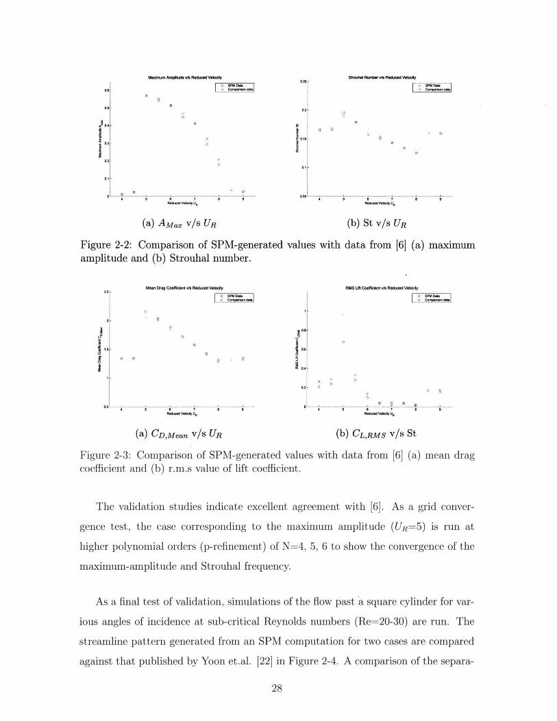
2-2 Comparison of SPM-generated values with data from [6] (a) maximum
amplitude and (b) Strouhal number. . . . . . . . . . . . . . . . . . . . . 28
2-3 Comparison of SPM-generated values with data from [6] (a) mean drag
coefficient and (b) r.m.s value of lift coefficient. . . . . . . . . . . . . . . 28
2-4 A comparison of the streamline pattern published by Yoon et.al. [22]
on the left, with those generated with SPM on the right, for the flow
past a stationary square cylinder at a sub-critical Reynolds number of
20. ........ ........................................ 29
2-5 Comparison of separation bubble length for selected cases. The mea-
sured length from SPM simulations is indicated on this figure adapted
from [22]. . . . . . . . . . . . . . . . . . . . . . . . . . . . . . . . . . . . . 29
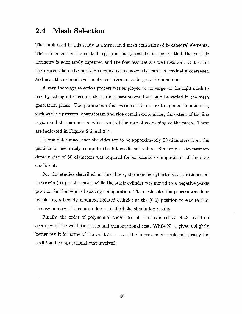
2-6 Image of the mesh used, extending 25 diameters ahead of the cylinder
location and 50 diameters on all other sides. . . . . . . . . . . . . . . . 31
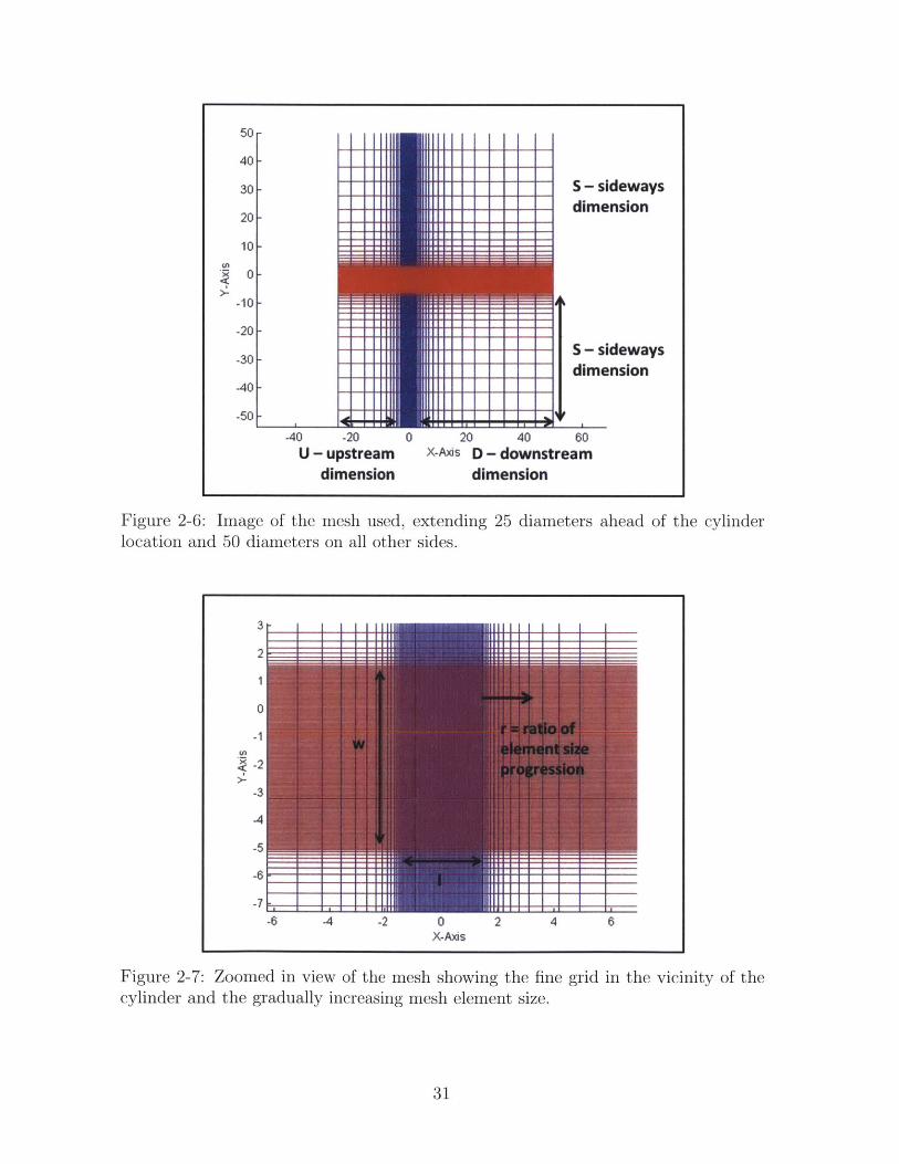
2-7 Zoomed in view of the mesh showing the fine grid in the vicinity of the
cylinder and the gradually increasing mesh element size. . . . . . . . . 31
9
3-1 Schematic image of the simulation configuration showing two cylinders
of diameter D in a sidy-by-side arrangement. The center-to-center
spacing of the two cylinders (S) and the freestream direction is indi-
cated. The bottom cylinder is rigidly mounted while the top cylinder
is flexibly mounted, as indicated by the spring. . . . . . . . . . . . . . . 34
3-2 Representative cylinder trajactories: (left) periodic oscillation observed
UR=5.0 and (right) aperiodic oscillation observed for UR=9.0, both for
the configuration where the spacing is 1.6D. . . . . . . . . . . . . . . . . 35
3-3 On the left are contour plots of the peak of the amplitude response
(top) and the rms of the amplitude response (bottom) for the various
separation and reduced velocity cases. On the right are two measures of
periodicity of the cylinder trajectory: (top) first metric indicates those
cases where the period-to-period amplitude does not vary by more than
10% (indicated with filled green circles) and the second metric (bottom)
indicates those cases where the amplitude rms is within 10% of that
expected for a sine-type curve for a sine curve (ARMS = AMAxIV2). . 36
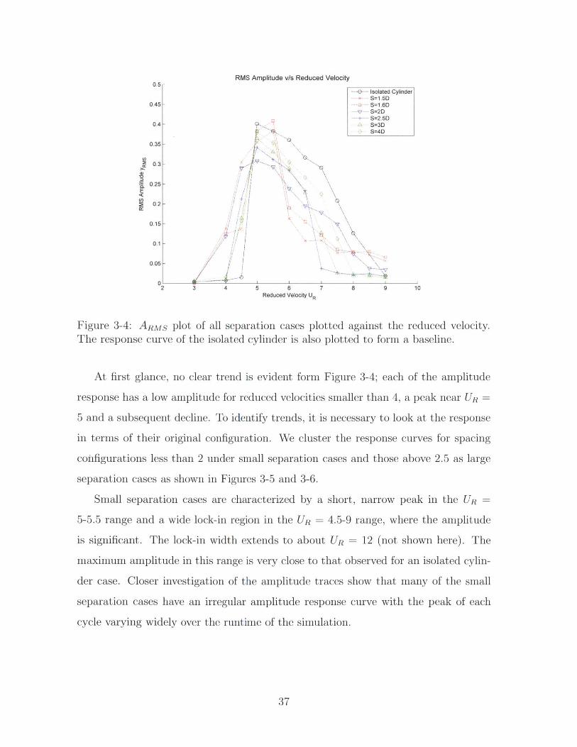
3-4 ARMS plot of all separation cases plotted against the reduced velocity.
The response curve of the isolated cylinder is also plotted to form a
baseline. . . . . . . . . . . . . . . . . . . . . . . . . . . . . . . . . . . . . . 37
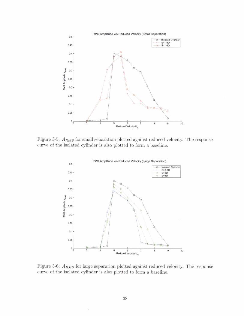
3-5 ARMS for small separation plotted against reduced velocity. The re-
sponse curve of the isolated cylinder is also plotted to form a baseline. 38
3-6 ARMS for large separation plotted against reduced velocity. The re-
sponse curve of the isolated cylinder is also plotted to form a baseline. 38
3-7 ARMS for all three regimes and the isolated cylinder baseline case. . . 39
3-8 CD,Mean plots from both regimes: (left) small separation and (right)
large separation. The curve for the isolated cylinder is plotted as a
baseline case. ........................................ 40
3-9 CL,RMS plots from both regimes: (left) small separation and (right)
large separation. The curve for the isolated cylinder is plotted as a
baseline case. ........................................ 40
10

3-10 Schematic image showing the two cylinders in a side-by-side arrange-
ment, and the three monitor points; the cylinder trajectory (o), the
moving wake (o) and the stationary wake (x). . . . . . . . . . . . . . . 41
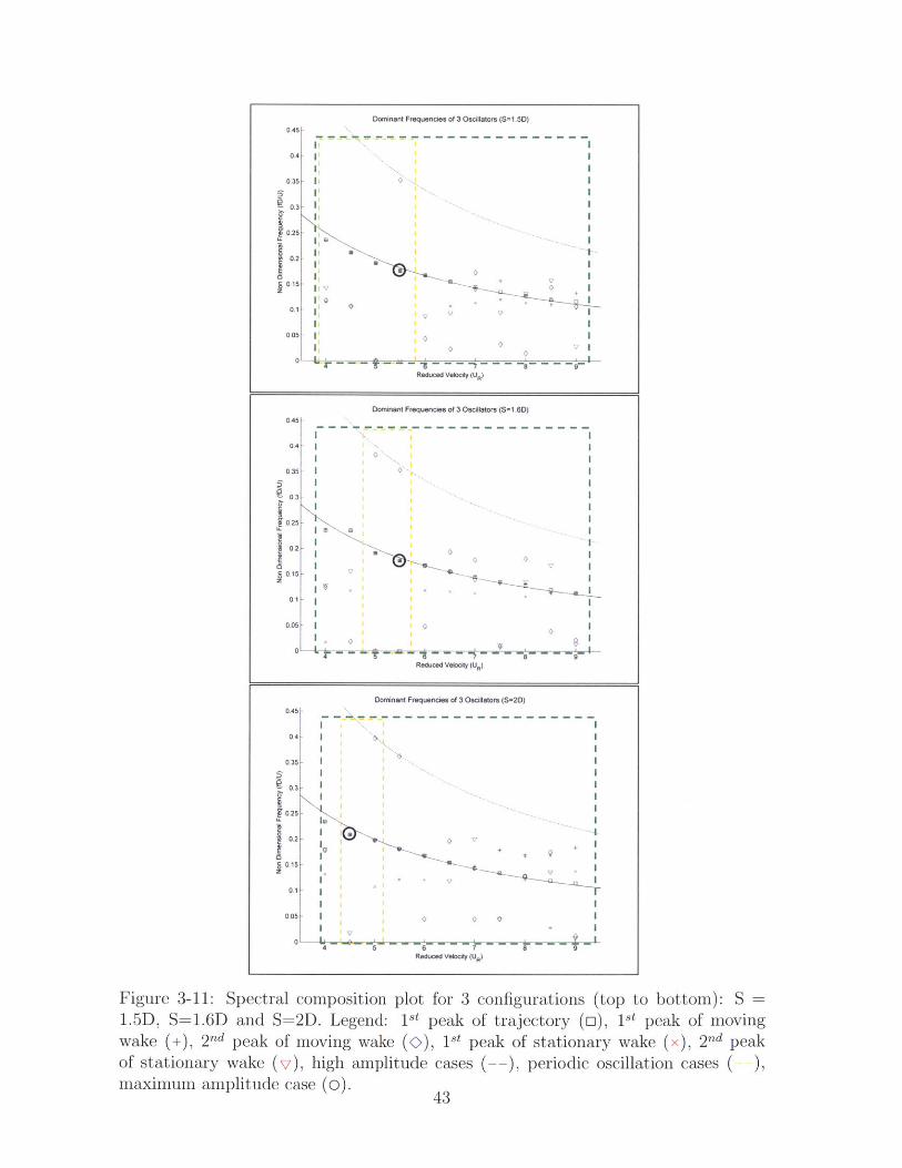
3-11 Spectral composition plot for 3 configurations (top to bottom): S -
1.5D, S=1.6D and S=2D. Legend: 1st peak of trajectory (o), 1st peak of
moving wake (+), 2nd peak of moving wake (0), 1st peak of stationary
wake (x), 2 nd peak of stationary wake (v), high amplitude cases (--),
periodic oscillation cases (--), maximum amplitude case (o). . . . . 43
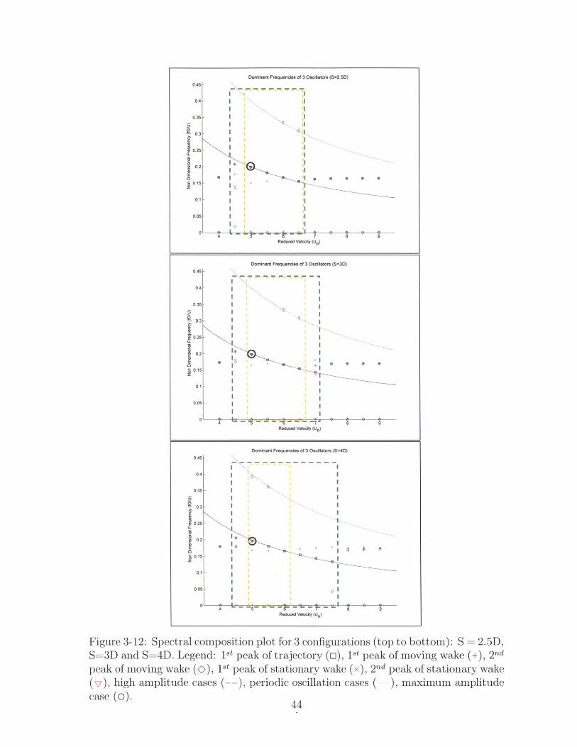
3-12 Spectral composition plot for 3 configurations (top to bottom): S =
2.5D, S=3D and S=4D. Legend: 1 st peak of trajectory (o), 1st peak of
moving wake (+), 2nd peak of moving wake (0), 1st peak of stationary
wake (x), 2nd peak of stationary wake (v), high amplitude cases (--),periodic oscillation cases (--), maximum amplitude case (o). . . . . 44
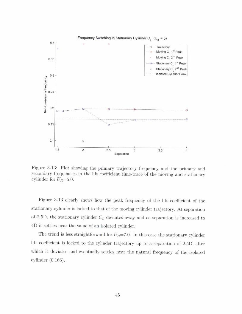
3-13 Plot showing the primary trajectory frequency and the primary and
secondary frequencies in the lift coefficient time-trace of the moving
and stationary cylinder for UR=5.0. . . . . . . . . . . . . . . . . . . . . . 45
3-14 Plot showing the primary trajectory frequency and the primary and
secondary frequencies in the lift coefficient time-trace of the moving
and stationary cylinder for UR=7.0. . . . . . . . . . . . . . . . . . . . . . 46
3-15 Panels of instantaneous vorticity fields for the S=1.6D configuration
under the following conditions (from top to bottom): rigid, UR=4.0,
UR=5.0, UR=6.0 and UR= 7 .0. The vorticity value ranges between -1.5
and 1.5. ........................................... 48
3-16 Panels of instantaneous vorticity fields for the S=4D configuration un-
der the following conditions (from top to bottom): rigid, UR=4.0,
UR=5.0, UR=6.0 and UR=7.0. The vorticity value ranges between -
1.5 and 1.5. . . . . . . . . . . . . . . . . . . . . . . . . . . . . . . . . . . . 49
3-17 Panels of instantaneous vorticity fields for an isolated cylinder under
the following conditions (from top to bottom): rigid, UR=4.0, UR=5.0,
UR=6.0 and UR=7.0. The vorticity value ranges between -1.5 and 1.5. 50
11

A-1 Vorticity snapshots over one cycle based on the lift-coefficient variation.
The vorticity value ranges between -1.5 and 1.5. . . . . . . . . . . . . . 61
A-2 Vorticity snapshots over one cycle of oscillation of the moving cylinder.
The vorticity value ranges between -1.5 and 1.5. . . . . . . . . . . . . . 62
A-3 Vorticity snapshots from one cycle of oscillation of the moving cylinder.
The vorticity value ranges between -1.5 and 1.5. . . . . . . . . . . . . . 62
A-4 Vorticity snapshots from one cycle of oscillation of the moving cylinder.
The vorticity value ranges between -1.5 and 1.5. . . . . . . . . . . . . . 63
A-5 Vorticity snapshots from one cycle of oscillation of the moving cylinder.
The vorticity value ranges between -1.5 and 1.5. . . . . . . . . . . . . . 63
A-6 Vorticity snapshots over one cycle based on the lift-coefficient variation.
The vorticity value ranges between -1.5 and 1.5. . . . . . . . . . . . . . 64
A-7 Vorticity snapshots over one cycle of oscillation of the moving cylinder.
The vorticity value ranges between -1.5 and 1.5. . . . . . . . . . . . . . 65
A-8 Vorticity snapshots from one cycle of oscillation of the moving cylinder.
The vorticity value ranges between -1.5 and 1.5. . . . . . . . . . . . . . 65
A-9 Vorticity snapshots from one cycle of oscillation of the moving cylinder.
The vorticity value ranges between -1.5 and 1.5. . . . . . . . . . . . . . 66
A-10 Vorticity snapshots from one cycle of oscillation of the moving cylinder.
The vorticity value ranges between -1.5 and 1.5. . . . . . . . . . . . . . 66
A-11 Vorticity snapshots over one cycle based on the lift-coefficient variation.
The vorticity value ranges between -1.5 and 1.5. . . . . . . . . . . . . . 67
A-12 Vorticity snapshots over one cycle of oscillation of the moving cylinder.
The vorticity value ranges between -1.5 and 1.5. . . . . . . . . . . . . . 68
A-13 Vorticity snapshots from one cycle of oscillation of the moving cylinder.
The vorticity value ranges between -1.5 and 1.5. . . . . . . . . . . . . . 68
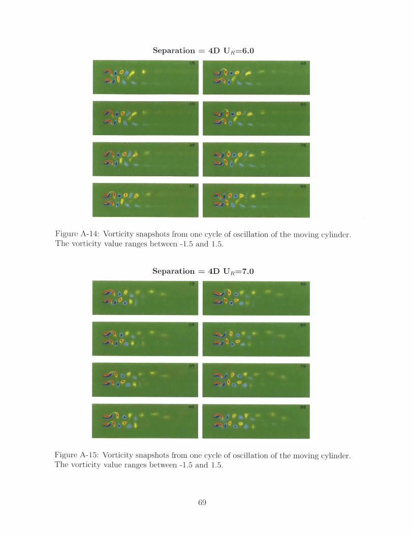
A-14 Vorticity snapshots from one cycle of oscillation of the moving cylinder.
The vorticity value ranges between -1.5 and 1.5. . . . . . . . . . . . . . 69
A-15 Vorticity snapshots from one cycle of oscillation of the moving cylinder.
The vorticity value ranges between -1.5 and 1.5. . . . . . . . . . . . . . 69
12

B-i Figure adapted from [3] show the mean lift and drag forces on the
downstream cylinder at different cross-flow positions corresponding to
a tandem configuration of separation 4D. . . . . . . . . . . . . . . . . . 72
B-2 Variation of the mean lift coefficient CL,Mean on the downstream cylin-
der at different cross-flow positions y/Duc, corresponding to various
inline separations T. . . . . . . . . . . . . . . . . . . . . . . . . . . . . . . 73
B-3 Variation of the mean drag coefficient CD,Mean on the downstream
cylinder at different cross-flow positions y/Duc, corresponding to var-
ious inline separations T. . . . . . . . . . . . . . . . . . . . . . . . . . . . 73
13

14
List of Tables
2.1 Comparison of results for static cylinder at Re=100 . . . . . . . . . . . 27
2.2 Scaling Properties of Nektar-SPM . . . . . . . . . . . . . . . . . . . . . . 32
3.1 Param eters Used . . . . . . . . . . . . . . . . . . . . . . . . . . . . . . . . 34
A.1 Period length (in non-dimensional time) for various cases (S=1.6D) . 61
A.2 Period length (in non-dimensional time) for various cases (S=2D) . . 64
A.3 Period length (in non-dimensional time) for various cases (S=4D) . . 67
15

16
Chapter 1
Introduction
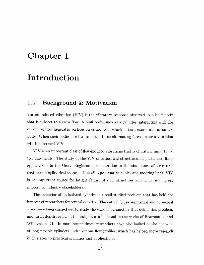
1.1 Background & Motivation
Vortex induced vibration (VIV) is the vibratory response observed in a bluff body
that is subject to a cross flow. A bluff body, such as a cylinder, interacting with the
oncoming flow generates vortices on either side, which in turn exerts a force on the
body. When such bodies are free to move, these alternating forces cause a vibration
which is termed VIV.
VIV is an important class of flow-induced vibrations that is of critical importance
to many fields. The study of the VIV of cylindrical structures, in particular, finds
applications in the Ocean Engineering domain due to the abundance of structures
that have a cylindrical shape such as oil pipes, marine cables and mooring lines. VIV
is an important source for fatigue failure of such structures and hence is of great
interest to industry stakeholders.
The behavior of an isolated cylinder is a well studied problem that has held the
interest of researchers for several decades. Theoretical [5], experimental and numerical
work have been carried out to study the various parameters that define this problem,
and an in-depth review of this subject can be found in the works of Bearman [4] and
Williamson [21]. In more recent times, researchers have also looked at the behavior
of long flexible cylinders under various flow profiles, which has helped move research
in this area to practical scenarios and applications.
17

Ocean structures, however, do not occur in isolation and it becomes important to
study the influence of bodies in proximity on their fluid-structure interaction behavior.
The study of interaction of cylinders dates back to the work of Zdravkovich [23, 24]
where he systematically investigated the effect of proximity on the response char-
acteristics. He classified interference regions as proximity region, wake-interference
region and no-interference region as shown in Figure 1-1. Furthermore, he classified
the flow patterns observed as shown in Figure 1-2.
Mmn
4
a.-
1
CF 3 4 5 6
LID
Figure 1-1: Figure adapted from [24] showing the various interference regimes.
Several recent studies that have examined the interaction of cylinders have in-
vestigated arrangements that include the tandem configuration [1, 2, 13, 25], the
side-by-side configuration [9, 13, 15, 25] and skewed configuration [25]. Recent exper-
imental work by Huera-Huarte et al. [8, 9, 10] have also looked at these configurations
18
I
Region of no-interference
31-Woke interference region
Proximity region
WI j i
i 1 1

Coupled(IIi7~ Ivouped (a) Single slender body~~j ~streets o~7
(b) Alternoe reoftachment
Biased gapd flow (c) Quasi-steady reattochment
(bistoble)b(st-b e) (e) Discontinuous
(d) Intermittent shedding jump dof and
. street . (f) Two vortex streetsS b C f
0 2 3 Bistable 4 5 6
One vortex street I ' Two vortex streets
LID
Figure 1-2: Figure adapted from [24] showing the various flow patterns for the side-by-side arrangement of stationary cylinders.
with flexible cylinders.
While there have been some studies investigating the side-by-side configuration
of a pair of cylinders, most involve cylinders with symmetric properties, i.e, they
are either both stationary, both forced to move at the same frequency or both free
to move under the same natural frequency. The author is aware of only one study
that breaks the symmetry of the problem by holding one of these cylinders rigid.
This study by Huera-Huarte & Gharib [9] looked at effect of this symmetry-breaking
configuration on the response of both degrees of freedom, showing that cross flow
motion is diminished while in-line motion is ampliffied. The study, however, does
not have a thorough analysis of the response characteristics and a qualification of the
interference effect.
The present work aims to look at this symmetry-breaking problem at greater
depth, by characterizing the response based on the separation, the wake patterns
observed and the frequency spectra in the wake.
19

1.2 Thesis Organization
The thesis is organized into the following chapters.
In Chapter 2, the numerical method used by Nektar-SPM is outlined, followed
by the validation of this numerical method, some comments on mesh selection and
computational costs.
In Chapter 3, the central problem that is the subject of this thesis is addressed.
The chapter describes the simulation configuration, the response characteristics and
looks at wake patterns and frequency spectra behind each cylinder.
The thesis closes with Chapter 4, where the major conclusions from this study
and recommendations for future work are listed.
20
Chapter 2
Numerical Method & Validation
2.1 Smoothed Profile Method Implementation
The numerical code employed for this study is the smoothed-profile-method (SPM)
implementation of Nektar, a spectral/hp element based direct-numerical-simulation
solver. While the original code has been in use for several years [19], the SPM im-
plementation is relatively new. This numerical method is the basis of the thesis work
of Luo [11, 12], where a detailed description of this method, error quantification and
validation can be found. Here, a concise description of the method is first presented,
followed by the validation studies that were performed.
2.1.1 Particle Representation
The smoothed-profile-method represents bodies with an indicator function, which is
unity inside the solid domain, zero in the fluid domain and varies smoothly between
these values along the interface of solid and the fluid. This representation of bodies
gives a grid-independent representation where a body can be defined on any grid
simply by the value of the indicator function. The indicator function over the whole
domain is constructed by calculating the distance of a given point from the surface
of the body.
21

(a) (b)
Figure 2-1: (a) Representation of a cylinder in SPM and (b) a zoomed in view of theparticle representation showing the solid domain, the fluid domain and the smoothinterfacial domain.
We use the following general form to represent bodies:
1 -di(x t)Oj(Xt) = -[tanh( ' ) + 1], (2.1)
2 i
where each body i has an indicator function field #j(x, t), defined once the signed
distance di(x, t) is known everywhere in the domain and the value for the interpolation
thickness j is defined. The distance is defined to be positive for points outside the
body and negative for those inside. For simple geometries, like the cylinder that is
used in this study, analytical expressions for this distance function can be obtained,
leading to a straightforward computation of the indicator function. Multiple bodies
(that do not overlap) are handled by separately computing the indicator function field
of each and summing them up to get a global indicator function field.
The smooth concentration field, for a domain consisting of N particles, is con-
structed next:
N
#(x, t) = #5(x, t). (2.2)
22

Based on this total indicator field and knowing the particle velocity V at time t for
each of N particles in the domain, the particle velocity field up(x, t) is constructed:
N
O(X, t)up(x, t) = W{(t)} (i t). (2.3)
The total velocity field is defined as the combination of the particle velocity field (up)
and the fluid velocity field (uf):
u(x, t) = #(x, t)up(x, t) + (1 - #(x, t))Uf (X, t). (2.4)
This total velocity field gives the particle velocity in the particle domain (u = up when
#= 1) and the fluid velocity in the fluid domain (u = uf when q= 0).
2.1.2 Solution Methodology
SPM solves the Navier-stokes equations:
+ (u.)u = v p +vv2 u + fs, (2.5)at p
v -u = 0, (2.6)
where p is the density of the fluid, p is the pressure field, v the kinematic viscosity of
the fluid and f, is the body force term that represents the interactions between the
particles and the fluid.
A two-step semi-discrete form is used to solve the velocity and pressure fields
[14]. First, SPM solves for an intermediate velocity and pressure fields u*, p* from
the previous step solution un, by integrating the advection and viscous stress using
forward Euler integration:
23
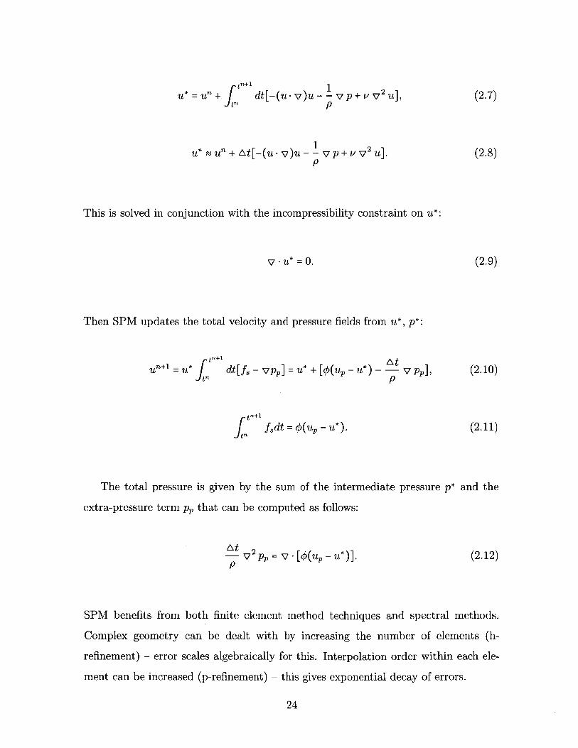
tn+1
U* = "+ 1-n dt[-(u - v)u -- vp+ v v2 u],p
1u* ~ + At[-(u - v)u - -v p+vv 2 u].
P
This is solved in conjunction with the incompressibility constraint on u*:
V - U* = 0.
Then SPM updates the total velocity and pressure fields from u*, p*:
tn+1
un+1 =U*At
dt[fS-vpp]=u*+[#(up-u*)- - pp],p
S'n+1 fdt = O(up - u*). (2.11)
The total pressure is given by the sum of the intermediate pressure p* and the
extra-pressure term pp that can be computed as follows:
AP P=vN.5(upu*)].p
(2.12)
SPM benefits from both finite element method techniques and spectral methods.
Complex geometry can be dealt with by increasing the number of elements (h-
refinement) - error scales algebraically for this. Interpolation order within each ele-
ment can be increased (p-refinement) - this gives exponential decay of errors.
24
(2.7)
(2.8)
(2.9)
(2.10)

2.2 Non Dimensional Parameters Used
This section defines some non-dimensional parameters that will be used in this study.
The primary non-dimensional number that is of significance to fluid mechanics is the
Reynolds number, defined as follows:
Re = UD (2.13)V
where U is the flow velocity, D is the characteristic length and v is the kinematic
viscosity of the fluid. In this study the characteristic length is the diameter D. This
non-dimensional number measures the relative importance of the inertial forces as
opposed to the viscous forces. This study is concerned with flows at a Reynolds
number value of 100 where the flow is still two-dimensional for an isolated cylinder.
The lift force (FLift) and drag force (FDrag) are non-dimensionalized to give the
list and drag coefficients, CL and CD:
CD=FDragCD Fr~ (2.14)- pU2A'
CL = FLift (2.15)gpU 2A'
where p is the fluid density and A is the projected area of the body in the direction
of the flow.
Finally, the motion of cylinders described in this thesis is controlled by two pa-
rameters, the reduced velocity and the mass ratio. Ignoring the effect of damping, the
equation of motion of a cylinder of mass m moving only in the cross-flow direction y
can be written as:
25
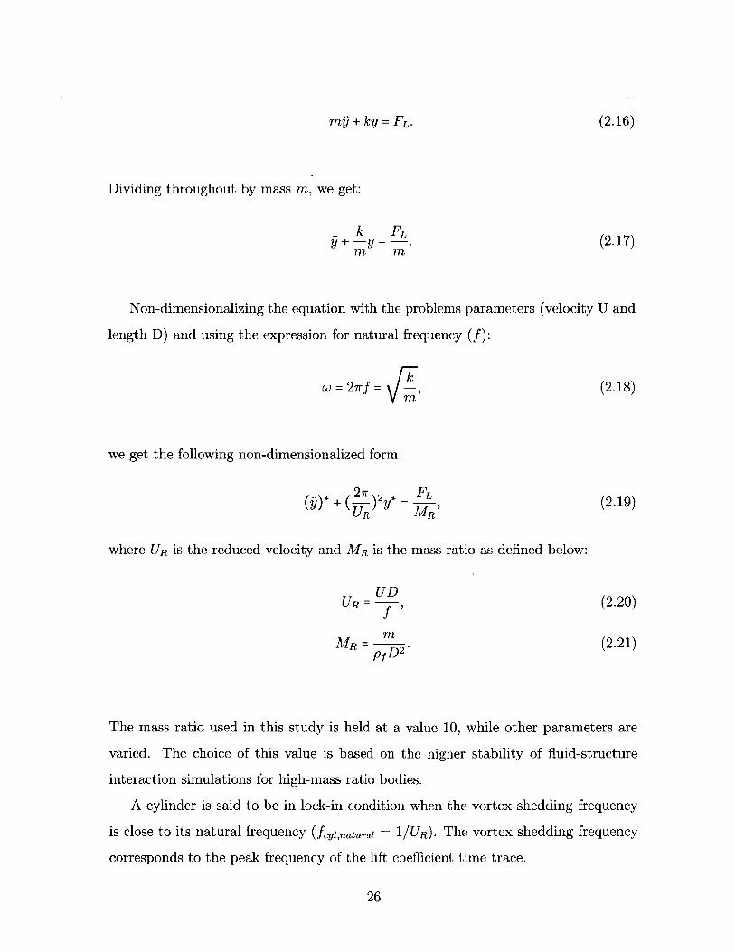
m+ ky = FL. (2.16)
Dividing throughout by mass m, we get:
k FLQ+-y . (2.17)
m m
Non-dimensionalizing the equation with the problems parameters (velocity U and
length D) and using the expression for natural frequency (f):
kw = 2-rf = , (2.18)
we get the following non-dimensionalized form:
(* + ( 27)2* = FL (2.19)UR MR)
where UR is the reduced velocity and MR is the mass ratio as defined below:
UR= UD (2.20)f
MR =M (2.21)pf D2
The mass ratio used in this study is held at a value 10, while other parameters are
varied. The choice of this value is based on the higher stability of fluid-structure
interaction simulations for high-mass ratio bodies.
A cylinder is said to be in lock-in condition when the vortex shedding frequency
is close to its natural frequency (fcyi,natura = 1/UR). The vortex shedding frequency
corresponds to the peak frequency of the lift coefficient time trace.
26
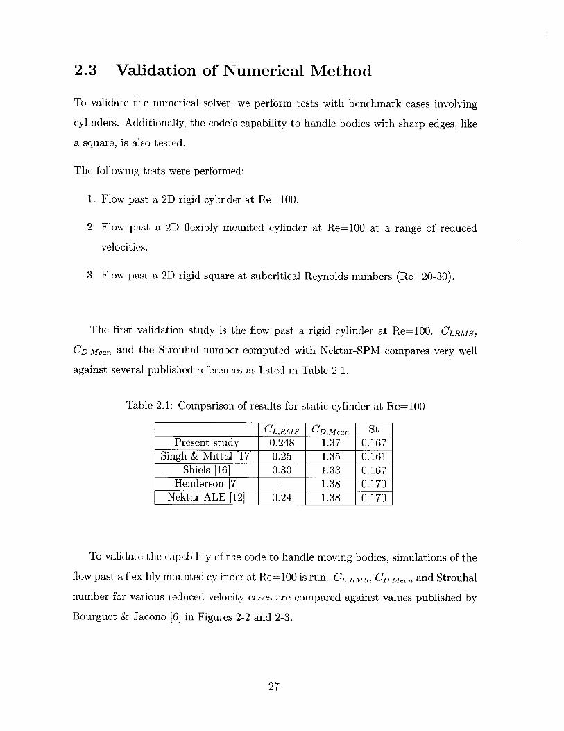
2.3 Validation of Numerical Method
To validate the numerical solver, we perform tests with benchmark cases involving
cylinders. Additionally, the code's capability to handle bodies with sharp edges, like
a square, is also tested.
The following tests were performed:
1. Flow past a 2D rigid cylinder at Re=100.
2. Flow past a 2D flexibly mounted cylinder at Re=100 at a
velocities.
range of reduced
3. Flow past a 2D rigid square at subcritical Reynolds numbers (Re=20-30).
The first validation study is the flow past a rigid cylinder at Re=100. CLRMS,
CD,Mean and the Strouhal number computed with Nektar-SPM compares very well
against several published references as listed in Table 2.1.
Table 2.1: Comparison of results for static cylinder at Re=100
CL,RMS CD,Mean StPresent study 0.248 1.37 0.167
Singh & Mittal [17] 0.25 1.35 0.161Shiels [16] 0.30 1.33 0.167
Henderson [7] - 1.38 0.170Nektar ALE [12] 0.24 1.38 0.170
To validate the capability of the code to handle moving bodies, simulations of the
flow past a flexibly mounted cylinder at Re=100 is run. CL,RMS, CD,Mean and Strouhal
number for various reduced velocity cases are compared against values published by
Bourguet & Jacono [6] in Figures 2-2 and 2-3.
27
S04
031
0 21
Reduced VeloCty U,
0.1S
0 11
(a) AMax v/s UR
Figure 2-2: Comparison of SPM-generated valuesamplitude and (b) Strouhal number.
4 5 it 7
Reduced Velouty U.
(b) St v/s UR
with data from [6] (a) maximum
Mean Drag Coefficient vIs Reduced Velocity
cotyaneoti itofo
2
1.5
RMS Lift Coefficient v/s Reduced Velocity
CF cptotid_ t
o.ob
SI
j0.61
0 2:-
Reduced Velociy U,
(a) CDMean v/s UR
Figure 2-3: Comparison of SPM-generated valuescoefficient and (b) r.m.s value of lift coefficient.
Reduced Velocity U,,
(b) CL,RMS V/s St
with data from [6] (a)
The validation studies indicate excellent agreement with [6]. As a grid conver-
gence test, the case corresponding to the maximum amplitude (UR-=5) is run at
higher polynomial orders (p-refinement) of N=4, 5, 6 to show the convergence of the
maximum-amplitude and Strouhal frequency.
As a final test of validation, simulations of the flow past a square cylinder for var-
ious angles of incidence at sub-critical Reynolds numbers (Re=20-30) are run. The
streamline pattern generated from an SPM computation for two cases are compared
against that published by Yoon et.al. [22] in Figure 2-4. A comparison of the separa-
28
O R:
0.5
Maximum Amplitude v/s Reduced Velocity
_._C oitola
Strouhal Number vis Reduced Velocity
I : " - dat
mean drag
0.26
9
2 5
01_

tion bubble sizes in shown in Figure 2-5. This demonstrates an excellent agreement
of the results obtained with Nektar-SPM.
This completes the validation process of the numerical method and its computational
implementation.
(a)
.0
x
(b)
0
Figure 2-4: A comparison of the streamline pattern published by Yoon et.al. [22] onthe left, with those generated with SPM on the right, for the flow past a stationarysquare cylinder at a sub-critical Reynolds number of 20.
3
21
10 20Re
30 40
1
0
Figure 2-5: Comparison of separation bubble length for selected cases. The measuredlength from SPM simulations is indicated on this figure adapted from [22].
29
- 3 Present, 0=00+- --- Present, 0=15.3"
-------- Present, 0=29.7"------ Present, 0=450- A Sharma and Eswaran(200 - --
2.4 Mesh Selection
The mesh used in this study is a structured mesh consisting of hexahedral elements.
The refinement in the central region is fine (dx=0.05) to ensure that the particle
geometry is adequately captured and the flow features are well resolved. Outside of
the region where the particle is expected to move, the mesh is gradually coarsened
and near the extremities the element sizes are as large as 5 diameters.
A very thorough selection process was employed to converge on the right mesh to
use, by taking into account the various parameters that could be varied in the mesh
generation phase. The parameters that were considered are the global domain size,
such as the upstream, downstream and side domain extremities, the extent of the fine
region and the parameters which control the rate of coarsening of the mesh. These
are indicated in Figures 2-6 and 2-7.
It was determined that the sides are to be approximately 50 diameters from the
particle to accurately compute the lift coefficient value. Similarly a downstream
domain size of 50 diameters was required for an accurate computation of the drag
coefficient.
For the studies described in this thesis, the moving cylinder was positioned at
the origin (0,0) of the mesh, while the static cylinder was moved to a negative y-axis
position for the required spacing configuration. The mesh selection process was done
by placing a flexibly mounted isolated cylinder at the (0,0) position to ensure that
the asymmetry of this mesh does not affect the simulation results.
Finally, the order of polynomial chosen for all studies is set at N=3 based on
accuracy of the validation tests and computational cost. While N=4 gives a slightly
better result for some of the validation cases, the improvement could not justify the
additional computational cost involved.
30
-40 -20U - upstream
dimension
0
50
40
Figure 2-6: Image of the mesh used, extending 25 diameters ahead of the cylinderlocation and 50 diameters on all other sides.
3
0
-1
-2
-3
-4
-5
-6
-72-2 U
X-Axis
Figure 2-7: Zoomed in view of the mesh showing the fine grid in the vicinity of thecylinder and the gradually increasing mesh element size.
31
S - sidewaysdimension
S -sidewaysdimension
20 40 60X-Axis D - downstream
dimension
30-
20
101-
0
-101-
-20
-30~
-40
-50
I
2.5 Computational Resources Used
Nektar-SPM is a parallelized solver and to take advantage of this feature, computer
clusters were employed for all simulations. The machine that was used for this project
is a supercomputer of the Cray-XE6 type architecture. This machine has several
thousand nodes available for processing, with each node split into two sets of 16 cores
each.
Processor scaling tests are used to study the scaling properties of Nektar-SPM
across different processor configurations to determine one that would make best use
of the available resources. The tests are normalized by choosing one representative
case and running the simulation for a total of 1000 time-steps.
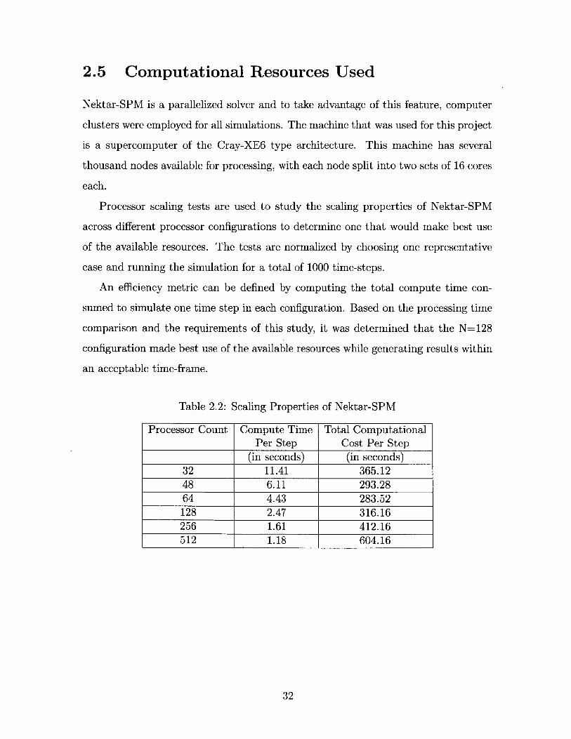
An efficiency metric can be defined by computing the total compute time con-
sumed to simulate one time step in each configuration. Based on the processing time
comparison and the requirements of this study, it was determined that the N=128
configuration made best use of the available resources while generating results within
an acceptable time-frame.
Table 2.2: Scaling Properties of Nektar-SPM
Processor Count Compute Time Total ComputationalPer Step Cost Per Step
(in seconds) (in seconds)32 11.41 365.1248 6.11 293.2864 4.43 283.52128 2.47 316.16256 1.61 412.16512 1.18 604.16
32
Chapter 3
Simulation Cases
3.1 Interaction of Side-By-Side Cylinders
3.1.1 Problem Description
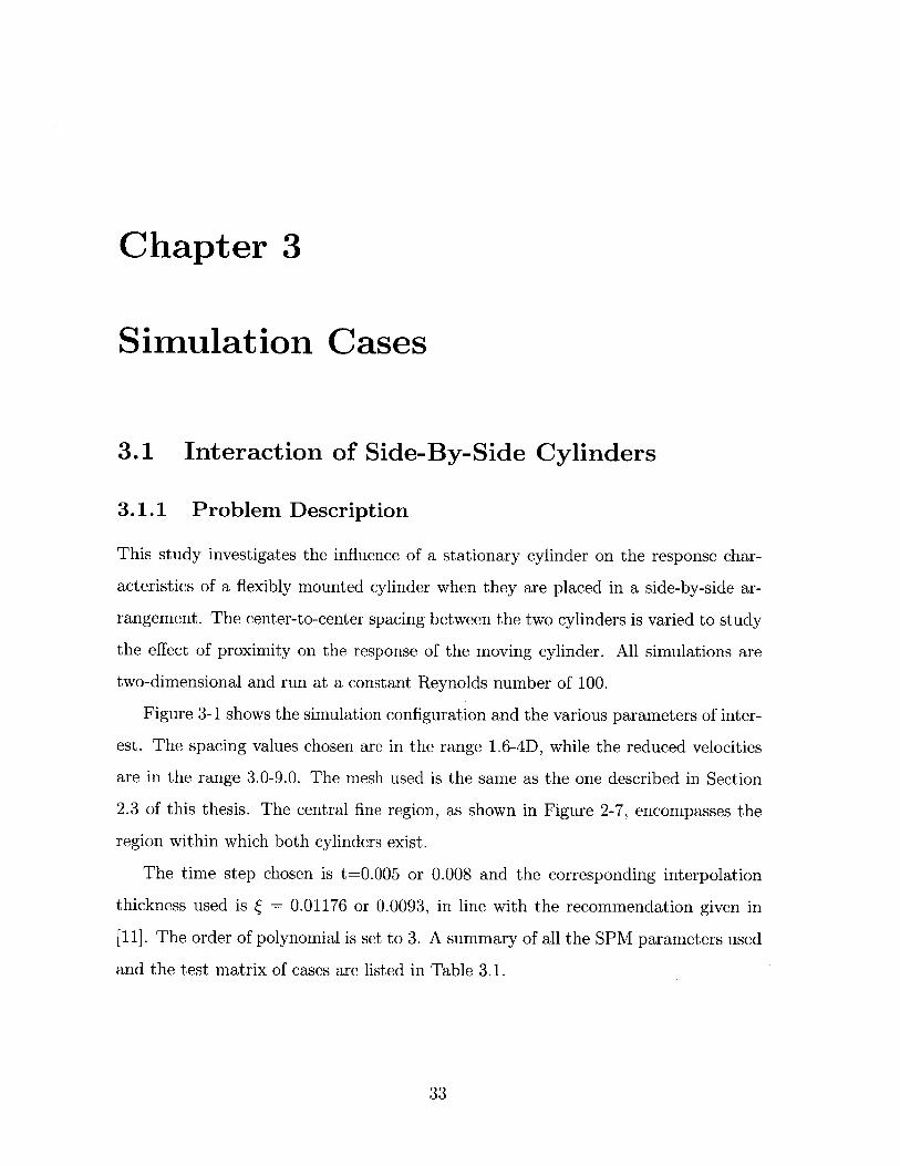
This study investigates the influence of a stationary cylinder on the response char-
acteristics of a flexibly mounted cylinder when they are placed in a side-by-side ar-
rangement. The center-to-center spacing between the two cylinders is varied to study
the effect of proximity on the response of the moving cylinder. All simulations are
two-dimensional and run at a constant Reynolds number of 100.
Figure 3-1 shows the simulation configuration and the various parameters of inter-
est. The spacing values chosen are in the range 1.6-4D, while the reduced velocities
are in the range 3.0-9.0. The mesh used is the same as the one described in Section
2.3 of this thesis. The central fine region, as shown in Figure 2-7, encompasses the
region within which both cylinders exist.
The time step chosen is t=0.005 or 0.008 and the corresponding interpolation
thickness used is = 0.01176 or 0.0093, in line with the recommendation given in
[11]. The order of polynomial is set to 3. A summary of all the SPM parameters used
and the test matrix of cases are listed in Table 3.1.
33
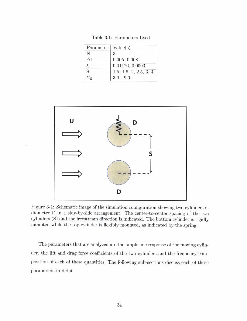
Table 3.1: Parameters Used
Parameter Value(s)N 3At 0.005, 0.008
0.01176, 0.0093S 1.5, 1.6, 2, 2.5, 3, 4UR 3.0 - 9.0
Figure 3-1: Schematic image of the simulation configuration showing two cylinders ofdiameter D in a sidy-by-side arrangement. The center-to-center spacing of the twocylinders (S) and the freestream direction is indicated. The bottom cylinder is rigidlymounted while the top cylinder is flexibly mounted, as indicated by the spring.
The parameters that are analyzed are the amplitude response of the moving cylin-
der, the lift and drag force coefficients of the two cylinders and the frequency com-
position of each of these quantities. The following sub-sections discuss each of these
parameters in detail.
34
U D
S
D

3.1.2 Amplitude Response
The maximum amplitude of an isolated cylinder under VIV at Re=100 was described
in Section 2.3 of this thesis and will form the comparison case for the side-by-side
simulation studies.
Unlike the isolated cylinder, the moving cylinder in the current simulations does
not, in general, exhibit a periodic oscillation. Two representative cases, from the
separation configuration of 1.6D, are shown in Figure 3-2. The UR=5.0 trajectory
shows a largely periodic oscillation where the maximum amplitude does not vary
much. The UR=9.0 case on the other hand shows a highly aperiodic amplitude
response.
425-
02
0
Figure 3-2: Representative cylinder trajactories: (left) periodic oscillation observedUR=5.O and (right) aperiodic oscillation observed for UR=9.O, both for the configu-ration where the spacing is 1.6D.
To better quantify the amplitude response the root mean square value of the
amplitude response, computed over a long interval, is used to characterize the re-
sponse. Figure 3-3 shows both the maximum amplitude and the r.m.s amplitude of
the various cases that were examined. This contour map shows the peak ridge to be
around UR=5.O. With increase in separation the width of the high-amplitude region
(ARMS > 0.1) first decreases, reaches a minimum at around separation of 2.5D and
increases beyond that.
35

Amplitude Response Map
4- 05
C 040
032m 02
01
4 5 6 7 8 9
Amplitude RMS Plot4 04
35- 0303-
02C 2.5
2- 01151
4 5 6 7Reduced Velocity
9
Figure 3-3: On the left are contour plots
PonocIApioic Map
4-0 ~35-
3-
4 5 8 7 a 9
Cbfonos to SneCWvo
3
25- 0 a 0 a a 0
2- *
4 5 6 7 8 9Rodxcod Vo ilc
of the peak of the amplitude response(top) and the rms of the amplitude response (bottom) for the various separationand reduced velocity cases. On the right are two measures of periodicity of thecylinder trajectory: (top) first metric indicates those cases where the period-to-periodamplitude does not vary by more than 10% (indicated with filled green circles) andthe second metric (bottom) indicates those cases where the amplitude rms is within10% of that expected for a sine-type curve for a sine curve (ARNS = AMAx/').
Also shown on the right-panel of Figure 3-3 are two metric of the aperiodic nature
of the response. The top sub-figure indicates periodic cases as determined by the
closeness of ampitude peaks in the response (a 10% criterion). The bottom sub-
figure indicates all cases where the trajectory deviates from a sinusiodal curve, by
measuring the deviation of the ratio of the peak amplitude to the rms-amplitude
from that expected for a sinusiodal curve, i.e., the deviation from the value of V'-.
We next look at the r.m.s. amplitude reponse curves of the various separation cases
in detail.
36
RMS Amplitude v/s Reduced Velocity
--- Isolated CylinderS=1.5DS=1.6DS=2D
4- S=2.5DS=3DS=4D
'0,
0.5-
0.45-
0.4-
0.35
0.3
0.25-
0.2-
0.15-
0.1 -
0.05
0-2 3 4 5 6
Reduced Velocity UR
0
CI
ii/
F -'~
/ I
1-7 8 9 10
Figure 3-4: ARMS plot ofThe response curve of the
all separation cases plotted against the reduced velocity.isolated cylinder is also plotted to form a baseline.
At first glance, no clear trend is evident form Figure 3-4; each of the amplitude
response has a low amplitude for reduced velocities smaller than 4, a peak near UR -
5 and a subsequent decline. To identify trends, it is necessary to look at the response
in terms of their original configuration. We cluster the response curves for spacing
configurations less than 2 under small separation cases and those above 2.5 as large
separation cases as shown in Figures 3-5 and 3-6.
Small separation cases are characterized by a short, narrow peak in the UR
5-5.5 range and a wide lock-in region in the UR- 4.5-9 range, where the amplitude
is significant. The lock-in width extends to about UR= 12 (not shown here). The
maximum amplitude in this range is very close to that observed for an isolated cylin-
der case. Closer investigation of the amplitude traces show that many of the small
separation cases have an irregular amplitude response curve with the peak of each
cycle varying widely over the runtime of the simulation.
37
E
Mi
-' I
RMS Amplitude v/s Reduced Velocity (Small Separation)
--e- Isolated CylinderS=1.5D
Fl S=1.6D
01 -
0.05-
2 3 4 5 6Reduced Velocity UR
0.5
0.45-
0.4
0.35-
0.3-
0.25-
G
Figure 3-5: ARMS for small separation plotted against reduced velocity. The responsecurve of the isolated cylinder is also plotted to form a baseline.
RMS Amplitude v/s Reduced Velocity (Large Separation)
- Isolated CylinderS=2.5DS=3DS=4D
G.
p
I
0.~
-c
2 3 4 5 6Reduced Velocity UR
7 8 9 10
Figure 3-6: ARMS for large separation plotted against reduced velocity. The responsecurve of the isolated cylinder is also plotted to form a baseline.
38
V
CL
E
0.2 k
0.15
0.4
0.35 -
0.3-
0.25 -
0.2
2
E
U)
0.15
0.1
0.05--
7 8 9 10
0.5-
0.45-
k
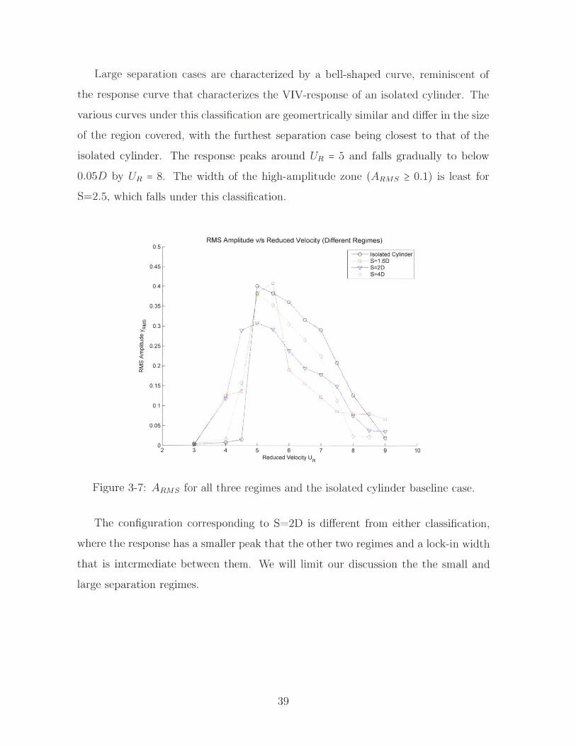
Large separation cases are characterized by a bell-shaped curve, reminiscent of
the response curve that characterizes the VIV-response of an isolated cylinder. The
various curves under this classification are geomertrically similar and differ in the size
of the region covered, with the furthest separation case being closest to that of the
isolated cylinder. The response peaks around UR = 5 and falls gradually to below
0.05D by UR = 8. The width of the high-amplitude zone (ARMS > 0.1) is least for
S=2.5, which falls under this classification.
E
0.5
0.45
0.4
0.35
0.3
0.25
0.2
0.15
0.1
0.05
0
RMS Amplitude v/s Reduced Velocity (Different Regimes)
-- Isolated CylinderS=1.6D
- S=2DS=D
0.
V,
5 6 7 8 9Reduced Velocity UR
10
Figure 3-7: ARMS for all three regimes and the isolated cylinder baseline case.
The configuration corresponding to S=2D is different from either classification,
where the response has a smaller peak that the other two regimes and a lock-in width
that is intermediate between them. We will limit our discussion the the small and
large separation regimes.
39
2 3 4
'0
3.1.3 Lift and Drag Force Behavior
Mean Drag Coefficient v/s Reduced Velocity (Small Separation)Ileetad Cyindes
Mean Drag Coefficient v/s Reduced Velocity (Large Separation)-sdafted Cyinder
s 4
0
6 5
2 3 4 5 81 7 8 9 10Reduced Velocity (U,,) Reduced Velocity (U.)
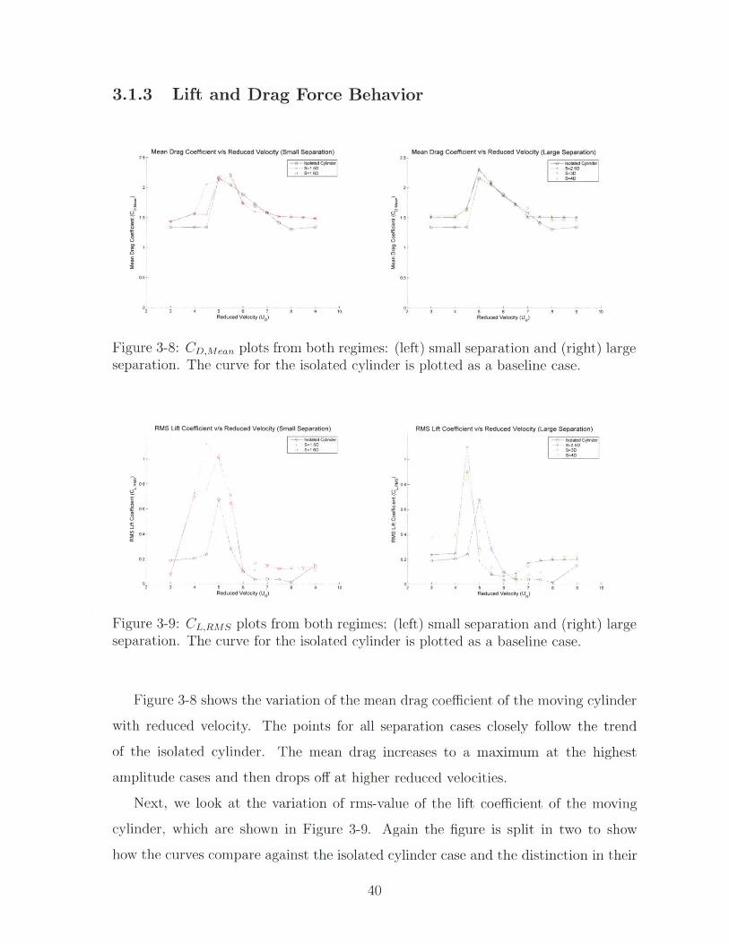
Figure 3-8: CD,Mean plots from both regimes: (left) small separation and (right) largeseparation. The curve for the isolated cylinder is plotted as a baseline case.
RMS Lift Coefficient v/s Reduced Velocity (Small Separation)s=td Cylc.0=
08-
02 0
2 3 4 5 8 7 BReduced Velocity (UR)
RMS Lift Coefficient v/s Reduced Velocity (Large Separation)3u06ftd Cyhndel
08
5aon-
02
Reduced Velocity (UR)
Figure 3-9: CL,RMS plots from both regimes: (left) small separation and (right) largeseparation. The curve for the isolated cylinder is plotted as a baseline case.
Figure 3-8 shows the variation of the mean drag coefficient of the moving cylinder
with reduced velocity. The points for all separation cases closely follow the trend
of the isolated cylinder. The mean drag increases to a maximum at the highest
amplitude cases and then drops off at higher reduced velocities.
Next, we look at the variation of rms-value of the lift coefficient of the moving
cylinder, which are shown in Figure 3-9. Again the figure is split in two to show
how the curves compare against the isolated cylinder case and the distinction in their
40
oe
L)
2 5 -
02 3
I10
shapes. The large separation cases all have the same general shape that compares
closely with the isolated cylinder: they rise at the beginning of the corresponding lock-
in region to a value close to 0.9, followed by a steep drop to a nearly zero value and
a subsequent recovery to a steady value of approximately 0.2 at the higher reduced
velocities. The small-separation cases are different from the isolated cylinder case
in two ways. First, the region where CL,RMS is large is wider and corresponds to
the peaking amplitude response zone of this regime. Second the drop is steeper and
abruptly settles near the value of 0.15, that is carried into the high reduced velocity
region.
3.1.4 Three Oscillator System
The earlier sections described how the lift and drag coefficient behavior is modified
by proximity and distinct response regimes were identified. To better understand the
underlying physical mechanism, we next examine the spectral composition of several
quantities: the trajectory of the moving cylinder, the lift and drag coefficients of both
cylinders and the cross-flow velocity component of monitor points in the wake.
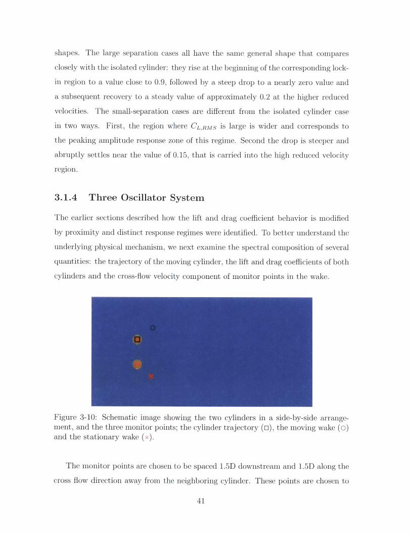
Figure 3-10: Schematic image showing the two cylinders in a side-by-side arrange-ment, and the three monitor points; the cylinder trajectory (n), the moving wake (o)and the stationary wake (x).
The monitor points are chosen to be spaced 1.5D downstream and 1.5D along the
cross flow direction away from the neighboring cylinder. These points are chosen to
41
capture the dynamics of the wake associated with each cylinder, thereby giving rise to
a three-oscillator system: the moving cylinder, the wake associated with the moving
cylinder (hereafter referred to as the moving wake) and the wake associated with the
stationary cylinder (hereafter referred to as the stationary wake).
For each spacing configuration, the data gathered is organized in the following
manner: the primary frequency of the cylinder trajectory is plotted, followed by the
primary and secondary peaks associated with each of the wakes. Within each plot,
the region corresponding to high amplitude (ARMS 0.1) is marked with a green box
and within each green box, the cases corresponding to periodic oscillations is marked
with a yellow box. These plots are shown in Figures 3-11 and 3-12.
For small separations, the characteristic feature is that there are multiple dominant
frequencies in the wake. The trajectory, however, has a clear peak within the range of
reduced velocities examined, and lies on or close to the natural frequency. The region
with significant amplitude (ARMS 0.1) spans the entire range displayed, while a
small-subset of cases exhibit a periodic oscillation. For all cases exhibiting a periodic
oscillation, the primary frequency of the trajectory is locked to one or more harmonics
of both the wakes and the maximum amplitude case always corresponds to a periodic
oscillation case.
For the large separation cases, the characteristic feature is the existence of one
dominant frequency for each oscillator. It is interesting to note that the moving
cylinder and moving wake are locked for all periodic oscillation cases and most high
amplitude cases. The stationary wake's primary frequency is not always locked to the
moving cylinder; however, at least the second frequency is, with diminishing effect as
the separation is increased.
To show the diminishing effect on the stationary cylinder, we pick two reduced
velocity cases (UR=5.0, 7.0) and track the evolution of the primary frequency of the
stationary cylinder. Due to the proximity of the moving cylinder to the stationary
one in the small separation cases, we would expect the frequency characteristics to
be primarily driven by the moving cylinder.
42
Dominant Frequencies of 3 Oscillators (S=1.5D)
- -I
.1
I8I ~
I';112
~1
0.05
0 -V -oc (U-)
Reduced Velocity (U,)
Dominant Frequencies of 3 Oscillators (S=1.60)
0.45 F
d
Reduced Velocity (UR)
Dominant Frequencies of 3 Oscillators (S=2D)
+ + I
V
1 1)) 0
4 5 6 7 85Reduced Velocity (UR)
Figure 3-11: Spectral composition plot for 3 configurations (top to bottom): S =1.5D, S=1.6D and S=2D. Legend: 1 st peak of trajectory (o), 1st peak of movingwake (+), 2 nd peak of moving wake (0), 1 st peak of stationary wake (x), 2nd peakof stationary wake (v), high amplitude cases (--), periodic oscillation cases ( ),maximum amplitude case (o). 43
0.45
0.4
0.35
0.3
0.25
0.2
0,15
0.1
0.4
0.35
0.3
0.25
S0.2
5 0.15
0.1
4
0.05F
0.45
0.4
0 35[
- I
3=,
0
0.3
0.25
0,2
0.15
0A
0.05 -
CL-
-r9~
- I
V
0
I
Dominant Frequencies of 3 OscIllators (S=2.5D)
I - -
- I
Reduced Velooty (UR)
A A
Dominant Frequencies of 3 Oscillators (S=3D)
0.45[
- I
- I
Is
a 4
'I~ I
Reduced Velocity (U.)a -
Dominant Frequencies of 3 Oscillators (S=4D)
045
0A
0.35
0.3
0.25
0.2
0.15
0.1
0.05
--
- I
I
QI
Reduced Velocity (U,)
Figure 3-12: Spectral composition plot for 3 configurations (top to bottom): S = 2.5D,S=3D and S=4D. Legend: Ist peak of trajectory (o), 1 st peak of moving wake (+), 2 nd
peak of moving wake (c), 1St peak of stationary wake (x), 2 nd peak of stationary wake(v), high amplitude cases (--), periodic oscillation cases ( ), maximum amplitudecase (o). 44
0.45F
0.4
0.35
0.3
0.25
0.2
0 15
0.1
0.05
0.4
0.35
0.3
*025
0.2
0 15
0.1
0.05
U , I -?, I e 9
a a
a a M0
Frequency Switching in Stationary Cylinder CL (UR = 5)0.4 -
-E) Trajectoryu Moving CL 1st Peak
0.35_ x Moving CL 2nd Peak
Stationary CL 1st Peak
x Stationary CL 2nd Peak
0.3 - Isolated Cylinder Peak
0.25-
C
0 .
0i 0.2 0z
0.15 -
0.1 - x
1.5 2 2.5 3 3.5 4Separation
Figure 3-13: Plot showing the primary trajectory frequency and the primary andsecondary frequencies in the lift coefficient time-trace of the moving and stationarycylinder for UR=5.0.
Figure 3-13 clearly shows how the peak frequency of the lift coefficient of thestationary cylinder is locked to that of the moving cylinder trajectory. At separation
of 2.5D, the stationary cylinder CL deviates away and as separation is increased to4D it settles near the value of an isolated cylinder.
The trend is less straightforward for UR=7.0. In this case the stationary cylinder
lift coefficient is locked to the cylinder trajectory up to a separation of 2.5D, after
which it deviates and eventually settles near the natural frequency of the isolated
cylinder (0.166).
45

0.4
0.35 1
0.3-
0.25-
0.2-
0.15
0.1
Frequency Switching in Stationary Cylinder CL (UR = 7)
-E- Trajectory-e Moving CL 1st Peak
x Moving CL 2nd Peak
-- Stationary CL 1st Peak
x Stationary CL 2"n PeakIsolated Cylinder Peak
x
x
1.5 2 2.5Separation
3 3.5 4
Figure 3-14: Plot showing the primary trajectory frequency and the primary andsecondary frequencies in the lift coefficient time-trace of the moving and stationarycylinder for UR= 7 .0.
46
Cr
0
E0
z
3.1.5 Wake Visualization
Small separation cases generate an unstructured wake for most reduced velocities due
to the effect of the gap flow and the competing influences of the vortex shedding
frequency of the stationary cylinder (~ 0.17) and the moving cylinder (~ 1/UR). The
proximity of the cylinder gives rise to an intermixing of these two primary frequencies.
The first panel in Figure 3-15 shows the visualization of the wake of the stationary
configuration. The flow is biased (upwards) and shows the interaction of vortices in
the near wake region. Panels 2, 4 and 5 corresponding to reduced velocities UR=4, 6
and 7 show the unstructured nature of the wakes.
The only exception to this rule is the UR=5.0 case, which exhibits a pair of 2S
wakes behind each cylinder that converge and coalesce downstream. The reasoning
behind this exception is that the high amplitude of oscillation of the moving cylinder
sets the vortex shedding frequency of the stationary one, which thereby leads to a
single primary frequency in the wake leading to an organized wake.
Large separation cases are characterized by a structured wake for most reduced
velocities. The relatively larger distance between the two cylinders allows for each
wake to form and evolve separately in the near wake region. The representative case
chosen from this regime is the configuration with a separation of 4, and images are
shown in Figure 3-16. For the purposes of comparison, a similar set of vorticity
snapshots for the isolated cylinder case is shown in Figure 3-17.
The UR=5.0 case clearly demonstrates how two distinct wake patterns can coexist
without significant intermingling up to about 10-15 diameters downstream. The P+S
mode of the moving cylinder and the 2S mode of the stationary cylinder can be
clearly seen in the visualization of the wake. The two cases UR=4.0 and UR=7.0,
which both have a comparable amplitude response, exhibit a pattern where each
cylinder generates a wake of the 2S mode at slightly different frequencies. The wakes
co-exist to further show the limited effect of proximity at a separation of 4D.
Wake visualization for several cases, including that of an isolated cylinder, with
snapshots taken across one time-period is included in Appendix A.
47
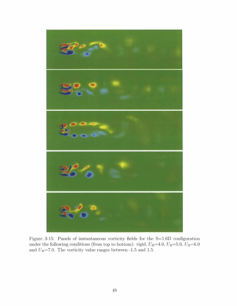
Figure 3-15: Panels of instantaneous vorticity fields for the S=1.6D configurationunder the following conditions (from top to bottom): rigid, UR=4.0, UR=5.0, UR=6.0and UR=7.0. The vorticity value ranges between -1.5 and 1.5.
48
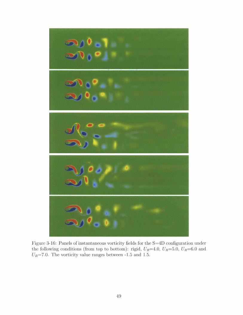
Figure 3-16: Panels of instantaneous vorticity fields for the S=4D configuration underthe following conditions (from top to bottom): rigid, UR=4.0, UR=5.0, UR=6.0 andUR=7.0. The vorticity value ranges between -1.5 and 1.5.
49
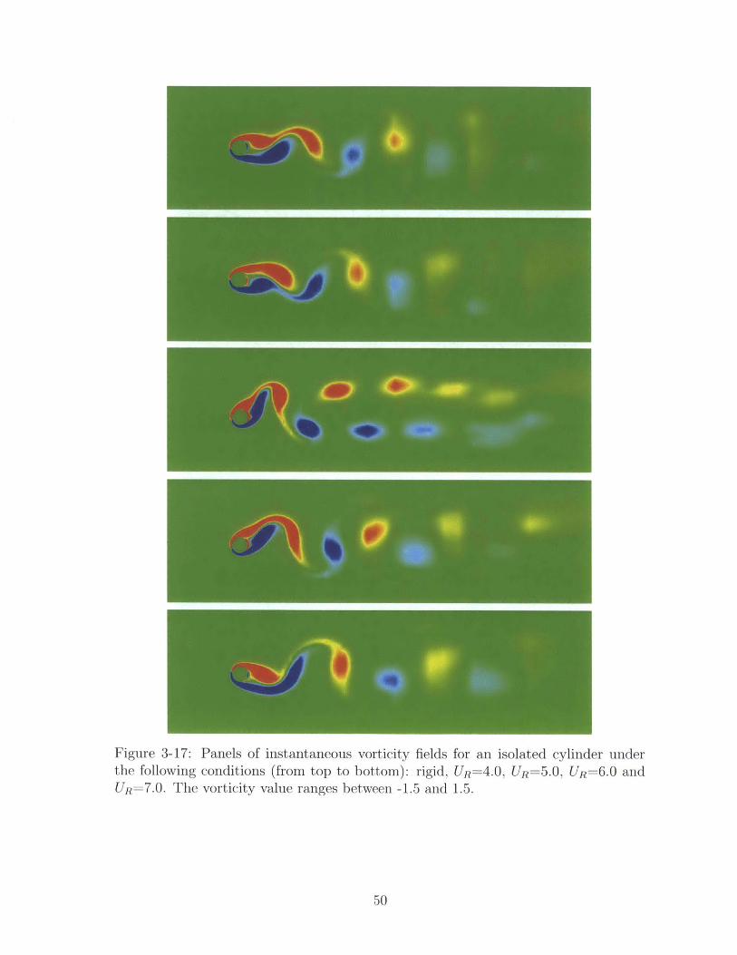
Figure 3-17: Panels of instantaneous vorticity fields for an isolated cylinder underthe following conditions (from top to bottom): rigid, UR=4.0, UR=5.0, UR=6.0 andUR=7.0. The vorticity value ranges between -1.5 and 1.5.
50

3.2 Concluding Remarks
The study of the side-by-side arrangement of cylinders with one being able to move
is an important symmetry-breaking study. The flexibility of one cylinder acts as
an additional frequency contributor to the wake frequencies. The proximity of the
cylinders determines the shape of the response curve and the relative strengths of
the frequency components in the response of the moving cylinder. Examining the
problem as a three oscillator model reveals the influence of the moving cylinder on
its wake and also the wake associated with the stationary cylinder. A detailed look
at the frequencies and the relative strengths of the frequencies indicates a diminish-
ing influence of the moving cylinder on the stationary cylinder both with increasing
separation and smaller amplitudes.
51

52
Chapter 4
Conclusions & Future Work
The major conclusions of the study on side-by-side cylinders are:
1. The amplitude response can be classified into two regimes: small and large
separation, each of which has distinguishing properties in terms of the shape of
the response curve and the CL,RMS curve.
(a) Small separation cases have a short, narrow peak near UR = 5 and a wide
lock-in range of UR=4.5-12 (beyond the parametric space discussed in this
thesis).
(b) Large separation cases have a bell-shaped curve with a peak near UR
5 and a narrower lock-in range of UR=4.5-8. The lock-in width is largest
for the largest separation case, with the bell-curve approaching that of the
response of an isolated cylinder.
2. The trajectory of the moving cylinder is observed to be periodic only in cases
where the amplitude is large (ARMS > 0.1) and when the 1st and/or 2 nd har-
monic of the moving wake are locked with it, corresponding to a situation where
all three oscillators are locked. The maximum amplitude for each spacing con-
figuration occurs at this point where a three-way synchronization occurs.
53
3. The stationary wake is strongly influenced by the moving cylinder in the small
separation configurations as evidenced by the frequency composition derived
from the monitor points in the wake. For the large separation configurations,
this influence is limited to those cases where the amplitude response is high,
when the moving cylinder is in lock-in condition.
4. The wake patterns show a clear distinction between the two regimes; small
separation cases are characterized by unstructured and chaotic wake patterns
while the large separation cases are characterized by structured wake patterns.
The coexistence of different types of wakes behind the two cylinders for a large
separation configuration point to a reduced degree of interference.
5. An examination of the monitor point spectra can reveal which regime the system
is in:
(a) For the small separation configuration, the stationary wake monitor point
either exhibits a strongly multi-frequency response (for low amplitude
cases) or a peak frequency away from the Strouhal frequency of a sta-
tionary cylinder (fstat,cyl ~ 0.17).
(b) For the large separation configuration, the stationary cylinder wake is
strongly mono-frequency, and this frequency is very close to the Strouhal
frequency of a stationary cylinder (fstat,cyl ~ 0.17). In addition, monitor
points near the moving cylinder is strongly mono-frequency and is locked
to cylinder's natural frequency.
On the basis of this work, the following new directions of work can be recommended:
1. The side-by-side studies, in close proximity revealed the influence of competing
frequencies of the response of the moving cylinder. A more thorough analysis
of the interference of competing frequencies can be studied by allowing both
cylinders to move, with each one being set to a different natural frequency.
54
2. The limit of the closeness of the initial configuration is around 1.5D, where some
reduced velocity cases lead to contact of the two cylinders. By implementing
a collision condition, the effect of closer separations on amplitude response can
be studied.
55

56
Bibliography
[1] G.R.S. Assi, J.R. Meneghini, J.A.P. Aranha, P.W. Bearman, E. Casaprima, Exper-
imental investigation of flow-induced vibration interference between two circular
cylinders, Journal of Fluids and Structures 22 (2006).
[2] G.R.S. Assi, P.W. Bearman, J.R. Meneghini, On the wake-induced vibration of
tandem circular cylinders: the vortex interaction excitation mechanism, Journal
of Fluid Mechanics 661 (2010).
[3] G.R.S. Assi, P.W. Bearman, B.S. Carmo, J.R. Meneghini, S.J. Sherwin, R.H.J.
Willden, The role of wake stiffness on the wake-induced vibration of the down-
stream cylinder of a tandem pair, Journal of Fluid Mechanics 718 (2013).
[4] P.W. Bearman, Vortex shedding from oscillating bluff bodies, Annual Review of
Fluid Mechanics 16 (1984).
[5] R.D. Blevins, Flow Induced Vibration, 2nd edition, Malabar FL: Krieger Publish-
ing (1994).
[6] R. Bourguet, D.L. Jacono, Flow-induced vibrations of a rotating cylinder, Journal
of Fluid Mechanics, 740 (2014).
[7] R.D. Henderson, Details of the drag curve near the onset of vortex shedding,
Physics of Fluids 7 (1995).
[8] F.J. Huera-Huarte, M. Gharib, Vortex and wake-induced vibrations of a tandem
arrangement of two flexible cylinders with near wake interference, Journal of Flu-
ids and Structures 27 (2011).
57
[9] F.J. Huera-Huarte, M. Gharib, Flow-induced vibration of a side-by-side arrange-
ment of two flexible cylinders, Journal of Fluids and Structures 27 (2011).
[10] F.J. Huera-Huarte, M. Gharib, Vortex and wake-induced vibrations of a tandem
arrangement of two flexible cylinders with far wake interference, Journal of Fluids
and Structures 27 (2011).
[11] X.Luo, M.R. Maxey, G.E. Karniadakis, Smoothed profile method for particulate
flows: Error analysis and simulations, Journal of Computational Physics 228
(2009).
[12] X.Luo, A spectral element/smoothed profile method for complex-geometry flows,
Ph.D thesis, Division of Applied Mathemetics, Brown University (2009).
[13] J.R. Meneghini, F. Saltara, C.L.R. Siqueira, J.A. Ferrari Jr., Numerical simula-
tion of flow interference between two circular cylinders in tandem and side-by-side
arrangement, Journal of Fluids and Structures 15 (2001).
[14] Y. Nakayama, R. Yamamoto, Simulation method to resolve hydrodynamic inter-
actions in colloidal dispersions, Physical Review Letters E 71 (2005).
[15] S. Ryu, S.B. Lee, B.H. Lee, J.C. Park, Estimation of hydrodynamic coefficients
for flow around cylinders in side-by-side arrangement with variation in separation
gap, Ocean Engineering (2009).
[16] D. Shiels, A. Leonard, A. Roshko, Flow-induced vibration of a circular cylinder
at limiting structural parameters, Journal of Fluids and Structures 15 (2001).
[17] S.P. Singh, S. Mittal, Vortex-induced oscillations at low Reynolds numbers: Hys-
terisis and vortex-shedding modes, Journal of Fluids and Structures 20 (2005).
[18] D. Sumner, Two circular cylinders in cross-flow: A review, Journal of Fluids
and Structures 26 (2010).
58
[19] T. Warburton, Spectral/hp element methods on polymorphic multi-domains: Al-
gorithms and applications, Ph.D thesis, Division of Applied Mathemetics, Brown
University (1998).
[20] C.H.K. Williamson, A. Roshko, Vortex formation in the wake of an oscillating
cylinder, Journal of Fluids and Structures 2 (1988).
[21] C.H.K Williamson, R. Govardhan, Vortex Induced Vibrations, Annual Review of
Fluid Mechanics 36 (2004).
[22] D.H. Yoon, K.S. Yang, C.B. Choi, Flow past a square cylinder with an angle of
incidence, Physics of Fluids 22 (2010).
[23] M.M. Zdravkovich, The effects of interference between circular cylinders in cross
flow, Journal of Fluids and Structures 1 (1987).
[24] M.M. Zdravkovich, Flow induced oscillations of two interfering circular cylinders,
Journal of Sound and Vibration 101 (1985).
[25] M. Zhao, Flow induced vibration of two rigidly coupled circular cylinder in tan-
dem and side-by-side arrangements at a low Reynolds number of 150, Physics of
Fluids 25 (2013).
59

60
Appendix A
Wake Visualization
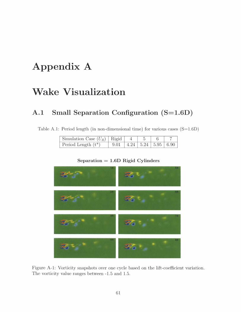
A.1 Small Separation Configuration (S=1.6D)
Table A.1: Period length (in non-dimensional time) for various cases (S=1.6D)
Simulation Case (UR) Rigid 4 5 6 7Period Length (t*) 9.01 4.24 5.24 5.95 6.90
Separation = 1.6D Rigid Cylinders
Figure A-1: Vorticity snapshots over one cycle based on the lift-coefficient variation.The vorticity value ranges between -1.5 and 1.5.
61
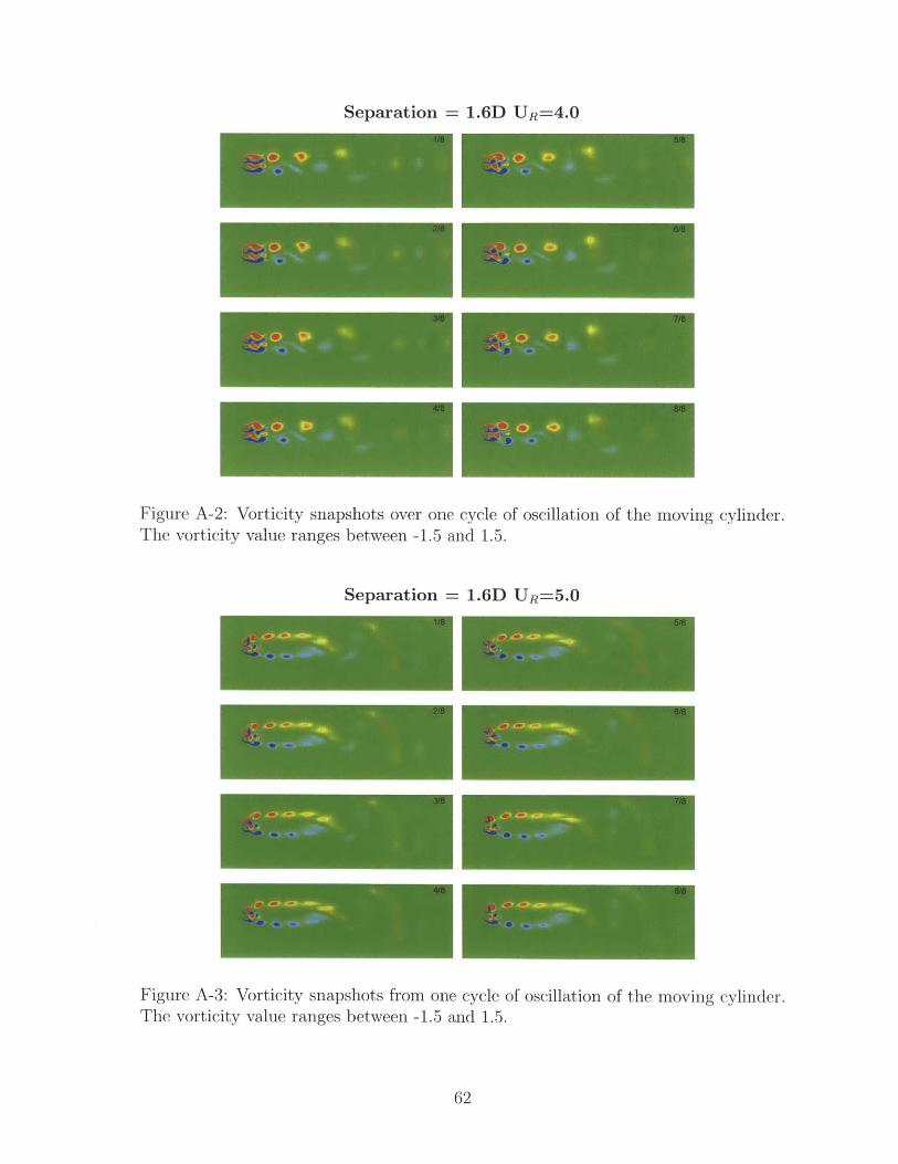
Separation = 1.6D UR= 4 .0
Figure A-2: Vorticity snapshots over one cycle of oscillation of the moving cylinder.The vorticity value ranges between -1.5 and 1.5.
Separation = 1.6D UR=5.0
Figure A-3: Vorticity snapshots from one cycle of oscillation of the moving cylinder.The vorticity value ranges between -1.5 and 1.5.
62

Separation = 1.6D UR=6.0
Figure A-4: Vorticity snapshots from one cycle of oscillation of the moving cylinder.The vorticity value ranges between -1.5 and 1.5.
Separation =
Figure A-5: Vorticity snapshots from oneThe vorticity value ranges between -1.5 a
1.6D UR='7.0
cycle of oscillation of the moving cylinder.
63

A.2 Intermediate Separation Configuration (S=2D)
Table A.2: Period length (in non-dimensional time) for various cases (S=2D)
Simulation Case (UR) Rigid 4 5 6 7Period Length (t*) 5.24 4.29 5.05 5.99 6.90
Separation = 2D Rigid Cylinders
Figure A-6: Vorticity snapshots over one cycle based on the lift-coefficient variation.The vorticity value ranges between -1.5 and 1.5.
64

Separation = 2D UR= 4 .0
Figure A-7: Vorticity snapshots over one cycleThe vorticity value ranges between -1.5 and 1.5
Separation =
of oscillation of the moving cylinder.
2D UR= 5 .0
Figure A-8: Vorticity snapshots from one cycle of oscillation of the moving cylinder.The vorticity value ranges between -1.5 and 1.5.
65

Separation
-I-I-I-I
Figure A-9: Vorticity snapshots from oneThe vorticity value ranges between -1.5 ai
Separation
Figure A-10: Vorticity snapshots from oneThe vorticity value ranges between -1.5 an,
2D UR= 6 .0
cycle of oscillation of the moving cylinder.
2D UR= 7 .0
cycle of oscillation of the moving cylinder.
66

A.3 Large Separation Configuration (S=4D)
Table A.3: Period length (in non-dimensional time) for various cases (S=4D)
Simulation Case (UR) Rigid 4 5 6 7Period Length (t*) 5.59 5.62 5.13 6.10 6.71
Separation = 4D
Figure A-11: Vorticity snapshots over oneThe vorticity value ranges between -1.5 ar
Rigid Cylinders
cycle based on the lift-coefficient variation.
67
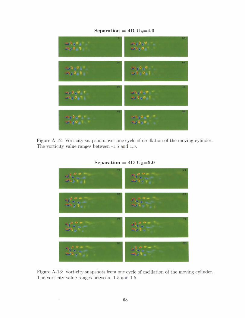
Separation = 4D UR= 4 .0
Figure A-12: Vorticity snapshots over one cycle of oscillation of the moving cylinder.The vorticity value ranges between -1.5 and 1.5.
Separation = 4D UR= 5 .0
Figure A-13: Vorticity snapshots from one cycle of oscillation of the moving cylinder.The vorticity value ranges between -1.5 and 1.5.
68
I
Separation = 4D UR= 6 .0
Figure A-14: Vorticity snapshots from one cycle of oscillation of the moving cylinder.The vorticity value ranges between -1.5 and 1.5.
Separation = 4D UR=7.0
Figure A-15: Vorticity snapshots from oneThe vorticity value ranges between -1.5 an
cycle of oscillation of the moving cylinder.
69

70

Appendix B
Tandem Cylinders
B.1 Wake Stiffness Effect
This section summarizes the results of simulations involving stationary cylinders of
unequal diameters in stagerred arrangements.
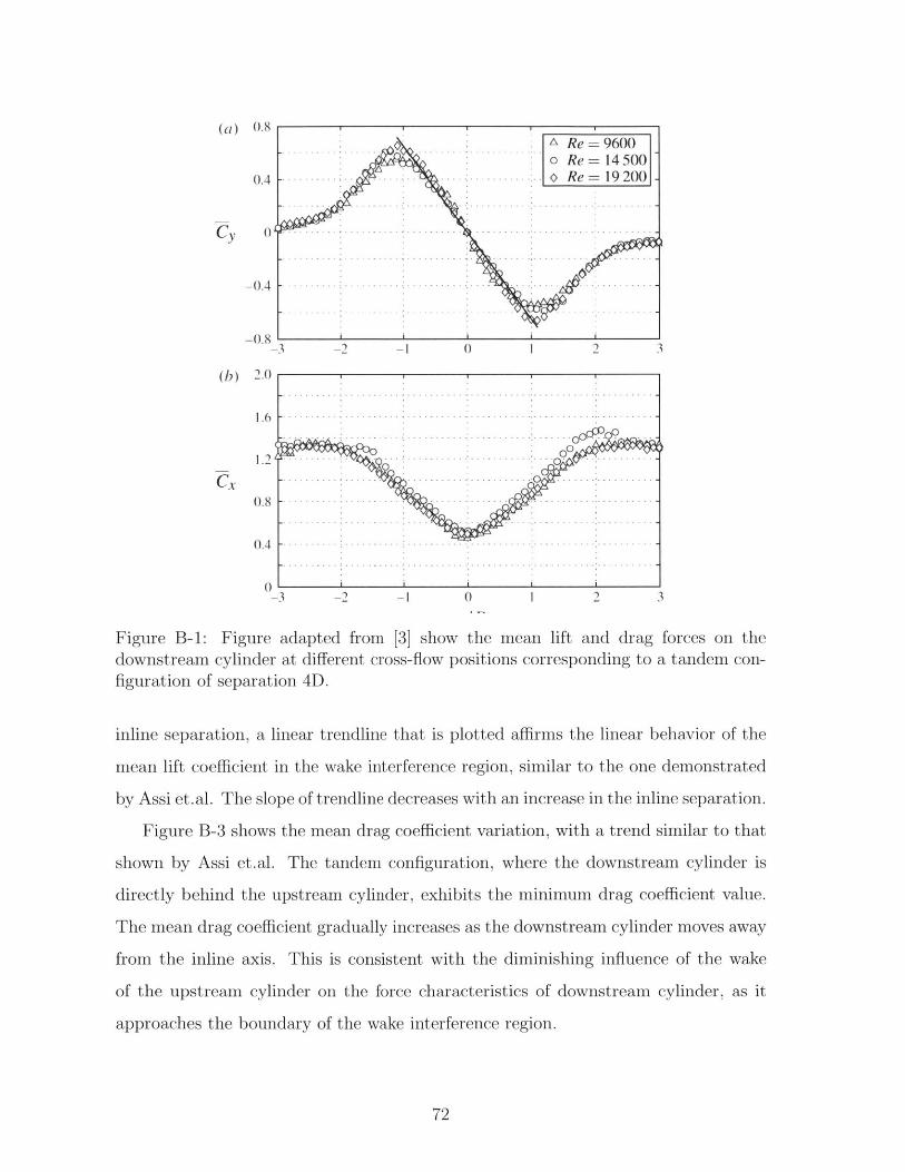
Assi et.al. [3] showed that for stationary cylinders of equal diameter, the mean
lift force on the downstream cylinder at staggered positions varies linearly with its
distance from the inline axis, for points within the wake interference region (2 <
1.0). Their experimental study shows this linear dependence for a range of Reynolds
numbers (Re=9600-19200) for an inline separation of 4 diameters, as shown in Figure
B-1. Furthermore, the slope of each of these curves, within the linear range was
determined to be approximately 0.65, independent of the Reynolds number.
We perform simulations at Re=100 to examine if this phonomenon exists at low
Reynolds numbers. Additionally, we have cylinders of unequal diamaters, with the
upstream cylinder diameter set to 2.5 times the diameter of the downstream one.
Furthermore, the inline separation (T) range is chosen to be in the range 3-5 DuC,
where DuC is the diameter of the upstream cylinder. Taking advantage of the sym-
metry of the problem, we survey only the positive direction of the crossflow axis
(0 y/Duc 0.75).
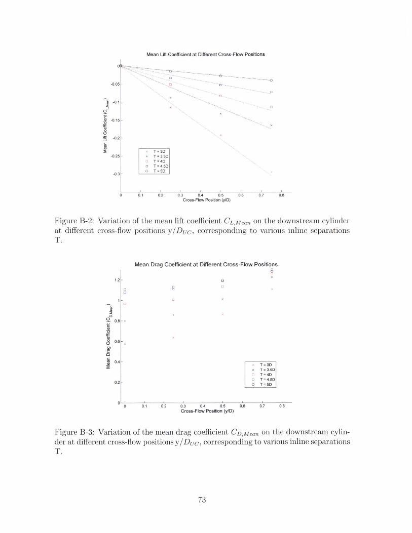
Figure B-2 shows the mean lift coefficient at different staggered positions. For each
71
( ) 0.8A Re - 9600o Re 14 500
0.4 . Re= 19 200
-0
-0.81-3 -1 0 1 2 3
([b) 2.0
0.8
Figure B-i: Figure adapted from [31 show the mean lift and drag forces on thedownstream cylinder at different cross-flow positions corresponding to a tandem con-figuration of separation 4D.
inline separation, a linear trendline that is plotted affirms the linear behavior of the
mean lift coefficient in the wake interference region, similar to the one demonstrated
by Assi et.al. The slope of trendline decreases with an increase in the inline separation.
Figure B-3 shows the mean drag coefficient variation, with a trend similar to that
shown by Assi et.al. The tandem configuration, where the downstream cylinder is
directly behind the upstream cylinder, exhibits the minimum drag coefficient value.
The mean drag coefficient gradually increases as the downstream cylinder moves away
from the inline axis. This is consistent with the diminishing influence of the wake
of the upstream cylinder on the force characteristics of downstream cylinder, as it
approaches the boundary of the wake interference region.
72
Mean Lift Coefficient at Different Cross-Flow Positions
:77 .. ....... .....
LI
x T = 3Dx T = 3.5DLl T=4D* T = 4.5D0 T=5D
0.1 0.2 0.3 0.4 0.5Cross-Flow Position (y/D)
0.6 0.7 0.8
Figure B-2: Variation of the mean lift coefficient CL,Mean on the downstream cylinderat different cross-flow positions y/Duc, corresponding to various inline separationsT.
Mean Drag Coefficient at Different Cross-Flow Positions
x T= 3Dx T = 3.5D* T=4D* T = 4.5D0 T=5D
0.1 0.2 0.3 0.4 0.5Cross-Flow Position (y/D)
0.6 0.7 0.8
Figure B-3: Variation of the mean drag coefficient CD,Mean on the downstream cylin-der at different cross-flow positions y/Duc, corresponding to various inline separationsT.
73
0
40051
-0.1
-0.15[-
-0.2 -
0
-0.25
-0.3
1.2-
1 -
0
UI
l
0.8 -A-)
0 0.6 -
0.4
0.2 F
0
Related Documents