Supercritical Fluid Extraction: A Study of Binary and Multicomponent Solid-Fluid Equilibria by Ronald Ted Kurnik B.S.Ch.E. Syracuse University (1976) M.S.Ch.E. Washington University (1977) SUBMITTED IN PARTIAL FULFILLMENT OF THE REQUIREMENTS FOR THE DEGREE OF DOCTOR OF SCIENCE at the MASSACHUSETTS INSTITUT.E OF TECHNOLOGY May, 1981 @Massachusetts Institute of Technology, 1981 Signature redacted Signature of Author -------""="--------,------------ Department of Chemical Engineering Certified by May, 1981 Signature redacted Robert C. Reid i:cnesis Supervisor / Signature redacted Accepted by ARC~J\'ES (_ ;- . _ . . . = . _ . .. _ MASSACHUSEIT . Chairman, Departmental OFTECHN&&is7rrurE Committee on Graduate Students OCT 2 8 1981 UBRARlES

Welcome message from author
This document is posted to help you gain knowledge. Please leave a comment to let me know what you think about it! Share it to your friends and learn new things together.
Transcript
Supercritical Fluid Extraction:
A Study of Binary and
Multicomponent Solid-Fluid
Equilibria
by
Ronald Ted Kurnik ~
B.S.Ch.E. Syracuse University (1976)
M.S.Ch.E. Washington University (1977)
SUBMITTED IN PARTIAL FULFILLMENT OF THE REQUIREMENTS FOR THE
DEGREE OF
DOCTOR OF SCIENCE
at the
MASSACHUSETTS INSTITUT.E OF TECHNOLOGY
May, 1981
@Massachusetts Institute of Technology, 1981
Signature redacted Signature of Author -------""="--------,------------Department of Chemical Engineering
Certified by
May, 1981
Signature redacted Robert C. Reid
i:cnesis Supervisor /
Signature redacted Accepted by ARC~J\'ES (_ ;- . _ . . . = . _ . .. _
MASSACHUSEIT . Chairman, Departmental OFTECHN&&is7rrurE Committee on Graduate Students
OCT 2 8 1981
UBRARlES
SUPERCRITICAL FLUID EXTRACTION:
A STUDY OF BINARY AND
MULTICOMPONENT SOLID-FLUID
EQUILIBRIA
by
RONALD TED KURNIK
Submitted to the Department of Chemical Engineeringon May 1981, in partial fulfillment of the
requirements for the degree of Doctor of Science
ABSTRACT
Solid-fluid equilibrium data for binary and multicom-ponent systems were determined experimentally using twosupercritical fluids -- carbon dioxide and ethylene, and sixsolid solutes. The data were taken for temperatures betweenthe upper and lower critical end points and for pressures from120 to 280 bar.
The existence of very large (106) enhancement (over theideal gas value) of solubilities of the solutes in the fluidphase was.observed with these systems. In addition, it wasfound that the solubility of a species in a multicomponentmixture could be significantly greater (as much as 300 per-cent) than the solubility of that same pure species inthe given supercritical fluid (at the same temperature andpressure).
Correlation of both pure and multicomponent solid-fluidequilibria was accomplished uiing the Peng-Ronbinson equationof state. In the case of multicomponent solid-fluid equil-ibrium it was necessary to introduce an additional binarysolute-solute interaction coefficient.
The existence of a maximum in solubility of a solid ina supercritical fluid was observed both theoretically andexperimentally. The reason for this maximum was explained.
Energy effects in solid-fluid equilibria were studiedand it was shown that in the retrograde solidification regionthat the partial molar enthalphy difference for the solutebetween the fluid and solid phase is exothermic.
Thesis Supervisor: Robert C. Reid
Title: Professor of Chemical Engineering
Department of Chemical EngineeringMassachusetts Institute of TechnologyCambridge, Massachusetts 02139
May, 1981
Professor George C. NewtonSecretary of the FacultyMassachusetts Institute of TechnologyCambridge, Massachusetts 02139
Dear Professor Newton:
In accordance with the regulations of the FacultyI herewith submit a thesis entitled "SupercriticalFluid Extraction: A Study of Binary and MulticomponentSolid-Fluid Equilibria" in partial fulfillment ofthe requirements for the degree of Doctor of Sciencein Chemical Engineering at the MassachusettsInstitute of Technology.
Respectfully submitted,
Ronald Ted Kurnik
5
ACKNOWLE DGEMENTS
The author gratefully acknowledges the support and
advice of Professor Robert C. Reid.
Many thanks are due to Dr. Val J. Krukonis for his
enthusiastic support of this work and for his help in the
experimental design of the equipment used in this thesis.
The help of Mike Mullins in constructing the equipment
is gratefully acknowledged.
Dr. Herb Britt, Dr. Joe Boston, Dr. Paul Mathias, Suphat
Watanasiri, and Fred Ziegler of the ASPEN project are
thanked for their many helpful discussions.
The members of my thesis committee, Professor Modell,
Professor Longwell, Professor Daniel I. C. Wang and Dr.
Charles Apt provided many helpful comments and suggestions.
Samuel Holla was helpful in obtaining some of the equil-
ibrium data used in this thesis.
The Nestle's Company is gratefully acknowledged for
their financial support in terms of a three year fellowship.
Financial support of the National Science Foundation is
appreciated.
To my many friends at MIT, especially those in the LNG
lab, thanks for good advice, endless encouragement, and many
fun filled hours when we were together. I wish you all
6
success, happiness, and lasting friendship in the years to
come.
Finally, I am most indebted to my brother, parents,
and grandmother for their continuous confidence and support
throughout my schooling.
Ronald Ted Kurnik
Cambridge, Massachusetts
May, 1981
7
CONTENTS
Page
1. SUMMARY 20
1-1 Introduction 201-2 Background 221-3 Thesis Objectives 271-4 Experimental Apparatus and Procedure 281-5 Results and Discussion 301-6 Recommendations 54
2. INTRODUCTION 57
2-1 Background 572-2 Phase Diagrams 852-3 Thermodynamic Modelling of Solid-Fluid
Equilibria 1152-4 Thesis Objectives 128
3. EXPERIMENTAL APPARATUS AND PROCEDURE 130
3-1 Review of Alternative Experimental 130Methods
3-2 Description of Equipment 1313-3 Operating Procedure 1343-4 Determination of Solid Mixture
Composition 1353-5 Safety- Considerations 136
4. RESULTS AND DISCUSSION OF RESULTS 137
4-1 Binary Solid-Fliud Equilibrium Data 1374-2 Ternary solid-Fluid Equilibrium Data 1594-3 Experimental Proof that T < Tq 189
5. UNIQUE SOLUBILITY PHENOMENA OF SUPERCRITICALFLUIDS 193
5-1 Solubilitv Minima 1935-2 Solubility Maxima 1945-3 A Method to Achieve 100% Solubility of
a Solid in a Supercritical Fluid Phase 2015-4 Entrainers in Supercritical Fluids 2025-5 Transport Properties of Supercritical Fluids 206
lo I
a
6. ENERGY EFFECTS
6-1 Theoretical Development6-2 Presentation and Discussion of
Theoretical Results
7. OVERALL CONCLUSIONS
8. RECOM ENDATIONS FOR FUTURE RESEARCH
8-18-28-3
Solid-Fluid EquilibriaLiquid-Fluid EquilibriaEquipment Design
APPENDIX I.
APPENDIX II.
APPENDIX III.
APPENDIX IV.
APPENDIX V.
APPENDIX VI.
APPENDIX VII.
APPENDIX VIII.
APPENDIX IX.
APPENDIX X.
APPENDIX XI.
APPENDIX XII.
Partial Molar Volume Using thePeng-Robinson Equation of State
Derivation of Slope Equality at aBinary Mixture Critical Point
Derivation of Enthalpy Changeof Solvation
Freezing Point Data for Multicom-ponent Mixtures
Physical Properties of SolutesStudied
Sources of Physical Propertiesof Complex Molecules
Listings of Pertinent ComputerPrograms
Detailed Equipment Specificationsand Operating Procedures
Operating Conditions and Calibra-tions for the Gas Chromatograph
Sample Calculations
Equipment Standardization andError Analysis
Location of Original Data,Computer Programs, and Output
NOTATION
Page
208
208
210
214
217
217218219
220
222
225
227
236
244
246
281
286
304
307
314
315

9
Page
LITERATURE CITED 320
BIOGRAPHICAL SKETCH 332
10
LIST OF FIGURES
Page
1-1 Equipment Flow Chart 29
1-2 The Pressure-Temperature-CompositionSurfaces for Equilibrium Between TwoPure Solid Phases, A Liquid Phase anda Vapor Phase 32
1-3 P-T Projection of a System in Which theThree Phase Line Does Not Cut theCritical Locus 33
1-4 P-T Projection of a System in whichthe Three Phase Line Cuts the CriticalLocus 35
1-5 Solubility of Benzoic Acid inSupercritical Carbon Dioxide 36
1-6 Solubility of 2,3-Dimethylnaphthalenein Supercritical Carbon Dioxide 37
1-7 Solubility of 2,3-Dimethylnaphthalenein Supercritical Ethylene 38
1-8 Solubility of Naphthalene inSupercritical Nitrogen 40
1-9 P-T Projection of a Four DimensionalSurface of Two Solid Phases in Equilibriumwith a Fluid Phase 42
1-10 Solubility of Phenanthrene from aPhenanthrene-Naphthalene Mixture inSupercritical Carbon Dioxide 44
1-11 Solubility of Naphthalene from aPhenanthrene-Naphthalene Mixture inSupercritical Carbon Dioxide 45
1-12 Selectivities in the Naphthalene-Phenanthrene-Carbon Dioxide System 47
11
Page
1-13 Solubility of Naphthalene inSupercritical Ethylene-IndicatingSolubility Maxima 49
1-14 Experimental Data ConfirmingSolubility Maxima of Naphthalenein Supercritical Ethylene 51
1-15 Partial Molar Volume of Naphthalenein Supercritical Ethylene 55
2-1 Solubility of Naphthalene inSupercritical Ethylene 65
2-2 Reduced Second Cross Virial Coefficientsof Anthracene in C02 , C 2 H 4 , C2 H6 , and
CH 4 as a Function of Reduced Temperature 67
2-3 Kerr-McGee Process to De-ash Coal 72
2-4 Phase Diagrams for a Ternary Solvent-Water-Fluid Type I System 75
2-5 Phase Diagrams for a Ternary Solvent-Water-Fluid Type II System 77
2-6 Phase Diagrams for a Ternary Solvent-Water-Fluid Type III System 78
2-7 Phase Equilibrium Diagram for Ethylene-Water-Methyl Ethyl Ketone
and
Schematic Flowsheet for EthyleneDehydration of Solvents
2-8 Supercritical Fluid (SCI) Operating
Regimes for Extraction Purposes 82
2-9 The Pressure-Temperature-CompositionSurfaces for the Equilibrium BetweenTwo Pure Solid Phases, A Liquid Phaseand a Vapor Phase 86
2-10 A Pressure Composition Section at aConstant Temperature Lying Between theMelting Points of the Pure Components 88
A Pressure Composition Section at a2-11
12
Page
Constant Temperature above theMelting Point of the Second Component 89
2-12 P-T Projection of a System in Whichthe Three Phase Line Does Not Cut theCritical Locus 90
2-13 P-T Projection of a System in Whichthe Three Phase Line Cuts the CriticalLocus 93
2-14 A P-T Projection Indicating Where theIsothermal P-x Projections of Figure2-15 are Located 94
2-15 Isothermal P-x Projections for Solid-Fluid Equilibria 95
2-16 Naphthalene-Carbon Dioxide SolubilityMap Calculated from the Peng-RobinsonEquation 98
2-17 Solubility of Phenanthrene inSupercritical Carbon Dioxide 99
2-18 Space Model in the Case Where theCritical Locus and the Three Phase LineIntersect 100
2-19 P-T Projection for Ethylene-Naphthalene 103
2-20 T-x Projection for Ethylene-Naphthalenefor Temperatures and Pressures abovethe Critical Locus 104
2-21 P-T Projection of a Four DimensionalSurface of Two Solid Phases inEquilibrt ium with a Fluid Phase 106
2-22 Solubility of CO2 in Air at 143 K 122
3-1 Equipment Flow Chart 132
4-1 Solubility of 2,3-Dimethylnaphthalenein Supercritical Carbon Dioxide 147
4-2 Solubility of 2,3-Dimethylnaphthalenein Supercritical Ethylene 148
4-3 Solubility of 2,6-Dimethylnaphthalenein Supercritical Carbon Dioxide 149
13
Page
4-4 Solubility of 2,6-Dimethylnaphthalenein Supercritical Ethylene 150
4-5 Solubility of Phenanthrene inSupercritical Carbon Dioxide 151
4-6 Solubility of Phenanthrene inSupercritical Ethylene 152
4-7 Solubility of Benzoic Acid inSupercritical Carbon Dioxide 153
4-s Solubility of Benzoic Acid inSupercritical Ethylene 154
4-9 Solubility of Hexachloroethane inSupercritical Carbon Dioxide 155
4-10 Solubility of Benzoic Acid inSupercritical Carbon Dioxide 158
4-11 Solubility of Naphthalene inSupercritical Nitrogen 160
4-12 Solubility of Naphthalene from aPhenanthrene-Naphthalene Mixture inSupercritical Carbon Dioxide at 308 K 172
4-13 Solubility of Phenanthrene from aPhenanthrene-Naphthalene Mixture inSupercritical Carbon Dioxide at 308 K 173
4-14 Solubility of 2,3-Dimethylnaphthalenefrom a 2,3-Dimethylnaphthalene-Naphthalene Mixture in SupercriticalCarbon Dioxide at 308 K 174
4-15 Solubility of Naphthalene from a2,3-Dimethylnaphthalene-NaphthaleneMixture in Supercritical Carbon Dioxideat 308 K 175
4-16 Solubility of Benzoic Acid from aBenzoic Acid-Naphthalene Mixture inSupercritical Carbon Dioxide at 308 K 176
4-17 Solubility of Naphthalene from a BenzoicAcid-Naphthalene Mixture in SupercriticalCarbon Dioxide at 308 K 177
14
Page
4-18 Solubility of 2,6-Dimethylnaphthalenefrom a 2,6-Dimethylnaphthalene;2,3-Dimethylnaphthalene Mixture inSupercritical Carbon Dioxide at 308 K 178
4-19 Solubility of 2,3-Dimethylnaphthalenefrom a 2,6-Dimethylnaphthalene;2,3-Dimethylnaphthalene Mixture inSupercritical Carbon Dioxide at 308 K 179
4-20 Solubility of 2,3-Dimethylnaphthalenefrom a 2,3-Dimethylnaphthalene;2,6-Dimethylnaphthalene Mixture inSupercritical Ethylene at 308 K 180
4-21 Solubility of 2,6-Dimethylnaphthalenefrom a 2,3-Dimethylnaphthalene;2,6-Dimethylnaphthalene Mixture inSupercritical Ethylene at 308 K 181
4-22 Solubility of 2,3-Dimethylnaphthalenefrom a 2,3-Dimethylnaphthalene;2,6-Dimethylnaphthalene Mixture inSupercritical Carbon Dioxide at 318 K 182
4-23 Solubility of 2,6-Dimethylnaphthalenefrom a 2,3-Dimethylnaphthalene;2,6-Dimethylnaphthalene Mixture inSupercritical Carbon Dioxide at 318 K 183
4-24 Selectivities in the Naphthalene-Phenanthrene-Carbon Dioxide System 185
4-25 Selectivities in the Naphthalene-2,3-Dimethylnaphthalene-Carbon DioxideSystem 186
4-26.. Selectivities in the Naphthalene-Benzoic Acid-Carbon Dioxide System 187
4-27 A Close Examination of the SystemNaphthalene-Ethylene Near the UpperCritical End Point 191
5-1 Solubility of Naphthalene in Supercrit-ical Ethylene-Indicating SolubilityMaxima 195
5-2 Experimental Data Confirming SolubilityMaxima of Naphthalene in SupercriticalEthylene 197
15
Page
5-3 Partial Molar Volume of Naphthalenein Supercritical Ethylene 200
5-4 P-T Projection for Ethylene-Naphthalene 203
5-5 T-x Projection for Ethylene-Naphthalene for Temperatures andPressures above the Critical Locus 204
11-1 The Molar Free Energy of Mixing as Ma Function of Mole Fraction, When gis a Continuous Function of x 223
IV-i Phenanthrene-Naphthalene FreezingCurves 234
VIII-l Extractor Design 282
IX-1 Gas Chromatograph Calibration Curvefor Phenanthrene/Benzoic Acid Mixtures 297
IX-2 Gas Chromatograph Calibration Curvefor Naphthalene/Benzoic Acid Mixtures 298
IX-3 Gas Chromatograph Calibration Curvefor 2,3-Dimethylnaphthalene/Phenan-threne Mixtures 299
IX-4 Gas Chromatograph Calibration Curve for2,6-Dimethylnaphthalene/2,3-Dimethyl-naphthalene Mixtures 300
IX-5 Gas Chromatograph Calibration Curvefor Naphthalene/Phenanthrene Mixtures 301
IX-6 Gas Chromatograph Calibration Curvefor Phenanthrene/2,6-Dimethylnaphthalene 302
IX-7 Gas Chromatograph Calibration Curve forNaphthalene/2,3-Dimethylnaphthalene 303
XI-1 Positions of Solid in Extractor forTest of Isothermality 312
16
LIST OF TABLES
PAGE
1-1 Comparison Between Experimental andTheoretical Solubility Maxima andthe Pressure at these Maxima 52
2-1 Solubility Data for Solid-FluidEquilibria Systems 59
2-2 Phase Diagrams Solid-Fluid Equilibria 63
2-3 Critical Point Data for Possible MobilePhases for Supercritical FluidChromatography 83
2-4 Comparison of Critical End Points forthe System Supercritical Ethylene-Naphthalene with the System Supercri-tical Ethylene-Naphthalene-Hexachloro-ethane 108
2-5 Comparison of Experimental vs TheoreticalValues of the Critical End Points forthe System Naphthalene-Ethylene 114
4-1 Co2 ; 2,3-Dimethylnaphthalene Data 138
4-2 C2 H 4 ; 2,3-Dimethylnaphthalene Data 139
4-3 CO2 ; 2,6-Dimethylnaphthalene Data 140
4-4 C2 H4 ; 2,6-Dimethylnaphthalene Data 141
4-5 CO2 ; Phenanthrene Data 142
4-6 C2 R4 ; Phenanthrene Data 143
4-7 CO2 ; Benzoic Acid Data 144
4-8 C2H 4 ; Benzoic Acid Data 145
4-9 CO2 ; Hexachloroethane Data 146
4-10 C02; Benzoic Acid; Naphthalene MixtureData at 308 K 161
17
PAGE
4-11 CO2 ; Benzoic Acid; NaphthaleneMixture Data at 318 K 162
4-12 C0 2 ; 2,3-Dimethylnaphthalene;Naphthalene Mixture Data at 308 K 163
4-13 CCe; Naphthalene; PhenanthreneMixture Data at 308 K 164
4-14 CO 2 ; 2,3-Dimethylnaphthalene; 2,6-Dimethylnaphthalene Mixture Dataat 308 K 165
4-15 C02 ; 2,3-Dimethylnaphthalene; 2,6-Dimethylnaphthalene Mixture Dataat 318 K 166
4-16 C2H4 ; 2,3-Dimethylnaphthalene; 2,6-Dimethylnaphthalene Mixture Data at308 K 167
4-17 CO 2 ; Benzoic Acid; PhenanthreneMixture Data at 308 K 168
4-18 CO2 ; 2,6-Dimethylnaphthalene;Phenanthrene Mixture Data at 308 K 169
4-19 CO2 ; 2,3-Dimethylnaphthalene;Phenanthrene Mixture Data at 308 K 170
4-20 CO2 ; 2,3-Direthylnaphthalene;Phenanthrene Mixture Data at 318 K 171
5-1 Comparison Between Experimental andTheoretical Solubility Maxima and thePressure at these Maxima 198
6-1 Differential Heats of Solution forPhenanthrene-Carbon Dioxide at 328 K 211
6-2 Differential Heats of Solution forPhenanthrene-Ethylene at 328 K 212
6-3 Differential Heats of Solution forBenzoic Acid-Carbon Dioxide at 328 K 213
IV-1 Comparison of Melting Point Curve fromLiterature vs. Experimental Data forthe System o-Chloronitrobenzene (1), 228with p-Chloronitrobenzene (2)
18
PAGE
IV-2 Experimental Freezing Curves forPhenanthrene with Naphthalene 229
IV-3 Experimental Freezing Curves forPhenanthrene with 2,6-Dimethylnaphthalene 230
IV-4 Experimental Freezing Curves forNaphthalene with 2,6-Dimethylnaphthalene 231
IV-5 Experimental Freezing Curves for 2,3-Dimethylnaphthalene with 2,6-Dimethyl-naphthalene 232
IV-6 Melting Points and Heats of Fusion 235
V-1 Physical Propertities of Solutes Studied 237
V-2 Vapor Pressure of Solutes Studied 238
VI-i Vapor Pressures of Solid Substances 245
VII-l Computer Program PENG 247
VII-2 Computer Program MPR 252
VII-3 Computer Program KIJSP 262
VII-4 Documentation for Subroutine GENLSQ 268
IX-1 Temperature Programmed Conditions andResponse Factors for Chromatography 287
IX-2 Sigma 10 Software for 2,6-DMN/2,3-DMNAnalysis 290
IX-3 Sigma 10 Software for Naphthalene/Phenanthrene Analysis 291
IX-4 Sigma 10 Software for 2,3-DMN/Phenanthrene Analysis 292
IX-5 Sigma 10 Software for 2,6-DMN/Phenanthrene Analysis 293
IX-6 Sigma 10 Software for Benzoic Acid/Phenanthrene Analysis 294
IX-7 Sigma 10 Software for Naphthalene/2,3-DMN Analysis 295
19
PAGE
IX- 8 Sigma 10 Software for Naphthalene-Benzoic Acid Analysis 296
XI-1 Equilibrium Solubilities of Naphthalenein Carbon Dioxide as a Function of FlowRate and Extractor Charge at 191 Bar and308 K 308
XI-2 Solubility of Naphthalene in SupercriticalCarbon Dioxide (Experimental Values vs.Literature) 310
20
1. SUMMARY
1-1 Introduction
Supercritical fluid extraction (SCF) is a rediscovered unit
operation for purification of solid and/or liquid mixtures.
It is of current interest and has potential utility in the
chemical process industry due to six reasons:
I. Sensitivity to all Process Variables
For supercritical fluid extraction, both temperature
and pressure may have a significant effect on the equilibrium
solubility. Small changes of temperature and/or pressure,
especially in the region near the critical point of the
solvent, can affect equilibrium solubilities by two or three
orders of magnitude. In liquid extraction, only temperature
has a strong effect on equilibrium solubility.
II. Non-Toxic Supercritical Fluids can be Used
Carbon dioxide, a substance which is non-toxic, non-
flammable, inexpensive, and has a conveniently low critical
temperature (304.2 K), can be used as an excellent solvent
for extracting substances. It is for this reason that many
food and pharmaceutical industries are involved in supercrit-
ical CO2 extraction research.
21
III. High Mass Transfer Rates Between Phases
A supercritical fluid phase has a low viscosity (near
that of a gas) while also having a high mass diffusivity
(between that of a gas and a liquid). Consequently, it is
currently believed that the mass transfer coefficient (and
hence the flux rate) will be higher for supercritical fluid
extraction than for typical liquid extractions.
IV. Ease of Solvent Regeneration
After a given supercritical fluid has extracted the
desired components, the system pressure can be reduced to a
low value causing all of the solute to precipate out. Then,
the supercritical fluid is left in pure form and can be easily
recycled. In typical liquid extraction using an organic solvent,
the spent solvent must usually be purified by a distillation
train.
V. Energy Saving
When compared to distillation, supercritical fluid ex-
traction is usually less energy intensive. For example, it
has been shown that dehydrating ethanol-water solutions is
more energy efficient using supercritical carbon dioxide than
azeotropic distillation (Krukonis, 1980).
VI. Sensitivity of Solubility to Trace Components
Solubility of components in supercritical fluids can
sometimes be affected by several hundred percent by the
addition to the fluid phase of small quantities (circa one
mole percent) of a volatile, often polar, material (entrainer).
22
In addition, selectivities in the extraction can be signifi-
cantly affected by an entrainer.
1-2 Background
Historical Summary
The earliest SCF extraction experiments were conducted
by Andrews (1887)* who studied the solubility of liquid
carbon dioxide in compressed nitrogen. Shortly thereafter,
Hannay and Hogarth (1879, 1880) found that the solubilities
of crystalline I2, KBr, CoCL2 , and CaCl2 in supercritical
ethanol were in excess of values predicted from the vapor
pressures of the solutes modified by the Poynting (1881)
correction. There have been many other studies since these
pioneering papers as summarized in the main body of this
thesis. In most of the investigations until recently, empha-
sis was placed on developing phase diagrams for the fluid-
solute systems investigated. The use of theory to correlate
the experimental data began with the application of the
virial equation of state, but the principal object was to
employ the extraction data to determine interaction second
virial coefficients (see, for example, Baughman et al., 1975;
Najour and King 1966, 1970; King and Robertson, 1962).
Applications to the Food Industry
The most often cited example of SCF in the food industry
*The paper describing Andrew's work was publIshed after
his death. The experiments were carried out in the 1870's.
23
is in the decaffeination of green coffee (Zosel, 1978).
British and German patents have been issued (Hag, A.G., 1974;
Vitzthum and Hubert, 12'75). While no data have been pub-
lished, it is believed that the supercritical C02 is rela-
tively selective for caffeine.
A patent has been issued to decaffeinate tea in a
similar manner (Hag, A.G., 1973). SCF has also been suggest-
ed to remove fats from foods, prepare spice extracts, make
cocoa butter, and produce hop extracts. These four applica-
tions are covered by patents of Hag, A.G. (1974b, 1973b,
1974c, 1975). In all these suggested processes, supercriti-
cal CO2 is recommended as a non-toxic solvent that may be
used in the temperature range where biological degradation
is minimized. It is suspected that extensive in-house,
non-published research is being conducted by the major food
industries.
Other Applications
Hubert and Vitzthum (1978) suggest the use of super-
critical CO2 to separate nicotine from tobacco. Desalina-
tion of sea water by supercritical Ci and C12 paraffinic
fractions has been successfully accomplished (Barton and
Fenske, 1970; Texaco, 1967). Other applications include
de-asphalting of petroleum fractions with supercritical pro-
pane/propylene mixtures (Zhuze, 1960), extraction of lanolin
from wool fat (Peter et al. , 1974), and the recovery of oil
from waste gear oil CStudiengesselschaft Kohle M.B.H., 1967).
24
Holm C1959) discussed the use of supercritical CO2 as a
scavenging fluid in tertiary oil recovery. These and other
processes are noted in reviews by Paul and Wise (1971),
Wilke L1978), Irani and Funk (1977) and Gangoli and Thodos
(1977).
Supercritical extraction in coal processing is being
studied by a number of companies. In Great Britain, the
National Coal Board has examined the de-ashingof coal with
supercritical toluene and water (Bartle et al., 1975). The
Kerr-McGee Company is said to have an operational process to
de-ash coal using pentane or proprietary solvents CKnebal
and Rhodes, 1978; Adams et al., 1978).
Modell et al., C1978, 1979) has proposed to regenerate
activated carbon with supercritical CO2.
Phase separations may be accomplished in some instances
by contacting a liquid. mixture with supercritical fluids.
CSnedeker, 1955; Elgin and Weinstock, 1959; Newsham and
Stigset, 1978; Balder and Prausnitz, 1966). The use of a
supercritical fluid as the "third" component in a binary
liquid mixture is analogous to the phase splits caused in the
salting out process. The advantages of the use of a super-
critical fluid over a soluble solid relate to the ease where-
by the supercritical fluid may be removed by a pressure
reduction. A current commercial venture is exploiting this
technology to separate ethanol-water mixtures (Krukonis,
1980).
25
Supercritical-Fluid Chromatography
One quite promising application of SCF is in chromato-
graphy. While no commercial equipment is yet available,
several investigators have fabricated their own prototype
units CSie et al., 1966; van Wasen et al., 1980; Klesper,
1978). Due to the higher operating pressures, there are
significant problems in developing detectors and sample-
injection techniques. The often drastic variation in solu-
bility with pressure allows one to employ both temperature
and pressure to optimize separations. Also, with the use of
supercritical fluids with low critical temperatures, it would
appear that separations could be made of high molecular weight
thermodegradable biological materials. Ionic species which
decompose in gas chromatography have been stabilized in
supercritical fluids CJentoft and Gouw, 1972).
Finally, supercritical chromatography has been employed
to obtain a variety of physical and thermodynamic properties
for infinitely dilute systems, e.g. diffusion coefficients,
activity coefficients, and interaction second. virial coefficients
Van Wasen et al., 1980; Bartmann and Schneider, 1973).
Theoretical Work
There are two ways to model solid-fluid equilibria:
Ca) the compressed gas model; Ob1 the expanded liquid model.
The compressed gas model assumes that an equation of state
can be used to estimate the fugacity coefficient of compon-
ent i in a fluid phase. With the assumptions that
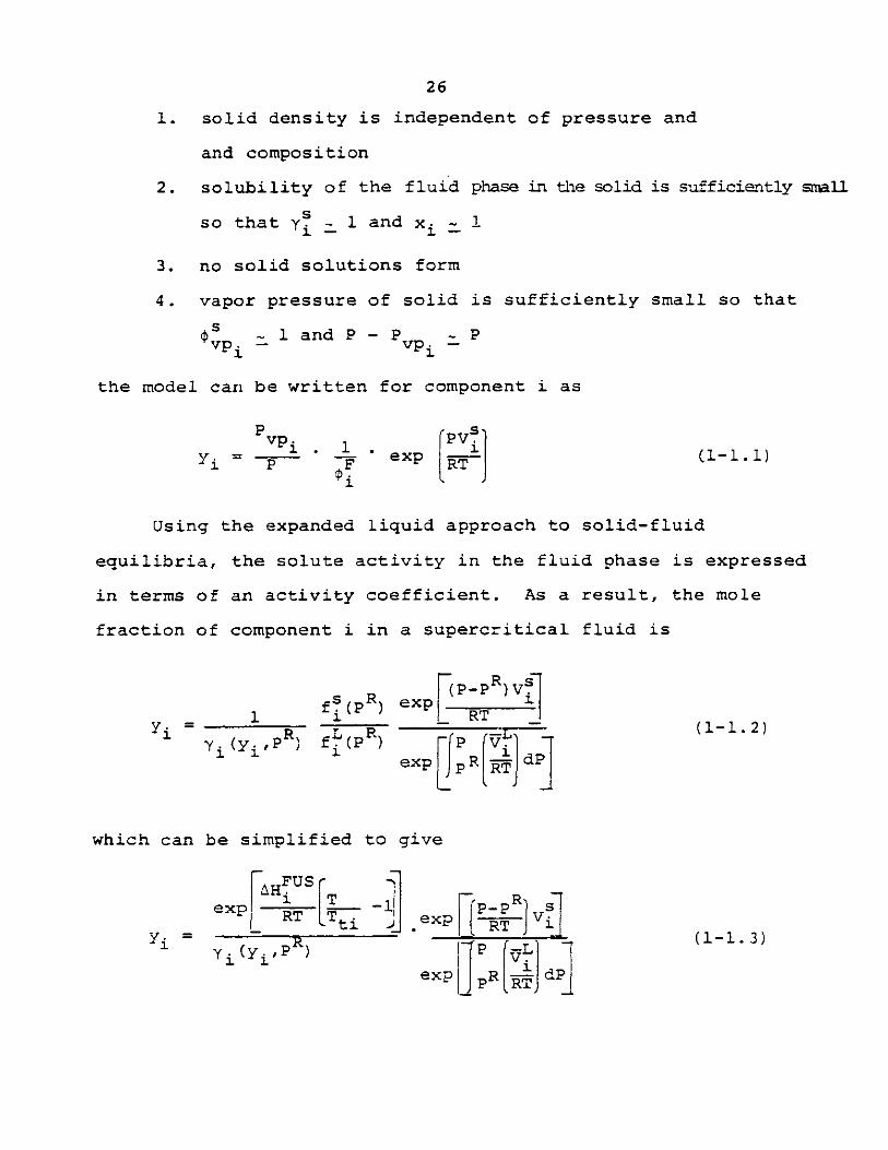
26
1. solid density is independent of pressure and
and composition
2. solubility of the fluid phase in the solid is sufficiently small
Sso that 1y and x. 1
3. no solid solutions form
4. vapor pressure of solid is sufficiently small so that
s ~l and P-P ~ Pvpi ~vpi
the model can be written for component i as
P -S.v .PV.
y =P F'exp (1-1.1)i
Using the expanded liquid approach to solid-fluid
equilibria, the solute activity in the fluid phase is expressed
in terms of an activity coefficient. As a result, the mole
fraction of component i in a supercritical fluid is
7R s(P-PR)V."
fS (PR) exp (= _iRT
R. = ~p~(1-1.2)Yi 'Y(i'"P )fi iR Pr
exp PR[RJ dP
which can be simplified to give
eR FUSp
IRT t % T J i
Y- = -t _T(1-1.3)
Y i ( Y ie x p P R d P
27
Mackay and Paulaitis (1979) have used a reference pressure of
RP = Pc,c
with P c the critical pressure of the pure fluid phase, and
the assumption that
Y(yPR (1-1.4)i. i- i c
.(yPR -(1-1.5)Si- i c
VT would then be found from an applicable equation of state
and y. would be treated as an adjustable parameter.
Of the two methods to model solid-fluid equilibria, the
first method (Equation 1-1.1) is preferred because it re-
quires only one adjustable parameter, k . (whereas Equation
1-1.3 requires two: k3. . and y" (PC) Also, it is much
easier to generalize Equation 1-1.1 to a multicomponent system
than it is to generalize Equation 1-1.3.
1-3 Thesis Objectives
The objectives of this thesis can be divided into three
parts: experimental, theoretical, and exploratory. Experi-
mentally, equilibrium solubility data for both polar and non-
polar solid solutes in supercritical fluids were to be
measured over wide ranges of temperature and pressure. In
addition, ternary equilibrium data (two solids, one fluid)
were to be measured. Carbon dioxide and ethylene were the
two supercritical fliuds to be used.
28
Theoretically, correlation of equilibrium solubility
data of both binary and multicomponent systems using rigorous
thermodynamics was to be done.
Finally, after obtaining equilibrium solubility data
and developing a thermodynamic model, it was desirable to use
this modelto explore the physics of solid-fluid equilibrium.
Using the model that was to be developed, such phenomena as
enthalpy changes of solvation of the solute in the supercrit-
ical solvent and changes in equilibrium solubility over wide
ranges of temperature and pressure were to be studied.
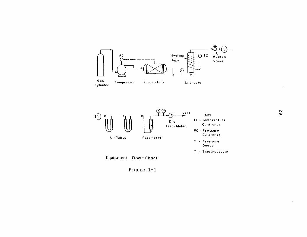
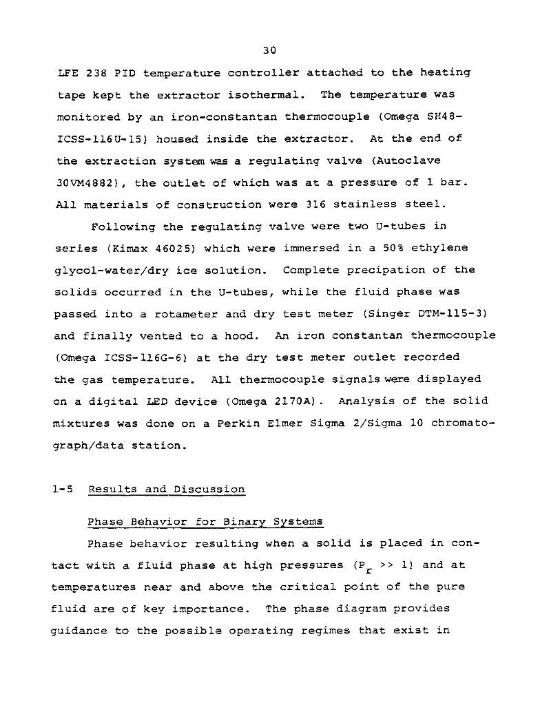
1-4 Experimental Apparatus and Procedure
The experimental method used in this thesis to measure
equilibrium solubilities was a one-pass flow through system.
A schematic is shown in Figure 1-1.
A gas cylinder was connected to an AMINCO line filter, (odel
49-14405) which feeds into an AMINCO single end compressor, (model
46-13411). The compressor was connected to a two liter magne-
drive packless autoclave (Autoclave Engineers) whose purpose
was to dampen the pressure fluctuations. In addition, an
on/off pressure control switch, Autoclave P481-P713 was used
to control the outlet pressure from the autoclave.
Upon leaving the autoclave, the fluid entered the
tubular extractor (Autoclave, CNLXl60121 which consisted of
a 30.5 cm tube, 1.75 cm in diameter. In the tube were alter-
nate layers of the solute species to be extracted and Pyrex
wool. The Pyrex wool was used to prevent entrainment. A
PC Heoig -01C Hua te0dlope I Valve
ELdDHetn lTICompressor Surge - lank Ex t r actor
Vent
DryTest - Meter
Rotometer
Key
TC - TemperotureCont roler
PC - Pressure
Cont roller
P - PressureGouge
I - lermocoople
Equipment Flow - Chort
Go sCy linder
U - lubes
Figure 1-1
30
LFE 238 PID temperature controller attached to the heating
tape kept the extractor isothermal. The temperature was
monitored by an iron-constantan thermocouple (Omega SH48-
ICSS-ll6U-15) housed inside the extractor. At the end of
the extraction system was a regulating valve (Autoclave
30VM4882), the outlet of which was at a pressure of 1 bar.
All materials of construction were 316 stainless steel.
Following the regulating valve were two U-tubes in
series (Kimax 46025) which were immersed in a 50% ethylene
glycol-water/dry ice solution. Complete precipation of the
solids occurred in the U-tubes, while the fluid phase was
passed into a rotameter and dry test meter (Singer DTM-ll5-3)
and finally vented to a hood. An iron constantan thermocouple
(Omega ICSS-l6G-6) at the dry test meter outlet recorded
the gas temperature. All thermocouple signals were displayed
on a digital LED device (Omega 2170A). Analysis of the solid
mixtures was done on a Perkin Elmer Sigma 2/Sigma 10 chromato-
graph/data station.
1-5 Results and Discussion
Phase Behavior for Binary Systems
Phase behavior resulting when a solid is placed in con-
tact with a fluid phase at high pressures (P r >> ) and at
temperatures near and above the critical point of the pure
fluid are of key importance. The phase diagram provides
guidance to the possible operating regimes that exist in
31
supercritical fluid extraction.
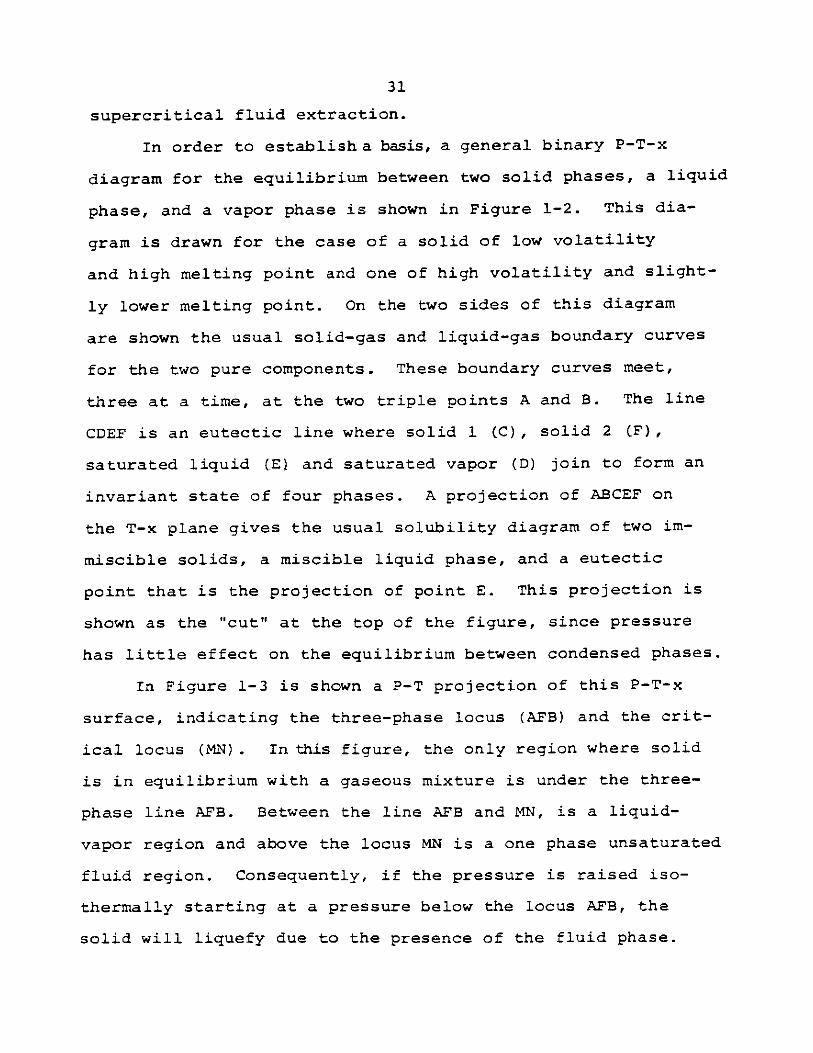
In order to establish a basis, a general binary P-T-x
diagram for the equilibrium between two solid phases, a liquid
phase, and a vapor phase is shown in Figure 1-2. This dia-
gram is drawn for the case of a solid of low volatility
and high melting point and one of high volatility and slight-
ly lower melting point. On the two sides of this diagram
are shown the usual solid-gas and liquid-gas boundary curves
for the two pure components. These boundary curves meet,
three at a time, at the two triple points A and B. The line
CDEF is an eutectic line where solid 1 CC), solid 2 (F),
saturated liquid (E) and saturated vapor (D) join to form an
invariant state of four phases. A projection of ABCEF on
the T-x plane gives the usual solubility diagram of two im-
miscible solids, a miscible liquid phase, and a eutectic
point that is the projection of point E. This projection is
shown as the "cut" at the top of the figure, since pressure
has little effect on the equilibrium between condensed phases.
In Figure 1-3 is shown a P-T projection of this P-T-x
surface, indicating the three-phase locus (AFB) and the crit-
ical locus (MN) . In this figure, the only region where solid
is in equilibrium with a gaseous mixture is under the three-
phase line AFB. Between the line AFB and MN, is a liquid-
vapor region and above the locus MN is a one phase unsaturated
fluid region. Consequently, if the pressure is raised iso-
thermally starting at a pressure below the locus AFB, the
solid will liquefy due to the presence of the fluid phase.

32
I- ________-
I II I
The Prcssure - Temperature - Composition Surfaces
for the Equilibrium Between Two Pura Solid
Phases, A Liquid Phase and a Vapor Phase
( Rowlinson and Richardson,1959 )
Figure 1-2
P
GH
ANI
B1~
Projaction of a System in Which thc
Thre2 Phase Linc Does Not Cut thc
Critical Locus
Figure 1-3
33
PN441
N
P-T
b
34
For some extractions, it is often desirable to keep the solute
a solid phase, and so Figure 1-3 is an undesirable situation.
Fortunately, Figure 1-3 in general, does not represent the
usual situation,as discussed below.
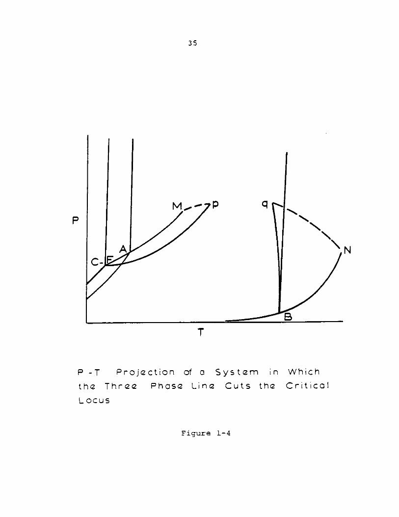
When a high molecular weight solid is in equilibirum
with a low molecular weight gas, the P-T projection that norm-
ally exists is as shown in Figure 1-4. Here, because the dif-
ferences in temperature between the triple points and criti-
cal points of these substances is large, the three phase line
AFB of Figure 1-3 can actually intersect the critical locus,
so as to "cut" it at two points: p- the lower critical end
point, and q- the upper critical end point. See Figure 1-4.
In this figure, M and N are the critical points of the super-
critical fluid and solid respectively. Critical end points
are mixture critical points in the presence of excess solid,
i.e., a liquid and gas of identical composition and proper-
ties in equilibrium with a solid.
The major consequence of a gap in the critical locus as
shown in Figure 1-4 is to allow at least a region in temper-
ature between T and T where one solid phase is in equlibrium
with one fluid phase with no liquid phase present.
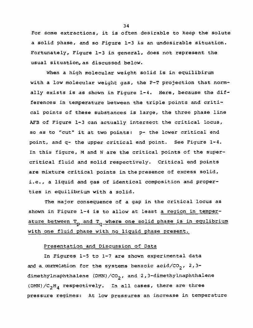
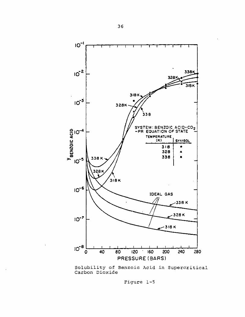
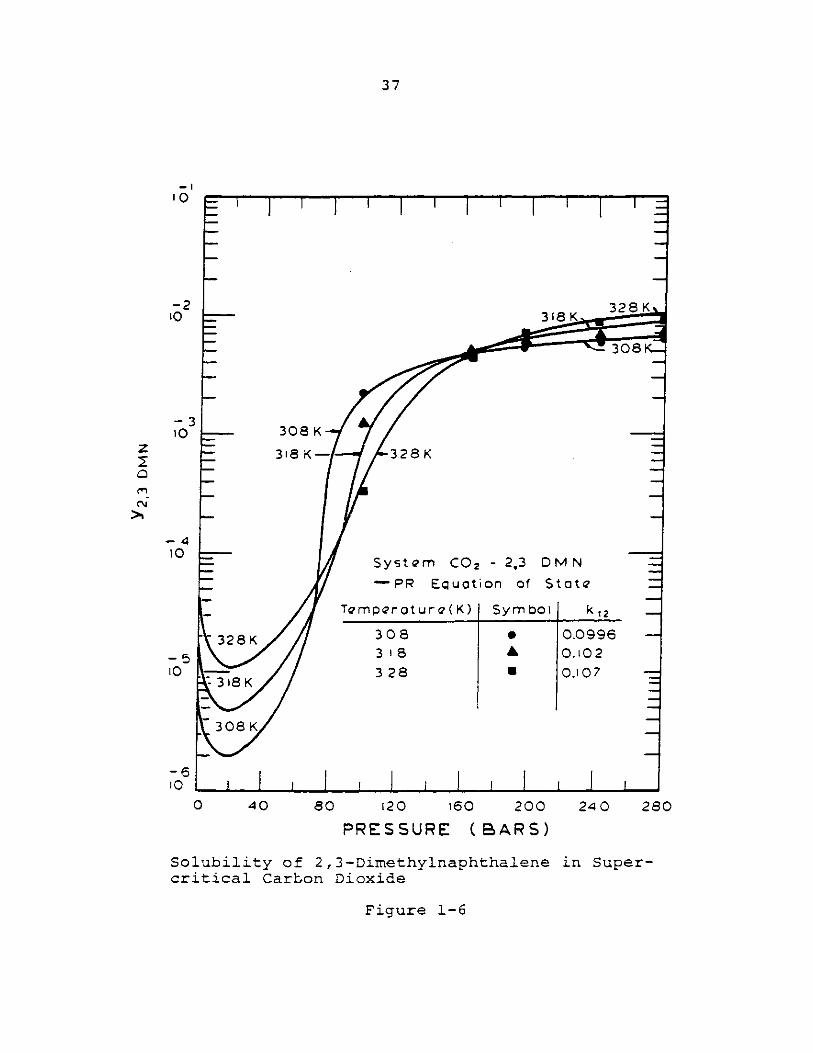
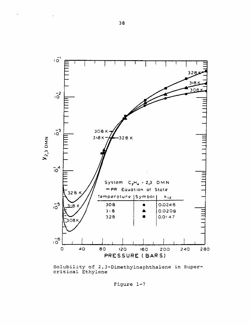
Presentation and Discussion of Data
In Figures 1-5 to 1-7 are shown experimental data
and acorrelation for the systems benzoic acid/CC2 , 2,3-
dimethylnaphthalene (DMN)/CO2 , and 2,3-dimethylnaphthalene
(DMN)/C2 H4 respectively. In all cases, there are three
pressure regimes: At low pressures an increase in temperature
35
AC-F.O
qN
NN
T
P -T Projection of a System in
the Three Phose Linc Outs th(2
Locus
Which
Critical
Figure 1-4
P
36
10 - ,- [ I I I I I
33810K 318K
318 K
10 ~ 328K
/ 338
SYSTEM: BENZOIC ACID-CO2a i~4 -- PR EQUATION OF STATE
rEMPERATURES(K) SYSOL
3182
328 a
10 5 -3 3
3283K
318 K10-
IDEAL GAS
a-,338 K
10-76- 3 28 K
-8 i 1 1 1 1 i t 1 1i 1 , -
0 40 80 120 160 200 240 280
PRESSURE (BARS)
Solubility of Benzoic Acid in SupercriticalCarbon Dioxide
Figure 1-5
37
-am I lI1
-2 32810 - 318 K
308
-. 310 - -- 30 8 K - -
z318 K- 328 K-
-4
10 SystOM C02- 2,3 DM N-- PR Equation of State.
Temper at ure (K) symbol k 12
328 K 30 08 .0996 -
_ g 3 IS O.t O210 .. 3 2 8 j.1 7-
-318 K-
308 K
10
0 40 80 120 160 20 0 24 0 280
PRESSURE ( BARS)
Solubili-ty of 2,3-Dimethylnaphthalene in Super-critical CarPon Dioxide
Ficure 1-6
38
1
328
318
30-2
10
-3 308K10--10318 K 32 8 K
S ys tem C2H4 -2,13 D M N
-2 K- PR Equa tion of Sto t4?
Temp4?rature Symbol k 12
105-21-8 K 308 0 .0246
3 t8 0 .0209
328 0 .0147308 K
-6t0
0 40 80 120 160 200 240 280
PRESSURE (BARS)
Solubility of 2,3-Dimethylnaphthalene in Super-critical Ethylene
Figure 1-7
39
increases solubility; at intermediate pressures, an increase
in temperature decreases solubility (retrograde solidifica-
tion) -- more apparent for carbon dioxide than ethylene; and
at high pressures an increase in temperature enhances slu-
bility. The reason the retrograde solidification region is
more significant for carbon dioxide than ethylene is because
CO2 is at a lower reduced temperature and therefore the den-
sity dependence on pressure is larger.
In all cases, the Peng-Robinson equation of state is able
to correlate the data well providing that the proper binary
interaction parameter is used. Although the binary parameters
were independent of pressure and composition, they have a weak
linear dependence on temperature.
The outstanding feature of all the data and simulations
is the extreme sensitivity of equilibrium solubility to temp-
erature and pressure. For example, consider Figure 1-5
(benzoic acid-carbon dioxide). There is about a two order of
magnitude change in solubility when decreasing pressure and
simultaneously increasing temperature from (318K, 180 bar)
to (338K, 90 bar). Also shown for convenience in Figure 1-5
is the solubility predicted by the ideal gas law:
ID P / y. = /PC1-5.l)i vp C"5.1
The ratio of real to ideal solubilities is called the en-
hancement factor and can take on values of 106 or larger.
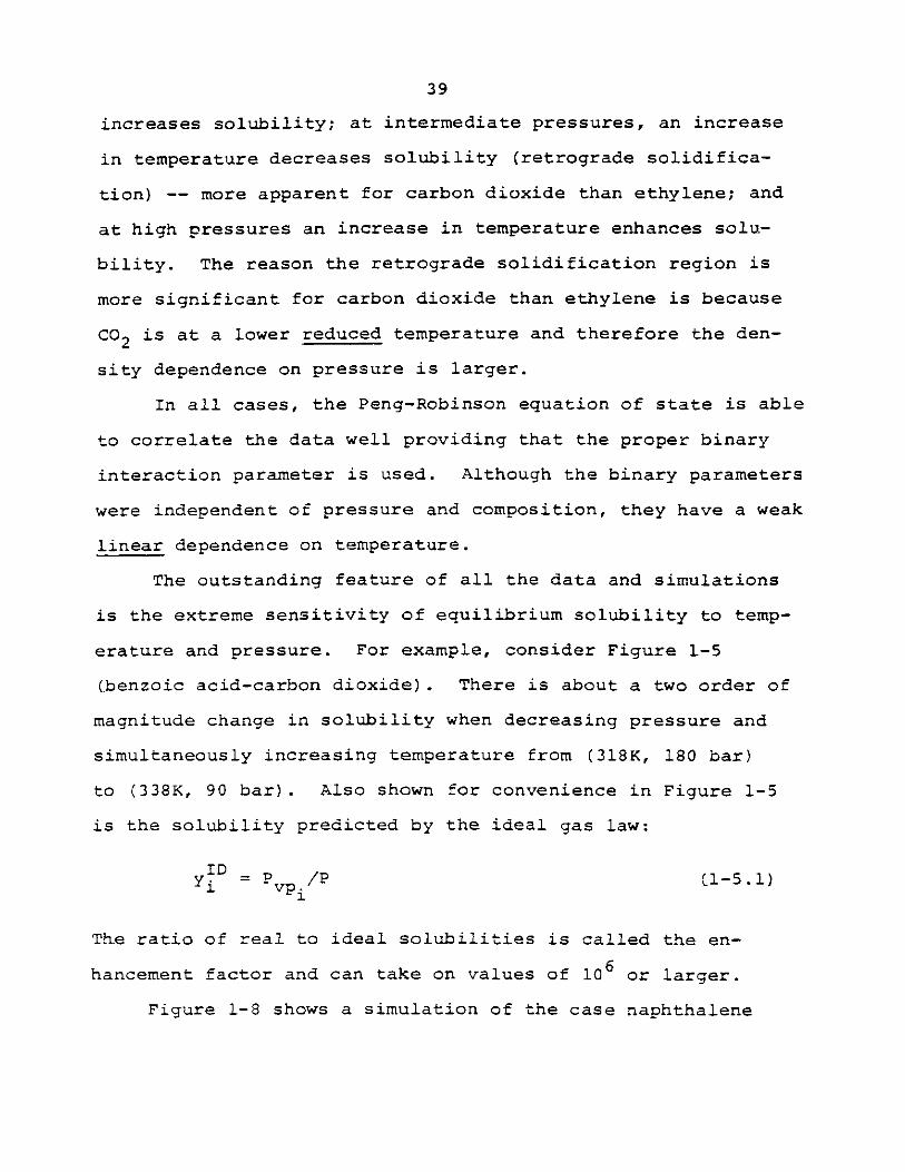
Figure 1-8 shows a simulation of the case naphthalene
40
,5210
-.310
10
10
0 40 80 120 160 200 240
PRESSURE ( BARS)
Solubility of Naphthalene in Supercritical
Figure 1-8
280
Nitrogen
System: Nitrogen - Nophthalone
-- PR Equation of State
k 12 =Q.1
- 328K
31 SK
-=MOK
LLid
zLid
41
in supercritical nitrogen. At no pressure does the isothermal
solubility of naphthalene even equal the solubility at one
bar pressure. The reason is because under these temperature
and pressure conditions, nitrogen is nearly an ideal gas with
fugacity coefficients and compressibility factors near unity.
Also, the density of nitrogen at high pressures is approxim-
ately 0.1 gm/cm3 as compared to 0.8 gm/cm3 for carbon dioxide
under the same conditions of temperature and pressure. The
dissolving power of supercritical fluids depends both on the
density Cthe higher the greater) and the nonideality (fugacity
coefficient) of the fluid phase.
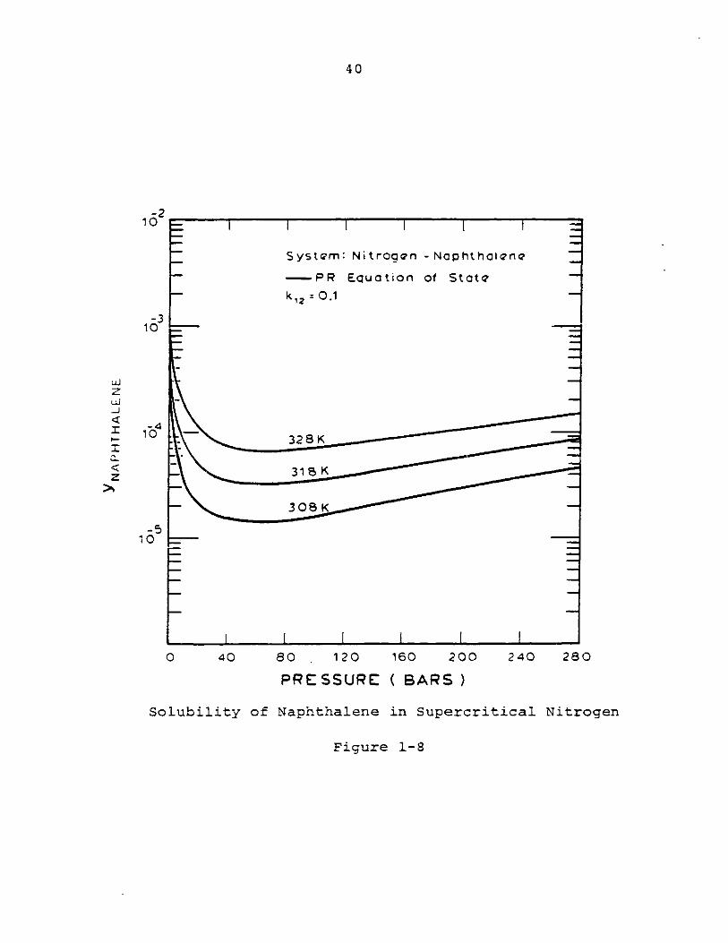
Ternary Solid-Fluid Equilibrium
As in the case of binary solId-fluid equilibrium, it is
useful to examine the P-T projection that results when two
solids that form a eutectic solution (not a solid solution)
are in equilibrium with a fluid phase. Such a P-T projection
of the four dimensional surface is shown in Figure 1-9. In
this diagram, K and K{ are the first and second lower criti-
cal-end points. These end points are the intersection with
the critical locus of the three-phase line formed by the solids
in equilibrium, with a liquid and a gas phase. Similarly,
K2 and K' are the first and second upper-critical end points.
In the case where no solid solutions form, there will exist
two eutectic points, and hence a four-phase line connecting
them. However, the four phase line may intersect the critical
locus at a lower double critical-end point and at a upper
I
K, p
KA/4K
/
q
K 2
K
,
L i
NN,
600
*1
P-T Projection of a Four Dimensionalin Equilibrium with a Fluid Phase
Surface of Two Solid Phases
Figure 1-9
P
N
43
double critical-endpoint -- shown as p and q respectively.
Only for temperatures between those corresponding to TP and
Tq , for any pressure, is one guaranteed that there are two
solid phases in equilibrium with a fluid phase with no liquid
phase forming.
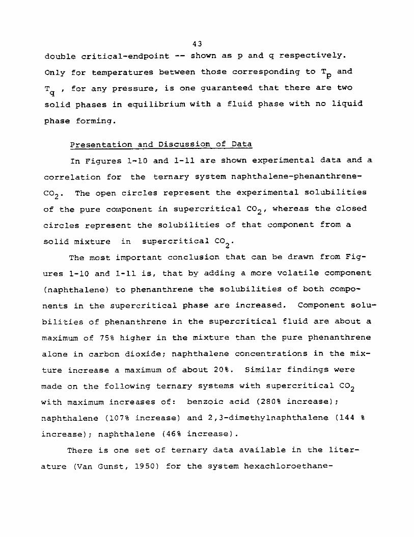
Presentation and Discussion of Data
In Figures 1-10 and 1-11 are shown experimental data and a
correlation for the ternary system naphthalene-phenanthrene-
co2. The open circles represent the experimental solubilities
of the pure component in supercritical CO2, whereas the closed
circles represent the solubilities of that component from a
solid mixture in supercritical CO2'
The most important conclusion that can be drawn from Fig-
ures 1-10 and 1-11 is, that by adding a more volatile component
(naphthalene) to phenanthrene the solubilities of both compo-
nents in the supercritical phase are increased. Component solu-
bilities of phenanthrene in the supercritical fluid are about a
maximum of 75% higher in the mixture than the pure phenanthrene
alone in carbon dioxide; naphthalene concentrations in the mix-
ture increase a maximum of about 20%. Similar findings were
made on the following ternary systems with supercritical CO2
with maximum increases of: benzoic acid (280% increase);
naphthalene (107% increase) and 2,3-dimethylnaphthalene (144 %
increase); naphthalene (46% increase).
There is one set of ternary data available in the liter-
ature (Van Gunst, 1950) for the system hexachloroethane-

44
..-10
C, 4 H1 o MIXTUREPR EQUATION
IQ-3
C14H IO PUR E, PR EQUA TION
10-4
10-5!
SYS TE M: C02-CIOHB -C14H 10() (2) (3)
TEMPER ATURE =308.2K0 PURE C(4Hjo IN C02
10-6. 0 MIXTURE C14 HIOIN CO2-- PR EQUAT"'ION OF STATE
k 20 .09w'59
k 13=0. 115
k23=0.05
10~7
I I) 40 80 120 160 200 240C0-
280
PRESSURE (BARS)
Solubility of Phenanthrene from a Phenanthrene-Naphthalene Mixture in Supercritical Carbon Dioxide
Figure 1-10
0r
0
45
10- -
Cio H8 MIXTURE, PR EQUATw1iu-N
10-2 ~CioH8 PURE, PR EQUATION
SYSTEM: CO 2-C 0 H8 -C 1 4 H1 O
(1) (2) (3)10-4
TEMPERATURE= 308.2K
0 PURE CfOH IN C 0 2 t* MIXTURE CIo H8 IN CO2
-- PR EQUATION OF STATE
k 12 =0.095910-5 k 13 =0.-11
k 2 3 =0.05
+DATA OF TSEKHANSKAYAet al. (1964)
0 40 80 120 160 200 240 280
PRESSURE (BARS)Solubility of Naphthalene from a Phenanthrene-Naphthalene Mixture in Supercritical Carbon Dioxide
Figure 1-11
46
naphthalene-ethylene. Both the naphthalene and hexachlor-
ethane solubilities increased by about 300% when they are
used in a binary solid system as compared to a pure solid
system.
For one case studied in this thesis, however, there was
a slight (10%) decrease in component solubilities in a
ternary mixture as compared to the binary system. This case
was the system phenanthrene; 2,3-DMN; CO2 .
In most experiments, the ternary data were well corre-
lated by the Peng-Robinson equation of state and Equation 1-1.
There are two solute-solvent interaction parameters that are
fixed from binary experiments and one solute-solute interac-
tion coefficient that must be introduced. The solute-solvent
interaction coefficients are those obtained by a nonlinear
regression from binary data. Only for the solute-solute inter-
action coefficient is ternary data required.
To check whether there was physical meaning in the
solute-solute parameter, the isomer system 2,3-DMN; 2,6-DMN
was examined in both supercritical carbon dioxide and ethyl-
ene. Correlation of the resultant data showed that k23 was
dependent on the supercritical fluid (component 1). Thus,
it can be concluded that k23 is an adjustable parameter --
not a true binary constant.
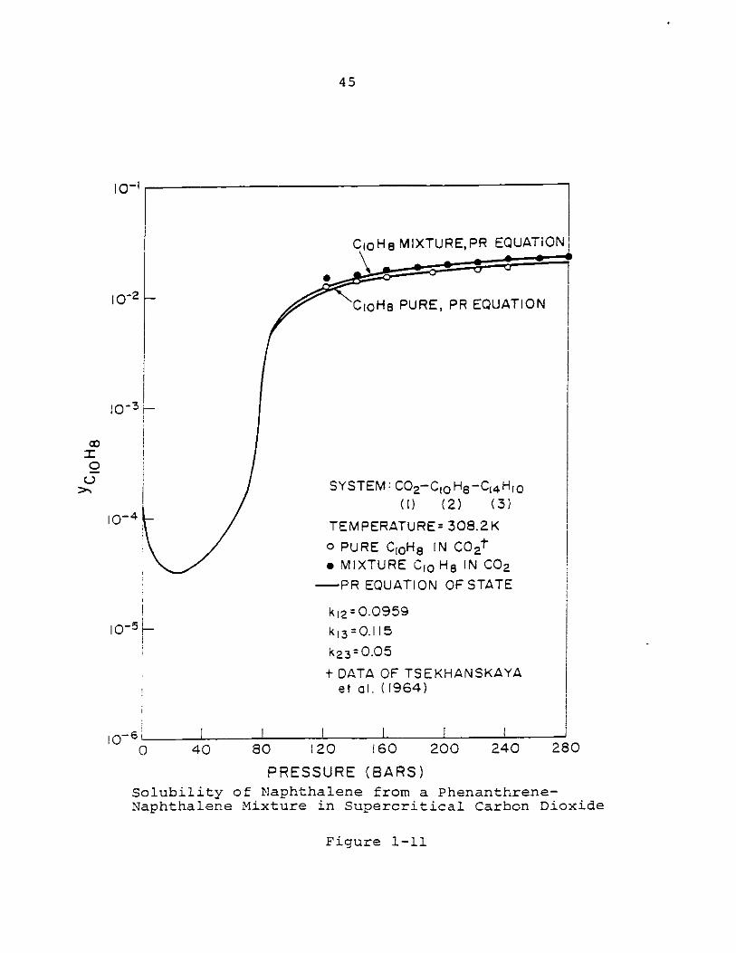
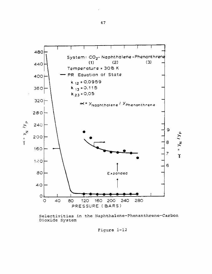
Selectivities in the naphthalene-phenanthrene-Co2
system are shown in Figure 1-12. At 1 bar, the selectivity
is the ratio of solute vapor pressures. Increasing the
system presure dramatically decreases the selectivity until
47
480-
440-
400.-
360-
320
280 -
240-
200
160 -
120-
80
40
01 I
-F- I I I I I I
System: C02- Naphthalene -Phenanthrenc(1) (2) (3) -
Temperature = 30B K
- PR Equation of State
k 12 = 0.0959
k 13 =0.1 15
k 2 3 = 0.05
0:< Naphtholene /Phenanthrane
0~
E xpcndcd
K w~9@9@9#T
90~
8 z
II
7
46
0 40 80 120 160 200 240 280PRESSURE (BARS)
Selectivities in the Naphthalene-Phenanthrene-CarbonDioxide System
Figure 1-12
a-
z
Ii
4
mmmmlmp
-M Aduk Admkk
48
it levels off at a nearly constant value just above the
solvent critical pressure. This type of selectivity curve
was found for all the ternary systems studied.
In conclusion, if in a given application, component
solubilities of a solid in a supercritical fluid are not large,
it may be possible to add to the original mixture a more
volatile solid component which causes substantial increases
in component solubilities of all species. Although this ef-
fect was shown only for solids in this thesis, it is believed
that volatile liquids (entrainers) can also be added to ac-
complish the same effect.
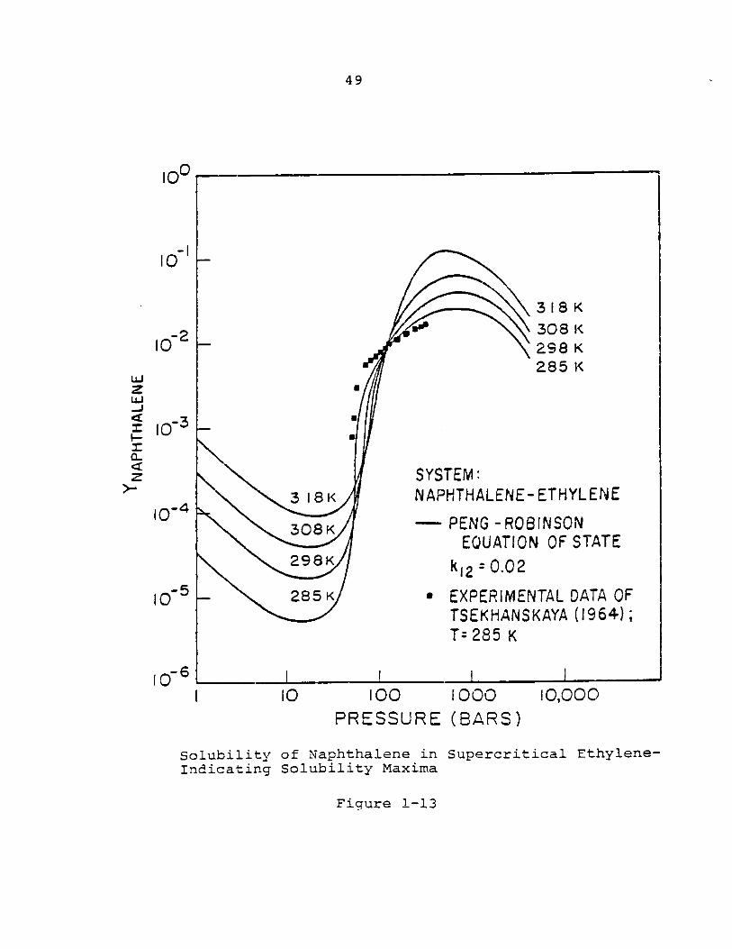
Solubility Maxima
Of the data and correlations shown in Figures 1-5 to 1-7,
the highest pressure attained was 280 bar. As these figures
indicate, the isothermal solubilities are still increasing
with pressure. It is interesting, therefore, to perform com-
puter simulations to very high pressures (Kurnik and
Reid, 1981). The results of such simulations are shown in
Figure 1-13 for the solubility of naphthalene in supercriti-
cal ethylene for pressures up to 4 kbar and for several temp-
eratures. Experimental data are shown only for the 285 K iso-
therm to indicate the range covered and the applicability of
the Peng-Robinson equation.
For the naphthalene-ethylene system, the solubility at-
tains a minimum value in the range of 15 to 20 bar and a
maximum at several hundred bar.
318K
308 Ka.8K285 K
SYSTEM:1K NAPHTHALENE-
308 K -- PENG - ROBEQUATION
29Kk, 2 .02
285 KEXPERIMENTSEKHANSIT: 285 K
ETHYLENE
INSONJ OF STATE
ITAL DATA OFKAYA (1964);
10 100
PRESSURE
Solubility of Naphthalene inIndicating Solubility Maxima
1000
(BARS)
Supercritical Ethylene-
Figure 1-13
49
to-I
z
C
z
-6
10,000I --- mmmwvmFvmwlm I I - I - F
I
50
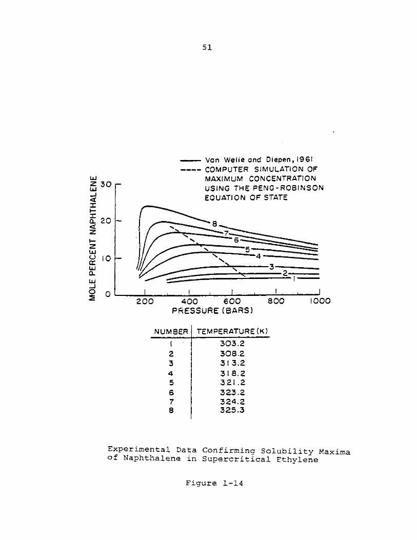
The existence of the concentration maxima for the
naphthalene-ethylene system is confirmed by considering the
earlier work of Van Welie and Diepen (1961). They also
graphed the mole fraction of naphthalene in ethylene as a
function of pressure and covered a range up to about I kbar.
Their smoothed data (as read from an enlargement of their
original graphs), are plotted in Figure 1-14. At temperatures
close to the upper critical end point (325.3 K), a maximum in
concentration is clearly evident. At lower temperatures, the
maximum is less obvious. The dashed curve in Figure 1-14
represents the results of calculating the concentration maxi-
mum from the Peng-Robinson equation of state. This simula-
tion could only be carried out to 322 K; above this tempera-
ture convergence becomes a problem as the second critical end
point is approached and the formation of two fluid phases is
predicted. Table 1-1 compares the theoretical versus experi-
mental maxima.
Concentration maxima have also been noted by Czubryt
et al. C1970) for the binary systems stearic acid-CO2 and
l-octadecanol-CO2 . In these cases, the experimental data
were all measured past the solubility maxima -- which for
both solutes occurred at a pressure of about 280 bar. An
approximate correlation of their data was achieved by a sol-
ubility parameter model.
Theoretical Development
The solubility minimum and maximum with pressure can be
51
-- Vn Welie and Diepen , 1961COMPUTER SIMULATION OF
WU MAXIMUM CONCENTRATIONZ 3Q USING THE PENG- ROBINSON
EQUATION OF STATE
a. 20
C 10 -C,LU / 3
200 400 600 800 1000PRESSURE (BARS)
NUMBER TEMPERATURECK)
1 -303.22 308.23 313.24 318.25 321.26 323.27 324.28 325.3
Experimental Data Confirming Solubility Maximaof Naphthalene in Supercritical Ethylene
Figure 1-14
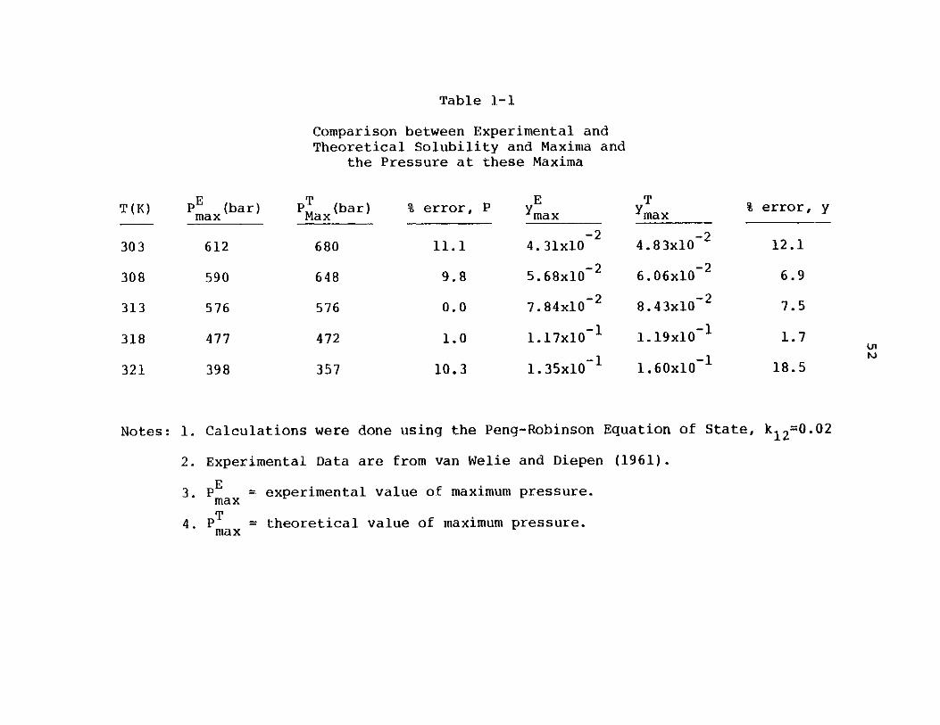
Table 1-1
Comparison between Experimental andTheoretical Solubility and Maxima and
the Pressure at these Maxima
E (bar)max
612
590
576
477
398
Pa (bar)max
680
648
576
472
357
% error, P
11.1
9.8
0.0
1.0
10.3
EYmax
-24. 31x10
5.68x10⁻²
7. 84x10-2
1.17x10 1
1. 35x10 1
TYmax
-24.83x10
6.06x10⁻²
8. 4 3x10⁻²
1. 19x10~
1. 60x10~ 1
% error, y
12.1
6.9
7.5
1.7
18.5
Notes: 1.
2.
3.
4.
Calculations were done using the Peng-Robinson Equation of State, k1 2=0.02
Experimental Data are from van Welie and Diepen (1961).
PE = experimental value of maximum pressure.max
P T = theoretical value of maximum pressure.max
T (K)
303
308
313
318
321
LnN~
53
related to the partial molar volume of the solute in the
supercritical phase. With subscript 1 representing the solute,
then with equilibrium between a pure solute and the solute
dissolved in the supercritical fluid,
dlnfj = dlnfs (1-5.2)
Expanding Eq. 1-5.2 at constant temperature and assuming that
no fluid dissolves in the solute,
~7F 3nF eSdP + nf1 dlny = dP (1-5.3)RT L alnyJ TP -RT
Using the definition of the fugacity coefficient,
F = F$ = f/y P (1-5.4)
Then Eq. 1-5.3 can be rearranged to give
31nylRT L T IT ~(1-5.5)T ln$
olnylT
may be expressed in terms of y1 , T, and P with an equation
of state (Kurnik et al., 1981). For naphthalene as the
solute in ethylene, (31nI/9lnyl)T,P was never less than -0.4
over a pressure range up to the 4 kbar limit studied. Thus
the extrema in concentration occur when V1s=
54
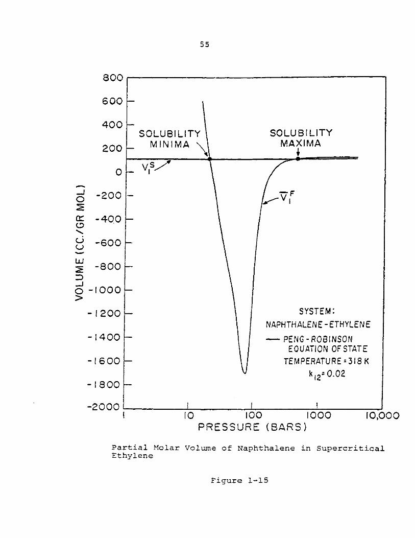
Again using the Peng-Robinson equation of state, 9I
for naphthalene is ethylene as a function of pressure and
temperature was computed. The 318 K isotherm is shown in
Figure 1-15. At low presures, V' is large and positive; it
would approach an ideal gas molar volume as P -+ 0. With an
increase in pressure, ~I decreases and becomes equal to V5
(111.9 cm3/mole) at a pressure of about 20 bar. This corres-
ponds to the solubility minimum. VY then becomes quite nega-1
tive. The minimum in 9' corresponds to the inflection point
in the concentration-pressure curve shown in Figure 1-13.
At high pressures, I'increases and eventually becomes equal
to VS; this then corresponds to the maximum in concentration
described earlier.
In conclusion, the existence of a solubility maximum
gives one a reference number that is useful to decide if a
certain extraction scheme is economical. Furthermore, if it
has been determined to perform a certain extraction, then it
can be quickly ascertained what the optimal extraction pressure
is.
1-6 Recommendations
The next research area for supercritical fluids should
be in the area of multicomponent liquid -- SCF extraction --
since most industrial separations are with liquids. Some
equilibrium data is available in the literature on bin-
ary liquid-fluid systems up to relatively low pressures (100
55
800
600
400
200
0
d -200
X -400
-600
;-800
o-1000
-1200,
-1400
-1600
-1800
-2000
SOLUBILITYMINIMA
SOLUBILITYMAXIMA
- Is
F
-F
NAPHTH
-- PEEC
TEA
10
Partial MolarEthylene
SYSTEM:
ALENE-ETHYLENE
NG - ROBINSON)UATION OF STATEMPERATURE=318 K
k 12=0.02
100 100PRESSURE (BARS)
10,000
Volume of Naphthalene in Supercritical
Figure 1-15
d1b,
=nowII
56
bar), but little is known about higher pressure solubilities
and selectivities in multicomponent systems.
A rewarding research program in this area would include
obtaining precise experimental data, correlating it with
thermodynamic theory, and evaluating the selectivities as a
function of temperature and pressure.
57
2. INTRODUCTION
2-1 Background
Supercritical fluid extraction can be considered to be
a unit operation akin to liquid extraction whereby a dense
gas is contacted with a solid or liquid mixture for the pur-
pose of separating components from the original mixture.
Advantages in using supercritical fluids over liquid extrac-
tion or distillation are many. Compared to distillation,
supercritical fluid extraction has shown to be more energy
efficient (Irani and Funk, 1977). The advantage of supercrit-
ical fluid extraction over liquid extraction is that
(1) solvent recovery is much easier (the pure supercritical
fluid can be obtained by expanding it to 1 bar pressure).
(2) Mon-toxic supercritical fluids can be used, such
carbon dioxide, to perform the extraction with solubilities
comparable to those by using liquid extraction. (3) Solu-
bility of the condensed phase in the supercritical fluid is
strongly controlled by the temperature and pressure of the
system, whereas in distillation and liquid extraction, the
major independent variable to control is only temperature.
Historically, the use of supercritical fluids dates back
to 1875 with the work of Andrews (1887). Although his work
was not published until after his death, Andrews was the true
pioneer in this field as a result of the data he obtained
58
on the system liquid carbon dioxide in supercritical nitrogen.
Shortly thereafter, Hannay and Hogarth (1879, 1880) found
that the solubility of the crystals I2, KBr, CoC 2 , and CaCl2
in supercritical ethanol were in considerable excess of that
predicted from the vapor pressure of the solute species and
the Poynting (1881) correction.
This increase in solubility of solids in the supercriti-
cal phase after the discovery of Andrews has led to many
studies, both experimental and theoretical, of solid fluid
equilibrium. In Table 2-1 there is shown a compilation of
available solid-fluid equilibrium data.
As is discussed in more detail in section 2-1, the phase
diagrams for solid-fluid equilibria are of great importance.
The reason for this is that there is only a selected temper-
ature interval where it is feasible to carry out supercritical
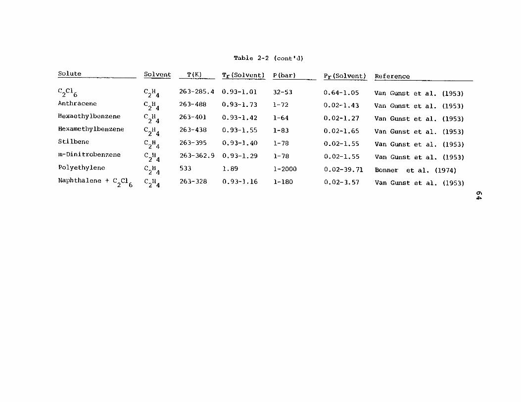
fluid extraction. For convenience, Table 2-2 provides a
compilation of all available solid-fluid equilibrium phase
projections.
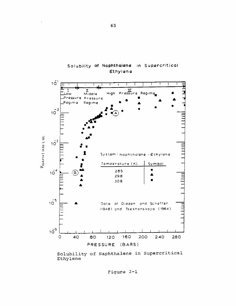
The basic features of supercritical fluid extraction
can be ascertained by studying the data of Diepan and
Scheffer (1948a, 1948b, 1953) and Tsekhanskaya (1964). They
measured the solubility of naphthalene in supercritical
ethylene over a wide range of temperatures and pressures.
Figure 2-1 shows a plot of their combined data. Many import-
ant trends can be observed. First, it is apparent that there
are three regimes of pressure. In the low pressure region,
an increase in temperature results in an increase in
-11,11,11,11,11flF
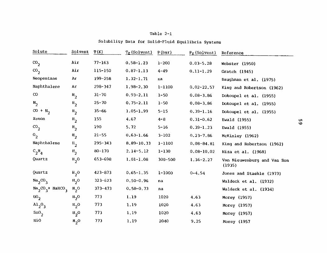
Table 2-1
Solubility Data for Solid-Fluid Equilibria Systems
Solute
CO2
Co2
Neopentane
Naphthalene
Co
N2
CO + N2Xenon
Co2
0 2Naphthalene
C2"4
Quartz
Quartz
Na 2CO3
Na CO3+ NaHCO3
UO2
Al2 03
SnO23
NiO
Solvent T (K)
Air
Air
Ar
Ar
112
H2
112
"2
2
H 0
2
"2
112 0
20
12011 2 0
11 2 0
Ho2
77-163
115-1,50
199-258
298-347
31-70
25-70
35-66
155
190
21-55
295-343
80-170
653-698
423-873
32 3-623
373-473
773
773
773
773
Tr (Solvent) P (bar) Pr (Solvent)
0.58-1.23
0.87-1.13
1.32-1.71
1.98-2.30
0.93-2.11
0.75-2.11
1.05-1.99
4.67
5.72
0.63-1.66
8.89-10.33
2.14-5.12
1.01-1.08
0.65-1.35
0.50-0.96
0.58-0.73
1.19
1.19
1.19
1.19
1-200
4-49
na
1-1100
1-50
1-50
5-15
4-8
5-16
3-102
1-1100
1-130
300-500
1-1000
na
na
1020
1020
1020
2040
0.03-5.28
0.11-1. 29
0.02-22. 57
0.08-3.86
0.08-3.86
0.39-1.16
0.31-0.62
0.39-1.23
0.23-7.86
0.08-84.81
0. 08-10.02
1.36-2.27
0-4.54
4.63
4.63
4.63
9.25
Reference
Webster (1950)
Gratch (1945)
Baughman et al. (1975)
King and Robertson (1962)
Dokoupel et al. (1955)
Dokoupel et al. (1955)
Dokoupel et al. (1955)
Ewald (1955)
Ewald (1955)
McKinley (1962)
King and Robertson (1962)
Hiza et al. (1968)
Van Nieuwenbur9 and Van Zon(1935)
Jones and Staehle (1973)
Waldeck et al. (1932)
Waldeck et al. (1934)
Morey (1957)
Morey (1957)
Morey (1957)
Morey (1957
uLk0
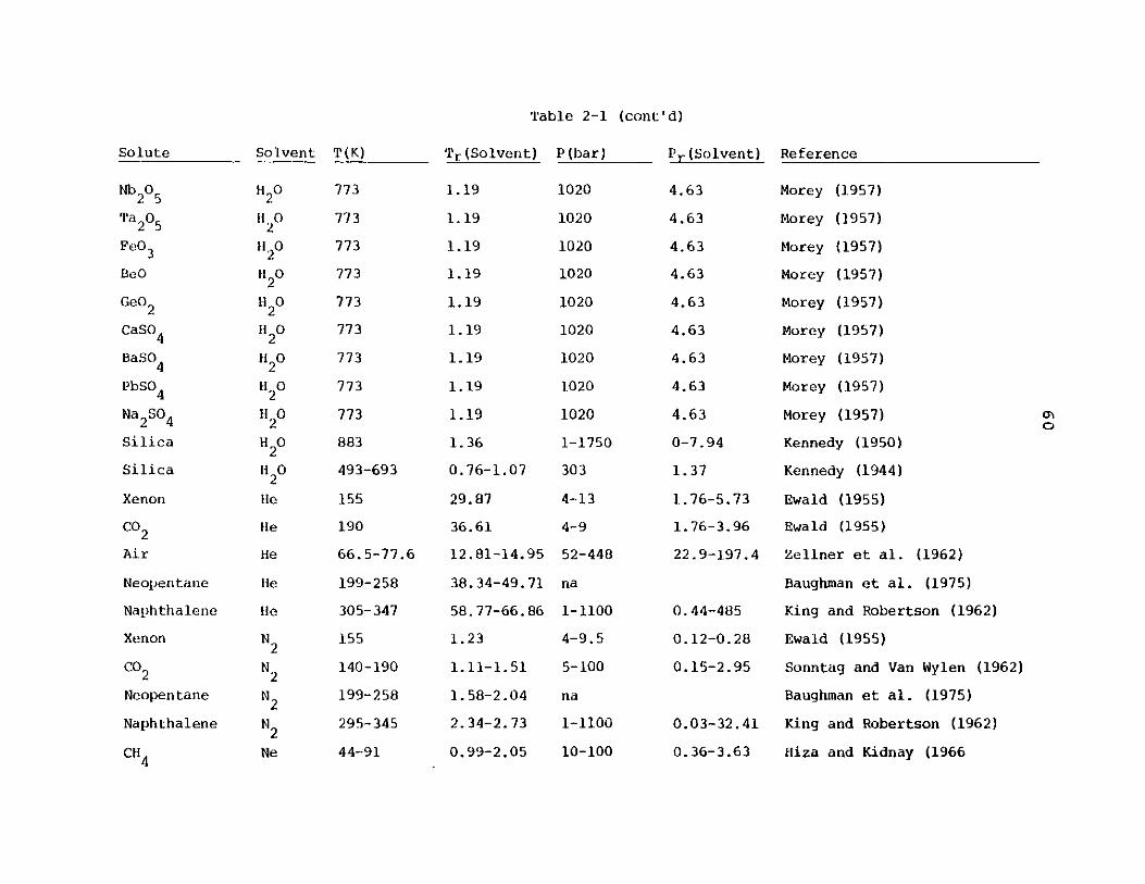
Table 2-1 (cont'd)
Solute
Nb2 05
Ta2 05
FeO3
BeO
GeO2
CaSO4
BaSO4
PbSO4
Na 2SO4
Silica
Silica
Xenon
CO2
Air
Neopentane
Naphthalene
Xenon
CO2
Neopentane
Naphthalene
CH 4
Solvent T(K)
H20H20
H20
I2 0
11 2 0H20
H20
H 20
I20
ii 0
If20
He 0
120
H 0H20
lie0
He
HeN2
lie
Ilie
N2
N2
N2
N 2
Ne
773
773
773
773
773
773
773
773
773
883
493-693
155
190
66.5-77.6
199-258
305-347
155
140-190
199-258
295-345
44-91
Tr (Solvent)
1.19
1.19
1.19
1.19
1.19
1.19
1.19
1.19
1.19
1.36
0.76-1.07
29.87
36.61
12.81-14.95
38.34-49.71
58.77-66.86
1.23
1.11-1.51
1.58-2.04
2.34-2.73
0.99-2.05
P (bar)
1020
1020
1020
1020
1020
1020
1020
1020
1020
1-1750
303
4-13
4-9
52-448
na
1-1100
4-9.5
5-100
na
1-1100
10-100
Pr (Solvent)
4.63
4.63
4.63
4.63
4.63
4.63
4.63
4.63
4.63
0-7.94
1.37
1.76-5.73
1.76-3.96
22.9-197.4
0.44-485
0.12-0.28
0.15-2.95
0.03-32.41
0.36-3.63
Re ference
Morey (1957)
Morey (1957)
Morey (1957)
Morey (1957)
Morey (1957)
Morey (1957)
Morey (1957)
Morey (1957)
Morey (1957)
Kennedy (1950)
Kennedy (1944)
Ewald (1955)
Ewald (1955)
Zellner et al. (1962)
Baughman et al. (1975)
King and Robertson (1962)
Ewald (1955)
Sonntag and Van Wylen (1962)
Baughman et al. (1975)
King and Robertson (1962)
fliza and Kidnay (1966
a'0
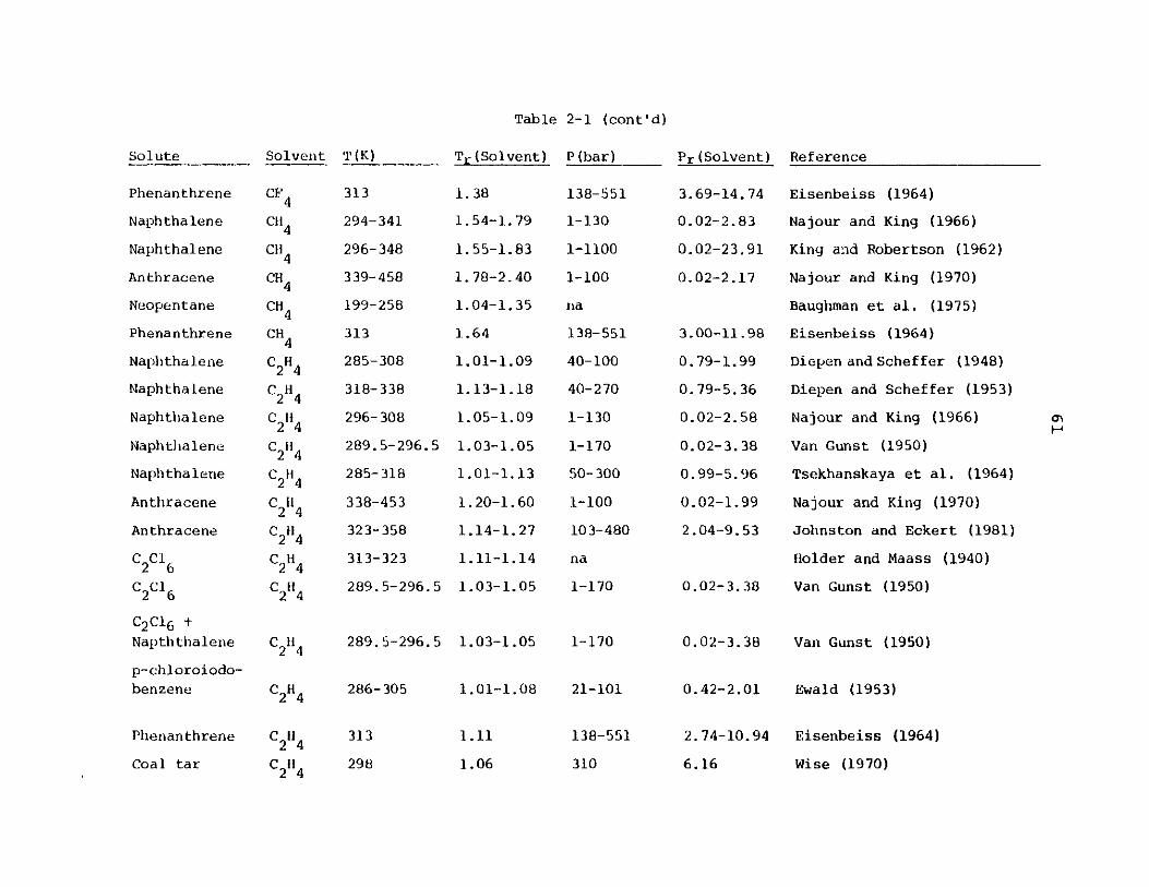
Table 2-1 (cont'd)
Solute
Phenanthrene
Naphthalene
Naphthalene
An thracene
Neopentane
Phenanthrene
Naphtha le ne
Naphtha lene
Naphthalene
Naphthalene
Naphthalene
Anthracene
Anthracene
C 2 C16c 2 ci6
C2 C16+Napththalene
p-chloroiodo-benzene
Phenanthrene
Coal tar
Solvent T(K)
CF4
C' 4
CH'4
Cl 4
CR4CH
C2 4CH 4
C H2 4
C 2 14C2 4
C 2 H4
C 2 l4C2 4
c2 42 4
c2 4
C2 4
C 2Hic214
313
294-341
296-348
339-458
199-258
313
285-308
318-338
296-308
289.5-296.5
285-318
338-453
323-358
313-323
289.5-296.5
289.5-296.5
286-305
313
298
Tr (Solvent)
1.38
1.54-1.79
1.55-1.83
1.78-2.40
1.04-1.35
1.64
1.01-1.09
1.13-1.18
1.05-1.09
1.03-1.05
1.01-1.13
1.20-1.60
1.14-1.27
1.11-1.14
1.03-1.05
1.03-1.05
1.01-1.08
1.11
1.06
P (bar)
138-551
1-130
1-1100
1-100
na
138-551
40-100
40-270
1-130
1-170
50-300
1-100
103-480
na
1-170
1-170
21-101
138-551
310
Pr (Solvent)
3.69-14. 74
0.02-2.83
0.02-23.91
0.02-2.17
3.00-11.98
0. 79-1. 99
0.79-5.36
0.02-2.58
0.02-3.38
0.99-5.96
0.02-1.99
2.04-9.53
0.02-3.38
0.02-3.38
0.42-2.01
2.74-10.94
6.16
Reference
Eisenbeiss (1964)
Najour and King (1966)
King and Robertson (1962)
Najour and King (1970)
Baughman et al. (1975)
Eisenbeiss (1964)
Diepen and Schef f er (1948)
Diepen and Scheffer (1953)
Najour and King (1966)
Van Gunst (1950)
Tsekhanskaya et al. (1964)
Najour and King (1970)
Johnston and Eckert (1981)
Holder and Maass (1940)
Van Gunst (1950)
Van Gunst (1950)
Ewald (1953)
Eisenbeiss (1964)
Wise (1970)
a'
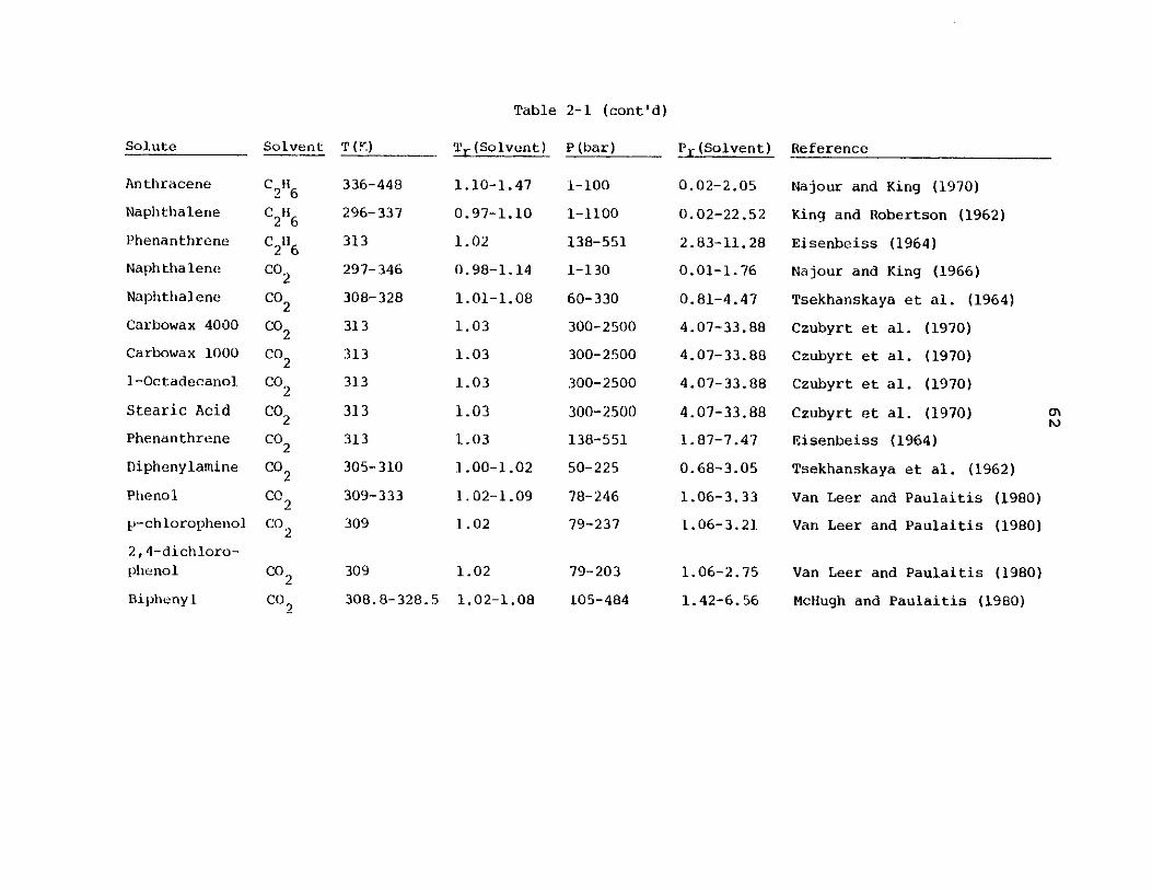
Table 2-1 (cont'd)
Solute Solvent T (f)
Anthracene
Naphthalene
Phenanthre ne
Naph tha lene
Naphthalene
Carbowax 4000
Carbowax 1000
1-Octadecanol
Stearic Acid
Phenanthrene
Diphenylamine
Phenol
p-chlorophenol
2, 4-dichloro-phenol
Bipheny l
26
C2 U
C2 6
CO26
Co2
Co2
Co 2
co2
CO2
Co2
Co2
Co2
CO2
CO2
co 2
336-448
296-337
313
297-346
308-328
313
313
313
313
313
305-310
309- 333
309
309
308.8-328.5
T (Solvent)
1.10-1.47
0.97-1.10
1.02
0.98-1.14
1.01-1.08
1.03
1.03
1.03
1.03
1.03
1.00-1.02
1 .02-1.09
1.02
1.02
1. 02-1. 08
P (bar) r T (Solvent)
1-100
1-1100
138-551
1-130
60-330
300-2500
300-2500
300-2500
300-2500
138-551
50-225
78-246
79-237
79-203
105-484
0.02-2.05
0.02-22.52
2.83-11.28
0.01-1.76
0.81-4.47
4.07-33.88
4.07-33.88
4.07-33.88
4.07-33.88
1.87-7.47
0.68-3.05
1.06-3.33
1.06-3.21
1.06-2.75
1. 42-6. 56
Reference
Najour and King (1970)
King and Robertson (1962)
Eisenbeiss (1964)
Najour and King (1966)
Tsekhanskaya et al. (1964)
Czubyrt et al. (1970)
Czubyrt et al. (1970)
Czubyrt et al. (1970)
Czubyrt et al. (1970)
Eisenbeiss (1964)
Tsekhanskaya et al. (1962)
Van Leer and Paulaitis (1980)
Van Leer and Paulaitis (1980)
Van Leer and Paulaitis (1980)
McHugh and Paulaitis (1980)
03
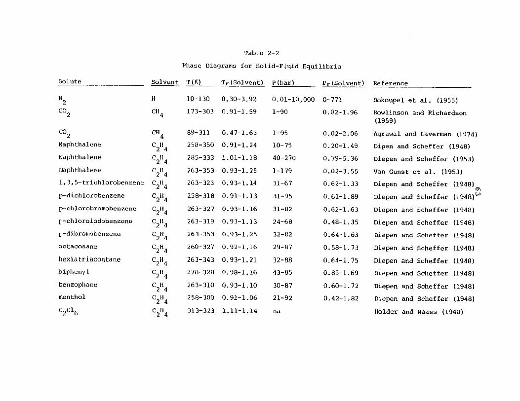
Table 2-2
Phase Diagrams for Solid-Fluid Equilibria
Solute Solvent T(K)
N2
Co2
H
C11 4
Co2
Naphthalene
Naphthalene
Naphthalene
1, 3, 5-trichlorobenzene
p-dichlorobenzene
p-ch lorobromoben ze ne
p-chloroiodobenzene
p-dibromobenzene
octacosane
hexiatriacontane
biphenyl
benzophone
menthol
CH 4
C2 4
c 2 14
C 2 i4
C 2 14
C 2 i4
c 2 14
c 2 i4
C 2 14
C 2 H4
c 2 H4
C2 4
C2 4c2 4
10-130
173-303
89- 311
258-350
285-333
263-353
263- 323
258-318
263-327
263-319
263-353
260-327
263-343
278-328
263-310
258-300
Tr (Solvent) P (bar)
0.30-3.92
0.91-1.59
0. 47-1. 63
0.91-1.24
1.01-1.18
0.93-1.25
0.93-1.14
0.91-1.13
0.93-1.16
0.93-1.13
0.93-1.25
0.92-1.16
0.93-1.21
0.98-1.16
0.93-1.10
0.91-1.06
0.01-10,000
1-90
1-95
10-75
40-270
1-179
31-67
31-95
31-82
24-68
32-82
29-87
32-88
43-85
30-87
21-92
Pr (Solvent)
0-771
0.02-1.96
0.02-2.06
0.20-1.49
0.79-5.36
0.02-3.55
0.62-1.33
0.61-1.89
0.62-1.63
0.48-1.35
0.64-1.63
0.58-1.73
0.64-1.75
0.85-1.69
0.60-1.72
0.42-1.82
Reference
Dokoupel et al. (1955)
Rowlinson and Richardson
(1959)
Agrawal and Laverman (1974)
Dipen and Scheffer (1948)
Diepen and Scheffer (1953)
Van Gunst et al. (1953)
Diepen
Diepen
Diepen
Diepen
Diepen
Diepen
Diepen
Diepen
Diepen
Diepen
and
and
and
and
and
and
and
and
and
and
Scheffer
Scheffer
Scheffer
Scheffer
Scheffer
Scheffer
Scheffer
Scheffer
Scheffer
Scheffer
(1948)
(1948)C
(1948)
(1948)
(1948)
(1948)
(1948)
(1948)
(1948)(1948)
C2 C 6C2 4 313-323 1.11-1.14 na Holder and Maass (1940)
Solute
c2 6Anthracene
Ilexaethylbenzene
Hexamethylbenzene
Stilbene
in-Dinitrobenzene
Polyethylene
Naphthalene + C2C16
Table 2-2 (cont'd)
Solvent T(K) Tr(Solvent) P(bar) Pr(Solvent) Reference
C2H
C2 4
2 4c2 4
C2 4C2
4
2H4C 2L1Ic2 4
263-285.4
263-488
263-401
263-438
263-395
263-362.9
533
263-328
0.93-1.01
0.93-1.73
0.93-1.42
0.93-1.55
0.93-1.40
0.93-1.29
1.89
0.93-1.16
32-53
1-72
1-64
1-83
1-78
1-78
1-2000
1-180
0.64-1.05
0.02-1.43
0.02-1.27
0.02-1.65
0.02-1.55
0.02-1.55
0.02-39.71
0.02-3.57
Van Gunst et al. (1953)
Van Gunst et al. (1953)
Van Gunst et al. (1953)
Van Gunst et al. (1953)
Van Gunst et al. (1953)
Van Gunst et al. (1953)
Bonner et al. (1974)
Van Gunst et al. (1953)
a'&6
High Pressure Ragame.
aU
SA
0
m
A0
65
Solubility of Naphthalene in Supercritical
Ethylene
MiddleP r assurRegime
-
I
04.0
0 .
Sa"
08OU
A
cData of DeP3n ona Scaffar
(1948) and Tsa khc ns kcyc (1964)
I I - -
Systam : Naphtholana - Ethylene
Timcpratur ( K) Symbol
285298308
0
0 40 80 120 160 200 240 280
PRESSURE (BARS)
Solubility of Naphthalene in SupercriticalEthylene
Figure 2-1
101
-
2
10
_Low.-Prassurz_R g M C
I
z
C
2.K
-310
-410
10
10
A
66
solubility; in the middle pressure regime, an increase in
temperature results in a decrease in solubility, and finally
in the high pressure regime, an increase in temperature re-
sults in an increase in solubility. It is also apparent that
the solubility covers a wide range in magnitude -- about 104.
By operating an extraction process, say at point A, one can
achieve the extract in pure form by changing the process
conditions to point B. Going from point A to point B results
in a two-order magnitude change in solubility for a small
increase in temperature and simultaneous decrease in pressure.
This, in short, is the significant feature of supercritical
fluid extraction.
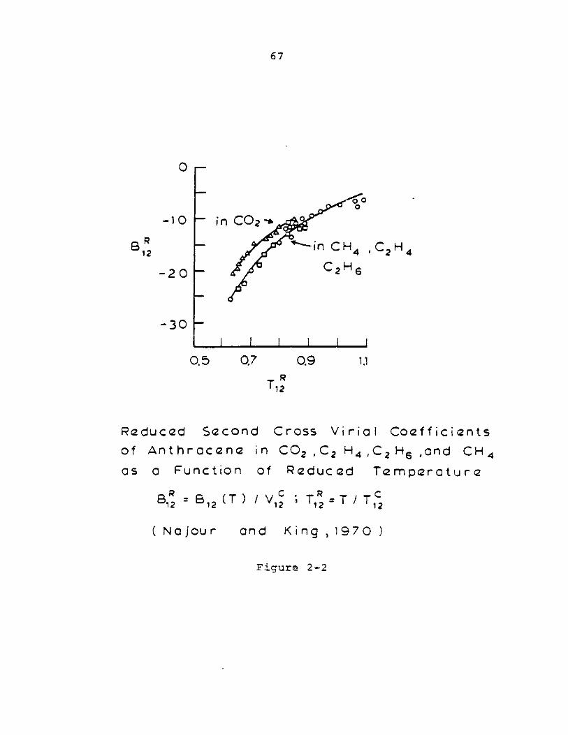
Second Interaction Virial Coefficients
Several investigators (Baughman et al., 1975; Najour and
King; 1970, 1966; and King and Robertson, 1962) have calcu-
lated second interaction virial coefficients for solid-fluid
equilibria systems. The virial equation of state is appli-
cable to systems where the gas phase density is less than
about one-half of the critical density of the gas phase. The
study of Najour and King (1970) is typical of all the investi-
gations performed and so their work will be discussed in more
detail. They examined the sys.tem solid anthracene or solid
phenanthrene in the supercritical fluids methane, ethylene,
ethane, and carbon dioxide. Figure 2-2 shows the result of
their calculations in the form of the reduced virial coeffi-
H Hcient B2* versus reduced mixture temperature TR 2 **. The data
67
0
-10
R R12
-20
-30
I
-i Cn H 4-
_ C2H6
0.7 0.9 1.1R
Reduced Second Cross Vi rio I Coefficiants
of Anthraccna in C02 ,C2 H 4 ,C2 H 6 ,and CH 4
as a Function of Reduced F2mpcraturz
6 R = 1(7)/V ;T1i2 B12 ( 12 I 12 =T/T1
( Najour and King , 1970 )
Figure 2-2
==mad
.5
68
for all four gases, except for carbon dioxide coincide on a
smooth curve. If, however, calculations are done to correct
the pure component critical temperature and critical volume
of carbon dioxide to those values that would exist without
the quadrupolar moment, then the carbon dioxide data can be
made to coincide with the other gases (Najour and King, 1970).
Also, it is interesting to note that Najour and King found
the reduced second interaction virial coefficients of
phenanthrene to be identical to those of anthracene.
Applications of Supercritical Fluid Extraction
Food Industry
One of the most active research areas in supercritical
fluid extraction is in the decaffination of coffee. Processes
are described in a review article by Zosel (1978) and in two
patents: a British patent granted to the German Company
Hag Aktiengesellschaft (1974) and a German patent granted to
Vitzthum and Hubert (1975). Basically, coffee is decaffin-
ated by contracting moist green coffee beans before roasting
with supercritical carbon dioxide. In a wet, unroasted
coffee bean it is caffeine that has the highest vapor pressure
of all substances present and is therefore selectively ex-
tracted by the carbon dioxide. In a similar manner, a
R C C I C 1/3+ C) 1 / 3
12 B1 2 (T1/V 2 , where V1 2 T + 2
TR C C C C1/212 = 12 ' where T 2 1 2
69
caffeine-free black tea can also be produced (Hag
Aktiengesellschaft, 1973).
Other food. related applications of supercritical fluid
extraction are removing of fats and oils from vegetables,
obtaining spice extracts, producing cocoa butter, and hop
extracts. These four applications are covered under the
patents of the German company Hag Aktiengesellschaft C1974b,
1973b, 1974c, 1975) respectively. The major reason for the
great interest in using supercritical carbon dioxide in the
food industry is due to the non-toxic properties of carbon
dioxide. Most other methods of purifying foods rely on using
organic solvents such as dichloromethane (Hubert and Vitzhum,
1978) which may pose toxicological problems.
Some food applications, however, rely on liquid carbon
dioxide CLCO2 ) for extraction. For example, Schultz et al.
(1967a, 1967b, 1970a, 1970b). Schultz and Randall (1970),
and Randall et al. C1971) have studied the extraction of
aromas and fruit juices from concord grapes, applies, oranges,
and pineapples. The major emphasis of these studies was to
find out the key chemical constituents which comprise the
flavor of a given species. For instance, although concord
grapes have over 100 chemical species, only one constituent;
methyl anthranilate is principally responsible for its
characteristic aroma. One reason to use LCO2 extraction
versus SCF extraction with carbon dioxide is that the selec-
tivity is improved at the lower temperatures of LCO2 Cat the
cost of lower solubilities), (Sims, 1979), see also Chapter4-2.
70
Non-Food Industry
Other applications of supercritical fluid extraction
industry are as follows. It has been suggested that a good
way to remove nicotine from tobacco is by the use of super-
critical carbon dioxide extraction (Hubert and Vitzthum,
1978; Hag Aktiengesellschaft, 1974). Desalination of sea
water by supercritical C1 1 and C1 2 paraffinic fractions has
been successfully accomplished (Barton and Fenske, 1970;
Texaco, 1967). Other uses include de-asphalting of petroleum
fractions using a supercritical propane/propylene mixture
(.Zhuze, 1960), extraction of lanolin from wool fat (Peter
et al., 1974), and recovery of purified oil from waste gear
oil (Studiengesellschaft Kohle M.B.H., 1967). Holm (1959)
discusses the use of supercritical carbon dioxide (T = 311 K,
P = 180 bar) as a scavenging fluid in tertiary oil recovery.
The SCF carbon dioxide aids in displacing the oils from the
pores of the reservoir rocks. Some of these applications
are also discussed in the review articles by Paul and Wise
(.19 71) , Wilke (1978), Irani and Funk (1977) , and Gangoli and
Thodos (1977).
Application to Coal
Supercritical extraction of coal is under study by at
least two industrial concerns. In England, the National Coal
Board (NCB) has done extensive work on de-ashing coal CBartle
et al., 1975), with supercritical toluene and supercritical
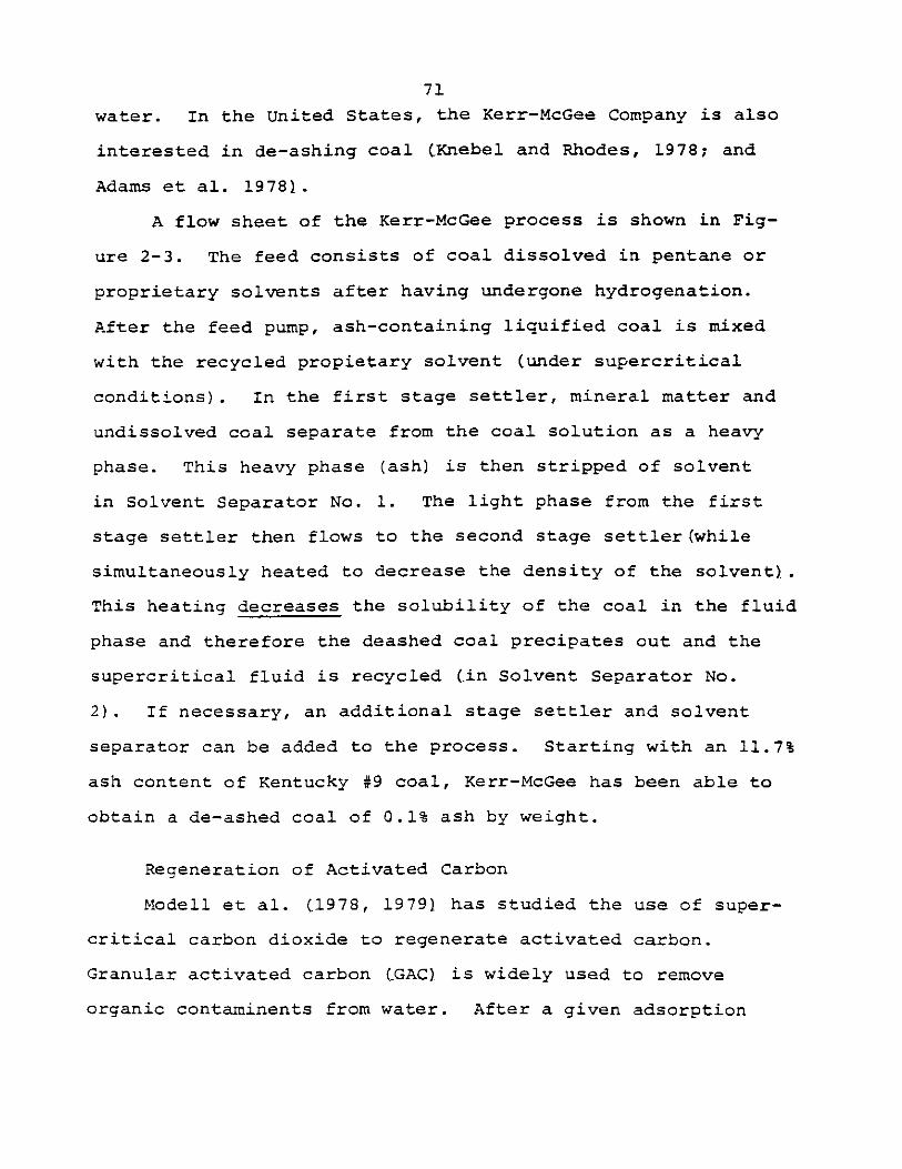
71
water. In the United States, the Kerr-McGee Company is also
interested in de-ashing coal CKnebel and Rhodes, 1978; and
Adams et al. 19781.
A flow sheet of the Kerr-McGee process is shown in Fig-
ure 2-3. The feed consists of coal dissolved in pentane or
proprietary solvents after having undergone hydrogenation.
After the feed pump, ash-containing liquified coal is mixed
with the recycled propietary solvent (under supercritical
conditions). In the first stage settler, mineral matter and
undissolved coal separate from the coal solution as a heavy
phase. This heavy phase (ash) is then stripped of solvent
in Solvent Separator No. 1. The light phase from the first
stage settler then flows to the second stage settler(while
simultaneously heated to decrease the density of the solvent).
This heating decreases the solubility of the coal in the fluid
phase and therefore the deashed coal precipates out and the
supercritical fluid is recycled tin Solvent Separator No.
2). If necessary, an additional stage settler and solvent
separator can be added to the process. Starting with an 11.7%
ash content of Kentucky #9 coal, Kerr-McGee has been able to
obtain a de-ashed coal of 0.1% ash by weight.
Regeneration of Activated Carbon
Modell et al. (1978, 1979) has studied the use of super-
critical carbon dioxide to regenerate activated carbon.
Granular activated carbon CGAC) is widely used to remove
organic contaminents from water. After a given adsorption
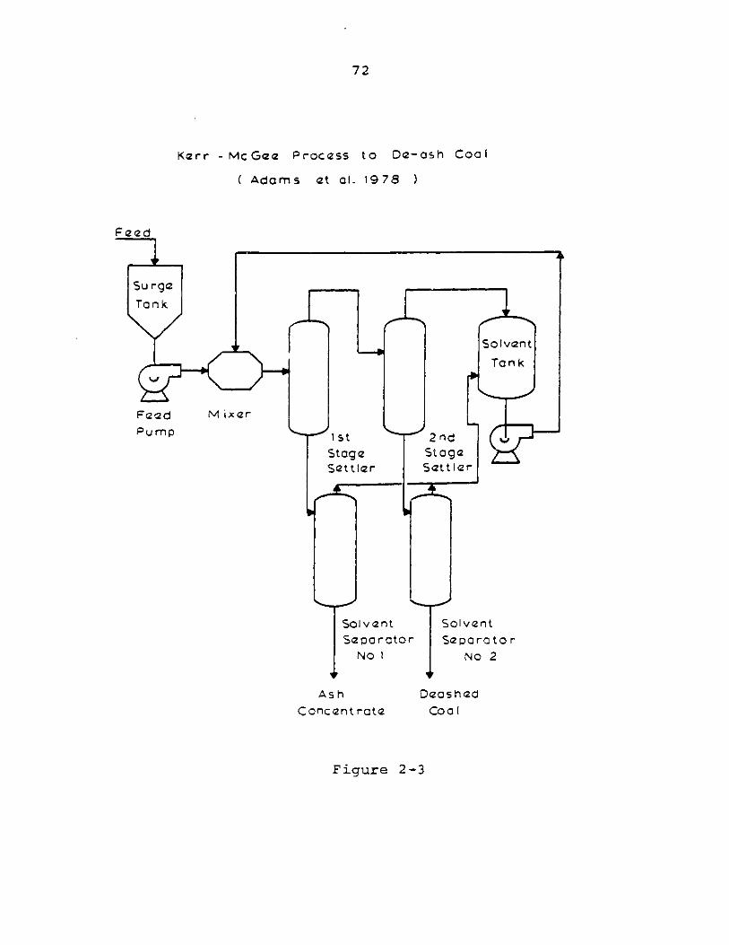
72
Karr - McGee Process to De-osh Cool
Adams et al. 1978
Fee d
Su rgaT nk
SOVontTank
F Q cd M ixer
Pump 21st 2 nd
Stag a StagaSat tler Sat t I ar
Sol v(2n t Solvent
Se parator Seporoto rNo I No 2
Ash DeoshedConcentrate Cool
Figure 2-3
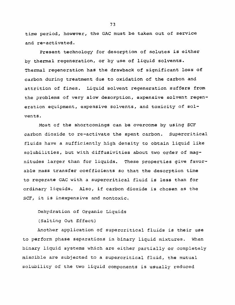
73
time period, however, the GAC must be taken out of service
and re-activated.
Present technology for desorption of solutes is either
by thermal regeneration, or by use of liquid solvents.
Thermal regeneration has the drawback of significant loss of
carbon during treatment due to oxidation of the carbon and
attrition of fines. Liquid solvent regeneration suffers from
the problems of very slow desorption, expensive solvent regen-
eration equipment, expensive solvents, and toxicity of sol-
vents.
Most of the shortcomings can be overcome by using SCF
carbon dioxide to re-activate the spent carbon. Supercritical
fluids have a sufficiently high density to obtain liquid like
solubilities, but with diffusivities about two order of mag-
nitudes larger than for liquids. These properties give favor-
able mass transfer coefficients so that the desorption time
to regerate GAC with a supercritical fluid is less than for
ordinary liquids. Also, if carbon dioxide is chosen as the
SCF, it is inexpensive and nontoxic.
Dehydration of Organic Liquids
(Salting Out Effect)
Another application of supercritical fluids is their use
to perform phase separations in binary liquid mixtures. When
binary liquid systems which are either partially or completely
miscible are subjected to a supercritical fluid, the mutual
solubility of the two liquid components is usually reduced
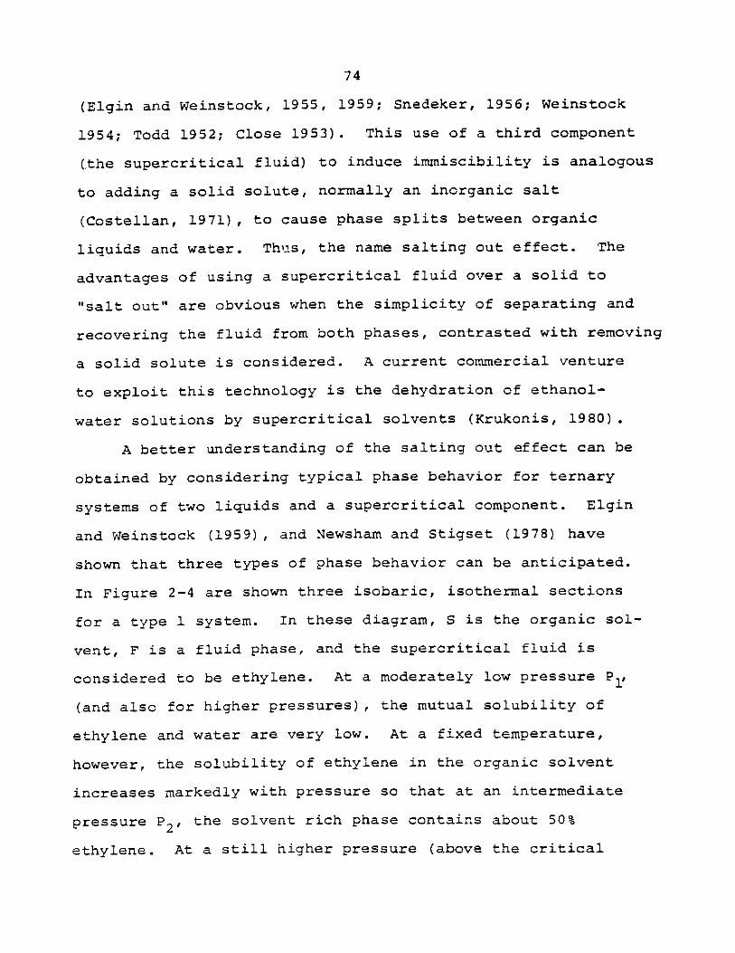
74
(Elgin and Weinstock, 1955, 1959; Snedeker, 1956; Weinstock
1954; Todd 1952; Close 1953). This use of a third component
(.the supercritical fluid) to induce immiscibility is analogous
to adding a solid solute, normally an inorganic salt
(Costellan, 1971), to cause phase splits between organic
liquids and water. Thus, the name salting out effect. The
advantages of using a supercritical fluid over a solid to
"salt out" are obvious when the simplicity of separating and
recovering the fluid from both phases, contrasted with removing
a solid solute is considered. A current commercial venture
to exploit this technology is the dehydration of ethanol-
water solutions by supercritical solvents (Krukonis, 1980).
A better understanding of the salting out effect can be
obtained by considering typical phase behavior for ternary
systems of two liquids and a supercritical component. Elgin
and Weinstock (1959), and Newsham and Stigset (1978) have
shown that three types of phase behavior can be anticipated.
In Figure 2-4 are shown three isobaric, isothermal sections
for a type 1 system. In these diagram, S is the organic sol-
vent, F is a fluid phase, and the supercritical fluid is
considered to be ethylene. At a moderately low pressure P1 ,
(and also for higher pressures), the mutual solubility of
ethylene and water are very low. At a fixed temperature,
however, the solubility of ethylene in the organic solvent
increases markedly with pressure so that at an intermediate
pressure P2 ' the solvent rich phase contains about 50%
ethylene. At a still higher pressure (above the critical
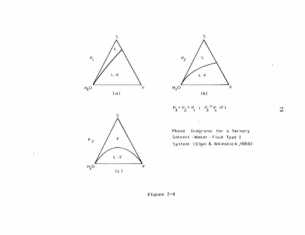
S
L
P
L-V
(a)
S
p 3 F
L -F
2
p >p >p P p P>P (F)3 2 1 3 c
Phose Diagroms or a oTernary
Solvent -Woter - Fluid Type I
Sys tem ([Elgin & Wainst oc k ,1959)
F
Figure 2-4
S
P2L
L -V
H20 F H 20
(b)
F
-4
(c )
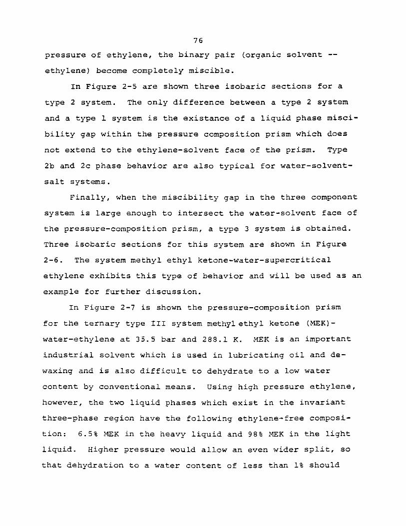
76
pressure of ethylene, the binary pair (organic solvent --
ethylene) become completely miscible.
In Figure 2-5 are shown three isobaric sections for a
type 2 system. The only difference between a type 2 system
and a type 1 system is the existance of a liquid phase misci-
bility gap within the pressure composition prism which does
not extend to the ethylene-solvent face of the prism. Type
2b and 2c phase behavior are also typical for water-solvent-
salt systems.
Finally, when the miscibility gap in the three component
system is large enough to intersect the water-solvent face of
the pressure-composition prism, a type 3 system is obtained.
Three isobaric sections for this system are shown in Figure
2-6. The system methyl ethyl ketone-water-supercritical
ethylene exhibits this type of behavior and will be used as an
example for further discussion.
In Figure 2-7 is shown the pressure-composition prism
for the ternary type III system methylethyl ketone (MEK)-
water-ethylene at 35.5 bar and 288.1 K. MEK is an important
industrial solvent which is used in lubricating oil and de-
waxing and is also difficult to dehydrate to a low water
content by conventional means. Using high pressure ethylene,
however, the two liquid phases which exist in the invariant
three-phase region have the following ethylene-free composi-
tion: 6.5% MEK in the heavy liquid and 98% MEK in the light
liquid. Higher pressure would allow an even wider split, so
that dehydration to a water content of less than 1% should
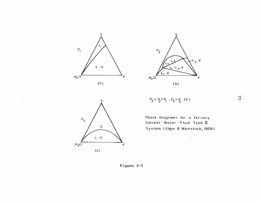
S
L
L -v
H2 0O
(a)
s
P3
F
L - F
H20
F
S
P2
2 L2~
LL -L 2-V
L, -VH 20 F
(b)
P3 > P2>FPj ;P >IP (F)3 2 1 3 c (F)
Phase Diogrom5 for a Ternory
Solvent - Woter - Fluid Type II
System ( Elgin & Weinstock, 1959)
F
Figure 2-5
(c)
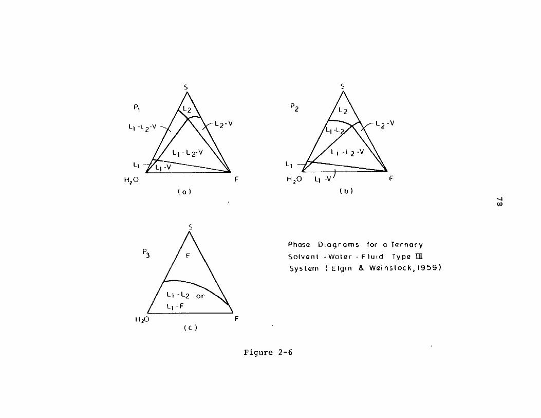
S
Pi L2
L, -L 2 -V L 2 -V
L1 -L2-V
L1 . L1-V
H20 F
S
3 F
Ll -L 2 or-F
H 20 F(c )
S
P2 L 2
L1 -L L2 -V
L1I -L 2 -V
H20 L1 -V F
(b)
00
Phose Diagroms for a Ternory
Solvent -Wotar - Fluid Type IR
System ( Elgin & WeInstock, 1959)
Figure 2-6
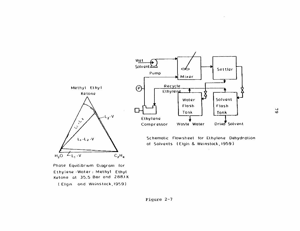
Methyl EthylKetone
L2- v
L, -L2 -V
H-20 - L, - v C2H4
Phose Equilibrium Diogrom for
Ethylene -Woter - Methyl EthylKetone at 35.5 BOr and 288.1K
( Elgin ond Wainstock.1959)
SolvmWntp--+
Pump------- +MixA Qr
P Rec ycleE thyle
Wot er Solvent
Fla sh Flosh
Tank Tank
E thy lene
Com pr essor Was te Water Dried SOIVent
Schematic Flowsheet for Ethylene Dehydrotionof Solvents (Elgin & Wei nstock,.1959 )
U,
Figure 2-7
80
be relatively easy to accomplish. A possible flowsheet for
a dehydration facility for MEK is shown in Figure 2-7.
The phase behavior for two liquid components and a super-
critical component can be modelled with standard thermodyn-
amics (Balder and Prausnitz, 1966). Using a two suffix
Margules equation for liquid phase activity coefficients,
they have been able to obtain qualitative agreement for the
seven systems studied by Elgin and Weinstock (1959). More
theoretical work, however, needs to be done in this interest-
ing area using more accurate models for the activities of the
liquid phase and the fugacity of the fluid phase.
Supercritical Fluid Chromatography
Another application of supercritical fluid extraction that
has developed is the use of supercritical fluids in chromato-
graphy. While no commercial equipment is yet available in
this area, several investigators (Sie et al., 1966; van Wasen,
et al., 1980; Klesper, 1978) have fabricated their own equip-
ment. Major problems of the design of these chromatographs
lie with the design of the detectors and the operation of a
system capable of injecting a small sample into a column at
pressures up to 300 bar.
The basic concept lying behind SCF chromatography is that
if a supercritical fluid is used as the mobile phase, then
by operating at sufficiently high pressures, the capacity
ratioCSTATSTATA
k. i (2-1.1)I CMB MOB
81
where CSTAT and CMOB are the concentrations of component i
in the stationary (stat) and mobile (mob) phase and VSTAT
and VMOB are the total volume of the stationary and mobile
phase in the column, will undergo a significant decrease with
increasing pressure. Whereas in gas chromatographyonly
temperature has a significant role in determining the capacity
ratio, in SCF chromatography, temperature and now, most signi-
ficantly pressure, has a great effect on the capacity ratio.
As a result, lower temperatures can be used so that high
molecular weight thermodegradeable biological materials as
complex as DNA may now be separated in SFC. Also, ionic
species (Jentoft and Gouw, 1972) which would decompose in gas
chromatography can be solubilized in a SCF and thus are amend-
able to supercritical chromatography.
The operating conditions where SFC will have its poten-
tial application is shown in Figure 2-8 in the form of a
reduced pressure, reduced density plot. Table 2-3 lists a
series of possible mobile phases for SFC. The "proper"
supercritical phase to choose is one whose critical tempera-
ture is close to, but slightly below the desired temperature
of operation.
An example application of SFC is in the resolution of
oligomers. For instance, stryene oligomers of nominal mole-
cular weight, NM = 2200 were separated into more than 30
fractions (Klesper and Hartmann, 1978) using a supercritical
phase of 95% n-pentane and 5% methanol.
Finally, SFC can be used to obtain thermodynamic
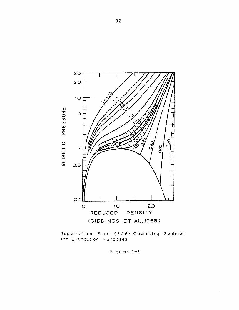
82
1.oREDUCED
(GIDDINGS
2.0D EN"S IT Y
ET AL,1968)
SupercrIcal Fluid ( SCF) Operating Regimesfor Extraction Purposes
Figure 2-8
30
20
10
5
1
0.5
LuD
LUc-C.
uQnLUJ
-2
Cr
NL
0.10
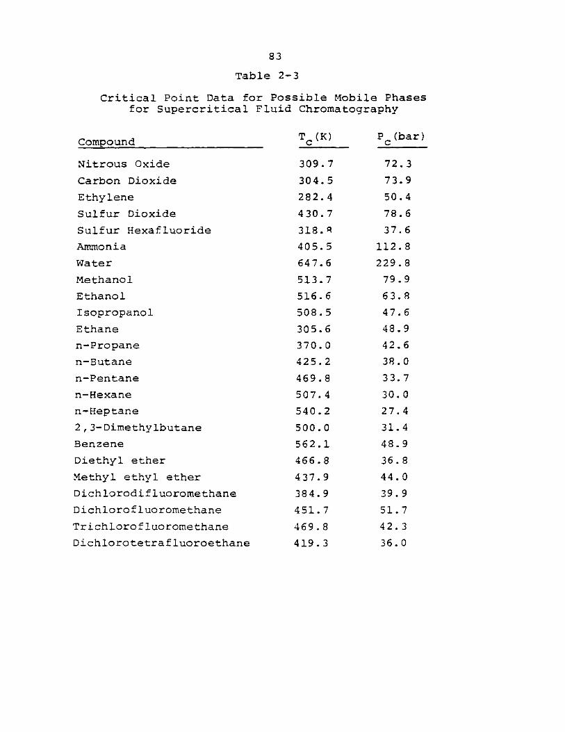
83
Table 2-3
Critical Point Data for Possible Mobile Phasesfor Supercritical Fluid Chromatography
Compound c c(bar)
Nitrous Oxide 309.7 72.3
Carbon Dioxide 304.5 73.9
Ethylene 282.4 50.4
Sulfur Dioxide 430.7 78.6
Sulfur Hexafluoride 318.R 37.6
Ammonia 405.5 112.8
Water 647.6 229.8
Methanol 513.7 79.9
Ethanol 516.6 63.8
Isopropanol 508.5 47.6
Ethane 305.6 48.9
n-Propane 370.0 42.6
n-Butane 425.2 38.0
n-Pentane 469.8 33.7
n-Hexane 507.4 30.0
n-Heptane 540.2 27.4
2,3-Dimethylbutane 500.0 31.4
Benzene 562.1 48.9
Diethyl ether 466.8 36.8
Methyl ethyl ether 437.9 44.0
Dichlorodifluoromethane 384.9 39.9
Dichlorofluoromethane 451.7 51.7
Trichlorofluoromethane 469.8 42.3
Dichlorotetrafluoroethane 419.3 36.0
84
properties for the materials being used as the supercritical
phase. van Wasen et al. (1980) and Bartmann and Schneider
(1973) describe the proper data reduction to obtain partial
molar volumes at infinite dilution, interaction second vivial
coefficients, and diffusion coefficients.
Rules of Thumb as to What can be Extracted
Stahl et al. (1980) presents some "rules of thumb" as to
what can be extracted into SCF carbon dioxide at 313 K. These
rules were obtained by performing qualitative studies on many
types of solid constituents.
1. Hydrocarbons and other typically lipophilic organic
compounds of relatively low polarity, e.g., esters,
lactones and epoxides can be extracted in the
pressure range 70-100 bar.
2. The introduction of strongly polar functional groups
(e.g. -OH, -COOH) makes the extraction more difficult.
In the range of benzene derivatives, substances with
three phenolic hydroxyls are still capable of extrac-
tion, as are compounds with one carboxyl and two
hydroxyl groups. Substances in this range that
cannot be extracted are those with one carboxyl and
three or more hydroxyl groups.
3. More strongly polar substances, e.g. sugars and amino
acids, cannot be extracted with pressures up to 400
bar.
85
2-2 Phase Diagrams
Binary Phase Behavior for Similar Components at Low
Pressures
Phase behavior resulting when a solid is placed in con-
tact with a fluid phase at temperatures near and above the
critical point of the pure fluid are of key importance. The
phase diagram provides guidance to possible operating regimes
that exist in supercritical fluid extraction.
In order to establish a basis, a general binary P-T-x
diagram for the equilibrium between two solid phases, a
liquid phase, and a vapor phase is shown in Figure 2-9. This
diagram is drawn for the case of a substance of low volatil-
ity and high melting point and one of high volatility and
slightly lower melting point. On the two sides of the dia-
gram are shown the usual solid-gas, solid-liquid, and liquid-
gas boundary curves for the two pure components. These bound-
ary curves meet, three at a time, at the two triple points A
and B. The line CDEF is an eutectic line where solid 1(C),
solid 2(F), saturated liquid (E), and saturated vapor (D) join
to form an invariant state of four phases. A projection of
ABCEF on the T-x plane gives the usual solubility diagram of
two immiscible solids, a miscible liquid phase, and a eutectic
point that is the projection of point E. This projection is
shown as the "cut" at the top of the figure, since pressure
has little effect on the equilibrium between condensed
phases.
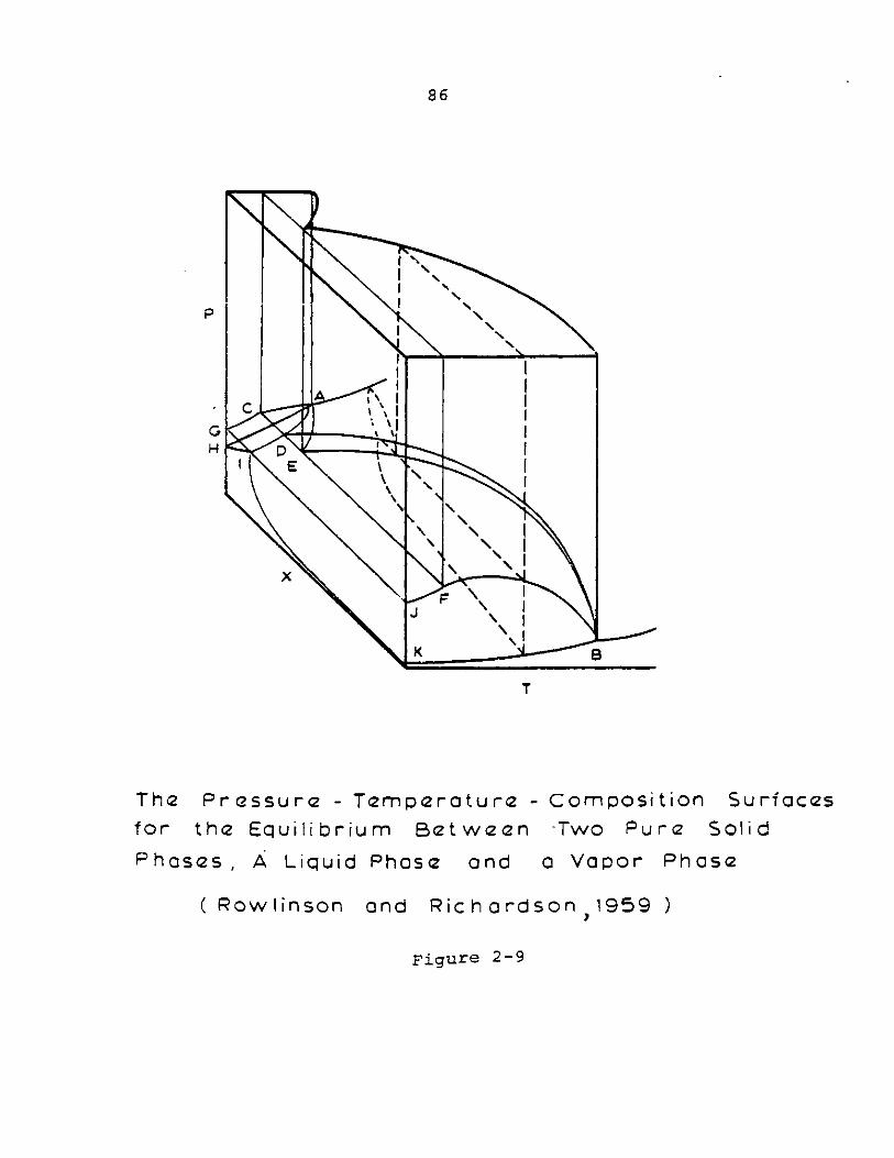
86
p
GH
T
The Pressure - Temperature - composition Surfacasfor the Equilibrium Between -Two Pure Solid
Phases, A Liquid Phase and a Vapor Phase
( Rowlinson and Richardson,1959 )
Figure 2-9
FI
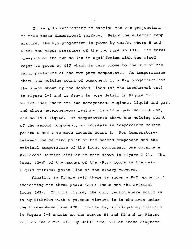
87
It is also interesting to examine the P-x projections
of this three dimensional surface. Below the eutectic temp-
erature, the P,x projection is given by GHIJK, where H and
K are the vapor pressures of the two pure solids. The total
pressure of the two solids in equilibrium with the mixed
vapor is given by GIJ which is very close to the sum of the
vapor pressures of the two pure components. At temperatures
above the melting point of component 1, a P-x projection has
the shape shown by the dashed lines Cof the isothermal cut)
in Figure 2-9 and is drawn in more detail in Figure 2-10.
Notice that there are two homogeneous regions, liquid and gas,
and three heterogeneous regions, liquid + gas-, solid + gas,
and solid + liquid. At temperatures above the melting point
of the second component, an increase in temperature causes
points W and Y to move towards point Z. For temperatures
between the melting point of the second component and the
critical temperature of the light component, one obtains a
P-x cross section similar to that shown in Figure 2-11. The
locus (M-N) of the maxima of the (P,x) loops is the gas-
iqui critca1 pint 4ne of the binary mixture
Finally, in Figure 2-12 there is shown a P-T projection
indicating the three-phase (AFB) locus and the critical
locus (MN). In this figure, the only region where solid is
in equilibrium with a gaseous mixture is in the area under
the three-phase line AFB. Similarly, solid-gas equilibrium
in Figure 2-9 exists on the curves HI and KI and in Figure
2-10 on the curve WX. Up until now, all of these diagrams
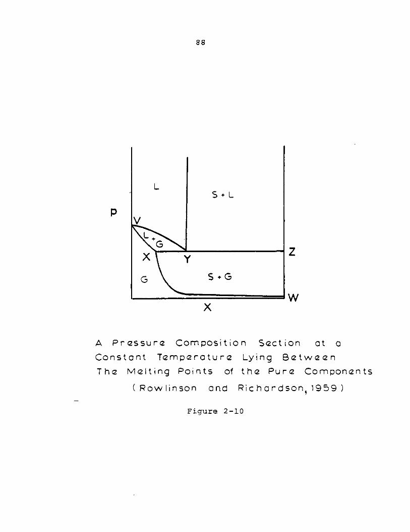
88
p
L
V,
x
G0
I'
S G
x
A Pressure Compositlo
Constant Temperature
The Melting Points of
z
w
n Sect ion at a
Lying Between
the Pure Components
( Rowlinson and Richordson, 1959 )
Figure 2-10
S+ L
I
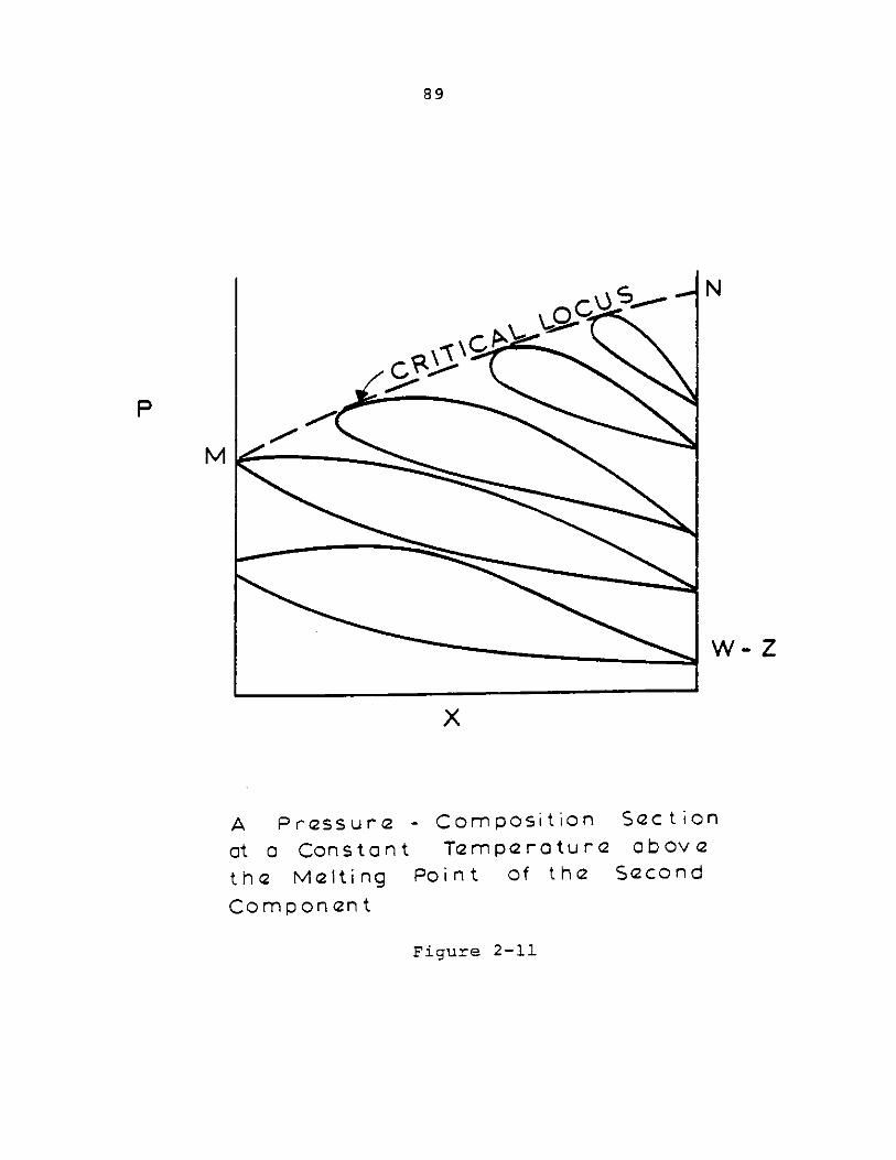
89
A Pressure - Composition SQctiOn
at a Constant Tampc raturc above
the Melting Point of the Second
Component
Figure 2-11

B
r
P-T Projection of
Three Phase Line
Critical Locus
a System
Does Not
in Which the
Cut the
Figure 2-12
90
PN
N
91
have been for similar substances and for relatively low pres-
sures. The next section discusses the case of very dissim-
ilar components and for very high pressures.
Binary Phase Behavior for Dissimilar Components at High
Pressures
Supercritical fluid extraction of solid solutes usually
operates with two very dissimilar substances (one is usually
a low molecular weight gas at room conditions; one a high mole-
cular weight solid at room conditions). Under these circum-
stances, the phase behavior discussed previously is not valid.
Instead, entirely new phenomena exist in the P-T-x phase
space. This phenomena, which is of most importance in
understanding the use and limitations of supercritical fluid
extraction, will be the topic of this section.
High pressure phase equilibria among dissimilar compon-
ents has been previously investigated by Rowlinson (1969),
Rowlinson and Richardson (1959), van Welie and Diepen (1961),
van Gunst et al. (1953a, 1953b), Diepen and Scheffer (.1948a,
1953)., Morey (1957), Smits (1909), and Zernike (1955). The
best way to introduce this subject is to reconsider the dia-
gram shown in Figure 2-12. If the two components are so
dissimilar that one is a low molecular weight gas at room
conditions and one is a high molecular weight solid, then
the difference in temperature between the triple points and
critical points of these substances is so large that the
three phase line AFB in Figure 2-12 can actually intersect
92
the critical locus so as to "cut" it into two points: p-
the lower critical end point, and q- the upper critical end
point. See Figure 2-13. In this figure, M and N are the
critical points of the supercritical fluid and solid respec-
tively. Critical end points are mixture critical points in
the presence of excess solid. Following the notation of
Morey (1954), these critical end points are commmonly written
as follows:
p : (G ELi) + S
q : (G EL2 ) + S
i.e., a liquid and gas of identical composition and proper-
ties in equilibrium with a pure solid.
The major consequence of a gap in the critical locus as
shown in Figure 2-13 is to allow at least* a region in
temperature between Tp and T where cne solid phase is in
equilibrium with one fluid phase with no liquid phase present.
In order to have a better visualization for the P-T
projection of the P-T-x surface, it is necessary to under-
stand various P-x and T-x projections. Figure 2-14 shows a
P-T projection indicating where isothermal P-x projections
are located in Figure 2-15. At T1 , the projection is
*A more general statement is discussed later in this
section.
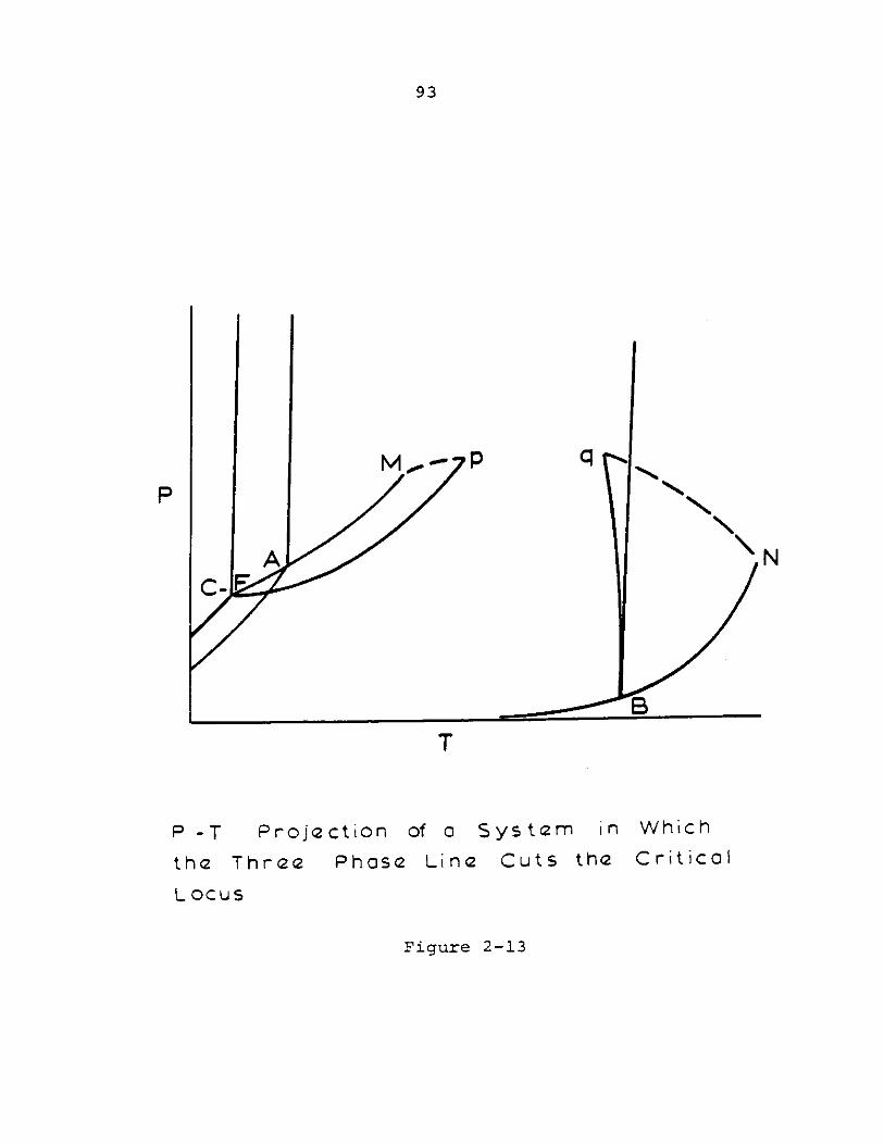
A0c- F
N N
BN
P -T Projaction
the Three Phas
of a System in Which
a Line Cuts the Critical
Locus
Figure 2-13
93
Pv
T
I
I
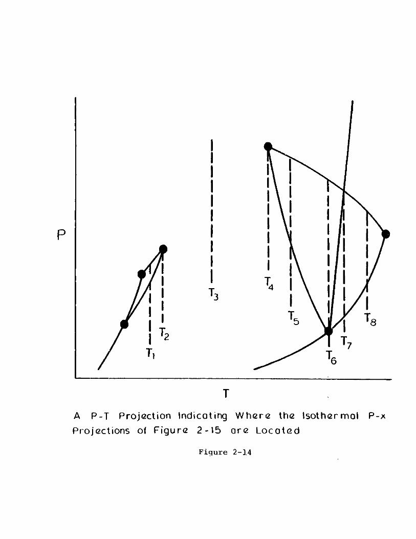
1 2Ti
IIIIIIIIII
1I
T5 T
TyT6
T
A P-T Projection Indicating Where the Isothermol P-x
Projections of Figure 2-15 ore Located
Figure 2-14
P
A
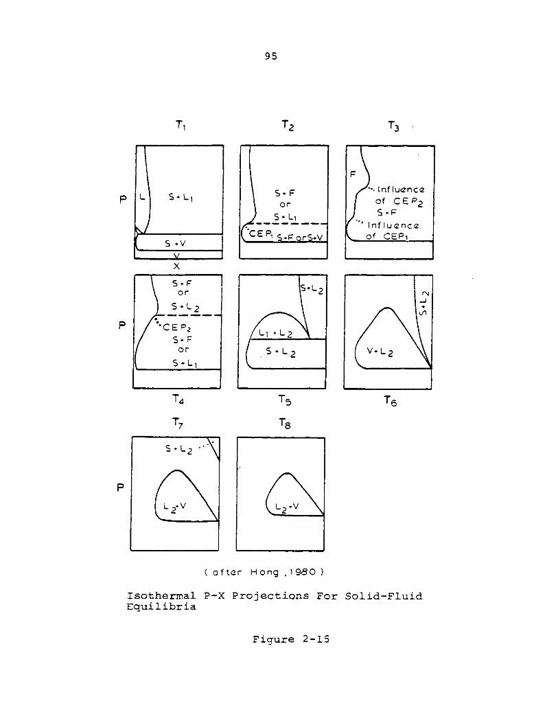
95
T,
L S+L1
S +V
x* For
S+ L 2
CE P2S+ For
5+L1
T4
T7
5-L2
Lz
T2
5+ For
S +L
CEP, S.F orStV
+L2
S+L2
Tz2
T8
2
T3-
F
Influenceof 0E2
.. -.FInf luenccof CEPi
V+'2
T6
( after Hong ,1980)
Isothermal P-X Projections For Solid-FluidEquilibria
Figure 2-15
p
p
P
p. I i
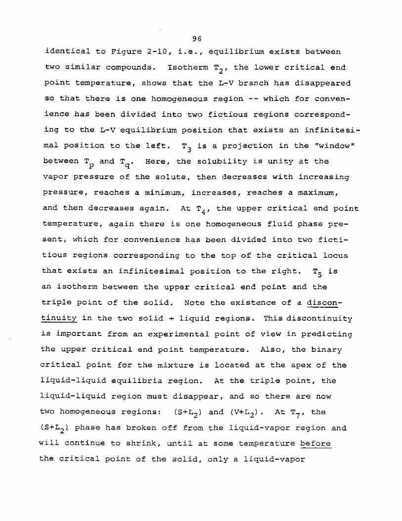
96
identical to Figure 2-10, i.e., equilibrium exists between
two similar compounds. Isotherm T2, the lower critical end
point temperature, shows that the L-V branch has disappeared
so that there is one homogeneous region -- which for conven-
ience has been divided into two fictious regions correspond-
ing to the L-V equilibrium position that exists an infinitesi-
mal position to the left. T3 is a projection in the "window"
between Tp and Tq. Here, the solubility is unity at the
vapor pressure of the solute, then decreases with increasing
pressure, reaches a minimum, increases, reaches a maximum,
and then decreases again. At T4 , the upper critical end point
temperature, again there is one homogeneous fluid phase pre-
sent, which for convenience has been divided into two ficti-
tious regions corresponding to the top of the critical locus
that exists an infinitesimal position to the right. T5 is
an isotherm between the upper critical end point and the
triple point of the solid. Note the existence of a discon-
tinuity in the two solid + liquid regions. This discontinuity
is important from an experimental point of view in predicting
the upper critical end point temperature. Also, the binary
critical point for the mixture is located at the apex of the
liquid-liquid equilibria region. At the triple point, the
liquid-liquid region must disappear, and so there are now
two homogeneous regions: (S+L2 ) and (V+L2). At T7 , the
CS+L2 1 phase has broken off from the liquid-vapor region and
will continue to shrink, until at some temperature before
the critical point of the solid, only a liquid-vapor
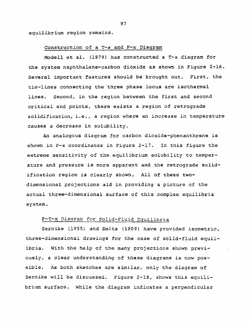
97
equilibrium region remains.
Construction of a T-x and P-x Diagram
Modell et al. (1979) has constructed a T-x diagram for
the system naphthalene-carbon dioxide as shown in Figure 2-16.
Several important features should be brought out. First, the
tie-lines connecting the three phase locus are isothermal
lines. Second, in the region between the first and second
critical end points, there exists a region of retrograde
solidification, i.e., a region where an increase in temperature
causes a decrease in solubility.
An analogous diagram for carbon dioxide-phenanthrene is
shown in P-x coordinates in Figure 2-17. In this figure the
extreme sensitivity of the equilibrium solubility to temper-
ature and pressure is more apparent and the retrograde solid-
ification region is clearly shown. All of these two-
dimensional projections aid in providing a picture of the
actual three-dimensional surface of this complex equilibria
system.
P-T-x Diagram for Solid-Fluid Equilibria
Zernike C1955) and Smits (1909) have provided isometric,
three-dimensional drawings for the case of solid-fluid equil-
ibria. With the help of the many projections shown previ-
ously, a clear understanding of these diagrams is now pos-
sible. As both sketches are similar, only the diagram of
Zernike will be discussed. Figure 2-18, shows this equili-
brium surface. While the diagram indicates a perpendicular
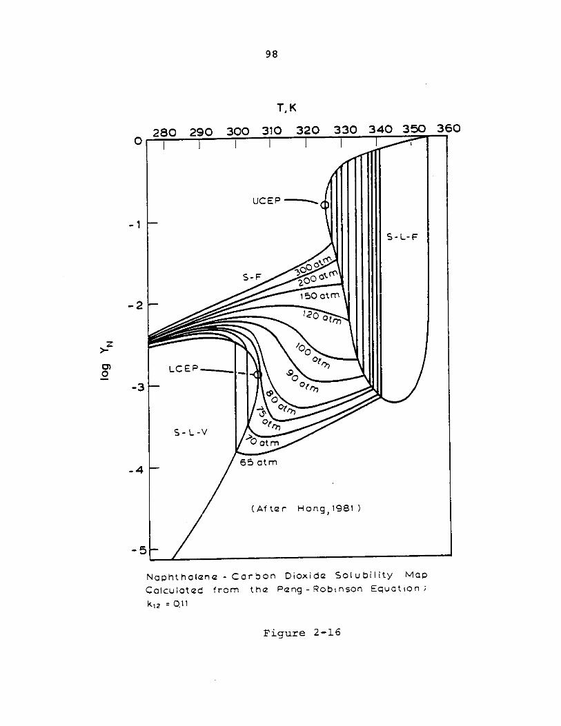
98
TK
280 290 300 310 320 330 340 350 3600 --
UCEP Mir
-~1-S- L-F
S-F o
2150 at\-2-
0
-3
5- L-V
55 atm- 4-
(Af ter Hong,1981)
Nophthalene - Carbon Dioxide Solubility Mop
Calculated from the Peng - Robinson Equation;
k12 = 0.11
Figure 2-16
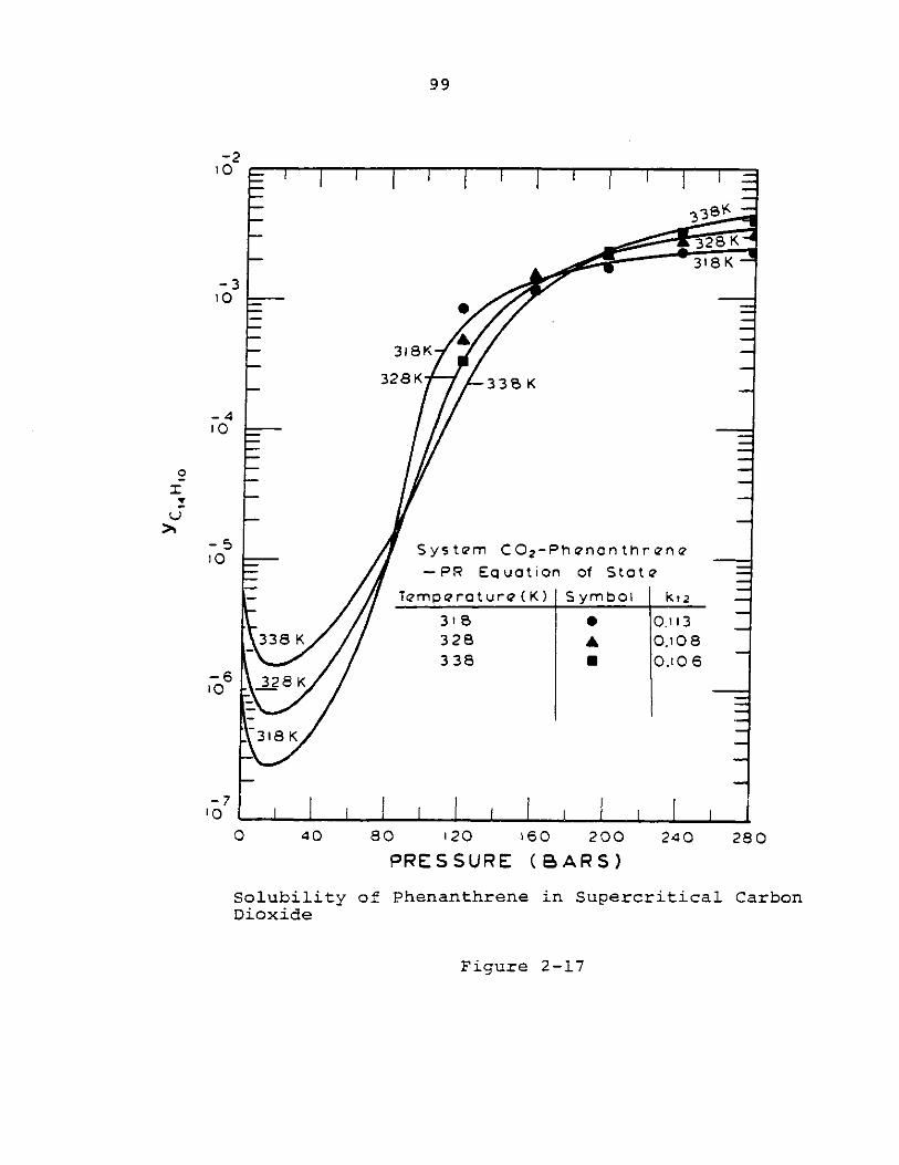
99
-210
328 K
-310
- 318K
328 K 33S K
-4
00
-5 System CO2 -Phenanthrene-PR Equation of Statq
Temperature (K) Symbol k12
318 0 0.113338 K 328 A O008
338 U 0.106-6328 K10
318 K
-7'0f
0 40 80 120 160 200 240 280
PRESSURE (BARS)
Solubility of Phenanthrene in Supercritical CarbonDioxide
Figure 2-17
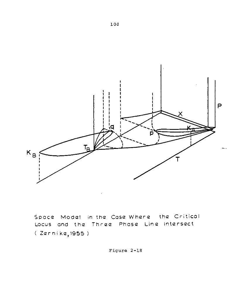
100
I
Space Model in theLocus and the Thre
Case Where the Critical
!e Phase Line Intersect
( Ze r n ike,1955 )
Figure 2-18
KB
P
101
dividing surface extending infinitely upward at the upper and
lower critical end point temperatures -- this surface is
fictitious because there is no phase transition to the left
or right of these critical end point temperatures. The div-
iding surface only indicates the uniqueness of the region
between TP and T . It is also apparent that the isothermal
P-x projections shown in Figure 2-15 "fit" nicely into the
three-dimensional surface. Note in Figure 2-18 that the
critical points of the two species and the upper and lower
critical end points are on different planes of this surface.
This is not obvious from two dimensional projections.
Solid-Fluid Equilibria Outside The Critical End Point
Bounds
As is clearly shown by the many P-T projections of Figure
2-15, there exist regions of temperature other than
T < T < T for which there is solid-fluid equilibrium.p - - q
These other regions of temperature, therefore, offer unique
possibilities for supercritical fluid extraction, but suffer
from the drawback that the pressure must be kept between
minimum and maximum bounds in order to guarantee that no
liquid phase will form. A major advantage, however, of
operating in these regions is that much higher solubilities
of the solid in the fluid phase can be achieved compared to
the solubilities that can be achieved in the region
T < T < T .p q
This particular phase behavior can be best understood
102
from Figure 2-15 isotherms, T 3 , T4 and T 5 . Since the (S+F)
isotherm T5 and the apex of the CL1 +L 2 ) isotherm T5 is on
the critical locus of the binary mixture, then it follows
that as long as the system pressure is greater than the maxi-
mum pressure on the critical locus connecting the upper ,
critical end point with the critical point of the solid com-
ponent, it is possible to operate with high solubilities in
the S+F region for temperatures T > T,. As the
P-x diagrams of Figure 2-15 show, the solubilities in this
region of solid-fluid equilibria will of necessity be higher
than the solubility in the region of temperatures Tp < T < T .
Consequently one can theoretically approach a solubility of
100 mole percent of solute in the fluid phase.
As an example, consider the system naphthalene-ethylene.
Figure 2-19 shows experimental P-T data for the critical
locus, the three-phase line and the upper critical end point.
From this figure, it can be concluded that if the system pres-
sure is greater than about 250 bar, that it is possible to
operate in a solid-fluid regime for T > T . Verification of
these ideas is shown in Figure 2-20. This is a graph of
temperature versus mole percent at a constant pressure of
274 bar. The large change in solubility occurs near the
upper critical end point temperature C52.1 C). Also note
the excellent agreement between the experimental data and
theory Cthe solid line calculated from the Peng-Robinson
equation of state,which is discussed later).
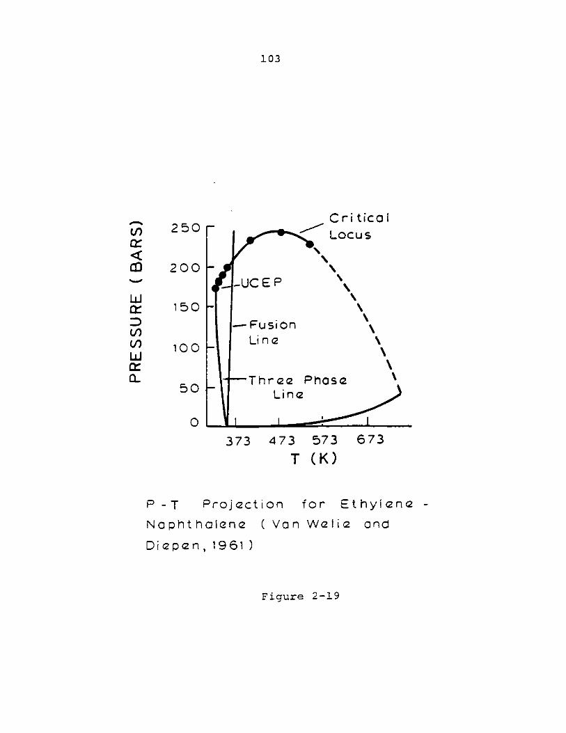
103
-UC E P
--- FusionLine
Thr oo
CriticalLocus
\B
PhasaLine
373 473 573
T (K)
P-T Projection for Et hylene -
Naphthalene (Van Welie and
Diepen, 1961)
Figure 2-19
V)
c1
Ld
LJUr
CL
250
200
150
100
50
0673
= I iiiiiiin sop k .- . - -- I -
I I I I I
I
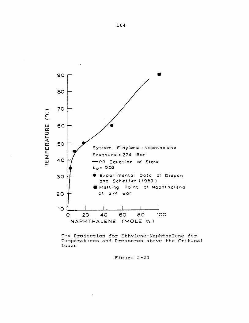
104
90
80
70
60
50
40
30
20
10:0 20 40 60 80
NAPHTHALENE (MOLE %/)
T-x Projection for Ethylene-Naphthalene forTemperatures and Pressures above the CriticalLocus
Figure 2-20
U
0
LU
0
I
CLI-
-U
K
-0
System Ethylene -Naphthalene
Pressure= 274 Bar
-PR Equation of State
k, 2 =0.02
0 Experimental Data of Diepenand Scheffer (1953 )
* Melting Point of Nophthalene
at 274 Bar
K - I100
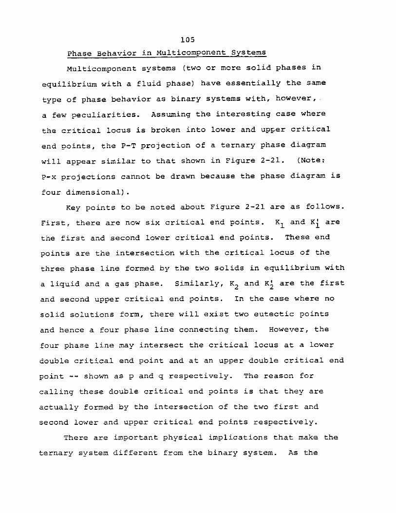
105
Phase Behavior in Multicomponent Systems
Multicomponent systems (two or more solid phases in
equilibrium with a fluid phase) have essentially the same
type of phase behavior as binary systems with, however,.
a few peculiarities. Assuming the interesting case where
the critical locus is broken into lower and upper critical
end points, the P-T projection of a ternary phase diagram
will appear similar to that shown in Figure 2-21. (Note:
P-X projections cannot be drawn because the phase diagram is
four dimensional).
Key points to be noted about Figure 2-21 are as follows.
First, there are now six critical end points. K1 and Ki are
the first and second lower critical end points. These end
points are the intersection with the critical locus of the
three phase line formed by the two solids in equilibrium with
a liquid and a gas phase. Similarly, K2 and K' are the first
and second upper critical end points. In the case where no
solid solutions form, there will exist two eutectic points
and hence a four phase line connecting them. However, the
four phase line may intersect the critical locus at a lower
double critical end point and at an upper double critical end
point -- shown as p and q respectively. The reason for
calling these double critical end points is that they are
actually formed by the intersection of the two first and
second lower and upper critical end points respectively.
There are important physical implications that make the
ternary system different from the binary system. As the
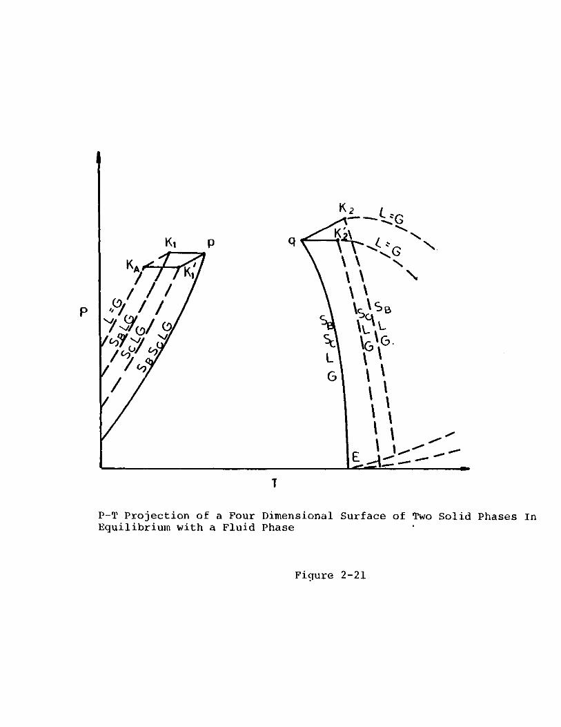
K1 p
KA K;
P/0/ (9
/
q Kiv G
't
L
T
P-T Projection of a Four Dimensional Surface of Two Solid Phases InEquilibrium with a Fluid Phase
Figure 2-21
P
H
I
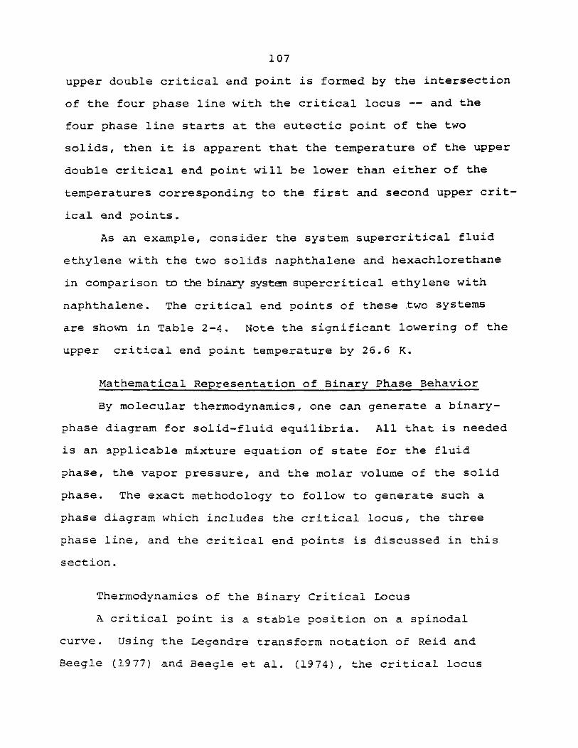
107
upper double critical end point is formed by the intersection
of the four phase line with the critical locus -- and the
four phase line starts at the eutectic point of the two
solids, then it is apparent that the temperature of the upper
double critical end point will be lower than either of the
temperatures corresponding to the first and second upper crit-
ical end points.
As an example, consider the system supercritical fluid
ethylene with the two solids naphthalene and hexachlorethane
in comparison to the binary system supercritical ethylene with
naphthalene. The critical end points of these .two systems
are shown in Table 2-4. Note the significant lowering of the
upper critical end point temperature by 26.6 K.
Mathematical Representation of Binary Phase Behavior
By molecular thermodynamics, one can generate a binary-
phase diagram for solid-fluid equilibria. All that is needed
is an applicable mixture equation of state for the fluid
phase, the vapor pressure, and the molar volume of the solid
phase. The exact methodology to follow to generate such a
phase diagram which includes the critical locus, the three
phase line, and the critical end points is discussed in this
section.
Thermodynamics of the Binary Critical Locus
A critical point is a stable position on a spinodal
curve. Using the Legendre transform notation of Reid and
Beegle (1977) and Beegle et al. (1974), the critical locus
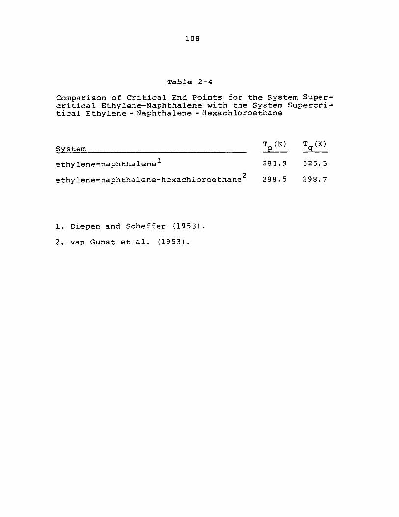
108
Table 2-4
Comparison of Critical End Points for the System Super-critical Ethylene-Naphthalene with the System Supercri-tical Ethylene -Naphthalene -Hexachloroethane
System
ethy lene-naphtha lene 1
ethylene-naphthalene-hexachloroethane2
1. Diepen and Scheffer (1953).
T (K) Tq(K)
283.9 325.3
288.5 298.7
2. van Gunst et al. (1953).
109
are those states that satisfy
(n) = 0 (2-2.1)Y(n+l) (n+l)
and
Y(n) = 0 (2-2.2)(n+l) (n+l) (n+l)
In terms of the Helmholtz free energy, these transforms can
be written (for a binary mixture) in terms of the two deter-
minants
Avv AvL =
AV1 A
=A A -Ai =0 (2-2.3)vvll VI
where
A a= A(2-2 .4)vv [WVJTx
A11 3t 2jC2.ST,x
2A = 2 (2-2.6)vi DVDx
T,x
110
A A
and MII = 0 (2-2.7)
F 3L1 (3L1
av J T,x L axTV
or,
2M =A A A +A A -JA A VA A 11 vvllvvl vvlll vvvlVll
-A A A + 2A 12 A =0 (2-2.8)11 vI vvv vlVV
Equations 2-2.3 and 2-2.8 are most conveniently solved sim-
ultaneously by a pressure explicit equation of state.
Modell et al. (1979) have derived these critical criteria
using the Peng-Robinson equation of state.
Determination of the Three Phase SLG Line
Thermodynamics requires that on the three-phase SLG line
that the following equalities must be satisfied:
fI(T,P) = fL (TPx1)(2-2.9)
f1(T,P) = fV (TPfyl)(2-2.10)
fj(T,P,y1 ) -fI(T,P,x1 ) (2-2.11)
f>(T,P,y1 ) =--TPx1)(2-2.12)
Of these four equations, only three are independent and a
convenient set to chose is the last three. The fugacity of
the solid phase is given by
illV' P
.sI(T, P) = PVP- *exp (2-2.13)
and the fugacity of the liquid and vapor phase by
f = x L$ (2-2.14)
fV = y1Pc (2-2.15)
where the fugacity coefficients L and $vare found from an
applicable equation of state. An iterative solution of Equa-
tions (2-2.10) through (2-2.12) coupled with the mass balance
X + X2 = 1 (2-2.16)
is sufficient to define the three-phase line. Numerical
techniques helpful in solving for the three phase line are
discussed by Francis and Paulaitis (1980).
Determination of Binary Critical End Points
There are two convenient methods whereby the upper and
lower critical end points may be calculated. One is to gen-
erate the entire critical locus and the entire three-phase
line, then plot the results on a P-T projection and graphi-
cally determine the end-points.
An easier way, however, is as follows. At a binary mix-
ture critical point, the following thermodynamic equality
must be satisfied.*
*See Appendix II for a derivation.
=0
112
ap Ia x 1 0 T l a
(2-2.17)
where x1 is the mole fraction of component 1 in the liquid
phase and subscript a denotes differentiation along the
three-phase curve. Thus, when the three phase curve is gen-
erated on the computer, a numerical check can be performed to
test for the equality of Equation 2-2.17. There will exist
two such equalities -- one at the upper critical end point
and one at the lower critical end point. Numerical techniques
helpful in solving for the binary critical end points are
discussed by Francis and Paulaitis (1980).
Experimental Methods to Determine Critical End Points
of Binary Systems
There are two methods whereby one can determine experi-
mentally the critical end points for binary systems. The
first method makes use of the rigorous thermodynamic relation-
ship that at a critical end point (see Appendix II).
dyjT=0 (2-2.18)
Thus, if careful experimental data are taken of isothermal
solubilities versus pressure, then two isotherms will exhibit
the zero slope criteria of Equation 2-2.18. These two condi-
tions will be the upper and lower critical end points.
Extremely precise solubility data must be taken for this
113
method to be reliable -- for the solubility is very sensitive
to temperature and pressure near the critical end points.
Alternatively, one can make use of the special nature
of the phase behavior near the critical end points to deter-
mine their values. Consider the isotherms T4 and T5 shown in
Figure 2-15. These figures imply that if isothermal solu-
bility data are taken at many pressures, that as the isotherm
just exceeds the upper critical end point temperature (or is
just less than the lower critical end point temperature), then
there will be a discontinuity in the isothermal solubility
curve. The temperature and pressure at which the discontin-
uity first occurs are the critical end point temperature and
pressure respectively. McHugh and Paulaitis (1980) have ob-
tained experimental values of the upper critical end points
for a few systems by the second method.
Comparison of Experimental Critical End Points
to Those Predicted by Theory
To date, there is only one system for which
there are both experimental measurements of critical end
points and also theoretical calculations of the critical end
points. This system is naphthalene-ethylene. Diepen and
Scheffer -1948a) and van Gunst et al. (1953) found the criti-
cal end points experimentally while Modell et al. (1979)
calculated them using the Peng-Robinson (1976) equation of
state. A comparison of experimental and theoretical results
is shown in Table 2-5. The agreement is satisfactory.
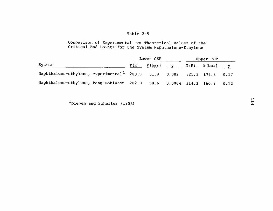
Table 2-5
Comparison of Experimental vs Theoretical Values of theCritical End Points for the System Naphthalene-Ethylene
Lower CEP Upper CEP
T (K) P(bar) y T (K) P (bar) y
Naphthalene-ethylene, experimentall 283.9
Naphthalene-ethylene, Peng-Robinson 282.8
1 Diepen and Scheffer (1953)
51.9 0.002 325.3 176.3
50.6 0.0004 314.3 160.9
System
0.17
0.12
HH
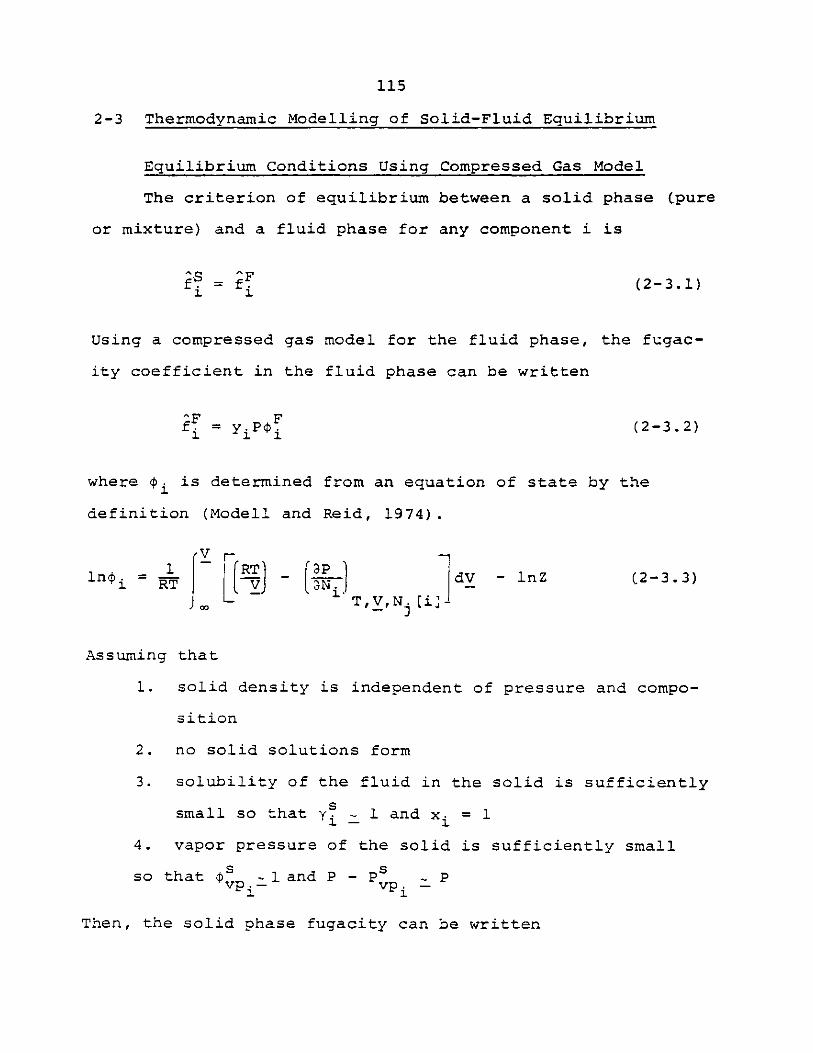
115
2-3 Thermodynamic Modelling of Solid-Fluid Equilibrium
Equilibrium Conditions Using Compressed Gas Model
The criterion of equilibrium between a solid phase (pure
or mixture) and a fluid phase for any component i is
^-S ^Ff% %= f (2-3.1)
Using a compressed gas model for the fluid phase, the fugac-
ity coefficient in the fluid phase can be written
^F Ff. = FyP$ (2-3.2)
where $ is determined from an equation of state by the
definition (Modell and Reid, 1974).
ST a Pln$ = K- 3j dV - lnZ (2-3.3)
- T,V,N. [il-
Assuming that
1. solid density is independent of pressure and compo-
sition
2. no solid solutions form
3. solubility of the fluid in the solid is sufficiently
Ssmall so that y. land x. = 1
4. vapor pressure of the solid is sufficiently small
so that 5 $s ~land P -P svp.- vpi
Then, the solid phase fugacity can be written
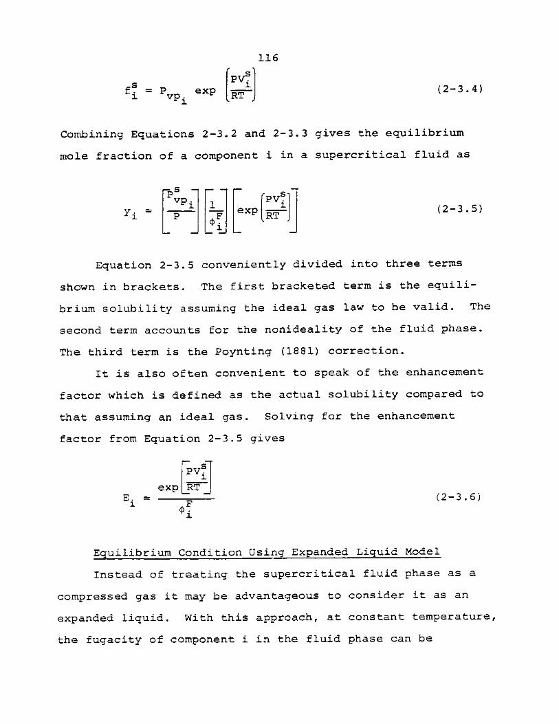
116
PV s
fs = P exp (2-3.4)i vp.RT
Combining Equations 2-3.2 and 2-3.3 gives the equilibrium
mole fraction of a component i in a supercritical fluid as
s ----
sy. = - exp (2-3.5)
S P 0F RT
Equation 2-3.5 conveniently divided into three terms
shown in brackets. The first bracketed term is the equili-
brium solubility assuming the ideal gas law to be valid. The
second term accounts for the nonideality of the fluid phase.
The third term is the Poynting (1881) correction.
It is also often convenient to speak of the enhancement
factor which is defined as the actual solubility compared to
that assuming an ideal gas. Solving for the enhancement
factor from Equation 2-3.5 gives
PV.s
expLRTE. e= (2-3.6)
Fi
Equilibrium Condition Using Expanded Liquid Model
Instead of treating the supercritical fluid phase as a
compressed gas it may be advantageous to consider it as an
expanded liquid. With this approach, at constant temperature,
the fugacity of component i in the fluid phase can be
117
expressed as
'R V.
f(y.,P) = y y.(y ,P )f(P )exp dP (2-3.7)
where PR is a reference pressure and f9 is a hypothetical1
fugacity of pure liquid i at the system temperature and at
the reference pressure PR. The solid phase fugacity can be
written as
'P V%s s R (PR) dP (2-3.8)
where fs (PR) is the fugacity of pure solid at the system
temperature and at the reference pressure PR. Making the
following assumptions: (1) the solid density is independent
of pressure and composition; (2) the solubility of fluid in
the solid is sufficiently small so that ys = 1 and xi_
and (3) no solid solutions form, then equation 2-3.8 can be
written as
Rs
f S = f(pR Kex RT)(2-3.9)1 1 )ep' RT
Combining Equations 2-3.7 and 2-3.9 gives
(P-PR)V.
f3(P )exp RT
yi = R Lf R - P'- - (2-3.10)
1 1' exp B[}dP
IpR RT,
118
It can be shown (Prausnitz, 1969) that to a very good approxi-
mation
fL(PR) AH N P- A C 'TTin (R R T]
AC I Ti t
+ R in T23.1
where Tt .is the triple point temperature of component i.
Furthermore, the last two terms on the right of Equation
2-3.11 are about equal in magnitude and opposite in sign.
Thus, Equation 2-3.11 can be approximated as
rAH rTexp R-T [ PRsexL t. LI.jj exp R
y.=RRTP i(2-3
exp dP
.12)
An accurate representation of y. (yF ,P ) and V must now be
obtained. Mackay and Paulaitis (1979) have used a reference
pressure of
p R =c
with Pc the critical pressure of the pure fluid phase, and
the assumptions that
R 00Yi cy ,P }~YiCPc) (2-3.13)
(2-3.11)
119
S (Y. ,P R) V~00 (P )(2-3.14)
V7 I(P ) then can be found from an applicable equation of statei c
by the definition
r(3V= im 1 (2-3.15)
N10 3N T,PCN
Y (P ) is treated as an adjustable constant.1 C
Using the Peng-Robinson (1976) equation of state, Mackay
and Paulaitis (1979) were able to correlate naphthalene solu-
bilities in supercritical carbon dioxide and supercritical
ethylene at a constant value of the binary interaction para-
meter and for a temperature dependent infinite dilution acti-
vity coefficients. The infinite dilution activity coefficients
they obtained, however, are quite large.
Applicable Equations of State
Both the compressed gas and the expanded liquid model
approach to solid-fluid equilibrium require an equation of
state to evaluate fluid phase fugacity coefficients (former
case and partial molar volumes (later case). This section
will discuss the types of equations of state applicable to
determine these thermodynamic quantities in the mixture state.
Virial Equation of State
The virial equation of state is applicable to the
120
correlation of the solubility of solids in compressed gases,
but only for relatively low pressures. When the pressure is
such that the density of the gas is less than about one-half
of the critical density, the virial equation of state,
truncated to the third term can be used. The virial equation
can be written
B CM= 1 + V + 9 + .* (2-3.16)
where:
BM i=yyB. C(.2-3.17)
1J
CM=ikaijk (2-3.18)ijk
A major advantage of the virial equation is that the virial
coefficients have a physical meaning in that they are related
to the intermolecular potential function. Under conditions
where the virial equation of state is applicable, the enhance-
ment factor has been calculated for the compressed gas model
(Ewald, 1955), (Ewald, et al., 1953) as:
Vsln E = 0B(P-P2) + 2 2B - B+x 2 B 2 -2x2 B )RT P92 + -x1 B11 -2 1 B12 2 2 2 22 RT
1 P4 2 3 2+ F-x43B2-x3(2C 4BB ) + x 3C2 1111111- 1112 1 112
3 2 2+x x 212B 1 B 2 xi 2x(6C1 1 2 +4B 1 B 2 2 +8B$
121
2+x X 2 6C1 2 2 - xx2 (6C1 1 2 +12B1 B 2 2)
13 12-12 12 2 42
+x x3 2B B +X 2 (2 B 2 +BB x4 B21 2 12 22 1 2 (12B1 2 1+61 2 2 )+x2 B2 2
-x3(2C 2 2 2 +4B 2 )+X2 3C2 2 2 J f 2 (2-3.19)
where: subscript 2 is the solid
subscript 1 is the fluid
P 0 is the vapor pressure of the solid2
V5 is the molar volume of the solid2
As an example, consider the application of the virial
equation to solid-fluid equilibrium calculations in the corre-
lation of solid carbon dioxide solubility in supercritical
air. The resultant plot is shown in Figure 2-22. Clearly, for
an accurate correlation past the solubility minimum, the third
virial coefficient must be taken into account. As the virial
equation is not valid for densities greater than about one-
half of the critical density of the mixture, one has to
resort to empirical equations of state for the high pressure
region.
Cubic Equations of State
Of all the equations of state used today, the cubic
equations of state are probably the most widely used. Evi-
dence of this is in the continuing effort to produce modifi-
cations of the original cubic equation of state: that of
van der Waals (1873). After the development of van der Waals
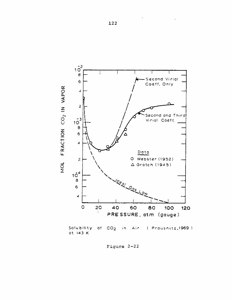
122
-210
S 1
6
4
2
10
6
4
2
1(548
6
0 20 40 60PRESSUREal
80 100 120Lm (gauge)
SolubilityOt 143 K
Of C02 in Air ( Prousnitz,1969 )
Figure 2-22
ix
CL
42zN
0L)
z0
LL
-j07
Second VIricCoeff. Only
-/
/Second and ThirdVirnai Coeff.
Data
- C Webster (1952)
a Gr(OtCh (1945)
- Nc
I I ' s
ff
123
equation, the most significant advance was the Redlich-Kwong
(1949) equation which modified the attractive term of van der
Waals. After Redlich-Kwong, Soave (19 72) made the next
major advance by introducing a temperature dependence on the
attractive term. Following Soave, many other equations of
state were developed (Peng and Robinson, 1976; Fuller, 1976;
Won, 1976; and Graboski and Daubert, 1978). Also, two review
articles on cubic equations of state were written (Abbott,
1973; Martin, 1979).
At the present time, it is believed that the best cubic
equation of state is that of Peng and Robinson (1976). Their
equation is:
P RT_ aCT)V-b V (V+b) + b CV-b)
R 2T2a. T ) = RT
i c a P.i
RTb (T ) = 2 c
i c b P.ci
(2-3. 20)
(2-3.21)
C2-3. 221
(2-3.23)a. (T) = a.(Tc) . a.CT ,w.)I c
b.(T) = b. CTc)x x c C2-3. 24)
.(T u) Li + K. (1-T 1 / 2 )x C ri
where
(2-3.25)
124
. = 0.37464 + 1.54226w. - 0.269922.
a = Zcl-k ).)a}/2 ah/ 2 x x.iJ
(2-3.26)
(2-3.27)
(2-3.28)b= Zb.x.1.
By definition of the fugacity coefficient (Modell and Reid,
1974)
l = fVFI- F4J32;0 %.1JT, Pt% [i]j
dv - InZ (2-3.29)
The fugacity coefficient of component i can be calculated as
b.Alnt. = (Z-l) - ln(Z-B) -A
b 2Y/IB
-22x.a..S13 bo nz +(CL+42)B
a b Z -(1- D)B,(2-3. 30)
A = aP/R2T2
B = bP/RT
(2-3. 31)
(2-3. 32)
Benedict-Webb-Rubin Equation of State
The Benedict-Webb-Rubin (BWR) equation of state (Benedict
et al., 1951, 1942, 1940), is another equation of state which
is often used. Originally, the BWR constants were tabulated
for only the light hydrocarbon systems. Later, Edmister et
al. (1968) expressed the eight parameters in terms of critical
where
125
pressures, temperatures, and acentric factors. Starling and
Han C1971, 1972a, 1972b) added three more parameters to the
original BWR equation of state and developed a correlation
for these parameters in terms of critical temperature, critical
volume, and acentric factor. Yamada (1973) developed a
fourty four parameter BWR equation and a correlation of these
parameters in terms of critical temperature, critical pres-
sure, and acentric factor. Lee and Kesler (1975) developed
a modified BWR equation within the context of Pitzer's three
parameter correlation.
These many types of BWR equations have proved to be very
successful for light hydrocarbon systems at conditions far
removed from the critical point. Near the critical point,
however, the BWR equations are less accurate as they do not
satisfy the two pure component stability criteria at a critical
point.
Perturbed Hard Sphere Equation of State
All of the cubic equations of state developed to date
have used the same repulsive term that van der Waals used in
1893, i.e.,
P - (2-3.33)
and have emphasized modifications on the attractive term.
It can be shown, however, (Carnahan and Starling, 1972) , that
a more accurate representation of the repulsive term is
126
2 3~
Pa_ RT 1++_- (2-3. 34)R V -(_ 3
where E = b/4V (2-3.35)
Equation 2-3.34 is quite precise since its virial expan-
sion closely agrees with the exact expression for rigid
spheres (Ree and Hoover, 1967). The equation of'state that
results when the repulsive term is replaced by Equation 2-3.34
is called a perturbed hand sphere (PHS) equation of state
(Oellrichet al., 1978).
Preliminary use of the PHS equation of state, augmented
by density dependent attractive forces (Alder et al., 1971)
for solid-fluid equilibria has been encouraging (Johnston and
Eckert, 1980). More development work, however, needs to be
done.
Conclus ions
The two general types of equation of state -- cubic and
Benedict-Webb-Rubin (BWR) have been tested for their ability
to correlate solid-fluid equlibrium data. For the cubic
equations of state, the Peng-Robinson (1976) and Soave (1972)
equations of state were used. Also, the Starling and Han
(1971, 1972a, 1972b) modifications of the BWR equation of
state were tried. In all cases the correlational ability
of these equations were tested on the systems naphthalene-
carbon dioxide and naphthalene-ethylene using the data of
Tsekhanskaya (1964).
127
Extensive testing of the Starling and Han modification
of the BWR equation of state showed that the solid-fluid equil-
ibrium data could not be accurately correlated unless the
binary interaction parameter was a function of both temper-
ature and pressure. In the case of the two cubic equations
of state (.Soave and Peng-Robinson), the solid-fluid equili-
brium data could be well correlated for a binary interaction
parameter that is a weak function of temperature. The ability
of both the Peng-Robinson and Soave equations of state to
correlate the solubility data was essentially identical, but
the two equations required different values of the binary
interaction parameter.
Clearly, it is more desirable to have the binary inter-
action parameter a function of as few variables as possible --
and so the two cubic equations prove to be superior to the
BWR equation. Of the two cubic equations of state, the Peng-
Robinson equation predicts molar volumes of the liquid phase
more accurately than the Soave equation of State (.Peng and
Robinson, 1976) and so the Peng-Robinson equation was chosen
as the equation to use in this thesis.
A possible reason for the better predictive abilities
of the cubic-type equation of state over the BWR-type equation
of state can be explained as follows. Cubic equations of
state contain two adjustable parameters. Typically, these
adjustable parameters are found by forcing the cubic equations
of state to satisfy the two pure component stability cri-
teria:
128
C J =0 (2-3.36)3VT
c
[ 2 'a- =P0(2-3.37)
c
Consequently, isotherms for cubic equations of state have the
correct slope in the critical region. BWR type equations,
however, have typically eight to eleven adjustable parameters.
These parameters are obtained by fitting the BWR equation to
P-V-T data by use of a non-linear regression routine. Thus,
the BWR equations may not satisfy pure component stability
criteria and thus,will tend not to correlate data well in the
critical region.
2-4 Thesis Objectives
The objectives of this thesis can be divided into three
parts: experimental, theoretical, and exploratory. Experi-
mentally, equilibrium solubility data for both polar and non-
polar solid solutes in supercritical fluids were to be
measured over wide ranges of temperature and presure. In
addition, ternary equilibrium data (two solids, one fluid)
were to be measured. Carbon dioxide and ethylene were the
two supercritical fluids to be used.
Theoretically, correlation of equilibrium solubility
data of both binary and multicomponent systems using rigorous
thermodynamics was to be done.
129
Finally, after obtaining equilibrium solubility data
and developing a thermodynamic model, it was desirable to
use this model to explore the physics of solid-fluid equili-
bria. Using the model that was to be developed, such
phenomena as enthalpy changes of solvation of the solute in
the supercritical solvent and changes in equilibrium solubil-
ity over wide ranges of temperature and pressure were to be
studied.
130
3. EXPERIMENTAL APPARATUS AND PROCEDURE
3-1 Review of Alternative Experimental Methods
Experimentally, there are three feasible methods to
determine equilibrium solubilities of slightly volatile solids
in supercritical fluids. These are static methods, flow
methods, and tracer methods.
Static Method
In the static method, the solute species to be extracted
is contacted with the supercritical fluid in a batch vessel.
After a sufficient length of time has passed so that an equil-
ibrium solubility has been obtained, fluid samples are removed
for analysis. Special care must be taken that no appreciable
pressure perturbations occur during sampling. This is
accomplisehd by taking very small samples or by a volumetric
compensation technique (such as mercury displacement).
Eisenbeiss (1964), Tsekhanskaya et al. (1962, 1964), and
Diepen and Scheffer C1948b) measured equilibrium solubilities
by this method.
Flow Method
In the flow method, the supercritical fluid is contacted
with the solute species to be extracted in a flow extractor.
The fluid stream exciting the extractor is then analyzed for
composition. In order to assure that an equilibrium
131
solubility has been achieved, the solubility is determined
at various flow rates and as long as the solubility is inde-
pendent of flow rate, it can be assured that equilibrium is
acheived. Several authors (Kurnik et al., 1981; Johnston
and Eckert, 1981; McHugh and Paulaitis, 1981) have success-
fully used this method.
Tracer Method
Tracer methods of determining solubility are done typi-
cally by using a radioactive isotope of the desired solute
species to be extracted. Using a static method, a Geiger
counter is then attached to the fluid portion of the equili-
brium cell. By careful calibration, the number rate of radio-
active counts can be converted to an equilibrium solubility.
Ewald et al. (1953) used this method to determine the equili-
brium solubility of iodine in supercritical ethylene.
3-2 Description of Equipment
The experimental method used in this thesis to measure
equilibrium solubilities was a one-pass flow system. A
schematic is shown in Figure 3-1. Details of various sections
of the equipment are discussed in Appendix VII.
A gas cylinder was connected to an AMINCO line filter, rodel
49-14405) which feed into an AMINCO single end compressor, model
46-13411). The compressor was connected to a two liter
magnedrive packless autoclave (Autovlave Engineers) whose
purpose was to dampen the pressure fluctuations. In addition,
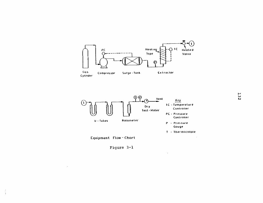
PCHetn --0 TC Hoe-- - - - - lope a Valve
Compressor Surge - lonk Ex t roctor
I PVent
DryTest- Meter
U - Tubes Rota meter
Key
TC - TemperotureCont roller
PC - PressureCont roller
P - PressureGouge
T - ThermocoOple
Equipment Flow - Chort
Figure 3-1
GO 5Cylinder
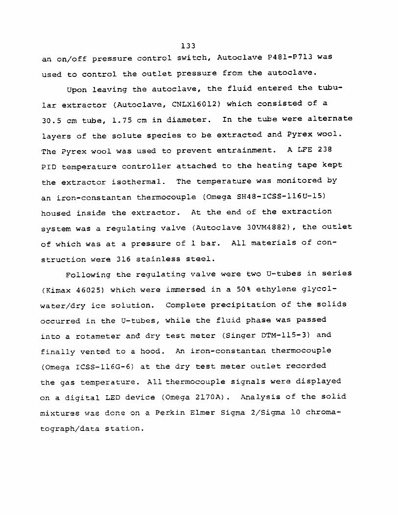
133
an on/off pressure control switch, Autoclave P481-P713 was
used to control the outlet pressure from the autoclave.
Upon leaving the autoclave, the fluid entered the tubu-
lar extractor (Autoclave, CNLXJ6012) which consisted of a
30.5 cm tube, 1.75 cm in diameter. In the tube were alternate
layers of the solute species to be extracted and Pyrex wool.
The Pyrex wool was used to prevent entrainment. A LFE 238
PID temperature controller attached to the heating tape kept
the extractor isothermal. The temperature was monitored by
an iron-constantan thermocouple (Omega SH48-ICSS-ll6U-15)
housed inside the extractor. At the end of the extraction
system was a regulating valve (Autoclave 30VM4882), the outlet
of which was at a pressure of I bar. All materials of con-
struction were 316 stainless steel.
Following the regulating valve were two U-tubes in series
(Kimax 46025) which were immersed in a 50% ethylene glycol-
water/dry ice solution. Complete precipitation of the solids
occurred in the U-tubes, while the fluid phase was passed
into a rotameter and dry test meter (Singer DTM-115-3) and
finally vented to a hood. An iron-constantan thermocouple
(Omega ICSS-116G-6) at the dry test meter outlet recorded
the gas temperature. All thermocouple signals were displayed
on a digital LED device (Omega 2170A). Analysis of the solid
mixtures was done on a Perkin Elmer Sigma 2/Sigma 10 chroma-
tograph/data station.
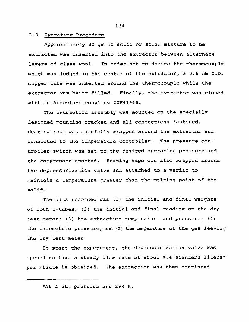
134
3-3 2eratingProcedure
Approximately 40 gm of solid or solid mixture to be
extracted was inserted into the extractor between alternate
layers of glass wool. In order not to damage the thermocouple
which was lodged in the center of the extractor, a 0.6 cm O.D.
copper tube was inserted around the thermocouple while the
extractor was being filled. Finally, the extractor was closed
with an Autoclave coupling 20F41666.
The extraction assembly was mounted on the specially
designed mounting bracket and all connections fastened.
Heating tape was carefully wrapped around the extractor and
connected to the temperature controller. The pressure con-
troller switch was set to the desired operating pressure and
the compressor started. Heating tape was also wrapped around
the depressurization valve and attached to a variac to
maintain a temperature greater than the melting point of the
solid.
The data recorded was (1) the initial and final weights
of both U-tubes; (2) the initial and final reading on the dry
test meter; (3) the extraction temperature and pressure; (4)
the barometric pressure, and (5) the temperature of the gas leaving
the dry test meter.
To start the experiment, the depressurization valve was
opened so that a steady flow rate of about 0.4 standard liters*
per minute is obtained. The extraction was then continued
*At 1 atm pressure and 294 K.
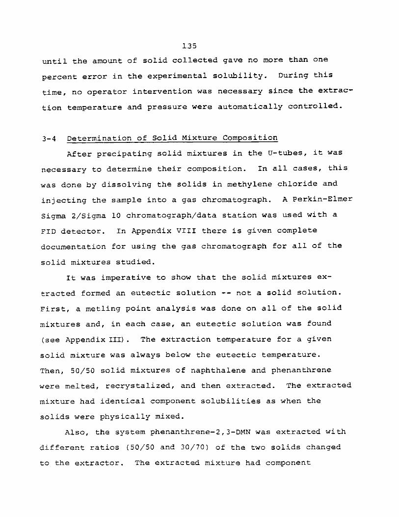
135
until the amount of solid collected gave no more than one
percent error in the experimental solubility. During this
time, no operator intervention was necessary since the extrac-
tion temperature and pressure were automatically controlled.
3-4 Determination of Solid Mixture Composition
After precipating solid mixtures in the U-tubes, it was
necessary to determine their composition. In all cases, this
was done by dissolving the solids in methylene chloride and
injecting the sample into a gas chromatograph. A Perkin-Elmer
Sigma 2/Sigma 10 chromatograph/data station was used with a
FID detector. In Appendix VIII there is given complete
documentation for using the gas chromatograph for all of the
solid mixtures studied.
It was imperative to show that the solid mixtures ex-
tracted formed an eutectic solution -- not a solid solution.
First, a metling point analysis was done on all of the solid
mixtures and, in each case, an eutectic solution was found
(see Appendix III). The extraction temperature for a given
solid mixture was always below the eutectic temperature.
Then, 50/50 solid mixtures of naphthalene and phenanthrene
were melted, recrystalized, and then extracted. The extracted
mixture had identical component solubilities as when the
solids were physically mixed.
Also, the system phenanthrene-2,3-DMN was extracted with
different ratios (50/50 and 30/70) of the two solids changed
to the extractor. The extracted mixture had component
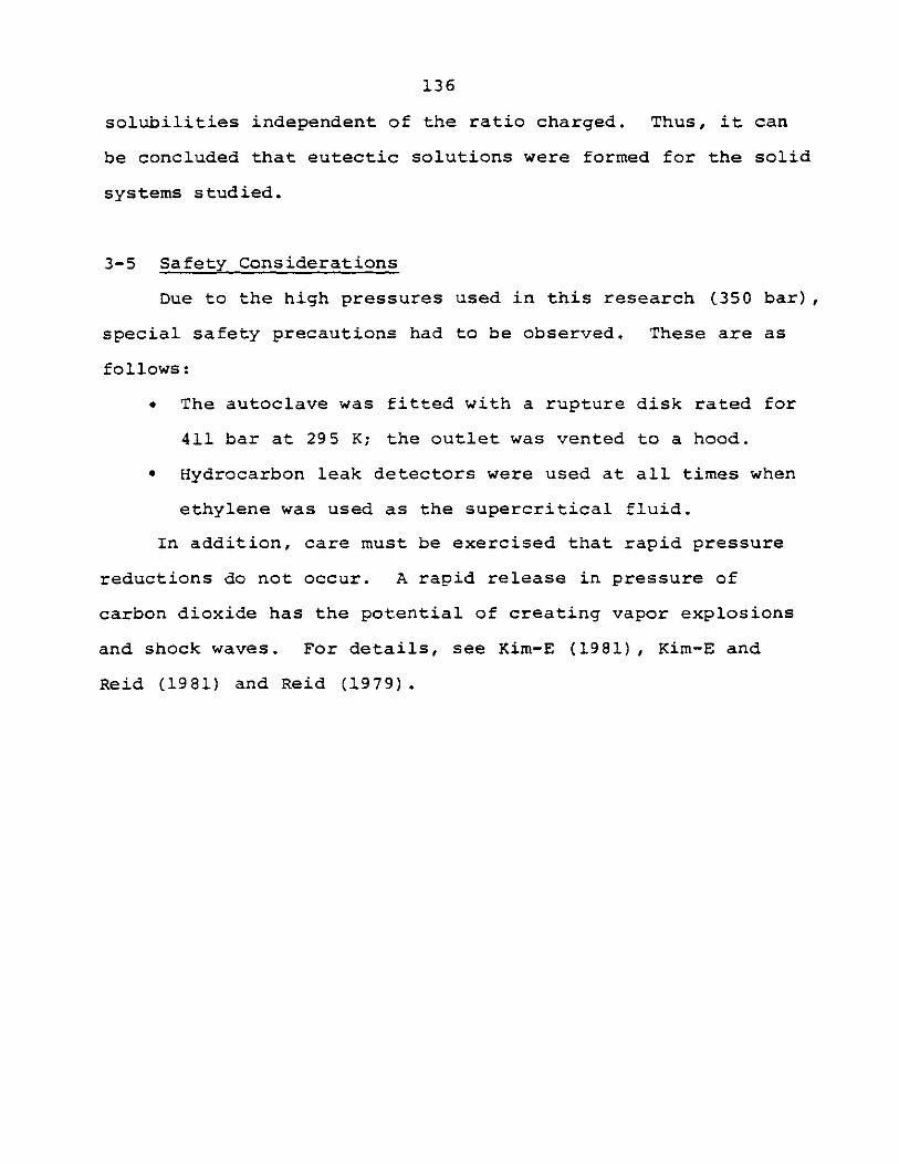
136
solubilities independent of the ratio charged. Thus, it can
be concluded that eutectic solutions were formed for the solid
systems studied.
3-5 Safety Considerations
Due to the high pressures used in this research (350 bar),
special safety precautions had to be observed. These are as
follows:
* The autoclave was fitted with a rupture disk rated for
411 bar at 295 K; the outlet was vented to a hood.
* Hydrocarbon leak detectors were used at all times when
ethylene was used as the supercritical fluid.
In addition, care must be exercised that rapid pressure
reductions do not occur. A rapid release in pressure of
carbon dioxide has the potential of creating vapor explosions
and shock waves. For details, see Kim-E (1981), Kim-E and
Reid (1981) and Reid (1979).
137
4. RESULTS AND DISCUSSION OF RESULTS
In this section, experimental solid-fluid equilibrium
data are given for both binary and multicomponent systems.
Also, graphs of the data points correlated with the Peng-
Robinson equation of state are shown.
4-1 Binary Solid-Fluid Equilibrium Data
Presented in Tables 4-1 through 4-9 are experimental
equilibrium data for the solubility of pure component solids
in supercritical carbon dioxide and ethylene at several temp-
eratures and pressures. Also shown with the data are iso-
thermal Peng-Robinson binary interaction coefficients obtained
by use of a non-linear least squares regression. Figures 4-1
through 4-9 show the experimental data are correlated with
the Peng-Robinson equation of state.
Binary Interaction Coeffients
In modelling the binary solid-fluid equilibrium problem
using the Peng-Robinson equation of state, there exists an
unknown binary interaction parameter, ki 1 , which must be
determined from experimental data (refer to Eq. 2-3.27).
The binary interaction parameter has been found to be a weak
function of temperature, but independent of pressure and
composition -- at least over the range studied here. One
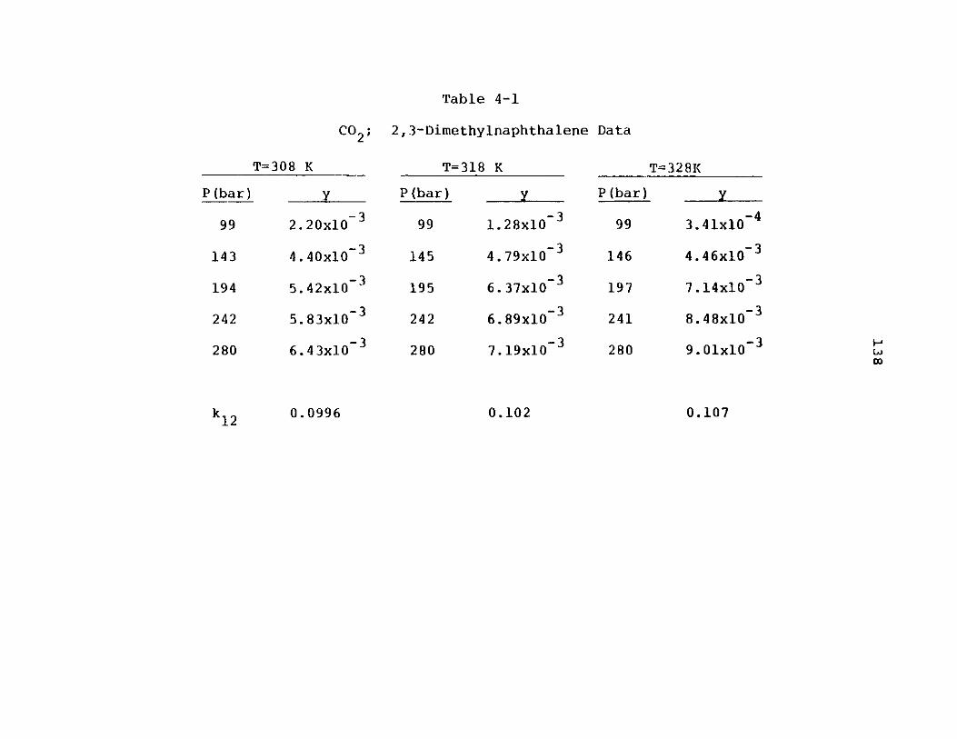
Table 4-1
2,3-Dimethylnaphthalene
T=308 K
y
2. 20x10-3
4. 40x10 3
5. 42x10-3
5. 83x10-3
6.43x10- 3
T=318 K
P(bar)
99 1.
145 4.
195 6.
242 6.
280 7.
T=328K
28x10-3
79x10-3
37x10- 3
89x10-3
19x10- 3
P(bar)
99
146
197
241
280
y
3. 41x10~4
4.46x10⁻³
7.14x10 3
8.48x10⁻³
9. 01x10 3
k12 0.0996
Co2 ; Data
P(bar)
99
143
194
242
280HLA)
OD
0.102 0.107
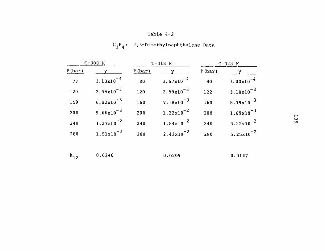
Table 4-2
2,3-Dimethylnaphthalene Data
T=308 K
P(bar) y
77 3.13x10~ 4
120 2.59x10⁻³
159 6.02x10⁻³
200 9.66x10 3
240 1.27xl0-2
280 1.51x10⁻²
T=318 K
P(bar) y
80 3. 67x10~ 4
120 2.59x10⁻³
160 7.18x10- 3
200 1.22x10⁻²
240 1.84x10⁻²
280 2.42x10 2
T=328 K
P(bar) y
80 3. 00x10~ 4
122 3.18x10⁻³
160 8.79x10⁻³
200 l.89x10-3
240 3.22x10⁻²
280 5.25x10⁻²
0.0147
2 H4;
HjU)ko
0.0246 0.0209
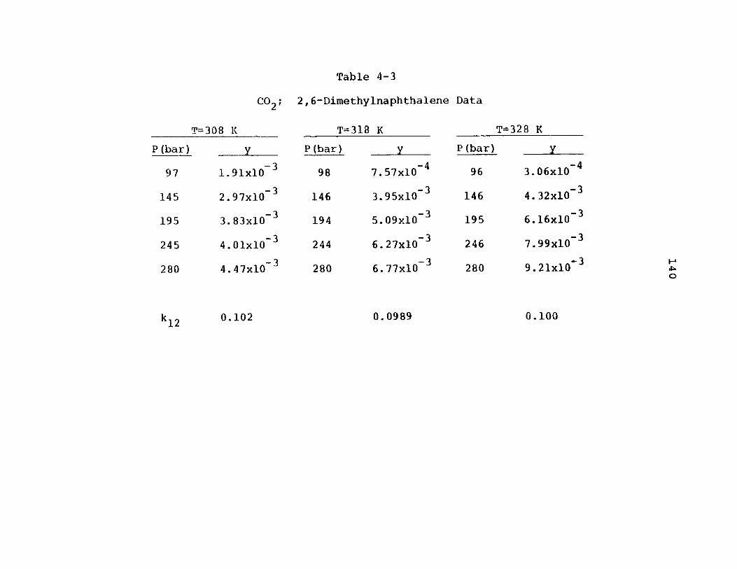
Table 4-3
2,6-Dimethylnaphthalene Data
T=308 K
y
1.91x10⁻³
2.97x10 3
3. 83x10-3
4. 01x10-3
4. 47x10-3
T=318 K
P (bar)
98 7.
146 3.
194 5.
244 6.
280 6.
T=328 K
y
57x10 4
95x10-3
09x10-3
27x10-3
77x10 3
P(bar)
96
146
195
246
280
3.06x10 4
4. 32x10- 3
6. 16x10- 3
7. 99x10-3
9. 21x10-3
0.0989
Co 2 ;
P(bar)
97
145
195
245
280H
0
0.1000.102
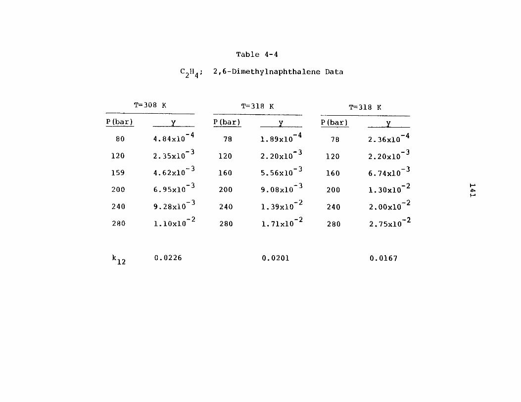
Table 4-4
C211 4 ; 2,6-Dimethylnaphthalene Data
T=308 K T=318 K
4. 84x10~ 4
2. 35x10-3
4. 62x10-3
6. 95x10-3
9. 28x10-3
1. 10x10-2
P(bar)
78
120
160
200
240
280
y
1. 89x10~ 4
2. 20x10-3
5. 56x10-3
9. 08x10-3
1.39x10⁻²
1. 71x10-2
T=318 K
P(bar)
78 2. 36x10'4
120 2.20x10⁻³
160 6.74x10⁻³
200 1.30x10⁻²
240 2.00xlO'2
280 2.75x10⁻²
k12 0.0226
P(bar)
80
120
159
200
240
280
H
0.0201 0.0167
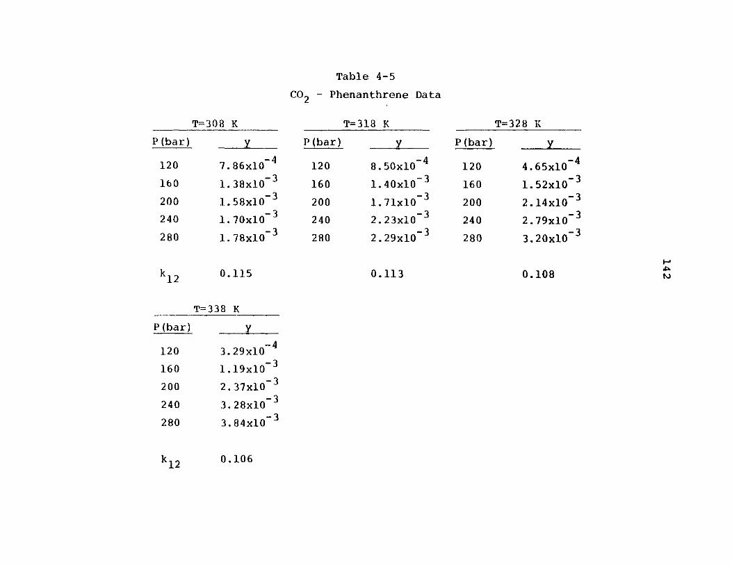
Table 4-5
CO2 - Phenanthrene Data
T=318 K
y
7. 86x10~ 4
1. 38x10- 3
1.58x10⁻³
1. 70x10-3
1. 78x10- 3
P(bar)
120
160
200
240
280
P (bar)
120
160
200
240
280
k12
y
8. 50x10~ 4
1.40x10- 3
1. 71x10- 3
2. 23x10- 3
2. 29x10- 3
P(bar)
120
160
200
240
280
0.113
y
4.65x10~ 4
1. 52x10-3
2. 14x10-3
2.79x10⁻³
3. 20x10- 3
0.108
T=338 K
y
3. 29x10 4
1.19x10 3
2. 37x10- 3
3. 28x10-3
3.84x10 3
0.106
T=308 K
0.115
T=328 K
P (bar)
120
160
200
240
280
H-
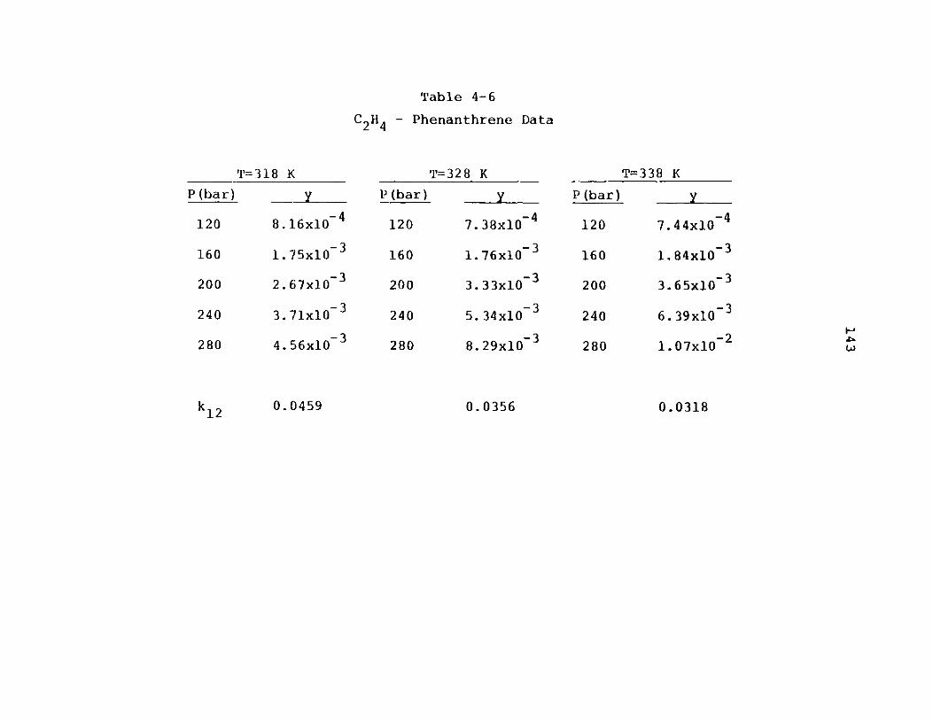
Table 4-6
C2 H - Phenanthrene Data
T=318 K
y
8. 16x10~ 4
1. 7 5x10- 3
-3
2. 67x10-
3. 71x10-3
4. 56x10-3
P(bar)
120
160
200
240
280
T=328 K
-Y
7. 38x10~ 4
1. 76x10-3
3. 33x10-3
5. 34x10-3
8. 29x10-3
T=338 K
P(bar)
120 7.44x10~ 4
160 1. 84x10 3
200 3.65x10⁻³
240 6.39x10⁻³
280 1.07x10⁻²
0.0356
P(bar)
120
160
200
240
280 LJ
k 12 0.0459 0.0318
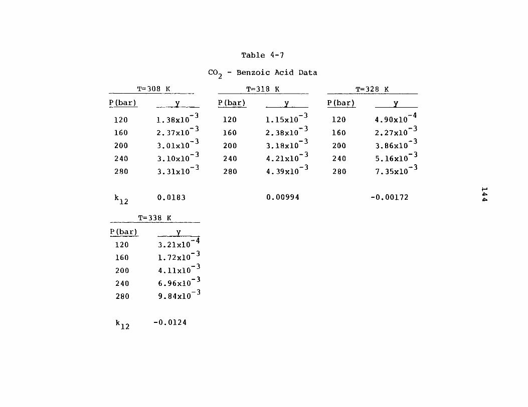
Table 4-7
CO - Benzoic Acid Data
T=318 K
y
1. 38x10-3
2. 37x10-3
3. 01x10-3
3. 10x10-3
3. 31x10-3
0.0183
P(bar)
120
160
200
240
280
y
1. 15x10-3
2. 38x10-3
3. 18x10-3
4.21x10⁻³
4. 39x10-3
P(bar)
120
160
200
240
280
0.00994
y
4. 90x10 4
2.27x10⁻³
3.86x10⁻³
5. 16x10- 3
7. 35x10-3
-0.00172
T=338 K
y
3.21x10~ 4
1. 72x10- 3
4. 11x10-3
6.96x10⁻³
9. 84x10-3
-0.0124
T=308 K
P(bar)
120
160
200
240
280
T=328 K
P(bar)
120
160
200
240
280
H
k12
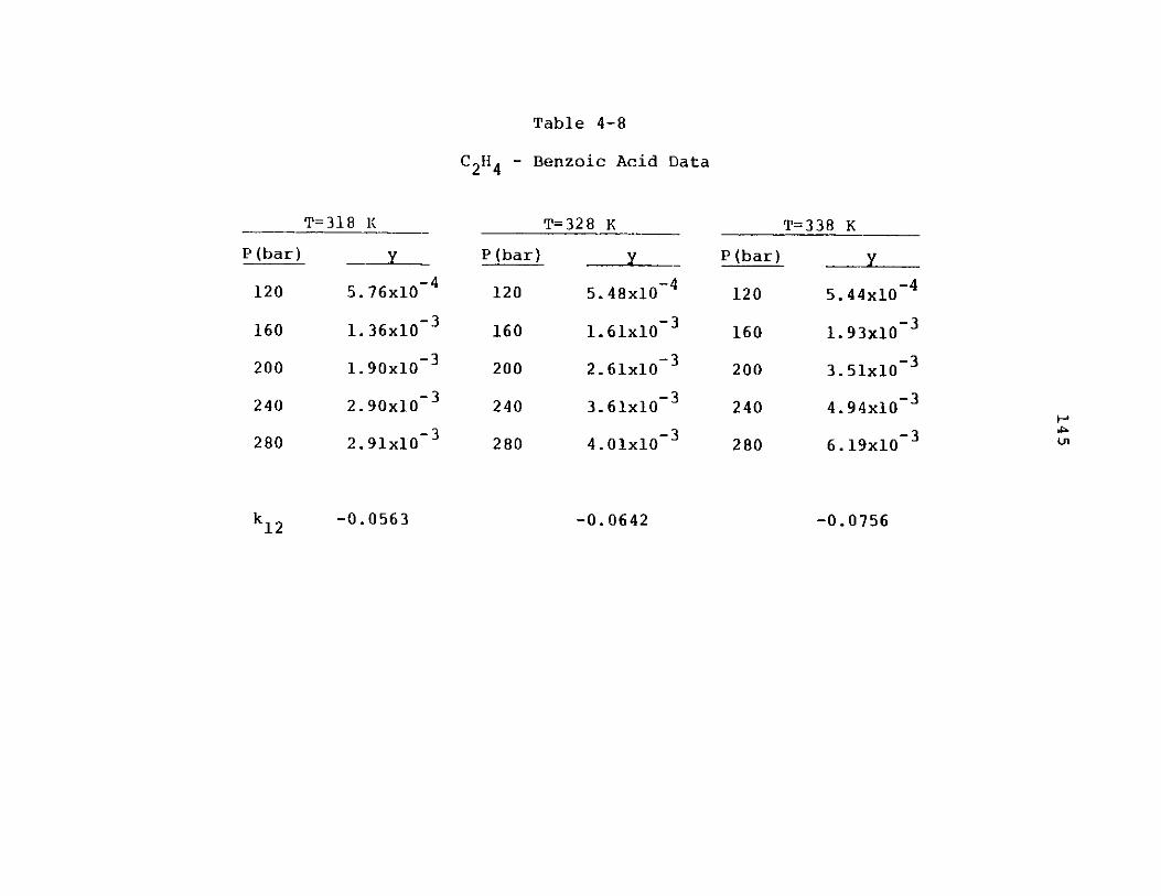
Table 4-8
C 24 - Benzoic Acid Data
=3 T=318 K
P(bar) y
120 5.76x10~ 4
160 1.36x10⁻³
200 1.90x10 3
240 2.90x10⁻³
280 2.91x10⁻³
T=328 K
P (bar)
120
160
200
240
280
T=338 K
5. 48x10~ 4
1.61x10- 3
2.61x10⁻³
3.61x10⁻³
4. 01x10-3
P(bar)
120
160
200
240
280
5. 44x10-4
1. 93x10-3
3. 51x10-3
4.94x10⁻³
6. 19x10-3
k12 -0.0563
H-,P(J1
-0.0642 -0.0756
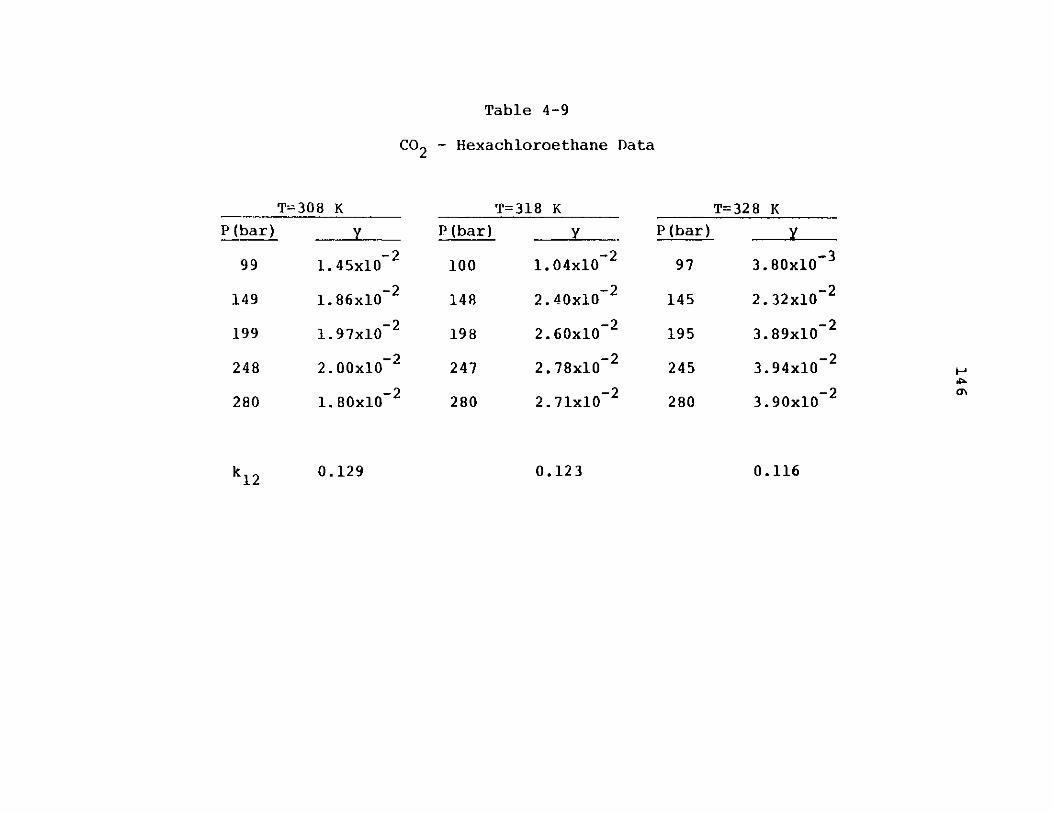
Table 4-9
Co - Hexachloroethane Data
T=308 K
P(bar) y
99 1.45x10⁻²
149 1.86x10⁻²
199 1.97x10⁻²
248 2.00x10⁻²
280 1.80x10⁻²
T=318 K
P(bar) y
100 1.04x10- 2
148 2.40x10- 2
198 2.60x10- 2
247 2.78x10⁻²
280 2.71x10⁻²
T=328 K
P(bar)
97 3.80x10- 3
145 2.32x10⁻²
195 3.89x10⁻²
245 3.94x10⁻²
280 3.90x10⁻²
k12 0.129
Ha'6
0.1160.123
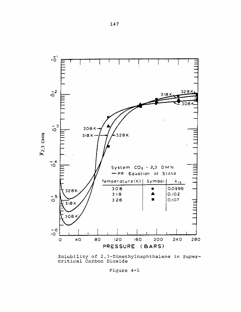
147
1
-2 32810 318 K
308 K-
-310 308 K
Z 318 K - 328 K
-410System C02 2,3 DM N
-PR Equction of Statc'
Temp2ratur4?(K) Symbol k 2
328K 308 0 0.099653 1 8 & 0.102
10 328 O.107 --318 K _
3 08 K
10 1| 1 | Il
0 40 s 120 '60 200 240 280
PRESSURE (BARS)
Solubility of 2,3-Dimethylnaphthalene in Super-critical Carbon Dioxide
Figure 4-1
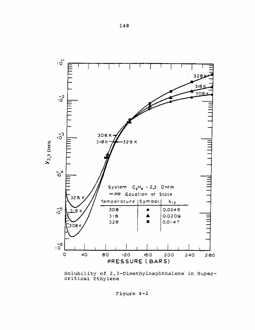
148
- 1
32
318
-2 3010
-3 308 K10Z r318K- 328 K
-410
System C2H4 - 2,3 DMN
328 K - PR Equation of State
-Tampqraturc- Symbol k12
-5 K308 0.024610 IL K3 18 0 .0209
328 0.0147308K
-610 ti|
0 40 80 120 160 200 240 280
PRESSURE (BARS)
Solubility of 2,3-Dimethylnaphthalene in Super-critical Ethylene
Figure 4-2
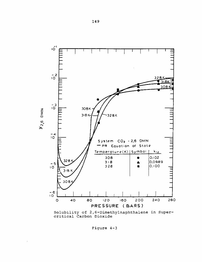
149
10
-210 -- 328
31 -
0308
-3z 10 308 K-
318 K- 328K
-40
Systlm CO2 -2,6 DMNPR Equation of Statc-
Temperature(K) Symbol k,2
308 0 01025 328 318 A 0.0989
1 .- 328 U 0.100.3118 K
-308
-6
0 40 80 120 160 200 240 280
PRESSURE (BARS)
Solubility of 2,6-Dimethylnaphthalene in Super-critical Carbon Dioxide
Figure 4-3
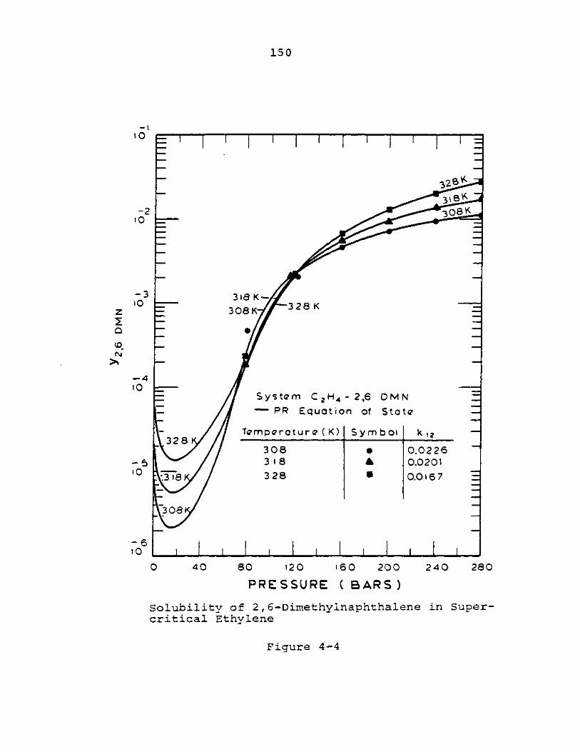
150
10
328
-3\
-2 308 K10 -
-3 318 K-
z -0 308K 328-
-4'0
S YSteM C 2 H4 -2,6 0M N
PR Equation of Stcte
- 328 Temperature(K) Sym bol k12
308 0 0.0226-5 31 & 0.02010 -318 328 0.0167
~08~
-610 I l
0 40 80 120 160 200 240 280
PRESSURE ( BARS)
Solubility of 2,6-Dimethylnaphthalene in Super-critical Ethylene
Figure 4-4
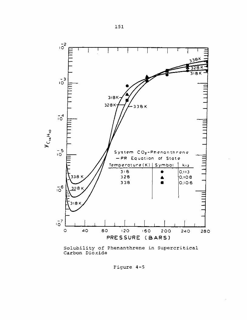
1531
-210
33
318 K-
-310
- 318K
328 K 3 3 BK
-410
~0 System C0 2 -Phenanthrenc'-PR Equation of State
Temper-oture(K) Symbol k12
3 1 8 0.113338K 328 4 0.108
338 U 0.106-6 328 K'0
.318 K
-710
0 40 80 120 '60 200 240 280
PRESSURE (BARS)
Solubility of Phenanthrene in SupercriticalCarbon Dioxide
Figure 4-5
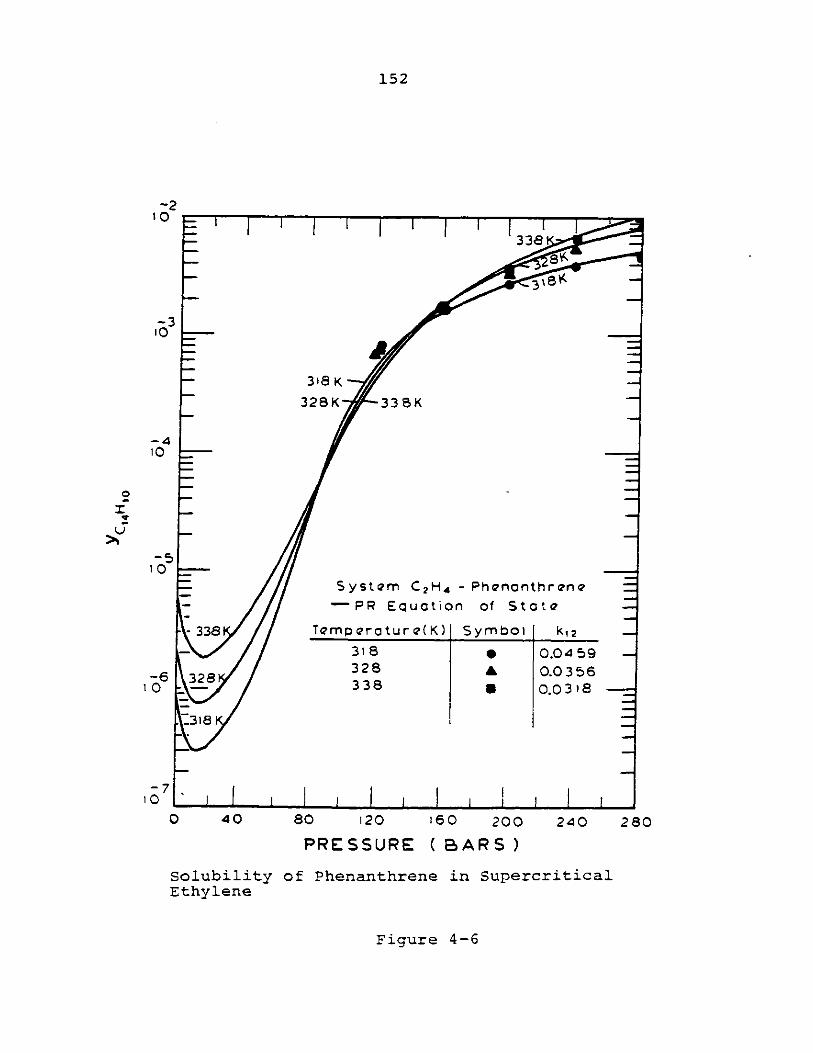
152
-210
338
-310
318 K-
328K v~ 338K
- 4
1 0
Systarm C2H4 -Phenanthrenm 2
-- PR Equation of St a t e-
- 338 Tqrmp ratur e(K) Symbol k12-
-318 0 0.0459 -
-6 328 328 0 .035610 -- 338 0 .0 318 -
.318
100 40 80 120 160 200 240 2830
PRESSURE ( BARS )
Solubility of Phenanthrene in SupercriticalEthylene
Figure 4-6
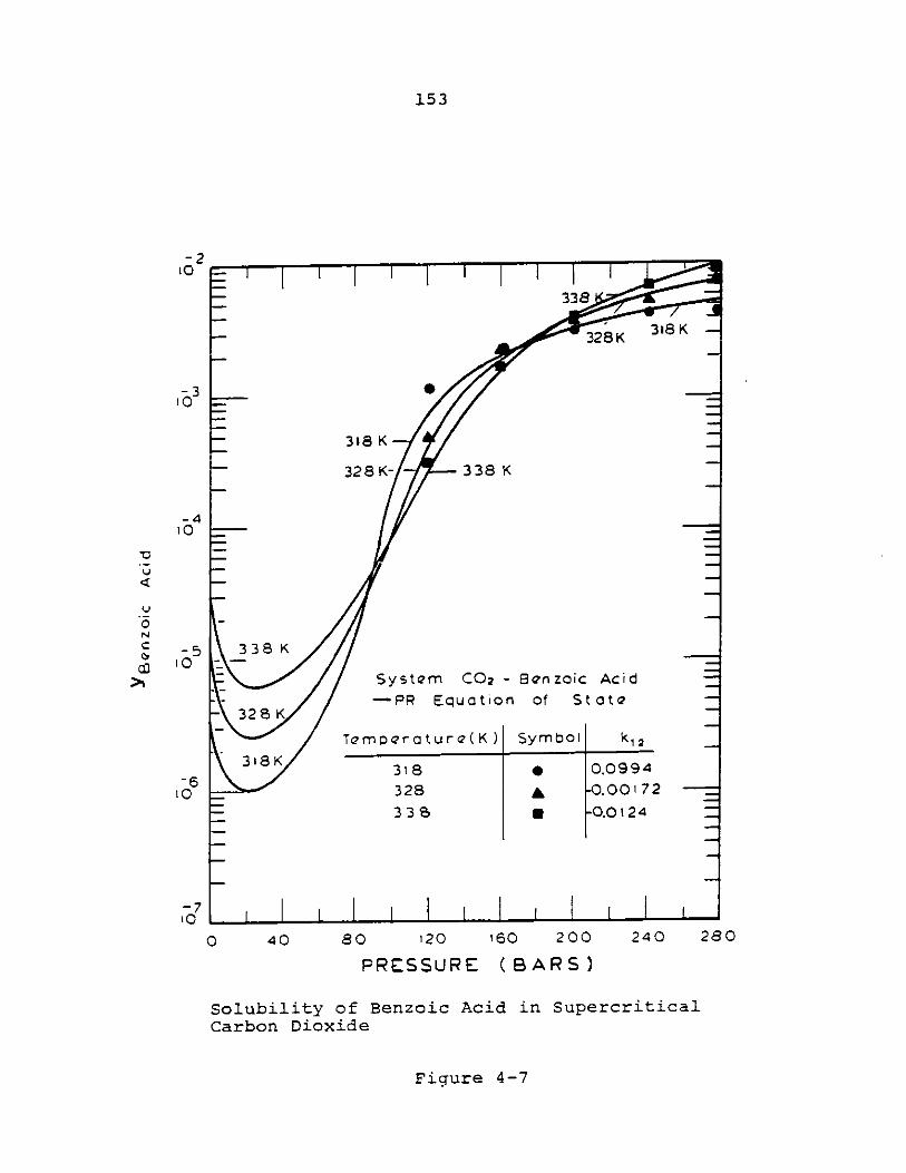
153
0 40 80 120 '60 200 240 280
PRESSURE (BARS)
Solubility of Benzoic Acid in SupercriticalCarbon Dioxide
Figure 4-7
-210
-310
-410
'a
V
NC09
>1
-5l0
-610
-710
-233A8
ItS 31099
328 328K3K2
318 K
328 K- 338 K
338 K
Syst C2 - [BenZoiC ACid- -PR E qu at io n of St ate-
-328 K
Tempqra tur e(K) Symbol k12
3 8 K 31 8 0 .0994
328 0.00172
3 38 -0.0124
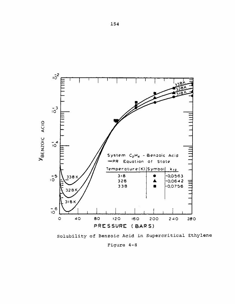
154
-2
10
- 3to
0 40 80 120 160 200 240 280
PRESSURE (BARS)
Solubility of Benzoic Acid in Supercritical Ethylene
Figure 4-8
u
zLL)
-410
System C 2H4 - Benzoic Acid
PR Equation of State
Temperoture(K) Symbol k1 2
338 K 3 18 9 -0.0563328 A -0.0642338 a -0.0756
-328K-
.318 K
-510
-6to
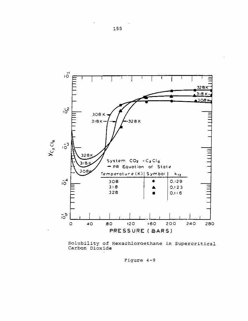
155
-1
328K-
A318 K
&308
-210308 K
318K- 328 K
-34
10 . - --
328K-
318Systcm CO2 -C2 C16
- PR Equation of Statce
308 TempraturQ (K) Symbol!k12
- 4 -308 0 0.129-_ 318 & 0.123
328 0.116
-510 _ _L 1 .. .l .I l I I i
0 40 80 120 160 200 240 280
PRESSURE (BARS)
Solubility of Hexachloroethane in SupercriticalCarbon Dioxide
Figure 4-9
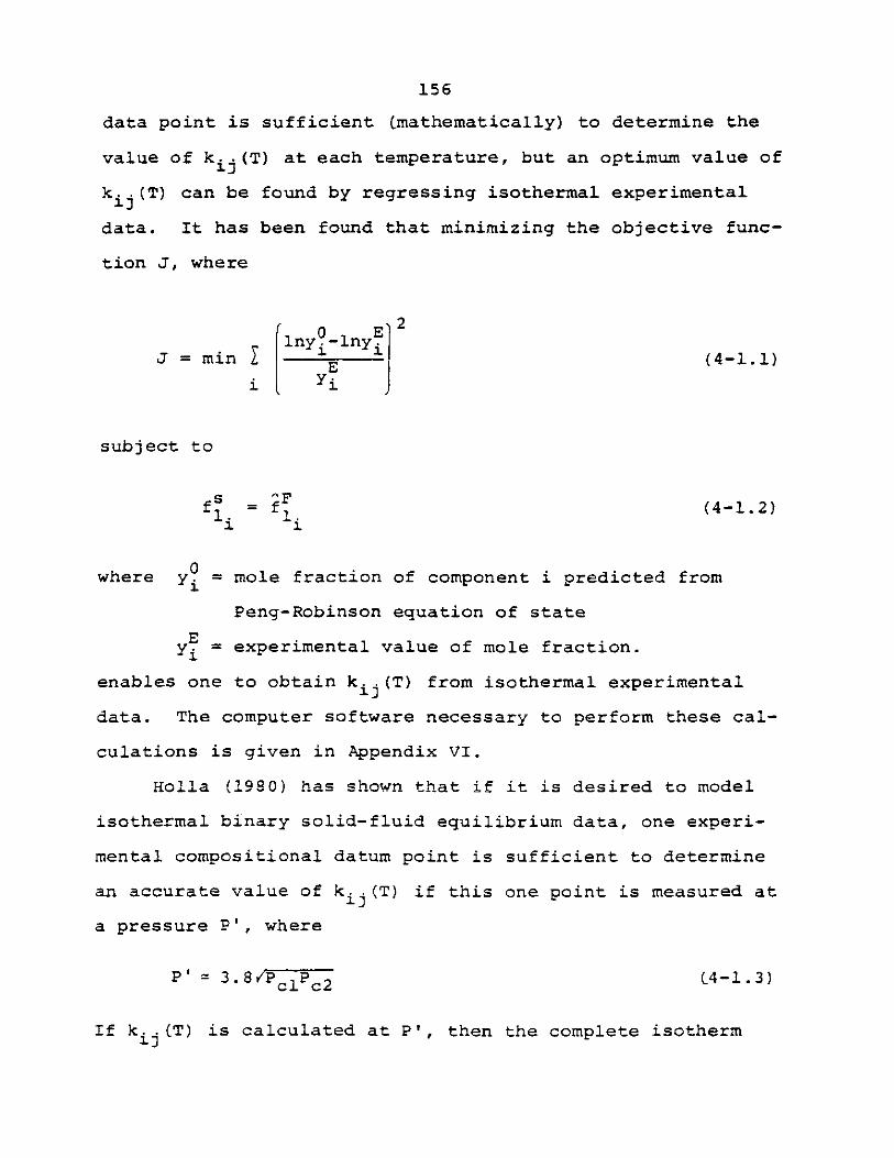
156
data point is sufficient (mathematically) to determine the
value of k..(T) at each temperature, but an optimum value ofIJ
k. (T) can be found by regressing isothermal experimental'Jdata. It has been found that minimizing the objective func-
tion J, where
0 -2lny.-Iny
J = min IE J(4-1.1)
subject to
f = f (4-1.2)
0where y. = mole fraction of component i predicted from
Peng-Robinson equation of state
Ey = experimental value of mole fraction.
enables one to obtain k. .(T) from isothermal experimental'adata. The computer software necessary to perform these cal-
culations is given in Appendix VI.
Holla (1980) has shown that if it is desired to model
isothermal binary solid-fluid equilibrium data, one experi-
mental compositional datum point is sufficient to determine
an accurate value of k. (T) if this one point is measured at
a pressure P', where
P' ~3.8/Pclc2 (4-1.3)
If kI..T) is calculated at P', then the complete isotherm'J
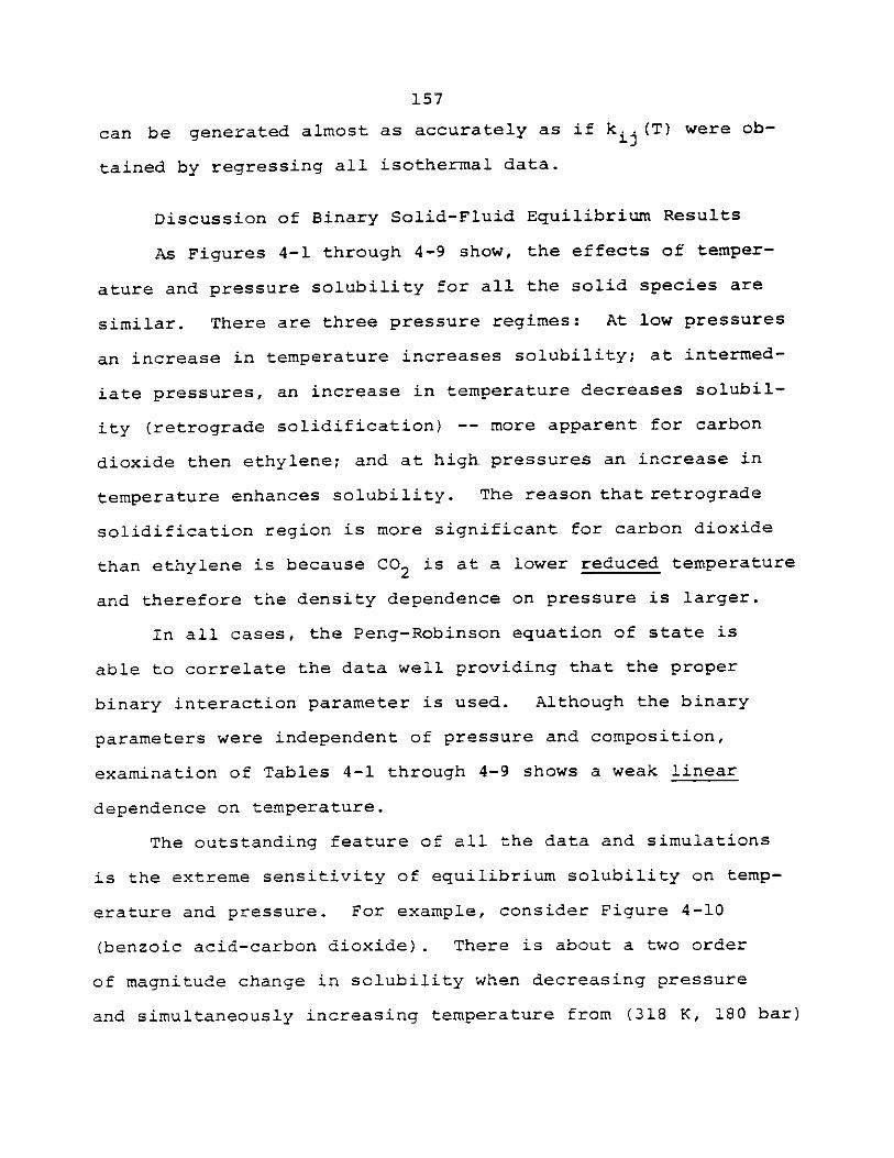
157
can be generated almost as accurately as if k. (T) were ob-
tained by regressing all isothermal data.
Discussion of Binary Solid-Fluid Equilibrium Results
As Figures 4-1 through 4-9 show, the effects of temper-
ature and pressure solubility for all the solid species are
similar. There are three pressure regimes: At low pressures
an increase in temperature increases solubility; at intermed-
iate pressures, an increase in temperature decreases solubil-
ity (retrograde solidification) -- more apparent for carbon
dioxide then ethylene; and at high. pressures an increase in
temperature enhances solubility. The reason that retrograde
solidification region is more significant for carbon dioxide
than ethylene is because CO2 is at a lower reduced temperature
and therefore the density dependence on pressure is larger.
In all cases, the Peng-Robinson equation of state is
able to correlate the data well providing that the proper
binary interaction parameter is used. Although the binary
parameters were independent of pressure and composition,
examination of Tables 4-1 through 4-9 shows a weak linear
dependence on temperature.
The outstanding feature of all the data and simulations
is the extreme sensitivity of equilibrium solubility on temp-
erature and pressure. For example, consider Figure 4-10
(benzoic acid-carbon dioxide). There is about a two order
of magnitude change in solubility when decreasing pressure
and simultaneously increasing temperature from (318 K, 180 bar)
a l
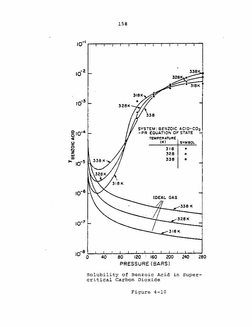
158
338
318K
318K
-O - 328K
/ 338
SYSTEM: BENZOIC AC!O-CO 290 -4 - -PR EQUATION OF STATE
TEMPERATUREo (K) SYMSOL
318328
S10-5 338K 338 *
328K
318 K
1006 -IDEAL GAS
- -338 K
10~ - 3 28 K
.3 18 K
0 40 so 120 160 200 240 280
PRESSURE (BARS)
Solubility of Benzoic Acid in Super-critical Carbon Dioxide
Figure 4-10
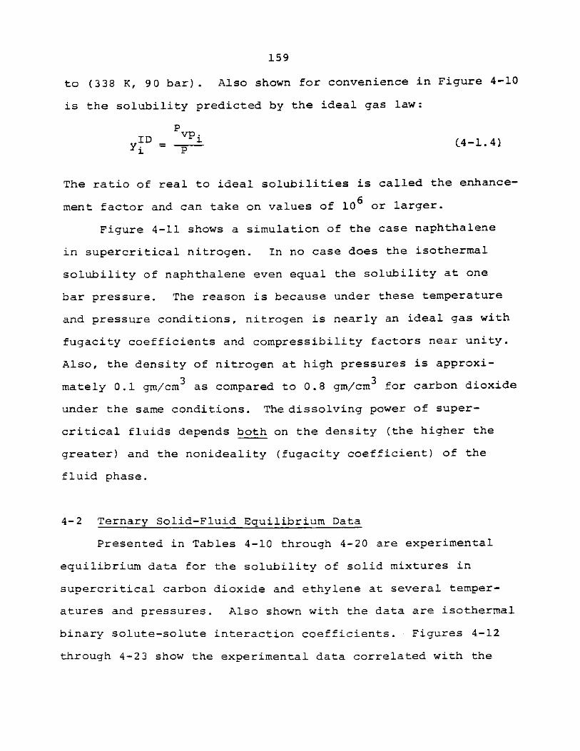
159
to (338 K, 90 bar). Also shown for convenience in Figure 4-10
is the solubility predicted by the ideal gas law:
P
yID - .i (4-1.41I P
The ratio of real to ideal solubilities is called the enhance-
ment factor and can take on values of 106 or larger.
Figure 4-11 shows a simulation of the case naphthalene
in supercritical nitrogen. In no case does the isothermal
solubility of naphthalene even equal the solubility at one
bar pressure. The reason is because under these temperature
and pressure conditions, nitrogen is nearly an ideal gas with
fugacity coefficients and compressibility factors near unity.
Also, the density of nitrogen at high pressures is approxi-
mately 0.1 gm/cm3 as compared to 0.8 gm/cm3 for carbon dioxide
under the same conditions. The dissolving power of super-
critical fluids depends both on the density (the higher the
greater) and the nonideality (fugacity coefficient) of the
fluid phase.
4-2 Ternary Solid-Fluid Equilibrium Data
Presented in Tables 4-10 through 4-20 are experimental
equilibrium data for the solubility of solid mixtures in
supercritical carbon dioxide and ethylene at several temper-
atures and pressures. Also shown with the data are isothermal
binary solute-solute interaction coefficients.- Figures 4-12
through 4-23 show the experimental data correlated with the
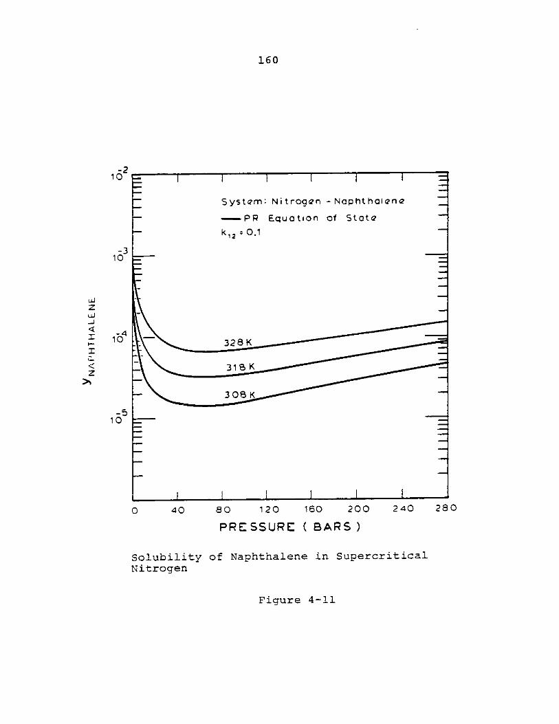
160
0 40
SolubilityNitrogen
80 120 160 200 240
PRESSURE ( BARS)
of Naphthalene in Supercritical
Figure 4-li
-210
-
3
10
-510
uJ
zJ
z
-_ I I I I I I -
Sys tem: NitroQen - Naphthol2ne
- PR Eqution of StatQ4
k12 :0.1
328 K
3 1K
W3 OWf8 K
280

161
Table 4-10
CO2 (1); Benzoic Acid (2); Naphthalene (3) Mixture Data
T=308K
y(Benzoic acid).
2. 93x10-3
4. 01x10-3
5.22x10⁻³
5.46x10⁻³
5. 61x10-3
y (Naphthalene)
1. 44x10-2
1. 73x10-2
2.06x10⁻²
2. 08x10-2
2. 12x10-2
k12= 0.0183
k13= 0.0959
k 23= 0.000
P (bar)
120
160
200
240
280
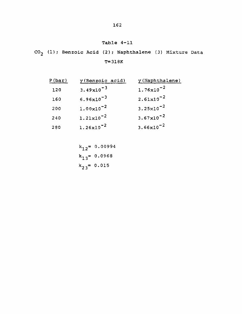
162
Table 4-11
CO2 (1); Benzoic Acid (2); Naphthalene (3) Mixture Data
T=318K
y(Benzoic acid)
3.49x10⁻³
6.96x10⁻³
1. 00x10-2
1.21x10⁻²
1.26x10⁻²
y(Naphthalene)
1.76x10⁻²
2.61x10⁻²
3.25x10⁻²
3.67x10⁻²
3.66x10⁻²
k12= 0.00994
k13= 0.0968
k 23= 0.015
P (bar)
120
160
200
240
280
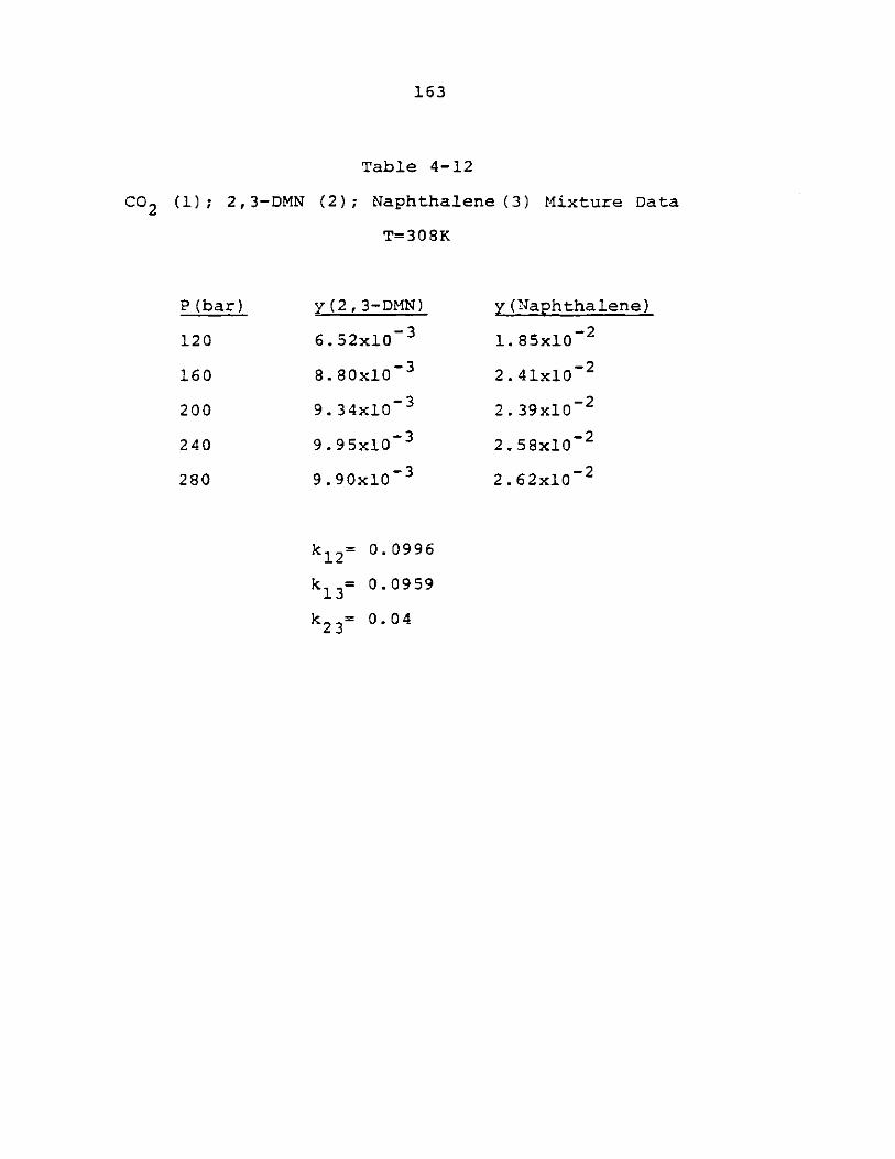
163
Table 4-12
co2 (1); 2,3-DMN (2); Naphthalene (3) Mixture Data
T=308K
y(2, 3-DMN)
6. 32x10-3
8.80x10- 3
9. 34x10-3
9.95x10⁻³
9.90x10⁻³
y (Naphthalene)
1.85x10⁻²
2.41x10⁻²
2. 39x10 -2
2.58x10⁻²
2.62x10⁻²
k 12=0.0996
kl3= 0.0959
k 23= 0.04
P (bar)
120
160
200
240
280
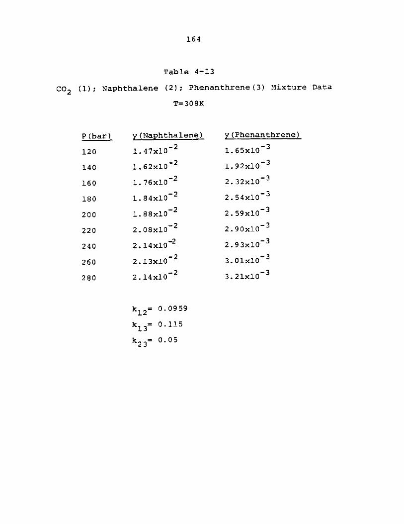
164
Table 4-13
CO 2 (1); Naphthalene (2); Phenanthrene(3) Mixture Data
T=308K
y (Naphthalene)
1. 47x10- 2
1. 62x10- 2
1. 76x10- 2
1. 84x10- 2
1. 88x10- 2
2. 08x10- 2
2. 14x10-2
2. 13x10-2
2. 14x10 2
y(Phenanthrene)
1.65x10⁻³
1.92xl0-3
2.32x10⁻³
2.54x10⁻³
2.59x10⁻³
2.90x10⁻³
2.93x10⁻³
3. 01x10-3
3. 21x10-3
k 12=0.0959
k13= 0.115
k23= 0.05
P (bar)
120
140
160
180
200
220
240
260
280
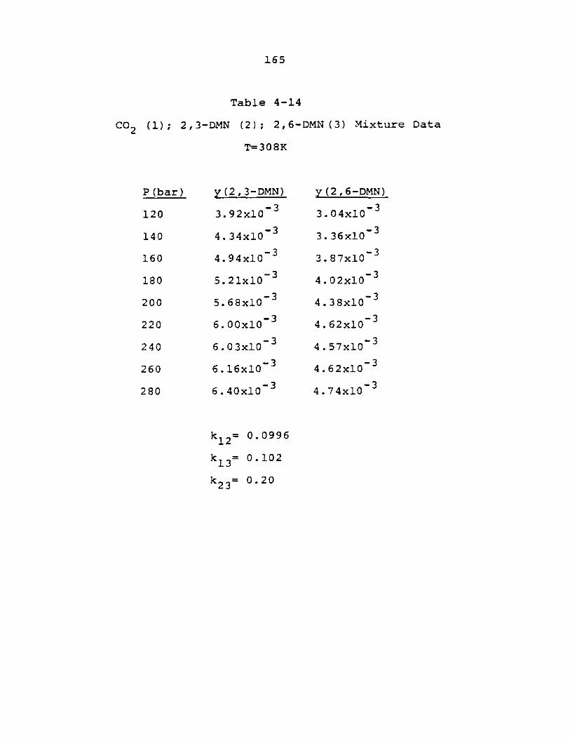
165
Table 4-14
CO2 (1); 2,3-DMN (2); 2,6-DMN (3) Mixture Data
T=308K
y (2,3-DMN)
3. 92xi0-3.
4. 34x10 -3
4. 94xl0-3
5. 21x10-3
5.68x10⁻³
6. 00x10-3
6.03x10⁻³
6. 16x10-3
6 . 40x10-3
y(2,6-DMN)
3. 04x10- 3
3. 36x10-3
3. 87x10 3
4. 02x10-3
4. 38x10 3
4.62x10⁻³
4.57x10⁻³
4. 62x10-3
4. 74x10-3
k12= 0.0996
k3 = 0.102
k23= 0.20
P (bar)
120
140
160
180
200
220
240
260
280
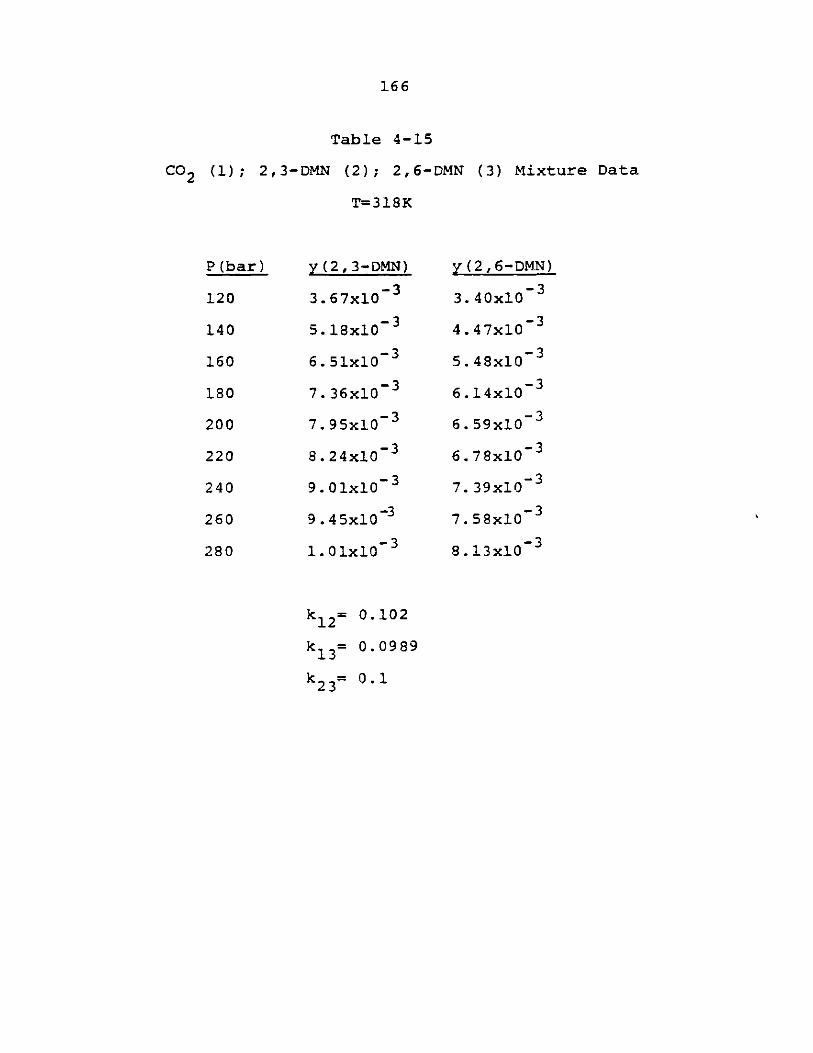
166
Table 4-15
Co2 (1); 2,3-DMN (2); 2,6-DMN (3) Mixture Data
T=318K
y(2,3-DMN)
3. 67x10- 3
5. 18x10-3
6. 51x10-3
7. 36x10-3
7. 95x10- 3
8. 24x10-3
9. 01x10-3
9. 45x10-3
1. 01x10-3
y(2,6-DMN)
3. 40x10- 3
4.47x10- 3
5. 48x10-3
6.14x10- 3
6. 59x10- 3
6. 78x10- 3
7. 39x10-3
7. 58x10-3
8.13x10⁻³
k 2= 0.102
k13= 0.0989
k 23= O
P (bar)
120
140
160
180
200
220
240
260
280
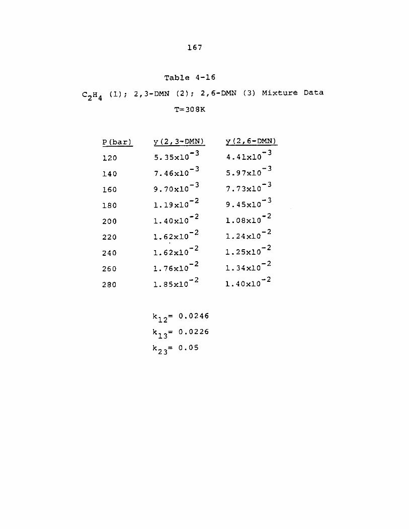
167
Table 4-16
C2 H4 (1); 2,3-DMN (2); 2,6-DMN (3) Mixture Data
T=308K
y(2,3-DMN)
5. 35x10-3
7. 46x10-3
9. 70x10-3
1. 19x10-2
1. 40x10-2
1. 62x10-2
1. 62x10-2
1. 76x10-2
1. 85x10-2
y(26-DMN)
4. 41x103
5.97x10⁻³
7. 73x103
9. 45x10-3
1.08x10⁻²
1. 24x10-2
1.25x10⁻²
1. 34x10-2
1. 40x10-2
k2 0.0246
k 3= 0.0226
k 23= 0.05
P (bar)
120
140
160
180
200
220
240
260
280

168
Table 4-17
CO2 (1); Benzoic Acid (2); Phenanthrene(3) Mixture Data
T=308K
y(Benzoic acid)
1. 84x10- 3
2.44x10⁻³
2. 95x10-3
3.28x10⁻³
3. 70x10-3
y(Phenanthrene)
1. 02x10- 3
1. 36x10-3
1. 63x10-3
1. 87x10-3
2. 05x10-3
k12= 0.0183
k13= 0 115
k23= 0.2
P (bar)
120
160
200
240
280
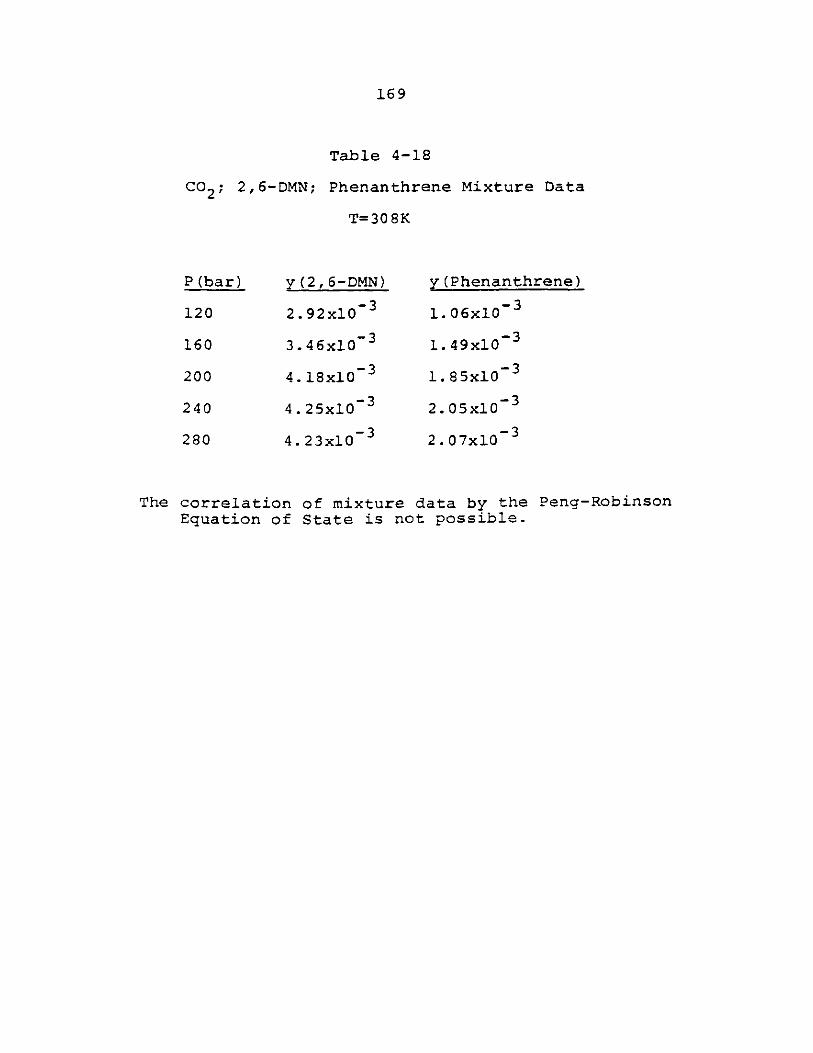
169
Table 4-18
Co2 ; 2,6-DMN; Phenanthrene Mixture Data
T=308K
y(2,6-DMN)
2. 92xl0-3
3.46x10⁻³
4. 18x10-3
4. 25x10-3
4.23xl 0-3
y(Phenanthrene)
1.06x10⁻³
1.49x10⁻³
1.85x10⁻³
2. 05xl03
2.07x10⁻³
The correlation of mixture data by the Peng-RobinsonEquation of State is not possible.
P (bar)
120
160
200
240
280
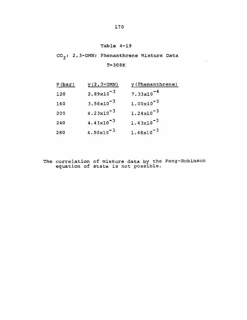
170
Table 4-19
co2; 2,3-DMN; Phenanthrene Mixture Data
T=308K
y (2, 3-DMN)
2. 89x10- 3
3.56x10- 3
4. 23x10-3
4. 43x10-3
4. 50x10- 3
y (Phenanthrene)
7. 33x4Q4
1. 00x10 3
1. 24xl0-3
1. 43x10 3
1. 48x10-3
The correlation of mixture data by the Peng-Robinsonequation of state is not possible.
P (bar)
120
160
200
240
280
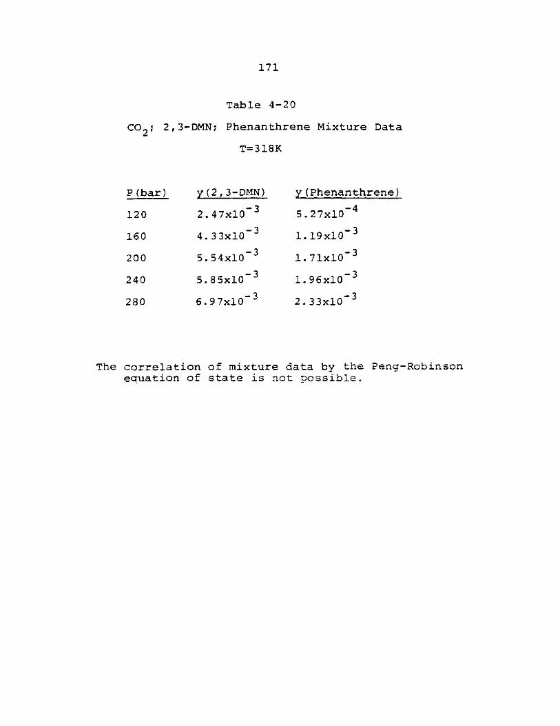
171
Table 4-20
Co2 ; 2,3-DMN; Phenanthrene Mixture Data
T=318K
y(2,3-DMN)
2. 47x10-3
4. 33xl0-3
5. 54x10-3
5. 85x10-3
6.97x10⁻³
y (Phenanthrene)
5. 27x10~ 4
1. 19x10-3
1. 71x10 3
1. 96x10-3
2. 33x10-3
The correlation of mixture data by the Peng-Robinsonequation of state is not possible.
P (bar)
120
160
200
240
280
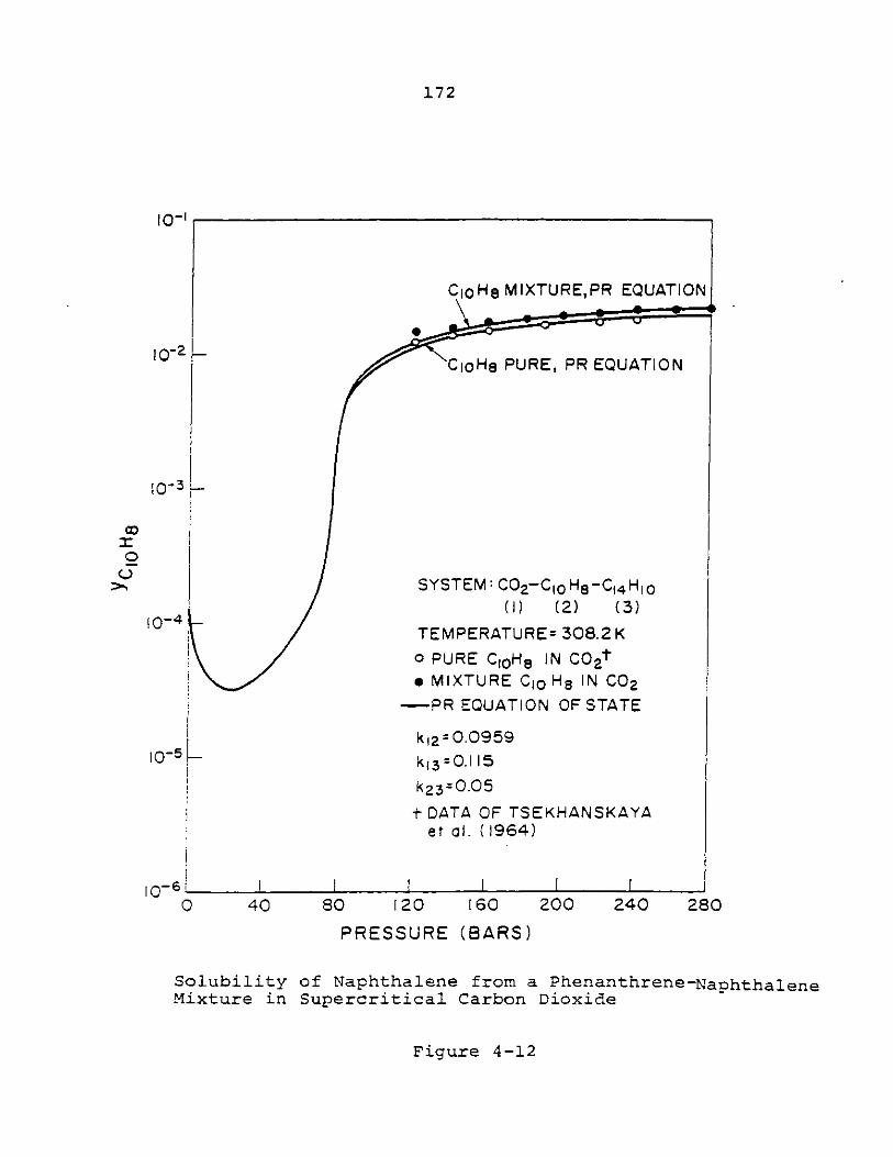
172
10-1
Cio HseMIXTUR E, PR EQUATION
10-2CioH8 PURE, PR EQUATION
10-
SYSTEM: CO-Cgo He8 0C14 HfQ(1) (2) (3)
TEMPERATURE= 308.2 K
o PURE COH8 IN C02t
e MIXTURE CIO H8 IN CO2
-PR EQUATION OF STATE
ka=0.095910-5k3= .lk13=O.I IS
k23z0.05
t DATA OF TSEKHANSKAYAet al. (1964)
10 6 11I I1 -- I -I0 40 80 120 160 200 240 280
PRESSURE (BARS)
Solubility of Naphthalene from a Phenanthrene-NaphthaleneMixture in Supercritical Carbon Dioxide
Figure 4-12
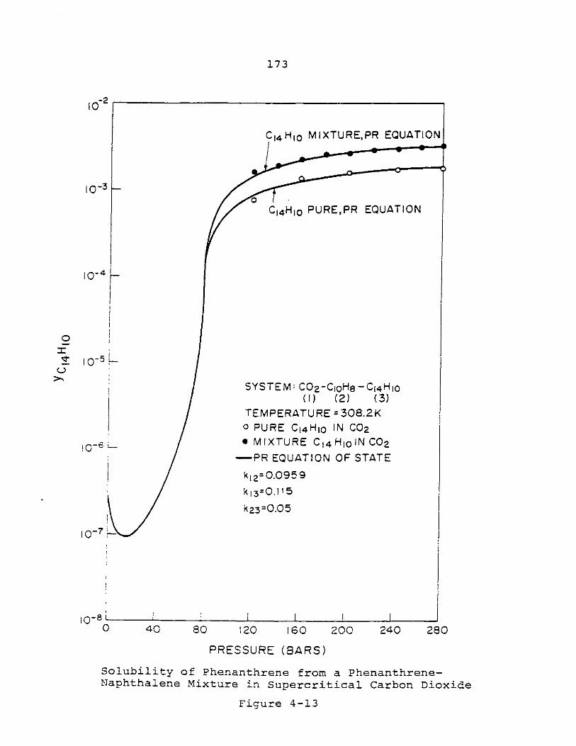
173
C14 HIO MIXTURE,PR EQUATION
10-3
100
io- -0C4 HIO PURE,PR EQUATION
10- 5
SYSTEM: CO 2 -CoHe-0C 4 H1 o(I) (2) (3)
TEMPERATURE =308.2K0 PURE C14 HIO IN C0 2
-_ * MIXTURE C1 4 HIOIN C0 2
-PR EQUATION OF STATE
ki=0.0 9 5 9
k 13=0.115
k23=0.05
10-7-1-
io- 8 40 40 80 120 160 200 240 280
PRESSURE (BARS)
Solubility of Phenanthrene from a Phenanthrene-Naphthalene Mixture in Supercritical Carbon Dioxide
Figure 4-13
0=
'1~C)
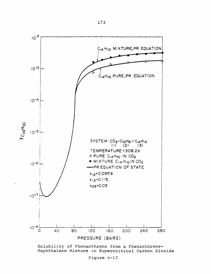
173
C14 H i MIXTURE, PR EQUA TION
10-3
C14HIO PURE,PR EQUATION
io-4
\0-5
SYSTEM: C0 2 -CIOH 8 --C14H 10(1) (2) (3)
TEMPERATURE =308.2K0 PURE C14 HIO IN C02
10-6 0 MIXTURE C14 HIOIN C0 2
-PR EQUATION OF STATE
k 2=0.0959
k 13 =0.115
k23=0.05
10~7
10-810 40 80 120 160 200 240 280
PRESSURE (BARS)
Solubility of Phenanthrene from a Phenanthrene-Naphthalene Mixture in Supercritical Carbon Dioxide
Figure 4-13
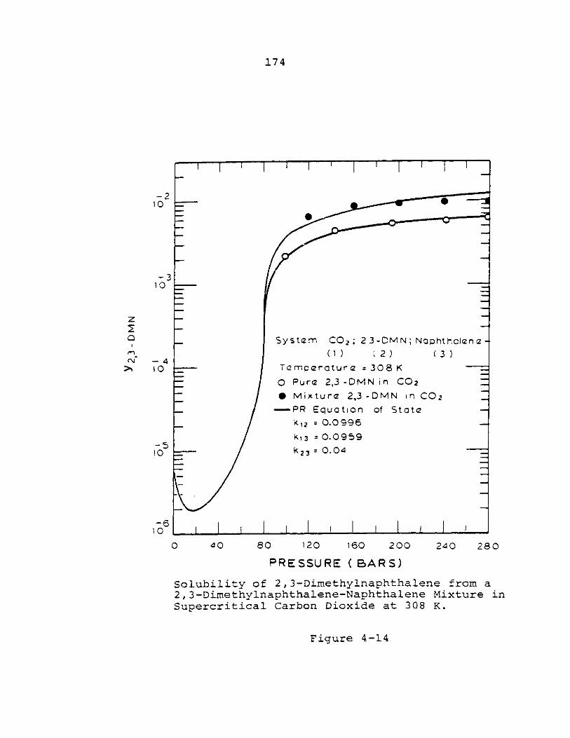
174
102
-310
Sys tzm C02; 2 3 -DM N; Nophthalnca -(1) (2) (3)
N 4> 10F---qmperature =308 K
0 Pure 2,3 -DMN in C02
* Mixture 2,3 -DMN In CO2-- PR Equation of State
k12=z-0.0996
k13 = :0.0959
0 _k 2 3 = 0.04
-610 1I I I
0 40 80 120 160 200 240 280
PRESSURE (BARS)
solubility of 2,3-Dimethylnaphthalene from a2,3-Dimethylnaphthalene-Naphthalene Mixture inSupercritical Carbon Dioxide at 308 K.
Figure 4-14
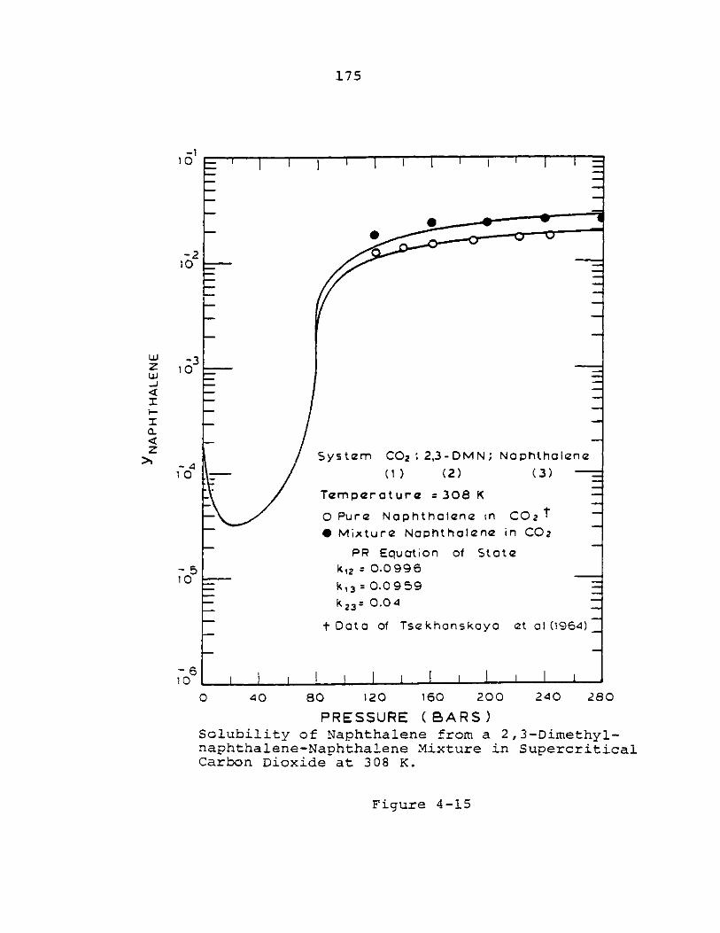
175
-110
-210
z 10--J
>1Sys t2m C02; 2,3-DMN; Nophthalana
10 -- ( ) (2) (3)
Tempercit ure = 308 K-
- O0 Pur(2 Naphthalene in C02
0Mixtur- Naphthalana In C02
PR Equation of Stata
-5 k12 = 00996
10 k13 = 0.0 959
k 23= 0.0 4
~ t Datao of Tse khonskaya (2t al (1964)
-610
0 40 80 120 160 200 240 280
PRESSURE (BARS)Solubility of Naphthalene from a 2,3-Dimethyl-naphthalene-Naphthalene Mixture in SupercriticalCarbon Dioxide at 308 K.
Figure 4-15
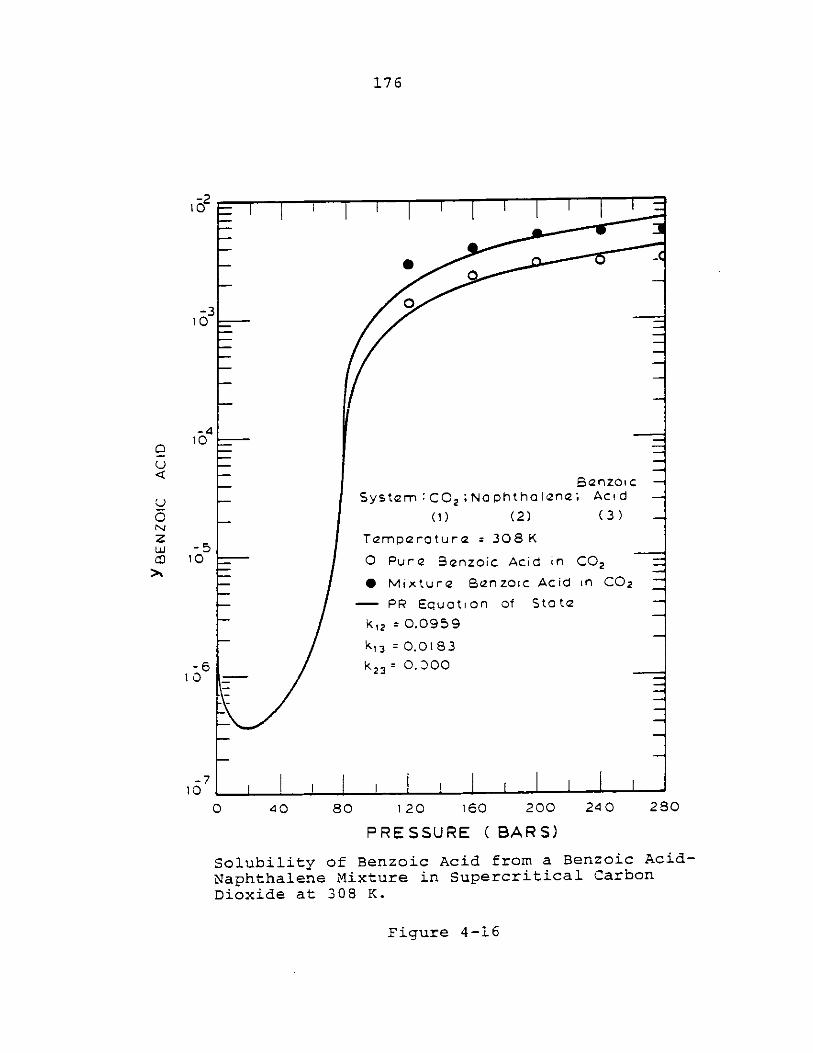
176
Bcnzoi cSystemCO 2M;Naphtholn; Acid
(1) (2) ( 3)
Temperature = 308 K
o Pure Benzoic Acid in C02* Mixture Ben zoic Acid in C02
- PR Equation of State
k12 =0.0959
k,3 0.0183
k 23 = 0.Z00
I I
0 40 80 120 160 200 240 280
PRESSURE (BARS)
Solubility of Benzoic Acid from a Benzoic Acid-Naphthalene Mixture in Supercritical CarbonDioxide at 308 K.
Figure 4-16
-210
-310
0u-
u
NJzuiJ -+
z~
-410
-510
-610
-710
I II I I I I I I I I I I- - I
I II I I I
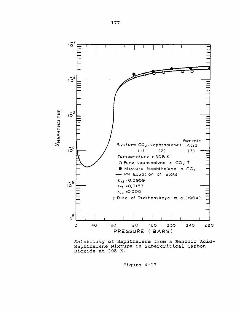
177
1
-210
- -3z 10
z ~Banzoi c
System: C0 2 ;Naphthalcne;ACid0(1) (2) (3)
Temperature = 308 K
o Pure Naphthalene in C02 t
* Mixture Naphtholene in 002- PR Equation of State
- k 12 =0-095910 k13 =0.0183
k23 =0.000
t Data of Tsekhonskaya et a.(1964)
-610 1ii _. I i 1
0 40 80 120 160 200 240 220PRESSURE (BARS)
Solubility of Naphthalene from a Benzoic Acid-Naphthalene Mixture in Supercritical CarbonDioxide at 308 K.
Figure 4-17
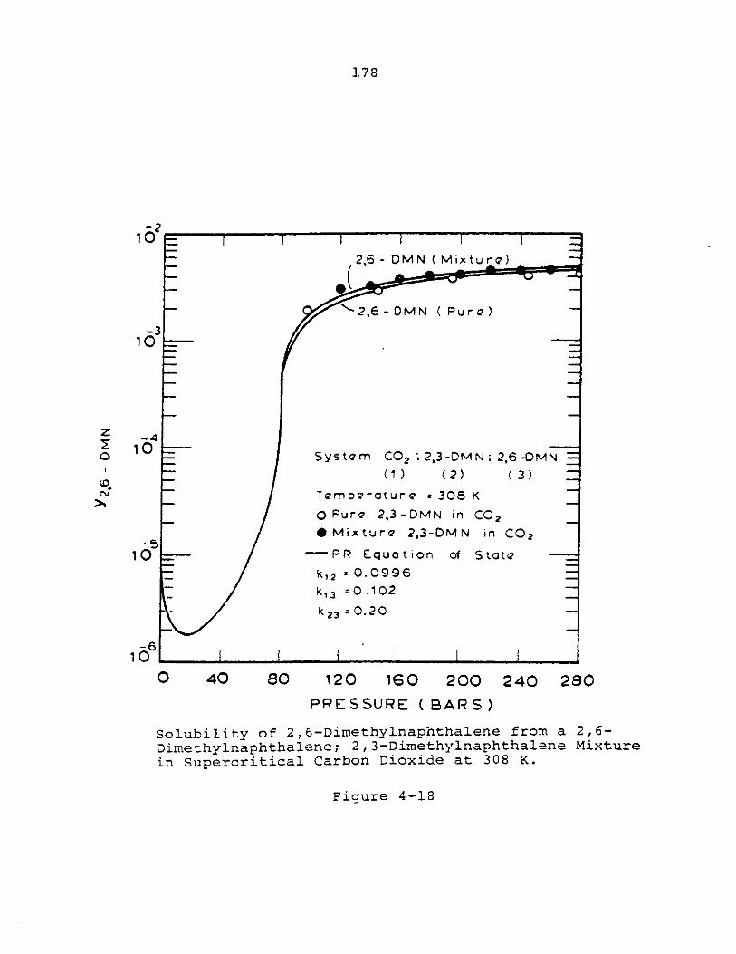
178
-210
2,16 - DMN ( MIxturq),,.
2,6 - OMN( Pur e)
-0
-4
10 - --S Osysteom C02 ;2,3-DM N; 2,6 -OMN
(1) (2) (3)
Temperoture = 308 K
o PurQe 2,3 - DMN in CO,*Mixture 2,3-DMN in C02
1----PR Equation of S tct -
k12 = 0.0996k13 0-102
k 23 z0.20
-610 .ii
0 40 80 120 160 200 240 280
PRESSURE (BARS)
Solubility of 2,6-Dimethylnaphthalene from a 2,6-Dimethylnaphthalene; 2,3-Dimethylnaphthalene Mixturein Supercritical Carbon Dioxide at 308 K.
Figure 4-18
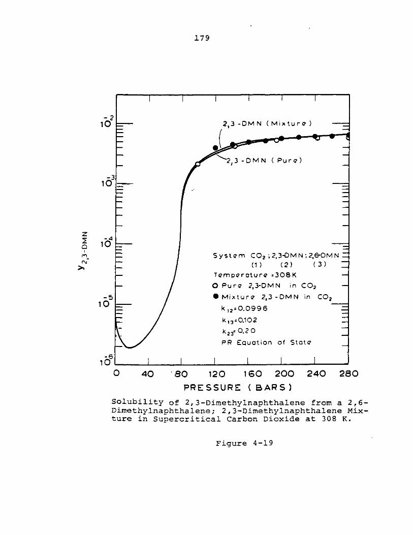
179
-210 =-2,3 -OMN (Mixtura -
23 -D0M N( Pu r 4)
-310-
System C0 2 ;2,3-DMN ;2,6-DMNS(1) (2) (3)
Temporoture =308K
0 Pure 2,3-DMN in C02
-5 *Mixturc' 2,3-DMN in C02
10 k 22-0.0996
k, 3 =O.102
k23=0.2 0PR Equation of StotQ
106
0 40 _80 120 160 200 240 280
PRESSURE (BARS)
Solubility of 2,3-Dimethylnaphthalene from a 2,6-Dimethylnaphthalene; 2, 3-Dimethylnaphthalene Mix-ture in Supercritical Carbon Dioxide at 308 K.
Figure 4-1.9
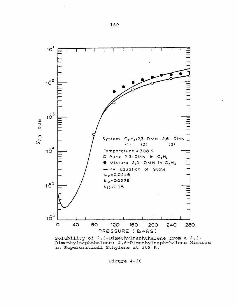
180
10-
-210
-310
z-
N System C 2 H4 ;2,3-DMN;2,6-DMN(i) (2) (3)
-410 Temperature = 308 K
o Pure 2.3-DMN in C 2H4
* Mixture 2,3-DMN in C2 H 4
-PR Equation of Stata
k1 2 =0.0246
-5 k13=0.022610 -- k 23 =0.0 5 ~ -
106
0 40 80 120- 160 200 240 280PRESSURE ( BARS)
Solubility of 2,3-Dimethylnaphthalene from a 2,3-Dimethylnaphthalene; 2,6-Direthylnaphthalene Mixturein Supercritical Ethylene at 308 K.
Figure 4-20
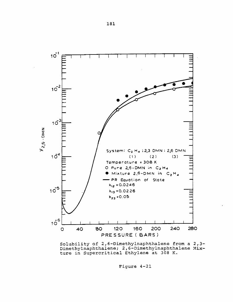
181
-110 1- - 1 1 1 1 1 1
10
-3id 2-
15 - ----z
System: C2 H 4 ;2,3 DMNi 2,6 DMN
10 (1) (2) (3)
Temperature = 308 Ko Pure 2,6-DMN in C2H4
*Mixture 2,6-DMN in C2 H 4-PR Equation of State
k1 2=0.0246
10 --T.k13 =0.02 26 ~~
10 1i i i . I
0 40 $0 120 160 200 240 280PRESSURE ( BARS)
Solubility of 2,6-Dimethylnaphthalene from a 2,3-Dimethylnaphthalene; 2,6-Dimethylnaphthalene Mix-ture in Supercritical Ethylene at 308 K.
Figure 4-21
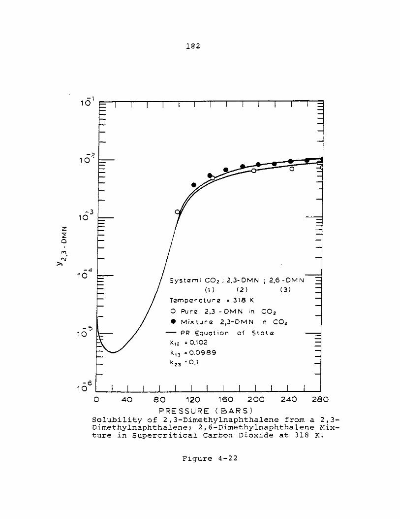
182
-110 -1 1 1 t
-210
-310
-410 System: C02 ;;2,3-DMN ; 2,6 -DMN
(1) (2) (3)
Temperature = 318 K
o Pure 2,3 - DMN in C02
* Mix ture 2,3-DMN in CO2
10- PR Equation of Sttate
k12 =0.102
k1,= 0.0989k 23 :0.1
-61 0 t_ I I I I I I I I I I I I
0 40 80 120 160 200 240 280
PRESSURE (BARS)Solubility of 2,3-Dimethylnaphthalene from a 2,3-Dimethylnaphthalene; 2,6-Dimethylnaphthalene Mix-ture in Supercritical Carbon Dioxide at 318 K.
Figure 4-22
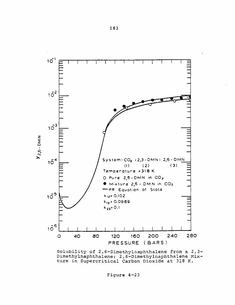
183
-110 1 I I
-210
-310
z
-4 System:C0 2 ;2,3-DMN - 2,6-DMN-0 (1) (2) (3) -
Temperature =318 K (3)
o Pure 2,6-DMN in C02
* Mixtura 2,6 - DMN in C02
PR Equation of State1(55--k 12= 0.102
k 3 =:0.09 89
k23 =O,1
-6
0 40 80 120 160 200 240 280PRESSURE (BARS)
Solubility of 2,6-Dimethylnaphthalene from a 2,3-Dimethylnaphthalene; 2,6-Dimethylnaphthalene Mix-ture in Supercritical Carbon Dioxide at 318 K.
Figure 4-23
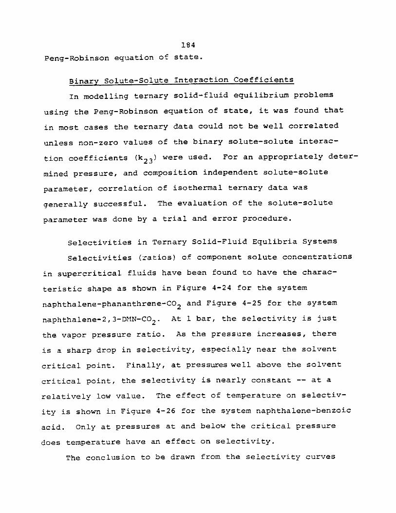
184
Peng-Robinson equation of state.
Binary Solute-Solute Interaction Coefficients
In modelling ternary solid-fluid equilibrium problems
using the Peng-Robinson equation of state, it was found that
in most cases the ternary data could not be well correlated
unless non-zero values of the binary solute-solute interac-
tion coefficients (k23 ) were used. For an appropriately deter-
mined pressure, and composition independent solute-solute
parameter, correlation of isothermal ternary data was
generally successful. The evaluation of the solute-solute
parameter was done by a trial and error procedure.
Selectivities in Ternary Solid-Fluid Equlibria Systems
Selectivities (ratios) of component solute concentrations
in supercritical fluids have been found to have the charac-
teristic shape as shown in Figure 4-24 for the system
naphthalene-phananthrene-CO2 and Figure 4-25 for the system
naphthalene-2,3-DMN-CO2 . At 1 bar, the selectivity is just
the vapor pressure ratio. As the pressure increases, there
is a sharp drop in selectivity, especially near the solvent
critical point. Finally, at pressures well above the solvent
critical point, the selectivity is nearly constant -- at a
relatively low value. The effect of temperature on selectiv-
ity is shown in Figure 4-26 for the system naphthalene-benzoic
acid. Only at pressures at and below the critical pressure
does temperature have an effect on selectivity.
The conclusion to be drawn from the selectivity curves
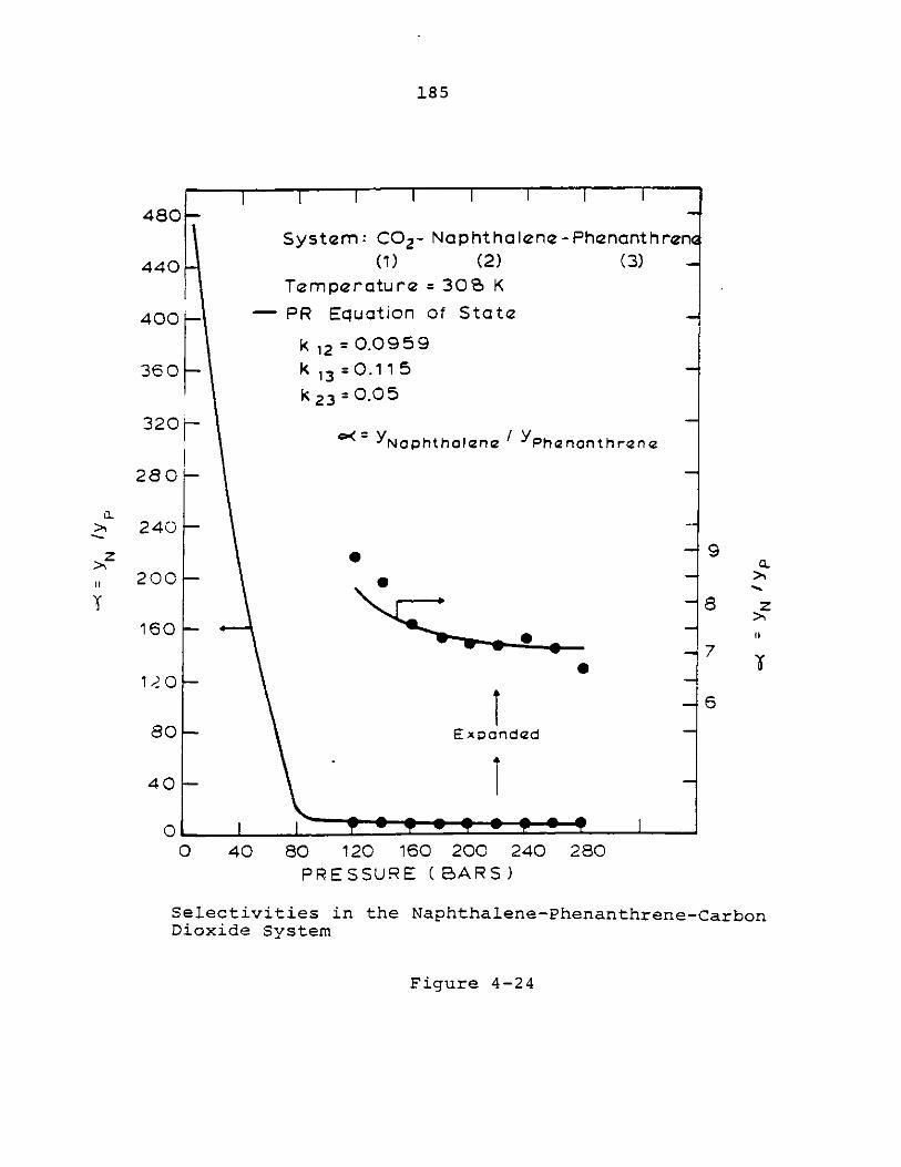
185
480
440
400
360-
3 2 0
280
240
200-
160 -
120 -
80-
40
0
Syste I
I I I I I
00 C2- Nap ht hale ne -Phencnt hrenc(1) (2) (3)
Temperature = 30% K
- PR Equation of State
k 12 = 0.0959k 13 = 0.11 5
k 2 3 = 0.05
0< NOphtholene /Phenanthrene
0
Expandad
IF w
C-
S z
-46
o 40 80 120 160 200 240 280PRESSURE (BARS)
Selectivities in the Naphthalene-Phenanthrene-CarbonDioxide System
Figure 4-24
C-
z
I'
y
40 1 a 1 40 00lahI
Adh
-9r
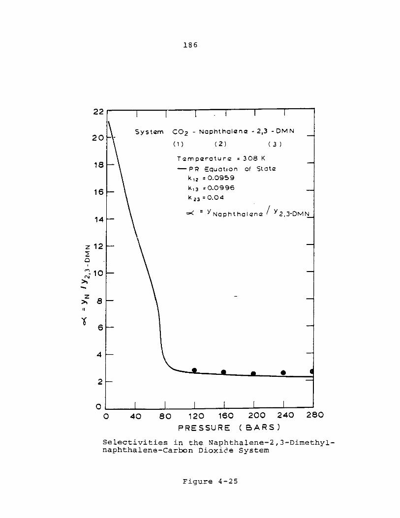
186
221
201
181
16
14
I I ILII0 40 80 120 160 200 240 280
PRESSURE (BARS)
Selectivities in the Naphthalene-2,3-Dimethyl-naphthalene-Carbon Dioxide System
Figure 4-25
System
I .- I I I
C02 - Naphthalana - 2,3 -DMN
(1) (2) (3)
Temperature = 308 K
-- PR Equation of Statek12 =0.0959
k 13 =0.0996
k 23 =0.04
Naphthalena / 2,3-DMN
~- p p-
12.
10
z20
C
~t.
z
II
'6
8
4
2
0
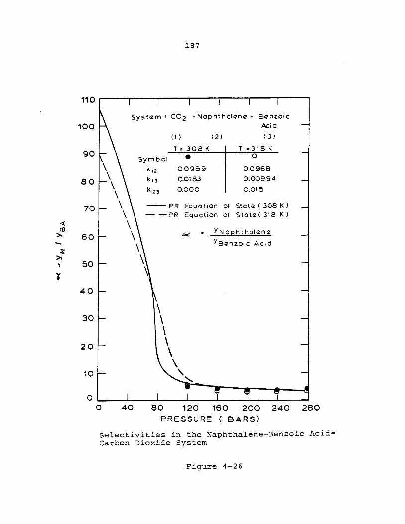
187
110
System C2 -Naphtholene - Benzoic
100 Acid
(1) (2) (3)
90 T=308K T =318 K
Symbol 0
k12 0.0959 0.0968
80-k,3 0.0183 0.00994
k23 0.000 0.015
70 PR Equation of State ( 308 K)
- -PR Equation of State( 318 K)
60 -z% "Benzolc Acid
50
40L
30
2o --
10
10
0 40 80 120 160 200 240 280PRESSURE C BARS)
Selectivities in the Naphthalene-Benzoic Acid-Carbon Dioxide System
Figure 4-26
188
is that at high reduced pressures (Pr '1). the selectivity
is low and therefore, both "high" and "low" volatile species
will be extracted. In order to get a good separation of
solute materials, the pressure must be kept less than the
solvent critical pressure, but here, the solubilities are also
low. (At pressures of about 1000 bar, computer simulations
predict that selectivities increase slightly.)
Discussion of Ternary Solid-Fluid Equilibrium Results
Ternary solid-fluid equilibria exhibits similar phenom-
ena to binary solid-fluid equilibrium. There are, however,
some unique characteristics: component solubilities in ternary
systems can be significantly higher than the solubility of
the pure component in a supercritical fluid under identical
operating conditions.
Careful examination of the ternary solid-fluid equili-
brium data taken shows that component solubilities are signi-
ficantly increased when an additional solid component of high
solubility C> 10- mole fraction) is added to the first
solid. If, however, the solubilities of both pure components
are low C< tO-3 mole fraction), then the solubility of the
components in the mixture will be almost identical to the
pure component solubilities. If the solubilities of both
components are high (> 10- mole fraction), then the solubil-
ities of both components in the mixture are significantly
increased.
Physically, what seems to be happening is that a high
189
concentration of a hydrocarbon solute in the supercritical
fluid phase aids in dissolving other hydrocarbon solutes --
by using the rule that "like dissolves like." In one case
studied in this thesis, however, there was a slight (10%)
decrease in component solubilities in a ternary mixture as
compared to the binary system. This case was the system
phenanthrene; 2,3-DMN; CO2.
In most cases, the ternary data can be correlated well
by the Peng-Robinson equation of state. Correlation of these
ternary systems requires, however, the use of a solute-solute
interaction coefficient (k23 ). To check the physical meaning
of this solute-solute parameter, the isomer system 2,3-DMN;
2,6-DMN was examined in both supercritical carbon dioxide and
ethylene. Correlation of the resultant data showed that k23
was dependent on the supercritical fluid (component 1). Thus
it can be concluded that k2 3 is an adjustable parameter -- not
a true binary constant.
4-3 Experimental Proof that T < Tq
As discussed in Chatper 2-2, it is only for system temp-
eratures less than the upper critical end point temperature
(T ) that one is guaranteed that no liquid phase will form.
Since all of the thermodynamic modelling used in this thesis
incorporated the assumption of T < Tq, it is necessary to
obtain experimental proof that this assumption was valid.
Such a proof can be inferred with experiments using the sys-
tem naphthalene-ethylene. For this system (Diepen and
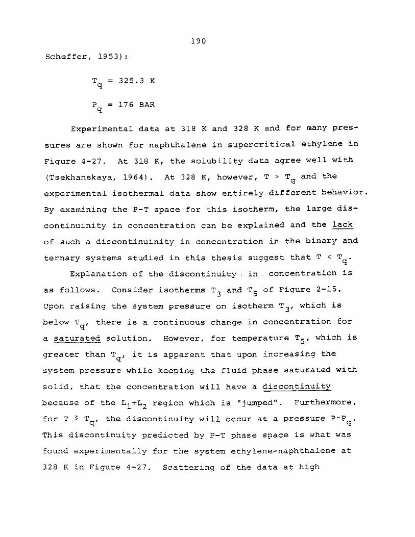
190
Scheffer, 1953):
T = 325.3 K
P = 176 BAR
Experimental data at 318 K and 328 K and for many pres-
sures are shown for naphthalene in supercritical ethylene in
Figure 4-27. At 318 K, the solubility data agree well with
(Tsekhanskaya, 1964). At 328 K, however, T > T and the
experimental isothermal data show entirely different behavior.
By examining the P-T space for this isotherm, the large dis-
continuinity in concentration can be explained and the lack
of such a discontinuinity in concentration in the binary and
ternary systems studied in this thesis suggest that T < T.
Explanation of the discontinuity in. concentration is
as follows. Consider isotherms T3 and T5 of Figure 2-15.
Upon raising the system pressure on isotherm T3 ' which is
below Tq, there is a continuous change in concentration for
a saturated solution. However, for temperature T5 ' which is
greater than T , it is apparent that upon increasing the
system pressure while keeping the fluid phase saturated with
solid, that the concentration will have a discontinuity
because of the L 1 +L2 region which is "jumped". Furthermore,,
for T 5T , the discontinuity will occur at a pressure P-P .
This discontinuity predicted by P-T phase space is what was
found experimentally for the system ethylene-naphthalene at
328 K in Figure 4-27. Scattering of the data at high
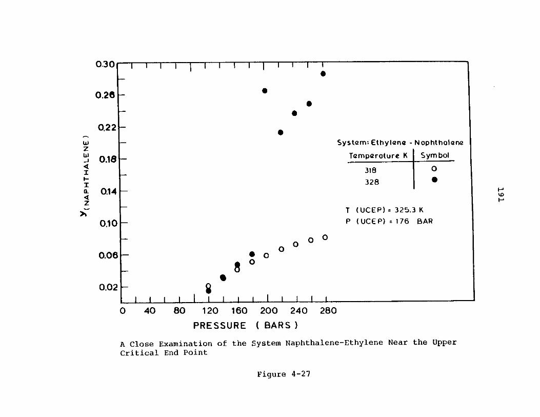
I I I I I I I I I I I I
0
S0
System: Ethylene - Nophtholene
Temperoture K I Sym bol
318
328 I 0
T (UCEP) 325.3 K
P (UCE P)=176 BAR
0.22
0.18
0.14
0.10
0.06
I I 1 I I I i I I I1 1 1 1 1 1 1 4- f I t
0 40 80 120 160 200 240 280
PRESSURE ( BARS)
A Close Examination of the System Naphthalene-Ethylene Near the Upper
Critical End Point
Figure 4-27
0.30
0.28
wzw
CL4
a.
z
S
~0
0.021
H
H
I I I
I I
I
192
pressures (and concentrations) results because of plugging
problems in the pressure let-down value. Finally, the lack
of such a discontinuity in the binary (and by analogy tern-
ary) systems studied in this thesis certainly indicates that
in all cases T < Tq
193
5. UNIQUE SOLUBILITY PHENOMENA OF SUPERCRITICAL FLUIDS
Solubility of solids in supercritical fluids exhibit
several unique phenomena not present in typical phase equil-
ibria situations. These pheneomena are the existance of a
maximum in isothermal solubilities at high pressures, a solu-
bility minimum at low pressures, and a method to achieve
essentially 100% solubility of a solid in a supercritical
phase. Solubility maxima (Kurnik and Reid, 1981) and a method
to achieve 100% solubilities of a solid in a supercritical
phase are new findings in this thesis.
5-1 Solubility Minima
As is clearly shown in typical isothermal solubility
diagrams of mole fraction versus pressure, a definite solu-
bility minimum exists at relatively low pressures (10 - 30
bar). At these pressures, the virial equation of state is
applicable and so it is possible to solve analytically for
the pressure and mole fraction at the solubility minimum.
As is shown by Hinckley and Reid (1964), the pressure and
mole fraction at the solubility minimum for binary systems
is:
2 eB1 2 PV1
y(min) =- (5-1.1)RT
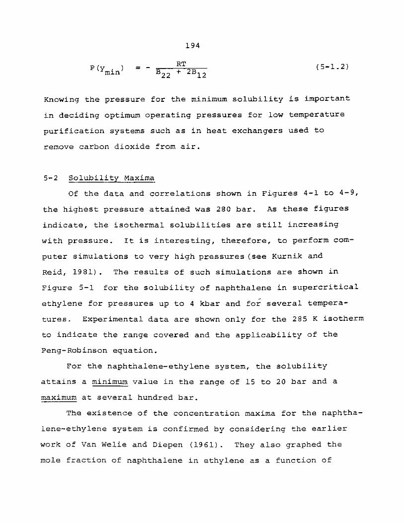
194
P(y.) RT (5-1.2)min B 22 + 2B12
Knowing the pressure for the minimum solubility is important
in deciding optimum operating pressures for low temperature
purification systems such as in heat exchangers used to
remove carbon dioxide from air.
5-2 Solubility Maxima
Of the data and correlations shown in Figures 4-1 to 4-9,
the highest pressure attained was 280 bar. As these figures
indicate, the isothermal solubilities are still increasing
with pressure. It is interesting, therefore, to perform com-
puter simulations to very high pressures (see Kurnik and
Reid, 1981). The results of such simulations are shown in
Figure 5-1 for the solubility of naphthalene in supercritical
ethylene for pressures up to 4 kbar and for several tempera-
tures. Experimental data are shown only for the 285 K isotherm
to indicate the range covered and the applicability of the
Peng-Robinson equation.
For the naphthalene-ethylene system, the solubility
attains a minimum value in the range of 15 to 20 bar and a
maximum at several hundred bar.
The existence of the concentration maxima for the naphtha-
lene-ethylene system is confirmed by considering the earlier
work of Van Welie and Diepen (1961). They also graphed the
mole fraction of naphthalene in ethylene as a function of
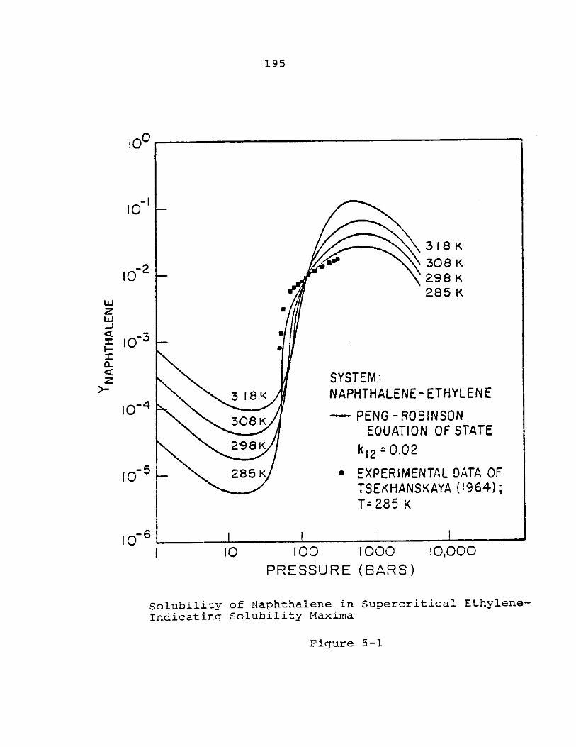
195
I
100
1
zu-I
10
C
z
10
3 18 K
308 K298 K285 K
SYSTEM:NAPHTHALENE- ETHYL
- PENG -ROBINSON
ENE
EQUATION OF STATEk12 :O .02
* EXPERIMENTAL DATA OFTSEKHANSKAYA (1964);T=:285 K
100 1000 10,000
PRESSURE (BARS)
Solubility of Naphthalene inIndicating Solubility Maxima
Supercritical Ethylene-
Figure 5-1
3 18K
308 K
298K
285 K
io-6 - I I -m m m m m w - - ---- -- I I -I
I
196
pressure and covered a range up to about 1 kbar. Their
smoothed data (as read from an enlargement of their origional
graphs), are plotted in Figure 5-2. At temperatures close
to the upper critical end point (325.3 K), a maximum in con-
centration is clearly evident. At lower temperatures,the
maximum is less obvious. The dashed curve in Figure 5-2
represents the results of calculating the concentration maxi-
mum from the Peng-Robinson equation of state. This simulation
could only be carried out to 322 K; above this temperature
convergence becomes a problem as the second critical end point
is approachedand the formation of two fluid phases is pre-
dicted. Table 5-1 compares the theoretical versus experimental
maxima.
Concentration maxima have also been noted by Czubryt
et al. (1970) for the binary systems stearic acid-CO2 and
1-octadecanol-CO2 In these cases, the experimental data
were all measured past the solubility maxima -- which for both
solutes occurred at a pressure of about 280 bar. An approxi-
mate correlation of their data was achieved by a solubility
parameter model.
Theoretical Development
The solubility minimum and maximum with pressure can be
rel 4ted to the partial molar volume of the solute in the
supercritical phase. With subscript I representing the solute,
then with equilibrium between a pure solute and the solute
dissolved in the supercritical fluid,
197
- Van Welie and Diepen, 1961COMPUTER SIMULATION OF
j 30-MAXIMUM CONCENTRATIONUSING THE PENG-ROBINSONEQUATION OF STATE
20=8
5C
-J-
a
LU
CIO-j0 0a 200 400 600 800 1000
PRESSURE (BARS)
NUMBER TEMPERATURE(K)
I 303.22 308.23 313.24 318.25 321.26 323.27 324.28 325.3
Experimental Data Confirming Solubility Maxima ofNaphthalene in Supercritical Ethylene
Figure 5-2
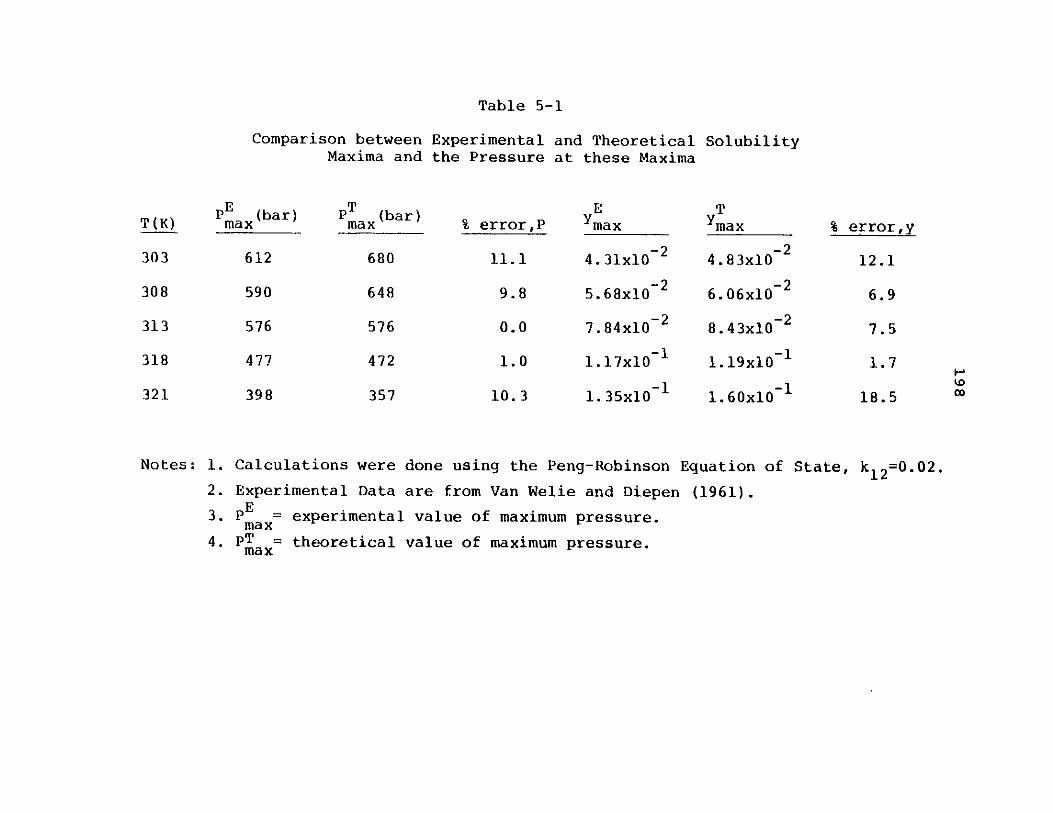
Table 5-1
Comparison between Experimental and TheoreticalMaxima and the Pressure at these Maxima
Solubility
T (bar)max
680
648
576
472
357
% error,P
11.1
9.8
0.0
1.0
10.3
EYmax
4. 31x10-2
5.68x10⁻²
7.84x10 2
1.17x10 1
1. 35x10 1
TYmax
4.83x10⁻²
6.06x10⁻²
8.43x10⁻²
a.19x10 1
1.60x10 1
% error,y
12.1
6.9
7.5
1.7
18.5
Notes: 1. Calculations were done using the Peng-Robinson Equation of State, kl2=0.02.
2. Experimental Data are from Van Welie and Diepen (1961).E3. P Ex= experimental value of maximum pressure.max
4. pT = theoretical value of maximum pressure.max
T(K)
303
308
313
318
321
E (bar)max
612
590
576
477
398Hk0OD
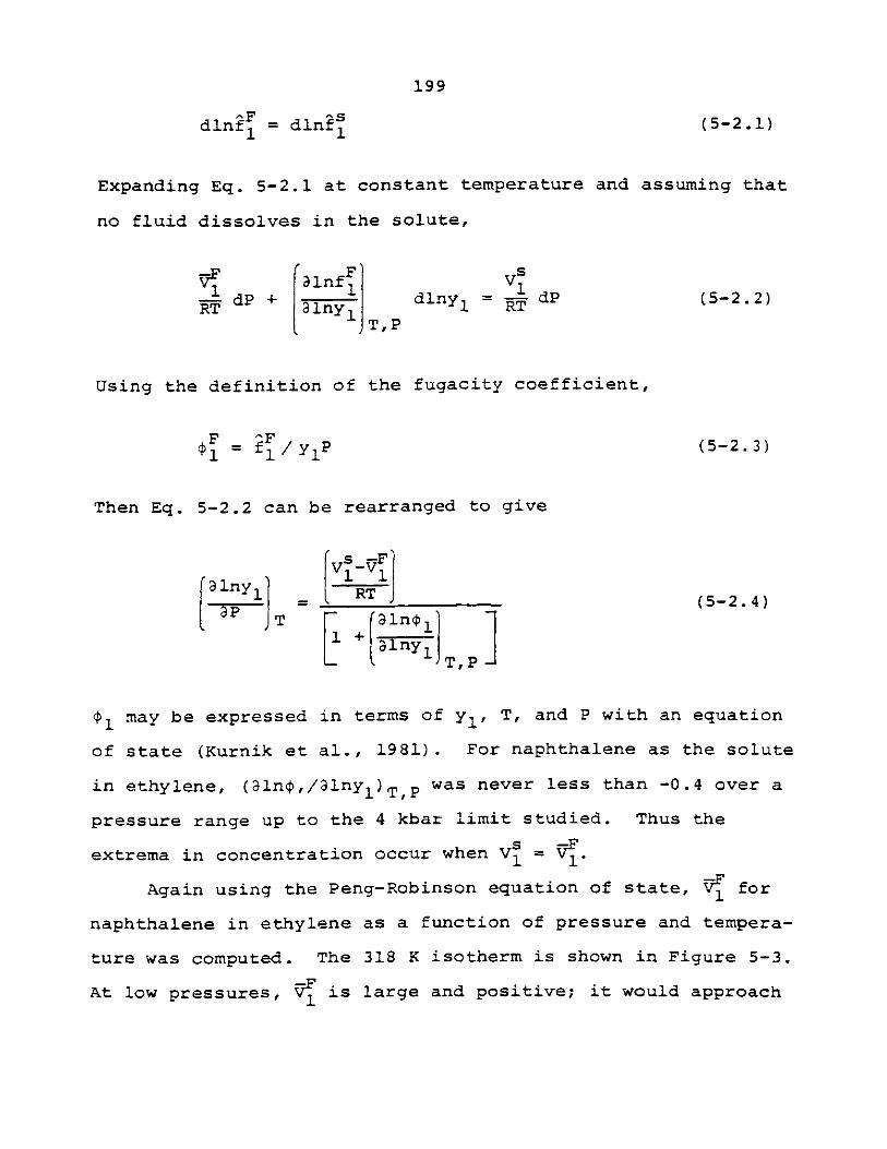
199
dmn4 = dlnfs (5-2.1)
Expanding Eq. 5-2.1 at constant temperature and assuming that
no fluid dissolves in the solute,
VF nF1dP + lny dlny1 =T dP (5-2.2)
1T,P
Using the definition of the fugacity coefficient,
F ^F$ -- f1 /yP (5-2.3)
Then Eq. 5-2.2 can be rearranged to give
Vs_
alnyl'RT H I [ (5-2.4)
T + ll+[alny
Tf,P-
$K may be expressed in terms of y1 , T, and P with an equation
of state (Kurnik et al., 1981). For naphthalene as the solute
in ethylene, (aln$,/3lnyl)T,P was never less than -0.4 over a
pressure range up to the 4 kbar limit studied. Thus the
extrema in concentration occur when Vs=
Again using the Peng-Robinson equation of state, 1 for
naphthalene in ethylene as a function of pressure and tempera-
ture was computed. The 318 K isotherm is shown in Figure 5-3.
At low pressures, 4 is large and positive; it would approach
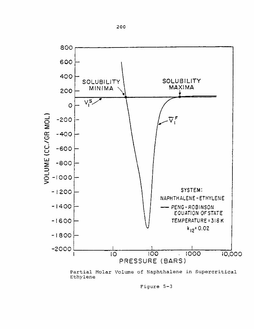
200
800
600
200
0
/ -200
Ct -400
- -600C-)
-800
o -1000
- I
- I
- I
200
400
600
-1800
-'Qn- . S 'W;
SOLUBILITYMINIMA
SOLUBILITYMAXIMA
- Is
-F
NAPHTH
- PEtE(
TE
10 100
SYSTEM:ALENE-ETHYLENE
NG-ROBINSONOUATION OF STATEMPERATURE =318 K
k =0.02
1000PRESSURE (BARS)
Partial Molar Volume of Naphthalene in SupercriticalEthylene
Figure 5-3
10,000I mmmm
400 [
I
I
201
an ideal gas molar volume as P -+- 0. With an increase in pres-
sure, decreases and becomes equal to Vs (111.9 cm3/mole)
at a pressure of about 20 bar. This corresponds to the solu-
bility minimum. V4 then becomes quite negative. The minimum
in 9'corresponds to the inflection point in the concentra-
tion-pressure curve shown in Figure 5-1. At high pressures,
VF increases and eventually becomes equal to Vs; this then1 thste
corresponds to the maximum in concentration described earlier.
5-3 A Method to Achieve 100% Solubility of a Solid in
a Supercritical Phase
Due to the unusual phase behavior of the solid-supercrit-
ical fluid surface described in Chapter 2-2, it is possible
to delineate regions of solid-fluid equilibria other than
between the lower and upper critical end points. Moreover,
in these regions, one can obtain significantly higher solu-
bilities than between the critical end points and actually
approach a solubility of 100% mole fraction. These unique
features of supercritical fluids are discussed in this section.
Consider the P-x isotherms shown in Figure 2-15 of the
P-T projection shown in Figure 2-14. These projections are
for the case where the three phase line intersects the criti-
cal locus. On isotherms T5, T6 and T7 , there is a distinct
solid + fluid (S+F) region existing for temperatures greater
than the upper critical end point temperature (T4).
One can, nevertheless, operate in the (S+F) region,
provided that the pressure is greater than the highest
202
pressure on the critical locus connecting the critical point
of the solute with the upper critical end point. In this
situation, a limiting composition of 100% solubility of the
solute in the supercritical phase may be achieved when the
temperature just equals the pure solid melting point temper-
ature at the operating pressure.
Consider the system naphthalene-ethylene. The maximum
pressure on the critical locus connecting the critical point
of the pure solid to the upper critical end point is approxi-
mately 250 bar (see Figure 5-4). Thus, at an operating
pressure greater than 250 bar, say 274 bar, one can achieve
100% solubility of a solid in a supercritical fluid by chosing
the operating temperature equal to the melting point temper-
ature of pure naphthalene at 274 bar. Diepen and Scheffer
(.1953) give the melting point of pure naphthalene at 274 bar
as 363 K.
A computer simulation of the ethylene-naphthalene system
at a constant pressure of 274 bar and for temperatures between
285 K and 363 K is shown in Figure 5-5. For comparison,
experimental data of Diepen and Scheffer (1953) under these
conditions is also shown. The Peng-Robinson equation appears
to simulate these extremely concentrated solutions quite well.
5-4 Entrainers in Supercritical Fluids
Solubilities of desired species in supercritical fluids
may not always be sufficiently large enough for certain
applications. In order to further increase component
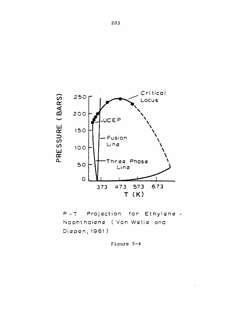
203
CriticalLocus
--UCEP '41~~
- FusionLine
-Thr ec PhoseLine
373 473 573T (K)
Projection for Et hylene -
Naphthalene (Van Welia and
Diepen, 1961)
Figure 5-4
4l:
Lo
CL
I250
200
150
100
50
0 - r
673
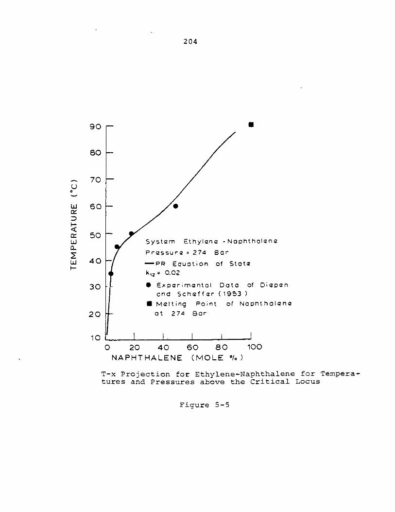
204
90-
0
System Ethylene - Na
Pressure = 274 Bar
-PR Equation of St
k12 = .02
. Experimental Datc
and Schaffer (195
* Melting Point of'
at 274 Bar
I I
80
70
60
50
40
30
20
101
0 20 40 60 80NAPHTHALENE (MOLE /0
U
phthalene
ate
of Diepen
3 )Naphtholaene
100
)
T-x Projection for Ethylene-Naphthalene for Tempera-tures and Pressures above the Critical Locus
Figure 5-5
0
LU
CL
- I- -
205
solubilities in supercritical fluids, it is possible in some
circumstances to add an additional component of higher
solubility -- called an entrainer.
At present, there is only one published case where en-
trainers were systematically used. This case is the separa-
tion of glyceride mixtures using supercritical carbon dioxide.
Quoting from Panzer et al. (1978): "Little separation was
achieved using pure carbon dioxide, but considerable improve-
ments resulted by the addition of the entrainers carbon
tetrachloride and n-hexane." Peter and Brunner (1978) made
similar observations with the system carbon dioxide- glycer-
ides, but with acetone as the entrainer. Selectivities of
the glycerides were different, however, with the different
entrainers.
Brunner (1980) has also noted that entrainers can signi-
ficantly change the retrograde temperature region.
Some exploratory investigations done in this thesis have
also shown the effect of entrainers. Several experiments
were performed whereby the solubility of natural alkaloids
in supercritical carbon dioxide were determined. Upon adding
water as an entrainer Cabout one weight percent in the fluid
phase), component solubilities of the alkaloids could be in-
creased from 10 to 50 percent.
Finally, the ternary solid-fluid systems that were system-
atically studied in this thesis show that small amounts of a
volatile component in a supercritical phase can significantly
effect the solubility of all components in the supercritical
206
phase.
Little is really known about the important topic of
entrainers in supercritical fluids. Clearly much more research
remains to be done.
5-5 Transport Properties of Supercritical Fluids
Mass transfer in supercritical fluids is of importance
for the design engineer in sizing equipment -- for rarely will
industrial applications operate at equilibrium. Very little
work has been done in this area -- a few binary diffusion
and self diffusion coefficients have been measured and flux
rates for one system have been measured.
It is the purpose of this section of the thesis to review
the literature on transport properties in supercritical
fluids and to make suggestions for further research.
Tsekhanskaya (1968, 1971) has made measurements of the
diffusivity for the systems p-nitrophenol-water and naphthal-
ene-carbon dioxide near the critical region. In dense fluids,
the diffusivities are slightly larger than those of liquids
(D 1 2 ~ 10~4cm2 /s), but when the critical point is approached,
the binary diffusivity approaches zero as suggested by theory
(Reid et al., 1977).
Iomtev and Tsekhanskaya C1964) and Morozov and Vinkler
C1975) have made extensive measurements on the diffusivity of
naphthalene in ethylene, carbon dioxide, and nitrogen.
Except for the measurements of Morozov and Vinkler, all
diffusivities were measured in static diffusion cells.
207
Morozov and Vinkler designed a dynamic method to obtain dif-
fusion coefficients which appears to give good results and
is also quite simple to construct and use.
Finally, Rance and Cussler (1974) measured flux rates
of iodine into supercritical carbon dioxide. Their data are
interesting as it suggests that there is no retrograde solid-
ification region with this system. Also, if equilibrium solu-
bility measurements are made on the system iodine-carbon
dioxide, then it would be possible to calculate mass transfer
coefficients from their flux data.
Suggestions for further research are to obtain binary
diffusivity data for additional solid-fluid systems and to
measure mass transfer coefficients to these systems. A gener-
alized correlation of the Sherwood number as a function of the
Reynold and Schmidt number would then be obtained.
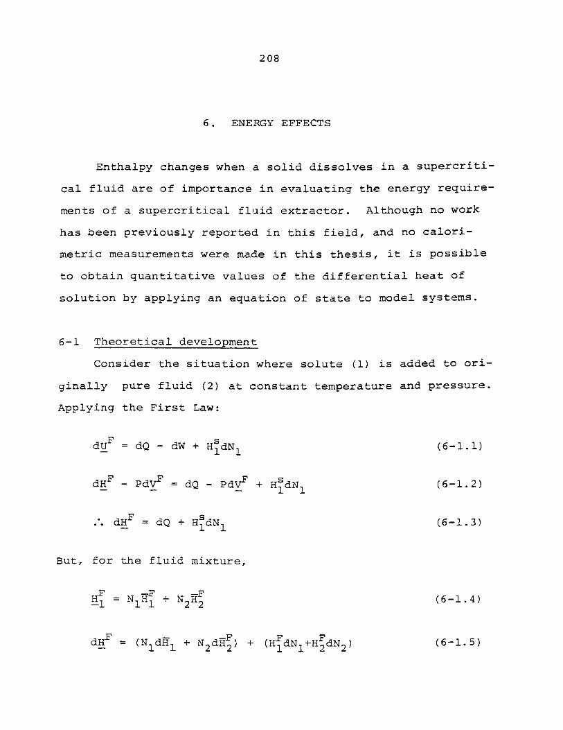
208
6. ENERGY EFFECTS
Enthalpy changes when a solid dissolves in a supercriti-
cal fluid are of importance in evaluating the energy require-
ments of a supercritical fluid extractor. Although no work
has been previously reported in this field, and no calori-
metric measurements were made in this thesis, it is possible
to obtain quantitative values of the differential heat of
solution by applying an equation of state to model systems.
6-1 Theoretical development
Consider the situation where solute (1) is added to ori-
ginally pure fluid (2) at constant temperature and pressure.
Applying the First Law:
dUF =dQ - dW + H dN (6-1.1)
dHF -PdVF= dQ - PdV+ HsdN1(6-1.2)
dHF = dQ + HsdN (6-1.3)
But, for the fluid mixture,
H- = NIH + N F (6-1.4)
dHF =(N dH + d FH (N1 H1 +"NZ 2dH2) + (H 1dN 1I+H 2dN 2 ) (6-1.5)
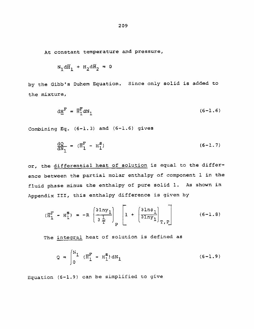
209
At constant temperature and pressure,
N1dH1 + H2 dH2 = 0
by the Gibb's Duhem Equation. Since only solid is added to
the mixture,
dH_F =F dN(6-1.6)
Combining Eq. (6-1.3) and (6-1.6) gives
dQ =--F HsdN (H1 - H) (6-1.7)
or, the differential heat of solution is equal to the differ-
ence between the partial molar enthalpy of component 1 in the
fluid phase minus the enthalpy of pure solid 1. As shown in
Appendix III, this enthalpy difference is given by
F 1~31ny 3 ln$(- - Hs) = -R [ + (6-1.8)
T P -M
The integral heat of solution is defined as
I'NQ = (( - Hs)dN 1(6-1.9)
Equation (6-1.9) can be simplified to give
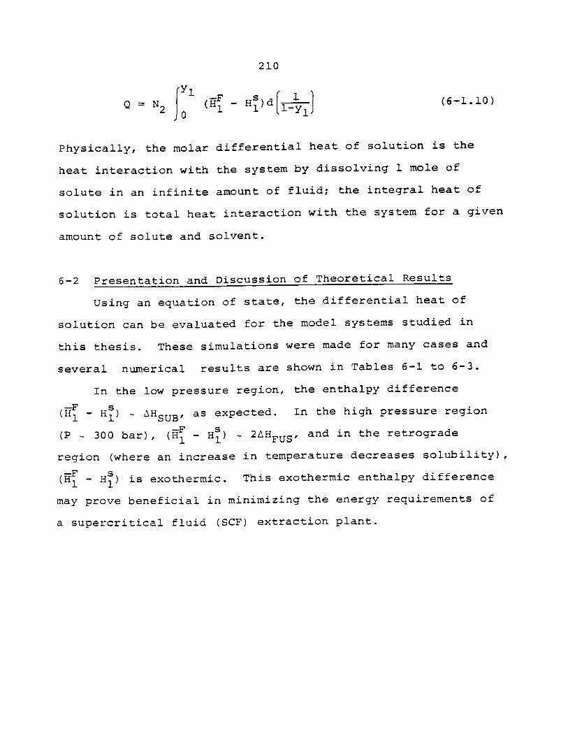
210
Q = N 2 { (H4 - H)d[(6-1.10)
Physically, the molar differential heat of solution is the
heat interaction with the system by dissolving 1 mole of
solute in an infinite amount of fluid; the integral heat of
solution is total heat interaction with the system for a given
amount of solute and solvent.
6-2 Presentation and Discussion of Theoretical Results
Using an equation of state, the differential heat of
solution can be evaluated for the model systems studied in
this thesis. These simulations were made for many cases and
several numerical results are shown in Tables 6-1 to 6-3.
In the low pressure region, the enthalpy difference
(if - H ) AHsusi as expected. In the high pressure region
(P 300 bar), (H1 - H1 ) 2 AHFUS, and in the retrograde
region (where an increase in temperature decreases solubility),
(HF - H ) is exothermic. This exothermic enthalpy difference
may prove beneficial in minimizing the energy requirements of
a supercritical fluid (SCF) extraction plant.
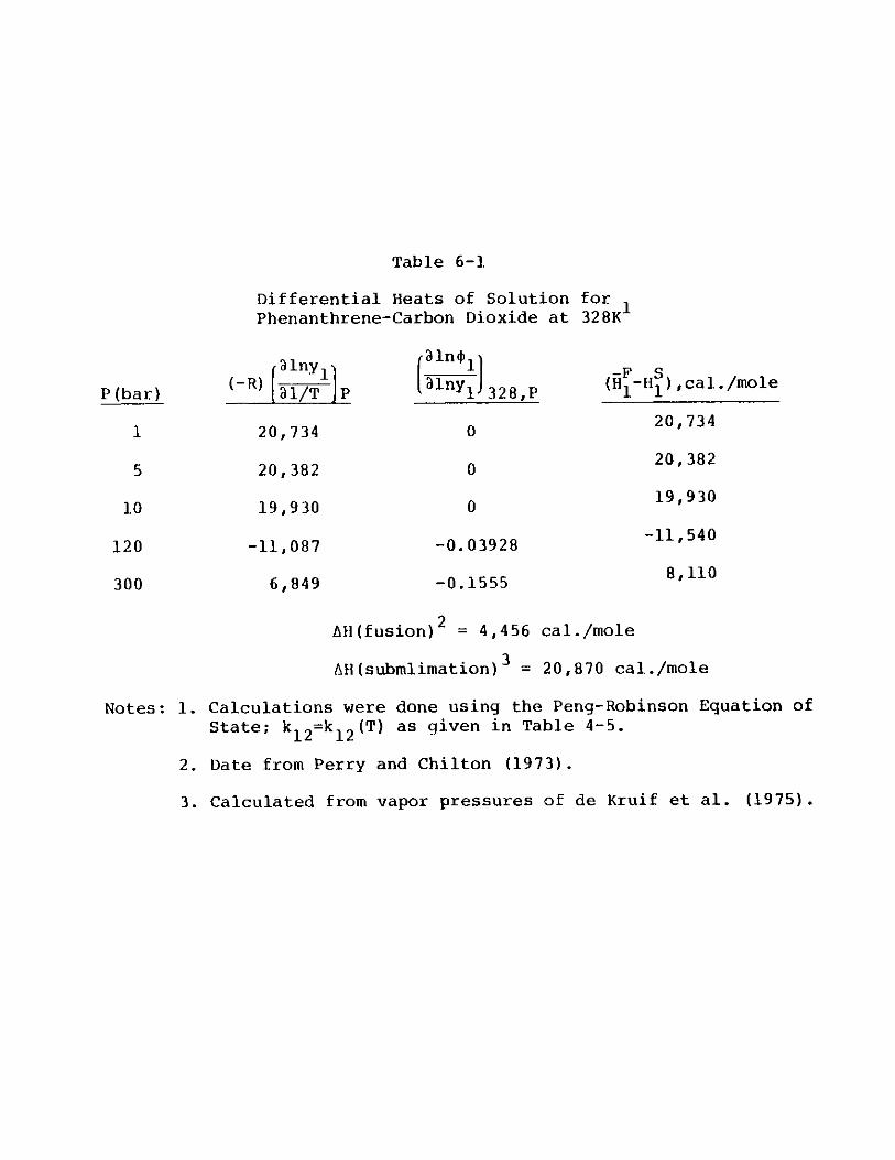
Table 6-1
Differential Heats of SolutionPhenanthrene-Carbon Dioxide at
31ny1 )ln$
S al/T P 3lnyj 328t,P
20,734 0
20 ,382 0
19,930 0
-11,087 -0.03928
6,849 -0.1555
for32 8K1
(H -H1),cal./mole
20, 734
20, 382
19,930
-11,540
8,110
Notes: 1.
2.
3.
AII(fusion) 2 = 4,456 cal./mole
AH(submlimation) 3 = 20,870 cal./mole
Calculations were done using the Peng-Robinson Equation of
State; k1 2 =k1 2 (T) as given in Table 4-5.
Date from Perry and Chilton (1973).
Calculated from vapor pressures of de Kruif et al. (1975).
P (bar)
1
5
10
120
300HH
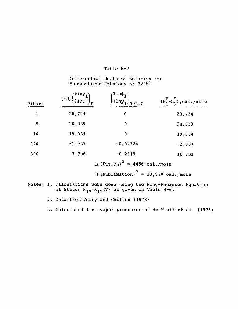
Table 6-2
Differential Heats of Solution forPhenanthrene-Ethylene at 328K1
alny Bn
P(bar) (-R)l/TJlny 2 P (5-H),cal./mole
1 20,724 0 20,724
5 20,339 0 20,339
10 19,834 0 19,834
120 -1,951 -0.04224 -2,037
300 7,706 -0.2819 10,731
AH(fusion) 2 = 4456 cal./mole
AH(sublimation)'3 = 20,870 cal./mole
Notes: 1. Calculations were done using the Peng-Robinson Equation
of State; k1 2=k1 2 (T) as given in Table 4-6.
2. Data from Perry and Chilton (1973)
3. Calculated from vapor pressures of de Kruif et al. (1975)
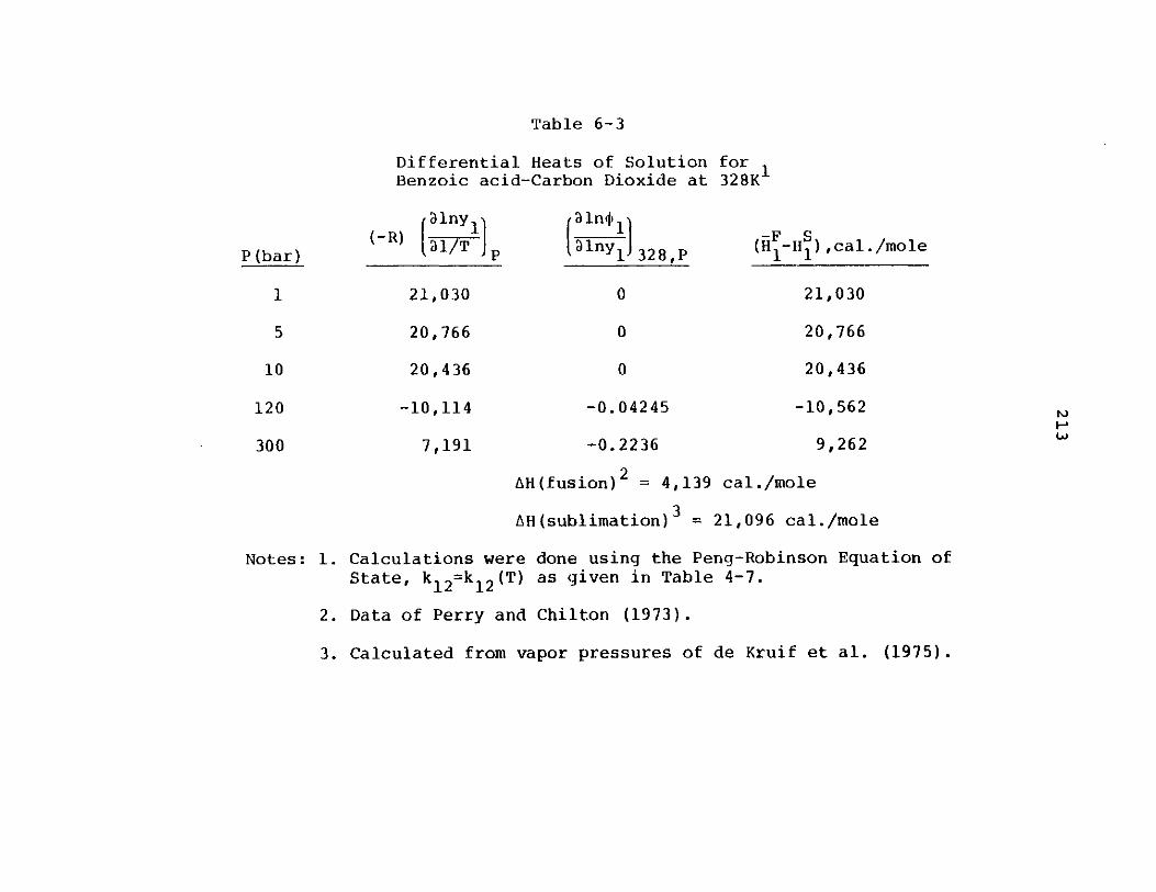
P(bar)
1
5
Table 6-3
Differential Heats of Solution forBenzoic acid-Carbon Dioxide at 328K'
3 lny I)3 l1$R) 131/TJ (3nyj 1328,P (H.
21,030 0
20,766 0
-H f ) ,cal. /mole1 )1
21,030
20,766
10 20,436 0 20,436
120 -10,114 -0.04245 -10,562
300 7,191 -0.2236 9,262
AH(fusion) 2 = 4,139 cal./mole
AH (sublimation) 3 = 21,096 cal./mole
Notes: 1. Calculations were done using the Peng-Robinson Equation ofState, k1 2=k1 2 (T) as given in Table 4-7.
2. Data of Perry and Chilton (1973).
3. Calculated from vapor pressures of de Kruif et al. (1975).
HWA
214
7. OVERALL CONCLUSIONS
Supercritical fluid extraction processes are seeing a
resurgence of interest -- both in academic institutions and
in industry. In academia, many of the phase equilibrium and
transport propertities of a condensed phase in equilibrium
with a fluid phase are being studied. In industry, the empha-
sis is on process development and solving the design and
engineering problems.
There are six major reasons why supercritical fluids are
receiving a widespread interest.
* High Mass Transfer Rates Between Phases
A supercritical fluid phase has a low viscosity (near that of
a gas) while also having a high mass diffusivity (between
that of a gas and a liquid). Consequently, it is currently
believed that the mass transfer coefficient (and hence the
flux rate) will be higher than for typical liquid extractions.
* Ease of Solvent Regeneration
After a given supercritical fluid has extracted the
desired components, the system pressure can be reduced to a
low value (20-30 bar) causing all of the solute to precipate
out. Then, the supercritical fluid is left in pure form and
can be easily recycled. In typical liquid extractions, using
an organic solvent, the spent solvent must usually be purified
by distillation.
215
. Sensitivity to all Process Variables
For supercritical fluid extraction, both temperature and
pressure have a significant effect on the equilibrium solubil-
ity. Small changes of temperature and/or pressure -- especi-
ally in the region near the critical point of the solvent,
can affect equilibrium solubilities by two or three orders of
magnitude. In liquid extraction, only temperature has a
strong effect on equilibrium solubility.
* Non-Toxic Supercritical Fluids Can Be Used
Carbon dioxide -- a chemical which is non-toxic, non-flammable,
inexpensive, and has a low critical temperature (304.2 K) can
be used as a solvent for extracting substances. It is for this
reason that many food and pharmaceutical industries are quite
interested in supercritical CO2 extraction research.
* Energy Saving
When compared to distillation, supercritical fluid extraction
is usually less energy intensive. A study by Arthur D.
Little, Inc. on dehydrating ethanol-water solutions by using
supercritical CO2 has shown to be more energy efficient than
azeotropic distillation (Krukonis, 1980).
. Sensitivity of Solubility to Trace Components
Solubility of components in supercritical fluids can be
changed by several hundred percent by the addition to the
fluid phase of small quantities (Cone mole percent) of a vola-
tile, often polar, material (entrainer). In addition, selec-
tivities of the extraction can be significantly affected by
the entrainer. More research on entrainers in multicomponent
216
systems will give a better physical understanding of the en-
hanced solubility as well as to enable one to develop guide-
lines to chose the best entrainer.
New developments in supercritical fluid extraction dis-
covered in this thesis are (1) the existance of a maximum in
isothermal solubilities with increasing pressure; (2) enhance-
ment of component solubilities in supercritical fluids by the
addition of a second volatile solid component; (3) differen-
tial heats of solution from solid to fluid phase changing
from endothermic in the low pressure regime to exothermic in
the middle pressure regime back to endothermic in the high
pressure regime; and (4) correlation and prediction of equili-
brium solubilities of binary and multicomponent solids in
supercritical fluids by use of rigorous thermodynamic theory.
217
8. RECOMMENDATIONS FOR FUTURE RESEARCH
8-1 Solid-Fluid Equilibria
In the area of solid-fluid equilibria, there are several
research topics which warrant further study. First, in this
thesis, only ternary systems were studied (two solids, one
fluid). It would be interesting to extend this work to even
higher order systems (more solid components) to answer sev-
eral questions:
a) Does the "temperature window" between p and q close?
b) Can one model a complex equilibria problem like coal
in supercritical CO2 by considering it to be made
up of many model compounds?
c) Do component solubilities in multicomponent systems
keep increasing in value over their value in a binary
system (when they do increase)?
Along with the experimental data of these higher order systems,
it would be interesting to examine the Peng-Robinson equation
(and others, such as Perturbed-Hard-Chain) to test their
ability to correlate higher order systems.
As solid-fluid extractions are most conveniently per-
formed in the region between the upper and lower critical end
points, a convenient way of theoretically and experimentally
determining these end points for multicomponent systems is a
topic for further study.
218
Correlation of the solid-fluid equilibrium data taken in
this thesis and the data available in the literature proved
satisfactory by using the Peng-Robinson model for the fluid
phase fugacity coefficient. A drawback of this model, how-
ever, is that there is a temperature dependent binary parameter,
k.., which up to now, cannot be determined apriori. Perhaps
correlation methods to predict k.(T) could be developed, or
better yet, a model for the fluid phase fugacity coefficient
that has a more theoretical framework (and without adjustable
parameters) than the Peng-Robinson equation of state could be
developed.
As discussed in Chapter 5-3 of this thesis, there are
temperature and pressure regimes other than those between the
upper and lower critical end points where solid is in equili-
brium with a fluid phase. Furthermore, in these other regimes,
it is possible to reach extremely high solubilities of solid
components in the fluid phase. As the experimental equipment
was designed in this thesis, however, it was impossible to
obtain reproducible data for high solubilities (30 percent
mole fraction or higher) due to plugging problems inside the
let-down valve. Perhaps with a refinement of the experimental
apparatus, equilibrium data in this very interesting regime
could be obtained (and correlated with theory).
8-2 Liquid-Fluid Extraction
The area of liquid-fluid extraction has much wider appli-
cations in industry than solid-fluid extraction -- since most
219
industrial separation problems are with liquids. Some
equilibrium data is available in the literature on binary
liquid-fluid systems up to relatively low pressures (100 bar),
but little is known about higher pressure solubilities and
solubilities in multicomponent systems.
An interesting research program would be to determine
experimentally the solubility of multicomponent liquids in
supercritical fluids and successfully model and correlate the
data. The effect of temperature and pressure on the distri-
bution coefficients in multicomponent systems could then be
examined.
8-3 Equipment Design
A visual observation extraction would be useful in
locating critical end points (in the case of solid-fluid
equilibria) by observing the appearance and disappearance
of a liquid phase.
As discovered in this thesis, there exists an iso-
thermal solubility maxima (with pressure) of component
solubilities of solids in supercritical fluids. This
maxima however, exists at relatively high pressures (600 bar),
and so it would be useful to have the capability to take
solubility measurements in this region, and therefore
give more support to this finding. A similar solubility
maxima will probably exist with some liquid-fluid
equilibria systems -- and this may be of value to
test.
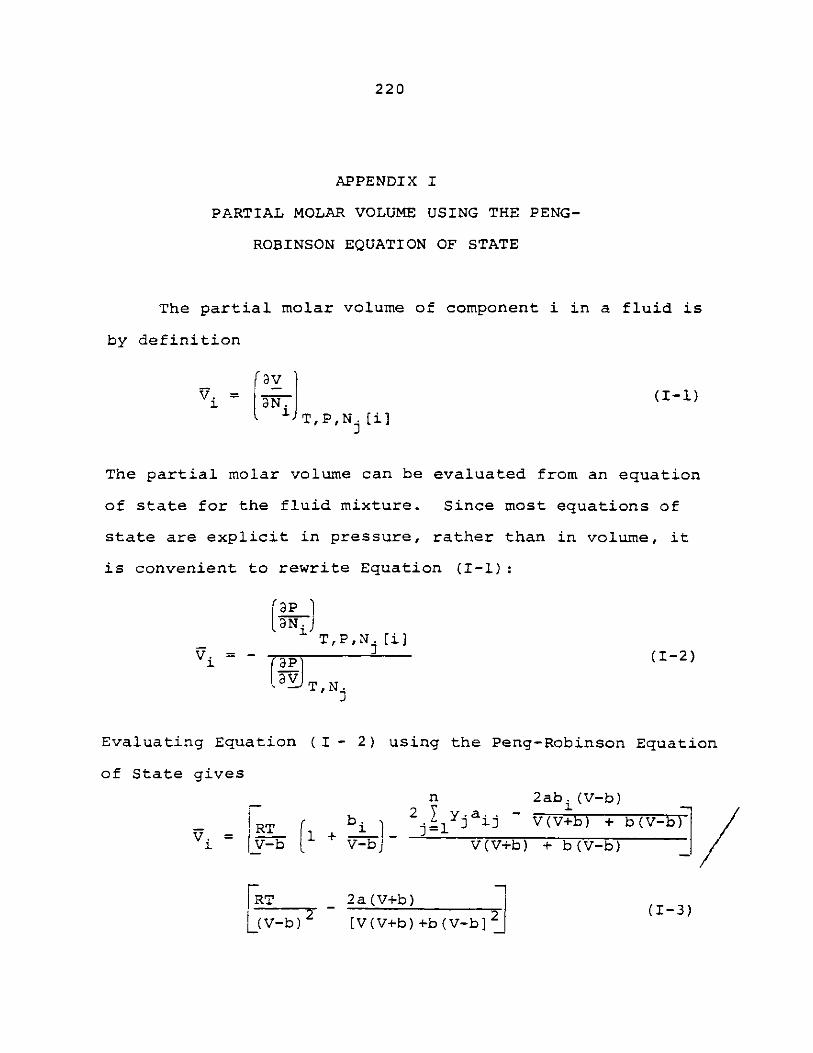
220
APPENDIX I
PARTIAL MOLAR VOLUME USING THE PENG-
ROBINSON EQUATION OF STATE
The partial molar volume of component i in a fluid is
by definition
S= (I-I)
J
The partial molar volume can be evaluated from an equation
of state for the fluid mixture. Since most equations of
state are explicit in pressure, rather than in volume, it
is convenient to rewrite Equation (I-1):
' P
T,P,N. i]V(i= 3P (1-2)
JT,N.
Evaluating Equation (I - 2) using the Peng-Robinson Equation
of State gives
n 2ab. (V-b)
-_2T1bja - V(V+b) + b(V-b)I V-b V-bJ V(V+b) + b(V-b)
22 (aI(V+b)2(1-3)
L(v-b ) [V(V+b)+b(V-b]

221
A similar derivation has been made by Lin and Daubert
(1980).
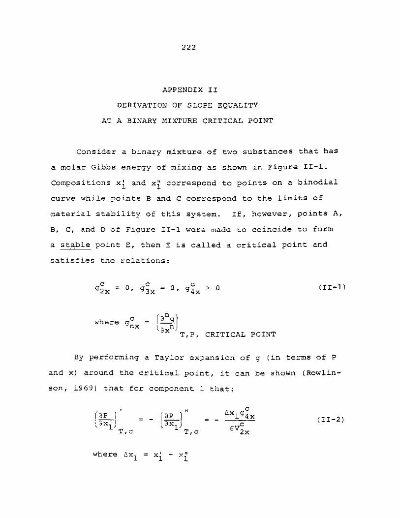
222
APPENDIX II
DERIVATION OF SLOPE EQUALITY
AT A BINARY MIXTURE CRITICAL POINT
Consider a binary mixture of two substances that has
a molar Gibbs energy of mixing as shown in Figure II-I.
Compositions x' and xf correspond to points on a binodial
curve while points B and C correspond to the limits of
material stability of this system. If, however, points A,
B, C, and D of Figure II-1 were made to coincide to form
a stable point E, then E is called a critical point and
satisfies the relations:
c=0,g = Qgc>0 (11-1)2 x 3x 4 x
where gc _ [tijTP, CRITICAL POINT
By performing a Taylor expansion of g (in terms of P
and x) around the critical point, it can be shown (Rowlin-
son, 1969) that for component 1 that:
c
-1-94x (11-2)LT 6V CT , c T,a 2x
where Ax = x - x
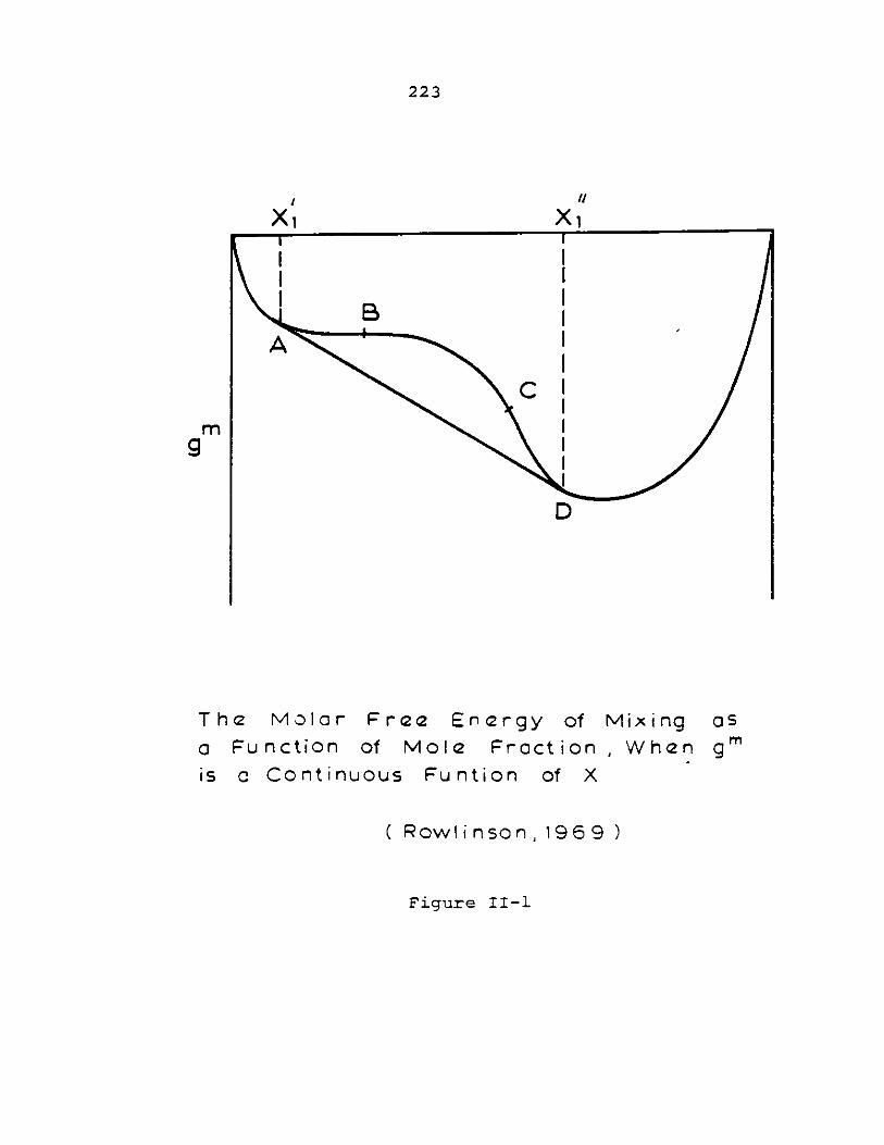
223
xi X1
A
mg
D
The Molar Free Energy of Mixing asa Function of Mole Fraction , When g'is a Continuous Funtion of X
( Rowlinson, 1969 )
Figure II-1
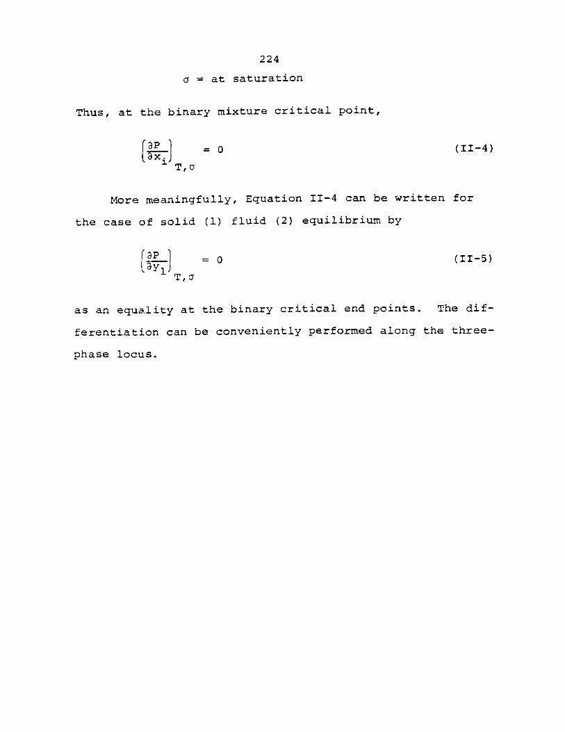
224
a = at saturation
Thus, at the binary mixture critical point,
SI- = 0 (I1-4)
T,cr
More meaningfully, Equation 11-4 can be written for
the case of solid (1) fluid (2) equilibrium by
3 =0 (11-5)
as an equality at the binary critical end points. The dif-
ferentiation can be conveniently performed along the three-
phase locus.
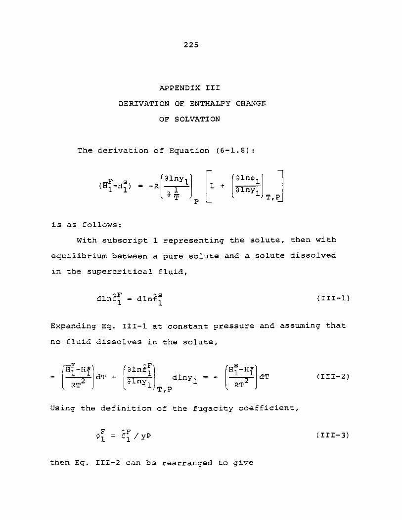
225
APPENDIX III
DERIVATION OF ENTHALPY CHANGE
OF SOLVATION
The derivation of Equation (6-1.8):
-F ' Dny,~ 'aln$
(i-Hs) = -RL + [ait1]
i .1P T, -
is as follows:
With subscript 1 representing the solute, then with
equilibrium between a pure solute and a solute dissolved
in the supercritical fluid,
dlnfF = dlnfs I1l-i)1 1
Expanding Eq. III-i at constant pressure and assuming that
no fluid dissolves in the solute,
iHF-Hr 3ln^F -H -H*
- dT + LY 1 dlny2 = - dT (111-2)RT2 y1RT
TP
Using the definition of the fugacity coefficient,
F -^FI = fI/ yP
then Eq. 111-2 can be rearranged to give
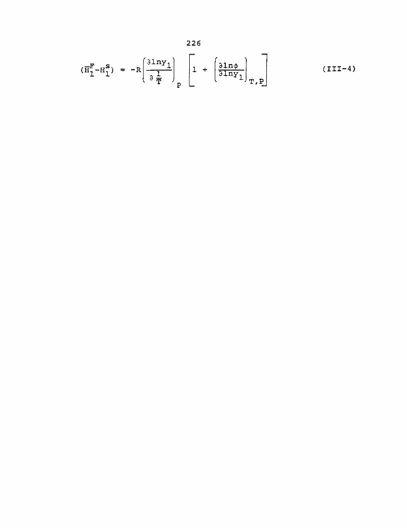
(F Hs) = -r3]nyR -R 1 j
- T -
226
[1 + Bln }TP 11+31ny9l-y TrPj
4
227
APPENDIX IV
FREEZING POINT DATA
FOR MULTICOMPONENT MIXTURES
A Fisher-Johns melting point apparatus (Fisher
Scientific, Model 12-144) was used to determine if the solid
mixtures used in this research formed solid solutions or an
eutectic mixture with the solid phases as pure components.
From the freezing point behavior, it can be determined if
the solids form a solid solution oran eutectic mixture.
Only in the latter case can the activity coefficient of the
solid phase be neglected -- see Equation (2-3.8).
In order to test the accuracy of the equipment, a known
eutectic mixture was examined: o-chloronitrobenzene with
p-chloronitrobenzene (Prigogine and Defay, 1954). As Table
IV-1 shows, the agreement between the literature and
experimental data for the melting point curve are within
+ 0.5 K.
Tables IV-2 through IV-5 give experimental freezing
point data for four of the binary systems investigated.Y Listed
in these tables are both T and Tf -- the initial and final
freezing points. In each case, since Tf is constant, the
formation of a eutectic composition is confirmed. Also
listed in Tables IV-2 through IV-5 are the eutectic temper-
atures predicted from ideal solution theory (Prausnitz,
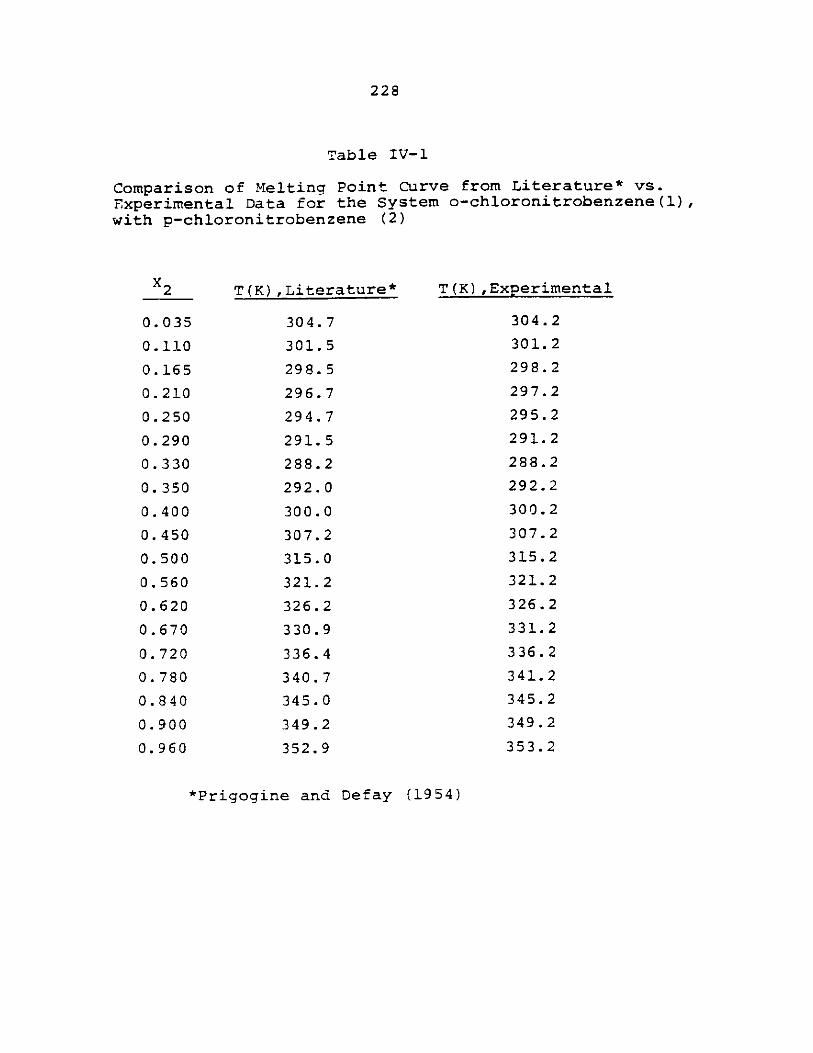
228
Table IV-
Comparison of Melting Point Curve from Literature* vs.Experimental Data for the System o-chloronitrobenzene(l),with p-chloronitrobenzene (2)
T(K) ,Literature*x2
0.035
0.110
0.165
0.210
0.250
0.290
0.330
0.350
0.400
0.450
0.500
0.560
0.620
0.670
0.720
0.780
0.840
0.900
0.960
T (K) ,Experimental
304.2
301.2
298.2
297.2
295.2
291.2
288.2
292.2
300.2
307.2
315.2
321.2
326.2
331.2
336.2
341.2
345.2
349.2
353.2
*Prigogine and Defay (1954)
304.7
301.5
298.5
296.7
294.7
291.5
288.2
292.0
300.0
307.2
315.0
321.2
326.2
330.9
336.4
340.7
345.0
349.2
352.9
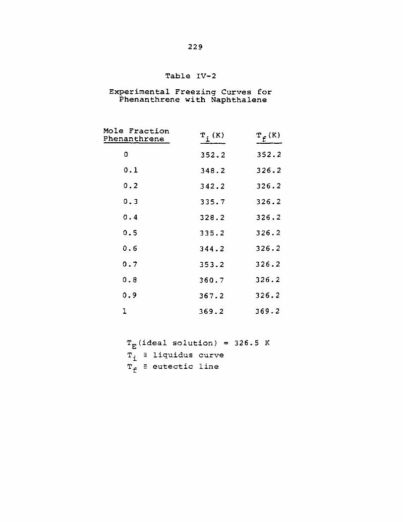
229
Table IV-2
Experimental Freezing Curves forPhenanthrene with Naphthalene
Mole Fraction T. (K) Tf(K)Phenanthrene i f
0 352.2 352.2
0.1 348.2 326.2
0.2 342.2 326.2
0.3 335.7 326.2
0.4 328.2 326.2
0.5 335.2 326.2
0.6 344.2 326.2
0.7 353.2 326.2
0.8 360.7 326.2
0.9 367.2 326.2
1 369.2 369.2
TE(ideal solution) = 326.5 K
T. E liquidus curve
T.== eutectic line
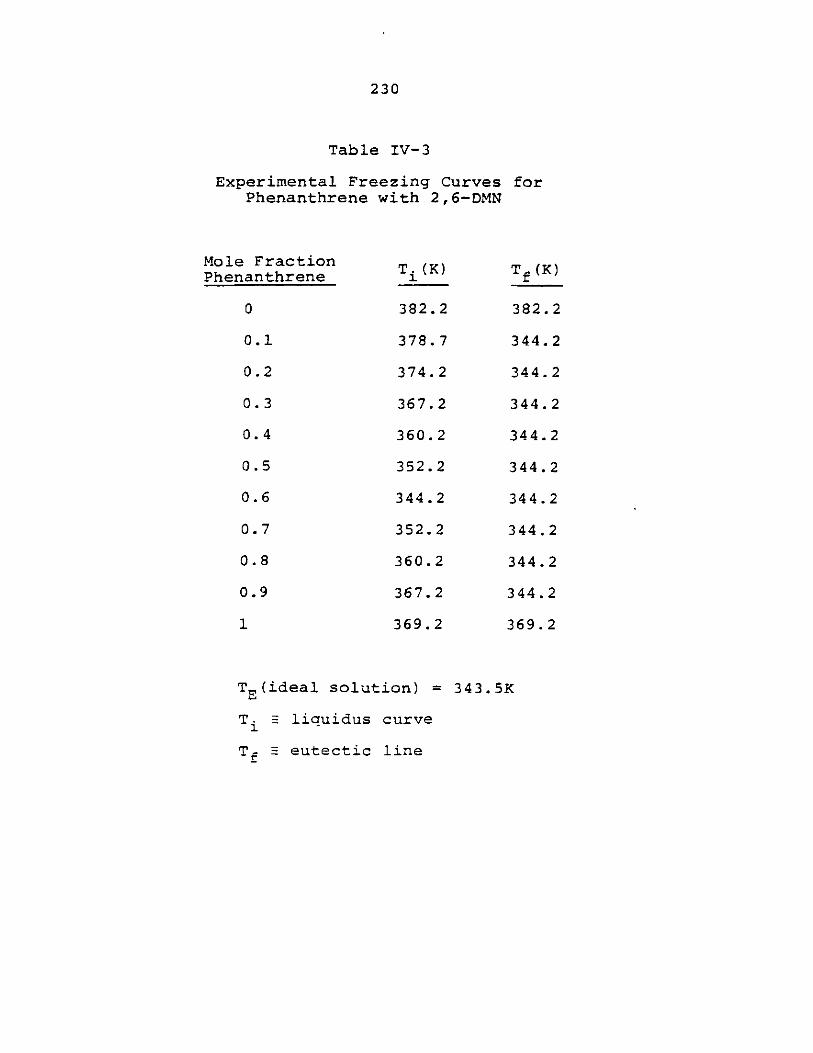
230
Table IV-3
Experimental Freezing Curves forPhenanthrene with 2,6-DMN
Mole Fraction T. (K) T (K)Phenanthrene i f
0 382.2 382.2
0.1 378.7 344.2
0.2 374.2 344.2
0.3 367.2 344.2
0.4 360.2 344.2
0.5 352.2 344.2
0.6 344.2 344.2
0.7 352.2 344.2
0.8 360.2 344.2
0.9 367.2 344.2
1 369.2 369.2
TE(ideal solution) = 343.5K
Ti liquidus curve
Tf eutectic line
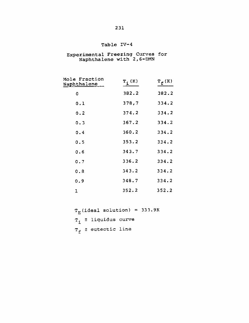
231
Table IV-4
Experimental Freezing Curves for
Naphthalene with 2,6-DMN
Mole Fraction T (K) Tf(K)Naphthalene i f
0 382.2 382.2
0.1 378,7 334.2
0.2 374.2 334.2
0.3 367.2 334.2
0.4 360.2 334.2
0.5 353.2 334.2
0.6 343.7 334.2
0.7 336.2 334.2
0.8 343.2 334.2
0.9 348.7 334.2
1 352.2 352.2
TE(ideal solution) = 333.9K
T. liquidus curve
T B eutectic line
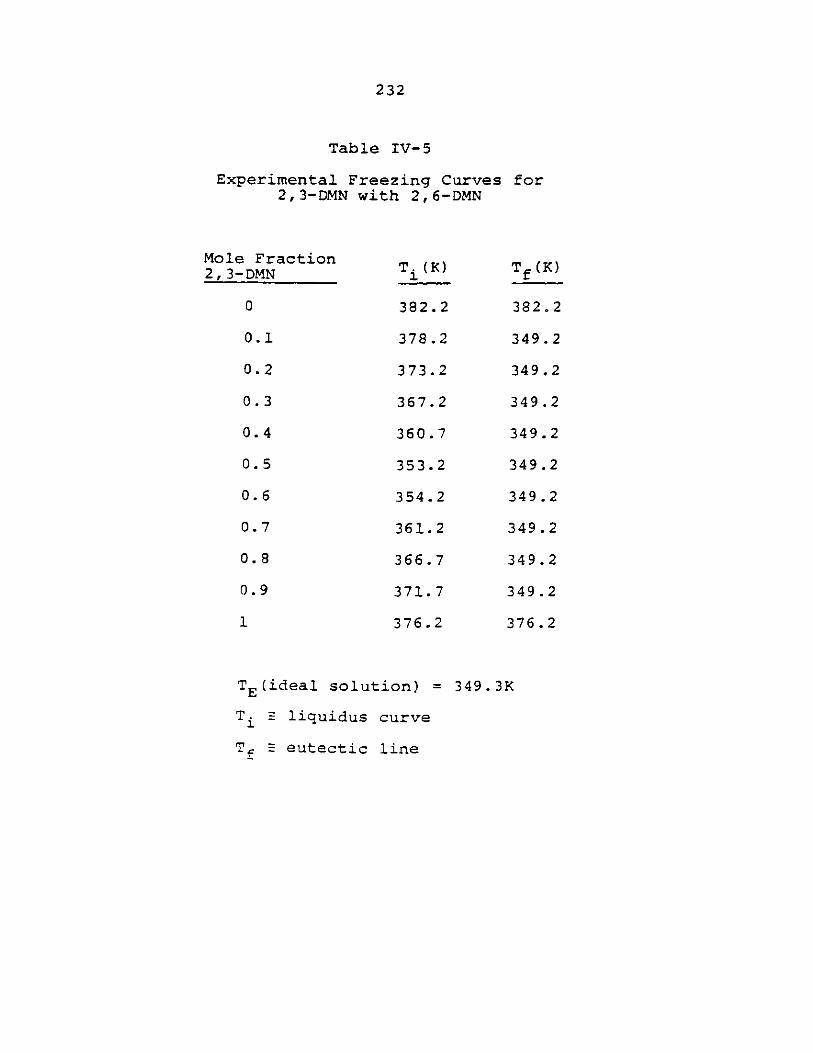
232
Table IV-5
Experimental Freezing Curves for2,3-DMN with 2,6-DMN
Mole Fraction T (K) T (K)2,3-DMN T (f
0 382.2 382.2
0.1 378.2 349.2
0.2 373.2 349.2
0.3 367.2 349.2
0.4 360.7 349.2
0.5 353.2 349.2
0.6 354.2 349.2
0.7 361.2 349.2
0.8 366.7 349.2
0.9 371.7 349.2
1 376.2 376.2
TE(ideal solution) = 349.3K
T. liquidus curve
T eutectic line
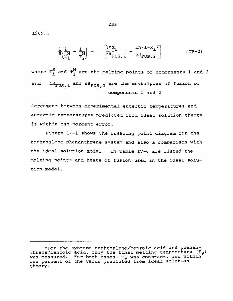
233
1969)
1 1lx ln (1-x 1 IV2--- = VnH AH(I-
T1 T LtHFUS,I I FUS,2]
where T and T2 are the melting points of comopnents 1 and 2
and AH FUS,1and H FUS,2are the enthalpies of fusion of
components 1 and 2
Agreement between experimental eutectic temperatures and
eutectic temperatures predicted from ideal solution theory
is within one percent error.
Figure IV-1 shows the freezing point diagram for the
naphthalene-phenanthrene system and also a comparison with
the ideal solution model. In Table IV-6 are listed the
melting points and heats of fusion used in the ideal solu-
tion model.
*For the systems naphthalene/benzoic acid and phenan-
threne/benzoic acid, only the final melting temperature (Tf)was measured. For both cases, Tf was constant, and withinone percent of the value predicted from ideal solutiontheory.
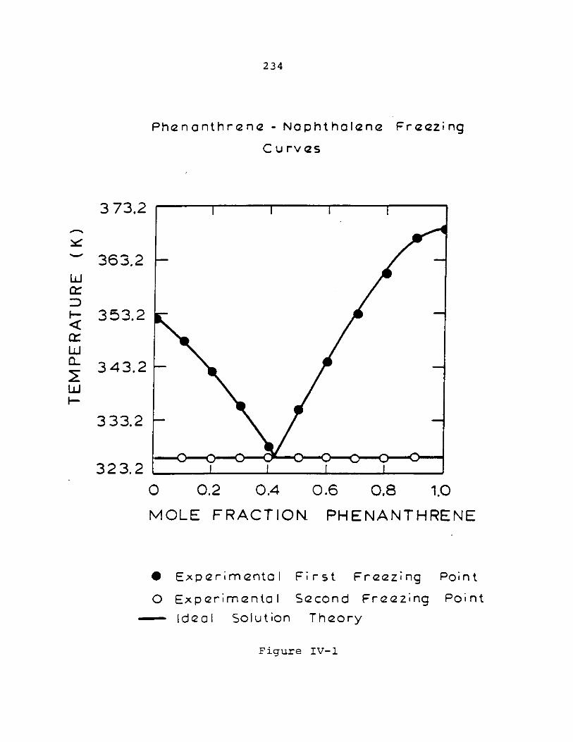
234
Phcncnthrcne - Naphtholene Freezing
C u rvs
0 0.2 04 0.6 o8 1.0
MOLE FRACTION
* Experimental First
PHENANTHRENE
Freezing
0 Experimental Second Freezing
Poin t
Point
--- Ideal Solution Theory
Figure IV-1
SI I I
LUJ
:D
LUCL2LUjH=
373.2
363.2
353.2
343.2
333.2
323.2
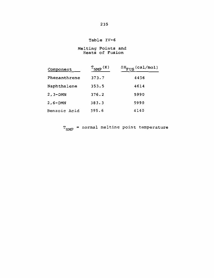
235
Table IV-6
Melting Points andHeats of Fusion
Component
Phenanthrene
Naphthalene
2,3-DMN
2,6-DMN
Benzoic Acid
T NMP(K)
373.7
353.5
376.2
383.3
395.6
AHFUS (cal/mol)
4456
4614
5990
5990
4140
T NMP = normal melting point temperature
236
APPENDIX V
PHYSICAL PROPERTIES OF SOLUTES STUDIED
In Table V-1 are listed physical properties of the
supercritical fluids and the solutes studied in this
research. Table V-2 lists vapor pressure data for all
the solutes.
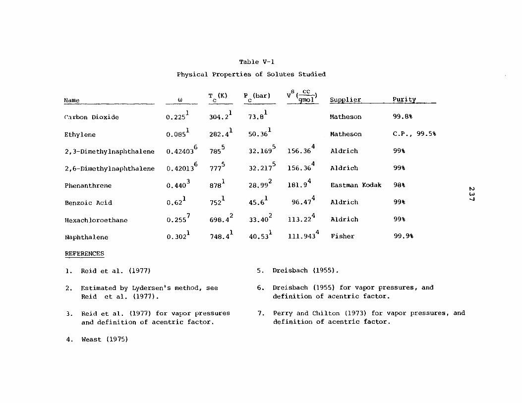
Table V-1
Physical Properties of Solutes Studied
T (K) P (bar) Vs ccName __C
Carbon Dioxide 0.2251 304.2
11Ethylene 0.0851 282.4
2,3-Dimethylnaphthalene 0.424036 7855
2,6-Dimethylnaphthalene 0.42013 7775
Phenanthrene 0.440 8781
Benzoic Acid 0.621 7521
7Hexachloroethane 0.255 698.4
Naphthalene 0.3021 748.4
REFERENCES
1. Reid et al. (1977)
2. Estimated by Lydersen's method, see
Reid et al. (1977).
3. Reid et al. (1977) for vapor pressures
and definition of acentric factor.
4. Weast (1975)
c gmoli
73.81
50.361
32.1695
32.27 5
28.992
45.61
33.42
40.531
L
156.36 4
156.36 4
181.9 4
96.474
113.224
111.9434
Supplier
Matheson
Matheson
Aldrich
Aldrich
Eastman Kodak
Aldrich
Aldrich
Fisher
Purity
99.8%
C.P., 99.5%
99%
99%
98%
99%
99%
99.9%
5. Dreisbach (1955).
6. Dreisbach (1955) for vapor pressures, and
definition of acentric factor.
7. Perry and Chilton (1973) for vapor pressures, and
definition of acentric factor.
LA)
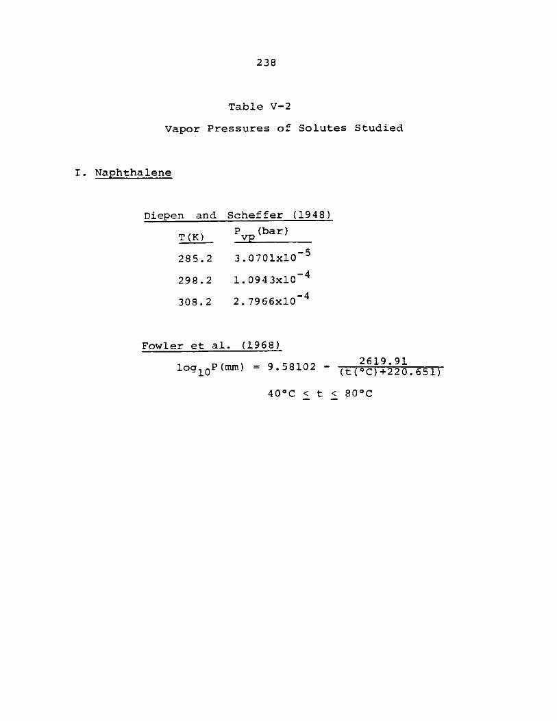
238
Table V-2
Vapor Pressures of Solutes Studied
I. Naphthalene
Diepen and
T (K)
285.2
298.2
308.2
Scheffer (1948)
vp (bar)
3. 0701x10 -5
1. 0943x10 4
2. 7966x10~ 4
Fowler et al. (1968)
2619.91log1 0 P(mm) = 9.58102 (t(0 C)+220. 651)
40*C < t < 800C
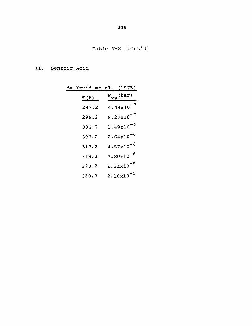
239
Table V-2 (cont 'd)
II. Benzoic Acid
de Kruif et
T (K)
293.2
298.2
303.2
308.2
313.2
318.2
323.2
328.2
al. (1975)
P (bar)VP
4. 49x10~ 7
8. 27x10
1. 49x10-6
2. 64x10 -6
4. 57x10-6
7. 80x10-6
1. 31x10 -5
2. 16x10 -5
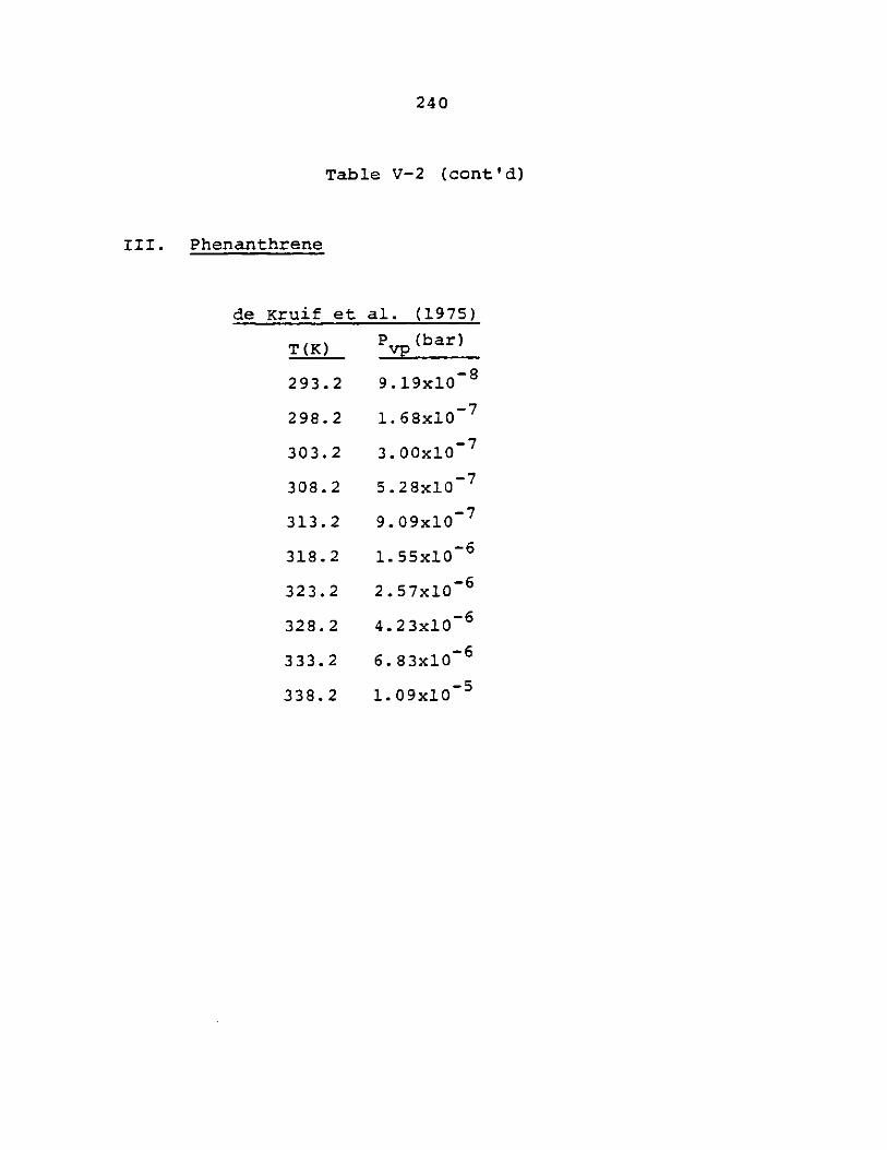
240
Table V-2 (cont'd)
III. Phenanthrene
de Kruif et al. (1975)
T(K) PV (bar)
293.2 9.19x10 8
298.2 1.68x10 7
303.2 3.00x10 7
308.2 5.28x10 7
313.2 9. 09x10 7
318.2 1.55x10 -6
323. 2 2.57x10⁻⁶
328.2 4.23x10⁻⁶
333.2 6.83x10⁻⁶
338.2 1.09x10⁻⁵
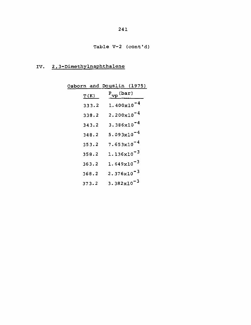
241
Table V-2 (cont'd)
IV. 2, 3-Dimethylnaphthalene
Osborn and Douslin (1975)
TO(K) vp (bar)
333.2 1.400x10 4
338.2 2.200x10 4
343.2 3.386x10C4
348.2 5.093x10~ 4
353.2 7.653x10~ 4
358.2 1.136x10⁻³
363.2 1.649x10⁻³
368.2 2.376x10⁻³
373.2 3.382x10⁻³
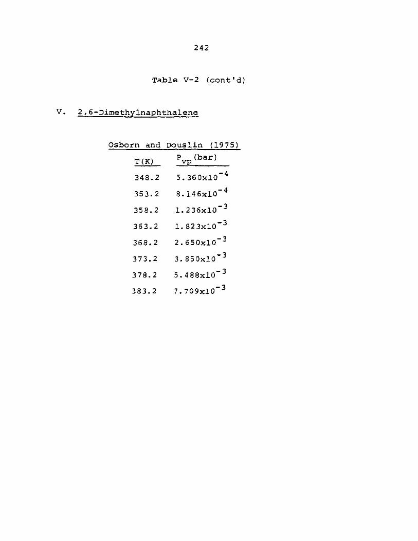
242
Table V-2 (cont'd)
V. 2,6-Dimethylnaphthalene
Osborn and
T (K)
348.2
353.2
358.2
363.2
368.2
373.2
378.2
383.2
Douslin (1975)
P (bar)
5. 360x10 4
8.146x10o 4
1. 236x10- 3
1. 823x10 -3
2. 650x10- 3
3. 850x10-3
5. 488x10-3
7. 709xlO 3
w
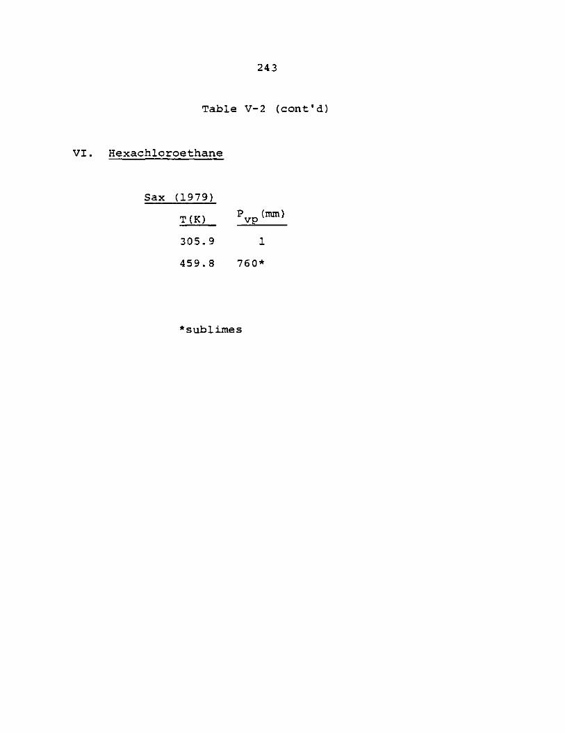
243
Table V-2 (cont'd)
VI. Hexachloroethane
Sax (1979)
T (K)
305.9
459. 8
vp (m)
1
76 0*
*sublimes
244
APPENDIX VI
SOURCES OF PHYSICAL PROPERTIES OF COMPLEX MOLECULES
Required physical property data for simulating equil-
ibrium solubilities in binary and multicomponent solid-
fluid equilibrium systems are: critical temperatures,
critical pressures, and acentric factors for solute and
solvent and vapor pressure and molar volumes of the solute.
Of these properties, those which are usually unknown are
solid vapor pressures and solid critical properties. It
is the purpose of this appendix to summarize these solid
properties. This summary is not meant to be all-inclusive,
but it covers physical property data found during the
author's work. Table VI-I lists references containing
solid vapor pressures along with the temperature range
covered. Sources of critical property data are given by
Reid et al. (1977) and Ambrose and Townsend (1978).
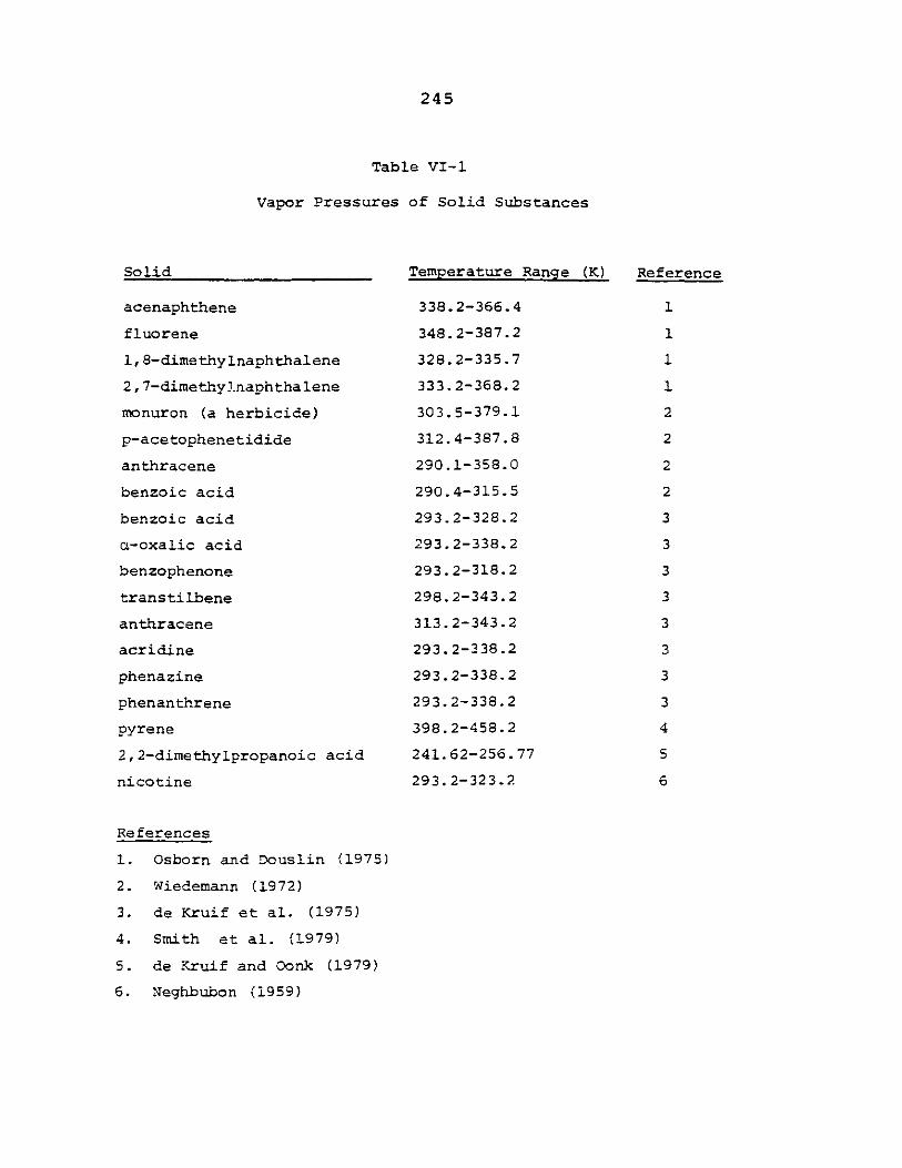
245
Table VI-1
Vapor Pressures of Solid Substances
Solid
acenaphthene
fluorene
1, 8-dimethylnaphthalene
2 , 7-dimethy3naphtha lene
monuron (a herbicide)
p-acetophenetidide
anthracene
benzoic acid
benzoic acid
a-oxalic acid
benzophenone
trans tilbene
anthracene
acridine
phenazine
phenanthrene
pyrene
2, 2-dimethylpropanoic acid
nicotine
References
1. Osborn and Douslin (1975)
2. Wiedemann (1972)
3. de Kruif et al. (1975)
4. Smith et al. (1979)
5. de Kruif and Oonk (1979)
6. Neghbubon (1959)
Temperature Range (K)
338. 2-366 .4
348.2-387.2
328.2-335.7
333.2-368.2
303.5-379.1
312.4-387.8
290.1-358.0
290.4-315.5
293.2-328.2
293.2-338.2
293.2-318.2
298.2-343.2
313.2-343.2
293.2-338.2
293.2-338.2
293. 2-338.2
398.2-458.2
241. 62-256. 77
293.2-323.2
Reference
2
2
2
2
3
3
3
3
3
3
3
3
4
5
6
246
APPENDIX VII
LISTINGS OF THE PERTINENT COMPUTER PROGRAMS
In this appendix, three computer programs, written
in FORTRAN, are listed.
Table VII-l is the listing of the program PENG. This
program is used to calculate the equilibrium solubility of
a solid in a fluid for binary systems. The Peng-Robinson
equation of state is used.
Table VII-2 lists the program MPR and eight subroutines.
This program calculates equilibrium solubilities for multi-
component solid-fluid equilibria with the Peng-Robinson
equation of state.
Table VII-3 lists the program KIJSP and two subroutines.
These programs call a non-linear least squares regression
subroutine (GENLSQ) to determine a binary interaction para-
meter for solid-fluid equilibria. The interaction para-
meters are those for the Peng-Robinson equation of state.
Table VII-4 gives detailed documentation of the non-
linear least squares subroutine GENLSQ that performs the
actual regression. This documentation is supplied courtesy
of Dr. Herb Britt.
The input parameters for each of these programs are
explained in the beginning of the respective programs.
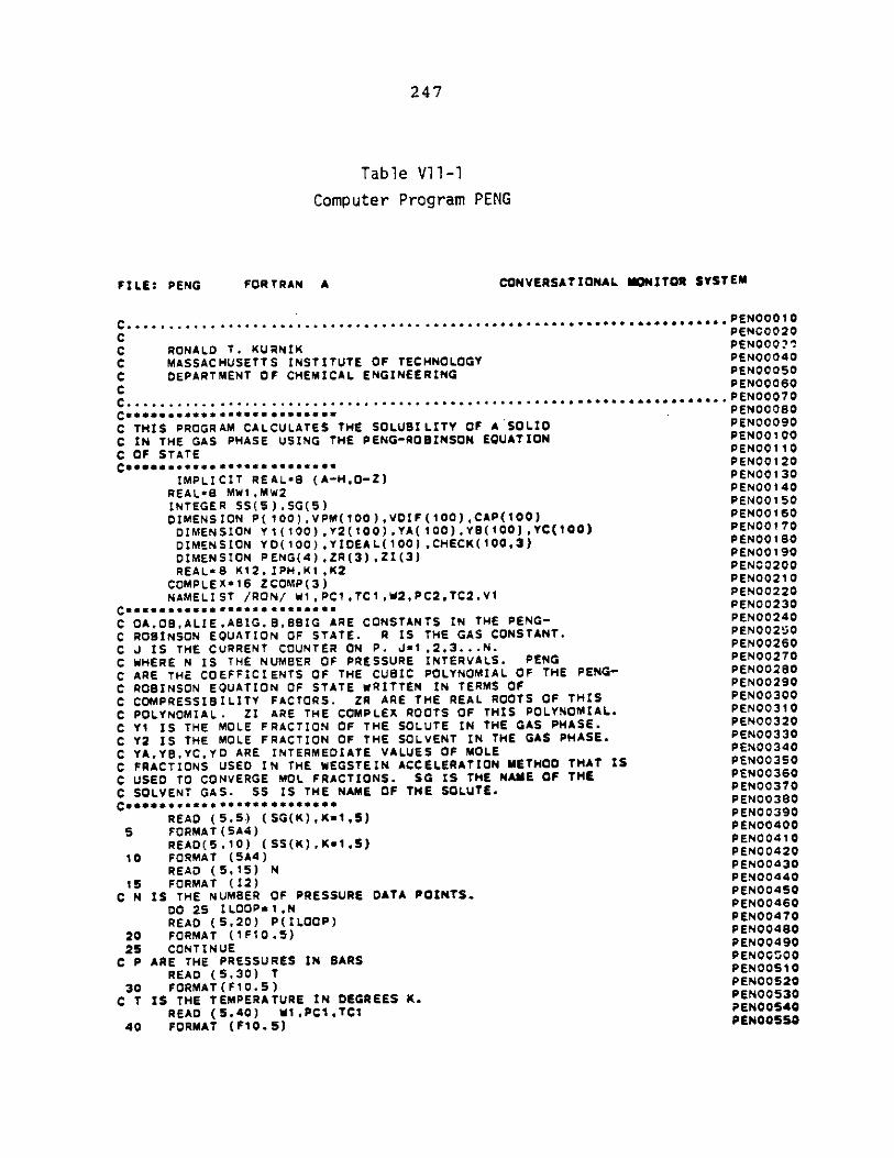
OSSOON3d (SOW ) WU0 ot
ovBOON~d L1' 3'LS (010s) 0I3kf
OCSOON3d w"N S33NO30 NI 3flfl Ib3dW3 3HI4 51 0
OCSCON3d ( s'o0L A) lvuW0 J or
o LSOON3d (oc's) Oa~b
0OGOON~d StiV9 NI SmifSSatd 314 IUW d 3
06tOON3d InNIINDOD se
O8VOON~d (r*OL L)L Ikio i Oc
OLV0ON3d (d0011l)d (or's) Oaim
O9vOONad N~td0O1I Sr 00
OSOOON~d OS NIOd VIVO 3bfSSfld 0 b39wfN 314 SI N 3
OVVOON~d (ri) vwuo siOCPOON3d N (GL'S) C3V~
CZV00N3d (oYs) vwb0 CL
o LVOON3d ('LsuN'(N)SS) (OL'S)013b
CCV00N3d (vl9) IW~D s
O6EOON3d (S'- S('S) Oann
O9CO0N3d *~Ss*S**S*#*@
OLCOON~d '3 liOS 3ml 2 0 3WYN 314 SI SS 'SV0 N3A1OS 3
OSCOON~d 3M14 0 3KVN 314 SI VS 'SNDIO 31 IOW 3Dn3AN03 0 O3Sfl 3
OSCOON~d S IV 11 OM1001 KNOI Vb31333Y N13 S03M 314 NI Q3Sfl SNOIZDYbi 3
OCDCON3d 310W .0 SnifVA 3 VIC3W83 NI 3ml OA'3A'9A'VA 3
OCCOON~d *3511d SYD 314 NI N3A1OS 314 0 NOI 31n 310W 314 SI CA 3
OCCOON~d *3SV14d SIC 314 NI 3 fl10S 314 AD 0 NI 3Vb 310W 314 SI A 3
O&COON~d IIW0NA10d 5SIMI 0 SIOOb X31dW0O3H 314 3 I12 'iIIWONA1Od 3
COCOON~d 5114 0 SICOonIV~b 314 mY fl SbD 3Y AII9ISS38dW03 3
O6ZO0N3d 0 SW63 NI N3 IbM 31 S 0 NoIuvrIONSNI90b 3
CerOON~d -DN3d 314 : 0 lYIWONAlOd 319113 314 0 S N3131 30:)3H3 I0
OLZOON3d DN3d 'SlVAU3 NI bnASS~bd 0JO IBIAAAN 314 51 N 3n314M 3
OSCOON~d WN "C'rl d NO tf3 Nfl03 N3bAO3H34 I 'r3
CcGr00N3d LNY 5N03 SIC) 314 SI b '31 5 0 NOXivnCI N0SNI90U 3
OvZOON~d -Om~d 314 NI S NV 5N0O3 mV 019'9D19r'311'90'I0 3
OCE00N3dOrrooN~d Lr rdr'3'3'M/NOH/ S113WVN
o trooNad (C)dwOO)Z SL*x31dW03
C0rOON3d rVWx14d1 'rLi 8BelVa
C6LOON3d (C)IZiCE)bZ'(t')DN~d NOISNIWIO
OSLOON~d (E'OCL))3314'(CL)1V3OIA'(OOL)O3A NOISNSWIC
Ch&OON3d (C)A(O)A(OLV'CLr(o)ANOISNIINICOSLOON~d (OOL)dV3'(OCL) IOA'(OO1)WdA'(COL)d NOISNIWIC
OSLOON~d (S)DV'(S)SS bi03iNi
OPLOON~d rMW'LMW 9.1I3b
OCLOON~d (Z0'14-I) BalV~b L IIdWI
CL LOON~d 3VI S j90
COLOON~d NOI 1fl03 NOSNI9OA-DN3d 314 VNISA ISY~d SIC)314 NI 3
O6000N3d 011051 A IAn 10iS 34 1f3 113 iinvowIE)Obd 51M 3
OtODON~d ' @ *.. ... .. .......... .. 3
C9000N3d 3
0OOON~d DNIh33NIDN3 1W3143 0 N3W~dVdlO 30
OVOOON3d AD0I0N1433 0 31Ani iSNI S 35111431551W 3C000N3d )INunl. *1 IN0b 3
oroOwNd 3
C I CON~d .*p@...... * U.. ... ............. ..3
N31SAS NOIC W VNOI VSU3AN03 V NVtl W0 (mid :3114
DN3d we.A5o-ad.aa;ndwoc,
-ILA aLqej
LAVZ
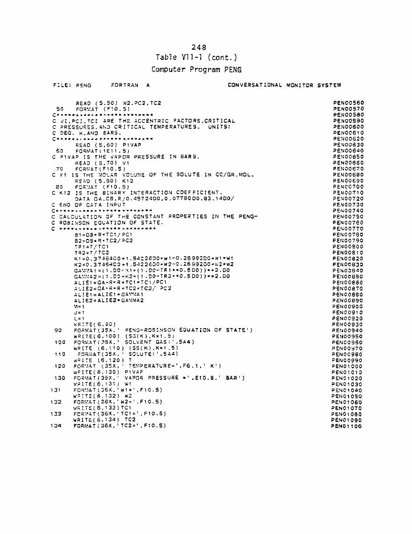
248Table VlI-1 (cont.)
Computer Program PENG
FILE: PENG FORTRAN A CONVERSATIONAL MONITOR SYSTEM
READ (5.50) W2,PC2,TC250 FOR!.0AT (F4O.5)
C ZI,PCI,TCI ARE THE ACCENTRIC FACTORS.CRITICALC PRESSURES.,AND CRITICAL TEMPERATURES. UNITS:C DEG. K.AND EARS.c- ***, W --A ****** -U ***
READ (5,60) PIVAP60 FORMAT(1EI1.5)
C PIVAP IS THE VAPOR PRESSURE IN BARS.READ (5,70) VI
70 FCRMAT(F10.5)C VI IS THE OLAR VOLUME OF THE SOLUTE IN CC/GR.MOL.
READ (5.90) K12!0 FORMAT (FIO.5)
C K12 IS THE BINARY INTERACTION COEFFICIENT.DATA CA,0B.R/0.45724DO,0.0778000,83.1400/
C END OF CATA INPUTC CWWU ** *- * * $ * 3 *
C CALCULATION OF THE CONSTANT PROPERTIES IN THE PENG-C ROBINSON EQUATION OF STATE.C S*...*-a.*****.SSS***
B1=03'wR-TCI/IPC1B2=0S*P.-TC2/PC2TP1=T,/TCTR2=T/ TC2K1=0.3746400+1.54226DOw1-0.26992OsW1*W1K2=0.3746400+1.54226.O*W2-0.2699200-W2*W2GAM1AI=(I.D0-A1w(I.00-TR1**0.5D0))*s2.O0GA IA2=(I.I0.e2 (1.00-TR2**0.5DO))*2.DO0ALIEI=OAR*RSTC1'TC1/PC1A,-!E2=CA-RRTC2vTC2/ PC2ALIE1 =ALIEICwGAMV.AIALIE2=ALIE2*GAMMA2M= 1U=1L=1TWRITE(6,30)
90 FORMAT(35X' PENS-ROBINSON EQUATION OF STATE')WprTE(6,100) (SG(K),K=l,5)
100 FORMAT(35X.' SOLVENT GAS:',5A4)WRITE (6,110) (SS(K),K=1,5)
110 FORMAT(35X.' SOLUTE:',5A4).ITE (6,120) T1
120 FORMAT (35X, ' TEMPERATURE=',F6.,' K' )WRITE(6,130) PiVAP
130 FORMAT(35X,' VAPOR PRESSURE =' ,E0.5.' BAR')w;ITE(6.131 W1
131 FO RAAT(36X,'W1=',F10.5)WPATE(6.132) W2
132 FORMAT(36X.'W2=',F10.5)WRITE(6.133)TC1
133 FCRAT(36X.'TC1=',Fl0.5)WRITE(6.134) TC2
134 FORMAT(36X.'TC2=',F10.5)
PENOO560PENOO570PENOO580PEN00590PENOO600PENOO610PEN00620PENOO630PENOO640PEN00650PENO0660PENOO670PENOO6SOPENOO690PENOO700PENOO710PENOO720PENOO730PENOO740PENOO750PEN00760PENOO770PENO0780PENCO 790PENOOBOOPEN0810PENOOS20PEN0O830PENOO4OPENOO850
PENOo60PENOO870PENOOSSOPENOO890PENO0900PEN00910PENOO920PENO930PENO094OPEN0O950PENCO960PENOO70PENOOSSOPENOO990PENO1000PENO1010PENO1020PEN01030PENO1040PENO1050PENO1060PENO1070PENO1080PENO1090PEN01100
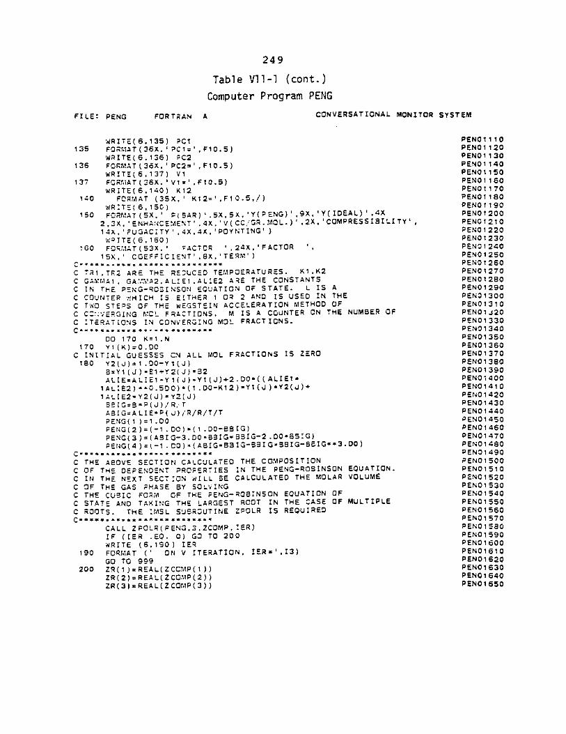
249
Table Vll-1 (cont.)
Computer Program PENG
FILE: PENG FORTRAN A CONVERSATIONAL MONITOR SYSTEM
WRITE(6.135) PC1 PENO1110135 FoRMAT(36X,'PC1=',F10.5) PENO1120
WRITE(6.136) PC2 PENO1130136 FORMAT(36X.'PC2=',F10.5) PEN1140
WRITE(6,137) Vi PENO1150137 FORMAT(26X.'V1='.F10.5) PEN01160
WRITE(6.140) K12 PEN01170140 FORMAT (35X,' K12=',FIO.5,/) PENO1180
WRITE(6,150) PENO1190150 FORMAT(SX.' P(BAR)'.5X,5X,'Y(PENG)',9X,Y(IDEAL)'.4X PENO1200
2,-3X2, 'ENHANCEMENT ' .4X. -V( CC/GR. MOL.),2X, 'COMPRESSIBILITY, PENO1210
14X,'FUGACITY',4X,4X,'POYNTING') PENO1220
V2ITE(6,160) PENO1230160 FORMAT(53X, FACTOR ',24X,'FACTOR ', PENO1240
15X,' COEFFICIENT',SX,'TERM') PENO12SO
C a..*...u..s......... PEN01260
C TR1,TR2 ARE THE REUCED TEMPOERATURES. K1,K2 PENO1270
C GAMMA1, GA.',A2,ALIE1.ALIE2 ARE THE CONSTANTS PENO12SOC IN THE PENG-RO5INSON EQUATION OF STATE. L IS A PENO1290
C COUNTER '!HICH IS EITHER 1 OR 2 AND IS USED IN THE PENO1300
C TWO STEPS OF THE wEGSTEIN ACCELERATION METHOD OF PEN0131o
C C:%VERGING MCL FRACTIONS. M IS A COUNTER ON THE NUMBER OF PENO1J20
C ITERATIONS IN CONVERGING MOL FRACTIONS. PENO1330
C* PENO1340
00 170 K=1,N PENO1350170 Y1(K)=0.DO PENO1360
C INITIAL GUESSES CN ALL MOL FRACTIONS IS ZERO PENO1370
180 Y2(J)=1.DO-YI(J) PENO1380
B=Y1(J)-E1+Y2(J) -92 PENO1390
ALIE=ALIE1-Y1(J)+Y1(J)+2.D0*((ALIEl* PENO1400
1AL'E2)--0.SDO)*(1.D0-K12)*Y1(J)*Y2(d)+ PENO1410
1ALIE2-Y2(J)-Y2(J) PENO1420
SELG=B-P(J)/R: T PENO1430
ABIG=ALIE*P(J)/R/R/T/T PENO1440
PENG(1 )=1.DO PENO1450
PENG(2)=(-1.DO)*(1.D00-BIG) PENO1460
PENC(3)=(ASIG-3.DO-BSIGBBIG-2.DO*BSIG) PENO1470
PENG(4)=(-1.CO)(ABIG-BBIG-BBIGvBSIG-BBIG**3 .DO) PENO1480
C CtU*catinssS ws.-mSeein-n PENO1490
C THE ABOVE SECTION CALCULATED THE COMPOSITION PENO1500
C OF THE DEPENDENT PROPERTIES IN THE PENG-ROBINSON EQUATION. PENO1510
C IN THE NEXT SECTION WILL BE CALCULATED THE MOLAR VOLUME PENO152O
C OF THE GAS PHASE BY SOLVING PENO1530
C THE CUBIC FORM OF THE FENG-ROBINSON EQUATION OF PENO154O
C STATE AND TAKING THE LARGEST ROOT IN THE CASE OF MULTIPLE PENO1550
C ROOTS. THE IMSL SUBROUTINE ZPOLR IS REQUIRED PENO1560
C *nssssasms*i*--ns*ni*.sk PENO1570
CALL ZPOLR(PENG,3,ZCOMP,IER) PENO1580
IF (IER .EQ. 0) GO TO 200 PENO1590
WRITE (6,190) IER PENO1600
190 FORMAT (' ON V ITERATION, IER='.13) PENO1610
GO TO 999 PENO1620
200 ZR(1)=REAL(ZCCMP(1)) PENO1630
ZR(2)=REAL(ZCOMP(2)) PENOI640
ZR(3)=REAL(ZCOMP(3)) PENO1650
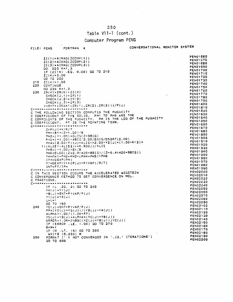
250
Table Vll-l (cont.)
Computer Program PENG
FILE: PENG FORTRAN A CONVERSATIONAL MONITOR SYSTEM
ZI(1)=AIMAG(ZCOMP(1)) PENOI660
ZI(2)=AIMAG(ZCCMP(2)) PENC0170
ZI(3)=AIMAG(ZCOMP(3)) PENO1660
DO 220 K=1,3 PEN01690
IF (ZI(K) .EQ. 0.00) GO TO 210 PEN01700
ZI(K)=0.DO PENO1710
GO TO 220 PENO1720
210 ZI(K)=1.DO PENO1730
220 CONTINUE PENO1740
DO 230 K=1.3 PENO1750
230 ZR(K)=ZR(K)ZI(K) PENO1760
CHECK(J,1 )=ZR(1) PENO1770
CHECK(J.2)=ZR(2) PENO1780
CHECK (J,3) =ZR(3) PENOI790
V=R-T. D0MAXI(ZR(IVZR(2),ZR(3)))/P(J) PENO18OOC PENGI 610
C THE FOLLOWING SECTION COMPUTES THE FUGACITY PENO1820
C COEFFICIENT OF THE SOLID. PHI TO PH6 ARE THE PENO1830
C COMPONENTS OF THE FUGACITY. PH IS THE LOG OF THE FUGACITY PEN01840
C COEFFICIENT. PT IS TME POYNTING TERM. PENOl 85
C p SS-- * - $* * S * * W * P E N O 1 6 6 0
Z=P(J)sV/R/T PENO1870
PH1=B1*(Z-1.00)/B PENO1880
PH2=(-1.DOP-L1Z-BBIG)PPH3=L-1.DO).ABtG'2.DO/BSIG/0SQRT(2.DO) PENO1900
PH4=(2.DO-Y1(J)PALIE1+2.DO*Y2(J)*(1.00-K12)* PENO1910
1( (ALIEI.-ALIE2)--0.5DO))/ALIE PEN01920
PH5=(-1.D00) 61/8 PEN01930
PH6=DLOG((Z+2.414DO-BBIG)/(Z0-.414O*BIG)) PENO1940
H=PH 1 PH2 PHS (PH4+PHS)PNPHE1950
!PH=DEXo(PH) PENO1960
P=DEXP( VI* (P(J)-P1VAP) /'R/T) PENO1970
ENT=PT/IPH PENO1980
C *PENO1990C IN THIS SECTION OCCURS THE ACCELERATED wEGSTEIN PEN02000
C CONVERGENCE r,'ETHOD TO GET CONVERGENCE ON MOL. PENO2OI0
C FRACTIONS. PENO2200PENO2C3O0
IF (L .EQ. 2) GO TO 240 PENO2040
YA(.j =Y1 (J) PENO2050
YB(J)=ENTwP1VAP/P(J) PENO2060
Y1(J)=Y(J) PENO2070
L=L+1 PENO-2080
GO TO 180 PENO2090
240 YC(J)=ENT*PIVAP/P(J) PEN02100
FP=(YC(U)-YS(J))/(YB(J)-YA(J)) PENO2110
ALPHA=1.D/(.OO-FP) PENO2120
YO(J)=YB(J)+ALPHA*(YC(J)-YB(J)) PENO2130
ERRO;=1.34*CAsS((YC(J)-YB(J))/YC(J)) PENO2140
IF (ERROR .LE. 1.00) GO TO 270 PEN02150
M= M+ I PEN02I160
IF 1 .LT. 15) GO TO 260 PEN02180
WRITE (6,250) M
250 FORMAT (' Y NOT CONVERGED IN '.12,' ITERATIONS') PENO2190
GO TO 888 PEN02200
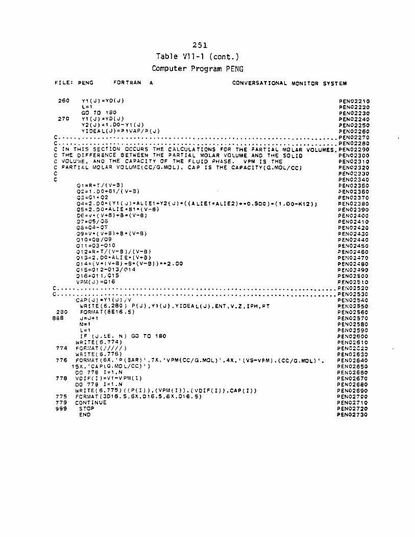
251
Table Vl-1 (cont.)
Computer Program PENG
FILE: PENG FORTRAN A CONVERSATIONAL MONITOR SYSTEM
260 Y1(d)=YD(J) PENO2210L=1 PEN02220GO TO 180 PEN02230
270 Y1(U)=YD(J) PEN02240Y2(J)=1.DO-Y1(4) PENO22SOYIDEAL(J)=PIVAP/P(U) PEN02260
C...... .................................................................PENO2270C.......................................................................PENO2280C IN THIS SECTION OCCURS THE CALCULATIONS FOR THE PARTIAL MOLAR VOLUMES,PEN02290C THE DIFFERENCE BETWEEN THE PARTIAL MOLAR VOLUME AND THE SOLID PENO2300C VOLUME, AND THE CAPACITY OF THE FLUID PHASE. VPM IS THE PEN02310C PARTIAL MOLAR VOLUME(CC/G.MOL), CAP IS THE CAPACITY(G.MOL/CC) PEN02320C PEN02330C PENO2340
Q1=RsT/(V-8) PENO235002=1.DO+B1/( V-B) PEN02360Q3=Q1 02 PEN02370Q4=2.DO'(Yl(J)-ALIE1+Y2(J)*((ALIE1*ALIE2)**0.500)s(1.0-K12)) PEN02380Q5=2.DO*ALIE*81*(V-S) PEN02390QS=V*(V+B)+BS(V-B) PENO240007=05/06 PENO241006=04-07 PEN02420Q9=V*(V+3)+B*(V-B) PENO2430010=08/09 PEN02440011=03-010 PENO2450Q12=R-T/(V-B)/(V-B) PEN02460Q13=2.DOALIE-(V+B) PEN02470Q14=(V*(V+)+*B(V-B))*s2.0 PENO248O15=Q12-013/014 PEN02490
016=011/015 PENO2500VPM(J)0=G16 PENO2510
C........................................................................PENO2520C............. .. ............. -....................................... PENO2530
CAP(J)=Y1(J)/V PENO254OWRITE(6,280) P(J),Y1(U),YIDEAL(J),ENT,VZ,IPH,PT PENO2550
230 FORMAT(8E16.5) PEN02560888 J=J+1 PEN02570
N1=1 PENO2580L=1 PENO2590IF (d.LE. N) GO TO 180 PENO2600
WR:TE(6,774) PENO2610774 FORMAT (/////) PEN2C20
WRITE(6,776) PENO4630776 FORMAT(X,'O(BAR)',7X,'VPM(CC/G.ML)',4X,'(VS-VPM).(CC/G.MOL)', PEN02640
15X,'CAP(G.MOL/CC)') PENO2650DO 778 I=1,N PEN02660
778 VDIF(I)=V1-VPM(I) PEN02670DO 779 I=1,N PENO26OWRITE(6,775)((P(I)),(VPM(I)),(VDIF(I)),CAP(I)) PEN02690
775 FCRMAT(3D16.5,6X,D16.5,6X.016.5) PENO2700779 CONTINUE PEN02710999 STOP PEN02720
END PEN02730
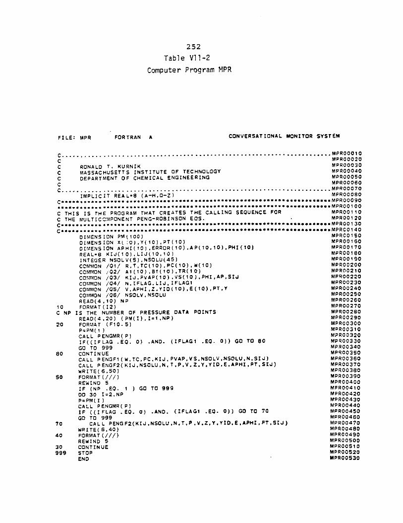
252
Table Vl-2
Computer Program MPR
FILE: MPR FORTRAN A CONVERSATIONAL MONITOR SYSTEM
C.......----..-.............................................................* ... MPROOO10
C MPROOO20
C RONALD T. KURNIK MPROO30
C MASSACHUSETTS INSTITUTE OF TECHNOLOGY MPROOO40
C DEPARTMENT OF CHEMICAL ENGINEERING MPROOOSOC MPROOO60
C............. ..................................................................... MPROOO70
IMPLICIT REAL*8 (A-H.O-Z) MPROOO80
Ceases. sans assss*asse*s eassa as*ess gatea** as*a**s**s* sa*a**asassess*sasMPROOO9O
C THIS IS THE PROGRAM THAT CREATES THE CALLING SEQUENCE FOR MPROO110
C THE MULTICOMPONENT PENG-ROBINSON EOS. MPROO120
Cse*ssee*ssawa*asss,*aea*a**a*s,************ssasa*asas*ss*,s**MPROO13OCss*sas**a***ass*ss***ass*a*s**s*a*s*ss********~*a******************sa*s**MPROOI4O
DIMENSION PM(100) MPROO150
DIMENSION X(:0),Y(10),PT(10) MPROO160
DIMENSION APHI(10),ERROR(10),AP(10,10),PHI(1O) MPROO170
REAL'8 KIJ(10).LIJ(10,10) MPROO1IO
INTEGER NSOLV(S),NSOLU(45) MPROO190
COMMON /01/ R,T,TC(10),PC(10),W(10) MPROO200
COMMON /Q2/ A1(10),B1(10),TR(10) MPROO210
COMMON /03/ KIJ,PVAP(10),VS(10),PHI,AP,SIJ MPROO220
COMMON /04/ N,IFLAG,LIJ,IFLAG1 MPR00230
COMMON /Q5/ VAPHI,Z,YID(10),E(10),PTY MPROO240
COMMON /06/ NSOLV,NSOLU MPR00250READ(4,10) NP MPROO26O
10 FORMAT(I2) MPR00270
C NP IS THE NUMBER OF PRESSURE DATA POINTS MPROO20
READ(4,20) (PM(I),I=1,NP) MPROO290
20 FORMAT (F10.5) MPROO300
P=PM(1 ) MPROO310
CALL PENGMR(P) MPROO320
IF((IFLAG .EQ. 0) .AND. (IFLAG1 .EQ. 0)) GO TO 80 MPROO33OGO TO 999 MPROO34O
80 CONTINUE MPROO350
CALL PENGF1(W,TC,PC,KIJ,PVAP,VS.NSOLVNSOLU,N,SIJ) MPROO360
CALL PENGF2(KIJ,NSOLU,N,T,P,VZ.Y,YID,E.APHI.PT,SIJ) MPR00370
WRITE(6,50) MPROO380
50 FORMAT(///) MPR00390
REWIND 5 MPROO400IF (NP .EQ. 1 ) GO TO 999 MPROO410
DO 30 I=2,NP MPR00420P=PM(I) MPR00430
CALL PENGMR(P) MPROO440
IF ((IFLAG .EQ. 0) .AND. (IFLAGI .EQ. 0)) GO TO 70 MPROO450
GO TO 999 MPROO460
70 CALL PENGF2(KIJNSOLU,NT,P.V,Z,YYID,E,APHIPT.SIJ) MPROO470WRITE(6,40) MPROO480
40 FORMAT(///) MPR00490
REWIND 5 MPROO500
30 CONTINUE MPROO510
999 STOP MPROO520END MPROO530
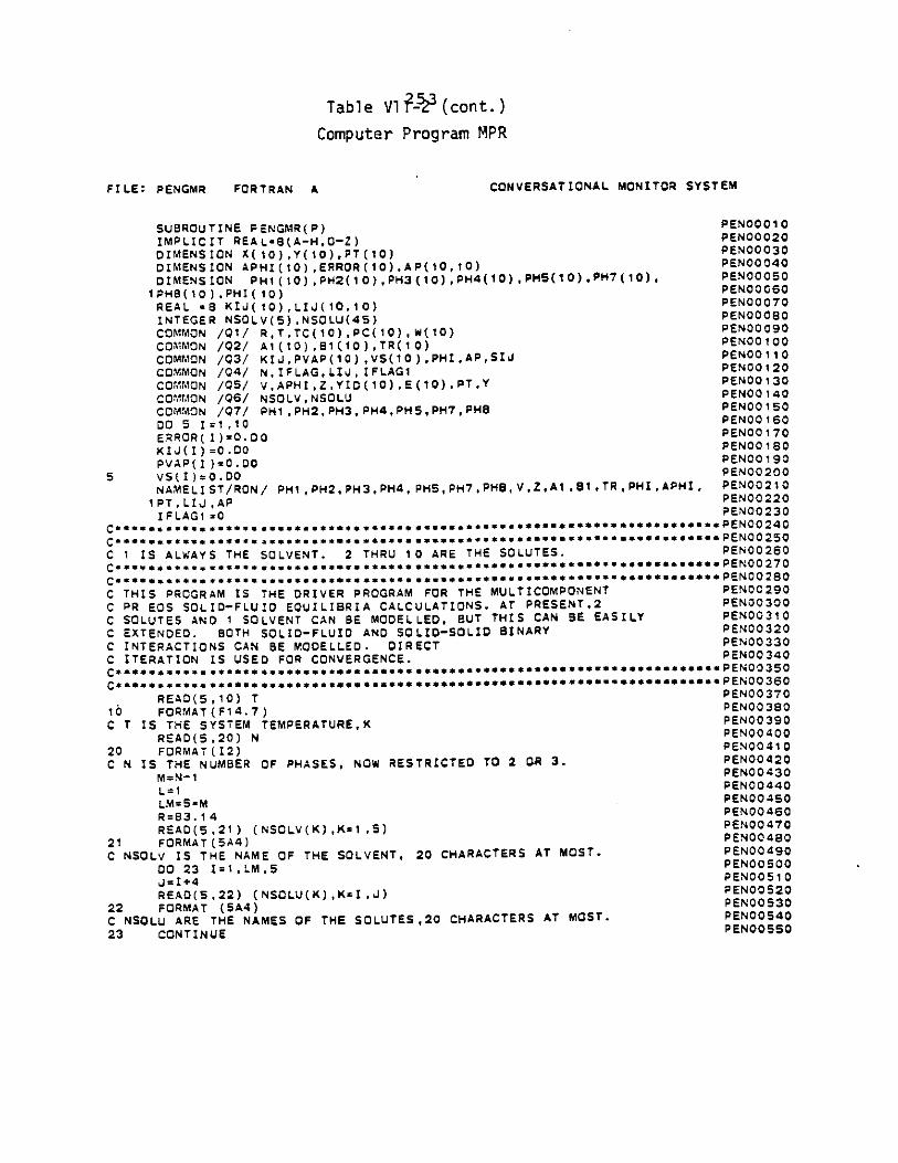
Table Vl - 3 (cont.)
Computer Program MPR
FILE: PENGMR FORTRAN A CONVERSATIONAL MONITOR SYSTEM
SUBROUTINE PENGMR(P) PENOOO10
IMPLICIT REAL8(A-H,O-Z) PENOO20
DIMENSION X(10),Y(10),PT(10) PENOOO3O
DIMENSION APHI(10),ERROR(10),AP(10,10) PEN040
DIMENSION PHl(l0),PH2(10),PH3(10),PH4(10),PHS(1O),PH7 (1O), PENOOO50
1PHB(10),PHI(10) PENOOO6
REAL *8 KIJ(10),LIJ(10,10) PENOOO70
INTEGER NSOLV(5).NSOLU(45) PENOOO80
COMMON /01/ R,TTC(10),PC(10),W(10) PENOOO90
COMMON /02/ A1(10),B1(10),TR(10) PENOO100COMMON /Q3/ KIJ,PVAP(10),VS(10),PHI,AP,SIJ PENOO110
COMMON /04/ N,IFLAG,LIJIFLAG1 PEN0120
COMMON /05/ V,APHI,Z,YID(1O),E(10).PTY PENOO130
COMMON /06/ NSOLV,NSOLU PENO140
COMMON /07/ PH1,PH2,PH3,PH4,PH5,PH7,PH8 PENOO150
DO 5 I=1,10 PENOO160
ERROR(I)=0.DO PENOO170
KIJ(I)=0.DO PENO180
PVAP(I)=O.DO PENOO190
5 VS(I)=0.DO PENOO200
NAMELIST/RON/ PH1,PH2,PH3,PH4,PH5,PH7,PH8,V,Z,A1,B ,TRPHI,APHI, PENOO210
1PT,LIJ,AP PENO220
IFLAGi sQPENOO230C ses* assess as*** am assess*** mesas***e****s******asses**e*s****seesses*essPENOO24O
C 1 IS ALWAYS THE SOLVENT. 2 THRU 10 ARE THE SOLUTES. PENOO260
Cs***sse**ssssss**ssssass*e*e*s*sSS****sss**e*******ssssss**eas*s*esseePENOO280C THIS PROGRAM IS THE DRIVER PROGRAM FOR THE MULTICOMPONENT PENOC290
C PR EOS SOLID-FLUID EQUILIBRIA CALCULATIONS. AT PRESENT,2 PENOO300
C SOLUTES AND I SOLVENT CAN BE MODELLED, BUT THIS CAN BE EASILY PENOO310
C EXTENDED. BOTH SOLID-FLUID AND SOLID-SOLID BINARY PENOO320
C INTERACTIONS CAN BE MODELLED. DIRECT PENO330
C ITERATION IS USED FOR CONVERGENCE. PENO340
READ(5,10) T PENOO370
10 FORMAT(F14.7) PENOO380
C T IS THE SYSTEM TEMPERATURE,K PENO390
READ(5,20) N PENOO400
20 FORMAT(12) PENOO410
C N IS THE NUMBER OF PHASES, NOW RESTRICTED TO 2 OR 3. PENOO420
M=N-1 PENOO430
L=1 PENOO44O
LM=5SM PENOO450
R=83.14 PENOO460
READ(5,21) (NSOLV(K),K*l,5) PENOO470
21 FORMAT(5A4) PENOO480
C NSOLV IS THE NAME OF THE SOLVENT, 20 CHARACTERS AT MOST. PENOO490
DO 23 I=1,LM,5 PENOOSQO
J=I+4 PENOO510
READ(5,22) (NSOLU(K),K=I,J) PENOOS20
22 FORMAT (5A4) PENOO530
C NSOLU ARE THE NAMES OF THE SOLUTES,20 CHARACTERS AT MOST. PENOOS40
23 CONTINUE PENOOSSO
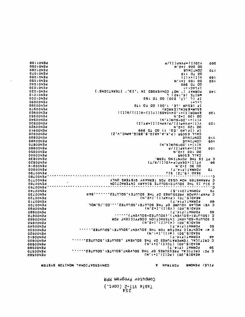
OOL LON~d d/(I)dYAds(I)CXA oor060 LONid NrzI ocr 00090 LCN3d IflNIZLNO3 OtOLD LON3d OLLC01DOSOLON~d ( I) A= (I)X 091090 LONUd N'11 091 CC OSL0O0 LONUd 666 01 CDOCO ONUdkL LOY'l4iOrOLONU (,SNCI 1n3lI ACI s NI C3Db3ANC3 ION A).VWUO.4 Of7L010 LONUd 1 (o00V9) 3116m000 LON3d 091 01 00 (Oocr*Ile1) -41O6600N3d 1+1=1OS600N~d OiL 0.1 CD (oc6L 31r wnss) Al0i600N3d(03)133IfS09600N3d (IX(IX())Sva' =I)C3 OctOSSOON~d NrZ=1 OCtOCOV600N3d (N'"A)IAwfs-o0 1 =(Li),A0C600N3d (I He. x) IHdl/d/ (I)evAe= CI A ortOr0OoNid N'r=IOC 00o t600N3d 666 Cio!CD(Lt0030 Dviii) .i100600N3d (Z'AIlHdY 'DISS'9DsrrV'Xd) 8063 111306900N3d 3IrlNI NCO OI1LoBBOON~d 3flN1 N03 SOtOL900N3d (N"x)vuns-o L(L)XOSSOON~d d/(1)e1Ad2(1)X 001OSBOON~d N'r=I 001 CCOVS0ON~d 89063 1113OtBOON3d *W83 DNIINAOd 3HZ sI ide 3OCSOON3d (18b/ ()SA~d)dxbo= CI lie 0o IBOONUd N'r=I 06 00OOBOON3d (zioti.)lvwoi riO66.00N3d PIS (r22S) 0138Oe 00N3 d..............................................................OLLOONUd AIND SW31SAS A81N831 804 C03Sfl MON b313W1b1d 3OSLOONUd NCI13Z"NI A8YNIS 3ifllCS-3nDcS 3HZ I snrs oOSLO0N~d...............................................OVLtOON3d (suaILoa) Lrj oA oLOCtOON3d i19' . ari~riiOs'ti3tno0s 3H 40o S38flSS3bd 8CdYA:dlAeOrL~oN3d (N'r =I I) dvAe) (oz ' S)ovb0 ILOON~d (Lz0tp L i) vilO:4 OSOOL00N3d i1CrD/OO'*o'r3if1CS't3fl1CS 3HZ 40 3Ifl1CA 81101N:SA 306900N3d (N"'ZVI(I)SA) (O9'S)03809900N3d ('taL ji) .1 wJ80i4 09OL900N~d 6 (N3A1CSr3flCS)'(ZINSA-1CS-L~Inf1S) 3O9900N3d U804 lN3101JJ303 NCIIV313lNlI .NA1OS-SlfllCS 30SSOON~d (N'0'(~ne O9)ov38Ot900N3d (l.vLjLIvw8Ci CsOC900N3d *onr 31nlOS'131nnoCsIN3AlCS 3HZ 880 014314 318.1dN33V 14:Or0ooNid (N 6 L =I(IM ) (09"S)01V380 L900N3d (Lvt'LlWtlC4 Ot'00900N3d tzfl1CoS' ,L~iCS' INIAlOS 3HZ 40 S38flZY83eIN3J I 131 183 306S00N3d (N :1l'(z)3 ) (ot"S)C13tOSSOON~d (L ovLi) 11i80i QoCOLSOON3d 0 ''r*3 rfl0s'ti 1CStlN3A1OS 3HZ 40 S38flSS38e 1131 183 :3d 3OSSOONid (N =V0(z)0) (Or"S)013b
W31SAS U0 IN0W 11N01.LVS83ANO3 V N18Z8C4 8WDN3d :3114
EfdW WeJBOad Je4ndwo3(t4uoz) Z-LLA eLqej
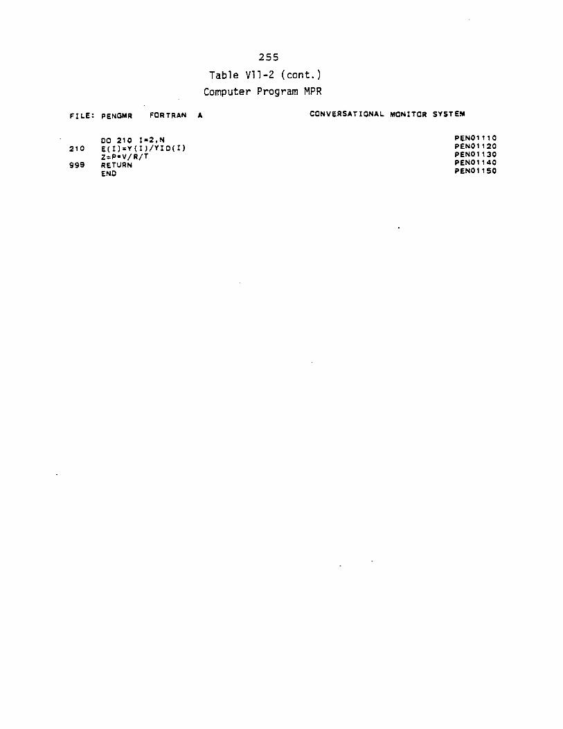
255
Table V1-2 (cont.)
Computer Program MPR
FILE: PENGMR FORTRAN A CONVERSATIONAL MONITOR SYSTEM
DO 210 I=2,N PEN01110
210 E(I)sY(I)/YID(1) PENO1120Z=P*V/R/T PENO1130
999 RETURN PENO1140
END PEN0I150
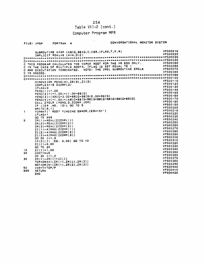
256Table Vl-2 (cont.)
Computer Program MPR
FILE: VPSP FORTRAN A CONVERSATIONAL MONITOR SYSTEM
SUBROUTINE VPSP (ABIG,BBIG,V,IERIFLAG,T,PR) VPS00010
IMPLICIT REAL*B (A-HO-Z) VPS00020
Css**s.*****5.ss *****e**s********ss*s****esees t***t*** te **sVPS0003O
C s*sesass*e a*ses*t*s**s*ss*****************555**** S55S***eesssssesssw*VPSO0040
C THIS PROGRAM CALCULATES THE VAPOR ROOT FOR THE PR EOS ONLY. VPSOOOS0
C IN THE CASE OF MULTIPLE ROOTS. IFLAG IS SET EQUAL TO 1 VPSooo60
C AND EXECUTATION TERMINATED. NOTE: THE IMSL SUBROUTINE ZPOLR VPSO0O70
C IS NEEDED. VPSOO080
DIMENSION PENG(4),ZR(3),ZI(3) VPSOO110
COMPLEX-16 ZCOMP(3) VPS0O120
IFLAG=O VPSOO140PENG(1 )=1.D0 VPSOOI54PENG(2)=(-1.DO)*(1.DO-BBIG) VPSOOIS0
PENG(3)=(ABIG-3.D0*BBIG*SBIG-2.D0*BBIG) VPSOO16O
PENG(4)=(-1.DO)*(ABIGBBIG-BBIG*BBIG-BBIGtBBIG*BBIG) VPSOO170
CALL ZPOLR (PENG,3,ZCOMPIER) VPSOO180
IF (IER .NE. 131) GO TO S VPSOO190
WRITE(6,1) VPSOO200
I FORMAT(' ROOT FINDING ERRORIER=131') VPSOO210
IFLAG=1 VPS00220
GO TO 999 VPSOO230
5 ZR(1)zREAL(ZCCMP(1)) VPS00240
ZR(2)=REAL(ZCOMP(2)) VPS00250
ZR(3)=REAL(ZCOMP(3)) VPSOO260
ZI(1)=AIMAG(ZCOMP(1)) VPS0O270
ZI(2)=AIMAG(ZCOMP(2)) VPSOO280
ZU(3)=AIMAG(ZCOMP(3)) VPS00290
DO 20 1=1,3 VPS00300
IF(ZI(I) .EQ. 0.00) GO TO 10 VPSOO310
ZI(I)=0.DO VPS00320
GO TO 20 VPS00330
10 ZI(I)=1.00 VPS00340
20 CONTINUE VPSOO350
O 30 1=1,3 VPSOO360
30 ZR(I)=ZR(I)*ZI(I) VPSOO37O
TOP=DMAX1 (ZR(1) ,ZR(i) ,ZR(3)) VPS00380
BOT=DMIN1(ZR(1),ZR(2),ZR(3)) VPS00390
50 V=R*T*TOP/P VPS00400
999 RETURN VPSOO410END VP500420
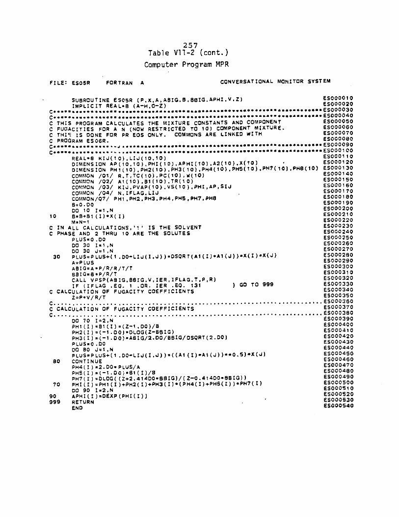
257Table VlI-2 (cont.)
Computer Program MPR
FILE: ESOSR FORTRAN A CONVERSATIONAL MONITOR SYSTEM
SUBROUTINE ESOSR (P,X,A,ABIG,BBBIGAPHI,VZ) ES000010IMPLICIT REALeB (A-H,O-Z) ES000020
C eses $**** **S******$****ea************************ ****S eass 5000040
C THIS PROGRAM CALCULATES THE MIXTURE CONSTANTS ANO COMPONENT ES000050
C FUGACITIES FOR A N (NOW RESTRICTED TO 10) COMPONENT MIXTURE. ES000060C THI IS DONE FOR PR EOS ONLY. COMMONS ARE LINKED WITH E000070
C PROGRAM ESO6R. ES000080
REAL*8 KIJ(10),LIJ(10,10) ES000110
DIMENSION AP(10,10),PHI(10),APHI(10),A2(10),X(10) E000120DIMENSION PH1(10),PH2(10),PH3(10),PH4(10),PH5(10),PH7(10),PHS(10) E5000130
COMMON /01/ R,T,TC(I0),PC(10).W(10) ES000140
COMMON /Q2/ A1(10),B1(10),TR(10) ES000150COMMON /03/ KIJ,PVAP(10),VS(10),PHI,AP.SId ES000160COMMON /Q4/ NIFLAG,LIJ E5000170COMMON/Q7/ PH1,PH2,PH3,PH4,PH5,PH7,PH8 ES0001805=0.00 ES000190DO 10 I1,N E5000200
10 5=B+Bl(I)*X(I) E5000210
M=N-1 E5000220C IN ALL CALCULATIONS,'1' IS THE SOLVENT E5000230C PHASE AND 2 THRU 10 ARE THE SOLUTES ES000240
PLUS=O.DO ES000250DO 30 I=1,N E5000260
DO 30 J=1,N E5000270
30 PLUS=PLUS+(1.0E-LI5(I,J))*DSQRT(A1(I)*Al(J))*X(I)*X(J) ES000280A=PLUS E5000290ABIG=A*P/R/R/T/T E5000300
BBIG=B*P/R/T ES000310CALL VPSP(ABIG,BBIGV,IER,IFLAGT.P,R) E5000320
IF (IFLAG .EQ. 1 .OR. IER .EQ. 131 ) GO TO 999 E5000330
C CALCULATION OF FUGACITY COEFFICIENTS ES000340
Z=P*V/R/T ES000350C...... ...................................... ......................... E5000360
C CALCULATION OF FUGACITY COEFFICIENTS E5000370
C. ..........................................................--- -.--.-- -- E5000380
DO 70 I=2,N E5000390
PH1(I)zB1(I)=(Z-1.D0)/B E5000400
PH2(I)=(-1.D0)*DLOG(Z-BBLG) ES000410
PH3(I)=-(-1.DO)*ABIG/2.DO/BBIG/DSQRT(2.DO) E5000420
PLUS=0.DO ES000430
DO 80 J=1,N E5000440
PLUS=PLUS+(1.DO-LIJ(I,J))s((A1(I)*A(J))**o.5)*X(J) ES000450
80 CONTINUE E5000460
PH4(I)=2.DO*PLUS/A E5000470
P115(I) =(-1 .D0)a(I)/B E5000480
PH7(I)=DLOG((Z+2.414DOBBIG)/(Z-0.41400*BBIG)) E5000490
70 PHI(I)=PM1(I)+PH2(I)+PH3(I)*(PH4(I)+PH5(I))*PH7(I) ES000500DO 90 Is2,N ES000510
90 APHI(I)=DEXP(PHI(I)) ES000520
999 RETURN E5000530
END E000540
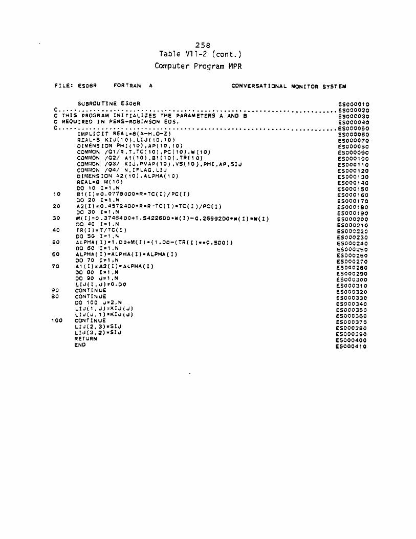
258Table V1L-2 (cont.)
Computer Program MPR
FILE: ESO6R FORTRAN A CONVERSATIONAL MONITOR SYSTEM
SUBROUTINE ESO6R 5000010C.----- ------------- ---------.................. E....................................5000020C THIS PROGRAM INITIALIZES THE PARAMETERS A AND B 5000030C REQUIRED IN PENG-ROBINSON EOS. E5000040C ......................................... 5000050
IMPLICIT REALs8(A-H,O-Z) E5000060REAL*6 KIJ(10),LIJ(10,10) E5000070DIMENSION PHI(10),AP(10,10) E5000080COMMON /Q1/R.TTC(10),PC(10),W(10) E5000090COMMON /02/ A1(10),81(10),TR(10) ES000100COMMON /Q3/ KIJ.PVAP(10),VS(10),PHI,AP,SIJ E5000110COMMON /04/ N,IFLAGLIJ ES000120DIMENSION A2(10),ALPHA(10) 5000130REAL*8 M(10) 5000140CO 10 I=1,N 5000150
10 81(I)=0.07780DOsR*TC(I)/PC(I) 500016000 20 I=1,N ES000170
20 A2(I)sO.4572400*R*R'TC(I)*TC(I)/PC(I) 5000180DO 30 I1,N E5000190
30 M(I)=0.3746400+1.5422600*W(I)-0.2699200*w(I)*W(z) 5000200DO 40 I=1.N ES000210
40 TR(I)=T/TC(I) E5000220DO 50 I=1,N E5000230
50 ALPHA(I)=1.DO+M(I)*(1.D0-(TR(I)*0.500)) ES000240DO 60 I=1,N E5000250
60 ALPHA(I)=ALPHA(I)*ALPHA(I) ES00026000 70 1=1,N 5000270
70 A1(I)=A2(I)*ALPHA(I) E000280DO 80 I=1,N E000290DO 90 J=1,N 5000300LIJ(I,d)=0.DO E000310
90 CONTINUE E5000320so CONTINUE E000330
DO 100 J=2,N 5000340LIJ(1,J)=KIJ(J) ES000350LIJ(J,1))KIJ(J) ES000360
100 CONTINUE ES000370LIJ(2,3)=SIJ 5000380LIJ(3,2)&SIJ ES000390RETURN ES000400END ES000410
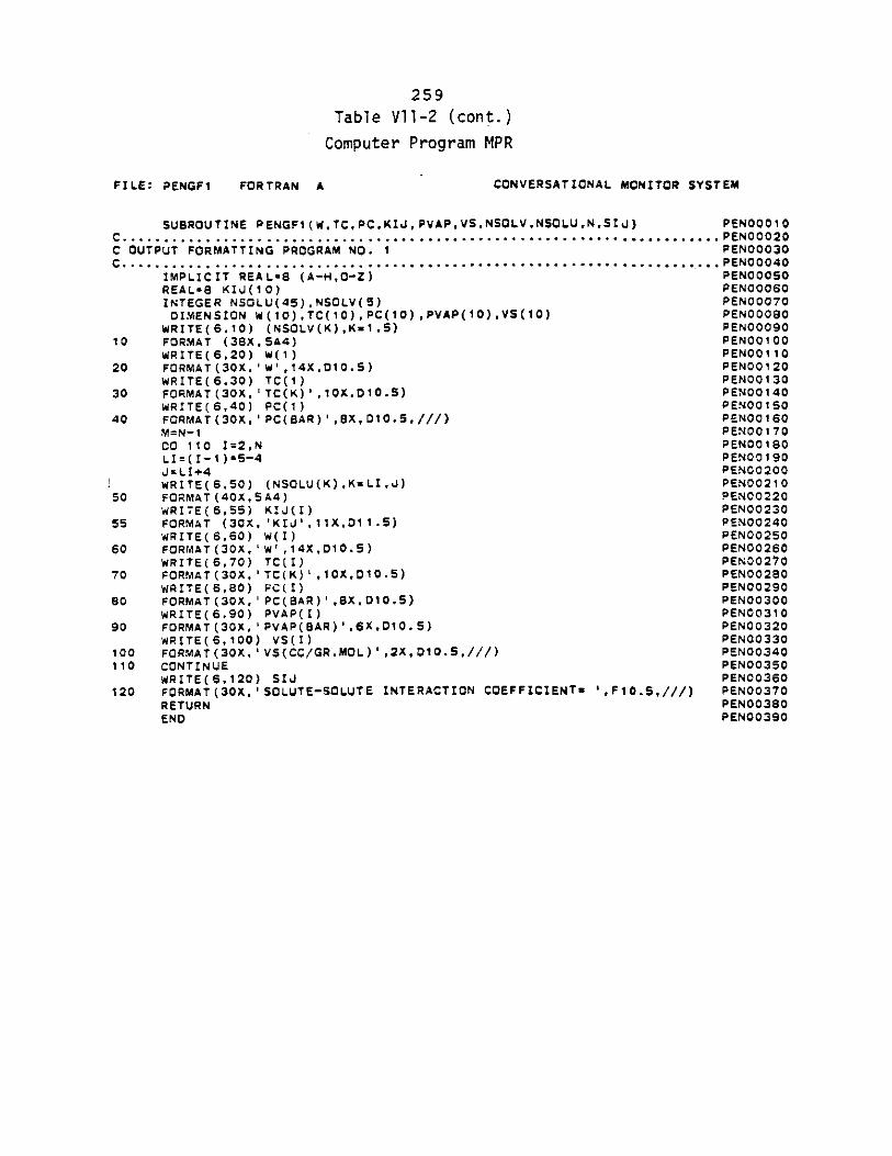
259Table Vll-2 (cont.)
Computer Program MPR
FILE: PENGF1 FORTRAN A CONVERSATIONAL MONITOR SYSTEM
SUBROUTINE PENGF1(WTCPC.KIJPVAPVS.NSOLVNSOLU,N,SIJ) PENOQO10C........................................................--...............PENOOO2OC OUTPUT FORMATTING PROGRAM NO. 1 PEN00030C...............................................................-..............PEN00040
IMPLICIT REAL*8 (A-H,O-Z) PENQOOSOREAL*8 KIJ(10) PENOOO60INTEGER NSOLU(45),NSOLV(5) PENOOO70DIMENSION W(1O),TC(10),PC(10),PVAP(1l),VS(10) PENCOOSO
WRITE(6,10) (NSOLV(K),Ks1,5) PENOOO9010 FORMAT (38X,5A4) PENOO100
WRITE(6,20) W(1) PENOO11020 FORMAT(30X,'W',14XD10.5) PENOO120
WRITE(6,30) TC(1) PEN0013030 FORMAT(30X,'TC(K)',10XD10.5) PEN00140
WRITE(6,40) PC(1) PENOQ15040 FORMAT(30X,'PC(BAR)',BX,D10.5,///) PENO0160
M=N-1 PENOO170CO 110 1=2,N PEN0180LI=(I-1)*5-4 PEN0O190J=LI+4 PEN00200WRITE(6,50) (NSOLU(K),KzL,J) PEN00210
50 FORMAT(40X.5A4) PEN00220WRITE(6,55) KIJ(I) PENOO230
55 FORMAT (30X,'KIJ',11X,D11.5) PEN00240WRITE(6,60) W(I) PENOO250
60 FORMAT(30X,'W',14X,D10.5) PEN00260WRITE(6,70) TC(I) PEN00270
70 FORMAT(30X,'TC(K)',10X,D10.5) PEN00280WRITE(6.80) PC(I) PENOO290
so FORMAT(30X,'PC(BAR)',8XD10.5) PENOO300WRITE(6.90) PVAP(I) PEN00310
90 FORMAT(30X,'PVAP(BAR)',6XDO.5) PEN00320WRITE(6,100) VS(I) PEN00330
100 FORMAT(30X,'VS(CC/GR.MOL)',2XDIO.5,///) PEN00340110 CONTINUE PEN00350
WRITE(6,120) SId PENOO360120 FORMAT(30X.'SOLUTE-SOLUTE INTERACTION COEFFICIENTS ,F10.5,///) PEN00370
RETURN PEN00380END PEN00390
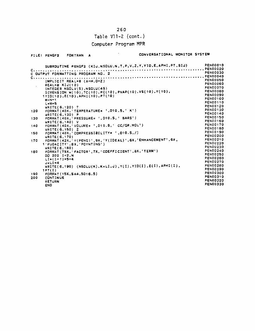
260
Table V1I-2 (cont.)
Computer Program MPR
FILE: PENGF2 FORTRAN A CONVERSATIONAL MONITOR SYSTEM
SUBROUTINE PENGF2 (KIJ,NSOLUNT,PV,Z,YYIO.E.APHI.PT.SIJ) PENOOO10
C0.-....-........--......--....-......--...----...------....-----..----PENOOO2C OUTPUT FORMATTING PROGRAM NO. 2 PENOOO30
c.----.... .... ............- PENOO04OIMPLICIT REAL*8 (A-HO-Z) PENOOSO
REAL*8 KIJ(10) PENOOO6
INTEGER NSOLV(5),NSOLU(45) PENOOO7O
DIMENSION W(10),TC(10),PC(10),PVAP(10),VS(10),Y(IO), PENOOO8O
I Y(10(10),E(10),APHI (10),PT(10) PENOOO90
M=N-1 PEN0O100
L=M*5 PENOO110
WRITE(6,120) T PENOO12O
120 FORMAT(40X,' TEMPERATURE= ',D10.5,' K') PENOO130
WRITE(6,130) P PENOO140
130 FORMAT(40X,'PRESSUREz ',010.5,' BARS') PENOO150
WRITE(6,140) V PENOO16O
140 FORMAT(40X,'VOLUME= ',D10.5,' CC/GR.MOL') PENOO170
WRITE(6.150) z PENOO180
150 FORMAT(40X.'COMPRESSIBILITYs ',010.5./) PENOC190WRITE(6,170) PEN0O200
170 FORMAT(42X,'Y(PENG)',9X,'Y(IOEAL)',6X,'ENHANCEMENT'USX, PENOO210
1'FUGACITY',8X,'POYNTING') PENO0220
WRITE(6,180) PENOO230
180 FORMAT(75XU'FACTOR',7X,'COEFFICIENT',SX,'TERM') PENOO24O
00 200 I=29N PEN00250
LIZ(I-I)*5-4 PEN00260J=L1+4 PENOO27O
WRITE(6,190) (NSOLU(K),K=LI,d),Y(I),YID(I),E(I),APHI(I), PENOO280
IPT(I) PENOO290
190 FORAAT(15X5A4,5016.5) PENOO300
200 CONTINUE PENOO310
RETURN PEN00320
END PENOO330
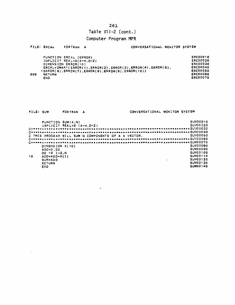
26I
Table V1l-2 (cont.)Computer Program MPR
FILE: ERCAL FORTRAN A CONVERSATIONAL MONITOR SYSTEM
FUNCTION ERCAL (ERROR) ERCOCO10IMPLICIT REALsS(A-HO-Z) ERCOOO20DIMENSION ERROR(10) ERCOOO30ERCAL=DMAXI(ERROR(1),ERROR(2),ERROR(3),ERROR(4),ERROR(5), ERCOO401ERROR(6),ERROR(7),ERROR(B),ERROR(9),ERROR(10)) ERCOOO50
999 RETURN ERCOOC60END ERCOOO70
FILE: SUM FORTRAN A CONVERSATIONAL MONITOR SYSTEM
FUNCTION SUM(X,N) SUMOOO10IMPLICIT REAL*G (A-H,O-Z) SU41100020
C assssssssseseassssss*sssssssssssasssssassasss*ssssaasasstassssss*ss*e*SU.10030Ca*s*s** Ss**6*********asses.*assess***s*s s****** asse*** ***s*a*ss**s**SUMOOO4O
C THIS PROGRAM WILL SUM N COMPONENTS OF A x VECTOR. SUMOCOSOCss**s*assseesss*ssassaseassssssass*sssssa*sss****s****w**s***s**5sSUMOOO6
sa**e s a*s*es* se**e*w***sse*** *ssess* a*****s*s5***s****s* s*5 s~s e*msSUMOOODIMENSION X(10) SUMOO8QADD=0. o SUMOO090DO 10 I=2,N SUMOC 100
10 ADD=ADD+X(I) SUMOO110SUM=ADD -SUMOOI120
RETURN SUM0O130END SUMOO140
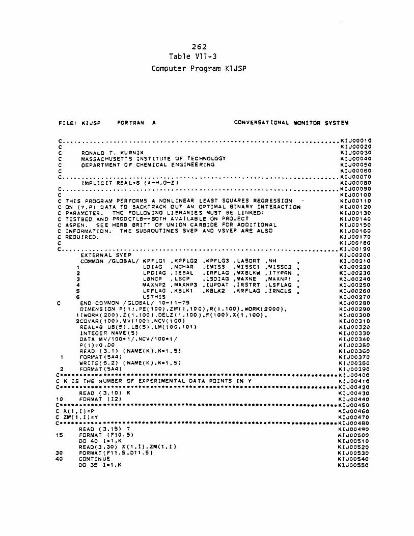
262Table Vl-3
Computer Program KlJSP
FILE: KIJSP FORTRAN A CONVERSATIONAL MONITOR SYSTEM
C........................................................... .............KIJOO10C KIdOOO2C RONALD T. KURNIK KIJ00030C MASSACHUSETTS INSTITUTE OF TECHNOLOGY KIJ00040C DEPARTMENT OF CHEMICAL ENGINEERING KIJOOSOC KI100060C...................KIJOOO70
IMPLICIT REAL*8 (A-H.O-Z) KIJOOOSOC...... ........................................ ......................... KIJOOO90C KIdOO100C THIS PROGRAM PERFORMS A NONLINEAR LEAST SQUARES REGRESSION - KIJOO110C ON (YP) DATA TO BACKTRACK OUT AN OPTIMAL BINARY INTERACTION KIJOO120C PARAMETER. THE FOLLOWING LIBRARIES MUST BE LINKED: KIJOO130C TESTBED AND PRODCTLB--BOTH AVAILABLE ON PROJECT KIJ00140C ASPEN. SEE HERB BRITT OF UNION CARBIDE FOR ADDITIONAL KIJOO150C INFORMATION. THE SUBROUTINES SVEP AND VSVEP ARE ALSO KIJOO160C REQUIRED. KIJOO170c KIJO0180C............ ....................... .... ............................... KIJOO190
EXTERNAL SVEP KIO200COMMON /GLOBAL/ KPFLG1 ,KPFLG2 ,KPFLG3 ,LABORT ,NH , KIJ00210
I LDIAG ,NCHAR ,IMISS ,MISSCI ,MESSC2 , KIJO2202 LPDIAG ,IEBAL ,IRFLAG ,MXBLKW ,ITYPRN , KIJ002303 LBNCP ,LBCP ,LSDIAG ,MAXNE ,MAXNPI , KJ002404 MAXNP2 ,MAXNP3 ,IUPDAT ,IRSTRT ,LSFLAG , KId002505 LRFLAG ,KSLKI ,KSLK2 ,KRFLAG ,IRNCLS , KIJ002606 LS THIS KIJ00270
C END COMMON /GLOBAL/ 10-11-79 KIJ00280DIMENSION P(1),PE(100),ZM(1,00),R(1,100),WORK(2000), KIJ00290
IIWORK(200).Z(1,100).DELZ(1,100),F(100),X(1,I00), KIJ003002COVAR(100).MV(100),NCV(100) KId00310REAL*8 UB(5),L(S),LM(100,101) KIJOO320INTEGER NAME(5) KJO0330DATA MV/100*1/.NCV/100*1/ KIJ00340P(1)=0.00 KIJOO350READ (3,1) (NAME(K),Ks1,5) KJO0360
1 FORMAT(5A4) KIJ00370WRITE(6,2) (NAME(K),Ks1,5) KUO4030
2 FORMAT(SA4) KIJO0390C**S**S***S****S*****S***************SSS@**S*****S**S*S*S*K1400400
C K IS THE NUMBER OF EXPERIMENTAL DATA POINTS IN Y KIJ00410Caa*sse*es*c*s*ss*ss*s***s**s**sesssse****s*es**********ss*.*.*..sKIJ00420
READ (3,10) K KIJ0043010 FORMAT (12) KIJ00440Cass*sseseses*sSS*SSSSSS*S**S***S**********sseSS*****as**sessssKIJ0O450
C X(1,1)=P KIJ00460C ZM(1,I)=Y KIJ00470Csssas*ceea*s***************************s**Sss***ssss**s****seos*KIJOO4O
READ (3,15) T KIJOO49015 FORMAT (F10.5) KIJ00500
DO 40 I=1,K KIJ0510READ(3,30) X(I,I),ZM(I,I) KIJ00520
30 FORMAT(F11.5,D11.5) KIJOO53040 CONTINUE KIJOO540
DO 35 I=1,K KIJ00550
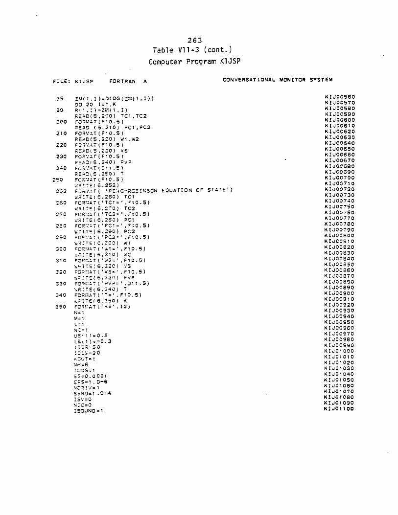
263Table Vll-3 (cont.)
Computer Program KlJSP
FILE: KIJSP FORTRAN A CONVERSATIONAL MONITOR SYSTEM
35 ZM(1. I)=DLOG(ZM(1 I))00 20 1=1,K
20 Rf1,1)=ZVi(11), IREAD(5,200) TC1,TC2
200 FORMAT(F10.5)READ (5.210) PCl,PC2
210 FORMAT(F10.5)READ(5,220) WI,W2
220 F0*dAT(F10.5)READ(5.230) VS
230 FORIAT(F10.5)pEAD(5,240) PVP
240 FCRMAT(11.5)REA(5,2E0) T
250 FC..MAT(F10.5)
WVIE( 6,252)252 FZ~hAT( PENG-RCSINSON
WR:TE(6,260) TC1260 FQRMAT('T01= '.F0.5)
& sTE(6,Z70) TC2
270 FO;:AT'TC2= .F10.5)r7E(6,280) PC1
280 FCRT(c'PC=,IFlo.5)WR1ITE(6,290) PC2
290 F0rtA7('PC2=',F10.5)w~rTE(C,300) W1
300 FCPMAT('w1z',FO.5);.rTE(6,310) w2
310 FR4R.AT('W2='pr10.5)wITE6,32C) VS
320 FPMAT('VS=',RIO.5)-ITE(6,
2 3 0 ) PVP330 FR9MAT('PVP=',D11.5)
.RITE(6.340) T340 FORtAAT('T=',F10.5)
v3.1T(6,350) K350 FCRMAT('K=',I12)
N=1=1NC=1
Us, '1)=0.5LS 1)=-O.3ITER=501DE..=20,CUT= 1
NH=6IODS=155=0.000lEPS=1.0-6
SSNS=1 .0-4ISv=0N I C=0ISOUND1
EQUATION OF STATE')
KIJ00560KIJO570KlUO0580
KIJ00590KIJ00600KIJ00610KlOOC620KIJ00630KIJC0640KIJ00650KIJ00660KIJ00670KIJO0680KIJ00690KIJ00700KIJ00710K1JO0720KIJ00730KIJ00740KIJ00750
KIJ00760KIJ00770
KI 400780KIJ00790K10100800
KIJOOS10KIJOOE20KIJ00830KIJOO40KI00C50K1100860KIJ00870KIJO890KIJ0090KI OO900KIJOO910KIJO920K 1J00930
Kl1O0940KIJ00950KIJ00960KIJ00970KIJOC980KIJ00990Kj%101000KIJO1010KIJ01020KIJO1030KI101040KIJ01050KIJ01060KIJ01070KI01080Kl1O1090KIJ01100
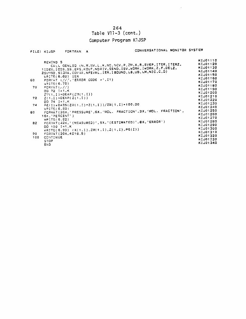
264Table V11-3 (cont.)
Computer Program K1JSP
FILE: KIJSP FORTRAN A CONVERSATIONAL MONITOR SYSTEM
REWIND 5 KIJO1110
CALL GENLSQ (NM,,V.L,KNC,NCVP,ZMXRSVEPITERITERZ, KIJ01120
1 10E7,ICODS. S-, EPS, KOUTNDRTISSND. ISV,wORK, IWORK, Z, F,DE LZKIJ01130IwoKIJ011402SU SQ .SI3MA , COV AR , NFEVAL ,IER ,I8BOUNDLSUB ,LMNICC,) KIJ01 140
'-.WPJTE (6, 60) IER KIJ0116060 FORI:XT //.', 'ERROR CODE =I1)IJ010
W,2ITE(6,7D) KIJO118070 FORMAT(,//) KIJO1190
DO 72 I=1.K KIJUC20Z ( , )=DEXP (Z-1(1I . I) KIJ01210
72 Z(1,I)DEXP(Z(1,I)) KIJ01220DO 74 I=1,K0KIJO0;20
74 PE(I)=DAES(ZM(1 , I) -Z(1 , I ))/ZM(1,I)10 0
. KIJO1230
WPITE( 6,203 KIJOI1240
80 FCRMvAT(2GX,'PRESSURE,6X,'MCL. PRACTICN',3X,'MOL. FRACTION', KIJOI2SO
16x 'PERCENT') KIJO1260
WPTE( 6.62) KIJO1270KIJ01 280
82 FCRMTAT(42X,'(MEASURED)',5x,'(ESTIMATED)',8X,'ERROR') KIJ01290DO 100 I=1.K KIJ0120W'RITE(6,90) (X(1,I).ZM(1,1),Z(1,I),PE(I)) KIJO1300
90 FOR.AT (20X,4D16.5)4KIJOI310100 CONTINUE KIJO1320
STO0 P KIJO1w30
EIND KIJ0I1340
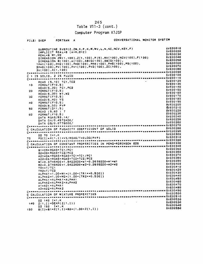
265Table VII-3 (cont.)
Computer Program K1JSP
FILE: SVEP FORTRAN A CONVERSATIONAL MONITOR SYSTEM
SUBROUTINE SVEP(Z,ZM,X,P,K,M,MV.L,N,NC,NCVKEY,F) SVEOO0IO
IMPLICIT REAL-8 (A-H,O-Z) SVEOOO20
REAL'S M1,M2 SVEOO3O
DIMENSION ZM(1,100),Z(1,100),P(S),MV(100),NCV(100)LF(100) SVE00004
DIMENSION B(100),A(100),ASIG(100),SSIG(100). SVEOOOSO
IPH1(100),PH2(100),PH3(100),PH4(100),PH5(100),PS(100), SVE000602PH6(100),PV(100),PV1(100),PV2(100),ZC(100), SVE00070
3v(100),X(1,100) SVEOOCOS
Cases5*sens* **ca*s******sn******ceasee*secant*eases cnacuuesseesseu eSVEOOO
C I IS SOLID, 2 IS FLUID SVEOOIOO
C*******a*** sc************ *s*****.e s* scsesssc at5 5S*SVEOO110
READ (5,10) TC1,TC2 SVEOO120
10 FORMAT(F10.5) SVEOO130
READ(5,20) PC1,PC2 SVEOO140
20 FORMAT(F1O.5) SVEOO150
REAO(5,30) W1,W2 SVE016O
30 FORMAT(FI0.5) SVE00170
READ(5,40) VS SVEOO180
40 FORMAT(FIO.5) SVEOO190
READ(5,50) PVP SVEO0200
so FORMAT(DI1.5) S/EOO210
READ (5,60 ) T VE00220
60 FORMAT(F10.5) SVE00230
DATA RGAS/93.14/ SVE00240
DATA OA/0.4572400/ SVE00250DATA OB/0.0778000/ SVE00260
C*****ce*sca**a*sass*** s**ans**************s***es asa c***ees ees 5VE00270
C CALCULATION OF FUGACITY COEFFICIENT OF SOLID SVEOO280
DO 70 I=1,K SVEOO300
70 PS(I)=X(1,I)eVS/RGAS/T+DLOG(PVP) SVEOO310
Ceue*u********se**s**m*su*s*ss*ss*a*as****maau**e*e*s*aeess**ssass esses cae sSVE00320C CALCULATION OF CONSTANT PROPERITIES IN PENG-ROBINSON EOS SVE00330CC55*********ess*assess*assess*sene e~aseesess ssecss assesseeeseeee S VE00340
B1=OB*RGASCTCi/PC1 SVEOO350
82=O*RGASwTC2/PC2 SVEOO36OA21=OA*RGASPRGAS*TC*TC1/PC1 SVEOO370
A22=0A*RGAS-RGAS-TC2-TC2/PC2 SVEOO380
Ml=0.3746400+1.54226DOW1-0.269920*W1W1 SVEOO390
M2=0.3746400+1.54226DO*W2-0.26992DO*W2*W2 SVE00400
TR1=T/TC1 SVE00410
TR2=T/TC2 SVE00420ALPHA11.D+M1(1.D0-(TR1eO.500)) SVE00430
ALPHA2=1.D0+M2"(1.DO-(TR2**O.5D0)) SVE00440
ALPHA1=ALPHA1*ALPHAI SVEOO450
ALPHA2=ALPHA2*ALPHA2 SVE00460
AI=A21*ALPHAI SVE00470A2=A22*ALPHA2 SVEOO480
Cae****. a*e**a****s******e**es****s*********a***s*assess svsa ssses eee *SVEOO49O
C CALCULATION OF MIXTURE PROPERITIES SVEOO500
C ssseaa*.sn*u*ea*s*****ae***s**a*es**s****s***s***s***seesaessucsuesSVEOO O
DO 140 I=1,K SVEOO520
140 Z(1,I)=DEXP(Z(1,I)) SVE00530
DO 150 I=1,K SVE00540
150 B(I)=BlaZ(1,I)+82*(1.00-Z(1,1)) SVEOO550
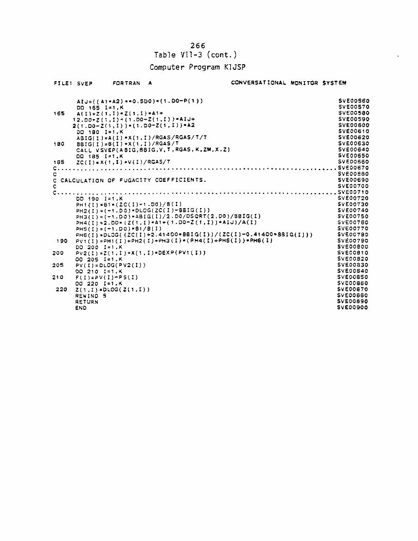
266Table V1l-3 (cont.)
Computer Program K1JSP
FILE: SVEP FORTRAN A CONVERSATIONAL MONITOR SYSTEM
AIJ=((Al*A2)**0.5DO)*(1.DO-P(1)) SVE00560DO 165 I=1,K SVE00570
165 A(I)=Z(1,I)*Z(iI)*AI+ SVE0058012.DO*Z('6,&)-(1.00-Z(1,I))*AIU+ SVE005902(1.Do-Z(1,I))*(1.00-Z(1,I))*A2 SVEOO600DO 180 I=1,K SVEOO610ABIG(I)=A(I)*X(1,I)/RGAS/RGAS/T/T SVEOO620
180 BBIG(I)=(I)*X(1,I)/RGAS/T SVE00630CALL VSVEP(ABIG,BBIGO,V,T,RGAS,KZM,X.Z) SVE00640DO 185 I=lK SVEOO650
185 ZC(I)=X(1,I)*V(I)/RGAS/T SVE00660C............................................................ .......... SVEOO670C SVE00680C CALCULATION OF FUGACITY COEFFICIENTS. SVEOO690C SVE00700C...............................................................................5VE00710
DO 190 1=1,K SVE00720PH1(I)=B1*(ZC(I)-1.DO)/B(I) SVE00730PH2(I)=(-1.00)*DLOG(ZC(I)-BBIG(I)) SVE00740PH3(I)=(-1.DO)ABIG(I)/2.DO/DSQRT(2.00)/BBIG(I) SVEOO750PH4(I)=2.DO* (Z(1,I)*A+(1.0O-Z(1I))*AI)/A(I) SVEOO760PHS(I)=(-1.D0)w81/8(I) SVE00770PH6(I)=DLOG((ZC(I)+2.41400*BBIG(I))/(ZC(I)-O.41400*'BIG(I))) SVEOO780
190 PV1(I)=PH1(I)+PH2(I)+PH3(I)*(PH4(I)+PHS(I))*PH6(I) SVE00790DO 200 I=1,K SvEOOBOO
200 Pv2(I)=Z(1,1 )*X(1,I)*DEXP(PV1(I)) SVE0081000 205 I=1,K SVE00820
205 PV(I)=0LOG(PV2(I)) SVE00830DO 210 I=1,K SVE00840
210 F( I)=PV(I)-PS(I) SVEOOSSODO 220 I=1,K SVE00860
220 Z(1,I)=DLOG(Z(1,I)) SVEOO870REWIND S SVEOOS8ORETURN SVE00890END SVE00900
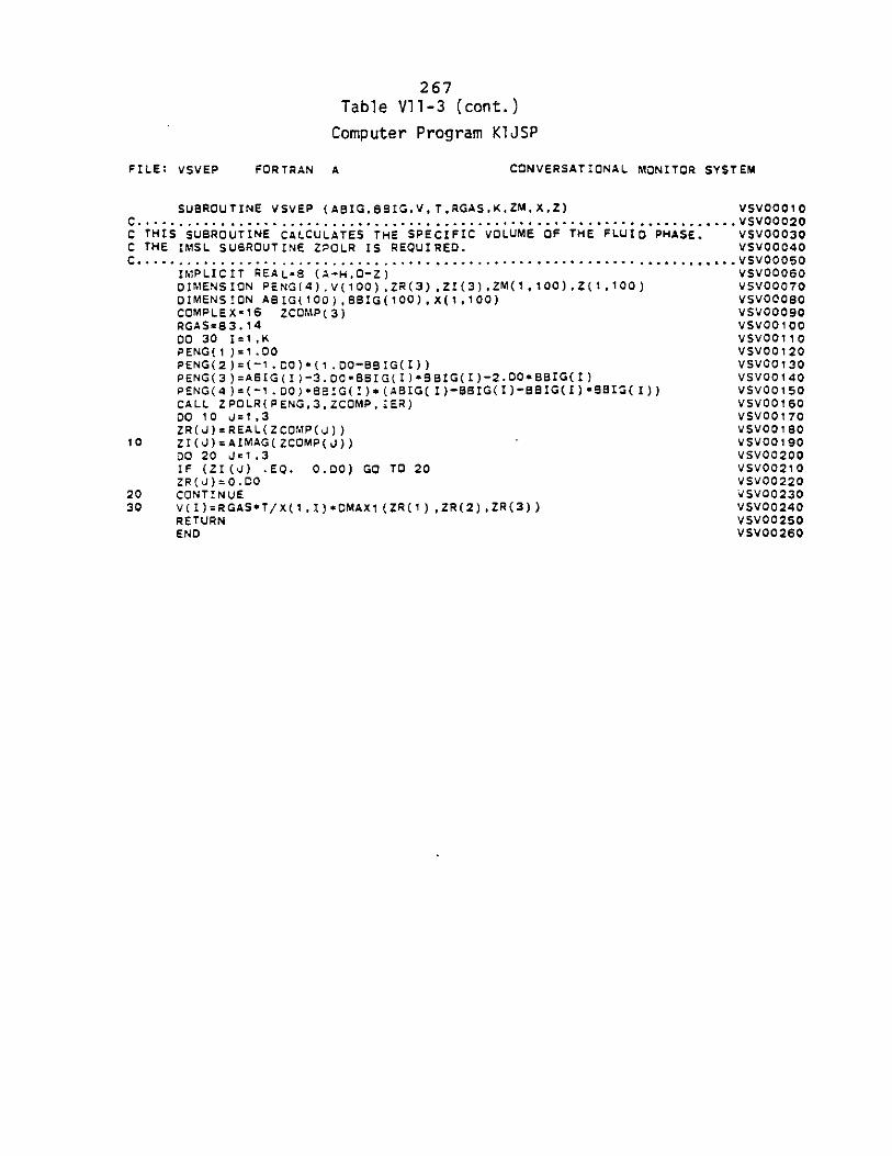
267Table Vll-3 (cont.)
Computer Program K1JSP
FILE: VSVEP FORTRAN A CONVERSATIONAL MONITOR SYSTEM
SUBROUTINE VSVEP (ABIG,BSIG,V,TRGAS,K,ZMX,Z) VSVOOOo1C.......................................................................VSVOOO2OC THIS SUBROUTINE CALCULATES THE SPECIFIC VOLUME OF THE FLUID PHASE. VSVO0030C THE IMSL SUBROUTINE ZPOLR IS REQUIRED. VSVOOO40C ................................................................................... VSVQOO50
IMPLICIT REAL*8 (A-HO-Z) VSVOOO00DIMENSION PENG(4).V(100),ZR(3),ZI(3),ZM(1,100),Z(1,100) VSVOOO70DIMENS ION ABIG( 100),v BBIG( 100),X(1 ,100) VSVOOO80COMPLEX-16 ZCOMP(3) VSVOO090RGAS=83.14 VSVOO10000 30 I=1,K vsV00110PENG(1)=1.DO VSVOO120PENG(2)=(-1.CO)*(1.DO-BBIG(I)) VSVOO130PENG(3)=ABIG(I)-3.D0*BBIG(I)*BBIG(I)-2.OO*BBIG(I) VSVO0140PENG(4)=(-1.D0)wBBIG(I)*(ABIG(I)-BBIG(I)-BBIG(I)*BBI(I)) VSVOO1SOCALL ZPOLR(PENG,3,ZCOMP,IER) VSVOO160DO 10 J=1,3 VSVOO170ZR(J)=REAL(ZCOMP(J)) VSV00180
10 ZI(J)=AIMAG(ZCOMP(J)) VSVOO19000 20 Jc1,3 VSVOO200IF (ZI(J) .EQ. 0.DO) GO TO 20 VSVOO210ZR(J)=0.DO VSVO0220
20 CONTINUE VSVO023030 V(I)=RGAS*T/X(1,t)*DMAXI(ZR(1),ZR(2),ZR(3)) VSVO0240
RETURN VSVO0250END VSVO0260
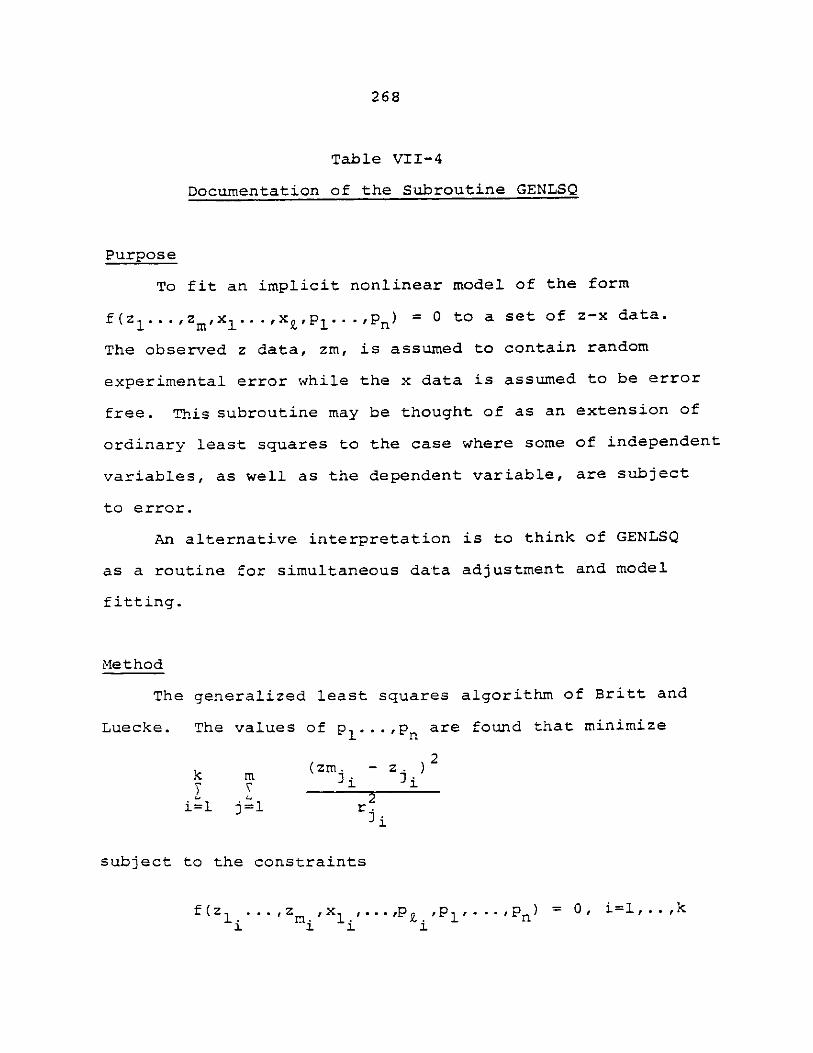
268
Table VII-4
Documentation of the Subroutine GENLSQ
Purpose
To fit an implicit nonlinear model of the form
f(z1 ... ,ZXm'l' '..'vX L'''n) = 0 to a set of z-x data.
The observed z data, zm, is assumed to contain random
experimental error while the x data is assumed to be error
free. This subroutine may be thought of as an extension of
ordinary least squares to the case where some of independent
variables, as well as the dependent variable, are subject
to error.
An alternative interpretation is to think of GENLSQ
as a routine for simultaneous data adjustment and model
fitting.
Method
The generalized least squares algorithm of Britt and
Luecke. The values of p1 .. . ,p are found that minimize
k m(zm . - z. )2
L 2i=l j=1 r.
3i
subject to the constraints
f(z ... ,z ,x ,0, i=1,..,kI M n
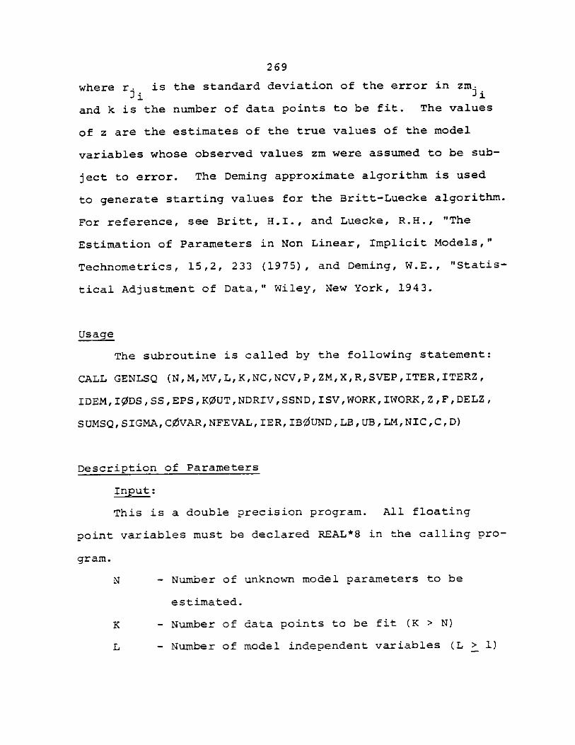
269
where r. is the standard deviation of the error in zm.Ji Ji
and k is the number of data points to be fit. The values
of z are the estimates of the true values of the model
variables whose observed values zm were assumed to be sub-
ject to error. The Deming approximate algorithm is used
to generate starting values for the Britt-Luecke algorithm.
For reference, see Britt, H.I., and Luecke , R.H. , "The
Estimation of Parameters in Non Linear, Implicit Models,"
Technometrics, 15,2, 233 (1975), and Deming, EW.E., "Statis-
tical Adjustment of Data," Wiley, New York, 1943.
Usage
The subroutine is called by the following statement:
CALL GENLSQ (NM,MVL,K,NCNCVP,ZM,X,R,SVEPITER,ITERZ,
IDEM, IODSSS, EPS , KOUTNDRIVSSND, ISVWORK, IWORK, Z , F, DELZ,
SUMSQ, SIGMA, C0VAR, NFEVAL, IER, IBUND ,LB, UB, LMNIC, C, D)
Description of Parameters
Input:
This is a double precision program. All floating
point variables must be declared REAL*8 in the calling pro-
gram.
N - Number of unknown model parameters to be
estimated.
K - Number of data points to be fit (K > N)
L - Number of model independent variables (L > 1)
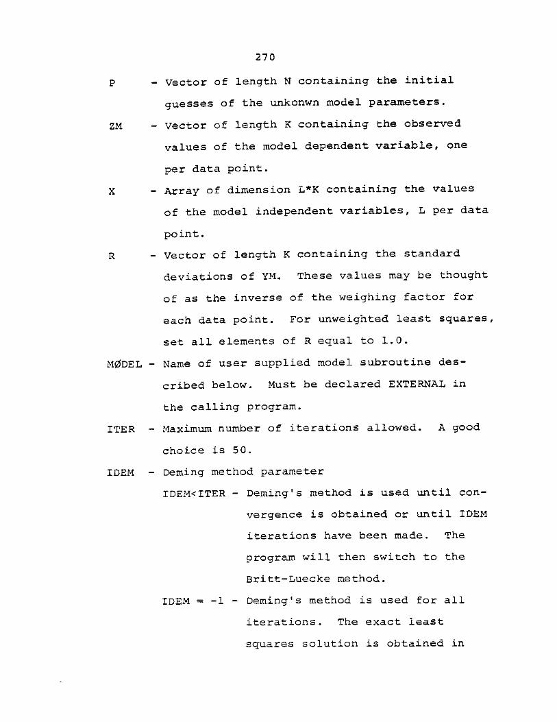
270
P - Vector of length N containing the initial
guesses of the unkonwn model parameters.
ZM - Vector of length K containing the observed
values of the model dependent variable, one
per data point.
X - Array of dimension L*K containing the values
of the model independent variables, L per data
point.
R - Vector of length K containing the standard
deviations of YM. These values may be thought
of as the inverse of the weighing factor for
each data point. For unweighted least squares,
set all elements of R equal to 1.0.
MODEL - Name of user supplied model subroutine des-
cribed below. Must be declared EXTERNAL in
the calling program.
ITER - Maximum number of iterations allowed. A good
choice is 50.
IDEM - Deming method parameter
IDEM<ITER - Deming's method is used until con-
vergence is obtained or until IDEM
iterations have been made. The
program will then switch to the
Britt-Luecke method.
IDEM = -1 - Deming's method is used for all
iterations. The exact least
squares solution is obtained in
271
only certain special cases.
IODS - Key for one dimensional search during Deming
iterations. See Remark 2.
I4DS=O No one dimensional search. Take SS
times the predicted Gauss-Newton step
on each iteration.
lqDS=l Search for the minimum in the Gauss-
Newton direction on each iteration.
On the 1st iteration, begin the search
by taking SS times the predicted
Gauss-Newton step. On subsequent
iterations, begin the search with the
optimum value of SS from the previous
iteration.
lWDS=2 Search for the minimum in the Gauss-
Newton direction on each iteration.
Begin the search on each iteration by
taking SS times the predicted Gauss-
Newton step.
SS - Step size parameter. See lDS above and Remark
2.
EPS - Convergence tolerance. Convergence is declared
if the root mean square fractional change in P
is less than EPS. A good choice is 1.D-6.
KWUT - Print output key.
0 No printed output.
1 Final results only.
272
2 Minimum amount of information per
iteration and final results.
3,4 Relatively more output per iteration.
Used for debugging purposes.
NDRIV - Derivative key.
0 User supplied model subroutine evalu-
ates model and its first derivatives
with respect to P and Z.
I User supplied model subroutine evalu-
ates model only. Derivatives are
calculated numerically by GENLSQ.
SSND - Step size to be used in calculating numerical
derivatives. Applies only if NDRIV=l. A good
choice is l.D-4.
ISV - Variance-covariance matrix computation key.
See Remark 4.
ISV=0 It is assumed that the input values
(R) of the standard deviations of ZM
are proportional to the correct
values. The constant of proportion-
ality is estimated by the standard
error of curve fit (SIGMA) and R is
adjusted accordingly before the vari-
ance-covariance matrix (COVAR) of the
parameter estimates is computed.
ISV=l It is assumed that the input values
(R) of the stadnard deviations of ZM
273
are correct. Their values are not
adjusted by the standard error of
curve fit (SIGMA) before the variance-
covariance matrix (C0VAR) of the
parameter estimates is computed.
It is suggested that ISV=Q be used unless R is
known with a high degree of certainty.
- Work vector of length 2N + 3K + MK + NK +
3max(N,M)K + 3 N(N+l)
- Integer work vector of length N.
- Array of dimension (M,K).
- Vector of length K.
- Array of dimension (M,K).
- Vector of length N(N+1)/2.
- Vector containing the least squares parameter
estimates if converged or most recent values
if not converged.
- Number of iterations used.
- Array containing the estimates of the true
values of the model variables whose observed
values (ZM) were assumed to be subject to ran-
dom experimental error.
- Weighted sum of squares of residuals at P,
i.e., the minimized sum of squares value.
- Standard error of curve fit.
Outp.
WQRK
IWORK
z
F
DELZ
COVAR
at
p
ITER
z
SUMSQ
SIGMA
274
COVAR - Vector representing the lower triangular part
of the (symmetric) variance-covariance matrix
of the parameter estimates, stored by columns.
For example, the order of storage is
1
2 4
3 5 6
for N=3. Parameter estimate standard deviations
are obtained by taking the square root of the
diagonal elements of this matrix.
NFEVAL- Number of times the user supplied subroutine
was called by GENLSQ.
IER - Error code.
0 - No error.
1 - Minimum not found in ITER iterations.
2 - Steps taken to overcome matrix
singularity have caused COVAR to be
modified. It is no longer the
variance-covariance matrix. This
problem is caused by highly corre-
lated model parameters. Reformula-
tion of the model with fewer, less
dependent parameters may help.
3 - Program stopped because of matrix
inversion problems. Comments for
IER=2 apply.
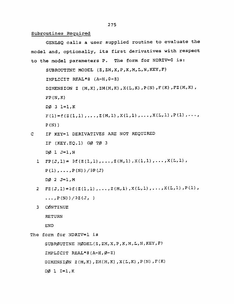
275
Subroutines Required
GENLSQ calls a user supplied routine to evaluate the
model and, optionally, its first derivatives with respect
to the model parameters P. The form for NDRIV=O is:
SUBROUTINE MODEL (ZZMX,P,K,M,L,N,KEYF)
IMPLICIT REAL*8 (A-HO-Z)
DIMENSION Z (M,K),ZM(M,K),X(L,K),P(N),F(K),FZ(M,K)
FP(N,K)
DO 3 l=l,K
P(N))
C IF KEY=1 DERIVATIVES ARE NOT REQUIRED
IF (KEY.EQ.1) Go To 3
Do 1 J=l,N
1 FP(Jl)= 3f(Z(ll),...,Z(M,l),X(ll),...,X(L,l)
PCl),...,P(N))/3PCJ)
Do 2 J=l,M
2 FZ(J,1)=af(Z(1,1),...,Z(M,1),X(LI1),...,X(L,1),PCl)
... ,P(N))/9Z(J,
3 C&NTINUE
RETURN
END
The form for NDRIV=1 is
SUBROUTINE MODEL(Z, ZM,X,P,K,M,L,N,KEYF)
IMPLICIT REAL*8(A-H,0-Z)
DIMENSION Z(MK),ZM(M,K),X(L,K) ,P(N) ,F(K)
Do 1 I=l,K
276
1 F(1)=f(Z(l,1),...,rZ(Mrl),X(,1),...,X(L,1),P(l),
... ,PCN))
RETURN
END
NOTE: It is permissible for the model function to change
with 1.
The subroutine name (not necessarily MODEL) must appear
in the argument list of GENLSQ at the proper position and
must also appear in an EXTERNAL statement in the program
which invokes GENLSQ.
A subroutine LUEBRI, supplied by the catalogued pro-
cedure, is called by GENLSQ to do the actual calculations.
Space Requirement
? decimal bytes.
Remarks
1. For explicit models with significant error in only the
dependent variable, use subroutine NLLSQ.
2. The Deming approximate algorithm is an excellent
initialization method for the Britt-Luecke algorithm since
it usually produces estimtaes very close to the exact
Britt-Luecke estimates and is less prone to convergence
problems. The Britt-Luecke algorithm almost always con-
verges rapidly from a converged Deming solution. Both
algorithms are of the Gauss-Newton type; that is they are
based on model linearization.
277
When convergence problems do arise during the Deming
initialization, they can often be overcome by step size
(SS) adjustment. GENLSQ uses the unmodified Deming method
when 10DS=0 and SS=1.0. Setting SS=1.0 damps the search
and is often helpful. Setting 10DS=1 or 2 causes a one-
dimensional search to be made in the Gauss-Newton direction
on each iteration to find a near-optimum value of SS. The
following strategy is recommended:
(a) Make sure you are providing the program with the
best initial guesses of P 1 ...P. you can come up
with.
(b) Try using 1DS=0, SS=1.0. This should result in
rapid convergnece for most problems.
.c) If (b) fails, try damping the search. A range of
.1 to .5 is recommended for SS. Leave I0DS=0.
(d). If (c) fails, try 10DS=l, SS=.l.
(e) If (d) fails, contact H. 1. Britt, Applied Mathe-
matics and Computing Group.
The significance of Step (a) depends greatly on the
particular model and data. In the event that you are having
convergence problems that appear to be due to poor starting
values, and you are unable to come up with better ones, a
randomized start is recommended. A procedure for doing
this is described on page 15 of the UCC R&D Report
"SIDEWINDER IV" by C.D. Hendrix, File No. 18454, dated
June 11, 1973. This tactic also provides some protection
against converging to a local minimum rather than the global
278
minimum.
There is no one dimensional search during the Britt-
Luecke iterations, however the step size is adjusted by the
SS parameter.
3. The X array is not used by GENLSQ. It is only a ve-
hicle for passing data to the user supplied model subrou-
tine. As a result, it can be dimensioned any way the user
pleases, although X(L,K) is the normal case.
5. The weighing factors in the least squares criteria have
2been denoted 1/r., rather than the more typical wi, to em-
phasize the statistical aspects of the curve fitting prob-
lem. If the errors in measuring the y's are independent of
each other and normally distributed with zero mean and
2 2variance a 2r. then GENLSQ produces the maximum liklihood
estimate of p 1 ,...,p. The factor a2 need not be known.
In other words, it is only the ratios of the standard
deviations that need be known. For example, it is often
assumed that the error in measuring pressure is proportional
to the pressure (constant relative error). Therefore, if
pressure were the dependent variable in a curve fitting
problem, it would be appropriate to set R=ZMir i1 . . k.
The output variable SIGMA would then be the estimated con-
stant of proportionality.
Example
Suppose it is desired to fit the Antoine equation
lnP=A - BT+c
279
to 100 data points using unweighted least squares with
lnP as the independent variable. Input to GENLSQ would be
as follows:
N=3 A, B, and C are the unkonwn parameters
K=100 There are 100 sets of T-lnP data.
K=1 T is the single independent variable.
P(l, P(2), P(3) Are initial guesses of A, B, & C,
respectively.
ZM(l,l)-ZM(1,100)Are the 100 measured values of P.
ZM(2,1)-ZM(2,l00)Are the corresponding 100 measured
values of T.
X Not used since there are no model vari-
ables whose values are assumed to be
known exactly.
R(1,1)-R(l,l00) Are set equal to 0.OlP for the corres-
ponding 100 pressures.
R(2,l)-R(2,l00) Are all set equal to 0.01.
ANTOIN Is the name of the user supplied sub-
routine.
ITER=50 A maximum of 50 iterations will be al-
lowed, including Deming iterations.
IDEM=20 A maximum of 20 Deming iterations will
be made before switching to the Britt-
Luecke algorithm.
IODS=0, SS=l.0 The unmodified search will be tried.
EPS=1.D-6 Convergnece tolerance.
KOUT=l The program is to print the final
I
280
results.
NDRIV=l Numerical derivatives.
SSND=l.D-4 Numerical derivative step size.
The main program would include the following statements:
EXTERNAL ANTOIN
DIMENSION P(3), ZM(2,l00), R(2L,00), WORK(1124),
IWORK(3), Z(2,100), F(100), DELZ.(2,l00), COVAR(6)
The user supplied subroutine would be:
SUBROUTINE ANTOIN(Z,ZM,X,P,K,M,L,N,KEYF)
IMPLICIT REAL*8 (A-H,0-Z)
DIMENSION Z(M,K) ,ZM(MK) ,P(N) ,F(K)
Do 1I=1, K
I F(I)=DLOG(Z(1,I) )-P(l)+P(2)/(Z(2,I)i+P(3))
RETURN
END
281
APPENDIX VIII
DETAILED EQUIPMENT SPECIFICATIONS
AND OPERATING PROCEDURES
Extractor
The extractor used in this thesis consists of an
Autoclave CNLXl6012 medium pressure tube, 30.48 cm in
length and 1.75 cm in diameter. Attached to the extractor
inlet are openings for the thermocouple assembly and for
the fluid inlet stream. Details of the extractor are shown
in Figure VIII-1.
Temperature Control of Extractor
The extraction temperature was controlled by use of
a heating tape (Fisher ll-463-55D) wrapped around the ex-
tractor and connected to a LFE 238 PID temperature control-
ler with a 20 AMP integral power pack. The temperature
sensor was an iron-constantan thermocouple (Omega SH48-
ICSS-ll6U-15) housed inside the extractor.
Optimal temperature control (+ 0.5 K) was obtained
with the following settings on the temperature controller:
proportional control: proportional band = 10
integral control: 16 minutes
derivative control: off
cycle time: minimum
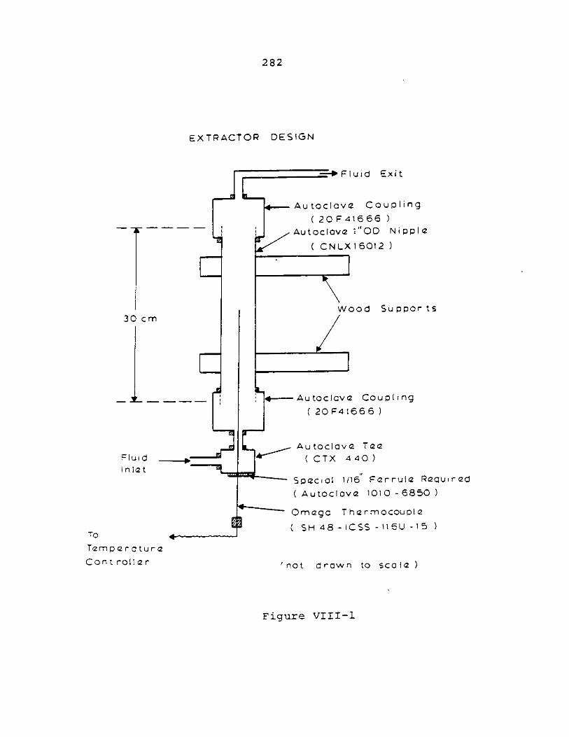
282
EXTRACTOR DESIGN
-+Fluid Exit
Autoclave Coupling
(20 F41666Autoclave "OD Nipple
CNLX16012
Wood Suppor ts
+--AutoclOve Coupling
(20 F41666)
Autoclave Tee( CTX 4 40 )
Special 1/16I Ferrule Required( Autoclave 1010 - 6850)
Omega Thermocouple
(CSH 48 -ICSS-I11SU,-15% )
'not drawn to scOle)
30 cm
FluidInlet
To
TempersturaCont roller
Figure VIII-1
283
With these controller values, the digital set point should
be put at a temperature 2 K below the desired extraction
temperature. Electronic reference junctions for the thermo-
couples were standard with the controller and digital
temperature readout.
Pressure Control of Extractor
Pressure was controlled in the extractor by an on/off
controller (Autoclave P481-P713) located at the surge
tank outlet. Control action was directly to the compressor.
As the system was configured, the controller was in the
high limit off mode. Positioning the set point at the
desired pressure (making use of the more accurate calibra-
tion from the Heise gauge Ct,400, with thermal compensation
and slotted link protection) enables the pressure to be
controlled to + 1 bar.
Surge Tank
A two liter magnedrive packless autoclave was used as
the surge tank. As the system is configured, there were
three Autoclave SW 2072 valves connected to the autoclave
-- one at the inlet, one at the outlet, and one for vent-
ing purposes. The purpose of the inlet and outlet valves
were to enable the autoclave to be isolated from the rest
of the system. Isolation was necessary when changing gas
cylinders, depressurizing the extractor, and venting the
autoclave.
284
In addition to its use as a surge tank, the autoclave
is also useful as a device to pre-saturate the supercritical
fluid with a liquid solvent before the fliud contacts the
solute species. When used in this mode, the autoclave
must be preheated to the desired temperature. For this
purpose a LFE 232 10 Amp proportional controller was used
to control the power input to heating tape wrapped around
the autoclave. Also, the connecting tubing between the
autoclave and the extractor must be heated to prevent
condensation of the liquid species. A variac was conveni-
ently located for connection to heating tapes for this
purpose.
Start up Procedure
After the extractor is charged with the solute species
to be extracted, the outlet valve of the surge tank was
cracked open so that the pressure in the extractor was
slowly increased to the autoclave pressure. When the pres-
sures of the two vessels were equal (but below the desired
extraction pressure), the set point on the pressure con-
troller was adjusted to the desired value and the compres-
sor switch turned on.
Simultaneously, the temperature controller switch was
turned on. It takes about one-half hour for the system to
stabilize at the desired operating temperature and pressure.
After the system had stabilized, the extraction could be
started by opening the exist regulating valve until a steady
285
flow rate of about 0.4 standard liters per minute was achieved.
Shut Down Procedure
To shut down the extraction system, the compressor and
temperature controller switches were turned off (but the
thermocouple switch left on since this switch also turns the
heating tape on the exit regulating value on and off).
Then, the exit value on the autoclave was completely shut
off so as to isolate the autoclave from the rest of the system
After attaching the tygon tube vent pipe (connected to the
hood) to the regulating valve outlet, the regulating valve was
slowly opened until the extractor was depressurized. Finally,
the thermocouple switch was turned off and the entire system
disasembled and cleaned.
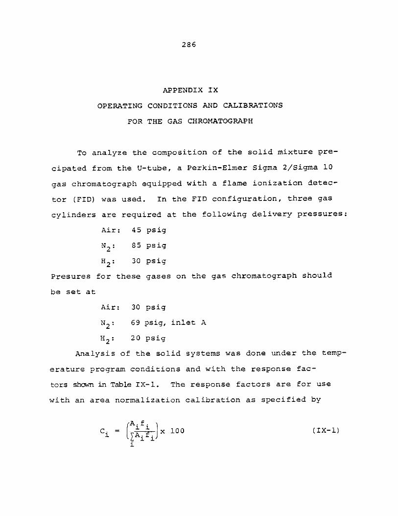
286
APPENDIX IX
OPERATING CONDITIONS AND CALIBRATIONS
FOR THE GAS CHROMATOGRAPH
To analyze the composition of the solid mixture pre-
cipated from the U-tube, a Perkin-Elmer Sigma 2/Sigma 10
gas chromatograph equipped with a flame ionization detec-
tor (FID) was used. In the FID configuration, three gas
cylinders are required at the following delivery pressures:
Air: 45 psig
*2: 85 psig
H2 : 30 psig
Presures for these gases on the gas chromatograph should
be set at
Air: 30 psig
N2 : 69 psig, inlet A
Hi2 : 20 psig
Analysis of the solid systems was done under the temp-
erature program conditions and with the response fac-
tors shown in Table IX-l. The response factors are for use
with an area normalization calibration as specified by
C= x 100 (IX-1)
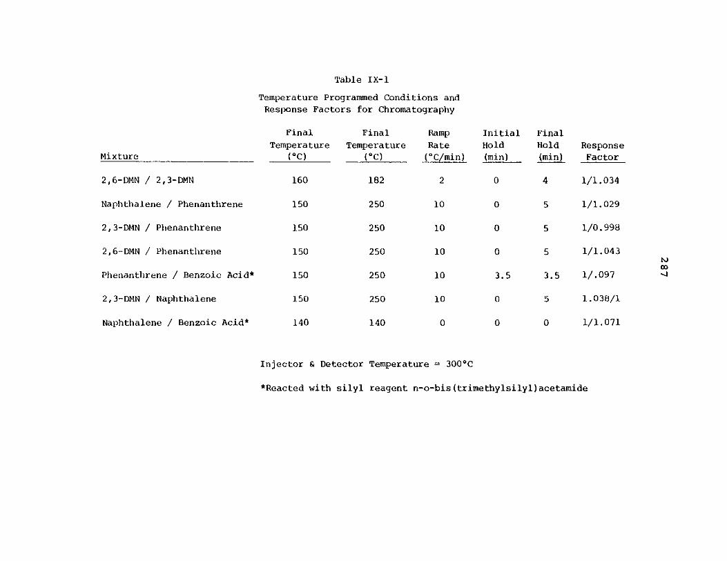
Mixture
2,6-DMN / 2,3-DMN
Naphthalene / Phenanthrene
2,3-DMN / Phenanthrene
2,6-DMN / Phenanthrene
Phenanthrene / Benzoic Acid*
2,3-DMN / Naphthalene
Naphthalene / Benzoic Acid*
Table IX-l
Temperature Programmed Conditions andResponse Factors for Chromatography
Final Final Ramp
Temperature Temperature Rate
(0C) (C) (0C/min)
160 182 2
150 250 10
150 250 10
150 250 10
150 250 10
150 250 10
140 140 0
Injector & Detector
*Reacted with silyl
InitialHold(min)
0
0
0
0
3.5
0
0
FinalHold(min)
4
5
5
5
3.5
5
0
ResponseFactor
1/1.034
1/1.029
1/0.998
1/1.043
1/.097
1.038/1
1/1.071
Temperature = 300'C
reagent n-o-bis(trimethylsilyl)acetamide
NOD
288
where f . is the response factor
A. is the peak area
C. is the concentration in weight %.
Solid Preparation
The precipitated solid in all cases was dissolved in
methylene chloride at a concentration of about 0.5 weight
percent. This dilute solution was satisfactory for injec-
tion into the GC system. In the case of mixtures contain-
ing benzoic acid, however, a silyl reagent had to be added
to the solution in a 10% weight ratio to prevent severe
tailing of the acid peak. The reagent used was N,0-bis
(trimethylsilyl) acetamide, purchased from Supelco.
Gas Chromatograph Column and Septa
The column used for all separations was a 10% SP-2100
methyl silicone stationary phase on a 100/120 Supeloport
support with the following dimensions:
length: 10 ft
O.D.: 1/8"
material: 316 SS
This column is a stock column from Supelco Inc. In all
cases, nitrogen was the carrier gas at a flow rate of
30 ml/min.
For the injection conditions used in this thesis, the
best septa was Supelco Thermogreen, LB-i, llmm.
289
Data Station Operating Methods
The Sigma 10 data station requires operating software
for each sample. Software for each of the solid systems
investigated are shown in Tables IX-2 through IX-3.
Detector Linearity and Response Factors
Calibration curves for each of the mixture species
studied were examined to determine the range of linearity
and the response factors of the detector. These curves
are shown in Figures IX-1 through IX-7.
In all cases, the detector was linear over the range
studied. Response factors are given in Table IX-l.
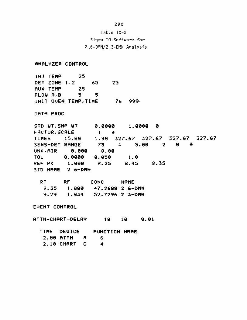
290
Table 1X-2
Sigma 10 Software for
2,6-DMN/2,3-DMN Analysis
ANALYZER CONTROL
INJ TEMP 25DET ZONE 1,2 65AUX TEMP 25FLOW RB 5 5INIT OVEN TEMPTIME
25
76 999-
DATA PROC
STD WT,5MP WTFACTORoSCALETIMES 15.0SENS-DET RANGEUNK.,AIR 8.80TOL 0.0000REF PK 1.000STD NAME 2 6-DMN
0 .00001.0000 01 o
1.90 327.67 327.67 327.67 327.6775 4 5.00 2 0 0
0.000.050 1.08.25 8.45 8.35
CONC47.268852.7296
NAME2 6-DMN2 3-DMN
EVENT CONTROL
ATTN-CHART-DELAY
TIME DEVICE
2.80 ATTN A2.10 CHART C
10 18
FUNCTION NAME64
RT8.359.29
RF1.001.034
8.01
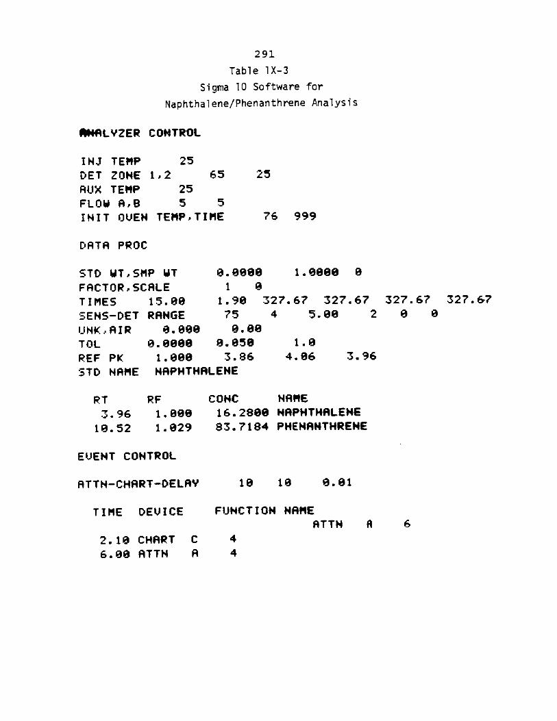
291
Table 1X-3
Sigma 10 Software for
Naphthalene/Phenanthrene Analysis
04ALYZER CONTROL
INJ TEMP 25
DET ZONE 1,2 65
AUX TEMP 25FLOW A,8 5 5
INIT OVEN TEMPTIME
25
76 999
DATA PROC
STD WTSMP WT 0.0899 1.089 9
FACTORSCALE 1 0
TIMES 15.99 1.98 327.67 327.67 327.67 327.&7
SENS-DET RANGE 75 4 5.00 2 0 0
UNKAIR 0.900 0.08
TOL 0.08e 8.950 1.8
REF PK 1.00 3.86 4.86 3.96
STD NAME NAPHTHALENE
CONC16.280083.7184
NAMENRPHTHALENEPHENANTHRENE
EVENT CONTROL
ATTN-CHART-DELAY
TIME DEVICE
2.10 CHART
6.89 ATTNCA
18 10 0.81
FUNCTION NAMEATTN A 6
44
RT3.96
10.52
RF1.000
1.929
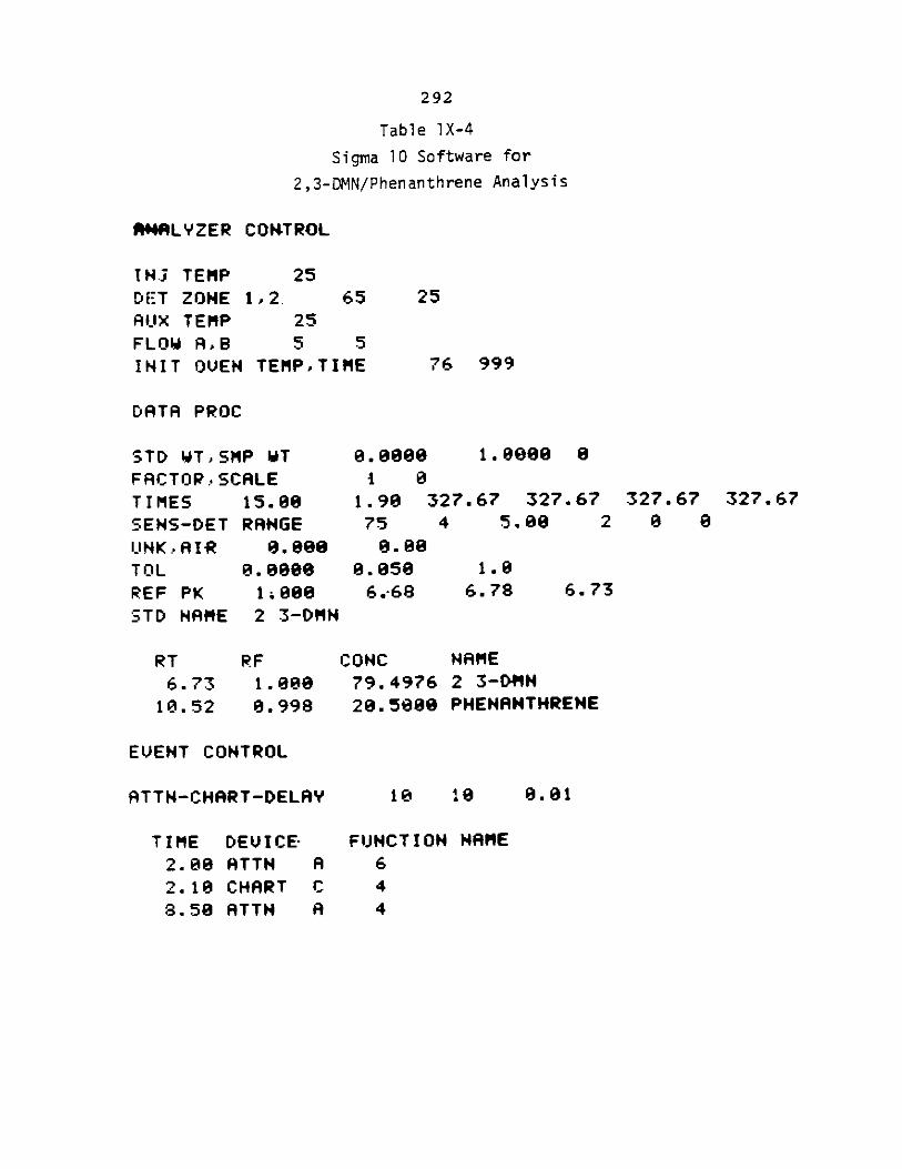
292
Table 1X-4
Sigma 10 Software for
2,3-DMN/Phenanthrene Analysis
RHALYZER CONTROL
INj TEMP 25DET ZONE 1,f2. 65AUX TEMP 25FLOW AB 5 5INIT OVEN TEMPTIME
25
76 999
DATA PROC
STD WTSMP WTFACTOP. SCALETIMES 15.00SENS-DET RANGE
UNKAIR 9.9000TOL 8.80000REF PK I;eloSSTD NAME 2 3-DMN
8w.eeee1.8099 8
1 01.99 327.67 327.67 327.67 327.67
75 4 5.8 2 0 89.80
8.858 I.e6.-68 6.78 6.73
CONC79. 497629. 5080
NAME2 3-DM4
PHENANTHRENE
EVENT CONTROL
ATTN-CHART-DELAY
TIME DEVICE-2.89 ATTN A
2.18 CHART C
8.58 ATTN A
10 19
FUNCTION NAME644
RT6.73
10.52
RF1 .8 OR90.998
8.91
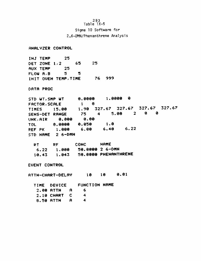
293Table 1X-5
Sigma 10 Software for
2,6-DMN/Phenanthrene Analysis
ANALYZER CONTROL
INJ TEMP 25
DET ZONE 1.2 65
AUX TEMP 25
FLOW A.B 5 5
INIT OVEN TEMPTIME
25
76 999
DATA PROC
STD WTaSMP WTFACTORoSCALETIMES 15.080SENS-DET RANGE
UNK.AIR 8.0003
TOL 8.0000REF PK 1.00STD NAME 2 6-DMN
8.0001 0
1.90750.80
8.8506.00
1.8800 8
327.67 327.67 327.67 327.67
4 5.00 2 0 8
1.86.40 6.22
CONC50.eeo850.0000
NAME2 6-DMNPHENANTHRENE
EVENT CONTROL
ATTN-CHART-DELAY
TIME DEVICE
2.80 ATTH2.18 CHART8.50 ATTN
ACA
18 10
FUNCTION NAME
644
RT6.2218.43
RF1.8001.843
0.081
I
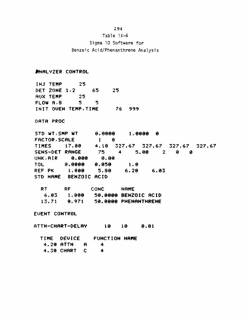
294
Table 1X-6
Sigma 10 Software for
Benzoic Acid/Phenanthrene Analysis
ANALYZER CONTROL
INJ TEMP 25DET ZONE 1,2 65AUX TEMP 25FLOW RB 5 5INIT OVEN TEMPPTIME
25
76 999
DATA PROC
STD WTSMP WTFACTORPSCALETIMES 17.00SENS-DET RRNGEUNKAIR 8.088TOL 8.8888REF PK 1.680STD NAME BENZOIC
8.888 1.8888 81 8
4.18 327.67 327.67 327.67 327.6775 4 5.80 2 0 88.88.858 1.85.88 6.28 6.83
ACID
CONC58.80058. 888
NAMEBENZOIC ACIDPHEMANTHRENE
EVENT CONTROL
ATTN-CHART-DELAY
TIME DEVICE4.28 ATTN A4.38 CHART C
18 18
FUNCTION NAME44
RT6.03
13.71
RF1.8988.971
8.81
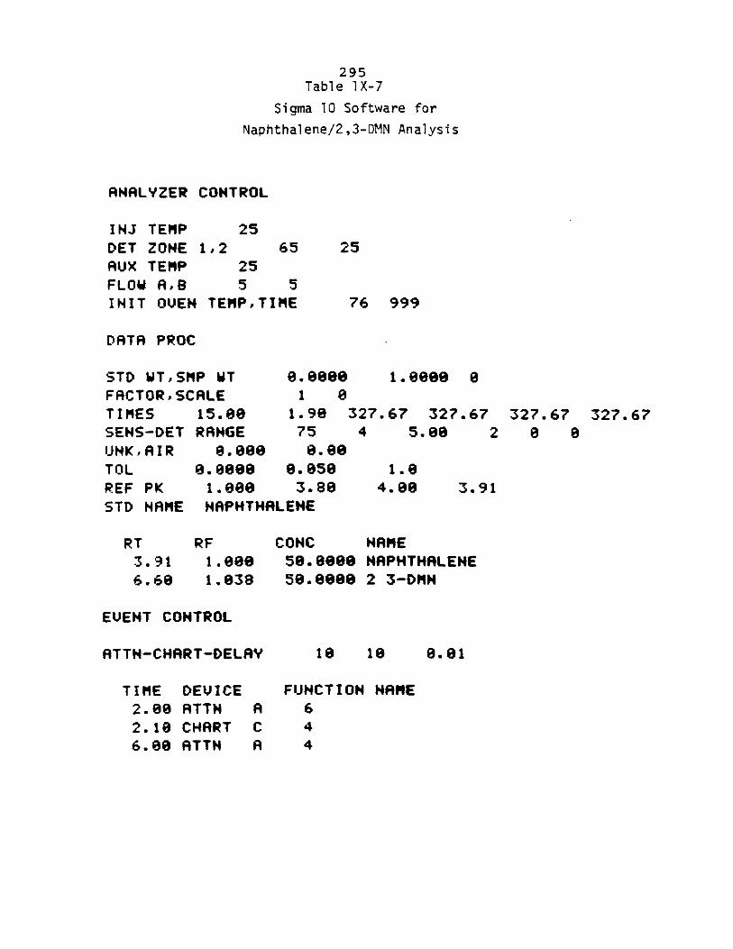
295Table 1X-7
Sigma 10 Software for
Naphthalene/2,3-DMN Analysis
ANALYZER CONTROL
INJ TEMP 25DET ZONE 1,2 65AUX TEMP 25FLOW AB 5 5INIT OVEN TEMPTIME
25
76 999
DATA PROC
STD WTSMP WT 0.88000FACTORSCALE 1 8TIMES 15.88 1.90SENS-DET RANGE 75
UNKAIR 8.880 8.88
TOL e.888 0.8518
REF PK 1.888 3.80
STD NAME NAPHTHALEHE
RT3.916.618
RF1.8881.838
CONC50.0800050.08000
1.8888 8
327.67 327.67 327.67 327.674 5.88 2 8 0
1.84.88 3.91
NAMENAPHTHALENE2 3-DMH
EVENT CONTROL
ATTN-CHART-DELAY
TIME DEVICE2.88 ATTN2.18 CHART6.8 ATTH
ACA
18 18
FUNCTION NAME64
4
8.81
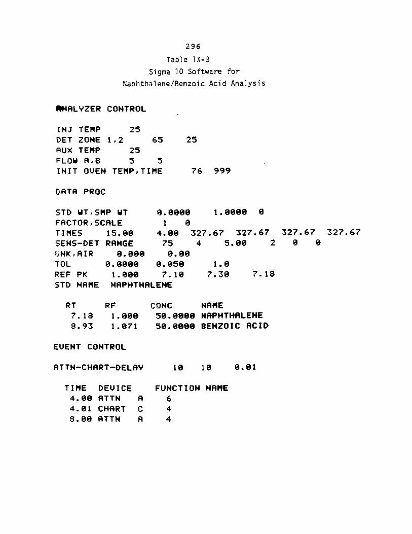
296
Table 1X-8
Sigma 10 Software for
Naphthalene/Benzoic Acid Analysis
#4ALYZER CONTROL
INJ TEMP 25DET ZONE 1,2 65AUX TEMP 25FLOW AB 5 5INIT OVEN TEMPTIME
25
76 999
DATA PROC
STD WTSMP WT 8.08000 i.00 0FACTORSCALE 1 0TIMES 15.0 4.88 327.67 327.67 327.67 327.67
SENS-DET RANGE 75 4 5.88 2 0 0UJNKAIR 8.800 8.88TOL 000080 8.850 1.8REF PK 1.800 7.18 7.38 7.18STD NAME NAPHTHALENE
CONC58.80058.8000
NAMENAPHTHALENEBENZOIC ACID
EVENT CONTROL
ATTN-CHART-DELAY
TIME DEVICE4.8 ATTN A4.81 CHART C8.80 ATTN A
18 18
FUNCTION NAME644
RT7.188.93
RF1.80I1.871
8.81
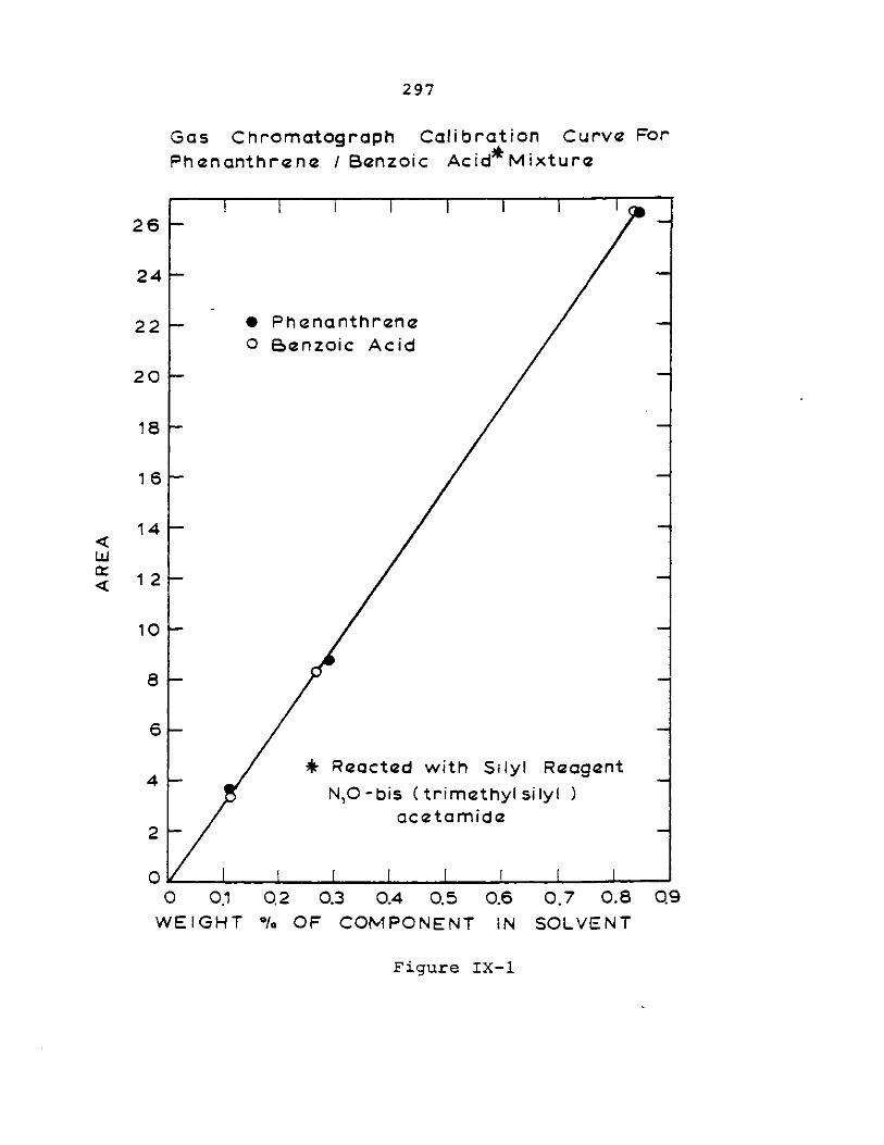
297
Gas Chromatograph Calibration Curve For
Phenanthrene I Benzoic Acid Mixture
I II |26
24
22 * Phcnanthrene0 Benzoic Acid
20
18
16-
14
LU
12
10
8
6-
4-* Reacted with Silyl ReagentN,O -bis (trimethyl silyl
ace tamide2
0
0 0.1 0.2 0.3 0.4 0.5 0.6 0.7 0.8 Q9WEIGHT % OF COMPONENT IN SOLVENT
Figure IX-1
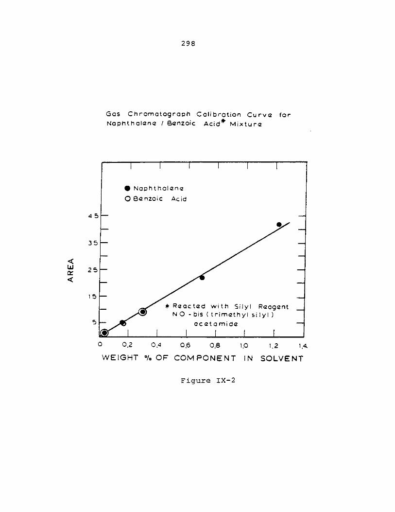
298
Gas Chromatograph Calibration Curve forNaphthalene / Benzoic Acid* Mixture
0 0.2 0.4 0.6 0.8 1.0 1.2 104
WEIGHT %OF COMPONENT IN SOLVENT
Figure IX-2
45
351
4wz4
5
Nophtholene
QBenzoic Acid
* Reacted with Silyl ReagentNO- bis (trimethyl siyl ) H
0 1ocatomid
I
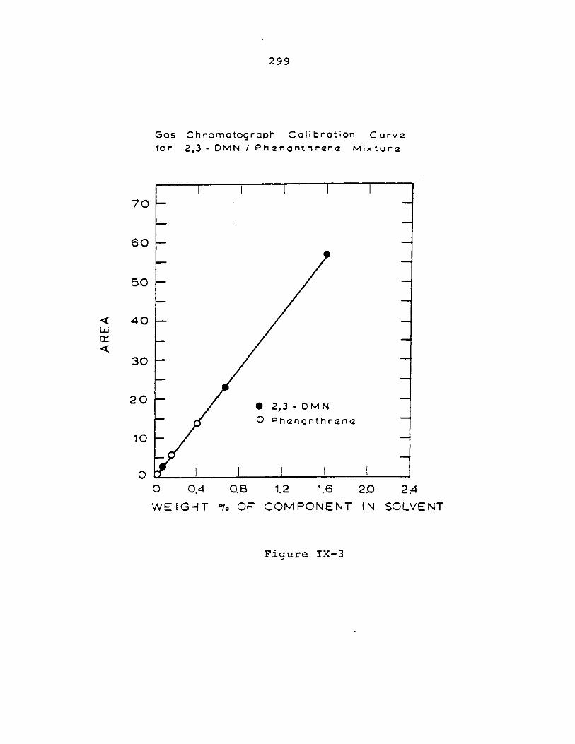
299
Gas Chromatograph Calibration Curvafor 2,3 - DMN / Phananthrena Mix ture
70
60
50
40
30
20
10
01.2 1.6 2.0
COMPONENT IN
2.4
SOLVENT
Figure IX-3
LUI
0 0.4 0.8
WEIGHT % OF
-* 2,3 -D0MN
o Phinanthrena
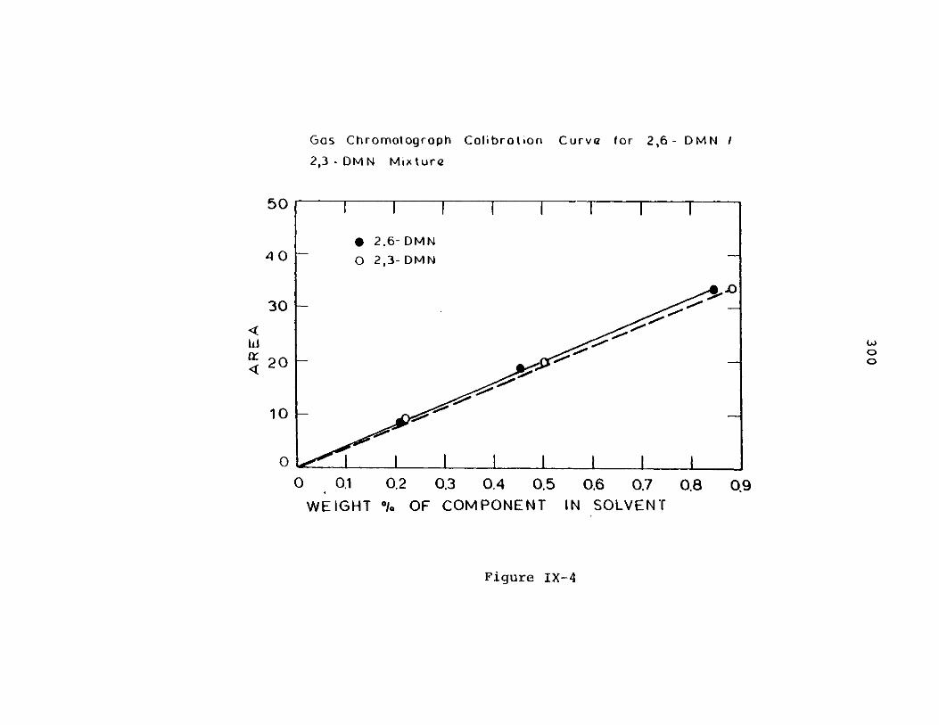
Gas Chromotograph
2,3 - DMN Mixture
Colibrotion Curve for 2,6- DMN /
* 2,6- DMN
S2,3- DMN
0 0.1 0.2 0.3 0,4 0.5 0.6 0.7 0.8 09WEIGHT %Ol OF COMPONENT IN SOLVENT
Figure IX-4
50
40
30
4d
20
10
0
(A)
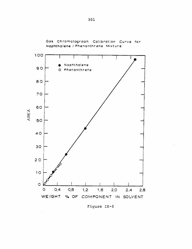
301
Gas Chromatograph Calibration Curve forNaphthclene I Phenanthrene Mixture
100
* Naphtholene90 0 Phenanthrene
80
70
60
< 50
40
30
20
10 /
00 0.4 0.8 1.2 1.6 2.0 2.4 2.8
WEIGHT % OF COMPONENT IN SOLVENT
Figure IX-5
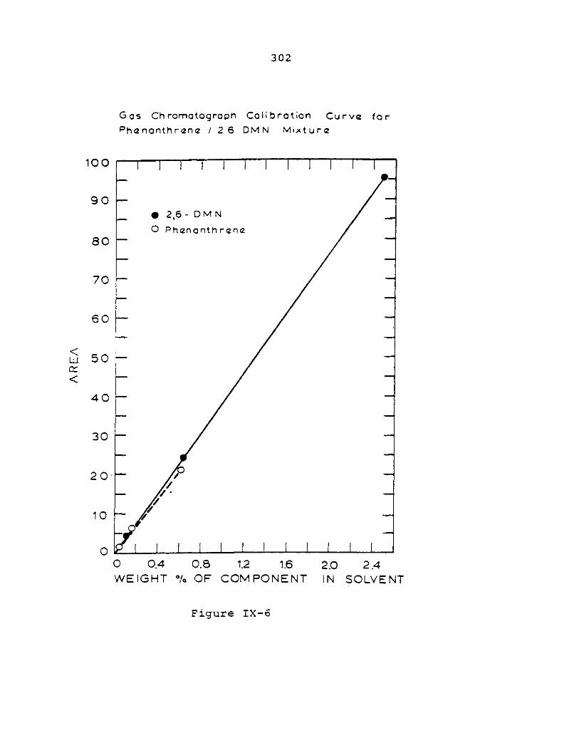
302
Gas Chromatograph Calibration Curve for
Phananthrene / 26 DMN Mixture
100
90* 216-DMN
o Phenanthrena
707
60-
40-
30
20--
10 /
0IJ0 0.4 0.8 1.2 1.6 2.0 2.4WEIGHT / OF COMPONENT IN SOLVENT
Figure IX-6
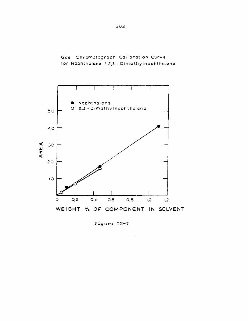
303
Gas Chromotograph Colibration Curve
for Naphtholene / 2,3 - Dimethyinophthclene
.2 0.4 0.6 0.8 1.0 1.2
WEIGHT % OF COMPONENT IN SOLVENT
Figure IX-7
* Nophtholene
o 2,3 - Dimethyf ncphtholne
-=o-
50
40
30wA
20
10
C )
I -- - - slamommommomm
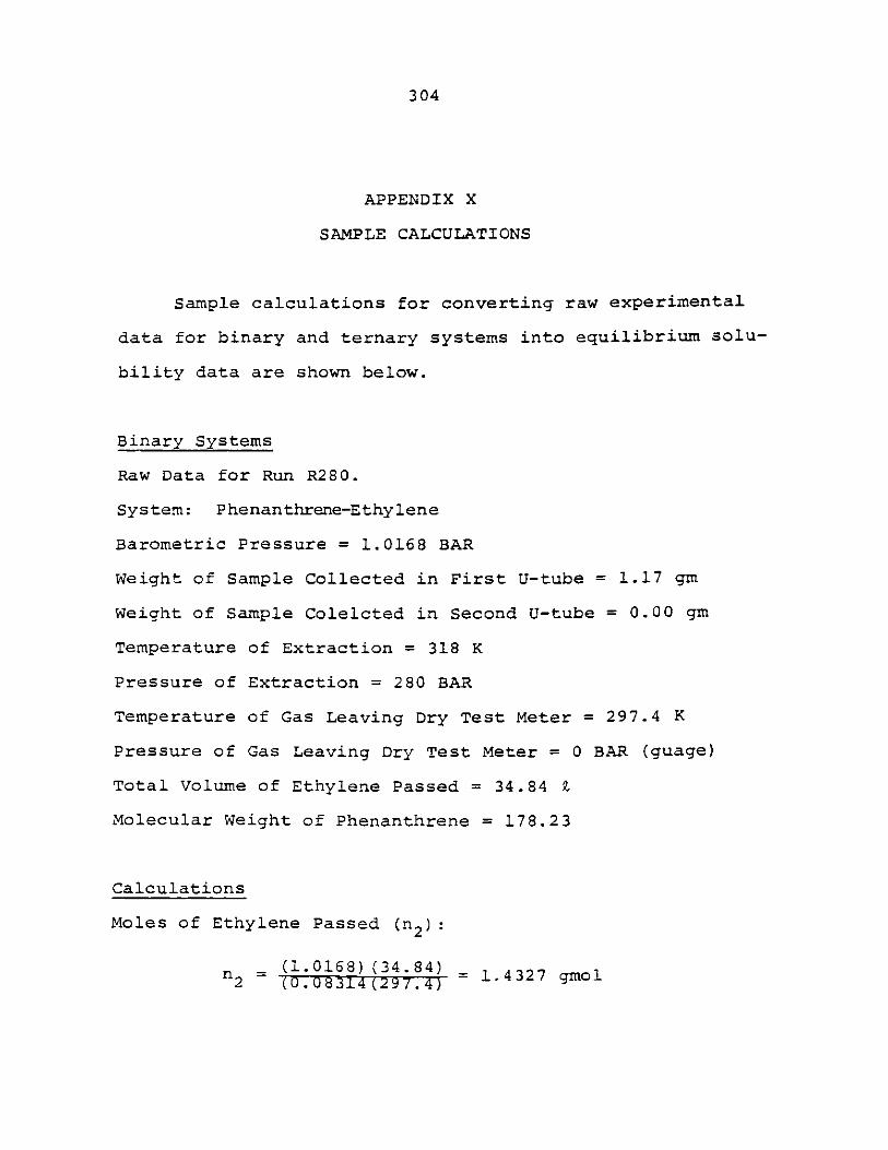
304
APPENDIX X
SAMPLE CALCULATIONS
Sample calculations for converting raw experimental
data for binary and ternary systems into equilibrium solu-
bility data are shown below.
Binary Systems
Raw Data for Run R280.
System: Phenanthrene-Ethylene
Barometric Pressure = 1.0168 BAR
Weight of Sample Collected in First U-tube = 1.17 gm
Weight of Sample Colelcted in Second U-tube = 0.00 gm
Temperature of Extraction = 318 K
Pressure of Extraction = 280 BAR
Temperature of Gas Leaving Dry Test Meter = 297.4 K
Pressure of Gas Leaving Dry Test Meter = 0 BAR (guage)
Total Volume of Ethylene Passed = 34.84 Z
Molecular Weight of Phenanthrene = 178.23
Calculations
Moles of Ethylene Passed (n2
n= ({.0168) (34.84) 1.4327 gmoln2 *(0. 083-14T(2-977.7- .37g
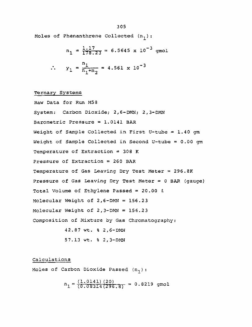
305
Moles of Phenanthrene Collected (n):
1.17 -3n1= = 6.5645 x 10 gmol
Y,= nn2=4.561 x 10 3
Ternary Systems
Raw Data for Run M58
System: Carbon Dioxide; 2,6-DMN; 2,3-DMN
Barometric Pressure = 1.0141 BAR
Weight of Sample Collected in First U-tube = 1.40 gm
weight of Sample Collected in Second U-tube = 0.00 gm
Temperature of Extraction = 308 K
Pressure of Extraction = 260 BAR
Temperature of Gas Leaving Dry Test Meter = 296.8K
Pressure of Gas Leaving Dry Test Meter = 0 BAR (gauge)
Total Volume of Ethylene Passed = 20.00
Molecular Weight of 2,6-DMN = 156.23
Molecular Weight of 2,3-DMN = 156.23
Composition of Mixture by Gas Chromatography:
42.87 wt. % 2,6-DMN
57.13 wt. % 2,3-DMN
Calculations
Moles of Carbon Dioxide Passed (n9:
= (1.0141) (20) 0.8219 gmoln1--(0.0 8314 (296 .8) = .829gl
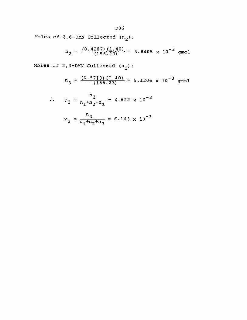
306
Moles of 2,6-DMN Collected (n2
(0.4287) (1.40) -3n 2 (156.23) = 3.8405 x 10 gmol
Moles of 2,3-DMN Collected (n3
n3 (0.573 (16.340) 5.1206 x 10O3 gmol
n2 -3Y2 n +n2+n = 4.622 x 10
y n n3+n = 6.163 x 10⁻³³ n1 n2 +n3
307
APPENDIX XI
EQUIPMENT STANDARDIZATION AND ERROR ANALYSIS
Equipment standardization and error analysis consists
of verifying that the extraction was (within experimental
error): isothermal, isobaric, and at equilibrium. As
discussed in Appendix VIII the extraction is kept isotherm-
al by means of a PID temperature controller and isobaric
by means of an on/off pressure controller. The maximum
deviation of the extraction temperature from the set point
was 0.5 K. The on/off pressure controller kept the extrac-
tion isobaric to within + 1 bar.
Since a flow system is used to obtain solubility data,
there are several key points to check to verify that the
data obtained are equilibrium data. First, solubility has
to be independent of flow rate. After showing this, the
data has to reproduce accepted equilibrium data from the
literature. Finally, comparisons of the system residence
time to the extraction residence time must be made and
shown not to matter.
Examining the first question of independence of flow
rate, shown in Table XI-1 is the solubility of naphthalene
in supercritical carbon dioxide at 191 bar and 308 K as a
function of flow rate (and charge to the extractor). As
the average deviation from the maximum solubility is low
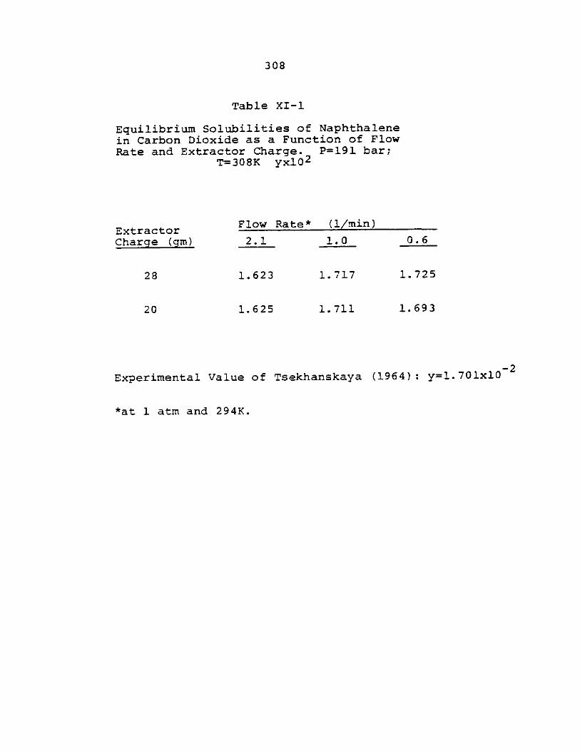
308
Table XI-1
Equilibrium Solubilities of Naphthalenein Carbon Dioxide as a Function of FlowRate and Extractor Charge. P=191 bar;
T=308K yxl02
ExtractorCharge (gM)
28
20
Flow Rate* (1/min)
2.1
1.623
1.625
1.0
1.717
1. 711
Experimental Value of Tsekhanskaya (1964): y=1.701x10 2
*at 1 atm and 294K.
0.6
1.725
1.693
309
(2.8%), it is confirmed that the solubility is independent
of flow rate. At the same conditions of temperature and
pressure Tsekhanskaya (1964) reports and equilibrium solu-
bility of 1.701 x 10- mole fraction. The average devia-
tion of the experimental data from that obtained from
Tsekhanskaya is 2.07%. As all the experimental data taken
in this thesis was at a flow rate of 0.4 liters per minute*
or less, and at a reactor charge of at least 28 grams,
equilibrium can be assured.
To further check the agreement between experimental
data and that published in the literature, additional data
on the system naphthalene - carbon dioxide were taken at
328 K and for various pressures as shown in Table XI-2. The
average percent error of 1.28% confirms that equilibrium
was achieved in the extractor.
Additional Isothermal Calibration
At the extraction conditions of 197 bar and 328 K,
additional checks were performed on the isothermality of
the extractor as follows. Transverses of the thermocouple
inside the extractor (the set point thermocouple) were
made. Equilibrium solubilities obtained by positioning
the thermocouple at the top or bottom of the extractor
(the usual position was the middle) were within 2% of the
data of Tsekhanskaya (1964).
*At 1 atm and 294 K.
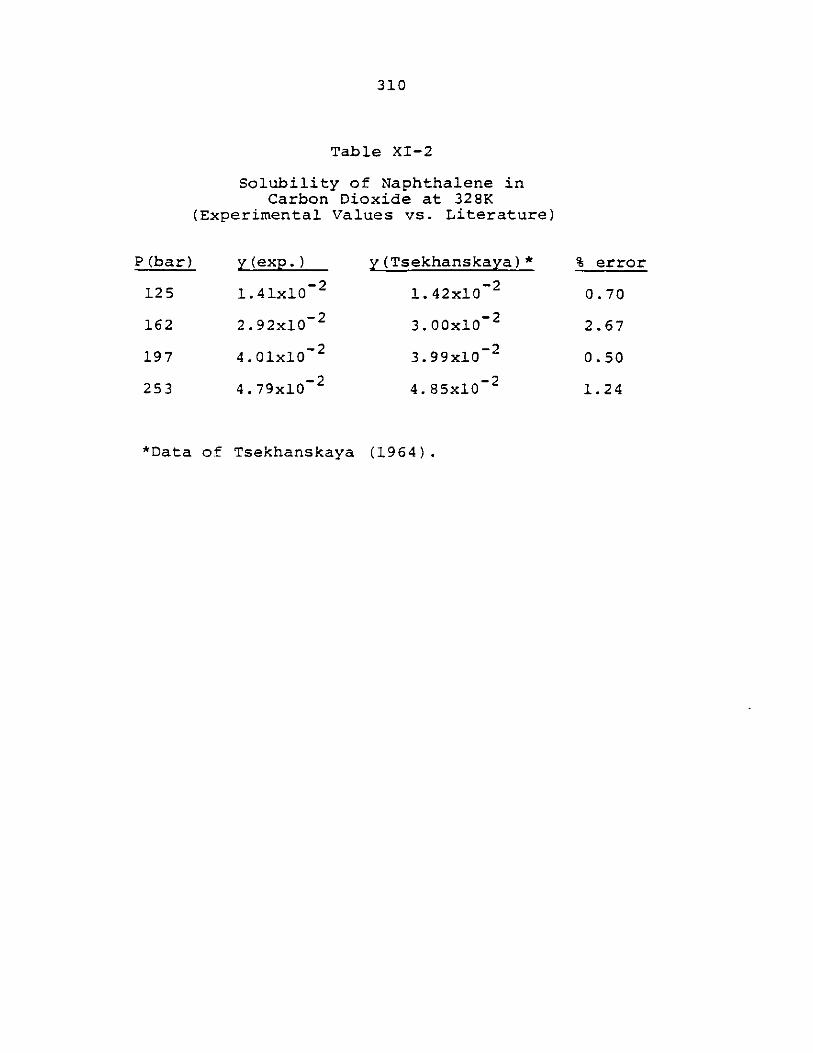
310
Table XI-2
Solubility of Naphthalene inCarbon Dioxide at 328K
(Experimental Values vs. Literature)
y_(exp.)_
1.41x10⁻²
2. 92x10-2
4.0x1-24.OlxlQ-2
4 . 79x10 2
y(Tsekhanskaya)*
1.42x10⁻²
3.00x10⁻²
3.99x10⁻²
4.85x10⁻²
*Data of Tsekhanskaya (1964).
P(bar)
125
162
197
253
% error
0.70
2.67
0.50
1.24
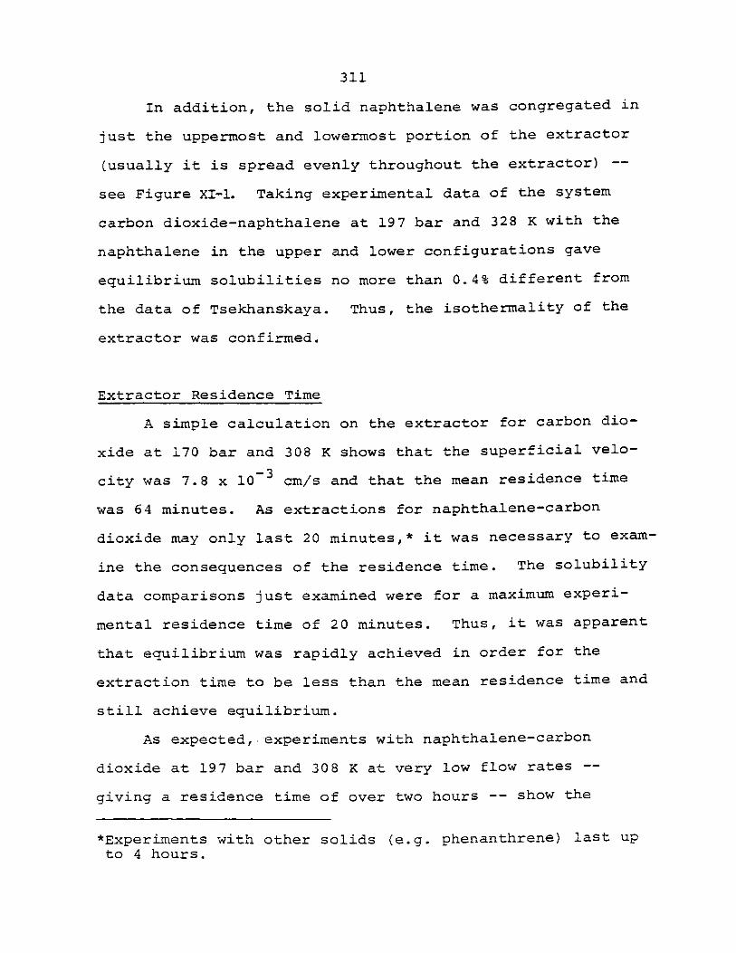
311
In addition, the solid naphthalene was congregated in
just the uppermost and lowermost portion of the extractor
(usually it is spread evenly throughout the extractor) --
see Figure XI-1. Taking experimental data of the system
carbon dioxide-naphthalene at 197 bar and 328 K with the
naphthalene in the upper and lower configurations gave
equilibrium solubilities no more than 0.4% different from
the data of Tsekhanskaya. Thus, the isothermality of the
extractor was confirmed.
Extractor Residence Time
A simple calculation on the extractor for carbon dio-
xide at 170 bar and 308 K shows that the superficial velo-
city was 7.8 x 10⁻³ cm/s and that the mean residence time
was 64 minutes. As extractions for naphthalene-carbon
dioxide may only last 20 minutes,* it was necessary to exam-
ine the consequences of the residence time. The solubility
data comparisons just examined were for a maximum experi-
mental residence time of 20 minutes. Thus, it was apparent
that equilibrium was rapidly achieved in order for the
extraction time to be less than the mean residence time and
still achieve equilibrium.
As expected,.experiments with naphthalene-carbon
dioxide at 197 bar and 308 K at very low flow rates --
giving a residence time of over two hours -- show the
*Experiments with other solids (e.g. phenanthrene) last up
to 4 hours.
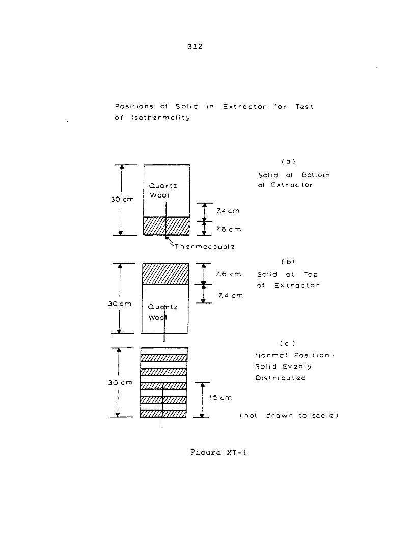
312
Positions of Solid in Extractor for Test
of Isothermality
Quartz
30 cm Wool
7.4 cm
7.6 cm
Th ermocouple
(a)
Solid at Bottomof Extrac tor
30 cm Oaua tz
Woo
30 cm
7.6 cm
7.4 cm
15cm
( b)
Solid at Top
of Extractor
(c )Normal Position
Solid Evenly
Distributed
(not drawn to scale)
Figure XI-1

313
experimental data to agree to within one percent of the
data of Tsekhanskaya.
314
APPENDIX XII
LOCATION OF ORIGIONAL DATA,
COMPUTER PROGRAMS, AND OUTPUT
The original binary and ternary data obtained during
this thesis are in the possession of the author. Duplicate
copies of these data can be obtained from Professor Robert
C. Reid. Card decks for the computer programs can be ob-
tained from the author, or Professor Robert C. Reid.
Computer outputs are in the possession of the author.
315
NOTATION
a , a. .,IA
Avv' vI' A1
BMf B1 , B1 2 ,
CM
C
E
f
G
H
K1 , K{, K2 , K
KA, KB, Kc
L
L
N
P
Q
R
SB' Sc
T
U
parameters in Peng-Robinson Equation of State
derivatives of Helmholtz Free Energy
parameters in Peng-Robinson Equation of State
B22 second virial coefficients
third virial coefficient
heat capcity (cal/gmol K)
eutectic point; enhancement factor
fugacity (bar)
gas phase
enthalpy (cal/mole)
binary critical end points
critical points
Peng-Robinson binary interaction parameter
liquid phase
stability matrix
stability matrix
moles
pressure (bar)
heat (cal/mole)
gas constant
solid B, C
temperature (K)
internal energy (cal/mole)
1
2
316
v volume (cm3/mole)
y mole fraction, Legendre Transform
Z compressibility factor
317
SUPERSCRIPTS
C critical point
E experimental
F fluid
FUS fusion
ID ideal gas
L liquid phase
M melting point
R reduced property
S solid phase
SUB sublimation
t triple point
Vp vapor pressure
component property
partial molar property
at infinite dilution
318
SUBSCRIPTS
component 1, 2, i
mixture property of components 1 and 2
lower critical end point
upper critical end point
1, 2, i
12
p
q
319
GREEK LETTERS
parameter in Peng-Robinson Equation of State
Y activity coefficient
< parameter in Peng-Robinson Equation of State
dimensionless density (b/V)
property to be evaluated at saturation
fugacity coefficient
wo acentric factor
a Qb constants in the Peng-Robinson Equation of State
320
LITERATURE CITED
Abbott, M.M., "Cubic Equations of State," AIChE J, 19,596 (1973).
Adams, R.M., Alfred H. Knebel, and Donald E. Rhodes,"Critical Solvent Deashing of Liquified Coal," paperpresented at 71st AIChE meeting, Miami, Nov 15, (1978).
Agrawal, G.M. and R.J. Laverman, "Phase Behavior of theMethane-Carbon Dioxide System in the Solid-VaporRegion," Adv. In Cry. Eng., Vol. 19, (1974).
Alder, B.J., D.A. Young, and M.A. Mark, "Studies in Mole-cular Dynamics. X. Corrections to the Augmentedvan der Waals Theory for the Square Well Fluid,"J. Chem. Phys., 56, 3013 (1972).
Ambrose, D. and R. Townsend, "Vapor-Liquid Critical Proper-ties," National Physical Laboratory, England (1978).
Andrews, "On the Properties of Matter in the Gaseous andLiquid States under Various Conditions of Temperatureand Pressure," Phil. Trans Roy. Soc. London, 178, 45(1887).
Balder, J.R. and J.M. Prausnitz, "Thermodynamics of TernaryLiquid-Supercritical Gas Systems with Applications forHigh Pressure Vapor Extraction," Ind. Eng. Chem. Fund,5, 449 (1966).
Bartle, K.D., T.G. Martin, and D.F. Williams, "ChemicalNature of a Supercritical-Gas Extract of Coal at 350 C,"Fuel, 54, 227 (1975).
Barton, P. and M.R. Fenske, "Hydrocarbon Extraction ofSaline Waters," Ind. Eng. Chem. Proc. Des. Dev., 9,18 (1970).
Bartmann, D. and G.M. Schneider, "Experimental Results andPhysico-Chemical ASpects of Supercritical Chromato-graphy with Carbon Dioxide as the Mobile Phase," J.Chromat., 83, 135 (1973).
Baughman, G.L., S.P. Westhoff, S. Dincer, D.D. Duston,and A.J. Kidnay, "The Solid + Vapor Phase Equilibriumand Interaction Second Virial Coefficients for Argon +
321
Nigrogen + Methane +, and Helium + Neopentane,"II. Analysis of Results", J. Chem. Thermo., 7, 875(1975).
Beegle, B.L., M. Modell, and R.C.Reid, "Legendre Transformsand their Applications in Thermodynamics," AIChE J.,20, 1194 (1974).
Benedict, M., G.B. Webb, and L.C. Rubin, "An EmpiricalEquation for Thermodynamic Properties of LightHydrocarbons and their Mixtures," I. Methane, Ethane,Propane, and n-Butane," J. Chem. Phys., 8, 334 (1940).
Benedict, M., G.B. Webb, and L.C. Rubin, "An EmpiricalEquation for Thermodynamic Properties of Light Hydro-carbons and their Mixtures. Constants for TwelveHydrocarbons," Chem. Eng. Prog., 47, 419 (1951)..
Benedict, M., G.B. Webb, and L.C. Rubin, "An EmpiricalEquation for Thermodymamic Properties of LightHydrocarbons and their Mixtures II. Mixtures ofMethane, Ethane, Propane, and n-Butane," J. Chem.Phys., 10, 747 (.19421.
Bonner, D.C., D.P. Maloney, and J.M. Prausnitz, "Calcula-tion of High Pressure Phase Equilibria and MolecularWeight Distribution in Partial Decompression ofPolyethylene-Ethylene Mixtures," Ind. Eng. Chem. Proc.Des. Dev., 13, 91 (1974).
Brunner, G., Discussion at the Supercritical Fluid Extrac-tion Symposium Electrochemical Meeting, St. Louis,Missouri, May 14-15 (1980).
Carnahan, N.F. and K.E. Starling, "Intermolecular Repulsionsand the Equation of State for Fluids," AIChE J., 18,1184 (1972).
Castellan, G.W., "Physical Chemistry," 2nd ed., Addison-Wesley, Mass. (1971).
Close, R.E., "Vapor-Liquid Equilibrium in the CriticalRegion: Systems of Alphatic Alcohols in the Propaneand Propylene," Ph.D. Thesis, Princeton University,(1953).
Czubryt, J.J., M.N. Myers, and J.C. Giddings, "SolubilityPhenomena in Dense Carbon Dioxide Gas in the Range 270to 1900 Atmospheres," J. Phys. Chem., 74, 4260 (1970).
de Kruif, C.G., and Oonk, H.A.J., "Enthalpies of Vaporiza-tion and Vapor Pressures of Seven Aliphatic CarboxylicAcids," J. Chem. Therm., 11, 287 (1979).
322
de Kruif, C.G., C.H.D. van Ginkel, and J. Voogel, "Torsion-Effusion Vapor Pressure Measurements of OrganicCompounds, "Quatrieme Conference Internationale de
Thermodynamique Chemique," 26 au 30, Aout, Montpellier,France (1975).
Diepen, G.A.M. and F.E.C. Scheffer, "On Critical Phenomenaof Saturated Solutions in Binary Systems," J. Am.Chem. Soc., 70, 4081 (1948a).
Diepen, G.A.M. and F.E.C. Scheffer, "The Solubility ofNaphthalene in Supercritical Ethylene," J. Am. Chem.Soc., 70, 4085 (1948b).
Diepen, G.A.M., and F.E.C. Scheffer, "The Solubility ofNaphthalene in Supercritical Ethylene II," J. Phys.Chem., 57, 575 (1953).
Dokoupel, Z., G. van Soest and M.D.P. Swenker, "On theEquilibrium Between the Solid Phase and the Gas Phaseof the Systems Hydrogen-Nitrogen, Hydrogen-CarbonMonoxide, and Hydrogen-Nitrogen-Carbon Monoxide,"App. Sci. Res., A5, 182 (1955).
Dreishbach, R.R., "Physical Properties of Chemical Com-
pounds," American Chemical Society, Washington, D.C.,p. 215 (1955).
Edmister, W.C., J. Vairags, and A.J. Klekers, "A GeneralizedBWR Equation of State," AIChE J., 14, 479 (1968).
Elgin, J.C., and J.J. Weinstock, "Phase Equilibria MolecularTransport Thermodynamics," J. Chem. Eng. Data, 4,3 (1959).
Eisenbeiss, J., "A Basic Study of the Solubility of Solidsin Gases at High Pressures, "Final Report, ContractNo. DA 18-108-AtMC-244(A), Southwest Research Institute,
San Antonio, August (1964).
Ewald, A.H., "The Solubility of Solids in Gases, Part III,The Solubility of Solid Xenon and Carbon Dioxide,"Trans. Far. Soc., 51, 347 (1955).
Ewald, A.H., W.B. Jepson, and J.S. Rowlinson, "The Solubil-ity of Solids in Gases," Disc. Far. Soc., A5, 238(1953).
Fowler, L., W. Trump, and C. Vogler, "Vapor Pressure of
Naphthalene," J. Chem. Eng. Data, 13, 209 (1968).
323
Francis, D. and M. Paulaitis, "Solid Solubilities in Super-critical Fuilds -- High Pressure Phase EquilibriumCalculations Near the Upper Critical End Point Usingthe Lee-Kesler Equation of State," submitted for
publication (1981).
Fuller, G.G. , "A Modified Redlich-Kwong-Soave Equation of
State Capable of Representing the Liquid State,"Ind. Eng. Chem. Fund. ,15, 254 (1976).
Gangoli, N. and G. Thodos, "Liquid Fuels and Chemical Feed-
stocks from Coal by Supercritical Gas Extraction,,"
Ind. Eng. Chem. Prod. Res. Dev., 16, 208 (1977).
Graboski, M.S. and T.E. Daubert , "A Modified Soave Equationof State for Phase Equilibrium Calculations.1. Hydrocarbon Systems," Ind. Eng. Chem. Proc. Des.
Dev., 17, 443 (1978).
Gratch, S., Proj G-9A, Univ. of Penn. ThermodynamicsResearch Laboratory, "Low Temperature Properties of
CO -Air-Mixtures by Means of a One Stage Experiment(1945-46).
Hag, A.G.,, "Method of Producing Hop Extracts," Br. 1 388581 (1975).
Hag, A.G. , "Method of Extracting Nicotine from Tobacco,"Br. 1 357 645 (1974).
Hag, A.G.,, "Method of Producing Caffeine-Free Coffee
Extract," Br. 1 346 134 (.1974).
Hag, A.G. "Method of Producing Caffeine-Free Black Tea,"
Br. 1 333 362 (1973).
Hag, A.G., "Method of Producing Vegetable Fats and Oils,,"
Br. 1 356 749 (1974).
Hag, A.G.,, "Method of Producing Cocoa Butter," Br. 1 356
750 (.1974) .
Hag, A.G., "Method of Producing Spice Extracts with a
Natural Composition," Br. 1 336 511 (1973).
Hannay, J.B. and J. Hogarth, "On the Solubility of Solids
in Gases," Proc. Roy. Soc. (London), 30, 178 (1880).
Hannay, J.B. and J. Hogarth, "On the Solubility of Solidsin Gases" Proc. Roy. Soc. (London),, 29, 324 (1879).
Hannay, J.B., "On the Solubility of- Solids in Gases,"Proc. Roy. Soc. (London), 30, 4t.4 (1880).
324
Hinckley, R.B. and R.C. Reid, "Rapid Estimation of MinimumSolubility of Solids in Gases," AIChEJ, 10, 416 (1964).
Hiza, M.J. and A.J. Kidnay, "Solid-Vapor Equilibrium inthe System Neon-Methane," Cryogenics, 6, 348 (1966).
Hiza, M.J., C.K. Heck, and A.J. Kidnay,, "Liquid-Vapor andSolid-Vapor Equilibrium in the System Hydrogen-Ethyl-ene," Chem. Eng. Prog. Symp. Ser., No. 88, 64, 57(1968).
Holder, C.H. and 0. Maass, "Solubility Measurements in.the Region of the Critical Point," Can. J. Res., 18B,293 (1940).
Holm. L.W. , "Carbon Dioxide Flooding for Increased OilRecovery," AIME Petro. Trans., 216, 225 (1959).
Holla, S.J. "Supercritical Fulid Extraction," M.S. Thesis,M.I.T., (1980).
Hong, G., personal communication, (1981).
Hubert, P. and 0. Vitzhum, "Fluid Extraction of Hops,Spices, and Tobacco with Supercritical Gases,"Angew. Chem. Int. Ed. Engl., 17, 710 (1978).
Iomtev, M.B. and Y.V. Tsekhanskaya, "Diffusion of Napthalenein Compressed Ethylene and Carbon Dioxide, " Russ. J.Phys. Chem., 38, 485 (1964) .
Irani, C.A. and E.W. Funk, "Separations Using SupercriticalGases," CRC Handbook: Recent Developments in SeparationScience, CRC Press, Boca Raton, Florida, (1977).
Jantoft, R.E. and T.H. Gouw, "Apparatus for SupercriticalFluid Chromatography with Carbon Dioxide as the MobilePhase," Anal. Chem., 44, 681 (1972).
Johnston, K.P. and C.A. Eckert, "An Analytical Carnahan-Starling-van der Waals Model for Solubility of Hydro-carbon Solids in Supercritical Fluids," submitted toAIChE J. (1981).
Jones, D. and R. Staehle, "High Temperature Electrochemistryin Aqueous Solutions," Central Electricity ResearchLaboratory, National Society of Corrosion Engineers,p. 131 (1973).
Kennedy, G.C. , "The Hydrothermal Solubility of Silica,"Economic Geology, 39, 25 C1944).
325
Kennedy, G.C., "A Portion of the System Silica-Water,"Economic Geology, 45, 629 (1950).
Kim-E, Miral, "The Possible Consequences of Rapidly Depres-surizing a Fulid," M.S. Thesis, MIT (1981).
Kim-E, M. and R.C. Reid, "The Rapid Depressurization ofHot, High Pressure Liquids or Supercritical Fluids,"paper presented at the AIChE Annual Meeting, NewOrleans, (1981).
King, A.R. and W.W. Robertson, "Solubility of Naphthalenein Comprssed Gases," J. Chem. Phys., 37, 1453 (1962).
Klesper, E. and W. Hartmann, "Apparatus and Separations in
Supercritical Fluid Chromatography," Eur. Polym. J., 1477 (1978).
Klesper, E., "Chromatography with Supercritical Fluids,"Angew. Chem. Int. Ed. Engl. 17, 738 (1978).
Knebel, A.H. and D.E. Rhodes, "Critical Solvent Deashingof Liquified Coal," paper presented at the 13thIntersociety Energy conversion Engineering Conference(1978).
Krukonis, Val, private communication C1980).
Kurnik, R.T. and R.C. Reid, "Solubility Extrema in Solid-Fluid Equilibria," accepted for publication inAIChE J, (.1981).
Kurnik, R.T., S.J. Holla, and R.C. Reid, "Solubility ofSolids in Supercritical Carbon Dioxide and Ethylene,"
J. Chem. Eng. Data. 26, 47 (1981).
Lee, B.E. and M.G. Kesler, AIChEJ, 21, 510 (1975).
Lin, C.T. and T.E. Daubert, "Estimation of Partial MolarVolume and Fugacity Coefficients of Components inMixtures from the Soave and Peng-Robinson Equationsof State," Ind. Eng. Chem.Proc. Des. Dev., 19, 51(1980).
Mackay, M. and M. Paulaitis, "Solid Solubilities of HeavyHydrocarbons in Supercritical Solvents," Ind. Eng.Chem. Fund., 18, 149 (1979).
Martin, J.J., "Cubic Equations of State -- Which?" Ind.Eng. Chem. Fund., 18, 81 (1979).
326
McHugh, M. and M. Paulaitis, "Solid Solubilities ofNaphthalene and Biphenyl in Supercritical CarbonDioxide," J. Chem. Eng. Data, 25, 326 (1980).
McKinley, C., J. Brewer, and E.S.J. Wang, "Solid-VaporEquilibria of the Oxygen-Hydrogen System," Adv. Cry.Eng., 7, 114 (1962).
Modell, M., R.P. deFilippi, and V. Krukonis, "Regenerationof Activated,Carbon with Supercritical Carbon Dioxide,"paper presented at ACS meeting, Miami, Sept. 14(1978).
Modell, M., R. Robey, V. Krukonis, R. de Felippi, and D.Oestreich, "Supercritical Fluid Regeneration ofActivated Carbon," paper presented at 87th Nationalmeeting AIChE, Boston (1979).
Modell, M., G. Hong, and A. Herba, "The Use of the Peng-Robinson Equation in Determining Supercritical Behav-ior," paper presented before 72nd Annual meeting AIChE,San Francisco, Nov. C1979).
Modell, M. and R.C. Reid, "Thermodynamics and its Applica-tions," Prentice Hall, Englewood, New Jersey, (1974).
Morey, G.W., "The Solubility of Solids in Gases," EconomicGeology, 52, 227 (1957).
Morozev, V.S.,and E.G. Vinkler, "Measurement of DiffusionCoefficients of Vapors of Solids in Compressed Gases.I. Dynamic Method for Measurement of Diffusion Coeffi-cients," Russ. J. Phys. Chem., 49, 1404 (1975a).
Morozev, V.S. and E.G. Vinkler, "Measurements of DiffusionCoefficients of Vapors of Solids in Compressed Gases,II. Diffusion Coefficients of Naphthalene in Nitrogenand Carbon Dioxide," Russ. J. Phys. Chem., 49, 1405(1975b).
Najour, G.C. and A.D. King, Jr., "Solubility of Anthracenein Comprssed Methane, Ethylene, Ethane, and CarbonDioxide: The Correlation of Anthracene -- Gas SecondVirial Coefficients Using Pseudo Critical Parameters,"J. Chem. Phys., 52, 5206 (1970).
Najour, G.C. and A.D. King, Jr., "Solubility of Naphthalenein Compressed Methane, Ethylene, and Carbon Dioxide,"J. Chem. Phys., 45, 1915 (1966).
Neghbubon, W. (ed.), "Handbook of Toxicology," Vol. III,Interscience, New York, (1959).
327
Newsham, D.M.T. and O.P. Stigset, "Separation ProcessesInvolving Supercritical Gases," J. Chem. E. Symp.Ser. No. 54, (1978).
Oellrich, L.R., H. Knapp and J.1M. Prausnitz, "A SimplePerturbed-Hard Chain Equation of State Applicable toSubcritical and Supercritical Temperatures," FluidPhase Equilibria, 2, 163 (1978).
Osborn, A.G., and D.R. Douslin, "Vapor Pressures and Der-ived Enthalpies of Vaporization for Some CondensedRing Hydrocarbons," J. Chem. Eng. Data, 20, 229 (1975).
Panzer, F., S.R.M. Ellis, and T.R. Bott, "Separation ofGlycerides in the Presence of Supercritical CarbonDioxide," Ind. Eng. Chem. Symp. Ser. No. 54, p. 165(1978).
Paul, P.F.M. and W.S. Wise, "The Principles of Gas Extrac-tion," Mills and Boon, Ltd., London, Monograph CE/5,(1971).
Peng, D.Y. and D.B. Robinson, "A New Two Constant Equationof State," Ind. Eng. Chem. Fund., 15, 59 (.1976).
Perry, R.H. and C.H. Chilton, (ed.)1" Chemical Engineers'Handbook," McGraw Hill, New York (1973).
Peter, S., G. Brunner,, and R. Riha, "Phasengleichgewichtebei holen Drtcken und Mbglichkeiten ihrer technischenAnwendung, "Chem. Ing. Tech. 46, 623 (1974).
Peter, S., and G. Brunner, "The Separation of NonvolatileSubstances by Means of Comprssed Gases in Countercur-rent Processes," Angew, Chem. Int. Ed. Eng. , 17, 746(1978).
Poynting, "Change of State: Solid-Liquid," Phil, Mag.,12, 32 (1881).
Prausnitz, J.M., "Molecular Thermodynamics of Fluid PhaseEquilibria," Prentice-Hall, Englewood Cliffs, N.J.(1969).
Prausnitz, J.M., "Solubility of Solids in Dense Gases,"Nat. Bur of Stds., Tech. Note 316, July (1965).
Prigogine, L. and R. Defay, "Chemical Thermodynamics,"Longmans Green and Co. Inc., London (1954).
Rance, R.W. and E.L. Cussler, "Fast Fluxes with Supercriti-
cal Solvents," AIChE J, 20, 353 (1974).
328
Randall, J.M., W.G. Schultz, and A.I. Morgan Jr., "Extrac-tion of Fruit Juices and Concentrated Essences withLiquid Carbon Dioxide," Confructa, 16, 10 (1971).
Redlich, 0. and J.N.S. Kwong, "On the Thermodynamics ofSolutions. V. An Equation of State. Fugacities ofGaseous Solutions," Cheri. Rev., 44, 233 (1949).
Ree, R.H. and W.G. Hoover, "Seventh Virial Coefficientsfor Hard Spheres and Hard Disks," J. Chem. Phys.,46, 4181 (1967).
Reid, R.C. and B.L. Beegle, "Critical Point Criteria inLegendre Transform Notation, " AIChE J, 23, 726(1977).
Reid, R.C., "A Possible Mechanism for Pressurized-LiquidTank Explosions or BLEVES, Science, 203, 1263 (1979).
Reid, R.C., J.M. Prausnitz, and T.K. Sherwood, "The Proper-ties of Gases and Liquids," McGraw Hill, New York(1977).
Rowlinson, T.S. and M.J. Richardson, "Solubility of Solidsin Compressed Gases," Adv. Chem. Phys., Vol. II, 85(1959).
Rowlinson, J.S., "Liquids and Liquid Mixtures," 2nd ed.,Butterworths, London Q1969).
Sax, N.I., "Dangerous Properties of Industrial Materials,"5th ed., Van Nostrand Reinhold Co., p. 718 (1979).
Schultz, W.G. and J.M. Randall, "Liquid Carbon Dioxide forSelective Aroma Extraction," Food Tech., 24, 94 (1970).
Schultz, T.H., D.R. Black, J.L. Bomben, T.R. Mon, andR. Teranishi, "Volatiles from Oranges. 6. Constituentsof the Essence Identified by Mass Spectra," J. FoodSci. , 32, 698 (1967al .
Schultz, T.H., R.A. Flath, D.R. Black, D.G. Gudagni, W.G.Schultz, and R. Teramishi, "Volatiles from DeliciousApple Essence -- Extraction Methods," J. Food Sci.,32, 279 (.1967b).
Schultz, W.G., T.H. Schultz, R.A. Carlson, and J.S. Hudson,"Pilot Plant Extraction with Liquid CO 2 ," Food Tech,24, 1282 (1970a).
Schultz, T.H., T.R. Mon, and R.R. Forrey, "Variations ofRelative Retention Times in Open-Tubular Gas-Chromato-
329
graphic Columns: Relevancy to Fruit Volatiles,"J. Food Sci., 35, 165 (1970b) .
Sie, S.T., W. Van Beersum, and G.W.A. Rijnders, "High-Pressure Gas Chromatography and Chromatography withSupercritical Fluids I. The Effect of Pressure onPartition Coefficients in Gas-Liquid Chromatographywith Carbon Dioxide as a Carrier Gas," Sep. Sci. , 1,459 (1966).
Sims, M., "Extracting Natural Materials with Liquid CO2 '"unpublished paper, (1979).
Smith, N.K., R.C. Stewart, Jr., A.G. Osborn, and D.W.Scott, "Pyrene, Vapor Pressure, Enthalpy of Combus-tion and Chemical Thermodynamic Properties," submittedto J. Chem. Thermodynamics (1979).
Smits, A., "The P-T-x-Spacial Representation of the SystemEther-Anthraquinone," Proc. Roy. Acad. Sci., Amsterdam,12, 231 (1909-10).
Snedeker, R.A. , "Phase Equilibria in Systems with Supercrit-ical Carbon Dioxide," Ph.D. Thesis, Princeton Univ.,(.1955).
Soave, G.,, "Equilibrium Constants from a Modified Redlich-Kwong Equation of State," Chem. Eng. Sci. , 27, 1197(.1972).
Sonntag, R.E. and G.J. Van Wylen, "The Solid-Vapor Equili-brium of Carbon Dioxide-Nitrogen," Adv. Cry. Eng.,, 7,99 (1962).
Stahl, E. et al. "Quick Method for the MicroanalyticalEvaluation of the Dissolving Power of SupercriticalGases," Angew. Chem. Int. Ed. Engl., 17, 731 (.1978).
Starling, K.E., "Thermo Data Refined for LPG," Hydro. Proc.51, 107 (1972a).
Starling, K.E. , "Thermo Data Refined for LPG," Hydro Proc.,51, 129 (.1972b).
Starling, K.E. , "Thermo Data Refined for LPG" Hydro Proc.,50, 101 (1971).
Studiengesellschaft, Kohle, M.B.H. , Br. 1 057 911 (.1967).
Texaco, U.S. 3 318 805 (1967).
Todd, D.B., "Phase Equilibria in Systems with SupercriticalEthylene," Ph.D. Thesis, Princeton Univ., (1952).
330
Todd, D.B. and J.C. Elgin, "Phase Equilibria in Systems withEthylene Above its Critical Temperature," AIChE J, 1,20 (1955).
Tsekhanskaya, Y.V., M.B. Iomtev, and E.V. Mushkina, "Solu-bility of Diphenylamine and Naphthalene in CarbonDioxide Under Pressure," Russ. J. Phys. Chem., 36,1177 (1962).
Tsekhanskaya, Y.V., M.B. Iomtev, and E.V. Mushkina, "Solu-bility of Naphthalene in Ethylene and Carbon DioxideUnder Pressure," Zh. Fiz. Khim., 38, 2166 (1964).
Van der Waals, "The Equilibrium Between a Solid Body and a
Fluid Phase, Especially in the Neighborhood of theCritical State," Proc. Roy. Acad. Sci., Oct 31, 439 (1903).
Van Gunst, C.A., F.E.C. Scheffer, and G.A.M. Diepen, "OnCritical Phenomena of Saturated Solutions in BinarySystems, II. J. Phys., Chem., 57, 581 (1953a).
Van Gunst, C.A., F.E.C. Scheffer, and G.A.M. Diepen, "OnCritical Phenomena of Saturated Solutions in TernarySystems," J. Phys. Chem., 57, 578 (1953b).
Van Gunst, "De Oplosbaarheid Van Mengsels Van VasteStoffen In Superkritische Gassen, "Dissertation, Delft(1950).
Van Leer, R.A. and M. Paulaitis, "Solubilities of Phenoland Chlorinated Phenols in Supercritical CarbonDioxide," J. Chem. Eng. Data., 25, 257 (1980).
Van Nieuwenburg, C.J. and P.M. Van Zon, "Semi-QuantitativeMeasurement of the Solubility of Quartz in Steam,,"Rec. Trav. Chim, 54, 129 (1935) .
Van Wasen, "Physicochemical Principles -and Applications ofSupercritical Fluid Chromatography," Angew. Chem. Int.Ed. Engl., 19, 575 (1980).
Van Welie, G.S.A. and G.A.M. Diepen, "The P-T-x Space Modelof the System Ethylene-Naphthalene," J. Recl. Trav.Chim., 80, 659 (1961).
Vitzthum, 0. and P. Hubert, Ger. Patent, 2 357 590 (1975).
Waldeck, W., G. Lynn, and A. Hill, "Aqueous Solubility ofSalts at High Temperatures. I. Solubility of SodiumCarbonate from 50 to 3480, " J. Am. Chem. Soc., 54928 (1932).
331
Waldeck, W., G. Lynn, and A. Hill, "Aqueous Solubility ofSalts at High Temperature. II. The Ternary SystemNa2CO3 -NaHCO3 -H20 from 100 to 2000,6" J. Am. Chem.Soc., 56, 43 (1934).
Weast, R.C. (ed.), "CRC Handbook of Chemstry and Physics,"CRC Press, Ohio, 55th ed. , (1975).
Webster, T.J., "The Effect of Water Vapor of SupercbmposedAir Pressure," J. Chem. Soc. (London),, 69,, 343 (1950).
Weinstock, J.J., "Phase Equilibria at Elevated Pressuresin Ternary Systems of Ethylene and Water with OrganicLiquids," Ph.D. Thesis, Princeton Univ., (1954).
Wiedmann, H. G. , "Applications of Thermogravimetry for VaporPressure Determination," Thermochimica Acta, 3, 355(1972).
Wilke, G., "Extraction with Supercritical Gases," Angew.Chem. Int. Ed. Eng., ,17 701 (1978).
Wise, W.S. , "Solvent Extraction of Coal," Chem. Ind. (London),950 (1970).
Won, K.W. "Predicted Solubilities of Methanol in CompressedNatural Gas at Low Temperatures and High Pressures,"Adv. in Cry. Eng.., Plenum Press,, 23, 544(1978).
Yamada, T.,, "An Improved Generalized Equation of State,,"AIChEJ, ,19 286 (1973) .
Zellner, M.G., C.J. Sterner, L.C. Claitor, and J.M. Geist,"Vapor Phase Solubility of Oxygen in Helium at LowTemperatures and Pressures up to 6500 psi," paperpresented at the AIChE meeting, Denver, Co., August(1962).
Zernike, J.,, "Chemical Phase Theory," Gregory Lounz, NewYork, p. 146 (1957).
Zhuze, T.P., "Compressed Hydrocarbon Gases as a Solvent,"Petroleum (London), 23, 298 (.1960).
Zosel, K., "Separation with Supercritical Gases: PracticalApplications," Angew. Chem. Int. Ed. Engl. , 17, 702(1978).
332
BIOGRAPHICAL SKETCH
Ronald Ted Kurnik was born on May 2, 1954 in Bridge-
port, Connecticut. At Syracuse University, he obtained
the Bachelor of Science degree in Chemical Engineering;
at Washington University, he obtained the Master of Science
degree in Chemical Engineering. In September 1977, he
entered M.I.T. to pursue studies leading to the Sc.D. degree.
During his stay at M.I.T., he held an M.I.T. fellowship
(l year) and a Nestle fellowship (3 years). Upon gradua-
tion, Mr. Kurnik will join the Corporate Research Staff of
General Electric Co., Schenectady, New York.
Mr. Kurnik is a member of the American Institute of
Chemical Engineers, the American Chemical Society, the
American Association for the Advancement of Science, and
the Societies of Sigma Xi, Phi Kappa Phi, and Tau Beta Pi.
He is the author of eight technical papers and has
one patent pending.
Related Documents