UNIVERSITY OF TECHNOLOGY SYDNEY Faculty of Engineering and Information Technology Signal Processing for Joint Communication and Radar Sensing Techniques in Autonomous Vehicular Networks by Yuyue Luo A Thesis Submitted in Partial Fulfillment of the Requirements for the Degree Doctor of Philosophy Sydney, Australia 2019

Welcome message from author
This document is posted to help you gain knowledge. Please leave a comment to let me know what you think about it! Share it to your friends and learn new things together.
Transcript

UNIVERSITY OF TECHNOLOGY SYDNEY
Faculty of Engineering and Information Technology
Signal Processing for Joint Communication and Radar Sensing Techniques in Autonomous
Vehicular Networks
by
Yuyue Luo
A Thesis Submittedin Partial Fulfillment of theRequirements for the Degree
Doctor of Philosophy
Sydney, Australia
2019

Certificate of Authorship/Originality
I, Yuyue Luo declare that this thesis, is submitted in fulfilment of the requirements
for the award of Doctor of Philosophy, in the School of Electrical and Data Engi-
neering at the University of Technology Sydney.
This thesis is wholly my own work unless otherwise reference or acknowledged.
In addition, I certify that all information sources and literature used are indicated
in the thesis. This document has not been submitted for qualifications at any other
academic institution.
I certify that the work in this thesis has not previously been submitted for a
degree nor has it been submitted as part of the requirements for a degree at any
other academic institution except as fully acknowledged within the text. This thesis
is the result of a Collaborative Doctoral Research Degree program with University
of Electronic Science and Technology of China.
This research is supported by the Australian Government Research Training
Program.
Signature:
Date: 27/04/2020
Production Note:
Signature removed prior to publication.

ABSTRACT
Signal Processing for Joint Communication and Radar Sensing
Techniques in Autonomous Vehicular Networks
by
Yuyue Luo
Joint communication and radar (radio) sensing (JCAS, also known as Radar-
Communications) technology is promising for autonomous vehicular networks, for
its appealing capability of realizing communication and radar sensing functions in
an integrated system. Millimeter wave (mmWave) band has great potential for
JCAS, and such mmWave systems often require the use of steerable array radiation
beams. Therefore, beamforming (BF) is becoming a demanding feature in JCAS.
Multibeam technology enables the use of two or more subbeams in JCAS systems,
to meet different requirements of beamwidth and pointing directions. Generating
and optimizing multibeam subject to the requirements is critical and challenging,
particularly for systems using analog arrays.
In this thesis, we investigate the BF techniques for JCAS, addressing the follow-
ing two issues:
1. The multibeam generation and optimization for JCAS, considering both com-
munication and sensing performance;
2. BF generation in the presence of hardware imperfections in mmWave JCAS
systems, particularly those associated with quantized phase shifters, and the
radiation characteristics of antenna arrays.
Regarding the first issue, we mainly study two classes of multibeam generation
methods: 1) the optimal combination of two pre-generated subbeams, and their
BF vectors, using a combining phase coefficient; 2) global optimization methods

which directly find solutions for a single BF vector. For the optimal combination
problems, we firstly study the communication-focused optimization in two typical
scenarios. We also develop constrained optimization problems, considering both the
communication and sensing performances. Closed-form solutions for the optimal
combination coefficient are provided in these works. We also formulate several global
optimization problems and managed to provide near-optimal solutions to the original
intractable complex NP-hard optimization problems, using semidefinite relaxation
(SDR) techniques.
Towards the second issue, we firstly study the quantization of the BF weight
vector with the use of phase shifters. We focus on the two-phase-shifter array,
where two phase shifters are used to represent each BF weight. We propose novel
joint quantization methods by combining the codebooks of the two phase shifters.
Analytically, the mean squared quantization error (MSQE) is derived for various
quantization methods. We also propose BF methods by embedding the active pat-
tern of antennas in the robust BF algorithms: 1) the diagonal loading and 2) the
worst-case performance optimization algorithms. With the use of a more accurate
array model, these methods can significantly reduce performance degradation caused
by inconsistency between hypothesized ideal array models and practical ones.

Dedication
To my parents Xianzhi Yu and Rui Luo.

Acknowledgements
I would like to start by expressing my deepest gratitude to my UTS principal super-
visor Prof. Jian Andrew Zhang, who has always been a fantastic advisor and role
model for my research. His insightful guidance, generous support, as well as timely
encouragement and education, have kept me company during the period working
with him. His systematic and accurate understanding of knowledge, creative ideas,
and meticulous attitude towards technical details have taught me how to become a
good researcher. I can always remember the carefully revised manuscripts he sent to
me at midnight or at the weekends, the research experience he shared unreservedly
in our group meetings, and his considerate concern about our study progress and
daily life. Andrew is one of the most diligent supervisors I have ever met, but as
one of his students, I have never felt being pushed or forced during my Ph.D. study.
The experience with Andrew is something that I will always cherish as it has greatly
helped me to grow professionally and intellectually.
I am also extremely grateful to my supervisor Prof. Jin Pan, who is with the
University of Electronic Science and Technology of China (UESTC). My skills to
grab the crucial part of knowledge, basic logic of learning, and the way of thinking,
has been deeply influenced by him. He has a big picture of everything and has
extraordinary wisdom of the logic of maths and physics, especially for electromag-
netism. As time goes on, I am increasingly aware of the significance of his often-said
sentence “Be a thinking person”, which lays the foundation of my study, research,
and attitude towards life. Another important skill I have learned from him is the
way to express and explain my ideas, especially the technical ones. Although still
far from his level, the capability of expression has already started to benefit me in
communications and technical presentations. He is also a generous superior, who
always considers his students’ benefits, with many supports provided. I will cherish

vii
and remember all his education and support, with great appreciation.
I would like to express my sincere gratitude to the other members of my Ph.D.
supervisory committee, Dr. Wei Ni, with Commonwealth Scientific and Industrial
Research Organisation (CSIRO), Prof. Xiaojing Huang with UTS, and Prof. De-
qiang Yang with UESTC. Dr. Wei Ni’s active mind, creative thoughts, insightful
ideas towards technical problems, incredible writing skills, and timely response ev-
ery time, have significantly improved the quality of my research and publications.
Prof. Xiaojing Huang, and Prof. Deqiang Yang are always being very generous
and supportive, and have provided valuable help and suggestions for my study and
research.
I would like to thank all of my UTS and UESTC colleagues including Shaode
Huang, Boyuan Ma, Yubo Wen, Xiangyu Xie, Ping Chu, Weiwei Zhou, Bai Yan, Xin
Yuan, Helia Farhood, Md Lushanur Rahman, Lang Chen, Pengfei Cui, Chuan Qin,
Zhenguo Shi, Qingqing Cheng, Qianwen Ye, and all the other friendly lab mates. It
is always enjoyable to work with them.
I am also thankful for my incredibly supportive friends, including Xiangliang
Liu, Jing Zhang, Qingqing Song, Yuanyuan Tan, Wei Mi, Yichao Dong, Meladie
Cao, Pamela Sharpe, and many other lovely companions. They have brought me a
lot of encouragement, comforts, and happiness during my doctoral study. I feel so
lucky to have friends like them in my life.
I would like to deeply thank my partner Yaohui Wang. I could never get through
all the hard times and get rid of the occasionally occurred frustrated feelings, without
his love, understanding, support, and of course, hilarious jokes. To express my
sincere love and appreciation, I would like to grant Mr. Yaohui Wang the award of
“Best Joke Producer Behind Yuyue Luo’s Thesis”, for his special contributions.
Finally, my deepest gratitude is owed to my parents Rui Luo and Xianzhi Yu.
Their unreserved and endless love is the source of my courage. They always let
me independently make decisions for my life, without giving any restriction, but I
can still feel safe and protected. When pursuing my dreams, I am not so afraid of

viii
failures because I know I could always go back to them if the worst happens. I know
you are always proud of me, and being your daughter is one of my biggest pride,
too. You are the best parents. I love you!

List of Publications
0.1 Publications Related to This Thesis
Journal Papers
J-1. Y. Luo, J. Andrew Zhang, X. Huang, W. Ni, and J. Pan, “Optimization and
Quantization of Multibeam Beamforming Vector for Joint Communication and
Radio Sensing,” in IEEE Trans. Commun., vol. 67, no. 9, pp. 6468-6482,
2019.
J-2. Y. Luo, J. Pan, J. A. Zhang, and S. Huang “Worst-Case Performance Opti-
mization Beamformer with Embedded Array’s Active Pattern,” in Int. J. of
Antennas and Propagat., vol. 2018, Article ID 9237321.
J-3. Y. Luo, J. Andrew Zhang, X. Huang, W. Ni, and J. Pan, “Multibeam Opti-
mization for Joint Communication and Radio Sensing Using Analog Antenna
Arrays,” submitted to IEEE Trans. Veh. Technol..
Conference Papers
C-1. Y. Luo, J. A. Zhang, S. Huang, J. Pan, and X. Huang, “Quantization with
Combined Codebook for Hybrid Array Using Two-Phase-Shifter Structure,”
IEEE Int. Conf. on Commun. (ICC 2019), May 20-24, 2019.
C-2. Y. Luo, J. A. Zhang, W. Ni, J. Pan, and X. Huang, “Constrained Multibeam
Optimization for Joint Communication and Radio Sensing,” IEEE Global
Communi. Conf. (GLOBECOM 2019), Dec. 9-13, 2019.
C-3. Y. Luo, S. Huang, J. Pan, “A New Robust Beamforming Algorithm: Embed-
ding Array’s Active Pattern in Diagonal Loading Method,” IEEE Asia-Pac.
Microwave Conf. (APMC 2017), Nov. 13-16, 2017.

x
0.2 Other Publications
J-4 S. Huang, P. Jin, Y. Luo, and Deqiang Yang, “Single-Source Surface Integral
Equation Formulations for Characteristic Modes of Fully Dielectric-Coated
Objects,” in IEEE Trans. Antennas Propagat., vol. 67, no. 7, pp. 4914 -
4919, 2019.
J-5 S. Huang, P. Jin, and Y. Luo, “Investigations of Non-Physical Characteristic
Modes of Material Bodies,” in IEEE ACCESS, pp: 17198-17204, Mar. 2018.
J-6 S. Huang, P. Jin, and Y. Luo, “Study on the Relationships between Eigen-
modes, Natural Modes, and Characteristic Modes of Perfectly Electric Con-
ducting Bodies,” in Int. J. of Antennas and Propagat., vol. 2018, Article ID
8735635.
J-7 Y. Wang, J. Hu, Y. Luo, “A Terahertz Tunable Waveguide Bandpass Filter
Based on Bimorph Microactuators,” in IEEE Microwave Wireless Compon.
Lett., vol. 29, no. 2, pp. 110 - 112, 2019.
J-8 B. Ma, P. Jin, E. Wang, and Y. Luo, “Conformal Bent Dielectric Resonator
Antennas With Curving Ground Plane,” in IEEE Trans. Antennas Propagat.,
vol. 67(3), pp: 1931-1936, Mar. 2019.
J-9 B. Ma, P. Jin, E. Wang, and Y. Luo, “Fixing and Aligning Methods for
Dielectric Resonator Antennas in K Band and Beyond,” in IEEE ACCESS,
pp: 12638-12646 , Jan. 2019.

Contents
Certificate ii
Abstract iii
Dedication v
Acknowledgments vi
List of Publications ix
0.1 Publications Related to This Thesis . . . . . . . . . . . . . . . . . . . ix
0.2 Other Publications . . . . . . . . . . . . . . . . . . . . . . . . . . . . . x
List of Figures xv
Abbreviation xix
Notation xxii
1 Introduction 1
1.1 Background . . . . . . . . . . . . . . . . . . . . . . . . . . . . . . . . . 1
1.2 Motivations and Objectives . . . . . . . . . . . . . . . . . . . . . . . . 2
1.3 Approach and Contribution . . . . . . . . . . . . . . . . . . . . . . . . 3
1.4 Thesis Organization . . . . . . . . . . . . . . . . . . . . . . . . . . . . 4
2 Literature Review 6
2.1 Introduction . . . . . . . . . . . . . . . . . . . . . . . . . . . . . . . . 6
2.2 Dual-Functional Communication and Radar Sensing . . . . . . . . . . 10
2.2.1 Embedding Radar Function to Communication Waveform . . 10

xii
2.2.2 Embedding Communication Function to Radar Waveform . . 14
2.2.3 Joint Communication and Radar Waveform Design . . . . . . 16
2.3 BF Techniques for JCAS . . . . . . . . . . . . . . . . . . . . . . . . . 18
2.3.1 Comparison of BF Architectures . . . . . . . . . . . . . . . . . 18
2.3.2 Hardware Related BF Problems . . . . . . . . . . . . . . . . . 20
3 System Model and Multibeam Generation for JCAS 24
3.1 JCAS System Architecture, Protocol and Signal Model . . . . . . . . . 24
3.1.1 System Architecture and Protocol . . . . . . . . . . . . . . . . 25
3.1.2 Formulation of Signal Model . . . . . . . . . . . . . . . . . . . 28
3.1.3 Subbeam-combination for Multibeam Generation . . . . . . . 29
3.2 Communication-focused Optimal Phase Alignment for JCAS . . . . . 34
3.2.1 Impact of Combining Coefficient . . . . . . . . . . . . . . . . . 34
3.2.2 Optimal Solution when H is Known at Transmitter . . . . . . 35
3.2.3 Optimal Solution when Only the Dominating AoD is Known
at Transmitter . . . . . . . . . . . . . . . . . . . . . . . . . . 38
3.2.4 Simulation Results . . . . . . . . . . . . . . . . . . . . . . . . 41
3.3 Summary . . . . . . . . . . . . . . . . . . . . . . . . . . . . . . . . . . 43
4 Joint Multibeam Optimization for JCAS 45
4.1 Constrained Optimal Combination for Pre-generated Subbeams . . . . 46
4.1.1 Maximizing Received Signal Power with Constraints on
Scanning Waveform . . . . . . . . . . . . . . . . . . . . . . . . 46
4.1.2 Optimizing Scanning Subbeam with Constraint on Received
Signal Power . . . . . . . . . . . . . . . . . . . . . . . . . . . 54
4.2 Global Optimization for wt . . . . . . . . . . . . . . . . . . . . . . . . 57

xiii
4.2.1 Maximizing Received Signal Power with Constraints on BF
Waveform . . . . . . . . . . . . . . . . . . . . . . . . . . . . . 58
4.2.2 Constrained Optimization of BF Waveform . . . . . . . . . . . 64
4.2.3 Complexity of Global Optimization . . . . . . . . . . . . . . . 65
4.3 Simulation Results . . . . . . . . . . . . . . . . . . . . . . . . . . . . . 66
4.3.1 Simulation Setup . . . . . . . . . . . . . . . . . . . . . . . . . 67
4.3.2 Results . . . . . . . . . . . . . . . . . . . . . . . . . . . . . . . 68
4.4 Summary . . . . . . . . . . . . . . . . . . . . . . . . . . . . . . . . . . 72
5 Quantization of Multibeam BF vectors 73
5.1 Analog BF System with Phase Shifters . . . . . . . . . . . . . . . . . . 73
5.2 Joint Quantization Using Combined Quantization Codebooks . . . . . 76
5.2.1 Generation of Combined Codebook . . . . . . . . . . . . . . . 76
5.2.2 Quantization with Optimized Scaling Factor . . . . . . . . . . 79
5.2.3 Simulation Results . . . . . . . . . . . . . . . . . . . . . . . . 81
5.3 Quantization Error Analysis . . . . . . . . . . . . . . . . . . . . . . . 84
5.3.1 1-PS Array . . . . . . . . . . . . . . . . . . . . . . . . . . . . 85
5.3.2 2-PS with Parallel Structure Using Separate Quantization . . 85
5.3.3 2-PS with Serial Structure Using Separate Search . . . . . . . 87
5.3.4 2-PS Using Joint Quantization . . . . . . . . . . . . . . . . . . 88
5.3.5 Comparison of MSQE for Different Quantization Methods . . 91
5.4 Summary . . . . . . . . . . . . . . . . . . . . . . . . . . . . . . . . . . 93
6 Robust BF Methods with Embedded Active Patterns of
Array 95
6.1 Signal Model and Improved Array Steering Vector . . . . . . . . . . . 95

xiv
6.1.1 Signal Model . . . . . . . . . . . . . . . . . . . . . . . . . . . 95
6.1.2 Improved Array Steering Vector . . . . . . . . . . . . . . . . . 96
6.2 Beamformers with Embedded Active Pattern of Antennas . . . . . . . 99
6.2.1 Diagonal Loading Beamformer with Embedded Active
Pattern of the Array . . . . . . . . . . . . . . . . . . . . . . . 100
6.2.2 Worst-Case Performance Optimization Beamformer with
Embedded Active Pattern of the Array . . . . . . . . . . . . . 105
6.2.3 The Prospect of the AP Based Methods in mmWave
Applications . . . . . . . . . . . . . . . . . . . . . . . . . . . . 108
6.3 Summary . . . . . . . . . . . . . . . . . . . . . . . . . . . . . . . . . . 110
7 Conclusions 112
7.1 Summary . . . . . . . . . . . . . . . . . . . . . . . . . . . . . . . . . . 112
7.2 Future Work . . . . . . . . . . . . . . . . . . . . . . . . . . . . . . . . 114
Bibliography 116

List of Figures
2.1 A vehicular network on an urban road. . . . . . . . . . . . . . . . . . 7
3.1 Block diagram of the basic transceiver that uses two analog arrays.
The two arrays are mainly used for suppressing leakage signal from
the transmitter to the receiver so that the receiver can operate all
the time. . . . . . . . . . . . . . . . . . . . . . . . . . . . . . . . . . . 25
3.2 Procedure of communications and sensing in a point-to-point
connection scenario. Communication is in the TDD mode. . . . . . . 27
3.3 Example of two separately generated subbeams and the combined
multibeam using Method 1 in [1]. Communication subbeam points
at 0 degree, and scanning subbeam points at -12.3 (top subfigure)
and 10.8 (bottom subfigure) degrees. . . . . . . . . . . . . . . . . . . 32
3.4 Normalized signal power at the receiver (Rx) and at the dominating
AoD versus combining phase ϕ for a fixed sensing subbeam pointing
at 10.8◦, for a random channel realization. . . . . . . . . . . . . . . . 43
3.5 Normalized mean received signal power versus power distribution
factor ρ for optimized ϕ when the sensing subbeam points to 10.8◦. . 44
3.6 Averaged normalized received signal power for different combining
coefficients when the sensing subbeam points to various directions. . . 44

xvi
4.1 BF waveform (radiation pattern) when the scanning subbeam points
at 5.01◦. For “MaxRxP-SG”, “MaxRxP-SP”,“MaxSG-RxP”, and
“MaxSP-RxP”, Cs = 0.9, Csp = 0.9, and Cp = 0.725, respectively.
For the methods constraining the power of the scanning subbeam,
the integral range (θs2 − θs1) is 8.59◦ (3dB beamwidth). . . . . . . . 69
4.2 For constrained multibeam generating methods, BF performance
with varying bounds for the constraints. The scanning beam points
to −6.45◦. . . . . . . . . . . . . . . . . . . . . . . . . . . . . . . . . 70
4.3 Normalized received signal power for communications and MSE of
the scanning BF waveform for different BF methods when the
scanning subbeam points to various directions. The scanning
subbeams point to −23.63◦, −17.90◦, −12.18◦, −6.45◦, 5.01◦, 10.74◦,
16.47◦, 22.20◦, respectively. The values of Cs, Csp, Cp and
(θs2 − θs1) are the same as those in Fig. 4.1. . . . . . . . . . . . . . 71
4.4 Normalized received signal power and MSE of BF waveform with
varying number of paths Lp when the scanning beam points to
−18.21◦. The other settings are the same as those for Fig. 4.3. For
“P1: RxP-SG”, Cs = 0.9. . . . . . . . . . . . . . . . . . . . . . . . . 72
5.1 Optional parallel and serial structures with two phase shifters. . . . . 74
5.2 Constellation of codebook C via φ when b1 = b2 = 2. . . . . . . . . . . 78
5.3 Constellation of codebook C via varying b1 and b2, when φ = ∆β2/2. . 78
5.4 BF radiation pattern for different number of quantization bits. The
scanning beam points to −12.3◦. . . . . . . . . . . . . . . . . . . . . . 82
5.5 Comparison of normalized received signal power for 2-PS using
IGSS-Q method and 1-PS using FBND method with the same
number of 6 total quantization bits. . . . . . . . . . . . . . . . . . . . 83

xvii
5.6 BER for different methods with b = 4 (quantization bits) and the
sensing subbeam pointing at −12.3◦. . . . . . . . . . . . . . . . . . . 84
5.7 Constellation plot used for analyzing dmax for Codebook 2 (b = 3). . . 89
5.8 MSQE versus number of quantization bits for various quantization
schemes. . . . . . . . . . . . . . . . . . . . . . . . . . . . . . . . . . . 94
6.1 A miniature circular microstrip array. The center frequency of each
right-hand circular polarized element is f0 = 1.268 GHz. The
dielectric substrate has RDP of εr = 20 and LT of tan δ = 0.004.
The metal working platform is elliptical, with a
2a ≈ 0.28λ = 134mm major axis and a 2b ≈ 0.26λ = 121 mm minor
axis. The radius of the array is r = 0.16λ = 38 mm and the
inter-element spacing is d = 0.23λ = 54 mm. Each antenna is set at
an inclined angle of θw = 5◦ on the workbench. . . . . . . . . . . . . . 98
6.2 The simulated active patterns of the antenna array. . . . . . . . . . . 99
6.3 Steering vector mismatches (norm of the difference) under different
situations: a. The position mismatch of element 1 (+2mm along
axis y); b. Working platform mismatch (2a = 136mm); c. 1) The
RDP mismatch of element 1 (εr = 20.3 ); 2) The LT mismatch of
element 1 ( tan δ = 0.005). . . . . . . . . . . . . . . . . . . . . . . . . 100
6.4 Output SINR versus antenna elements’ position. Element 1 is
moved along the y axis from -2mm to 2mm, 1 mm at a time. . . . . . 102
6.5 Output SINR versus the size of the working platform. The length of
the major axis of the elliptical platform varies from 132mm to 136mm.103
6.6 Output SINR versus the RDP of the substrate. The RDP of
Element 1 varies from 19.6 to 20.4. . . . . . . . . . . . . . . . . . . . 103
6.7 Output SINR versus the LT of the substrate. The LT of each
element varies from 0.0005 to 0.005. . . . . . . . . . . . . . . . . . . . 104

xviii
6.8 Output SINR versus training data size for SNR=25 dB. . . . . . . . . 105
6.9 Output SINR versus SNR for training data size of N = 100. . . . . . 105
6.10 Output SINR versus the position of antenna elements. Element 1 is
moved along the y axis from -2 mm to 2 mm, 1 mm at a time. . . . . 107
6.11 Output SINR versus the size of the working platform. The length of
the major axis of the elliptical platform varies from 132 mm to 136
mm. . . . . . . . . . . . . . . . . . . . . . . . . . . . . . . . . . . . . 107
6.12 Output SINR versus the RDP of the substrate. The RDP of
Element 1 varies from 19.6 to 20.4. . . . . . . . . . . . . . . . . . . . 108
6.13 Output SINR versus the LT of the substrate. The LT of each
element varies from 0.0005 to 0.005. . . . . . . . . . . . . . . . . . . . 108
6.14 Output SINR versus training data size for SNR=25 dB. . . . . . . . . 109
6.15 Output SINR versus SNR for training data size of N = 100. . . . . . 109
6.16 A mmWave ULA based on microstrip structure. The antennas are
spaced at half wavelength along the x-axis. The center frequency of
each element is f0 = 60 GHz. The dielectric substrate
(RT/duroid5880) has thickness of 127µm, RDP of εr = 2.2, and LT
of tan δ = 0.0009. . . . . . . . . . . . . . . . . . . . . . . . . . . . . . 110
6.17 Simulated active patterns for some antenna elements. . . . . . . . . . 111
6.18 Output SINR with varying substrate’s RDP from 2.16 to 2.24. . . . . 111

Abbreviation
1-PS - One-Phase-Shifter
2-PS - Two-Phase-Shifter
AoA: Angle of Arrival
AoD: Angle of Departure
AP: Active Pattern
APDL: Active Pattern embedded Diagonal Loading
APWC: Active Pattern Worst-Case
AWGN: Additive White Gaussian Noise
BER - Bit Error Rate
BF - Beamforming
CRB - Cramer–Rao bound
CRPS - Communication Reception and Passive Sensing
CTAS - Communication Transmission and Active Sensing
DFCS - Dual-functional Communication and Radar Sensing
DL - Diagonal Loading
DoA - Direction of Arrival
DSRC - Dedicated Short Range Communication
DSSS - Direct Sequence Spread Spectrum
EC-R - Embedding Communication function in Radar waveform
ER-C - Embedding Radar function in Communication waveform
FBND - Fast Block Noncoherent Decoding
GLRT - Generalized Likelihood Ratio Test
GSM - Global System for Mobile Communications

xx
ILS: Iterative Least Square
INR: Interference-to-Noise-Ratio
ISM: Industrial, Scientific and Medical
JCAS: Joint Communication and Radar Sensing
JCR: Joint Communication and Radar waveform design
LGSS: Improved Golden Section Search
LGSS-Q: Improved Golden Section Search-Quantization
LOS: Line-of-Sight
LT: Loss Tangent
LSMI: Loaded Sample Matrix Inversion
MFCW: Multiple Frequency Continuous Wave
MIMO: Multi input multi output
MSE - Mean Squared Error
MSQE - Mean Squared Quantization Error
NLOS: Non-Line-of-Sight
NP-hard: Non-deterministic Polynomial-time hard
OFDM - Orthogonal Frequency Division Multiplexing
PBR - Passive Bistatic Radar
PSK - Phase-shift Keying
QAM - Quadrature Amplitude Modulation
QCQP - Quadratically Constrained Quadratic Programs
RDP - Relative Dielectric Permittivity
RCC - Radar-communication Coexistence
RF - Radio Frequency
Rx - Receive
SDR - Semidefinite Relaxation
SDP - Semidefinite Programming

xxi
SINR - Signal-to-Interference-plus-Noise Ratio
SLL - Sidelobe Level
SNR - Signal-to-Noise Ratio
SMI - Sample Matrix Inversion
SVD: Singular value decomposition
TDD - Time Division Duplex
Tx - Transmit
ULA: Uniform Linear Array
V2V: Vehicle-to-vehicle
V2I: Vehicle-to-everything
V2P: Vehicle-to-pedestrian
V2X: Vehicle-to-everything
WAVE: Wireless Access in Vehicular Environments
WCRB: Worst-Case performance optimization Robust Beamformer

Nomenclature and Notation
Bold lower-case alphabets denote column vectors.
Bold Capital letters denote matrices.
(·)H , (·)∗, (·)T , (·)−1, and (·)† denote the Hermitian transpose, conjugate, transpose,
inverse, and pseudo-inverse, respectively.
| · | and ‖ · ‖ denote the element-wise absolute value and the Euclidean norm, re-
spectively.
E(·) denotes the expected value.
arg(·) denotes the argument of a complex number. arg max and arg min denote
arguments of the maxima and the minimum, respectively.
Re{·} and Im{·} denote the real and imaginary part of a complex variable, respec-
tively.
Rn and Sn denote the set of all real n×n matrices and real symmetric n×n matrices,
respectively.

1
Chapter 1
Introduction
1.1 Background
Future autonomous vehicular networks will be equipped with high-quality wire-
less services, such as high-data-rate communications and high-resolution radar sens-
ing capabilities. Rooting in traditional radar technology, radar sensing here is re-
ferred to as information retrieval for the environment surrounding radar transceivers,
based on estimating the position, speed, and feature signal of objects, activities,
and events. With the ability of sharing both the frequency spectrum and hardware
platform for communications and sensing functionalities, joint communication and
radar (radio) sensing (JCAS) techniques have received strong interest from both
academia and industry [2–5]. JCAS systems have appealing features such as low-
cost, resource-saving, reduced size and weight, and mutual sharing of information
for improved communication and sensing performance.
Millimeter wave (mmWave, defined at 30-300 GHz) is particularly promising for
JCAS due to its very wide bandwidth and hence, fine resolution capability. However,
there are also particular challenges associated with its usage of beamforming (BF).
For mmWave, BF with steerable beams is essential for overcoming large propagation
attenuation, supporting mobility, and estimating sensing parameters such as angle-
of-arrival (AoA) and angle-of-departure (AoD) of signals.
One of the most primary challenges is that communication and sensing have
different requirements for BF. In vehicular networks, radio sensing typically requires
time-varying directional scanning beams, while a stable and accurately-pointing

2
beam is usually expected for communication. Here, “time-varying” and “stable”
are relative concepts which means the directions of as scanning beams are changing
much faster than the communication beam. In specific high-mobility scenarios, the
direction of the communication beam could change in the order of sub-second, while
the scanning subbeam is typically changing every packet period.
The other challenge lies in the problems caused by hardware realization for BF in
mmWave. Firstly, to reduce the hardware complexity and cost, BF in mmWave sys-
tems is typically realized by using an analog antenna array or hybrid array [6]. These
practical arrays only have phase shifters with discrete phase shifting values, while
most of the BF designs for JCAS only consider continuous and non-quantized BF
vectors. Quantization of BF vectors can cause large mismatches on radiation beam-
pattern (also called BF waveform in this thesis) and degradation on BF gain [7, 8],
particularly when BF weights can only be quantized as discrete phase shifting values
with uniform amplitude. Secondly, there can be inevitable mismatches between the
practical and ideal array model, caused by the gain and phase of array elements,
and serious mutual coupling between close-spaced elements in mmWave.
Therefore, in this dissertation, we comprehensively investigate and develop the
BF technology for mmWave JCAS systems, addressing the problems discussed above.
1.2 Motivations and Objectives
The motivations and objectives of the dissertation are as follows:
i. A novel multibeam framework using steerable analog antenna arrays proposed
in [1] can potentially solve the BF conflict in JCAS systems, by the use of a sta-
ble pointed communication beam and a time-varying scanning sensing beam.
However, only several suboptimal BF techniques were provided in this work.
Based on the multibeam framework, we conduct studies of BF techniques that

3
can satisfy the different requirements of communication and sensing;
ii. Towards the quantization problem of the BF weight vector, a novel two-phase
shifter (2-PS) structure can provide complex values with changeable ampli-
tudes and phases, and is essentially superior to the conventional one-phase
shifter structure. Since no explicit quantization methods have been proposed,
we conduct studies of quantization methods for this 2-PS structure;
iii. Concerning the mismatches of the array modeling, most of the robust BF
studies solve uncertain problems based on statistical assumptions, ignoring
the physical characteristics of the antenna array. Combining with the active
radiation pattern of antennas, we develop robust BF methods embedding elec-
tromagnetic characteristics of the array.
1.3 Approach and Contribution
In this dissertation, we first study the multibeam BF technology, which enables
the use of BF waveform with more than one mainlobe (called subbeams hereafter)
for JCAS. We mainly study two types of multibeam generation methods: 1) the
optimal combination of pre-generated communication and sensing subbeams; 2) the
global optimization that directly optimizes the BF vector. For the first category,
we provide closed-form solutions for the combining coefficient in different problems.
For the global optimization methods, we introduce a novel method to convert the
original NP-hard complex problems to real quadratically constrained quadratic pro-
grams (QCQPs), which are then solved efficiently by the semidefinite relaxation
(SDR) techniques [9]. These methods achieve nearly-optimal solutions, providing
benchmarks for the performance evaluation of suboptimal combination methods.
We then investigate the quantization of phase shifters in analog JCAS systems.
We propose new quantization methods, based on the two-phase-shifter structure.

4
With the proposed codebooks, particularly the one established by introducing a
fixed phase shifting value to one of the phase shifters, we show that even scalar
quantization can achieve performance close to the non-quantized case when there
are more than 3 quantization bits in each phase shifter. Besides, we develop an
improved golden section search-quantization (IGSS-Q) method that enables better
scalar quantization by considering the property of vector quantization. We also
analytically evaluate and compare the mean squared quantization error (MSQE) for
several quantization methods.
We also study the robust BF methods that can improve the performance degra-
dation caused by the imperfections of the array modeling. The electromagnetic
characteristics of the array are modeled in the proposed robust BF algorithms by
embedding the active pattern of each antenna. We demonstrate that the new beam-
former can achieve significantly better performance (e.g., higher signal to interfer-
ence and noise ratio, SINR) than many existing schemes. It has a better tolerance
to both engineering and electromagnetic mismatches caused by the modeling, man-
ufacturing, aperture assembling, and channel debugging of the antenna array.
1.4 Thesis Organization
This thesis is organized as follows:
• Chapter 2: As a literature review chapter, this chapter firstly presents a survey
of JCAS technology, with more emphasis on the dual-functional communica-
tion and radar sensing (DFCS) techniques sharing the same waveform and
hardware, since they are more practical and promising for autonomous ve-
hicular networks. Next, a brief overview of BF techniques is given in this
chapter, due to their significance for mmWave systems. Research on two prac-
tical hardware-related problems for mmWave BF, as mentioned in Section 1.1,

5
is also reviewed.
• Chapter 3: In this chapter, we present the existing multibeam design for a novel
JCAS system using the analog array. Basic system protocol, signal models,
and a flexible subbeam-combination method, are first introduced. Next, for
the subbeam-combination method, communication-focused optimizations of
the combining coefficient are proposed, under two practical scenarios.
• Chapter 4: This chapter demonstrates multibeam optimization techniques that
consider both communication and sensing performance. A range of constrained
subbeam combination methods, as well as global optimization techniques, are
developed.
• Chapter 5: In this chapter, we study the BF techniques considering the quan-
tization of phase shifters. Mainly focusing on the two-phase-shifter structure,
we propose joint quantization methods with novel combined codebooks. Per-
formance analysis for the MSQE is also provided in this chapter.
• Chapter 6: In this chapter, the robust BF methods embedding the electromag-
netic characteristics of antennas are proposed. Those methods can efficiently
improve the performance degradation caused by the imperfections of array
modeling. The possibility of applying those methods to mmWave JCAS sys-
tems is also preliminarily investigated.
• Chapter 7: A brief summary of the contents and contributions of this thesis
is given in this chapter. Possible research directions for future work are also
discussed.
6
Chapter 2
Literature Review
2.1 Introduction
In next-generation autonomous vehicular networks, there will be an increasingly
large number of communication demands, from vehicle-to-vehicle (V2V), vehicle-
to-infrastructure (V2I), vehicle-to-pedestrian (V2P), to vehicle-to-everything (V2X)
interactions. A typical vehicular network in the urban environment is shown in Fig.
2.1. V2V communication allows information sharing between vehicles in a neigh-
borhood, providing each other with their own information such as speed, location,
safety warnings, and so on. V2I communication conveys the data between vehicles
and road-side units, such as base stations, road signs, and traffic lights. In V2P
communication, the word “pedestrian” encompasses a broad set of road users, in-
cluding people walking, bicyclists, passengers embarking and disembarking buses
and trains, people using wheelchairs or other mobility devices, and so on. V2P
communication can improve pedestrians’ safety by sending mobile-device warnings.
As a unified concept, the V2X communication includes all the information exchange
from a vehicle to any entity that may affect the vehicle, and vice versa. Due to
the nature of vehicular networks, the nodes in such networks often have high rela-
tive speed, and the network topology is often continually changing. Therefore, to
guarantee safety and efficiency, real-time operations will require high-data-rate and
low-latency communications [10].
Simultaneously, radio sensing with high resolution, which enables accurate tar-
get detection, direction, and velocity estimation, is also expected in autonomous

7
Figure 2.1 : A vehicular network on an urban road.
vehicular networks.
Conventionally, radar sensing systems are often designed at mmWave or even
higher frequency bands. Nowadays, both academia and industry have shown strong
interests in mmWave wireless communications owing to the appealing features such
as the very wide bandwidth and hence high communication capacity. This can fur-
ther increase the congestion of the mmWave spectrum. Therefore, JCAS techniques
exploring the coexistence and cooperation of communication and radio sensing are
becoming increasingly significant in autonomous vehicular networks.
The benefits of employing JCAS in autonomous vehicular networks are as follows:
i. In JCAS systems, the communication and sensing often use the same frequency
spectrum, which can reduce the spectrum congestion, and hence improve the
bandwidth allocated for both functions and save the precious spectral resource.
ii. JCAS systems can employ the same hardware, such as antenna arrays, TX/RX
RF components, and signal processing modules for both communication and

8
sensing functions. Therefore, JCAS technology can largely reduce the size,
weight, power consumption and cost of the system, which is beneficial for
autonomous vehicular networks demanding portability and cost-effectiveness.
iii. JCAS also enables the mutual sharing of real-time information between two
systems, thus can potentially lead to improved communication and sensing
performance in the fast-changing vehicular networks.
The concept of spectrum sharing or system fusion between communication and
radar can date back to the last century [11]. However, it is only in the last decade
that attention has been paid to this concept, thanks to the development of wire-
less systems such as advanced radio frequency (RF) front-end architectures, diverse
waveform design approaches, and efficient optimization methods based on software-
defined platforms. The current research on JCAS technology can be applied to
many different areas, such as the intelligent transportation systems, wireless sen-
sor networks, unmanned aerial vehicle (UAV) communication and sensing networks,
and many military applications such as radar-assisted covert communications [3,12].
Despite the different application scenarios, JCAS technology can be generally cat-
egorized into two classes: 1) radar-communication coexistence (RCC) and 2) dual-
functional communication and radar sensing (DFCS).
Literature [5] has comprehensively reviewed the RCC techniques. Therefore, we
will only give a brief overview of RCC here, and readers are referred to [5] and
references therein for more details. The research on RCC can be divided into two
types:
• RCC based on spectrum sharing, where radar and communication systems
are both equipped with active transmitters using a shared frequency spectrum
[2, 3, 5]. In such RCC architectures, radar and communication systems are
individual from each other, and their waveforms should be carefully designed to

9
mitigate the mutual interference. [5] has categorized these methods into “radar-
centric” [13–15], “communication-centric” [16–18] and “coordinated design”
[19–22], according to the degrees of operation between the two systems, and
the emphasized performance metric in the problem formulations. In [2,3], the
waveform design for RCC is summarized, and their pros and cons are also
compared and discussed.
• RCC based on cognitive radio networks [22, 23], which enables the environ-
ment sensing at either the communication or radar receiver, by detecting and
identifying the available bands in the spectrum. The spectral overlap between
radar and communications can be avoided by adaptive cognition.
Recently, the similarities between radar and communication hardware platforms
have brought new investigations of the system fusion. Different from the RCC
schemes, the DFCS systems often use a single hardware platform, sharing the same
transmitted/received signals that can perform both communication and radar sens-
ing functions. Hence, for DFCS, there is naturally no need to particularly consider
the interference between radar and communication signals, as the shared waveform
is used. Besides, the DFRC systems can significantly reduce the hardware weight,
size, power consumption, and cost. Therefore, DFCS becomes a practical choice
for automotive networks. Next, we will present a comprehensive overview of DFCS
techniques, with emphasis on its applications in mmWave autonomous vehicular
networks.
Due to the significance of BF technology in mmWave, in Section 2.3, we will
introduce the BF techniques in DFCS systems. We compare different architectures
of the BF system, and discuss some practical problems in mmWave BF systems,
including the quantization of BF weight vectors, and BF performance considering
the radiation characteristics of the antenna array.

10
2.2 Dual-Functional Communication and Radar Sensing
According to the waveform design scheme, we henceforth define three major
architectures for DFCS:
I. Embedding radar function in communication waveform (ER-C);
II. Embedding communication function in radar waveform (EC-R);
III. Joint communication and radar waveform design (JCR).
Giving priority to communications, architectures in Category I generally employ
the existing communication waveform to realize automotive radar functions. We can
further divide the approaches to IEEE 802.11p-based ER-C, and IEEE 802.11ad-
based ER-C, WiFi/GSM based passive sensing. As a counterpart, the approaches
in Category II are solving problems of embedding communication information in
radar waveform. Different from the above two categories, architectures in III do not
explicitly implement the existing communication or radar waveforms, and directly
design the joint waveform to realize the communication and radio sensing functions.
Next, we will comprehensively review the three DFCS architectures.
2.2.1 Embedding Radar Function to Communication Waveform
IEEE 802.11p for vehicular communication and IEEE 802.11ad for mmWave
communication, are the most studied standardized protocols for DFCS. The tech-
niques based on these protocols will be firstly reviewed, respectively. Without loss
of generality, the sensing techniques using passive radar, which can detect and track
objects by processing reflections from non-cooperative communication signals, will
also be introduced in this section.

11
ER-C based on IEEE 802.11p
Based on IEEE 802.11p protocol, literature [24–26] explores the DFCS for ve-
hicular networks. Released in 2010, IEEE 802.11p is an amendment to IEEE Std
802.11, to support wireless communications in a vehicular environment, i.e., wire-
less access in vehicular environments (WAVE). IEEE 802.11p standard divides the
5.9 GHz band (5.850 - 5.925 GHz) into 7 Dedicated Short Range Communication
(DSRC) channels with typically 10MHz bandwidth for each.
Employing transmitted OFDM signals according to the IEEE 802.11p stan-
dard, [24] proposes a DFCS system concept to implement radar function with such
communication signals. Simulation and measurement results demonstrated that in
their scheme based on inverse discrete Fourier transform, an adjacent Industrial,
Scientific and Medical (ISM) band has to be concurrently used to improve the range
resolution. However, DSRC channels usually do not allow broadcasting across over
two or three channels, and hence the addition of waveband can be impractical.
The proposed framework in [25] models the IEEE 802.11p waveform as multiple
frequency continuous wave (MFCW) radar waveform, without changes to spectrum
allocation. This work mainly focuses on vehicular collision avoidance, when one ve-
hicle is approaching head-on, without consideration of more realistic channel models
for vehicular networks.
[26] also proposes range and target detection algorithms using IEEE 802.11p-
based OFDM waveform. Simulation and measurement results show that using
IEEE 802.11 packets with a 20MHz channel bandwidth, meter-level accuracy can
be achieved. Assuming single target environments, the authors consider a simplified
two-path channel model containing a direct path, which could come from antenna
sidelobe or other leakages, and a single reflect path from the target. In [26], the
costly brute-force optimization algorithm is used for estimation.

12
More works are expected with regard to computational-complexity reduced esti-
mation algorithms, and more practical channel models with multiple vehicles in the
environment.
ER-C Based on IEEE 802.11ad
One common limitation of the above IEEE 802.11p-based frameworks is the
insufficient allocated bandwidth in the 5.9 GHz waveband. Alternatively, based on
IEEE 802.11ad developed for mmWave communication, several DFCS frameworks
have been put forward. The available frequency band of IEEE 802.11ad is 57 to
71 GHz, and can be subdivided into 6 different channels. Typically, each channel
occupies 2160 MHz of space and can provide 1760 MHz of bandwidth, which is
significantly larger than the bandwidth assigned by IEEE 802.11p. The mmWave
can potentially provide higher data rates and lower latency for communications, as
well as higher detection range and resolution for radar.
[27] initially propose a full-duplex radar based on IEEE 802.11ad, using the
preamble of a single-carrier physical layer frame, for a single target scenario. Basic
radar performance, such as the probability of detection, mean-square error (MSE)
of the range, and velocity estimation, are examined in their study. The simulation
results show that when the SNR is low, the velocity estimation is not accurate.
The authors have improved this work in [28], by extending the framework to a
multi-target model, developing more performance metrics such as false alarm rate
detection, and employing more accurate Doppler shift estimation.
[29, 30] proposes opportunistic radar in IEEE 802.11ad networks, by solving
a generalized likelihood ratio test (GLRT) under different design assumptions con-
cerning the transmitted signal and the channel fluctuation. The Cramer–Rao bound
(CRB) was also derived to access the radar performance, which reveals that the short
duration of the probing signal limits the accuracy in velocity estimation.

13
ER-C Based on Passive Radar
Without dedicated radar transmitters, passive radar can detect and track targets
by processing reflections from non-cooperative sources, such as GSM or WiFi signals.
Recently, passive bistatic radar (PBR) technology has also been applied to velocity
measurement and traffic monitoring in vehicular networks.
[31–33] develops approaches of WiFi-based PBR, employing waveforms of ei-
ther direct sequence spread spectrum (DSSS) or OFDM according to IEEE 802.11
protocols. These methods address some performance metrics: 1) the useful dy-
namic range, with plenty of clutters and multipath echoes in the environment; 2)
the target localization and tracking capability; 3) the system resolution for moving
targets. Whether to use an additional dedicated Rx channel to remove the undesired
contributions caused by echoes/clutters is also a significant issue.
Employing signals from the GSM base transceiver station, the GSM-based PBR
[34, 35] serves as another potential solution for traffic monitoring, both in urban
areas, and on small roads and highways. The results in [34, 35] show that with
the reconstruction of reference GSM signal and cross-correlation calculation, the
Doppler-time map can be finally generated, and hence lead to the detection of
moving targets.
Although practical experiments have shown the feasibility of using PBR for out-
door traffic surveillance, the current PBR applications can only serve as assistant
approaches in autonomous vehicular networks. This is because of the inferior sens-
ing capability and reliability of passive radar, compared to active radar operations.
The main limitations of PBR can be the non-optimal waveforms, uncooperative
transmitters, and limited bandwidth and power of signals.

14
2.2.2 Embedding Communication Function to Radar Waveform
For the EC-R approaches, radar sensing is regarded as the primary function,
while communications are secondary. For the existing EC-R schemes, the commu-
nication information is embedded in radar signals, either in 1) the radiation beam
pattern of the antenna array or 2) the radar waveform modulation.
EC-R Using Beam Pattern Modulation
Without a change of radar waveform, the approaches in [36] embed the commu-
nication information in the array beam pattern using the BF technique. Through
the control of the sidelobe level (SLL) at the communication direction, amplitude-
modulated communication symbols are transmitted at each radar pulse. Meanwhile,
to guarantee radar performance, the beam pattern shape of the mainlobe transmit-
ting the radar waveform is maintained the same. [36] was also extended to the
MIMO radar scenario using multiple orthogonal waveforms [4]. Similar to [36], one
bit of binary communication signal is transmitted at each waveform per radar pulse,
employing either a high or low SLL of the beam pattern. For these methods, the
communication capability is restricted by power and directions, since the communi-
cation directions are within the sidelobes, whose radiation ability is limited.
Instead of the amplitude modulation at the sidelobes, in [37], the phase modu-
lation of the communication signal is implemented by controlling the phase of the
transmitted beam pattern in the communication direction (either within or without
the mainbeam), without any change of the amplitude of the BF radiation pattern.
If the channel information is accurately estimated, and the phase synchronization
between the transmitter and receiver is achievable, the communication signal can
be directly demodulated. Otherwise, the demodulation is still possible by the use of
two orthogonal radar waveforms and pairs of transmitting BF weight vectors, with
the detailed procedure given in [37]. The latter scheme achieves half the data rate

15
of the former, but with more operability.
EC-R Using Waveform Modulation Approaches
In [38], the radar waveforms are designed to differ from pulse to pulse, and
the index of the available orthogonal waveforms is employed as the communication
codebook. To achieve desirable radar performance, the autocorrelation across pulses
is required to remain constant despite the waveform change. For communication, the
cross correlation between different pairs of waveforms should also be small enough.
Therefore, the binary PSK modulated Gold and Kasami codes are implemented
in [39] to achieve satisfactory cross correlation.
Under the MIMO radar protocol, [40,41] embeds communication information by
sending different waveforms at each antenna. Combining the index of the wave-
forms and the frequency-hopping code [40], PSK communication symbols can be
embedded in the frequency hop. The performance analysis of this method is pro-
vided in [42], and the derived ambiguity function shows that the frequency-hopping
modulation can benefit both communication and radar functions. In [41], the com-
munication symbols are embedded by shuffling the orthogonal waveforms across the
antenna array, with arbitrary antenna selection. Hence, the achievable bit rate of
communication is improved.
For [4, 36–38, 40, 41] mentioned above, the achievable data rate for communi-
cation is tied to the pulse repetition frequency of the radar waveform, and hence
has limited communication capacity. One way to improve the communication data
rate is to implement waveform modulation in the fast time. In [43, 44], the radar
pulse is divided into a number of subpulses, and a communication symbol, which
can be either PSK modulated as in [43] or continuous phase modulated as in [44], is
embedded into each subpulse. In these methods, the improved data rates can lead
to reduced radar performance.

16
2.2.3 Joint Communication and Radar Waveform Design
A noticeable drawback of the ER-C and EC-R architectures is that the priority
of one function can highly restrict the other. For the ER-C frameworks based on
communication protocols, the sensing range is limited within the communication di-
rection ranges, which can be carried out by a narrow communication beam. For the
EC-R approaches, the achievable data rate for communications is often constrained
by the radar waveform and its pulse repetition frequency. Therefore, another type
of joint design schemes for DFCS is developed, giving equal emphasis on both com-
munications and radar functions. The JCR techniques can mainly be divided into
two categories: 1) joint waveform design for DFCS; 2) joint spatial BF for DFCS.
Joint Waveform Design for DFCS
OFDM has been widely used in modern communication systems for its strong
ability to deal with severe channel conditions. According to [45, 46], the OFDM
waveform can also give satisfactory radar performances and experience no range-
Doppler coupling. Therefore, DFCS systems using OFDM have been developed [47,
48]. However, in those methods, there are conflicting requirements for subcarriers,
considering cyclic prefix length, range ambiguities, and mitigating peak-to-average-
power-ratio (PAPR).
For the radar systems using OFDM waveform, the symbol-based radar receiver
architectures were proposed in [49, 50] and were applied to DFCS systems in [51,
52]. Based on the weighted cyclic prefixed OFDM, a monostatic radar receiver
is proposed in [52] from a statistical viewpoint. In this work, the performance
degradation in the radar receiver was analytically estimated.
For bistatic DFCS, [53] investigated and compared phase-modulated-continuous-
wave (PMCW), which is a popular choice for automotive radars, and orthogonal
frequency division multiple access (OFDMA) waveforms. In both cases, multiplexing

17
strategies are designed, and statistical bounds are derived.
The above methods mainly studied the temporal and spectral processing for
the joint waveform, and have not concerned the spatial processing, which can be
very beneficial for DFCS. In the following section, we will review the spatial BF
approaches for DFCS.
Joint Spatial BF for DFCS
To mitigate the mutual-interference, in [54–56], the communication and radar
beams are spatially separated with multibeam BF approaches, using BF network,
e.g., Butler Matrix [54], or BF algorithms [55,56]. Transmitting communication/radar
signals with different subbeams is simple, but is also highly restricted, because the
pointing directions and beamwidth of both beams are restricted by each other. The
inevitable power leakage through sidelobes can also cause performance degradation.
A novel multibeam generation framework was proposed in [1] using steerable
analog antenna arrays. In this scheme, the same OFDM waveform is employed
for both communications and radio sensing. It provides a fixed communication
subbeam along with direction-varying scanning subbeams across different packets.
Therefore, satisfactory communication performance can be achieved with the stable
communication subbeam, and meanwhile, a large sensing range can be guaranteed
through the scanning sensing subbeam. However, in this work, only suboptimal
multibeam generation methods are available.
With full degree-of-freedom, BF techniques for DFCS were also studied [57–
59]. In [57], sparse antenna array configuration and BF optimization were studied
for communication-embedded MIMO radar systems. In [58], multibeam waveform
optimization was designed to minimize the difference between the generated and the
desired sensing waveforms under the constraints on the signal-to-interference-and-
noise ratio (SINR) of multiuser MIMO communications. In [59], globally optimal

18
BF waveforms were derived for multiple desired radar beam patterns, based on the
criterion of minimizing multiuser interference for communications.
The hybrid array technique, which will be introduced with more details in Section
2.3.1, is quite promising for the mmWave vehicular networks. With some initial work
being done [60], more studies on hybrid BF for DFCS are expected in the future.
2.3 BF Techniques for JCAS
Due to the very small wavelength, the path loss, attenuation, and blockage of
electromagnetic waves can become severe in mmWave. For example, materials
such as brick can cause 40 to 80 dB attenuation of mmWave [7]. Therefore, ar-
ray BF technology, which can produce definable high-directional spatial beams and
hence efficiently transmit/receive the signals, are becoming increasingly significant
in mmWave. Besides, the small size of the microwave components in mmWave po-
tentially provides opportunities to design large antenna arrays, that is, arrays with
a large number of elements. This is a promising feature of designing more flexible
and powerful BF algorithms. To address the usage of BF approaches in JCAS sys-
tems, we will give more details during the upcoming comparison of the different BF
architectures.
2.3.1 Comparison of BF Architectures
According to the usage of RF chains, and whether the signals transmitted at
each antenna are precoded at baseband, the array BF architectures can be classified
into three categories: 1) Analog BF; 2) digital BF; 3) hybrid analog-digital BF.
Next, we will briefly review the three architectures and discuss their applications in
JCAS systems.

19
Analog BF
Sharing a single RF chain for each antenna, analog BF is a straightforward
architecture with low cost and low hardware complexity. A well-known example of
analog BF is the phased array technique, which uses a network of digitally controlled
phase shifters connecting to each antenna. By designing the value achieved by each
phase shifter, the desirable BF radiation pattern can be adaptively achieved.
Although analog BF has superior advantages in terms of cost and complexity,
it has restricted accuracy and flexibility due to the following reasons: 1) The single
data stream used at the baseband can only achieve limited spatial multiplexing gain;
2) the limited performance of analog components, such as the quantization of phase
shifters, can further lead to undesired performance degradation.
For the pre-introduced JCAS frameworks, [1,27,29,30,36,37,54,61,62] consider
analog BF, and have less capability of simultaneously serving multi-users or detect-
ing multi-targets.
Digital BF
In the fully digital array, an independent RF chain is employed by each antenna,
transmitting signals formed in baseband. Therefore, the digital array can realize
accurate BF with full capacity and flexibility. Thanks to this appealing feature,
the digital BF has been widely studied in JCAS systems [41,55–59]. However, those
digital BF schemes are not always feasible for mmWave due to high power consump-
tion, hardware complexity, and cost [7]. Therefore, more cost-effective options for
mmWave JCAS were suggested to be analog or hybrid analog-digital arrays.
Hybrid Analog-Digital Precoding and Combining
As a compromise solution, hybrid analog-digital array usually consists of multiple
analog sub-arrays, each of which has an independent RF chain. The hybrid antenna

20
array enables the digital baseband processing at each RF chain, as well as the
analog adjustment at each antenna, using phase shifters, switches, or lenses [7, 63].
Therefore, the hybrid architecture provides more flexibility of BF and can improve
the capability of the system in dealing with multi-user scenarios. The concept of the
hybrid array has already be investigated in either MIMO communication [6,64,65] or
radar systems [66–68], and is shown to have some unique advantages. The readers are
referred to [6,63,69–71] for more details about the hybrid precoding and combining
technique.
Hybrid precoding and combining techniques are also suitable for mmWave JCAS
systems, particularly when more than one communication node exists, with medium
cost and hardware complexity. Recently, a interesting hybrid precoding scheme for
DFCS between base station and user equipments has been proposed in [12,60], and
further research in autonomous vehicular networks is expected.
2.3.2 Hardware Related BF Problems
In the realization of mmWave BF, many hardware-related problems can cause
performance degradation of BF. In this dissertation, we particularly study two is-
sues: 1) the quantization of BF weight caused by phase shifters; 2) the mismatches
between the real radiation characteristics of the antenna array, and the simplified
array models used in typical signal processing algorithms. Literature addressing
these two issues will be clarified in the following sections.
Quantization of BF Weight Vectors
For the practical analog and hybrid BF in mmWave, analog phase shifters are
often used in the RF domain, with discrete phase shifting values and constant modu-
lus. However, in most of the BF algorithms, only continuous and non-quantized BF
vectors are considered. Quantization of BF vectors can cause significant mismatches

21
on BF waveform and degradation on BF gain and signal-to-noise ratio (SNR) [7,8],
particularly when BF weights can only be quantized as discrete phase shifting values
without amplitude adjustment.
When the quantization bit is small, formulating BF vector quantization as non-
coherent detection problems can be an effective approach for reducing quantiza-
tion distortion at an affordable complexity. Regarding the quantized value of phase
shifters as phase-shift keying (PSK) codebook, approaches designed for limited feed-
back MIMO BF can be applied [72–76], for example, trellis based searching algo-
rithms [74,75] or maximum likelihood (ML) detection algorithms [76].
Various quantization methods have been studied for mmWave hybrid array [7,77].
In a hybrid array, the digital precoder can mitigate performance degradation due to
the quantization error in the RF BF [77–79]. However, the RF BF forms part of the
equivalent channel, and quantization error still has a notable impact on the overall
system performance.
Different to conventional phase shifter structures where only one phase shift is
used to represent one BF weight, a two-phase-shifter (2-PS) structure was recently
proposed and analyzed in [80,81]. The 2-PS structure uses two phase shifters either
serially or in parallel to represent one BF weight. Using the 2-PS structures, RF pre-
coder/combiner can potentially represent any precoding coefficients with very small
quantization error, when the number of quantization bits is sufficiently large. Basic
performance analysis for this method can be found in [81], implicitly considering
quantization for each phase shifter separately in the 2-PS structure. Such separated
quantization can lead to large quantization error, unless the number of quantization
bits in each phase shifter is very large.

22
BF Considering Array Manifold Mismatches
The assumption of ideal array elements in conventional BF technologies can cause
severe performance degradation in real implementations due to ignored array imper-
fections (e.g., gain and phase mismatches, and mutual coupling between elements),
particularly for increasingly widely used small-profile arrays with a large number of
elements working in mmWave. Robust BF algorithms have been proposed to deal
with these imperfections by treating array response inconsistencies as non-specific
manifold mismatches.
From the aspect of signal processing, there are some classic algorithms. The
diagonal loading (DL) method (also called loaded sample matrix inversion (LSMI)
beamformer) [82], can improve the performance of the widely used sample matrix
inversion (SMI) beamformer by adding a quadratic penalty term to the objective
function. By converting a constrained optimization problem to convex second-order
cone (SOC) programming problems, the worst-case performance optimization ro-
bust beamformer (WCRB) [83] is also a powerful method in dealing with modeling
mismatches of the array. More approaches are summarized in [84, 85]. The WCRB
approach [83] is also extended and applied to several specific scenarios [86–89]. How-
ever, most robust BF methods solve uncertain problems based on simplified array
models, without considering the array electromagnetic characteristics, which are ac-
tually essential to the manifold mismatches and are critical for the performance of
the methods in practice.
The problem of array modeling mismatches is typically studied by antenna re-
searchers. An earlier work exploiting the gain and frequency properties of practi-
cal antennas was reported in [90], without considering the mutual coupling effect.
In [91], improvement to [90] is made by incorporating the active pattern (AP) of an
antenna introduced in [92]. The AP is able to calculate the radiation of elements

23
and its impact on the array environment (both mutual coupling between elements
and workspace radiation) [93], which is an appealing feature. However, these meth-
ods rely on the exact knowledge of the electromagnetic characteristics of the array
and are quite sensitive to measurement mismatches. Beamformers considering both
statistical robustness and the electromagnetic characteristics of the array are yet to
be developed.
So far, we have reviewed the JCAS techniques, particularly the DFCS techniques
using the shared hardware platform, addressing their applications in mmWave ve-
hicular networks. We have also presented a brief overview of BF techniques in JCAS
systems, due to their significance for mmWave systems. Research on two practical
hardware-related problems for mmWave BF has also been reviewed. In the following
chapters, we will introduce our work that brings new contributions to the existing
research.

24
Chapter 3
System Model and Multibeam Generation for
JCAS
In this chapter, we firstly introduce the novel analog JCAS system and the signal
model used in this dissertation. Then we present and compare the existing multi-
beam generation methods for this JCAS system, including the BF waveform opti-
mization and the subbeam-combination method, which combines two pre-generated
subbeams using a power distribution factor and a combining coefficient. Developing
the subbeam-combination method in [1], we propose communication-focused multi-
beam optimization approaches. By maximizing the received signal power (equivalent
to output SNR) for communications, we derive the optimal coefficients for combin-
ing communication and sensing subbeams when (1) the full channel matrix H is
known, and (2) the (estimated) AoD of the dominating path is known.
3.1 JCAS System Architecture, Protocol and Signal Model
The novel multibeam scheme proposed in [1] has the appealing ability to bal-
ance the different BF requirements between communication and radar sensing. In
this paper, we consider the same system set-up as in [1] where the multibeam is
generated with two easy-to-implement analog arrays. Two nodes perform two-way
point-to-point communication in time division duplex (TDD) mode, and simultane-
ously sensing the environment to determine locations and speed of nearby objects.
Using TDD allows better hardware sharing and avoids complex synchronization be-
tween two-way transmissions, compared to frequency division duplex. Each node
uses two spatially (widely) separated steerable antenna arrays. The primary goal

25
Figure 3.1 : Block diagram of the basic transceiver that uses two analog arrays. Thetwo arrays are mainly used for suppressing leakage signal from the transmitter tothe receiver so that the receiver can operate all the time.
for using two arrays is to suppress the leakage from transmitter to receiver, as the
receiver always needs to be in operation, time-switched between sensing and com-
munication. One array is dedicated to the receiver, and the other can be shared by
transmitter and receiver through time division. We consider orthogonal frequency
division multiplexing (OFDM) here for its popularity in modern communication
systems, and its strong potential for sensing [47].
3.1.1 System Architecture and Protocol
Fig. 3.1 shows the diagram of the proposed transceiver. The transmitter base-
band module is common to communication and sensing. The baseband signal is
sent to the transmitter radio frequency (RF) frontend, and radiated through Array
1. Array 1 is primarily used for the transmitter and can be optionally connected
to the receiver through an electronic switch and a digitally controlled phase shifter.
The transmitter RF signal after power amplifier can also be optionally fed to the
receiver RF for canceling leakage signal from the transmitter.

26
Fig. 3.2 illustrates the proposed procedure and protocol for JCAS between two
nodes A and B. The two nodes communicate in the TDD mode, and the transmitted
signal from each node is used for both communication and sensing. Note that there
is no interference between communication and sensing signals since the shared sig-
nal is used. For each node one complete cycle includes two stages: Communication
Transmission and Active Sensing (CTAS), and Communication Reception and Pas-
sive Sensing (CRPS). We refer active and passive sensing to the cases where sensing
signal is transmitted by the node itself and by other nodes, respectively. There are
two major differences between them: 1) In the former the transmitter and receiver
can be synchronized in clock and hence the measured time delay is absolute; while in
the latter, the measurement is typically relative due to the lack of synchronization;
2) The transmitted signal is known to the receiver in the former, while it is typically
unknown, but may be decoded and reconstructed, in the latter.
For a node in a vehicular network, the sensed targets and environment can be
different due to different propagations. In active sensing, most received signals are
reflected ones and the sensing results are more of a radio imaging of the environment
that the node confronts. In passive sensing, most received signals are refracted ones
and they also contain the transmitter’s information.
From Node A’s viewpoint, we now describe the detailed implementation in the
two stages. In the CTAS stage of Node A, when Node B is in the CRPS stage,
Node A’s transmitter uses Array 1 to generate a multibeam, with one subbeam
pointing to Node B and the other subbeam adapting to the sensing requirement.
During this stage Array 2 of Node A is used for sensing only. It typically forms
one narrow single-beam and scans the direction corresponding to the transmitter
scanning beam. At the end of the CTAS stage, there is a short transition period
between transmission and reception, as usually exists in a TDD transceiver. This
period also serves as a guard interval for Array 2, such that the reflected signals

27
Figure 3.2 : Procedure of communications and sensing in a point-to-point connectionscenario. Communication is in the TDD mode.
from its own transmitter will be separated from the received signals from Node B’s
transmitter in the following CRPS stage.
In Node A’s CRPS stage when Node B is in its CTAS stage, Array 2, as well as
Array 1 optionally through a switch, work in the receiving mode, and their signals are
combined and processed, primarily for communication, and optionally for passive
sensing. Sensing in this case uses the transmitted signal from Node B. The two
arrays in this stage can be treated equally, and optimized jointly to achieve best
results for communication, as well as passive sensing.
This protocol reuses the TDD frame structure for communication and sensing,
i.e., downlink and uplink sensing uses downlink and uplink slots, respectively. The
TDD frame structure impacts the continuity of sensing, and if possible, it can be
optimized by jointly considering communication and sensing needs.
To make the system work, BF design, generation and updating of the multibeam,
and the corresponding sensing and communication algorithms are critical problems

28
to be solved. The multibeam generation problems will be addressed in this thesis.
3.1.2 Formulation of Signal Model
We consider M -element uniform linear arrays (ULAs), with half-wavelength an-
tenna spacing. Considering planar wave-front and a narrow-band BF model, the
array response vector is given by
a(θ) = [1, ejπ sin(θ), · · · , ejπ(M−1) sin(θ)]T , (3.1)
where θ is either the angle-of-arrival (AoA) or angle-of-departure (AoD).
Similar to [7, 77, 78, 94], this work considers a narrowband beamforming model
and a narrowband sparse channel model with a dominant line-of-sight (LOS) path
and a limited number of much weaker non-line-of-sight (NLOS) paths. On one
hand, the validity of the narrowband beamforming model relies on the fractional
bandwidth, which is defined as the ratio between signal bandwidth W and carrier
frequency fc. When the fractional bandwidth is sufficiently small, i.e., W/fc � 1,
the variation of the phase shift across different frequencies, i.e., the beam squint ef-
fect, is ignorable and the narrowband beamforming model is valid [7]. On the other
hand, in a typical mmWave environment, the power ratio between the LOS and
NLOS paths is typically very large [95, 96]. For example, referring to the measure-
ment channel data for a typical urban environment when the carrier frequency is 73
GHz [96], the power ratio between LOS and NLOS paths is more than 30 dB when
the Tx-Rx separation distance is 100 m. Therefore, frequency selectivity is negligible
and the consideration of a narrowband channel model is reasonable in this paper. In
particular, all multipath signals are assumed to cause negligible inter-symbol inter-
ference in communications. Consider an L-path channel with AoDs θt,` and AoAs

29
θr,`, l = 1, · · · , L. The quasi-static physical channels [7] can be represented as
H =L∑`=1
b`δ(t− τ`)ej2πfD,`ta(θr,`)aT (θt,`), (3.2)
where, for the `-th path, b` is its amplitude, τ` is the propagation delay, and fD,` is
the associated Doppler frequency.Note that this channel model can be used for both
communication and sensing, although the values of their parameters are different.
Readers can refer to [1] for the detailed application of the channel model in sensing
algorithms.
Let the transmitted baseband signal be s(t), and the transmitter and receiver
BF vectors be wt and wr, respectively. The received signal for either sensing or
communication can be written as:
y(t) = wTr Hwt s(t) + wT
r z(t)
=L∑`=1
b`ej2πfD,`t
(wTr a(θr,`)
)(aT (θt,`)wt
)s(t− τ`) + wT
r z(t),(3.3)
where z(t) is the independently and identically distributed additive white Gaussian
noise (AWGN) vector at the receiving antennas. Consequently, the received signal-
to-noise ratio (SNR) can be written as
γ =||wT
r Hwt||2
||wr||2· σ
2s
σ2n
, (3.4)
where σ2s is the mean power of s(t) and σ2
n is the variance of AWGN.
3.1.3 Subbeam-combination for Multibeam Generation
We want to generate a BF waveform with one subbeam (mainlobe) for commu-
nication and another one or more subbeams for sensing which may need to scan
areas in different directions from communication. For this purpose, two multibeam

30
generation methods were proposed in [1].
Both methods in [1] use an iterative least square (ILS) method to generate the
BF vectors according to the desired beam patterns, which are usually specified as the
magnitude of the BF waveform. The details are given as follows. For a conventional
BF design problem, the least-square (LS) problem is
Aw = dv,
s.t. wHw = 1. (3.5)
The solution is given by wLS = A†dv, where w is the BF vector, A = [a1, · · · , aK ]T
is the array response matrix at K specified directions, dv = [dv1 , · · · , dvK ]T is the
desired array response at these directions, and A† = (A∗A)−1A∗ denote the pseudo-
inverse of A. In general, we can only specify the desired magnitude of the elements
in dv, but not their phases. Let
dv = Dvpv, (3.6)
where Dv is a diagonal matrix with diagonal elements being the magnitude of the
elements in dv, and pv is the phase vector for dv. Actually, the phases provide
significant degree-of-freedom for minimizing the least square error ‖ A†v − dv ‖22.
This can be further formulated as
pv,opt = arg minpv‖ (A† − I)Dvpv ‖2
2 . (3.7)
This optimization problem is not easy to solve since each element of pv needs to be
on a unit circle. The two-step iterative least squares (ILS) method in [97] provide
a sub-optimal solution for wopt by exploiting the freedom of choosing pv,opt. Both
wt,c and wt,s is generated by the above ILS method in this thesis.

31
The first method generates two BF vectors for communication and sensing re-
spectively based on their desired beam pattern. Then it combines the two BF vectors
using a phase shifting term ejϕ and power distribution factor ρ, as shown below
wt =√ρwt,c +
√1− ρejϕwt,s, (3.8)
where wt,c and wt,s are the respective BF vectors for communication and sensing,
the power distribution factor ρ (0 < ρ < 1) controls the power allocation between
the two BF vectors. The value of ρ can be flexibly set. For a given shape of the BF
waveform, it is shown in [1] that BF pointing to a different direction can be easily
generated by multiplying a phase shifting sequence to the basic BF vectors. The
second method generates a single BF vector directly based on the desired joint BF
waveform for communication and sensing.
The second method has the advantage in generating a BF waveform with the
shape closer to the desired one. However, the first subbeam-combination method is
more appealing owing to the following advantages. 1) It provides great flexibility for
varying BF directions and power distribution between communication and sensing;
2) It potentially enables the constructive combination of communication and sens-
ing subbeams at the communication receiver to improve the received signal power,
especially when the two subbeams are overlapped. One example of the multibeam
is shown in Fig. 3.3.
In this chapter, we further study the first multibeam generation method, by
proposing in-principal optimal solutions to the phase shifting term when the com-
munication performance is mainly considered.
The optimization of multibeam generation in (3.8) involves both ρ and ϕ. Here,
we consider a sub-optimal two-stage process for determining the values of ρ and ϕ. In
the first stage, ρ can be decided based on the required communication performance

32
-60 -40 -20 0 20 40 60
-20
-10
0
10MultibeamCommunication beamSensing beam
-60 -40 -20 0 20 40 60Scanning direction in Degrees
-20
-10
0
10
BF ra
diat
ion
patte
rn (d
B)
overlapped
overlapped
Figure 3.3 : Example of two separately generated subbeams and the combinedmultibeam using Method 1 in [1]. Communication subbeam points at 0 degree,and scanning subbeam points at -12.3 (top subfigure) and 10.8 (bottom subfigure)degrees.
and the sensing ranges considering fading; and in the second stage, ϕ is uniquely
optimized for any given ρ. Although suboptimal, this two-stage process is well
suitable for practical mmWave systems, where the channel fading varies fast due to
the small wavelength of mmWave signals, while the path loss can remain stable over
a relatively long period. Over this period, we only need to update ϕ in response to
fast-changing channel fading.
The value of ρ depends on specific communication and sensing requirements.
It can be adjusted to trade off between the performances of communication and
sensing. When sensing is given priority, the required power for sensing can be first
decided based on the desired sensing distance and channel fading, and then the
proper modulation and coding scheme can be decided for communication. When

33
communication is given priority, the power can be allocated to meet the communi-
cation capacity, while being reserved to meet the requirement for a minimal sensing
distance. In either case, the allocation is straightforward. Hence we ignore detailed
design of ρ here and focus on optimizing the value of ϕ for a given ρ. As will be
shown later, the optimized ϕ can significantly increase the received signal power for
communications.
When optimizing ϕ, we focus on its impact on communication signals. This
is because its impact on the sensing waveform is generally much weaker. Firstly,
the proposed methods generally cause insignificant variation of the BF waveform.
Secondly, the combined beam pattern only deviates notably from the desired one
when the sensing and communication subbeams are very close in directions. In
our multibeam scheme, the reflected signals of the communication subbeam is also
used for sensing. In this case, the combined beam still provides good coverage for
the targeted sensing area as the total energy of the beam remains unchanged and
concentrated in these directions.
Compared to existing globally optimal solutions such as those reported in [58,59],
low complexity and fast adaptation to time-varying channels are the key advantages
of our multibeam scheme. For a given shape of the BF waveform, it was shown in [1]
that BF pointing to a different direction can be easily generated by multiplying a
phase shifting sequence to the basic BF vectors with the computational complexity
of O(M). Since the BF vector for generating the basic BF waveform can typically
be pre-computed and stored in the system, the complexity for computing wt,s and
wt,c is negligible. The complexity of finding the optimal ϕ is O(M) (or O(M2)),
when the dominating AoD (or the full channel matrix) is known at the transmitter,
as will be shown in Section 3.2. Therefore, the complexity of our multibeam schemes
is much lower than the global optimization schemes for MIMO JCAS systems, e.g.,
in [58, 59].

34
3.2 Communication-focused Optimal Phase Alignment for
JCAS
In this section, we first demonstrate the impact of the phase shifting term ejϕ on
the received signal power, and then propose approaches for determining optimal ϕ in
two scenarios, where (1) the full channel matrix and (2) the AoD of the dominating
path is known at the transmitter.
3.2.1 Impact of Combining Coefficient
The combing coefficient, i.e., the phase shifting term ejϕ in (3.8), can have a
significant impact on the received signal power for communication. An example can
be seen from Fig. 3.4 that will be presented in Section 3.2.4. In [1], a method for
determining ejϕ was developed, which is effective but not optimized. Let e1 denote
the right eigenvector corresponding to the maximum eigenvalue of H when H is
known, and q = e1/‖e1‖. When only the dominating path direction is known, q
denotes the conjugate of the array steering vector at that direction. The method
simply aligns the phases of the two outputs qHwt,c and qHwt,s via letting
ejϕ =qHwt,c(q
Hwt,s)H
|qHwt,c(qHwt,s)H |. (3.9)
Although this guarantees that the two subbeams can be constructively added up
at the communication receiver, it is not optimal. This is because w needs to be
normalized to ||w||2 which may not be the smallest for the choice of ejϕ in (3.9).
Thus the overall optimality is not guaranteed by simply aligning the phase as in
(3.9).

35
3.2.2 Optimal Solution when H is Known at Transmitter
When H is known at the transmitter, eigenbeam is the ideal BF, and the trans-
mitter and receiver BF vectors, wt and wr, shall be the left and right eigenvectors
of H. However, wt needs to vary over packets and hence cannot always be the
eigenvector. Hence we do not particularly consider the optimization of wt,c and
wt,s, but study how to optimize the phase parameter ϕ for any given wt,c and wt,s.
The optimal ϕ, ϕopt, is obtained when the receiver SNR is maximized, which can
be formulated as
ϕopt = arg maxϕ{γ; ||wt||2 = 1} = arg max
ϕ
||wTr Hwt||2
||wr||2||wt||2, (3.10)
where the transmit BF vector wt is normalized to ensure equal transmission power
for different wt values. For wr, we assume that maximal ratio combining (MRC) [98]
is applied in the analog domain and wr = (Hwt)∗. We can then rewrite (3.10) as
ϕopt = arg maxϕ
wHt HHHwt
||wt||2,
with wt =√ρwt,c +
√1− ρejϕwt,s.
(3.11)
Since an MRC receiver maximizes the received power, we can see the equivalence
between maximizing the received SNR and power here.
Let g1(ϕ) = wHt HHHwt and g2(ϕ) = |wt|2. Equation (3.11) can be rewritten as
ϕopt = arg maxϕ
(f(ϕ) ,
g1(ϕ)
g2(ϕ)
),
with
g1(ϕ) = ρ‖Hwt,c‖2 + (1− ρ)‖Hwt,s‖2 + PejϕwHt,cH
HHwt,s + Pe−jϕwHt,sH
HHwt,c,
g2(ϕ) = ρ‖wt,c‖2 + (1− ρ)‖wt,s‖2 + PejϕwHt,cwt,s + Pe−jϕwH
t,swt,c, (3.12)

36
where P ,√ρ(1− ρ).
Next, we study the monotonicity of f(ϕ) and try to look for its maximum via
its derivatives. The first-order derivative of f(ϕ) with respect to ϕ is
f ′(ϕ) =g′1(ϕ)g2(ϕ)− g′2(ϕ)g1(ϕ)
g2(ϕ)2(3.13)
Obviously, g22(ϕ) > 0. Let the numerator in (3.13) be h(ϕ), and let wH
t,cHHHwt,s =
a1ejα1 and wH
t,cwt,s = a2ejα2 , where a1 ≥ 0 and a2 ≥ 0. We have
h(ϕ) = −2Pa1 sin(ϕ+ α1)− 4P 2a1a2 sin(α1 − α2)
+ 2Pa2[ρ‖Hwt,c‖2 + (1− ρ)‖Hwt,s‖2] sin(ϕ+ α2)
= X1 sinϕ+X2 cosϕ+ L,
where
X1 ,2P |a1| cosα1 + 2P |a2|[ρ‖Hwt,c‖2 + (1− ρ)‖Hwt,s‖2] cosα2,
X2 ,− 2P |a1| sinα1 + 2P |a2|[ρ‖Hwt,c‖2 + (1− ρ)‖Hwt,s‖2] sinα2,
L ,− 4P 2|a1||a2| sin(α1 − α2).
By considering the sign of X1, h(ϕ) can be represented as
h(ϕ) =
√X2
1 +X22 sin(ϕ+ ζ) + L, if X1 ≥ 0
−√X2
1 +X22 sin(ϕ+ ζ) + L, if X1 < 0,
where ζ = arctan(X2/X1).
Since h(ϕ) is a periodic function and the period is 2π, we study the monotonicity
of f(ϕ) in one period. During a period of length π, f(ϕ) keeps increasing if h(ϕ) > 0,
and keeps decreasing otherwise. So at the transition point where h(ϕ) = 0, we can

37
obtain either the maximum or minimum of f(ϕ). From h(ϕ) = 0, we can get
ϕ =
−µ0 − ζ, if X1 ≥ 0
µ0 − ζ, if X1 < 0,(3.14)
where µ0 = arcsin (L√
X21 +X2
2
).
To make sure that µ0 exists, the following inequation needs to be satisfied:
L2
X21 +X2
2
6 1. (3.15)
That is
4P 2|a1|2|a2|2 sin2(α1 − α2) 6
|a1|2 + |a2|2[ρ‖Hwt,c‖2 + (1− ρ)‖Hwt,s‖2]2
− 2|a1||a2|[ρ‖Hwt,c‖2 + (1− ρ)‖Hwt,s‖2] cos(α1 − α2).
The right part of the inequality can be converted to
|a1|2 + |a2|2[ρ‖Hwt,c‖2 + (1− ρ)‖Hwt,s‖2]2 cos2(α1 − α2)− 2|a1||a2|[ρ‖Hwt,c‖2
+ (1− ρ)‖Hwt,s‖2] cos(α1 − α2)− |a2|2[ρ‖Hwt,c‖2 + (1− ρ)‖Hwt,s‖2]2 cos2(α1 − α2)
+ |a2|2[ρ‖Hwt,c‖2 + (1− ρ)‖Hwt,s‖2]2
= [|a1| − |a2|[ρ‖Hwt,c‖2 + (1− ρ)‖Hwt,s‖2]cos(α1 − α2)]2︸ ︷︷ ︸1©
+ |a2|2[ρ‖Hwt,c‖2 + (1− ρ)‖Hwt,s‖2]2 sin2(α1 − α2)︸ ︷︷ ︸2©
.

38
Table 3.1 : For X1 > 0, the monotonicity and maximum of f(ϕ) in one period.
(a) L > 0
Range of ϕ (−2π − µ0 − ζ,−π + µ0 − ζ) −π + µ0 − ζ (−π + µ0 − ζ,−µ0 − ζ) −µ0 − ζ (−µ0 − ζ, π + µ0 − ζ) π + µ0 − ζSign of f ′(ϕ) > 0 0 < 0 0 > 0 0
f(ϕ) monotonically increasing maximum monotonically decreasing minimum monotonically increasing maximum
(b) L < 0
Range of ϕ (−π + µ0 − ζ,−µ0 − ζ) −µ0 − ζ (−µ0 − ζ, π + µ0 − ζ) π + µ0 − ζ (π + µ0 − ζ, 2π − µ0 − ζ) · · ·Sign of f ′(ϕ) < 0 0 > 0 0 < 0 · · ·
f(ϕ) monotonically decreasing minimum monotonically increasing maximum monotonically decreasing · · ·
It can be easily verified that the term 1© > 0. For the term 2©,
|a2|2[ρ‖Hwt,c‖2 + (1− ρ)‖Hwt,s‖2]2 sin2(α1 − α2)
> |a2|2[2√ρ√
1− ρ‖Hwt,c‖2‖Hwt,s‖2]2sin2(α1 − α2) > 4P 2|a1|2|a2|2 sin2(α1 − α2).
Therefore, (3.15) is proven.
Table 3.1 shows the monotonic intervals of h(ϕ), and when X1 < 0, the monotony
of f(ϕ) is opposite to when X1 > 0.
Therefore, the maximum of f(ϕ) can then be found as
ϕopt =
π + µ0 − ζ + 2lπ, if X1 ≥ 0,
µ0 − ζ + 2lπ, if X1 < 0,
l = 0,±1,±2 · · · (3.16)
The complexity of calculating ϕopt here is O(M2).
3.2.3 Optimal Solution when Only the Dominating AoD is Known at
Transmitter
It is generally challenging to get the full knowledge on the channel matrix H,
while it is more practical to estimate the dominating AoD. Here, we derive the op-
timal phase ϕopt that maximizes the power at the dominating AoD θt. The problem

39
can be formulated as
ϕopt = arg maxϕ
‖aT (θt)wt‖2
||wt||2
with wt =√ρwt,c +
√1− ρejϕwt,s,
(3.17)
where a(θt) is the steering vector at the dominating AoD θt. Let g1(ϕ) = ‖aT (θt)wt‖2
and g2(ϕ) = ||wt||2. Then (3.17) can be rewritten as
ϕopt = arg maxϕ
g1(ϕ)
g2(ϕ),
with
g1(ϕ) =ρ‖wHt,ca∗‖2 + (1− ρ)‖wH
t,sa∗‖2 + PejϕwH
t,ca∗aTwt,s + Pe−jϕwH
t,sa∗aTwt,c,
g2(ϕ) =ρ‖wt,c‖2 + (1− ρ)‖wt,s‖2 + PejϕwHt,cwt,s + Pe−jϕwH
t,swt,c.
Similar to the process in Section 3.2.2, for different values of ϕ, we evaluate the
sign of h(ϕ) = g′1(ϕ)g2(ϕ)− g′2(ϕ)g1(ϕ). Let wHt,cwt,s = a1e
jα1 , wHt,ca∗ = a2e
jα2 , and
aTwt,s = a3ejα3 , where a1, a2, a3 ≥ 0, we can define
h(ϕ) =X1 sinϕ+ X2 cosϕ+ L
where
X1 ,− 2P a2a3 cos(α2 + α3) + 2P a1(ρa22 + (1− ρ)a2
3) cos α1
X2 ,− 2P a2a3 sin(α2 + α3) + 2P a1(ρa22 + (1− ρ)a2
3) sin α1
L ,− 4P 2a1a2a3 sin(α2 + α3 − α1).
Thus h(ϕ) can be further written as
h(ϕ) =
√X2
1 + X22 sin(ϕ+ ζ) + L, if X1 ≥ 0
−√X2
1 + X22 sin(ϕ+ ζ) + L, if X1 < 0,

40
where γ = arctan(X2/X1). Applying the derivation similar to that in Section 3.2.2,
we can obtain ϕopt as
ϕopt =
π + µ0 − ζ + 2lπ, if X1 > 0,
µ0 − ζ + 2lπ, if X1 < 0,
l = 0,±1,±2 · · ·
(3.18)
where µ0 = arcsin (L/√X2
1 + X22 ). The proof for the condition |L| ≤
√X2
1 + X22 is
provided as follows.
From (3.18), we need to prove
L2
X21 + X2
2
6 1. (3.19)
That is
4P 2|a1|2|a2|2|a3|2 sin2(α2 + α3 − α1)
6 |a2|2|a3|2 + |a1|2(ρ|a2|2 + (1− ρ)|a3|2)2
− 2|a1||a2||a3|(ρ|a2|2 + (1− ρ)|a3|2) cos(α2 + α3 − α1).
The right part of the inequality can be converted to
[|a2||a3| − |a1|(ρ|a2|2 + (1− ρ)|a3|2) cos(α2 + α3 − α1)]2︸ ︷︷ ︸1©
+ |a1|2(ρ|a2|2 + (1− ρ)|a3|2)2 sin2(α2 + α3 − α1)︸ ︷︷ ︸2©
.

41
Note that term 1© > 0. For the term 2©, there is
|a1|2(ρ|a2|2 + (1− ρ)|a3|2)2 sin2(α2 + α3 − α1)
> |a1|2(2√ρ√
1− ρ|a2||a3|)2 sin2(α2 + α3 − α1)
= 4P 2|a1|2|a2|2|a3|2 sin2(α2 + α3 − α1).
Therefore, (3.19) is proven.
The complexity of calculating ϕopt is O(M).
3.2.4 Simulation Results
In this section, simulation results are presented to verify the proposed combina-
tion methods in Section 3.2.2 and 3.2.3. For all simulations, a uniform linear array
with M = 16 omnidirectional antennas (spaced at half wavelength) is used. We
assume that the basic reference beam for communication and sensing are pointed
at zero degree. The 3dB beamwidth for a linear array with Ks antennas is approx-
imately 2 arcsin( 1.2Ks
) in radius. We generate the basic beams with Ks = 16 and
Ks = 12 for the communication and sensing subbeams, respectively. The reason for
using a wider subbeam for scanning is to cover the sensing directions from -60 to 60
degrees with fewer times of scanning. The desired actual pointing directions of the
8 scanning subbeams is at -54.3, -37.8, -24.4, -12.3, 10.8, 22.8, 35.9 and 51.9 degrees.
Note the nonuniform actual scanning directions are because of the requirement of
applying the simple displaced BF waveform generation method as described in [1].
The power distribution factor ρ is set as 0.5 unless noted otherwise.
In the simulation, wt,c is set pointing to the dominating AoD, and wt,s is gen-
erated by multiplying a phase-shifting sequence to the basic sensing subbeam to
change the pointing directions, as described in [1]. For all results on the received
signal power, an MRC receiver is assumed to be used, and they are normalized to

42
the power value when the whole transmitter array generates a single beam pointing
to the dominating AoD.
Assume there is an LOS path between the transmitting and receiving nodes for
communication. All the other multipath components are randomly and uniformly
distributed within an angular range of 14 degrees centered in the LOS direction.
The total number of paths Lp is 8. The mean power ratio between the LOS and the
NLOS signals is 10dB.
We first demonstrate the effect of improved received signal power via optimizing
the combining coefficient value. We denote the cases when the full channel or only
the dominating AoD is known at transmitter as “H-known” and “AoD-known”,
respectively. The first method in [1] is denoted as “M1-Zhang19”.
In Fig. 3.4, we present the signal power at the receiver and at the dominating
AoD ‖aT (θt)wt‖2 with varying phase values ϕ, when the scanning beam points to
10.8◦. The optimal values obtained by our solutions for “H-known” and “AoD-
known”, together with the actual one via exhaustive search, are also shown for
comparison. We can see that there is up to about 30% variation of the power at
the receiver and 20% variation at the dominating AoD between the optimal and
non-optimal phase values, and the derived optimal phase values match the actual
ones very well.
Fig. 3.5 demonstrates how the normalized mean received signal power varies
with the value of the power distribution factor ρ when the optimized combining
phase values are used. The figure shows that the proposed optimization methods
efficiently increase the received signal power, almost linearly with the increasing of
ρ.
Fig. 3.6 plots the normalized received signal power for different combining coef-
ficients: the one without phase shifting (i.e., with coefficient 1), Method 1 in [1] as

43
-200 -150 -100 -50 0 50 100 150 2000.4
0.45
0.5
0.55
0.6
0.65
0.7
0.75
0.8
0.85
Nor
mal
ized
Pow
er
Figure 3.4 : Normalized signal power at the receiver (Rx) and at the dominatingAoD versus combining phase ϕ for a fixed sensing subbeam pointing at 10.8◦, for arandom channel realization.
described in (3.9), and the two optimized values for Case 1 and Case 2. The commu-
nication subbeam always points to the dominating AoD, and the sensing subbeam
points at one of the nine different directions as shown in the figure. We can see
when the communication and sensing subbeams overlap considerably, the optimized
phase shifting terms lead to the higher received signal power.
3.3 Summary
In this Chapter, Section 3.1 provides the basic knowledge, such as a JCAS system
architecture and protocol used in this dissertation, the basic signal model, as well as
the multibeam scheme for this system. In Section 3.2, we developed communication-
focused multibeam optimization methods, when the full channel matrix or only the
AoD of the dominating LOS path is known at the transmitter. In both cases,

44
0 0.2 0.4 0.6 0.8 10.2
0.4
0.6
0.8
1
Mea
n N
orm
aliz
ed S
igna
l Pow
er a
t Rx
H-knownAoD-known
Figure 3.5 : Normalized mean received signal power versus power distribution factorρ for optimized ϕ when the sensing subbeam points to 10.8◦.
-60 -40 -20 0 20 40 60Scanning direction in Degrees
0.7
0.72
0.74
0.76
0.78
0.8
0.82
Mea
n no
rmal
ized
sign
al p
ower
at R
x Without phase alignmentM1-Zhang19Proposed method (Case 1)Proposed method (Case 2)
Figure 3.6 : Averaged normalized received signal power for different combiningcoefficients when the sensing subbeam points to various directions.
closed-form expressions for the optimal combining coefficients that maximize the
received communication signal power are derived. The effectiveness of the proposed
multibeam optimization methods is validated by the provided simulation results.

45
Chapter 4
Joint Multibeam Optimization for JCAS
Two remaining important issues are yet to be addressed in the multibeam design
introduced in Chapter 3. Firstly, in Section 3.2, the optimization of the combin-
ing coefficient was conducted by mainly maximizing the received signal power at
the communication receiver, without explicit consideration on the sensing wave-
form. Although the impact was demonstrated to be statistically small via numerical
simulations, the waveform at the sensing directions can be distorted occasionally.
Secondly, although the subbeam-combination method investigated in Chapter 3 is
simple and flexible for implementation, it is suboptimal because the BF weights
are separately pre-generated for the two subbeams and combined by only a single
variable. It is unclear what its performance gap from the optimal one and whether
the latter exists.
In this chapter, we propose new multibeam optimization techniques, which take
into account both communication and sensing performance of a JCAS system with
analog arrays, hence addressing both of the above issues comprehensively. In the
case where the channel matrix is known, we are particularly interested in two classes
of optimization problems: 1) maximizing the received signal power for communica-
tions subject to the constraints on the scanning subbeam, and 2) optimizing the
BF waveform with constraints on the received signal power for communications.
For both problems, we first study the subbeam combination method in [1] and 3.2
but with new holistic analysis and solutions developed, and then design the global
optimization techniques.

46
Table 4.1 : A summary of important notations used in this paper.
w BF vectors
wt TX BF vectorwr RX BF vectorwt,c TX BF vector for communicationswt,s TX BF vector for radio sensing
w(q)t , q = 1, 2, · · · , 8 Optimal BF vectors for the qth problem formulation
ϕ Phase shifting coefficientϕopt Optimal phase shifting value without consideration of constraints
ϕ(q)opt, q = 1, 2, · · · , 8 Optimal phase shifting value for the qth problem formulation
k Range of phisatisfying constraints
ki, i = 1, 2, . . . , Ns Range of ϕ satisfying the ith constraint in (5b)ks Range of ϕ satisfying (5b)kp Range of ϕ satisfying (13b)kg Range of ϕ satisfying (17c)
θ AoDs/AoAs
θt,l AoD at the lth path, l = 1, 2, · · · , Lθr,l AoA at the lth path, l = 1, 2, · · · , Lθsi The ith sensing direction with constraint on the minimum BF gain
θsl , θsr Bounds of the range of AoD considering the total power constraint
CScaling coefficient for
the bounds of theconstraints
Csi The ith scaling coefficient to the maximum achievable BF gainCsp The scaling coefficient to the BF powerCp The scaling coefficient to the output signal power
εBounds of the
constraints usingSDR
εwThe bound of the constraint for mismatches betweenthe generated and the desired BF waveforms
εsiThe ith bound of the constraint for BF gain of theconcerned scanning direction
εpThe bound of the constraint power over a range ofconsecutive scanning directions
In the next sections, problem formulations of BF for JCAS will be proposed.
The variables used in the formulations are summarized in Table 4.1.
4.1 Constrained Optimal Combination for Pre-generated Sub-
beams
In this section, we investigate several constrained optimization methods for the
design of the BF vector in (3.8). We consider two types of optimization problems: (1)
Maximizing the received signal power for communications subject to BF waveform
constraints on scanning subbeams; (2) Optimizing the BF waveform of the scanning
subbeam subject to constraints on the received signal power for communications.
4.1.1 Maximizing Received Signal Power with Constraints on Scanning
Waveform
Inheriting the methods in Chapter 3, we intend to maximize the received signal
power and equivalently the received signal-to-noise ratio (SNR) for communications,

47
while meeting constraints on the BF waveform. We study two types of constraints
on the sensing subbeam in the following sections.
Constrained BF Gain in Discrete Scanning Directions
We consider the cases where there are constraints on the minimum BF gain
in several sensing directions. Let the threshold in the i-th sensing direction θsi be
C2si
(1−ρ)M , where Csi ∈ [0, 1] is a scaling coefficient, representing the ratio between
the gain of the scanning subbeam in the direction of interest and the maximum gain
that the array can achieve for sensing, i.e., (1 − ρ)M . In a practical system, the
value of Cs,i depends on the specific requirement of the BF gain in the directions
of interest, which depends on the radar sensing parameters, such as the desired
range of detection and the distance of targets. We can formulate the constrained
optimization problem as
P1 : ϕ(1)opt = arg max
ϕ
wHt HHHwt
‖wt‖2, (4.1a)
s.t.|aT (θsi)wt|2
||wt||2≥ C2
si(1− ρ)M, i = 1, 2, · · · , Ns, (4.1b)
where Ns is the number of the total constraints.
Let ϕopt be the unconstrained optimal solution for (4.1a), which was already
obtained in Section 3.2.2. To solve the constrained optimization problem, we can
first evaluate the range of ϕ for each of these constraints in (4.1b), and then check
ϕopt against their intersection. Expanding the left-hand side of the i-th inequality

48
of (4.1b), we obtain
|aT (θsi)wt|2 = ρ|wHt,ca∗(θsi)|2 + (1− ρ)|wH
t,sa∗(θsi)|2
+ 2PRe{ejϕwHt,ca∗(θsi)a
T (θsi)wt,s},
||wt||2 = ρ‖wt,c‖2 + (1− ρ)‖wt,s‖2 + 2PRe{ejϕwHt,cwt,s}
= 1 + 2PRe{ejϕwHt,cwt,s}, (4.2)
where P ,√ρ(1− ρ). Let wH
t,cwt,s = b1ejβ1 , wH
t,ca∗(θsi) = b2ie
jβ2i , aT (θsi)wt,s =
b3iejβ3i , where the cross-product terms are represented by their magnitude and phase.
Further let B1i , [ρb22i + (1− ρ)b2
3i]/(2P ), and B2i ,MC2si
(1− ρ)/(2P ). Thus each
inequality in (4.1b) can be converted to
C1i sinϕ+ C2i cosϕ ≥ B2i − B1i,
C1i , 2Pb1B2i sin β1 − b2ib3i sin(β2i + β3i),
C2i , b2ib3i cos(β2i + β3i)− 2Pb1B2i cos β1.
(4.3)
We can now obtain the range of ϕ by considering the following three cases.
i. Case (i): When |B2i −B1i| ≤√C2
1i + C22i: We can get the solution to (4.3) as
a set ϕ ∈ ki = [ϕ1i, ϕ2i], where ϕ1i and ϕ2i denote the two bounds of the set.
The set is given by
ki = [ϕ1i, ϕ2i] =
[µi − σi,−µi + π − σi] , if C1i ≥ 0,
[µi + π − σi,−µi + 2π − σi] , if C1i < 0,(4.4)
where µi , arcsin( B2i−B1i√C2
1i+C22i
) + 2kπ, k = ±1,±2, · · · , and σi , arctan(C2i
C1i).
Here, ki is periodic and the basic period is 2π.
ii. Case (ii): When B2i − B1i ≤ −√C2
1i + C22i: We have ki = R, i.e., any ϕ
satisfies (4.2).

49
iii. Case (iii): When B2i − B1i ≥√C2
1i + C22i: We have ki ∈ ∅, i.e., no feasible
ϕ can be found at the required ratio Csi . This case needs to be avoided by
carefully setting the values of Csi .
After obtaining the sets for all inequality constraints, we can derive the final
range of ϕ by finding their intersection. To make the comparison simpler, for each
ki satisfying Case (i), we select a segment in an 2π-length section, that is, the interval
is but not limited to [−π, π]. The selected segment is
ki =
[−π, ϕi2] ∪ [ϕi1, π], if ± π ∈ ki,
[ϕi1, ϕi2] , otherwise,
Then we can find the intersection over the 2π period as
ϕ ∈ K , {k1 ∩ k2 ∩ · · · ∩ kNs} = [ϕs1, ϕs2]. (4.5)
It is worth noting that generally, the range of ϕ decreases with the increase of Ns.
For a specific constraint |aT (θsi)wt|/||wt|| ≥ Csi√
(1− ρ)M , reducing the value of
Csi can reduce the restrictions on ϕ, and decrease the gain in the direction θsi .
Overall, the chance of K = ∅ increase with the increase of the values of Ns and Csi .
Note that this extreme case is not caused by the flaw of the proposed algorithm, but
the interrelated constraints that sometimes brings a null intersection of ϕ. Here,
we provide two practical ways to cope with this problem and obtain alternative
suboptimal solutions of K. Since K = ∅ only occasionally occurs, these following
methods are generally efficient. The first one is to impartially relax the constraints,
by progressively reducing the value of Csi or discard part of the constraints until
K 6= ∅. The other choice is to firstly obtain the main segment of ϕ, which is defined
as the section [ϕ1m, ϕ2m] that satisfying the constraint with priority. The constraint
can be but not limited to the one constraining BF gain in the dominating AoD.

50
After that, a alternative section of ϕ, i.e., [ϕs1, ϕs2] ⊂ [ϕ1m, ϕ1m] that satisfy the
further relaxed other constraints can be set as K.
The feasible range of ϕ can be then expressed as
ϕ ∈ ks = [ϕs1, ϕs2] = [ϕs1+2kπ, ϕs2 + 2kπ], (4.6)
k = ±1,±2, · · · .
After that, by comparing ks with ϕopt, the constrained optimal combining phase
can be obtained as
ϕ(1)opt =
ϕopt, if ϕopt ∈ ks,
ϕs1, if ϕopt /∈ ks and f(ϕs1) ≤ f(ϕs2),
ϕs2, if ϕopt /∈ ks and f(ϕs1) > f(ϕs2),
(4.7)
where f(ϕ) =wHt HHHwt
‖wt‖2. Since the period of f(ϕ) is 2π, and the length of the
range [ϕs1, ϕs2] is no greater than 2π, referring to the monotonicity analysis in Table
3.1, we can see for the cases where ϕopt /∈ ks, the optimal value ϕ(1)opt is either reached
at ϕs1 or ϕs2. By comparing the values of f(ϕs1) and f(ϕs2), we can directly decide
which one is the optimal solution, as described in (4.7).
According to Section 3.2.2, the complexity of calculating ϕopt is O(M2), and the
additional complexity of calculating ϕ(1)opt is also bounded by O(M2), since Ns ≤M
in most cases.
When a single constraint on the desired scanning direction to which wt,s points is
employed, a relatively simple yet practical solution can be obtained without looking
into complicated computation of the intersection. In this case, K = k1 = [ϕ11, ϕ21],

51
where k1 is the range of ϕ, and ϕ(1)opt can be obtained as
ϕ(1)opt =
ϕopt, if ϕopt ∈ ks,
ϕ11, if ϕopt /∈ ks and f(ϕ11) ≤ f(ϕ12),
ϕ12, if ϕopt /∈ ks and f(ϕ11) > f(ϕ12).
(4.8)
Constrained Total Scanning Power over a Range of Directions
As shown in Section 4.1.1, when Ns is large, finding the range for ϕ that meets
the gain constraints on multiple discrete directions can be operationally complicated.
It is not always possible to find the optimal solution unless the intersection K exists.
More practically, we can set a minimum total power constraint over a range of
scanning directions. In this section, we investigate the optimization problem under
such a minimum total power constraint. The problem can be formulated as
P2 : ϕ(2)opt = arg max
ϕ
wHt HHHwt
‖wt‖2, (4.9a)
s.t.
∫ θs2
θs1
|aT (θ)wt|2
||wt||2dθ ≥ Csp
∫ θs2
θs1
|aT (θ)w2|2dθ, (4.9b)
where θs1 and θs2 are the bounds of the BF range of interest, Csp is a scaling
coefficient, and w2, with ‖w2‖ = 1 is the BF weight exclusively optimized for the
BF waveform in Method 2 in [1]. The threshold does not affect our methodology for
solving this problem and can be changed to other ones. We use the one in (4.9b) to
provide a concrete reference only.
Note that the integration is conducted based on θ and is independent of wt, we
can move wt out of the integration in (4.9b). This leads to
∫ θs2
θs1
|aT (θ)wt|2
||wt||2dθ =
wHt
(∫ θs2θs1
Aint(θ) dθ)
wt
||wt||2, (4.10)

52
where Aint(θ) = a∗(θ)aT (θ).The integration on the right-hand side of (4.10) is based
on each element in the matrix Aint(θ), and the output of the integration is also a
matrix. We cannot obtain a closed-form result for the integral of each element in
Aint(θ). We can instead approximate the integral as a summation, as follows.
A =
∫ θs2
θs1
Aint(θ)dθ ≈NI∑i=1
δθAint(θs1 + iδθ), (4.11)
where δθ = (θs2 − θs1)/NI is the step size and NI is the total number of steps. It is
assumed that NI is large enough to guarantee a small enough step size. For a set
of values of θs1 and θs2 , we can pre-calculate and store the numerical results. Since
Aint is a Toeplitz matrix, only (2M − 1) numerical integrations are calculated and
stored for a given range of sensing BF directions. The complexity of calculating A
is O(MNI).
Once the matrix A is obtained, we can proceed to specify the range of ϕ, i.e.,
[ϕp1, ϕp2], according to the constraint. We rewrite (4.9b) as
hp1(ϕ)
hp2(ϕ)≥CspwH
2 Aw2 (or Csp2wHs Aws), (4.12)
where
hp1(ϕ) =ρwHt,cAwt,c + (1− ρ)wH
t,sAwt,s + 2PRe{ejϕwHt,cAwt,s}, (4.13)
hp2(ϕ) =ρ‖wt,c‖2 + (1− ρ)‖wt,s‖2 + 2PRe{ejϕwHt,cwt,s} = 1 + 2PRe{ejϕwH
t,cwt,s}.
(4.14)
Let wHt,cAwt,s = bpe
jβp , Bp1 , [ρwHt,cAwt,c + (1 − ρ)wH
t,sAwt,s]/2P , and Bp2 ,

53
CspwH2 Aw2/2P , and (4.12) can be converted to
Cp1 sinϕ+ Cp2 cosϕ ≥ Bp2 − Bp1 ,
Cp1 , 2Pb1Bp2 sin β1 − bp sin βp,
Cp2 , bp cos βp − 2Pb1Bp2 cos β1.
(4.15)
Consider the following three cases:
i. For |Bp2 − Bp1 | ≤√C2p1
+ C2p2
, we can obtain
ϕ ∈ kp = [ϕp1, ϕp2] =
[µp − σp,−µp + π − σp] , if Cp1 ≥ 0,
[µp + π − σp,−µp + 2π − σp] , if Cp1 < 0,
where µp , arcsin(Bp2−Bp1√C2p1
+C2p2
) + 2kπ, k = ±1,±2, · · · and σp , arctan(Cp2Cp1
).
ii. When Bp2 − Bp1 ≤ −√C2p1
+ C2p2
, we have kp = R.
iii. When Bp2 − Bp1 >√C2p1
+ C2p2
, we have kp ∈ ∅. By setting proper Csp, it
can be generally guaranteed that kp /∈ ∅.
Therefore, ϕ(2)opt under the constrained total power can be obtained as
ϕ(2)opt =
ϕopt, if ϕopt ∈ kp,
ϕp1, if ϕopt /∈ kp and f(ϕp1) ≤ f(ϕp2),
ϕp2, if ϕopt /∈ kp and f(ϕp1) > f(ϕp2),
(4.16)
The complexity of calculating ϕ(2)opt is O(M2), if M ≥ NI ; or O(MNI), otherwise.
The above sensing constraints can be chosen based on the practical requirements
for the sensing subbeam. For example, if in a radar sensing scenario, the BF per-
formance in particular directions is significant, the targeted BF gain constraints are

54
suggested to be chosen; if the total power in a range of directions is more important
than discrete directions, choosing the scanning power constraint is more convenient.
4.1.2 Optimizing Scanning Subbeam with Constraint on Received Sig-
nal Power
We can also optimize the BF waveform of the scanning subbeam while meeting
the constraint on the received signal power for communications. The optimization
problem is formulated as
P3 : ϕ(3)opt = arg max
ϕ
|aT (θs0)wt|2
‖wt‖2, (4.17a)
or P4 : ϕ(4)opt = arg max
ϕ
∫ θs2
θs1
|aT (θ)wt|2
||wt||2dθ, (4.17b)
s.t.wHt HHHwt
||wt||2≥ CpPc, (4.17c)
where (4.17a) maximizes the gain at the dominating AoD of the scanning beam,
and (4.17b) maximizes the power over a range of scanning directions. Cp is the
scaling coefficient, and Pc = ‖Hwt,c‖2 is the output signal power when only a
single communication beam is used. Here, either (4.17a) or (4.17b) can be used,
depending on the objective. For this optimization problem, we can first find the
optimal solution to one of (4.17a) and (4.17b), and then check it against the range
that can be obtained from (4.17c).
Similar to (4.2), the objective function in (4.17a) can be rewritten as
g(ϕ) =[ρb2
20 + (1− ρ)b230] + 2Pb20b30 cos(ϕ+ β20 + β30)
1 + 2Pb1 cos(ϕ+ β1),
where wHt,cwt,s = b1e
jβ1 , wHt,ca∗(θs0) = b20e
jβ20 , and aT (θs0)wt,s = b30ejβ30 . By letting
g′(ϕ) = 0 and analyzing the monotonicity of g(ϕ), we can obtain ϕsmax, which

55
achieves the maximal value of g(ϕ), as
ϕ(3)smax =
π + η0 − ζ0 + 2kπ, if D1 ≥ 0,
η0 − ζ0 + 2kπ, if D1 < 0,
k = 0,±1,±2 · · · (4.18)
where
η0 , arcsin (Ls/√D2
1 +D22), ζ0 , arctan(D2/D1),
D1 ,− 2Pb20b30 cos(β2 + β3) + 2Pb1[ρb220 + (1− ρ)b2
30] cos β1
D2 ,− 2Pb20b30 sin(β2 + β3) + 2Pb1[ρb220 + (1− ρ)b2
30] sin β1
Ls ,− 4P 2b1b20b30 sin(β2 + β3 − β1).
(4.19)
Similarly, if (4.17b) is used as the objective function, we can obtain
ϕ(4)smax =
π + η0 − ζ0 + 2kπ, if D1 ≥ 0,
η0 − ζ0 + 2kπ, if D1 < 0,
k = 0,±1,±2 · · · (4.20)
where
η0 , arcsin(Ls/
√D2
1 + D22
), ζ0 , arctan(D2/D1),
D1 ,− 2P |bp| cos βp + 2P |b1|[ρwHt,cAwt,c + (1− ρ)wH
t,sAwt,s] cos β1,
D2 ,− 2P |bp| sin βp + 2P |b1|[ρwHt,cAwt,c + (1− ρ)wH
t,sAwt,s] sin β1,
Ls ,4P 2|b1||bp| sin(β1 − βp).
The range of ϕ determined by (4.17c), can be derived in a similar way to (4.1b)
and (4.9b) with the following process. Start with expanding the left-hand side of

56
(4.17c). Expansion of its denominator is the same with (4.2), and for the numerator
we have
wHt HHHwt (4.21)
= ρ‖Hwt,c‖2 + (1− ρ)‖Hwt,s‖2 + PejϕwHt,cH
HHwt,s + Pe−jϕwHt,sH
HHwt,c.
Let wHt,cH
HHwt,s = bgejβg , Bg1 , [ρ‖Hwt,c‖2 + (1 − ρ)‖Hwt,s‖2]/2P , and Bg2 ,
CpPc/2P . Then (4.17c) can be converted to
Cg1 sinϕ+ Cg2 cosϕ ≥ Bg2 − Bg1 ,
Cg1 , 2Pb1Bg2 sin β1 − bg sin βg,
Cg2 , bg cos βg − 2Pb1Bg2 cos β1.
(4.22)
Considering the three cases as being similar to those in Section 4.1.1, we can specify
the range of ϕ as
kg =
[ϕg1, ϕg2] , if |Bg2 − Bg1 | ≤
√C2g1
+ C2g2,
R, if Bg2 − Bg1 ≤ −√C2g1
+ C2g2,
∅, if Bg2 − Bg1 >√C2g1
+ C2g2.
(4.23)
where
[ϕg1, ϕg2] =
[µg − σg,−µg + π − σg] , if Cg1 ≥ 0,
[µg + π − σg,−µg + 2π − σg] , if Cg1 < 0,(4.24)
and
µg , arcsin(Bg2 − Bg1√C2g1
+ C2g2
) + 2kπ, k = ±1,±2, · · ·
σg , arctan(Cg2
Cg1
).

57
With the range of ϕ, [ϕg1 , ϕg2 ] given in (4.24), the optimal solutions, ϕ(3)opt and ϕ
(4)opt,
to problems P3 and P4 can be obtained as
ϕ(3)opt =
ϕ
(3)smax, if ϕ
(3)smax ∈ kg,
ϕg1, if ϕ(3)smax /∈ kg and g(ϕg1) ≤ g(ϕg2),
ϕg2, if ϕ(3)smax /∈ kg and g(ϕg1) > g(ϕg2),
(4.25)
or
ϕ(4)opt =
ϕ
(4)smax, if ϕ
(4)smax ∈ kg,
ϕg1, if ϕ(4)smax /∈ kg and g(ϕg1) ≤ g(ϕg2),
ϕg2, if ϕ(4)smax /∈ kg and g(ϕg1) > g(ϕg2),
(4.26)
To calculate ϕ(3)opt, the complexity is upper bounded by O(M2). Similar to the
optimization in Section 4.1.1, the complexity of calculating ϕ(4)opt is O(M2), if M ≥
NI ; or O(MNI), otherwise.
The above subbeam-combiner methods have the quadratic complexity (O(M2) or
O(MNI)). In real-time operations, wt is regenerated every packet duration. Even
with tens of antenna elements, e.g., M = 64, the period is more than enough for the
calculations mentioned above with the current commercial signal processing devices,
such as Intelr Stratixr 10 FPGAs [99].
4.2 Global Optimization for wt
The optimization methods proposed in Sections 4.1 and 3.2, as well as Method 1
in [1], seek the optimal combining weight ϕ based on the pre-generated, known BF
vectors wt,c and wt,s. These results are relatively simple and practical for implemen-
tation, but they are sub-optimal. In this section, we develop global optimization
methods that directly optimize wt, considering communication and sensing require-

58
ments. These methods allow us to obtain the globally near-optimal solutions, and
also enable us to clearly evaluate the performance loss of the suboptimal solutions.
We first study constrained maximization of the received signal power for communi-
cation, and then investigate the constrained optimization of the BF waveform for
sensing.
4.2.1 Maximizing Received Signal Power with Constraints on BF Wave-
form
We first maximize the received signal power for communication, with one or
other constraints on the BF waveform. The global optimization problem for wt can
be formulated as
P5 : w(5)t = arg max
wt,wHt wt=1
wHt HHHwt, (4.27a)
s.t. ‖D(Awt − csdv)‖2 ≤ εw, (4.27b)
|a(θsi)Twt|2 ≥ εsi , i = 1, 2, · · · , Ns, and/or (4.27c)∫ θs2
θs1
|a(θ)Twt|2dθ ≥ εp, , (4.27d)
where (4.27b) bounds the mismatches between the generated and the desired BF
waveforms (i.e., array radiation patterns), (4.27c) constrains the gain of the scan-
ning subbeam in Ns concerned directions, (4.27d) constrains the power over a range
of consecutive scanning directions, and εw, εsi and εp are the bounds for those con-
straints. These constraints can be applied individually or jointly. The constraints
(4.27c) and (4.27d) correspond to those we have discussed in Section 4.1. We elab-
orate on the constraint (4.27b) below.
In (4.27b), A = [a(θ1), a(θ2), · · · , a(θN)]T is the array response matrix in N spec-
ified directions. D is a pre-chosen real diagonal weighting matrix that can be used
to impose different accuracy requirements on different segments of the generated BF

59
waveform. By setting the value of Dv, the peak to sidelobe level ratio of the BF
waveform can be adjusted. cs is a real scaling factor. dv = Dvpv is the complex
desired BF waveform, where Dv is a diagonal matrix with diagonal elements being
the magnitude of the desired BF waveform, and pv is a vector containing the cor-
responding phase. In most BF cases, only Dv needs to be specified, and pv can be
optimized by using, for example, the two-step ILS method [97]. When ILS is used,
the value of pv is updated by p(l)v = exp{j arg(Aw
(l−1)t )} at the lth literation. The
scaling factor cs can be determined to minimize the BF waveform mismatch. Taking
the derivative of ‖D(Awt− csdv)‖2 with respect to cs and letting it be zero, we can
obtain
cs =Re{dHv DHDAwt}
‖dv‖2. (4.28)
Then we can rewrite (4.27b) as
‖DAwt‖2 −Re2{dHv DHDAwt}/‖dv‖2 ≤ εw. (4.29)
Since (4.27) is a nonconvex NP-hard problem, it is challenging to obtain a closed-
form solution to wt. However, we can convert this problem to a homogeneous QCQP
problem and apply the SDR technique [9].

60
We first convert the original complex optimization problem to a real one. Let
A ,
Re{A} −Im{A}
Im{A} Re{A}
, A ,
Re{A} −Im{A}
Im{A} Re{A}
,H ,
Re{H} −Im{H}
Im{H} Re{H}
, D ,
D 0
0 D
,Asi ,
Re{aT (θsi)} −Im{aT (θsi)}
Im{aT (θsi)} Re{aT (θsi)}
,wt ,
[Re{wT
t } Im{wTt }]T, dv ,
[Re{dTv } Im{dTv }
]T,
(4.30)
where wt and dv are 2M × 1 vectors, and A, A, As, H, D ∈ S2M .
Separating the real part from the imaginary one, A, wt, and dv can be written
as
A = Re{A}+ jIm{A} = AR + jAI ,
wt = Re{wt}+ jIm{wt} = wtR + jwtI ,
dv = Re{dv}+ jIm{dv} = dvR + jdvI .
(4.31)
Substituting (4.31) into the constraint (4.29), we can obtain
‖DAwt‖2
= (wTtR − jwT
tI)(ATR − jAT
I )DTD(AR + jAI)(wtR + jwtI)
= (wTtRAT
R −wTtIA
TI )DTD(ARwtR −AIwtI)+
(wTtIA
TR + wT
tRATI )DTD(ARwtI −AIwtR),
(4.32)

61
and
Re2{dHv DHDAwt}/‖dv‖2
= Re2{(dTvR − jdTvI)DTD(AR + jAI)(wtR + jwtI)}
= |(dTvRDTDAR + dTvIDTDAI)wtR+
(dTvIDTDAR − dTvRDTDAI)wtI |2/(‖dvR‖2 + ‖dvI‖2).
(4.33)
Using A, wt, D, dv defined in (4.30), it is easy to verify that
|DT Awt|2 = (wTtRAT
R −wTtIA
TI )DTD(ARwtR −AIwtI)+
(wTtIA
TR + wT
tRATI )DTD(ARwtI −AIwtR),
|dTv DT DAwt|2/‖dv‖2
= |(dTvRDTDAR + dTvIDTDAI)wtR+
(dTvIDTDAR − dTvRDTDAI)wtI |2/(‖dvR‖2 + ‖dvI‖2).
(4.34)
After some mathematical manipulation, |DT Awt|2 − |dTv DT DAwt|2/‖dv‖2 can be
converted to the form of the waveform constraint (4.35b). The equivalence between
the objective function and other constraints in (4.27) and (4.35) can also be es-
tablished in the same way. Therefore, using the real variables, we can recast the
problem of complex variables in (4.27) to
w(5)t = arg min
wt,wTt wt=1
−wTt HT Hwt, (4.35a)
s.t. wTt AT DT (I− Ddvd
Tv DT
‖dv‖2)DAwt ≤ εw, (4.35b)
wTt AT
siAsiwt ≥ εsi , i = 1, 2, · · · , Ns and/or (4.35c)
wTt Awt ≥ εp. (4.35d)

62
where I is a 2M × 2M identity matrix. (4.35) is an inhomogeneous QCQP problem,
and can be further converted to a homogeneous QCQP problem. Let
A , AT DT (I− dvdTv /‖dv‖2)DA, Asi , AT
siAsi , H , HT H, (4.36)
where A, Asi , H ∈ S2M . We can rewrite (4.35) as
w(5)t = arg min
wt,wTt wt=1
−wTt Hwt,
s.t. wTt Awt ≤ εw,
wTt Asiwt ≥ εsi , i = 1, 2, · · · , Ns, and/or
wtAwt ≥ εp.
(4.37)
The real-valued homogeneous QCQP problem in (4.37) can be relaxed to
W(5) = arg minW,Tr (W)=1, W≥0
Tr (−HW)
s.t. Tr (AW) ≤ εw,
Tr (AsiW) ≥ εsi , i = 1, 2, · · · , Ns, and/or
Tr (AW) ≥ εp,
(4.38)
where W = wtwTt , and W ≥ 0 indicates that W is positive definite.
The problem in (4.38) can now be solved by the semidefinite programming (SDP)
techniques, e.g., the convex optimization toolbox CVX [100], and the globally opti-
mal solution W(5) to (4.38) can be obtained. Once W(5) is obtained, we can apply
one of several ways [9] to obtain an approximated solution for w(5)t , and the simplest
one is to apply the eigenvalue decomposition to W(5). The eigen-decomposition
method is efficient since the rank of W(5) is observed to be very low (mostly 1 and
occasionally 2) in our simulations. This also applies to the following three problem

63
Algorithm 1 SDP-ILS Algorithm
Input: H, A, A, D, dv, pv0 = [1, · · · , 1]T , θs, Lmax, εsi , εp, εw.Output: Near-optimal wt
0) pv = pv0 , go to 1);1) If l < Lmax, compute H, A, Asi , A through (4.30) and (4.36), go to 2); Ifl = Lmax, go to 5);2) Compute W(5) in (4.38) using SDP, go to 3);3) Calculate the approximate w?
t using (4.39) and (4.40), or other methods, e.g.,the randomization procedure in [9]. Go to 4);4) With w?
t , let pv = exp{j arg(Aw?t )}, go to 1);
5) Compute the γmax = ‖Hw?t ‖2.
Output: w?t , γmax
formulations in this section. Let
w?t =
√λ1q1, (4.39)
where λ1 is the maximal eigenvalue of W(5), and q1 is its corresponding eigenvector.
Then the complex BF vector w?t is given by
w?t =
w?t [1 : M ] + j w?
t [M + 1 : 2M ]
||wt||2, (4.40)
where w?t [1 : M ] and w?
t [M + 1 : 2M ] denote the first and last M elements of wt,
respectively. The normalization is applied to w?t to make the power of w?
t equals to
1.
Since the optimal pv cannot be directly obtained in one iteration, the computa-
tion is recursively applied several times until convergence or the maximal iteration
is reached. The iterative algorithm is summarized in Algorithm 1. Similar to the
ILS approach in [97], the suboptimal value of pv can be iteratively calculated, and
the optimization algorithm can be shown to converge after a few iterations in most
of the time.

64
4.2.2 Constrained Optimization of BF Waveform
Seeking the global optimal solutions, we can also target at optimizing the BF
waveform of the scanning subbeam under various constraints. Such optimization
problem can be formulated in different ways. Here, we consider an example of
minimizing the mismatch between the desired and the generated BF waveforms.
The problem can be formulated as
P6 : w(6)t = arg min
wt,wHt wt=1,cs,pv
‖D(Awt − csDvpv)‖2, (4.41a)
s.t. wHt HHHwt ≥ CpPc, (4.41b)
optionally, |a(θsi)Twt|2 ≥ εsi , i = 1, 2, · · · , Ns (4.41c)
optionally,
∫ θs2
θs1
|a(θ)Twt|2dθ ≥ εp, , (4.41d)
where (4.41b) requires the received signal power to meet the communication require-
ment, and the other two constraints (4.41c) and (4.41d) are optional. Using the value
of cs (4.28), we can rewrite the objective function in (4.41a) as the left-hand side of
the inequality (4.29).
Similar to the derivation in Section 4.2.1, we can relax the original problem with
complex variables in (4.41) to a homogeneous QCQP problem with real variables.
The relaxed version of (4.41) can be obtained as
W(6) = arg minW,Tr (W)=1, W≥0
Tr (AW)
s.t. Tr (HW) ≥ CpPc,
Optionally, Tr (AsiW) ≥ εsi , i = 1, 2, · · · , Ns
Optionally, Tr (AW) ≥ εp,
(4.42)
which can be solved by SDP. A suboptimal solution for w?t can be obtained.

65
We may formulate other objective functions such as maximizing the BF gain over
some specified directions or energy over a range of directions, subject to constraints
on communication performance. These problems can be solved, in the same way as
in the above example. Here, we only list two additional formulations that will be
simulated for comparison with other schemes. The details are omitted.
i. Maximize BF gain in specified directions:
P7 : w(7)t = arg max
wt,wHt wt=1
|a(θs0)Twt|2,
s.t. ‖D(Awt − csdv)‖2 ≤ εw,
wHt HHHwt ≥ CpPc,
Optionally, |a(θsi)Twt|2 ≥ εsi i = 1, 2, · · · , Ns − 1;
(4.43)
ii. Maximize BF energy over a given range:
P8 : w(8)t = arg max
wt
∫ θs2
θs1
|a(θ)Twt|2dθ,
s.t. ‖D(Awt − csdv)‖2 ≤ εw,
wHt HHHwt ≥ CpPc,
Optionally, |a(θsi)Twt|2 ≥ εsi , i = 1, 2, · · · , Ns.
(4.44)
4.2.3 Complexity of Global Optimization
The complexity of the proposed global optimization methods is much higher than
the sub-optimal ones in Section 4.1, due to the SDP algorithm and iterations.
Applying SDP, the proposed methods in Section 4.2 have polynomial complexi-
ties, and in the worst case, the complexity is O(Lmaxmax{Ncs, 2M}4√
2M log(1/ε)),
where ε > 0 is the required solution accuracy, and Ncs is the number of constraints,

66
e.g., Ncs = Ns + 3 if (4.38) is solved. For the JCAS system with mmWave an-
tenna arrays, 2M is typically greater than Ncs. Hence the worst-case computational
complexity is O(16√
2LmaxM4.5 log(1/ε)). As will be observed in simulations, the
algorithms can typically converge within 3 to 6 iterations. The complexity can
be reduced by employing fast real-time convex optimization solvers, which use the
possible special features of the data matrices’ structures such as sparsity [9, 101].
Usually, the practical computational complexity achieved by the SDP solvers [100]
is much lower than the worst-case complexity.
For arrays with medium numbers of antenna elements, e.g., M = 10, even with
the worst-case complexity, the real-time realization of these algorithms is possible,
with the advanced commercial signal processing devices with computing perfor-
mance of more than ten teraFLOPS (TFLOPS), such as Intelr AgilexTM [102].
When the number of array elements is large, the realization of these algorithms can
be costly at present. However, these methods still provide benchmarks for the per-
formance evaluation of suboptimal solutions, and can also be regarded as a reference
for the rapidly developing future systems.
4.3 Simulation Results
In this section, simulation results are presented to verify the proposed optimiza-
tion methods. The proposed methods in this paper are compared to three existing
schemes: Methods 1 and 2 in [1] and the method in Section 3.2.2 without any con-
straint on sensing waveform, which are denoted as “M1-Zhang19”, “M2-Zhang19”
and “Without Cons” in the legends of all the figures, respectively. ”M2-Zhang19”
and ”Without Cons” can be treated as the benchmarking methods that achieve
superior BF waveform and received signal power for communications, respectively.
The solutions to the problem formulations P1, P2, P3, and P4 in Section 4.1.2 are
denoted as “P1: RxP-SG”, “P2: RxP-SP”, “P3: SG-RxP”, and “P4: SP-RxP ”,

67
respectively. The solutions to problems P5, P6, P7, and P8 in Section 4.2 are de-
noted as “P5: SDP-RxP”, “P6: SDP-Err”, “P7: SDP-SG”, and “P8: SDP-SP”,
respectively.
4.3.1 Simulation Setup
For the simulations in this section, most of the setups about the antenna array,
basic reference subbeams, and channel information are similar with those in Section
3.2.4. The readers are referred to Section 3.2.4 if a parameter is not specified in this
section.
In this section, the cases of the overlapping fixed and scanning subbeams are
studied. The power distribution factor ρ is set as 0.5. All results on the received
signal power for communications are normalized to the power value when the whole
transmitter array generates a single beam pointing to the dominating AoD. To
obtain the MSE of the BF waveform, the squared Euclidean norm of the difference
between the generated BF radiation pattern and the desired one is averaged over
randomly generated channel matrices.
For the methods in Section 4.1, wt,c points to the dominating AoD, and wt,s is
generated by multiplying a phase-shifting sequence to the basic scanning subbeam
to change the pointing directions, as described in [1]. In the cases where the integral
of the total scanning power needs to be calculated by (4.11), we let NI = 16. It
is observed that when NI ≥ 12, each element in A can achieve errors smaller than
10−3, compared to the convergence limits. The BF radiation pattern achieved by
these values are nearly identical.
For the methods in Section 4.2, the MATLABr CVXr toolbox is used and the
SDPT3 solver with default precision is employed. ε =√ε0, where ε0 = 2.22× 10⁻¹⁶
is the machine precision [100]. The number of iterations Lmax is set to 5. The
values of the thresholds εw, εsi , and εp are set to be the product between a scalar

68
in [0.5, 1] and the received signal power and the MSE of the BF waveform achieved
by Methods 1 and 2 in [1], respectively.
With the above simulation settings, the computational complexity for the pro-
posed methods in Section ?? is O(162), and the worst-case complexity of the methods
developed in Section 4.2 is O(20√
2× 165 × (log 2.22 + 8)) ≈ O(2.475× 10⁸).
4.3.2 Results
Fig. 4.1 shows the effectiveness of the proposed approaches in correcting the
mismatches of the waveform. We can see that there can be a more than 4.5 dB gain
reduction in the desired scanning directions when only the received signal power is
optimized, as compared to ”M2-Zhang19”. With multiple optimization objectives
and constraints considered, the approaches proposed in this chapter can achieve the
BF waveforms much closer to the one using Method 2 in [1]. Compared with “M2-
Zhang” which only optimizes the BF vector according to the desired BF waveform,
the sidelobes of the BF waveform generated by the proposed methods are observed
to slightly improve. This can disperse the power transmitted from the mainlobe
and increase the signal power in undesired directions. Nevertheless, the proposed
methods can balance between the performance of communication and sensing. The
sidelobes can also be suppressed by imposing constraints on the desired BF waveform
in these directions.
Figs. 4.2(a) and 4.2(b) present how the values of the constraint thresholds in-
fluence the BF performance. The figures show that an increased threshold of the
received power for communication generally results in a larger MSE of the sensing
BF waveform, and vice versa. We also observe that compared with the subbeam-
combination methods, the global BF optimization generally achieves better overall
performance. For example, when Cs ≥ 0.85 or Cp < 0.84, the global BF optimiza-
tion methods achieve a higher received signal power and smaller MSEs of the BF

69
-40 -30 -20 -10 0 10 20 30 40Scan direction in Degrees
-10
-5
0
5
BF ra
diat
ion
patte
rn (d
B)
-40 -30 -20 -10 0 10 20 30 40Scan direction in Degrees
-10
-5
0
5
BF ra
diat
ion
patte
rn (d
B)
Figure 4.1 : BF waveform (radiation pattern) when the scanning subbeam pointsat 5.01◦. For “MaxRxP-SG”, “MaxRxP-SP”,“MaxSG-RxP”, and “MaxSP-RxP”,Cs = 0.9, Csp = 0.9, and Cp = 0.725, respectively. For the methods constrainingthe power of the scanning subbeam, the integral range (θs2 − θs1) is 8.59◦ (3dBbeamwidth).
waveform than the subbeam-combination methods, for any given value of Cs or Cp.
In Fig. 4.3, we show the normalized received signal power and the MSE of the
sensing BF waveform in several different scanning directions. From the two sub-
figures, we can see that the global optimization methods achieve 5% − 10% higher
received signal power than the subbeam-combination methods, simultaneously with
a reduced MSE of the BF waveform. Within the subbeam-combination methods,
the constrained methods lead to a slightly decreased received power, but better
BF waveform, as compared to the one without constraints. When the fixed and
scanning subbeams overlap largely, the global optimization methods achieve a sig-
nificantly lower waveform MSE (by up to approximately 50%, as compared to the
unconstrained case), while maintaining a high received signal power. Generally, the
waveform MSEs are larger when the constraints are imposed on the received signal
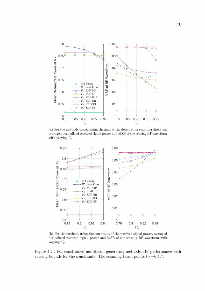
70
0.55 0.65 0.75 0.85 0.950.5
0.55
0.6
0.65
0.7
0.75
0.8
Mea
n N
orm
aliz
ed P
ower
at R
x
0.55 0.65 0.75 0.85 0.950
0.01
0.02
0.03
0.04
0.05
0.06
MSE
of B
F W
avef
orm
(a) For the methods constraining the gain at the dominating scanning direction,averaged normalized received signal power and MSE of the sensing BF waveformwith varying Cs.
0.78 0.8 0.82 0.840.5
0.55
0.6
0.65
0.7
0.75
0.8
0.85
Mea
n N
orm
aliz
ed P
ower
at R
x
0.78 0.8 0.82 0.840
0.01
0.02
0.03
0.04
0.05
0.06
MSE
of B
F W
avef
orm
(b) For the methods using the constraint of the received signal power, averagednormalized received signal power and MSE of the sensing BF waveform withvarying Cp.
Figure 4.2 : For constrained multibeam generating methods, BF performance withvarying bounds for the constraints. The scanning beam points to −6.45◦.

71
-20 -10 0 10 20Scanning direction in Degrees
0.35
0.4
0.45
0.5
0.55
0.6
0.65
0.7
0.75
0.8
0.85
Mea
n N
orm
aliz
ed P
ower
at R
x
-20 -10 0 10 20Scanning direction in Degrees
0
0.01
0.02
0.03
0.04
0.05
0.06
0.07
MSE
of B
F W
avef
orm
Figure 4.3 : Normalized received signal power for communications and MSE of thescanning BF waveform for different BF methods when the scanning subbeam pointsto various directions. The scanning subbeams point to −23.63◦, −17.90◦, −12.18◦,−6.45◦, 5.01◦, 10.74◦, 16.47◦, 22.20◦, respectively. The values of Cs, Csp, Cp and(θs2 − θs1) are the same as those in Fig. 4.1.
power (i.e., solutions to P3, P4, P7, and P8), because of the nature of constrained
optimization.
In Fig. 4.4, we show how the BF performances are affected by the number of
NLOS paths. When the scanning subbeam points to −12.18◦, which means some
paths may not be within the 3dB beamwidth of both fixed and scanning subbeams,
the waveform MSE increases with the growth of L. For “P5: SDP-RxP”, the MSE of
the scanning BF waveform is even smaller than the other two subbeam-combination
methods, although the received signal power for “P5: SDP-RxP” is larger. Similar
results can also be observed for the other methods and in other directions, which
are not shown for the clarity of this figure. The figure also illustrates that the global
optimization methods can balance and better control the different aspects of the BF
performance.

72
4 6 8 10 12 140.4
0.45
0.5
0.55
0.6
Mea
n N
orm
aliz
ed P
ower
at R
x
4 6 8 10 12 140
0.005
0.01
0.015
0.02
0.025
0.03
0.035
0.04
MSE
of B
F W
avef
orm
Figure 4.4 : Normalized received signal power and MSE of BF waveform with varyingnumber of paths Lp when the scanning beam points to −18.21◦. The other settingsare the same as those for Fig. 4.3. For “P1: RxP-SG”, Cs = 0.9.
4.4 Summary
In this chapter, we studied a range of multibeam optimization methods for JCAS
systems using analog arrays, considering requirements for both communication and
sensing. We first proposed new constrained optimization methods, which provide
closed-form optimal solutions to the phase coefficient for combining fixed and scan-
ning BF vectors. We also proposed new global optimization methods that directly
generate single BF vectors. We presented the process of converting the original NP-
hard problems to QCQP, which can be solved efficiently by using SDR techniques.
The global optimization methods that achieve near-optimal solutions provide the
benchmarks for evaluating the performance tradeoff of other methods. Simulation
results demonstrate that the proposed optimization methods can achieve a good
balance between communication and sensing performances.

73
Chapter 5
Quantization of Multibeam BF vectors
In practical analog arrays, BF weights can typically be represented only as quantized
and discrete values instead of continuous ones. In this Chapter, we study the impact
of BF vector quantization on multibeam generation, by using phase shifters in the
array only.
We introduce several quantization methods for the BF vector, particularly for
the two-phase-shifter (2-PS) arrays introduced in Section 5.1. In Section 5.2.1,
we propose a novel joint quantization method that combines the codebooks of the
two phase shifters. With the new codebooks, particular the one established by
introducing a fixed phase shifting value to one of the phase shifters, we show that
even scalar quantization can achieve performance close to the non-quantized case
when there are more than 3 quantization bits in each phase shifter. We also develop
the improved golden section search-quantization (IGSS-Q) method in Section 5.2.2.
The IGSS-Q method enables better scalar quantization by considering the property
of vector quantization.
In Section 5.3, we analytically evaluate and compare the MSQE for several one-
phase-shifter (1-PS) and 2-PS quantization methods. These analytical results are
shown to match the simulated results well.
5.1 Analog BF System with Phase Shifters
After obtaining wt via methods in Chapter 3 and Chapter 4, the quantization
is applied to the final BF vector wt = {wi} = {|wi|ejψi}, i = 1, · · · ,M , where ψi =

74
(a) Option 1: parallel structure (b) Option 2: serial structure
Figure 5.1 : Optional parallel and serial structures with two phase shifters.
∠(wi). Let b be the number of quantization bits in each phase shifter. We assume
that the discrete phase values are equally spaced over [0, 2π] with a quantization
step of ∆ = 2π2−b.
In this Chapter, we will mainly study element-wise scalar quantization where
each component of the beamforming vector is quantized separately. Although vec-
tor quantization can achieve better performance than element-wise quantization, its
complexity is higher. As we will see in the simulation results, element-wise quan-
tization, particularly for the 2-PS array, can achieve performance approaching to a
non-quantized one when the number of quantization bit b is moderately large, for ex-
ample, b � 3. When b is small, formulating BF vector quantization as non-coherent
detection problems can be an effective approach for reducing quantization distor-
tion at an affordable complexity, e.g., trellis based searching algorithms [74, 75] or
maximum likelihood (ML) detection algorithms [72, 76]. Here, vector quantization
means to directly search for the quantized BF vector from the finite list of possible
BF vectors to represent wt.
We study two cases when a single and double phase shifters, abbreviated as 1-
PS and 2-PS, are used respectively. The two optional structures for 2-PS are shown
in Fig. 5.1. As shown in [81], the 2-PS array can provide significantly reduced
quantization errors compared to 1-PS, at increased hardware cost.

75
For the 1-PS array, the element-wise quantization can be represented as
β(i) = arg minβ∈B|mod2π(ψi − β)| (5.1)
where β ∈ B = {0,∆β, 2∆β, . . . , (2b−1)∆} with quantization step ∆β, and mod2π(x)
stands for x modulo 2π.
Since the 1-PS array only represents a value with unit magnitude, the resulting
amplitude mismatches can cause notable sidelobe even using phase shifters with
an infinite number of quantization bits [7, 8]. This can cause a waste of energy and
difficulty for the angle of arrival estimation in multibeam sensing. This problem may
be solved by adding power amplifiers/attenuators for each phase shifter. It can also
be solved by using the 2-PS array, which is the main approach being investigated in
this chapter.
For the parallel and serial structures in Fig. 5.1, the phase shifting values satisfy
wi = |wi|ejψi = ejβ(i)1 + ejβ
(i)2 , (5.2a)
and
wi = |wi|ejψi = ejβ(i)1 (1 + ejβ
(i)2 ), (5.2b)
respectively. Thus, the ideal non-quantized phase values for the parallel and serial
structures can be derived as
β(i)1 = ψi + arccos(|wi|/2), β
(i)2 = ψi − arccos(|wi|/2), (5.3a)
β(i)1 = ψi − arccos (
|wi|2
), β(i)2 = 2 arccos (
|wi|2
), (5.3b)
respectively.

76
A straightforward and simple way to decide the quantized phase shifts is then
through quantizing each of them separately. This is given by
β(i)1 = arg min
β1∈B1
|mod2π(β(i)1 − β1)|, β(i)
2 = arg minβ2∈B2
|mod2π(β(i)2 − β2)|, (5.4)
where β1 ∈ B1 = {0,∆β1 , 2∆β1 , . . . , (2b1 − 1)∆β1} and β2 ∈ B2 = {0,∆β2 , 2∆β2 , . . . ,
(2b2 − 1)∆β2} are the sets of the quantized phase values. ∆β1 and ∆β2 are the quan-
tization steps depending on the number of quantization bits b1 and b2 respectively.
Such separated quantization used in [81] can lead to large quantization error, unless
the number of quantization bits in each phase shifter is very large.
5.2 Joint Quantization Using Combined Quantization Code-
books
In this section, we propose several methods for determining the phase shift-
ing values in the two 2-PS structures. Different from the separated quantization
described above, novel joint quantization methods using combined codebooks are
studied. Based on the new codebook, we propose low-complexity element-wise quan-
tization methods with refined scaling of the BF vector. We also propose a simple
one-dimensional searching algorithm for finding the optimal scaling factor based on
the improved golden section search (IGSS) method [103].
5.2.1 Generation of Combined Codebook
We consider a pair of generalized codebooks containing the quantized phase
values
B1 = {0,∆β1 , 2∆β1 , . . . , (2b1 − 1)∆β1},
B2 = {φ, φ+ ∆β2 , . . . , φ+ (2b2 − 1)∆β2},(5.5)

77
where φ, 0 ≤ φ ≤ ∆β2/2, is a constant for any fixed phase shifter. Such a constant
phase shift can be realized easily by, for example, a fixed length of delay line in the
circuit for either structure in Fig. 5.1.
A combined codebook can be generated from these two codebooks. Let β1 and
β2 be any quantized phase shifts in B1 and B2, respectively. A combined codebook
C is generated by
c = ejβ1 + ejβ2 or c = ejβ1(1 + ejβ2), c ∈ C, (5.6)
corresponding to Fig. 5.1(a) or 5.1(b). The codes in C do not have unit magnitude
any more. Note that the parallel and serial structures generate the same codebooks
and the two options are essentially equivalent when using the combined codebook.
This phase shift φ can influence the number of codes in C as well as the dis-
tribution of the constellation plot, as shown in Fig. 5.2. If φ = 0, there will be
2b repetitive values out of the total 22b codes in C. Reduced number of distinct
codes will lead to increased quantization errors. It can also be observed that when
φ = ∆β2/2, the constellation is uniformly and symmetrically distributed over the
complex plane, which can be a beneficial feature in generating a random precoding
coefficient.
Besides, if the quantization bits of the two phase shifters are different, the con-
stellations of the codebook C will be quite different. Fig. 5.3 plots the constellation
for various options with b1 + b2 = 6 and φ = π/4. It is discovered that when b1 6= b2,
the values of c tend to gather at some specific regions on the complex plane. In
comparison, c has a more uniform distribution when b1 = b2. In this thesis, we
study two exemplified codebooks: C1 with φ = 0 and C2 with φ = ∆β2/2, both
having b1 = b2 = b. The number of different codes in C1 and C2 are nc1 = 22b−1 and
nc2 = 22b, respectively. The two codebooks are chosen for the uniform and sym-

78
Real Part
Imaginary Part= /8
Real Part
Imaginary Part= /6
Real Part
Imaginary Part= /4
Real Part
Imaginary Part= /2
Figure 5.2 : Constellation of codebook C via φ when b1 = b2 = 2.
Real Part
Imaginary Part
(a) b1 = 1 and b2 = 5.
Real Part
Imaginary Part
(b) b1 = 2 and b2 = 4.
Real Part
Imaginary Part
(c) b1 = 3 and b2 = 3.
Figure 5.3 : Constellation of codebook C via varying b1 and b2, when φ = ∆β2/2.
metric distribution of their constellation plots. The proposed analytical methods,
i.e., the geometric position analysis of codes in a constellation plot, can be easily
extended to other codebooks using different quantization bits and φ.
Since the BF vectors are often normalized to ‖wt‖ = 1, the codebooks C1 and C2

79
are normalized by
h1 =
√√√√ N
2b−1
2b−1∑i=1
c2k,i =
√2 + 22−b
√N, (5.7)
and
h2 =
√√√√N
2b
2b∑i=1
c2k,i =
√2N, (5.8)
respectively. So E[|ck,i|2] = 1/N , where ck,i is the i-th element in Ck.
For the codebook Ck, we can then apply the element-wise quantization for each
BF weight wi and obtain
wi0 = arg minc∈Ck|wi − ck,i|2. (5.9)
With the BF vector w0 = [w10 , w20 , · · · , wM0 ]T , the quantized BF vector can be
obtained by
w =w0
‖w0‖, (5.10)
where w is normalized to ‖w‖ = 1. As we are going to show in Section 5.2.3, the
element-wise quantization algorithm based on our proposed codebooks can already
achieve sufficiently good performance with only a small number of quantization bits.
5.2.2 Quantization with Optimized Scaling Factor
In the Section 5.2, our codebook Ck was normalized to hk, but hk are statistical
values which cannot guarantee the instantaneous optimality for quantizing a partic-
ular BF vector wt. With the goal of finding a better solution, we propose an algo-
rithm, what we call as IGSS-Q, based on the improved golden section search (IGSS)
algorithm [103]. The IGSS algorithm is an efficient one-dimension linear searching

80
method that relaxes the unimodal requirement for the classic golden-section search
method.
Our IGSS-Q method solves the following problem
νopt = arg minν‖νwt − q(ν)‖2
2 (5.11)
iteratively. In each iteration, q(ν) is obtained by scalar quantization with Ck and
the i-th element of q(ν) is given by
qi = arg minc∈Ck|νwi − ck,i|2, (5.12)
where i ∈ {1, · · · ,M}. For a fixed ν and the qi values obtained in (5.12), the
quantization error e(ν) can be expressed as
e(ν) =M∑i=1
|νwi − qi|2. (5.13)
The IGSS-Q method starts with setting the initial searching interval ν ∈ [a1, a2]
and then defines interior points x1 and x2 to divide the golden section in this interval.
In each iteration, the IGSS-Q method finds the corresponding quantized values and
compute the errors via (5.12) and (5.13) for ν = a1, a2, x1, and x2. By comparing
e(a1), e(a2) with e(x1) and e(x2), the searching interval is updated and narrowed
down gradually. Repeat this process until e(x1)− e(x2) is smaller than a preset tiny
positive threshold ε0 or the maximal iteration times Lmax is reached. The detailed
process of the IGSS-Q method is provided in Algorithm 2.
The computational complexity of IGSS-Q is low and can be approximately rep-
resented as O(MLmax), where Lmax is the number of iterations. With the output q

81
Algorithm 2 IGSS-Q Algorithm
Input: a1, a2, Lmax, ε0, ρ =√
5−12
.
1) l = 0, a(0)1 = a1, a
(0)2 = a2, d(0) = a
(0)2 − a
(0)1 , x
(0)1 = a
(0)1 + (1 − ρ)d(0),
x(0)2 = a
(0)1 + ρd(0); go to 2).
2) d(l) = a(l)2 − a
(l)1 ; If l ≤ Lmax & |d(l)| > ε0, go to 3); otherwise, go to 5).
3) Calculate e(a(l)1 ), e(x
(l)1 ), e(x
(l)2 ) and e(a
(l)2 ) through (5.13); Then [I
(l)min, emin] =
min{e(a(0)1 ), e(x
(0)1 ), e(x
(0)2 ), e(a
(0)2 )}, where I
(l)min is the index value and I
(l)min ∈
{1, 2, 3, 4}. Go to 4);
4) With the results in 3), update the values of a(l)1 , a
(l)2 , x
(l)1 , x
(l)2 , and l, through the
IGSS method in [103], (5.12) and (5.13). Go to 2);
5) νmin = arg minx
(l)i
{e(x(l)i )}, i = 1 or 2, break.
6) Compute qi via (5.12) and νmin.Output: νmin, q = [q1, q2, · · · , qM ]T
from the algorithm, we can get the quantized BF vector as
wt =q
‖q‖, q = [q1, q2, · · · , qM ]T . (5.14)
5.2.3 Simulation Results
Fig. 5.4 shows how the BF radiation pattern varies with the number of quanti-
zation bits for our proposed joint quantization schemes, together with 1-PS vector
quantization using the fast block noncoherent decoding (FBND) method [72] for
comparison. From Fig. 5.4(a), we can see that for 1-PS, the sidelobe of the wave-
form for the quantized BF vector is quite large, even when the number of quanti-
zation bits is as large as 5. There is also a notable distortion in the mainlobe. So
vector quantization cannot improve the quantization error floor for the case with
only quantized phase values. Comparatively, joint quantization for 2-PS achieves a
good match in the mainlobe with the non-quantized one and much lower sidelobe,
as can be seen from Fig. 5.4(b), 5.4(c) and 5.4(d). For example, when the number
of quantization bits is larger than 3, the power level of the sidelobe of the quantized
results with codebook C2 is very close to the non-quantized one. It can also be

82
-60 -40 -20 0 20 40 60Scanning direction in Degrees
-25
-20
-15
-10
-5
0
5
10
BF ra
diat
ion
patte
rn (d
B)
Without quantizationbit=2bit=3bit=4bit=5
(a) FBND quantization for 1-PS.
-60 -40 -20 0 20 40 60Scanning direction in Degrees
-25
-20
-15
-10
-5
0
5
10
BF ra
diat
ion
patte
rn (d
B)
Without quantizationbit=2bit=3bit=4bit=5
(b) Joint quantization for 2-PS with Code-book C1.
-60 -40 -20 0 20 40 60Scanning direction in Degrees
-25
-20
-15
-10
-5
0
5
10
BF ra
diat
ion
patte
rn (d
B)
Without quantizationbit=2bit=3bit=4bit=5
(c) Joint quantization for 2-PS with Code-book C2.
-60 -40 -20 0 20 40 60Scanning direction in Degrees
-25
-20
-15
-10
-5
0
5
10
BF ra
diat
ion
patte
rn (d
B)
Without quantizationbit=2bit=3bit=4bit=5
(d) IGSS-Q for 2-PS with Codebook C2.
Figure 5.4 : BF radiation pattern for different number of quantization bits. Thescanning beam points to −12.3◦.
observed that IGSS-Q can slightly reduce the sidelobe when b ≥ 4, compared with
element-wise scalar quantization.
Using the unquantized BF weight vector derived through the method proposed
in Section 3.2.2, and related simulation setup in Section 3.2.4, we now further look
at the impact of quantization on the received signal power and signal demodulation
performance.
In Fig. 5.5, we show the received signal power for the 1-PS FBND quantization
and the joint IGSS-Q method with Codebooks C1 and C2 (denoted as “Codebook
1” and “Codebook 2”), when the total number of quantization bits in each method
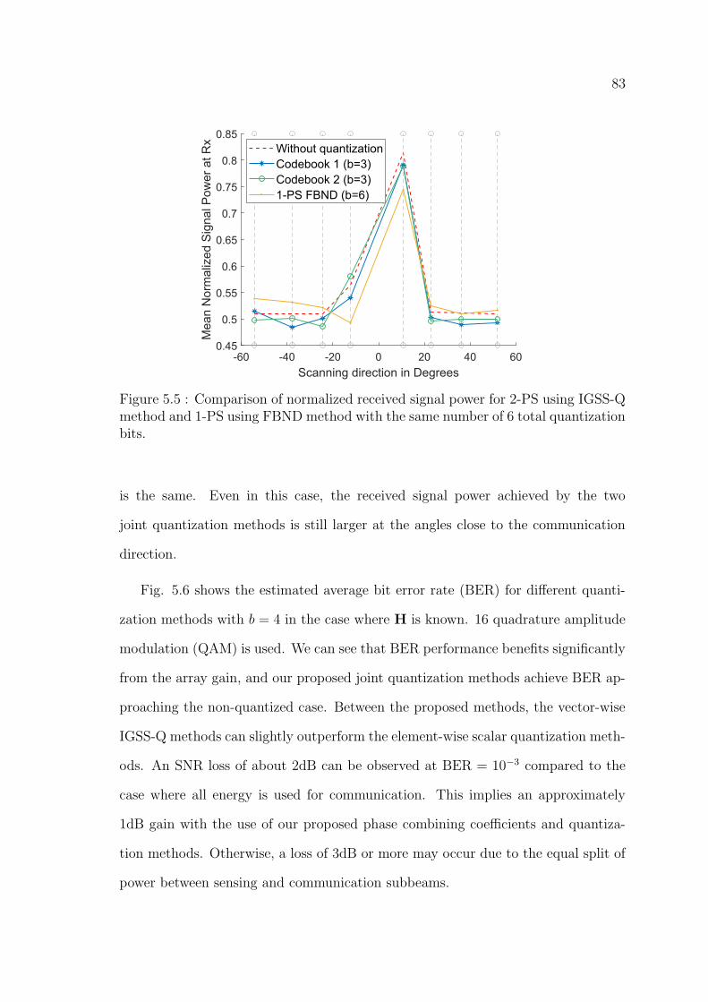
83
-60 -40 -20 0 20 40 60Scanning direction in Degrees
0.45
0.5
0.55
0.6
0.65
0.7
0.75
0.8
0.85
Mea
n N
orm
aliz
ed S
igna
l Pow
er a
t Rx Without quantization
Codebook 1 (b=3)Codebook 2 (b=3)1-PS FBND (b=6)
Figure 5.5 : Comparison of normalized received signal power for 2-PS using IGSS-Qmethod and 1-PS using FBND method with the same number of 6 total quantizationbits.
is the same. Even in this case, the received signal power achieved by the two
joint quantization methods is still larger at the angles close to the communication
direction.
Fig. 5.6 shows the estimated average bit error rate (BER) for different quanti-
zation methods with b = 4 in the case where H is known. 16 quadrature amplitude
modulation (QAM) is used. We can see that BER performance benefits significantly
from the array gain, and our proposed joint quantization methods achieve BER ap-
proaching the non-quantized case. Between the proposed methods, the vector-wise
IGSS-Q methods can slightly outperform the element-wise scalar quantization meth-
ods. An SNR loss of about 2dB can be observed at BER = 10−3 compared to the
case where all energy is used for communication. This implies an approximately
1dB gain with the use of our proposed phase combining coefficients and quantiza-
tion methods. Otherwise, a loss of 3dB or more may occur due to the equal split of
power between sensing and communication subbeams.

84
-6 -4 -2 0 2 4 6Eb/No (dB)
10-6
10-5
10-4
10-3
10-2
10-1
Mea
n Bi
t Erro
r Rat
e
Single Beam for CommunicationWithout quantization (H-known)FBND2PS-S2Codebook1-ScalarCodebook2-ScalarCodebook1-IGSSCodebook2-IGSS
Figure 5.6 : BER for different methods with b = 4 (quantization bits) and thesensing subbeam pointing at −12.3◦.
To summarize, in terms of both BF waveform and the received signal power and
demodulation performance, we can conclude that the proposed joint quantization
method with codebook C2 can achieve performance approaching to the non-quantized
one.
5.3 Quantization Error Analysis
In this section, we analyze element-wise quantization error for the 1-PS and
2-PS quantization schemes presented in Section 5.1. We use the MSQE as the
performance metric, which directly influences the performance of BF algorithms
despite the communication and sensing metrics. The MSQE is defined as
ε = E[1
M
M∑i=1
(|wi − wi|2)], (5.15)
where wi is the quantized BF weight. For both 1-PS quantization and 2-PS separate
quantization, we provide more accurate analytical results compared with [81]. For

85
2-PS joint quantization, our analytical results are new, as well as the quantization
scheme itself.
5.3.1 1-PS Array
When only one phase shift is used to represent a BF weight, the ith element of
the quantized BF vector can be represented as wi = 1√Mej(ψi+δψ), where δψ denotes
the phase quantization error. Assume that δψ is uncorrelated with ψ and uniformly
distributed over [−∆ψ/2,∆ψ/2). The MSQE in this case can be expanded to
ε0 = E(|wi − wi|2) =
∫ ∆ψ2
−∆ψ2
|wi − wi|21
∆ψ
dδψ
=1
M+ E(|wi|2)− 2E(|wi|)√
M(
2
∆ψ
sin∆ψ
2).
(5.16)
When b is large, and in the extreme case ∆ψ → 0, we have
lim∆ψ→0
ε0 =1
M+ E(|wi|2)− 2E(|wi|)√
M= E[(|wi| −
1√M
)2] + Var(|wi|) ≥ Var(|wi|),
(5.17)
where Var(|wi|) is the variance of |wi|. This clearly shows that the quantization error
does not vanish by only using phase shifting values to represent the BF weights with
varying magnitudes. There will be an error floor despite the value of the quantization
step.
5.3.2 2-PS with Parallel Structure Using Separate Quantization
When phase shifts are quantized, wi = ejβ(i)1 +δβ1 + ejβ
(i)2 +δβ2 , where δβ1 and δβ2
are the phase quantization errors (referring to (5.2a)). The MSQE ε1 is then given

86
by
ε1 =4 + 2E[cos (β1 − β2)]− 2E[cos (β1 − β2)]·
{E(cos δβ1)− E(cos δβ2)− E[cos (δβ1 − δβ2)]} − 2E(cos δβ1 + cos δβ2).
(5.18)
The quantization errors δβ1 and δβ2 are assumed to be uncorrelated and uniformly
distributed over [−∆β1/2,∆β1/2) and [−∆β2/2,∆β2/2), respectively. It can be cal-
culated that
E(cos δβ1) =2
∆β1
sin (∆β1
2), E(cos δβ2) =
2
∆β2
sin (∆β2
2),
E[cos (δβ1 − δβ2)] = E[cos (δβ1 + δβ2)] =4
∆β1∆β2
sin (∆β1
2) sin (
∆β2
2),
E(sin δβ1) = E(sin δβ2) = 0, E[sin (δβ1 − δβ2)] = E[sin (δβ1 + δβ2)] = 0.
Since E[cos (β1 − β2)] = E(|wi|2 − 1
2), (5.18) can be expressed as
ε1 =3 + E(|wi|2) + E(|wi|2)[4
∆β1∆β2
sin (∆β1
2) sin (
∆β2
2)− 2
∆β1
sin (∆β1
2)
− 2
∆β2
sin (∆β2
2)]− 2
∆β1
sin (∆β1
2)− 4
∆β1∆β2
sin (∆β1
2) sin (
∆β2
2)
− 2
∆β2
sin (∆β2
2).
(5.19)
When x is small, the function sin x can be approximated as sin x ≈ x− x3
6using
the Taylor series expansion for sin x. To this end, (5.19) can be approximated as
ε1 ≈∆2β1
12+
∆2β2
12− (E(|wi|2)− 1)
∆2β1
∆2β2
576. (5.20)
Note that the first two terms in (5.20) are just the results in [81]. Our result here
provides a closer approximation to the MSQE ε1.

87
In the extreme case of ∆β1 → 0, ∆β2 → 0, we can get
lim∆β1
, ∆β2→0ε1 = 0. (5.21)
This shows that with the 2-PS parallel structure, the MSQE can reach zero when
the quantization bit b is sufficiently large, even when the actual BF weights have
varying amplitudes.
5.3.3 2-PS with Serial Structure Using Separate Search
For the 2-PS array with the serial structure, wi = ej(β(i)1 +δβ1
)[1 + ej(β(i)2 +δβ2
)].
Thus, the MSQE ε2 can be written as
ε2 =4 + 2E(cos β2)[1− 2
∆β1
sin (∆β1
2) +
2
∆β2
sin (∆β2
2)]
− 2E(cos β2 + 1)4
∆β1∆β2
sin (∆β1
2) sin (
∆β2
2)− 4
∆β1
sin (∆β1
2).
Since E(cos(β2)) = E( |wi|2
2− 1), ε2 can be rewritten as
ε2 =2 + E(|wi|2)[1− 2
∆β1
sin (∆β1
2) +
2
∆β2
sin (∆β2
2)
− 4
∆β1∆β2
sin (∆β1
2) sin (
∆β2
2)]− 4
∆β2
sin (∆β2
2).
Using sin x ≈ x− x3
6, we can approximate ε2 as
ε2 ≈1 + E(|wi|2)
12∆2β1− E(|wi|2)
576∆2β1
∆2β2. (5.22)
Similarly, we can show that
lim∆β1
, ∆β2→0ε2 = 0. (5.23)

88
5.3.4 2-PS Using Joint Quantization
We consider the case when the two phase shifters have the same number of
quantization bits.
To derive a closed-form MSQE expression, we approximate the quantization error
|δc| for each BF weight as a variable following a uniform distribution over [0, δc,max].
On the complex plane, δc,max can be computed as the maximum of all the distances
between any point aejα to its nearest constellation points c. For simplicity, when
analyzing δc,max, we only consider the case when a ≤ |c|max since the probability of
a > |c|max is low. The MSQE metric for joint quantization becomes
ε = E[1
M
M∑i=1
(|νminwi − wi|2)].
When element-wise scalar quantization is used, νmin = 1.
MSQE for Codebook C1
For the normalized codebook C1 with φ = 0, δc,max is the distance between (0, 0)
to the nearest points, and is given by δc,max =√
2−2 cos ∆ν1,min
. The corresponding MSQE
is
εc1 = [E(|δc|)]2 + Var(|δc|) =2− 2 cos ∆
3E[ν21,min]
. (5.24)
When the quantization step is small, 1− cos ∆ ∼ ∆2
2, and (5.24) can be approx-
imated as
εc1 ≈∆2
3E[ν21,min]
≈ ∆2
3h21
=∆2
3(2 + 22−b)M. (5.25)
Note that (5.25) is also the MSQE for element-wise scalar quantization using code-
book C1. This implies that scalar quantization using the proposed codebook can

89
(a) Constellation and the sector selectedfor analysis.
(b) Key points in the sector.
Figure 5.7 : Constellation plot used for analyzing dmax for Codebook 2 (b = 3).
achieve comparable performance to IGSS-Q, when quantization bits are sufficiently
large.
MSQE for Codebook C2
Now we analyze δc,max for codebook C2. Because the constellation of C2 is sym-
metrical, we can select a circular segment (the shaded region in Fig. 5.7(a)) for
analyzing δc,max.
In this segment, the points that can achieve the maximal distance between two
adjacent constellation points are marked as Oi, i = 1, 2, · · · , 2b−1, as shown in Fig.
5.7(b). Obviously, every Oi locates on the y-axis. Note that for simplicity, in the
following analysis, we temporarily let h2 = 1, as its value is independent of the
position relationship between constellation points. According to (5.2), it can be
easily derived that for the constellation points Ai,
|AiO| = ri−1 =
√2− 2 cos [(i− 1)∆ +
∆
2], i = 1, 2, · · · (5.26)

90
Assume that there existsO1, making |A1O1| = |A′2O1| = |A1O| = r0 =√
2− 2 cos ∆2
.
Then |A′2O| = |OM1|+|A2M |. According to the cosine rule, |OM1| = 2|A1O| cos2 (∆4
).
Thus, |A′2O| = |OM1| + |A2M | = |OM1| + (|OM1| − |A1O|) = 4r0 cos2 (∆4
) −
r0 =√
2− 8 cos3 (∆2
) + 6 cos (∆2
) = |A2O| =√
2− 2 cos (3∆2
). Since cos (3∆2
) =
4 cos3 (∆2
)− 3 cos (∆2
), from (5.26) we get
|A2O| =√
2− 2 cos (3∆
2) =
√2− 8 cos3 (
∆
2) + 6 cos (
∆
2). (5.27)
Therefore, we can find that A′2 overlaps with A2. This implies that in the sector
A2OB2, d ≤ δc,max = r0.
According to the Cosine law, if Oi(yiej2π) satisfies |AiOi| = |Ai+1Oi|, that is
r2i + y2
i − 2riyi cos (∆
4) = r2
i+1 + y2i − 2ri+1yi cos(
∆
4).
Solving this equation, we get yi =ri+1 + ri
2 cos (∆4
). Therefore,
|AiOi|2 =r2i+1 + r2
i − 2riri+1 cos (∆2
)
2 cos(∆2
) + 2. (5.28)
Assuming |AiOi|2 = r20 = 2− 2 cos (∆
2), we have
r2i+1 + r2
i − 2riri+1 cos (∆
2) = 2− 2 cos ∆. (5.29)
According to the Cosine law again, the left part of (5.29) can be seen as |AiBi+1|.
Because of the symmetry of the constellation, |AiBi+1| is equal to the distance

91
between two constellation points with similar positional relationship:
|AiBi+1| = |(1 + ej(∆2
+i∆))− (1 + ej(∆2
+i∆+∆))|
= |ej∆ − 1| = 2− 2 cos ∆.
(5.30)
Therefore, |AiOi|2 = r20 is proven. In summary, for a aejα satisfying a ≤ r2b−1 ,
the maximal error distance δc,max = r0 =
√2−2 cos ∆
2
h2.
Thus, the MSQE in this case can be obtained as
εc2 =2− 2 cos (∆
2)
3E[ν22,min]
. (5.31)
When ∆ is small, 1− cos ∆2∼ ∆2
8, and (5.31) can be approximated as
εc2 ≈∆2
3h22
=∆2
24M. (5.32)
Similarly, (5.32) is also the MSQE for element-wise scalar quantization using code-
book C2.
When ∆→ 0, we have
lim∆→0
εc1 = 0, lim∆→0
εc2 = 0. (5.33)
5.3.5 Comparison of MSQE for Different Quantization Methods
Referring to the approximated values of MSQE in (5.20), (5.22), (5.25), and
(5.32), we compare the performance for these quantization methods.
Since ||wt|| = 1, we see 0 < |wi| < 1. According to (5.20) and (5.22), it can
be found that ε2 < ε1, which indicates that for 2-PS, separate quantization using

92
Table 5.1 : Comparison of phase shifter structures and different searching methods.
1-PS Array2-PS Arrays
Separate Search Joint SearchMSQE ε0 ε1 > ε2 εc1 > εc2, lowest overall
limb→∞
εi, i = 0, 1, 2 E[(|wi| − 1M
)2] +D(|wi|) > 0 0
Number of Phase Shifters M 2MHardware Complexity normal relatively complex
Drawbacks large error floor exists large error more constellation points to be compared and storedComputation Complexity O(2bM) O(2b+1M) O(2ncM) (Scalar) O(2ncM2) (IGSS-Q)
the parallel structure can achieve slightly better performance than using the serial
structure, when the quantization step is reasonably small.
From (5.7), we can find that for b ≥ 2,√
2M < h1 ≤√
3M . Therefore, εc1
satisfies
∆2
9M≤ εc1 <
∆2
6M.
For large arrays with more than, e.g., M = 8 antennas, it can be readily verified
that
εc2 < εc1 < ε2 < ε1. (5.34)
This indicates that joint quantization using the codebook C2 achieves the smallest
quantization error.
In Table 5.1, we summarize the comparison results for these quantization meth-
ods.
In Fig. 5.8, we show MSQE versus the number of quantization bits for various
quantization methods. Apart from those studied and analysed in this chapter, we
also compute and plot the MSQE in [81], which is denoted as “εx-Lin2017” in the
legend. The values of wi = |wi|ejψi in wt are generated randomly with |wi| following
a uniform distribution over [0, 2) and with ψi following a uniform distribution over

93
[0, 2π). The vector of wt is then normalized so that its norm is 1. The MSQE is
averaged over 105 realizations for the simulated values. From the figure, we can
see that most of the analytical results match the simulated ones very well, except
for εc1. The analytical results provided in this chapter are shown to offer better
accuracy than the one in [81], although the difference is small for this simulated
example. When b > 2, the simulated εc1 deviates from the analytical εc1 derived
in Section 5.3.4. This is because for Codebook C1, many of the largest distances
between any two nearest constellation points are smaller than δc,max. Therefore, the
uniform distribution assumption in Section5.3.4 is not accurate enough. Overall,
the joint quantization method using Codebook C2 achieves the lowest quantization
error, as we have shown analytically in (5.34).
5.4 Summary
In this chapter, considering the practical constraint that BF weights in ana-
log arrays are of discrete values, we investigated various element-wise quantization
methods. The structures where two phase shifters are used to represent one BF
weight are particularly studied. We proposed novel joint quantization methods us-
ing combined codebooks for the 2-PS array structure. These methods are shown
to achieve BF waveforms closely matching the one with a non-quantized BF vec-
tor, as well as the received signal power, using a medium number of quantization
bits. We also provided analytical expressions of the mean squared quantization error
(MSQE) for these quantization methods. Simulation results match these analytical
MSQE results well. Overall, the joint quantization methods can approach the per-
formance achieved by the non-quantized BF vector, and hence is very promising for
the multibeam JCAS system.

94
2 2.5 3 3.5 4Number of quantization bits
-16
-14
-12
-10
-8
-6
-4
-2M
SQE
(dB) Simulated 0
0 in (27)
Simulated 1
1
1-Lin2017
Simulated 2
2
2-Lin2017
(a)
2 2.5 3 3.5 4Number of quantization bits
-20
-15
-10
-5
0
MSQ
E (d
B)
c1(simulated)
c1
c2(simulated)
c2
(b)
Figure 5.8 : MSQE versus number of quantization bits for various quantizationschemes.

95
Chapter 6
Robust BF Methods with Embedded Active
Patterns of Array
In previous chapters, the antenna arrays are ideally modeled from the aspect of sig-
nal processing, ignoring the array imperfections, such as gain and phase mismatches,
and mutual coupling between elements. The assumption of ideal array elements can
cause severe performance degradation in real implementations, particularly for the
small-profile arrays considered in mmWave JCAS systems. The proposed methods in
this chapter can significantly reduce the performance degradation of the beamform-
ers caused by inconsistency between hypothesized ideal array models and practical
ones by embedding active patterns of antennas. Although some of the BF algorithms
are not initially designed for JCAS systems, in the future, we can easily apply the
proposed concept to JCAS with prepared practical hardware platforms.
6.1 Signal Model and Improved Array Steering Vector
6.1.1 Signal Model
In this chapter, we consider an M -element two-dimension antenna array and a
narrow-band system. Without considering any imperfections, its steering vector a
can be represented as
a(f, θr, ϕr, r) = [1, ejkr1(θr,ϕr), · · · , ejkrM−1(θr,ϕr)], (6.1)
where k = 2πf/v is the wavenumber, f and v denote the frequency and the speed
of the electromagnetic wave, respectively, θr and ϕr are the AoA, and ri(θr, ϕr) is

96
the location vector of the (i+ 1)th sensor.
Assume omnidirectional antenna elements. Let s(t) be the transmitted data
symbol at time t and the AoA of signal and interference be (θr,s, ϕr,s) and (θr,i, ϕr,i),
respectively. The signal received at the array is given by
x(t) = s(t)aS(θr,S, ϕr,S) + i(t)aI(θr,I , ϕr,I) + n(t) (6.2)
where x(t) = [x1(t), x2(t) · · · , xM(t)]T ∈ CM×1, aS(θr,S, ϕr,S) and aI(θr,I , ϕr,I) are
the steering vectors of signal and multiuser interference respectively. n(t) is an
M × 1 vector denoting the combined self-interference from mismatches and noise
components.
With the purpose of adaptively receiving the communication signals in one direc-
tion and reducing interference in another, the well-known sample matrix inversion
(SMI) beamformer is considered. A constrained minimization problem is solved as
minw
wHRw s.t. wHaS = 1, (6.3)
where w is the complex BF vector, and R is the sample covariance matrix of x(t).
6.1.2 Improved Array Steering Vector
There are always mismatches between the ideal steering vector a and the actual
one_
a, which is brought by each antenna’s radiation directivity, the mutual coupling
effects between antenna elements, and the influence of the environment. In this
chapter, we use an improved array steering vector a, by taking the radiation property

97
of array aperture into consideration [90].
a(f, θr, ϕr, r) = [g1(f, θr, φr), g2(f, θr, φr)ejkr2(θr,ϕr), · · · , gM(f, θr, φr)e
jkrM−1(θr,ϕr)]
(6.4)
where gi(f, θr, ϕr) is the known active gain response of the i-th antenna. The active
radiation pattern of an antenna is obtained when only itself is excited, with all other
array elements terminated with matched loads [104]. The active gain can be obtained
during antenna design using electromagnetic simulation software or through actual
measurements.
However, there are always fluctuations of array parameters during design, pro-
cessing, measuring and assembling, between the steering vector a achieved by (6.4)
and the actual one_
a. Mismatches generally have a minor impact on the electromag-
netic characteristics of a single antenna element, such as current distribution and
boundary conditions, and hence cause small changes to the basic radiation struc-
ture of each element, as well as the radiation pattern and directivity. Such small
changes, however, when BF is formed, can cause large BF gain variations, due to
gain, sometimes phase, misalignment between different antenna elements [105]. In
practice, the radiation performance of an an array can be significantly affected by
such array mismatches.
Define the approximation error between the real array steering vector_
a, and the
array models with and without considering the simulated radiation pattern as
e =_
a − a,
e =_
a − a, (6.5)
respectively. The new steering vector a in (6.4) is a closer approximate to the
real steering vector_
a, compared to the one a without considering mismatches, i.e.,

98
Figure 6.1 : A miniature circular microstrip array. The center frequency of eachright-hand circular polarized element is f0 = 1.268 GHz. The dielectric substratehas RDP of εr = 20 and LT of tan δ = 0.004. The metal working platform iselliptical, with a 2a ≈ 0.28λ = 134mm major axis and a 2b ≈ 0.26λ = 121 mmminor axis. The radius of the array is r = 0.16λ = 38 mm and the inter-elementspacing is d = 0.23λ = 54 mm. Each antenna is set at an inclined angle of θw = 5◦
on the workbench.
‖e‖ < ‖e‖.
We refer to a practical 4-element uniform circular microstrip array shown in
Fig. 6.1 as a standard model in our simulation. The commercial electromagnetic
simulation software ANSYS HFSS is used for all antenna simulations.
Fig. 6.2 shows the active patterns of each element. Obviously, the patterns are
significantly different to the ideal omnidirectional models.
We simulate array mismatches using ANSYSr HFSSr and then abstract and
store the corresponding AP for each mismatch. Three types of common mismatches
are studied, including (a) position mismatches of an element, (b) size errors of the
metal working platform, and (c) dielectric parameter errors of the substrate of ele-

99
(a) The AP of element 1. (b) The AP of element 2.
(c) The AP of element 3. (d) The AP of element 4.
Figure 6.2 : The simulated active patterns of the antenna array.
ments, including relative dielectric permittivity (RDP) and loss tangent (LT). The
sample covariance matrix R, which reflects the varying electromagnetic environ-
ment, varies with different pre-stored AP data. Using some of the data, Fig. 6.3
compares the norm e =‖ e ‖ and e =‖ e ‖ in (6.5) under different types of mis-
matches. The results clearly show that our adopted radiation expression with AP
in (6.4) approximates the real radiation pattern much better than the one without
considering mismatch.
6.2 Beamformers with Embedded Active Pattern of Anten-
nas
In this section, we propose two BF methods to make the performance robust to
perturbations caused by ‖e‖ .

100
-80 -60 -40 -20 0 20 40 60 800.0
0.2
0.4
0.6
0.8
1.0
1.2
1.4
STEE
RIN
G V
ECTO
R M
ISM
ATC
H
THETA (°)
Situation a. Situation a. Situation b. Situation b. Situation c.1) Situation c.1) Situation c.2) Situation c.2)
e
e
e
e
e
e
e
e
Figure 6.3 : Steering vector mismatches (norm of the difference) under differentsituations: a. The position mismatch of element 1 (+2mm along axis y); b. Workingplatform mismatch (2a = 136mm); c. 1) The RDP mismatch of element 1 (εr = 20.3); 2) The LT mismatch of element 1 ( tan δ = 0.005).
6.2.1 Diagonal Loading Beamformer with Embedded Active Pattern of
the Array
Referring to the DL method [82] and the AP method [90], we propose the active
pattern embedded diagonal loading (APDL) algorithm. By adding an extra loading
item the sample covariance matrix, its constrained problem can be expressed as:
minw
wH(R + ξI)w s.t. wH aS = 1. (6.6)
Similar to the DL method, ξ is the DL factor, and I denotes the M ×M identity
matrix. Particularly, the ideal signal steering vector aS in conventional DL method
is modified as aS in our method. Then, the weight vector of APDL can be written

101
as:
wAPDL
= αAPDL
(ξI + R)−1aS, (6.7)
where αAPDL
= 1/[aHS (ξI + R)−1aS]. It has been proved that the loading item can
reduce the impact of the array mismatches by reducing the interference of the small
eigenvalues [106]. Usually, the DL factor is chosen in a more ad hoc way, typically
σ2n. Here, σ2
n is the noise power in a single sensor.
The APDL BF algorithm has a comparable computational cost of the DL method,
i.e., O(M3). Although the APDL method needs to extract the prestored active gain
data of the specific DoA, this procedure is not time-consuming.
We assume that the desired signal and interference have plane wavefront with
(θS, ϕS) = (70◦, 6◦) and (θI , ϕI) = (1◦, 90◦) respectively. For each simulated point,
we ran 200 implementations. The input signal-to-noise-ratio (SNR) and interference-
to-noise-ratio (INR) in a single antenna element are equal to 25dB and 30dB, respec-
tively. Signals are in the training data cell (training data size N = 100 unless stated
otherwise). Additive noise in the array is modeled as spatially and temporally inde-
pendent complex Gaussian noise with zero mean and unit variance. The mean out-
put signal-to-interference-plus-noise ratio (SINR) for the following five algorithms is
compared under mismatch situations: the SMI beamformer, the LSMI method [82],
the AP beamformer [91], the WCRB method [83] and the APDL method proposed
in this section. The SMI beamformer can represent the performance of the basic BF
algorithm without considering the array model imperfection. The LSMI and WCRB
methods can represent the performance of the conventional robust BF algorithms,
and the AP method represents the performance of the beamformer directly using
the measured array radiation pattern. The optimal SINR, SINRopt = σ2sa
HS R−1
I+NaS,
is also shown.

102
Figure 6.4 : Output SINR versus antenna elements’ position. Element 1 is movedalong the y axis from -2mm to 2mm, 1 mm at a time.
Fig. 6.4 shows how the output SINR of the beamformer is affected by the posi-
tion mismatches of the antenna element. Fig. 6.5 illustrates how the performance
changes with the size of the working platform, as an example of the working environ-
ment variation. It indicates that the size variation of the metal working platform can
cause the change of edge scattering and affect the electromagnetic radiation, par-
ticularly for AP and SMI algorithms. Both figures show that the proposed APDL
method outperforms other methods with improved SINR and robustness.
In Figs. 6.6 and 6.7, we present how the output SINR changes with the RDP and
LT of the substrate (the range of variation is determined by engineering experience).
From the two figures we can see that the proposed APDL method also achieves
improved SINR and robustness under these two types of mismatches.
With the measured data, we assessed the performance of the earlier mentioned
algorithms using the same parameters (e.g., DoA and INR) with Figs. 6.4-6.7.
The array mentioned has been fabricated, debugged, and then measured in the
microwave anechoic chamber. Due to the small mismatches introduced in the process

103
Figure 6.5 : Output SINR versus the size of the working platform. The length ofthe major axis of the elliptical platform varies from 132mm to 136mm.
Figure 6.6 : Output SINR versus the RDP of the substrate. The RDP of Element1 varies from 19.6 to 20.4.
of fabrication, we can expect the numerical difference of the AP between the designed
and practical arrays. Such difference is shown in Table 6.1, which compares the
active gain data of array elements in (θS, ϕS) = (70◦, 6◦) and (θI , ϕI) = (1◦, 90◦),
the assumed DoAs of signal and interference, respectively.
Figs. 6.8 and 6.9 show the mean SINR with varying number of snapshots, and dif-

104
Figure 6.7 : Output SINR versus the LT of the substrate. The LT of each elementvaries from 0.0005 to 0.005.
Table 6.1 : The Active gain of designed array (Gd) and fabricated array (Gf ) fromthe DOAs of signal and interference.
Element’s Gd(dB) Gf (dB)
NumberθS = 70◦
ϕS = 6◦θI = 1◦
ϕI = 90◦θS = 70◦
ϕS = 6◦θI = 1◦
ϕI = 90◦
1 -4.91 -0.40 -3.03 -0.482 -2.84 -0.50 -2.53 -0.543 -3.62 -0.24 -3.38 -0.534 -3.56 -0.50 -0.81 -0.12
ferent SNRs. These figures demonstrate that the proposed APDL method achieves
better performance than other methods when the input SNR is relatively large.
These measured results demonstrate that the proposed APDL method gives satis-
factory performance in practice.

105
Figure 6.8 : Output SINR versus training data size for SNR=25 dB.
Figure 6.9 : Output SINR versus SNR for training data size of N = 100.
6.2.2 Worst-Case Performance Optimization Beamformer with Embed-
ded Active Pattern of the Array
Assume that the norm of e is bounded by a known constant εAPWC > 0. We can
formulate the APWC problem as a constrained minimization problem
minw
wHRw (6.8)
s.t. |wH c| ≥ 1, for all c ∈ A(εAPWC
),
where A(εAPWC
) , {c|c = aS + e, ‖e‖ ≤ εAPWC}.

106
According to [83], in (6.8), the distortionless response is maintained by inequality
constraints for all possible array response vectors given by A(εAPWC
). (6.8) guar-
antees that the response error e is maintained in the worse case, and hence the
robustness of the beamformer is improved. (6.8) can be rewritten as
minw
wHRw (6.9)
s.t. (wH aS − 1)/‖w‖ ≥ εAPWC
, Im{wH aS} = 0.
The APWC method belongs to the class of DL method. Similar to the WCRB
method [83], the weight solution to (6.10) can be derived to be
w = β(R + ξI)−1aS, (6.10)
where β = λ/
[λaHS
(R + λε2I
)−1
aS − 1
], λ is a Lagrange multiplier, and ξ = λε2.
Equation (6.10) can also be converted to a convex second-order cone problem and
finally solved via interior point method. The computational cost of the APWC
algorithm is O(M3) per iteration.
Similar assumptions and simulation setups with Section 6.2.2 are applied, and
different methods are compared towards the array mismatches in Figs. 6.10 - 6.13.
We also assessed the performance of the BF methods with the measured data
of the practical array given in Section 6.1.2. Figs. 6.12 and 6.13 present the mean
SINR with a varying number of training snapshots, and different SNRs respectively.
Fig. 6.14 and Fig. 6.15 demonstrate that the proposed APWC method consistently
achieves better performance than other methods at varying input SNR values and
snapshots numbers. We can also compare the simulation and measured results here,
referring to the parameters SNR = 25 dB and N = 100 that are available in both
results. Compared to the simulation results that are impacted by a single type of

107
Figure 6.10 : Output SINR versus the position of antenna elements. Element 1 ismoved along the y axis from -2 mm to 2 mm, 1 mm at a time.
Figure 6.11 : Output SINR versus the size of the working platform. The length ofthe major axis of the elliptical platform varies from 132 mm to 136 mm.
mismatch, the SINR of the measured results is reduced by about 2 dB, which is the
consequence of combined mismatches.

108
Figure 6.12 : Output SINR versus the RDP of the substrate. The RDP of Element1 varies from 19.6 to 20.4.
Figure 6.13 : Output SINR versus the LT of the substrate. The LT of each elementvaries from 0.0005 to 0.005.
6.2.3 The Prospect of the AP Based Methods in mmWave Applications
The methods in Sections 6.2.1 and 6.2.2 are particularly suitable for mmWave
JCAS systems with small and compact arrays. For these antenna arrays, serious
mutual coupling and environment scattering can significantly influence antennas’

109
Figure 6.14 : Output SINR versus training data size for SNR=25 dB.
Figure 6.15 : Output SINR versus SNR for training data size of N = 100.
radiation and the performance of conventional BF algorithms.
As shown in Fig. 6.16, a 16-element ULA array based on microstrip is designed
by ANSYS HFSS. Considering one of the popular wavebands allocated to the au-
tomotive vehicular network, the center frequency of each antenna is f0 = 60 GHz.
The readers are referred to [107] for more details of the design of this antenna array.

110
Figure 6.16 : A mmWave ULA based on microstrip structure. The antennas arespaced at half wavelength along the x-axis. The center frequency of each elementis f0 = 60 GHz. The dielectric substrate (RT/duroid5880) has thickness of 127µm,RDP of εr = 2.2, and LT of tan δ = 0.0009.
Similar to simulations in Sections 6.2.1 and 6.2.2, the AP of each element is
extracted and pre-stored, with or without array mismatches. We selectively show
some typical active patterns of the array elements in Fig. 6.17. It can be seen
that the APs are significantly different from the omnidirectional model. With the
influence of mutual coupling, the AP of each antenna also differs from each other,
although their structures are the same. In Fig. 6.18, we present how the output
SINR changes with substrate’s RDP when θr,s = 5◦, θr,i = 60◦ and ϕr,s = ϕr,i = 0◦.
The results are similar to those in Sections 6.2.1 and 6.2.2, which illustrate that
the proposed method based on APs of the array can also be applied to mmWave
systems.
6.3 Summary
In this chapter, we propose improved adaptive BF algorithms APDL and APWC,
which embed the electromagnetic characteristics of the array in robust beamformers.
Mathematical analysis, computer simulation, and practically measured results illus-
trate the effectiveness and robustness of the proposed algorithm to array manifold
mismatches. Although those methods are not initially designed for mmWave JCAS

111
(a) The AP of the 1st ele-ment on the left.
(b) The AP of the 3rd ele-ment from the left.
(c) The AP of the 7th ele-ment from the left.
Figure 6.17 : Simulated active patterns for some antenna elements.
2.16 2.17 2.18 2.19 2.2 2.21 2.22 2.23 2.24RELATEVE DIELECTRIC PERMITTIVITY
-30
-20
-10
0
10
20
30
40
OU
TPU
T SI
NR
(dB)
Optimal SINRPractical SMILSMIWorst-case-basedAPAPDLAPWC
Figure 6.18 : Output SINR with varying substrate’s RDP from 2.16 to 2.24.
systems, some preliminary simulations have validated the feasibility of embedding
the physical characteristics of the antenna array into mmWave BF algorithms.

112
Chapter 7
Conclusions
7.1 Summary
This thesis studied the BF techniques for JCAS, considering a DFCS framework
in autonomous vehicular networks. We developed the multibeam BF techniques
for a novel JCAS scheme proposed in [1]. We also investigated the hardware re-
lated problems that can significantly influence the performance of BF algorithms in
mmWave systems. The relevant literature review can be found in Chapter 2.
To solve the conflict BF requirements between communication and radar sensing,
we profoundly studied the multibeam optimization problems in Chapters 3 and
4, considering different performance metrics of both communication and sensing.
In Chapters 5 and 6, we studied two types of hardware related problems which
are closely related to the practical implementation of BF algorithms in mmWave
JCAS systems. The main work and contributions of Chapter 3 to Chapter 6 are
summarized as below.
In Chapter 3, we proposed the communication-focused multibeam optimization
algorithms based on the subbeam-combination method. We studied two practical
cases where 1) the full channel knowledge or 2) the dominating AoD is known,
and provided closed-form expressions for the optimal combining coefficients that
maximize the received signal power in each case. Simulation results proved the cor-
rectness of our derivation processes and showed the optimized combining coefficients
can efficiently improve the communication performance in terms of received signal
power.

113
In Chapter 4, considering requirements for both communication and sensing,
we first proposed new constrained optimization algorithms based on the subbeam-
combination method, which provide closed-form optimal solutions to the phase co-
efficient. We also proposed new global optimization methods that directly generate
single BF vectors. We presented the process of converting the original NP-hard
problems to QCQP, which can be solved efficiently by using SDR techniques. The
global optimization methods provide the benchmarks for evaluating the performance
tradeoff of other methods. Simulation results show that the proposed optimization
methods can achieve a good balance between communication and sensing perfor-
mances.
Chapters 3 and 4 provided a range of solutions to the multibeam optimization
in a JCAS system using analog antenna arrays. Methods emphasizing different per-
formance metrics were comprehensively compared in terms of both communication
and sensing performances, as well as computational complexity and real-time im-
plementation possibilities. Therefore, our work provides a good reference to the BF
techniques in JCAS systems, especially the ones considering analog BF.
In Chapter 5, considering the practical constraint that BF weights in analog ar-
rays are of discrete values, we investigated various element-wise quantization meth-
ods, particularly for the structures where two phase shifters are used to represent
one BF weight. We proposed novel joint quantization methods using a combined
codebook for the 2-PS scheme. These methods are shown to achieve BF waveforms
closely matching the ones with non-quantized BF vector, as well as the received sig-
nal power, using a medium number of quantization bits. We also provided analytical
expressions of the mean squared quantization error (MSQE) for these quantization
methods. Simulation results match these analytical MSQE results well. Overall,
the joint quantization method can approach the performance of non-quantized BF
vector, and hence is very promising for the multibeam JCAS system.

114
In Chapter 6, we proposed improved adaptive BF algorithms, which embeds the
electromagnetic characteristics of antennas in robust beamformers. Mathematical
analysis, computer simulation, and practically measured results illustrate the effec-
tiveness and robustness of the proposed algorithm to array manifold mismatches.
These BF methods are particularly suitable for systems with small and compact ar-
rays in mmWave, where serious mutual coupling and environment scattering could
significantly influence the radiation of the array and the performance of conventional
BF algorithms.
7.2 Future Work
The work in this thesis can be potentially enriched in, but not limited to, the
following various aspects.
i. Our multibeam generation scheme can potentially be extended to the case
where more than two subbeams are generated. Generating multiple subbeams
that can communicate with more than one node and detect multiple radar
targets can be more practical for vehicular networks. There are different op-
timization problems to be solved in such BF schemes. For example, if more
than one sensing subbeam is generated, the scanning speed can be improved,
at the cost of reduced power allocated to each subbeam and hence reduced
sensing distance. The hybrid arrays [6] with multiple analog subarrays and
RF chains can offer the capability of fine-tuning individual analog subarrays
to improve digital beam synthesis, hence are more suitable for the above sce-
narios. Recently, some interesting work on JCAS between the base station
and user equipments was developed in [12], and hybrid precoding algorithms
in vehicular networks are expected in the future.
ii. The performance metric of radar sensing is the spatial beam patterns of the

115
scanning subbeam in this thesis. In the future, we can consider more practical
parameters in vehicular networks, such as the distance, speed, and direction
of the target, and the expected radar sensing range. Therefore, more radar-
specific metrics, such as detection probability, MSE for the target estimation,
Cramer–Rao bound (CRB), and false-alarm probability need to be developed
in the future problem formulations.
iii. In this thesis, we considered the OFDM waveform, which is widely used in
communication and proved to be promising in radar systems. More advanced
efficient joint waveforms that can conduct both high-quality communication
and accurate radar detection are also expected in future work.
iv. When studying the quantization of the BF vectors employing the 2-PS struc-
ture, we mainly considered the scalar quantization using the proposed new
joint quantization codebooks. For the cases where the quantization bits are
low, the scalar quantization methods can be further improved by developing
vector quantization methods considering the proposed joint codebooks. A rea-
sonable way is to apply the ideas in noncoherent decoding methods [74–76,108],
for example, to develop new partition methods for the 2-PS codebooks and
employ trellis based searching methods [74, 109], or to formulate new search-
ing problems using ideas in ML detection [72,76,110]. Besides, new analytical
results regarding the influence quantization
v. In Chapter 6, the robust beamformers considering the active patterns of an-
tenna array were not initially developed for JCAS systems. In future work,
with the practical implementation of JCAS systems, the concept of applying
the electromagnetic characteristics of the antenna array can be further applied
to the BF algorithms in JCAS systems.

116
Bibliography
[1] J. A. Zhang, X. Huang, Y. J. Guo, J. Yuan, and R. W. Heath, “Multibeam for
joint communication and radar sensing using steerable analog antenna arrays,”
IEEE Trans. Veh. Technol., vol. 68, no. 1, pp. 671–685, 2019.
[2] C. Sturm and W. Wiesbeck, “Waveform design and signal processing aspects
for fusion of wireless communications and radar sensing,” Proc. IEEE, vol. 99,
no. 7, pp. 1236–1259, 2011.
[3] L. Han and K. Wu, “Joint wireless communication and radar sensing systems–
state of the art and future prospects,” IET Microw. Antennas Propag., vol. 7,
no. 11, pp. 876–885, 2013.
[4] A. Hassanien, M. G. Amin, Y. D. Zhang, and F. Ahmad, “A dual function
radar-communications system using sidelobe control and waveform diversity,”
in 2015 IEEE Radar Conference (RadarCon). IEEE, 2015, pp. 1260–1263.
[5] L. Zheng, M. Lops, Y. C. Eldar, and X. Wang, “Radar and communication co-
existence: An overview: A review of recent methods,” IEEE Signal Processing
Magazine, vol. 36, no. 5, pp. 85–99, 2019.
[6] J. A. Zhang, X. Huang, V. Dyadyuk, and Y. J. Guo, “Massive hybrid antenna
array for millimeter-wave cellular communications,” IEEE Wireless Commun.
Mag., vol. 22, no. 1, pp. 79–87, 2015.
[7] R. W. Heath, N. Gonzalez-Prelcic, S. Rangan, W. Roh, and A. M. Sayeed, “An
overview of signal processing techniques for millimeter wave MIMO systems,”

117
IEEE J. Sel. Topics Signal Process., vol. 10, no. 3, pp. 436–453, 2016.
[8] W. Jiang, Y. Guo, T. Liu, W. Shen, and W. Cao, “Comparison of random
phasing methods for reducing beam pointing errors in phased array,” IEEE
Trans. Antennas Propagat., vol. 51, no. 4, pp. 782–787, 2003.
[9] W.-K. K. Ma, “Semidefinite relaxation of quadratic optimization problems
and applications,” IEEE Signal Processing Magazine, vol. 1053, no. 5888/10,
2010.
[10] Z. Amjad, A. Sikora, B. Hilt, and J.-P. Lauffenburger, “Low latency V2X ap-
plications and network requirements: Performance evaluation,” in 2018 IEEE
Intelligent Vehicles Symposium (IV). IEEE, 2018, pp. 220–225.
[11] R. M. Mealey, “A method for calculating error probabilities in a radar com-
munication system,” IEEE Transactions on Space Electronics and Telemetry,
vol. 9, no. 2, pp. 37–42, 1963.
[12] F. Liu, C. Masouros, A. Petropulu, H. Griffiths, and L. Hanzo, “Joint
radar and communication design: Applications, state-of-the-art, and the road
ahead,” IEEE Transactions on Communications, 2020.
[13] A. Aubry, A. De Maio, M. Piezzo, and A. Farina, “Radar waveform design
in a spectrally crowded environment via nonconvex quadratic optimization,”
IEEE Transactions on Aerospace and Electronic Systems, vol. 50, no. 2, pp.
1138–1152, 2014.
[14] A. Aubry, A. De Maio, Y. Huang, M. Piezzo, and A. Farina, “A new radar
waveform design algorithm with improved feasibility for spectral coexistence,”
IEEE Transactions on Aerospace and Electronic Systems, vol. 51, no. 2, pp.
1029–1038, 2015.
118
[15] H. Deng and B. Himed, “Interference mitigation processing for spectrum-
sharing between radar and wireless communications systems,” IEEE Trans-
actions on Aerospace and Electronic Systems, vol. 49, no. 3, pp. 1911–1919,
2013.
[16] L. Zheng, M. Lops, and X. Wang, “Adaptive interference removal for uncoor-
dinated radar/communication coexistence,” IEEE Journal of Selected Topics
in Signal Processing, vol. 12, no. 1, pp. 45–60, 2017.
[17] F. Liu, C. Masouros, A. Li, T. Ratnarajah, and J. Zhou, “MIMO radar and cel-
lular coexistence: A power-efficient approach enabled by interference exploita-
tion,” IEEE Transactions on Signal Processing, vol. 66, no. 14, pp. 3681–3695,
2018.
[18] N. Nartasilpa, A. Salim, D. Tuninetti, and N. Devroye, “Communications
system performance and design in the presence of radar interference,” IEEE
Transactions on Communications, vol. 66, no. 9, pp. 4170–4185, 2018.
[19] B. Li, A. P. Petropulu, and W. Trappe, “Optimum co-design for spectrum
sharing between matrix completion based MIMO radars and a MIMO com-
munication system,” IEEE Transactions on Signal Processing, vol. 64, no. 17,
pp. 4562–4575, 2016.
[20] B. Li and A. P. Petropulu, “Joint transmit designs for coexistence of MIMO
wireless communications and sparse sensing radars in clutter,” IEEE Trans-
actions on Aerospace and Electronic Systems, vol. 53, no. 6, pp. 2846–2864,
2017.
[21] J. Qian, M. Lops, L. Zheng, X. Wang, and Z. He, “Joint system design for
coexistence of MIMO radar and MIMO communication,” IEEE Transactions
on Signal Processing, vol. 66, no. 13, pp. 3504–3519, 2018.

119
[22] L. Zheng, M. Lops, X. Wang, and E. Grossi, “Joint design of overlaid commu-
nication systems and pulsed radars,” IEEE Transactions on Signal Processing,
vol. 66, no. 1, pp. 139–154, 2017.
[23] D. Cohen and Y. C. Eldar, “Sub-nyquist radar systems: Temporal, spectral,
and spatial compression,” IEEE Signal Processing Magazine, vol. 35, no. 6,
pp. 35–58, 2018.
[24] L. Reichardt, C. Sturm, F. Grunhaupt, and T. Zwick, “Demonstrating the
use of the IEEE 802.11 p car-to-car communication standard for automotive
radar,” in 2012 6th European Conference on Antennas and Propagation (EU-
CAP). IEEE, 2012, pp. 1576–1580.
[25] B. Kihei, J. A. Copeland, and Y. Chang, “Design considerations for vehicle-
to-vehicle IEEE 802.11 p radar in collision avoidance,” in 2015 IEEE Global
Communications Conference (GLOBECOM). IEEE, 2015, pp. 1–7.
[26] R. C. Daniels, E. R. Yeh, and R. W. Heath, “Forward collision vehicular radar
with IEEE 802.11: Feasibility demonstration through measurements,” IEEE
Transactions on Vehicular Technology, vol. 67, no. 2, pp. 1404–1416, 2017.
[27] P. Kumari, N. Gonzalez-Prelcic, and R. W. Heath, “Investigating the IEEE
802.11 ad standard for millimeter wave automotive radar,” in 2015 IEEE 82nd
Vehicular Technology Conference (VTC2015-Fall). IEEE, 2015, pp. 1–5.
[28] P. Kumari, J. Choi, N. Gonzalez-Prelcic, and R. W. Heath, “IEEE 802.11 ad-
based radar: An approach to joint vehicular communication-radar system,”
IEEE Transactions on Vehicular Technology, vol. 67, no. 4, pp. 3012–3027,
2017.
[29] E. Grossi, M. Lops, L. Venturino, and A. Zappone, “Opportunistic automotive
radar using the IEEE 802.11 ad standard,” in 2017 IEEE Radar Conference

120
(RadarConf). IEEE, 2017, pp. 1196–1200.
[30] ——, “Opportunistic radar in IEEE 802.11 ad networks,” IEEE Transactions
on Signal Processing, vol. 66, no. 9, pp. 2441–2454, 2018.
[31] F. Colone, P. Falcone, C. Bongioanni, and P. Lombardo, “WiFi-based pas-
sive bistatic radar: Data processing schemes and experimental results,” IEEE
Transactions on Aerospace and Electronic Systems, vol. 48, no. 2, pp. 1061–
1079, 2012.
[32] P. Falcone, F. Colone, C. Bongioanni, and P. Lombardo, “Experimental results
for OFDM WiFi-based passive bistatic radar,” in 2010 ieee radar conference.
IEEE, 2010, pp. 516–521.
[33] P. Falcone, F. Colone, and P. Lombardo, “Potentialities and challenges of
WiFi-based passive radar,” IEEE Aerospace and Electronic Systems Magazine,
vol. 27, no. 11, pp. 15–26, 2012.
[34] P. Krysik, P. Samczynski, M. Malanowski, L. Maslikowski, and K. Kulpa, “Ve-
locity measurement and traffic monitoring using a GSM passive radar demon-
strator,” IEEE Aerospace and Electronic Systems Magazine, vol. 27, no. 10,
pp. 43–51, 2012.
[35] P. Samczynski, K. Kulpa, M. Malanowski, P. Krysik et al., “A concept of GSM-
based passive radar for vehicle traffic monitoring,” in 2011 MICROWAVES,
RADAR AND REMOTE SENSING SYMPOSIUM. IEEE, 2011, pp. 271–
274.
[36] J. Euziere, R. Guinvarc’h, M. Lesturgie, B. Uguen, and R. Gillard, “Dual
function radar communication time-modulated array,” in 2014 International
Radar Conference. IEEE, 2014, pp. 1–4.

121
[37] A. Hassanien, M. G. Amin, Y. D. Zhang, and F. Ahmad, “Dual-function radar-
communications using phase-rotational invariance,” in 2015 23rd European
Signal Processing Conference (EUSIPCO). IEEE, 2015, pp. 1346–1350.
[38] S. D. Blunt, M. R. Cook, and J. Stiles, “Embedding information into radar
emissions via waveform implementation,” in 2010 International waveform di-
versity and design conference. IEEE, 2010, pp. 000 195–000 199.
[39] T. W. Tedesso and R. Romero, “Code shift keying based joint radar and
communications for EMCON applications,” Digital Signal Processing, vol. 80,
pp. 48–56, 2018.
[40] A. Hassanien, B. Himed, and B. D. Rigling, “A dual-function MIMO radar-
communications system using frequency-hopping waveforms,” in 2017 IEEE
Radar Conference (RadarConf). IEEE, 2017, pp. 1721–1725.
[41] A. Hassanien, E. Aboutanios, M. G. Amin, and G. A. Fabrizio, “A dual-
function MIMO radar-communication system via waveform permutation,”
Digital Signal Processing, vol. 83, pp. 118–128, 2018.
[42] I. P. Eedara, A. Hassanien, M. G. Amin, and B. D. Rigling, “Ambiguity func-
tion analysis for dual-function radar communications using PSK signaling,” in
2018 52nd Asilomar Conference on Signals, Systems, and Computers. IEEE,
2018, pp. 900–904.
[43] M. Nowak, M. Wicks, Z. Zhang, and Z. Wu, “Co-designed radar-
communication using linear frequency modulation waveform,” IEEE Aerospace
and Electronic Systems Magazine, vol. 31, no. 10, pp. 28–35, 2016.
[44] C. Sahin, J. Jakabosky, P. M. McCormick, J. G. Metcalf, and S. D. Blunt,
“A novel approach for embedding communication symbols into physical radar

122
waveforms,” in 2017 IEEE Radar Conference (RadarConf). IEEE, 2017, pp.
1498–1503.
[45] G. Franken, H. Nikookar, and P. Van Genderen, “Doppler tolerance of OFDM-
coded radar signals,” in 2006 European radar conference. IEEE, 2006, pp.
108–111.
[46] C. Sturm, T. Zwick, and W. Wiesbeck, “An OFDM system concept for joint
radar and communications operations,” in VTC Spring 2009-IEEE 69th Ve-
hicular Technology Conference. IEEE, 2009, pp. 1–5.
[47] Y. L. Sit, C. Sturm, L. Reichardt, T. Zwick, and W. Wiesbeck, “The OFDM
joint radar-communication system: An overview,” in Proc. Int. Conf. Ad-
vances in Satellite and Space Communications (SPACOMM 2011), 2011, pp.
69–74.
[48] Y. L. Sit, L. Reichardt, C. Sturm, and T. Zwick, “Extension of the OFDM
joint radar-communication system for a multipath, multiuser scenario,” in
2011 IEEE RadarCon (RADAR). IEEE, 2011, pp. 718–723.
[49] C. Sturm, E. Pancera, T. Zwick, and W. Wiesbeck, “A novel approach to
OFDM radar processing,” in 2009 IEEE Radar Conference. IEEE, 2009, pp.
1–4.
[50] C. Sturm, T. Zwick, W. Wiesbeck, and M. Braun, “Performance verification
of symbol-based ofdm radar processing,” in 2010 IEEE Radar Conference.
IEEE, 2010, pp. 60–63.
[51] M. Braun, C. Sturm, A. Niethammer, and F. K. Jondral, “Parametrization of
joint OFDM-based radar and communication systems for vehicular applica-
tions,” in 2009 IEEE 20th International Symposium on Personal, Indoor and
Mobile Radio Communications. IEEE, 2009, pp. 3020–3024.

123
[52] S. Mercier, D. Roque, and S. Bidon, “Study of the target self-interference
in a low-complexity OFDM-based radar receiver,” IEEE Transactions on
Aerospace and Electronic Systems, 2018.
[53] S. H. Dokhanchi, B. S. Mysore, K. V. Mishra, and B. Ottersten, “A
mmWave automotive joint radar-communications system,” IEEE Transactions
on Aerospace and Electronic Systems, 2019.
[54] S. Y. Nusenu, S. Huaizong, P. Ye, W. Xuehan, and A. Basit, “Dual-function
radar-communication system design via sidelobe manipulation based on FDA
butler matrix,” IEEE Antennas and Wireless Propagation Letters, vol. 18,
no. 3, pp. 452–456, 2019.
[55] P. M. McCormick, S. D. Blunt, and J. G. Metcalf, “Simultaneous radar and
communications emissions from a common aperture, Part I: Theory,” in 2017
IEEE Radar Conference (RadarConf). IEEE, 2017, pp. 1685–1690.
[56] P. M. McCormick, B. Ravenscroft, S. D. Blunt, A. J. Duly, and J. G. Met-
calf, “Simultaneous radar and communication emissions from a common aper-
ture, part II: experimentation,” in 2017 IEEE Radar Conference (RadarConf).
IEEE, 2017, pp. 1697–1702.
[57] B. Wang, F. Gao, S. Jin, H. Lin, and G. Y. Li, “Spatial-and frequency-
wideband effects in millimeter-wave massive MIMO systems,” vol. 66, no. 13,
pp. 3393–3406, 2018.
[58] F. Liu, C. Masouros, A. Li, H. Sun, and L. Hanzo, “MU-MIMO communica-
tions with MIMO radar: From co-existence to joint transmission,” 2018.
[59] F. Liu, L. Zhou, C. Masouros, A. Li, W. Luo, and A. Petropulu, “Toward dual-
functional radar-communication systems: Optimal waveform design,” vol. 66,
no. 16, pp. 4264–4279, 2018.

124
[60] F. Liu and C. Masouros, “Hybrid beamforming with sub-arrayed MIMO radar:
Enabling joint sensing and communication at mmwave band,” in ICASSP
2019-2019 IEEE International Conference on Acoustics, Speech and Signal
Processing (ICASSP). IEEE, 2019, pp. 7770–7774.
[61] P. Kumari, J. Choi, N. Gonzalez-Prelcic, and R. W. Heath, “IEEE 802.11 ad-
based radar: An approach to joint vehicular communication-radar system,”
IEEE Trans. Veh. Technol., vol. 67, no. 4, pp. 3012–3027, 2018.
[62] J. A. Zhang, A. Cantoni, X. Huang, Y. J. Guo, and R. W. Heath Jr, “Joint
communications and sensing using two steerable analog antenna arrays,” in
IEEE Veh. Technol. Conf., 2017. IEEE, 2017, pp. 1–5.
[63] R. Mendez-Rial, C. Rusu, N. Gonzalez-Prelcic, A. Alkhateeb, and R. W.
Heath, “Hybrid MIMO architectures for millimeter wave communications:
Phase shifters or switches?” IEEE Access, vol. 4, pp. 247–267, 2016.
[64] A. Liu and V. Lau, “Phase only rf precoding for massive MIMO systems with
limited RF chains,” IEEE Transactions on Signal Processing, vol. 62, no. 17,
pp. 4505–4515, 2014.
[65] S. He, J. Wang, Y. Huang, B. Ottersten, and W. Hong, “Codebook-based
hybrid precoding for millimeter wave multiuser systems,” IEEE Transactions
on Signal Processing, vol. 65, no. 20, pp. 5289–5304, 2017.
[66] D. R. Fuhrmann, J. P. Browning, and M. Rangaswamy, “Signaling strategies
for the hybrid MIMO phased-array radar,” IEEE Journal of Selected Topics
in Signal Processing, vol. 4, no. 1, pp. 66–78, 2010.
[67] D. Wilcox and M. Sellathurai, “On MIMO radar subarrayed transmit beam-
forming,” IEEE Transactions on Signal Processing, vol. 60, no. 4, pp. 2076–
2081, 2011.

125
[68] A. Hassanien and S. A. Vorobyov, “Phased-MIMO radar: A tradeoff between
phased-array and MIMO radars,” IEEE Transactions on Signal Processing,
vol. 58, no. 6, pp. 3137–3151, 2010.
[69] I. Ahmed, H. Khammari, A. Shahid, A. Musa, K. S. Kim, E. De Poorter, and
I. Moerman, “A survey on hybrid beamforming techniques in 5G: Architecture
and system model perspectives,” IEEE Communications Surveys & Tutorials,
vol. 20, no. 4, pp. 3060–3097, 2018.
[70] A. Alkhateeb, J. Mo, N. Gonzalez-Prelcic, and R. W. Heath, “MIMO precod-
ing and combining solutions for millimeter-wave systems,” IEEE Communi-
cations Magazine, vol. 52, no. 12, pp. 122–131, 2014.
[71] S. Han, I. Chih-Lin, Z. Xu, and C. Rowell, “Large-scale antenna systems
with hybrid analog and digital beamforming for millimeter wave 5G,” IEEE
Communications Magazine, vol. 53, no. 1, pp. 186–194, 2015.
[72] W. Sweldens, “Fast block noncoherent decoding,” IEEE Commun. Lett., vol. 5,
no. 4, pp. 132–134, 2001.
[73] D. J. Love, R. W. Heath, V. K. Lau, D. Gesbert, B. D. Rao, and M. Andrews,
“An overview of limited feedback in wireless communication systems,” IEEE
Journal on selected areas in Communications, vol. 26, no. 8, pp. 1341–1365,
2008.
[74] C. K. Au-Yeung, D. J. Love, and S. Sanayei, “Trellis coded line packing:
Large dimensional beamforming vector quantization and feedback transmis-
sion,” IEEE Trans. Wireless Commun., vol. 10, no. 6, pp. 1844–1853, 2011.
[75] J. Choi, Z. Chance, D. J. Love, and U. Madhow, “Noncoherent trellis coded
quantization: A practical limited feedback technique for massive MIMO sys-
tems,” IEEE Trans. Commun., vol. 61, no. 12, pp. 5016–5029, 2013.

126
[76] D. J. Ryan, I. V. L. Clarkson, I. B. Collings, D. Guo, and M. L. Honig, “QAM
and PSK codebooks for limited feedback MIMO beamforming,” IEEE Trans.
Commun., vol. 57, no. 4, 2009.
[77] A. Alkhateeb, O. El Ayach, G. Leus, and R. W. Heath, “Channel estimation
and hybrid precoding for millimeter wave cellular systems,” IEEE Journal of
Selected Topics in Signal Processing, vol. 8, no. 5, pp. 831–846, 2014.
[78] O. El Ayach, S. Rajagopal, S. Abu-Surra, Z. Pi, and R. W. Heath, “Spatially
sparse precoding in millimeter wave MIMO systems,” IEEE Transactions on
Wireless Communications, vol. 13, no. 3, pp. 1499–1513, 2014.
[79] X. Gao, L. Dai, S. Han, I. Chih-Lin, and R. W. Heath, “Energy-efficient hybrid
analog and digital precoding for mmWave MIMO systems with large antenna
arrays,” IEEE Journal on Selected Areas in Communications, vol. 34, no. 4,
pp. 998–1009, 2016.
[80] E. Zhang and C. Huang, “On achieving optimal rate of digital precoder by RF-
baseband codesign for MIMO systems,” in Vehicular Technology Conference
(VTC Fall), 2014 IEEE 80th. IEEE, 2014, pp. 1–5.
[81] Y.-P. Lin, “On the quantization of phase shifters for hybrid precoding sys-
tems,” IEEE Trans. Signal Processing, vol. 65, no. 9, pp. 2237–2246, 2017.
[82] H. Cox, R. Zeskind, and M. Owen, “Robust adaptive beamforming,” IEEE
Transactions on Acoustics, Speech, and Signal Processing, vol. 35, no. 10, pp.
1365–1376, 1987.
[83] S. A. Vorobyov, A. B. Gershman, and Z.-Q. Luo, “Robust adaptive beam-
forming using worst-case performance optimization: A solution to the signal
mismatch problem,” IEEE Transactions on Signal Processing, vol. 51, no. 2,
pp. 313–324, 2003.

127
[84] J. Li and P. Stoica, Robust adaptive beamforming. John Wiley & Sons, 2005,
vol. 88.
[85] A. Khabbazibasmenj, S. A. Vorobyov, and A. Hassanien, “Robust adaptive
beamforming based on steering vector estimation with as little as possible
prior information,” IEEE Transactions on Signal Processing, vol. 60, no. 6,
pp. 2974–2987, 2012.
[86] J. Zhuang, B. Shi, X. Zuo, and A. H. Ali, “Robust adaptive beamforming with
minimum sensitivity to correlated random errors,” Signal Processing, vol. 131,
pp. 92–98, 2017.
[87] J. Xu, G. Liao, L. Huang, and H.-C. So, “Robust adaptive beamforming for
fast-moving target detection with fda-stap radar.” IEEE Trans. Signal Pro-
cessing, vol. 65, no. 4, pp. 973–984, 2017.
[88] B. Liao, C. Guo, L. Huang, Q. Li, and H. C. So, “Robust adaptive beamform-
ing with precise main beam control,” IEEE Transactions on Aerospace and
Electronic Systems, vol. 53, no. 1, pp. 345–356, 2017.
[89] V. Joroughi, M. A. Vazquez, and A. I. Perez-Neira, “Precoding in multigate-
way multibeam satellite systems,” IEEE Transactions on Wireless Communi-
cations, vol. 15, no. 7, pp. 4944–4956, 2016.
[90] D. F. Kelley and W. L. Stutzman, “Array antenna pattern modeling methods
that include mutual coupling effects,” IEEE Transactions on antennas and
propagation, vol. 41, no. 12, pp. 1625–1632, 1993.
[91] R. Goossens and H. Rogier, “Optimal beam forming in the presence of mutual
coupling,” in Communications and Vehicular Technology, 2006 Symposium on.
IEEE, 2006, pp. 13–18.
128
[92] B. Ng, “Array shape self-calibration technique for direction finding problems,”
in IEE Proceedings H (Microwaves, Antennas and Propagation), vol. 139,
no. 6. IET, 1992, pp. 521–525.
[93] S. Henault and Y. Antar, “Unifying the theory of mutual coupling compensa-
tion in antenna arrays,” IEEE Antennas and Propagation Magazine, vol. 57,
no. 2, pp. 104–122, 2015.
[94] A. Alkhateeb, G. Leus, and R. W. Heath, “Limited feedback hybrid precod-
ing for multi-user millimeter wave systems,” IEEE Transactions on Wireless
Communications, vol. 14, no. 11, pp. 6481–6494, 2015.
[95] T. S. Rappaport, S. Sun, R. Mayzus, H. Zhao, Y. Azar, K. Wang, G. N.
Wong, J. K. Schulz, M. Samimi, and F. Gutierrez, “Millimeter wave mobile
communications for 5G cellular: It will work!” IEEE Access, vol. 1, pp. 335–
349, 2013.
[96] G. R. MacCartney and T. S. Rappaport, “73 GHz millimeter wave propagation
measurements for outdoor urban mobile and backhaul communications in New
York City,” in IEEE International Conference on Communications. IEEE,
2014, pp. 4862–4867.
[97] Z. Shi and Z. Feng, “A new array pattern synthesis algorithm using the two-
step least-squares method,” IEEE Signal Processing Lett., vol. 12, no. 3, pp.
250–253, 2005.
[98] T. K. Lo, “Maximum ratio transmission,” in Commun., 1999. ICC’99. 1999
IEEE Int. Conf. on, vol. 2. IEEE, 1999, pp. 1310–1314.
[99] A. Corporation, “Stratix 10: The most powerful, most efficient FPGA for sig-
nal processing,” https://www.intel.ru/content/dam/www/programmable/us/
en/pdfs/literature/backgrounder/stratix10-floating-point-backgrounder.pdf.

129
[100] M. Grant and S. Boyd, “CVX: Matlab software for disciplined convex pro-
gramming.”
[101] J. Mattingley and S. Boyd, “Real-time convex optimization in signal process-
ing,” IEEE Signal Processing Mag., vol. 27, no. 3, pp. 50–61, 2010.
[102] I. Corporation, “Intel Agilex F-Series and SoC FPGA product ta-
ble,” https://www.intel.cn/content/dam/www/programmable/us/en/pdfs/
literature/pt/intel-agilex-f-series-product-table.pdf.
[103] E. Hopfinger, “On the solution of the unidimensional local minimization prob-
lem,” J. Optimiz. Theory Appl., vol. 18, no. 3, pp. 425–428, 1976.
[104] D. M. Pozar, “The active element pattern,” IEEE Transactions on Antennas
and Propagation, vol. 42, no. 8, pp. 1176–1178, 1994.
[105] J. Ruze, “Antenna tolerance theory–a review,” Proceedings of the IEEE,
vol. 54, no. 4, pp. 633–640, 1966.
[106] X. Gou, Z. Liu, and Y. Xu, “Fully automatic robust adaptive beamforming
using the constant modulus feature,” IET Signal Processing, vol. 8, no. 8, pp.
823–830, 2014.
[107] V. Semkin, F. Ferrero, A. Bisognin, J. Ala-Laurinaho, C. Luxey, F. Devillers,
and A. Raisanen, “Beam switching conformal antenna array for mm-wave
communications,” IEEE Antennas and Wireless Propagation Letters, vol. 15,
pp. 28–31, 2015.
[108] G. Colavolpe and R. Raheli, “Noncoherent sequence detection,” IEEE Trans-
actions on Communications, vol. 47, no. 9, pp. 1376–1385, 1999.
[109] G. Ungerboeck, “Channel coding with multilevel/phase signals,” IEEE Trans-
actions on Information Theory, vol. 28, no. 1, pp. 55–67, 1982.

130
[110] K. Mackenthun, “A fast algorithm for multiple-symbol differential detection
of mpsk,” IEEE Transactions on Communications, vol. 42, no. 234, pp. 1471–
1474, 1994.
Related Documents