Signal Space - University of Ottawa

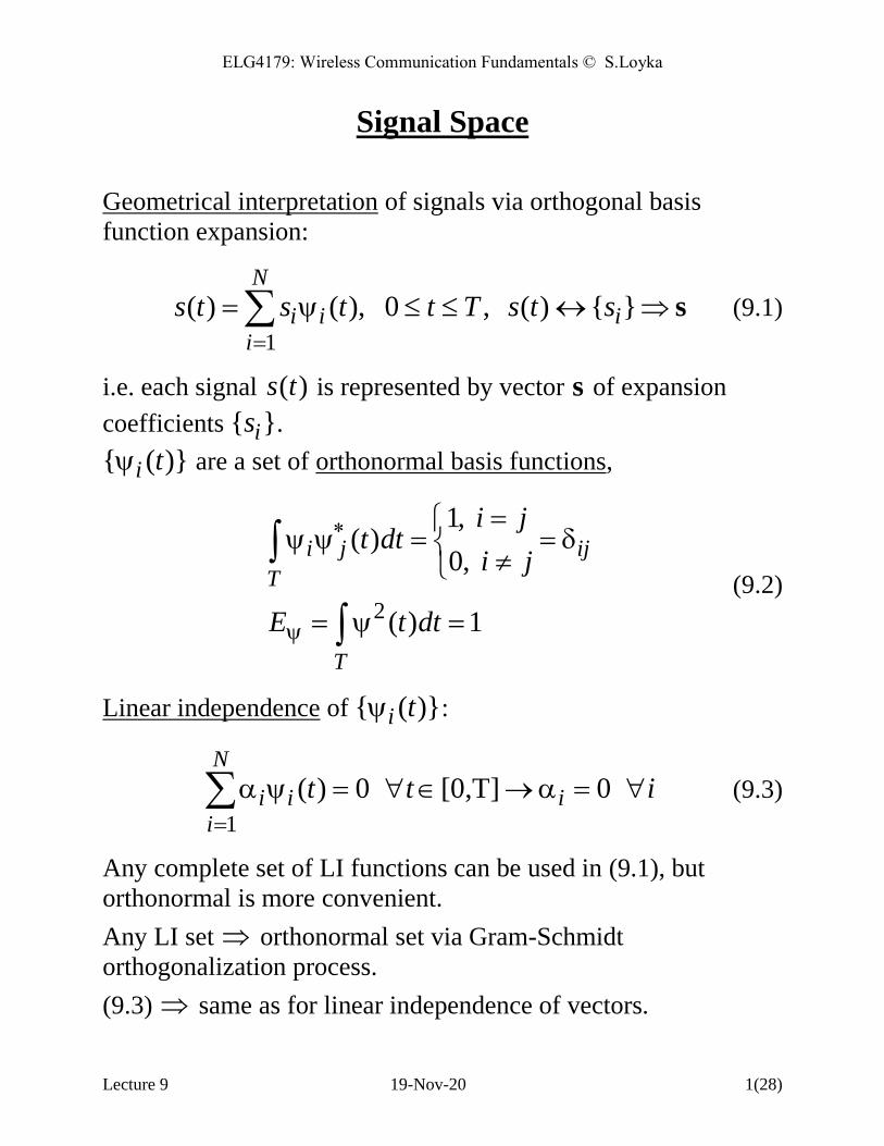
ELG4179: Wireless Communication Fundamentals © S.Loyka

Lecture 9 19-Nov-20 1(28)

Signal Space

Geometrical interpretation of signals via orthogonal basis

function expansion:

1

( ) ( ), 0 , ( ) { }N

i i ii

s t s t t T s t s

s (9.1)

i.e. each signal ( )s t is represented by vector s of expansion

coefficients { }is .

{ ( )}i t are a set of orthonormal basis functions,

2

1, ( )

0,

( ) 1

i j ij

T

T

i jt dt

i j

E t dt

(9.2)

Linear independence of { ( )}i t :

1

( ) 0 [0,T] 0 N

i i ii

t t i

(9.3)

Any complete set of LI functions can be used in (9.1), but

orthonormal is more convenient.

Any LI set orthonormal set via Gram-Schmidt

orthogonalization process.

(9.3) same as for linear independence of vectors.



Example: Fourier series

Consider periodic signal ( ) ( ) t,s t T s t

2 21

( ) , ( )j kt j kt

T Tk k

k T

s t c e c s t e dtT

(9.4)

Can take 1 2

( ) , j tk t e

TT

fundamental frequency,

( ) ( )k n kn

T

t t dt (9.5)

Complex vs. real form of FS: { , }k k kc a b

0

( ) cos( ) sin( )k kk

s t a k t b k t

(9.6)

Can take 1, 2,2 2

( ) cos( ), ( ) sin( )k kt k t t k tT T

.

Example: M-PAM

( ) ( ), 1... , 0i is t A p t i M t T (9.7)

Take 1

( ) ( )p

t p tE

.



Example: QAM

I – Q representation of bandpass signals:

( ) ( )cos ( )sinI Qx t m t t m t t (9.8)

Take 1 22 2

( ) cos , ( ) sint t t tT T

.

These basis functions are very important and are used often in

communications.

{ }isHow to find ?

( ) ( ) ( ) ( )i i i iiT

s s t t dt s t s t (9.9)

Signal energy: (“distance” from 0)

22 2

( )s iiT

E s t dt s s (9.10)

Scalar product of ( )x t and ( )y t :

( ) ( )i ii T

x y x t y t dt x y (9.11)



Distance between ( )x t and ( )y t :

22 2

( ) ( )i ii T

x y x t y t dt x y (9.12)

{ ( )}i t basis “vectors” in the signal space.

Optimal Rx structure (Lec. 7):

* Optimality was not proved.

* Will be proved below via probabilistic analysis in the signal

space.



Optimal Rx in Signal Space (AWGN)

Key idea: replace ( )r t by r and detect it. No loss of optimality

(can be proved).

( ) ( ) ( ) r t s t t r s ξ (9.13)

m estimated message (Rx)

m selected message (S)

s transmitted signal

r received signal

Assume ( )t AWGN, then

0

0

( ) ( ) ( ) ( ), ( ) 0, 2

( ) PSD

NR t t t

S f N

(9.14)

and

2 2 00 0

2

200

(0, ), var( )2

1( ) exp

( )

i

N

NN

pNN

ξ I

ξξ

(9.15)



Also 20( , )N r s I for a given s .

Transmitter: 1; { ... } { }i M im m m m m s

1 { ... } { }M i s s s s

Receiver: m r s

Optimal Rx: mineP ,

1

Pr{ } , { }i i

M

e i e e ii

P m P P

s s (9.16)

Consider the equiprobable messages (why important?):

1Pr{ }km

M if k k im m i k r s r s (9.17)

i.e. the maximum-likelihood (ML) decision rule. Can also be

used when Pr{ }km are not known.

ML min. distance in AWGN (9.18)



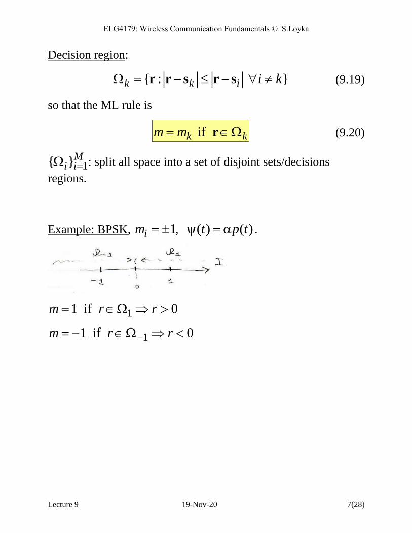
Decision region:

{ : }k k i i k r r s r s (9.19)

so that the ML rule is

if k km m r (9.20)

1{ }Mi i : split all space into a set of disjoint sets/decisions

regions.

Example: BPSK, 1, ( ) ( )im t p t .

1

1

1 if 0

1 if 0

m r r

m r r



Example: QPSK

1

2

1 3

2 4

1 2,3,4

2( ) cos

2( ) sin

[1,1] [ 1, 1]

[ 1,1] [1, 1]

? ?

T T

T T

t tT

t tT

s s

s s

Signal constellation = { ( )}is t in the signal space, i.e. { }is .

Signals: Points (vectors) in the signal space.



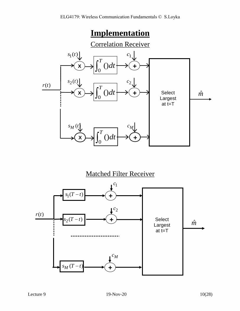
Receiver Implementation

The rule (9.17) can be expressed in a different form using

2 22

2k k k r s r rs s (9.21)

Since 2

r is independent of s ,it can be dropped and (9.17)

becomes

,k k i ic c i k r s r s (9.22)

where

1

N

k i kii

r s

r s is a scalar product and 2

/ 2k kc s . It

can be expressed as

( ) ( )k k

T

r t s t dt r s (9.23)

Q. Prove it.

(9.23) can be implemented using a correlation receiver or a

matched filter receiver.

Matched filter impulse response

( ) ( )k kh t s T t (9.24)

so the output sampled at time T is

( )* ( ) ( ) ( )k k

T

t h t r t s t dt (9.25)


Lecture 9 19-Nov-20 10(28)

Implementation

Correlation Receiver

Matched Filter Receiver

+

+

+

1( )s T t

2 ( )s T t

( )Ms T t

1c

2c

Mc

m̂

( )r tSelect

Largest at t=T

Select Largest at t=T

m̂

( )r t

X +

2 ( )s t 2c

0()

Tdt

X +

1( )s t 1c

0()

Tdt

X +

( )Ms t Mc

0()

Tdt


Lecture 9 19-Nov-20 11(28)

Another Form of Implementation

Correlation receiver in the signal space

Q.: detector =?

Detector m̂

( )r t2 ( )t

0()

Tdt

1( )t

0()

Tdt

0()

Tdt×

×

×1r

( )N t

2r

Nr

r


Lecture 9 19-Nov-20 12(28)

An Example: BPSK

Time-domain expression of the signal is

( ) ( 1) ( ), 0,1iis t A t i (9.26)

where ( )t is a basis pulse shape (may be cos( )t ); A is the

amplitude.

Constellation:

The ML receive computes the following decision variable,

( ) ( )

T

z r t t dt (9.27)

and sets

0, 0ˆ

1, 0

if zm

if z

Q.: block diagram of the receiver?

A A

0 1

0

I


Lecture 9 19-Nov-20 13(28)

Comparison of M-ary Modulation Schemes

M-PSK: the phase can assume M different values

2 2cos , 0,1,..., 1

0

i cE

s t t i i MT M

t T

(9.28)

2log M bits are transmitted by each symbol.

The symbol error probability (SER):

0 0

22 sinse

E EP Q Q

N M N

(9.29)

Q: constellation example? Minimum distance mind ?

*rectangular pulse or RC pulse with 1

see (9.45) for the power/bandwidth efficiency tradeoff.

T.S. Rappaport, Wireless Communications, Prentice Hall, 2002


Lecture 9 19-Nov-20 14(28)

M-ary Quadrature AM (M-QAM)

M levels with different phases and amplitudes

cos sini i c i cs t a t b t (9.30)

ia and ib - I and Q components.

The BER of M-QAM ( 2kM and k is even):

2

2 0

4 1 1/ 3log

log 1

be

M EMP Q

M M N

(9.31)

The threshold SNR: ~ 10lgth M

I(ai)

Q(bi)

M=4

Q

I

M=16



Lecture 9 19-Nov-20 15(28)

Frequency Shift Keying (FSK)

M-ary FSK:

2

cos , i 1,..., 0i iE

s t t M t TT

(9.32)

Note: signal orhtogonality imposes a limit on 1i i .

Q: find min such that the signals are orthogonal.

For orthogonal BFSK (coherently detected),

eP Q (9.33)

Note: non-coherent detection results in different BER,

/ 2

, / 2e NP e (9.34)

Performance loss is a few dBs.

For 2M , the tight upper bound on SER is

1esP M Q (9.35)

for orthogonal signals and coherent demodulation.



Lecture 9 19-Nov-20 16(28)

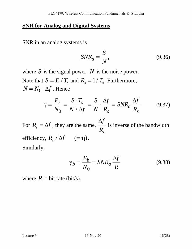
SNR for Analog and Digital Systems

SNR in an analog systems is

,aS

SNRN

(9.36)

where S is the signal power, N is the noise power.

Note that / sS E T and 1/s sR T . Furthermore,

0N N f . Hence

0 /

s sa

s s

E S T S f fSNR

N N f N R R

(9.37)

For sR f , they are the same.

s

f

R

is inverse of the bandwidth

efficiency, / ( )sR f .

Similarly,

0

bb a

E fSNR

N R

(9.38)

where R = bit rate (bit/s).


Lecture 9 19-Nov-20 17(28)

SER and Signal Constellation

SER can be expressed through minimum distance between

points of the signal constellation.

Generic bound for the SER is (coherent detection),

2

min

0

( 1)2

e

dP M Q

N

(9.39)

where mind is determined from signal constellation (minimum

distance), see the next slide.

An approximation at high SNR:

2

min

02e e

dP N Q

N

(9.40)

where eN # of nearest neighbours.

The BER can be approximated at high SNR as

2

1

logb eP P

M (9.41)

Q.: what is an interpretation of (9.41)?


Lecture 9 19-Nov-20 18(28)

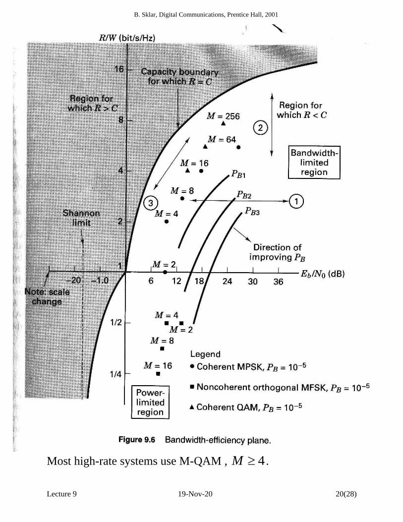
Comparison of Various Modulation Formats

Fundamental limit is provided by the Shannon’s channel

capacity theorem (AWGN channel):

2log 1C f (9.42)

C = channel capacity [bit/s]

f = bandwidth [Hz]

= SNR, /P N , where P - signal power, N - noise power.

Almost error-free transmission is possible if R C , and is not

possible for R C ; R bit rate [b/s].

Using b bE PT ,

0

bb

E f

N R

,

2log 1 /b

CR f

f

(9.43)

SinceR C for reliable communications, then

2log 1 /bR

R ff

(9.44)

/ (bit/s/Hz)R f is the spectral efficiency. Required SNR is

/2 1ln 2 1.6

/

R f

b dBR f

(9.45)

LB is monotonically increasing in /R f - power/bandwidth

efficiency tradeoff (see the tables).


Lecture 9 19-Nov-20 19(28)

Fundamental Limit: Spectral Efficiency [bit/s/Hz] vs.

SNR/bit [dB]

5 0 5 10 15 201 10

3

0.01

0.1

1

10

Spectral efficiency [bit/s/Hz] vs. SNR [dB]

SNR: Eb/N0 [dB]

Rb

/W [

bit

/s/H

z]

1.6

/2 11.6

/

R f

b dBR f

achievable


Lecture 9 19-Nov-20 20(28)

Important Conclusions:

Power-limited region: for large bandwidth available. For

f ,

ln 2 1.6b dB (9.46)

No error-free transmission is possible for 1.6b dB !

Bandwidth –limited region: for large power available.

Trade-off: increasing power efficiency decreases spectrum

efficiency and vice-versa.

Note: for f , 0/ ln 2C P N .

Spectral Efficiency of Digital Modulation:

Null-to-null bandwidth (or absolute bandwidth assuming a raised

cosine pulse with 1 ) of a modulated signal,

M-PSK and M-QAM:

2

2

log

Rf

M or 2log

2

MR

f

(9.47)

M-FSK (non-coherent):

2

2

log

R Mf

M

or 2log

2

MR

f M

(9.48)

M-PSK(QAM) is much better than M-FSK in terms of spectral

efficiency.

Most high-rate systems use M-QAM , 4M .

B. Sklar, Digital Communications, Prentice Hall, 2001


Lecture 9 19-Nov-20 21(28)

Spectrum of Digital Modulation (RF)

0 0.5 1 1.5 260

40

20

0

BPSK

QPSK8PSK

MSK

(f-fc)*Tb

dB

.


Lecture 9 19-Nov-20 22(28)

BER: Comparison of Various Modulation Formats

0 5 10 151 10

6

1 105

1 104

1 103

0.01

0.1

1

OOKBPSK

DPSK

QPSK

8PSK

8QAMCoherent BFSK

Non-coherent BFSK

BER in AWGN channels

SNR: Eb/N0 [dB]

Per

ror

.


Lecture 9 19-Nov-20 23(28)

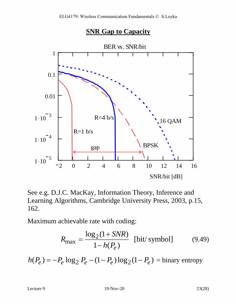
SNR Gap to Capacity

See e.g. D.J.C. MacKay, Information Theory, Inference and

Learning Algorithms, Cambridge University Press, 2003, p.15,

162.

Maximum achievable rate with coding:

2max

log (1 ) [bit/ symbol]

1 ( )e

SNRR

h P

(9.49)

2 2( ) log (1 ) log (1 )e e e e eh P P P P P = binary entropy

2 0 2 4 6 8 10 12 14 161 10

5

1 104

1 103

0.01

0.1

1BER vs. SNR/bit

BPSK

16 QAM

R=1 b/s

R=4 b/s

SNR/bit [dB]

gap


Lecture 9 19-Nov-20 24(28)

SOME REFERENCES ON CHANNEL CODING/MODULATION:

Books:

E. Biglieri, Coding for Wireless Channels, Springer, 2005.

W.E. Ryan and S. Lin, Channel Codes: Classical and Modern.

Cambridge, U.K.: Cambridge Univ. Press, 2009.

T.K. Moon, Error Correction Coding—Mathematical Methods

and Algorithms. New York, NY, USA: Wiley, 2005.

I.B. Djordjevic, W. Ryan, and B. Vasic, Coding for Optical

Channels. New York, NY, USA: Springer, 2010.

I.B. Djordjevic, Advanced Optical and Wireless

Communications Systems, Springer, 2018.

Review Papers:

D.J. Costello, G.D. Forney, Channel coding: The road to channel

capacity, Proc. IEEE, vol. 95, no. 6, pp. 1150–1177, Jun. 2007.

D.J. Costello, et al, Applications of error-control coding, IEEE

Trans. Info. Theory, vol. 44, no. 6, pp. 2531–2560, Oct. 1998.

G.D. Forney, G. Ungerboeck, Modulation and coding for linear

Gaussian channels, IEEE Trans. Info. Theory, v. 44, no. 6, pp.

2384-2415, Oct. 1998.

A. Leven, L. Schmalen, Status and Recent Advances on Forward

Error Correction Technologies for Lightwave Systems, IEEE J.

Lightwave Tech., v. 32, no. 16, pp. 2735-2750, Aug. 2014.

M.Nakazawa et al, Extremely Higher-Order Modulation

Formats, Optical Fiber Telecommunications: Systems and

Networks, 2013, v. B, pp. 297-336.


Lecture 9 19-Nov-20 25(28)

STATE-OF-THE-ART (IN OPTICAL COMMUNICATIONS)


Lecture 9 19-Nov-20 26(28)

Summary

Geometric representation of signals via signal space.

Optimum receiver (MAP, ML) in the signal space.

BPSK, QPSK, QAM.

M-ary modulation formats. Comparisson.

Power and bandwidth efficiency.

BER and SER.

Fundamental limits. Channel capacity.

Reading:

Rappaport, Ch. 6 (expect 6.11, 6.12).

Other books (see the reference list).

Note: Do not forget to do end-of-chapter problems. Remember

the learning efficiency pyramid!


Lecture 9 19-Nov-20 27(28)

Appendix: Optimal Rx

Optimal Rx selects km m with largest a posteriori probability:

if Pr{ | } Pr{ | } k k im m m m i k r r (9.50)

Pr{ | }Pr{ }

Pr{ | }Pr{ }

k kk

m mm

rr

r (9.51)

To prove its optimality, observe that the probability of correct

decision Pr{ | }kc m given that the Rx selects km m is

Pr{ | } Pr{ | }k kc m m r , which is maximized by (9.50).

This rule also maximizes unconditional probability of correct

decision ( 1 )c eP P :

1

Pr{ }Pr{ | } , Pr{ | } Pr{ | }Pr{ }M

c k kk

P c d c m m

r r r r r

(9.52)

From (9.50), (9.51), the maximum a posteriori probability

(MAP) decision rule follows:

if Pr{ | }Pr{ } Pr{ | }Pr{ } k k k i im m i k r s s r s s (9.53)

since Pr{ } Pr{ }, Pr{ | } Pr{ | }i i i im m s r s r , i.e. decide in

favor of such km that maximizes a posteriori probability of

observed r .


Lecture 9 19-Nov-20 28(28)

From (9.15), 2

200

1Pr{ | } ( ) exp( )

( )

kk k N

PNN

r sr s r s (9.54)

So that the decision rule in (9.53) becomes

2 2

if , k k k i im m c c i k r s r s (9.55)

where 0 ln Pr{ }k kc N m .

Signal Space - University of Ottawa

Documents