TU Wien Department of Geodesy and Geoinformation Research Division Higher Geodesy Outline Signal Propagation Johannes Böhm Third IVS VLBI School March 2019, Gran Canaria

Welcome message from author
This document is posted to help you gain knowledge. Please leave a comment to let me know what you think about it! Share it to your friends and learn new things together.
Transcript

TU Wien
Department of Geodesy and Geoinformation
Research Division Higher Geodesy
OutlineSignal Propagation
Johannes Böhm
Third IVS VLBI School
March 2019, Gran Canaria

TU WienDepartment of Geodesy and GeoinformationResearch Division Higher Geodesy
Atmosphere
• Atmospheric opacity
Wikipedia.de

TU WienDepartment of Geodesy and GeoinformationResearch Division Higher Geodesy
Atmosphere
Wikipedia.de
TU WienDepartment of Geodesy and GeoinformationResearch Division Higher Geodesy
Ionosphere
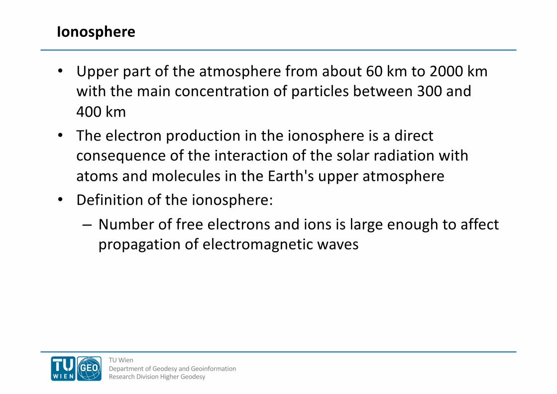
• Upper part of the atmosphere from about 60 km to 2000 km with the main concentration of particles between 300 and 400 km
• The electron production in the ionosphere is a direct consequence of the interaction of the solar radiation with atoms and molecules in the Earth's upper atmosphere
• Definition of the ionosphere: – Number of free electrons and ions is large enough to affect
propagation of electromagnetic waves
TU WienDepartment of Geodesy and GeoinformationResearch Division Higher Geodesy
Ionosphere
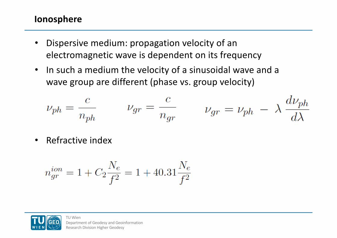
• Dispersive medium: propagation velocity of an electromagnetic wave is dependent on its frequency
• In such a medium the velocity of a sinusoidal wave and a wave group are different (phase vs. group velocity)
• Refractive index

TU WienDepartment of Geodesy and GeoinformationResearch Division Higher Geodesy
TEC - Total Electron Content
• Represents the total amount of free electrons in a cylinder with a cross section on 1 m2 and a height equal to the slant signal path
• Measured in TEC Units (TECU) § 1 TECU is equivalent to 1016 electrons/m2

TU WienDepartment of Geodesy and GeoinformationResearch Division Higher Geodesy
TEC - Total Electron Content
• 1 TECU corresponds to§ 7.6 cm at S-band (2.3 GHz)§ 0.6 cm at X-band (8.4 GHz)

TU WienDepartment of Geodesy and GeoinformationResearch Division Higher Geodesy
X/S VLBI and the ionosphere
• Only relative values of STEC can be determined
Hobiger, 2005

TU WienDepartment of Geodesy and GeoinformationResearch Division Higher Geodesy
X/S VLBI and the ionosphere
• Ionosphere-free group delay based on effective frequencies
• Instrumental biases are included (estimated w clocks)

TU WienDepartment of Geodesy and GeoinformationResearch Division Higher Geodesy
X/S VLBI and the ionosphere
• Vertical TEC estimation from VLBI– only possible with appropriate use of constraints
Hobiger

TU WienDepartment of Geodesy and GeoinformationResearch Division Higher Geodesy
VGOS and the ionosphere
• Phases are connected across the whole band• Ionosphere delays are estimated together with the group
delays in the fringe-fitting process

TU Wien
Department of Geodesy and Geoinformation
Research Division Higher Geodesy
Troposphere
• Troposphere delays: strictly speaking delays in the neutral
atmosphere (up to 100 km)
• Essentially no frequency dependency across microwave
regime
• Refractivity N versus refractive index n
§ N » 300, n » 1.0003
§ Units of N: ppm, mm/km, "Neper"

TU WienDepartment of Geodesy and GeoinformationResearch Division Higher Geodesy
Refractivity
• Refractivity as a function of pressure, temperature and humidity, (and liquid water)
• Dry - wet ® hydrostatic - "wet"• Wet delay larger than "wet" delay by about 3 %
hydrostatic “wet”

TU WienDepartment of Geodesy and GeoinformationResearch Division Higher Geodesy
Refractivity
• Wet part: surface values not representative for the upper air conditions
Radiosonde profile Vienna

TU WienDepartment of Geodesy and GeoinformationResearch Division Higher Geodesy
Path delay
• Electric path length L is minimized
• Bending effect S - G about 2 dm at 5 degrees elevation
TU WienDepartment of Geodesy and GeoinformationResearch Division Higher Geodesy
Hydrostatic zenith delay
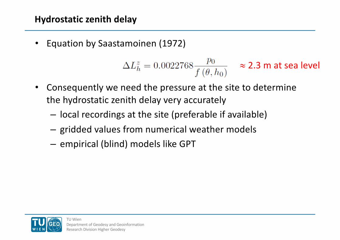
• Equation by Saastamoinen (1972)
• Consequently we need the pressure at the site to determine the hydrostatic zenith delay very accurately
– local recordings at the site (preferable if available)
– gridded values from numerical weather models
– empirical (blind) models like GPT
» 2.3 m at sea level
TU WienDepartment of Geodesy and GeoinformationResearch Division Higher Geodesy
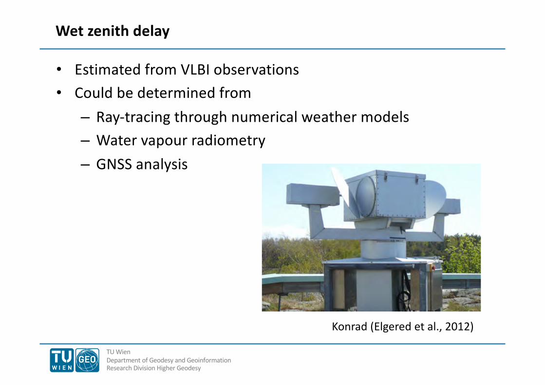
Wet zenith delay
• Estimated from VLBI observations• Could be determined from
– Ray-tracing through numerical weather models– Water vapour radiometry– GNSS analysis
Konrad (Elgered et al., 2012)

TU WienDepartment of Geodesy and GeoinformationResearch Division Higher Geodesy
Mapping functions
• Elevation dependent mapping functions used for a priori hydrostatic delay and estimating zenith wet delays
• Zenith wet delays estimated every 20 to 60 minutes• Correlation between height, clocks and zenith delays• Partials are sin(e), 1, and mf(e)• Separation into hydrostatic and wet part

TU WienDepartment of Geodesy and GeoinformationResearch Division Higher Geodesy
Mapping functions
• Mapping function not perfectly known• Errors via correlations also in station heights (and clocks)• Low elevations necessary to de-correlate heights, clocks, and
zenith delays• Trade-off ® about 5 degrees cut off elevation angle
(sometimes with down-weighting)

TU WienDepartment of Geodesy and GeoinformationResearch Division Higher Geodesy
Mapping functions
Dz
e DL
DL(e) = Dz · m(e)
DL(e) = Dz'· m(e)'
• The station height error is about 1/5 of the delay error at 5 degrees elevation (if cutoff is at 5 degrees)
• The corresponding decrease of the zenith delay is about half of the station height increase

TU WienDepartment of Geodesy and GeoinformationResearch Division Higher Geodesy
Mapping functions
• Continued fraction form (Herring, 1992)
• Example Vienna Mapping Functions– Empirical functions for b and c coefficients – Coefficients a by ray-tracing and inversion using 6h data of
the ECMWF– Available for all VLBI sites and on global grid

TU WienDepartment of Geodesy and GeoinformationResearch Division Higher Geodesy
Mapping functions
• VMF1 versus GMF at Fortaleza (Brazil) at 5 deg. elevation

TU WienDepartment of Geodesy and GeoinformationResearch Division Higher Geodesy
Tropospheric gradients
• Chen and Herring (1997)
• Typical gradient: 1 mm (corresponds to 1 dm at 5 deg. elevation)
• Estimated e.g. every 3 hours
• Caused by weather fronts, coastal situations, atmospheric bulge, ..

TU WienDepartment of Geodesy and GeoinformationResearch Division Higher Geodesy
Tropospheric gradients
• Mean hydrostatic north and east gradients (Landskron, 2018)

TU WienDepartment of Geodesy and GeoinformationResearch Division Higher Geodesy
Ray-tracing
n=1
• To find the ray-path from the source to the telescope (has to be done iteratively, "shooting")
• Easier in 2D case (6 equations), because no out-of-plane components

TU WienDepartment of Geodesy and GeoinformationResearch Division Higher Geodesy
VMF Open Access Data
• http://vmf.geo.tuwien.ac.at/
• Ray-traced delays for the complete history of VLBI observations available there
• Online tool to do your own ray-tracing at VLBI sites• Vienna Mapping Functions coefficients (from analysis and
forecast data)• 6h hydrostatic and wet gradients • Empirical “backup” mapping functions, e.g. GPT3
TU WienDepartment of Geodesy and GeoinformationResearch Division Higher Geodesy
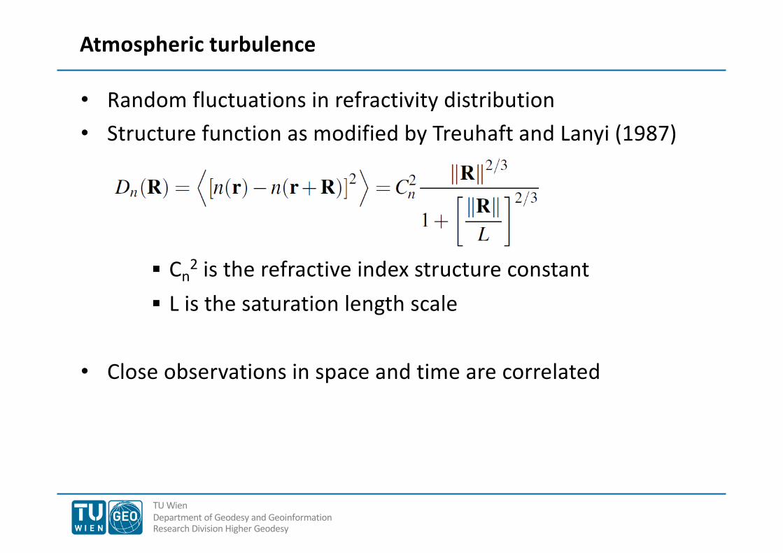
Atmospheric turbulence
• Random fluctuations in refractivity distribution• Structure function as modified by Treuhaft and Lanyi (1987)
§ Cn2 is the refractive index structure constant
§ L is the saturation length scale
• Close observations in space and time are correlated

TU WienDepartment of Geodesy and GeoinformationResearch Division Higher Geodesy
Atmospheric turbulence
• Frozen flow theory for equivalence of correlation in space and time
Halsig, 2018
TU WienDepartment of Geodesy and GeoinformationResearch Division Higher Geodesy
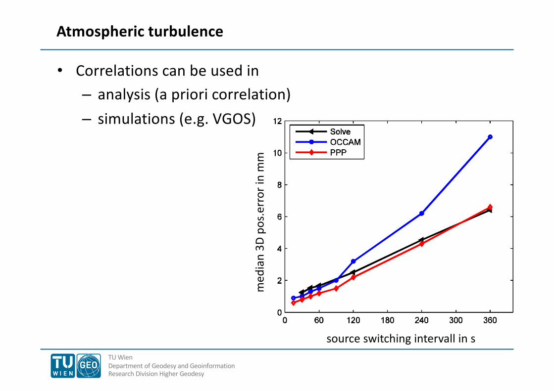
Atmospheric turbulence
• Correlations can be used in – analysis (a priori correlation)– simulations (e.g. VGOS)
med
ian
3Dpo
s.err
orin
mm
source switching intervall in s

TU WienDepartment of Geodesy and GeoinformationResearch Division Higher Geodesy
Climate studies
• Zenith wet delays at Wettzell (Landskron, 2018)m
m

TU WienDepartment of Geodesy and GeoinformationResearch Division Higher Geodesy
OutlineQuestions?
Related Documents