Signal Processing Toolbox - ARTTS · The ARTTS Signal Processing toolbox is a library of MATLAB routines that provide functionality for general operations on MATLAB images and for

Project no. IST-34107Project acronym: ARTTS

Project title: Action Recognition and Tracking based on Time-of-flight Sensors

Signal Processing Toolbox

Duration of the project: October 2006 – September 2009

Partners of the project consortium:

INB, University of Lübeck, GermanyIMM, Technical University of Denmark, DenmarkLAPI, University Politehnica Bucuresti, RomaniaSwiss Center for Electronics and Microtechnology, SwitzerlandSensoMotoric Instruments GmbH, Germany

Project website:

www.artts.eu

Project co-funded by the European Commission within the Sixth Framework Programme (2002-2006)

1 IntroductionThe ARTTS Signal Processing toolbox is a library of MATLAB routines that provide functionality for general operations on MATLAB images and for signal processing and signal improvement. Here is an overview of the functionality included in the toolbox:

Image saving and loading in ARTTS range file format

Image acquisition

Visualization of range maps, textured with intensity data

Foreground object segmentation

Signal improvement, using a variety of techniques: Adaptive neighbourhood filtering (ANF), range-based amplitude image correction, amplitude-based range image filtering, correction of errors caused by lens flare and diffuse reflection, and image improvement using the shading constraint

Computation of image features (geometric features and sparse spatiotemporal features)

Graphical user interface for accessing functionality in the toolbox

2 LicenceThe ARTTS Signal Processing toolbox (code and accompanying documentation, including this document) is provided under the following licence:

Copyright 2006-2009 The ARTTS Consortium

You may use this code for non-commercial purposes. However, you may not redistribute the code, distribute modified versions of the code or use the code for commercial purposes without prior permission from the ARTTS Consortium. Contact the Consortium ([email protected]) for details.

This code and the accompanying documentation are provided without any warranty, not even the implied warranty of merchantability or fitness for a particular purpose.

This work was developed within the ARTTS project (www.artts.eu), which is funded by the European Commission (contract no. IST-34107) within the Information Society Technologies (IST) priority of the 6th Framework Programme. Neither the European Commission nor the ARTTS Consortium can be held responsible for any consequence of using this code and the accompanying documentation.

3 InstallationTo install the toolbox, copy the directory sp_toolbox to a suitable location, then add this directory and the subdirectory sp_toolbox/shading to MATLAB's search path. The best way to do this is to include the corresponding addpath calls in your startup.m file.

2

Some components of the toolbox require supporting libraries to be present:

If you want to acquire range images using acquire_artts_range, make sure that the MATLAB SwissRanger interface is on your MATLAB search path. Additionally, you need to install the Geodise XML toolbox for MATLAB. Download it from www.geodise.org/toolboxes/generic/xml_toolbox.htm, install it, and put it on your MATLAB search path.

If you want to use the routines for image improvement using the shading constraint (see Section 4.9), you need to compile some MEX files first. To do this, change to the directory sp_toolbox/shading, edit the makefile so that the variable MEX points to the location of your MEX compiler, then run the makefile by executing the command make.

You will also need the Polak-Ribière conjugate gradients minimizer by Carl Edward Ramussen. Download the file minimize.m from www.kyb.tuebingen.mpg.de/bs/people/carl/code/minimize and copy it to the directory sp_toolbox/shading.

If you want to compute the scale-invariant version of the geometric features (see Section 4.10), you need to install two libraries (NFFT and FFTW) and compile some MEX files that use these libraries. Here are the steps you need to follow:

1. Download the source code for the FFTW library (version 3.2.1 or later) from www.fftw.org, compile it, and install it to a suitable location.

2. Download the source code for the NFFT library (version 3.1.0 or later) from www-user.tu-chemnitz.de/~potts/nfft, compile it, and install it to a suitable location.

3. Change to the directory sp_toolbox and edit the makefile. Make sure that the FFTW and NFFT libraries are on the include path and library search path by adding appropriate options to NFFT_INCLUDES and NFFT_LIBS. The variable MEX should point to the location of your MEX compiler. When you have made the appropriate changes to the makefile, run it by executing the command make.

If you want to use the routines for sparse coding features (Section 4.11), you need to install Bruno Olshausen's sparse coding routines from https://redwood.berkeley.edu/bruno/sparsenet/ and add them to the MATLAB search path.

4 ComponentsThis section gives a more detailed overview of the components included in the toolbox. For each of the major components, we will give a description of the functionality, including links to relevant publications, a list of the routines that implement this functionality, and an example of how to use the routines.

3

For detailed description of the routines, refer to the documentation that is included directly in the source code of the routines; this can be accessed from MATLAB by typing

help <routine name>

For example, the documentation for the routine read_artts_range can be displayed by typing

help read_artts_range

4.1 File Saving / LoadingARTTS defines a file format for range files as well as for databases of range files. A range file database is a collection of range files that associates various parameters with each file; for a face detection database, for example, these parameters might be the position of the face in each image. The range file and database format is defined in detail in Section 5.

The following routines deal with the saving and loading of ARTTS range files and databases:

read_artts_rangeReads an ARTTS range file

write_artts_rangeWrites an ARTTS range file

read_arttsidxReads an ARTTS database index file (but not the associated range files)

read_artts_dbReads an ARTTS range file database (including the parameters from the index file and the associated range files)

view_artts_dbInteractively displays the images in an ARTTS range file database

Here is an example of how to use these routines:

% Read an image from the file 'data/face.arttsrng' and store it in% 'img'img=read_artts_range('data/face.arttsrng');

% As an example of how to access the image, find the maximum amplitude% in the imagemax_amp=max(img.amplitude(:));

% Write the image to a different filewrite_artts_range('temp.arttsrng', img);

% Read names and parameters from database index file, and get name and% parameters of first file[names, params]=read_arttsidx('data/db/db.arttsidx');disp(names{1});disp(params{1});

% Read images and parameters from database[images, params]=read_artts_db('data/db/db.arttsidx');

% View the images in the database interactively. Press Space to go the% next image and 'b' to go to the last image

4

view_artts_db('data/db/db.arttsidx');

4.2 Basic OperationsThe toolbox provides a set of basic operations for displaying, acquiring, and converting range images:

show_range_imageDisplays the range and amplitude components of a range image in the current figure window

acquire_artts_rangeAcquires an image from the camera in a format that can be saved using write_artts_range

rescale_artts_rangeRescales the range map so that the range values are in metres and the amplitude values lie in the interval [0,1]

xyz_from_rangeConverts a range image to Cartesian coordinates

Here is an example of how to load and display an image:

% Load a range imageimg=read_artts_range('data/face.arttsrng');

% Display the imageshow_range_image(img);

Here is an example of how to acquire an image:

% Open camera devicedev=sr_open();

% Acquire an imageimg=acquire_artts_range(dev);

% Close camera devicesr_close(dev);

Here is an example of how to rescale and image and convert it to Cartesian coordinates:

% Rescale the image so that range values are in metres and amplitude% values are between 0 and 1fprintf('Max amp before rescale: %g\n', max(img.amplitude(:)));img=rescale_artts_range(img);fprintf('Max amp after rescale: %g\n', max(img.amplitude(:)));

% Convert image to Cartesian coordinates[X, Y, Z]=xyz_from_range(img);

4.3 VisualizationThe routine show_range_image_3d can be used to display a 3D rendering of the range map, textured with the intensity image:

% Load image

5

img=read_artts_range('data/face.arttsrng');

% Visualize imageshow_range_image_3d(img);

4.4 Foreground object segmentationThe routine segment_foreground can be used to segment the largest foreground object from the background. The segmentation is carried out using an Otsu threshold on the amplitude image and a range threshold that isolates the first peak in the range histogram. Additionally, the routine suppresses small spurious foreground components that are caused by noise.

Here is an example of how to use segment_foreground:

% Load imageimg=read_artts_range('data/person.arttsrng');

% Segment foreground objectmask=segment_foreground(img);

% Segment range map: Set background to maximum range of% foreground objectrng=img.range;rng(~mask)=max(rng(mask(:)));

% Display range mapimagesc(rng);colorbar;

4.5 Adaptive-neighbourhood filtering (ANF)This component provides functionality for filtering the range map using an adaptive-neighbourhood filter (ANF). The basic principle of ANF (originally developed for gray-scale and colour images) is to derive, for each image pixel, a variable-sized, variable-shaped neighbourhood that, ideally, contains only pixels belonging to the same statistical population as the central pixel (called “seed” when being processed).

To adjust the adaptive-neighbourhood filter to the specific properties of the range map, the preprocessing step was changed slightly (we used a modified median filter to compute a more reliable initial value for the seed pixel). Experiments show that the adaptive-neighbourhood filter generally outperforms classical filters in terms of both noise power reduction and detail preservation.

For more details, see the following papers:

Rangaraj M. Rangayyan, Mihai Ciuc, and Farshad Faghih. Adaptive-neighborhood filtering of images corrupted by signal–dependent noise. Applied Optics, volume 37, number 20, pages 4477–4487, July 1998.

Şerban Oprişescu, Dragoş Fălie, Mihai Ciuc, and Vasile Buzuloiu. Measurements with ToF cameras and their necessary corrections. Proceedings of the IEEE International Symposium on Signals, Circuits & Systems (ISSCS), volume 1, pages 221–224, Iasi, Romania, 2007.

The following routine is used to apply the ANF filter:

6

anf_tof_callApplies the ANF filter to a range map. The routine has four input parameters: input image, noise type (additive or multiplicative), noise dispersion value, and maximum region growing limit. It returns the filtered image.

This routine uses a MEX file that should get compiled automatically the first time the routine is called; alternatively, you can compile the MEX file manually using the command mex anf_tof.cpp.

Here is an example of how to use this routine:

% Load sample imageimg=read_artts_range('data/scene_B138.arttsrng');

% Call the ANF function with four parameters:% image, noise type (additive =1 or multiplicative=2),% noise dispersion value, and maximum region growing limit:img=anf_tof_call('../data/scene_B138.arttsrng',2,0.03,5);

% Show the imageshow_range_image(img);

4.6 Range-based amplitude image correctionA typical effect in TOF images is that the illumination irradiance decreases with the square of the distance. This causes objects with the same reflectance located at different distances from the camera to appear in the image with different distances.

This component provides a routine that corrects the intensity image to compensate for this effect by multiplying each pixel's intensity with the square of the distance:

I' i,j =I i,j ⋅D2 i,j

where A’(i,j) is the corrected intensity for the pixel, A(i,j) is the original intensity, and D(i,j) is the distance.

For more details, see the following paper:

Şerban Oprişescu, Dragoş Fălie, Mihai Ciuc, and Vasile Buzuloiu. Measurements with ToF cameras and their necessary corrections. Proceedings of the IEEE International Symposium on Signals, Circuits & Systems (ISSCS), volume 1, pages 221–224, Iasi, Romania, 2007.

The following routine is used to apply the intensity correction:

amp_corPerforms the distance-based amplitude image correction as defined above (when called with selector==1), or a simple square root correction (when called with selector~=1). The function returns the corrected image.

Here is an example of how to use this routine:

% Load sample imageimg=read_artts_range('data/scene_B138.arttsrng');

% Correct intensity of sample imageimg=amp_cor(img, 1);

7

% Show the imageshow_range_image(img);

4.7 Amplitude-based range image filteringAs noted in Section 3.9, a TOF camera's illumination irradiance decreases with the square of the distance, causing a corresponding decrease in the signal-to-noise ratio. This component provides a routine for adaptively filtering the range image based on the intensity (amplitude) of the pixel. The routine applies a median filter to regions with poor illumination and a (stronger) mean filter to regions with very poor illumination.

The following routine implements the algorithm:

amp_range_filtPerforms an amplitude-based range image filtering. as described above. The routine uses 3×3-pixel neighbourhoods and a standard deviation test to detect high noise regions; it also uses two thresholds: a higher one for median filtering and a lower one for mean filtering.

Here is an example of how to use this routine:

% Load sample imageimg_orig=read_artts_range('data/scene_hall_B.arttsrng');

% Apply amplitude-based range image filteringimg=amp_range_filt(img_orig);

% Show the original imagesubplot(1, 2, 1);show_range_image(img_orig);title('Original image');

% Show the filtered imagesubplot(1, 2, 2);show_range_image(img);title('Filtered image');

4.8 Correction of errors caused by lens flare and diffuse reflectionIn many TOF cameras, an object's reflectivity influences the distance measurement; two objects at the same distance but with different reflectivities may produce different distance measurements.

This component corrects this reflectivity-dependent error. To do this, two contrast tags are placed in the scene at different distances from the camera. Each tag has a white part and a black part; the distance values measured on the tags are used to compute a correction vector, which can then be used to correct the reflectivity-dependent error. It should be noted that such a tag need not be an object that is specially introduced into the scene; any object with bright and dark parts in close proximity can be used.

The method mainly corrects the errors produced lens flare (light reflected and scattered inside the camera lens) and some errors produced by diffusely reflected light on glossy surfaces. Lens flare affects dark objects more than bright ones, causing the measured distance to an object to depends on its reflectivity. Diffuse light can produce a similar error if the tag’s surface is glossy; again, dark glossy objects are affected more than bright objects. These errors are caused by a perturbing signal produced by the lens flare and diffusely reflected light, and

8

the problem is to find the value of this perturbing signal which causes the measured distance error between the bright and dark part of the tag.

There is an infinite number of perturbing vectors that can cause the same measured distance error. If a mate tag with calibrated reflectivity is placed in the scene, it is possible to compute the value of the perturbing vector. Another more practical option is to use the perturbing vector with the minimum amplitude value which corrects the distance error between the white and black parts of a single tag. The range map in regions close to the tag is reasonably corrected by subtracting this vector from the vector image.

For more details, see:

Dragoş Fălie. 3D Image Correction for Time of Flight (ToF) Cameras. International Conference of Optical Instruments and Technology, Beijing, China, in Proceedings of SPIE, volume 7156, 2008.

The range map correction described above is implemented in the routine improve_3d_tof.

Here is an example of how to use this routine:

% Perform correction on a sample imageimprove_3d_tof();

4.9 Image improvement using the shading constraintThis component provides functionality for improving the quality of range maps based on the insight that the range map and intensity image are not independent but are linked by the shading constraint: If the reflectance properties of the surface are known, a certain range map implies a corresponding intensity image. For more details, see

Martin Böhme, Martin Haker, Thomas Martinetz, and Erhardt Barth. Shading Constraint Improves Accuracy of Time-of-Flight Measurements. CVPR 2008 Workshop on Time-of-Flight-based Computer Vision (TOF-CV), 2008.

Note: The toolbox contains images that are used to correct for illumination inhomogeneity. These images are of course specific to an individual camera; if you are going to apply the shading constraint algorithms to another camera, you will need to acquire new images for the illumination inhomogeneity correction to obtain optimal results. These images should be images of a planar surface with uniform reflectance, such as a white wall.

The following routines are used to apply the shading constraint to a TOF image:

sfs_local_albedoApplies the shading constraint to a TOF image, allowing albedo to vary locally across the image

sfs_global_albedoApplies the shading constraint to a TOF image, allowing albedo to vary globally for the whole image

sfs_no_albedoApplies the shading constraint to a TOF image using a predetermined albedo value

sfs_sr3000_optionsReturns an options structure that is appropriate for the range and intensity variance in images of a SwissRanger SR3000 camera

9

illumination_inhomogeneityReturns the illumination correction matrix for a given integration time

create_wave_imageCreates a synthetic TOF image of a rotationally symmetric sinusoid

create_cuboid_imageCreates a synthetic TOF image of two planar surfaces meeting at a corner

Here is an example of how to apply the shading constraint to an image of a face:

% Load sample imageimg=read_artts_range('data/shading_face.arttsrng');

% Set appropriate options for images recorded using SR3000 cameraoptions=sfs_sr3000_options();

% Get illumination correction matrixoptions.illum_correction=illumination_inhomogeneity(20);

% Call shading constraint algorithmsfs_local_albedo(img, options);

And here is an example of how to apply the shading constraint to a synthetic test image:

% Create synthetic image with an albedo of 0.2img=create_wave_image(0.2);

% Add noise to range map and intensity imageimg.range=img.range + 0.02*randn(size(img.range));img.amplitude=img.amplitude + 0.003*randn(size(img.amplitude));

% Set options appropriately for synthetic imageoptions.range_sigma=0.02;options.intensity_sigma=0.003;

% Call shading constraint algorithmsfs_global_albedo(img, options);

4.10Geometric featuresThis component provides functionality for computing geometric features (the so-called generalized eccentricities) on both the range map and the intensity images. These features can be computed either in image coordinates (where they are scale-variant) or in world coordinates (where they are scale-invariant). The geometric features are used in the Object Tracking toolbox for facial feature detection.

For more details, see the following papers:

Martin Haker, Martin Böhme, Thomas Martinetz, and Erhardt Barth. Geometric invariants for facial feature tracking with 3D TOF cameras. Proceedings of the IEEE International Symposium on Signals, Circuits & Systems (ISSCS), volume 1, pages 109–112, Iasi, Romania, 2007.

Martin Haker, Martin Böhme, Thomas Martinetz, and Erhardt Barth. Scale-invariant range features for time-of-flight camera applications. CVPR 2008 Workshop on Time-of-Flight-based Computer Vision (TOF-CV), 2008.

10

Martin Böhme, Martin Haker, Thomas Martinetz, and Erhardt Barth. A facial feature tracker for human-computer interaction based on 3D Time-of-Flight cameras. International Journal of Intelligent Systems Technologies and Applications, 5(3/4):264–273, 2008.

The following routines are used for computing the geometric features:

compute_feature_imagesComputes the geometric features

default_feat_optsReturns a structure containing the default options for computing features

Here is an example of how to compute geometric features:

% Load image of faceimg=read_artts_range('data/face.arttsrng');

% Set default options for computing geometric featuresoptions=default_feat_opts();

% Compute featuresfeat=compute_feature_images(img, options);

% Display first feature image (epsilon_0 on range map)% 'feat' contains the following features:% feat(:,:,1) epsilon_0 on range map% feat(:,:,2) epsilon_2 on range map% feat(:,:,3) epsilon_0 on intensity image% feat(:,:,4) epsilon_2 on intensity imageimagesc(feat(:,:,1));

By default, the features are computed in image coordinates and are thus scale-variant. Here is an example (following on from the code above) of how to compute scale-invariant features in world coordinates:

% Compute scale-invariant features using the NFFToptions.use_nfft=1;feat=compute_feature_images(img, options);

4.11Sparse coding featuresThis component provides routines for computing sparse coding features for TOF images. The features can either be computed for range or amplitude alone or for both types of data simultaneously. The parameters of the method are set in such a way that templates of certain image features can be learned, which can then be used for object detection, e.g. nose detection. For more details, see

Martin Haker, Thomas Martinetz, and Erhardt Barth. Multimodal sparse features for object detection. Proceedings of the 19th International Conference on Artificial Neural Networks – ICANN 2009, Limassol, Cyprus, September 14-17, 2009.

The following routines are used to compute the sparse coding templates:

sparse_featuresComputes the sparse coding features for a set of training images. For each training images a region of interest defines the area where image patches for training are taken from

11

display_sparse_featuresVisualizes the the network of sparse features

sparse_feature_optionsDefines several default parameters used for computing the sparse coding features on TOF images

Note: The method is based on the sparse coding algorithm proposed by Olshausen and Field. For more details, see

Bruno Olshausen and David Field. Emergence of simple-cell receptive field properties by learning a sparse code for natural images. Nature, Vol. 381, No. 6583, pp. 607– 609, 1996.

The rountines display_sparse_features and display_sparse_features are based on Bruno Olshausen's original implementation and were adapted to the use of both range and amplitude data simultaneously. The original source code is available at:https://redwood.berkeley.edu/bruno/sparsenet. Our implementation makes use of some additional functions that are part of the original version. In order to use our code you need to download Bruno Olshausen's implementation and place them on the MATLAB search path.

We thank Bruno Olshausen for his kind permission to distribute modified versions of his code. Any publications that make use of these routines should cite the paper by Olshausen and Field referenced above.

Here is an example of how to use these routines:

% Load a sequence of range imagesimages=read_artts_db('data/db/db.arttsidx');

% Load labeled position of nosespositions=load('data/db/nose.txt');

% Load default optionsoptions=sparse_feature_options;

% Estimate and visualize human pose on those images of the sequence% that contain a face (the first image does not contain a face and % is omitted)A=sparse_features(images(2:end), positions(:,2:end), options);

% Visualize sparse featuresdisplay_sparse_features(A, [], options);

Note: The above example produces suboptimal results due to the small amount of training data provided with this toolbox. Increasing the amount of training images will yield better sparse coding features.

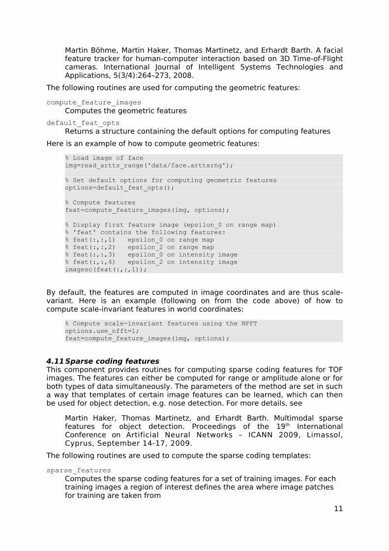
4.12Graphical user interfaceThe signal-processing toolbox contains a graphical user interface (GUI) that can be used to access some of the functionality in the toolbox. The GUI is opened by calling the routine sp_toolbox_gui. Here is a sample screenshot of the GUI:

12

The following sections will describe the individual menus of the GUI.

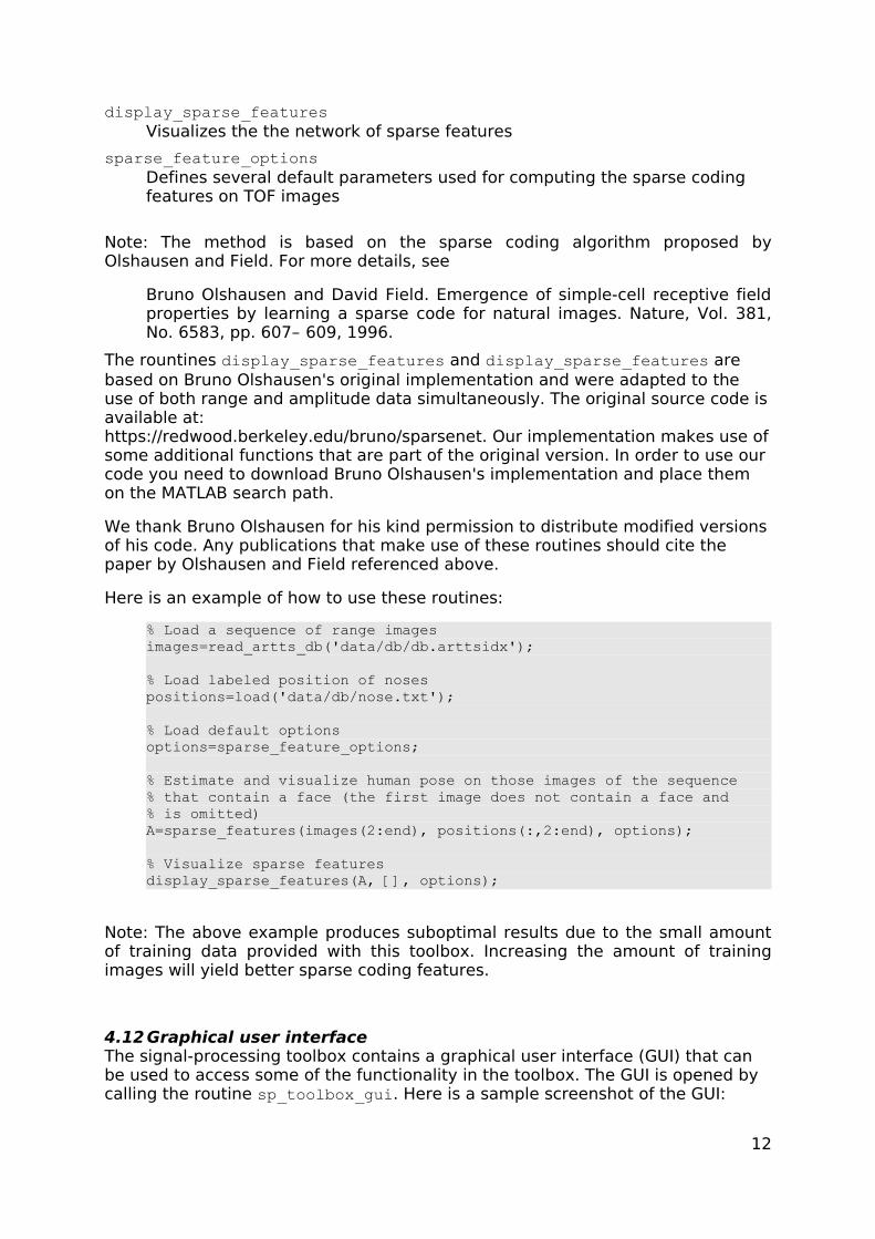
4.12.1 File menu

• Load… (Ctrl+O)

Opens a dialog window for selecting a TOF file with the “arttsrng” exten-sion and displays the range map and normalized intensity image in the in-terface window.

• Acquire sample…

Acquires a new range image from the camera.

• Save (Ctrl+S)

Saves the current TOF image.

• Save as…

Saves the current TOF image under a new file name.

• Close (Ctrl+W)

Closes the GUI.

13

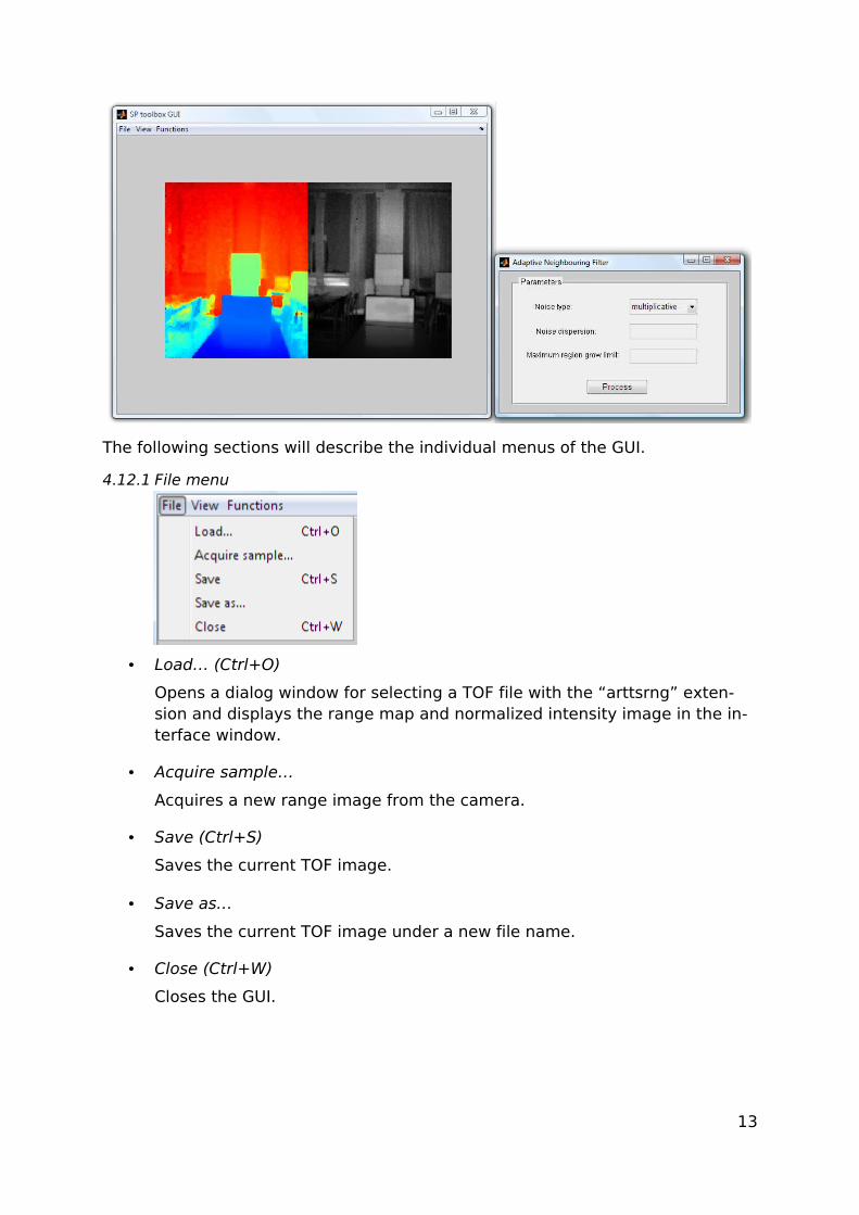
4.12.2 View menu

• Range image… (Ctrl+V)

Opens a dialog window for selecting a TOF file with the “arttsrng” exten-sion and displays it in a new window.

• Range image 3D…

Opens a dialog window for selecting a TOF file with the “arttsrng” exten-sion and displays the 3D representation of the image in a new window.

• Database images…

Opens a dialog window for selecting an ARTTS image database index file with the “arttsidx” extension. The TOF images in the database are dis-played in a new window; press the space bar to go to the next image and B to go to the previous image.

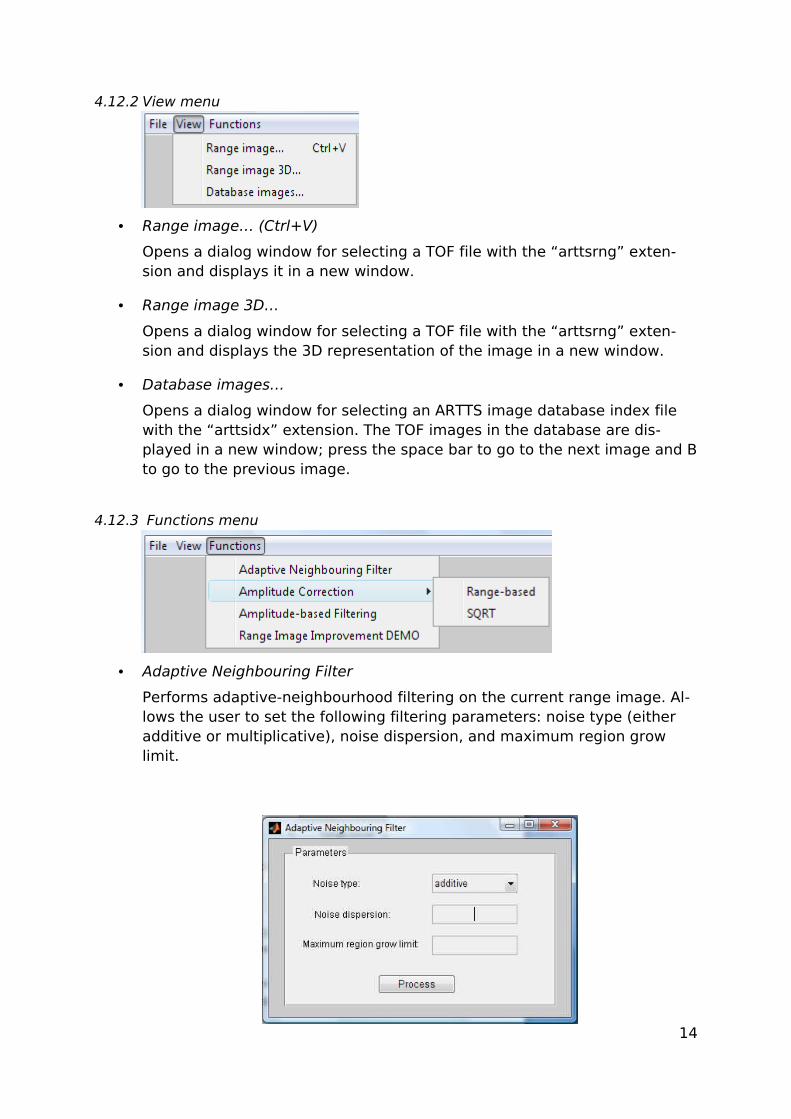
4.12.3 Functions menu

• Adaptive Neighbouring Filter

Performs adaptive-neighbourhood filtering on the current range image. Al-lows the user to set the following filtering parameters: noise type (either additive or multiplicative), noise dispersion, and maximum region grow limit.

14

After these parameters have been input, clicking “Process” filters the cur-rent imageand displays the resulting image in the GUI window.

• Amplitude Correction

Performs amplitude correction, either distance-based, or a simple square root correction of the current range image (last saved or loaded) and dis-plays the result in the GUI window.

• Amplitude-based Filtering

Performs amplitude-based range map filtering on the current image and displays the result in the GUI window.

• Range image improvement DEMO

Improves the 3D representation of an image by reducing the distance er-rors on dark objects.Since this is a demo, it automatically loads the range image “new_bear_im-age.arttsrng” from the “data” folder, selects a predefined high-contrast zone, performs foreground and background corrections in the regions around the selected zone, and displays the original and the corrected im-ages in two new windows.

5 File Format Specifications

5.1 ARTTS Image Database File FormatAn image database consists of a directory containing a number of images in ARTTS range file format (see Section 5.2) together with an index file that provides additional information about each image, typically a list of parameters (e.g. rotation angles).

The standard file extension for an ARTTS database index file is ".arttsidx".

An index file is formatted in human-readable ASCII and consists of a number of lines; line ends are marked by a carriage return (CR, 0x0D) followed by a line feed (LF, 0x0A).

The index file contains one line for each image in the database. Each line begins with the name of the corresponding image file (stored in the same directory) or an asterisk ('*') as a placeholder to indicate that no image has yet been acquired. This can be used to prepare an index file with the parameters for an image set that is to be acquired; the empty index file can then be fed to an image acquisition application, which replaces the placeholders with the names of the acquired images.

The image file name (or asterisk) is followed by the image parameters (separated by at least one space), which continue to the end of the line. The format of these parameters is specific to the particular database.

The file may contain comment lines, which are ignored. Comment lines are identified by a hash mark ('#') as the first character of the line; no whitespace

15

may precede the hash mark. Comments must have a line to themselves; they may not appear at the end of a line describing an image.

Here is an example of a database index file:

# Head in various orientations # First parameter is yaw in degrees, second parameter is pitch in degrees img00001.arttsrng 0 0 img00002.arttsrng 20 0 img00003.arttsrng -20 0 img00004.arttsrng 0 10 img00005.arttsrng 0 -10

5.2 ARTTS Range File FormatAn ARTTS range file contains a range and an amplitude image. These images may contain a single camera frame, or they may be the result of averaging several camera frames. In the latter case, the file also includes images containing the standard deviation of each pixel in the range and the amplitude image.

An ARTTS range file does not contain the Cartesian (XYZ) coordinates of the image points; these can be reconstructed from the data contained in the file as explained in Section 5.3.

The standard file extension for an ARTTS range file is ".arttsrng".

An ARTTS range file is split into two sections: A human-readable ASCII header (containing information such as the resolution and camera parameters) and a binary section containing the actual image data.

5.2.1 HeaderThe file header is formatted in human-readable ASCII. Line ends are marked by a carriage return (CR, 0x0D) followed by a line feed (LF, 0x0A).

The header may contain comment lines, which are ignored. Comment lines are identified by a hash mark ('#') as the first character of the line; no whitespace may precede the hash mark. Comments must have a line to themselves; they may not appear at the end of a line containing data.

The header must begin with the following line, which identifies the file as an ARTTS range file:

artts_range_file version 1.0

No comment lines may precede this line.

The '1.0' identifies the file format version; this is the only valid file format version at this time. The version number is intended to support future modifications of the format while maintaining downward compatibility.

The semantics of the version number are as follows: A change in the major version number indicates a change in the macroscopic structure of the file. A change in the minor version number indicates that the general structure of the file remains the same, but that there may be a slight difference in semantics or that new keyword-value pairs (see below) have been added.

An application faced with a major version number that it does not know how to interpret should exit with an error, because it will not be able to interpret the file correctly. An application faced with a known major version number but an unknown minor version number may attempt to read the file, but it should output a warning to indicate that some of the information in the file may not be read or may be read incorrectly.

16

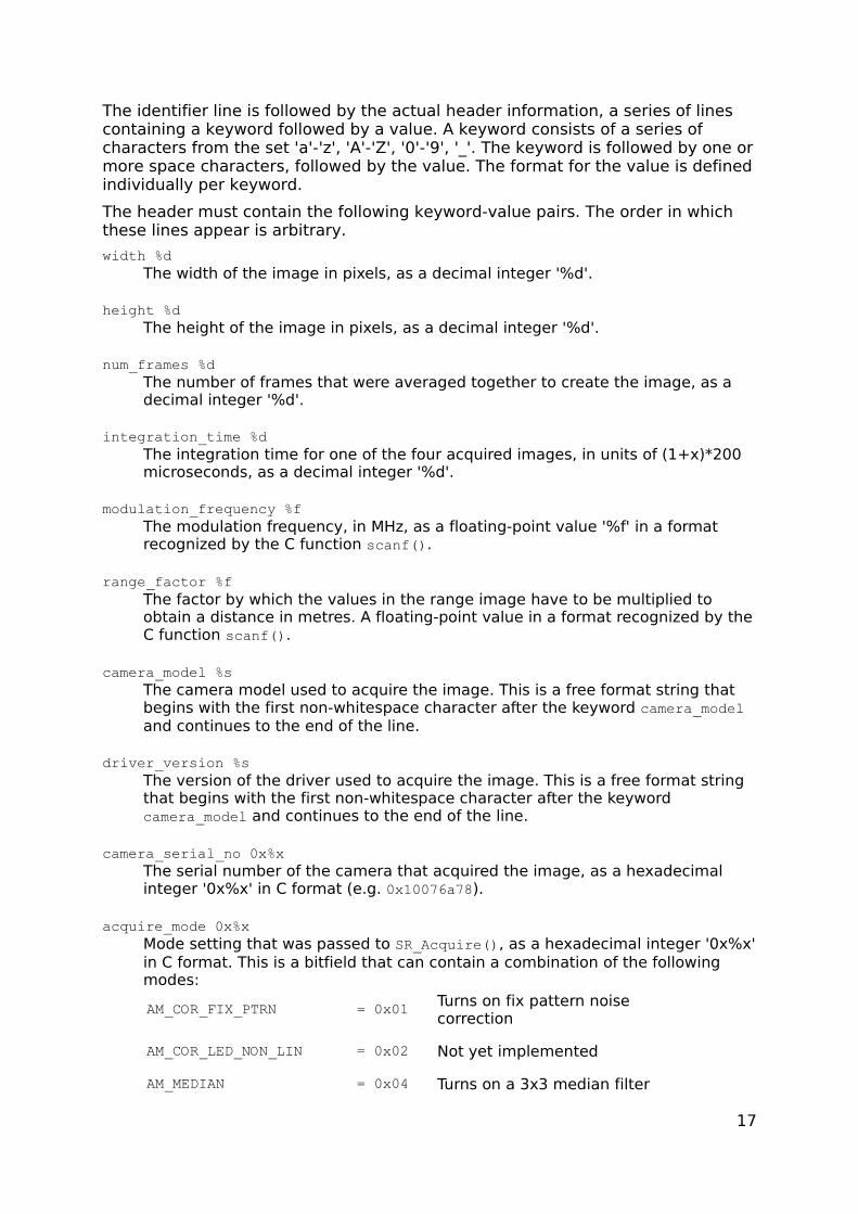
The identifier line is followed by the actual header information, a series of lines containing a keyword followed by a value. A keyword consists of a series of characters from the set 'a'-'z', 'A'-'Z', '0'-'9', '_'. The keyword is followed by one or more space characters, followed by the value. The format for the value is defined individually per keyword.

The header must contain the following keyword-value pairs. The order in which these lines appear is arbitrary.

width %d The width of the image in pixels, as a decimal integer '%d'.

height %d The height of the image in pixels, as a decimal integer '%d'.

num_frames %d The number of frames that were averaged together to create the image, as a decimal integer '%d'.

integration_time %d The integration time for one of the four acquired images, in units of (1+x)*200 microseconds, as a decimal integer '%d'.

modulation_frequency %f The modulation frequency, in MHz, as a floating-point value '%f' in a format recognized by the C function scanf().

range_factor %f The factor by which the values in the range image have to be multiplied to obtain a distance in metres. A floating-point value in a format recognized by the C function scanf().

camera_model %s The camera model used to acquire the image. This is a free format string that begins with the first non-whitespace character after the keyword camera_model and continues to the end of the line.

driver_version %s The version of the driver used to acquire the image. This is a free format string that begins with the first non-whitespace character after the keyword camera_model and continues to the end of the line.

camera_serial_no 0x%x The serial number of the camera that acquired the image, as a hexadecimal integer '0x%x' in C format (e.g. 0x10076a78).

acquire_mode 0x%x Mode setting that was passed to SR_Acquire(), as a hexadecimal integer '0x%x' in C format. This is a bitfield that can contain a combination of the following modes:

AM_COR_FIX_PTRN = 0x01 Turns on fix pattern noise correction

AM_COR_LED_NON_LIN = 0x02 Not yet implemented

AM_MEDIAN = 0x04 Turns on a 3x3 median filter

17

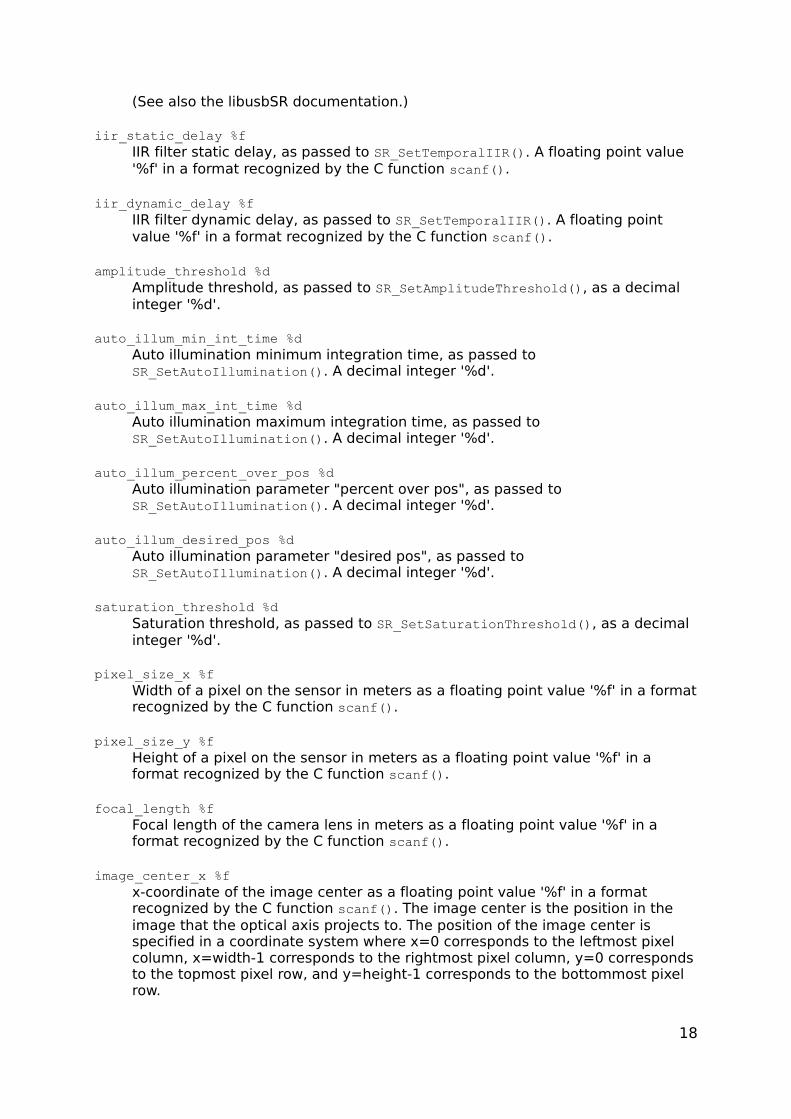
(See also the libusbSR documentation.)

iir_static_delay %f IIR filter static delay, as passed to SR_SetTemporalIIR(). A floating point value '%f' in a format recognized by the C function scanf().

iir_dynamic_delay %f IIR filter dynamic delay, as passed to SR_SetTemporalIIR(). A floating point value '%f' in a format recognized by the C function scanf().

amplitude_threshold %d Amplitude threshold, as passed to SR_SetAmplitudeThreshold(), as a decimal integer '%d'.

auto_illum_min_int_time %d Auto illumination minimum integration time, as passed to SR_SetAutoIllumination(). A decimal integer '%d'.

auto_illum_max_int_time %d Auto illumination maximum integration time, as passed to SR_SetAutoIllumination(). A decimal integer '%d'.

auto_illum_percent_over_pos %d Auto illumination parameter "percent over pos", as passed to SR_SetAutoIllumination(). A decimal integer '%d'.

auto_illum_desired_pos %d Auto illumination parameter "desired pos", as passed to SR_SetAutoIllumination(). A decimal integer '%d'.

saturation_threshold %d Saturation threshold, as passed to SR_SetSaturationThreshold(), as a decimal integer '%d'.

pixel_size_x %f Width of a pixel on the sensor in meters as a floating point value '%f' in a format recognized by the C function scanf().

pixel_size_y %f Height of a pixel on the sensor in meters as a floating point value '%f' in a format recognized by the C function scanf().

focal_length %f Focal length of the camera lens in meters as a floating point value '%f' in a format recognized by the C function scanf().

image_center_x %f x-coordinate of the image center as a floating point value '%f' in a format recognized by the C function scanf(). The image center is the position in the image that the optical axis projects to. The position of the image center is specified in a coordinate system where x=0 corresponds to the leftmost pixel column, x=width-1 corresponds to the rightmost pixel column, y=0 corresponds to the topmost pixel row, and y=height-1 corresponds to the bottommost pixel row.

18

image_center_y %f y-coordinate of the image center as a floating point value '%f' in a format recognized by the C function scanf().

To ensure upward compatibility, applications should ignore unrecognized keywords that may appear in the file.

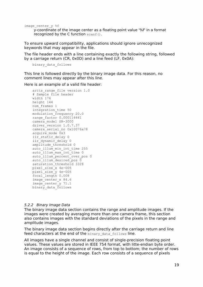
The file header ends with a line containing exactly the following string, followed by a carriage return (CR, 0x0D) and a line feed (LF, 0x0A):

binary_data_follows

This line is followed directly by the binary image data. For this reason, no comment lines may appear after this line.

Here is an example of a valid file header:

artts_range_file version 1.0 # Sample file header width 176 height 144 num_frames 1 integration_time 50 modulation_frequency 20.0 range_factor 0.000114441 camera_model SR-3000 driver_version 1.0.7.37 camera_serial_no 0x10076a78 acquire_mode 0x3 iir_static_delay 0 iir_dynamic_delay 0 amplitude_threshold 0 auto_illum_min_int_time 255 auto_illum_max_int_time 0 auto_illum_percent_over_pos 0 auto_illum_desired_pos 0 saturation_threshold 3328 pixel_size_x 4e-005 pixel_size_y 4e-005 focal_length 0.008 image_center_x 84.6 image_center_y 71.1 binary_data_follows

5.2.2 Binary Image DataThe binary image data section contains the range and amplitude images. If the images were created by averaging more than one camera frame, this section also contains images with the standard deviations of the pixels in the range and amplitude images.

The binary image data section begins directly after the carriage return and line feed characters at the end of the binary_data_follows line.

All images have a single channel and consist of single-precision floating point values. These values are stored in IEEE 754 format, with litte-endian byte order. An image consists of a sequence of rows, from top to bottom; the number of rows is equal to the height of the image. Each row consists of a sequence of pixels

19

(single-precision values), from left to right; the number of pixels is equal to the width of the image. No padding is applied between rows.

The image data section contains the following images in sequence:

a) The range image. This contains either the raw range values from a single camera frame or, for the case where an image was obtained by averaging over several frames (num_frames > 1), the averaged range values over all frames. Range values can lie between 0 and 65.535 (inclusive); for num_frames = 1, all values are guaranteed to be integer. Range values can be multiplied by the value specified in the header under range_factor to obtain a distance in metres.

b) The amplitude image. This contains either the raw amplitude values from a single camera frame or, for num_frames > 1, the averaged amplitude values over all frames. Amplitude values can lie between 0 and 65.535 (inclusive); for num_frames = 1, all values are guaranteed to be integer.

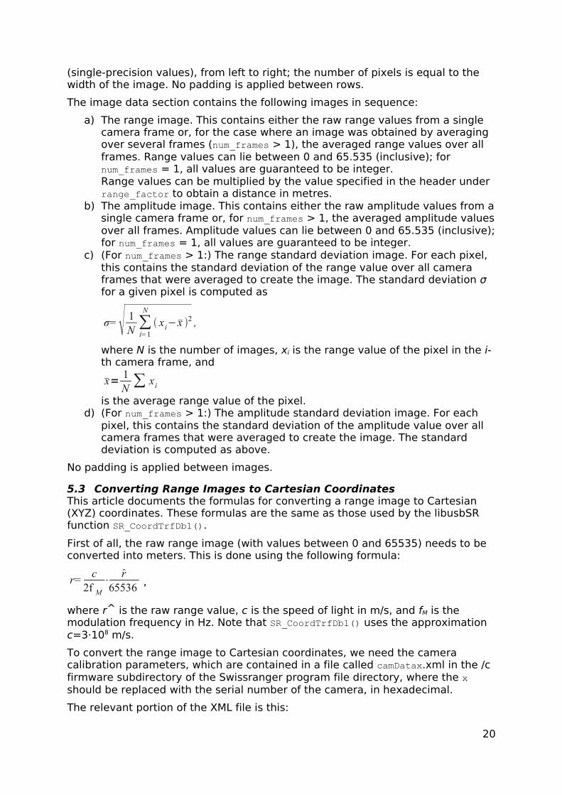
c) (For num_frames > 1:) The range standard deviation image. For each pixel, this contains the standard deviation of the range value over all camera frames that were averaged to create the image. The standard deviation σ for a given pixel is computed as

σ= 1N∑i=1N

xi−x 2 ,

where N is the number of images, xi is the range value of the pixel in the i-th camera frame, and

x=1N∑ x i

is the average range value of the pixel.d) (For num_frames > 1:) The amplitude standard deviation image. For each

pixel, this contains the standard deviation of the amplitude value over all camera frames that were averaged to create the image. The standard deviation is computed as above.

No padding is applied between images.

5.3 Converting Range Images to Cartesian CoordinatesThis article documents the formulas for converting a range image to Cartesian (XYZ) coordinates. These formulas are the same as those used by the libusbSR function SR_CoordTrfDbl().

First of all, the raw range image (with values between 0 and 65535) needs to be converted into meters. This is done using the following formula:

r=c2f M

⋅r

65536 ,

where r^ is the raw range value, c is the speed of light in m/s, and fM is the modulation frequency in Hz. Note that SR_CoordTrfDbl() uses the approximation c=3·108 m/s.

To convert the range image to Cartesian coordinates, we need the camera calibration parameters, which are contained in a file called camDatax.xml in the /c firmware subdirectory of the Swissranger program file directory, where the x should be replaced with the serial number of the camera, in hexadecimal.

The relevant portion of the XML file is this:

20

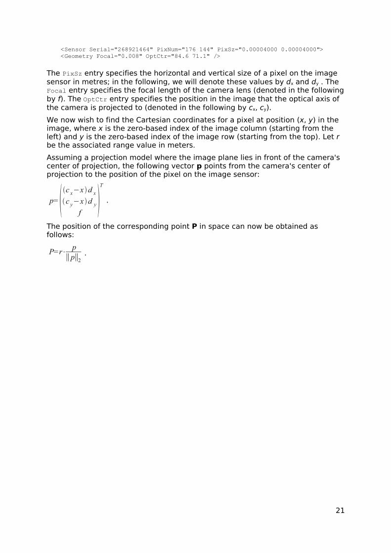
<Sensor Serial="268921464" PixNum="176 144" PixSz="0.00004000 0.00004000"> <Geometry Focal="0.008" OptCtr="84.6 71.1" />

The PixSz entry specifies the horizontal and vertical size of a pixel on the image sensor in metres; in the following, we will denote these values by dx and dy . The Focal entry specifies the focal length of the camera lens (denoted in the following by f). The OptCtr entry specifies the position in the image that the optical axis of the camera is projected to (denoted in the following by cx, cy).

We now wish to find the Cartesian coordinates for a pixel at position (x, y) in the image, where x is the zero-based index of the image column (starting from the left) and y is the zero-based index of the image row (starting from the top). Let r be the associated range value in meters.

Assuming a projection model where the image plane lies in front of the camera's center of projection, the following vector p points from the camera's center of projection to the position of the pixel on the image sensor:

p=c x−x d xc y−x d y

fT

.

The position of the corresponding point P in space can now be obtained as follows:

P=r⋅p

∥p∥2.

21