signal processing techniques for artifact removal in

SIGNAL PROCESSING TECHNIQUES FOR ARTIFACT REMOVAL IN

ELECTROENCEPHALOGRAM

(EEG)

by

JYOTI BHAT

Presented to the Faculty of the Graduate School of The University of Texas at Arlington in Partial

Fulfillment of

the Requirements

for the Degree of

MASTER OF SCIENCE IN BIOMEDICAL ENGINEERING

THE UNIVERSITY OF TEXAS AT ARLINGTON

DECEMBER 2009

Copyright © by JYOTI BHAT 2009

All Rights Reserved

I dedicate this thesis to my Mom, Dad, brother and grandmother who have worked very hard and made so

many sacrifices to help me pursue my dreams.

iv

ACKNOWLEDGEMENTS

I would like to thank my supervising professor Dr. Thomas Ferree, for being an extremely

inspiring and encouraging mentor and providing me with invaluable advice in the course of my graduate

degree. Also, I would like to thank him for his assistance in preparation of this thesis work.

I am extremely grateful to Dr. Khosrow Behbehani and Dr. George Alexandrakis for their interest

in my research work, giving timely suggestions and for accepting the invitation to be my committee

members.

Special thanks to Dr. Mark Pflieger (Source Signal Imaging, Inc.), for contributing original work

that was developed further as part of this thesis, Matt Brier who acquired data for our studies, and Dr. Ken

Tatebe for his valuable guidance, suggestions and insights into this project.

I also thank Michael Newman, our lab technician, who taught me valuable information related to

the preprocessing of these datasets and helping me in data collection and Drs. Richard Briggs, John Hart

and Robert Haley for financial and other support.

I wish to thank my lab mate Deepali Shewale for her technical support and help. I also wish to

thank my friend Dipen Rana who has proofread my thesis and helped me to complete this thesis. I express

my gratitude towards all my friends who have supported me through thick and thin.

Lastly, and most importantly, I am indebted to my parents, Mrs. Deepa Bhat and Mr. Vidyadhar

Bhat, brother, Tejas Bhat and my grandmother Smt. Vandana Bhat, who have always been there for me. I

would not have made it this far without their help, encouragement and support. Thank you Mom and Dad,

for being my role model and supporting me in all the decisions I have taken to date.

November 23, 2009

v

ABSTRACT

SIGNAL PROCESSING TECHNIQUES FOR ARTIFACT

REMOVAL IN ELECTROENCEPHALOGRAM

(EEG)

Jyoti Bhat, M.S.

The University of Texas at Arlington, 2009

Supervising Professor: Dr. Thomas Ferree

The electroencephalographic recordings measure the electric impulses generated in the brain, in

response to a given stimulus. The spontaneous EEG data is used for diagnosis and treatment of some brain

diseases. For the data to be used for clinical applications, it needs to be free of the various artifacts like the

eye blinks, movement, head movements and muscle activity. These artifacts need to be corrected or the

affected parts need to be removed in the preprocessing of the EEG dataset. This pre-processing is normally

done manually, which tends to be not only time-consuming but also subjective. With large number of

datasets to be analyzed, it is necessary to have uniformity in the analysis. Uniformity, reproducibility and

reliability in the preprocessed data can be obtained if a statistical approach is taken while preprocessing the

datasets. Ideally, this can be semi- or fully- automated. This approach therefore, needs to be taken while

removing the less frequently occurring artifacts and correcting the more frequently occurring artifacts, so as

to retain more complete datasets for further research or clinical purposes.

vi

This thesis covers the entire span of EEG data preprocessing and data quality assurance. It

emphasizes the correction of eye blink artifact, one of the most frequently occurring artifacts. The spatial

filter method, which makes use of the underlying brain activity data segment while computing its filter

coefficients, is introduced as an effective approach for correcting ocular artifacts. This spatial filter

described is based on the spatial distribution of the eye blink over the entire scalp region. In order to detect

and reject subtle artifact, a novel set of signal attributes are proposed that describe the head movements,

horizontal eye movements, and spurious bad electrodes. The resultant data obtained after the pre-

processing steps are clean, i.e. free of artifact contamination free.

In order to quantify the results, data was visually inspected after each step of EEG data

preprocessing. Instances of the artifacts in each step were visually identified before and after

preprocessing. The results of the visual inspection done by an expert in EEG data analysis were then

validated with the results obtained from the automated preprocessing method developed. The results

obtained by manual as well as semi-automated preprocessing method matched perfectly, with the semi-

automated method not only taking less time for computations but also increases the reproducibility of the

data.

vii

TABLE OF CONTENTS

ACKNOWLEDGEMENTS ............................................................................................................ iv

ABSTRACT .................................................................................................................................... v

LIST OF ILLUSTRATIONS ........................................................................................................... x

CHAPTER Page

1 INTRODUCTION .......................................................................................................... 1

1.1 Artifacts ............................................................................................................... 2

1.1.1 Ocular Artifacts ....................................................................................... 2

1.1.2 Muscle Artifact ........................................................................................ 4

1.1.3 ECG/EKG Artifact .................................................................................. 5

1.1.4 Sixty Hz Line Interference ...................................................................... 6

1.1.5 Change in Electrode Impedance .............................................................. 7

1.2 Need for Automatic Artifact Removal Process ................................................... 8

1.3 Preprocessing Steps ............................................................................................. 9

1.3.1 Gross Artifact Removal ........................................................................... 9

1.3.2 EOG Artifact Removal ............................................................................ 9

1.3.3 Subtle Artifact Removal .........................................................................10

1.4 Statement of the Problem....................................................................................10

viii

2 GROSS ARTIFACT REMOVAL ................................................................................................11

2.1 Method ................................................................................................................11

2.1.1 Participants .............................................................................................11

2.1.2 Data Acquisition .....................................................................................12

2.2 Data Segments ....................................................................................................12

2.2.1 Signal Attributes .....................................................................................12

2.2.2 Statistical Test ........................................................................................14

2.2.3 Results ...................................................................................................15

2.3 Malfunctioning Electrodes..................................................................................17

2.3.1 Signal Attributes .....................................................................................17

2.3.2 Statistical Test ........................................................................................18

2.3.3 Results ...................................................................................................20

3 OCULAR ARTIFACT REMOVAL ............................................................................................22

3.1 EOG & Its Effect on EEG ..................................................................................22

3.2 Previous Work ....................................................................................................24

3.2.1 EOG Subtraction/Regression Analysis ...................................................24

3.2.2 Dipole Modeling ....................................................................................24

3.2.3 ICA /Blind Source Methods ...................................................................25

3.2.4 Spatial Filter ...........................................................................................26

3.3 Theory of The Spatial Filter ...............................................................................27

3.4 Method ................................................................................................................29

3.4.1 Clean Data File .......................................................................................29

ix

3.4.2 Average Eye Blink File ..........................................................................30

3.4.3 Sensitivity to Number of Components Retained ....................................30

3.5 Results ................................................................................................................31

3.5.1 GUI for Eye Blink Epoch Selection .......................................................31

3.5.2 Sensitivity to Number of Components Retained ....................................34

3.5.3 Corrected EEG .......................................................................................35

3.5.4 Relation to Commercial Implementations ..............................................36

3.5.5 Extension to Vertical Eye Movements ...................................................37

4 SUBTLE ARTIFACT REMOVAL ..............................................................................................39

4.1 Muscle Artifacts .................................................................................................39

4.2 Horizontal Eye Movement Artifact ....................................................................41

4.3 Head Movement Artifact ....................................................................................43

4.4 Inter-Electrode Gap ............................................................................................44

4.5 Sporadic Changes ...............................................................................................45

4.6 Statistical Test ....................................................................................................46

4.7 Results ................................................................................................................47

5 FUTURE WORK AND CONCLUSION .....................................................................................49

REFERENCES ................................................................................................................................51

BIOGRAPHICAL INFORMATION ..............................................................................................54

x

LIST OF ILLUSTRATIONS

Figure Page

1.1: Contamination due to ocular artifacts (marked by red blocks) ................................................. 3

1.2: Contamination due to muscle artifact ........................................................................................ 4

1.3: Contamination due to ECG artifact ........................................................................................... 5

1.4: Contamination due to 60 Hz line interference ........................................................................... 6

1.5: Change in electrode impedance seen......................................................................................... 7

2.1: Data segments affected by filter (marked in red block) ...........................................................15

2.2: Malfunctioning electrodes clearly visible after removal of affected data segments .................16

2.3: Malfunctioning electrodes AF4, FT8, TP8, O2 ........................................................................20

2.4: Histogram of the 3 parameters .................................................................................................21

2.5: EOG artifact clearly visible after removal of malfunctioning electrodes from data.................21

3.1: Electrooculogram (EOG) [3] ....................................................................................................23

3.2: Effect of EOG in EEG..............................................................................................................23

3.3: Spatial filter [20] ......................................................................................................................26

3.4: GUI prepared for eye blink epoch selection .............................................................................32

3.5: Average eye blink signal in the VEOG electrode ....................................................................33

3.6 : Topography of the average eye blink ......................................................................................33

xi

3.7: Scree plot of the eigenvalues ....................................................................................................34

3.8 : Topography of first two eigenvectors .....................................................................................35

3.9: Eye blink corrected data ...........................................................................................................36

3.10: Correlation coefficient topography ........................................................................................37

3.11: Data showing eye blink and VEOG movement .....................................................................38

3.12: Eye blink and VEOG movement removed from the data .......................................................38

4.1: Muscle artifact in the data ........................................................................................................40

4.2: Muscle artifact removed ...........................................................................................................41

4.3: HEOG artifact ..........................................................................................................................42

4.4: Head movement artifact in the data ..........................................................................................43

4.5: Epochs showing larger inter-electrode distance .......................................................................44

4.6: Sporadic change seen in the electrode P6 ................................................................................45

4.7: The histogram obtained while detecting the inter-electrode distance ......................................46

4.8: Clean data .................................................................................................................................48

1

CHAPTER 1

INTRODUCTION

Neurons in the brain are electrically active cells. When activated these neurons generate action

potentials. The action potential travelling down the axon, releases chemical neurotransmitters at the

synapse. With the release of the chemical neurotransmitters at the synapse, activation of the chemical

neuroreceptors located on the dendrite of the post-synaptic neuron is observed. This generates a post-

synaptic potential at the synapse. Electrodes when placed on the scalp of the subject record a spatial

average of these post-synaptic potentials. The recorded signal is known as the electroencephalogram

(EEG). Derived measures of EEG activity are informative biomarkers for brain activity [1]. The electrical

fluctuations in the brain are generally in the range of ±50 micro volts, µV [2]. The acquired EEG data

needs to be preprocessed before it could use it for clinical purposes.

Preprocessing of the EEG data is mainly required to eliminate the artifact signals which, are

acquired along with the EEG signal. The most damaging artifacts are those seen with the largest change in

the amplitude of the recorded EEG signal. Artifact signals in the data are usually assumed to be

uncorrelated with the signal of interest i.e. the EEG signal.

This work describes a preprocessing protocol that removes the artifacts in a semi-automated

manner. The focus of this work is removal of the eye blink artifact from the EEG dataset using the spatial

filter technique with preservation of clean EEG. We would look at removing the gross artifacts in the

Chapter 2. We will then look at the algorithm for removing the eye blink artifact in the Chapter 3. In

2

Chapter 4, we would look at removing the subtle artifacts from the data. The semi-automated artifact

removal algorithm is developed in MATLAB (R2007b, The MathWorks, USA).

1.1 Artifacts

Contamination of the EEG signal at the various time points is seen while the EEG data is being

acquired. Artifacts are defined as any signal whose source is extraneous to the brain. The artifacts in an

EEG dataset can be broadly classified into two categories, namely, physiological artifacts and

extra-physiological artifacts. Physiological artifacts are generated from sources in the patient’s body while,

extra-physiological artifacts are generated by sources outside the patient’s body. The different types of

artifacts that are commonly seen are as follows:

1.1.1 Ocular Artifacts

‘The human eye is a seat of steady electric potential field’ [3]. To use the battery analogy, the

positive terminal for the human eye resides in the cornea while the retina acts like the negative terminal.

As a result of this electric field, the eye movement or the eye blink causes a change in the electric fields.

The electric potential recorded because of the eye movement or the eye blink is known as the electro-

oculogram (EOG). This signal can be recorded with the help of peri-orbital electrodes placed near the eyes.

The vertical EOG electrodes (VEOG) electrodes placed above and below the orbit of the eyes record

change in the potential caused by the vertical eye movements and the eye blinks [3 and 4]. The horizontal

EOG electrodes (HEOG) placed in the left and right outer canthi of the eyes record the change in the

potential due to horizontal eye movements [3 and 4].

The voltage difference generated due an eye blink or movement is large compared to the voltage

in the EEG electrodes. This is due to volume conduction effect seen in these underlying tissues. These

large potentials contaminated the EEG electrodes in a way that the voltage at these electrodes falls of

3

roughly as the square of the distance from the eyes [4]. Hence the frontal electrodes are largely affected by

the vertical eye movements and eye blinks. Away from the eyes the amount of contamination reduces.

Hence, the occipital electrodes are comparatively less affected by the eye blink artifact and the vertical eye

movement artifact. The horizontal eye movements are propagated more in the temporal electrodes and are

negligible in the other electrodes [5]. The Figure 1.1 shows the contamination of EEG electrodes due to

ocular artifact in red blocks. The contamination due to vertical eye movements and eye blinks is largely

seen in frontal electrodes and that due to horizontal eye movements is seen in temporal electrodes.

Figure 1.1: Contamination due to ocular artifacts (marked by red blocks)

While this clearly illustrates EOG contamination in EEG, it is also the case that the EEG potential

contaminates the EOG electrodes. This effect needs to be considered while developing algorithms to

remove the contamination caused by this type of artifact in the EEG signal [4].

4

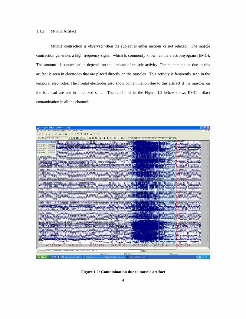
1.1.2 Muscle Artifact

Muscle contraction is observed when the subject is either anxious or not relaxed. The muscle

contraction generates a high frequency signal, which is commonly known as the electromyogram (EMG).

The amount of contamination depends on the amount of muscle activity. The contamination due to this

artifact is seen in electrodes that are placed directly on the muscles. This activity is frequently seen in the

temporal electrodes. The frontal electrodes also show contamination due to this artifact if the muscles on

the forehead are not in a relaxed state. The red block in the Figure 1.2 below shows EMG artifact

contamination in all the channels.

Figure 1.2: Contamination due to muscle artifact

5

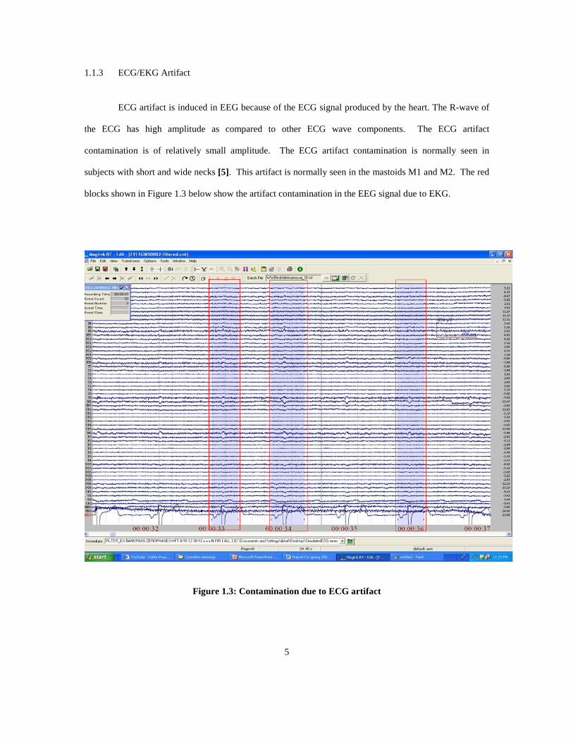
1.1.3 ECG/EKG Artifact

ECG artifact is induced in EEG because of the ECG signal produced by the heart. The R-wave of

the ECG has high amplitude as compared to other ECG wave components. The ECG artifact

contamination is of relatively small amplitude. The ECG artifact contamination is normally seen in

subjects with short and wide necks [5]. This artifact is normally seen in the mastoids M1 and M2. The red

blocks shown in Figure 1.3 below show the artifact contamination in the EEG signal due to EKG.

Figure 1.3: Contamination due to ECG artifact

6

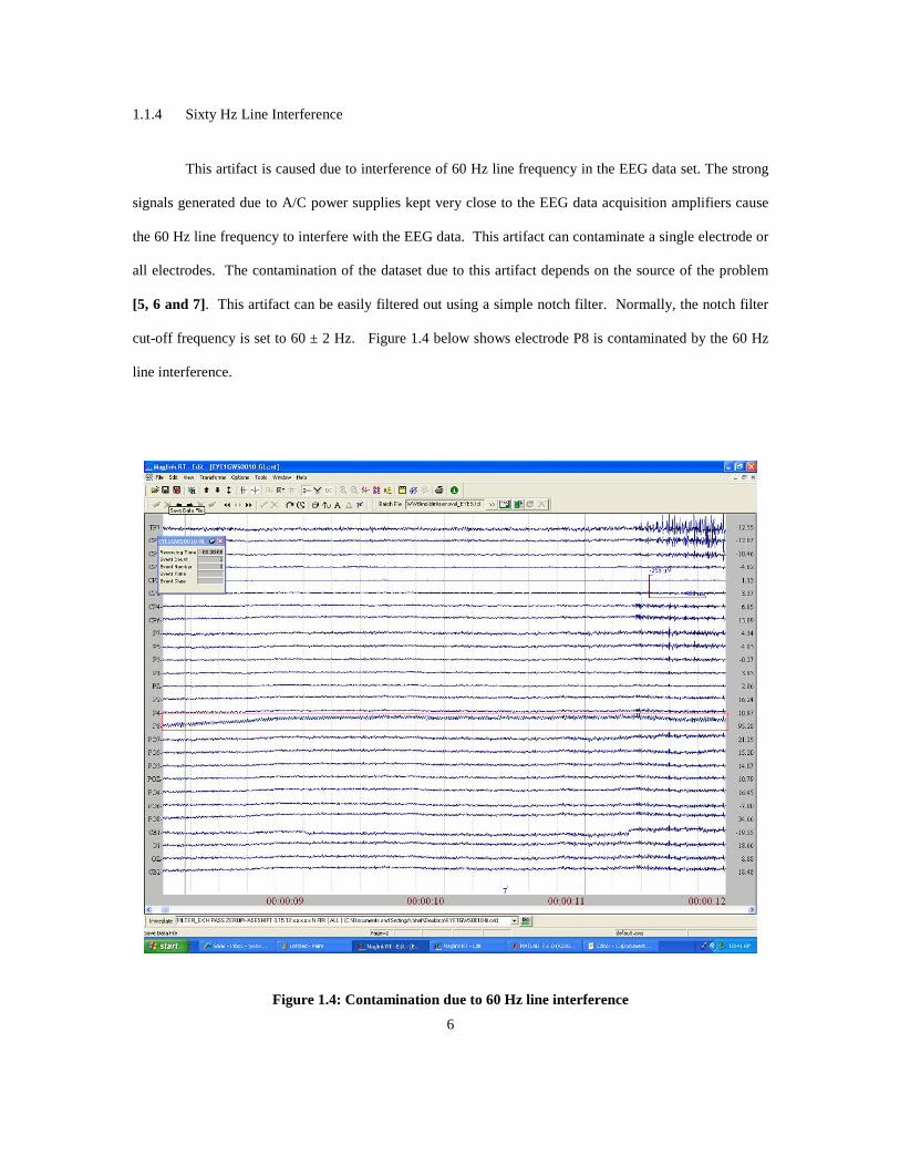
1.1.4 Sixty Hz Line Interference

This artifact is caused due to interference of 60 Hz line frequency in the EEG data set. The strong

signals generated due to A/C power supplies kept very close to the EEG data acquisition amplifiers cause

the 60 Hz line frequency to interfere with the EEG data. This artifact can contaminate a single electrode or

all electrodes. The contamination of the dataset due to this artifact depends on the source of the problem

[5, 6 and 7]. This artifact can be easily filtered out using a simple notch filter. Normally, the notch filter

cut-off frequency is set to 60 ± 2 Hz. Figure 1.4 below shows electrode P8 is contaminated by the 60 Hz

line interference.

Figure 1.4: Contamination due to 60 Hz line interference

7

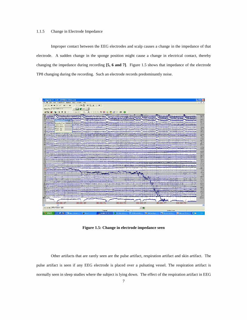
1.1.5 Change in Electrode Impedance

Improper contact between the EEG electrodes and scalp causes a change in the impedance of that

electrode. A sudden change in the sponge position might cause a change in electrical contact, thereby

changing the impedance during recording [5, 6 and 7]. Figure 1.5 shows that impedance of the electrode

TP8 changing during the recording. Such an electrode records predominantly noise.

Figure 1.5: Change in electrode impedance seen

Other artifacts that are rarely seen are the pulse artifact, respiration artifact and skin artifact. The

pulse artifact is seen if any EEG electrode is placed over a pulsating vessel. The respiration artifact is

normally seen in sleep studies where the subject is lying down. The effect of the respiration artifact in EEG

8

data is seen as slow or sharp pulses which are in synchronization with inhalation or exhalation. The skin

artifacts are seen if the scalp of the subject perspires. Sweat on the scalp then causes change in the

impedances [5 and 7].

1.2 Need for Automatic Artifact Removal Process

As discussed in the above section a number of artifacts contaminating the EEG data affects the

data analysis. Precise screening of the EEG data is required for accurate spatial mapping, for source signal

analysis, for current density measures and also for accurate temporal analysis based on single - trial

methods [8]. The frequency of occurrence of few artifacts is large and some of the artifact contaminations

cannot be avoided. Techniques need to be developed which will help remove these artifacts from the EEG

data. Some of these artifacts can be treated by rejecting contaminated parts of the data while for other

artifacts filtering techniques are developed. Rejecting data segments contaminated by the artifacts reduces

the amount of data available for further analysis. If the amount of data to be analyzed is vast then, it is very

difficult to manually clean such large amount of datasets for artifact removal. This increases manpower

time and labor. The process of preprocessing thus becomes very subjective and hence there is no

repeatability in the results of this type of preprocessing [9 and 10]. Hence statistical analysis needs to be

used for artifact removal.

Some artifacts like the 60 Hz line interference can be easily removed using a notch filter technique

[7]. The electrodes that do record artifacts due to changes in the electrode impedance can be detected and

rejected automatically using some characteristics like the first derivative of the signal over time, etc [8].

Other artifacts like the ocular artifacts can be removed using different filtering techniques or segments

affected can be removed from further analysis. A systematic, automatic or semi-automatic and statistics

based method needs to be developed which will help remove the contaminations in the EEG data [9].

9

1.3 Preprocessing Steps

After the EEG data acquisition is completed, the offline EEG data preprocessing starts with

filtering the data. In filtering the dataset helps remove the unwanted high frequencies from the data. The

acquired data is high pass filtered at a frequency of 0.15Hz and 12dB/octave. This filtering step removes

and detrends the low frequency drifts, below the range of frequencies normally studied (typically 1Hz-

45Hz) further in the EEG analysis.

The overall approach to this work is to characterize each artifact by its temporal characteristics

and/or spatial characteristics and use those to design a procedure which would help eliminate as many

artifacts as possible. The common steps that are followed during preprocessing of EEG data are:

1.3.1 Gross Artifact Removal

The gross contaminated channels and data segments are removed in this step. The electrodes or

segments of data that are removed are the electrodes and data segments which appear much larger to the

eye blink artifact contamination and which would affect the EOG artifact removal. These electrodes or

data segments overshadow the rest of the artifacts present in the EEG data and are rejected from the further

analysis by any EEG experimenter.

1.3.2 EOG Artifact Removal

The EOG artifact i.e. eye blinks and vertical eye movements affect the data largely. Rejection of

the data affected by this artifact would result in considerable loss of the data and hence, various techniques

have been devised for correction of this artifact. A new technique which makes use of the background

artifact free EEG data while computing the filter coefficients is discussed in detail in this work. After

removal of the EOG artifact the subtle artifacts become more evident.

10

1.3.3 Subtle Artifact Removal

After the EOG algorithm, remaining artifacts include horizontal eye movements, muscle artifacts,

head movements which are seen as drifts in the data, etc. Together these are the called subtle artifacts,

because they are not as prominent as those discussed previously, but they can still affect subsequent

spectral analysis and hence must be removed from the data.

This is the last step of preprocessing. The data then obtained is artifact free and hence can be

easily used for doing the further spectral analysis or for clinical purposes.

1.4 Statement of the Problem

The primary goal of this work is to design and develop an automated/ semi-automated algorithm

for artifact removal. In order to do this with maximum flexibility, algorithms were developed in Matlab.

The EEGLAB Toolbox was used to read in data, so most functions were written to operate on the EEGLAB

data structure. The entire preprocessing algorithm discussed in the section 1.3 was implemented in Matlab.

Our implementation of the ocular artifact filtering algorithm in Matlab was validated against the

implementation in Scan Edit (NeuroScan, Inc.) and was then used for further studies of sensitivity to

analysis parameters, etc.

11

CHAPTER 2

GROSS ARTIFACT REMOVAL

The presence of artifacts in an EEG dataset is seen as a large change in the amplitude of the

recorded EEG signal. The gross artifacts are seen in one or more particular electrodes and/or throughout

some temporal segments of the EEG data segment. The 0.15 Hz high-pass filter affects the first few and

the last few seconds of the data, and is discarded. Other artifacts present at this point in the data pipeline

are easily identified by their amplitudes, and their automated – detection and rejection proceeds on these

grounds.

2.1 Method

2.1.1 Participants

Our lab has analyzed on the order of 100 datasets, using the methods discussed herein. In order to

test and quantify the effectiveness of our algorithms, data were acquired from 60 male subjects recruited for

the Gulf War Illness and Chemical Exposure study program at the University of Texas Southwestern

Medical Center at Dallas. Subjects participated in a wide range of experiments, including different neuro-

imaging modalities. EEG data collected as part of this large program is used to test the effectiveness of the

algorithms. A written consent was obtained from each subject participating in this study according to the

Institutional Review Board University of Texas Southwestern Medical Center at Dallas.

12

2.1.2 Data Acquisition

Continuous EEG data were acquired using a 64-channel Quickcap and Neuroscan SynAmps2

amplifier (Compumedics, Inc.). The Scan Acquire 4.3 software (Compumedics, Inc.) sampled the EEG at

1 kHz, and hardware filtered at 200 Hz. Impedances of all the electrodes were kept below typically 10 kΩ.

Vertical eye movements and eye blinks were recorded with electrodes placed above and below the orbit of

the left eye. Horizontal eye movements were recorded with electrodes placed at the left and right outer

canthi of the eyes [4]. The subject was instructed to stay relaxed to reduce muscle artifact contamination.

Datasets were acquired in alternating eyes open eyes closed conditions. Duration for each condition was

about 1minute. Five trials for each condition were acquired, thus making the entire duration of the EEG

dataset about 10 minutes. This acquired data were high pass finite impulse response (FIR) filtered in Scan

Edit 4.3 (Compumedics, Inc.). The filter used had cut-off frequency 0.15 Hz and slope 12 dB/octave.

2.2 Data Segments

The effects of filtering are seen as huge drifts at the beginning and end of the dataset. In most

studies, the number of data segments to be removed from the analysis is subjective decision. The goal of

this work is develop an automated or semi-automated method to render this decision more objective and

based on clear statistical tests.

2.2.1 Signal Attributes

In preparation for spectral analysis, the entire data length was divided into 1-second data

segments. The effect of the filter varies across electrodes and across subjects. The root mean square (RMS)

voltage indicates the rate at which voltage of that electrode varies over the length of the data segment [11].

The RMS value for each electrode each data segment was calculated using the following formula:

13

1

1

1

2),,(

),( t

Vt

ttec

ec

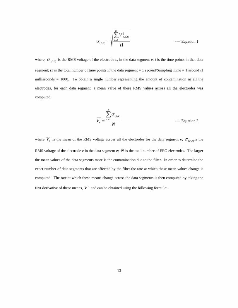
∑==σ ---- Equation 1

where, ),( ecσ is the RMS voltage of the electrode c, in the data segment e; t is the time points in that data

segment; t1 is the total number of time points in the data segment = 1 second/Sampling Time = 1 second /1

milliseconds = 1000. To obtain a single number representing the amount of contamination in all the

electrodes, for each data segment, a mean value of these RMS values across all the electrodes was

computed:

N

V

N

cec

e

∑== 1

),(σ

---- Equation 2

where eV is the mean of the RMS voltage across all the electrodes for the data segment e; ),( ecσ is the

RMS voltage of the electrode c in the data segment e; N is the total number of EEG electrodes. The larger

the mean values of the data segments more is the contamination due to the filter. In order to determine the

exact number of data segments that are affected by the filter the rate at which these mean values change is

computed. The rate at which these means change across the data segments is then computed by taking the

first derivative of these means, V ′ and can be obtained using the following formula:

14

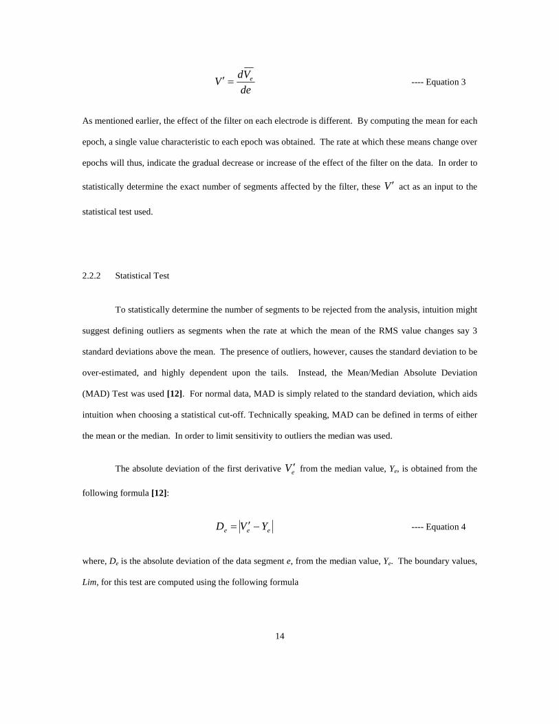
de

VdV e=′ ---- Equation 3

As mentioned earlier, the effect of the filter on each electrode is different. By computing the mean for each

epoch, a single value characteristic to each epoch was obtained. The rate at which these means change over

epochs will thus, indicate the gradual decrease or increase of the effect of the filter on the data. In order to

statistically determine the exact number of segments affected by the filter, these V ′ act as an input to the

statistical test used.

2.2.2 Statistical Test

To statistically determine the number of segments to be rejected from the analysis, intuition might

suggest defining outliers as segments when the rate at which the mean of the RMS value changes say 3

standard deviations above the mean. The presence of outliers, however, causes the standard deviation to be

over-estimated, and highly dependent upon the tails. Instead, the Mean/Median Absolute Deviation

(MAD) Test was used [12]. For normal data, MAD is simply related to the standard deviation, which aids

intuition when choosing a statistical cut-off. Technically speaking, MAD can be defined in terms of either

the mean or the median. In order to limit sensitivity to outliers the median was used.

The absolute deviation of the first derivative eV ′ from the median value, Ye, is obtained from the

following formula [12]:

eee YVD −′= ---- Equation 4

where, De is the absolute deviation of the data segment e, from the median value, Ye. The boundary values,

Lim, for this test are computed using the following formula

15

ee XYLim ∗+= λ ---- Equation 5

where Ye is the median value of the first derivative valueseV ′ ; Xe is the median of the absolute deviations,

De; λ is the confidence coefficient [8]. For the present purpose, the value of λ = 3can be interpreted as an

equivalent of p value < 0.01.

The first derivative values of data segments crossing these limits are then declared as outlier data

segments. Outlier data segments adjacent to the first and the last data segment are then selected to be

rejected from the dataset. The outlier data segments in the middle portion of the data are simply ignored

and not removed. The original dataset is then truncated to this new time length.

2.2.3 Results

Figure 2.1 shows the first segment of the data affected by the filter (marked by red block).

Figure 2.1: Data segments affected by filter (marked in red block)

16

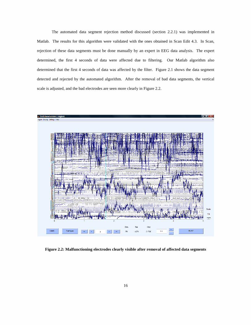
The automated data segment rejection method discussed (section 2.2.1) was implemented in

Matlab. The results for this algorithm were validated with the ones obtained in Scan Edit 4.3. In Scan,

rejection of these data segments must be done manually by an expert in EEG data analysis. The expert

determined, the first 4 seconds of data were affected due to filtering. Our Matlab algorithm also

determined that the first 4 seconds of data was affected by the filter. Figure 2.1 shows the data segment

detected and rejected by the automated algorithm. After the removal of bad data segments, the vertical

scale is adjusted, and the bad electrodes are seen more clearly in Figure 2.2.

Figure 2.2: Malfunctioning electrodes clearly visible after removal of affected data segments

17

2.3 Malfunctioning Electrodes

For accurate recording of the electric field of the brain, the number of electrodes used in most labs

is 32, 64 or 128, and some labs uses as many as 256 or even 512 electrodes. As the number of electrodes

increases, the probability of an electrode having poor contact also increases. It thus, makes the precise

screening for artifact removal a difficult task with large amounts of data to be analyzed. Statistical control

of artifact contaminated electrodes is highly preferable in such large dense array systems [8]. The rejection

of electrodes contaminated due to artifacts at this stage is limited to grossly bad electrodes. As mentioned

earlier, these are the electrodes that are contaminated due to change in the electrode impedance during data

acquisition.

EEG voltage in a good electrode is in the range of ±50µV [2]. The effect of change in electrode

impedance is difficult to characterize in time or frequency domain. It is however, comparatively easy to

characterize as a measure of voltage. In order to characterize the electrode as a measure of voltage,

computation of three different signal attributes is done which helps to determine the bad electrodes

statistically [8].

2.3.1 Signal Attributes

The three signal attributes used in detection of the bad electrodes are; the standard deviation of the

voltage, the maximum absolute value of the voltage and the maximum of the gradient of the voltage [8].

All these parameters are computed at each EEG electrode and over the entire time length of the dataset.

The standard deviation of the voltage:

( )

1

2

1),(

−

−

=∑=

T

VVT

t

ctc

cσ ---- Equation 6

18

where, cσ is the standard deviation of the electrode c, ),( tcV is the voltage of the electrode c at the time

point t, cV is the mean voltage of the electrode c, T is the time length of the entire dataset [8].

The maximum absolute value of the voltage [8]:

),(max tcc VAV = ---- Equation 7

where, cAV is the maximum absolute value of the voltage over the entire time t (1: T) for electrode c.

The maximum of the gradient of the voltage over time or the first derivative of voltage [8].

dt

dVV c

c =′ ---- Equation 8

where, cV′ is the first derivative of voltage for electrode c over the entire time. These parameter matrices or

editing matrices are column matrices with the number of rows in the column equal to the number of EEG

electrodes. These parameters are then used as an input for statistical detection of outliers.

2.3.2 Statistical Test

In the paper by Junghöfer et al. [8] determination of the outlier electrodes was made by a statistical

test based upon the following expression [8]:

( )

11

2),(

−

−

∗+=∑=

N

YV

YLim

N

cpcp

pp λ ---- Equation 9

where pY is the median for each of the parameters p (i.e. p = 1 for standard deviation of the voltage, p = 2

for maximum absolute value of the voltage and p = 3 for maximum value of the voltage over time i.e. the

19

first derivative of the voltage over time), V(p,c) is the parameter p for the electrode c, N is the total number of

electrodes and λ is the confidence coefficient which is set to 3 [8 and section 2.2.2]. The term under the

square root sign is similar to that of the standard deviation except calculated over the median and not mean

[8]. Although intuitive, this expression has no precedent in the statistical literature. For this reason, and

the reasons given above, we used the MAD statistic instead. As a first step in this analysis, the median

value, pY of all three parameters (i.e. p = 1 for standard deviation of the voltage, p = 2 for maximum

absolute value of the voltage and p = 3 for maximum value of the voltage over time i.e. the first derivative

of the voltage over time) is computed. A median is selected over the mean, since it is less sensitive to

outliers as compared to the mean. The absolute deviation can be written as [12],

pcpcp YVD −= ),(),( ---- Equation 10

where D(p,c) is the deviation of parameter p for the electrode c, V(p,c) is the parameter p for the electrode c; Yp

is the median of the parameter p (i.e. p = 1 for standard deviation of the voltage, p = 2 for maximum

absolute value of the voltage and p = 3 for maximum value of the voltage over time i.e. the first derivative

of the voltage over time).

An electrode is determined to be an outlier, if the absolute deviation of that electrode for any of

the three parameters, crosses the boundary values computed by the formula:

ppp XYLim ∗+= λ ---- Equation 11

where Yp is the median of the parameter p (i.e. p = 1 for standard deviation of the voltage, p = 2 for

maximum absolute value of the voltage and p = 3 for maximum value of the voltage over time i.e. the first

derivative of the voltage over time) and Xp is the median of the absolute deviation values, Dp, of the

parameter p (i.e. p = 1 for standard deviation of the voltage, p = 2 for maximum absolute value of the

voltage and p = 3 for maximum value of the voltage over time i.e. the first derivative of the voltage over

time) and λ is the confidence coefficient which is set to 3 [8and section 2.2.2].

20

2.3.3 Results

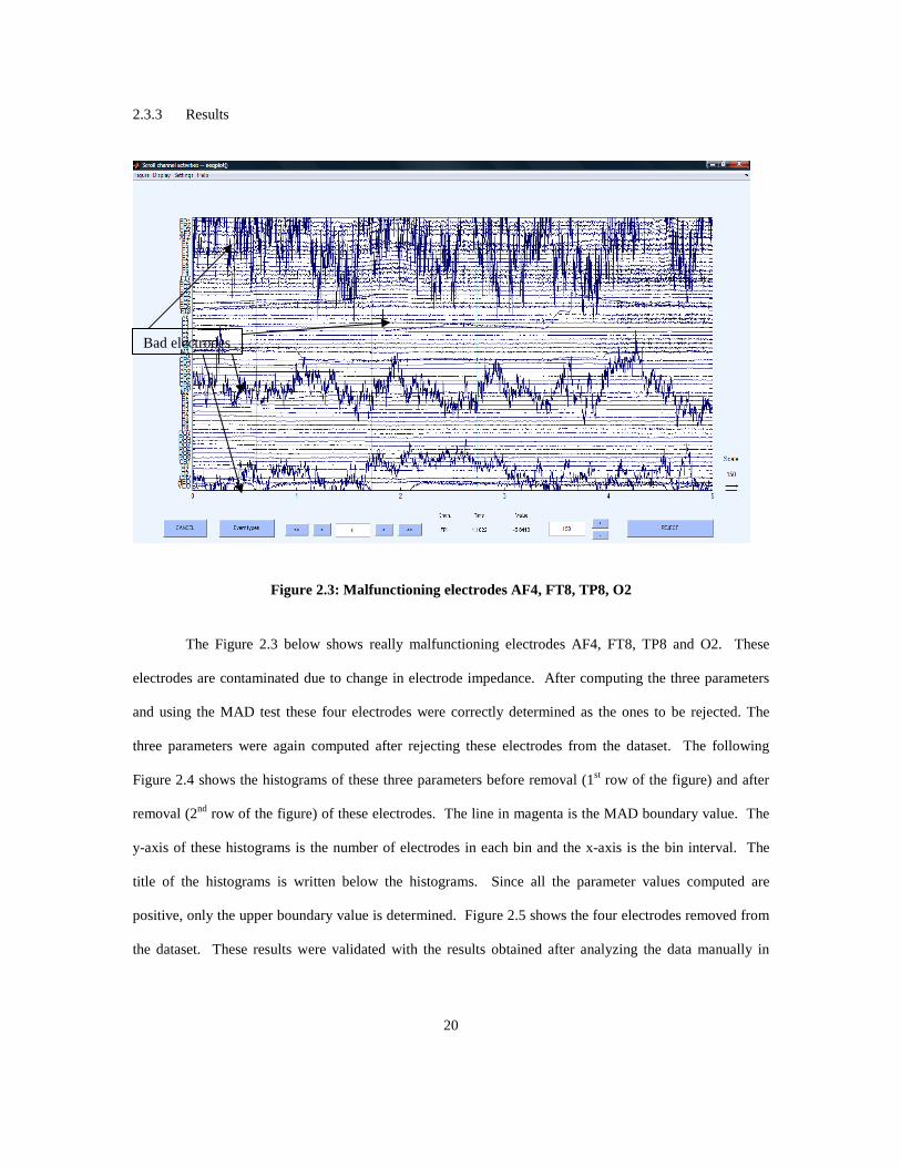
Figure 2.3: Malfunctioning electrodes AF4, FT8, TP8, O2

The Figure 2.3 below shows really malfunctioning electrodes AF4, FT8, TP8 and O2. These

electrodes are contaminated due to change in electrode impedance. After computing the three parameters

and using the MAD test these four electrodes were correctly determined as the ones to be rejected. The

three parameters were again computed after rejecting these electrodes from the dataset. The following

Figure 2.4 shows the histograms of these three parameters before removal (1st row of the figure) and after

removal (2nd row of the figure) of these electrodes. The line in magenta is the MAD boundary value. The

y-axis of these histograms is the number of electrodes in each bin and the x-axis is the bin interval. The

title of the histograms is written below the histograms. Since all the parameter values computed are

positive, only the upper boundary value is determined. Figure 2.5 shows the four electrodes removed from

the dataset. These results were validated with the results obtained after analyzing the data manually in

Bad electrodes

21

Scan by an expert in EEG data analysis. The presence of the other artifact like the ocular artifacts is clearly

seen after completion of the first step of preprocessing i.e. gross artifact removal.

Figure 2.4: Histogram of the 3 parameters

Figure 2.5: EOG artifact clearly visible after removal of malfunctioning electrodes from data

22

CHAPTER 3

OCULAR ARTIFACT REMOVAL

As the first step of pre-processing, the gross artifacts are removed as discussed in earlier Chapter.

The data segments or electrodes which are characterized as outliers in the gross artifact removal procedure

have negligible amount of EEG recorded. Therefore instead of correcting this artifact, data affected is

rejected. After the gross artifact removal, the physiological artifacts need to be treated. The most frequent

of the physiological artifacts seen contaminating the EEG data is the eye blink artifact. The principle of

rejection of data segments affected by the eye blink artifacts, if adopted, will lead to considerable reduction

in the amount of data available for further analysis. Hence, the principle of correction of the data segments

contaminated due to this artifact is adopted. Reliable techniques which would help correct for these

artifacts, without distorting the underlying brain activity are developed. The spatial filter technique for

removal of the eye blink artifact is discussed to great details. The discussed spatial filter technique uses the

pure (artifact-free), background EEG for computing its filter coefficients. To understand the EOG

algorithm it is necessary to know about the EOG and how it affects the underlying EEG signal in brief.

3.1 EOG & Its Effect on EEG

Analogy can be made between the human eye and a battery. The positive terminal of the eye is at

the cornea and the negative terminal is at the retina. The movement of the eye or the eye lid thus, generates

a potential difference. This potential forms a basis for a signal which, is measured with the help of

23

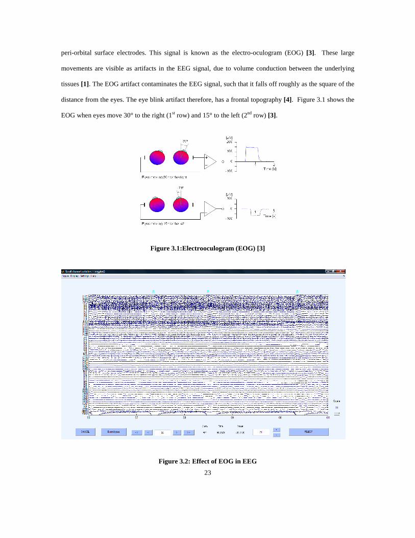
peri-orbital surface electrodes. This signal is known as the electro-oculogram (EOG) [3]. These large

movements are visible as artifacts in the EEG signal, due to volume conduction between the underlying

tissues [1]. The EOG artifact contaminates the EEG signal, such that it falls off roughly as the square of the

distance from the eyes. The eye blink artifact therefore, has a frontal topography [4]. Figure 3.1 shows the

EOG when eyes move 30° to the right (1st row) and 15° to the left (2nd row) [3].

Figure 3.1:Electrooculogram (EOG) [3]

Figure 3.2: Effect of EOG in EEG

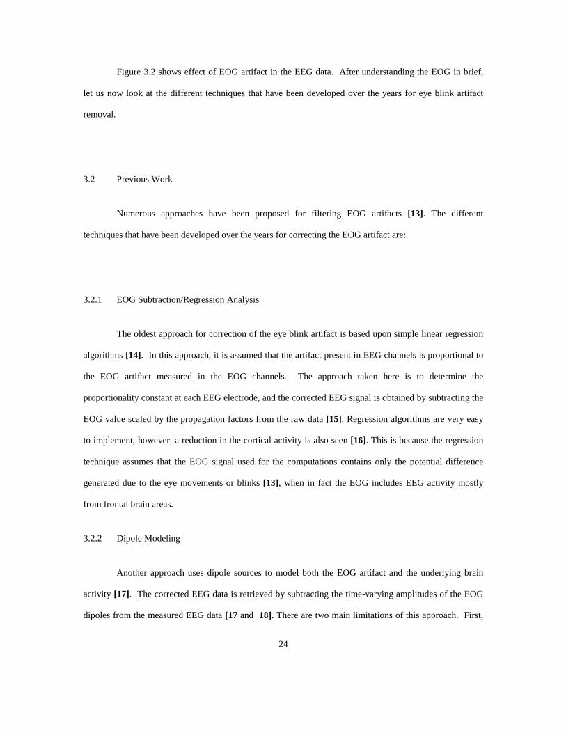
24

Figure 3.2 shows effect of EOG artifact in the EEG data. After understanding the EOG in brief,

let us now look at the different techniques that have been developed over the years for eye blink artifact

removal.

3.2 Previous Work

Numerous approaches have been proposed for filtering EOG artifacts [13]. The different

techniques that have been developed over the years for correcting the EOG artifact are:

3.2.1 EOG Subtraction/Regression Analysis

The oldest approach for correction of the eye blink artifact is based upon simple linear regression

algorithms [14]. In this approach, it is assumed that the artifact present in EEG channels is proportional to

the EOG artifact measured in the EOG channels. The approach taken here is to determine the

proportionality constant at each EEG electrode, and the corrected EEG signal is obtained by subtracting the

EOG value scaled by the propagation factors from the raw data [15]. Regression algorithms are very easy

to implement, however, a reduction in the cortical activity is also seen [16]. This is because the regression

technique assumes that the EOG signal used for the computations contains only the potential difference

generated due to the eye movements or blinks [13], when in fact the EOG includes EEG activity mostly

from frontal brain areas.

3.2.2 Dipole Modeling

Another approach uses dipole sources to model both the EOG artifact and the underlying brain

activity [17]. The corrected EEG data is retrieved by subtracting the time-varying amplitudes of the EOG

dipoles from the measured EEG data [17 and 18]. There are two main limitations of this approach. First,

25

the accuracy of this technique depends upon the accuracy of the dipole models, which requires an accurate

electrode model [18]. That in turn requires measurements of the electrode locations, a structural MRI for

defining head tissues, and estimates of tissue conductivities, which are variable across subjects and

locations on the head and are therefore not well known [4]. Second, it is exceedingly difficult and perhaps

not even sensible to model spontaneous brain activity with a small number of dipoles. It is advantageous to

have a method of ocular artifact reduction that does not require head modeling and works for both

continuous and event-related studies [13].

3.2.3 ICA /Blind Source Methods

Principal component analysis (PCA) and independent component analysis (ICA) assume that the

EEG signal is a linear mixture of statistically independent sources. An unmixing matrix is defined which is

optimized to enforce statistical independence [15]. Both techniques decompose the given signal into

spatially and temporally distinct components. The first step of ICA is PCA, so the ICs span the sub-space

of the PCs. In cases where the artifact is superimposed linearly on the signal, represented by a few

components, and among the larger components in the total signal, these techniques may be effective at

isolating the artifact. The rejected components are selected by visual inspection [15]. The corrected data is

then obtained by back-projecting all the components except those corresponding to the eye blinks [15, 19].

It has been shown that ICA is quite effective at removing certain types of artifacts, including line noise [19]

and ocular artifacts [15 and 19]. Its main limitation is that memory requirements typically prohibit the

application of ICA to long continuous data sets and hence epoched datasets need to be used [15]. This is

problematic for two reasons. First, segmenting continuous data has the strong likelihood of bisecting

artifact waveforms. If only the edge of an eye blink artifact were caught in a given epoch, for example, it

seems unlikely that it would appear as a prominent component to survive sub-space selection. Second, in

practical terms, it is often preferable to remove artifacts from data before segmenting according to a given

stimulus or response. There may be multiple segmenting strategies available in a given data set, and

26

comparisons between conditions may become biased by independent application of artifact filtering. For

all these reasons, we prefer an artifact filtering strategy that can be applied to continuous data [13].

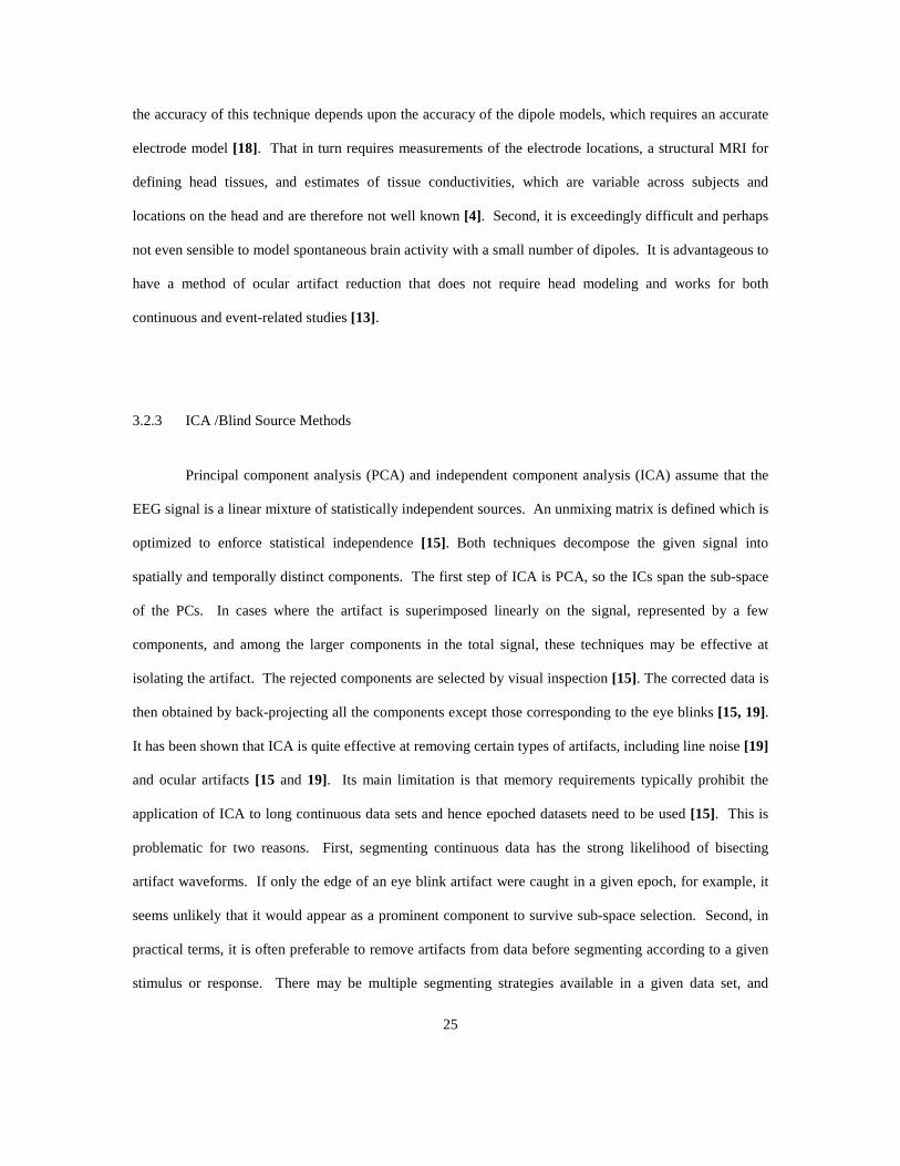
3.2.4 Spatial Filter

The waveform of a given EEG data segment is considered as a linear combination of two other

waveform signals namely, the artifact signal and brain activity signal. These two signals are used to model

their own topographies in other words, the spatial distribution over the entire scalp region. The

topographies thus gives the spatial distribution while, the waveform indicates their time course variation.

Figure 3.3 shows the decomposition of a small EEG data segment into its artifact and brain signal

components and then further into their respective topographies and waveforms. This modeled artifact

topography is then inverted to obtain the spatial filter coefficients [20].

Figure 3.3: Spatial filter [20]

27

3.3 Theory of The Spatial Filter

Multi-channel EEG data comprises a multivariate dataset having dimensions N*T, where N is the

number of electrodes, and T is the number of sample points for each electrode. The spatial filter algorithm

described here uses two files, generated from the original data file: an average artifact file, and an artifact-

free file. The average artifact file is the average of all epochs generated from artifact examples, and has

dimension N*TE, where N is the number of electrodes, and TE is the duration of the artifact epoch. For an

eye blink, this duration is normally 800 milliseconds (–200 to +600 ms relative to the peak). This average

artifact file has the EEG signal at all the electrodes suppressed approximately by 1/√E, where E is the total

number of epochs contributing in the average. The pre-whitening filter is constructed from the artifact-free

file, typically 30-60 seconds long. The spatial covariance of each of these files is N*N. Covariance is used

rather than correlation, to preserve the spatial variations in amplitude that characterize ocular artifacts.

In order to motivate the analytical form of the spatial filter and its pre-whitening matrix, consider

the average eye blink signal, a, to be a superposition of the pure blink signal, b, and pure EEG signal, c.

Recording blinks without any superimposed EEG signal is not practical; hence the best estimate of the eye

blink is obtained by removing the contributions of the background EEG data. In the present formulation,

these contributions are removed only at the level of the signal covariance, which is sufficient for linear

spectral analysis. This transformation is achieved by pre-multiplying the multivariate average eye blink file

by the matrix C–1/2, where C is the covariance matrix of the preserved or pure EEG data, i.e., C = ccT. This

step is a type of pre-whitening of the data. Let ā (having the same dimensions as that of a) be the average

eye blink in the transformed system.

The covariance matrix, Ā, of the matrix ā, having dimensions N*N, can be written

TaaA=

( )( )TaCaCA 2/12/1 −−=

28

( )TT CaaCA 2/12/1 −−=

2/12/1 −−= ACCA ---- Equation 12

Since C–1/2 is a real Hermitian matrix, it remains unchanged by the transpose operation. The

covariance matrix of the average blink signal with the covariance of EEG present i.e. a, can be written as

( )( )TT cbcbaaA ++==

TT ccbbA += ---- Equation 13

The two cross terms (bcT and cbT) are dropped from the further computations, under the

assumption that the blink artifact is uncorrelated with the brain EEG. Recent reports suggest that this may

be not entirely correct, nevertheless, it is assumed here to simplify the derivation. The above equation thus

represents sum of two covariance matrices: pure blink B = bbT, and pure EEG C = ccT. The matrix Ā

therefore can be manipulated as follows:

2/12/1 −−= ACCA ---- Equation 14

2/12/12/12/1 −−−− += CCCBCCA /2

IBCCA += −− 2/12/1

TUWUA= ---- Equation 15

Since B and C are covariance matrices, the matrix Ā is also symmetric. It is trivial to show that

pure EEG data, when pre-whitened, gives the identity matrix, I. The eigenvalue decomposition of the

matrix Ā, gives the eigenvalue matrix W and eigenvector matrix U. Note that the eigenvalues are equal to

those the matrix C–1/2 B C–1/2, simply increased by 1:

29

( ) xxxIM +=+ λ ---- Equation 16

( ) ( )xxIM 1+=+ λ

A corollary is that the eigenvectors are identical. This implies that, even though the topography of

the pure blink is not available, the topography of the pre-whitened eye blink can be obtained. The

eigenvectors of this pre-whitened eye blink give us the projection of the eye blink over the scalp. The

artifact (eye blink) subspace is captured by UrUrT, where r is the number of components corresponding to

the artifact. The number of components can be determined subjectively or on statistical grounds (section

3.4.3). To remove the projections of the artifact from the data, the artifact subspace is subtracted from the

identity matrix (I - UrUrT) [21].

In order to filter artifacts from the data, consider the spatial filter defined by

( ) 2/12/1 −−= CUUICF Trr ---- Equation 17

To correct the artifact contaminated data we pre-multiply the filter coefficients, F, to the EEG data. The

EEG data has the covariance due to EEG present. The projections in Ur are of the pre-whitened eye blink.

It is hence required that before the artifact subspace is removed from the EEG data, the covariance due to

EEG be removed. The artifact subspace therefore needs to be post-multiplied by the matrix C-1/2. In order

to get the corrected data without the distortion we need to restore the covariance due to EEG. Hence, the

artifact subspace is pre-multiplied by the matrix C1/2 [13 and 22].

3.4 Method

3.4.1 Clean Data File

As discussed in Section 3.3, for removing the EEG covariance from the average eye blink file, a

clean pure EEG file representing the underlying brain activity is required. This clean or artifact-free EEG

30

file was created in Scan Edit 4.3. Data segments having no artifact contamination were selected manually.

These data segments were then concatenated. This file is then imported to Matlab using the EEGLAB

Toolbox. The covariance of this file is then computed thus forming the matrix, C.

3.4.2 Average Eye Blink File

With gross artifacts removed, eye blinks were identified in the VEOG electrode by setting a

voltage threshold at -200µV. Markers were inserted at the time points where the voltage of the VEOG

electrode exceeds the set threshold (99 is the eye blink marker that is inserted after VEOG voltage

threshold see Figure 3.2). This file with the eye blink markers was then segmented around these markers.

The eye blink epochs span -200 to +600 milliseconds around these eye blink markers. This file is a three-

way array with dimensions N*TE*E, where N is the number of electrodes, TE is the epoch length (in our

case 800 milliseconds), and E is the number of epochs. This file was then used as an input to a GUI,

created in Matlab, which helps selection of the eye blinks epochs (section 3.5.1). The average eye blink

after file is then made from the selected epochs and used to determine the number of components to be

retained, as discussed below.

3.4.3 Sensitivity to Number of Components Retained

The selection of r, the number of components to retain in the eigenvalue decomposition of the

artifact template, is the key to the formation of the spatial filter F. The most common method, for

determining r, is to retain enough components to explain a specified fraction of the total variance, but the

choice of that fraction remains arbitrary. There is a substantial literature on statistical methods for making

this choice objectively. We have investigated these methods in recent work [23], and found parallel

analysis to perform well. This is essentially a generalization of the familiar eigenvalue-greater-than-one

criterion [24]. That criterion is applicable to correlation matrices, and uses the fact that a correlation matrix

31

formed from an infinite number of samples of Gaussian distributed data has all eigenvalues equal to one

[25]. For finite correlation matrices, however, it is known that null data have eigenvalues distributed

around one. A refinement, therefore, is to form an ensemble of null data matrices with the same

dimensions as the original data matrix, and compute a null distribution for each eigenvalue [24]. Parallel

analysis [25 generalizes this approach further, to accommodate covariance matrices whose eigenvalues

deviate from one according to the magnitudes of the numbers in the original data matrix. In our

implementation of parallel analysis, the null data matrices were generated by shuffling all of the values in

the original data matrix, mixing both rows and columns [23].

In order to select r, Scan Edit 4.3 permits the user to select a percent variance to retain, but

provides no guidance on how to select that percentage. In order to assess the sensitivity of the spatial filter

to r, that parameter was varied in our Matlab implementation as the spatial filter was applied to the model

data set [13].

3.5 Results

3.5.1 GUI for Eye Blink Epoch Selection

The VEOG channels of eyes open and normal blinking dataset were voltage threshold and eye

blink markers were added to obtain the epoched file (section 3.4.2). Epochs from the epoched file which

resembled the time series of an eye blink were used to compute the average eye blink file. For selection of

these epochs a Graphic User Interface (GUI) as shown in the Figure 3.4 was created.

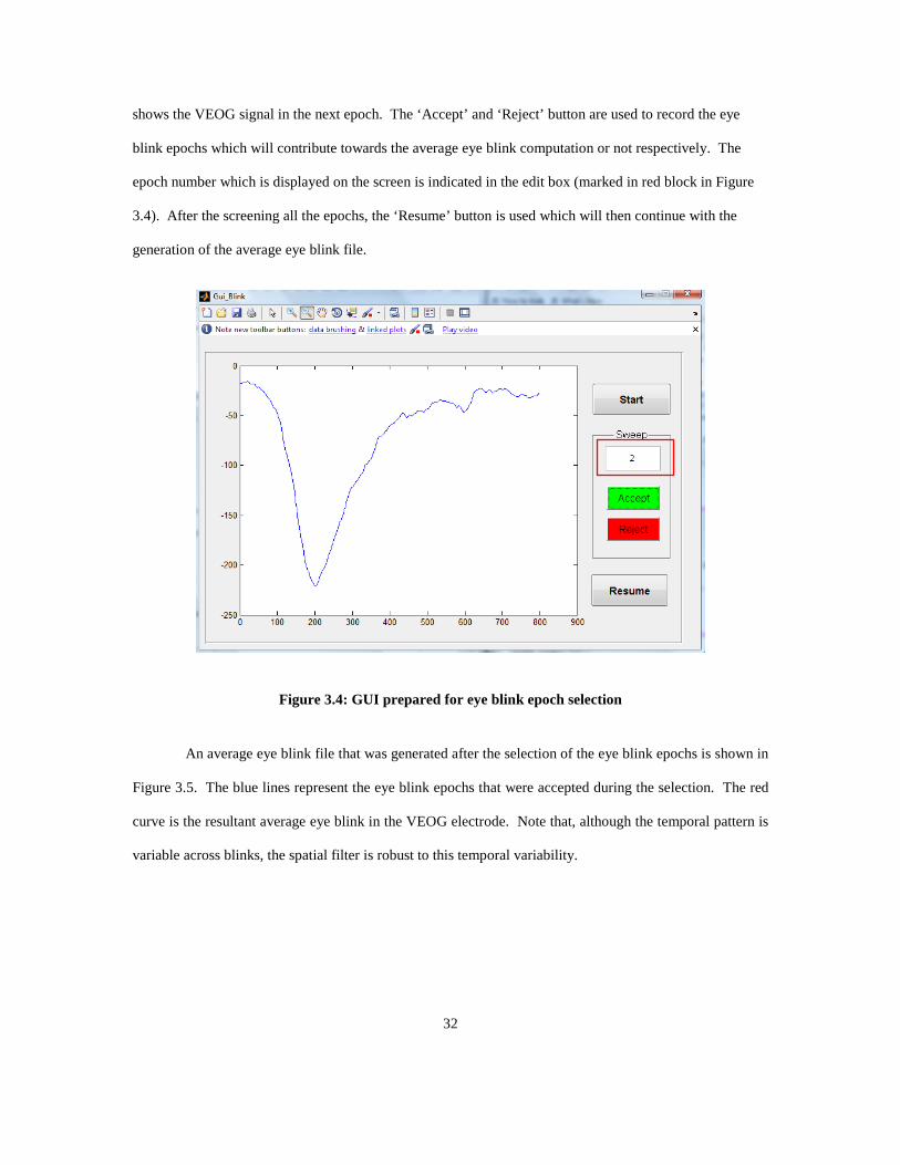
The GUI displays the VEOG signal in each epoch. The ‘Start’ button is used to start the display

of the VEOG signal in the 1st epoch. After display of the VEOG signal decision is made to either accept or

reject this epoch. The epoch is accepted only if it resembles the eye blinks seen in the entire file. The

‘Accept’ button is then used to record this epoch number. If the signal in the epoch does not look like an

eye blink then ‘Reject’ button is used which records the epoch number. The display is then refreshed and it

32

shows the VEOG signal in the next epoch. The ‘Accept’ and ‘Reject’ button are used to record the eye

blink epochs which will contribute towards the average eye blink computation or not respectively. The

epoch number which is displayed on the screen is indicated in the edit box (marked in red block in Figure

3.4). After the screening all the epochs, the ‘Resume’ button is used which will then continue with the

generation of the average eye blink file.

Figure 3.4: GUI prepared for eye blink epoch selection

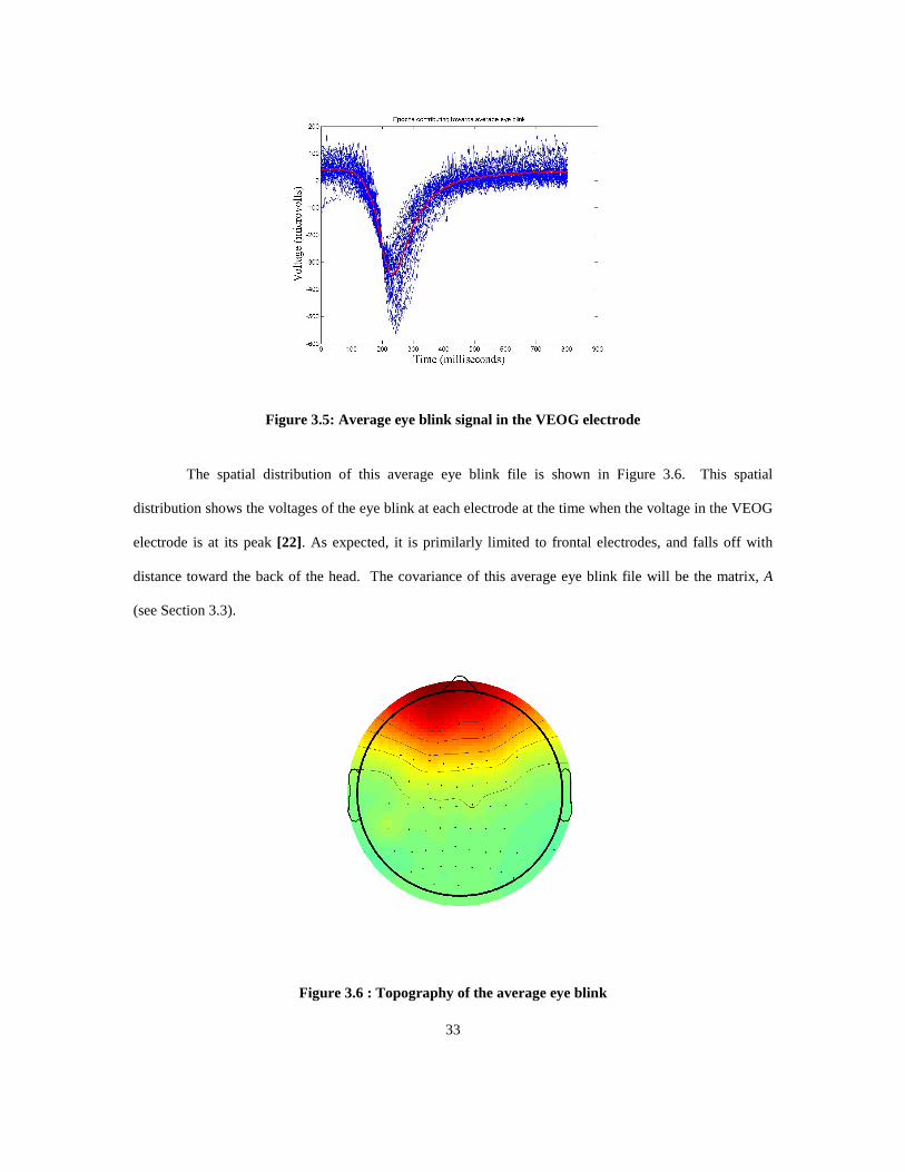
An average eye blink file that was generated after the selection of the eye blink epochs is shown in

Figure 3.5. The blue lines represent the eye blink epochs that were accepted during the selection. The red

curve is the resultant average eye blink in the VEOG electrode. Note that, although the temporal pattern is

variable across blinks, the spatial filter is robust to this temporal variability.

33

Figure 3.5: Average eye blink signal in the VEOG electrode

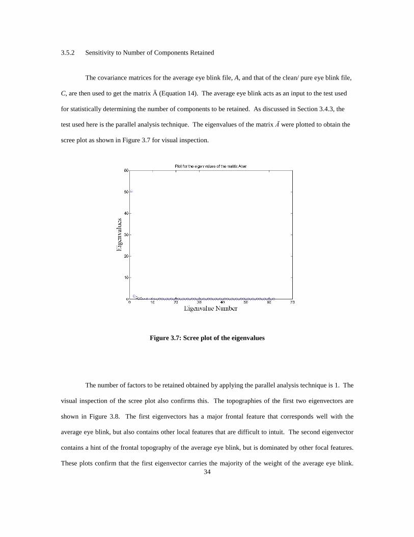
The spatial distribution of this average eye blink file is shown in Figure 3.6. This spatial

distribution shows the voltages of the eye blink at each electrode at the time when the voltage in the VEOG

electrode is at its peak [22]. As expected, it is primilarly limited to frontal electrodes, and falls off with

distance toward the back of the head. The covariance of this average eye blink file will be the matrix, A

(see Section 3.3).

Figure 3.6 : Topography of the average eye blink

34

3.5.2 Sensitivity to Number of Components Retained

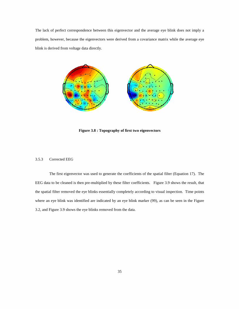
The covariance matrices for the average eye blink file, A, and that of the clean/ pure eye blink file,

C, are then used to get the matrix Ā (Equation 14). The average eye blink acts as an input to the test used

for statistically determining the number of components to be retained. As discussed in Section 3.4.3, the

test used here is the parallel analysis technique. The eigenvalues of the matrix Ā were plotted to obtain the

scree plot as shown in Figure 3.7 for visual inspection.

Figure 3.7: Scree plot of the eigenvalues

The number of factors to be retained obtained by applying the parallel analysis technique is 1. The

visual inspection of the scree plot also confirms this. The topographies of the first two eigenvectors are

shown in Figure 3.8. The first eigenvectors has a major frontal feature that corresponds well with the

average eye blink, but also contains other local features that are difficult to intuit. The second eigenvector

contains a hint of the frontal topography of the average eye blink, but is dominated by other focal features.

These plots confirm that the first eigenvector carries the majority of the weight of the average eye blink.

35

The lack of perfect correspondence between this eigenvector and the average eye blink does not imply a

problem, however, because the eigenvectors were derived from a covariance matrix while the average eye

blink is derived from voltage data directly.

Figure 3.8 : Topography of first two eigenvectors

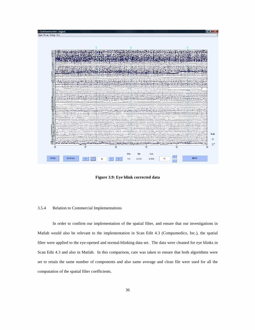
3.5.3 Corrected EEG

The first eigenvector was used to generate the coefficients of the spatial filter (Equation 17). The

EEG data to be cleaned is then pre-multiplied by these filter coefficients. Figure 3.9 shows the result, that

the spatial filter removed the eye blinks essentially completely according to visual inspection. Time points

where an eye blink was identified are indicated by an eye blink marker (99), as can be seen in the Figure

3.2, and Figure 3.9 shows the eye blinks removed from the data.

36

Figure 3.9: Eye blink corrected data

3.5.4 Relation to Commercial Implementations

In order to confirm our implementation of the spatial filter, and ensure that our investigations in

Matlab would also be relevant to the implementation in Scan Edit 4.3 (Compumedics, Inc.), the spatial

filter were applied to the eye-opened and normal-blinking data set. The data were cleaned for eye blinks in

Scan Edit 4.3 and also in Matlab. In this comparison, care was taken to ensure that both algorithms were

set to retain the same number of components and also same average and clean file were used for all the

computation of the spatial filter coefficients.

37

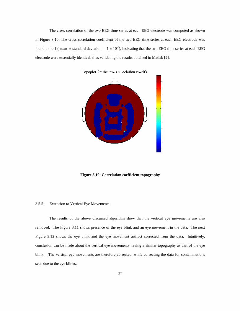
The cross correlation of the two EEG time series at each EEG electrode was computed as shown

in Figure 3.10. The cross correlation coefficient of the two EEG time series at each EEG electrode was

found to be 1 (mean ± standard deviation = 1 ± 10-6), indicating that the two EEG time series at each EEG

electrode were essentially identical, thus validating the results obtained in Matlab [9].

Figure 3.10: Correlation coefficient topography

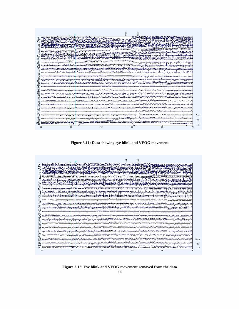
3.5.5 Extension to Vertical Eye Movements

The results of the above discussed algorithm show that the vertical eye movements are also

removed. The Figure 3.11 shows presence of the eye blink and an eye movement in the data. The next

Figure 3.12 shows the eye blink and the eye movement artifact corrected from the data. Intuitively,

conclusion can be made about the vertical eye movements having a similar topography as that of the eye

blink. The vertical eye movements are therefore corrected, while correcting the data for contaminations

seen due to the eye blinks.

38

Figure 3.11: Data showing eye blink and VEOG movement

Figure 3.12: Eye blink and VEOG movement removed from the data

39

CHAPTER 4

SUBTLE ARTIFACT REMOVAL

After removing gross artifacts and eye blinks, data typically have other more subtle artifacts

present. These include horizontal eye movements, muscle artifacts, etc. Effect of each of these artifacts

seen on the EEG data is different and hence, needs to be treated differently. Each artifact therefore, needs

to be characterized differently depending on the effect seen on the data. Similar to the gross artifact

removal, a statistical and automated method is presented to remove or correct these subtle artifacts from the

dataset. In the approach presented below, several common artifacts are dealt with in order of their

amplitude or severity.

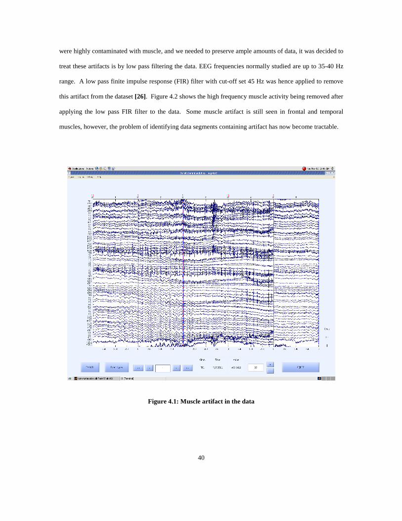
4.1 Muscle Artifacts

Muscle artifacts are second most frequent artifacts seen in the acquired EEG data as seen in Figure

4.1. Myogenic potentials are the cause of the muscle artifact. These potentials are generated due to stress

on the frontal muscles or movement or clenching of the jaw. These artifacts generated are mainly seen as

broad-banded noise in the data, or on the basis of its morphology and duration [5]. The simplest approach

to eliminate muscle artifacts would be to discard those data segments. In studies such as ours, however, in

which muscle artifacts are prominent, little data would be left with that approach. Another obvious

approach would be to use ICA to isolate muscle artifacts into a small number of components, which could

be eliminated by discarding those components. In our investigations, however, ICA is ineffective for this

problem, because muscle activity appears in most or all components produced by ICA. Because our data

40

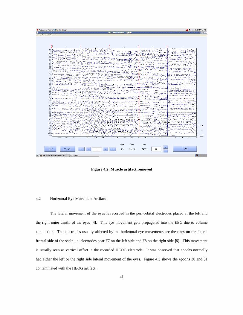
were highly contaminated with muscle, and we needed to preserve ample amounts of data, it was decided to

treat these artifacts is by low pass filtering the data. EEG frequencies normally studied are up to 35-40 Hz

range. A low pass finite impulse response (FIR) filter with cut-off set 45 Hz was hence applied to remove

this artifact from the dataset [26]. Figure 4.2 shows the high frequency muscle activity being removed after

applying the low pass FIR filter to the data. Some muscle artifact is still seen in frontal and temporal

muscles, however, the problem of identifying data segments containing artifact has now become tractable.

Figure 4.1: Muscle artifact in the data

41

Figure 4.2: Muscle artifact removed

4.2 Horizontal Eye Movement Artifact

The lateral movement of the eyes is recorded in the peri-orbital electrodes placed at the left and

the right outer canthi of the eyes [4]. This eye movement gets propagated into the EEG due to volume

conduction. The electrodes usually affected by the horizontal eye movements are the ones on the lateral

frontal side of the scalp i.e. electrodes near F7 on the left side and F8 on the right side [5]. This movement

is usually seen as vertical offset in the recorded HEOG electrode. It was observed that epochs normally

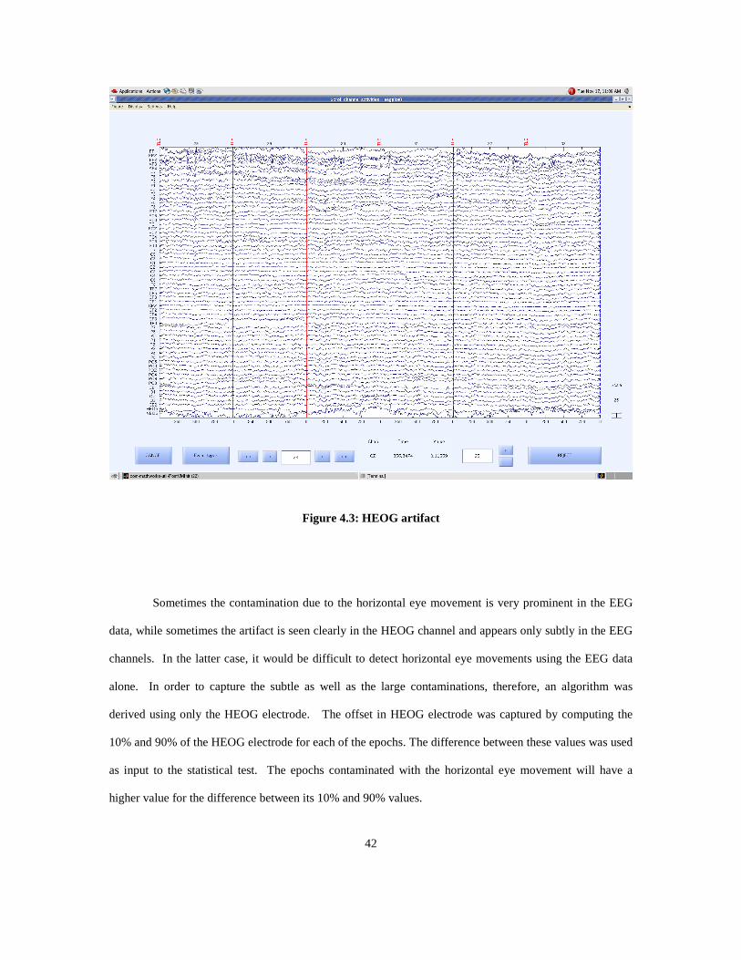
had either the left or the right side lateral movement of the eyes. Figure 4.3 shows the epochs 30 and 31

contaminated with the HEOG artifact.

42

Figure 4.3: HEOG artifact

Sometimes the contamination due to the horizontal eye movement is very prominent in the EEG

data, while sometimes the artifact is seen clearly in the HEOG channel and appears only subtly in the EEG

channels. In the latter case, it would be difficult to detect horizontal eye movements using the EEG data

alone. In order to capture the subtle as well as the large contaminations, therefore, an algorithm was

derived using only the HEOG electrode. The offset in HEOG electrode was captured by computing the

10% and 90% of the HEOG electrode for each of the epochs. The difference between these values was used

as input to the statistical test. The epochs contaminated with the horizontal eye movement will have a

higher value for the difference between its 10% and 90% values.

43

4.3 Head Movement Artifact

Head movements made by the subject get propagated into the EEG data. The effect of the head

movement is seen as long drifts in the EEG data. The effect of the head movements is seen in all

electrodes. The direction of the drift is different in different electrodes. A mean across all the electrodes at

all time points in the epoch is computed. This mean signal thus represents the behavior of the epoch. A 1st

degree polynomial is then fitted to this mean of the epoch. The slope of this equation is then an input to the

statistical test. The higher the slope value the more is the contamination due to the head movement.

Figure 4.4: Head movement artifact in the data

44

4.4 Inter-Electrode Gap

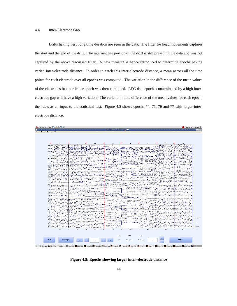
Drifts having very long time duration are seen in the data. The fitter for head movements captures

the start and the end of the drift. The intermediate portion of the drift is still present in the data and was not

captured by the above discussed fitter. A new measure is hence introduced to determine epochs having

varied inter-electrode distance. In order to catch this inter-electrode distance, a mean across all the time

points for each electrode over all epochs was computed. The variation in the difference of the mean values

of the electrodes in a particular epoch was then computed. EEG data epochs contaminated by a high inter-

electrode gap will have a high variation. The variation in the difference of the mean values for each epoch,

then acts as an input to the statistical test. Figure 4.5 shows epochs 74, 75, 76 and 77 with larger inter-

electrode distance.

Figure 4.5: Epochs showing larger inter-electrode distance

45

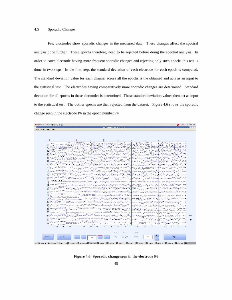
4.5 Sporadic Changes

Few electrodes show sporadic changes in the measured data. These changes affect the spectral

analysis done further. These epochs therefore, need to be rejected before doing the spectral analysis. In

order to catch electrode having more frequent sporadic changes and rejecting only such epochs this test is

done in two steps. In the first step, the standard deviation of each electrode for each epoch is computed.

The standard deviation value for each channel across all the epochs is the obtained and acts as an input to

the statistical test. The electrodes having comparatively more sporadic changes are determined. Standard

deviation for all epochs in these electrodes is determined. These standard deviation values then act as input

to the statistical test. The outlier epochs are then rejected from the dataset. Figure 4.6 shows the sporadic

change seen in the electrode P6 in the epoch number 74.

Figure 4.6: Sporadic change seen in the electrode P6

46

4.6 Statistical Test

The statistical test used here to determine the outlier epochs/ channels is the two tailed - Median

Absolute Deviation test (refer section 2.2.2). A two tailed test is chosen over a one-tailed test since, not all

input quantities are positive. Hence both the upper as well as lower boundary values were determined.

Boundary values are given by the following formula,

ee XYLim ∗±= λ ---- Equation 18

where, Ye is the median of the input values, λ is the confidence coefficient and set to 3 [2.2.2 and 8], Xe is

the median of the absolute deviations, De of the values, Ve from their medians. The absolute deviations are

computed using following formula,

eee YVD −= ---- Equation 19

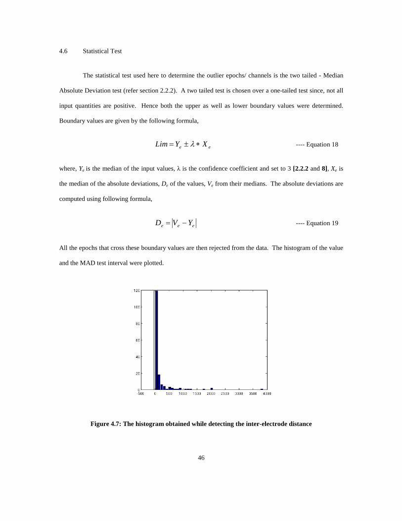
All the epochs that cross these boundary values are then rejected from the data. The histogram of the value

and the MAD test interval were plotted.

Figure 4.7: The histogram obtained while detecting the inter-electrode distance

47

Figure 4.7 shows the histogram showing the value computed while determining the epochs with

unusual inter-electrode distance. The epochs that were determined to be outliers where visually inspected

for correctness. The results of this statistical test were verified by visual inspection of the data and showed

a good agreement.

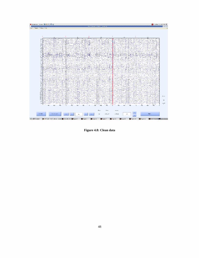
4.7 Results

Figure 4.8 shows the resultant artifact free clean data. After the entire subtle artifact removal

algorithm was used, the dataset looks completely artifact free. In fact, visual inspection of the entire data

record showed small residual artifacts that were not caught by our algorithms. The effort was still a

success, however, for two reasons. First, these small and infrequent artifacts are not likely to have a large

influence on any subsequent calculations, e.g., event-related potentials, Fourier power spectrum or

coherence. Second, the cleanliness of the data now makes it very simple for an EEG technician to review

the data visually and make additional rejections.

48

Figure 4.8: Clean data

49

CHAPTER 5

FUTURE WORK AND CONCLUSION

The goal of this work was to develop a semi-automatic data pipeline for rejecting and/or filtering

artifacts seen commonly in EEG data, with the intention that the output signal obtained after preprocessing

of the EEG data can be easily used by scientists and clinicians. This facilitates further research in at least

three ways. First, in large studies with many subjects, this improves efficiency. Second, because the tests

for rejecting data are phrased in statistical terms, it can be argued that the approach is more valid that visual

inspection. Third, because the statistical thresholds can be stated precisely, this permits the methodology to

be articulated clearly, making it possible to reproduce the results of preprocessing across studies,

technicians and laboratories.

In its present form, this data pipeline is semi-automatic, but with more work it could be

automated essentially completely. Automation of this process would not only reduce manpower time but

also further increase the reliability and reproducibility. Additional steps need to be taken for selection of

the eye blink epochs and generation of the clean EEG data segments. One of the approaches, which could

be used taken to solve this problem, is correlating a standard eye blink signal for the VEOG electrode with

the VEOG electrode of file to be analyzed. This standard eye blink signal is computed in two steps. In the

first step of the computation, averaging is done across a number of trials for each individual. This signal

obtained for each individual is then averaged across all the individuals. Since averaging is done twice, the

background EEG in the standard eye blink signal is infinitesimally small. Automatically generating a clean

data file, however, is a much more difficult proposition. One approach might be to use the techniques

designed for gross artifact detection to find segments of data with the smallest amplitudes. This is

50

justifiable because, assuming that the desired EEG and artifacts are uncorrelated, contaminated data

segments can only have larger amplitudes. In this way, data segments with the smallest amplitudes can be

assumed to be clean. One danger with this approach, however, is that legitimate brain activity fluctuates

through time. Selecting data segments with the smallest amplitudes may exclude time intervals in which

typical EEG is in fact present. This could bias the performance of the spatial filter.

Another important extension of this work is the consideration of the number of task conditions

when selecting clean data for building the spatial filter. Imagine that two task conditions different in their

degree of frontal brain activity. If the clean file were generated from data acquired during one task

condition primarily, then the clean data file would be biased to include or exclude that activity. Further

work is required to quantify this effect. If one were concerned about this point then, ideally, one would

take care that the clean data file contained data from both conditions in equal amounts. In this way, there

would be no systematic bias in the formation of the clean data file, although the effect if the difference in

brain activity between conditions may still not be entirely negligible.

51

REFERENCES

1. http://en.wikipedia.org/wiki/Electroencephalography

2. Nunez, P. (1981). Electric Fields of the Brain. Oxford University Press

3. Malmivuo, J. and Plonsey, R. (1995). Bioelectromagnetism –Principles and Applications of

Bioelectric and Biomagnetic Fields. Oxford University Press

4. Croft, R. and Barry, R. (1999). Removal of ocular artifact from the EEG: a review. Neurophysiol

Clin, 30, 5-19

5. http://emedicine.medscape.com/article/1140247-overview

6. Knight, J. (2003). Signal Fraction Analysis and Artifact Removal in EEG. Thesis. Colorado State

University, United States

7. Ille, N. (2001). Artifact correction in continuous recordings of the electro- and magneto-

encephalogram by spatial filtering. Dissertation. University of Mannheim, Germany

8. Junghöfer, M., Elbert, T., Tucker, D. and Rockstroh, B. (2000). Statistical Control of Artifacts in

dense array EEG/MEG studies. Psychophysiology, 37, 523-532

9. Lawson, J., Galin, H., Adams, S., Brunet, D., Criollo, M. and MacCrimmon, D. (2003).

Artefacting reliability in QEEG topographic maps. Clin Neurophysiol, 114, 883-888

10. Viola, F., Thorne, J., Edmonds, B., Schneider, T., Eichele, T., Debener, S. (2009). Semi-automatic

identification of independent components representing EEG artifact. Clin Neurophysiol, 120, 868-

877

11. http://en.wikipedia.org/wiki/Root_mean_square

12. http://en.wikipedia.org/wiki/Mean_absolute_deviation

52

13. Bhat, J., Tatebe, K., Brier, M., Pflieger, M., Ferree, T. Spatial Filtering to Remove Ocular

Artifacts: A Pre-whitening Approach to Preserve the EEG. (In preparation for Psychophysiology)

14. Jervis, B., Coelho, M. and Morgan, G. (1989). Effect on EEG responses of removing ocular

artefacts by proportional EEG subtraction. Med Biol Eng Comput, 27, 484-490.

15. Hoffmann, S. and Falkenstein, M. (2008). The Correction of Eye Blink Artefacts in the EEG: A

Comparison of Two Prominent Methods. PLoS ONE, 3, e2004.

16. Schögl, A., Keinrath, C., Zimmermann, D., Scherer, R., Leeb, R. and Pfurtscheller, G. (2007). A

fully automated correction method of EOG artifacts in EEG recordings. Clin Neurophysiol, 118,

98-104.

17. Berg, P. and Scherg, M. (1993). A multiple source approach to the correction of eye artifacts.

Electroencephalogr Clin Neurophysiol, 90, 229-241.

18. Berg, P. and Scherg, M. (1990). Dipole models of the eye movements and blinks.

Electroencephalogr Clin Neurophysiol, 79, 36-44.

19. Jung, T., Makeig, S., Humphries, C., Lee, T. (2000). Removing electroencephalographic artifacts

by blind source separation. Psychophysiol, 37, 163-178

20. Ille, N., Berg, P. and Scherg, M.(2002). Artifact Correction of the Ongoing EEG Using Spatial

Filters based on Artifact and Brain Signal Topographies. J Clin Neurophysiol, 19, 113-124.

21. Huotilainen, M., Ilmoniemi, R., Tiitinen, H., Lavikainen, J., Alho, K., Kajola, M. and Näätänen,

R. (1995). The projection method in removing eye-blink artefacts from multichannel MEG

measurements. In: Baumgartner, C., Deecke, L., Stroink, G., Williamson, S. J., eds.

Biomagnetism: fundamental research and clinical applications: Elsevier Science, IOS Press, 363-

367.

22. Pflieger, M. (2001). Theory of a Spatial Filter for Removing Ocular Artifacts with Preservation of

EEG, presented at EMSE Workshop at Princeton, 2001.

23. Ferree, T., Brier, M., Hart, J., Kraut, M. (2009). Space-time frequency analysis of EEG data using

within-subject statistical test followed by sequential PCA. Neuroimage, 45, 109-121.

53

24. Zwick, W. and Velicer, W. (1986). Comparison of Five Rules for Determining the Number of

Comparison to Retain. Psychological Bulletin, 99, 432-442.

25. Horn, J. (1965). A Rationale and Test for the Number of Factors in Factor Analysis.

Psychometrica, 30, 179-185.

26. http://sccn.ucsd.edu/eeglab/allfunctions/index.html

54

BIOGRAPHICAL INFORMATION

Jyoti Bhat, was born in March 1985, in Pune, Maharashtra, India. She completed her Bachelor of

Engineering Degree in Instrumentation and Control from Cummins College of Engineering for Women,

University of Pune, India in July 2007. She joined the University of Texas at Arlington, in fall 2007 to

pursue her Master’s of Science Degree in Bioengineering. Her research interests include Digital Signal

Processing and Neuro-imaging.