Signal Detection Basics - CFAR • Types of noise (clutter) and signals (targets) • Signal separation by comparison (threshold detection) • Signal Statistics - Parameter estimation • Threshold determination based on the required P fa • CFAR detectors design • Detection Performance Vassilis Anastassopoulos, Physics Department

Welcome message from author
This document is posted to help you gain knowledge. Please leave a comment to let me know what you think about it! Share it to your friends and learn new things together.
Transcript

Signal Detection Basics - CFAR
• Types of noise (clutter) and signals (targets)
• Signal separation by comparison (threshold detection)
• Signal Statistics - Parameter estimation
• Threshold determination based on the required Pfa
• CFAR detectors design
• Detection Performance
Vassilis Anastassopoulos, Physics Department
2/35
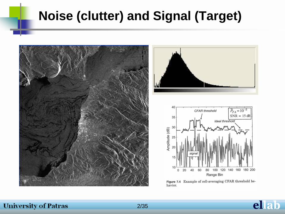
Noise (clutter) and Signal (Target)
3/35
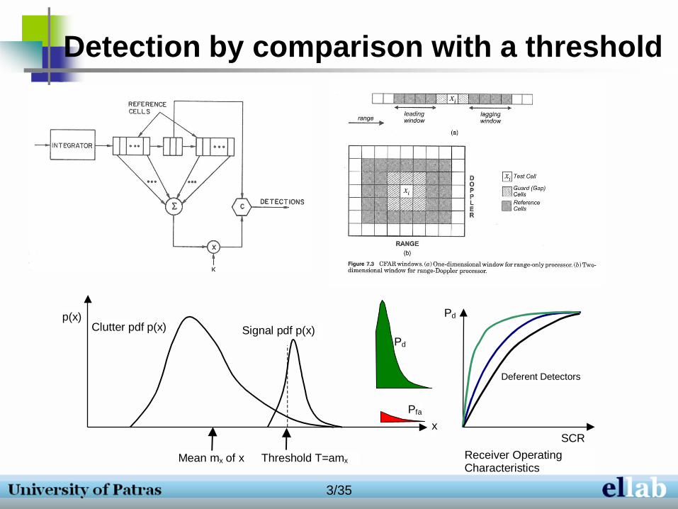
Detection by comparison with a threshold
Threshold T=amx
Clutter pdf p(x) Signal pdf p(x)
p(x)
x
Pd
Pfa
Mean mx of x
Pd
SCR
Receiver Operating Characteristics
Deferent Detectors
4/35
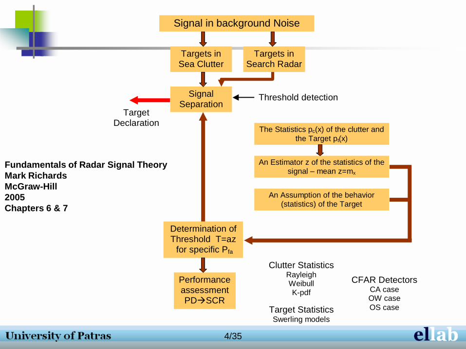
Signal in background Noise
Targets in Sea Clutter
Targets in Search Radar
Signal Separation
Threshold detection
The Statistics pc(x) of the clutter and
the Target pt(x)
An Estimator z of the statistics of the signal – mean z=mx
An Assumption of the behavior (statistics) of the Target
Determination of Threshold T=az for specific Pfa
Performance assessment PDSCR
Target Declaration
Clutter Statistics Rayleigh Weibull K-pdf
CFAR Detectors CA case OW case
OS case Target Statistics Swerling models
Fundamentals of Radar Signal Theory
Mark Richards
McGraw-Hill
2005
Chapters 6 & 7
5/35
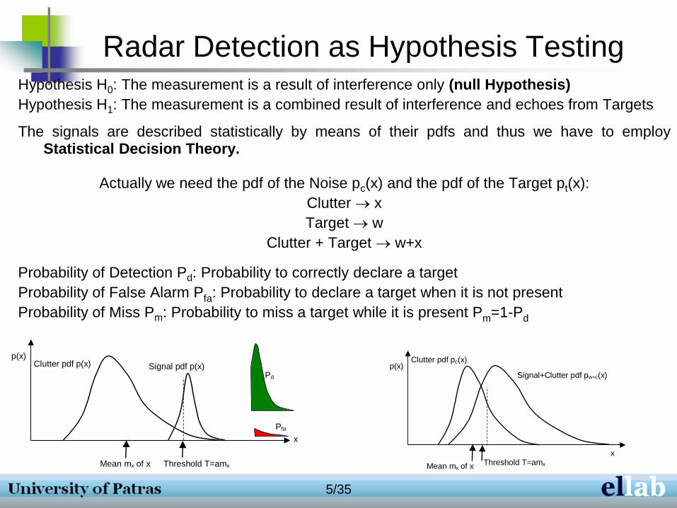
Radar Detection as Hypothesis Testing Hypothesis H0: The measurement is a result of interference only (null Hypothesis)
Hypothesis H1: The measurement is a combined result of interference and echoes from Targets
The signals are described statistically by means of their pdfs and thus we have to employ Statistical Decision Theory.
Actually we need the pdf of the Noise pc(x) and the pdf of the Target pt(x):
Clutter x
Target w
Clutter + Target w+x
Probability of Detection Pd: Probability to correctly declare a target
Probability of False Alarm Pfa: Probability to declare a target when it is not present
Probability of Miss Pm: Probability to miss a target while it is present Pm=1-Pd
Threshold T=amx
Clutter pdf p(x) Signal pdf p(x)
p(x)
x
Pd
Pfa
Mean mx of x
Threshold T=amx
Clutter pdf pc(x)
Signal+Clutter pdf pw+c(x) p(x)
x
Mean mx of x
6/35
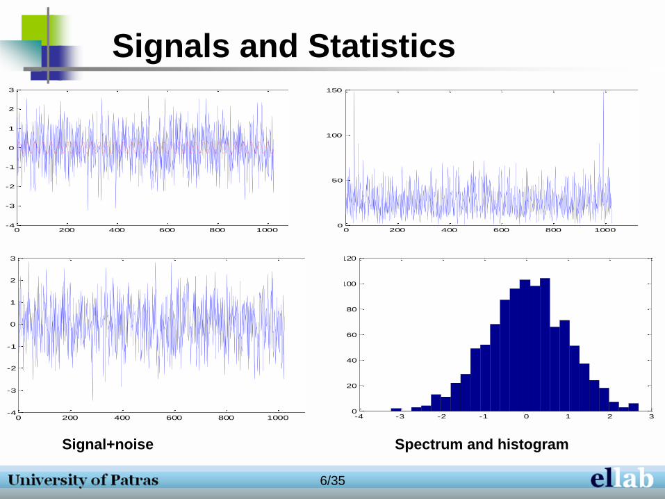
Signals and Statistics
0 200 400 600 800 1000 1200-4
-3
-2
-1
0
1
2
3
0 200 400 600 800 1000 1200-4
-3
-2
-1
0
1
2
3
0 200 400 600 800 1000 12000
50
100
150
-4 -3 -2 -1 0 1 2 30
20
40
60
80
100
120
Signal+noise Spectrum and histogram
7/35
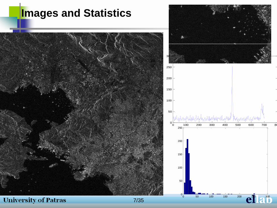
Images and Statistics
0 100 200 300 400 500 600 700 8000
50
100
150
200
250
300
0 50 100 150 200 250 3000
50
100
150
200
250
8/35
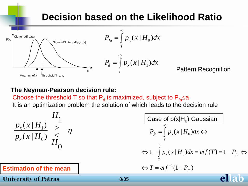
Decision based on the Likelihood Ratio
Pattern Recognition
Threshold T=amx
Clutter pdf pc(x)
Signal+Clutter pdf pw+c(x) p(x)
x
Mean mx of x
The Neyman-Pearson decision rule:
Choose the threshold T so that Pd is maximized, subject to Pfaa
It is an optimization problem the solution of which leads to the decision rule
T
xd dxHxpP )|( 1
T
xfa dxHxpP )|( 0
0
1
)|(
)|(
0
1
H
H
Hxp
Hxp
x
x
Case of p(x|H0) Gaussian
)1(
1)()|(1
)|(
1
0
0
fa
fa
T
x
T
xfa
PerfT
PTerfdxHxp
dxHxpP
Estimation of the mean
9/35
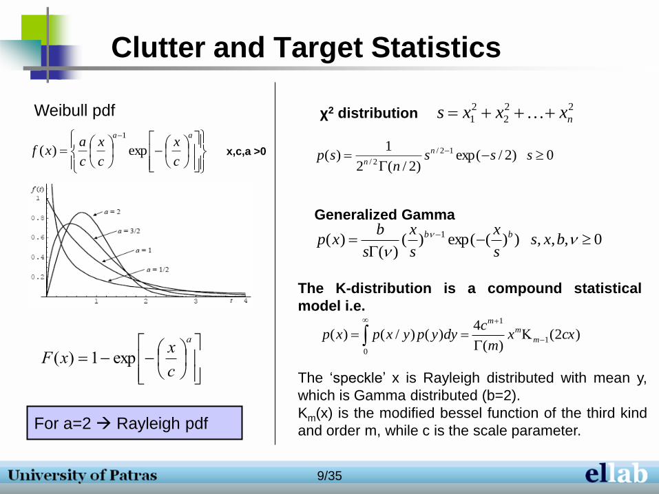
Clutter and Target Statistics
aa
c
x
c
x
c
axf exp)(
1
x,c,a >0
a
c
xxF exp1)(
Weibull pdf
For a=2 Rayleigh pdf
0 )2/exp()2/(2
1)( 12/
2/
sss
nsp n
n
χ2 distribution 22
2
2
1 nxxxs
0,,, ))(exp()()(
)( 1
bxss
x
s
x
s
bxp bb
Generalized Gamma
0
1
1
)2()(
4)()/()( cxx
m
cdyypyxpxp m
mm
The K-distribution is a compound statistical
model i.e.
The ‘speckle’ x is Rayleigh distributed with mean y,
which is Gamma distributed (b=2).
Km(x) is the modified bessel function of the third kind
and order m, while c is the scale parameter.
10/35
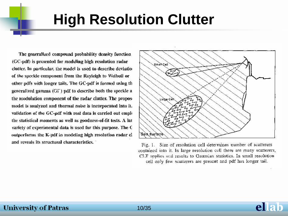
High Resolution Clutter
11/35
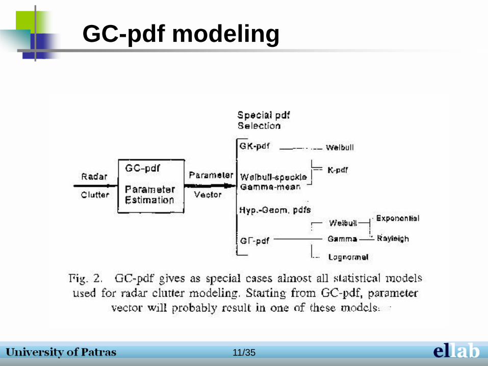
GC-pdf modeling
12/35
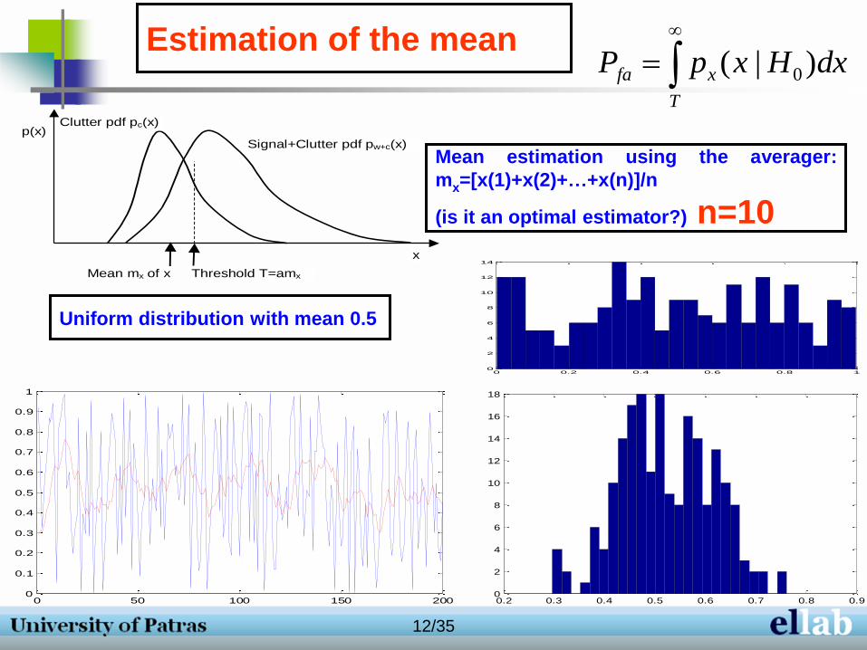
Estimation of the mean
Threshold T=amx
Clutter pdf pc(x)
Signal+Clutter pdf pw+c(x) p(x)
x
Mean mx of x
T
xfa dxHxpP )|( 0
0 0.2 0.4 0.6 0.8 10
2
4
6
8
10
12
14
0.2 0.3 0.4 0.5 0.6 0.7 0.8 0.90
2
4
6
8
10
12
14
16
18
0 50 100 150 2000
0.1
0.2
0.3
0.4
0.5
0.6
0.7
0.8
0.9
1
Mean estimation using the averager:
mx=[x(1)+x(2)+…+x(n)]/n
(is it an optimal estimator?) n=10
Uniform distribution with mean 0.5
13/35
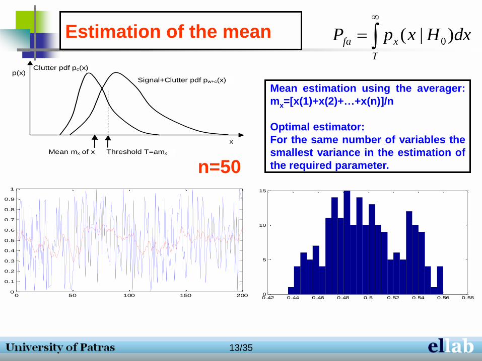
Estimation of the mean
T
xfa dxHxpP )|( 0
0 50 100 150 2000
0.1
0.2
0.3
0.4
0.5
0.6
0.7
0.8
0.9
1
0.42 0.44 0.46 0.48 0.5 0.52 0.54 0.56 0.580
5
10
15
Threshold T=amx
Clutter pdf pc(x)
Signal+Clutter pdf pw+c(x) p(x)
x
Mean mx of x
Mean estimation using the averager:
mx=[x(1)+x(2)+…+x(n)]/n
Optimal estimator:
For the same number of variables the
smallest variance in the estimation of
the required parameter. n=50
14/35
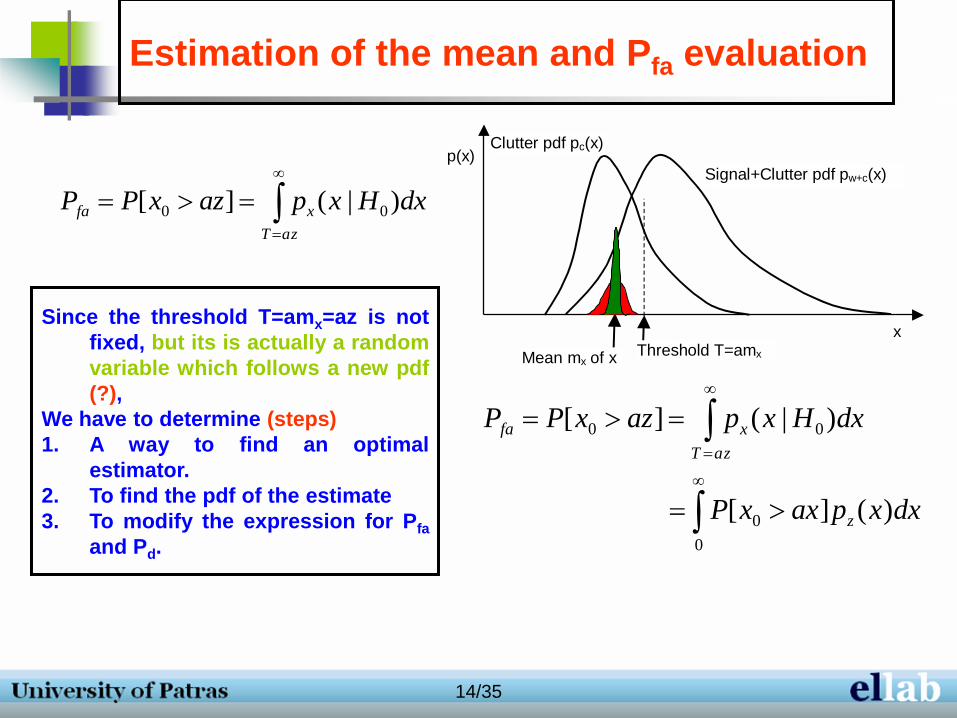
Estimation of the mean and Pfa evaluation
Since the threshold T=amx=az is not
fixed, but its is actually a random
variable which follows a new pdf
(?),
We have to determine (steps)
1. A way to find an optimal
estimator.
2. To find the pdf of the estimate
3. To modify the expression for Pfa
and Pd.
azT
xfa dxHxpazxPP )|(][ 00
0
0
00
)(][
)|(][
dxxpaxxP
dxHxpazxPP
z
azT
xfa
Threshold T=amx
Clutter pdf pc(x)
Signal+Clutter pdf pw+c(x) p(x)
x
Mean mx of x
15/35
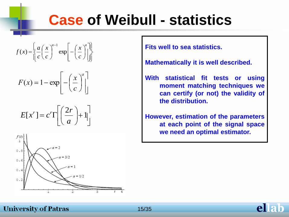
Case of Weibull - statistics
aa
c
x
c
x
c
axf exp)(
1
a
c
xxF exp1)(
1
2][
a
rcxE rr
Fits well to sea statistics.
Mathematically it is well described.
With statistical fit tests or using
moment matching techniques we
can certify (or not) the validity of
the distribution.
However, estimation of the parameters
at each point of the signal space
we need an optimal estimator.
16/35
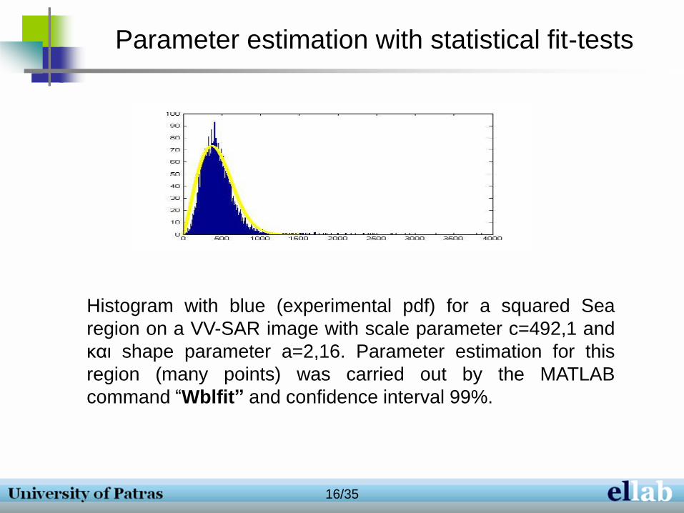
Parameter estimation with statistical fit-tests
Histogram with blue (experimental pdf) for a squared Sea
region on a VV-SAR image with scale parameter c=492,1 and
και shape parameter a=2,16. Parameter estimation for this
region (many points) was carried out by the MATLAB
command “Wblfit” and confidence interval 99%.
17/35
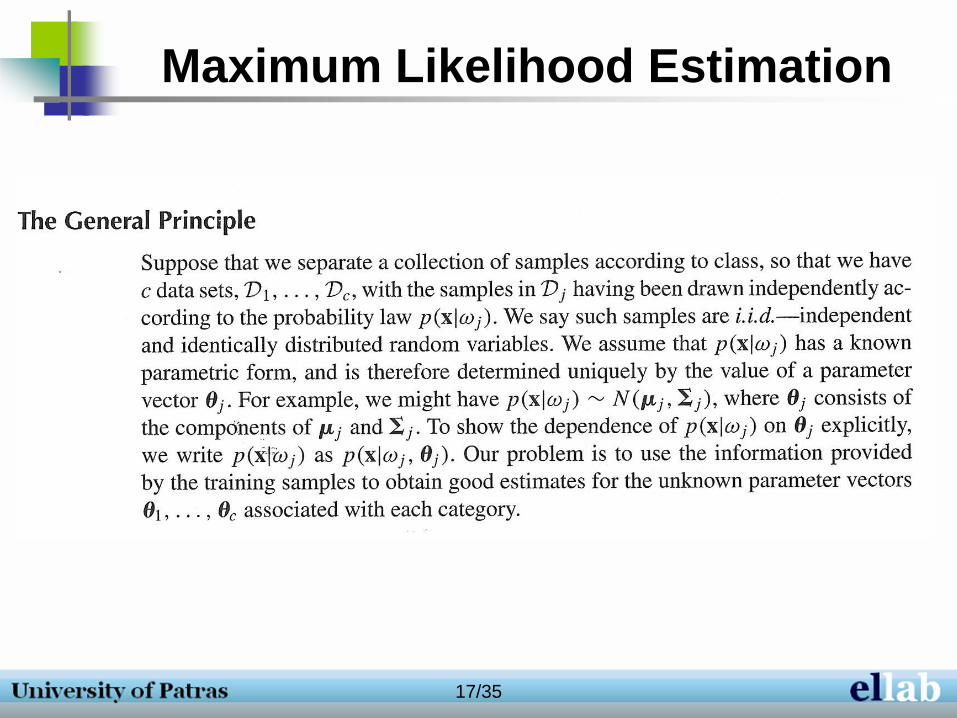
Maximum Likelihood Estimation

18/35
Maximum Likelihood Estimation
19/35
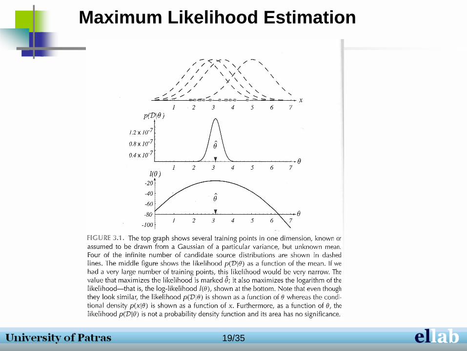
Maximum Likelihood Estimation
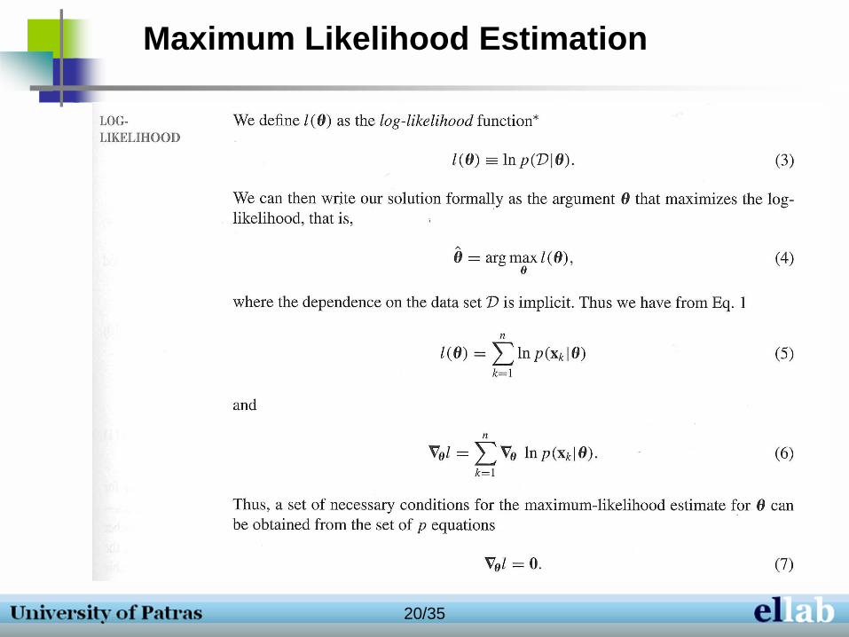
20/35
Maximum Likelihood Estimation
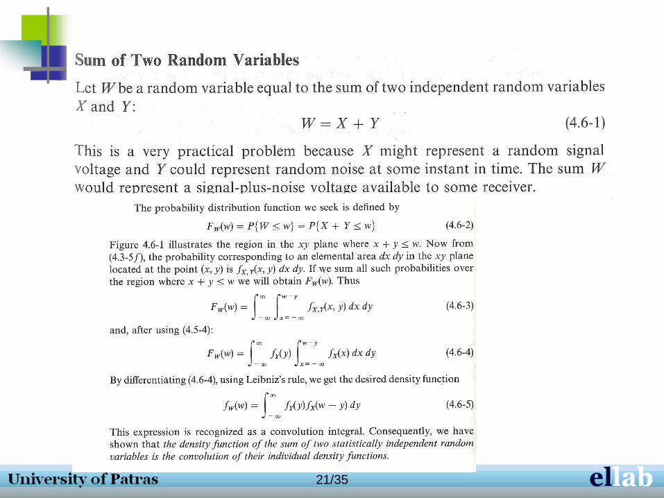
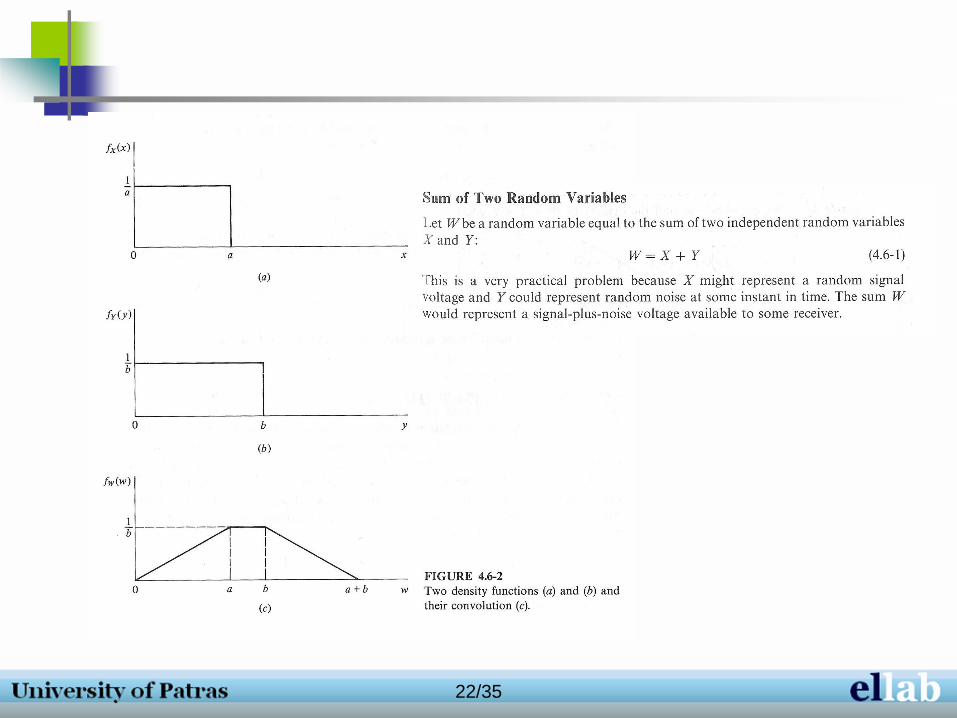
21/35
22/35
23/35

24/35
25/35
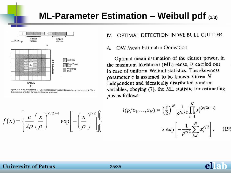
ML-Parameter Estimation – Weibull pdf (1/3)
2/1)2/(
exp2
)(
cc
xxcxf

26/35
ML-Parameter Estimation – Weibull pdf (2/3)
27/35
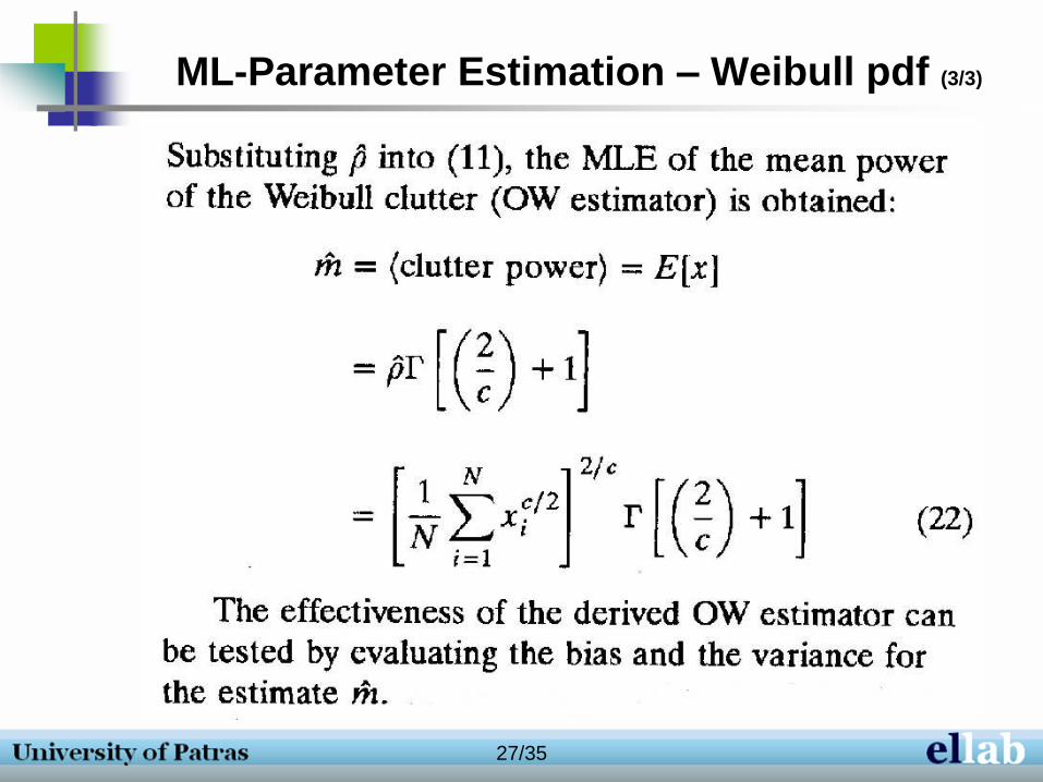
ML-Parameter Estimation – Weibull pdf (3/3)
28/35
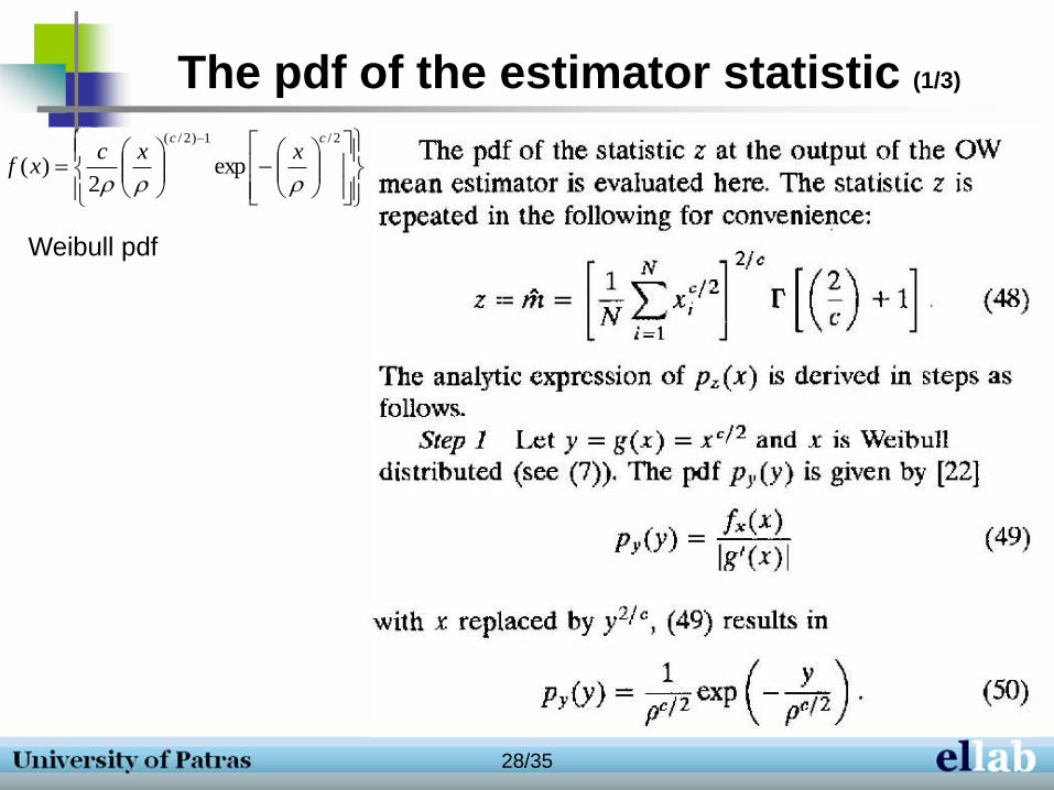
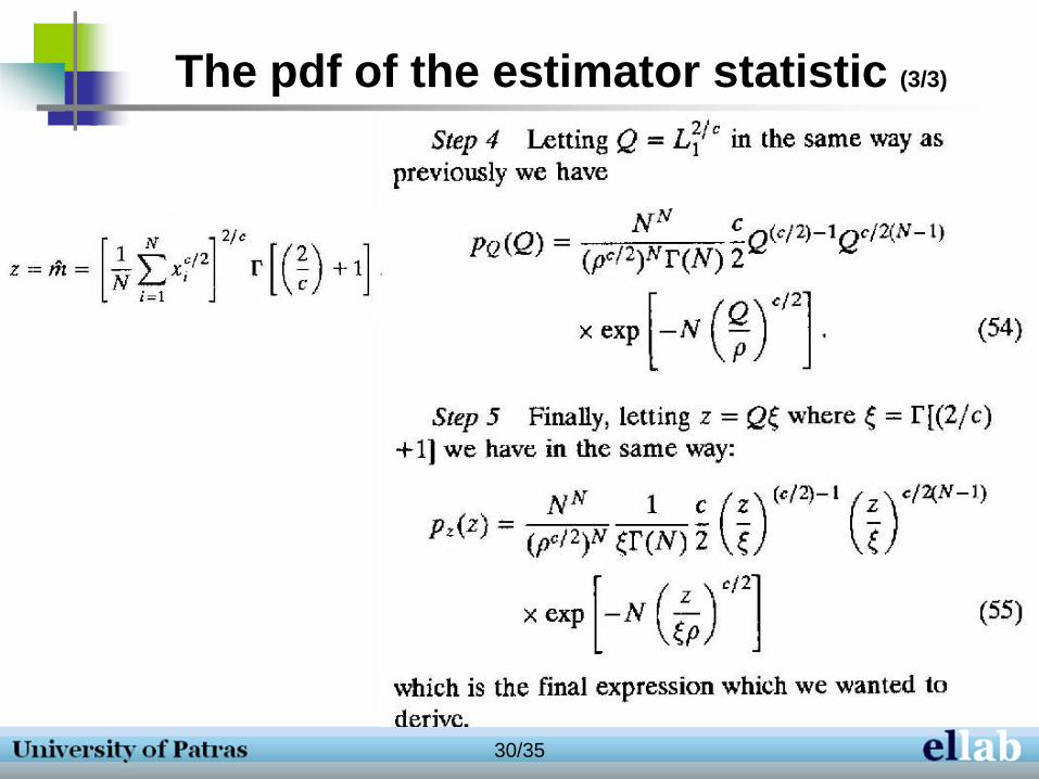
The pdf of the estimator statistic (1/3)
2/1)2/(
exp2
)(
cc
xxcxf
Weibull pdf
29/35
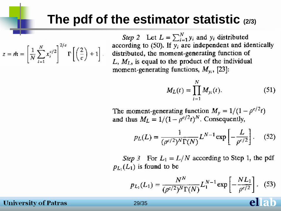
The pdf of the estimator statistic (2/3)
30/35
The pdf of the estimator statistic (3/3)

31/35
OW-CFAR Performance
32/35
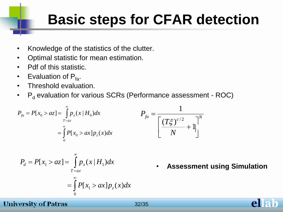
Basic steps for CFAR detection
• Knowledge of the statistics of the clutter.
• Optimal statistic for mean estimation.
• Pdf of this statistic.
• Evaluation of Pfa.
• Threshold evaluation.
• Pd evaluation for various SCRs (Performance assessment - ROC)
0
0
00
)(][
)|(][
dxxpaxxP
dxHxpazxPP
z
azT
xfa Nc
fa
N
TP
1)(
1
2/
0
1
11
)(][
)|(][
dxxpaxxP
dxHxpazxPP
z
azT
xd • Assessment using Simulation
33/35
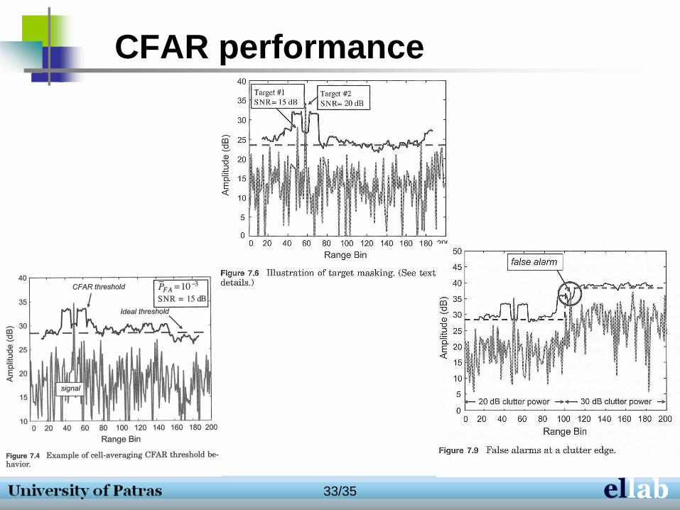
CFAR performance
34/35
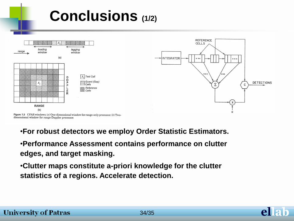
Conclusions (1/2)
•For robust detectors we employ Order Statistic Estimators.
•Performance Assessment contains performance on clutter
edges, and target masking.
•Clutter maps constitute a-priori knowledge for the clutter
statistics of a regions. Accelerate detection.

35/35
• We examined CFAR detection of point
targets in specific clutter statistics and
described performance assessment.
• Many other detection topics remain:
- Distributed targets
- Coherent detection
- Detection using multi-channel signals
• What is detection and its quality; How this
can be used in decision fusion;
Conclusions (2/2)
Related Documents