Sigmoidal Functions: Some Computational and Modelling Aspects

Article Biomath Communications 1 (2014)

Biomath Communications

www.biomathforum.org/biomath/index.php/conference

Sigmoidal Functions: Some Computational andModelling Aspects 1

Nikolay Kyurkchiev, Svetoslav MarkovInstitute of Mathematics and Informatics, Bulgarian Academy of Sciences

[email protected]

Dedicated to the 210th anniversary of the birth of P.-F. Verhulst

Abstract

We focus on some computational, modelling and approximationissues related to the logistic sigmoidal function and to Heaviside stepfunction. The Hausdorff approximation of the Heaviside interval stepfunction by sigmoidal functions is discussed from various computa-tional and modelling aspects. Some relations between Verhulst modeland certain biochemical reaction equations are discussed and ana-lyzed. Numerical examples are presented using CAS Mathematica.

Keywords. Interval functions, Heaviside step function, Approxima-tion, Sigmoidal functions.

1 Introduction

Many biological dynamic processes, such as certain enzyme kinetic and pop-ulation growth processes, develop almost step-wise [9], [13]. Such processesare usually described or approximated by smooth sigmoidal functions; suchfunctions are widely used in the theory of neural networks [3], [4]. Step-wiseinterval functions are a special class of sigmoidal functions; such functions

1 Citation: N. Kyurkchiev, S. Markov, Sigmoidal Functions: Some Computationaland Modelling Aspects. Biomath Communications 1/2 (2014) http://dx.doi.org/10.

11145/j.bmc.2015.03.081

1

are “almost” continuous, or Hausdorff continuous (H-continuous) [2]. De-pending on the particular modelling situation one may decide to use eithercontinuous or H-continous (step-wise) functions. Moreover, in many casesboth types of modelling tools can be used interchangeably. This motivatesus to study the closeness of both classes of functions. To substitute a sig-moidal function by a step function (or conversely) we need to know theapproximation error between the two functions. A natural metric used insuch a situation is the Hausdorff metric between the graphs of the functions.To this end we recall some basic results concerning the class of intervalHausdorff continuous functions and the related concept of Hausdorff ap-proximation. We then focus on classes of logistic sigmoidal functions whichare solutions of the Verhulst population model. We demonstrate that Ver-hulst model arises from simple autocatalytic (bio)chemical reactions andthus can be considered as special case of a biochemical reproduction re-action mechanism. The latter implies a more general model that permitsthe formulation of some important modelling and computational problemsincluding nonautonomous, impulsive and delay DE.

In section 2 we consider sigmoidal and step functions arising from bi-ological applications. The Hausdorff distance between the Heaviside stepfunction and the sigmoidal Verhulst function is discussed. In section 3 wediscuss certain kinetic mechanisms yielding Verhulst model via the massaction law. We show that the Verhulst model arises from some simpleautocatalytic (bio)chemical reactions.

2 Sigmoidal and step functions

2.1 Hausdorff continuity

The concept of Hausdorff continuity (H-continuity) generalizes the familiarconcept of continuity so that essential properties of the usual continuous realfunctions remain present. It is possible to extend the algebraic operationson the set of continuous real functions C(Ω) to the set H(Ω) of H-continuousfunctions in such a way that the set H(Ω) becomes a commutative ring anda linear space with respect to the extended operations [2]. In this workwe restrict ourselves to functions of one real variable, that is real functionsdefined on a subset Ω ⊆ R.

2

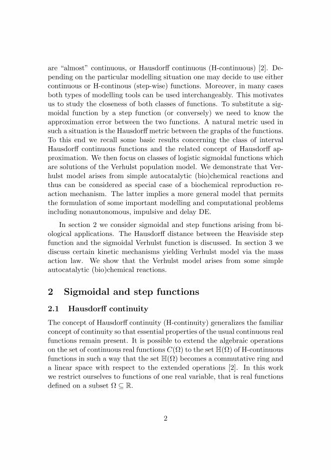
2.2 Step functions

For r ∈ R denote by hr ∈ H(R) the (interval) Heaviside step function givenby

hr(t) =

0, if t < r,

[0, 1], if t = r,

1, if t > r,

(1)

cf. Fig. 1. For r = 0 we obtain the basic Heaviside step function

h0(t) =

0, if t < 0,

[0, 1], if t = 0,

1, if t > 0.

(2)

Functions (1)–(2) are examples sigmoidal functions. A sigmoidal func-tion on R with a range [a, b] is defined as a monotone function s(t) : R →[a, b] such that limt→−∞ s(t) = a, limt→∞ s(t) = b.

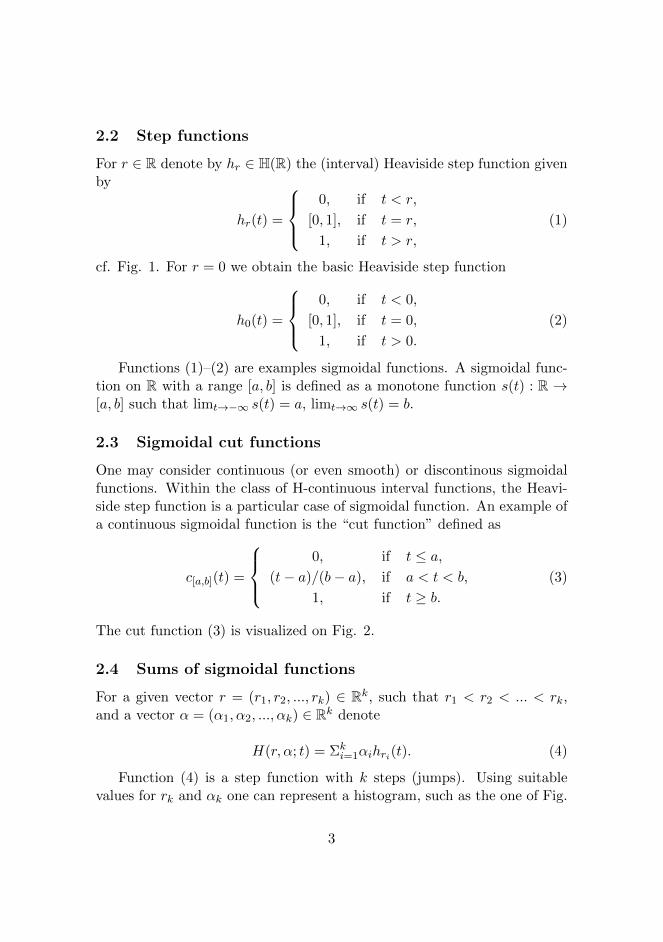
2.3 Sigmoidal cut functions

One may consider continuous (or even smooth) or discontinous sigmoidalfunctions. Within the class of H-continuous interval functions, the Heavi-side step function is a particular case of sigmoidal function. An example ofa continuous sigmoidal function is the “cut function” defined as

c[a,b](t) =

0, if t ≤ a,

(t− a)/(b− a), if a < t < b,

1, if t ≥ b.(3)

The cut function (3) is visualized on Fig. 2.

2.4 Sums of sigmoidal functions

For a given vector r = (r1, r2, ..., rk) ∈ Rk, such that r1 < r2 < ... < rk,and a vector α = (α1, α2, ..., αk) ∈ Rk denote

H(r, α; t) = Σki=1αihri(t). (4)

Function (4) is a step function with k steps (jumps). Using suitablevalues for rk and αk one can represent a histogram, such as the one of Fig.

3

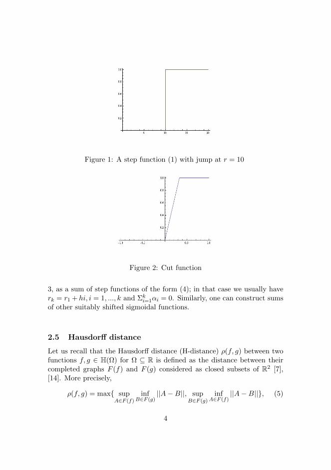
Figure 1: A step function (1) with jump at r = 10

Figure 2: Cut function

3, as a sum of step functions of the form (4); in that case we usually haverk = r1 + hi, i = 1, ..., k and Σk

i=1αi = 0. Similarly, one can construct sumsof other suitably shifted sigmoidal functions.

2.5 Hausdorff distance

Let us recall that the Hausdorff distance (H-distance) ρ(f, g) between twofunctions f, g ∈ H(Ω) for Ω ⊆ R is defined as the distance between theircompleted graphs F (f) and F (g) considered as closed subsets of R2 [7],[14]. More precisely,

ρ(f, g) = max supA∈F (f)

infB∈F (g)

||A−B||, supB∈F (g)

infA∈F (f)

||A−B||, (5)

4

Figure 3: A histogram (from wikipedia)

wherein ||.|| is a norm in R2. According to (5) the H-distance ρ(f, g) be-tween two functions f, g ∈ H(Ω) for Ω ⊆ R makes use of the maximum normin R2 so that the distance between the points A = (tA, xA), B = (tB, xB)in R2 is given by ||A−B|| = max(|tA − tB|, |xA − xB|).

2.6 The logistic sigmoidal function

Sigmoidal functions find multiple applications to neural networks and cellgrowth population models [4], [9].

Several practically important families of smooth sigmoidal functionsarise from population dynamics. A classical example is the Verhulst pop-ulation growth model to be discussed below. Verhulst model makes anextensive use of the “logistic” sigmoidal function

s0(t) =a

1 + e−kt, (6)

see Fig. 4. We next focus on the approximation of the Heaviside stepfunction (2) by logistic functions of the form (6) in Hausdorff distance.

2.7 Approximation issues

In what follows we shall estimate the H-distance (5) between a step functionand a logistic sigmoidal function. W. l. g. we can consider the Heavisidestep function f = ah0 and the logistic sigmoidal function (6): g = s0.As visualized on Fig. 5, the H-distance d = ρ(f, g) = ρ(ah0, s0) between

5

Figure 4: Logistic sigmoidal function (6)

Figure 5: Reaction rate k = 20; Hausdorff distance d = 0.106402

the step function ah0 and the sigmoidal function s0 satisfies the relations0 < d < a/2 and a− s0(d) = d, that is

(a− d)/d = ekd, (0 < d < a/2). (7)

Obviously d → 0 implies k → ∞ (and vice versa). From (7) we obtaina straightforward expression for the rate parameter k as a function of d:

Proposition 1. The rate parameter k can be expressed in terms of theH-distance d as follows:

k = k(d) =1

dlna− dd

= O(d−1 ln(d−1)). (8)

6

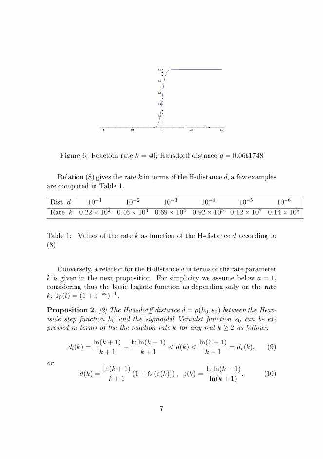
Figure 6: Reaction rate k = 40; Hausdorff distance d = 0.0661748

Relation (8) gives the rate k in terms of the H-distance d, a few examplesare computed in Table 1.

Dist. d 10−1 10−2 10−3 10−4 10−5 10−6

Rate k 0.22× 102 0.46× 103 0.69× 104 0.92× 105 0.12× 107 0.14× 108

Table 1: Values of the rate k as function of the H-distance d according to(8)

Conversely, a relation for the H-distance d in terms of the rate parameterk is given in the next proposition. For simplicity we assume below a = 1,considering thus the basic logistic function as depending only on the ratek: s0(t) = (1 + e−kt)−1.

Proposition 2. [2] The Hausdorff distance d = ρ(h0, s0) between the Heav-iside step function h0 and the sigmoidal Verhulst function s0 can be ex-pressed in terms of the the reaction rate k for any real k ≥ 2 as follows:

dl(k) =ln(k + 1)

k + 1− ln ln(k + 1)

k + 1< d(k) <

ln(k + 1)

k + 1= dr(k), (9)

or

d(k) =ln(k + 1)

k + 1(1 +O (ε(k))) , ε(k) =

ln ln(k + 1)

ln(k + 1). (10)

7

Figure 7: Reaction rate k = 200; Hausdorff distance d = 0.01957.

A proof of relations (9)–(10) is given in [2]. Some computational exam-ples using relations (9)–(10) are presented in Table 2, see also Figures 6, 7,resp. Appendix 1. The last column of Table 2 contains the values of d forprescribed values of k computed by solving the nonlinear equation (7).

k dl(k) dr(k) ∆ = dr − dl ε(k) d(k) by (7)

2 0.334 0.366 0.032 0.0856 0.337416100 0.0305 0.0456 0.015 0.3313 0.0335921000 0.00497 0.00691 0.0019 0.2797 0.00524510000 0.000698 0.000921 0.00022 0.2410 0.000723

Table 2: Bounds for d(k) computed by (9)–(10) for various rates k

Remarks. a) For the general case a 6= 1 one should substitute every-where in formulae (9)–(10) the expression k+ 1 by k+a−1. b) An estimatesimilar to (10) in integral metric has been obtained in [6].

2.8 Shifted logistic functions

Here we are interested in arbitrary shifted (horizontally translated) logis-tic functions. Both the step function and the logistic function preservetheir form under horizontal translation—note that Verhulst equation pos-sess constant isoclines. Hence the shifted step function hr is approximatedby the shifted logistic function sr in the same way as function h0 is approx-

8

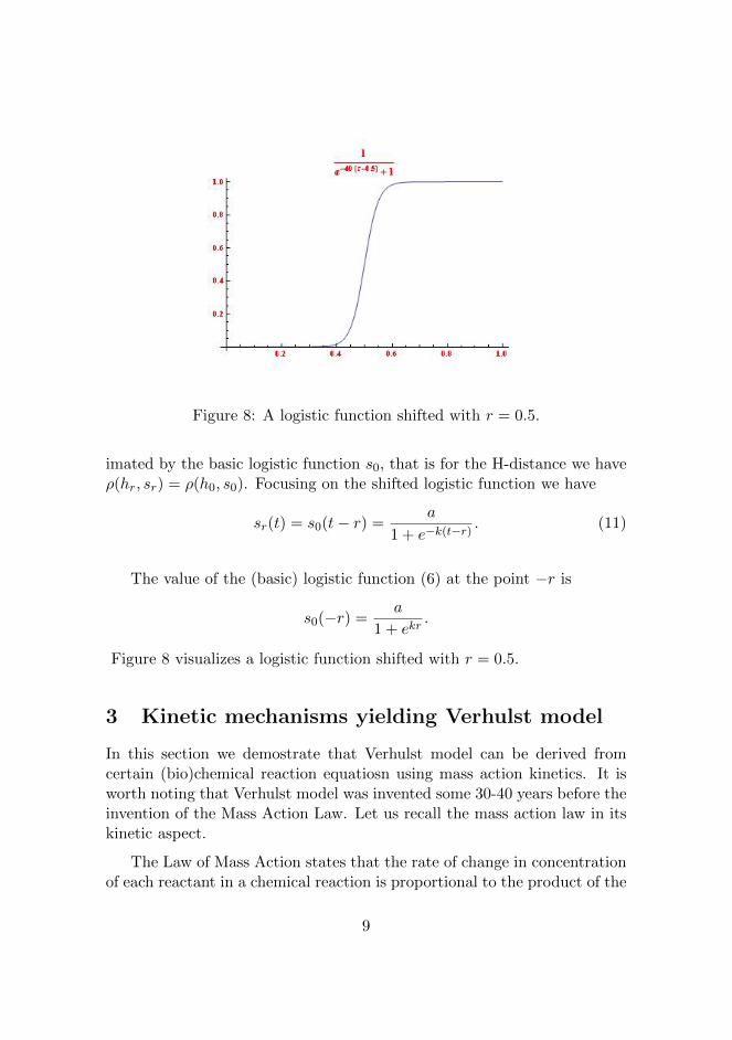
Figure 8: A logistic function shifted with r = 0.5.

imated by the basic logistic function s0, that is for the H-distance we haveρ(hr, sr) = ρ(h0, s0). Focusing on the shifted logistic function we have

sr(t) = s0(t− r) =a

1 + e−k(t−r). (11)

The value of the (basic) logistic function (6) at the point −r is

s0(−r) =a

1 + ekr.

Figure 8 visualizes a logistic function shifted with r = 0.5.

3 Kinetic mechanisms yielding Verhulst model

In this section we demostrate that Verhulst model can be derived fromcertain (bio)chemical reaction equatiosn using mass action kinetics. It isworth noting that Verhulst model was invented some 30-40 years before theinvention of the Mass Action Law. Let us recall the mass action law in itskinetic aspect.

The Law of Mass Action states that the rate of change in concentrationof each reactant in a chemical reaction is proportional to the product of the

9

concentrations of the reactants in that reaction. If a particular reactantis involved in several reactions, then the rate of change of this reactant ismade by adding up all positive rates and subtracting all negative ones [12].

3.1 A simple autocatalytic reaction

Consider the following autocatalytic reversible reaction mechanism:

Xk−→←−

k−1

X +X, (12)

which can be also written as Xk−→←−

k−1

2X.

Applying the mass action law we obtain the Verhulst model:

x′ = kx− k−1x2 = kx(1− (k−1/k)x). (13)

The stationary point is x∗ = k/k−1.

Another kinetic mechanism inducing Verhulst model that seems theo-retically possible and better practically justified follows.

3.2 Autocatalytic reaction involving nutrient substrate

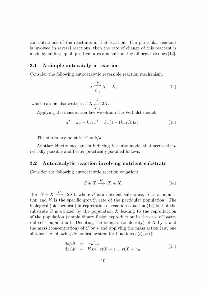
Consider the following autocatalytic reaction equation:

S +Xk′−→ X +X, (14)

(or S + Xk′−→ 2X), where S is a nutrient substance, X is a popula-

tion and k′ is the specific growth rate of the particular population. Thebiological (biochemical) interpretation of reaction equation (14) is that thesubstrate S is utilized by the population X leading to the reproductionof the population (simple binary fusion reproduction in the case of bacte-rial cells population). Denoting the biomass (or density) of X by x andthe mass (concentration) of S by s and applying the mass action law, oneobtains the following dynamical system for functions s(t), x(t):

ds/dt = −k′xs,dx/dt = k′xs, s(0) = s0, x(0) = x0.

(15)

10

Figure 9: Reaction rate k = 40; s0 = 1, x0 = 1.× 10−9

The solutions s, x of (15) for reaction rate k = 40 and initial conditionss0 = 1, x0 = 1.× 10−9 are iluustrated on Fig. 9, see Appendix 2. Noticingthat ds/dt+dx/dt = 0, hence s+x = const = x0+s0 = a, we can substitutes = a−x in the differential equation for x to obtain the differential equationdx/dt = k′sx = k′x(a− x) also known as Verhulst model [15]–[17].

dx

dt= k′x(a− x). (16)

Clearly, the solution x of the initial problem (15) coincides with thesolution x of problem (16) with initial condition x(0) = x0:

dx

dt= k′x(a− x). x(0) = x0. (17)

Conversely, the solution of (17) coincides with the solution x of the initalproblem (15) whenever s0 = a− x0. The above can be summarized in thefollowing:

Proposition 3. The autocatalytic reaction (14) via mass action kineticinduces the dynamic model (15). Models (15) and (17) are equivalent inthe sense that their solutions x coincide (for x0 + s0 = a).

We see that the underlying mechanism in Verhulst model (17) is a bio-chemical reproduction reaction (14) based on the utilization of a nutrient

11

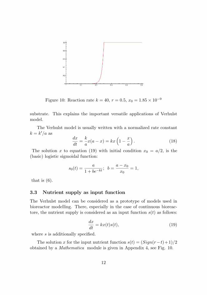
Figure 10: Reaction rate k = 40, r = 0.5, x0 = 1.85× 10−9

substrate. This explains the important versatile applications of Verhulstmodel.

The Verhulst model is usually written with a normalized rate constantk = k′/a as

dx

dt=k

ax(a− x) = kx

(1− x

a

). (18)

The solution x to equation (19) with initial condition x0 = a/2, is the(basic) logistic sigmoidal function:

s0(t) =a

1 + be−kt; b =

a− x0x0

= 1,

that is (6).

3.3 Nutrient supply as input function

The Verhulst model can be considered as a prototype of models used inbioreactor modelling. There, especially in the case of continuous bioreac-tore, the nutrient supply is considered as an input function s(t) as follows:

dx

dt= kx(t)s(t), (19)

where s is additionally specified.

The solution x for the input nutrient function s(t) = (Sign(r− t)+1)/2obtained by a Mathematica module is given in Appendix 4, see Fig. 10.

12

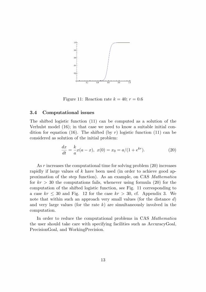
Figure 11: Reaction rate k = 40; r = 0.6

3.4 Computational issues

The shifted logistic function (11) can be computed as a solution of theVerhulst model (16); in that case we need to know a suitable initial con-dition for equation (16). The shifted (by r) logistic function (11) can beconsidered as solution of the initial problem:

dx

dt=k

ax(a− x), x(0) = x0 = a/(1 + ekr). (20)

As r increases the computational time for solving problem (20) increasesrapidly if large values of k have been used (in order to achieve good ap-proximation of the step function). As an example, on CAS Mathematicafor kr > 30 the computations fails, whenever using formula (20) for thecomputation of the shifted logistic function, see Fig. 11 corresponding toa case kr ≤ 30 and Fig. 12 for the case kr > 30, cf. Appendix 3. Wenote that within such an approach very small values (for the distance d)and very large values (for the rate k) are simultaneously involved in thecomputation.

In order to reduce the computational problems in CAS Mathematicathe user should take care with specifying facilities such as AccuracyGoal,PrecisionGoal, and WorkingPrecision.

13

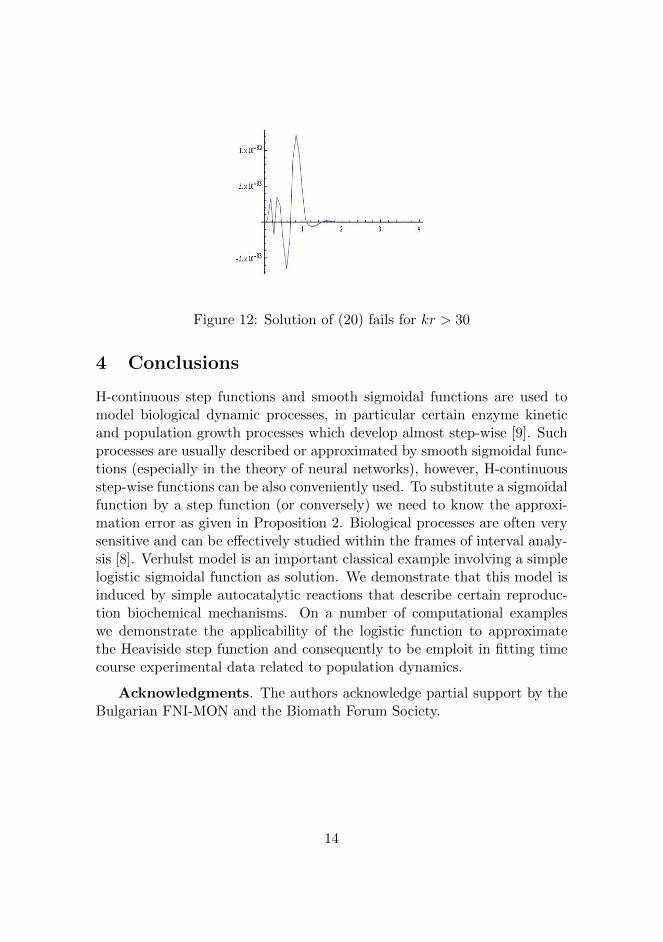
Figure 12: Solution of (20) fails for kr > 30

4 Conclusions

H-continuous step functions and smooth sigmoidal functions are used tomodel biological dynamic processes, in particular certain enzyme kineticand population growth processes which develop almost step-wise [9]. Suchprocesses are usually described or approximated by smooth sigmoidal func-tions (especially in the theory of neural networks), however, H-continuousstep-wise functions can be also conveniently used. To substitute a sigmoidalfunction by a step function (or conversely) we need to know the approxi-mation error as given in Proposition 2. Biological processes are often verysensitive and can be effectively studied within the frames of interval analy-sis [8]. Verhulst model is an important classical example involving a simplelogistic sigmoidal function as solution. We demonstrate that this model isinduced by simple autocatalytic reactions that describe certain reproduc-tion biochemical mechanisms. On a number of computational exampleswe demonstrate the applicability of the logistic function to approximatethe Heaviside step function and consequently to be emploit in fitting timecourse experimental data related to population dynamics.

Acknowledgments. The authors acknowledge partial support by theBulgarian FNI-MON and the Biomath Forum Society.

14

References

[1] Alt, R., S. Markov, Theoretical and computational studies of somebioreactor models, Computers and Mathematics with Applications64 (2012), 350–360.

[2] Anguelov, R., Markov, S.: Hausdorff Continuous Interval Func-tions and Approximations, submitted to LNCS (SCAN 2014 Pro-ceedings)

[3] Basheer, I. A., M. Hajmeer, Artificial neural networks: fundamen-tals, computing, design, and application, Journal of Microbiologi-cal Methods 43 (2000), 3–31.

[4] Costarelli, D., Spigler, R.: Approximation results for neural net-work operators activated by sigmoidal functions, Neural Networks44, 101–106 (2013).

[5] Dimitrov, S., G. Velikova, V. Beschkov, S. Markov, On the Numer-ical Computation of Enzyme Kinetic Parameters, Biomath Com-munications 1 (2), 2014.

[6] Glover, Ian, The Approximation of Continuous Functions by Mul-tilayer Perceptrons.http://www.manicai.net/ai/assets/approx cts fn.pdf

[7] Hausdorff, F.: Set theory (2 ed.), New York, Chelsea Publ.,1962[1957], ISBN 978-0821838358 (Republished by AMS-Chelsea 2005).

[8] Markov, S.: Biomathematics and Interval Analysis: A ProsperousMarriage, in: Christov, Ch. and Todorov, M. D. (eds), Proc. ofthe 2nd Intern. Conf. on Application of Mathematics in Technicaland Natural Sciences (AMiTaNS’10), AIP Conf. Proc. 1301, 26–36.2010.

[9] Markov, S.: Cell Growth Models Using Reaction Schemes: BatchCultivation, Biomath 2/2 (2013), 1312301http://dx.doi.org/10.11145/j.biomath.2013.12.301

15

[10] Markov, S., On the Use of Computer Algebra Systems and Enclo-sure Methods in the Modelling and Optimization of Biotechnologi-cal Processes, Bioautomation (Intern. Electronic Journal) 3, 2005,1–9.

[11] Markov, S., On the mathematical modelling of microbial growth:some computational aspects, Serdica J. Computing 5 (2), 153–168(2011).

[12] Murray J. D., Mathematical Biology: I. An Introduction, ThirdEdition, Springer, 2002.

[13] Radchenkova, N., M. Kambourova, S. Vassilev, R. Alt, S. Markov,On the Mathematical Modelling of EPS Production by a Ther-mophilic Bacterium, Biomath 4 (2014), 1407121.http://dx.doi.org/10.11145/j.biomath.2014.07.121

[14] Sendov, B.: Hausdorff Approximations, Kluwer, Boston, 1990.

[15] Verhulst, P.-F., Notice sur la loi que la population poursuit dansson accroissement, Correspondance mathematique et physique 10:113–121 (1838).

[16] Verhulst, P.-F., Recherches mathematiques sur la loid’accroissement de la population (Mathematical Researchesinto the Law of Population Growth Increase), Nouveaux Memoiresde l’Academie Royale des Sciences et Belles-Lettres de Bruxelles18: 1–42 (1845).

[17] Verhulst, P.-F., Deuxieme memoire sur la loi d’accroissement dela population, Memoires de l’Academie Royale des Sciences, desLettres et des Beaux-Arts de Belgique 20: 1–32 (1847).

16

Appendix 1. Calculation of the value of the Hausdorff distance d between theHeaviside step function h and the sigmoidal Verhulst function s in terms of the reactionrate k

17

Appendix 2. A kinetic mechanism yielding Verhulst model

18

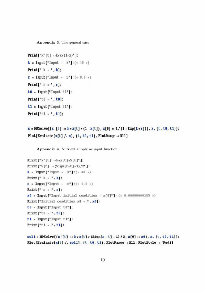
Appendix 3. The general case

Appendix 4. Nutrient supply as input function

19