SIFT - The Scale Invariant Feature Transform - The Scale Invariant Feature Transform Distinctive image features from scale-invariant keypoints. David G. Lowe, International Journal

SIFT - The Scale Invariant SIFT - The Scale Invariant Feature TransformFeature Transform

Distinctive image features from scale-invariant keypoints. David G. Lowe, International Journal of Computer Vision, 60, 2 (2004), pp. 91-110

Presented by Ofir Pele.

Based upon slides from:- Sebastian Thrun and Jana Košecká- Neeraj Kumar

Correspondence■ Fundamental to many of the core vision problems

– Recognition– Motion tracking– Multiview geometry

■ Local features are the key

Images from: M. Brown and D. G. Lowe. Recognising Panoramas. In Proceedings of the ( the International Conference on Computer Vision (ICCV2003

Local Features:Detectors & Descriptors

Detected

Interest Points/Regions

Descriptors

<0 12 31 0 0 23 …>

<5 0 0 11 37 15 …>

<14 21 10 0 3 22 …>

Ideal Interest Points/Regions■ Lots of them■ Repeatable■ Representative orientation/scale■ Fast to extract and match

DetectorSIFT Overview

1. Find Scale-Space Extrema

2. Keypoint Localization & Filtering– Improve keypoints and throw out bad ones

3. Orientation Assignment– Remove effects of rotation and scale

4. Create descriptor– Using histograms of orientations

Descriptor


1.1. Find Scale-Space ExtremaFind Scale-Space Extrema2. Keypoint Localization & Filtering

– Improve keypoints and throw out bad ones



Descriptor

Scale Space■ Need to find ‘characteristic scale’ for feature■ Scale-Space: Continuous function of scale σ

– Only reasonable kernel is Gaussian:

( ) ( ) ( )yxIyxGyxL DD ,*,,,, σσ =

[Koenderink 1984, Lindeberg 1994]

Scale Selection■ Experimentally, Maxima of Laplacian-of-Gaussian gives

best notion of scale:

■ Thus use Laplacian-of-Gaussian (LoG) operator:

Mikolajczyk 2002

G22 ∇σ

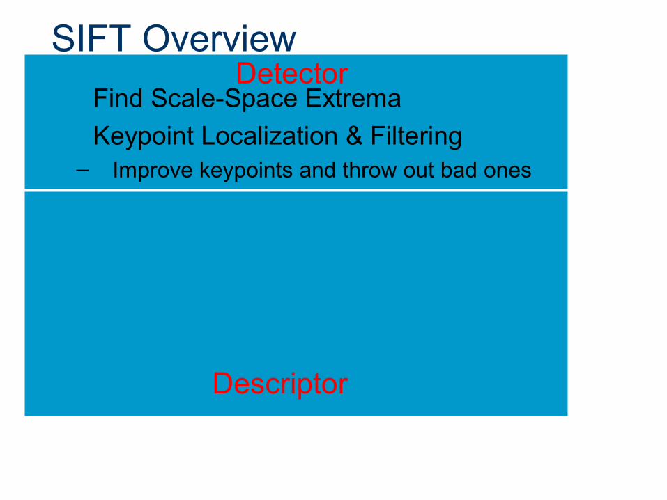
Approximate LoG■ LoG is expensive, so let’s approximate it■ Using the heat-diffusion equation:

■ Define Difference-of-Gaussians (DoG):

( ) ( )σσ

σσσ

σ−−≈

∂∂=∇

k

GkGGG2

( ) ( ) ( )( ) IGkGD *σσσ −≡

( ) ( ) ( )σσσ GkGGk −≈∇− 221

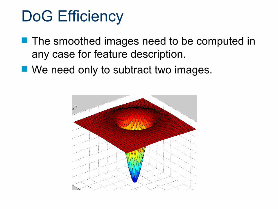
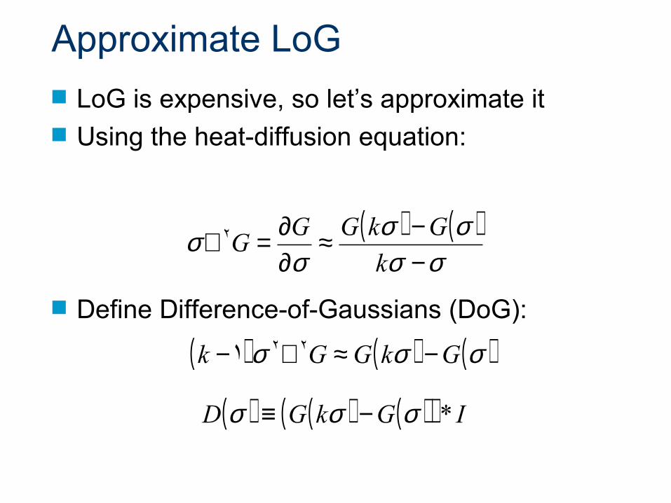
DoG Efficiency ■ The smoothed images need to be computed in

any case for feature description.■ We need only to subtract two images.

DoB Filter (`Difference of Boxes')

Bay et al., ECCV 2006

■ Even faster approximation is using box filters (by integral image)

B

B

A

AD=

Integral Image Computation

C C+ -

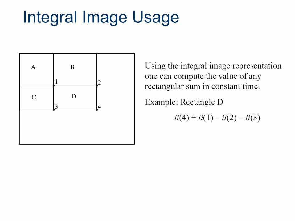
Integral Image Usage

Scale-Space Construction■ First construct scale-space:

σ increasing

First octave Second octave

( ) IG *σ

( ) IkG *σ( ) IkG *2σ

( ) IG *2σ

( ) IkG *2 σ

( ) IkG *2 2σ

Difference-of-Gaussianss■ Now take differences:

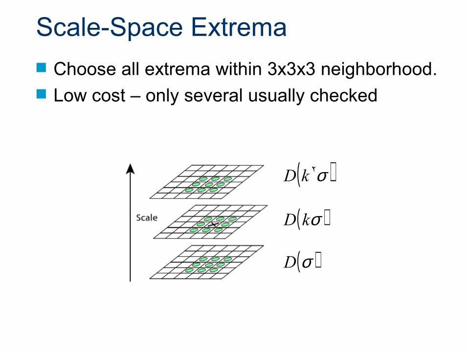
Scale-Space Extrema■ Choose all extrema within 3x3x3 neighborhood. ■ Low cost – only several usually checked

( )σD

( )σkD

( )σ2kD



2.2. Keypoint Localization & FilteringKeypoint Localization & Filtering– Improve keypoints and throw out bad ones



Descriptor

Keypoint Localization & Filtering■ Now we have much less points than pixels.■ However, still lots of points (~1000s)…

– With only pixel-accuracy at best• At higher scales, this corresponds to several pixels in base

image

– And this includes many bad points

Brown & Lowe 2002

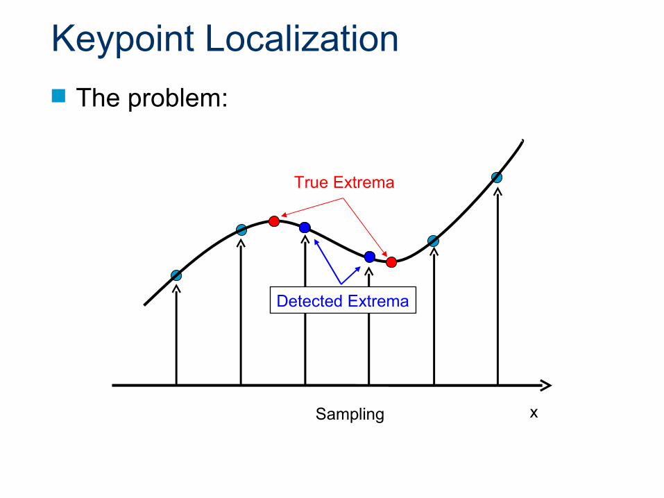
Keypoint Localization■ The problem:

xSampling

Detected Extrema

True Extrema

Keypoint Localization■ The Solution:

– Take Taylor series expansion:

– Minimize to get true location of extrema:

( ) xx

Dxx

x

DDxD

TT

T

2

2

2

1

∂∂+

∂∂+=

Brown & Lowe 2002

x

D

x

Dx ∂

∂∂∂−=

−1

2

2

ˆ

Keypoints

(a) 233x189 image(b) 832 DOG extrema

Keypoint Filtering - Low Contrast■ Reject points with bad contrast

is smaller than 0.03 (image values in [0,1]) ( )xD ˆ

Keypoint Filtering - Edges■ Reject points with strong edge response in one

direction only■ Like Harris - using Trace and Determinant of

Hessian

Point can move along edge

Point constrained

Point detection Point detection

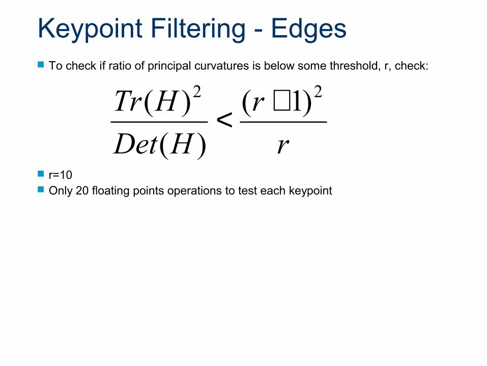
Keypoint Filtering - Edges■ To check if ratio of principal curvatures is below some threshold, r, check:

■ r=10■ Only 20 floating points operations to test each keypoint

r

r

HDet

HTr 22 )1(

)(

)( +<

Keypoint Filtering

(c) 729 left after peak value threshold (from 832)(d) 536 left after testing ratio of principle curvatures






DescriptorDescriptor

Ideal Descriptors■ Robust to:

– Affine transformation– Lighting– Noise

■ Distinctive■ Fast to match

– Not too large

– Usually L1 or L2 matching




3.3. Orientation AssignmentOrientation Assignment– Remove effects of rotation and scale


Descriptor

Orientation Assignment■ Now we have set of good points■ Choose a region around each point

– Remove effects of scale and rotation

Orientation Assignment■ Use scale of point to choose correct image:

■ Compute gradient magnitude and orientation using finite differences:

( ) ( ) ( )yxIyxGyxL ,*,,, σ=

( ) ( ) ( )( ) ( )( )

( ) ( )( )( ) ( )( )

−−+

−−+=

−−++−−+=

−

yxLyxL

yxLyxLyx

yxLyxLyxLyxLyxm

,1,1

)1,(1,tan,

)1,(1,,1,1,

1

22

θ

Orientation Assignment■ Create gradient histogram (36 bins)

– Weighted by magnitude and Gaussian window ( is 1.5 times that of the scale of a keypoint)

σ

Orientation Assignment■ Any peak within 80% of the highest peak is used

to create a keypoint with that orientation■ ~15% assigned multiplied orientations, but

contribute significantly to the stability■ Finally a parabola is fit to the 3 histogram values

closest to each peak to interpolate the peak position for better accuracy





4.4. Create descriptorCreate descriptor– Using histograms of orientations

Descriptor

SIFT Descriptor■ Each point so far has x, y, σ, m, θ■ Now we need a descriptor for the region

– Could sample intensities around point, but…• Sensitive to lighting changes• Sensitive to slight errors in x, y, θ

■ Look to biological vision– Neurons respond to gradients at certain frequency and

orientation• But location of gradient can shift slightly!

Edelman et al. 1997

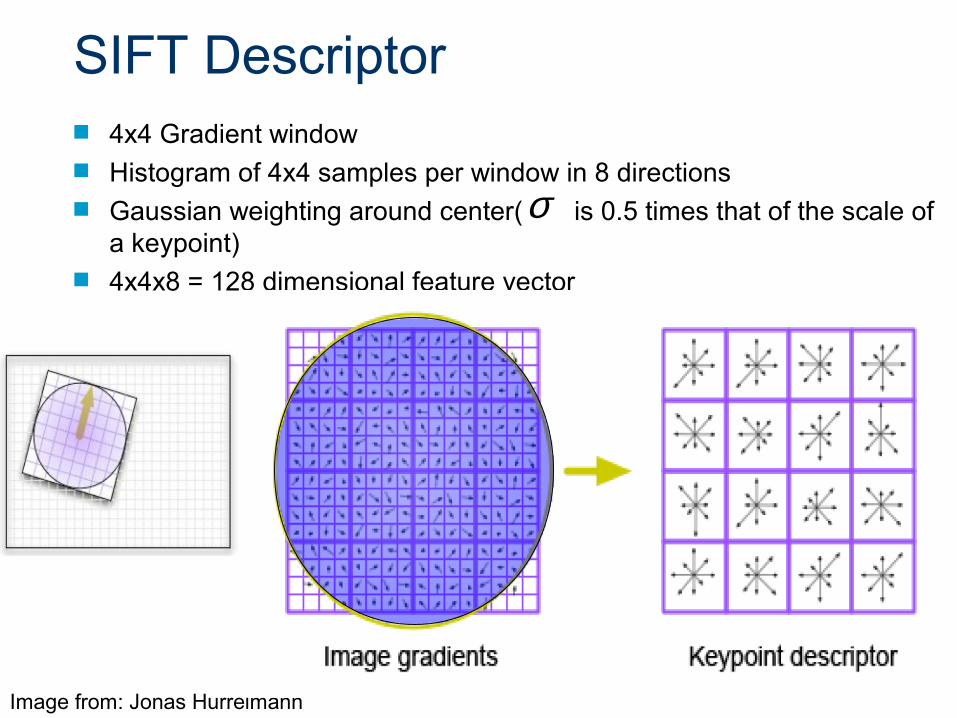
SIFT Descriptor■ 4x4 Gradient window■ Histogram of 4x4 samples per window in 8 directions■ Gaussian weighting around center( is 0.5 times that of the scale of

a keypoint)■ 4x4x8 = 128 dimensional feature vector

Image from: Jonas Hurrelmann

σ

SIFT Descriptor – Lighting changes■ Gains do not affect gradients■ Normalization to unit length removes contrast■ Saturation affects magnitudes much more than

orientation■ Threshold gradient magnitudes to 0.2 and renormalize

Performance■ Very robust

– 80% Repeatability at:• 10% image noise• 45° viewing angle• 1k-100k keypoints in database

■ Best descriptor in [Mikolajczyk & Schmid 2005]’s extensive survey

■ 3670+ citations on Google Scholar

Typical Usage■ For set of database images:

1. Compute SIFT features2. Save descriptors to database

■ For query image:1. Compute SIFT features2. For each descriptor:

• Find a match

3. Verify matches• Geometry• Hough transform

Matching Descriptors■ Threshold on Distance – bad performance■ Nearest Neighbor – better■ Ratio Test – best performance

Matching Descriptors - Distance■ L2 norm – used by Lowe■ SIFTDIST: linear time EMD algorithm that adds

robustness to orientation shiftsPele and Werman, ECCV 2008

Ratio Test

Best Match

False 2nd best match

True 2nd best match

Image 2 Image 1

Fast Nearest-Neighbor Matching to Feature Database

■ Hypotheses are generated by approximate nearest neighbor matching of each feature to vectors in the database – SIFT use best-bin-first (Beis & Lowe, 97) modification to k-d

tree algorithm– Use heap data structure to identify bins in order by their

distance from query point

■ Result: Can give speedup by factor of 1000 while finding nearest neighbor (of interest) 95% of the time

3D Object Recognition■ Only 3 keys are needed for

recognition, so extra keys provide robustness

Recognition under occlusion

Test of illumination Robustness

■ Same image under differing illumination

273 keys verified in final match

Location recognition

Image Registration Results

[Brown & Lowe 2003]

Cases where SIFT didn’t work

Large illumination change ■ Same object under differing illumination■ 43 keypoints in left image and the corresponding closest

keypoints on the right (1 for each)

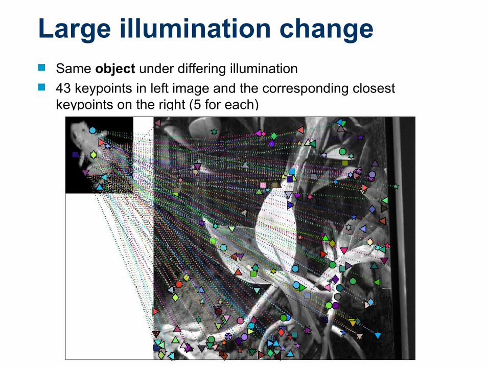
Large illumination change■ Same object under differing illumination■ 43 keypoints in left image and the corresponding closest


Non rigid deformations■ 11 keypoints in left image and the corresponding closest


Non rigid deformations■ 11 keypoints in left image and the corresponding closest


Conclusion: SIFT■ Built on strong foundations

– First principles (LoG and DoG)– Biological vision (Descriptor)– Empirical results

■ Many heuristic optimizations– Rejection of bad points– Sub-pixel level fitting– Thresholds carefully chosen

Conclusion: SIFT■ In wide use both in academia and industry■ Many available implementations:

– Binaries available at Lowe’s website– C/C++ open source by A. Vedaldi (UCLA)– C# library by S. Nowozin (Tu-Berlin)

■ Protected by a patent

Conclusion: SIFT■ Empirically found2 to show very good performance, robust to

image rotation, scale, intensity change, and to moderate affine transformations

1 Mikolajczyk & Schmid 2005

Scale = 2.5Rotation = 450

A note regarding invariance/robustness■ There is a tradeoff between invariance and

distinctiveness.■ For some tasks it is better not to be invariant ■ Local features and kernels for classification of

texture and object categories: An in-depth study - Zhang, Marszalek, Lazebnik and Schmid. IJCV 2007.

■ 11 color names - J. van de Weijer, C. Schmid, Applying Color Names to Image Description. ICIP 2007

Conclusion: Local features■ Much work left to be done

– Efficient search and matching– Combining with global methods– Finding better features

SIFT extensions

Color

■ Color SIFT - G. J. Burghouts and J. M. Geusebroek. Performance evaluation of local colour invariants. Comput. Vision Image Understanding, 2009

■ Hue and Opponent histograms - J. van de Weijer, C. Schmid. Coloring Local Feature Extraction.

ECCV 2006

■ 11 color names - J. van de Weijer, C. Schmid, Applying Color Names to Image Description. ICIP 2007

PCA-SIFT

■ Only change step 4 (creation of descriptor)■ Pre-compute an eigen-space for local gradient

patches of size 41x41■ 2x39x39=3042 elements■ Only keep 20 components■ A more compact descriptor■ In K.Mikolajczyk, C.Schmid 2005 PCA-SIFT

tested inferior to original SIFT

Speed Improvements■ SURF - Bay et al. 2006■ Approx SIFT - Grabner et al. 2006■ GPU implementation - Sudipta N. Sinha et al. 2006

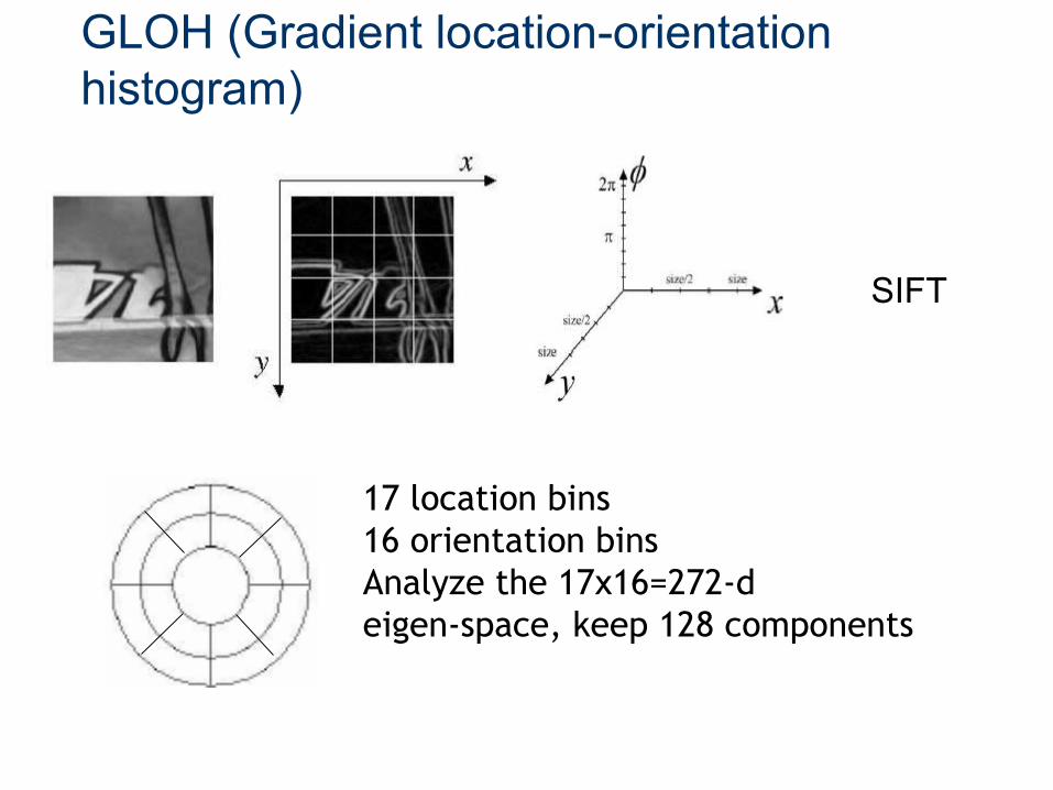
GLOH (Gradient location-orientation histogram)

17 location bins16 orientation binsAnalyze the 17x16=272-d eigen-space, keep 128 components

SIFT

SIFT - The Scale Invariant Feature Transform - The Scale Invariant Feature Transform Distinctive image features from scale-invariant keypoints. David G. Lowe, International Journal

Documents