SIFT Implementation and Optimization for General-Purpose GPU

SIFT Implementation and Optimization for General-Purpose GPU

S. Heymann Fraunhofer HHI Einsteinufer 37

Germany 10587, Berlin

[email protected]

K. Müller Fraunhofer HHI Einsteinufer 37

Germany 10587, Berlin

[email protected]

A.Smolic Fraunhofer HHI Einsteinufer 37

Germany 10587, Berlin

[email protected]

B. Fröhlich Bauhaus University Weimar

Fakultät Medien Germany 99423, Weimar

[email protected]

T. Wiegand Fraunhofer HHI Einsteinufer 37

Germany 10587, Berlin

[email protected]

ABSTRACT With the addition of free programmable components to modern graphics hardware, graphics processing units (GPUs) become increasingly interesting for general purpose computations, especially due to utilizing parallel buffer processing. In this paper we present methods and techniques that take advantage of modern graphics hardware for real-time tracking and recognition of feature-points. The focus lies on the generation of feature vectors from input images in the various stages. For the generation of feature-vectors the Scale Invariant Feature Transform (SIFT) method [Low04a] is used due to its high stability against rotation, scale and lighting condition changes of the processed images. We present results of the various stages for feature vector generation of our GPU implementation and compare it to the CPU version of the SIFT algorithm. The approach works well on Geforce6 series graphics board and above and takes advantage of new hardware features, e.g. dynamic branching and multiple render targets (MRT) in the fragment processor [KF05]. With the presented methods feature-tracking with real time frame rates can be achieved on the GPU and meanwhile the CPU can be used for other tasks.

Keywords GPU, SIFT, feature extraction, tracking.

1. INTRODUCTION With the inclusion of programmable parts in modern graphics hardware, such as vertex and fragment processors, developers started using the power of graphics processing units (GPUs) for general purpose computations beyond creating beautiful pictures and creating high-end game engines. The research field that arose from those efforts is known as GPGPU (general purpose computations on GPUs). To make use of the GPU for more general computations it is

necessary to transform the algorithms under investigation such that it optimally utilizes the parallel processing model used on modern graphics hardware. A number of algorithms and applications have been implemented onto GPGPUs, e.g. kd-tree search [FS05], sorting algorithm acceleration [GHLM05] and database search [GLW*04]. An overview of concepts for algorithm transformation to GPU architecture is given in [Har05] and [OLG*05].

In this paper we show, how a feature extraction algorithm can be adapted to make use of modern graphics hardware and which processing acceleration can be obtained by optimizing all stages of the algorithm. Specifically, the SIFT Algorithm [Low04a] was implemented on a NVIDIA QuadroFX 3400 GPU with 256MB video RAM, taking advantage of new functionalities, e.g. dynamic branching and multiple render targets (MRTs) of the

Permission to make digital or hard copies of all or part of this work for personal or classroom use is granted without fee provided that copies are not made or distributed for profit or commercial advantage and that copies bear this notice and the full citation on the first page. To copy otherwise, or republish, to post on servers or to redistribute to lists, requires prior specific permission and/or a fee. Copyright UNION Agency – Science Press, Plzen, Czech Republic.

fragment and vertex processor. After reviewing the related work, we give a short overview of the algorithm, followed by the stage-by-stage GPU implementation and the obtained overall acceleration of the algorithm in comparison to standard CPU implementation.

2. RELATED WORK One of the main problems of computer vision is the generation of stable feature-points from natural images. These feature-points are used for correspondence matching to find known objects and gain information about their presence, position, size or rotation in other images [BL02]. One approach for feature tracking is given in [Fun05], but the extracted feature points were not invariant to scale and the application was focused on the usage of multiple parallel graphics cards. One method to create highly stable feature-vectors from images is the Scale Invariant Feature Transform (SIFT) introduced by David Lowe [Low04a]. SIFT features are invariant against rotation, changes in scale and lighting/contrast and can therefore be well applied to scene modeling, recognition and tracking [GL04] and panorama creation.

3. SIFT OVERVIEW The SIFT method consists of different stages to obtain relevant feature points. These stages where analyzed and individually adapted to maximize GPU parallel processing using only few CPU accesses. The single SIFT stages are:

1. Search for potential points of interest by creation of a Difference of Gaussian (DoG) scale-space pyramid as image representation and filtering for extreme values

2. Further filtering and reduction of the obtained points from 1. to select stable points with high contrast. To each remaining point, its position and size are assigned.

3. Orientation assignment to each point by finding a characteristic direction.

4. Feature vector calculation based on the characteristic direction from 3. to provide rotation invariance.

5. The whole process is stacked in a way that only a subset of elements from the beginning of a stage is passed onto the next stage.

To achieve scale invariance it is necessary to create a representation of the image frequencies. This is realized using a scale space pyramid as introduced by Witkin [Wit83]. Each image within the pyramid refers to different image frequencies. By searching in

all images of the scale space pyramid, the obtained feature point candidates become scale invariant. The scale-space pyramid is constructed by taking a gray-scaled version of the original image and convolving it repeatedly with Gaussian convolution kernels of increasing size. Thus a number of images with increasing blurriness is constructed as shown in the stack of four 640x480 images in Figure 1 top-left. In the next stage, the most blurred image from this stack is downscaled by a factor of two and afterwards convolved with the same set of Gaussian kernels as before to create the next stack of four 320x240 images. The whole process is repeated until a specified size has been reached, which is 80x60 in the example in Figure 1 top-right.

Figure 1. Gaussian pyramid (top) and difference

of Gaussian (bottom). Now the pyramid consists of continuously convolved versions of the original image with different sizes and blurriness. To calculate the single frequencies of the image, adjacent images or stages of the same size of the pyramid have to be subtracted to create the Difference of Gaussian (DoG) representation, as shown in Figure 1 bottom. Finally, the obtained DoG pyramid is filtered to find the global extreme values. The filtering is applied pixel wise by comparing the luminance of the current pixel to its 8 neighbors within the same image, as well as to its 9 non-shifted neighbors of both adjacent layers of the same size. If the luminance valueof the pixel under investigation is a minimum or maximum among all these neighboring luminance values, the pixel is considered as feature point candidate.

In the next step, the obtained candidates are further filtered to eliminate feature points that are unsuitable for correspondence detection. Here, mainly two types of unsuitable points are considered. First, points erroneously found due to noise in the input image and second points that lay on edges. The first type is eliminated by introducing a threshold for luminance differences between a possible feature point and its neighbors. Only, if the threshold is exceeded, the

point is further processed and considered as candidates. Edge points need to be excluded, since they are unsuitable for tracking and correspondence matching. For edge point detection, the surface curvature around the surface D(x,y) of a candidate point at position (x,y) can be analyzed using the Hessian Matrix H of second order local derivatives:

⎥⎥⎥

⎦

⎤

⎢⎢⎢

⎣

⎡=

∂∂

∂∂∂

∂∂∂

∂∂

2

22

2

2

2

),(),(

),(),(

yyxD

yxyxD

yxyxD

xyxD

H . (1)

As shown by Harris and Stephens [HS88], the curvature of D(x,y) is proportional to the Eigen vectors of H. Since we are only interested in a criterion for edge or non-edge points, only the ratio between both Eigen values e1 and e2 with e1 ≥ e2 is important. Let r = e1/e2 be this ratio, then:

( ) ( )( ) .det

and1trace2221

221

reee

eree

==

+=+=

H

H (2)

From this, the criterion for non-edge points is derived as:

( ) ( )r

r 22 1)det(

trace +<HH

. (3)

In Lowe [Low04b], best results for excluding edge points have been reported for r = 10.

In the third step, the remaining feature points are assigned with their main orientation to achieve rotation invariance. Therefore, the gradients within a certain distance around each feature point are transformed into polar coordinates:

( ) ( ) ( )

( )⎟⎟⎟

⎠

⎞

⎜⎜⎜

⎝

⎛=

+=

∂∂

∂∂

−

∂∂

∂∂

xyxD

yyxD

yyxD

xyxD

yx

yxm

),(

),(1

2),(2),(

tan,

,,

θ. (4)

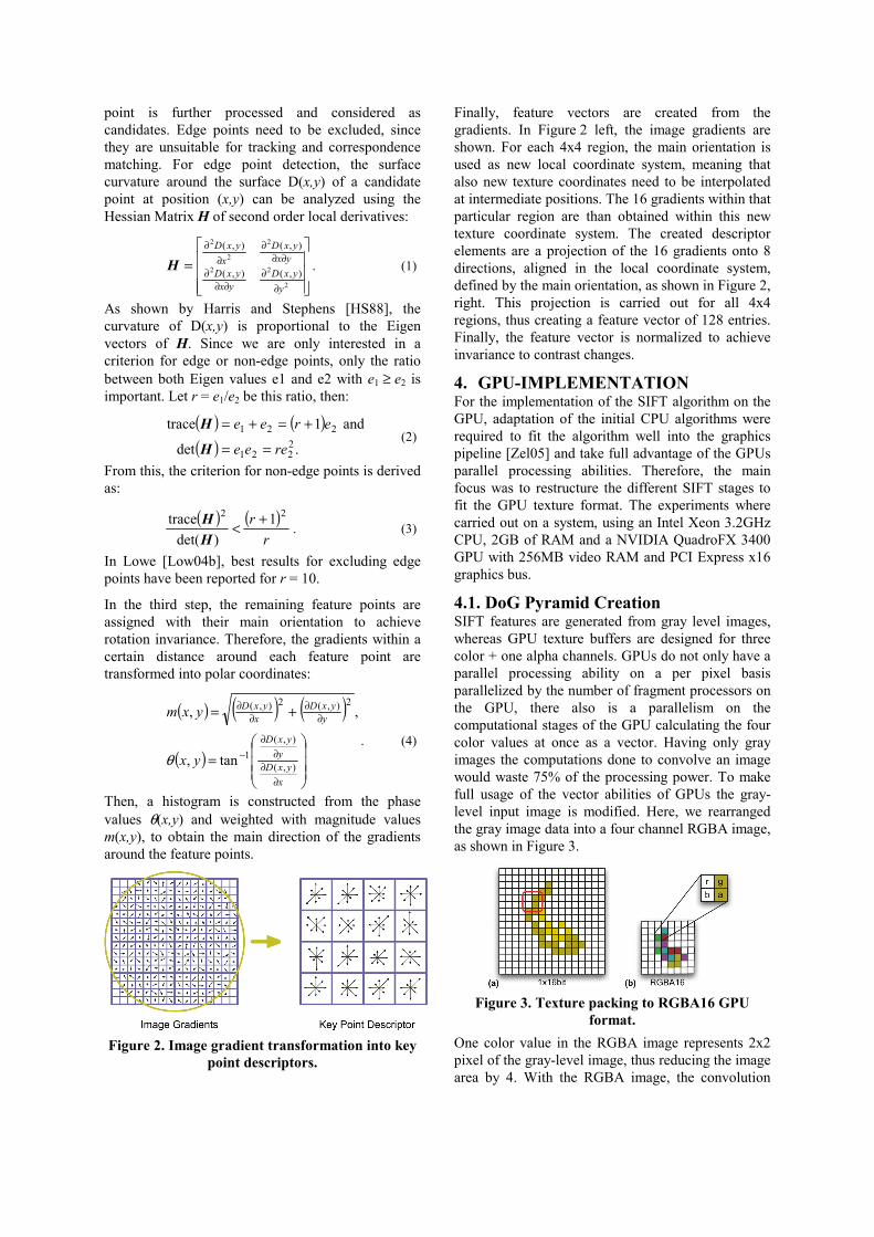
Then, a histogram is constructed from the phase values θ(x,y) and weighted with magnitude values m(x,y), to obtain the main direction of the gradients around the feature points.

Figure 2. Image gradient transformation into key

point descriptors.

Finally, feature vectors are created from the gradients. In Figure 2 left, the image gradients are shown. For each 4x4 region, the main orientation is used as new local coordinate system, meaning that also new texture coordinates need to be interpolated at intermediate positions. The 16 gradients within that particular region are than obtained within this new texture coordinate system. The created descriptor elements are a projection of the 16 gradients onto 8 directions, aligned in the local coordinate system, defined by the main orientation, as shown in Figure 2, right. This projection is carried out for all 4x4 regions, thus creating a feature vector of 128 entries. Finally, the feature vector is normalized to achieve invariance to contrast changes.

4. GPU-IMPLEMENTATION For the implementation of the SIFT algorithm on the GPU, adaptation of the initial CPU algorithms were required to fit the algorithm well into the graphics pipeline [Zel05] and take full advantage of the GPUs parallel processing abilities. Therefore, the main focus was to restructure the different SIFT stages to fit the GPU texture format. The experiments where carried out on a system, using an Intel Xeon 3.2GHz CPU, 2GB of RAM and a NVIDIA QuadroFX 3400 GPU with 256MB video RAM and PCI Express x16 graphics bus.

4.1. DoG Pyramid Creation SIFT features are generated from gray level images, whereas GPU texture buffers are designed for three color + one alpha channels. GPUs do not only have a parallel processing ability on a per pixel basis parallelized by the number of fragment processors on the GPU, there also is a parallelism on the computational stages of the GPU calculating the four color values at once as a vector. Having only gray images the computations done to convolve an image would waste 75% of the processing power. To make full usage of the vector abilities of GPUs the gray-level input image is modified. Here, we rearranged the gray image data into a four channel RGBA image, as shown in Figure 3.

Figure 3. Texture packing to RGBA16 GPU

format. One color value in the RGBA image represents 2x2 pixel of the gray-level image, thus reducing the image area by 4. With the RGBA image, the convolution

can be processed without wasting computational power on the GPU. In the case of a convolution, the processing on the packed data is straightforward, since here mostly linear operations, such as pixel- wise additions or multiplications are applied. In cases of operations, where pixel processing also depends on neighboring pixels, the algorithm adaptation for packed data becomes complicated, since all neighboring references need to be redirected. Reorganizing the input image creates some computational overhead which is comparatively low since the data remains in this packed format for the whole process of scale-space and DoG pyramid creation. The packing is implemented using a simple fragment shader that takes a block of 2x2 adjacent pixels and arranges them into one RGBA pixel. The Gaussian convolution is directly applied onto the packed RGBA format, as shown in Figure 4 with a 9tap Gaussian kernel. Here, the Gaussian kernel is split into even and odd values to carry out two separate semi-convolutions, which are added afterwards for the final result. Each pixel of the Gaussian kernel is multiplied with all four color components in one calculation, thus only requiring one texture access. The calculations with even and odd Gaussian kernel pixels are implemented in the same fragment shader and therefore the same texture access can be used for both steps.

Figure 4. Gaussian convolution in RGBA16 GPU

format, (a) odd and (b) even samples. Horizontal and vertical filtering with Gaussian kernels of different sizes is applied successively and the differently blurred images are subtracted to create the DoG pyramid, described above.

Using this technique allows us to convert a color image into a gray level image and pack the pixels in the described way in one rendering pass.

4.2. Key Point Filtering and Orientation For the detection of feature points, as described before, dynamic branching is used to keep the whole selection process in the GPU. Therefore, the criteria for possible feature points where rearranged starting with the luminance difference threshold, which excludes 50% of possible feature points. Then the search for global extreme values first compares a point with its 8 neighbors within the same buffer,

leaving only 0.6% of possible points followed by comparison with the 9 pixel of the adjacent buffers within the DoG stack. Possible feature points are shown in Figure 5(b). Afterwards, the exclusion of noise and edge points is carried out, leaving stable feature points, as shown in Figure 5(c).

Figure 5. Extraction and filtering of features.

After filtering and localization of potential feature points, the corresponding feature vectors are calculated. To calculate the gradient direction and magnitude, MRT functionality is used. For both values, only the four direct neighboring pixels are required, which keeps the referencing for calculation relatively simple. The reqired pixel access and operations are shown in Figure 6.

Figure 6. Gradient magnitude (top) and direction

(bottom) calculation for red channel. Here, the central texel “rgba” with its packed 4 original pixels as the four color components is processed. The magnitude and direction calculation for the central “r” component are shown in Figure 6, which require the four neighboring components that are highlighted as solid colors. Each central component requires two other components from the central texel and two from adjacent texels. The required operations for magnitude and direction calculation are also shown in Figure 6. Both calculations require the same input data. Since the input data is already packed, the use of two color components for magnitude and direction respectively is not possible. Instead, the use of MRTs greatly accelerates the processing, since both calculations can be carried out at once, writing the results into two separate rendering targets. Thus, time consuming OpenGL context switching is avoided and only one texel access for both operations is required, since

magnitude and direction use the same intermediate calculation (i.e. horizontal and vertical subtraction).

4.3. Feature Descriptor Creation Both render targets are now used to create the weighted histograms of the 4x4 regions around each feature point, as shown in the theoretical part in Figure 2. Each region is associated with 8 directions, adding up to a 128-element output vector. This operation differs from previously implemented operations, since for each single input element (or extreme point) 128 output elements are created. This operation can not be carried out at once, even with MRTs. Therefore, each region is processed in one fragment shader call, as there is no possibility to split the histogram calculation itself. For this calculation, it is useful to select a structure, where for each fragment different data can be accessed. A simple rectangular area, as used for the other calculations is not sufficient, since interpolation algorithms would interpolate the four corner attributes across the area, whereas here, each point requires independent attributes. A suitable representation for such independent attribute purposes is a vertex grid that can be created from geometry points via glVertex2f() or a line of multiple segments.

For easier processing, magnitude and direction values are rearranged from the two rendering targets into one texture to further process them with the precalculated texture directions, as shown in Figure 7.

Figure 7. Gradient map unpacking into one

texture. Here, the packed values for magnitude and direction are unpacked and interleaved at the same time, such that one output value only contains one magnitude and one associated direction value. In this form, both values are contained in one texture that can be further processed without format change.

For the final feature creation, gradient histograms for the 4x4 areas of each extreme point are created. Each area has to be processed in one fragment shader call, since the histogram calculation itself cannot be split up without expensive calculations. To carry out the histogram calculation in one shader cycle, 8 output values have to be calculated simultaneously. This again can be achieved, using MRTs on advanced

graphics cards. In Figure 8(a) the data structure for the feature generation is shown. As an example, a feature vector is shown in Figure 8(b), which consists of 16 vertices and is mapped into the two render targets.

Figure 8. Render Targets for Feature Generation. (a) Frame buffers in both render targets and (b)

feature point position in image and access on pre-calculated texture coordinates.

Each vertex of a feature vector is associated with appropriate attributes in the CPU. These attributes contain relative texture coordinates, magnitude and direction of gradient areas. The corresponding calculations can be carried out independently and all necessary parameters are coded in the feature vectors. As a result, each render target from Figure 8(a) contains a complete data set for half the feature vectors.

These SIFT feature vectors can now be used for correspondence matching between different images, e.g. for tracking in an image sequence. For this purpose, the Euclidean distance D between two feature vectors V1 and V2 with length N is calculated, as shown in (5).

( )∑=

−=N

iii VVD

1

221 . (5)

In our SIFT implementation, each vector has N = 128 elements. The associated subtractions in (5) can be well calculated in parallel. In a test, a CPU and GPU implementation were compared in terms of processing time. For this test, a number of feature vectors K were taken, with K varying between 500 and 3000. Each feature vector was compared with each other, resulting in K2 comparisons. While the processing time for 3000x3000 comparisons was 13sec using the CPU implementation, the GPU implementation only required 0.5sec.

4.4. Results After optimizing all SIFT stages for efficient GPU processing, the entire algorithm was tested and compared against the original CPU implementation

and a manually SSE (Streaming SIMD Extension) optimized version. The results are shown in Figure 9.

Here, the manually SSE optimized version requires 0.312sec compared to 0.406sec for the original CPU implementation. In comparison to that, the SIFT algorithm could be drastically accelerated by utilizing massive parallel GPU processing and thus achieving a processing time of only 0.058sec. Thus, SIFT feature extraction can be carried out in real time at approximately 20 frames/sec.

Figure 9. Results for all SIFT operator stages of

the GPU implementation in comparison to standard CPU processing.

5. CONCLUSION In this paper we have shown, how the SIFT algorithm can considerably be accelerated by utilizing GPU parallel processing. After arranging the luminance values of the input image into the GPU texture buffers RGBA format, all follow-up operations have also been adapted to this texture format and make use of new GPU technology, namely dynamic branching for the detection of relevant feature points and MRTs for parallel gradient direction and magnitude calculation. As a result, the SIFT algorithm can be applied to image sequences with 640x480 pixels at 20 frames/sec. Future work will mainly focus on real-time applications using SIFT features, e.g. calibration estimation for 3D scene reconstruction for image sequences.

6. References [BL03] Brown, M. and Lowe, D. G., “Recognising

Panoramas”, Proc. of the 9th International Conference on Computer Vision (ICCV2003), pp. 1218-1225, Nice, France, 2003.

[BL02] Brown, M. and Lowe, D., “Invariant Features from Interest Point Groups”, British Machine

Vision Conference, BMVC 2002, Cardiff, Wales, 2002.

[FS05] Foley, T. and Sugerman, J., ”KD-Tree Acceleration Structures for a GPU Raytracer”, Eurographics Report, Graphics Hardware, 2005.

[Fun05] Fung, J., “Computer Vision on the GPU”, GPU Gems 2, pp. 649-666, Addison-Wesley, 2005.

[GL04] Gordon, I. and Lowe, D.G., “Scene modeling, recognition and tracking with invariant image features”, International Symposium on Mixed and Augmented Reality (ISMAR), Arlington, USA, 2004.

[GLW*04] Govindaraju, N.K., Lloyd, B., Wang, W., Lin, M. and Manocha, D., „Fast Computation of Database Operations using Graphics Processors”, Proc. ACM SIGMOD 2004, Paris, France, 2004.

[GHLM05] Govindaraju, N.K., Henson, M., Lin, M. and Manocha, N., “Interactive Visibility Ordering of Geometric Primitives in Complex Environments”, Proc. ACM SIGGRAPH i3d, Washington DC, USA, 2005.

[HS88] Harris, C., Stephens, M., “A Combined Corner Edge Detector”, Proc. Alvey Vision Conference, pp. 189-192, Manchester, 1988.

[Har05] Harris, M., “Mapping Computational Concepts to GPUs”, GPU Gems 2, pp. 493-508, Addison-Wesley, 2005.

[KF05] Kilgariff, E., Fernando, R., “The GeForce 6 Series GPU Architecture”, GPU Gems 2, pp. 471-491, Addison-Wesley, 2005.

[Low04a] Lowe, D.G. 2004, “Object Recognition from local scale-invariant features”, Proc. International Conference on Computer Vision, pp.1150-1157, Corfu, Greece.

[Low04b] Lowe, D.G., “Distinctive Image Features from Scale-Invariant Keypoints”, International Journal of Computer Vision, 2004.

[OLG*05] Owens, J.D., Luebke, D., Govindaraju, N.K., Harris, M., Krüger, J., Lefohn, A.E., Purcell, T.J., “A Survey of General-Purpose Computation on Graphics Hardware”, Eurographics 2005, State of the Art Reports, Dublin, Ireland, 2005.

[Wit83] Witkin, A.P., “Scale-space filtering, Proc. International Joint Conference on Artificial Intelligence, pp. 1019-1022, Karlsruhe, Germany, 1983.

[Zel05] Zeller, C., “Introduction to the Hardware Graphics Pipeline”, ACM SIGGRAPH i3d, Invited Speech, Washington DC, USA, 2005.