SINUMERIK SINUMERIK 840D sl/SINUMERIK 828D Fundamentals Preface Fundamental geometrical principles 1 Fundamental principles of NC programming 2 Creating an NC program 3 Tool change 4 Tool offsets 5 Spindle motion 6 Feed control 7 Geometry settings 8 Motion commands 9 Tool radius compensation 10 Path action 11 Coordinate transformations (frames) 12 Auxiliary function outputs 13 Supplementary commands 14 Other information 15 Tables 16 Appendix A SINUMERIK SINUMERIK 840D sl/ SINUMERIK 828D Fundamentals Programming Manual 06/2009 6FC5398-1BP20-0BA0 Valid for Control System SINUMERIK 840D sl/840DE sl SINUMERIK 828D Software Version NCU system software for 840D sl/840DE sl 2.6 NCU System software for 828D 2.6

Siemens 828D Programing Manual
Jan 02, 2016
Welcome message from author
This document is posted to help you gain knowledge. Please leave a comment to let me know what you think about it! Share it to your friends and learn new things together.
Transcript

SINUMERIK SINUMERIK 840D sl/SINUMERIK 828D Fundamentals
Preface Fundamental geometrical principles
1Fundamental principles of NC programming
2
Creating an NC program
3
Tool change
4
Tool offsets
5
Spindle motion
6
Feed control
7
Geometry settings
8
Motion commands
9
Tool radius compensation
10
Path action
11Coordinate transformations (frames)
12
Auxiliary function outputs
13
Supplementary commands
14
Other information
15
Tables
16
Appendix
A
SINUMERIK
SINUMERIK 840D sl/ SINUMERIK 828D Fundamentals
Programming Manual
06/2009 6FC5398-1BP20-0BA0
Valid for Control System SINUMERIK 840D sl/840DE sl SINUMERIK 828D Software VersionNCU system software for 840D sl/840DE sl 2.6 NCU System software for 828D 2.6

Legal information Legal information Warning notice system
This manual contains notices you have to observe in order to ensure your personal safety, as well as to prevent damage to property. The notices referring to your personal safety are highlighted in the manual by a safety alert symbol, notices referring only to property damage have no safety alert symbol. These notices shown below are graded according to the degree of danger.
DANGER indicates that death or severe personal injury will result if proper precautions are not taken.
WARNING indicates that death or severe personal injury may result if proper precautions are not taken.
CAUTION with a safety alert symbol, indicates that minor personal injury can result if proper precautions are not taken.
CAUTION without a safety alert symbol, indicates that property damage can result if proper precautions are not taken.
NOTICE indicates that an unintended result or situation can occur if the corresponding information is not taken into account.
If more than one degree of danger is present, the warning notice representing the highest degree of danger will be used. A notice warning of injury to persons with a safety alert symbol may also include a warning relating to property damage.
Qualified Personnel The device/system may only be set up and used in conjunction with this documentation. Commissioning and operation of a device/system may only be performed by qualified personnel. Within the context of the safety notes in this documentation qualified persons are defined as persons who are authorized to commission, ground and label devices, systems and circuits in accordance with established safety practices and standards.
Proper use of Siemens products Note the following:
WARNING Siemens products may only be used for the applications described in the catalog and in the relevant technical documentation. If products and components from other manufacturers are used, these must be recommended or approved by Siemens. Proper transport, storage, installation, assembly, commissioning, operation and maintenance are required to ensure that the products operate safely and without any problems. The permissible ambient conditions must be adhered to. The information in the relevant documentation must be observed.
Trademarks All names identified by ® are registered trademarks of the Siemens AG. The remaining trademarks in this publication may be trademarks whose use by third parties for their own purposes could violate the rights of the owner.
Disclaimer of Liability We have reviewed the contents of this publication to ensure consistency with the hardware and software described. Since variance cannot be precluded entirely, we cannot guarantee full consistency. However, the information in this publication is reviewed regularly and any necessary corrections are included in subsequent editions.
Siemens AG Industry Sector Postfach 48 48 90026 NÜRNBERG GERMANY
Order number: 6FC5398-1BP20-0BA0 Ⓟ 06/2009
Copyright © Siemens AG 2009. Technical data subject to change

Fundamentals Programming Manual, 06/2009, 6FC5398-1BP20-0BA0 3
Preface
SINUMERIK Documentation The SINUMERIK documentation is organized in three parts: ● General Documentation ● User Documentation ● Manufacturer/service documentation Information on the following topics is available at http://www.siemens.com/motioncontrol/docu: ● Ordering documentation
Here you can find an up-to-date overview of publications ● Downloading documentation
Links to more information for downloading files from Service & Support. ● Researching documentation online
Information on DOConCD and direct access to the publications in DOConWeb. ● Compiling individual documentation on the basis of Siemens contents with the My
Documentation Manager (MDM), refer to http://www.siemens.com/mdm. My Documentation Manager provides you with a range of features for generating your own machine documentation.
● Training and FAQs Information on our range of training courses and FAQs (frequently asked questions) are available via the page navigation.
Target group This publication is intended for: ● Programmers ● Project engineers
Benefits With the programming manual, the target group can develop, write, test, and debug programs and software user interfaces.

Preface
Fundamentals 4 Programming Manual, 06/2009, 6FC5398-1BP20-0BA0
Standard scope This Programming Manual describes the functionality afforded by standard functions. Extensions or changes made by the machine tool manufacturer are documented by the machine tool manufacturer. Other functions not described in this documentation might be executable in the control. This does not, however, represent an obligation to supply such functions with a new control or when servicing. Further, for the sake of simplicity, this documentation does not contain all detailed information about all types of the product and cannot cover every conceivable case of installation, operation or maintenance.
Technical Support If you have any questions, please contact our hotline: Europe/Africa Phone +49 180 5050 - 222 Fax +49 180 5050 - 223 €0.14/min. from German landlines, mobile phone prices may differ Internet http://www.siemens.de/automation/support-request
America Phone +1 423 262 2522 Fax +1 423 262 2200 E-mail mailto:[email protected]
Asia/Pacific Phone +86 1064 757575 Fax +86 1064 747474 E-mail mailto:[email protected]
Note You will find telephone numbers for other countries for technical support on the Internet: http://www.automation.siemens.com/partner

Preface
Fundamentals Programming Manual, 06/2009, 6FC5398-1BP20-0BA0 5
Questions about the manual If you have any queries (suggestions, corrections) in relation to this documentation, please fax or e-mail us: Fax: +49 9131- 98 2176 E-mail: mailto:[email protected]
A fax form is available in the appendix of this document.
SINUMERIK Internet address http://www.siemens.com/sinumerik
"Fundamentals" and "Job planning" Programming Manual The description of the NC programming is divided into two manuals: 1. Fundamentals
This "Fundamentals" Programming Manual is intended for use by skilled machine operators with the appropriate expertise in drilling, milling and turning operations. Simple programming examples are used to explain the commands and statements which are also defined according to DIN 66025.
2. Job planning The Programming Manual "Job planning" is intended for use by technicians with in-depth, comprehensive programming knowledge. By virtue of a special programming language, the SINUMERIK control enables the user to program complex workpiece programs (e.g. for free-form surfaces, channel coordination, ...) and makes programming of complicated operations easy for technologists.
Availability of the described NC language elements All NC language elements described in the manual are available for the SINUMERIK 840D sl. The availability regarding SINUMERIK 828D can be found in column "828D" of the "List of statements (Page 483) ".

Preface
Fundamentals 6 Programming Manual, 06/2009, 6FC5398-1BP20-0BA0

Fundamentals Programming Manual, 06/2009, 6FC5398-1BP20-0BA0 7
Table of contents
Preface ...................................................................................................................................................... 3 1 Fundamental geometrical principles ........................................................................................................ 13
1.1 Workpiece positions.....................................................................................................................13 1.1.1 Workpiece coordinate systems....................................................................................................13 1.1.2 Cartesian coordinates ..................................................................................................................14 1.1.3 Polar coordinates .........................................................................................................................18 1.1.4 Absolute dimensions....................................................................................................................19 1.1.5 Incremental dimension.................................................................................................................21 1.2 Working planes ............................................................................................................................23 1.3 Zero points and reference points .................................................................................................25 1.4 Coordinate systems .....................................................................................................................27 1.4.1 Machine coordinate system (MCS)..............................................................................................27 1.4.2 Basic coordinate system (BCS) ...................................................................................................31 1.4.3 Basic zero system (BZS) .............................................................................................................33 1.4.4 Settable zero system (SZS) .........................................................................................................34 1.4.5 Workpiece coordinate system (WCS)..........................................................................................35 1.4.6 What is the relationship between the various coordinate systems?............................................36
2 Fundamental principles of NC programming............................................................................................ 37 2.1 Name of an NC program..............................................................................................................37 2.2 Structure and contents of an NC program...................................................................................39 2.2.1 Blocks and block components .....................................................................................................39 2.2.2 Block rules....................................................................................................................................42 2.2.3 Value assignments.......................................................................................................................43 2.2.4 Comments....................................................................................................................................44 2.2.5 Skipping blocks ............................................................................................................................45
3 Creating an NC program.......................................................................................................................... 47 3.1 Basic procedure ...........................................................................................................................47 3.2 Available characters.....................................................................................................................49 3.3 Program header ...........................................................................................................................51 3.4 Program examples.......................................................................................................................53 3.4.1 Example 1: First programming steps ...........................................................................................53 3.4.2 Example 2: NC program for turning .............................................................................................54 3.4.3 Example 3: NC program for milling..............................................................................................56
4 Tool change............................................................................................................................................. 59 4.1 Tool change without tool management........................................................................................60 4.1.1 Tool change with T command......................................................................................................60 4.1.2 Tool change with M6....................................................................................................................61 4.2 Tool change with tool management (option)................................................................................63 4.2.1 Tool change with T command with active tool management (option)..........................................63 4.2.2 Tool change with M6 with active tool management (option)........................................................66

Table of contents
Fundamentals 8 Programming Manual, 06/2009, 6FC5398-1BP20-0BA0
4.3 Behavior with faulty T programming ........................................................................................... 68 5 Tool offsets .............................................................................................................................................. 69
5.1 General information about the tool offsets .................................................................................. 69 5.2 Tool length compensation........................................................................................................... 70 5.3 Tool radius compensation........................................................................................................... 71 5.4 Tool compensation memory........................................................................................................ 72 5.5 Tool types.................................................................................................................................... 74 5.5.1 General information about the tool types .................................................................................... 74 5.5.2 Milling tools ................................................................................................................................. 75 5.5.3 Drills ............................................................................................................................................ 77 5.5.4 Grinding tools .............................................................................................................................. 78 5.5.5 Turning tools ............................................................................................................................... 80 5.5.6 Special tools................................................................................................................................ 82 5.5.7 Chaining rule ............................................................................................................................... 83 5.6 Tool offset call (D) ....................................................................................................................... 84 5.7 Change in the tool offset data ..................................................................................................... 87 5.8 Programmable tool offset (TOFFL, TOFF, TOFFR).................................................................... 88
6 Spindle motion......................................................................................................................................... 95 6.1 Spindle speed (S), direction of spindle rotation (M3, M4, M5).................................................... 95 6.2 Cutting rate (SVC)..................................................................................................................... 100 6.3 Constant cutting rate (G96/G961/G962, G97/G971/G972, G973, LIMS, SCC) ....................... 108 6.4 Constant grinding wheel peripheral speed (GWPSON, GWPSOF).......................................... 115 6.5 Programmable spindle speed limitation (G25, G26)................................................................. 118
7 Feed control........................................................................................................................................... 119 7.1 Feedrate (G93, G94, G95, F, FGROUP, FL, FGREF).............................................................. 119 7.2 Traversing positioning axes (POS, POSA, POSP, FA, WAITP, WAITMC) .............................. 129 7.3 Position-controlled spindle operation (SPCON, SPCOF) ......................................................... 134 7.4 Positioning spindles (SPOS, SPOSA, M19, M70, WAITS)....................................................... 135 7.5 Feedrate for positioning axes/spindles (FA, FPR, FPRAON, FPRAOF) .................................. 146 7.6 Programmable feedrate override (OVR, OVRRAP, OVRA) ..................................................... 150 7.7 Programmable acceleration override (ACC) (option)................................................................ 152 7.8 Feedrate with handwheel override (FD, FDA) .......................................................................... 154 7.9 Feedrate optimization for curved path sections (CFTCP, CFC, CFIN)..................................... 158 7.10 Several feedrate values in one block (F, ST, SR, FMA, STA, SRA)......................................... 161 7.11 Non-modal feedrate (FB) .......................................................................................................... 164 7.12 Tooth feedrate (G95 FZ) ........................................................................................................... 165
8 Geometry settings.................................................................................................................................. 173 8.1 Settable work offset (G54 to G57, G505 to G599, G53, G500, SUPA, G153) ......................... 173
Table of contents
Fundamentals Programming Manual, 06/2009, 6FC5398-1BP20-0BA0 9
8.2 Selection of the working plane (G17/G18/G19) .........................................................................179 8.3 Dimensions ................................................................................................................................183 8.3.1 Absolute dimensions (G90, AC).................................................................................................183 8.3.2 Incremental dimensions (G91, IC) .............................................................................................186 8.3.3 Absolute and incremental dimensions for turning and milling (G90/G91) .................................190 8.3.4 Absolute dimension for rotary axes (DC, ACP, ACN)................................................................191 8.3.5 Inch or metric dimensions (G70/G700, G71/G710) ...................................................................194 8.3.6 Channel-specific diameter/radius programming (DIAMON, DIAM90, DIAMOF,
DIAMCYCOF) ............................................................................................................................197 8.3.7 Axis-specific diameter/radius programming (DIAMONA, DIAM90A, DIAMOFA,
DIACYCOFA, DIAMCHANA, DIAMCHAN, DAC, DIC, RAC, RIC) ............................................200 8.4 Position of workpiece for turning................................................................................................205
9 Motion commands ................................................................................................................................. 207 9.1 Travel commands with Cartesian coordinates (G0, G1, G2, G3, X..., Y..., Z...) ........................209 9.2 Travel commands with polar coordinates ..................................................................................211 9.2.1 Reference point of the polar coordinates (G110, G111, G112).................................................211 9.2.2 Travel commands with polar coordinates (G0, G1, G2, G3, AP, RP)........................................213 9.3 Rapid traverse movement (G0, RTLION, RTLIOF) ...................................................................217 9.4 Linear interpolation (G1) ............................................................................................................222 9.5 Circular interpolation ..................................................................................................................225 9.5.1 Circular interpolation types (G2/G3, ...) .....................................................................................225 9.5.2 Circular interpolation with center point and end point (G2/G3, X... Y... Z..., I... J... K...) ...........229 9.5.3 Circular interpolation with radius and end point (G2/G3, X... Y... Z.../ I... J... K..., CR) .............233 9.5.4 Circular interpolation with opening angle and center point (G2/G3, X... Y... Z.../ I... J...
K..., AR)......................................................................................................................................236 9.5.5 Circular interpolation with polar coordinates (G2/G3, AP, RP)..................................................239 9.5.6 Circular interpolation with intermediate point and end point (CIP, X... Y... Z..., I1... J1...
K1...)...........................................................................................................................................242 9.5.7 Circular interpolation with tangential transition (CT, X... Y... Z...)..............................................246 9.6 Helical interpolation (G2/G3, TURN) .........................................................................................250 9.7 Involute interpolation (INVCW, INVCCW)..................................................................................253 9.8 Contour definitions .....................................................................................................................259 9.8.1 Contour definitions: One straight line (ANG) .............................................................................260 9.8.2 Contour definitions: Two straight lines (ANG)............................................................................262 9.8.3 Contour definitions: Three straight line (ANG)...........................................................................265 9.8.4 Contour definitions: End point programming with angle ............................................................269 9.9 Thread cutting with constant lead (G33)....................................................................................270 9.9.1 Thread cutting with constant lead (G33, SF) .............................................................................270 9.9.2 Programmable run-in and run-out paths (DITS, DITE)..............................................................278 9.10 Thread cutting with increasing or decreasing lead (G34, G35) .................................................281 9.11 Tapping without compensating chuck (G331, G332) ................................................................283 9.12 Tapping with compensating chuck (G63) ..................................................................................288 9.13 Fast retraction for thread cutting (LFON, LFOF, DILF, ALF, LFTXT, LFWP, LFPOS,
POLF, POLFMASK, POLFMLIN)...............................................................................................290 9.14 Chamfer, rounding (CHF, CHR, RND, RNDM, FRC, FRCM)....................................................295
Table of contents
Fundamentals 10 Programming Manual, 06/2009, 6FC5398-1BP20-0BA0
10 Tool radius compensation...................................................................................................................... 301 10.1 Tool radius compensation (G40, G41, G42, OFFN) ................................................................. 301 10.2 Contour approach and retraction (NORM, KONT, KONTC, KONTT)....................................... 312 10.3 Compensation at the outside corners (G450, G451, DISC) ..................................................... 319 10.4 Smooth approach and retraction............................................................................................... 323 10.4.1 Approach and retraction (G140 to G143, G147, G148, G247, G248, G347, G348, G340,
G341, DISR, DISCL, FAD, PM, PR) ......................................................................................... 323 10.4.2 Approach and retraction with enhanced retraction strategies (G460, G461, G462)................. 335 10.5 Collision monitoring (CDON, CDOF, CDOF2) .......................................................................... 340 10.6 2D tool compensation (CUT2D, CUT2DF)................................................................................ 344 10.7 Keep tool radius compensation constant (CUTCONON, CUTCONOF) ................................... 347 10.8 Tools with a relevant cutting edge position ............................................................................... 350
11 Path action............................................................................................................................................. 353 11.1 Exact stop (G60, G9, G601, G602, G603)................................................................................ 353 11.2 Continuous-path mode (G64, G641, G642, G643, G644, G645, ADIS, ADISPOS)................. 357
12 Coordinate transformations (frames) ..................................................................................................... 369 12.1 Frames ...................................................................................................................................... 369 12.2 Frame instructions..................................................................................................................... 371 12.3 Programmable zero offset......................................................................................................... 376 12.3.1 Zero offset (TRANS, ATRANS)................................................................................................. 376 12.3.2 Axial zero offset (G58, G59)...................................................................................................... 381 12.4 Programmable rotation (ROT, AROT, RPL) ............................................................................. 384 12.5 Programmable frame rotations with solid angles (ROTS, AROTS, CROTS) ........................... 396 12.6 Programmable scale factor (SCALE, ASCALE)........................................................................ 398 12.7 Programmable mirroring (MIRROR, AMIRROR) ...................................................................... 403 12.8 Frame generation according to tool orientation (TOFRAME, TOROT, PAROT) ...................... 410 12.9 Deselect frame (G53, G153, SUPA, G500) .............................................................................. 414 12.10 Deselecting overlaid movements (DRFOF, CORROF) ............................................................ 415
13 Auxiliary function outputs ....................................................................................................................... 419 13.1 M functions................................................................................................................................ 423
14 Supplementary commands .................................................................................................................... 427 14.1 Messages (MSG) ...................................................................................................................... 427 14.2 Working area limitation.............................................................................................................. 429 14.2.1 Working area limitation in BCS (G25/G26, WALIMON, WALIMOF) ......................................... 429 14.2.2 Working area limitation in WCS/SZS (WALCS0 ... WALCS10) ................................................ 433 14.3 Reference point approach (G74) .............................................................................................. 436 14.4 Fixed-point approach (G75, G751) ........................................................................................... 437 14.5 Travel to fixed stop (FXS, FXST, FXSW).................................................................................. 443

Table of contents
Fundamentals Programming Manual, 06/2009, 6FC5398-1BP20-0BA0 11
14.6 Acceleration behavior ................................................................................................................449 14.6.1 Acceleration mode (BRISK, BRISKA, SOFT, SOFTA, DRIVE, DRIVEA) .................................449 14.6.2 Influence of acceleration on following axes (VELOLIMA, ACCLIMA, JERKLIMA)....................452 14.6.3 Activation of technology-specific dynamic values (DYNNORM, DYNPOS, DYNROUGH,
DYNSEMIFIN, DYNFINISH) ......................................................................................................454 14.7 Traversing with feedforward control, FFWON, FFWOF.............................................................456 14.8 Contour accuracy, CPRECON, CPRECOF...............................................................................457 14.9 Dwell time (G4) ..........................................................................................................................458 14.10 Internal preprocessing stop........................................................................................................460
15 Other information................................................................................................................................... 461 15.1 Axes ...........................................................................................................................................461 15.1.1 Main axes/Geometry axes .........................................................................................................463 15.1.2 Special axes...............................................................................................................................464 15.1.3 Main spindle, master spindle .....................................................................................................464 15.1.4 Machine axes.............................................................................................................................465 15.1.5 Channel axes .............................................................................................................................465 15.1.6 Path axes ...................................................................................................................................465 15.1.7 Positioning axes.........................................................................................................................466 15.1.8 Synchronized axes.....................................................................................................................467 15.1.9 Command axes..........................................................................................................................467 15.1.10 PLC axes....................................................................................................................................467 15.1.11 Link axes ....................................................................................................................................468 15.1.12 Lead link axes ............................................................................................................................470 15.2 From travel command to machine movement ...........................................................................473 15.3 Path calculation..........................................................................................................................474 15.4 Addresses ..................................................................................................................................475 15.5 Identifiers....................................................................................................................................479 15.6 Constants ...................................................................................................................................481
16 Tables.................................................................................................................................................... 483 16.1 List of statements.......................................................................................................................483 16.2 Addresses ..................................................................................................................................558 16.3 G function groups.......................................................................................................................568 16.4 Predefined subroutine calls........................................................................................................588 16.5 Predefined subroutine calls in motion-synchronous actions......................................................607 16.6 Predefined functions ..................................................................................................................608
A Appendix................................................................................................................................................ 617 A.1 List of abbreviations ...................................................................................................................617 A.2 Feedback on the documentation................................................................................................623 A.3 Documentation overview............................................................................................................625
Glossary ................................................................................................................................................ 627 Index...................................................................................................................................................... 655

Table of contents
Fundamentals 12 Programming Manual, 06/2009, 6FC5398-1BP20-0BA0

Fundamentals Programming Manual, 06/2009, 6FC5398-1BP20-0BA0 13
Fundamental geometrical principles 11.1 1.1 Workpiece positions
1.1.1 Workpiece coordinate systems In order that the machine or the control can work with the positions specified in the NC program, these specifications have to be made in a reference system that can be transferred to the directions of motion of the machine axes. A coordinate system with the axes X, Y and Z is used for this purpose. DIN 66217 stipulates that machine tools must use clockwise, right-angled (Cartesian) coordinate systems.
Figure 1-1 Workpiece coordinate system for milling

Fundamental geometrical principles 1.1 Workpiece positions
Fundamentals 14 Programming Manual, 06/2009, 6FC5398-1BP20-0BA0
Figure 1-2 Workpiece coordinate system for turning
The workpiece zero (W) is the origin of the workpiece coordinate system. Sometimes it is advisable or even necessary to work with negative position specifications. For this reason, positions that are to the left of the zero point are assigned a negative sign ("-").
1.1.2 Cartesian coordinates The axes in the coordinate system are assigned dimensions. In this way, it is possible to clearly describe every point in the coordinate system and therefore every workpiece position through the direction (X, Y and Z) and three numerical values The workpiece zero always has the coordinates X0, Y0, and Z0.

Fundamental geometrical principles 1.1 Workpiece positions
Fundamentals Programming Manual, 06/2009, 6FC5398-1BP20-0BA0 15
Position specifications in the form of Cartesian coordinates To simplify things, we will only consider one plane of the coordinate system in the following example, the X/Y plane:
Points P1 to P4 have the following coordinates: Position Coordinates P1 X100 Y50 P2 X-50 Y100 P3 X-105 Y-115 P4 X70 Y-75

Fundamental geometrical principles 1.1 Workpiece positions
Fundamentals 16 Programming Manual, 06/2009, 6FC5398-1BP20-0BA0
Example: Workpiece positions for turning With lathes, one plane is sufficient to describe the contour:
Points P1 to P4 have the following coordinates: Position Coordinates P1 X25 Z-7.5 P2 X40 Z-15 P3 X40 Z-25 P4 X60 Z-35

Fundamental geometrical principles 1.1 Workpiece positions
Fundamentals Programming Manual, 06/2009, 6FC5398-1BP20-0BA0 17
Example: Workpiece positions for milling For milling, the feed depth must also be described, i.e. the third coordinate (in this case Z) must also be assigned a numerical value.
Points P1 to P3 have the following coordinates: Position Coordinates P1 X10 Y45 Z-5 P2 X30 Y60 Z-20 P3 X45 Y20 Z-15

Fundamental geometrical principles 1.1 Workpiece positions
Fundamentals 18 Programming Manual, 06/2009, 6FC5398-1BP20-0BA0
1.1.3 Polar coordinates Polar coordinates can be used instead of Cartesian coordinates to describe workpiece positions. This is useful when a workpiece or part of a workpiece has been dimensioned with radius and angle. The point from which the dimensioning starts is called the "pole".
Position specifications in the form of polar coordinates Polar coordinates are made up of the polar radius and the polar angle. The polar radius is the distance between the pole and the position. The polar angle is the angle between the polar radius and the horizontal axis of the working plane. Negative polar angles are in the clockwise direction, positive polar angles in the counterclockwise direction.
Example
Points P1 and P2 can then be described – with reference to the pole – as follows: Position Polar coordinates P1 RP=100 AP=30 P2 RP=60 AP=75 RP: Polar radius AP: Polar angle
Fundamental geometrical principles 1.1 Workpiece positions
Fundamentals Programming Manual, 06/2009, 6FC5398-1BP20-0BA0 19
1.1.4 Absolute dimensions
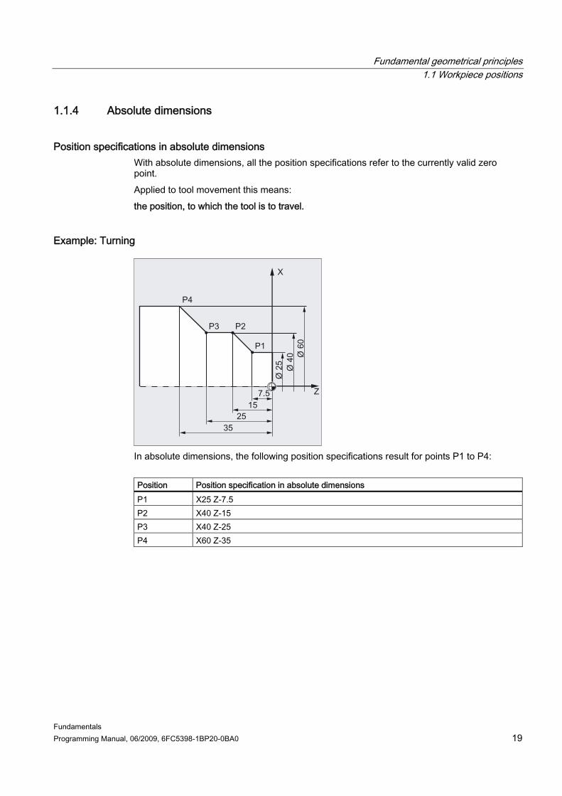
Position specifications in absolute dimensions With absolute dimensions, all the position specifications refer to the currently valid zero point. Applied to tool movement this means: the position, to which the tool is to travel.
Example: Turning
In absolute dimensions, the following position specifications result for points P1 to P4: Position Position specification in absolute dimensions P1 X25 Z-7.5 P2 X40 Z-15 P3 X40 Z-25 P4 X60 Z-35

Fundamental geometrical principles 1.1 Workpiece positions
Fundamentals 20 Programming Manual, 06/2009, 6FC5398-1BP20-0BA0
Example: Milling
In absolute dimensions, the following position specifications result for points P1 to P3: Position Position specification in absolute dimensions P1 X20 Y35 P2 X50 Y60 P3 X70 Y20

Fundamental geometrical principles 1.1 Workpiece positions
Fundamentals Programming Manual, 06/2009, 6FC5398-1BP20-0BA0 21
1.1.5 Incremental dimension
Position specifications in incremental dimensions In production drawings, the dimensions often do not refer to a zero point, but to another workpiece point. So that these dimensions do not have to be converted, they can be specified in incremental dimensions. In this method of dimensional notation, a position specification refers to the previous point. Applied to tool movement this means: The incremental dimensions describe the distance the tool is to travel.
Example: Turning
In incremental dimensions, the following position specifications result for points P2 to P4: Position Position specification in incremental dimensions The specification refers to: P2 X15 Z-7.5 P1 P3 Z-10 P2 P4 X20 Z-10 P3
Note With DIAMOF or DIAM90 active, the set distance in incremental dimensions (G91) is programmed as a radius dimension.

Fundamental geometrical principles 1.1 Workpiece positions
Fundamentals 22 Programming Manual, 06/2009, 6FC5398-1BP20-0BA0
Example: Milling The position specifications for points P1 to P3 in incremental dimensions are:
In incremental dimensions, the following position specifications result for points P1 to P3: Position Position specification in incremental
dimensions The specification refers to:
P1 X20 Y35 Zero point P2 X30 Y20 P1 P3 X20 Y -35 P2

Fundamental geometrical principles 1.2 Working planes
Fundamentals Programming Manual, 06/2009, 6FC5398-1BP20-0BA0 23
1.2 1.2 Working planes An NC program must contain information about the plane in which the work is to be performed. Only then can the control unit calculate the correct tool offsets during the execution of the NC program. The specification of the working plane is also relevant for certain types of circular-path programming and polar coordinates. Two coordinate axes define a working plane. The third coordinate axis is perpendicular to this plane and determines the infeed direction of the tool (e.g. for 2D machining).
Working planes for turning/milling
Figure 1-3 Working planes for turning

Fundamental geometrical principles 1.2 Working planes
Fundamentals 24 Programming Manual, 06/2009, 6FC5398-1BP20-0BA0
Figure 1-4 Working planes for milling
Programming of the working planes The working planes are defined in the NC program with the G commands G17, G18 and G19 as follows: G command Working plane Infeed direction Abscissa Ordinate Applicate G17 X/Y Z X Y Z G18 Z/X Y Z X Y G19 Y/Z X Y Z X

Fundamental geometrical principles 1.3 Zero points and reference points
Fundamentals Programming Manual, 06/2009, 6FC5398-1BP20-0BA0 25
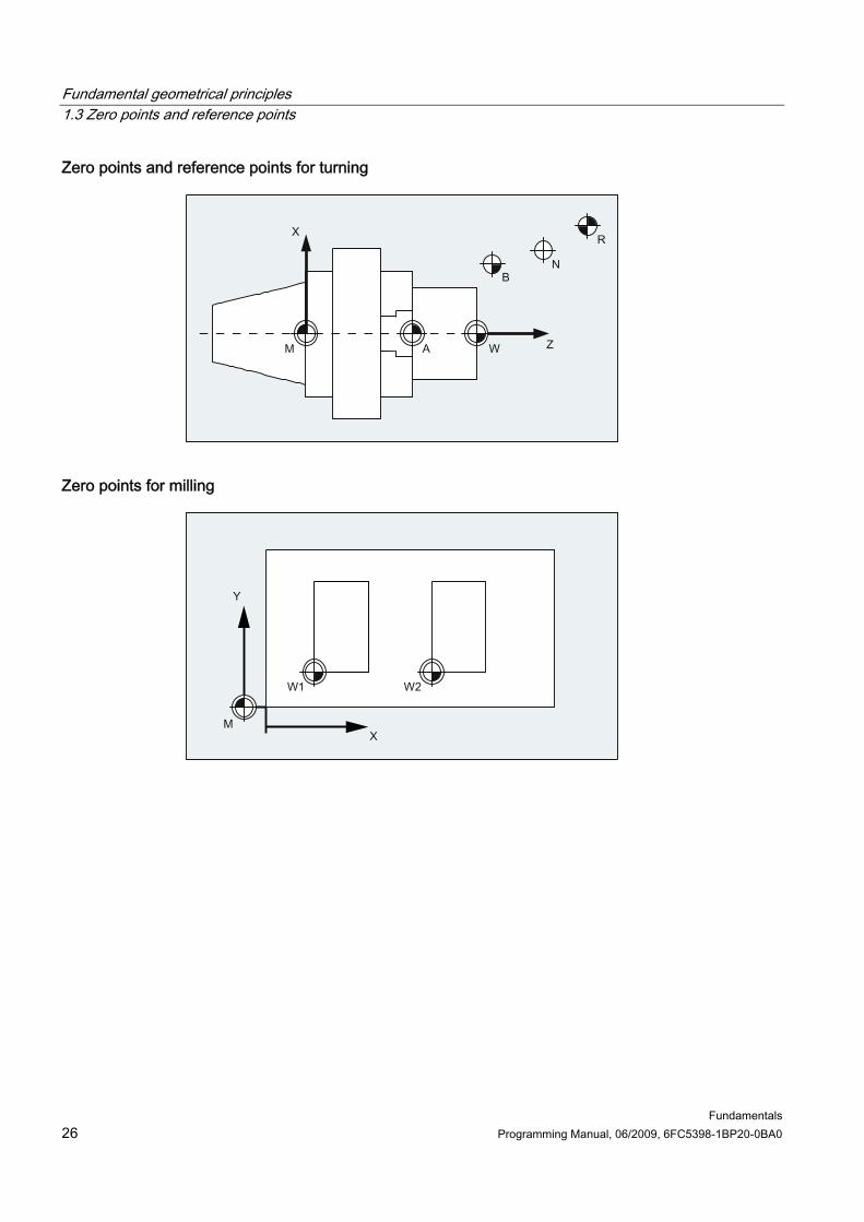
1.3 1.3 Zero points and reference points Various zero points and reference points are defined on an NC machine: Zero points
M Machine zero
The machine zero defines the machine coordinate system (MCS). All other reference points refer to the machine zero.
W Workpiece zero = program zero
The workpiece zero defines the workpiece coordinate system in relation to the machine zero.
A Blocking point
Can be the same as the workpiece zero (only for lathes).
Reference points
R Reference point Position defined by output cam and measuring system. The distance to the machine zero M must be known so that the axis position at this point can be set exactly to this value.
B Starting point
Can be defined by the program. The first machining tool starts here.
T Toolholder reference point
Is on the toolholder. By entering the tool lengths, the control calculates the distance between the tool tip and the toolholder reference point.
N Tool change point
Fundamental geometrical principles 1.3 Zero points and reference points
Fundamentals 26 Programming Manual, 06/2009, 6FC5398-1BP20-0BA0
Zero points and reference points for turning
Zero points for milling
Fundamental geometrical principles 1.4 Coordinate systems
Fundamentals Programming Manual, 06/2009, 6FC5398-1BP20-0BA0 27
1.4 1.4 Coordinate systems A distinction is made between the following coordinate systems: ● Machine coordinate system (MCS) (Page 27) with the machine zero M ● Basic coordinate system (BCS) (Page 31) ● Basic zero system (BZS) (Page 33) ● Settable zero system (SZS) (Page 34) ● Workpiece coordinate system (WCS) (Page 35) with the workpiece zero W
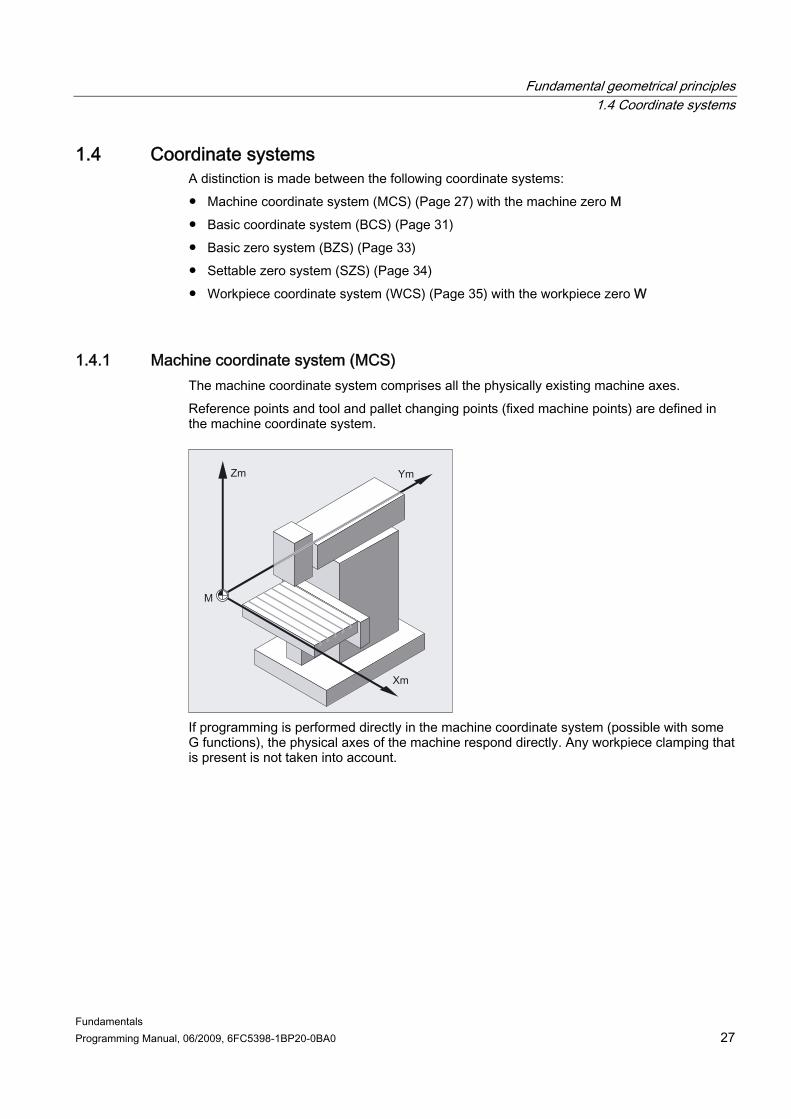
1.4.1 Machine coordinate system (MCS) The machine coordinate system comprises all the physically existing machine axes. Reference points and tool and pallet changing points (fixed machine points) are defined in the machine coordinate system.
If programming is performed directly in the machine coordinate system (possible with some G functions), the physical axes of the machine respond directly. Any workpiece clamping that is present is not taken into account.
Fundamental geometrical principles 1.4 Coordinate systems
Fundamentals 28 Programming Manual, 06/2009, 6FC5398-1BP20-0BA0
Note If there are various machine coordinate systems (e.g. 5-axis transformation), then an internal transformation is used to map the machine kinematics on the coordinate system in which the programming is performed.
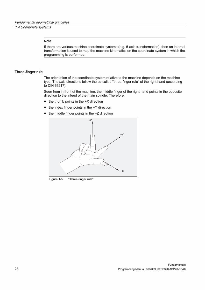
Three-finger rule The orientation of the coordinate system relative to the machine depends on the machine type. The axis directions follow the so-called "three-finger rule" of the right hand (according to DIN 66217). Seen from in front of the machine, the middle finger of the right hand points in the opposite direction to the infeed of the main spindle. Therefore: ● the thumb points in the +X direction ● the index finger points in the +Y direction ● the middle finger points in the +Z direction
Figure 1-5 "Three-finger rule"

Fundamental geometrical principles 1.4 Coordinate systems
Fundamentals Programming Manual, 06/2009, 6FC5398-1BP20-0BA0 29
Rotary motions around the coordinate axes X, Y and Z are designated A, B and C. If the rotary motion is in a clockwise direction when looking in the positive direction of the coordinate axis, the direction of rotation is positive:

Fundamental geometrical principles 1.4 Coordinate systems
Fundamentals 30 Programming Manual, 06/2009, 6FC5398-1BP20-0BA0
Position of the coordinate system in different machine types The position of the coordinate system resulting from the "three-finger rule" can have a different orientation for different machine types. Here are a few examples:

Fundamental geometrical principles 1.4 Coordinate systems
Fundamentals Programming Manual, 06/2009, 6FC5398-1BP20-0BA0 31
1.4.2 Basic coordinate system (BCS) The basic coordinate system (BCS) consists of three mutually perpendicular axes (geometry axes) as well as other special axes, which are not interrelated geometrically.
Machine tools without kinematic transformation BCS and MCS always coincide when the BCS can be mapped onto the MCS without kinematic transformation (e.g. 5-axis transformation, TRANSMIT/TRACYL/TRAANG). On such machines, machine axes and geometry axes can have the same names.
Figure 1-6 MCS = BCS without kinematic transformation
Machine tools with kinematic transformation BCS and MCS do not coincide when the BCS is mapped onto the MCS with kinematic transformation (e.g. 5-axis transformation, TRANSMIT/TRACYL/TRAANG). On such machines the machine axes and geometry axes must have different names.
Fundamental geometrical principles 1.4 Coordinate systems
Fundamentals 32 Programming Manual, 06/2009, 6FC5398-1BP20-0BA0
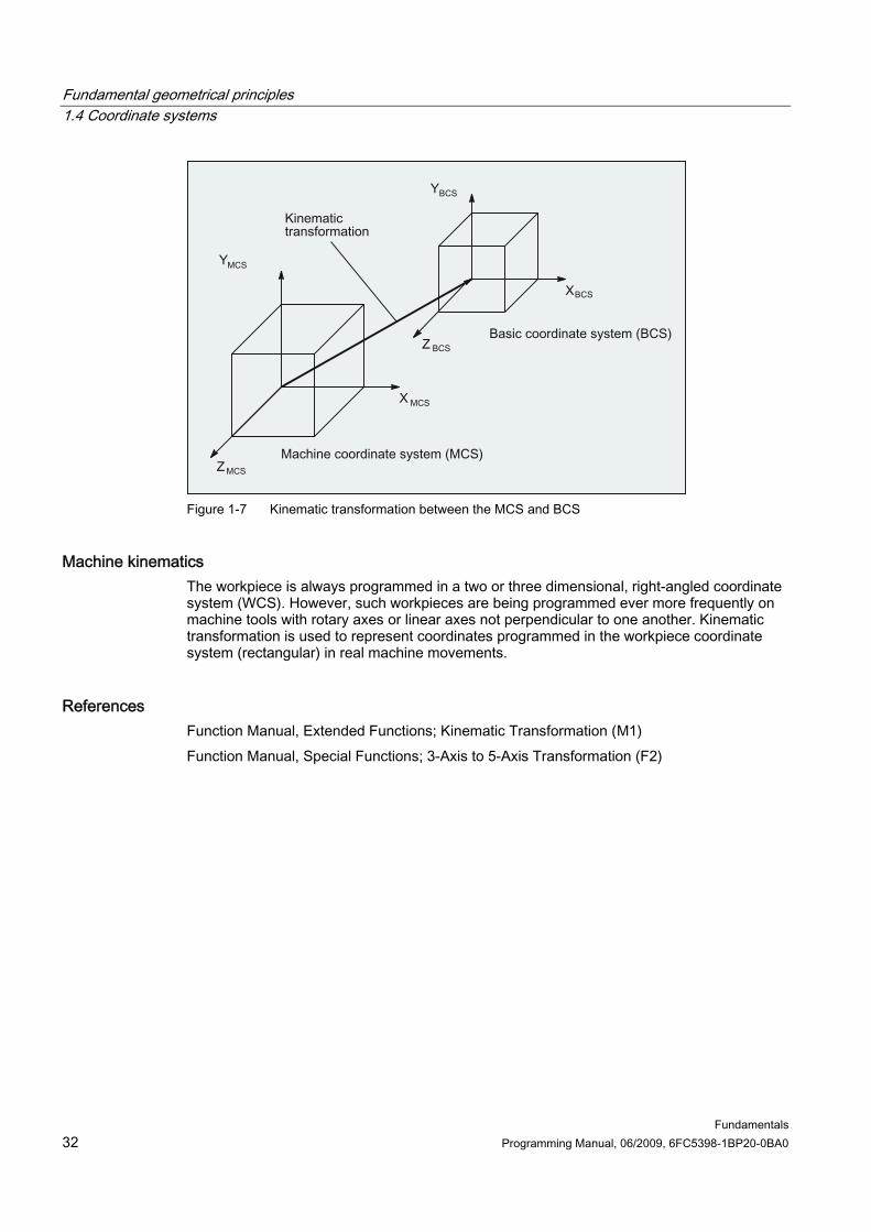
Figure 1-7 Kinematic transformation between the MCS and BCS
Machine kinematics The workpiece is always programmed in a two or three dimensional, right-angled coordinate system (WCS). However, such workpieces are being programmed ever more frequently on machine tools with rotary axes or linear axes not perpendicular to one another. Kinematic transformation is used to represent coordinates programmed in the workpiece coordinate system (rectangular) in real machine movements.
References Function Manual, Extended Functions; Kinematic Transformation (M1) Function Manual, Special Functions; 3-Axis to 5-Axis Transformation (F2)

Fundamental geometrical principles 1.4 Coordinate systems
Fundamentals Programming Manual, 06/2009, 6FC5398-1BP20-0BA0 33
1.4.3 Basic zero system (BZS) The basic zero system (BZS) is the basic coordinate system with a basic offset.
Basic offset The basic offset describes the coordinate transformation between BCS and BZS. It can be used, for example, to define the palette window zero. The basic offset comprises: ● Zero offset external ● DRF offset ● Overlaid movement ● Chained system frames ● Chained basic frames
References Function Manual, Basic Functions; Axes, Coordinate Systems, Frames (K2)

Fundamental geometrical principles 1.4 Coordinate systems
Fundamentals 34 Programming Manual, 06/2009, 6FC5398-1BP20-0BA0
1.4.4 Settable zero system (SZS)
Settable zero offset The "settable zero system" (SZS) results from the basic zero system (BZS) through the settable zero offset. Settable zero offsets are activated in the NC program with the G commands G54...G57 and G505...G599 as follows:
If no programmable coordinate transformations (frames) are active, then the "settable zero system" is the workpiece coordinate system (WCS).

Fundamental geometrical principles 1.4 Coordinate systems
Fundamentals Programming Manual, 06/2009, 6FC5398-1BP20-0BA0 35
Programmable coordinate transformations (frames) Sometimes it is useful or necessary within an NC program, to move the originally selected workpiece coordinate system (or the "settable zero system") to another position and, if required, to rotate it, mirror it and/or scale it. This is performed using programmable coordinate transformations (frames). See Section: "Coordinate transformations (frames)"
Note Programmable coordinate transformations (frames) always refer to the "settable zero system".
1.4.5 Workpiece coordinate system (WCS) The geometry of a workpiece is described in the workpiece coordinate system (WCS). In other words, the data in the NC program refer to the workpiece coordinate system. The workpiece coordinate system is always a Cartesian coordinate system and assigned to a specific workpiece.

Fundamental geometrical principles 1.4 Coordinate systems
Fundamentals 36 Programming Manual, 06/2009, 6FC5398-1BP20-0BA0
1.4.6 What is the relationship between the various coordinate systems? The example in the following figure should help clarify the relationships between the various coordinate systems:
① A kinematic transformation is not active, i.e. the machine coordinate system and the basic
coordinate system coincide. ② The basic zero system (BZS) with the pallet zero result from the basic offset. ③ The "settable zero system" (SZS) for Workpiece 1 or Workpiece 2 is specified by the settable
zero offset G54 or G55. ④ The workpiece coordinate system (WCS) results from programmable coordinate
transformation.
Fundamentals Programming Manual, 06/2009, 6FC5398-1BP20-0BA0 37
Fundamental principles of NC programming 2
Note DIN 66025 is the guideline for NC programming.
2.1 2.1 Name of an NC program
Rules for program names Each NC program has a different name; the name can be chosen freely during program creation, taking the following conditions into account: ● The name should not have more than 24 characters as only the first 24 characters of a
program name are displayed on the NC. ● Permissible characters are:
– Letters: A...Z, a...z – Numbers: 0...9 – Underscores: _
● The first two characters should be: – Two letters
or – An underscore and a letter If this condition is satisfied, then an NC program can be called as subroutine from another program just by specifying the program name. However, if the program name starts with a number then the subroutine call is only possible via the CALL statement.
Examples: _MPF100 SHAFT SHAFT_2

Fundamental principles of NC programming 2.1 Name of an NC program
Fundamentals 38 Programming Manual, 06/2009, 6FC5398-1BP20-0BA0
Files in punch tape format Externally created program files that are read into the NC via the RS-232-C must be present in punch tape format. The following additional rules apply for the name of a file in punch tape format: ● The program name must begin with "%":
%<Name> ● The program name must have a 3-character identifier:
%<Name>_xxx Examples: ● %_N_SHAFT123_MPF ● %Flange3_MPF
Note The name of a file stored internally in the NC memory starts with "_N_".
References For further information on transferring, creating and storing part programs, please refer to the Operating Manual for your user interface.

Fundamental principles of NC programming 2.2 Structure and contents of an NC program
Fundamentals Programming Manual, 06/2009, 6FC5398-1BP20-0BA0 39
2.2 2.2 Structure and contents of an NC program
2.2.1 Blocks and block components
Blocks An NC program consists of a sequence of NC blocks. Each block contains the data for the execution of a step in the workpiece machining.
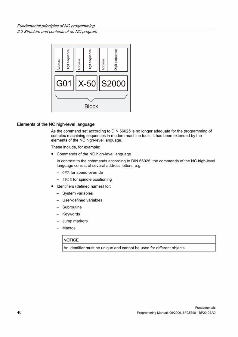
Block components NC blocks consist of the following components: ● Commands (statements) according to DIN 66025 ● Elements of the NC high-level language
Commands according to DIN 66025 The commands according to DIN 66025 consist of an address character and a digit or sequence of digits representing an arithmetic value. Address character (address) The address character (generally a letter) defines the meaning of the command. Examples: Address character Meaning G G function (preparatory function) X Position data for the X axis S Spindle speed
Digit sequence The digit sequence is the value assigned to the address character. The sequence of digits can contain a sign and decimal point. The sign always appears between the address letter and the sequence of digits. Positive signs (+) and leading zeroes (0) do not have to be specified.
Fundamental principles of NC programming 2.2 Structure and contents of an NC program
Fundamentals 40 Programming Manual, 06/2009, 6FC5398-1BP20-0BA0
Elements of the NC high-level language As the command set according to DIN 66025 is no longer adequate for the programming of complex machining sequences in modern machine tools, it has been extended by the elements of the NC high-level language. These include, for example: ● Commands of the NC high-level language
In contrast to the commands according to DIN 66025, the commands of the NC high-level language consist of several address letters, e.g. – OVR for speed override – SPOS for spindle positioning
● Identifiers (defined names) for: – System variables – User-defined variables – Subroutine – Keywords – Jump markers – Macros
NOTICE
An identifier must be unique and cannot be used for different objects.

Fundamental principles of NC programming 2.2 Structure and contents of an NC program
Fundamentals Programming Manual, 06/2009, 6FC5398-1BP20-0BA0 41
● Relational operators ● Logic operators ● Arithmetic functions ● Control structures References: Programming Manual, Job Planning; Section: Flexible NC programming
Effectiveness of commands Commands are either modal or non-modal: ● Modal
Modal commands retain their validity with the programmed value (in all following blocks) until: – A new value is programmed under the same command – A command is programmed that revokes the effect of the previously valid command
● Non-modal Non-modal commands only apply for the block in which they were programmed.
End of program The last block in the execution sequence contains a special word for the end of program: M2, M17 or M30.

Fundamental principles of NC programming 2.2 Structure and contents of an NC program
Fundamentals 42 Programming Manual, 06/2009, 6FC5398-1BP20-0BA0
2.2.2 Block rules
Start of block NC blocks can be identified at the start of the block by block numbers. These consist of the character "N" and a positive integer, e.g. N40 ...
The order of the block numbers is arbitrary, however, block numbers in rising order are recommended.
Note Block numbers must be unique within a program in order to achieve an unambiguous result when searching.
End of block A block ends with character "LF" (LINE FEED = new line).
Note "LF" does not have to be written. It is generated automatically by the line change.
Block length A block can contain a maximum of 512 characters (including the comment and end-of-block character "LF").
Note Three blocks of up to 66 characters each are normally displayed in the current block display on the screen. Comments are also displayed. Messages are displayed in a separate message window.
Fundamental principles of NC programming 2.2 Structure and contents of an NC program
Fundamentals Programming Manual, 06/2009, 6FC5398-1BP20-0BA0 43
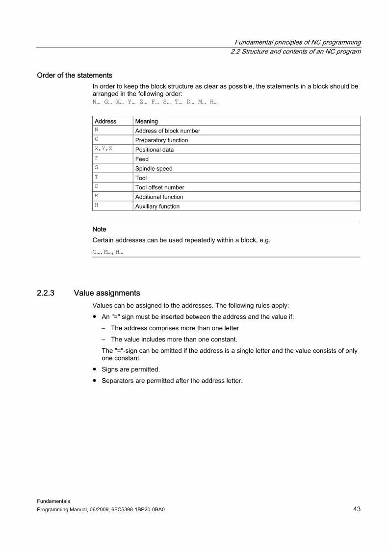
Order of the statements In order to keep the block structure as clear as possible, the statements in a block should be arranged in the following order: N… G… X… Y… Z… F… S… T… D… M… H…
Address Meaning N Address of block number G Preparatory function X,Y,Z Positional data F Feed S Spindle speed T Tool D Tool offset number M Additional function H Auxiliary function
Note Certain addresses can be used repeatedly within a block, e.g. G…, M…, H…
2.2.3 Value assignments Values can be assigned to the addresses. The following rules apply: ● An "=" sign must be inserted between the address and the value if:
– The address comprises more than one letter – The value includes more than one constant. The "="-sign can be omitted if the address is a single letter and the value consists of only one constant.
● Signs are permitted. ● Separators are permitted after the address letter.
Fundamental principles of NC programming 2.2 Structure and contents of an NC program
Fundamentals 44 Programming Manual, 06/2009, 6FC5398-1BP20-0BA0
Examples: X10 Value assignment (10) to address X, "=" not required X1=10 Value assignment (10) to address (X) with numeric
extension (1), "=" required X=10*(5+SIN(37.5)) Value assignment by means of a numeric expression, "="
required
Note A numeric extension must always be followed by one of the special characters "=", "(", "[", ")", "]", ",", or an operator, in order to distinguish an address with numeric extension from an address letter with a value.
2.2.4 Comments To make an NC program easier to understand, comments can be added to the NC blocks. A comment is at the end of a block and is separated from the program section of the NC block by a semicolon (";"). Example 1: Program code Comments
N10 G1 F100 X10 Y20 ; Comment to explain the NC block
Example 2: Program code Comment
N10 ; Company G&S, order no. 12A71
N20 ; Program written by H. Smith, Dept. TV 4 ;on November 21, 1994
N50 ; Section no. 12, housing for submersible pump type TP23A
Note Comments are stored and appear in the current block display when the program is running.
Fundamental principles of NC programming 2.2 Structure and contents of an NC program
Fundamentals Programming Manual, 06/2009, 6FC5398-1BP20-0BA0 45
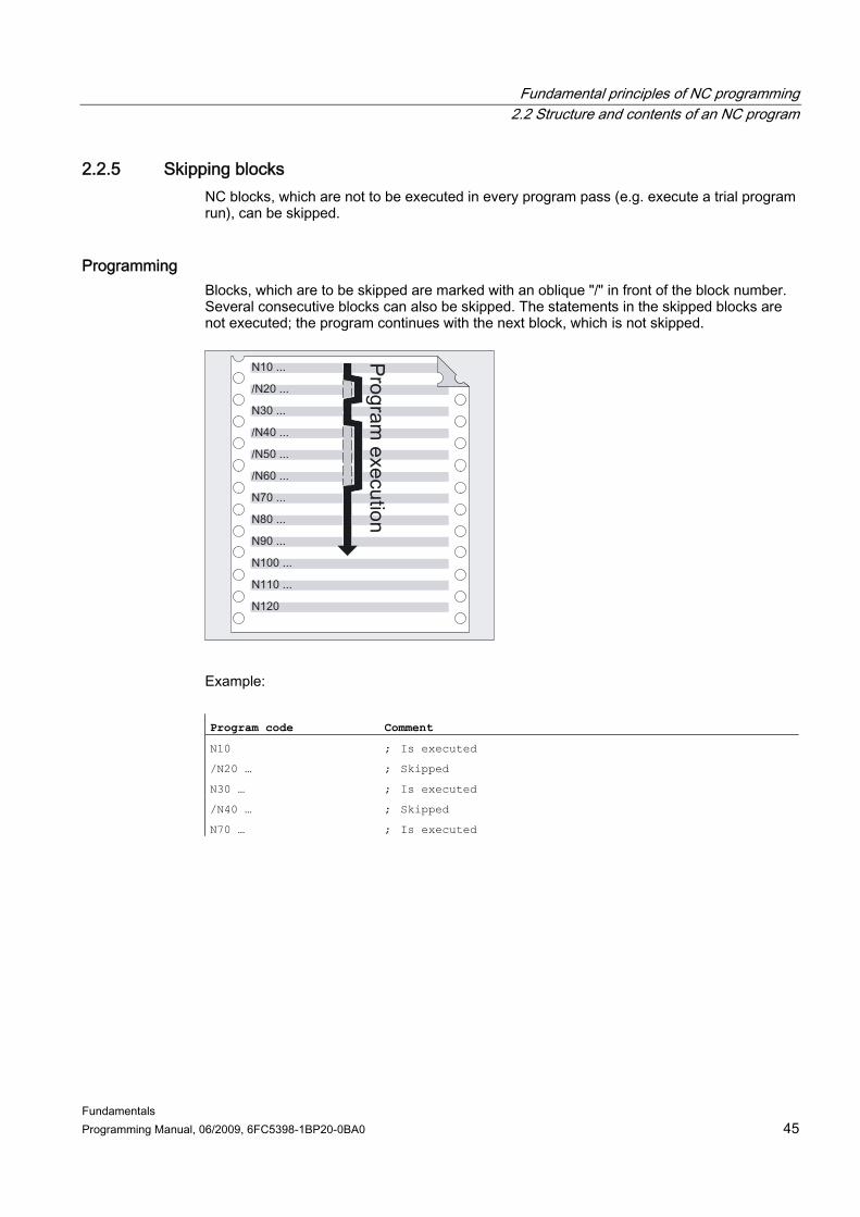
2.2.5 Skipping blocks NC blocks, which are not to be executed in every program pass (e.g. execute a trial program run), can be skipped.
Programming Blocks, which are to be skipped are marked with an oblique "/" in front of the block number. Several consecutive blocks can also be skipped. The statements in the skipped blocks are not executed; the program continues with the next block, which is not skipped.
Example: Program code Comment
N10 ; Is executed
/N20 … ; Skipped
N30 … ; Is executed
/N40 … ; Skipped
N70 … ; Is executed
Fundamental principles of NC programming 2.2 Structure and contents of an NC program
Fundamentals 46 Programming Manual, 06/2009, 6FC5398-1BP20-0BA0
Skip levels Blocks can be assigned to skip levels (max. 10), which can be activated via the user interface. Programming is performed by assigning a forward slash, followed by the number of the skip level. Only one skip level can be specified for each block. Example: Program code Comment
/ ... ; Block is skipped (1st skip level)
/0 ... ; Block is skipped (1st skip level)
/1 N010... ; Block is skipped (2nd skip level)
/2 N020... ; Block is skipped (3rd skip level)
...
/7 N100... ; Block is skipped (8th skip level)
/8 N080... ; Block is skipped (9th skip level)
/9 N090... ; Block is skipped (10th skip level)
Note The number of skip levels that can be used depends on a display machine data item.
Note System and user variables can also be used in conditional jumps in order to control program execution.

Fundamentals Programming Manual, 06/2009, 6FC5398-1BP20-0BA0 47
Creating an NC program 33.1 3.1 Basic procedure
The programming of the individual operation steps in the NC language generally represents only a small proportion of the work in the development of an NC program. Programming of the actual instructions should be preceded by the planning and preparation of the operation steps. The more accurately you plan in advance how the NC program is to be structured and organized, the faster and easier it will be to produce a complete program, which is clear and free of errors. Clearly structured programs are especially advantageous when changes have to be made later. As every part is not identical, it does not make sense to create every program in the same way. However, the following procedure has shown itself to be suitable in the most cases.
Procedure 1. Prepare the workpiece drawing
– Define the workpiece zero – Draw the coordinate system – Calculate any missing coordinates
2. Define the machining sequence – Which tools are used when and for the machining of which contours? – In which order will the individual elements of the workpiece be machined? – Which individual elements are repeated (possibly also rotated) and should be stored in
a subroutine? – Are there contour sections in other part programs or subroutines that could be used
for the current workpiece? – Where are zero offsets, rotating, mirroring and scaling useful or necessary (frame
concept)?
Creating an NC program 3.1 Basic procedure
Fundamentals 48 Programming Manual, 06/2009, 6FC5398-1BP20-0BA0
3. Create a machining plan Define all machining operations step-by-step, e.g. – Rapid traverse movements for positioning – Tool change – Define the machining plane – Retraction for checking – Switch spindle, coolant on/off – Call up tool data – Feed – Path correction – Approaching the contour – Retraction from the contour – etc.
4. Compile machining steps in the programming language – Write each individual step as an NC block (or NC blocks).
5. Combine the individual steps into a program
Creating an NC program 3.2 Available characters
Fundamentals Programming Manual, 06/2009, 6FC5398-1BP20-0BA0 49
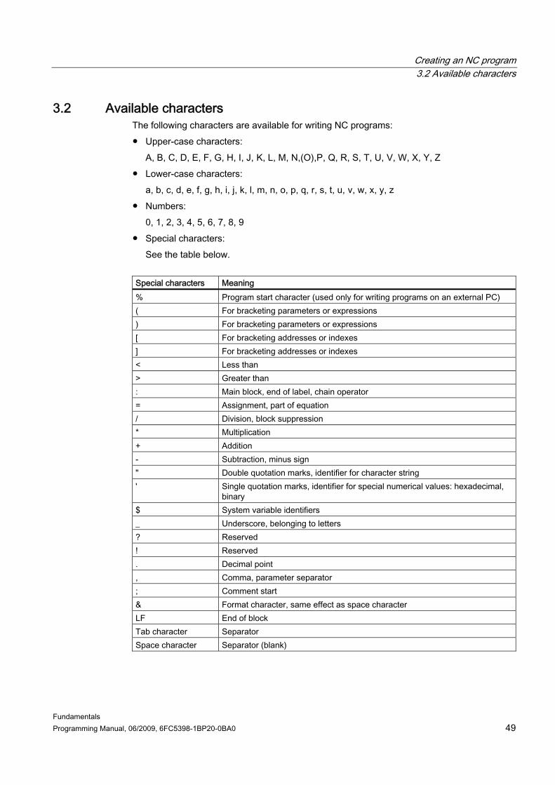
3.2 3.2 Available characters The following characters are available for writing NC programs: ● Upper-case characters:
A, B, C, D, E, F, G, H, I, J, K, L, M, N,(O),P, Q, R, S, T, U, V, W, X, Y, Z ● Lower-case characters:
a, b, c, d, e, f, g, h, i, j, k, l, m, n, o, p, q, r, s, t, u, v, w, x, y, z ● Numbers:
0, 1, 2, 3, 4, 5, 6, 7, 8, 9 ● Special characters:
See the table below. Special characters Meaning % Program start character (used only for writing programs on an external PC) ( For bracketing parameters or expressions ) For bracketing parameters or expressions [ For bracketing addresses or indexes ] For bracketing addresses or indexes < Less than > Greater than : Main block, end of label, chain operator = Assignment, part of equation / Division, block suppression * Multiplication + Addition - Subtraction, minus sign " Double quotation marks, identifier for character string ' Single quotation marks, identifier for special numerical values: hexadecimal,
binary $ System variable identifiers _ Underscore, belonging to letters ? Reserved ! Reserved . Decimal point , Comma, parameter separator ; Comment start & Format character, same effect as space character LF End of block Tab character Separator Space character Separator (blank)

Creating an NC program 3.2 Available characters
Fundamentals 50 Programming Manual, 06/2009, 6FC5398-1BP20-0BA0
NOTICE Take care to differentiate between the letter "O" and the digit "0".
Note No distinction is made between upper and lower-case characters (exception: tool call).
Note Non-printable special characters are treated like blanks.

Creating an NC program 3.3 Program header
Fundamentals Programming Manual, 06/2009, 6FC5398-1BP20-0BA0 51
3.3 3.3 Program header The NC blocks that are placed in front of the actual motion blocks for the machining of the workpiece contour, are called the program header. The program header contains information/statements regarding: ● Tool change ● Tool offsets ● Spindle motion ● Feed control ● Geometry settings (zero offset, selection of the working plane)
Program header for turning The following example shows the typical structure of an NC program header for turning: Program code Comment
N10 G0 G153 X200 Z500 T0 D0 ; Retract toolholder before tool turret is rotated.
N20 T5 ; Swing in tool 5.
N30 D1 ; Activate cutting edge data record of the tool.
N40 G96 S300 LIMS=3000 M4 M8 ; Constant cutting rate (Vc) = 300 m/min, speed limitation = 3000 rpm, direction of rotation counterclockwise, cooling on.
N50 DIAMON ; X axis will be programmed in diameter.
N60 G54 G18 G0 X82 Z0.2 ; Call zero offset and working plane, approach starting position.
...

Creating an NC program 3.3 Program header
Fundamentals 52 Programming Manual, 06/2009, 6FC5398-1BP20-0BA0
Program header for milling The following example shows the typical structure of an NC program header for milling: Program code Comment
N10 T="SF12" ; Alternative: T123
N20 M6 ; Trigger tool change
N30 D1 ; Activate cutting edge data record of the tool
N40 G54 G17 ; Zero offset and working plane
N50 G0 X0 Y0 Z2 S2000 M3 M8 ; Approach to the workpiece, spindle and coolant on
...
If tool orientation / coordinate transformation is being used, any transformations still active should be deleted at the start of the program: Program code Comment
N10 CYCLE800() ; Resetting of the swiveled plane
N20 TRAFOOF ; Resetting of TRAORI, TRANSMIT, TRACYL, ...
...

Creating an NC program 3.4 Program examples
Fundamentals Programming Manual, 06/2009, 6FC5398-1BP20-0BA0 53
3.4 3.4 Program examples
3.4.1 Example 1: First programming steps Program example 1 is to be used to perform and test the first programming steps on the NC.
Procedure 1. Create a new part program (name) 2. Edit the part program 3. Select the part program 4. Activate single block 5. Start the part program References: Operating Manual for the existing user interface
Note In order that the program can run on the machine, the machine data must have been set appropriately (→ machine manufacturer!).
Note Alarms can occur during program verification. These alarms have to be reset first.
Program example 1 Program code Comment
N10 MSG("THIS IS MY NC PROGRAM") ; Message "THIS IS MY NC PROGRAM" displayed in the alarm line
N20 F200 S900 T1 D2 M3 ; Feedrate, spindle, tool, tool offset, spindle clockwise
N30 G0 X100 Y100 ; Approach position in rapid traverse
N40 G1 X150 ; Rectangle with feedrate, straight line in X
N50 Y120 ; Straight line in Y
N60 X100 ; Straight line in X
N70 Y100 ; Straight line in Y
N80 G0 X0 Y0 ; Retraction in rapid traverse
N100 M30 ; End of block

Creating an NC program 3.4 Program examples
Fundamentals 54 Programming Manual, 06/2009, 6FC5398-1BP20-0BA0
3.4.2 Example 2: NC program for turning Program example 2 is intended for the machining of a workpiece on a lathe. It contains radius programming and tool radius compensation.
Note In order that the program can run on the machine, the machine data must have been set appropriately (→ machine manufacturer!).
Dimension drawing of the workpiece
Figure 3-1 Top view

Creating an NC program 3.4 Program examples
Fundamentals Programming Manual, 06/2009, 6FC5398-1BP20-0BA0 55
Program example 2 Program code Comment
N5 G0 G53 X280 Z380 D0 ; Starting point
N10 TRANS X0 Z250 ; Zero offset
N15 LIMS=4000 ; Speed limitation (G96)
N20 G96 S250 M3 ; Select constant cutting rate
N25 G90 T1 D1 M8 ; Select tool selection and offset
N30 G0 G42 X-1.5 Z1 ; Set tool with tool radius compensation
N35 G1 X0 Z0 F0.25
N40 G3 X16 Z-4 I0 K-10 ; Turn radius 10
N45 G1 Z-12
N50 G2 X22 Z-15 CR=3 ; Turn radius 3
N55 G1 X24
N60 G3 X30 Z-18 I0 K-3 ; Turn radius 3
N65 G1 Z-20
N70 X35 Z-40
N75 Z-57
N80 G2 X41 Z-60 CR=3 ; Turn radius 3
N85 G1 X46
N90 X52 Z-63
N95 G0 G40 G97 X100 Z50 M9 ; Deselect tool radius compensation and approach tool change location
N100 T2 D2 ; Call tool and select offset
N105 G96 S210 M3 ; Select constant cutting rate
N110 G0 G42 X50 Z-60 M8 ; Set tool with tool radius compensation
N115 G1 Z-70 F0.12 ; Turn diameter 50
N120 G2 X50 Z-80 I6.245 K-5 ; Turn radius 8
N125 G0 G40 X100 Z50 M9 ; Retract tool and deselect tool radius compensation
N130 G0 G53 X280 Z380 D0 M5 ; Approach tool change location
N135 M30 ; End of program
Creating an NC program 3.4 Program examples
Fundamentals 56 Programming Manual, 06/2009, 6FC5398-1BP20-0BA0
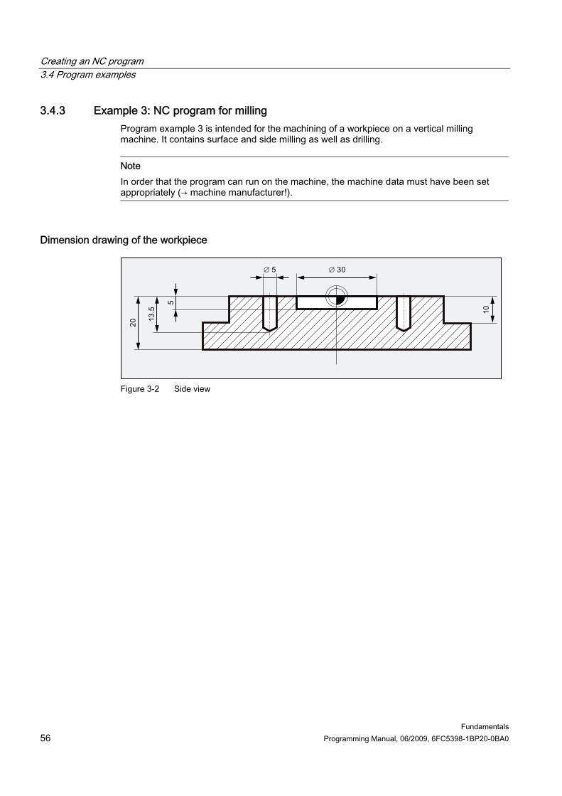
3.4.3 Example 3: NC program for milling Program example 3 is intended for the machining of a workpiece on a vertical milling machine. It contains surface and side milling as well as drilling.
Note In order that the program can run on the machine, the machine data must have been set appropriately (→ machine manufacturer!).
Dimension drawing of the workpiece
Figure 3-2 Side view
Creating an NC program 3.4 Program examples
Fundamentals Programming Manual, 06/2009, 6FC5398-1BP20-0BA0 57
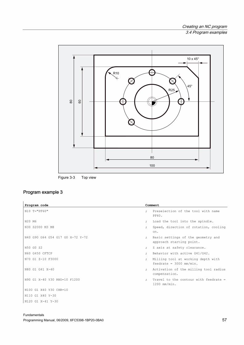
Figure 3-3 Top view
Program example 3 Program code Comment
N10 T="PF60" ; Preselection of the tool with name PF60.
N20 M6 ; Load the tool into the spindle.
N30 S2000 M3 M8 ; Speed, direction of rotation, cooling on.
N40 G90 G64 G54 G17 G0 X-72 Y-72 ; Basic settings of the geometry and approach starting point.
N50 G0 Z2 ; Z axis at safety clearance.
N60 G450 CFTCP ; Behavior with active G41/G42.
N70 G1 Z-10 F3000 ; Milling tool at working depth with feedrate = 3000 mm/min.
N80 G1 G41 X-40 ; Activation of the milling tool radius compensation.
N90 G1 X-40 Y30 RND=10 F1200 ; Travel to the contour with feedrate = 1200 mm/min.
N100 G1 X40 Y30 CHR=10
N110 G1 X40 Y-30
N120 G1 X-41 Y-30

Creating an NC program 3.4 Program examples
Fundamentals 58 Programming Manual, 06/2009, 6FC5398-1BP20-0BA0
Program code Comment
N130 G1 G40 Y-72 F3000 ; Deselection of the milling tool radius compensation.
N140 G0 Z200 M5 M9 ; Retraction of the milling tool, spindle + cooling off.
N150 T="SF10" ; Preselection of the tool with name SF10.
N160 M6 ; Load the tool into the spindle.
N170 S2800 M3 M8 ; Speed, direction of rotation, cooling on.
N180 G90 G64 G54 G17 G0 X0 Y0 ; Basic settings of the geometry and approach starting point.
N190 G0 Z2
N200 POCKET4(2,0,1,-5,15,0,0,0,0,0,800,1300,0,21,5,,,2,0.5) ; Call of the pocket milling cycle.
N210 G0 Z200 M5 M9 ; Retraction of the milling tool, spindle + cooling off.
N220 T="ZB6" ; Call center drill 6 mm.
N230 M6
N240 S5000 M3 M8
N250 G90 G60 G54 G17 X25 Y0 ; Exact stop G60 for exact positioning.
N260 G0 Z2
N270 MCALL CYCLE82(2,0,1,-2.6,,0) ; Modal call of the drilling cycle.
N280 POSITION: ; Jump mark for repetition.
N290 HOLES2(0,0,25,0,45,6) ; Position pattern for drilling.
N300 ENDLABEL: ; End identifier for repetition.
N310 MCALL ; Resetting of the modal call.
N320 G0 Z200 M5 M9
N330 T="SPB5" ; Call twist drill D 5 mm.
N340 M6
N350 S2600 M3 M8
N360 G90 G60 G54 G17 X25 Y0
N370 MCALL CYCLE82(2,0,1,-13.5,,0) ; Modal call of the drilling cycle.
N380 REPEAT POSITION ; Repetition of the position description from centering.
N390 MCALL ; Resetting of the drilling cycle
N400 G0 Z200 M5 M9
N410 M30 ; End of program.

Fundamentals Programming Manual, 06/2009, 6FC5398-1BP20-0BA0 59
Tool change 4
Tool change method In chain, rotary-plate and box magazines, a tool change normally takes place in two stages: 1. The tool is sought in the magazine with the T command. 2. The tool is then loaded into the spindle with the M command. In circular magazines on turning machines, the T command carries out the entire tool change, that is, locates and inserts the tool.
Note The tool change method is set via a machine data (→ machine manufacturer).
Conditions Together with the tool change: ● The tool offset values stored under a D number have to be activated. ● The appropriate working plane has to be programmed (basic setting: G18). This ensures
that the tool length compensation is assigned to the correct axis.
Tool management (option) The programming of the tool change is performed differently for machines with active tool management (option) than for machines without active tool management. The two options are therefore described separately.
Tool change 4.1 Tool change without tool management
Fundamentals 60 Programming Manual, 06/2009, 6FC5398-1BP20-0BA0
4.1 4.1 Tool change without tool management
4.1.1 Tool change with T command
Function There is a direct tool change when the T command is programmed.
Application For turning machines with circular magazine.
Syntax Tool selection: T<number> T=<number> T<n>=<number>
Tool deselection: T0 T0=<number>
Meaning T: Command for tool selection including tool change and activation of the tool
offset <n>: Spindle number as address extension
Note: The possibility of programming a spindle number as address extension depends on the configuration of the machine; → see machine manufacturer's specifications) Number of the tool <number>: Range of values: 0 - 32000
T0: Command for deselection of the active tool
Example Program code Comment
N10 T1 D1 ; Loading of tool T1 and activation of the tool offset D1.
...
N70 T0 ; Deselect tool T1.
...

Tool change 4.1 Tool change without tool management
Fundamentals Programming Manual, 06/2009, 6FC5398-1BP20-0BA0 61
4.1.2 Tool change with M6
Function The tool is selected when the T command is programmed. The tool only becomes active with M6 (including tool offset).
Application For milling machines with chain, rotary-plate or box magazines.
Syntax Tool selection: T<number> T=<number> T<n>=<number>
Tool change: M6
Tool deselection: T0 T0=<number>
Significance T: Command for the tool selection <n>: Spindle number as address extension
Note: The possibility of programming a spindle number as address extension depends on the configuration of the machine; → see machine manufacturer's specifications. Number of the tool <number>: Range of values: 0 - 32000
M6: M function for the tool change (according to DIN 66025) M6 activates the selected tool (T…) and the tool offset (D...).
T0: Command for deselection of the active tool
Tool change 4.1 Tool change without tool management
Fundamentals 62 Programming Manual, 06/2009, 6FC5398-1BP20-0BA0
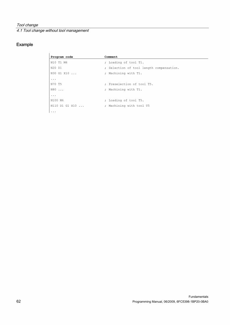
Example Program code Comment
N10 T1 M6 ; Loading of tool T1.
N20 D1 ; Selection of tool length compensation.
N30 G1 X10 ... ; Machining with T1.
...
N70 T5 ; Preselection of tool T5.
N80 ... ; Machining with T1.
...
N100 M6 ; Loading of tool T5.
N110 D1 G1 X10 ... ; Machining with tool T5
...

Tool change 4.2 Tool change with tool management (option)
Fundamentals Programming Manual, 06/2009, 6FC5398-1BP20-0BA0 63
4.2 4.2 Tool change with tool management (option)
Tool management The optional "Tool management" function ensures that at any given time the correct tool is in the correct location and that the data assigned to the tool are up to date. It also allows fast tool changes and avoids both scrap by monitoring the tool service life and machine downtimes by using spare tools.
Tool name On a machine tool with active tool management, the tools must be assigned a name and number for clear identification (e.g. "Drill", "3"). The tool call can then be via the tool name, e.g. T="Drill"
NOTICE The tool name may not contain any special characters.
4.2.1 Tool change with T command with active tool management (option)
Function There is a direct tool change when the T command is programmed.
Application For turning machines with circular magazine.
Syntax Tool selection: T=<location> T=<name> T<n>=<location> T<n>=<name>
Tool deselection: T0
Tool change 4.2 Tool change with tool management (option)
Fundamentals 64 Programming Manual, 06/2009, 6FC5398-1BP20-0BA0
Significance
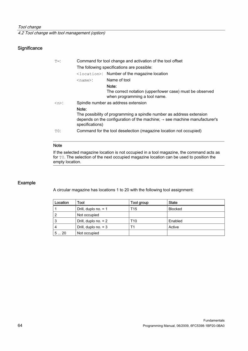
Command for tool change and activation of the tool offset The following specifications are possible: <location>: Number of the magazine location
T=:
<name>: Name of tool Note: The correct notation (upper/lower case) must be observed when programming a tool name.
<n>: Spindle number as address extension Note: The possibility of programming a spindle number as address extension depends on the configuration of the machine; → see machine manufacturer's specifications)
T0: Command for the tool deselection (magazine location not occupied)
Note If the selected magazine location is not occupied in a tool magazine, the command acts as for T0. The selection of the next occupied magazine location can be used to position the empty location.
Example A circular magazine has locations 1 to 20 with the following tool assignment: Location Tool Tool group State 1 Drill, duplo no. = 1 T15 Blocked 2 Not occupied 3 Drill, duplo no. = 2 T10 Enabled 4 Drill, duplo no. = 3 T1 Active 5 ... 20 Not occupied

Tool change 4.2 Tool change with tool management (option)
Fundamentals Programming Manual, 06/2009, 6FC5398-1BP20-0BA0 65
The following tool call is programmed in the NC program: N10 T=1
The call is processed as follows: 1. Magazine location 1 is considered and the tool identifier determined. 2. The tool management recognizes that this tool is blocked and therefore cannot be used. 3. A tool search for T="drill" is initiated in accordance with the search method set:
"Find the active tool; or else, select the one with the next highest duplo number." 4. The following usable tool is then found:
"Drill", duplo no. 3 (at magazine location 4) This completes the tool selection process and the tool change is initiated.
Note If the "Select the first available tool from the group" search method is employed, the sequence must first be defined within the tool group being loaded. In this case group T10 is loaded, as T15 is blocked. When the strategy "Take the first tool with "active" status from the group" is applied, T1 is loaded.

Tool change 4.2 Tool change with tool management (option)
Fundamentals 66 Programming Manual, 06/2009, 6FC5398-1BP20-0BA0
4.2.2 Tool change with M6 with active tool management (option)
Function The tool is selected when the T command is programmed. The tool only becomes active with M6 (including tool offset).
Application For milling machines with chain, rotary-plate or box magazines.
Syntax Tool selection: T=<location> T=<name> T<n>=<location> T<n>=<name>
Tool change: M6
Tool deselection: T0
Significance
Command for the tool selection The following specifications are possible: <location>: Number of the magazine location
T=:
<name>: Name of tool Note: The correct notation (upper/lower case) must be used when programming a tool name.
<n>: Spindle number as address extension Note: The possibility of programming a spindle number as an address extension depends on the configuration of the machine; → see machine manufacturer's specifications.
M6: M function for the tool change (according to DIN 66025) M6 activates the selected tool (T…) and the tool offset (D...).
T0: Command for tool deselection (magazine location not occupied)

Tool change 4.2 Tool change with tool management (option)
Fundamentals Programming Manual, 06/2009, 6FC5398-1BP20-0BA0 67
Note If the selected magazine location is not occupied in a tool magazine, the command acts as for T0. The selection of the next occupied magazine location can be used to position the empty location.
Example Program code Comment
N10 T=1 M6 ; Loading of the tool from magazine location 1.
N20 D1 ; Selection of tool length compensation.
N30 G1 X10 ... ; Machining with tool T=1.
...
N70 T="Drill" ; Preselection of the tool with name "Drill".
N80 ... ; Machining with tool T=1.
...
N100 M6 ; Loading of the drill.
N140 D1 G1 X10 ... ; Machining with drill.
...
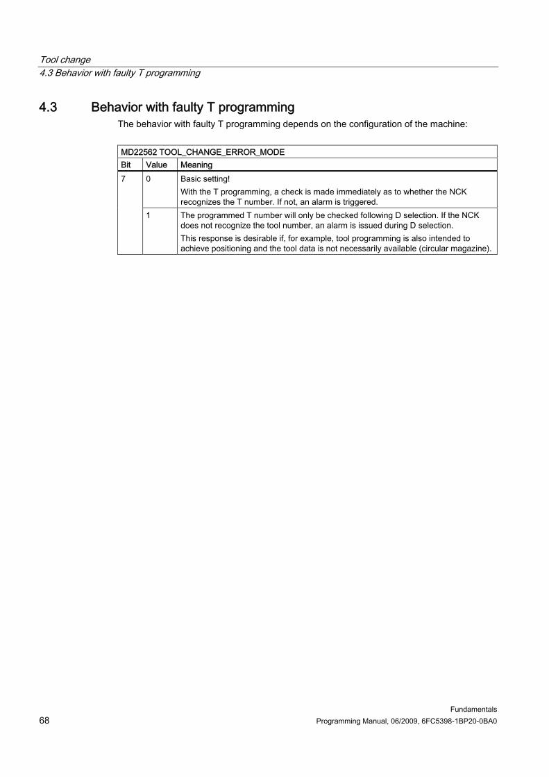
Tool change 4.3 Behavior with faulty T programming
Fundamentals 68 Programming Manual, 06/2009, 6FC5398-1BP20-0BA0
4.3 4.3 Behavior with faulty T programming The behavior with faulty T programming depends on the configuration of the machine: MD22562 TOOL_CHANGE_ERROR_MODE Bit Value Meaning
0 Basic setting! With the T programming, a check is made immediately as to whether the NCK recognizes the T number. If not, an alarm is triggered.
7
1 The programmed T number will only be checked following D selection. If the NCK does not recognize the tool number, an alarm is issued during D selection. This response is desirable if, for example, tool programming is also intended to achieve positioning and the tool data is not necessarily available (circular magazine).

Fundamentals Programming Manual, 06/2009, 6FC5398-1BP20-0BA0 69
Tool offsets 55.1 5.1 General information about the tool offsets
Workpiece dimensions are programmed directly (e.g. according to the production drawing). Therefore, tool data such as milling tool diameter, cutting edge position of the turning tool (counterclockwise/clockwise turning tool) and tool length does not have to be taken into consideration when creating the program.
The control corrects the travel path When machining a workpiece, the tool paths are controlled according to the tool geometry such that the programmed contour can be machined using any tool. In order that the control can calculate the tool paths, the tool data must be entered in the tool compensation memory of the control. Only the required tool (T...) and the required offset data record (D...) are called via the NC program. While the program is being processed, the control fetches the offset data it requires from the tool compensation memory and corrects the tool path individually for different tools:

Tool offsets 5.2 Tool length compensation
Fundamentals 70 Programming Manual, 06/2009, 6FC5398-1BP20-0BA0
5.2 5.2 Tool length compensation The tool length compensation compensates for the differences in length between the tools used. The tool length is the distance between the toolholder reference point and the tool tip:
F FFF
This length is measured and entered in the tool compensation memory of the control together with definable wear values. From this data, the control calculates the traversing movements in the infeed direction.
Note The offset value for the tool length is dependent upon the spatial orientation of the tool.
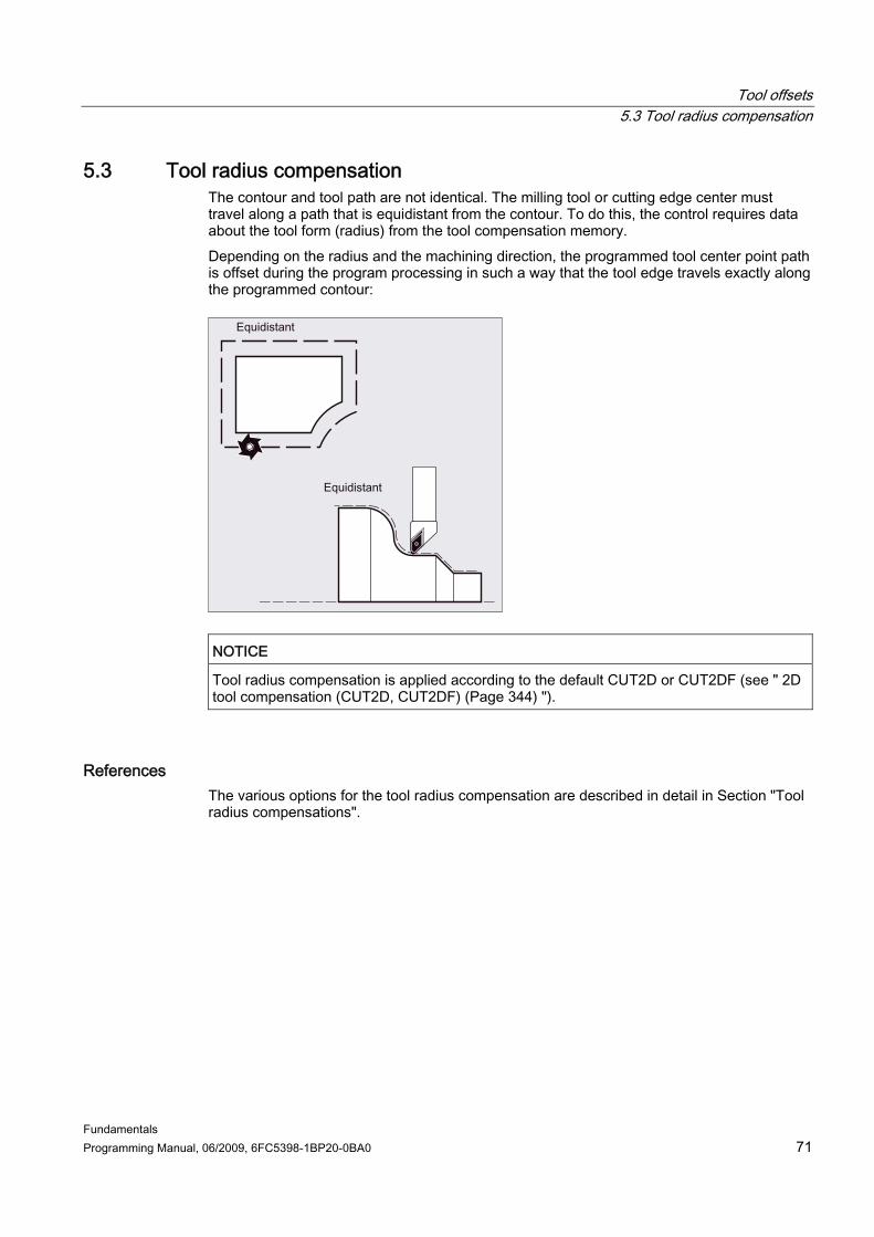
Tool offsets 5.3 Tool radius compensation
Fundamentals Programming Manual, 06/2009, 6FC5398-1BP20-0BA0 71
5.3 5.3 Tool radius compensation The contour and tool path are not identical. The milling tool or cutting edge center must travel along a path that is equidistant from the contour. To do this, the control requires data about the tool form (radius) from the tool compensation memory. Depending on the radius and the machining direction, the programmed tool center point path is offset during the program processing in such a way that the tool edge travels exactly along the programmed contour:
NOTICE Tool radius compensation is applied according to the default CUT2D or CUT2DF (see " 2D tool compensation (CUT2D, CUT2DF) (Page 344) ").
References The various options for the tool radius compensation are described in detail in Section "Tool radius compensations".
Tool offsets 5.4 Tool compensation memory
Fundamentals 72 Programming Manual, 06/2009, 6FC5398-1BP20-0BA0
5.4 5.4 Tool compensation memory The following data must be available in the tool compensation memory of the control for each tool edge: ● Tool type ● Cutting edge position ● Tool geometry variables (length, radius) This data is entered as tool parameters (max. 25). Which parameters are required for a tool depends on the tool type. Any tool parameters that are not required must be set to "zero" (corresponds to the default setting of the system).
NOTICE Values that have been entered once in the compensation memory are included in the processing at each tool call.
Tool type The tool type (drill, milling or turning tool) determines which geometry data is necessary and how this is taken into account.
Cutting edge position The cutting edge position describes the position of the tool tip P in relation to the cutting edge center point S. The cutting edge position is required together with the cutting edge radius for the calculation of the tool radius compensation for turning tools (tool type 5xx).

Tool offsets 5.4 Tool compensation memory
Fundamentals Programming Manual, 06/2009, 6FC5398-1BP20-0BA0 73
Tool geometry variables (length, radius)
The tool geometry variables consist of several components (geometry, wear). The control computes the components to a certain dimension (e.g. overall length 1, total radius). The respective overall dimension becomes effective when the compensation memory is activated. How these values are calculated in the axes is determined by the tool type and the current plane (G17/G18/G19).
References Function Manual, Basic Functions; Tool Offsets (W1); Section "Tool edge"

Tool offsets 5.5 Tool types
Fundamentals 74 Programming Manual, 06/2009, 6FC5398-1BP20-0BA0
5.5 5.5 Tool types
5.5.1 General information about the tool types Tools are divided into tool types. Each tool type is assigned a 3-digit number. The first digit assigns the tool type to one of the following groups depending on the technology used: Tool type Tool group 1xy Milling tools 2xy Drills 3xy Reserved 4xy Grinding tools 5xy Turning tools 6xy Reserved 7xy Special tools such as a slotting saw

Tool offsets 5.5 Tool types
Fundamentals Programming Manual, 06/2009, 6FC5398-1BP20-0BA0 75
5.5.2 Milling tools The following tool types are available in the "Milling tools" group: 100 Milling tool according to CLDATA (Cutter Location Data) 110 Ballhead cutter (cylindrical die milling tool) 111 Ballhead cutter (tapered die milling tool) 120 End mill (without corner rounding) 121 End mill (with corner rounding) 130 Angle head cutter (without corner rounding) 131 Angle head cutter (with corner rounding) 140 Facing tool 145 Thread cutter 150 Side mill 151 Saw 155 Bevel cutter (without corner rounding) 156 Bevel cutter (with corner rounding) 157 Tapered die milling tool 160 Drill and thread milling cutter
Tool parameters The following figures provide an overview of which tool parameters (DP...) for milling tools are entered in the compensation memory:

Tool offsets 5.5 Tool types
Fundamentals 76 Programming Manual, 06/2009, 6FC5398-1BP20-0BA0
Note Brief description of the tool parameters can be found on the user interface. For further information, see: References: Function Manual, Basic Functions; Tool Offset (W1)

Tool offsets 5.5 Tool types
Fundamentals Programming Manual, 06/2009, 6FC5398-1BP20-0BA0 77
5.5.3 Drills The following tool types are available in the "Drills" group: 200 Twist drill 205 Drill 210 Boring bar 220 Center drill 230 Countersink 231 Counterbore 240 Tap regular thread 241 Tap fine thread 242 Tap Whitworth thread 250 Reamer
Tool parameters The following figure provides an overview of which tool parameters (DP...) for drills are entered in the compensation memory:
Note Brief description of the tool parameters can be found on the user interface. For further information, see: References: Function Manual, Basic Functions; Tool Offset (W1)

Tool offsets 5.5 Tool types
Fundamentals 78 Programming Manual, 06/2009, 6FC5398-1BP20-0BA0
5.5.4 Grinding tools The following tool types are available in the "Grinding tools" group: 400 Surface grinding wheel 401 Surface grinding wheel with monitoring 402 Surface grinding wheel without monitoring without base dimension (TOOLMAN) 403 Surface grinding wheel with monitoring without base dimension for grinding
wheel peripheral speed GWPS 410 Facing wheel 411 Facing wheel (TOOLMAN) with monitoring 412 Facing wheel (TOOLMAN) without monitoring 413 Facing wheel with monitoring without base dimension for grinding wheel
peripheral speed GWPS 490 Dresser
Tool parameters The following figure provides an overview of which tool parameters (DP...) for grinding tools are entered in the compensation memory:

Tool offsets 5.5 Tool types
Fundamentals Programming Manual, 06/2009, 6FC5398-1BP20-0BA0 79
Note Brief description of the tool parameters can be found on the user interface. For further information, see: References: Function Manual, Basic Functions; Tool Offset (W1)

Tool offsets 5.5 Tool types
Fundamentals 80 Programming Manual, 06/2009, 6FC5398-1BP20-0BA0
5.5.5 Turning tools The following tool types are available in the "Turning tools" group: 500 Roughing tool 510 Finishing tool 520 Plunge cutter 530 Parting tool 540 Threading tool 550 Button tool/forming tool (TOOLMAN) 560 Rotary drill (ECOCUT) 580 Probe with cutting edge position parameters
Tool parameters The following figures provide an overview of which tool parameters (DP...) for turning tools are entered in the compensation memory:
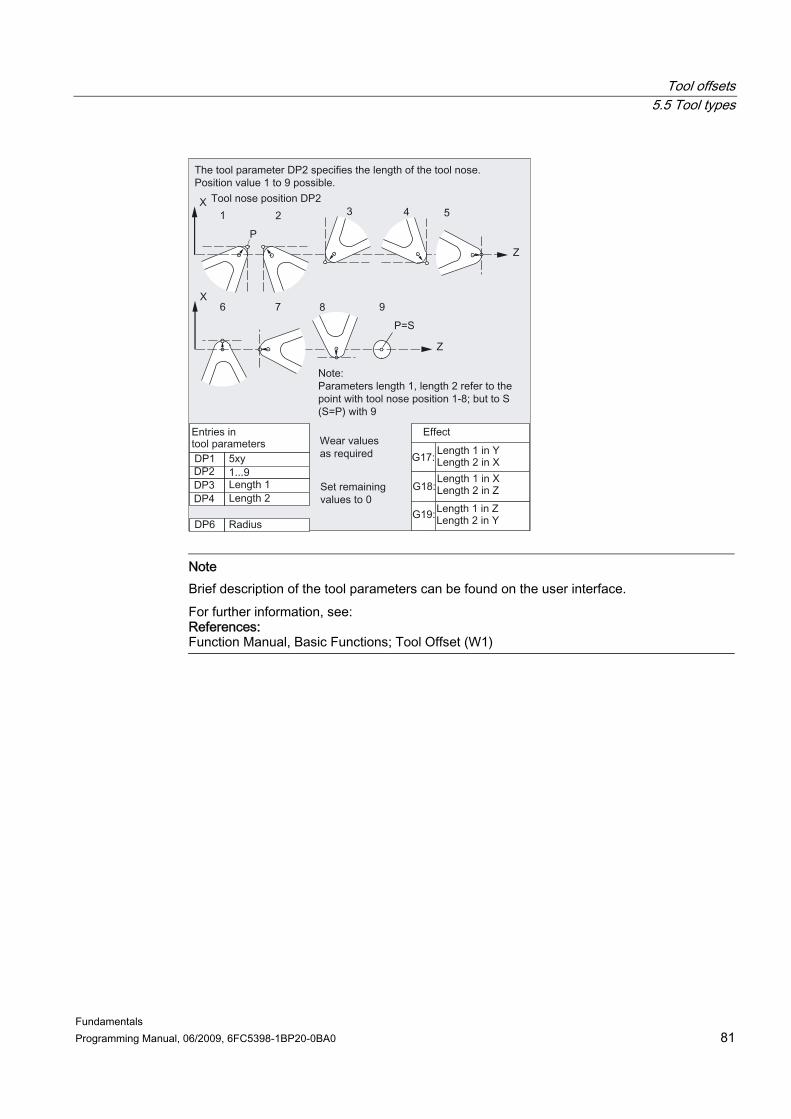
Tool offsets 5.5 Tool types
Fundamentals Programming Manual, 06/2009, 6FC5398-1BP20-0BA0 81
Note Brief description of the tool parameters can be found on the user interface. For further information, see: References: Function Manual, Basic Functions; Tool Offset (W1)
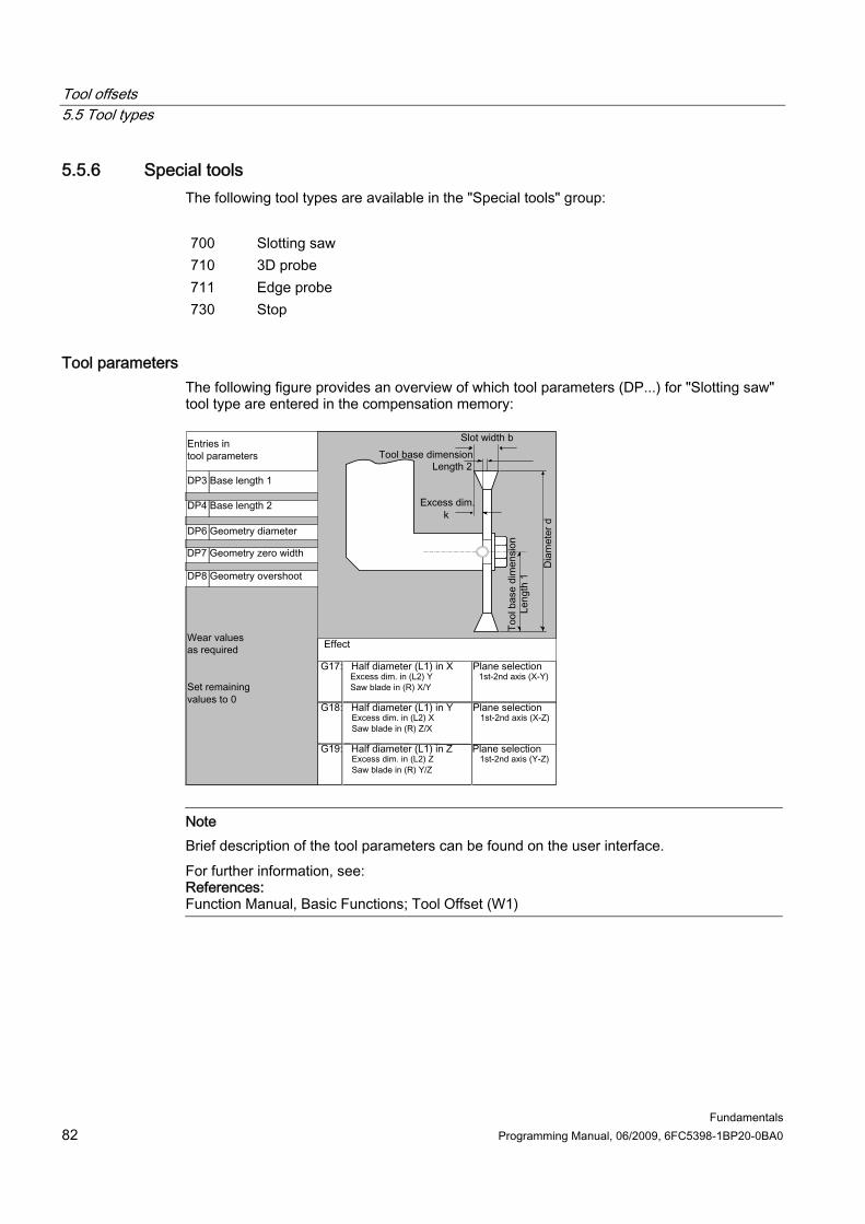
Tool offsets 5.5 Tool types
Fundamentals 82 Programming Manual, 06/2009, 6FC5398-1BP20-0BA0
5.5.6 Special tools The following tool types are available in the "Special tools" group: 700 Slotting saw 710 3D probe 711 Edge probe 730 Stop
Tool parameters The following figure provides an overview of which tool parameters (DP...) for "Slotting saw" tool type are entered in the compensation memory:
Note Brief description of the tool parameters can be found on the user interface. For further information, see: References: Function Manual, Basic Functions; Tool Offset (W1)

Tool offsets 5.5 Tool types
Fundamentals Programming Manual, 06/2009, 6FC5398-1BP20-0BA0 83
5.5.7 Chaining rule The geometry tool length compensations, wear and base dimension can be chained for both the left and the right tool nose radius compensation, i.e. if the tool length compensations are changed for the left cutting edge, then the values are also automatically entered for the right cutting edge and vice versa.
References Function Manual, Extended Functions; Grinding (W4)

Tool offsets 5.6 Tool offset call (D)
Fundamentals 84 Programming Manual, 06/2009, 6FC5398-1BP20-0BA0
5.6 5.6 Tool offset call (D)
Function Cutting edges 1 to 8 (with active TOOLMAN 12) of a tool can be assigned different tool offset data records (e.g. different offset values for the left and right cutting edge of a grooving tool). Activation of the offset data (including the data for the tool length compensation) of a special cutting edge is performed by calling the D number. When D0 is programmed, offsets for the tool have no effect. A tool radius compensation must also be activated via G41/G42.
Note Tool length offsets take immediate effect when the D number is programmed. If no D number is programmed, the default setting defined via the machine data is active for a tool change (→ see machine manufacturer's specifications).
Syntax Activation of a tool offset data record: D<number>
Activate the tool radius compensation: G41 ... G42 ...
Deactivation of the tool offsets: D0 G40
Significance D: Command for the activation of an offset data record for the active tool
The tool length compensation is applied with the first programmed traverse of the associated length compensation axis. Notice: A tool length compensation can also take effect without D programming, when the automatic activation of a tool edge has been configured for the tool change (→ see machine manufacturer's specifications).

Tool offsets 5.6 Tool offset call (D)
Fundamentals Programming Manual, 06/2009, 6FC5398-1BP20-0BA0 85
The tool offset data record to be activated is specified via the <number> parameter. The type of D programming depends on the configuration of the machine (see paragraph "Type of D programming").
<number>:
Range of values: 0 - 32,000 D0: Command for the deactivation of the offset data record for the active tool G41: Command for the activation of the tool radius compensation with
machining direction left of the contour G42: Command for the activation of the tool radius compensation with
machining direction right of the contour G40: Command for the deactivation of the tool radius compensation
Note The tool radius compensation is described in detail in the section "Tool radius compensation" section.
Type of D programming The type of D programming is defined via machine data. This can be done as follows: ● D number = cutting edge number
D numbers ranging from 1 to max. 12 are available for every tool T<number> or T="Name" (with TOOLMAN). These D numbers are assigned directly to the tool cutting edges. A compensation data record ($TC_DPx[t,d]) belongs to each D number (= cutting edge number).
● Free selection of D numbers The D numbers can be freely assigned to the cutting edge numbers of a tool. The upper limit for the D numbers that can be used is limited by a machine data.
● Absolute D number without reference to the T number Independence between D number and T number can be selected in systems without tool management. The reference of T number, cutting edge and offset by the D number is defined by the user. The range of D numbers is between 1 and 32000.
References: Function Manual, Basic Functions; Tool Offset (W1), Function Manual, Tool Management, Chapter: "Variants of D-number assignments"
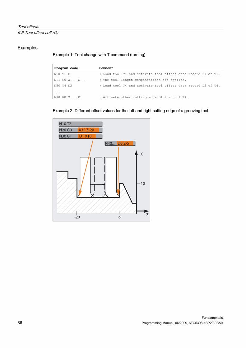
Tool offsets 5.6 Tool offset call (D)
Fundamentals 86 Programming Manual, 06/2009, 6FC5398-1BP20-0BA0
Examples Example 1: Tool change with T command (turning) Program code Comment
N10 T1 D1 ; Load tool T1 and activate tool offset data record D1 of T1.
N11 G0 X... Z... ; The tool length compensations are applied.
N50 T4 D2 ; Load tool T4 and activate tool offset data record D2 of T4.
...
N70 G0 Z... D1 ; Activate other cutting edge D1 for tool T4.
Example 2: Different offset values for the left and right cutting edge of a grooving tool
N40... D6 Z-5
N30 G1 D1 X10
Z
X
N20 G0
N10 T2
X35 Z-20
-5-20
10

Tool offsets 5.7 Change in the tool offset data
Fundamentals Programming Manual, 06/2009, 6FC5398-1BP20-0BA0 87
5.7 5.7 Change in the tool offset data
Effectiveness A change in the tool offset data takes effect the next time the T or D number is programmed. Set tool offset data to be active immediately The following machine data can be used to specify that entered tool offset data takes effect immediately: MD9440 $MM_ACTIVATE_SEL_USER
DANGER If MD9440 is set, tool offsets resulting from changes in tool offset data during the part program stop, are applied when the part program is continued.

Tool offsets 5.8 Programmable tool offset (TOFFL, TOFF, TOFFR)
Fundamentals 88 Programming Manual, 06/2009, 6FC5398-1BP20-0BA0
5.8 5.8 Programmable tool offset (TOFFL, TOFF, TOFFR)
Function The user can use the commands TOFFL/TOFF and TOFFR to modify the effective tool length or the effective tool radius in the NC program, without changing the tool offset data stored in the compensation memory. These programmed offsets are deleted again at the end of the program. Tool length offset Depending on the type of programming, programmed tool length offsets are assigned either to the tool length components L1, L2 and L3 (TOFFL) stored in the compensation memory or to the geometry axes (TOFF). The programmed offsets are treated accordingly for a plane change (G17/G18/G19 ↔ G17/G18/G19): ● If the offset values are assigned to the tool length components, the directions in which the
programmed offsets apply, are replaced accordingly. ● If the offset values are assigned to the geometry axes, a plane change does not effect the
assignment in relation to the coordinate axes. Tool radius offset The command TOFFR is available for the programming of a tool radius offset.
Syntax Tool length offset: TOFFL=<value> TOFFL[1]=<value> TOFFL[2]=<value> TOFFL[3]=<value> TOFF[<geometry axis>]=<value>
Tool radius offset: TOFFR=<value>
Tool offsets 5.8 Programmable tool offset (TOFFL, TOFF, TOFFR)
Fundamentals Programming Manual, 06/2009, 6FC5398-1BP20-0BA0 89
Significance TOFFL: Command for the compensation of the effective tool length
TOFFL can be programmed with or without index: • Without index: TOFFL=
The programmed offset value is applied in the same direction as the tool length component L1 stored in the compensation memory.
• With index: TOFFL[1]=, TOFFL[2]= or TOFFL[3]= The programmed offset value is applied in the same direction as the tool length component L1, L2 or L3 stored in the offset memory.
The commands TOFFL and TOFFL[1] have an identical effect. Note: How these tool length offset values are calculated in the axes is determined by the tool type and the current working plane (G17/G18/G19).
TOFF: Command for the compensation of the tool length in the component parallel to the specified geometry axis TOFF is applied in the direction of the tool length component, which is effective with non-rotated tool (orientable toolholder or orientation transformation) parallel to the <geometry axis> specified in the index. Note: A frame does not influence the assignment of the programmed values to the tool length components, i.e. the workpiece coordinate system (WCS) is not used for the assignment of the tool length components to the geometry axes, but the tool in the basic tool position.
<geometry axis> Identifier of the geometry axis TOFFR: Command for the compensation of the effective tool radius
TOFFR changes the effective tool radius with active tool radius compensation by the programmed offset value. Offset value for the tool length or radius <value>: Type: REAL
Tool offsets 5.8 Programmable tool offset (TOFFL, TOFF, TOFFR)
Fundamentals 90 Programming Manual, 06/2009, 6FC5398-1BP20-0BA0
Note The TOFFR command has almost the same effect as the OFFN command (see "Tool radius compensation (Page 301)"). There is only a difference with active peripheral curve transformation (TRACYL) and active slot side compensation. In this case, the tool radius is affected by OFFN with a negative sign, but by TOFFR with a positive sign. OFFN and TOFFR can be effective simultaneously. They then generally have an additive effect (except for slot side compensation).
Further syntax rules ● The tool length can be changed simultaneously in all three components. However,
commands of the TOFFL/TOFFL[1..3] group and commands of the TOFF[<geometry axis>] may not be used simultaneously in one block. TOFFL and TOFFL[1] may also not be written simultaneously in one block.
● If all three tool length components are not programmed in a block, the components not programmed remain unchanged. In this way, it is possible to build up offsets for several components block-by-block. However, this only applies as long as the tool components have been modified either only with TOFFL or only with TOFF. Changing the programming type from TOFFL to TOFF or vice versa deletes any previously programmed tool length offsets (see example 3).
Tool offsets 5.8 Programmable tool offset (TOFFL, TOFF, TOFFR)
Fundamentals Programming Manual, 06/2009, 6FC5398-1BP20-0BA0 91
Supplementary conditions ● Evaluation of setting data
The following setting data is evaluated when assigning the programmed offset values to the tool length components: SD42940 $SC_TOOL_LENGTH_CONST (change of tool length components on change of planes). SD42950 $SC_TOOL_LENGTH_TYPE (assignment of the tool length compensation independent of tool type) If this setting data has valid values not equal to 0, then these take preference over the contents of G code group 6 (plane selection G17 - G19) or the tool type ($TC_DP1[<T no.>, <D no.>]) contained in the tool data, i.e. this setting data influences the evaluation of the offsets in the same way as the tool length components L1 to L3.
● Tool change All offset values are retained during a tool change (cutting edge change), e.g. they are also effective for the new tool (new cutting edge).
Examples Example 1: Positive tool length offset The active tool is a drill with length L1 = 100 mm. The active plane is G17, i.e. the drill points in the Z direction. The effective drill length is to be increased by 1 mm. The following variants are available for the programming of this tool length offset: TOFFL=1
or TOFFL[1]=1
or TOFF[Z]=1

Tool offsets 5.8 Programmable tool offset (TOFFL, TOFF, TOFFR)
Fundamentals 92 Programming Manual, 06/2009, 6FC5398-1BP20-0BA0
Example 2: Negative tool length offset The active tool is a drill with length L1 = 100 mm. The active plane is G18, i.e. the drill points in the Y direction. The effective drill length is to be decreased by 1 mm. The following variants are available for the programming of this tool length offset: TOFFL=-1
or TOFFL[1]=-1
or TOFF[Y]=1
Example 3: Changing the programming type from TOFFL to TOFF The active tool is a milling tool. The active plane is G17. Program code Comment
N10 TOFFL[1]=3 TOFFL[3]=5 ; Effective offsets: L1=3, L2=0, L3=5
N20 TOFFL[2]=4 ; Effective offsets: L1=3, L2=4, L3=5
N30 TOFF[Z]=1.3 ; Effective offsets: L1=0, L2=0, L3=1.3
Example 4: Plane change Program code Comment
N10 $TC_DP1[1,1]=120
N20 $TC_DP3[1,1]= 100 ; Tool change L1=100mm
N30 T1 D1 G17
N40 TOFF[Z]=1.0 ; Offset in Z direction (corresponds to L1 for G17).
N50 G0 X0 Y0 Z0 ; Machine axis position X0 Y0 Z101
N60 G18 G0 X0 Y0 Z0 ; Machine axis position X0 Y100 Z1
N70 G17
N80 TOFFL=1.0 ; Offset in L1 direction (corresponds to Z for G17).
N90 G0 X0 Y0 Z0 ; Machine axis position X0 Y0 Z101.
N100 G18 G0 X0 Y0 Z0 ; Machine axis position X0 Y101 Z0.
In this example, the offset of 1 mm in the Z axis is retained when changing to G18 in block N60; the effective tool length in the Y axis is the unchanged tool length of 100 mm. However, in block N100, the offset is effective in the Y axis when changing to G18 as it was assigned to tool length L1 in the programming and this length component is effective in the Y axis with G18.
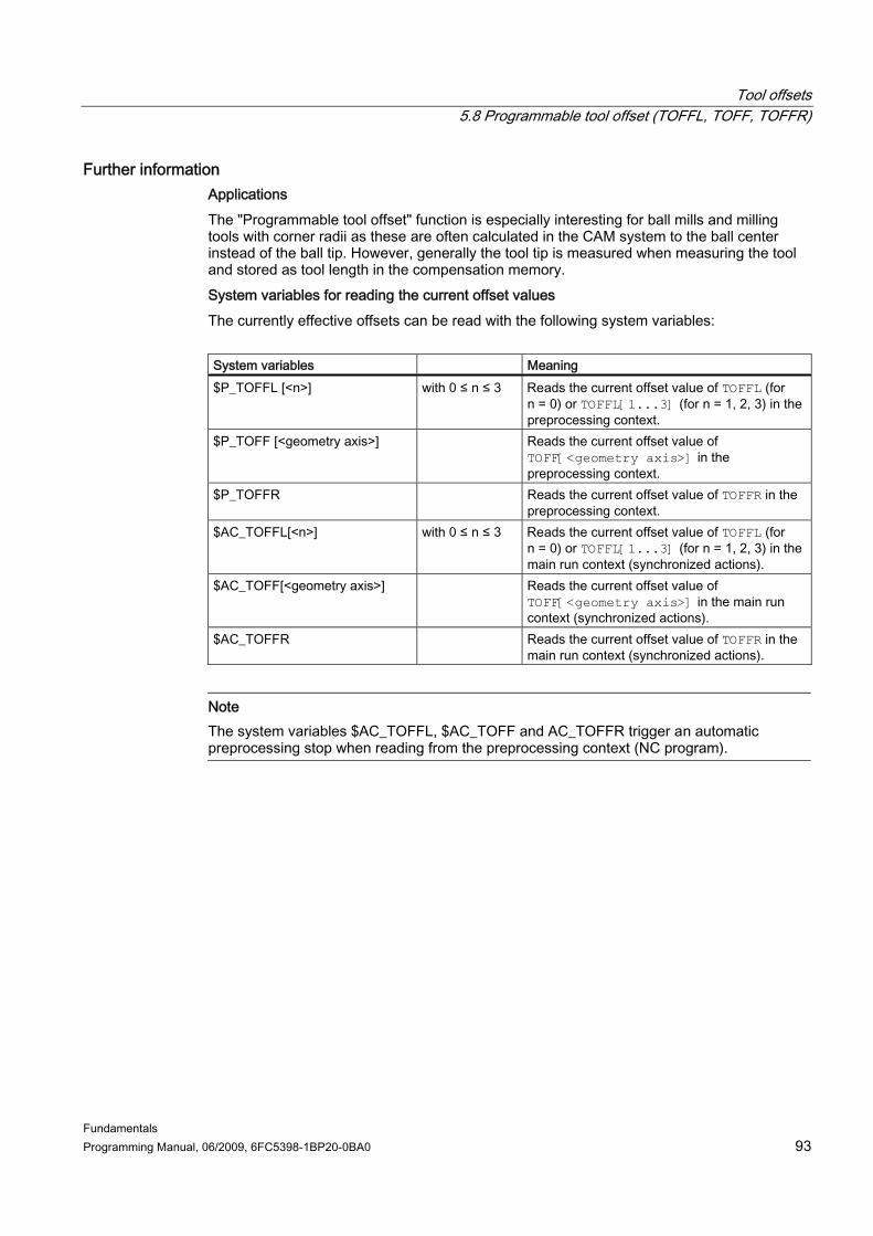
Tool offsets 5.8 Programmable tool offset (TOFFL, TOFF, TOFFR)
Fundamentals Programming Manual, 06/2009, 6FC5398-1BP20-0BA0 93
Further information Applications The "Programmable tool offset" function is especially interesting for ball mills and milling tools with corner radii as these are often calculated in the CAM system to the ball center instead of the ball tip. However, generally the tool tip is measured when measuring the tool and stored as tool length in the compensation memory. System variables for reading the current offset values The currently effective offsets can be read with the following system variables: System variables Meaning $P_TOFFL [<n>] with 0 ≤ n ≤ 3 Reads the current offset value of TOFFL (for
n = 0) or TOFFL[1...3] (for n = 1, 2, 3) in the preprocessing context.
$P_TOFF [<geometry axis>] Reads the current offset value of TOFF[<geometry axis>] in the preprocessing context.
$P_TOFFR Reads the current offset value of TOFFR in the preprocessing context.
$AC_TOFFL[<n>] with 0 ≤ n ≤ 3 Reads the current offset value of TOFFL (for n = 0) or TOFFL[1...3] (for n = 1, 2, 3) in the main run context (synchronized actions).
$AC_TOFF[<geometry axis>] Reads the current offset value of TOFF[<geometry axis>] in the main run context (synchronized actions).
$AC_TOFFR Reads the current offset value of TOFFR in the main run context (synchronized actions).
Note The system variables $AC_TOFFL, $AC_TOFF and AC_TOFFR trigger an automatic preprocessing stop when reading from the preprocessing context (NC program).
Tool offsets 5.8 Programmable tool offset (TOFFL, TOFF, TOFFR)
Fundamentals 94 Programming Manual, 06/2009, 6FC5398-1BP20-0BA0

Fundamentals Programming Manual, 06/2009, 6FC5398-1BP20-0BA0 95
Spindle motion 66.1 6.1 Spindle speed (S), direction of spindle rotation (M3, M4, M5)
Function The spindle speed and direction of rotation values set the spindle in rotary motion and provide the conditions for chip removal.
Figure 6-1 Spindle motion during turning
Other spindles may be available in addition to the main spindle (e.g. the counterspindle or an actuated tool on turning machines). As a rule, the main spindle is declared the master spindle in the machine data. This assignment can be changed using an NC command.

Spindle motion 6.1 Spindle speed (S), direction of spindle rotation (M3, M4, M5)
Fundamentals 96 Programming Manual, 06/2009, 6FC5398-1BP20-0BA0
Syntax S... / S<n>=... M3 / M<n>=3 M4 / M<n>=4 M5 / M<n>=5 SETMS(<n>)
...
SETMS
Significance S… : Spindle speed in rpm for the master spindle S<n>=... : Spindle speed in rpm for spindle <n> Note:
The speed specified with S0=… applies to the master spindle. M3: Direction of spindle rotation clockwise for master spindle M<n>=3: Spindle direction of rotation CW for spindle <n> M4: Direction of spindle rotation counterclockwise for master spindle M<n>=4: Spindle direction of rotation CCW for spindle <n> M5: Spindle stop for master spindle M<n>=5: Spindle stop for spindle <n> SETMS(<n>): Set spindle <n> as master spindle SETMS: If SETMS is programmed without a spindle name, the configured
master spindle is used instead.
Note Up to three S-values can be programmed per NC block, e.g.: S... S2=... S3=...
Note SETMS must be in a separate block.

Spindle motion 6.1 Spindle speed (S), direction of spindle rotation (M3, M4, M5)
Fundamentals Programming Manual, 06/2009, 6FC5398-1BP20-0BA0 97
Example S1 is the master spindle, S2 is the second spindle. The part is to be machined from two sides. To do this, it is necessary to divide the operations into steps. After the cut-off point, the synchronizing device (S2) takes over machining of the workpiece after the cut off. To do this, this spindle S2 is defined as the master spindle to which G95 then applies.
Program code Comment
N10 S300 M3 ; Speed and direction of rotation for drive spindle = preset master spindle
... ; Machining of the right-hand workpiece side
N100 SETMS(2) ; S2 is now the master spindle
N110 S400 G95 F… ; Speed for new master spindle
... ; Machining of the left-hand workpiece side
N160 SETMS ; Switching back to master spindle S1

Spindle motion 6.1 Spindle speed (S), direction of spindle rotation (M3, M4, M5)
Fundamentals 98 Programming Manual, 06/2009, 6FC5398-1BP20-0BA0
Further information Interpretation of the S-value for the master spindle If function G331 or G332 is active in G function group 1 (modally valid motion commands), the programmed S-value will always be interpreted as the speed in rpm. Otherwise, the interpretation of the S-value will depend upon G function group 15 (feedrate type): If G96, G961 or G962 is active, the S-value is interpreted as a constant cutting rate in m/min; otherwise, it is interpreted as a speed in rpm. Changing from G96/G961/G962 to G331/G332 sets the value of the constant cutting rate to zero; changing from G331/G332 to a function within the G function group other than G331/G332 sets the speed value to zero. The corresponding S-values have to be reprogrammed if required. Preset M commands M3, M4, M5 In a block with axis commands, functions M3, M4, M5 are activated before the axis movements commence (basic setting on the control). Example: Program code Comment
N10 G1 F500 X70 Y20 S270 M3 ; The spindle ramps up to 270 rpm, then the movements are executed in X and Y.
N100 G0 Z150 M5 ; Spindle stop before the retraction movement in Z.
Note Machine data can be used to set when axis movements should be executed; either once the spindle has powered up to the setpoint speed, or immediately after the programmed switching operations have been traversed.
Spindle motion 6.1 Spindle speed (S), direction of spindle rotation (M3, M4, M5)
Fundamentals Programming Manual, 06/2009, 6FC5398-1BP20-0BA0 99
Working with multiple spindles 5 spindles (master spindle plus 4 additional spindles) can be available in one channel at the same time. One of the spindles is defined in machine data as the master spindle. Special functions such as thread cutting, tapping, revolutional feedrate, and dwell time apply to this spindle. For the remaining spindles (e.g. a second spindle and an actuated tool) the numbers corresponding to the speed and the direction of rotation/spindle stop must be specified. Example: Program code Comment
N10 S300 M3 S2=780 M2=4 ; Master spindle: 300 rpm, CW rotation
2nd spindle: 780 rpm, CCW rotation
Programmable switchover of master spindle The SETMS(<n>) command can be used in the NC program to define any spindle as the master spindle. SETMS must be in a separate block. Example: Program code Comment
N10 SETMS (2) ; Spindle 2 is now the master spindle.
Note The speed specified with S..., along with the functions programmed with M3, M4, M5, now apply to the newly declared master spindle.
If SETMS is programmed without a spindle name, the master spindle programmed in the machine data is used instead.

Spindle motion 6.2 Cutting rate (SVC)
Fundamentals 100 Programming Manual, 06/2009, 6FC5398-1BP20-0BA0
6.2 6.2 Cutting rate (SVC)
Function As an alternative to the spindle speed, the tool cutting rate, which is more commonly used in practice, can be programmed for milling operations.
The control uses the radius of the active tool to calculate the effective spindle speed from the programmed tool cutting rate: S = (SVC * 1000) / (RT * 2π)
S: Spindle speed in rpm SVC: Cutting rate in m/min or feet/min
where:
RT: Radius of the active tool in mm The tool type ($TC_DP1) of the active tool is not taken into account. The programmed cutting rate is independent of the path feedrate F and G function group 15. The direction of rotation and the spindle start are programmed using M3 and M4 respectively and the spindle stop using M5. A change to the tool radius data in the offset memory will be applied the next time a tool offset is selected or the next time the active offset data is updated. Changing the tool or selecting/deselecting a tool offset data record generates a recalculation of the effective spindle speed.
Spindle motion 6.2 Cutting rate (SVC)
Fundamentals Programming Manual, 06/2009, 6FC5398-1BP20-0BA0 101
Conditions The programming of the cutting speed requires: ● the geometric ratios of a rotating tool (milling cutter or drilling tool) ● An active tool offset data record
Syntax SVC[<n>]=<value>
Note In the block with SVC, the tool radius must be known; in other words, a corresponding tool including a tool offset data record must be active or selected in the block. There is no fixed sequence for SVC and T/D selection during programming in the same block.
Significance
Cutting rate [<n>]: Number of spindle
This address extension specifies which spindle the programmed cutting rate is to be applied for. In the absence of an address extension, the rate is always applied to the master spindle. Note: A separate cutting rate can be preset for each spindle. Note: Programming SVC without an address extension requires that the master spindle has the active tool. If the master spindle changes, the user will need to select a tool accordingly.
SVC:
Unit: m/min or ft/min (dependent upon G700/G710)
Spindle motion 6.2 Cutting rate (SVC)
Fundamentals 102 Programming Manual, 06/2009, 6FC5398-1BP20-0BA0
Note Changing between SVC and S Changing between SVC and S programming is possible at will, even while the spindle is turning. In each case, the value that is not active is deleted.
Note Maximum tool speed System variable $TC_TP_MAX_VELO[<tool number>] can be used to preset a maximum tool speed (spindle speed). If no speed limit has been defined, there will be no monitoring.
Note SVC programming is not possible if the following are active: • G96/G961/G962 • GWPS • SPOS/SPOSA/M19 • M70 Conversely, programming one of these commands will lead to the deselection of SVC.
Note The tool paths of "standard tools" generated e.g. using CAD systems which already take the tool radius into account and only contain the deviation from the standard tool in the tool nose radius are not supported in conjunction with SVC programming.

Spindle motion 6.2 Cutting rate (SVC)
Fundamentals Programming Manual, 06/2009, 6FC5398-1BP20-0BA0 103
Examples The following shall apply to all examples: Toolholder = spindle (for standard milling) Example 1: Milling cutter 6 mm radius Program code Comment
N10 G0 X10 T1 D1 ; Selection of milling cutter with e.g. $TC_DP6[1,1] = 6 (tool radius = 6 mm)
N20 SVC=100 M3 ; Cutting rate = 100 m/min
⇒ Resulting spindle speed: S = (100 m/min * 1,000) / (6.0 mm * 2 * 3.14) = 2653.93 rpm
N30 G1 X50 G95 FZ=0.03 ; SVC and tooth feedrate
...
Example 2: Tool selection and SVC in the same block Program code Comment
N10 G0 X20
N20 T1 D1 SVC=100 ; Tool and offset data record selection together with SVC in block (no specific sequence)
N30 X30 M3 ; Spindle start with CW direction of rotation, cutting rate 100 m/min
N40 G1 X20 F0.3 G95 ; SVC and revolutional feedrate
Example 3: Defining cutting rates for two spindles Program code Comment
N10 SVC[3]=100 M6 T1 D1
N20 SVC[5]=200 ; The tool radius of the active tool offset is the same for both spindles. The effective speed is different for spindle 3 and spindle 5.

Spindle motion 6.2 Cutting rate (SVC)
Fundamentals 104 Programming Manual, 06/2009, 6FC5398-1BP20-0BA0
Example 4: Assumptions: Master or tool change is determined by the toolholder. MD20124 $MC_TOOL_MANAGEMENT_TOOLHOLDER > 1 In the event of a tool change the old tool offset is retained. A tool offset for the new tool is only activated when D is programmed: MD20270 $MC_CUTTING_EDGE_DEFAULT = - 2
Program code Comment
N10 $TC_MPP1[9998,1]=2 ; Magazine location is toolholder
N11 $TC_MPP5[9998,1]=1 ; Magazine location is toolholder 1
N12 $TC_MPP_SP[9998,1]=3 ; Toolholder 1 is assigned to spindle 3
N20 $TC_MPP1[9998,2]=2 ; Magazine location is toolholder
N21 $TC_MPP5[9998,2]=4 ; Magazine location is toolholder 4
N22 $TC_MPP_SP[9998,2]=6 ; Toolholder 4 is assigned to spindle 6
N30 $TC_TP2[2]="WZ2"
N31 $TC_DP6[2,1]=5.0 ; Radius = 5.0 mm of T2, offset D1
N40 $TC_TP2[8]="WZ8"
N41 $TC_DP6[8,1]=9.0 ; Radius = 9.0 mm of T8, offset D1
N42 $TC_DP6[8,4]=7.0 ; Radius = 7.0 mm of T8, offset D4
...
N100 SETMTH(1) ; Set master toolholder number
N110 T="WZ2" M6 D1 ; Tool T2 is loaded and offset D1 is activated.
N120 G1 G94 F1000 M3=3 SVC=100 ; S3 = (100 m/min * 1,000) / (5.0 mm * 2 * 3.14) = 3184.71 rpm
N130 SETMTH(4) ; Set master toolholder number
N140 T="WZ8" ; Corresponds to T8="WZ8"
N150 M6 ; Corresponds to M4=6
Tool "WZ8" is in the master toolholder, but because MD20270=–2, the old tool offset remains active.
N160 SVC=50 ; S3 = (50 m/min * 1,000) / (5.0 mm * 2 * 3.14) = 1592.36 rpm
The offset applied to toolholder 1 is still active and toolholder 1 is assigned to spindle 3.
N170 D4 Offset D4 of the new tool "WZ8" becomes active (in toolholder 4).
N180 SVC=300 ; S6 = (300 m/min * 1,000) / (7.0 mm * 2 * 3.14) = 6824.39 rpm
Spindle 6 is assigned to toolholder 4.

Spindle motion 6.2 Cutting rate (SVC)
Fundamentals Programming Manual, 06/2009, 6FC5398-1BP20-0BA0 105
Example 5: Assumptions: Spindles are toolholders at the same time: MD20124 $MC_TOOL_MANAGEMENT_TOOLHOLDER = 0 In the event of a tool change tool offset data record D4 is selected automatically. MD20270 $MC_CUTTING_EDGE_DEFAULT = 4
Program code Comment
N10 $TC_MPP1[9998,1]=2 ; Magazine location is toolholder
N11 $TC_MPP5[9998,1]=1 ; Magazine location is toolholder 1 = spindle 1
N20 $TC_MPP1[9998,2]=2 ; Magazine location is toolholder
N21 $TC_MPP5[9998,2]=3 ; Magazine location is toolholder 3 = spindle 3
N30 $TC_TP2[2]="WZ2"
N31 $TC_DP6[2,1]=5.0 ; Radius = 5.0 mm of T2, offset D1
N40 $TC_TP2[8]="WZ8"
N41 $TC_DP6[8,1]=9.0 ; Radius = 9.0 mm of T8, offset D1
N42 $TC_DP6[8,4]=7.0 ; Radius = 7.0 mm of T8, offset D4
...
N100 SETMS(1) ; Spindle 1 = master spindle
N110 T="WZ2" M6 D1 ; Tool T2 is loaded and offset D1 is activated.
N120 G1 G94 F1000 M3 SVC=100 ; S1 = (100 m/min * 1,000) / (5.0 mm * 2 * 3.14) = 3184.71 rpm
N200 SETMS(3) ; Spindle 3 = master spindle
N210 M4 SVC=150 ; S3 = (150 m/min * 1,000) / (5.0 mm * 2 * 3.14) = 4777.07 rpm
Refers to tool offset D1 of T="WZ2", S1 continues to turn at previous speed.
N220 T="WZ8" ; Corresponds to T8="WZ8"
N230 M4 SVC=200 ; S3 = (200 m/min * 1,000) / (5.0 mm * 2 * 3.14) = 6369.43 rpm
Refers to tool offset D1 of T="WZ2".
N240 M6 ; Corresponds to M3=6
Tool "WZ8" is in the master spindle, tool offset D4 of the new tool becomes active.
N250 SVC=50 ; S3 = (50 m/min * 1,000) / (7.0 mm * 2 * 3.14) = 1137.40 rpm
Offset D4 on master spindle is active.
N260 D1 ; Offset D1 of new tool "WZ8" active.
N270 SVC[1]=300 ; S1 = (300 m/min * 1,000) / (9.0 mm * 2 * 3.14) = 5307.86 rpm
S3 = (50 m/min * 1,000) / (9.0 mm * 2 * 3.14) = 884.64 rpm
...
Spindle motion 6.2 Cutting rate (SVC)
Fundamentals 106 Programming Manual, 06/2009, 6FC5398-1BP20-0BA0
Further information Tool radius The following tool offset data (associated with the active tool) affect the tool radius when: ● $TC_DP6 (radius - geometry) ● $TC_DP15 (radius - wear) ● $TC_SCPx6 (offset for $TC_DP6) ● $TC_ECPx6 (offset for $TC_DP6) The following are not taken into account: ● Online radius compensation ● Allowance on the programmed contour (OFFN) Tool radius compensation (G41/G42) Although tool radius compensation (G41/G42) and SVC both refer to the tool radius, with regard to function, they are not linked and are independent of one another. Tapping without compensating chuck (G331, G332) SVC programming is also possible in conjunction with G331 or G332. Synchronized actions SVC cannot be programmed from synchronized actions.
Spindle motion 6.2 Cutting rate (SVC)
Fundamentals Programming Manual, 06/2009, 6FC5398-1BP20-0BA0 107
Reading the cutting rate and the spindle speed programming variant The cutting rate of a spindle and the speed programming variant (spindle speed S or cutting rate SVC) can be read using system variables: ● With preprocessing stop in the part program via system variables:
$AC_SVC[<n>] Cutting rate applied when the current main run record for spindle number <n> was preprocessed. Spindle speed programming variant applied when the current main run record for spindle number <n> was preprocessed. Value: Significance: 1 Spindle speed S in rpm
$AC_S_TYPE[<n>]
2 Cutting rate SVC in m/min or ft/min ● Without preprocessing stop in the part program via system variables:
$P_SVC[<n>] Programmed cutting rate for spindle <n> Programmed spindle speed programming variant for spindle <n> Value: Significance: 1 Spindle speed S in rpm
$P_S_TYPE[<n>]
2 Cutting rate SVC in m/min or ft/min

Spindle motion 6.3 Constant cutting rate (G96/G961/G962, G97/G971/G972, G973, LIMS, SCC)
Fundamentals 108 Programming Manual, 06/2009, 6FC5398-1BP20-0BA0
6.3 6.3 Constant cutting rate (G96/G961/G962, G97/G971/G972, G973, LIMS, SCC)
Function When the "Constant cutting rate" function is active, the spindle speed is modified as a function of the respective workpiece diameter so that the cutting rate S in m/min or ft/min remains constant at the tool edge.
This results in the following advantages: ● Uniformity and consequently improved surface quality of turned parts ● Machining process is kinder to tools
Syntax Activating/Deactivating constant cutting rate for the master spindle: G96/G961/G962 S...
...
G97/G971/G972/G973
Speed limitation for the master spindle: LIMS=<value> LIMS[<spindle>]=<value>
Other reference axis for G96/G961/G962: SCC[<axis>]
Spindle motion 6.3 Constant cutting rate (G96/G961/G962, G97/G971/G972, G973, LIMS, SCC)
Fundamentals Programming Manual, 06/2009, 6FC5398-1BP20-0BA0 109
Note SCC[<axis>] can be programmed together with G96/G961/G962 or in isolation.
Significance G96: Constant cutting rate with feedrate type G95: ON
G95 is activated automatically with G96. If G95 has not been activated previously, a new feedrate value F... will have to be specified when G96 is called.
G961: Constant cutting rate with feedrate type G94: ON Constant cutting rate with feedrate type G94 or G95: ON G962: Note: See " Feedrate (G93, G94, G95, F, FGROUP, FL, FGREF) (Page 119)" for information about G94 and G95. In conjunction with G96, G961 or G962, S... is not interpreted as a spindle speed but as a cutting rate. The cutting rate is always applied to the master spindle. Unit: m/min (for G71/G710) or feet/min (for G70/G700)
S... :
Range of values: 0.1 m/min to 9999 9999.9 m/min G97: Deactivate constant cutting rate with feedrate type G95
After G97 (or G971), S... is again interpreted as a spindle speed in rpm. In the absence of a new spindle speed being specified, the last speed set with G96 (or G961) is retained.
G971: Deactivate constant cutting rate with feedrate type G94 G972: Deactivate constant cutting rate with feedrate type G94 or G95 G973: Deactivate constant cutting rate without activating spindle speed limitation

Spindle motion 6.3 Constant cutting rate (G96/G961/G962, G97/G971/G972, G973, LIMS, SCC)
Fundamentals 110 Programming Manual, 06/2009, 6FC5398-1BP20-0BA0
Speed limitation for the master spindle (only applied if G96/G961/G97 active)On machines with selectable master spindles, limitations of differing values can be programmed for up to four spindles within one block. <spindle>: Number of spindle
LIMS:
<value>: Spindle speed upper limit in rpm SCC: If any of the G96/G961/G962 functions are active, SCC[<axis>] can be
used to assign any geometry axis as a reference axis.
Note When G96/G961/G962 is selected for the first time, a constant cutting rate S... must be entered; when G96/G961/G962 is selected again, the entry is optional.
Note The speed limitation programmed with LIMS must not exceed the speed limit programmed with G26 or defined in the setting data.
Note The reference axis for G96/G961/G962 must be a geometry axis assigned to the channel at the time when SCC[<axis>] is programmed. SCC[<axis>] can also be programmed when any of the G96/G961/G962 functions are active.
Examples Example 1: Activating the constant cutting rate with speed limitation Program code Comment
N10 SETMS (3)
N20 G96 S100 LIMS=2500 ; Constant cutting rate = 100 m/min, max. speed 2,500 rpm
...
N60 G96 G90 X0 Z10 F8 S100 LIMS=444 ; Max. speed = 444 rpm

Spindle motion 6.3 Constant cutting rate (G96/G961/G962, G97/G971/G972, G973, LIMS, SCC)
Fundamentals Programming Manual, 06/2009, 6FC5398-1BP20-0BA0 111
Example 2: Defining speed limitation for 4 spindles Speed limitations are defined for spindle 1 (master spindle) and spindles 2, 3, and 4: Program code
N10 LIMS=300 LIMS[2]=450 LIMS[3]=800 LIMS[4]=1500
...
Example 3: Y-axis assignment for face cutting with X axis Program code Comment
N10 G18 LIMS=3000 T1 D1 ; Speed limitation to 3,000 rpm
N20 G0 X100 Z200
N30 Z100
N40 G96 S20 M3 ; Constant cutting rate = 20 m/min, is dependent upon X axis.
N50 G0 X80
N60 G1 F1.2 X34 ; Face cutting in X at 1.2 mm/revolution.
N70 G0 G94 X100
N80 Z80
N100 T2 D1
N110 G96 S40 SCC[Y] ; Y axis is assigned to G96 and G96 is activated (can be achieved in a single block). Constant cutting rate = 40 m/min, is dependent upon X axis.
...
N140 Y30
N150 G01 F1.2 Y=27 ; Grooving in Y, feedrate F = 1.2 mm/revolution.
N160 G97 ; Constant cutting rate off.
N170 G0 Y100

Spindle motion 6.3 Constant cutting rate (G96/G961/G962, G97/G971/G972, G973, LIMS, SCC)
Fundamentals 112 Programming Manual, 06/2009, 6FC5398-1BP20-0BA0
Further information Calculation of the spindle speed The ENS position of the face axis (radius) is the basis for calculating the spindle speed from the programmed cutting rate.
Note Frames between WCS and SZS (e.g. programmable frames such as SCALE, TRANS or ROT) are taken into account in the calculation of the spindle speed and can bring about a change in speed (for example, if there is a change in the effective diameter in the case of SCALE).
Speed limitation LIMS If a workpiece that varies greatly in diameter needs to be machined, it is advisable to specify a speed limit for the spindle with LIMS (maximum spindle speed). This prevents excessively high speeds with small diameters. LIMS is only applied when G96, G961, and G97 are active. LIMS is not applied when G971is selected.
Note On loading the block into the main run, all programmed values are transferred into the setting data.
Spindle motion 6.3 Constant cutting rate (G96/G961/G962, G97/G971/G972, G973, LIMS, SCC)
Fundamentals Programming Manual, 06/2009, 6FC5398-1BP20-0BA0 113
Deactivating the constant cutting rate (G97/G971/G973) After G97/G971, the control interprets an S value as a spindle speed in rpm again. If you do not specify a new spindle speed, the last speed set with G96/G961 is retained. The G96/G961 function can also be deactivated with G94 or G95. In this case, the last speed programmed S... is used for subsequent machining operations. G97 can be programmed without G96 beforehand. The function then has the same effect as G95; LIMS can also be programmed. Using G973, the constant cutting rate can be deactivated without activating a spindle speed limitation.
Note The transverse axis must be defined in machine data.
Rapid traverse G0 With rapid traverse G0, there is no change in speed. Exception: If the contour is approached in rapid traverse and the next NC block contains a G1/G2/G3/etc. path command, the speed is adjusted in the G0approach block for the next path command. Other reference axis for G96/G961/G962 If any of the G96/G961/G962 functions are active, SCC[<axis>] can be used to assign any geometry axis as a reference axis. If the reference axis changes, which will in turn affect the TCP (tool center point) reference position for the constant cutting rate, the resulting spindle speed will be reached via the set braking or acceleration ramp. Axis replacement of the assigned channel axis The reference axis property for G96/G961/G962 is always assigned to a geometry axis. In the event of an axis exchange involving the assigned channel axis, the reference axis property for G96/G961/G962 is retained in the old channel. A geometry axis exchange will not affect how the geometry axis is assigned to the constant cutting rate. If the TCP reference position for G96/G961/G962 is affected by a geometry axis exchange, the spindle will reach the new speed via a ramp.
Spindle motion 6.3 Constant cutting rate (G96/G961/G962, G97/G971/G972, G973, LIMS, SCC)
Fundamentals 114 Programming Manual, 06/2009, 6FC5398-1BP20-0BA0
If no new channel axis is assigned as a result of a geometry axis exchange (e.g. GEOAX(0,X)), the spindle speed will be frozen in accordance with G97. Examples for geometry axis exchange with assignments of the reference axis: Program code Comment
N05 G95 F0.1
N10 GEOAX(1, X1) ; Channel axis X1 becomes first geometry axis.
N20 SCC[X] ; First geometry axis (X) becomes reference axis for G96/G961/G962.
N30 GEOAX(1, X2) ; Channel axis X2 becomes first geometry axis.
N40 G96 M3 S20 ; Reference axis for G96 is channel axis X2.
Program code Comment
N05 G95 F0.1
N10 GEOAX(1, X1) ; Channel axis X1 becomes first geometry axis.
N20 SCC[X1] ; X1 and implicitly the first geometry axis (X) becomes the reference axis for G96/G961/G962.
N30 GEOAX(1, X2) ; Channel axis X2 becomes first geometry axis.
N40 G96 M3 S20 ; Reference axis for G96 is X2 or X, no alarm.
Program code Comment
N05 G95 F0.1
N10 GEOAX(1, X2) ; Channel axis X2 becomes first geometry axis.
N20 SCC[X1] ; X1 is not a geometry axis, alarm.
Program code Comment
N05 G0 Z50
N10 X35 Y30
N15 SCC[X] ; Reference axis for G96/G961/G962 is X.
N20 G96 M3 S20 ; Constant cutting rate ON at 10 mm/min.
N25 G1 F1.5 X20 ; Face cutting in X at 1.5 mm/revolution.
N30 G0 Z51
N35 SCC[Y] ; Reference axis for G96 is Y, reduction in spindle speed (Y30).
N40 G1 F1.2 Y25 ; Face cutting in Y at 1.2 mm/revolution.
References: Function Manual, Basic Functions; Transverse Axes (P1) and Feedrates (V1)

Spindle motion 6.4 Constant grinding wheel peripheral speed (GWPSON, GWPSOF)
Fundamentals Programming Manual, 06/2009, 6FC5398-1BP20-0BA0 115
6.4 6.4 Constant grinding wheel peripheral speed (GWPSON, GWPSOF)
Function The "Constant grinding wheel peripheral speed (GWPS)" function is used to set the grinding wheel speed so that, taking account of the current radius, the grinding wheel peripheral speed remains constant.
Syntax GWPSON(<t no.>) GWPSOF(<t no.>) S.../S<n>=...
Significance GWPSON: Select constant grinding wheel peripheral speed GWPSOF: Deselect constant grinding wheel peripheral speed <t no.>: It is only necessary to specify the T number if the tool with this T
number is not active. S…: Peripheral speed in m/s or ft/s for the master spindle S<n>=… : Peripheral speed in m/s or ft/s for spindle <n>
Note: The peripheral speed specified with S0=… applies to the master spindle.
Note A grinding wheel peripheral speed can only be programmed for grinding tools (types 400 to 499).
Spindle motion 6.4 Constant grinding wheel peripheral speed (GWPSON, GWPSOF)
Fundamentals 116 Programming Manual, 06/2009, 6FC5398-1BP20-0BA0
Example A constant grinding wheel peripheral speed is to be used for grinding tools T1 and T5. T1 is the active tool. Program code Comment
N20 T1 D1 ; Select T1 and D1.
N25 S1=1000 M1=3 ; 1000 rpm for spindle 1
N30 S2=1500 M2=3 ; 1500 rpm for spindle 2
…
N40 GWPSON ; Selection of GWPS for active tool.
N45 S1=60 ; Set GWPS to 60 m/s for active tool.
…
N50 GWPSON(5) ; GWPS selection for tool 5 (spindle 2).
N55 S2=40 ; Set GWPS to 40 m/s for spindle 2.
…
N60 GWPSOF ; Deactivate GWPS for active tool.
N65 GWPSOF(5) ; Deactivate GWPS for tool 5 (spindle 2).
Further information Tool-specific parameters In order to activate the function "Constant peripheral speed", the tool-specific grinding data $TC_TPG1, $TC_TPG8 and $TC_TPG9 must be set accordingly. When the GWPS function is active, even online offset values (= wear parameters; cf. "Grinding-specific tool monitoring in the parts program TMON, TMOF" or PUTFTOC, PUTFTOCF) must be taken into account when changing speed. Select GWPS: GWPSON, programming GWPS After selecting the GWPS with GWPSON, each subsequent S value for this spindle is interpreted as a grinding wheel peripheral speed. Selection of grinding wheel peripheral speed with GWPSON does not cause the automatic activation of tool length compensation or tool monitoring. The GWPS can be active for several spindles on a channel with different tool numbers. If GWPS is to be selected for a new tool on a spindle where GWPS is already active, the active GWPS must first be deselected with GWPSOF.

Spindle motion 6.4 Constant grinding wheel peripheral speed (GWPSON, GWPSOF)
Fundamentals Programming Manual, 06/2009, 6FC5398-1BP20-0BA0 117
Deactivate GWPS: GWPSOF When GWPS is deselected with GWPSOF, the last speed to be calculated remains valid as the setpoint. GWPS programming is reset at the end of the parts program or on RESET. Query active GWPS: $P_GWPS[<spindle no.>] This system variable can be used to query from the parts program whether the GWPS is active for a specific spindle. TRUE: GWPS is active. FALSE: GWPS is inactive.

Spindle motion 6.5 Programmable spindle speed limitation (G25, G26)
Fundamentals 118 Programming Manual, 06/2009, 6FC5398-1BP20-0BA0
6.5 6.5 Programmable spindle speed limitation (G25, G26)
Function The minimum and maximum spindle speeds defined in the machine and setting data can be modified by means of a part program command. Programmed spindle speed limitations are possible for all spindles of the channel.
CAUTION A spindle speed limitation programmed with G25 or G26 overwrites the speed limits in the setting data and, therefore, remains stored even after the end of the program.
Syntax G25 S… S1=… S2=… G26 S… S1=… S2=…
Significance G25: Lower spindle speed limit G26: Upper spindle speed limit
Minimum or maximum spindle speed(s) Note: A maximum of three spindle speed limits can be programmed for each block.
S... S1=… S2=… :
Range of values: 0.1 to 9999 9999.9 rpm
Example Program code Comment
N10 G26 S1400 S2=350 S3=600 ; Upper speed limit for master spindle, spindle 2 and spindle 3.
Fundamentals Programming Manual, 06/2009, 6FC5398-1BP20-0BA0 119
Feed control 77.1 7.1 Feedrate (G93, G94, G95, F, FGROUP, FL, FGREF)
Function These commands are used in the NC program to set the feedrates for all axes involved in the machining sequence.
Syntax G93/G94/G95 F... FGROUP(<axis1>,<axis2>, etc.) FGREF[<rotary axis>]=<reference radius> FL[<axis>]=<value>
Significance G93: Inverse-time feedrate (in rpm) G94: Linear feedrate (in mm/min, inch/min or °/min) G95: Revolutional feedrate (in mm/revolution or inch/revolution)
G95 refers to the revolutions of the master spindle (usually the cutting spindle or the main spindle on the turning machine)
F... : Feedrate of the geometry axes involved in the movement The unit set with G93/G94/G95 applies.
FGROUP: The feedrate programmed under F is valid for all axes specified under FGROUP (geometry axes/rotary axes).
FGREF: FGREF is used to program the effective radius (<reference radius>) for each of the rotary axes specified under FGROUP. Limit velocity for synchronized/path axes The unit set with G94 applies. One FL value can be programmed per axis (channel axes, geometry axis or orientation axis).
FL:
<axis>: The axis identifiers of the basic coordinate system should be used (channel axes, geometry axes).

Feed control 7.1 Feedrate (G93, G94, G95, F, FGROUP, FL, FGREF)
Fundamentals 120 Programming Manual, 06/2009, 6FC5398-1BP20-0BA0
Examples Example 1: Mode of operation of FGROUP The following example is intended to demonstrate the effect of FGROUP on the path and path feedrate. The variable $AC_TIME contains the time of the block start in seconds. It can only be used in synchronized actions. Program code Comment
N100 G0 X0 A0
N110 FGROUP(X,A)
N120 G91 G1 G710 F100 ; Feedrate = 100 mm/min or 100 degrees/min
N130 DO $R1=$AC_TIME
N140 X10 ; Feedrate = 100 mm/min, path = 10 mm, R1 = approx. 6 s
N150 DO $R2=$AC_TIME
N160 X10 A10 ; Feedrate = 100 mm/min, path = 14.14 mm, R2 = approx. 8 s
N170 DO $R3=$AC_TIME
N180 A10 ; Feedrate = 100 degrees/min, path = 10 degrees, R3 = approx. 6 s
N190 DO $R4=$AC_TIME
N200 X0.001 A10 ; Feedrate = 100 mm/min, path = 10 mm, R4 = approx. 6 s
N210 G700 F100 ; Feedrate = 2540 mm/min or 100 degrees/min
N220 DO $R5=$AC_TIME
N230 X10 ; Feedrate = 2540 mm/min, path = 254 mm, R5 = approx. 6 s
N240 DO $R6=$AC_TIME
N250 X10 A10 ; Feedrate = 2540 mm/min, path = 254.2 mm, R6 = approx. 6 s
N260 DO $R7=$AC_TIME
N270 A10 ; Feedrate = 100 degrees/min, path = 10 degrees, R7 = approx. 6 s
N280 DO $R8=$AC_TIME
N290 X0.001 A10 ; Feedrate = 2540 mm/min, path = 10 mm, R8 = approx. 0.288 s
N300 FGREF[A]=360/(2*$PI)
; Set 1 degree = 1 inch via the effective radius.
N310 DO $R9=$AC_TIME
N320 X0.001 A10 ; Feedrate = 2540 mm/min, path = 254 mm, R9 = approx. 6 s
N330 M30
Example 2: Traverse synchronized axes with limit velocity FL The path velocity of the path axes is reduced if the synchronized axis Z reaches the limit velocity. Program code
N10 G0 X0 Y0
N20 FGROUP(X)
N30 G1 X1000 Y1000 G94 F1000 FL[Y]=500
N40 Z-50

Feed control 7.1 Feedrate (G93, G94, G95, F, FGROUP, FL, FGREF)
Fundamentals Programming Manual, 06/2009, 6FC5398-1BP20-0BA0 121
Example 3: Helical interpolation Path axes X and Y traverse with the programmed feedrate, the infeed axis Z is a synchronized axis.
Program code Comment
N10 G17 G94 G1 Z0 F500 ; Feed of the tool.
N20 X10 Y20 ; Approach of the starting position
N25 FGROUP(X,Y) ; Axes X/Y are path axes, Z is a synchronized axis.
N30 G2 X10 Y20 Z-15 I15 J0 F1000 FL[Z]=200 ; On the circular path, the feedrate is 1,000 mm/min, traversing in the Z direction is synchronized.
...
N100 FL[Z]=$MA_AX_VELO_LIMIT[0,Z] ; The limit speed is deselected by reading the speed from the MD. Read the value from the MD.
N110 M30 ; End of program.

Feed control 7.1 Feedrate (G93, G94, G95, F, FGROUP, FL, FGREF)
Fundamentals 122 Programming Manual, 06/2009, 6FC5398-1BP20-0BA0
Further information Feedrate for path axes (F) The path feedrate is generally composed of the individual speed components of all geometry axes participating in the movement and refers to the center point of the cutter or the tip of the turning tool.
The feedrate is specified under address F. Depending on the default setting in the machine data, the units of measurement specified with the G commands are either in mm or inch. One F value can be programmed per NC block. The feedrate unit is defined using one of the G commands G93/G94/G95. The feedrate F acts only on path axes and remains active until a new feedrate is programmed. Separators are permitted after the address F. Examples: F100 or F 100 F.5 F=2*FEED Feedrate type (G93/G94/G95) The G commands G93, G94 and G95 are modal. In the event of switching between G93, G94 and G95, the path feedrate value has to be reprogrammed. When machining with rotary axes, the feedrate can also be specified in degrees/min.
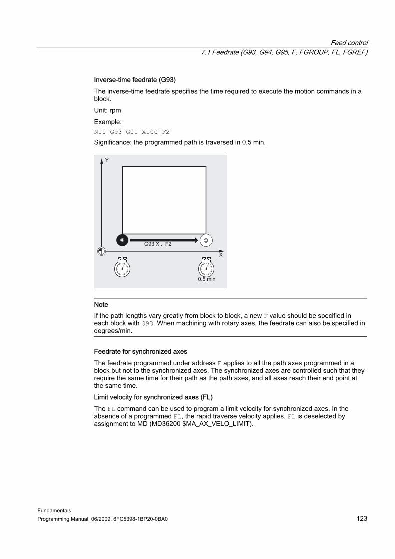
Feed control 7.1 Feedrate (G93, G94, G95, F, FGROUP, FL, FGREF)
Fundamentals Programming Manual, 06/2009, 6FC5398-1BP20-0BA0 123
Inverse-time feedrate (G93) The inverse-time feedrate specifies the time required to execute the motion commands in a block. Unit: rpm Example: N10 G93 G01 X100 F2 Significance: the programmed path is traversed in 0.5 min.
Note If the path lengths vary greatly from block to block, a new F value should be specified in each block with G93. When machining with rotary axes, the feedrate can also be specified in degrees/min.
Feedrate for synchronized axes The feedrate programmed under address F applies to all the path axes programmed in a block but not to the synchronized axes. The synchronized axes are controlled such that they require the same time for their path as the path axes, and all axes reach their end point at the same time. Limit velocity for synchronized axes (FL) The FL command can be used to program a limit velocity for synchronized axes. In the absence of a programmed FL, the rapid traverse velocity applies. FL is deselected by assignment to MD (MD36200 $MA_AX_VELO_LIMIT).

Feed control 7.1 Feedrate (G93, G94, G95, F, FGROUP, FL, FGREF)
Fundamentals 124 Programming Manual, 06/2009, 6FC5398-1BP20-0BA0
Traverse path axis as synchronized axis (FGROUP) FGROUP is used to define whether a path axis should be traversed with path feedrate or as a synchronized axis. In helical interpolation, for example, it is possible to define that only two geometry axes, X and Y, are to be traversed at the programmed feedrate. The infeed axis Z is the synchronized axis in this case. Example: FGROUP(X,Y) Change FGROUP The setting made with FGROUP can be changed: 1. By reprogramming FGROUP: e.g. FGROUP(X,Y,Z) 2. By programming FGROUP without a specific axis: FGROUP()
In accordance with FGROUP(), the initial setting in the machine data applies: Geometry axes are now once again traversed in the path axis grouping.
Note With FGROUP, axis identifiers must be the names of channel axes.
Units of measurement for feedrate F In addition to the geometrical settings G700 and G710, the G commands are also used to define the measuring system for the feedrates F. In other words: ● For G700: [inch/min] ● For G710: [mm/min]
Note G70/G71 have no effect on feedrate settings.
Unit of measurement for synchronized axes with limit speed FL The unit set for F using G command G700/G710 is also valid for FL.
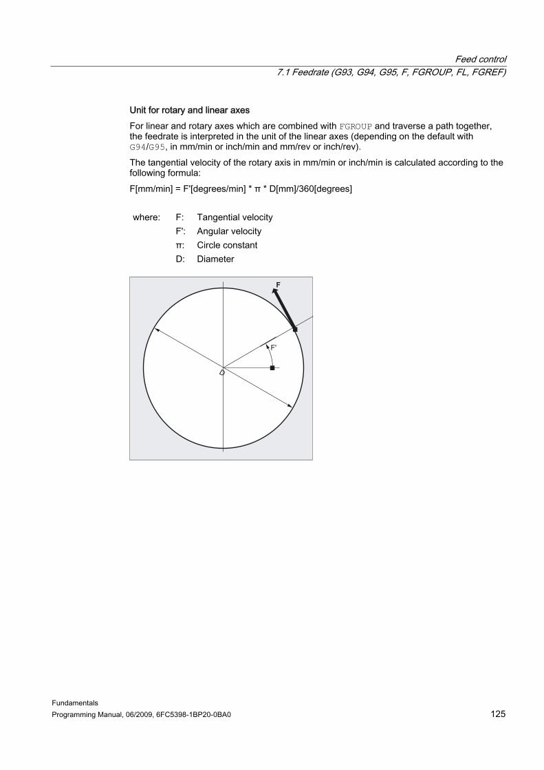
Feed control 7.1 Feedrate (G93, G94, G95, F, FGROUP, FL, FGREF)
Fundamentals Programming Manual, 06/2009, 6FC5398-1BP20-0BA0 125
Unit for rotary and linear axes For linear and rotary axes which are combined with FGROUP and traverse a path together, the feedrate is interpreted in the unit of the linear axes (depending on the default with G94/G95, in mm/min or inch/min and mm/rev or inch/rev). The tangential velocity of the rotary axis in mm/min or inch/min is calculated according to the following formula: F[mm/min] = F'[degrees/min] * π * D[mm]/360[degrees]
F: Tangential velocity F': Angular velocity π: Circle constant
where:
D: Diameter
D
F
F'

Feed control 7.1 Feedrate (G93, G94, G95, F, FGROUP, FL, FGREF)
Fundamentals 126 Programming Manual, 06/2009, 6FC5398-1BP20-0BA0
Traverse rotary axes with path velocity F (FGREF) For machining operations, in which the tool or the workpiece or both are moved by a rotary axis, the effective machining feedrate is to be interpreted as a path feed in the usual way by reference to the F value. This requires the specification of an effective radius (reference radius) for each of the rotary axes involved. The unit of the reference radius depends on the G70/G71/G700/G710 setting. All axes involved must be included in the FGROUP command to be taken into account in the calculation of the path feedrate. In order to ensure compatibility with the behavior with no FGREF programming, the factor 1 degree = 1 mm is activated on system power up and RESET. This corresponds to a reference radius of FGREF= 360 mm/(2π) = 57.296 mm.
Note This default is independent of the active basic system (MD10240 $MN_SCALING_SYSTEM_IS_METRIC) and the currently active G70/G71/G700/G710 setting.
Special situations: Program code
N100 FGROUP(X,Y,Z,A)
N110 G1 G91 A10 F100
N120 G1 G91 A10 X0.0001 F100
With this type of programming, the F value programmed in N110 is evaluated as the rotary axis feedrate in degrees/min, while the feedrate evaluation in N120 is either 100 inch/min or 100 mm/min, dependent upon the currently active G70/G71/G700/G710 setting.
CAUTION FGREF evaluation also works if only rotary axes are programmed in the block. The normal F value interpretation as degree/min applies in this case only if the radius reference corresponds to the FGREF default: • For G71/G710: FGREF[A]=57.296 • For G70/G700: FGREF[A]=57.296/25.4

Feed control 7.1 Feedrate (G93, G94, G95, F, FGROUP, FL, FGREF)
Fundamentals Programming Manual, 06/2009, 6FC5398-1BP20-0BA0 127
Read reference radius The value of the reference radius of a rotary axis can be read using system variables: ● In synchronized actions or with preprocessing stop in the part program via system
variable: $AA_FGREF[<axis>] Current main run value
● Without preprocessing stop in the part program via system variable: $PA_FGREF[<axis>] Programmed value
If no values are programmed, the default 360 mm/(2π) = 57.296 mm (corresponding to 1 mm per degree) will be read in both variables. For linear axes, the value in both variables is always 1 mm. Read path axes affecting velocity The axes involved in path interpolation can be read using system variables: ● In synchronized actions or with preprocessing stop in the part program via system
variables: $AA_FGROUP[<axis>] Returns the value "1" if the specified axis affects the
path velocity in the current main run record by means of the basic setting or through FGROUP programming. Otherwise, the variable returns the value "0".
$AC_FGROUP_MASK Returns a bit key of the channel axes programmed with FGROUP which are to affect the path velocity.
● Without preprocessing stop in the part program via system variables: $PA_FGROUP[<axis>] Returns the value "1" if the specified axis affects the
path velocity by means of the basic setting or through FGROUP programming. Otherwise, the variable returns the value "0".
$P_FGROUP_MASK Returns a bit key of the channel axes programmed with FGROUP which are to affect the path velocity.
Feed control 7.1 Feedrate (G93, G94, G95, F, FGROUP, FL, FGREF)
Fundamentals 128 Programming Manual, 06/2009, 6FC5398-1BP20-0BA0
Path reference factors for orientation axes with FGREF With orientation axes the mode of operation of the FGREF[] factors is dependent upon whether the change in the orientation of the tool is implemented by means of rotary axis or vector interpolation. In the case of rotary axis interpolation, as is the case with rotary axes, the relevant FGREF factors of the orientation axes are calculated individually as reference radius for the axis paths. In the case of vector interpolation, an effective FGREF factor, which is calculated as the geometric mean value of the individual FGREF factors, is applied. FGREF[effective] = nth root of [(FGREF[A] * FGREF[B]...)]
A: Axis identifier of 1st orientation axis B: Axis identifier of 2nd orientation axis C: Axis identifier of 3rd orientation axis
where:
n: Number of orientation axes Example: Since there are two orientation axes for a standard 5-axis transformation, the effective factor is, therefore, the root of the product of the two axial factors: FGREF[effective] = square root of [(FGREF[A] * FGREF[B])]
Note It is, therefore, possible to use the effective factor for orientation axes FGREF to define a reference point on the tool to which the programmed path feedrate refers.

Feed control 7.2 Traversing positioning axes (POS, POSA, POSP, FA, WAITP, WAITMC)
Fundamentals Programming Manual, 06/2009, 6FC5398-1BP20-0BA0 129
7.2 7.2 Traversing positioning axes (POS, POSA, POSP, FA, WAITP, WAITMC)
Function Positioning axes are traversed independently of the path axes at a separate, axis-specific feedrate. There are no interpolation commands. The POS/POSA/POSP commands are used to traverse the positioning axes and coordinate the motion sequences at the same time. The following are typical examples of positioning axes: ● Pallet feed equipment ● Gauging stations WAITP can be used to identify a position in the NC program where the program is to wait until an axis programmed with POSA in a previous NC block reaches its end position. WAITMC loads the next NC block immediately when the specified wait marker is received.
Syntax POS[<axis>]=<position> POSA[<axis>]=<position> POSP[<axis>]=(<end position>,<partial length>,<mode>) FA[<axis>]=<value> WAITP(<axis>) ; Programming in a separate NC block. WAITMC(<wait marker>)
Feed control 7.2 Traversing positioning axes (POS, POSA, POSP, FA, WAITP, WAITMC)
Fundamentals 130 Programming Manual, 06/2009, 6FC5398-1BP20-0BA0
Significance
Move positioning axis to specified position POS and POSA have the same functionality but differ in their block change behavior: • POS delays the enabling of the NC block until the position has been
reached. • POSA enables the NC block even if the position has not been
reached.
<axis>: Name of the axis to be traversed (channel or geometry axis identifier) Axis position to be approached
POS/POSA:
<position>: Type: REAL
Move positioning axis to specified end position in sections <end position>: Axis end position to be approached <partial length>:
Length of a section
Approach mode = 0: For the last two sections, the path
remaining until the end position is split into two residual sections of equal size (preset).
<mode>:
= 1: The partial length is adjusted so that the total of all calculated partial lengths corresponds exactly to the path up to the end position.
POSP:
Note: POSP is used specifically to program oscillating motion. References: Programming Manual, Job Planning; Chapter "Oscillation"
Feedrate for the specified positioning axis <axis>: Name of the axis to be traversed (channel or geometry axis
identifier) Feedrate <value>: Unit: mm/min or inch/min or deg/min
FA:
Note: Up to 5 FA values can be programmed for each NC block.
Feed control 7.2 Traversing positioning axes (POS, POSA, POSP, FA, WAITP, WAITMC)
Fundamentals Programming Manual, 06/2009, 6FC5398-1BP20-0BA0 131
Wait for a positioning axis to be traversed The subsequent blocks are not processed until the specified positioning axis programmed in a previous NC block with POSA has reached its end position (with exact stop fine). <axis>: Name of the axis (channel or geometry axis identifier) for
which the WAITP command is to be applied
WAITP:
Note: With WAITP, an axis can be made available as an oscillating axis or for traversing as a concurrent positioning axis (via PLC).
WAITMC: Wait for the specified wait marker to be received
When the wait marker is received, the next NC block is loaded immediately.
<wait marker>: Number of the wait marker
CAUTION Travel with POSA If a command, which implicitly causes a preprocessing stop, is read in a following block, this block is not executed until all other blocks, which are already preprocessed and stored have been executed. The previous block is stopped in exact stop (as G9).
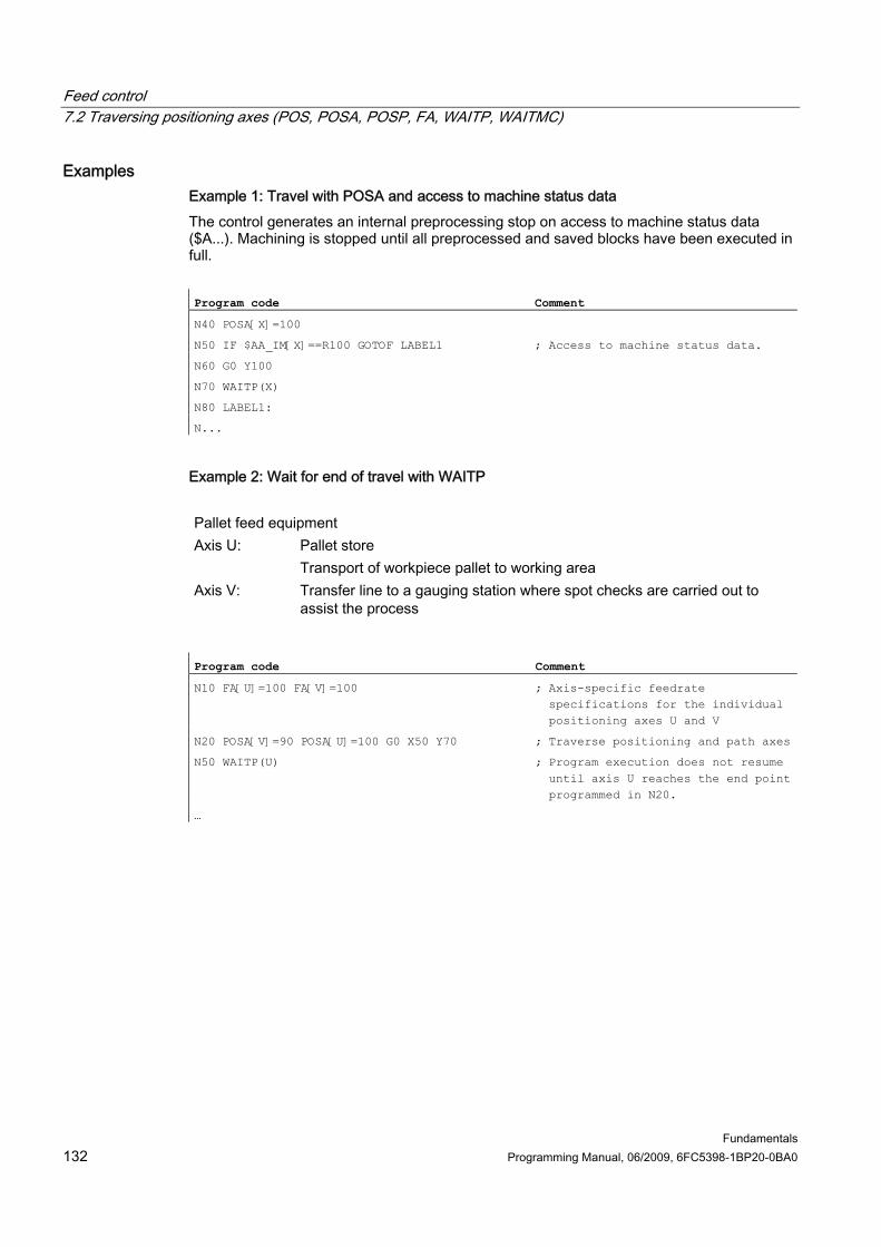
Feed control 7.2 Traversing positioning axes (POS, POSA, POSP, FA, WAITP, WAITMC)
Fundamentals 132 Programming Manual, 06/2009, 6FC5398-1BP20-0BA0
Examples Example 1: Travel with POSA and access to machine status data The control generates an internal preprocessing stop on access to machine status data ($A...). Machining is stopped until all preprocessed and saved blocks have been executed in full. Program code Comment
N40 POSA[X]=100
N50 IF $AA_IM[X]==R100 GOTOF LABEL1 ; Access to machine status data.
N60 G0 Y100
N70 WAITP(X)
N80 LABEL1:
N...
Example 2: Wait for end of travel with WAITP Pallet feed equipment Axis U: Pallet store
Transport of workpiece pallet to working area Axis V: Transfer line to a gauging station where spot checks are carried out to
assist the process
Program code Comment
N10 FA[U]=100 FA[V]=100 ; Axis-specific feedrate specifications for the individual positioning axes U and V
N20 POSA[V]=90 POSA[U]=100 G0 X50 Y70 ; Traverse positioning and path axes
N50 WAITP(U) ; Program execution does not resume until axis U reaches the end point programmed in N20.
…
Feed control 7.2 Traversing positioning axes (POS, POSA, POSP, FA, WAITP, WAITMC)
Fundamentals Programming Manual, 06/2009, 6FC5398-1BP20-0BA0 133
Further information Travel with POSA Block step enable or program execution is not affected by POSA. The movement to the end position can be performed during execution of subsequent NC blocks. Travel with POS The next block is not executed until all axes programmed under POS reach their end positions. Wait for end of travel with WAITP After a WAITP, assignment of the axis to the NC program is no longer valid; this applies until the axis is programmed again. This axis can then be operated as a positioning axis through the PLC, or as a reciprocating axis from the NC program/PLC or HMI. Block change in the braking ramp with IPOBRKA and WAITMC An axis is only decelerated if the wait marker has not yet been reached or if another end-of-block criterion is preventing the block change. After a WAITMC, the axis starts immediately if no other end-of-block criterion is preventing the block change.

Feed control 7.3 Position-controlled spindle operation (SPCON, SPCOF)
Fundamentals 134 Programming Manual, 06/2009, 6FC5398-1BP20-0BA0
7.3 7.3 Position-controlled spindle operation (SPCON, SPCOF)
Function Position-controlled spindle mode may be advisable in some cases, e.g. in conjunction with large-pitch thread cutting with G33, where better quality can be achieved. The SPCON NC command is used to switch over to position-controlled spindle mode.
Note SPCON requires a maximum of 3 interpolation cycles.
Syntax SPCON/SPCON(<n>)/SPCON(<n>,<m>, etc.) ... SPCOF/SPCOF(<n>)/SPCOF(<n>,<m>, etc.)
Significance SPCON: Activate position-controlled mode
The specified spindle is switched over from speed control to position control. SPCON s modal and is retained until SPCOF.
SPCOF: Deactivate position-controlled mode The specified spindle is switched over from position control to speed control.
<n>: Number of the spindle to be switched over. If a spindle number is not specified, SPCON/SPCOF will be applied to the master spindle.
<n>,<m>, etc.: SPCON or SPCOF can even be used to switch over multiple spindles in one block.
Note The speed is specified with S…. M3, M4 and M5 apply in respect of the directions of rotation and spindle stop.
Note With synchronized spindle setpoint value linkage, the master spindle must be operated in position-control mode.

Feed control 7.4 Positioning spindles (SPOS, SPOSA, M19, M70, WAITS)
Fundamentals Programming Manual, 06/2009, 6FC5398-1BP20-0BA0 135
7.4 7.4 Positioning spindles (SPOS, SPOSA, M19, M70, WAITS)
Function SPOS, SPOSA or M19 can be used to set spindles to specific angular positions, e.g. during tool change.
SPOS, SPOSA and M19 induce a temporary switchover to position-controlled mode until the next M3/M4/M5/M41 to M45. Positioning in axis mode The spindle can also be operated as a path axis, synchronized axis or positioning axis at the address defined in the machine data. When the axis identifier is specified, the spindle is in axis mode. M70 switches the spindle directly to axis mode. End of positioning The end-of-motion criterion when positioning the spindle can be programmed using FINEA, CORSEA, IPOENDA or IPOBRKA. The program advances to the next block if the end of motion criteria for all spindles or axes programmed in the current block plus the block change criterion for path interpolation are fulfilled. Synchronization In order to synchronize spindle movements, WAITS can be used to wait until the spindle position is reached.

Feed control 7.4 Positioning spindles (SPOS, SPOSA, M19, M70, WAITS)
Fundamentals 136 Programming Manual, 06/2009, 6FC5398-1BP20-0BA0
Conditions The spindle to be positioned must be capable of operation in position-controlled mode.
Syntax Position spindle: SPOS=<value>/SPOS[<n>]=<value> SPOSA=<value>/SPOSA[<n>]=<value> M19/M<n>=19 Switch spindle over to axis mode: M70/M<n>=70 Define end-of-motion criterion: FINEA/FINEA[S<n>] COARSEA/COARSEA[S<n>] IPOENDA/IPOENDA[S<n>] IPOBRKA/IPOBRKA(<axis>[,<instant in time>]) ; Programming in a separate NC block. Synchronize spindle movements: WAITS/WAITS(<n>,<m>) ; Programming in a separate NC block.

Feed control 7.4 Positioning spindles (SPOS, SPOSA, M19, M70, WAITS)
Fundamentals Programming Manual, 06/2009, 6FC5398-1BP20-0BA0 137
Significance
Set spindle to specified angle SPOS and SPOSA have the same functionality but differ in their block change behavior: • SPOS delays the enabling of the NC block until the position has been
reached. • SPOSA enables the NC block even if the position has not been reached.
<n>: Number of the spindle to be positioned. If a spindle number is not specified or if the spindle number is set to "0", SPOS or SPOSA will be applied to the master spindle. Angular position to which the spindle is to be set. Unit: degrees Type: REAL The following options are available about programming the position approach mode: =AC(<value>): Absolute dimensions Range of values: 0 … 359.9999 =IC(<value>): Incremental dimensions Range of values: 0 … ±99 999.999 =DC(<value>): Approach absolute value directly =ACN(<value>): Absolute dimension, approach in
negative direction =ACP(<value>): Absolute dimension, approach in
positive direction
SPOS/SPOSA:
<value>:
=<value>: as DC(<value>)

Feed control 7.4 Positioning spindles (SPOS, SPOSA, M19, M70, WAITS)
Fundamentals 138 Programming Manual, 06/2009, 6FC5398-1BP20-0BA0
M<n>=19: Set the master spindle (M19 or M0=19) or spindle number <n> (M<n>=19) to the angular position preset with SD43240 $SA_M19_SPOS with the position approach mode preset in SD43250 $SA_M19_SPOSMODE. The NC block is not enabled until the position has been reached.
M<n>=70: Switch the master spindle (M70 or M0=70) or spindle number <n>
(M<n>=70) over to axis mode. No defined position is approached. The NC block is enabled after the switchover has been performed.
FINEA: Motion end when "Exact stop fine" reached COARSEA: Motion end when "Exact stop coarse" reached IPOENDA: End of motion on reaching "interpolator stop"
Spindle for which the programmed end-of-motion criterion is to be effective <n>: Spindle number
S<n>:
If a spindle is not specified in [S<n>] or a spindle number of "0" is specified, the programmed end-of-motion criterion will be applied to the master spindle. A block change is possible in the braking ramp. <axis>: Channel axis identifier
Instant in time of the block change with reference to the braking ramp Unit: Percent Range of values: 100 (application point of the
braking ramp) to 0 (end of the braking ramp)
IPOBRKA:
<instant in time>:
If a value is not assigned to the <instant in time> parameter, the current value of the setting data is applied: SD43600 $SA_IPOBRAKE_BLOCK_EXCHANGE Note: IBOBRKA with an instant in time of "0" is identical to IPOENDA.
Feed control 7.4 Positioning spindles (SPOS, SPOSA, M19, M70, WAITS)
Fundamentals Programming Manual, 06/2009, 6FC5398-1BP20-0BA0 139
Synchronization command for the specified spindle(s) The subsequent blocks are not processed until the specified spindle(s) programmed in a previous NC block with SPOSA has (have) reached its (their) end position(s) (with exact stop fine). WAITS after M5: Wait for the specified spindle(s) to come to a
standstill. WAITS after M3/M4: Wait for the specified spindle(s) to reach their
setpoint speed.
WAITS:
<n>,<m>: Numbers of the spindles to which the synchronization command is to be applied. If a spindle number is not specified or if the spindle number is set to "0", WAITS will be applied to the master spindle.
Note Three spindle positions are possible for each NC block.
Note With incremental dimensions IC(<value>), spindle positioning can take place over several revolutions.
Note If position control was activated with SPCON prior to SPOS, this remains active until SPCOF is issued.
Note The control detects the transition to axis mode automatically from the program sequence. Explicit programming of M70 in the part program is, therefore, essentially no longer necessary. However, M70 can continue to be programmed, e.g to increase the legibility of the part program.

Feed control 7.4 Positioning spindles (SPOS, SPOSA, M19, M70, WAITS)
Fundamentals 140 Programming Manual, 06/2009, 6FC5398-1BP20-0BA0
Examples Example 1: Position spindle with negative direction of rotation Spindle 2 is to be positioned at 250° with negative direction of rotation: Program code Comment
N10 SPOSA[2]=ACN(250) ; The spindle is decelerated if necessary and accelerated in the opposite direction to that of the positioning movement.

Feed control 7.4 Positioning spindles (SPOS, SPOSA, M19, M70, WAITS)
Fundamentals Programming Manual, 06/2009, 6FC5398-1BP20-0BA0 141
Example 2: Spindle positioning in axis mode
Program variant 1: Program code Comment
...
N10 M3 S500
...
N90 SPOS[2]=0 ; Position control on, spindle 2 positioned to 0, axis mode can be used in the next block.
N100 X50 C180 ; Spindle 2 (C axis) is traversed with linear interpolation synchronized with X.
N110 Z20 SPOS[2]=90 ; Spindle 2 is positioned to 90 degrees.
Program variant 2: Program code Comment
...
N10 M3 S500
...
N90 M2=70 ; Spindle 2 switches to axis mode.
N100 X50 C180 ; Spindle 2 (C axis) is traversed with linear interpolation synchronous to X.
N110 Z20 SPOS[2]=90 ; Spindle 2 is positioned to 90 degrees.
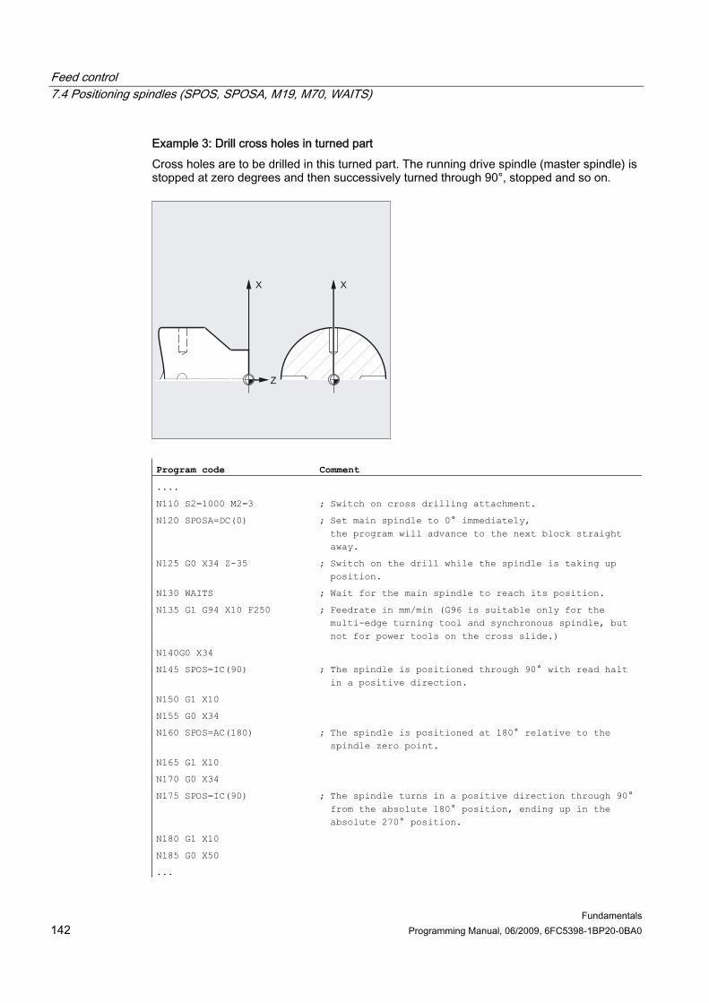
Feed control 7.4 Positioning spindles (SPOS, SPOSA, M19, M70, WAITS)
Fundamentals 142 Programming Manual, 06/2009, 6FC5398-1BP20-0BA0
Example 3: Drill cross holes in turned part Cross holes are to be drilled in this turned part. The running drive spindle (master spindle) is stopped at zero degrees and then successively turned through 90°, stopped and so on.
Program code Comment
....
N110 S2=1000 M2=3 ; Switch on cross drilling attachment.
N120 SPOSA=DC(0) ; Set main spindle to 0° immediately, the program will advance to the next block straight away.
N125 G0 X34 Z-35 ; Switch on the drill while the spindle is taking up position.
N130 WAITS ; Wait for the main spindle to reach its position.
N135 G1 G94 X10 F250 ; Feedrate in mm/min (G96 is suitable only for the multi-edge turning tool and synchronous spindle, but not for power tools on the cross slide.)
N140G0 X34
N145 SPOS=IC(90) ; The spindle is positioned through 90° with read halt in a positive direction.
N150 G1 X10
N155 G0 X34
N160 SPOS=AC(180) ; The spindle is positioned at 180° relative to the spindle zero point.
N165 G1 X10
N170 G0 X34
N175 SPOS=IC(90) ; The spindle turns in a positive direction through 90° from the absolute 180° position, ending up in the absolute 270° position.
N180 G1 X10
N185 G0 X50
...

Feed control 7.4 Positioning spindles (SPOS, SPOSA, M19, M70, WAITS)
Fundamentals Programming Manual, 06/2009, 6FC5398-1BP20-0BA0 143
Further information Positioning with SPOSA The block step enable or program execution is not affected by SPOSA. The spindle positioning can be performed during execution of subsequent NC blocks. The program moves onto the next block if all the functions (except for spindle) programmed in the current block have reached their block end criterion. The spindle positioning operation may be programmed over several blocks (see WAITS).
NOTICE If a command, which implicitly causes a preprocessing stop, is read in a following block, execution of this block is delayed until all positioning spindles are stationary.
Positioning with SPOS/M19 The block step enabling condition is met when all functions programmed in the block reach their end-of-block criterion (e.g. all auxiliary functions acknowledged by the PLC, all axes at their end point) and the spindle reaches the programmed position. Velocity of the movements: The velocity and the delay response for positioning are stored in the machine data. The configured values can be modified by programming or by synchronized actions, see: ● Feedrate for positioning axes/spindles (FA, FPR, FPRAON, FPRAOF) (Page 146) ● Programmable acceleration override (ACC) (option) (Page 152) Specification of spindle positions: As the G90/G91 commands are not effective here, the corresponding dimensions apply explicitly, e.g. AC, IC, DC, ACN, ACP. If no specifications are made, traversing automatically takes place as for DC.

Feed control 7.4 Positioning spindles (SPOS, SPOSA, M19, M70, WAITS)
Fundamentals 144 Programming Manual, 06/2009, 6FC5398-1BP20-0BA0
Synchronize spindle movements with WAITS WAITS can be used to identify a point at which the NC program waits until one or more spindles programmed with SPOSA in a previous NC block reach their positions. Example: Program code Comment
N10 SPOSA[2]=180 SPOSA[3]=0
...
N40 WAITS(2,3) ; The block waits until spindles 2 and 3 have reached the positions specified in block N10.
WAITS can be used after M5 to wait until the spindle(s) has (have) stopped. WAITS can be used after M3/M4 to wait until the spindle(s) has (have) reached the specified speed/direction of rotation.
Note If the spindle has not yet been synchronized with synchronization marks, the positive direction of rotation is taken from the machine data (state on delivery).
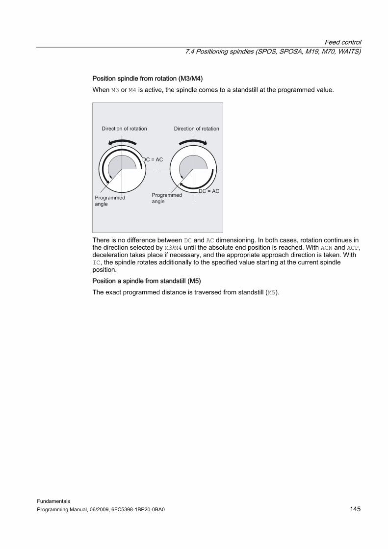
Feed control 7.4 Positioning spindles (SPOS, SPOSA, M19, M70, WAITS)
Fundamentals Programming Manual, 06/2009, 6FC5398-1BP20-0BA0 145
Position spindle from rotation (M3/M4) When M3 or M4 is active, the spindle comes to a standstill at the programmed value.
There is no difference between DC and AC dimensioning. In both cases, rotation continues in the direction selected by M3/M4 until the absolute end position is reached. With ACN and ACP, deceleration takes place if necessary, and the appropriate approach direction is taken. With IC, the spindle rotates additionally to the specified value starting at the current spindle position. Position a spindle from standstill (M5) The exact programmed distance is traversed from standstill (M5).

Feed control 7.5 Feedrate for positioning axes/spindles (FA, FPR, FPRAON, FPRAOF)
Fundamentals 146 Programming Manual, 06/2009, 6FC5398-1BP20-0BA0
7.5 7.5 Feedrate for positioning axes/spindles (FA, FPR, FPRAON, FPRAOF)
Function Positioning axes such as workpiece transport systems, tool turrets and end supports are traversed independently of path and synchronized axes. A separate feedrate is therefore defined for each positioning axis. A separate axial feedrate can also be programmed for spindles. It is also possible to derive the revolutional feedrate for path and synchronized axes or for individual positioning axes/spindles from another rotary axis or spindle.
Syntax Feedrate for positioning axis: FA[<axis>]=…
Axis feedrate for spindle: FA[SPI(<n>)]=… FA[S<n>]=…
Derive revolutional feedrate for path/synchronized axes: FPR (<rotary axis>) FPR(SPI(<n>)) FPR(S<n>) Derive rotational feedrate for positioning axes/spindles: FPRAON(<axis>,<rotary axis>) FPRAON(<axis>,SPI(<n>)) FPRAON(<axis>,S<n>) FPRAON(SPI(<n>),<rotary axis>) FPRAON(S<n>,<rotary axis>) FPRAON(SPI(<n>),SPI(<n>)) FPRAON(S<n>,S<n>) FPRAOF(<axis>,SPI(<n>), etc.) FPRAOF(<axis>,S<n>, etc.)

Feed control 7.5 Feedrate for positioning axes/spindles (FA, FPR, FPRAON, FPRAOF)
Fundamentals Programming Manual, 06/2009, 6FC5398-1BP20-0BA0 147
Significance
Feedrate for the specified positioning axis or positioning speed (axial feedrate) for the specified spindle Unit: mm/min or inch/min or deg/min
FA[...]=... :
Range of values: … 999 999.999 mm/min, deg/min … 39 999.9999 inch/min
FPR(...): FPR is used to identify the rotary axis (<rotary axis>) or spindle (SPI(<n>)/S<n>) from which the revolutional feedrate for the revolutional feedrate of the path and synchronized axes programmed under G95 is to be derived.
FPRAON(...): Derive rotational feedrate for positioning axes and spindles The first parameter (<axis>/SPI(<n>)/S<n>) identifies the positioning axis/spindle to be traversed with revolutional feedrate. The second parameter (<rotary axis>/SPI(<n>)/S<n>) identifies the rotary axis/spindle from which the revolutional feedrate is to be derived. Note: The second parameter can be omitted, in which case the feedrate will be derived from the master spindle.
FPRAOF(...): FPRAOF is used to deselect the derived revolutional feedrate for the specified axes or spindles.
<axis>: Axis identifier (positioning or geometry axis)
Spindle identifier SPI(<n>) and S<n> are identical in terms of function. <n>: Spindle number
SPI(<n>)/S<n>:
Note: SPI converts spindle numbers into axis identifiers. The transfer parameter (<n>) must contain a valid spindle number.

Feed control 7.5 Feedrate for positioning axes/spindles (FA, FPR, FPRAON, FPRAOF)
Fundamentals 148 Programming Manual, 06/2009, 6FC5398-1BP20-0BA0
Note The programmed feedrate FA[...] is modal. Up to five feedrates for positioning axes or spindles can be programmed in each NC block.
Note The derived feedrate is calculated according to the following formula: Derived feedrate = programmed feedrate * absolute master feedrate
Examples Example 1: Synchronous spindle coupling With synchronous spindle coupling, the positioning speed of the following spindle can be programmed independently of the master spindle, e.g. for positioning operations. Program code Comment
...
FA[S2]=100 ; Positioning speed of the following spindle (spindle 2) = 100 deg/min
...
Example 2: Derived revolutional feedrate for path axes Path axes X, Y must be traversed at the revolutional feedrate derived from rotary axis A: Program code
...
N40 FPR(A)
N50 G95 X50 Y50 F500
...
Example 3: Derive revolutional feedrate for master spindle Program code Comment
N30 FPRAON(S1,S2) ; The revolutional feedrate for the master spindle (S1) must be derived from spindle 2.
N40 SPOS=150 ; Position master spindle.
N50 FPRAOF(S1) ; Deselect revolutional feedrate for the master spindle.
Feed control 7.5 Feedrate for positioning axes/spindles (FA, FPR, FPRAON, FPRAOF)
Fundamentals Programming Manual, 06/2009, 6FC5398-1BP20-0BA0 149
Example 4: Derive revolutional feedrate for positioning axis Program code Comment
N30 FPRAON(X) ; The revolutional feedrate for positioning axis X must be derived from the master spindle.
N40 POS[X]=50 FA[X]=500 ; The positioning axis is traversing at 500 mm/revolution of the master spindle.
N50 FPRAOF(X)
Further information FA[…] The feedrate type is always G94. When G70/G71 is active, the unit is metric/inches according to the default setting in the machine data. G700/G710 can be used to modify the unit in the program.
NOTICE If no FA is programmed, the value defined in the machine data applies.
FPR(…) As an extension of the G95command (revolutional feedrate referring to the master spindle), FPR allows the revolutional feedrate to be derived from any chosen spindle or rotary axis. G95 FPR(…) is valid for path and synchronized axes. If the rotary axis/spindle specified in the FPR command is operating on position control, then the setpoint linkage is active. Otherwise the actual-value linkage is effective. FPRAON(…) FPRAON is used to derive the revolutional feedrate for positioning axes and spindles from the current feedrate of another rotary axis or spindle. FPRAOF(…) The revolutional feedrate can be deactivated for one or a number of axes/spindles simultaneously with the FPRAOF command.

Feed control 7.6 Programmable feedrate override (OVR, OVRRAP, OVRA)
Fundamentals 150 Programming Manual, 06/2009, 6FC5398-1BP20-0BA0
7.6 7.6 Programmable feedrate override (OVR, OVRRAP, OVRA)
Function The velocity of path/positioning axes and spindles can be modified in the NC program.
Syntax OVR=<value> OVRRAP=<value> OVRA[<axis>]=<value> OVRA[SPI(<n>)]=<value> OVRA[S<n>]=<value>
Significance OVR: Feedrate modification for path feedrate F OVRRAP: Feedrate modification for rapid traverse velocity OVRA: Feedrate modification for positioning feedrate FA or for spindle
speed S <axis>: Axis identifier (positioning or geometry axis)
Spindle identifier SPI(<n>) and S<n> are identical in terms of function. <n>: Spindle number
SPI(<n>)/S<n>:
Note: SPI converts spindle numbers into axis identifiers. The transfer parameter (<n>) must contain a valid spindle number.
Feedrate modification in percent The value refers to or is combined with the feedrate override set on the machine control panel. Range of values: … 200%, integers
<value>:
Note: With path and rapid traverse override, the maximum velocities set in the machine data are not overshot.
Feed control 7.6 Programmable feedrate override (OVR, OVRRAP, OVRA)
Fundamentals Programming Manual, 06/2009, 6FC5398-1BP20-0BA0 151
Examples Example 1: Set feedrate override: 80% Program code Comment
N10 ... F1000
N20 OVR=50 ; The programmed path feedrate F1000 is changed in F400 (1000 * 0.8 * 0.5).
...
Example 2: Program code Comment
N10 OVRRAP=5 ; The rapid traverse velocity is reduced to 5%.
...
N100 OVRRAP=100 ; The rapid traverse velocity is reset to 100% (= default setting).
Example 3: Program code Comment
N... OVR=25 OVRA[A1]=70 ; The path feedrate is reduced to 25% and the positioning feedrate for positioning axis A1 is reduced to 70%.
Example 4: Program code Comment
N.. OVRA[SPI(1)]=35 ; The speed for spindle 1 is reduced to 35%.
or Program code Comment
N.. OVRA[S1]=35 ; The speed for spindle 1 is reduced to 35%.

Feed control 7.7 Programmable acceleration override (ACC) (option)
Fundamentals 152 Programming Manual, 06/2009, 6FC5398-1BP20-0BA0
7.7 7.7 Programmable acceleration override (ACC) (option)
Function In critical program sections, it may be necessary to limit the acceleration to below the maximum values, e.g. to prevent mechanical vibrations from occurring. The programmable acceleration override can be used to modify the acceleration for each path axis or spindle via a command in the NC program. The limit is effective for all types of interpolation. The values defined in the machine data apply as 100% acceleration.
Syntax ACC[<axis>]=<value> ACC[SPI(<n>)]=<value> ACC(S<n>)=<value>
Deactivate: ACC[...]=100
Syntax ACC: Acceleration change for the specified path axis or speed change
for the specified spindle. <axis>: Channel axis name of path axis
Spindle identifier SPI(<n>) and S<n> are identical in terms of function. <n>: Spindle number
SPI(<n>)/S<n>:
Note: SPI converts spindle numbers into axis identifiers. The transfer parameter (<n>) must contain a valid spindle number.
Acceleration change in percent The value refers to or is combined with the feedrate override set on the machine control panel.
<value>:
Range of values: 1 to 200%, integers
NOTICE With a greater acceleration rate, the values permitted by the manufacturer may be exceeded.
Feed control 7.7 Programmable acceleration override (ACC) (option)
Fundamentals Programming Manual, 06/2009, 6FC5398-1BP20-0BA0 153
Example Program code Comment
N50 ACC[X]=80 ; The axis slide in the X direction should only be traversed with 80% acceleration.
N60 ACC[SPI(1)]=50 ; Spindle 1 should only accelerate or brake with 50% of the acceleration capacity.
Further information Acceleration override programmed with ACC The acceleration override programmed with ACC[...] is always taken into consideration on output as in system variable $AA_ACC. Readout in the parts program and in synchronized actions takes place at different times in the NC processing run. In the part program The value written in the part program is then only taken into consideration in system variable $AA_ACC as written in the part program if ACC has not been changed in the meantime by a synchronized action. In synchronized actions The following thus applies: The value written to a synchronized action is then only considered in system variable $AA_ACC as written to the synchronized action if ACC has not been changed in the meantime by a part program. The preset acceleration can also be changed via synchronized actions (see Function Manual, Synchronized Actions). Example: Program code
...
N100 EVERY $A_IN[1] DO POS[X]=50 FA[X]=2000 ACC[X]=140
The current acceleration value can be called with system variable $AA_ACC[<axis>]. Machine data can be used to define whether the last ACC value set should apply on RESET/part program end or whether 100% should apply.
Feed control 7.8 Feedrate with handwheel override (FD, FDA)
Fundamentals 154 Programming Manual, 06/2009, 6FC5398-1BP20-0BA0
7.8 7.8 Feedrate with handwheel override (FD, FDA)
Function The FD and FDA commands can be used to traverse axes with handwheels during execution of the part program. The programmed settings for traversing the axes are then overlaid with the handwheel pulses evaluated as path or velocity defaults. Path axes In the case of path axes, the programmed path feedrate can be overlaid. The handwheel is evaluated as the first geometry axis of the channel. The handwheel pulses evaluated per interpolation cycle dependent on the direction of rotation correspond to the path velocity to be overlaid. The path velocity limit values which can be achieved by means of handwheel override are: ● Minimum: 0 ● Maximum: Machine data limit values of the path axes involved in traversing
Note Path feedrate The path feedrate F and the handwheel feedrate FD cannot be programmed in the same NC block.
Positioning axes In the case of positioning axes, the travel path or velocity can be overlaid as an axial value. The handwheel assigned to the axis is evaluated. ● Path override
The handwheel pulses evaluated dependent on the direction of rotation correspond to the axis path to be traveled. Only handwheel pulses in the direction of the programmed position are evaluated.
● Velocity override The handwheel pulses evaluated per interpolation cycle dependent on the direction of rotation correspond to the axial velocity to be overlaid. The path velocity limit values which can be achieved by means of handwheel override are: – Minimum: 0 – Maximum: Machine data limit values of the positioning axis
A detailed description of how to set handwheel parameters appears in: References: /FB2/ Function Manual, Extended Functions; Manual Travel and Handwheel Travel (H1)

Feed control 7.8 Feedrate with handwheel override (FD, FDA)
Fundamentals Programming Manual, 06/2009, 6FC5398-1BP20-0BA0 155
Syntax FD=<velocity> FDA[<axis>]=<velocity>
Significance FD=<velocity>: Path feedrate and enabling of velocity override
with handwheel <velocity>: • Value = 0: Not allowed! • Value ≠ 0: Path velocity
FDA[<axis>]=<velocity>: Axial feedrate <velocity>: • Value = 0: Path default with handwheel • Value ≠ 0: Axial velocity
<axis>: Axis identifier of positioning axis
Note FD and FDA are non-modal.
Example
Path definition: The grinding wheel oscillating in the Z direction is traversed to the workpiece in the X direction with the handwheel. The operator can continue to feed manually until the sparks are flying uniformly. Activating "Delete distance-to-go" switches to the next NC block and machining continues in AUTOMATIC mode.
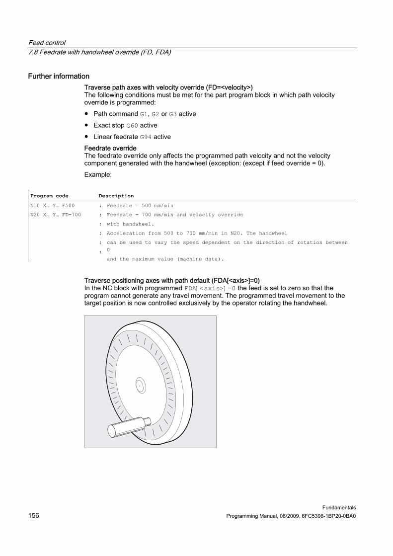
Feed control 7.8 Feedrate with handwheel override (FD, FDA)
Fundamentals 156 Programming Manual, 06/2009, 6FC5398-1BP20-0BA0
Further information Traverse path axes with velocity override (FD=<velocity>) The following conditions must be met for the part program block in which path velocity override is programmed: ● Path command G1, G2 or G3 active ● Exact stop G60 active ● Linear feedrate G94 active Feedrate override The feedrate override only affects the programmed path velocity and not the velocity component generated with the handwheel (exception: (except if feed override = 0). Example:
Program code Description
N10 X… Y… F500 ; Feedrate = 500 mm/min
N20 X… Y… FD=700 ;
;
;
;
;
Feedrate = 700 mm/min and velocity override
with handwheel.
Acceleration from 500 to 700 mm/min in N20. The handwheel
can be used to vary the speed dependent on the direction of rotation between 0
and the maximum value (machine data).
Traverse positioning axes with path default (FDA[<axis>]=0) In the NC block with programmed FDA[<axis>]=0 the feed is set to zero so that the program cannot generate any travel movement. The programmed travel movement to the target position is now controlled exclusively by the operator rotating the handwheel.

Feed control 7.8 Feedrate with handwheel override (FD, FDA)
Fundamentals Programming Manual, 06/2009, 6FC5398-1BP20-0BA0 157
Example: Program code Description
...
N20 POS[V]=90 FDA[V]=0 ;
;
;
;
Target position = 90 mm, axial feedrate = 0 mm/min and
path override with handwheel.
Velocity of axis V at start of block = 0 mm/min.
Path and speed defaults are set using handwheel pulses
Direction of movement, travel velocity The axes follow the path set by the handwheel in the direction of the sign. Forward and backwards travel is possible dependent on the direction of rotation. The faster the handwheel rotates, the higher the traversing speed. Traversing range: The traversing range is limited by the starting position and the programmed end point. Traverse positioning axis with velocity override (FDA[<axis>]=<velocity>) In NC blocks with programmed FDA[…]=…, the feedrate from the last programmed FA value is accelerated or decelerated to the value programmed under FDA. Starting from the current feedrate FDA, the handwheel can be turned to accelerate the programmed movement to the target position or decelerate it to zero. The values set as parameters in the machine data serve as the maximum velocity. Example:
Program code Description
N10 POS[V]=… FA[V]=100 ; Axial feedrate = 100 mm/min
N20 POS[V]=100 FAD[V]=200 ;
;
;
;
;
;
Axial target position = 100, axial feedrate = 200 mm/min
and velocity override with handwheel.
Acceleration from 100 to 200 mm/min in N20. The
handwheel can be used to vary the velocity dependent on the direction of rotation
between 0 and the maximum value (machine data).
Traversing range: The traversing range is limited by the starting position and the programmed end point.
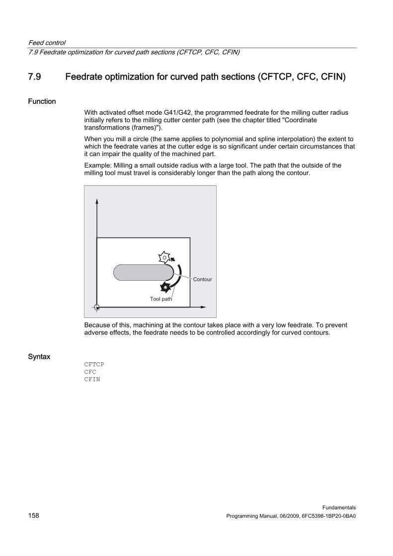
Feed control 7.9 Feedrate optimization for curved path sections (CFTCP, CFC, CFIN)
Fundamentals 158 Programming Manual, 06/2009, 6FC5398-1BP20-0BA0
7.9 7.9 Feedrate optimization for curved path sections (CFTCP, CFC, CFIN)
Function With activated offset mode G41/G42, the programmed feedrate for the milling cutter radius initially refers to the milling cutter center path (see the chapter titled "Coordinate transformations (frames)"). When you mill a circle (the same applies to polynomial and spline interpolation) the extent to which the feedrate varies at the cutter edge is so significant under certain circumstances that it can impair the quality of the machined part. Example: Milling a small outside radius with a large tool. The path that the outside of the milling tool must travel is considerably longer than the path along the contour.
Because of this, machining at the contour takes place with a very low feedrate. To prevent adverse effects, the feedrate needs to be controlled accordingly for curved contours.
Syntax CFTCP CFC CFIN
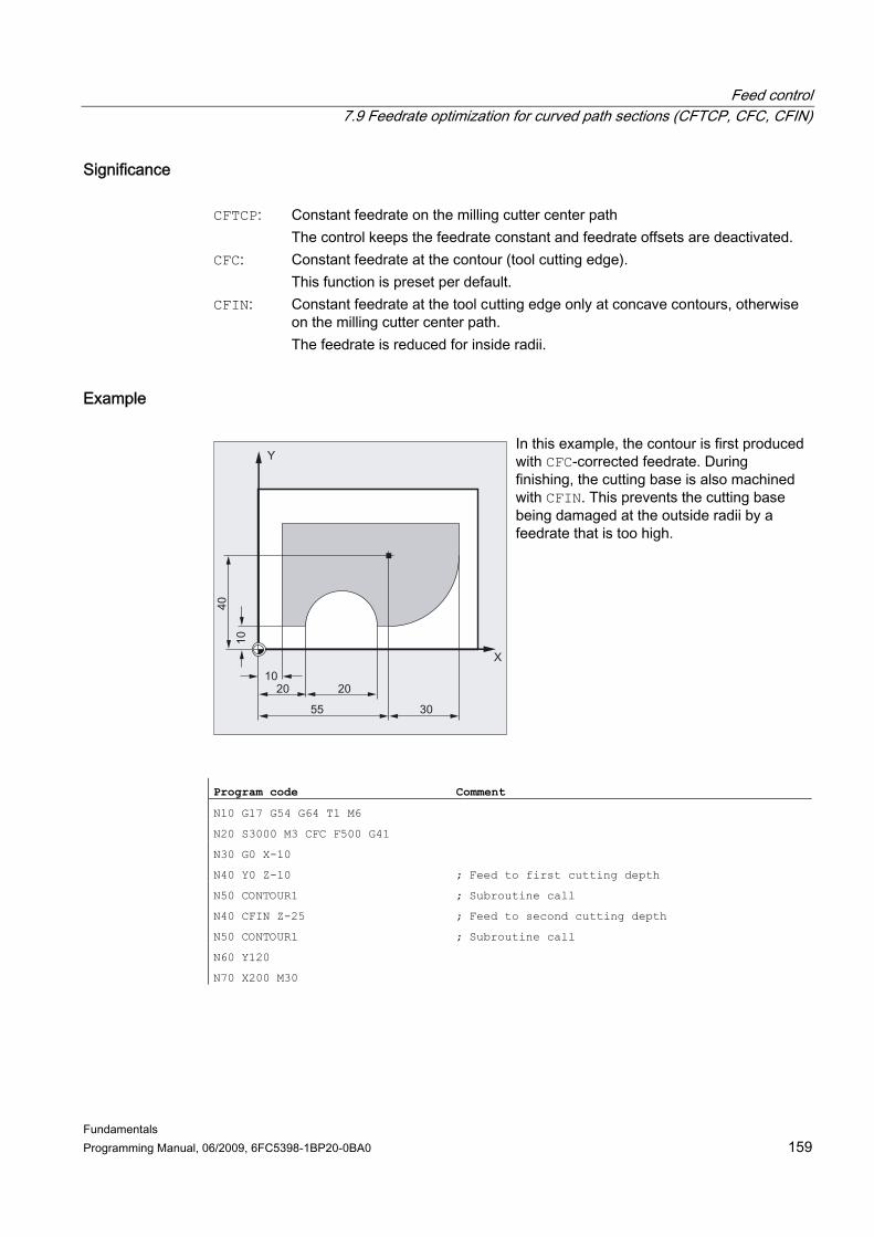
Feed control 7.9 Feedrate optimization for curved path sections (CFTCP, CFC, CFIN)
Fundamentals Programming Manual, 06/2009, 6FC5398-1BP20-0BA0 159
Significance CFTCP: Constant feedrate on the milling cutter center path
The control keeps the feedrate constant and feedrate offsets are deactivated. CFC: Constant feedrate at the contour (tool cutting edge).
This function is preset per default. CFIN: Constant feedrate at the tool cutting edge only at concave contours, otherwise
on the milling cutter center path. The feedrate is reduced for inside radii.
Example
In this example, the contour is first produced with CFC-corrected feedrate. During finishing, the cutting base is also machined with CFIN. This prevents the cutting base being damaged at the outside radii by a feedrate that is too high.
Program code Comment
N10 G17 G54 G64 T1 M6
N20 S3000 M3 CFC F500 G41
N30 G0 X-10
N40 Y0 Z-10 ; Feed to first cutting depth
N50 CONTOUR1 ; Subroutine call
N40 CFIN Z-25 ; Feed to second cutting depth
N50 CONTOUR1 ; Subroutine call
N60 Y120
N70 X200 M30
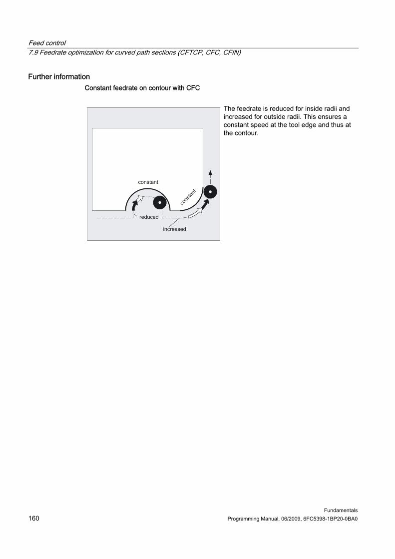
Feed control 7.9 Feedrate optimization for curved path sections (CFTCP, CFC, CFIN)
Fundamentals 160 Programming Manual, 06/2009, 6FC5398-1BP20-0BA0
Further information Constant feedrate on contour with CFC
The feedrate is reduced for inside radii and increased for outside radii. This ensures a constant speed at the tool edge and thus at the contour.

Feed control 7.10 Several feedrate values in one block (F, ST, SR, FMA, STA, SRA)
Fundamentals Programming Manual, 06/2009, 6FC5398-1BP20-0BA0 161
7.10 7.10 Several feedrate values in one block (F, ST, SR, FMA, STA, SRA)
Function The "Multiple feedrates in one block" function can be used to activate different feedrate values for an NC block, a dwell time or a retraction motion-synchronously, dependent on external digital and/or analog inputs. The HW input signals are combined in one input byte.
Syntax F2=... to F7=... ST=... SR=...
FMA[2,<axis>]=... to FMA[7,<axis>]=... STA[<axis>]=... SRA[<axis>]=...
Significance
The path feedrate is programmed under the address F and remains valid during the absence of an input signal. In addition to the path feedrate, up to 6 further feedrates can be programmed in the block. The numerical expansion indicates the bit number of the input that activates the feedrate when changed:
F2=... to F7=... :
Effective: non-modal Dwell time in s (for grinding technology: sparking-out time) Input bit: 1
ST=... :
Effective: non-modal Retraction path The unit for the retraction path refers to the current valid unit of measurement (mm or inch). Input bit: 0
SR=... :
Effective: non-modal
Feed control 7.10 Several feedrate values in one block (F, ST, SR, FMA, STA, SRA)
Fundamentals 162 Programming Manual, 06/2009, 6FC5398-1BP20-0BA0
The axial feedrate is programmed under the address FA and remains valid during the absence of an input signal. In addition to the axial feedrate FA up to 6 further feedrates per axis can be programmed in the block with FMA. The first parameter indicates the bit number of the input and the second the axis for which the feedrate is to apply.
FMA[2,<axis>]=... to FMA[7,<axis>]=... :
Effective: non-modal Axial dwell time in s (for grinding technology: sparking-out time) Input bit: 1
STA[<axis>]=... :
Effective: non-modal Axial retraction path Input bit: 0
SRA[<axis>]=... :
Effective: non-modal
Note If input bit 1 is activated for the dwell time or bit 0 for the return path, the distance to go for the path axes or the relevant single axes is deleted and the dwell time or return started.
Note The axial feedrate (FA or FMA value) or path feedrate (F value) corresponds to 100% feedrate. The "Multiple feedrate values in one block" function can be used to achieve feedrates smaller than or equal to the axial feedrate or path feedrate.
Note If feedrates, dwell time or return path are programmed for an axis on account of an external input, this axis must not be programmed as POSA axis (positioning axis over multiple blocks) in this block.
Note Look Ahead is also active for multiple feedrates in one block. In this way, the current feedrate is restricted by the Look Ahead value.

Feed control 7.10 Several feedrate values in one block (F, ST, SR, FMA, STA, SRA)
Fundamentals Programming Manual, 06/2009, 6FC5398-1BP20-0BA0 163
Examples Example 1: Path motion Program code Comment
F7=1000 ; 7 corresponds to input bit 7
F2=20 ; 2 corresponds to input bit 2
ST=1 ; Dwell time (s) input bit 1
SR=0.5 ; Return path (mm) input bit 0
Example 2: Axial motion Program code Comment
FMA[3,x]=1000 ; Axial feedrate with the value 1,000 for X axis, 3 corresponds to input bit 3.
Example 3: Multiple operations in one block Program code Comment
N20 T1 D1 F500 G0 X100 ; Initial setting
N25 G1 X105 F=20 F7=5 F3=2.5 F2=0.5 ST=1.5 SR=0.5 ; Normal feedrate with F, roughing with F7, finishing with F3, smooth-finishing with F2, dwell time 1.5 s, return path 0.5 mm
...
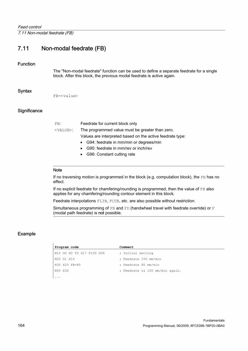
Feed control 7.11 Non-modal feedrate (FB)
Fundamentals 164 Programming Manual, 06/2009, 6FC5398-1BP20-0BA0
7.11 7.11 Non-modal feedrate (FB)
Function The "Non-modal feedrate" function can be used to define a separate feedrate for a single block. After this block, the previous modal feedrate is active again.
Syntax FB=<value>
Significance FB: Feedrate for current block only <VALUE>: The programmed value must be greater than zero.
Values are interpreted based on the active feedrate type: • G94: feedrate in mm/min or degrees/min • G95: feedrate in mm/rev or inch/rev • G96: Constant cutting rate
Note If no traversing motion is programmed in the block (e.g. computation block), the FB has no effect. If no explicit feedrate for chamfering/rounding is programmed, then the value of FB also applies for any chamfering/rounding contour element in this block. Feedrate interpolations FLIN, FCUB, etc. are also possible without restriction. Simultaneous programming of FB and FD (handwheel travel with feedrate override) or F (modal path feedrate) is not possible.
Example Program code Comment
N10 G0 X0 Y0 G17 F100 G94 ; Initial setting
N20 G1 X10 ; Feedrate 100 mm/min
N30 X20 FB=80 ; Feedrate 80 mm/min
N40 X30 ; Feedrate is 100 mm/min again.
...
Feed control 7.12 Tooth feedrate (G95 FZ)
Fundamentals Programming Manual, 06/2009, 6FC5398-1BP20-0BA0 165
7.12 7.12 Tooth feedrate (G95 FZ)
Function Primarily for milling operations, the tooth feedrate, which is more commonly used in practice, can be programmed instead of the revolutional feedrate:
The control uses the $TC_DPNT (number of teeth) tool parameter associated with the active tool offset data record to calculate the effective revolutional feedrate for each traversing block from the programmed tooth feedrate. F = FZ * $TC_DPNT
F: Revolutional feedrate in mm/rev or inch/rev FZ: Tooth feedrate in mm/tooth or inch/tooth
where:
$TC_DPNT: Tool parameter: Number of teeth/rev The tool type ($TC_DP1) of the active tool is not taken into account. The programmed tooth feedrate is independent of the tool change and the selection/deselection of a tool offset data record; it is retained in modal format. A change to the $TC_DPNT tool parameter associated with the active tool cutting edge will be applied the next time a tool offset is selected or the next time the active offset data is updated.

Feed control 7.12 Tooth feedrate (G95 FZ)
Fundamentals 166 Programming Manual, 06/2009, 6FC5398-1BP20-0BA0
Changing the tool or selecting/deselecting a tool offset data set generates a recalculation of the effective revolutional feedrate.
Note The tooth feedrate refers only to the path (axis-specific programming is not possible).
Syntax G95 FZ...
Note In the block, G95 and FZ can be programmed together or in isolation. There is no fixed programmed sequence.
Significance G95: Type of feedrate: Revolutional feedrate in mm/rev or inch/rev (dependent upon
G700/G710) For G95 see "Feedrate (G93, G94, G95, F, FGROUP, FL, FGREF) (Page 119)" Tooth feedrate Activation: with G95 Effective: modal
FZ:
Unit: mm/tooth or inch/tooth (dependent upon G700/G710)
Note Switchover between G95 F... and G95 FZ... Switching over between G95 F... (revolutional feedrate) and G95 FZ... (tooth feedrate) will delete the non-active feedrate value in each case.
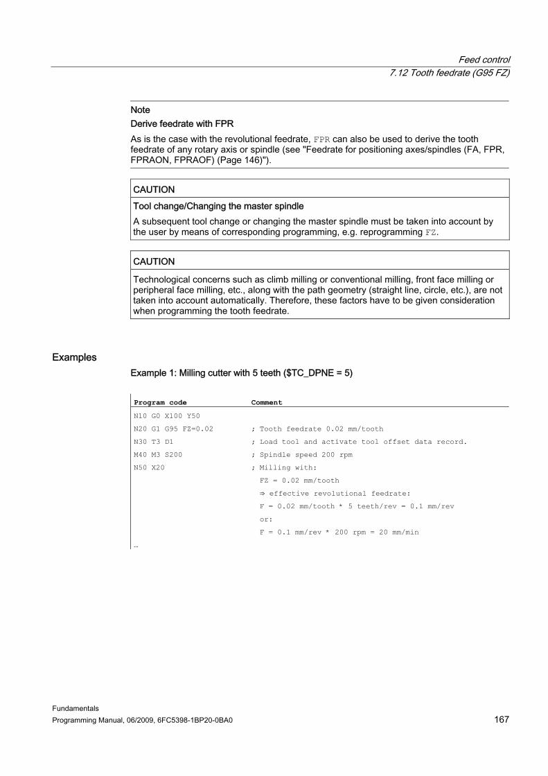
Feed control 7.12 Tooth feedrate (G95 FZ)
Fundamentals Programming Manual, 06/2009, 6FC5398-1BP20-0BA0 167
Note Derive feedrate with FPR As is the case with the revolutional feedrate, FPR can also be used to derive the tooth feedrate of any rotary axis or spindle (see "Feedrate for positioning axes/spindles (FA, FPR, FPRAON, FPRAOF) (Page 146)").
CAUTION Tool change/Changing the master spindle A subsequent tool change or changing the master spindle must be taken into account by the user by means of corresponding programming, e.g. reprogramming FZ.
CAUTION Technological concerns such as climb milling or conventional milling, front face milling or peripheral face milling, etc., along with the path geometry (straight line, circle, etc.), are not taken into account automatically. Therefore, these factors have to be given consideration when programming the tooth feedrate.
Examples Example 1: Milling cutter with 5 teeth ($TC_DPNE = 5) Program code Comment
N10 G0 X100 Y50
N20 G1 G95 FZ=0.02 ; Tooth feedrate 0.02 mm/tooth
N30 T3 D1 ; Load tool and activate tool offset data record.
M40 M3 S200 ; Spindle speed 200 rpm
N50 X20 ; Milling with:
FZ = 0.02 mm/tooth
⇒ effective revolutional feedrate: F = 0.02 mm/tooth * 5 teeth/rev = 0.1 mm/rev
or:
F = 0.1 mm/rev * 200 rpm = 20 mm/min
…
Feed control 7.12 Tooth feedrate (G95 FZ)
Fundamentals 168 Programming Manual, 06/2009, 6FC5398-1BP20-0BA0
Example 2: Switchover between G95 F... and G95 FZ... Program code Comment
N10 G0 X100 Y50
N20 G1 G95 F0.1 ; Revolutional feedrate 0.1 mm/rev
N30 T1 M6
N35 M3 S100 D1
N40 X20
N50 G0 X100 M5
N60 M6 T3 D1 ; Load tool with e.g. 5 teeth ($TC_DPNT = 5).
N70 X22 M3 S300
N80 G1 X3 G95 FZ=0.02 ; Change G95 F… to G95 FZ…, tooth feedrate active with 0.02 mm/tooth.
…
Example 3: Derive tooth feedrate of a spindle (FBR) Program code Comment
…
N41 FPR(S4) ; Tool in spindle 4 (not the master spindle).
N51 G95 X51 FZ=0.5 ; Tooth feedrate 0.5 mm/tooth dependent upon spindle S4.
…
Example 4: Subsequent tool change Program code Comment
N10 G0 X50 Y5
N20 G1 G95 FZ=0.03 ; Tooth feedrate 0.03 mm/tooth
N30 M6 T11 D1 ; Load tool with e.g. 7 teeth ($TC_DPNT = 7).
N30 M3 S100
N40 X30 ; Effective revolutional feedrate 0.21 mm/rev
N50 G0 X100 M5
N60 M6 T33 D1 ; Load tool with e.g. 5 teeth ($TC_DPNT = 5).
N70 X22 M3 S300
N80 G1 X3 ; Tooth feedrate modal 0.03 mm/tooth
⇒ effective revolutional feedrate: 0.15 mm/rev …

Feed control 7.12 Tooth feedrate (G95 FZ)
Fundamentals Programming Manual, 06/2009, 6FC5398-1BP20-0BA0 169
Example 5: Changing the master spindle Program code Comment
N10 SETMS (1) ; Spindle 1 is the master spindle.
N20 T3 D3 M6 ; Tool 3 is changed to spindle 1.
N30 S400 M3 ; Speed S400 of spindle 1 (and, therefore, T3).
N40 G95 G1 FZ0.03 ; Tooth feedrate 0.03 mm/tooth
N50 X50 ; Path motion, the effective feedrate is dependent upon:
- The tooth feedrate FZ
- The speed of spindle 1
- The number of teeth of the active tool T3
N60 G0 X60
...
N100 SETMS(2) ; Spindle 2 becomes the master spindle.
N110 T1 D1 M6 ; Tool 1 is changed to spindle 2.
N120 S500 M3 ; Speed S500 of spindle 2 (and, therefore, T1).
N130 G95 G1 FZ0.03 X20 ; Path motion, the effective feedrate is dependent upon:
- The tooth feedrate FZ
- The speed of spindle 2
- The number of teeth of the active tool T1
Note Following the change in master spindle (N100) the user also has to select an offset affecting the tool actuated by spindle 2.
Feed control 7.12 Tooth feedrate (G95 FZ)
Fundamentals 170 Programming Manual, 06/2009, 6FC5398-1BP20-0BA0
Further information Changing between G93, G94 and G95 FZ can also be programmed when G95 is not active, although it will have no effect and is deleted when G95 is selected. In other words, when changing between G93, G94, and G95, in the same way as with F, the FZ value is also deleted. Reselection of G95 Reselecting G95 when G95 is already active has no effect (unless a change between F and FZ has been programmed). Non-modal feedrate (FB) When G95 FZ... (modal) is active, a non-modal feedrate FB... is interpreted as a tooth feedrate. SAVE mechanism In subprograms with the SAVE attribute FZ is written to the value prior to the subprogram starting (in the same way as F). Multiple feedrate values in one block The "Multiple feedrate values in one block" function is not possible with tooth feedrate. Synchronized actions FZ cannot be programmed from synchronized actions.

Feed control 7.12 Tooth feedrate (G95 FZ)
Fundamentals Programming Manual, 06/2009, 6FC5398-1BP20-0BA0 171
Read tooth feedrate and path feedrate type The tooth feedrate and the path feedrate type can be read using system variables. ● With preprocessing stop in the part program via system variables:
$AC_FZ Tooth feedrate effective when the current main run record was preprocessed. Path feedrate type effective when the current main run record was preprocessed. Value: Significance: 0 mm/min 1 mm/rev 2 inch/min 3 inch/rev 11 mm/tooth
$AC_F_TYPE
31 inch/tooth ● Without preprocessing stop in the part program via system variables:
$P_FZ Programmed tooth feedrate Programmed path feedrate type Value: Significance: 0 mm/min 1 mm/rev 2 inch/min 3 inch/rev 11 mm/tooth
$P_F_TYPE
31 inch/tooth
Note If G95 is not active, the $P_FZ and $AC_FZ variables will always return a value of zero.

Feed control 7.12 Tooth feedrate (G95 FZ)
Fundamentals 172 Programming Manual, 06/2009, 6FC5398-1BP20-0BA0

Fundamentals Programming Manual, 06/2009, 6FC5398-1BP20-0BA0 173
Geometry settings 88.1 8.1 Settable work offset (G54 to G57, G505 to G599, G53, G500, SUPA,
G153)
Function The workpiece zero in relation to the zero point of the basic coordinate system is set up by the settable zero offset (G54 to G57 and G505 to G599) in all axes. In this way it is possible to call zero points program-wide per G command (e.g. for different devices). Milling:

Geometry settings 8.1 Settable work offset (G54 to G57, G505 to G599, G53, G500, SUPA, G153)
Fundamentals 174 Programming Manual, 06/2009, 6FC5398-1BP20-0BA0
Turning:
Note During turning, for example, the offset value for returning of the chuck is entered in G54.
Syntax Activating settable zero offset: G54 ... G57 G505 ... G599
Deactivating settable zero offset: G500 G53 G153 SUPA

Geometry settings 8.1 Settable work offset (G54 to G57, G505 to G599, G53, G500, SUPA, G153)
Fundamentals Programming Manual, 06/2009, 6FC5398-1BP20-0BA0 175
Meaning G54 to G57: Call of the 1st to 4th settable zero offset (ZO) G505 to G599: Call of the 5th to 99th settable zero offset
Deactivation of the current settable zero offset G500=zero frame: (default setting; contains no offset, rotation, mirroring or scaling)
Deactivation of the settable zero offset until the next call, activation of the entire basic frame ($P_ACTBFRAME).
G500:
G500 not equal to 0: Activation of the first settable zero offset ($P_UIFR[0]) and activation of the entire basic frame ($P_ACTBFRAME) or possibly a modified basic frame is activated.
G53: G53 suppresses the settable work offset and the programmable work offset non-modally.
G153: G153 has the same effect as G53 and also suppresses the entire basic frame.
SUPA: SUPA has the same effect as G153 and also suppresses: • Handwheel offsets (DRF) • Overlaid movements • External zero offset • PRESET offset
References: See Section "Coordinate transformations (frames)" for the programmable zero offset.
Note The basic setting at the start of the program, e.g. G54 or G500, can be set via machine data.

Geometry settings 8.1 Settable work offset (G54 to G57, G505 to G599, G53, G500, SUPA, G153)
Fundamentals 176 Programming Manual, 06/2009, 6FC5398-1BP20-0BA0
Example
Three workpieces that are arranged on a pallet in accordance with the zero offset values G54 to G56 are to be machined in succession. The machining sequence is programmed in subroutine L47.
Program code Comment
N10 G0 G90 X10 Y10 F500 T1 ; Approach
N20 G54 S1000 M3 ; Call of the first ZO, spindle clockwise
N30 L47 ; Program pass as subroutine
N40 G55 G0 Z200 ; Call of the second ZO, Z via obstruction
N50 L47 ; Program pass as subroutine
N60 G56 ; Call of the third ZO
N70 L47 ; Program pass as subroutine
N80 G53 X200 Y300 M30 ; Suppress zero offset, end of program
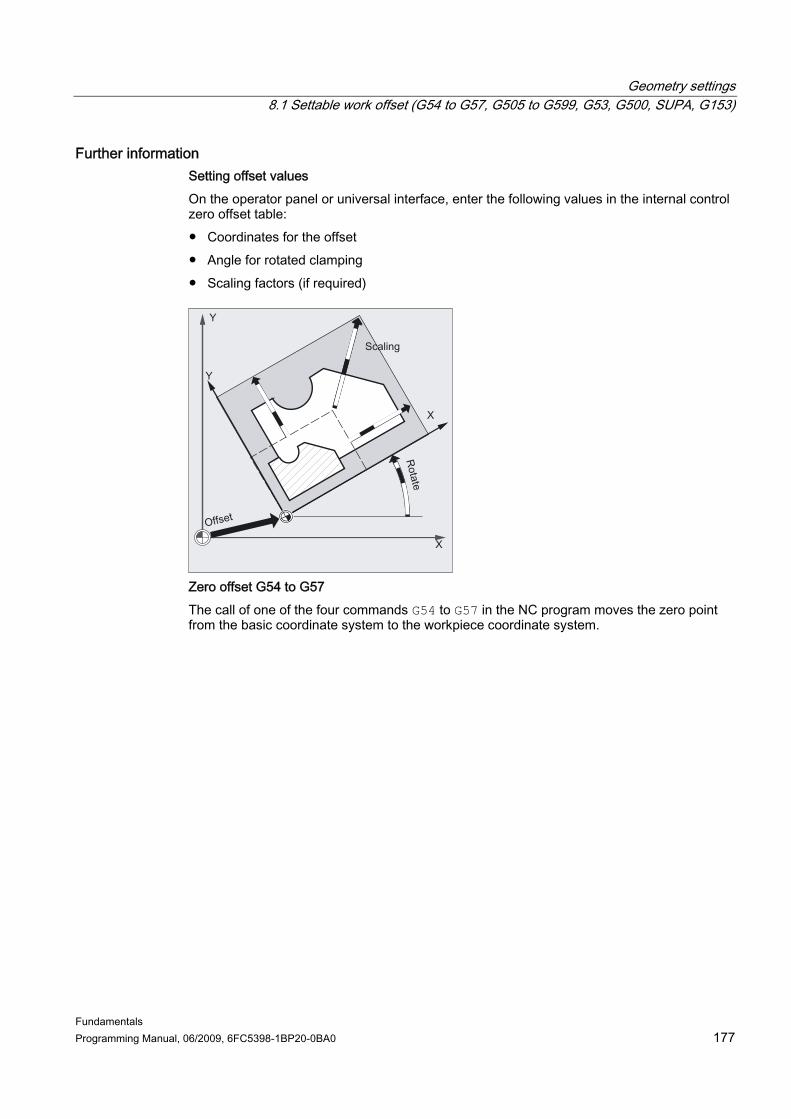
Geometry settings 8.1 Settable work offset (G54 to G57, G505 to G599, G53, G500, SUPA, G153)
Fundamentals Programming Manual, 06/2009, 6FC5398-1BP20-0BA0 177
Further information Setting offset values On the operator panel or universal interface, enter the following values in the internal control zero offset table: ● Coordinates for the offset ● Angle for rotated clamping ● Scaling factors (if required)
Zero offset G54 to G57 The call of one of the four commands G54 to G57 in the NC program moves the zero point from the basic coordinate system to the workpiece coordinate system.
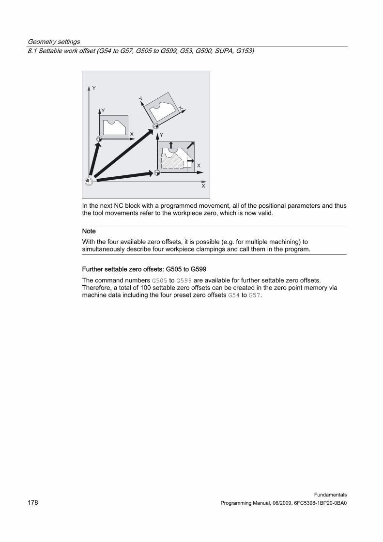
Geometry settings 8.1 Settable work offset (G54 to G57, G505 to G599, G53, G500, SUPA, G153)
Fundamentals 178 Programming Manual, 06/2009, 6FC5398-1BP20-0BA0
In the next NC block with a programmed movement, all of the positional parameters and thus the tool movements refer to the workpiece zero, which is now valid.
Note With the four available zero offsets, it is possible (e.g. for multiple machining) to simultaneously describe four workpiece clampings and call them in the program.
Further settable zero offsets: G505 to G599 The command numbers G505 to G599 are available for further settable zero offsets. Therefore, a total of 100 settable zero offsets can be created in the zero point memory via machine data including the four preset zero offsets G54 to G57.
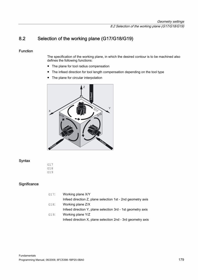
Geometry settings 8.2 Selection of the working plane (G17/G18/G19)
Fundamentals Programming Manual, 06/2009, 6FC5398-1BP20-0BA0 179
8.2 8.2 Selection of the working plane (G17/G18/G19)
Function The specification of the working plane, in which the desired contour is to be machined also defines the following functions: ● The plane for tool radius compensation ● The infeed direction for tool length compensation depending on the tool type ● The plane for circular interpolation
Syntax G17 G18 G19
Significance G17: Working plane X/Y
Infeed direction Z, plane selection 1st - 2nd geometry axis G18: Working plane Z/X
Infeed direction Y, plane selection 3rd - 1st geometry axis G19: Working plane Y/Z
Infeed direction X, plane selection 2nd - 3rd geometry axis
Geometry settings 8.2 Selection of the working plane (G17/G18/G19)
Fundamentals 180 Programming Manual, 06/2009, 6FC5398-1BP20-0BA0
Note In the default setting, G17 (X/Y plane) is defined for milling and G18 (Z/X plane) is defined for turning. When calling the tool path correction G41/G42 (see Section "Tool radius compensation"), the working plane must be defined so that the control can correct the tool length and radius.
Example The "conventional" approach for milling is: 1. Define working plane (G17 default setting for milling). 2. Select tool type (T) and tool offset values (D). 3. Switch on path correction (G41). 4. Program traversing movements. Program code Comment
N10 G17 T5 D8 ; Selection of working plane X/Y, call tool. Tool length compensation is performed in the Z direction.
N20 G1 G41 X10 Y30 Z-5 F500 ; Radius compensation is performed in the X/Y plane.
N30 G2 X22.5 Y40 I50 J40 ; Circular interpolation/tool radius compensation in the X/Y plane.

Geometry settings 8.2 Selection of the working plane (G17/G18/G19)
Fundamentals Programming Manual, 06/2009, 6FC5398-1BP20-0BA0 181
Further information
General It is recommended that the working plane G17 to G19 be selected at the start of the program. In the default setting, the Z/X plane is preset for turning G18. Turning:
The control requires the specification of the working plane for the calculation of the direction of rotation (see circular interpolation G2/G3). Machining on inclined planes Rotate the coordinate system with ROT (see Section "Coordinate system offset") to position the coordinate axes on the inclined surface. The working planes rotate accordingly.
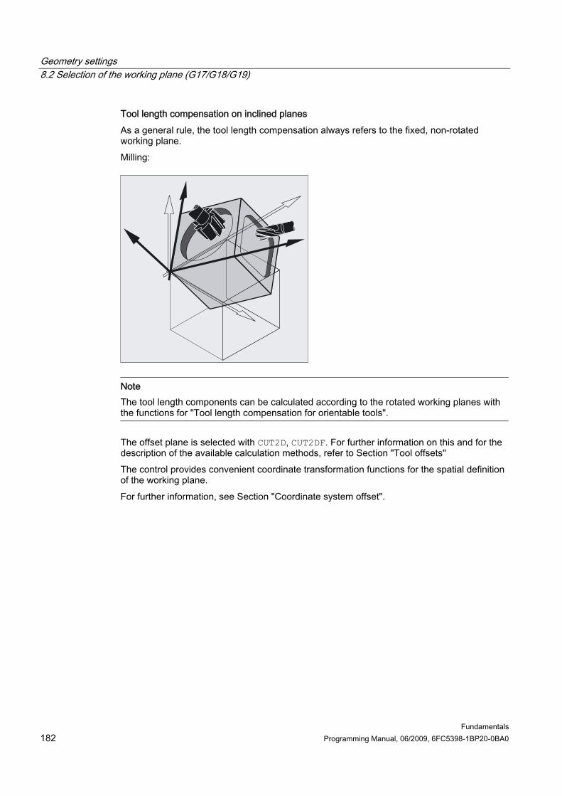
Geometry settings 8.2 Selection of the working plane (G17/G18/G19)
Fundamentals 182 Programming Manual, 06/2009, 6FC5398-1BP20-0BA0
Tool length compensation on inclined planes As a general rule, the tool length compensation always refers to the fixed, non-rotated working plane. Milling:
Note The tool length components can be calculated according to the rotated working planes with the functions for "Tool length compensation for orientable tools".
The offset plane is selected with CUT2D, CUT2DF. For further information on this and for the description of the available calculation methods, refer to Section "Tool offsets" The control provides convenient coordinate transformation functions for the spatial definition of the working plane. For further information, see Section "Coordinate system offset".

Geometry settings 8.3 Dimensions
Fundamentals Programming Manual, 06/2009, 6FC5398-1BP20-0BA0 183
8.3 8.3 Dimensions The basis of most NC programs is a workpiece drawing with specific dimensions. These dimensions can be: ● In absolute dimensions or in incremental dimensions ● In millimeters or inches ● In radius or diameter (for turning) Specific programming commands are available for the various dimension options so that the data from a dimension drawing can be transferred directly (without conversion) to the NC program.
8.3.1 Absolute dimensions (G90, AC)
Function With absolute dimensions, the position specifications always refer to the zero point of the currently valid coordinate system, i.e. the absolute position is programmed, on which the tool is to traverse. Modal absolute dimensions Modal absolute dimensions are activated with the G90 command. Generally it applies to all axes programmed in subsequent NC blocks. Non-modal absolute dimensions With preset incremental dimensions (G91), the AC command can be used to set non-modal absolute dimensions for individual axes.
Note Non-modal absolute dimensions (AC) are also possible for spindle positioning (SPOS, SPOSA) and interpolation parameters (I, J, K).
Syntax G90 <axis>=AC(<value>)
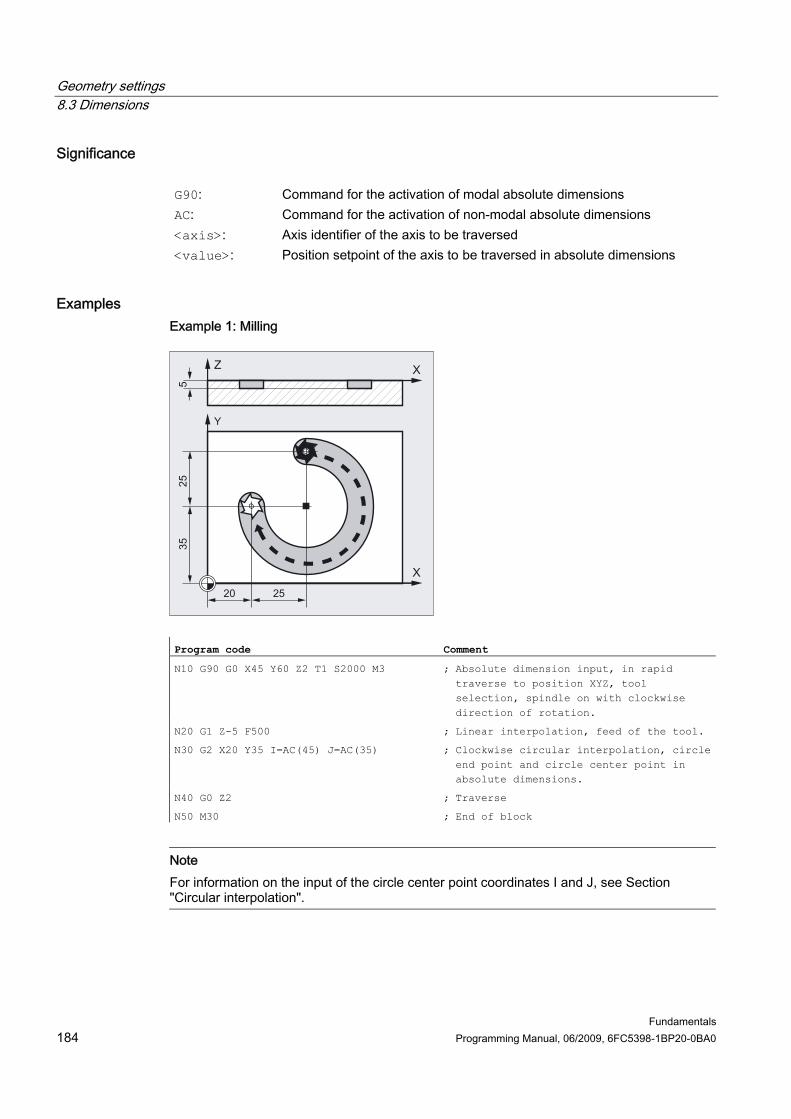
Geometry settings 8.3 Dimensions
Fundamentals 184 Programming Manual, 06/2009, 6FC5398-1BP20-0BA0
Significance G90: Command for the activation of modal absolute dimensions AC: Command for the activation of non-modal absolute dimensions <axis>: Axis identifier of the axis to be traversed <value>: Position setpoint of the axis to be traversed in absolute dimensions
Examples Example 1: Milling
Program code Comment
N10 G90 G0 X45 Y60 Z2 T1 S2000 M3 ; Absolute dimension input, in rapid traverse to position XYZ, tool selection, spindle on with clockwise direction of rotation.
N20 G1 Z-5 F500 ; Linear interpolation, feed of the tool.
N30 G2 X20 Y35 I=AC(45) J=AC(35) ; Clockwise circular interpolation, circle end point and circle center point in absolute dimensions.
N40 G0 Z2 ; Traverse
N50 M30 ; End of block
Note For information on the input of the circle center point coordinates I and J, see Section "Circular interpolation".
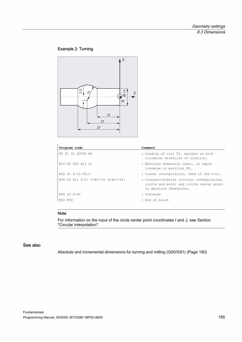
Geometry settings 8.3 Dimensions
Fundamentals Programming Manual, 06/2009, 6FC5398-1BP20-0BA0 185
Example 2: Turning
Program code Comment
N5 T1 D1 S2000 M3 ; Loading of tool T1, spindle on with clockwise direction of rotation.
N10 G0 G90 X11 Z1 ; Absolute dimension input, in rapid traverse to position XZ.
N20 G1 Z-15 F0.2 ; Linear interpolation, feed of the tool.
N30 G3 X11 Z-27 I=AC(-5) K=AC(-21) ; Counterclockwise circular interpolation, circle end point and circle center point in absolute dimensions.
N40 G1 Z-40 ; Traverse
N50 M30 ; End of block
Note For information on the input of the circle center point coordinates I and J, see Section "Circular interpolation".
See also Absolute and incremental dimensions for turning and milling (G90/G91) (Page 190)
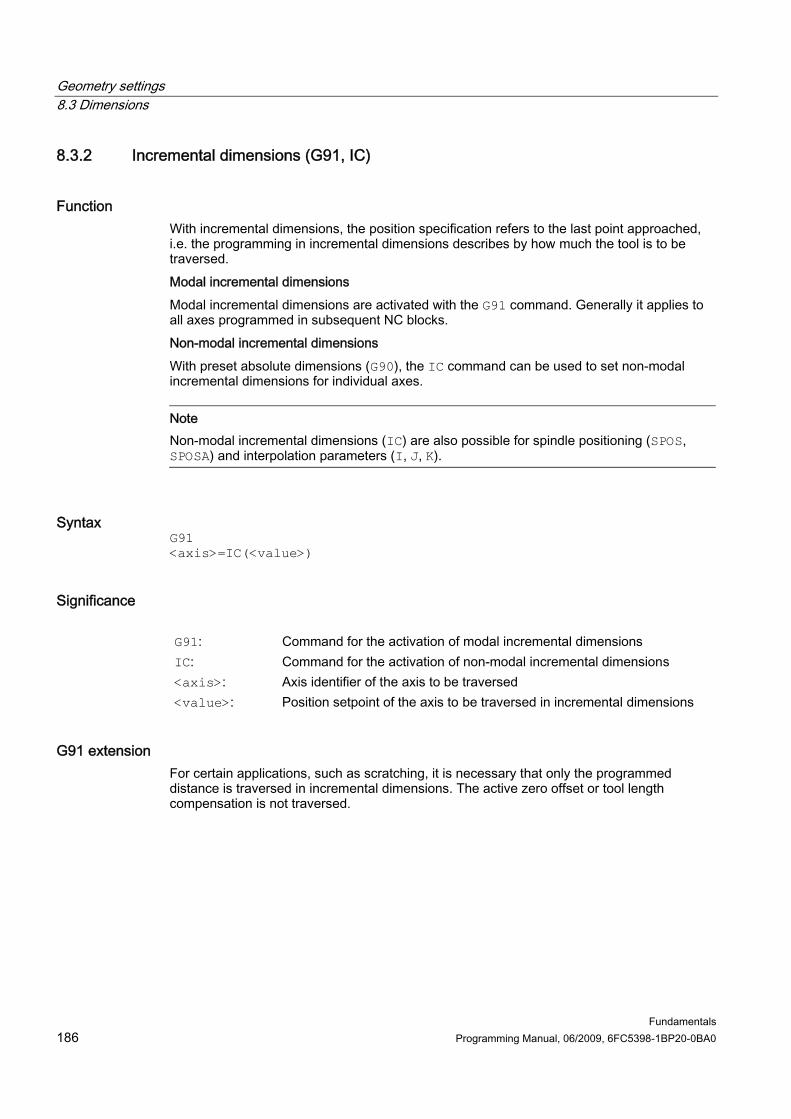
Geometry settings 8.3 Dimensions
Fundamentals 186 Programming Manual, 06/2009, 6FC5398-1BP20-0BA0
8.3.2 Incremental dimensions (G91, IC)
Function With incremental dimensions, the position specification refers to the last point approached, i.e. the programming in incremental dimensions describes by how much the tool is to be traversed. Modal incremental dimensions Modal incremental dimensions are activated with the G91 command. Generally it applies to all axes programmed in subsequent NC blocks. Non-modal incremental dimensions With preset absolute dimensions (G90), the IC command can be used to set non-modal incremental dimensions for individual axes.
Note Non-modal incremental dimensions (IC) are also possible for spindle positioning (SPOS, SPOSA) and interpolation parameters (I, J, K).
Syntax G91 <axis>=IC(<value>)
Significance G91: Command for the activation of modal incremental dimensions IC: Command for the activation of non-modal incremental dimensions <axis>: Axis identifier of the axis to be traversed <value>: Position setpoint of the axis to be traversed in incremental dimensions
G91 extension For certain applications, such as scratching, it is necessary that only the programmed distance is traversed in incremental dimensions. The active zero offset or tool length compensation is not traversed.
Geometry settings 8.3 Dimensions
Fundamentals Programming Manual, 06/2009, 6FC5398-1BP20-0BA0 187
This behavior can be set separately for the active zero offset and tool length compensation via the following setting data: SD42440 $SC_FRAME_OFFSET_INCR_PROG (zero offsets in frames) SD42442 $SC_TOOL_OFFSET_INCR_PROG (tool length compensations) Value Meaning 0 With incremental programming (incremental dimensions) of an axis, the zero offset or the
tool length compensation is not traversed. 1 With incremental programming (incremental dimensions) of an axis, the zero offset or the
tool length compensation is traversed.
Examples Example 1: Milling
Program code Comment
N10 G90 G0 X45 Y60 Z2 T1 S2000 M3 ; Absolute dimension input, in rapid traverse to position XYZ, tool selection, spindle on with clockwise direction of rotation
N20 G1 Z-5 F500 ; Linear interpolation, feed of the tool.
N30 G2 X20 Y35 I0 J-25 ; Clockwise circular interpolation, circle end point in absolute dimensions, circle center point in incremental dimensions.
N40 G0 Z2 ; Traverse
N50 M30 ; End of block

Geometry settings 8.3 Dimensions
Fundamentals 188 Programming Manual, 06/2009, 6FC5398-1BP20-0BA0
Note For information on the input of the circle center point coordinates I and J, see Section "Circular interpolation".
Example 2: Turning
Program code Comment
N5 T1 D1 S2000 M3 ; Loading of tool T1, spindle on with clockwise direction of rotation.
N10 G0 G90 X11 Z1 ; Absolute dimension input, in rapid traverse to position XZ.
N20 G1 Z-15 F0.2 ; Linear interpolation, feed of the tool.
N30 G3 X11 Z-27 I-8 K-6 ; Counterclockwise circular interpolation, circle end point in absolute dimensions, circle center point in incremental dimensions.
N40 G1 Z-40 ; Traverse
N50 M30 ; End of block
Note For information on the input of the circle center point coordinates I and J, see Section "Circular interpolation".
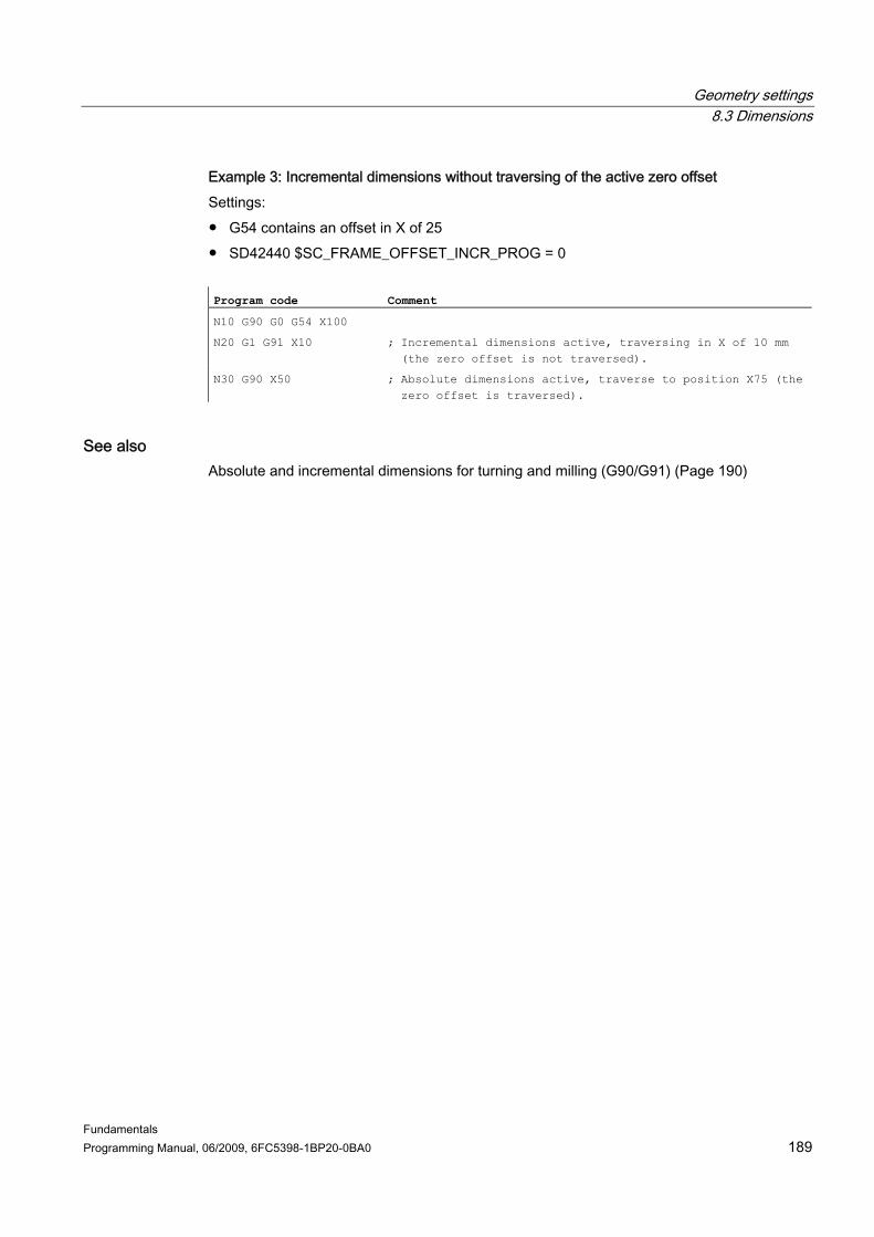
Geometry settings 8.3 Dimensions
Fundamentals Programming Manual, 06/2009, 6FC5398-1BP20-0BA0 189
Example 3: Incremental dimensions without traversing of the active zero offset Settings: ● G54 contains an offset in X of 25 ● SD42440 $SC_FRAME_OFFSET_INCR_PROG = 0 Program code Comment
N10 G90 G0 G54 X100
N20 G1 G91 X10 ; Incremental dimensions active, traversing in X of 10 mm (the zero offset is not traversed).
N30 G90 X50 ; Absolute dimensions active, traverse to position X75 (the zero offset is traversed).
See also Absolute and incremental dimensions for turning and milling (G90/G91) (Page 190)
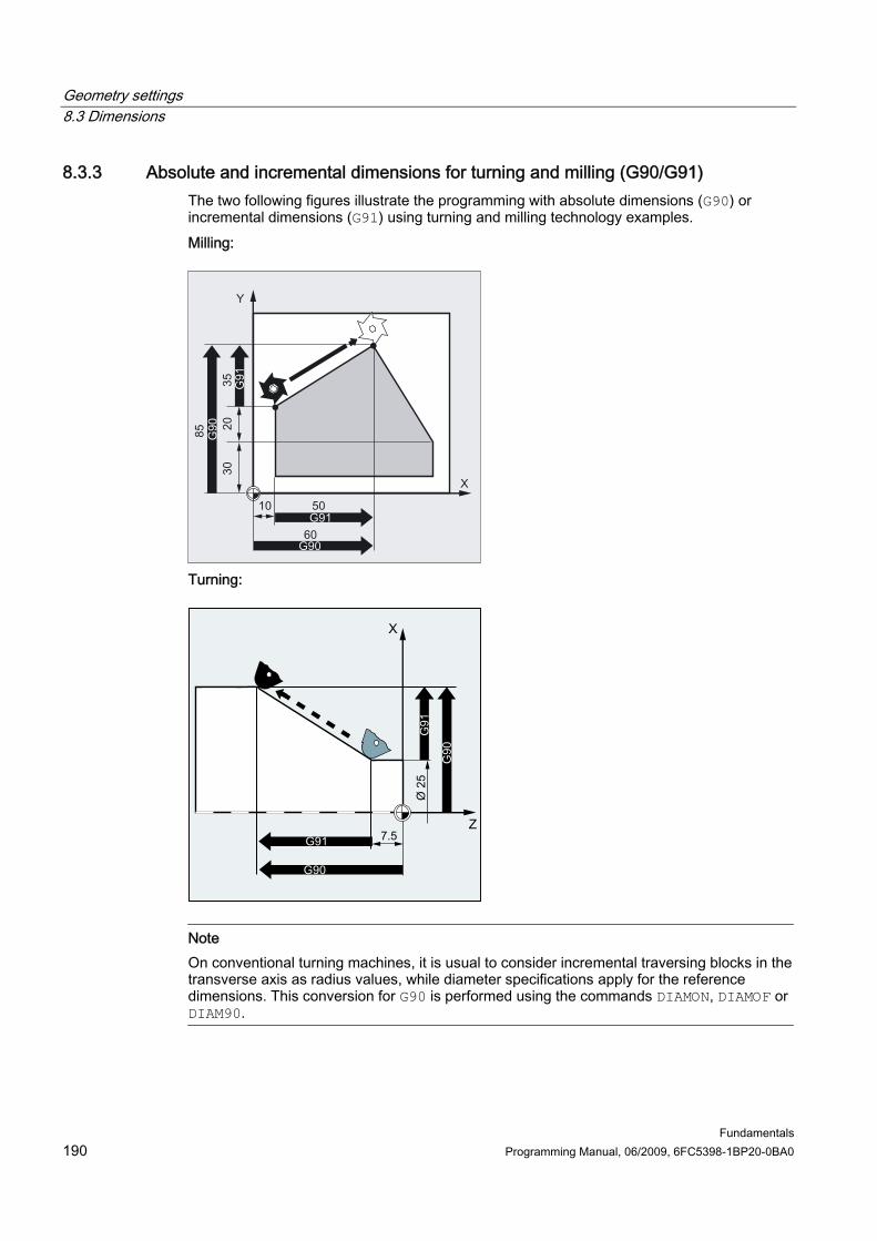
Geometry settings 8.3 Dimensions
Fundamentals 190 Programming Manual, 06/2009, 6FC5398-1BP20-0BA0
8.3.3 Absolute and incremental dimensions for turning and milling (G90/G91) The two following figures illustrate the programming with absolute dimensions (G90) or incremental dimensions (G91) using turning and milling technology examples. Milling:
Turning:
Note On conventional turning machines, it is usual to consider incremental traversing blocks in the transverse axis as radius values, while diameter specifications apply for the reference dimensions. This conversion for G90 is performed using the commands DIAMON, DIAMOF or DIAM90.

Geometry settings 8.3 Dimensions
Fundamentals Programming Manual, 06/2009, 6FC5398-1BP20-0BA0 191
8.3.4 Absolute dimension for rotary axes (DC, ACP, ACN)
Function The non-modal and G90/G91-independent commands DC, ACP and ACN are available for the positioning of rotary axes in absolute dimensions. DC, ACP and ACN differ in the basic approach strategy:
Syntax <rotary axis>=DC(<value>) <rotary axis>=ACP(<value>) <rotary axis>=ACN(<value>)
Significance <rotary axis>: Identifier of the rotary axis that is to be traversed (e.g. A, B or C) DC: Command for the direct approach to the position
The rotary axis approaches the programmed position directly on the shortest path. The rotary axis traverses a maximum range of 180°.
ACP: Command to approach the position in a positive direction The rotary axis traverses to the programmed position in the positive direction of axis rotation (counterclockwise).

Geometry settings 8.3 Dimensions
Fundamentals 192 Programming Manual, 06/2009, 6FC5398-1BP20-0BA0
ACN: Command to approach the position in a negative direction The rotary axis traverses to the programmed position in the negative direction of axis rotation (clockwise). Rotary axis position to be approached in absolute dimensions <value>: Range of values: 0 - 360 degrees
Note The positive direction of rotation (clockwise or counterclockwise) is set in the machine data.
Note The traversing range between 0° and 360° must be set in the machine data (modulo behavior) for positioning with direction specification (ACP, ACN). G91 or IC must be programmed to traverse modulo rotary axes more than 360° in a block.
Note The commands DC, ACP and ACN can also be used for spindle positioning (SPOS, SPOSA) from standstill. Example: SPOS=DC(45)

Geometry settings 8.3 Dimensions
Fundamentals Programming Manual, 06/2009, 6FC5398-1BP20-0BA0 193
Example Milling on a rotary table
The tool is stationary, the table turns to 270° in a clockwise direction to produce a circular groove.
Program code Comment
N10 SPOS=0 ; Spindle in position control
N20 G90 G0 X-20 Y0 Z2 T1 ; Absolute dimensions, feed tool T1 in rapid traverse.
N30 G1 Z-5 F500 ; Lower tool during feed
N40 C=ACP(270) ; Table turns clockwise to 270 degrees (positive), the tool mills a circular groove.
N50 G0 Z2 M30 ; Retraction, end of program
References Function Manual, Extended Functions; Rotary Axes (R2)
Geometry settings 8.3 Dimensions
Fundamentals 194 Programming Manual, 06/2009, 6FC5398-1BP20-0BA0
8.3.5 Inch or metric dimensions (G70/G700, G71/G710)
Function The following G functions can be used to switch between the metric measuring system and the inch measuring system.
Syntax G70/G71 G700/G710
Significance G70: Activation of the inch measuring system
The inch measuring system is used to read and write geometric data in units of length. Technological data in units of length, e.g. feedrates, tool offsets or settable work offsets, as well as machine data and system variables, are read and written using the parameterized basic system (MD10240 $MN_SCALING_SYSTEM_IS_METRIC).
G71: Activation of the metric measuring system The metric measuring system is used to read and write geometric data in units of length. Technological data in units of length, e.g. feedrates, tool offsets or settable work offsets, as well as machine data and system variables, are read and written using the parameterized basic system (MD10240 $MN_SCALING_SYSTEM_IS_METRIC).
G700: Activation of the inch measuring system All geometrical and technological data in units of length (see above) is read and written using the inch measuring system.
G710: Activation of the metric measuring system All geometrical and technological data in units of length (see above) is read and written using the metric measuring system.

Geometry settings 8.3 Dimensions
Fundamentals Programming Manual, 06/2009, 6FC5398-1BP20-0BA0 195
Example Changeover between inch system and metric system The parameterized basic system is metric: MD10240 $MN_SCALING_SYSTEM_IS_METRIC = TRUE
Program code Comment
N10 G0 G90 X20 Y30 Z2 S2000 M3 T1 ; X=20 mm, Y=30 mm, Z=2 mm, F=rapid traverse mm/min
N20 G1 Z-5 F500 ; Z=-5 mm, F=500 mm/min
N30 X90 ; X=90 mm
N40 G70 X2.75 Y3.22 ; Prog. meas. system: inch
X=2.75 inch, Y=3.22 inch, F=500 mm/min
N50 X1.18 Y3.54 ; X=1.18 inch, Y=3.54 inch, F=500 mm/min
N60 G71 X20 Y30 ; Prog. meas. system: metric
X=20 mm, Y=30 mm, F=500 mm/min
N70 G0 Z2 ; Z=2 mm, F=rapid traverse mm/min
N80 M30 ; End of program
Geometry settings 8.3 Dimensions
Fundamentals 196 Programming Manual, 06/2009, 6FC5398-1BP20-0BA0
Further information G70/G71 With G70/G71 active, only the following geometric data is interpreted in the relevant measuring system: ● Position data (X, Y, Z, …) ● Circular-path programming:
– Interpolation point coordinates (I1, J1, K1) – Interpolation parameters (I, J, K) – Circle radius (CR)
● Pitch (G34, G35) ● Programmable zero offset (TRANS) ● Polar radius (RP) Synchronized actions If, in a synchronized action (condition component and/or action component) no explicit measuring system is programmed (G70/G71/G700/G710), the measuring system which was active in the channel at the point of execution will be applied to the synchronized action (condition component and/or action component).
NOTICE Read position data in synchronized actions If a measuring system has not been explicitly programmed in the synchronized action (condition component and/or action component) position data specified in units of length in the synchronized action are always read in the parameterized basic system.
References ● Function Manual, Basic Functions; Speeds, Setpoint/Actual-Value System, Closed-Loop
Control (G2), Section "Metric/inch dimension system" ● Programming Manual, Job Planning; Section "Motion-synchronous actions" ● Function Manual, Synchronized Actions

Geometry settings 8.3 Dimensions
Fundamentals Programming Manual, 06/2009, 6FC5398-1BP20-0BA0 197
8.3.6 Channel-specific diameter/radius programming (DIAMON, DIAM90, DIAMOF, DIAMCYCOF)
Function During turning, the dimensions for the transverse axis can be specified in the diameter (①) or in the radius (②):
So that the dimensions from a technical drawing can be transferred directly (without conversion) to the NC program, channel-specific diameter or radius programming is activated using the modal commands DIAMON, DIAM90, DIAMOF, and DIAMCYCOF.
Note The channel-specific diameter/radius programming refers to the geometry axis defined as transverse axis via MD20100 $MC_DIAMETER_AX_DEF (→ see machine manufacturer's specifications). Only one transverse axis per channel can be defined via MD20100.
Syntax DIAMON DIAM90 DIAMOF

Geometry settings 8.3 Dimensions
Fundamentals 198 Programming Manual, 06/2009, 6FC5398-1BP20-0BA0
Significance
Command for the activation of the independent channel-specific diameter programming The effect of DIAMON is independent of the programmed dimensions mode (absolute dimensions G90 or incremental dimensions G91): • for G90: Dimensions in the diameter
DIAMON:
• for G91: Dimensions in the diameter Command for the activation of the dependent channel-specific diameter programming The effect of DIAM90 depends on the programmed dimensions mode: • for G90: Dimensions in the diameter
DIAM90:
• for G91: Dimensions in the radius Command for the deactivation of the channel-specific diameter programming Channel-specific radius programming takes effect when diameter programming is deactivated. The effect of DIAMOF is independent of the programmed dimensions mode: • for G90: Dimensions in the radius
DIAMOF:
• for G91: Dimensions in the radius DIAMCYCOF: Command for the deactivation of channel-specific diameter programming
during cycle processing. In this way, computations in the cycle can always be made in the radius. The last G function active in this group remains active for the position indicator and the basic block indicator.
Note With DIAMON or DIAM90, the transverse-axis actual values will always be displayed as a diameter. This also applies to reading of actual values in the workpiece coordinate system with MEAS, MEAW, $P_EP[x] and $AA_IW[x].
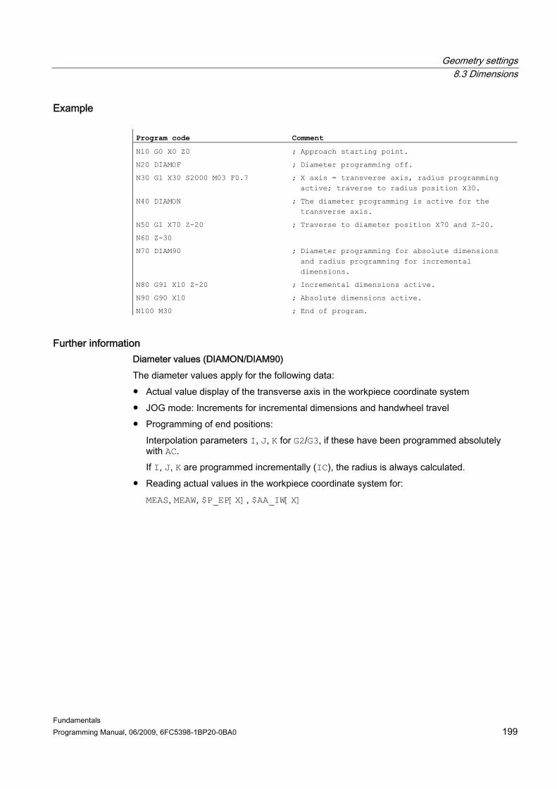
Geometry settings 8.3 Dimensions
Fundamentals Programming Manual, 06/2009, 6FC5398-1BP20-0BA0 199
Example Program code Comment
N10 G0 X0 Z0 ; Approach starting point.
N20 DIAMOF ; Diameter programming off.
N30 G1 X30 S2000 M03 F0.7 ; X axis = transverse axis, radius programming active; traverse to radius position X30.
N40 DIAMON ; The diameter programming is active for the transverse axis.
N50 G1 X70 Z-20 ; Traverse to diameter position X70 and Z-20.
N60 Z-30
N70 DIAM90 ; Diameter programming for absolute dimensions and radius programming for incremental dimensions.
N80 G91 X10 Z-20 ; Incremental dimensions active.
N90 G90 X10 ; Absolute dimensions active.
N100 M30 ; End of program.
Further information Diameter values (DIAMON/DIAM90) The diameter values apply for the following data: ● Actual value display of the transverse axis in the workpiece coordinate system ● JOG mode: Increments for incremental dimensions and handwheel travel ● Programming of end positions:
Interpolation parameters I, J, K for G2/G3, if these have been programmed absolutely with AC. If I, J, K are programmed incrementally (IC), the radius is always calculated.
● Reading actual values in the workpiece coordinate system for: MEAS, MEAW, $P_EP[X], $AA_IW[X]
Geometry settings 8.3 Dimensions
Fundamentals 200 Programming Manual, 06/2009, 6FC5398-1BP20-0BA0
8.3.7 Axis-specific diameter/radius programming (DIAMONA, DIAM90A, DIAMOFA, DIACYCOFA, DIAMCHANA, DIAMCHAN, DAC, DIC, RAC, RIC)
Function In addition to channel-specific diameter programming, the axis-specific diameter programming function enables the modal or non-modal dimensions and display in the diameter for one or more axes.
Note The axis-specific diameter programming is only possible for axes that are permitted as further transverse axes for the axis-specific diameter programming via MD30460 $MA_BASE_FUNCTION_MASK (→ see machine manufacturer's specifications).
Syntax Modal axis-specific diameter programming for several transverse axes in the channel: DIAMONA[<axis>] DIAM90A[<axis>] DIAMOFA[<axis>] DIACYCOFA[<axis>]
Acceptance of the channel-specific diameter/radius programming: DIAMCHANA[<axis>] DIAMCHAN
Non-modal axis-specific diameter/radius programming: <axis>=DAC(<value>) <axis>=DIC(<value>) <axis>=RAC(<value>) <axis>=RIC(<value>)
Meaning Modal axis-specific diameter programming
Command for the activation of the independent axis-specific diameter programming The effect of DIAMONA is independent of the programmed dimensions mode (G90/G91 or AC/IC): • for G90, AC: Dimensions in the diameter
DIAMONA:
• for G91, IC: Dimensions in the diameter
Geometry settings 8.3 Dimensions
Fundamentals Programming Manual, 06/2009, 6FC5398-1BP20-0BA0 201
Command for the activation of the dependent axis-specific diameter programming The effect of DIAM90A depends on the programmed dimensions mode: • for G90, AC: Dimensions in the diameter
DIAM90A:
• for G91, IC: Dimensions in the radius Command for the deactivation of the axis-specific diameter programming Axis-specific radius programming takes effect when diameter programming is deactivated. The effect of DIAMOFA is independent of the programmed dimensions mode: • for G90, AC: Dimensions in the radius
DIAMOFA:
• for G91, IC: Dimensions in the radius DIACYCOFA: Command for the deactivation of axis-specific diameter programming
during cycle processing. In this way, computations in the cycle can always be made in the radius. The last G function active in this group remains active for the position indicator and the basic block indicator. Axis identifier of the axis for which the axis-specific diameter programming is to be activated Permitted axis identifiers are as follows: • Geometry/channel axis name
or • Machine axis name
<axis>:
Range of values: The axis specified must be a known axis in the channel. Other conditions: • The axis must be permitted for the axis-specific
diameter programming via MD30460 $MA_BASE_FUNCTION_MASK.
• Rotary axes are not permitted to serve as transverse axes.

Geometry settings 8.3 Dimensions
Fundamentals 202 Programming Manual, 06/2009, 6FC5398-1BP20-0BA0
Acceptance of the channel-specific diameter/radius programming DIAMCHANA: With the DIAMCHANA[<axis>] command, the specified axis accepts
the channel status of the diameter/radius programming and is then assigned to the channel-specific diameter/radius programming.
DIAMCHAN: With the DIAMCHAN command, all axes permitted for the axis-specific diameter programming accept the channel status of the diameter/radius programming and are then assigned to the channel-specific diameter/radius programming.
Non-modal axis-specific diameter/radius programming The non-modal axis-specific diameter/radius programming specifies the dimension type as a diameter or radius value in the part program and synchronized actions. The modal status of diameter/radius programming remains unchanged. DAC: The DAC command sets the following dimensions to non-modal for the
specified axis: Diameter in absolute dimensions
DIC: The DIC command sets the following dimensions to non-modal for the specified axis: Diameter in incremental dimensions
RAC: The RAC command sets the following dimensions to non-modal for the specified axis: Radius in absolute dimensions
RIC: The RIC command sets the following dimensions to non-modal for the specified axis: Radius in incremental dimensions
Note With DIAMONA[<axis>] or DIAM90A[<axis>], the transverse-axis actual values are always displayed as a diameter. This also applies to reading of actual values in the workpiece coordinate system with MEAS, MEAW, $P_EP[x] and $AA_IW[x].
Note During the replacement of an additional transverse axis because of a GET request, the status of the diameter/radius programming in the other channel is accepted with RELEASE[<axis>].
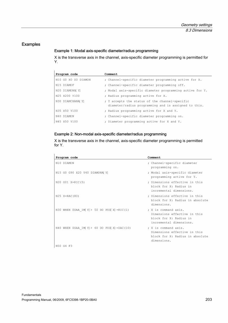
Geometry settings 8.3 Dimensions
Fundamentals Programming Manual, 06/2009, 6FC5398-1BP20-0BA0 203
Examples Example 1: Modal axis-specific diameter/radius programming X is the transverse axis in the channel, axis-specific diameter programming is permitted for Y. Program code Comment
N10 G0 X0 Z0 DIAMON ; Channel-specific diameter programming active for X.
N15 DIAMOF ; Channel-specific diameter programming off.
N20 DIAMONA[Y] ; Modal axis-specific diameter programming active for Y.
N25 X200 Y100 ; Radius programming active for X.
N30 DIAMCHANA[Y] ; Y accepts the status of the channel-specific diameter/radius programming and is assigned to this.
N35 X50 Y100 ; Radius programming active for X and Y.
N40 DIAMON ; Channel-specific diameter programming on.
N45 X50 Y100 ; Diameter programming active for X and Y.
Example 2: Non-modal axis-specific diameter/radius programming X is the transverse axis in the channel, axis-specific diameter programming is permitted for Y. Program code Comment
N10 DIAMON ; Channel-specific diameter programming on.
N15 G0 G90 X20 Y40 DIAMONA[Y] ; Modal axis-specific diameter programming active for Y.
N20 G01 X=RIC(5) ; Dimensions effective in this block for X: Radius in incremental dimensions.
N25 X=RAC(80) ; Dimensions effective in this block for X: Radius in absolute dimensions.
N30 WHEN $SAA_IM[Y]> 50 DO POS[X]=RIC(1) ; X is command axis. Dimensions effective in this block for X: Radius in incremental dimensions.
N40 WHEN $SAA_IM[Y]> 60 DO POS[X]=DAC(10) ; X is command axis. Dimensions effective in this block for X: Radius in absolute dimensions.
N50 G4 F3
Geometry settings 8.3 Dimensions
Fundamentals 204 Programming Manual, 06/2009, 6FC5398-1BP20-0BA0
Further information Diameter values (DIAMONA/DIAM90A) The diameter values apply for the following data: ● Actual value display of the transverse axis in the workpiece coordinate system ● JOG mode: Increments for incremental dimensions and handwheel travel ● Programming of end positions:
Interpolation parameters I, J, K for G2/G3, if these have been programmed absolutely with AC. If I, J, K are programmed incrementally (IC), the radius is always calculated.
● Reading actual values in the workpiece coordinate system for: MEAS, MEAW, $P_EP[X], $AA_IW[X]
Non-modal axis-specific diameter programming (DAC, DIC, RAC, RIC) The statements DAC, DIC, RAC, RIC are permissible for any commands for which channel-specific diameter programming is relevant: ● Axis position: X..., POS, POSA ● Oscillating: OSP1, OSP2, OSS, OSE, POSP ● Interpolation parameters: I, J, K ● Contour definition: Straight line with specified angle ● Rapid retraction: POLF[AX] ● Movement in tool direction: MOVT ● Smooth approach and retraction:
G140 to G143, G147, G148, G247, G248, G347, G348, G340, G341
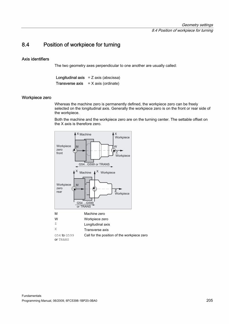
Geometry settings 8.4 Position of workpiece for turning
Fundamentals Programming Manual, 06/2009, 6FC5398-1BP20-0BA0 205
8.4 8.4 Position of workpiece for turning
Axis identifiers The two geometry axes perpendicular to one another are usually called: Longitudinal axis = Z axis (abscissa) Transverse axis = X axis (ordinate)
Workpiece zero Whereas the machine zero is permanently defined, the workpiece zero can be freely selected on the longitudinal axis. Generally the workpiece zero is on the front or rear side of the workpiece. Both the machine and the workpiece zero are on the turning center. The settable offset on the X axis is therefore zero.
M Machine zero W Workpiece zero Z Longitudinal axis X Transverse axis G54 to G599 or TRANS
Call for the position of the workpiece zero

Geometry settings 8.4 Position of workpiece for turning
Fundamentals 206 Programming Manual, 06/2009, 6FC5398-1BP20-0BA0
Transverse axis Generally the dimensions for the transverse axis are diameter specifications (double path dimension compared to other axes):
The geometry axis that is to serve as transverse axis is defined in the machine data (→ machine manufacturer).

Fundamentals Programming Manual, 06/2009, 6FC5398-1BP20-0BA0 207
Motion commands 9
Contour elements The programmed workpiece contour can be made up of the following contour elements: ● Straight lines ● Circular arcs ● Helical curves (through overlaying of straight lines and circular arcs)
Travel commands The following travel commands are available for the creation of these contour elements: ● Rapid traverse motion (G0) ● Linear interpolation (G1) ● Circular interpolation clockwise (G2) ● Circular interpolation counterclockwise (G3) The travel commands are modal.
Target positions A motion block contains the target positions for the axes to be traversed (path axes, synchronized axes, positioning axes). The target positions can be programmed in Cartesian coordinates or in polar coordinates.
CAUTION The axis address may only be programmed once per block.
Starting point - target point The traversing motion is always for the last point reached to the programmed target position. This target position is then the starting position for the next travel command.

Motion commands 8.4 Position of workpiece for turning
Fundamentals 208 Programming Manual, 06/2009, 6FC5398-1BP20-0BA0
Workpiece contour The motion blocks produce the workpiece contour when performed in succession:
Figure 9-1 Motion blocks for turning
Figure 9-2 Motion blocks for milling
NOTICE Before machining, the workpiece must be positioned in such a way that the tool or workpiece cannot be damaged.

Motion commands 9.1 Travel commands with Cartesian coordinates (G0, G1, G2, G3, X..., Y..., Z...)
Fundamentals Programming Manual, 06/2009, 6FC5398-1BP20-0BA0 209
9.1 9.1 Travel commands with Cartesian coordinates (G0, G1, G2, G3, X..., Y..., Z...)
Function The position specified in the NC block with Cartesian coordinates can be approached with rapid traverse motion G0, linear interpolation G1 or circular interpolation G2 /G3.
Syntax G0 X... Y... Z... G1 X... Y... Z... G2 X... Y... Z... ... G3 X... Y... Z... ...
Significance G0: Command for the activation of the rapid traverse motion G1: Command for the activation of the linear interpolation G2: Command for the activation of the clockwise circular interpolation G3: Command for the activation of the counterclockwise circular interpolation X...: Cartesian coordinate of the target position in the X direction Y...: Cartesian coordinate of the target position in the Y direction Z...: Cartesian coordinate of the target position in the Z direction
Note In addition to the coordinates of the target position X..., Y..., Z..., the circular interpolation G2 / G3 also requires further data (e.g. the circle center point coordinates; see "Circular interpolation types (Page 225)").

Motion commands 9.1 Travel commands with Cartesian coordinates (G0, G1, G2, G3, X..., Y..., Z...)
Fundamentals 210 Programming Manual, 06/2009, 6FC5398-1BP20-0BA0
Example
Program code Comment
N10 G17 S400 M3 ; Selection of the working plane, spindle clockwise
N20 G0 X40 Y-6 Z2 ; Approach of the starting position specified with Cartesian coordinates in rapid traverse
N30 G1 Z-3 F40 ; Activation of the linear interpolation, feed of the tool
N40 X12 Y-20 ; Travel on an inclined line to an end position specified with Cartesian coordinates
N50 G0 Z100 M30 ; Retraction in rapid traverse for tool change
Motion commands 9.2 Travel commands with polar coordinates
Fundamentals Programming Manual, 06/2009, 6FC5398-1BP20-0BA0 211
9.2 9.2 Travel commands with polar coordinates
9.2.1 Reference point of the polar coordinates (G110, G111, G112)
Function The point from which the dimensioning starts is called the pole. The pole can be specified in Cartesian or polar coordinates. The reference point for the pole coordinates is clearly defined with the G110 to G112 commands. Absolute or incremental dimension inputs therefore have no effect.
Syntax G110/G111/G112 X… Y… Z… G110/G111/G112 AP=… RP=…
Significance G110 ...: With the command G110, the following pole coordinates refer to the last
position reached. G111 ...: With the command G111, the following pole coordinates refer to the zero
point of the current workpiece coordinate system. G112 ...: With the command G112, the following pole coordinates refer to the last
valid pole. Note:
The commands G110...G112 must be programmed in a separate NC block.
X… Y… Z…: Specification of the pole in Cartesian coordinates Specification of the pole in polar coordinates
Polar angle Angle between the polar radius and the horizontal axis of the working plane (e.g. X axis for G17). The positive direction of rotation runs counterclockwise.
AP=…:
Range of values: ± 0…360°
AP=… RP=…:
RP=…: Polar radius The specification is always in absolute positive values in [mm] or [inch].

Motion commands 9.2 Travel commands with polar coordinates
Fundamentals 212 Programming Manual, 06/2009, 6FC5398-1BP20-0BA0
Note It is possible to switch block-by-block in the NC program between polar and Cartesian dimensions. It is possible to return directly to the Cartesian system by using Cartesian coordinate identifiers (X..., Y..., Z...). The defined pole is moreover retained up to program end.
Note If no pole has been specified, the zero point of the current workpiece coordinate system applies.
Example
Poles 1 to 3 are defined as follows: • Pole 1 with G111 X… Y… • Pole 2 with G110 X… Y… • Pole 3 with G112 X… Y…

Motion commands 9.2 Travel commands with polar coordinates
Fundamentals Programming Manual, 06/2009, 6FC5398-1BP20-0BA0 213
9.2.2 Travel commands with polar coordinates (G0, G1, G2, G3, AP, RP)
Function Travel commands with polar coordinates are useful when the dimensions of a workpiece or part of the workpiece are measured from a central point and the dimensions are specified in angles and radii (e.g. for drilling patterns).
Syntax G0/G1/G2/G3 AP=… RP=…
Significance G0: Command for the activation of rapid traverse motion G1: Command for the activation of linear interpolation G2: Command for the activation of clockwise circular interpolation G3: Command for the activation of counter-clockwise circular interpolation

Motion commands 9.2 Travel commands with polar coordinates
Fundamentals 214 Programming Manual, 06/2009, 6FC5398-1BP20-0BA0
Polar angle Angle between the polar radius and the horizontal axis of the working plane (e.g. X axis for G17). The positive direction of rotation runs counter-clockwise. Range of values: ± 0…360° The angle can be specified either incremental or absolute: AP=AC(...): Absolute dimension input AP=IC(...): Incremental dimension input
With incremental dimension input, the last programmed angle applies as reference.
AP:
The polar angle remains stored until a new pole is defined or the working plane is changed.
RP: Polar radius The specification is always in absolute positive values in [mm] or [inch]. The polar radius remains stored until a new value is entered.
Note The polar coordinates refer to the pole specified with G110 ... G112 and apply in the working plane selected with G17 to G19.
Note The 3rd geometry axis, which lies perpendicular to the working plane, can also be specified in Cartesian coordinates.
This enables spatial parameters to be programmed in cylindrical coordinates. Example: G17 G0 AP… RP… Z…
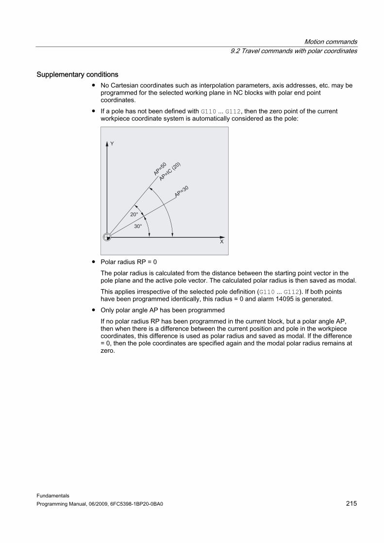
Motion commands 9.2 Travel commands with polar coordinates
Fundamentals Programming Manual, 06/2009, 6FC5398-1BP20-0BA0 215
Supplementary conditions ● No Cartesian coordinates such as interpolation parameters, axis addresses, etc. may be
programmed for the selected working plane in NC blocks with polar end point coordinates.
● If a pole has not been defined with G110 ... G112, then the zero point of the current workpiece coordinate system is automatically considered as the pole:
● Polar radius RP = 0
The polar radius is calculated from the distance between the starting point vector in the pole plane and the active pole vector. The calculated polar radius is then saved as modal. This applies irrespective of the selected pole definition (G110 ... G112). If both points have been programmed identically, this radius = 0 and alarm 14095 is generated.
● Only polar angle AP has been programmed If no polar radius RP has been programmed in the current block, but a polar angle AP, then when there is a difference between the current position and pole in the workpiece coordinates, this difference is used as polar radius and saved as modal. If the difference = 0, then the pole coordinates are specified again and the modal polar radius remains at zero.

Motion commands 9.2 Travel commands with polar coordinates
Fundamentals 216 Programming Manual, 06/2009, 6FC5398-1BP20-0BA0
Example Creation of a drilling pattern
The positions of the holes are specified in polar coordinates. Each hole is machined with the same production sequence: Rough-drilling, drilling as dimensioned, reaming … The machining sequence is stored in the subroutine.
Program code Comment
N10 G17 G54 ; Working plane X/Y, workpiece zero.
N20 G111 X43 Y38 ; Specification of the pole.
N30 G0 RP=30 AP=18 Z5G0 ; Approach starting point, specification in cylindrical coordinates.
N40 L10 ; Subprogram call.
N50 G91 AP=72 ; Approach next position in rapid traverse, polar angle in incremental dimensions, polar radius from block N30 remains saved and does not have to be specified.
N60 L10 ; Subprogram call.
N70 AP=IC(72) .
N80 L10 …
N90 AP=IC(72)
N100 L10 …
N110 AP=IC(72)
N120 L10 …
N130 G0 X300 Y200 Z100 M30 ; Retract tool, end of program.
N90 AP=IC(72)
N100 L10 …
See also Circular interpolation types (G2/G3, ...) (Page 225)
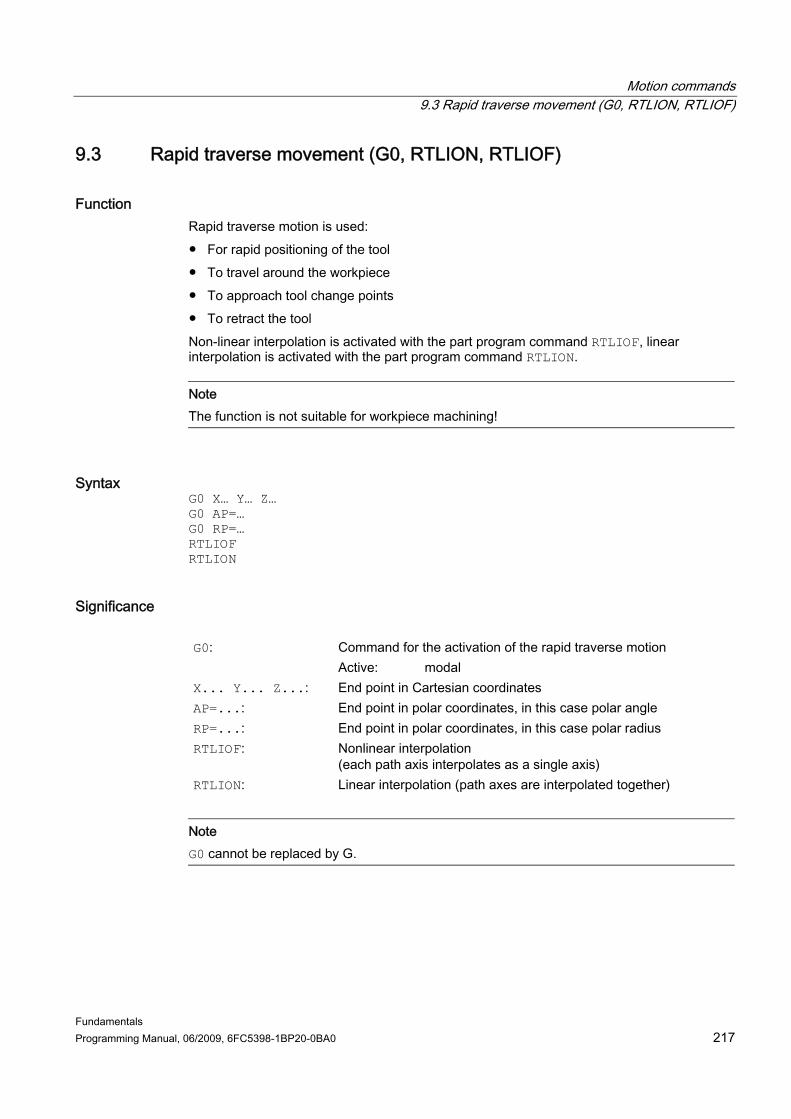
Motion commands 9.3 Rapid traverse movement (G0, RTLION, RTLIOF)
Fundamentals Programming Manual, 06/2009, 6FC5398-1BP20-0BA0 217
9.3 9.3 Rapid traverse movement (G0, RTLION, RTLIOF)
Function Rapid traverse motion is used: ● For rapid positioning of the tool ● To travel around the workpiece ● To approach tool change points ● To retract the tool Non-linear interpolation is activated with the part program command RTLIOF, linear interpolation is activated with the part program command RTLION.
Note The function is not suitable for workpiece machining!
Syntax G0 X… Y… Z… G0 AP=… G0 RP=… RTLIOF RTLION
Significance
Command for the activation of the rapid traverse motion G0: Active: modal
X... Y... Z...: End point in Cartesian coordinates AP=...: End point in polar coordinates, in this case polar angle RP=...: End point in polar coordinates, in this case polar radius RTLIOF: Nonlinear interpolation
(each path axis interpolates as a single axis) RTLION: Linear interpolation (path axes are interpolated together)
Note G0 cannot be replaced by G.
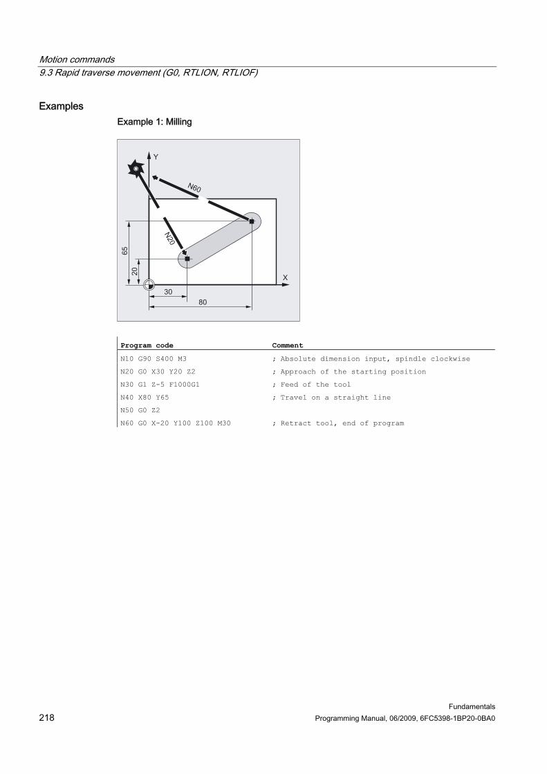
Motion commands 9.3 Rapid traverse movement (G0, RTLION, RTLIOF)
Fundamentals 218 Programming Manual, 06/2009, 6FC5398-1BP20-0BA0
Examples Example 1: Milling
Program code Comment
N10 G90 S400 M3 ; Absolute dimension input, spindle clockwise
N20 G0 X30 Y20 Z2 ; Approach of the starting position
N30 G1 Z-5 F1000G1 ; Feed of the tool
N40 X80 Y65 ; Travel on a straight line
N50 G0 Z2
N60 G0 X-20 Y100 Z100 M30 ; Retract tool, end of program
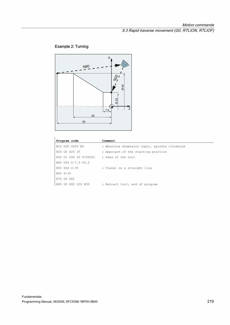
Motion commands 9.3 Rapid traverse movement (G0, RTLION, RTLIOF)
Fundamentals Programming Manual, 06/2009, 6FC5398-1BP20-0BA0 219
Example 2: Turning
Program code Comment
N10 G90 S400 M3 ; Absolute dimension input, spindle clockwise
N20 G0 X25 Z5 ; Approach of the starting position
N30 G1 G94 Z0 F1000G1 ; Feed of the tool
N40 G95 Z-7.5 F0.2
N50 X60 Z-35 ; Travel on a straight line
N60 Z-50
N70 G0 X62
N80 G0 X80 Z20 M30 ; Retract tool, end of program
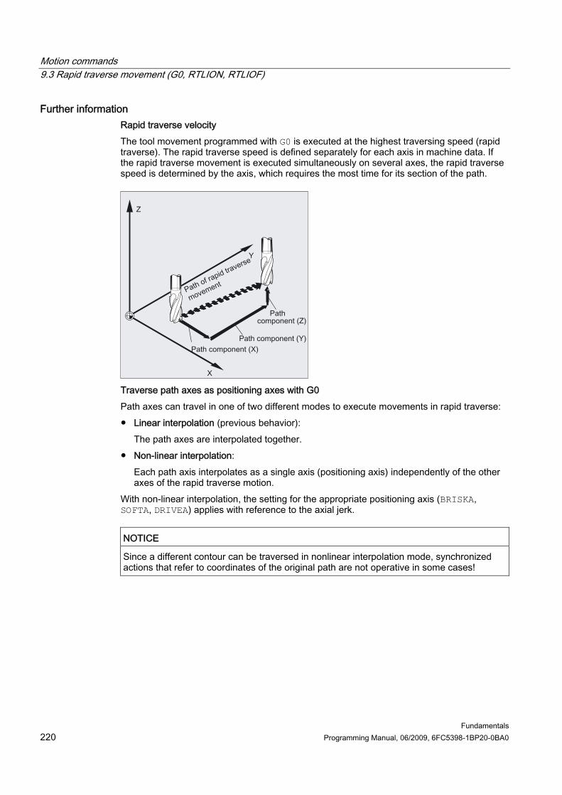
Motion commands 9.3 Rapid traverse movement (G0, RTLION, RTLIOF)
Fundamentals 220 Programming Manual, 06/2009, 6FC5398-1BP20-0BA0
Further information Rapid traverse velocity The tool movement programmed with G0 is executed at the highest traversing speed (rapid traverse). The rapid traverse speed is defined separately for each axis in machine data. If the rapid traverse movement is executed simultaneously on several axes, the rapid traverse speed is determined by the axis, which requires the most time for its section of the path.
Traverse path axes as positioning axes with G0 Path axes can travel in one of two different modes to execute movements in rapid traverse: ● Linear interpolation (previous behavior):
The path axes are interpolated together. ● Non-linear interpolation:
Each path axis interpolates as a single axis (positioning axis) independently of the other axes of the rapid traverse motion.
With non-linear interpolation, the setting for the appropriate positioning axis (BRISKA, SOFTA, DRIVEA) applies with reference to the axial jerk.
NOTICE Since a different contour can be traversed in nonlinear interpolation mode, synchronized actions that refer to coordinates of the original path are not operative in some cases!

Motion commands 9.3 Rapid traverse movement (G0, RTLION, RTLIOF)
Fundamentals Programming Manual, 06/2009, 6FC5398-1BP20-0BA0 221
Linear interpolation applies in the following cases: ● For a G-code combination with G0 that does not permit positioning axis motion (e.g.
G40/G41/G42) ● For a combination of G0 with G64 ● When the compressor is active ● When a transformation is active Example: Program code
G0 X0 Y10
G0 G40 X20 Y20
G0 G95 X100 Z100 M3 S100
Path POS[X]=0 POS[Y]=10 is traversed in path mode. No revolutional feedrate is active if path POS[X]=100 POS[Z]=100 is traversed. Settable block change time with G0 For single-axis interpolation, a new end-of-motion criterion FINEA or COARSEA or IPOENDA can be set for block change even within the braking ramp. Consecutive axes are handled in G0 like positioning axes. With the combination of ● "Block change settable in the braking ramp of the single axis interpolation" and ● "Traversing path axes in rapid traverse movement as positioning axes with G0" all axes can travel to their end point independently of one another. In this way, two sequentially programmed X and Z axes are treated like positioning axes in conjunction with G0. The block change to axis Z can be initiated by axis X as a function of the braking ramp time setting (100-0%). Axis Z starts to move while axis X is still in motion. Both axes approach their end point independently of one another. For further information, please refer to "Feed control and spindle motion".
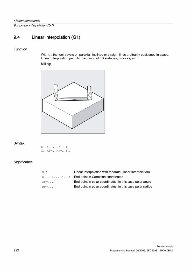
Motion commands 9.4 Linear interpolation (G1)
Fundamentals 222 Programming Manual, 06/2009, 6FC5398-1BP20-0BA0
9.4 9.4 Linear interpolation (G1)
Function With G1 the tool travels on paraxial, inclined or straight lines arbitrarily positioned in space. Linear interpolation permits machining of 3D surfaces, grooves, etc. Milling:
Syntax G1 X… Y… Z … F… G1 AP=… RP=… F…
Significance G1: Linear interpolation with feedrate (linear interpolation) X... Y... Z...: End point in Cartesian coordinates AP=...: End point in polar coordinates, in this case polar angle RP=...: End point in polar coordinates, in this case polar radius

Motion commands 9.4 Linear interpolation (G1)
Fundamentals Programming Manual, 06/2009, 6FC5398-1BP20-0BA0 223
F...: Feedrate in mm/min. The tool travels at feedrate F along a straight line from the current starting point to the programmed destination point. You can enter the destination point in Cartesian or polar coordinates. The workpiece is machined along this path. Example: G1 G94 X100 Y20 Z30 A40 F100 The end point on X, Y, Z is approached at a feedrate of 100 mm/min; the rotary axis A is traversed as a synchronized axis, ensuring that all four movements are completed at the same time.
Note G1 is modal. Spindle speed S and spindle direction M3/M4 must be specified for the machining. Axis groups, for which path feedrate F applies, can be defined with FGROUP. You will find more information in the "Path behavior" section.
Examples Example 1: Machining of a groove (milling)
The tool travels from the starting point to the end point in the X/Y direction. Infeed takes place simultaneously in the Z direction.

Motion commands 9.4 Linear interpolation (G1)
Fundamentals 224 Programming Manual, 06/2009, 6FC5398-1BP20-0BA0
Program code Comment
N10 G17 S400 M3 ; Selection of the working plane, spindle clockwise
N20 G0 X20 Y20 Z2 ; Approach of the starting position
N30 G1 Z-2 F40 ; Feed of the tool
N40 X80 Y80 Z-15 ; Travel on an inclined line
N50 G0 Z100 M30 ; Retraction for tool change
Example 2: Machining of a groove (turning)
Program code Comment
N10 G17 S400 M3 ; Selection of the working plane, spindle clockwise
N20 G0 X40 Y-6 Z2 ; Approach of the starting position
N30 G1 Z-3 F40 ; Feed of the tool
N40 X12 Y-20 ; Travel on an inclined line
N50 G0 Z100 M30 ; Retraction for tool change
Motion commands 9.5 Circular interpolation
Fundamentals Programming Manual, 06/2009, 6FC5398-1BP20-0BA0 225
9.5 9.5 Circular interpolation
9.5.1 Circular interpolation types (G2/G3, ...)
Possibilities of programming circular movements The control provides a range of different ways to program circular movements. This allows you to implement almost any type of drawing dimension directly. The circular movement is described by the: ● Center point and end point in the absolute or incremental dimension (default) ● Radius and end point in Cartesian coordinates ● Opening angle and end point in Cartesian coordinates or center point under the
addresses ● Polar coordinates with the polar angle AP= and the polar radius RP= ● Intermediate and end point ● End point and tangent direction at the start point.
Syntax G2/G3 X… Y… Z… I=AC(…) J=AC(…) K=AC(…) ; Absolute center point and end point
with reference to the workpiece zero G2/G3 X… Y… Z… I… J… K… ; Center point in incremental
dimensions with reference to the circle starting point
G2/G3 X… Y… Z… CR=… ; Circle radius CR= and circle end position in Cartesian coordinates X..., Y..., Z...
G2/G3 X… Y… Z… AR=… ; Opening angle AR= end point in Cartesian coordinates X..., Y..., Z...
Motion commands 9.5 Circular interpolation
Fundamentals 226 Programming Manual, 06/2009, 6FC5398-1BP20-0BA0
G2/G3 I… J… K… AR=… ; Opening angle AR= center point at addresses I..., J..., K...
G2/G3 AP=… RP=… ; Polar coordinates with the polar angle AP= and the polar radius RP=
CIP X… Y… Z… I1=AC(…) J1=AC(…) K1=(AC…) ;
The intermediate point at addresses I1=, J1=, K1=
CT X… Y… Z… ; Circle through starting and end point and tangent direction at starting point
Significance G2: Circular interpolation, clockwise G3: Circular interpolation, counterclockwise CIP: Circular interpolation through intermediate point CT: Circle with tangential transition defines the circle X Y Z : End point in Cartesian coordinates I J K : Circle center point in Cartesian coordinates in X, Y, Z
direction CR= : Circle radius AR= : Opening angle AP= : End point in polar coordinates, in this case polar angle RP= : End point in polar coordinates, in this case polar radius
corresponding to circle radius I1= J1= K1= : Intermediate points in Cartesian coordinates in X, Y, Z
direction
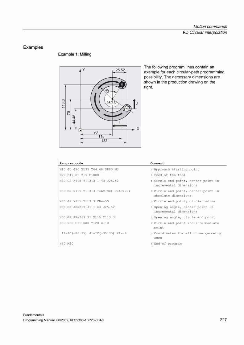
Motion commands 9.5 Circular interpolation
Fundamentals Programming Manual, 06/2009, 6FC5398-1BP20-0BA0 227
Examples Example 1: Milling
The following program lines contain an example for each circular-path programming possibility. The necessary dimensions are shown in the production drawing on the right.
Program code Comment
N10 G0 G90 X133 Y44.48 S800 M3 ; Approach starting point
N20 G17 G1 Z-5 F1000 ; Feed of the tool
N30 G2 X115 Y113.3 I-43 J25.52 ; Circle end point, center point in incremental dimensions
N30 G2 X115 Y113.3 I=AC(90) J=AC(70) ; Circle end point, center point in absolute dimensions
N30 G2 X115 Y113.3 CR=-50 ; Circle end point, circle radius
N30 G2 AR=269.31 I-43 J25.52 ; Opening angle, center point in incremental dimensions
N30 G2 AR=269.31 X115 Y113.3 ; Opening angle, circle end point
N30 N30 CIP X80 Y120 Z-10 ; Circle end point and intermediate point
I1=IC(-85.35) J1=IC(-35.35) K1=-6 ; Coordinates for all three geometry axes
N40 M30 ; End of program

Motion commands 9.5 Circular interpolation
Fundamentals 228 Programming Manual, 06/2009, 6FC5398-1BP20-0BA0
Example 2: Turning
Program code Comment
N.. ...
N120 G0 X12 Z0
N125 G1 X40 Z-25 F0.2
N130 G3 X70 Y-75 I-3.335 K-29.25 ; Circle end point, center point in incremental dimensions
N130 G3 X70 Y-75 I=AC(33.33) K=AC(-54.25) ; Circle end point, center point in absolute dimensions
N130 G3 X70 Z-75 CR=30 ; Circle end point, circle radius
N130 G3 X70 Z-75 AR=135.944 ; Opening angle, circle end point
N130 G3 I-3.335 K-29.25 AR=135.944 ; Opening angle, center point in incremental dimensions
N130 G3 I=AC(33.33) K=AC(-54.25) AR=135.944 ; Opening angle, center point in absolute dimensions
N130 G111 X33.33 Z-54.25 ; Polar coordinates
N135 G3 RP=30 AP=142.326 ; Polar coordinates
N130 CIP X70 Z-75 I1=93.33 K1=-54.25 ; Circular arc with intermediate point and end point
N140G1 Z-95
N.. ...
N40 M30 ; End of program

Motion commands 9.5 Circular interpolation
Fundamentals Programming Manual, 06/2009, 6FC5398-1BP20-0BA0 229
9.5.2 Circular interpolation with center point and end point (G2/G3, X... Y... Z..., I... J... K...)
Function Circular interpolation enables machining of full circles or arcs.
The circular movement is described by: ● The end point in Cartesian coordinates X, Y, Z and ● The circle center point at addresses I, J, K. If the circle is programmed with a center point but no end point, the result is a full circle.
Syntax G2/G3 X… Y… Z… I… J… K… G2/G3 X… Y… Z… I=AC(…) J=AC(…) K=(AC…)
Significance G2: Circular interpolation clockwise G3: Circular interpolation counter-clockwise X Y Z : End point in Cartesian coordinates I: Coordinates of the circle center point in the X direction J: Coordinates of the circle center point in the Y direction K: Coordinates of the circle center point in the Z direction =AC(…): Absolute dimensions (non-modal)

Motion commands 9.5 Circular interpolation
Fundamentals 230 Programming Manual, 06/2009, 6FC5398-1BP20-0BA0
Note G2 and G3 are modal. The default settings G90/G91 absolute and incremental dimensions are only valid for the circle end point. Per default, the center point coordinates I, J, K are entered in incremental dimensions in relation to the circle starting point. You can program the absolute center point dimensions in relation to the workpiece zero block-by-block with: I=AC(…), J=AC(…), K=AC(…). One interpolation parameter I, J, K with value 0 can be omitted, but the associated second parameter must always be specified.
Examples Example 1: Milling
Center point data using incremental dimensions N10 G0 X67.5 Y80.211 N20 G3 X17.203 Y38.029 I–17.5 J–30.211 F500
Center point data using absolute dimensions N10 G0 X67.5 Y80.211 N20 G3 X17.203 Y38.029 I=AC(50) J=AC(50)
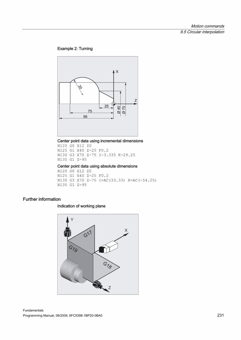
Motion commands 9.5 Circular interpolation
Fundamentals Programming Manual, 06/2009, 6FC5398-1BP20-0BA0 231
Example 2: Turning
Center point data using incremental dimensions N120 G0 X12 Z0 N125 G1 X40 Z-25 F0.2 N130 G3 X70 Z-75 I-3.335 K-29.25 N135 G1 Z-95
Center point data using absolute dimensions N120 G0 X12 Z0 N125 G1 X40 Z-25 F0.2 N130 G3 X70 Z-75 I=AC(33.33) K=AC(-54.25) N135 G1 Z-95
Further information Indication of working plane

Motion commands 9.5 Circular interpolation
Fundamentals 232 Programming Manual, 06/2009, 6FC5398-1BP20-0BA0
The control needs the working plane parameter (G17 to G19) to calculate the direction of rotation for the circle (G2 is clockwise or G3 is counter-clockwise).
It is advisable to specify the working plane generally. Exception: You can also machine circles outside the selected working plane (not with arc angle and helix parameters). In this case, the axis addresses that you specify as an end point determine the circle plane. Programmed feedrate FGROUP can be used to specify which axes are to be traversed with a programmed feedrate. For more information please refer to the Path behavior section.
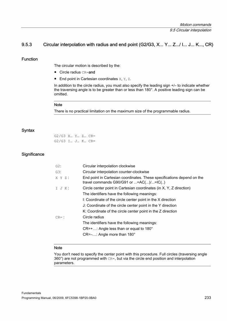
Motion commands 9.5 Circular interpolation
Fundamentals Programming Manual, 06/2009, 6FC5398-1BP20-0BA0 233
9.5.3 Circular interpolation with radius and end point (G2/G3, X... Y... Z.../ I... J... K..., CR)
Function The circular motion is described by the: ● Circle radius CR=and ● End point in Cartesian coordinates X, Y, Z. In addition to the circle radius, you must also specify the leading sign +/– to indicate whether the traversing angle is to be greater than or less than 180°. A positive leading sign can be omitted.
Note There is no practical limitation on the maximum size of the programmable radius.
Syntax G2/G3 X… Y… Z… CR= G2/G3 I… J… K… CR=
Significance G2: Circular interpolation clockwise G3: Circular interpolation counter-clockwise X Y Z : End point in Cartesian coordinates. These specifications depend on the
travel commands G90/G91 or ...=AC(...)/...=IC(..) I J K : Circle center point in Cartesian coordinates (in X, Y, Z direction)
The identifiers have the following meanings: I: Coordinate of the circle center point in the X direction J: Coordinate of the circle center point in the Y direction K: Coordinate of the circle center point in the Z direction
CR= : Circle radius The identifiers have the following meanings: CR=+…: Angle less than or equal to 180° CR=–…: Angle more than 180°
Note You don't need to specify the center point with this procedure. Full circles (traversing angle 360°) are not programmed with CR=, but via the circle end position and interpolation parameters.
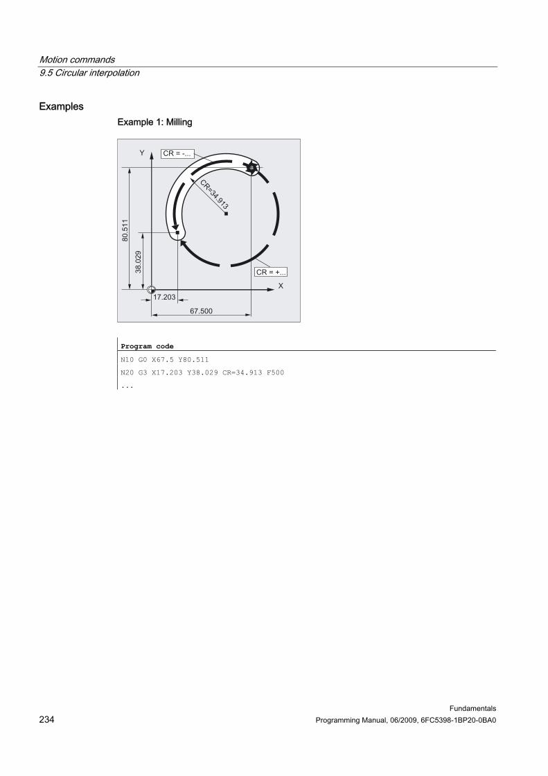
Motion commands 9.5 Circular interpolation
Fundamentals 234 Programming Manual, 06/2009, 6FC5398-1BP20-0BA0
Examples Example 1: Milling
Program code
N10 G0 X67.5 Y80.511
N20 G3 X17.203 Y38.029 CR=34.913 F500
...
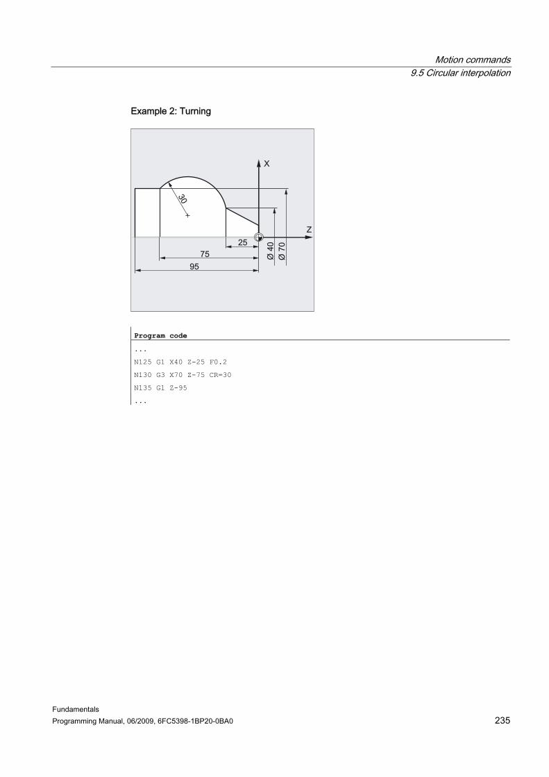
Motion commands 9.5 Circular interpolation
Fundamentals Programming Manual, 06/2009, 6FC5398-1BP20-0BA0 235
Example 2: Turning
Program code
...
N125 G1 X40 Z-25 F0.2
N130 G3 X70 Z-75 CR=30
N135 G1 Z-95
...

Motion commands 9.5 Circular interpolation
Fundamentals 236 Programming Manual, 06/2009, 6FC5398-1BP20-0BA0
9.5.4 Circular interpolation with opening angle and center point (G2/G3, X... Y... Z.../ I... J... K..., AR)
Function The circular movement is described by: ● The opening angle AR = and ● The end point in Cartesian coordinates X, Y, Z or ● The circle center at addresses I, J, K
Syntax G2/G3 X… Y… Z… AR= G2/G3 I… J… K… AR=
Significance G2: Circular interpolation clockwise G3: Circular interpolation counter-clockwise X Y Z : End point in Cartesian coordinates I J K : Circle center point in Cartesian coordinates (in X, Y, Z direction)
The identifiers have the following meanings: I: Coordinate of the circle center point in the X direction J: Coordinate of the circle center point in the Y direction K: Coordinate of the circle center point in the Z direction
AR= : Opening angle, range of values 0° to 360° =AC(…): Absolute dimensions (non-modal)
Note Full circles (traversing angle 360°) cannot be programmed with AR=, but must be programmed using the circle end position and interpolation parameters. The center point coordinates I, J, K are normally entered in incremental dimensions with reference to the circle starting point. You can program the absolute center point dimensions in relation to the workpiece zero block-by-block with: I=AC(…), J=AC(…), K=AC(…). One interpolation parameter I, J, K with value 0 can be omitted, but the associated second parameter must always be specified.

Motion commands 9.5 Circular interpolation
Fundamentals Programming Manual, 06/2009, 6FC5398-1BP20-0BA0 237
Examples Example 1: Milling
Program code
N10 G0 X67.5 Y80.211
N20 G3 X17.203 Y38.029 AR=140.134 F500
N20 G3 I–17.5 J–30.211 AR=140.134 F500

Motion commands 9.5 Circular interpolation
Fundamentals 238 Programming Manual, 06/2009, 6FC5398-1BP20-0BA0
Example 2: Turning
Z
X
54.2554.252525
9595 Ø 3
3.33
Ø 3
3.33
3030
Ø 4
0Ø
40
142.326°
Program code
N125 G1 X40 Z-25 F0.2
N130 G3 X70 Z-75 AR=135.944
N130 G3 I-3.335 K-29.25 AR=135.944
N130 G3 I=AC(33.33) K=AC(-54.25) AR=135.944
N135 G1 Z-95

Motion commands 9.5 Circular interpolation
Fundamentals Programming Manual, 06/2009, 6FC5398-1BP20-0BA0 239
9.5.5 Circular interpolation with polar coordinates (G2/G3, AP, RP)
Function The circular movement is described by: ● The polar angle AP=... ● The polar radius RP=... The following rule applies: ● The pole lies at the circle center. ● The polar radius corresponds to the circle radius.
Syntax G2/G3 AP= RP=
Significance G2: Circular interpolation clockwise G3: Circular interpolation counter-clockwise X Y Z : End point in Cartesian coordinates AP= : End point in polar coordinates, in this case polar angle RP= : End point in polar coordinates, in this case polar radius corresponds to circle
radius
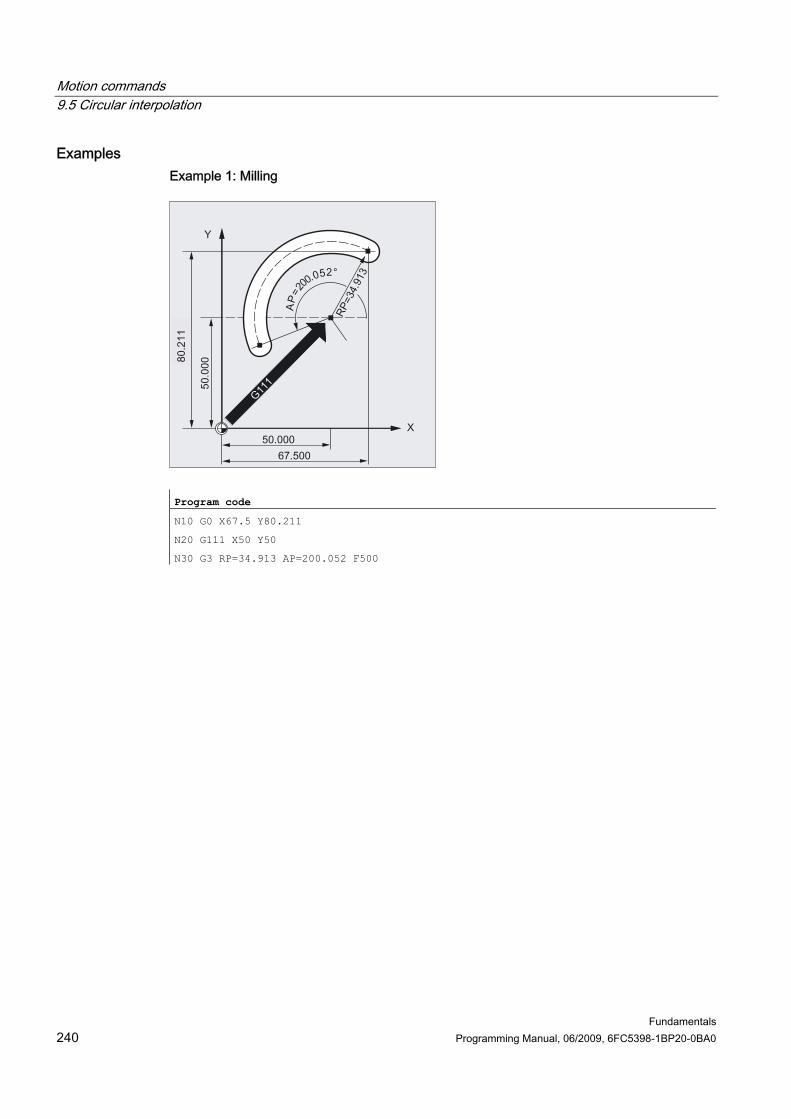
Motion commands 9.5 Circular interpolation
Fundamentals 240 Programming Manual, 06/2009, 6FC5398-1BP20-0BA0
Examples Example 1: Milling
Program code
N10 G0 X67.5 Y80.211
N20 G111 X50 Y50
N30 G3 RP=34.913 AP=200.052 F500
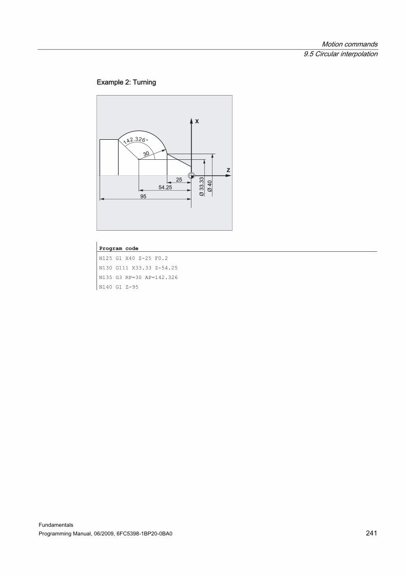
Motion commands 9.5 Circular interpolation
Fundamentals Programming Manual, 06/2009, 6FC5398-1BP20-0BA0 241
Example 2: Turning
Z
X
54.2554.252525
9595 Ø 3
3.33
Ø 3
3.33
3030
Ø 4
0Ø
40
142.326°
Program code
N125 G1 X40 Z-25 F0.2
N130 G111 X33.33 Z-54.25
N135 G3 RP=30 AP=142.326
N140 G1 Z-95

Motion commands 9.5 Circular interpolation
Fundamentals 242 Programming Manual, 06/2009, 6FC5398-1BP20-0BA0
9.5.6 Circular interpolation with intermediate point and end point (CIP, X... Y... Z..., I1... J1... K1...)
Function CIP can be used to program arcs. These arcs can also be inclined in space. In this case, you describe the intermediate and end points with three coordinates. The circular movement is described by: ● The intermediate point at addresses I1=, J1=, K1= and ● The end point in Cartesian coordinates X, Y, Z.
The traversing direction is determined by the order of the starting point, intermediate point and end point.
Syntax CIP X… Y… Z… I1=AC(…) J1=AC(…) K1=(AC…)
Motion commands 9.5 Circular interpolation
Fundamentals Programming Manual, 06/2009, 6FC5398-1BP20-0BA0 243
Meaning CIP: Circular interpolation through intermediate point X Y Z : End point in Cartesian coordinates. These specifications
depend on the travel commands G90/G91 or ...=AC(...)/...=IC(..)
I1= J1= K1= : Circle center point in Cartesian coordinates (in X, Y, Z direction) The identifiers have the following meanings: I: Coordinate of the circle center point in the X direction J: Coordinate of the circle center point in the Y direction K: Coordinate of the circle center point in the Z direction
=AC(…): Absolute dimensions (non-modal) =IC(…): Incremental dimensions (non-modal)
Note CIP is modal.
Input in absolute and incremental dimensions The G90/G91 defaults for absolute or incremental dimensions are valid for the intermediate and circle end points. With G91, the circle starting point is used as the reference for the intermediate point and end point.

Motion commands 9.5 Circular interpolation
Fundamentals 244 Programming Manual, 06/2009, 6FC5398-1BP20-0BA0
Examples Example 1: Milling
In order to machine an inclined circular groove, a circle is described by specifying the intermediate point with three interpolation parameters, and the end point with 3 coordinates.
Program code Comment
N10 G0 G90 X130 Y60 S800 M3 ; Approach starting point.
N20 G17 G1 Z-2 F100 ; Feed of the tool.
N30 CIP X80 Y120 Z-10 ; Circle end point and intermediate point.
I1= IC(-85.35)J1=IC(-35.35) K1=-6 ; Coordinates for all 3 geometry axes.
N40 M30 ; End of program.

Motion commands 9.5 Circular interpolation
Fundamentals Programming Manual, 06/2009, 6FC5398-1BP20-0BA0 245
Example 2: Turning
Program code
N125 G1 X40 Z-25 F0.2
N130 CIP X70 Z-75 I1=IC(26.665) K1=IC(-29.25)
N130 CIP X70 Z-75 I1=93.33 K1=-54.25
N135 G1 Z-95

Motion commands 9.5 Circular interpolation
Fundamentals 246 Programming Manual, 06/2009, 6FC5398-1BP20-0BA0
9.5.7 Circular interpolation with tangential transition (CT, X... Y... Z...)
Function The Tangential transition function is an expansion of the circle programming. The circle is defined by: ● The start and end point and ● The tangent direction at the start point. The G code CT produces an arc that lies at a tangent to the contour element programmed previously.
Determination of the tangent direction The tangent direction in the starting point of a CT block is determined from the end tangent of the programmed contour of the last block with a traversing motion. There can be any number of blocks without traversing information between this block and the current block.
Syntax CT X… Y… Z…

Motion commands 9.5 Circular interpolation
Fundamentals Programming Manual, 06/2009, 6FC5398-1BP20-0BA0 247
Significance CT: Circle with tangential transition X... Y... Z...: End point in Cartesian coordinates
Note CT is modal. As a rule, the circle is clearly defined by the tangent direction as well as the starting point and end point.
Examples Example 1: Milling
Milling a circular arc with CT directly after the straight part.
Program code Comment
N10 G0 X0 Y0 Z0 G90 T1 D1
N20 G41 X30 Y30 G1 F1000 ; Activation of TRC.
N30 CT X50 Y15 ; Circular-path programming with tangential transition.
N40 X60 Y-5
N50 G1 X70
N60 G0 G40 X80 Y0 Z20
N70 M30

Motion commands 9.5 Circular interpolation
Fundamentals 248 Programming Manual, 06/2009, 6FC5398-1BP20-0BA0
Example 2: Turning
Program code Comment
N110 G1 X23.293 Z0 F10
N115 X40 Z-30 F0.2
N120 CT X58.146 Z-42 ; Circular-path programming with tangential transition.
N125 G1 X70
Motion commands 9.5 Circular interpolation
Fundamentals Programming Manual, 06/2009, 6FC5398-1BP20-0BA0 249
Further information Splines In the case of splines, the tangential direction is defined by the straight line through the last two points. In the case of A and C splines with active ENAT or EAUTO, this direction is generally not the same as the direction at the end point of the spline. The transition of B splines is always tangential, the tangent direction is defined as for A or C splines and active ETAN. Frame change If a frame change takes place between the block defining the tangent and the CT block, the tangent is also subjected to this change. Limit case If the extension of the start tangent runs through the end point, a straight line is produced instead of a circle (limit case: circle with infinite radius). In this special case, TURN must either not be programmed or the value must be TURN=0.
Note When the values tend towards this limit case, circles with an unlimited radius are produced and machining with TURN unequal 0 is generally aborted with an alarm due to violation of the software limits.
Position of the circle plane The position of the circle plane depends on the active plane (G17-G19). If the tangent of the previous block does not lie in the active plane, its projection in the active plane is used. If the start and end points do not have the same position components perpendicular to the active plane, a helix is produced instead of a circle.
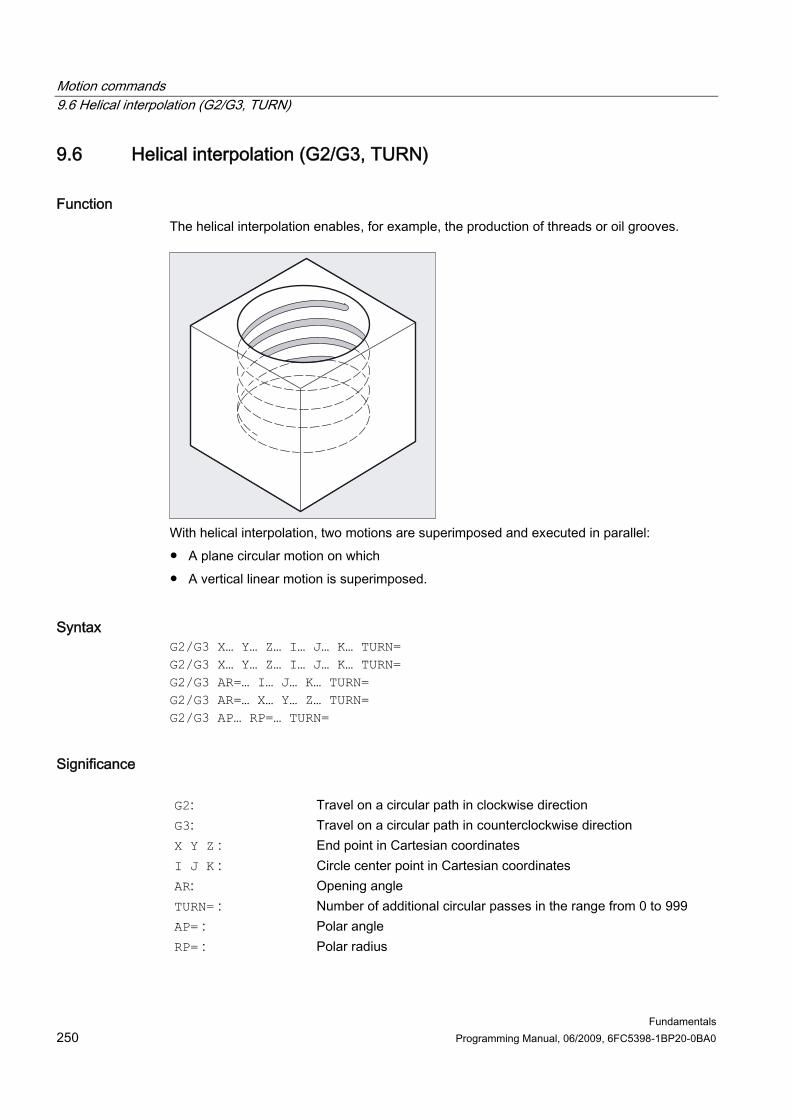
Motion commands 9.6 Helical interpolation (G2/G3, TURN)
Fundamentals 250 Programming Manual, 06/2009, 6FC5398-1BP20-0BA0
9.6 9.6 Helical interpolation (G2/G3, TURN)
Function The helical interpolation enables, for example, the production of threads or oil grooves.
With helical interpolation, two motions are superimposed and executed in parallel: ● A plane circular motion on which ● A vertical linear motion is superimposed.
Syntax G2/G3 X… Y… Z… I… J… K… TURN= G2/G3 X… Y… Z… I… J… K… TURN= G2/G3 AR=… I… J… K… TURN= G2/G3 AR=… X… Y… Z… TURN= G2/G3 AP… RP=… TURN=
Significance G2: Travel on a circular path in clockwise direction G3: Travel on a circular path in counterclockwise direction X Y Z : End point in Cartesian coordinates I J K : Circle center point in Cartesian coordinates AR: Opening angle TURN= : Number of additional circular passes in the range from 0 to 999 AP= : Polar angle RP= : Polar radius

Motion commands 9.6 Helical interpolation (G2/G3, TURN)
Fundamentals Programming Manual, 06/2009, 6FC5398-1BP20-0BA0 251
Note G2 and G3 are modal. The circular motion is performed in those axes that are defined by the specification of the working plane.
Example
Program code Comment
N10 G17 G0 X27.5 Y32.99 Z3 ; Approach of the starting position.
N20 G1 Z-5 F50 ; Feed of the tool.
N30 G3 X20 Y5 Z-20 I=AC(20) J=AC(20) TURN=2 ; Helix with the specifications: Execute 2 full circles after the starting position, then travel to end point.
N40 M30 ; End of program.

Motion commands 9.6 Helical interpolation (G2/G3, TURN)
Fundamentals 252 Programming Manual, 06/2009, 6FC5398-1BP20-0BA0
Further information Sequence of motions 1. Approach starting point 2. Execute the full circles programmed with TURN=. 3. Approach circle end position, e.g. as part rotation. 4. Execute steps 2 and 3 across the infeed depth. The pitch, with which the helix is to be machined is calculated from the number of full circles plus the programmed circle end position (executed across the infeed depth).
Programming the end point for helical interpolation Please refer to circular interpolation for a detailed description of the interpolation parameters. Programmed feedrate For helical interpolation, it is advisable to specify a programmed feedrate override (CFC). FGROUP can be used to specify which axes are to be traversed with a programmed feedrate. For more information please refer to the Path behavior section.

Motion commands 9.7 Involute interpolation (INVCW, INVCCW)
Fundamentals Programming Manual, 06/2009, 6FC5398-1BP20-0BA0 253
9.7 9.7 Involute interpolation (INVCW, INVCCW)
Function The involute of the circle is a curve traced out from the end point on a "piece of string" unwinding from the curve. Involute interpolation allows trajectories along an involute. It is executed in the plane in which the basic circle is defined and runs from the programmed starting point to the programmed end point.
The end point can be programmed in two ways: 1. Directly via Cartesian coordinates 2. Indirectly by specifying an opening angle (also refer to the programming of the opening
angle for the circular-path programming) If the starting point and the end point are in the plane of the basic circle, then, analogous to the helical interpolation for circles, there is a superimposition to a curve in space. With additional specification of paths perpendicular to the active plane, an involute can be traversed in space (comparable to the helical interpolation for circles).

Motion commands 9.7 Involute interpolation (INVCW, INVCCW)
Fundamentals 254 Programming Manual, 06/2009, 6FC5398-1BP20-0BA0
Syntax INVCW X... Y... Z... I... J... K... CR=... INVCCW X... Y... Z... I... J... K... CR=... INVCW I... J... K... CR=... AR=... INVCCW I... J... K... CR=... AR=...
Meaning INVCW: Command to travel on an involute in clockwise direction INVCCW: Command to travel on an involute in counterclockwise
direction X... Y... Z... : Direct programming of the end point in Cartesian coordinates I... J... K... : Interpolation parameters for the description of the center point
of the basic circle in Cartesian coordinates Note: The coordinate specifications refer to the starting point of the involute.
CR=... : Radius of the basic circle Indirect programming of the end point through specification of an opening angle (angle of rotation) The origin of the opening angle is the line from the circle center point to the starting point. AR > 0: The path of the involute moves away from the
basic circle.
AR=... :
AR < 0: The path of the involute moves towards the basic circle. For AR < 0, the maximum angle of rotation is restricted by the fact that the end point must always be outside the basic circle.
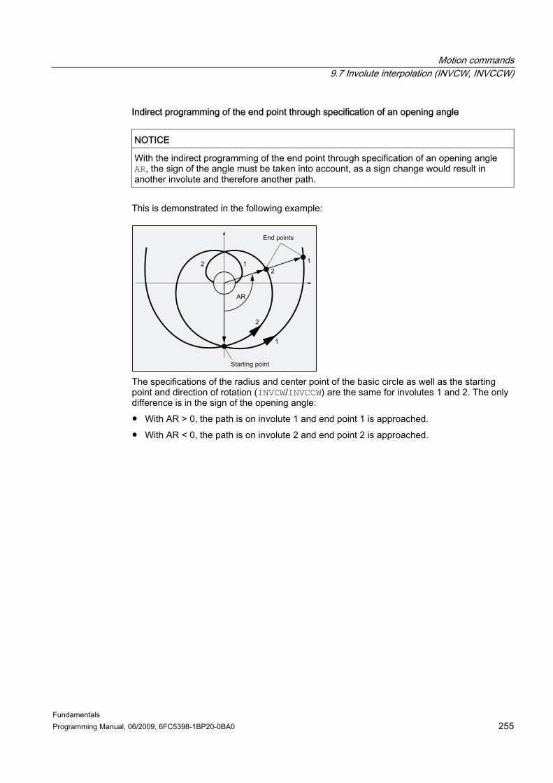
Motion commands 9.7 Involute interpolation (INVCW, INVCCW)
Fundamentals Programming Manual, 06/2009, 6FC5398-1BP20-0BA0 255
Indirect programming of the end point through specification of an opening angle
NOTICE With the indirect programming of the end point through specification of an opening angle AR, the sign of the angle must be taken into account, as a sign change would result in another involute and therefore another path.
This is demonstrated in the following example:
The specifications of the radius and center point of the basic circle as well as the starting point and direction of rotation (INVCW/INVCCW) are the same for involutes 1 and 2. The only difference is in the sign of the opening angle: ● With AR > 0, the path is on involute 1 and end point 1 is approached. ● With AR < 0, the path is on involute 2 and end point 2 is approached.

Motion commands 9.7 Involute interpolation (INVCW, INVCCW)
Fundamentals 256 Programming Manual, 06/2009, 6FC5398-1BP20-0BA0
Supplementary conditions ● Both the starting point and the end point must be outside the area of the basic circle of
the involute (circle with radius CR around the center point specified by I, J, K). If this condition is not satisfied, an alarm is generated and the program processing is aborted.
● The two options for the programming of the end point (directly via Cartesian coordinates or indirectly via the specification of an opening angle) are mutually exclusive. Consequently, only one of the two programming options may be used in a block.
● If the programmed end point does not lie exactly on the involute defined by the starting point and basic circle, interpolation takes place between the two involutes defined by the starting and end points (see following figure).
The maximum deviation of the end point is determined by a machine data (→ machine manufacturer). If the deviation of the programmed end point in the radial direction is greater than that by the MD, then an alarm is generated and the program processing aborted.

Motion commands 9.7 Involute interpolation (INVCW, INVCCW)
Fundamentals Programming Manual, 06/2009, 6FC5398-1BP20-0BA0 257
Examples Example 1: Counterclockwise involute from the starting point to the programmed end point and back again as clockwise involute
Program code Comment
N10 G1 X10 Y0 F5000 ; Approach of the starting position.
N15 G17 ; Selection of the X/Y plane as working plane.
N20 INVCCW X32.77 Y32.77 CR=5 I-10 J0 ; Counterclockwise involute, end point in Cartesian coordinates.
N30 INVCW X10 Y0 CR=5 I-32.77 J-32.77 ; Clockwise involute, starting point is end point from N20, new end point is starting point from N20, new circle center point refers to a new starting point and is the same as the old circle center point.
...

Motion commands 9.7 Involute interpolation (INVCW, INVCCW)
Fundamentals 258 Programming Manual, 06/2009, 6FC5398-1BP20-0BA0
Example 2: Counterclockwise involute with indirect programming of the end point through specification of an opening angle
Program code Comment
N10 G1 X10 Y0 F5000 ; Approach of the starting position.
N15 G17 ; Selection of the X/Y plane as working plane.
N20 INVCCW CR=5 I-10 J0 AR=360 ; Counterclockwise involute and away from the basic circle (as positive angle specification) with one full revolution (360 degrees).
...
References For more information about machine data and supplementary conditions that are relevant to involute interpolation, see: Function Manual, Basic Functions; Various NC/PLC interface signals and functions (A2), Chapter: "Settings for involute interpolation"
Motion commands 9.8 Contour definitions
Fundamentals Programming Manual, 06/2009, 6FC5398-1BP20-0BA0 259
9.8 9.8 Contour definitions
Function The contour definition programming is used for the quick input of simple contours. Programmable are contour definitions with one, two, three or more points with the transition elements chamfer or rounding, through specification of Cartesian coordinates and/or angles. Arbitrary further NC addresses can be used, e.g. address letters for further axes (single axes or axis perpendicular to the machining plane), auxiliary function specifications, G codes, velocities, etc. in the blocks that describe contour definitions.
Note Contour calculator The contour definitions can be programmed easily with the aid of the contour calculator. This is a user interface tool that enables the programming and graphic display of simple and complex workpiece contours. The contours programmed via the contour calculator are transferred to the part program. References: Operating Manual
Assigning parameters The identifiers for angle, radius and chamfer are defined via machine data: MD10652 $MN_CONTOUR_DEF_ANGLE_NAME (name of the angle for contour definitions) MD10654 $MN_RADIUS_NAME (name of the radius for contour definitions) MD10656 $MN_CHAMFER_NAME (name of the chamfer for contour definitions)
Note See machine manufacturer's specifications.

Motion commands 9.8 Contour definitions
Fundamentals 260 Programming Manual, 06/2009, 6FC5398-1BP20-0BA0
9.8.1 Contour definitions: One straight line (ANG)
Note In the following description it is assumed that • G18 is active (⇒ active working plane is the Z/X plane).
(However, the programming of contour definitions is also possible without restrictions with G17 or G19.)
• The following identifiers have been defined for angle, radius and chamfer: – ANG (angle) – RND (radius) – CHR (chamfer)
Function The end point of the straight line is defined by the following specifications: ● Angle ANG ● One Cartesian end point coordinate (X2 or Z2)
ANG: Angle of the straight line X1, Z1: Start coordinates X2, Z2: End point coordinates of the straight line

Motion commands 9.8 Contour definitions
Fundamentals Programming Manual, 06/2009, 6FC5398-1BP20-0BA0 261
Syntax X… ANG=… Z… ANG=…
Significance X... : End point coordinate in the X direction Z... : End point coordinate in the Z direction ANG: Identifier for the angle programming
The specified value (angle) refers to the abscissa of the active working plane (Z axis with G18).
Example Program code Comment
N10 X5 Z70 F1000 G18 ; Approach of the starting position.
N20 X88.8 ANG=110 ; Straight line with angle specification.
N30 ...
or Program code Comment
N10 X5 Z70 F1000 G18 ; Approach of the starting position.
N20 Z39.5 ANG=110 ; Straight line with angle specification.
N30 ...

Motion commands 9.8 Contour definitions
Fundamentals 262 Programming Manual, 06/2009, 6FC5398-1BP20-0BA0
9.8.2 Contour definitions: Two straight lines (ANG)
Note In the following description it is assumed that: • G18 is active (⇒ active working plane is the Z/X plane).
(However, the programming of contour definitions is also possible without restrictions with G17 or G19.)
• The following identifiers have been defined for angle, radius and chamfer: – ANG (angle) – RND (radius) – CHR (chamfer)
Function The end point of the first straight line can be programmed by specifying the Cartesian coordinates or by specifying the angle of the two straight lines. The end point of the second straight line must always be programmed with Cartesian coordinates. The intersection of the two straight lines can be designed as a corner, curve or chamfer.
ANG1: Angle of the first straight line ANG2: Angle of the second straight line X1, Z1: Start coordinates of the first straight line X2, Z2: End point coordinates of the first straight line or
start coordinates of the second straight line X3, Z3: End point coordinates of the second straight line
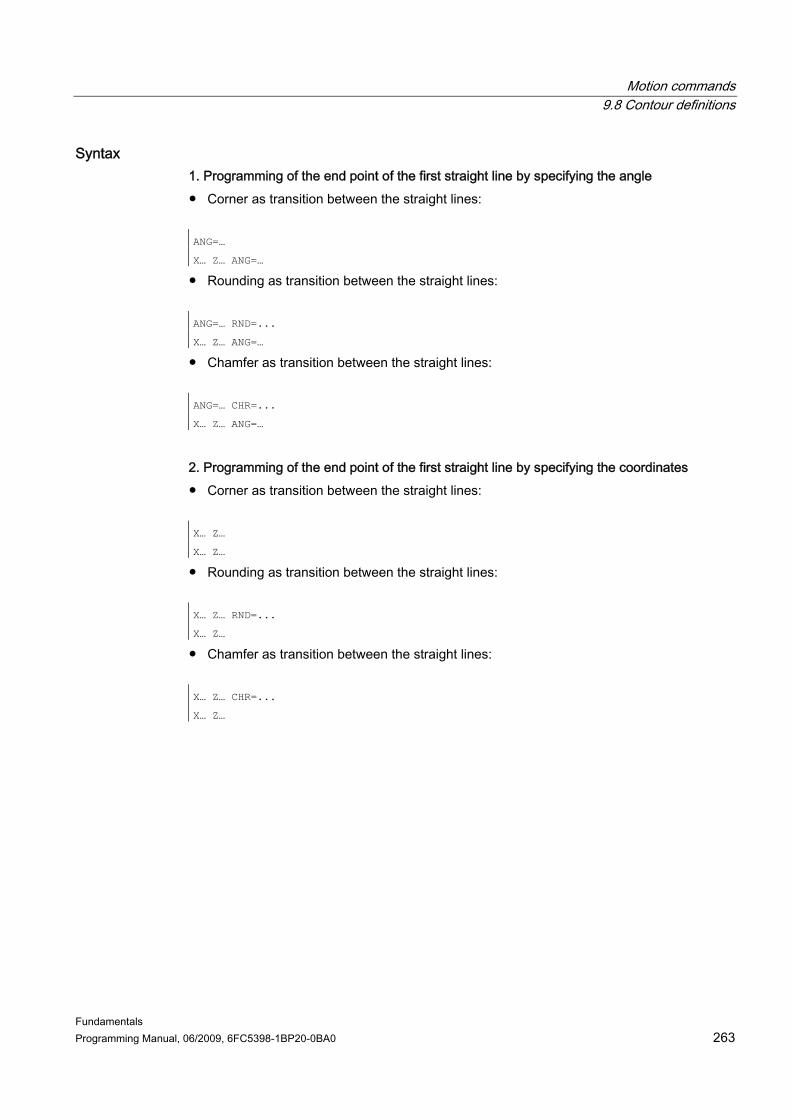
Motion commands 9.8 Contour definitions
Fundamentals Programming Manual, 06/2009, 6FC5398-1BP20-0BA0 263
Syntax 1. Programming of the end point of the first straight line by specifying the angle ● Corner as transition between the straight lines: ANG=…
X… Z… ANG=…
● Rounding as transition between the straight lines: ANG=… RND=...
X… Z… ANG=…
● Chamfer as transition between the straight lines: ANG=… CHR=...
X… Z… ANG=…
2. Programming of the end point of the first straight line by specifying the coordinates ● Corner as transition between the straight lines: X… Z…
X… Z…
● Rounding as transition between the straight lines: X… Z… RND=...
X… Z…
● Chamfer as transition between the straight lines: X… Z… CHR=...
X… Z…

Motion commands 9.8 Contour definitions
Fundamentals 264 Programming Manual, 06/2009, 6FC5398-1BP20-0BA0
Significance ANG=... : Identifier for angle programming
The specified value (angle) refers to the abscissa of the active working plane (Z axis with G18).
RND=... : Identifier for the programming of a rounding The specified value corresponds to the radius of the rounding:
CHR=... : Identifier for the programming of a chamfer The specified value corresponds to the width of the chamfer in the direction of motion:
X... : Coordinates in the X direction Z... : Coordinates in the Z direction
Note For further information on the programming of a chamfer or rounding, see "Chamfer, rounding (CHF, CHR, RND, RNDM, FRC, FRCM) (Page 295)".

Motion commands 9.8 Contour definitions
Fundamentals Programming Manual, 06/2009, 6FC5398-1BP20-0BA0 265
Example Program code Comment
N10 X10 Z80 F1000 G18 ; Approach of the starting position.
N20 ANG=148.65 CHR=5.5 ; Straight line with angle and chamfer specification.
N30 X85 Z40 ANG=100 ; Straight line with angle and end point specification.
N40 ...
9.8.3 Contour definitions: Three straight line (ANG)
Note In the following description it is assumed that: • G18 is active (⇒ active working plane is the Z/X plane).
(However, the programming of contour definitions is also possible without restrictions with G17 or G19.)
• The following identifiers have been defined for angle, radius and chamfer: – ANG (angle) – RND (radius) – CHR (chamfer)
Function The end point of the first straight line can be programmed by specifying the Cartesian coordinates or by specifying the angle of the two straight lines. The end point of the second and third straight lines must always be programmed with Cartesian coordinates. The intersection of the straight lines can be designed as a corner, a curve, or a chamfer.
Note The programming described here for a three point contour definition can be expanded arbitrarily for contour definitions with more than three points.
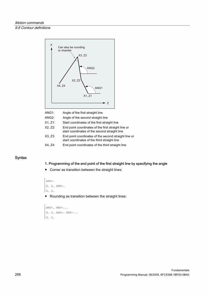
Motion commands 9.8 Contour definitions
Fundamentals 266 Programming Manual, 06/2009, 6FC5398-1BP20-0BA0
ANG1: Angle of the first straight line ANG2: Angle of the second straight line X1, Z1: Start coordinates of the first straight line X2, Z2: End point coordinates of the first straight line or
start coordinates of the second straight line X3, Z3: End point coordinates of the second straight line or
start coordinates of the third straight line X4, Z4: End point coordinates of the third straight line
Syntax 1. Programming of the end point of the first straight line by specifying the angle ● Corner as transition between the straight lines: ANG=…
X… Z… ANG=…
X… Z…
● Rounding as transition between the straight lines: ANG=… RND=...
X… Z… ANG=… RND=...
X… Z…

Motion commands 9.8 Contour definitions
Fundamentals Programming Manual, 06/2009, 6FC5398-1BP20-0BA0 267
● Chamfer as transition between the straight lines: ANG=… CHR=...
X… Z… ANG=… CHR=...
X… Z…
2. Programming of the end point of the first straight line by specifying the coordinates ● Corner as transition between the straight lines: X… Z…
X… Z…
X… Z…
● Rounding as transition between the straight lines: X… Z… RND=...
X… Z… RND=...
X… Z…
● Chamfer as transition between the straight lines: X… Z… CHR=...
X… Z… CHR=...
X… Z…
Significance ANG=... : Identifier for angle programming
The specified value (angle) refers to the abscissa of the active working plane (Z axis with G18).
RND=... : Identifier for programming a rounding The specified value corresponds to the radius of the rounding:
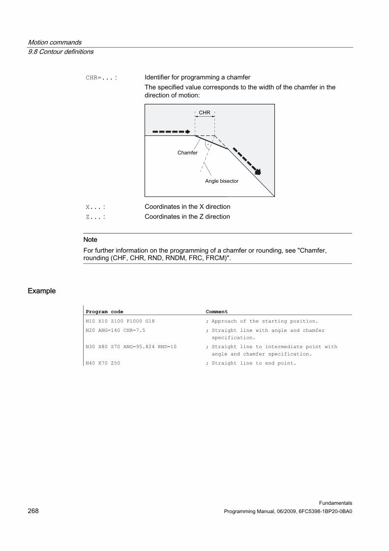
Motion commands 9.8 Contour definitions
Fundamentals 268 Programming Manual, 06/2009, 6FC5398-1BP20-0BA0
CHR=... : Identifier for programming a chamfer The specified value corresponds to the width of the chamfer in the direction of motion:
X... : Coordinates in the X direction Z... : Coordinates in the Z direction
Note For further information on the programming of a chamfer or rounding, see "Chamfer, rounding (CHF, CHR, RND, RNDM, FRC, FRCM)".
Example Program code Comment
N10 X10 Z100 F1000 G18 ; Approach of the starting position.
N20 ANG=140 CHR=7.5 ; Straight line with angle and chamfer specification.
N30 X80 Z70 ANG=95.824 RND=10 ; Straight line to intermediate point with angle and chamfer specification.
N40 X70 Z50 ; Straight line to end point.
Motion commands 9.8 Contour definitions
Fundamentals Programming Manual, 06/2009, 6FC5398-1BP20-0BA0 269
9.8.4 Contour definitions: End point programming with angle
Function If the address letter A appears in an NC block, either none, one or both of the axes in the active plane may also be programmed. Number of programmed axes ● If no axis of the active plane has been programmed, then this is either the first or second
block of a contour definition consisting of two blocks. If it is the second block of such a contour definition, then this means that the starting point and end point in the active plane are identical. The contour definition is then at best a motion perpendicular to the active plane.
● If exactly one axis of the active plane has been programmed, then this is either a single straight line whose end point can be clearly defined via the angle and programmed Cartesian coordinate or the second block of a contour definition consisting of two blocks. In the second case, the missing coordinate is set to the same as the last (modal) position reached.
● If two axes of the active plane have been programmed, then this is the second block of a contour definition consisting of two blocks. If the current block has not been preceded by a block with angle programming without programmed axes of the active plane, then this block is not permitted.
Angle A may only be programmed for linear or spline interpolation.

Motion commands 9.9 Thread cutting with constant lead (G33)
Fundamentals 270 Programming Manual, 06/2009, 6FC5398-1BP20-0BA0
9.9 9.9 Thread cutting with constant lead (G33)
9.9.1 Thread cutting with constant lead (G33, SF)
Function Threads with constant lead can be machined with G33: ● Cylinder thread ③ ● Face thread ② ● Tapered thread ①
Note Technical requirement for thread cutting with G33 is a variable-speed spindle with position measuring system.

Motion commands 9.9 Thread cutting with constant lead (G33)
Fundamentals Programming Manual, 06/2009, 6FC5398-1BP20-0BA0 271
Multiple thread Multiple thread (thread with offset cuts) can be machined by specifying a starting point offset. The programming is performed in the G33 block at address SF.
Note If no starting point offset is specified, the "starting angle for thread" defined in the setting data is used.
Thread chain A thread chain can be machined with several G33 blocks programmed in succession:

Motion commands 9.9 Thread cutting with constant lead (G33)
Fundamentals 272 Programming Manual, 06/2009, 6FC5398-1BP20-0BA0
Note With continuous-path mode G64, the blocks are linked by the look-ahead velocity control in such a way that there are no velocity jumps.
Direction of rotation of the thread The direction of rotation of the thread is determined by the direction of rotation of the spindle: ● Clockwise with M3 produces a right-hand thread ● Counterclockwise with M4 produces a left-hand thread
Syntax Cylinder thread: G33 Z… K… G33 Z… K… SF=…
Face thread: G33 X… I… G33 X… I… SF=…
Tapered thread: G33 X… Z… K… G33 X… Z… K… SF=… G33 X… Z… I… G33 X… Z… I… SF=…
Significance G33: Command for thread cutting with constant lead X... Y... Z... : End point(s) in Cartesian coordinates I... : Thread lead in X direction J... : Thread lead in Y direction K... : Thread lead in Z direction Z: Longitudinal axis X: Transverse axis Z... K... : Thread length and lead for cylinder threads X... I... : Thread diameter and thread lead for face threads
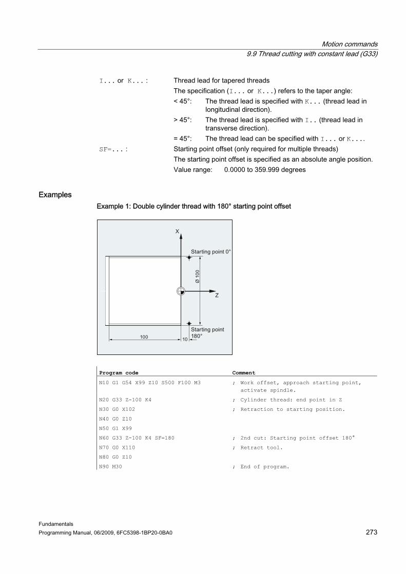
Motion commands 9.9 Thread cutting with constant lead (G33)
Fundamentals Programming Manual, 06/2009, 6FC5398-1BP20-0BA0 273
Thread lead for tapered threads The specification (I... or K...) refers to the taper angle: < 45°: The thread lead is specified with K... (thread lead in
longitudinal direction). > 45°: The thread lead is specified with I.. (thread lead in
transverse direction).
I... or K... :
= 45°: The thread lead can be specified with I... or K.... Starting point offset (only required for multiple threads) The starting point offset is specified as an absolute angle position.
SF=... :
Value range: 0.0000 to 359.999 degrees
Examples Example 1: Double cylinder thread with 180° starting point offset
Program code Comment
N10 G1 G54 X99 Z10 S500 F100 M3 ; Work offset, approach starting point, activate spindle.
N20 G33 Z-100 K4 ; Cylinder thread: end point in Z
N30 G0 X102 ; Retraction to starting position.
N40 G0 Z10
N50 G1 X99
N60 G33 Z-100 K4 SF=180 ; 2nd cut: Starting point offset 180°
N70 G0 X110 ; Retract tool.
N80 G0 Z10
N90 M30 ; End of program.
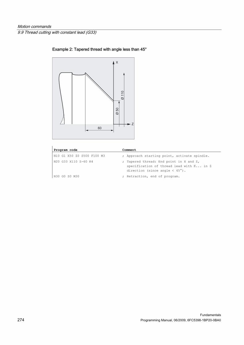
Motion commands 9.9 Thread cutting with constant lead (G33)
Fundamentals 274 Programming Manual, 06/2009, 6FC5398-1BP20-0BA0
Example 2: Tapered thread with angle less than 45°
Program code Comment
N10 G1 X50 Z0 S500 F100 M3 ; Approach starting point, activate spindle.
N20 G33 X110 Z-60 K4 ; Tapered thread: End point in X and Z, specification of thread lead with K... in Z direction (since angle < 45°).
N30 G0 Z0 M30 ; Retraction, end of program.
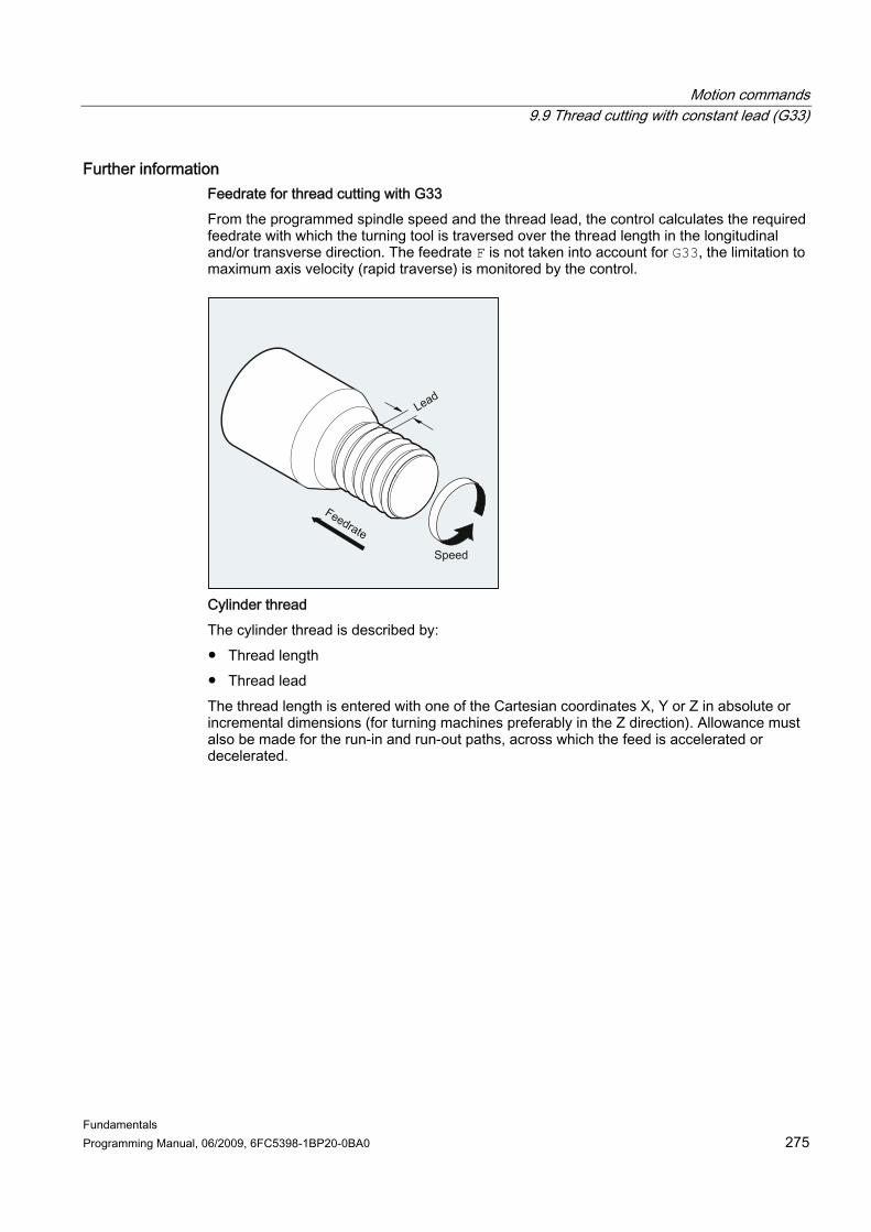
Motion commands 9.9 Thread cutting with constant lead (G33)
Fundamentals Programming Manual, 06/2009, 6FC5398-1BP20-0BA0 275
Further information Feedrate for thread cutting with G33 From the programmed spindle speed and the thread lead, the control calculates the required feedrate with which the turning tool is traversed over the thread length in the longitudinal and/or transverse direction. The feedrate F is not taken into account for G33, the limitation to maximum axis velocity (rapid traverse) is monitored by the control.
Cylinder thread The cylinder thread is described by: ● Thread length ● Thread lead The thread length is entered with one of the Cartesian coordinates X, Y or Z in absolute or incremental dimensions (for turning machines preferably in the Z direction). Allowance must also be made for the run-in and run-out paths, across which the feed is accelerated or decelerated.

Motion commands 9.9 Thread cutting with constant lead (G33)
Fundamentals 276 Programming Manual, 06/2009, 6FC5398-1BP20-0BA0
The thread lead is entered at addresses I, J, K (K is preferable for turning machines).
Face thread The face thread is described by: ● Thread diameter (preferably in the X direction) ● Thread lead (preferably with I)

Motion commands 9.9 Thread cutting with constant lead (G33)
Fundamentals Programming Manual, 06/2009, 6FC5398-1BP20-0BA0 277
Tapered thread The tapered thread is described by: ● End point in the longitudinal and transverse direction (taper contour) ● Thread lead The taper contour is entered in Cartesian coordinates X, Y, Z in absolute or incremental dimensions - preferentially in the X and Z direction for machining on turning machines. Allowance must also be made for the run-in and run-out paths, across which the feed is accelerated or decelerated. The specification of the lead depends on the taper angle (angle between the longitudinal axis and the outside of the taper):
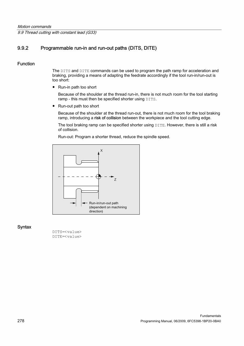
Motion commands 9.9 Thread cutting with constant lead (G33)
Fundamentals 278 Programming Manual, 06/2009, 6FC5398-1BP20-0BA0
9.9.2 Programmable run-in and run-out paths (DITS, DITE)
Function The DITS and DITE commands can be used to program the path ramp for acceleration and braking, providing a means of adapting the feedrate accordingly if the tool run-in/run-out is too short: ● Run-in path too short
Because of the shoulder at the thread run-in, there is not much room for the tool starting ramp - this must then be specified shorter using DITS.
● Run-out path too short Because of the shoulder at the thread run-out, there is not much room for the tool braking ramp, introducing a risk of collision between the workpiece and the tool cutting edge. The tool braking ramp can be specified shorter using DITE. However, there is still a risk of collision. Run-out: Program a shorter thread, reduce the spindle speed.
Syntax DITS=<value> DITE=<value>
Motion commands 9.9 Thread cutting with constant lead (G33)
Fundamentals Programming Manual, 06/2009, 6FC5398-1BP20-0BA0 279
Significance DITS: Define thread run-in path DITE: Define thread run-out path
Value specification for the run-in/run-out path <value>: Range of values: -1, 0, ... n
Note Only paths, and not positions, are programmed with DITS and DITE.
Note The DITS and DITE commands relate to setting data SD42010 $SC_THREAD_RAMP_DISP[0,1], in which the programmed paths are written. If no run-in/deceleration path is programmed before or in the first thread block, the corresponding value is determined by the current value of SD42010. References: Function Manual, Basic Functions; Feedrates (V1)
Example Program code Comment
...
N40 G90 G0 Z100 X10 SOFT M3 S500
N50 G33 Z50 K5 SF=180 DITS=1 DITE=3 ; Start of smoothing with Z=53.
N60 G0 X20

Motion commands 9.9 Thread cutting with constant lead (G33)
Fundamentals 280 Programming Manual, 06/2009, 6FC5398-1BP20-0BA0
Further information If the run-in and/or run-out path is very short, the acceleration of the thread axis is higher than the configured value. This causes an acceleration overload on the axis. Alarm 22280 ("Programmed run-in path too short") is then issued for the thread run-in (with the appropriate configuration in MD11411 $MN_ENABLE_ALARM_MASK). The alarm is purely for information and has no effect on part program execution. MD10710 $MN_PROG_SD_RESET_SAVE_TAB can be used to specify that the value written by the part program is written to the corresponding setting data during RESET. The values are, therefore, retained following power off/on.
Note DITE acts at the end of the thread as a rounding clearance. This achieves a smooth change in the axis movement. When a block with the DITS and/or DITE command is loaded to the interpolator, the path programmed under DITS is written to SD42010 $SC_THREAD_RAMP_DISP[0] and the pathprogrammed under DITE is written to SD42010 $SC_THREAD_RAMP_DISP[1]. The current dimensions setting (inch/metric) is applied to the programmed run-in/run-out path.

Motion commands 9.10 Thread cutting with increasing or decreasing lead (G34, G35)
Fundamentals Programming Manual, 06/2009, 6FC5398-1BP20-0BA0 281
9.10 9.10 Thread cutting with increasing or decreasing lead (G34, G35)
Function With the commands G34 and G35, the G33 functionality has been extended with the option of programming a change in the thread lead at address F. With G34, this results in a linear increase and with G35 to a linear decrease of the thread lead. The commands G34 and G35 can therefore be used for the machining of self-tapping threads.
Syntax Cylinder thread with increasing lead: G34 Z… K… F...
Cylinder thread with decreasing lead: G35 Z… K… F...
Face thread with increasing lead: G34 X… I… F...
Face thread with decreasing lead: G35 X… I… F...
Taper thread with increasing lead: G34 X… Z… K… F... G34 X… Z… I… F...
Taper thread with decreasing lead: G35 X… Z… K… F... G35 X… Z… I… F...
Significance G34: Command for thread cutting with linear increasing lead G35: Command for thread cutting with linear decreasing lead X... Y... Z... : End point(s) in Cartesian coordinates I... : Thread lead in X direction J... : Thread lead in Y direction K... : Thread lead in Z direction
Thread lead change If you already know the starting and final lead of a thread, you can calculate the thread lead change to be programmed according to the following equation:
The identifiers have the following meanings:
F...:
ka: Thread lead (thread lead of axis target point coordinate) [mm/rev]
Motion commands 9.10 Thread cutting with increasing or decreasing lead (G34, G35)
Fundamentals 282 Programming Manual, 06/2009, 6FC5398-1BP20-0BA0
kG: Starting thread lead (programmed under I, J, or K) [mm/rev] IG: Thread length [mm]
Example Program code Comment
N1608 M3 S10 ; Spindle on.
N1609 G0 G64 Z40 X216 ; Approach starting point.
N1610 G33 Z0 K100 SF=R14 ; Thread cutting with constant lead (100 mm/rev)
N1611 G35 Z-200 K100 F17.045455 ; Lead decrease: 17.0454 mm/rev2
Lead at end of block: 50mm/rev
N1612 G33 Z-240 K50 ; Traverse thread block without jerk.
N1613 G0 X218
N1614 G0 Z40
N1615 M17
References Function Manual, Basic Functions; Feedrates (V1), Section "Linear increasing/decreasing thread lead change with G34 and G35"
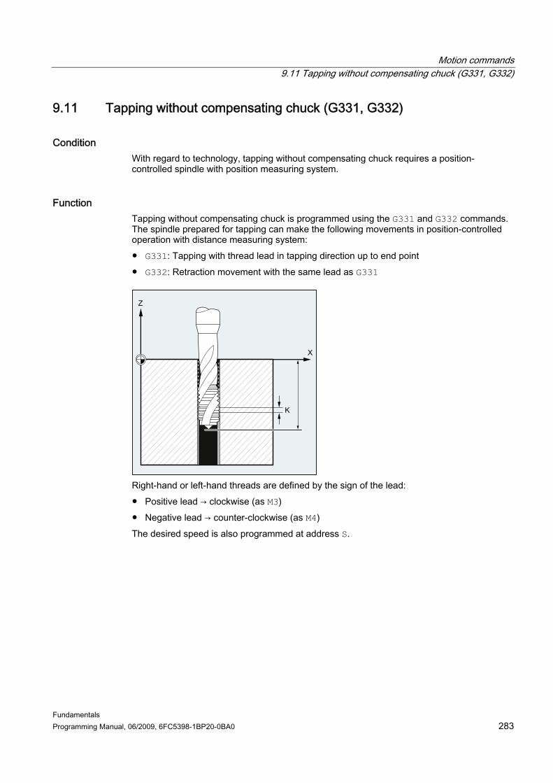
Motion commands 9.11 Tapping without compensating chuck (G331, G332)
Fundamentals Programming Manual, 06/2009, 6FC5398-1BP20-0BA0 283
9.11 9.11 Tapping without compensating chuck (G331, G332)
Condition With regard to technology, tapping without compensating chuck requires a position-controlled spindle with position measuring system.
Function Tapping without compensating chuck is programmed using the G331 and G332 commands. The spindle prepared for tapping can make the following movements in position-controlled operation with distance measuring system: ● G331: Tapping with thread lead in tapping direction up to end point ● G332: Retraction movement with the same lead as G331
Right-hand or left-hand threads are defined by the sign of the lead: ● Positive lead → clockwise (as M3) ● Negative lead → counter-clockwise (as M4) The desired speed is also programmed at address S.

Motion commands 9.11 Tapping without compensating chuck (G331, G332)
Fundamentals 284 Programming Manual, 06/2009, 6FC5398-1BP20-0BA0
Syntax SPOS=<value>
G331 S...
G331 X… Y… Z… I… J… K…
G332 X… Y… Z… I… J… K…
● SPOS (or M70) only has to be programmed prior to tapping: – For threads requiring multiple machining operations for their production – For production processes requiring a defined thread starting position Conversely, when machining multiple threads one after the other, SPOS (or M70) does not have to be programmed (advantage: saves time).
● The spindle speed has to be in a dedicated G331 block without axis motion before tapping (G331 X… Y… Z… I… J… K…).
Significance
Command: Tapping The hole is defined by the drilling depth and the thread lead.
G331:
Effective: modal Command: Tapping retraction This movement is described with the same lead as the G331 movement. The direction of rotation of the spindle is reversed automatically.
G332:
Effective: modal X... Y... Z... : Drilling depth (end point of the thread in Cartesian coordinates) I... : Thread lead in X direction J... : Thread lead in Y direction K... : Thread lead in Z direction Value range of lead: ±0.001 to 2000.00 mm/rev
Note After G332 (retraction), the next thread can be tapped with G331.

Motion commands 9.11 Tapping without compensating chuck (G331, G332)
Fundamentals Programming Manual, 06/2009, 6FC5398-1BP20-0BA0 285
Note Second gear-stage data record To achieve effective adaptation of spindle speed and motor torque and be able to accelerate faster, a second gear-stage data record for two further configurable switching thresholds (maximum speed and minimum speed) can be preset in axis-specific machine data deviating from the first gear step data record and also independent of these speed switching thresholds. Please see the machine manufacturer’s specifications for further details. References: Function Manual, Basic Functions; Spindles (S1), Chapter: "Configurable gear adaptations".
Examples Example 1: Output the programmed drilling speed in the current gear stage Program code Comment
N05 M40 S500 ; Gear stage 1 is engaged since the programmed spindle speed of 500 rpm is in the range between 20 and 1,028 rpm.
...
N55 SPOS=0 ; Align spindle.
N60 G331 Z-10 K5 S800 ; Machine thread, spindle speed is 800 rpm in gear stage 1.
The appropriate gear stage for the programmed spindle speed S500 with M40 is determined on the basis of the first gear-stage data record. The programmed drilling speed S800 is output in the current gear stage and, if necessary, is limited to the maximum speed of the gear stage. No automatic gear-stage change is possible following an SPOS operation. In order for an automatic change in gear stage to be performed, the spindle must be in speed-control mode.
Note If gear stage 2 is selected at a spindle speed of 800 rpm, then the switching thresholds for the maximum and minimum speed must be configured in the relevant machine data of the second gear-stage data record (see the examples below).

Motion commands 9.11 Tapping without compensating chuck (G331, G332)
Fundamentals 286 Programming Manual, 06/2009, 6FC5398-1BP20-0BA0
Example 2: Application of the second gear-stage data record The switching thresholds of the second gear-stage data record for the maximum and minimum speed are evaluated for G331/G332 and when programming an S value for the active master spindle. Automatic M40 gear-stage change must be active. The gear stage as determined in the manner described above is compared with the active gear stage. If they are found to be different, a gear-stage change is performed. Program code Comment
N05 M40 S500 ; Gear stage 1 is selected.
...
N50 G331 S800 ; Master spindle with second gear-stage data record: Gear stage 2 is selected.
N55 SPOS=0 ; Align spindle.
N60 G331 Z-10 K5 ; Tapping, spindle acceleration from second gear-stage data record.
Example 3: No speed programming → monitoring of the gear stage If no speed is programmed when using the second gear-stage data record with G331, then the last speed programmed will be used to produce the thread. The gear stage does not change. However, monitoring is performed in this case to check that the last speed programmed is within the preset speed range (defined by the maximum and minimum speed thresholds) for the active gear stage. If it is not, alarm 16748 is signaled. Program code Comment
N05 M40 S800 ; Gear stage 1 is selected, the first gear-stage data record is active.
...
N55 SPOS=0
N60 G331 Z-10 K5 ; Monitoring of spindle speed 800 rpm with gear-stage data record 2: Gear stage 2 should be active, alarm 16748 is signaled.
Motion commands 9.11 Tapping without compensating chuck (G331, G332)
Fundamentals Programming Manual, 06/2009, 6FC5398-1BP20-0BA0 287
Example 4: Gear stage cannot be changed → monitoring of gear stage If the spindle speed is programmed in addition to the geometry in the G331 block when using the second gear-stage data record, if the speed is not within the preset speed range (defined by the maximum and minimum speed thresholds) of the active gear stage, it will not be possible to change gear stages, because the path motion of the spindle and the infeed axis (axes) would not be retained. As in the example above, the speed and gear stage are monitored in the G331 block and alarm 16748 is signaled if necessary. Program code Comment
N05 M40 S500 ; Gear stage 1 is selected.
...
N55 SPOS=0
N60 G331 Z-10 K5 S800 ; Gear stage cannot be changed, monitoring of spindle speed 800 rpm with gear-stage data record 2: Gear stage 2 should be active, alarm 16748 is signaled.
Example 5: Programming without SPOS Program code Comment
N05 M40 S500 ; Gear stage 1 is selected.
...
N50 G331 S800 ; Master spindle with second gear-stage data record: Gear stage 2 is selected.
N60 G331 Z-10 K5 ; Machine thread, spindle acceleration from second gear-stage data record.
Thread interpolation for the spindle starts from the current position, which is determined by the previously processed section of the part program, e.g. if the gear stage was changed. Therefore, it might not be possible to remachine the thread.
Note Please note that when machining with multiple spindles, the drill spindle also has to be the master spindle. SETMS(<spindle number>) can be programmed to set the drill spindle as the master spindle.

Motion commands 9.12 Tapping with compensating chuck (G63)
Fundamentals 288 Programming Manual, 06/2009, 6FC5398-1BP20-0BA0
9.12 9.12 Tapping with compensating chuck (G63)
Function With G63 you can tap a compensating chuck. The following are programmed: ● Drilling depth in Cartesian coordinates ● Spindle speed and spindle direction ● Feedrate The chuck compensates for any deviations occurring in the path.
Retraction movement Programming also with G63, but with spindle rotation in the opposite direction.
Syntax G63 X… Y… Z…
Significance G63: Tapping with compensating chuck X... Y... Z... : Drilling depth (end point) in Cartesian coordinates
Motion commands 9.12 Tapping with compensating chuck (G63)
Fundamentals Programming Manual, 06/2009, 6FC5398-1BP20-0BA0 289
Note G63 is non-modal. After a block with programmed G63, the last interpolation command programmed (G0, G1, G2, etc.) is reactivated.
Feedrate
Note The programmed feed must match the ratio of the speed to the thread lead of the tap. Thumb rule: Feedrate F in mm/min = spindle speed S in rpm x thread lead in mm/rev Not only the feedrate, but also the spindle speed override switch are set to 100% with G63.
Examples Example 1: Program code Comment
N10 SPOS[n]=0 ; Prepare tapping.
N20 G0 X0 Y0 Z2 ; Approach starting point.
N30 G331 Z-50 K-4 S200 ; Tapping, drilling depth 50, lead K negative = counterclockwise spindle rotation.
N40 G332 Z3 K-4 ; Retraction, automatic reversal of direction.
N50 G1 F1000 X100 Y100 Z100 S300 M3 ; Spindle operates in spindle mode again.
N60 M30 ; End of program.
Example 2: In this example, an M5 thread is to be drilled. The lead of an M5 thread is 0.8 (according to the table). With a selected speed of 200 rpm, the feedrate F is 160 mm/min. Program code Comment
N10 G1 X0 Y0 Z2 S200 F1000 M3 ; Approach starting point, activate spindle.
N20 G63 Z-50 F160 ; Tapping, drilling depth 50.
N30 G63 Z3 M4 ; Retraction, programmed reversal of direction.
N40 M30 ; End of program.

Motion commands 9.13 Fast retraction for thread cutting (LFON, LFOF, DILF, ALF, LFTXT, LFWP, LFPOS, POLF, POLFMASK, POLFMLIN)
Fundamentals 290 Programming Manual, 06/2009, 6FC5398-1BP20-0BA0
9.13 9.13 Fast retraction for thread cutting (LFON, LFOF, DILF, ALF, LFTXT, LFWP, LFPOS, POLF, POLFMASK, POLFMLIN)
Function The "Fast retraction for thread cutting (G33)" function can be used to interrupt thread cutting without causing irreparable damage in the following circumstances: ● NC Stop/NC RESET ● Switching of a rapid input (see "Fast retraction from the contour" in the Programming
Manual, Job Planning) Retraction movement to a specific retraction position can be programmed by: ● Specifying the length of the retraction path and the retraction distance
or ● Specifying an absolute retraction position Fast retraction cannot be used in the context of tapping (G331/G332).
Syntax Fast retraction for thread cutting with specification of the length of the retraction path and the retraction direction: G33 ... LFON DILF=<value> LFTXT/LFWP ALF=<value>
Fast retraction for thread cutting with specification of an absolute retraction position: POLF[<geometry axis name>/<machine axis name>]=<value> LFPOS POLFMASK/POLFMLIN(<axis 1 name>,<axis 2 name>, etc.) G33 ... LFON
Disable fast retraction for thread cutting: LFOF
Significance LFON: Enable fast retraction for thread cutting (G33) LFOF: Disable fast retraction for thread cutting (G33)
Define length of retraction path DILF= : The value preset during MD configuration (MD21200 $MC_LIFTFAST_DIST) can be modified in the part program by programming DILF. Note: The configured MD value is always active following NC-RESET.

Motion commands 9.13 Fast retraction for thread cutting (LFON, LFOF, DILF, ALF, LFTXT, LFWP, LFPOS, POLF, POLFMASK, POLFMLIN)
Fundamentals Programming Manual, 06/2009, 6FC5398-1BP20-0BA0 291
The retraction direction is controlled in conjunction with ALF with G functions LFTXT and LFWP. LFTXT: The plane in which the retraction movement is executed is
calculated from the path tangent and the tool direction (default setting).
LFTXT LFWP:
LFWP: The plane in which the retraction movement is executed is the active working plane.
The direction is programmed in discrete degree increments with ALF in the plane of the retraction movement. With LFTXT, retraction in the tool direction is defined for ALF=1. With LFWP, the direction in the working/machining plane has the following assignment: • G17 (X/Y plane)
ALF=1 ; Retraction in the X direction ALF=3 ; Retraction in the Y direction
• G18 (Z/X plane) ALF=1 ; Retraction in the Z direction ALF=3 ; Retraction in the X direction
• G19 (Y/Z plane) ALF=1 ; Retraction in the Y direction
ALF=3 ; Retraction in the Z direction
ALF= :
References: Programming options with ALF are also described in "Traverse direction for fast retraction from the contour" in the Programming Manual, Job Planning.
LFPOS: Retraction of the axis declared using POLFMASK or POLFMLIN to the absolute axis position programmed with POLF.
POLFMASK: Release of axes (<axis 1 name>,<axis 1 name>, etc.) for independent retraction to absolute position
Motion commands 9.13 Fast retraction for thread cutting (LFON, LFOF, DILF, ALF, LFTXT, LFWP, LFPOS, POLF, POLFMASK, POLFMLIN)
Fundamentals 292 Programming Manual, 06/2009, 6FC5398-1BP20-0BA0
POLFMLIN: Release of axes for retraction to absolute position in linear relation Note: Depending on the dynamic response of all the axes involved, the linear relation cannot always be established before the lift position is reached. Define absolute retraction position for the geometry axis or machine axis in the index Effective: modal
POLF[]:
=<value>: In the case of geometry axes, the assigned value is interpreted as a position in the workpiece coordinate system. In the case of machine axes, it is interpreted as a position in the machine coordinate system. The values assigned can also be programmed as incremental dimensions: =IC<value>
Note LFON or LFOF can always be programmed, but the evaluation is performed exclusively during thread cutting (G33).
Note POLF with POLFMASK/POLFMLIN are not restricted to thread cutting applications.

Motion commands 9.13 Fast retraction for thread cutting (LFON, LFOF, DILF, ALF, LFTXT, LFWP, LFPOS, POLF, POLFMASK, POLFMLIN)
Fundamentals Programming Manual, 06/2009, 6FC5398-1BP20-0BA0 293
Examples Example 1: Enable fast retraction for thread cutting Program code Comment
N55 M3 S500 G90 G18 ; Active machining plane
... ; Approach of the starting position
N65 MSG ("thread cutting") ; Feed of the tool
MM_THREAD:
N67 $AC_LIFTFAST=0 ; Reset before starting the thread.
N68 G0 Z5
N68 X10
N70 G33 Z30 K5 LFON DILF=10 LFWP ALF=7 ; Enable fast retraction for thread cutting.
Retraction path = 10 mm
Retraction plane: Z/X (because of G18)
Retraction direction: -X
(with ALF=3: Retraction direction +X)
N71 G33 Z55 X15
N72 G1 ; Deselect thread cutting.
N69 IF $AC_LIFTFAST GOTOB MM_THREAD ; If thread cutting has been interrupted.
N90 MSG ("")
...
N70 M30
Example 2: Deactivate fast retraction before tapping Program code Comment
N55 M3 S500 G90 G0 X0 Z0
...
N87 MSG ("tapping")
N88 LFOF ; Deactivate fast retraction before tapping.
N89 CYCLE... ; Tapping cycle with G33.
N90 MSG ("")
...
N99 M30

Motion commands 9.13 Fast retraction for thread cutting (LFON, LFOF, DILF, ALF, LFTXT, LFWP, LFPOS, POLF, POLFMASK, POLFMLIN)
Fundamentals 294 Programming Manual, 06/2009, 6FC5398-1BP20-0BA0
Example 3: Fast retraction to absolute retraction position Path interpolation of X is suppressed in the event of a stop and a motion executed to position POLF[X] at maximum velocity instead. The motion of the other axes continues to be determined by the programmed contour or the thread lead and the spindle speed. Program code Comment
N10 G0 G90 X200 Z0 S200 M3
N20 G0 G90 X170
N22 POLF[X]=210 LFPOS
N23 POLFMASK(X) ; Activate (enable) fast retraction from axis X.
N25 G33 X100 I10 LFON
N30 X135 Z-45 K10
N40 X155 Z-128 K10
N50 X145 Z-168 K10
N55 X210 I10
N60 G0 Z0 LFOF
N70 POLFMASK() ; Disable lift for all axes.
M30
Motion commands 9.14 Chamfer, rounding (CHF, CHR, RND, RNDM, FRC, FRCM)
Fundamentals Programming Manual, 06/2009, 6FC5398-1BP20-0BA0 295
9.14 9.14 Chamfer, rounding (CHF, CHR, RND, RNDM, FRC, FRCM)
Function Contour corners within the active working plane can be executed as roundings or chamfers. For optimum surface quality, a separate feedrate can be programmed for chamfering/rounding. If a feedrate is not programmed, the standard path feedrate F will be applied. The "Modal rounding" function can be used to round multiple contour corners in the same way one after the other.
Syntax Chamfer the contour corner: G... X... Z... CHR/CHF=<value> FRC/FRCM=<value> G... X... Z...
Round the contour corner: G... X... Z... RND=<value> FRC=<value> G... X... Z...
Modal rounding: G... X... Z... RNDM=<value> FRCM=<value>
...
RNDM=0
Note The technology (feedrate, feedrate type, M commands, etc.) for chamfering/rounding is derived from either the previous or the next block dependent on the setting of bit 0 in machine data MD20201 $MC_CHFRND_MODE_MASK (chamfer/rounding behavior). The recommended setting is the derivation from the previous block (bit 0 = 1).
Motion commands 9.14 Chamfer, rounding (CHF, CHR, RND, RNDM, FRC, FRCM)
Fundamentals 296 Programming Manual, 06/2009, 6FC5398-1BP20-0BA0
Significance
Chamfer the contour corner CHF=… : <value>: Length of the chamfer (unit corresponding to G70/G71) Chamfer the contour corner CHR=… : <value>: Width of the chamfer in the original direction of motion (unit
corresponding to G70/G71) Round the contour corner RND=… : <value>: Radius of the rounding (unit corresponding to G70/G71) Modal rounding (rounding multiple contour corners in the same way one after the other)
Radius of the roundings (unit corresponding to G70/G71)
RNDM=… :
<value>: Modal rounding is deactivated with RNDM=0.
Non-modal feedrate for chamfering/rounding FRC=… : <value>: Feedrate in mm/min (with active G94) or mm/rev (with active
G95) Modal feedrate for chamfering/rounding
Feedrate in mm/min (with active G94) or mm/rev (with active G95)
FRCM=… : <value>:
FRCM=0 deactivates modal feedrate for chamfering/rounding and activates the feedrate programmed under F.
Note Chamfering/Rounding If the values programmed for chamfering (CHF/CHR) or rounding (RND/RNDM) are too high for the contour elements involved, chamfering or rounding will automatically be reduced to an appropriate value. No chamfering/rounding is performed if: • No straight or circular contour is available in the plane • A movement takes place outside the plane • The plane is changed • A number of blocks specified in the machine data not to contain any information about
traversing (e.g., only command outputs) is exceeded
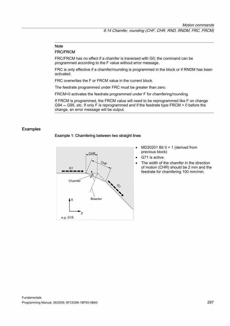
Motion commands 9.14 Chamfer, rounding (CHF, CHR, RND, RNDM, FRC, FRCM)
Fundamentals Programming Manual, 06/2009, 6FC5398-1BP20-0BA0 297
Note FRC/FRCM FRC/FRCM has no effect if a chamfer is traversed with G0; the command can be programmed according to the F value without error message. FRC is only effective if a chamfer/rounding is programmed in the block or if RNDM has been activated. FRC overwrites the F or FRCM value in the current block. The feedrate programmed under FRC must be greater than zero. FRCM=0 activates the feedrate programmed under F for chamfering/rounding. If FRCM is programmed, the FRCM value will need to be reprogrammed like F on change G94 ↔ G95, etc. If only F is reprogrammed and if the feedrate type FRCM > 0 before the change, an error message will be output.
Examples Example 1: Chamfering between two straight lines
• MD20201 Bit 0 = 1 (derived from previous block)
• G71 is active. • The width of the chamfer in the direction
of motion (CHR) should be 2 mm and the feedrate for chamfering 100 mm/min.

Motion commands 9.14 Chamfer, rounding (CHF, CHR, RND, RNDM, FRC, FRCM)
Fundamentals 298 Programming Manual, 06/2009, 6FC5398-1BP20-0BA0
Programming can be performed in two ways: ● Programming with CHR Program code
...
N30 G1 Z… CHR=2 FRC=100
N40 G1 X…
...
● Programming with CHF Program code
...
N30 G1 Z… CHF=2(cosα*2) FRC=100
N40 G1 X…
...
Example 2: Rounding between two straight lines
• MD20201 Bit 0 = 1 (derived from previous block)
• G71 is active. • The radius of the rounding should be
2 mm and the feedrate for rounding 50 mm/min.
Program code
...
N30 G1 Z… RND=2 FRC=50
N40 G1 X…
...

Motion commands 9.14 Chamfer, rounding (CHF, CHR, RND, RNDM, FRC, FRCM)
Fundamentals Programming Manual, 06/2009, 6FC5398-1BP20-0BA0 299
Example 3: Rounding between straight line and circle The RND function can be used to insert a circle contour element with tangential connection between the linear and circle contours in any combination.
• MD20201 Bit 0 = 1 (derived from previous block)
• G71 is active. • The radius of the rounding should be
2 mm and the feedrate for rounding 50 mm/min.
Program code
...
N30 G1 Z… RND=2 FRC=50
N40 G3 X… Z… I… K…
...
Example 4: Modal rounding to deburr sharp workpiece edges Program code Comment
...
N30 G1 X… Z… RNDM=2 FRCM=50 ; Activate modal rounding.
Radius of rounding: 2 mm
Feedrate for rounding: 50 mm/min
N40...
N120 RNDM=0 ; Deactivate modal rounding.
...

Motion commands 9.14 Chamfer, rounding (CHF, CHR, RND, RNDM, FRC, FRCM)
Fundamentals 300 Programming Manual, 06/2009, 6FC5398-1BP20-0BA0
Example 5: Apply technology from following block or previous block ● MD20201 Bit 0 = 0: Derived from following block (default setting!) Program code Comment
N10 G0 X0 Y0 G17 F100 G94
N20 G1 X10 CHF=2 ; Chamfer N20-N30 with F=100 mm/min
N30 Y10 CHF=4 ; Chamfer N30-N40 with FRC=200 mm/min
N40 X20 CHF=3 FRC=200 ; Chamfer N40-N60 with FRCM=50 mm/min
N50 RNDM=2 FRCM=50
N60 Y20 ; Modal rounding N60-N70 with FRCM=50 mm/min
N70 X30 ; Modal rounding N70-N80 with FRCM=50 mm/min
N80 Y30 CHF=3 FRC=100 ; Chamfer N80-N90 with FRC=100 mm/min
N90 X40 ; Modal rounding N90-N100 with F=100 mm/min (deselection of FRCM)
N100 Y40 FRCM=0 ; Modal rounding N100-N120 with G95 FRC=1 mm/rev
N110 S1000 M3
N120 X50 G95 F3 FRC=1
...
M02
● MD20201 Bit 0 = 1: Derived from previous block (recommended setting!) Program code Comment
N10 G0 X0 Y0 G17 F100 G94
N20 G1 X10 CHF=2 ; Chamfer N20-N30 with F=100 mm/min
N30 Y10 CHF=4 FRC=120 ; Chamfer N30-N40 with FRC=120 mm/min
N40 X20 CHF=3 FRC=200 ; Chamfer N40-N60 with FRC=200 mm/min
N50 RNDM=2 FRCM=50
N60 Y20 ; Modal rounding N60-N70 with FRCM=50 mm/min
N70 X30 ; Modal rounding N70-N80 with FRCM=50 mm/min
N80 Y30 CHF=3 FRC=100 ; Chamfer N80-N90 with FRC=100 mm/min
N90 X40 ; Modal rounding N90-N100 with FRCM=50 mm/min
N100 Y40 FRCM=0 ; Modal rounding N100-N120 with F=100 mm/min
N110 S1000 M3
N120 X50 CHF=4 G95 F3 FRC=1 ; Chamfer N120-N130 with G95 FRC=1 mm/rev
N130 Y50 ; Modal rounding N130-N140 with F=3 mm/rev
N140 X60
...
M02

Fundamentals Programming Manual, 06/2009, 6FC5398-1BP20-0BA0 301
Tool radius compensation 1010.1 10.1 Tool radius compensation (G40, G41, G42, OFFN)
Function When tool radius compensation (TRC) is active, the control automatically calculates the equidistant tool paths for various tools.
Syntax G0/G1 X... Y… Z... G41/G42 [OFFN=<value>]
...
G40 X... Y… Z...
Significance G41: Activate TRC with machining direction left of the contour. G42: Activate TRC with machining direction right of the contour. OFFN=<value>: Allowance on the programmed contour (normal contour offset)
(optional), e.g. to generate equidistant paths for rough finishing.
G40: Deactivate TRC.

Tool radius compensation 10.1 Tool radius compensation (G40, G41, G42, OFFN)
Fundamentals 302 Programming Manual, 06/2009, 6FC5398-1BP20-0BA0
Note In the NC block with G40/G41/G42, G0 or G1 has to be active and at least one axis has to be specified on the selected working plane. If only one axis is specified on activation, the last position on the second axis is added automatically and traversed with both axes. The two axes must be active as geometry axes in the channel. This can be achieved by means of GEOAX programming.
Examples Example 1: Milling
Program code Comment
N10 G0 X50 T1 D1
; Only tool length compensation is activated. X50 is approached without compensation.
N20 G1 G41 Y50 F200
; Radius compensation is activated, point X50/Y50 is approached with compensation.
N30 Y100
…

Tool radius compensation 10.1 Tool radius compensation (G40, G41, G42, OFFN)
Fundamentals Programming Manual, 06/2009, 6FC5398-1BP20-0BA0 303
Example 2: "Conventional" procedure based on the example of milling "Conventional" procedure: 1. Tool call 2. Change tool. 3. Activate working plane and tool radius compensation.
Program code Comment
N10 G0 Z100 ; Retraction for tool change.
N20 G17 T1 M6 ; Tool change
N30 G0 X0 Y0 Z1 M3 S300 D1 ; Call tool offset values, select length compensation.
N40 Z-7 F500 ; Feed in tool.
N50 G41 X20 Y20 ; Activate tool radius compensation, tool machines to the left of the contour.
N60 Y40 ; Mill contour.
N70 X40 Y70
N80 X80 Y50
N90 Y20
N100 X20
N110 G40 G0 Z100 M30 ; Retract tool, end of program.

Tool radius compensation 10.1 Tool radius compensation (G40, G41, G42, OFFN)
Fundamentals 304 Programming Manual, 06/2009, 6FC5398-1BP20-0BA0
Example 3: Turning
Ø 2
0
Ø 1
00
20
20 1
Program code Comment
…
N20 T1 D1 ; Only tool length compensation is activated.
N30 G0 X100 Z20 ; X100 Z20 is approached without compensation.
N40 G42 X20 Z1 ; Radius compensation is activated, point X20/Z1 is approached with compensation.
N50 G1 Z-20 F0.2
…

Tool radius compensation 10.1 Tool radius compensation (G40, G41, G42, OFFN)
Fundamentals Programming Manual, 06/2009, 6FC5398-1BP20-0BA0 305
Example 4: Turning
Program code Comment
N5 G0 G53 X280 Z380 D0 ; Starting point
N10 TRANS X0 Z250 ; Zero offset
N15 LIMS=4000 ; Speed limitation (G96)
N20 G96 S250 M3 ; Select constant feedrate
N25 G90 T1 D1 M8 ; Select tool selection and offset
N30 G0 G42 X-1.5 Z1 ; Set tool with tool radius compensation
N35 G1 X0 Z0 F0.25
N40 G3 X16 Z-4 I0 K-10 ; Turn radius 10
N45 G1 Z-12
N50 G2 X22 Z-15 CR=3 ; Turn radius 3
N55 G1 X24
N60 G3 X30 Z-18 I0 K-3 ; Turn radius 3
N65 G1 Z-20
N70 X35 Z-40
N75 Z-57
N80 G2 X41 Z-60 CR=3 ; Turn radius 3
N85 G1 X46

Tool radius compensation 10.1 Tool radius compensation (G40, G41, G42, OFFN)
Fundamentals 306 Programming Manual, 06/2009, 6FC5398-1BP20-0BA0
Program code Comment
N90 X52 Z-63
N95 G0 G40 G97 X100 Z50 M9 ; Deselect tool radius compensation and approach tool change location
N100 T2 D2 ; Call tool and select offset
N105 G96 S210 M3 ; Select constant cutting rate
N110 G0 G42 X50 Z-60 M8 ; Set tool with tool radius compensation
N115 G1 Z-70 F0.12 ; Turn diameter 50
N120 G2 X50 Z-80 I6.245 K-5 ; Turn radius 8
N125 G0 G40 X100 Z50 M9 ; Retract tool and deselect tool radius compensation
N130 G0 G53 X280 Z380 D0 M5 ; Approach tool change location
N135 M30 ; End of program
Further information The control requires the following information in order to calculate the tool paths: ● Tool no. (T...), cutting edge no. (D...) ● Machining direction (G41/G42) ● Working plane (G17/G18/G19) Tool no. (T...), cutting edge no. (D...) The distance between tool path and workpiece contour is calculated from the milling cutter radii or cutting edge radii and the tool point direction parameters.
G42
G42
G41
G41
G41
With a flat D number structure, only the D number has to be programmed.
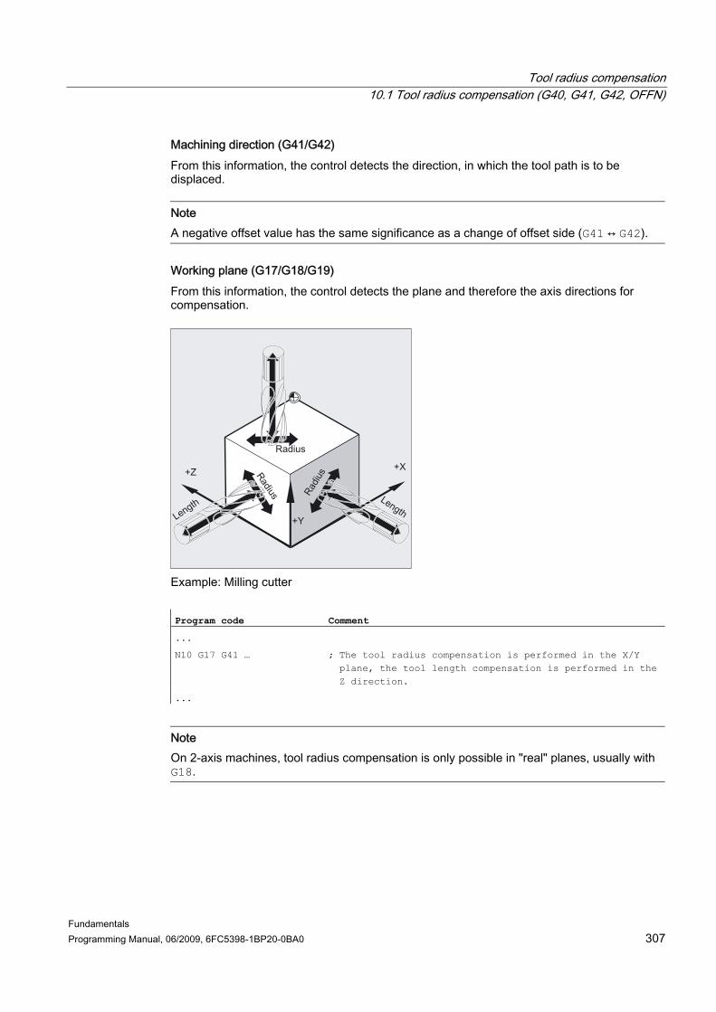
Tool radius compensation 10.1 Tool radius compensation (G40, G41, G42, OFFN)
Fundamentals Programming Manual, 06/2009, 6FC5398-1BP20-0BA0 307
Machining direction (G41/G42) From this information, the control detects the direction, in which the tool path is to be displaced.
Note A negative offset value has the same significance as a change of offset side (G41 ↔ G42).
Working plane (G17/G18/G19) From this information, the control detects the plane and therefore the axis directions for compensation.
Example: Milling cutter Program code Comment
...
N10 G17 G41 … ; The tool radius compensation is performed in the X/Y plane, the tool length compensation is performed in the Z direction.
...
Note On 2-axis machines, tool radius compensation is only possible in "real" planes, usually with G18.

Tool radius compensation 10.1 Tool radius compensation (G40, G41, G42, OFFN)
Fundamentals 308 Programming Manual, 06/2009, 6FC5398-1BP20-0BA0
Tool length compensation The wear parameter assigned to the diameter axis on tool selection can be defined as the diameter value using an MD. This assignment is not automatically altered when the plane is subsequently changed. To do this, the tool must be selected again after the plane has been changed. Turning:
NORM and KONT can be used to define the tool path on activation and deactivation of compensation mode (see "Contour approach and retraction (NORM, KONT, KONTC, KONTT) (Page 312)").

Tool radius compensation 10.1 Tool radius compensation (G40, G41, G42, OFFN)
Fundamentals Programming Manual, 06/2009, 6FC5398-1BP20-0BA0 309
Point of intersection The intersection point is selected in the setting data: SD42496 $SC_CUTCOM_CLSD_CONT (response of tool radius compensation with closed contour) Value Significance FALSE If two intersections appear on the inside when offsetting an (virtually) closed contour,
which consists of two circle blocks following on from one another, or from one circle block and one linear block, the intersection positioned closest to the end of block on the first partial contour is selected, in accordance with standard procedure. A contour is deemed to be (virtually) closed if the distance between the starting point of the first block and the end point of the second block is less than 10% of the effective compensation radius, but not more than 1,000 path increments (corresponds to 1 mm with 3 decimal places).
TRUE In the same situation as described above, the intersection positioned on the first partial contour closer to the block start is selected.
Change in compensation direction (G41 ↔ G42) A change in compensation direction (G41 ↔ G42) can be programmed without an intermediate G40.
G41
G42

Tool radius compensation 10.1 Tool radius compensation (G40, G41, G42, OFFN)
Fundamentals 310 Programming Manual, 06/2009, 6FC5398-1BP20-0BA0
Changing the working plane The working plane (G17/G18/G19) cannot be changed if G41/G42 is active. Change in tool offset data record (D…) The tool offset data record can be changed in compensation mode. A modified tool radius is active with effect from the block, in which the new D number is programmed.
CAUTION The radius change or compensation movement is performed across the entire block and only reaches the new equidistance at the programmed end point.
In the case of linear movements, the tool travels along an inclined path between the starting point and end point:
Circular interpolation produces spiral movements.
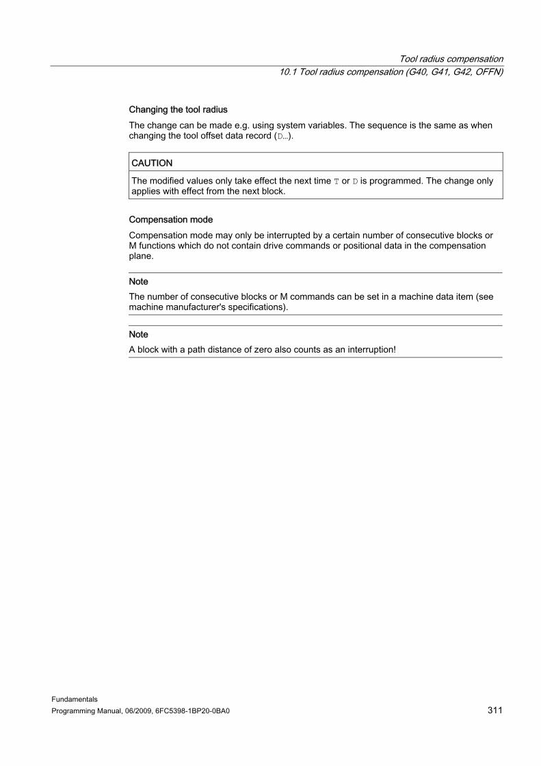
Tool radius compensation 10.1 Tool radius compensation (G40, G41, G42, OFFN)
Fundamentals Programming Manual, 06/2009, 6FC5398-1BP20-0BA0 311
Changing the tool radius The change can be made e.g. using system variables. The sequence is the same as when changing the tool offset data record (D…).
CAUTION The modified values only take effect the next time T or D is programmed. The change only applies with effect from the next block.
Compensation mode Compensation mode may only be interrupted by a certain number of consecutive blocks or M functions which do not contain drive commands or positional data in the compensation plane.
Note The number of consecutive blocks or M commands can be set in a machine data item (see machine manufacturer's specifications).
Note A block with a path distance of zero also counts as an interruption!

Tool radius compensation 10.2 Contour approach and retraction (NORM, KONT, KONTC, KONTT)
Fundamentals 312 Programming Manual, 06/2009, 6FC5398-1BP20-0BA0
10.2 10.2 Contour approach and retraction (NORM, KONT, KONTC, KONTT)
Function If tool radius compensation is active (G41/G42), the NORM, KONT, KONTC or KONTT command can be used to adapt the tool's approach and retract paths to the required contour profile or blank form. KONTC or KONTT ensure observance of the continuity conditions in all three axes. It is, therefore, permissible to program a path component perpendicular to the offset plane simultaneously.
Condition The KONTC and KONTT commands will only be available if the "Polynomial interpolation" option has been enabled in the control.
Syntax G41/G42 NORM/KONT/KONTC/KONTT X... Y... Z...
...
G40 X... Y... Z...
Significance NORM: Activate direct approach/retraction to/from a straight line.
The tool is oriented perpendicular to the contour point. KONT: Activate approach/retraction with travel around the starting/end point
according to the programmed corner behavior G450 or G451. KONTC: Activate approach/retraction with constant curvature. KONTT: Activate approach/retraction with constant tangent.
Note Only G1 blocks are permissible as original approach/retraction blocks for KONTC and KONTT. The control replaces these with polynomials for the appropriate approach/retract path.

Tool radius compensation 10.2 Contour approach and retraction (NORM, KONT, KONTC, KONTT)
Fundamentals Programming Manual, 06/2009, 6FC5398-1BP20-0BA0 313
General conditions KONTT and KONTC are not available in 3D variants of tool radius compensation (CUT3DC, CUT3DCC, CUT3DF). If they are programmed, the control switches internally to NORM without an error message.
Example KONTC The full circle is approached beginning at the circle center point. The direction and curvature radius at the block end point of the approach block are identical to the values of the next circle. Infeed takes place in the Z direction in both approach/retraction blocks simultaneously. The figure below shows the perpendicular projection of the tool path.
Figure 10-1 Perpendicular projection
The associated NC program segment is as follows: Program code Comment
$TC_DP1[1,1]=121 ; Milling tool
$TC_DP6[1,1]=10 ; Radius 10 mm
N10 G1 X0 Y0 Z60 G64 T1 D1 F10000
N20 G41 KONTC X70 Y0 Z0 ; Approach
N30 G2 I-70 ; Full circle
N40 G40 G1 X0 Y0 Z60 ; Retract
N50 M30
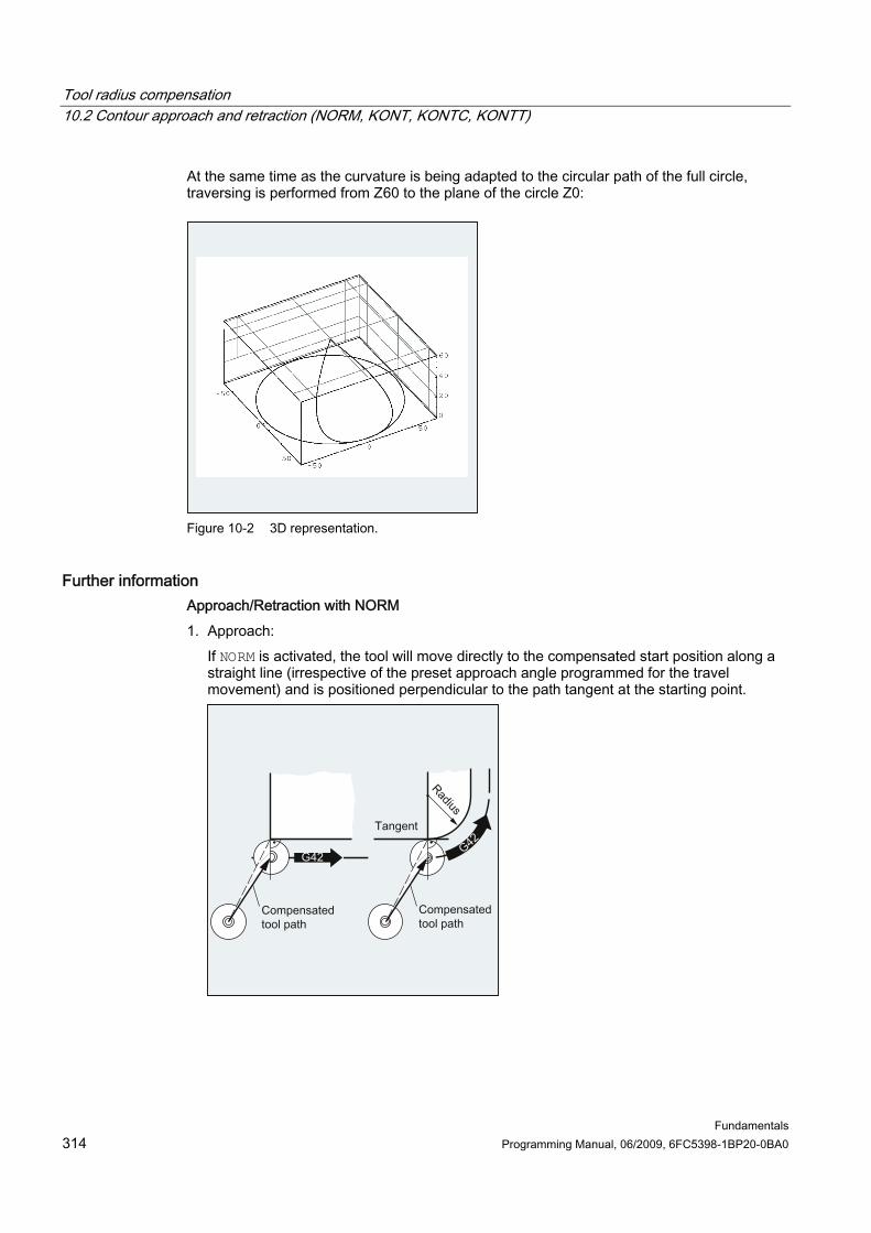
Tool radius compensation 10.2 Contour approach and retraction (NORM, KONT, KONTC, KONTT)
Fundamentals 314 Programming Manual, 06/2009, 6FC5398-1BP20-0BA0
At the same time as the curvature is being adapted to the circular path of the full circle, traversing is performed from Z60 to the plane of the circle Z0:
Figure 10-2 3D representation.
Further information Approach/Retraction with NORM 1. Approach:
If NORM is activated, the tool will move directly to the compensated start position along a straight line (irrespective of the preset approach angle programmed for the travel movement) and is positioned perpendicular to the path tangent at the starting point.

Tool radius compensation 10.2 Contour approach and retraction (NORM, KONT, KONTC, KONTT)
Fundamentals Programming Manual, 06/2009, 6FC5398-1BP20-0BA0 315
2. Retract: The tool is perpendicular to the last compensated path end point and then moves (irrespective of the preset approach angle programmed for the travel movement) directly in a straight line to the next uncompensated position, e.g. to the tool change point.
Modifying approach/retract angles introduces a collision risk:
CAUTION Modified approach/retract angles must be taken into account during programming in order that potential collisions can be avoided.
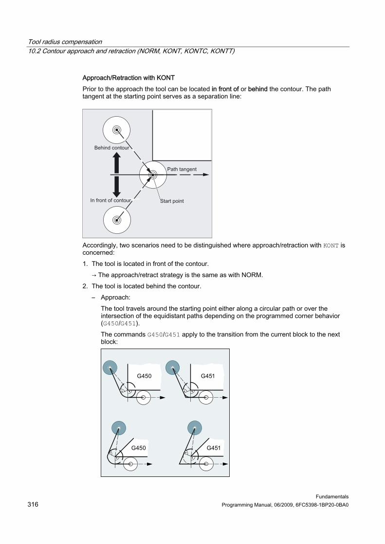
Tool radius compensation 10.2 Contour approach and retraction (NORM, KONT, KONTC, KONTT)
Fundamentals 316 Programming Manual, 06/2009, 6FC5398-1BP20-0BA0
Approach/Retraction with KONT Prior to the approach the tool can be located in front of or behind the contour. The path tangent at the starting point serves as a separation line:
Accordingly, two scenarios need to be distinguished where approach/retraction with KONT is concerned: 1. The tool is located in front of the contour.
→ The approach/retract strategy is the same as with NORM. 2. The tool is located behind the contour.
– Approach: The tool travels around the starting point either along a circular path or over the intersection of the equidistant paths depending on the programmed corner behavior (G450/G451). The commands G450/G451 apply to the transition from the current block to the next block:
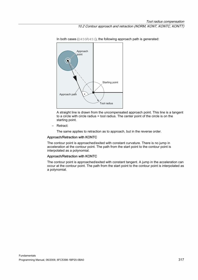
Tool radius compensation 10.2 Contour approach and retraction (NORM, KONT, KONTC, KONTT)
Fundamentals Programming Manual, 06/2009, 6FC5398-1BP20-0BA0 317
In both cases (G450/G451), the following approach path is generated:
A straight line is drawn from the uncompensated approach point. This line is a tangent to a circle with circle radius = tool radius. The center point of the circle is on the starting point.
– Retract: The same applies to retraction as to approach, but in the reverse order.
Approach/Retraction with KONTC The contour point is approached/exited with constant curvature. There is no jump in acceleration at the contour point. The path from the start point to the contour point is interpolated as a polynomial. Approach/Retraction with KONTC The contour point is approached/exited with constant tangent. A jump in the acceleration can occur at the contour point. The path from the start point to the contour point is interpolated as a polynomial.

Tool radius compensation 10.2 Contour approach and retraction (NORM, KONT, KONTC, KONTT)
Fundamentals 318 Programming Manual, 06/2009, 6FC5398-1BP20-0BA0
Differences between KONTC and KONTT
The figure below shows the differences in approach/retraction behavior between KONTT and KONTC. A circle with a radius of 20 mm about the center point at X0 Y-40 is compensated with a tool with an external radius of 20 mm. The tool center point therefore moves along a circular path with radius 40 mm. The end point of the approach blocks is at X40 Y30. The transition between the circular block and the retraction block is at the zero point. Due to the extended continuity of curvature associated with KONTC, the retraction block first executes a movement with a negative Y component. This will often be undesired. This response does not occur with the KONTT retraction block. However, with this block, an acceleration step change occurs at the block transition. If the KONTT or KONTC block is the approach block rather than the retraction block, the contour is exactly the same, but it is machined in the opposite direction.

Tool radius compensation 10.3 Compensation at the outside corners (G450, G451, DISC)
Fundamentals Programming Manual, 06/2009, 6FC5398-1BP20-0BA0 319
10.3 10.3 Compensation at the outside corners (G450, G451, DISC)
Function With tool radius compensation activated (G41/G42), command G450 or G451 can be used to define the course of the compensated tool path when traveling around outside corners:
With G450 the tool center point travels around the workpiece corner across an arc with tool radius.
With G451 the tool center point approaches the intersection of the two equidistants, which lie in the distance between the tool radius and the programmed contour. G451 applies only to circles and straight lines.
Note G450/G451 is also used to define the approach path with KONT active and approach point behind the contour (see "Contour approach and retraction (NORM, KONT, KONTC, KONTT)(Page 312)").
The DISC command can be used to distort the transition circles with G450, thereby producing sharper contour corners.

Tool radius compensation 10.3 Compensation at the outside corners (G450, G451, DISC)
Fundamentals 320 Programming Manual, 06/2009, 6FC5398-1BP20-0BA0
Syntax G450 [DISC=<value>] G451
Significance G450: G450 is used to travel around workpiece corners on a circular path.
Flexible programming of the circular path with G450 (optional) Type: INT Range of values: 0, 1, 2 to 100
0 Transition circle
DISC: <value>:
Significance: 100 Intersection of the equidistant paths
(theoretical value) G451: G451 is used to approach the intersection point of the two equidistant paths in
the case of workpiece corners. The tool backs off from the workpiece corner.
Note DISC only applies with call of G450, but can be programmed in a previous block without G450. Both commands are modal.
Example
In this example, a transition radius is programmed for all outside corners (corresponding to the programming of the corner behavior in block N30). This prevents the tool stopping and backing off at the change of direction.

Tool radius compensation 10.3 Compensation at the outside corners (G450, G451, DISC)
Fundamentals Programming Manual, 06/2009, 6FC5398-1BP20-0BA0 321
Program code Comment
N10 G17 T1 G0 X35 Y0 Z0 F500 ; Starting conditions
N20 G1 Z-5 ; Feed in tool.
N30 G41 KONT G450 X10 Y10 ; Activate TRC with KONT approach/retract mode and corner behavior G450.
N40 Y60 ; Mill the contour.
N50 X50 Y30
N60 X10 Y10
N80 G40 X-20 Y50 ; Deactivate compensation mode, retraction on transition circle.
N90 G0 Y100
N100 X200 M30
Further information G450/G451 At intermediate point P*, the control executes operations such as infeed movements or switching functions. These operations are programmed in blocks inserted between the two blocks forming the corner. With G450 the transition circle belongs to the next travel command with respect to the data. DISC When DISC values greater than 0 are specified, intermediate circles are shown with a magnified height – the result is transition ellipses or parabolas or hyperbolas:
An upper limit can be defined in machine data – generally DISC=50.

Tool radius compensation 10.3 Compensation at the outside corners (G450, G451, DISC)
Fundamentals 322 Programming Manual, 06/2009, 6FC5398-1BP20-0BA0
Traversing behavior When G450 is activated and with acute contour angles and high DISC values, the tool is lifted off the contour at the corners. In the case of contour angles equal to or greater than 120°, there is uniform travel around the contour:
When G451 is activated and with acute contour angles, superfluous non-cutting tool paths can result from lift-off movements. A parameter can be used in the machine data to define automatic switchover to transition circle in such cases.
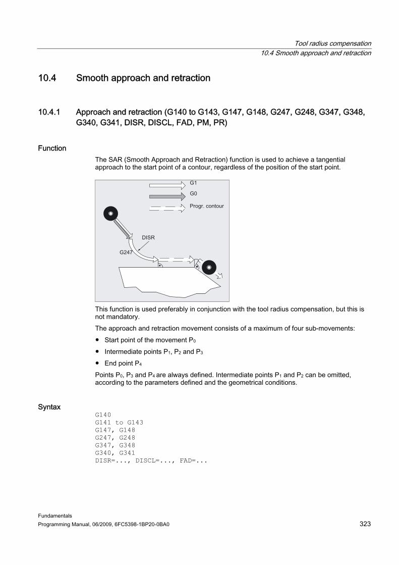
Tool radius compensation 10.4 Smooth approach and retraction
Fundamentals Programming Manual, 06/2009, 6FC5398-1BP20-0BA0 323
10.4 10.4 Smooth approach and retraction
10.4.1 Approach and retraction (G140 to G143, G147, G148, G247, G248, G347, G348, G340, G341, DISR, DISCL, FAD, PM, PR)
Function The SAR (Smooth Approach and Retraction) function is used to achieve a tangential approach to the start point of a contour, regardless of the position of the start point.
This function is used preferably in conjunction with the tool radius compensation, but this is not mandatory. The approach and retraction movement consists of a maximum of four sub-movements: ● Start point of the movement P0 ● Intermediate points P1, P2 and P3 ● End point P4 Points P0, P3 and P4 are always defined. Intermediate points P1 and P2 can be omitted, according to the parameters defined and the geometrical conditions.
Syntax G140 G141 to G143 G147, G148 G247, G248 G347, G348 G340, G341 DISR=..., DISCL=..., FAD=...

Tool radius compensation 10.4 Smooth approach and retraction
Fundamentals 324 Programming Manual, 06/2009, 6FC5398-1BP20-0BA0
Significance G140: Approach and retraction direction dependent on the current compensation
side (basic setting) G141: Approach from the left or retraction to the left G142: Approach from the right or retraction to the right G143: Approach and retraction direction dependent on the relative position of the
start or end point to the tangent direction G147: Approach with a straight line G148: Retraction with a straight line G247: Approach with a quadrant G248: Retraction with a quadrant G347: Approach with a semicircle G348: Retraction with a semicircle G340: Approach and retraction in space (basic setting) G341: Approach and retraction in the plane DISR: Approach and retraction with straight lines (G147/G148)
Distance of the milling tool edge to the starting point of the contour Approach and retraction along circles (G247, G347/G248, G348) Radius of the tool center path Notice: For REPOS with a semicircle, DISR is the circle diameter
DISCL: DISCL=... distance of the end point of the fast feed movement to the machining plane DISCL=AC(...) specification of the absolute position of the end point of the fast feed movement
FAD: Speed of the slow feed movement FAD=... the programmed value is applied corresponding to the G code of group 15 (feedrate; G93, G94, etc.) FAD=PM(...) the programmed value is interpreted irrespective of the active G code, group 15 as linear feedrate (as G94) FAD=PR(...) the programmed value is interpreted irrespective of the active G code, group 15 as revolutional feedrate (as G95).

Tool radius compensation 10.4 Smooth approach and retraction
Fundamentals Programming Manual, 06/2009, 6FC5398-1BP20-0BA0 325
Example
● Smooth approach (block N20 activated) ● Approach with quadrant (G247) ● Approach direction not programmed, G140 applies, i.e. TRC is active (G41) ● Contour offset OFFN=5 (N10) ● Current tool radius=10, and so the effective compensation radius for TRC=15, the radius
of the SAR contour =25, with the result that the radius of the tool center path is equal to DISR=10
● The end point of the circle is obtained from N30, since only the Z position is programmed in N20
● Infeed movement – From Z20 to Z7 (DISCL=AC(7)) with rapid traverse. – Then to Z0 with FAD=200. – Approach circle in X-Y-plane and following blocks with F1500 (for this velocity to take
effect in the following blocks, the active G0 in N30 must be overwritten with G1, otherwise the contour would be machined further with G0).
● Smooth retraction (block N60 activated) ● Retraction with quadrant (G248) and helix (G340) ● FAD not programmed, since irrelevant for G340 ● Z=2 in the starting point; Z=8 in the end point, since DISCL=6 ● When DISR=5, the radius of the SAR contour=20, the radius of the tool center point
path=5 Retraction movements from Z8 to Z20 and the movement parallel to the X-Y plane to X70 Y0.

Tool radius compensation 10.4 Smooth approach and retraction
Fundamentals 326 Programming Manual, 06/2009, 6FC5398-1BP20-0BA0
Program code Comment
$TC_DP1[1,1]=120 ; Tool definition T1/D1
$TC_DP6[1,1]=10 ; Radius
N10 G0 X0 Y0 Z20 G64 D1 T1 OFFN=5 ; (P0app)
N20 G41 G247 G341 Z0 DISCL=AC(7) DISR=10 F1500 FAD=200 ; Approach (P3app)
N30 G1 X30 Y-10 ; (P4app)
N40 X40 Z2
N50 X50 ; (P4ret)
N60 G248 G340 X70 Y0 Z20 DISCL=6 DISR=5 G40 F10000 ; Retraction (P3ret)
N70 X80 Y0 ; (P0ret)
N80 M30
Further information Selecting the approach and retraction contour The appropriate G command can be used: ● to approach or retract with a straight line (G147, G148), ● a quadrant (G247, G248) or ● a semicircle (G347, G348).

Tool radius compensation 10.4 Smooth approach and retraction
Fundamentals Programming Manual, 06/2009, 6FC5398-1BP20-0BA0 327
Selecting the approach and retraction direction Use the tool radius compensation (G140, basic setting) to determine the approach and retraction direction with positive tool radius: ● G41 active → approach from left ● G42 active → approach from right G141, G142 and G143 provide further approach options. The G codes are only significant when the approach contour is a quadrant or a semicircle.
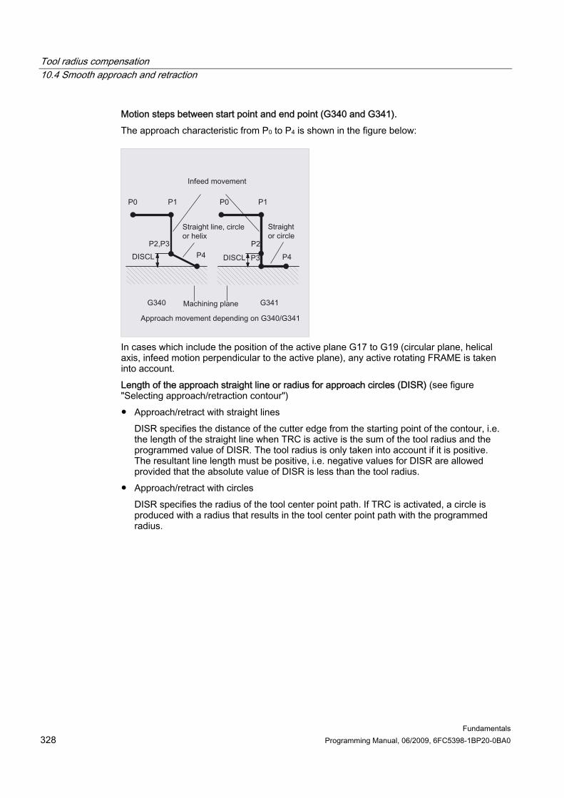
Tool radius compensation 10.4 Smooth approach and retraction
Fundamentals 328 Programming Manual, 06/2009, 6FC5398-1BP20-0BA0
Motion steps between start point and end point (G340 and G341). The approach characteristic from P0 to P4 is shown in the figure below:
In cases which include the position of the active plane G17 to G19 (circular plane, helical axis, infeed motion perpendicular to the active plane), any active rotating FRAME is taken into account. Length of the approach straight line or radius for approach circles (DISR) (see figure "Selecting approach/retraction contour") ● Approach/retract with straight lines
DISR specifies the distance of the cutter edge from the starting point of the contour, i.e. the length of the straight line when TRC is active is the sum of the tool radius and the programmed value of DISR. The tool radius is only taken into account if it is positive. The resultant line length must be positive, i.e. negative values for DISR are allowed provided that the absolute value of DISR is less than the tool radius.
● Approach/retract with circles DISR specifies the radius of the tool center point path. If TRC is activated, a circle is produced with a radius that results in the tool center point path with the programmed radius.

Tool radius compensation 10.4 Smooth approach and retraction
Fundamentals Programming Manual, 06/2009, 6FC5398-1BP20-0BA0 329
Distance of the point from the machining plane (DISCL) (see figure when selecting approach/retraction contour) If the position of point P2 is to be specified by an absolute reference on the axis perpendicular to the circle plane, the value must be programmed in the form DISCL=AC(...). The following applies for DISCL=0: ● With G340: The whole of the approach motion now only consists of two blocks (P1, P2
and P3 are combined). The approach contour is formed by P1 to P4. ● With G341: The whole approach contour consists of three blocks (P2 and P3 are
combined). If P0 and P4 are on the same plane, only two blocks result (infeed movement from P1 to P3 is omitted).
● The point defined by DISCL is monitored to ensure that it is located between P1 and P3, i.e. the sign must be identical for the component perpendicular to the machining plane in all motions that possess such a component.
● On detection of a direction reversal, a tolerance defined by the machine data SAR_CLEARANCE_TOLERANCE is permitted.
Programming the end point P4 for approach or P0 for retraction The end point is generally programmed with X... Y... Z... ● Programming during approach
– P4 in SAR block. – P4 is defined by means of the end point of the next traversing block.
More blocks can be inserted between an SAR block and the next traversing block without moving the geometry axes.
Example: Program code Comment
$TC_DP1[1,1]=120 ; Milling tool T1/D1
$TC_DP6[1,1]=7 ; Tool with 7 mm radius
N10 G90 G0 X0 Y0 Z30 D1 T1
N20 X10
N30 G41 G147 DISCL=3 DISR=13 Z=0 F1000
N40 G1 X40 Y-10
N50 G1 X50
...

Tool radius compensation 10.4 Smooth approach and retraction
Fundamentals 330 Programming Manual, 06/2009, 6FC5398-1BP20-0BA0
N30/N40 can be replaced by: 1. Program code Comment
N30 G41 G147 DISCL=3 DISR=13 X40 Y-10 Z0 F1000
2. Program code Comment
N30 G41 G147 DISCL=3 DISR=13 F1000
N40 G1 X40 Y-10 Z0

Tool radius compensation 10.4 Smooth approach and retraction
Fundamentals Programming Manual, 06/2009, 6FC5398-1BP20-0BA0 331
● Programming during retraction – For an SAR block without programmed geometry axis,
the contour ends in P2. The position in the axes that form the machining plane are obtained from the retraction contour. The axis component perpendicular to this is defined by DISCL. If DISCL=0, movement runs fully in the plane.
– If in the SAR block only the axis perpendicular to the machining plane is programmed, the contour will end at P1. The positions of the remaining axes will result, as described above. If the SAR block is also the TRC disable block, an additional path from P1 to P0 is inserted such that no motion results at the end of the contour when disabling the TRC.
– If only one axis on the machining plane is programmed, the missing second axis is modally added from its last position in the previous block.
– For an SAR block without programmed geometry axis, the contour ends in P2. The position in the axes that form the machining plane are obtained from the retraction contour. The axis component perpendicular to this is defined by DISCL. If DISCL=0, movement runs fully in the plane.
– If in the SAR block only the axis perpendicular to the machining plane is programmed, the contour will end at P1. The positions of the remaining axes will result, as described above. If the SAR block is also the TRC disable block, an additional path from P1 to P0 is inserted such that no motion results at the end of the contour when disabling the TRC.
– If only one axis on the machining plane is programmed, the missing second axis is modally added from its last position in the previous block.

Tool radius compensation 10.4 Smooth approach and retraction
Fundamentals 332 Programming Manual, 06/2009, 6FC5398-1BP20-0BA0
Approach and retraction velocities ● Velocity of the previous block (G0):
All motions from P0 up to P2 are executed at this velocity, i.e. the motion parallel to the machining plane and the part of the infeed motion up to the safety clearance.
● Programming with FAD: Specification of the feedrate for – G341: infeed movement perpendicular to the machining plane from P2 to P3 – G340: from point P2 or P3 to P4
If FAD is not programmed, this part of the contour is also traversed at the modally active speed of the previous block, if no F word is programmed in the SAR block.
● Programmed feedrate F: This feedrate value is effective as of P3 or P2 if FAD is not programmed. If no F word is programmed in the SAR block, the speed of the previous block is active.
Example: Program code Comment
$TC_DP1[1,1]=120 ; Milling tool T1/D1
$TC_DP6[1,1]=7 ; Tool with 7 mm radius
N10 G90 G0 X0 Y0 Z20 D1 T1
N20 G41 G341 G247 DISCL=AC(5) DISR=13 FAD 500 X40 Y-10 Z=0 F200
N30 X50
N40 X60
...
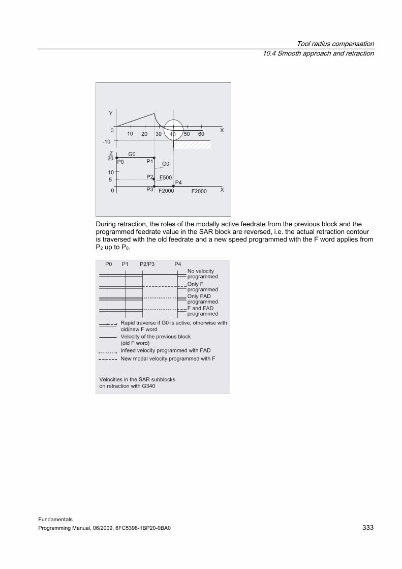
Tool radius compensation 10.4 Smooth approach and retraction
Fundamentals Programming Manual, 06/2009, 6FC5398-1BP20-0BA0 333
During retraction, the roles of the modally active feedrate from the previous block and the programmed feedrate value in the SAR block are reversed, i.e. the actual retraction contour is traversed with the old feedrate and a new speed programmed with the F word applies from P2 up to P0.
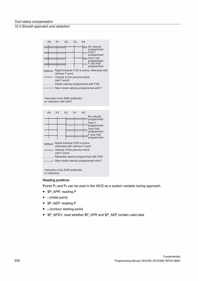
Tool radius compensation 10.4 Smooth approach and retraction
Fundamentals 334 Programming Manual, 06/2009, 6FC5398-1BP20-0BA0
Reading positions Points P3 and P4 can be read in the WCS as a system variable during approach. ● $P_APR: reading P ● 3 (initial point) ● $P_AEP: reading P ● 4 (contour starting point) ● $P_APDV: read whether $P_APR and $P_AEP contain valid data

Tool radius compensation 10.4 Smooth approach and retraction
Fundamentals Programming Manual, 06/2009, 6FC5398-1BP20-0BA0 335
10.4.2 Approach and retraction with enhanced retraction strategies (G460, G461, G462)
Function In certain special geometrical situations, special extended approach and retraction strategies, compared with the previous implementation with activated collision detection for the approach and retraction block, are required in order to activate or deactivate tool radius compensation. A collision detection can result, for example, in a section of the contour not being completely machined, see following figure:
Figure 10-3 Retraction behavior with G460
Syntax G460 G461 G462
Significance G460: As previously (activation of the collision detection for the approach and retraction
block) G461: Insertion of a circle in the TRC block, if it is not possible to have an intersection
whose center point is in the end point of the uncorrected block, and whose radius is the same as the tool radius. Up to the intersection, machining is performed with an auxiliary circle around the contour end point (i.e. up to the end of the contour).
G462: Insertion of a circle in the TRC block, if it is not possible to have an intersection; the block is extended by its end tangent (default setting). Machining is performed up to the extension of the last contour element (i.e. until shortly before the end of the contour).

Tool radius compensation 10.4 Smooth approach and retraction
Fundamentals 336 Programming Manual, 06/2009, 6FC5398-1BP20-0BA0
Note The approach behavior is symmetrical to the retraction behavior. The approach/retraction behavior is determined by the state of the G command in the approach/retraction block. The approach behavior can therefore be set independently of the retraction behavior.
Examples Example 1: Retraction behavior with G460 The following example describes only the situation for deactivation of tool radius compensation: The behavior for approach is exactly the same. Program code Comment
G42 D1 T1 ; Tool radius 20 mm
...
G1 X110 Y0
N10 X0
N20 Y10
N30 G40 X50 Y50
Example 2: Approach with G461 Program code Comment
N10 $TC_DP1[1,1]=120 ; Milling tool type
N20 $TC_DP6[1,1]=10 ; Tool radius
N30 X0 Y0 F10000 T1 D1
N40 Y20
N50 G42 X50 Y5 G461
N60 Y0 F600
N70 X30
N80 X20 Y-5
N90 X0 Y0 G40
N100 M30
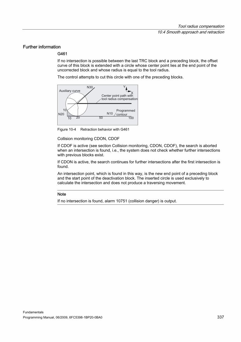
Tool radius compensation 10.4 Smooth approach and retraction
Fundamentals Programming Manual, 06/2009, 6FC5398-1BP20-0BA0 337
Further information G461 If no intersection is possible between the last TRC block and a preceding block, the offset curve of this block is extended with a circle whose center point lies at the end point of the uncorrected block and whose radius is equal to the tool radius. The control attempts to cut this circle with one of the preceding blocks.
Figure 10-4 Retraction behavior with G461
Collision monitoring CDON, CDOF If CDOF is active (see section Collision monitoring, CDON, CDOF), the search is aborted when an intersection is found, i.e., the system does not check whether further intersections with previous blocks exist. If CDON is active, the search continues for further intersections after the first intersection is found. An intersection point, which is found in this way, is the new end point of a preceding block and the start point of the deactivation block. The inserted circle is used exclusively to calculate the intersection and does not produce a traversing movement.
Note If no intersection is found, alarm 10751 (collision danger) is output.

Tool radius compensation 10.4 Smooth approach and retraction
Fundamentals 338 Programming Manual, 06/2009, 6FC5398-1BP20-0BA0
G462 If no intersection is possible between the last TRC block and a preceding block, a straight line is inserted, on retraction with G462 (initial setting), at the end point of the last block with tool radius compensation (the block is extended by its end tangent). The search for the intersection is then identical to the procedure for G461.
Retraction behavior with G462 (see example) With G462, the corner generated by N10 and N20 in the example program is not machined to the full extent actually possible with the tool used. However, this behavior may be necessary if the part contour (as distinct from the programmed contour), to the left of N20 in the example, is not permitted to be violated even with y values greater than 10 mm.
Tool radius compensation 10.4 Smooth approach and retraction
Fundamentals Programming Manual, 06/2009, 6FC5398-1BP20-0BA0 339
Corner behavior with KONT If KONT is active (travel round contour at start or end point), the behavior differs according to whether the end point is in front of or behind the contour. ● End point in front of contour
If the end point is in front of the contour, the retraction behavior is the same as with NORM. This property does not change even if the last contour block for G451 is extended with a straight line or a circle. Additional circumnavigation strategies to avoid a contour violation in the vicinity of the contour end point are therefore not required.
● End point behind contour If the end point is behind the contour, a circle or straight line is always inserted depending on G450/G451. In this case, G460-462 has no effect. If the last traversing block in this situation has no intersection with a preceding block, an intersection with the inserted contour element or with the straight line of the end point of the bypass circle to the programmed endpoint can result. If the inserted contour element is a circle (G450), and this forms an interface with the preceding block, this is equal to the interface that would occur with NORM and G461. In general, however, a remaining section of the circle still has to be traversed. For the linear part of the retraction block, no further calculation of intersection is required. In the second case, if no interface of the inserted contour element with the preceding blocks is found, the intersection between the retraction straight line and a preceding block is traversed. Therefore, a behavior that deviates from G460 can only occur with active G461 or G462 either if NORM is active or the behavior with KONT is geometrically identical to that with NORM.
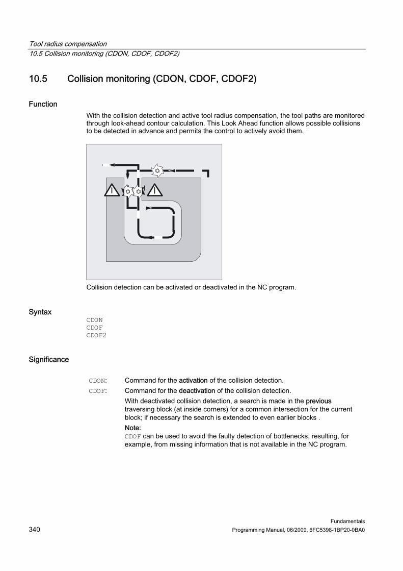
Tool radius compensation 10.5 Collision monitoring (CDON, CDOF, CDOF2)
Fundamentals 340 Programming Manual, 06/2009, 6FC5398-1BP20-0BA0
10.5 10.5 Collision monitoring (CDON, CDOF, CDOF2)
Function With the collision detection and active tool radius compensation, the tool paths are monitored through look-ahead contour calculation. This Look Ahead function allows possible collisions to be detected in advance and permits the control to actively avoid them.
Collision detection can be activated or deactivated in the NC program.
Syntax CDON CDOF CDOF2
Significance CDON: Command for the activation of the collision detection. CDOF: Command for the deactivation of the collision detection.
With deactivated collision detection, a search is made in the previous traversing block (at inside corners) for a common intersection for the current block; if necessary the search is extended to even earlier blocks . Note: CDOF can be used to avoid the faulty detection of bottlenecks, resulting, for example, from missing information that is not available in the NC program.

Tool radius compensation 10.5 Collision monitoring (CDON, CDOF, CDOF2)
Fundamentals Programming Manual, 06/2009, 6FC5398-1BP20-0BA0 341
CDOF2: Command for the deactivation of the collision detection during 3D circumferential milling. The tool offset direction is determined from adjacent block parts with CDOF2. CDOF2 is only effective for 3D circumferential milling and has the same significance as CDOF for all other types of machining (e.g. 3D face milling).
Note The number of NC blocks that are included in the collision detection, can be set via machine data.
Example Milling on the center point path with standard tool The NC program describes the center point path of a standard tool. The contour for a tool that is actually used results in undersize, which is shown unrealistically large to demonstrate the geometric relationships in the following figure. The control also only has an overview of three blocks in the example.
Figure 10-5 Compensation motion for missing intersection
Since an intersection exists only between the offset curves of the two blocks N10 and N40, the two blocks N20 and N30 would have to be omitted. In the example, the control does not know in block N40 if N10 has to be completely processed. Only a single block can therefore be omitted. With active CDOF2, the compensation motion shown in the figure is executed and not stopped. In this situation, an active CDOF or CDON would result in an alarm.
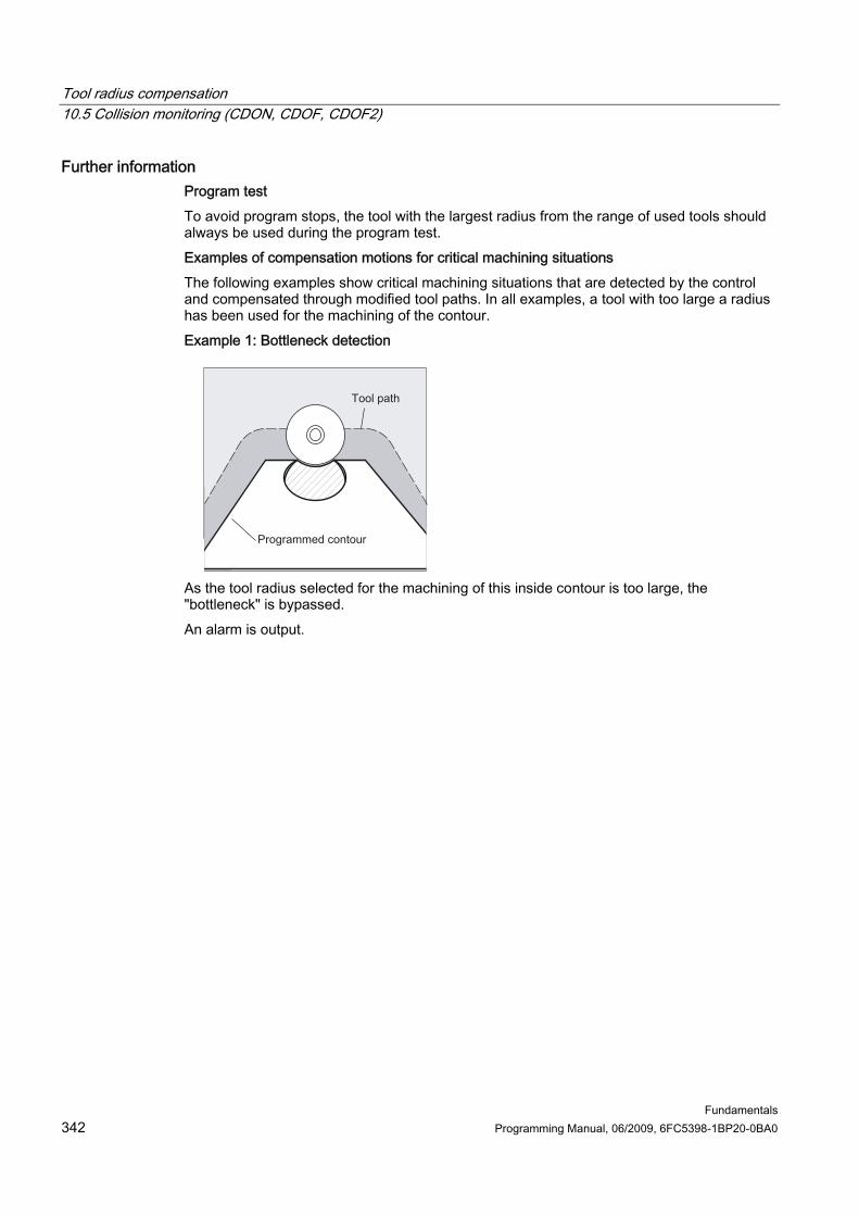
Tool radius compensation 10.5 Collision monitoring (CDON, CDOF, CDOF2)
Fundamentals 342 Programming Manual, 06/2009, 6FC5398-1BP20-0BA0
Further information Program test To avoid program stops, the tool with the largest radius from the range of used tools should always be used during the program test. Examples of compensation motions for critical machining situations The following examples show critical machining situations that are detected by the control and compensated through modified tool paths. In all examples, a tool with too large a radius has been used for the machining of the contour. Example 1: Bottleneck detection
As the tool radius selected for the machining of this inside contour is too large, the "bottleneck" is bypassed. An alarm is output.
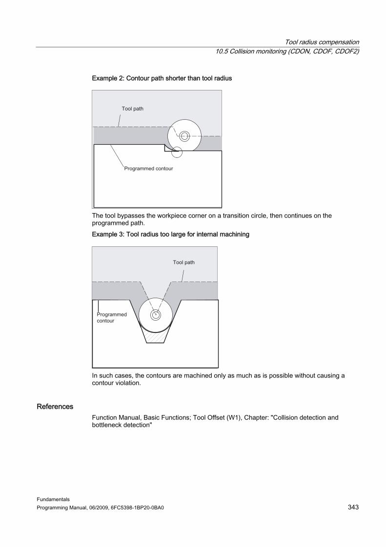
Tool radius compensation 10.5 Collision monitoring (CDON, CDOF, CDOF2)
Fundamentals Programming Manual, 06/2009, 6FC5398-1BP20-0BA0 343
Example 2: Contour path shorter than tool radius
The tool bypasses the workpiece corner on a transition circle, then continues on the programmed path. Example 3: Tool radius too large for internal machining
In such cases, the contours are machined only as much as is possible without causing a contour violation.
References Function Manual, Basic Functions; Tool Offset (W1), Chapter: "Collision detection and bottleneck detection"

Tool radius compensation 10.6 2D tool compensation (CUT2D, CUT2DF)
Fundamentals 344 Programming Manual, 06/2009, 6FC5398-1BP20-0BA0
10.6 10.6 2D tool compensation (CUT2D, CUT2DF)
Function With CUT2D or CUT2DF you define how the tool radius compensation is to act or to be interpreted when machining in inclined planes. Tool length compensation The tool length compensation generally always refers to the fixed, non-rotated working plane. 2D tool radius compensation with contour tools The tool radius compensation for contour tools is used for automatic cutting-edge selection in the case of non-axially symmetrical tools that can be used for piece-by-piece machining of individual contour segments.
Syntax CUT2D CUT2DF 2D tool radius compensation for contour tools is activated if either of the two machining directions G41 or G42 is programmed with CUT2D or CUT2DF.
Note If tool radius compensation is not activated, a contour tool will behave like a standard tool with only the first cutting edge.
Significance CUT2D: Activate 2 1/2 D radius compensation (default) CUT2DF: Activate 2 1/2 D radius compensation, tool radius compensation relative to
the current frame or to inclined planes CUT2D is used when the orientation of the tool cannot be changed and the workpiece is rotated for machining on inclined surfaces. CUT2D is generally the standard setting and does not, therefore, have to be specified explicitly.
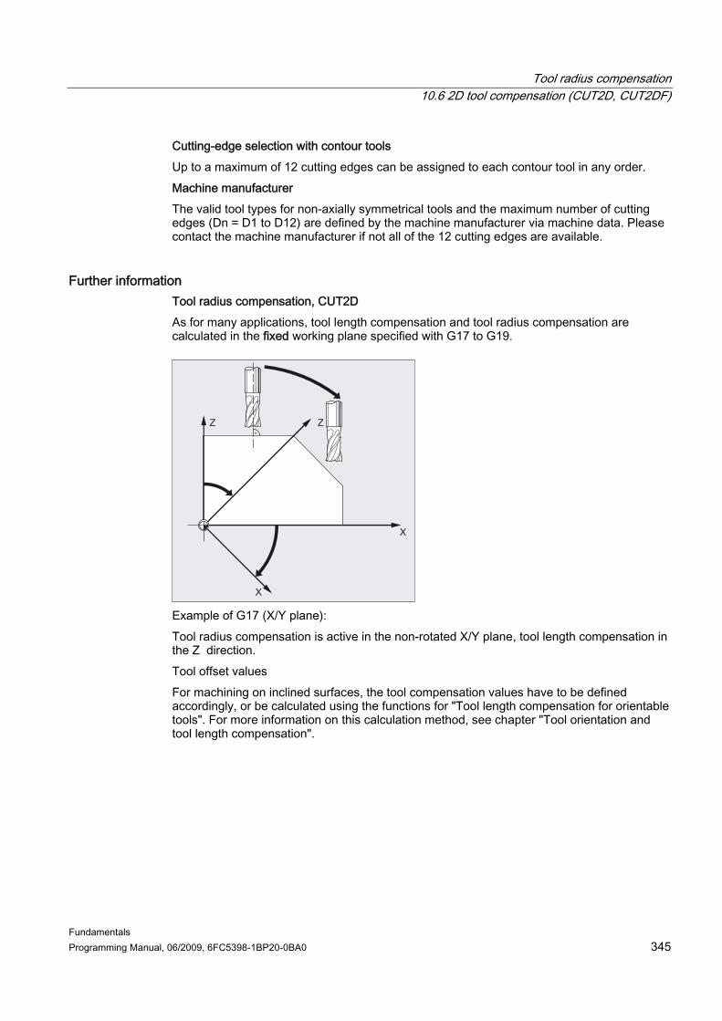
Tool radius compensation 10.6 2D tool compensation (CUT2D, CUT2DF)
Fundamentals Programming Manual, 06/2009, 6FC5398-1BP20-0BA0 345
Cutting-edge selection with contour tools Up to a maximum of 12 cutting edges can be assigned to each contour tool in any order. Machine manufacturer The valid tool types for non-axially symmetrical tools and the maximum number of cutting edges (Dn = D1 to D12) are defined by the machine manufacturer via machine data. Please contact the machine manufacturer if not all of the 12 cutting edges are available.
Further information Tool radius compensation, CUT2D As for many applications, tool length compensation and tool radius compensation are calculated in the fixed working plane specified with G17 to G19.
Example of G17 (X/Y plane): Tool radius compensation is active in the non-rotated X/Y plane, tool length compensation in the Z direction. Tool offset values For machining on inclined surfaces, the tool compensation values have to be defined accordingly, or be calculated using the functions for "Tool length compensation for orientable tools". For more information on this calculation method, see chapter "Tool orientation and tool length compensation".

Tool radius compensation 10.6 2D tool compensation (CUT2D, CUT2DF)
Fundamentals 346 Programming Manual, 06/2009, 6FC5398-1BP20-0BA0
Tool radius compensation, CUT2DF In this case, it is possible to arrange the tool orientation perpendicular to the inclined working plane on the machine.
If a frame containing a rotation is programmed, the compensation plane is also rotated with CUT2DF. The tool radius compensation is calculated in the rotated machining plane.
Note The tool length compensation continues to be active relative to the non-rotated working plane.
Definition of contour tools, CUT2D, CUT2DF A contour tool is defined by the number of cutting edges (on the basis of D nos) associated with a T no. The first cutting edge of a contour tool is the cutting edge that is selected when the tool is activated. If, for example, D5 is activated on T3 D5, then it is this cutting edge and the subsequent cutting edges that define the contour tool either partially or as a whole. The previous cutting edges will be ignored.
References Function Manual, Basic Functions; Tool Offset (W1)

Tool radius compensation 10.7 Keep tool radius compensation constant (CUTCONON, CUTCONOF)
Fundamentals Programming Manual, 06/2009, 6FC5398-1BP20-0BA0 347
10.7 10.7 Keep tool radius compensation constant (CUTCONON, CUTCONOF)
Function The "Keep tool radius compensation constant" function is used to suppress tool radius compensation for a number of blocks, whereby a difference between the programmed and the actual tool center path traveled set up by tool radius compensation in the previous blocks is retained as the compensation. It can be an advantage to use this method when several traversing blocks are required during line milling in the reversal points, but the contours produced by the tool radius compensation (follow strategies) are not wanted. It can be used independently of the type of tool radius compensation (21/2D, 3D face milling, 3D circumferential milling).
Syntax CUTCONON CUTCONOF
Significance CUTCONON: Command to activate the "Keep tool radius compensation constant"
function CUTCONOF: Command to deactivate the "Keep tool radius compensation constant"
function
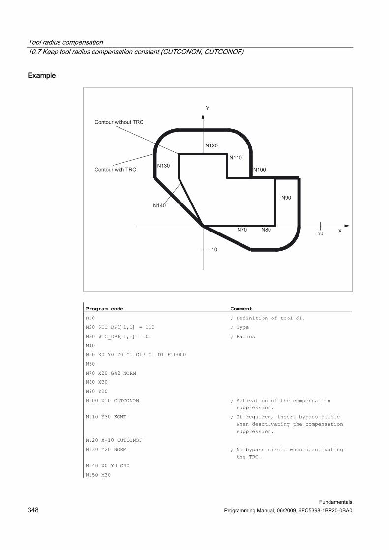
Tool radius compensation 10.7 Keep tool radius compensation constant (CUTCONON, CUTCONOF)
Fundamentals 348 Programming Manual, 06/2009, 6FC5398-1BP20-0BA0
Example
Program code Comment
N10 ; Definition of tool d1.
N20 $TC_DP1[1,1] = 110 ; Type
N30 $TC_DP6[1,1]= 10. ; Radius
N40
N50 X0 Y0 Z0 G1 G17 T1 D1 F10000
N60
N70 X20 G42 NORM
N80 X30
N90 Y20
N100 X10 CUTCONON ; Activation of the compensation suppression.
N110 Y30 KONT ; If required, insert bypass circle when deactivating the compensation suppression.
N120 X-10 CUTCONOF
N130 Y20 NORM ; No bypass circle when deactivating the TRC.
N140 X0 Y0 G40
N150 M30

Tool radius compensation 10.7 Keep tool radius compensation constant (CUTCONON, CUTCONOF)
Fundamentals Programming Manual, 06/2009, 6FC5398-1BP20-0BA0 349
Further information Tool radius compensation is normally active before the compensation suppression and is still active when the compensation suppression is deactivated again. In the last traversing block before CUTCONON, the offset point in the block end point is approached. All following blocks in which offset suppression is active are traversed without offset. However, they are offset by the vector from the end point of the last offset block to its offset point. These blocks can have any type of interpolation (linear, circular, polynomial). The deactivation block of the compensation suppression, i.e. the block that contains CUTCONOF, is compensated normally. It starts in the offset point of the starting point. One linear block is inserted between the end point of the previous block, i.e. the last programmed traversing block with active CUTCONON, and this point. Circular blocks, for which the circle plane is perpendicular to the compensation plane (vertical circles), are treated as though they had CUTCONON programmed. This implicit activation of the offset suppression is automatically canceled in the first traversing block that contains a traversing motion in the offset plane and is not such a circle. Vertical circle in this sense can only occur during circumferential milling.

Tool radius compensation 10.8 Tools with a relevant cutting edge position
Fundamentals 350 Programming Manual, 06/2009, 6FC5398-1BP20-0BA0
10.8 10.8 Tools with a relevant cutting edge position In the case of tools with a relevant tool point direction (turning and grinding tools – tool types 400–599; see chapter "Sign evaluation wear"), a change from G40 to G41/G42 or vice-versa is treated as a tool change. If a transformation is active (e.g., TRANSMIT), this leads to a preprocessing stop (decoding stop) and hence possibly to deviations from the intended part contour. This original functionality changes with regard to: 1. Preprocessing stop on TRANSMIT 2. Calculation of intersection points at approach and retraction with KONT 3. Tool change with active tool radius compensation 4. Tool radius compensation with variable tool orientation at transformation
Further information The original functionality has been modified as follows: ● A change from G40 to G41/G42 and vice-versa is no longer treated as a tool change.
Therefore, a preprocessing stop no longer occurs with TRANSMIT. ● The straight line between the tool edge center points at the block start and block end is
used to calculate intersection points with the approach and retraction block. The difference between the tool edge reference point and the tool edge center point is superimposed on this movement. On approach and retraction with KONT (tool circumnavigates the contour point, see above subsection "Contour approach and retraction"), superimposition takes place in the linear part block of the approach or retraction motion. The geometric conditions are therefore identical for tools with and without a relevant tool point direction. Deviations from the previous behavior occur only in relatively rare cases where the approach or retraction block does not intersect with an adjacent traversing block, see the following figure:
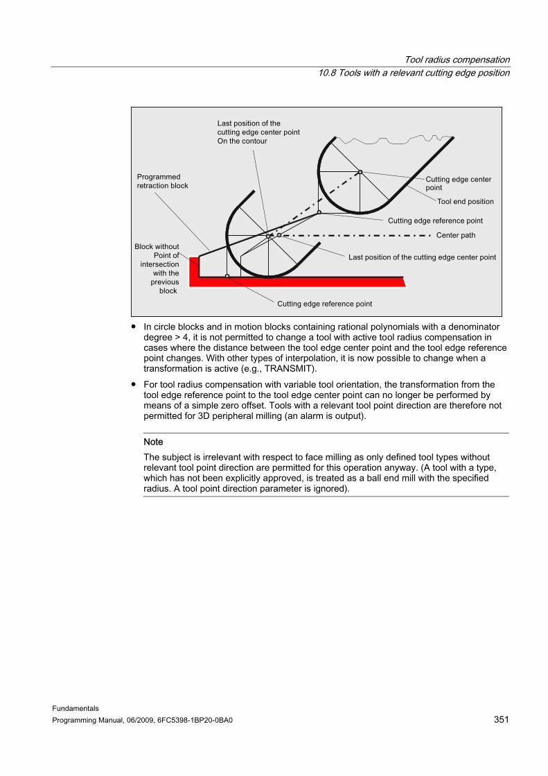
Tool radius compensation 10.8 Tools with a relevant cutting edge position
Fundamentals Programming Manual, 06/2009, 6FC5398-1BP20-0BA0 351
● In circle blocks and in motion blocks containing rational polynomials with a denominator
degree > 4, it is not permitted to change a tool with active tool radius compensation in cases where the distance between the tool edge center point and the tool edge reference point changes. With other types of interpolation, it is now possible to change when a transformation is active (e.g., TRANSMIT).
● For tool radius compensation with variable tool orientation, the transformation from the tool edge reference point to the tool edge center point can no longer be performed by means of a simple zero offset. Tools with a relevant tool point direction are therefore not permitted for 3D peripheral milling (an alarm is output).
Note The subject is irrelevant with respect to face milling as only defined tool types without relevant tool point direction are permitted for this operation anyway. (A tool with a type, which has not been explicitly approved, is treated as a ball end mill with the specified radius. A tool point direction parameter is ignored).

Tool radius compensation 10.8 Tools with a relevant cutting edge position
Fundamentals 352 Programming Manual, 06/2009, 6FC5398-1BP20-0BA0
Fundamentals Programming Manual, 06/2009, 6FC5398-1BP20-0BA0 353
Path action 1111.1 11.1 Exact stop (G60, G9, G601, G602, G603)
Function In exact stop traversing mode, all path axes and special axes involved in the traversing motion that are not traversed modally, are decelerated at the end of each block until they come to a standstill. Exact stop is used when sharp outside corners have to be machined or inside corners finished to exact dimensions. The exact stop specifies how exactly the corner point has to be approached and when the transition is made to the next block: ● "Exact stop fine"
The block change is performed as soon as the axis-specific tolerance limits for "Exact stop fine" are reached for all axes involved in the traversing motion.
● "Exact stop coarse" The block change is performed as soon as the axis-specific tolerance limits for "Exact stop coarse" are reached for all axes involved in the traversing motion.
● "Interpolator end" The block change is performed as soon as the control has calculated a set velocity of zero for all axes involved in the traversing motion. The actual position or the following error of the axes involved are not taken into account
Note The tolerance limits for "Exact stop fine" and "Exact stop coarse" can be set for each axis via the machine data.
Syntax G60 ... G9 ... G601/G602/G603, etc.

Path action 11.1 Exact stop (G60, G9, G601, G602, G603)
Fundamentals 354 Programming Manual, 06/2009, 6FC5398-1BP20-0BA0
Significance G60: Command for activation of the modal exact stop G9: Command for activation of the non-modal exact stop G601: Command for activation of the exact stop criterion "Exact stop fine" G602: Command for activation of the exact stop criterion "Exact stop coarse" G603: Command for activation of the exact stop criterion "Interpolator end"
Note The commands for activating the exact stop criteria (G601/G602/G603) are only effective if G60 or G9 is active.
Example Program code Comment
N5 G602 ; Criterion "Exact stop coarse" selected.
N10 G0 G60 Z... ; Exact stop modal active.
N20 X... Z... ; G60 continues to act.
...
N50 G1 G601 ; Criterion "Exact stop fine" selected.
N80 G64 Z... ; Switchover to continuous-path mode.
...
N100 G0 G9 ; Exact stop acts only in this block.
N110 ... ; Continuous-path mode active again.

Path action 11.1 Exact stop (G60, G9, G601, G602, G603)
Fundamentals Programming Manual, 06/2009, 6FC5398-1BP20-0BA0 355
Further information G60, G9 G9 generates the exact stop in the current block, G60 in the current block and in all following blocks. Continuous-path-mode commands G64 or G641 - G645 are used to deactivate G60. G601, G602
The movement is decelerated and stopped briefly at the corner point.
Note Do not set the limits for the exact stop criteria any tighter than necessary. The tighter the limits, the longer it takes to position and approach the target position.

Path action 11.1 Exact stop (G60, G9, G601, G602, G603)
Fundamentals 356 Programming Manual, 06/2009, 6FC5398-1BP20-0BA0
G603 The block change is initiated when the control has calculated a set velocity of zero for the axes involved. At this point, the actual value lags behind by a proportionate factor depending on the dynamic response of the axes and the path velocity. The workpiece corners can now be rounded.
Configured exact stop criterion A channel-specific setting can be made for G0 and the other commands in the first G function group indicating that contrary to the programmed exact stop criterion a preset criterion should be used automatically (see machine manufacturer's specifications).
References Function Manual, Basic Functions, Continuouspath Mode, Exact Stop, Look Ahead (B1)

Path action 11.2 Continuous-path mode (G64, G641, G642, G643, G644, G645, ADIS, ADISPOS)
Fundamentals Programming Manual, 06/2009, 6FC5398-1BP20-0BA0 357
11.2 11.2 Continuous-path mode (G64, G641, G642, G643, G644, G645, ADIS, ADISPOS)
Function In continuous-path mode, the path velocity at the end of the block (for the block change) is not decelerated to a level which would permit the fulfillment of an exact stop criterion. The objective of this mode is, in fact, to avoid rapid deceleration of the path axes at the block-change point so that the axis velocity remains as constant as possible when the program moves to the next block. To achieve this objective, the "LookAhead" function is also activated when continuous-path mode is selected. Continuouspath mode with smoothing facilitates the tangential shaping and/or smoothing of angular block transitions caused by local changes in the programmed contour. Continuouspath operation: ● Rounds the contour ● Reduces machining times by eliminating braking and acceleration processes that are
required to fulfill the exact-stop criterion ● Improves cutting conditions because of the more constant velocity Continuouspath mode is suitable if: ● A contour needs to be traversed as quickly as possible (e.g. with rapid traverse) ● The exact contour may deviate from the programmed contour within a specific tolerance
for the purpose of obtaining a continuous contour Continuous-path mode is not suitable if: ● A contour needs to be traversed precisely ● An absolutely constant velocity is required
Note Continuous-path mode is interrupted by blocks which trigger a preprocessing stop implicitly, e.g. due to: • Access to specific machine status data ($A...) • Auxiliary function outputs

Path action 11.2 Continuous-path mode (G64, G641, G642, G643, G644, G645, ADIS, ADISPOS)
Fundamentals 358 Programming Manual, 06/2009, 6FC5398-1BP20-0BA0
Syntax G64... G641 ADIS=… G641 ADISPOS=… G642... G643... G644... G645...
Meaning G64: Continuous-path mode with reduced velocity as per the overload factorG641: Continuous-path mode with smoothing as per distance criterion ADIS=... : Distance criterion with G641 for path functions G1, G2, G3, etc. ADISPOS=... : Distance criterion with G641 for rapid traverse G0 The distance criterion (= rounding clearance) ADIS or ADISPOS
describes the maximum distance the rounding block may cover before the end of the block, or the distance after the end of block within which the rounding block must be terminated respectively. Note: If ADIS/ADISPOS is not programmed, a value of "zero" applies and the traversing behavior therefore corresponds to G64. The rounding clearance is automatically reduced (by up to 36%) for short traversing distances.
G642: Continuous-path mode with smoothing within the defined tolerances In this mode, under normal circumstances smoothing takes place within the maximum permissible path deviation. However, instead of these axis-specific tolerances, observation of the maximum contour deviation (contour tolerance) or the maximum angular deviation of the tool orientation (orientation tolerance) can be configured. Note: Expansion to include contour and orientation tolerance is only supported on systems featuring the "Polynomial interpolation" option.
Path action 11.2 Continuous-path mode (G64, G641, G642, G643, G644, G645, ADIS, ADISPOS)
Fundamentals Programming Manual, 06/2009, 6FC5398-1BP20-0BA0 359
G643: Continuous-path mode with smoothing within the defined tolerances (block-internal) G643 differs from G642 in that is not used to generate a separate rounding block; instead, axis-specific block-internal rounding movements are inserted. The rounding clearance can be different for each axis.
G644: Continuous-path mode with smoothing with maximum possible dynamic response Note: G644 is not available with an active kinematic transformation. The system switches internally to G642.
G645: Continuous-path mode with smoothing and tangential block transitions within the defined tolerances G645 has the same effect on corners as G642. With G645, rounding blocks are also only generated on tangential block transitions if the curvature of the original contour exhibits a jump in at least one axis.
Note Rounding cannot be used as a substitute for smoothing (RND). The user should not make any assumptions with respect to the appearance of the contour within the rounding area. The type of rounding can depend on dynamic conditions, e.g. on the tool path velocity. Rounding on the contour is therefore only practical with small ADIS values. RND must be used if a defined contour is to be traversed at the corner.
NOTICE If a rounding movement initiated by G641, G642, G643, G644 or G645 is interrupted, the starting or end point of the original traversing block (as appropriate for REPOS mode) will be used for subsequent repositioning (REPOS), rather than the interruption point.
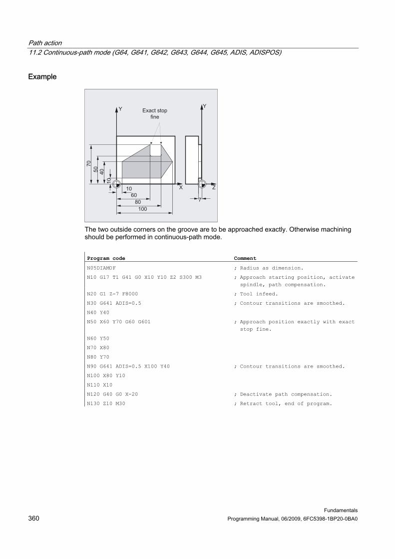
Path action 11.2 Continuous-path mode (G64, G641, G642, G643, G644, G645, ADIS, ADISPOS)
Fundamentals 360 Programming Manual, 06/2009, 6FC5398-1BP20-0BA0
Example
The two outside corners on the groove are to be approached exactly. Otherwise machining should be performed in continuous-path mode. Program code Comment
N05DIAMOF ; Radius as dimension.
N10 G17 T1 G41 G0 X10 Y10 Z2 S300 M3 ; Approach starting position, activate spindle, path compensation.
N20 G1 Z-7 F8000 ; Tool infeed.
N30 G641 ADIS=0.5 ; Contour transitions are smoothed.
N40 Y40
N50 X60 Y70 G60 G601 ; Approach position exactly with exact stop fine.
N60 Y50
N70 X80
N80 Y70
N90 G641 ADIS=0.5 X100 Y40 ; Contour transitions are smoothed.
N100 X80 Y10
N110 X10
N120 G40 G0 X-20 ; Deactivate path compensation.
N130 Z10 M30 ; Retract tool, end of program.
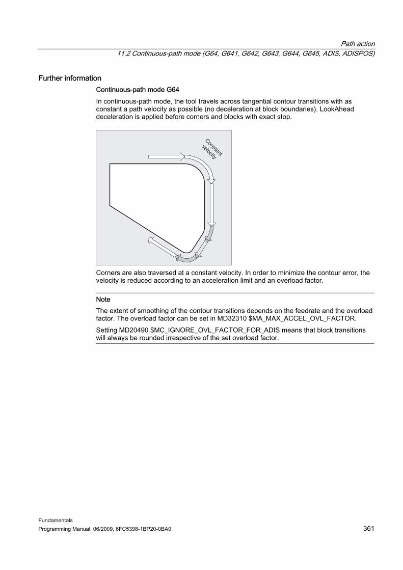
Path action 11.2 Continuous-path mode (G64, G641, G642, G643, G644, G645, ADIS, ADISPOS)
Fundamentals Programming Manual, 06/2009, 6FC5398-1BP20-0BA0 361
Further information Continuous-path mode G64 In continuous-path mode, the tool travels across tangential contour transitions with as constant a path velocity as possible (no deceleration at block boundaries). LookAhead deceleration is applied before corners and blocks with exact stop.
Corners are also traversed at a constant velocity. In order to minimize the contour error, the velocity is reduced according to an acceleration limit and an overload factor.
Note The extent of smoothing of the contour transitions depends on the feedrate and the overload factor. The overload factor can be set in MD32310 $MA_MAX_ACCEL_OVL_FACTOR. Setting MD20490 $MC_IGNORE_OVL_FACTOR_FOR_ADIS means that block transitions will always be rounded irrespective of the set overload factor.
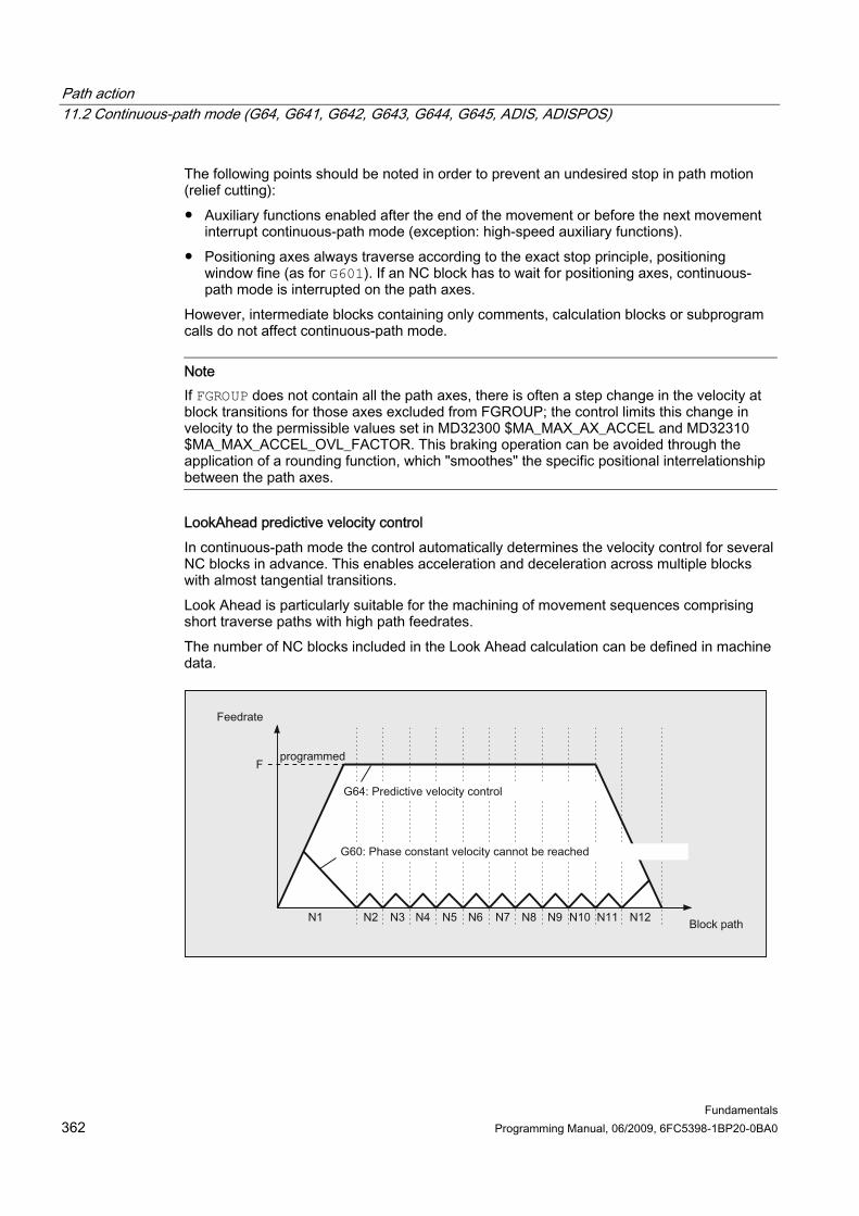
Path action 11.2 Continuous-path mode (G64, G641, G642, G643, G644, G645, ADIS, ADISPOS)
Fundamentals 362 Programming Manual, 06/2009, 6FC5398-1BP20-0BA0
The following points should be noted in order to prevent an undesired stop in path motion (relief cutting): ● Auxiliary functions enabled after the end of the movement or before the next movement
interrupt continuous-path mode (exception: high-speed auxiliary functions). ● Positioning axes always traverse according to the exact stop principle, positioning
window fine (as for G601). If an NC block has to wait for positioning axes, continuous-path mode is interrupted on the path axes.
However, intermediate blocks containing only comments, calculation blocks or subprogram calls do not affect continuous-path mode.
Note If FGROUP does not contain all the path axes, there is often a step change in the velocity at block transitions for those axes excluded from FGROUP; the control limits this change in velocity to the permissible values set in MD32300 $MA_MAX_AX_ACCEL and MD32310 $MA_MAX_ACCEL_OVL_FACTOR. This braking operation can be avoided through the application of a rounding function, which "smoothes" the specific positional interrelationship between the path axes.
LookAhead predictive velocity control In continuous-path mode the control automatically determines the velocity control for several NC blocks in advance. This enables acceleration and deceleration across multiple blocks with almost tangential transitions. Look Ahead is particularly suitable for the machining of movement sequences comprising short traverse paths with high path feedrates. The number of NC blocks included in the Look Ahead calculation can be defined in machine data.

Path action 11.2 Continuous-path mode (G64, G641, G642, G643, G644, G645, ADIS, ADISPOS)
Fundamentals Programming Manual, 06/2009, 6FC5398-1BP20-0BA0 363
Continuous-path mode with smoothing as per distance criterion (G641) With G641, the control inserts transition elements at contour transitions. The rounding clearance ADIS (or ADISPOS for G0) specifies the maximum extent to which the corners can be rounded. Within this rounding clearance, the control is free to ignore the path construct and replace it with a dynamically optimized distance. Disadvantage: Only one ADIS value is available for all axes. The effect of G641 is similar to RNDM; however, it is not restricted to the axes of the working plane. Like G64, G641 works with LookAhead predictive velocity control. Corner rounding blocks with a high degree of curvature are approached at reduced velocity. Example: Program code Comment
N10 G641 ADIS=0.5 G1 X... Y... ; The rounding block must begin no more than 0.5 mm before the programmed end of the block and must finish 0.5 mm after the end of the block. This setting remains modal.
Note Smoothing cannot and should not replace the functions for defined smoothing (RND, RNDM, ASPLINE, BSPLINE, CSPLINE).
Path action 11.2 Continuous-path mode (G64, G641, G642, G643, G644, G645, ADIS, ADISPOS)
Fundamentals 364 Programming Manual, 06/2009, 6FC5398-1BP20-0BA0
Smoothing with axial precision with G642 With G642, smoothing does not take place within a defined ADIS range, but the axial tolerances defined with MD33100 $MA_COMPRESS_POS_TOL are complied with. The rounding clearance is determined based on the shortest rounding clearance of all axes. This value is taken into account when generating a rounding block. Block-internal smoothing with G643 The maximum deviations from the precise contour in the case of smoothing with G643 are defined for each axis using machine data MD33100 $MA_COMPRESS_POS_TOL. G643 is not used to generate a separate rounding block, but axis-specific block-internal rounding movements are inserted. In the case of G643, the rounding clearance of each axis can be different. Smoothing with contour and orientation tolerance with G642/G643 MD20480 $MC_SMOOTHING_MODE can be used to configure rounding with G642 and G643 so that instead of the axis-specific tolerances, a contour tolerance and an orientation tolerance can be applied. The contour tolerance and orientation tolerance are set in the channel-specific setting data: SD42465 $SC_SMOOTH_CONTUR_TOL (maximum contour deviation) SD42466 $SC_SMOOTH_ORI_TOL (maximum angular deviation of the tool orientation) The setting data can be programmed in the NC program; this means that it can be specified differently for each block transition. Very different specifications for the contour tolerance and the tolerance of the tool orientation can only take effect with G643.
Note Expansion to include contour and orientation tolerance is only supported on systems featuring the "Polynomial interpolation" option.
Note An orientation transformation must be active for smoothing within the orientation tolerance.
Path action 11.2 Continuous-path mode (G64, G641, G642, G643, G644, G645, ADIS, ADISPOS)
Fundamentals Programming Manual, 06/2009, 6FC5398-1BP20-0BA0 365
Corner rounding with greatest possible dynamic response in G644 Smoothing with maximum possible dynamic response is configured in the thousands place with MD20480 $MC_SMOOTHING_MODE. Value Significance 0 Specification of maximum axial deviations with:
MD33100 $MA_COMPRESS_POS_TOL 1 Specification of maximum rounding clearance by programming:
ADIS=... or ADISPOS=... 2 Specification of the maximum possible frequencies of each axis occurring in the rounding
area with: MD32440 $MA_LOOKAH_FREQUENCY The rounding area is defined such that no frequencies in excess of the specified maximum can occur while the rounding motion is in progress.
3 When rounding with G644, neither the tolerance nor the rounding distance are monitored. Each axis traverses around a corner with the maximum possible dynamic response. With SOFT, both the maximum acceleration and the maximum jerk of each axis is maintained. With the BRISK command, the jerk is not limited; instead, each axis travels at the maximum possible acceleration.
Smoothing of tangential block transitions with G645 With G645, the smoothing movement is defined so that the acceleration of all axes involved remains smooth (no jumps) and the parameterized maximum deviations from the original contour (MD33120 $MA_PATH_TRANS_POS_TOL) are not exceeded. In the case of angular non-tangential block transitions, the smoothing behavior is the same as with G642.

Path action 11.2 Continuous-path mode (G64, G641, G642, G643, G644, G645, ADIS, ADISPOS)
Fundamentals 366 Programming Manual, 06/2009, 6FC5398-1BP20-0BA0
No intermediate rounding blocks An intermediate rounding block is not inserted in the following cases: ● The axis stops between the two blocks.
This occurs when: – The following block contains an auxiliary function output before the movement. – The following block does not contain a path movement. – An axis is traversed for the first time as a path axis for the following block when it was
previously a positioning axis. – An axis is traversed for the first time as a positioning axis for the following block when
it was previously a path axis. – The previous block traverses geometry axes and the following block does not. – The following block traverses geometry axes and the previous block does not. – Before tapping, the following block uses G33 as preparatory function and the previous
block does not. – A change is made between BRISK and SOFT. – Axes involved in the transformation are not completely assigned to the path motion
(e.g. for oscillation, positioning axes). ● The rounding block would slow down the part program execution.
This occurs: – Between two very short blocks.
Since each block requires at least one interpolation cycle, the added intermediate block would double the machining time.
– If a block transition G64 (continuous-path mode without smoothing) can be traversed without a reduction in velocity. Corner rounding would increase the machining time. This means that the value of the permitted overload factor (MD32310 $MA_MAX_ACCEL_OVL_FACTOR) affects whether a block transition is rounded or not. The overload factor is only taken into account for corner rounding with G641/G642. The overload factor has no effect in the case of smoothing with G643 (this behavior can also be set for G641 and G642 by setting MD20490 $MC_IGNORE_OVL_FACTOR_FOR_ADIS to TRUE).

Path action 11.2 Continuous-path mode (G64, G641, G642, G643, G644, G645, ADIS, ADISPOS)
Fundamentals Programming Manual, 06/2009, 6FC5398-1BP20-0BA0 367
● Rounding is not parameterized. This occurs when: – For G641 in G0 blocks ADISPOS = 0 (default!) – For G641 in non-G0 blocks ADIS = 0 (default!) – For G641 on transition from G0 and non-G0 or non-G0 and G0 respectively, the smaller
value from ADISPOS and ADIS applies. – ForG642/G643, all axis-specific tolerances are zero.
● The block does not contain traversing motion (zero block). This occurs when: – Synchronized actions are active.
Normally, the interpreter eliminates zero blocks. However, if synchronous actions are active, this zero block is included and also executed. In so doing, an exact stop is initiated corresponding to the active programming. This allows the synchronous action to also switch.
– Zero blocks are generated by program jumps. Continuous-path mode in rapid traverse G0 One of the specified functions G60/G9 or G64, or G641 - G645, also has to be specified for rapid traverse motion. Otherwise, the default in the machine data is used. Message as executable block During continuous-path mode, a message from the part program can also be output as executable block. To do this, the MSG command must be programmed with the second call parameter and the parameter value "1": MSG("Text",1)
If MSG is programmed without the second parameter, the message is output with the next executable block.
References For further information about continuous-path mode see: Function Manual, Basic Functions; Continuous-Path Mode, Exact Stop, LookAhead (B1).

Path action 11.2 Continuous-path mode (G64, G641, G642, G643, G644, G645, ADIS, ADISPOS)
Fundamentals 368 Programming Manual, 06/2009, 6FC5398-1BP20-0BA0

Fundamentals Programming Manual, 06/2009, 6FC5398-1BP20-0BA0 369
Coordinate transformations (frames) 1212.1 12.1 Frames
Frame The frame is a self-contained arithmetic rule that transforms one Cartesian coordinate system into another Cartesian coordinate system.
Basic frame (basic offset) The basic frame describes coordinate transformation from the basic coordinate system (BCS) to the basic zero system (BZS) and has the same effect as settable frames. See Basic coordinate system (BCS) (Page 31).
Settable frames Settable frames are the configurable work offsets which can be called from within any NC program with the G54 to G57 and G505 to G599 commands. The offset values are predefined by the user and stored in the zero offset memory on the control. They are used to define the settable zero system (SZS). See: ● Settable zero system (SZS) (Page 34) ● Settable work offset (G54 to G57, G505 to G599, G53, G500, SUPA, G153) (Page 173)

Coordinate transformations (frames) 12.1 Frames
Fundamentals 370 Programming Manual, 06/2009, 6FC5398-1BP20-0BA0
Programmable frames Sometimes it is useful or necessary to move the originally selected workpiece coordinate system (or the "settable zero system") to another position within an NC program and, if required, to rotate it, mirror it and/or scale it. This can be achieved using programmable frames.
See Frame instructions (Page 371).
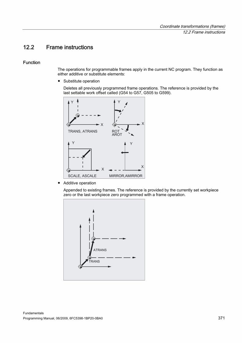
Coordinate transformations (frames) 12.2 Frame instructions
Fundamentals Programming Manual, 06/2009, 6FC5398-1BP20-0BA0 371
12.2 12.2 Frame instructions
Function The operations for programmable frames apply in the current NC program. They function as either additive or substitute elements: ● Substitute operation
Deletes all previously programmed frame operations. The reference is provided by the last settable work offset called (G54 to G57, G505 to G599).
● Additive operation
Appended to existing frames. The reference is provided by the currently set workpiece zero or the last workpiece zero programmed with a frame operation.

Coordinate transformations (frames) 12.2 Frame instructions
Fundamentals 372 Programming Manual, 06/2009, 6FC5398-1BP20-0BA0
Applications ● Offset the zero point to any position on the workpiece. ● Align the coordinate axes by rotating parallel to the desired working plane.
Advantages In one setting: ● Inclined surfaces can be machined ● Drill holes with various angles can be produced ● Multi-face machining can be performed
Note Depending on the machine kinematics, the conventions for working plane and tool offsets must be taken into account for the machining in inclined working planes
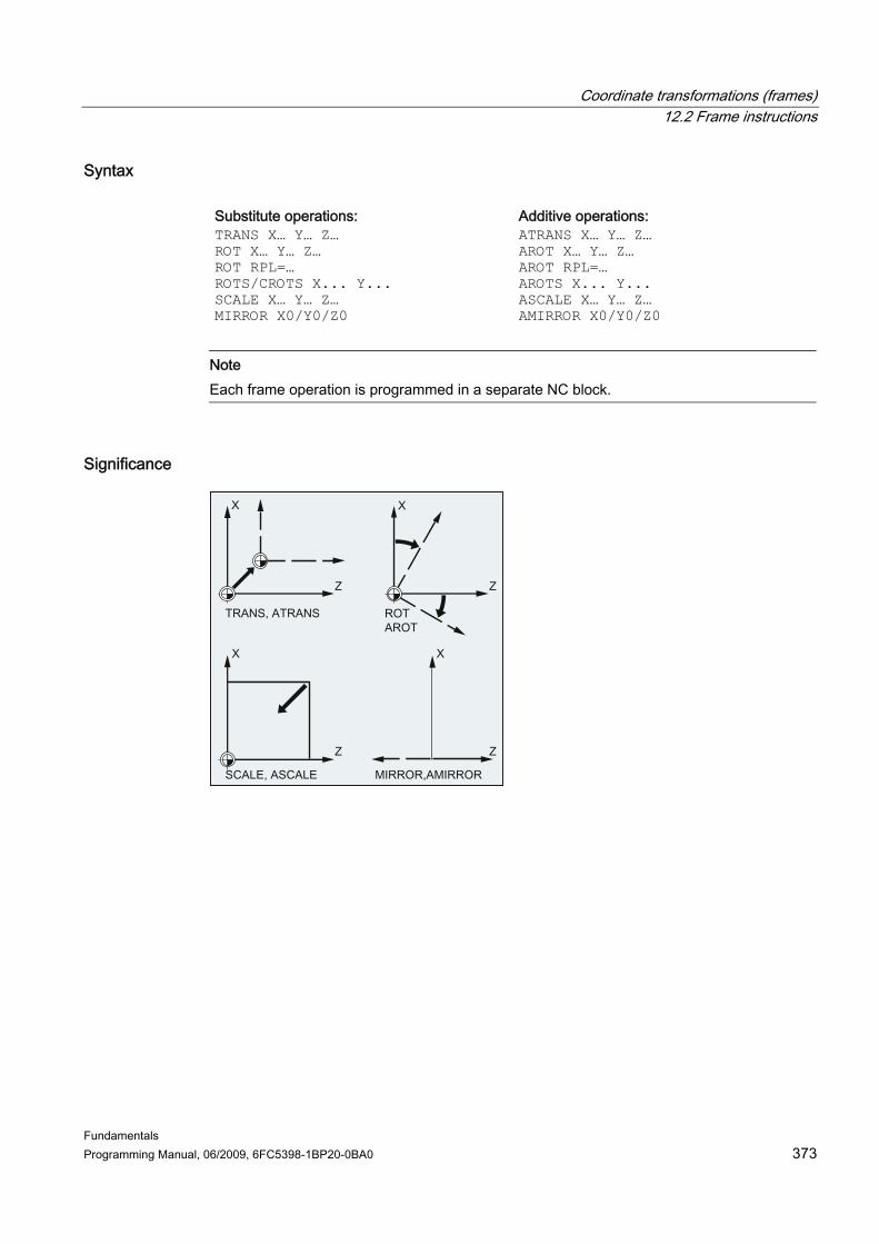
Coordinate transformations (frames) 12.2 Frame instructions
Fundamentals Programming Manual, 06/2009, 6FC5398-1BP20-0BA0 373
Syntax Substitute operations: Additive operations: TRANS X… Y… Z… ATRANS X… Y… Z… ROT X… Y… Z… AROT X… Y… Z… ROT RPL=… AROT RPL=… ROTS/CROTS X... Y... AROTS X... Y... SCALE X… Y… Z… ASCALE X… Y… Z… MIRROR X0/Y0/Z0 AMIRROR X0/Y0/Z0
Note Each frame operation is programmed in a separate NC block.
Significance

Coordinate transformations (frames) 12.2 Frame instructions
Fundamentals 374 Programming Manual, 06/2009, 6FC5398-1BP20-0BA0
TRANS/ATRANS: Workpiece coordinate system offset in the direction of the specified geometry axis or axes Workpiece coordinate system rotation: • By linking individual rotations around the specified geometry
axis or axes or
• Around the angle RPL=... in the current working plane (G17/G18/G19)
Direction of rotation:
With RPY notation: Z, Y', X'' Rotation sequence:With Euler angle: Z, X', Z'' The angles of rotation are only defined unambiguously in the following ranges:
-180 ≤ x ≤ 180-90 < y < 90
With RPY notation:
-180 ≤ z ≤ 1800 ≤ x < 180
-180 ≤ y ≤ 180
ROT/AROT:
Range of values:
With Euler angle:
-180 ≤ z ≤ 180
Coordinate transformations (frames) 12.2 Frame instructions
Fundamentals Programming Manual, 06/2009, 6FC5398-1BP20-0BA0 375
ROTS/AROTS: Workpiece coordinate system rotation by means of the specification of solid angles The orientation of a plane in space is defined unambiguously by specifying two solid angles. Therefore, up to 2 solid angles may be programmed: ROTS/AROTS X... Y... / Z... X... / Y... Z...
CROTS: CROTS works in the same way as ROTS but refers to the valid frame in the database.
SCALE/ASCALE: Scaling in the direction of the specified geometry axis or axes to increase/reduce the size of a contour
MIRROR/AMIRROR: Workpiece coordinate system mirroring by means of mirroring (direction change) the specified geometry axis
Value: freely selectable (in this case "0")
Note Frame operations can be used individually or combined at will.
CAUTION Frame operations are executed in the programmed sequence.
Note Additive statements are frequently used in subroutines. The basic functions defined in the main program are not lost after the end of the subroutine if the subroutine has been programmed with the SAVE attribute.

Coordinate transformations (frames) 12.3 Programmable zero offset
Fundamentals 376 Programming Manual, 06/2009, 6FC5398-1BP20-0BA0
12.3 12.3 Programmable zero offset
12.3.1 Zero offset (TRANS, ATRANS)
Function TRANS/ATRANS can be used to program work offsets for all path and positioning axes in the direction of the axis specified in each case. This means that it is possible to work with changing zero points, e.g. during repetitive machining operations at different workpiece positions. Milling: Turning:
Z
YM
X M
ZM
Y
X
G54
TRANS
Syntax TRANS X… Y… Z… ATRANS X… Y… Z…
Note Each frame operation is programmed in a separate NC block.

Coordinate transformations (frames) 12.3 Programmable zero offset
Fundamentals Programming Manual, 06/2009, 6FC5398-1BP20-0BA0 377
Significance TRANS: Absolute work offset, with reference to the currently valid
workpiece zero set with G54 to G57, G505 to G599. ATRANS: As TRANS, but with additive work offset X... Y... Z... : Offset values in the direction of the specified geometry axes
Examples Example 1: Milling
With this workpiece, the illustrated shapes recur several times in the same program. The machining sequence for this shape is stored in a subroutine. Work offset is used to set the workpiece zeros required in each case and then call the subprogram.
Program code Comment
N10 G1 G54 ; Working plane X/Y, workpiece zero
N20 G0 X0 Y0 Z2 ; Approach starting point
N30 TRANS X10 Y10 ; Absolute offset
N40 L10 ; Subroutine call
N50 TRANS X50 Y10 ; Absolute offset
N60 L10 ; Subroutine call
N70 M30 ; End of program

Coordinate transformations (frames) 12.3 Programmable zero offset
Fundamentals 378 Programming Manual, 06/2009, 6FC5398-1BP20-0BA0
Example 2: Turning
Program code Comment
N.. ...
N10 TRANS X0 Z150 ; Absolute offset
N15 L20 ; Subroutine call
N20 TRANS X0 Z140 (or ATRANS Z-10) ; Absolute offset
N25 L20 ; Subroutine call
N30 TRANS X0 Z130 (or ATRANS Z-10) ; Absolute offset
N35 L20 ; Subroutine call
N.. ...

Coordinate transformations (frames) 12.3 Programmable zero offset
Fundamentals Programming Manual, 06/2009, 6FC5398-1BP20-0BA0 379
Further information TRANS X... Y... Z... Translation through the offset values programmed in the specified axis directions (path, synchronized axes and positioning axes). The reference is provided by the last settable work offset called (G54 to G57, G505 to G599).
NOTICE The TRANS command resets all frame components of the previously activated programmable frame.
Note ATRANS can be used to program an offset to be added to existing frames.
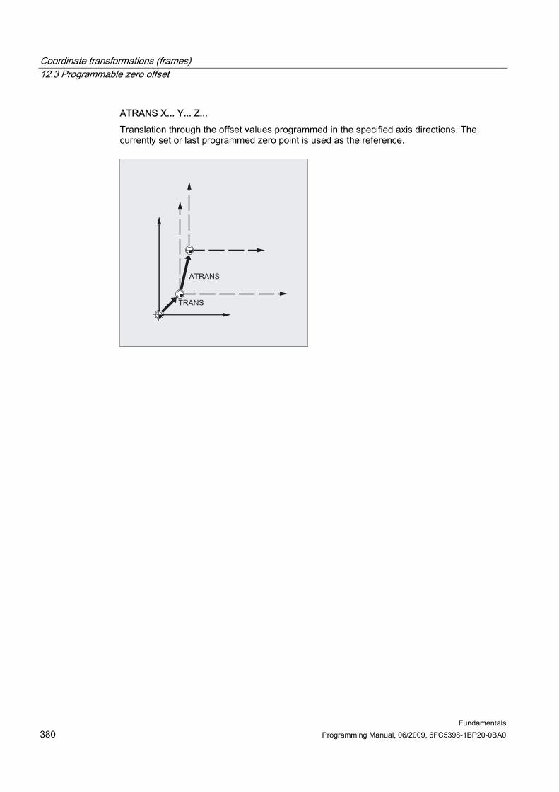
Coordinate transformations (frames) 12.3 Programmable zero offset
Fundamentals 380 Programming Manual, 06/2009, 6FC5398-1BP20-0BA0
ATRANS X... Y... Z... Translation through the offset values programmed in the specified axis directions. The currently set or last programmed zero point is used as the reference.
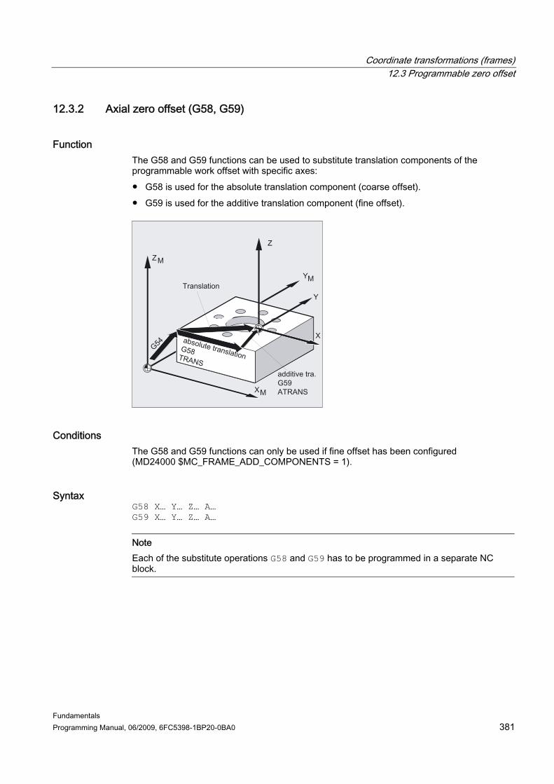
Coordinate transformations (frames) 12.3 Programmable zero offset
Fundamentals Programming Manual, 06/2009, 6FC5398-1BP20-0BA0 381
12.3.2 Axial zero offset (G58, G59)
Function The G58 and G59 functions can be used to substitute translation components of the programmable work offset with specific axes: ● G58 is used for the absolute translation component (coarse offset). ● G59 is used for the additive translation component (fine offset).
Conditions The G58 and G59 functions can only be used if fine offset has been configured (MD24000 $MC_FRAME_ADD_COMPONENTS = 1).
Syntax G58 X… Y… Z… A… G59 X… Y… Z… A…
Note Each of the substitute operations G58 and G59 has to be programmed in a separate NC block.
Coordinate transformations (frames) 12.3 Programmable zero offset
Fundamentals 382 Programming Manual, 06/2009, 6FC5398-1BP20-0BA0
Significance G58: G58 replaces the absolute translation component of the programmable
work offset for the specified axis, but the programmed additive offset remains valid The reference is provided by the last settable work offset called (G54 to G57, G505 to G599).
G59: G59 replaces the additive translation component of the programmable work offset for the specified axis, but the programmed absolute offset remains valid
X… Y… Z…: Offset values in the direction of the specified geometry axes
Example Program code Comment
...
N50 TRANS X10 Y10 Z10 ; Absolute translation component X10 Y10 Z10
N60 ATRANS X5 Y5 ; Additive translation component X5 Y5
⇒ Total offset: X15 Y15 Z10 N70 G58 X20 ; Absolute translation component X20
+ additive translation component X5 Y5
⇒ Total offset X25 Y15 Z10 N80 G59 X10 Y10 ; Additive translation component X10 Y10
+ absolute translation component X20 Y10
⇒ Total offset X30 Y20 Z10 ...

Coordinate transformations (frames) 12.3 Programmable zero offset
Fundamentals Programming Manual, 06/2009, 6FC5398-1BP20-0BA0 383
Further information The absolute translation component is modified by the following commands: ● TRANS ● G58 ● CTRANS ● CFINE ● $P_PFRAME[X,TR] The additive translation component is modified by the following commands: ● ATRANS ● G59 ● CTRANS ● CFINE ● $P_PFRAME[X,FI] The table below describes the effect of various program commands on the absolute and additive offsets. Command Coarse or
absolute offset Fine or additive offset
Comment
TRANS X10 10 unchanged Absolute offset for X G58 X10 10 unchanged Overwrites absolute offset for X $P_PFRAME[X,TR]=10 10 unchanged Progr. offset in X ATRANS X10 unchanged Fine (old) + 10 Additive offset for X G59 X10 unchanged 10 Overwriting additive offset for X $P_PFRAME[X,FI]=10 unchanged 10 Progr. fine offset in X CTRANS(X,10) 10 0 Offset for X CTRANS() 0 0 Deselection of offset (including
fine offset component) CFINE(X,10) 0 10 Fine offset in X

Coordinate transformations (frames) 12.4 Programmable rotation (ROT, AROT, RPL)
Fundamentals 384 Programming Manual, 06/2009, 6FC5398-1BP20-0BA0
12.4 12.4 Programmable rotation (ROT, AROT, RPL)
Function ROT/AROT can be used to rotate the workpiece coordinate system around each of the three geometry axes X, Y, Z or through an angle RPL in the selected working plane G17 to G19 (or around the perpendicular infeed axis). This allows inclined surfaces or multiple workpiece faces to be machined in one setting.
Syntax ROT X… Y… Z… ROT RPL=… AROT X… Y… Z… AROT RPL=…
Note Each frame operation is programmed in a separate NC block.
Coordinate transformations (frames) 12.4 Programmable rotation (ROT, AROT, RPL)
Fundamentals Programming Manual, 06/2009, 6FC5398-1BP20-0BA0 385
Significance ROT: Absolute rotation, with reference to the currently valid workpiece
zero set with G54 to G57, G505 to G599. RPL: Rotation in the plane: Angle through which the coordinate system
is rotated (plane set with G17 to G19) The sequence in which the rotation is to be performed can be specified via the machine data. The default setting is RPY notation (= Roll, Pitch, Yaw) with Z, Y, X.
AROT: Additive rotation in relation to the currently valid set or programmed zero point
X... Y... Z... : Rotation in space: Geometry axes around which the rotation is performed
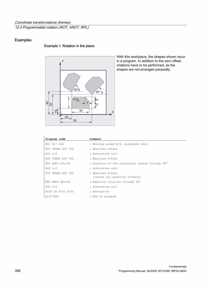
Coordinate transformations (frames) 12.4 Programmable rotation (ROT, AROT, RPL)
Fundamentals 386 Programming Manual, 06/2009, 6FC5398-1BP20-0BA0
Examples Example 1: Rotation in the plane
With this workpiece, the shapes shown recur in a program. In addition to the zero offset, rotations have to be performed, as the shapes are not arranged paraxially.
Program code Comment
N10 G17 G54 ; Working plane X/Y, workpiece zero
N20 TRANS X20 Y10 ; Absolute offset
N30 L10 ; Subroutine call
N40 TRANS X55 Y35 ; Absolute offset
N50 AROT RPL=45 ; Rotation of the coordinate system through 45°
N60 L10 ; Subroutine call
N70 TRANS X20 Y40 ; Absolute offset (resets all previous offsets)
N80 AROT RPL=60 ; Additive rotation through 60°
N90 L10 ; Subroutine call
N100 G0 X100 Y100 ; Retraction
N110 M30 ; End of program

Coordinate transformations (frames) 12.4 Programmable rotation (ROT, AROT, RPL)
Fundamentals Programming Manual, 06/2009, 6FC5398-1BP20-0BA0 387
Example 2: Spatial rotation
In this example, paraxial and inclined workpiece surfaces are to be machined in a clamping. Condition: The tool must be aligned perpendicular to the inclined surface in the rotated Z direction.
Program code Comment
N10 G17 G54 ; Working plane X/Y, workpiece zero
N20 TRANS X10 Y10 ; Absolute offset
N30 L10 ; Subroutine call
N40 ATRANS X35 ; Additive offset
N50 AROT Y30 ; Rotation around the Y axis
N60 ATRANS X5 ; Additive offset
N70 L10 ; Subroutine call
N80 G0 X300 Y100 M30 ; Retraction, end of program

Coordinate transformations (frames) 12.4 Programmable rotation (ROT, AROT, RPL)
Fundamentals 388 Programming Manual, 06/2009, 6FC5398-1BP20-0BA0
Example 3: Multi-face machining
In this example, identical shapes are machined in two workpiece surfaces perpendicular to one another via subroutines. In the new coordinate system on the right-hand workpiece surface, infeed direction, working plane and the zero point have been set up as on the top surface. Therefore, the conditions required for the subroutine execution still apply: working plane G17, coordinate plane X/Y, infeed direction Z.
Program code Comment
N10 G17 G54 ; Working plane X/Y, workpiece zero
N20 L10 ; Subroutine call
N30 TRANS X100 Z-100 ; Absolute offset

Coordinate transformations (frames) 12.4 Programmable rotation (ROT, AROT, RPL)
Fundamentals Programming Manual, 06/2009, 6FC5398-1BP20-0BA0 389
Program code Comment
N40 AROT Y90 ; Rotation of the coordinate system around Y
Z
X
Y
Z
X
Y
AROT Y90
N50 AROT Z90 ; Rotation of the coordinate system around Z
Z
X
Y
Z
X
Y
AROT Z90
N60 L10 ; Subroutine call
N70 G0 X300 Y100 M30 ; Retraction, end of program

Coordinate transformations (frames) 12.4 Programmable rotation (ROT, AROT, RPL)
Fundamentals 390 Programming Manual, 06/2009, 6FC5398-1BP20-0BA0
Further information Rotation in the plane The coordinate system is rotated: ● in the plane selected with G17 to G19.
Substitute operation ROT RPL=... or additive operation AROT RPL=... ● in the current plane around the angle of rotation programmed with RPL=....
Note See "Rotation in space" for more information.
Plane change
WARNING If you program a change of plane (G17 to G19) after a rotation, the angles of rotation programmed for the relevant axes are retained and continue to apply in the new working plane. It is, therefore, advisable to deactivate rotation before a change of plane.

Coordinate transformations (frames) 12.4 Programmable rotation (ROT, AROT, RPL)
Fundamentals Programming Manual, 06/2009, 6FC5398-1BP20-0BA0 391
Deactivate rotation For all axes: ROT (without axis parameter)
CAUTION All frame components of the previously programmed frame are reset.
ROT X... Y... Z... The coordinate system is rotated through the programmed angle around the specified axes. The center of rotation is provided by the last settable work offset specified (G54 to G57, G505 to G599).
NOTICE The ROT command resets all frame components of the previously activated programmable frame.
Note AROT can be used to program a new rotation to be added to existing frames.

Coordinate transformations (frames) 12.4 Programmable rotation (ROT, AROT, RPL)
Fundamentals 392 Programming Manual, 06/2009, 6FC5398-1BP20-0BA0
AROT X... Y... Z... Rotation through the angle values programmed in the axis direction parameters. The center of rotation is the currently set or last programmed zero point.
Note In the case of both operations, please bear in mind the sequence and direction in which the rotations are being executed!
Direction of rotation The following is defined as the positive direction of rotation: The view in the direction of the positive coordinate axis and clockwise rotation.

Coordinate transformations (frames) 12.4 Programmable rotation (ROT, AROT, RPL)
Fundamentals Programming Manual, 06/2009, 6FC5398-1BP20-0BA0 393
Order of rotation Up to 3 geometry axes can be rotated simultaneously in one NC block. The sequence in which the rotations are to be executed is defined using machine data (MD10600 $MN_FRAME_ANGLE_INPUT_MODE): ● RPY notation: Z, Y', X''
or ● Euler angles: Z, X', Z'' RPY notation (the default setting) results in the following sequence: 1. Rotation around the 3rd geometry axis (Z) 2. Rotation around the 2nd geometry axis (Y) 3. Rotation around the 1st geometry axis (X)
Z
Y
0
1
2X
This order applies if the geometry axes are programmed in a single block. It also applies irrespective of the input sequence. If only two axes are to be rotated, the parameter for the 3rd axis (value zero) can be omitted.

Coordinate transformations (frames) 12.4 Programmable rotation (ROT, AROT, RPL)
Fundamentals 394 Programming Manual, 06/2009, 6FC5398-1BP20-0BA0
Value range with RPY angle The angles are defined uniquely only within the following value ranges: Rotation around 1st geometry axis: -180° ≤ X ≤ +180° Rotation around 2nd geometry axis: -90° ≤ Y ≤ +90° Rotation around 3rd geometry axis: -180° ≤ Z ≤ +180° All possible rotations can be represented with this value range. Values outside the range are normalized by the control into the above range during writing and reading. This value range applies to all frame variables. Examples of reading back in RPY $P_UIFR[1] = CROT(X, 10, Y, 90, Z, 40) returns on reading back: $P_UIFR[1] = CROT(X, 0, Y, 90, Z, 30) $P_UIFR[1] = CROT(X, 190, Y, 0, Z, -200) returns on reading back $P_UIFR[1] = CROT(X, -170, Y, 0, Z, 160)
When frame rotation components are read and written, the value range limits must be observed to ensure that the same results are obtained for read or write, or repeat write operations. Value range with Euler angle The angles are defined uniquely only within the following value ranges: Rotation around 1st geometry axis: 0° ≤ X ≤ +180° Rotation around 2nd geometry axis: -180° ≤ Y ≤ +180° Rotation around 3rd geometry axis: -180° ≤ Z ≤ +180° All possible rotations can be represented with this value range. Values outside the range are normalized by the control into the above range. This value range applies to all frame variables.
CAUTION To ensure the angles written are read back unambiguously, it is absolutely essential to observe the defined value ranges.

Coordinate transformations (frames) 12.4 Programmable rotation (ROT, AROT, RPL)
Fundamentals Programming Manual, 06/2009, 6FC5398-1BP20-0BA0 395
Note If you want to define the order of the rotations individually, program the desired rotation successively for each axis with AROT.
The working plane also rotates The working plane defined with G17, G18 or G19 rotates with the spatial rotation. Example: Working plane G17 X/Y, the workpiece coordinate system is positioned on the top surface of the workpiece. Translation and rotation is used to move the coordinate system to one of the side faces. Working plane G17 also rotates. This feature can be used to program plane destination positions in X/Y coordinates and the infeed in the Z direction.
Condition: The tool must be positioned perpendicular to the working plane. The positive direction of the infeed axis points in the direction of the toolholder. Specifying CUT2DF activates the tool radius compensation in the rotated plane.

Coordinate transformations (frames) 12.5 Programmable frame rotations with solid angles (ROTS, AROTS, CROTS)
Fundamentals 396 Programming Manual, 06/2009, 6FC5398-1BP20-0BA0
12.5 12.5 Programmable frame rotations with solid angles (ROTS, AROTS, CROTS)
Function Orientations in space can be defined by programming frame rotations with solid angles. The ROTS, AROTS and CROTS commands are available for this purpose. ROTS and AROTS behave in the same way asROT and AROT.
Syntax The orientation of a plane in space is defined unambiguously by specifying two solid angles. Therefore, up to 2 solid angles may be programmed: ● When programming the solid angles X and Y, the new X axis lies in the old Z/X plane.
ROTS X... Y... AROTS X... Y... CROTS X... Y...
● When programming the solid angles Z and X, the new Z axis lies in the old Y/Z plane. ROTS Z... X... AROTS Z... X... CROTS Z... X...
● When programming the solid angles Y and Z, the new Y axis lies in the old X/Y plane. ROTS Y... Z... AROTS Y... Z... CROTS Y... Z...
Note Each frame operation is programmed in a separate NC block.
Coordinate transformations (frames) 12.5 Programmable frame rotations with solid angles (ROTS, AROTS, CROTS)
Fundamentals Programming Manual, 06/2009, 6FC5398-1BP20-0BA0 397
Significance ROTS: Absolute frame rotations with solid angles, with reference to
the currently valid workpiece zero set with G54 to G57, G505 to G599.
AROTS: Additive frame rotations with solid angles with reference to the currently valid set or programmed zero point
CROTS: Frame rotations with solid angles, with reference to the valid frame in the database with rotations in the specified axes
X… Y… / Z… X… / Y… Z… : Specification of solid angles
Note ROTS/AROTS/CROTS can also be programmed together with RPL to generate a rotation in the plane set with G17 to G19: ROTS/AROTS/CROTS RPL=...

Coordinate transformations (frames) 12.6 Programmable scale factor (SCALE, ASCALE)
Fundamentals 398 Programming Manual, 06/2009, 6FC5398-1BP20-0BA0
12.6 12.6 Programmable scale factor (SCALE, ASCALE)
Function SCALE/ASCALE can be used to program up or down scale factors for all path, synchronized, and positioning axes in the direction of the axes specified in each case. This makes it possible, therefore, to take geometrically similar shapes or different shrinkage allowances into account in the programming.
Syntax SCALE X… Y… Z… ASCALE X… Y… Z…
Note Each frame operation is programmed in a separate NC block.
Significance SCALE: Scale up/down absolute in relation to the currently valid coordinate
system set with G54 to G57, G505 to G599. ASCALE: Scale up/down additive in relation to the currently valid set or
programmed coordinate system X… Y… Z…: Scale factors in the direction of the specified geometry axes

Coordinate transformations (frames) 12.6 Programmable scale factor (SCALE, ASCALE)
Fundamentals Programming Manual, 06/2009, 6FC5398-1BP20-0BA0 399
Example
The pocket occurs twice on this workpiece, but with different sizes and rotated in relation to one another. The machining sequence is stored in the subroutine. The required workpiece zeroes are set with work offset and rotation, the contour is scaled down with scaling and the subprogram is then called again.
Program code Comment
N10 G17 G54 ; Working plane X/Y, workpiece zero
N20 TRANS X15 Y15 ; Absolute offset
N30 L10 ; Machine large pocket
N40 TRANS X40 Y20 ; Absolute offset
N50 AROT RPL=35 ; Rotation in the plane through 35°
N60 ASCALE X0.7 Y0.7 ; Scaling factor for the small pocket
N70 L10 ; Machine small pocket
N80G0 X300 Y100 M30 ; Retraction, end of program
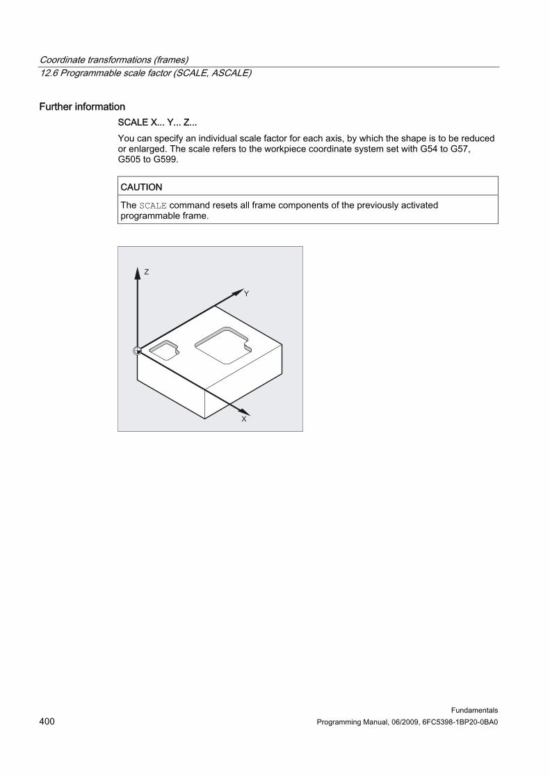
Coordinate transformations (frames) 12.6 Programmable scale factor (SCALE, ASCALE)
Fundamentals 400 Programming Manual, 06/2009, 6FC5398-1BP20-0BA0
Further information SCALE X... Y... Z... You can specify an individual scale factor for each axis, by which the shape is to be reduced or enlarged. The scale refers to the workpiece coordinate system set with G54 to G57, G505 to G599.
CAUTION The SCALE command resets all frame components of the previously activated programmable frame.

Coordinate transformations (frames) 12.6 Programmable scale factor (SCALE, ASCALE)
Fundamentals Programming Manual, 06/2009, 6FC5398-1BP20-0BA0 401
ASCALE X... Y... Z... The ASCALE command is used to program scale changes to be added to existing frames. In this case, the last valid scale factor is multiplied by the new one. The currently set or last programmed coordinate system is used as the reference for the scale change.
AROT
TRANS
ASCA
LE
Scaling and offset
Note If an offset is programmed with ATRANS after SCALE, the offset values will also be scaled.
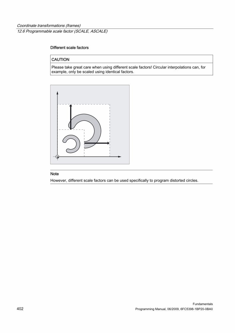
Coordinate transformations (frames) 12.6 Programmable scale factor (SCALE, ASCALE)
Fundamentals 402 Programming Manual, 06/2009, 6FC5398-1BP20-0BA0
Different scale factors
CAUTION Please take great care when using different scale factors! Circular interpolations can, for example, only be scaled using identical factors.
Note However, different scale factors can be used specifically to program distorted circles.

Coordinate transformations (frames) 12.7 Programmable mirroring (MIRROR, AMIRROR)
Fundamentals Programming Manual, 06/2009, 6FC5398-1BP20-0BA0 403
12.7 12.7 Programmable mirroring (MIRROR, AMIRROR)
Function MIRROR/AMIRROR can be used to mirror workpiece shapes on coordinate axes. All traversing movements programmed after the mirror call (e.g. in the subprogram) are executed with mirroring.
Syntax MIRROR X... Y... Z... AMIRROR X... Y... Z...
Note Each frame operation is programmed in a separate NC block.
Significance MIRROR: Mirror absolute in relation to the currently valid coordinate system
set with G54 to G57, G505 to G599. AMIRROR: Additive mirror image with reference to the currently valid set or
programmed coordinate system X... Y... Z... : Geometry axis whose direction is to be changed. The value
specified here can be chosen freely, e.g. X0 Y0 Z0.

Coordinate transformations (frames) 12.7 Programmable mirroring (MIRROR, AMIRROR)
Fundamentals 404 Programming Manual, 06/2009, 6FC5398-1BP20-0BA0
Examples Example 1: Milling
The contour shown here is programmed once as a subprogram. The 3 other contours are generated using mirroring. The workpiece zero is located at the center of the contours.
Program code Comment
N10 G17 G54 ; Working plane X/Y, workpiece zero
N20 L10 ; Machine first contour at top right
N30 MIRROR X0 ; Mirror X axis (the direction is changed in X)
N40 L10 ; Machine second contour at top left
N50 AMIRROR Y0 ; Mirror Y axis (the direction is changed in Y)
N60 L10 ; Machine third contour at bottom left
N70 MIRROR Y0 ; MIRROR resets previous frames. Mirror Y axis (the direction is changed in Y)
N80 L10 ; Machine fourth contour at bottom right
N90 MIRROR ; Deactivate mirroring
N100 G0 X300 Y100 M30 ; Retraction, end of program

Coordinate transformations (frames) 12.7 Programmable mirroring (MIRROR, AMIRROR)
Fundamentals Programming Manual, 06/2009, 6FC5398-1BP20-0BA0 405
Example 2: Turning
The actual machining is stored as a subprogram and execution at the respective spindle is implemented by means of mirroring and offsets.
Program code Comment
N10 TRANS X0 Z140 ; Zero offset to W
... ; Machining of the first side with spindle 1
N30 TRANS X0 Z600 ; Zero offset to spindle 2
N40 AMIRROR Z0 ; Mirroring of the Z axis
N50 ATRANS Z120 ; Zero offset to W1
... ; Machining of the second side with spindle 2

Coordinate transformations (frames) 12.7 Programmable mirroring (MIRROR, AMIRROR)
Fundamentals 406 Programming Manual, 06/2009, 6FC5398-1BP20-0BA0
Further information MIRROR X... Y... Z... The mirror is programmed by means of an axial change of direction in the selected working plane. Example: Working plane G17 X/Y The mirror (on the Y axis) requires a direction change in X and, accordingly, is programmed with MIRROR X0. The contour is then mirrored on the opposite side of the mirror axis Y.
Mirroring is implemented in relation to the currently valid coordinate system set with G54 to G57, G505 to G599.
CAUTION The MIRROR command resets all frame components of the previously activated programmable frame.

Coordinate transformations (frames) 12.7 Programmable mirroring (MIRROR, AMIRROR)
Fundamentals Programming Manual, 06/2009, 6FC5398-1BP20-0BA0 407
AMIRROR X... Y... Z... A mirror image, which is to be added to an existing transformation, is programmed with AMIRROR. The currently set or last programmed coordinate system is used as the reference.
Deactivate mirroring For all axes: MIRROR (without axis parameter) All frame components of the previously programmed frame are reset.
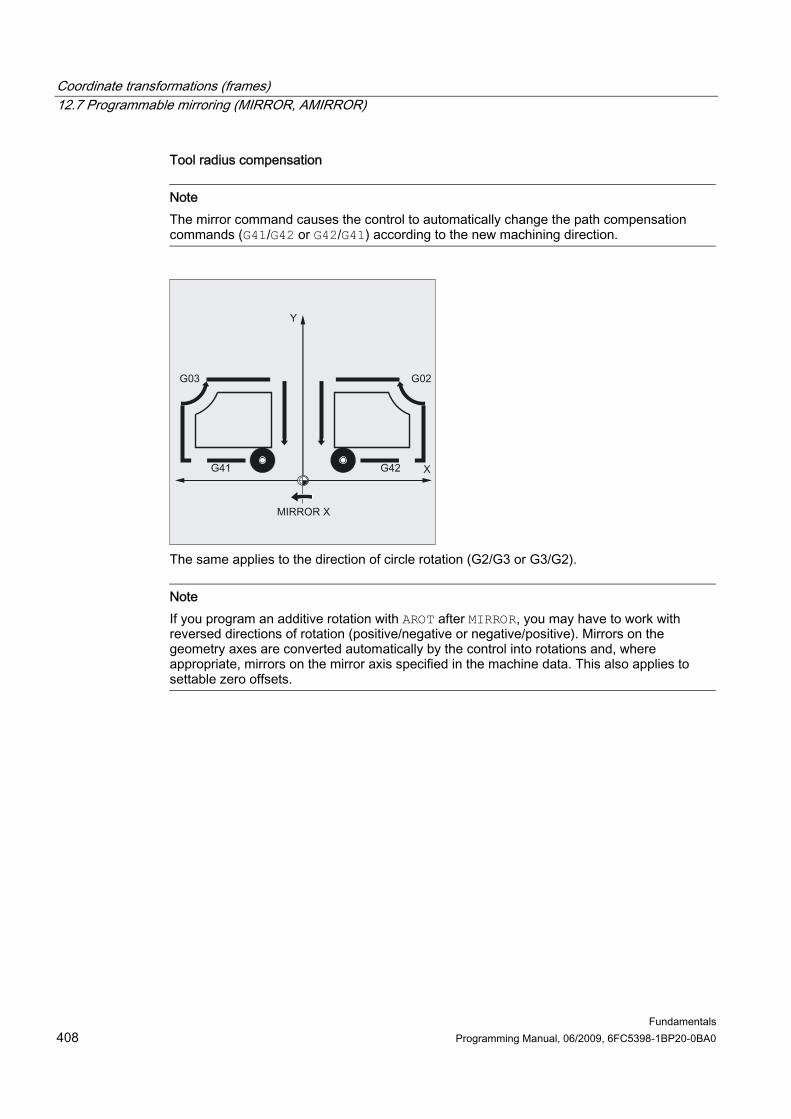
Coordinate transformations (frames) 12.7 Programmable mirroring (MIRROR, AMIRROR)
Fundamentals 408 Programming Manual, 06/2009, 6FC5398-1BP20-0BA0
Tool radius compensation
Note The mirror command causes the control to automatically change the path compensation commands (G41/G42 or G42/G41) according to the new machining direction.
The same applies to the direction of circle rotation (G2/G3 or G3/G2).
Note If you program an additive rotation with AROT after MIRROR, you may have to work with reversed directions of rotation (positive/negative or negative/positive). Mirrors on the geometry axes are converted automatically by the control into rotations and, where appropriate, mirrors on the mirror axis specified in the machine data. This also applies to settable zero offsets.
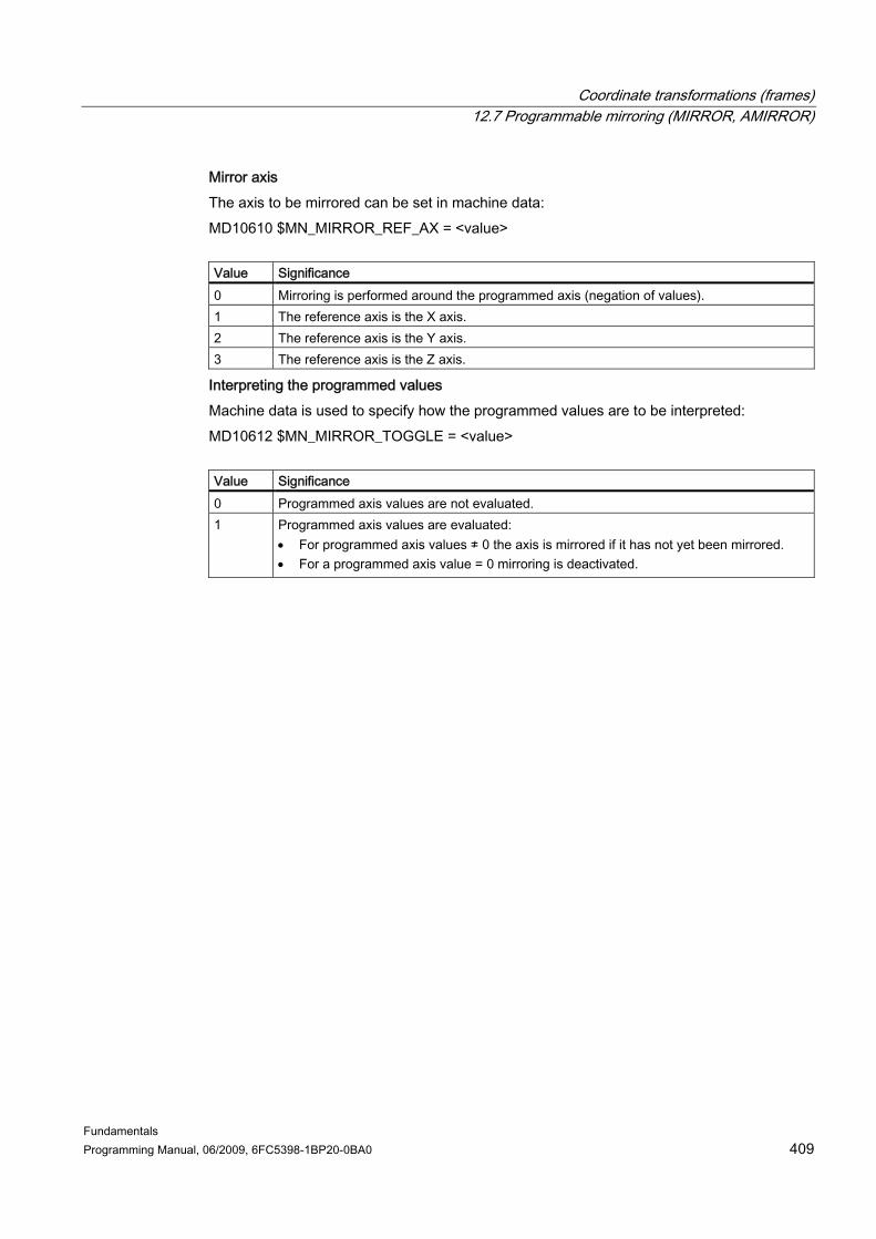
Coordinate transformations (frames) 12.7 Programmable mirroring (MIRROR, AMIRROR)
Fundamentals Programming Manual, 06/2009, 6FC5398-1BP20-0BA0 409
Mirror axis The axis to be mirrored can be set in machine data: MD10610 $MN_MIRROR_REF_AX = <value> Value Significance 0 Mirroring is performed around the programmed axis (negation of values). 1 The reference axis is the X axis. 2 The reference axis is the Y axis. 3 The reference axis is the Z axis.
Interpreting the programmed values Machine data is used to specify how the programmed values are to be interpreted: MD10612 $MN_MIRROR_TOGGLE = <value> Value Significance 0 Programmed axis values are not evaluated. 1 Programmed axis values are evaluated:
• For programmed axis values ≠ 0 the axis is mirrored if it has not yet been mirrored. • For a programmed axis value = 0 mirroring is deactivated.

Coordinate transformations (frames) 12.8 Frame generation according to tool orientation (TOFRAME, TOROT, PAROT)
Fundamentals 410 Programming Manual, 06/2009, 6FC5398-1BP20-0BA0
12.8 12.8 Frame generation according to tool orientation (TOFRAME, TOROT, PAROT)
Function TOFRAME generates a rectangular frame whose Z axis coincides with the current tool orientation. This means that the user can retract the tool in the Z direction without risk of collision (e.g. after a tool break in a 5-axis program). The position of the X and Y axes is determined by the setting in machine data MD21110 $MC_X_AXES_IN_OLD_X_Z_PLANE (coordinate system with automatic frame definition). The new coordinate system is either left as generated from the machine kinematics or is turned around the new Z axis additionally so that the new X axis lies in the old Z/X plane (see machine manufacturer's specifications). The resulting frame describing the orientation is written in the system variable for the programmable frame ($P_PFRAME). TOROT only overwrites the rotation component in the programmed frame. All other components remain unchanged. TOFRAME and TOROT are designed for milling operations in which G17 (working plane X/Y) is typically active. In the case of turning operations or generally when G18 or G19 is active, however, frames are needed where the X or Y axis matches the orientation of the tool. These frames are programmed with the TOFRAMEX/TOROTX or TOFRAMEY/TOROTY commands. PAROT aligns the workpiece coordinate system on the workpiece.
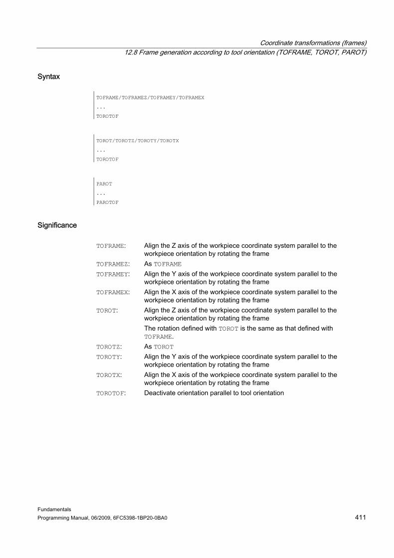
Coordinate transformations (frames) 12.8 Frame generation according to tool orientation (TOFRAME, TOROT, PAROT)
Fundamentals Programming Manual, 06/2009, 6FC5398-1BP20-0BA0 411
Syntax TOFRAME/TOFRAMEZ/TOFRAMEY/TOFRAMEX
...
TOROTOF
TOROT/TOROTZ/TOROTY/TOROTX
...
TOROTOF
PAROT
...
PAROTOF
Significance TOFRAME: Align the Z axis of the workpiece coordinate system parallel to the
workpiece orientation by rotating the frame TOFRAMEZ: As TOFRAME TOFRAMEY: Align the Y axis of the workpiece coordinate system parallel to the
workpiece orientation by rotating the frame TOFRAMEX: Align the X axis of the workpiece coordinate system parallel to the
workpiece orientation by rotating the frame TOROT: Align the Z axis of the workpiece coordinate system parallel to the
workpiece orientation by rotating the frame The rotation defined with TOROT is the same as that defined with TOFRAME.
TOROTZ: As TOROT TOROTY: Align the Y axis of the workpiece coordinate system parallel to the
workpiece orientation by rotating the frame TOROTX: Align the X axis of the workpiece coordinate system parallel to the
workpiece orientation by rotating the frame TOROTOF: Deactivate orientation parallel to tool orientation

Coordinate transformations (frames) 12.8 Frame generation according to tool orientation (TOFRAME, TOROT, PAROT)
Fundamentals 412 Programming Manual, 06/2009, 6FC5398-1BP20-0BA0
PAROT: Rotate frame to align workpiece coordinate system on workpiece Translations, scaling and mirroring in the active frame remain valid.
PAROTOF: The workpiece-specific frame rotation activated with PAROT is deactivated with PAROTOF.
Note The TOROT command ensures consistent programming with active orientable toolholders for each kinematic type. Just as in the situation for rotatable toolholders, PAROT can be used to activate a rotation of the work table. This defines a frame which changes the position of the workpiece coordinate system in such a way that no compensatory movement is performed on the machine. Language command PAROT is not rejected if no toolholder with orientation capability is active.
Example Program code Comment
N100 G0 G53 X100 Z100 D0
N120 TOFRAME
N140 G91 Z20 ; TOFRAME is included in the calculation, all programmed geometry axis movements refer to the new coordinate system.
N160 X50
...

Coordinate transformations (frames) 12.8 Frame generation according to tool orientation (TOFRAME, TOROT, PAROT)
Fundamentals Programming Manual, 06/2009, 6FC5398-1BP20-0BA0 413
Further information Assigning axis direction If one of the TOFRAMEX, TOFRAMEY, TOROTX, TOROTY commands is programmed instead of TOFRAME/TOFRAMEZ or TOROT/TOROTZ, the axis direction commands listed in this table will apply: Command Tool direction
(applicate) Secondary axis (abscissa)
Secondary axis (ordinate)
TOFRAME/TOFRAMEZ / TOROT/TOROTZ
Z X Y
TOFRAMEY/TOROTY Y Z X TOFRAMEX/TOROTX X Y Z
Separate system frame for TOFRAME or TOROT The frames resulting from TOFRAME or TOROT can be written in a separate system frame $P_TOOLFRAME. For this purpose, bit 3 must be enabled in machine data MD28082 $MC_MM_SYSTEM_FRAME_MASK. The programmable frame remains unchanged. Differences occur when the programmable frame is processed further elsewhere.
References For further information about machines with orientable toolholder, see: ● Programming Manual, Job Planning; Chapter: "Tool orientation" ● Function Manual, Basic Functions; Tool Offset (W1),
Chapter: "Toolholder with orientation capability"

Coordinate transformations (frames) 12.9 Deselect frame (G53, G153, SUPA, G500)
Fundamentals 414 Programming Manual, 06/2009, 6FC5398-1BP20-0BA0
12.9 12.9 Deselect frame (G53, G153, SUPA, G500)
Function When executing certain processes, such as approaching the tool change point, various frame components have to be defined and suppressed at different times. Settable frames can either be deactivated modally or suppressed non-modally. Programmable frames can be suppressed or deleted non-modally.
Syntax Non-modal suppression: G53/G153/SUPA
Modal deactivation: G500
Delete: TRANS/ROT/SCALE/MIRROR
Meaning G53: Non-modal suppression of all programmable and
settable frames G153: G153 has the same effect as G53 and also
suppresses the entire basic frame ($P_ACTBFRAME).
SUPA: SUPA has the same effect as G153 and also suppresses: • Handwheel offsets (DRF) • Overlaid movements • External work offset • PRESET offset
G500: Modal deactivation of all settable frames (G54 to G57,
G505 to G599) if G500 does not contain a value. TRANS/ROT/SCALE/MIRROR: TRANS/ROT/SCALE/MIRROR without an axis
parameter will delete the programmable frames.

Coordinate transformations (frames) 12.10 Deselecting overlaid movements (DRFOF, CORROF)
Fundamentals Programming Manual, 06/2009, 6FC5398-1BP20-0BA0 415
12.10 12.10 Deselecting overlaid movements (DRFOF, CORROF)
Function The additive work offsets set by means of handwheel traversal (DRF offsets) and the position offsets programmed using system variable $AA_OFF[<axis>] can be deselected using the part program commands DRFOF and CORROF. Deselection triggers a preprocessing stop and the position component of the deselected overlaid movement (DRF offset or position offset) is written to the position in the basic coordinate system (in other words, no axes are traversed). The value of system variable $AA_IM[<axis>] (current machine coordinate system setpoint of an axis) does not change; the value of system variable $AA_IW[<axis>] (current workpiece coordinate system setpoint of an axis) does change, because it now contains the deselected component from the overlaid movement.
Syntax DRFOF CORROF(<axis>,"<character string>"[,<axis>,"<character string>"])
Significance
Command for the deactivation (deselection) of DRF handwheel offsets for all active axes in the channel
DRFOF:
Active: modal Command for the deactivation (deselection) of the DRF offset/position offset ($AA_OFF) for individual axes Effective: modal <axis>: Axis identifier (channel, geometry or machine axis identifier)
== "DRF": DRF offset of axis is deselected
CORROF:
"<character string>":
== "AA_OFF": $AA_OFF position offset of axis is deselected
Note CORROF is only possible from the part program, not via synchronized actions.

Coordinate transformations (frames) 12.10 Deselecting overlaid movements (DRFOF, CORROF)
Fundamentals 416 Programming Manual, 06/2009, 6FC5398-1BP20-0BA0
Examples Example 1: Axial deselection of a DRF offset (1) A DRF offset is generated in the X axis by DRF handwheel traversal. No DRF offsets are operative for any other axes in the channel. Program code Comment
N10 CORROF(X,"DRF") ; CORROF has the same effect as DRFOF here.
...
Example 2: Axial deselection of a DRF offset (2) A DRF offset is generated in the X and Y axes by DRF handwheel traversal. No DRF offsets are operative for any other axes in the channel. Program code Comment
N10 CORROF(X,"DRF") ; Only the DRF offset of the X axis is deselected; the DRF offset of the Y axis is retained (in the case of DRFOF both offsets would have been deselected).
...
Example 3: Axial deselection of a $AA_OFF position offset Program code Comment
N10 WHEN TRUE DO $AA_OFF[X]=10 G4 F5 ; A position offset == 10 is interpolated for the X axis.
...
N80 CORROF(X,"AA_OFF") ; The position offset of the X axis is deselected with: $AA_OFF[X]=0
The X axis is not traversed.
The position offset is added to the current position of the X axis.
…
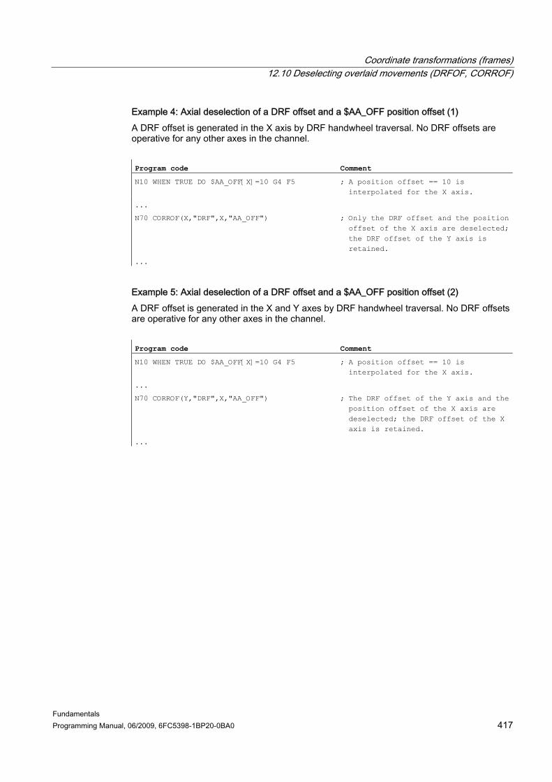
Coordinate transformations (frames) 12.10 Deselecting overlaid movements (DRFOF, CORROF)
Fundamentals Programming Manual, 06/2009, 6FC5398-1BP20-0BA0 417
Example 4: Axial deselection of a DRF offset and a $AA_OFF position offset (1) A DRF offset is generated in the X axis by DRF handwheel traversal. No DRF offsets are operative for any other axes in the channel. Program code Comment
N10 WHEN TRUE DO $AA_OFF[X]=10 G4 F5 ; A position offset == 10 is interpolated for the X axis.
...
N70 CORROF(X,"DRF",X,"AA_OFF") ; Only the DRF offset and the position offset of the X axis are deselected; the DRF offset of the Y axis is retained.
...
Example 5: Axial deselection of a DRF offset and a $AA_OFF position offset (2) A DRF offset is generated in the X and Y axes by DRF handwheel traversal. No DRF offsets are operative for any other axes in the channel. Program code Comment
N10 WHEN TRUE DO $AA_OFF[X]=10 G4 F5 ; A position offset == 10 is interpolated for the X axis.
...
N70 CORROF(Y,"DRF",X,"AA_OFF") ; The DRF offset of the Y axis and the position offset of the X axis are deselected; the DRF offset of the X axis is retained.
...

Coordinate transformations (frames) 12.10 Deselecting overlaid movements (DRFOF, CORROF)
Fundamentals 418 Programming Manual, 06/2009, 6FC5398-1BP20-0BA0
Further information $AA_OFF_VAL Once the position offset has been deselected by means of $AA_OFF, system variable $AA_OFF_VAL (integrated distance of axis override) for the corresponding axis will equal zero. $AA_OFF in JOG mode In JOG mode too, if $AA_OFF changes, the position offset will be interpolated as an overlaid movement if this function has been enabled via machine data MD 36750 $MA_AA_OFF_MODE. $AA_OFF in synchronized action If a synchronized action which immediately resets $AA_OFF (DO $AA_OFF[<axis>]=<value>) is active when the position offset is deselected using the CORROF(<axis>,"AA_OFF") part program command, then $AA_OFF will be deselected and not reset, and alarm 21660 will be signaled. However, if the synchronized action becomes active later, e.g. in the block after CORROF, $AA_OFF will remain set and a position offset will be interpolated. Automatic channel axis exchange If an axis for which CORROF has been programmed is active in another channel, it will be pulled into the channel when the axis changes (condition: MD30552 $MA_AUTO_GET_TYPE > 0) and then the position offset and/or the DRF offset will be deselected.
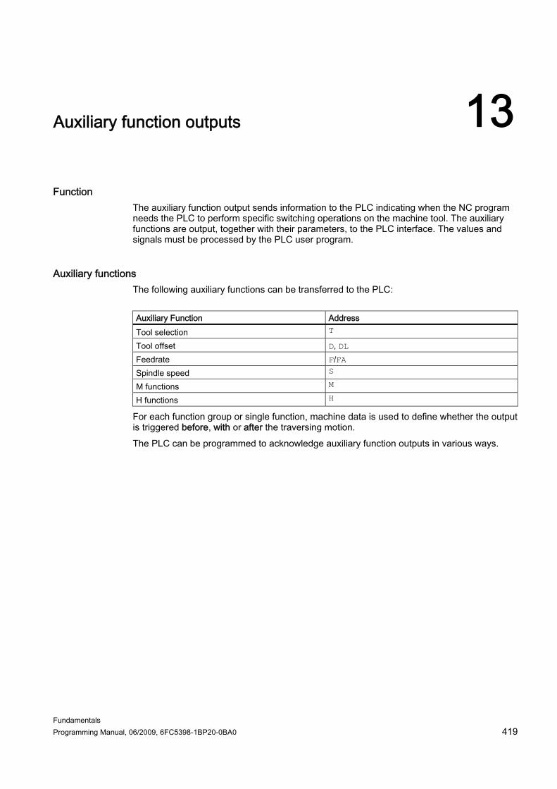
Fundamentals Programming Manual, 06/2009, 6FC5398-1BP20-0BA0 419
Auxiliary function outputs 13
Function The auxiliary function output sends information to the PLC indicating when the NC program needs the PLC to perform specific switching operations on the machine tool. The auxiliary functions are output, together with their parameters, to the PLC interface. The values and signals must be processed by the PLC user program.
Auxiliary functions The following auxiliary functions can be transferred to the PLC: Auxiliary Function Address Tool selection T
Tool offset D, DL Feedrate F/FA Spindle speed S
M functions M
H functions H
For each function group or single function, machine data is used to define whether the output is triggered before, with or after the traversing motion. The PLC can be programmed to acknowledge auxiliary function outputs in various ways.

Auxiliary function outputs 12.10 Deselecting overlaid movements (DRFOF, CORROF)
Fundamentals 420 Programming Manual, 06/2009, 6FC5398-1BP20-0BA0
Properties Important properties of the auxiliary function are shown in the following overview table:
Address extension Value Function Meaning Range Range Type Meaning
Explanations Maximum number per block
- 0 (implicit)
0 ... 99 INT Function The address extension is 0 for the range between 0 and 99. Mandatory without address extension: M0, M1, M2, M17, M30
Spindle no. 1 - 12 1 ... 99 INT Function M3, M4, M5, M19, M70 with address extension spindle no. (e.g. M2=5; spindle stop for spindle 2). Without spindle number, the function applies for the master spindle.
M
Any 0 - 99 100 ... 2147483647
INT Function User M function*
5
S Spindle no. 1 - 12 0 ... ± 1,8*10308 REAL Spindle speed
Without spindle number, the function applies for the master spindle.
3
H Any 0 - 99 0 ... ± 2147483647 ± 1,8*10308
INT REAL
Any Functions have no effect in the NCK; only to be implemented on the PLC.*
3
T Spindle no. (for active tool management)
1 - 12 0 - 32000 (or tool names with active tool management)
INT Tool selection
Tool names are not passed to the PLC interface.
1
D - - 0 - 12 INT Tool offset selection
D0: Deselection Default setting: D1
1
DL Location-dependent offset
1 - 6 0 ... ± 1,8*10308 REAL Tool fine offset selection
Refers to previously selected D number.
1
F - - 0.001 - 999 999.999
REAL Path feedrate
6
FA Axis No. 1 - 31 0.001 - 999 999.999
REAL Axial feedrate
* The meaning of the functions is defined by the machine manufacturer (see machine manufacturer's specifications).

Auxiliary function outputs 12.10 Deselecting overlaid movements (DRFOF, CORROF)
Fundamentals Programming Manual, 06/2009, 6FC5398-1BP20-0BA0 421
Further information Number of function outputs per NC block Up to 10 function outputs can be programmed in one NC block. Auxiliary functions can also be output from the action component of synchronized actions. References: Function Manual, Synchronized Actions Grouping The functions described can be grouped together. Group assignment is predefined for some M commands. The acknowledgment behavior can be defined by the grouping. High-speed function outputs (QU) Functions, which have not been programmed as high-speed outputs, can be defined as high-speed outputs for individual outputs with the keyword QU. Program execution continues without waiting for the acknowledgment of the miscellaneous function (the program waits for the transport acknowledgment). This helps avoid unnecessary hold points and interruptions to traversing movements.
Note The appropriate machine data must be set for the "High-speed function outputs" function (→ machine manufacturer).
Function outputs for travel commands The transfer of information as well as waiting for the appropriate response takes time and therefore influences the traversing movements.

Auxiliary function outputs 12.10 Deselecting overlaid movements (DRFOF, CORROF)
Fundamentals 422 Programming Manual, 06/2009, 6FC5398-1BP20-0BA0
High-speed acknowledgment without block change delay Block change behavior can be influenced by machine data. When the "without block change delay" setting is selected, the system response with respect to high-speed auxiliary functions is as follows: Auxiliary function output Response Before the movement The block transition between blocks with high-speed auxiliary functions
occurs without interruption and without a reduction in velocity. The auxiliary function output takes place in the first interpolation cycle of the block. The following block is executed with no acknowledgment delay.
During the movement The block transition between blocks with high-speed auxiliary functions occurs without interruption and without a reduction in velocity. The auxiliary function output takes place during the block. The following block is executed with no acknowledgment delay.
After the movement The movement stops at the end of the block. The auxiliary function output takes place at the end of the block. The following block is executed with no acknowledgment delay.
CAUTION Function outputs in continuous-path mode Function outputs before the traversing movements interrupt the continuous-path mode (G64/G641) and generate an exact stop for the previous block. Function outputs after the traversing movements interrupt the continuous-path mode (G64/G641) and generate an exact stop for the current block. Important: A wait for an outstanding acknowledgment signal from the PLC can also interrupt the continuous-path mode, e.g. for M command sequences in blocks with extremely short path lengths.
Auxiliary function outputs 13.1 M functions
Fundamentals Programming Manual, 06/2009, 6FC5398-1BP20-0BA0 423
13.1 13.1 M functions
Function The M functions initiate switching operations, such as "Coolant ON/OFF" and other functions on the machine.
Syntax M<value> M[<address extension>] = <value>
Significance M: Address for the programming of the M functions. <address extension>: The extended address notation applies for some M
functions (e.g. specification of the spindle number for spindle functions). Assignment is made to a certain machine function through the value assignment (M function number). Type: INT
<value>:
Range of values: 0 ... 2147483647 (max. INT value)

Auxiliary function outputs 13.1 M functions
Fundamentals 424 Programming Manual, 06/2009, 6FC5398-1BP20-0BA0
Predefined M functions Certain important M functions for program execution are supplied as standard with the control: M function Meaning M0* Programmed stop M1* Optional stop M2* End of main program with return to beginning of program M3 Spindle clockwise M4 Spindle counterclockwise M5 Spindle stop M6 Tool change (default setting) M17* End of subroutine M19 Position the spindle M30* End of program (as M2) M40 Automatic gear change M41 Gear stage 1 M42 Gear stage 2 M43 Gear stage 3 M44 Gear stage 4 M45 Gear stage 5 M70 Spindle is switched to axis mode
NOTICE Extended address notation cannot be used for the functions marked with *. The commands M0, M1, M2, M17 and M30 are always issued after the traversing movement.

Auxiliary function outputs 13.1 M functions
Fundamentals Programming Manual, 06/2009, 6FC5398-1BP20-0BA0 425
M functions defined by the machine manufacturer All free M function numbers can be used by the machine manufacturer, e.g. for switching functions to control the clamping devices or for the activation/deactivation of further machine functions.
NOTICE The functions assigned to the free M function numbers are machine-specific. A certain M function can therefore have a different functionality on another machine. Refer to the machine manufacturer's specifications for the M functions available on a machine and their functions.
Examples Example 1: Maximum number of M functions in a block Program code Comment
N10 S...
N20 X... M3 ; M function in the block with axis movement, spindle accelerates before the X axis movement
N180 M789 M1767 M100 M102 M376 ; Maximum of five M functions in the block
Example 2: M function as high-speed output Program code Comment
N10 H=QU(735) ; Fast output for H735.
N10 G1 F300 X10 Y20 G64 ;
N20 X8 Y90 M=QU(7) ; Fast output for M7.
M7 has been programmed as high-speed output so that the continuous-path mode (G64) is not interrupted.
Note Only use this function in special cases as, for example, the chronological alignment is changed in combination with other function outputs.

Auxiliary function outputs 13.1 M functions
Fundamentals 426 Programming Manual, 06/2009, 6FC5398-1BP20-0BA0
Further information about the predefined M commands Programmed stop: M0 The machining is stopped in the NC block with M0. You can now remove chips, remeasure, etc. Programmed stop 1 - optional stop: M1 M1 can be set via: ● HMI / dialog box "Program Control"
or ● NC/PLC interface The program execution of the NC is stopped by the programmed blocks. Programmed stop 2 - an auxiliary function associated with M1 with stop in the program execution Programmed stop 2 can be set via the HMI / dialog box "Program Control" and allows the technological sequences to be interrupted at any time at the end of the part to be machined. In this way, the operator can interrupt the production, e.g. to remove chip flows. End of program: M2, M17, M30 A program is terminated with M2, M17 or M30 and reset to the start of the program. If the main program is called from another program (as subroutine), M2/M30 has the same effect as M17 and vice versa, i.e. M17 has the same effect in the main program as M2/M30. Spindle functions: M3, M4, M5, M19, M70 The extended address notation with specification of the spindle number applies for all spindles. Example: Program code Comment
M2=3 ; Clockwise spindle rotation for the second spindle
If an address extension has not been programmed, the function applies for the master spindle.

Fundamentals Programming Manual, 06/2009, 6FC5398-1BP20-0BA0 427
Supplementary commands 1414.1 14.1 Messages (MSG)
Function Messages can be programmed to provide the user with information about the current machining situation during program execution.
Syntax MSG("<message text>") MSG ()
Significance MSG: Keyword for the programming of a message text.
Character string that is to be displayed as a message. Type: STRING
<message text>:
A message text can be up to 124 characters long and is displayed in two lines (2*62 characters). Contents of variables can also be displayed in message texts. A message can be deleted by programming MSG() without message text.
Supplementary commands 14.1 Messages (MSG)
Fundamentals 428 Programming Manual, 06/2009, 6FC5398-1BP20-0BA0
Examples Example 1: Activate/delete messages Program code Comment
N10 MSG ("Roughing the contour") ; Activate message
N20 X… Y…
N …
N90 MSG () ; Delete message from N10
Example 2: Message text contains variable Program code Comment
N10 R12=$AA_IW [X] ; Current position of the X axis in R12
N20 MSG ("Check position of X axis"<<R12<<) ; Activate message
N …
N90 MSG () ; Delete message from N20

Supplementary commands 14.2 Working area limitation
Fundamentals Programming Manual, 06/2009, 6FC5398-1BP20-0BA0 429
14.2 14.2 Working area limitation
14.2.1 Working area limitation in BCS (G25/G26, WALIMON, WALIMOF)
Function G25/G26 limits the working area (working field, working space) in which the tool can traverse. The areas outside the working area limitations defined with G25/G26 are inhibited for any tool motion.
The coordinates for the individual axes apply in the basic coordinate system:
Supplementary commands 14.2 Working area limitation
Fundamentals 430 Programming Manual, 06/2009, 6FC5398-1BP20-0BA0
The working area limitation for all validated axes must be programmed with the WALIMON command. The WALIMOF command deactivates the working area limitation. WALIMON is the default setting. Therefore, it only has to be programmed if the working area limitation has been disabled beforehand.
Syntax G25 X…Y…Z… G26 X…Y…Z… WALIMON WALIMOF
Significance G25: Lower working area limitation
Assignment of values in channel axes in the basic coordinate system G26: Upper working area limitation
Assignment of values in channel axes in the basic coordinate system X… Y… Z…: Lower or upper working area limits for individual channel axes
The limits specified refer to the basic coordinate system. WALIMON: Switch working area limitation on for all axes WALIMOF: Switch working area limitation off for all axes
In addition to programming values using G25/G26, values can also be entered using axis-specific setting data: SD43420 $SA_WORKAREA_LIMIT_PLUS (Working area limitation plus) SD43430 $SA_WORKAREA_LIMIT_MINUS (Working area limitation minus) Activating and de-activating the working area limitation, parameterized using SD43420 and SD43430, are carried-out for a specific direction using the axis-specific setting data that becomes immediately effective: SD43400 $SA_WORKAREA_PLUS_ENABLE (Working area limitation active in the positive direction) SD43410 $SA_WORKAREA_MINUS_ENABLE (Working area limitation active in the negative direction) Using the direction-specific activation/de-activation, it is possible to limit the working range for an axis in just one direction.
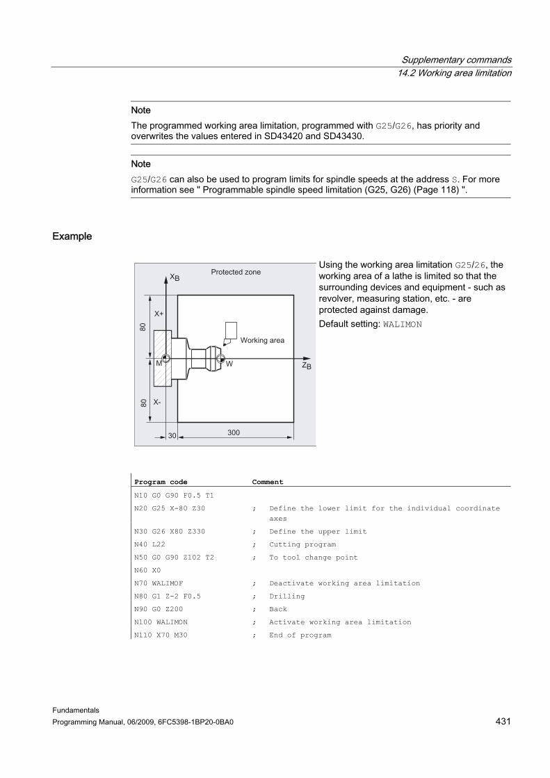
Supplementary commands 14.2 Working area limitation
Fundamentals Programming Manual, 06/2009, 6FC5398-1BP20-0BA0 431
Note The programmed working area limitation, programmed with G25/G26, has priority and overwrites the values entered in SD43420 and SD43430.
Note G25/G26 can also be used to program limits for spindle speeds at the address S. For more information see " Programmable spindle speed limitation (G25, G26) (Page 118) ".
Example
Using the working area limitation G25/26, the working area of a lathe is limited so that the surrounding devices and equipment - such as revolver, measuring station, etc. - are protected against damage. Default setting: WALIMON
Program code Comment
N10 G0 G90 F0.5 T1
N20 G25 X-80 Z30 ; Define the lower limit for the individual coordinate axes
N30 G26 X80 Z330 ; Define the upper limit
N40 L22 ; Cutting program
N50 G0 G90 Z102 T2 ; To tool change point
N60 X0
N70 WALIMOF ; Deactivate working area limitation
N80 G1 Z-2 F0.5 ; Drilling
N90 G0 Z200 ; Back
N100 WALIMON ; Activate working area limitation
N110 X70 M30 ; End of program

Supplementary commands 14.2 Working area limitation
Fundamentals 432 Programming Manual, 06/2009, 6FC5398-1BP20-0BA0
Further information Reference point at the tool When tool length compensation is active, the tip of the tool is monitored as reference point, otherwise it is the toolholder reference point. Consideration of the tool radius must be activated separately. This is done using channel-specific machine data: MD21020 $MC_WORKAREA_WITH_TOOL_RADIUS If the tool reference point lies outside the working area defined by the working area limitation or if this area is left, the program sequence is stopped.
Note If transformations are active, then tool data are taken into consideration (tool length and tool radius) can deviate from the described behavior. References: /FB1/ Function Manual, Basic Functions; Axis Monitoring, Protection Zones (A3), Chapter: "Monitoring the working area limitation"
Programmable working area limitation, G25/G26 An upper (G26) and a lower (G25) working area limitation can be defined for each axis. These values are effective immediately and remain effective for the corresponding MD setting (→ MD10710 $MN_PROG_SD_RESET_SAVE_TAB) after RESET and after being powered-up again.
Note The CALCPOSI subroutine is described in the Job Planning Programming Manual Using this subroutine before any traversing motion is made, it can be checked as to whether the predicted path is moved through taking into account the working area limits and/or the protection zones.

Supplementary commands 14.2 Working area limitation
Fundamentals Programming Manual, 06/2009, 6FC5398-1BP20-0BA0 433
14.2.2 Working area limitation in WCS/SZS (WALCS0 ... WALCS10)
Function In addition to the working area limitation with WALIMON (see "Working area limitation in BCS (G25/G26, WALIMON, WALIMOF) (Page 429)") there is an additional working area limitation that is activated using the G commands WALCS1 to WALCS10. Contrary to the working area limitation with WALIMON, the working area here is not in the basic coordinate system, but is limited coordinate system-specific in the workpiece coordinate system (WCS) or in the settable zero system (SZS). Using the G commands WALCS1 - WALCS10, a data set (working area limitation group) is selected under the up to ten channel-specific data sets for the coordinate system-specific working area limitations. A data set contains the limit values for all axes in the channel. The limitations are defined by channel-specific system variables.
Application The working area limitation with WALCS1 - WALCS10 ("Working area limitation in the WCS/SZS") is mainly used for working area limitations for conventional lathes. They allow the programmer to use the defined "end stops" - when moving the axis "manually" to define a working area limitation referred to the workpiece.
Syntax The "working area limitation in the "WCS/SZS" is activated by selecting a working area limitation group. G commands are used to make the selection: WALCS1 Activating working area limitation group No. 1 ... WALCS10 Activating working area limitation group No. 10
The de-activation of the "working area limitation in the WCS/SZS" is realized using G commands: WALCS0 De-activating the active working area limitation group

Supplementary commands 14.2 Working area limitation
Fundamentals 434 Programming Manual, 06/2009, 6FC5398-1BP20-0BA0
Meaning The working area limitations of the individual axes are set and the reference frame (WCS or SZS), in which the working area limits are to be effective, activated with WALCS1 - WALCS10, by writing to channel-specific system variables:
System variable Description Setting the working area limits $AC_WORKAREA_CS_PLUS_ENABLE [WALimNo, ax] Validity of the working area limitation in the positive axis
direction. $AC_WORKAREA_CS_LIMIT_PLUS [WALimNo, ax] Working area limitation in the positive axis direction.
Only effective, if: $AC_WORKAREA_CS_PLUS_ENABLE = TRUE
$AC_WORKAREA_CS_MINUS_ENABLE [WALimNo, ax] Validity of the working area limitation in the negative axis direction.
$AC_WORKAREA_CS_LIMIT_MINUS [WALimNo, ax] Working area limitation in the negative axis direction. Only effective, if: $AC_WORKAREA_CS_PLUS_ENABLE = TRUE
Selecting the reference frame Coordinate system to which the working area limitation group is referred: Value Description 1 Workpiece coordinate system (WCS)
$AC_WORKAREA_CS_COORD_SYSTEM [WALimNo]
3 Settable zero system (SZS)
<WALimNo>: Number of the working area limitation group. <ax>: Channel axis name of the axis for which the value is valid.
Example Three axes are defined in the channel: X, Y and Z A working area limitation group No. 2 is to be defined and then activated in which the axes are to be limited in the WCS acc. to the following specifications: ● X axis in the plus direction: 10 mm ● X axis in the minus direction: No limitation ● Y axis in the plus direction: 34 mm ● Y axis in the minus direction: -25 mm ● Z axis in the plus direction: No limitation ● Z axis in the minus direction: -600 mm
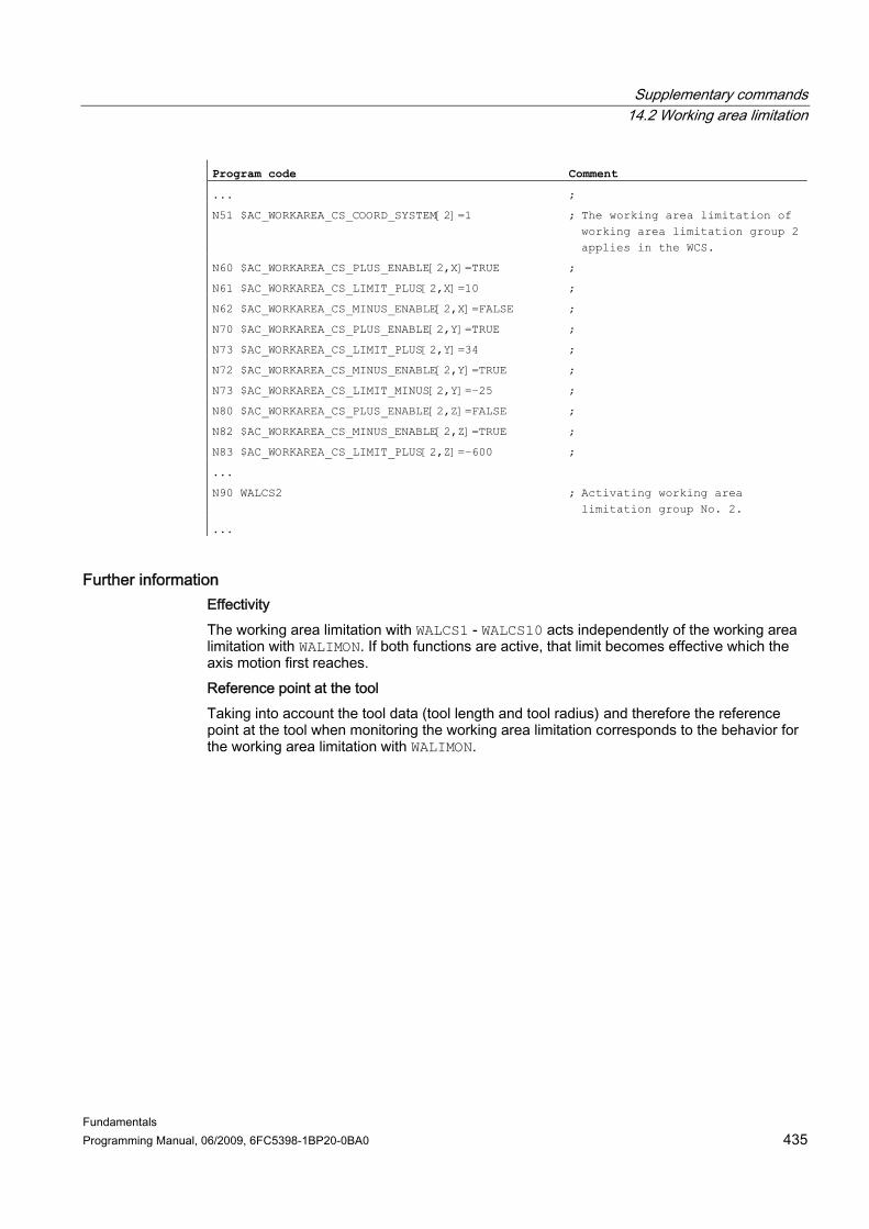
Supplementary commands 14.2 Working area limitation
Fundamentals Programming Manual, 06/2009, 6FC5398-1BP20-0BA0 435
Program code Comment
... ;
N51 $AC_WORKAREA_CS_COORD_SYSTEM[2]=1 ; The working area limitation of working area limitation group 2 applies in the WCS.
N60 $AC_WORKAREA_CS_PLUS_ENABLE[2,X]=TRUE ;
N61 $AC_WORKAREA_CS_LIMIT_PLUS[2,X]=10 ;
N62 $AC_WORKAREA_CS_MINUS_ENABLE[2,X]=FALSE ;
N70 $AC_WORKAREA_CS_PLUS_ENABLE[2,Y]=TRUE ;
N73 $AC_WORKAREA_CS_LIMIT_PLUS[2,Y]=34 ;
N72 $AC_WORKAREA_CS_MINUS_ENABLE[2,Y]=TRUE ;
N73 $AC_WORKAREA_CS_LIMIT_MINUS[2,Y]=–25 ;
N80 $AC_WORKAREA_CS_PLUS_ENABLE[2,Z]=FALSE ;
N82 $AC_WORKAREA_CS_MINUS_ENABLE[2,Z]=TRUE ;
N83 $AC_WORKAREA_CS_LIMIT_PLUS[2,Z]=–600 ;
...
N90 WALCS2 ; Activating working area limitation group No. 2.
...
Further information Effectivity The working area limitation with WALCS1 - WALCS10 acts independently of the working area limitation with WALIMON. If both functions are active, that limit becomes effective which the axis motion first reaches. Reference point at the tool Taking into account the tool data (tool length and tool radius) and therefore the reference point at the tool when monitoring the working area limitation corresponds to the behavior for the working area limitation with WALIMON.

Supplementary commands 14.3 Reference point approach (G74)
Fundamentals 436 Programming Manual, 06/2009, 6FC5398-1BP20-0BA0
14.3 14.3 Reference point approach (G74)
Function When the machine has been powered up (where incremental position measuring systems are used), all of the axis slides must approach their reference mark. Only then can traversing movements be programmed. The reference point can be approached in the NC program with G74.
Syntax G74 X1=0 Y1=0 Z1=0 A1=0 … ; Programmed in a separate NC block
Significance G74: Search for reference X1=0 Y1=0 Z1=0 … : Specified machine axis address X1, Y1, Z1… Search for
reference for linear axes A1=0 B1=0 C1=0 … : Specified machine axis address A1, B1, C1… Search for
reference for rotary axes.
Note A transformation must not be programmed for an axis which is to approach the reference point with G74.
The transformation is deactivated with command TRAFOOF.
Example When the measurement system is changed, the reference point is approached and the workpiece zero point is initialized. Program code Comment
N10 SPOS=0 ; Spindle in position control
N20 G74 X1=0 Y1=0 Z1=0 C1=0 ; Reference point approach for linear axes and rotary axes
N30 G54 ; Zero offset
N40 L47 ; Cutting program
N50 M30 ; End of program

Supplementary commands 14.4 Fixed-point approach (G75, G751)
Fundamentals Programming Manual, 06/2009, 6FC5398-1BP20-0BA0 437
14.4 14.4 Fixed-point approach (G75, G751)
Function The non-modal command G75/G751 can be used to move axes individually and independently of one another to fixed points in the machine space, e.g. to tool change points, loading points, pallet change points, etc. The fixed points are positions in the machine coordinate system which are stored in the machine data (MD30600 $MA_FIX_POINT_POS[n]). A maximum of four fixed points can be defined for each axis. The fixed points can be approached from every NC program irrespective of the current tool or workpiece positions. An internal preprocessing stop is executed prior to moving the axes. The approach can be made directly (G75) or via an intermediate point (G751):
Supplementary commands 14.4 Fixed-point approach (G75, G751)
Fundamentals 438 Programming Manual, 06/2009, 6FC5398-1BP20-0BA0
Conditions The following conditions must be satisfied to approach fixed points with G75/G751: ● The fixed-point coordinates must have been calculated exactly and written to machine
data. ● The fixed points must be located within the valid traversing range (→ note the software
limit switch limits!) ● The axes to be traversed must be referenced. ● No tool radius compensation must be active. ● A kinematic transformation may not be active. ● None of the axes to be traversed must be involved in active transformation. ● None of the axes to be traversed must be a following axis in an active coupling. ● None of the axes to be traversed must be an axis in a gantry grouping. ● Compile cycles must not activate motion components.
Syntax G75/G751 <axis name><axis position> ... FP=<n>
Significance G75: Approach fixed point directly G751: Approach fixed point via intermediate point <axis name>: Name of the machine axis to be traversed to the fixed point
All axis identifiers are permitted. <axis position>: In the case of G75 the specified position value is irrelevant. A
value of "0" is, therefore, usually specified. Things are different for G751, where the position of the intermediate point to be approached has to be specified as the value. Fixed point that is to be approached
Fixed point number <n>: Range of values: 1, 2, 3, 4
FP=:
Note: In the absence of FP=<n> or a fixed point number, or if FP=0 has been programmed, this is interpreted as FP=1 and fixed point 1 is approached.

Supplementary commands 14.4 Fixed-point approach (G75, G751)
Fundamentals Programming Manual, 06/2009, 6FC5398-1BP20-0BA0 439
Note Multiple axes can be programmed in one G75/751 block. The axes are then traversed simultaneously to the specified fixed point.
Note The following applies for G751: Axes which are to only approach the fixed point without first moving to an intermediate point cannot be programmed.
Note The value of the address FP must not be greater than the number of fixed points specified for each programmed axis (MD30610 $MA_NUM_FIX_POINT_POS).
Examples Example 1: G75 For a tool change, axes X (= AX1) and Z (= AX3) need to move to the fixed machine axis position 1 where X = 151.6 and Z = -17.3. Machine data: ● MD30600 $MA_FIX_POINT_POS[AX1,0] = 151.6 ● MD30600 $MA_FIX_POINT[AX3,0] = 17.3 NC program: Program code Comment
…
N100 G55 ; Activate adjustable work offset.
N110 X10 Y30 Z40 ; Approach positions in workpiece coordinate system.
N120 G75 X0 Z0 FP=1 M0 ; The X axis moves to 151.6 and the Z axis moves to 17.3 (in the machine coordinate system). Each axis travels at the maximum velocity it is capable of reaching. No additional movements are permitted to be active in this block. To continue to prevent any additional movements once the end positions have been reached, a stop is inserted here.
N130 X10 Y30 Z40 ; The position of N110 is approached again. The work offset is reactivated.
…
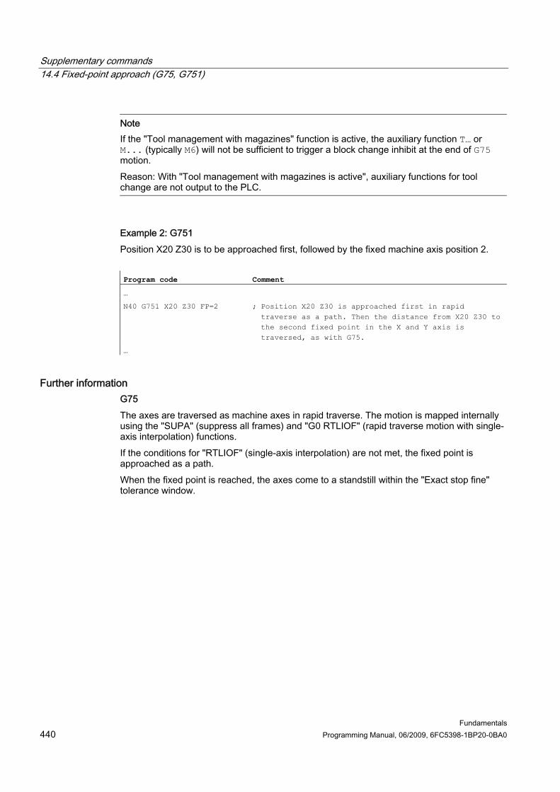
Supplementary commands 14.4 Fixed-point approach (G75, G751)
Fundamentals 440 Programming Manual, 06/2009, 6FC5398-1BP20-0BA0
Note If the "Tool management with magazines" function is active, the auxiliary function T… or M... (typically M6) will not be sufficient to trigger a block change inhibit at the end of G75 motion. Reason: With "Tool management with magazines is active", auxiliary functions for tool change are not output to the PLC.
Example 2: G751 Position X20 Z30 is to be approached first, followed by the fixed machine axis position 2. Program code Comment
…
N40 G751 X20 Z30 FP=2 ; Position X20 Z30 is approached first in rapid traverse as a path. Then the distance from X20 Z30 to the second fixed point in the X and Y axis is traversed, as with G75.
…
Further information G75 The axes are traversed as machine axes in rapid traverse. The motion is mapped internally using the "SUPA" (suppress all frames) and "G0 RTLIOF" (rapid traverse motion with single-axis interpolation) functions. If the conditions for "RTLIOF" (single-axis interpolation) are not met, the fixed point is approached as a path. When the fixed point is reached, the axes come to a standstill within the "Exact stop fine" tolerance window.

Supplementary commands 14.4 Fixed-point approach (G75, G751)
Fundamentals Programming Manual, 06/2009, 6FC5398-1BP20-0BA0 441
G751 The intermediate position is approached with rapid traverse and active offset (tool offset, frames, etc.), and the axes move with interpolation. The next fixed-point approach is executed as with G75. Once the fixed point has been reached the offsets are reactivated (as with G75). Additional axis movements The following additional axis movements are taken into account at the point at which the G75/G751 block is interpolated: ● External work offset ● DRF ● Synchronization offset ($AA_OFF) After this, the additional axis movements are not permitted to change until the end of traversing is reached by the G75/G751 block. Additional movements following interpretation of the G75/G751 block will offset the approach to the fixed point accordingly. The following additional movements are not taken into account, irrespective of the point at which interpolation takes place, and will offset the target position accordingly. ● Online tool offset ● Additional movements from compile cycles in the BCS and machine coordinate system Active frames All active frames are ignored. Traversing is performed in the machine coordinate system. Working area limitation in the workpiece coordinate system/SZS Coordinate-system-specific working area limitation (WALCS0 ... WALCS10) is not effective in the block with G75/G751. The destination point is monitored as the starting point of the following block.

Supplementary commands 14.4 Fixed-point approach (G75, G751)
Fundamentals 442 Programming Manual, 06/2009, 6FC5398-1BP20-0BA0
Axis/Spindle movements with POSA/SPOSA If programmed axes/spindles were previously traversed with POSA or SPOSA, these movements will be completed first before the fixed point is approached. Spindle functions in the G75/G751 block If the spindle is excluded from "Fixed-point approach", then additional spindle functions (e.g. positioning with SPOS/SPOSA) can be programmed in the G75/G751 block. Modulo axes In the case of modulo axes, the fixed point is approached along the shortest distance. References For further information about "Fixed-point approach", see: Function Manual, Extended Functions; Manual and Handwheel Travel (H1), Chapter: "Fixed-point approach in JOG"

Supplementary commands 14.5 Travel to fixed stop (FXS, FXST, FXSW)
Fundamentals Programming Manual, 06/2009, 6FC5398-1BP20-0BA0 443
14.5 14.5 Travel to fixed stop (FXS, FXST, FXSW)
Function The "Travel to fixed stop" function can be used to establish defined forces for clamping workpieces, such as those required for tailstocks, quills and grippers. The function can also be used for the approach of mechanical reference points.
With sufficiently reduced torque, it is also possible to perform simple measurement operations without connecting a probe. The "travel to fixed stop" function can be implemented for axes as well as for spindles with axis-traversing capability.
Syntax FXS[<axis>]=… FXST[<axis>]=… FXSW[<axis>]=… FXS[<axis>]=… FXST[<axis>]=… FXS[<axis>]=… FXST[<axis>]=… FXSW[<axis>]=…

Supplementary commands 14.5 Travel to fixed stop (FXS, FXST, FXSW)
Fundamentals 444 Programming Manual, 06/2009, 6FC5398-1BP20-0BA0
Significance
Command for activation and deactivation of the "Travel to fixed stop" function FXS[<axis>]=1: Activate function
FXS:
FXS=[<axis>]=0: Deactivate function FXST: Optional command for setting the clamping torque
Specified as % of the maximum drive torque FXSW: Optional command for setting the window width for the fixed stop
monitoring Specified in mm, inches or degrees
<axis>: Machine axis name Machine axes (X1, Y1, Z1, etc.) are programmed
Note The commands FXS, FXST and FXSW are modal. The programming of FXST and FXSW is optional: If no parameter is specified, the last programmed value or the value set in the relevant machine data applies.
Activate travel to fixed stop: FXS[<axis>] = 1 The movement to the destination point can be described as a path or positioning axis movement. With positioning axes, the function can be performed across block boundaries. Travel to fixed stop can be performed simultaneously for several axes and parallel to the movement of other axes. The fixed stop must be located between the start and end positions. Example: Program code Comment
X250 Y100 F100 FXS[X1]=1 FXST[X1]=12.3 FXSW[X1]=2 ; Axis X1 travels with feed F100 (parameter optional) to destination position X=250 mm.
The clamping torque is 12.3% of the maximum drive torque, monitoring is performed in a 2 mm wide window.
...
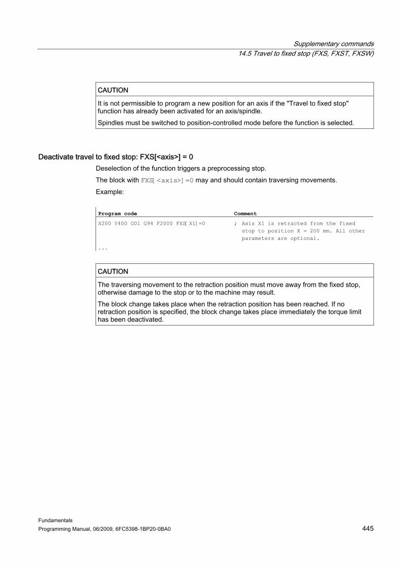
Supplementary commands 14.5 Travel to fixed stop (FXS, FXST, FXSW)
Fundamentals Programming Manual, 06/2009, 6FC5398-1BP20-0BA0 445
CAUTION It is not permissible to program a new position for an axis if the "Travel to fixed stop" function has already been activated for an axis/spindle. Spindles must be switched to position-controlled mode before the function is selected.
Deactivate travel to fixed stop: FXS[<axis>] = 0 Deselection of the function triggers a preprocessing stop. The block with FXS[<axis>]=0 may and should contain traversing movements. Example: Program code Comment
X200 Y400 G01 G94 F2000 FXS[X1]=0 ; Axis X1 is retracted from the fixed stop to position X = 200 mm. All other parameters are optional.
...
CAUTION The traversing movement to the retraction position must move away from the fixed stop, otherwise damage to the stop or to the machine may result. The block change takes place when the retraction position has been reached. If no retraction position is specified, the block change takes place immediately the torque limit has been deactivated.
Supplementary commands 14.5 Travel to fixed stop (FXS, FXST, FXSW)
Fundamentals 446 Programming Manual, 06/2009, 6FC5398-1BP20-0BA0
Clamping torque (FXST) and monitoring window (FXSW) Any programmed torque limiting FXST is effective from the block start, i.e. the fixed stop is also approached at a reduced torque. FXST and FXSW can be programmed and changed in the part program at any time. The changes take effect before traversing movements in the same block. Programming of a new fixed stop monitoring window causes a change not only in the window width, but also in the reference point for the center of the window if the axis has moved prior to reprogramming. The actual position of the machine axis when the window is changed is the new window center point.
CAUTION The window must be selected such that only a breakaway from the fixed stop causes the fixed stop monitoring to respond.
Further information Rise ramp A rate of rise ramp for the new torque limit can be defined in MD to prevent any abrupt changes to the torque limit setting (e.g. insertion of a quill). Alarm suppression The fixed stop alarm can be suppressed for applications by the part program by masking the alarm in a machine data item and activating the new MD setting with NEW_CONF. Activating The commands for travel to fixed stop can be called from synchronized actions or technology cycles. They can be activated without initiation of a motion, the torque is limited instantaneously. As soon as the axis is moved via a setpoint, the limit stop monitor is activated.

Supplementary commands 14.5 Travel to fixed stop (FXS, FXST, FXSW)
Fundamentals Programming Manual, 06/2009, 6FC5398-1BP20-0BA0 447
Activation from synchronized actions Example: If the expected event ($R1) occurs and travel to fixed stop is not yet running, FXS should be activated for axis Y. The torque must correspond to 10% of the rated torque value. The width of the monitoring window is set to the default.
Program code
N10 IDS=1 WHENEVER (($R1=1) AND ($AA_FXS[Y]==0)) DO $R1=0 FXS[Y]=1 FXST[Y]=10
The normal part program must ensure that $R1 is set at the desired point in time. Deactivation from synchronized actions Example: If an anticipated event ($R3) has occurred and the status "Limit stop contacted" (system variable $AA_FXS) is reached, then FXS must be deselected.
Program code
IDS=4 WHENEVER (($R3==1) AND ($AA_FXS[Y]==1)) DO FXS[Y]=0 FA[Y]=1000 POS[Y]=0
Fixed stop reached When the fixed stop has been reached: ● The distance-to-go is deleted and the position setpoint is corrected. ● The drive torque increases to the programmed limit value FXSW and then remains
constant. ● Fixed stop monitoring is activated within the specified window width.
Supplementary commands 14.5 Travel to fixed stop (FXS, FXST, FXSW)
Fundamentals 448 Programming Manual, 06/2009, 6FC5398-1BP20-0BA0
Supplementary conditions ● Measurement with deletion of distance-to-go
"Measure with deletion of distance-to-go" (MEAS command) and "Travel to fixed stop" cannot be programmed at the same time in one block. Exception: One function acts on a path axis and the other on a positioning axis or both act on positioning axes.
● Contour monitoring Contour monitoring is not performed while "Travel to fixed stop" is active.
● Positioning axes For "Travel to fixed stop" with positioning axes, the block change is performed irrespective of the fixed stop movement.
● Link and container axes Travel to fixed stop is also permitted for link and container axes. The status of the assigned machine axis is maintained beyond the container rotation. This also applies for modal torque limiting with FOCON. References: – Function Manual, Extended Functions; Several Control Panels on Multiple NCUs,
Distributed Systems (B3) – Programming Manual, Job Planning; Subject: "Travel to fixed stop (FXS and
FOCON/FOCOF)" ● Travel to fixed stop is not possible:
– With gantry axes – For concurrent positioning axes that are controlled exclusively from the PLC (FXS
must be selected from the NC program). ● If the torque limit is reduced too far, the axis will not be able to follow the specified
setpoint; the position controller then goes to the limit and the contour deviation increases. In this operating state, an increase in the torque limit may result in sudden, jerky movements. To ensure that the axis can follow the setpoint, check the contour deviation to make sure it is not greater than the deviation with an unlimited torque.
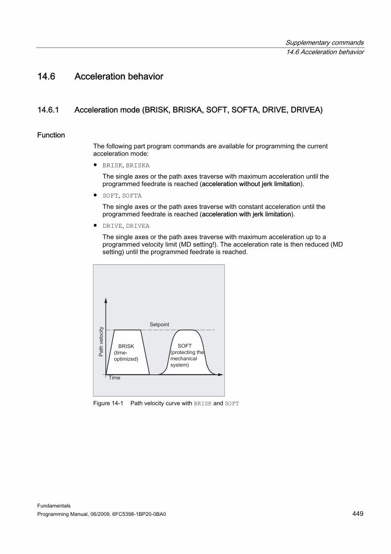
Supplementary commands 14.6 Acceleration behavior
Fundamentals Programming Manual, 06/2009, 6FC5398-1BP20-0BA0 449
14.6 14.6 Acceleration behavior
14.6.1 Acceleration mode (BRISK, BRISKA, SOFT, SOFTA, DRIVE, DRIVEA)
Function The following part program commands are available for programming the current acceleration mode: ● BRISK, BRISKA
The single axes or the path axes traverse with maximum acceleration until the programmed feedrate is reached (acceleration without jerk limitation).
● SOFT, SOFTA The single axes or the path axes traverse with constant acceleration until the programmed feedrate is reached (acceleration with jerk limitation).
● DRIVE, DRIVEA The single axes or the path axes traverse with maximum acceleration up to a programmed velocity limit (MD setting!). The acceleration rate is then reduced (MD setting) until the programmed feedrate is reached.
Figure 14-1 Path velocity curve with BRISK and SOFT

Supplementary commands 14.6 Acceleration behavior
Fundamentals 450 Programming Manual, 06/2009, 6FC5398-1BP20-0BA0
Figure 14-2 Path velocity curve with DRIVE
Syntax BRISK BRISKA(<axis1>,<axis2>,…) SOFT SOFTA(<axis1>,<axis2>,…) DRIVE DRIVEA(<axis1>,<axis2>,…)
Significance BRISK: Command for activating the "acceleration without jerk
limitation" for the path axes. BRISKA: Command for activating the "acceleration without jerk
limitation" for single axis movements (JOG, JOG/INC, positioning axis, oscillating axis, etc.).
SOFT: Command for activating the "acceleration with jerk limitation" for the path axes.
SOFTA: Command for activating the "acceleration with jerk limitation" for single axis movements (JOG, JOG/INC, positioning axis, oscillating axis, etc.).
DRIVE: Command for activating the reduced acceleration above a configured velocity limit (MD35220 $MA_ACCEL_REDUCTION_SPEED_POINT) for the path axes.
Supplementary commands 14.6 Acceleration behavior
Fundamentals Programming Manual, 06/2009, 6FC5398-1BP20-0BA0 451
DRIVEA: Command for activating the reduced acceleration above a configured velocity limit (MD35220 $MA_ACCEL_REDUCTION_SPEED_POINT) for single axis movements (JOG, JOG/INC, positioning axis, oscillating axis, etc.).
(<axis1>,<axis2>, etc.): Single axes for which the called acceleration mode is to apply.
Supplementary conditions Changing acceleration mode during machining If the acceleration mode is changed in a part program during machining (BRISK ↔ SOFT), then there is a block change with exact stop at the end of the block during the transition even with continuous-path mode.
Examples Example 1: SOFT and BRISKA Program code
N10 G1 X… Y… F900 SOFT
N20 BRISKA(AX5,AX6)
...
Example 2: DRIVE and DRIVEA Program code
N05 DRIVE
N10 G1 X… Y… F1000
N20 DRIVEA (AX4, AX6)
...
References Function Manual, Basic Functions; Acceleration (B2)

Supplementary commands 14.6 Acceleration behavior
Fundamentals 452 Programming Manual, 06/2009, 6FC5398-1BP20-0BA0
14.6.2 Influence of acceleration on following axes (VELOLIMA, ACCLIMA, JERKLIMA)
Function In the case of axis couplings (tangential correction, coupled motion, master value coupling, electronic gear; → see Programming Manual, Job Planning) following axes/spindles are traversed dependent on one or more master axes/spindles. The dynamics limits of the following axes/spindles can be manipulated using the VELOLIMA, ACCLIMA, and JERKLIMA functions from the part program or from synchronized actions, even if the axis coupling is already active.
Note The JERKLIMA function is not available for all types of coupling. References: • Function Manual, Special Functions; Axis Couplings (M3) • Function Manual, Extended Functions; Synchronous Spindle (S3)
Note Availability for SINUMERIK 828D The VELOLIMA, ACCLIMA and JERKLIMA functions can only be used with SINUMERIK 828D in conjunction with the "coupled motion" function!
Syntax VELOLIMA(<axis>)=<value> ACCLIMA(<axis>)=<value> JERKLIMA(<axis>)=<value>
Significance VELOLIMA: Command to correct the parameterized maximum velocity ACCLIMA: Command to correct the parameterized maximum acceleration JERKLIMA: Command to correct the parameterized maximum jerk <axis>: Following axis whose dynamics limits need to be corrected <value>: Percentage offset value
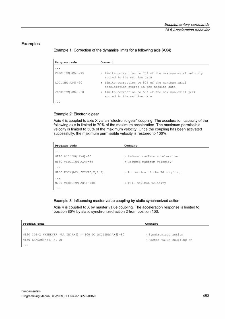
Supplementary commands 14.6 Acceleration behavior
Fundamentals Programming Manual, 06/2009, 6FC5398-1BP20-0BA0 453
Examples Example 1: Correction of the dynamics limits for a following axis (AX4) Program code Comment
...
VELOLIMA[AX4]=75 ; Limits correction to 75% of the maximum axial velocity stored in the machine data
ACCLIMA[AX4]=50 ; Limits correction to 50% of the maximum axial acceleration stored in the machine data
JERKLIMA[AX4]=50 ; Limits correction to 50% of the maximum axial jerk stored in the machine data
...
Example 2: Electronic gear Axis 4 is coupled to axis X via an "electronic gear" coupling. The acceleration capacity of the following axis is limited to 70% of the maximum acceleration. The maximum permissible velocity is limited to 50% of the maximum velocity. Once the coupling has been activated successfully, the maximum permissible velocity is restored to 100%. Program code Comment
...
N120 ACCLIMA[AX4]=70 ; Reduced maximum acceleration
N130 VELOLIMA[AX4]=50 ; Reduced maximum velocity
...
N150 EGON(AX4,"FINE",X,1,2) ; Activation of the EG coupling
...
N200 VELOLIMA[AX4]=100 ; Full maximum velocity
...
Example 3: Influencing master value coupling by static synchronized action Axis 4 is coupled to X by master value coupling. The acceleration response is limited to position 80% by static synchronized action 2 from position 100.
Program code Comment
...
N120 IDS=2 WHENEVER $AA_IM[AX4] > 100 DO ACCLIMA[AX4]=80 ; Synchronized action
N130 LEADON(AX4, X, 2) ; Master value coupling on
...

Supplementary commands 14.6 Acceleration behavior
Fundamentals 454 Programming Manual, 06/2009, 6FC5398-1BP20-0BA0
14.6.3 Activation of technology-specific dynamic values (DYNNORM, DYNPOS, DYNROUGH, DYNSEMIFIN, DYNFINISH)
Function Using the "Technology" G group, the appropriate dynamic response can be activated for five varying technological machining steps. Dynamic values and G commands can be configured and are, therefore, dependent on machine data settings (→ machine manufacturer). References: Function Manual, Basic Functions; Continuous-Path Mode, Exact Stop, Look Ahead (B1)
Syntax Activate dynamic values: DYNNORM DYNPOS DYNROUGH DYNSEMIFIN DYNFINISH
Note The dynamic values are already active in the block in which the associated G command is programmed. Machining is not stopped.
Read or write a specific field element: R<m>=$MA...[n,X] $MA...[n,X]=<value>
Significance DYNNORM: G command for activating normal dynamic response DYNPOS: G command for activating the dynamic response for positioning mode,
tapping DYNROUGH: G command for activating the dynamic response for roughing DYNSEMIFIN: G command for activating the dynamic response for finishing DYNFINISH: G command for activating the dynamic response for smooth-finishing

Supplementary commands 14.6 Acceleration behavior
Fundamentals Programming Manual, 06/2009, 6FC5398-1BP20-0BA0 455
R<m>: R-parameter with number <m> $MA...[n,X]: Machine data with field element affecting dynamic response
Array index Range of values: 0 ... 4 0 Normal dynamic response (DYNNORM) 1 Dynamic response for positioning mode (DYNPOS) 2 Dynamic response for roughing (DYNROUGH) 3 Dynamic response for finishing (DYNSEMIFIN)
<n>:
4 Dynamic response for smooth-finishing (DYNFINISH) <X> : Axis address <value>: Dynamic value
Examples Example 1: Activate dynamic values Program code Comment
DYNNORM G1 X10 ; Basic position
DYNPOS G1 X10 Y20 Z30 F… ; Positioning mode, tapping
DYNROUGH G1 X10 Y20 Z30 F10000 ; Roughing
DYNSEMIFIN G1 X10 Y20 Z30 F2000 ; Finishing
DYNFINISH G1 X10 Y20 Z30 F1000 ; Smooth finishing
Example 2: Read or write a specific field element Maximum acceleration for roughing, axis X Program code Comment
R1=$MA_MAX_AX_ACCEL[2,X] ; Read
$MA_MAX_AX_ACCEL[2,X]=5 ; Write
Supplementary commands 14.7 Traversing with feedforward control, FFWON, FFWOF
Fundamentals 456 Programming Manual, 06/2009, 6FC5398-1BP20-0BA0
14.7 14.7 Traversing with feedforward control, FFWON, FFWOF
Function The feedforward control reduces the velocity-dependent overtravel when contouring towards zero. Traversing with feedforward control permits higher path accuracy and thus improved machining results.
Syntax FFWON FFWOF
Significance FFWON: Command to activate the feedforward control FFWOF: Command to deactivate the feedforward control
Note The type of feedforward control and which path axes are to be traversed with feedforward control is specified via machine data. Default: Velocity-dependent feedforward control Option: Acceleration-dependent feedforward control
Example Program code
N10 FFWON
N20 G1 X… Y… F900 SOFT

Supplementary commands 14.8 Contour accuracy, CPRECON, CPRECOF
Fundamentals Programming Manual, 06/2009, 6FC5398-1BP20-0BA0 457
14.8 14.8 Contour accuracy, CPRECON, CPRECOF
Function In machining operations without feedforward control (FFWON), errors may occur on curved contours as a result of velocity-related differences between setpoint and actual positions. The programmable contour accuracy function CPRECON makes it possible to store a maximum permissible contour violation in the NC program which must never be overshot. The magnitude of the contour violation is specified with setting data $SC_CONTPREC. The Look Ahead function allows the entire path to be traversed with the programmed contour accuracy.
Syntax CPRECON CPRECOF
Significance CPRECON: Activate programmable contour accuracy CPRECOF: Deactivate programmable contour accuracy
Note A minimum velocity can be defined via the setting data item $SC_MINFEED, which is not undershot, and the same value can also be written directly out from the part program via the system variable $SC_CONTPREC. On the basis of the value of the contour violation $SC_CONTPREC and the servo gain factor (velocity/following error ratio) of the geometry axes concerned, the control calculates the maximum path velocity at which the contour violation produced by the overtravel does not exceed the minimum value stored in the setting data.
Example Program code Comment
N10 X0 Y0 G0
N20 CPRECON ; Activate contour accuracy
N30 F10000 G1 G64 X100 ; Machining at 10 m/min in continuous-path mode
N40 G3 Y20 J10 ; Automatic feed limitation in circular block
N50 X0 ; Feedrate without limitation 10 m/min

Supplementary commands 14.9 Dwell time (G4)
Fundamentals 458 Programming Manual, 06/2009, 6FC5398-1BP20-0BA0
14.9 14.9 Dwell time (G4)
Function G4 can be used to program a "dwell time" between two NC blocks during which workpiece machining is interrupted.
Note G4 interrupts continuous-path mode.
Application For example, for relief cutting.
Syntax G4 F…/S<n>=...
Note G4 must be programmed in a separate NC block.

Supplementary commands 14.9 Dwell time (G4)
Fundamentals Programming Manual, 06/2009, 6FC5398-1BP20-0BA0 459
Significance G4: Activate dwell time F…: The dwell time is programmed in seconds at address F.
The dwell time is programmed in spindle revolutions at address S. S<n>=…: <n>: The numeric extension indicates the number of the spindle to which
the dwell time is to be applied. In the absence of a numeric extension (S...) the dwell time will be applied to the master spindle.
Note Addresses F and S are only used for time parameters in the G4 block. The feedrate F... and the spindle speed S... programmed upstream of the G4 block are retained.
Example Program code Comment
N10 G1 F200 Z-5 S300 M3 ; Feedrate F, spindle speed S
N20 G4 F3 ; Dwell time: 3 s
N30 X40 Y10
N40 G4 S30 ; Dwelling 30 revolutions of the spindle (at S=300 rpm and 100% speed override, corresponds to t = 0.1 min).
N50 X... ; The feedrate and spindle speed programmed in N10 continue to apply.

Supplementary commands 14.10 Internal preprocessing stop
Fundamentals 460 Programming Manual, 06/2009, 6FC5398-1BP20-0BA0
14.10 14.10 Internal preprocessing stop
Function The control generates an internal preprocessing stop on access to machine status data ($A...). The following block is not executed until all preprocessed and saved blocks have been executed in full. The previous block is stopped in exact stop (as G9).
Example Program code Comments
...
N40 POSA[X]=100
N50 IF $AA_IM[X]==R100 GOTOF MARKE1 ; Access to machine status data ($A...), the control generates an internal preprocessing stop.
N60 G0 Y100
N70 WAITP(X)
N80 LABEL1:
...

Fundamentals Programming Manual, 06/2009, 6FC5398-1BP20-0BA0 461
Other information 1515.1 15.1 Axes
Axis types A distinction is made between the following types of axes when programming: ● Machine axes ● Channel axes ● Geometry axes ● Special axes ● Path axes ● Synchronized axes ● Positioning axes ● Command axes (motion-synchronous actions) ● PLC axes ● Link axes ● Lead link axes

Other information 15.1 Axes
Fundamentals 462 Programming Manual, 06/2009, 6FC5398-1BP20-0BA0
Behavior of programmed axis types Geometry, synchronized and positioning axes are programmed. ● Path axes traverse with feedrate F in accordance with the programmed travel commands. ● Synchronized axes traverse synchronously to path axes and take the same time to
traverse as all path axes. ● Positioning axes traverse asynchronously to all other axes. These traversing movements
take place independently of path and synchronized movements. ● Command axes traverse asynchronously to all other axes. These traversing movements
take place independently of path and synchronized movements. ● PLC axes are controlled by the PLC and can traverse asynchronously to all other axes.
The traversing movements take place independently of path and synchronized movements.

Other information 15.1 Axes
Fundamentals Programming Manual, 06/2009, 6FC5398-1BP20-0BA0 463
15.1.1 Main axes/Geometry axes The main axes define a right-angled, right-handed coordinate system. Tool movements are programmed in this coordinate system. In NC technology, the main axes are called geometry axes. This term is also used in this Programming Manual. Replaceable geometry axes The "Replaceable geometry axes" function (see Function Manual, Job Planning) can be used to alter the geometry axes grouping configured using machine data from the part program. Here any geometry axis can be replaced by a channel axis defined as a synchronous special axis. Axis identifier For turning machines: Geometry axes X and Z are used, and sometimes Y.
For milling machines: Geometry axes X, Y and Z are used. Further information A maximum of three geometry axes are used for programming frames and the workpiece geometry (contour). The identifiers for geometry and channel axes may be the same, provided a reference is possible. Geometry axis and channel axis names can be the same in any channel so that the same programs can be executed.
Other information 15.1 Axes
Fundamentals 464 Programming Manual, 06/2009, 6FC5398-1BP20-0BA0
15.1.2 Special axes In contrast to the geometry axes, no geometrical relationship is defined between the special axes. Typical special axes are: ● Tool revolver axes ● Swivel table axes ● Swivel head axes ● Loader axes Axis identifier On a turning machine with circular magazine, for example: ● Revolver position U ● Tailstock V Programming example Program code Comment
N10 G1 X100 Y20 Z30 A40 F300 ; Path axis movements
N20 POS[U]=10POS[X]=20 FA[U]=200 FA[X]=350 ; Positioning axis movements
N30 G1 X500 Y80 POS[U]=150FA[U]=300 F550 ; Path and positioning axis
N40 G74 X1=0 Z1=0 ; Approach home position
15.1.3 Main spindle, master spindle The machine kinematics determine, which spindle is the main spindle. This spindle is usually declared as the master spindle in the machine data. This assignment can be changed with the SETMS(<spindle number>) program command. SETMS can be used without specifying a spindle number to switch back to the master spindle defined in the machine data. Special functions such as thread cutting are supported by the master spindle. Spindle identifier S or S0
Other information 15.1 Axes
Fundamentals Programming Manual, 06/2009, 6FC5398-1BP20-0BA0 465
15.1.4 Machine axes Machine axes are the axes physically existing on a machine. The movements of axes can still be assigned by transformations (TRANSMIT, TRACYL, or TRAORI) to the machine axes. If transformations are intended for the machine, different axis names must be specified during the commissioning (machine manufacturer). The machine axis names are only programmed in special circumstances (e.g. for reference point or fixed point approach). Axis identifier The axis identifiers can be set in the machine data. Standard identifiers: X1, Y1, Z1, A1, B1, C1, U1, V1 There are also standard axis identifiers that can always be used: AX1, AX2, …, AX<n>
15.1.5 Channel axes Channel axes are all axes, which traverse in a channel. Axis identifier X, Y, Z, A, B, C, U, V
15.1.6 Path axes Path axes define the path and therefore the movement of the tool in space. The programmed feed is active for this path. The axes involved in this path reach their position at the same time. As a rule, these are the geometry axes. However, default settings define, which axes are the path axes, and therefore determine the velocity. Path axes can be specified in the NC program with FGROUP. For more information about FGROUP, see "Feedrate (G93, G94, G95, F, FGROUP, FL, FGREF) (Page 119)".
Other information 15.1 Axes
Fundamentals 466 Programming Manual, 06/2009, 6FC5398-1BP20-0BA0
15.1.7 Positioning axes Positioning axes are interpolated separately; in other words, each positioning axis has its own axis interpolator and its own feedrate. Positioning axes do not interpolate with the path axes. Positioning axes are traversed by the NC program or the PLC. If an axis is to be traversed simultaneously by the NC program and the PLC, an error message appears. Typical positioning axes are: ● Loaders for moving workpieces to machine ● Loaders for moving workpieces away from machine ● Tool magazine/turret
Types A distinction is made between positioning axes with synchronization at the block end or over several blocks. POS axes Block change occurs at the end of the block when all the path and positioning axes programmed in this block have reached their programmed end point. POSA axes The movement of these positioning axes can extend over several blocks. POSP axes The movement of these positioning axes for approaching the end position takes place in sections.
Note Positioning axes become synchronized axes if they are traversed without the special POS/POSA identifier. Continuous-path mode (G64) for path axes is only possible if the positioning axes (POS) reach their final position before the path axes. Path axes programmed with POS/POSA are removed from the path axis grouping for the duration of this block.
For more information about POS, POSA, and POSP, see "Traversing positioning axes (POS, POSA, POSP, FA, WAITP, WAITMC) (Page 129)".

Other information 15.1 Axes
Fundamentals Programming Manual, 06/2009, 6FC5398-1BP20-0BA0 467
15.1.8 Synchronized axes Synchronized axes traverse synchronously to the path from the start position to the programmed end position. The feedrate programmed in F applies to all the path axes programmed in the block, but does not apply to synchronized axes. Synchronized axes take the same time as the path axes to traverse. A synchronized axis can be a rotary axis, which is traversed synchronously to the path interpolation.
15.1.9 Command axes Command axes are started from synchronized actions in response to an event (command). They can be positioned, started, and stopped fully asynchronous to the parts program. An axis cannot be moved from the part program and from synchronized actions simultaneously. Command axes are interpolated separately; in other words, each command axis has its own axis interpolator and its own feedrate. References: Function Manual, Synchronized Actions
15.1.10 PLC axes PLC axes are traversed by the PLC via special function blocks in the basic program; their movements can be asynchronous to all other axes. Traversing movements take place independently of path and synchronized movements.

Other information 15.1 Axes
Fundamentals 468 Programming Manual, 06/2009, 6FC5398-1BP20-0BA0
15.1.11 Link axes Link axes are axes, which are physically connected to another NCU and whose position is controlled from this NCU. Link axes can be assigned dynamically to channels of another NCU. Link axes are non-local axes from the perspective of a specific NCU.
The axis container concept is used for the dynamic modification of the assignment to an NCU. Axis exchange with GET and RELEASE from the part program is not available for link axes.
Further information Prerequisites ● The participating NCUs, NCU1 and NCU2, must be connected by means of high-speed
communication via the link module. References: Configuration Manual, NCU
● The axis must be configured appropriately by machine data. ● The "Link axis" option must be installed.

Other information 15.1 Axes
Fundamentals Programming Manual, 06/2009, 6FC5398-1BP20-0BA0 469
Description The position control is implemented on the NCU on which the axis is physically connected to the drive. This NCU also contains the associated axis VDI interface. The position setpoints for link axes are generated on another NCU and communicated via the NCU link. The link communication must provide the means of interaction between the interpolators and the position controller or PLC interface. The setpoints calculated by the interpolators must be transported to the position control loop on the home NCU and, vice versa, the actual values must be returned from there back to the interpolators. References: For more detailed information about link axes see: Function Manual, Advanced Functions; Multiple Operator Panels and NCUs (B3) Axis container An axis container is a circular buffer data structure, in which local axes and/or link axes are assigned to channels. The entries in the circular buffer can be shifted cyclically. In addition to the direct reference to local axes or link axes, the link axis configuration in the logical machine axis image also allows references to axis containers. This type of reference consists of: ● A container number and ● a slot (circular buffer location within the container) The entry in a circular buffer location contains: ● a local axis or ● a link axis Axis container entries contain local machine axes or link axes from the perspective of an individual NCU. The entries in the logical machine axis image (MD10002 $MN_AXCONF_LOGIC_MACHAX_TAB) of an individual NCU are fixed. References: The axis container function is described in: Function Manual, Advanced Functions; Multiple Operator Panels and NCUs (B3)

Other information 15.1 Axes
Fundamentals 470 Programming Manual, 06/2009, 6FC5398-1BP20-0BA0
15.1.12 Lead link axes A leading link axis is one that is interpolated by one NCU and utilized by one or several other NCUs as the master axis for controlling slave axes.
An axial position controller alarm is sent to all other NCUs, which are connected to the affected axis via a leading link axis. NCUs that are dependent on the leading link axis can utilize the following coupling relationships with it: ● Master value (setpoint, actual master value, simulated master value) ● Coupled motion ● Tangential correction ● Electronic gear (ELG) ● Synchronous spindle

Other information 15.1 Axes
Fundamentals Programming Manual, 06/2009, 6FC5398-1BP20-0BA0 471
Programming Master NCU: Only the NCU, which is physically assigned to the master value axis can program travel motions for this axis. The travel program must not contain any special functions or operations. NCUs of slave axes: The travel program on the NCUs of the slave axes must not contain any travel commands for the leading link axis (master value axis). Any violation of this rule triggers an alarm. The leading link axis is addressed in the usual way via channel axis identifiers. The states of the leading link axis can be accessed by means of selected system variables.
Further information Conditions ● The dependent NCUs, i.e., NCU1 to NCU<n> (n equals max. of 8), must be
interconnected via the link module for high-speed communication. References: Configuration Manual, NCU
● The axis must be configured appropriately via machine data. ● The "Link axis" option must be installed. ● The same interpolation cycle must be configured for all NCUs connected to the leading
link axis. Restrictions ● A master axis which is a leading link axis cannot be a link axis, i.e. it cannot be traversed
by NCUs other than its home NCU. ● A master axis which is a leading link axis cannot be a container axis, i.e. it cannot be
addressed alternately by different NCUs. ● A leading link axis cannot be the programmed leading axis in a gantry grouping. ● Couplings with leading link axes cannot be cascaded. ● Axis replacement can only be implemented within the home NCU of the leading link axis.
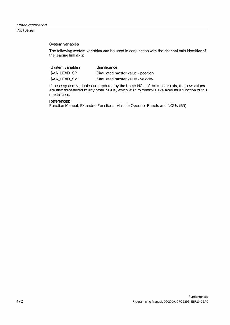
Other information 15.1 Axes
Fundamentals 472 Programming Manual, 06/2009, 6FC5398-1BP20-0BA0
System variables The following system variables can be used in conjunction with the channel axis identifier of the leading link axis: System variables Significance $AA_LEAD_SP Simulated master value - position $AA_LEAD_SV Simulated master value - velocity
If these system variables are updated by the home NCU of the master axis, the new values are also transferred to any other NCUs, which wish to control slave axes as a function of this master axis. References: Function Manual, Extended Functions; Multiple Operator Panels and NCUs (B3)
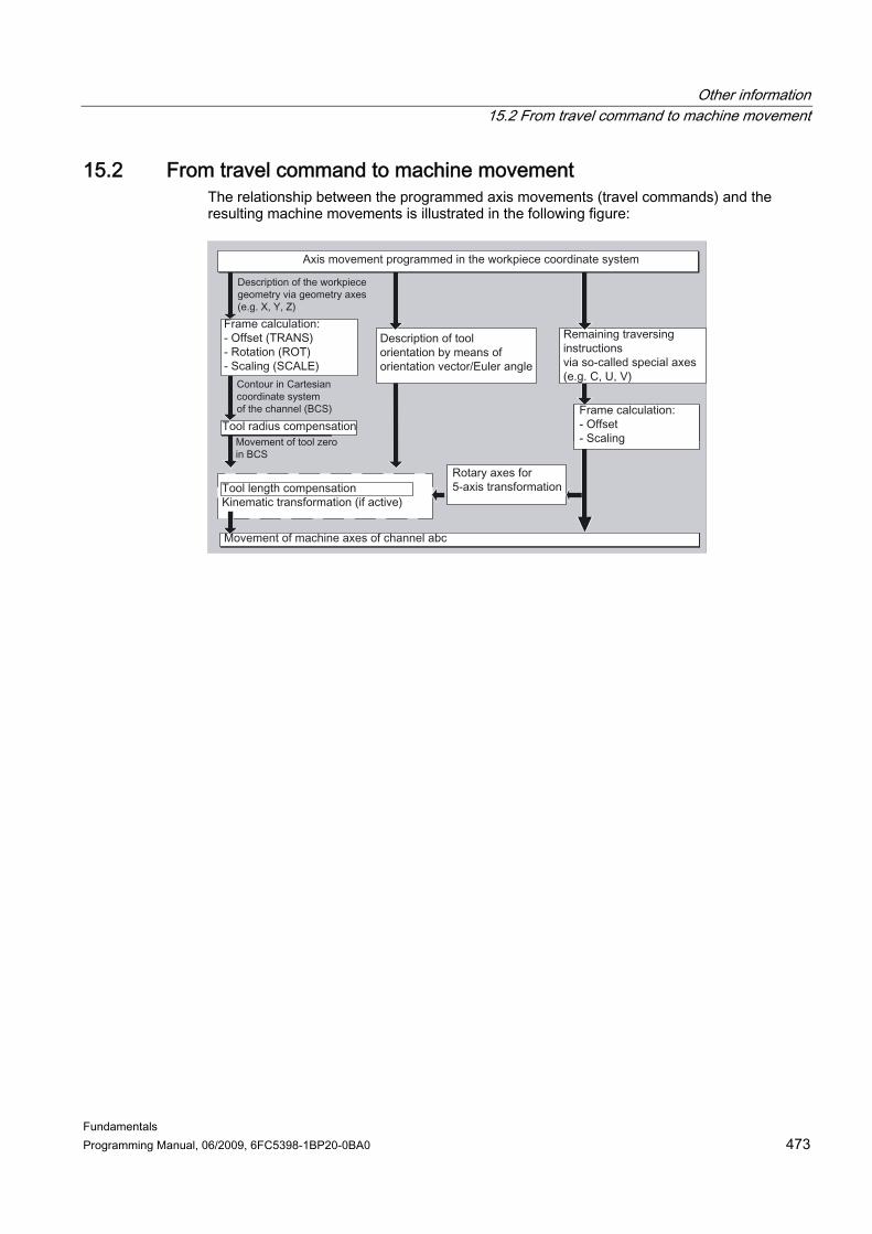
Other information 15.2 From travel command to machine movement
Fundamentals Programming Manual, 06/2009, 6FC5398-1BP20-0BA0 473
15.2 15.2 From travel command to machine movement The relationship between the programmed axis movements (travel commands) and the resulting machine movements is illustrated in the following figure:

Other information 15.3 Path calculation
Fundamentals 474 Programming Manual, 06/2009, 6FC5398-1BP20-0BA0
15.3 15.3 Path calculation The path calculation determines the distance to be traversed in a block, taking into account all offsets and compensations. In general: Distance = setpoint - actual value + zero offset (ZO) + tool offset (TO)
If a new zero offset and a new tool offset are programmed in a new program block, the following applies: ● With absolute dimensioning:
Distance = (absolute dimension P2 - absolute dimension P1) + (WO P2 - WO P1) + (TO P2 - TO P1).
● With incremental dimensioning: Distance = incremental dimension + (WO P2 - WO P1) + (TO P2 - TO P1).
Other information 15.4 Addresses
Fundamentals Programming Manual, 06/2009, 6FC5398-1BP20-0BA0 475
15.4 15.4 Addresses
Fixed and settable addresses Addresses can be divided into two groups: ● Fixed addresses
These addresses are permanently set, i.e. the address characters cannot be changed. ● Settable addresses
The machine manufacturer may assign another name to these addresses via machine data.
Some important addresses are listed in the following table. The last column indicates whether it is a fixed or a settable address. Address Meaning (default setting) Name A=DC(...) A=ACP(...) A=ACN(...)
Rotary axis Settable
ADIS Rounding clearance for path functions Fixed B=DC(...) B=ACP(...) B=ACN(...)
Rotary axis Settable
C=DC(...) C=ACP(...) C=ACN(...)
Rotary axis Settable
CHR=... Chamfer the contour corner Fixed D... Cutting edge number Fixed F... Feedrate Fixed FA[axis]=... or FA[spindle]=... or [SPI(spindle)]=...
Axial feedrate (only if spindle no. defined by variable)
Fixed
G... Preparatory function Fixed H... H=QU(...)
Auxiliary function Auxiliary function without read stop
Fixed
I... Interpolation parameter Settable J... Interpolation parameter Settable K... Interpolation parameter Settable L... Subroutine call Fixed M... M=QU
Additional function Additional function without read stop
Fixed
N... Subblock Fixed OVR Path override Fixed P... Number of program passes Fixed POS[Axis]=... Positioning axis Fixed POSA[Axis]=... Positioning axis across block boundary Fixed

Other information 15.4 Addresses
Fundamentals 476 Programming Manual, 06/2009, 6FC5398-1BP20-0BA0
SPOS=... SPOS[n]=...
Spindle position Fixed
SPOSA=... SPOSA[n
Spindle position across block boundary Fixed
Q... Axis Settable R0=... to Rn=... R...
- R parameter, n can be set via MD (standard 0 - 99) - Axis
Fixed Settable
RND Round the contour corner Fixed RNDM Round contour corner (modal) Fixed S... Spindle speed Fixed T... Tool number Fixed U... Axis Settable V... Axis Settable W... Axis Settable X... X=AC(...) X=IC
Axis " absolute " incremental
Settable
Y... Y=AC(...) Y=IC
Axis Settable
Z... Z=AC(...) Z=IC
Axis Settable
AR+=... Opening angle Settable AP=... Polar angle Settable CR=... Circle radius Settable RP=... Polar radius Settable
Note Settable addresses Settable addresses must be unique within the control, i.e. the same address name may not be used for different address types. A distinction is made between the following address types: • Axis values and end points • Interpolation parameters • Feedrates • Corner rounding criteria • Measurement • Axis, spindle behavior

Other information 15.4 Addresses
Fundamentals Programming Manual, 06/2009, 6FC5398-1BP20-0BA0 477
Modal/non-modal addresses Modal addresses remain valid with the programmed value (in all subsequent blocks) until a new value is programmed at the same address. Non-modal addresses only apply in the block, in which they were programmed. Example: Program code Comment
N10 G01 F500 X10 ;
N20 X10 ; Feedrate F from N10 remains active until a new feedrate is entered.
Addresses with axial extension In addresses with axial extension, an axis name is inserted in square brackets after the address. The axis name assigns the axis. Example: Program code Comment
FA[U]=400 ; Axis-specific feedrate for U axis.
Fixed addresses with axial extension: Address Meaning (default setting) AX Axis value (variable axis programming) ACC Axial acceleration FA Axial feedrate FDA Axis feedrate for handwheel override FL Axial feedrate limitation IP Interpolation parameter (variable axis programming) OVRA Axial override PO Polynomial coefficient POS Positioning axis POSA Positioning axis across block boundary
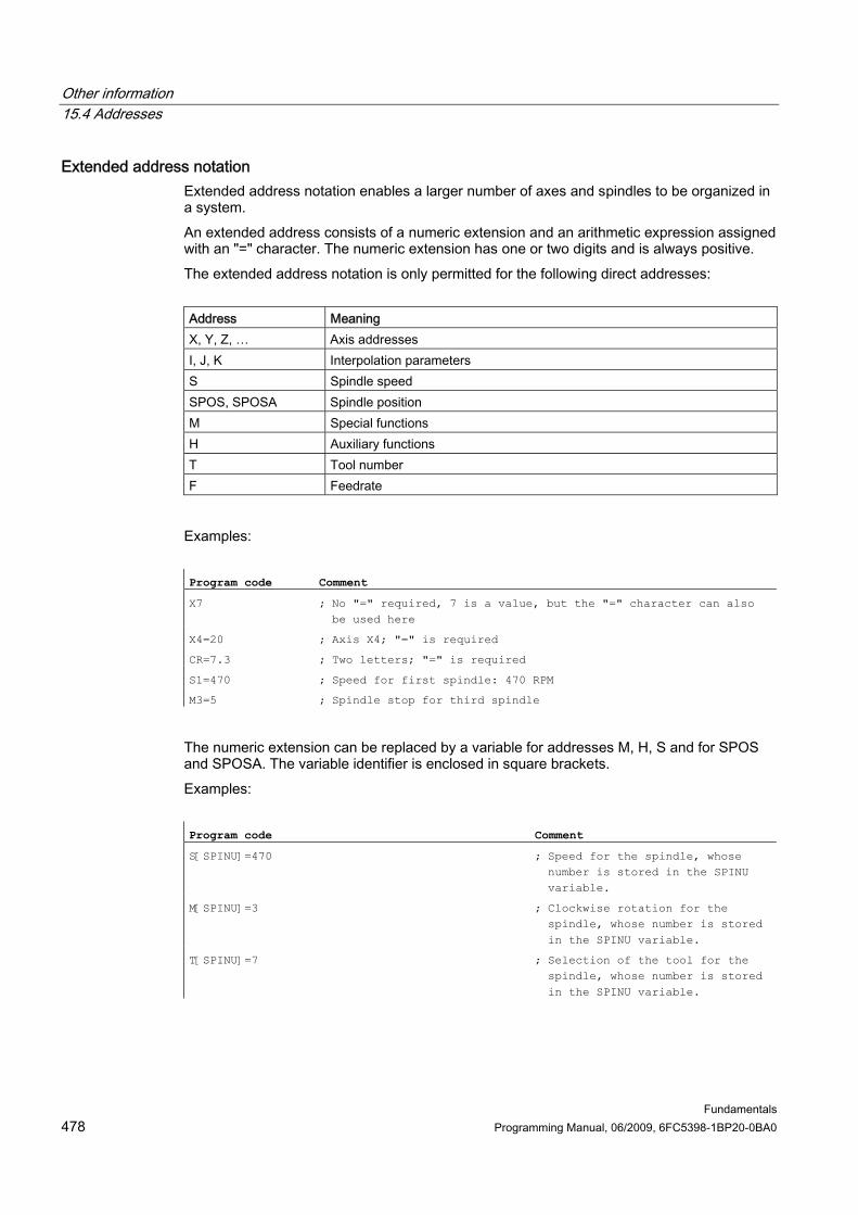
Other information 15.4 Addresses
Fundamentals 478 Programming Manual, 06/2009, 6FC5398-1BP20-0BA0
Extended address notation Extended address notation enables a larger number of axes and spindles to be organized in a system. An extended address consists of a numeric extension and an arithmetic expression assigned with an "=" character. The numeric extension has one or two digits and is always positive. The extended address notation is only permitted for the following direct addresses: Address Meaning X, Y, Z, … Axis addresses I, J, K Interpolation parameters S Spindle speed SPOS, SPOSA Spindle position M Special functions H Auxiliary functions T Tool number F Feedrate
Examples: Program code Comment
X7 ; No "=" required, 7 is a value, but the "=" character can also be used here
X4=20 ; Axis X4; "=" is required
CR=7.3 ; Two letters; "=" is required
S1=470 ; Speed for first spindle: 470 RPM
M3=5 ; Spindle stop for third spindle
The numeric extension can be replaced by a variable for addresses M, H, S and for SPOS and SPOSA. The variable identifier is enclosed in square brackets. Examples: Program code Comment
S[SPINU]=470 ; Speed for the spindle, whose number is stored in the SPINU variable.
M[SPINU]=3 ; Clockwise rotation for the spindle, whose number is stored in the SPINU variable.
T[SPINU]=7 ; Selection of the tool for the spindle, whose number is stored in the SPINU variable.

Other information 15.5 Identifiers
Fundamentals Programming Manual, 06/2009, 6FC5398-1BP20-0BA0 479
15.5 15.5 Identifiers The commands according to DIN 66025 are supplemented with so-called identifiers by the NC high-level language. Identifiers can stand for: ● System variables ● User-defined variables ● Subroutines ● Keywords ● Jump markers ● Macros
Note Identifiers must be unique. It is not permissible to use the same identifier for different objects.
Rules for names The following rules apply when assigning identifier names: ● Maximum number of characters:
– For program names: 24 – Axis identifiers: 8 – Variable identifiers: 31
● Permissible characters are: – Letters – Numbers – Underscores
● The first two characters must be letters or underscores. ● Separators are not permitted between the individual characters.
Note Reserved keywords must not be used as identifiers.
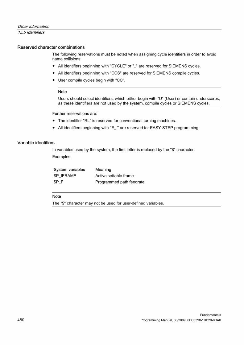
Other information 15.5 Identifiers
Fundamentals 480 Programming Manual, 06/2009, 6FC5398-1BP20-0BA0
Reserved character combinations The following reservations must be noted when assigning cycle identifiers in order to avoid name collisions: ● All identifiers beginning with "CYCLE" or "_" are reserved for SIEMENS cycles. ● All identifiers beginning with "CCS" are reserved for SIEMENS compile cycles. ● User compile cycles begin with "CC”.
Note Users should select identifiers, which either begin with "U" (User) or contain underscores, as these identifiers are not used by the system, compile cycles or SIEMENS cycles.
Further reservations are: ● The identifier "RL" is reserved for conventional turning machines. ● All identifiers beginning with "E_ " are reserved for EASY-STEP programming.
Variable identifiers In variables used by the system, the first letter is replaced by the "$" character. Examples: System variables Meaning $P_IFRAME Active settable frame $P_F Programmed path feedrate
Note The "$" character may not be used for user-defined variables.

Other information 15.6 Constants
Fundamentals Programming Manual, 06/2009, 6FC5398-1BP20-0BA0 481
15.6 15.6 Constants
Integer constants An integer constant is an integer value with or without sign, e.g. a value assignment to an address. Examples: X10.25 Assignment of the value +10.25 to address X X-10.25 Assignment of the value -10.25 to address X X0.25 Assignment of the value +0.25 to address X X.25 Assignment of the value +0.25 to address X without leading "0" X=-.1EX-3 Assignment of the value -0.1*10-3 to address X X0 Assignment of the value 0 to address X (X0 cannot be replaced by X)
Note If, in an address, which permits decimal point input, more decimal places are specified than actually provided for the address, then they are rounded to fit the number of places provided.
Hexadecimal constants Constants can also be interpreted in hexadecimal format. The letters "A" to "F" stand for the digits 10 to 15. Hexadecimal constants are enclosed in single quotation marks and start with the letter "H", followed by the value in hexadecimal notation. Separators are allowed between the letters and digits. Example: Program code Comment
$MC_TOOL_MANAGEMENT_MASK='H3C7F' ; Assignment of hexadecimal constants to machine data: MD18080 $MN_MM_TOOL_MANAGEMENT_MASK

Other information 15.6 Constants
Fundamentals 482 Programming Manual, 06/2009, 6FC5398-1BP20-0BA0
Note The maximum number of characters is limited by the value range of the integer data type.
Binary constants Constants can also be interpreted in binary format. In this case, only the digits "0" and "1" are used. Binary constants are enclosed in single quotation marks and start with the letter "B", followed by the binary value. Separators are allowed between the digits. Example: Program code Comment
$MN_AUXFU_GROUP_SPEC='B10000001' ; The assignment of binary constants sets Bit0 and Bit7 in the machine data.
Note The maximum number of characters is limited by the value range of the integer data type.
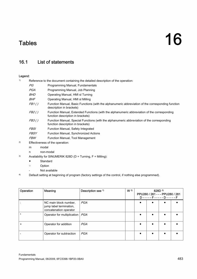
Fundamentals Programming Manual, 06/2009, 6FC5398-1BP20-0BA0 483
Tables 1616.1 16.1 List of statements
Legend:
Reference to the document containing the detailed description of the operation: PG Programming Manual, Fundamentals PGA Programming Manual, Job Planning BHD Operating Manual, HMI sl Turning BHF Operating Manual, HMI sl Milling FB1 ( ) Function Manual, Basic Functions (with the alphanumeric abbreviation of the corresponding function
description in brackets) FB2 ( ) Function Manual, Extended Functions (with the alphanumeric abbreviation of the corresponding
function description in brackets) FB3 ( ) Function Manual, Special Functions (with the alphanumeric abbreviation of the corresponding
function description in brackets) FBSI Function Manual, Safety Integrated FBSY Function Manual, Synchronized Actions
1)
FBW Function Manual, Tool Management Effectiveness of the operation: m modal
2)
n non-modal Availability for SINUMERIK 828D (D = Turning, F = Milling): ● Standard ○ Option
3)
- Not available 4) Default setting at beginning of program (factory settings of the control, if nothing else programmed).
Operation Meaning Description see 1) W 2) 828D 3)
PPU260 / 261 - - - PPU280 / 281D - - - - - F - - - - - D - - - - - F
: NC main block number, jump label termination, concatenation operator
PGA
● ● ● ●
* Operator for multiplication PGA
● ● ● ●
+ Operator for addition PGA
● ● ● ●
- Operator for subtraction PGA
● ● ● ●

Tables 16.1 List of statements
Fundamentals 484 Programming Manual, 06/2009, 6FC5398-1BP20-0BA0
Operation Meaning Description see 1) W 2) 828D 3) PPU260 / 261 - - - PPU280 / 281
D - - - - - F - - - - - D - - - - - F < Comparison operator,
less than PGA
● ● ● ●
<< Concatenation operator for strings
PGA
● ● ● ●
<= Comparison operator, less than or equal to
PGA
● ● ● ●
= Assignment operator PGA
● ● ● ●
>= Comparison operator, greater than or equal to
PGA
● ● ● ●
/ Operator for division PGA
● ● ● ●
/0 … … /7
Block is skipped (1st skip level) Block is skipped (8th skip level)
PG Skipping blocks (Page 45)
●
○
●
○
●
○
●
○ A Axis name PGA
m/n ● ● ● ●
A2 Tool orientation: RPY or Euler angle
PGA
n ● ● ● ●
A3 Tool orientation: Direction/surface normal vector component
PGA
n ● ● ● ●
A4 Tool orientation: Surface normal vector for beginning of block
PGA
n ● ● ● ●
A5 Tool orientation: Surface normal vector for end of block
PGA
n ● ● ● ●
ABS Absolute value (amount) PGA
● ● ● ●
AC Absolute dimensions of coordinates/positions
PG Absolute dimensions (G90, AC) (Page 183)
n ● ● ● ●

Tables 16.1 List of statements
Fundamentals Programming Manual, 06/2009, 6FC5398-1BP20-0BA0 485
Operation Meaning Description see 1) W 2) 828D 3) PPU260 / 261 - - - PPU280 / 281
D - - - - - F - - - - - D - - - - - F ACC Effect of current axial
acceleration PG Programmable acceleration override (ACC) (option) (Page 152)
m ● ● ● ●
ACCLIMA Effect of current maximum axial acceleration
PG Influence of acceleration on following axes (VELOLIMA, ACCLIMA, JERKLIMA) (Page 452)
m ● ● ● ●
ACN Absolute dimensions for rotary axes, approach position in negative direction
PG Absolute dimension for rotary axes (DC, ACP, ACN) (Page 191)
n ● ● ● ●
ACOS Arc cosine (trigon. function)
PGA
● ● ● ●
ACP Absolute dimensions for rotary axes, approach position in positive direction
PG Absolute dimension for rotary axes (DC, ACP, ACN) (Page 191)
n ● ● ● ●
ACTBLOCNO Output of current block number of an alarm block, even if "current block display suppressed" (DISPLOF) is active.
PGA
● ● ● ●
ADDFRAME Inclusion and possible activation of a measured frame
PGA, FB1(K2)
● ● ● ●
ADIS Rounding clearance for path functions G1, G2, G3, ...
PG Continuous-path mode (G64, G641, G642, G643, G644, G645, ADIS, ADISPOS) (Page 357)
m ● ● ● ●
ADISPOS Rounding clearance for rapid traverse G0
PG Continuous-path mode (G64, G641, G642, G643, G644, G645, ADIS, ADISPOS) (Page 357)
m ● ● ● ●

Tables 16.1 List of statements
Fundamentals 486 Programming Manual, 06/2009, 6FC5398-1BP20-0BA0
Operation Meaning Description see 1) W 2) 828D 3) PPU260 / 261 - - - PPU280 / 281
D - - - - - F - - - - - D - - - - - F ADISPOSA Size of the tolerance
window for IPOBRKA PGA
m ● ● ● ●
ALF LIFTFAST angle PGA
m ● ● ● ●
AMIRROR Programmable mirroring PG Programmable mirroring (MIRROR, AMIRROR) (Page 403)
n ● ● ● ●
AND Logical AND PGA
● ● ● ●
ANG Contour angle PG Contour definitions: One straight line (ANG) (Page 260)
n ● ● ● ●
AP Polar angle PG Travel commands with polar coordinates (G0, G1, G2, G3, AP, RP) (Page 213)
m/n ● ● ● ●
APR Read/show access protection
PGA
● ● ● ●
APRB Read access right, OPI PGA
● ● ● ●
APRP Read access right, part program
PGA
● ● ● ●
APW Write access protection PGA
● ● ● ●
APWB Write access right, OPI PGA
● ● ● ●
APWP Write access right, part program
PGA
● ● ● ●
APX Definition of the access right for executing the specified language element
PGA
● ● ● ●

Tables 16.1 List of statements
Fundamentals Programming Manual, 06/2009, 6FC5398-1BP20-0BA0 487
Operation Meaning Description see 1) W 2) 828D 3) PPU260 / 261 - - - PPU280 / 281
D - - - - - F - - - - - D - - - - - F AR Opening angle PG
Circular interpolation with opening angle and center point (G2/G3, X... Y... Z.../ I... J... K..., AR) (Page 236)
m/n ● ● ● ●
AROT Programmable rotation PG Programmable rotation (ROT, AROT, RPL) (Page 384)
n ● ● ● ●
AROTS Programmable frame rotations with solid angles
PG Programmable frame rotations with solid angles (ROTS, AROTS, CROTS) (Page 396)
n ● ● ● ●
SL Macro definition PGA
● ● ● ●
ASCALE Programmable scaling PG Programmable scale factor (SCALE, ASCALE) (Page 398)
n ● ● ● ●
ASIN Arithmetic function, arc sine
PGA
● ● ● ●
ASPLINE Akima spline PGA
m - ○ - ○
ATAN2 Arc tangent 2 PGA
● ● ● ●
ATOL Axis-specific tolerance for compressor functions, orientation smoothing and smoothing types
PGA
- ● - ●
ATRANS Additive programmable translation
PG Zero offset (TRANS, ATRANS) (Page 376)
n ● ● ● ●
AX Variable axis identifier PGA
m/n ● ● ● ●
AXCSWAP Advance container axis PGA
- - - -

Tables 16.1 List of statements
Fundamentals 488 Programming Manual, 06/2009, 6FC5398-1BP20-0BA0
Operation Meaning Description see 1) W 2) 828D 3) PPU260 / 261 - - - PPU280 / 281
D - - - - - F - - - - - D - - - - - F AXCTSWE Advance container axis PGA
- - - -
AXCTSWED Rotate axis container PGA
- - - -
AXIS Axis identifier, axis address
PGA
● ● ● ●
AXNAME Converts input string into axis identifier
PGA
● ● ● ●
AXSTRING Converts string spindle number
PGA
● ● ● ●
AXTOCHAN Request axis for a specific channel. Possible from NC program and synchronized action.
PGA
● ● ● ●
AXTOSPI Converts axis identifier into a spindle index
PGA
● ● ● ●
B Axis name PGA
m/n ● ● ● ●
B2 Tool orientation: RPY or Euler angle
PGA
n ● ● ● ●
B3 Tool orientation: Direction/surface normal vector component
PGA
n ● ● ● ●
B4 Tool orientation: Surface normal vector for beginning of block
PGA
n ● ● ● ●
B5 Tool orientation: Surface normal vector for end of block
PGA
n ● ● ● ●
B_AND Bit AND PGA
● ● ● ●
B_OR Bit OR PGA
● ● ● ●

Tables 16.1 List of statements
Fundamentals Programming Manual, 06/2009, 6FC5398-1BP20-0BA0 489
Operation Meaning Description see 1) W 2) 828D 3) PPU260 / 261 - - - PPU280 / 281
D - - - - - F - - - - - D - - - - - F B_NOT Bit negation PGA
● ● ● ●
B_XOR Bit exclusive OR PGA
● ● ● ●
BAUTO Definition of the first spline section by means of the next 3 points
PGA
m - ○ - ○
BLOCK Together with the keyword TO defines the program part to be processed in an indirect subprogram call
PGA
● ● ● ●
BLSYNC Processing of interrupt routine is only to start with the next block change
PGA
● ● ● ●
BNAT 4) Natural transition to first spline block
PGA
m - ○ - ○
BOOL Data type: Boolean value TRUE/FALSE or 1/0
PGA
● ● ● ●
BOUND Tests whether the value falls within the defined value range. If the values are equal, the test value is returned.
PGA
● ● ● ●
BRISK 4) Fast non-smoothed path acceleration
PG Acceleration mode (BRISK, BRISKA, SOFT, SOFTA, DRIVE, DRIVEA) (Page 449)
m ● ● ● ●
BRISKA Switch on brisk path acceleration for the programmed axes
PG Acceleration mode (BRISK, BRISKA, SOFT, SOFTA, DRIVE, DRIVEA) (Page 449)
● ● ● ●
BSPLINE B-spline PGA
m - ○ - ○
BTAN Tangential transition to first spline block
PGA
m - ○ - ○
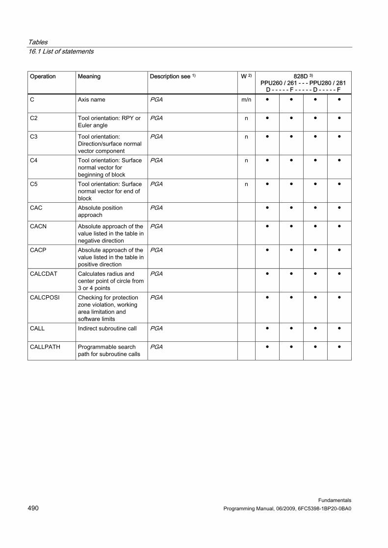
Tables 16.1 List of statements
Fundamentals 490 Programming Manual, 06/2009, 6FC5398-1BP20-0BA0
Operation Meaning Description see 1) W 2) 828D 3) PPU260 / 261 - - - PPU280 / 281
D - - - - - F - - - - - D - - - - - F C Axis name PGA
m/n ● ● ● ●
C2 Tool orientation: RPY or Euler angle
PGA
n ● ● ● ●
C3 Tool orientation: Direction/surface normal vector component
PGA
n ● ● ● ●
C4 Tool orientation: Surface normal vector for beginning of block
PGA
n ● ● ● ●
C5 Tool orientation: Surface normal vector for end of block
PGA
n ● ● ● ●
CAC Absolute position approach
PGA
● ● ● ●
CACN Absolute approach of the value listed in the table in negative direction
PGA
● ● ● ●
CACP Absolute approach of the value listed in the table in positive direction
PGA
● ● ● ●
CALCDAT Calculates radius and center point of circle from 3 or 4 points
PGA
● ● ● ●
CALCPOSI Checking for protection zone violation, working area limitation and software limits
PGA
● ● ● ●
CALL Indirect subroutine call PGA
● ● ● ●
CALLPATH Programmable search path for subroutine calls
PGA
● ● ● ●

Tables 16.1 List of statements
Fundamentals Programming Manual, 06/2009, 6FC5398-1BP20-0BA0 491
Operation Meaning Description see 1) W 2) 828D 3) PPU260 / 261 - - - PPU280 / 281
D - - - - - F - - - - - D - - - - - F CANCEL Cancel modal
synchronized action PGA
● ● ● ●
CASE Conditional program branch
PGA
● ● ● ●
CDC Direct approach of a position
PGA
● ● ● ●
CDOF 4) Collision detection OFF PG Collision monitoring (CDON, CDOF, CDOF2) (Page 340)
m ● ● ● ●
CDOF2 Collision detection OFF, for 3D circumferential milling
PG Collision monitoring (CDON, CDOF, CDOF2) (Page 340)
m ● ● ● ●
CDON Collision detection ON PG Collision monitoring (CDON, CDOF, CDOF2) (Page 340)
m ● ● ● ●
CFC 4) Constant feedrate on contour
PG Feedrate optimization for curved path sections (CFTCP, CFC, CFIN) (Page 158)
m ● ● ● ●
CFIN Constant feedrate for internal radius only, not for external radius
PG Feedrate optimization for curved path sections (CFTCP, CFC, CFIN) (Page 158)
m ● ● ● ●
CFINE Assignment of fine offset to a FRAME variable
PGA
● ● ● ●
CFTCP Constant feedrate in tool center point (center point path)
PG Feedrate optimization for curved path sections (CFTCP, CFC, CFIN) (Page 158)
m ● ● ● ●
CHAN Specify validity range for data
PGA
● ● ● ●

Tables 16.1 List of statements
Fundamentals 492 Programming Manual, 06/2009, 6FC5398-1BP20-0BA0
Operation Meaning Description see 1) W 2) 828D 3) PPU260 / 261 - - - PPU280 / 281
D - - - - - F - - - - - D - - - - - F CHANDATA Set channel number for
channel data access PGA
● ● ● ●
CHAR Data type: ASCII character
PGA
● ● ● ●
CHECKSUM Forms the checksum over an array as a fixed-length STRING
PGA
● ● ● ●
CHF Chamfer; value = length of chamfer
PG Chamfer, rounding (CHF, CHR, RND, RNDM, FRC, FRCM) (Page 295)
n ● ● ● ●
CHKDM Uniqueness check within a magazine
FBW ● ● ● ●
CHKDNO Check for unique D numbers
PGA
● ● ● ●
CHR Chamfer; value = length of chamfer in direction of movement
PG Chamfer, rounding (CHF, CHR, RND, RNDM, FRC, FRCM) (Page 295)
● ● ● ●
CIC Approach position by increments
PGA
● ● ● ●
CIP Circular interpolation through intermediate point
PG Circular interpolation with intermediate point and end point (CIP, X... Y... Z..., I1... J1... K1...) (Page 242)
m ● ● ● ●
CLEARM Reset one/several markers for channel coordination
PGA
- - - -
CLRINT Deselect interrupt: PGA
● ● ● ●
CMIRROR Mirror on a coordinate axis
PGA
● ● ● ●
COARSEA Motion end when "Exact stop coarse" reached
PGA
m ● ● ● ●
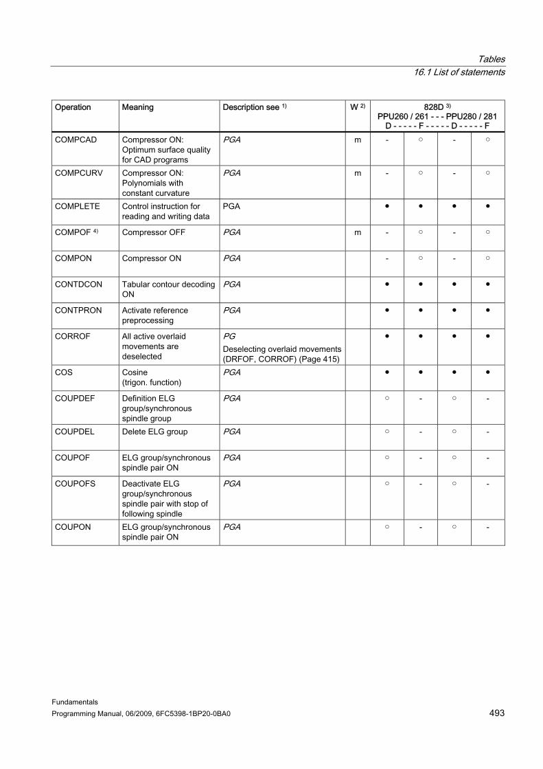
Tables 16.1 List of statements
Fundamentals Programming Manual, 06/2009, 6FC5398-1BP20-0BA0 493
Operation Meaning Description see 1) W 2) 828D 3) PPU260 / 261 - - - PPU280 / 281
D - - - - - F - - - - - D - - - - - F COMPCAD Compressor ON:
Optimum surface quality for CAD programs
PGA
m - ○ - ○
COMPCURV Compressor ON: Polynomials with constant curvature
PGA
m - ○ - ○
COMPLETE Control instruction for reading and writing data
PGA
● ● ● ●
COMPOF 4) Compressor OFF PGA
m - ○ - ○
COMPON Compressor ON PGA
- ○ - ○
CONTDCON Tabular contour decoding ON
PGA
● ● ● ●
CONTPRON Activate reference preprocessing
PGA
● ● ● ●
CORROF All active overlaid movements are deselected
PG Deselecting overlaid movements (DRFOF, CORROF) (Page 415)
● ● ● ●
COS Cosine (trigon. function)
PGA
● ● ● ●
COUPDEF Definition ELG group/synchronous spindle group
PGA
○ - ○ -
COUPDEL Delete ELG group PGA
○ - ○ -
COUPOF ELG group/synchronous spindle pair ON
PGA
○ - ○ -
COUPOFS Deactivate ELG group/synchronous spindle pair with stop of following spindle
PGA
○ - ○ -
COUPON ELG group/synchronous spindle pair ON
PGA
○ - ○ -
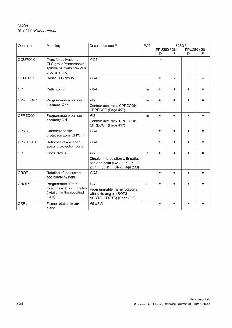
Tables 16.1 List of statements
Fundamentals 494 Programming Manual, 06/2009, 6FC5398-1BP20-0BA0
Operation Meaning Description see 1) W 2) 828D 3) PPU260 / 261 - - - PPU280 / 281
D - - - - - F - - - - - D - - - - - F COUPONC Transfer activation of
ELG group/synchronous spindle pair with previous programming
PGA
○ - ○ -
COUPRES Reset ELG group PGA
○ - ○ -
CP Path motion PGA
m ● ● ● ●
CPRECOF 4) Programmable contour accuracy OFF
PG Contour accuracy, CPRECON, CPRECOF (Page 457)
m ● ● ● ●
CPRECON Programmable contour accuracy ON
PG Contour accuracy, CPRECON, CPRECOF (Page 457)
m ● ● ● ●
CPROT Channel-specific protection zone ON/OFF
PGA
● ● ● ●
CPROTDEF Definition of a channel-specific protection zone
PGA
● ● ● ●
CR Circle radius PG Circular interpolation with radius and end point (G2/G3, X... Y... Z.../ I... J... K..., CR) (Page 233)
n ● ● ● ●
CROT Rotation of the current coordinate system.
PGA
● ● ● ●
CROTS Programmable frame rotations with solid angles (rotation in the specified axes)
PG Programmable frame rotations with solid angles (ROTS, AROTS, CROTS) (Page 396)
n ● ● ● ●
CRPL Frame rotation in any plane
FB1(K2) ● ● ● ●

Tables 16.1 List of statements
Fundamentals Programming Manual, 06/2009, 6FC5398-1BP20-0BA0 495
Operation Meaning Description see 1) W 2) 828D 3) PPU260 / 261 - - - PPU280 / 281
D - - - - - F - - - - - D - - - - - F CSCALE Scale factor for multiple
axes PGA
● ● ● ●
CSPLINE Cubic spline PGA
m - ○ - ○
CT Circle with tangential transition
PG Circular interpolation with tangential transition (CT, X... Y... Z...) (Page 246)
m ● ● ● ●
CTAB Define following axis position according to leading axis position from curve table
PGA
- - - -
CTABDEF Table definition ON PGA
- - - -
CTABDEL Clear curve table PGA
- - - -
CTABEND Table definition OFF PGA
- - - -
CTABEXISTS Checks the curve table with number n
PGA
- - - -
CTABFNO Number of curve tables still possible in the memory
PGA
- - - -
CTABFPOL Number of polynomials still possible in the memory
PGA
- - - -
CTABFSEG Number of curve segments still possible in the memory
PGA
- - - -
CTABID Returns table number of the nth curve table
PGA
- - - -
CTABINV Define leading axis position according to following axis position from curve table
PGA
- - - -

Tables 16.1 List of statements
Fundamentals 496 Programming Manual, 06/2009, 6FC5398-1BP20-0BA0
Operation Meaning Description see 1) W 2) 828D 3) PPU260 / 261 - - - PPU280 / 281
D - - - - - F - - - - - D - - - - - F CTABISLOCK Returns the lock state of
the curve table with number n
PGA
- - - -
CTABLOCK Delete and overwrite, lock
PGA
- - - -
CTABMEMTYP Returns the memory in which curve table number n is created
PGA
- - - -
CTABMPOL Max. number of polynomials still possible in the memory
PGA
- - - -
CTABMSEG Max. number of curve segments still possible in the memory
PGA
- - - -
CTABNO Number of defined curve tables in SRAM or DRAM
FB3(M3) - - - -
CTABNOMEM Number of defined curve tables in SRAM or DRAM
PGA
- - - -
CTABPERIOD Returns the table periodicity of curve table number n
PGA
- - - -
CTABPOL Number of polynomials already used in the memory
PGA
- - - -
CTABPOLID Number of the curve polynomials used by the curve table with number n
PGA
- - - -
CTABSEG Number of curve segments already used in the memory
PGA
- - - -
CTABSEGID Number of the curve segments used by the curve table with number n
PGA
- - - -

Tables 16.1 List of statements
Fundamentals Programming Manual, 06/2009, 6FC5398-1BP20-0BA0 497
Operation Meaning Description see 1) W 2) 828D 3) PPU260 / 261 - - - PPU280 / 281
D - - - - - F - - - - - D - - - - - F CTABSEV Returns the final value of
the following axis of a segment of the curve table
PGA
- - - -
CTABSSV Returns the initial value of the following axis of a segment of the curve table
PGA
- - - -
CTABTEP Returns the value of the leading axis at curve table end
PGA
- - - -
CTABTEV Returns the value of the the following axis at curve table end
PGA
- - - -
CTABTMAX Returns the maximum value of the following axis of the curve table
PGA
- - - -
CTABTMIN Returns the minimum value of the following axis of the curve table
PGA
- - - -
CTABTSP Returns the value of the leading axis at curve table start
PGA
- - - -
CTABTSV Returns the value of the following axis at curve table start
PGA
- - - -
CTABUNLOCK Revoke delete and overwrite lock
PGA
- - - -
CTOL Contour tolerance for compressor functions, orientation smoothing and smoothing types
PGA
- ○ - ○
CTRANS Zero offset for multiple axes
PGA
● ● ● ●
CUT2D 4) 2D tool offset PG 2D tool compensation (CUT2D, CUT2DF) (Page 344)
m ● ● ● ●

Tables 16.1 List of statements
Fundamentals 498 Programming Manual, 06/2009, 6FC5398-1BP20-0BA0
Operation Meaning Description see 1) W 2) 828D 3) PPU260 / 261 - - - PPU280 / 281
D - - - - - F - - - - - D - - - - - F CUT2DF 2D tool offset The tool
offset is applied relative to the current frame (inclined plane).
PG 2D tool compensation (CUT2D, CUT2DF) (Page 344)
m ● ● ● ●
CUT3DC 3D tool offset circumferential milling
PGA
m - - - -
CUT3DCC 3D tool offset circumferential milling with limitation surfaces
PGA
m - - - -
CUT3DCCD 3D tool offset circumferential milling with limitation surfaces with differential tool
PGA
m - - - -
CUT3DF 3D tool offset face milling PGA
m - - - -
CUT3DFF 3D tool offset face milling with constant tool orientation dependent on active frame
PGA
m - - - -
CUT3DFS 3D tool offset face milling with constant tool orientation independent of active frame
PGA
m - - - -
CUTCONOF 4) Constant radius compensation OFF
PG Keep tool radius compensation constant (CUTCONON, CUTCONOF) (Page 347)
m ● ● ● ●
CUTCONON Constant radius compensation ON
PG Keep tool radius compensation constant (CUTCONON, CUTCONOF) (Page 347)
m ● ● ● ●
CUTMOD Activate "Modification of the offset data for rotatable tools"
PGA
● ● ● ●
CYCLE... Measuring cycles BHD/BHF

Tables 16.1 List of statements
Fundamentals Programming Manual, 06/2009, 6FC5398-1BP20-0BA0 499
Operation Meaning Description see 1) W 2) 828D 3) PPU260 / 261 - - - PPU280 / 281
D - - - - - F - - - - - D - - - - - F D Tool offset number PG
Tool offset call (D) (Page 84) ● ● ● ●
D0 With D0, offsets for the tool are ineffective.
PG Tool offset call (D) (Page 84)
● ● ● ●
DAC Absolute non-modal axis-specific diameter programming
PG Axis-specific diameter/radius programming (DIAMONA, DIAM90A, DIAMOFA, DIACYCOFA, DIAMCHANA, DIAMCHAN, DAC, DIC, RAC, RIC) (Page 200)
n ● ● ● ●
DC Absolute dimensions for rotary axes, approach position directly
PG Absolute dimension for rotary axes (DC, ACP, ACN) (Page 191)
n ● ● ● ●
DEF Variable definition PGA
● ● ● ●
DEFINE Keyword for macro definitions
PGA
● ● ● ●
DEFAULT Branch in CASE branch PGA
● ● ● ●
DELAYFSTON Define the start of a stop delay section
PGA
m ● ● ● ●
DELAYFSTOF Define the end of a stop delay section
PGA
m ● ● ● ●
DELDL Delete additive offsets PGA
● ● ● ●
DELDTG Deletion of distance-to-go PGA
● ● ● ●
DELETE Delete the specified file. The file name can be specified with path and file identifier.
PGA
● ● ● ●

Tables 16.1 List of statements
Fundamentals 500 Programming Manual, 06/2009, 6FC5398-1BP20-0BA0
Operation Meaning Description see 1) W 2) 828D 3) PPU260 / 261 - - - PPU280 / 281
D - - - - - F - - - - - D - - - - - F DELTOOLENV Delete data records
describing tool environments
FB1(W1) ● ● ● ●
DIACYCOFA Axis-specific modal diameter programming: OFF in cycles
FB1(P1) m ● ● ● ●
DIAM90 Diameter programming for G90, radius programming for G91
PGA Channel-specific diameter/radius programming (DIAMON, DIAM90, DIAMOF, DIAMCYCOF) (Page 197)
m ● ● ● ●
DIAM90A Axis-specific modal diameter programming for G90 and AC, radius programming for G91 and IC
PG Axis-specific diameter/radius programming (DIAMONA, DIAM90A, DIAMOFA, DIACYCOFA, DIAMCHANA, DIAMCHAN, DAC, DIC, RAC, RIC) (Page 200)
m ● ● ● ●
DIAMCHAN Transfer of all axes from MD axis functions to diameter programming channel status
PG Axis-specific diameter/radius programming (DIAMONA, DIAM90A, DIAMOFA, DIACYCOFA, DIAMCHANA, DIAMCHAN, DAC, DIC, RAC, RIC) (Page 200)
● ● ● ●
DIAMCHANA Transfer of the diameter programming channel status
PG Axis-specific diameter/radius programming (DIAMONA, DIAM90A, DIAMOFA, DIACYCOFA, DIAMCHANA, DIAMCHAN, DAC, DIC, RAC, RIC) (Page 200)
● ● ● ●
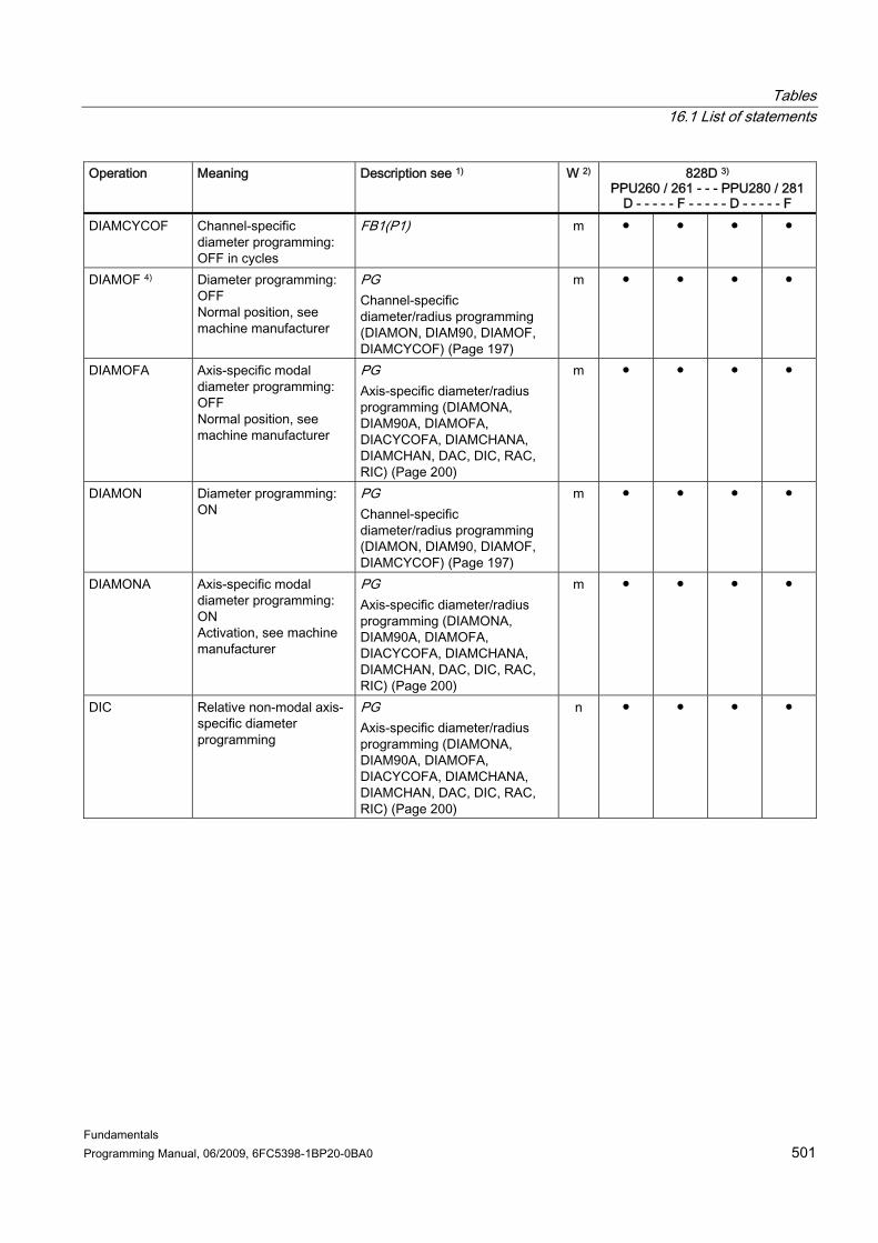
Tables 16.1 List of statements
Fundamentals Programming Manual, 06/2009, 6FC5398-1BP20-0BA0 501
Operation Meaning Description see 1) W 2) 828D 3) PPU260 / 261 - - - PPU280 / 281
D - - - - - F - - - - - D - - - - - F DIAMCYCOF Channel-specific
diameter programming: OFF in cycles
FB1(P1) m ● ● ● ●
DIAMOF 4) Diameter programming: OFF Normal position, see machine manufacturer
PG Channel-specific diameter/radius programming (DIAMON, DIAM90, DIAMOF, DIAMCYCOF) (Page 197)
m ● ● ● ●
DIAMOFA Axis-specific modal diameter programming: OFF Normal position, see machine manufacturer
PG Axis-specific diameter/radius programming (DIAMONA, DIAM90A, DIAMOFA, DIACYCOFA, DIAMCHANA, DIAMCHAN, DAC, DIC, RAC, RIC) (Page 200)
m ● ● ● ●
DIAMON Diameter programming: ON
PG Channel-specific diameter/radius programming (DIAMON, DIAM90, DIAMOF, DIAMCYCOF) (Page 197)
m ● ● ● ●
DIAMONA Axis-specific modal diameter programming: ON Activation, see machine manufacturer
PG Axis-specific diameter/radius programming (DIAMONA, DIAM90A, DIAMOFA, DIACYCOFA, DIAMCHANA, DIAMCHAN, DAC, DIC, RAC, RIC) (Page 200)
m ● ● ● ●
DIC Relative non-modal axis-specific diameter programming
PG Axis-specific diameter/radius programming (DIAMONA, DIAM90A, DIAMOFA, DIACYCOFA, DIAMCHANA, DIAMCHAN, DAC, DIC, RAC, RIC) (Page 200)
n ● ● ● ●
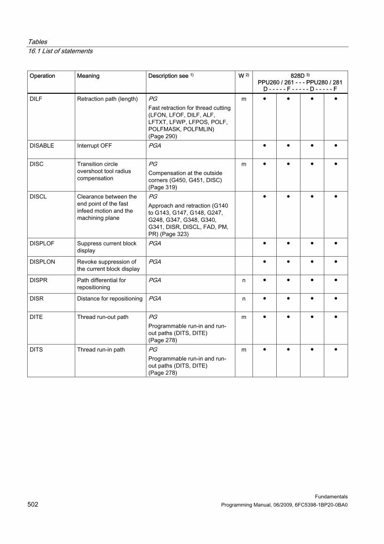
Tables 16.1 List of statements
Fundamentals 502 Programming Manual, 06/2009, 6FC5398-1BP20-0BA0
Operation Meaning Description see 1) W 2) 828D 3) PPU260 / 261 - - - PPU280 / 281
D - - - - - F - - - - - D - - - - - F DILF Retraction path (length) PG
Fast retraction for thread cutting (LFON, LFOF, DILF, ALF, LFTXT, LFWP, LFPOS, POLF, POLFMASK, POLFMLIN) (Page 290)
m ● ● ● ●
DISABLE Interrupt OFF PGA
● ● ● ●
DISC Transition circle overshoot tool radius compensation
PG Compensation at the outside corners (G450, G451, DISC) (Page 319)
m ● ● ● ●
DISCL Clearance between the end point of the fast infeed motion and the machining plane
PG Approach and retraction (G140 to G143, G147, G148, G247, G248, G347, G348, G340, G341, DISR, DISCL, FAD, PM, PR) (Page 323)
● ● ● ●
DISPLOF Suppress current block display
PGA
● ● ● ●
DISPLON Revoke suppression of the current block display
PGA
● ● ● ●
DISPR Path differential for repositioning
PGA
n ● ● ● ●
DISR Distance for repositioning PGA
n ● ● ● ●
DITE Thread run-out path PG Programmable run-in and run-out paths (DITS, DITE) (Page 278)
m ● ● ● ●
DITS Thread run-in path PG Programmable run-in and run-out paths (DITS, DITE) (Page 278)
m ● ● ● ●

Tables 16.1 List of statements
Fundamentals Programming Manual, 06/2009, 6FC5398-1BP20-0BA0 503
Operation Meaning Description see 1) W 2) 828D 3) PPU260 / 261 - - - PPU280 / 281
D - - - - - F - - - - - D - - - - - F DIV Integer division PGA
● ● ● ●
DL Select location-dependent additive tool offset (DL, total set-up offset)
PGA
m - - - -
DO Keyword for synchronized action, triggers action when condition is fulfilled
PGA
● ● ● ●
DRFOF Deactivation of handwheel offsets (DRF)
PG Deselecting overlaid movements (DRFOF, CORROF) (Page 415)
m ● ● ● ●
DRIVE Velocity-dependent path acceleration
PG Acceleration mode (BRISK, BRISKA, SOFT, SOFTA, DRIVE, DRIVEA) (Page 449)
m ● ● ● ●
DRIVEA Activate bent acceleration characteristic curve for the programmed axes
PG Acceleration mode (BRISK, BRISKA, SOFT, SOFTA, DRIVE, DRIVEA) (Page 449)
● ● ● ●
DYNFINISH Dynamic response for smooth finishing
PG Activation of technology-specific dynamic values (DYNNORM, DYNPOS, DYNROUGH, DYNSEMIFIN, DYNFINISH) (Page 454)
m ● ● ● ●
DYNNORM Standard dynamic response
PG Activation of technology-specific dynamic values (DYNNORM, DYNPOS, DYNROUGH, DYNSEMIFIN, DYNFINISH) (Page 454)
m ● ● ● ●

Tables 16.1 List of statements
Fundamentals 504 Programming Manual, 06/2009, 6FC5398-1BP20-0BA0
Operation Meaning Description see 1) W 2) 828D 3) PPU260 / 261 - - - PPU280 / 281
D - - - - - F - - - - - D - - - - - F DYNPOS Dynamic response for
positioning mode, tapping PG Activation of technology-specific dynamic values (DYNNORM, DYNPOS, DYNROUGH, DYNSEMIFIN, DYNFINISH) (Page 454)
m ● ● ● ●
DYNROUGH Dynamic response for roughing
PG Activation of technology-specific dynamic values (DYNNORM, DYNPOS, DYNROUGH, DYNSEMIFIN, DYNFINISH) (Page 454)
m ● ● ● ●
DYNSEMIFIN Dynamic response for finishing
PG Activation of technology-specific dynamic values (DYNNORM, DYNPOS, DYNROUGH, DYNSEMIFIN, DYNFINISH) (Page 454)
m ● ● ● ●
DZERO Marks all D numbers of the TO unit as invalid
PGA
● ● ● ●
EAUTO Definition of the last spline section by means of the last 3 points
PGA
m - ○ - ○
EGDEF Definition of an electronic gear
PGA
- - - -
EGDEL Delete coupling definition for the following axis
PGA
- - - -
EGOFC Turn off electronic gear continuously
PGA
- - - -
EGOFS Turn off electronic gear selectively
PGA
- - - -
EGON Turn on electronic gear PGA
- - - -
EGONSYN Turn on electronic gear PGA
- - - -

Tables 16.1 List of statements
Fundamentals Programming Manual, 06/2009, 6FC5398-1BP20-0BA0 505
Operation Meaning Description see 1) W 2) 828D 3) PPU260 / 261 - - - PPU280 / 281
D - - - - - F - - - - - D - - - - - F EGONSYNE Turn on electronic gear,
with specification of approach mode
PGA
- - - -
ELSE Program branch, if IF condition not fulfilled
PGA
● ● ● ●
ENABLE Interrupt ON PGA
● ● ● ●
ENAT 4) Natural transition to next traversing block
PGA
m - ○ - ○
ENDFOR End line of FOR counter loop
PGA
● ● ● ●
ENDIF End line of IF branch PGA
● ● ● ●
ENDLABEL End label for part program repetitions with REPEAT
PGA, FB1(K1)
● ● ● ●
ENDLOOP End line of endless program loop LOOP
PGA
● ● ● ●
ENDPROC End line of program with start line PROC
● ● ● ●
ENDWHILE End line of WHILE loop PGA
● ● ● ●
ETAN Tangential transition to next traversing block at spline begin
PGA
m - ○ - ○
EVERY Execute synchronized action on transition of condition from FALSE to TRUE
PGA
● ● ● ●
EX Keyword for value assignment in exponential notation
PGA
● ● ● ●

Tables 16.1 List of statements
Fundamentals 506 Programming Manual, 06/2009, 6FC5398-1BP20-0BA0
Operation Meaning Description see 1) W 2) 828D 3) PPU260 / 261 - - - PPU280 / 281
D - - - - - F - - - - - D - - - - - F EXECSTRING Transfer of a string
variable with the executing part program line
PGA
● ● ● ●
EXECTAB Execute an element from a motion table
PGA
● ● ● ●
EXECUTE Program execution ON PGA
● ● ● ●
EXP Exponential function ex PGA
● ● ● ●
EXTCALL Execute external subprogram
PGA
● ● ● ●
EXTERN Declaration of a subprogram with parameter transfer
PGA
● ● ● ●
F Feedrate value (in conjunction with G4 the dwell time is also programmed with F)
PG Feedrate (G93, G94, G95, F, FGROUP, FL, FGREF) (Page 119)
● ● ● ●
FA Axial feedrate PG Traversing positioning axes (POS, POSA, POSP, FA, WAITP, WAITMC) (Page 129)
m ● ● ● ●
FAD Infeed rate for soft approach and retraction
PG Approach and retraction (G140 to G143, G147, G148, G247, G248, G347, G348, G340, G341, DISR, DISCL, FAD, PM, PR) (Page 323)
● ● ● ●
FALSE Logical constant: Incorrect
PGA
● ● ● ●
FB Non-modal feedrate PG Non-modal feedrate (FB) (Page 164)
● ● ● ●
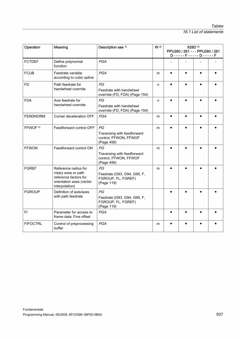
Tables 16.1 List of statements
Fundamentals Programming Manual, 06/2009, 6FC5398-1BP20-0BA0 507
Operation Meaning Description see 1) W 2) 828D 3) PPU260 / 261 - - - PPU280 / 281
D - - - - - F - - - - - D - - - - - F FCTDEF Define polynomial
function PGA
- - - -
FCUB Feedrate variable according to cubic spline
PGA
m ● ● ● ●
FD Path feedrate for handwheel override
PG Feedrate with handwheel override (FD, FDA) (Page 154)
n ● ● ● ●
FDA Axis feedrate for handwheel override
PG Feedrate with handwheel override (FD, FDA) (Page 154)
n ● ● ● ●
FENDNORM Corner deceleration OFF PGA
m ● ● ● ●
FFWOF 4) Feedforward control OFF PG Traversing with feedforward control, FFWON, FFWOF (Page 456)
m ● ● ● ●
FFWON Feedforward control ON PG Traversing with feedforward control, FFWON, FFWOF (Page 456)
m ● ● ● ●
FGREF Reference radius for rotary axes or path reference factors for orientation axes (vector interpolation)
PG Feedrate (G93, G94, G95, F, FGROUP, FL, FGREF) (Page 119)
m ● ● ● ●
FGROUP Definition of axis/axes with path feedrate
PG Feedrate (G93, G94, G95, F, FGROUP, FL, FGREF) (Page 119)
● ● ● ●
FI Parameter for access to frame data: Fine offset
PGA
● ● ● ●
FIFOCTRL Control of preprocessing buffer
PGA
m ● ● ● ●
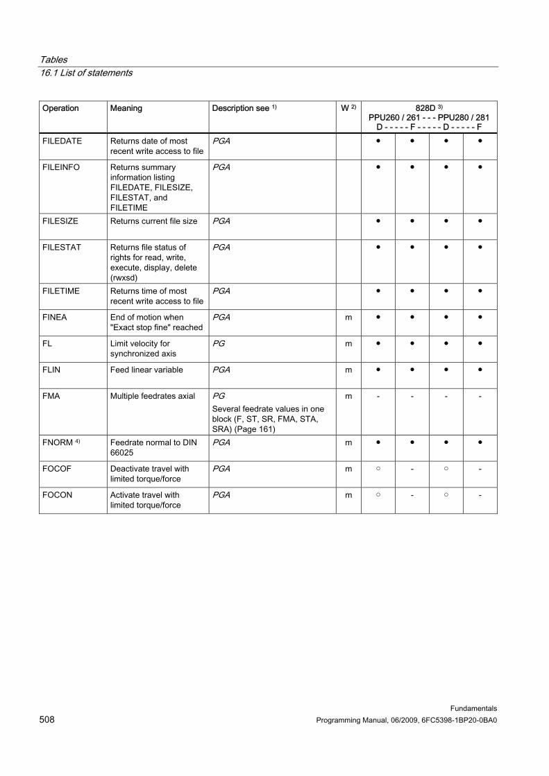
Tables 16.1 List of statements
Fundamentals 508 Programming Manual, 06/2009, 6FC5398-1BP20-0BA0
Operation Meaning Description see 1) W 2) 828D 3) PPU260 / 261 - - - PPU280 / 281
D - - - - - F - - - - - D - - - - - F FILEDATE Returns date of most
recent write access to file PGA
● ● ● ●
FILEINFO Returns summary information listing FILEDATE, FILESIZE, FILESTAT, and FILETIME
PGA
● ● ● ●
FILESIZE Returns current file size PGA
● ● ● ●
FILESTAT Returns file status of rights for read, write, execute, display, delete (rwxsd)
PGA
● ● ● ●
FILETIME Returns time of most recent write access to file
PGA
● ● ● ●
FINEA End of motion when "Exact stop fine" reached
PGA
m ● ● ● ●
FL Limit velocity for synchronized axis
PG
m ● ● ● ●
FLIN Feed linear variable PGA
m ● ● ● ●
FMA Multiple feedrates axial PG Several feedrate values in one block (F, ST, SR, FMA, STA, SRA) (Page 161)
m - - - -
FNORM 4) Feedrate normal to DIN 66025
PGA
m ● ● ● ●
FOCOF Deactivate travel with limited torque/force
PGA
m ○ - ○ -
FOCON Activate travel with limited torque/force
PGA
m ○ - ○ -
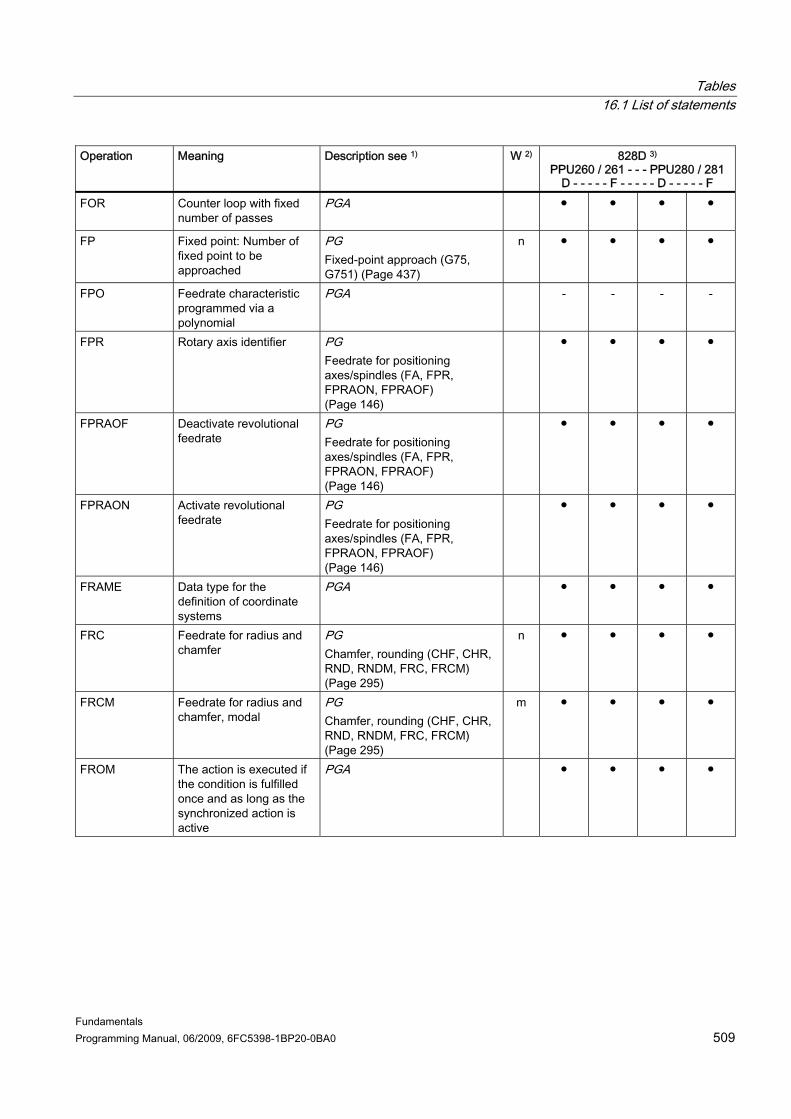
Tables 16.1 List of statements
Fundamentals Programming Manual, 06/2009, 6FC5398-1BP20-0BA0 509
Operation Meaning Description see 1) W 2) 828D 3) PPU260 / 261 - - - PPU280 / 281
D - - - - - F - - - - - D - - - - - F FOR Counter loop with fixed
number of passes PGA
● ● ● ●
FP Fixed point: Number of fixed point to be approached
PG Fixed-point approach (G75, G751) (Page 437)
n ● ● ● ●
FPO Feedrate characteristic programmed via a polynomial
PGA
- - - -
FPR Rotary axis identifier PG Feedrate for positioning axes/spindles (FA, FPR, FPRAON, FPRAOF) (Page 146)
● ● ● ●
FPRAOF Deactivate revolutional feedrate
PG Feedrate for positioning axes/spindles (FA, FPR, FPRAON, FPRAOF) (Page 146)
● ● ● ●
FPRAON Activate revolutional feedrate
PG Feedrate for positioning axes/spindles (FA, FPR, FPRAON, FPRAOF) (Page 146)
● ● ● ●
FRAME Data type for the definition of coordinate systems
PGA
● ● ● ●
FRC Feedrate for radius and chamfer
PG Chamfer, rounding (CHF, CHR, RND, RNDM, FRC, FRCM) (Page 295)
n ● ● ● ●
FRCM Feedrate for radius and chamfer, modal
PG Chamfer, rounding (CHF, CHR, RND, RNDM, FRC, FRCM) (Page 295)
m ● ● ● ●
FROM The action is executed if the condition is fulfilled once and as long as the synchronized action is active
PGA
● ● ● ●

Tables 16.1 List of statements
Fundamentals 510 Programming Manual, 06/2009, 6FC5398-1BP20-0BA0
Operation Meaning Description see 1) W 2) 828D 3) PPU260 / 261 - - - PPU280 / 281
D - - - - - F - - - - - D - - - - - F FTOC Change fine tool offset PG
● ● ● ●
FTOCOF 4) Online fine tool offset OFF
PGA
m ● ● ● ●
FTOCON Online fine tool offset ON PGA
m ● ● ● ●
FXS Travel to fixed stop ON PG
m ● ● ● ●
FXST Torque limit for travel to fixed stop
PG
m ● ● ● ●
FXSW Monitoring window for travel to fixed stop
PG
● ● ● ●
FZ Tooth feedrate PG Tooth feedrate (G95 FZ) (Page 165)
m ● ● ● ●
G0 Linear interpolation with rapid traverse (rapid traverse motion)
PG Rapid traverse movement (G0, RTLION, RTLIOF) (Page 217)
m ● ● ● ●
G1 4) Linear interpolation with feedrate (linear interpolation)
PG Linear interpolation (G1) (Page 222)
m ● ● ● ●
G2 Circular interpolation clockwise
PG Circular interpolation types (G2/G3, ...) (Page 225)
m ● ● ● ●
G3 Circular interpolation counter-clockwise
PG Circular interpolation types (G2/G3, ...) (Page 225)
m ● ● ● ●
G4 Dwell time, preset PG Dwell time (G4) (Page 458)
n ● ● ● ●
G5 Oblique plunge-cut grinding
PGA
n ● ● ● ●
G7 Compensatory motion during oblique plunge-cut grinding
PGA
n ● ● ● ●

Tables 16.1 List of statements
Fundamentals Programming Manual, 06/2009, 6FC5398-1BP20-0BA0 511
Operation Meaning Description see 1) W 2) 828D 3) PPU260 / 261 - - - PPU280 / 281
D - - - - - F - - - - - D - - - - - F G9 Exact stop - deceleration PG
Exact stop (G60, G9, G601, G602, G603) (Page 353)
n ● ● ● ●
G17 4) Selection of working plane X/Y
PG Selection of the working plane (G17/G18/G19) (Page 179)
m ● ● ● ●
G18 Selection of working plane Z/X
PG Selection of the working plane (G17/G18/G19) (Page 179)
m ● ● ● ●
G19 Selection of working plane Y/Z
PG Selection of the working plane (G17/G18/G19) (Page 179)
m ● ● ● ●
G25 Lower working area limitation
PG Programmable spindle speed limitation (G25, G26) (Page 118)
n ● ● ● ●
G26 Upper working area limitation
PG Programmable spindle speed limitation (G25, G26) (Page 118)
n ● ● ● ●
G33 Thread cutting with constant lead
PG Thread cutting with constant lead (G33) (Page 270)
m ● ● ● ●
G34 Thread cutting with linear increasing lead
PG Thread cutting with increasing or decreasing lead (G34, G35) (Page 281)
m ● ● ● ●
G35 Thread cutting with linear decreasing lead
PG Thread cutting with increasing or decreasing lead (G34, G35) (Page 281)
m ● ● ● ●
G40 4) Tool radius compensation OFF
PG Tool radius compensation (G40, G41, G42, OFFN) (Page 301)
m ● ● ● ●
G41 Tool radius compensation left of contour
PG Tool radius compensation (G40, G41, G42, OFFN) (Page 301)
m ● ● ● ●

Tables 16.1 List of statements
Fundamentals 512 Programming Manual, 06/2009, 6FC5398-1BP20-0BA0
Operation Meaning Description see 1) W 2) 828D 3) PPU260 / 261 - - - PPU280 / 281
D - - - - - F - - - - - D - - - - - F G42 Tool radius compensation
right of contour PG Tool radius compensation (G40, G41, G42, OFFN) (Page 301)
m ● ● ● ●
G53 Suppression of current work offset (non-modal)
PG Settable work offset (G54 to G57, G505 to G599, G53, G500, SUPA, G153) (Page 173)
n ● ● ● ●
G54 1st adjustable work offset PG Settable work offset (G54 to G57, G505 to G599, G53, G500, SUPA, G153) (Page 173)
m ● ● ● ●
G55 2nd adjustable work offset
PG Settable work offset (G54 to G57, G505 to G599, G53, G500, SUPA, G153) (Page 173)
m ● ● ● ●
G56 3rd adjustable work offset PG Settable work offset (G54 to G57, G505 to G599, G53, G500, SUPA, G153) (Page 173)
m ● ● ● ●
G57 4th adjustable work offset PG Settable work offset (G54 to G57, G505 to G599, G53, G500, SUPA, G153) (Page 173)
m ● ● ● ●
G58 Axial programmable work offset, absolute, coarse offset
PG Axial zero offset (G58, G59) (Page 381)
n ● ● ● ●
G59 Axial programmable work offset, additive, fine offset
PG Axial zero offset (G58, G59) (Page 381)
n ● ● ● ●
G60 4) Exact stop - velocity deceleration
PG Exact stop (G60, G9, G601, G602, G603) (Page 353)
m ● ● ● ●
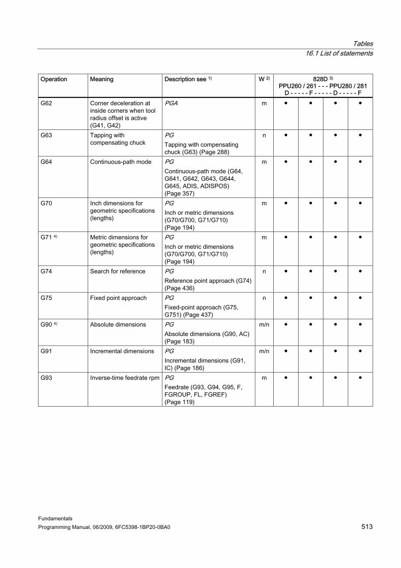
Tables 16.1 List of statements
Fundamentals Programming Manual, 06/2009, 6FC5398-1BP20-0BA0 513
Operation Meaning Description see 1) W 2) 828D 3) PPU260 / 261 - - - PPU280 / 281
D - - - - - F - - - - - D - - - - - F G62 Corner deceleration at
inside corners when tool radius offset is active (G41, G42)
PGA
m ● ● ● ●
G63 Tapping with compensating chuck
PG Tapping with compensating chuck (G63) (Page 288)
n ● ● ● ●
G64 Continuous-path mode PG Continuous-path mode (G64, G641, G642, G643, G644, G645, ADIS, ADISPOS) (Page 357)
m ● ● ● ●
G70 Inch dimensions for geometric specifications (lengths)
PG Inch or metric dimensions (G70/G700, G71/G710) (Page 194)
m ● ● ● ●
G71 4) Metric dimensions for geometric specifications (lengths)
PG Inch or metric dimensions (G70/G700, G71/G710) (Page 194)
m ● ● ● ●
G74 Search for reference PG Reference point approach (G74) (Page 436)
n ● ● ● ●
G75 Fixed point approach PG Fixed-point approach (G75, G751) (Page 437)
n ● ● ● ●
G90 4) Absolute dimensions PG Absolute dimensions (G90, AC) (Page 183)
m/n ● ● ● ●
G91 Incremental dimensions PG Incremental dimensions (G91, IC) (Page 186)
m/n ● ● ● ●
G93 Inverse-time feedrate rpm PG Feedrate (G93, G94, G95, F, FGROUP, FL, FGREF) (Page 119)
m ● ● ● ●
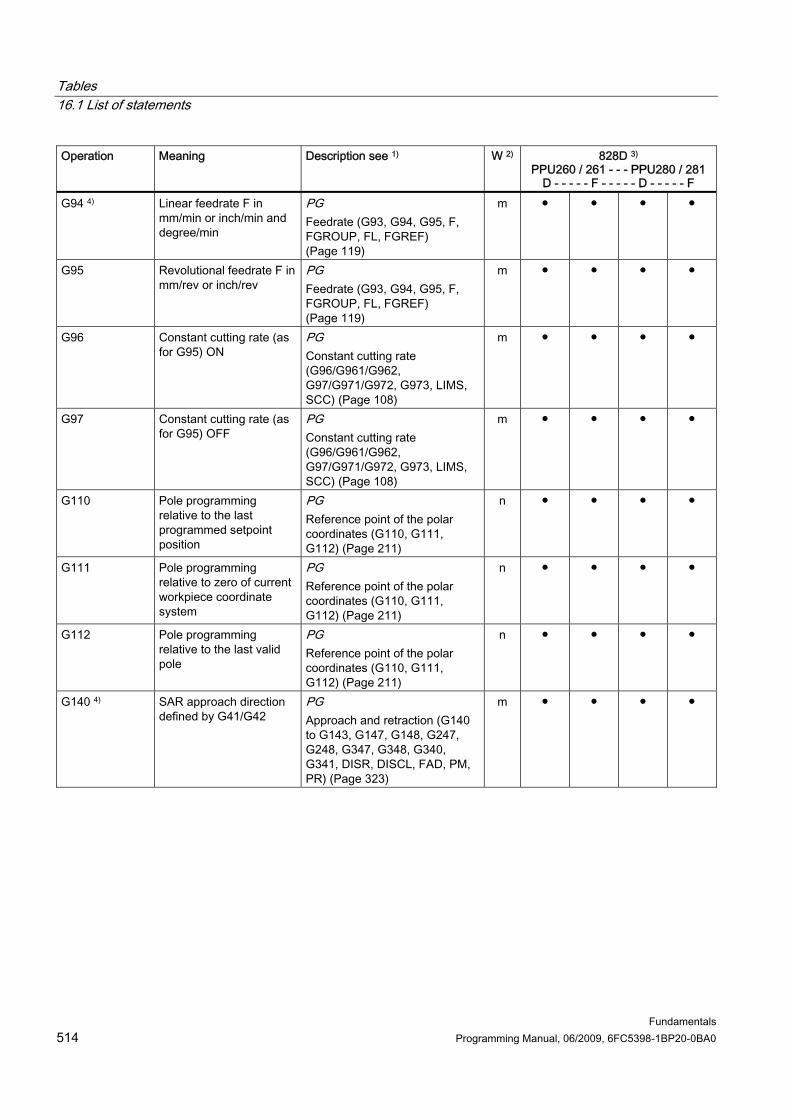
Tables 16.1 List of statements
Fundamentals 514 Programming Manual, 06/2009, 6FC5398-1BP20-0BA0
Operation Meaning Description see 1) W 2) 828D 3) PPU260 / 261 - - - PPU280 / 281
D - - - - - F - - - - - D - - - - - F G94 4) Linear feedrate F in
mm/min or inch/min and degree/min
PG Feedrate (G93, G94, G95, F, FGROUP, FL, FGREF) (Page 119)
m ● ● ● ●
G95 Revolutional feedrate F in mm/rev or inch/rev
PG Feedrate (G93, G94, G95, F, FGROUP, FL, FGREF) (Page 119)
m ● ● ● ●
G96 Constant cutting rate (as for G95) ON
PG Constant cutting rate (G96/G961/G962, G97/G971/G972, G973, LIMS, SCC) (Page 108)
m ● ● ● ●
G97 Constant cutting rate (as for G95) OFF
PG Constant cutting rate (G96/G961/G962, G97/G971/G972, G973, LIMS, SCC) (Page 108)
m ● ● ● ●
G110 Pole programming relative to the last programmed setpoint position
PG Reference point of the polar coordinates (G110, G111, G112) (Page 211)
n ● ● ● ●
G111 Pole programming relative to zero of current workpiece coordinate system
PG Reference point of the polar coordinates (G110, G111, G112) (Page 211)
n ● ● ● ●
G112 Pole programming relative to the last valid pole
PG Reference point of the polar coordinates (G110, G111, G112) (Page 211)
n ● ● ● ●
G140 4) SAR approach direction defined by G41/G42
PG Approach and retraction (G140 to G143, G147, G148, G247, G248, G347, G348, G340, G341, DISR, DISCL, FAD, PM, PR) (Page 323)
m ● ● ● ●

Tables 16.1 List of statements
Fundamentals Programming Manual, 06/2009, 6FC5398-1BP20-0BA0 515
Operation Meaning Description see 1) W 2) 828D 3) PPU260 / 261 - - - PPU280 / 281
D - - - - - F - - - - - D - - - - - F G141 SAR approach direction
to left of contour PG Approach and retraction (G140 to G143, G147, G148, G247, G248, G347, G348, G340, G341, DISR, DISCL, FAD, PM, PR) (Page 323)
m ● ● ● ●
G142 SAR approach direction to right of contour
PG Approach and retraction (G140 to G143, G147, G148, G247, G248, G347, G348, G340, G341, DISR, DISCL, FAD, PM, PR) (Page 323)
m ● ● ● ●
G143 SAR approach direction tangent-dependent
PG Approach and retraction (G140 to G143, G147, G148, G247, G248, G347, G348, G340, G341, DISR, DISCL, FAD, PM, PR) (Page 323)
m ● ● ● ●
G147 Soft approach with straight line
PG Approach and retraction (G140 to G143, G147, G148, G247, G248, G347, G348, G340, G341, DISR, DISCL, FAD, PM, PR) (Page 323)
n ● ● ● ●
G148 Soft retraction with straight line
PG Approach and retraction (G140 to G143, G147, G148, G247, G248, G347, G348, G340, G341, DISR, DISCL, FAD, PM, PR) (Page 323)
n ● ● ● ●
G153 Suppression of current frames including basic frame
PG Settable work offset (G54 to G57, G505 to G599, G53, G500, SUPA, G153) (Page 173)
n ● ● ● ●
G247 Soft approach with quadrant
PG Approach and retraction (G140 to G143, G147, G148, G247, G248, G347, G348, G340, G341, DISR, DISCL, FAD, PM, PR) (Page 323)
n ● ● ● ●

Tables 16.1 List of statements
Fundamentals 516 Programming Manual, 06/2009, 6FC5398-1BP20-0BA0
Operation Meaning Description see 1) W 2) 828D 3) PPU260 / 261 - - - PPU280 / 281
D - - - - - F - - - - - D - - - - - F G248 Soft retraction with
quadrant PG Approach and retraction (G140 to G143, G147, G148, G247, G248, G347, G348, G340, G341, DISR, DISCL, FAD, PM, PR) (Page 323)
n ● ● ● ●
G290 Switch over to SINUMERIK mode ON
FBW m ● ● ● ●
G291 Switch over to ISO2/3 mode ON
FBW m ● ● ● ●
G331 Rigid tapping, positive lead, clockwise
PG Tapping without compensating chuck (G331, G332) (Page 283)
m ● ● ● ●
G332 Rigid tapping, negative lead, counter-clockwise
PG Tapping without compensating chuck (G331, G332) (Page 283)
m ● ● ● ●
G340 4) Spatial approach block (depth and in plane at the same time (helix))
PG Approach and retraction (G140 to G143, G147, G148, G247, G248, G347, G348, G340, G341, DISR, DISCL, FAD, PM, PR) (Page 323)
m ● ● ● ●
G341 Initial infeed on perpendicular axis (z), then approach in plane
PG Approach and retraction (G140 to G143, G147, G148, G247, G248, G347, G348, G340, G341, DISR, DISCL, FAD, PM, PR) (Page 323)
m ● ● ● ●
G347 Soft approach with semicircle
PG Approach and retraction (G140 to G143, G147, G148, G247, G248, G347, G348, G340, G341, DISR, DISCL, FAD, PM, PR) (Page 323)
n ● ● ● ●
G348 Soft retraction with semicircle
PG Approach and retraction (G140 to G143, G147, G148, G247, G248, G347, G348, G340, G341, DISR, DISCL, FAD, PM, PR) (Page 323)
n ● ● ● ●

Tables 16.1 List of statements
Fundamentals Programming Manual, 06/2009, 6FC5398-1BP20-0BA0 517
Operation Meaning Description see 1) W 2) 828D 3) PPU260 / 261 - - - PPU280 / 281
D - - - - - F - - - - - D - - - - - F G450 4) Transition circle PG
Compensation at the outside corners (G450, G451, DISC) (Page 319)
m ● ● ● ●
G451 Intersection of equidistances
PG Compensation at the outside corners (G450, G451, DISC) (Page 319)
m ● ● ● ●
G460 4) Activation of collision detection for the approach and retraction block
PG Approach and retraction with enhanced retraction strategies (G460, G461, G462) (Page 335)
m ● ● ● ●
G461 Insertion of a circle into the TRC block
PG Approach and retraction with enhanced retraction strategies (G460, G461, G462) (Page 335)
m ● ● ● ●
G462 Insertion of a straight line into the TRC block
PG Approach and retraction with enhanced retraction strategies (G460, G461, G462) (Page 335)
m ● ● ● ●
G500 4) Deactivation of all adjustable frames, basic frames are active
PG Settable work offset (G54 to G57, G505 to G599, G53, G500, SUPA, G153) (Page 173)
m ● ● ● ●
G505 to G599 5th ... 99th adjustable work offset
PG Settable work offset (G54 to G57, G505 to G599, G53, G500, SUPA, G153) (Page 173)
m ● ● ● ●
G601 4) Block change on exact stop fine
PG Exact stop (G60, G9, G601, G602, G603) (Page 353)
m ● ● ● ●
G602 Block change on exact stop coarse
PG Exact stop (G60, G9, G601, G602, G603) (Page 353)
m ● ● ● ●
G603 Block change at IPO block end
PG Exact stop (G60, G9, G601, G602, G603) (Page 353)
m ● ● ● ●

Tables 16.1 List of statements
Fundamentals 518 Programming Manual, 06/2009, 6FC5398-1BP20-0BA0
Operation Meaning Description see 1) W 2) 828D 3) PPU260 / 261 - - - PPU280 / 281
D - - - - - F - - - - - D - - - - - F G621 Corner deceleration at all
corners PGA
m ● ● ● ●
G641 Continuous-path mode with smoothing as per distance criterion (= programmable rounding clearance)
PG Continuous-path mode (G64, G641, G642, G643, G644, G645, ADIS, ADISPOS) (Page 357)
m ● ● ● ●
G642 Continuous-path mode with smoothing within the defined tolerances
PG Continuous-path mode (G64, G641, G642, G643, G644, G645, ADIS, ADISPOS) (Page 357)
m ● ● ● ●
G643 Continuous-path mode with smoothing within the defined tolerances (block-internal)
PG Continuous-path mode (G64, G641, G642, G643, G644, G645, ADIS, ADISPOS) (Page 357)
m ● ● ● ●
G644 Continuous-path mode with smoothing with maximum possible dynamic response
PG Continuous-path mode (G64, G641, G642, G643, G644, G645, ADIS, ADISPOS) (Page 357)
m ● ● ● ●
G645 Continuous-path mode with smoothing and tangential block transitions within the defined tolerances
PG Continuous-path mode (G64, G641, G642, G643, G644, G645, ADIS, ADISPOS) (Page 357)
m ● ● ● ●
G700 Inch dimensions for geometric and technological specifications (lengths, feedrate)
PG Inch or metric dimensions (G70/G700, G71/G710) (Page 194)
m ● ● ● ●
G710 4) Metric dimensions for geometric and technological specifications (lengths, feedrate)
PG Inch or metric dimensions (G70/G700, G71/G710) (Page 194)
m ● ● ● ●
G751 Approach fixed point via intermediate point
PG Fixed-point approach (G75, G751) (Page 437)
n ● ● ● ●
G810 4), ..., G819
G group reserved for the OEM user
PGA
● ● ● ●

Tables 16.1 List of statements
Fundamentals Programming Manual, 06/2009, 6FC5398-1BP20-0BA0 519
Operation Meaning Description see 1) W 2) 828D 3) PPU260 / 261 - - - PPU280 / 281
D - - - - - F - - - - - D - - - - - F G820 4), ..., G829
G group reserved for the OEM user
PGA
● ● ● ●
G931 Feedrate specified by traversing time
m ● ● ● ●
G942 Freeze linear feedrate and constant cutting rate or spindle speed
m ● ● ● ●
G952 Freeze revolutional feedrate and constant cutting rate or spindle speed
m ● ● ● ●
G961 Constant cutting rate and linear feedrate
PG Constant cutting rate (G96/G961/G962, G97/G971/G972, G973, LIMS, SCC) (Page 108)
m ● ● ● ●
G962 Linear or revolutional feedrate and constant cutting rate
PG Constant cutting rate (G96/G961/G962, G97/G971/G972, G973, LIMS, SCC) (Page 108)
m ● ● ● ●
G971 Freeze spindle speed and linear feedrate
PG Constant cutting rate (G96/G961/G962, G97/G971/G972, G973, LIMS, SCC) (Page 108)
m ● ● ● ●
G972 Freeze linear or revolutional feedrate and constant spindle speed
PG Constant cutting rate (G96/G961/G962, G97/G971/G972, G973, LIMS, SCC) (Page 108)
m ● ● ● ●
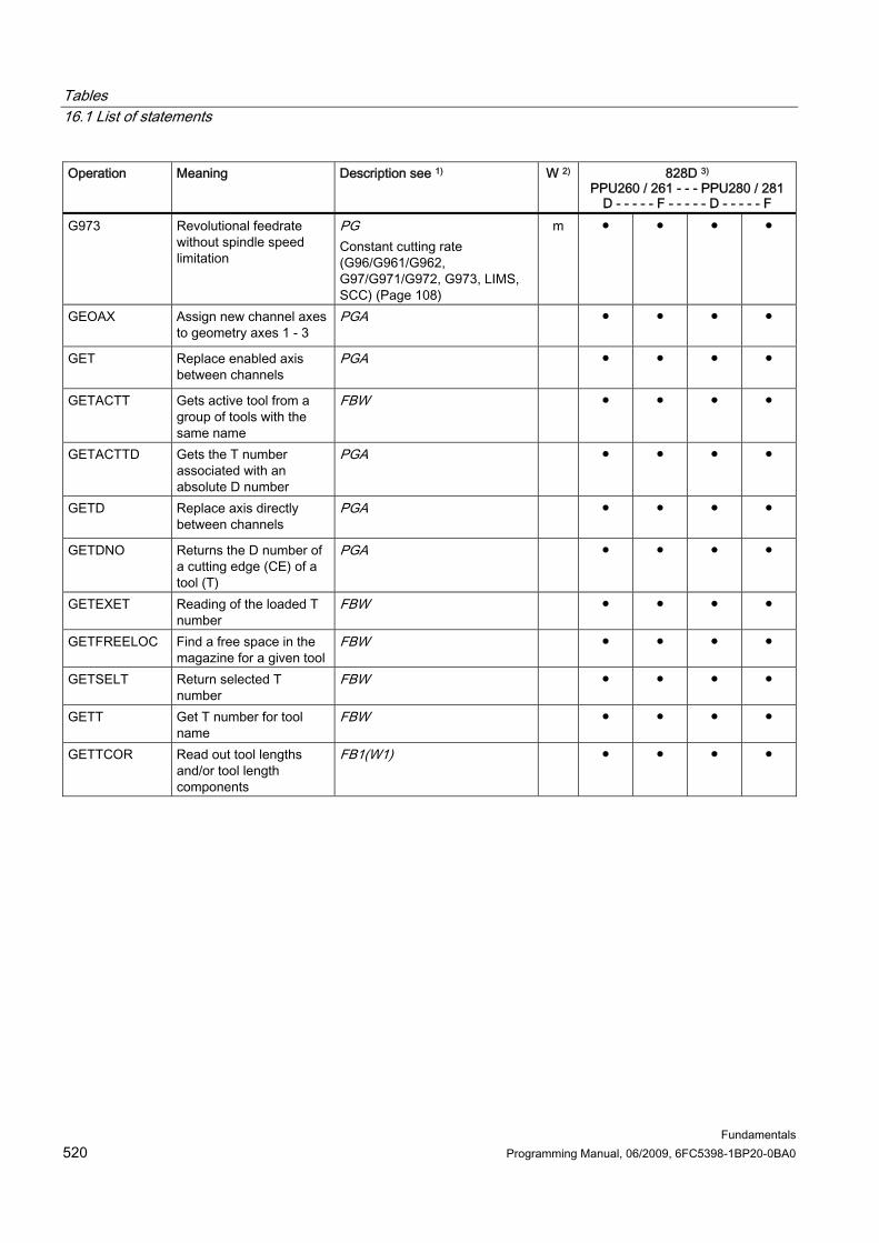
Tables 16.1 List of statements
Fundamentals 520 Programming Manual, 06/2009, 6FC5398-1BP20-0BA0
Operation Meaning Description see 1) W 2) 828D 3) PPU260 / 261 - - - PPU280 / 281
D - - - - - F - - - - - D - - - - - F G973 Revolutional feedrate
without spindle speed limitation
PG Constant cutting rate (G96/G961/G962, G97/G971/G972, G973, LIMS, SCC) (Page 108)
m ● ● ● ●
GEOAX Assign new channel axes to geometry axes 1 - 3
PGA
● ● ● ●
GET Replace enabled axis between channels
PGA
● ● ● ●
GETACTT Gets active tool from a group of tools with the same name
FBW ● ● ● ●
GETACTTD Gets the T number associated with an absolute D number
PGA
● ● ● ●
GETD Replace axis directly between channels
PGA
● ● ● ●
GETDNO Returns the D number of a cutting edge (CE) of a tool (T)
PGA
● ● ● ●
GETEXET Reading of the loaded T number
FBW ● ● ● ●
GETFREELOC Find a free space in the magazine for a given tool
FBW ● ● ● ●
GETSELT Return selected T number
FBW ● ● ● ●
GETT Get T number for tool name
FBW ● ● ● ●
GETTCOR Read out tool lengths and/or tool length components
FB1(W1) ● ● ● ●
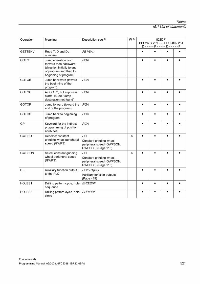
Tables 16.1 List of statements
Fundamentals Programming Manual, 06/2009, 6FC5398-1BP20-0BA0 521
Operation Meaning Description see 1) W 2) 828D 3) PPU260 / 261 - - - PPU280 / 281
D - - - - - F - - - - - D - - - - - F GETTENV Read T, D and DL
numbers FB1(W1) ● ● ● ●
GOTO Jump operation first forward then backward (direction initially to end of program and then to beginning of program)
PGA
● ● ● ●
GOTOB Jump backward (toward the beginning of the program)
PGA
● ● ● ●
GOTOC As GOTO, but suppress alarm 14080 "Jump destination not found"
PGA
● ● ● ●
GOTOF Jump forward (toward the end of the program)
PGA
● ● ● ●
GOTOS Jump back to beginning of program
PGA
● ● ● ●
GP Keyword for the indirect programming of position attributes
PGA
● ● ● ●
GWPSOF Deselect constant grinding wheel peripheral speed (GWPS)
PG Constant grinding wheel peripheral speed (GWPSON, GWPSOF) (Page 115)
n ● ● ● ●
GWPSON Select constant grinding wheel peripheral speed (GWPS)
PG Constant grinding wheel peripheral speed (GWPSON, GWPSOF) (Page 115)
n ● ● ● ●
H... Auxiliary function output to the PLC
PG/FB1(H2) Auxiliary function outputs (Page 419)
● ● ● ●
HOLES1 Drilling pattern cycle, hole sequence
BHD/BHF ● ● ● ●
HOLES2 Drilling pattern cycle, hole circle
BHD/BHF ● ● ● ●

Tables 16.1 List of statements
Fundamentals 522 Programming Manual, 06/2009, 6FC5398-1BP20-0BA0
Operation Meaning Description see 1) W 2) 828D 3) PPU260 / 261 - - - PPU280 / 281
D - - - - - F - - - - - D - - - - - F I Interpolation parameters PG
Circular interpolation with center point and end point (G2/G3, X... Y... Z..., I... J... K...) (Page 229)
n ● ● ● ●
I1 Intermediate point coordinate
PG Circular interpolation with opening angle and center point (G2/G3, X... Y... Z.../ I... J... K..., AR) (Page 236)
n ● ● ● ●
IC Incremental dimensions PG Incremental dimensions (G91, IC) (Page 186)
n ● ● ● ●
ICYCOF All blocks of a technology cycle are processed in one interpolation cycle following ICYCOF
PGA
● ● ● ●
ICYCON Each block of a technology cycle is processed in a separate interpolation cycle following ICYCON
PGA
● ● ● ●
ID Identifier for modal synchronized actions
PGA
m ● ● ● ●
IDS Identifier for modal static synchronized actions
PGA
● ● ● ●
IF Introduction of a conditional jump in the part program/technology cycle
PGA
● ● ● ●
INDEX Define index of character in input string
PGA
● ● ● ●
INIPO Initialization of variables at POWER ON
PGA
● ● ● ●
INIRE Initialization of variables at reset
PGA
● ● ● ●

Tables 16.1 List of statements
Fundamentals Programming Manual, 06/2009, 6FC5398-1BP20-0BA0 523
Operation Meaning Description see 1) W 2) 828D 3) PPU260 / 261 - - - PPU280 / 281
D - - - - - F - - - - - D - - - - - F INICF Initialization of variables
at NewConfig PGA
● ● ● ●
INIT Selection of a particular NC program for execution in a particular channel
PGA
- - - -
INITIAL Generation of an INI file across all areas
PGA
● ● ● ●
INT Data type: Integer with sign
PGA
● ● ● ●
INTERSEC Calculate intersection between two contour elements
PGA
● ● ● ●
INVCCW Trace involute, counter-clockwise
PG Involute interpolation (INVCW, INVCCW) (Page 253)
m - - - -
INVCW Trace involute, clockwise PG Involute interpolation (INVCW, INVCCW) (Page 253)
m - - - -
INVFRAME Calculate the inverse frame from a frame
FB1(K2) ● ● ● ●
IP Variable interpolation parameter
PGA
● ● ● ●
IPOBRKA Motion criterion from braking ramp activation
PGA
m ● ● ● ●
IPOENDA End of motion when “IPO stop” reached
PGA
m ● ● ● ●
IPTRLOCK Freeze start of the untraceable program section at next machine function block
PGA
m ● ● ● ●
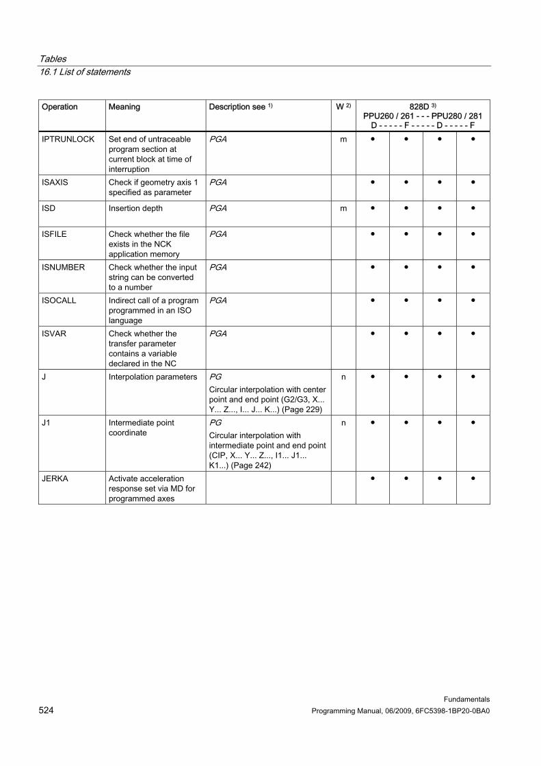
Tables 16.1 List of statements
Fundamentals 524 Programming Manual, 06/2009, 6FC5398-1BP20-0BA0
Operation Meaning Description see 1) W 2) 828D 3) PPU260 / 261 - - - PPU280 / 281
D - - - - - F - - - - - D - - - - - F IPTRUNLOCK Set end of untraceable
program section at current block at time of interruption
PGA
m ● ● ● ●
ISAXIS Check if geometry axis 1 specified as parameter
PGA
● ● ● ●
ISD Insertion depth PGA
m ● ● ● ●
ISFILE Check whether the file exists in the NCK application memory
PGA
● ● ● ●
ISNUMBER Check whether the input string can be converted to a number
PGA
● ● ● ●
ISOCALL Indirect call of a program programmed in an ISO language
PGA
● ● ● ●
ISVAR Check whether the transfer parameter contains a variable declared in the NC
PGA
● ● ● ●
J Interpolation parameters PG Circular interpolation with center point and end point (G2/G3, X... Y... Z..., I... J... K...) (Page 229)
n ● ● ● ●
J1 Intermediate point coordinate
PG Circular interpolation with intermediate point and end point (CIP, X... Y... Z..., I1... J1... K1...) (Page 242)
n ● ● ● ●
JERKA Activate acceleration response set via MD for programmed axes
● ● ● ●
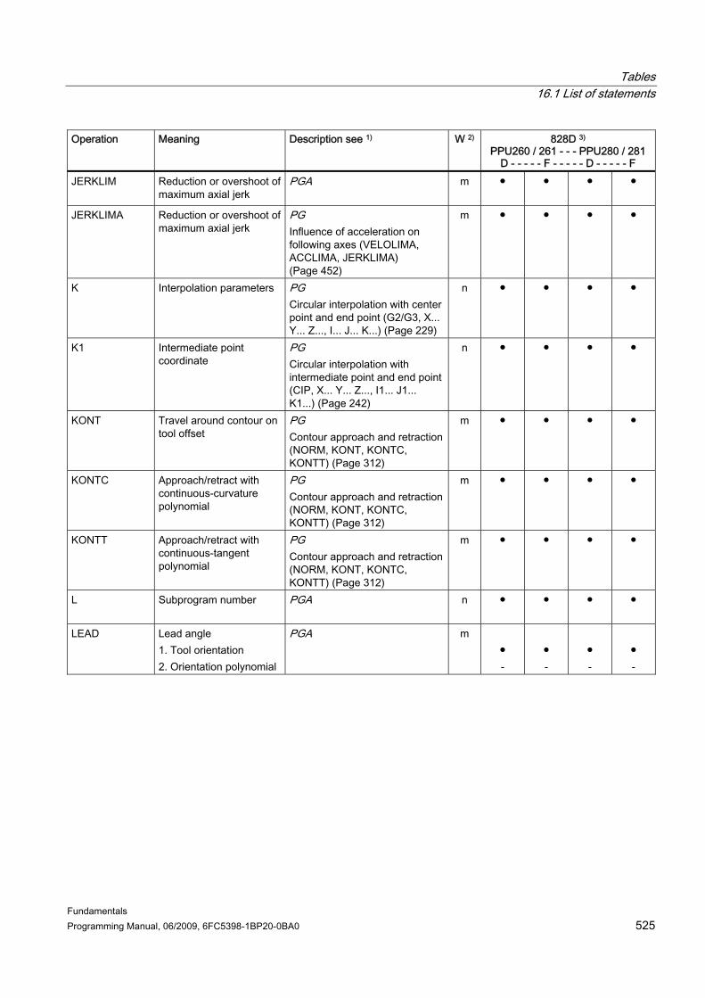
Tables 16.1 List of statements
Fundamentals Programming Manual, 06/2009, 6FC5398-1BP20-0BA0 525
Operation Meaning Description see 1) W 2) 828D 3) PPU260 / 261 - - - PPU280 / 281
D - - - - - F - - - - - D - - - - - F JERKLIM Reduction or overshoot of
maximum axial jerk PGA
m ● ● ● ●
JERKLIMA Reduction or overshoot of maximum axial jerk
PG Influence of acceleration on following axes (VELOLIMA, ACCLIMA, JERKLIMA) (Page 452)
m ● ● ● ●
K Interpolation parameters PG Circular interpolation with center point and end point (G2/G3, X... Y... Z..., I... J... K...) (Page 229)
n ● ● ● ●
K1 Intermediate point coordinate
PG Circular interpolation with intermediate point and end point (CIP, X... Y... Z..., I1... J1... K1...) (Page 242)
n ● ● ● ●
KONT Travel around contour on tool offset
PG Contour approach and retraction (NORM, KONT, KONTC, KONTT) (Page 312)
m ● ● ● ●
KONTC Approach/retract with continuous-curvature polynomial
PG Contour approach and retraction (NORM, KONT, KONTC, KONTT) (Page 312)
m ● ● ● ●
KONTT Approach/retract with continuous-tangent polynomial
PG Contour approach and retraction (NORM, KONT, KONTC, KONTT) (Page 312)
m ● ● ● ●
L Subprogram number PGA
n ● ● ● ●
LEAD Lead angle 1. Tool orientation 2. Orientation polynomial
PGA
m ● -
● -
● -
● -

Tables 16.1 List of statements
Fundamentals 526 Programming Manual, 06/2009, 6FC5398-1BP20-0BA0
Operation Meaning Description see 1) W 2) 828D 3) PPU260 / 261 - - - PPU280 / 281
D - - - - - F - - - - - D - - - - - F LEADOF Master value coupling
OFF PGA
- - - -
LEADON Master value coupling ON
PGA
- - - -
LENTOAX Provides information about the assignment of tool lengths L1, L2, and L3 of the active tool to the abscissa, ordinate and applicate
FB1(W1) ● ● ● ●
LFOF 4) Fast retraction for thread cutting OFF
PG Fast retraction for thread cutting (LFON, LFOF, DILF, ALF, LFTXT, LFWP, LFPOS, POLF, POLFMASK, POLFMLIN) (Page 290)
m ● ● ● ●
LFON Fast retraction for thread cutting ON
PG Fast retraction for thread cutting (LFON, LFOF, DILF, ALF, LFTXT, LFWP, LFPOS, POLF, POLFMASK, POLFMLIN) (Page 290)
m ● ● ● ●
LFPOS Retraction of the axis declared with POLFMASK or POLFMLIN to the absolute axis position programmed with POLF
PG Fast retraction for thread cutting (LFON, LFOF, DILF, ALF, LFTXT, LFWP, LFPOS, POLF, POLFMASK, POLFMLIN) (Page 290)
m ● ● ● ●
LFTXT The plane of the retraction movement for fast retraction is determined from the path tangent and the current tool direction
PG Fast retraction for thread cutting (LFON, LFOF, DILF, ALF, LFTXT, LFWP, LFPOS, POLF, POLFMASK, POLFMLIN) (Page 290)
m ● ● ● ●

Tables 16.1 List of statements
Fundamentals Programming Manual, 06/2009, 6FC5398-1BP20-0BA0 527
Operation Meaning Description see 1) W 2) 828D 3) PPU260 / 261 - - - PPU280 / 281
D - - - - - F - - - - - D - - - - - F LFWP The plane of the
retraction movement for fast retraction is determined by the current working plane (G17/G18/G19)
PG Fast retraction for thread cutting (LFON, LFOF, DILF, ALF, LFTXT, LFWP, LFPOS, POLF, POLFMASK, POLFMLIN) (Page 290)
m ● ● ● ●
LIFTFAST Fast retraction PG
● ● ● ●
LIMS Speed limitation for G96/G961 and G97
PG Constant cutting rate (G96/G961/G962, G97/G971/G972, G973, LIMS, SCC) (Page 108)
m ● ● ● ●
LLI Lower limit value of variables
PGA
● ● ● ●
LN Natural logarithm PGA
● ● ● ●
LOCK Disable synchronized action with ID (stop technology cycle)
PGA
● ● ● ●
LONGHOLE Milling pattern cycle of elongated holes on a circle
BHD/BHF - - - -
LOOP Introduction of an endless loop
PGA
● ● ● ●
M0 Programmed stop PG M functions (Page 423)
● ● ● ●
M1 Optional stop PG M functions (Page 423)
● ● ● ●
M2 End of main program with return to beginning of program
PG M functions (Page 423)
● ● ● ●
M3 Direction of spindle rotation clockwise for master spindle
PG M functions (Page 423)
● ● ● ●
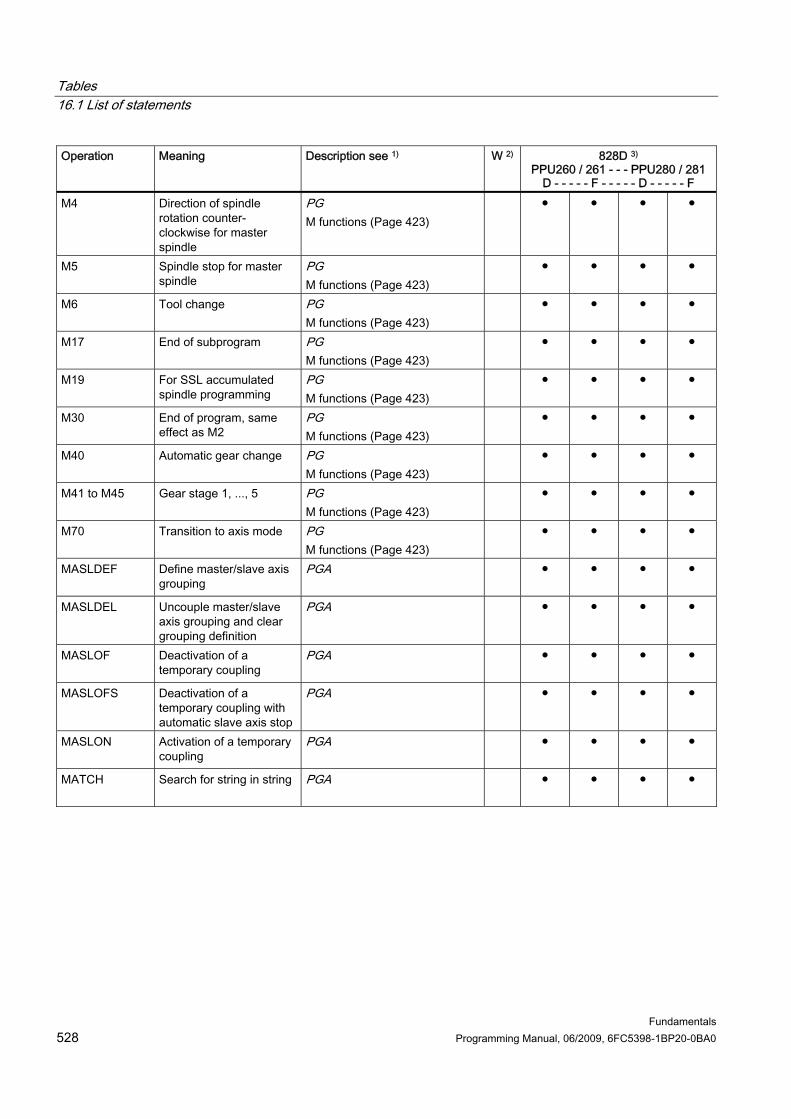
Tables 16.1 List of statements
Fundamentals 528 Programming Manual, 06/2009, 6FC5398-1BP20-0BA0
Operation Meaning Description see 1) W 2) 828D 3) PPU260 / 261 - - - PPU280 / 281
D - - - - - F - - - - - D - - - - - F M4 Direction of spindle
rotation counter-clockwise for master spindle
PG M functions (Page 423)
● ● ● ●
M5 Spindle stop for master spindle
PG M functions (Page 423)
● ● ● ●
M6 Tool change PG M functions (Page 423)
● ● ● ●
M17 End of subprogram PG M functions (Page 423)
● ● ● ●
M19 For SSL accumulated spindle programming
PG M functions (Page 423)
● ● ● ●
M30 End of program, same effect as M2
PG M functions (Page 423)
● ● ● ●
M40 Automatic gear change PG M functions (Page 423)
● ● ● ●
M41 to M45 Gear stage 1, ..., 5 PG M functions (Page 423)
● ● ● ●
M70 Transition to axis mode PG M functions (Page 423)
● ● ● ●
MASLDEF Define master/slave axis grouping
PGA
● ● ● ●
MASLDEL Uncouple master/slave axis grouping and clear grouping definition
PGA
● ● ● ●
MASLOF Deactivation of a temporary coupling
PGA
● ● ● ●
MASLOFS Deactivation of a temporary coupling with automatic slave axis stop
PGA
● ● ● ●
MASLON Activation of a temporary coupling
PGA
● ● ● ●
MATCH Search for string in string PGA
● ● ● ●

Tables 16.1 List of statements
Fundamentals Programming Manual, 06/2009, 6FC5398-1BP20-0BA0 529
Operation Meaning Description see 1) W 2) 828D 3) PPU260 / 261 - - - PPU280 / 281
D - - - - - F - - - - - D - - - - - F MAXVAL Larger value of two
variables (arithm. function)
PGA
● ● ● ●
MCALL Modal subprogram call PGA
● ● ● ●
MEAC Continuous measurement without deletion of distance-to-go
PGA
n - - - -
MEAFRAME Frame calculation from measuring points
PGA
● ● ● ●
MEAS Measurement with touch-trigger probe
PGA
n ● ● ● ●
MEASA Measurement with deletion of distance-to-go
PGA
n - - - -
MEASURE Calculation method for workpiece and tool measurement
FB2(M5)
● ● ● ●
MEAW Measurement with touch-trigger probe without deletion of distance-to-go
PGA
n ● ● ● ●
MEAWA Measurement without deletion of distance-to-go
PGA
n - - - -
MI Access to frame data: Mirroring
PGA
● ● ● ●
MINDEX Define index of character in input string
PGA
● ● ● ●
MINVAL Smaller value of two variables (arithm. function)
PGA
● ● ● ●
MIRROR Programmable mirroring PGA Programmable mirroring (MIRROR, AMIRROR) (Page 403)
n ● ● ● ●
MMC Call the dialog window interactively from the part program on the HMI
PGA
● ● ● ●

Tables 16.1 List of statements
Fundamentals 530 Programming Manual, 06/2009, 6FC5398-1BP20-0BA0
Operation Meaning Description see 1) W 2) 828D 3) PPU260 / 261 - - - PPU280 / 281
D - - - - - F - - - - - D - - - - - F MOD Modulo division PGA
● ● ● ●
MODAXVAL Determine modulo position of a modulo rotary axis
PGA
● ● ● ●
MOV Start positioning axis PGA
● ● ● ●
MSG Programmable messages PG Messages (MSG) (Page 427)
m ● ● ● ●
MVTOOL Language command to move tool
FBW
● ● ● ●
N NC auxiliary block number
PG Block rules (Page 42)
● ● ● ●
NCK Specification of range of validity for data
PGA
● ● ● ●
NEWCONF Apply modified machine data (corresponds to "Activate machine data")
PGA
● ● ● ●
NEWT Create new tool PGA
● ● ● ●
NORM 4) Standard setting in starting point and end point with tool offset
PG Contour approach and retraction (NORM, KONT, KONTC, KONTT) (Page 312)
m ● ● ● ●
NOT Logic NOT (negation) PGA
● ● ● ●
NPROT Machine-specific protection zone ON/OFF
PGA
● ● ● ●
NPROTDEF Definition of a machine-specific protection zone
PGA
● ● ● ●
NUMBER Convert input string to number
PGA
● ● ● ●
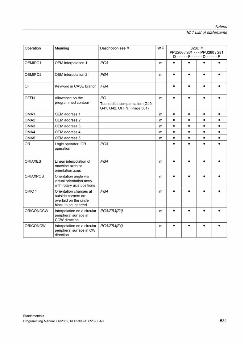
Tables 16.1 List of statements
Fundamentals Programming Manual, 06/2009, 6FC5398-1BP20-0BA0 531
Operation Meaning Description see 1) W 2) 828D 3) PPU260 / 261 - - - PPU280 / 281
D - - - - - F - - - - - D - - - - - F OEMIPO1 OEM interpolation 1 PGA
m ● ● ● ●
OEMIPO2 OEM interpolation 2 PGA
m ● ● ● ●
OF Keyword in CASE branch PGA
● ● ● ●
OFFN Allowance on the programmed contour
PG Tool radius compensation (G40, G41, G42, OFFN) (Page 301)
m ● ● ● ●
OMA1 OEM address 1 m ● ● ● ● OMA2 OEM address 2 m ● ● ● ● OMA3 OEM address 3 m ● ● ● ● OMA4 OEM address 4 m ● ● ● ● OMA5 OEM address 5 m ● ● ● ● OR Logic operator, OR
operation PGA
● ● ● ●
ORIAXES Linear interpolation of machine axes or orientation axes
PGA
m ● ● ● ●
ORIAXPOS Orientation angle via virtual orientation axes with rotary axis positions
m ● ● ● ●
ORIC 4) Orientation changes at outside corners are overlaid on the circle block to be inserted
PGA
m ● ● ● ●
ORICONCCW Interpolation on a circular peripheral surface in CCW direction
PGA/FB3(F3)
m ● ● ● ●
ORICONCW Interpolation on a circular peripheral surface in CW direction
PGA/FB3(F4)
m ● ● ● ●

Tables 16.1 List of statements
Fundamentals 532 Programming Manual, 06/2009, 6FC5398-1BP20-0BA0
Operation Meaning Description see 1) W 2) 828D 3) PPU260 / 261 - - - PPU280 / 281
D - - - - - F - - - - - D - - - - - F ORICONIO Interpolation on a circular
peripheral surface with intermediate orientation setting
PGA/FB3(F4)
m ● ● ● ●
ORICONTO Interpolation on circular peripheral surface in tangential transition (final orientation)
PGA/FB3(F5)
m ● ● ● ●
ORICURVE Interpolation of orientation with specification of motion of two contact points of tool
PGA/FB3(F6)
m ● ● ● ●
ORID Orientation changes are performed before the circle block
PGA
m ● ● ● ●
ORIEULER Orientation angle via Euler angle
PGA
m ● ● ● ●
ORIMKS Tool orientation in the machine coordinate system
PGA
m ● ● ● ●
ORIPATH Tool orientation in relation to path
PGA
m ● ● ● ●
ORIPATHS Tool orientation in relation to path, blips in the orientation characteristic are smoothed
PGA
m ● ● ● ●
ORIPLANE Interpolation in a plane (corresponds to ORIVECT), large-radius circular interpolation
PGA
m ● ● ● ●
ORIRESET Initial tool orientation with up to 3 orientation axes
PGA
● ● ● ●
ORIROTA Angle of rotation to an absolute direction of rotation
PGA
m ● ● ● ●
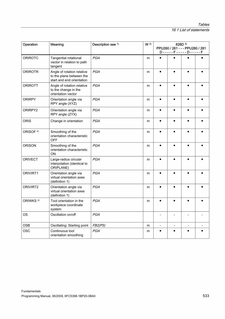
Tables 16.1 List of statements
Fundamentals Programming Manual, 06/2009, 6FC5398-1BP20-0BA0 533
Operation Meaning Description see 1) W 2) 828D 3) PPU260 / 261 - - - PPU280 / 281
D - - - - - F - - - - - D - - - - - F ORIROTC Tangential rotational
vector in relation to path tangent
PGA
m ● ● ● ●
ORIROTR Angle of rotation relative to the plane between the start and end orientation
PGA
m ● ● ● ●
ORIROTT Angle of rotation relative to the change in the orientation vector
PGA
m ● ● ● ●
ORIRPY Orientation angle via RPY angle (XYZ)
PGA
m ● ● ● ●
ORIRPY2 Orientation angle via RPY angle (ZYX)
PGA
m ● ● ● ●
ORIS Change in orientation PGA
m ● ● ● ●
ORISOF 4) Smoothing of the orientation characteristic OFF
PGA
m ● ● ● ●
ORISON Smoothing of the orientation characteristic ON
PGA
m ● ● ● ●
ORIVECT Large-radius circular interpolation (identical to ORIPLANE)
PGA
m ● ● ● ●
ORIVIRT1 Orientation angle via virtual orientation axes (definition 1)
PGA
m ● ● ● ●
ORIVIRT2 Orientation angle via virtual orientation axes (definition 1)
PGA
m ● ● ● ●
ORIWKS 4) Tool orientation in the workpiece coordinate system
PGA
m ● ● ● ●
OS Oscillation on/off PGA
- - - -
OSB Oscillating: Starting point FB2(P5) m - - - - OSC Continuous tool
orientation smoothing PGA
m ● ● ● ●

Tables 16.1 List of statements
Fundamentals 534 Programming Manual, 06/2009, 6FC5398-1BP20-0BA0
Operation Meaning Description see 1) W 2) 828D 3) PPU260 / 261 - - - PPU280 / 281
D - - - - - F - - - - - D - - - - - F OSCILL Axis: 1 - 3 infeed axes PGA
m - - - -
OSCTRL Oscillation options PGA
m - - - -
OSD Smoothing of tool orientation by specifying smoothing distance with SD
PGA
m ● ● ● ●
OSE Oscillation end position PGA
m - - - -
OSNSC Oscillating: Number of spark-out cycles
PGA
m - - - -
OSOF 4) Tool orientation smoothing OFF
PGA
m ● ● ● ●
OSP1 Oscillating: Left reversal point
PGA
m - - - -
OSP2 Oscillation right reversal point
PGA
m - - - -
OSS Tool orientation smoothing at end of block
PGA
m ● ● ● ●
OSSE Tool orientation smoothing at start and end of block
PGA
m ● ● ● ●
OST Smoothing of tool orientation by specifying angular tolerance in degrees with SD (maximum deviation from programmed orientation characteristic)
PGA
m ● ● ● ●
OST1 Oscillating: Stopping point in left reversal point
PGA
m - - - -
OST2 Oscillating: Stopping point in right reversal point
PGA
m - - - -

Tables 16.1 List of statements
Fundamentals Programming Manual, 06/2009, 6FC5398-1BP20-0BA0 535
Operation Meaning Description see 1) W 2) 828D 3) PPU260 / 261 - - - PPU280 / 281
D - - - - - F - - - - - D - - - - - F OTOL Orientation tolerance for
compressor functions, orientation smoothing and smoothing types
PGA
- ● - ●
OVR Speed offset PGA Programmable feedrate override (OVR, OVRRAP, OVRA) (Page 150)
m ● ● ● ●
OVRA Axial speed offset PGA Programmable feedrate override (OVR, OVRRAP, OVRA) (Page 150)
m ● ● ● ●
OVRRAP Rapid traverse override PGA Programmable feedrate override (OVR, OVRRAP, OVRA) (Page 150)
m ● ● ● ●
P Number of subprogram cycles
PGA
● ● ● ●
PAROT Align workpiece coordinate system on workpiece
PG Frame generation according to tool orientation (TOFRAME, TOROT, PAROT) (Page 410)
m ● ● ● ●
PAROTOF Deactivate frame rotation in relation to workpiece
PG Frame generation according to tool orientation (TOFRAME, TOROT, PAROT) (Page 410)
m ● ● ● ●
PCALL Call subprograms with absolute path and parameter transfer
PGA
● ● ● ●
PDELAYOF Punching with delay OFF PGA
m - - - -
PDELAYON 4) Punching with delay ON PGA
m - - - -

Tables 16.1 List of statements
Fundamentals 536 Programming Manual, 06/2009, 6FC5398-1BP20-0BA0
Operation Meaning Description see 1) W 2) 828D 3) PPU260 / 261 - - - PPU280 / 281
D - - - - - F - - - - - D - - - - - F PHU Physical unit of a variable PGA
● ● ● ●
PL 1. B spline: Node clearance 2. Polynomial interpolation: Length of the parameter interval for polynomial interpolation
PGA 1. 2.
n - -
○ -
- -
○ -
PM Per minute PG Approach and retraction (G140 to G143, G147, G148, G247, G248, G347, G348, G340, G341, DISR, DISCL, FAD, PM, PR) (Page 323)
● ● ● ●
PO Polynomial coefficient for polynomial interpolation
PGA
n - - - -
POCKET3 Milling cycle, rectangular pocket (any milling cutter)
BHD/BHF
● ● ● ●
POCKET4 Milling cycle, circular pocket (any milling cutter)
BHD/BHF ● ● ● ●
POLF LIFTFAST retraction position
PG/PGA Fast retraction for thread cutting (LFON, LFOF, DILF, ALF, LFTXT, LFWP, LFPOS, POLF, POLFMASK, POLFMLIN) (Page 290)
m ● ● ● ●
POLFA Start retraction position of single axes with $AA_ESR_TRIGGER
PG Fast retraction for thread cutting (LFON, LFOF, DILF, ALF, LFTXT, LFWP, LFPOS, POLF, POLFMASK, POLFMLIN) (Page 290)
m ● ● ● ●
POLFMASK Enable axes for retraction without a connection between the axes
PG Fast retraction for thread cutting (LFON, LFOF, DILF, ALF, LFTXT, LFWP, LFPOS, POLF, POLFMASK, POLFMLIN) (Page 290)
m ● ● ● ●
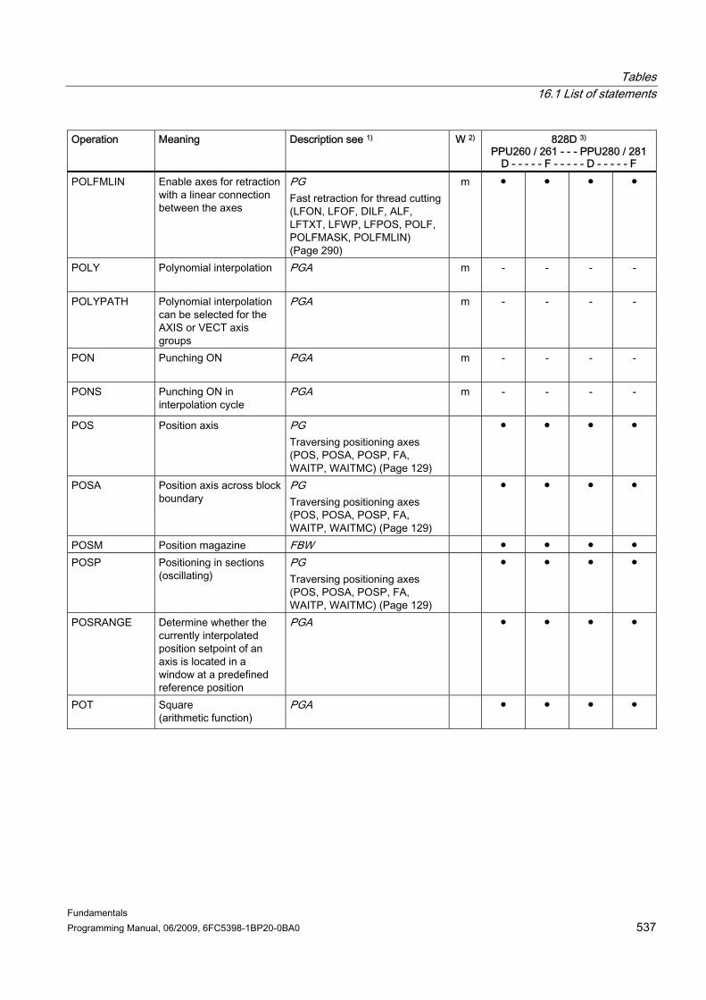
Tables 16.1 List of statements
Fundamentals Programming Manual, 06/2009, 6FC5398-1BP20-0BA0 537
Operation Meaning Description see 1) W 2) 828D 3) PPU260 / 261 - - - PPU280 / 281
D - - - - - F - - - - - D - - - - - F POLFMLIN Enable axes for retraction
with a linear connection between the axes
PG Fast retraction for thread cutting (LFON, LFOF, DILF, ALF, LFTXT, LFWP, LFPOS, POLF, POLFMASK, POLFMLIN) (Page 290)
m ● ● ● ●
POLY Polynomial interpolation PGA
m - - - -
POLYPATH Polynomial interpolation can be selected for the AXIS or VECT axis groups
PGA
m - - - -
PON Punching ON PGA
m - - - -
PONS Punching ON in interpolation cycle
PGA
m - - - -
POS Position axis PG Traversing positioning axes (POS, POSA, POSP, FA, WAITP, WAITMC) (Page 129)
● ● ● ●
POSA Position axis across block boundary
PG Traversing positioning axes (POS, POSA, POSP, FA, WAITP, WAITMC) (Page 129)
● ● ● ●
POSM Position magazine FBW ● ● ● ● POSP Positioning in sections
(oscillating) PG Traversing positioning axes (POS, POSA, POSP, FA, WAITP, WAITMC) (Page 129)
● ● ● ●
POSRANGE Determine whether the currently interpolated position setpoint of an axis is located in a window at a predefined reference position
PGA
● ● ● ●
POT Square (arithmetic function)
PGA
● ● ● ●

Tables 16.1 List of statements
Fundamentals 538 Programming Manual, 06/2009, 6FC5398-1BP20-0BA0
Operation Meaning Description see 1) W 2) 828D 3) PPU260 / 261 - - - PPU280 / 281
D - - - - - F - - - - - D - - - - - F PR Per revolution PG
Approach and retraction (G140 to G143, G147, G148, G247, G248, G347, G348, G340, G341, DISR, DISCL, FAD, PM, PR) (Page 323)
● ● ● ●
PREPRO Identify subprograms with preparation
PGA
● ● ● ●
PRESETON Set actual values for programmed axes
PGA
● ● ● ●
PRIO Keyword for setting the priority for interrupt processing
PGA
● ● ● ●
PROC First operation in a program
PGA
● ● ● ●
PTP Point-to-point motion PGA
m ● ● ● ●
PTPG0 Point-to-point motion only with G0, otherwise CP
PGA
m ● ● ● ●
PUNCHACC Travel-dependent acceleration for nibbling
PGA
- - - -
PUTFTOC Tool fine offset for parallel dressing
PGA
● ● ● ●
PUTFTOCF Tool fine offset dependent on a function for parallel dressing defined with FCTDEF
PGA
● ● ● ●
PW B spline, point weight PGA
n - ○ - ○
QECLRNOF Quadrant error compensation learning OFF
PGA
● ● ● ●
QECLRNON Quadrant error compensation learning ON
PGA
● ● ● ●
QU Fast additional (auxiliary) function output
PG Auxiliary function outputs (Page 419)
● ● ● ●

Tables 16.1 List of statements
Fundamentals Programming Manual, 06/2009, 6FC5398-1BP20-0BA0 539
Operation Meaning Description see 1) W 2) 828D 3) PPU260 / 261 - - - PPU280 / 281
D - - - - - F - - - - - D - - - - - F R... Arithmetic parameter also
as settable address identifier and with numerical extension
PGA
● ● ● ●
RAC Absolute non-modal axis-specific radius programming
PG Axis-specific diameter/radius programming (DIAMONA, DIAM90A, DIAMOFA, DIACYCOFA, DIAMCHANA, DIAMCHAN, DAC, DIC, RAC, RIC) (Page 200)
n ● ● ● ●
RDISABLE Read-in disable PGA
● ● ● ●
READ Reads one or more lines in the specified file and stores the information read in the array
PGA
● ● ● ●
REAL Data type: Floating-point variable with sign (real numbers)
PGA
● ● ● ●
REDEF Setting for machine data, NC language elements and system variables, specifying the user groups they are displayed for
PGA
● ● ● ●
RELEASE Release machine axes for axis exchange
PGA
● ● ● ●
REP Keyword for initialization of all elements of an array with the same value
PGA
● ● ● ●

Tables 16.1 List of statements
Fundamentals 540 Programming Manual, 06/2009, 6FC5398-1BP20-0BA0
Operation Meaning Description see 1) W 2) 828D 3) PPU260 / 261 - - - PPU280 / 281
D - - - - - F - - - - - D - - - - - F REPEAT Repetition of a program
loop PGA
● ● ● ●
REPEATB Repetition of a program line
PGA
● ● ● ●
REPOSA Linear repositioning with all axes
PGA
n ● ● ● ●
REPOSH Repositioning with semicircle
PGA
n ● ● ● ●
REPOSHA Repositioning with all axes; geometry axes in semicircle
PGA
n ● ● ● ●
REPOSL Linear repositioning PGA
n ● ● ● ●
REPOSQ Repositioning in a quadrant
PGA
n ● ● ● ●
REPOSQA Linear repositioning with all axes, geometry axes in quadrant
PGA
n ● ● ● ●
RESET Reset technology cycle PGA
● ● ● ●
RESETMON Language command for setpoint activation
FBW
● ● ● ●
RET End of subprogram PGA
● ● ● ●
RIC Relative non-modal axis-specific radius programming
PG
n ● ● ● ●
RINDEX Define index of character in input string
PGA
● ● ● ●

Tables 16.1 List of statements
Fundamentals Programming Manual, 06/2009, 6FC5398-1BP20-0BA0 541
Operation Meaning Description see 1) W 2) 828D 3) PPU260 / 261 - - - PPU280 / 281
D - - - - - F - - - - - D - - - - - F RMB Repositioning to start of
block PGA
m ● ● ● ●
RME Repositioning to end of block
PGA
m ● ● ● ●
RMI 4) Repositioning to interrupt point
PGA
m ● ● ● ●
RMN Repositioning to the nearest path point
PGA
m ● ● ● ●
RND Round the contour corner PG Chamfer, rounding (CHF, CHR, RND, RNDM, FRC, FRCM) (Page 295)
n ● ● ● ●
RNDM Modal rounding PG Chamfer, rounding (CHF, CHR, RND, RNDM, FRC, FRCM) (Page 295)
m ● ● ● ●
ROT Programmable rotation PG Programmable rotation (ROT, AROT, RPL) (Page 384)
n ● ● ● ●
ROTS Programmable frame rotations with solid angles
PG Programmable frame rotations with solid angles (ROTS, AROTS, CROTS) (Page 396)
n ● ● ● ●
ROUND Rounding of decimal places
PGA
● ● ● ●
ROUNDUP Rounding up of an input value
PGA
● ● ● ●
RP Polar radius PG Travel commands with polar coordinates (G0, G1, G2, G3, AP, RP) (Page 213)
m/n ● ● ● ●

Tables 16.1 List of statements
Fundamentals 542 Programming Manual, 06/2009, 6FC5398-1BP20-0BA0
Operation Meaning Description see 1) W 2) 828D 3) PPU260 / 261 - - - PPU280 / 281
D - - - - - F - - - - - D - - - - - F RPL Rotation in the plane PG
Programmable frame rotations with solid angles (ROTS, AROTS, CROTS) (Page 396)
n ● ● ● ●
RT Parameter for access to frame data: Rotation
PGA
● ● ● ●
RTLIOF G0 without linear interpolation (single-axis interpolation)
PG Rapid traverse movement (G0, RTLION, RTLIOF) (Page 217)
m ● ● ● ●
RTLION G0 with linear interpolation
PG Rapid traverse movement (G0, RTLION, RTLIOF) (Page 217)
m ● ● ● ●
S Spindle speed (with G4, G96/G961 different significance)
PG Spindle speed (S), direction of spindle rotation (M3, M4, M5) (Page 95)
m/n ● ● ● ●
SAVE Attribute for saving information when subprograms are called
PGA
● ● ● ●
SBLOF Suppress single block PGA
● ● ● ●
SBLON Revoke suppression of single block
PGA
● ● ● ●
SC Parameter for access to frame data: Scaling
PGA
● ● ● ●
SCALE Programmable scaling PG Programmable scale factor (SCALE, ASCALE) (Page 398)
n ● ● ● ●
SCC Selective assignment of transverse axis to G96/G961/G962. Axis identifiers may take the form of geometry, channel or machine axes
PG Constant cutting rate (G96/G961/G962, G97/G971/G972, G973, LIMS, SCC) (Page 108)
● ● ● ●
SCPARA Program servo parameter set
PGA
● ● ● ●

Tables 16.1 List of statements
Fundamentals Programming Manual, 06/2009, 6FC5398-1BP20-0BA0 543
Operation Meaning Description see 1) W 2) 828D 3) PPU260 / 261 - - - PPU280 / 281
D - - - - - F - - - - - D - - - - - F SD Spline degree PGA
n - ○ - ○
SEFORM Structuring operation in the Step editor to generate the step view for HMI Advanced
PGA
● ● ● ●
SET Keyword for initialization of all elements of an array with listed values
PGA
● ● ● ●
SETAL Set alarm PGA
● ● ● ●
SETDNO Assign the D number of a cutting edge (CE) of a tool (T)
PGA
● ● ● ●
SETINT Define which interrupt routine is to be activated when an NCK input is present
PGA
● ● ● ●
SETM Setting of markers in dedicated channel
PGA
- - - -
SETMS Reset to the master spindle defined in machine data
Spindle speed (S), direction of spindle rotation (M3, M4, M5) (Page 95)
● ● ● ●
SETMS(n) Set spindle n as master spindle
PG Spindle speed (S), direction of spindle rotation (M3, M4, M5) (Page 95)
● ● ● ●
SETMTH Set master toolholder number
FBW ● ● ● ●
SETPIECE Set piece number for all tools assigned to the spindle
FBW ● ● ● ●
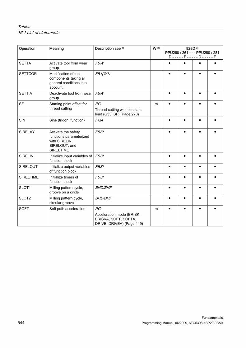
Tables 16.1 List of statements
Fundamentals 544 Programming Manual, 06/2009, 6FC5398-1BP20-0BA0
Operation Meaning Description see 1) W 2) 828D 3) PPU260 / 261 - - - PPU280 / 281
D - - - - - F - - - - - D - - - - - F SETTA Activate tool from wear
group FBW ● ● ● ●
SETTCOR Modification of tool components taking all general conditions into account
FB1(W1) ● ● ● ●
SETTIA Deactivate tool from wear group
FBW ● ● ● ●
SF Starting point offset for thread cutting
PG Thread cutting with constant lead (G33, SF) (Page 270)
m ● ● ● ●
SIN Sine (trigon. function) PGA
● ● ● ●
SIRELAY Activate the safety functions parameterized with SIRELIN, SIRELOUT, and SIRELTIME
FBSI ● ● ● ●
SIRELIN Initialize input variables of function block
FBSI ● ● ● ●
SIRELOUT Initialize output variables of function block
FBSI ● ● ● ●
SIRELTIME Initialize timers of function block
FBSI ● ● ● ●
SLOT1 Milling pattern cycle, groove on a circle
BHD/BHF ● ● ● ●
SLOT2 Milling pattern cycle, circular groove
BHD/BHF ● ● ● ●
SOFT Soft path acceleration PG Acceleration mode (BRISK, BRISKA, SOFT, SOFTA, DRIVE, DRIVEA) (Page 449)
m ● ● ● ●

Tables 16.1 List of statements
Fundamentals Programming Manual, 06/2009, 6FC5398-1BP20-0BA0 545
Operation Meaning Description see 1) W 2) 828D 3) PPU260 / 261 - - - PPU280 / 281
D - - - - - F - - - - - D - - - - - F SOFTA Activate soft axis
acceleration for the programmed axes
PG Acceleration mode (BRISK, BRISKA, SOFT, SOFTA, DRIVE, DRIVEA) (Page 449)
● ● ● ●
SON Nibbling ON PGA
m - - - -
SONS Nibbling ON in interpolation cycle
PGA
m - - - -
SPATH 4) Path reference for FGROUP axes is arc length
PGA
m ● ● ● ●
SPCOF Switch master spindle or spindle(s) from position control to speed control
PG Position-controlled spindle operation (SPCON, SPCOF) (Page 134)
m ● ● ● ●
SPCON Switch master spindle or spindle(s) from speed control to position control
PGA Position-controlled spindle operation (SPCON, SPCOF) (Page 134)
m ● ● ● ●
SPI Converts spindle number into axis identifier
PGA
● ● ● ●
SPIF1 4) Fast NCK inputs/outputs for punching/nibbling byte 1
FB2(N4) m - - - -
SPIF2 Fast NCK inputs/outputs for punching/nibbling byte 2
FB2(N4) m - - - -
SPLINEPATH Define spline grouping PGA
- ○ - ○
SPN Number of path sections per block
PGA
n - - - -
SPOF 4) Stroke OFF, nibbling, punching OFF
PGA
m - - - -

Tables 16.1 List of statements
Fundamentals 546 Programming Manual, 06/2009, 6FC5398-1BP20-0BA0
Operation Meaning Description see 1) W 2) 828D 3) PPU260 / 261 - - - PPU280 / 281
D - - - - - F - - - - - D - - - - - F SPOS Spindle position PG
Positioning spindles (SPOS, SPOSA, M19, M70, WAITS) (Page 135)
m ● ● ● ●
SPOSA Spindle position across block boundaries
PG Positioning spindles (SPOS, SPOSA, M19, M70, WAITS) (Page 135)
m ● ● ● ●
SPP Length of a path section PGA
m - - - -
SQRT Square root (arithmetic function)
PGA
● ● ● ●
SR Oscillation retraction path for synchronized action
PG Several feedrate values in one block (F, ST, SR, FMA, STA, SRA) (Page 161)
n - - - -
SRA Oscillation retraction path with external input axial for synchronized action
PG Several feedrate values in one block (F, ST, SR, FMA, STA, SRA) (Page 161)
m - - - -
ST Oscillation sparking-out time for synchronized action
PG Several feedrate values in one block (F, ST, SR, FMA, STA, SRA) (Page 161)
n - - - -
STA Oscillation sparking-out time axial for synchronized action
PG Several feedrate values in one block (F, ST, SR, FMA, STA, SRA) (Page 161)
m - - - -
START Start selected programs simultaneously in several channels from current program
PGA
- - - -
STARTFIFO 4) Execute; fill preprocessing memory simultaneously
PGA
m ● ● ● ●

Tables 16.1 List of statements
Fundamentals Programming Manual, 06/2009, 6FC5398-1BP20-0BA0 547
Operation Meaning Description see 1) W 2) 828D 3) PPU260 / 261 - - - PPU280 / 281
D - - - - - F - - - - - D - - - - - F STAT Position of joints PGA
n ● ● ● ●
STOPFIFO Stop machining; fill preprocessing memory until STARTFIFO is detected, preprocessing memory is full or end of program
PGA
m ● ● ● ●
STOPRE Preprocessing stop until all prepared blocks in main run are executed
PGA
● ● ● ●
STOPREOF Revoke preprocessing stop
PGA
● ● ● ●
STRING Data type: Character string
PGA
● ● ● ●
STRINGFELD Selection of a single character from the progr. string field
PGA
● ● ● ●
STRINGIS Checks the present scope of NC language and the NC cycle names, user variables, macros, and label names belonging specifically to this command to establish whether these exist, are valid, defined or active
PGA
● ● ● ●
STRINGVAR Selection of a single character from the progr. string
PGA
- - - -
STRLEN Define string length PGA
● ● ● ●
SUBSTR Define index of character in input string
PGA
● ● ● ●

Tables 16.1 List of statements
Fundamentals 548 Programming Manual, 06/2009, 6FC5398-1BP20-0BA0
Operation Meaning Description see 1) W 2) 828D 3) PPU260 / 261 - - - PPU280 / 281
D - - - - - F - - - - - D - - - - - F SUPA Suppression of current
work offset, including programmed offsets, system frames, handwheel offsets (DRF), external work offset, and overlaid movement
PG Deselect frame (G53, G153, SUPA, G500) (Page 414)
n ● ● ● ●
SVC Tool cutting rate PG Cutting rate (SVC) (Page 100)
m ● ● ● ●
SYNFCT Evaluation of a polynomial as a function of a condition in the motion-synchronous action
PGA
● ● ● ●
SYNR The variable is read synchronously, i.e. at the time of execution
PGA
● ● ● ●
SYNRW The variable is read and written synchronously, i.e. at the time of execution
PGA
● ● ● ●
SYNW The variable is written synchronously, i.e. at the time of execution
PGA
● ● ● ●
T Call tool (only change if specified in machine data; otherwise M6 command necessary)
PG Tool change with T command (Page 60)
● ● ● ●
TAN Tangent (trigon. function) PGA
● ● ● ●
TANG Definition of axis grouping tangential correction
PGA
- - - -
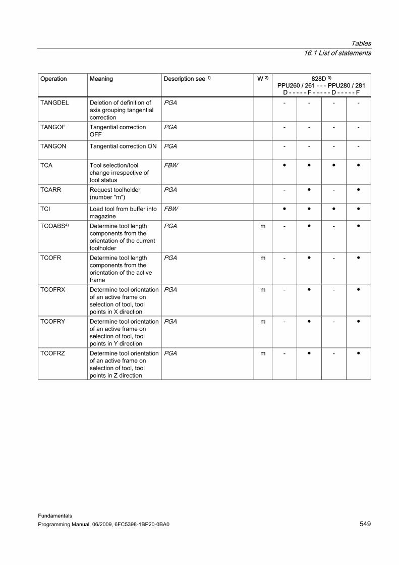
Tables 16.1 List of statements
Fundamentals Programming Manual, 06/2009, 6FC5398-1BP20-0BA0 549
Operation Meaning Description see 1) W 2) 828D 3) PPU260 / 261 - - - PPU280 / 281
D - - - - - F - - - - - D - - - - - F TANGDEL Deletion of definition of
axis grouping tangential correction
PGA
- - - -
TANGOF Tangential correction OFF
PGA
- - - -
TANGON Tangential correction ON PGA
- - - -
TCA Tool selection/tool change irrespective of tool status
FBW ● ● ● ●
TCARR Request toolholder (number "m")
PGA
- ● - ●
TCI Load tool from buffer into magazine
FBW ● ● ● ●
TCOABS4) Determine tool length components from the orientation of the current toolholder
PGA
m - ● - ●
TCOFR Determine tool length components from the orientation of the active frame
PGA
m - ● - ●
TCOFRX Determine tool orientation of an active frame on selection of tool, tool points in X direction
PGA
m - ● - ●
TCOFRY Determine tool orientation of an active frame on selection of tool, tool points in Y direction
PGA
m - ● - ●
TCOFRZ Determine tool orientation of an active frame on selection of tool, tool points in Z direction
PGA
m - ● - ●
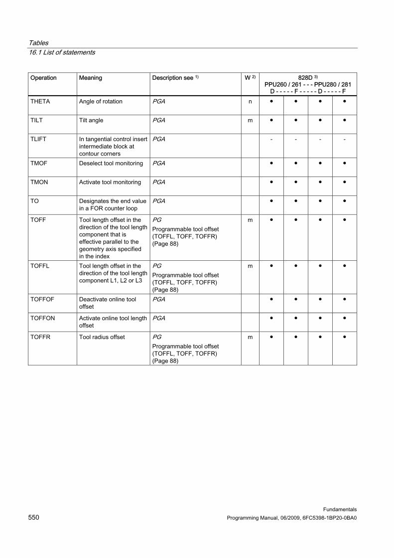
Tables 16.1 List of statements
Fundamentals 550 Programming Manual, 06/2009, 6FC5398-1BP20-0BA0
Operation Meaning Description see 1) W 2) 828D 3) PPU260 / 261 - - - PPU280 / 281
D - - - - - F - - - - - D - - - - - F THETA Angle of rotation PGA
n ● ● ● ●
TILT Tilt angle PGA
m ● ● ● ●
TLIFT In tangential control insert intermediate block at contour corners
PGA
- - - -
TMOF Deselect tool monitoring PGA
● ● ● ●
TMON Activate tool monitoring PGA
● ● ● ●
TO Designates the end value in a FOR counter loop
PGA
● ● ● ●
TOFF Tool length offset in the direction of the tool length component that is effective parallel to the geometry axis specified in the index
PG Programmable tool offset (TOFFL, TOFF, TOFFR) (Page 88)
m ● ● ● ●
TOFFL Tool length offset in the direction of the tool length component L1, L2 or L3
PG Programmable tool offset (TOFFL, TOFF, TOFFR) (Page 88)
m ● ● ● ●
TOFFOF Deactivate online tool offset
PGA
● ● ● ●
TOFFON Activate online tool length offset
PGA
● ● ● ●
TOFFR Tool radius offset PG Programmable tool offset (TOFFL, TOFF, TOFFR) (Page 88)
m ● ● ● ●

Tables 16.1 List of statements
Fundamentals Programming Manual, 06/2009, 6FC5398-1BP20-0BA0 551
Operation Meaning Description see 1) W 2) 828D 3) PPU260 / 261 - - - PPU280 / 281
D - - - - - F - - - - - D - - - - - F TOFRAME Align the Z axis of the
workpiece coordinate system parallel to the workpiece orientation by rotating the frame
PG Frame generation according to tool orientation (TOFRAME, TOROT, PAROT) (Page 410)
m ● ● ● ●
TOFRAMEX Align the X axis of the workpiece coordinate system parallel to the workpiece orientation by rotating the frame
PG Frame generation according to tool orientation (TOFRAME, TOROT, PAROT) (Page 410)
m ● ● ● ●
TOFRAMEY Align the Y axis of the workpiece coordinate system parallel to the workpiece orientation by rotating the frame
PG Frame generation according to tool orientation (TOFRAME, TOROT, PAROT) (Page 410)
m ● ● ● ●
TOFRAMEZ As TOFRAME PG Frame generation according to tool orientation (TOFRAME, TOROT, PAROT) (Page 410)
m ● ● ● ●
TOLOWER Convert the letters of a string into lowercase
PGA
● ● ● ●
TOOLENV Save current states which are of significance to the evaluation of the tool data stored in the memory
FB1(W1)
● ● ● ●
TOROT Align the Z axis of the workpiece coordinate system parallel to the workpiece orientation by rotating the frame
PG Frame generation according to tool orientation (TOFRAME, TOROT, PAROT) (Page 410)
m ● ● ● ●
TOROTOF Frame rotations in tool direction OFF
PG Frame generation according to tool orientation (TOFRAME, TOROT, PAROT) (Page 410)
m ● ● ● ●

Tables 16.1 List of statements
Fundamentals 552 Programming Manual, 06/2009, 6FC5398-1BP20-0BA0
Operation Meaning Description see 1) W 2) 828D 3) PPU260 / 261 - - - PPU280 / 281
D - - - - - F - - - - - D - - - - - F TOROTX Align the X axis of the
workpiece coordinate system parallel to the workpiece orientation by rotating the frame
PG Frame generation according to tool orientation (TOFRAME, TOROT, PAROT) (Page 410)
m ● ● ● ●
TOROTY Align the Y axis of the workpiece coordinate system parallel to the workpiece orientation by rotating the frame
PG Frame generation according to tool orientation (TOFRAME, TOROT, PAROT) (Page 410)
m ● ● ● ●
TOROTZ As TOROT PG Frame generation according to tool orientation (TOFRAME, TOROT, PAROT) (Page 410)
m ● ● ● ●
TOUPPER Convert the letters of a string into uppercase
PGA
● ● ● ●
TOWBCS Wear values in basic coordinate system (BCS)
PGA
m - ● - ●
TOWKCS Wear values in the coordinate system of the tool head for kinetic transformation (differs from machine coordinate system through tool rotation)
PGA
m - ● - ●
TOWMCS Wear values in machine coordinate system
PGA
m - ● - ●
TOWSTD Initial setting value for offsets in tool length
PGA
m - ● - ●

Tables 16.1 List of statements
Fundamentals Programming Manual, 06/2009, 6FC5398-1BP20-0BA0 553
Operation Meaning Description see 1) W 2) 828D 3) PPU260 / 261 - - - PPU280 / 281
D - - - - - F - - - - - D - - - - - F TOWTCS Wear values in the tool
coordinate system (toolholder ref. point T at the tool holder)
PGA
m - ● - ●
TOWWCS Wear values in workpiece coordinate system
PGA
m - ● - ●
TR Offset component of a frame variable
PGA
● ● ● ●
TRAANG Transformation inclined axis
PGA
- - ○ -
TRACON Cascaded transformation PGA
- - ○ -
TRACYL Cylinder: Peripheral surface transformation
PGA
○ ○ ○ ○
TRAFOOF Deactivate active transformations in the channel
PGA
● ● ● ●
TRAILOF Asynchronous coupled motion OFF
PGA
● ● ● ●
TRAILON Asynchronous coupled motion ON
PGA
● ● ● ●
TRANS Programmable offset PG Zero offset (TRANS, ATRANS) (Page 376)
n ● ● ● ●
TRANSMIT Pole transformation (face machining)
PGA
○ ○ ○ ○
TRAORI 4-axis, 5-axis transformation, generic transformation
PGA
- ● - ●
TRUE Logical constant: True PGA
● ● ● ●
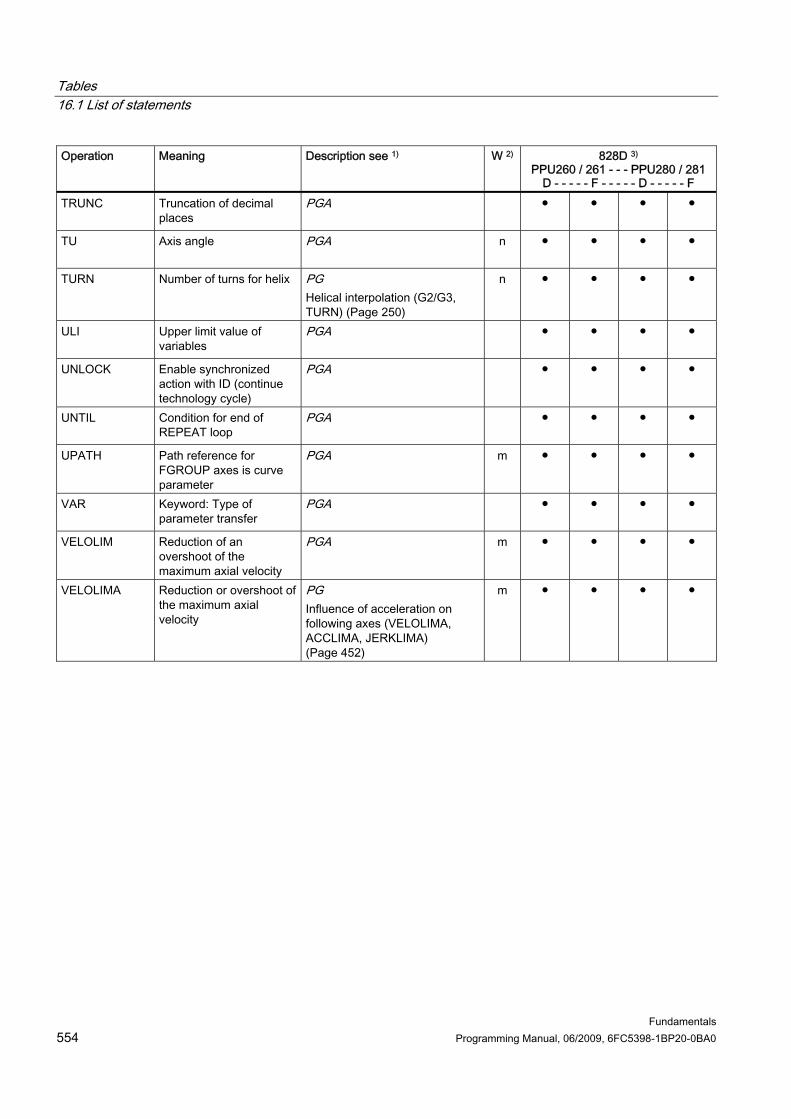
Tables 16.1 List of statements
Fundamentals 554 Programming Manual, 06/2009, 6FC5398-1BP20-0BA0
Operation Meaning Description see 1) W 2) 828D 3) PPU260 / 261 - - - PPU280 / 281
D - - - - - F - - - - - D - - - - - F TRUNC Truncation of decimal
places PGA
● ● ● ●
TU Axis angle PGA
n ● ● ● ●
TURN Number of turns for helix PG Helical interpolation (G2/G3, TURN) (Page 250)
n ● ● ● ●
ULI Upper limit value of variables
PGA
● ● ● ●
UNLOCK Enable synchronized action with ID (continue technology cycle)
PGA
● ● ● ●
UNTIL Condition for end of REPEAT loop
PGA
● ● ● ●
UPATH Path reference for FGROUP axes is curve parameter
PGA
m ● ● ● ●
VAR Keyword: Type of parameter transfer
PGA
● ● ● ●
VELOLIM Reduction of an overshoot of the maximum axial velocity
PGA
m ● ● ● ●
VELOLIMA Reduction or overshoot of the maximum axial velocity
PG Influence of acceleration on following axes (VELOLIMA, ACCLIMA, JERKLIMA) (Page 452)
m ● ● ● ●

Tables 16.1 List of statements
Fundamentals Programming Manual, 06/2009, 6FC5398-1BP20-0BA0 555
Operation Meaning Description see 1) W 2) 828D 3) PPU260 / 261 - - - PPU280 / 281
D - - - - - F - - - - - D - - - - - F WAITC Wait for the coupling
block change criterion to be fulfilled for the axes/spindles
PGA
- - ○ -
WAITE Wait for end of program in another channel
PGA
- - - -
WAITM Wait for marker in specified channel; terminate previous block with exact stop
PGA
- - - -
WAITMC Wait for marker in specified channel; exact stop only if the other channels have not yet reached the marker.
PGA
- - - -
WAITP Wait for end of traversing PG Traversing positioning axes (POS, POSA, POSP, FA, WAITP, WAITMC) (Page 129)
● ● ● ●
WAITS Wait for spindle position to be reached
PG Positioning spindles (SPOS, SPOSA, M19, M70, WAITS) (Page 135)
● ● ● ●
WALCS0 Workpiece coordinate system working area limitation deselected
PG Working area limitation in WCS/SZS (WALCS0 ... WALCS10) (Page 433)
m ● ● ● ●
WALCS1 Workpiece coordinate system working area limitation group 1 active
PG Working area limitation in WCS/SZS (WALCS0 ... WALCS10) (Page 433)
m ● ● ● ●
WALCS2 Workpiece coordinate system working area limitation group 2 active
PG Working area limitation in WCS/SZS (WALCS0 ... WALCS10) (Page 433)
m ● ● ● ●

Tables 16.1 List of statements
Fundamentals 556 Programming Manual, 06/2009, 6FC5398-1BP20-0BA0
Operation Meaning Description see 1) W 2) 828D 3) PPU260 / 261 - - - PPU280 / 281
D - - - - - F - - - - - D - - - - - F WALCS3 Workpiece coordinate
system working area limitation group 3 active
PG Working area limitation in WCS/SZS (WALCS0 ... WALCS10) (Page 433)
m ● ● ● ●
WALCS4 Workpiece coordinate system working area limitation group 4 active
PG Working area limitation in WCS/SZS (WALCS0 ... WALCS10) (Page 433)
m ● ● ● ●
WALCS5 Workpiece coordinate system working area limitation group 5 active
PG Working area limitation in WCS/SZS (WALCS0 ... WALCS10) (Page 433)
m ● ● ● ●
WALCS6 Workpiece coordinate system working area limitation group 6 active
PG Working area limitation in WCS/SZS (WALCS0 ... WALCS10) (Page 433)
m ● ● ● ●
WALCS7 Workpiece coordinate system working area limitation group 7 active
PG Working area limitation in WCS/SZS (WALCS0 ... WALCS10) (Page 433)
m ● ● ● ●
WALCS8 Workpiece coordinate system working area limitation group 8 active
PG Working area limitation in WCS/SZS (WALCS0 ... WALCS10) (Page 433)
m ● ● ● ●
WALCS9 Workpiece coordinate system working area limitation group 9 active
PG Working area limitation in WCS/SZS (WALCS0 ... WALCS10) (Page 433)
m ● ● ● ●
WALCS10 Workpiece coordinate system working area limitation group 10 active
PG Working area limitation in WCS/SZS (WALCS0 ... WALCS10) (Page 433)
m ● ● ● ●
WALIMOF BCS working area limitation OFF
PG Working area limitation in BCS (G25/G26, WALIMON, WALIMOF) (Page 429)
m ● ● ● ●
WALIMON 4) BCS working area limitation ON
PG Working area limitation in BCS (G25/G26, WALIMON, WALIMOF) (Page 429)
m ● ● ● ●

Tables 16.1 List of statements
Fundamentals Programming Manual, 06/2009, 6FC5398-1BP20-0BA0 557
Operation Meaning Description see 1) W 2) 828D 3) PPU260 / 261 - - - PPU280 / 281
D - - - - - F - - - - - D - - - - - F WHEN The action is executed
cyclically when the condition is fulfilled.
PGA
● ● ● ●
WHENEVER The action is executed once whenever the condition is fulfilled.
PGA
● ● ● ●
WHILE Start of WHILE program loop
PGA
● ● ● ●
WRITE Write text to file system Appends a block to the end of the specified file.
PGA
● ● ● ●
WRTPR Delays the machining job without interrupting continuous-path mode
● ● ● ●
X Axis name PG Travel commands with Cartesian coordinates (G0, G1, G2, G3, X..., Y..., Z...) (Page 209)
m/n ● ● ● ●
XOR Logic exclusive OR PGA
● ● ● ●
Y Axis name PG Travel commands with Cartesian coordinates (G0, G1, G2, G3, X..., Y..., Z...) (Page 209)
m/n ● ● ● ●
Z Axis name PG Travel commands with Cartesian coordinates (G0, G1, G2, G3, X..., Y..., Z...) (Page 209)
m/n ● ● ● ●

Tables 16.2 Addresses
Fundamentals 558 Programming Manual, 06/2009, 6FC5398-1BP20-0BA0
16.2 16.2 Addresses
List of addresses The list of addresses consists of: ● Address letters ● Fixed addresses ● Fixed addresses with axis expansion ● Settable addresses
Address letters The following address letters are available:
Letter Meaning Numeric
extension A Settable address identifier x B Settable address identifier x C Settable address identifier x D Selection/deselection of tool length compensation, tool cutting edge E Settable address identifier F Feedrate
dwell time in seconds x
G G function H H function x I Settable address identifier x J Settable address identifier x K Settable address identifier x L Subroutines, subroutine call M M function x N Subblock number O Unassigned P Number of program runs Q Settable address identifier x R Variable identifier (arithmetic parameter) / settable address identifier without numerical
extension x
S Spindle value dwell time in spindle revolutions
x x
T Tool number x U Settable address identifier x V Settable address identifier x W Settable address identifier x X Settable address identifier x Y Settable address identifier x
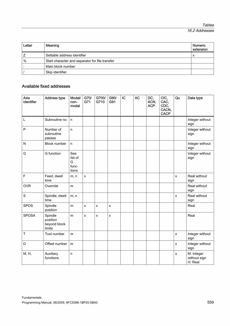
Tables 16.2 Addresses
Fundamentals Programming Manual, 06/2009, 6FC5398-1BP20-0BA0 559
Letter Meaning Numeric extension
Z Settable address identifier x % Start character and separator for file transfer : Main block number / Skip identifier
Available fixed addresses Axis identifier
Address type Modal/non-modal
G70/G71
G700/G710
G90/G91
IC AC DC, ACN, ACP
CIC, CAC, CDC, CACN, CACP
Qu Data type
L Subroutine no. n Integer without sign
P Number of subroutine passes
n Integer without sign
N Block number n Integer without sign
G G function See list of G func-tions
Integer without sign
F Feed, dwell time
m, n x x Real without sign
OVR Override m Real without sign
S Spindle, dwell time
m, n x Real without sign
SPOS Spindle position
m x x x Real
SPOSA Spindle position beyond block limits
m x x x Real
T Tool number m x Integer without sign
D Offset number m x Integer without sign
M, H, Auxiliary functions
n x M: Integer without sign H: Real

Tables 16.2 Addresses
Fundamentals 560 Programming Manual, 06/2009, 6FC5398-1BP20-0BA0
Fixed addresses with axis expansion Axis identifier
Address type Modal/non-modal
G70/G71
G700/G710
G90/G91
IC AC DC, ACN, ACP
CIC, CAC, CDC, CACN, CACP
Qu Data type
AX: Axis Variable axis identifier
*) x x x x x x Real
IP: Interpola-tion para-meter
Variable interpolation parameter
n x x x x x Real
POS: Positioning axis
Positioning axis
m x x x x x x x Real
POSA: Positioning axis above end of block
Positioning axis across block boundaries
m x x x x x x x Real
POSP: Positioning axis in parts
Positioning axis in parts (oscillation)
m x x x x x x Real: End position / Real: Partial length Integer: Option
PO: Polynomial
Polynomial coefficient
n x x Real without sign 1 - 8 times
FA: Feed axial
Axial feedrate m x x Real without sign
FL: Feed limit
Axial feed limit
m x Real without sign
OVRA: Override
Axial override m x Real without sign
ACC: Axial acceleration
Axial acceleration
m Real without sign
FMA: Feedrate multiple axial
Synchronous feedrate axial
m x Real without sign
STA: Sparking-out time axial
Sparking out time axial
m Real without sign

Tables 16.2 Addresses
Fundamentals Programming Manual, 06/2009, 6FC5398-1BP20-0BA0 561
Axis identifier
Address type Modal/non-modal
G70/G71
G700/G710
G90/G91
IC AC DC, ACN, ACP
CIC, CAC, CDC, CACN, CACP
Qu Data type
SRA: Sparking-out retract
Retraction path on external input axial
m x x Real without sign
OS: Oscillating ON/OFF
Oscillation ON/OFF
m Integer without sign
OST1: Oscillating time 1
Stopping time at left reversal point (oscillation)
m Real
OST2: Oscillating time 2
Stopping time at right reversal point (oscillation)
m Real
OSP1: Oscillating position 1
Left reversal point (oscillation)
m x x x x x x Real
OSP2: Oscillating position 2
Right reversal point (oscillation)
m x x x x x x Real
OSB: Oscillating start
position m x x x x x x Real
OSE: Oscillating end position
Oscillation end position
m x x x x x x Real
OSNSC: Oscillating: number spark-out cycles
Number of spark-out cycles (oscillation)
m Integer without sign
OSCTRL: Oscillating control
Oscillation control options
m Integer without sign: set options, integer without sign: reset options
OSCILL: Oscillating
Axis assignment for oscillation activate oscillation
m Axis: 1 - 3 infeed axes

Tables 16.2 Addresses
Fundamentals 562 Programming Manual, 06/2009, 6FC5398-1BP20-0BA0
Axis identifier
Address type Modal/non-modal
G70/G71
G700/G710
G90/G91
IC AC DC, ACN, ACP
CIC, CAC, CDC, CACN, CACP
Qu Data type
FDA: Feedrate DRF axial
Axis feedrate for handwheel override
n x Real without sign
FGREF Reference radius
m x x Real without sign
POLF LIFTFAST position
m x x Real without sign
FXS: Fixed stop
Travel to fixed stop ON
m Integer without sign
FXST: Fixed stop torque
Torque limit for travel to fixed stop
m Real
FXSW: Fixed stop window
Monitoring window for travel to fixed stop
m Real
In these addresses, an axis or an expression of axis type is specified in square brackets. The data type in the above column shows the type of value assigned. *) Absolute end points: modal, incremental end points: non-modal, otherwise modal/non-modal depending on syntax of G function.
Settable addresses Axis identifier Address
type Modal/non-modal
G70/G71
G700/G710
G90/G91
IC AC DC, ACN, ACP
CIC, CAC, CDC, CACN, CACP
Qu Max. num-ber
Data type
Axis values and end points X, Y, Z, A, B, C
Axis *) x x x x x x 8 Real
AP: Angle polar
Polar angle m/n* x x x 1 Real
RP: Polar radius
Polar radius m/n* x x x x x 1 Real without sign
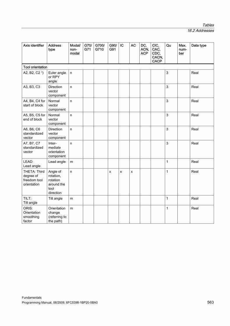
Tables 16.2 Addresses
Fundamentals Programming Manual, 06/2009, 6FC5398-1BP20-0BA0 563
Axis identifier Address type
Modal/non-modal
G70/G71
G700/G710
G90/G91
IC AC DC, ACN, ACP
CIC, CAC, CDC, CACN, CACP
Qu Max. num-ber
Data type
Tool orientation A2, B2, C2 1) Euler angle
or RPY angle
n 3 Real
A3, B3, C3 Direction vector component
n
3 Real
A4, B4, C4 for start of block
Normal vector component
n 3 Real
A5, B5, C5 for end of block
Normal vector component
n 3 Real
A6, B6, C6 standardized vector
Direction vector component
n 3 Real
A7, B7, C7 standardized vector
Inter-mediate orientation component
n 3 Real
LEAD: Lead angle
Lead angle m 1 Real
THETA: Third degree of freedom tool orientation
Angle of rotation, rotation around the tool direction
n x x x 1 Real
TILT: Tilt angle
Tilt angle m 1 Real
ORIS: Orientation smoothing factor
Orientation change (referring to the path)
m 1 Real
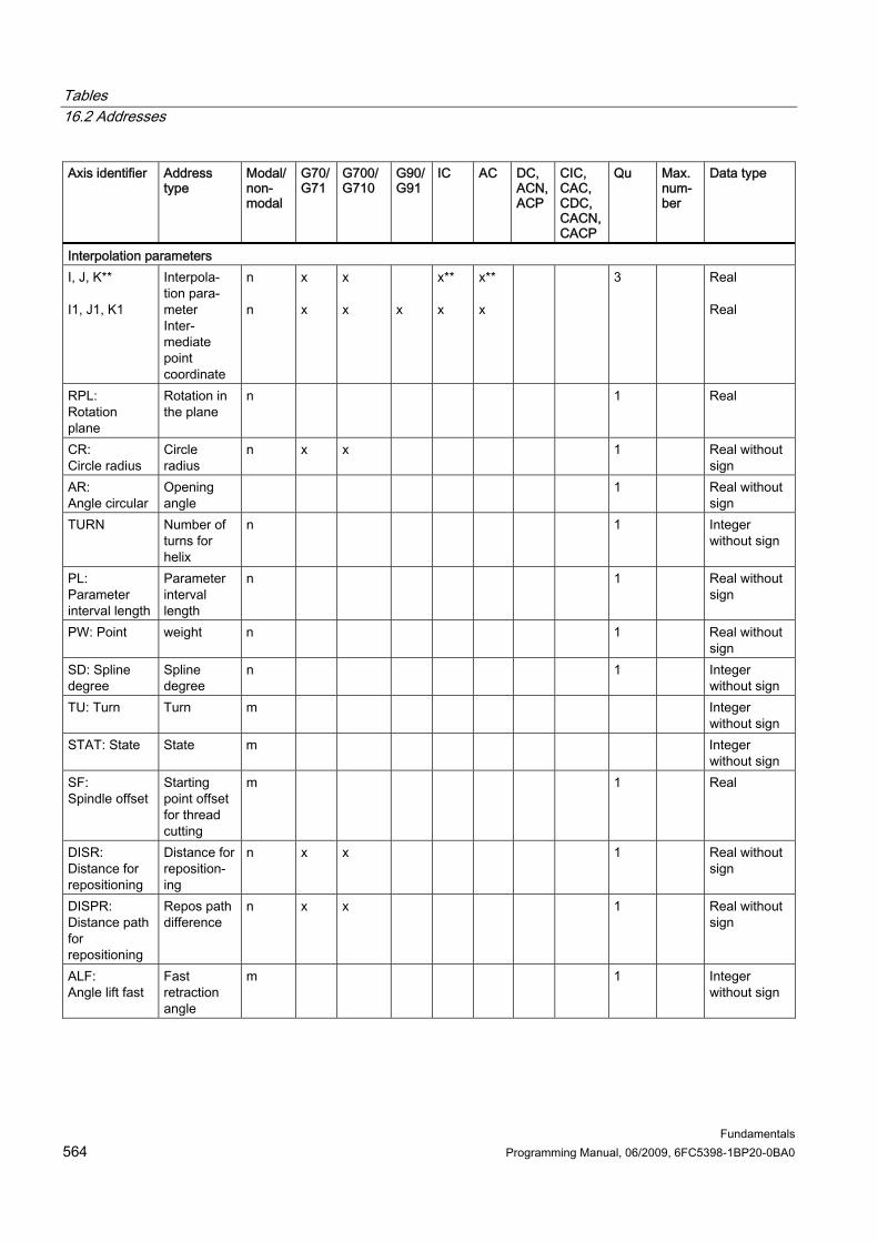
Tables 16.2 Addresses
Fundamentals 564 Programming Manual, 06/2009, 6FC5398-1BP20-0BA0
Axis identifier Address type
Modal/non-modal
G70/G71
G700/G710
G90/G91
IC AC DC, ACN, ACP
CIC, CAC, CDC, CACN, CACP
Qu Max. num-ber
Data type
Interpolation parameters I, J, K** I1, J1, K1
Interpola-tion para-meter Inter-mediate point coordinate
n n
x x
x x
x
x** x
x** x
3 Real Real
RPL: Rotation plane
Rotation in the plane
n 1 Real
CR: Circle radius
Circle radius
n x x 1 Real without sign
AR: Angle circular
Opening angle
1 Real without sign
TURN Number of turns for helix
n 1 Integer without sign
PL: Parameter interval length
Parameter interval length
n 1 Real without sign
PW: Point weight n 1 Real without sign
SD: Spline degree
Spline degree
n 1 Integer without sign
TU: Turn Turn m Integer without sign
STAT: State State m Integer without sign
SF: Spindle offset
Starting point offset for thread cutting
m 1 Real
DISR: Distance for repositioning
Distance for reposition-ing
n x x 1 Real without sign
DISPR: Distance path for repositioning
Repos path difference
n x x 1 Real without sign
ALF: Angle lift fast
Fast retraction angle
m 1 Integer without sign

Tables 16.2 Addresses
Fundamentals Programming Manual, 06/2009, 6FC5398-1BP20-0BA0 565
Axis identifier Address type
Modal/non-modal
G70/G71
G700/G710
G90/G91
IC AC DC, ACN, ACP
CIC, CAC, CDC, CACN, CACP
Qu Max. num-ber
Data type
DILF: Distance lift fast
Fast retraction length
m x x 1 Real
FP Fixed point: Number of fixed point to approach
n 1 Integer without sign
RNDM: Round modal
Modal rounding
m x x 1 Real without sign
RND: Round
Non-modal rounding
n x x 1 Real without sign
CHF: Chamfer
Chamfer non-modal
n x x 1 Real without sign
CHR: Chamfer
Chamfer in initial direction of motion
n x x 1 Real without sign
ANG: Angle Contour angle
n 1 Real
ISD: Insertion depth
Insertion depth
m x x 1 Real
DISC: Distance
Transition circle overshoot tool offset
m x x 1 Real without sign
OFFN Offset contour - normal
m x x 1 Real
DITS Thread run-in path
m x x 1 Real
DITE Thread run-out path
m x x 1 Real
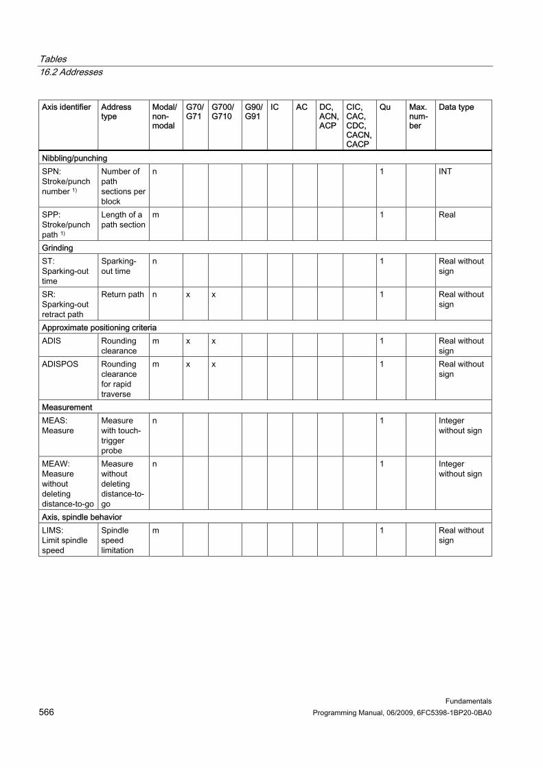
Tables 16.2 Addresses
Fundamentals 566 Programming Manual, 06/2009, 6FC5398-1BP20-0BA0
Axis identifier Address type
Modal/non-modal
G70/G71
G700/G710
G90/G91
IC AC DC, ACN, ACP
CIC, CAC, CDC, CACN, CACP
Qu Max. num-ber
Data type
Nibbling/punching SPN: Stroke/punch number 1)
Number of path sections per block
n 1 INT
SPP: Stroke/punch path 1)
Length of a path section
m 1 Real
Grinding ST: Sparking-out time
Sparking-out time
n 1 Real without sign
SR: Sparking-out retract path
Return path n x x 1 Real without sign
Approximate positioning criteria ADIS Rounding
clearance m x x 1 Real without
sign ADISPOS Rounding
clearance for rapid traverse
m x x 1 Real without sign
Measurement MEAS: Measure
Measure with touch-trigger probe
n 1 Integer without sign
MEAW: Measure without deleting distance-to-go
Measure without deleting distance-to-go
n 1 Integer without sign
Axis, spindle behavior LIMS: Limit spindle speed
Spindle speed limitation
m 1 Real without sign
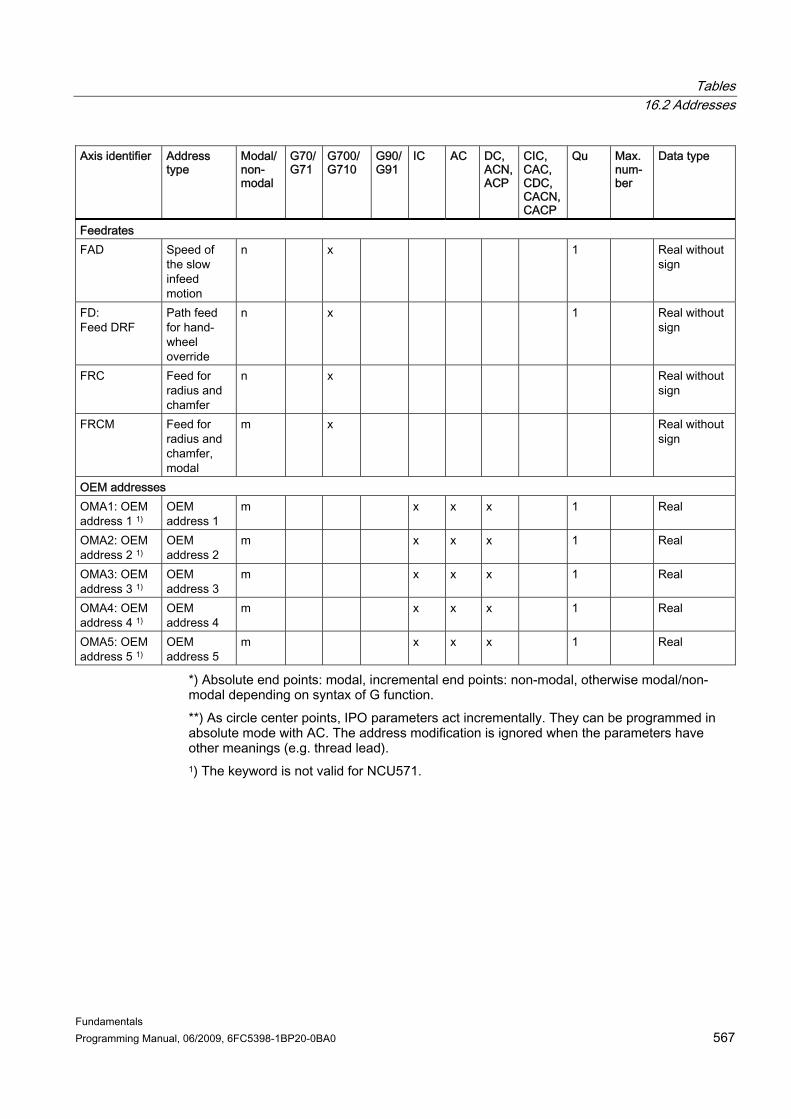
Tables 16.2 Addresses
Fundamentals Programming Manual, 06/2009, 6FC5398-1BP20-0BA0 567
Axis identifier Address type
Modal/non-modal
G70/G71
G700/G710
G90/G91
IC AC DC, ACN, ACP
CIC, CAC, CDC, CACN, CACP
Qu Max. num-ber
Data type
Feedrates FAD
Speed of the slow infeed motion
n x 1 Real without sign
FD: Feed DRF
Path feed for hand-wheel override
n x 1 Real without sign
FRC Feed for radius and chamfer
n x Real without sign
FRCM Feed for radius and chamfer, modal
m x Real without sign
OEM addresses OMA1: OEM address 1 1)
OEM address 1
m x x x 1 Real
OMA2: OEM address 2 1)
OEM address 2
m x x x 1 Real
OMA3: OEM address 3 1)
OEM address 3
m x x x 1 Real
OMA4: OEM address 4 1)
OEM address 4
m x x x 1 Real
OMA5: OEM address 5 1)
OEM address 5
m x x x 1 Real
*) Absolute end points: modal, incremental end points: non-modal, otherwise modal/non-modal depending on syntax of G function. **) As circle center points, IPO parameters act incrementally. They can be programmed in absolute mode with AC. The address modification is ignored when the parameters have other meanings (e.g. thread lead). 1) The keyword is not valid for NCU571.

Tables 16.3 G function groups
Fundamentals 568 Programming Manual, 06/2009, 6FC5398-1BP20-0BA0
16.3 16.3 G function groups The G functions are divided into function groups. Only one G function of a group can be programmed in a block. A G function can be either modal (until it is canceled by another function of the same group) or only effective for the block in which it is programmed (non-modal) Key: 1) Internal number (e.g. for PLC interface)
Configurability of the G function as a delete setting for the function group on power up, reset or end of part program with MD20150 $MC_GCODE_RESET_VALUES: + Configurable
2)
- Not configurable Effectiveness of the G function: m modal
3)
n non-modal Default setting If no function from the group is programmed with modal G functions, the default setting, which can be changed in the machine data (MD20150 $MN_$MC_GCODE_RESET_VALUES), applies: SAG Default setting Siemens AG
4)
MM Default setting Machine Manufacturer (see machine manufacturer's specifications)
5) The G function is not valid for NCU571.
Group 1: Modally valid motion commands
STD 4) G function No. 1) Meaning MD20150 2) W 3) SAG MM
G0 1. Rapid traverse + m G1 2. Linear interpolation (linear interpolation) + m x G2 3. Circular interpolation clockwise + m G3 4. Circular interpolation counterclockwise + m CIP 5. Circular interpolation through intermediate point + m ASPLINE 6. Akima spline + m BSPLINE 7. B-spline + m CSPLINE 8. Cubic spline + m POLY 9. Polynomial interpolation + m G33 10. Thread cutting with constant lead + m G331 11. Tapping + m G332 12. Retraction (tapping) + m

Tables 16.3 G function groups
Fundamentals Programming Manual, 06/2009, 6FC5398-1BP20-0BA0 569
OEMIPO1 5) 13. Reserved + m OEMIPO2 5) 14. Reserved + m CT 15. Circle with tangential transition + m G34 16. Thread cutting with linear increasing lead + m G35 17. Thread cutting with linear decreasing lead + m INVCW 18. Involute interpolation clockwise + m INVCCW 19. Involute interpolation counter-clockwise + m If no function from the group is programmed with modal G functions, the default setting, which can be changed in the machine data (MD20150 $MN_$MC_GCODE_RESET_VALUES), applies:
Group 2: Non-modally valid motions, dwell time
STD 4) G function No. 1) Significance MD20150 2) W 3) SAG MM
G4 1. Dwell time preset - n G63 2. Tapping without synchronization - n G74 3. Reference point approach with synchronization - n G75 4. Fixed-point approach - n REPOSL 5. Linear repositioning - n REPOSQ 6. Repositioning in a quadrant - n REPOSH 7. Repositioning in semicircle - n REPOSA 8. Linear repositioning with all axes - n REPOSQA 9. Linear repositioning with all axes, geometry axes in
quadrant - n
REPOSHA 10. Repositioning with all axes; geometry axes in semicircle
- n
G147 11. Approach contour with straight line - n G247 12. Approach contour with quadrant - n G347 13. Approach contour with semicircle - n G148 14. Leave contour with straight line - n G248 15. Leave contour with quadrant - n G348 16. Leave contour with semicircle - n G5 17. Oblique plunge-cut grinding - n G7 18. Compensatory motion during oblique plunge-cut
grinding - n

Tables 16.3 G function groups
Fundamentals 570 Programming Manual, 06/2009, 6FC5398-1BP20-0BA0
Group 3: Programmable frame, working area limitation and pole programming STD 4) G function No. 1) Significance MD20150 2) W 3)
SAG MM TRANS 1. TRANSLATION: Programmable offset - n ROT 2. ROTATION: Programmable rotation - n SCALE 3. SCALE: Programmable scaling - n MIRROR 4. MIRROR: Programmable mirroring - n ATRANS 5. Additive TRANSLATION: Additive programmable
offset - n
AROT 6. Additive ROTATION: Programmable rotation - n ASCALE 7. Additive SCALE: Programmable scaling - n AMIRROR 8. Additive MIRROR: Programmable mirroring - n 9. Unassigned G25 10. Minimum working area limitation/spindle speed
limitation - n
G26 11. Maximum working area limitation/spindle speed limitation
- n
G110 12. Pole programming relative to the last programmed setpoint position
- n
G111 13. Polar programming relative to origin of current workpiece coordinate system
- n
G112 14. Pole programming relative to the last valid pole - n G58 15. Programmable offset, absolute axial substitution - n G59 16. Programmable offset, additive axial substitution - n ROTS 17. Rotation with solid angle - n AROTS 18. Additive rotation with solid angle - n
Group 4: FIFO
STD 4) G function No. 1) Significance MD20150 2) W 3) SAG MM
STARTFIFO 1. Start FIFO Execute and simultaneously fill preprocessing memory
+ m x
STOPFIFO 2. STOP FIFO, stop machining; fill preprocessing memory until STARTFIFO is detected, FIFO is full or end of program
+ m
FIFOCTRL 3. Activation of automatic preprocessing memory control + m

Tables 16.3 G function groups
Fundamentals Programming Manual, 06/2009, 6FC5398-1BP20-0BA0 571
Group 6: Plane selection STD 4) G function No. 1) Significance MD20150 2) W 3)
SAG MM G17 1. Plane selection 1st - 2nd geometry axis + m x G18 2. Plane selection 3rd - 1st geometry axis + m G19 3. Plane selection 2nd - 3rd geometry axis + m
Group 7: Tool radius compensation
STD 4) G function No. 1) Significance MD20150 2) W 3) SAG MM
G40 1. No tool radius compensation + m x G41 2. Tool radius compensation left of contour - m G42 3. Tool radius compensation right of contour - m
Group 8: Settable zero offset
STD 4) G function No. 1) Significance MD20150 2) W 3) SAG MM
G500 1. Deactivation of adjustable work offset (G54 to G57, G505 to G599)
+ m x
G54 2. 1st settable zero offset + m G55 3. 2nd adjustable work offset + m G56 4. 3rd adjustable work offset + m G57 5. 4th adjustable work offset + m G505 6. 5th adjustable work offset + m ... ... ... + m G599 100. 99th adjustable work offset + m Each of the G functions in this group is used to activate an adjustable user frame $P_UIFR[ ]. G54 corresponds to frame $P_UIFR[1], G505 corresponds to frame $P_UIFR[5]. The number of adjustable user frames and, therefore, the number of G functions in this group, can be parameterized using machine data MD28080 $MC_MM_NUM_USER_FRAMES.

Tables 16.3 G function groups
Fundamentals 572 Programming Manual, 06/2009, 6FC5398-1BP20-0BA0
Group 9: Frame suppression STD 4) G function No. 1) Significance MD20150 2) W 3)
SAG MM G53 1. Suppression of current frames:
Programmable frame including system frame for TOROT and TOFRAME and active adjustable frame (G54 to G57, G505 to G599).
- n
SUPA 2. As for G153 including suppression of system frames for actual-value setting, scratching, ext. work offset, PAROT including handwheel offsets (DRF), [external work offset], overlaid movement
- n
G153 3. As for G53 including suppression of all channel-specific and/or NCU-global basic frames
- n
Group 10: Exact stop - continuous-path mode
STD 4) G function No. 1) Significance MD20150 2) W 3) SAG MM
G60 1. Exact stop + m x G64 2. Continuous-path mode + m G641 3. Continuous-path mode with smoothing as per
distance criterion (= programmable rounding clearance)
+ m
G642 4. Continuous-path mode with smoothing within the defined tolerances
+ m
G643 5. Continuous-path mode with smoothing within the defined tolerances (block-internal)
+ m
G644 6. Continuous-path mode with smoothing with maximum possible dynamic response
+ m
G645 7. Continuous-path mode with smoothing and tangential block transitions within the defined tolerances
+ m
Group 11: Exact stop, non-modal
STD 4) G function No. 1) Significance MD20150 2) W 3) SAG MM
G9 1. Exact stop - n

Tables 16.3 G function groups
Fundamentals Programming Manual, 06/2009, 6FC5398-1BP20-0BA0 573
Group 12: Block change criteria at exact stop (G60/G9) STD 4) G function No. 1) Significance MD20150 2) W 3)
SAG MM G601 1. Block change at exact stop fine + m x G602 2. Block change at exact stop coarse + m G603 3. Block change at IPO - end of block + m
Group 13: Workpiece measuring inch/metric
STD 4) G function No. 1) Significance MD20150 2) W 3) SAG MM
G70 1. Input system inches (length) + m G71 2. Input system metric mm (lengths) + m x G700 3. Input system inch, inch/min
(lengths + velocity + system variable) + m
G710 4. Input system metric mm, mm/min (lengths + velocity + system variable)
+ m
Group 14: Workpiece measuring absolute/incremental
STD 4) G function No. 1) Significance MD20150 2) W 3) SAG MM
G90 1. Absolute dimension + m x G91 2. Incremental dimension input + m
Group 15: Feed type
STD 4) G function No. 1) Significance MD20150 2) W 3) SAG MM
G93 1. Inverse-time feedrate 1/rpm + m G94 2. Linear feedrate in mm/min, inch/min + m x G95 3. Revolutional feedrate in mm/rev, inch/rev + m G96 4. Constant cutting rate and type of feedrate as for G95
ON + m
G97 5. Constant cutting rate and type of feedrate as for G95 OFF
+ m
G931 6. Feedrate specification by means of traversing time, deactivate constant path velocity
+ m
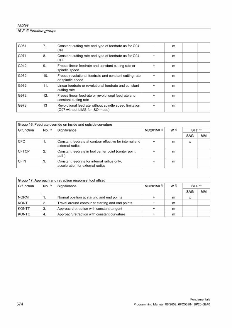
Tables 16.3 G function groups
Fundamentals 574 Programming Manual, 06/2009, 6FC5398-1BP20-0BA0
G961 7. Constant cutting rate and type of feedrate as for G94 ON
+ m
G971 8. Constant cutting rate and type of feedrate as for G94 OFF
+ m
G942 9. Freeze linear feedrate and constant cutting rate or spindle speed
+ m
G952 10. Freeze revolutional feedrate and constant cutting rate or spindle speed
+ m
G962 11. Linear feedrate or revolutional feedrate and constant cutting rate
+ m
G972 12. Freeze linear feedrate or revolutional feedrate and constant cutting rate
+ m
G973 13 Revolutional feedrate without spindle speed limitation (G97 without LIMS for ISO mode)
+ m
Group 16: Feedrate override on inside and outside curvature
STD 4) G function No. 1) Significance MD20150 2) W 3) SAG MM
CFC 1. Constant feedrate at contour effective for internal and external radius
+ m x
CFTCP 2. Constant feedrate in tool center point (center point path)
+ m
CFIN 3. Constant feedrate for internal radius only, acceleration for external radius
+ m
Group 17: Approach and retraction response, tool offset
STD 4) G function No. 1) Significance MD20150 2) W 3) SAG MM
NORM 1. Normal position at starting and end points + m x KONT 2. Travel around contour at starting and end points + m KONTT 3. Approach/retraction with constant tangent + m KONTC 4. Approach/retraction with constant curvature + m

Tables 16.3 G function groups
Fundamentals Programming Manual, 06/2009, 6FC5398-1BP20-0BA0 575
Group 18: Corner behavior, tool offset STD 4) G function No. 1) Significance MD20150 2) W 3)
SAG MM G450 1. Transition circle
(tool travels around workpiece corners on a circular path)
+ m x
G451 2. Intersection of equidistant paths (tool backs off from the workpiece corner)
+ m
Group 19: Curve transition at beginning of spline
STD 4) G function No. 1) Significance MD20150 2) W 3) SAG MM
BNAT 1. Natural transition to first spline block + m x BTAN 2. Tangential transition to first spline block + m BAUTO 3. Definition of the first spline section by means of the
next 3 points + m
Group 20: Curve transition at end of spline
STD 4) G function No. 1) Significance MD20150 2) W 3) SAG MM
ENAT 1. Natural transition to next traversing block + m x ETAN 2. Tangential transition to next traversing block + m EAUTO 3. Definition of the last spline section by means of the
last 3 points + m
Group 21: Acceleration profile
STD 4) G function No. 1) Significance MD20150 2) W 3) SAG MM
BRISK 1. Fast non-smoothed path acceleration + m x SOFT 2. Soft smoothed path acceleration + m DRIVE 3. Velocity-dependent path acceleration + m

Tables 16.3 G function groups
Fundamentals 576 Programming Manual, 06/2009, 6FC5398-1BP20-0BA0
Group 22: Tool offset type STD 4) G function No. 1) Significance MD20150 2) W 3)
SAG MM CUT2D 1. 2½D tool offset determined by G17-G19 + m x CUT2DF 2. 2½D tool offset determined by frame
The tool offset is effective in relation to the current frame (inclined plane).
+ m
CUT3DC 5) 3. 3D tool offset circumferential milling + m CUT3DF 5) 4. 3D tool offset face milling with non-constant tool
orientation + m
CUT3DFS 5) 5. 3D tool offset face milling with constant tool orientation independent of active frame
+ m
CUT3DFF 5) 6. 3D tool offset face milling with fixed tool orientation dependent on active frame
+ m
CUT3DCC 5) 7. 3D tool offset circumferential milling with limitation surfaces
+ m
CUT3DCCD 5) 8. 3D tool offset circumferential milling with limitation surfaces and differential tool
+ m
Group 23: Collision monitoring at inside contours
STD 4) G function No. 1) Significance MD20150 2) W 3) SAG MM
CDOF 1. Collision detection OFF + m x CDON 2. Collision detection ON + m CDOF2 3. Collision detection OFF
(currently only for CUT3DC) + m
Group 24: Feedforward control
STD 4) G function No. 1) Significance MD20150 2) W 3) SAG MM
FFWOF 1. Feedforward control OFF + m x FFWON 2. Feedforward control ON + m
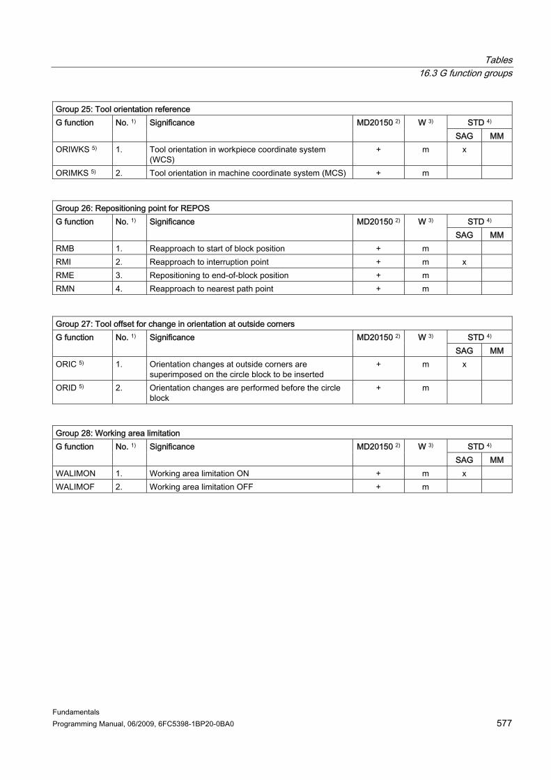
Tables 16.3 G function groups
Fundamentals Programming Manual, 06/2009, 6FC5398-1BP20-0BA0 577
Group 25: Tool orientation reference STD 4) G function No. 1) Significance MD20150 2) W 3)
SAG MM ORIWKS 5) 1. Tool orientation in workpiece coordinate system
(WCS) + m x
ORIMKS 5) 2. Tool orientation in machine coordinate system (MCS) + m
Group 26: Repositioning point for REPOS
STD 4) G function No. 1) Significance MD20150 2) W 3) SAG MM
RMB 1. Reapproach to start of block position + m RMI 2. Reapproach to interruption point + m x RME 3. Repositioning to end-of-block position + m RMN 4. Reapproach to nearest path point + m
Group 27: Tool offset for change in orientation at outside corners
STD 4) G function No. 1) Significance MD20150 2) W 3) SAG MM
ORIC 5) 1. Orientation changes at outside corners are superimposed on the circle block to be inserted
+ m x
ORID 5) 2. Orientation changes are performed before the circle block
+ m
Group 28: Working area limitation
STD 4) G function No. 1) Significance MD20150 2) W 3) SAG MM
WALIMON 1. Working area limitation ON + m x WALIMOF 2. Working area limitation OFF + m
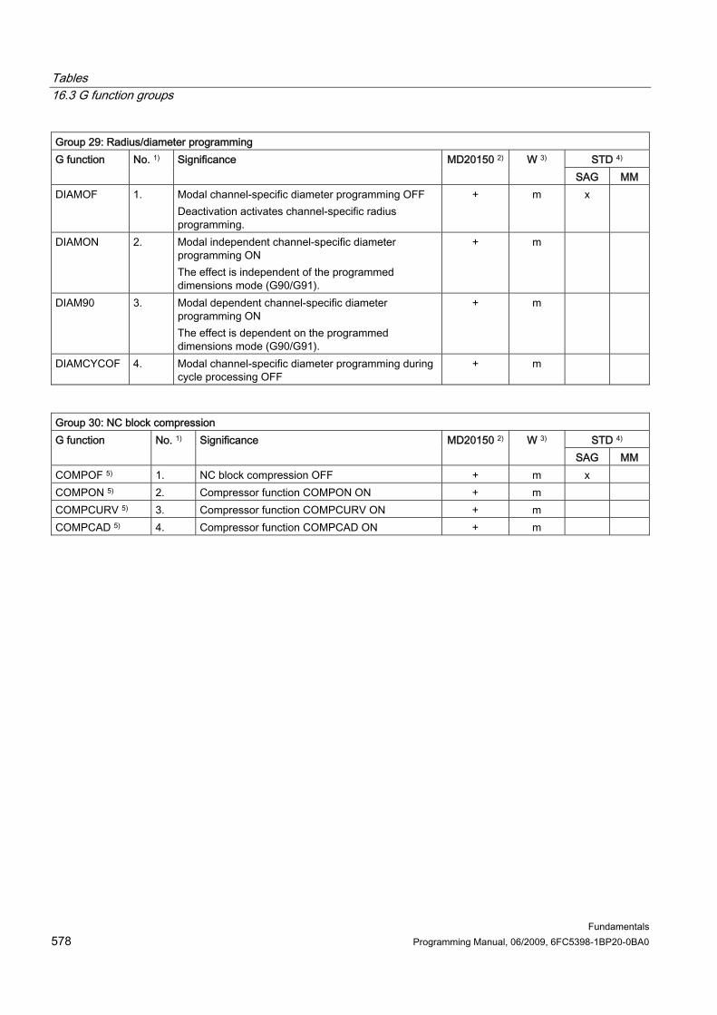
Tables 16.3 G function groups
Fundamentals 578 Programming Manual, 06/2009, 6FC5398-1BP20-0BA0
Group 29: Radius/diameter programming STD 4) G function No. 1) Significance MD20150 2) W 3)
SAG MM DIAMOF 1. Modal channel-specific diameter programming OFF
Deactivation activates channel-specific radius programming.
+ m x
DIAMON 2. Modal independent channel-specific diameter programming ON The effect is independent of the programmed dimensions mode (G90/G91).
+ m
DIAM90 3. Modal dependent channel-specific diameter programming ON The effect is dependent on the programmed dimensions mode (G90/G91).
+ m
DIAMCYCOF 4. Modal channel-specific diameter programming during cycle processing OFF
+ m
Group 30: NC block compression
STD 4) G function No. 1) Significance MD20150 2) W 3) SAG MM
COMPOF 5) 1. NC block compression OFF + m x COMPON 5) 2. Compressor function COMPON ON + m COMPCURV 5) 3. Compressor function COMPCURV ON + m COMPCAD 5) 4. Compressor function COMPCAD ON + m

Tables 16.3 G function groups
Fundamentals Programming Manual, 06/2009, 6FC5398-1BP20-0BA0 579
Group 31: OEM G function group STD 4) G function No. 1) Significance MD20150 2) W 3)
SAG MM G810 5) 1. OEM G function - m G811 5) 2. OEM G function - m G812 5) 3. OEM G function - m G813 5) 4. OEM G function - m G814 5) 5. OEM G function - m G815 5) 6. OEM G function - m G816 5) 7. OEM G function - m G817 5) 8. OEM G function - m G818 5) 9. OEM G function - m G819 5) 10. OEM G function - m Two G function groups are reserved for the OEM user. This enables the OEM to program functions that can be customized.
Group 32: OEM G function group
STD 4) G function No. 1) Significance MD20150 2) W 3) SAG MM
G820 5) 1. OEM - G function - m G821 5) 2. OEM G function - m G822 5) 3. OEM G function - m G823 5) 4. OEM G function - m G824 5) 5. OEM G function - m G825 5) 6. OEM G function - m G826 5) 7. OEM G function - m G827 5) 8. OEM G function - m G828 5) 9. OEM G function - m G829 5) 10. OEM G function - m Two G function groups are reserved for the OEM user. This enables the OEM to program functions that can be customized.
Group 33: Settable fine tool offset
STD 4) G function No. 1) Significance MD20150 2) W 3) SAG MM
FTOCOF 5) 1. Online fine tool offset OFF + m x FTOCON 5) 2. Online fine tool offset ON - m
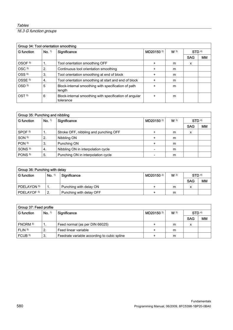
Tables 16.3 G function groups
Fundamentals 580 Programming Manual, 06/2009, 6FC5398-1BP20-0BA0
Group 34: Tool orientation smoothing STD 4) G function No. 1) Significance MD20150 2) W 3)
SAG MM OSOF 5) 1. Tool orientation smoothing OFF + m x OSC 5) 2. Continuous tool orientation smoothing + m OSS 5) 3. Tool orientation smoothing at end of block + m OSSE 5) 4. Tool orientation smoothing at start and end of block + m OSD 5) 5 Block-internal smoothing with specification of path
length + m
OST 5) 6 Block-internal smoothing with specification of angular tolerance
+ m
Group 35: Punching and nibbling
STD 4) G function No. 1) Significance MD20150 2) W 3) SAG MM
SPOF 5) 1. Stroke OFF, nibbling and punching OFF + m x SON 5) 2. Nibbling ON + m PON 5) 3. Punching ON + m SONS 5) 4. Nibbling ON in interpolation cycle - m PONS 5) 5. Punching ON in interpolation cycle - m
Group 36: Punching with delay
STD 4) G function No. 1) Significance MD20150 2) W 3) SAG MM
PDELAYON 5) 1. Punching with delay ON + m x PDELAYOF 5) 2. Punching with delay OFF + m
Group 37: Feed profile
STD 4) G function No. 1) Significance MD20150 2) W 3) SAG MM
FNORM 5) 1. Feed normal (as per DIN 66025) + m x FLIN 5) 2. Feed linear variable + m FCUB 5) 3. Feedrate variable according to cubic spline + m
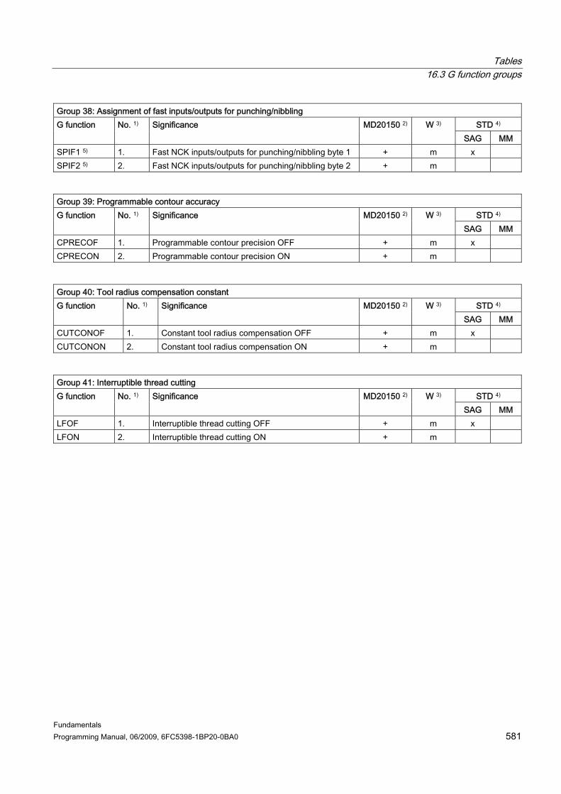
Tables 16.3 G function groups
Fundamentals Programming Manual, 06/2009, 6FC5398-1BP20-0BA0 581
Group 38: Assignment of fast inputs/outputs for punching/nibbling STD 4) G function No. 1) Significance MD20150 2) W 3)
SAG MM SPIF1 5) 1. Fast NCK inputs/outputs for punching/nibbling byte 1 + m x SPIF2 5) 2. Fast NCK inputs/outputs for punching/nibbling byte 2 + m
Group 39: Programmable contour accuracy
STD 4) G function No. 1) Significance MD20150 2) W 3) SAG MM
CPRECOF 1. Programmable contour precision OFF + m x CPRECON 2. Programmable contour precision ON + m
Group 40: Tool radius compensation constant
STD 4) G function No. 1) Significance MD20150 2) W 3) SAG MM
CUTCONOF 1. Constant tool radius compensation OFF + m x CUTCONON 2. Constant tool radius compensation ON + m
Group 41: Interruptible thread cutting
STD 4) G function No. 1) Significance MD20150 2) W 3) SAG MM
LFOF 1. Interruptible thread cutting OFF + m x LFON 2. Interruptible thread cutting ON + m
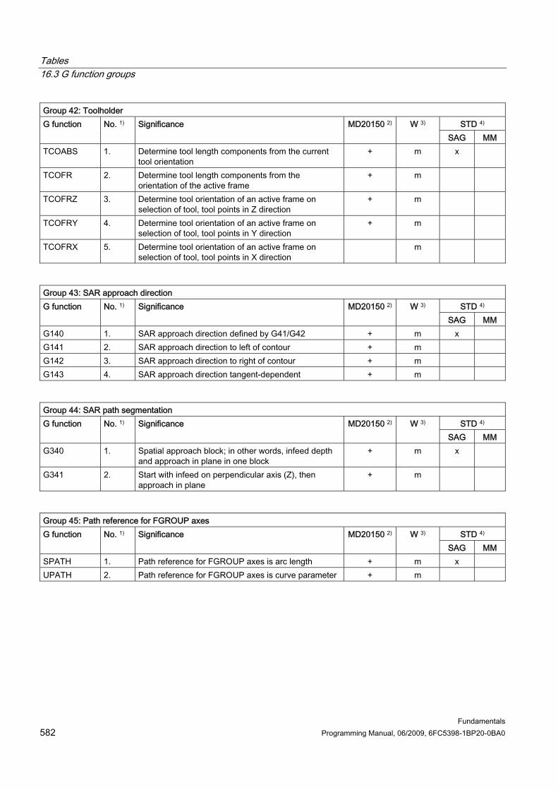
Tables 16.3 G function groups
Fundamentals 582 Programming Manual, 06/2009, 6FC5398-1BP20-0BA0
Group 42: Toolholder STD 4) G function No. 1) Significance MD20150 2) W 3)
SAG MM TCOABS 1. Determine tool length components from the current
tool orientation + m x
TCOFR 2. Determine tool length components from the orientation of the active frame
+ m
TCOFRZ 3. Determine tool orientation of an active frame on selection of tool, tool points in Z direction
+ m
TCOFRY 4. Determine tool orientation of an active frame on selection of tool, tool points in Y direction
+ m
TCOFRX 5. Determine tool orientation of an active frame on selection of tool, tool points in X direction
m
Group 43: SAR approach direction
STD 4) G function No. 1) Significance MD20150 2) W 3) SAG MM
G140 1. SAR approach direction defined by G41/G42 + m x G141 2. SAR approach direction to left of contour + m G142 3. SAR approach direction to right of contour + m G143 4. SAR approach direction tangent-dependent + m
Group 44: SAR path segmentation
STD 4) G function No. 1) Significance MD20150 2) W 3) SAG MM
G340 1. Spatial approach block; in other words, infeed depth and approach in plane in one block
+ m x
G341 2. Start with infeed on perpendicular axis (Z), then approach in plane
+ m
Group 45: Path reference for FGROUP axes
STD 4) G function No. 1) Significance MD20150 2) W 3) SAG MM
SPATH 1. Path reference for FGROUP axes is arc length + m x UPATH 2. Path reference for FGROUP axes is curve parameter + m

Tables 16.3 G function groups
Fundamentals Programming Manual, 06/2009, 6FC5398-1BP20-0BA0 583
Group 46: Plane selection for fast retraction STD 4) G function No. 1) Significance MD20150 2) W 3)
SAG MM LFTXT 1. The plane is determined from the path tangent and
the current tool orientation + m x
LFWP 2. The plane is determined by the current working plane (G17/G18/G19)
+ m
LFPOS 3. Axial retraction to a position + m
Group 47: Mode switchover for external NC code
STD 4) G function No. 1) Significance MD20150 2) W 3) SAG MM
G290 1. Activate SINUMERIK language mode + m x G291 2. Activate ISO language mode + m
Group 48: Approach and retraction response with tool radius compensation
STD 4) G function No. 1) Significance MD20150 2) W 3) SAG MM
G460 1. Collision detection for approach and retraction block ON
+ m x
G461 2. Extend border block with arc if no intersection in TRC block
+ m
G462 3. Extend border block with straight line if no intersection in TRC block
+ m
Group 49: Point-to-point motion
STD 4) G function No. 1) Significance MD20150 2) W 3) SAG MM
CP 1. Path motion + m x PTP 2. Point-to-point motion (synchronized axis motion) + m PTPG0 3. Point-to-point motion only with G0, otherwise path
motion CP + m

Tables 16.3 G function groups
Fundamentals 584 Programming Manual, 06/2009, 6FC5398-1BP20-0BA0
Group 50: Orientation programming STD 4) G function No. 1) Significance MD20150 2) W 3)
SAG MM ORIEULER 1. Orientation angle via Euler angle + m x ORIRPY 2. Orientation angle via RPY angle (rotation sequence
XYZ) + m
ORIVIRT1 3. Orientation angle via virtual orientation axes (definition 1)
+ m
ORIVIRT2 4. Orientation angle via virtual orientation axes (definition 2)
+ m
ORIAXPOS 5. Orientation angle via virtual orientation axes with rotary axis positions
+ m
ORIRPY2 6. Orientation angle via RPY angle (rotation sequence ZYX)
+ m
Group 51: Interpolation type for orientation programming
STD 4) G function No. 1) Significance MD20150 2) W 3) SAG MM
ORIVECT 1. Large-radius circular interpolation (identical to ORIPLANE)
+ m x
ORIAXES 2. Linear interpolation of machine axes or orientation axes
+ m
ORIPATH 3. Tool orientation trajectory referred to path + m ORIPLANE 4. Interpolation in plane (identical to ORIVECT) + m ORICONCW 5. Interpolation on a peripheral surface of the cone
in clockwise direction + m
ORICONCCW 6. Interpolation on the peripheral surface of a taper in the counter-clockwise direction
+ m
ORICONIO 7. Interpolation on a conical peripheral surface with intermediate orientation setting
+ m
ORICONTO 8. Interpolation on a peripheral surface of the cone with tangential transition
+ m
ORICURVE 9. Interpolation with additional space curve for orientation
+ m
ORIPATHS 10. Tool orientation in relation to path, blips in the orientation characteristic are smoothed
+ m

Tables 16.3 G function groups
Fundamentals Programming Manual, 06/2009, 6FC5398-1BP20-0BA0 585
Group 52: Frame rotation in relation to workpiece STD 4) G function No. 1) Significance MD20150 2) W 3)
SAG MM PAROTOF 1. Frame rotation in relation to workpiece OFF + m x PAROT 2. Frame rotation in relation to workpiece ON
The workpiece coordinate system is aligned on the workpiece.
+ m
Group 53: Frame rotation in relation to tool
STD 4) G function No. 1) Significance MD20150 2) W 3) SAG MM
TOROTOF 1. Frame rotation in relation to tool OFF + m x TOROT 2. Align the Z axis of the workpiece coordinate system
parallel to the workpiece orientation by rotating the frame
+ m
TOROTZ 3. As TOROT + m TOROTY 4. Align the Y axis of the workpiece coordinate system
parallel to the workpiece orientation by rotating the frame
+ m
TOROTX 5. Align the X axis of the workpiece coordinate system parallel to the workpiece orientation by rotating the frame
+ m
TOFRAME 6. Align the Z axis of the workpiece coordinate system parallel to the workpiece orientation by rotating the frame
+ m
TOFRAMEZ 7. As TOFRAME + m TOFRAMEY 8. Align the Y axis of the workpiece coordinate system
parallel to the workpiece orientation by rotating the frame
+ m
TOFRAMEX 9. Align the X axis of the workpiece coordinate system parallel to the workpiece orientation by rotating the frame
+ m
Group 54: Vector rotation for polynomial programming
STD 4) G function No. 1) Significance MD20150 2) W 3) SAG MM
ORIROTA 1. Vector rotation absolute + m x ORIROTR 2. Vector rotation relative + m ORIROTT 3. Vector rotation tangential + m ORIROTC 4. Tangential rotational vector in relation to path tangent + m

Tables 16.3 G function groups
Fundamentals 586 Programming Manual, 06/2009, 6FC5398-1BP20-0BA0
Group 55: Rapid traverse with/without linear interpolation STD 4) G function No. 1) Significance MD20150 2) W 3)
SAG MM RTLION 1. Rapid traverse motion with linear interpolation ON + m x RTLIOF 2. Rapid traverse motion with linear interpolation OFF
Rapid traverse motion is achieved with single-axis interpolation.
+ m
Group 56: Inclusion of tool wear
STD 4) G function No. 1) Significance MD20150 2) W 3) SAG MM
TOWSTD 1. Initial setting value for offsets in tool length + m x TOWMCS 2. Wear values in the machine coordinate system + m TOWWCS 3. Wear values in the workpiece coordinate system + m TOWBCS 4. Wear values in the basic coordinate system (BCS) + m TOWTCS 5. Wear values in the tool coordinate system (toolholder
ref. point T at the tool holder) + m
TOWKCS 6. Wear values in the coordinate system of the tool head for kinetic transformation (differs from machine coordinate system through tool rotation)
+ m
Group 57: Corner deceleration
STD 4) G function No. 1) Significance MD20150 2) W 3) SAG MM
FENDNORM 1. Corner deceleration OFF + m x G62 2. Corner deceleration at inside corners when tool
radius compensation is active (G41/G42) + m
G621 3. Corner deceleration at all corners + m
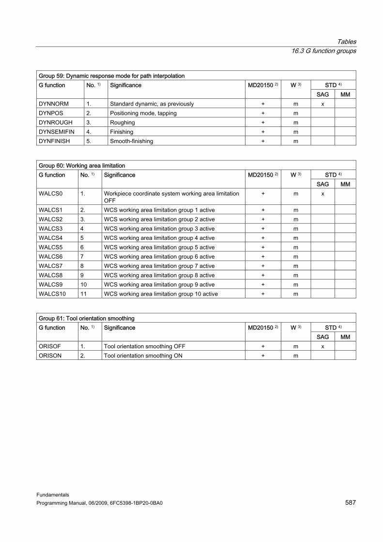
Tables 16.3 G function groups
Fundamentals Programming Manual, 06/2009, 6FC5398-1BP20-0BA0 587
Group 59: Dynamic response mode for path interpolation STD 4) G function No. 1) Significance MD20150 2) W 3)
SAG MM DYNNORM 1. Standard dynamic, as previously + m x DYNPOS 2. Positioning mode, tapping + m DYNROUGH 3. Roughing + m DYNSEMIFIN 4. Finishing + m DYNFINISH 5. Smooth-finishing + m
Group 60: Working area limitation
STD 4) G function No. 1) Significance MD20150 2) W 3) SAG MM
WALCS0 1. Workpiece coordinate system working area limitation OFF
+ m x
WALCS1 2. WCS working area limitation group 1 active + m WALCS2 3. WCS working area limitation group 2 active + m WALCS3 4 WCS working area limitation group 3 active + m WALCS4 5 WCS working area limitation group 4 active + m WALCS5 6 WCS working area limitation group 5 active + m WALCS6 7 WCS working area limitation group 6 active + m WALCS7 8 WCS working area limitation group 7 active + m WALCS8 9 WCS working area limitation group 8 active + m WALCS9 10 WCS working area limitation group 9 active + m WALCS10 11 WCS working area limitation group 10 active + m
Group 61: Tool orientation smoothing
STD 4) G function No. 1) Significance MD20150 2) W 3) SAG MM
ORISOF 1. Tool orientation smoothing OFF + m x ORISON 2. Tool orientation smoothing ON + m

Tables 16.4 Predefined subroutine calls
Fundamentals 588 Programming Manual, 06/2009, 6FC5398-1BP20-0BA0
16.4 16.4 Predefined subroutine calls 1. Coordinate system Keyword/ subroutine identifier
1st parameter 2nd parameter 3rd-15th parameter
4th-16th parameter
Explanation
PRESETON AXIS*: Axis identifier Machine axis
REAL: Preset offset G700/G7100 context
3rd-15th parameter as 1 ...
4th-16th parameter as2 ...
Sets the actual value for programmed axes. One axis identifier is programmed at a time, with its respective value in the next parameter. PRESETON can be used to program preset offsets for up to 8 axes.
DRFOF Deletes the DRF offset for all axes assigned to the channel.
*) As a general rule, geometry or special axis identifiers can also be used instead of the machine axis identifier, as long as the reference is unambiguous.
2. Axis groupings Keyword/ subroutine identifier
1st-8th parameter
Explanation
FGROUP Channel axis identifiers
Variable F value reference: defines the axes to which the path feed refers. Maximum axis number: 8 The default setting for the F value reference is activated with FGROUP ( ) without parameters.
1st-8th parameter
2nd-9th parameter
Explanation
SPLINEPATH INT: Spline group (must be 1)
AXIS: Geometry or special axis identifier
Definition of the spline group Maximum number of axes: 8
BRISKA AXIS Switch on brisk axis acceleration for the programmed axes SOFTA AXIS Switch on jerk limited axis acceleration for programmed axes JERKA AXIS The acceleration behavior set in machine data
$MA_AX_JERK_ENABLE is active for the programmed axes.

Tables 16.4 Predefined subroutine calls
Fundamentals Programming Manual, 06/2009, 6FC5398-1BP20-0BA0 589
3. Coupled motion Keyword/ subroutine identifier
1st parameter 2nd param.
3rd param.
4th param.
5th param.
6th param.
Explanation
TANG AXIS: Axis name following axis
AXIS: Leading axis 1
AXIS: Leading axis 2
REAL: Coupling factor
CHAR: Option: "B": follow-up in basic coord. system "W": follow-up in work-piece coord. system
CHAR Optimization: "S" default "P" autom. with rounding travel, angle tolerance
Preparatory statement for the definition of a tangential follow-up: The tangent for the follow-up is determined by the two master axes specified. The coupling factor specifies the relationship between a change in the angle of tangent and the following axis. It is usually 1. Optimization: See PGA
TANGON AXIS: Axis name following axis
REAL: Offset Angle
REAL: Round-ing travel
REAL: Angle toler-ance
Tangential follow-up mode ON: par. 3, 4 with TANG Par. 6 = "P"
TANGOF AXIS: Axis name following axis
Tangential follow-up mode OFF
TLIFT AXIS: Following axis
REAL: Lift-off path
REAL: Factor
Tangential lift: tangential follow-up mode, stop at contour end rotary axis lift-off possible
TRAILON AXIS: Following axis
AXIS: Leading axis
REAL: Coupling factor
Trailing ON: Asynchronous coupled motion ON
TRAILOF AXIS: Following axis
AXIS: Leading axis
Trailing OFF: Asynchronous coupled motion OFF

Tables 16.4 Predefined subroutine calls
Fundamentals 590 Programming Manual, 06/2009, 6FC5398-1BP20-0BA0
6. Revolutional feedrate Keyword/ subroutine identifier
1st parameter 2nd parameter Explanation
FPRAON AXIS: Axis, for which revolutional feedrate is activated
AXIS: Axis/spindle, from which revolutional feedrate is derived. If no axis has been programmed, the revolutional feedrate is derived from the master spindle.
Feedrate per revolution axial ON: Axial revolutional feedrate ON.
FPRAOF AXIS: Axis for which revolutional feedrate is deactivated
Feedrate per revolution axial OFF: Axial revolutional feedrate OFF. The revolutional feedrate can be deactivated for several axes at once. You can program as many axes as are permitted in a block.
FPR AXIS: Axis/spindle, from which revolutional feedrate is derived. If no axis has been programmed, the revolutional feedrate is derived from the master spindle.
Feedrate per revolution: Selection of a rotary axis or spindle from which the revolutional feedrate of the path is derived if G95 is programmed. If no axis/spindle has been programmed, the revolutional feedrate is derived from the master spindle. The setting made with FPR is modal.
It is also possible to program a spindle instead of an axis: FPR(S1) or FPR(SPI(1))
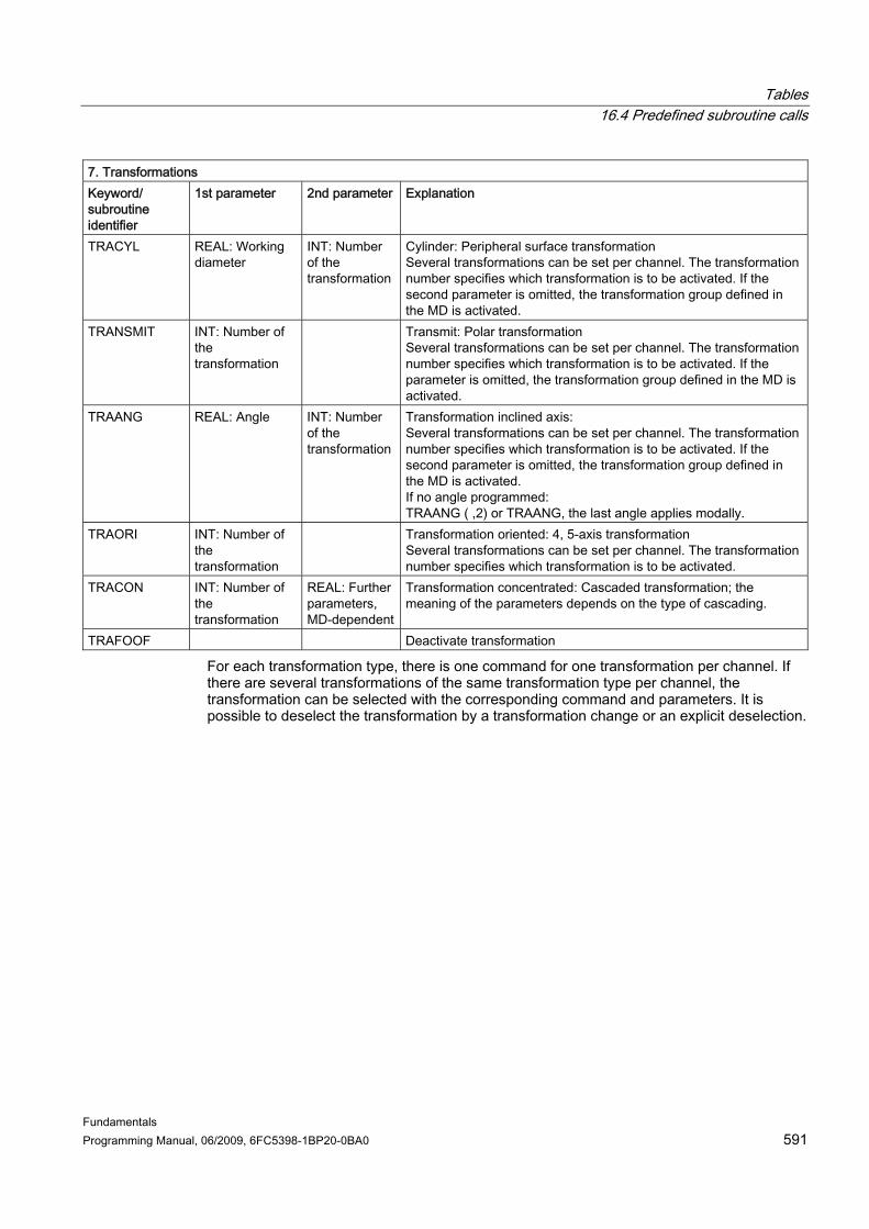
Tables 16.4 Predefined subroutine calls
Fundamentals Programming Manual, 06/2009, 6FC5398-1BP20-0BA0 591
7. Transformations Keyword/ subroutine identifier
1st parameter 2nd parameter Explanation
TRACYL REAL: Working diameter
INT: Number of the transformation
Cylinder: Peripheral surface transformation Several transformations can be set per channel. The transformation number specifies which transformation is to be activated. If the second parameter is omitted, the transformation group defined in the MD is activated.
TRANSMIT INT: Number of the transformation
Transmit: Polar transformation Several transformations can be set per channel. The transformation number specifies which transformation is to be activated. If the parameter is omitted, the transformation group defined in the MD is activated.
TRAANG REAL: Angle INT: Number of the transformation
Transformation inclined axis: Several transformations can be set per channel. The transformation number specifies which transformation is to be activated. If the second parameter is omitted, the transformation group defined in the MD is activated. If no angle programmed: TRAANG ( ,2) or TRAANG, the last angle applies modally.
TRAORI INT: Number of the transformation
Transformation oriented: 4, 5-axis transformation Several transformations can be set per channel. The transformation number specifies which transformation is to be activated.
TRACON INT: Number of the transformation
REAL: Further parameters, MD-dependent
Transformation concentrated: Cascaded transformation; the meaning of the parameters depends on the type of cascading.
TRAFOOF Deactivate transformation
For each transformation type, there is one command for one transformation per channel. If there are several transformations of the same transformation type per channel, the transformation can be selected with the corresponding command and parameters. It is possible to deselect the transformation by a transformation change or an explicit deselection.

Tables 16.4 Predefined subroutine calls
Fundamentals 592 Programming Manual, 06/2009, 6FC5398-1BP20-0BA0
8. Spindles Keyword/ subroutine identifier
1st parameter 2nd parameter and others
Explanation
SPCON INT: Spindle number
INT: Spindle number
Spindle position control ON: Switch to position-controlled spindle operation.
SPCOF INT: Spindle number
INT: Spindle number
Spindle position control OFF: Switch to speed-controlled spindle operation.
SETMS INT: Spindle number
Set master spindle: Declaration of spindle as master spindle for current channel. With SETMS( ), the machine-data default applies automatically without any need for parameterization.
9. Grinding Keyword/ subroutine identifier
1st parameter Explanation
GWPSON INT: Spindle number
Grinding wheel peripheral speed ON: Constant grinding wheel peripheral speed ON. If the spindle number is not programmed, then grinding wheel peripheral speed is selected for the spindle of the active tool.
GWPSOF INT: Spindle number
Grinding wheel peripheral speed OFF. Constant grinding wheel peripheral speed OFF. If the spindle number is not programmed, grinding wheel peripheral speed is deselected for the spindle of the active tool.
TMON INT: Spindle number
Tool monitoring ON: If no T number is programmed, monitoring is activated for the active tool.
TMOF INT: T number Tool monitoring OFF: If no T number is programmed, monitoring is deactivated for the active tool.

Tables 16.4 Predefined subroutine calls
Fundamentals Programming Manual, 06/2009, 6FC5398-1BP20-0BA0 593
10. Stock removal Keyword/ subroutine identifier
1st parameter 2nd parameter 3rd parameter
4th parameter
Explanation
CONTPRON REAL [ , 11]: Contour table
CHAR: Stock removal method "L": Longitudinal turning: External mach. "P": Face turning: External mach. "N": Face turning: Internal machining "G": Longitudinal turning: Internal machining
INT: Number of relief cuts
INT: Status of calculation: 0: unchanged 1: Calculation forwards and backwards
Contour preparation on: Activate reference-point editing. The contour programs or NC blocks which are called in the following steps are divided into individual movements and stored in the contour table. The number of relief cuts is returned.
CONTDCON REAL [ , 6]: Contour table
INT: 0: In programmed direction
Contour decoding The blocks for a contour are stored in a named table with one table line per block and coded to save memory.
EXECUTE INT: Error status
EXECUTE: Activate program execution. This switches back to normal program execution from reference-point-editing mode or after setting up a protection zone.
11. Execute table Keyword/ subroutine identifier
1st parameter Explanation
EXECTAB REAL [ 11]: Element from motion table
Execute table: Execute an element from a motion table.

Tables 16.4 Predefined subroutine calls
Fundamentals 594 Programming Manual, 06/2009, 6FC5398-1BP20-0BA0
12. Protection zones Keyword/ subroutine identifier
1st parameter 2nd parameter 3rd parameter 4th parameter 5th parameter Explanation
CPROTDEF INT: Number of the protection zone
BOOL: TRUE: Tool-oriented protection zone
INT: 0: 4th and 5th parameters not evaluated 1: 4th parameter evaluated 2: 5th parameter evaluated 3: 4th and 5th parameters evaluated
REAL: Limit in plus direction
REAL: Limit in minus direction
Channel-specific protection zone definition: Definition of a channel-specific protection zone
NPROTDEF INT: Number of the protection zone
BOOL: TRUE: Tool-oriented protection zone
INT: 0: 4th and 5th parameters not evaluated 1: 4th parameter evaluated 2: 5th parameter evaluated 3: 4th and 5th parameters evaluated
REAL: Limit in plus direction
REAL: Limit in minus direction
NCK-specific protection zone definition: Definition of a machine-specific protection zone

Tables 16.4 Predefined subroutine calls
Fundamentals Programming Manual, 06/2009, 6FC5398-1BP20-0BA0 595
CPROT INT: Number of the protection zone
INT: Option 0: Protection zone OFF 1: Preactivate protection zone 2: Protection zone ON 3: Preactivate protection zone with conditional stop, only with protection zones active
REAL: Offset of protection zone in 1st geometry axis
REAL: Offset of protection zone in 2nd geometry axis
REAL: Offset of protection zone in 3rd geometry axis
Channel-specific protection zone ON/OFF
NPROT INT: Number of the protection zone
INT: Option 0: Protection zone OFF 1: Preactivate protection zone 2: Protection zone ON 3: Preactivate protection zone with conditional stop, only with protection zones active
REAL: Offset of protection zone in 1st geometry axis
REAL: Offset of protection zone in 2nd geometry axis
REAL: Offset of protection zone in 3rd geometry axis
Machine-specific protection zone ON/OFF
EXECUTE VAR INT: Error status
EXECUTE: Activate program execution. This switches back to normal program execution from reference point editing mode or after setting up a protection zone.
13. Preprocessing/single block STOPRE Stop processing: Preprocessing stop until all prepared blocks are executed in main
run

Tables 16.4 Predefined subroutine calls
Fundamentals 596 Programming Manual, 06/2009, 6FC5398-1BP20-0BA0
14. Interrupts Keyword/ subroutine identifier
1st parameter Explanation
ENABLE INT: Number of the interrupt input
Activate interrupt: Activates the interrupt routine assigned to the hardware input with the specified number. An interrupt is enabled after the SETINT statement.
DISABLE INT: Number of the interrupt input
Deactivate interrupt: Deactivates the interrupt routine assigned to the hardware input with the specified number. Fast retraction is not executed. The assignment between the hardware input and the interrupt routine made with SETINT remains valid and can be reactivated with ENABLE.
CLRINT INT: Number of the interrupt input
Select interrupt: Cancel the assignment of interrupt routines and attributes to an interrupt input. The interrupt routine is deactivated and no reaction occurs when the interrupt is generated.
15. Motion synchronization Keyword/ subroutine identifier
1st parameter Explanation
CANCEL INT: Number of synchronized action
Aborts the modal motion-synchronous action with the specified ID
16. Function definition Keyword/ subroutine identifier
1st parameter 2nd parameter 3rd parameter 4th-7th parameter
Explanation
FCTDEF INT: Function number
REAL: Lower limit value
REAL: Upper limit value
REAL: Coefficients a0 – a3
Define polynomial. This is evaluated in SYFCT or PUTFTOCF.

Tables 16.4 Predefined subroutine calls
Fundamentals Programming Manual, 06/2009, 6FC5398-1BP20-0BA0 597
17. Communication Keyword/ subroutine identifier
1st parameter
2nd parameter Explanation
MMC STRING: Command
CHAR: Acknowledgement mode** "N": Without acknowledgment "S": Synchronous acknowledgment "A": Asynchronous acknowledgment
MMC command: Command ON MMC command interpreter for the configuration of windows via NC program see /IAM/ Commissioning CNC; Expanding base software and HMI Embedded/Advanced in BE1 user interface
** Acknowledgement mode: Commands are acknowledged on request from the executing component (channel, NC, etc.). Without acknowledgement: Program execution is continued when the command has been transmitted. The sender is not informed if the command cannot be executed successfully.
18. Program coordination Keyword/ subroutine identifier
1st parameter
2nd parameter
3rd parameter
4th parameter
5th parameter
6th-8th parameter
Explanation
INIT # INT: Channel numbers 1 - 10 or STRING: Channel name $MC_CHAN_NAME
STRING: path
CHAR: Acknowledgement mode**
Selection of a module for execution in a channel. 1 : 1st channel; 2 : 2nd channel. As an alternative to the channel number, the channel name defined in $MC_CHAN_NAME can also be used.
START # INT: Channel numbers 1 - 10 or STRING: Channel name $MC_CHAN_NAME
Starts selected programs simultaneously on multiple channels from running program. The command has no effect on the existing channel. 1 : 1st channel; 2 : 2nd channel or channel name defined in $MC_CHAN_NAME.
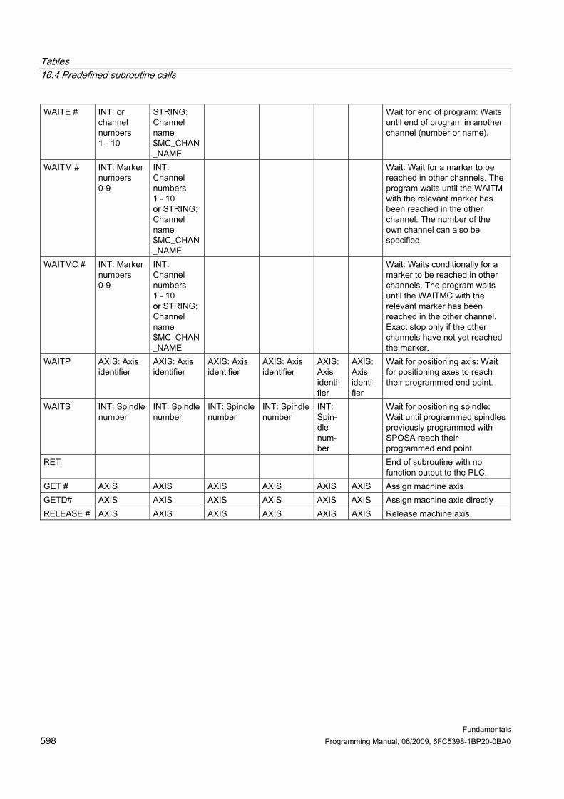
Tables 16.4 Predefined subroutine calls
Fundamentals 598 Programming Manual, 06/2009, 6FC5398-1BP20-0BA0
WAITE # INT: or channel numbers 1 - 10
STRING: Channel name $MC_CHAN_NAME
Wait for end of program: Waits until end of program in another channel (number or name).
WAITM # INT: Marker numbers 0-9
INT: Channel numbers 1 - 10 or STRING: Channel name $MC_CHAN_NAME
Wait: Wait for a marker to be reached in other channels. The program waits until the WAITM with the relevant marker has been reached in the other channel. The number of the own channel can also be specified.
WAITMC # INT: Marker numbers 0-9
INT: Channel numbers 1 - 10 or STRING: Channel name $MC_CHAN_NAME
Wait: Waits conditionally for a marker to be reached in other channels. The program waits until the WAITMC with the relevant marker has been reached in the other channel. Exact stop only if the other channels have not yet reached the marker.
WAITP AXIS: Axis identifier
AXIS: Axis identifier
AXIS: Axis identifier
AXIS: Axis identifier
AXIS: Axis identi-fier
AXIS: Axis identi-fier
Wait for positioning axis: Wait for positioning axes to reach their programmed end point.
WAITS INT: Spindle number
INT: Spindle number
INT: Spindle number
INT: Spindle number
INT: Spin-dle num-ber
Wait for positioning spindle: Wait until programmed spindles previously programmed with SPOSA reach their programmed end point.
RET End of subroutine with no function output to the PLC.
GET # AXIS AXIS AXIS AXIS AXIS AXIS Assign machine axis GETD# AXIS AXIS AXIS AXIS AXIS AXIS Assign machine axis directly RELEASE # AXIS AXIS AXIS AXIS AXIS AXIS Release machine axis

Tables 16.4 Predefined subroutine calls
Fundamentals Programming Manual, 06/2009, 6FC5398-1BP20-0BA0 599
PUTFTOC # REAL: Offset value
INT: Parameter number
INT: Channel number or STRING: Channel name $MC_CHAN_NAME
INT: Spindle number
Put fine tool correction: Fine tool compensation
PUTFTOCF #
INT: No. of function The number used here must be specified in FCTDEF.
VAR REAL: Reference value *)
INT: Parameter number
INT: Channel numbers 1 - 10 or STRING: Channel name $MC_CHAN_NAME
INT: Spin-dle num-ber
Put fine tool correction function dependent: Change online tool compensation according to a function defined with FCTDEF (max. 3rd degree polynomial).
The SPI function can also be used to program a spindle instead of an axis: GET(SPI(1)) #) The keyword is not valid for NCU571. ** Acknowledgement mode: Commands are acknowledged on request from the executing component (channel, NC, etc.). Without acknowledgement: Program execution is continued when the command has been transmitted. The executing component is not informed if the command cannot be executed successfully. Acknowledgment mode "N" or "n". Synchronous acknowledgement: The program execution is paused until the receiving component acknowledges the command. If the acknowledgement is positive, the next command is executed. If the acknowledgement is negative an error is output. Acknowledgement "S", "s" or to be omitted. For some commands, the acknowledgement response is predefined, for others it is programmable. The acknowledgement response for program-coordination commands is always synchronous. If the acknowledgement mode is not specified, synchronous acknowledgement is the default response.
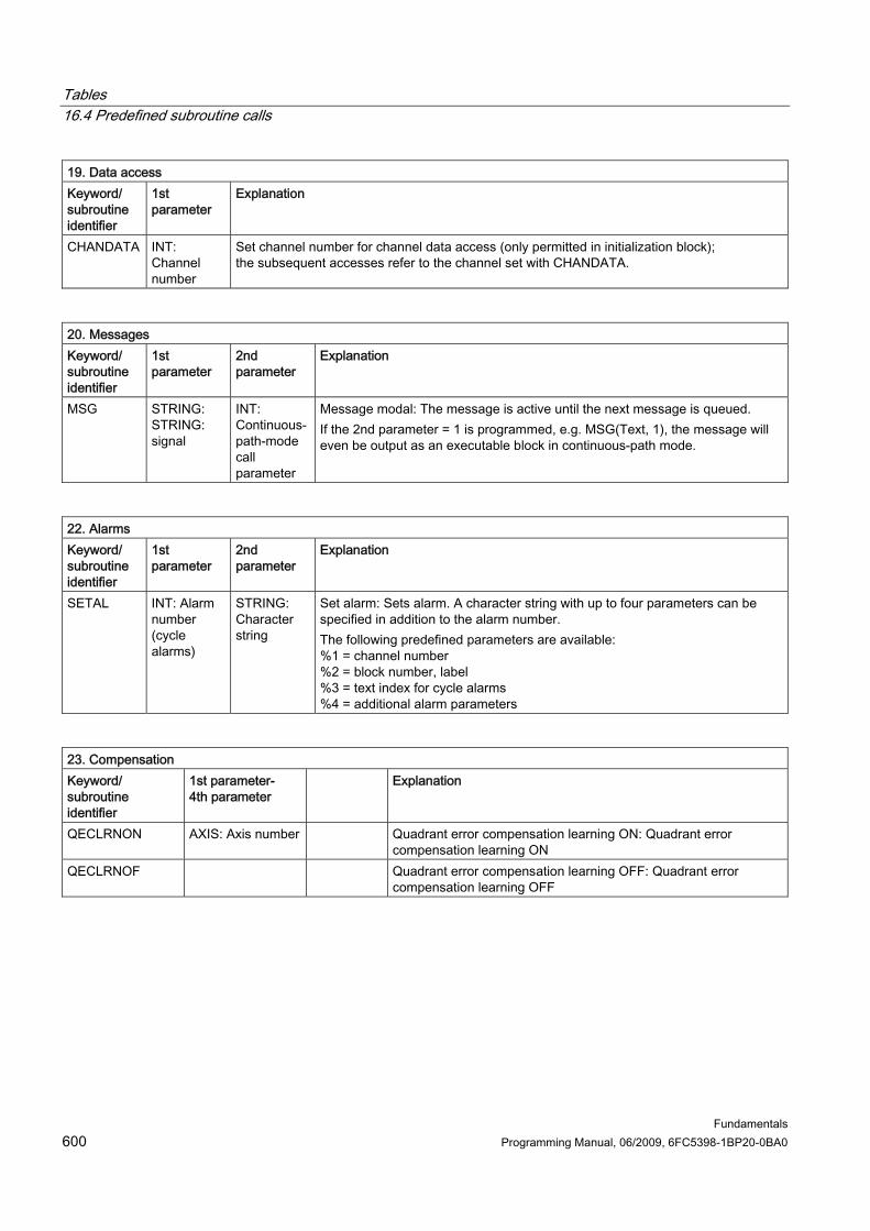
Tables 16.4 Predefined subroutine calls
Fundamentals 600 Programming Manual, 06/2009, 6FC5398-1BP20-0BA0
19. Data access Keyword/ subroutine identifier
1st parameter
Explanation
CHANDATA INT: Channel number
Set channel number for channel data access (only permitted in initialization block); the subsequent accesses refer to the channel set with CHANDATA.
20. Messages Keyword/ subroutine identifier
1st parameter
2nd parameter
Explanation
MSG STRING: STRING: signal
INT: Continuous-path-mode call parameter
Message modal: The message is active until the next message is queued. If the 2nd parameter = 1 is programmed, e.g. MSG(Text, 1), the message will even be output as an executable block in continuous-path mode.
22. Alarms Keyword/ subroutine identifier
1st parameter
2nd parameter
Explanation
SETAL INT: Alarm number (cycle alarms)
STRING: Character string
Set alarm: Sets alarm. A character string with up to four parameters can be specified in addition to the alarm number. The following predefined parameters are available: %1 = channel number %2 = block number, label %3 = text index for cycle alarms %4 = additional alarm parameters
23. Compensation Keyword/ subroutine identifier
1st parameter- 4th parameter
Explanation
QECLRNON AXIS: Axis number Quadrant error compensation learning ON: Quadrant error compensation learning ON
QECLRNOF Quadrant error compensation learning OFF: Quadrant error compensation learning OFF

Tables 16.4 Predefined subroutine calls
Fundamentals Programming Manual, 06/2009, 6FC5398-1BP20-0BA0 601
24. Tool management Keyword/ subroutine identifier
1st parameter 2nd parameter 3rd parameter
Explanation
DELT STRING[32]: Tool designation
INT: Duplo number
Delete tool. Duplo number can be omitted.
GETSELT VAR INT: T number (return value)
INT: Spindle number
Get selected T number. If no spindle number is specified, the command for the master spindle applies.
SETPIECE INT: Count INT: Spindle number
Takes account of set piece number for all tools assigned to the spindle. If no spindle number is specified, the command for the master spindle applies.
SETDNO INT: Tool number T INT: Tool edge no.
INT: D no. Set D no. of tool (T) and its tool edge to new.
DZERO Set D numbers of all tools of the TO unit assigned to the channel to invalid
DELDL INT: Tool number T INT: D no. Delete all additive offsets of the tool edge (or of a tool if D is not specified).
SETMTH INT: Tool-holder no.
Set toolholder no.
POSM INT: Location no. for positioning
INT: No. of the magazine to be moved
INT: Location number of the internal magazine
INT: Magazine number of the internal magazine
Position magazine
SETTIA VAR INT: Status = result of the operation (return value)
INT: Magazine number
INT: Wear group no.
Deactivate tool from wear group
SETTA VAR INT: Status = result of the operation (return value)
INT: Magazine number
INT: Wear group no.
Activate tool from wear group
RESETMON VAR INT: Status = result of the operation (return value)
INT: Internal T no.
INT: D no. of tool
Set actual value of tool to setpoint
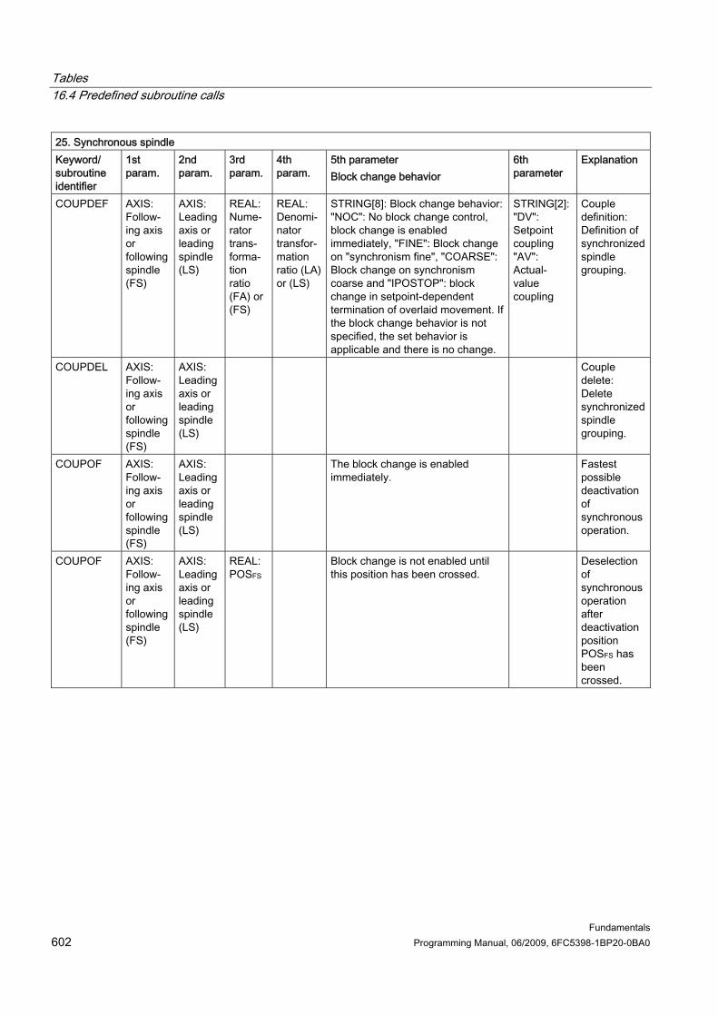
Tables 16.4 Predefined subroutine calls
Fundamentals 602 Programming Manual, 06/2009, 6FC5398-1BP20-0BA0
25. Synchronous spindle Keyword/ subroutine identifier
1st param.
2nd param.
3rd param.
4th param.
5th parameter Block change behavior
6th parameter
Explanation
COUPDEF AXIS: Follow-ing axis or following spindle (FS)
AXIS: Leading axis or leading spindle (LS)
REAL: Nume-rator trans-forma-tion ratio (FA) or (FS)
REAL: Denomi-nator transfor-mation ratio (LA) or (LS)
STRING[8]: Block change behavior:"NOC": No block change control, block change is enabled immediately, "FINE": Block change on "synchronism fine", "COARSE": Block change on synchronism coarse and "IPOSTOP": block change in setpoint-dependent termination of overlaid movement. If the block change behavior is not specified, the set behavior is applicable and there is no change.
STRING[2]: "DV": Setpoint coupling "AV": Actual-value coupling
Couple definition: Definition of synchronized spindle grouping.
COUPDEL AXIS: Follow-ing axis or following spindle (FS)
AXIS: Leading axis or leading spindle (LS)
Couple delete: Delete synchronized spindle grouping.
COUPOF AXIS: Follow-ing axis or following spindle (FS)
AXIS: Leading axis or leading spindle (LS)
The block change is enabled immediately.
Fastest possible deactivation of synchronous operation.
COUPOF AXIS: Follow-ing axis or following spindle (FS)
AXIS: Leading axis or leading spindle (LS)
REAL: POSFS
Block change is not enabled until this position has been crossed.
Deselection of synchronous operation after deactivation position POSFS has been crossed.

Tables 16.4 Predefined subroutine calls
Fundamentals Programming Manual, 06/2009, 6FC5398-1BP20-0BA0 603
COUPOF AXIS: Follow-ing axis or following spindle (FS)
AXIS: Leading axis or leading spindle (LS)
REAL: POSFS
REAL: POSLS
Block change is not enabled until both programmed positions have been crossed. Range of POSFS, POSLS: 0 ... 359.999 degrees.
Deselection of synchronous operation after the two deactivation positions. POSFS and POSLS have been crossed.
COUPOFS AXIS: Follow-ing axis or following spindle (FS)
AXIS: Leading axis or leading spindle (LS)
Block change performed as quickly as possible with immediate block change.
Deactivation of couple with following-spindle stop.
COUPOFS AXIS: Follow-ing axis or following spindle (FS)
AXIS: Leading axis or leading spindle (LS)
REAL: POSFS
After the programmed deactivation position that refers to the machine coordinate system has been crossed, the block change is not enabled until the deactivation positions POSFS have been crossed. Value range 0 ... 359.999 degrees.
Only deactivated after programmed following-axis deactivation position has been crossed.
COUPON AXIS: Follow-ing axis or following spindle (FS)
AXIS: Leading axis or leading spindle (LS)
The block change is enabled immediately.
Fastest possible activation of synchronous operation with any angular reference between the leading and following spindles.

Tables 16.4 Predefined subroutine calls
Fundamentals 604 Programming Manual, 06/2009, 6FC5398-1BP20-0BA0
COUPON AXIS: Follow-ing axis or following spindle (FS)
AXIS: Leading axis or leading spindle (LS)
REAL: POSFS
The block change is enabled according to the defined setting. Range of POSFS: 0 ... 359.999 degrees.
Activation with a defined angular offset POSFS between the following and leading spindles. This offset is referred to the zero degrees position of the leading spindle in a positive direction of rotation.
COUPONC AXIS: Follow-ing axis or following spindle (FS)
AXIS: Leading axis or leading spindle (LS)
An offset position cannot be pro-gram-med.
Acceptance of activation with previously programmed M3 S.. or M4 S... Immediate acceptance of rotational speed difference.
COUPRES AXIS: Follow-ing axis or following spindle (FS)
AXIS: Leading axis or leading spindle (LS)
Couple reset: Reset synchronous spindle group. The programmed values become invalid. The machine data values are valid.
For synchronous spindles, the axis parameters are programmed with SPI(1) or S1.

Tables 16.4 Predefined subroutine calls
Fundamentals Programming Manual, 06/2009, 6FC5398-1BP20-0BA0 605
26. Structure statements in the STEP editor (editor-based program support) Keyword/ subroutine identifier
1st parameter 2nd parameter 3rd parameter Explanation
SEFORM STRING[128]: section name
INT: level STRING[128]: icon
Current section name for STEP editor
Keyword/ subroutine identifier
1st parameter
2nd parameter
3rd parameter
4th parameter
Explanation
COUPON AXIS: Following axis
AXIS: Leading axis
REAL: Activation position of following axis
Couple on: Activate ELG group/synchronous spindle pair. If no activation positions are specified, the couple is activated as quickly as possible (ramp). If an activation position is specified for the following axis and spindle, this refers absolutely or incrementally to the master axis or spindle. Parameters 4 and 5 only have to be programmed if the 3rd parameter is specified.
COUPOF AXIS: Following axis
AXIS: Leading axis
REAL: Deactivation position of following axis (absolute)
REAL: Deactivation position of master axis (absolute)
Couple OFF: Deactivate ELG group/synchronous spindle pair. The couple parameters are retained. If positions are specified, the couple is only canceled when all the specified positions have been overtraveled. The following spindle continues to revolve at the last speed programmed before deactivation of the couple.
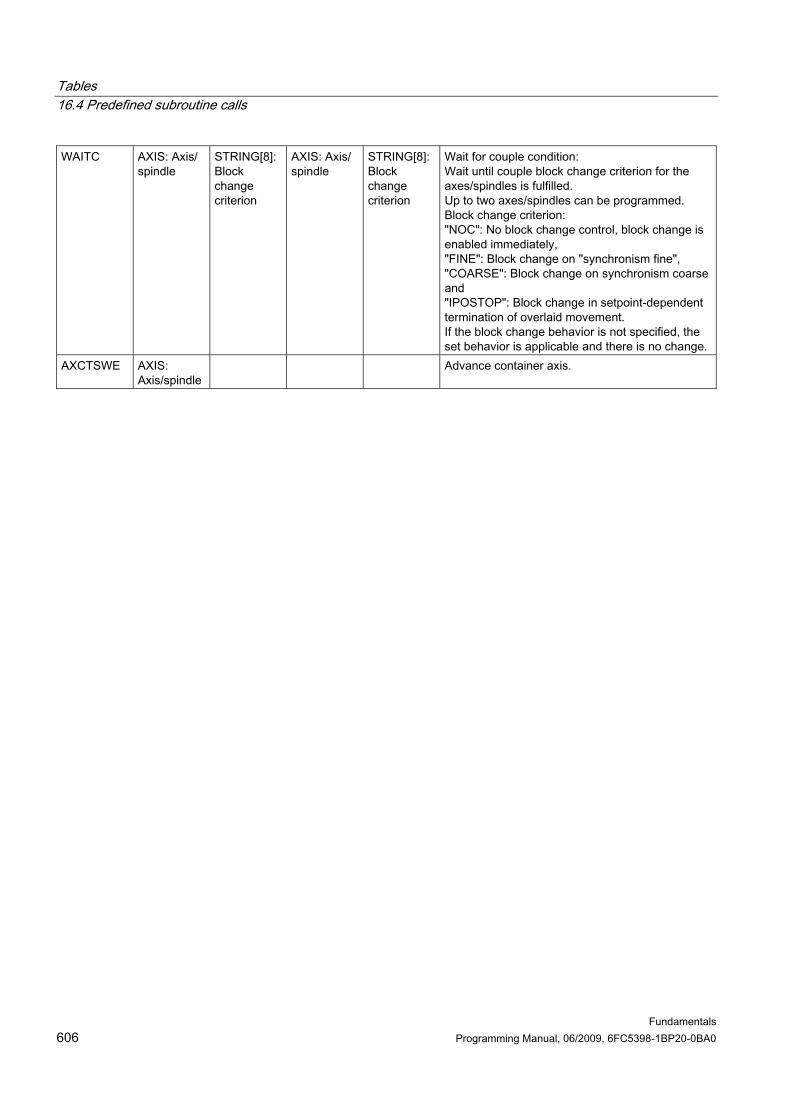
Tables 16.4 Predefined subroutine calls
Fundamentals 606 Programming Manual, 06/2009, 6FC5398-1BP20-0BA0
WAITC AXIS: Axis/ spindle
STRING[8]: Block change criterion
AXIS: Axis/spindle
STRING[8]: Block change criterion
Wait for couple condition: Wait until couple block change criterion for the axes/spindles is fulfilled. Up to two axes/spindles can be programmed. Block change criterion: "NOC": No block change control, block change is enabled immediately, "FINE": Block change on "synchronism fine", "COARSE": Block change on synchronism coarse and "IPOSTOP": Block change in setpoint-dependent termination of overlaid movement. If the block change behavior is not specified, the set behavior is applicable and there is no change.
AXCTSWE AXIS: Axis/spindle
Advance container axis.

Tables 16.5 Predefined subroutine calls in motion-synchronous actions
Fundamentals Programming Manual, 06/2009, 6FC5398-1BP20-0BA0 607
16.5 16.5 Predefined subroutine calls in motion-synchronous actions 27. Synchronous procedures Keyword/ function identifier
1st parameter 2nd parameter 3rd parameter to 5th parameter
Explanation
STOPREOF Stop preparation OFF: A synchronized action with a STOPREOF command causes a preprocessing stop after the next output block (= block for the main run). The preprocessing stop is canceled with the end of the output block or when the STOPREOF condition is fulfilled. All synchronized action statements with the STOPREOF command are therefore interpreted as having been executed.
RDISABLE Read-in disable Read-in disable DELDTG AXIS: Axis for
axial delete distance-to-go (optional). If the axis is omitted, delete distance-to-go is triggered for the path distance
Delete distance-to-go: A synchronized action with the DELDTG command causes a preprocessing stop after the next output block (= block for the main run). The preprocessing stop is canceled with the end of the output block or when the first DELDTG condition is fulfilled. The axial distance to the destination point on an axial delete distance-to-go is stored in $AA_DELT[axis]; the distance-to-go is stored in $AC_DELT.
SYNFCT INT: Number of polynomial function defined with FCTDEF.
VAR REAL: Result variable*)
VAR REAL: Input variable **)
If the condition in the motion synchronous action is fulfilled, the polynomial determined by the first expression is evaluated at the input variable. The upper and lower range of the value is limited and the input variable is assigned.
FTOC INT: Number of polynomial function defined with FCTDEF
VAR REAL: Input variable **)
INT: Length 1, 2, 3 INT: Channel number INT: Spindle number
Modify tool fine compensation according to a function defined with FCTDEF (polynomial no higher than 3rd degree). The number used here must be specified in FCTDEF.
*) Only special system variables are permissible as result variables. These are described in the Programming Manual Advanced in the section on "Write main run variable". **) Only special system variables are permissible as input variables. These variables are described in the Programming Manual Advanced in the list of system variables.

Tables 16.6 Predefined functions
Fundamentals 608 Programming Manual, 06/2009, 6FC5398-1BP20-0BA0
16.6 16.6 Predefined functions
Predefined functions Predefined functions are invoked by means of a function call. Function calls return a value. They can be included as an operand in an expression.
1. Coordinate system Keyword/ function identifier
Result 1st parameter 2nd parameter Explanation
CTRANS FRAME AXIS REAL: Offset 3rd-15th parameter as 1 ...
4th-16th parameter as 2 ...
Translation: Zero offset for multiple axes. One axis identifier is programmed at a time, with its respective value in the next parameter. CTRANS can be used to program offset for up to 8 axes.
CROT FRAME AXIS REAL: Rotation
3rd/5th parameter as 1 ...
4th/6th parameter as 2 ...
Rotation: Rotation of the current coordinate system. Maximum number of parameters: 6 (one axis identifier and one value per geometry axis)

Tables 16.6 Predefined functions
Fundamentals Programming Manual, 06/2009, 6FC5398-1BP20-0BA0 609
CSCALE FRAME AXIS REAL: Scale factor
3rd-15th parameter as 1 ...
4th-16th parameter as 2 ...
Scale: Scale factor for multiple axes. Maximum number of parameters is 2* maximum number of axes (axis identifier and value). One axis identifier is programmed at a time, with its respective value in the next parameter. CSCALE can be used to program scale factors for up to 8 axes.
CMIRROR FRAME AXIS 2nd - 8th parameter as 1 ...
Mirror: Mirror on a coordinate axis
MEAFRAME FRAME 2-dim. REAL array
2-dim. REAL array
3rd parameter REAL variables
Frame calculation from 3 measuring points in space
Frame functions CTRANS, CSCALE, CROT and CMIRROR are used to generate frame expressions.

Tables 16.6 Predefined functions
Fundamentals 610 Programming Manual, 06/2009, 6FC5398-1BP20-0BA0
2. Geometry functions Keyword/ function identifier
Result 1st parameter 2nd parameter 3rd parameter Explanation
CALCDAT BOOL: Error status
VAR REAL [,2]:Table with input points (abscissa and ordinate forpoints 1, 2, 3, etc.)
INT: Number of input points for calculation (3 or 4)
VAR REAL [3]:Result: Abscissa, ordinate and radius of calculated circle center point
CALCDAT: Calculate circle data Calculates radius and center point of a circle from 3 or 4 points (according to parameter 1), which must lie on a circle. The points must be different.
Names Result 1st parameter 2nd parameter 3rd parameter 4th parameter 5th
parameter 6th parameter
CALCPOSI INT: Status 0 OK -1 DLIMIT neg. -2 Trans. n.def. 1 SW limit 2 Working area 3 Prot. zone See PGA for more
REAL: Starting position in WCS [0] Abscissa [1] Ordinate [2] Applicate
REAL: Increment: Path definition [0] Abscissa [1] Ordinate [2] Applicate referred to starting position
REAL: Minimum clearances of limits to be observed [0] Abscissa [1] Ordinate [2] Applicate [3] Lin. machine Axis [4] Rot. Axis
REAL: Return value possible incr. path if path from parameter 3 cannot be fully traversed without violating limit
BOOL: 0: Evaluation G code group 13 (inch/metr.) 1: Reference to basic control system, independent of active G codes group 13
bin encoded to be monitored 1 SW limits2 working area 4 active protection zone 8 preactive protection zone
Explanation: CALCPOSI
CALCPOSI is for checking whether, starting from a defined starting point, the geometry axes can traverse a defined path without violating the axis limits (software limits), working area limitations, or protection zones. If the defined path cannot be traversed without violating limits, the maximum permissible value is returned.

Tables 16.6 Predefined functions
Fundamentals Programming Manual, 06/2009, 6FC5398-1BP20-0BA0 611
INTERSEC BOOL: Error status
VAR REAL [11]:First contour element
VAR REAL [11]: Second contour element
VAR REAL [2]: Result vector: Intersection coordinate, abscissa and ordinate
Intersection: Calculation of intersection The intersection between two contour elements is calculated. The intersection coordinates are return values. The error status indicates whether an intersection was found.
3. Axis functions Result 1st parameter 2nd parameter Explanation AXNAME AXIS:
Axis identifier STRING [ ]: Input string
AXNAME: Get axis identifier Converts the input string to an axis identifier. An alarm is generated if the input string does not contain a valid axis identifier.
AXTOSPI INT: Spindle number
AXIS: Axis identifier
AXTOSPI: Convert axis to spindle Converts an axis identifier into a spindle number. An alarm is set if the transfer parameter does not contain a valid axis identifier.
SPI AXIS: Axis identifier
INT: Spindle number
SPI: Convert spindle to axis Converts a spindle number to an axis identifier. An alarm is generated if the passed parameter does not contain a valid spindle number.
ISAXIS BOOL TRUE: Axis exists: Otherwise: FALSE
INT: Number of the geometry axis (1 to 3)
Check whether the geometry axis 1 to 3 specified as parameter exists in accordance with $MC_AXCONF_GEOAX_ASSIGN_TAB.
AXSTRING STRING AXIS Convert axis identifier into string.

Tables 16.6 Predefined functions
Fundamentals 612 Programming Manual, 06/2009, 6FC5398-1BP20-0BA0
4. Tool management Result 1st parameter 2nd parameter Explanation NEWT INT:
T number STRING [32]: Tool name
INT: Duplo number
Create new tool (prepare tool data). The duplo number can be omitted.
GETT50 INT: T number
STRING [32]: Tool name
INT: Duplo number
Get T number for tool identifier.
GETACTT INT: Status
INT: T number
STRING[32]: Tool name
Get active tool from a group of tools with the same name.
TOOLENV INT: Status
STRING: Name
Save a tool environment in SRAM with the specified name.
DELTOOLENV INT: Status
STRING: Name
Delete a tool environment in SRAM with the specified name. All tool environments if no name specified.
GETTENV INT: Status
STRING: Name
INT: Number = [0] Number = [1] Number = [2]
Reading: T number, D number, DL number from a tool environment with the specified name
Result 1st par. 2nd par. 3rd par. 4th par. 5th par. 6th par. Explanation GETTCOR INT:
Status REAL: Length [11]
STRING: Compo-nents: Coordi-nate system
STRING:Tool environ-ment/ " "
INT: Int. T number
INT: D number
INT: DL number
Read tool lengths and tool length components from tool environment or current environment Details: See /FB1/ Function Manual Basic Functions; (W1)
Result 1st par. 2nd par. 3rd par. 4th par. 5th par. 6th par. 7th par. 8th par. 9th par. SETTCOR INT:
Status REAL: Offset vector [0-3]
STRING: Compo-nent(s)
INT: Compo-nent(s) to be offset
INT: Type of write operation
INT: Index of geo. axis
STRING:Name of tool environ-ment
INT: Int. T number
INT: D number
INT: DL number
Explanation Changing tool components whilst observing all marginal conditions that are included in the evaluation of the individual components. Details: See Function Manual Basic Functions; (W1)
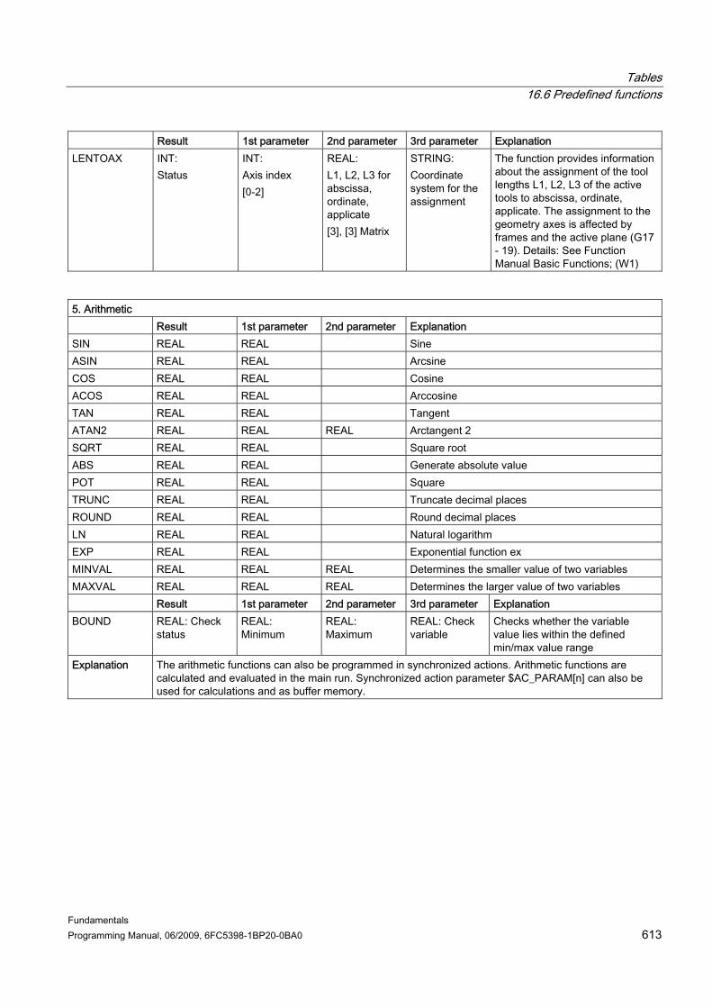
Tables 16.6 Predefined functions
Fundamentals Programming Manual, 06/2009, 6FC5398-1BP20-0BA0 613
Result 1st parameter 2nd parameter 3rd parameter Explanation LENTOAX INT:
Status INT: Axis index [0-2]
REAL: L1, L2, L3 for abscissa, ordinate, applicate [3], [3] Matrix
STRING: Coordinate system for the assignment
The function provides information about the assignment of the tool lengths L1, L2, L3 of the active tools to abscissa, ordinate, applicate. The assignment to the geometry axes is affected by frames and the active plane (G17 - 19). Details: See Function Manual Basic Functions; (W1)
5. Arithmetic Result 1st parameter 2nd parameter Explanation SIN REAL REAL Sine ASIN REAL REAL Arcsine COS REAL REAL Cosine ACOS REAL REAL Arccosine TAN REAL REAL Tangent ATAN2 REAL REAL REAL Arctangent 2 SQRT REAL REAL Square root ABS REAL REAL Generate absolute value POT REAL REAL Square TRUNC REAL REAL Truncate decimal places ROUND REAL REAL Round decimal places LN REAL REAL Natural logarithm EXP REAL REAL Exponential function ex MINVAL REAL REAL REAL Determines the smaller value of two variables MAXVAL REAL REAL REAL Determines the larger value of two variables Result 1st parameter 2nd parameter 3rd parameter Explanation BOUND REAL: Check
status REAL: Minimum
REAL: Maximum
REAL: Check variable
Checks whether the variable value lies within the defined min/max value range
Explanation The arithmetic functions can also be programmed in synchronized actions. Arithmetic functions are calculated and evaluated in the main run. Synchronized action parameter $AC_PARAM[n] can also be used for calculations and as buffer memory.

Tables 16.6 Predefined functions
Fundamentals 614 Programming Manual, 06/2009, 6FC5398-1BP20-0BA0
6. String functions Result 1st parameter 2nd parameter
to 3rd parameter
Explanation
ISNUMBER BOOL STRING Check whether the input string can be converted to a number. Result is TRUE if conversion is possible.
ISVAR BOOL STRING Check whether the transfer parameter contains a variable known in the NC. (Machine data, setting data, system variable, general variables such as GUDs) Result is TRUE if all the following checks produce positive results according to the (STRING) transfer parameter: – The identifier exists – It is a 1- or 2-dimensional array – An array index is allowed. For axial variables, the axis names are accepted as an index but not checked.
NUMBER REAL STRING Convert the input string into a number. TOUPPER STRING STRING Convert all alphabetic characters in the input string
to upper case. TOLOWER STRING STRING Convert all alphabetic characters in the input string
to lower case. STRLEN INT STRING The result is the length of the input string up to the
end of the string (0). INDEX INT STRING CHAR Find the character (2nd parameter) in the input
string (1st parameter). The reply gives the place, at which the character was first found. The search is from left to right. The 1st character in the string has the index 0.
RINDEX INT STRING CHAR Find the character (2nd parameter) in the input string (1st parameter). The reply gives the place, at which the character was first found. The search is from right to left. The 1st character in the string has the index 0.

Tables 16.6 Predefined functions
Fundamentals Programming Manual, 06/2009, 6FC5398-1BP20-0BA0 615
MINDEX INT STRING STRING Find one of the characters specified in the 2nd parameter in the input string (1st parameter). The place where one of the characters was first found is output. The search is from left to right. The first character in the string has the index 0.
SUBSTR STRING STRING INT Returns the substring of the input string (1st parameter), defined by the start character (2nd parameter) and number of characters (3rd parameter). Example: SUBSTR("ACKNOWLEDGEMENT:10 to 99", 10, 2) returns substring "10".

Tables 16.6 Predefined functions
Fundamentals 616 Programming Manual, 06/2009, 6FC5398-1BP20-0BA0

Fundamentals Programming Manual, 06/2009, 6FC5398-1BP20-0BA0 617
A Appendix AA.1 A.1 List of abbreviations A Output AS Automation system ASCII American Standard Code for Information Interchange ASIC Application Specific Integrated Circuit: User switching circuit ASUB Asynchronous subroutine AuxF Auxiliary function AV Job planning BA Operating mode BB Ready to run BCD Binary Coded Decimals: Decimal numbers encoded In binary code BCS Basic Coordinate System BIN Binary files (Binary Files) BIOS Basic Input Output System BOT Boot files: Boot files for SIMODRIVE 611 digital BP Basic program C Bus Communication bus CAD Computer-Aided Design CAM Computer-Aided Manufacturing CNC Computerized Numerical Control COM Communication COR Coordinate rotation CP Communications Processor CPU Central Processing Unit CR Carriage Return CRC Cutter radius compensation CRT Cathode Ray Tube picture tube CSB Central Service Board: PLC module CSF Function plan (PLC programming method) CTS Clear To Send: Signal from serial data interfaces CUTOM Cutter radius compensation: Tool radius compensation
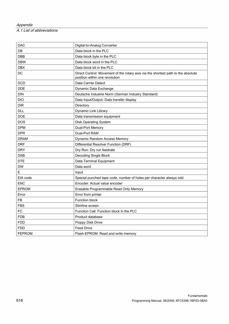
Appendix A.1 List of abbreviations
Fundamentals 618 Programming Manual, 06/2009, 6FC5398-1BP20-0BA0
DAC Digital-to-Analog Converter DB Data block in the PLC DBB Data block byte in the PLC DBW Data block word in the PLC DBX Data block bit in the PLC DC Direct Control: Movement of the rotary axis via the shortest path to the absolute
position within one revolution DCD Data Carrier Detect DDE Dynamic Data Exchange DIN Deutsche Industrie Norm (German Industry Standard) DIO Data Input/Output: Data transfer display DIR Directory DLL Dynamic Link Library DOE Data transmission equipment DOS Disk Operating System DPM Dual-Port Memory DPR Dual-Port RAM DRAM Dynamic Random Access Memory DRF Differential Resolver Function (DRF) DRY Dry Run: Dry run feedrate DSB Decoding Single Block DTE Data Terminal Equipment DW Data word E Input EIA code Special punched tape code, number of holes per character always odd ENC Encoder: Actual value encoder EPROM Erasable Programmable Read Only Memory Error Error from printer FB Function block FBS Slimline screen FC Function Call: Function block in the PLC FDB Product database FDD Floppy Disk Drive FDD Feed Drive FEPROM Flash-EPROM: Read and write memory

Appendix A.1 List of abbreviations
Fundamentals Programming Manual, 06/2009, 6FC5398-1BP20-0BA0 619
FIFO First In First Out: Memory that works without address specification and whose data are read in the same order in which they were stored.
FIPO Fine InterPOlator FM Function Module FPU Floating Point Unit Floating Point Unit FRA Frame block FRAME Data record (frame) FST Feed Stop GUD Global User Data HD Hard Disk HEX Abbreviation for hexadecimal number HHU Handheld unit HMI Human Machine Interface HMI Human Machine Interface: Operator functionality of SINUMERIK for operation,
programming and simulation. HMS High-resolution Measuring System HW Hardware I/O Input/Output I/R Infeed/regenerative-feedback unit (power supply) of the
SIMODRIVE 611digital IBN Startup IF Drive module pulse enable IK (GD) Implicit communication (global data) IKA Interpolative Compensation: Interpolatory compensation IM Interface Module Interconnection module IMR Interface Module Receive: Interconnection module for receiving data IMS Interface Module Send: Interconnection module for sending data INC Increment INI Initializing Data IPO Interpolator IS Interface signal ISA Industry Standard Architecture ISO International Standardization Organization ISO code Special punched tape code, number of holes per character always even JOG Jogging: Setup mode K1 .. K4 Channel 1 to channel 4 KUE Speed ratio Kv Servo gain factor
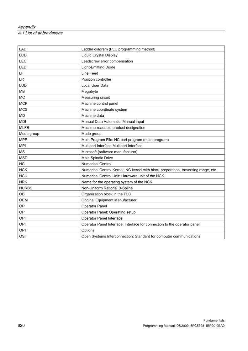
Appendix A.1 List of abbreviations
Fundamentals 620 Programming Manual, 06/2009, 6FC5398-1BP20-0BA0
LAD Ladder diagram (PLC programming method) LCD Liquid Crystal Display LEC Leadscrew error compensation LED Light-Emitting Diode LF Line Feed LR Position controller LUD Local User Data MB Megabyte MC Measuring circuit MCP Machine control panel MCS Machine coordinate system MD Machine data MDI Manual Data Automatic: Manual input MLFB Machine-readable product designation Mode group Mode group MPF Main Program File: NC part program (main program) MPI Multiport Interface Multiport Interface MS Microsoft (software manufacturer) MSD Main Spindle Drive NC Numerical Control NCK Numerical Control Kernel: NC kernel with block preparation, traversing range, etc. NCU Numerical Control Unit: Hardware unit of the NCK NRK Name for the operating system of the NCK NURBS Non-Uniform Rational B-Spline OB Organization block in the PLC OEM Original Equipment Manufacturer OP Operator Panel OP Operator Panel: Operating setup OPI Operator Panel Interface OPI Operator Panel Interface: Interface for connection to the operator panel OPT Options OSI Open Systems Interconnection: Standard for computer communications
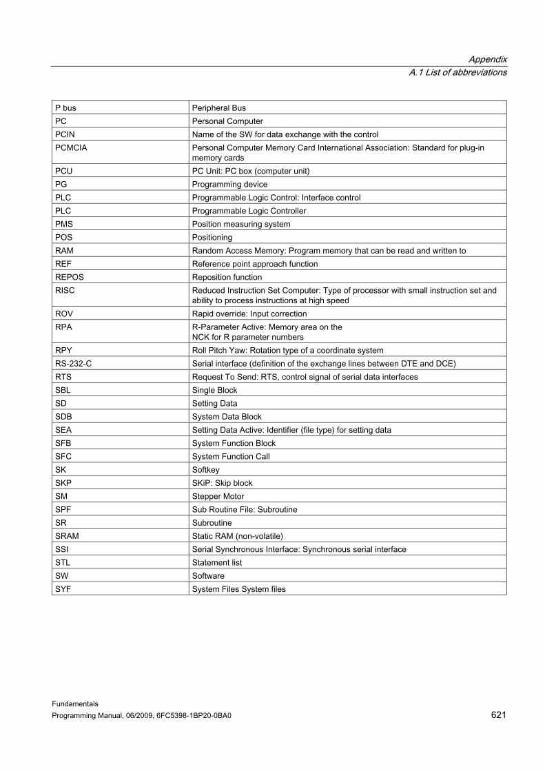
Appendix A.1 List of abbreviations
Fundamentals Programming Manual, 06/2009, 6FC5398-1BP20-0BA0 621
P bus Peripheral Bus PC Personal Computer PCIN Name of the SW for data exchange with the control PCMCIA Personal Computer Memory Card International Association: Standard for plug-in
memory cards PCU PC Unit: PC box (computer unit) PG Programming device PLC Programmable Logic Control: Interface control PLC Programmable Logic Controller PMS Position measuring system POS Positioning RAM Random Access Memory: Program memory that can be read and written to REF Reference point approach function REPOS Reposition function RISC Reduced Instruction Set Computer: Type of processor with small instruction set and
ability to process instructions at high speed ROV Rapid override: Input correction RPA R-Parameter Active: Memory area on the
NCK for R parameter numbers RPY Roll Pitch Yaw: Rotation type of a coordinate system RS-232-C Serial interface (definition of the exchange lines between DTE and DCE) RTS Request To Send: RTS, control signal of serial data interfaces SBL Single Block SD Setting Data SDB System Data Block SEA Setting Data Active: Identifier (file type) for setting data SFB System Function Block SFC System Function Call SK Softkey SKP SKiP: Skip block SM Stepper Motor SPF Sub Routine File: Subroutine SR Subroutine SRAM Static RAM (non-volatile) SSI Serial Synchronous Interface: Synchronous serial interface STL Statement list SW Software SYF System Files System files
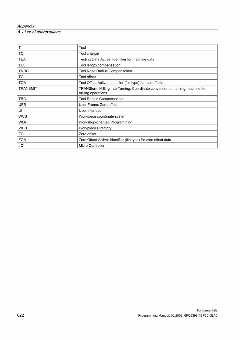
Appendix A.1 List of abbreviations
Fundamentals 622 Programming Manual, 06/2009, 6FC5398-1BP20-0BA0
T Tool TC Tool change TEA Testing Data Active: Identifier for machine data TLC Tool length compensation TNRC Tool Nose Radius Compensation TO Tool offset TOA Tool Offset Active: Identifier (file type) for tool offsets TRANSMIT TRANSform Milling Into Turning: Coordinate conversion on turning machine for
milling operations TRC Tool Radius Compensation UFR User Frame: Zero offset UI User interface WCS Workpiece coordinate system WOP Workshop-oriented Programming WPD Workpiece Directory ZO Zero offset ZOA Zero Offset Active: Identifier (file type) for zero offset data µC Micro Controller

Appendix A.2 Feedback on the documentation
Fundamentals Programming Manual, 06/2009, 6FC5398-1BP20-0BA0 623
A.2 A.2 Feedback on the documentation This document will be continuously improved with regard to its quality and ease of use. Please help us with this task by sending your comments and suggestions for improvement via e-mail or fax to: E-mail: mailto:[email protected] Fax: +49 9131 - 98 2176
Please use the fax form on the back of this page.

Appendix A.2 Feedback on the documentation
Fundamentals 624 Programming Manual, 06/2009, 6FC5398-1BP20-0BA0

Appendix A.3 Documentation overview
Fundamentals Programming Manual, 06/2009, 6FC5398-1BP20-0BA0 625
A.3 A.3 Documentation overview

Appendix A.3 Documentation overview
Fundamentals 626 Programming Manual, 06/2009, 6FC5398-1BP20-0BA0
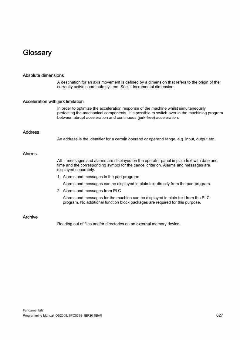
Fundamentals Programming Manual, 06/2009, 6FC5398-1BP20-0BA0 627
Glossary
Absolute dimensions A destination for an axis movement is defined by a dimension that refers to the origin of the currently active coordinate system. See → Incremental dimension
Acceleration with jerk limitation In order to optimize the acceleration response of the machine whilst simultaneously protecting the mechanical components, it is possible to switch over in the machining program between abrupt acceleration and continuous (jerk-free) acceleration.
Address An address is the identifier for a certain operand or operand range, e.g. input, output etc.
Alarms All → messages and alarms are displayed on the operator panel in plain text with date and time and the corresponding symbol for the cancel criterion. Alarms and messages are displayed separately. 1. Alarms and messages in the part program:
Alarms and messages can be displayed in plain text directly from the part program. 2. Alarms and messages from PLC
Alarms and messages for the machine can be displayed in plain text from the PLC program. No additional function block packages are required for this purpose.
Archive Reading out of files and/or directories on an external memory device.

Glossary
Fundamentals 628 Programming Manual, 06/2009, 6FC5398-1BP20-0BA0
Asynchronous subroutine Part program that can be started asynchronously to (independently of) the current program status using an interrupt signal (e.g. "Rapid NC input" signal).
Automatic Operating mode of the control (block sequence operation according to DIN): Operating mode for NC systems in which a → subprogram is selected and executed continuously.
Auxiliary functions Auxiliary functions enable → part programs to transfer → parameters to the → PLC, which then trigger reactions defined by the machine manufacturer.
Axes In accordance with their functional scope, the CNC axes are subdivided into: ● Axes: interpolating path axes ● Auxiliary axes: non-interpolating feed and positioning axes with an axis-specific feed rate.
Auxiliary axes are not involved in actual machining, e.g. tool feeder, tool magazine.
Axis address See → Axis identifier
Axis identifier Axes are identifed using X, Y, and Z as defined in DIN 66217 for a dextrorotatory, right-angled → coordinate system. Rotary axes rotating around X, Y, and Z are identified using A, B, and C. Additional axes situated parallel to the specified axes can be designated using other letters.
Axis name See → Axis identifier
Glossary
Fundamentals Programming Manual, 06/2009, 6FC5398-1BP20-0BA0 629
Backlash compensation Compensation for a mechanical machine backlash, e.g. backlash on reversal for ball screws. Backlash compensation can be entered separately for each axis.
Backup battery The backup battery ensures that the → user program in the → CPU is stored so that it is safe from power failure and so that specified data areas and bit memory, timers and counters are stored retentively.
Base axis Axis whose setpoint or actual value position forms the basis of the calculation of a compensation value.
Basic Coordinate System Cartesian coordinate system which is mapped by transformation onto the machine coordinate system. The programmer uses axis names of the basic coordinate system in the → part program. The basic coordinate system exists parallel to the → machine coordinate system if no → transformation is active. The difference between the two coordinate systems lies in the → axis identifiers.
Baud rate Rate of data transfer (Bit/s).
Blank Workpiece as it is before it is machined.
Block "Block" is the term given to any files required for creating and processing programs.
Glossary
Fundamentals 630 Programming Manual, 06/2009, 6FC5398-1BP20-0BA0
Block search For debugging purposes or following a program abort, the "Block search" function can be used to select any location in the part program at which the program is to be started or resumed.
Booting Loading the system program after power ON.
C axis Axis around which the tool spindle describes a controlled rotational and positioning movement.
Channel A channel is characterized by the fact that it can process a → part program independently of other channels. A channel exclusively controls the axes and spindles assigned to it. Part program runs of different channels can be coordinated through → synchronization.
Circular interpolation The → tool moves on a circle between specified points on the contour at a given feed rate, and the workpiece is thereby machined.
CNC See → NC
COM Component of the NC for the implementation and coordination of communication.
Compensation axis Axis with a setpoint or actual value modified by the compensation value

Glossary
Fundamentals Programming Manual, 06/2009, 6FC5398-1BP20-0BA0 631
Compensation memory Data range in the control, in which the tool offset data are stored.
Compensation table Table containing interpolation points. It provides the compensation values of the compensation axis for selected positions on the basic axis.
Compensation value Difference between the axis position measured by the encoder and the desired, programmed axis position.
Connecting cables Connecting cables are pre-assembled or user-assembled 2-wire cables with a connector at each end. This connecting cable connects the → CPU to a → programming device or to other CPUs by means of a → multi-point interface (MPI).
Continuous-path mode The objective of continuous-path mode is to avoid substantial deceleration of the → path axes at the part program block boundaries and to change to the next block at as close to the same path velocity as possible.
Contour Contour of the → workpiece
Contour monitoring The following error is monitored within a definable tolerance band as a measure of contour accuracy. An unacceptably high following error can cause the drive to become overloaded, for example. In such cases, an alarm is output and the axes are stopped.
Coordinate system See → Machine coordinate system, → Workpiece coordinate system
Glossary
Fundamentals 632 Programming Manual, 06/2009, 6FC5398-1BP20-0BA0
CPU Central processing unit, see → PLC
C-Spline The C-Spline is the most well-known and widely used spline. The transitions at the interpolation points are continuous, both tangentially and in terms of curvature. 3rd order polynomials are used.
Curvature The curvature k of a contour is the inverse of radius r of the nestling circle in a contour point (k = 1/r).
Cycles Protected subroutines for execution of repetitive machining operations on the → workpiece.
Data Block 1. Data unit of the → PLC that → HIGHSTEP programs can access. 2. Data unit of the → NC: Data modules contain data definitions for global user data. These
data can be initialized directly when they are defined.
Data word Two-byte data unit within a → data block.
Diagnosis 1. Operating area of the control. 2. The control has both a self-diagnostics program as well as test functions for servicing
purposes: status, alarm, and service displays
Dimensions specification, metric and inches Position and lead values can be programmed in inches in the machining program. Irrespective of the programmable dimensions (G70/G71), the controller is set to a basic system.

Glossary
Fundamentals Programming Manual, 06/2009, 6FC5398-1BP20-0BA0 633
DRF Differential Resolver Function: NC function which generates an incremental zero offset in Automatic mode in conjunction with an electronic handwheel.
Drive The drive is the unit of the CNC that performs the speed and torque control based on the settings of the NC.
Dynamic feedforward control Inaccuracies in the → contour due to following errors can be practically eliminated using dynamic, acceleration-dependent feedforward control. This results in excellent machining accuracy even at high → path velocities. Feedforward control can be selected and deselected on an axis-specific basis via the → part program.
Editor The editor makes it possible to create, edit, extend, join, and import programs/texts/program blocks.
Exact stop When an exact stop statement is programmed, the position specified in a block is approached exactly and, if necessary, very slowly. To reduce the approach time, → exact stop limits are defined for rapid traverse and feed.
Exact stop limit When all path axes reach their exact stop limits, the control responds as if it had reached its precise destination point. A block advance of the → part program occurs.
External zero offset Zero offset specified by the → PLC.

Glossary
Fundamentals 634 Programming Manual, 06/2009, 6FC5398-1BP20-0BA0
Fast retraction from contour When an interrupt occurs, a motion can be initiated via the CNC machining program, enabling the tool to be quickly retracted from the workpiece contour that is currently being machined. The retraction angle and the distance retracted can also be parameterized. After fast retraction, an interrupt routine can also be executed (SINUMERIK 840D).
Feed override The programmed velocity is overriden by the current velocity setting made via the → machine control panel or from the → PLC (0 to 200%). The feedrate can also be corrected by a programmable percentage factor (1-200%) in the machining program.
Finished-part contour Contour of the finished workpiece. See → Raw part.
Fixed machine point Point that is uniquely defined by the machine tool, e.g. machine reference point.
Fixed-point approach Machine tools can approach fixed points such as a tool change point, loading point, pallet change point, etc. in a defined way. The coordinates of these points are stored in the control. The control moves the relevant axes in → rapid traverse, whenever possible.
Frame A frame is an arithmetic rule that transforms one Cartesian coordinate system into another Cartesian coordinate system. A frame contains the following components: → zero offset, → rotation, → scaling, → mirroring.
Geometry Description of a → workpiece in the → workpiece coordinate system.
Geometry axis Geometry axes are used to describe a 2- or 3-dimensional area in the workpiece coordinate system.
Glossary
Fundamentals Programming Manual, 06/2009, 6FC5398-1BP20-0BA0 635
Ground Ground is taken as the total of all linked inactive parts of a device which will not become live with a dangerous contact voltage even in the event of a malfunction.
Helical interpolation The helical interpolation function is ideal for machining internal and external threads using form milling cutters and for milling lubrication grooves. The helix comprises two movements: ● Circular movement in one plane ● A linear movement perpendicular to this plane
High-level CNC language The high-level language offers: → user-defined variables, → system variables, → macro techniques.
High-speed digital inputs/outputs The digital inputs can be used for example to start fast CNC program routines (interrupt routines). The digital CNC outputs can be used to trigger fast, program-controlled switching functions (SINUMERIK 840D).
HIGHSTEP Summary of programming options for → PLCs of the AS300/AS400 system.
Identifier In accordance with DIN 66025, words are supplemented using identifiers (names) for variables (arithmetic variables, system variables, user variables), subroutines, key words, and words with multiple address letters. These supplements have the same meaning as the words with respect to block format. Identifiers must be unique. It is not permissible to use the same identifier for different objects.

Glossary
Fundamentals 636 Programming Manual, 06/2009, 6FC5398-1BP20-0BA0
Inch measuring system Measuring system, which defines distances in inches and fractions of inches.
Inclined surface machining Drilling and milling operations on workpiece surfaces that do not lie in the coordinate planes of the machine can be performed easily using the function "inclined-surface machining".
Increment Travel path length specification based on number of increments. The number of increments can be stored as → setting data or be selected by means of a suitably labeled key (i.e. 10, 100, 1000, 10000).
Incremental dimension Also incremental dimension: A destination for axis traversal is defined by a distance to be covered and a direction referenced to a point already reached. See → Absolute dimension.
Intermediate blocks Motions with selected → tool offset (G41/G42) may be interrupted by a limited number of intermediate blocks (blocks without axis motions in the offset plane), whereby the tool offset can still be correctly compensated for. The permissible number of intermediate blocks which the control reads ahead can be set in system parameters.
Interpolator Logic unit of the → NCK that defines intermediate values for the motions to be carried out in individual axes based on information on the end positions specified in the part program.
Interpolatory compensation Interpolatory compensation is a tool that enables manufacturing-related leadscrew error and measuring system error compensations (SSFK, MSFK).

Glossary
Fundamentals Programming Manual, 06/2009, 6FC5398-1BP20-0BA0 637
Interrupt routine Interrupt routines are special → subroutines that can be started by events (external signals) in the machining process. A part program block which is currently being worked through is interrupted and the position of the axes at the point of interruption is automatically saved.
Inverse-time feedrate With SINUMERIK 840D, the time required for the path of a block to be traversed can be programmed for the axis motion instead of the feed velocity (G93).
JOG Control operating mode (setup mode): In JOG mode, the machine can be set up. Individual axes and spindles can be traversed in JOG mode by means of the direction keys. Additional functions in JOG mode include: → Reference point approach, → Repos, and → Preset (set actual value).
Key switch The key switch on the → machine control panel has four positions that are assigned functions by the operating system of the control. The key switch has three different colored keys that can be removed in the specified positions.
Keywords Words with specified notation that have a defined meaning in the programming language for → part programs.
KV Servo gain factor, a control variable in a control loop.
Leading axis The leading axis is the → gantry axis that exists from the point of view of the operator and programmer and, thus, can be influenced like a standard NC axis.
Leadscrew error compensation Compensation for the mechanical inaccuracies of a leadscrew participating in the feed. The control uses stored deviation values for the compensation.
Glossary
Fundamentals 638 Programming Manual, 06/2009, 6FC5398-1BP20-0BA0
Limit speed Maximum/minimum (spindle) speed: The maximum speed of a spindle can be limited by specifying machine data, the → PLC or → setting data.
Linear axis In contrast to a rotary axis, a linear axis describes a straight line.
Linear interpolation The tool travels along a straight line to the destination point while machining the workpiece.
Load memory The load memory is the same as → RAM for the CPU 314 of the → PLC.
Look Ahead The Look Ahead function is used to achieve an optimal machining speed by looking ahead over an assignable number of traversing blocks.
Machine axes Physically existent axes on the machine tool.
Machine control panel An operator panel on a machine tool with operating elements such as keys, rotary switches, etc., and simple indicators such as LEDs. It is used to directly influence the machine tool via the PLC.
Machine coordinate system A coordinate system, which is related to the axes of the machine tool.
Machine zero Fixed point of the machine tool to which all (derived) measuring systems can be traced back.
Glossary
Fundamentals Programming Manual, 06/2009, 6FC5398-1BP20-0BA0 639
Machining channel A channel structure can be used to shorten idle times by means of parallel motion sequences, e.g. moving a loading gantry simultaneously with machining. Here, a CNC channel must be regarded as a separate CNC control system with decoding, block preparation and interpolation.
Macro techniques Grouping of a set of statements under a single identifier. The identifier represents the set of consolidated statements in the program.
Main block A block prefixed by ":" introductory block, containing all the parameters required to start execution of a -> part program.
Main program The → part program designated by a number or an identifer in which additional main programs, subroutines, or → cycles can be called.
MDA Control operating mode: Manual Data Automatic. In the MDA mode, individual program blocks or block sequences with no reference to a main program or subroutine can be input and executed immediately afterwards through actuation of the NC start key.
Messages All messages programmed in the part program and → alarms detected by the system are displayed on the operator panel in plain text with date and time and the corresponding symbol for the cancel criterion. Alarms and messages are displayed separately.

Glossary
Fundamentals 640 Programming Manual, 06/2009, 6FC5398-1BP20-0BA0
Metric measuring system Standardized system of units: For length, e.g. mm (millimeters), m (meters).
Mirroring Mirroring reverses the signs of the coordinate values of a contour, with respect to an axis. It is possible to mirror with respect to more than one axis at a time.
Mode group Axes and spindles that are technologically related can be combined into one mode group. Axes/spindles of a BAG can be controlled by one or more → channels. The same → mode type is always assigned to the channels of the mode group.
Mode of operation An operating concept on a SINUMERIK control. The following modes are defined: → Jog, → MDA, → Automatic.
NC Numerical Control: Numerical control (NC) includes all components of machine tool control: → NCK, → PLC, HMI, → COM.
Note A more correct term for SINUMERIK 840D controls would be: Computerized Numerical Control

Glossary
Fundamentals Programming Manual, 06/2009, 6FC5398-1BP20-0BA0 641
NCK Numerical Control Kernel: Component of NC that executes the → part programs and basically coordinates the motion operations for the machine tool.
Network A network is the connection of multiple S7-300 and other end devices, e.g. a programming device via a → connecting cable. A data exchange takes place over the network between the connected devices.
NRK Numeric robotic kernel (operating system of → NCK)
NURBS The motion control and path interpolation that occurs within the control is performed based on NURBS (Non Uniform Rational B-Splines). As a result, a uniform process is available within the control for all interpolations for SINUMERIK 840D.
OEM The scope for implementing individual solutions (OEM applications) for the SINUMERIK 840D has been provided for machine manufacturers, who wish to create their own operator interface or integrate process-oriented functions in the control.
Operator Interface The user interface (UI) is the display medium for a CNC in the form of a screen. It features horizontal and vertical softkeys.

Glossary
Fundamentals 642 Programming Manual, 06/2009, 6FC5398-1BP20-0BA0
Oriented spindle stop Stops the workpiece spindle in a specified angular position, e.g. in order to perform additional machining at a particular location.
Oriented tool retraction RETTOOL: If machining is interrupted (e.g. when a tool breaks), a program command can be used to retract the tool in a user-specified orientation by a defined distance.
Overall reset In the event of an overall reset, the following memories of the → CPU are deleted: ● → Work memory ● Read/write area of → load memory ● → System memory ● → Backup memory
Override Manual or programmable control feature, which enables the user to override programmed feedrates or speeds in order to adapt them to a specific workpiece or material.
Glossary
Fundamentals Programming Manual, 06/2009, 6FC5398-1BP20-0BA0 643
Part program block Part of a → part program that is demarcated by a line feed. There are two types: → main blocks and → subblocks.
Part program management Part program management can be organized by → workpieces. The size of the user memory determines the number of programs and the amount of data that can be managed. Each file (programs and data) can be given a name consisting of a maximum of 24 alphanumeric characters.
Path axis Path axes include all machining axes of the → channel that are controlled by the → interpolator in such a way that they start, accelerate, stop, and reach their end point simultaneously.
Path feedrate Path feed affects → path axes. It represents the geometric sum of the feed rates of the → geometry axes involved.
Path velocity The maximum programmable path velocity depends on the input resolution. For example, with a resolution of 0.1 mm the maximum programmable path velocity is 1000 m/min.
PCIN data transfer program PCIN is an auxiliary program for sending and receiving CNC user data (e.g. part programs, tool offsets, etc.) via a serial interface. The PCIN program can run in MS-DOS on standard industrial PCs.
Glossary
Fundamentals 644 Programming Manual, 06/2009, 6FC5398-1BP20-0BA0
Peripheral module I/O modules represent the link between the CPU and the process. I/O modules are: ● → Digital input/output modules ● → Analog input/output modules ● → Simulator modules
PLC Programmable Logic Control: → Programmable logic controller. Component of → NC: Programmable controller for processing the control logic of the machine tool.
PLC program memory SINUMERIK 840D: The PLC user program, the user data and the basic PLC program are stored together in the PLC user memory.
PLC Programming The PLC is programmed using the STEP 7 software. The STEP 7 programming software is based on the WINDOWS standard operating system and contains the STEP 5 programming functions with innovative enhancements.
Polar coordinates A coordinate system, which defines the position of a point on a plane in terms of its distance from the origin and the angle formed by the radius vector with a defined axis.
Polynomial interpolation Polynomial interpolation enables a wide variety of curve characteristics to be generated, such as straight line, parabolic, exponential functions (SINUMERIK 840D).
Glossary
Fundamentals Programming Manual, 06/2009, 6FC5398-1BP20-0BA0 645
Positioning axis Axis that performs an auxiliary movement on a machine tool (e.g. tool magazine, pallet transport). Positioning axes are axes that do not interpolate with → path axes.
Pre-coincidence Block change occurs already when the path distance approaches an amount equal to a specifiable delta of the end position.
Program block Program blocks contain the main program and subroutines of → part programs.
Programmable frames Programmable → frames enable dynamic definition of new coordinate system output points while the part program is being executed. A distinction is made between absolute definition using a new frame and additive definition with reference to an existing starting point.
Programmable Logic Control Programmable logic controllers (PLC) are electronic controls, the function of which is stored as a program in the control unit. This means that the layout and wiring of the device do not depend on the function of the control. The programmable logic controller has the same structure as a computer; it consists of a CPU (central module) with memory, input/output modules and an internal bus system. The peripherals and the programming language are matched to the requirements of the control technology.
Glossary
Fundamentals 646 Programming Manual, 06/2009, 6FC5398-1BP20-0BA0
Programmable working area limitation Limitation of the motion space of the tool to a space defined by programmed limitations.
Programming key Character and character strings that have a defined meaning in the programming language for → part programs.
Protection zone Three-dimensional zone within the → working area into which the tool tip must not pass.
Quadrant error compensation Contour errors at quadrant transitions, which arise as a result of changing friction conditions on the guideways, can be virtually entirely eliminated with the quadrant error compensation. Parameterization of the quadrant error compensation is performed by means of a circuit test.
R parameters Arithmetic parameter that can be set or queried by the programmer of the → part program for any purpose in the program.
Rapid traverse The highest traverse rate of an axis. For example, rapid traverse is used when the tool approaches the → workpiece contour from a resting position or when the tool is retracted from the workpiece contour. The rapid traverse velocity is set on a machine-specific basis using a machine data element.
Glossary
Fundamentals Programming Manual, 06/2009, 6FC5398-1BP20-0BA0 647
Reference point Machine tool position that the measuring system of the → machine axes references.
Rotary axis Rotary axes apply a workpiece or tool rotation to a defined angular position.
Rotation Component of a → frame that defines a rotation of the coordinate system around a particular angle.
Rounding axis Rounding axes rotate a workpiece or tool to an angular position corresponding to an indexing grid. When a grid index is reached, the rounding axis is "in position".
Safety functions The control is equipped with permanently active montoring functions that detect faults in the → CNC, the → PLC, and the machine in a timely manner so that damage to the workpiece, tool, or machine is largely prevented. In the event of a fault, the machining operation is interrupted and the drives stopped. The cause of the malfunction is logged and output as an alarm. At the same time, the PLC is notified that a CNC alarm has been triggered.
Scaling Component of a → frame that implements axis-specific scale modifications.

Glossary
Fundamentals 648 Programming Manual, 06/2009, 6FC5398-1BP20-0BA0
Selecting Series of statements to the NC that act in concert to produce a particular → workpiece. Likewise, this term applies to execution of a particular machining operation on a given → raw part.
Serial RS-232-C interface For data input/output, the PCU 20 has one serial V.24 interface (RS232) while the PCU 50/70 has two V.24 interfaces. Machining programs and manufacturer and user data can be loaded and saved via these interfaces.
Setting data Data, which communicates the properties of the machine tool to the NC, as defined by the system software.
Softkey A key, whose name appears on an area of the screen. The choice of soft keys displayed is dynamically adapted to the operating situation. The freely assignable function keys (soft keys) are assigned defined functions in the software.
Software limit switch Software limit switches limit the traversing range of an axis and prevent an abrupt stop of the slide at the hardware limit switch. Two value pairs can be specified for each axis and activated separately by means of the → PLC.
Spline interpolation With spline interpolation, the controller can generate a smooth curve characteristic from only a few specified interpolation points of a set contour.

Glossary
Fundamentals Programming Manual, 06/2009, 6FC5398-1BP20-0BA0 649
SRT Transformation ratio
Standard cycles Standard cycles are provided for machining operations, which are frequently repeated: ● Cycles for drilling/milling applications ● for turning technology The available cycles are listed in the "Cycle support" menu in the "Program" operating area. Once the desired machining cycle has been selected, the parameters required for assigning values are displayed in plain text.
Subblock Block preceded by "N" containing information for a sequence, e.g. positional data.
Subroutine Sequence of statements of a → part program that can be called repeatedly with different defining parameters. The subroutine is called from a main program. Every subroutine can be protected against unauthorized read-out and display. → Cycles are a form of subroutines.
Synchronization Statements in → part programs for coordination of sequences in different → channels at certain machining points.

Glossary
Fundamentals 650 Programming Manual, 06/2009, 6FC5398-1BP20-0BA0
Synchronized actions 1. Auxiliary function output
During workpiece machining, technological functions (→ auxiliary functions) can be output from the CNC program to the PLC. For example, these auxiliary functions are used to control additional equipment for the machine tool, such as quills, grabbers, clamping chucks, etc.
2. Fast auxiliary function output For time-critical switching functions, the acknowledgement times for the → auxiliary functions can be minimized and unnecessary hold points in the machining process can be avoided.
Synchronized axes Synchronized axes take the same time to traverse their path as the geometry axes take for their path.
Synchronized axis A synchronized axis is the → gantry axis whose set position is continuously derived from the motion of the → leading axis and is, thus, moved synchronously with the leading axis. From the point of view of the programmer and operator, the synchronized axis "does not exist".
System memory The system memory is a memory in the CPU in which the following data is stored: ● Data required by the operating system ● The operands times, counters, markers
System variables A variable that exists without any input from the programmer of a → part program. It is defined by a data type and the variable name preceded by the character $. See → User-defined variable.
Glossary
Fundamentals Programming Manual, 06/2009, 6FC5398-1BP20-0BA0 651
Tapping without compensating chuck This function allows threads to be tapped without a compensating chuck. By using the interpolating method of the spindle as a rotary axis and the drilling axis, threads can be cut to a precise final drilling depth, e.g. for blind hole threads (requirement: spindles in axis operation).
Text editor See → Editor
TOA area The TOA area includes all tool and magazine data. By default, this area coincides with the → channel area with regard to the reach of the data. However, machine data can be used to specify that multiple channels share one → TOA unit so that common tool management data is then available to these channels.
TOA unit Each → TOA area can have more than one TOA unit. The number of possible TOA units is limited by the maximum number of active → channels. A TOA unit includes exactly one tool data block and one magazine data block. In addition, a TOA unit can also contain a toolholder data block (optional).
Tool Active part on the machine tool that implements machining (e.g. turning tool, milling tool, drill, LASER beam, etc.).
Tool nose radius compensation Contour programming assumes that the tool is pointed. Because this is not actually the case in practice, the curvature radius of the tool used must be communicated to the control which then takes it into account. The curvature center is maintained equidistantly around the contour, offset by the curvature radius.
Glossary
Fundamentals 652 Programming Manual, 06/2009, 6FC5398-1BP20-0BA0
Tool offset Consideration of the tool dimensions in calculating the path.
Tool radius compensation To directly program a desired → workpiece contour, the control must traverse an equistant path to the programmed contour taking into account the radius of the tool that is being used (G41/G42).
Transformation Additive or absolute zero offset of an axis.
Traversing range The maximum permissible travel range for linear axes is ± 9 decades. The absolute value depends on the selected input and position control resolution and the unit of measurement (inch or metric).
User memory All programs and data, such as part programs, subroutines, comments, tool offsets, and zero offsets/frames, as well as channel and program user data, can be stored in the shared CNC user memory.
User program User programs for the S7-300 automation systems are created using the programming language STEP 7. The user program has a modular layout and consists of individual blocks. The basic block types are: ● Code blocks
These blocks contain the STEP 7 commands. ● Data blocks
These blocks contain constants and variables for the STEP 7 program.
User-defined variable Users can declare their own variables for any purpose in the → part program or data block (global user data). A definition contains a data type specification and the variable name. See → System variable.
Glossary
Fundamentals Programming Manual, 06/2009, 6FC5398-1BP20-0BA0 653
Variable definition A variable definition includes the specification of a data type and a variable name. The variable names can be used to access the value of the variables.
Velocity control In order to achieve an acceptable traverse rate in the case of very slight motions per block, an anticipatory evaluation over several blocks (→ Look Ahead) can be specified.
WinSCP WinSCP is a freely available open source program for Windows for the transfer of files.
Working area Three-dimensional zone into which the tool tip can be moved on account of the physical design of the machine tool. See → Protection zone.
Working area limitation With the aid of the working area limitation, the traversing range of the axes can be further restricted in addition to the limit switches. One value pair per axis may be used to describe the protected working area.
Working memory RAM is a work memory in the → CPU that the processor accesses when processing the application program.
Workpiece Part to be made/machined by the machine tool.
Workpiece contour Set contour of the → workpiece to be created or machined.
Workpiece coordinate system The workpiece coordinate system has its starting point in the → workpiece zero-point. In machining operations programmed in the workpiece coordinate system, the dimensions and directions refer to this system.
Workpiece zero The workpiece zero is the starting point for the → workpiece coordinate system. It is defined in terms of distances to the → machine zero.
Glossary
Fundamentals 654 Programming Manual, 06/2009, 6FC5398-1BP20-0BA0
Zero offset Specifies a new reference point for a coordinate system through reference to an existing zero point and a → frame. 1. Settable
SINUMERIK 840D: A configurable number of settable zero offsets are available for each CNC axis. The offsets - which are selected by means of G functions - take effect alternately.
2. External In addition to all the offsets which define the position of the workpiece zero, an external zero offset can be overridden by means of the handwheel (DRF offset) or from the PLC.
3. Programmable Zero offsets can be programmed for all path and positioning axes using the TRANS statement.

Fundamentals Programming Manual, 06/2009, 6FC5398-1BP20-0BA0 655
Index
$ $AA_ACC, 153 $AA_FGREF, 127 $AA_FGROUP, 127 $AA_OFF, 415 $AC_F_TYPE, 171 $AC_FGROUP_MASK, 127 $AC_FZ, 171 $AC_S_TYPE, 107 $AC_SVC, 107 $AC_TOFF, 93 $AC_TOFFL, 93 $AC_TOFFR, 93 $AC_WORKAREA_CS_LIMIT_MINUS, 434 $AC_WORKAREA_CS_LIMIT_PLUS, 434 $AC_WORKAREA_CS_MINUS_ENABLE, 434 $AC_WORKAREA_CS_PLUS_ENABLE, 434 $P_F_TYPE, 171 $P_FGROUP_MASK, 127 $P_FZ, 171 $P_GWPS, 117 $P_S_TYPE, 107 $P_SVC, 107 $P_TOFF, 93 $P_TOFFL, 93 $P_TOFFR, 93 $PA_FGREF, 127 $PA_FGROUP, 127 $TC_DPNT, 165 $TC_TP_MAX_VELO, 102 $TC_TPG1/...8/...9, 116
A A, 119 A=..., 191 Absolute dimensions, 19 AC, 183, 236 ACC, 152 Acceleration
Mode, 449 ACCLIMA, 452 ACN, 191 ACP, 191
Address, 39 Adjustable, 562 Extended address, 478 Fixed addresses, 559 modally effective, 477 non-modal, 477 Value assignment, 43 With axial extension, 477 With axis expansion, 560
Address letters, 558 Addresses, 475 ADIS, 357 ADISPOS, 357 ALF, 290 AMIRROR, 371 AMIRROR, 403 ANG, 260, 265 ANG1, 262 ANG2, 262, 265 Angle
Contour angle, 260 Contour definition angle, 262, 265
AP, 217, 222, 225, 239, 250 AP, 213 Approach point/angle, 314 AR, 225, 236, 250, 253 AROT, 371, 384 AROTS, 396 ASCALE, 371, 398 ATRANS, 371, 376 Auxiliary function output
High-speed, 421 In continuous-path mode, 422
Auxiliary function outputs, 419 Availability
System-dependent, 5 Axes
Channel, 465 Command, 467 Geometry, 463 Lead link axis, 470 Link, 468 Machine, 465 Main, 463 Path, 465 PLC, 467

Index
Fundamentals 656 Programming Manual, 06/2009, 6FC5398-1BP20-0BA0
Positioning, 466 Synchronized, 467
Axis Container, 469 Types, 461
Axis types Special axes, 464
B B=..., 191 Basic coordinate system (BCS), 31 Basic offset, 33 Basic zero system, 33 Binary
Constant, 482 Block, 39
Components, 39 End, 42 Length, 42 Number, 42 Order of the statements, 43 Skip, 45, 46 Structure, 39
Blocking point, 25 Bottleneck
Detection, 342 BRISK, 449 BRISKA, 449 BZS, 33
C C=..., 191 CALCPOSI, 432, 610 Cartesian coordinates, 15 CDOF, 340 CDOF2, 340 CDON, 340 CFC, 158 CFIN, 158 CFTCP, 158 Chamfer, 295 Channel
Axes, 465 Character set, 49 CHF, 295 CHR, 262, 265, 295 CIP, 225, 242 Circular interpolation
Helical interpolation, 250
Circular-path programming With center and end points, 225, 229 With interpolation and end points, 225, 242 With opening angle and center point, 225, 236 With polar angle and polar radius, 225 With polar coordinates, 239 With radius and end point, 225, 233 With tangential transition, 225
Clamping torque, 446 Collision detection, 340 Command, 39
Axes, 467 Comments, 44 Compensation
Plane, 346 Tool length, 70 Tool radius, 71
Compensation memory, 72 Constant
Binary constant, 482 Hexadecimal constant, 481 Integer constant, 481
Continuous-path mode, 357 Contour
Accuracy, programmable, 457 Approach/leave, 312 Calculator, 259 Definition, 259 Element, 207 Point, 317
Contour corner Chamfer, 295 Round, 295
Contour definitions 3 straight lines, 265 Straight line with angle, 260 Two straight lines, 262
Coordinate system Workpiece, 35
Coordinate systems, 13 Coordinate systems, 27 Coordinate transformations (frames), 35 Coordinates
Cartesian, 15, 209 Cylindrical, 214 Polar, 18, 213
Corner rounding, 357 CORROF, 415 CPRECOF, 457 CPRECON, 457 CR, 225, 233, 253 CROTS, 396

Index
Fundamentals Programming Manual, 06/2009, 6FC5398-1BP20-0BA0 657
CT, 225, 246 CUT2D, 344 CUT2DF, 344 CUTCONOF, 347 CUTCONON, 347 Cutting edge
Center point, 72 Position, 72 Radius, 72
Cutting edges Number of contour tools, 345
Cutting rate, 100 Constant, 108
Cylinder thread, 275 Cylindrical coordinates, 214
D D number, 84 D..., 84 D0, 84 DAC, 200 DC, 191 DIACYCOFA, 200 DIAM90, 197 DIAM90A, 200 DIAMCHAN, 200 DIAMCHANA, 200 DIAMCYCOF, 197 Diameter programming, 197 DIAMOF, 197 DIAMOFA, 200 DIAMON, 197 DIAMONA, 200 DIC, 200 DILF, 290 Dimensions, 183
For rotary axes and spindles, 191 In inches, 194 In millimeters, 194 In the diameter, 197 In the radius, 197
Dimensions in inches, 194 Dimensions in millimeters, 194 DIN 66025, 39 DIN 66217, 28 Direction of rotation, 29 DISC, 319 DISCL, 323 DISR, 323 Distance
Calculation, 474
DITE, 278 DITS, 278 DRFOF, 415 Drill, 77 DRIVE, 449 DRIVEA, 449 Dwell time, 458 DYNFINISH, 454 DYNNORM, 454 DYNPOS, 454 DYNROUGH, 454 DYNSEMIFIN, 454
E Edges
Number, 85 Effectiveness
modal, 477 Non-modal, 477
End of block LF, 49 Exact stop, 353 Extended address, 478
F F..., 119, 222, 281 FA, 129, 146 Face thread, 276 FAD, 323 FB, 164 FD, 154 FDA, 154 Feed
for positioning axes, 146 Feedrate, 119, 222
For path axes, 122 For synchronized axes, 123 Inverse-time, 123 Override, 156 Override, programmable, 150 Tooth, 165 Units, 124 With handwheel override, 154
FFWOF, 456 FFWON, 456 FGREF, 119 FGROUP, 119 Fixed point
Approach, 437
Index
Fundamentals 658 Programming Manual, 06/2009, 6FC5398-1BP20-0BA0
Fixed stop, 443 Clamping torque, 446 Monitoring, 446
FL, 119 FMA, 161 FP, 437 FPR, 146 FPRAOF, 146 FPRAON, 146 Frame, 369
Deselect, 414 Mirroring, programmable, 403 Operations, 371 Rotation, with solid angle, 396 Scaling, programmable, 398
Frames, 35 FRC, 295 FRCM, 295 FXS, 443 FXST, 443 FXSW, 443 FZ, 165
G G function groups, 568 G functions, 568 G group
Technology, 454 G0, 213, 217 G1, 213, 222 G110, 211 G111, 211 G112, 211 G140, 323 G141, 323 G142, 323 G143, 323 G147, 323 G148, 323 G153, 173, 414 G17, 179, 345 G18, 179 G19, 179, 345 G2, 213, 225, 229, 233, 236, 239 G247, 323 G248, 323 G25, 118, 429 G26, 118, 429 G3, 213, 225, 229, 233, 236, 239 G33, 270 G331, 283
G332, 283 G34, 281 G340, 323 G341, 323 G347, 323 G348, 323 G35, 281 G4, 458 G40, 301 G41, 84, 301 G42, 84, 301 G450, 319 G451, 319 G460, 335 G461, 335 G462, 335 G500, 173 G505 to G599, 173 G53, 173, 414 G54, 173 G55, 173 G56, 173 G57, 173 G58, 381 G59, 381 G60, 353 G601, 353 G602, 353 G603, 353 G63, 288 G64, 357 G641, 357 G642, 357 G643, 357 G644, 357 G645, 357 G70, 194 G700, 194 G71, 194 G710, 194 G74, 436 G75, 437 G751, 437 G9, 353 G90, 183 G91, 186 G93, 119 G94, 119 G95, 119 G96, 108 G961, 108 G962, 108
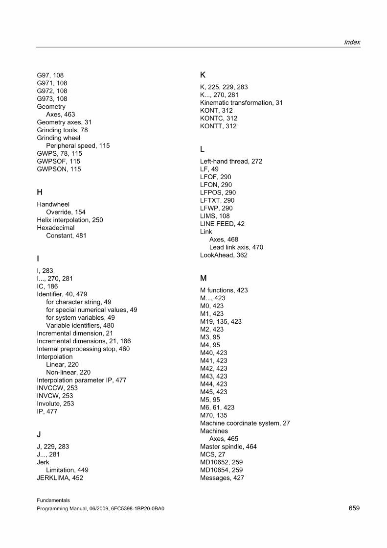
Index
Fundamentals Programming Manual, 06/2009, 6FC5398-1BP20-0BA0 659
G97, 108 G971, 108 G972, 108 G973, 108 Geometry
Axes, 463 Geometry axes, 31 Grinding tools, 78 Grinding wheel
Peripheral speed, 115 GWPS, 78, 115 GWPSOF, 115 GWPSON, 115
H Handwheel
Override, 154 Helix interpolation, 250 Hexadecimal
Constant, 481
I I, 283 I..., 270, 281 IC, 186 Identifier, 40, 479
for character string, 49 for special numerical values, 49 for system variables, 49 Variable identifiers, 480
Incremental dimension, 21 Incremental dimensions, 21, 186 Internal preprocessing stop, 460 Interpolation
Linear, 220 Non-linear, 220
Interpolation parameter IP, 477 INVCCW, 253 INVCW, 253 Involute, 253 IP, 477
J J, 229, 283 J..., 281 Jerk
Limitation, 449 JERKLIMA, 452
K K, 225, 229, 283 K..., 270, 281 Kinematic transformation, 31 KONT, 312 KONTC, 312 KONTT, 312
L Left-hand thread, 272 LF, 49 LFOF, 290 LFON, 290 LFPOS, 290 LFTXT, 290 LFWP, 290 LIMS, 108 LINE FEED, 42 Link
Axes, 468 Lead link axis, 470
LookAhead, 362
M M functions, 423 M..., 423 M0, 423 M1, 423 M19, 135, 423 M2, 423 M3, 95 M4, 95 M40, 423 M41, 423 M42, 423 M43, 423 M44, 423 M45, 423 M5, 95 M6, 61, 423 M70, 135 Machine coordinate system, 27 Machines
Axes, 465 Master spindle, 464 MCS, 27 MD10652, 259 MD10654, 259 Messages, 427
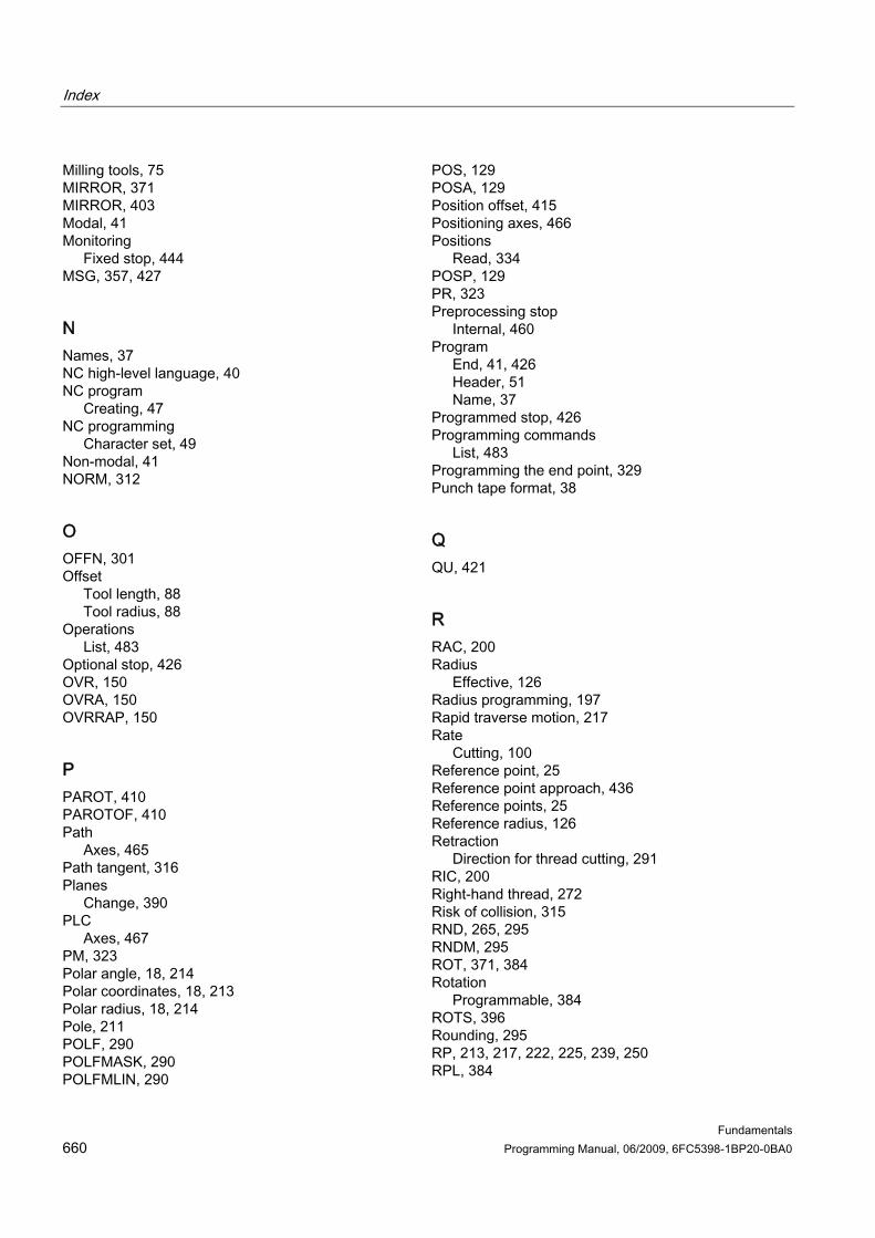
Index
Fundamentals 660 Programming Manual, 06/2009, 6FC5398-1BP20-0BA0
Milling tools, 75 MIRROR, 371 MIRROR, 403 Modal, 41 Monitoring
Fixed stop, 444 MSG, 357, 427
N Names, 37 NC high-level language, 40 NC program
Creating, 47 NC programming
Character set, 49 Non-modal, 41 NORM, 312
O OFFN, 301 Offset
Tool length, 88 Tool radius, 88
Operations List, 483
Optional stop, 426 OVR, 150 OVRA, 150 OVRRAP, 150
P PAROT, 410 PAROTOF, 410 Path
Axes, 465 Path tangent, 316 Planes
Change, 390 PLC
Axes, 467 PM, 323 Polar angle, 18, 214 Polar coordinates, 18, 213 Polar radius, 18, 214 Pole, 211 POLF, 290 POLFMASK, 290 POLFMLIN, 290
POS, 129 POSA, 129 Position offset, 415 Positioning axes, 466 Positions
Read, 334 POSP, 129 PR, 323 Preprocessing stop
Internal, 460 Program
End, 41, 426 Header, 51 Name, 37
Programmed stop, 426 Programming commands
List, 483 Programming the end point, 329 Punch tape format, 38
Q QU, 421
R RAC, 200 Radius
Effective, 126 Radius programming, 197 Rapid traverse motion, 217 Rate
Cutting, 100 Reference point, 25 Reference point approach, 436 Reference points, 25 Reference radius, 126 Retraction
Direction for thread cutting, 291 RIC, 200 Right-hand thread, 272 Risk of collision, 315 RND, 265, 295 RNDM, 295 ROT, 371, 384 Rotation
Programmable, 384 ROTS, 396 Rounding, 295 RP, 213, 217, 222, 225, 239, 250 RPL, 384
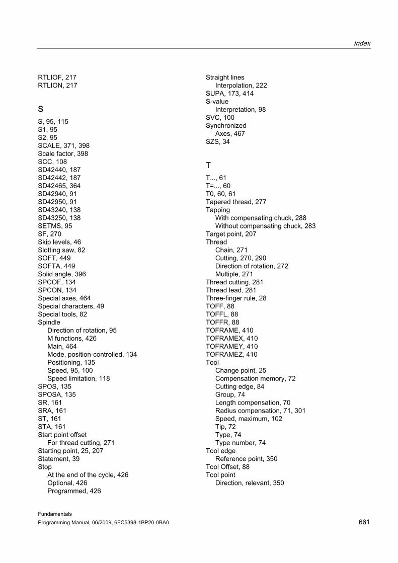
Index
Fundamentals Programming Manual, 06/2009, 6FC5398-1BP20-0BA0 661
RTLIOF, 217 RTLION, 217
S S, 95, 115 S1, 95 S2, 95 SCALE, 371, 398 Scale factor, 398 SCC, 108 SD42440, 187 SD42442, 187 SD42465, 364 SD42940, 91 SD42950, 91 SD43240, 138 SD43250, 138 SETMS, 95 SF, 270 Skip levels, 46 Slotting saw, 82 SOFT, 449 SOFTA, 449 Solid angle, 396 SPCOF, 134 SPCON, 134 Special axes, 464 Special characters, 49 Special tools, 82 Spindle
Direction of rotation, 95 M functions, 426 Main, 464 Mode, position-controlled, 134 Positioning, 135 Speed, 95, 100 Speed limitation, 118
SPOS, 135 SPOSA, 135 SR, 161 SRA, 161 ST, 161 STA, 161 Start point offset
For thread cutting, 271 Starting point, 25, 207 Statement, 39 Stop
At the end of the cycle, 426 Optional, 426 Programmed, 426
Straight lines Interpolation, 222
SUPA, 173, 414 S-value
Interpretation, 98 SVC, 100 Synchronized
Axes, 467 SZS, 34
T T..., 61 T=..., 60 T0, 60, 61 Tapered thread, 277 Tapping
With compensating chuck, 288 Without compensating chuck, 283
Target point, 207 Thread
Chain, 271 Cutting, 270, 290 Direction of rotation, 272 Multiple, 271
Thread cutting, 281 Thread lead, 281 Three-finger rule, 28 TOFF, 88 TOFFL, 88 TOFFR, 88 TOFRAME, 410 TOFRAMEX, 410 TOFRAMEY, 410 TOFRAMEZ, 410 Tool
Change point, 25 Compensation memory, 72 Cutting edge, 84 Group, 74 Length compensation, 70 Radius compensation, 71, 301 Speed, maximum, 102 Tip, 72 Type, 74 Type number, 74
Tool edge Reference point, 350
Tool Offset, 88 Tool point
Direction, relevant, 350

Index
Fundamentals 662 Programming Manual, 06/2009, 6FC5398-1BP20-0BA0
Tool radius compensation At outside corners, 319 CUT2D, 345
Toolholder Reference point, 25
Tooth feedrate, 165 TOROT, 410 TOROTOF, 410 TOROTX, 410 TOROTY, 410 TOROTZ, 410 TRAFOOF, 436 TRANS, 371, 376 Transition circle, 343 Transition radius, 320 Transverse axis, 197, 206 Travel command, 207 TURN, 250 Turning tools, 80
V Value assignment, 43 Variable identifiers, 480 VELOLIMA, 452
W WAB, 323 WAITMC, 129 WAITP, 129 WAITS, 135 WALCS0, 433 WALCS1-10, 433 WALIMOF, 429 WALIMON, 429 WCS, 35 Working area limitation
in BCS, 429 in WCS/SZS, 433 Reference points on the tool, 432
Working plane, 23, 179 Workpiece
Contour, 208 Workpiece coordinate system, 35
Align on workpiece, 410
X X..., 209 X2, 260 X3, 262
Y Y..., 209
Z Z..., 209 Z1, 262, 265 Z2, 260, 262, 265 Z3, 265 Z4, 265 Zero frame, 175 Zero offset
Offset values, 177 Settable, 34 Variable, 173
Zero point Offset, programmable, 376
Zero point Machine, 25 Workpiece, 25
Zero point Offset, axial, 381
Zero points, 25 For turning, 205
Zero system Settable, 34
Related Documents