Boise State University ScholarWorks Civil Engineering Faculty Publications and Presentations Department of Civil Engineering 6-1-2018 Shuffled Complex-Self Adaptive Hybrid EvoLution (SC-SAHEL) Optimization Framework Mojtaba Sadegh Boise State University For a complete list of authors, please see article. Publication Information Sadegh, Mojtaba. (2018). "Shuffled Complex-Self Adaptive Hybrid EvoLution (SC-SAHEL) Optimization Framework". Environmental Modelling & Soſtware, 104, 215-235. hp://dx.doi.org/10.1016/j.envsoſt.2018.03.019

Welcome message from author
This document is posted to help you gain knowledge. Please leave a comment to let me know what you think about it! Share it to your friends and learn new things together.
Transcript
Boise State UniversityScholarWorksCivil Engineering Faculty Publications andPresentations Department of Civil Engineering
6-1-2018
Shuffled Complex-Self Adaptive Hybrid EvoLution(SC-SAHEL) Optimization FrameworkMojtaba SadeghBoise State University
For a complete list of authors, please see article.
Publication InformationSadegh, Mojtaba. (2018). "Shuffled Complex-Self Adaptive Hybrid EvoLution (SC-SAHEL) Optimization Framework".Environmental Modelling & Software, 104, 215-235. http://dx.doi.org/10.1016/j.envsoft.2018.03.019
Shuffled Complex-Self Adaptive Hybrid EvoLution (SC-SAHEL) Optimization 1
Framework 2
Matin Rahnamay Naeini1, Tiantian Yang1,2, Mojtaba Sadegh1,3, Amir Aghakouchak1, Kuo-3
lin Hsu1 , Soroosh Sorooshian1, Qingyun Duan4, and Xiaohui Lei5 4
1Center for Hydrometeorology and Remote Sensing (CHRS) & Department of Civil and 5
Environmental Engineering, University of California, Irvine, California, USA. 6
2Deltares USA Inc., Silver Spring, Maryland, USA 7
3Department of Civil Engineering, Boise State University, Boise, Idaho, USA. 8
4Beijing Normal University, Faculty of Geographical Sciences. Beijing, China 9
5China Institute of Water Resources and Hydropower Research, Beijing, China 10
11
12
13
14
15
16
17
18
19
Corresponding author: Tiantian Yang ([email protected]) 20

Abstract 21
Simplicity and flexibility of Meta-Heuristic optimization algorithms have attracted lots of 22
attention in the field of optimization. Different optimization methods, however, hold algorithm-23
specific strengths and limitations, and selecting best-performing algorithm for a specific problem 24
is a tedious task. We introduce a new hybrid optimization framework, entitled Shuffled Complex-25
Self Adaptive Hybrid EvoLution (SC-SAHEL), which combines strengths of different 26
Evolutionary Algorithms (EAs) in a parallel computing scheme. SC-SAHEL explores 27
performance of different EAs, i.e., capability to escape local attractions, speed, convergence, etc., 28
during population evolution as each individual EA suits differently to various response surfaces. 29
The SC-SAHEL algorithm is benchmarked over 29 conceptual test functions, and a real-world 30
case - hydropower reservoir model. Results show that the SC-SAHEL algorithm is rigorous and 31
effective in finding global optimum for a majority of test cases, and computationally efficient 32
comparing to individual EAs. 33
Keywords 34
Shuffled Complex Evolution (SCE); Hybrid Optimization; Evolutionary Algorithm (EA); 35
Reservoir Operation; Hydropower 36
37

Software availability 38
Name of software: SC-SAHEL 39
Developer: Matin Rahnamay Naeini 40
Contact address: [email protected] 41
Program language: MATLAB 42
Year first available: 2018 43
Availability: Freely available to public at chrs.web.uci.edu/software.php and MathWorks website 44
Software requirements: MATLAB 9.0 45

1 Introduction 46
Meta-Heuristic optimization algorithms have gained a great deal of attention in science and 47
engineering (Blum and Roli 2003, Boussaïd et al. 2013, Lee and Geem 2005, Maier et al. 2014, 48
Nicklow et al. 2010, Reed et al. 2013). Simplicity and flexibility of these algorithms, along with 49
their robustness make them attractive tools for solving optimization problems (Coello et al. 2007, 50
Lee and Geem 2005). Many of the meta-heuristic algorithms are inspired by a physical 51
phenomenon, such as animals social and foraging behavior and natural selection. For example, 52
Simulated Annealing (Kirkpatrick et al. 1983), Big Bang-Big Crunch (Erol and Eksin 2006), 53
Gravitational Search Algorithm (Rashedi et al. 2009), Charged System Search (Kaveh and 54
Talatahari 2010) are inspired by various physical phenomena. Ant Colony Optimization (Dorigo 55
et al. 1996), Particle Swarm Optimization (Kennedy 2010), Bat-inspired Algorithm (Yang 2010), 56
Firefly Algorithm (Yang 2009), Dolphin Echolocation (Kaveh and Farhoudi 2013), Grey Wolf 57
Optimizer (Mirjalili et al. 2014), Bacterial Foraging (Passino 2002), Genetic Algorithm (Golberg 58
1989, Holland 1992), and Differential Evolution (Storn and Price 1997) are examples of algorithms 59
inspired by animal’s social and foraging behavior, and the natural selection mechanism of 60
Darwin’s Evolution Theorem. According to the No-Free-Lunch (NFL) (Wolpert and Macready 61
1997) theorem, none of these algorithms are consistently superior to others over a variety of 62
problems, although some of them may outperform on a certain type of optimization problem. 63
The NFL theorem has been a source of motivation for developing hybrid optimization 64
algorithms (Mirjalili et al. 2014, Woodruff et al. 2013). It has encouraged scientists and researchers 65
to combine the strengths of different algorithms and devise more robust and efficient optimization 66
algorithms that suit a broad class of problems (Qin and Suganthan 2005, Vrugt and Robinson 2007, 67
Vrugt et al. 2009, Hadka and Reed 2013, Sadegh et al. 2017). These efforts led to emergence of 68
multi-method and self-adaptive optimization algorithms such as Self-adaptive DE algorithm 69

(SaDE) (Qin and Suganthan 2005), A Multialgorithm Genetically Adaptive Method for Single 70
Objective Optimization (AMALGAM-SO) (Vrugt and Robinson 2007, Vrugt et al. 2009) and Borg 71
(Hadka and Reed 2013). They all reguarly update the search mechanism during the course of 72
optimization according to the information obtained from the response surface. 73
Here, we propose a new self-adaptive hybrid optimization framework, entitled Shuffled 74
Complex-Self Adaptive Hybrid EvoLution (SC-SAHEL). The SC-SAHEL framework employs 75
multiple Evolutionary Algorithms (EAs) as search cores, and enables competition among different 76
algorithms as optimization run progresses. The proposed framework differs from other multi-77
method algorithms as it grants independent evolution of population by each EA. In this framework, 78
population is partitioned into equally sized groups, so-called complexes; each assigned to different 79
EAs. Number of complexes assigned to each EA is regularly updated according to their 80
performance. In general, the newly developed framework has two main characteristics. First, all 81
the EAs evolve population in a parallel structure. Second, each participating EA works 82
independent of other EAs. The architecture of SC-SAHEL is inspired by the concept of the 83
Shuffled Complex Evolution algorithm - University of Arizona (SCE-UA) (Duan et al. 1992). The 84
SCE-UA algorithm is a population-evolution based algorithm (Madsen 2003), which evolves 85
individuals by partitioning population into different complexes. The complexes are evolved for a 86
specific number of iterations independent of other complexes, and then are forced to shuffle. 87
The SCE-UA framework employs Nelder-Mead simplex (Nelder and Mead 1965) 88
technique along with the concept of controlled random search (Price 1987), clustering (Kan and 89
Timmer 1987), competitive evolution (Holland 1975) and complex shuffling (Duan et al. 1993) to 90
offer a global optimization strategy. By employing these techniques, the SCE-UA algorithm 91
provides a robust optimization framework and has shown numerically to be competitive and 92
efficient comparing to other algorithms, such as GA, for calibrating rainfall-runoff models (Beven 93

2011, Gan and Biftu 1996, Wagener et al. 2004, Wang et al. 2010). The SCE-UA algorithm has 94
been widely used in water resources management (Barati et al. 2014, Eckhardt and Arnold 2001, 95
K. Ajami et al. 2004, Lin et al. 2006, Liong and Atiquzzaman 2004, Madsen 2000, Sorooshian et 96
al. 1993, Toth et al. 2000, Yang et al. 2015, Yapo et al. 1996), as well as other fields of study, such 97
as pyrolysis modeling (Ding et al. 2016, Hasalová et al. 2016) and Artificial Intelligence (Yang et 98
al. 2017). 99
Application of the SCE-UA is not limited to solving single objective optimization 100
problems. The Multi-Objective Complex evolution, University of Arizona (MOCOM-UA), is an 101
extension of the SCE-UA for solving multi-objective problems (Boyle et al. 2000, Yapo et al. 102
1998). Besides, the SCE-UA architecture has been used to develop Markov Chain Monte Carlo 103
(MCMC) sampling, named Shuffled Complex Evolution Metropolis algorithm (SCEM-UA) and 104
the Multi-Objective Shuffled Complex Evolution Metropolis (MOSCEM) to infer posterior 105
parameter distribution of hydrologic models (Vrugt et al. 2003a, Vrugt et al. 2003b). The 106
Metropolis scheme is used as the search kernel in the SCEM-UA and MOSCEM-UA (Chu et al. 107
2010, Vrugt et al. 2003a, Vrugt et al. 2003b). There is also an enhanced version of SCE-UA, which 108
is developed by Chu et al. (2011) entitled the Shuffled Complex strategy with Principle Component 109
Analysis, developed at the University of California, Irvine (SP-UCI). Chu et al. (2011) found that 110
the SCE-UA algorithm may not converge to the best solution on high-dimensional problems due 111
to “population degeneration” phenomenon. The “population degeneration” refers to the situation 112
when the search particles span a lower dimension space than the original search space (Chu et al. 113
2010), which causes the search algorithm to fail in finding the global optimum. To address this 114
issue, the SP-UCI algorithm employs Principle Component Analysis (PCA) in order to find and 115
restore the missing dimensions during the course of search (Chu et al. 2011). 116

Both SCE-UA and SP-UCI start the evolution process by generating a population within 117
the feasible parameters space. Then, population is partitioned into different complexes, and each 118
complex is evolved independently. Each member of the complex has the potential to contribute to 119
offspring in the evolution process. In each evolution step, more than two parents may contribute 120
to generating offspring. To make the evolution process competitive, a triangular probability 121
function is used to select parents. As a result, the fittest individuals will have a higher chance of 122
being selected. Each complex is evolved for a specific number of iterations, and then complexes 123
are shuffled to globally share the information attained by individuals during the search. 124
The Competitive Complex Evolution (CCE) and Modified Competitive Complex 125
Evolution (MCCE) are the search cores of the SCE-UA and SP-UCI algorithm, respectively. The 126
CCE and MCCE evolutionary processes are developed based on Nelder-Mead (Nelder and Mead 127
1965) method with some modification. The evolution process in the SCE-UA is not limited to 128
these algorithms. In fact, several studies have incorporated different EAs into the structure of the 129
SCE-UA algorithm. For example, the Frog Leaping (FL) is developed by adapting Particle Swarm 130
Optimization (PSO) algorithm to the SCE-UA structure for solving discrete problems (Eusuff et 131
al. 2006, Eusuff and Lansey 2003). Mariani et al. (2011) proposed an SCE-UA algorithm which 132
employs DE for evolving the complexes. These studies revealed the flexibility of the SCE-UA in 133
combination with other types of EAs; however, the potential of combining different algorithms 134
into a hybrid shuffled complex scheme has not been investigated. 135
The unique structure of the SCE-UA algorithm along with the flexibility of the algorithm 136
for using different EAs, motivated us to use the SCE-UA as the cornerstone of the SC-SAHEL 137
framework. The SC-SAHEL algorithm employs multiple EAs for evolving the population in a 138
similar structure as that of the SCE-UA, with the goal of selecting the most suitable search 139
algorithm at each optimization step. On the one hand, some EAs are more capable of visiting the 140

new regions of the search space and exploring the problem space, and hence are particularly 141
suitable at the beginning of the optimization (Olorunda and Engelbrecht 2008). On the other hand, 142
some EAs are more capable of searching within the visited regions of the search space, and hence 143
boosting the convergence process after finding the region of interest (Mirjalili and Hashim 2010). 144
Balancing between these two steps, which are referred to as exploration and exploitation (Moeini 145
and Afshar 2009), is a challenging task in stochastic optimization methods (Črepinšek et al. 2013). 146
The SC-SAHEL algorithm maintains a balance between exploration and exploitation phases by 147
evaluating the performance of participating EAs at each optimization step. EAs contribute to the 148
population evolution according to their performance in previous steps. The algorithms’ 149
performance is evaluated by comparing the evolved complexes before and after evolution. In this 150
process, the most suitable algorithm for the problem space become the dominant search core. 151
In this study, four different EAs are used as search cores in the proposed SC-SAHEL 152
framework, including Modified Competitive Complex Evolution (MCCE) used in the SP-UCI 153
algorithm, Modified Frog Leaping (MFL), Modified Grey Wolf Optimizer (MGWO), and 154
Differential Evolution (DE). To better illustrate the performance of the hybrid SC-SAHEL 155
algorithm, the framework is benchmarked over 29 test functions and compared to SC-SAHEL with 156
single EA. Among the 29 employed test functions, there are 23 classic test functions (Xin et al. 157
1999) and 6 composite test functions (Liang et al. 2005), which are commonly used as benchmarks 158
in comparing optimization algorithms. 159
Furthermore, the SC-SAHEL framework is tested for a conceptual hydropower model, 160
which is built for the Folsom reservoir located in the northern California, USA. The objective is 161
to maximize the hydropower generation, by finding the optimum discharge from the reservoir. The 162
study period covers run-off season in California from April to June, in which reservoirs have the 163
highest annual storage volume (Field and Lund 2006). Using the proposed framework, we 164

compared different EAs’ capability of finding a near-optimum solution for dry, wet, and below-165
normal scenarios. The results support that the proposed algorithm is not only competitive in terms 166
of increasing power generation, but also is able to reveal the advantages and disadvantages of 167
participating EAs. 168
The rest of the paper is organized as follow. In section 2, structure of the SC-SAHEL 169
algorithm and details of four EAs are presented. Section 3 presents the test functions, settings of 170
the experiments, and results obtained for each test function. Section 4 introduces the reservoir 171
model and the optimization results for the case study. Finally, in section 5, we draw conclusion, 172
summarize some limitations about the newly introduced framework, and suggest some directions 173
for future work. 174
175
2 Methodology 176
The SC-SAHEL algorithm is a parallel optimization framework, which is built based on 177
the original SCE-UA architecture. SC-SAHEL, however, differs from the original SCE-UA 178
algorithm by using multiple search mechanisms instead of only employing the Nelder-Mead 179
simplex downhill method. In this section, we first introduce the main structure of SC-SAHEL. 180
Then, we present four different EAs, which are employed as search cores in the SC-SAHEL 181
framework. These algorithms are selected for illustrative purpose only and can be replaced by 182
other evolutionary algorithms. Some modifications are made to the original form of these 183
algorithms, to allow fair competition between EAs. These modifications are detailed in the 184
appendix A-D. 185
186

2.1 The SC-SAHEL framework 187
The proposed SC-SAHEL optimization strategy starts with generating a population with a 188
pre-defined sampling method within feasible parameters’ range. The framework supports user-189
defined sampling methods, besides built-in Uniform Random Sampling (URS) and Latin 190
Hypercube Sampling (LHS). The population is then partitioned into different complexes. The 191
partitioning process warrants maintaining diversity of population in each complex. In doing so, 192
population is first sorted according to (objective) function values. Then, sorted population is 193
divided into NGS equally-sized groups (NGS being the number of complexes), ensuring that 194
members of each group have similar objective function values. Each complex subsequently will 195
randomly select a member from each of these groups. This procedure maintains diversity of the 196
population within each complex. The complexes are then assigned to EAs and evolved. In contrast 197
to the original concept of the SCE-UA, the complexes are evolved with different EAs rather than 198
single search mechanism. At the beginning of the search, an equal number of complexes is 199
assigned to each evolutionary method. For instance, if population is partitioned into 8 complexes 200
and 4 different EAs are used, each algorithm will evolve 2 complexes independently (2-2-2-2). 201
After evolving the complexes for pre-specified number of steps, the Evolutionary Method 202
Performance (EMP) metric (Eq.1) will be calculated for each EA, 203
EMP = mean(𝐹𝐹)−mean(𝐹𝐹𝑁𝑁)mean(𝐹𝐹) , (1) 204
in which, 𝐹𝐹 and 𝐹𝐹𝑁𝑁 are objective function values of individuals in each complex before and after 205
evolution, respectively. 206
The EMP metric measures change in the mean objective function value of individuals in 207
each complex in comparison to their previous state. A higher EMP value indicates a larger 208
reduction in the mean objective function value obtained by the individuals in the complex. The 209

performance of each evolutionary algorithm is then evaluated based on the mean value of EMP 210
calculated for each evolved complex. The algorithms are then ranked according to the EMP values. 211
Ranks are in turn used to assign number of complexes to each evolutionary method for the next 212
iteration. The highest ranked algorithm will be assigned an additional complex to evolve in the 213
next shuffling step, while, the lowest ranked evolutionary algorithm will lose one complex for the 214
next step. For instance, if all the EAs have 2 complexes to evolve (2-2-2-2 case), the number of 215
complexes assigned to each EA can be updated to 3-2-2-1. In other words, this logic is an “award 216
and punishment” process, in which the algorithm with best performances will be “awarded” with 217
an additional complex to evolve in the next iteration, while the worst-performing algorithm will 218
be “punished” by losing one complex. 219
It is worth mentioning that as some of the algorithms may have poor performance in the 220
exploration phase, they might lose all their complexes during the adaptation process. This might 221
be troublesome as these algorithms may be superior in the exploitation phase. If use of such 222
algorithms are terminated in the exploration phase, they cannot be selected during the convergence 223
steps. Hence, EAs termination is avoided to fully utilize the potential of EAs in all the optimization 224
steps and balance the exploration and exploitation phases. The minimum number of complexes 225
assigned to each evolutionary method is restricted to at least 1 complex in this case. If the lowest 226
ranked EA has only 1 complex to evolve, it won’t lose its last complex. If an algorithm outperforms 227
others throughout the evolution of complexes, the number of complexes assigned to the superior 228
EA will be equal to the total number of complexes minus the number of EAs plus one. In this case, 229
all other algorithms are evolving one complex only. As all algorithms are evolving at least one 230
complex, they have the chance to outperform other EAs and gain more complexes during the 231
optimization process, and to potentially become the dominant search method as the search 232

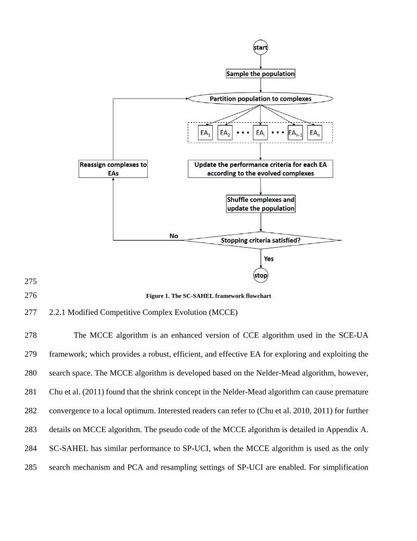
continues toward exploitation phase. Figure 1 briefly shows the flowchart of the SC-SAHEL 233
algorithm, pseudo code of which is as follows: 234
Step 0. Initialization. Select NGS > 1 and NPS (suggested NPS > 2n+1, where n is the 235
dimension of the problem), where NGS is the number of complexes and NPS is the number 236
of individuals in the complexes. NGS should be proportional to the number of evolutionary 237
algorithms so that all the participating EAs have an equal number of complexes at the 238
beginning of the search. 239
Step 1. Sample NPT points in the feasible parameter space using a user-defined sampling 240
method, where NPT equals to NGS×NPS. Compute objective function value for each point. 241
Step 2. Rank and sort all individuals in the order of increasing objective function value. 242
Step 3. Partition the entire population into complexes. Assign complexes to the 243
participating EAs. 244
Step 4. Monitor and restore population dimensionality using PCA algorithm (Optional). 245
Step 5. Evolve each complex using the corresponding EA. 246
Step 6. After evolving the complexes for a pre-defined number of iterations, calculate the 247
mean EMP for each EA. 248
Step 7. Rank the participating EAs according to the mean EMP value of each evolutionary 249
method. The highest ranked method will get additional complex in the next iteration, while 250
the worst evolutionary method will lose one. 251
Step 8. Shuffle complexes and form a new population. 252
Step 9. Check whether the convergence criteria are satisfied, otherwise go to step 3. 253
SC-SAHEL allows for different settings that can influence the performance of the 254
algorithm. Careful consideration should be devoted to the selection of these settings, including 255
number of complexes, number of individuals within each complex, number of evolution steps 256

before each shuffling, and stopping criteria thresholds. Some of these settings are adopted from 257
the suggested settings for the SCE-UA. For instance, the number of points within each complex is 258
set to 2𝑑𝑑 + 1, where 𝑑𝑑 is dimension of the problem. However, some of the suggested settings 259
cannot be applied to the SC-SAHEL framework due to use of different EAs. These settings can be 260
changed according to the complexity of the problem and the EAs used within the framework. For 261
instance, the number of complexes, the number of points within each complex, and the number of 262
evolution steps before each shuffling are problem dependent. 263
The SC-SAHEL framework employs three different stopping criteria which are adopted 264
from SCE-UA and SP-UCI. These stopping criteria include number of function evaluations, range 265
of samples that span the search space, and improvement in the objective function value in the last 266
m shuffling steps. These criteria are compared to pre-defined thresholds, which can in turn be tuned 267
according to the complexity of the problem. Improper selection of these thresholds may lead to 268
early or delayed convergence. 269
2.2 Evolutionary algorithms used in the SC-SAHEL 270
In this paper, we employ four different EAs to illustrate the flexibility of the SC-SAHEL 271
framework in adopting various EAs and show the algorithms competition. These algorithms are 272
briefly presented here. The pseudo code and details of these algorithms can be found in Appendix 273
A-D. 274
275
Figure 1. The SC-SAHEL framework flowchart 276
2.2.1 Modified Competitive Complex Evolution (MCCE) 277
The MCCE algorithm is an enhanced version of CCE algorithm used in the SCE-UA 278
framework; which provides a robust, efficient, and effective EA for exploring and exploiting the 279
search space. The MCCE algorithm is developed based on the Nelder-Mead algorithm, however, 280
Chu et al. (2011) found that the shrink concept in the Nelder-Mead algorithm can cause premature 281
convergence to a local optimum. Interested readers can refer to (Chu et al. 2010, 2011) for further 282
details on MCCE algorithm. The pseudo code of the MCCE algorithm is detailed in Appendix A. 283
SC-SAHEL has similar performance to SP-UCI, when the MCCE algorithm is used as the only 284
search mechanism and PCA and resampling settings of SP-UCI are enabled. For simplification 285

and comparison, SC-SAHEL with the MCCE algorithm as search core is referred as SP-UCI, 286
hereafter. 287
288
2.2.2 Modified Frog Leaping (MFL) 289
The Frog Leaping (FL) algorithm uses adapted PSO algorithm as a local search tool within the 290
SCE-UA framework (Eusuff and Lansey 2003). FL has shown to be an efficient search algorithm 291
for discrete optimization problems, and can find optimum solution much faster as compared to the 292
GA algorithm (Eusuff et al. 2006). In order to adapt the FL algorithm to the SC-SAHEL parallel 293
framework, we introduce a slightly modified version of FL algorithm entitled MFL. Further details 294
and pseudo code of the MFL can be found in Appendix B. The original FL algorithm and the MFL 295
have four main differences. First, the original FL is designed for discrete optimization problems, 296
however, the MFL is modified for continuous domain. Second, the modified FL uses the best point 297
in the subcomplex for generating new points, however, in the original FL framework new points 298
are generated using the best point in the complex and the entire population. The reason for this 299
modification is to avoid using any external information by participating EAs. In other words, the 300
amount of information given to each EAs is limited to the complex assigned to the EAs. Third, as 301
the MFL algorithm only uses the best point within the complex for generating the new generation, 302
two different jump rates are used. The reason for different jump rates is to allow MFL to have a 303
better exploration and exploitation ability during optimization process. These jump rates are 304
selected by trial and error and may need further investigation to achieve a better performance by 305
MFL algorithm. Fourth, when the generated offspring is not better than the parents, a new point is 306
randomly selected within the range of individuals in the subcomplex. This process, which is 307
referred to as censorship step in the FL algorithm (Eusuff et al. 2006), is different from the original 308
algorithm. The MFL algorithm uses the range of points in the complex rather than the whole 309

feasible parameters range. Resampling within the whole parameter space can decrease the 310
convergence speed of the FL. Hence, the resampling process is carried out only within the range 311
of points in the complex. Hereafter, the SC-SAHEL with MFL algorithm as the only search core 312
is referred as SC-MFL. 313
314
2.2.3 Modified Grey Wolf Optimizer (MGWO) 315
The Grey Wolf Optimizer is a meta-heuristic algorithm inspired by the social hierarchy 316
and hunting behavior of grey wolves (Mirjalili et al. 2014, Mirjalili et al. 2016). The Grey wolves 317
hunting strategy has three main steps: first, chasing and approaching the prey; second, encircling 318
and pursuing the prey, and finally attacking the prey (Mirjalili et al. 2014). The GWO process 319
resembles the hunting strategy of the Grey wolves. In this algorithm, the top three fittest 320
individuals are selected and contribute to the evolution of population. Hence, the individuals in the 321
population are navigated toward the best solution. The GWO algorithm has shown to be effective 322
and efficient in many test functions and engineering problems. Furthermore, performance of the 323
GWO is comparable to other popular optimization algorithms, such as GA and PSO (Mirjalili et 324
al. 2014). GWO follows an adaptive process to update the jump rates, to maintain balance between 325
exploration and exploitation phases. The adaptive jump rate of the GWO is removed here and 3 326
different jump rates are used instead. The reason for this modification is that the information given 327
to each EA is limited to its assigned complex. Similar to MFL algorithm, the modified GWO 328
(MGWO) algorithm uses the range of parameters to resample individuals, when the generated 329
offspring are not superior to their parents. Details and pseudo code of the MGWO algorithm can 330
be found in the Appendix C. Hereafter, the SC-SAHEL with MGWO algorithm as the only search 331
core is referred as SC-MGWO. 332
333

2.2.4 Differential Evolution (DE) 334
The DE algorithm is a powerful but simple heuristic population-based optimization 335
algorithm (Omran et al. 2005, Sadegh and Vrugt 2014) proposed by Storn and Price (1997). In 336
2011, Mariani et al. (2011) integrated the DE algorithm into SCE-UA framework and showed that 337
the new framework is able to provide more robust solutions for some optimization problems in 338
comparison to the SCE-UA. Similar to the work by Mariani et al. (2011), we use a slightly 339
modified DE algorithm based on the concepts from Omran et al. (2005), in order to integrate the 340
DE algorithm into the SC-SAHEL framework. As the DE algorithm has slower performance in 341
comparison to other EAs used here, we have added multiple steps to the DE. Here, the DE 342
algorithm uses three different mutation rates in three attempts. In the first attempt, the algorithm 343
uses a larger mutation rate. This helps exploring the search space with larger jump rates. In the 344
second attempt, the algorithm reduces the mutation rate to a quarter of the first attempt. This will 345
enhance the exploitation capability of the EA. If none of these mutation rates could generate a 346
better offspring than the parents, in the next attempt the mutation rate is set to half of the first 347
attempt. Lastly, if none of these attempts generate a better offspring in comparison to the parents, 348
a new point is randomly selected within the range of individuals in the complex. The pseudo code 349
of the modified DE algorithm is detailed in Appendix D. The SC-SAHEL algorithm is referred to 350
as SC-DE, when the DE algorithm is used as the only search algorithm. 351
3 Conceptual test functions and results 352
3.1 Test functions 353
The SC-SAHEL framework is benchmarked over 29 mathematical test functions using 354
single-method and multi-method search mechanisms. This includes 23 classic test functions 355
obtained from Xin et al. (1999). The name and formulation of these functions along with their 356
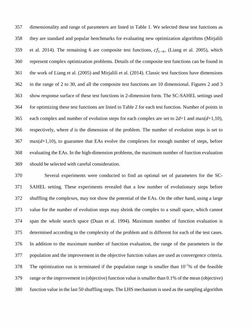
dimensionality and range of parameters are listed in Table 1. We selected these test functions as 357
they are standard and popular benchmarks for evaluating new optimization algorithms (Mirjalili 358
et al. 2014). The remaining 6 are composite test functions, 𝑐𝑐𝑐𝑐1−6 , (Liang et al. 2005), which 359
represent complex optimization problems. Details of the composite test functions can be found in 360
the work of Liang et al. (2005) and Mirjalili et al. (2014). Classic test functions have dimensions 361
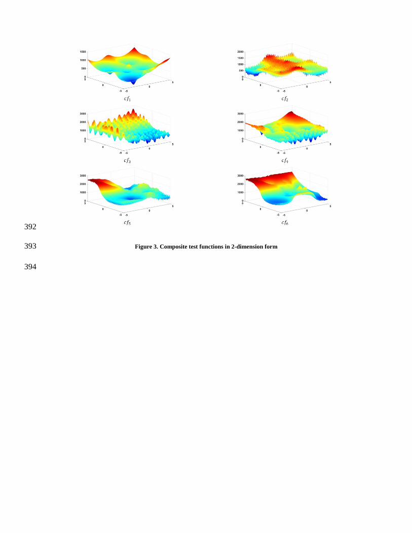
in the range of 2 to 30, and all the composite test functions are 10 dimensional. Figures 2 and 3 362
show response surface of these test functions in 2-dimension form. The SC-SAHEL settings used 363
for optimizing these test functions are listed in Table 2 for each test function. Number of points in 364
each complex and number of evolution steps for each complex are set to 2d+1 and max(d+1,10), 365
respectively, where d is the dimension of the problem. The number of evolution steps is set to 366
max(d+1,10), to guarantee that EAs evolve the complexes for enough number of steps, before 367
evaluating the EAs. In the high-dimension problems, the maximum number of function evaluation 368
should be selected with careful consideration. 369
Several experiments were conducted to find an optimal set of parameters for the SC-370
SAHEL setting. These experiments revealed that a low number of evolutionary steps before 371
shuffling the complexes, may not show the potential of the EAs. On the other hand, using a large 372
value for the number of evolution steps may shrink the complex to a small space, which cannot 373
span the whole search space (Duan et al. 1994). Maximum number of function evaluation is 374
determined according to the complexity of the problem and is different for each of the test cases. 375
In addition to the maximum number of function evaluation, the range of the parameters in the 376
population and the improvement in the objective function values are used as convergence criteria. 377
The optimization run is terminated if the population range is smaller than 10-7% of the feasible 378
range or the improvement in (objective) function value is smaller than 0.1% of the mean (objective) 379
function value in the last 50 shuffling steps. The LHS mechanism is used as the sampling algorithm 380

of SC-SAHEL for generating the initial population. The framework provides multiple settings for 381
boundary handling, which can be selected by the user. SC-SAHEL uses reflection as the default 382
boundary handling method. Other initial sampling and boundary handling methods are also 383
implemented in the SC-SAHEL framework. Sensitivity of the initial sampling and boundary 384
handling on the performance of the SC-SAHEL algorithm is not studied in this paper. The 385
aforementioned settings can be applied to a wide range of problems. 386

Table 1. The detailed information of 23 test functions from Xin et al. (1999), including mathematical expression, 387 dimension, parameters range and global optimum value (𝒇𝒇𝒎𝒎𝒎𝒎𝒎𝒎). 388
Function Number Name Function Dim Range 𝑐𝑐𝑚𝑚𝑚𝑚𝑚𝑚
𝑐𝑐1(𝑥𝑥) Sphere Model 𝑐𝑐(𝑥𝑥) = � 𝑥𝑥𝑚𝑚2𝑚𝑚
𝑚𝑚=1 30 [-100,100] 0
𝑐𝑐2(𝑥𝑥) Schwefel’s Problem 2.22 𝑐𝑐(𝑥𝑥) = � |𝑥𝑥𝑚𝑚| + � |𝑥𝑥𝑚𝑚|
𝑚𝑚
𝑚𝑚=1
𝑚𝑚
𝑚𝑚=1 30 [-10,10] 0
𝑐𝑐3(𝑥𝑥) Schwefel’s Problem 1.2 𝑐𝑐(𝑥𝑥) = � �� 𝑥𝑥𝑗𝑗𝑚𝑚
𝑗𝑗=1�2𝑚𝑚
𝑚𝑚=1 30 [-100,100] 0
𝑐𝑐4(𝑥𝑥) Schwefel’s Problem 2.21 𝑐𝑐(𝑥𝑥) = 𝑚𝑚𝑚𝑚𝑥𝑥𝑚𝑚{|𝑥𝑥𝑚𝑚|, 1 ≤ 𝑖𝑖 ≤ 𝑛𝑛} 30 [-100,100] 0
𝑐𝑐5(𝑥𝑥) Generalized Rosenbrock’s Function 𝑐𝑐(𝑥𝑥) = � �100�𝑥𝑥𝑚𝑚+1 − 𝑥𝑥𝑚𝑚2�
2+ (𝑥𝑥𝑚𝑚 − 1)2�
𝑚𝑚−1
𝑚𝑚=1 30 [-30,30] 0
𝑐𝑐6(𝑥𝑥) Step Function 𝑐𝑐(𝑥𝑥) = � (⌊𝑥𝑥𝑚𝑚 + 0.5⌋)2𝑚𝑚
𝑚𝑚=1 30 [-100,100] 0
𝑐𝑐7(𝑥𝑥) Quartic Function 𝑐𝑐(𝑥𝑥) = � 𝑖𝑖𝑥𝑥𝑚𝑚4 + 𝑟𝑟𝑚𝑚𝑛𝑛𝑑𝑑𝑟𝑟𝑚𝑚[0,1)𝑚𝑚
𝑚𝑚=1 30 [-1.28,1.28] 0
𝑐𝑐8(𝑥𝑥) Generalized Schwefel’s Problem 2.26 𝑐𝑐(𝑥𝑥) = � −𝑥𝑥𝑚𝑚 sin ��|𝑥𝑥𝑚𝑚|�
𝑚𝑚
𝑚𝑚=1 30 [-500,500] -12569.5
𝑐𝑐9(𝑥𝑥) Generalized Rastrigin’s Function 𝑐𝑐(𝑥𝑥) = � [𝑥𝑥𝑚𝑚2 − 10 cos(2𝜋𝜋𝑥𝑥𝑚𝑚) + 10]
𝑚𝑚
𝑚𝑚=1 30 [-5.12,5.12] 0
𝑐𝑐10(𝑥𝑥) Ackley’s Function 𝑐𝑐(𝑥𝑥) = −20 exp�−0.2�1𝑛𝑛� 𝑥𝑥𝑚𝑚2
𝑚𝑚
𝑚𝑚=1� − exp �
1𝑛𝑛� cos(2𝜋𝜋𝑥𝑥𝑚𝑚)
𝑚𝑚
𝑚𝑚=1� + 20 + 𝑒𝑒 30 [-32,32] 0
𝑐𝑐11(𝑥𝑥) Generalized Griewank Function 𝑐𝑐(𝑥𝑥) =
14000
� 𝑥𝑥𝑚𝑚2 −� cos �𝑥𝑥𝑚𝑚√𝑖𝑖� + 1
𝑚𝑚
𝑚𝑚=1
𝑚𝑚
𝑚𝑚=1 30 [-600,600] 0
𝑐𝑐12(𝑥𝑥) Generalized Penalized Functions
𝑐𝑐(𝑥𝑥) = 𝜋𝜋𝑛𝑛�10sin2(𝜋𝜋𝑦𝑦𝑚𝑚) + � (𝑦𝑦𝑚𝑚 − 1)2[1 + 10sin2(πyi+1)]
𝑚𝑚−1
𝑚𝑚=1+ (𝑦𝑦𝑚𝑚 − 1)2�
+ � 𝑢𝑢(𝑥𝑥𝑚𝑚 , 10,100,4),𝑚𝑚
𝑚𝑚=1
𝑦𝑦𝑚𝑚 = 1 +14
(𝑥𝑥𝑚𝑚 + 1),
𝑢𝑢(𝑥𝑥𝑚𝑚 ,𝑚𝑚, 𝑘𝑘,𝑚𝑚) = �𝑘𝑘(𝑥𝑥𝑚𝑚 − 𝑚𝑚)𝑚𝑚, 𝑥𝑥𝑚𝑚 > 𝑚𝑚0, − 𝑚𝑚 ≤ 𝑥𝑥𝑚𝑚 ≤ 𝑚𝑚𝑘𝑘(−𝑥𝑥𝑚𝑚 − 𝑚𝑚)𝑚𝑚, 𝑥𝑥𝑚𝑚 < −𝑚𝑚
30 [-50,50] 0
𝑐𝑐13(𝑥𝑥) Generalized Penalized Functions
𝑐𝑐(𝑥𝑥) = 0.1 �sin2(3𝜋𝜋𝑥𝑥1) + � (𝑥𝑥𝑚𝑚 − 1)2[1 + sin2(3𝜋𝜋𝑥𝑥𝑚𝑚 + 1)]𝑚𝑚
𝑚𝑚=1+ (𝑥𝑥𝑚𝑚 − 1)2[1 + sin2(2𝜋𝜋𝑥𝑥𝑚𝑚)]�
+ � 𝑢𝑢(𝑥𝑥𝑚𝑚 , 5,100,4)𝑚𝑚
𝑚𝑚=1
𝑢𝑢(𝑥𝑥𝑚𝑚 ,𝑚𝑚, 𝑘𝑘,𝑚𝑚) = �𝑘𝑘(𝑥𝑥𝑚𝑚 − 𝑚𝑚)𝑚𝑚, 𝑥𝑥𝑚𝑚 > 𝑚𝑚0, − 𝑚𝑚 ≤ 𝑥𝑥𝑚𝑚 ≤ 𝑚𝑚𝑘𝑘(−𝑥𝑥𝑚𝑚 − 𝑚𝑚)𝑚𝑚, 𝑥𝑥𝑚𝑚 < −𝑚𝑚
30 [-50,50] 0
𝑐𝑐14(𝑥𝑥) Shekel’s Foxholes Function 𝑐𝑐(𝑥𝑥) = �
1500
+ �1
𝑗𝑗 + ∑ �𝑥𝑥𝑚𝑚 − 𝑚𝑚𝑚𝑚𝑗𝑗�62
𝑚𝑚=1
25
𝑗𝑗=1� 2 [-65.536,65.536] 1
𝑐𝑐15(𝑥𝑥) Kowalik’s Function 𝑐𝑐(𝑥𝑥) = � �𝑚𝑚𝑚𝑚 −𝑥𝑥1�𝑏𝑏𝑚𝑚2 + 𝑏𝑏𝑚𝑚𝑥𝑥2�𝑏𝑏𝑚𝑚2 + 𝑏𝑏𝑚𝑚𝑥𝑥3 + 𝑥𝑥4
�211
𝑚𝑚=1 4 [-5,5] 0.0003075
𝑐𝑐16(𝑥𝑥) Six-Hump Camel-Back Function 𝑐𝑐(𝑥𝑥) = 4𝑥𝑥12 − 2.1𝑥𝑥14 +
13𝑥𝑥16 + 𝑥𝑥1𝑥𝑥2 − 4𝑥𝑥22 + 4𝑥𝑥24 2 [-5,5] -1.0316285
𝑐𝑐17(𝑥𝑥) Branin Function 𝑐𝑐(𝑥𝑥) = �𝑥𝑥2 −5.14𝜋𝜋2
𝑥𝑥12 +5𝜋𝜋𝑥𝑥1 − 6�
2
+ 10 �1 −1
8𝜋𝜋� cos(𝑥𝑥1) + 10 2 [-5,10]×[0,15] 0.398
𝑐𝑐18(𝑥𝑥) Goldstein-Price Function
𝑐𝑐(𝑥𝑥) = [1 + (𝑥𝑥1 + 𝑥𝑥2 + 1)2(19 − 14𝑥𝑥1 + 3𝑥𝑥12 − 14𝑥𝑥2 + 6𝑥𝑥1𝑥𝑥2 + 3𝑥𝑥22)]× [30 + (2𝑥𝑥1 − 3𝑥𝑥2)2(18 − 32𝑥𝑥1 + 12𝑥𝑥12 + 48𝑥𝑥2 − 36𝑥𝑥1𝑥𝑥2 + 27𝑥𝑥22)] 2 [-2,2] 3
𝑐𝑐19(𝑥𝑥) Hartman’s Family 𝑐𝑐(𝑥𝑥) = −� 𝑐𝑐𝑚𝑚exp4
𝑚𝑚=1�−� 𝑚𝑚𝑚𝑚𝑗𝑗�𝑥𝑥𝑗𝑗 − 𝑝𝑝𝑚𝑚𝑗𝑗�
24
𝑗𝑗=1� 4 [0,1] -3.86
𝑐𝑐20(𝑥𝑥) Hartman’s Family 𝑐𝑐(𝑥𝑥) = −� 𝑐𝑐𝑚𝑚 exp �−� 𝑚𝑚𝑚𝑚𝑗𝑗�𝑥𝑥𝑗𝑗−𝑝𝑝𝑚𝑚𝑗𝑗�26
𝑗𝑗=1�
4
𝑚𝑚=1 6 [0,1] -3.32
𝑐𝑐21(𝑥𝑥) Shekel’s Family 𝑐𝑐(𝑥𝑥) = −� [(𝑥𝑥 − 𝑚𝑚𝑚𝑚)(𝑥𝑥 − 𝑚𝑚𝑚𝑚)𝑇𝑇 + 𝑐𝑐𝑚𝑚]−15
𝑚𝑚=1 4 [0,10] -10.1532
𝑐𝑐22(𝑥𝑥) Shekel’s Family 𝑐𝑐(𝑥𝑥) = −� [(𝑥𝑥 − 𝑚𝑚𝑚𝑚)(𝑥𝑥 − 𝑚𝑚𝑚𝑚)𝑇𝑇 + 𝑐𝑐𝑚𝑚]−17
𝑚𝑚=1 4 [0,10] -10.4028
𝑐𝑐23(𝑥𝑥) Shekel’s Family 𝑐𝑐(𝑥𝑥) = −� [(𝑥𝑥 − 𝑚𝑚𝑚𝑚)(𝑥𝑥 − 𝑚𝑚𝑚𝑚)𝑇𝑇 + 𝑐𝑐𝑚𝑚]−110
𝑚𝑚=1 4 [0,10] -10.5363

389 Figure 2. Classic test functions in 2-dimension form 390
391
392
Figure 3. Composite test functions in 2-dimension form 393
394

Table 2. List of the settings for the SC-SAHEL algorithm for classic and composite test functions. NGS is the number of 395 complexes, NPS denotes the number of points in each complex and I is the maximum number of function evaluation. 396
Function NGS NPS I 𝑐𝑐1 8 61 100,000 𝑐𝑐2 8 61 100,000 𝑐𝑐3 8 61 300,000 𝑐𝑐4 8 61 300,000 𝑐𝑐5 8 61 500,000 𝑐𝑐6 8 61 100,000 𝑐𝑐7 8 61 200,000 𝑐𝑐8 8 61 200,000 𝑐𝑐9 8 61 200,000 𝑐𝑐10 8 61 200,000 𝑐𝑐11 8 61 200,000 𝑐𝑐12 8 61 300,000 𝑐𝑐13 8 61 400,000 𝑐𝑐14 8 10 100,000 𝑐𝑐15 8 10 100,000 𝑐𝑐16 8 10 100,000 𝑐𝑐17 8 10 100,000 𝑐𝑐18 8 10 100,000 𝑐𝑐19 8 10 100,000 𝑐𝑐20 8 13 100,000 𝑐𝑐21 8 10 100,000 𝑐𝑐22 8 10 100,000 𝑐𝑐23 8 10 100,000 𝑐𝑐𝑐𝑐1 16 61 100,000 𝑐𝑐𝑐𝑐2 16 61 100,000 𝑐𝑐𝑐𝑐3 16 61 100,000 𝑐𝑐𝑐𝑐4 16 61 100,000 𝑐𝑐𝑐𝑐5 16 61 100,000 𝑐𝑐𝑐𝑐6 16 61 100,000
3.2 Results and Discussion 397
Table 3 illustrates the statistics of the final function values at 30 independent runs on 29 398
test functions using the hybrid SC-SAHEL and individual EAs, with the goal to minimize the 399
function values. The best mean function value obtained for each test function is expressed in bold 400
in Table 3. Results show that the hybrid SC-SAHEL achieved the lowest function values in 15 out 401
of 29 test functions, compared to the mean function values achieved by all individual algorithms. 402
It is noteworthy that in 20 out of 29 test functions, the hybrid SC-SAHEL was among the top two 403
optimization methods in finding the minimum function value. A two-sample t-test (with 5% 404
significance level) also showed that the result generated with the SC-SAHEL algorithm is 405

generally similar to the best performing algorithms. Comparing among single-method algorithms, 406
in general, the statistics obtained by SP-UCI are superior to other participating EAs. In 12 out of 407
29 test functions, the SP-UCI algorithm achieved the lowest function value. SC-MFL, SC-MGWO, 408
and SC-DE were superior to other algorithms in 10, 11, and 6 out of 29 test functions, respectively. 409
In test functions 𝑐𝑐6, 𝑐𝑐16, 𝑐𝑐17, 𝑐𝑐18, 𝑐𝑐19, 𝑐𝑐20, and 𝑐𝑐23, the single-method and multi-method algorithms 410
achieved same function values on average in most cases. In these cases, according to the statistics 411
shown in Table 3, the SP-UCI and SC-SAHEL algorithms offer lower standard deviation values 412
and show more consistent results as compared to other EAs. The low standard deviation values 413
obtained by SP-UCI and SC-SAHEL indicate the robustness and consistency of these two 414
algorithms in comparison to other algorithms. 415
Table 3. The mean and Standard deviation (Std) of objective function values for 30 independent runs on 29 test functions 416 using the SC-SAHEL algorithm with single-method and multi-method search mechanism. 417
Function SC-SAHEL (MCCE, MFL, MGWO, DE) SP-UCI (SC-MCCE) SC-MFL SC-MGWO SC-DE
Mean Std Mean Std Mean Std Mean Std Mean Std 𝑐𝑐1 3.68E-11 1.60E-11 1.68E-11 1.18E-11 4.29E-11 1.01E-11 5.92E-05 5.51E-05 2.13E-06 2.98E-06 𝑐𝑐2 3.14E-06 3.92E-07 3.00E-06 5.94E-07 2.35E-06 2.75E-07 4.12E-03 1.27E-03 6.38E-04 5.26E-04 𝑐𝑐3 2.11E-10 6.08E-11 8.95E-10 4.37E-10 4.50E-10 9.15E-11 1.22E+03 2.16E+03 1.86E-09 1.48E-09 𝑐𝑐4 4.89E-06 7.88E-07 8.98E-05 4.60E-05 3.65E-06 5.43E-07 5.26E-06 5.59E-07 3.50E-01 2.35E-01 𝑐𝑐5 7.81E-09 3.15E-09 2.54E-08 1.52E-08 2.58E+01 2.85E-01 1.28E+01 1.85 1.33 1.91 𝑐𝑐6 0 0 0 0 0 0 3.33E-02 1.83E-01 6.33E-01 6.69E-01 𝑐𝑐7 1.09E-03 5.33E-04 4.78E-04 3.44E-04 1.37E-03 6.36E-04 1.34E-02 4.90E-03 2.08E-03 8.93E-04
𝑐𝑐8 -9.87E+03 6.14E+02 -5.09E+03 2.27E+02 -4.36E+03 2.90E+02 -4.91E+03 3.75E+02 -9.75E+03 6.41E+02
𝑐𝑐9 8.29E-01 1.73 3.32E-02 1.82E-01 1.60E+01 9.78 2.01E+02 1.19E+01 2.67E+01 4.57E+01 𝑐𝑐10 1.49E-06 2.43E-07 1.08E-06 2.55E-07 1.52E-06 2.00E-07 5.47E-06 5.34E-07 1.42 4.98E-01 𝑐𝑐11 8.05E-11 2.08E-11 1.77E-10 5.19E-11 1.61E-04 8.81E-04 7.21E-03 1.15E-02 1.42E-02 1.51E-02 𝑐𝑐12 1.58E-13 5.02E-14 5.27E-13 3.38E-13 1.31E-01 8.80E-02 1.06E-12 1.80E-13 3.11E-02 7.77E-02 𝑐𝑐13 3.66E-04 2.01E-03 2.55E-12 8.69E-13 7.15E-02 8.94E-03 1.62E-11 3.31E-12 3.97E-03 6.59E-03 𝑐𝑐14 9.98E-01 1.40E-16 9.98E-01 1.27E-16 2.53 3.13 9.98E-01 2.16E-16 1.99 1.51 𝑐𝑐15 3.07E-04 5.61E-17 1.19E-03 3.80E-03 1.08E-03 3.68E-03 3.07E-04 8.87E-14 2.98E-03 6.93E-03 𝑐𝑐16 -1.03 1.37E-15 -1.03 7.61E-16 -1.03 6.28E-07 -1.03 9.51E-15 -1.03 1.18E-15 𝑐𝑐17 3.98E-01 1.47E-15 3.98E-01 0 3.98E-01 2.05E-04 3.98E-01 7.63E-15 3.98E-01 0.00 𝑐𝑐18 3.00 2.20E-14 3.00 1.25E-14 3.00 1.81E-05 3.00 7.30E-14 3.00 1.72E-14 𝑐𝑐19 -3.86 2.08E-15 -3.86 2.12E-15 -3.86 5.46E-05 -3.86 1.61E-15 -3.86 1.97E-15 𝑐𝑐20 -3.32 2.17E-02 -3.32 2.17E-02 -3.31 3.03E-02 -3.25 5.92E-02 -3.31 4.11E-02 𝑐𝑐21 -9.16 2.58 -5.92 3.28 -9.69 1.75 -9.48 1.75 -8.97 2.18 𝑐𝑐22 -1.02E+01 9.63E-01 -9.64 2.31 -1.04E+01 4.56E-04 -1.04E+01 5.05E-13 -9.35 2.46 𝑐𝑐23 -1.05E+01 1.93E-13 -1.03E+01 1.22 -1.05E+01 6.96E-06 -1.05E+01 5.00E-13 -9.64 2.35 𝑐𝑐𝑐𝑐1 6.67 2.54E+01 3.33 1.83E+01 1.00E+01 3.05E+01 9.41E-12 3.42E-12 1.35E-11 5.66E-12 𝑐𝑐𝑐𝑐2 2.00E+01 4.84E+01 1.23E+02 6.79E+01 7.76E+01 4.59E+01 3.94E+01 1.44E+01 3.14E+01 5.39E+01 𝑐𝑐𝑐𝑐3 1.32E+02 9.33E+01 1.33E+02 8.22E+01 2.80E+02 3.16E+01 3.00E+02 4.21E+01 1.28E+02 3.83E+01 𝑐𝑐𝑐𝑐4 2.71E+02 6.67E+01 2.93E+02 8.38E+01 3.46E+02 1.47E+01 3.30E+02 4.15E+01 2.63E+02 3.20E+01 𝑐𝑐𝑐𝑐5 1.70E+01 3.77E+01 9.75E+01 1.83E+01 3.05E+01 4.33E+01 3.37 1.83E+01 1.10E+01 3.05E+01 𝑐𝑐𝑐𝑐6 6.71E+02 2.00E+02 8.72E+02 6.59E+01 7.80E+02 1.85E+02 5.40E+02 1.23E+02 6.38E+02 1.86E+02
418

In the test functions that the hybrid SC-SAHEL algorithm was not able to produce the best 419
mean function value, the achieved mean function values deviation from that of the best-performing 420
algorithms are marginal. For instance, on the test functions 𝑐𝑐2, 𝑐𝑐4, 𝑐𝑐10, and 𝑐𝑐22, the statistics of the 421
values obtained by SC-SAHEL are similar to that achieved by the best-performing methods, which 422
are SP-UCI, and SC-MFL, respectively. In general, the hybrid SC-SAHEL algorithm is superior 423
to algorithms with individual EA on most of the test functions, although on some test functions, 424
the SC-SAHEL algorithm is slightly inferior to the best-performing algorithm with only marginal 425
differences. The performance of the SC-SAHEL in these test functions can be attributed to two 426
main reasons. First, in the hybrid algorithm, all the EAs are involved in the evolution of the 427
population. Hence, if one of the algorithms have poor performance in comparison to other EAs, it 428
still evolves a portion of the population. As the complexes are evolved independently, the poor-429
performing EAs may devastate a part of the information in the evolving complex. On the other 430
hand, when the algorithms are used individually in the SC-SAHEL framework, the EA utilizes the 431
information in all the complexes and the whole population. In this case, better result will be 432
achieved in comparison to the hybrid SC-SAHEL, if the EA is the fittest algorithm for the problem 433
space. Second, some of the EAs are faster and more efficient in a specific optimization phase 434
(exploration/exploitation) than others. However, they might not be as effective as other EAs for 435
other optimization phases. Hence, dominance of these algorithm during the exploration or 436
exploitation phases can mislead other EAs and cause early (and premature) convergence. 437
Engagement of other algorithms in the evolution process may prevent early convergence in these 438
cases. Generally, the performance criteria, EMP, is responsible for selecting the most suitable 439
algorithm in each optimization step, however, the criteria used in the SC-SAHEL is not guaranteed 440
to perform well in all problem spaces. The performance criteria are problem dependent and need 441

further investigations based on the problem space and EAs. However, the EMP metric seems to be 442
a suitable metric for a wide range of problems. 443
To further evaluate the performance of the hybrid SC-SAHEL algorithm, we present the 444
success rate of the algorithms in Figure 4. The success rate is defined by setting target values for 445
the function value for each test function. When the function value is smaller than the target value, 446
the goal of optimization is reached, and therefore, the algorithm is considered successful. A higher 447
success rate resembles a better performance. We use same target value for all algorithms in order 448
to have a fair comparison. According to Figure 4, in 16 out of 29 test functions, the hybrid 449
algorithm achieved 100% success rate. In other cases, the success rates achieved by the proposed 450
hybrid algorithm are comparable to the best-performing algorithm with single EA. For instance, 451
on the test function 𝑐𝑐9, the SC-MGWO, SC-DE and SC-MFL are not successful in finding the 452
optimum solution (success rates are 0%, 0%, and 10%, respectively). However, the hybrid SC-453
SAHEL algorithm has similar performance (80% success rate) to SP-UCI (97% success rate). On 454
the test function 𝑐𝑐21, the success rate of the hybrid SC-SAHEL algorithm (87%) is close to the SC-455
MGWO (93%), which is the most successful algorithm. The hybrid SC-SAHEL algorithm also 456
achieved a higher success rate than SP-UCI algorithm (33%) in this test function. According to 457
Figure 4, the average success rate of SC-SAHEL is about 80% over all 29 test functions, and it is 458
the highest compared to the average success rate of other EAs, i.e., 73%, 58%, 58%, and 54% for 459
SP-UCI, SC-MFL, SC-MGWO, and SC-DE algorithm, respectively. 460
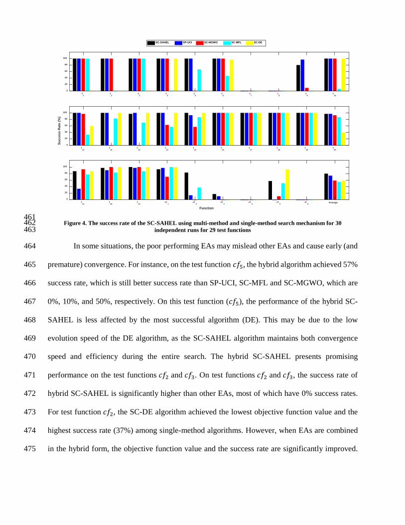
461 Figure 4. The success rate of the SC-SAHEL using multi-method and single-method search mechanism for 30 462
independent runs for 29 test functions 463
In some situations, the poor performing EAs may mislead other EAs and cause early (and 464
premature) convergence. For instance, on the test function 𝑐𝑐𝑐𝑐5, the hybrid algorithm achieved 57% 465
success rate, which is still better success rate than SP-UCI, SC-MFL and SC-MGWO, which are 466
0%, 10%, and 50%, respectively. On this test function (𝑐𝑐𝑐𝑐5), the performance of the hybrid SC-467
SAHEL is less affected by the most successful algorithm (DE). This may be due to the low 468
evolution speed of the DE algorithm, as the SC-SAHEL algorithm maintains both convergence 469
speed and efficiency during the entire search. The hybrid SC-SAHEL presents promising 470
performance on the test functions 𝑐𝑐𝑐𝑐2 and 𝑐𝑐𝑐𝑐3. On test functions 𝑐𝑐𝑐𝑐2 and 𝑐𝑐𝑐𝑐3, the success rate of 471
hybrid SC-SAHEL is significantly higher than other EAs, most of which have 0% success rates. 472
For test function 𝑐𝑐𝑐𝑐2, the SC-DE algorithm achieved the lowest objective function value and the 473
highest success rate (37%) among single-method algorithms. However, when EAs are combined 474
in the hybrid form, the objective function value and the success rate are significantly improved. 475
f1
f2
f3
f4
f5
f6
f7
f8
f9
f10
0
20
40
60
80
100
SC-SAHEL SP-UCI SC-MGWO SC-MFL SC-DE
f11
f12
f13
f14
f15
f16
f17
f18
f19
f20
0
20
40
60
80
100
Succ
ess
Rat
e (%
)
f21
f22
f23
cf1
cf2
cf3
cf4
cf5
cf6
Average
Function
0
20
40
60
80
100
This shows that SC-SAHEL has the capability of solving complex problems by utilizing the 476
potentials and advantages of all participating algorithms and improving the search success rate. 477
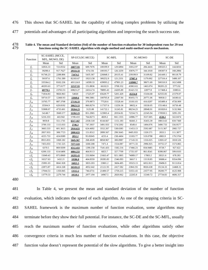
Table 4. The mean and Standard deviation (Std) of the number of function evaluation for 30 independent runs for 29 test 478 functions using the SC-SAHEL algorithm with single-method and multi-method search mechanism. 479
Function SC-SAHEL (MCCE, MFL, MGWO, DE) SP-UCI (SC-MCCE) SC-MFL SC-MGWO SC-DE
Mean Std Mean Std Mean Std Mean Std Mean Std 𝑐𝑐1 32816.33 723.0532 26877.93 609.7676 100199.9 129.6894 33012.97 284.4416 100325.5 144.6016
𝑐𝑐2 39298.4 917.7627 29333.33 674.156 100193.7 126.3259 35876.77 344.1018 100307.9 168.2884
𝑐𝑐3 91746.23 2288.806 73474.5 5435.367 226848.3 20135.41 239199.9 31109.82 241449.1 90118.79
𝑐𝑐4 50197.6 1761.589 82183.67 19213.58 300252.9 121.2331 37987.4 1170.002 227316.4 5488.107
𝑐𝑐5 335364.2 8102.236 401124.8 14599.33 439093.2 47901.23 118900.7 38671.69 500310.9 163.5498
𝑐𝑐6 40293.63 377.0177 32537.93 151.8836 66102.9 3708.332 43063.63 1463.074 90205.23 5773.92
𝑐𝑐7 69779.5 23763.53 69823.27 24314.74 78895.43 24205.89 81421.53 22877.8 117468.4 33083.6
𝑐𝑐8 71834.83 9826.963 54020 17225.97 65629.77 5201.429 45254.8 15104.68 62555.83 21579.07
𝑐𝑐9 59710.57 12460.93 33949.6 996.5881 100705.8 22607.84 85055.73 20771.06 90930.3 34180.61
𝑐𝑐10 33765.77 887.3708 27116.33 379.9873 77520.6 15528.44 33181.03 416.0297 165489.4 4726.909
𝑐𝑐11 35504.9 629.8192 30623.53 860.8274 117357.6 13250.36 38652.4 19330.05 155148.6 16730.48
𝑐𝑐12 55908.07 4735.601 39264.23 3125.88 141722.1 31245.81 88234.23 28948.91 181820.6 5132.966
𝑐𝑐13 54148.7 3949.577 32262.23 851.2965 123903.4 20354.81 72334.73 22345.94 170930.5 3295.191
𝑐𝑐14 5216.333 443.942 5708.433 764.8273 4829.2 841.1355 14986.77 3537.605 4530.2 322.0474
𝑐𝑐15 9059.8 551.1741 6517.167 2358.518 8144.667 1151.183 66441.3 35455.39 18813.63 659.7369
𝑐𝑐16 3700.133 1115.033 2746.3 747.3937 3491.933 574.5392 8549.4 1494.076 3490.733 556.9577
𝑐𝑐17 3665.533 601.3615 2910.633 624.4692 3552.267 538.6385 11453.13 2592.687 5115.367 2082.727
𝑐𝑐18 2837.933 308.7723 2000.633 151.8512 2899.567 299.5645 8405.933 1320.571 2833.5 111.3877
𝑐𝑐19 4225.733 424.8389 2852.2 95.83045 4233.4 238.4404 13183.77 519.0798 4983.9 179.5704
𝑐𝑐20 8915.833 1069.182 5645.567 268.4028 8858.967 300.0987 17143.33 1316.025 12691.67 1818.526
𝑐𝑐21 7455.033 1741.525 7377.533 3260.208 7471.4 1554.087 18771.33 2996.925 10755.57 1573.865
𝑐𝑐22 6370.5 869.9209 4512.433 1290.258 7541.433 1582.216 17466.23 834.9485 8728.7 927.622
𝑐𝑐23 6200.133 614.6406 4084.233 464.9113 6823.7 327.7709 17351.87 861.8541 8398.067 599.0103
𝑐𝑐𝑐𝑐1 15049.43 875.8969 10293.43 233.9694 21663.47 921.1805 74089.17 17803.2 28321.6 678.283
𝑐𝑐𝑐𝑐2 16527.63 1432.21 10586.8 464.8359 20285.83 2346.093 36617.1 13118.85 30686.4 9354.096
𝑐𝑐𝑐𝑐3 25991.03 8041.928 16021.5 3833.203 23801.2 3604.495 19323.13 6052.813 29496.9 9113.814
𝑐𝑐𝑐𝑐4 22873.87 4414.168 16510.13 4052.642 21121.93 2417.582 23841.93 8026.638 35134.33 14468.31
𝑐𝑐𝑐𝑐5 17044.53 1350.845 13512.2 746.6731 21400.57 1759.215 53551.43 23577.95 39200.77 4125.908
𝑐𝑐𝑐𝑐6 13779.33 2279.744 10518.1 2977.194 14967.5 2820.062 22265.8 15340.72 27734.83 4606.317
480
In Table 4, we present the mean and standard deviation of the number of function 481
evaluation, which indicates the speed of each algorithm. As one of the stopping criteria in SC-482
SAHEL framework is the maximum number of function evaluation, some algorithms may 483
terminate before they show their full potential. For instance, the SC-DE and the SC-MFL, usually 484
reach the maximum number of function evaluations, while other algorithms satisfy other 485
convergence criteria in much less number of function evaluations. In this case, the objective 486
function value doesn’t represent the potential of the slow algorithms. To give a better insight into 487

this matter, the mean and standard deviation (Std) of the number of function evaluations are 488
compared in Table 4. The goal is to compare the speed of the individual EAs and the hybrid 489
optimization algorithm. According to Table 4, in most of the test cases, the SP-UCI algorithm has 490
the least number of function evaluations, regardless of the objective function value achieved by 491
the EAs. 492
Comparing the success rate and the number of function evaluation for different EAs shows 493
that SP-UCI achieved 100% success rate with the lowest number of function evaluation, in 15 out 494
of 29 test functions. The SC-MGWO algorithm only achieved 100% success rate with the lowest 495
number of function evaluation in one test function. Although the hybrid SC-SAHEL algorithm is 496
not the fastest algorithm, its speed is usually close to the fastest algorithm. This is due to the 497
contribution of different EAs in the evolution process and the EAs behavior on different problem 498
spaces. For instance, DE algorithm is slower in comparison to MCCE (SP-UCI) algorithm in most 499
of the test functions. Hence, when the algorithms are working in a hybrid form, the hybrid 500
algorithm will be slower than the situation when the MCCE (SP-UCI) algorithm is used 501
individually. 502
Figures 5, 6, and 7 compare the average number of complexes assigned to each EA for the 503
29 employed test functions during the course of the search. The variation of the number of 504
complexes assigned to each EA indicates the dominance of each EA during the course of the 505
search. Hence, the performance of EAs at each optimization step can be monitored. In many test 506
cases, MCCE (SP-UCI) algorithm has a relatively higher number of complexes than other EAs 507
during the search. This shows that MCCE is a dominant search algorithm on most of the test 508
functions. However, in some other cases, MCCE is only dominant in a certain period of the search, 509
while other EAs have demonstrated better efficiency during the entire search. For example, on test 510
functions 𝑐𝑐7 and 𝑐𝑐20, MCCE algorithm appears to be dominant only during the beginning of the 511

search. In the test function 𝑐𝑐7, the exploration process starts with the dominance of the MCCE and 512
shifts between MGWO and MFL after the first 20 shuffling steps. In some of the test functions, 513
such as 𝑐𝑐7, a more random fluctuation is observed in the number of complexes assigned to each 514
EA. The reason for this behavior is that EAs have very close competition in these shuffling steps. 515
Due to the noisy response surface of the test function 𝑐𝑐7, most of the EAs cannot significantly 516
improve the (objective) function values during the exploitation phase. On test functions 𝑐𝑐8 and 𝑐𝑐18, 517
the MFL and DE algorithms are the dominant, respectively, during the beginning of the run, while 518
MCCE algorithm becomes dominant only when the algorithm is in exploitation phase. Lastly, on 519
test functions 𝑐𝑐9, 𝑐𝑐22, 𝑐𝑐𝑐𝑐1, and 𝑐𝑐𝑐𝑐4, the variations of the number of complexes and the precedence 520
of different EAs as the most dominant search algorithm are observed. 521
It is worth mentioning that, Figures 5, 6, and 7 show the number of complexes assigned to 522
each EA for a single optimization run. Our observation of each individual run results (not shown 523
herein) shows variation of the number of complexes among different runs is similar to each other 524
for most test cases. The observed variation for individual runs follows a specific pattern and is not 525
random. The similarity of the EAs dominance pattern indicates that the selection of the EAs by the 526
SC-SAHEL framework only depends on the characteristics of the problem space and the EAs 527
employed. This also indicates that different EAs have pros and cons on different optimization 528
problems. 529

530
531
Figure 5. Number of complexes assigned to EAs during the entire optimization process on test function 𝒇𝒇𝟏𝟏-𝒇𝒇𝟏𝟏𝟏𝟏 532
533
Figure 6. Number of complexes assigned to EAs during the entire optimization process on test function 𝒇𝒇𝟏𝟏𝟏𝟏-𝒇𝒇𝟐𝟐𝟏𝟏 534

535
Figure 7. Number of complexes assigned to EAs during the entire optimization process on test function 𝒇𝒇𝟐𝟐𝟏𝟏-𝒇𝒇𝟐𝟐𝟐𝟐 and 𝒄𝒄𝒇𝒇𝟏𝟏-536
𝒄𝒄𝒇𝒇𝟔𝟔 537
As a summary of our experiments on the conceptual test functions (Tables 3, and 4, and 538
Figure 4, 5, 6, and 7), the main advantage of the SC-SAHEL algorithm over other optimization 539
methods is its capability of revealing the trade-off among different EAs and illustrating the 540
competition of participating EAs. Different optimization problems have different complexity, 541
which introduces various challenges for each EA. By incorporating different types of EAs in a 542
parallel computing framework, and implementing an “award and punishment” logic, the newly 543
developed SC-SAHEL framework not only provides an effective tool for global optimization but 544
also gives the user insights about advantages and disadvantages of each participating EAs on 545
individual optimization tasks. This shows the potential of the SC-SAHEL framework for solving 546
different class of problems with different level of complexity. Besides, the hybrid SC-SAHEL 547
algorithm is superior to shuffled complex-based methods with single search mechanism, such as 548
SP-UCI, in an absolute majority of the test functions. 549

4 Example applications and results 550
In this section, we demonstrate an example application of the newly developed SC-SAHEL 551
algorithm. A conceptual reservoir model is developed with the goal of maximizing hydropower 552
generation on a daily-basis operation. The model is applied to the Folsom reservoir in Northern 553
California. 554
4.1 Reservoir Model 555
A conceptual model is set up based on the relationship between the hydropower generation, 556
storage, water head and bathymetry of the Folsom reservoir. Daily releases from the reservoir in 557
the study period are treated as the parameters of the model, which in turn determines the problem 558
dimensionality. The model objective is to maximize the hydropower generation for a specific 559
period. The total hydropower production is a function of the water head difference between forebay 560
and tailwater and the turbine flow rate. The driving equation of the model is based on mass balance 561
(water budget), which is formulated as, 562
𝑆𝑆𝑡𝑡 = 𝑆𝑆𝑡𝑡−1 + 𝐼𝐼𝑡𝑡 − 𝑅𝑅𝑡𝑡 ± 𝑀𝑀𝑡𝑡, (2) 563
where 𝑆𝑆𝑡𝑡 is storage at time step 𝑡𝑡, 𝐼𝐼𝑡𝑡 and 𝑅𝑅𝑡𝑡 signify total inflow and release from the reservoir at 564
time 𝑡𝑡, respectively. 𝑀𝑀𝑡𝑡 is total outflow/inflow error which is derived by setting up mass balance 565
for daily observed data. The objective function employed here is, 566
OF = ∑ 1 − 𝑃𝑃𝑡𝑡𝑃𝑃𝑐𝑐
𝑁𝑁𝑡𝑡=1 , (3) 567
where 𝑃𝑃𝑐𝑐 is total power plant capacity in MW and 𝑃𝑃𝑡𝑡 is total power generated in day 𝑡𝑡 in MW. For 568
each day 𝑃𝑃𝑡𝑡 is derived as follow, 569
𝑃𝑃𝑡𝑡 = 𝜂𝜂𝜂𝜂𝜂𝜂𝑄𝑄𝑡𝑡𝐻𝐻𝑡𝑡, (4) 570
where 𝜂𝜂 signifies turbine efficiency, 𝜂𝜂 is water density (Kg/m3), g is gravity (9.81 m/s2) and 𝑄𝑄𝑡𝑡 is 571
discharge (m3/s) at time step t. 𝐻𝐻𝑡𝑡 is hydraulic head (m) at time step t, which is defined as, 572

𝐻𝐻𝑡𝑡 = ℎ𝑓𝑓 − ℎ𝑡𝑡𝑡𝑡, (5) 573
where ℎ𝑓𝑓 and ℎ𝑡𝑡𝑡𝑡 are water elevation in forebay and tailwater, respectively. ℎ𝑓𝑓 and ℎ𝑡𝑡𝑡𝑡 are 574
derived by fitting a polynomial to reservoir bathymetry data. 575
In the reservoir model coined above, multiple constraints are considered for better 576
representation of the real behavior of the system. These constraints include power generation 577
capacity, storage level, spill capacity, and changes in the daily hydropower discharge. Total daily 578
power generation is compared to maximum capacity of the hydropower plant. Also, rule curve is 579
used to control reservoir storage level during the operation period. Besides, final simulated 580
reservoir storage is constrained to 0.9 - 1.1 of the observed storage. In another word, 10% variation 581
from the observation data is allowed for the final simulated storage level. This constraint adds 582
information from real reservoir operation into the optimization process. This constraint can be 583
replaced by other operation rules for simulation purposes. The spill capacity of dam is calculated 584
according to the water level in the forebay and compared to simulated spilled water. A quadratic 585
function is fitted to the water level and spill capacity data, to derive the spill capacity at each time 586
step. The change in daily hydropower release is also constrained to better represent actual 587
hydropower discharge and avoid large variation in a daily release. 588
The reservoir model used here is non-linear and continuous. The constraints of the model 589
render finding the feasible solution a challenging task for all the EAs. The SC-SAHEL framework 590
is used to maximize the hydropower generation by minimizing the objective function value. The 591
settings used for the SC-SAHEL is similar to the settings used for the mathematical test functions. 592
However, the maximum number of function evaluations is set to 106. Lower bound of the 593
parameters’ range varies monthly due to the operational rules; however, upper bound is determined 594
according to the hydraulic structure of the dam. 595
596

4.2 Study basin 597
Folsom reservoir is located on the American river, in northern California and near 598
Sacramento, California. Folsom dam was built by the US Army Corps of Engineers during 1948 599
to 1956, and is a multi-purpose facility. The main functions of the facility are flood control, water 600
supply for irrigation, hydropower generation, maintaining environmental flow, water quality 601
purposes, and providing recreational area. The reservoir has a capacity of 1,203,878,290 m3 and 602
the power plant has a total capacity of 198.7 MW. Three different periods are considered here. The 603
first study period is April 1st, 2010 to June 30th, 2010. The year 2010 is categorized as below-604
normal period according to California Department of Water Resources. The same period is 605
selected in 2011 and 2015, as former is categorized by California Department of Water Resources 606
as wet, and latter is classified as critical dry year. The input and output from the reservoir are 607
obtained from California Data Exchange Center (CDEC). Note that demand is not included in the 608
model because the demand data was not available from a public data source. 609
610
4.3 Results and Discussion 611
The boxplot of the objective function values is shown in Figure 8 for the Folsom reservoir 612
during the runoff season in 2015, 2010, and 2011, which are dry, below-normal, and wet years, 613
respectively. The presented results are based on 30 independent optimization runs; however, 614
infeasible objective function values are removed. The feasibility of the solution is evaluated 615
according to the objective function values. Due to the large values returned by the penalty function 616
considered for infeasible solutions, such solutions can be distinguished from the feasible solutions. 617
For wet year (2011) case, SC-MGWO, and SC-DE didn’t find a feasible solution in 2, and 4 runs 618
out of 30 independent runs, respectively. The hybrid SC-SAHEL found feasible solutions in all 619

the cases; however, some of these solutions are not global optima. On average, the hybrid SC-620
SAHEL algorithm is able to achieve the lowest objective function value as compared to other 621
algorithms during dry and below-normal period. During dry and below-normal periods, SC-622
SAHEL, SP-UCI, and SC-DE show similar performance. In the wet period, the SP-UCI algorithm 623
achieved the lowest objective function value. The SC-SAHEL algorithm ranked second, 624
comparing the mean objective function values. In this period, the results achieved by the SC-DE 625
is also comparable to SC-SAHEL and SP-UCI. The results show that overall, the hybrid SC-626
SAHEL algorithm has similar or superior performance in comparison to the single-method 627
algorithms. Also, the results achieved by SC-SAHEL and SP-UCI algorithms has less variability 628
in comparison to other algorithms, which show the robustness of these algorithms. The worst 629
performing algorithm is the SC-MGWO, which achieved the least mean objective function value 630
in all the study periods. 631
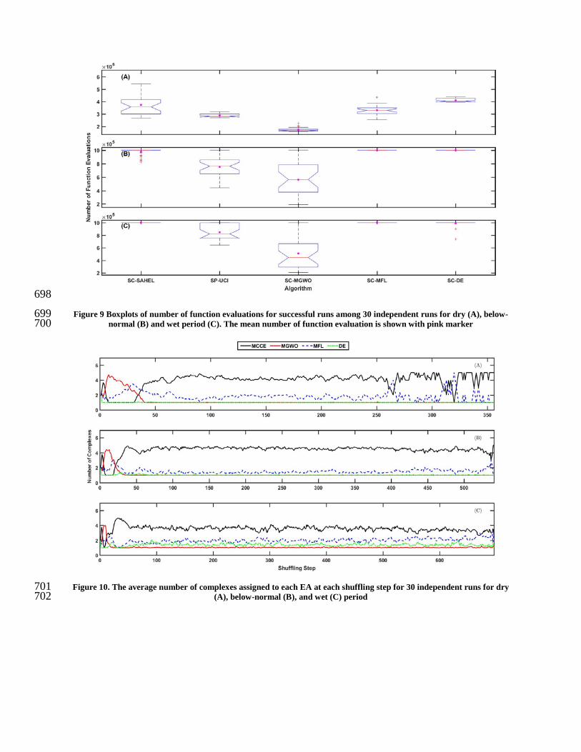
In Figure 9, boxplot of the number of function evaluations is presented for successful runs 632
from the 30 independent runs during dry, below-normal and wet period years. Although the SC-633
MGWO algorithm satisfied convergence criteria in the least number of function evaluation, the 634
SC-MGWO was not successful in achieving the optimum solution in many cases. The SP-UCI 635
algorithm is the second fastest method among all the algorithms. The hybrid SC-SAHEL, SC-636
MFL, and SC-DE are the slowest algorithm for satisfying the convergence criteria, in almost all 637
cases. The slow performance of the hybrid SC-SAHEL is due to the fact that 2 out of 4 (DE and 638
MFL) participating EAs have very slow performance over the response surface. Figure 10 639
demonstrates the number of complexes assigned to each EA during the search, which indicates the 640
dominance of the participating algorithms, and the “award and punishment” logic in the reservoir 641
model. As seen in Figure 10, the MGWO algorithm is dominant in the beginning of the search; 642
although, it is not capable of finding the optimum solution in most cases. The reason for the 643

dominance of the MGWO is the speed of the algorithm in exploring the search space. MGWO is 644
superior to other EAs in the beginning of the search, however, after a few iterations, the MCCE 645
algorithm took the precedence and become the dominant algorithm over other EAs. MGWO and 646
DE are less involved in the rest of the optimization process after the initial steps. However, 647
competition between MCCE and MFL continues. Although contribution of MGWO and DE are at 648
minimum in rest of the optimization process, they are utilizing a part of information within the 649
population. This can affect the speed and performance of the SC-SAHEL algorithm. In both the 650
wet and below-normal cases, the hybrid SC-SAHEL algorithm is mostly terminated by reaching 651
the maximum number of function evolution. However, the mean objective function value obtained 652
by the hybrid SC-SAHEL is still superior to most of the algorithms. 653
The performance of the SC-SAHEL can be affected by the settings of the algorithm. 654
Different settings have been tested and evaluated for the reservoir model. The results show that 655
the number of evolution steps before shuffling can influence the performance of the hybrid SC-656
SAHEL algorithm. In the current setting, the number of evolution steps within each complex is set 657
to d+1 (d is dimension of the problem). Although this setting seems to provide acceptable 658
performance for a wide range of problems, it may not be the optimum setting for all the problems 659
spaces and EAs. In the reservoir model, as the study period has 91 days, the model evolves each 660
complex for 92 steps. This number of evolution steps allows the algorithms to navigate the 661
complexes toward local solutions and increase the total number of function evaluations without 662
specific gain. Decreasing the number of evolution steps allows the algorithms to communicate 663
more frequently, so they can use the information obtained by other EAs. Here, for demonstrative 664
purposes, the same setting has been applied to all the problems. However, better performance is 665
observed for the hybrid SC-SAHEL algorithm when the number of evolution steps are set to a 666

value smaller than 92. The algorithm is less sensitive to other settings for the reservoir model, 667
however they can still affect the performance of the algorithm. 668
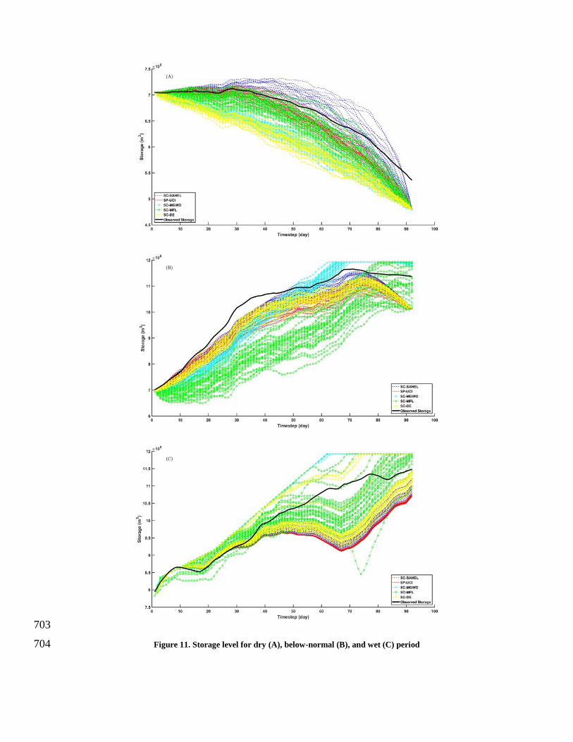
In Figure 11, we present the simulated storage level for different study periods achieved 669
by different EAs. During the dry period, not only the SC-SAHEL algorithm achieved the lowest 670
objective function value, but also the storage level is higher than the observed storage level in most 671
of the period. This is due to the fact that, power generation is a function of water height, as well as 672
discharge rate. During below-normal period, SC-SAHEL, SP-UCI, and SC-DE algorithms show a 673
similar behavior in terms of the storage level. During wet period, storage level simulated by SP-674
UCI and SC-SAHEL algorithm is lower than all other algorithms. It is worth noting that, during 675
wet period, SC-SAHEL and SP-UCI algorithms are able to find optimum solution (which objective 676
function value is 0) in some of the runs. However, the simulated storage by these algorithms show 677
some level of uncertainties (Figure 11). This shows equifinality in simulation, which means that 678
same hydropower generation can be achieved by different sets of parameters (Feng et al. 2017). 679
This equifinality can be due to deficiencies in the model structure, or the boundary conditions 680
(Freer et al. 1996). The wet period seems to offer a more complex response surface for the reservoir 681
model. During the wet period, some algorithms, such as SC-DE, are not capable of finding a 682
feasible solution in some of the runs. In this period, the large input volume and the rule curve 683
added more complexity to the optimization problem. In other study periods, the reservoir level is 684
always below the rule curve. 685
The results of the real-world application show the potential of the newly developed SC-686
SAHEL framework for solving high dimension problems. In general, the hybrid algorithm was 687
more successful in finding a feasible solution in comparison to single-method algorithms. In some 688
cases, the hybrid SC-SAHEL was terminated due to the large number of function evaluations. 689
However, the performance of the hybrid SC-SAHEL is always comparable to the best performing 690

method. This shows the potential of the SC-SAHEL for solving a broad class of optimization 691
problems. Besides, the framework provides insight into the performance of the algorithms at 692
different steps of the optimization process. This feature of the SC-SAHEL algorithm can aid the 693
user to select the best setting and EA for the problem. 694
695
Figure 8. Boxplots of objective function values for successful runs among 30 independent runs, for dry (A), below-normal 696 (B) and wet period (C). The mean of objective functions values is shown with pink marker. 697
698
Figure 9 Boxplots of number of function evaluations for successful runs among 30 independent runs for dry (A), below-699 normal (B) and wet period (C). The mean number of function evaluation is shown with pink marker 700
Figure 10. The average number of complexes assigned to each EA at each shuffling step for 30 independent runs for dry 701 (A), below-normal (B), and wet (C) period 702
703
Figure 11. Storage level for dry (A), below-normal (B), and wet (C) period 704

5 Conclusions and remarks 705
We developed a hybrid optimization framework, named Shuffled Complex Self Adaptive 706
Hybrid EvoLution (SC-SAHEL), which uses an “award and punishment” logic in junction with 707
various types of Evolutionary Algorithms (EAs), and selects the best EA that fits well to different 708
optimization problems. The framework provides an arsenal of tools for testing, evaluating and 709
developing optimization algorithms. We compared the performance of the hybrid SC-SAHEL 710
with single-method algorithms on 29 test functions. The results showed that the SC-SAHEL 711
algorithm is superior to most of single-method optimization algorithms and in general offers a 712
more robust and efficient algorithm for optimizing various problems. Furthermore, the proposed 713
algorithm is able to reveal the characteristics of different EAs during entire search period. The 714
algorithm is also designed to work in a parallel framework which can take the advantage of 715
available computation resources. The newly developed SC-SAHEL offers different advantages 716
over conventional optimization tools. Some of the SC-SAHEL characteristics are: 717
- Intelligent evolutionary method adaptation during the optimization process 718
- Flexibility of the algorithm for using different evolutionary methods 719
- Flexibility of the algorithm for using initial sampling and boundary handling method 720
- Independent parallel evolution of complexes 721
- Population degeneration avoidance using PCA algorithm 722
- Robust and Fast optimization process 723
- Evolutionary algorithms comparison for different types of problems 724
Although the presented results support advantage of the hybrid SC-SAHEL to individual 725
EAs algorithms, there are multiple directions for further improvement of the framework. For 726
example, EAs’ performance metric for evaluating the search mechanism. In the current algorithm, 727
the complex allocation to different EA is carried out by ranking the algorithm according to the 728
EMP metric. The performance criteria can change the allocation process and affect the 729
performance of the algorithm. Depending on the application a more comprehensive performance 730
criterion may be necessary for achieving the best performance. However, the current EMP criterion 731
does not affect the conclusion and comparison of different EAs. In addition, the current SC-732
SAHEL framework is designed to solve single objective optimization problems. A multi-objective 733
version can be developed to extend the scope of the application. This paper serves as an 734
introduction to the newly developed SC-SAHEL algorithm. We hope that more investigation on 735
the interaction among different EAs, boundary handling schemes and response surface in different 736
case studies and optimization problems reveal the advantages and limitations of SC-SAHEL. 737
Acknowledgments and data 738
This work is supported by U.S. Department of Energy (DOE Prime Award # DE-739
IA0000018), California Energy Commission (CEC Award # 300-15-005), NSF CyberSEES 740
Project (Award CCF-1331915), NOAA/NESDIS/NCDC (Prime award NA09NES4400006 and 741
NCSU CICS and subaward 2009-1380-01), and the U.S. Army Research Office (award W911NF-742
11-1-0422). The Folsom reservoir bathymetry information used here is provided by Dr. Erfan 743
Goharian from UC Davis, who also helped us for setting up the reservoir model. The authors would 744
like to thank the comments of the fours anonymous reviewers which significantly improved the 745
quality of the paper. 746
References 747
Barati, R., Neyshabouri, S.S. and Ahmadi, G. (2014) Sphere drag revisited using shuffled 748
complex evolution algorithm. 749
Beven, K.J. (2011) Rainfall-runoff modelling: the primer, John Wiley & Sons. 750
Blum, C. and Roli, A. (2003) Metaheuristics in combinatorial optimization: Overview and 751
conceptual comparison. ACM Comput. Surv. 35(3), 268-308. 752
Boussaïd, I., Lepagnot, J. and Siarry, P. (2013) A survey on optimization metaheuristics. 753
Information sciences 237(Supplement C), 82-117. 754
Boyle, D.P., Gupta, H.V., and Sorooshian, S. (2000) Toward improved calibration of 755
hydrologic models: Combining the strengths of manual and automatic methods. Water Resources 756
Research 36(12), 3663-3674. 757
Chu, W., Gao, X. and Sorooshian, S. (2010) Improving the shuffled complex evolution 758
scheme for optimization of complex nonlinear hydrological systems: Application to the 759
calibration of the Sacramento soil-moisture accounting model. Water Resources Research 46(9), 760
n/a-n/a. 761
Chu, W., Gao, X. and Sorooshian, S. (2011) A new evolutionary search strategy for global 762
optimization of high-dimensional problems. Information sciences 181(22), 4909-4927. 763
Coello, C.A.C., Lamont, G.B. and Van Veldhuizen, D.A. (2007) Evolutionary algorithms for 764
solving multi-objective problems, Springer. 765
Črepinšek, M., Liu, S.-H. and Mernik, M. (2013) Exploration and exploitation in 766
evolutionary algorithms: A survey. ACM Computing Surveys (CSUR) 45(3), 35. 767
Ding, Y., Wang, C., Chaos, M., Chen, R. and Lu, S. (2016) Estimation of beech pyrolysis 768
kinetic parameters by Shuffled Complex Evolution. Bioresource Technology 200, 658-665. 769
Dorigo, M., Maniezzo, V. and Colorni, A. (1996) Ant system: optimization by a colony of 770
cooperating agents. IEEE Transactions on Systems, Man, and Cybernetics, Part B (Cybernetics) 771
26(1), 29-41. 772
Duan, Q., Sorooshian, S. and Gupta, V. (1992) Effective and efficient global optimization for 773
conceptual rainfall-runoff models. Water Resources Research 28(4), 1015-1031. 774
Duan, Q.Y., Gupta, V.K. and Sorooshian, S. (1993) Shuffled complex evolution approach for 775
effective and efficient global minimization. Journal of Optimization Theory and Applications 776
76(3), 501-521. 777

Duan Q., Sorooshian S., Gupta V.K. Optimal use of the SCE-UA global optimization method 778
for calibrating watershed models. Journal of hydrology. 1994 Jun 15;158(3-4):265-84. 779
Eckhardt, K. and Arnold, J.G. (2001) Automatic calibration of a distributed catchment 780
model. Journal of Hydrology 251(1–2), 103-109. 781
Erol, O.K. and Eksin, I. (2006) A new optimization method: big bang–big crunch. Advances 782
in Engineering Software 37(2), 106-111. 783
Eusuff, M., Lansey, K. and Pasha, F. (2006) Shuffled frog-leaping algorithm: a memetic 784
meta-heuristic for discrete optimization. Engineering Optimization 38(2), 129-154. 785
Eusuff, M.M. and Lansey, K.E. (2003) Optimization of water distribution network design 786
using the shuffled frog leaping algorithm. Journal of Water Resources Planning and Management 787
129(3), 210-225. 788
Feng, M., Liu, P., Guo, S., Shi, L., Deng, C. and Ming, B. (2017) Deriving adaptive 789
operating rules of hydropower reservoirs using time-varying parameters generated by the EnKF. 790
Water Resources Research 53(8), 6885-6907. 791
Field, R. and Lund, J.R. (2006) Operating Reservoirs in Changing Conditions, pp. 205-214. 792
Freer, J., Beven, K. and Ambroise, B. (1996) Bayesian Estimation of Uncertainty in Runoff 793
Prediction and the Value of Data: An Application of the GLUE Approach. Water Resources 794
Research 32(7), 2161-2173. 795
Gan, T.Y. and Biftu, G.F. (1996) Automatic Calibration of Conceptual Rainfall-Runoff 796
Models: Optimization Algorithms, Catchment Conditions, and Model Structure. Water 797
Resources Research 32(12), 3513-3524. 798
Golberg, D.E. (1989) Genetic algorithms in search, optimization, and machine learning. 799
Addion wesley 1989, 102. 800
Hadka, D., Madduri, K. and Reed, P. (2013) Scalability analysis of the asynchronous, 801
master-slave Borg multiobjective evolutionary algorithm, pp. 425-434, IEEE. 802
Hadka, D. and Reed, P. (2013) Borg: An Auto-Adaptive Many-Objective Evolutionary 803
Computing Framework. Evolutionary Computation 21(2), 231-259. 804
Hasalová, L., Ira, J. and Jahoda, M. (2016) Practical observations on the use of Shuffled 805
Complex Evolution (SCE) algorithm for kinetic parameters estimation in pyrolysis modeling. 806
Fire Safety Journal 80, 71-82. 807
Holland, J.H. (1975) Adaptation in Natural and Artificial Systems, Univ. of Mich. Press. Ann 808
Arbor. 809
Holland, J.H. (1992) Adaptation in natural and artificial systems. 1975. Ann Arbor, MI: 810
University of Michigan Press and. 811
K. Ajami, N., Gupta, H., Wagener, T. and Sorooshian, S. (2004) Calibration of a semi-812
distributed hydrologic model for streamflow estimation along a river system. Journal of 813
Hydrology 298(1), 112-135. 814
Kan, A.R. and Timmer, G.T. (1987) Stochastic global optimization methods part I: 815
Clustering methods. Mathematical programming 39(1), 27-56. 816
Kaveh, A. and Farhoudi, N. (2013) A new optimization method: Dolphin echolocation. 817
Advances in Engineering Software 59, 53-70. 818
Kaveh, A. and Talatahari, S. (2010) A novel heuristic optimization method: charged system 819
search. Acta Mechanica 213(3), 267-289. 820
Kennedy, J. (2010) Encyclopedia of Machine Learning. Sammut, C. and Webb, G.I. (eds), 821
pp. 760-766, Springer US, Boston, MA. 822
Kirkpatrick, S., Gelatt, C.D. and Vecchi, M.P. (1983) Optimization by simmulated annealing. 823
science 220(4598), 671-680. 824
Lee, K.S. and Geem, Z.W. (2005) A new meta-heuristic algorithm for continuous 825
engineering optimization: harmony search theory and practice. Computer Methods in Applied 826
Mechanics and Engineering 194(36), 3902-3933. 827
Liang, J.J., Suganthan, P.N. and Deb, K. (2005) Novel composition test functions for 828
numerical global optimization, pp. 68-75. 829
Lin, J.-Y., Cheng, C.-T. and Chau, K.-W. (2006) Using support vector machines for long-830
term discharge prediction. Hydrological Sciences Journal 51(4), 599-612. 831
Liong, S.-Y. and Atiquzzaman, M. (2004) Optimal design of water distribution network 832
using shuffled complex evolution. Journal of The Institution of Engineers, Singapore 44(1), 93-833
107. 834
Madsen, H. (2000) Automatic calibration of a conceptual rainfall–runoff model using 835
multiple objectives. Journal of Hydrology 235(3), 276-288. 836
Madsen, H. (2003) Parameter estimation in distributed hydrological catchment modelling 837
using automatic calibration with multiple objectives. Advances in Water Resources 26(2), 205-838
216. 839
Maier, H.R., Kapelan, Z., Kasprzyk, J., Kollat, J., Matott, L.S., Cunha, M.C., Dandy, G.C., 840
Gibbs, M.S., Keedwell, E., Marchi, A., Ostfeld, A., Savic, D., Solomatine, D.P., Vrugt, J.A., 841
Zecchin, A.C., Minsker, B.S., Barbour, E.J., Kuczera, G., Pasha, F., Castelletti, A., Giuliani, M. 842
and Reed, P.M. (2014) Evolutionary algorithms and other metaheuristics in water resources: 843
Current status, research challenges and future directions. Environmental Modelling & Software 844
62(Supplement C), 271-299. 845
Mariani, V.C., Justi Luvizotto, L.G., Guerra, F.A. and dos Santos Coelho, L. (2011) A hybrid 846
shuffled complex evolution approach based on differential evolution for unconstrained 847
optimization. Applied Mathematics and Computation 217(12), 5822-5829. 848
Mirjalili, S. and Hashim, S.Z.M. (2010) A new hybrid PSOGSA algorithm for function 849
optimization, pp. 374-377. 850
Mirjalili, S., Mirjalili, S.M. and Lewis, A. (2014) Grey Wolf Optimizer. Advances in 851
Engineering Software 69, 46-61. 852
Mirjalili, S., Saremi, S., Mirjalili, S.M. and Coelho, L.d.S. (2016) Multi-objective grey wolf 853
optimizer: A novel algorithm for multi-criterion optimization. Expert Systems with Applications 854
47(Supplement C), 106-119. 855
Moeini, R. and Afshar, M. (2009) Application of an ant colony optimization algorithm for 856
optimal operation of reservoirs: a comparative study of three proposed formulations. Sci Iran 857
Trans A Civ Eng 16(4), 273-285. 858
Nelder, J.A. and Mead, R. (1965) A simplex method for function minimization. The 859
computer journal 7(4), 308-313. 860
Nicklow, J., Reed, P., Savic, D., Dessalegne, T., Harrell, L., Chan-Hilton, A., Karamouz, M., 861
Minsker, B., Ostfeld, A., Singh, A. and Zechman, E. (2010) State of the Art for Genetic 862
Algorithms and Beyond in Water Resources Planning and Management. Journal of Water 863
Resources Planning and Management 136(4), 412-432. 864
Olorunda, O. and Engelbrecht, A.P. (2008) Measuring exploration/exploitation in particle 865
swarms using swarm diversity, pp. 1128-1134. 866
Omran, M.G.H., Salman, A. and Engelbrecht, A.P. (2005) Computational Intelligence and 867
Security: International Conference, CIS 2005, Xi’an, China, December 15-19, 2005, Proceedings 868
Part I. Hao, Y., Liu, J., Wang, Y., Cheung, Y.-m., Yin, H., Jiao, L., Ma, J. and Jiao, Y.-C. (eds), 869
pp. 192-199, Springer Berlin Heidelberg, Berlin, Heidelberg. 870
Passino, K.M. (2002) Biomimicry of bacterial foraging for distributed optimization and 871
control. IEEE Control Systems 22(3), 52-67. 872
Price, W. (1987) Global optimization algorithms for a CAD workstation. Journal of 873
Optimization Theory and Applications 55(1), 133-146. 874
Qin, A.K. and Suganthan, P.N. (2005) Self-adaptive differential evolution algorithm for 875
numerical optimization, pp. 1785-1791 Vol. 1782. 876
Rashedi, E., Nezamabadi-Pour, H. and Saryazdi, S. (2009) GSA: a gravitational search 877
algorithm. Information sciences 179(13), 2232-2248. 878
Reed, P.M., Hadka, D., Herman, J.D., Kasprzyk, J.R. and Kollat, J.B. (2013) Evolutionary 879
multiobjective optimization in water resources: The past, present, and future. Advances in Water 880
Resources 51(Supplement C), 438-456. 881
Sadegh M, Vrugt JA. (2014) Approximate bayesian computation using markov chain monte 882
carlo simulation: Dream (abc). Water Resources Research. 50(8), 6767-6787. 883
Sadegh M., Ragno E., AghaKouchak A. Multivariate Copula Analysis Toolbox (MvCAT): 884
Describing dependence and underlying uncertainty using a Bayesian framework. Water 885
Resources Research. 2017 Jun 1. 886
Sorooshian, S., Duan, Q. and Gupta, V.K. (1993) Calibration of rainfall-runoff models: 887
Application of global optimization to the Sacramento Soil Moisture Accounting Model. Water 888
Resources Research 29(4), 1185-1194. 889
Storn, R. and Price, K. (1997) Differential Evolution – A Simple and Efficient Heuristic for 890
global Optimization over Continuous Spaces. Journal of Global Optimization 11(4), 341-359. 891
Toth, E., Brath, A. and Montanari, A. (2000) Comparison of short-term rainfall prediction 892
models for real-time flood forecasting. Journal of Hydrology 239(1), 132-147. 893
Vrugt, J.A., Gupta, H.V., Bastidas, L.A., Bouten, W. and Sorooshian, S. (2003a) Effective 894
and efficient algorithm for multiobjective optimization of hydrologic models. Water Resources 895
Research 39(8), n/a-n/a. 896
Vrugt, J.A., Gupta, H.V., Bouten, W. and Sorooshian, S. (2003b) A Shuffled Complex 897
Evolution Metropolis algorithm for optimization and uncertainty assessment of hydrologic model 898
parameters. Water Resources Research 39(8), n/a-n/a. 899
Vrugt, J.A. and Robinson, B.A. (2007) Improved evolutionary optimization from genetically 900
adaptive multimethod search. Proceedings of the National Academy of Sciences 104(3), 708-901
711. 902
Vrugt, J.A., Robinson, B.A. and Hyman, J.M. (2009) Self-Adaptive Multimethod Search for 903
Global Optimization in Real-Parameter Spaces. IEEE Transactions on Evolutionary Computation 904
13(2), 243-259. 905
Wagener, T., Wheater, H. and Gupta, H.V. (2004) Rainfall-runoff modelling in gauged and 906
ungauged catchments, World Scientific. 907
Wang, Y.-C., Yu, P.-S. and Yang, T.-C. (2010) Comparison of genetic algorithms and 908
shuffled complex evolution approach for calibrating distributed rainfall–runoff model. 909
Hydrological processes 24(8), 1015-1026. 910
Wolpert, D.H. and Macready, W.G. (1997) No free lunch theorems for optimization. IEEE 911
Transactions on Evolutionary Computation 1(1), 67-82. 912
Woodruff, M.J., Reed, P.M. and Simpson, T.W. (2013) Many objective visual analytics: 913
rethinking the design of complex engineered systems. Structural and Multidisciplinary 914
Optimization 48(1), 201-219. 915
Xin, Y., Yong, L. and Guangming, L. (1999) Evolutionary programming made faster. IEEE 916
Transactions on Evolutionary Computation 3(2), 82-102. 917
Yang, T., Asanjan, A.A., Faridzad, M., Hayatbini, N., Gao, X. and Sorooshian, S. (2017) An 918
enhanced artificial neural network with a shuffled complex evolutionary global optimization 919
with principal component analysis. Information sciences 418, 302-316. 920
Yang, T., Gao, X., Sellars, S.L. and Sorooshian, S. (2015) Improving the multi-objective 921
evolutionary optimization algorithm for hydropower reservoir operations in the California 922
Oroville–Thermalito complex. Environmental Modelling & Software 69, 262-279. 923
Yang, X.-S. (2009) Stochastic Algorithms: Foundations and Applications: 5th International 924
Symposium, SAGA 2009, Sapporo, Japan, October 26-28, 2009. Proceedings. Watanabe, O. and 925
Zeugmann, T. (eds), pp. 169-178, Springer Berlin Heidelberg, Berlin, Heidelberg. 926
Yang, X.-S. (2010) Nature Inspired Cooperative Strategies for Optimization (NICSO 2010). 927
González, J.R., Pelta, D.A., Cruz, C., Terrazas, G. and Krasnogor, N. (eds), pp. 65-74, Springer 928
Berlin Heidelberg, Berlin, Heidelberg. 929
Yapo, P.O., Gupta, H.V. and Sorooshian, S. (1996) Automatic calibration of conceptual 930
rainfall-runoff models: sensitivity to calibration data. Journal of Hydrology 181(1), 23-48. 931
Yapo, P.O., Gupta, H.V. and Sorooshian, S. (1998) Multi-objective global optimization for 932
hydrologic models. Journal of Hydrology 204(1-4), 83-97. 933

Appendix A. Modified Competitive Complex Evolution (MCCE) 934
MCCE algorithm pseudo code is as follow: 935
Step 0. Initialize i = 1, and get maximum number of iteration allowed, I. 936
Step 1. Sort individuals in order of increasing objective function value. Assign individuals a 937
triangular probability (except for the fittest point) according to: 938
𝑝𝑝 = 2(NPT+1−𝑚𝑚)NPT(NPT+1)
, (A1) 939
where NPT is the number of individuals in the complex and 𝑛𝑛 is the rank of the sorted 940
individuals. 941
Step 2. Select d+1 individuals (d is problem dimension) from the complex including the fittest 942
individual in the complex. 943
Step 3. The selected individuals are then stored in S, forming a simplex. Generate offspring 944
according to following steps. 945
I. Sort individuals in S according to their objective function value. Find centroid, 𝑐𝑐, of the 946
first q individuals. 947
II. Reflection: Reflect the worst individual in S, 𝑤𝑤��⃑ , across the centroid to generate a new 948
point, 𝑟𝑟, according to following equation: 949
𝑟𝑟 = 2𝑐𝑐 − 𝑤𝑤��⃑ . (A2) 950
Evaluate objective function for the new point, 𝑐𝑐𝑟𝑟. If 𝑐𝑐1 < 𝑐𝑐𝑟𝑟 < 𝑐𝑐𝑑𝑑 set offspring, �⃑�𝑟 = 𝑟𝑟, 951
and go to (VII). 952
III. Expansion: If 𝑐𝑐𝑟𝑟 < 𝑐𝑐1, reflect 𝑐𝑐 across 𝑟𝑟 and generate 𝑒𝑒, 953
𝑒𝑒 = 2𝑟𝑟 − 𝑐𝑐. (A3) 954
Evaluate objective function for the new point, 𝑐𝑐𝑒𝑒. If 𝑐𝑐𝑒𝑒 < 𝑐𝑐𝑟𝑟, set �⃑�𝑟 = 𝑒𝑒 and go to (VII); 955
otherwise, �⃑�𝑟 = 𝑟𝑟 and go to (VII). 956

IV. Outside contraction: If 𝑐𝑐𝑑𝑑 ≤ 𝑐𝑐𝑟𝑟 < 𝑐𝑐𝑡𝑡, calculate the outside contraction point, 957
𝑟𝑟𝑐𝑐����⃑ = 𝑐𝑐 + 0.5(𝑟𝑟 − 𝑐𝑐). (A4) 958
Evaluate the outside contraction point, 𝑐𝑐𝑜𝑜𝑐𝑐. If 𝑐𝑐𝑜𝑜𝑐𝑐 < 𝑐𝑐𝑟𝑟 set �⃑�𝑟 = 𝑟𝑟𝑐𝑐����⃑ and go to (VII); 959
otherwise, �⃑�𝑟 = 𝑟𝑟 and go to (VII). 960
V. Inside contraction: If 𝑐𝑐𝑡𝑡 < 𝑐𝑐𝑟𝑟 calculate inside contraction point, 961
𝚤𝚤𝑐𝑐���⃑ = 𝑐𝑐 + 0.5(𝑤𝑤��⃑ − 𝑐𝑐). (A5) 962
Evaluate inside contraction point, 𝑐𝑐𝑚𝑚𝑐𝑐. If 𝑐𝑐𝑚𝑚𝑐𝑐 < 𝑐𝑐𝑟𝑟 set �⃑�𝑟 = 𝚤𝚤𝑐𝑐���⃑ and go to (VII); otherwise 963
continue to (VI). 964
VI. Multinormal sampling: If the steps above, did not generate a better offspring, an 965
individual will be drawn with a multinormal distribution defined by simplex and replace 966
the worst individual in the simplex, regardless of objective function value. The 967
multinormal sampling is as follow, 968
a. Calculate the covariance matrix, R, for the simplex and store diagonal of matrix in 969
𝐷𝐷��⃑ . 970
b. Modify 𝐷𝐷��⃑ as follow 971
𝐷𝐷𝑚𝑚������⃑ = 2(𝐷𝐷��⃑ + 𝑚𝑚𝑒𝑒𝑚𝑚𝑛𝑛(𝐷𝐷��⃑ )). (A6) 972
c. Generate a new covariance matrix 𝑅𝑅′, with 𝐷𝐷𝑚𝑚������⃑ as diagonal and zeroes everywhere 973
else. 974
d. Sample a point with multinormal distribution with mean of 𝑐𝑐 and covariance of 𝑅𝑅′ 975
and store in �⃑�𝑟. 976
VII. Replace the worst individual in the complex with �⃑�𝑟. Let 𝑖𝑖 = 𝑖𝑖 + 1. If 𝑖𝑖 ≤ 𝐼𝐼, go to (Step 977
1); otherwise sort the complex and return the evolved complex. 978

Appendix B. Modified Frog Leaping (MFL) 979
Modified FL (MFL) algorithm is as follow, 980
Step 0. Initialize i = 1, and get maximum number of iteration allowed , I. 981
Step 1. Sort individuals in order of increasing objective function. Assign individuals a triangular 982
probability using following equation: 983
𝑝𝑝 = 2(NPT+1−𝑚𝑚)NPT(NPT+1)
, (B1) 984
where NPT is the number of individuals in the complex and 𝑛𝑛 is the rank of the sorted 985
individuals. 986
Step 2. Select d+1 individuals (d is problem dimension) from the complex. 987
Step 3. The selected individuals are stored in S, forming a subcomplex. Generate offspring 988
according to following steps. 989
I. Generate a new point with the worst point in S, 𝑤𝑤��⃑ and best point 𝑏𝑏�⃑ in the subcomplex, as 990
follow, 991
𝑛𝑛𝑏𝑏����⃑ = 𝑤𝑤��⃑ + ( 0.5 × 𝑅𝑅 + 1.5)(𝑏𝑏�⃑ − 𝑤𝑤��⃑ ), (B2) 992
where 𝑅𝑅 is a random number in the range of [0,1]. Evaluate objective function for the 993
new point and get 𝑐𝑐𝑏𝑏. If 𝑐𝑐𝑏𝑏 < 𝑐𝑐𝑡𝑡; set �⃑�𝑟 = 𝑛𝑛𝑏𝑏����⃑ and go to (IV). 994
II. If 𝑐𝑐𝑡𝑡 < 𝑐𝑐𝑏𝑏, generate a new point with the worst point in S,𝑤𝑤��⃑ and best point 𝑏𝑏�⃑ in the 995
subcomplex, as follow, 996
𝑛𝑛𝐵𝐵����⃑ = 𝑤𝑤��⃑ + 0.5 × 𝑅𝑅(𝑏𝑏�⃑ − 𝑤𝑤��⃑ ), (B3) 997
Evaluate objective function for the new point and get 𝑐𝑐𝐵𝐵. If 𝑐𝑐𝐵𝐵 < 𝑐𝑐𝑡𝑡 set the offspring set 998
�⃑�𝑟 = 𝑛𝑛𝐵𝐵����⃑ and go to (IV). 999
III. Censorship step: If 𝑐𝑐𝑡𝑡 < 𝑐𝑐𝐵𝐵, randomly generate the offspring, �⃑�𝑟 by sampling within 1000
the range of individuals in the subcomplex. 1001

IV. Replace the worst individual in the complex with the offspring, �⃑�𝑟. Let 𝑖𝑖 = 𝑖𝑖 + 1. If 𝑖𝑖 ≤ 𝐼𝐼, 1002
go to (Step 1); otherwise sort the complex and return the evolved complex. 1003

Appendix C. Modified Grey Wolf Optimizer (GWO) 1004
Modified Grey Wolf Optimizer is as follow: 1005
Step 0. Initialize i = 1, and get maximum number of iteration allowed, I. 1006
Step 1. Sort the individuals in the order of increasing objective function value. Assign individuals 1007
a triangular probability (except for the fittest point) using following equation: 1008
𝑝𝑝 = 2(NPT+1−𝑚𝑚)NPT(NPT+1)
, (C1) 1009
where NPT is the number of individuals in the complex and 𝑛𝑛 is the rank of the sorted 1010
individuals. 1011
Step 2. Select d+1 individuals (d is problem dimension) from the complex, with triangular 1012
probability, including the fittest point in the complex and store them in S. 1013
Step 3. Select the best three points in the S and store them in �⃑�𝛼, 𝛽𝛽 and �⃑�𝛾, respectively. The worst 1014
point in the S, is stored in 𝑤𝑤��⃑ 1015
Step 4. For each of �⃑�𝛼, 𝛽𝛽 and �⃑�𝛾 , evolve individuals according to the following procedure, 1016
I. Derive 𝐴𝐴 and 𝐶𝐶 as follow for �⃑�𝛼, 𝛽𝛽 and �⃑�𝛾, 1017
𝐴𝐴 = 4 × 𝑟𝑟1 − 2, (C2) 1018
𝐶𝐶 = 2 × 𝑟𝑟2. (C3) 1019
where 𝑟𝑟1���⃑ , 𝑟𝑟2���⃑ are two independent random vectors, which have d dimensions and values in 1020
range of [0,1). 1021
II. Derive 𝐷𝐷��⃑ , for �⃑�𝛼, 𝛽𝛽 and �⃑�𝛾 as follow, 1022
𝐷𝐷𝛼𝛼�����⃑ = �𝐶𝐶𝛼𝛼����⃑ × 𝑋𝑋𝛼𝛼����⃑ − 𝑤𝑤��⃑ � , 𝐷𝐷𝛽𝛽����⃑ = �𝐶𝐶𝛽𝛽����⃑ × 𝑋𝑋𝛽𝛽����⃑ − 𝑤𝑤��⃑ � , 𝐷𝐷𝛾𝛾����⃑ = �𝐶𝐶𝛾𝛾����⃑ × 𝑋𝑋𝛾𝛾����⃑ − 𝑤𝑤��⃑ �. (C4) 1023
III. Derive �⃑�𝑍, for �⃑�𝛼, 𝛽𝛽 and �⃑�𝛾 as follow, 1024
𝑍𝑍𝛼𝛼����⃑ = 𝑋𝑋𝛼𝛼����⃑ − 𝐴𝐴𝛼𝛼�����⃑ . (𝐷𝐷𝛼𝛼�����⃑ ) , 𝑍𝑍𝛽𝛽����⃑ = 𝑋𝑋𝛽𝛽����⃑ − 𝐴𝐴𝛽𝛽����⃑ . (𝐷𝐷𝛽𝛽����⃑ ) , 𝑍𝑍𝛾𝛾����⃑ = 𝑋𝑋𝛾𝛾����⃑ − 𝐴𝐴𝛾𝛾����⃑ . (𝐷𝐷𝛾𝛾����⃑ ) . (C5) 1025

IV. Generate new point by finding the centroid of 𝑍𝑍𝛼𝛼����⃑ , 𝑍𝑍𝛽𝛽����⃑ and 𝑍𝑍𝛾𝛾����⃑ , 1026
𝐶𝐶 = 𝑍𝑍𝛼𝛼�����⃑ +𝑍𝑍𝛽𝛽�����⃑ +𝑍𝑍𝛾𝛾����⃑
3. (C6) 1027
V. Calculate and store objective function value for the new point, 𝑐𝑐𝐶𝐶 . If the new point is 1028
better than the worst point among the selected points, 𝑐𝑐𝐶𝐶 < 𝑐𝑐𝑡𝑡, set �⃑�𝑟 = 𝐶𝐶, go to step 7. 1029
Step 5. If 𝑐𝑐𝐶𝐶 > 𝑐𝑐𝑡𝑡, go to step 4, and use a smaller range for 𝐴𝐴. In this step, 𝐴𝐴 is calculated as 1030
follow: 1031
𝐴𝐴 = 2 × 𝑟𝑟1 − 1, (C7) 1032
Step 6. If the newly generated individual is worse than the worst individuals in subcomplex, 1033
generate a new point with uniform random sampling within the range of individuals in the 1034
complex. Store the new point in �⃑�𝑟. 1035
Step 7. Replace the worst individual among selected points in the complex with the offspring, �⃑�𝑟. 1036
Let 𝑖𝑖 = 𝑖𝑖 + 1. If 𝑖𝑖 ≤ 𝐼𝐼, go to (Step 1); otherwise sort the complex and return the evolved 1037
complex. 1038

Appendix D. Modified Differential Evolution (DE) 1039
Modified differential evolution algorithm is as follow: 1040
Step 0. Initialize i = 1, and get maximum number of iteration allowed, I. 1041
Step 1. Sort the individuals in the order of increasing objective function value. Assign individuals 1042
a triangular probability, using following equation: 1043
𝑝𝑝 = 2(NPT+1−𝑚𝑚)NPT(NPT+1)
, (D1) 1044
where NPT is the number of individuals in the complex and 𝑛𝑛 is the rank of the sorted 1045
individuals. 1046
Step 2. Select d+1 points (d is problem dimension) from the complex with the assigned 1047
probability and store them along with the fittest point in the complex in S. 1048
Step 3. The selected individuals are sorted and stored in S, forming a subcomplex. Generate 1049
offspring according to following steps. 1050
I. Generate a new point with the worst point in S, 𝑤𝑤��⃑ and using the top three individuals in 1051
the subcomplex, 1052
𝑉𝑉1���⃑ = 𝑤𝑤��⃑ + 2𝑐𝑐(𝑠𝑠1���⃑ − 𝑤𝑤��⃑ ) + 2𝑐𝑐(𝑠𝑠2���⃑ − 𝑠𝑠3���⃑ ), (D2) 1053
where 𝑤𝑤��⃑ is the worst point in the S, 𝑠𝑠1���⃑ , 𝑠𝑠2���⃑ , and 𝑠𝑠3���⃑ are three selected individuals. Then 1054
mutation, and crossover operator is applied to the 𝑤𝑤��⃑ and 𝑉𝑉1���⃑ to generate 𝑉𝑉𝑚𝑚1������⃑ . The objective 1055
function value for the new point is calculated and stored in 𝑐𝑐𝑚𝑚1. If 𝑐𝑐𝑚𝑚1 < 𝑐𝑐𝑡𝑡; set �⃑�𝑟 = 𝑉𝑉𝑚𝑚1������⃑ 1056
and go to (V). 1057
II. If 𝑐𝑐𝑡𝑡 < 𝑐𝑐𝑚𝑚1, generate a new point with the worst point in S, 𝑤𝑤��⃑ and using the top three 1058
points in the subcomplex as follow, 1059
𝑉𝑉2���⃑ = 𝑤𝑤��⃑ + 0.5𝑐𝑐(𝑠𝑠1���⃑ − 𝑤𝑤��⃑ ) + 0.5𝑐𝑐(𝑠𝑠2���⃑ − 𝑠𝑠3���⃑ ), (D3) 1060

After mutation, crossover operator is applied to the 𝑤𝑤��⃑ and 𝑉𝑉2���⃑ to generate 𝑉𝑉𝑚𝑚2������⃑ . Then, the 1061
objective function for the new point is derived and stored in 𝑐𝑐𝑚𝑚2. If 𝑐𝑐𝑚𝑚2 < 𝑐𝑐𝑡𝑡; set �⃑�𝑟 = 𝑉𝑉𝑚𝑚2������⃑ 1062
and go to (V). 1063
III. If 𝑐𝑐𝑡𝑡 < 𝑐𝑐𝑚𝑚2, generate a new point with the worst point in S, 𝑤𝑤��⃑ and using the top three 1064
points in the subcomplex as follow, 1065
𝑉𝑉3���⃑ = 𝑤𝑤��⃑ + 𝑐𝑐(𝑠𝑠1���⃑ − 𝑤𝑤��⃑ ) + 𝑐𝑐(𝑠𝑠2���⃑ − 𝑠𝑠3���⃑ ), (D4) 1066
After mutation, crossover operator is applied to the 𝑤𝑤��⃑ and 𝑉𝑉3���⃑ to generate 𝑉𝑉𝑚𝑚3������⃑ . The 1067
objective function value is calculated and stored in 𝑐𝑐𝑚𝑚3. If 𝑐𝑐𝑚𝑚3 < 𝑐𝑐𝑡𝑡; set �⃑�𝑟 = 𝑉𝑉𝑚𝑚3������⃑ and go to 1068
(V). 1069
IV. If the newly generated point is worse than the worst point in subcomplex, generate a new 1070
point from uniform random distribution within the range of points in the complex. Store 1071
the new point in �⃑�𝑟. 1072
V. Replace the worst point in the complex with the offspring, �⃑�𝑟. Let 𝑖𝑖 = 𝑖𝑖 + 1. If 𝑖𝑖 ≤ 𝐼𝐼, go to 1073
(Step 1); otherwise sort the complex and return the evolved complex. 1074

Abbreviation 1075
AMALGAM-SO: A Multialgorithm Genetically Adaptive Method for Single Objective 1076
Optimization 1077
CCE: Competitive Complex Evolution 1078
DE: Differential Evolution 1079
EA: Evolutionary Algorithm 1080
EMP: Evolutionary Methods Performance 1081
FL: Frog Leaping 1082
GWO: Grey Wolf Optimizer 1083
LHS: Latin Hypercube Sampling 1084
MCCE: Modified Competitive Complex Evolution 1085
MFL: Modified Frog Leaping 1086
MGWO: Modified Grey Wolf Optimizer 1087
MOCOM-UA: Multi-Objective Complex evolution, University of Arizona 1088
MOSCEM: Multi-Objective Shuffled Complex Evolution Metropolis 1089
NFL: No Free Lunch 1090
PCA: Principal Component Analysis 1091
PSO: Particle Swarm Optimization 1092
SaDE: Self-adaptive DE algorithm 1093
SCE-UA: Shuffle Complex Evolution-developed at University of Arizona 1094
SCEM-UA: Shuffled Complex Evolution Metropolis algorithm-developed at University of 1095
Arizona 1096
SC-SAHEL: Shuffle Complex-Self Adaptive Hybrid EvoLution 1097

SP-UCI: Shuffled Complex strategy with Principal component analysis-developed at University 1098
of California, Irvine 1099
URS: Uniform Random Sampling 1100
Related Documents