Short-distance contribution to the spectrum of Hawking radiation

arX

iv:h

ep-t

h/06

1135

5v2

6 N

ov 2

007

hep-th/0611355

Short-distance contribution to the spectrum of Hawking radiation

I. Agulloa,b and J. Navarro-Salasa∗

a) Departamento de Fısica Teorica and IFIC, Centro Mixto Universidad de Valencia-CSIC.

Facultad de Fısica, Universidad de Valencia, Burjassot-46100, Valencia, Spain.

b) Enrico Fermi Institute and Department of Physics, University of Chicago, Chicago, IL 60637 USA

Gonzalo J. Olmo and Leonard Parker†

Physics Department, University of Wisconsin-Milwaukee, P.O.Box 413, Milwaukee, WI 53201 USA

(Dated: March 1st, 2007)

The Hawking effect can be rederived in terms of two-point functions and in such a way thatit makes it possible to estimate, within the conventional semiclassical theory, the contribution ofultrashort distances at I+ to the Planckian spectrum. The analysis shows that, for Schwarzschildastrophysical black holes, the Hawking radiation (for both bosons and fermions) is very robust upto very high frequencies (typically two orders above Hawking’s temperature). Below this scale, thecontribution of ultrashort distances to the spectrum is negligible. We argue, using a simple modelwith modified two-point functions, that the above result seems to have a general validity and that itis related to the observer independence of the short-distance behavior of the corresponding two-pointfunction. The above suggests that only at high emission frequencies could an underlying quantumtheory of gravity potentially predict significant deviations from Hawking’s semiclassical result.

PACS numbers: 04.62.+v,04.70.Dy

I. INTRODUCTION

Semiclassical gravity predicts the radiation of quanta by black holes [1, 2]. The emission rate is given by the productof the Planckian factor times the grey-body coefficient Γlmp(w)

dNlmp(w)

dwdt=

1

2πΓlmp(w)

1

e2πκ−1(w−mΩH−qΦH ) ± 1, (1)

where κ, ΩH and ΦH are the surface gravity, angular velocity and the electric potential of the black hole horizon.The signs ± in the denominator account for the Bose or Fermi statistics, and m, p and q are the corresponding axialangular momentum, helicity, and charge of the radiated particle.The deep connection of this result with thermodynamics [3] and, in particular, with a generalized second law [4]strongly supports its robustness [5, 6, 7]. However, as stressed in [8], a crucial ingredient in deriving Hawkingradiation via semiclassical gravity is the fact that any emitted quanta, even those with very low frequency at futureinfinity, will suffer a divergent blueshift when propagated backwards in time and measured by a freely falling observer.Also, in the derivation of Fredenhagen and Haag [9], the role of the short-distance behavior of the two-point functionis fundamental. All derivations seem to invoke Planck-scale physics. The exponential blueshift effect of the horizonof the black hole could thus be regarded as a magnifying glass that makes visible the ultrashort-distance physicsto external observers. According to this reasoning the microscopic structure offered by string theory (or any otherunderlying theory) could leave some imprint or signal in the emission rate. However, the results of string theoryseem to agree with Hawking’s prediction. For the emission of low-energy quanta (with wavelength large comparedto the black hole radius), and for some particular near-extremal charged black holes, the prediction of string theory[10, 11] coincides with the rate (1). This agreement is complete, despite the fact that the two calculations are verydifferent. For instance, whereas in semiclassical gravity one can naturally split the emission rate into two factors(pure Planckian black-body term and grey-body factor), in the D-brane derivation one gets directly the final answerwithout the above mentioned splitting.

While the calculation of string theory requires low frequencies for the emitted particles, in the arena of semiclassicalgravity the result is valid for all wavelengths, even those smaller than the size of the black hole. The thermodynamic

∗Electronic address: [email protected] , [email protected]†Electronic address: [email protected] , [email protected]

2

picture strongly suggests the robustness of Hawking’s prediction and its interpretation as a low-energy effect, notaffected by the particular underlying theory of quantum gravity (see also [12]), and expected to be valid for a largerange of frequencies. However, from the perspective of quantum field theory in curved spacetime, it is unclear how tointroduce a cutoff in the scheme (parameterizing our ignorance on trans-Planckian physics) in such a way that, for low-energy emitted quanta, the decay rate (1) is kept unaltered. The aim of this work is to study this issue in some detail1.

In section II we will review the standard derivation of black hole radiation emphasizing the role of ultrahighfrequencies to get the Planckian spectrum. In section III we rederive the Hawking effect in terms of two-pointfunctions, instead of Bogolubov transformations (for a general reference see [13]), for both massless scalar and spin-1/2 fields. The new derivation of the black hole decay rate offers an explicit way to evaluate the contribution ofultrashort (Planck-scale) distances to the thermal Hawking spectrum. This is the subject of section IV. In sectionV we present a simple model, where the two-point functions are deformed with a Planck-length parameter, to showhow the previous results emerge in this new scenario and support their robustness. We point out that a generalizedHadamard condition plays a fundamental role to keep unaltered the bulk of the Hawking effect. Finally, in sectionVI, we summarize our conclusions and make some speculative comments. In the appendices we give details of somecalculations used in the body of the text.

II. BOGOLUBOV COEFFICIENTS AND BLACK HOLE RADIANCE

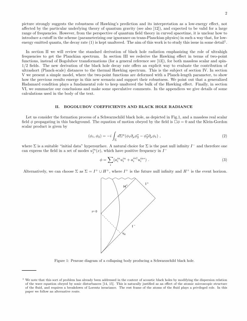
Let us consider the formation process of a Schwarzschild black hole, as depicted in Fig.1, and a massless real scalarfield φ propagating in this background. The equation of motion obeyed by the field is φ = 0 and the Klein-Gordonscalar product is given by

(φ1, φ2) = −i∫

Σ

dΣµ(φ1∂µφ∗2 − φ∗2∂µφ1) , (2)

where Σ is a suitable “initial data” hypersurface. A natural choice for Σ is the past null infinity I− and therefore onecan express the field in a set of modes uin

j (x), which have positive frequency in I−

φ =∑

i

(aini u

ini + ain†

i uin∗i ) . (3)

Alternatively, we can choose Σ as Σ = I+ ∪H+, where I+ is the future null infinity and H+ is the event horizon.

Ι

Ι

+

−

r= 0

Η

vH

+

Figure 1: Penrose diagram of a collapsing body producing a Schwarzschild black hole.

1 We note that this sort of problem has already been addressed in the context of acoustic black holes by modifying the dispersion relationof the wave equation obeyed by sonic disturbances [14, 15]. This is naturally justified as an effect of the atomic microscopic structureof the fluid, and requires a breakdown of Lorentz invariance. The rest frame of the atoms of the fluid plays a privileged role. In thispaper we follow an alternative route.

3

According to this we can then expand the field in an orthonormal set of modes uouti (x), which have positive frequency

with respect to the inertial time at I+ and have zero Cauchy data in H+, together with a set of modes uinti (x) with

null outgoing component at I+. Therefore we can write

φ =∑

i

(aouti uout

i + aout†i uout∗

i ) + (ainti uint

i + aint†i uint∗

i ) . (4)

The particular choice of modes uinti does not affect the computation of particle production at I+, so we leave them

unspecified.The modes uout

j (x) can be expressed in terms of the basis uini

uoutj (x) =

∑

i

αjiuini (x) + βjiu

in∗i (x) , (5)

where the coefficients αji and βji are the so-called Bogolubov coefficients and are given by the scalar products

αij = (uouti , uin

j ) , βij = −(uouti , uin∗

j ) . (6)

The above expansion leads to an analogous relation for the creation and annihilation operators:

aouti =

∑

j

(α∗ija

inj − β∗

ijain†j ) . (7)

When the coefficients βij do not vanish the vacuum states |in〉 and |out〉, defined as aini |in〉 = 0 and aout

i |out〉 = 0,do not coincide and, as a consequence, the number of particles measured in the ith mode by an “out” observer,

Nouti = ~

−1aout†i aout

i , in the state |in〉 is given by

〈in|Nouti |in〉 =

∑

k

|βik|2 . (8)

Let us now briefly summarize the main steps of Hawking’s derivation. Assuming for simplicity that the backgroundis spherically symmetric we can choose the following basis for the ingoing and outgoing modes

uinwlm|I− ∼ 1√

4πw

e−iwv

rY m

l (θ, φ) , (9)

uoutwlm|I+ ∼ 1√

4πw

e−iwu

rY m

l (θ, φ) . (10)

Here Y ml (θ, φ) are the spherical harmonics. One can evaluate the coefficients βwlm,w′l′m′ according to previous

expressions by making the convenient choice Σ = I−

βwlm,w′l′m′ = i

∫

I−

dvr2dΩ(uoutwlm∂vu

inw′l′m′ − uin

w′l′m′∂vuoutwlm) . (11)

The angular integration is straightforward and leads to delta functions δll′ δm,−m′ for the β coefficients. The relevantpoint is to realize that the coefficients can be evaluated and have a unique answer, which turns out to be independentof the details of the collapse, if uout

i represents a late-time wave-packet mode (i.e., centered around an instant u withu → +∞ along I+). When these modes are propagated backwards in time they are largely blueshifted when theyapproach the event horizon. After passing through the collapsing body they are scattered to I− in a very smallinterval just before vH . To know how they behave on I− (as needed to evaluate the scalar product with uin

wlm) onecan apply the geometrical optics approximation since the effective frequency, as measured by freely falling observers,is very large. The (late-time) mode uout

wlm, which is of the form (10) at I+, evolves and arrives at I− with the form

uoutwlm|I− ∼ tl(w)√

4πw

e−iwu(v)

rY m

l (θ, φ)Θ(vH − v) , (12)

where tl(w) is the transmission coefficient for the Schwarzschild metric and the relation between null inertial coordi-nates u at I+ and v at I− is typically given by the logarithmic term

u = vH − κ−1 lnκ|vH − v| , (13)

4

where, for the Schwarzschild black hole, κ = 1/4M and vH represents the location of the null ray that will form theevent horizon H+ (see Fig. 1). One has then all ingredients to work out the (late-time) Bogolubov coefficients

βwlm,w′l′m′ =−(−)mtl(w)

2π

√

w′

w

∫ vH

−∞dve−iw(vH−κ−1 ln κ|vH−v|)−iw′vδll′δm −m′ . (14)

They can be evaluated explicitly

βwlm,w′l′m′ =−(−)mtl(w)

2πκ

√

w′

w

e−i(w+w′)vH

(−κ−1w′i+ ǫ)1+κ−1wiΓ(1 + κ−1wi)δll′δm−m′ , (15)

where we have introduced a negative real part (−ǫ) into the exponent of (14) to ensure convergence of the correspondingintegrals. To compute the particle production at I+ one has to evaluate the integral (from now on in this section weshall omit, for simplicity, the subscripts l,m)

∫ +∞

0

dw′βw1w′β∗w2w′ . (16)

The integration in w′ reduces to

∫ +∞

0

dw′

w′ e−κ−1w1i ln(−κ−1w′−iǫ)eκ−1w2i ln(κ−1w′−iǫ) = 2πκe−πκ−1w1δ(w1 − w2) , (17)

from which we finally get

∫ +∞

0

dw′βw1w′β∗w2w′ =

|tl(w1)|2e2πκ−1w1 − 1

δ(w1 − w2) , (18)

where the coefficient in front of δ(w1 − w2) represents a steady thermal flow of radiation of frequency w = w1

dNlm(w)

dwdt≡ 1

2π〈in|Nout

wlm|in〉 =1

2π

Γl(w)

e2πκ−1w − 1, (19)

and the grey-body factor is given by Γl(w) ≡ |tl(w)|2. For a generic collapse the result leads to formula (1).

It is important to remark at this point that a basic step to exactly obtain the Planckian spectrum is (17), whichcrucially requires an unbounded integration in all frequencies w′. In fact, if we introduce an ultraviolet cutoff Λ forw′ we should replace (17) by

∫ +Λ

0

dw′

w′ e−κ−1w1i ln(−κ−1w′−iǫ)eκ−1w2i ln(κ−1w′−iǫ) = e−πκ−1w12πδσ[κ−1(w1 − w2)] , (20)

where we have defined

δσ[κ−1(w1 − w2)] =sin

[

κ−1(w1−w2)σ

]

πκ−1(w1 − w2)(21)

σ =1

ln[κ−1Λ](22)

Note that in the limit as σ goes to zero δσ turns into Dirac’s delta function and we recover (17). The new expressionis, however, qualitatively different from the previous one. To evaluate the new emission rate requires making use ofnormalized wave-packet modes. Introducing the standard ones [1]

uoutjnlm =

1√ǫ

∫ (j+1)ǫ

jǫ

dw e2πiwn/ǫ uoutwlm , (23)

where j ≥ 0 and n are integers, representing wave-packets peaked around the retarded time un = 2πn/ǫ and centered,with width ǫ, around the frequency wj ≡ (j + 1/2)ǫ; and, accordingly, defining

βjn,w′ =1√ǫ

∫ (j+1)ǫ

jǫ

dw e2πiwn/ǫ βww′ , (24)

5

the emission rate results (see appendix A):

〈in|Nout,σjn |in〉 ≈ |tl(wj)|2

e2πκ−1wj − 1

sin[(

2πnǫ − vH

)

πκσ2

]

[(

2πnǫ − vH

)

πκσ2

] (25)

From this expression2 we see that the rate of emitted particles depends on the retarded time un = 2πn/ǫ and decayswith time for any small but nonzero value of σ = 1/ ln[Λ/κ]. Only when Λ goes to infinity (no high frequency cutoff)do we recover the steady thermal flux of radiation.

In conclusion, the above discussion shows that the radiation is now time-dependent and decays for all finite valuesof Λ. The decay in time would also occur at low frequencies, where string theory agrees with Hawking’s prediction.Therefore, as expected from conventional arguments, the mathematical role of the ultrahigh frequencies is veryimportant for the late-time behavior. Nevertheless, since they only enter as virtual quanta, their actual status isunclear [16]. A derivation of the Hawking effect based on quantities defined on the asymptotically flat region, wherephysical observations are made, would be preferable. This turns out to be possible if, instead of working withBogolubov coefficients, one uses two-point functions. They are defined in the I+ region where a Planck-length cutoffin “distances” can be naturally introduced. This is the task of next sections.

III. TWO-POINT FUNCTIONS AND BLACK HOLE RADIANCE

This section will be devoted to rederive Hawking radiation by means of two-point functions. Intuitively the idea issimple. In the conventional analysis in terms of Bogolubov coefficients, we first perform the integration in distances(to compute the scalar product required for the β coefficients) and leave to the end the integration in frequenciesw′. In contrast, we can invert the order and perform first the integration in frequencies (which naturally leads tointroduce the two-point function of the matter field) and perform the integration in distances at the end.

Let us rewrite the basic expression (8), or more precisely, the expectation values of the operator Nouti1i2

≡~−1 aout†

i1aouti2

, as follows

〈in|Nouti1i2 |in〉 =

∑

k

βi1kβ∗i2k = −

∑

k

(uouti1 , uin∗

k )(uout∗i2 , uin

k ) =

=∑

k

(∫

Σ

dΣµ1u

outi1 (x1)

↔∂ µu

ink (x1)

) (∫

Σ

dΣν2u

out∗i2 (x2)

↔∂ νu

in∗k (x2)

)

. (26)

If we now consider the sum in modes before making the integrals of the two scalar products, and take into accountthat

〈in|φ(x1)φ(x2)|in〉 = ~

∑

k

uink (x1)u

ink

∗(x2) , (27)

we obtain a simple expression for the particle production number in terms of the two-point function

〈in|Nouti1i2 |in〉 = ~

−1

∫

Σ

dΣµ1dΣ

ν2 [uout

i1 (x1)↔∂ µ][uout∗

i2 (x2)↔∂ ν ]〈in|φ(x1)φ(x2)|in〉 . (28)

In the above expression the two-point function should be then interpreted in the distributional sense. The “iǫ-prescription” (see eq.(35) below) is therefore assumed for the two-point distribution 〈in|φ(x1)φ(x2)|in〉 and it verifies

the Hadamard condition3 [5, 17]. Alternatively, taking into account the trivial identity 〈out|aout†i1a

outi2

|out〉 = 0 wecan rewrite the above expression as [18]

〈in|Nouti1i2 |in〉 = ~

−1

∫

Σ

dΣµ1dΣ

ν2 [uout

i1 (x1)↔∂ µ][uout∗

i2 (x2)↔∂ ν ]〈in| : φ(x1)φ(x2) : |in〉 , (29)

where 〈in| : φ(x1)φ(x2) : |in〉 ≡ 〈in|φ(x1)φ(x2)|in〉 − 〈out|φ(x1)φ(x2)|out〉. Now the Hadamard condition for both|in〉 and |out〉 states ensures that 〈in| : φ(x1)φ(x2) : |in〉 is a smooth function.

2 We note that the oscillatory behavior in (25) is an artifact of the particular way we have introduced the cutoff. If the cutoff is introduced

in a different way, see appendix A, the oscillatory term disappears but the decay with time is maintained as ∼ e−[(2πn/ǫ−vH )(πκσ/2)]2 .3 The two-point distribution should have, for all physical states, a short-distance structure similar to that of the ordinary vacuum state

in Minkowski space: (2π)−2(σ + 2iǫt + ǫ2)−1, where σ(x1, x2) is the squared geodesic distance.

6

A. Thermal spectrum for a scalar field

Let us now apply this scheme in the formation process of a spherically symmetric black hole and restrict the “out”region to I+. The “in” region is, as usual, defined by I−. At I+ we can consider the conventional radial plane-wavemodes

uoutwlm(t, r, θ, φ)|I+ ∼ uout

w (u)Y m

l (θ, φ)

r, (30)

where uoutw (u) = e−iwu

√4πw

. We shall now evaluate the matrix coefficients 〈in|Nouti1i2

|in〉 where i1,2 ≡ (w1,2, l1,2,m1,2).

Taking as the initial value hypersurface I− and integrating by parts we obtain

〈in|Nouti1i2 |in〉 =

4

~

∫

I−

r21dv1dΩ1

∫

I−

r22dv2dΩ2uoutw1uout∗

w2×

Y m1

l1(θ1, φ1)

r1

Y m2∗l2

(θ2, φ2)

r2∂v1∂v2〈in|φ(x1)φ(x2)|in〉 . (31)

The two-point function above can be now expanded at I− as

〈in|φ(x1)φ(x2)|in〉 = ~

∫ ∞

0

dw∑

l,m

e−iwv1

√4πw

Y ml (θ1, φ1)

r1

eiwv2

√4πw

Y m∗l (θ2, φ2)

r2. (32)

Recall that the radial part of the late-time “out” modes uoutwlm, when they are propagated backward in time and reach

I−, takes the form

uoutw |I− ∼ tl(w)

e−iwu(v)

√4πw

Θ(vH − v) (33)

where u(v) ≈ vH − κ−1 lnκ(vH − v). Performing now angular integrations and taking into account that

∂v1∂v2

∫ ∞

0

dwe−iw(v1−v2)

4πw= − 1

4π

1

(v1 − v2 − iǫ)2, (34)

we get

〈in|Nouti1i2 |in〉 = −

tl1(w1)t∗l2

(w2)

4π2√w1w2

∫ vH

−∞dv1dv2

e−iw1u(v1)+iw2u(v2)

(v1 − v2 − iǫ)2δl1l2δm1m2 , (35)

where the limit ǫ → 0+ is understood. Alternatively, since we are interested in quantities measured at Σ = I+, wecould use this latter hypersurface to carry out the calculations. In this case, the expression for the particle productionrate becomes

〈in|Nouti1i2 |in〉 = −

tl1(w1)t∗l2

(w2)

4π2√w1w2

∫ ∞

−∞du1du2

dvdu (u1)

dvdu (u2)

[v(u1) − v(u2) − iǫ]2e−iw1u1+iw2u1δl1l2δm1m2 , (36)

and leads to

〈in|Nouti1i2 |in〉 =

−tl1(w1)t∗l2

(w2)

4π2√w1w2

∫ +∞

−∞du1du2

(κ2 )2e−iw1u1+iw2u2

[sinh κ2 (u1 − u2 − iǫ)]2

δl1l2δm1m2 . (37)

This last expression is more convenient for computational purposes. Since the function in the integral depends onlyon the difference z ≡ u2 − u1, the integral in u2 + u1 can be performed immediately and leads to a delta function infrequencies

〈in|Nouti1i2 |in〉 = −

tl1(w1)t∗l2

(w2)δ(w1 − w2)

2π√w1w2

∫ +∞

−∞dze−i

w1+w22 z (κ

2 )2δl1l2δm1m2

[sinh κ2 (z − iǫ)]2

, (38)

Performing the integration in z we recover the Planckian spectrum and the particle production rate

〈in|Noutwlm|in〉 =

|tl(w)|2e2πκ−1w − 1

. (39)

7

This derivation of black hole radiation is somewhat parallel to the one given in [9]. The emphasis is in the two-pointfunction of the quantum state, instead of the usual treatment in terms of Bogolubov transformations. It is worthnoting that (35) displays an apparent sensitivity to ultrashort distances due to the highly oscillatory behavior of themodes in a small region before vH . A similar conclusion can be obtained from (38) when z → 0. The sensitivity toshort distances is, however, less apparent if we repeat the above calculations using the expression (29) instead of (28).In this case, we find

〈in|Nouti1i2 |in〉 = −

tl1(w1)t∗l2

(w2)

4π2√w1w2

∫ vH

−∞dv1dv2e

−iw1u(v1)+iw2u(v2) ×[

1

(v1 − v2)2−

dudv (v1)

dudv (v2)

[u(v1) − u(v2)]2

]

δl1l2δm1m2 , (40)

where we have dropped the iǫ terms since they are now redundant. Note that the short-distance divergence of

1/(v1−v2)2 in (40) is exactly cancelled bydudv (v1) du

dv (v2)

[u(v1)−u(v2)]2for any smooth choice of the function u(v). This cancellation is

a consequence of the Hadamard condition that verify both “in” and “out” vacuum states. It is also important to remarkthat the above formula exhibits the absence of particle production under conformal-type (Mobius) transformations

v =au+ b

cu+ d(41)

where ab− cd = 1.4

If the calculation is performed using Σ = I+, one finds

〈in|Nouti1i2 |in〉 = −

tl1(w1)t∗l2

(w2)

4π2√w1w2

∫

I+

du1du2e−iw1u1+iw2u2 ×

[

dvdu (u1)

dvdu (u2)

(v(u1) − v(u2))2− 1

[u1 − u2]2

]

δl1l2δm1m2 , (42)

which leads to

〈in|Nouti1i2 |in〉 = −

tl1(w1)t∗l2

(w2)δ(w1 − w2)

2π√w1w2

∫ +∞

−∞dze−i

w1+w22 z ×

[

(κ2 )2

(sinh κ2 z)

2− 1

z2

]

δl1l2δm1m2 . (43)

The integral in distances z also leads, as expected, to the Hawking formula5

〈in|Noutwlm|in〉 = −|tl(w)|2

2πw

∫ +∞

−∞dze−iwz

[

(κ2 )2

(sinh κ2 z)

2− 1

z2

]

=|tl(w)|2

e2πwκ−1 − 1. (44)

B. Thermal spectrum for a s = 1/2 field

In this subsection we shall extend the analysis of the scalar field to a fermionic s = 1/2 field. For simplicity we takea massless Dirac field, obeying the wave equation

γµ∇µψ = 0 , (45)

4 This leads, immediately, to the expected result that there is no particle production under Lorentz transformations.5 For Kerr-Newman black holes the calculation is similar up to a shift in the wave function e−iwz , which should be now replaced by

e−i(w−mΩH−qΦH )z , as an effect of wave propagation through the corresponding potential barrier.

8

where γµ = V µa γ

a are the curved space counterparts of the Dirac matrices γa (see appendix B for calculations omittedin this section). The Klein-Gordon scalar product (2) is now replaced by

(ψ1, ψ2) =

∫

Σ

dΣµψ1γµψ2 . (46)

Therefore the expression for the expectation values (28) is replaced by

〈in|Nouti1i2 |in〉 = ~

−1

∫

Σ

dΣµ1dΣ

ν2 [uout

i2 (x2)γν ]b[γµuouti1 (x1)]

a〈in|ψa(x1)ψb(x2)|in〉 . (47)

At I+ we can consider the normalized radial plane-wave modes6

uoutwκjmj

(t, r, θ, φ)|I+ ∼ e−iwu

√4πr

(

η(r)mjκj

(r~σ)η(r)mjκj

)

, (48)

where η(r)mjκj are two-component spinor harmonics (see appendix B). Note that the angular momentum quantum

number j is uniquely determined by the relation κj = ±(j + 1/2). The above modes, when propagated backwards intime and reach I−, turn into

uoutwκjmj

(t, r, θ, φ)|I− ∼ tκj (w)e−iwu(v)

√4πr

(

η(r)mjκj

−(r~σ)η(r)mjκj

)

Θ(vH − v)

√

du(v)

dv, (49)

where the last term√

du(v)/dv appears due to the fermionic character of the field7. Proceeding as in the bosoniccase we can expand the two-point function as

〈in|ψa(x1)ψb(x2)|in〉 = ~

∑

k

vink,a(x1)v

in,bk (x2) (50)

where vink are negative-energy solutions which in I− take the form

vink → vin

wκjm(t, r, θ, φ)|I− ∼ eiwv

√4πr

(

η(r)mjκj

−(r~σ)η(r)mjκj

)

, (51)

Performing first the angular integrations and taking into account the orthonormality relations of the spinor harmonicsη(r)

mjκj , the above formulas get simplified and become

〈in|Nouti1i2 |in〉 = −i

tκj1(w1)t

∗κj2

(w2)

4π2δmj1mj2

δκj1κj2×

×∫ vH

−∞dv1dv2

√

du(v1)

dv

du(v2)

dv

e−iw1u(v1)+iw2u(v2)

(v1 − v2 − iǫ)(52)

As in the bosonic case, we rewrite this expression as an integral over I+

〈in|Nouti1i2 |in〉 = −i

tκj1(w1)t

∗κj2

(w2)

4π2δmj1mj2

δκj1κj2×

×∫ ∞

−∞du1du2e

−iw1u1+iw2u2(κ

2 )

sinh[κ2 (u1 − u2 − iǫ)]

(53)

We can also split the integral in a product of a function dependent on u2 + u1 and another function which dependson z ≡ u2 − u1. The former leads to a delta function in frequencies and we are left with

〈in|Nouti1i2 |in〉 = − i

2πtκj1

(w1)t∗κj2

(w2)δmj1mj2δκj1κj2

δ(w1 − w2) ×

×∫ +∞

−∞dze−i

w1+w22 z (κ

2 )

sinh[κ2 (z − iǫ)]

, (54)

6 On physical grounds we should use left-handed spinors uoutL,wjmj

≡ 1√2(uout

w |κj |mj− uout

w −|κj |mj). The final result is not changed. See

appendix B.7 The vierbein fields needed to properly write the field equation in a curved spacetime have been trivially fixed in the asymptotic flat

regions, so its transformation law under change of coordinates is then translated to the spinor itself (see also appendix B).

9

Performing now the integration in z

−i2π

∫ +∞

−∞dze−iwz (κ

2 )

sinh[κ2 (z − iǫ)]

=1

e2πwκ−1 + 1, (55)

we recover the Planckian spectrum, with the Dirac-Fermi statistics, and the corresponding particle production rate

〈in|Noutwmjκj

|in〉 =|tκj (w)|2

e2πκ−1w + 1. (56)

Analogously as in the bosonic case, if we use the normal-ordering prescription instead of the iǫ one we find

〈in|Nouti1i2 |in〉 = −i

tκj1(w1)tκj2

(w2)∗

4π2

∫ vH

−∞dv1dv2

√

du(v1)

dv

du(v2)

dv× (57)

e−iw1u(v1)+iw2u(v2)

1

[v1 − v2]−

√

du(v1)dv

du(v2)dv

[u(v1) − u(v2)]

δκj1κj2δmj1mj2

.

Changing the integration surface to I+ we get

〈in|Nouti1i2 |in〉 = −i

tκj1(w1)tκj2

(w2)∗

4π2

∫

I+

du1du2

√

dv(u1)

du

dv(u2)

du× (58)

e−iw1u1+iw2u2

√

dv(u1)du

dv(u2)du

[v(u1) − v(u2)]− 1

[u1 − u2]

δκj1κj2δmj1mj2

.

Note again that the short-distance divergence of the two-point function of the “out” state 1[u1−u2] is exactly cancelled

by the corresponding one of the “in” state

q

dv(u1)du

dv(u2)du

[v(u1)−v(u2)], since both vacua are Hadamard states. After some algebra

we get

〈in|Noutwκjmj

|in〉 = −i |tκj(w)|22π

∫ +∞

−∞dze−iwz

[

(κ2 )

sinh(κ2 z)

− 1

z

]

, (59)

and taking into account

−i2π

∫ +∞

−∞dze−iwz

[

(κ2 )

sinh(κ2 z)

− 1

z

]

=1

e2πwκ−1 + 1, (60)

we newly recover the fermionic thermal spectrum.

IV. SHORT-DISTANCE CONTRIBUTION TO THE PLANCKIAN SPECTRUM

A. Bosons

We have seen in the previous section that it is possible to rederive the Hawking effect in terms of two-point functions.Either via expressions (28), (36) or, equivalently, via expressions (29),(42). Both prescriptions are equivalent and leadto the Planckian spectrum modulated by grey-body factors. The advantage of the final expression (44) is that it offersan explicit evaluation of the contribution of distances to the Planckian spectrum. To be more explicit, the integral8

IB(wκ−1, ακ) = − 1

2πw

∫ +α

−α

dze−iwz

[

(κ2 )2

(sinh κ2 z)

2− 1

z2

]

, (61)

8 We have intentionally omitted the grey-body factors |tl(w)|2 in (61) because they are irrelevant for the discussion of this section.

10

can be interpreted as the contribution of short-distances z ∈ [−α, α] to the (bosonic) thermal spectrum when α isclose to the Planck length lP . One could, alternatively, be tempted to propose, according to (36), the integral

IBiǫ (wκ−1, ακ) ≡ −1

2πw

∫ +α

−α

dze−iwz (κ2 )2

[sinh κ2 (z − iǫ)]2

(62)

as a legitimate expression to account for the short-distance contributions. However, this interpretation is not physicallysound. In the absence of a black hole, when there is no radiation at all, the above expression becomes

−1

2πw

∫ +α

−α

dze−iwz 1

(z − iǫ)2. (63)

For α → +∞ this expression vanishes, as expected due to the absence of radiation. However, for finite α it isnon-vanishing. In contrast, the proposed expression (61), does not suffer from this weird behavior, due to thepresence of the second term.

In conclusion, the calculation of black hole radiation using the prescription (29) offers the possibility to re-evaluateHawking radiation by removing the range of distances where physics can be dominated by an underlying theorybeyond field theory. We shall now work out explicitly the short-distance contribution to Hawking radiation to seewhether it is fundamental or not in order to obtain the thermal spectrum. The integral (61) can be worked outanalytically

IB(wκ−1, ακ) = −Si(αw)

π− κ

4πweiαw(F [1,−iwκ−1, 1 − iwκ−1, e−ακ]

−F [1, iwκ−1, 1 + iwκ−1, eακ]) + e−iαw(F [1, iwκ−1, 1 + iwκ−1, e−ακ]

−F [1,−iwκ−1, 1 − iwκ−1, eακ]) +1

2παwcos(αw)

[

ακ(1 + eακ)

(eακ − 1)− 2

]

(64)

where F is a hypergeometric function and Si(x) =∫ x

0 dtsin t

t . To get some insight about the properties of this formula,

we find useful to expand it in powers of wκ−1 and ακ. The expansion in ακ assumes that the microscopic lengthscale α ∼ lP is much smaller than the typical emission wavelength ∼ κ−1 of the black hole, whose (macroscopic)temperature is TH = κ/2π. For a Solar-mass black hole ακ ∼ 10−40 and for a primordial black hole of 1015 gακ ∼ 10−21. The expansion in wκ−1 means that we are looking at frequencies below the typical emission frequency,wtypical ∼ TH , of the black hole. The result is as follows

IB(wκ−1, ακ) =

(

1

12πακ− 1

720π(ακ)3 + O[(ακ)5]

)

κ

w

−(

1

72π(ακ)3 +O[(ακ)5]

)

w

κ+

(

O[(ακ)5])

(w

κ)3 + . . . (65)

From this expansion we conclude that the contribution of short distances to the spectrum is completely negligible inthe very low energy regime w/κ ≪ 1 since

limwκ−1→0

IB(wκ−1, ακ)

(e2πwκ−1 − 1)−1=ακ

6≪ 1 . (66)

Moreover, due to the smallness of ακ, we find that IB(wtypicalκ−1, κα) can be well approximated by (65) even for

frequencies close to the typical emission frequency, which leads to

IB(wtypicalκ−1, ακ)

(e2πwtypicalκ−1 − 1)−1∼ 0.3 ακ ≪ 1 . (67)

Again, since ακ ≪ 1, we find a negligible contribution at wtypical ∼ TH . To be precise, for a Schwarzschild blackhole of three solar masses, when α is around the Planck length lP = 1.6 × 10−33cm, the relative contribution to the

Planckian distribution IB(wκ−1,ακ)

(e2πwκ−1−1)−1is, for w = wtypical, of order 10−38%. For primordial black holes, M ∼ 1015 g,

the relative contribution is still insignificant: 10−19%. Even more, using the expansion (65) we easily get

IB(wκ−1, ακ)

(e2πwκ−1 − 1)−1≈ ακ(e2πwκ−1 − 1)

12πwκ−1, (68)

11

and we find that, for a black hole of three solar masses, we need to look at the high frequency region, w/wtypical ≈ 96,to find that the contribution of Planck distances IB(wκ−1, lPκ) is of order of the total spectrum itself9 . For primordialblack holes we find w/wtypical ≈ 52. The same numerical estimates can be found using the exact analytical expressions.

We can also naturally ask about the contribution to the spectrum of large distances. This question is immediatelyanswered using our analytical expression (64). The contribution of distances up to α = 20rg, where rg is thegravitational radius, represents 90% of the thermal peak at wtypical. For α = 200rg we obtain 99.7% and forα = 2 × 104rg the percentage is around 99.99998% .

Summarizing, we have provided a quantitative estimate of how much of Hawking radiation is actually due toPlanckian distances. It turns out that the contribution of ultrashort distances is negligible and thermal radiationis very robust up to frequencies of order 96TH (for Schwarzschild black holes of three solar masses) or 52TH (forprimordial black holes). In parallel and dual to this, the contribution of large distances is also insignificant.

It is interesting to repeat the same calculations with the iǫ-prescription. As we have already stressed with thisprescription one cannot expect a meaningful result. The outcome is completely different. The contribution of distancesin the interval z ∈ [−α,+α] is now

IBiǫ→0(wκ

−1, ακ) =eακ(1−iwκ−1) + eiαw

2πwκ−1(eακ − 1)+

1

2π(i+ wκ−1)eακ(1−iwκ) ×

F [1, 1 − iwκ−1, 2 − iwκ−1, eακ] − e−ακ(1−iwκ) ×F [1, 1 − iwκ−1, 2 − iwκ−1, e−ακ] (69)

Here, even in the very low energy regime, the contribution of short distances is not negligible. In fact, it is muchbigger than the thermal spectrum itself. To see this we can approximate IB

iǫ (wκ−1, ακ) as

IBiǫ (wκ−1, ακ) =

(

1

πακ+

ακ

12π− (ακ)3

720π+O((ακ)5)

)

κ

w− 1

2

+

(

ακ

2π− (ακ)3

72π+O((ακ)5)

)

w

κ−

(

(ακ)3

72π+O((ακ)5)

)

(w

κ)3 + ... (70)

Note that in this case the dominant term is of order 1/ακ, therefore

limκ−1w→0

IBiǫ (wκ−1, ακ)

(e2πwκ−1 − 1)−1=

2

ακ≫ 1 . (71)

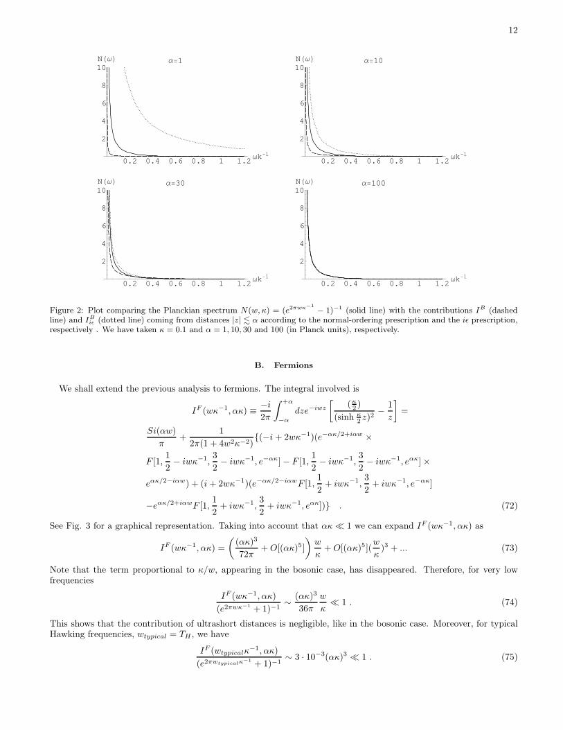
A similar behavior can be found for w ≈ wtypical.We illustrate the difference between both calculations in Fig.2. With the normal-ordering prescription the short-

distance contribution is small, in contrast with the iǫ-prescription. We have chosen a large surface gravity and differentvalues of α to better show the effect in the drawings. We clearly observe that, although both prescriptions lead tothe thermal result when α→ +∞, they do the job in very different ways.

9 The exponential behavior in frequencies of the ratio (68) explains why potential deviations from thermality arise at frequencies muchlower than w ∼ 1/lP .

12

0.2 0.4 0.6 0.8 1 1.2Ωk-1

2

4

6

8

10NHΩL Α=30

0.2 0.4 0.6 0.8 1 1.2Ωk-1

2

4

6

8

10NHΩL Α=100

0.2 0.4 0.6 0.8 1 1.2Ωk-1

2

4

6

8

10NHΩL Α=1

0.2 0.4 0.6 0.8 1 1.2Ωk-1

2

4

6

8

10NHΩL Α=10

Figure 2: Plot comparing the Planckian spectrum N(w, κ) = (e2πwκ−1

− 1)−1 (solid line) with the contributions IB (dashedline) and IB

iǫ (dotted line) coming from distances |z| . α according to the normal-ordering prescription and the iǫ prescription,respectively . We have taken κ = 0.1 and α = 1, 10, 30 and 100 (in Planck units), respectively.

B. Fermions

We shall extend the previous analysis to fermions. The integral involved is

IF (wκ−1, ακ) ≡ −i2π

∫ +α

−α

dze−iwz

[

(κ2 )

(sinh κ2 z)

2− 1

z

]

=

Si(αw)

π+

1

2π(1 + 4w2κ−2)(−i+ 2wκ−1)(e−ακ/2+iαw ×

F [1,1

2− iwκ−1,

3

2− iwκ−1, e−ακ] − F [1,

1

2− iwκ−1,

3

2− iwκ−1, eακ] ×

eακ/2−iαw) + (i+ 2wκ−1)(e−ακ/2−iαwF [1,1

2+ iwκ−1,

3

2+ iwκ−1, e−ακ]

−eακ/2+iαwF [1,1

2+ iwκ−1,

3

2+ iwκ−1, eακ]) . (72)

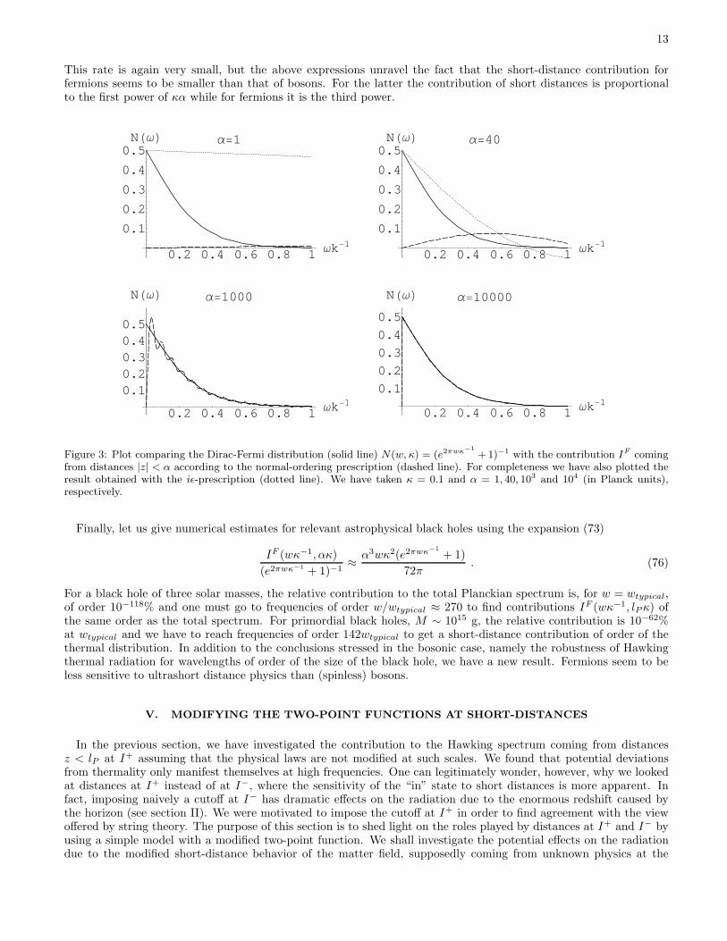
See Fig. 3 for a graphical representation. Taking into account that ακ≪ 1 we can expand IF (wκ−1, ακ) as

IF (wκ−1, ακ) =

(

(ακ)3

72π+O[(ακ)5]

)

w

κ+O[(ακ)5](

w

κ)3 + ... (73)

Note that the term proportional to κ/w, appearing in the bosonic case, has disappeared. Therefore, for very lowfrequencies

IF (wκ−1, ακ)

(e2πwκ−1 + 1)−1∼ (ακ)3

36π

w

κ≪ 1 . (74)

This shows that the contribution of ultrashort distances is negligible, like in the bosonic case. Moreover, for typicalHawking frequencies, wtypical = TH , we have

IF (wtypicalκ−1, ακ)

(e2πwtypicalκ−1+ 1)−1

∼ 3 · 10−3(ακ)3 ≪ 1 . (75)

13

This rate is again very small, but the above expressions unravel the fact that the short-distance contribution forfermions seems to be smaller than that of bosons. For the latter the contribution of short distances is proportionalto the first power of κα while for fermions it is the third power.

0.2 0.4 0.6 0.8 1 Ωk-1

0.10.20.30.40.5

NHΩL Α=1000

0.2 0.4 0.6 0.8 1 Ωk-1

0.1

0.2

0.3

0.4

0.5

NHΩL Α=10000

0.2 0.4 0.6 0.8 1 Ωk-1

0.1

0.2

0.3

0.4

0.5NHΩL Α=1

0.2 0.4 0.6 0.8 1 Ωk-1

0.1

0.2

0.3

0.4

0.5NHΩL Α=40

Figure 3: Plot comparing the Dirac-Fermi distribution (solid line) N(w, κ) = (e2πwκ−1

+1)−1 with the contribution IF comingfrom distances |z| < α according to the normal-ordering prescription (dashed line). For completeness we have also plotted theresult obtained with the iǫ-prescription (dotted line). We have taken κ = 0.1 and α = 1, 40, 103 and 104 (in Planck units),respectively.

Finally, let us give numerical estimates for relevant astrophysical black holes using the expansion (73)

IF (wκ−1, ακ)

(e2πwκ−1 + 1)−1≈ α3wκ2(e2πwκ−1

+ 1)

72π. (76)

For a black hole of three solar masses, the relative contribution to the total Planckian spectrum is, for w = wtypical,of order 10−118% and one must go to frequencies of order w/wtypical ≈ 270 to find contributions IF (wκ−1, lPκ) ofthe same order as the total spectrum. For primordial black holes, M ∼ 1015 g, the relative contribution is 10−62%at wtypical and we have to reach frequencies of order 142wtypical to get a short-distance contribution of order of thethermal distribution. In addition to the conclusions stressed in the bosonic case, namely the robustness of Hawkingthermal radiation for wavelengths of order of the size of the black hole, we have a new result. Fermions seem to beless sensitive to ultrashort distance physics than (spinless) bosons.

V. MODIFYING THE TWO-POINT FUNCTIONS AT SHORT-DISTANCES

In the previous section, we have investigated the contribution to the Hawking spectrum coming from distancesz < lP at I+ assuming that the physical laws are not modified at such scales. We found that potential deviationsfrom thermality only manifest themselves at high frequencies. One can legitimately wonder, however, why we lookedat distances at I+ instead of at I−, where the sensitivity of the “in” state to short distances is more apparent. Infact, imposing naively a cutoff at I− has dramatic effects on the radiation due to the enormous redshift caused bythe horizon (see section II). We were motivated to impose the cutoff at I+ in order to find agreement with the viewoffered by string theory. The purpose of this section is to shed light on the roles played by distances at I+ and I− byusing a simple model with a modified two-point function. We shall investigate the potential effects on the radiationdue to the modified short-distance behavior of the matter field, supposedly coming from unknown physics at the

14

Planck scale. We shall see how our model maintains the robustness of the Hawking thermal spectrum at I+, whileat the same time being insensitive to sub-Planckian distances at I−.

Let us assume that the standard two-point function for the spin zero “in” and “out” vacuum states at I− and I+,respectively, gets modified by new physics at very short distances and becomes

Gin|I− ≡ − 1

4π

1

(v1 − v2)2→ Gin

α |I− ≡ − 1

4π

1

(v1 − v2)2 + α2

Gout|I+ ≡ − 1

4π

1

(u1 − u2)2→ Gout

α |I+ ≡ − 1

4π

1

(u1 − u2)2 + α2, (77)

where α is a parameter of order of the Planck length: α ∼ lP . With this modification the expression (40) for theblack hole particle production becomes (we omit the transmission coefficients tl(w) and the angular delta functionsδl1l2δm1m2 since they are also irrelevant for the discussion of this section)

〈in|Nouti1i2 |in〉 = 4

∫ vH

−∞dv1dv2u

outw1

(v1)uout∗w2

(v2) ×[

− 1

4π

1

(v1 − v2)2 + α2− du

dv(v1)

du

dv(v2)G

outα |I−

]

, (78)

where uoutw and Gout

α |I− are understood to be the “out” modes and the “out” two-point function, respectively, prop-agated back to I−. Since, according to the standard derivation, the propagation to I− implies a strong blueshift,the uout

w modes and Goutα might manifest some dependence on the particular details of the modified theory, which

are unknown to us. Thus, we see no simple way to estimate the form of the uoutw modes at I−. For this reason, it is

preferable to evaluate the particle production as an integral on I+, as in (42),

〈in|Nouti1i2 |in〉 = 4

∫

I+

du1du2uoutw1

(u1)uout∗w2

(u2) ×

×[

dv1du1

dv2du2

Ginα |I+ +

1

4π

1

(u1 − u2)2 + α2

]

, (79)

where Ginα |I+ is understood to be the “in” two-point function propagated to I+. In this region we can use the standard

form of the “out” modes uoutw1

(u1) = e−iw1u1√4πw

since we are considering emission frequencies much lower than the Planck

frequency wP ∼ 1/lP . We still have to unravel the evolution of Ginα to evaluate the above expression. The modified

short-distance physics near the horizon could dramatically modify the evolution of the two-point function, so that itsform at I+ could be rather different from the standard one Gin|I− . However, we can make the reasonable assumptionthat the propagation to I+ is affected by new physics in such a way that the short-distance behavior of dv1

du1

dv2

du2Gin

α at

I+ is identical to that of the two-point function for the “out” state

limu1→u2

dv

du(u1)

dv

du(u2)G

inα |I+ ∼ lim

u1→u2

Goutα (u1, u2)|I+ . (80)

The above condition can be seen as a natural generalization of the Hadamard condition, i.e., universality of theshort-distance behavior for all quantum states. The Hadamard condition, which plays a pivotal role in the algebraicformulation of QFT in curved spacetime [5], ensures the regularity of expression (29) to evaluate the Hawking radiation.Let us see now how (80) constraints the evolution of Gin

α from I− to I+. Note that Ginα can be rewritten as

Ginα =

Gin

1 + α2Gin, (81)

where Gin is the unmodified two-point function. Since, at late times, Gin evolves according to geometrical opticsapproximation

Gin|I+ ≡ dv

du(u1)

dv

du(u2)G

in|I+ = − 1

4π

dv1

du1

dv2

du2

(v(u1) − v(u2))2, (82)

expression (81) suggests the following evolution for Ginα

Ginα |I+ ≡ dv

du(u1)

dv

du(u2)G

inα |I+ = − 1

4π

dv(u1)du

dv(u2)du

(v1 − v2)2 + α2 dv1

du1

dv2

du2

. (83)

15

This expression guarantees immediately the Hadamard condition (80). We should stress, however, that the evolutionof the modified two-point function itself is not equivalent, at least for very small point separations (u2 − u1)

2 ∼ α2,to the ray tracing (or geometrical optics approximation), which would produce instead (91) (see later) and violatethe Hadamard condition. For larger separations (u2 − u1)

2 ≫ α2 the propagation agrees, as it must, with standardrelativistic field theory and is driven by the large redshift (implying then the usual geometrical optics approximation).Plugging this expression in (79) we obtain

〈in|Nouti1i2 |in〉 =

−1

4π2√ω1ω2

∫

I+

du1du2e−i(w1u1−w2u2)

×[

dv(u1)du

dv(u2)du

(v1 − v2)2 + α2 dv(u1)du

dv(u2)du

− 1

(u1 − u2)2 + α2

]

. (84)

It is worth noting that the modified term

− 4πGinα |I+ ≡ dv1

du1

dv2du2

1

(v1 − v2)2 + α2 dv1

du1

dv2

du2

, (85)

which can also be regarded as a transformation law under the change v = v(u), guarantees the absence of particleproduction under the same group of symmetry transformations (Mobius rescalings) as those of the theory withα = 0.10 Assuming that the geometry remains classical (the black hole scale κ is well above the Planck scale α), wecan use in (84) the expression v(u) = vH −κ−1e−κu, which represents the relation between the “in” and “out” inertialcoordinates. Performing then the integration in u2 + u1, we are left with (z ≡ u2 − u1)

〈in|Noutwlm|in〉 = − 1

2πw

∫ +∞

−∞dze−iwz

[

(κ2 )2

(sinh κ2 z)

2 + (κ2 )2α2

− 1

z2 + α2

]

. (86)

Finally, performing the integration in the complex plane, the particle production rate becomes

〈in|Noutwlm|in〉 =

1

(e2πwκ−1 − 1)

1

2wα√

1 − α2κ2/4(ewκ−1θ − ewκ−1(2π−θ)) +

e−wα

2αw(87)

where

θ = arctanακ

√

1 − α2κ2/4

(1 − α2κ2/2). (88)

The thermal Planckian spectrum is smoothly recovered in the limit α → 0. Moreover, for α ∼ lP , the deviation tothe thermal spectrum is negligible for small values of wκ−1. This deviation can be expanded as

〈in|Noutwlm|in〉

(e2πwκ−1 − 1)−1≈ 1 − ακ(e2πwκ−1 − 1)

16wκ−1. (89)

For astrophysical black holes, κα≪ 1, the second factor is negligible for frequencies up to ∼ 102wtypical, in completeagreement with the results obtained in section IV (compare, for instance, with (68)).

The above discussion shows that, despite the apparent sensitivity of Hawking radiation to high energy physics (seesection II), a Planck-scale modification of the two-point function does not necessarily imply a substantial change ofthe Planckian spectrum. This is so, at least, if the modified two-point function obeys a modified Hadamard-typecondition. The simplest realization of this condition turns out to be equivalent to the preservation of the powerfulconformal (Mobius) symmetry existing in the unmodified theory. This seems an unavoidable requirement if thecorrections to the Planckian spectrum are to be in agreement with the results of string theory in the low-frequencylimit w → 0. The effect of the generalized Hadamard condition is to constrain the short-distance behavior of thepropagated “in” two-point function, Gin

α |I+ , in such a way that it remains close to −1/(4πα2) through its evolution

10 Even more, it is what exactly guarantees the invariance of the production rate, up to a shift on the emission frequency, under a radialboost with rapidity ξ: u → u = eξu, v → v = e−ξv.

16

to I+, despite the large blueshift. In fact, Ginα |I+ is an observer-independent quantity in the limit x1 → x2, i.e., it

tends to −1/(4πα2) for any function v = v(u). Note in passing that this condition is somewhat related to approachesto quantum gravity aimed at deforming Lorentz symmetry while keeping the principle of relativity [19].

To conclude, we note that if the deformed two-point function at I−

Ginα |I− ≡ − 1

4π

1

(v1 − v2)2 + α2, (90)

is naively propagated (i.e., by ray tracing) to I+ as

Ginα |I+ = − 1

4π

dv1

du1

dv2

du2

(v(u1) − v(u2))2 + α2, (91)

where Ginα |I+ ≡ dv

du (u1)dvdu (u2)G

inα |I+ , the particle production rate is now time-dependent and the thermal spectrum

is lost for any nonvanishing α.

VI. CONCLUSIONS AND FINAL COMMENTS

It is highly non-trivial [8] to truncate Hawking’s derivation of black hole radiance to account for unknown physicsat the Planck scale. A simple estimate of the contribution of virtual high frequencies apparently shows that theyare essential to produce the thermal outcome. One can then change strategy and try to evaluate the contribution ofPlanckian physics in position space, which requires a rederivation of the Hawking calculation in terms of two-pointfunctions, as we have explicitly shown in section III. When these two-point functions are treated in the distributionalsense, with the usual iǫ prescription, one reproduces exactly the thermal result. However, one can equivalently handlethe divergence of the two-point function by trivially taking normal ordering. The consistency of this procedureis guaranteed by the Hadamard condition: the short-distance behavior is universal for all physical states. Theadvantage of this second option is that it offers a natural way to evaluate the contribution of short distances at I+

to Hawking radiation.

We have found that the contribution of short-distances at low frequencies w ≪ κ is negligible. Our analysis allowsus to go further and investigate the short-distance contribution for frequencies of order the Hawking temperatureTH and beyond. We find that the contribution of ultrashort distances is also negligible for frequencies of order TH .In fact, for a black hole of three solar masses we need to look at high frequencies, w/wtypical ≈ 96 (for bosons) orw/wtypical ≈ 270 (for fermions), to find that the contribution of Planck distances is of order of the total spectrumitself. This suggests that Hawking thermal radiation is very robust, as it has been confirmed in completely differentanalyses based on black hole analogues; in string theory (for large wavelength) in near-extremal charged black holes;and also in some models of canonical quantum gravity [20].

One can legitimately ask why, in section IV, we evaluate distances at I+, instead of just at I−, where the sensitivityof the “in” state to high energy scales is more apparent, as we showed in section II. Our heuristic motivation is basedon the view offered by string theory, where the Hawking radiation is obtained as the result of collisions between openstring excitations. In that approach, the standard large blueshift of low-energy gravity theory does not seem to playthe pivotal role that it does in the pure semiclassical treatment. The fact that we consider the fundamental Planckscale at I+ does not immediately guarantee that the Hawking radiation is kept unaltered from Planck-scale physics.As we show in section IV, with the standard iǫ-prescription the short-distance contribution to Hawking radiation isnot negligible. In contrast, with the normal-ordering prescription the bulk of the Hawking effect is maintained at lowfrequencies, in agreement with the results of string theory.

In addition to the above arguments we have approached the problem in section V in a different way. We haveconsidered an explicit modification of the two-point function at the Planck scale. Motivated by the crucial role playedby the Hadamard condition in the ordinary relativistic theory, we have assumed that the short-distance behavior ofthe modified theory should also satisfy a sort of generalized Hadamard condition (universal short-distance behavior).The simplest realization of this idea turns out to be equivalent to the preservation of the powerful conformal (Mobius)symmetry existing in the unmodified theory. Armed with this condition, the contribution to the particle productionrate of the “in” and “out” two-point functions in (84) is similar when they are compared in the same ultrashort range ofdistances, despite the large blueshift horizon effect. As a result, the two contributions compensate each other and lead

17

to an emission spectrum very insensitive to trans-Planckian physics. The generalized Hadamard condition, therefore,seems to be necessary to maintain the bulk of the Hawking effect. Moreover, it is in this context that the apparent ten-sion between I+ and I− to measure separations is elliminated since in both we find the same finite short distance limit.

A last comment is now in order. In the string theory analysis one has, at least, two relevant parameters: the surfacegravity κ and the radius rg of the supersymmetric, charged black hole. The surface gravity is assumed to be small, incomparison with the inverse of the size of the black hole, i.e., κ≪ 1/rg. The emission frequency can reach κ, but cannever reach 1/rg (or become larger) to guarantee the validity of the string theory calculation. Obviously the analysisof string theory excludes astrophysical black holes of the Schwarzschild type (for which κ ∼ 1/rg). Our results,however, suggest that one could also expect string theory to predict in this case, in some subtle way, agreement withHawking’s results for frequencies around 1/rg and, at least, a few orders beyond. This is so because we do not observeany significant contribution to the thermal spectrum coming from the short-distance region, where new physics couldarise, up to such high frequencies. This fact offers a very non-trivial challenge for any quantum theory of gravityhaving computational rules very different from those of semiclassical gravity (as in string theory or background-independent approaches), since when w ∼ 1/rg the grey-body factors Γi(w) cannot be computed analytically. Theyare only known numerically [21], as a result of solving field wave equations in the black hole background. String theorymanages to account for the greybody factors in the low-energy regime, where they admit an analytic expression. Infact, for all spherically symmetric black holes, the low-energy absorption cross section is proportional to the areaof the horizon [22, 23]. But for typical Hawking frequencies the grey-body factors remain elusive for any analytictreatment. Reobtaining them from such a different computation would be extremely impressive.

Appendix A

We will complete here the steps missing in the derivation that led to the emission rate (25). Using the wave packets(23) we can express it as

〈in|Nout,σj1n1,j2n2

|in〉 =

∫ Λ

0

dw′βj1n1,w′β∗j2n2,w′ = (92)

1

ǫ

∫ (j1+1)ǫ

j1ǫ

dw1

∫ (j2+1)ǫ

j2ǫ

dw2 e2πiw1n1/ǫ e−2πiw2n2/ǫ

∫ Λ

0

dw′βw1w′β∗w2w′ .

Using (20) we get

〈in|Nout,σj1n1,j2n2

|in〉 =1

ǫ

∫ (j1+1)ǫ

j1ǫ

dw1

∫ (j2+1)ǫ

j2ǫ

dw2 ei2πw1n1

ǫ e−i2πw2n2

ǫ

tl(w1)t∗l (w2)

e−i(w1−w2)vH

2π√w1w2

e−πκ−1ω1i−iκ−1(w1−w2)

Γ(1 + iκ−1w1)Γ(1 − iκ−1w2)δσ[κ−1(w1 − w2)] . (93)

This integral can be estimated explicitly when the width ǫ of the frequency interval [jǫ, (j+1)ǫ] is assumed, as usual,small. In this case, the integral is essentially as follows

〈in|Nout,σj1n1,j2n2

|in〉 ≈ δj1j2

|tl(wj)|2|Γ(1 + iκ−1wj)|22πwj

e−πκ−1wje2π(n1−n2)wj

ǫ In1n2(σ) (94)

where

In1n2(σ) =1

ǫ

∫ ǫ/2

−ǫ/2

dx1

∫ ǫ/2

−ǫ/2

dx2ei[

2πn1ǫ −vH ]x1−i[

2πn2ǫ −vH ]x2−πκ−1(x1+x2)/2δσ[κ−1(x1 − x2)] (95)

and x1,2 ≡ w1,2 − (j + 1/2)ǫ. The factor δj1j2 in (94) is due to the role of δσ, which selects frequencies on a verynarrow band of order |w1 − w2| ∼ κσ. For this reason, it is also convenient to introduce a new variable y = x1 − x2

and rewrite In1n2(σ) as follows

In1n2(σ) ≈ 1

ǫ

∫ ǫ/2

−ǫ/2

dx1e2π(n1−n2)x1

ǫ

∫ x1+ǫ/2

x1−ǫ/2

dyei[2πn2

ǫ −vH ]yδσ[κ−1y] . (96)

18

In writing this we have neglected the term eπκ−1(x1+x2)/2 which is almost constant (unity) over the integral. We cannow estimate the integral over y having in mind that δσ is very well approximated by a square step of width πκσ andheight 1/(πσ) centered at y = 0. This means that the main contribution comes from the interval [−πκσ

2 , πκσ2 ]. This

fact makes the outcome of the integral independent of x1, which also allows us to perform the integral in x1. Puttingall together we find

In1n2(σ) ≈ κδn1n2

sin[(

2πn2

ǫ − vH

)

πκσ2

]

[(

2πn2

ǫ − vH

)

πκσ2

] (97)

Plugging this result back into (94) we find (25).

We will now briefly consider the effect of introducing the cutoff in frequencies in a different way. The cutoff wasintroduced in (20) in the form

∫ ∞

−∞d log[w/κ]e−iκ−1(w1−w2) log[w/κ] →

∫ log[Λ/κ]

− log[Λ/κ]

d log[w/κ]e−iκ−1(w1−w2) log[w/κ] (98)

We will now consider the change

∫ log[Λ/κ]

− log[Λ/κ]

dλe−iκ−1(w1−w2)λ →∫ ∞

−∞dλe−iκ−1(w1−w2)λe−(λ/Λ)2 (99)

where Λ must be of order ∼ log[Λ/κ]. This modification leads to a redefinition of δσ

δσ[κ−1(w1 − w2)] =

exp

(

−[

κ−1(w1−w2)2σ

]2)

2σ√π

(100)

which in the limit 2σ → 0 also becomes Dirac’s delta function. One can then proceed as above and define thecorresponding function In1n2(σ), which this time can be evaluated extending up to infinity the limits of integrationover the variable y = x1 − x2. This leads to

In1n2(σ) = κδn1n2e−[( 2πn2

ǫ −vH)κσ]2

(101)

The corresponding emission rate is now

〈in|Nout,σj1n1,j2n2

|in〉 = δj1j2δn1n2

|tl(wj)|2e2πκ−1wj − 1

e−[( 2πn2ǫ −vH)κσ]

2

(102)

This expression is always positive definite and exhibits the same decay rate as (25) if we identify 2σ with σ, which infact is the right choice for the definition of (100).

Appendix B

We will proceed now to solve the massless Dirac equation in a curved background with spherical symmetry. Theequation to solve is11

γµ∇µψ = 0 (103)

where γµ = γaV µa (x) satisfy γµ, γν = 2gµν, γa, γb = 2ηab and V µ

a Vνb η

ab = gµν represent the vierbeins12. Note

that ∇µψ = (∂µ − Γµ)ψ where Γµ = − 14γ

bγcV νb ∇µVνc represents the spin connection. We will take the curved space

11 For earlier references see [24], and for a more advanced treatment (no needed for the purposed of this paper) see [25].12 Due to our convention for the metric signature the γa matrices should verify the conditions (γ0)2 = −I, (γi)2 = I. However, to agree

with the standard notation for Dirac matrices in this appendix we have flipped the metric signature to (+,−,−,−). This is, however,irrelevant for the computations carried out in the body of this paper.

19

line element ds2 = e2ρdx+dx− − r2dΩ2, with dx+dx− = dt2 − dr∗2, and ηab = diag(1,−1,−1,−1). Introducing the

ansatz ψ = e−ρ/2

r Φ and making the simplest choice for vierbeins (i.e., to be parallel to the unit vectors in t, r∗, θ, φdirections), the Dirac equation (103) becomes

γaV ia∂iΦ +

1

r

[

γ2

sin1/2 θ∂θ sin1/2 θ +

γ3

sin θ∂φ

]

Φ = 0 (104)

where the index i runs over the non-angular variables. Since for x± = t ± r∗ we have γaV ia∂i = e−ρ[γ0∂t + γ1∂r∗ ],

(104) can be written in the more familiar form

∂tΦ = −γ0γ1

[

∂r∗ +eρ

r

(

γ2γ1

sin1/2 θ∂θ sin1/2 θ +

γ3γ1

sin θ∂φ

)]

Φ (105)

The angular part of this equation can be reexpressed as eργ0K/r:

∂tΦ = −γ0γ1

[

∂r∗ − eρ

rγ0K

]

Φ (106)

where the operator K

K = γ0

(

γ1γ2

sin1/2 θ∂θ sin1/2 θ +

γ1γ3

sin θ∂φ

)

(107)

commutes with the Dirac equation as well as ~J2 and J3 and, therefore, its eigenvalues can be used to characterize theangular part χmjκj of the modes: Kχmjκj = (−κj)χmjκj , with κ2

j = (j + 12 )2. Moreover the eigenfunctions χmjκj

admit the following decomposition χmjκj = c+χ+mjκj

+ c−χ−mjκj

, with

χ+mjκj

=

η(r)mjκj

0

(108)

χ−mjκj

=

0

η(r)mj

−κj

(109)

Therefore, in a stationary spacetime, ρ = ρ(r), a general solution can then be expressed as

ψwκjmj (x) =e−ρ/2e−iwt

r

Gwκj (r)η(r)mjκj

−iFwκj (r)σ1η(r)

mjκj

(110)

where we have used that σ1η(r)mjκj = η(r)

mj

−κjand the functions Fwκj (r

∗) and Gwκj (r∗) satisfy the following equations

(see also [23])

∂r∗Gwκj = −eρ

rκjGwκj + wFwκj (111)

∂r∗Fwκj =eρ

rκjFwκj − wGwκj (112)

Adding the time-dependent part, the above equations lead to plane-wave solutions ∼ e−iw(t±r∗) = e−iwx±

for all κj

as r → ∞.

We note that the form of the eigenfunctions χmjκj can be worked out immediately if the vierbeins are chosen to

be parallel to unit vectors in the standard t, x, y, z directions13. The bispinors ηmjκj can be constructed, as it is

13 With this orientation for the vierbeins K can be written as K = γ0(I +2~S · ~L), which is the standard form of this operator in Minkowskispace.

20

well-known, using the Clebsch-Gordon rules for addition of angular momentum in terms of spherical harmonics andtwo-component spinors, and the result is

η(r)mj

κj<0 =

√

j+mj

2j Ymj−1/2

j−1/2 (θ, φ)√

j−mj

2j Ymj+1/2

j−1/2 (θ, φ)

(113)

and

η(r)mj

κj>0 =

√

j+1−mj

2j+2 Ymj−1/2

j+1/2 (θ, φ)

−√

j+1+mj

2j+2 Ymj+1/2

j+1/2 (θ, φ)

(114)

With the modes given in (110) conveniently normalized, the quantized Dirac field can be expanded in modes as

ψ(x) =∑

κjmj

∫

dw[

awκjmjuwκjmj (x) + b†wκjmjvwκjmj (x)

]

(115)

where uwκjmj (x) and vwκjmj (x) represent positive and negative energy solutions respectively. On the otherhand, since we are dealing with massless spinors, it is necessary, on physical grounds, to use states with welldefined helicity. In particular, left-handed spinors can be obtained from (110) by projecting with PL = 1

2 (I − γ5),

where γ5 = iγ0γ1γ2γ3. We will therefore be working with the (normalized) modes ψLwjmj

= 1√2(ψw|κj|mj

−ψw−|κj|mj).

We will now carry out the calculations that lead to (52) (adapted now for chiral spinors). First thing to note is

that the propagated backwards mode (49) contains a term of the form√

du(v)/dv. A simple way to realize why thisterm arises is that it is necessary to ensure the invariance of the scalar product under time evolution. Putting asidebackscattering effects, the Dirac scalar product for out modes can be written, equivalently, as

∫

I+

dΩdur2uoutγ+uout =

∫

I−

dΩr2dvuoutγ−uout . (116)

The above equality requires, up to relative signs in the spinor components, that

uout(v)|I+ =√

du(v)/dvΘ(vH − v)uout(u)|I− . (117)

Note that the factor e−ρ/2 in (110) also signals this behavior. Since the spinor ψ(x) does behave as a scalar undergeneral changes of coordinates, it follows that the functions F and G must somehow compensate the change in e−ρ/2

under conformal transformations.Let us now focus on the integration over the angular variables prior to (52). This integration can be readily

performed if we put the result of (50) into (47). We then find

〈in|Ni1i2 |in〉 =∑

k

∫

I−

dv2r22dΩ2

(

uout,Li2

(x2)[γ0 − γ1]

2vin,L

k (x2)

)

×

×∫

I−

dv1r21dΩ1

(

vin,Lk (x1)

[γ0 − γ1]

2uout,L

i1(x1)

)

(118)

where the indices i1, i2 and k denote (w, j,mj). Using the modes of eqs.(49) and (51) it is immediate to verify that

∫

dΩ2uout,Li2

(x2)[γ0 − γ1]

2vin,L

k (x2) =t∗j2(w2)

2πr22

√

du(v)

dvΘ(vH − v) ×

× eiw2u(v2)+iwv2δmj2mkδj2jk

(119)

where we have used that∫

dΩ ηmj†κj (r)η

mj′

κj′(r) = δmjmj′

δκjκj′. An analogous calculation applies to the second factor

in (118). Plugging these results back into (118) we obtain

〈in|Ni1i2 |in〉 = δmj1mj2δj1j2

tj1(w1)t∗j2

(w2)

4π2

∫ vH

−∞dv1dv2 (120)

√

du(v1)

dv

du(v2)

dve−iw1u(v1)+iw2u(v2)

∫ ∞

0

dwe−iw(v1−v2)

21

There remains to perform the integration in w, which yields

∫ ∞

0

dwe−iw(v1−v2) = limǫ→0

−i(v1 − v2 − iǫ)

(121)

and leads to the sought-after result.

Acknowledgements

I.Agullo thanks MEC for a FPU fellowship and R.M. Wald for his kind hospitality at the University of Chicago.This work has been partially supported by grants FIS2005-05736-C03-03 and EU network MRTN-CT-2004-005104.G.J.Olmo and L.Parker have been supported by NSF grants PHY-0071044 and PHY-0503366. I.Agullo also thanksR.M. Wald for many discussions and useful comments. J. Navarro-Salas thanks P. Anderson, R. Balbinot, A. Fabbriand R. Parentani for interesting discussions.

[1] S.W. Hawking, Nature 248 (1974) 30 ; S. W. Hawking, Comm. Math. Phys. 43199 (1975); S. W. Hawking, Phys. Rev.

D14, 2460 (1976)[2] L. Parker Phys. Rev. D 12 1519 (1975); R. M. Wald Commun. Math. Phys. 45 9 (1975)[3] J.M. Bardeen, B. Carter and S.W. Hawking, Commun. Math. Pys. 31, 181 (1973)[4] J.D. Bekenstein, Phys. Rev. D 7, 2333 (1973); 9, 3292 (1974)[5] R. M. Wald, Quantum field theory in curved spacetime and black hole thermodynamics, CUP, Chicago (1994); Living

Rev.Rel. 4, 6 (2001)[6] V.P. Frolov and I.D. Novikov, Black hole physics, Kluwer Academic Publishers, Dordrecht (1998)[7] A. Fabbri and J.Navarro-Salas, Modeling black hole evaporation, ICP-World Scientific, London (2005)[8] T. Jacobson, Phys. Rev. D 44 1731 (1991); Phys. Rev D 48 728 (1993)[9] K. Fredenhagen and R. Haag, Commun. Math. Phys. 127 273 (1990)

[10] C. Callan and J. Maldacena, Nucl.Phys. B475, 645 (1996); A. Dhar, G. Mandal and S. R. Wadia,Phys. Lett. B388, 51(1996); S. Das and S. Mathur,Nucl. Phys. B478, 561 (1996)

[11] J. M. Maldacena, Nucl. Phys. Pro. Supp., 61A, 111 (1998), hep-th/9705078; A. W. Peet, TASI lectures on black holes in

string theory, hep-th/0008241; J. R. David, G. Mandal and S. R. Wadia, Phys. Rep. 369 549 (2002)[12] J. Maldacena and A. Strominger, Phys. Rev. D56, 4975 (1997)[13] L. Parker and D. J. Toms,Principles and applications of quantum field theory in curved spacetime, Cambridge University

Press (to be published)[14] W.G. Unruh, Phys. Rev. D 51 2827 (1995)[15] R. Brout, S. Massar, R. Parentani and P. Spindel,Phys. Rev. D 52 4559 (1995); S. Corley and T. Jacobson, Phys. Rev.

D 54 1568 (1996); Phys.Rev. D 59 124011 (1999); S. Corley, Phys. Rev. D 57 6280 (1998); R. Balbinot, A. Fabbri, S.Fagnocchi and R. Parentani, Riv. Nuovo Cimento 28, 1 (2005),gr-qc/0601079

[16] L.Parker, in “Asymptotic structure of space-time”, ed. by F.P.Esposito and L.Witten, Plenum Press,N.Y.(1977), see page195

[17] B.S. Kay and R.M. Wald, Phys. Rep. 207, 59 (1991)[18] I. Agullo, J. Navarro-Salas and G.J. Olmo, Phys. Rev. Lett. 97, 041302 (2006)[19] G. Amelino-Camelia, Int. J. Mod. Phys. D 11 35 (2002). J. Maguejo and L. Smolin, Phys. Rev. Lett. 88, 190403 (2002)[20] C. Kiefer, J. Mueller-Hill, T.P. Singh and C. Vaz, Hawking radiation from the quantum Lemaitre-Tolman-Bondi model,

gr-qc/0703008[21] D.N. Page, Phys. Rev. D 13, 198 (1976)[22] S. Das, G. Gibbons and S. Mathur,Phys. Rev. Lett. 78, 417 (1997)[23] W.G. Unruh, Phys. Rev. D 14, 3251 (1976)[24] D.R. Brill and J.A. Wheeler, Rev. Mod. Phys. 29, 465 (1957); D.G. Boulware, Phys. Rev. D 12, 350 (1975)[25] S. Chandrasekar, The mathematical theory of black holes, Oxford University Press, New-York (1983)