Power and Energy Series 51 Short-circuit Currents J. Schlabbach

Welcome message from author
This document is posted to help you gain knowledge. Please leave a comment to let me know what you think about it! Share it to your friends and learn new things together.
Transcript
Power and Energy Series 51
Short-circuit Currents
J. Schlabbach


To my wife Bettina and my children Marina and Tobias


Contents
List of figures xiii
List of tables xxiii
Foreword xxvii
1 Introduction 11.1 Objectives 11.2 Importance of short-circuit currents 11.3 Maximal and minimal short-circuit currents 31.4 Norms and standards 4
2 Theoretical background 112.1 General 112.2 Complex calculations, vectors and phasor diagrams 112.3 System of symmetrical components 14
2.3.1 Transformation matrix 142.3.2 Interpretation of the system of symmetrical
components 182.3.3 Transformation of impedances 192.3.4 Measurement of impedances of the symmetrical
components 202.4 Equivalent circuit diagram for short-circuits 242.5 Series and parallel connection 272.6 Definitions and terms 302.7 Ohm-system, p.u.-system and %/MVA-system 32
2.7.1 General 322.7.2 Correction factor using %/MVA- or p.u.-system 34
2.8 Examples 342.8.1 Vector diagram and system of symmetrical
components 34
viii Contents
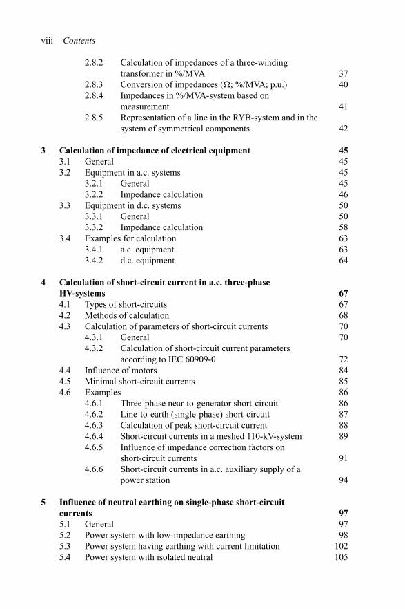
2.8.2 Calculation of impedances of a three-windingtransformer in %/MVA 37
2.8.3 Conversion of impedances (�; %/MVA; p.u.) 402.8.4 Impedances in %/MVA-system based on
measurement 412.8.5 Representation of a line in the RYB-system and in the
system of symmetrical components 42
3 Calculation of impedance of electrical equipment 453.1 General 453.2 Equipment in a.c. systems 45
3.2.1 General 453.2.2 Impedance calculation 46
3.3 Equipment in d.c. systems 503.3.1 General 503.3.2 Impedance calculation 58
3.4 Examples for calculation 633.4.1 a.c. equipment 633.4.2 d.c. equipment 64
4 Calculation of short-circuit current in a.c. three-phaseHV-systems 674.1 Types of short-circuits 674.2 Methods of calculation 684.3 Calculation of parameters of short-circuit currents 70
4.3.1 General 704.3.2 Calculation of short-circuit current parameters
according to IEC 60909-0 724.4 Influence of motors 844.5 Minimal short-circuit currents 854.6 Examples 86
4.6.1 Three-phase near-to-generator short-circuit 864.6.2 Line-to-earth (single-phase) short-circuit 874.6.3 Calculation of peak short-circuit current 884.6.4 Short-circuit currents in a meshed 110-kV-system 894.6.5 Influence of impedance correction factors on
short-circuit currents 914.6.6 Short-circuit currents in a.c. auxiliary supply of a
power station 94
5 Influence of neutral earthing on single-phase short-circuitcurrents 975.1 General 975.2 Power system with low-impedance earthing 985.3 Power system having earthing with current limitation 1025.4 Power system with isolated neutral 105
Contents ix
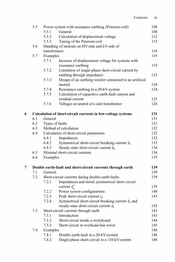
5.5 Power system with resonance earthing (Petersen-coil) 1085.5.1 General 1085.5.2 Calculation of displacement voltage 1125.5.3 Tuning of the Petersen-coil 115
5.6 Handling of neutrals on HV-side and LV-side oftransformers 116
5.7 Examples 1195.7.1 Increase of displacement voltage for systems with
resonance earthing 1195.7.2 Limitation of single-phase short-circuit current by
earthing through impedance 1235.7.3 Design of an earthing resistor connected to an artificial
neutral 1245.7.4 Resonance earthing in a 20-kV-system 1245.7.5 Calculation of capacitive earth-fault current and
residual current 1255.7.6 Voltages at neutral of a unit transformer 126
6 Calculation of short-circuit currents in low-voltage systems 1316.1 General 1316.2 Types of faults 1316.3 Method of calculation 1326.4 Calculation of short-circuit parameters 132
6.4.1 Impedances 1326.4.2 Symmetrical short-circuit breaking current Ib 1336.4.3 Steady-state short-circuit current Ik 134
6.5 Minimal short-circuit currents 1346.6 Examples 135
7 Double earth-fault and short-circuit currents through earth 1397.1 General 1397.2 Short-circuit currents during double earth-faults 139
7.2.1 Impedances and initial symmetrical short-circuitcurrent I ′′
k 1397.2.2 Power system configurations 1407.2.3 Peak short-circuit current ip 1437.2.4 Symmetrical short-circuit breaking current Ib and
steady-state short-circuit current Ik 1437.3 Short-circuit currents through earth 143
7.3.1 Introduction 1437.3.2 Short-circuit inside a switchyard 1447.3.3 Short-circuit at overhead-line tower 145
7.4 Examples 1467.4.1 Double earth-fault in a 20-kV-system 1467.4.2 Single-phase short-circuit in a 110-kV-system 148
x Contents
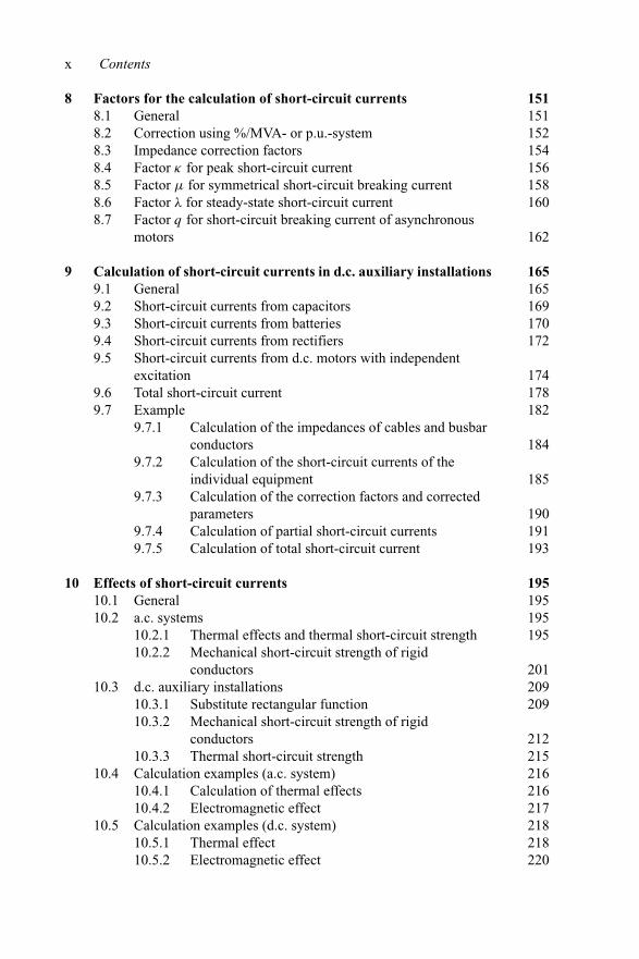
8 Factors for the calculation of short-circuit currents 1518.1 General 1518.2 Correction using %/MVA- or p.u.-system 1528.3 Impedance correction factors 1548.4 Factor κ for peak short-circuit current 1568.5 Factor μ for symmetrical short-circuit breaking current 1588.6 Factor λ for steady-state short-circuit current 1608.7 Factor q for short-circuit breaking current of asynchronous
motors 162
9 Calculation of short-circuit currents in d.c. auxiliary installations 1659.1 General 1659.2 Short-circuit currents from capacitors 1699.3 Short-circuit currents from batteries 1709.4 Short-circuit currents from rectifiers 1729.5 Short-circuit currents from d.c. motors with independent
excitation 1749.6 Total short-circuit current 1789.7 Example 182
9.7.1 Calculation of the impedances of cables and busbarconductors 184
9.7.2 Calculation of the short-circuit currents of theindividual equipment 185
9.7.3 Calculation of the correction factors and correctedparameters 190
9.7.4 Calculation of partial short-circuit currents 1919.7.5 Calculation of total short-circuit current 193
10 Effects of short-circuit currents 19510.1 General 19510.2 a.c. systems 195
10.2.1 Thermal effects and thermal short-circuit strength 19510.2.2 Mechanical short-circuit strength of rigid
conductors 20110.3 d.c. auxiliary installations 209
10.3.1 Substitute rectangular function 20910.3.2 Mechanical short-circuit strength of rigid
conductors 21210.3.3 Thermal short-circuit strength 215
10.4 Calculation examples (a.c. system) 21610.4.1 Calculation of thermal effects 21610.4.2 Electromagnetic effect 217
10.5 Calculation examples (d.c. system) 21810.5.1 Thermal effect 21810.5.2 Electromagnetic effect 220
Contents xi
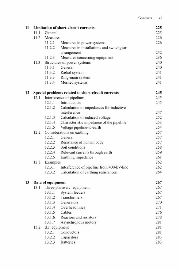
11 Limitation of short-circuit currents 22511.1 General 22511.2 Measures 226
11.2.1 Measures in power systems 22611.2.2 Measures in installations and switchgear
arrangement 23211.2.3 Measures concerning equipment 236
11.3 Structures of power systems 24011.3.1 General 24011.3.2 Radial system 24111.3.3 Ring-main system 24111.3.4 Meshed systems 241
12 Special problems related to short-circuit currents 24512.1 Interference of pipelines 245
12.1.1 Introduction 24512.1.2 Calculation of impedances for inductive
interference 24712.1.3 Calculation of induced voltage 25212.1.4 Characteristic impedance of the pipeline 25312.1.5 Voltage pipeline-to-earth 254
12.2 Considerations on earthing 25712.2.1 General 25712.2.2 Resistance of human body 25712.2.3 Soil conditions 25812.2.4 Relevant currents through earth 25912.2.5 Earthing impedance 261
12.3 Examples 26212.3.1 Interference of pipeline from 400-kV-line 26212.3.2 Calculation of earthing resistances 264
13 Data of equipment 26713.1 Three-phase a.c. equipment 267
13.1.1 System feeders 26713.1.2 Transformers 26713.1.3 Generators 27013.1.4 Overhead lines 27113.1.5 Cables 27613.1.6 Reactors and resistors 27813.1.7 Asynchronous motors 281
13.2 d.c. equipment 28113.2.1 Conductors 28113.2.2 Capacitors 28313.2.3 Batteries 283

xii Contents
Symbols, superscripts and subscripts 287
References 293
Index 299

List of figures
Figure 1.1 Importance of short-circuit currents and definition of tasks asper IEC 60781, IEC 60865, IEC 60909 and IEC 61660 2
Figure 2.1 Vector diagram and time course of a.c. voltage 12Figure 2.2 Definition of vectors for current, voltage and power in
three-phase a.c. systems. (a) Power system diagram and(b) electrical diagram for symmetrical conditions(positive-sequence component) 14
Figure 2.3 Vector diagram of current, voltage and power of a three-phasea.c. system represented by the positive-sequence component.(a) Consumer vector system and (b) generator vectorsystem 15
Figure 2.4 Differentially small section of homogeneous three-phasea.c. line 16
Figure 2.5 Vector diagram of voltages in RYB-system and in thezero-sequence component, positive- and negative-sequencecomponents are NIL 18
Figure 2.6 Vector diagram of voltages in RYB-system andpositive-sequence component, zero- and negative-sequencecomponents are NIL 19
Figure 2.7 Vector diagram of voltages in RYB-system andnegative-sequence component, zero- and positive-sequencecomponents are NIL 19
Figure 2.8 Measurement of impedance in the system of symmetricalcomponents. (a) Positive-sequence component (identical withnegative-sequence component) and (b) zero-sequencecomponent 21
Figure 2.9 Measuring of zero-sequence impedance of a two-windingtransformer (YNd). Diagram indicates winding arrangementof the transformer: (a) measuring at star-connected windingand (b) measuring at delta-connected winding 22
Figure 2.10 Measurement of positive-sequence impedance of athree-winding transformer (YNyn + d). Diagram indicateswinding arrangement of the transformer 22
xiv List of figures
Figure 2.11 Measurement of zero-sequence impedance of a three-windingtransformer (YNyn + d). Diagram indicates windingarrangement of the transformer 23
Figure 2.12 General scheme for the calculation of short-circuit currents inthree-phase a.c. systems using the system of symmetricalcomponents 25
Figure 2.13 Equivalent circuit diagram of a single-phase short-circuit inRYB-system 25
Figure 2.14 Equivalent circuit diagram in the system of symmetricalcomponents for a single-phase short-circuit 26
Figure 2.15 Equations for impedance analysis in power systems 30Figure 2.16 Equivalent circuit diagram of a power system with different
voltage levels 34Figure 2.17 Graphical construction of voltages in the system of
symmetrical components: (a) vector diagram RYB, (b) vectordiagram of voltage in the zero-sequence component, (c) vectordiagram of voltage in the positive-sequence component and(d) vector diagram of voltage in the negative-sequencecomponent 38
Figure 2.18 Simplified equivalent circuit diagram in RYB-components 41Figure 2.19 Equivalent circuit diagram in the system of symmetrical
components 42Figure 2.20 Equivalent circuit diagram of an overhead line of infinitesimal
length with earth return in RYB-system 43Figure 2.21 Equivalent circuit diagram of an overhead line of infinitesimal
length with earth return in 012-system. (a) Positive-sequencecomponent, (b) negative-sequence component and(c) zero-sequence component 43
Figure 4.1 Types of short-circuits and short-circuit currents.(a) Three-phase short-circuit, (b) double-phase short-circuitwithout earth/ground connection, (c) double-phaseshort-circuit with earth/ground connection and(d) line-to-earth (line-to-ground) short-circuit 68
Figure 4.2 Time-course of short-circuit currents. (a) Near-to-generatorshort-circuit (according to Figure 12 of IEC 60909:1988),(b) far-from-generator short-circuit (according to Figure 1 ofIEC 60909:1988). I ′′
k – initial (symmetrical) short-circuitcurrent, ip – peak short-circuit current, Ik – steady-stateshort-circuit current and A – initial value of the aperiodiccomponent idc 69
Figure 4.3 Example for short-circuit current calculation with anequivalent voltage source at s.-c. location. (a) Three-phasea.c. system with three-phase short-circuit, (b) equivalentcircuit diagram in 012-system (positive-sequence system),(c) equivalent circuit diagram in 012-system with equivalentvoltage source 70

List of figures xv
Figure 4.4 Estimate of maximal initial short-circuit current for differenttypes of short-circuit and different impedance ratios Z1/Z0and Z2/Z1. Phase angle of Z0, Z1 and Z2 assumed to beidentical. Parameter r: ratio of asymmetrical short-circuitcurrent to three-phase short-circuit current 74
Figure 4.5 Equivalent circuit diagram for the calculation of short-circuitcurrents inside power plant 75
Figure 4.6 Equivalent circuit diagram for single-fed three-phaseshort-circuit 77
Figure 4.7 Factor κ for the calculation of peak short-circuit current 78Figure 4.8 Equivalent circuit diagram for three-phase short-circuit
fed from non-meshed sources 78Figure 4.9 Equivalent circuit diagram of a three-phase short-circuit in
a meshed system 79Figure 4.10 Factor μ for calculation of symmetrical short-circuit breaking
current 81Figure 4.11 Factors λmax and λmin for turbine generators (Figure 17 of DIN
EN 60909.0 (VDE 0102)). (a) Series one and (b) series two 83Figure 4.12 Factors λmax and λmin for salient-pole generators (Figure 18 of
DIN EN 60909.0 (VDE 0102) 1988). (a) Series one and (b)series two 83
Figure 4.13 Factor q for the calculation of symmetrical short-circuitbreaking current 86
Figure 4.14 Equivalent circuit diagram of a 220-kV-system withshort-circuit location 87
Figure 4.15 Equivalent circuit diagram of a 110-kV-system with220-kV-feeder 88
Figure 4.16 Equivalent circuit diagram of a 10-kV system, f = 50 Hz 89Figure 4.17 A 110-kV system with short-circuit location 90Figure 4.18 System with different voltage levels with short-circuit
location 91Figure 4.19 High-voltage system configuration for the auxiliary supply of
a power station 95Figure 5.1 Equivalent circuit diagram of a single-phase short-circuit
(system with low-impedance earthing). (a) Diagram inRYB-system, (b) equivalent circuit diagram in the system ofsymmetrical components 100
Figure 5.2 Ratio of single-phase to three-phase short-circuit currentdepending on Z1/Z0 and (γ1 − γ0) 101
Figure 5.3 Earth-fault factors in relation to Z1/Z0 and (γ1 − γ0).(a) Earth-fault factor δY and (b) earth-fault factor δB 103
Figure 5.4 Earth-fault factor δ depending on X0/X1 for different ratiosR0/X0 and R1/X1 = 0.01 104
Figure 5.5 Earth-fault factor δ and ratio I ′′k1/I ′′
k3 depending on X0/X1 104
xvi List of figures
Figure 5.6 Power system with isolated neutral with single-phaseearth-fault. (a) Equivalent circuit diagram in RYB-system and(b) equivalent circuit diagram in the system of symmetricalcomponents 105
Figure 5.7 Limit for self-extinguishing of capacitive currents in airaccording to VDE 0228 part 2 106
Figure 5.8 Vector diagram of voltages, power system with isolatedneutral. (a) Prior to fault and (b) during earth-fault 107
Figure 5.9 Time course of phase-to-earth voltages, displacement voltageand earth-fault current. System with isolated neutral,earth-fault in phase R 108
Figure 5.10 System with resonance earthing, earth-fault in phase R.(a) Equivalent diagram in RYB-system and (b) equivalentdiagram in the system of symmetrical components 109
Figure 5.11 Current limits according to VDE 0228 part 2:12.87 ofohmic currents IRes and capacitive currents ICE 111
Figure 5.12 Equivalent circuit diagram of a power system withasymmetrical phase-to-earth capacitances. (a) Equivalentcircuit diagram in the RYB-system and (b) equivalent circuitdiagram in the system of symmetrical components 112
Figure 5.13 Polar plot of the displacement voltage in a power system withresonance earthing 114
Figure 5.14 Voltages and residual current in the case of an earth-fault;displacement voltage without earth-fault 115
Figure 5.15 Current–voltage characteristic of a Petersen-coil;Ur = 20 kV/
√3; Ir = 640 A. (a) Minimal adjustment (50 A)
and (b) maximal adjustment (640 A) 117Figure 5.16 Displacement voltage in non-faulted operation and residual
current under earth-fault conditions; non-linear characteristicof the Petersen-coil 118
Figure 5.17 Transformation of voltage in the zero-sequence component oftransformers in the case of single-phase faults. (a) Equivalentcircuit diagram in RYB-system and (b) equivalent circuitdiagram in the system of symmetrical components 119
Figure 5.18 Alternate earthing of transformer neutrals by Petersen-coils.(a) Two parallel transformers and (b) earthing at artificialneutral with reactor XD2 121
Figure 5.19 Fault current in the MV-system in the case of a short-circuit inthe HV-system 121
Figure 5.20 Resonance curve (displacement voltage) for different detuningfactors in a 20-kV-system for different conditions 122
Figure 5.21 Voltages in a 20-kV-system with resonance earthing fordifferent tuning factors. (a) Phase-to-earth voltages and(b) displacement voltage (resonance curve) 123
List of figures xvii
Figure 5.22 Equivalent circuit diagram of a 20-kV-system with resonanceearthing 125
Figure 5.23 Connection of a power station to a 220-kV-system withshort-circuit location 126
Figure 5.24 Equivalent diagram in the zero-sequence component for faultlocation F 128
Figure 6.1 Equivalent circuit diagram of a LV-installation 135Figure 7.1 Equivalent circuit diagram with short-circuit inside
switchyard B 144Figure 7.2 Equivalent circuit diagram with short-circuit at overhead-line
tower 146Figure 7.3 Equivalent circuit diagram of a 20-kV-system 147Figure 7.4 Equivalent circuit diagram of a 110-kV-system with
short-circuit location 148Figure 8.1 Equivalent circuit diagram of a power system with different
voltage levels 152Figure 8.2 Equivalent circuit diagram for the calculation of impedance
correction factor using %/MVA- or p.u.-system 153Figure 8.3 Generator directly connected to the power system.
(a) Equivalent system diagram and (b) equivalent circuitdiagram in the positive-sequence component 154
Figure 8.4 Determination of the short-circuit current by superposition 155Figure 8.5 Equivalent circuit diagram of a power system with three-phase
short-circuit. (a) Circuit diagram, (b) simplified diagram ofa single-fed three-phase short-circuit and (c) time course ofvoltage with voltage angle ϕU 157
Figure 8.6 Characteristic saturation curve method for determination ofPotier’s reactance 161
Figure 8.7 Calculated and measured values of factor q for the calculationof short-circuit breaking current of asynchronous motors;values of q as per Figure 4.13 (According to Figure 20 ofIEC 60909-1:1991.) 163
Figure 9.1 Equivalent circuit diagrams of equipment in d.c. auxiliaryinstallations; typical time course of short-circuit current(according to Figure 1 of DIN EN 61660-1 (VDE 0102Teil 10)). (a) Capacitor, (b) battery, (c) rectifier in three-phasea.c. bridge connection and (d) d.c. motor with independentexcitation 166
Figure 9.2 Standard approximation function of the short-circuit current(according to Figure 2 of IEC 61660-1:1997) 167
Figure 9.3 Factor κC for the calculation of peak short-circuit current ofcapacitors (according to Figure 12 of IEC 61660-1:1997) 169
Figure 9.4 Time-to-peak tpC for the calculation of short-circuitcurrents of capacitors (according to Figure 13 ofIEC 61660-1:1997) 170
xviii List of figures
Figure 9.5 Factor k1C for the calculation of rise-time constant (accordingto Figure 14 of IEC 61660-1:1997) 171
Figure 9.6 Factor k2C for the calculation of decay-time constant(according to Figure 15 of IEC 61660-1:1997) 171
Figure 9.7 Rise-time constant τ1B and time to peak tpB of short-circuitcurrents of batteries (according to Figure 10 ofIEC 61660-1:1997) 172
Figure 9.8 Factor λD for the calculation of quasi steady-state short-circuitcurrent of rectifiers (according to Figure 7 ofIEC 61660-1:1997) 173
Figure 9.9 Factor κD for the calculation of peak short-circuit currents ofrectifiers. Factor: R∗ = (RN/XN)(1 + 2RDBr/3RN)
(according to Figure 8 of IEC 61660-1:1997) 173Figure 9.10 Factor κM for the calculation of peak short-circuit current of
d.c. motors with independent excitation (according toFigure 17 of IEC 61660-1:1997) 176
Figure 9.11 Time to peak of short-circuit currents for d.c. motors withindependent excitation and τMec < 10 ∗ τF (according toFigure 19 of IEC 61660-1:1997) 176
Figure 9.12 Factor k1M in the case of d.c. motors with independentexcitation and τMec ≥ 10 ∗ τF (according to Figure 18 ofIEC 61660-1:1997) 177
Figure 9.13 Factor k2M in the case of d.c. motors with independentexcitation and τMec < 10 ∗ τF (according to Figure 19 ofIEC 61660-1:1997) 177
Figure 9.14 Factor k3M in the case of d.c. motors with independentexcitation and τMec < 10 ∗ τF (according to Figure 20 ofIEC 61660-1:1997) 178
Figure 9.15 Factor k4M in the case of d.c. motors with independentexcitation and τMec < 10 ∗ τF (according to Figure 21 ofIEC 61660-1:1997) 178
Figure 9.16 Equivalent circuit diagram of a d.c. auxiliary installation 180Figure 9.17 Typical time curves of total short-circuit current in
d.c. auxiliary installations, e.g., (a) with dominating part ofmotors, (b) with dominating part of rectifiers, (c) withdominating part of batteries and (d) in the case of low rectifierload (according to Figure 22 of DIN EN 61660-1 (VDE 0102Teil 10)) 181
Figure 9.18 Equivalent circuit diagram of the d.c. auxiliary installation(220 V), e.g., of a power station 182
Figure 9.19 Partial short-circuit currents and total short-circuit current,d.c. auxiliary system as per Figure 9.18 193
Figure 9.20 Total short-circuit current, obtained by superposition of thepartial short-circuit currents and approximated short-circuitcurrent, d.c. auxiliary system as per Figure 9.18 194

List of figures xix
Figure 10.1 Factor n for the calculation of thermal short-time current(heat dissipation of a.c. component) (according to Figure 22 ofIEC 60909-0:2001) 197
Figure 10.2 Factor m for the calculation of thermal short-time current(heat dissipation of d.c. component) (according to Figure 21 ofIEC 60909-0:2001) 198
Figure 10.3 Rated short-time current density of conductors. δ0 is thetemperature at beginning of short-circuit and δ1 is thetemperature at end of short-circuit. (a) ____: Copper;- - - -: unalloyed steel and steel cables and (b) Al, aluminiumalloy, ACSR 199
Figure 10.4 Maximal permissible thermal short-circuit current forimpregnated paper-insulated cables Un up to 10 kV 200
Figure 10.5 Arrangement of parallel conductors 202Figure 10.6 Correction factor k12 for the calculation of effective distance
(according to Figure 1 of IEC 61660-2:1997) 203Figure 10.7 Factors Vσ and Vσ s for the calculation of bending stress
(according to Figure 4 of IEC 60865-1:1993) 205Figure 10.8 Factors Vr and Vrs for the calculation of bending stress
(according to Figure 5 of IEC 60865-1:1993) 205Figure 10.9 Factor VF for the calculation of bending stress (according to
Figure 4 of IEC 60865-1:1993) 207Figure 10.10 Calculation of mechanical natural frequency (Factor c).
Arrangement of distance elements and calculation equation(according to Figure 3 of IEC 60865-1:1993) 208
Figure 10.11 Standard approximation function (a) and substitute rectangularfunction (b) (according to Figure 4 of IEC 60660-2:1997). Notto scale 210
Figure 10.12 Factors Vσ and Vσ s for the calculation of bending stress onconductors (according to Figure 9 of IEC 61660-2:1997) 214
Figure 10.13 Factor VF for the calculation of forces on supports (accordingto Figure 9 of IEC 61660-2:1997) 215
Figure 10.14 Equivalent circuit diagram, data of equipment, resistanceat 20◦C 216
Figure 10.15 Equivalent circuit diagram of a power system withwind power plant 217
Figure 10.16 Arrangement of busbar conductor (data, see text) 219Figure 10.17 Standardised rectangular function and approximated total
short-circuit current 223Figure 11.1 Selection of suitable voltage level for the connection of power
stations 226Figure 11.2 Schematic diagram of a 400/132-kV-system for urban load;
values of short-circuit currents in case of operation as twosubsystems 228
Figure 11.3 Schematic diagram of a 132-kV-system with power station 229

xx List of figures
Figure 11.4 Equivalent circuit diagram of a 30-kV-system with feeding132-kV-system: (a) Operation with transformers in parallel and(b) limitation of short-circuit current. Result of three-phaseshort-circuit current: S′′
kQ = 3.2 GVA; SrT = 40 MVA;ukrT = 12%; trT = 110/32; OHTL 95Al; ltot = 56 km 230
Figure 11.5 Equivalent circuit diagram of a 380-kV-system and results ofthree-phase short-circuit current calculation: (a) Radial fedsystem and (b) ring fed system. S′′
kQ = 8 GVA; OHTLACSR/AW 4 × 282/46; li = 120 km 231
Figure 11.6 Schematic diagram of a 110-kV-substation fed from the220-kV-system: (a) Operation with buscoupler closed and(b) operation with buscoupler open. Result of three-phaseshort-circuit current calculation 232
Figure 11.7 Equivalent circuit diagram of a 6-kV-industrial system. Resultsof three-phase short-circuit current calculation: (a) Busbarsectionaliser closed and (b) Busbar sectionaliser open 233
Figure 11.8 Equivalent circuit diagram of switchgear with singlebusbar 234
Figure 11.9 Time course of short-circuit current in installations with andwithout Ip-limiter 235
Figure 11.10 Cutaway view of an Ip-limiter support: (1) insulating tube,(2) explosive loading, (3) main conductor, (4) fuse elementand (5) transducer 236
Figure 11.11 Equivalent circuit diagram of a 10-kV-system with incomingfeeder. Results of three-phase short-circuit current calculation:(a) impedance voltage 13% and (b) impedancevoltage 17.5% 237
Figure 11.12 Equivalent circuit diagram of a 10-kV-system withshort-circuit limiting reactors. Results of three-phaseshort-circuit current calculation 238
Figure 11.13 Equivalent circuit diagram of 11.5-kV-system fed from the132-kV-system 239
Figure 11.14 Equivalent circuit diagram of a power station with132-kV-busbar. Results of three-phase short-circuit currentcalculation: SrG = 150 MVA; x′′
d = 12–17.8% 240Figure 11.15 General structure of a radial system with one incoming
feeder 241Figure 11.16 General structures of ring-main systems: (a) Simple structure
with one feeding busbar and (b) structure with two feedingbusbars (feeding from opposite sides) 242
Figure 11.17 Principal structure of a high voltage system with differentvoltage levels 243
Figure 11.18 Principal structure of meshed low voltage system:(a) Single-fed meshed system and (b) meshed system withoverlapping feeding 244
List of figures xxi
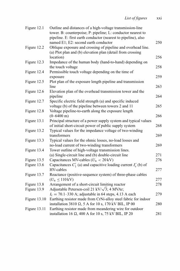
Figure 12.1 Outline and distances of a high-voltage transmission-linetower. B: counterpoise; P: pipeline; L: conductor nearest topipeline. E: first earth conductor (nearest to pipeline), alsonamed E1; E2: second earth conductor 250
Figure 12.2 Oblique exposure and crossing of pipeline and overhead line.(a) Plot plan and (b) elevation plan (detail from crossinglocation) 256
Figure 12.3 Impedance of the human body (hand-to-hand) depending onthe touch voltage 258
Figure 12.4 Permissible touch voltage depending on the time ofexposure 259
Figure 12.5 Plot plan of the exposure length pipeline and transmissionline 263
Figure 12.6 Elevation plan of the overhead transmission tower and thepipeline 264
Figure 12.7 Specific electric field strength (a) and specific inducedvoltage (b) of the pipeline between towers 2 and 11 265
Figure 12.8 Voltage pipeline-to-earth along the exposure length(0–6400 m) 266
Figure 13.1 Principal structure of a power supply system and typical valuesof initial short-circuit power of public supply system 268
Figure 13.2 Typical values for the impedance voltage of two-windingtransformers 269
Figure 13.3 Typical values for the ohmic losses, no-load losses andno-load current of two-winding transformers 269
Figure 13.4 Tower outline of high-voltage transmission lines.(a) Single-circuit line and (b) double-circuit line 271
Figure 13.5 Capacitances MV-cables (Un < 20 kV) 276Figure 13.6 Capacitances C′
1 (a) and capacitive loading current I ′c (b) of
HV-cables 277Figure 13.7 Reactance (positive-sequence system) of three-phase cables
(Un ≤ 110 kV) 277Figure 13.8 Arrangement of a short-circuit limiting reactor 278Figure 13.9 Adjustable Petersen-coil 21 kV/
√3; 4 MVAr;
Ir = 70.1–330 A; adjustable in 64 steps, 4.13 A each 279Figure 13.10 Earthing resistor made from CrNi-alloy steel fabric for indoor
installation 3810 �, 5 A for 10 s, 170 kV BIL, IP 00 280Figure 13.11 Earthing resistor made from meandering wire for outdoor
installation 16 �, 400 A for 10 s, 75 kV BIL, IP 20 281

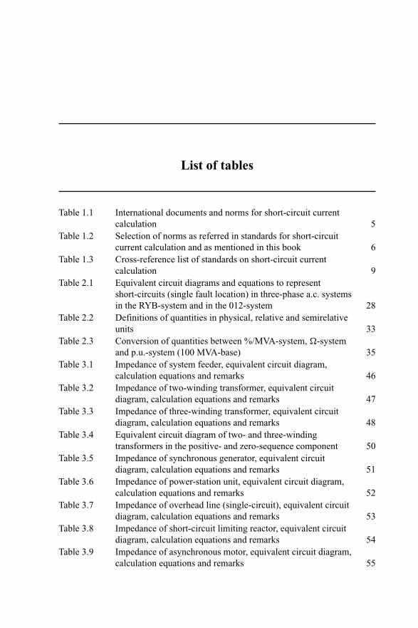
List of tables
Table 1.1 International documents and norms for short-circuit currentcalculation 5
Table 1.2 Selection of norms as referred in standards for short-circuitcurrent calculation and as mentioned in this book 6
Table 1.3 Cross-reference list of standards on short-circuit currentcalculation 9
Table 2.1 Equivalent circuit diagrams and equations to representshort-circuits (single fault location) in three-phase a.c. systemsin the RYB-system and in the 012-system 28
Table 2.2 Definitions of quantities in physical, relative and semirelativeunits 33
Table 2.3 Conversion of quantities between %/MVA-system, �-systemand p.u.-system (100 MVA-base) 35
Table 3.1 Impedance of system feeder, equivalent circuit diagram,calculation equations and remarks 46
Table 3.2 Impedance of two-winding transformer, equivalent circuitdiagram, calculation equations and remarks 47
Table 3.3 Impedance of three-winding transformer, equivalent circuitdiagram, calculation equations and remarks 48
Table 3.4 Equivalent circuit diagram of two- and three-windingtransformers in the positive- and zero-sequence component 50
Table 3.5 Impedance of synchronous generator, equivalent circuitdiagram, calculation equations and remarks 51
Table 3.6 Impedance of power-station unit, equivalent circuit diagram,calculation equations and remarks 52
Table 3.7 Impedance of overhead line (single-circuit), equivalent circuitdiagram, calculation equations and remarks 53
Table 3.8 Impedance of short-circuit limiting reactor, equivalent circuitdiagram, calculation equations and remarks 54
Table 3.9 Impedance of asynchronous motor, equivalent circuit diagram,calculation equations and remarks 55
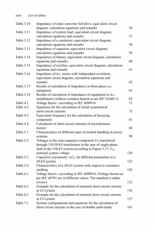
xxiv List of tables
Table 3.10 Impedance of static converter fed drive, equivalent circuitdiagram, calculation equations and remarks 56
Table 3.11 Impedance of system load, equivalent circuit diagram,calculation equations and remarks 57
Table 3.12 Impedance of a conductor, equivalent circuit diagram,calculation equations and remarks 58
Table 3.13 Impedance of capacitor, equivalent circuit diagram,calculation equations and remarks 59
Table 3.14 Impedance of battery, equivalent circuit diagram, calculationequations and remarks 60
Table 3.15 Impedance of rectifier, equivalent circuit diagram, calculationequations and remarks 61
Table 3.16 Impedance of d.c. motor with independent excitation,equivalent circuit diagram, calculation equations andremarks 62
Table 3.17 Results of calculation of impedance in three-phase a.c.equipment 63
Table 3.18 Results of calculation of impedance of equipment in d.c.installations (without common branch as per IEC 61660-1) 65
Table 4.1 Voltage factor c according to IEC 60909-0 71Table 4.2 Equations for the calculation of initial symmetrical
short-circuit currents 73Table 4.3 Equivalent frequency for the calculation of decaying
component 81Table 4.4 Calculation of short-circuit currents of asynchronous
motors 84Table 5.1 Characteristics of different types of neutral handling in power
systems 99Table 5.2 Voltages in the zero-sequence component U0 transferred
through 110/10-kV-transformer in the case of single-phasefault in the 110-kV-system according to Figure 5.17; Un:nominal system voltage 120
Table 5.3 Capacitive asymmetry CE for different parameters in a20-kV-system 122
Table 5.4 Characteristics of a 20-kV-system with respect to resonanceearthing 126
Table 6.1 Voltage factor c according to IEC 60909-0. (Voltage factors asper IEC 60781 are of different values. The standard is underreview) 132
Table 6.2 Example for the calculation of maximal short-circuit currentsin LV-system 136
Table 6.3 Example for the calculation of minimal short-circuit currentsin LV-system 137
Table 7.1 System configurations and equations for the calculation ofshort-circuit currents in the case of double earth-faults 141
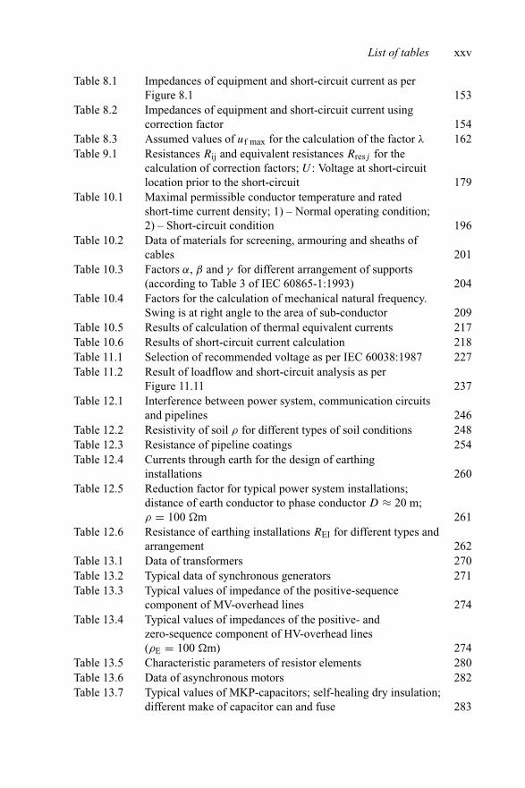
List of tables xxv
Table 8.1 Impedances of equipment and short-circuit current as perFigure 8.1 153
Table 8.2 Impedances of equipment and short-circuit current usingcorrection factor 154
Table 8.3 Assumed values of uf max for the calculation of the factor λ 162Table 9.1 Resistances Rij and equivalent resistances Rresj for the
calculation of correction factors; U : Voltage at short-circuitlocation prior to the short-circuit 179
Table 10.1 Maximal permissible conductor temperature and ratedshort-time current density; 1) – Normal operating condition;2) – Short-circuit condition 196
Table 10.2 Data of materials for screening, armouring and sheaths ofcables 201
Table 10.3 Factors α, β and γ for different arrangement of supports(according to Table 3 of IEC 60865-1:1993) 204
Table 10.4 Factors for the calculation of mechanical natural frequency.Swing is at right angle to the area of sub-conductor 209
Table 10.5 Results of calculation of thermal equivalent currents 217Table 10.6 Results of short-circuit current calculation 218Table 11.1 Selection of recommended voltage as per IEC 60038:1987 227Table 11.2 Result of loadflow and short-circuit analysis as per
Figure 11.11 237Table 12.1 Interference between power system, communication circuits
and pipelines 246Table 12.2 Resistivity of soil ρ for different types of soil conditions 248Table 12.3 Resistance of pipeline coatings 254Table 12.4 Currents through earth for the design of earthing
installations 260Table 12.5 Reduction factor for typical power system installations;
distance of earth conductor to phase conductor D ≈ 20 m;ρ = 100 �m 261
Table 12.6 Resistance of earthing installations REI for different types andarrangement 262
Table 13.1 Data of transformers 270Table 13.2 Typical data of synchronous generators 271Table 13.3 Typical values of impedance of the positive-sequence
component of MV-overhead lines 274Table 13.4 Typical values of impedances of the positive- and
zero-sequence component of HV-overhead lines(ρE = 100 �m) 274
Table 13.5 Characteristic parameters of resistor elements 280Table 13.6 Data of asynchronous motors 282Table 13.7 Typical values of MKP-capacitors; self-healing dry insulation;
different make of capacitor can and fuse 283

xxvi List of tables
Table 13.8 Typical values of MKP-capacitors; resin insulation;round can 284
Table 13.9 Resistance of loaded batteries (data from severalmanufacturers) 284
Foreword
Short-circuit currents are the dominating parameters for the design of equipmentand installations, for the operation of power systems and for the analysis of outagesand faults. Besides the knowledge about design of equipment in power systems,in auxiliary installations and about system operation constraints, the calculation ofshort-circuit currents is a central task for power system engineers. The book describesthe individual equipment in power systems with respect of the parameters needed forshort-circuit current calculation as well as methods for analysing the different typesof short-circuits in power systems using the system of symmetrical components.Besides detailed explanation of the calculation methods for short-circuit currents andtheir thermal and electromagnetic effects on equipment and installations, short-timeinterference problems and measures for the limitation of short-circuit currents areexplained. Detailed calculation procedures for the parameters and typical data ofequipment are given in a separate chapter for easy reference. All aspects of the bookare explained with examples based on engineering studies carried out by the author.
The preparation of the book was finalised in December 2004 and reflects the actualstatus of the technique, norms and standards. Carrying out short-circuit studies alwaysrequires the application of the latest editions of standards, norms and technical rec-ommendations, which can be obtained from the IEC-secretariat or from the nationalstandard organisation. All comments in this book are given in good faith, based onthe comprehensive technical experience of the author.
The author wishes to thank very much his former colleague Dipl.-Ing. HeinerRofalski for revising the text and improving the book. Most of the drawings wereprepared by my students Stefan Drees and Elmar Vogel who spent much effort toobtain clear and understandable presentation. My thanks go also to the staff of IEE-publishers, especially to Ms. Sarah Cramer who encouraged me to write this book.
Comments are highly appreciated.
Bielefeld, December [email protected]

xxviii Foreword
Professor Dr.-Ing. Jürgen Schlabbach, born 1952, member IEEE and VDI,studied power system engineering at the Technical University of Darmstadt/Germany,from where he got his Ph.D. in 1982. Until 1992 he was working in a consultingengineering company, responsible for planning and design of public and industrialsupply systems. Since 1992 he has been professor for ‘Power system engineeringand utilisation of renewable energy’ at the University of Applied Sciences in Biele-feld/Germany. His main working areas are planning of power systems, analysis offaults, power quality, interference problems and connection of renewable energysources to power systems. He is also a consulting engineer in the mentioned fields.
More information can be found on the author’s web-page http://www.fh-bielefeld.de/fb2/labor-ev.
Chapter 1
Introduction
1.1 Objectives
This book deals with the calculation of short-circuit currents in two- and three-phasea.c. systems as well as in d.c. systems, installed as auxiliary installations in powerplants and substations. It is not the objective of this book to repeat definitions andrules of norms and standards, but to explain the procedure for calculating short-circuitcurrents and their effects on installations and equipment. In some cases repetitionof equations, tables and diagrams from norms and standards however are deemednecessary for easy understanding. It should be emphasised in this respect that thepresentation within this book is mainly concentrated on installations and equipmentin high voltage systems, i.e., voltage levels up to 500 kV. Special considerations haveto be taken in the case of long transmission lines and in power systems with nominalvoltages above 500 kV. The calculation of short-circuit currents and of their effectsare based on the procedures and rules defined in the IEC documents 61660, 60909,60865 and 60781 as outlined in Table 1.1.
1.2 Importance of short-circuit currents
Electrical power systems have to be planned, projected, constructed, commissionedand operated in such a way to enable a safe, reliable and economic supply of theload. The knowledge of the loading of the equipment at the time of commissioningand as foreseeable in the future is necessary for the design and determinationof the rating of the individual equipment and of the power system as a whole.Faults, i.e., short-circuits in the power system cannot be avoided despite carefulplanning and design, good maintenance and thorough operation of the system. Thisimplies influences from outside the system, such as short-circuits following light-ning strokes into phase-conductors of overhead lines and damages of cables due toearth construction works as well as internal faults, e.g., due to ageing of insulation

2 Short-circuit currents
materials. Short-circuit currents therefore have an important influence on the designand operation of equipment and power systems.
Switchgear and fuses have to switch-off short-circuit currents in short time andin a safe way; switches and breakers have to be designed to allow even switch-on toan existing short-circuit followed by the normal switch-off operation. Short-circuitcurrents flowing through earth can induce impermissible voltages in neighbouringmetallic pipelines, communication and power circuits. Unsymmetrical short-circuitscause displacement of the voltage neutral-to-earth and are one of the dominat-ing criteria for the design of neutral handling. Short-circuits stimulate mechanicaloscillations of generator units which will lead to oscillations of active and reac-tive power as well, thus causing problems of stability of the power transfer whichcan finally result in system black-out. Furthermore, equipment and installationsmust withstand the expected thermal and electromagnetic (mechanical) effects ofshort-circuit currents.
In Figure 1.1 the typical time course of a short-circuit current is shown, whichcan be measured at high-voltage installations in the vicinity of power stations withsynchronous generators, characterised by decaying a.c. and d.c. components of the
• Electromagnetic effects IEC 60865-1• Switch-on capability IEC 60265-1
Total time duration
r.m.s. value
Further aspects
Peak short-circuit current(Maximal instantaneous value) Short-circuit breaking current
(r.m.s. value at switching instant tmin)
• Breaking capability IEC 60265-1 IEC 60265-1 etc.
• Touch and step voltages DIN VDE 0141• Interference DIN VDE 0228• Surge arresters IEC 60099-4• Overvoltages IEC 60071-1 IEC 60071-2• Neutral point earthing DIN VDE 0141 Insulation co-ordination IEC 60071-1 IEC 60071-2• Surge arresters IEC 60099-4
• Thermal effects IEC 60865-1• Protection measures against touch voltages in LV-installations DIN VDE 0100-470• Protection in HV-systems
24
19
14
9
4
–1
–6
–11
–16
kA
tmin
Figure 1.1 Importance of short-circuit currents and definition of tasks as perIEC 60781, IEC 60865, IEC 60909 and IEC 61660

Introduction 3
current. It is assumed that the short-circuit is switched-off approximately 14 periodsafter its initiation, which seems a rather long time, but was chosen for reason of a bettervisibility in the figure. Attention shall be put on four parameters of the short-circuitcurrent.
• The total time duration of the short-circuit current consists of the operating timeof the protection devices and the total breaking time of the switchgear.
• The peak short-circuit current, which is the maximal instantaneous value of theshort-circuit current, occurs approximately a quarter period after the initiation ofthe short-circuit. As electromagnetic forces are proportional to the instantaneousvalue of the current, the peak short-circuit current is necessary to know in orderto calculate the forces on conductors and construction parts affected by the short-circuit current.
• The r.m.s.-value of the short-circuit current is decaying in this example due to thedecaying a.c. component. Currents through conductors will heat the conductordue to ohmic losses. The r.m.s. value of the short-circuit current, combined withthe total time duration, is a measure for the thermal effects of the short-circuit.
• The short-circuit breaking current is the r.m.s.-value of the short-circuit currentat switching instant, i.e., at time of operating the circuit-breaker. While openingthe contacts of the circuit-breaker, the arc inside the breaker will heat up theinstallation, which depends obviously on the breaking time as well.
1.3 Maximal and minimal short-circuit currents
Depending on the task of engineering studies, the maximal or minimal short-circuitcurrent has to be calculated. The maximal short-circuit current is the main designcriteria for the rating of equipment to withstand the effects of short-circuit currents,i.e., thermal and electromagnetic effects. The minimal short-circuit current is neededfor the design of protection systems and the minimal setting of protection relays.The short-circuit current itself depends on various parameters, such as voltage level,actual operating voltage, impedance of the system between any generation unit andthe short-circuit location, impedance at the short-circuit location itself, the numberof generation units in the system, the temperature of the equipment influencing theresistances and other parameters. The determination of the maximal and the minimalshort-circuit current therefore is not as simple as might be seen at this stage [36]. Itrequires detailed knowledge of the system operation, i.e., which cables, overhead-lines, transformers, generators, machines and reactors are in operation and which areswitched-off. The assessment of the results of any calculation of short-circuit currentsmust take into account these restrictions in order to ensure that the results are on thesafe side, i.e., that the safety margin of the calculated maximal short-circuit current islarge enough without resulting in an uneconomic high rating of the equipment. Thesame applies to the minimal short-circuit current for which the safety margin mustbe assessed in such a way as to distinguish between the highest operating current andany short-circuit current, which has to be switched-off.

4 Short-circuit currents
1.4 Norms and standards
Technical standards are harmonised on international basis. The internationalorganisation to coordinate the works and strategies is the ISO (International StandardsOrganisation), whereas IEC (International Electrotechnical Commission) is respon-sible for the electrotechnical standardisation. The national standard organisationssuch as CENELEC in Europe, BSI in the United Kingdom, DKE in Germany, ANSIin the United States, JSI in Japan as well as national electrotechnical organisationssuch as IEE, VDE, IEEE, JES etc. are working in the working groups of IEC toinclude their sight and knowledge on technical items in the international standardsand documents. On national basis, standards are adopted to the widest extent tothe internationally agreed standards and documents. In some cases additions to theinternational standards are included in the national standards, however their status is‘for information only’.
The application of norms and standards has to be based on the latest issues, whichcan be obtained in Germany from Beuth-Verlag GmbH, Burggrafenstr. 6, D-10787Berlin or from VDE-Verlag GmbH, Bismarckstr. 33, D-10625 Berlin. English ver-sions are available from British Standards Institution, London/UK, in the UnitedStates from American National Standards Institute or any national standard organi-sation. Standards can also be searched and ordered through the web on the followingURLs (appearance in alphabetical order):
American National Standards Institute http://www.nssn.org/help.htmlBritish Standards Institute http://www.bsonline.techindex.co.ukDeutsches Institut für Normung http://din.deInternational Electrotechnical Commission http://www.iec.chVDE-Verlag http://vde-verlag.de
The structure of standards and norms dealing with short-circuit current calculationas published in IEC or EN-norms are outlined in Table 1.1. The listing should notbe understood as a complete catalogue of standards but represents an overview only.Some of the mentioned standards are actually in draft status; others include cor-rections, additions and appendices. For details reference should be made to theIEC-homepage or the homepage of the national standards committee. The officialactual standards catalogue is the only relevant document for any technical appli-cation. IEC-documents and national standards refer to other norms and standards.A short overview of these references is outlined in Table 1.2.
With respect to the calculation of short-circuit currents and their effects, thestandards are harmonised in most of the countries. The procedures and methodsdescribed are identical to those defined in the mentioned IEC-documents. Table 1.3shows a cross-reference list between IEC, EN and BS.
The classification numbers of the different standards differ in some cases fromthose of the IEC-documents or the EN-norms, however in most of the cases, classi-fication numbers are similar, e.g.: Australian standard AS 3865, Swedish standardSS-EN 60865-1 and British standard BS EN 60865-1 are identical to IEC 60865-1

Introduction 5
(Short-circuit currents – calculation of effects; Part 1: Definitions and calculationmethods). The standards’ catalogue of American National Standards Institute, to beaccessed through the home-page of National Standards Systems Network, directlyindicates the IEC- resp. EN-documents under the heading ‘short-circuit currents’. It istherefore fully sufficient to apply the IEC-documents for calculation of short-circuitcurrents and the analysis of their effects.
Table 1.1 International documents and norms (with related VDE-classification) forshort-circuit current calculation
IEC (year) EN (year) DIN; VDE (year) Title, contents
61660-1 61660-1 VDE 0102 Short-circuit currents in d.c. auxiliary(1997) (1997) Part 10 installations in power plants and
(1998–06) substationsPart 1: Calculation of short-circuit currents
61660-2 61660-2 VDE 0103 Short-circuit currents in d.c. auxiliary(1997) (1997) Part 10 installations in power plants and
(1998–05) substationsPart 2: Calculation of effects
61660-3 61660-3 Appendix 1 Short-circuit currents in d.c. auxiliary(2000) VDE 0102 installations in power plants and
Part 10 substations(2002–11) Examples of calculation of short-circuit
current and effects
60781 HD 581 S1 Appendix 2 Application guide for calculation(1989) (1991) VDE 0102 of short-circuit currents in
(1992–09) low-voltage radial systems
60865-1 60865-1 VDE 0103 Short-circuit currents – Calculation(1993) (1993) (1994–11) of effects
Part 1: Definitions and calculation methods
— — Appendix 1 Short-circuit currents – Calculation ofVDE 103 effects(1996–06) Part 1: Definitions and calculation methods
Examples for calculation
60909-0 60909-0 VDE 0102 Short-circuit current calculation(2001) (2001) (2002–07) in a.c. systems
6 Short-circuit currents
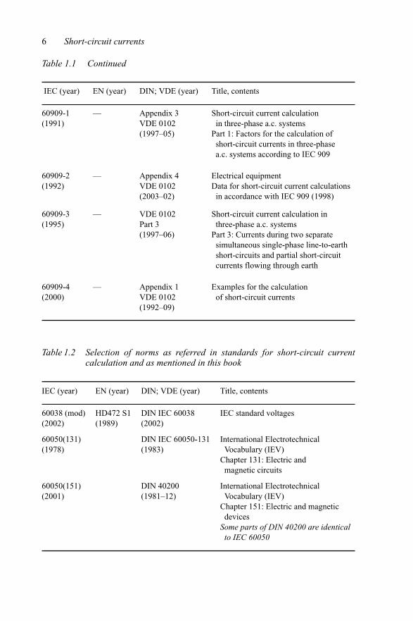
Table 1.1 Continued
IEC (year) EN (year) DIN; VDE (year) Title, contents
60909-1 — Appendix 3 Short-circuit current calculation(1991) VDE 0102 in three-phase a.c. systems
(1997–05) Part 1: Factors for the calculation ofshort-circuit currents in three-phasea.c. systems according to IEC 909
60909-2 — Appendix 4 Electrical equipment(1992) VDE 0102 Data for short-circuit current calculations
(2003–02) in accordance with IEC 909 (1998)
60909-3 — VDE 0102 Short-circuit current calculation in(1995) Part 3 three-phase a.c. systems
(1997–06) Part 3: Currents during two separatesimultaneous single-phase line-to-earthshort-circuits and partial short-circuitcurrents flowing through earth
60909-4 — Appendix 1 Examples for the calculation(2000) VDE 0102 of short-circuit currents
(1992–09)
Table 1.2 Selection of norms as referred in standards for short-circuit currentcalculation and as mentioned in this book
IEC (year) EN (year) DIN; VDE (year) Title, contents
60038 (mod) HD472 S1 DIN IEC 60038 IEC standard voltages(2002) (1989) (2002)
60050(131) DIN IEC 60050-131 International Electrotechnical(1978) (1983) Vocabulary (IEV)
Chapter 131: Electric andmagnetic circuits
60050(151) DIN 40200 International Electrotechnical(2001) (1981–12) Vocabulary (IEV)
Chapter 151: Electric and magneticdevices
Some parts of DIN 40200 are identicalto IEC 60050

Introduction 7
Table 1.2 Continued
IEC (year) EN (year) DIN; VDE (year) Title, contents
60050(195) International Electrotechnical(1998) Vocabulary (IEV)
Chapter 195: Earthing and protectionagainst electric shock
60050(441) International Electrotechnical(1998) Vocabulary (IEV)
Chapter 441: Switchgear,controlgear and fuses
60071-1 60071-1 VDE 0111 Part 1 Insulation coordination(1993) (1995) (1996–07) Definitions, principles and rules
60071-2 60071-2 VDE 0111 Part 2 Insulation coordination(1996) (1997) (1997–09) Application guide
TS 60479-1 Effects of currents on(1994) human being and livestock
Part 1: General aspects
TS 60479-2 Effects of currents passing(1982) through the human body
Part 2: Special aspects
60986 Short-circuit temperature limits(2000) of electric cables with rated
voltages from 6 kV up to 30 kV
60949 Calculation of thermally permissible(1988) short-circuit currents, taking into
account non-adiabatic heating effects
60896-1 60896-1 Stationary lead-acid batteries – General(1987) (1991) requirements and methods of
test – Part 1: Vented types
61071-1 (mod) 61071-1 VDE 0560 Part 120 Capacitors for power electronics(1991) (1996) (1997–08)
60265, 60282, VDE 0670 Switchgear, circuit-breakers, fuses, etc.60298, 60420, Various documents of IEC,60517, 60644, parts of VDE 067060694, etc.
60099, 61643 60099-1 VDE 0675 Part 1 Surge arresters(1994) (2000–08) Various documents of IEC,
parts of VDE 0670
60949 Calculation of thermally permissible(1988) short-circuit currents, taking into
account non-adiabatic heating effects

8 Short-circuit currents
Table 1.2 Continued
IEC (year) EN (year) DIN; VDE (year) Title, contents
60986 Guide to the short-circuit temperature(2000) limits of electrical cables with a rated
voltage from 1.8/3 (3.6) kV to18/30 (36) kV
VDE 0141 Earthing of special systems for(2000–01) electrical energy with nominal
voltages above 1 kV
VDE 0228 Part 1 Proceedings in the case of interference(1987–12) on telecommunication installations
by electrical powerinstallations – General
VDE 0228 Part 2 Proceedings in the case of interference(1987–12) on telecommunication installations
by electrical power installationsinterference by three-phaseinstallations
VDE 0228 Part 3 Proceedings in the case of interference(1988–09) on telecommunication installations
by electrical power installationsinterference by alternating currenttraction systems
VDE 0228 Part 4 Proceedings in the case of interference(1987–12) on telecommunication installations
by electrical power installationsinterference by direct current systems
VDE 0226 Part 1000 Current carrying capacity(1995–06) General, conversion factors
DIN 13321 Electric power engineering;(1978–04) components in three-phase networks
Concepts, quantities and their lettersymbols
DIN 40110-1 Quantities used in alternating(1994) current theory; two-line circuits
DIN 40110-2 Quantities used in alternating(2002) current theory; three-line circuits
EN 50160 DIN EN 50160 Voltage characteristics of electricity(1999) (2000–03) supplied by public distribution
systems
Introduction 9
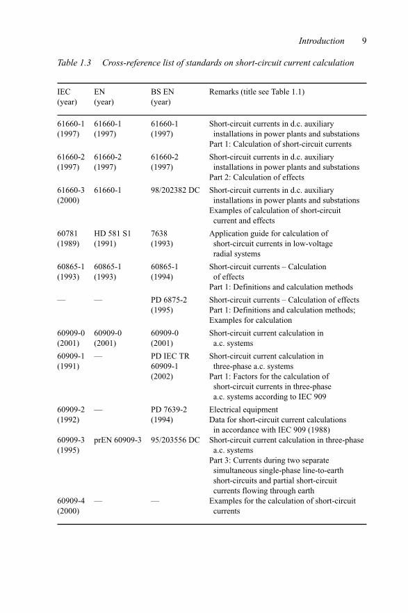
Table 1.3 Cross-reference list of standards on short-circuit current calculation
IEC EN BS EN Remarks (title see Table 1.1)(year) (year) (year)
61660-1 61660-1 61660-1 Short-circuit currents in d.c. auxiliary(1997) (1997) (1997) installations in power plants and substations
Part 1: Calculation of short-circuit currents
61660-2 61660-2 61660-2 Short-circuit currents in d.c. auxiliary(1997) (1997) (1997) installations in power plants and substations
Part 2: Calculation of effects
61660-3 61660-1 98/202382 DC Short-circuit currents in d.c. auxiliary(2000) installations in power plants and substations
Examples of calculation of short-circuitcurrent and effects
60781 HD 581 S1 7638 Application guide for calculation of(1989) (1991) (1993) short-circuit currents in low-voltage
radial systems
60865-1 60865-1 60865-1 Short-circuit currents – Calculation(1993) (1993) (1994) of effects
Part 1: Definitions and calculation methods
— — PD 6875-2 Short-circuit currents – Calculation of effects(1995) Part 1: Definitions and calculation methods;
Examples for calculation
60909-0 60909-0 60909-0 Short-circuit current calculation in(2001) (2001) (2001) a.c. systems
60909-1 — PD IEC TR Short-circuit current calculation in(1991) 60909-1 three-phase a.c. systems
(2002) Part 1: Factors for the calculation ofshort-circuit currents in three-phasea.c. systems according to IEC 909
60909-2 — PD 7639-2 Electrical equipment(1992) (1994) Data for short-circuit current calculations
in accordance with IEC 909 (1988)60909-3 prEN 60909-3 95/203556 DC Short-circuit current calculation in three-phase(1995) a.c. systems
Part 3: Currents during two separatesimultaneous single-phase line-to-earthshort-circuits and partial short-circuitcurrents flowing through earth
60909-4 — — Examples for the calculation of short-circuit(2000) currents

Chapter 2
Theoretical background
2.1 General
A detailed deduction of the mathematical procedure is not given within the contextof this book, but only the final equations are quoted. For further reading, reference ismade to [1], [13]. In general, equipment in power systems is represented by equivalentcircuits, which are designed for the individual tasks of power system analysis. For thecalculation of no-load current and the no-load reactive power of a transformer, theno-load equivalent circuit is sufficient. Regarding the calculation of short-circuits,voltage drops and load characteristic a different equivalent circuit is required. Theindividual components of the equivalent circuits are resistance, inductive and capaci-tive reactance (reactor and capacitor), voltage source and ideal transformer. Voltageand currents of the individual components and of the equivalent circuit are linked byOhm’s law.
2.2 Complex calculations, vectors and phasor diagrams
When dealing with two- and three-phase a.c. systems, it should be noted that currentsand voltages are generally not in phase. The phase position depends on the amount ofinductance, capacitance and resistances of the impedance. The time course, e.g., of acurrent or voltage in accordance with
u(t) = √2 ∗ U ∗ sin(ωt + ϕU ) (2.1a)
i(t) = √2 ∗ I ∗ sin(ωt + ϕI ) (2.1b)
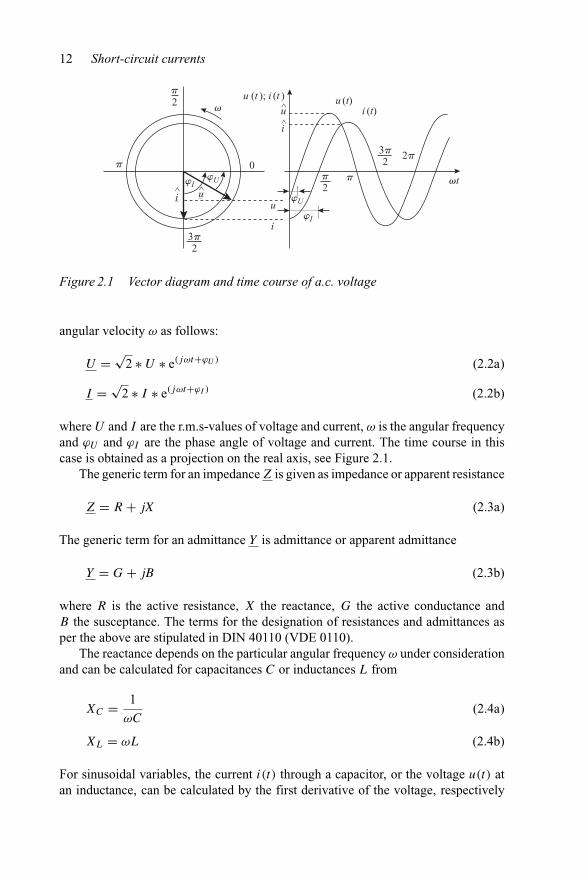
can in this case be shown as a line diagram as per Figure 2.1. In the case of sinu-soidal variables, these can be shown in the complex numerical level by rotatingpointers, which rotate in the mathematically positive sense (counterclockwise) with
12 Short-circuit currents
2
0
p
v
vtwIwU
wU
wI
p
23p
23p 2p
2p p
i
i
^ uu
u (t ); i (t )
^
u
i
u (t)i (t)
Figure 2.1 Vector diagram and time course of a.c. voltage
angular velocity ω as follows:
U = √2 ∗ U ∗ e(jωt+ϕU ) (2.2a)
I = √2 ∗ I ∗ e(jωt+ϕI ) (2.2b)
where U and I are the r.m.s-values of voltage and current, ω is the angular frequencyand ϕU and ϕI are the phase angle of voltage and current. The time course in thiscase is obtained as a projection on the real axis, see Figure 2.1.
The generic term for an impedance Z is given as impedance or apparent resistance
Z = R + jX (2.3a)
The generic term for an admittance Y is admittance or apparent admittance
Y = G + jB (2.3b)
where R is the active resistance, X the reactance, G the active conductance andB the susceptance. The terms for the designation of resistances and admittances asper the above are stipulated in DIN 40110 (VDE 0110).
The reactance depends on the particular angular frequency ω under considerationand can be calculated for capacitances C or inductances L from
XC = 1
ωC(2.4a)
XL = ωL (2.4b)
For sinusoidal variables, the current i(t) through a capacitor, or the voltage u(t) atan inductance, can be calculated by the first derivative of the voltage, respectively

Theoretical background 13
current, as follows:
i(t) = C ∗ du(t)
dt(2.5a)
u(t) = L ∗ di(t)
dt(2.5b)
The derivation for sinusoidal currents and voltages at a reactance establishes thatthe current achieves its maximum value a quarter period after the voltage. Whenconsidering the process in the complex level, the pointer of the voltage precedes thepointer of the current by 90◦. This corresponds to a multiplication by +j .
For a capacitance on the other hand, the voltage does not reach its maximumvalue until a quarter period after the current; the voltage pointer lags behind thecurrent by 90◦, which corresponds to a multiplication by −j .
This enables the relationships between current and voltage for inductances andcapacitances to be shown in a complex notation
U = jωL ∗ I (2.6a)
I = 1
jωC∗ U (2.6b)
The individual explanations of the quantities are given in the text above.Vectors are used to describe electrical processes. They are therefore used in d.c.,
a.c. and three-phase systems. Vector systems can, by definition, be chosen as required,but must not be changed during an analysis or calculation. It should also be noted thatthe appropriate choice of the vector system is of substantial assistance in describingand calculating special tasks. The need for vector systems is clear if one considersthe Kirchhoff’s laws, for which the positive direction of currents and voltages mustbe specified. In this way, the positive directions of the active and reactive powers arethen also stipulated.
For comparison and transfer reasons, the vector system for the three-phase net-work (RYB components) is also to be used for other component systems (e.g., systemof symmetrical components), which describe the three-phase network.
If vectors are drawn as shown in Figure 2.2, the active and reactive powersgenerated by a generator in overexcited operation mode are positive. This vectorsystem is designated as a generator vector system. Accordingly, the active and reactivepower consumed by the load are positive when choosing the consumer vector system.
When describing electrical systems voltage vectors are drawn from the phaseconductor (named L1, L2, L3 or also R, Y, B) to earth (E). In other componentsystems, for instance in the system of symmetrical components (Section 2.3), thedirection of the voltage vector is drawn from the conductor towards the particularreference conductor. On the other hand, vectors in phasor diagrams are shown inthe opposite direction. The vector of a voltage conductor to earth is therefore shownin the phasor diagram from earth potential to conductor potential.

14 Short-circuit currents
Positivesequencesystem
IRQ
UYQ= U1Q
IRQ
R(L3)
Y(L2)
B(L1)
IYQ
IBQ
UBQ UYQ
IRQ + IYQ + IBQ = 0; URQ + UYQ + UBQ = 0; UYQ = UQ /
URQ
+P+Q
+P+Q(a) (b)
E 01
3
Three-phasea.c. system
Figure 2.2 Definition of vectors for current, voltage and power in three-phasea.c. systems. (a) Power system diagram and (b) electrical diagram forsymmetrical conditions (positive-sequence component)
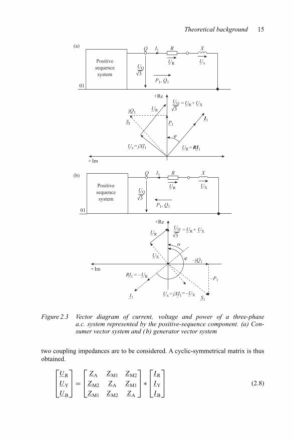
Based on the definition of the vector system, the correlation of voltage and currentof an electrical system can be shown in phasor diagrams. Where steady-state or quasi-steady-state operation is shown, r.m.s. value phasors are generally used. Figure 2.3shows the phasor diagram of an ohmic-inductive load in the generator and in theconsumer vector system.
2.3 System of symmetrical components
2.3.1 Transformation matrix
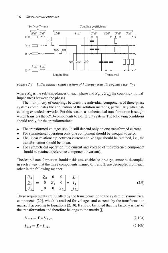
The relationships between voltages and currents of a three-phase system can be repre-sented by a matrix equation, e.g., with the aid of the impedance or admittance matrix.The equivalent circuits created by electrical equipment, such as lines, cables, trans-formers and machines, in this case have couplings in the three-phase system whichare of an inductive, capacitive and galvanic type. This can be explained by usingany short element of an overhead line in accordance with Figure 2.4 as an example,see also [1], [7].
The correlation of currents I and voltages U of the RYB system is as follows:
⎡⎢⎣
UR
UY
UB
⎤⎥⎦ =
⎡⎢⎣
ZRR ZRY ZRB
ZYR ZYY ZYB
ZBR ZBY ZBB
⎤⎥⎦ ∗
⎡⎢⎣
I R
I Y
I B
⎤⎥⎦ (2.7)
where ZRR, ZYY, ZBB are the self-impedances of each phase; ZRY, ZRB the coupling(mutual) impedances between phase R and Y, respectively, B; ZYR, ZYB the coupling(mutual) impedances between phase Y and R, respectively, B; and ZBR, ZBY thecoupling (mutual) impedances between phase B and R, respectively, Y.
All the values of this impedance matrix can generally be different. Because of thecyclic-symmetrical construction of three-phase systems only the self-impedance and
Theoretical background 15
Positivesequencesystem
UQ
I1
UR
jQ1
Ux = jXI1
P1, Q1
+Re
Q XR
–3
UQ–3
–
UR–
––
Ux = jXI1– ––
RI1 = – UR– –
–
UR = RI1
I1
–
–
–
SI– P1–
Ux–
– –
01
Positivesequencesystem
I1
UR
P1, Q1
Q XR
UQ–3
–
UR–
UX–
UX–
01
= UR + UX
UQ–3
– –= UR + UX
+ Im
w
w
a
+ Im
+Re
–jQ1
–P1
= –UXI1–S1
(a)
(b)
Figure 2.3 Vector diagram of current, voltage and power of a three-phasea.c. system represented by the positive-sequence component. (a) Con-sumer vector system and ( b) generator vector system
two coupling impedances are to be considered. A cyclic-symmetrical matrix is thusobtained.⎡
⎢⎣UR
UY
UB
⎤⎥⎦ =
⎡⎢⎣
ZA ZM1 ZM2
ZM2 ZA ZM1
ZM1 ZM2 ZA
⎤⎥⎦ ∗
⎡⎢⎣
I R
I Y
I B
⎤⎥⎦ (2.8)
16 Short-circuit currents
R�dl L�dl L�Ldl
R�Edl L�Edl
L�Edl C�Edl
TransversalLongitudinal
Self coefficients Coupling coefficients
G�EdlC�Ldl G�LdlB
Y
R
E
Figure 2.4 Differentially small section of homogeneous three-phase a.c. line
where ZA is the self-impedances of each phase and ZM1, ZM2 the coupling (mutual)impedances between the phases.
The multiplicity of couplings between the individual components of three-phasesystems complicates the application of the solution methods, particularly when cal-culating extended networks. For this reason, a mathematical transformation is soughtwhich transfers the RYB-components to a different system. The following conditionsshould apply for the transformation:
• The transformed voltages should still depend only on one transformed current.• For symmetrical operation only one component should be unequal to zero.• The linear relationship between current and voltage should be retained, i.e., the
transformation should be linear.• For symmetrical operation, the current and voltage of the reference component
should be retained (reference component invariant).
The desired transformation should in this case enable the three systems to be decoupledin such a way that the three components, named 0, 1 and 2, are decoupled from eachother in the following manner:⎡
⎢⎣U0
U1
U2
⎤⎥⎦ =
⎡⎢⎣
Z0 0 0
0 Z1 0
0 0 Z2
⎤⎥⎦ ∗
⎡⎢⎣
I 0
I 1
I 2
⎤⎥⎦ (2.9)
These requirements are fulfilled by the transformation to the system of symmetricalcomponents [29], which is realised for voltages and currents by the transformationmatrix T according to Equations (2.10). It should be noted that the factor 1
3 is part ofthe transformation and therefore belongs to the matrix T.
U012 = T ∗ URYB (2.10a)
I 012 = T ∗ I RYB (2.10b)

Theoretical background 17
⎡⎢⎣
U0
U1
U2
⎤⎥⎦ = 1
3
⎡⎢⎣
1 1 1
1 a a2
1 a2 a
⎤⎥⎦ ∗
⎡⎢⎣
UR
UY
UB
⎤⎥⎦ (2.10c)
⎡⎢⎣
I 0
I 1
I 2
⎤⎥⎦ = 1
3
⎡⎢⎣
1 1 1
1 a a2
1 a2 a
⎤⎥⎦ ∗
⎡⎢⎣
I R
I Y
I B
⎤⎥⎦ (2.10d)
The voltage vector of the 012-system is linearly linked to the voltage vector ofthe RYB-system (the same applies for the currents). The system of symmetricalcomponents is defined according to DIN 13321.
The reverse transformation of the 012-system to the RYB-system is achieved bythe matrix T−1 in accordance with
URYB = T−1 ∗ U012 (2.11a)
I RYB = T−1 ∗ I 012 (2.11b)
⎡⎢⎣
UR
UY
UB
⎤⎥⎦ =
⎡⎢⎣
1 1 1
1 a2 a
1 a a2
⎤⎥⎦ ∗
⎡⎢⎣
U0
U1
U2
⎤⎥⎦ (2.11c)
⎡⎢⎣
I R
I Y
I B
⎤⎥⎦ =
⎡⎢⎣
1 1 1
1 a2 a
1 a a2
⎤⎥⎦ ∗
⎡⎢⎣
I 0
I 1
I 2
⎤⎥⎦ (2.11d)
The following applies for both transformation matrices T and T−1:
T ∗ T−1 = E (2.12)
with the identity matrix E. The complex rotational phasors a and a2 have the followingmeanings:
a = ej120◦ = − 12 + j 1
2
√3 (2.13a)
a2 = ej240◦ = − 12 − j 1
2
√3 (2.13b)
1 + a + a2 = 0 (2.13c)
Multiplication of a vector with either a or a2 will only change the phase shift of thevector by 120◦ or 240◦ but will not change the length (amount) of it.
18 Short-circuit currents
2.3.2 Interpretation of the system of symmetrical components
If only one zero-sequence component exists, the following applies:⎡⎢⎣
UR
UY
UB
⎤⎥⎦ =
⎡⎢⎣
1 1 1
1 a2 a
1 a a2
⎤⎥⎦ ∗
⎡⎢⎣
U0
0
0
⎤⎥⎦ =
⎡⎢⎣
U0
U0
U0
⎤⎥⎦ (2.14)
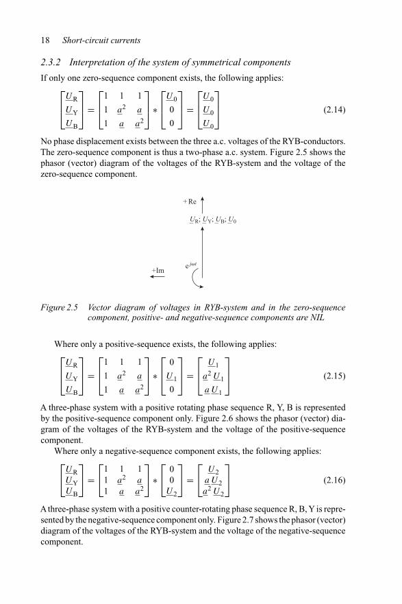
No phase displacement exists between the three a.c. voltages of the RYB-conductors.The zero-sequence component is thus a two-phase a.c. system. Figure 2.5 shows thephasor (vector) diagram of the voltages of the RYB-system and the voltage of thezero-sequence component.
+ Re
+Im
UR; UY; UB; U0– – – –
e jvt
Figure 2.5 Vector diagram of voltages in RYB-system and in the zero-sequencecomponent, positive- and negative-sequence components are NIL
Where only a positive-sequence exists, the following applies:⎡⎢⎣
UR
UY
UB
⎤⎥⎦ =
⎡⎢⎣
1 1 1
1 a2 a
1 a a2
⎤⎥⎦ ∗
⎡⎢⎣
0
U1
0
⎤⎥⎦ =
⎡⎢⎣
U1
a2 U1
a U1
⎤⎥⎦ (2.15)
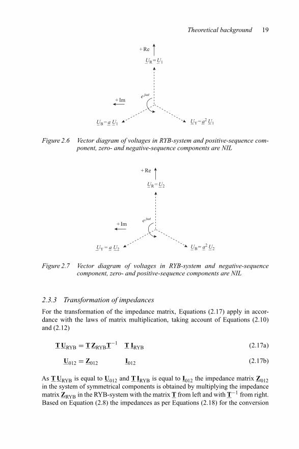
A three-phase system with a positive rotating phase sequence R, Y, B is representedby the positive-sequence component only. Figure 2.6 shows the phasor (vector) dia-gram of the voltages of the RYB-system and the voltage of the positive-sequencecomponent.
Where only a negative-sequence component exists, the following applies:⎡⎣UR
UYUB
⎤⎦ =
⎡⎣1 1 1
1 a2 a
1 a a2
⎤⎦ ∗
⎡⎣ 0
0U2
⎤⎦ =
⎡⎣ U2
a U2a2 U2
⎤⎦ (2.16)
Athree-phase system with a positive counter-rotating phase sequence R, B, Y is repre-sented by the negative-sequence component only. Figure 2.7 shows the phasor (vector)diagram of the voltages of the RYB-system and the voltage of the negative-sequencecomponent.
Theoretical background 19
+ Re
UR = U1
+ Ime jvt
––
UY = a2 U1UB = a U1
Figure 2.6 Vector diagram of voltages in RYB-system and positive-sequence com-ponent, zero- and negative-sequence components are NIL
+ Re
UR = U2
+ Ime jvt
UB = a2 U2UY = a U2
Figure 2.7 Vector diagram of voltages in RYB-system and negative-sequencecomponent, zero- and positive-sequence components are NIL
2.3.3 Transformation of impedances
For the transformation of the impedance matrix, Equations (2.17) apply in accor-dance with the laws of matrix multiplication, taking account of Equations (2.10)and (2.12)
T URYB = T ZRYBT−1 T IRYB (2.17a)
U012 = Z012 I012 (2.17b)
As T URYB is equal to U012 and T IRYB is equal to I012 the impedance matrix Z012in the system of symmetrical components is obtained by multiplying the impedancematrix ZRYB in the RYB-system with the matrix T from left and with T−1 from right.Based on Equation (2.8) the impedances as per Equations (2.18) for the conversion
20 Short-circuit currents
of the impedances of the three-phase system to the 012-system are obtained.
Z0 = ZA + ZM1 + ZM2 (2.18a)
Z1 = ZA + a2 ZM1 + a ZM2 (2.18b)
Z2 = ZA + a ZM1 + a2 ZM2 (2.18c)
The impedance values of the positive-sequence and negative-sequence componentsare generally equal. This applies to all non-rotating equipment. The impedanceof the zero-sequence component mainly has a different value from the impedanceof the positive-sequence component. If mutual coupling is absent, as perhaps withthree single-pole transformers connected together to form a three-phase transformer,the impedance of the zero-sequence component is equal to the impedance of thepositive- or (negative-) sequence component.
2.3.4 Measurement of impedances of the symmetrical components
Any equipment can be represented by an equivalent circuit diagram using the systemof symmetrical components, which can be determined. To obtain the parameters of theequivalent circuit diagram either short-circuit measurement or no-load measurementhas to be carried out in accordance with Figure 2.8 with a voltage system representingthe individual component of the system of symmetrical components, i.e.,
• Three-phase voltage system with positive rotating phase sequence RYB tomeasure the positive-sequence component.
• Three-phase voltage system with positive counter-rotating phase sequence RBYto measure the negative-sequence component.
• a.c. voltage system without any phase displacement of the voltage in the threephases of the equipment to measure the zero-sequence component.
It should be noted in this respect that the type of measurement, i.e., short-circuit mea-surement or no-load measurement, depends on the type of analysis to be carried out.For short-circuit current calculation or voltage drop estimate, the parameters obtainedby short-circuit measurement are needed. Impedance will be calculated based on themeasured voltage and current as outlined in Figure 2.8.
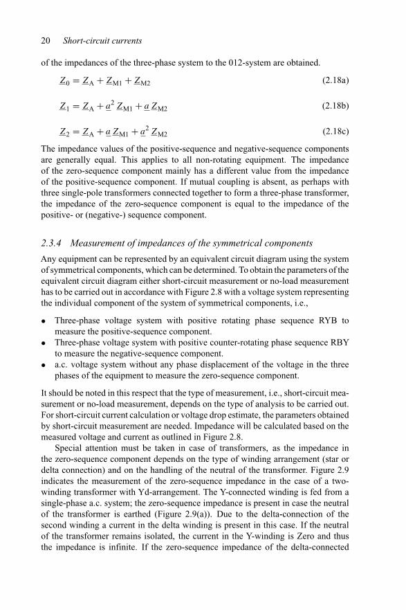
Special attention must be taken in case of transformers, as the impedance inthe zero-sequence component depends on the type of winding arrangement (star ordelta connection) and on the handling of the neutral of the transformer. Figure 2.9indicates the measurement of the zero-sequence impedance in the case of a two-winding transformer with Yd-arrangement. The Y-connected winding is fed from asingle-phase a.c. system; the zero-sequence impedance is present in case the neutralof the transformer is earthed (Figure 2.9(a)). Due to the delta-connection of thesecond winding a current in the delta winding is present in this case. If the neutralof the transformer remains isolated, the current in the Y-winding is Zero and thusthe impedance is infinite. If the zero-sequence impedance of the delta-connected

Theoretical background 21
GS Y
UR
R
B
3~
IR
1)(a)
2)
(b)
G1~
Y
UR
R
B
IR
1)
2)
Figure 2.8 Measurement of impedance in the system of symmetrical components.(a) Positive-sequence component (identical with negative-sequencecomponent) and (b) zero-sequence component
winding shall be measured, the current in the delta winding is Zero in any case and thezero-sequence impedance of the delta-connected winding is infinite (Figure 2.9(b)).
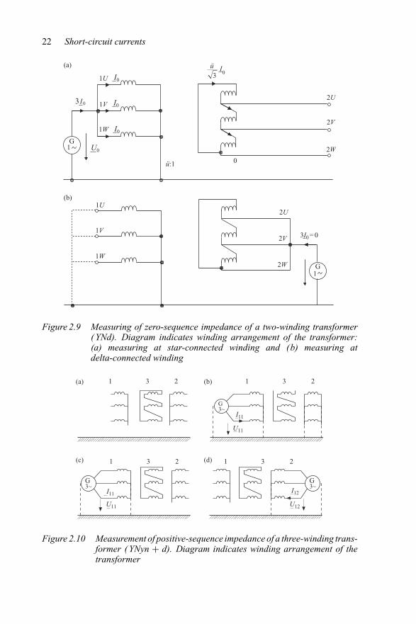
To measure the impedance of three-winding transformers in the positive- andzero-sequence component three different measurements have to be carried out. Forthe positive-sequence component the measurement is outlined in Figure 2.10 andfurther explained as below:
1. Feeding with three-phase a.c. system at winding 1 (HV-side)Short-circuit at winding 2 (MV-side)Measurement of uk12, respectively, ukHVMV
2. Feeding with three-phase a.c. system at winding 1 (HV-side)Short-circuit at winding 3 (LV-side)Measurement of uk13, respectively, ukHVLV
3. Feeding with three-phase a.c. system at winding 2 (MV-side)Short-circuit at winding 3 (LV-side)Measurement of uk23, respectively, ukMVLV
The impedances (reactances) as per the equivalent circuit diagram (seeTable 3.3) are
XTHV = 0.5 ∗(
ukHVMV
SrTHVMV+ ukHVLV
SrTHVLV− ukMVLV
SrTMVLV
)(2.19a)
XTMV = 0.5 ∗(
ukMVLV
SrTMVLV+ ukHVMV
SrTHVMV− ukHVLV
SrTHVLV
)(2.19b)
XTLV = 0.5 ∗(
ukHVLV
SrTHVLV+ ukMVLV
SrTMVLV− ukHVMV
SrTHVMV
)(2.19c)
22 Short-circuit currents
03 I
1U
1W
1V
I0
I0
I0
U0
ü:1
03Iü
2U
2V
2WG
1
(a)
(b)1U
1V
1W
2U
2V
2W G1
3I0 = 0
0
Figure 2.9 Measuring of zero-sequence impedance of a two-winding transformer( YNd). Diagram indicates winding arrangement of the transformer:(a) measuring at star-connected winding and (b) measuring atdelta-connected winding
I11
U11
I12
U12U11
I11
(a)
(c)
(b)
(d)
1 3 2
1 3 2 1 3 2
1 3 2
G3~
G3~
G3~
Figure 2.10 Measurement of positive-sequence impedance of a three-winding trans-former ( YNyn + d). Diagram indicates winding arrangement of thetransformer
Theoretical background 23
G1~ U01
3I01
1 3 2(b)(a)
OS
1 3 2
US MS
1 3 2(d)(c) 1 3 2
G1~ U01
3I01
G1~
3I02U02
Figure 2.11 Measurement of zero-sequence impedance of a three-winding trans-former ( YNyn + d). Diagram indicates winding arrangement of thetransformer; for explanations see text
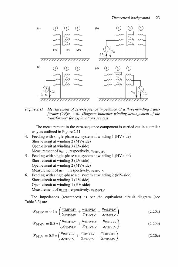
The measurement in the zero-sequence component is carried out in a similarway as outlined in Figure 2.11.
4. Feeding with single-phase a.c. system at winding 1 (HV-side)Short-circuit at winding 2 (MV-side)Open-circuit at winding 3 (LV-side)Measurement of uk012, respectively, uk0HVMV
5. Feeding with single-phase a.c. system at winding 1 (HV-side)Short-circuit at winding 3 (LV-side)Open-circuit at winding 2 (MV-side)Measurement of uk013, respectively, uk0HVLV
6. Feeding with single-phase a.c. system at winding 2 (MV-side)Short-circuit at winding 3 (LV-side)Open-circuit at winding 1 (HV-side)Measurement of uk023, respectively, uk0MVLV
The impedances (reactances) as per the equivalent circuit diagram (seeTable 3.3) are
X0THV = 0.5 ∗(
u0kHVMV
SrTHVMV+ u0kHVLV
SrTHVLV− u0kMVLV
SrTMVLV
)(2.20a)
X0TMV = 0.5 ∗(
u0kMVLV
SrTMVLV+ u0kHVMV
SrTHVMV− u0kHVLV
SrTHVLV
)(2.20b)
X0TLV = 0.5 ∗(
u0kHVLV
SrTHVLV+ u0kMVLV
SrTMVLV− u0kHVMV
SrTHVMV
)(2.20c)
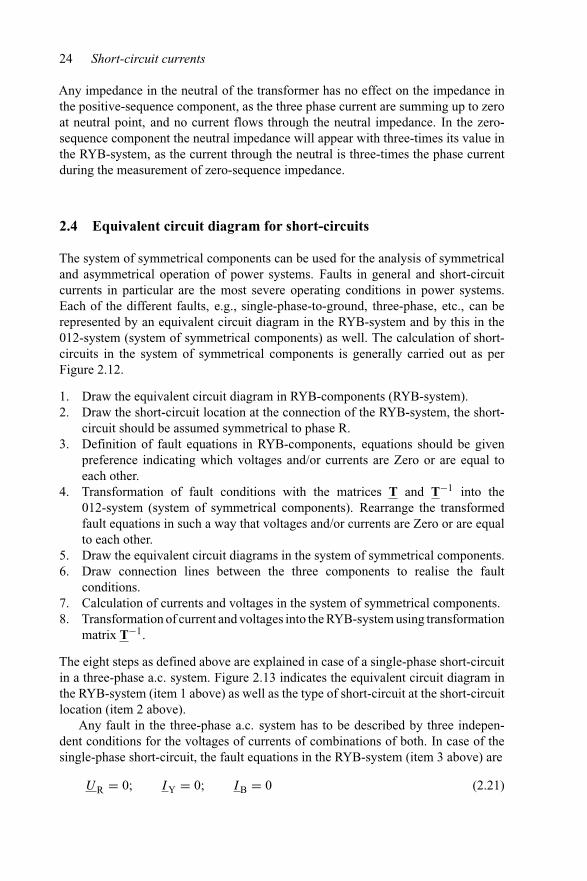
24 Short-circuit currents
Any impedance in the neutral of the transformer has no effect on the impedance inthe positive-sequence component, as the three phase current are summing up to zeroat neutral point, and no current flows through the neutral impedance. In the zero-sequence component the neutral impedance will appear with three-times its value inthe RYB-system, as the current through the neutral is three-times the phase currentduring the measurement of zero-sequence impedance.
2.4 Equivalent circuit diagram for short-circuits
The system of symmetrical components can be used for the analysis of symmetricaland asymmetrical operation of power systems. Faults in general and short-circuitcurrents in particular are the most severe operating conditions in power systems.Each of the different faults, e.g., single-phase-to-ground, three-phase, etc., can berepresented by an equivalent circuit diagram in the RYB-system and by this in the012-system (system of symmetrical components) as well. The calculation of short-circuits in the system of symmetrical components is generally carried out as perFigure 2.12.
1. Draw the equivalent circuit diagram in RYB-components (RYB-system).2. Draw the short-circuit location at the connection of the RYB-system, the short-
circuit should be assumed symmetrical to phase R.3. Definition of fault equations in RYB-components, equations should be given
preference indicating which voltages and/or currents are Zero or are equal toeach other.
4. Transformation of fault conditions with the matrices T and T−1 into the012-system (system of symmetrical components). Rearrange the transformedfault equations in such a way that voltages and/or currents are Zero or are equalto each other.
5. Draw the equivalent circuit diagrams in the system of symmetrical components.6. Draw connection lines between the three components to realise the fault
conditions.7. Calculation of currents and voltages in the system of symmetrical components.8. Transformation of current and voltages into the RYB-system using transformation
matrix T−1.
The eight steps as defined above are explained in case of a single-phase short-circuitin a three-phase a.c. system. Figure 2.13 indicates the equivalent circuit diagram inthe RYB-system (item 1 above) as well as the type of short-circuit at the short-circuitlocation (item 2 above).
Any fault in the three-phase a.c. system has to be described by three indepen-dent conditions for the voltages of currents of combinations of both. In case of thesingle-phase short-circuit, the fault equations in the RYB-system (item 3 above) are
UR = 0; I Y = 0; I B = 0 (2.21)
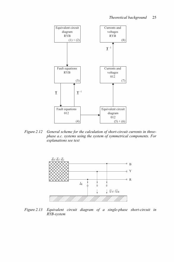
Theoretical background 25
(5) + (6)
(3) (7)
(4)
T –1
T –1
T
Equivalent circuitdiagram
RYB
Currents andvoltages
RYB(1) + (2) (8)
Fault equationsRYB
Currents andvoltages
012
Fault equations012
Equivalent circuitdiagram
012
Figure 2.12 General scheme for the calculation of short-circuit currents in three-phase a.c. systems using the system of symmetrical components. Forexplanations see text
B
Y
RIR
UY; UB
Z0; Z1; Z2
Figure 2.13 Equivalent circuit diagram of a single-phase short-circuit inRYB-system

26 Short-circuit currents
The transformation into the system of symmetrical components (item 4 above) iscarried out using the transformation matrices by Equations (2.10) and (2.11). Thefault equations for the voltages in the system of symmetrical components are
UR = 0 = U0 + U1 + U2 (2.22a)
and for the currents
I 0 = I 1 (2.22b)
I 0 = I 2 (2.22c)
The fault conditions as per Equations (2.22) can only be realised by a series con-nection of the positive-, negative- and zero-sequence component. The equivalentcircuit diagram (item 5 above) in the system of symmetrical components is outlinedin Figure 2.14 as well as the connection of the individual components to realise thefault conditions (item 6 above).
The positive-, negative- and zero-sequence component are represented by theimpedances Z1; Z2; Z0. The currents and voltages of the system of symmetrical
E1
Z1
U1
U2
U0
I1
I2
I0
Z2
Z0
01
02
00
Figure 2.14 Equivalent circuit diagram in the system of symmetrical componentsfor a single-phase short-circuit
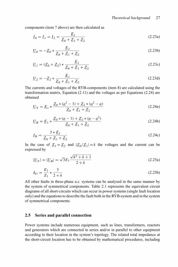
Theoretical background 27
components (item 7 above) are then calculated as
I 0 = I 1 = I 2 = E1
Z0 + Z1 + Z2(2.23a)
U0 = −Z0 ∗ E1
Z0 + Z1 + Z2(2.23b)
U1 = (Z0 + Z2) ∗ E1
Z0 + Z1 + Z2(2.23c)
U2 = −Z2 ∗ E1
Z0 + Z1 + Z2(2.23d)
The currents and voltages of the RYB-components (item 8) are calculated using thetransformation matrix, Equation (2.11) and the voltages as per Equations (2.24) areobtained
UY = E1 ∗ Z0 ∗ (a2 − 1) + Z2 ∗ (a2 − a)
Z0 + Z1 + Z2(2.24a)
UB = E1 ∗ Z0 ∗ (a − 1) + Z2 ∗ (a − a2)
Z0 + Z1 + Z2(2.24b)
I R = 3 ∗ E1
Z0 + Z1 + Z2(2.24c)
In the case of Z1 = Z2 and |Z0/Z1| = k the voltages and the current can beexpressed by
|UY| = |UB| = √3E1
√k2 + k + 1
2 + k(2.25a)
Ik1 = E1
Z1∗ 3
2 + k(2.25b)
All other faults in three-phase a.c. systems can be analysed in the same manner bythe system of symmetrical components. Table 2.1 represents the equivalent circuitdiagrams of all short-circuits which can occur in power systems (single fault locationonly) and the equations to describe the fault both in the RYB-system and in the systemof symmetrical components.
2.5 Series and parallel connection
Power systems include numerous equipment, such as lines, transformers, reactorsand generators which are connected in series and/or in parallel to other equipmentaccording to their location in the system’s topology. The related total impedance atthe short-circuit location has to be obtained by mathematical procedures, including
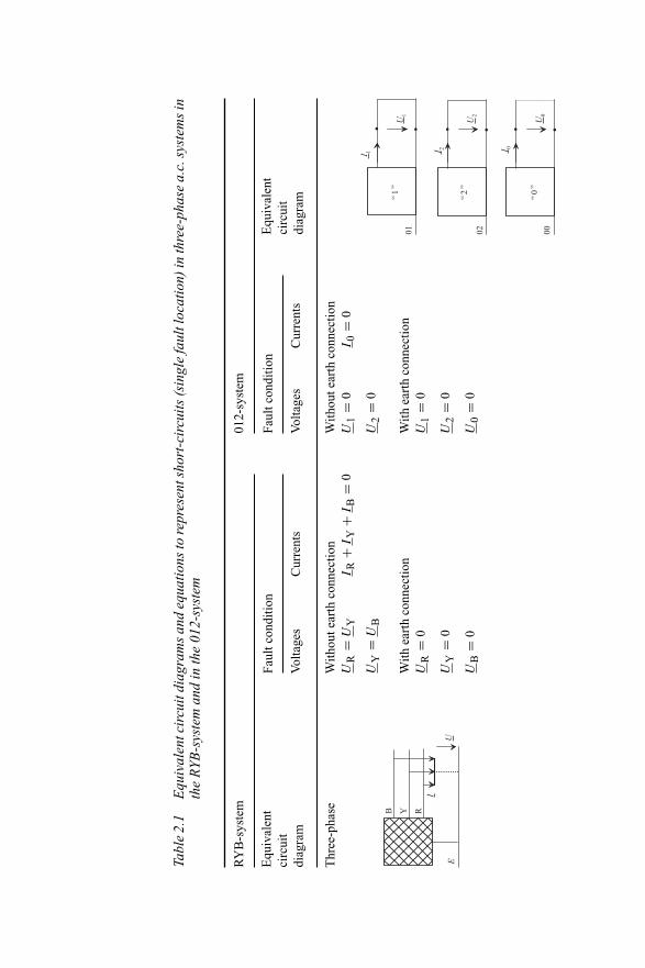
Tabl
e2.
1E
quiv
alen
tcir
cuit
diag
ram
san
deq
uatio
nsto
repr
esen
tsho
rt-c
ircu
its(s
ingl
efa
ultl
ocat
ion)
inth
ree-
phas
ea.
c.sy
stem
sin
the
RYB
-sys
tem
and
inth
e01
2-sy
stem
RY
B-s
yste
m01
2-sy
stem
Equ
ival
ent
circ
uit
diag
ram
Equ
ival
ent
circ
uit
diag
ram
Faul
tcon
ditio
nFa
ultc
ondi
tion
Vol
tage
sC
urre
nts
Vol
tage
sC
urre
nts
Thr
ee-p
hase
With
oute
arth
conn
ectio
nW
ithou
tear
thco
nnec
tion
UR
=U
YI
R+
IY
+I
B=
0U
1=
0I
0=
0
UY
=U
BU
2=
0
With
eart
hco
nnec
tion
With
eart
hco
nnec
tion
UR
=0
U1
=0
UY
=0
U2
=0
UB
=0
U0
=0
I
U
RYB
E
01 02 00
U1
I 1 I 2 I 0
U2
U0
“1
”
“2
”
“0
”

Dou
ble-
phas
eW
ithou
tear
thco
nnec
tion
With
oute
arth
conn
ectio
nU
Y=
UB
IR
=0
U1
=U
2I
1=
−I2
IY
=−I
BI
0=
0
With
eart
hco
nnec
tion
With
eart
hco
nnec
tion
UY
=0
IR
=0
U1
=U
2I
1+
I2
+I
0=
0
UB
=0
U1
=U
0
I
U
RYB
E
01 02 00
I 0I 2
U2
U0
U1
I 1
“1
”
“2
”
“0
”
Lin
e-to
-gro
und
UR
=0
IY
=0
U1
+U
2+
U0
=0
I1
=I
2
IB
=0
I1
=U
0
I
U
RYB
E
01 02 00
U2
U0
U1
I 0I 2I 1
“1
”
“2
”
“0
”

30 Short-circuit currents
star-delta- and delta-star-transformation. The equations to calculate total impedancewithin a given system topology are outlined in Figure 2.15.
2.6 Definitions and terms
A clear usage of terms defined in standards and norms is essential in all areas oftechnique. The knowledge of IEC-documents, national standards and norms therefore
Diagram Impedance–admittance Current–voltages
Serial connection
I1 I2Z1 Z2
1
1Z = 1/Y
2
2 Z = Z1 + Z2 I = I1 = I2
Y = Y 1Y 2Y 1 + Y 2
U = U1 + U2
Parallel connection
I
I1Z = 1/Y1
I2 Z2 = 1/Y2
Z = 1/Y
21
21 2I
Z = Z1Z2Z1 + Z2
I = I1 + I2
Y = Y 1 + Y 2 U = U1 = U2
Star-delta-transformation
Z1 = 1/Y1
Z2= 1/Y2Z3= 1/Y3
I1
I2I3
0
3 2
1Z12 = Z1Z2 + Z1Z3 + Z2Z3
Z3I1 + I2 + I3 = 0
Z13 = Z1Z2 + Z1Z3 + Z2Z3Z2
Z23 = Z1Z2 + Z1Z3 + Z2Z3Z1
Z13= 1/Y13 Z12= 1/Y12
Z23= 1/Y23
I13 I12
I21
I23I32
I31
1
3 2
Impedance: Z = R + jX
Y 12 = Y 1Y 2Y 1 + Y 2 + Y 3
I12 = I1Z1 − I2Z2Z12
Y 13 = Y 1Y 3Y 1 + Y 2 + Y 3
I13 = I1Z1 − I3Z3Z13
Y 23 = Y 2Y 3Y 1 + Y 2 + Y 3
I23 = I2Z2 − I3Z3Z23
Figure 2.15 Equations for impedance analysis in power systems [30,31]
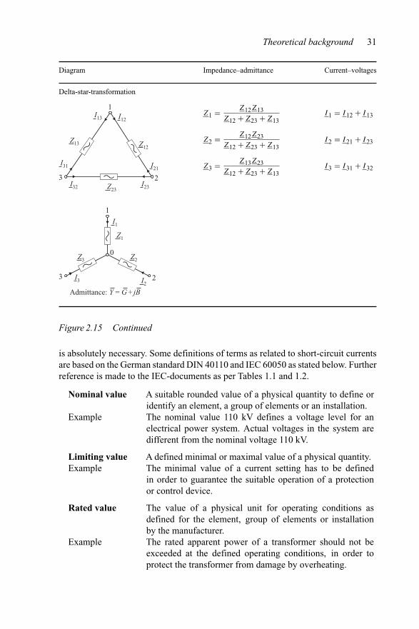
Theoretical background 31
Diagram Impedance–admittance Current–voltages
Delta-star-transformation
Z13 Z12
Z23
I13 I12
I21
I23I32
I31
1
3 2
Z1 = Z12Z13Z12 + Z23 + Z13
I1 = I12 + I13
Z2 = Z12Z23Z12 + Z23 + Z13
I2 = I21 + I23
Z3 = Z13Z23Z12 + Z23 + Z13
I3 = I31 + I32
Z3 Z2
Z1
I1
I2I3
0
3 2
1
Admittance: Y = G + jB
Figure 2.15 Continued
is absolutely necessary. Some definitions of terms as related to short-circuit currentsare based on the German standard DIN 40110 and IEC 60050 as stated below. Furtherreference is made to the IEC-documents as per Tables 1.1 and 1.2.
Nominal value A suitable rounded value of a physical quantity to define oridentify an element, a group of elements or an installation.
Example The nominal value 110 kV defines a voltage level for anelectrical power system. Actual voltages in the system aredifferent from the nominal voltage 110 kV.
Limiting value A defined minimal or maximal value of a physical quantity.Example The minimal value of a current setting has to be defined
in order to guarantee the suitable operation of a protectionor control device.
Rated value The value of a physical unit for operating conditions asdefined for the element, group of elements or installationby the manufacturer.
Example The rated apparent power of a transformer should not beexceeded at the defined operating conditions, in order toprotect the transformer from damage by overheating.
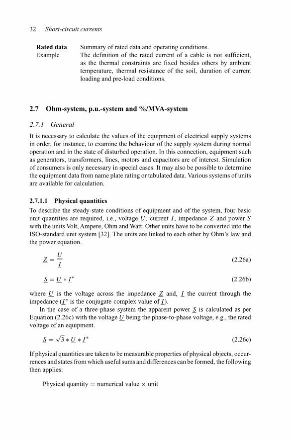
32 Short-circuit currents
Rated data Summary of rated data and operating conditions.Example The definition of the rated current of a cable is not sufficient,
as the thermal constraints are fixed besides others by ambienttemperature, thermal resistance of the soil, duration of currentloading and pre-load conditions.
2.7 Ohm-system, p.u.-system and %/MVA-system
2.7.1 General
It is necessary to calculate the values of the equipment of electrical supply systemsin order, for instance, to examine the behaviour of the supply system during normaloperation and in the state of disturbed operation. In this connection, equipment suchas generators, transformers, lines, motors and capacitors are of interest. Simulationof consumers is only necessary in special cases. It may also be possible to determinethe equipment data from name plate rating or tabulated data. Various systems of unitsare available for calculation.
2.7.1.1 Physical quantities
To describe the steady-state conditions of equipment and of the system, four basicunit quantities are required, i.e., voltage U , current I , impedance Z and power S
with the units Volt, Ampere, Ohm and Watt. Other units have to be converted into theISO-standard unit system [32]. The units are linked to each other by Ohm’s law andthe power equation.
Z = U
I(2.26a)
S = U ∗ I ∗ (2.26b)
where U is the voltage across the impedance Z and, I the current through theimpedance (I ∗ is the conjugate-complex value of I ).
In the case of a three-phase system the apparent power S is calculated as perEquation (2.26c) with the voltage U being the phase-to-phase voltage, e.g., the ratedvoltage of an equipment.
S = √3 ∗ U ∗ I ∗ (2.26c)
If physical quantities are taken to be measurable properties of physical objects, occur-rences and states from which useful sums and differences can be formed, the followingthen applies:
Physical quantity = numerical value × unit
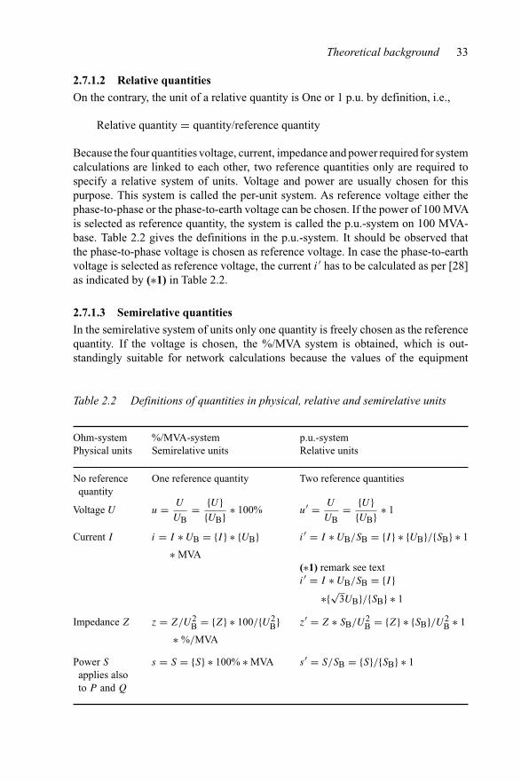
Theoretical background 33
2.7.1.2 Relative quantities
On the contrary, the unit of a relative quantity is One or 1 p.u. by definition, i.e.,
Relative quantity = quantity/reference quantity
Because the four quantities voltage, current, impedance and power required for systemcalculations are linked to each other, two reference quantities only are required tospecify a relative system of units. Voltage and power are usually chosen for thispurpose. This system is called the per-unit system. As reference voltage either thephase-to-phase or the phase-to-earth voltage can be chosen. If the power of 100 MVAis selected as reference quantity, the system is called the p.u.-system on 100 MVA-base. Table 2.2 gives the definitions in the p.u.-system. It should be observed thatthe phase-to-phase voltage is chosen as reference voltage. In case the phase-to-earthvoltage is selected as reference voltage, the current i′ has to be calculated as per [28]as indicated by (∗1) in Table 2.2.
2.7.1.3 Semirelative quantities
In the semirelative system of units only one quantity is freely chosen as the referencequantity. If the voltage is chosen, the %/MVA system is obtained, which is out-standingly suitable for network calculations because the values of the equipment
Table 2.2 Definitions of quantities in physical, relative and semirelative units
Ohm-system %/MVA-system p.u.-systemPhysical units Semirelative units Relative units
No reference One reference quantity Two reference quantitiesquantity
Voltage U u = U
UB= {U}
{UB} ∗ 100% u′ = U
UB= {U}
{UB} ∗ 1
Current I i = I ∗ UB = {I } ∗ {UB} i′ = I ∗ UB/SB = {I } ∗ {UB}/{SB} ∗ 1
∗ MVA(∗1) remark see texti′ = I ∗ UB/SB = {I }
∗{√3UB}/{SB} ∗ 1
Impedance Z z = Z/U2B = {Z} ∗ 100/{U2
B} z′ = Z ∗ SB/U2B = {Z} ∗ {SB}/U2
B ∗ 1
∗ %/MVA
Power S s = S = {S} ∗ 100% ∗ MVA s′ = S/SB = {S}/{SB} ∗ 1applies alsoto P and Q
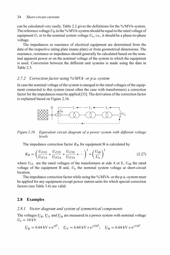
34 Short-circuit currents
can be calculated very easily. Table 2.2 gives the definitions for the %/MVA-system.The reference voltage UB in the %/MVA-system should be equal to the rated voltage ofequipment Ur or to the nominal system voltage Un, i.e., it should be a phase-to-phasevoltage.
The impedances or reactance of electrical equipment are determined from thedata of the respective rating plate (name plate) or from geometrical dimensions. Thereactance, resistance or impedance should generally be calculated based on the nom-inal apparent power or on the nominal voltage of the system in which the equipmentis used. Conversion between the different unit systems is made using the data inTable 2.3.
2.7.2 Correction factor using %/MVA- or p.u.-system
In case the nominal voltage of the system is unequal to the rated voltages of the equip-ment connected to this system (most often the case with transformers) a correctionfactor for the impedances must be applied [33]. The derivation of the correction factoris explained based on Figure 2.16.
Q Ti
Un
ZB
T1T2
Figure 2.16 Equivalent circuit diagram of a power system with different voltagelevels
The impedance correction factor KB for equipment B is calculated by
KB =(
UrT1E
UrT1A∗ UrT2E
UrT2A∗ UrT3E
UrT3A∗ · · ·
)2
∗(
UrB
Un
)2
(2.27)
where UrT.. are the rated voltages of the transformers at side A or E, UrB the ratedvoltage of the equipment B and, Un the nominal system voltage at short-circuitlocation.
The impedance correction factor while using the %/MVA- or the p.u.-system mustbe applied for any equipment except power station units for which special correctionfactors (see Table 3.6) are valid.
2.8 Examples
2.8.1 Vector diagram and system of symmetrical components
The voltages UR, UY and UB are measured in a power system with nominal voltageUn = 10 kV.
UR = 6.64 kV ∗ ej00; UY = 6.64 kV ∗ ej2500
; UB = 6.64 kV ∗ ej1100
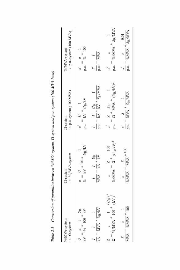
Tabl
e2.
3C
onve
rsio
nof
quan
titie
sbe
twee
n%
/MVA
-sys
tem
,�-s
yste
man
dp.
u.-s
yste
m(1
00M
VA-b
ase)
%/M
VA
-sys
tem
�-s
yste
m�
-sys
tem
%/M
VA
-sys
tem
→�
-sys
tem
→%
/M
VA
-sys
tem
→p.
u.-s
yste
m(1
00M
VA
)→
p.u.
-sys
tem
(100
MV
A)
U kV=
u %∗
1 100
∗UB
kV
u %=
U kV∗1
00∗
1
UB
/kV
u′
p.u.
=U kV
∗1
UB
/kV
u′
p.u.
=u %
∗1 100
I kA=
i
MV
A∗
1
UB
/kV
i
MV
A=
I kA∗U
B
kV
i′ p.u.
=I kA
∗UB
kV∗
1
SB
/M
VA
i′ p.u.
=i
MV
A
Z �=
z
%/M
VA
∗1 100
∗( UB
kV
) 2z
%/M
VA
=Z �
∗10
0
(UB
/kV
)2z′
p.u.
=Z �
∗S
B
MV
A∗
1
(UB
/kV
)2z′
p.u.
=z
%/M
VA
∗1
SB
/M
VA
S
MV
A=
s
%M
VA
∗1 100
s
%M
VA
=S
MV
A∗1
00s′
p.u.
=S
MV
A∗
1
SB
/M
VA
s′
p.u.
=s
%M
VA
∗0.
01
SB
/M
VA
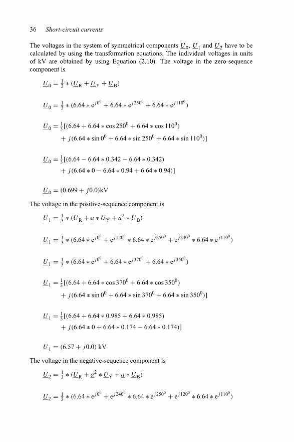
36 Short-circuit currents
The voltages in the system of symmetrical components U0, U1 and U2 have to becalculated by using the transformation equations. The individual voltages in unitsof kV are obtained by using Equation (2.10). The voltage in the zero-sequencecomponent is
U0 = 13 ∗ (UR + UY + UB)
U0 = 13 ∗ (6.64 ∗ ej00 + 6.64 ∗ ej2500 + 6.64 ∗ ej1100
)
U0 = 13 [(6.64 + 6.64 ∗ cos 2500 + 6.64 ∗ cos 1100)
+ j(6.64 ∗ sin 00 + 6.64 ∗ sin 2500 + 6.64 ∗ sin 1100)]
U0 = 13 [(6.64 − 6.64 ∗ 0.342 − 6.64 ∗ 0.342)
+ j(6.64 ∗ 0 − 6.64 ∗ 0.94 + 6.64 ∗ 0.94)]
U0 = (0.699 + j0.0)kV
The voltage in the positive-sequence component is
U1 = 13 ∗ (UR + a ∗ UY + a2 ∗ UB)
U1 = 13 ∗ (6.64 ∗ ej00 + ej1200 ∗ 6.64 ∗ ej2500 + ej2400 ∗ 6.64 ∗ ej1100
)
U1 = 13 ∗ (6.64 ∗ ej00 + 6.64 ∗ ej3700 + 6.64 ∗ ej3500
)
U1 = 13 [(6.64 + 6.64 ∗ cos 3700 + 6.64 ∗ cos 3500)
+ j(6.64 ∗ sin 00 + 6.64 ∗ sin 3700 + 6.64 ∗ sin 3500)]
U1 = 13 [(6.64 + 6.64 ∗ 0.985 + 6.64 ∗ 0.985)
+ j(6.64 ∗ 0 + 6.64 ∗ 0.174 − 6.64 ∗ 0.174)]
U1 = (6.57 + j0.0) kV
The voltage in the negative-sequence component is
U2 = 13 ∗ (UR + a2 ∗ UY + a ∗ UB)
U2 = 13 ∗ (6.64 ∗ ej00 + ej2400 ∗ 6.64 ∗ ej2500 + ej1200 ∗ 6.64 ∗ ej1100
)

Theoretical background 37
U2 = 13 ∗ (6.64 ∗ ej00 + 6.64 ∗ ej4900 + 6.64 ∗ ej2300
)
U2 = 13 [(6.64 + 6.64 ∗ cos 4900 + 6.64 ∗ cos 2300)
+ j(6.64 ∗ sin 00 + 6.64 ∗ sin 4900 + 6.64 ∗ sin 2300)]
U2 = 13 [(6.64 − 6.64 ∗ 0.643 − 6.64 ∗ 0.643)
+ j(6.64 ∗ 0 + 6.64 ∗ 0.766 − 6.64 ∗ 0.766)]
U2 = (−0.633 + j0.0) kV
The voltages in the system of symmetrical components can be obtained by graphicalconstruction as well as outlined in Figure 2.17. The voltages are assumed to have thesame value and phase displacement as mentioned above.
2.8.2 Calculation of impedances of a three-winding transformerin %/MVA
The impedances of a three-winding transformer are calculated in units of %/MVAby using the Equations (2.19). The data as mentioned below are taken from thename-plate:
Rated voltages UrHV/UrMV/UrTLV = 110 kV/30 kV/10 kVRated apparent power SrHV = 30 MVA; SrMV = 20 MVA; SrLV = 10 MVARated impedance voltage ukrHVMV = 10%; ukrHVLV = 4.5%;
ukrMVLV = 10.2%
It should be noted that the rated apparent power Sr as per above indicates theapparent power of the individual winding. The maximal permissible apparentpower to be transferred between the windings involved for measurement of theimpedance voltage had to be taken for the calculation of impedances, i.e., SrHVMV =MAX{SrHV; SrMV} = 20 MVA. The impedance of the high-voltage winding iscalculated by
XTHV = 0.5 ∗(
ukHVMV
SrTHVMV+ ukHVLV
SrTHVLV− ukMVLV
SrTMVLV
)
XTHV = 0.5 ∗(
10%
20 MVA+ 4.5%
10 MVA− 10.2%
10 MVA
)
XTHV = −0.035%
MVA

38 Short-circuit currents
The impedance of the medium-voltage winding is calculated by
XTMV = 0.5 ∗(
ukMVLV
SrTMVLV+ ukHVMV
SrTHVMV− ukHVLV
SrTHVLV
)
XTMV = 0.5 ∗(
10.2%
10 MVA+ 10%
20 MVA− 4.5%
10 MVA
)
XTMV = 0.535%
MVA
+ Im
+ Re
UR
UYUB
+ Re
+ Im
UB UY
UB
UR
UY
(a)
(b)
3 · U0
Figure 2.17 Graphical construction of voltages in the system of symmetrical com-ponents: (a) vector diagram RYB, (b) vector diagram of voltage inthe zero-sequence component, (c) vector diagram of voltage in thepositive-sequence component and (d) vector diagram of voltage in thenegative-sequence component

Theoretical background 39
+ Im
+ Re
UR
UYUB
(d)
a ·UB
a2 ·UY
3 · U2
+ Im
+ Re
UR
U1
UYUB
(c)
13
a2 ·UB
13
a ·UY
13
·UR
Figure 2.17 Continued
The impedance of the low-voltage winding is calculated by
XTLV = 0.5 ∗(
ukHVLV
SrTHVLV+ ukMVLV
SrTMVLV− ukHVMV
SrTHVMV
)
XTLV = 0.5 ∗(
4.5%
10 MVA+ 10.2%
10 MVA− 10%
20 MVA
)
XTLV = 0.485%
MVA

40 Short-circuit currents
It should be noted that the negative value of XTHV shall not be interpreted to have aphysical meaning. The model (see Table 3.4) describes the performance of the three-winding transformer at the connection point HV, MV and LV only. The impedancebetween any two connection points appears physically correct with a positive value.
2.8.3 Conversion of impedances (�; %/MVA; p.u.)
Impedance values shall be converted from one unit system into the other unitsystems (%/MVA-system and p.u.-system on 100 MVA-base) by using equationsas per Tables 2.2 and 2.3.
• Overhead line Z = (6.2 + j53.4) � at Un = 380 kVThe impedance in the %/MVA-system is calculated by
z = (6.2 + j53.4) � ∗ 100%
(380 kV)2 = (0.0043 + 0.037)%
MVA
The impedance in the p.u.-system on 100 MVA-base is calculated by
z′ = (6.2 + j53.4) � ∗ 100 MVA
(380 kV)2 = (0.0043 + 0.037) p.u.
• Apparent power of a transformer S = (1.22 + j300) MVAThe apparent power in the %/MVA-system is calculated by
s = (1.22 + j300) MVA ∗ 100% = (122 + j30000)%/MVA
The apparent power in the p.u.-system on 100 MVA-base is calculated by
s′ = (1.22 + j300) MVA
100 MVA= (0.0122 + j3) p.u.
• Voltage drop U = 12.5 kV in a 132 kV-systemThe voltage drop in the %/MVA-system is calculated by
u = 12.5 kV ∗ 100%
132 kV= 9.47%
The voltage drop in the p.u.-system on 100 MVA-base is calculated by
u′ = 12.5 kV ∗ 1
132 kV= 0.0947 p.u.
• Rated current of a 320 MVA-transformer on 115 kV-side Ir = 1.607 kAThe current in the %/MVA-system is calculated by
ir = 1.607 kA ∗ 115 kV = 184.81 MVA
The current in the p.u.-system on 100 MVA-base is calculated by
i′r = 1.607 kA ∗ 115 kV
100 MVA= 0.185 p.u.

Theoretical background 41
2.8.4 Impedances in %/MVA-system based on measurement
A simplified example for the application of the system of symmetrical components inrepresenting electrical equipment is outlined in Figure 2.18 by using a short elementof an overhead line in accordance to Figure 2.4. The impedance matrix (RYB-system)is thus obtained
ZRYB =⎡⎢⎣
R + jX jXM jXM
jXM R + jX jXM
jXM jXM R + jX
⎤⎥⎦ (2.28)
where R is the resistance of the line, X the reactance of the line and XM the mutualreactance between the individual phases.
jXMjXIRYB
URYB
jX
jXR
R
R
B
R
Y
Figure 2.18 Simplified equivalent circuit diagram in RYB-components
Voltages at the individual components R, Y and B are obtained from the currentand the impedance by Ohm’s law.
The voltage of phase R (component R) is given as follows:
UR = (R + jX) ∗ I R + jXM ∗ I Y + jXM ∗ I B (2.29)
and depends on the currents of all three phases (components) I R, I Y and I B. Usingthe system of symmetrical components, see Equation (2.18), the impedance matrixis simplified in such a way that the three components are decoupled from each otherin the following manner:
Z012 =⎡⎣R + j(X + 2XM) 0 0
0 R + j(X − XM) 00 0 R + j(X − XM)
⎤⎦ (2.30)
The equivalent circuit diagram in the system of symmetrical components is outlinedin Figure 2.19.

42 Short-circuit currents
j(X – XM)
U1
U2
U0
I1
I2
I0
R
01
j(X – XM)R
02
j(X + 2XM)R
00
Figure 2.19 Equivalent circuit diagram in the system of symmetrical components
The voltage U1 of the component 1 (positive-sequence component) is given asbelow:
U1 = (R + j(X − XM)) ∗ I 1 (2.31a)
and depends only on the current I 1 of the same component. Impedance of the com-ponents 1 and 2 (positive- and negative-sequence components) is identical. Voltageof the negative-sequence system therefore is given by
U2 = (R + j(X − XM)) ∗ I 2 (2.31b)
The impedance of the component 0 (zero-sequence component) is different from theothers and the voltage in the zero-sequence component is given by
U0 = (R + j(X + 2XM)) ∗ I 0 (2.31c)
2.8.5 Representation of a line in the RYB-system and in the system ofsymmetrical components
Overhead lines are represented in the RYB-system by lumped elements, indicatingthe inductive and capacitive coupling as well as the impedance of earth return path.The equivalent circuit diagram of an infinitesimal small section of a line is outlinedin Figure 2.20.
The representation in the system of symmetrical components (012-system) caneither be done by transformation of the individual elements using the transformation
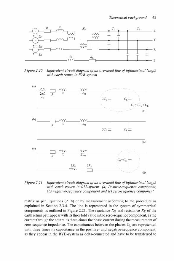
Theoretical background 43
XM CL CEX
XE RE
ER
R~
~
~
B
R
E
Y
EY
EB
Figure 2.20 Equivalent circuit diagram of an overhead line of infinitesimal lengthwith earth return in RYB-system
E1
R X –XM
3CL CE
C1 = 3CL + CE
C0 = CE
01
R X –XM
3CL CE
02
R X
3XE 3RE
2XM
00
(a)
(b)
(c)
Figure 2.21 Equivalent circuit diagram of an overhead line of infinitesimal lengthwith earth return in 012-system. (a) Positive-sequence component,(b) negative-sequence component and (c) zero-sequence component
matrix as per Equations (2.18) or by measurement according to the procedure asexplained in Section 2.3.4. The line is represented in the system of symmetricalcomponents as outlined in Figure 2.21. The reactance XE and resistance RE of theearth return path appear with its threefold value in the zero-sequence component, as thecurrent through the neutral is three-times the phase current during the measurement ofzero-sequence impedance. The capacitances between the phases CL are representedwith three times its capacitance in the positive- and negative-sequence component,as they appear in the RYB-system as delta-connected and have to be transferred to

44 Short-circuit currents
a star-connection for representation in the 012-system. The capacitance line-to-earthCE is represented in the three components with the same value.
Please observe that the mutual reactance XM appears with different values inthe positive- (negative-) and zero-sequence component as outlined in Section 2.3.3.The negative value of the reactance in the positive-, respectively, negative-sequencesystem has no physical meaning, as the total of the mutual reactance XM and theself-reactance X still remains positive and therefore physically correct.
The equivalent voltage source E1, which is the internal voltage of a generator, isonly present in the positive-sequence component as the symmetrical operation of thesystem is represented by this component.

Chapter 3
Calculation of impedance ofelectrical equipment
3.1 General
In general, equipment in power systems are represented by equivalent circuits, whichare designed for the individual tasks of power system analysis, e.g., for the calculationof no-load current and the no-load reactive power of a transformer, the no-load equiv-alent circuit is sufficient. Regarding the calculation of short-circuits, voltage dropsand load characteristic a different equivalent circuit is required. The individual com-ponents of the equivalent circuits are resistance, inductive and capacitive reactance(reactor and capacitor), voltage source and ideal transformer. Voltage and currents ofthe individual components and of the equivalent circuit are interlaced by Ohm’s law,which is valid for the three-phase system (RYB-system) as well as for the systemof symmetrical components (012-system). A detailed deduction of the mathematicalmethods and equations is not given within the context of this section of the book, butonly the final equations are quoted. For further reading, reference is made to [1,13].
3.2 Equipment in a.c. systems
3.2.1 General
Impedances of equipment are calculated based on name plate data, frommanufacturer’s data or from geometrical arrangement. For the calculation ofimpedances of generators, power plants, step-up and step-down transformers, correc-tion factors are necessary. The calculation equations as per Tables 3.1–3.11 are givenin the Ohm-system only. For conversion to %/MVA-system, respectively, p.u.-systemTables 2.2 and 2.3 can be used. If not marked by index ‘1’, e.g., Z1Q, in a differentway, impedances are given for the positive-sequence component. The impedance inthe zero-sequence system is marked with index ‘0’, e.g., Z0Q.

Tabl
e3.
1Im
peda
nce
ofsy
stem
feed
er,e
quiv
alen
tcir
cuit
diag
ram
,cal
cula
tion
equa
tions
and
rem
arks
3.2.
2Im
peda
nce
calc
ulat
ion
Figu
reIm
peda
nce
Rem
arks
Posi
tive-
sequ
ence
syst
emc
Vol
tage
fact
orac
cord
ing
toTa
ble
4.1
I′′ k1
QIn
itial
shor
t-ci
rcui
tcur
rent
(sin
gle-
phas
esh
ort-
circ
uit)
I′′ k3
QIn
itial
shor
t-ci
rcui
tcur
rent
(thr
ee-p
hase
shor
t-ci
rcui
t)
S′′ kQ
Initi
alsh
ort-
circ
uitp
ower
(thr
ee-p
hase
shor
t-ci
rcui
t)
UnQ
Nom
inal
syst
emvo
ltage
atco
nnec
tion
poin
t
Z1Q
=c
∗U2 nQ
S′′ kQ
Z1Q
=c
∗UnQ
√ 3∗I
′′ k3Q
Ass
umpt
ions
for
resi
stan
ce:
•RQ
≈0
ifU
nQ≥
35kV
;sys
tem
with
over
head
tran
smis
sion
lines
•RQ
=0.
1XQ
resp
ectiv
ely
XQ
=0.
995Z
Q•T
heim
peda
nce
inth
eze
ro-s
eque
nce
com
pone
ntno
rmal
lyis
give
nas
ara
tioof
the
impe
danc
ein
the
posi
tive-
sequ
ence
com
pone
nt.I
fth
esi
ngle
-pha
sesh
ort-
circ
uitc
urre
ntfr
omth
esy
stem
feed
eris
know
n,th
eze
ro-s
eque
nce
impe
danc
eca
nbe
calc
ulat
ed.
•Ref
eren
ceIt
em3.
2of
IEC
6090
9
X1Q
=Z
1Q√ 1
+(R
1Q/X
1Q)2
Zer
o-se
quen
ceco
mpo
nent
Z0Q
=3∗Z
1Q∗I
′′ k3Q
I′′ k1
Q−2
∗Z1Q
RQ
XQ
E
01
Equ
ival
ent c
ircu
it di
agra
m
Sym
bol
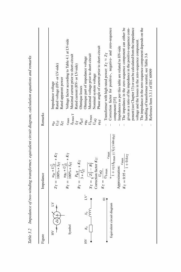
Tabl
e3.
2Im
peda
nce
oftw
o-w
indi
ngtr
ansf
orm
er,e
quiv
alen
tcir
cuit
diag
ram
,cal
cula
tion
equa
tions
and
rem
arks
Figu
reIm
peda
nce
Rem
arks
ZT
=u
kr∗U
2 rT10
0%∗S
rT∗K
Tu
krIm
peda
nce
volta
geU
rTR
ated
volta
ge(H
V-
orLV
-sid
e)S
rTR
ated
appa
rent
pow
er
RT
=u
Rr∗U
2 rT10
0%∗S
rT∗K
Tc m
axV
olta
gefa
ctor
acco
rdin
gto
Tabl
e4.
1at
LV-s
ide
I bm
axT
Max
imal
curr
entp
rior
tosh
ort-
circ
uit
I rT
Rat
edcu
rren
t(H
V-
orLV
-sid
e)P
krT
Ohm
ique
loss
esu
Rr
Ohm
ique
part
ofim
peda
nce
volta
geU
bm
axM
axim
alvo
ltage
prio
rto
shor
t-ci
rcui
tU
nQN
omin
alsy
stem
volta
geϕ
bTPh
ase
angl
eof
curr
entp
rior
tosh
ort-
circ
uit
RT
=P
krT
3∗I
2 rT
∗KT
XT
=√ Z
2 T−
R2 T
Cor
rect
ion
fact
orK
T:
KT
=U
nQ
Ub
max
∗c m
ax
1+
xT
(Ib
max
T/I r
T)
sin
ϕbT
–T
rans
form
erw
ithhi
ghra
ted
pow
er:X
T≈
ZT
–C
orre
ctio
nfa
ctor
for
posi
tive-
,ne
gativ
e-an
dze
ro-s
eque
nce
com
pone
nt[3
5]–
Impe
danc
esas
per
this
tabl
ear
ere
late
dto
HV
-sid
e–
The
impe
danc
ein
the
zero
-seq
uenc
eco
mpo
nent
can
eith
erbe
give
nas
ara
tioof
the
impe
danc
ein
the
posi
tive-
sequ
ence
com
-po
nent
(see
Cha
pter
13)o
rcan
beca
lcul
ated
from
the
impe
danc
evo
ltage
and
the
loss
esin
the
zero
-seq
uenc
eco
mpo
nent
.–
The
impe
danc
ein
the
zero
-seq
uenc
eco
mpo
nent
depe
nds
onth
eha
ndlin
gof
tran
sfor
mer
neut
ral,
see
Tabl
e3.
6–
Ref
eren
ceIt
em3.
3.1
ofIE
C60
909
App
roxi
mat
ion:
KT
=0.
95∗
c max
1+
0.6x
T
RT
XT
01LV
�
HV
LV
Equ
ival
ent c
ircu
it di
agra
m
Sym
bol
HV
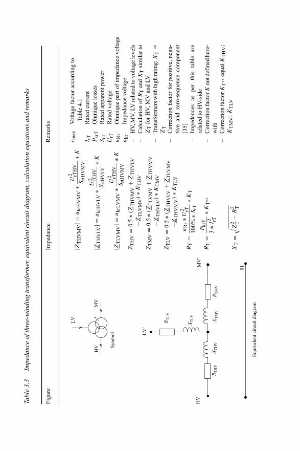
Tabl
e3.
3Im
peda
nce
ofth
ree-
win
ding
tran
sfor
mer
,equ
ival
entc
ircu
itdi
agra
m,c
alcu
latio
neq
uatio
nsan
dre
mar
ks
Figu
reIm
peda
nce
Rem
arks
c max
Vol
tage
fact
orac
cord
ing
toTa
ble
4.1
I rT
Rat
edcu
rren
tP
krT
Ohm
ique
loss
esS
rTR
ated
appa
rent
pow
erU
rTR
ated
volta
geu
Rr
Ohm
ique
part
ofim
peda
nce
volta
geu
krIm
peda
nce
volta
ge
|ZT
HV
MV
|=u
krH
VM
V∗
U2 rT
HV
Srt
HV
MV
∗K
|ZT
HV
LV|=
ukr
HV
LV∗
U2 rT
HV
Srt
HV
LV∗K
|ZT
LVM
V|=
ukr
LVM
V∗
U2 rT
HV
Srt
HV
MV
∗K
ZT
HV
=0.
5∗(
ZT
HV
MV
+Z
TH
VLV
−ZT
LVM
V)∗K
TH
V
ZT
MV
=0.
5∗(
ZT
LVM
V+
ZT
HV
MV
−ZT
HV
LV)∗K
TM
V
ZT
LV=
0.5
∗(Z
TH
VLV
+Z
TLV
MV
−ZT
HV
MV
)∗K
TLV
–H
V,M
V,L
Vre
late
dto
volta
gele
vels
–C
alcu
latio
nof
RT
and
XT
sim
ilar
toZ
Tfo
rH
V,M
Van
dLV
–T
rans
form
ersw
ithhi
ghra
ting:
XT
≈Z
T–
Cor
rect
ion
fact
orfo
rpo
sitiv
e,ne
ga-
tive
and
zero
-seq
uenc
eco
mpo
nent
[35]
–Im
peda
nces
aspe
rth
ista
ble
are
rela
ted
toH
V-s
ide
–C
orre
ctio
nfa
ctor
Kno
tdef
ined
here
-w
ith–
Cor
rect
ion
fact
orK
T∗∗
equa
lKT
HV
;K
TM
V;K
TLV
RT
=u
Rr∗U
2 rT10
0%∗S
rT∗K
T
RT
=P
krT
3∗I
2 rT
∗KT
∗∗
XT
=√ Z
2 T−
R2 T
01
HV
LV
�
MV
�
XT
LV
XT
MV
RT
MV
LV
MV
HV Sy
mbo
l
RT
LV
XT
HV
RT
HV
Equ
ival
ent c
ircu
it di
agra
m
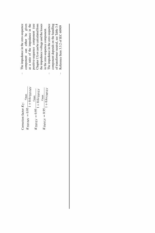
Cor
rect
ion
fact
orK
T:
KT
HV
MV
=0.
95c m
ax
1+
0.6x
TH
VM
V
KT
HV
LV=
0.95
c max
1+
0.6x
TH
VLV
KT
MV
LV=
0.95
c max
1+
0.6x
TM
VLV
–T
heim
peda
nce
inth
eze
ro-s
eque
nce
com
pone
ntca
nei
ther
begi
ven
asa
ratio
ofth
eim
peda
nce
inth
epo
sitiv
e-se
quen
ceco
mpo
nent
(see
Cha
pter
13)o
rcan
beca
lcul
ated
from
the
impe
danc
evo
ltage
and
the
loss
esin
the
zero
-seq
uenc
eco
mpo
nent
.–
The
impe
danc
ein
the
zero
-seq
uenc
eco
mpo
nent
depe
nds
onth
eha
ndlin
gof
tran
sfor
mer
neut
ral,
see
Tabl
e3.
4–
Ref
eren
ceIt
em3.
3.2
ofIE
C60
909

50 Short-circuit currents
Table 3.4 Equivalent circuit diagram of two- and three-winding transformers in thepositive- and zero-sequence component
Zero-sequence component
3X3X11 2X2
01
X011 2
00
X011 2
3ZS00
21
1 2X1
01
1 2X1
01
3X3X11 2X2
01
X01 2
3ZS00
01
1 2X1
3
X03
X011 2X023ZS
00
00
3
X03
X011 2X02
3ZS2(U1/U2)2
3ZS1
X3X1 X2
01
3
1 2
00
3
X03
X011 2X02ES
3XL(U1/U2)2
1
ES XL
1 3 2
1 3
ZS1 ZS2
2
21 3
ZS
ZS
21
ZSor
21
ZS
YNy
YNd
YNy + d
YNyn + d
ZNy; ZNd
Equivalent diagram in RYB-system
Type of transformer(any vector group)
Equivalent diagram in system of symmetrical components
Positive-sequence component
3.3 Equipment in d.c. systems
3.3.1 General
For the calculation of short-circuit currents in d.c. systems, the parameters of equip-ment contributing to the short-circuit current, i.e., capacitor, battery, rectifier andd.c. motor need to be known besides the parameter of conductors. The calculationequations as per Tables 3.12 to 3.16 are given in the Ohm-system only. For conversionto %/MVA system, p.u. system, respectively, Tables 2.2 and 2.3 can be used.
Tables 3.12 to 3.16 mention the term ‘common branch’. The common branch ind.c. systems is the branch (conductor) leading parts of the short-circuit current fromseveral different sources (capacitor, battery, rectifier and d.c. motor) according toIEC 61660-1.

Tabl
e3.
5Im
peda
nce
ofsy
nchr
onou
sge
nera
tor,
equi
vale
ntci
rcui
tdia
gram
,cal
cula
tion
equa
tions
and
rem
arks
Figu
reIm
peda
nce
Rem
arks
X1G
=x′′ d
∗U2 rG
100%
∗SrG
∗KG
c max
Vol
tage
fact
orac
cord
ing
toTa
ble
4.1
pG
Vol
tage
cont
rolr
ange
:UrG
=co
nst⇒
pG
=0
SrG
Rat
edap
pare
ntpo
wer
UrG
Rat
edvo
ltage
x′′ d
Subt
rans
ient
reac
tanc
eϕ
rGPh
ase
angl
ebe
twee
nU
rGan
dI r
G
Salie
ntpo
lege
nera
tors
:X
2G=
0.5
∗(X
′′ d+
X′′ q)∗K
G
Zer
o-se
quen
ceco
mpo
nent
X0G
≈(0
.4–0
.8)X
′′ d∗K
G
Cor
rect
ion
fact
orK
G:
KG
=U
nQ
UrG
(1+
pG
)∗
c max
1+
x′′ d
∗sin
ϕrG
Fict
itiou
sre
sist
ance
ofst
ator
RG
f(f
orpe
aks.
-c.c
urre
nt)
HV
:R
Gf
=0.
05∗X
G:S
rG≥
100
MV
AR
Gf
=0.
07∗X
G:S
rG<
100
MV
ALV
:R
Gf
=0.
15∗X
G
–C
orre
ctio
nfa
ctor
for
posi
tive-
,ne
gativ
e-an
dze
ro-s
eque
nce
com
pone
nt–
Sync
hron
ous
mot
ors
iden
tical
tosy
nchr
onou
sge
nera
tors
–C
alcu
latio
nof
deca
ying
d.c.
com
pone
ntw
ithre
alre
sist
ance
ofst
ator
–Im
peda
nce
inth
eze
ro-s
eque
nce
com
pone
ntde
pend
son
the
type
ofw
indi
ngof
the
gene
rato
r–
Ref
eren
ceIt
em3.
6of
IEC
6090
9
RG
fX
G
EG
01
GS
3~ Equ
ival
ent c
ircu
it di
agra
m
Sym
bol
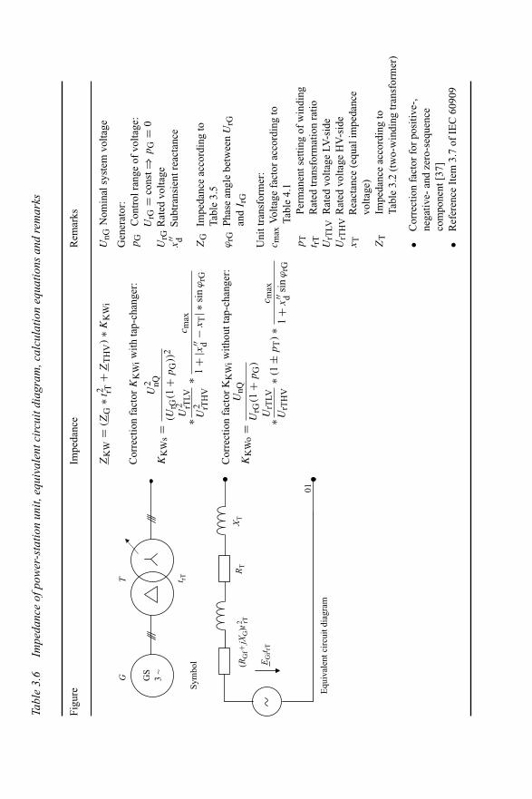
Tabl
e3.
6Im
peda
nce
ofpo
wer
-sta
tion
unit,
equi
vale
ntci
rcui
tdia
gram
,cal
cula
tion
equa
tions
and
rem
arks
Figu
reIm
peda
nce
Rem
arks
ZK
W=
(ZG
∗t2 rT
+Z
TH
V)∗K
KW
iU
nGN
omin
alsy
stem
volta
ge
Gen
erat
or:
pG
Con
trol
rang
eof
volta
ge:
UrG
=co
nst⇒
pG
=0
UrG
Rat
edvo
ltage
x′′ d
Subt
rans
ient
reac
tanc
e
Cor
rect
ion
fact
orK
KW
iw
ithta
p-ch
ange
r:
KK
Ws=
U2 nQ
(UrG
(1+
pG
))2
∗U2 rT
LV
U2 rT
HV
∗c m
ax
1+
|x′′ d−
xT|∗
sin
ϕrG
Cor
rect
ion
fact
orK
KW
iw
ithou
ttap
-cha
nger
:
KK
Wo
=U
nQ
UrG
(1+
pG
)
∗UrT
LV
UrT
HV
∗(1
±p
T)∗
c max
1+
x′′ d
sin
ϕrG
ZG
Impe
danc
eac
cord
ing
toTa
ble
3.5
ϕrG
Phas
ean
gle
betw
een
UrG
and
I rG
Uni
ttra
nsfo
rmer
:c m
axV
olta
gefa
ctor
acco
rdin
gto
Tabl
e4.
1p
TPe
rman
ents
ettin
gof
win
ding
t rT
Rat
edtr
ansf
orm
atio
nra
tioU
rTLV
Rat
edvo
ltage
LV-s
ide
UrT
HV
Rat
edvo
ltage
HV
-sid
ex
TR
eact
ance
(equ
alim
peda
nce
volta
ge)
ZT
Impe
danc
eac
cord
ing
toTa
ble
3.2
(tw
o-w
indi
ngtr
ansf
orm
er)
•C
orre
ctio
nfa
ctor
for
posi
tive-
,ne
gativ
e-an
dze
ro-s
eque
nce
com
pone
nt[3
7]•
Ref
eren
ceIt
em3.
7of
IEC
6090
9
GT
EG
it rT
01
RT
XT
GS
3 ~
t rTSy
mbo
l (RG
f+jX
G)t
2 rT
Equ
ival
ent c
ircu
it di
agra
m
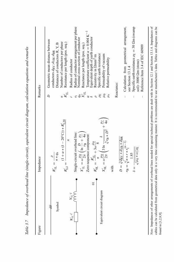
Tabl
e3.
7Im
peda
nce
ofov
erhe
adlin
e(s
ingl
e-ci
rcui
t),e
quiv
alen
tcir
cuit
diag
ram
,cal
cula
tion
equa
tions
and
rem
arks
Figu
reIm
peda
nce
Rem
arks
DG
eom
etri
cm
ean
dist
ance
betw
een
R′ 1L
=ρ
n∗q
nco
nduc
tors
dR
Y;d
YB
;dB
RD
ista
nces
ofco
nduc
tors
R,Y
,Bn
Num
ber
ofco
nduc
tors
per
phas
eR
′ Lδ
=(1
+α
∗(δ
−20
◦ C))
∗R′ L
20n
R′ 1L
Res
ista
nce
per
leng
th(p
os.s
eq.)
rR
adiu
sof
cond
ucto
rSi
ngle
-cir
cuit
over
head
line:
r tR
adiu
sof
cond
ucto
rarr
ange
men
tper
phas
e
X′ 1L
=ω
μ0
2π
( lnD r B
+μ
r
4n
)q
nN
omin
alcr
oss-
sect
ion
ofco
nduc
tor
X′ 1L
Rea
ctan
cepe
rle
ngth
(pos
.seq
.)Z
ero-
sequ
ence
com
pone
nt:
αTe
mpe
ratu
reco
effi
cien
tα=
0.00
4K
−1δ
Equ
ival
entd
epth
ofea
rth
cond
ucto
rR
′ 0L=
R′ 1L n
+3ω
μ0 8
ρR
esis
tivity
in�
mm
2/m
ρE
Spec
ific
eart
hre
sist
ance
X′ 0L
=ω
μ0
2π
( 3ln
δ
3√ r B∗D
2+
μr
4n
)μ
0Pe
rmea
bilit
yof
vacu
umμ
rR
elat
ive
perm
eabi
lity
with
Rea
ctan
ce:
D=
3√ dR
Y∗d
YB
∗dB
R–
Cal
cula
tion
from
geom
etri
cal
arra
ngem
ent,
see
Sect
ion
13.1
.4–
Spec
ific
eart
hre
sist
ance
ρE
=30
�m
(sw
amp
soil)
–300
0�
m(s
tone
)–
Ref
eren
ceIt
em3.
4of
IEC
6090
9
r B=
n√ n∗r
∗r(n
−1)
t
δ=
1.85
√ μ0
∗ω/ρ
E
01
Sym
bol
Equ
ival
ent c
ircu
it di
agra
m
X� 1L
·R
� 1L·
Not
e:Im
peda
nces
ofot
her
arra
ngem
ents
ofov
erhe
adlin
esne
eded
for
spec
ial
tech
nica
lpr
oble
ms
are
deal
tw
ithin
Sect
ion
12.1
and
Sect
ion
13.1
.4.
Impe
danc
esof
cabl
esca
nbe
calc
ulat
edfr
omge
omet
rica
lda
taon
lyin
ave
rytim
eco
nsum
ing
man
ner.
Itis
reco
mm
ende
dto
use
man
ufac
ture
r’s
data
.Ta
bles
and
diag
ram
sca
nbe
foun
din
[1,2
,8,9
].

Tabl
e3.
8Im
peda
nce
ofsh
ort-
circ
uitl
imiti
ngre
acto
r,eq
uiva
lent
circ
uitd
iagr
am,c
alcu
latio
neq
uatio
nsan
dre
mar
ks
Figu
reIm
peda
nce
Rem
arks
I rD
rate
dcu
rren
tZ
D=
ukr
100%
∗U
n√ 3
∗IrD
SrD
Rat
edap
pare
ntpo
wer
Un
Nom
inal
syst
emvo
ltage
SrD
=√ 3
∗Un
∗IrD
ukr
Rat
edvo
ltage
drop
(im
peda
nce
volta
ge)
–Im
peda
nces
inpo
sitiv
e-,n
egat
ive-
and
zero
-seq
uenc
eco
mpo
nent
iden
tical
inca
seof
sym
met
rica
lco
nstr
uctio
n–
RD
≈0
–Im
peda
nce
inth
eze
ro-s
eque
nce
com
pone
nteq
ualt
oth
eim
peda
nce
inth
epo
sitiv
e-se
quen
ceco
mpo
nent
inca
seth
ree
sing
le-p
hase
reac
tors
are
used
–R
efer
ence
Item
3.5
ofIE
C60
909
01
Sym
bol Z D
≈X
D
Equ
ival
ent c
ircu
it di
agra
m
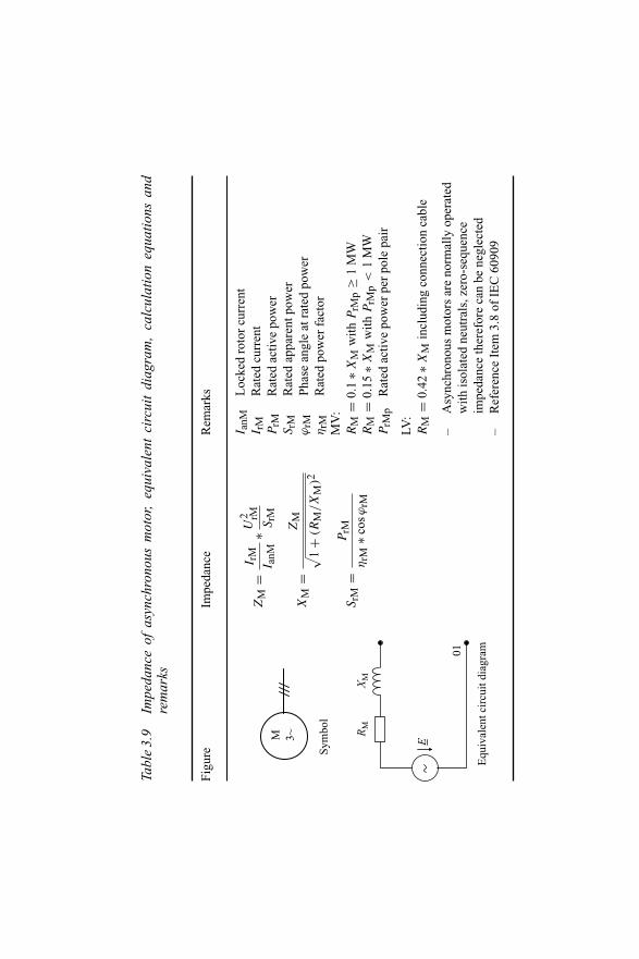
Tabl
e3.
9Im
peda
nce
ofas
ynch
rono
usm
otor
,eq
uiva
lent
circ
uit
diag
ram
,ca
lcul
atio
neq
uatio
nsan
dre
mar
ks
Figu
reIm
peda
nce
Rem
arks
ZM
=I r
M
I anM
∗U2 rM
SrM
I anM
Loc
ked
roto
rcu
rren
tI r
MR
ated
curr
ent
PrM
Rat
edac
tive
pow
er
XM
=Z
M√ 1
+(R
M/X
M)2
SrM
Rat
edap
pare
ntpo
wer
ϕrM
Phas
ean
gle
atra
ted
pow
erη
rMR
ated
pow
erfa
ctor
SrM
=P
rM
ηrM
∗cos
ϕrM
MV
:R
M=
0.1
∗XM
with
PrM
p≥
1M
WR
M=
0.15
∗XM
with
PrM
p<
1M
WP
rMp
Rat
edac
tive
pow
erpe
rpo
lepa
ir
LV:
RM
=0.
42∗X
Min
clud
ing
conn
ectio
nca
ble
–A
sync
hron
ous
mot
ors
are
norm
ally
oper
ated
with
isol
ated
neut
rals
,zer
o-se
quen
ceim
peda
nce
ther
efor
eca
nbe
negl
ecte
d–
Ref
eren
ceIt
em3.
8of
IEC
6090
9
RM
XM
01
EM 3~
Equ
ival
ent c
ircu
it di
agra
m
Sym
bol

Tabl
e3.
10Im
peda
nce
ofst
atic
conv
erte
rfe
ddr
ive,
equi
vale
ntci
rcui
tdia
gram
,cal
cula
tion
equa
tions
and
rem
arks
Figu
reIm
peda
nce
Rem
arks
ZM
=I r
M
I anM
∗U2 rM
SrM
I anM
Loc
ked
roto
rcu
rren
tI r
MR
ated
curr
ent
SrM
Rat
edap
pare
ntpo
wer
RM
XM
=0.
1U
rMR
ated
volta
ge
–I a
nM/I r
M=
3–
Onl
yfo
rre
ctif
iers
,abl
eto
tran
sfer
ener
gyfo
rde
cele
ratio
ndu
ring
the
dura
tion
ofsh
ort-
circ
uit
–St
atic
conv
erte
rsfo
rph
otov
olta
icge
nera
tors
orfu
elce
llsco
ntri
bute
tosh
ort-
circ
uit
curr
ents
only
with
thei
rra
ted
curr
ent
–R
efer
ence
Item
3.9
ofIE
C60
909
Sym
bol RM
XM
01
E
Equ
ival
ent c
ircu
it di
agra
m

Tabl
e3.
11Im
peda
nce
ofsy
stem
load
,equ
ival
entc
ircu
itdi
agra
m,c
alcu
latio
neq
uatio
nsan
dre
mar
ks
Figu
reIm
peda
nce
Rem
arks
ZL
=U
2 rLS
rL
RL
=U
2 rLP
rL
ωL
L=
U2 rL
QrL
1
ωC
L=
U2 rL
QrL
PrL
Rat
edac
tive
pow
erQ
rLR
ated
reac
tive
pow
erS
rLR
ated
appa
rent
pow
erU
rLR
ated
volta
ge
•In
case
UrL
isun
know
n,th
eno
min
alsy
stem
volta
geU
nis
tobe
used
•R
efer
ence
Item
3.10
ofIE
C60
909
0101
RL
XL
XC
Z L
0101
Sym
bol,
Equ
ival
ent c
ircu
it di
agra
m

Tabl
e3.
12Im
peda
nce
ofa
cond
ucto
r,eq
uiva
lent
circ
uitd
iagr
am,c
alcu
latio
neq
uatio
nsan
dre
mar
ks
3.3.
2Im
peda
nce
calc
ulat
ion
Figu
reIm
peda
nce
Rem
arks
R′ L
=ρ qn
R′ L
δ=
(1+
α∗
(δ−
20◦ C
))∗
R′ L
20
Loo
pby
sing
leca
bles
L′ =
μ0
π∗( 0.
25+
ln( a r
))L
oop
bybu
sbar
s
L′ =
μ0
π∗( 1.
5+
ln(
a
d+
b
))
Res
ista
nce
ofbo
lted
join
t:
RJ
=14
∗ρ∗d
qn
aD
ista
nce
ofco
nduc
tors
bH
eigh
tof
cond
ucto
r(b
usba
r)d
Thi
ckne
ssof
cond
ucto
rR
JR
esis
tanc
eof
bolte
djo
int
R′ L
Spec
ific
resi
stan
ceR
L20
Res
ista
nce
at20
◦ CR
Lδ
Res
ista
nce
atte
mpe
ratu
reδ
rR
adiu
sof
cond
ucto
rq
nC
ross
-sec
tion
ofco
nduc
tor
αTe
mpe
ratu
reco
effi
cien
t(fo
rA
l,C
u)α
=0.
004
K−1
δTe
mpe
ratu
rein
◦ Cρ
Res
istiv
ityin
�m
m2/m
μ0
Perm
eabi
lity
–R
Jfo
rca
lcul
atio
nof
min
imal
s.-c
.cur
rent
son
ly–
Cal
cula
tion
ofL
′ for
sim
ple
arra
ngem
ent
only
–R
efer
ence
Item
2.3
ofIE
C61
660-
1
Sym
bol
R� L
·R
� JL�
·
Equ
ival
ent c
ircu
it di
agra
m
q n
d
Con
duct
or
Con
duct
or jo
int
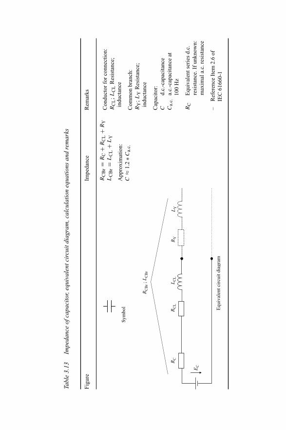
Tabl
e3.
13Im
peda
nce
ofca
paci
tor,
equi
vale
ntci
rcui
tdia
gram
,cal
cula
tion
equa
tions
and
rem
arks
Figu
reIm
peda
nce
Rem
arks
RC
Br=
RC
+R
CL
+R
YL
CB
r=
LC
L+
LY
App
roxi
mat
ion:
C≈
1.2
∗Ca.
c.
Con
duct
orfo
rco
nnec
tion:
RC
L;L
CL
Res
ista
nce;
indu
ctan
ce
Com
mon
bran
ch:
RY
;LY
Res
ista
nce;
indu
ctan
ce
Cap
acito
r:C
d.c.
-cap
acita
nce
Ca.
c.a.
c.-c
apac
itanc
eat
100
Hz
RC
Equ
ival
ents
erie
sd.
c.re
sist
ance
.If
unkn
own:
max
imal
a.c.
resi
stan
ce
–R
efer
ence
Item
2.6
ofIE
C61
660-
1
RC
RC
LL C
L
EC
L YR
Y
Sym
bol
RC
Br ;
LC
Br
Equ
ival
ent c
ircu
it di
agra
m
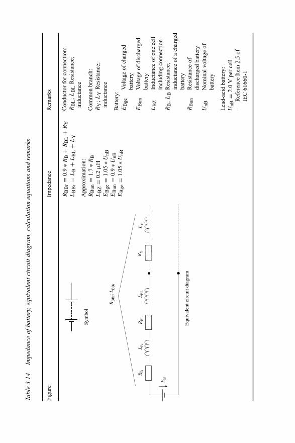
Tabl
e3.
14Im
peda
nce
ofba
ttery
,equ
ival
entc
ircu
itdi
agra
m,c
alcu
latio
neq
uatio
nsan
dre
mar
ks
Figu
reIm
peda
nce
Rem
arks
RB
Br=
0.9
∗RB
+R
BL
+R
YL
BB
r=
LB
+L
BL
+L
Y
App
roxi
mat
ion:
RB
un=
1.7
∗RB
LB
Z=
0.2
μH
EB
ge=
1.05
∗UnB
EB
un=
0.9
∗UnB
EB
ge=
1.05
∗UnB
Con
duct
orfo
rco
nnec
tion:
RB
L;L
BL
Res
ista
nce;
indu
ctan
ce
Com
mon
bran
ch:
RY
;LY
Res
ista
nce;
indu
ctan
ce
Bat
tery
:E
Bge
Vol
tage
ofch
arge
dba
ttery
EB
unV
olta
geof
disc
harg
edba
ttery
LB
ZIn
duct
ance
ofon
ece
llin
clud
ing
conn
ectio
nR
B;L
BR
esis
tanc
e;in
duct
ance
ofa
char
ged
batte
ryR
Bun
Res
ista
nce
ofdi
scha
rged
batte
ryU
nBN
omin
alvo
ltage
ofba
ttery
Lea
d-ac
idba
ttery
:U
nB=
2.0
Vpe
rce
ll–
Ref
eren
ceIt
em2.
5of
IEC
6166
0-1
RB
L BR
BL
L BL
EB
RY
L Y
Sym
bol
Equ
ival
ent c
ircu
it di
agra
m
RB
Br;
L BB
r

Tabl
e3.
15Im
peda
nce
ofre
ctifi
er,e
quiv
alen
tcir
cuit
diag
ram
,cal
cula
tion
equa
tions
and
rem
arks
Figu
reIm
peda
nce
Rem
arks
ac-s
ide
Indi
ces
for
ac-s
ide:
RN
=R
Q+
RP
+R
T+
RD
DC
omm
utat
ing
reac
tor
XN
=X
Q+
XP
+X
T+
XD
NTo
tal
QSy
stem
feed
erP
Con
nect
ion
atse
cond
ary
side
oftr
ansf
orm
er–
ZQ
min
(RQ
and
XQ
)fo
rca
lcul
atio
nof
max
.sh
ort-
circ
uitc
urre
nt–
ZQ
max
(RQ
and
XQ
)fo
rca
lcul
atio
nof
min
.sh
ort-
circ
uitc
urre
nt
dc-s
ide
Indi
ces
for
dc-s
ide:
RD
Br=
RS
+R
L+
RY
LPo
wer
supp
lyca
ble
LD
Br=
LS
+L
L+
LY
SD
Csa
tura
ted
smoo
thin
gre
acto
r
Cou
plin
gbr
anch
:L
Ssa
tura
ted
indu
ctan
ceR
Y;L
YR
esis
tanc
e;in
duct
ance
–R
efer
ence
Item
2.4
ofIE
C61
660-
1
Q
Sym
bol
Equ
ival
ent c
ircu
it di
agra
m
RQ
;XQ
RQ
;XQ
RP
;XP
RT
;XT
RD
;XD
RS
L SL L
L YR
LR
Y
RD
Br;L
DB
r
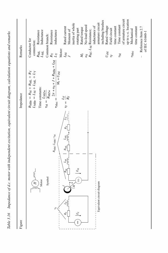
Tabl
e3.
16Im
peda
nce
ofd.
c.m
otor
with
inde
pend
ente
xcita
tion,
equi
vale
ntci
rcui
tdia
gram
,cal
cula
tion
equa
tions
and
rem
arks
Figu
reIm
peda
nce
Rem
arks
RM
Br=
RM
+R
ML
+R
YC
ondu
ctor
for
LM
Br=
LM
+L
ML
+L
Yco
nnec
tion:
RM
LR
esis
tanc
eT
ime
cons
tant
s:
τ M=
LM
Zw
RM
Zw
τ Mec
=2π
∗n0
∗J∗R
MB
r∗I
rM
Mr∗U
rM
τ F=
LF
RF
LM
LIn
duct
ance
Com
mon
bran
ch:
RY
Res
ista
nce
LY
indu
ctan
ce
Mot
or:
I rM
Rat
edcu
rren
tJ
Mom
ento
fin
ertia
ofw
hole
rota
ting
part
Mr
Rat
edto
rque
n0
No-
load
spee
dR
M;L
MR
esis
tanc
e;in
duct
ance
ofar
mat
ure
circ
uit
incl
udin
gbr
ushe
sU
rMR
ated
volta
geτ F
Fiel
dci
rcui
ttim
eco
nsta
ntτ M
Tim
eco
nsta
ntof
arm
atur
eci
rcui
tup
tos.
-c.l
ocat
ion
τ Mec
Mec
hani
cal
time
cons
tant
–R
efer
ence
Item
2.7
ofIE
C61
660-
1
RF
L F
EF
EM
RM
L ML M
LR
ML
RM
Br;
L MB
r;� M
RY
L Y
MJ
n
� F
M Sym
bol
Mot
or
Equ
ival
ent c
ircu
it di
agra
m

Calculation of impedance of electrical equipment 63
3.4 Examples for calculation
3.4.1 a.c. equipment
The impedance (resistance and reactance) of equipment in a.c. three-phase powersystems has to be calculated based on the data as below. Results are summarised inTable 3.17.
Power system feeder Q: S′′kQ = 3000 MVA; UnQ = 110 kV
Two-winding SrT = 70 MVA; UrTHV/UrTLV = 115 kV/10.5 kV;transformer: ukr = 12%; uRr = 0.5%
Three-winding UrT = 110 kV/30 kV/10 kV;transformer: SrT = 30 MVA/20 MVA/10 MVA
ukrHVMV =10%; ukrHVLV =4.5%; ukrMVLV =10.2%uRrHVMV =0.5%; uRrHVLV =0.6%; uRrMVLV =0.65%
Synchronous machine: SrG = 70 MVA; UrG = 10.5 kV; cos ϕrG = 0.9;x′′
d = 17%; pG = ±10%
Power plant consisting SrG = 70 MVA; UrG = 10.5 kV; x′′d = 17%;
of synchronous machine pG = ±10%and two-winding SrT = 70 MVA; UrTHV/UrTLV = 115 kV/10.5 kV;transformer: ukr = 12%;
URr = 0.5%; without tap-changer
Overhead transmission line: Al/St 240/40; r = 10.9 mm; Line length 10 kmFlat arrangement, distance between phase wires 4 m
s.-c. limiting reactor: ukr = 6%; IrD = 630 A; Un = 10 kV
Asynchronous motor: PrM = 1.2 MW; UrM = 6 kV; cos ϕrM = 0.84;ηrM = 0.93; Ian/IrM = 5.6; 2 pairs of poles
Rectifier: SrM = 4 MVA; UrM = 6.2 kV
System load: SrL = 6 MVA; cos ϕL = 0.87; Un = 10 kV
Table 3.17 Results of calculation of impedance in three-phase a.c. equipment
Equipment Z (�) R (�) X (�) Remark Tab.
System feeder 4.437 0.441 4.414 RQ/XQ not defined 3.1XQ ≈ 0.995 × ZQ
Two-winding 22.76 0.945 22.74 Without correction factor 3.2transformer Impedance related to 110 kV
22.19 0.921 22.17 KT = 0.975Impedance related to 110 kV

64 Short-circuit currents
Table 3.17 Continued
Equipment Z (�) R (�) X (�) Remark Tables
Three-winding −3.24 1.31 −2.97 Impedance related to 110 kV 3.3transformer 62.89 1.67 62.87 including correction factors
58.65 6.08 58.33 KT = 0.986–1.018–0.985Values from top: HV ∗ MV ∗ LV
Synchronous 0.268 0.019 0.267 Without correction factor 3.5machine 0.238 0.017 0.237 KG = 0.887; UnQ = 10 kV
Power plant 65.14 3.22 54.77 KKWo = 0.891; UnQ = 110 kV 3.6
Overhead 4.19 1.23 4.01 D = 5.04 m 3.7transmission line
s.-c. limiting 0.55 0 0.55 XD ≈ ZD 3.8reactor
Asynchronous 4.14 0.41 4.12 SrM = 1.53 MVA 3.9machine
Rectifier 28.83 2.88 28.69 RM/XM = 0.1 3.10
System load 16.67 14.5 8.22 — 3.11
3.4.2 d.c. equipment
The impedance (resistance and reactance) of equipment in d.c. systems has to becalculated based on the data as below. Results are summarised in Table 3.18.
Conductor Busbar arrangement, copper (120 × 10): qn = 1200 mm2;with joint: Distance a = 50 mm; Length of line loop 30 m
Capacitor: MKP dry-type, self-healing; C = 9000 μF; RC = 0.5 m�
Connected to short-circuit location with conductor as above,l = 20 m
Two bolted joints
Battery: Sealed lead-acid-type; 108 cells, each:150 Ah; UnB = 2.0 V; RB = 0.83 m�; LB = 0.21 mH
Connected to short-circuit location with conductor as above,l = 15 m
Two bolted joints
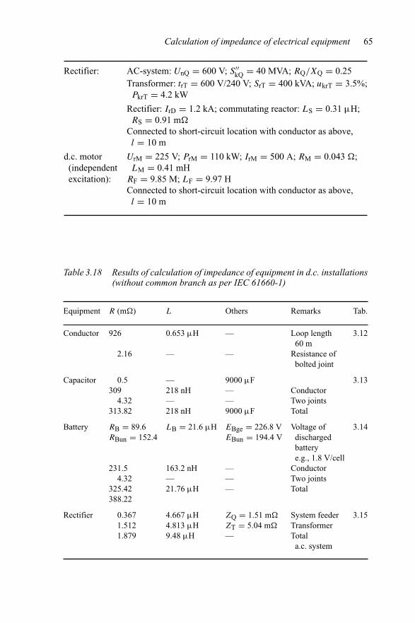
Calculation of impedance of electrical equipment 65
Rectifier: AC-system: UnQ = 600 V; S′′kQ = 40 MVA; RQ/XQ = 0.25
Transformer: trT = 600 V/240 V; SrT = 400 kVA; ukrT = 3.5%;PkrT = 4.2 kW
Rectifier: IrD = 1.2 kA; commutating reactor: LS = 0.31 μH;RS = 0.91 m�
Connected to short-circuit location with conductor as above,l = 10 m
d.c. motor UrM = 225 V; PrM = 110 kW; IrM = 500 A; RM = 0.043 �;(independent LM = 0.41 mHexcitation): RF = 9.85 M; LF = 9.97 H
Connected to short-circuit location with conductor as above,l = 10 m
Table 3.18 Results of calculation of impedance of equipment in d.c. installations(without common branch as per IEC 61660-1)
Equipment R (m�) L Others Remarks Tab.
Conductor 926 0.653 μH — Loop length 3.1260 m
2.16 — — Resistance ofbolted joint
Capacitor 0.5 — 9000 μF 3.13309 218 nH — Conductor
4.32 — — Two joints313.82 218 nH 9000 μF Total
Battery RB = 89.6 LB = 21.6 μH EBge = 226.8 V Voltage of 3.14RBun = 152.4 EBun = 194.4 V discharged
batterye.g., 1.8 V/cell
231.5 163.2 nH — Conductor4.32 — — Two joints
325.42 21.76 μH — Total388.22
Rectifier 0.367 4.667 μH ZQ = 1.51 m� System feeder 3.151.512 4.813 μH ZT = 5.04 m� Transformer1.879 9.48 μH — Total
a.c. system

66 Short-circuit currents
Table 3.18 Continued
Equipment R (m�) L Others Remarks Tab.
0.91 0.31 μH — Commutatingreactor
154.3 0.11 μH — Conductor155.21 0.42 μH — Total
d.c. system
d.c. motor 43.3 0.41 mH — Motor 3.16with 154.3 0.11 μH Conductorindependent 197.6 0.411 mH τM = 2.08 ms Totalexcitation τF = 1.01 s
Chapter 4
Calculation of short-circuit current in a.c.three-phase HV-systems
4.1 Types of short-circuits
In three-phase a.c. systems it has to be distinguished between different types ofshort-circuits (s.-c.), as outlined in Figure 4.1.
Short-circuit currents can be carried out with different methods and in differentdetails, depending on the available data and the technical needs. IEC 60909-0 cal-culates characteristic parameters of the short-circuit current, which are necessary forthe design of power system equipment. The course of time of short-circuit currentsis outlined in Figure 4.2. Generally, one has to distinguish between near-to-generatorand far-from-generator short-circuits. A near-to-generator short-circuit exists if thecontribution to the short-circuit current of one synchronous generator is greater thantwice its rated current, or if the contribution to the short-circuit current of synchronousor asynchronous motors is greater than 5 per cent of the short-circuit current withoutmotors.
The analysis of the short-circuit current in the case of near-to-generator short-circuit as per Figure 4.2(a) indicates two components, besides the decaying d.c.component, a subtransient and a transient decaying a.c. component. The first orsubtransient component is determined by the impedance between stator and damp-ing winding, called subtransient reactance X′′
d . The subtransient component decayswith the subtransient time constant T ′′ which is normally in the range of someperiods of the system frequency, i.e., T ′′ < 70 ms. The transient component isdetermined by the reactance between the stator and exciter winding, called transientreactance X′
d. The transient component decays with the transient time constant T ′,which can last up to 2.2 s for large generators. Finally, the short-circuit current isdetermined by the saturated synchronous reactance Xd.
In the case of a far-from-generator short-circuit as per Figure 4.2(b), the a.c.component remains constant throughout the total time duration of the short-circuit, asthe influence of the changing reactance of generators can be neglected. The decaying
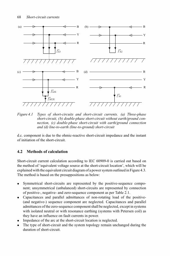
68 Short-circuit currents
B
Y
R
Y
B
R
I �k3
I �k2E
I �kE2E
I �k2
I �k1
(a) (b)
B
Y
R R
B
Y
(c) (d)
Figure 4.1 Types of short-circuits and short-circuit currents. (a) Three-phaseshort-circuit, (b) double-phase short-circuit without earth/ground con-nection, (c) double-phase short-circuit with earth/ground connectionand (d) line-to-earth (line-to-ground) short-circuit
d.c. component is due to the ohmic-reactive short-circuit impedance and the instantof initiation of the short-circuit.
4.2 Methods of calculation
Short-circuit current calculation according to IEC 60909-0 is carried out based onthe method of ‘equivalent voltage source at the short-circuit location’, which will beexplained with the equivalent circuit diagram of a power system outlined in Figure 4.3.The method is based on the presuppositions as below:
• Symmetrical short-circuits are represented by the positive-sequence compo-nent; unsymmetrical (unbalanced) short-circuits are represented by connectionof positive-, negative- and zero-sequence component as per Table 2.1.
• Capacitances and parallel admittances of non-rotating load of the positive-(and negative-) sequence component are neglected. Capacitances and paralleladmittances of the zero-sequence component shall be neglected, except in systemswith isolated neutral or with resonance earthing (systems with Petersen coil) asthey have an influence on fault currents in power.
• Impedance of the arc at the short-circuit location is neglected.• The type of short-circuit and the system topology remain unchanged during the
duration of short-circuit.

Calculation of short-circuit current 69
22I
� k
2 2Iki p
A
22I
� k
2 2Ik
i p
A
(a)
(b)
Figure 4.2 Time-course of short-circuit currents. (a) Near-to-generator short-circuit (according to Figure 12 of IEC 60909:1988), (b) far-from-generator short-circuit (according to Figure 1 of IEC 60909:1988). I ′′
k– initial (symmetrical) short-circuit current, ip – peak short-circuit cur-rent, Ik – steady-state short-circuit current and A – initial value of theaperiodic component idc
• The tap-changers of all transformers are assumed to be in main-position (middleposition).
• All internal voltages of system feeders, generators and motors are short-circuitedand an equivalent voltage source with value cUn/
√3 is introduced at the short-
circuit location. The voltage factor c shall be selected in accordance with Table 4.1.
The voltage factor c takes account of the differences between the voltage at theshort-circuit location and the internal voltage of system feeders, motors and generators
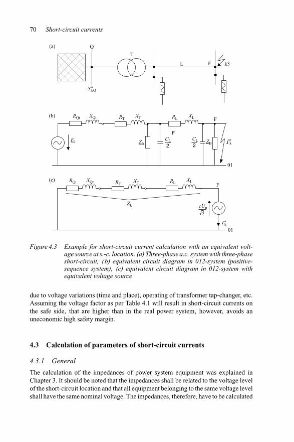
70 Short-circuit currents
Q
T
S �kQ
L F
(a)
k3
RQt RLXL F
RLXL
F
XQt RTXT
RQt XQt RTXT
ZBCL2
CL2
F
Zk cUn
ZB
01
(b)
(c)
01
3
I �k
I �k
E1
Figure 4.3 Example for short-circuit current calculation with an equivalent volt-age source at s.-c. location. (a) Three-phase a.c. system with three-phaseshort-circuit, (b) equivalent circuit diagram in 012-system (positive-sequence system), (c) equivalent circuit diagram in 012-system withequivalent voltage source
due to voltage variations (time and place), operating of transformer tap-changer, etc.Assuming the voltage factor as per Table 4.1 will result in short-circuit currents onthe safe side, that are higher than in the real power system, however, avoids anuneconomic high safety margin.
4.3 Calculation of parameters of short-circuit currents
4.3.1 General
The calculation of the impedances of power system equipment was explained inChapter 3. It should be noted that the impedances shall be related to the voltage levelof the short-circuit location and that all equipment belonging to the same voltage levelshall have the same nominal voltage. The impedances, therefore, have to be calculated

Calculation of short-circuit current 71
Table 4.1 Voltage factor c according to IEC 60909-0
Nominal system voltage Un Voltage factor c for calculation of
Maximals.-c. currentcmax
Minimals.-c. currentcmin
LV: 100 V up to 1000 V (inclusive)(IEC 60038, Table I)
Voltage tolerance +6% 1.05 0.95Voltage tolerance +10% 1.10 0.95
MV: >1 kV up to 35 kV (inclusive)(IEC 60038, Table III)
1.10 1.00
HV: >35 kV (IEC 60038, Table IV) 1.10 1.00
Remark: cmaxUn shall not exceed the highest voltage of equipment Um as per IEC 60071.
in relation to the rated apparent power Sr of the equipment itself, respectively to thenominal system voltage Un. In case the %/MVA-system or the p.u.-system is used,attention must be given to deviations of rated votages of the equipment from nominalsystem voltages, see Section 2.7.2.
The presentation within the following sections is closely related to IEC 60909-0.The IEC-document includes items for the calculation of impedances and for thecalculation of the short-circuit parameters for balanced and unbalanced short-circuits,both near-to-generator and far-from-generator short-circuits. Calculation of short-circuit currents during two separate single-phase to earth short-circuits and the partialshort-circuit currents flowing through earth are dealt with in IEC 60909-3, which iscurrently under review. These items are explained in Chapter 7.
Depending on the task, the maximal or minimal short-circuit current has to becalculated. The maximal short-circuit current is the main design criteria for the ratingof equipment to withstand the effects of short-circuit currents. For the calculation ofmaximal short-circuit current, the items shall be considered as below:
• For the equivalent voltage source at the short-circuit location the voltage factorcmax as per Table 4.1 shall be used. National standards can define voltage factorsdifferent from those in Table 4.1.
• Short-circuit impedance of system feeders shall be minimal (ZQmin), so that thecontribution to the short-circuit current is maximal.
• The contribution of motors has to be assessed and eventually be taken into account,see Section 4.4.
• Resistance of lines is to be calculated for a temperature of 20◦C.• Operation of power plants and system feeders shall be in such a way that the
contribution to short-circuit currents will be maximal.• System topology leading to the maximal short-circuit currents shall be taken into
account.
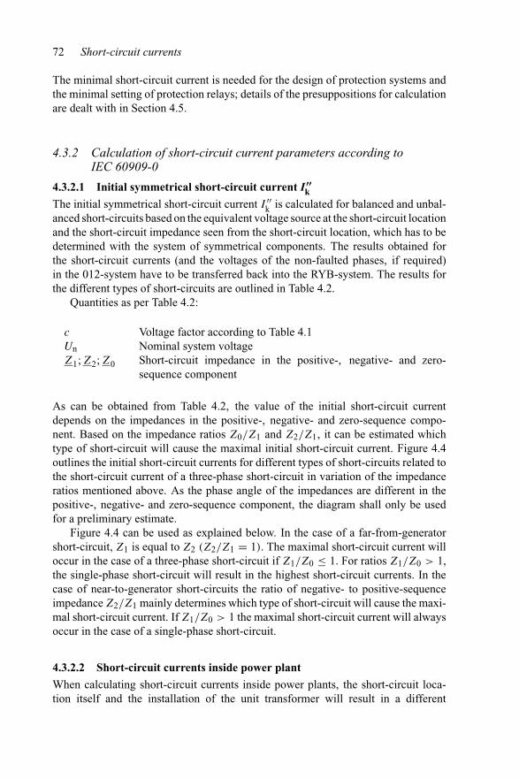
72 Short-circuit currents
The minimal short-circuit current is needed for the design of protection systems andthe minimal setting of protection relays; details of the presuppositions for calculationare dealt with in Section 4.5.
4.3.2 Calculation of short-circuit current parameters according toIEC 60909-0
4.3.2.1 Initial symmetrical short-circuit current I ′′k
The initial symmetrical short-circuit current I ′′k is calculated for balanced and unbal-
anced short-circuits based on the equivalent voltage source at the short-circuit locationand the short-circuit impedance seen from the short-circuit location, which has to bedetermined with the system of symmetrical components. The results obtained forthe short-circuit currents (and the voltages of the non-faulted phases, if required)in the 012-system have to be transferred back into the RYB-system. The results forthe different types of short-circuits are outlined in Table 4.2.
Quantities as per Table 4.2:
c Voltage factor according to Table 4.1Un Nominal system voltageZ1; Z2; Z0 Short-circuit impedance in the positive-, negative- and zero-
sequence component
As can be obtained from Table 4.2, the value of the initial short-circuit currentdepends on the impedances in the positive-, negative- and zero-sequence compo-nent. Based on the impedance ratios Z0/Z1 and Z2/Z1, it can be estimated whichtype of short-circuit will cause the maximal initial short-circuit current. Figure 4.4outlines the initial short-circuit currents for different types of short-circuits related tothe short-circuit current of a three-phase short-circuit in variation of the impedanceratios mentioned above. As the phase angle of the impedances are different in thepositive-, negative- and zero-sequence component, the diagram shall only be usedfor a preliminary estimate.
Figure 4.4 can be used as explained below. In the case of a far-from-generatorshort-circuit, Z1 is equal to Z2 (Z2/Z1 = 1). The maximal short-circuit current willoccur in the case of a three-phase short-circuit if Z1/Z0 ≤ 1. For ratios Z1/Z0 > 1,the single-phase short-circuit will result in the highest short-circuit currents. In thecase of near-to-generator short-circuits the ratio of negative- to positive-sequenceimpedance Z2/Z1 mainly determines which type of short-circuit will cause the maxi-mal short-circuit current. If Z1/Z0 > 1 the maximal short-circuit current will alwaysoccur in the case of a single-phase short-circuit.
4.3.2.2 Short-circuit currents inside power plant
When calculating short-circuit currents inside power plants, the short-circuit loca-tion itself and the installation of the unit transformer will result in a different

Calculation of short-circuit current 73
Table 4.2 Equations for the calculation of initial symmetrical short-circuit currents
Type ofshort-circuit
Equation SectionIEC 60909-0
Remarks
Three-phaseI ′′k3 = cUn√
3|Z1|4.2.1 Short-circuited
phases R, Yand B
4.3.14.6.1–4.6.3
Double-phaseshort-circuitwithout earthconnection
I ′′k2 = cUn
|2Z1|4.2.2 Short-circuited
phases Y and B4.3.24.6.4
Double-phaseshort-circuit withearth connection
I ′′kE2E =
∣∣∣∣∣ −√3cUnZ2
Z1Z2 + Z1Z0 + Z2Z0
∣∣∣∣∣4.2.3 Current flowing
through earth4.3.34.6.4
General I ′′k2EY =
∣∣∣∣ −jcUn(Z0 − a Z2)
Z1Z2 + Z1Z0 + Z2Z0
∣∣∣∣ Current ofphase Y
I ′′k2EB =
∣∣∣∣∣ jcUn(Z0 − a2Z2)
Z1Z2 + Z1Z0 + Z2Z0
∣∣∣∣∣ Current ofphase B
Short-circuitedphases Y and B
Far-from-generator(Z1 = Z2) I ′′
kE2E =√
3cUn
|Z1 + 2Z0|4.2.3 Current flowing
through earth4.3.34.6.4
I ′′k2EY = cUn|Z0/Z1 − a|
|Z1 + 2Z0| Current ofphase Y
I ′′k2EB = cUn|Z0/Z1 − a2|
|Z1 + 2Z0| Current ofphase B
Short-circuitedphases Y and B
Line-to-earthsingle-phaseshort-circuit
I ′′k1 =
√3cUn
|Z1 + Z2 + Z0|4.2.4 Short-circuited
phase R4.3.44.6.4
General
Far-from-generator(Z1 = Z2)
I ′′k1 =
√3cUn
|2Z1 + Z0|
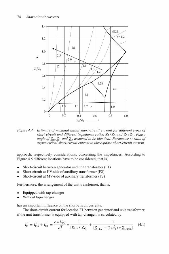
74 Short-circuit currents
2.52.0
1.51.3
1.2
r = 1.2
1.01.5 1.3 1.2
k1
k3
k2
k2E
0 0.2 0.60.4 0.8 1.0
0.2
0.4
0.6
0.8
1.0
1.4
1.2
0
kE2E
Z1/Z
Z0
r
r
Z2 / Z1
Figure 4.4 Estimate of maximal initial short-circuit current for different types ofshort-circuit and different impedance ratios Z1/Z0 and Z2/Z1. Phaseangle of Z0, Z1 and Z2 assumed to be identical. Parameter r: ratio ofasymmetrical short-circuit current to three-phase short-circuit current
approach, respectively considerations, concerning the impedances. According toFigure 4.5 different locations have to be considered, that is,
• Short-circuit between generator and unit transformer (F1)• Short-circuit at HV-side of auxiliary transformer (F2)• Short-circuit at MV-side of auxiliary transformer (F3)
Furthermore, the arrangement of the unit transformer, that is,
• Equipped with tap-changer• Without tap-changer
has an important influence on the short-circuit currents.The short-circuit current for location F1 between generator and unit transformer,
if the unit transformer is equipped with tap-changer, is calculated by
I ′′k = I ′′
kG + I ′′kT = c ∗ UrG√
3∗ 1
|KGs ∗ ZG| + 1
|ZTLV + (1/t2rT) ∗ ZQ min|
(4.1)
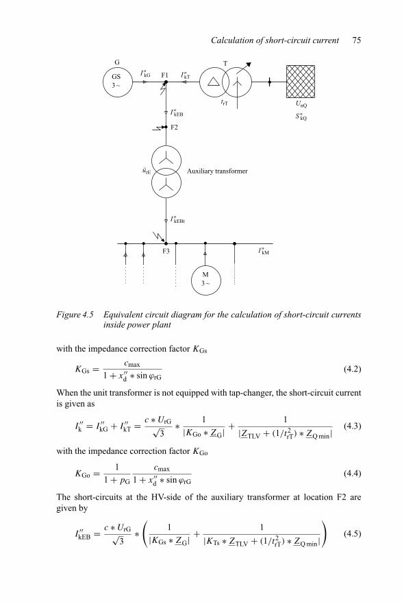
Calculation of short-circuit current 75
G T
Auxiliary transformer
GS3 ~
F1
F2
F3
M3 ~
I �kG
I �kEB
I �kEBt
I �kM
I �kT
trT
ürE
S �kQ
UnQ
Figure 4.5 Equivalent circuit diagram for the calculation of short-circuit currentsinside power plant
with the impedance correction factor KGs
KGs = cmax
1 + x′′d ∗ sin ϕrG
(4.2)
When the unit transformer is not equipped with tap-changer, the short-circuit currentis given as
I ′′k = I ′′
kG + I ′′kT = c ∗ UrG√
3∗ 1
|KGo ∗ ZG| + 1
|ZTLV + (1/t2rT) ∗ ZQ min|
(4.3)
with the impedance correction factor KGo
KGo = 1
1 + pG
cmax
1 + x′′d ∗ sin ϕrG
(4.4)
The short-circuits at the HV-side of the auxiliary transformer at location F2 aregiven by
I ′′kEB = c ∗ UrG√
3∗(
1
|KGs ∗ ZG| + 1
|KTs ∗ ZTLV + (1/t2rT) ∗ ZQ min|
)(4.5)

76 Short-circuit currents
with impedance correction factor for the generator
KGs = cmax
1 + x′′d ∗ sin ϕrG
(4.6a)
and the unit transformer
KTs = cmax
1 + xT ∗ sin ϕrG(4.6b)
If the unit transformer is installed without tap-changer the impedance correctionfactors are given for the generator
KGo = 1
1 + pG∗ cmax
1 + x′′d ∗ sin ϕrG
(4.7a)
and for the unit transformer
KTo = 1
1 + pG∗ cmax
1 + xT ∗ sin ϕrG(4.7b)
which shall be used instead of correction factors KGs and KTs as per Equations (4.6),respectively. The impedance Zrsl
Zrsl = 1
|KGs ∗ ZG| + 1
|KTs ∗ ZTLV + (1/t2rT) ∗ ZQ min|
(4.8)
including the correction factors is called the coupling impedance.Quantities of Equations (4.1)–(4.8) are
ZG Impedance of the generatorZTLV Impedance of the unit transformer at LV-side (generator voltage)ZQ min Impedance of the system feeder for maximal short-circuit currenttrT Transformation ratio of the unit transformer (trT ≥ 1)
UrG Rated voltage of generatorc; cmax Voltage factor as per Table 4.1xT Reactance of the transformer in p.u. (impedance voltage)x′′
d Subtransient reactance of the generator in p.u.pG Voltage control range of generator in p.u.sin ϕrG Power factor of generator at rated operating conditions
Other quantities are explained previously.Short-circuits at MV-side of the auxiliary transformer at location F3 or at the
auxiliary busbar are a superposition of the partial short-circuit current I ′′kEBt of the
auxiliary transformer related to the voltage level of the short-circuit location and ofthe contribution of the motors in the auxiliary system to the short-circuit current. Inthe case of a unit transformer without tap-changer the impedance correction factorsKGo and KTo have to be considered accordingly.
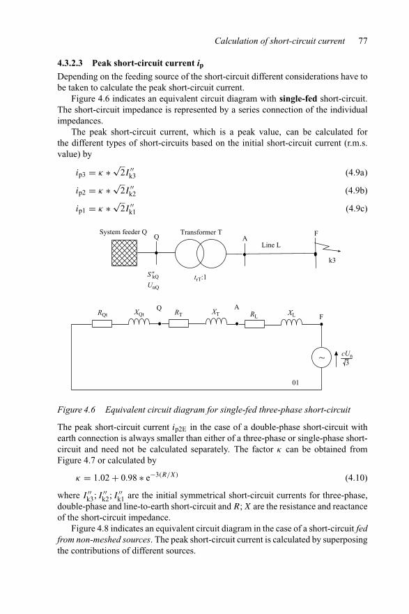
Calculation of short-circuit current 77
4.3.2.3 Peak short-circuit current ipDepending on the feeding source of the short-circuit different considerations have tobe taken to calculate the peak short-circuit current.
Figure 4.6 indicates an equivalent circuit diagram with single-fed short-circuit.The short-circuit impedance is represented by a series connection of the individualimpedances.
The peak short-circuit current, which is a peak value, can be calculated forthe different types of short-circuits based on the initial short-circuit current (r.m.s.value) by
ip3 = κ ∗ √2I ′′
k3 (4.9a)
ip2 = κ ∗ √2I ′′
k2 (4.9b)
ip1 = κ ∗ √2I ′′
k1 (4.9c)
S �kQ
UnQ
RQt XQt RT RLXL
cUn3
XTQ
trT:1
QSystem feeder Q
AF
k3
Line L
Transformer T
01
AF
~
Figure 4.6 Equivalent circuit diagram for single-fed three-phase short-circuit
The peak short-circuit current ip2E in the case of a double-phase short-circuit withearth connection is always smaller than either of a three-phase or single-phase short-circuit and need not be calculated separately. The factor κ can be obtained fromFigure 4.7 or calculated by
κ = 1.02 + 0.98 ∗ e−3(R/X) (4.10)
where I ′′k3; I ′′
k2; I ′′k1 are the initial symmetrical short-circuit currents for three-phase,
double-phase and line-to-earth short-circuit and R; X are the resistance and reactanceof the short-circuit impedance.
Figure 4.8 indicates an equivalent circuit diagram in the case of a short-circuit fedfrom non-meshed sources. The peak short-circuit current is calculated by superposingthe contributions of different sources.

78 Short-circuit currents
1
1.1
1.2
1.3
1.4
1.5
1.6
1.7
1.8
1.9
2
0 0.2 0.4 0.6 0.8 1 1.2 1.4 1.6 1.8 2R/X
k
Figure 4.7 Factor κ for the calculation of peak short-circuit current
T2
Q1BT1
Q2
S �kQ1
S �kQ2
I �kT1
I �kT2
I �k ; ip
ipT1
ipT2
Figure 4.8 Equivalent circuit diagram for three-phase short-circuit fed fromnon-meshed sources
The peak short-circuit currents ip3T1 and ip3T2 of each branch, fed through thetransformers T1 and T2, are calculated separately as well as the factors κT1 and κT2.
ip3T1 = κ1 ∗ √2 ∗ I ′′
k3T1 (4.11a)
ip3T2 = κ2 ∗ √2 ∗ I ′′
k3T2 (4.11b)

Calculation of short-circuit current 79
The total peak short-circuit current ip3 is given by
ip3 = ip3T1 + ip3T2 (4.11c)
Particular considerations are to be taken in the case of short-circuits in meshed net-works according to Figure 4.9. The peak short-circuit current at the short-circuitlocation cannot be calculated by superposition as the R/X-ratios of the individ-ual branches feeding the short-circuit are different and the direction of the branchshort-circuit currents through the system is defined by the Ohmic law.
Q
F
Figure 4.9 Equivalent circuit diagram of a three-phase short-circuit in a meshedsystem
In principle, the peak short-circuit current in a meshed system will be calculated by
ip3 = κ ∗ √2I ′′
k3 (4.9a)
as given for three-phase short-circuits, and for other types of short-circuits accord-ingly. The factor κ , however, will be determined with different methods asbelow.
Uniform (smallest) ratio R/X. The factor κ is calculated based on the smallestratio R/X of all branches of the network. Only those branches need to be takeninto account which contribute to the short-circuit current in the power system corre-sponding to the short-circuit location, respectively those branches connected throughtransformers to the short-circuit location. The results are always on the safe side,however the accuracy is low.
Ratio R/X at short-circuit location. Based on the ratio R/X of the total systemimpedance at the short-circuit location, the factor κ is calculated taking account ofa safety factor of 1.15 to allow for deviations due to the different ratios R/X in thedifferent branches.
κb = 1.15 ∗ κ (4.12)
The factor 1.15 ∗ κ should not exceed the value of 1.8 in LV-systems and shall notexceed 2.0 in HV-systems. The safety factor 1.15 is neglected when R/X ≤ 0.3.
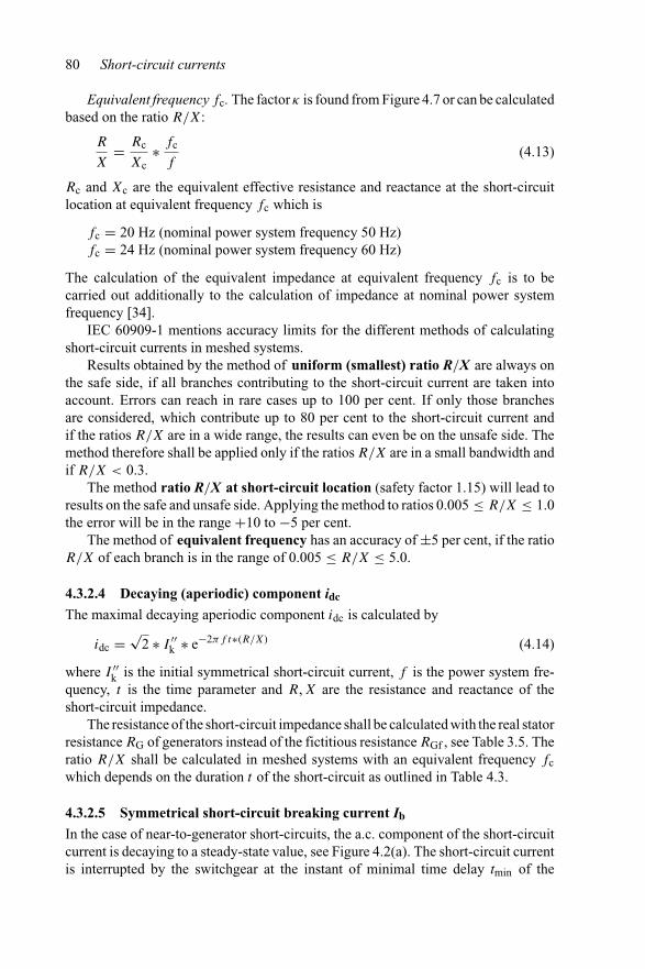
80 Short-circuit currents
Equivalent frequency fc. The factor κ is found from Figure 4.7 or can be calculatedbased on the ratio R/X:
R
X= Rc
Xc∗ fc
f(4.13)
Rc and Xc are the equivalent effective resistance and reactance at the short-circuitlocation at equivalent frequency fc which is
fc = 20 Hz (nominal power system frequency 50 Hz)fc = 24 Hz (nominal power system frequency 60 Hz)
The calculation of the equivalent impedance at equivalent frequency fc is to becarried out additionally to the calculation of impedance at nominal power systemfrequency [34].
IEC 60909-1 mentions accuracy limits for the different methods of calculatingshort-circuit currents in meshed systems.
Results obtained by the method of uniform (smallest) ratio R/X are always onthe safe side, if all branches contributing to the short-circuit current are taken intoaccount. Errors can reach in rare cases up to 100 per cent. If only those branchesare considered, which contribute up to 80 per cent to the short-circuit current andif the ratios R/X are in a wide range, the results can even be on the unsafe side. Themethod therefore shall be applied only if the ratios R/X are in a small bandwidth andif R/X < 0.3.
The method ratio R/X at short-circuit location (safety factor 1.15) will lead toresults on the safe and unsafe side. Applying the method to ratios 0.005 ≤ R/X ≤ 1.0the error will be in the range +10 to −5 per cent.
The method of equivalent frequency has an accuracy of ±5 per cent, if the ratioR/X of each branch is in the range of 0.005 ≤ R/X ≤ 5.0.
4.3.2.4 Decaying (aperiodic) component idc
The maximal decaying aperiodic component idc is calculated by
idc = √2 ∗ I ′′
k ∗ e−2πf t∗(R/X) (4.14)
where I ′′k is the initial symmetrical short-circuit current, f is the power system fre-
quency, t is the time parameter and R, X are the resistance and reactance of theshort-circuit impedance.
The resistance of the short-circuit impedance shall be calculated with the real statorresistance RG of generators instead of the fictitious resistance RGf , see Table 3.5. Theratio R/X shall be calculated in meshed systems with an equivalent frequency fcwhich depends on the duration t of the short-circuit as outlined in Table 4.3.
4.3.2.5 Symmetrical short-circuit breaking current Ib
In the case of near-to-generator short-circuits, the a.c. component of the short-circuitcurrent is decaying to a steady-state value, see Figure 4.2(a). The short-circuit currentis interrupted by the switchgear at the instant of minimal time delay tmin of the

Calculation of short-circuit current 81
Table 4.3 Equivalent frequency for the calculation of decaying component
Factor f ∗ t <1 <2.5 <5 <12.5
Ratio of equivalent frequencyto power system frequency
fc/f 0.27 0.15 0.092 0.055
Example: f = 50 Hz t <0.02 s <0.05 s <0.1 s <0.25 sfc 13.5 Hz 7.5 Hz 4.6 Hz 2.75 Hz
Example: f = 60 Hz t <0.02 s <0.05 s <0.1 s <0.25 sfc 16.2 Hz 9.0 Hz 5.52 Hz 3.3 Hz
protection. The calculation of the symmetrical short-circuit breaking current Ib isbased on the initial short-circuit current and on the factor μ,
Ib = μ ∗ I ′′k (4.15)
The factor μ can be taken from Figure 4.10 or calculated by
μ = 0.84 + 0.26 ∗ e−0.26(I ′′kG/IrG) for tmin = 0.02 s (4.16a)
μ = 0.71 + 0.51 ∗ e−0.30(I ′′kG/IrG) for tmin = 0.05 s (4.16b)
μ = 0.62 + 0.72 ∗ e−0.32(I ′′kG/IrG) for tmin = 0.10 s (4.16c)
μ = 0.56 + 0.94 ∗ e−0.38(I ′′kG/IrG) for tmin ≥ 0.25 s (4.16d)
1.1
0.9
0.8
0.7
0.6
0.50 2 4 6 8 10 12
1
m
I 0kG /IrG or I 0kM /IrM
0.02 s
0.05 s
0.1 s
> 0.25 s
Minimum time delay
Figure 4.10 Factor μ for calculation of symmetrical short-circuit breaking current

82 Short-circuit currents
where I ′′kG is the initial symmetrical short-circuit current of the generator, IrG is
the rated current of the generator and tmin is the minimal time delay of the protec-tion, switchgear and auxiliaries, that is, minimal time for switching the short-circuitcurrent off.
The factor μ is valid for high-voltage synchronous generators, excited by rotat-ing machines of rectifiers. If the excitation system is not known the factor shall beset to μ = 1.
In the case of far-from-generator short-circuits, the symmetrical short-circuitbreaking current Ib is equal to the initial short-circuit current I ′′
k as the a.c. componentis not decaying.
4.3.2.6 Steady-state short-circuit current Ik
The steady-state short-circuit current Ik in the case of near-to-generator short-circuitsdepends on various factors such as saturation effects, power factor of generators,change of system topology due to operation of switching, etc. and can therefore onlybe determined with a certain inaccuracy. The method as per IEC 60909 determineslower and upper limits only when one synchronous machine is feeding the short-circuit. The calculation is based on the generator-rated current assuming a factor λ
which depends on the ratio of initial symmetrical short-circuit current to rated currentof the generator and on the saturated synchronous reactance.
Maximal excitation of the synchronous machine leads to the maximal symmetricalshort-circuit breaking current
Ik max = λmax ∗ IrG (4.17a)
The factor λmax is valid for turbine generators according to Figure 4.11 and forsalient-pole generators as per Figure 4.12.
The minimal symmetrical short-circuit breaking current is calculated for constantno-load excitation of the generator with the factor λmin.
Ik min = λmin ∗ IrG (4.17b)
The values for λmin are included in Figures 4.11 and 4.12. Reference is made to theremarks in IEC 60909-0 on the factors.
Quantities as used above are
IrG Rated current of the generatorI ′′
kG Initial synchronous short-circuit current of the generatorxdsat Saturated synchronous reactance of the generator, equal to the reciprocal
of the short-circuit ratio of the generator
In the case of far-from-generator short-circuits, the symmetrical short-circuitbreaking current Ib is equal to the initial short-circuit current I ′′
k as the a.c. componentis not decaying.

Calculation of short-circuit current 83
2.8
2.6
2.4
2.2
2.0
1.8
1.6
1.4
1.2
1.0
0.8
0.6
0.4
0.2
00 1 2 3 4 5
Three-phase short circuit I 0kG/IrG
6 7 8
�
2.8
2.6
2.4
2.2
2.0
1.8
1.6
1.4
1.2
1.0
0.8
0.6
0.4
0.2
00 1 2 3 4 5
Three-phase short circuit I 0kG /IrG
6 7 8
�
(a) (b)
�max
�min
xdsat
�min
�max
xdsat
1.21.41.61.82.02.2
1.2
1.41.61.82.02.2
Figure 4.11 Factors λmax and λmin for turbine generators (Figure 17 of DIN EN60909-0 (VDE 0102)). (a) Series one and (b) series two
5.5
5.0
4.5
4.0
3.5
3.0
2.5
2.0
1.5
1.0
0.5
0
5.5
5.0
4.5
4.0
3.5
3.0
2.5
2.0
1.5
1.0
0.5
00 1 2 3 4 5
Three-phase short circuit I 0kG/IrG
6 7 8
�
0 1 2 3 4 5
Three-phase short circuit I 0kG /IrG
6 7 8
�
(a) (b)
�max
�min
xdsat
�min
�max
xdsat
0.6
0.8
1.0
2.0
1.21.7
0.6
0.8
1.0
1.2
1.72.0
Figure 4.12 Factors λmax and λmin for salient-pole generators (Figure 18 of DINEN 60909-0 (VDE 0102) 1988). (a) Series one and (b) series two
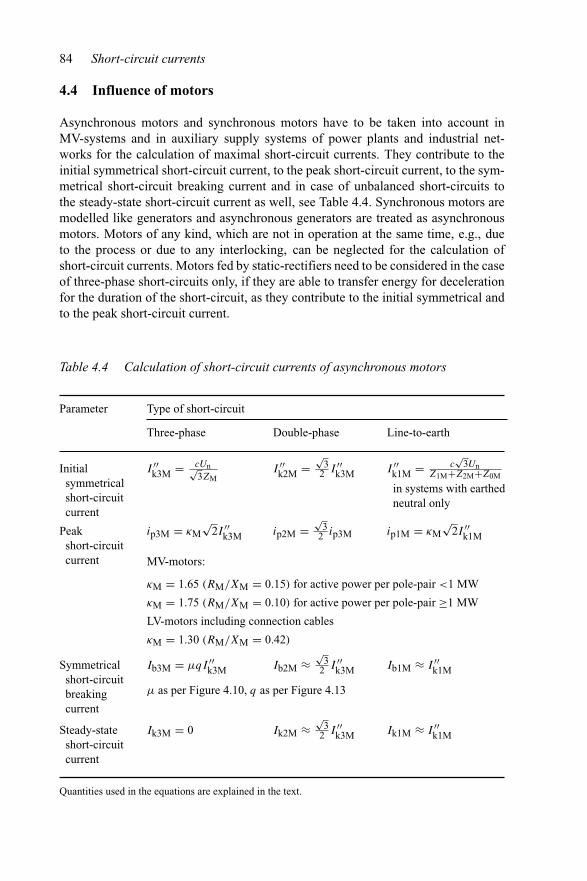
84 Short-circuit currents
4.4 Influence of motors
Asynchronous motors and synchronous motors have to be taken into account inMV-systems and in auxiliary supply systems of power plants and industrial net-works for the calculation of maximal short-circuit currents. They contribute to theinitial symmetrical short-circuit current, to the peak short-circuit current, to the sym-metrical short-circuit breaking current and in case of unbalanced short-circuits tothe steady-state short-circuit current as well, see Table 4.4. Synchronous motors aremodelled like generators and asynchronous generators are treated as asynchronousmotors. Motors of any kind, which are not in operation at the same time, e.g., dueto the process or due to any interlocking, can be neglected for the calculation ofshort-circuit currents. Motors fed by static-rectifiers need to be considered in the caseof three-phase short-circuits only, if they are able to transfer energy for decelerationfor the duration of the short-circuit, as they contribute to the initial symmetrical andto the peak short-circuit current.
Table 4.4 Calculation of short-circuit currents of asynchronous motors
Parameter Type of short-circuit
Three-phase Double-phase Line-to-earth
Initialsymmetricalshort-circuitcurrent
I ′′k3M = cUn√
3ZMI ′′k2M =
√3
2 I ′′k3M I ′′
k1M = c√
3UnZ1M+Z2M+Z0M
in systems with earthedneutral only
Peakshort-circuitcurrent
ip3M = κM√
2I ′′k3M ip2M =
√3
2 ip3M ip1M = κM√
2I ′′k1M
MV-motors:
κM = 1.65 (RM/XM = 0.15) for active power per pole-pair <1 MW
κM = 1.75 (RM/XM = 0.10) for active power per pole-pair ≥1 MW
LV-motors including connection cables
κM = 1.30 (RM/XM = 0.42)
Symmetricalshort-circuitbreakingcurrent
Ib3M = μqI ′′k3M Ib2M ≈
√3
2 I ′′k3M Ib1M ≈ I ′′
k1M
μ as per Figure 4.10, q as per Figure 4.13
Steady-stateshort-circuitcurrent
Ik3M = 0 Ik2M ≈√
32 I ′′
k3M Ik1M ≈ I ′′k1M
Quantities used in the equations are explained in the text.

Calculation of short-circuit current 85
Asynchronous motors in public supply systems are considered when
• the sum of the rated currents is greater than 1 per cent of the initial symmetricalshort-circuit current without motors;
• the contribution to the initial symmetrical short-circuit current without motorsis greater or equal to 5 per cent of the initial symmetrical short-circuit currentwithout motors.
Medium- and low-voltage asynchronous motors connected through two-windingtransformers to the short-circuit are considered if∑
PrM∑SrT
>0.8
|((c ∗ 100∑
SrT)/(√
3UnQ/I ′′k )) − 0.3| (4.18)
where UnQ is the nominal system voltage,∑
SrT is the sum of rated apparent powerof all transformers, directly connected to motors feeding the short-circuit, I ′′
k is theinitial symmetrical short-circuit current without motors and
∑PrM is the sum of
rated active power of all low- and medium-voltage motors.In order to calculate the branch short-circuit current of asynchronous motors,
Table 4.4 can be used. The factor q (three-phase short-circuit) depending on theminimal time delay of the protection tmin can be obtained from Figure 4.13 or by
q = 1.03 + 0.12 ∗ ln(m), tmin = 0.02 s (4.19a)
q = 0.79 + 0.12 ∗ ln(m), tmin = 0.05 s (4.19b)
q = 0.57 + 0.12 ∗ ln(m), tmin = 0.10 s (4.19c)
q = 0.26 + 0.10 ∗ ln(m), tmin ≥ 0.25 s (4.19d)
where tmin is the minimal time delay of the protection, switchgear and auxiliaries,i.e., minimal time for switching the short-circuit current off and m is the active powerof the motor per pole-pair in p.u. based on 1-MW-base. The factor q should not begreater than 1.
4.5 Minimal short-circuit currents
In order to calculate the minimal short-circuit current, the voltage factor cmin accord-ing to Table 4.1 for the equivalent voltage source at the short-circuit location has tobe considered. Furthermore,
• System topology, generator dispatch and short-circuit power of feeding networkshave to be defined in such a way that the minimal short-circuit current is expected.This normally applies for low-load conditions.
• Motors are to be neglected.• Resistances of overhead lines and cables shall be calculated with the maximal
permissible temperature at the end of the short-circuit, e.g., 80◦C in low-voltagesystems.

86 Short-circuit currents
1
0.9
0.8
0.7
0.6
0.5
0.4
0.3
0.2
0.1
00.01 0.1 1 10
m (active power per pair of poles)100MW
q
Minimum time delay
0.02 s
0.05 s
0.1 s
> 0.25 s
Figure 4.13 Factor q for the calculation of symmetrical short-circuit breakingcurrent
These assumptions have to be taken in the case of balanced and unbalanced short-circuits, except where other presuppositions are mentioned.
4.6 Examples
Examples for the calculation of short-circuit currents are included in IEC 60909-4besides those given below. Reference is made to the relevant chapters where theindividual quantities are explained.
4.6.1 Three-phase near-to-generator short-circuit
Figure 4.14 outlines the equivalent circuit diagram of a 220-kV system. For three-phase short-circuit at busbar B (maximal s.-c. currents) the branch short-circuitcurrents of the generators and the system feeder as well as the contribution of thegenerators to the symmetrical short-circuit breaking current and to the steady-stateshort-circuit current (tmin = 0.1 s; xdsat = 140%; Turbine generator (Series 1)) areto be calculated.
Data of equipment taken from nameplates:
SrG1 = 120 MVA; UrG1 = 10.5 kV; cos ϕrG1 = 0.8; x′′dG1 = 18%
SrG2 = 80 MVA; UrG2 = 10.5 kV; cos ϕrG2 = 0.85; x′′dG2 = 16%
SrT1 = 120 MVA; UrT1HV/UrT1LV = 220 kV/10.5 kV; ukrT1 = 14%SrT2 = 80 MVA; UrT2HV/UrT2LV = 220 kV/10.5 kV; ukrT2 = 12%SrT3 = 200 MVA; UrT3HV/UrT3LV = 400 kV/220 kV; ukrT3 = 12%

Calculation of short-circuit current 87
UnQ = 380 kV Un = 220 kV
Q A
B G1
G2
L1
T1
T2
GS3 ~
L2
GS3 ~
Figure 4.14 Equivalent circuit diagram of a 220-kV-system with short-circuitlocation
S′′kQ = 5 GVA; UnQ = 380 kV
X′L1 = X′
L2 = 0.4 �/km; l = 50 km
The impedances of equipment (positive-sequence component) including correctionfactors are
XQK = 9.632 �
XT3 = 28.31 �
XL1 = XL2 = 20.04 �
XKW1K = 138.67 �
XKW2K = 182.52 �
The short-circuit impedance at the short-circuit location is XkB = 29.82 �
The initial symmetrical short-circuit currents are:
I ′′k3 = 4.69 kA, at s.-c. location
I ′′k3Q = 1.69 kA, branch s.-c. current of system feeder
The contribution of the generators to the short-circuit currents is outlined in the tablebelow.
Parameter Generator 1 Generator 2 Section
I ′′k3 21.11 kA 16.04 kA 4.3.2.1
μ 0.879 0.844Ib 18.55 kA 13.54 kA 4.3.2.5λmax/λmin 1.75/0.46 1.82/0.47Ik max/Ik min 11.55 kA/3.04 kA 8.01 kA/2.07 kA
4.6.2 Line-to-earth (single-phase) short-circuit
The initial short-circuit current for a single-phase short-circuit at location F accordingto Figure 4.15 shall be calculated.

88 Short-circuit currents
Q A
B
T1
L2
1
L3C
UnQ = 220 kV
Un = 110 kV
T2
Figure 4.15 Equivalent circuit diagram of a 110-kV-system with 220-kV-feeder
The data of equipment are:
S′′kQ = 5 GVA; X0/X1 = 4
SrT = 100 MVA; ukr = 12%; trT = 220 kV/115 kV; X0/X1 = 3X′
L = 0.13 �/km; lL = 10 km; X0/X1 = 3.5
The impedances in the positive- (negative-) and zero-sequence component includingcorrection factors are:
X1QK = 2.904 �; X0QK = 11.62 �
X1T1K = X1T2K = 15.49 �; X0T1K = X0T2K = 46.34 �
X1L1 = X1L2 = X1L3 = 1.295 �; X0L1 = X0L2 = X0L3 = 4.538 �
The impedances at the short-circuit location are X1k = 11.507 �; X0k = 49.368 �
and the initial short-circuit current is I ′′k1 = 2.895 kA.
4.6.3 Calculation of peak short-circuit current
The peak short-circuit current for a three-phase short-circuit at location F accordingto Figure 4.16 shall be calculated with the different methods, i.e., ‘superpositionmethod’, ‘ratio R/X at s.-c. location’ and ‘equivalent frequency’. The accuracy ofthe results is to be assessed.
The data of equipment are
S′′kQ = 1000 MVA; UnQ = 110 kV
SrT = 10 MVA; ukrT = 10%; PkT = 70 kW; trT = 125 kV/12 kVSrG = 20 MVA; UrG = 10.5 kV; cos ϕrG = 0.8; x′′
dG = 10%X′
L = 0.09 �/km; R′L = 0.123 �/km; lL = 5 km
The impedances of equipment including correction factors are
XGK = 0.5448 �; RGfK = 0.5448 �
XL = 0.45 �; RL = 0.615 �

Calculation of short-circuit current 89
B
AQ
UnQ = 110 kV Un = 10 kV
GS
3 ~
Figure 4.16 Equivalent circuit diagram of a 10-kV system, f = 50 Hz
XQ = 0.122 �; RQ = 0.0122 �
XT = 1.416 �; RT = 0.0994 �
The results of short-circuit calculation are outlined in the table below:
Method Impedance I ′′k3 κ ip
Impedance ats.-c. location
Zk = (0.244 + 0.649) � 9.16 kA — —
Superpositionof feeders Aand B
ZkA = (0.1116 + 1.5381) � I ′′k3A = 4.118 kA 1.837 ipA = 10.7 kA
ZkB = (0.653 + 0.9948) � I ′′k3B = 5.337 kA 1.157 ipB = 8.73 kA
ipges = 19.43 kA
Ratio R/X ats.-c. location
Zk = (0.244 + 0.649) � 9.16 kA 1.337 19.92 kA
Equivalentfrequency
ZkAc = (0.1116 + 0.6112) � 9.16 kA 1.485 19.24 kAZkBc = (0.653 + 0.3979) �
Zkc = (0.2509 + 0.4036) �
The results obtained with the superposition method are the correct results.
4.6.4 Short-circuit currents in a meshed 110-kV-system
The three-phase short-circuit current for the short-circuit location at busbar E ina meshed 110-kV-system shall be calculated. The system diagram is outlined inFigure 4.17.
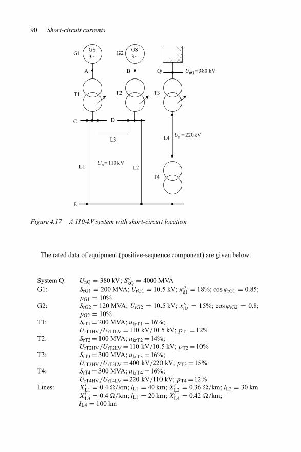
90 Short-circuit currents
GS3 ~
G1
A B Q UnQ = 380 kV
T1 T2 T3
L4
T4
G2GS3 ~
Un = 220 kV
Un = 110 kVL2
L3
L1
E
C D
Figure 4.17 A 110-kV system with short-circuit location
The rated data of equipment (positive-sequence component) are given below:
System Q: UnQ = 380 kV; S′′kQ = 4000 MVA
G1: SrG1 = 200 MVA; UrG1 = 10.5 kV; x′′d1 = 18%; cos ϕrG1 = 0.85;
pG1 = 10%G2: SrG2 = 120 MVA; UrG2 = 10.5 kV; x′′
d2 = 15%; cos ϕrG2 = 0.8;pG2 = 10%
T1: SrT1 = 200 MVA; ukrT1 = 16%;UrT1HV/UrT1LV = 110 kV/10.5 kV; pT1 = 12%
T2: SrT2 = 100 MVA; ukrT2 = 14%;UrT2HV/UrT2LV = 110 kV/10.5 kV; pT2 = 10%
T3: SrT3 = 300 MVA; ukrT3 = 16%;UrT3HV/UrT3LV = 400 kV/220 kV; pT3 = 15%
T4: SrT4 = 300 MVA; ukrT4 = 16%;UrT4HV/UrT4LV = 220 kV/110 kV; pT4 = 12%
Lines: X′L1 = 0.4 �/km; lL1 = 40 km; X′
L2 = 0.36 �/km; lL2 = 30 kmX′
L3 = 0.4 �/km; lL1 = 20 km; X′L4 = 0.42 �/km;
lL4 = 100 km
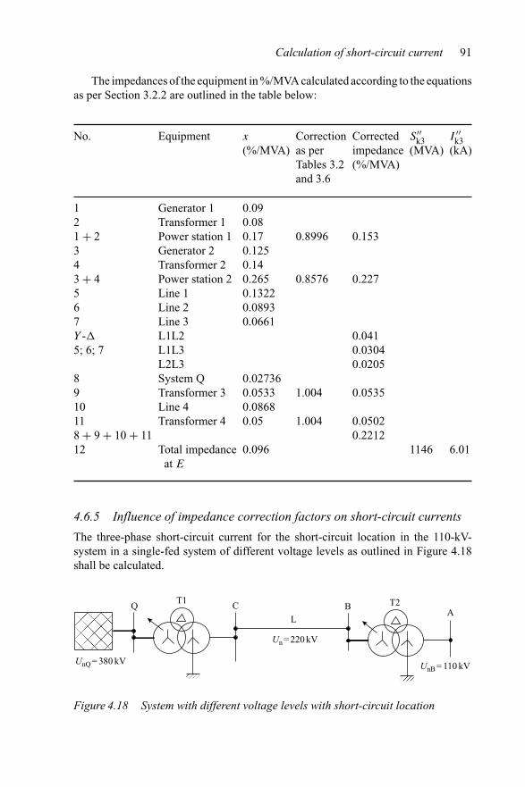
Calculation of short-circuit current 91
The impedances of the equipment in %/MVA calculated according to the equationsas per Section 3.2.2 are outlined in the table below:
No. Equipment x
(%/MVA)Correctionas perTables 3.2and 3.6
Correctedimpedance(%/MVA)
S′′k3
(MVA)I ′′
k3(kA)
1 Generator 1 0.092 Transformer 1 0.081 + 2 Power station 1 0.17 0.8996 0.1533 Generator 2 0.1254 Transformer 2 0.143 + 4 Power station 2 0.265 0.8576 0.2275 Line 1 0.13226 Line 2 0.08937 Line 3 0.0661Y - L1L2 0.0415; 6; 7 L1L3 0.0304
L2L3 0.02058 System Q 0.027369 Transformer 3 0.0533 1.004 0.053510 Line 4 0.086811 Transformer 4 0.05 1.004 0.05028 + 9 + 10 + 11 0.221212 Total impedance 0.096 1146 6.01
at E
4.6.5 Influence of impedance correction factors on short-circuit currents
The three-phase short-circuit current for the short-circuit location in the 110-kV-system in a single-fed system of different voltage levels as outlined in Figure 4.18shall be calculated.
QT1 C
LB
AT2
Un = 220 kV
UnQ = 380 kV UnB = 110 kV
Figure 4.18 System with different voltage levels with short-circuit location

92 Short-circuit currents
The rated data of equipment (positive-sequence component) are given below:
System Q: UnQ = 380 kV; S′′kQ = 5000 MVA
T1: SrT1 = 200 MVA; ukrT1 = 16%; UrT1HV/UrT1LV = 400 kV/
220 kV; pT1 = 12%T2: SrT2 = 200 MVA; ukrT2 = 16%; UrT2HV/UrT2LV = 220 kV/
120 kV; pT2 = 10%Line: X′
L = 0.4 �/km; lL = 100 km
The impedances of the equipment in %/MVA and the short-circuit current calculatedaccording to the equations as per Section 3.2.2 are outlined in the table below:
No. Equipment x
(%/MVA)S′′
k3(MVA)
I ′′k3
(kA)
1 System Q 0.02192 Transformer 1 0.083 Line 0.08264 Transformer 2 0.085 Total impedance 0.2645 415.9 2.18
at 110 kV
As indicated by the rated data of equipment and as can be seen in Figure 4.18, therated voltage of the transformers differ from the nominal voltages of the 380-kV- andthe 110-kV-systems. Correction factors for those equipment connected to the short-circuit location through transformers must be taken into account. The results of thecalculation with impedance correction factor as per Figure 2.16 and Equation (2.27)are given below.
No. Equipment x
(%/MVA)Correctionfactoras perFigure 2.16
Correctedimpedance(%/MVA)
S′′k3
(MVA)I ′′
k3(kA)
1 System Q 0.0219 1.074 0.02352 Transformer 1 0.08 1.19 0.09523 Line 0.0826 1.19 0.09834 Transformer 2 0.08 1.19 0.09525 Total impedance 0.3122 352.3 1.85
at 110 kV

Calculation of short-circuit current 93
The calculation of transformer impedances furthermore requires impedancecorrection factor as outlined in Table 3.3. The results of the analysis, taking accountof both correction factors (Figure 2.16 and Table 3.3), are outlined in the table below:
No. Equipment x
(%/MVA)Correctionfactoras perFigure 2.16
Correctionfactoras perTable 3.3
Correctedimpedance(%/MVA)
S′′k3
(MVA)I ′′
k3(kA)
1 System Q 0.0219 1.074 0.02352 Transformer 1 0.08 1.19 1.004 0.09563 Line 0.0826 1.19 0.09834 Transformer 2 0.08 1.19 1.004 0.09565 Total 0.2645 0.313 351.4 1.84
impedanceat 110 kV
Calculating the short-circuit current in the p.u.-system is similar to the calculationin the %/MVA-system. Correction factors as per Table 3.3 for the transformers andFigure 2.16 due to differences between the rated voltages of equipment and the nom-inal system voltages have to be taken into account. The reference voltage is equalto the nominal voltage at the short-circuit location UB = 110 kV and the referencepower is 100 MVA. The results are outlined in the table below:
No. Equipment x′(p.u.)
Correctionfactoras perFigure 2.16
Correctionfactoras perTable 3.3
Correctedimpedance(p.u.)
s′k3
(p.u.)i′k3(p.u.)
1 System Q 0.0219 1.074 0.02352 Transformer 1 0.08 1.19 1.004 0.09563 Line 0.0826 1.19 0.09834 Transformer 2 0.08 1.19 1.004 0.09565 Total 0.2645 0.313 3.514 2.024
impedanceat 110 kV
If the short-circuit current is calculated using the �-system only the correction factoras per Table 3.3 for the transformers has to be taken into account. The results as per
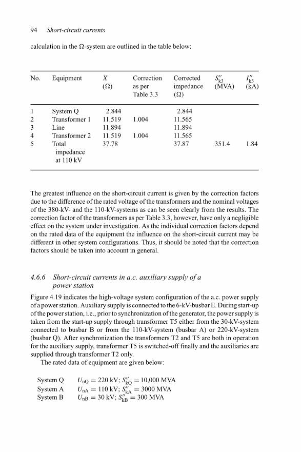
94 Short-circuit currents
calculation in the �-system are outlined in the table below:
No. Equipment X
(�)Correctionas perTable 3.3
Correctedimpedance(�)
S′′k3
(MVA)I ′′
k3(kA)
1 System Q 2.844 2.8442 Transformer 1 11.519 1.004 11.5653 Line 11.894 11.8944 Transformer 2 11.519 1.004 11.5655 Total 37.78 37.87 351.4 1.84
impedanceat 110 kV
The greatest influence on the short-circuit current is given by the correction factorsdue to the difference of the rated voltage of the transformers and the nominal voltagesof the 380-kV- and the 110-kV-systems as can be seen clearly from the results. Thecorrection factor of the transformers as per Table 3.3, however, have only a negligibleeffect on the system under investigation. As the individual correction factors dependon the rated data of the equipment the influence on the short-circuit current may bedifferent in other system configurations. Thus, it should be noted that the correctionfactors should be taken into account in general.
4.6.6 Short-circuit currents in a.c. auxiliary supply of apower station
Figure 4.19 indicates the high-voltage system configuration of the a.c. power supplyof a power station. Auxiliary supply is connected to the 6-kV-busbar E. During start-upof the power station, i.e., prior to synchronization of the generator, the power supply istaken from the start-up supply through transformer T5 either from the 30-kV-systemconnected to busbar B or from the 110-kV-system (busbar A) or 220-kV-system(busbar Q). After synchronization the transformers T2 and T5 are both in operationfor the auxiliary supply, transformer T5 is switched-off finally and the auxiliaries aresupplied through transformer T2 only.
The rated data of equipment are given below:
System Q UnQ = 220 kV; S′′kQ = 10,000 MVA
System A UnA = 110 kV; S′′kA = 3000 MVA
System B UnB = 30 kV; S′′kB = 300 MVA
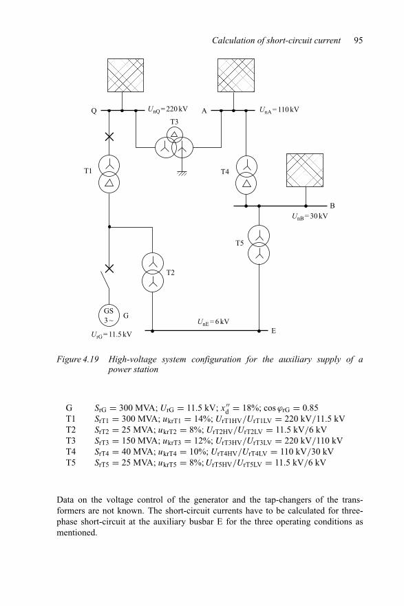
Calculation of short-circuit current 95
T3
T4
T5
T2
UnE = 6 kVG
E
GS3 ~
B
UnQ = 220 kVQ UnA = 110 kV
UnB = 30 kV
UrG = 11.5 kV
A
T1
×
×
Figure 4.19 High-voltage system configuration for the auxiliary supply of apower station
G SrG = 300 MVA; UrG = 11.5 kV; x′′d = 18%; cos ϕrG = 0.85
T1 SrT1 = 300 MVA; ukrT1 = 14%; UrT1HV/UrT1LV = 220 kV/11.5 kVT2 SrT2 = 25 MVA; ukrT2 = 8%; UrT2HV/UrT2LV = 11.5 kV/6 kVT3 SrT3 = 150 MVA; ukrT3 = 12%; UrT3HV/UrT3LV = 220 kV/110 kVT4 SrT4 = 40 MVA; ukrT4 = 10%; UrT4HV/UrT4LV = 110 kV/30 kVT5 SrT5 = 25 MVA; ukrT5 = 8%; UrT5HV/UrT5LV = 11.5 kV/6 kV
Data on the voltage control of the generator and the tap-changers of the trans-formers are not known. The short-circuit currents have to be calculated for three-phase short-circuit at the auxiliary busbar E for the three operating conditions asmentioned.
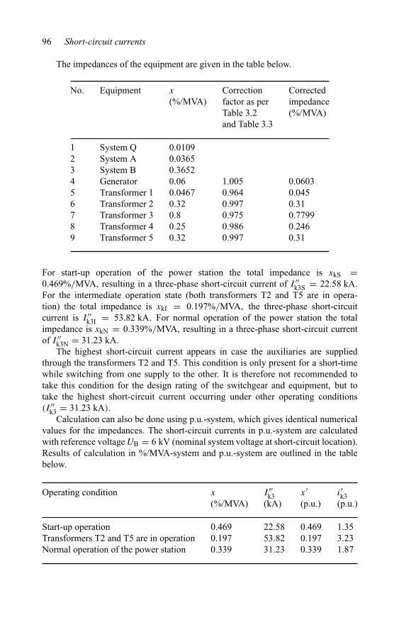
96 Short-circuit currents
The impedances of the equipment are given in the table below.
No. Equipment x
(%/MVA)Correctionfactor as perTable 3.2and Table 3.3
Correctedimpedance(%/MVA)
1 System Q 0.01092 System A 0.03653 System B 0.36524 Generator 0.06 1.005 0.06035 Transformer 1 0.0467 0.964 0.0456 Transformer 2 0.32 0.997 0.317 Transformer 3 0.8 0.975 0.77998 Transformer 4 0.25 0.986 0.2469 Transformer 5 0.32 0.997 0.31
For start-up operation of the power station the total impedance is xkS =0.469%/MVA, resulting in a three-phase short-circuit current of I ′′
k3S = 22.58 kA.For the intermediate operation state (both transformers T2 and T5 are in opera-tion) the total impedance is xkI = 0.197%/MVA, the three-phase short-circuitcurrent is I ′′
k3I = 53.82 kA. For normal operation of the power station the totalimpedance is xkN = 0.339%/MVA, resulting in a three-phase short-circuit currentof I ′′
k3N = 31.23 kA.The highest short-circuit current appears in case the auxiliaries are supplied
through the transformers T2 and T5. This condition is only present for a short-timewhile switching from one supply to the other. It is therefore not recommended totake this condition for the design rating of the switchgear and equipment, but totake the highest short-circuit current occurring under other operating conditions(I ′′
k3 = 31.23 kA).Calculation can also be done using p.u.-system, which gives identical numerical
values for the impedances. The short-circuit currents in p.u.-system are calculatedwith reference voltage UB = 6 kV (nominal system voltage at short-circuit location).Results of calculation in %/MVA-system and p.u.-system are outlined in the tablebelow.
Operating condition x
(%/MVA)I ′′
k3(kA)
x′(p.u.)
i′k3(p.u.)
Start-up operation 0.469 22.58 0.469 1.35Transformers T2 and T5 are in operation 0.197 53.82 0.197 3.23Normal operation of the power station 0.339 31.23 0.339 1.87

Chapter 5
Influence of neutral earthing on single-phaseshort-circuit currents
5.1 General
The theoretical approach to calculate short-circuit (s.-c.) currents with symmetricalcomponents in general and especially in the case of single-phase short-circuit wasexplained in detail in Chapter 2. Current and voltages in case of short-circuits withearth connection (e.g., single-phase short-circuits) depend on the positive- and zero-sequence impedances Z1 and Z0. If the ratio of zero-sequence to positive-sequenceimpedance is k = Z0/Z1 the voltages in the non-faulted phases (see Equation (2.25a))and the single-phase short-circuit current (see Equation (2.25b)) are
|UY| = |UB| = E1 ∗ √3 ∗
√k2 + k + 1
2 + k(5.1a)
I ′′k1 = E1
Z1∗ 3
2 + k(5.1b)
If the voltage E1 is set to E1 = Un/√
3, similar to the equivalent voltage atshort-circuit location then
|UY| = |UB| = Un ∗√
k2 + k + 1
2 + k(5.1c)
I ′′k1 = Un√
3 ∗ Z1∗ 3
2 + k(5.1d)
The impedances in the positive-sequence (and negative-sequence) system aredetermined only by the network topology. The single-phase short-circuit current andthe voltages of the non-faulted phases can be changed only by changing the ratioof positive-sequence to zero-sequence impedance, i.e., by changing the handling oftransformer neutrals.

98 Short-circuit currents
The type of neutral earthing determines the impedance Z0 of the zero-sequencecomponent and has a dominating influence on the short-circuit current through earth,i.e., I ′′
k1 in case of single-phase short-circuits and I ′′kE2E in case of two-phase short-
circuit with earth connection. In order to change the zero-sequence impedance ofthe system, it is possible to earth any number of neutrals, i.e., none, a few or alltransformer neutrals, leading to the highest zero-sequence impedance (no neutralearthed), respectively the lowest zero-sequence impedance (all neutrals earthed).The system is characterised less by the number of neutrals to be earthed, than by thevalue of the single-phase short-circuit current and by the voltages in the non-faultedphases.
The different types of neutral handling in power systems (high-voltage systemsonly) are outlined in Table 5.1.Quantities as per Table 5.1
Un Nominal system voltageU0max Maximal voltage in the zero-sequence system, i.e., at neutral of
transformerω Angular velocity of the power systemCE Line-to-earth capacitance of the power systemZ0; Z1 Zero-sequence, respectively positive-sequence, impedance of the
systemδ0 Damping of the power system (see Section 5.5)v Ratio indicating capacitance to reactance (see Section 5.5)
5.2 Power system with low-impedance earthing
Low-impedance earthing is applied in medium-voltage and high-voltage systemsworldwide with nominal voltages above 10 kV. Power systems having nominalvoltages Un ≥ 132 kV are generally operated with low-impedance earthing. In orderto realise a power system with low-impedance earthing, it is not necessary that theneutrals of all transformers are earthed, but to fulfil the criteria, that the voltages ofthe non-faulted phases remain below 140 per cent of the nominal system voltage inthe case of a single-phase short-circuit. The disadvantage while earthing all neutralsis seen in an increased single-phase short-circuit current, sometimes exceeding thethree-phase short-circuit current. The neutral of unit transformers in power stationsshall not be earthed at all, as the single-phase short-circuit current will then dependon the generation dispatch. As the contribution of one unit transformer is in the rangeof up to 8 kA, the influence on the single-phase short-circuit currents is significant.
Based on Figure 5.1 and assuming a far-from-generator short-circuit with positive-sequence impedance equal to negative-sequence impedance Z1 = Z2, the single-phase short-circuit current is calculated by
I ′′k1 = c ∗ √
3 ∗ Un
2 ∗ Z1 + Z0(5.1e)
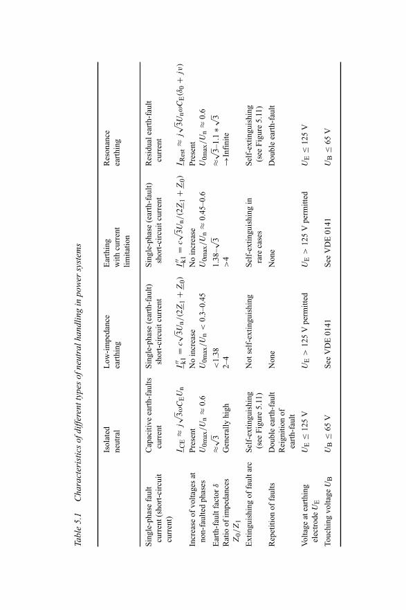
Tabl
e5.
1C
hara
cter
istic
sof
diffe
rent
type
sof
neut
ralh
andl
ing
inpo
wer
syst
ems
Isol
ated
Low
-im
peda
nce
Ear
thin
gR
eson
ance
neut
ral
eart
hing
with
curr
ent
eart
hing
limita
tion
Sing
le-p
hase
faul
tC
apac
itive
eart
h-fa
ults
Sing
le-p
hase
(ear
th-f
ault)
Sing
le-p
hase
(ear
th-f
ault)
Res
idua
lear
th-f
ault
curr
ent(
shor
t-ci
rcui
tcu
rren
tsh
ort-
circ
uitc
urre
ntsh
ort-
circ
uitc
urre
ntcu
rren
tcu
rren
t)I
CE
≈j√ 3ω
CE
Un
I′′ k1
=c√ 3U
n/(2
Z1
+Z
0)
I′′ k1
=c√ 3U
n/(2
Z1
+Z
0)
IR
est≈
j√ 3U
nω
CE
(δ0
+jv)
Incr
ease
ofvo
ltage
sat
Pres
ent
No
incr
ease
No
incr
ease
Pres
ent
non-
faul
ted
phas
esU
0max
/U
n≈
0.6
U0m
ax/U
n<
0.3–
0.45
U0m
ax/U
n≈
0.45
–0.6
U0m
ax/U
n≈
0.6
Ear
th-f
ault
fact
orδ
≈√ 3<
1.38
1.38
–√ 3≈√ 3–
1.1
∗√ 3R
atio
ofim
peda
nces
Gen
eral
lyhi
gh2–
4>
4→
Infi
nite
Z0/Z
1
Ext
ingu
ishi
ngof
faul
tarc
Self
-ext
ingu
ishi
ngN
otse
lf-e
xtin
guis
hing
Self
-ext
ingu
ishi
ngin
Self
-ext
ingu
ishi
ng(s
eeFi
gure
5.11
)ra
reca
ses
(see
Figu
re5.
11)
Rep
etiti
onof
faul
tsD
oubl
eea
rth-
faul
tN
one
Non
eD
oubl
eea
rth-
faul
tR
eign
ition
ofea
rth-
faul
t
Vol
tage
atea
rthi
ngU
E≤
125
VU
E>
125
Vpe
rmitt
edU
E>
125
Vpe
rmitt
edU
E≤
125
Vel
ectr
ode
UE
Touc
hing
volta
geU
BU
B≤
65V
See
VD
E01
41Se
eV
DE
0141
UB
≤65
V
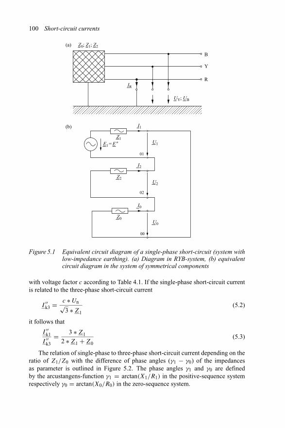
100 Short-circuit currents
R
Y
B
Z0; Z1; Z2
IR
UY; UB
(a)
U1
U2
U0
I1
I2
I0
Z1
Z2
Z0
E1 = E 0
01
02
00
(b)
Figure 5.1 Equivalent circuit diagram of a single-phase short-circuit (system withlow-impedance earthing). (a) Diagram in RYB-system, (b) equivalentcircuit diagram in the system of symmetrical components
with voltage factor c according to Table 4.1. If the single-phase short-circuit currentis related to the three-phase short-circuit current
I ′′k3 = c ∗ Un√
3 ∗ Z1
(5.2)
it follows that
I ′′k1
I ′′k3
= 3 ∗ Z1
2 ∗ Z1 + Z0(5.3)
The relation of single-phase to three-phase short-circuit current depending on theratio of Z1/Z0 with the difference of phase angles (γ1 − γ0) of the impedancesas parameter is outlined in Figure 5.2. The phase angles γ1 and γ0 are definedby the arcustangens-function γ1 = arctan(X1/R1) in the positive-sequence systemrespectively γ0 = arctan(X0/R0) in the zero-sequence system.
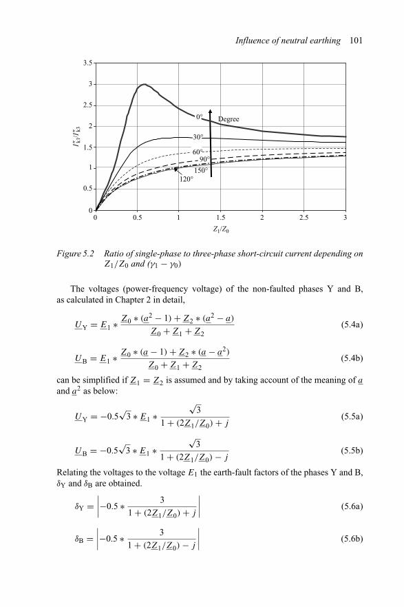
Influence of neutral earthing 101
0
0.5
1
1.5
2
2.5
3
3.5
0 0.5 1 1.5 2 2.5 3
Z1/Z0
Degree
I0 k1/
I0 k3
0°
30°
60°90°
120°150°
Figure 5.2 Ratio of single-phase to three-phase short-circuit current depending onZ1/Z0 and (γ1 − γ0)
The voltages (power-frequency voltage) of the non-faulted phases Y and B,as calculated in Chapter 2 in detail,
UY = E1 ∗ Z0 ∗ (a2 − 1) + Z2 ∗ (a2 − a)
Z0 + Z1 + Z2(5.4a)
UB = E1 ∗ Z0 ∗ (a − 1) + Z2 ∗ (a − a2)
Z0 + Z1 + Z2(5.4b)
can be simplified if Z1 = Z2 is assumed and by taking account of the meaning of a
and a2 as below:
UY = −0.5√
3 ∗ E1 ∗√
3
1 + (2Z1/Z0) + j(5.5a)
UB = −0.5√
3 ∗ E1 ∗√
3
1 + (2Z1/Z0) − j(5.5b)
Relating the voltages to the voltage E1 the earth-fault factors of the phases Y and B,δY and δB are obtained.
δY =∣∣∣∣−0.5 ∗ 3
1 + (2Z1/Z0) + j
∣∣∣∣ (5.6a)
δB =∣∣∣∣−0.5 ∗ 3
1 + (2Z1/Z0) − j
∣∣∣∣ (5.6b)
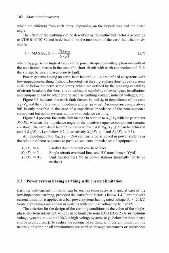
102 Short-circuit currents
which are different from each other, depending on the impedances and the phaseangle.
The effect of the earthing can be described by the earth-fault factor δ accordingto VDE 0141/07.89 and is defined to be the maximum of the earth-fault factors δYand δB
δ = MAX{δY; δB} = ULE max
U/√
3(5.7)
where ULEmax is the highest value of the power-frequency voltage phase-to-earth ofthe non-faulted phases in the case of a short-circuit with earth connection and U isthe voltage between phases prior to fault.
Power systems having an earth-fault factor δ < 1.4 are defined as systems withlow-impedance earthing. It should be noted that the single-phase short-circuit currentsshall be below the permissible limits, which are defined by the breaking capabilityof circuit-breakers, the short-circuit withstand capability of switchgear, installationsand equipment and by other criteria such as earthing voltage, induced voltages, etc.
Figure 5.3 indicates the earth-fault factors δY and δB in dependence of the ratioZ1/Z0 and the difference of impedance angles (γ1 − γ0). An impedance angle above90◦ is only possible in the case of a capacitive impedance of the zero-sequencecomponent but not in systems with low-impedance earthing.
Figure 5.4 presents the earth-fault factor δ in relation to X0/X1 with the parameterR0/X0, whereas the impedance angle in the positive-sequence component remainsconstant. The earth-fault factor δ remains below 1.4 if X0/X1 ≤ 5 can be achievedand if R0/X0 is kept below 0.2 (alternatively X0/X1 ≤ 4 and R0/X0 < 0.3).
An impedance ratio X0/X1 = 2–4 can easily be achieved in power systems asthe relation of zero-sequence to positive-sequence impedances of equipment is
X0/X1 ≈ 4 Parallel double-circuit overhead linesX0/X1 ≈ 3 Single-circuit overhead lines and HV-transformers Yy(d)X0/X1 ≈ 0.3 Unit transformers Yd in power stations (normally not to be
earthed)
5.3 Power system having earthing with current limitation
Earthing with current limitation can be seen in some cases as a special case of thelow-impedance earthing, provided the earth-fault factor is below 1.4. Earthing withcurrent limitation is applied in urban power systems having rated voltage Un ≤ 20 kV.Some applications are known in systems with nominal voltage up to 132 kV.
The criterion for the design of the earthing conditions is the value of the single-phase short-circuit current, which can be limited to some kA (1 kA or 2 kA) in medium-voltage systems or to some 10 kA in high-voltage systems (e.g., below the three-phaseshort-circuit current). To realise the scheme of earthing with current limitation, theneutrals of some or all transformers are earthed through reactances or resistances
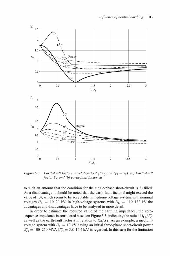
Influence of neutral earthing 103
3
3
0
0.5
1
1.5
2
2.5
0 0.5 1 1.5 2 2.5Z1/Z0
dY
dB
120°
90°
60°
30°150°
0°Degree
(a)
(b)
0
0.5
1
1.5
2
2.5
3
3.5
4
0 0.5 1 1.5 2 2.5Z1/Z0
150°120° 90°60°
30°
0° Degree
Figure 5.3 Earth-fault factors in relation to Z1/Z0 and (γ1 − γ0). (a) Earth-faultfactor δY and (b) earth-fault factor δB
to such an amount that the condition for the single-phase short-circuit is fulfilled.As a disadvantage it should be noted that the earth-fault factor δ might exceed thevalue of 1.4, which seems to be acceptable in medium-voltage systems with nominalvoltages Un = 10–20 kV. In high-voltage systems with Un = 110–132 kV theadvantages and disadvantages have to be analysed in more detail.
In order to estimate the required value of the earthing impedance, the zero-sequence impedance is considered based on Figure 5.5, indicating the ratio of I ′′
k1/I ′′k3
as well as the earth-fault factor δ in relation to X0/X1. As an example, a medium-voltage system with Un = 10 kV having an initial three-phase short-circuit powerS′′
k3 = 100–250 MVA (I ′′k3 = 5.8–14.4 kA) is regarded. In this case for the limitation

104 Short-circuit currents
0.6
0.8
1
1.2
1.4
1.6
1.8
0 1 2 3 4 5 6 7 8 9 10 11 12X0/X1
0.01
0.02
0.5
1.02.0
3.0
R0 /X0
d
Figure 5.4 Earth-fault factor δ depending on X0/X1 for different ratios R0/X0 andR1/X1 = 0.01
–12 –10 –8 –6 –4 –2 0
X0/X1
2 4 6 8 10 12
2.5
2.0
1.5
I� k1
I �k1/I �k3
I� k3
1.0
0.5
0
d
d;
d
3
Low-impedanceearthing
30.8
Figure 5.5 Earth-fault factor δ and ratio I ′′k1/I ′′
k3 depending on X0/X1
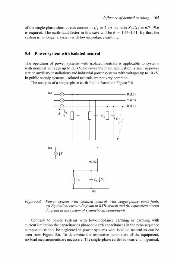
Influence of neutral earthing 105
of the single-phase short-circuit current to I ′′k1 = 2 kA the ratio X0/X1 = 6.7–19.6
is required. The earth-fault factor in this case will be δ = 1.44–1.61. By this, thesystem is no longer a system with low-impedance earthing.
5.4 Power system with isolated neutral
The operation of power systems with isolated neutrals is applicable to systemswith nominal voltages up to 60 kV, however the main application is seen in powerstation auxiliary installations and industrial power systems with voltages up to 10 kV.In public supply systems, isolated neutrals are not very common.
The analysis of a single-phase earth-fault is based on Figure 5.6.
~
~
~
E Un
GE
B (L3)
Y (L2)
R (L1)
CE3
=
~ E1
GE CE U0
01/02
00
(a)
(b)
Figure 5.6 Power system with isolated neutral with single-phase earth-fault.(a) Equivalent circuit diagram in RYB-system and (b) equivalent circuitdiagram in the system of symmetrical components
Contrary to power systems with low-impedance earthing or earthing withcurrent limitation the capacitances phase-to-earth capacitances in the zero-sequencecomponent cannot be neglected in power systems with isolated neutral as can beseen from Figure 5.6. To determine the respective parameters of the equipment,no-load measurements are necessary. The single-phase earth-fault current, in general,
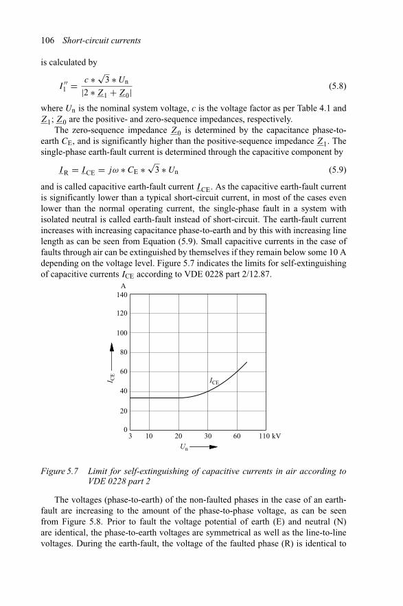
106 Short-circuit currents
is calculated by
I ′′1 = c ∗ √
3 ∗ Un
|2 ∗ Z1 + Z0|(5.8)
where Un is the nominal system voltage, c is the voltage factor as per Table 4.1 andZ1; Z0 are the positive- and zero-sequence impedances, respectively.
The zero-sequence impedance Z0 is determined by the capacitance phase-to-earth CE, and is significantly higher than the positive-sequence impedance Z1. Thesingle-phase earth-fault current is determined through the capacitive component by
I R = I CE = jω ∗ CE ∗ √3 ∗ Un (5.9)
and is called capacitive earth-fault current I CE. As the capacitive earth-fault currentis significantly lower than a typical short-circuit current, in most of the cases evenlower than the normal operating current, the single-phase fault in a system withisolated neutral is called earth-fault instead of short-circuit. The earth-fault currentincreases with increasing capacitance phase-to-earth and by this with increasing linelength as can be seen from Equation (5.9). Small capacitive currents in the case offaults through air can be extinguished by themselves if they remain below some 10 Adepending on the voltage level. Figure 5.7 indicates the limits for self-extinguishingof capacitive currents ICE according to VDE 0228 part 2/12.87.
140
100
80
60
40
20
3 10 20 30 60
Un
ICEI CE
110 kV0
120
A
Figure 5.7 Limit for self-extinguishing of capacitive currents in air according toVDE 0228 part 2
The voltages (phase-to-earth) of the non-faulted phases in the case of an earth-fault are increasing to the amount of the phase-to-phase voltage, as can be seenfrom Figure 5.8. Prior to fault the voltage potential of earth (E) and neutral (N)are identical, the phase-to-earth voltages are symmetrical as well as the line-to-linevoltages. During the earth-fault, the voltage of the faulted phase (R) is identical to
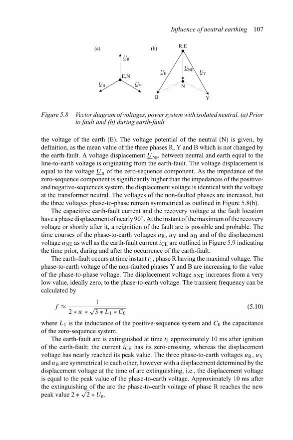
Influence of neutral earthing 107
UR
UYUB
E,N
R;E
N
B Y
UB UYUNE
(a) (b)
Figure 5.8 Vector diagram of voltages, power system with isolated neutral. (a) Priorto fault and (b) during earth-fault
the voltage of the earth (E). The voltage potential of the neutral (N) is given, bydefinition, as the mean value of the three phases R, Y and B which is not changed bythe earth-fault. A voltage displacement UNE between neutral and earth equal to theline-to-earth voltage is originating from the earth-fault. The voltage displacement isequal to the voltage U0 of the zero-sequence component. As the impedance of thezero-sequence component is significantly higher than the impedances of the positive-and negative-sequences system, the displacement voltage is identical with the voltageat the transformer neutral. The voltages of the non-faulted phases are increased, butthe three voltages phase-to-phase remain symmetrical as outlined in Figure 5.8(b).
The capacitive earth-fault current and the recovery voltage at the fault locationhave a phase displacement of nearly 90◦. At the instant of the maximum of the recoveryvoltage or shortly after it, a reignition of the fault arc is possible and probable. Thetime courses of the phase-to-earth voltages uR, uY and uB and of the displacementvoltage uNE as well as the earth-fault current iCE are outlined in Figure 5.9 indicatingthe time prior, during and after the occurrence of the earth-fault.
The earth-fault occurs at time instant t1, phase R having the maximal voltage. Thephase-to-earth voltage of the non-faulted phases Y and B are increasing to the valueof the phase-to-phase voltage. The displacement voltage uNE increases from a verylow value, ideally zero, to the phase-to-earth voltage. The transient frequency can becalculated by
f ≈ 1
2 ∗ π ∗ √3 ∗ L1 ∗ C0
(5.10)
where L1 is the inductance of the positive-sequence system and C0 the capacitanceof the zero-sequence system.
The earth-fault arc is extinguished at time t2 approximately 10 ms after ignitionof the earth-fault; the current iCE has its zero-crossing, whereas the displacementvoltage has nearly reached its peak value. The three phase-to-earth voltages uR, uYand uB are symmetrical to each other, however with a displacement determined by thedisplacement voltage at the time of arc extinguishing, i.e., the displacement voltageis equal to the peak value of the phase-to-earth voltage. Approximately 10 ms afterthe extinguishing of the arc the phase-to-earth voltage of phase R reaches the newpeak value 2 ∗ √
2 ∗ Un.

108 Short-circuit currents
2.0
1.5
1.0
0.5
0
–0.5
–1.5
–1.0
3uY
uY
uY
uB
uB
uB
Voltages
Earth-faultcurrent
t1
iCE
t2 t3
uR
uR
uR
uNE
uNE
u/U^^
Figure 5.9 Time courses of phase-to-earth voltages, displacement voltage andearth-fault current. System with isolated neutral, earth-fault in phase R
This voltage may cause a reignition of the earth-fault due to the very high-voltagestress. This reignition takes place at time instant t3 with the phase-to-earth voltageof phase R having its peak value. The voltages of the non-faulted phases againare increasing, this time starting from a higher value and reaching the peak valuenearly to
√3 ∗ √
2 ∗ Un.Besides the power-frequency overvoltage in the case of an earth-fault, the transient
overvoltage with frequency according to Equation (5.10) has to be considered. Theovervoltage factor kLE, taking account of both types of overvoltages, is given by themaximal peak voltage related to the peak value of phase-to-earth voltage
kLE = uü√2 ∗ U/
√3
(5.11)
where uü is the maximal peak voltage during the earth fault and U the phase-to-earthvoltage (power-frequency).
In theory, the overvoltage factor after multiple reignition of the earth-fault canreach kLE = 3.5. Due to the system damping, the overvoltage factor will be belowkLE < 3 in most of the cases.
5.5 Power system with resonance earthing (Petersen-coil)
5.5.1 General
Power systems with resonance earthing are widely in operation in Central Europeancountries. The German power system statistic [3] indicates that 87 per cent of the

Influence of neutral earthing 109
MV-systems having nominal voltages Un = 10–30 kV and nearly 80 per cent of110-kV-systems are operated with resonance earthing (Criteria: Total line lengths).Some MV-systems are operated with a combined scheme of resonance earthingunder normal operating conditions and low-impedance earthing in case of earth-fault. Resonance earthing, therefore, is the dominating type of system earthing inGermany for power systems with voltage 10 kV up to 110 kV. In other countries suchas India, South Africa and China, power systems with resonance earthing have gainedan increasing importance during the last decades, however are still not so commonas systems with low-voltage earthing.
Resonance earthing is realised by earthing of one or several neutrals of trans-formers through reactances (Petersen-coils), normally adjustable, which will be set inresonance to the phase-to-earth capacitances of the system. The principal arrangementof a power system with resonance earthing is outlined in Figure 5.10.
The impedances of transformers and lines of the positive-sequence component canbe neglected compared with those of the zero-sequence component due to the orderof magnitude of the impedances. The admittance of the zero-sequence component is
~
~
~
E Un
U0LD
GE
B (L3)
Y (L2)
R (L1)
CE
3=
~ E1
GECE
U0
01/02
00
(a)
(b)
310
3LD
3RD
Figure 5.10 System with resonance earthing, earth-fault in phase R. (a) Equivalentdiagram in RYB-system and (b) equivalent diagram in the system ofsymmetrical components

110 Short-circuit currents
given by
Y 0 = jω ∗ CE + 1
3 ∗ RD + j3 ∗ XD+ GE (5.12)
where CE is the phase-to-earth capacitance of the system, ω is the angular frequencyof the system, RD is the resistance of the Petersen-coil, XD is the reactance of thePetersen-coil XD = ωL and GE is the admittance representing the phase-to-earth linelosses.
After some conversions it follows that
Y 0 = jω ∗ CE ∗(
1 − 1
3 ∗ ω2 ∗ LD ∗ CE ∗ (1 − j(RD/XD))
)+ GE (5.13a)
The impedance of the Petersen-coil appears with its threefold value in the zero-sequence component [1]. It is assumed that RD � XD and that the losses of thePetersen-coil are summed up with the phase-to-earth losses and are represented asadmittance GE of the line. The admittance in the zero-sequence component is then
Y 0 = jω ∗ CE ∗(
1 − 1
3 ∗ ω2 ∗ LD ∗ CE
)+ GE (5.13b)
The maximal impedance is obtained if the imaginary part as per Equation (5.13b) isequal to zero; the current from the Petersen-coil ID is equal to the capacitive currentICE of the system. As indicated in Figure 5.10, the capacitance phase-to-earth CE,the reactance 3LD and the ohmic losses R0 = 1/GE are forming a parallel resonancecircuit with the resonance frequency
ω = 1√3 ∗ LD ∗ CE
(5.14)
The resonance frequency in the case of resonance earthing shall be the nominalfrequency of f = 50 Hz or f = 60 Hz, respectively. Defining the detuning factor v
v = ID − ICE
ICE= 1 − 1
3 ∗ ω2 ∗ LD ∗ CE(5.15a)
and the damping d
d = GE
ω ∗ CE(5.15b)
the admittance of the zero-sequence component is given by
Y 0 = ω ∗ CE ∗ (jv + d) (5.16)
The admittance will be minimal and the impedance will be maximal in the case ofresonance tuning (v = 0). The earth-fault current I Res, in general, is obtained by
I Res ≈ √3 ∗ Un ∗ ω ∗ CE ∗ (jv + d) (5.17a)
In case of resonance tuning (v = 0) the earth-fault current is a pure ohmic current
I Res ≈ √3 ∗ Un ∗ ω ∗ CE ∗ d (5.17b)

Influence of neutral earthing 111
The phase-to-earth voltages of the non-faulted phases increase to the value of thephase-to-phase voltage in the case of a single-phase earth-fault, which is furthermoreincreased due to asymmetrical system voltages resulting in a higher displacementvoltage between neutral and earth. In order to avoid the high voltages in the case ofexact resonance tuning a small detuning of 8–12 per cent is chosen in practice.
The task of resonance earthing is to reduce the earth-fault current at the faultlocation to the minimum or nearly to the minimum by adjusting the Petersen-coil toresonance or nearly to resonance with the phase-to-earth capacitances. The ohmicpart of the residual current IRes cannot be compensated by this. If the residual currentis small enough, a self-extinguishing of the arc at the fault location is possible.VDE 0228 part 2:12.87 defines the limits for self-extinguishing of residual currentsIRes (and capacitive earth-fault currents ICE) for different voltage levels as outlined inFigure 5.11. It can be seen from Figure 5.11 that the limit for ohmic currents, e.g., in30-kV-systems, is twice the limit for capacitive currents.
The Petersen-coil can only be tuned for one frequency (nominal frequency) inresonance; harmonics present in the system voltage are increasing the residual currentat the fault location.
As the phase-to-earth capacitances are changing during system operation, e.g.,due to switching of lines, the Petersen-coil has to be changed also to keep systemoperation with resonance tuning. Reliable criteria have to be established to tune thePetersen-coil in resonance with the phase-to-earth capacitances.
140
120
A
100
80
60
40
20
03 10 20 30
Un
60 110 kV
ICE
IRes
I Res
; IC
E
Figure 5.11 Current limits according to VDE 0228 part 2:12.87 of ohmic currentsIRes and capacitive currents ICE

112 Short-circuit currents
5.5.2 Calculation of displacement voltage
In real power systems, the phase-to-earth capacitances are unequal, e.g., in the case ofa transmission line due to different clearance of the phase-wires above ground or thecase of cables due to manufacturing tolerances. Under normal operating conditions,a displacement voltage between transformer neutral and earth UNE can be measured.As mentioned in previous sections, this voltage is equal to the voltage U0 in the zero-sequence component. The calculation of the displacement voltage can be carriedout in the RYB-system (Figure 5.12(a)) as well as with the system of symmetricalcomponents (Figure 5.12(b)).
Based on Figure 5.12(a) the displacement voltage is calculated as
UNE = Un√3
∗ jω ∗ (CRE + a2 ∗ CYE + a ∗ CBE)
jω ∗ (CRE + CYE + CBE) − j(1/(ω ∗ LD)) + 3 ∗ GE(5.18)
~
~
~
E Un
U0
LD
GEΔC
B (L3)
Y (L2)
R (L1)
CRE
3=
~ E1
GECE
U0
01/02
00
(a)
(b)
310
3LD
13
ΔCE
0
1 + 2
= UNE
CBE CYE
Figure 5.12 Equivalent circuit diagram of a power system with asymmetricalphase-to-earth capacitances. (a) Equivalent circuit diagram in theRYB-system and (b) equivalent circuit diagram in the system ofsymmetrical components
Influence of neutral earthing 113
where Un is the nominal system voltage, ω is the angular frequency of the system, CRE;CYE; CBE are the line-to-earth capacitances as per Figure 5.12(a), LD is the inductanceof the Petersen-coil and GE is the admittance representing the phase-to-earth linelosses.
If the phase-to-earth capacitances are different and if the asymmetry is assumedto be placed in phases R and Y, the capacitances are
CRE = CE + CRE (5.19a)
CYE = CE + CYE (5.19b)
CBE = CE (5.19c)
where CRE; CYE are the asymmetry of the line-to-earth capacitances.The displacement voltage is given by
UNE = Un√3
∗ CRE + a2 ∗ CYE
(3 ∗ CE + CRE + CYE) − j(1/(ω ∗ LD)) + 3 ∗ GE(5.20)
Defining the asymmetry factor k
k = CRE + a2 ∗ CYE + a ∗ CBE
CRE + CYE + CBE
= CRE + a2 ∗ CYE
3 ∗ CE + CRE + CYE(5.21a)
the system damping d
d = 3 ∗ GE
ω ∗ (CRE + CYE + CBE)
= 3 ∗ GE
ω ∗ (3 ∗ CE + CRE + CYE)(5.21b)
and the detuning factor v
v = 1/(ω ∗ LD) − ω ∗ (CRE + CYE + CBE)
ω ∗ (CRE + CYE + CBE)
= 1/(ω ∗ LD) − ω ∗ (3 ∗ CE + CRE + CYE)
ω ∗ (3 ∗ CRE + CRE + CYE)(5.21c)
the displacement voltage UNE is calculated by
UNE = Un√3
∗ k
v + jd(5.22)
Assuming the asymmetrical capacitance CE concentrated in phase R (CE �CRE and CE � CYE) the displacement voltage UNE, equal to the voltagein the zero-sequence component U0, is calculated with the system of symmetrical

114 Short-circuit currents
components based on Figure 5.12(b)
U0 = Un√3
∗ jω ∗ CE
jω ∗ 3 ∗ CE∗ 1
1 − (1/(3 ∗ ω2 ∗ LD ∗ CE)) − j(GE(ω ∗ CE))
(5.23)
The asymmetry factor k, the system damping d and the detuning factor v can becalculated based on these assumptions:
k = CE
3 ∗ CE(5.24a)
d = GE
ω ∗ CE(5.24b)
v = 1 − 1
3 ∗ ω2 ∗ LD ∗ CE(5.24c)
The displacement voltage UNE, equal to the voltage in the zero-sequence componentU0, is calculated by
UNE = U0 = Un√3
∗ k
v + jd(5.25)
The polar plot of the displacement voltage UNE as per Equations (5.22) and (5.25)and outlined in Figure 5.13 indicates a circular plot through the zero point. Thephase angle of the diameter location at v = 0 is determined by the phase angle of thecapacitive asymmetry. The diameter of the polar plot is defined as per Equation (5.25)as the ratio of capacitive asymmetry k and damping d.
The capacitive asymmetry is comparatively high in power systems with overheadtransmission lines, resulting in a sufficient high-displacement voltage. Cable systemshave a comparative small asymmetry, resulting for most of the cable systems in
+ Re
+ Im
UR
UY
UB
y = 0
Figure 5.13 Polar plot of the displacement voltage in a power system with resonanceearthing

Influence of neutral earthing 115
an insufficient low-displacement voltage and problems while tuning the Petersen-coil into resonance. Capacitors between two phases or between one phase and earthwill increase the displacement voltage to the required value.
5.5.3 Tuning of the Petersen-coil
The Petersen-coil can be constructed as a plunger-coil (tuning-coil) with continuousadjustment of the reactance, which can be tuned into resonance by successive opera-tion. The displacement voltage measured at the Petersen-coil is maximal in the caseof resonance tuning; the value depends on the capacitive asymmetry and on the lossesof the reactor. The earth-fault current will be minimal in this case and the power fre-quency component of the capacitive earth-fault current is compensated by the reactivecurrent of the Petersen-coil. Figure 5.14 indicates the displacement voltage and theresidual current for different tuning of the reactor.
The displacement voltage shall be limited to UNE < 10 kV. It is obvious that theresidual current is increased as can be seen from Figure 5.14. Residual currentsabove 130 A in 110-kV-systems, respectively 60 A in 10-kV-systems, are notself-extinguishing; both parameters define the tuning limits of the Petersen-coil asindicated in Figure 5.14. Tuning of the Petersen-coil can be done in such a waythat the resonance circuit is either capacitive (undertuning; v < 0), resulting in an
Umax
ULE
UminUB
U0
UY
Unsymmetry
IRes IRes< 130 A
U0 < 10 kV
–30% –15% 0 15% 30%V
UR
UL
EU
0;I R
es
ULE
100%
Max. voltage Umax
Min. voltage Umin
Max. voltage unbalance ku
Max. displacement voltage Umin
Max. residual earth-fault current IRes
Permissibletuning range
Figure 5.14 Voltages and residual current in the case of an earth-fault; displace-ment voltage without earth-fault
116 Short-circuit currents
ohmic-capacitive residual current or inductive (overtuning; v > 0), resulting in anohmic-inductive residual current at the earth-fault location. A small overtuning (over-compensation) up to v = 10% is often recommended as the displacement voltagewill not increase in the case of switching of lines, because the capacitances will bereduced by this and the resonance circuit will be detuned without any further adjust-ment. The limits for the displacement voltage and the residual current as indicated inFigure 5.14 have to be guaranteed even under outage conditions.
Figure 5.14 also indicates the phase-to-earth voltages for different tuning factors(system parameters are: Un = 110 kV; ICE = 520 A; d = 3%; k = 1.2%) whichalso limit the range of detuning of the Petersen-coil. Assuming a minimal permissiblevoltage of Umin = 0.9 ∗ (Un/
√3) according to IEC 60038, a maximal permissible
voltage according to IEC 60071-1 of Umax = 123 kV/√
3 and a permissible asym-metry of the three voltages according to DIN EN 50160 of p = 2% it can be seenthat the permissible tuning range of the Petersen-coil is v = 12–22%.
All considerations carried out so far are based on a linear current-voltage-characteristic of the Petersen-coil. Figure 5.15 indicates the non-linear characteristicof a Petersen-coil (Ur = 20 kV/
√3; Ir = 640 A) for minimal and maximal adjustment.
Due to the non-linear characteristic, the minimum of the residual current is notachieved at the maximal displacement voltage (adjustment criteria of the Petersen-coil). The difference is typically in the range of 3–15% of the rated current as outlinedin Figure 5.16.
5.6 Handling of neutrals on HV-side and LV-side of transformers
Special attention must be placed while selecting the type of neutral handling onHV-side and LV-side of transformers. The neutral earthing on one side of the trans-former has an influence on the system performance on the other side, in case ofearth-faults or single-phase short-circuits as the voltages in the zero-sequence com-ponent are transferred from one side of the transformer to the other. The neutralearthing of a 110/10-kV-transformer (vector group Yyd) according to Figure 5.17 istaken as an example. It is assumed [15] that XC0/R0 = 0.1–0.05, first value is appliedfor systems with overhead lines, second value with cables.
The impedances ZE1 and ZE2 as per Figure 5.17 representing the earthing aredifferent depending on the type of neutral earthing. In case of a single-phase fault inthe high-voltage system (110 kV), the voltage U0 in the zero-sequence componentis transferred to the medium-voltage system (10 kV) with the same amount. Similarconsideration indicates that the voltage in the zero-sequence component is transferredto the HV-side in case of a single-phase fault in the LV-system. In both cases, a faultcurrent is measured in the system, having no fault. Table 5.2 indicates the results ofa fault-analysis [16] with the voltages transferred through the transformer in case offaults.
The 110/10-kV-transformer can be operated with low-impedance earthing on bothsides if a third winding (compensation winding, vector group d) is available, as can beseen from Table 5.2. If the transformer is not equipped with compensation winding,
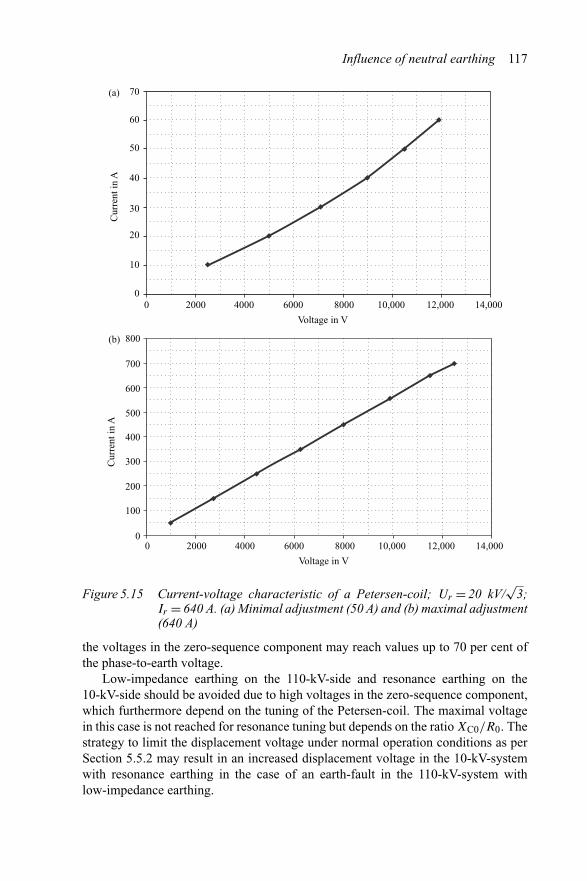
Influence of neutral earthing 117
70
60
50
40
Cur
rent
in A
30
20
10
00 2000 4000 6000 8000
Voltage in V
10,000 12,000 14,000
(a)
800
700
600
500
Cur
rent
in A
400
300
200
100
00 2000 4000 6000 8000
Voltage in V
10,000 12,000 14,000
(b)
Figure 5.15 Current-voltage characteristic of a Petersen-coil; Ur = 20 kV/√
3;Ir = 640 A. (a) Minimal adjustment (50 A) and (b) maximal adjustment(640 A)
the voltages in the zero-sequence component may reach values up to 70 per cent ofthe phase-to-earth voltage.
Low-impedance earthing on the 110-kV-side and resonance earthing on the10-kV-side should be avoided due to high voltages in the zero-sequence component,which furthermore depend on the tuning of the Petersen-coil. The maximal voltagein this case is not reached for resonance tuning but depends on the ratio XC0/R0. Thestrategy to limit the displacement voltage under normal operation conditions as perSection 5.5.2 may result in an increased displacement voltage in the 10-kV-systemwith resonance earthing in the case of an earth-fault in the 110-kV-system withlow-impedance earthing.
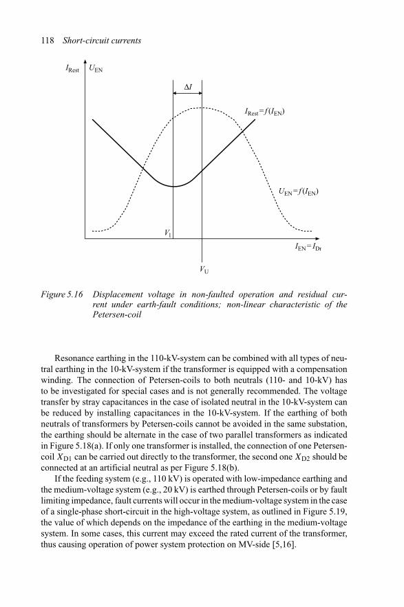
118 Short-circuit currents
IRest
IRest = f (IEN)
UEN
IEN = IDr
ΔI
UEN = f (IEN)
VU
Vl
Figure 5.16 Displacement voltage in non-faulted operation and residual cur-rent under earth-fault conditions; non-linear characteristic of thePetersen-coil
Resonance earthing in the 110-kV-system can be combined with all types of neu-tral earthing in the 10-kV-system if the transformer is equipped with a compensationwinding. The connection of Petersen-coils to both neutrals (110- and 10-kV) hasto be investigated for special cases and is not generally recommended. The voltagetransfer by stray capacitances in the case of isolated neutral in the 10-kV-system canbe reduced by installing capacitances in the 10-kV-system. If the earthing of bothneutrals of transformers by Petersen-coils cannot be avoided in the same substation,the earthing should be alternate in the case of two parallel transformers as indicatedin Figure 5.18(a). If only one transformer is installed, the connection of one Petersen-coil XD1 can be carried out directly to the transformer, the second one XD2 should beconnected at an artificial neutral as per Figure 5.18(b).
If the feeding system (e.g., 110 kV) is operated with low-impedance earthing andthe medium-voltage system (e.g., 20 kV) is earthed through Petersen-coils or by faultlimiting impedance, fault currents will occur in the medium-voltage system in the caseof a single-phase short-circuit in the high-voltage system, as outlined in Figure 5.19,the value of which depends on the impedance of the earthing in the medium-voltagesystem. In some cases, this current may exceed the rated current of the transformer,thus causing operation of power system protection on MV-side [5,16].

Influence of neutral earthing 119
~
~ ~
~
~
~
~ ~
E
ZE1
X1Q
X1Q
X0Q X01T + 3ZE1 X12T + 3ZE2
C1Q X13TU1F
C1Q
C0Q C0 U0U0F R0X03T
C1
01
02
00
C1
X13TU2F
X11T
X11T
X12T
X12T
ZE2
110-kV-system Transformer 10-kV-systemB
Y
R
k1
(b)
(a)
Figure 5.17 Transformation of voltage in the zero-sequence component of trans-formers in the case of single-phase faults. (a) Equivalent circuitdiagram in RYB-system and (b) equivalent circuit diagram in the systemof symmetrical components
5.7 Examples
5.7.1 Increase of displacement voltage for systems with resonance earthing
The capacitive asymmetry k of cable systems normally is below k < 0.1%; thesystem damping is in the range of d ≈ 2–4% resulting in a displacement voltage

120 Short-circuit currents
Table 5.2 Voltages in the zero-sequence component U0 transferred through110/10-kV-transformer in the case of single-phase fault in the 110-kV-system according to Figure 5.17; Un: nominal system voltage
10-kV-system 110-kV-system and compensation windingof the transformer
ZE2 Limitation Low-impedance earthing ResonanceIk1 u0 = U0/(Un/
√3) earthing
With Without Withcompensation compensation compensationwinding winding winding
Low-resistance earthing 0.2 0.6 0.03ZE2 = 0 �
Current limitation 2000 A 0.2 0.6 0.03ZE2 inductive 500 A 0.25 0.7 0.04Current limitation 2000 A 0.2 0.6 0.03ZE2 ohmic 500 A 0.2 0.6 0.03Resonance earthing <7 >10 <0.3Isolated neutral Voltage transfer through stray capacitances
which is too low for the operation of the resonance controller. For a given capacitiveasymmetry of k = 0.1% and system damping d = 2% the displacement voltagewill be UNE = 0.005 ∗ Un/
√3 for resonance tuning (v = 0%); if the detuning shall
be v = 5% the displacement voltage will be UNE = 0.002 ∗ Un/√
3 only [17].Resonance controller normally operates sufficiently if the displacement voltage isabove UNE > 0.03∗Un/
√3. The displacement voltage, therefore, had to be increased
by installing an additional capacitor in one phase [18]. The required capacitance CEfor different parameters is given in Table 5.3 for a 20-kV-system earthed throughPetersen-coil.
Documentation of system data normally do not indicate exact values of the line-to-earth capacitances CE in each phase, furthermore the system damping d, the exactlength of the cables and the non-linear characteristic of the Petersen-coil are alsounknown or only to an insufficient extent and are not suitable to determine the dis-placement voltage UNE without measurement. It should be noted that the systemdamping changes with the system load as well as in the case of a power system witha significant number of overhead lines and with external climatic conditions. It canbe deducted from this, that:
• the asymmetrical capacitance (absolute value)• the angle of the asymmetrical capacitance (with respect to the three phases)• the value of the displacement voltage, and• the resonance curve for different detuning factors
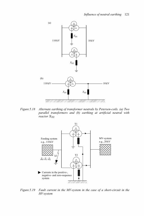
Influence of neutral earthing 121
XD1
XD1 XD2
XD2
110 kV
110 kV
10 kV
10 kV
(b)
(a)
Figure 5.18 Alternate earthing of transformer neutrals by Petersen-coils. (a) Twoparallel transformers and (b) earthing at artificial neutral withreactor XD2
Feeding systeme.g., 110 kV
Currents in the positive-,negative- and zero-sequencesystem
MV-systeme.g., 20 kV
Z0; Z1; Z2
T2k1
T1
Figure 5.19 Fault current in the MV-system in the case of a short-circuit in theHV-system
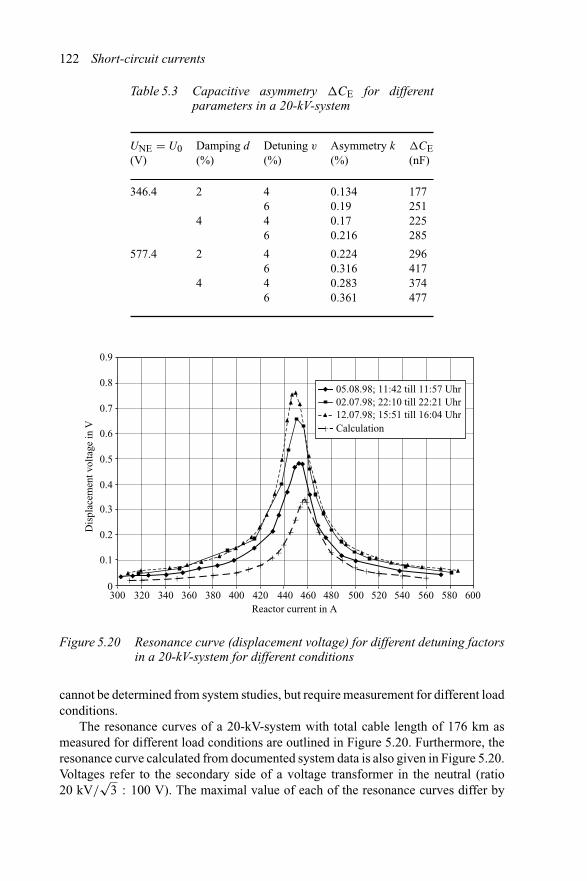
122 Short-circuit currents
Table 5.3 Capacitive asymmetry CE for differentparameters in a 20-kV-system
UNE = U0 Damping d Detuning v Asymmetry k CE(V) (%) (%) (%) (nF)
346.4 2 4 0.134 1776 0.19 251
4 4 0.17 2256 0.216 285
577.4 2 4 0.224 2966 0.316 417
4 4 0.283 3746 0.361 477
0.9
0.8
0.7
0.6
0.5
0.4
0.3
0.2
0.1
0300 320 340 360 400380 420 440 460
Reactor current in A
Dis
plac
emen
t vol
tage
in V
480 500 520 540 560 580 600
+++ ++ ++
+
+
+++++
++
+++
++++++
+
05.08.98; 11:42 till 11:57 Uhr02.07.98; 22:10 till 22:21 Uhr12.07.98; 15:51 till 16:04 UhrCalculation
Figure 5.20 Resonance curve (displacement voltage) for different detuning factorsin a 20-kV-system for different conditions
cannot be determined from system studies, but require measurement for different loadconditions.
The resonance curves of a 20-kV-system with total cable length of 176 km asmeasured for different load conditions are outlined in Figure 5.20. Furthermore, theresonance curve calculated from documented system data is also given in Figure 5.20.Voltages refer to the secondary side of a voltage transformer in the neutral (ratio20 kV/
√3 : 100 V). The maximal value of each of the resonance curves differ by

Influence of neutral earthing 123
12.212.112.011.911.811.7
11.611.511.411.3
11.2
10.910.8
250 275 300 325 350 375 400 425 450Reactor current in A
475 500 525 550 575 600 625
11.111.0
Lin
e-to
-ear
th v
olta
ges
in k
VU phase R
U phase Y
U phase B
Figure 5.21 Voltages in a 20-kV-system with resonance earthing for different tuningfactors. (a) Phase-to-earth voltages and (b) displacement voltage(resonance curve)
more than 60 per cent for different load conditions and is higher than the calculatedvalue. The resonance tuning (v = 0) of calculated and measured resonance curvesdiffers also by 6 per cent as can be seen from Figure 5.20.
A capacitance of CE = 173.3 nF was installed in phase B in order to increase thedisplacement voltage up to 3–5 per cent (350–580 V) of the nominal system voltagefor resonance tuning. The total phase-to-earth capacitance of the 20-kV-system wasdetermined to be CE = 44 μF. The results of measurement of the phase-to-earthvoltages and the displacement voltage for different detuning of the Petersen-coil areoutlined in Figure 5.21 (voltage transformer ratio 20 kV/
√3 : 100 V).
It can be seen from Figure 5.21 that the maximal displacement voltage is in therequired range between 3 and 5 per cent of the phase-to-earth voltage. For resonancetuning, the maximal phase-to-earth voltage appears in phase R with UR ≈ 12.1 kVand the minimal voltage in phase Y with UY ≈ 10.9 kV, which is only 94 per cent ofthe nominal phase-to-earth voltage. Exact resonance tuning shall be avoided in thissystem due to the low voltage in one phase and the resulting high asymmetry factor.
Other measures to increase the displacement voltage such as installation of areactor in one phase to earth and voltage additions are not considered in detailhere [19].
5.7.2 Limitation of single-phase short-circuit current by earthing throughimpedance
An urban 11.5-kV-system is fed from a 132-kV-system; both systems are pure cablesystems. The substations are equipped with four transformers each, having ratedvalues of Sr = 40 MVA, ukr1 = 14% and ukr0 = 16%. Both systems are earthed

124 Short-circuit currents
by low impedance in such a way that all transformer neutrals are solidly connectedto earth. The short-circuit current level in the 132-kV-system is high, whereas thesingle-phase short-circuit currents is higher than the three-phase short-circuit currents(I ′′
k3 ≈ 29.3 kA; I ′′k1 ≈ 37.3 kA). The maximal permissible short-circuit current in
the 132-kV-system is I ′′kmax = 40 kA; in the 11.5-kV-system I ′′
kmax = 25 kA. The132/11.5-kV-transformers cannot be operated in parallel due to the high short-circuitcurrents. In the case of low-impedance earthing the neutrals of each transformer, thesingle-phase short-circuit current of one transformer is I ′′
k1 = 15.04 kA in case of ashort-circuit at the 11.5-kV-busbar. In the case of two transformers in parallel, theshort-circuit current is increased to I ′′
k1 = 29.27 kA, which is above the maximalpermissible short-circuit current of the 11.5-kV-system.
The limitation of single-phase short-circuit currents to 25 kA in case two trans-formers shall be operated in parallel is possible by earthing of the 11.5-kV-transformerneutrals through a resistor having RE = 0.31 � or through a reactor havingXE = 0.1 � (see also Figure 11.13).
5.7.3 Design of an earthing resistor connected to an artificial neutral
The short-circuit limitation in a 20-kV-system having initial short-circuit powerS′′
kQ = 700 MVA and an impedance ratio Z0/Z1 = 4 is explained below. The single-phase short-circuit current in case of low-impedance earthing is I ′′
k1 = 12.1 kA. Thesingle-phase short-circuit current shall be limited to I ′′
k1max = 1.5 kA (I ′′k1 = 3I0)
realised by earthing through a resistor to be connected to an artificial neutral. As thecurrent through the artificial neutral is only one-third of the single-phase short-circuitcurrent, the rated power shall be
SrS min = 0.33 ∗ √3 ∗ I ′′
k1 max ∗ Un = 17.55 MVA
A transformer with vector group Zz is selected for the artificial neutral withSrS = 20 MVA; PCu = 1.3 kW and uk0 = 45% resulting in a required zero-sequenceimpedance of Z0S = 9 � (R0S = 3.75 �; X0S = 8.18 �). The required rating ofthe earthing resistor resulting from the calculation is RE = 4.21 �. The value of theinitial short-circuit power of the system has only a marginal effect on the rating ofthe earthing.
A typical design rating of the resistor is given below:
Rn = 4.21 � at 20◦C (Tolerance ±5 per cent or ±10 per cent); CrNi-alloyed steelIr = 1.5 kA, rated short-time duration t = 5 s or 10 sUr = 13.3 kVIsolation according to IEC 60071-1, Table 5.2: Um = 17.5 kV IP 00
5.7.4 Resonance earthing in a 20-kV-system
Figure 5.22 shows a 20-kV-system fed from two sides by one transformer in each ofthe substations S/S A and S/S B. The system is split at S/S C into two subsystems Aand B during summer months. During winter months, a part of system A is connectedto system B, but both systems are still operated separately.

Influence of neutral earthing 125
110 kV
50–5
00A
300
A
60–5
90A
190
A
S/S A System A
S/S C
System B
6.4 MW
S/S B110 kV
Figure 5.22 Equivalent circuit diagram of a 20-kV-system with resonance earthing
The 20-kV-system A is a pure cable-system having a total system length of 490 kmof the XLPE-type. The capacitive earth-fault current is calculated to be Ires = 453 A.The transformer in substation A has a rating of 12.5 MVA; current carrying capac-ity of the neutral is 361 A. The system shall be operated with resonance earthing,i.e., a reactor has to be installed in the neutral having a rated current of more than450 A to compensate the capacitive earth-fault current. It is obvious that the reac-tor cannot be connected to the neutral of the transformer in substation S/S A as therequired current for resonance earthing exceeds the permissible current of the trans-former neutral. An additional fixed reactor with rated current 300 A is installed insubstation S/S C and connected at an artificial neutral of a Zz-transformer.
System B is a pure cable-system as well, having a total system length of 386 kmof different type (XLPE and mass-impregnated cables); the earth-fault current iscalculated to be Ires = 632 A. The feeding transformer in substation B has a ratedpower Sr = 25 MVA and a current carrying capacity of the neutral of 721 A. Reso-nance earthing is done with a fixed reactor (190 A) in parallel with a tuning-reactor(60–590 A) capable of compensating the total capacitive earth-fault current ofsystem B.
Operation in wintertime differs from the described scheme as additional genera-tion in a combined-cycle plant is in operation with a power of 6.4 MW. In order toavoid back-feeding into the 110-kV-system additional load from system A is suppliedfrom system B. The capacitive earth-fault current of system A is reduced and the cur-rent in system B is increased accordingly (see Table 5.4 for details). As the earthingreactor in S/S C is connected in wintertime as well to system B, the compensationscheme with different reactors at different substations are capable of realising theresonance earthing for both systems under different operating conditions.
5.7.5 Calculation of capacitive earth-fault current and residual current
A 10-kV-system with isolated neutral (overhead lines, system length 170 km,C′
B = 9.5 nF/km; CE/CL = 5) shall be extended by cables. The existing earthing
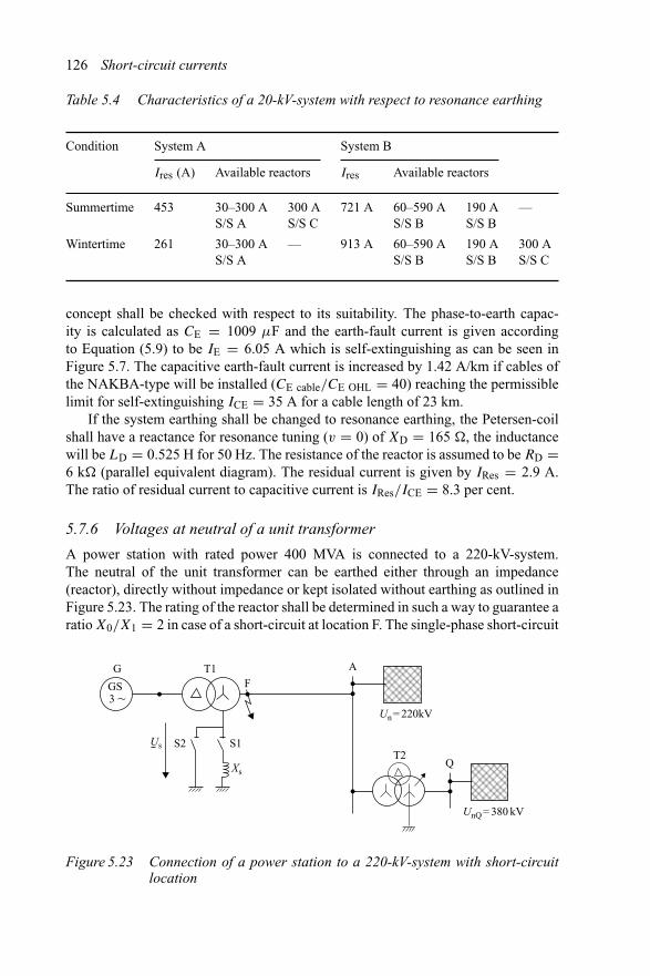
126 Short-circuit currents
Table 5.4 Characteristics of a 20-kV-system with respect to resonance earthing
Condition System A System B
Ires (A) Available reactors Ires Available reactors
Summertime 453 30–300 A 300 A 721 A 60–590 A 190 A —S/S A S/S C S/S B S/S B
Wintertime 261 30–300 A — 913 A 60–590 A 190 A 300 AS/S A S/S B S/S B S/S C
concept shall be checked with respect to its suitability. The phase-to-earth capac-ity is calculated as CE = 1009 μF and the earth-fault current is given accordingto Equation (5.9) to be IE = 6.05 A which is self-extinguishing as can be seen inFigure 5.7. The capacitive earth-fault current is increased by 1.42 A/km if cables ofthe NAKBA-type will be installed (CE cable/CE OHL = 40) reaching the permissiblelimit for self-extinguishing ICE = 35 A for a cable length of 23 km.
If the system earthing shall be changed to resonance earthing, the Petersen-coilshall have a reactance for resonance tuning (v = 0) of XD = 165 �, the inductancewill be LD = 0.525 H for 50 Hz. The resistance of the reactor is assumed to be RD =6 k� (parallel equivalent diagram). The residual current is given by IRes = 2.9 A.The ratio of residual current to capacitive current is IRes/ICE = 8.3 per cent.
5.7.6 Voltages at neutral of a unit transformer
A power station with rated power 400 MVA is connected to a 220-kV-system.The neutral of the unit transformer can be earthed either through an impedance(reactor), directly without impedance or kept isolated without earthing as outlined inFigure 5.23. The rating of the reactor shall be determined in such a way to guarantee aratio X0/X1 = 2 in case of a short-circuit at location F. The single-phase short-circuit
G
GS3 ~
T1
S2 S1T2
QXs
F
A
Us
Un = 220kV
UnQ = 380 kV
Figure 5.23 Connection of a power station to a 220-kV-system with short-circuitlocation
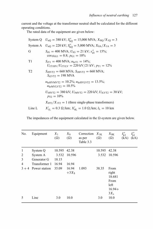
Influence of neutral earthing 127
current and the voltage at the transformer neutral shall be calculated for the differentoperating conditions.
The rated data of the equipment are given below:
System Q UnQ = 380 kV; S′′kQ = 15,000 MVA; X0Q/X1Q = 3
System A UnQ = 220 kV; S′′kQ = 5,000 MVA; X0A/X1A = 3
G SrG = 400 MVA; UrG = 21 kV; x′′d1 = 15%;
cos ϕrG1 = 0.8; pG1 = 10%
T1 SrT1 = 400 MVA; ukrT1 = 14%;UrT1HV/UrT1LV = 220 kV/21 kV; pT1 = 12%
T2 SrHVT2 = 660 MVA; SrMVT2 = 660 MVA;SrLVT2 = 198 MVA
ukrHVMVT2 = 10.2%; ukrHVLVT2 = 13.5%;ukrMVLVT2 = 10.5%
UrHVT2 = 380 kV; UrMVT2 = 220 kV; UrLVT2 = 30 kV;pT2 = 10%
X0T2/X1T2 = 1 (three single-phase transformers)
Line L X′1L = 0.3 �/km; X′
0L = 1.0 �/km; lL = 10 km
The impedances of the equipment calculated in the �-system are given below.
No. Equipment X1 X0 Correction X1K X0K I ′′k3 I ′′
k1(�) (�) as per (�) (�) (kA) (kA)
Table 3.3
1 System Q 10.595 42.38 10.595 42.382 System A 3.532 10.596 3.532 10.5963 Generator G 18.154 Transformer 1 16.94 16.943 + 4 Power station 35.09 16.94 1.093 38.35 From
+3XS right18.681Fromleft16.94+3Xs
5 Line 3.0 10.0 3.0 10.0
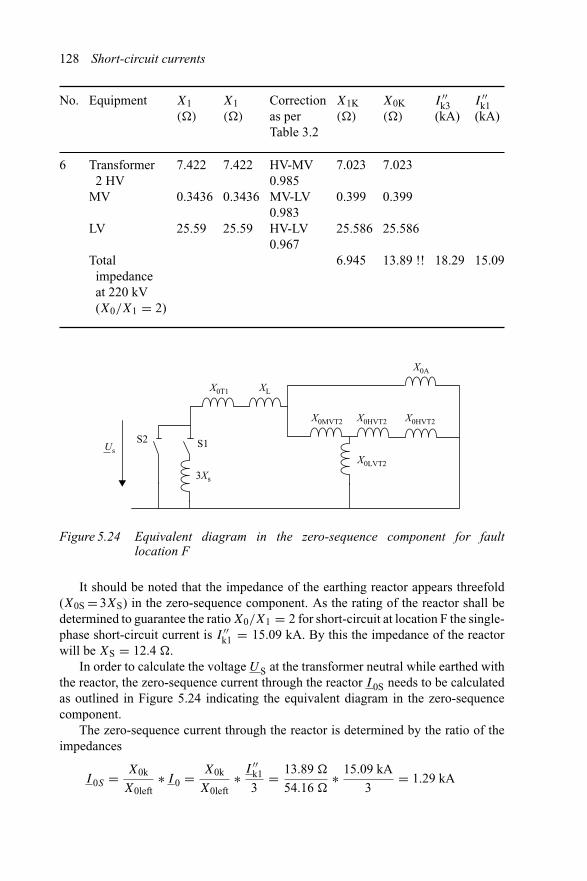
128 Short-circuit currents
No. Equipment X1 X1 Correction X1K X0K I ′′k3 I ′′
k1(�) (�) as per (�) (�) (kA) (kA)
Table 3.2
6 Transformer 7.422 7.422 HV-MV 7.023 7.0232 HV 0.985
MV 0.3436 0.3436 MV-LV 0.399 0.3990.983
LV 25.59 25.59 HV-LV 25.586 25.5860.967
Total 6.945 13.89 !! 18.29 15.09impedanceat 220 kV(X0/X1 = 2)
UsS2 S1
3Xs
X0T1
X0MVT2 X0HVT2
X0LVT2
X0HVT2
XL
X0A
Figure 5.24 Equivalent diagram in the zero-sequence component for faultlocation F
It should be noted that the impedance of the earthing reactor appears threefold(X0S = 3XS) in the zero-sequence component. As the rating of the reactor shall bedetermined to guarantee the ratio X0/X1 = 2 for short-circuit at location F the single-phase short-circuit current is I ′′
k1 = 15.09 kA. By this the impedance of the reactorwill be XS = 12.4 �.
In order to calculate the voltage US at the transformer neutral while earthed withthe reactor, the zero-sequence current through the reactor I 0S needs to be calculatedas outlined in Figure 5.24 indicating the equivalent diagram in the zero-sequencecomponent.
The zero-sequence current through the reactor is determined by the ratio of theimpedances
I 0S = X0k
X0left∗ I 0 = X0k
X0left∗ I ′′
k1
3= 13.89 �
54.16 �∗ 15.09 kA
3= 1.29 kA

Influence of neutral earthing 129
The voltage across the reactor USe at the transformer neutral is calculated by
USe = I 0S ∗ 3 ∗ XS = 1.29 kA ∗ 3 ∗ 12.41 � = 48.03 kV
In this case, the transformer neutral is kept isolated (S1 and S2 open); the zero-sequence current through the reactor will be Zero. The voltage is determined by thezero-sequence current determined by the remaining equipment (see Figure 5.24). Thezero-sequence impedance is X0 = 18.681 �. The single-phase short-circuit currentwithout earthing is calculated by
I ′′k1 = 1.1 ∗ √
3 ∗ Un
X0 + 2 ∗ X1= 1.1 ∗ √
3 ∗ 220 kV
18.681 � + 2 ∗ 6.945 �= 12.87 kA
The voltage across the reactor USi is calculated by
USi = I ′′k1
3∗ X0 = 12.87 kA
3∗ 18.681 � = 80.14 kV
The insulation of the transformer neutral must be designed for the maximal voltage,i.e., 80.14 kV.

Chapter 6
Calculation of short-circuit currents inlow-voltage systems
6.1 General
IEC 60781 presents an application guide for the calculation of short-circuit currentsin low-voltage radial systems. The methods described there are identical to thoseas per IEC 60909-0 and as outlined in Chapter 3. The short-circuits are treated asfar-from-generator short-circuits. This assumption is valid in the future as well, evenwith an increasing number of distributed generation units in low-voltage systems.New generation will be connected to the system in the case of
• Photovoltaic installations by rectifier (six-pulse bridge or PWM-rectifier).• Small wind turbines, low-rated combined heat and power units and small
hydro power plants by asynchronous generators (rotor fed).
Installations with synchronous generators are comparatively rare.The following chapters describe the approach and special conditions for the
calculation of short-circuit currents in low-voltage systems.
6.2 Types of faults
Depending on the type of protection against electrical shock in low-voltage systemsall types of short-circuit, i.e., three-phase, double-phase with and without earth con-nection and single-phase-to-earth short-circuits can occur. The maximal short-circuitcurrent depends on the impedances of the positive- and zero-sequence component.Reference is made to Figure 4.4. The ratio Z2/Z1 can be set to 1, as low-voltagesystems for the most part have no generation by synchronous generators. The three-phase short-circuit will lead in those cases to the maximal short-circuit current. Specialattention must be given to the currents flowing through earth, as the phase angles ofthe impedances in the positive- and zero-sequence components differ a lot from eachother in low-voltage systems.
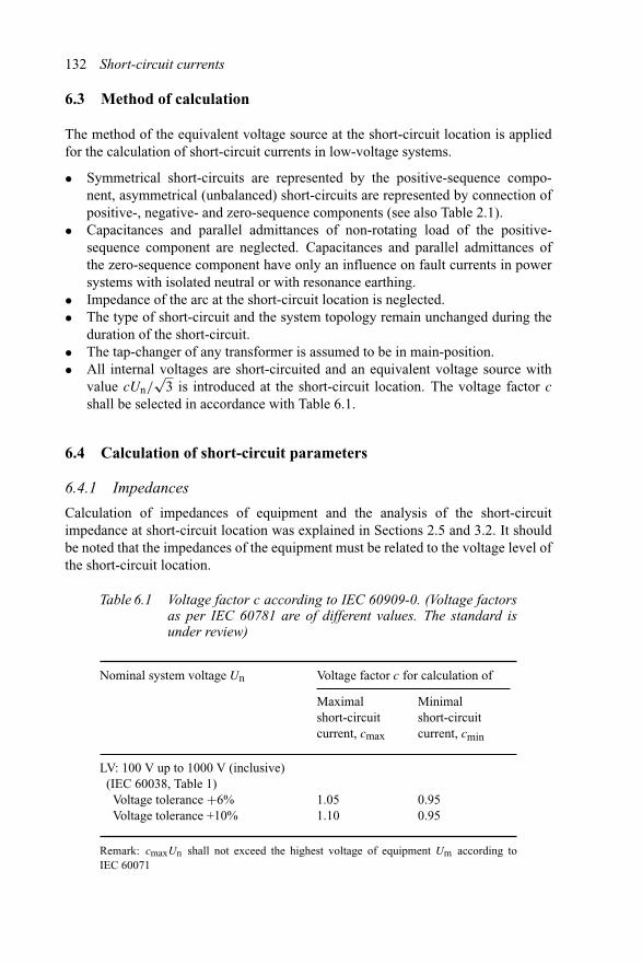
132 Short-circuit currents
6.3 Method of calculation
The method of the equivalent voltage source at the short-circuit location is appliedfor the calculation of short-circuit currents in low-voltage systems.
• Symmetrical short-circuits are represented by the positive-sequence compo-nent, asymmetrical (unbalanced) short-circuits are represented by connection ofpositive-, negative- and zero-sequence components (see also Table 2.1).
• Capacitances and parallel admittances of non-rotating load of the positive-sequence component are neglected. Capacitances and parallel admittances ofthe zero-sequence component have only an influence on fault currents in powersystems with isolated neutral or with resonance earthing.
• Impedance of the arc at the short-circuit location is neglected.• The type of short-circuit and the system topology remain unchanged during the
duration of the short-circuit.• The tap-changer of any transformer is assumed to be in main-position.• All internal voltages are short-circuited and an equivalent voltage source with
value cUn/√
3 is introduced at the short-circuit location. The voltage factor c
shall be selected in accordance with Table 6.1.
6.4 Calculation of short-circuit parameters
6.4.1 Impedances
Calculation of impedances of equipment and the analysis of the short-circuitimpedance at short-circuit location was explained in Sections 2.5 and 3.2. It shouldbe noted that the impedances of the equipment must be related to the voltage level ofthe short-circuit location.
Table 6.1 Voltage factor c according to IEC 60909-0. (Voltage factorsas per IEC 60781 are of different values. The standard isunder review)
Nominal system voltage Un Voltage factor c for calculation of
Maximal Minimalshort-circuit short-circuitcurrent, cmax current, cmin
LV: 100 V up to 1000 V (inclusive)(IEC 60038, Table 1)
Voltage tolerance +6% 1.05 0.95Voltage tolerance +10% 1.10 0.95
Remark: cmaxUn shall not exceed the highest voltage of equipment Um according toIEC 60071
Calculation of short-circuit currents 133
When data for generation in LV-systems are not known, approximation as belowshall be used for the branch short-circuit currents [12]:
Synchronous generator Branch short-circuit current equal to eight times ratedcurrent
Asynchronous generator Branch short-circuit current equal to six times ratedcurrent
Generator with rectifier Branch short-circuit current equal to rated current
This approximation does not include the effect of conductors between the generationunit and the short-circuit location.
6.4.1.1 Initial symmetrical short-circuit current I ′′k
The initial symmetrical short-circuit current I ′′k is calculated for balanced and unbal-
anced short-circuits based on the equivalent voltage source at the short-circuitlocation. The short-circuit impedance seen from the short-circuit location has to bedetermined with the system of symmetrical components. The results obtained forthe short-circuit currents (and the voltages of the non-faulted phases, if required)in the 012-system have to be transferred back into the RYB-system. The results forthe different types of short-circuits are outlined in Table 4.2.
6.4.1.2 Peak short-circuit current ipDepending on the feeding source of the short-circuit, different considerations haveto be taken to calculate the peak short-circuit current. Short-circuits in low-voltagesystems normally are single-fed short-circuits. The short-circuit impedance is repre-sented by a series connection of the individual impedances. The peak short-circuitcurrent can be calculated for the different types of short-circuit by
ip3 = κ ∗ √2I ′′
k3 (6.1a)
ip2 = κ ∗ √2I ′′
k2 (6.1b)
ip1 = κ ∗ √2I ′′
k1 (6.1c)
The factor κ
κ = 1.02 + 0.98 ∗ e−3R/X (6.2)
obtained from the ratio R/X for three-phase short-circuit shall be taken for all typesof short-circuits as well. All other assumptions as per Section 4.3.2.3 are valid inlow-voltage systems as well.
6.4.2 Symmetrical short-circuit breaking current Ib
Short-circuits in low-voltage systems normally are far-from-generator short-circuits.The symmetrical short-circuit breaking current is identical to the initial symmetricalshort-circuit current.

134 Short-circuit currents
6.4.3 Steady-state short-circuit current Ik
Short-circuits in low-voltage systems normally are far-from-generator short-circuits. The steady-state short-circuit current is identical to the initial symmetricalshort-circuit current.
6.4.3.1 Influence of motors
Asynchronous motors contribute to the initial symmetrical short-circuit current, tothe peak short-circuit current, to the symmetrical short-circuit breaking current and inthe case of unbalanced short-circuits to the steady-state short-circuit current as well.Synchronous motors are modelled like generators and asynchronous generators aretreated as asynchronous motors. Motors of any kind, which are not in operation atthe same time, e.g., due to the process or due to any interlocking, can be neglectedfor the calculation of short-circuit current to such an extent that only those motorsare to be taken into account which lead to the highest contribution of the short-circuitcurrent under realistic operating conditions. Motors fed by static-rectifiers need to beconsidered in the case of three-phase short-circuits only if they are able to transferenergy for deceleration at the time of short-circuit, as they contribute to the initialsymmetrical and to the peak short-circuit current.
Asynchronous motors in public supply systems are considered when
• the sum of the rated currents is greater than 1 per cent of the initial symmetricalshort-circuit current without motors;
• the contribution to the initial symmetrical short-circuit current is greater or equalto 5 per cent without motors.
Medium-and low-voltage motors connected through two-winding transformers to theshort-circuit are considered if∑
PrM∑SrT
>0.8
|(c100∑
SrT/(√
3UnQ/I ′′k )) − 0.3| (6.3)
The influence of asynchronous motors in low-voltage systems can be neglected if∑IrM ≤ 0.01 ∗ I ′′
k (6.4)
where UnQ is the nominal system voltage at short-circuit location Q,∑
SrT is thesum of rated apparent power of all transformers, directly connected to motors feedingthe short-circuit, I ′′
k is the initial symmetrical short-circuit current without motors,∑PrM is the sum of rated active power of all motors and
∑IrM is the sum of rated
currents of all motors.
6.5 Minimal short-circuit currents
In order to calculate the minimal short-circuit current the voltage factor cmin accordingto Table 6.1 for the equivalent voltage source at the short-circuit location has to be

Calculation of short-circuit currents 135
considered. Furthermore,
• System topology, generator dispatch and short-circuit power of feeding networkshave to be defined in such a way that the minimal short-circuit current is expected.This normally applies for low-load conditions.
• Motors are to be neglected.• Resistances of overhead lines and cables shall be calculated with the maximal
permissible temperature at the end of the short-circuit, e.g., 80◦C in low-voltagesystems.
These assumptions have to be made in the case of balanced and unbalanced short-circuits, except when other presuppositions are mentioned.
6.6 Examples
Examples for the calculation of short-circuit currents in LV-systems are included inIEC 60781. The calculation is carried out with form-sheets, which are used for thecalculation of impedances of equipment as well as for short-circuit current calculationitself. The voltage factor cmax = 1.0 as given in the examples shall be cmax = 1.05or cmax = 1.1 according to IEC 60909-0. Reference is made to Table 6.1.
Short-circuit current calculation can easily be carried out with spreadsheet analysisusing, e.g., EXCEL [14]. Figure 6.1 outlines an example for a low-voltage installa-tion. The initial symmetrical and the peak short-circuit current both for minimal andmaximal conditions shall be calculated for short-circuit either at location A or atlocation B. The data of the equipment are given below:
System feeder Un = 10 kV; S′′kQmax = 240 MVA; S′′
kQmin = 190 MVATransformer SrT = 630 kVA; ukrT = 6%; urRT = 1.1%; trT = 10/0.4 kV;
R0/R1 = 1; X0/X1 = 1
Cable Each 4 × 240 mm2; R′K = 77.4 m�/km; X′
K = 78 m�/km;R0/R1 = 4; X0/X1 = 4.1; l = 35 m
Motor PrM = 50 kW; UrM = 0.41 kV; cos ϕrM = 0.84; ηrM = 0.94;IanM/IrM = 6
UnQ = 10 kV
Un = 0.4 kV ± 6%
QM
3 ~
A B35 m
Figure 6.1 Equivalent circuit diagram of a LV-installation

Tabl
e6.
2E
xam
ple
for
the
calc
ulat
ion
ofm
axim
alsh
ort-
circ
uitc
urre
nts
inLV
-sys
tem
Dat
a In
put
Nom
inal
vol
tage
in k
Vc m
ax/c
min
Syst
emfe
eder
S� k
Qm
ax in
MV
A
S� k
Qm
in in
MV
A0.
0421
0.42
030.
4225
0.03
330.
3328
0.33
45
S rT in
kV
AH
HV
-sid
eL
V-s
ide
u 1kT
in %
15.2
381
15.4
93u 1
rRT in
%2.
7937
u 0kT
in %
15.2
381
15.4
93u 0
rRT in
%2.
7937
Cab
leL
engt
h in
mC
able
s in
par
alle
lM
ax. t
emp.
°C
X1�
in m
Ω/k
m0.
911.
282
R1�
in m
Ω/k
m0.
903
X0�
in m
Ω/k
m3.
731
5.19
3R
0� in
mΩ
/km
3.61
2
Mot
orA
ctiv
e po
wer
in k
W17
1.34
407.
9344
2.46
Ur i
n V
cos
I a/I
rZ
ero
seq.
Im
p. in
mΩ
9999
9999
Rat
ed c
urre
ntA
mpe
re89
.17
Ass
essm
ent o
f m
otor
s1%
of
s.-c
. cur
rent
in A
mpe
re14
7.8
Ass
essm
ent o
f m
otor
s5%
of
s.-c
. cur
rent
in A
mpe
re73
9
Low
volta
ge
Tra
nsfo
rmer
9999
99996
0.94
0.8441050
309.
631
9.8
77.478803351.16 6
1.1
0.410630
240
190
1.1
0.4
R mΩ
X mΩ
Z 1 mΩ
Z 0 mΩ
I� k3m
inkA
I� k2m
inkA
I� k1m
axkA
I� kE
2EkA
15.9
7
Rk/
Xk 0.18
235
.86
13.8
331
.83
16.2
536
.49
16.1
136
.18
i p3
kAi p
2kA
i p1
kAi p
E2E
kA
I� k3m
inkA
I� k2m
inkA
I� k1m
axkA
I� kE
2EkA
14.7
8
Rk/
Xk 0.22
631
.72
12.8
27.4
713
.02
27.9
513
.84
29.7
i p3
kAi p
2kA
i p1
kAi p
E2E
kA
I� k3m
axkA
I� k2m
axkA
I� k1m
axkA
I� kE
2EkA
0.58
Rk/
Xk 0.
421.
070.
510.
930.
010.
020.
010.
02
i p3
kAi p
2kA
i p1
kAi p
E2E
kA
s.-c
. at l
ocat
ion
B
s.-c
. at l
ocat
ion
A
Bra
nch
s.-c
. cur
rent
of
mot
or
Bra
nch
s.-c
. cur
rent
of
mot
or to
be
negl
ecte
d
Zer
o se
q. s
yste
m
Pos.
seq
. sys
tem
Pos.
seq
. sys
tem
Pos.
seq
. sys
tem
Zer
o se
q. s
yste
m
h

Tabl
e6.
3E
xam
ple
for
the
calc
ulat
ion
ofm
inim
alsh
ort-
circ
uitc
urre
nts
inLV
-sys
tem
Inpu
t dat
a
Nom
inal
vol
tage
in k
Vc m
ax/c
min
Syst
em f
eede
r
0.04
21
Tra
nsfo
rmer
S rT in
kV
AH
V-s
ide
LV
-sid
e
u 1kT
in %
15
.238
115
.493
u 1rR
T in
%2.
7937
u0kT
in %
u0rR
T in
%
Len
gth
in m
Cab
les
in p
aral
lel
Max
. tem
p. °C
X1�
in m
Ω/k
m0.
911.
443
R1�
in m
Ω/k
m1.
1198
X0�
in m
Ω/k
m
Low
volta
ge
Pos.
seq
. sys
tem
Pos.
seq
. sys
tem
Zer
o se
q. s
yste
m
Cab
le
Pos.
seq
. sys
tem
Zer
ose
q.sy
stem
R mΩ
X mΩ
Z 1 mΩ
Z 0 mΩ
0.42
030.
4225
I� k3m
inkA
I� k2m
inkA
I� km
inkA
I� kE
2EkA
13.7
8
Rk/
Xk
0.18
230
.87
11.8
426
.81
14.0
431
.53
13.8
131
.24
i p3
kAi p
2kA
i p1
kAi p
E2E
kA
I� k3m
inkA
I� k2m
inkA
I� k1m
inkA
I� kE
2EkA
12.6
4
Rk/
Xk
0.23
926
.79
10.9
523
.21
10.9
723
.25
11.7
524
.9
i p3
kAi p
2kA
i p1
kAi p
E2E
kA
s.-c
. at l
ocat
ion
A
s.-c
. at l
ocat
ion
B
0.4
0.95 630 10 6
0.4
1.1 35 3 80 78
77.4
240
S� kQ
max
in M
VA
2 S
� kQm
in in
MV
A1
0.03
330.
3328
0.33
4519
0
2.79
371.
1615
.493
15.2
381
R0�
in m
Ω/k
m4.
4789
309.
63.
731
5.83
319.
8

138 Short-circuit currents
The calculation is carried out with EXCEL; the spreadsheet is shown in Tables 6.2and 6.3. Data for the calculation of minimal short-circuit currents are automaticallytransferred; results are highlighted in the tinted boxes. All fields, except the inputfields, are blocked against unintentional modification.

Chapter 7
Double earth-fault and short-circuit currentsthrough earth
7.1 General
IEC 60909-3 describes methods and procedures for the calculation of currents duringtwo separate simultaneous single-phase line-to-earth short-circuits (s.-c.) at differentlocations of the system, which are called ‘double earth-fault’ in the context ofthis section. The double earth-fault is not identical to a double-phase short-circuit,where two phases have a short-circuit at the same location. Furthermore, the branchshort-circuit currents flowing through earth are dealt with.
7.2 Short-circuit currents during double earth-faults
7.2.1 Impedances and initial symmetrical short-circuit current I ′′k
In order to calculate the short-circuit currents I ′′kEE in the case of a double earth-fault,
the mutual impedance in the positive- and zero-sequence component between thetwo short-circuit locations is needed. As the mutual impedance comparatively difficultto determine, the double earth-fault can only be analysed in a simple manner for specialsystem configurations. The following cases are considered:
• Both short-circuit locations are on the same line.• The short-circuit locations are on different lines.• Single-fed line.• Double-fed line.
In the case of a single-fed (radial) line, both short-circuit locations are on the sameline and the double earth-fault is identical to a double-phase short-circuit without earthconnection, as seen from the feeding point of the line. In the case of a double-fed
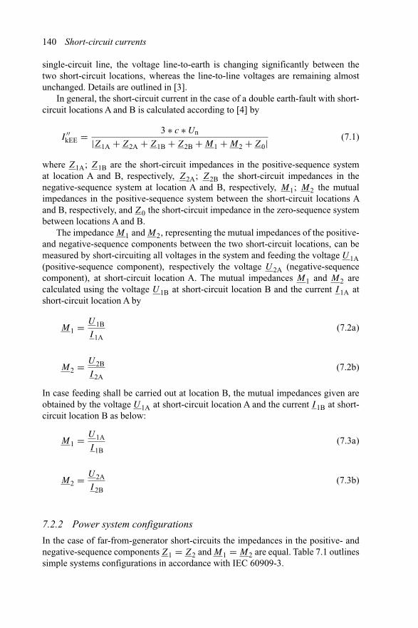
140 Short-circuit currents
single-circuit line, the voltage line-to-earth is changing significantly between thetwo short-circuit locations, whereas the line-to-line voltages are remaining almostunchanged. Details are outlined in [3].
In general, the short-circuit current in the case of a double earth-fault with short-circuit locations A and B is calculated according to [4] by
I ′′kEE = 3 ∗ c ∗ Un
|Z1A + Z2A + Z1B + Z2B + M1 + M2 + Z0|(7.1)
where Z1A; Z1B are the short-circuit impedances in the positive-sequence systemat location A and B, respectively, Z2A; Z2B the short-circuit impedances in thenegative-sequence system at location A and B, respectively, M1; M2 the mutualimpedances in the positive-sequence system between the short-circuit locations Aand B, respectively, and Z0 the short-circuit impedance in the zero-sequence systembetween locations A and B.
The impedance M1 and M2, representing the mutual impedances of the positive-and negative-sequence components between the two short-circuit locations, can bemeasured by short-circuiting all voltages in the system and feeding the voltage U1A(positive-sequence component), respectively the voltage U2A (negative-sequencecomponent), at short-circuit location A. The mutual impedances M1 and M2 arecalculated using the voltage U1B at short-circuit location B and the current I 1A atshort-circuit location A by
M1 = U1B
I 1A(7.2a)
M2 = U2B
I 2A(7.2b)
In case feeding shall be carried out at location B, the mutual impedances given areobtained by the voltage U1A at short-circuit location A and the current I 1B at short-circuit location B as below:
M1 = U1A
I 1B(7.3a)
M2 = U2A
I 2B(7.3b)
7.2.2 Power system configurations
In the case of far-from-generator short-circuits the impedances in the positive- andnegative-sequence components Z1 = Z2 and M1 = M2 are equal. Table 7.1 outlinessimple systems configurations in accordance with IEC 60909-3.
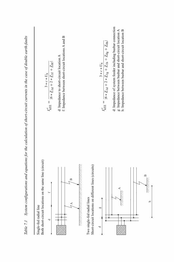
Tabl
e7.
1Sy
stem
conf
igur
atio
nsan
deq
uatio
nsfo
rth
eca
lcul
atio
nof
shor
t-ci
rcui
tcur
rent
sin
the
case
ofdo
uble
eart
h-fa
ults
Sing
le-f
edra
dial
line
Bot
hsh
ort-
circ
uitl
ocat
ions
onth
esa
me
line
(cir
cuit)
I′′ kE
E=
3∗c
∗Un
|6∗Z
1d+
2∗Z
1f+
Z0f
|d:
Impe
danc
eto
shor
t-ci
rcui
tloc
atio
nA
f:Im
peda
nce
betw
een
shor
t-ci
rcui
tloc
atio
nsA
and
B
AB
df
Two
sing
le-f
edra
dial
lines
Shor
t-ci
rcui
tloc
atio
nson
diff
eren
tlin
es(c
ircu
its)
I′′ kE
E=
3∗c
∗Un
|6∗Z
1d+
2∗Z
1g+
Z1h
+Z
0g+
Z0h
|d:
Impe
danc
eof
syst
emfe
eder
incl
udin
gbu
sbar
conn
ectio
ng:
Impe
danc
ebe
twee
nbu
sbar
and
shor
t-ci
rcui
tloc
atio
nA
h:Im
peda
nce
betw
een
busb
aran
dsh
ort-
circ
uitl
ocat
ion
BA
dg
Bh

Tabl
e7.
1C
ontin
ued
Dou
ble-
fed
line
Bot
hsh
ort-
circ
uitl
ocat
ions
onth
esa
me
line
(cir
cuit)
I′′ kE
E=
3∗c
∗Un
|(6∗Z
1d∗Z
1e+
2∗Z
1f(Z
1d+
Z1e
))/(Z
1d+
Z1f
+Z
1e)+
Z0f
|d:
Impe
danc
efr
omle
fttil
lsho
rt-c
ircu
itlo
catio
nA
e:Im
peda
nce
from
righ
ttill
shor
t-ci
rcui
tloc
atio
nB
f:Im
peda
nce
betw
een
shor
t-ci
rcui
tloc
atio
nsA
and
B
df
e
AB
Syst
em f
eede
rle
ftSy
stem
fee
der
righ
t
Ear
thin
gim
peda
nces
inth
esw
itchy
ard
and
atth
eov
erhe
adto
wer
can
bene
glec
ted.
The
volta
gefa
ctor
csh
allb
ese
lect
edin
acco
rdan
ceto
Tabl
e4.
1.In
dice
s:0,
1an
d2:
zero
-,po
sitiv
e-an
dne
gativ
e-se
quen
ceco
mpo
nent
s.d,
e,f,
g,h:
leng
thof
the
line
asin
dica
ted
inth
edr
awin
gof
the
firs
tcol
umn.
Double earth-fault and short-circuit currents 143
7.2.3 Peak short-circuit current ip
The calculation of peak short-circuit current is carried out in the same manner asdescribed in Section 4.3.2.3. The peak short-circuit current is calculated by
ipEE = κ ∗ √2 ∗ I ′′
kEE (7.4)
The factor κ shall be the maximum of the factors obtained for three-phase short-circuitat location A or B.
κ = MAX{κA; κB} (7.5)
For explanations and calculation method of quantities reference is made to Chapter 4.
7.2.4 Symmetrical short-circuit breaking current Ib and steady-stateshort-circuit current Ik
In the case of far-from-generator short-circuits, the symmetrical short-circuit breakingcurrent and the steady-state short-circuit current are identical to the initial symmetricalshort-circuit current. In other cases, reference is made to Chapter 4.
7.3 Short-circuit currents through earth
7.3.1 Introduction
Branch short-circuit currents can flow through earth in the case of unbalanced short-circuits with earth connection, i.e., line-to-earth (single-phase) short-circuit anddouble-phase short-circuit with earth connection. Single-phase short-circuits are thedominating fault type in power systems with earthed neutrals and are leading to themaximal branch short-circuit currents flowing through earth. The current I ′′
k1 flow-ing through earth is equal to three-times the current in the zero-sequence componentflowing towards the short-circuit location. Type, number and arrangement of earthconductors of overhead lines, the installation of counterpoise, shielding, armouringand sheaths of cables, and their connection to the earthing grid of the switchyarddetermine the part of the short-circuit current that will flow through the earthinginstallations. This part is described by means of the reduction factor p
E, sometimes
represented as r . The reduction factor is defined as the ratio of branch short-circuitcurrent I Etot flowing through earth to the total short-circuit current 3I 0, which canbe described by the ratio of impedances
pE
= I Etot
3I 0= 1 − ZLE
ZE(7.6)
where ZE is the impedance of earth conductor with earth return, ZLE is the mutualimpedance between earth and line conductor with common earth return, I Etot isthe branch short-circuit current through earth and I 0 is the total zero-sequenceshort-circuit current.

144 Short-circuit currents
The loop-impedance ZE of the earth conductor and earth return is given by
Z′E = R′ + μ0
8∗ ω + j
(μ0
2π∗ ω ∗
(ln(
δ
r
)+ μr
4
))(7.7)
The mutual impedance ZLE of the loop earth conductor and conductor with earthreturn is given by
Z′LE = μ0
8∗ ω + j
(μ0
2π∗ ω ∗
(ln
δ
dLE
))(7.8)
where r is the radius of earth conductor, μ0 is the absolute permeability, μr is therelative permeability, ω is the angular frequency, R′ is the resistance of earth wire perunit length, δ is the depth of the earth return path δ = 1.85/
√ω ∗ μ0/ρE, ρE is the
resistivity of soil depending on soil conditions and dLE is the distance between theearth conductor and phase conductor. Equations for the calculation of the impedancesZE and ZLE are also given in [1,6].
7.3.2 Short-circuit inside a switchyard
Figure 7.1 outlines the equivalent circuit diagram of a power system (HV) with short-circuit inside the switchyard B. All quantities are defined according to Figure 7.1.
The single-phase short-circuit current is calculated using
I ′′k1 = 3 ∗ I 0A + 3 ∗ I 0B + 3 ∗ I 0C (7.9)
The total current through the earth grid at location B is
I ZB = pA
∗ 3 ∗ I 0A + pC
∗ 3 ∗ I 0C (7.10)
(I–pA)3I0A
3I0A
3I0B
3I0B
pA3I0A
I 0K1
(I–pC)3I0C Earthwire
B CA
ZEA ZEB ZECUEBIZA IZB IZC
pC3I0C
3I0C
Earth
Figure 7.1 Equivalent circuit diagram with short-circuit inside switchyard B
Double earth-fault and short-circuit currents 145
The potential at the earth grid is then
UEB = ZEB ∗ I ZB (7.11)
with the earthing impedance of the switchyard
ZEB = 1
1/RE +∑1/ZP
(7.12)
where RE is the resistance of the earth grid and ZP is the driving point impedance(impedance of earth conductor with earth return and earthing impedance of overheadtowers, respectively, input impedance of shielding, sheaths and armouring of cables).
The considerations mentioned above are only valid when the short-circuit location(switchyard B) is far away from other switchyards (A and C in Figure 7.1). Thecurrent through earth is lower when the distance to the short-circuit is lower than thefar-from-station distance dF defined as
dF = 3 ∗√RTo ∗ dTo
Re{√ZE} (7.13)
where RTo is the footing resistance of tower, dTo is the distance between two towersand ZE is the impedance of earth conductor with earth return.
7.3.3 Short-circuit at overhead-line tower
Figure 7.2 outlines the equivalent circuit diagram of a power system with short-circuitoutside the switchyard (distance d > dF, see Equation (7.13)). The single-phaseshort-circuit current is calculated by
I ′′k1 = 3 ∗ I 0A + 3 ∗ I 0B + 3 ∗ I 0C (7.14)
The branch current through the earthing of the tower at short-circuit location is
I ZF = pC
∗ (3 ∗ I 0A + 3 ∗ I 0C) + pC
∗ 3 ∗ I 0C = pC
∗ I ′′k1 (7.15)
and the potential at the earth grid
UEF = ZEF ∗ I ZF (7.16)
with the earthing impedance of the installation
ZEF = 1
1/RTo + 2/ZP(7.17)
where RTo is the footing resistance of tower and ZP is the driving point impedance(impedance of earth conductor with earth return and earthing impedance of overhead-line towers, respectively, input impedance of shielding, sheaths and armouringof cables).
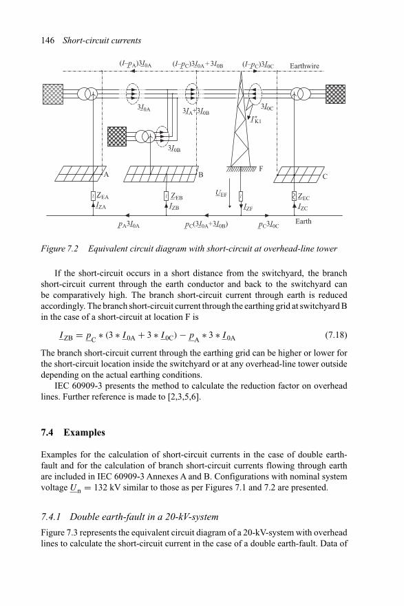
146 Short-circuit currents
(I–pA)3I0A (I–pC)3I0A + 3I0B
3I0A
pA3I0A
3I0B
3IA+3I0B
(I–pC)3I0C Earthwire
BF
CA
ZEA ZEBUEF ZEC
IZFIZA IZB IZC
pC(3I0A+3I0B) pC3I0C
I 0K1
3I0C
Earth
~ ~ ~Figure 7.2 Equivalent circuit diagram with short-circuit at overhead-line tower
If the short-circuit occurs in a short distance from the switchyard, the branchshort-circuit current through the earth conductor and back to the switchyard canbe comparatively high. The branch short-circuit current through earth is reducedaccordingly. The branch short-circuit current through the earthing grid at switchyard Bin the case of a short-circuit at location F is
I ZB = pC
∗ (3 ∗ I 0A + 3 ∗ I 0C) − pA
∗ 3 ∗ I 0A (7.18)
The branch short-circuit current through the earthing grid can be higher or lower forthe short-circuit location inside the switchyard or at any overhead-line tower outsidedepending on the actual earthing conditions.
IEC 60909-3 presents the method to calculate the reduction factor on overheadlines. Further reference is made to [2,3,5,6].
7.4 Examples
Examples for the calculation of short-circuit currents in the case of double earth-fault and for the calculation of branch short-circuit currents flowing through earthare included in IEC 60909-3 Annexes A and B. Configurations with nominal systemvoltage Un = 132 kV similar to those as per Figures 7.1 and 7.2 are presented.
7.4.1 Double earth-fault in a 20-kV-system
Figure 7.3 represents the equivalent circuit diagram of a 20-kV-system with overheadlines to calculate the short-circuit current in the case of a double earth-fault. Data of
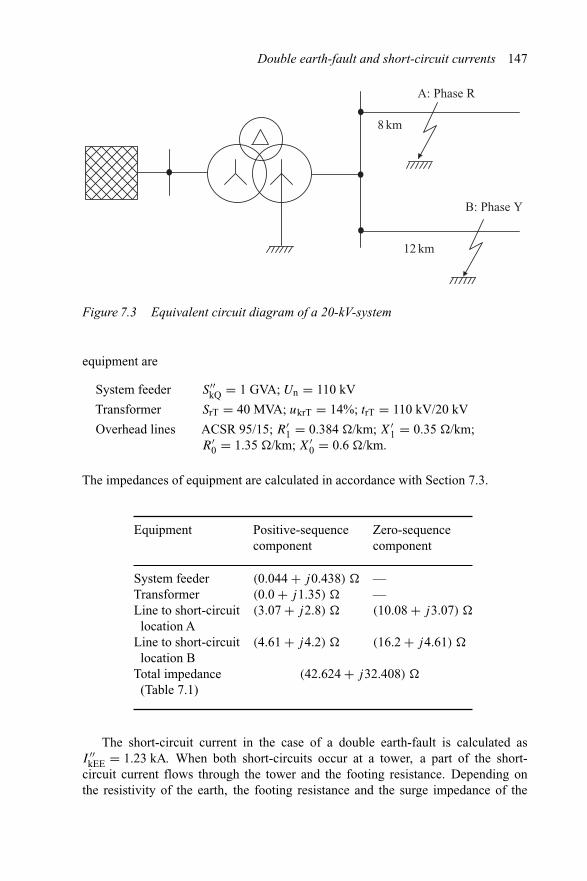
Double earth-fault and short-circuit currents 147
A: Phase R
8 km
12 km
B: Phase Y
Figure 7.3 Equivalent circuit diagram of a 20-kV-system
equipment are
System feeder S′′kQ = 1 GVA; Un = 110 kV
Transformer SrT = 40 MVA; ukrT = 14%; trT = 110 kV/20 kV
Overhead lines ACSR 95/15; R′1 = 0.384 �/km; X′
1 = 0.35 �/km;R′
0 = 1.35 �/km; X′0 = 0.6 �/km.
The impedances of equipment are calculated in accordance with Section 7.3.
Equipment Positive-sequence Zero-sequencecomponent component
System feeder (0.044 + j0.438) � —Transformer (0.0 + j1.35) � —Line to short-circuit (3.07 + j2.8) � (10.08 + j3.07) �
location ALine to short-circuit (4.61 + j4.2) � (16.2 + j4.61) �
location BTotal impedance (42.624 + j32.408) �
(Table 7.1)
The short-circuit current in the case of a double earth-fault is calculated asI ′′
kEE = 1.23 kA. When both short-circuits occur at a tower, a part of the short-circuit current flows through the tower and the footing resistance. Depending onthe resistivity of the earth, the footing resistance and the surge impedance of the

148 Short-circuit currents
line, this part is approximately 10–25 per cent smaller than the total short-circuitcurrent.
7.4.2 Single-phase short-circuit in a 110-kV-system
Figure 7.4 indicates the equivalent circuit diagram of a 110-kV-system with short-circuit location F. The single-phase short-circuit current, the branch short-circuitcurrents flowing through the earth and the potential of the earth grid shall be calculated.The data of equipment are
C
BA
UEBZEB
80 km
45 km
Un = 110 kV
Earth wire
Figure 7.4 Equivalent circuit diagram of a 110-kV-system with short-circuitlocation
Feeder A S′′kQA = 1.5 GVA; SrT = 250 MVA; u1kT = 16%; u0kT = 20%;
u0rR = 0.2%
Feeder B S′′kQB = 2.0 GVA; SrT = 350 MVA; u1kT = 14%; u0kT = 18%;
u0rR = 0.2%
Feeder C S′′kQC = 1.1 GVA; SrT = 200 MVA; u1kT = 15%; u0kT =
19%; u0rR = 0.2%
Line ACSR 2 × 240/40; earth wire 240/40; reduction factorp ≈ 0.6
Z′1 = (0.059 + j0.302) �/km; Z′
0 = (0.27 + j1.51) �/km

Double earth-fault and short-circuit currents 149
The impedances of equipment are calculated in accordance to Section 7.3 andSection 3.2.
Equipment Positive-sequence Zero-sequencecomponent component
Feeder A including (0.0 + j8.87) � (0.1 + j9.68) �
transformerFeeder B including (0.0 + j6.66) � (0.06 + j6.22) �
transformerFeeder C including (0.0 + j12.1) � (0.12 + j11.5) �
transformerLine A–B (2.655 + j13.59) � (12.15 + j21.6) �
Line B–C (4.72 + j24.16) � (67.95 + j120.8) �
Impedance at short-circuit (0.178 + j4.512) � (0.407 + j5.11) �
location
The single-phase short-circuit current is calculated as I ′′k1 = (0.798 − j14.785) kA
and |I ′′k1| = 14.8 kA, respectively. The current in the zero-sequence component is
I 0 = 13 I ′′
k1 = (0.266 − j4.928) kA and the branch short-circuit currents of the threefeeders A, B and C are
I 0A = (0.179 − j0.732) kA
I 0B = (0.502 − j4.036) kA
I 0C = (0.057 − j0.16) kA
The total current through the earth grid is I ZB = (0.425−j1.426) kA. The impedanceof the earth grid depends on the resistivity of the soil, the footing resistance of the towerand the surge impedance of the line. Assuming (in accordance with IEC 60909-3) theimpedance of the earthing grid to be ZEB = (0.68 + j0.49) � the potential of theearth grid is UEB = (0.987 − j0.761) kV and |UEB| = 1.246 kV, respectively.

Chapter 8
Factors for the calculation ofshort-circuit currents
8.1 General
Several factors for the calculation of short-circuit (s.-c.) currents have been introducedin previous sections, the origin of which will be explained within this section.
• Voltage factor cmax and cmin for different voltage levels as per Table 4.1.• Correction factor using the %/MVA- or the p.u.-system as mentioned in Chapter 2.• Impedance correction factors for synchronous machines, power station units and
transformers as per Tables 3.2, 3.3, 3.5 and 3.6.• Factors for the calculation of different parameters of the short-circuit current based
on the initial short-circuit current as per Chapter 4.
The factors are necessary as the method of the equivalent voltage source at theshort-circuit location is used for the calculation of short-circuit currents which is basedon some simplifications such as neglecting the load current prior to fault, assumingthe tap-changer of transformers in middle-position, calculating the impedance ofequipment based on the name-plate data or on data for rated operating conditionsand neglecting voltage control gear for generators and transformers. The main taskof short-circuit analysis is to determine the maximal short-circuit current which isone of the main criteria for the rating of equipment in electrical power systems.It is obvious that the parameters of the short-circuit current as calculated with theequivalent voltage source at the short-circuit location will differ from those currents,which may be measured during short-circuit tests or may be calculated with transientnetwork analysing programmes. In order to obtain results on the safe side withoutuneconomic safety margin the correction factors will be applied. Detailed deductionsof the various correction factors are given in IEC 60909-1:1991-10.
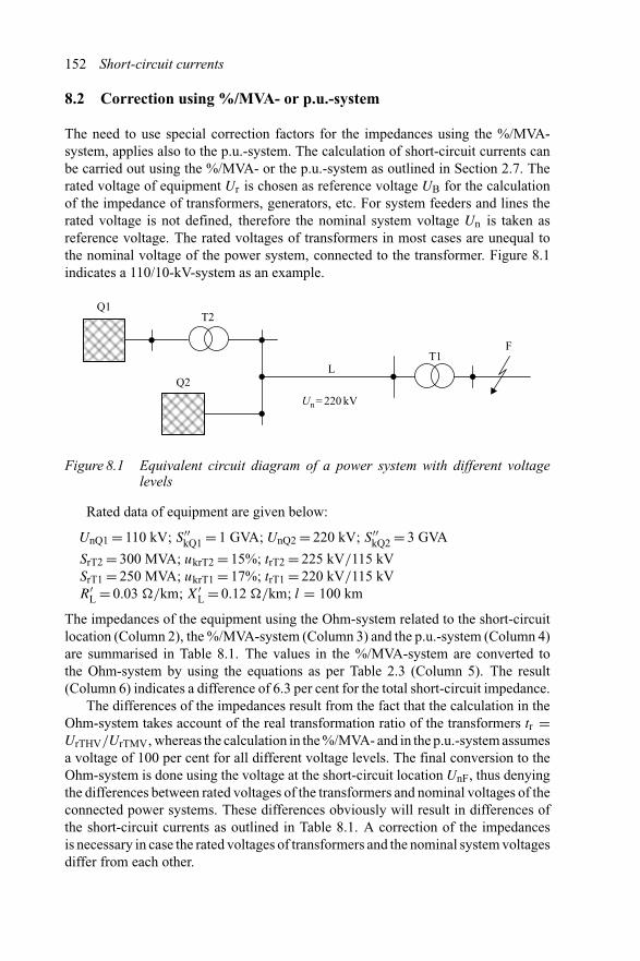
152 Short-circuit currents
8.2 Correction using %/MVA- or p.u.-system
The need to use special correction factors for the impedances using the %/MVA-system, applies also to the p.u.-system. The calculation of short-circuit currents canbe carried out using the %/MVA- or the p.u.-system as outlined in Section 2.7. Therated voltage of equipment Ur is chosen as reference voltage UB for the calculationof the impedance of transformers, generators, etc. For system feeders and lines therated voltage is not defined, therefore the nominal system voltage Un is taken asreference voltage. The rated voltages of transformers in most cases are unequal tothe nominal voltage of the power system, connected to the transformer. Figure 8.1indicates a 110/10-kV-system as an example.
Q1T2
T1F
L
Un = 220 kV
Q2
Figure 8.1 Equivalent circuit diagram of a power system with different voltagelevels
Rated data of equipment are given below:
UnQ1 = 110 kV; S′′kQ1 = 1 GVA; UnQ2 = 220 kV; S′′
kQ2 = 3 GVA
SrT2 = 300 MVA; ukrT2 = 15%; trT2 = 225 kV/115 kVSrT1 = 250 MVA; ukrT1 = 17%; trT1 = 220 kV/115 kVR′
L = 0.03 �/km; X′L = 0.12 �/km; l = 100 km
The impedances of the equipment using the Ohm-system related to the short-circuitlocation (Column 2), the %/MVA-system (Column 3) and the p.u.-system (Column 4)are summarised in Table 8.1. The values in the %/MVA-system are converted tothe Ohm-system by using the equations as per Table 2.3 (Column 5). The result(Column 6) indicates a difference of 6.3 per cent for the total short-circuit impedance.
The differences of the impedances result from the fact that the calculation in theOhm-system takes account of the real transformation ratio of the transformers tr =UrTHV/UrTMV, whereas the calculation in the %/MVA- and in the p.u.-system assumesa voltage of 100 per cent for all different voltage levels. The final conversion to theOhm-system is done using the voltage at the short-circuit location UnF, thus denyingthe differences between rated voltages of the transformers and nominal voltages of theconnected power systems. These differences obviously will result in differences ofthe short-circuit currents as outlined in Table 8.1. A correction of the impedancesis necessary in case the rated voltages of transformers and the nominal system voltagesdiffer from each other.

Factors for the calculation of short-circuit currents 153
Table 8.1 Impedances of equipment and short-circuit current as per Figure 8.1
1 2 3 4 5 6
Equipment Impedance Impedance Impedance Impedance Differencerelated to (%/MVA) (p.u.) (%/MVA) → (�) (%)s.-c. (p.u.) → (�)
location(�)
System Q1 13.929 0.11 0.11 13.31 4.7Transformer T2 6.917 0.05 0.05 6.05 14.3System Q2 4.849 0.037 0.037 4.48 8.2Line L 3.279 0.0248 0.0248 3.0 9.3Transformer T1 8.993 0.068 0.068 8.228 9.3Total s.-c. 16.206 0.126 0.126 15.246 6.3
impedanceShort-circuit 4.31 kA 4.60 kA 10.12 p.u. — 6.3
current
Q Ti
Un
ZB
T1T2
Figure 8.2 Equivalent circuit diagram for the calculation of impedance correctionfactor using %/MVA- or p.u.-system
The impedance correction factors (see Figure 8.2 for explanation) are obtainedstarting from the short-circuit location F indicated in Figure 8.1 by multiplying theratios of the rated voltages of all transformers T1–Ti between the short-circuit loca-tion F and the equipment under consideration B, then going back with the ratio of therated voltage of the equipment UrB and the nominal voltage Un at the short-circuitlocation. For system feeders and lines the nominal system voltage at the very locationUnB has to be taken instead of the rated voltage, which is not defined for feeders andlines. The impedance correction factor KB is calculated by
KB =(
UrT1E
UrT1A∗ UrT2E
UrT2A∗ UrT3E
UrT3A∗ · · ·
)2
∗(
UrB
UnF
)2
(8.1)
The impedance correction factor using the %/MVA- or the p.u.-system must be appliedfor any equipment [33] except power station units for which special correction factorsare valid.

154 Short-circuit currents
Table 8.2 Impedances of equipment and short-circuit current using correctionfactor
1 2 3 4 5 6
Equipment Impedance Impedance Correction factor Impedance Impedancerelated to s.-c. (%/MVA) KB as per (%/MVA) (p.u.)location (�) Equation (8.1) using KB using KB
System Q1 13.929 0.11 1.046 0.115 0.115Transformer T2 6.917 0.05 1.093 0.057 0.057System Q2 4.849 0.037 1.143 0.04 0.04Line L 3.279 0.0248 1.093 0.027 0.027Transformer T1 8.993 0.068 1.093 0.0743 0.0743Total s.-c. 16.206 0.126 — 0.134 0.134
impedanceShort-circuit 4.31 kA — — 4.31 A 9.48 p.u.
current
Applying the impedance correction factors as per Equation (8.1) the impedancescalculated with the %/MVA- and the p.u.-system are identical to those obtained byusing the Ohm-system as outlined in Table 8.2.
8.3 Impedance correction factors
Within this book the deduction of the impedance correction factor KG for synchronousmachines (generators) is given. The factor is valid for generators connected directlywithout unit transformers to the power system which is normally the fact in medium-voltage and low-voltage systems [37]. Assuming an overexcited turbine generator asper Figure 8.3 with voltage control at the terminal connection to UG = (1 ± pG)∗UrG,the control range normally is set to (1 + pG) = 1.05. Prior to fault the generatorgenerates the apparent power SG = PG + jQG to be fed into the system.
~ ~GS3
UGUn
RG
UrG
IG
UrG
(a) (b) X �d
E�3
01
Figure 8.3 Generator directly connected to the power system. (a) Equivalent systemdiagram and ( b) equivalent circuit diagram in the positive-sequencecomponent
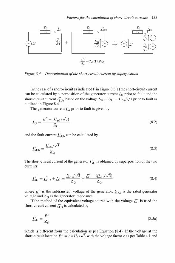
Factors for the calculation of short-circuit currents 155
ZG ZG ZGIG I 0kUb I 0kG
UGE 0 E 03
UG
3
UG
3
UG
3
UG
3= UrG (1�PG)
~ ~ ~~
~
~ ~ ~
Figure 8.4 Determination of the short-circuit current by superposition
In the case of a short-circuit as indicated F in Figure 8.3(a) the short-circuit currentcan be calculated by superposition of the generator current I G prior to fault and theshort-circuit current I ′′
kUb based on the voltage Ub = UG = UrG/√
3 prior to fault asoutlined in Figure 8.4.
The generator current I G prior to fault is given by
I G = E′′ − (U rG/√
3)
ZG(8.2)
and the fault current I ′′kUb can be calculated by
I ′′kUb = U rG/
√3
ZG(8.3)
The short-circuit current of the generator I ′′kG is obtained by superposition of the two
currents
I ′′kG = I ′′
kUb + I G = U rG/√
3
ZG+ E′′ − (U rG/
√3)
ZG(8.4)
where E′′ is the subtransient voltage of the generator, U rG is the rated generatorvoltage and ZG is the generator impedance.
If the method of the equivalent voltage source with the voltage E′′ is used theshort-circuit current I ′′
kG is calculated by
I ′′kG = E′′
ZG(8.5a)
which is different from the calculation as per Equation (8.4). If the voltage at theshort-circuit location E′′ = c ∗ Un/
√3 with the voltage factor c as per Table 4.1 and
156 Short-circuit currents
an impedance correction factor KG are introduced, the short-circuit current I ′′kG is
found to be
I ′′kG = c ∗ Un√
3 ∗ ZG ∗ KG
= c ∗ Un√3 ∗ (RG + jX′′
d) ∗ KG
(8.5b)
where KG is the impedance correction factor (to be determined), Un is the nominalsystem voltage, ZG is the generator impedance, RG is the stator resistance of thegenerator and X′′
d is the subtransient reactance of the generator.Equations (8.5a) and (8.5b) are set to be equal. The unknown internal subtransient
voltage of the generator E′′ can be found in accordance with Figure 8.3(b).
E′′ = U rG√3
+ IG ∗ (cos ϕG − j sin ϕG) ∗ (RG + jX′′d) (8.6)
where U rG is the rated voltage of the generator and ϕG is the phase angle of thegenerator current (power factor: cos ϕ) and other quantities are explained above.
The impedance correction factor KG is then calculated by
KG = Un
UrG∗ c ∗
[1 +
√3 ∗ IG
UrG∗ (RG ∗ cos ϕG + X′′
d ∗ sin ϕG)
+ j
√3 ∗ IG
UrG∗ (X′′
d ∗ cos ϕG − RG ∗ sin ϕG)
]−1
(8.7)
The resistance RG normally can be neglected against the subtransient reactance X′′d
of the generator; the correction factor then results in
KG ≈ Un
UrG∗ c
1 + (IG/IrG) ∗ x′′d ∗ sin ϕG
(8.8)
whereas the subtransient reactance is introduced as a p.u.-value x′′d = (X′′
d/U2rG)∗SrG.
The correction factor is maximal when the maximal voltage factor cmax and ratedoperating conditions with IG = IrG and ϕG = ϕrG are applied. The impedancecorrection factor KG is given by
KG ≈ Un
UrG∗ cmax
1 + x′′d ∗ sin ϕG
(8.9)
For other equipment such as power station units and transformers impedance cor-rection factors can be deducted in a similar way [35] as explained for the correctionfactor of the generator. Details can be found in IEC 60909-1.
8.4 Factor κ for peak short-circuit current
The peak short-circuit current is the maximal instant value of the short-circuit currentwhich occurs normally within the first few milliseconds after the occurrence of theshort-circuit. The system configuration with a single-fed three-phase short-circuit isdealt with in Figure 8.5.

Factors for the calculation of short-circuit currents 157
QT
S �kQ
RtotXtot
t = 0ik(t)
Un
Uk; SrT; UrT
u (t) =c Un~ 23
.sin (v)
vtwu
u
u (t)
(a)
(b)
(c)
Figure 8.5 Equivalent circuit diagram of a power system with three-phase short-circuit. (a) Circuit diagram, ( b) simplified diagram of a single-fed three-phase short-circuit and (c) time course of voltage with voltage angle ϕU
The time course of the short-circuit current ik(t) is calculated from the differentialequation
L ∗ dik(t)
dt+ R ∗ ik(t) = √
2 ∗ c ∗ Un√3
∗ sin(ωt + ϕU) (8.10)
The solution of the differential equation is given by
ik(t) = √2 ∗ c ∗ Un√
3∗ 1√
R2 + X2∗ (sin(ωt + ϕU − γ ) − e−t/T
∗ sin(ϕU − γ )) (8.11)
where Un is the nominal system voltage, ϕU is the angle of voltage related to zerocrossing as per Figure 8.5, c is the voltage factor according to Table 4.1, T is the timeconstant: T = L/R, X is the reactance of the short-circuit impedance: X = ωL, R
is the resistance of the short-circuit impedance, ω is the angular velocity and γ theangle of the short-circuit impedance: γ = arctan(X/R).
158 Short-circuit currents
The initial short-circuit current I ′′k is equal to the first part (periodic term) of
Equation (8.11), the second term is the aperiodic and decaying d.c.-component of thecurrent. If the time course of the short-circuit current as per Equation (8.11) is relatedto the peak value of the initial short-circuit current
I ′′k = √
2 ∗ c ∗ Un√3
∗ 1√R2 + X2
(8.12)
the peak factor κ is obtained
κ(t) = sin(ωt + ϕU − γ ) − e−t/T ∗ sin(ϕU − γ ) (8.13a)
The maximum of the peak factor κ determines the maximum of the short-circuitcurrent (peak short-circuit current ip) to be calculated by partial differentiation ofEquation (8.13a) with respect to ϕU and t . The maximum of the peak factor alwaysoccurs for short-circuits at ϕU = 0 and t ≤ 10 ms (50 Hz), respectively t ≤ 8.33 ms(60 Hz), whatever the ratio R/X might be
κ(t) = sin(ωt − γ ) + e−(R/X)∗ωt ∗ sin γ (8.13b)
A sufficient approximation of the peak factor κ is given by
κ = 1.02 + 0.98 ∗ e−3(R/X) (8.14)
Special attention for the calculation of peak short-circuit current must be given inthe case of short-circuits in meshed systems or in systems having parallel lines withR/X-ratios different from each other [34]. A detailed analysis of these conditions isgiven in IEC 60909-1 and is mentioned in Chapter 4. The peak factor κ according toEquation (8.14) is outlined in Figure 4.7.
8.5 Factor μ for symmetrical short-circuit breaking current
The short-circuit current in the case of a near-to-generator short-circuit decays sig-nificantly during the first periods after initiation of the short-circuit due to the changeof the rotor flux in the generator. This behaviour cannot be calculated exactly as eddycurrents in the forged rotor of turbine generators, non-linearities of the iron and satura-tion effects especially in the stator tooth are difficult to be calculated. Furthermore, thedecay of the short-circuit current and by this the breaking current depend on differentgenerator and system parameters such as time constants of the generator itself, loca-tion of short-circuit in the system, operational condition prior to the fault, operationof excitation and voltage control device, tap-changer position of transformers, etc.which cause unpredictable deviations of the calculated results from those obtainedfrom measurements. Detailed calculations with digital programmes are therefore onlyapplicable in special cases if high safety requirements are to be met.

Factors for the calculation of short-circuit currents 159
The time decay of the a.c. part of the short-circuit current is calculated by
Ikac(t) = (I ′′k − I ′
k) ∗ e−t/T ′′N + (I ′
k − Ik) ∗ e−t/T ′N + Ik (8.15)
Equation (8.15) is composed of the initial short-circuit current
I ′′k = E′′
X′′d + XN
(8.16a)
the transient short-circuit current
I ′k = E′
X′d + XN
(8.16b)
and the steady-state short-circuit current
Ik = E
Xd + XN(8.16c)
where E; E′; E′′ are the steady-state, transient and subtransient voltages, Xd; X′d;
X′′d is the steady-state, transient and subtransient reactance of the generator and XN
is the reactance between the generator and the short-circuit location, e.g., includingthe reactance of the unit transformer.
The individual components of the short-circuit currents as per Equations (8.15)and (8.16) are declining with different time constants, i.e., the subtransient time con-stant T ′′
N which can be set approximately equal to the subtransient time constant T ′′dN
in the direct axis. Typical values of the time constants are T ′′N ≈ 0.03–0.04 s and
T ′N ≈ 1.0–1.5 s and are calculated by
T ′′N = T ′′ ∗ X′
d
X′′d
∗ X′′d + XN
X′d + XN
(8.17a)
T ′N = T ′ ∗ Xd
X′d
∗ X′d + XN
X′d + XN
(8.17b)
The units T ′′ and T ′ are the subtransient and transient time constants of the gen-erator. Regarding the time course of the decaying a.c. part of the current as perEquation (8.15), the approximation e−t/T ′
N ≈ 1 can be assumed if the time range(minimal time delay of circuit-breakers) t = tmin = 0.02–0.25 s is considered:
Ikac(t) ≈ I ′′k ∗
[(1 − X′′
d + XN
X′d + XN
)∗ e−tmin/T ′′
N + X′′d + XN
X′d + XN
]= I ′′
k ∗ μ (8.18)
with tmin being the minimal time for breaking the short-circuit current. The second partof Equation (8.18) is taken as the factor μ for the calculation of the breaking current.
160 Short-circuit currents
As the exponent tmin/T ′′N may be greater or smaller than 1, the infinite progression
for e−t/T ′′N is applied. For no-load conditions, where E′′ ≈ E′ ≈ E ≈ UrG/
√3, the
factor μ is obtained by
μ ≈ 1 − X′d − X′′
d
T ′′0 ∗ (UrG/
√3)
∗ I ′′k ∗ tmin + X′
d − X′′d
X′d + XN
∗(
tmin
T ′′N
+ e−tmin/T ′′N − 1
)(8.19)
with the no-load subtransient time constant
T ′′0 = T ′′ ∗ X′
d
X′′d
(8.17c)
When if tmin � T ′′N the last part of Equation (8.19) can be neglected. The factor μ
can be presented depending on the minimal time delay of the circuit-breaker tmin andthe ratio I ′′
k /IrG as outlined in Figure 4.10.
8.6 Factor λ for steady-state short-circuit current
The steady-state short-circuit currents of generators are determined by the methodof excitation, the maximal possible excitation voltage, the type of voltage controland strongly by the saturation effects. As salient-pole and turbine generators differsignificantly with respect to their reactances and are mostly equipped with differenttypes of excitation, the steady-state short-circuit currents of both generators will differeven if all other conditions are equal. The calculation is carried out with the factor λ
based on the rated current IrG of the generator which is determined separately forminimal and maximal current.
Ik max = λmax ∗ IrG (8.20a)
Ik min = λmin ∗ IrG (8.20b)
The factor λ is found from the characteristic curve method as per Figure 8.6 definingPotier’s reactance XP.
Ik = E0(If )
XP + XN(8.21)
where XP is the Potier’s reactance as per Figure 8.6, E0 is the no-load voltage, If is theexcitation current and XN is the reactance between the generator and the short-circuitlocation, e.g., including the reactance of the unit transformer.
The value of Potier’s reactance is between the transient reactance X′d (pole
saturation only) and the stator leakage reactance Xσ (teeth saturation only).The method to determine Potier’s reactance requires detailed knowledge of the sat-
uration within the machine and is not practicable for the determination of the factor λ.
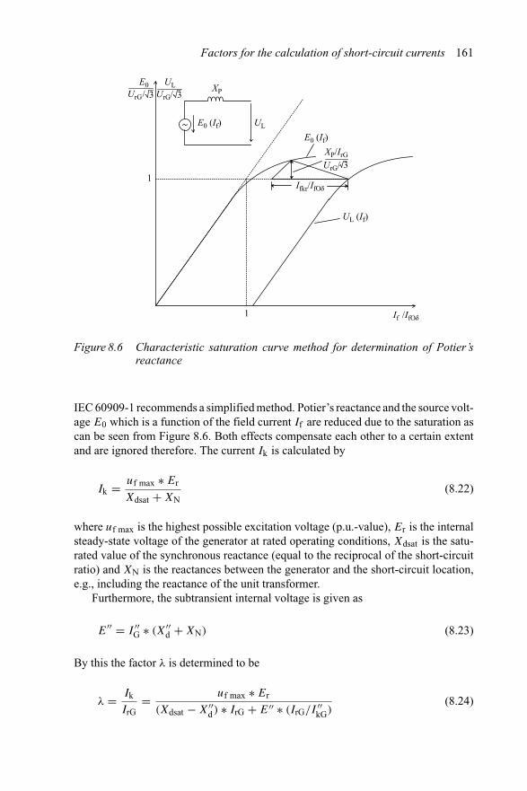
Factors for the calculation of short-circuit currents 161
3/UrG
E0
3
3
/UrG
UL
1
1
XP
E0 (If) UL
E0 (If)
UL (If)
If /IfOd
Ifkr/IfOd
XP/IrG
UrG/
Figure 8.6 Characteristic saturation curve method for determination of Potier’sreactance
IEC 60909-1 recommends a simplified method. Potier’s reactance and the source volt-age E0 which is a function of the field current If are reduced due to the saturation ascan be seen from Figure 8.6. Both effects compensate each other to a certain extentand are ignored therefore. The current Ik is calculated by
Ik = uf max ∗ Er
Xdsat + XN(8.22)
where uf max is the highest possible excitation voltage (p.u.-value), Er is the internalsteady-state voltage of the generator at rated operating conditions, Xdsat is the satu-rated value of the synchronous reactance (equal to the reciprocal of the short-circuitratio) and XN is the reactances between the generator and the short-circuit location,e.g., including the reactance of the unit transformer.
Furthermore, the subtransient internal voltage is given as
E′′ = I ′′G ∗ (X′′
d + XN) (8.23)
By this the factor λ is determined to be
λ = Ik
IrG= uf max ∗ Er
(Xdsat − X′′d) ∗ IrG + E′′ ∗ (IrG/I ′′
kG)(8.24)

162 Short-circuit currents
Table 8.3 Assumed values of uf max for the calcula-tion of the factor λ
uf max = Uf max/Ufr
Type of synchronous machine Series 1 Series 2Salient-pole generator 1.3 1.6Turbine generator 1.6 2.0
The voltages E′′ and Er can be determined if RG � X′′d by
E′′ ≈ UrG√3
∗ (1 + x′′d ∗ sin ϕrG) (8.25)
Er ≈ Ur√3
∗√
1 + x2dsat + 2 ∗ xdsat ∗ sin ϕrG (8.26)
where x′′d = X′′
d ∗ ((√
3 ∗ IrG)/UrG) and xdsat = Xdsat ∗ ((√
3 ∗ IrG)/UrG).The rated impedance is ZrG = UrG/(
√3 ∗ IrG). The values for λmax and λmin as
per Figures 4.11 and 4.12 are calculated by Equations (8.23)–(8.25), cos ϕrG = 0.85and X′
d = 0.2 ∗ ZrG. The highest possible excitation voltage (p.u.-value) uf max isassumed for the calculation in accordance with the values as per Table 8.3.
8.7 Factor q for short-circuit breaking current of asynchronousmotors
Asynchronous motors are contributing to the short-circuit current as outlined inChapter 4. As the short-circuit current of asynchronous motors decays faster ascompared with the short-circuit current of synchronous machines, the short-circuitbreaking current is based on the initial short-circuit current of the motor I ′′
kM usingthe factor μ which is identical to the factor for the calculation of breaking current ofsynchronous generators and an additional factor q
IbM = q ∗ μ ∗ I ′′kM (8.27)
The factor q as per Figure 4.13 is derived from the results of transient calcula-tions and measurements using 28 motors with different rating PrM = 11–160 kWin the low-voltage range and up to PrM = 160 kW–10 MW in the medium-voltage range. A detailed list of the rated data of the asynchronous motors isincluded in Table 2 of IEC 60909-1:1991 (similar to those given in Tables 13.6
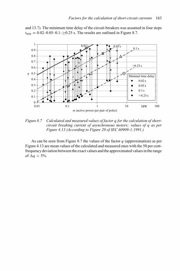
Factors for the calculation of short-circuit currents 163
and 13.7). The minimum time delay of the circuit-breakers was assumed in four stepstmin = 0.02–0.05–0.1–≥0.25 s. The results are outlined in Figure 8.7.
0
0.1
0.2
0.3
0.4
0.5
0.6
0.7
0.8
0.9
1
0.01 0.1 1 10 100m (active power per pair of poles)
q
MW
0.02 s
0.05 s
0.1 s
> 0.25 s
Minimal time delay
0.02 s 0.05 s0.1 s
>0.25 s
Figure 8.7 Calculated and measured values of factor q for the calculation of short-circuit breaking current of asynchronous motors; values of q as perFigure 4.13 (According to Figure 20 of IEC 60909-1:1991.)
As can be seen from Figure 8.7 the values of the factor q (approximation) as perFigure 4.13 are mean values of the calculated and measured ones with the 50 per cent-frequency deviation between the exact values and the approximated values in the rangeof q < 5%.

Chapter 9
Calculation of short-circuit currents ind.c. auxiliary installations
9.1 General
The calculation of short-circuit currents in d.c. auxiliary installations, e.g., in powerplants and substations is dealt with in IEC 61660-1. Contrary to the approach for thecalculation of short-circuit currents in a.c. three-phase systems, the determination ofthe exact time course of the short-circuit current is needed besides the calculation ofdefined parameters [42]. The equipment as below contribute to short-circuit currentsin d.c. installations:
• Smoothing capacitors• Stationary batteries (normally of the lead-acid type)• Rectifiers (IEC 61660-1 deals only with rectifiers in three-phase a.c. bridge
connection for 50 Hz, parameters for 60 Hz are actually under consideration)• d.c. motors with independent excitation.
The branch short-circuit currents from the equipment mentioned above are char-acterised by different time course, depending on the ohmic, inductive and capacitiveparts, the d.c. voltage source and other parameters. Figure 9.1 presents the equivalentcircuit diagrams of the equipment and the typical time course of the short-circuitcurrent.
d.c. installations in auxiliary supply systems include several pieces of equipment;the total short-circuit current at the short-circuit location is the superposition of theindividual branch short-circuit currents from the different equipment. In principle theshort-circuit current can be defined by a time function i1(t), describing the time spantp from short-circuit initiation till the maximal short-circuit current ip (peak short-circuit current) and a time function i2(t), describing the decaying time course to the
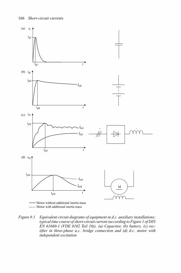
166 Short-circuit currents
iC
ipC
iB
ipB
IkB
tpB
iD
ipD
tpD
iM
tpM
ipM
IkM
IkM
IkD
IkD
tpC t
t
t
t
Motor without additional inertia massMotor with additional inertia mass
~ –
M
(a)
(b)
(c)
(d)
Figure 9.1 Equivalent circuit diagrams of equipment in d.c. auxiliary installations;typical time course of short-circuit current (according to Figure 1 of DINEN 61660-1 (VDE 0102 Teil 10)). (a) Capacitor, (b) battery, (c) rec-tifier in three-phase a.c. bridge connection and (d) d.c. motor withindependent excitation

Calculation in d.c. auxiliary installations 167
0
0.2
0.4
0.6
0.8
1
1.2
0 2 4 6 8 10 12 14 16 18t
i/ip
t2
�1ip
Tk
Ik
i1(t)
tP i2(t)
Figure 9.2 Standard approximation function of the short-circuit current (accordingto Figure 2 of IEC 61660-1:1997)
quasi steady-state short-circuit current Ik as outlined in Figure 9.2. Time functionscan be calculated according to [50] by
i1(t) = ip ∗ 1 − e−t/τ1
1 − e−tp/τ1for 0 ≤ t ≤ tp (9.1a)
i2(t) = ip
((1 − Ik
ip
)∗ e−(t−tp)/τ2 + Ik
ip
)for tp ≤ t ≤ Tk (9.1b)
If no distinct maximum of the short-circuit current is present, the peak short-circuit current ip and the quasi steady-state short-circuit current Ik are equal. Thistime course as well is described by the standard approximation function according toFigure 9.2.
The approach to calculate the parameter ip and Ik, the time constants τ1 and τ2and the time to peak tp is explained below:
• The parameter of the short-circuit current will be calculated for each branchseparately, i.e., for each individual equipment contributing to the short-circuitcurrent.
• In case of several sources, the short-circuit parameters will be calculated bysuperposition of the branch short-circuit currents by:– Calculation of the branch short-circuit currents taking account of the com-
mon branch, i.e., that branch in the installation carrying branch short-circuitcurrents from different sources.
– Correction of the branch short-circuit currents by a factor σ , which dependson the different resistances.

168 Short-circuit currents
– Calculation of the time course of the branch short-circuit currents with thecorrected impedances.
– Superposition of the calculated time functions of the branch short-circuitcurrents to determine the total short-circuit current.
– The thermal and electromagnetic effects of short-circuit currents are calculatedusing the standard approximation function.
The calculation of impedances of the sources in d.c. auxiliary installations feedingthe short-circuit current was dealt with in Section 3.3. The calculation of the short-circuit parameters is carried out as mentioned above and explained below. For thecalculation of maximal short-circuit currents in d.c. auxiliary installations the itemsas below had to be taken into account:
• Short-circuit impedance of system shall be minimal (ZQmin), so that thecontribution to the short-circuit current is maximal.
• Resistance of lines is to be calculated for a temperature of 20◦C.• System topology leading to the maximal short-circuit currents shall be taken into
account.• Joint resistance of busbars shall be neglected.• Control circuits to limit the contribution of rectifiers are disconnected, i.e.,
limitation is not active.• Batteries are fully charged.• Systems coupled by diodes are regarded as directly connected.
For the calculation of minimal short-circuit currents in d.c. auxiliary installationsthe items as stated below shall be considered:
• Short-circuit impedance of system shall be maximal (ZQmax), so that thecontribution to the short-circuit current is minimal.
• System topology leading to the minimal short-circuit currents shall be taken intoaccount.
• Resistance of lines shall be calculated for maximal permissible operatingtemperature.
• Joint resistance of busbar has to be taken into account.• Contribution of rectifiers to the short-circuit current is limited to the rated value
of the current limiter.• Voltage of batteries shall be defined equal to the minimal discharge voltage as per
manufacturer’s information.• Systems coupled by diodes are regarded as disconnected.
The current limiting characteristic of fuses and switchgear in d.c. auxiliary instal-lations has to be taken into account for the calculation of both maximal and minimalshort-circuit current.
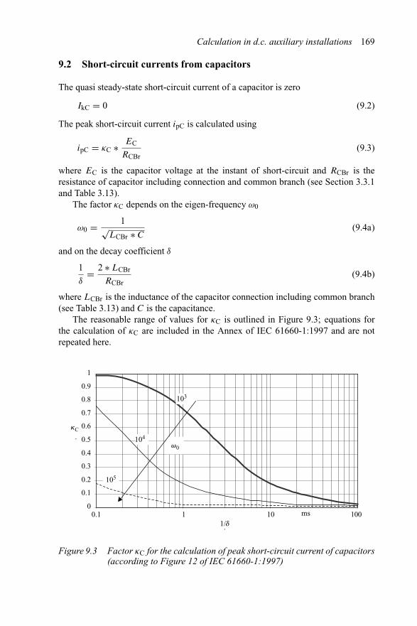
Calculation in d.c. auxiliary installations 169
9.2 Short-circuit currents from capacitors
The quasi steady-state short-circuit current of a capacitor is zero
IkC = 0 (9.2)
The peak short-circuit current ipC is calculated using
ipC = κC ∗ EC
RCBr(9.3)
where EC is the capacitor voltage at the instant of short-circuit and RCBr is theresistance of capacitor including connection and common branch (see Section 3.3.1and Table 3.13).
The factor κC depends on the eigen-frequency ω0
ω0 = 1√LCBr ∗ C
(9.4a)
and on the decay coefficient δ
1
δ= 2 ∗ LCBr
RCBr(9.4b)
where LCBr is the inductance of the capacitor connection including common branch(see Table 3.13) and C is the capacitance.
The reasonable range of values for κC is outlined in Figure 9.3; equations forthe calculation of κC are included in the Annex of IEC 61660-1:1997 and are notrepeated here.
0
0.1
0.2
0.3
0.4
0.5
0.6
0.7
0.8
0.9
1
0.1 1 101/d
kC
100
v0
ms
103
104
105
.
.
Figure 9.3 Factor κC for the calculation of peak short-circuit current of capacitors(according to Figure 12 of IEC 61660-1:1997)
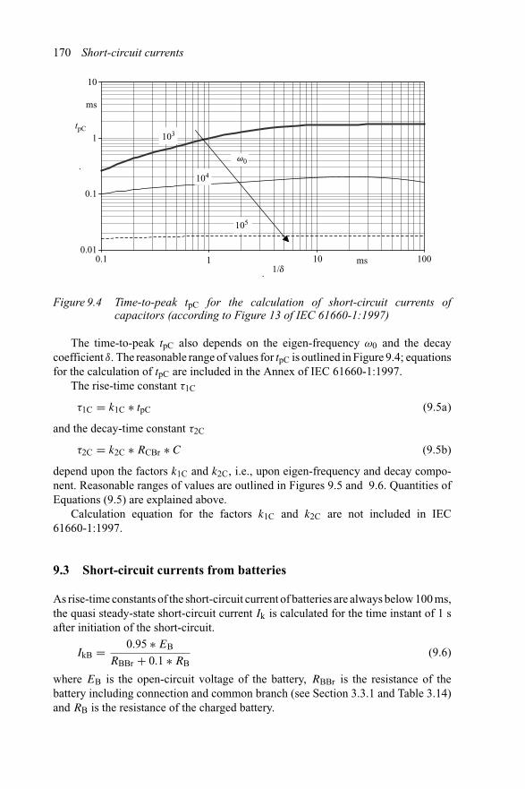
170 Short-circuit currents
0.01
0.1
1
10
0.1 1 10 100
.
.
ms
ms
v0
1/d
tpC103
104
105
Figure 9.4 Time-to-peak tpC for the calculation of short-circuit currents ofcapacitors (according to Figure 13 of IEC 61660-1:1997)
The time-to-peak tpC also depends on the eigen-frequency ω0 and the decaycoefficient δ. The reasonable range of values for tpC is outlined in Figure 9.4; equationsfor the calculation of tpC are included in the Annex of IEC 61660-1:1997.
The rise-time constant τ1C
τ1C = k1C ∗ tpC (9.5a)
and the decay-time constant τ2C
τ2C = k2C ∗ RCBr ∗ C (9.5b)
depend upon the factors k1C and k2C, i.e., upon eigen-frequency and decay compo-nent. Reasonable ranges of values are outlined in Figures 9.5 and 9.6. Quantities ofEquations (9.5) are explained above.
Calculation equation for the factors k1C and k2C are not included in IEC61660-1:1997.
9.3 Short-circuit currents from batteries
As rise-time constants of the short-circuit current of batteries are always below 100 ms,the quasi steady-state short-circuit current Ik is calculated for the time instant of 1 safter initiation of the short-circuit.
IkB = 0.95 ∗ EB
RBBr + 0.1 ∗ RB(9.6)
where EB is the open-circuit voltage of the battery, RBBr is the resistance of thebattery including connection and common branch (see Section 3.3.1 and Table 3.14)and RB is the resistance of the charged battery.
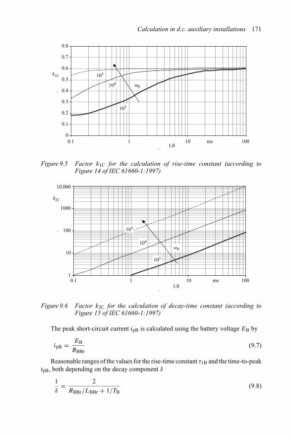
Calculation in d.c. auxiliary installations 171
0
0.1
0.2
0.3
0.4
0.5
0.6
0.7
0.8
v0
0.1 1 10 100
.
.
ms1/d
k1C 105
104
103
Figure 9.5 Factor k1C for the calculation of rise-time constant (according toFigure 14 of IEC 61660-1:1997)
1
10
100
1000
10,000
0.1 1 10 100
.
.
ms1/d
k2C
105
104
103
v0
Figure 9.6 Factor k2C for the calculation of decay-time constant (according toFigure 15 of IEC 61660-1:1997)
The peak short-circuit current ipB is calculated using the battery voltage EB by
ipB = EB
RBBr(9.7)
Reasonable ranges of the values for the rise-time constant τ1B and the time-to-peaktpB, both depending on the decay component δ
1
δ= 2
RBBr/LBBr + 1/TB(9.8)

172 Short-circuit currents
0.1
1
10
100
0.1 1 10 100
.
.
ms
ms
1/d
tpB
�1B
tpB
�1B
Figure 9.7 Rise-time constant τ1B and time to peak tpB of short-circuit currents ofbatteries (according to Figure 10 of IEC 61660-1:1997)
where LBBr is the reactance of the battery including connection and common branch(see Table 3.14) and TB is the time constant of the battery assumed to be TB = 30 ms(outlined in Figure 9.7). The decay-time constant is set to τ2B = 100 ms.
More details of the calculation of short-circuit currents fed from batteries areincluded in [56].
9.4 Short-circuit currents from rectifiers
The quasi steady-state short-circuit current IkD of a rectifier in three-phase a.c. bridgeconnection is
IkD = λD ∗ 3 ∗ √2
π∗ c ∗ Un√
3 ∗ ZN∗ UrTLV
UrTHV(9.9)
where Un is the nominal system voltage on a.c. side of rectifier, ZN is the networkimpedance a.c. side, UrTLV is the rated voltage at low voltage side of transformer (a.c.side) and UrTHV is the rated voltage at high voltage side of transformer (a.c. side).
The factor λD depends on the ratio RN/XN of the a.c. side of the rectifier as wellas on the ratio of the resistances RDBr/RN (ratio of resistance d.c. side to resistancea.c. side). A reasonable range of values of the factor λD is outlined in Figure 9.8.Equations for the calculation of λD are included in IEC 61660-1:1997.
The peak short-circuit current is calculated using
ipD = κD ∗ IkD (9.10)
whereas the factor κD depends on the ratio of the inductivities LDBr/LN (ratio ofinductance d.c. side to inductance a.c. side) and on the resistances and reactances
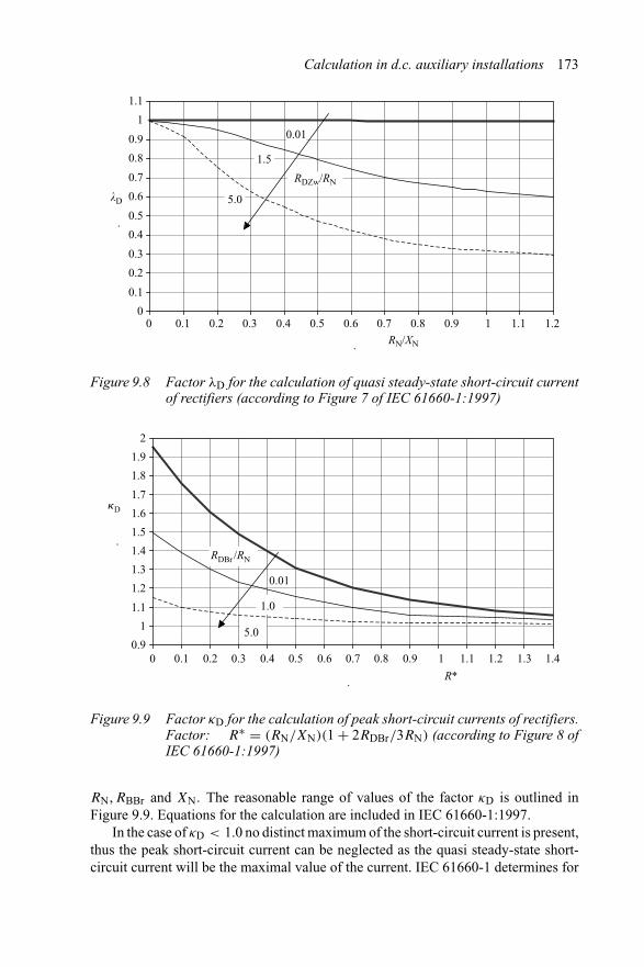
Calculation in d.c. auxiliary installations 173
0
0.1
0.2
0.3
0.4
0.5
0.6
0.7
0.8
0.9
1
1.1
0 0.1 0.2 0.3 0.4 0.5 0.6 0.7 0.8 0.9 1 1.1 1.2
.
.
RN/XN
�D
0.01
1.5
5.0
RDZw/RN
Figure 9.8 Factor λD for the calculation of quasi steady-state short-circuit currentof rectifiers (according to Figure 7 of IEC 61660-1:1997)
0.9
1
1.1
1.2
1.3
1.4
1.5
1.6
1.7
1.8
1.9
2
0 0.1 0.2 0.3 0.4 0.5 0.6 0.7 0.8 0.9 1 1.1 1.2 1.3 1.4
.
.
R*
kD
RDBr /RN
1.0
0.01
5.0
Figure 9.9 Factor κD for the calculation of peak short-circuit currents of rectifiers.Factor: R∗ = (RN/XN)(1 + 2RDBr/3RN) (according to Figure 8 ofIEC 61660-1:1997)
RN, RBBr and XN. The reasonable range of values of the factor κD is outlined inFigure 9.9. Equations for the calculation are included in IEC 61660-1:1997.
In the case of κD < 1.0 no distinct maximum of the short-circuit current is present,thus the peak short-circuit current can be neglected as the quasi steady-state short-circuit current will be the maximal value of the current. IEC 61660-1 determines for
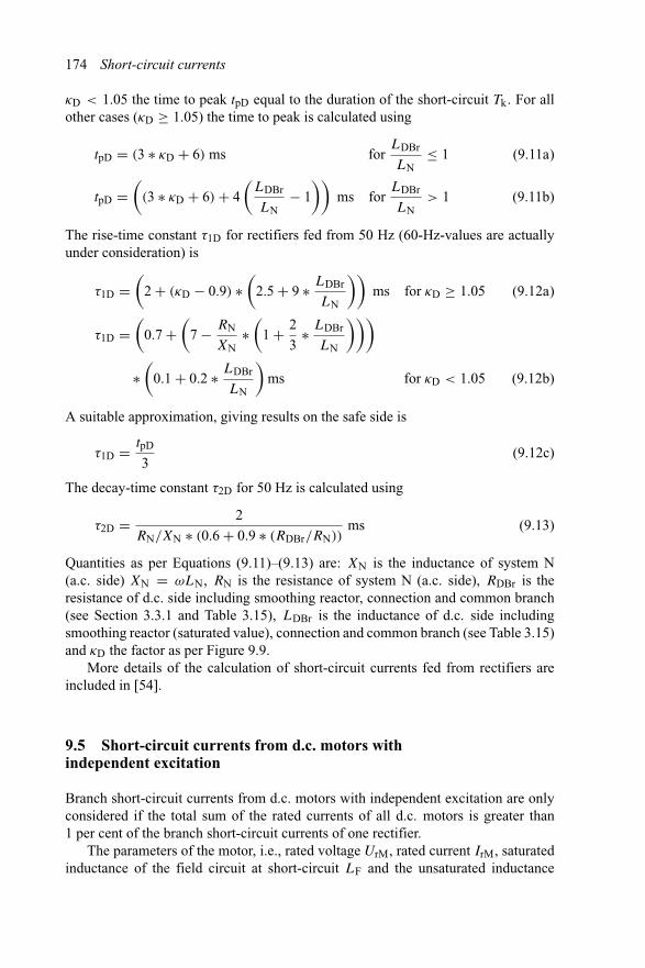
174 Short-circuit currents
κD < 1.05 the time to peak tpD equal to the duration of the short-circuit Tk. For allother cases (κD ≥ 1.05) the time to peak is calculated using
tpD = (3 ∗ κD + 6) ms forLDBr
LN≤ 1 (9.11a)
tpD =(
(3 ∗ κD + 6) + 4(
LDBr
LN− 1
))ms for
LDBr
LN> 1 (9.11b)
The rise-time constant τ1D for rectifiers fed from 50 Hz (60-Hz-values are actuallyunder consideration) is
τ1D =(
2 + (κD − 0.9) ∗(
2.5 + 9 ∗ LDBr
LN
))ms for κD ≥ 1.05 (9.12a)
τ1D =(
0.7 +(
7 − RN
XN∗(
1 + 2
3∗ LDBr
LN
)))
∗(
0.1 + 0.2 ∗ LDBr
LN
)ms for κD < 1.05 (9.12b)
A suitable approximation, giving results on the safe side is
τ1D = tpD
3(9.12c)
The decay-time constant τ2D for 50 Hz is calculated using
τ2D = 2
RN/XN ∗ (0.6 + 0.9 ∗ (RDBr/RN))ms (9.13)
Quantities as per Equations (9.11)–(9.13) are: XN is the inductance of system N(a.c. side) XN = ωLN, RN is the resistance of system N (a.c. side), RDBr is theresistance of d.c. side including smoothing reactor, connection and common branch(see Section 3.3.1 and Table 3.15), LDBr is the inductance of d.c. side includingsmoothing reactor (saturated value), connection and common branch (see Table 3.15)and κD the factor as per Figure 9.9.
More details of the calculation of short-circuit currents fed from rectifiers areincluded in [54].
9.5 Short-circuit currents from d.c. motors withindependent excitation
Branch short-circuit currents from d.c. motors with independent excitation are onlyconsidered if the total sum of the rated currents of all d.c. motors is greater than1 per cent of the branch short-circuit currents of one rectifier.
The parameters of the motor, i.e., rated voltage UrM, rated current IrM, saturatedinductance of the field circuit at short-circuit LF and the unsaturated inductance

Calculation in d.c. auxiliary installations 175
of the field circuit at no-load LOF, determine the quasi steady-state short-circuitcurrent IkM which is calculated using
IkM = LF
LOF∗(
UrM − IrM ∗ RM
RMBr
)(9.14)
where LF is the field inductance, LOF is field inductance at no-load, UrM is therated voltage, IrM is the rated current of the motor, RM is the resistance of the motorand RMBr the resistance of the motor including connection and common branch (seeSection 3.3.1 and Table 3.16).
Equation (9.14) is valid when the speed of the motor remains constant during theduration of the short-circuit. When the speed of the motor decreases to zero (n → 0)the quasi steady-state short-circuit current is IkM = 0.
The mechanical time constant τMec, the time constants of the field circuit τFand the armature circuit τM determine the peak short-circuit current ipM, which iscalculated using
ipM = κM ∗ UrM − IrM ∗ RM
RMBr(9.15)
The factor κM is equal to One in the case of nominal speed and in all cases whereτMec ≥ 10∗tF, else (τMec < 10 ∗ τF). κM depends on the eigen-frequency ω0,
ω0 =√
1
τMec ∗ τM∗(
1 − RM ∗ IrM
UrM
)(9.16a)
where τMec is the mechanical time constant (see Table 3.16) and τM the time constantof armature circuit up to short-circuit location (see Table 3.16); and on the decaycoefficient δ.
1
δ= 2 ∗ τM (9.16b)
The reasonable range of the factor κM is outlined in Figure 9.10.The time to peak tpM, the rise-time and the decay-time constants τ1M and τ2M
depend on the value of the mechanical time constant τMec. IEC 61660-1:1997 definesfour factors k1M, k2M, k3M and k4M which are outlined in Figures 9.12 to 9.15.Calculation equations are not included in IEC 61000-1:1997.
When the motor speed remains constant or in all cases when τMec ≥ 10 ∗ τF thetime to peak tpM is calculated using
tpM = k1M ∗ τM (9.17)
the rise-time constant τ1M
τ1M = k2M ∗ τM (9.18)

176 Short-circuit currents
0
0.1
0.2
0.3
0.4
0.5
0.6
0.7
0.8
0.9
1
1.1
1 10 100
.
.
ms
1/d
�M
100
�0
1
20
Figure 9.10 Factor κM for the calculation of peak short-circuit current of d.c.motors with independent excitation (according to Figure 17 of IEC61660-1:1997)
100
�0
110
tpM
.
1
10
100
1000
ms
1 10 100.
ms1/�
Figure 9.11 Time to peak of short-circuit currents for d.c. motors with indepen-dent excitation and τMec < 10 ∗ τF (according to Figure 19 of IEC61660-1:1997)
and the decay-time constant τ2M
τ2M = τF n = nn = const. (9.19a)
τ2M = k4M ∗ LOF
LF∗ τMec n → 0 (9.19b)
For all other cases, i.e., τMec < 10 ∗ τF the reasonable range of the time to peak tpMis outlined in Figure 9.11.
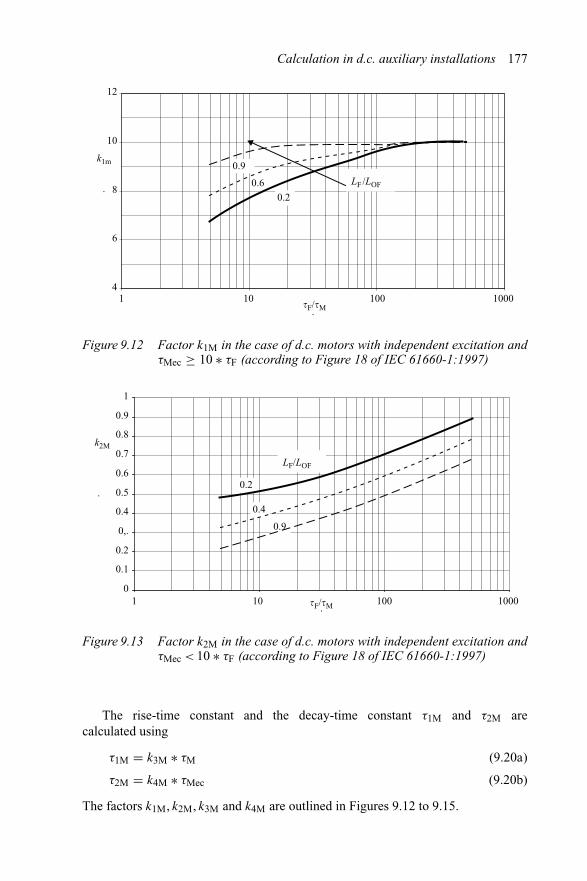
Calculation in d.c. auxiliary installations 177
1 10 100 1000.
LF /LOF
0.20.6
0.9
4
6
8
10
12.
k1m
�F/�M
Figure 9.12 Factor k1M in the case of d.c. motors with independent excitation andτMec ≥ 10 ∗ τF (according to Figure 18 of IEC 61660-1:1997)
.
0.2
0.4
0.9
LF/LOF
0
0.1
0.2
0,.
0.4
0.5
0.6
0.7
0.8
0.9
1
.
k2M
1 10 100 1000�F/�M
Figure 9.13 Factor k2M in the case of d.c. motors with independent excitation andτMec < 10 ∗ τF (according to Figure 18 of IEC 61660-1:1997)
The rise-time constant and the decay-time constant τ1M and τ2M arecalculated using
τ1M = k3M ∗ τM (9.20a)
τ2M = k4M ∗ τMec (9.20b)
The factors k1M, k2M, k3M and k4M are outlined in Figures 9.12 to 9.15.
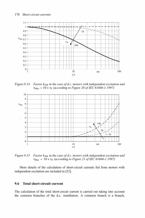
178 Short-circuit currents
1 10 100
.
ms
�0
10
100
1/�
0
0.1
0.2
0.3
0.4
0.5
0.6
0.7
0.8
0.9
1
1.1.
k3M
1
Figure 9.14 Factor k3M in the case of d.c. motors with independent excitation andτMec < 10 ∗ τF (according to Figure 20 of IEC 61660-1:1997)
.
�0
100
50
1–10
k4M
0
1
2
3
4
5
6
7
8
9
10
1 10 100ms1/�
Figure 9.15 Factor k4M in the case of d.c. motors with independent excitation andτMec < 10 ∗ τF (according to Figure 21 of IEC 61660-1:1997)
More details of the calculation of short-circuit currents fed from motors withindependent excitation are included in [52].
9.6 Total short-circuit current
The calculation of the total short-circuit current is carried out taking into accountthe common branches of the d.c. installation. A common branch is a branch,

Calculation in d.c. auxiliary installations 179
e.g., conductor circuit, which carries branch short-circuit currents from differentsources.
When no common branch exists in the d.c. installation, the total short-circuitcurrent is calculated by adding the branch (partial) short-circuit currents. Otherwise,the partial short-circuit currents of the different sources (Index j) are to be corrected(Index kor) with factors σj, which reflect the different resistances of the sourcesand the common branches RY. The peak short-circuit current and quasi steady-stateshort-circuit current are calculated by
ipkorj = σj ∗ ipj (9.21a)
Ikkorj = σj ∗ Ikj (9.21b)
with the correction factor σj for each source j
σj = Rresj ∗ (Rij + RY)
Rresj ∗ Rij + Rij ∗ RY + Rresj ∗ RY(9.22)
The resistance up to the common branch of a source is named Rij and the equivalentresistance of the other sources up to the common branch which contributes to theshort-circuit current is named Rresj . Resistances of capacitors are neglected and theresistance of motors shall only be taken into account if the motor contributes tothe quasi steady-state short-circuit current.
The calculation equations of the resistances Rij and equivalent resistances Rresjare outlined in Table 9.1. It is assumed, that all four sources are contributing to theshort-circuit current through one common branch, as outlined in Figure 9.16.
Table 9.1 Resistances Rij and equivalent resistances Rresj for the calcu-lation of correction factors; U: Voltage at short-circuit locationprior to the short-circuit [42,50,57]
Source j Resistance Rij Equivalent resistance Rresj
Capacitor RiC = RC + RCL RresC = 1
1/RiD + 1/RiB + 1/RiM
Battery RiB = RB + RBL RresB = 1
1/RiD + 1/RiM
Rectifier RiD = U
IkD− RY RresD = 1
1/RiB + 1/RiM
d.c. motor with RiM = RM + RML RresM = 1
1/RiD + 1/RiBindependentexcitation
Remarks: Index L – Connection of equipment; index Y – Common branch (see Section 3.3.1);and indices C; B; D; M – Capacitor; battery; rectifier; motor
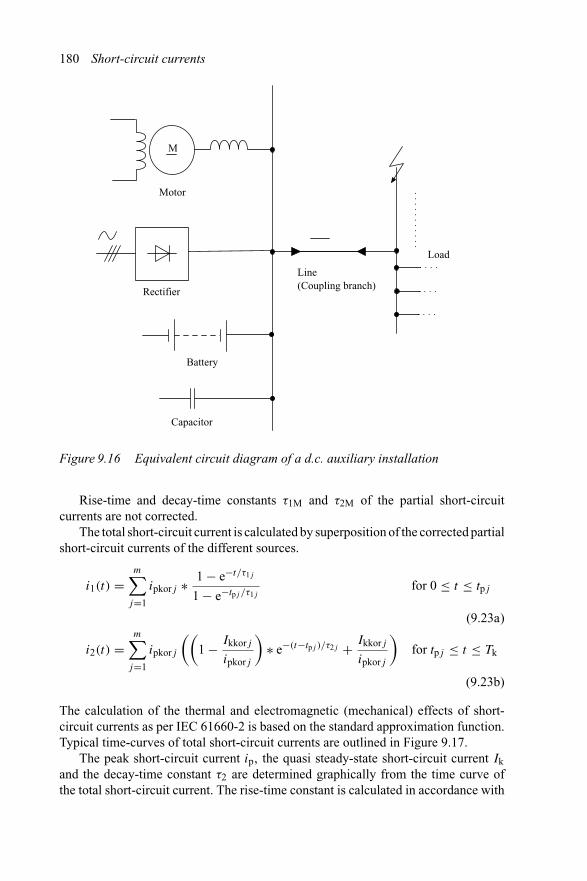
180 Short-circuit currents
M
Motor
Rectifier
Battery
Capacitor
Line(Coupling branch)
Load
Figure 9.16 Equivalent circuit diagram of a d.c. auxiliary installation
Rise-time and decay-time constants τ1M and τ2M of the partial short-circuitcurrents are not corrected.
The total short-circuit current is calculated by superposition of the corrected partialshort-circuit currents of the different sources.
i1(t) =m∑
j=1
ipkorj ∗ 1 − e−t/τ1j
1 − e−tpj /τ1jfor 0 ≤ t ≤ tpj
(9.23a)
i2(t) =m∑
j=1
ipkorj
((1 − Ikkorj
ipkorj
)∗ e−(t−tpj )/τ2j + Ikkorj
ipkorj
)for tpj ≤ t ≤ Tk
(9.23b)
The calculation of the thermal and electromagnetic (mechanical) effects of short-circuit currents as per IEC 61660-2 is based on the standard approximation function.Typical time-curves of total short-circuit currents are outlined in Figure 9.17.
The peak short-circuit current ip, the quasi steady-state short-circuit current Ikand the decay-time constant τ2 are determined graphically from the time curve ofthe total short-circuit current. The rise-time constant is calculated in accordance with
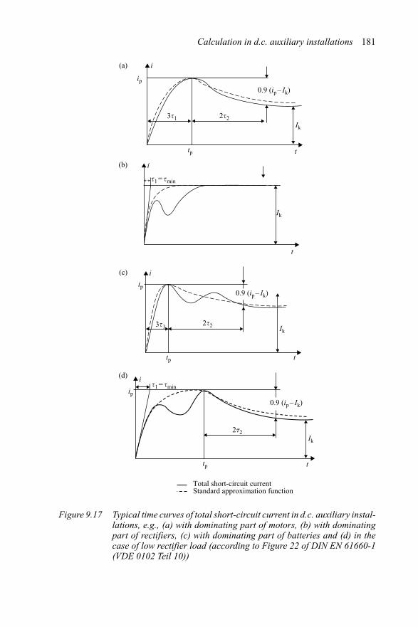
Calculation in d.c. auxiliary installations 181
3�1 2�2
3�1 2�2
0.9 (ip – Ik)
0.9 (ip – Ik)
ip
ip
tp
tp
i(a)
(b)
(c)
(d)
Ik
�1 = �min
Ik
i
Ik
i
t
i
ip
2t2Ik
ttp
t
t
�1 = �min
0.9 (ip – Ik)
Total short-circuit currentStandard approximation function
Figure 9.17 Typical time curves of total short-circuit current in d.c. auxiliary instal-lations, e.g., (a) with dominating part of motors, (b) with dominatingpart of rectifiers, (c) with dominating part of batteries and (d) in thecase of low rectifier load (according to Figure 22 of DIN EN 61660-1(VDE 0102 Teil 10))

182 Short-circuit currents
Figure 9.17(a) and (c), respectively by
τ1 = tp
3(9.24a)
and for time curves as per Figure 9.17(b) or (d)
τ1 = MIN{τ1C; τ1B; τ1D; τ1M} (9.24b)
The rise-time constant τ1C of capacitors is neglected in the case where
ipC ≤ 0.5 ∗ ip (9.25)
The decay-time constant τ2 is equal to 50 per cent of that time span in which theshort-circuit current i2(t) is reduced to 0.9 ∗ (ip–Ik), i.e., the short-circuit current hasthe value of (Ik + 0.1 ∗ ip). Reference is made to Figure 9.17.
i2(tp + 2τ2) = 0.9 ∗ (ip − Ik) (9.26a)
and
i2(tp + 2τ2) = Ik + 0.1 ∗ ip (9.26b)
9.7 Example
The short-circuit currents at location F at the main busbar of the auxiliary supplyinstallation of a power station are to be calculated. The 220-V-installation as outlinedin Figure 9.18 include a battery of 1100 Ah, feeding from an a.c. LV-system throughrectifier with smoothing capacitor and a d.c. motor. The data and parameter of theequipment are given below:
RectifierCapacitor L2
TQ
Q L4
D C L1
Cable
Load
Motor
M
MF
L3
Cablecoupling branch
Cable
Battery Busbar
Figure 9.18 Equivalent circuit diagram of the d.c. auxiliary installation (220 V),e.g., of a power station

Calculation in d.c. auxiliary installations 183
Equipment Quantity Parameter Remarks
Battery B Nominal voltage UnB = 225 V Table 3.14Capacity for K10 = 1100 Ah
10 h-dischargeResistance per cell RBZ = 0.12 m�
Inductance per cell LBZ = 0.2 μHNumber of cells n = 109
Power system Nominal voltage UnQ = 660 V Table 3.1Initial short-circuit S′′
kQ = 33.3 MVApower
Resistance RQ/XQ = 0.28
AC/DC- Rated voltages UrTHV/UrTLV = Table 3.2transformer 660 V/240 V
Rated power SrT = 380 kVAImpedance voltage ukT = 3.2%Losses; resistance PCu = 4 kW;voltage uRT = 0.5%
Rectifier D Rated voltage UrD = 220 V Table 3.15Rated current IrD = 1000 A
Smoothing Resistance RDBr = 0.87 m� Table 3.15reactor Reactance XDBr = 29 μH
Smoothing a.c. capacitance Cac = 70 mF Table 3.13capacitor C Resistance RC = 8 m�
d.c. motor M Rated voltage UrM = 220 V Table 3.16Rated power PrM = 95 kWRated current IrM = 432 ANo-load speed n0 = 25 s−1
Inductance of LM = 0.4 mHarmature circuit
Resistance of RM = 41.9 m�
armatureInductance of LF = 9.9 H
field circuitResistance of RF = 9.9 �
field circuitMoment of inertia J = 6.5 kg m2
Motor speed n → 0Tk > 1 s

184 Short-circuit currents
Equipment Quantity Parameter Remarks
Cables Cross section qn = 300 mm2 Table 3.12L1; L2; L3 Number of cables 3 in parallel (triangle)
Specific resistance ρ = 0.0173 �mm2/mRadius of conductor r = 10.5 mmLength of cables L1 = 2 m; L2 = 6 m;
L3 = 20 m
Conductor Cross section qn = 400 mm2 Table 3.12bars L4 Number of bars 2 in parallel
Width and height d × b = 10 mm × 40 mmSpecific resistance ρ = 0.0173 �mm2/mDistance between aS = 10 mm
sub-conductorsDistance of bars am = 75 mmLength of bar L4 = 14 m
The calculation of the short-circuit current is as follows:
1 Calculation of the impedances of cables and busbar conductors (Section 9.7.1).2 Calculation of the short-circuit currents of the individual equipment
(Section 9.7.2).3 Calculation of the correction factors (Section 9.7.3).4 Calculation of partial short-circuit currents (Section 9.7.4).5 Calculation of total short-circuit current (Section 9.7.5).
9.7.1 Calculation of the impedances of cables and busbar conductors
Three cables are laid in triangle arrangement. Specific resistance and inductance arecalculated according to Table 3.12.
R′ = 2ρ
3qn= 2
0.0173 �mm2/m
3 ∗ 300 mm2 = 0.0384 m�/m
L′ = μ0
π∗(
lna
rB+ 1
4n
)
with rB = n√
n ∗ rT ∗ rn−1 = 3√
3 ∗ 17.3 mm ∗ (10.5 mm)2 = 17.9 mm
L′ = 4π ∗ 10−7 H/m
π
(ln
75 mm
17.9 mm+ 1
4 ∗ 3
)= 0.607 μH/m
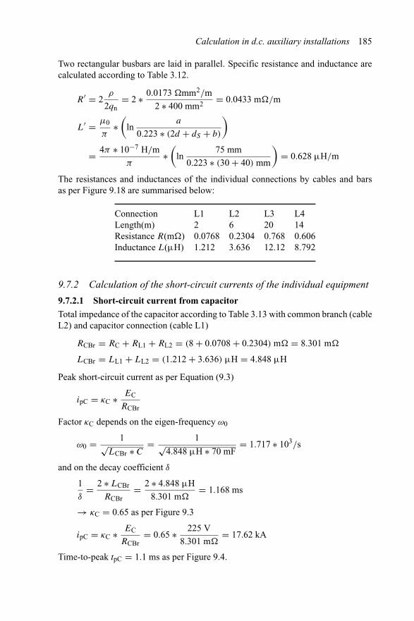
Calculation in d.c. auxiliary installations 185
Two rectangular busbars are laid in parallel. Specific resistance and inductance arecalculated according to Table 3.12.
R′ = 2ρ
2qn= 2 ∗ 0.0173 �mm2/m
2 ∗ 400 mm2 = 0.0433 m�/m
L′ = μ0
π∗(
lna
0.223 ∗ (2d + dS + b)
)
= 4π ∗ 10−7 H/m
π∗(
ln75 mm
0.223 ∗ (30 + 40) mm
)= 0.628 μH/m
The resistances and inductances of the individual connections by cables and barsas per Figure 9.18 are summarised below:
Connection L1 L2 L3 L4Length(m) 2 6 20 14Resistance R(m�) 0.0768 0.2304 0.768 0.606Inductance L(μH) 1.212 3.636 12.12 8.792
9.7.2 Calculation of the short-circuit currents of the individual equipment
9.7.2.1 Short-circuit current from capacitor
Total impedance of the capacitor according to Table 3.13 with common branch (cableL2) and capacitor connection (cable L1)
RCBr = RC + RL1 + RL2 = (8 + 0.0708 + 0.2304) m� = 8.301 m�
LCBr = LL1 + LL2 = (1.212 + 3.636) μH = 4.848 μH
Peak short-circuit current as per Equation (9.3)
ipC = κC ∗ EC
RCBr
Factor κC depends on the eigen-frequency ω0
ω0 = 1√LCBr ∗ C
= 1√4.848 μH ∗ 70 mF
= 1.717 ∗ 103/s
and on the decay coefficient δ
1
δ= 2 ∗ LCBr
RCBr= 2 ∗ 4.848 μH
8.301 m�= 1.168 ms
→ κC = 0.65 as per Figure 9.3
ipC = κC ∗ EC
RCBr= 0.65 ∗ 225 V
8.301 m�= 17.62 kA
Time-to-peak tpC = 1.1 ms as per Figure 9.4.
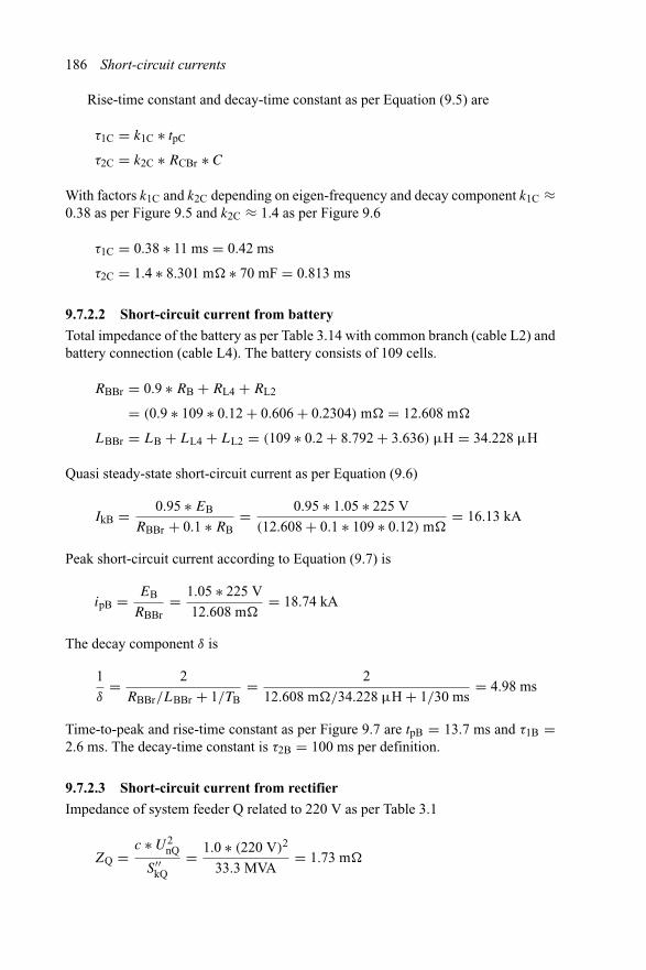
186 Short-circuit currents
Rise-time constant and decay-time constant as per Equation (9.5) are
τ1C = k1C ∗ tpC
τ2C = k2C ∗ RCBr ∗ C
With factors k1C and k2C depending on eigen-frequency and decay component k1C ≈0.38 as per Figure 9.5 and k2C ≈ 1.4 as per Figure 9.6
τ1C = 0.38 ∗ 11 ms = 0.42 ms
τ2C = 1.4 ∗ 8.301 m� ∗ 70 mF = 0.813 ms
9.7.2.2 Short-circuit current from battery
Total impedance of the battery as per Table 3.14 with common branch (cable L2) andbattery connection (cable L4). The battery consists of 109 cells.
RBBr = 0.9 ∗ RB + RL4 + RL2
= (0.9 ∗ 109 ∗ 0.12 + 0.606 + 0.2304) m� = 12.608 m�
LBBr = LB + LL4 + LL2 = (109 ∗ 0.2 + 8.792 + 3.636) μH = 34.228 μH
Quasi steady-state short-circuit current as per Equation (9.6)
IkB = 0.95 ∗ EB
RBBr + 0.1 ∗ RB= 0.95 ∗ 1.05 ∗ 225 V
(12.608 + 0.1 ∗ 109 ∗ 0.12) m�= 16.13 kA
Peak short-circuit current according to Equation (9.7) is
ipB = EB
RBBr= 1.05 ∗ 225 V
12.608 m�= 18.74 kA
The decay component δ is
1
δ= 2
RBBr/LBBr + 1/TB= 2
12.608 m�/34.228 μH + 1/30 ms= 4.98 ms
Time-to-peak and rise-time constant as per Figure 9.7 are tpB = 13.7 ms and τ1B =2.6 ms. The decay-time constant is τ2B = 100 ms per definition.
9.7.2.3 Short-circuit current from rectifier
Impedance of system feeder Q related to 220 V as per Table 3.1
ZQ = c ∗ U2nQ
S′′kQ
= 1.0 ∗ (220 V)2
33.3 MVA= 1.73 m�

Calculation in d.c. auxiliary installations 187
Resistance and reactance due to the ratio of RQ/XQ
XQ = 0.963 ∗ ZQ = 1.666 m�
RQ =√
Z2Q − X2
Q = 0.466 m�
Impedance of transformer according to Table 3.2
ZT = ukT
SrT∗ U2
rTLV
100%= 3.2%
380 kVA∗ (240 V)2
100%= 4.85 m�
RT = uRT
SrT∗ U2
rTLV
100%= 1.05%
380 kVA∗ (240 V)2
100%= 1.592 m�
XT =√
Z2T − R2
T = 4.581 m�
Total impedance a.c. side according to Table 3.15
RN = RQ + RT = (0.466 + 1.592) m� = 2.058 m�
XN = XQ + XT = (1.666 + 4.581) m� = 6.247 m�
and inductance
LN = XN/ω = (6.247/100 ∗ π) μH = 4.581 μH
Total impedance d.c. side according to Table 3.15 with common branch (cable L2)
RDBr = RS + RL1 + RL2 = (0.87 + 0.0768 + 0.2304) m� = 1.177 m�
LDBr = LS + LL1 + LL2 = (29 + 1.212 + 3.636) μH = 33.85 μH
Quasi steady-state short-circuit current of the rectifier as per Equation (9.9)
IkD = λD ∗ 3 ∗ √2
π∗ c ∗ Un√
3 ∗ ZN∗ UrTLV
UrTHV
Factor λD depending on RN/XN and RDBr/RN
RN/XN = 0.33 and RDBr/RN = 0.572 → λD = 0.92 as per Figure 9.8
IkD = 0.92 ∗ 3 ∗ √2
π∗ 1.0 ∗ 240 V√
3 ∗ 6.58 m�∗ 240 V
660 V= 26.44 kA
Peak short-circuit current as per Equation (9.10)
ipD = κD ∗ IkD
Factor κD depends on LDBr/LN and RN, RBBr and XN
LDBr/LN = 1.702 andRN
XN
(1 + 2
3∗ RDBr
RN
)= 0.455 → κD = 1.12
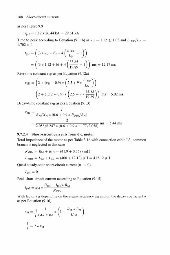
188 Short-circuit currents
as per Figure 9.9
ipD = 1.12 ∗ 26.44 kA = 29.61 kA
Time to peak according to Equation (9.11b) as κD = 1.12 ≥ 1.05 and LDBr/LN =1.702 > 1
tpD =(
(3 ∗ κD + 6) + 4(
LDBr
LN− 1
))
=(
(3 ∗ 1.12 + 6) + 4(
33.85
19.89− 1
))ms = 12.17 ms
Rise-time constant τ1D as per Equation (9.12a)
τ1D =(
2 + (κD − 0.9) ∗(
2.5 + 9 ∗ LDBr
LN
))
=(
2 + (1.12 − 0.9) ∗(
2.5 + 9 ∗ 33.85
19.89
))ms = 5.92 ms
Decay-time constant τ2D as per Equation (9.13)
τ2D = 2
RN/XN ∗ (0.6 + 0.9 ∗ RDBr/RN)
= 2
2.058/6.247 ∗ (0.6 + 0.9 ∗ 1.177/2.058)ms = 5.44 ms
9.7.2.4 Short-circuit currents from d.c. motor
Total impedance of the motor as per Table 3.16 with connection cable L3, commonbranch is neglected in this case
RMBr = RM + RL3 = (41.9 + 0.768) m�
LMBr = LM + LL3 = (400 + 12.12) μH = 412.12 μH
Quasi steady-state short-circuit current (n → 0)
IkM = 0
Peak short-circuit current according to Equation (9.15)
ipM = κM ∗ UrM − IrM ∗ RM
RMBr
With factor κM depending on the eigen-frequency ω0 and on the decay coefficient δ
as per Equation (9.16)
ω0 =√
1
τMec ∗ τM∗(
1 − RM ∗ IrM
UrM
)
1
δ= 2 ∗ τM
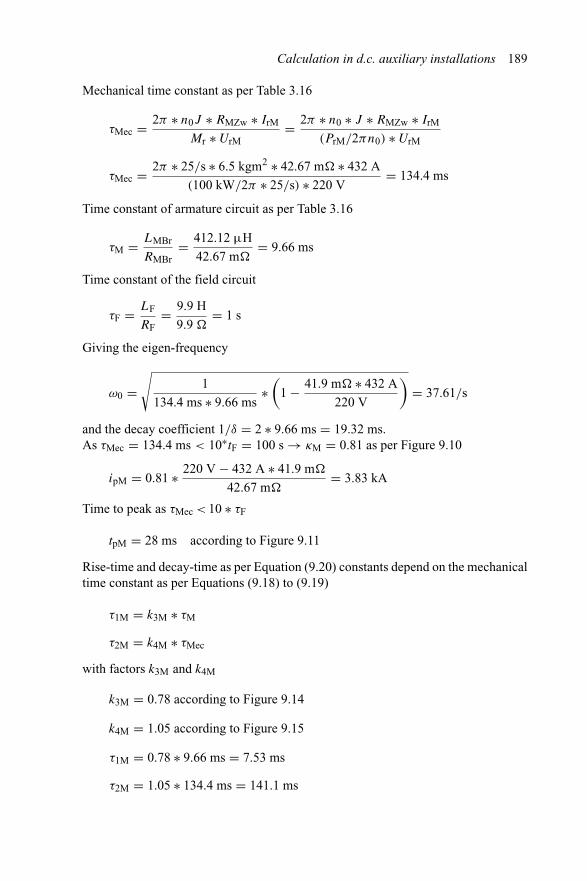
Calculation in d.c. auxiliary installations 189
Mechanical time constant as per Table 3.16
τMec = 2π ∗ n0J ∗ RMZw ∗ IrM
Mr ∗ UrM= 2π ∗ n0 ∗ J ∗ RMZw ∗ IrM
(PrM/2πn0) ∗ UrM
τMec = 2π ∗ 25/s ∗ 6.5 kgm2 ∗ 42.67 m� ∗ 432 A
(100 kW/2π ∗ 25/s) ∗ 220 V= 134.4 ms
Time constant of armature circuit as per Table 3.16
τM = LMBr
RMBr= 412.12 μH
42.67 m�= 9.66 ms
Time constant of the field circuit
τF = LF
RF= 9.9 H
9.9 �= 1 s
Giving the eigen-frequency
ω0 =√
1
134.4 ms ∗ 9.66 ms∗(
1 − 41.9 m� ∗ 432 A
220 V
)= 37.61/s
and the decay coefficient 1/δ = 2 ∗ 9.66 ms = 19.32 ms.As τMec = 134.4 ms < 10∗tF = 100 s → κM = 0.81 as per Figure 9.10
ipM = 0.81 ∗ 220 V − 432 A ∗ 41.9 m�
42.67 m�= 3.83 kA
Time to peak as τMec < 10 ∗ τF
tpM = 28 ms according to Figure 9.11
Rise-time and decay-time as per Equation (9.20) constants depend on the mechanicaltime constant as per Equations (9.18) to (9.19)
τ1M = k3M ∗ τM
τ2M = k4M ∗ τMec
with factors k3M and k4M
k3M = 0.78 according to Figure 9.14
k4M = 1.05 according to Figure 9.15
τ1M = 0.78 ∗ 9.66 ms = 7.53 ms
τ2M = 1.05 ∗ 134.4 ms = 141.1 ms
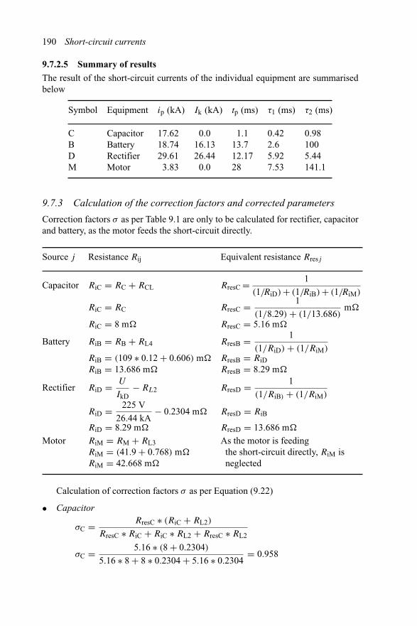
190 Short-circuit currents
9.7.2.5 Summary of results
The result of the short-circuit currents of the individual equipment are summarisedbelow
Symbol Equipment ip (kA) Ik (kA) tp (ms) τ1 (ms) τ2 (ms)
C Capacitor 17.62 0.0 1.1 0.42 0.98B Battery 18.74 16.13 13.7 2.6 100D Rectifier 29.61 26.44 12.17 5.92 5.44M Motor 3.83 0.0 28 7.53 141.1
9.7.3 Calculation of the correction factors and corrected parameters
Correction factors σ as per Table 9.1 are only to be calculated for rectifier, capacitorand battery, as the motor feeds the short-circuit directly.
Source j Resistance Rij Equivalent resistance Rresj
Capacitor RiC = RC + RCL RresC = 1
(1/RiD) + (1/RiB) + (1/RiM)
RiC = RC RresC = 1
(1/8.29) + (1/13.686)m�
RiC = 8 m� RresC = 5.16 m�
Battery RiB = RB + RL4 RresB = 1
(1/RiD) + (1/RiM)RiB = (109 ∗ 0.12 + 0.606) m� RresB = RiDRiB = 13.686 m� RresB = 8.29 m�
Rectifier RiD = U
IkD− RL2 RresD = 1
(1/RiB) + (1/RiM)
RiD = 225 V
26.44 kA− 0.2304 m� RresD = RiB
RiD = 8.29 m� RresD = 13.686 m�
Motor RiM = RM + RL3 As the motor is feedingRiM = (41.9 + 0.768) m� the short-circuit directly, RiM isRiM = 42.668 m� neglected
Calculation of correction factors σ as per Equation (9.22)
• Capacitor
σC = RresC ∗ (RiC + RL2)
RresC ∗ RiC + RiC ∗ RL2 + RresC ∗ RL2
σC = 5.16 ∗ (8 + 0.2304)
5.16 ∗ 8 + 8 ∗ 0.2304 + 5.16 ∗ 0.2304= 0.958

Calculation in d.c. auxiliary installations 191
• Battery
σB = RresB ∗ (RiB + RL2)
RresC ∗ RiB + RiB ∗ RL2 + RresB ∗ RL2
σB = 8.29 ∗ (13.686 + 0.2304)
8.29 ∗ 13.686 + 13.686 ∗ 0.2304 + 8.29 ∗ 0.2304= 0.973
• Rectifier
σD = RresD ∗ (RiD + RL2)
RresD ∗ RiD + RiD ∗ RL2 + RresD ∗ RL2
σD = 13.686 ∗ (8.29 + 0.2304)
13.686 ∗ 8.29 + 8.29 ∗ 0.2304 + 13.686 ∗ 0.2304= 0.984
• MotorCorrection factor of the motor is set to 1, as the motor is feeding the short-circuitdirectly.
• Correction of parametersCorrection of peak short-circuit current and quasi steady-state short-circuit currentis carried out for the individual results based on Equation (9.21)
ipkorj = σj ∗ ipj
Ikkorj = σj ∗ Ikj
Symbol Equipment σ ip Ik ipkor Ikkor tp τ1 τ2(kA) (kA) (kA) (kA) (ms) (ms) (ms)
C Capacitor 0.958 17.62 0.0 16.88 0.0 1.1 0.42 0.98B Battery 0.973 18.74 16.13 18.23 15.69 13.7 2.6 100D Rectifier 0.984 29.61 26.44 29.14 26.02 12.17 5.92 5.44M Motor 1 3.83 0.0 3.83 0.0 28 7.53 141.1
9.7.4 Calculation of partial short-circuit currents
The partial short-circuit currents are calculated based on Equation (9.1)
i1(t) = ip ∗ 1 − e−t/τ1
1 − e−tp/τ1for 0 ≤ t ≤ tp
i2(t) = ip
((1 − Ik
ip
)∗ e−(t−tp)/τ2 + Ik
ip
)for tp ≤ t ≤ Tk
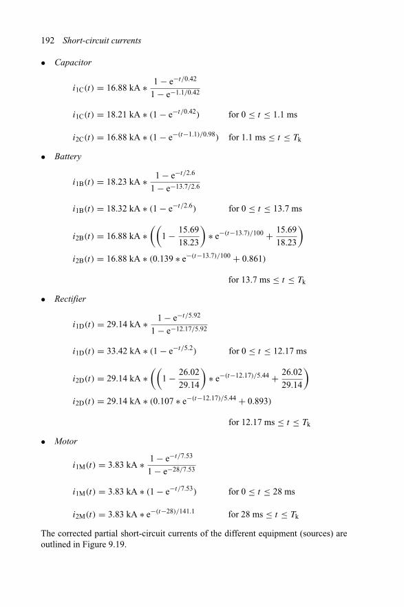
192 Short-circuit currents
• Capacitor
i1C(t) = 16.88 kA ∗ 1 − e−t/0.42
1 − e−1.1/0.42
i1C(t) = 18.21 kA ∗ (1 − e−t/0.42) for 0 ≤ t ≤ 1.1 ms
i2C(t) = 16.88 kA ∗ (1 − e−(t−1.1)/0.98) for 1.1 ms ≤ t ≤ Tk
• Battery
i1B(t) = 18.23 kA ∗ 1 − e−t/2.6
1 − e−13.7/2.6
i1B(t) = 18.32 kA ∗ (1 − e−t/2.6) for 0 ≤ t ≤ 13.7 ms
i2B(t) = 16.88 kA ∗((
1 − 15.69
18.23
)∗ e−(t−13.7)/100 + 15.69
18.23
)
i2B(t) = 16.88 kA ∗ (0.139 ∗ e−(t−13.7)/100 + 0.861)
for 13.7 ms ≤ t ≤ Tk
• Rectifier
i1D(t) = 29.14 kA ∗ 1 − e−t/5.92
1 − e−12.17/5.92
i1D(t) = 33.42 kA ∗ (1 − e−t/5.2) for 0 ≤ t ≤ 12.17 ms
i2D(t) = 29.14 kA ∗((
1 − 26.02
29.14
)∗ e−(t−12.17)/5.44 + 26.02
29.14
)
i2D(t) = 29.14 kA ∗ (0.107 ∗ e−(t−12.17)/5.44 + 0.893)
for 12.17 ms ≤ t ≤ Tk
• Motor
i1M(t) = 3.83 kA ∗ 1 − e−t/7.53
1 − e−28/7.53
i1M(t) = 3.83 kA ∗ (1 − e−t/7.53) for 0 ≤ t ≤ 28 ms
i2M(t) = 3.83 kA ∗ e−(t−28)/141.1 for 28 ms ≤ t ≤ Tk
The corrected partial short-circuit currents of the different equipment (sources) areoutlined in Figure 9.19.

Calculation in d.c. auxiliary installations 193
0
10
20
30
40
50
60
0 10 20 30 40 50 60Time in ms
Cur
rent
in A
Motor
Battery
Rectifier
Total
Capacitor tp = 12.1 ms
Ik = 46.6 kA
2t2 = 34.5 ms
ip = 50.5 kA0.9(ip–Ik)
Figure 9.19 Partial short-circuit currents and total short-circuit current, d.c.auxiliary system as per Figure 9.18
9.7.5 Calculation of total short-circuit current
The total short-circuit current is calculated by superposition of the corrected partialshort-circuit currents of the different sources as per Equation (9.23)
i1(t) =m∑
j=1
ipkorj ∗ 1 − e−t/τ1j
1 − e−tpj /τ1jfor 0 ≤ t ≤ tpj
i2(t) =m∑
j=1
ipkorj
((1 − Ikkorj
ipkorj
)∗ e−(t−tpj )/τ2j + Ikkorj
ipkorj
)for tpj ≤ t ≤ TK
The total short-circuit current obtained by superposition is outlined in Figure 9.19.The peak short-circuit current
ip = 50.5 kA
the quasi steady-state short-circuit current
Ik = 46.6 kA
the time-to-peak
tp = 12.1 ms
and the decay-time constant
τ2 = 17.3 ms

194 Short-circuit currents
0
10
20
30
40
50
60
0 10 20 30 40 50 60Time in ms
Cur
rent
in A
Total short-circuit current by superposition Isup
Approximated total short-circuit current Iappr
Iappr
Isup
Figure 9.20 Total short-circuit current, obtained by superposition of the partialshort-circuit currents and approximated short-circuit current, d.c.auxiliary system as per Figure 9.18
are obtained from Figure 9.19 as indicated. The rise-time constant can be estimatedaccording to Equation (9.24) either by
τ1 = tp
3= 12.1 ms
3= 4.03 ms (time course as per Figure 9.17(a) and (c))
or
τ1 = MIN{τ1C; τ1B; τ1D; τ1M} (time course as per Figure 9.17(b) and (d))
τ1 = MIN{5.92; 2.6; 0.42; 7.53} ms = 0.42 ms
Comparison of the two different values revealed that the approximated time courseof the total short-circuit current fits best to the superposition of the partial short-circuitcurrents, see Figure 9.20, if the rise-time constant is τ1 = 4.03 ms, which also is inline with the typical time course of the short-circuit current as per Figure 9.17(b)and (d).

Chapter 10
Effects of short-circuit currents
10.1 General
Calculation methods for the thermal and electromagnetic effects of short-circuitcurrents are dealt with within IEC 61660-2, which is applicable to short-circuit cur-rents in d.c. auxiliary installations in power plants and substations and IEC 60865-1,related to three-phase a.c. systems.
10.2 a.c. systems
10.2.1 Thermal effects and thermal short-circuit strength
The thermal withstand capability (thermal short-circuit strength) of equipment isdetermined by the maximal permissible conductor temperature prior to the short-circuit, the duration of the short-circuit and the short-circuit current itself. Themaximal permissible temperature of conductors under normal operating conditionsand in the case of short-circuits, e.g., as per DIN VDE 0276, is summarised inTable 10.1. Figures are given for a short-circuit duration of Tk = 5 s. It is assumed thatno heat transfer is taking place during the short-circuit duration (adiabatic heating).Skin- and proximity-effects are neglected, the specific caloric heat of the conductorand insulation is constant and the relation resistance-to-temperature is linear. Specialconsideration is to be taken for conductors in a.c. installations with cross-sectionabove 600 mm2, as the skin-effect has to be taken into account. Additional require-ments according to IEC 60986:1989 and IEC 60949:1988 for cables and isolatedconductors are to be met.
10.2.1.1 Conductors and equipment
The analysis is based on the calculation of the thermal equivalent short-time current Ith
Ith =√
Q
R ∗ Tk=√∫ Tk
0 i2k(t) dt
R ∗ Tk(10.1)
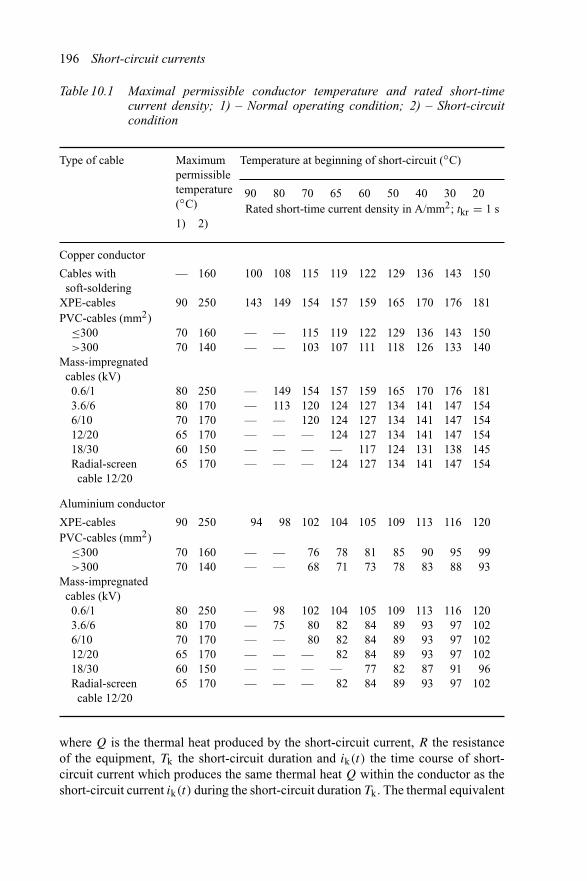
196 Short-circuit currents
Table 10.1 Maximal permissible conductor temperature and rated short-timecurrent density; 1) – Normal operating condition; 2) – Short-circuitcondition
Type of cable Maximumpermissibletemperature(◦C)
Temperature at beginning of short-circuit (◦C)
90 80 70 65 60 50 40 30 20Rated short-time current density in A/mm2; tkr = 1 s
1) 2)
Copper conductor
Cables with — 160 100 108 115 119 122 129 136 143 150soft-soldering
XPE-cables 90 250 143 149 154 157 159 165 170 176 181PVC-cables (mm2)
≤300 70 160 — — 115 119 122 129 136 143 150>300 70 140 — — 103 107 111 118 126 133 140
Mass-impregnatedcables (kV)
0.6/1 80 250 — 149 154 157 159 165 170 176 1813.6/6 80 170 — 113 120 124 127 134 141 147 1546/10 70 170 — — 120 124 127 134 141 147 15412/20 65 170 — — — 124 127 134 141 147 15418/30 60 150 — — — — 117 124 131 138 145Radial-screen 65 170 — — — 124 127 134 141 147 154
cable 12/20
Aluminium conductor
XPE-cables 90 250 94 98 102 104 105 109 113 116 120PVC-cables (mm2)
≤300 70 160 — — 76 78 81 85 90 95 99>300 70 140 — — 68 71 73 78 83 88 93
Mass-impregnatedcables (kV)
0.6/1 80 250 — 98 102 104 105 109 113 116 1203.6/6 80 170 — 75 80 82 84 89 93 97 1026/10 70 170 — — 80 82 84 89 93 97 10212/20 65 170 — — — 82 84 89 93 97 10218/30 60 150 — — — — 77 82 87 91 96Radial-screen 65 170 — — — 82 84 89 93 97 102
cable 12/20
where Q is the thermal heat produced by the short-circuit current, R the resistanceof the equipment, Tk the short-circuit duration and ik(t) the time course of short-circuit current which produces the same thermal heat Q within the conductor as theshort-circuit current ik(t) during the short-circuit duration Tk. The thermal equivalent
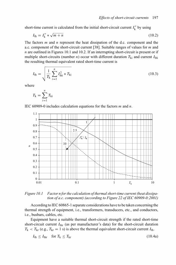
Effects of short-circuit currents 197
short-time current is calculated from the initial short-circuit current I ′′k by using
Ith = I ′′k ∗ √
m + n (10.2)
The factors m and n represent the heat dissipation of the d.c. component and thea.c. component of the short-circuit current [38]. Suitable ranges of values for m andn are outlined in Figures 10.1 and 10.2. If an interrupting short-circuit is present or ifmultiple short-circuits (number n) occur with different duration Tki and current Ithithe resulting thermal equivalent rated short-time current is
Ith =√√√√ 1
Tk
n∑i=1
I 2thi ∗ Tki (10.3)
where
Tk =n∑
i=1
Tki
IEC 60909-0 includes calculation equations for the factors m and n.
0
0.1
0.2
0.3
0.4
0.5
0.6
0.7
0.8
0.9
1
1.1
0.01 0.1 1 10
.
n
Tk
10
2.5
I �k / Ik
.1
Figure 10.1 Factor n for the calculation of thermal short-time current (heat dissipa-tion of a.c. component) (according to Figure 22 of IEC 60909-0:2001)
According to IEC 60865-1 separate considerations have to be taken concerning thethermal strength of equipment, i.e., transformers, transducers, etc., and conductors,i.e., busbars, cables, etc.
Equipment have a suitable thermal short-circuit strength if the rated short-timeshort-circuit current Ithr (as per manufacturer’s data) for the short-circuit durationTk < Tkr (e.g., Tkr = 1 s) is above the thermal equivalent short-circuit current Ith.
Ith ≤ Ithr for Tk ≤ Tkr (10.4a)

198 Short-circuit currents
0
0.2
0.4
0.6
0.8
1
1.2
1.4
1.6
1.8
2
0.1 1 10 100 1000
m
Tk
1.95
1.1
1.6 k
Figure 10.2 Factor m for the calculation of thermal short-time current (heat dissipa-tion of d.c. component) (according to Figure 21 of IEC 60909-0:2001)
In case the short-circuit duration Tk is longer than the rated short-circuit duration Tkr,the thermal short-circuit strength is fulfilled if
Ith ≤ Ithr ∗√
Tkr
Tkfor Tk ≥ Tkr (10.4b)
The maximal permissible values for conductor material can be obtained fromFigure 10.3.
In the case of bare conductors the thermal short-time current density Jth is cal-culated on the basis of the thermal equivalent short-time current and the conductorcross-section qn.
Jth = Ith
qn(10.5)
where qn is the nominal cross-section of conductor and Ith is the equivalentshort-circuit current.
In the case of overhead line conductors of the Al/St-type, only the cross-sectionof the aluminium part is considered. Conductors have sufficient thermal short-circuitstrength if
Jth ≤ Jthr ∗√
Tkr
Tk(10.6)
Values for the rated short-time current density are included in Table 10.1 andFigure 10.3. In IEC 60865 equations for the calculation of rated short-time currentdensity are included.
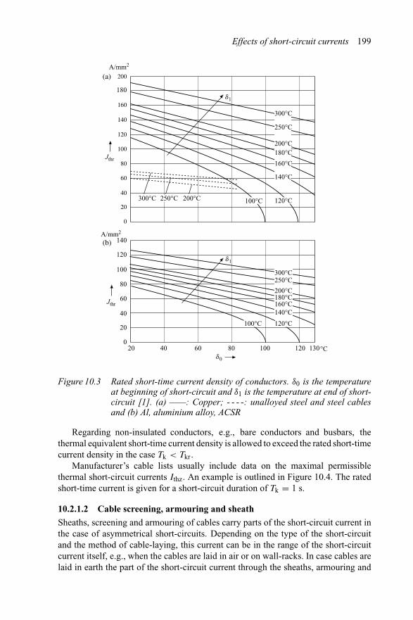
Effects of short-circuit currents 199
200
180
A/mm2
120
100
140
160
80
60
40
20
0
Jthr
(a)
(b)
300°C
250°C
200°C180°C
160°C
140°C
120°C300°C 250°C 200°C
A/mm2
100
140
120
80
60
40
20
020 40 60 80 100 120 130°C
Jthr
300°C250°C
200°C180°C160°C140°C
120°C100°C
100°C
d0
d1
d1
Figure 10.3 Rated short-time current density of conductors. δ0 is the temperatureat beginning of short-circuit and δ1 is the temperature at end of short-circuit [1]. (a) ——: Copper; - - - -: unalloyed steel and steel cablesand (b) Al, aluminium alloy, ACSR
Regarding non-insulated conductors, e.g., bare conductors and busbars, thethermal equivalent short-time current density is allowed to exceed the rated short-timecurrent density in the case Tk < Tkr.
Manufacturer’s cable lists usually include data on the maximal permissiblethermal short-circuit currents Ithz. An example is outlined in Figure 10.4. The ratedshort-time current is given for a short-circuit duration of Tk = 1 s.
10.2.1.2 Cable screening, armouring and sheath
Sheaths, screening and armouring of cables carry parts of the short-circuit current inthe case of asymmetrical short-circuits. Depending on the type of the short-circuitand the method of cable-laying, this current can be in the range of the short-circuitcurrent itself, e.g., when the cables are laid in air or on wall-racks. In case cables arelaid in earth the part of the short-circuit current through the sheaths, armouring and

200 Short-circuit currents
100
8090
60
40
kA
70
50
30
25
20
15
109876
5
4
3
2
10.1 0.2 0.3 0.4 0.5 0.6 0.8 1.5 2 3 4 5s1
tk
1.5
2.5
Ithz
CuAl
300
240
300185240150185120150
95
1207095
5070
3550
25352516
q
mm2
Figure 10.4 Maximal permissible thermal short-circuit current for impregnatedpaper-insulated cables Un up to 10 kV
Source: KABELRHEYDT
screening is lower than the short-circuit current, as one part is flowing through earthas well. Due to the comparatively high specific resistance of lead (used for sheaths)and steel (used for armouring), the short-circuit current preferably flows throughthe screening made from copper or aluminium. Data of the different materials areoutlined in Table 10.2. Due to different production processes and degree of purity ofthe material, data obtained from other tables can be slightly different.
The maximal permissible temperature δ0 or screening and sheaths of cables areto be observed in the case of short-circuits. It is assumed for the analysis that the heat

Effects of short-circuit currents 201
Table 10.2 Data of materials for screening, armouring and sheathsof cables
Material Specificcaloric heat(J/K ∗ mm3)
Specificresistance(� ∗ mm2/m)
Temperaturecoefficient ofresistance (K−1)
Copper 3.48 ∗ 10−3 17.28 ∗ 10−6 3.8 ∗ 10−3
Aluminium 2.39 ∗ 10−3 28.6 ∗ 10−6 4.0 ∗ 10−3
Lead 1.45 ∗ 10−3 214 ∗ 10−6 4.35 ∗ 10−3
Steel 3.56 ∗ 10−3 143 ∗ 10−6 4.95 ∗ 10−3
production within the cable during the short-circuit duration is an adiabatic process.The heat is dissipated to the surroundings only after the short-circuit is switched-off.The maximal permissible short-circuit current density Jthz, respectively the maximalpermissible short-circuit current Ithz, for the given cross-section qn is calculated by
Jthz =√
Qc ∗ (β + 20◦C)
ρ20∗ ln
(δ1 + β
δ0 + β
)∗ 1√
Tkr(10.7a)
Ithz =√
Qc ∗ (β + 20◦C)
ρ20∗ ln
(δ1 + β
δ0 + β
)∗ qn√
Tkr(10.7b)
where Qc is the specific caloric heat, α0 is the thermal coefficient of resistance,β is the parameter: β = 1/α0 − 20◦C, δ1 is the maximal permissible temperatureat end of short-circuit, δ0 is the maximal permissible temperature at beginning ofshort-circuit, ρ20 is the specific resistance at 20◦C, qn the nominal cross-section ofscreening or sheath and Tkr is the rated short-circuit duration.
The calculation for short-circuit duration different from the rated short-circuitduration is performed using
Ith ≤ Ithr ∗√
Tkr
Tkfor Tk ≥ Tkr (10.4b)
10.2.2 Mechanical short-circuit strength of rigid conductors
10.2.2.1 General
Currents in conductors induce electromagnetic forces into other conductors. Thearrangement of parallel conductors, such as busbars and conductors of overheadlines, is of special interest as the electromagnetic forces will be maximal as comparedwith transversal arrangements. Three-phase and double-phase short-circuits withoutearth connection normally cause the highest forces. The currents inducing the elec-tromagnetic forces are a function of time; therefore the forces are also a function of
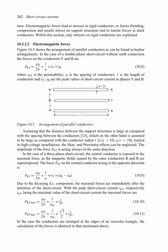
202 Short-circuit currents
time. Electromagnetic forces lead to stresses in rigid conductors, to forces (bending,compression and tensile stress) on support structures and to tensile forces in slackconductors. Within this section, only stresses on rigid conductors are explained.
10.2.2.2 Electromagnetic forces
Figure 10.5 shows the arrangement of parallel conductors as can be found in busbararrangements. In the case of a double-phase short-circuit without earth connectionthe forces on the conductors Y and B are
Fk2 = μ0
2π∗ l
a∗ iY ∗ iB (10.8)
where μ0 is the permeability, a is the spacing of conductors, l is the length ofconductors and iY; iB are the peak values of short-circuit current in phases Y and B.
a
a
lR
Y
B� = 2r
Figure 10.5 Arrangement of parallel conductors
Assuming that the distance between the support structures is large as comparedwith the spacing between the conductors [13], which on the other hand is assumedto be large as compared with the conductor radius r (l/a > 10; a/r > 10), typicalin high-voltage installations, the Skin- and Proximity-effects can be neglected. Theamplitude of the force Fk2 is acting always in the same direction.
In the case of a three-phase short-circuit, the central conductor is exposed to themaximal force, as the magnetic fields caused by the outer conductors R and B aresuperimposed. The force Fk3 on the central conductor acting in the opposite directionis
Fk3 = μ0
2π∗ l
a∗ iY ∗ (iR − iB) (10.9)
Due to the decaying d.c. component, the maximal forces act immediately after theinitiation of the short-circuit. With the peak short-circuit current ip2, respectivelyip3, being the maximal value of the short-circuit current the maximal forces are
Fk2 max = μ0
2π∗ l
am∗ i2
p2 (10.10)
Fk3 max = μ0
2π∗ l
am∗
√3
2∗ i2
p3 (10.11)
In the case the conductors are arranged at the edges of an isosceles triangle, thecalculation of the forces is identical to that mentioned above.
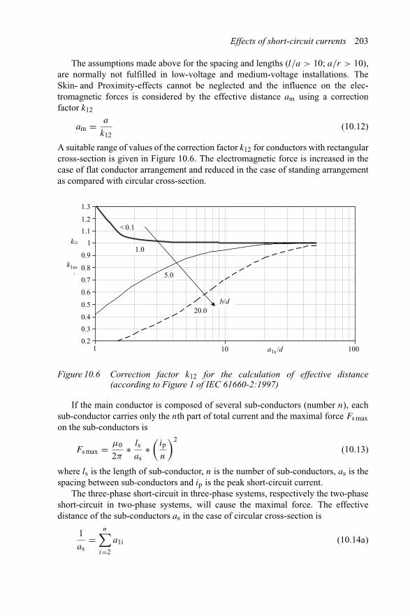
Effects of short-circuit currents 203
The assumptions made above for the spacing and lengths (l/a > 10; a/r > 10),are normally not fulfilled in low-voltage and medium-voltage installations. TheSkin- and Proximity-effects cannot be neglected and the influence on the elec-tromagnetic forces is considered by the effective distance am using a correctionfactor k12
am = a
k12(10.12)
A suitable range of values of the correction factor k12 for conductors with rectangularcross-section is given in Figure 10.6. The electromagnetic force is increased in thecase of flat conductor arrangement and reduced in the case of standing arrangementas compared with circular cross-section.
0.2
0.3
0.4
0.5
0.6
0.7
0.8
0.9
1
1.1
1.2
1.3
1 10 100
.
b/d
< 0.1
1.0
5.0
20.0
k12
k1ss
a1s /d
Figure 10.6 Correction factor k12 for the calculation of effective distance(according to Figure 1 of IEC 61660-2:1997)
If the main conductor is composed of several sub-conductors (number n), eachsub-conductor carries only the nth part of total current and the maximal force Fs maxon the sub-conductors is
Fs max = μ0
2π∗ ls
as∗(
ip
n
)2
(10.13)
where ls is the length of sub-conductor, n is the number of sub-conductors, as is thespacing between sub-conductors and ip is the peak short-circuit current.
The three-phase short-circuit in three-phase systems, respectively the two-phaseshort-circuit in two-phase systems, will cause the maximal force. The effectivedistance of the sub-conductors as in the case of circular cross-section is
1
as=
n∑i=2
a1i (10.14a)

204 Short-circuit currents
and for rectangular cross-section
1
as=
n∑i=2
k1i
a1i(10.14b)
whereas the factor k1i (named k1ss) can be taken from Figure 10.6.
10.2.2.3 Calculation of stresses in rigid conductors
The forces on the support structures of conductors and the stresses in the conductorsthemselves depend on the type of mechanical fixing and the elasticity. The mechanicalsystem composed of conductor, fixing and supporting structure has a mechanicalnatural frequency, which can be actuated by the frequency of the current (50 Hz or60 Hz), thus increasing the mechanical forces. As axial forces in rigid conductors canbe neglected, the bending stress σm for the main conductor, respectively σs for thesub-conductors, are calculated using
σm = Vσ ∗ Vr ∗ β ∗ Fm ∗ l
8 ∗ Z(10.15a)
σs = Vσ s ∗ Vrs ∗ Fs ∗ ls
8 ∗ Zs(10.15b)
where l; ls are the lengths of conductor, respectively sub-conductor, Fm; Fs are theforces on main conductor respectively on sub-conductor, V is the factor as explainedbelow and Zs is the section moduli depending on the shape of conductor. Whereas Fmrespectively Fs is the force Fm3 in the case of three-phase short-circuits in three-phasesystems. In two-phase systems the force Fm2 in the case of two-phase short-circuitshas to be used. Typical ranges of values of the factors Vσ , Vr (respectively Vσ s, Vrs)are shown in Figures 10.7 and 10.8. The factor β takes account of type and numberof supports and can be obtained from Table 10.3.
Table 10.3 Factors α, β and γ for different arrangement of supports(according to Table 3 of IEC 60865-1:1993)
Type of bar and fixing of support Factor α Factor β Factor γ
Support A Support B
Single-span bar Both simple 0.5 0.5 1 1.57A: fixed 0.625 0.375 0.73 2.45B: simpleBoth fixed 0.5 0.5 0.5 3.56
Multiple-span barwith equidistantsimple supports
2 spans 0.375 1.25 0.73 2.45A:fixedB: simple3 and more bars 0.4 1.1 0.73 3.56A: fixedB: simple
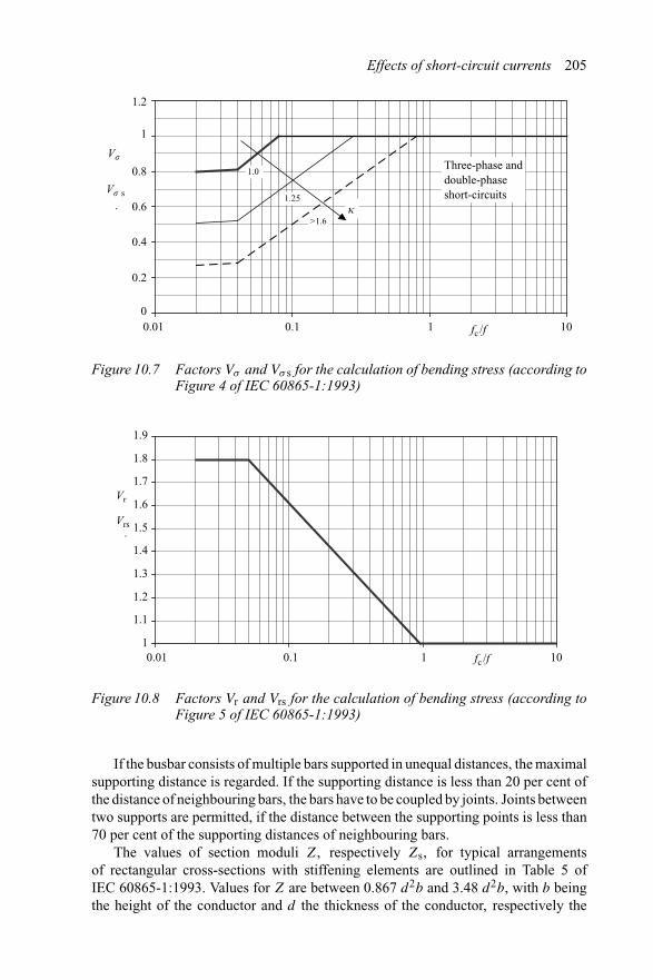
Effects of short-circuit currents 205
0
0.2
0.4
0.6
0.8
1
1.2
0.01 0.1 1 10
. . �
1.0
1.25
>1.6
fc /f
V�
V� s
Three-phase anddouble-phaseshort-circuits
Figure 10.7 Factors Vσ and Vσ s for the calculation of bending stress (according toFigure 4 of IEC 60865-1:1993)
1
1.1
1.2
1.3
1.4
1.5
1.6
1.7
1.8
1.9
0.01 0.1 1 10
.
fc /f
Vr
Vrs
Figure 10.8 Factors Vr and Vrs for the calculation of bending stress (according toFigure 5 of IEC 60865-1:1993)
If the busbar consists of multiple bars supported in unequal distances, the maximalsupporting distance is regarded. If the supporting distance is less than 20 per cent ofthe distance of neighbouring bars, the bars have to be coupled by joints. Joints betweentwo supports are permitted, if the distance between the supporting points is less than70 per cent of the supporting distances of neighbouring bars.
The values of section moduli Z, respectively Zs, for typical arrangementsof rectangular cross-sections with stiffening elements are outlined in Table 5 ofIEC 60865-1:1993. Values for Z are between 0.867 d2b and 3.48 d2b, with b beingthe height of the conductor and d the thickness of the conductor, respectively the

206 Short-circuit currents
stiffening element. Furthermore, the factor of plasticity q has to be considered.Values of q are given for typical arrangements in Table 4 of IEC EN 60865-1:1993. Values for q are between 1.19 and 1.83 for rectangular cross-section and forU-, H- and I-shape profiles. In the case of circular ring section type conductors, thefactor of plasticity depends on the diameter and the thickness of the wall. Referenceis made to IEC 61865-1:1993.
The conductor has sufficient electromagnetic strength with respect to bendingstress, if the bending stress value σm is below the product of factor of plasticity andthe stress corresponding to the yield point.
σm ≤ q ∗ Rp0.2 (10.16)
When the distance between the conductors is affected significantly by the short-circuit, the value of the plasticity factor shall be set to q = 1. If the conductor iscomposed of sub-conductors the total bending stress, i.e., the sum of σm and σs asper above has to be considered. The short-circuit strength is given, if
σtot = σm + σs ≤ q ∗ Rp0.2 (10.17)
If only limit values of the stress corresponding to the yield point rather than readingsare available, the minimal values should be used.
Quantities as per Equations (10.16) and (10.17) are
q Factor of plasticityRp0.2 Stress corresponding to the yield point
More information on mechanical short-circuit stress on rigid conductors is includedin [47].
10.2.2.4 Forces on supports
The relevant force to be considered for short-circuit strength is the dynamic force Fdto be calculated by
Fd = VF ∗ Vr ∗ α ∗ Fm (10.18)
The three-phase short-circuit in three-phase systems, respectively the two-phaseshort-circuit in two-phase systems, will cause the maximal force to be used for theforce Fm. Typical values for the factors Vr and VF are shown in Figures 10.8 and 10.9.The factor α depends on the type and the number of supports and can be obtainedfrom Table 10.3.
The short-circuit strength of supports and fixing material is sufficient, if thedynamic force Fd is below the rated force FrB as per manufacturer’s data.
Fd ≤ FrB (10.19)
Standards for the short-circuit stress on foundations are actually under discussion.

Effects of short-circuit currents 207
0
1
2
3
0.01 0.1 1 10
.
1.0
1.25
> 1.6
Maximal value fordouble-phaseshort-circuits
Maximal value forthree-phaseshort-circuitsVF
fc /f
k
Figure 10.9 Factor VF for the calculation of bending stress (according to Figure 4of IEC 60865-1:1993)
10.2.2.5 Influence of conductor oscillation
In Sections 10.2.2.3 and 10.2.2.4, factors are explained which take accountof the function of time of the bending stress and forces. Deviations from valuesfor Vσ , Vr , Vσ s, Vrs and VF are permitted, if the mechanical natural frequency of thearrangement is taken into account. It should be noted in this respect that the requireddata are difficult to obtain.
The mechanical natural frequency fc of a conductor, either main or sub-conductoris calculated by
fc = γ
l2 ∗√
E ∗ J
m′ (10.20)
The mechanical natural frequency of main conductors, composed of severalsub-conductors with rectangular cross-sections, can be calculated by
fc = c ∗ γ
l2 ∗√
E ∗ Js
m′s
(10.21a)
and for sub-conductors by
fcs = 3.56
l2 ∗√
E ∗ Js
m′s
(10.21b)

208 Short-circuit currents
Quantities as per Equations (10.20) and (10.21) are:
γ Factor taking account of type and number of supports (Table 10.3)E Young’s modulusJ ; Js Second mechanical moment of the conductor, respectively sub-
conductorm′; m′
s Specific mass (mass per length), respectively sub-conductorl; ls Conductor length, respectively sub-conductor lengthc Factor as per Equation (10.21c) taking account of stiffening elements
(Figure 10.10).
c = cc√1 + ξm(mz/(n ∗ l ∗ m′
s))(10.21c)
where cc is the factor as per Table 10.4, ξm is the factor as per Table 10.4, mz thespecific mass of stiffening elements and n is the number of sub-conductors.
k = 1
k = 4
l
ls
ls
Figure 10.10 Calculation of mechanical natural frequency (Factor c). Arrangementof distance elements and calculation equation (according to Figure 3of IEC 60865-1:1993)
Number k and type of distance of stiffening elements, the ratio of the mass ofstiffening (distance) elements mz to the specific mass of the conductor m′
sl separatelyfor the two swing directions in parallel or rectangular to the side with largest cross-section and the second moments J and Js of the conductor, respectively the sub-conductor area, are duly considered. The Young’s modulus E and the specific mass m′depend on the construction and on the type of material. The remarks as per Annex A.3of IEC 60865:1993 shall be observed.
The bending stress and the dynamic force on supports are calculated takingaccount of the mechanical natural frequency fc and the factors Vσ , Vr , Vσ s, Vrs and VF

Effects of short-circuit currents 209
Table 10.4 Factors for the calculation ofmechanical natural frequency.Swing is at right angle to the areaof sub-conductor
Stiffening or distance elements ls/l ξm
Number k Stiffeningelement cc
Distanceelement cc
0 1.0 1.0 — 0.01 1.0 1.0 0.5 2.52 1.48 1.0 0.33 3.03 1.75 1.0 0.25 4.04 2.14 1.0 0.2 5.0
obtained from Figures 10.7 to 10.9. Parameters are the factor κ as per Chapter 4 andthe ratio of mechanical natural frequency fc to power frequency f (50 or 60 Hz).Calculation equations are included in the Annex of IEC 60865-1:1993.
More information on the electromechanical effects and conductor oscillations canbe found in [46,49,51,53,55].
10.3 d.c. auxiliary installations
10.3.1 Substitute rectangular function
The calculation of thermal and electromagnetic effects of short-circuit currents ind.c. auxiliary installations is carried out similar to the analysis in a.c. systems.In general, two alternatives for the calculation are possible. The simplified approach(first alternative) is based on the standard approximation function [41] of theshort-circuit current
i1(t) = ip ∗ 1 − e−t/τ1
1 − e−tp/τ1for 0 ≤ t ≤ tp (10.22a)
i2(t) = ip
((1 − Ik
ip
)∗ e−(t−tp)/τ2 + Ik
ip
)for tp ≤ t ≤ Tk (10.22b)
The electromagnetic effects are calculated using the peak short-circuit current ip ofthe standard approximation function. The second alternative is based on the substituterectangular function, which achieves the same effects as the standard approximationfunction [40,41]. Quantities as per Equations (10.22) are explained in Figure 10.11.The substitute rectangular function is defined by I 2
R and tR according to Figure 10.11
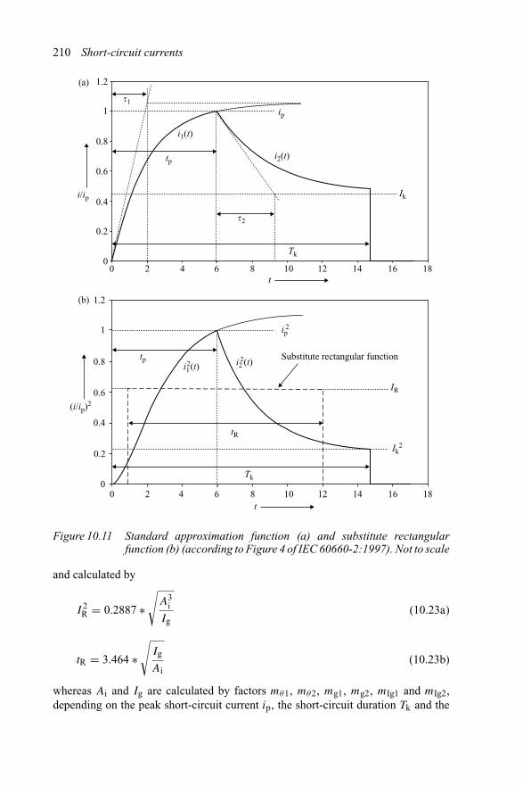
210 Short-circuit currents
1.2
0.8
0.6
0.4
0.2
00 2 4 6 8 10
t12 14 16 18
1
i/ip
ip
Ik
Tk
tp
�1
�2
i2(t)
i1(t)
1.2
0.8
0.6
0.4
0.2
00 2 4 6 8 10
t12 14 16 18
1
(i/ip)2
ip2
Ik2
IR
Tk
tR
tpi12(t) i2
2(t)Substitute rectangular function
(a)
(b)
Figure 10.11 Standard approximation function (a) and substitute rectangularfunction (b) (according to Figure 4 of IEC 60660-2:1997). Not to scale
and calculated by
I 2R = 0.2887 ∗
√A3
i
Ig(10.23a)
tR = 3.464 ∗√
Ig
Ai(10.23b)
whereas Ai and Ig are calculated by factors mθ1, mθ2, mg1, mg2, mIg1 and mIg2,depending on the peak short-circuit current ip, the short-circuit duration Tk and the
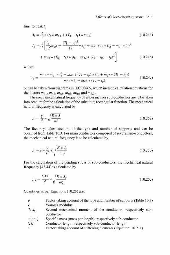
Effects of short-circuit currents 211
time to peak tp
Ai = i2p ∗ (tp ∗ mθ1 + (Tk − tp) ∗ mθ2) (10.24a)
Ig = i2p
[t3p
12mIg1 + (Tk − tp)3
12mIg2 + mθ1 ∗ tp ∗ (tg − mg1 ∗ tp)2
+ mθ2 ∗ (Tk − tp) ∗ (tp + mg2 ∗ (Tk − tp) − tg)2]
(10.24b)
where
tg = mθ1 ∗ mg1 ∗ t2p + mθ2 ∗ (Tk − tp) ∗ (tp + mg2 ∗ (Tk − tp))
mθ1 ∗ tp + mθ2 ∗ (Tk − tp)(10.24c)
or can be taken from diagrams in IEC 60865, which include calculation equations forthe factors mθ1, mθ2, mg1, mg2, mIg1 and mIg2.
The mechanical natural frequency of either main or sub-conductors are to be takeninto account for the calculation of the substitute rectangular function. The mechanicalnatural frequency is calculated by
fc = γ
l2 ∗√
E ∗ J
m′ (10.25a)
The factor γ takes account of the type and number of supports and can beobtained from Table 10.3. For main conductors composed of several sub-conductors,the mechanical natural frequency is to be calculated by
fc = c ∗ γ
l2 ∗√
E ∗ Js
m′s
(10.25b)
For the calculation of the bending stress of sub-conductors, the mechanical naturalfrequency [43,44] is calculated by
fcs = 3.56
l2 ∗√
E ∗ Js
m′s
(10.25c)
Quantities as per Equations (10.25) are:
γ Factor taking account of the type and number of supports (Table 10.3)E Young’s modulusJ ; Js Second mechanical moment of the conductor, respectively sub-
conductorm′; m′
s Specific mass (mass per length), respectively sub-conductorl; ls Conductor length, respectively sub-conductor lengthc Factor taking account of stiffening elements (Equation 10.21c).
212 Short-circuit currents
The vibration period Tme of the main conductor, respectively Tmes of the sub-conductor is calculated by
Tme = 1
fc(10.26a)
Tmes = 1
fcs(10.26b)
where fc; fcs are the natural mechanical frequency of the conductor, respectivelysub-conductors.
The parameters tR and I 2R of the substitute rectangular function are calculated
for the short-circuit duration Tk, in the case Tk ≤ 0.5Tme. In the case Tk > 0.5Tmethe parameters are calculated for the equivalent short-circuit duration being Tke =MAX{0.5Tme; 1.5tp}. In the case Tk = tp, i.e., the short-circuit current has a decreas-ing function only, the substitute rectangular function is calculated, independentlyfrom the vibration period Tme for the total short-circuit duration Tk.
The calculation of the force for the main conductor is done by
FR max = μ0
2π∗ ls
am∗ I 2
R (10.27a)
respectively, in the case of sub-conductors (number n) by
FRs max = μ0
2π∗ ls
as∗(
IRs
n
)2
(10.27b)
where IR; IRs are the current of the substitute rectangular function, l; ls is the lengthof conductor, respectively sub-conductor, am; as is the effective distance betweenconductor, respectively sub-conductor, and n is the number of sub-conductors.
10.3.2 Mechanical short-circuit strength of rigid conductors
10.3.2.1 Forces
The calculation of electromagnetic effects on rigid conductors is based on the sub-stitute rectangular function as per Figure 10.11 and described in Section 10.3.1.The substitute rectangular function leads to identical bending stress and forcesas the standard approximation function. The forces between main conductors arecalculated by
FR = μ0
2π∗ l
am∗ I 2
R (10.28a)
and between sub-conductors (number n) by using
FRs = μ0
2π∗ ls
as∗(
IRs
n
)2
(10.28b)
Effects of short-circuit currents 213
Quantities as per Equations (10.28) are:
IR; IRs Current of the substitute rectangular functionl; ls Length of conductor, respectively sub-conductoram; as Effective distance between conductor, respectively sub-conductorn Number of sub-conductors
The bending stress and forces on supports for both main and sub-conductors arecalculated similar to a.c. installations as described in Sections 10.2.2.2 to 10.2.2.4.
The effective distance of main conductors am is calculated from the distance a by
am = a
k12(10.29)
with the correction factor k12 according to Figure 10.6.The effective distance of sub-conductors as in the case of circular conductors is
calculated by
1
as=
n∑i=2
a1i (10.30a)
respectively, in the case of rectangular cross-sections
1
as=
n∑i=2
k1i
a1i(10.30b)
with the factor k1i according to Figure 10.6.
10.3.2.2 Bending stress
The bending stress on main conductors σm, respectively on sub-conductors σs,resulting from the bending forces is calculated using
σm = Vσ ∗ β ∗ FR ∗ l
8 ∗ Z(10.31a)
σs = Vσ s ∗ FRs ∗ ls
16 ∗ Zs(10.31b)
where Z; Zs are the section moduli of the main, respectively sub-conductors, V is thefactor as explained below, l; ls is the length of conductor, respectively sub-conductor,and β is the factor taking account of the type and number of supports (Table 10.3).
The forces FR and FRs are the forces as calculated for the substitute rectangularfunction. Typical values of Vσ and Vσ s are outlined in Figure 10.12. IEC 61660-2:1997indicates in Table 2 that Vσ and Vσ s should be lower than 1.
If the busbar consists of multiple bars supported in unequal distances, the maximalsupporting distance is to be considered. If a supporting distance is less than 20 per centof the distance of neighbouring bars, the bars have to be coupled by joints. Jointsbetween two supports are permitted, if the distance between the supporting points isless than 70 per cent of the supporting distances of neighbouring bars.

214 Short-circuit currents
0
0.2
0.4
0.6
0.8
1
1.2
0 0.1 0.2 0.3 0.4 0.5.
.
tR/Tme
Vs
VsS
Figure 10.12 Factors Vσ and Vσ s for the calculation of bending stress on conductors(according to Figure 9 of IEC 61660-2:1997)
The conductor has sufficient electromagnetic strength with respect to bendingstress, if the bending stress σm is below the product of factor of plasticity and stresscorresponding to the yield point
σm ≤ q ∗ Rp0.2 (10.32a)
In the case of several sub-conductors the total bending stress, i.e., the sum of thestresses σm and σs is to be considered
σtot = σm + σs ≤ q ∗ Rp0.2 (10.32b)
where q is the factor of plasticity and Rp0.2 is the stress corresponding to the yieldpoint.
Values for the factor of plasticity q for typical arrangements are included inTable 4 of IEC 60660-2:1997. Values are between q = 1.19–1.83 for rectangularcross-sections, U-, H- and I-shape profiles. For circular ring section type conductorsthe factor of plasticity depends on the diameter and wall thickness. Reference is madeto IEC 61660-2:1997.
10.3.2.3 Forces on supports
The dynamical force Fd is the dominating parameter for the short-circuit strength ofsupports to be calculated by
Fd = VF ∗ α ∗ FR (10.33)
whereas the force FR is the force calculated on the basis of the substitute rectangularfunction. Typical values of VF are outlined in Figure 10.13. The factor α takes accountof the type and number of supports and can be obtained from Table 10.3.
The requirements regarding the short-circuit strength of supports and fixingmaterial are fulfilled if the dynamical force Fd remains below the rated value FrB

Effects of short-circuit currents 215
0
0.2
0.4
0.6
0.8
1
1.2
1.4
1.6
1.8
2
2.2
0 0.05 0.1 0.15 0.2 0.25 0.3 0.35 0.4 0.45 0.5
.
tR/Tme
VF
Figure 10.13 Factor VF for the calculation of forces on supports (according toFigure 9 of IEC 61660-2:1997)
as per manufacturer’s data
Fd ≤ FrB (10.34)
Standardisation of stresses on foundations is actually under consideration. Moreinformation on the theoretical background can be found in [43–45,48].
10.3.3 Thermal short-circuit strength
The thermal short-circuit strength is analysed using the thermal equivalent short-timecurrent Ith and the short-circuit duration Tk.
Ith =√
Ai
Tk(10.35)
with Ai as per Equation (10.24a). The upper limit of the thermal equivalent short-timecurrent is defined as Ith = ip. IEC 61660-2 indicates that separate considerations forequipment (e.g., transformers, transducers) and conductors (e.g., busbars, cables)have to be taken.
The thermal short-circuit strength of equipment is fulfilled if the thermalequivalent short-time current Ith is below the rated thermal equivalent short-timecurrent Ithr
Ith ≤ Ithr for Tk ≤ Tkr (10.36a)
with the rated short-circuit duration Tkr assumed equal to 1 s. If the short-circuitduration Tk is longer than the rated short-circuit duration Tkr, the thermal short-circuit
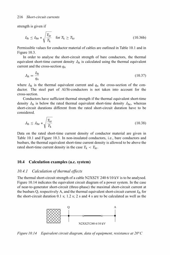
216 Short-circuit currents
strength is given if
Ith ≤ Ithr ∗√
Tkr
Tkfor Tk ≥ Tkr (10.36b)
Permissible values for conductor material of cables are outlined in Table 10.1 and inFigure 10.3.
In order to analyse the short-circuit strength of bare conductors, the thermalequivalent short-time current density Jth is calculated using the thermal equivalentcurrent and the cross-section qn
Jth = Ith
qn(10.37)
where Ith is the thermal equivalent current and qn the cross-section of the con-ductor. The steel part of Al/St-conductors is not taken into account for thecross-section.
Conductors have sufficient thermal strength if the thermal equivalent short-timedensity Jth is below the rated thermal equivalent short-time density Jthr, whereasshort-circuit durations different from the rated short-circuit duration have to beconsidered.
Jth ≤ Jthr ∗√
Tkr
Tk(10.38)
Data on the rated short-time current density of conductor material are given inTable 10.1 and Figure 10.3. In non-insulated conductors, i.e., bare conductors andbusbars, the thermal equivalent short-time current density is allowed to be above therated short-time current density in the case Tk < Tkr.
10.4 Calculation examples (a.c. system)
10.4.1 Calculation of thermal effects
The thermal short-circuit strength of a cable N2XS2Y 240 6/10 kV is to be analysed.Figure 10.14 indicates the equivalent circuit diagram of a power system. In the caseof near-to-generator short-circuit (three-phase) the maximal short-circuit current atthe busbars Q, respectively A, and the thermal equivalent short-circuit current Ith forthe short-circuit duration 0.1 s; 1.2 s; 2 s and 4 s are to be calculated as well as the
Q A
N2XS2Y240 6/10 kV
Figure 10.14 Equivalent circuit diagram, data of equipment, resistance at 20◦C

Effects of short-circuit currents 217
short-circuit current density Jthz permitted for a cable sheath of copper (initial tem-perature 80◦C; temperature at the end of short-circuit 350◦C; short-circuit duration0.2 s; 1.2 s; 2 s).
Data of equipment are given below:
UnQ = 10 kV; S′′kQ = 520 MVA
R′K = 0.0754 �/km; X′
K = 0.11 �/km; l = 2 km
The maximal short-circuit current is given for short-circuits at the sending-end ofthe cable (approximately identical to location Q) I ′′
k3Q = 30.03 kA. The maximalshort-circuit current at location A is I ′′
k3A = 13.28 kA. Table 10.1 indicates a valueof Jthr = 143 A/mm2. The thermal equivalent rated current is Ithr = 34.32 kA.The calculation results are outlined in Table 10.5.
Table 10.5 Results of calculation of thermalequivalent currents
tk Ithz IthQ IthA Jthz(s) (kA) (kA) (kA) (A/mm2)
0.2 76.26 14.12 31.92 6891.2 31.33 11.73 26.52 2852 24.27 9.62 21.86 2214 17.16 8.81 19.92 —
The short-circuit strength is sufficient if Ith ≤ Ithz. This is fulfilled if tk < 2 s forshort-circuits near busbar A and tk < 4 s for short-circuits near busbar Q.
10.4.2 Electromagnetic effect
A wind power plant is connected to the public supply system by four cables in parallellaid on racks as indicated in Figure 10.15. The relevant parameters of the short-circuitcurrent and the maximal forces on the cables, respectively on the fixing material, areto be calculated. The permissible distance of the fixing clamps is to be determined.The maximal permissible force on the clamps is Fzul = 40 kN.
TQ
3 ~GS
4 × 3 Single-core cablesG
F2 F1
Figure 10.15 Equivalent circuit diagram of a power system with wind power plant
The data of equipment are given below:
S′′kQ = 1000 MVA; UnQ = 110 kV
SrT = 2.5 MVA; ukrT = 6%; uRrT = 0.8%; trT = 20 kV/0.66 kV
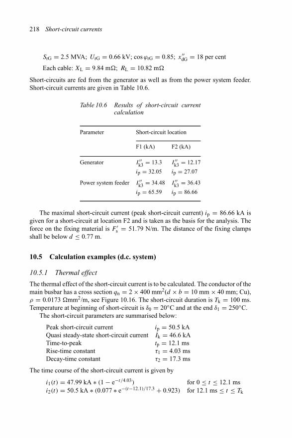
218 Short-circuit currents
SrG = 2.5 MVA; UrG = 0.66 kV; cos ϕrG = 0.85; x′′dG = 18 per cent
Each cable: XL = 9.84 m�; RL = 10.82 m�
Short-circuits are fed from the generator as well as from the power system feeder.Short-circuit currents are given in Table 10.6.
Table 10.6 Results of short-circuit currentcalculation
Parameter Short-circuit location
F1 (kA) F2 (kA)
Generator I ′′k3 = 13.3 I ′′
k3 = 12.17
ip = 32.05 ip = 27.07
Power system feeder I ′′k3 = 34.48 I ′′
k3 = 36.43
ip = 65.59 ip = 86.66
The maximal short-circuit current (peak short-circuit current) ip = 86.66 kA isgiven for a short-circuit at location F2 and is taken as the basis for the analysis. Theforce on the fixing material is F ′
s = 51.79 N/m. The distance of the fixing clampsshall be below d ≤ 0.77 m.
10.5 Calculation examples (d.c. system)
10.5.1 Thermal effect
The thermal effect of the short-circuit current is to be calculated. The conductor of themain busbar has a cross section qn = 2 × 400 mm2(d × b = 10 mm × 40 mm; Cu),ρ = 0.0173 �mm2/m, see Figure 10.16. The short-circuit duration is Tk = 100 ms.Temperature at beginning of short-circuit is δ0 = 20◦C and at the end δ1 = 250◦C.
The short-circuit parameters are summarised below:
Peak short-circuit current ip = 50.5 kAQuasi steady-state short-circuit current Ik = 46.6 kATime-to-peak tp = 12.1 msRise-time constant τ1 = 4.03 msDecay-time constant τ2 = 17.3 ms
The time course of the short-circuit current is given by
i1(t) = 47.99 kA ∗ (1 − e−t/4.03) for 0 ≤ t ≤ 12.1 msi2(t) = 50.5 kA ∗ (0.077 ∗ e−(t−12.1)/17.3 + 0.923) for 12.1 ms ≤ t ≤ Tk

Effects of short-circuit currents 219
am
I
ls height bd
asa12
Figure 10.16 Arrangement of busbar conductor (data, see text)
The thermal equivalent short-time current Ith as per Equation (10.35)
Ith =√
Ai
Tk=√
206.11 kA2
0.1 s= 45.4 kA
with Ai as per Equation (10.24a)
Ai = i2p ∗ (tp ∗ mθ1 + (Tk − tp) ∗ mθ2) = 50.52 kA2
∗ (0.0121 s ∗ 0.65 + (0.1 s − 0.0121 s) ∗ 0.83) = 206.11 kA2
Factors mθ1 and mθ2 are calculated as per IEC 61660-2
mθ1 = 0.65
mθ2 = 0.83
The thermal equivalent short-time current density Jth according to Equation (10.37)is calculated as
Jth = Ith
qn= 45(4) kA
2(400) mm2 = 56.75 A/mm2
Conductors have sufficient thermal strength if the thermal equivalent short-timedensity Jth is below the rated thermal equivalent short-time density Jthr taken fromFigure 10.3 (Jthr = 190 A/mm2).
Jth ≤ Jthr ∗√
Tkr
Tk
56.75 A/mm2 ≤ 190 A/mm2 ∗√
1 s
0.1 s= 600 A/mm2
The busbar-conductor has sufficient thermal short-circuit strength.

220 Short-circuit currents
10.5.2 Electromagnetic effect
The configuration as per Sections 9.7 and 10.5.1 is regarded. The conductor arrange-ment is outlined in Figure 10.16. The distances are: am = 75 mm; b = 40 mm;as = 10 mm; l = 1050 mm; ls = 35 mm. The mechanical constants of the busbar are:
Stress corresponding to the yield point Rp0.2 = 340 N/mm2
Specific mass of subconductor m′s = 3.5 kg/m
Young’s modulus E = 106 kN/mm2
Stiffening elements have dimension 40/40/10 mm.
10.5.2.1 Calculation of forces with simplified approach
Peak force between main conductors
FRm = μ0
2π∗ l
ami2p = 4π ∗ 10−7 ∗ (Vs/Am)
2π∗ 1.05 m
0.0765 m∗ 50.52 ∗ kA2
= 7000.7 N
Effective distance of main conductors am according to Equation (10.29)
am = a
k12= 0.075 m
0.98= 0.0765 m
with the correction factor k12 = 0.98 according to Figure 10.6.Peak force between sub-conductors
FRs = μ0
2π∗ ls
as
(ip
n
)2
= 4π ∗ 10−7 ∗ (Vs/Am)
2π∗ 0.35 m
0.028 m∗(
50.5 ∗ kA
2
)2
= 1593.9 N
Effective distance of sub-conductors as
as = a12
k12= 0.02 m
0.72= 0.028 m
with the correction factor k12 = 0.72 according to Figure 10.6.
10.5.2.2 Calculation of forces with substitute rectangular function
Parameters of short-circuit current remain identical to those mentioned above.
ip = 50.5 kA; tp = 12.1 ms; Tk = 100 ms
Mechanical natural frequency of main conductor as per Equation (10.25)
fc = c ∗ γ
l2 ∗√
E ∗ Js
m′s

Effects of short-circuit currents 221
with c ≈ 1.44 as per Figure 10.10, factor γ as per Table 10.3 and the secondmechanical moment J of the conductor, respectively sub-conductor
J = Js = d3 ∗ b
12= 0.013 ∗ 0.04
12m4 = 3.33 ∗ 10−9 m4
fc = 1.44 ∗ 3.56
1.052 m2 ∗√
106 kN/mm2 ∗ 3.33 ∗ 10−9 m4
3.5 kg/m= 46.7 Hz
Vibration period Tme as per Equation (10.26)
Tme = 1
fc= 1
46.7s = 21.4 ms
Mechanical natural frequency of sub-conductors
fcs = 3.56
l2s
∗√
E ∗ Js
m′s
= 3.56
0.352 m2 ∗√
106 kN/mm2 ∗ 3.33 ∗ 10−9 m4
3.5 kg/m
= 291.8 Hz
Vibration period Tmes
Tmes = 1
fc= 1
291.8s = 3.43 ms
Substitute rectangular function to be calculated for the equivalent short-circuitduration Tke, as Tk > 0.5Tme.
Tke = MAX{0.5 ∗ Tme; 1.5 ∗ tp} = MAX{0.5 ∗ 21.4 ms; 1.5 ∗ 12.1 ms}= 18.2 ms
Parameters of the substitute rectangular function (in this case identical for themain conductor and for the sub-conductors) as per Equations (10.23) and (10.24)
I 2R = 0.2887 ∗
√A3
i
Ig
tR = 3.464 ∗√
Ig
Ai
Ig = i2p
[t3p
12mIg1 + (Tk − tp)3
12mIg2 + mθ1 ∗ tp ∗ (tg − mg1 ∗ tp)2
+ mθ2 ∗ (Tk − tp) ∗ (tp + mg2 ∗ (Tk − tp) − tg)2]
Ai = i2p ∗ (tp ∗ mθ1 + (Tk − tp) ∗ mθ2)
tg = mθ1 ∗ mg1 ∗ t2p + mθ2 ∗ (Tk − tp) ∗ (tp + mg2 ∗ (Tk − tp))
mθ1 ∗ tp + mθ2 ∗ (Tk − tp)

222 Short-circuit currents
Factors mθ1, mθ2, mg1, mg2, mIg1 and mIg2 are calculated according to IEC 61660-2
mθ1 = 0.65; mθ2 = 0.83mg1 = 0.63; mg2 = 0.47mIg1 = 0.42; mIg2 = 0.86
Ai = (50.5 kA)2 ∗ (0.0121 s ∗ 0.65 + (0.0182 − 0.0121 s) ∗ 0.83)
= 32.97 kA2s
tg = [0.65 ∗ 0.63 ∗ (0.0121 s)2 + 0.83 ∗ (0.0182 − 0.0121 s)
∗ (0.0121 + 0.47 ∗ (0.0182 − 0.0121 s))]∗ [0.65 ∗ 0.0121 s + 0.83 ∗ (0.0182 − 0.0121 s)]−1
tg = 0.0105 s
Ig = (50.5 kA)
[t3p
12mIg1 + (Tk − tp)3
12mIg2 + mθ1 ∗ tp ∗ (tg − mg1 ∗ tp)2
+ mθ2 ∗ (Tk − tp) ∗ (tp + mg2 ∗ (Tk − tp) − tg)2]
Ig = (50.5 kA)2
⎡⎢⎢⎢⎢⎢⎢⎢⎣
(0.0121 s)3
12∗ 0.42 + (0.0182 − 0.0121 s)3
12∗ 0.86 + · · ·
· · · 0.65 ∗ 0.0121 s ∗ (0.0105 s − 0.63 ∗ 0.0121 s)3 + · · ·· · · 0.83 ∗ (0.0182 − 0.0121 s) ∗ (0.0121 s + 0.47
∗(0.0182 − 0.0121 s) − 0.0105 s)2
⎤⎥⎥⎥⎥⎥⎥⎥⎦
Ig = 457.2 A2s3
The parameters of the substitute rectangular function
I 2R = 0.2887 ∗
√(32.97 ∗ 106 A2s)3
457.2 A2s3 = 2556 ∗ 106 A2
tR = 3.464 ∗√
457.2 A2s3
32.97 ∗ 106 A2s= 12.9 ms
The standardised rectangular function and the approximated total short-circuit current(see e.g., Section 9.7) are outlined in Figure 10.17.
Peak force between main conductors as per Equation (10.27)
FRm = μ0
2π∗ l
am∗ I 2
R = 4π ∗ 10−7 ∗ (Vs/Am)
2π∗ 1.05 m
0.0765 m∗ 2556 ∗ 106 A2
= 7016.5 N
Effective distance of main conductors am = 0.0765 m as per above.
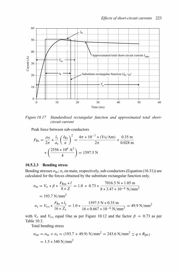
Effects of short-circuit currents 223
0
10
20
30
40
50
60
0 10 20 30 40 50 60
Time (ms)
Cur
rent
(A
) Approximated total short-circuit current Iappr
Substitute rectangular function (IR; tR)tR
IR
Tk
Tke
Figure 10.17 Standardised rectangular function and approximated total short-circuit current
Peak force between sub-conductors
FRs = μ0
2π∗ ls
as
(IRs
n
)2
= 4π ∗ 10−7 ∗ (Vs/Am)
2π∗ 0.35 m
0.028 m
∗(
2556 ∗ 106 A2
4
)= 1597.5 N
10.5.2.3 Bending stress
Bending stresses σm; σs on main, respectively, sub-conductors (Equation (10.31)) arecalculated for the forces obtained by the substitute rectangular function only.
σm = Vσ ∗ β ∗ FRm ∗ l
8 ∗ Z= 1.0 ∗ 0.73 ∗ 7016.5 N ∗ 1.05 m
8 ∗ 3.47 ∗ 10−6 N/mm2
= 193.7 N/mm2
σs = Vσ s ∗ FRs ∗ ls
16 ∗ Zs= 1.0 ∗ 1597.5 N ∗ 0.35 m
16 ∗ 0.667 ∗ 10−6 N/mm2 = 49.9 N/mm2
with Vσ and Vσ s equal One as per Figure 10.12 and the factor β = 0.73 as perTable 10.3.
Total bending stress
σtot = σm + σs = (193.7 + 49.9) N/mm2 = 243.6 N/mm2 ≤ q ∗ Rp0.2
= 1.5 ∗ 340 N/mm2
224 Short-circuit currents
Conductors have sufficient electromagnetic strength as
σtot ≤ q ∗ Rp0.2 = 1.5 ∗ 340 N/mm2 = 510 N/mm2
and if
σs ≤ Rp0.2 = 340 N/mm2
10.5.2.4 Forces on supports
Forces on outer supports
Fd = VF ∗ α ∗ FRm = 2.0 ∗ 0.4 ∗ 7016.5 N = 5.61 kN
Forces on inner supports
Fd = VF ∗ α ∗ FRm = 2.0 ∗ 1.1 ∗ 7016.5 N = 15.4 kN
Chapter 11
Limitation of short-circuit currents
11.1 General
The expansion of electrical power systems by new power stations and new lines(overhead transmission lines and cable circuits) results in an increase of short-circuitcurrents due to an increase in sources feeding the short-circuit and due to a reductionof system impedance. The improvement of existing installations and the replace-ment of equipment are necessary, in case the permissible short-circuit current will beexceeded. Measures to limit the short-circuit currents can also be realised which mightbe more economic than the replacement of equipment and installations. Differentmeasures have to be taken into account such as measures affecting the whole system(higher voltage level), measures concerning installations and substations (separateoperation of busbars) and measures related to equipment (Ip-limiter).
All measures have an influence on the system reliability as well, which must beguaranteed under outage conditions of equipment after the measures for limitation ofshort-circuit currents are in operation. Measures for short-circuit current limitationdecrease the voltage stability, increase the reactive power requirement, reduce thedynamic stability and increase the complexity of operation. Furthermore some mea-sures to limit short-circuit currents will contradict requirements for a high short-circuitlevel, e.g., to reduce flicker in the case of connection of arc-furnace.
The decision on location of power stations is determined beside other criteriaby the availability of primary energy (lignite coal fired power stations are build nearbythe coal mine), requirement of cooling water (thermal power stations are placed nearthe sea or at large rivers), geological conditions (hydro power stations can onlybe build if water reservoirs are available), requirements of the power system (eachpower station requires a system connection at suitable voltage level) and the vicinityto consumers (combined heat and energy stations need heat consumers nearby).
The connection of large power stations is determined by the branch short-circuitcurrent from the generators. Figure 11.1 outlines considerations to select the suitable
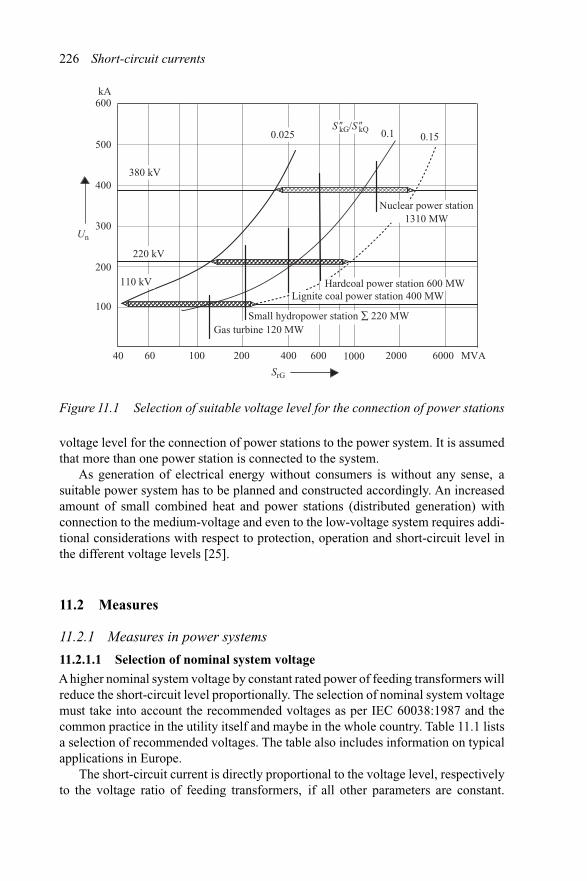
226 Short-circuit currents
40 60 100 200 400 600 1000 2000 6000 MVA
100
200
300
400
500
600kA
SrG
Un
0.025 0.1 0.15
380 kV
220 kV
110 kV
Nuclear power station1310 MW
Hardcoal power station 600 MWLignite coal power station 400 MW
Small hydropower station ∑ 220 MWGas turbine 120 MW
S �kG/S �kQ
Figure 11.1 Selection of suitable voltage level for the connection of power stations
voltage level for the connection of power stations to the power system. It is assumedthat more than one power station is connected to the system.
As generation of electrical energy without consumers is without any sense, asuitable power system has to be planned and constructed accordingly. An increasedamount of small combined heat and power stations (distributed generation) withconnection to the medium-voltage and even to the low-voltage system requires addi-tional considerations with respect to protection, operation and short-circuit level inthe different voltage levels [25].
11.2 Measures
11.2.1 Measures in power systems
11.2.1.1 Selection of nominal system voltage
Ahigher nominal system voltage by constant rated power of feeding transformers willreduce the short-circuit level proportionally. The selection of nominal system voltagemust take into account the recommended voltages as per IEC 60038:1987 and thecommon practice in the utility itself and maybe in the whole country. Table 11.1 listsa selection of recommended voltages. The table also includes information on typicalapplications in Europe.
The short-circuit current is directly proportional to the voltage level, respectivelyto the voltage ratio of feeding transformers, if all other parameters are constant.
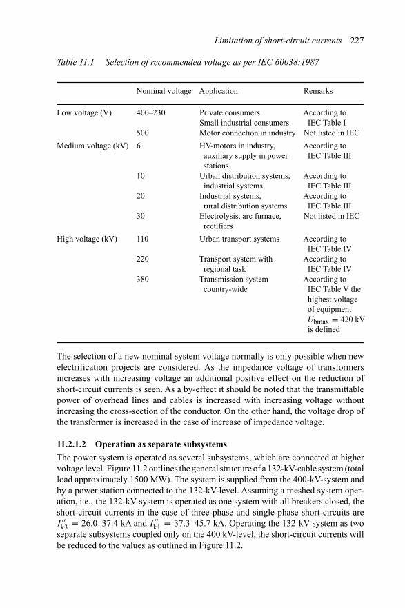
Limitation of short-circuit currents 227
Table 11.1 Selection of recommended voltage as per IEC 60038:1987
Nominal voltage Application Remarks
Low voltage (V) 400–230 Private consumers According toSmall industrial consumers IEC Table I
500 Motor connection in industry Not listed in IEC
Medium voltage (kV) 6 HV-motors in industry, According toauxiliary supply in power IEC Table IIIstations
10 Urban distribution systems, According toindustrial systems IEC Table III
20 Industrial systems, According torural distribution systems IEC Table III
30 Electrolysis, arc furnace, Not listed in IECrectifiers
High voltage (kV) 110 Urban transport systems According toIEC Table IV
220 Transport system with According toregional task IEC Table IV
380 Transmission system According tocountry-wide IEC Table V the
highest voltageof equipmentUbmax = 420 kVis defined
The selection of a new nominal system voltage normally is only possible when newelectrification projects are considered. As the impedance voltage of transformersincreases with increasing voltage an additional positive effect on the reduction ofshort-circuit currents is seen. As a by-effect it should be noted that the transmittablepower of overhead lines and cables is increased with increasing voltage withoutincreasing the cross-section of the conductor. On the other hand, the voltage drop ofthe transformer is increased in the case of increase of impedance voltage.
11.2.1.2 Operation as separate subsystems
The power system is operated as several subsystems, which are connected at highervoltage level. Figure 11.2 outlines the general structure of a 132-kV-cable system (totalload approximately 1500 MW). The system is supplied from the 400-kV-system andby a power station connected to the 132-kV-level. Assuming a meshed system oper-ation, i.e., the 132-kV-system is operated as one system with all breakers closed, theshort-circuit currents in the case of three-phase and single-phase short-circuits areI ′′
k3 = 26.0–37.4 kA and I ′′k1 = 37.3–45.7 kA. Operating the 132-kV-system as two
separate subsystems coupled only on the 400 kV-level, the short-circuit currents willbe reduced to the values as outlined in Figure 11.2.
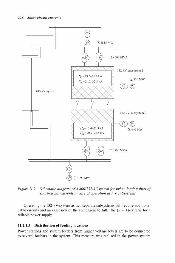
228 Short-circuit currents
∑ 1090 MW
∑ 440 MW
∑ 520 MW
∑ 2815 MWGS3~
GS3~
GS3~
GS3~
2 × 500 MVA
400-kV-system
132-kV-subsystem 2
132-kV-subsystem 1
2 × 500 MVA
I �k3= 19.3–26.1 kA
I �k3= 15.4–22.3 kA
I �1k = 20.9–26.5 kA
I �1k = 24.2–32.8 kA
Figure 11.2 Schematic diagram of a 400/132-kV-system for urban load; values ofshort-circuit currents in case of operation as two subsystems
Operating the 132-kV-system as two separate subsystems will require additionalcable circuits and an extension of the switchgear to fulfil the (n − 1)-criteria for areliable power supply.
11.2.1.3 Distribution of feeding locations
Power stations and system feeders from higher voltage levels are to be connectedto several busbars in the system. This measure was realised in the power system

Limitation of short-circuit currents 229
as per Figure 11.2, which is a by-effect to the system separation. A further example isoutlined in Figure 11.3. A power station of 395 MW is connected to a 132-kV-system,which has a second supply from the 220-kV-system. The 132-kV-system is a purecable network and the shortest cable length between any two substations is 11.2 km.In the case when the busbar-coupler K in the power station is closed, the three-phaseshort-circuit current at the busbar is I ′′
k3 = 37.6 kA; the short-circuit currents at thebusbars in the 132-kV-system remain below I ′′
k3 = 33.5 kA. If the busbar-coupler Kis operated opened, the short-circuit currents at the busbar in the power station areI ′′
k3 = 28.0 kA and I ′′k3 = 29.3 kA. For short-circuits at the busbars in the system itself
the short-circuit currents are reduced up to 4.1 kA.
GS3~
GS3~
K
132-kV-system
220-kV-system
∑ 192 MW
∑ 203 MW
Figure 11.3 Schematic diagram of a 132-kV-system with power station
The generators and the 132-kV-cables in the power stations need to be switched-on to the busbars in such a way that the generated power can be transferred to thepower system without overloading any of the cable even under outage conditions.

230 Short-circuit currents
11.2.1.4 Coupling of power system at busbars with low short-circuit level
Different parts of the power system shall be connected only at busbars with low short-circuit level. Figure 11.4 outlines a 30-kV-system with overhead lines, which is fedfrom the 110-kV-system by two transformers operated in parallel. The three-phaseshort-circuit current is I ′′
k3 = 10.09 kA. If the transformers are not operated in paralleland the system is coupled at busbar K7 the short-circuit current at the feeding busbaris I ′′
k3 = 5.94 kA.
EL9
EL5
3200 MVA
K1
K4
K2 K3
K5 K6
K8Un = 30.000 kVI 0k (L1) = 10.091 kAS 0k (L1) = 524.341 MVA
K9Un = 30.000 kVI 0k (L1) = 10.091 kAS 0k (L1) = 524.341 MVA
K7Un= 30.000 kVI 0k (L1) = 2.199 kAS 0k (L1) =114.241 MVA
EL9
EL5
3200 MVA
K1
K4
K2 K3
K5 K6
K8Un = 30.000 kVI 0k (L1) = 5.935 kAS 0k (L1) = 308.375 MVA
K9Un = 30.000 kVI 0k (L1) = 5.935 kAS 0k (L1) = 308.375 MVA
K7Un = 30.000 kVI 0k (L1) = 2.193 kAS 0k (L1) = 113.929 MVA
(a)
(b)
Figure 11.4 Equivalent circuit diagram of a 30-kV-system with feeding 132-kV-system: (a) Operation with transformers in parallel and (b) lim-itation of short-circuit current. Result of three-phase short-circuitcurrent: S′′
kQ = 3.2 GVA; SrT = 40 MVA; ukrT = 12%; trT = 110/32;OHTL 95Al; ltot = 56 km
It should be noted that the short-circuit level at busbar K7 is affected only to aminor extent. If the transformers are loaded only up to 50 per cent of their rated power

Limitation of short-circuit currents 231
and if the lines have sufficient thermal rating, both system configurations have thesame supply reliability.
11.2.1.5 Restructuring of the power system
Restructuring of power systems is comparatively costly and complicated. In mediumvoltage systems restructuring is in most cases only possible together with the commis-sioning of new primaries, loop-in and loop-out of cable (overhead line) circuits andthe operation of the system as a radial system. In a high voltage system, restructuringrequires a total different system topology. Figure 11.5 outlines the comparison of twosystem topologies, i.e., ring fed system and radial fed system.
Each systemI 0k (L1) = 12.155 kAS 0k (L1) = 8000.000 MVA
K12Un =380.000 kVI 0k (L1) =17.575 kAS 0k (L1) =11567.2 MVA
K11Un = 380.000 kVI 0k (L1) = 23.517 kAS 0k (L1) =15478.5 MVA
Eaeh systemI 0k (L1) = 12.155 kAS 0k (L1) = 8000.000 MVA
K20Un =380.000 kAI 0k (L1) = 22.668 kAS 0k (L1) =14919.6 MVA
K13 K14 K15 K16
K17 K18
K19
K21
EL166
EL169
EL173
EL179EL178
EL167
EL177
EL170
(a)
(b)
Figure 11.5 Equivalent circuit diagram of a 380-kV-system and results of three-phase short-circuit current calculation: (a) Radial fed system and(b) ring fed system. S′′
kQ = 8 GVA; OHTL ACSR/AW 4 × 282/46;li = 120 km
As can be seen from Figure 11.5 the short-circuit currents are reduced from I ′′k3 =
23.6 kA to I ′′k3 = 22.7 kA (3.8 per cent) with the new topology. The reduction of
the short-circuit currents is comparatively small, but will be more significant, if anincreased number of feeders (or generators) shall be connected [2].
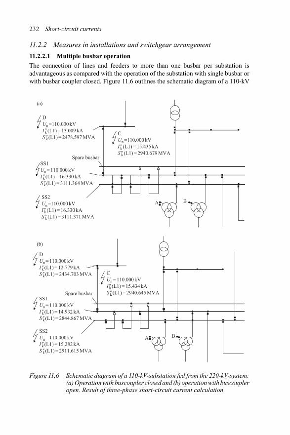
232 Short-circuit currents
11.2.2 Measures in installations and switchgear arrangement
11.2.2.1 Multiple busbar operation
The connection of lines and feeders to more than one busbar per substation isadvantageous as compared with the operation of the substation with single busbar orwith busbar coupler closed. Figure 11.6 outlines the schematic diagram of a 110-kV
DUn =110.000 kVI 0k (L1) = 13.009 kAS 0k (L1) = 2478.597 MVA
SS1Un = 110.000 kVI 0k (L1) = 16.330 kAS 0k (L1) = 3111.364 MVA
SS2Un =110.000 kVI 0k (L1) = 16.330 kAS 0k (L1) = 3111.371 MVA
DUn = 110.000 kVI 0k (L1) = 12.779 kAS 0k (L1) = 2434.703 MVA C
Un = 110.000 kVI 0k (L1) = 15.434 kAS 0k (L1) = 2940.645 MVA
SS2Un = 110.000 kVI 0k (L1) = 15.282 kAS 0k (L1) = 2911.615 MVA
SS1Un = 110.000 kVI 0k (L1) = 14.932 kAS 0k (L1) = 2844.867 MVA
CUn =110.000 kVI 0k (L1) = 15.435 kAS 0k (L1) = 2940.679 MVA
Spare busbar
A B
A B
Spare busbar
(a)
(b)
Figure 11.6 Schematic diagram of a 110-kV-substation fed from the 220-kV-system:(a) Operation with buscoupler closed and (b) operation with buscoupleropen. Result of three-phase short-circuit current calculation
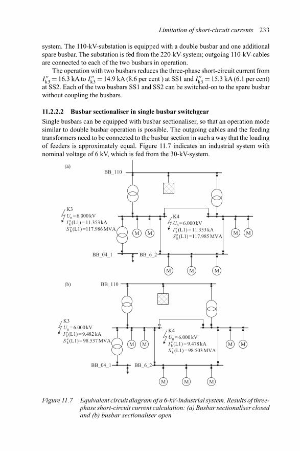
Limitation of short-circuit currents 233
system. The 110-kV-substation is equipped with a double busbar and one additionalspare busbar. The substation is fed from the 220-kV-system; outgoing 110-kV-cablesare connected to each of the two busbars in operation.
The operation with two busbars reduces the three-phase short-circuit current fromI ′′
k3 = 16.3 kA to I ′′k3 = 14.9 kA (8.6 per cent ) at SS1 and I ′′
k3 = 15.3 kA (6.1 per cent)at SS2. Each of the two busbars SS1 and SS2 can be switched-on to the spare busbarwithout coupling the busbars.
11.2.2.2 Busbar sectionaliser in single busbar switchgear
Single busbars can be equipped with busbar sectionaliser, so that an operation modesimilar to double busbar operation is possible. The outgoing cables and the feedingtransformers need to be connected to the busbar section in such a way that the loadingof feeders is approximately equal. Figure 11.7 indicates an industrial system withnominal voltage of 6 kV, which is fed from the 30-kV-system.
K3Un = 6.000 kVI 0k (L1) = 11.353 kAS 0k (L1) =117.986 MVA
K3Un = 6.000 kVI 0k (L1) = 9.482 kAS 0k (L1) = 98.537 MVA
K4Un = 6.000 kVI 0k (L1) = 9.478 kAS 0k (L1) = 98.503 MVA
K4Un = 6.000 kVI 0k (L1) = 11.353 kAS 0k (L1) =117.985 MVA
M M
M
M M M
M
M M
M M
BB_6_2BB_04_1
BB_110
BB_110
M M
M
BB_04_1 BB_6_2
(a)
(b)
Figure 11.7 Equivalent circuit diagram of a 6-kV-industrial system. Results of three-phase short-circuit current calculation: (a) Busbar sectionaliser closedand (b) busbar sectionaliser open

234 Short-circuit currents
The short-circuit current at the feeding busbar is reduced by 16.8 per cent fromI ′′
k3 = 11.4 kA to I ′′k3 = 9.48 kA in the case when the busbar sectionaliser is kept open.
The outgoing feeders have to be arranged in such a way that the loading will beapproximately equal for both busbar sections K3 and K4.
11.2.2.3 Short-circuit current limiting equipment
Short-circuit current limiting equipment and fuses (medium voltage and low voltagesystems) can be installed to reduce the short-circuit level in parts of the installations.In medium voltage installations, Ip-limiter can be installed. Figure 11.8 outlines theschematic diagram of an industrial system. The existing switchgear A with low short-circuit rating shall be extended with the busbar section B, which is fed by an additionalsystem feeder Q2. The maximal permissible short-circuit current I ′′
kAmax of busbarsection A is exceeded by this extension.
Q1
T 1
i1; I1
i3 = i1+ i2I3 = I1+ I2
Q2
T 2
i2; I2
BA
Figure 11.8 Equivalent circuit diagram of switchgear with single busbar
The total short-circuit current from both system feeders shall be limited to thepermissible short-circuit current I ′′
kAmax of busbar section A in the case of a short-circuit at busbar A. If the relation I ′′
kQ1/I ′′kQ2 depends on the ratio ZQ1/ZQ2 of the
feeders Q1 and Q2 it is sufficient to measure the partial short-circuit current throughthe Ip-limiter. The current ratio is
I1
I2= I ′′
kQ1
I ′′kQ2
(11.1)
and the total short-circuit current
I3 = I2 ∗(
1 + I ′′kQ1
I ′′kQ2
)≤ I ′′
kAmax (11.2)

Limitation of short-circuit currents 235
i1 + i2Without Ip-limiter
i1 + i2With Ip-limiter
40 kA
20 kA
i1
i2
t
i
Figure 11.9 Time course of short-circuit current in installations with and withoutIp-limiter
The threshold value I2an of the Ip-limiter is
I2an = I ′′kA max ∗ I ′′
kQ2
I ′′kQ1 + I ′′
kQ2(11.3)
When the permissible short-circuit currents I ′′kAmax and I ′′
kBmax of both busbar sectionsA and B are exceeded, the threshold value I1an of the Ip-limiter for short-circuits atbusbar section B is needed as well
I1an = I ′′kB max ∗ I ′′
kQ1
I ′′kQ2 + I ′′
kQ1(11.4)
The threshold value Ian of the Ip-limiter is set to the minimum of both values
Ian = MIN{I1an; I2an} (11.5)
The detailed design and determination of the settings are determined, besides otherfactors, by different topologies of the power system, different phase angles of thebranch short-circuit currents and different rating of the switchgear in the system.
Figure 11.9 outlines the time curves of short-circuit currents at section A as perFigure 11.8. The branch short-circuit current i2from system feeder Q2 is switched offby the Ip-limiter within 7 ms, thus reducing the peak short-circuit current significantly.
The technical layout of one phase of an Ip-limiter is shown in Figure 11.10.Inside an insulating tube (1) the main current conductor (3) with a breaking element,blown by a triggerable explosive loading, (2) is located. When the threshold valueis exceeded, the tripping circuit triggers the explosive loading; the arc inside theinsulating tube cannot be quenched and is commutated to the fuse element (4), which
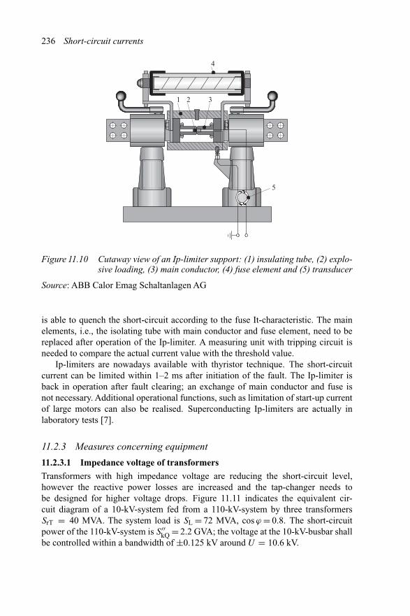
236 Short-circuit currents
4
1 2 3
5
Figure 11.10 Cutaway view of an Ip-limiter support: (1) insulating tube, (2) explo-sive loading, (3) main conductor, (4) fuse element and (5) transducer
Source: ABB Calor Emag Schaltanlagen AG
is able to quench the short-circuit according to the fuse It-characteristic. The mainelements, i.e., the isolating tube with main conductor and fuse element, need to bereplaced after operation of the Ip-limiter. A measuring unit with tripping circuit isneeded to compare the actual current value with the threshold value.
Ip-limiters are nowadays available with thyristor technique. The short-circuitcurrent can be limited within 1–2 ms after initiation of the fault. The Ip-limiter isback in operation after fault clearing; an exchange of main conductor and fuse isnot necessary. Additional operational functions, such as limitation of start-up currentof large motors can also be realised. Superconducting Ip-limiters are actually inlaboratory tests [7].
11.2.3 Measures concerning equipment
11.2.3.1 Impedance voltage of transformers
Transformers with high impedance voltage are reducing the short-circuit level,however the reactive power losses are increased and the tap-changer needs tobe designed for higher voltage drops. Figure 11.11 indicates the equivalent cir-cuit diagram of a 10-kV-system fed from a 110-kV-system by three transformersSrT = 40 MVA. The system load is SL = 72 MVA, cos ϕ = 0.8. The short-circuitpower of the 110-kV-system is S′′
kQ = 2.2 GVA; the voltage at the 10-kV-busbar shallbe controlled within a bandwidth of ±0.125 kV around U = 10.6 kV.

110 kVEL148
EL151EL148I 0k(L1) = 11.740 kAS 0k(L1) = 203.347 MVA
10-KVUn = 10.000 kAI 0k(L1) = 35.221 kAS 0k(L1) = 610.042 MVA
Each cableI 0k(L1) = 0.000 kAS 0k(L1) = 0.000 MVA
EL149 EL150
110 kVEL148
EL151 EL148I 0k(L1) = 9.719 kAS 0k(L1) =168.333 MVA
10-kVUn = 10.000 kVI 0k(L1) = 29.156 kAS 0k(L1) = 504.999 MVA
Each cableI 0k(L1) = 0.000 kAS 0k(L1) = 0.000 MVA
EL149 EL150
(a)
(b)
Figure 11.11 Equivalent circuit diagram of a 10-kV-system with incomingfeeder. Results of three-phase short-circuit current calculation:(a) Impedance voltage 13% and (b) impedance voltage 17.5%
Table 11.2 Result of loadflow and short-circuit analysisas per Figure 11.11
UkrT I ′′k3 I ′′
k1 Tap-changer Reactive power losses(%) (kA) (kA) position of one transformer
(Mvar)
13 35.2 22.5 +6 2.6117.5 29.2 20.7 +8 3.58
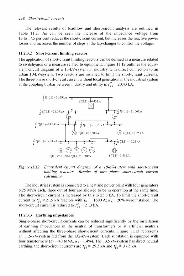
238 Short-circuit currents
The relevant results of loadflow and short-circuit analysis are outlined inTable 11.2. As can be seen the increase of the impedance voltage from13 to 17.5 per cent reduces the short-circuit current, but increases the reactive powerlosses and increases the number of steps at the tap-changer to control the voltage.
11.2.3.2 Short-circuit limiting reactor
The application of short-circuit limiting reactors can be defined as a measure relatedto switchyards or a measure related to equipment. Figure 11.12 outlines the equiv-alent circuit diagram of a 10-kV-system in industry with direct connection to anurban 10-kV-system. Two reactors are installed to limit the short-circuit currents.The three-phase short-circuit current without local generation in the industrial systemat the coupling busbar between industry and utility is I ′′
k3 = 20.43 kA.
I 0k(L1) = 21.29 kA
I 0k(L1) = 21.06 kA
M
M
M
M
I 0k(L1) =14.43 kA
I 0k(L1) = 1.60 kA
I 0k(L1) = 19.24 kA
I 0k(L1) = 1.75 kA
I 0k(L1) = 1.46 kA
I 0k(L1) =19.28 kA I 0k(L1) =19.28 kA
I 0k(L1) = 21.06 kA
I 0k(L1) =19.24 kA
I 0k(L1) = 1.32 kA Ik0(L1) = 1.80 kA
Figure 11.12 Equivalent circuit diagram of a 10-kV-system with short-circuitlimiting reactors. Results of three-phase short-circuit currentcalculation
The industrial system is connected to a heat and power plant with four generators6.25 MVA each, three out of four are allowed to be in operation at the same time.The short-circuit current is increased by this to 25.6 kA. To limit the short-circuitcurrent to I ′′
k3 ≤ 21.5 kA reactors with In = 1600 A; uk = 20% were installed. Theshort-circuit current is reduced to I ′′
k3 = 21.3 kA.
11.2.3.3 Earthing impedances
Single-phase short-circuit currents can be reduced significantly by the installationof earthing impedances in the neutral of transformers or at artificial neutralswithout affecting the three-phase short-circuit currents. Figure 11.13 representsan 11.5-kV-system fed from the 132-kV-system. Each substation is equipped withfour transformers (Sr = 40 MVA, uk = 14%). The 132-kV-system has direct neutralearthing, the short-circuit currents are I ′′
k3 ≈ 29.3 kA and I ′′k1 ≈ 37.3 kA.
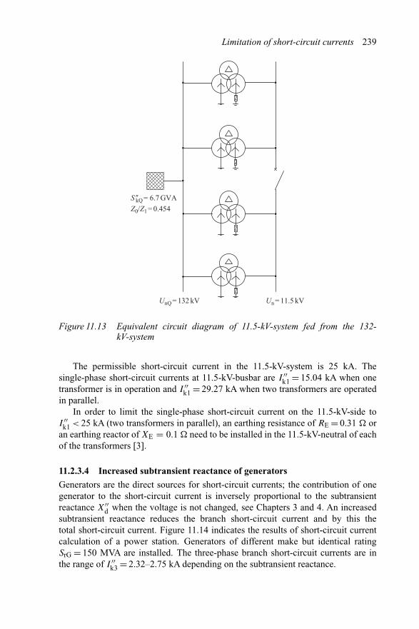
Limitation of short-circuit currents 239
S 0kQ = 6.7 GVA
Z0/Z1 = 0.454
UnQ = 132 kV Un = 11.5 kV
Figure 11.13 Equivalent circuit diagram of 11.5-kV-system fed from the 132-kV-system
The permissible short-circuit current in the 11.5-kV-system is 25 kA. Thesingle-phase short-circuit currents at 11.5-kV-busbar are I ′′
k1 = 15.04 kA when onetransformer is in operation and I ′′
k1 = 29.27 kA when two transformers are operatedin parallel.
In order to limit the single-phase short-circuit current on the 11.5-kV-side toI ′′
k1 < 25 kA (two transformers in parallel), an earthing resistance of RE = 0.31 � oran earthing reactor of XE = 0.1 � need to be installed in the 11.5-kV-neutral of eachof the transformers [3].
11.2.3.4 Increased subtransient reactance of generators
Generators are the direct sources for short-circuit currents; the contribution of onegenerator to the short-circuit current is inversely proportional to the subtransientreactance X′′
d when the voltage is not changed, see Chapters 3 and 4. An increasedsubtransient reactance reduces the branch short-circuit current and by this thetotal short-circuit current. Figure 11.14 indicates the results of short-circuit currentcalculation of a power station. Generators of different make but identical ratingSrG = 150 MVA are installed. The three-phase branch short-circuit currents are inthe range of I ′′
k3 = 2.32–2.75 kA depending on the subtransient reactance.
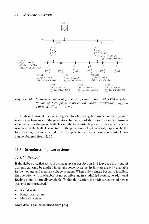
240 Short-circuit currents
EL144
400
EL142 EL143
EL143Ik(L1) = 7.967 kA Sk�(L1) = 1821.450 MVA
GT1A1TIk�(L1) = 2.749 kA Sk�(L1) = 628.456 MVA
GT2A1TIk�(L1) = 2.749 kA Sk�(L1) = 628.456 MVA
GT1TIk�(L1) = 2.535 kA Sk�(L1) = 579.469 MVA
GT3TIk�(L1) = 2.535 kA Sk�(L1) = 579.469 MVA
GT4A1TIk�(L1) = 2.749 kA Sk�(L1) = 628.456 MVA
132KUn =132.000 kV Ik�(L1) = 31.569 kA Sk�(L1) = 7217.597 MVA
GT2TIk�(L1) = 2.322 kA Sk�(L1) = 530.987 MVA
Figure 11.14 Equivalent circuit diagram of a power station with 132-kV-busbar.Results of three-phase short-circuit current calculation: SrG =150 MVA; x′′
d = 12–17.8%
High subtransient reactance of generators has a negative impact on the dynamicstability performance of the generators. In the case of short-circuits on the transmis-sion line with subsequent fault clearing the transmittable power from a power stationis reduced if the fault clearing time of the protection is kept constant, respectively, thefault clearing time must be reduced to keep the transmittable power constant. Detailscan be obtained from [2, 26].
11.3 Structures of power systems
11.3.1 General
It should be noted that some of the measures as per Section 11.2 to reduce short-circuitcurrents can only be applied in certain power systems. Ip-limiters are only availablein low voltage and medium voltage systems. When only a single busbar is installed,the operation with two busbars is not possible and in a radial fed system, no additionalfeeding point is normally available. Within this section, the main structures of powersystems are introduced:
• Radial system• Ring-main system• Meshed system
More details can be obtained from [26].

Limitation of short-circuit currents 241
11.3.2 Radial system
Radial systems represent the simplest topology of a power system and can usuallybe found in low voltage systems. Figure 11.15 outlines the general structure, withone feeding point and distributing of the lines in several branches. This structure issuitable in the case of low load density but also for the connection of high bulk-supplyloads. The calculation of short-circuit currents is comparatively easy, as there are nomeshed lines in the system and only one topology has to be analysed.
MV/LV-transformer
Figure 11.15 General structure of a radial system with one incoming feeder
11.3.3 Ring-main system
In a ring-main system the receiving end of each line of a radial system is to beconnected either back to the feeding busbar or to an additional feeding busbar. Ring-main systems are most often planned for medium voltage systems, and in rare casesfor low voltage systems as well. Normally ring-main systems are operated with openbreaker or isolator in one primary as indicated in Figure 11.16(a). This enables anoperation similar to radial systems but with a switchable reserve for all consumers.Feeding busbars can be planned at several locations of the system as indicated inFigure 11.16(b). Short-circuit current calculation is more complicated than in radialsystems as several operating conditions, i.e., system topologies, are to be taken intoaccount to determine the minimal and the maximal short-circuit current.
11.3.4 Meshed systems
Meshed systems are normally applied only for high voltage systems or in industrialsupply systems for MV-level as well. With the consideration of consumer load and

242 Short-circuit currents
Switch (normally open) MV/LV-transformer
(a)
(b)
Figure 11.16 General structures of ring-main systems: (a) Simple structure with onefeeding busbar and (b) structure with two feeding busbars (feedingfrom opposite sides)

GS
3~
GS
3~ GS
3~
GS
3~
20-
kV(3
5-kV
)
220-
kVsu
btra
nsm
issi
onsy
stem
(reg
iona
ldi
stri
butio
n)
380-
kVtr
ansm
issi
onsy
stem
Inte
rcon
nect
ion
lines
to
neig
bour
ing
coun
trie
s
110-
kV-s
yste
m
(ind
ustr
yw
ith g
ener
atio
n)
Indu
stri
alsy
stem
s35
-kV
10-k
V
20-k
V
110-
kV
syst
em(r
ural
are
as)
110-
kV
(urb
an a
rea
with
gene
ratio
n)
GS
3~
10-k
V (
20-k
V)
di
stri
butio
nsy
stem
Fig
ure
11.1
7P
rinc
ipal
stru
ctur
eof
ahi
ghvo
ltage
syst
emw
ithdi
ffere
ntvo
ltage
leve
ls

244 Short-circuit currents
capability of power stations, the system is planned, constructed and operated in sucha way as to allow the supply of consumers without overloading of any equipment andwithout violating the permissible voltage profile even under outage of one ((n − 1)-criteria) or more equipment at the same time. The calculation of maximal short-circuitcurrents seems relatively simple, if all equipment are assumed to be in operation. Asfar as different operation schedules of the power stations are considered, differentsystem topologies need to be considered. The calculation of the minimal short-circuitcurrent, however, is much more difficult, as a close cooperation between planningand operation is required. A large number of different topologies in the meshed powersystem have to be analysed to ensure that the calculated short-circuit current is theminimal current. The principal structure of a meshed high voltage system is outlinedin Figure 11.17.
A special type of meshed systems is applied to low voltage systems; the principalstructure is outlined in Figure 11.18. The reliability of supply is comparatively high,as reserve in the case of outage of any line or infeed is provided through the remaininglines.
Switch(normally open)
MV-cable(a)
(b) 1
3
32
2
2
3
1
1; 2; 3 Connection to MV-cable No. 1; 2; 3
1
3
1
2
Figure 11.18 Principal structure of meshed low voltage system: (a) Single-fedmeshed system and (b) meshed system with overlapping feeding
Chapter 12
Special problems related toshort-circuit currents
12.1 Interference of pipelines
12.1.1 Introduction
Interference between overhead lines, communication circuits and pipelines is causedby asymmetrical currents, which may be due to short-circuits, asymmetrical operationor asymmetrical design of equipment, especially asymmetrical outline of overheadline towers with respect to pipelines and communication circuits. This interferenceis based on inductive, ohmic and capacitive coupling between the short-circuit path(e.g., overhead line) and the circuit affected by interference (e.g., pipeline). Normaloperating currents, respectively voltages, cause magnetic as well as electric fieldswhich are asymmetrical in the vicinity of overhead lines which may cause interferenceproblems in the long-time range.
Short-circuit currents on overhead transmission lines and cables and short-circuitcurrents through earth cause interference in the short-time range only when the short-circuit is switched off after some seconds by the power system protection. Interferenceproblems may arise in cable and overhead line systems to a different extent dependingon the handling of the system neutral. The induced voltage in pipelines and commu-nication circuits may endanger technical installations and safety of workers whendefined limits will be exceeded. Within the context of this book, only the short-timeinterference, in the following called interference, is dealt with. Table 12.1 outlinesthe needs for the analysis of interference problems.
Interference problems may occur in most of the cases by inductive and ohmic cou-pling in power systems with low-impedance earthing consisting mainly of overheadlines, as can be seen from Table 12.1. In systems with isolated neutral or resonanceearthing interference problems have to be regarded only when the fault current is notself-extinguishing (see Chapters 5 and 7). Capacitive coupling does not cause any

Tabl
e12
.1In
terf
eren
cebe
twee
npo
wer
syst
em,c
omm
unic
atio
nci
rcui
tsan
dpi
pelin
es
Pow
ersy
stem
Inte
rfer
ence
ofco
mm
unic
atio
nci
rcui
tsan
dpi
pelin
esby
:
Han
dlin
gof
neut
rals
Ope
ratin
gco
nditi
onIn
duct
ive
coup
ling
Cap
aciti
veco
uplin
gO
hmic
coup
ling
Low
-im
peda
nce
With
outf
ault
OH
TL
Onl
yif
circ
uits
onsa
me
tow
erN
oin
terf
eren
ceea
rthi
ngC
able
No
inte
rfer
ence
prob
lem
s
Shor
t-ci
rcui
tO
HT
LPr
esen
tN
oin
terf
eren
cePr
esen
tC
able
Pres
enti
nsp
ecia
lcas
esN
oin
terf
eren
ceN
oin
terf
eren
ce
Isol
ated
neut
ral;
With
outf
ault
OH
TL
Onl
yif
circ
uits
onsa
me
tow
erN
oin
terf
eren
ceR
eson
ance
eart
hing
Cab
leN
oin
terf
eren
ce
Shor
t-ci
rcui
t;O
HT
LN
oin
terf
eren
cePr
esen
tN
oin
terf
eren
ceE
arth
faul
tC
able
No
inte
rfer
ence
Dou
ble
eart
hO
HT
LPr
esen
tN
oin
terf
eren
cePr
esen
tfa
ult
Cab
leN
oin
terf
eren
ceN
oin
terf
eren
ceN
oin
terf
eren
ce
Special problems related to short-circuit currents 247
severe problems in pipelines and communication circuits. It should be noted further-more that interference of communication circuits is decreasing due to the decreasinginstallations of overhead communication circuits, which are replaced by wirelesscommunication or by cable circuits, which can be protected easily against interfer-ence. The explanations on interference are therefore concentrated within this sectionto the interference of pipelines.
Regulations on the permissible values for voltages induced in pipelines and com-munication circuits and/or for touch voltages exist in various countries. The main aimis to protect any person likely to work on the pipeline or power circuit against elec-trocution hazard. According to an international survey carried out by CIGRE [20],the maximum permissible touch voltage is defined in different countries in differentways, ranging from 200 V up to 1500 V depending on the maximal fault durationtime. In Germany, the maximal permissible touch voltage and the maximal permissi-ble voltage pipeline-to-earth are both limited to 1000 V for a fault-duration of 0.5 s.Higher values are applied only in Australia (1500 V) and in Brazil (1700 V), whereasthe Brazilian regulation defines the admissible value of a touch current, which is con-verted for comparison into the voltage limit. Within this survey, only two US-utilitieshave answered the questions on voltage limits. The limit for the touch voltage appliedthere is given to be 500 V, whereas the voltage pipeline-to-earth should be less than5 kV. It is unclear and could not be clarified in the CIGRE-survey, why low value fortouch voltage (500 V) as compared with other countries resulted in a comparativelyhigh value for the pipeline-to-earth voltage (5 kV).
According to [21] the maximal permissible voltage pipeline-to-earth for short-time interference shall be below 1000 V. If ASME/IEEE-standard No. 80 is applieda maximal permissible touch voltage is defined in relation to the fault duration timefor different body weight of the person involved. If the most severe restrictionsare applied, i.e., 50 kg body weight and fault duration (clearing time) of 150 ms, themaximal permissible touch voltage Ut50 is 350 V. This is the recommended limit asper IEEE-standard No. 80 item 6, where it is mentioned that the actual transferredvoltage should be less than the maximum allowable touch voltage Etouch to ensuresafety.
12.1.2 Calculation of impedances for inductive interference
In order to calculate the interference of pipelines the loop-impedances, couplingimpedances and self-impedances of the line conductor, earth conductors and thepipeline itself are required. The loop-impedance of the pipeline with earth return is
Z′P = R′
P + μ0
8∗ ω + j
(μ0
2π∗ ω ∗
(ln
δ
rP+ μP
4
))(12.1)
where rP is the outer radius of the pipeline, μ0 is the absolute permeability, μP is thefictitious relative permeability of the pipeline, δ is the depth of earth return path andω is the angular frequency.
248 Short-circuit currents
Equation (12.1) is composed of
R′P Resistance of the pipeline per unit length
μ0
8∗ ω Resistance of the earth return path per unit length
μ0
2π∗ ω ∗ ln
δ
rPOuter reactance of the loop with earth return path perunit length
μ0
2π∗ ω ∗ μP
4Internal (inner) reactance of the conductor (pipeline)per unit length
The depth δ of the earth return path is given by Equation (12.2) with the resistivityof soil ρ (specific soil resistance) according to Table 12.2.
δ = 1.85√ω ∗ (μ0/ρ)
(12.2)
Table 12.2 Resistivity of soil ρ for different types of soil conditions
Parameters Type of soil
Alluvialsoil –swampsoil
Clay Limestoneclay –farm soil
Wetsand
Wetgravel
DrysandDraygravel
Stonysoil
Specific soil resistance 30 50 100 200 500 1000 3000ρ (�m)
σ = 1/ρ (μS/cm) 333 20 10 5 2 1 0.33Depth of earth return 510 660 930 1320 2080 2940 5100δ at 50 Hz (m)
Depth of earth return 465 600 850 1205 1900 2684 4655δ at 60 Hz (m)
The resistance R′P of the pipeline can be calculated from the conductivity κP and the
thickness d of the pipeline wall taking eddy currents and the dissipation of the currentinto the outer level of the pipeline wall into account.
R′P = R′
dc ∗(
x + 0.25 + 3
64 ∗ x
)(12.3)
The increase of the inner inductivity X′i is given by
X′i = R′
dc ∗(
x − 3
64 ∗ x+ 3
128 ∗ x2
)(12.4)
Special problems related to short-circuit currents 249
with the parameter x = d/(2 ∗ δP), the d.c. resistance of the pipeline wall R′dc, the
depth of current in the pipeline wall δP and d being the thickness of the pipeline wall:
δP = 1√ω/2 ∗ (κP ∗ μP ∗ μ0)
(12.5)
Comparing the loop-impedance as per Equation (12.1) with the inner inductanceof the pipeline as per Equation (12.4) the fictitious relative permeability of the pipelinewill be
μP = 4 ∗ R′dc ∗ x − 3/(64 ∗ x) + 3/(128 ∗ x2)
(ω ∗ μ0)/2π(12.6)
Coupling impedances [2] need to be calculated for the analysis of the interferenceproblems. For the individual distances and impedances reference is made to Figure12.1 indicating a typical interference problem between a 380-kV-line with two earthwires, counterpoise and a pipeline.
The coupling impedance ZLP of the loop conductor and pipeline with earth returnis obtained from
Z′LP = μ0
8∗ ω + j
(μ0
2π∗ ω ∗
(ln
δ
dLP min
))(12.7)
The coupling impedance ZEP of the loop earth conductor and pipeline with earthreturn is obtained from
Z′EP = μ0
8∗ ω + j
(μ0
2π∗ ω ∗
(ln
δ
dEP min
))(12.8)
Coupling impedance ZLE of the loop earth conductor and conductor with earth returnis given by
Z′LE = μ0
8∗ ω + j
(μ0
2π∗ ω ∗
(ln
δ
dLE
))(12.9)
In case a second earth conductor is installed, the coupling impedance ZEP2 of theloop second earth conductor and pipeline with earth return is calculated by
Z′EP2 = μ0
8∗ ω + j
(μ0
2π∗ ω ∗
(ln
δ
dEP2 min
))(12.10)
The coupling impedance ZLE2 of the loop second earth conductor and conductor withearth return is obtained from
Z′LE2 = μ0
8∗ ω + j
(μ0
2π∗ ω ∗
(ln
δ
dLE2
))(12.11)
The coupling impedance ZE12 of the loop first and second earth conductor andconductor with earth return is obtained from
Z′E12 = μ0
8∗ ω + j
(μ0
2π∗ ω ∗
(ln
δ
dE12
))(12.12)
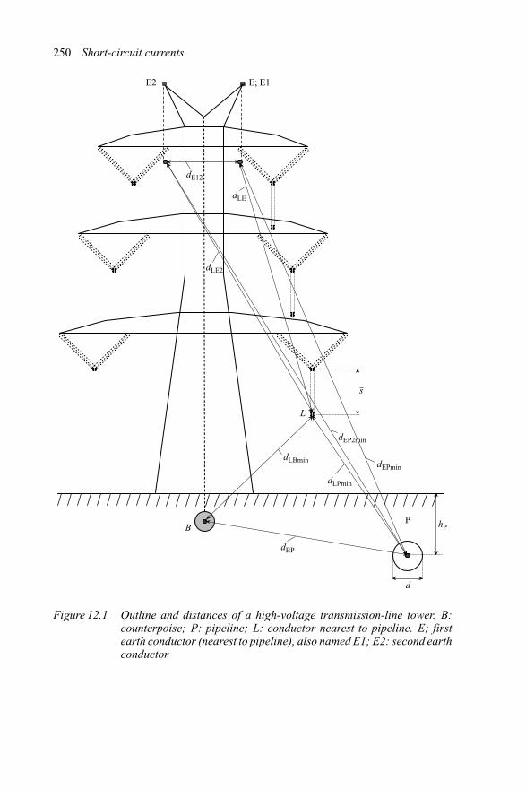
250 Short-circuit currents
dE12
E2 E; E1
dLE2
dLBmin
dBP
P hP
d
dLPmin
dEPmin
dEP2min
L
B
s
dLE
Figure 12.1 Outline and distances of a high-voltage transmission-line tower. B:counterpoise; P: pipeline; L: conductor nearest to pipeline. E; firstearth conductor (nearest to pipeline), also named E1; E2: second earthconductor
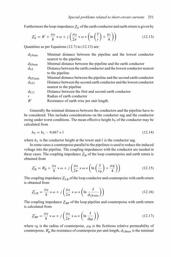
Special problems related to short-circuit currents 251
Furthermore the loop-impedance ZE of the earth conductor and earth return is given by
Z′E = R′ + μ0
8∗ ω + j
(μ0
2π∗ ω ∗
(ln(
δ
r
)+ μr
4
))(12.13)
Quantities as per Equations (12.7) to (12.13) are:
dLPmin Minimal distance between the pipeline and the lowest conductornearest to the pipeline
dEPmin Minimal distance between the pipeline and the earth conductordLE Distance between the earth conductor and the lowest conductor nearest
to the pipelinedEP2min Minimal distance between the pipeline and the second earth conductordLE2 Distance between the second earth conductor and the lowest conductor
nearest to the pipelinedE12 Distance between the first and second earth conductorr Radius of earth conductorR′ Resistance of earth wire per unit length.
Generally the minimal distances between the conductors and the pipeline have tobe considered. This includes considerations on the conductor sag and the conductorswing under worst conditions. The mean effective height hS of the conductor may becalculated from
hS = hL − 0.667 ∗ s (12.14)
where hL is the conductor height at the tower and s is the conductor sag.In some cases a counterpoise parallel to the pipelines is used to reduce the induced
voltage into the pipeline. The coupling impedances with the conductor are needed inthese cases. The coupling impedance ZB of the loop counterpoise and earth return isobtained from
Z′B = R′
B + μ0
8∗ ω + j
(μ0
2π∗ ω ∗
(ln(
δ
rB
)+ μB
4
))(12.15)
The coupling impedance ZLB of the loop conductor and counterpoise with earth returnis obtained from
Z′LB = μ0
8∗ ω + j
(μ0
2π∗ ω ∗
(ln
δ
dLB min
))(12.16)
The coupling impedance ZBP of the loop pipeline and counterpoise with earth returnis calculated from
Z′BP = μ0
8∗ ω + j
(μ0
2π∗ ω ∗
(ln
δ
dBP
))(12.17)
where rB is the radius of counterpoise, μB is the fictitious relative permeability ofcounterpoise, R′
B the resistance of counterpoise per unit length, dLBmin is the minimal

252 Short-circuit currents
distance between counterpoise and the lowest conductor nearest to the pipeline, dBPis the distance between counterpoise and pipeline.
12.1.3 Calculation of induced voltage
Based on the impedance calculations as per Section 12.1.2 the induced voltage intothe pipeline can be calculated for any configuration as follows:
U iP = −Z′LP ∗ r ′ ∗ I ′′
kE ∗ lPp ∗ w (12.18)
where Z′LP is the coupling impedance of the loop pipeline and conductor nearest
to earth with earth return, I ′′kE is the initial short-circuit current (asymmetrical) of
the overhead line, lPp is the length of parallel exposure between pipeline and over-head line, r ′ is the screening factor as per Equation (12.18) and w is a probabilityfactor taking into account that all worse conditions do not occur at the same timeinstant [21].
The screening factor depends on the presence of earth wires, counterpoises and anyother compensation circuit capable to reduce the induced voltage into the pipeline.If only one earth wire is present as compensation circuit the screening factor r ′ iscalculated based on the coupling and loop-impedances by
r ′ = 1 − Z′LE ∗ Z′
EP
Z′E ∗ Z′
LP(12.19)
If more than one earth conductor or additional compensation circuits are present,additional considerations for the screening factor are required. The total screeningfactor is then given by the difference of the individual factors of each earth conductorand/or compensation circuit taking into account the correction factor which representsthe influence of each earth wire and compensation circuit on the current in the otherwire [22]. In the case of two earth conductors the total screening factor r ′
tot is given by
r ′tot = 1 − Z′
LE ∗ Z′EP
Z′E ∗ Z′
LP∗ k2 − Z′
LE2 ∗ Z′EP2
Z′E2 ∗ Z′
LP∗ k1 (12.20)
Correction factors k1 and k2 are calculated by
k1 = 1 − (Z′LE ∗ Z′
E12)/(Z′E ∗ Z′
LE2)
1 − (Z′E12 ∗ Z′
E12)/(Z′E ∗ Z′
E2)(12.21a)
k2 = 1 − (Z′LE2 ∗ Z′
E12)/(Z′E2 ∗ Z′
LE)
1 − (Z′E12 ∗ Z′
E12)/(Z′E ∗ Z′
E2)(12.21b)

Special problems related to short-circuit currents 253
Correction factors for other arrangements and numbers of conductors can be obtained,respectively calculated, as per [39]. Impedances as per Equations (12.19) to (12.21)are calculated according to Section 12.1.2
ZLP Coupling impedance of the loop conductor and pipeline with earth returnas per Equation (12.7)
ZEP Coupling impedance of the loop first earth conductor and pipeline withearth return as per Equation (12.8)
ZLE Coupling impedance of the loop first earth conductor and conductor withearth return as per Equation (12.9)
ZEP2 Coupling impedance of the loop second earth conductor and pipelinewith earth return as per Equation (12.10)
ZLE2 Coupling impedance of the loop first earth conductor and conductor withearth return as per Equation (12.11)
ZE12 Coupling impedance of the loop first and second earth conductor withearth return as per Equation (12.12)
ZE Loop-impedance of earth conductor and earth return as per Equation(12.13)
ZE2 Loop-impedance of second earth conductor and earth return as perEquation (12.13)
For three and more compensation circuits, e.g., two earth conductors and a coun-terpoise, the screening factor needs to be calculated either from the individualcurrent distribution within the different compensation circuits or by means of themultiplication method or other methods as outlined in [3].
12.1.4 Characteristic impedance of the pipeline
The induced voltage U iP is only an indication for the inductive interference but doesnot take into account the earthing conditions and the conductivity of the pipelinecoating. In order to calculate step and touch voltages the voltage between pipelineand earth is to be calculated taking account of the earthing and conductivity con-ditions of the pipeline. Based on the analysis of the system equivalent, i.e., faultedphase conductor, presence of earth conductors, counterpoise, pipeline and earthingconditions, the pipeline must be represented by means of its characteristic impedanceand its conductivity.
The conductivity of the pipeline against the surrounding earth is determined bythe resistance R′
I of the pipeline coating and the resistance R′PE of the bare (uncoated)
pipeline in earth (see Table 12.3). The total resistance is given by
R′Ctot = R′
I + R′PE (12.22)
The specific reactance due to the capacitance of the pipeline can be neglected forinterference analysis as it is much smaller than the resistance. The resistance R′
PE of
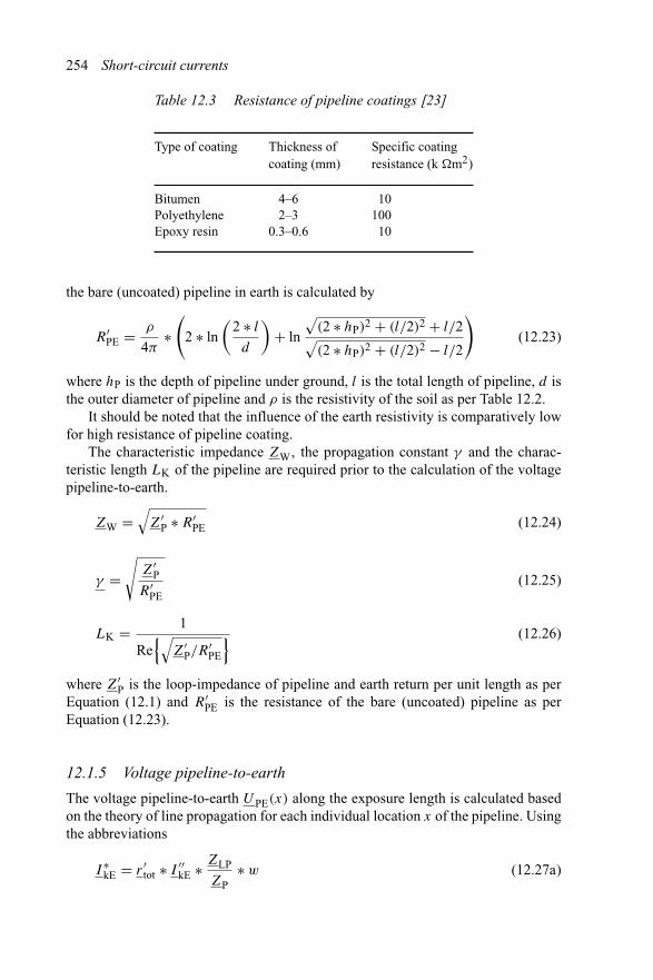
254 Short-circuit currents
Table 12.3 Resistance of pipeline coatings [23]
Type of coating Thickness of Specific coatingcoating (mm) resistance (k �m2)
Bitumen 4–6 10Polyethylene 2–3 100Epoxy resin 0.3–0.6 10
the bare (uncoated) pipeline in earth is calculated by
R′PE = ρ
4π∗(
2 ∗ ln(
2 ∗ l
d
)+ ln
√(2 ∗ hP)2 + (l/2)2 + l/2√(2 ∗ hP)2 + (l/2)2 − l/2
)(12.23)
where hP is the depth of pipeline under ground, l is the total length of pipeline, d isthe outer diameter of pipeline and ρ is the resistivity of the soil as per Table 12.2.
It should be noted that the influence of the earth resistivity is comparatively lowfor high resistance of pipeline coating.
The characteristic impedance ZW, the propagation constant γ and the charac-teristic length LK of the pipeline are required prior to the calculation of the voltagepipeline-to-earth.
ZW =√
Z′P ∗ R′
PE (12.24)
γ =√
Z′P
R′PE
(12.25)
LK = 1
Re{√
Z′P/R′
PE
} (12.26)
where Z′P is the loop-impedance of pipeline and earth return per unit length as per
Equation (12.1) and R′PE is the resistance of the bare (uncoated) pipeline as per
Equation (12.23).
12.1.5 Voltage pipeline-to-earth
The voltage pipeline-to-earth UPE(x) along the exposure length is calculated basedon the theory of line propagation for each individual location x of the pipeline. Usingthe abbreviations
I ∗kE = r ′
tot ∗ I ′′kE ∗ ZLP
ZP∗ w (12.27a)
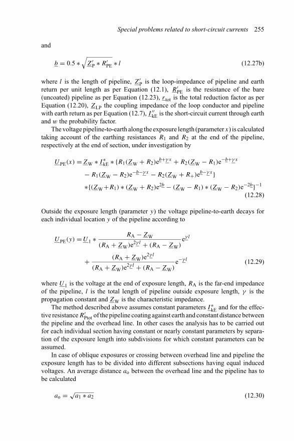
Special problems related to short-circuit currents 255
and
b = 0.5 ∗√
Z′P ∗ R′
PE ∗ l (12.27b)
where l is the length of pipeline, Z′P is the loop-impedance of pipeline and earth
return per unit length as per Equation (12.1), R′PE is the resistance of the bare
(uncoated) pipeline as per Equation (12.23), r tot is the total reduction factor as perEquation (12.20), ZLP the coupling impedance of the loop conductor and pipelinewith earth return as per Equation (12.7), I ′′
kE is the short-circuit current through earthand w the probability factor.
The voltage pipeline-to-earth along the exposure length (parameter x) is calculatedtaking account of the earthing resistances R1 and R2 at the end of the pipeline,respectively at the end of section, under investigation by
UPE(x) = ZW ∗ I ∗kE ∗ {R1(ZW + R2)eb+γ x + R2(ZW − R1)e−b+γ x
− R1(ZW − R2)e−b−γ x − R2(ZW + R+)eb−γ x}∗{(ZW+R1) ∗ (ZW + R2)e2b − (ZW − R1) ∗ (ZW − R2)e−2b}−1
(12.28)
Outside the exposure length (parameter y) the voltage pipeline-to-earth decays foreach individual location y of the pipeline according to
UPE(y) = U1 ∗ RA − ZW
(RA + ZW)e2γ l + (RA − ZW)eγ l
+ (RA + ZW)e2γ l
(RA + ZW)e2γ l + (RA − ZW)e−γ l (12.29)
where U1 is the voltage at the end of exposure length, RA is the far-end impedanceof the pipeline, l is the total length of pipeline outside exposure length, γ is thepropagation constant and ZW is the characteristic impedance.
The method described above assumes constant parameters I ∗kE and for the effec-
tive resistance R′Ptot of the pipeline coating against earth and constant distance between
the pipeline and the overhead line. In other cases the analysis has to be carried outfor each individual section having constant or nearly constant parameters by separa-tion of the exposure length into subdivisions for which constant parameters can beassumed.
In case of oblique exposures or crossing between overhead line and pipeline theexposure length has to be divided into different subsections having equal inducedvoltages. An average distance ao between the overhead line and the pipeline has tobe calculated
ao = √a1 ∗ a2 (12.30)

256 Short-circuit currents
lI
a1
a2
a3
lII
dLPc
L
L
Tower Tower
P
lIII lIVOHTL
Pipeline
(a)
(b)
Figure 12.2 Oblique exposure and crossing of pipeline and overhead line. (a) Plotplan and (b) elevation plan (detail from crossing location)
The parameters a1 and a2 are the distances at the ends of the oblique exposure,see Figure 12.2 for details. The ratio a1/a2 should not exceed the value of threeotherwise further subdivisions have to be selected. Distances of more than 1000 mbetween overhead line and pipeline can be neglected for short-time interference.
Crossings shall be handled similarly to oblique exposures with the restriction thatthe subdivisions in the vicinity of the crossing shall be selected as short as possible.
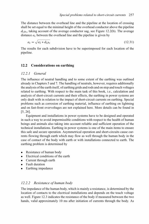
Special problems related to short-circuit currents 257
The distance between the overhead line and the pipeline at the location of crossingshall be set equal to the minimal height of the overhead conductor above the pipelinedLPc, taking account of the average conductor sag, see Figure 12.2(b). The averagedistance ac between the overhead line and the pipeline is given by
ac = √a2 ∗ dLPc (12.31)
The results for each subdivision have to be superimposed for each location of thepipeline.
12.2 Considerations on earthing
12.2.1 General
The influence of neutral handling and to some extent of the earthing was outlinedalready in Chapters 5 and 7. The handling of neutrals, however, requires additionallythe analysis of the earth itself, of earthing grids and rods and on step and touch voltagesrelated to earthing. With respect to the main task of this book, i.e., calculation andanalysis of short-circuit currents and their effects, the earthing in power systems areonly dealt with in relation to the impact of short-circuit currents on earthing. Specialproblems such as corrosion of earthing material, influence of earthing on lightningand on fast-front overvoltages are not explained here. More details can be found in[5, 26].
Equipment and installations in power systems have to be designed and operatedin such a way to avoid impermissible conditions with respect to the health of humanbeings and animals also taking into account reliable and sufficient operation of thetechnical installations. Earthing in power systems is one of the main items to ensurethis safe and secure operation. Asymmetrical operation and short-circuits cause cur-rents flowing through earth which may flow as well through the human body in thecase of contact of the body with earth or with installations connected to earth. Theearthing problem is determined by
• Resistance of human body• Electrical conditions of the earth• Current through earth• Fault duration• Earthing impedance
12.2.2 Resistance of human body
The impedance of the human body, which is mainly a resistance, is determined by thelocation of contacts to the electrical installations and depends on the touch voltageas well. Figure 12.3 indicates the resistance of the body if measured between the twohands, valid approximately 10 ms after initiation of currents through the body. As

258 Short-circuit currents
5
4.5
4
3.5
3
2.5
2
1.5
1
0.5
00 100 200 300 400 500 600 700 800
UB (V)
R(k
Ω)
Figure 12.3 Impedance of the human body (hand-to-hand) depending on the touchvoltage
can be seen the resistance is between 3.5 k� and 1.1 k� decreasing with increasingtouch voltage. For other contacts the resistance is reduced, e.g.,
• One hand to breast reduction to 45 per cent of resistance as per Figure 12.3• One hand to knee reduction to 70 per cent of resistance as per Figure 12.3• Two hands to breast reduction to 23 per cent of resistance as per Figure 12.3• Two hands to knee reduction to 45 per cent of resistance as per Figure 12.3
It should be noted in this respect that the current through the human body is thecritical physical phenomena causing uncontrolled operation of the heart (ventricleflicker) or muscle convulsion. The critical current is a function of the exposuretime [24]. The duration of the permissible touch voltage UB therefore depends onthe exposure time as well (fault duration) and is outlined in Figure 12.4.
The permissible touch voltage is set in most of the standards to UB = 65 V, result-ing in a negligible risk for ventricle flicker independent from the time of exposure.If this voltage limit cannot be guaranteed the exposure time must be limited.
12.2.3 Soil conditions
The resistivity of the soil depends on the type of soil (swamp soil, stony soil) asoutlined in Table 12.2. The differences are determined by the humidity of the soil.The value for swamp soil is between 10,000 �m (humidity less than 10 per cent)and 30 �m (humidity 90 per cent). It is obvious that the resistivity of the soil variesin a wider range if surface electrodes will be used for earthing as the soil humidity

Special problems related to short-circuit currents 259
0
100
200
300
400
500
600
700
800
0.1 1 10Time of exposure (s)
UB
(V
)
Figure 12.4 Permissible touch voltage depending on the time of exposure
varies in a wider range throughout the year as compared with deep-ground earthingby earthing rods. The resistivity for surface electrodes varies throughout the year ina range of ±30 per cent, in the case of deep-earthing only in a range of ±8 per centof the average value, the highest value occurring in March and the lowest value inAugust (European countries). It is therefore recommended to use surface electrodesonly in those installations where the soil humidity is nearly constant throughout theyear and to use deep-ground earthing for other conditions.
12.2.4 Relevant currents through earth
Currents through earth are only existing in the case of asymmetrical short-circuits withearth connection. In most of the cases (X0/X1 > 1), the single-phase short-circuitcurrent I ′′
k1 is greater than the current through earth I ′′kE2E in case of a double-phase
short-circuit. Only in case of power systems (e.g., 115 and 132 kV) having highamount of cables, power stations with high rating closely connected to the sys-tem under investigation and when all transformer neutrals are earthed through lowimpedance, can the ratio X0/X1 be below One. In these cases the double-phaseshort-circuit current may exceed the single-phase short-circuit current.
Current through earth causes voltage drops UE at the impedance of the earth, atthe earthing itself and at the connection lines between the equipment (e.g., neutralsof transformers, transformer tank, overhead line tower) and earth. The currents to betaken into account as summarised in Table 12.4 depend on the type of neutral handlingin the system.

Tabl
e12
.4C
urre
nts
thro
ugh
eart
hfo
rth
ede
sign
ofea
rthi
ngin
stal
latio
ns
Val
idfo
rTy
peof
neut
ralh
andl
ing
Isol
ated
neut
ral
Low
-im
peda
nce
Ear
thin
gw
ithR
eson
ance
eart
hing
eart
hing
curr
entl
imita
tion
Vol
tage
atea
rthi
ngI C
EC
urre
ntth
roug
hC
urre
ntth
roug
hW
ithre
acto
r:√ I
2 rD+
I2 re
s
Touc
hvo
ltage
eart
hing
impe
danc
eea
rthi
ngim
peda
nce
With
outr
eact
or:I
Res
The
rmal
stre
ssof
eart
hing
I′′ kE
EI′′ k1
orI′′ kE
2EI′′ k1
orI′′ kE
2EI′′ kE
Ean
dea
rthi
ngco
nnec
tions
Ear
thin
gco
nnec
tions
I CE
I′′ k1
orI′′ kE
2EI′′ k1
orI′′ kE
2EI′′ kE
E
Ear
thin
gvo
ltage
UE
UE
≤12
5V
:no
mea
sure
sre
quir
edTo
uch
volta
geU
BU
E>
125
Vth
enU
B≤
65V
UE
>12
5V
then
UB
acco
rdin
gto
UE
>12
5V
then
UB
≤65
Vor
equi
vale
ntm
easu
res
VD
E01
41de
pend
ing
onfa
ult
oreq
uiva
lent
mea
sure
sac
cord
ing
toV
DE
0141
dura
tion
orfa
stsw
itch-
off
acco
rdin
gto
VD
E01
41or
equi
vale
ntm
easu
res
acco
rdin
gto
VD
E01
41

Special problems related to short-circuit currents 261
Table 12.5 Reduction factor for typical power system installa-tions; distance of earth conductor to phase conductorD ≈ 20 m; ρ = 100 �m
Number of conductors Type and cross-section Reductionfactor
1 Earth conductor St 50–90 0.98Al/St 50/30 0.78Al/St 120/70 0.7Al/St 240/40 0.65Al/St 120/70; counterpoise Cu 120 0.52
2 Earth conductors Al/St 95/55 0.5Cable sheet NA2XS(2)Y; 150Al; 20 kV 0.5
Single-core cable; 110 kV 0.1N2XS(SL)2Y; 240Cu; 110 kV 0.27Cables in steel tube <0.05
As mentioned already in Section 7.3, a part of the single- or double-phase earth-fault current is flowing through earth and the relevant impedances of the earthinginstallations, depending on the reduction factor of the earth conductor and/or ofcable screens and sheets connected to earth. Detailed investigations are required todetermine the reduction factor. For rough estimates the reduction factors for typicalinstallations are given in Table 12.5.
12.2.5 Earthing impedance
The impedance, i.e., the resistance of the earthing installations is determined by thematerial of the earthing grid, electrodes and rods and by the presence of any con-nection of earth conductor, counterpoise, cable sheets and other earthed installationsin the vicinity of the earthing installation. The earthing resistance is proportional tothe resistivity of the soil and depends furthermore on the specific arrangements ofthe earthing installations as outlined in Table 12.6.
The equations as per Table 12.6 for the calculation of the resistance of earthinginstallation indicate that it is not recommendable to increase the number of meshesin an earthing grid in order to reduce the earthing impedance, as the effect is onlymarginal. Increasing the number of earthing rods on the same earthing installation ishighly recommendable as the total earthing impedance is approximately reciprocal tothe number of rods. Sufficient distance between the individual rods (at least more thanthe rod-length) shall be provided in this case. Material, cross-sections and laying of theearthing installations must comply with the relevant standards, e.g., ANSI C 33.8(standard for safety grounding and bonding equipment).
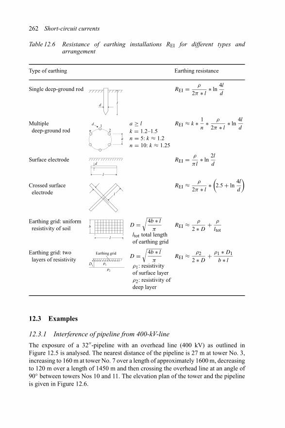
262 Short-circuit currents
Table 12.6 Resistance of earthing installations REI for different types andarrangement
Type of earthing Earthing resistance
Single deep-ground rod REI = ρ
2π ∗ l∗ ln
4l
d
ld
Multipledeep-ground rod
a ≥ l REI ≈ k ∗ 1
n∗ ρ
2π ∗ l∗ ln
4l
dk = 1.2–1.5n = 5: k ≈ 1.2n = 10: k ≈ 1.25
a
21
n
d
Surface electrode REI = ρ
πl∗ ln
2l
d
l
d
Crossed surfaceelectrode
REI ≈ ρ
2π ∗ l∗(
2.5 + ln4l
d
)l
Earthing grid: uniformresistivity of soil
D =√
4b ∗ l
πltot total lengthof earthing grid
REI ≈ ρ
2 ∗ D+ ρ
ltot
l
b
Earthing grid: twolayers of resistivity
D =√
4b ∗ l
πρ1: resistivityof surface layerρ2: resistivity ofdeep layer
REI ≈ ρ2
2 ∗ D+ ρ1 ∗ D1
b ∗ l
Earthing grid
D1r1
r2
12.3 Examples
12.3.1 Interference of pipeline from 400-kV-line
The exposure of a 32′′-pipeline with an overhead line (400 kV) as outlined inFigure 12.5 is analysed. The nearest distance of the pipeline is 27 m at tower No. 3,increasing to 160 m at tower No. 7 over a length of approximately 1600 m, decreasingto 120 m over a length of 1450 m and then crossing the overhead line at an angle of90◦ between towers Nos 10 and 11. The elevation plan of the tower and the pipelineis given in Figure 12.6.
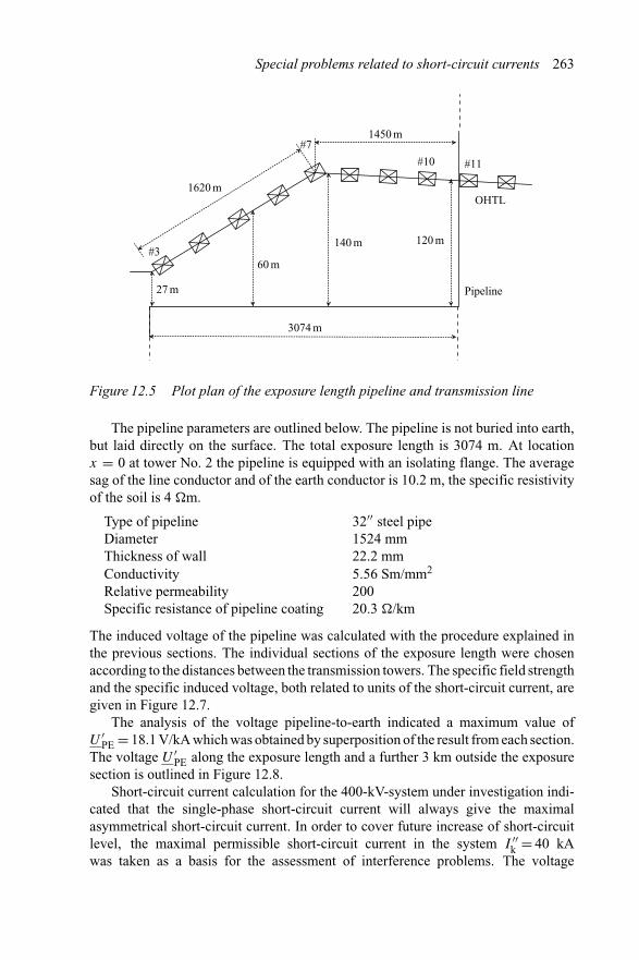
Special problems related to short-circuit currents 263
Pipeline
3074 m
27 m
60 m
140 m 120 m
OHTL
#3
#7
#10 #11
1620 m
1450 m
Figure 12.5 Plot plan of the exposure length pipeline and transmission line
The pipeline parameters are outlined below. The pipeline is not buried into earth,but laid directly on the surface. The total exposure length is 3074 m. At locationx = 0 at tower No. 2 the pipeline is equipped with an isolating flange. The averagesag of the line conductor and of the earth conductor is 10.2 m, the specific resistivityof the soil is 4 �m.
Type of pipeline 32′′ steel pipeDiameter 1524 mmThickness of wall 22.2 mmConductivity 5.56 Sm/mm2
Relative permeability 200Specific resistance of pipeline coating 20.3 �/km
The induced voltage of the pipeline was calculated with the procedure explained inthe previous sections. The individual sections of the exposure length were chosenaccording to the distances between the transmission towers. The specific field strengthand the specific induced voltage, both related to units of the short-circuit current, aregiven in Figure 12.7.
The analysis of the voltage pipeline-to-earth indicated a maximum value ofU ′
PE = 18.1 V/kA which was obtained by superposition of the result from each section.The voltage U ′
PE along the exposure length and a further 3 km outside the exposuresection is outlined in Figure 12.8.
Short-circuit current calculation for the 400-kV-system under investigation indi-cated that the single-phase short-circuit current will always give the maximalasymmetrical short-circuit current. In order to cover future increase of short-circuitlevel, the maximal permissible short-circuit current in the system I ′′
k = 40 kAwas taken as a basis for the assessment of interference problems. The voltage
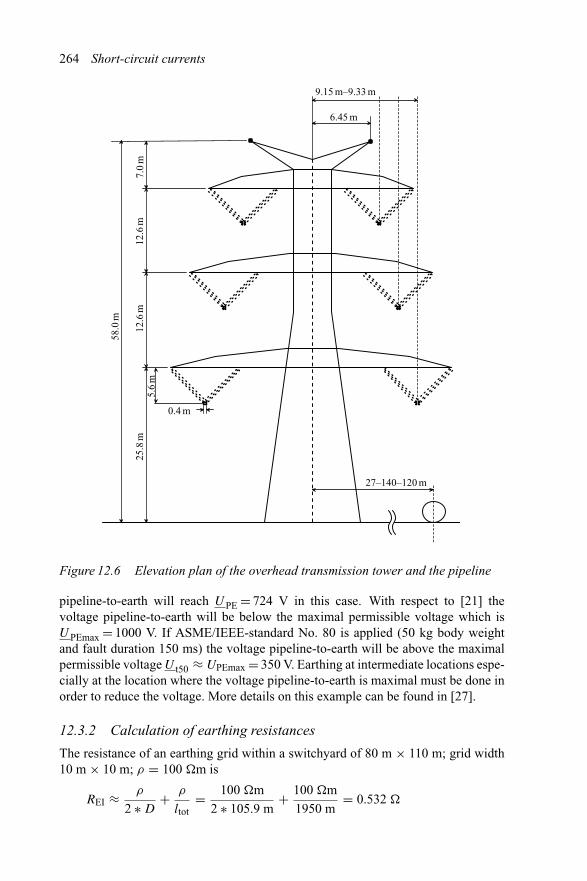
264 Short-circuit currents
9.15 m–9.33 m
6.45 m
27–140–120 m
7.0
m12
.6m
12.6
m25
.8m
58.0
m
5.6
m
0.4 m
Figure 12.6 Elevation plan of the overhead transmission tower and the pipeline
pipeline-to-earth will reach UPE = 724 V in this case. With respect to [21] thevoltage pipeline-to-earth will be below the maximal permissible voltage which isUPEmax = 1000 V. If ASME/IEEE-standard No. 80 is applied (50 kg body weightand fault duration 150 ms) the voltage pipeline-to-earth will be above the maximalpermissible voltage U t50 ≈ UPEmax = 350 V. Earthing at intermediate locations espe-cially at the location where the voltage pipeline-to-earth is maximal must be done inorder to reduce the voltage. More details on this example can be found in [27].
12.3.2 Calculation of earthing resistances
The resistance of an earthing grid within a switchyard of 80 m × 110 m; grid width10 m × 10 m; ρ = 100 �m is
REI ≈ ρ
2 ∗ D+ ρ
ltot= 100 �m
2 ∗ 105.9 m+ 100 �m
1950 m= 0.532 �
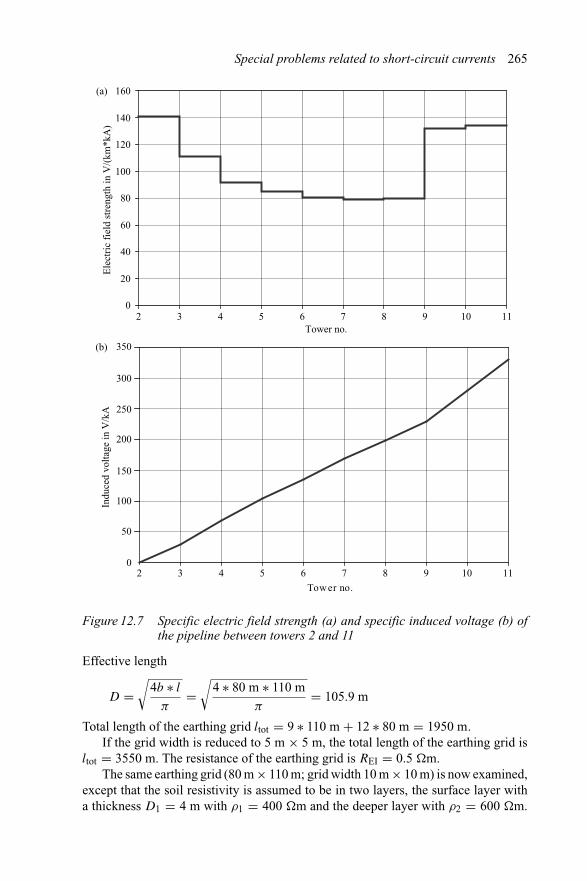
Special problems related to short-circuit currents 265
0
20
40
60
80
100
120
140
160(a)
(b)
2 3 4 5 6 7 8 9 10 11Tower no.
Ele
ctri
c fi
eld
stre
ngth
in V
/(km
*kA
)
0
50
100
150
200
250
300
350
2 3 4 5 6 7 8 9 10 11
Tower no.
Indu
ced
volta
ge in
V/k
A
Figure 12.7 Specific electric field strength (a) and specific induced voltage (b) ofthe pipeline between towers 2 and 11
Effective length
D =√
4b ∗ l
π=√
4 ∗ 80 m ∗ 110 m
π= 105.9 m
Total length of the earthing grid ltot = 9 ∗ 110 m + 12 ∗ 80 m = 1950 m.If the grid width is reduced to 5 m × 5 m, the total length of the earthing grid is
ltot = 3550 m. The resistance of the earthing grid is REI = 0.5 �m.The same earthing grid (80 m × 110 m; grid width 10 m × 10 m) is now examined,
except that the soil resistivity is assumed to be in two layers, the surface layer witha thickness D1 = 4 m with ρ1 = 400 �m and the deeper layer with ρ2 = 600 �m.
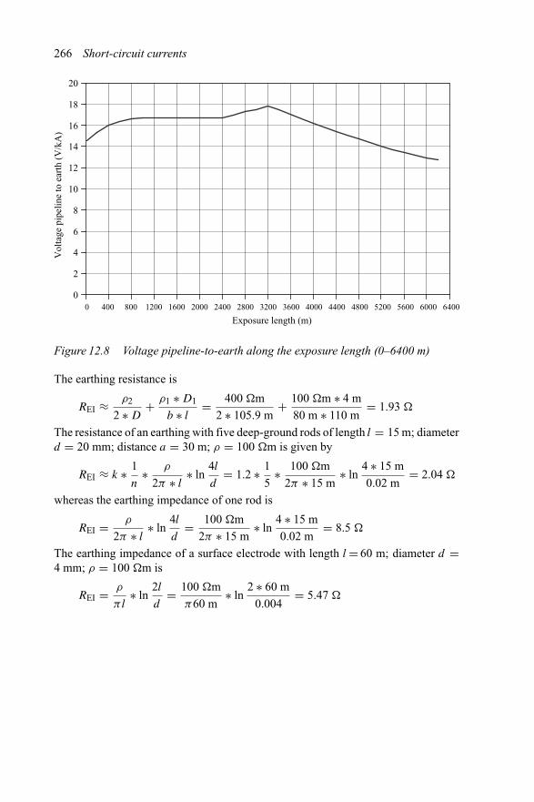
266 Short-circuit currents
0
2
4
6
8
10
12
14
16
18
20
0 400 800 1200 1600 2000 2400 2800 3200 3600 4000 4400 4800 5200 5600 6000 6400
Exposure length (m)
Vol
tage
pip
elin
e to
ear
th (
V/k
A)
Figure 12.8 Voltage pipeline-to-earth along the exposure length (0–6400 m)
The earthing resistance is
REI ≈ ρ2
2 ∗ D+ ρ1 ∗ D1
b ∗ l= 400 �m
2 ∗ 105.9 m+ 100 �m ∗ 4 m
80 m ∗ 110 m= 1.93 �
The resistance of an earthing with five deep-ground rods of length l = 15 m; diameterd = 20 mm; distance a = 30 m; ρ = 100 �m is given by
REI ≈ k ∗ 1
n∗ ρ
2π ∗ l∗ ln
4l
d= 1.2 ∗ 1
5∗ 100 �m
2π ∗ 15 m∗ ln
4 ∗ 15 m
0.02 m= 2.04 �
whereas the earthing impedance of one rod is
REI = ρ
2π ∗ l∗ ln
4l
d= 100 �m
2π ∗ 15 m∗ ln
4 ∗ 15 m
0.02 m= 8.5 �
The earthing impedance of a surface electrode with length l = 60 m; diameter d =4 mm; ρ = 100 �m is
REI = ρ
πl∗ ln
2l
d= 100 �m
π60 m∗ ln
2 ∗ 60 m
0.004= 5.47 �

Chapter 13
Data of equipment
13.1 Three-phase a.c. equipment
A summary of relevant data of equipment is given in IEC 60909-2:1992. The dataare based on a survey carried out by IEC TC 73. In some countries this documentdoes not have the character of a standard.
13.1.1 System feeders
Impedances of power system feeders, respectively, their initial short-circuit powerare difficult to determine as typical values, the structure of the power systems (cableor overhead line system), the voltage levels or the application task, i.e., for rural,urban or industrial power supply can vary in a wide range. Typical ranges of theinitial short-circuit power (three-phase short-circuit) are given in Figure 13.1 for apower system with different voltage levels.
13.1.2 Transformers
Transformers are constructed with defined rated power with respect to their applica-tion. In low-voltage and to a certain extent in medium-voltage systems, transformersare build with standard rated power and standard impedance voltage. Transformersin high-voltage systems, sometimes also in medium-voltage systems, have to meetspecial application conditions, such as the internal standard of the utility with specialdefined values for rated power, impedance voltage and ohmic losses. It should benoted in this respect that the minimisation of the impedance voltage is limited bythe minimal insulation thickness of the windings. Typical values for the impedancevoltage of transformers are outlined in Figure 13.2. Figure 13.3 gives data for theshort-circuit losses (ohmic losses). The relation of the impedance voltage (%-value)

268 Short-circuit currents
GS3~
GS3~
< 1 MVA
250–1300 MVA
GS3~
50–600 MVA
GS3~
< 60 MVA
380 kV
220 kVand 110 kV
10–30 kV
S �k = 20–50 GVA
S �k = 2–5 GVA
S �k = 100–500 MVA
S �k = 2–5 MVA0.4 kV
Sr = 630–1000 MVAuk = 10–16%
Sr = 12.5–63 MVAuk = 11–20%
Sr = 50–630 kVAuk = 4%Sr = 630–2.5 MVAuk = 6%
Figure 13.1 Principal structure of a power supply system and typical values ofinitial short-circuit power of public supply system [7]
to the rated power (MVA-value) as per IEC 60909-2:1992 is given below:
ukr = 8 + 0.92 ∗ ln(SrT) (13.1)
Further data are included in Table 13.1.The impedance voltage of auto-transformers is lower than that of full-winding
transformers.
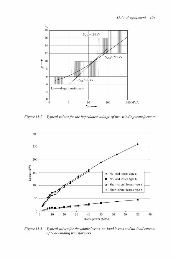
Data of equipment 269
0 1 100
100 1000 MVA
2
4
6
8
10
12
14
16
%18
UrOS = 110 kV
UrOS > 220 kV
UrOS < 30 kV
2
1
Low-voltage transformers
uk
SrT
Figure 13.2 Typical values for the impedance voltage of two-winding transformers
0
50
100
150
200
250
300
0 10 20 30 40 50 60 70 80 90
Rated power (MVA)
Los
ses
(kW
)
No-load losses type a
No-load losses type b
Short-circuit losses type a
Short-circuit losses type b
Figure 13.3 Typical values for the ohmic losses, no-load losses and no-load currentof two-winding transformers

270 Short-circuit currents
Table 13.1 Data of transformers
Voltage levels Sr ukr uRr(MVA) (%) (%)
MV/LV 0.05–0.63 4 1–2Un < 1 kV 0.63–2.5 6 1–1.5
MV/MV 2.5–25 6–9 0.7–1Un = 1–66 kV
HV/MV 25–63 10–16 0.6–0.8Un > 66 kV
The ratio of positive to negative sequence impedance of transformers depends onthe vector group and is typically in the range of
Vector group YNd X0/X1 ≈ 0.8–1.0
Vector group Yzn X0/X1 ≈ 0.1
Vector group Yyn (three-limb core) X0/X1 ≈ 3.0–10.0
Vector group Yyn X0/X1 ≈ 10.0–100.0
(five limb core and three single-phase
transformers)
Vector group YNynd X0/X1 ≈ 1.5–3.2
13.1.3 Generators
The parameters such as rated power, rated voltage, power factor and subtransientreactance and synchronous reactance are needed to calculate the impedance ofgenerators and by this the contribution to the short-circuit current.
Rated voltages within one power range may vary depending on the constructiontype of the generator. The subtransient reactance of synchronous generators is typi-cally in the range of 10–30 per cent depending on the rated power as mentioned inIEC 60909-2. The synchronous reactance is between 100 and 300 per cent, whereassalient pole generators normally have lower values than turbo generators. Typicalvalues are summarised in Table 13.2.
Power factor of generators with rated power below 20 MVA is approximatelycos ϕr = 0.8 and increases for high rated machines (>1000 MVA) to cos ϕr = 0.85 onaverage. The ratio of saturated to unsaturated reactance xdsat/xd is between 0.8 and0.9, whereas in the case of rated power below 100 MVA, the ratio can be between 0.65and 1.0. Zero-sequence reactance of synchronous generators are x0 ≈ (0.4–0.8)x′′
ddepending on the winding arrangement.

Data of equipment 271
Table 13.2 Typical data of synchronous generators (average values)
Rated power Rated voltage Subtransient reactance Synchronous reactanceSrG (MVA) UrG (kV) x′′
d (%) xd (%)
Below 4 0.48–11.5 10–25 110–170–2304–20 2.2–13.8 8–16 120–180–21020–200 6–22 10–20 160–205–260Above 200 20–27 18–30 220–230–240Synchronous motors Up to 11.5 12–25
13.1.4 Overhead lines
Impedances of overhead lines depend on the geometrical arrangement of phaseconductors, on the tower outline and on the number and type of conductors. The zero-sequence impedance furthermore depends on the earth resistivity, on the arrangementof earth conductors and on the design of the earthing system, including conductiveinstallations in earth, respectively, connected to earth, e.g., pipelines, counterpoiseand cable sheaths. The calculation of impedances of overhead lines in the positive-sequence and the zero-sequence component are outlined below based on the toweroutline as per Figure 13.4. The equations are valid for overhead lines which aresymmetrically constructed and operated. All circuits are assumed to be in operationexcept as noted.
Y
R
B
RY
Bb
r y
System aSystem b
E E(a) (b)
Figure 13.4 Tower outline of high-voltage transmission lines. (a) Single-circuit lineand (b) double-circuit line
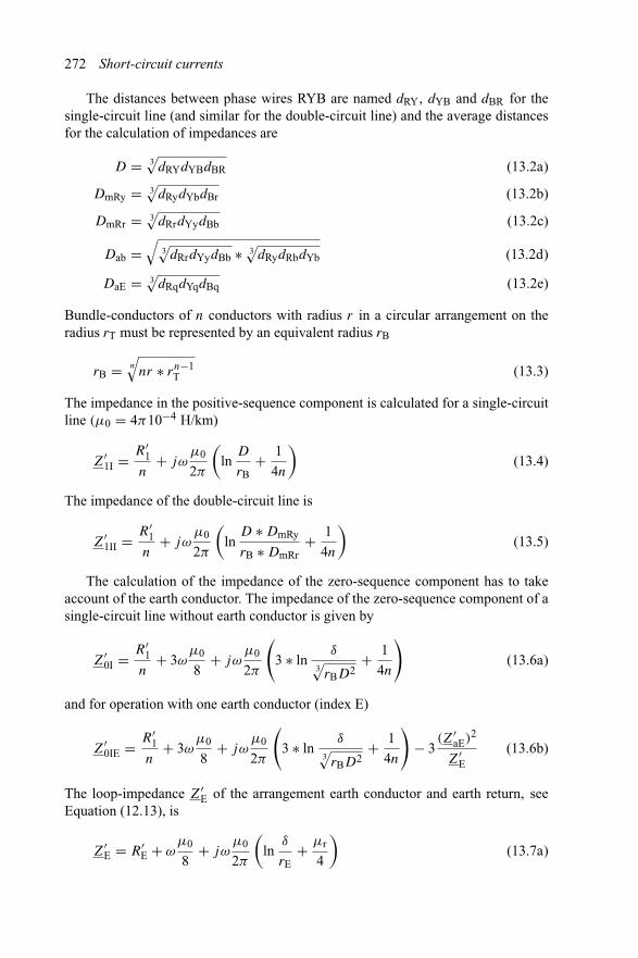
272 Short-circuit currents
The distances between phase wires RYB are named dRY, dYB and dBR for thesingle-circuit line (and similar for the double-circuit line) and the average distancesfor the calculation of impedances are
D = 3√
dRYdYBdBR (13.2a)
DmRy = 3√
dRydYbdBr (13.2b)
DmRr = 3√
dRrdYydBb (13.2c)
Dab =√
3√
dRrdYydBb ∗ 3√
dRydRbdYb (13.2d)
DaE = 3√
dRqdYqdBq (13.2e)
Bundle-conductors of n conductors with radius r in a circular arrangement on theradius rT must be represented by an equivalent radius rB
rB = n
√nr ∗ rn−1
T (13.3)
The impedance in the positive-sequence component is calculated for a single-circuitline (μ0 = 4π10−4 H/km)
Z′1I = R′
1
n+ jω
μ0
2π
(ln
D
rB+ 1
4n
)(13.4)
The impedance of the double-circuit line is
Z′1II = R′
1
n+ jω
μ0
2π
(ln
D ∗ DmRy
rB ∗ DmRr+ 1
4n
)(13.5)
The calculation of the impedance of the zero-sequence component has to takeaccount of the earth conductor. The impedance of the zero-sequence component of asingle-circuit line without earth conductor is given by
Z′0I = R′
1
n+ 3ω
μ0
8+ jω
μ0
2π
(3 ∗ ln
δ
3√
rBD2+ 1
4n
)(13.6a)
and for operation with one earth conductor (index E)
Z′0IE = R′
1
n+ 3ω
μ0
8+ jω
μ0
2π
(3 ∗ ln
δ
3√
rBD2+ 1
4n
)− 3
(Z′aE)2
Z′E
(13.6b)
The loop-impedance Z′E of the arrangement earth conductor and earth return, see
Equation (12.13), is
Z′E = R′
E + ωμ0
8+ jω
μ0
2π
(ln
δ
rE+ μr
4
)(13.7a)

Data of equipment 273
The coupling impedance Z′aq of phase conductor and earth conductor (see
Equation (12.11), where Z′aE is named Z′
LE2)
Z′aE = ω
μ0
8+ jω
μ0
2π∗ ln
δ
DaE(13.7b)
The distance Daq is given by Equation (13.2e) and the depth δ of the earth return path(see Equation (12.2)) is
δ = 1.85√μ0(ω/ρ)
(13.8)
The resistivity of the soil ρ is between 30 �m (Swamp soil) and 3000 �m (Stonysoil) as outlined in Table 12.2.
The impedance of the zero-sequence component of a double-circuit overhead linewithout earth conductor is given by
Z′0II = R′
1
n+ 3ω
μ0
8+ jω
μ0
2π
(3 ∗ ln
δ
3√
rBD2+ 1
4n
)+ 3Z′
ab (13.9a)
and in the case of operation with earth conductor
Z′0IIE = R′
1
n+ 3ω
μ0
8+ jω
μ0
2π
(3 ∗ ln
δ
3√
rBD2+ 1
4n
)+ 3Z′
ab − 6(Z′
aE)2
Z′E
(13.9b)
where Z′aE is the coupling impedance of phase conductor and earth conductor accord-
ing to Equation (13.7b), Z′E is the impedance of the loop phase conductor and earth
return according to Equation (13.7a) and Z′ab is the coupling impedance between the
systems a and b according to Equation (13.10).
Z′ab = ω
μ0
8+ jω
μ0
2π∗ ln
δ
Dab(13.10)
The relative permeability μr relevant for overhead lines is
Conductors from Cu or Al μr = 1Conductors from Al/St, cross-section ratio > 6 μr ≈ 1Conductors from Al/St, one layer of Al only μr ≈ 5–10Conductors from Steel (St) μr ≈ 25
Typical values for the impedances of MV-overhead lines are summarised inTable 13.3. Table 13.4 shows the impedances of HV-overhead lines.
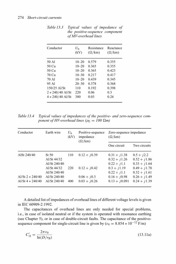
274 Short-circuit currents
Table 13.3 Typical values of impedance ofthe positive-sequence componentof MV-overhead lines
Conductor Un Resistance Reactance(kV) (�/km) (�/km)
50 Al 10–20 0.579 0.35550 Cu 10–20 0.365 0.35550 Cu 10–20 0.365 0.42370 Cu 10–30 0.217 0.41770 Al 10–20 0.439 0.34595 Al 20–30 0.378 0.368150/25 Al/St 110 0.192 0.3982 ∗ 240/40 Al/St 220 0.06 0.34 ∗ 240/40 Al/St 380 0.03 0.26
Table 13.4 Typical values of impedances of the positive- and zero-sequence com-ponent of HV-overhead lines (ρE = 100 �m)
Conductor Earth wire Un Positive-sequence Zero-sequence impedance(kV) impedance (�/km)
(�/km)One circuit Two circuits
AlSt 240/40 St 50 110 0.12 + j0.39 0.31 + j1.38 0.5 + j2.2Al/St 44/32 0.32 + j1.26 0.52 + j1.86Al/St 240/40 0.22 + j1.1 0.33 + j1.64Al/St 44/32 220 0.12 + j0.42 0.3 + j1.19 0.49 + j1.78Al/St 240/40 0.22 + j1.1 0.32 + j1.61
Al/St 2 ∗ 240/40 Al/St 240/40 0.06 + j0.3 0.16 + j0.98 0.26 + j1.49Al/St 4 ∗ 240/40 Al/St 240/40 400 0.03 + j0.26 0.13 + j0.091 0.24 + j1.39
A detailed list of impedances of overhead lines of different voltage levels is givenin IEC 60909-2:1992.
The capacitances of overhead lines are only needed for special problems,i.e., in case of isolated neutral or if the system is operated with resonance earthing(see Chapter 5), or in case of double-circuit faults. The capacitance of the positive-sequence component for single-circuit line is given by (ε0 = 8.854 ∗ 10−12 F/m)
C′1I = 2πε0
ln(D/rB)(13.11a)

Data of equipment 275
The capacitance of the positive-sequence component for a double-circuit line isgiven by
C′1II = 2πε0
ln(DDmRy/rBDmRr)(13.11b)
Similar to the calculation of the impedance of the zero-sequence component, theearth conductor has to be considered for the calculation of capacitances of the zero-sequence component. In the case of operation without earth conductor the capacitanceof the single-circuit line is calculated by
C′0I = 2πε0
3 ∗ ln(2h/3√
rBD2)(13.12a)
C′0IE = 2πε0
3 ∗ (ln(2h/ 3√
rBD2) − (ln((h + hq)/Daq))2/ ln(2hq/rq))(13.12b)
The capacitances of the double-circuit line are calculated by
C′0II = 2πε0
3 ∗ ln((
2h ∗√
4h2 + D2mRy
)/( 3√
rBD2 ∗ 3√
DmRrD2mRy
)) (13.13a)
C′0IIE = 2πε0/
{3 ∗ ln
2h ∗√
4h2 + D2mRy
3√
rBD2 ∗ 3√
DmRrD2mRy
− 2(ln ((h + hE)/DaE))2
ln(2hE/rE)
}
(13.13b)
To take account of the conductor sag, the average height h of the conductor is used
h = 3√
hRhYhB = 3√
hrhyhb (13.14)
The influence of the tower on the capacitance in the zero-sequence component isconsidered by an increase of 6 per cent (overhead lines with nominal voltage 400 kV),up to 10 per cent (overhead lines with nominal voltage 60 kV).
It should be observed that the capacitance in the positive-sequence component isgiven by
C1 = 3CL + CE (13.15a)
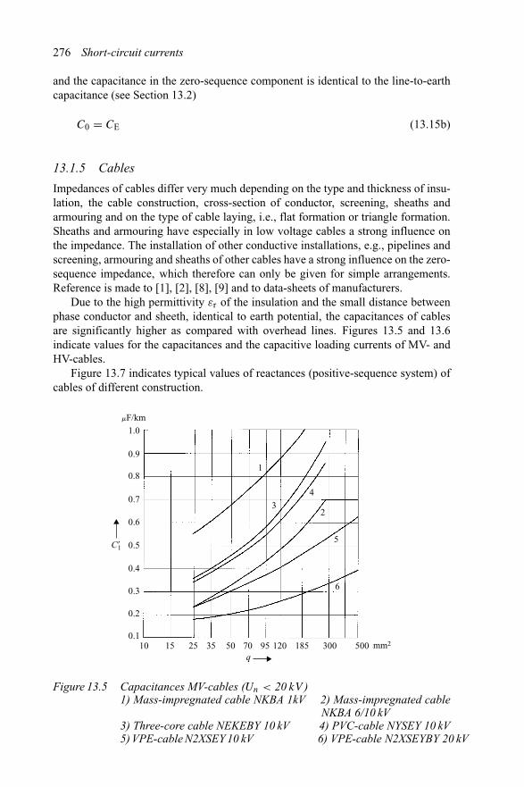
276 Short-circuit currents
and the capacitance in the zero-sequence component is identical to the line-to-earthcapacitance (see Section 13.2)
C0 = CE (13.15b)
13.1.5 Cables
Impedances of cables differ very much depending on the type and thickness of insu-lation, the cable construction, cross-section of conductor, screening, sheaths andarmouring and on the type of cable laying, i.e., flat formation or triangle formation.Sheaths and armouring have especially in low voltage cables a strong influence onthe impedance. The installation of other conductive installations, e.g., pipelines andscreening, armouring and sheaths of other cables have a strong influence on the zero-sequence impedance, which therefore can only be given for simple arrangements.Reference is made to [1], [2], [8], [9] and to data-sheets of manufacturers.
Due to the high permittivity εr of the insulation and the small distance betweenphase conductor and sheeth, identical to earth potential, the capacitances of cablesare significantly higher as compared with overhead lines. Figures 13.5 and 13.6indicate values for the capacitances and the capacitive loading currents of MV- andHV-cables.
Figure 13.7 indicates typical values of reactances (positive-sequence system) ofcables of different construction.
1.0
0.8
0.9
0.7
1
3
4
2
5
6
0.6
0.5
0.4
0.3
0.2
0.110 15 25 35 50 70 95 120 185 300 500 mm2
mF/km
C�1
q
Figure 13.5 Capacitances MV-cables (Un < 20 kV )1) Mass-impregnated cable NKBA 1kV 2) Mass-impregnated cable
NKBA 6/10 kV3) Three-core cable NEKEBY 10 kV 4) PVC-cable NYSEY 10 kV5) VPE-cable N2XSEY 10 kV 6) VPE-cable N2XSEYBY 20 kV
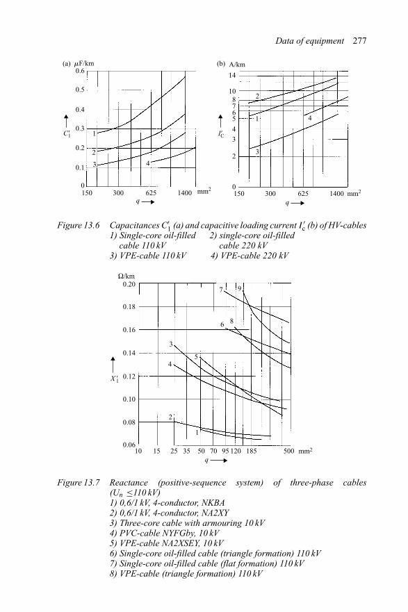
Data of equipment 277
0.6mF/km
0.5
0.4
0.31
2
3 4
1
2
3
4
0.2
0.1
0150 300 625
q1400 mm2
150 300 625q
1400 mm2
C�1
14
A/km
108765
43
2
0
I�C
(a) (b)
Figure 13.6 Capacitances C′1 (a) and capacitive loading current I ′
c (b) of HV-cables1) Single-core oil-filled 2) single-core oil-filled
cable 110 kV cable 220 kV3) VPE-cable 110 kV 4) VPE-cable 220 kV
0.20
0.18
0.16
0.14
0.12
0.10
0.08
0.0610 15 25 35 50 70
q95 120 185 500 mm2
X �1
Ω/km
7 9
86
5
3
4
2
1
Figure 13.7 Reactance (positive-sequence system) of three-phase cables(Un ≤110 kV)1) 0,6/1 kV, 4-conductor, NKBA2) 0,6/1 kV, 4-conductor, NA2XY3) Three-core cable with armouring 10 kV4) PVC-cable NYFGby, 10 kV5) VPE-cable NA2XSEY, 10 kV6) Single-core oil-filled cable (triangle formation) 110 kV7) Single-core oil-filled cable (flat formation) 110 kV8) VPE-cable (triangle formation) 110 kV

278 Short-circuit currents
13.1.6 Reactors and resistors
Short-circuit limiting reactors are constructed for all voltage levels, from low voltageup to 750 kV. The reactors are manufactured with oil-insulated windings and asair-insulated core-type reactors. Figure 13.8 shows a short-circuit limiting reactor(air-insulated core-type; 10 kV; 630 A; 6 per cent).
Petersen-coils are constructed as reactor with fixed reactance, with tap-changerand with continuous controllable reactors. The control range normally is limited to1 : 2.5 for tap-changer control and 1 : 10 for continuous control. Standards as per
Figure 13.8 Arrangement of a short-circuit limiting reactor
Source: Mohndruck
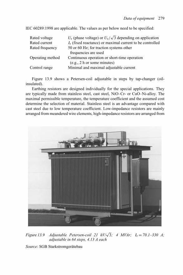
Data of equipment 279
IEC 60289:1998 are applicable. The values as per below need to be specified:
Rated voltage Ur (phase voltage) or Ur/√
3 depending on applicationRated current Ir (fixed reactance) or maximal current to be controlledRated frequency 50 or 60 Hz; for traction systems other
frequencies are usedOperating method Continuous operation or short-time operation
(e.g., 2 h or some minutes)Control range Minimal and maximal adjustable current
Figure 13.9 shows a Petersen-coil adjustable in steps by tap-changer (oil-insulated).
Earthing resistors are designed individually for the special applications. Theyare typically made from stainless steel, cast steel, NiO–Cr- or CuO–Ni-alloy. Themaximal permissible temperature, the temperature coefficient and the assumed costdetermine the selection of material. Stainless steel is an advantage compared withcast steel due to low temperature coefficient. Low-impedance resistors are mainlyarranged from meandered wire elements, high-impedance resistors are arranged from
Figure 13.9 Adjustable Petersen-coil 21 kV/√
3; 4 MVAr; Ir = 70.1–330 A;adjustable in 64 steps, 4.13 A each
Source: SGB Starkstromgerätebau
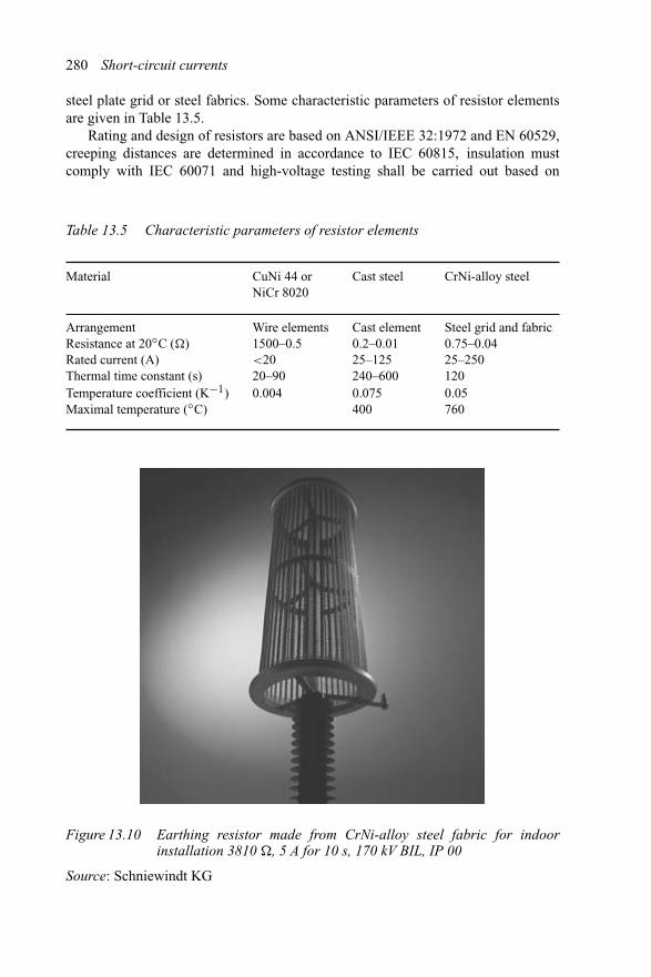
280 Short-circuit currents
steel plate grid or steel fabrics. Some characteristic parameters of resistor elementsare given in Table 13.5.
Rating and design of resistors are based on ANSI/IEEE 32:1972 and EN 60529,creeping distances are determined in accordance to IEC 60815, insulation mustcomply with IEC 60071 and high-voltage testing shall be carried out based on
Table 13.5 Characteristic parameters of resistor elements
Material CuNi 44 or Cast steel CrNi-alloy steelNiCr 8020
Arrangement Wire elements Cast element Steel grid and fabricResistance at 20◦C (�) 1500–0.5 0.2–0.01 0.75–0.04Rated current (A) <20 25–125 25–250Thermal time constant (s) 20–90 240–600 120Temperature coefficient (K−1) 0.004 0.075 0.05Maximal temperature (◦C) 400 760
Figure 13.10 Earthing resistor made from CrNi-alloy steel fabric for indoorinstallation 3810 �, 5 A for 10 s, 170 kV BIL, IP 00
Source: Schniewindt KG

Data of equipment 281
Figure 13.11 Earthing resistor made from meandering wire for outdoor installation16 �, 400 A for 10 s, 75 kV BIL, IP 20
Source: Schniewindt KG
IEC 60060. Earthing resistors can be suitably designed for indoor and outdoorinstallations. Figures 13.10 and 13.11 show two different types of resistors.
13.1.7 Asynchronous motors
Data of asynchronous motors are included in IEC 60781:1989 (mentioned as A inTable 13.6) , IEC 60909-2:1992, in [10] (mentioned as B in Table 13.6) and in IEC60909-1:1991 (mentioned as C in Table 13.6). Table 13.6 outlines the relevant dataof asynchronous motors for LV- and MV-application.
13.2 d.c. equipment
Data of d.c. equipment are not documented in a similar way as for a.c. equipment.Literature also presents less information. All data listed hereafter are based onmanufacturers’ data, information from calculation examples and incomplete datafrom literature. They should be used for preliminary information only.
13.2.1 Conductors
Resistance of conductors in d.c. auxiliary installations is calculated from the cross-section of the cable or busbar and the material constant. The specific resistance of
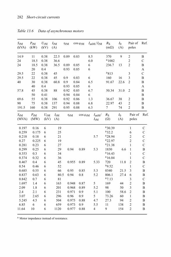
282 Short-circuit currents
Table 13.6 Data of asynchronous motors
SrM PrM UrM IrM ηrM cos ϕrM IanM/IrM RS I0 Pair of Ref.(kVA) (kW) (kV) (A) (m�) (A) poles
14.9 11 0.38 22.5 0.89 0.83 8.5 370 9 2 B24 18.5 0.38 36.6 6.0 a1002 2 C24 18.5 0.38 36.5 0.89 0.85 6 236.7 13 2 B
20 0.4 0.93 0.85 6 A29.5 22 0.38 45 a813 3 C29.5 22 0.38 45 0.9 0.83 6 160 16 3 B40 30 0.38 60.8 0.9 0.84 6.5 91.67 22.6 2 B
40 0.4 0.93 0.85 6 A57.8 45 0.38 88 0.92 0.85 6.7 50.34 31.0 2 B
50 0.41 0.94 0.84 6 B69.6 55 0.38 106 0.92 0.86 1.3 36.67 38 2 B90 75 0.38 137 0.94 0.88 6.8 22.97 43 2 B191.5 160 0.38 291 0.95 0.88 6.3 7 74 2 B
SrM PrM UrM IrM ηrM cos ϕrM IanM/ RS I0 Pair of Ref.(MVA) (MW) (kV) (A) IrM (�) (A) poles
0.197 0.16 6 19 a30.39 1 C0.259 0.175 6 25 a32.2 6 C0.218 0.18 6 21 5.7 a28.94 2 C0.27 0.225 6 19 a22.97 2 C0.281 0.23 6 27 a21.38 1 C0.299 0.25 6 29 0.94 0.89 5.3 1830 6.6 1 B0.353 0.3 6 34 a16.43 1 C0.374 0.32 6 36 a16.04 1 C0.467 0.4 6 45 0.955 0.89 5.33 720 11.8 2 B0.54 0.46 6 52 a9.52 1 C0.685 0.55 6 66 0.95 0.85 5.3 0340 21.5 3 B0.837 0.63 6 80.5 0.94 0.8 5.2 806.1 27.4 6 B0.842 0.7 6 81 a7.13 3 C1.697 1.4 6 163 0.948 0.87 5 169 44 2 B2.09 1.8 6 201 0.968 0.89 5.2 98 50 3 B2.4 2.1 6 231 0.971 0.9 5.1 100 58.6 2 B3.07 2.65 6 296 0.96 0.9 5 73.26 60 1 B5.245 4.5 6 504 0.975 0.88 4.7 27.3 94 2 B6.85 6 6 659 0.973 0.9 5.5 11 138 2 B
11.64 10 6 1120 0.977 0.88 4 9 154 2 B
a Motor impedance instead of resistance.
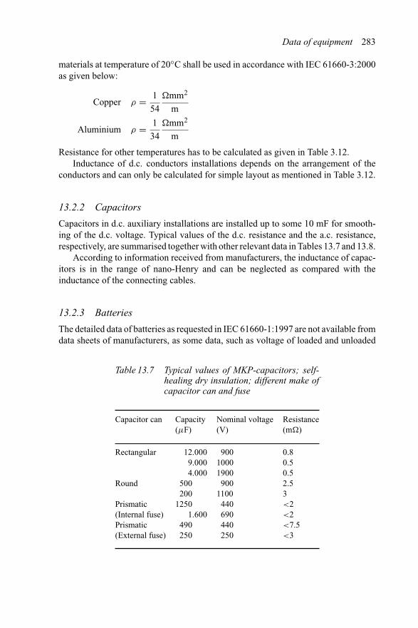
Data of equipment 283
materials at temperature of 20◦C shall be used in accordance with IEC 61660-3:2000as given below:
Copper ρ = 1
54
�mm2
m
Aluminium ρ = 1
34
�mm2
m
Resistance for other temperatures has to be calculated as given in Table 3.12.Inductance of d.c. conductors installations depends on the arrangement of the
conductors and can only be calculated for simple layout as mentioned in Table 3.12.
13.2.2 Capacitors
Capacitors in d.c. auxiliary installations are installed up to some 10 mF for smooth-ing of the d.c. voltage. Typical values of the d.c. resistance and the a.c. resistance,respectively, are summarised together with other relevant data in Tables 13.7 and 13.8.
According to information received from manufacturers, the inductance of capac-itors is in the range of nano-Henry and can be neglected as compared with theinductance of the connecting cables.
13.2.3 Batteries
The detailed data of batteries as requested in IEC 61660-1:1997 are not available fromdata sheets of manufacturers, as some data, such as voltage of loaded and unloaded
Table 13.7 Typical values of MKP-capacitors; self-healing dry insulation; different make ofcapacitor can and fuse
Capacitor can Capacity Nominal voltage Resistance(μF) (V) (m�)
Rectangular 12.000 900 0.89.000 1000 0.54.000 1900 0.5
Round 500 900 2.5200 1100 3
Prismatic 1250 440 <2(Internal fuse) 1.600 690 <2Prismatic 490 440 <7.5(External fuse) 250 250 <3
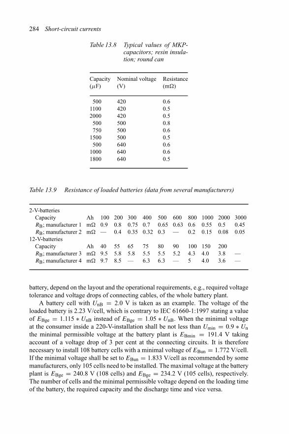
284 Short-circuit currents
Table 13.8 Typical values of MKP-capacitors; resin insula-tion; round can
Capacity Nominal voltage Resistance(μF) (V) (m�)
500 420 0.61100 420 0.52000 420 0.5
500 500 0.8750 500 0.6
1500 500 0.5500 640 0.6
1000 640 0.61800 640 0.5
Table 13.9 Resistance of loaded batteries (data from several manufacturers)
2-V-batteriesCapacity Ah 100 200 300 400 500 600 800 1000 2000 3000RB; manufacturer 1 m� 0.9 0.8 0.75 0.7 0.65 0.63 0.6 0.55 0.5 0.45RB; manufacturer 2 m� — 0.4 0.35 0.32 0.3 — 0.2 0.15 0.08 0.05
12-V-batteriesCapacity Ah 40 55 65 75 80 90 100 150 200RB; manufacturer 3 m� 9.5 5.8 5.8 5.5 5.5 5.2 4.3 4.0 3.8 —RB; manufacturer 4 m� 9.7 8.5 — 6.3 6.3 — 5 4.0 3.6 —
battery, depend on the layout and the operational requirements, e.g., required voltagetolerance and voltage drops of connecting cables, of the whole battery plant.
A battery cell with UnB = 2.0 V is taken as an example. The voltage of theloaded battery is 2.23 V/cell, which is contrary to IEC 61660-1:1997 stating a valueof EBge = 1.115 ∗ UnB instead of EBge = 1.05 ∗ UnB. When the minimal voltageat the consumer inside a 220-V-installation shall be not less than Umin = 0.9 ∗ Unthe minimal permissible voltage at the battery plant is EBmin = 191.4 V takingaccount of a voltage drop of 3 per cent at the connecting circuits. It is thereforenecessary to install 108 battery cells with a minimal voltage of EBun = 1.772 V/cell.If the minimal voltage shall be set to EBun = 1.833 V/cell as recommended by somemanufacturers, only 105 cells need to be installed. The maximal voltage at the batteryplant is EBge = 240.8 V (108 cells) and EBge = 234.2 V (105 cells), respectively.The number of cells and the minimal permissible voltage depend on the loading timeof the battery, the required capacity and the discharge time and vice versa.
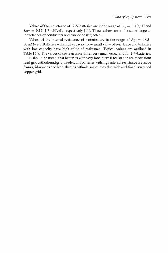
Data of equipment 285
Values of the inductance of 12-V-batteries are in the range of LB = 1–10 μH andLBZ = 0.17–1.7 μH/cell, respectively [11]. These values are in the same range asinductances of conductors and cannot be neglected.
Values of the internal resistance of batteries are in the range of RB = 0.05–70 m�/cell. Batteries with high capacity have small value of resistance and batterieswith low capacity have high value of resistance. Typical values are outlined inTable 13.9. The values of the resistance differ very much especially for 2-V-batteries.
It should be noted, that batteries with very low internal resistance are made fromlead-grid cathode and grid-anodes, and batteries with high internal resistance are madefrom grid-anodes and lead-sheaths cathode sometimes also with additional stretchedcopper grid.


Symbols, superscripts and subscripts
A detailed explanation of the quantities and symbols is included in the text for eachequation, table and figure. It cannot be avoided that some symbols and subscripts areused for different physical quantities. It should be noted that e.g., using the symbol‘J’ for the current density cannot be mixed up with the symbol ‘J’ for the secondmechanical moment, as both symbols will not occur in the same equations and evennot in a similar context.
Symbols for quantities
A Aperiodic currentC CapacitanceD Geometric mean distance, geometric factorE Young’s modulusE Matrix of unityE VoltageF Mechanical forceG ConductanceI CurrentJ Current densityK FactorL InductanceM Mutual impedanceP Active powerQ Reactive powerQ Thermal heatR ResistanceS Apparent powerT Total time, time constantU VoltageX ReactanceY Admittance
288 Symbols, superscripts and subscripts
Z ImpedanceZ Section modulia Distancea; a2 Complex operational phasorc Voltage factord Distance, diameterd Damping factorf Frequencyh Conductor heightk Factorl; l Lengthm Massn Numberp Control rangeq Cross-sectionq Factor of plasticityq Factorr Radiusr Reduction factors Conductor sagt Time instantt Transformation ratiov Detuning factorw Probability factorα Temperature & permittivity coefficientε Permittivityτ Time constantω Angular frequencyϕ Phase angleρ Resistivityμ Factor according to IEC 60909μ Permeabilityλ Factor according to IEC 60909κ Factor according to IEC 60909δ Earth-fault factor (a.c.)δ Decay coefficient (d.c.)δ Depth of earth return pathγ Impedance angleγ Propagation constantσ Mechanical stress
Quantities (Example U)
U Capital letter used for r.m.s-valueU Underlined capital letter indicates phasor (vector)
Symbols, superscripts and subscripts 289
U Peak value|U | Complex valueu %/MVA-valueu Instantaneous valueu(t) Time courseU Average valueU Vector (matrix)U Complex vector (matrix)
Superscripts (Example U)
U∗ Conjugate–complex valueu′ p.u.-valueU ′ Transient valueU ′′ Subtransient value
Order of subscripts (Example U)
First order Component (R, Y, B or 0, 1, 2) UYNext order Type of operation (n; r; b) UYbNext order Indication of equipment UYbTNext order Number of equipment UYbT4Next order Special condition UYbTmaxNext order Index UYbTmaxiUYbTmaxi Indicates voltage of phase Y before short-circuit, equipment is
T ransformer number 4 maximal value for alternative iIn most of the cases, positive-sequence system is used without subscript ‘1’
Subscripts, components, systems
0; 1; 2 Zero-, positive-, negative-sequence systemsac a.c. systemdc d.c. systemR; Y; B Phases of three-phase a.c. system
Subscripts, type of operation
0 No-load value, eigenvaluean Locked rotor, startingb Before (prior to) fault, beginningb Breakinge End

290 Symbols, superscripts and subscripts
k Short-circuit valuek1 Single-phase short-circuitk2 Double-phase short-circuitk3 Three-phase short-circuitm Highest value (IEC 60038)n Nominal valuer Rated values; sat Saturated valueδ At temperature δ
Subscripts, indication of equipment
B BatteryB CounterpoiseBr BranchC CapacitorD Reactor, rectifierE Earth, earth wireF FieldG GeneratorJ Joint for connectionKW Power stationL Line; loadM MotorM Mutual valueN Network (a.c. system)P PipelineQ System feederR ResistanceS Special earthing impedanceT TransformerTo Overhead-line towerX ReactanceY Common branch (d.c. system)Z Battery cell
Subscripts, special conditions
20 Value at 20◦Cf Fictitiousge Loadedmax Maximal valuemin Minimal value

Symbols, superscripts and subscripts 291
o Without tap-changerres Residuals With tap-changerth Thermaltot Totalun Unloaded
Other subscripts
0; 1 Condition at beginning or ending respectively1; 2; 3 Different sides of a transformera; b; c IndexB Base or referencec Equivalentd Direct axisHV; MV; LV High-, medium-, low-voltage side of a transformerI Currenti; j IndexMec Mechanicalm Main conductorp Pole pairq Quadrature axisres Equivalent resistances SubconductorU VoltageW Characteristic impedanceI One circuit in operationII Two circuits in operation

References
1 Schlabbach, J.: Electrical power system engineering (Elektroenergieversorgung).2nd revised edition, VDE-Verlag. Berlin, Offenbach/Germany, 2003. ISBN3-8007-2662-9.
2 Oeding, D. and Oswald, B.: Electrical systems and power stations (ElektrischeKraftwerke und Netze). 6th edition, Springer-Verlag. Berlin, Heidelberg,New York, 2004. ISBN 3-5400-0863-2.
3 Schlabbach, J.: Neutral handling (Sternpunktbehandlung). Systems engineering,Vol. 15. VWEW-Energieverlag, Frankfurt/Germany, 2002. ISBN 3-8022-0677-0.
4 CCITT: Directives CCITT, Vol. V, Chapter 5. ITU, Geneva/Switzerland.5 Niemand, T. and Kunz, H.: Earthing in power systems (Erdungsanlagen). Systems
engineering, Vol. 6. VWEW-Energieverlag, Frankfurt/Germany, 1996. ISBN3-8022-0362-3.
6 Arbitration agency of VDEW: Technical recommendation No. 1 – Induced volt-ages in telecommunication circuits. VWEW-Energieverlag, Frankfurt/Germany,1987.
7 Schlabbach, J., Blume, D., and Stephanblome, T.: Voltage quality in electricalpower systems. Power and Energy Series, No. 36. IEE-publishers, Stevenage,UK, 2001. ISBN 0-85296-975-9.
8 ABB: Switchgear Manual. 9th edition, Cornelsen-Girardet, Essen/Germany,1993. ISBN 3-464-48234-0.
9 VDEW: Cable-book (Kabelhandbuch). 6th edition, VWEW-Energieverlag,Frankfurt/Germany, 2001. ISBN 3-8022-0665-7.
10 Scheifele, J.: Contribution of asynchronous motors to short-circuit currents(Beitrag von Drehstrom-Asynchronmotoren zum Kurzschlussstrom). Ph.D. the-sis, Technical University of Darmstadt/Germany, 1984.
11 Gretsch, R.: Design of electrical installations in automobiles (Ein Beitrag zurGestaltung der elektrischen Anlage in Kraftfahrzeugen). Dr. -Ing. habil. thesis,University Erlangen-Nürnberg/Germany, 1979.
12 VDEW: Distributed generation in LV-systems (Eigenerzeugungsanlagen amNiederspannungsnetz). 4th edition, VWEW-Energieverlag, Frankfurt/Germany,2001. ISBN 3-8022-0790-4.

294 References
13 Balzer, G., Nelles, D., and Tuttas, C.: Short-circuit current calculationacc. VDE 0102 (Kurzschlußstromberechnung nach VDE 0102). VDE-technicalreports, Vol. 77. VDE-Verlag, Berlin, Offenbach/Germany, 2001. ISBN3-8007-2101-5.
14 Pistora, G.: Calculation of short-circuit currents and voltage drop (Berechnungvon Kurzschlussströmen und Spannungsfällen). VDE-technical reports, Vol. 118.VDE-Verlag, Berlin, Offenbach/Germany, 2004. ISBN 3-8007-2640-8.
15 Gröber, H. and Komurka, J.: Transformation of zero-sequence voltage throughtransformers (Übertragung der Nullspannung bei zweiseitig geerdeten Transfor-matoren). Technical report of FGH, Mannheim/Germany, 1973.
16 Balzer, G.: Double-side earthing of transformers (Beidseitige Sternpunkt-behandlung von Transformatoren). In VDE: Neutral handling in 10-kV- to110-kV-system. ETG-Report, Vol. 24. VDE-Verlag, Berlin, Offenbach/Germany,1988, pp. 172–187.
17 SPEZIELEKTRA: Resonant earthing controller EZR2 (Erdschlußkompensa-tionsregler EZR2). Operation manual N 9/4.88, Spezielektra, Linz/Austria,1988.
18 Schäfer, D., Schlabbach, J., Gehrmann, A., and Kroll, R.: Increase of dis-placement voltage in MV cable systems with resonant earthing (Erhöhung derVerlagerungsspannung in Mittelspannungs-Kabelnetzen mit Erdschlußkompen-sation). Elektrizitätswirtschaft, Vol. 93 (1994), VWEW-Energieverlag, Frankfurt/Germany, pp. 1295–1298.
19 Fiernkranz, K.: MV-systems with isolated neutrals or resonant earthing (Mit-telspannungsnetze mit isoliertem Sternpunkt oder Erdschlußkompensation).ETG-Report, Vol. 24. VDE-Verlag, Berlin, Offenbach/Germany, 1988.
20 Kouteynikoff, P. and Sforzini, A.: Results of an international survey of therules limiting interference coupled into metallic pipes. CIGRE Committee 36.ELECTRA, Geneva, Switzerland, 1986.
21 Arbitration agency of VDEW: Technical recommendation No. 3 – Measuresfor construction of pipelines in the vicinity of HV/AC three-phase installations(German). VWEW-Energieverlag, Frankfurt/Germany, 1982.
22 Arbitration agency of VDEW: Technical recommendation No. 5 – Principles ofcalculation and measurement of reduction factor of pipelines and earth wires(German). VWEW-Energieverlag, Frankfurt/Germany, 1980.
23 Arbitration agency of VDEW: Technical recommendation No. 7 – Measuresfor the installation and operation of pipelines in the vicinity of three-phasehigh-voltage installations (German). VWEW-Energieverlag, Frankfurt/Germany,1985.
24 IEC 60479-1: Effects of currents passing through the human body. Internationalelectrotechnical commission, Geneva, Switzerland, 1994.
25 Jenkins, N., Allan, R., Crossley, P., Kirschen, D., and Strbaq, G.: Embeddedgeneration. Power and Energy Series, No. 31. IEE Publishers, Stevenage, UK,2000. ISBN 0-85296-774-8.
26 Schlabbach, J. (Ed.) and Metz, D.: Power system engineering (Netzsystemtech-nik). VDE-Verlag, Berlin, Offenbach/Germany, 2005. ISBN 3-8007-2821-4.

References 295
27 Schlabbach, J.: Short-time interference of pipelines. Report on research and devel-opment No. 14. University of Applied Sciences, Bielefeld/Germany, 2000. ISBN3-923216-52-1.
28 Cory, B. and Weedy, B.: Electrical power systems. 4th edition. John Wiley &Sons Ltd., Chichester, England, 1998. ISBN 0-471-91659-5.
29 Funk, G.: System of symmetrical components (Symmetrische Komponenten).Elitera-Verlag, Berlin, Germany, 1976. ISBN 3-8708-7087-7.
30 Kories, R. and Schmidt-Walter, H.: Electrotechnical handbook (Taschenbuch derEletrotechnik). 6th revised edition, Verlag Harri Deutsch, Frankfurt/Germany,2004. ISBN 3-8171-1734-5.
31 Metz, D., Naundorf, U., and Schlabbach, J.: Handbook of electrotechnicalequations (Kleine Formelsammlung Elektrotechnik). 4th edition, FachbuchverlagLeipzig, Germany, 2003. ISBN 3-446-22545-5.
32 Wildi, T.: Units and conversion charts. IEEE Press, New York, USA, 1990. ISBN0-87942-273-4.
33 Oeding, D. and Schünemann, H.: Calculation of short-circuit currents inHV-systems using %/MVA-system (Berechnung der Kurzschlussströme inHochspannungsnetzen mit %/MVA-system). BBC-News, Mannheim/Germany,1965.
34 Koglin, H.: The decaying d.c. component of short-circuit currents (Der anklin-gende Gleichstrom beim Kurzschluss in Elektroenergieversorgungsnetzen). Ph.D.thesis, University of Darmstadt/Germany, 1971.
35 Pitz, V. and Waider, G.: Impedance correction factors of network trans-formers for short-circuit current calculation (Impedanzkorrekturfaktoren fürNetztransformatoren bei der Kurzschlussstromberechnung). Elektrie 47 (1993),pp. 301–304.
36 Scheifele, J. and Waider, G.: Maximal short-circuit currents through linear opti-misation (maximale Kurzschlussströme durch lineare Optimierung). etzArchiv 10(1998), pp. 275–280.
37 Oeding, D. and Waider, G.: Maximal partial short-circuit currents of powerstations (Maximale Teilkurzschlussströme von Kraftwerksblöcken ohne Stufen-schalter). etzArchiv 10 (1988), pp. 173–180.
38 Balzer, G. and Deter, O.: Calculation of thermal effects of equipment due toshort-circuit currents (Berechnung der thermischen Kurzschlussbeanspruchungvon Starkstromanlagen). etzArchiv 7 (1985), pp. 287–290.
39 Tuttas, C.: Approximation of reduction factors of complex conductor arrange-ment (Berechnung des Reduktionsfaktors komplizierter Leiteranordnungen).AEG-report 54, Frankfurt, Germany, 1981, pp. 153–157.
40 Hosemann, G., Nietsch, C., and Tsanakas, D.: Short-circuit stress in d.c. auxiliarysystems. Cigre-report 23-104, Geneva, Switzerland, 1992.
41 Tsanakas, D.: Substitution function for the calculation of mechanical and ther-mal stress due to short-circuits in d.c. installations (Ersatzfunktion für dieBestimmung der mechanischen und thermischen Kurzschlussbeanspruchung inGleichstromanlagen). etzArchiv 10 (1988), pp. 355–360.

296 References
42 Nietsch, C.: Calculation of short-circuit currents in d.c. installations. Universityof Erlangen/Germany, EV-report F254, 1989.
43 Tsanakas, D., Meyer, W., and Safigianni, A.: Dynamical short-circuit stress in d.c.installations (Dynamische Kurzschlussbeanspruchung in Gleichstromanlagen).Archiv für Eletrotechnik 74 (1991), pp. 305–313.
44 Tsanakas, D. and Papadias, A.: Influence of short-circuit duration on dynamicstresses in substations. IEEE Transactions PAS 102 (1983), pp. 492–501.
45 Hosemann, G. and Tsanakas, D.: Dynamic short-circuit stress of busbar structureswith stiff conductor. Parametric studies and conclusions. Electra 68, Geneva,Switzerland, 1980, pp. 37–64.
46 Meyer, W.: Additional calculation acc. IEC 60865-1 for the determination ofshort-circuit stress of lines (Ergänzung des Berechnungsverfahrens nach IEC60865-1 zur Ermittlung der Kurzschlussbeanspruchung von Leitungsseilen mitSchlaufen im Spannfeld). EE-report, University of Erlangen/Germany, 2002.
47 Meyer, W.: Mechanical short-circuit stress of rigid conductors in IEC865-1 – Information on the norm (Mechanische Kurzschlussbeanspruchungvon biegesteifen Leitern in IEC 865-1 – Hintergründe zur Norm). EE-report,University of Erlangen/Germany, 2002.
48 Tsanakas, D.: Dynamic stress in high-voltage structures by short-circuits ofshort-duration. CIGRE-Symposium High currents in power systems. Proc. Report500-01, Brussels, Belgium, 1985.
49 Rüger, W. and Hosemann, G.: Mechanical short-circuit effects of single-corecables. IEEE Trans. PD, 4 (1989) pp. 68–74.
50 Nietsch, C. and Tsanakas, D.: Short-circuit currents in d.c. auxiliary installations(Kurzschlussströme in Gleichstrom-Eigenbedarfsanlagen). Elektrie 46 (1992),pp. 18–22.
51 Hosemann, C., Zeitler, E., Miri, A., and Stein, N.: The behaviour of droppers inHV substations under short-circuit. Proceedings of the 5th International sympo-sium on short-circuit currents in power systems. Proc. Report 3.2, Zlin, CzechRepublic, 1992.
52 Tsanakas, D., Meyer, W., and Nietsch, C.: Short-circuit currents of motors ind.c. auxiliary installations in power plants and substations. Electromotion ’99,Patras/Greece, pp. 489–496.
53 Stein, N., Meyer, W., and Miri, A.: Test and calculation of short-circuit forces anddisplacements in HV substations with strained conductors and droppers. ETEP10 (2000), pp. 131–138.
54 Herold, G. and Kunz, M.: Fast analytical short-circuit current calculation ofrectifier fed auxiliary subsystems. ETEP 13 (2003), pp. 151–159.
55 Pitz, V., Köster, H.-J., et al.: Short-circuit mechanical effects on outdoor HV sub-stations with wide bundling. CIGRE-Session 2004. Proc. Report B3-107, Paris,France.
56 Wessnigk, K. and Griesbach, P.: Digital calculation of short-circuit cur-rent in battery-fed d.c. installations (Digitale Berechnung des zeitlichenKurzschlussstromverlaufs in batteriegespeisten Gleichstromnetzen). Elektrie 43(1989), pp. 379–381.
References 297
57 Albert, K., Apelt, O., Bär, G., and Koglin, H.-J. (Ed.): Electrical power sup-ply (Elektrischer Eigenbedarf). VDE-Verlag, Berlin, Offenbach/Germany, 1993.ISBN 3-8007-1586-4.
IEC-standards, EN-norms and other standards and norms mentioned within thecontext of this book are listed in Tables 1.1 and 1.2.
Extracts from the norms DIN EN 60909-0 (VDE 0102) and DIN EN 61660-1 (VDE0102 part 10) are permitted for this edition of the book by licensee agreement 392.004of DIN (Deutsches Institut für Normung e.V.) and VDE (Verband der Elektrotech-nik Elektronik Informationstechnik e.V.) on 16.12.2004. An additional permission isrequired for other usages and editions.
Standards are only to be applied based on their actual issues, available fromVDE-Verlag GmbH, Bismarckstr. 33, D-10625 Berlin, Beuth-Verlag GmbH,Burggrafenstr. 6, D-10787 Berlin or the national standard organisation. Englishversions of the norms are also available through BSI in London/UK.
The English text of this book was neither checked by DIN (Deutsches Institutfür Normung e.V., Berlin) nor by VDE (Verband der Elektrotechnik ElektronikInformationstechnik e.V., Frankfurt).

Index
%/MVA system semirelative units 33–4conversion of quantities with p.u. and
ohm systems 35example 40
correction factor 34HV three-phase examples 93
impedance based on measurementexample 41–2
impedance calculations for athree-winding transformer 37–40
impedance results of variousequipment 91
impedances calculation HV three-phaseexample 92
a.c. systems, impedance: see impedancecalculations for a.c. equipment
a.c. systems, mechanical effects: seeconductors, a.c., mechanical effectsof short circuits
a.c. systems, thermal effectsabout thermal effects 195see also conductors, a.c., thermal effects
admittance/reactance/impedance 12American National Standards Institute,
web address 4asynchronous motors
data of 281–2factor q for short-circuit breaking
current 162–3impedance calculations 55, 63–4
auxiliary installationssupply of a power station calculations
example 94–6see also batteries in d.c. auxiliary
installations; d.c. auxiliaryinstallations, effects of short circuits;d.c. auxiliary installations,
short-circuit current calculations; d.c.motors in auxiliary installations
batteries in d.c. auxiliary installationsexample data 283–5impedance calculations 60, 64, 65short-circuit currents 170–2
breaking current with short-circuits: seeshort-circuit breaking current
British Standards Institute, web address 4busbar/switchgear short-circuit current
limitation measuresbusbar sectionaliser in single busbar
switchgear 233–4Ip-limiter usage 234–6medium and low voltage limiting
equipment 234–6multiple busbar operation 232–6time curves of short-circuit currents 235
cablescapacitances 276–7impedances 276reactances 276–7see also conductors
capacitors in auxiliary installationsfactor κ 169–71impedance calculations 59, 64, 65short-circuit currents 169–70typical values of capacity and resistance
283–4causes of short circuit currents 1–3communication circuit interference: see
pipelines/communication circuits,interference with
complex calculations 11–14

300 Index
conductors, a.c., mechanical effectsof short circuits
about mechanical effects 201–2conductor oscillation influence 207–9
bending stress and dynamic force onsupports 208–9
mechanical natural frequency 207–8electromagnetic forces 202–4fixing clamps calculations example
217–18forces and stresses in rigid conductor
support calculations 204–7conductors, a.c., thermal effects of short
circuitsbare conductors 198–9cable calculation example 216–17cable screening, armouring and sheath
199–201maximal permissible short-circuit
current density 201maximal permissible temperature
200–1heat dissipation considerations,
factors m and n 197–8IEC 60865–1 197IEC 60909–0 197impregnated paper-insulated cables
199–200maximum permissible temperature and
current density table 196overhead line conductors type Al/St 198rated short-time current density 199thermal equivalent short-time current
195–7conductors, d.c. equipment,
impedance/resistance calculations58, 64, 65, 281–3
converter fed drive, impedance calculations56
correction factorsd.c. auxiliary installations, short-circuit
current calculations, σ 179example 190–1
with HV three-phase systems examples76, 91–4
impedance correction factor KG 154–6examples 91–4
impedances of equipment andshort-circuit current example 154
%/MVA- or p.u.-system 34, 152–4current limitation earthing power system
102–5earth-fault factor δ 103, 104
d.c. auxiliary installations, effects of shortcircuits
bending stress on conductors 213–14bending stress of sub-conductors 211
calculation example 223–4equivalent circuit diagrams and
short-circuit current time course 166force calculation for main- and
sub-conductors 212–15calculation example 222–3
forces on supports 214–15mechanical natural frequency of main and
sub-conductors 211standard approximation function
(simplified approach) 209electromagnetic effect example 220
substitute rectangular function approach209–16
calculation example 220–3thermal effects calculation example
218–19thermal short circuit strength 215–16vibration period and natural mechanical
frequency of conductors 212calculation example 220–1
d.c. auxiliary installations, short-circuitcurrent calculations
about auxiliary installations 165–8correction factor σ 179equivalent circuit diagram 180example
battery short-circuit current 186capacitor short-circuit current 185–6correction factors and corrected
parameters 190–1data and parameters 183–4equivalent diagram 182impedances of cable and busbar
conductors 184–5partial short-circuit currents 191–3rectifier short-circuit current 186–8total short-circuit current 193–4
maximal short-circuit current calculations168
minimal short-circuit current calculations168
time function calculations 167total short-circuit current 178–82typical time curves 181see also batteries in d.c. auxiliary
installations; capacitors in auxiliaryinstallations; d.c. motors in auxiliaryinstallations; impedance calculations

Index 301
for d.c. equipment; rectifiers inauxiliary installations
d.c. motors in auxiliary installationsfactor κ 175–8IEC 61000–1:1997 175IEC 61660–1:1997 175, 178impedance calculations 62, 65, 66with independent excitation, short-circuit
currents 174–8factors k 175–8
short-circuit current calculations,example 188–9
definitions and terms 30–2Deutsches Institute für Normung,
web address 4double earth-faults
about double-earth faults 139fault in a 20-kV-system example 146–8impedances 139–40peak short-circuit current 143power system configurations 140–2steady-state short-circuit current 143symmetrical short-circuit breaking
current 143symmetrical short-circuit current 139–40see also earth currents from short circuits
earth currents from short circuitsabout short-circuits through earth 143–5short-circuit at overhead-line tower
145–6short-circuit inside a switchyard 144–5single-phase short-circuit in a
110-kV-system example 148–9earth faults: see double earth-faults; earth
currents from short circuitsearth-fault factor δ
and current limitation earthing 103, 104and low impedance neutral earthing
effects 102earthing considerations
about earthing 257earthing grid resistance calculation
example 264–6earthing impedance 261–2
resistance of different types ofearthing 262
human body resistance 257–9relevant currents through earth 259–61
design information 260soil conditions and resistivity 258–9
earthing rods 259see also neutral earthing
earthing resistorsabout earthing resistors 279–81characteristic parameters 280–1
electromagnetic forces, on a.c. conductors202–4
equivalent circuit diagrams for short circuits24–9, 43
factorsabout factors 151factor k for d.c. motor short-circuit
currents 175–8factor κ for peak short-circuit current
77–80, 156–8with d.c. motors 175–8
factor q for short-circuit breaking currentof asynchronous motors 162–3
factor λ for steady-state short-circuitcurrent 82–3, 160–2
factor μ for symmetrical short-circuitbreaking current 81–2, 158–60
factors m and n, heat dissipation 197IEC 60909–1:1991–10 151, 162impedances of equipment and
short-circuit current example 152–3induced voltage calculation, screening
factor 252isolated neutral power system,
overvoltage factor 108see also correction factors
faults, as causes of short circuit currents 1–3fuses, and short circuit currents 2
generatorspower factor data 270rated voltage data 270–1short circuit current limitation,
subtransient reactance influence239–40
sutransient reactance data 270–1synchronous reactance data 270–1zero-sequence reactance data 270
human body resistance 257–9HV a.c. three-phase system short circuit
current calculationsabout HV short circuits 67–8about parameter calculations 70–2assumptions and methods 68–71auxiliary supply of a power station
calculations example 94–6decaying (aperiodic) component 80–1

302 Index
HV a.c. three-phase system short circuitcurrent calculations (continued)
far-from generator short-circuit 67–9IEC 60909–0 71, 72–83impedance correction factor examples
91–4initial symmetrical short-circuit current
72–4double-phase 73far-from-generator 73line-to-earth 73three-phase 73
inside power plant short-circuitcurrents 72–6
correction factors 76, 91–4equivalent circuit diagrams 74–5locations around transformers 74–6
line-to-earth (single-phase) short-circuitexample 87–8
maximal and minimal short-circuitcurrents 71–2
meshed 110-kV-system example 89–91minimal short-circuit currents 85–6motor influences 84–5near-to-generator short-circuit example
86–7peak short-circuit currents 77–80
calculation example 88–9equivalent frequency method 80factor κ 77–80meshed networks 79–80non-meshed fed 77–8ratio R/X method 80single-fed 77
steady-state short-circuit current 82–3factor λ 82–3
subtransient reactance 67symmetrical short-circuit breaking current
80–2factor μ 81–2
types of short circuit 67–9
IEC 60038 6, 226–7IEC 60050 6, 7IEC 60071 7IEC 60265 7IEC 60282 7IEC 60479 7IEC 60781 2, 5, 9, 131, 132IEC 60865 2, 5, 9, 197IEC 60896 7IEC 60909 5, 6, 9, 71, 72–83, 131, 132,
139, 151, 162, 197
IEC 60949 7IEC 60986 7, 8IEC 61000 175IEC 61071 7IEC 61660 5, 9, 175, 178IEC document list 5–9impedance
impedance/admittance/reactance 12impedances of a three-winding
transformer in MVA example 37–40measurement for symmetrical components
20–4in %/MVA-system for auxiliary supply 96in %/MVA-system based on measurement
example 41–2impedance calculations for a.c. equipment
about impedance for a.c. systems 45asynchronous motors 55, 63–4calculation examples 63–4converter fed drive 56for HV a.c. three-phase equipment under
short circuit examples 91overhead transmission lines 53, 63–4power-station unit 52, 63–4short-circuit limiting reactor 54, 63–4synchronous generators 51, 63–4system feeder 46, 63system loads 57, 63–4three-winding transformer 48–50, 63–4two-winding transformer 47, 63
impedance calculations for d.c. equipmentabout impedance for d.c. systems 50batteries 60, 64calculation examples 64–6capacitors 59, 64, 65conductors 58, 64, 65motors, d.c. 62, 65, 66rectifiers 61, 63–4, 65–6
impedance correction factor KG 154–6examples 91–4
impedance matrix, transformation of 19–20inductive interference calculations 247–52interference: see pipelines/communication
circuits, interference withInternational Electrotechnical Commission,
web address 4Ip-limiters 234–6isolated neutral power system 105–8
capacitive earth-fault current 106–7earth faults 105–8earth-fault arcs 107–8overvoltage factor 108
Index 303
limitation of short-circuit currentsabout limitation measures 225–6coupling of power system at busbars with
low short-circuit level 230–1distribution of feeding locations 228–9earthing impedances in neutral of
transformers 238and generator subtransient reactance
239–40meshed systems 241–4nominal system voltage selection 226–7
IEC 60038:1987 recommendedvoltages 226–7
operating subsystems separately 227–8radial systems 241restructuring power systems 231ring-main systems 241–2short-circuit limiting reactors 238see also busbar/switchgear short-circuit
current limitation measures;transformers
limiting value, definition 31low-impedance neutral earthing power
system 98–102earth-fault factor δ 102, 103, 104single-phase short-circuit current 98–100single/three-phase short circuit relation
100–1low-voltage (LV) systems, short circuit
current calculationsabout short-circuit currents in LV
systems 131calculation methods 132IEC 60781 131, 132IEC 60909–0 131, 132impedance calculations 132–3
approximations for generators andrectifiers 133
initial symmetrical short-circuit current133
maximal short-circuit current calculationexample 135–6
minimal short-circuit currents 134–5calculation example 135, 137
motor influences 134peak short-circuit current 133steady-state short-circuit current 134symmetrical short-circuit breaking current
133types of faults 131
matrix equations 14–17cyclic-symmetrical matrix 15–16
see also transformations/transformationmatrix
maximal and minmal short-circuit currents 3meshed systems, limitation of short-circuit
currents 241–4motors, influence for HV a.c. three-phase
systems 84–5motors, d.c.: see d.c. motors
neutral earthingabout neutral earthing 97–8characteristics of different fault types
summary 99design of an earthing resistor connected to
an artificial neutral example 124limitation of single-phase short-circuit
current by earthing throughimpedance example 123–4
transformer HV-side and LV-sideconsiderations 116–19
compensation windings 116–18voltages at neutral of a unit transformer
example 126–9see also current limitation earthing power
system; isolated neutral powersystem; low-impedance neutralearthing power system; resonanceearthing power systems(Peterson-coil)
nominal value, definition 31norms
about technical standards and norms 4–5international documents and norms 5–6norms as referred in standards 6–9
ohm-system physical quantitiesvoltage/current/impedance 32
conversion of quantities with p.u. and%/MVA systems 35
example 40HV three-phase correction factor
examples 94overhead transmission lines
capacitances 274–6conductor sag considerations 275coupling impedance 273distance between phase wires 272impedance calculations/data 53, 63–4,
271–6impedance in the positive-sequence
component for a single and doublecircuit line 272
304 Index
overhead transmission lines (continued)impedance of the zero-sequence
component 272loop impedance 272relative permeability for 273resistivity of soil 273thermal effects 198typical impedance values 274
parallel and series connection 27, 30peak short-circuit currents 2–3
double earth faults 143factor κ 77–80, 156–8, 175–8low-voltage (LV) systems 133see also HV a.c. three-phase system short
circuit current calculationsPeterson-coil: see resonance earthing power
systems (Peterson-coil)phasor diagrams 11–14pipelines/communication circuits,
interference withabout pipeline interference 245–7characteristic impedance of the pipeline
253–4pipeline coating resistance 254
coupling types summary table 246induced voltage calculation 252–3
coupling impedances 253screening factor 252
inductive interference calculations247–52
coupling impedances 249–51earth return path considerations 248–9
interference of pipeline from 400-kV-lineexample 262–6
pipeline-to-earth voltage 254–7oblique exposure 255–6
safety aspects 247Potier’s reactance 160–1power system short-circuit current
limitation: see limitation ofshort-circuit currents
power-station unit, impedance calculation52, 63–4
p.u.-system relative units 33–4conversion of quantities with ohm and
MVA systems 35example 40
correction factor 34
radial systems, limitation of short-circuitcurrents 241
rated data, definition 32
rated value, definition 31reactance/admittance/impedance 12reactors, short-circuit current limiting: see
resonance earthing power systems(Peterson-coil)
rectifiers in auxiliary installationsimpedance calculations 61, 63–4, 65–6short-circuit currents 172–4
relative quantities/p.u.-system 33–4resonance earthing power systems
(Peterson-coil) 108–16, 278–920-kV-system example 124–5about resonance earthing 108–11alternate earthing of parallel transformer
neutrals 118, 121basic principles 109–11capacitive earth-fault current and residual
current calculation example 125–6current limits 111displacement voltage calculations 112–15fault currents in MV-system from fault in
HV-system 118, 121impedance calculations 54, 63–4increase of displacement voltage example
119–23capacitive asymmetry in a
20-kV-system 120, 122resonance curve for detuning factors in
a 20-kV-system 122Peterson-coils 278–9
tuning 115–16resonance frequency/tuning 110–11usage worldwide 108–9see also neutral earthing
ring-main systems, limitation of short-circuitcurrents 241–2
r.m.s. value of short-circuit currents 2–3RYB-system
representation of a line example 42–4see also symmetrical components
safety, interference with pipelines andcommunication circuits 247
screening factor, pipelines/communicationcircuits 252
semirelative quantities and %/MVA system:see %/MVA system semirelativeunits
series and parallel connection 27, 30short-circuit breaking current
about breaking current value 2–3double earth faults 143
Index 305
factor μ for symmetrical breaking 81–2,158–60
low-voltage (LV) systems currentcalculations 133
three-phase systems calculations 80–2short-circuit current limitation: see
limitation of short-circuit currentsshort-circuit currents
about short circuit currents 1–3equivalent circuit diagrams 24–9importance of 1–3maximal and minimal 3typical time course 2–3see also busbar/switchgear short-circuit
current limitation measures; d.c.auxiliary installations, short-circuitcurrent calculations; earth currentsfrom short circuits; HV a.c.three-phase system short circuitcurrent calculations; limitation ofshort-circuit currents; low-voltage(LV) systems, short circuit currentcalculations
short-circuit limiting reactors: see resonanceearthing power systems(Peterson-coil)
soil conditions and resistivity 248, 258–9standards
about technical standards and norms 4–5American National Standards Institute 4British Standards Institute 4definitions and terms 30–2Deutsches Institute für Normung 4international documents and norms 5–6International Electrotechnical
Commission 4norms as referred in standards 6–9VDE-Verlag 4see also IEC
substitute rectangular function approach: seed.c. auxiliary installations, effects ofshort circuits
subtransient reactance of generators 67,239–40
switchgearand short circuit currents 2see also busbar/switchgear short-circuit
current limitation measuressymmetrical components
example 34–7impedance measurement of 20–4interpretation of the system of 18–19
and representation of a line in theRYB-system example 42–4
transformation of impedances 19–20transformation matrix 14–17see also ohm-system physical quantities
voltage/current/impedance; %/MVAsystem semirelative units;p.u.-system relative units
synchronous generators, impedancecalculation 51, 63–4
system feedersimpedance calculations 46, 63ranges of initial short-circuit power 267,
268system loads, impedance calculations 57,
63–4
terms and definitions 30–2thermal effects of short circuits: see
conductors, a.c., thermal effects ofshort circuits
thermal equivalent short-time current forconductors 195–7
three-phase systems: see HV a.c. three-phasesystem short circuit currentcalculations
time course of short circuit currents 2transformations/transformation matrix
14–17complex rotational phasors 17cyclic-symmetrical matrix 15–16delta-star-transformation 31reverse transformation 17star-delta-transformation 30transformation of impedances 19–20
transformersimpedance calculations in %/MVA 37–40and impedance measurement for
symmetrical components 20–3ratio of positive to negative sequence
impedance 270short-circuit current limitation measures
236–8earthing impedances in the neutrals
238–9impedance voltage considerations
236–8loadflow and short-circuit analysis
results 237three-winding, impedance calculations
21–4, 48–50, 63–4

306 Index
transformers (continued)two-winding, impedance calculations 47,
63typical values two-winding transformer
impedance voltage 267–70ohmic losses, no-load losses and
no-load current 267, 269see also neutral earthing
transmission lines: see overheadtransmission lines
VDE documents 5–9VDE-Verlag, web address 4vectors/vector diagrams 11–15
example 34–7
web addresses, standards institutions 4

Professor Dr-Ing Jürgen Schlabbach received his PhD in 1982 from the Technical University of Darmstadt, Germany. Until 1992 he worked as a Consultant Engineer with responsibility for the planning and design of public and industrial supply systems. Since 1992 he has worked at the University of Applied Sciences in Bielefeld, Germany as Professor for Power System Engineering and Utilisation of Renewable Energy. His main interests are power systems planning, fault analysis, power quality, interference problems and connection of renewable energy sources to power systems, and he carries out consultancy work in these fields. He is a member of the IEEE and VDI.
Short-circuit Currents
The calculation of short-circuit currents is a central task for Power System engineers, as they are essential parameters for the design of electrical equipment and installations, the operation of power systems and the analysis of outages and faults.
Short-circuit Currents gives an overview of the components within power systems with respect to the parameters needed for short-circuit current calculation. It also explains how to use the system of symmetrical components to analyse different types of short-circuits in power systems. The thermal and elctromagnetic effects of short-circuit currents on equipment and installations, short-time interference problems and measures for the limitation of short-circuit currents are also discussed. Detailed calculation procedures and typical data of equipment are provided in a separate chapter for easy reference, and worked examples are included throughout.
The Institution of Engineering and Technologywww.theiet.org 0-86341-514-8978-0-86341-514-2
Related Documents


