SHOPPER CITY - economics.ucr.edueconomics.ucr.edu/papers/papers08/08-11.pdfSHOPPER CITY Richard Arnott* and ... distinguished according to the effective variety of retail ... individuals

1

SHOPPER CITY

Richard Arnott* and Yundong Tu**

August 25, 2008

Abstract: The bulk of the literature on retail location looks at the topic from the

perspective of either the retail firm or the individual shopper. Another branch of the

literature examines the spatial distribution of retail activities within a city or region,

drawing on either central place theory or the Lowry model, neither of which incorporates

either markets or agglomeration economies. This paper looks at retail location from the

perspective of a general equilibrium model of location and land use, with agglomeration

economies in retailing. In particular, drawing on the Fujita-Ogawa (1982) model of non-

monocentric cities, it develops a model of retail location, assuming that retail firms

behave competitively, subject to spatial agglomeration economies. Locations are

distinguished according to the effective variety of retail goods they offer. Shoppers are

willing to pay more for goods at locations with greater effective variety, and in their

choice of where to shop trade off retail price, product variety, and accessibility to home.

Retail prices and land rents at different locations adjust to achieve spatial equilibrium.

Keywords: retail, agglomeration, variety, land use

JEL codes: R10, R20, R30

Acknowledgments: This paper is written to honor Curtis Eaton for his many contributions

to economic theory but especially for his work in spatial competition theory. Arnott

would like to thank Daniel Chen for his excellent research assistance in preparing a

literature survey on retail location, and participants at the Conference in Honor of B.

Curtis Eaton and at the Macroeconomics, Real Estate and Public Policy Workshop,

Istanbul for helpful comments, especially to John Quigley for reminding us of the Lowry

model. Tu would like to thank Edward J. Blakely Center for Sustainable Suburban

Development for financial assistance.

*Department of Economics, University of California, Riverside, CA 92506

[email protected] , 951-827-1581.

**Department of Economics, University of California, Riverside, CA 92507

[email protected].

2

Shopper City

1. Introduction

One of the authors has recently been participating in the development of a large-scale,

microeconomic metropolitan simulation model (tentatively called METRO-LA) that aims

to forecast transportation, land use, and pollution in the Los Angeles metropolitan area.

One of the many modeling questions that has arisen is: How should retail location be

modeled at such a geographic scale? The literature on retail location that is most familiar

to economists is strategic firm location theory/ spatial competition theory, to which Curtis

Eaton has made distinguished contributions1, many in co-authorship with Richard Lipsey.

Models in this literature solve for the Nash equilibrium of a game between firms, with

locations, prices, and perhaps entry as strategy variables. With space interpreted as

geographic space, this literature has provided many insights into the location and pricing

of firms; and with space interpreted as characteristics space, into product differentiation.

But spatial competition theory is not well suited to the analysis of retail location on a

broad geographical scale. For one thing, attempting to solve for the Nash equilibrium of

a game between thousands of firms, with many different types of consumer goods, is

intractable. For another, firm location theory is partial equilibrium in nature, taking the

location of consumers as given, but a satisfactory model of land use needs to take into

account the simultaneous location equilibrium of firms and households. For yet another,

land rent is ignored in spatial competition theory but in an urban setting plays an essential

role in location choice.

1 These include Eaton (1976), Eaton and Lipsey (1975, 1979, 1982), and Eaton and

Wooders (1985).

3

There is also a large literature on retail location outside economics, in marketing and

geography/regional science. The bulk of the marketing literature on retail location looks

at the topic from the perspective of either the individual retail firm or the individual

shopper. The former examines the most profitable location of a single retail firm or

shopping center, often taking into account strategic interaction with other retail firms2.

The latter examines the individual’s decision of where to shop3. The geography/regional

science literature on the subject, for which Harris (1985) provides an excellent review,

examines the spatial distribution of retail activities within a city or region, drawing on

central place theory (e.g. Berry, 1967), the Lowry model (Lowry, 1964,1967; and

Goldner, 1971), and spatial interaction theory (Wilson, 1970,1974). This branch of the

literature does not incorporate prices and markets, and does not treat agglomeration

economies, at least explicitly.

This paper looks at retail location from the perspective of a general equilibrium model of

location and land use, with agglomeration economies in retailing, adapting the approach

developed by Fujita and Ogawa (1982). Fujita and Ogawa solves for the simultaneous

location equilibrium of firms and households in a city. The model is essentially

competitive. Each firm decides where to locate taking prices, rents, household location,

and other firm locations as given, and produces under constant returns to scale. The

2There is a vast literature on the subject. Some well-known papers include Brown (1989,

1993), Clark, Bennison, and Pal (1997), Craig, Ghosh, and McLafferty (1984), Drezner

and Drezner (1996), Huff (1964, 1966), and Weisbrod, Parcells, and Kern (1984).

Kohsaka (1984) is representative of papers that look at optimal shopping center location.

3 The literature on this topic is less extensive. Three well-known papers are Bell, Ho, and

Tang (1998), Bucklin, Gupta, and Siddarth (1998), Cadwaller (1975).

4

economies of scale that give rise to agglomeration are external to the individual firm.

Closer proximity to other firms makes a firm more productive; firms learn from other

firms, incur lower transport costs in intermediate goods exchange, and have access to a

broader labor pool. In deciding where to locate, a firm trades off the higher productivity

of more proximate locations against the higher wages and rents there. Each individual

makes two location decisions, where to live and where to work, taking prices, rents, firm

location, and the location of all other households as given. In deciding where to live, she

trades off the higher commuting cost of a less central location against the lower land rent;

and in deciding where to work, she trades off the higher wage at a more central location

against the higher commuting cost. Equilibrium obtains when, by changing location, no

firm can increase its profits and no household can increase its utility. In equilibrium, land

and labor markets clear at all locations, and land goes to that use which bids the most for

it. Since there are economies of scale, there may be multiple equilibria, corresponding to

different location patterns. One possible equilibrium is monocentric, in which all firms

are located at the city center with residences surrounding them; another possible

equilibrium is completely mixed, with firms and households co-locating at all urban

locations; another has three centers; and so on Four parameters are particularly

important in determining which location patterns are equilibria, commuting cost per unit

distance, the spatial decay rate -- the exponential rate at which benefits from proximity to

other firms decays with distance, the population, and a parameter characterizing the

intensity of agglomeration economies in production. When, for instance, the spatial

decay rate is large and commuting costs are moderate, there are equilibria with many

small employment centers. Also, as the urban population increases, subcentering occurs.

5

This paper adapts the Fujita-Ogawa model by having firms sell differentiated retail goods

rather than produce. In order to highlight the basic economics, the model is made as

simple as possible. Agglomeration economies occur via individuals’ taste for product

variety rather than via external economies of scale in production; in particular, stores

have an incentive to co-locate in a shopping center since doing so raises the effective

variety there, which makes shopping there more attractive. Each of the identical

individuals receives an endowment of a generic good, which she spends on her lot,

transportation for shopping, and the differentiated retail goods. She decides where to

live, trading off rent against transport cost, and where to shop, trading off the greater

variety against the higher price and likely higher transport cost of shopping at a larger

center. Using only land, competitive retail firms transform the generic good into

differentiated retail goods and sell them. Thus, individuals and stores compete in the land

market. If population and shopping transport costs are low, if the taste for variety is high,

and if the benefit one store derives from proximity to other stores falls off moderately

rapidly with distance, then there exists a monocentric equilibrium with all stores at a

single, central shopping center. If shopping transport costs are high and if the taste for

variety is low, then an equilibrium exists in which stores and residences are intermixed.

The model is called “Shopper City” since individuals do nothing but shop and enjoy

consuming their differentiated retail goods on their lots.

A companion paper, Arnott and Erbil (2008), enriches the above model, developing a

computable static general equilibrium model with agglomeration in both retailing and

6

production. The CGE model is standard (allowing for labor and capital, as well as land,

in retail goods production, intermediate and wholesale goods production, structures of

variable density, multiple types of retail goods, multiple household groups, commodity

transportation, etc.) except that it treats residential location, household transportation for

commuting and shopping, and agglomeration economies in both production and retailing.

METRO-LA will have the same model structure, except that it will be dynamic. History

dependence will be incorporated through durable structures and the transmission of

industry- and zone-specific location potentials and zone-specific indices of effective

varieties from one period to the next. The present will be linked to the future via property

markets, with property values being determined under perfect foresight.

Section 2 lays out the basic model. Section 3 derives the parameter restrictions such that

a monocentric equilibrium exists. Section 4 performs the same exercise for a completely

mixed urban configuration. And section 5 concludes.

2. Model Description

The model adapts Fujita and Ogawa (1982), replacing agglomeration economies in

production with agglomeration economies in retailing.

• geography, population, and transportation

N identical individuals live in the city. Each resides on a lot of size S and requires s

units of retail land area4. Thus, the residential area is NS , the retail area Ns , and the

4 An earlier version of the paper employed the more realistic assumption that physical

sales volume per unit area is fixed. With this assumption, the algebra was considerably

more complex and little additional insight was obtained.

7

total urban area )( sSN + . The city is long and narrow, of unit width. The central location

is taken to be the origin, and both x and y are used to index location. The boundaries of

the city are 2/)( sSN + and 2/)( sSN + . Every day each individual makes a return

journey from her home to the shopping location5 of her choice at a transport cost of t per

unit distance.

• tastes

Each individual derives utility from differentiated retail goods and her lot. Since lot size

is fixed, utility can be treated as a function only of differentiated consumer goods. The

utility she receives from retail goods is a function of the quantity she purchases, Q , as

well as the effective variety, v :

QvvQuU == ),( . (1)

The multiplicative form is chosen to simplify the algebra. The effective variety for a

shopper who travels to location y to shop is measured as:

dxyxxakyvb

b}exp{)(1)( += , (2)

where )(xa is the proportion of land at x that is used by stores, k is a parameter

indexing the intensity of taste for variety or the degree of variety, and is the

exponential rate of spatial attenuation of benefits from variety. Thus, effective variety is

additive in the contribution to effective variety over locations, and the contribution to

effective variety of a store at location x to a shopper who travels to location y to shop

decreases exponentially in the distance between x and y . Observe that the effective

5 Trip frequency could be endogenized by adding home inventory costs. An individual

residing at a location that is less accessible to shops would travel less frequently to shop

and keep a larger inventory of goods at home.

8

variety offered by a completely isolated store is normalized to be unity. Note also that

(2) is a “reduced form” specification, only implicitly taking into account search costs.

Eq. (2) is the same as the Fujita-Ogawa location potential function6, except for the

addition of the 1.

• individual choice

Each individual decides where to reside, x , and where to shop, y , so as to maximize

utility, given by (1) and (2), subject to the budget constraint

0)()( =yxtQypSxRY , (3)

where Y is exogenous income (endowment of the generic good), )(xR is the rent

function at x , )(yp is the retail price function relating the retail price to shopping

location, and t is transport cost per unit distance.

• land ownership and alternative land uses

All land rents accrue to absentee landlords. Land not in urban use is employed in

agriculture at a rent of a

R .

• retail technology

Retailing is characterized by constant returns to scale. An atomistic store at x purchases

the generic good from households, transforms it into differentiated retail goods, which it

then sells at the competitively-determined retail price )(xp . Stores incur in addition a

fixed cost per unit area K , which can be interpreted as capital costs, as well as land rent.

Thus, the profit function per unit area is

6 )(xv could be termed the retail location potential function, but this term is used in the

earlier literature (e.g., Lowry,1964)) to refer to the profitability of a location to a store,

whereas )(xv refers to the attractiveness of a location from the perspective of a customer.

9

)(/)(]1)([)( xRKsxQxpx = ; (4)

)(xQ is the equilibrium quantity of retail goods purchased by an individual who shops at

x and s/1 is the number of individuals who shop at x , so that sxQ /)( is the retail sales

volume at x .

Equilibrium is defined to be a location pattern, described by )(xa the proportion of land

in retail use at x , )(xa the proportion of land in residential use at x , b the city

boundary, a retail price function )(xp , and a rent function )(xR , such that all markets

clear, no store can increase its profits per unit area by changing location, and no

individual can increase her utility by changing either her residential or her shopping

location. In equilibrium, all urban land is developed so that 1)()( =+ xaxa for

],[ bbx .

The constructive procedure to solve for equilibrium is the same as that employed in Fujita

and Ogawa. For each qualitatively different location pattern, one solves for the set of

parameter values consistent with the equilibrium conditions. To illustrate the procedure,

the next section derives the set of parameter values consistent with a symmetric

monocentric equilibrium, in which stores occupy the central area and on both sides

residential lots extend from the outer boundary of the retail area to the city boundary,

beyond which land is used in agriculture. Section 4 derives the set of parameter values

consistent with a completely mixed equilibrium, in which each individual purchases at a

backyard store.

10

One might reasonably object to our specification of agglomeration economies in retailing.

If one were to ask store owners why one location is more attractive than other, the first

thing they would mention is likely customer volume. In our model, in contrast, from the

perspective of store owners locations are differentiated according to the competitive

price. We defend our specification on three grounds: first, it is in keeping with our

competitive assumptions7; second, if the model were extended to allow for variable

structural density, shopping volume would be higher at locations with greater shopping

variety; and third, it is our impression that retail prices do differ significantly over

locations8.

3. Monocentric Urban Configuration

The city is symmetric around the origin. Letting f denote the distance of the retail-

residential boundary from the city center, the retail area, which extends from f to f ,

is flanked by two residential areas, one extending from b to f , the other from f to

b . To simplify, where applicable, the right-hand side of the city shall be considered, for

which the location index is positive. Thus:

7 One model could be adapted without difficulty so that retailers are monopolistically

competitive rather than perfectly competitive, but the treatment of other industry

structures (except monopoly, which is unrealistic) would result in intractability. 8 This is difficult to document because of sales, discounts, and product choice. Consider,

for example, goods that have a suggested retail price. A store owner can lower his

average markup on such goods by selling them at a deeper discount, by selling them at

the discounted price a greater proportion of the time, by have deeper and more frequent

store-wide sales, and by choosing to sell those goods for which the ratio of the suggested

retail price to the wholesale price is lower. The higher price of groceries in ghetto

locations is documented. Labor economists have used the McDonald’s wage to measure

intra-metropolitan spatial variation in wages. Perhaps the same could be done for product

prices.

11

2/Nsf = 2/NSfb = 2/)( sSNb += . (5)

This is a convenient point at which to record some properties of the effective variety

function, (2):

For ],0[ fx :

0)}(exp{)}(exp{1)( >++= dyxykdyyxkxvf

x

x

f

0)})(exp{)}((exp{)(' <+= xffxkxv

0)})(exp{)}((exp{)('' <++= xffxkxv . (6)

For ],( bfx :

)})(exp{)}()(exp{/(1)}(exp{1)( fxfxkdyyxkxvf

f++=+=

0)1)(()})(exp{)}((exp{)(' <=+= xvfxfxkxv

0)(')('' >= xvxv . (7)

Also,

})exp{1)(/2(1)0( fkv += , })2exp{1)(/(1)( fkfv +=

})2exp{1}(2/exp{)/(1)( fNSkbv += . (8)

Thus, on the right-hand side of the city, the effective variety function declines

monotonically with distance from the city center, is positive everywhere, is concave in

the retail area, and convex in the residential area.

The approach taken to solve for the monocentric equilibrium is essentially the same as

that employed in Fujita and Ogawa. First, solve for the retail bid-rent function and the

residential bid-rent function, taking as given two endogenous parameters, the equilibrium

12

level of utility and the equilibrium retail price at the retail-residential boundary. Second,

apply two equilibrium conditions to determine the two endogenous parameters, first that

the retail bid rent equal the residential bid rent at the retail-residential boundary, and

second that the residential bid rent equal the agricultural bid rent at the urban boundary.

Finally, check that the solution is consistent with the final equilibrium condition that

“land goes to that use which bids the most for it”; specifically, check that the retail bid

rent exceeds the residential bid rent everywhere in the retail area, and that the residential

bid rent exceeds the retail bid rent everywhere in the residential area.

• The retail bid-rent function

The retail bid rent at x , )(x , is the maximum amount a retail firm is willing to bid in

rent per unit area of land at x , which is the amount that drives its profits to zero. Thus,

the retail bid rent at x equals revenue minus non-land costs, the cost of wholesale goods

plus the fixed cost:

KsxQxpx = /)(]1)([)( . (9)

In equilibrium, all identical individuals receive the same level of utility, *U .

Furthermore, QvU = , so that

)(/)( *xvUxQ = . (10)

Substituting (10) into (9) yields

KxsvUxpx = ))(/(]1)([)( * . (11)

• The residential bid-rent function

The residential bid rent, ),( Ux , is the maximum amount an individual residing at x is

willing to pay in rent per unit area of land, consistent with utility U . For the moment,

consider the residential bid-rent function only in the residential area. Since, in

13

equilibrium, all individuals are indifferent as to where they shop in the retail area, without

loss of generality the individual who shops at f is considered. The residential bid-rent

function for ),( bfx is

SfxtfvUfpYUx /))()(/)((),( = . (12)

The individual at x spends )( fxt in shopping transport costs and when she shops at f

has to spend )(/)( fvUfp to achieve utility U , leaving )()(/)( fxtfvUfpY to

spend on lot rent. Observe that, over the residential area, the residential bid rent varies

with residential location so as to offset transport costs, that the residential bid-rent curve

is linear in x , and that with fixed lot size the sum of the expenditures on transport costs

and lot rent is constant across residential locations, which leaves a constant amount left

over to spend on the differentiated retail goods. Thus, over the residential area,

individual expenditure on differentiated retail goods is independent of both residential

and shopping location. The form of the residential bid-rent function in the retail area will

be considered later.

• Equal rent conditions

One of the equal rent conditions is that the residential bid-rent equal the agricultural bid

rent at the city boundary:

SfbtfvUfpYUbRa /))()(/)((),( == . (13)

Since transport costs at the urban boundary, as well as the boundary location are known,

this equation can be solved for the equilibrium expenditure on differentiated retail goods:

SRtNSYSRfbtYfvUfp aa == 2/)()(/)( . (14)

The other equal rent condition is that the residential bid rent equal the retail bid rent at the

residential-retail boundary:

14

),(/))(/)(())(/(]1)([)( UfSfvUfpYKfsvUfpf === , (15)

which can be rewritten as

SYKfsvUSsfvUfp /))(/(]/1/1)][(/)([ ++=+ . (16)

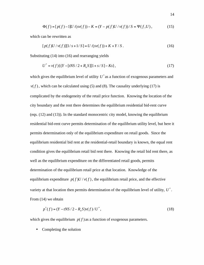
Substituting (14) into (16) and rearranging yields

}]/1][2/[){((* KsSsSRtNSYfvU a ++= , (17)

which gives the equilibrium level of utility *U as a function of exogenous parameters and

)( fv , which can be calculated using (5) and (8). The causality underlying (17) is

complicated by the endogeneity of the retail price function. Knowing the location of the

city boundary and the rent there determines the equilibrium residential bid-rent curve

(eqs. (12) and (13)). In the standard monocentric city model, knowing the equilibrium

residential bid-rent curve permits determination of the equilibrium utility level, but here it

permits determination only of the equilibrium expenditure on retail goods. Since the

equilibrium residential bid rent at the residential-retail boundary is known, the equal rent

condition gives the equilibrium retail bid rent there. Knowing the retail bid rent there, as

well as the equilibrium expenditure on the differentiated retail goods, permits

determination of the equilibrium retail price at that location. Knowledge of the

equilibrium expenditure )(/)( fvUfp , the equilibrium retail price, and the effective

variety at that location then permits determination of the equilibrium level of utility, *U .

From (14) we obtain

** /)()2/()( UfvSRtNSYfp a= , (18)

which gives the equilibrium )( fp as a function of exogenous parameters.

• Completing the solution

15

Thus far, the following have been solved for: the equilibrium residential bid-rent function

in the residential area, the equilibrium level of utility, and the equilibrium retail price and

retail bid rent at the residential-retail boundary. It remains to solve for the complete

equilibrium residential bid-rent, retail bid-rent, and retail price functions.

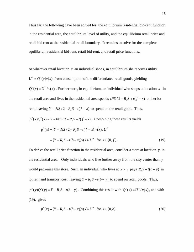
At whatever retail location x an individual shops, in equilibrium she receives utility

)()(**xvxQU = from consumption of the differentiated retail goods, yielding

)(/)( **xvUxQ = . Furthermore, in equilibrium, an individual who shops at location x in

the retail area and lives in the residential area spends )(2/ xftSRtNS a ++ on her lot

rent, leaving )(2/ xftSRtNSY a to spend on the retail good. Thus,

)(2/)()( ** xftSRtNSYxQxp a= . Combining these results yields

** /)()](2/[)( UxvxftSRtNSYxp a=

*/)()]([ UxvxbtSRYa

= for ],0[ fx . (19)

To derive the retail price function in the residential area, consider a store at location y in

the residential area. Only individuals who live further away from the city center than y

would patronize this store. Such an individual who lives at yx > pays )( ybtSRa + in

lot rent and transport cost, leaving )( ybtSRY a to spend on retail goods. Thus,

)()()( ** ybtSRYyQyp a= . Combining this result with )(/)( **xvUxQ = , and with

(19), gives

** /)()]([)( UxvxbtSRYxp a= for ],0[ bx . (20)

16

Notice that the retail price function is the product of two terms. The first, in square

brackets, which is increasing in x , reflects the reduced transport cost associated with less

accessible shopping locations; the second, which is decreasing in x , reflects the reduced

product variety at less accessible locations. As a result, the retail price function may be

either increasing or decreasing in x .

Having solved for the equilibrium retail price function, it is straightforward to solve for

the equilibrium retail bid-rent function:

KxsvUxpx = ))(/(]1)([)( *** . (21)

Notice that this function is a product of two terms. The first term, the retail markup, may

be either increasing or decreasing in x ; the second term, the quantity purchased, is

increasing in x . Consequently, the equilibrium retail bid-rent function may be either

increasing or decreasing in x .

The equilibrium residential bid-rent function for residential locations has already been

solved for. To solve for the function in the retail area, consider an individual who resides

in the retail area, ),0[ fx . She is indifferent between shopping at her residential

location and at any location closer to the city center; assume that she shops at her

residential location. She consumes a lot of size S there, receives a level of utility

)()(**xvxQU = from retail goods, and spends )()( **

xQxp on them. Thus, for

],0[ fx :

SxbtRSxvUxpYUx a /))(/))(/)((),( ***+== (using (20)). (22)

17

Expressed in terms of exogenous parameters, from (12), (19), (20), and (22), the

equilibrium residential bid-rent function is

SxbtRUxa

/))(),(*+= for ],0[ bx , (23)

which is linearly decreasing in x . And, using (20), and (21), the equilibrium retail bid-

rent function expressed in terms of exogenous parameters and )(xv is

KxsvUsxbtSRYxa

= ))(/(/)]([)( ** for ],0[ bx . (24)

As noted earlier, the retail bid-rent function may be either positively or negatively sloped.

Also,

])'(2''sgn[]/)(sgn[ 22*2vvvdxxd = . (25)

From (6) it follows that )(*x is concave in the retail area. In the residential area, from

(7), )2)(1()'(2'' 22= vvvvv , so that the retail bid-rent function is concave at those

residential locations for which 2>v and convex where 2<v .

• Checking that the solution is indeed a monocentric urban configuration

For the solution to characterize a monocentric urban configuration, it must be the case

that the residential bid rent exceed the retail bid rent everywhere in the retail area and that

the retail bid rent exceed the residential bid rent everywhere in the retail area. Since the

residential bid-rent curve is linear while the retail bid-rent curve is concave in the retail

area and can change curvature only once in the residential area, from concave to convex

as x increases, it follows that these two conditions are satisfied if, first, the retail bid rent

exceeds the residential bid rent at the city center, and, second, if the residential bid rent

exceed the retail bid rent at the urban boundary. The former condition, which we term

the first inequality, is

18

)0(/))0(/(/][)0( *=+>= StbRKsvUstbSRY

aa. (26)

The latter condition, which we term the second inequality, is that

)())(/(/][)( *bRKbsvUsSRYb

aa=<= . (27)

These conditions can be simplified by using the equilibrium condition that the residential

and retail bid rents are the same at the retail-residential boundary:

)(/)())(/(/)]([)( * fSfbtRKfsvUsfbtSRYf aa =+== . (28)

Combining (26) and (28), the first inequality reduces to

StfstfvfvsU //))0(/1)(/1)(/( *> . (29)

Substituting out for f and for )(/* fvU using (17), this inequality reduces to

)]0(/)2/(1}[)({( vNsvKsSsRYa

+

))0(/)2/(/1](2/)([ vNsvSsSstN ++> . (30)

Note that, as intuition suggests, the first inequality is easier to satisfy the lower is unit

transport cost. Now consider the second inequality. Combining (27) and (28) yields the

inequality

SfbtsfbtfvbvsU /)(/)())(/1)(/1)(/( *> . (31)

Substituting out for f and for )(/* fvU using (17), this inequality reduces to

]1)2/)((/)2/(}[)({( ++ SsNvNsvKsSsRYa

)2/)((/)2/(]2/)([ SsNvNsvSstN ++> . (32)

The second inequality, too, is easier to satisfy the lower is unit transport cost. That both

inequalities are easier to satisfy the lower is unit transport cost implies that a monocentric

urban configuration is “more likely” to be an equilibrium, the lower is unit transport cost,

19

as intuition would suggest. Note that the exogenous parameters in the above inequalities

are Y , t , N , S , s , K , ,and k .

Throughout the paper, we consider a single numerical example. The following parameter

values are employed: 4102=N , 25

102 mileS = , 2510 miles = , 29

/$10 mileK = ,

$1034

=Y , milet /$2700= , 26/$102.3 mileR

a= , 10= , and 6.0=k . With these

parameters, both a monocentric equilibrium and a completely mixed equilibrium exist.

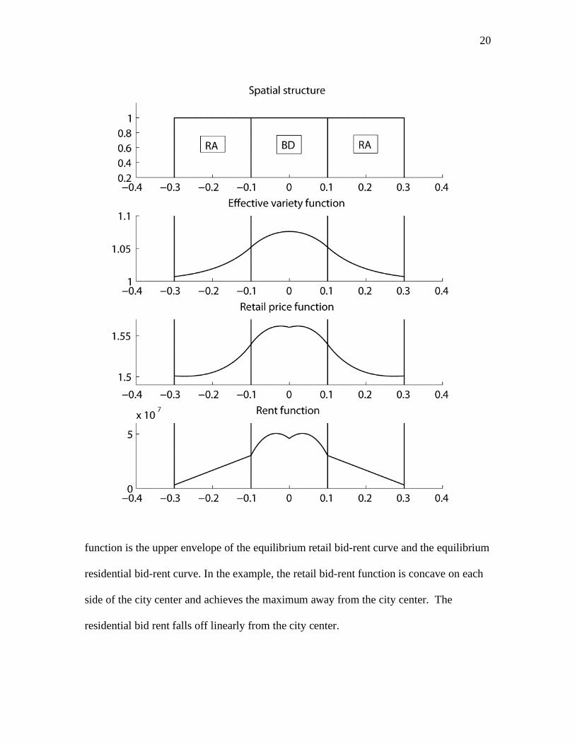
Figure 1 plots the equilibrium spatial configuration, and effective variety, retail price, and

rent, as functions of location, with these parameter values. The graphs are as expected.

The top panel shows that the retail district, marked as BD, is at the city center, and

flanked by residential areas, marked as RA. The effective variety function declines

monotonically from the city center with an inflection point at the retail-residential

boundary, between a concave region inside the retail-residential boundary and convex

regions outside it. The retail price function is concave on each side of the retail area (as

was derived above) and has its maximum away from the city center. The rent

Figure 1 Monocentric urban configuration

Note: 4102=N , 25

102 mileS = , 2510 miles = , 29

/$10 mileK = , $1034

=Y ,

milet /$2700= , 26/$102.3 mileR

a= , 10= , and 6.0=k .

S

20

function is the upper envelope of the equilibrium retail bid-rent curve and the equilibrium

residential bid-rent curve. In the example, the retail bid-rent function is concave on each

side of the city center and achieves the maximum away from the city center. The

residential bid rent falls off linearly from the city center.

21

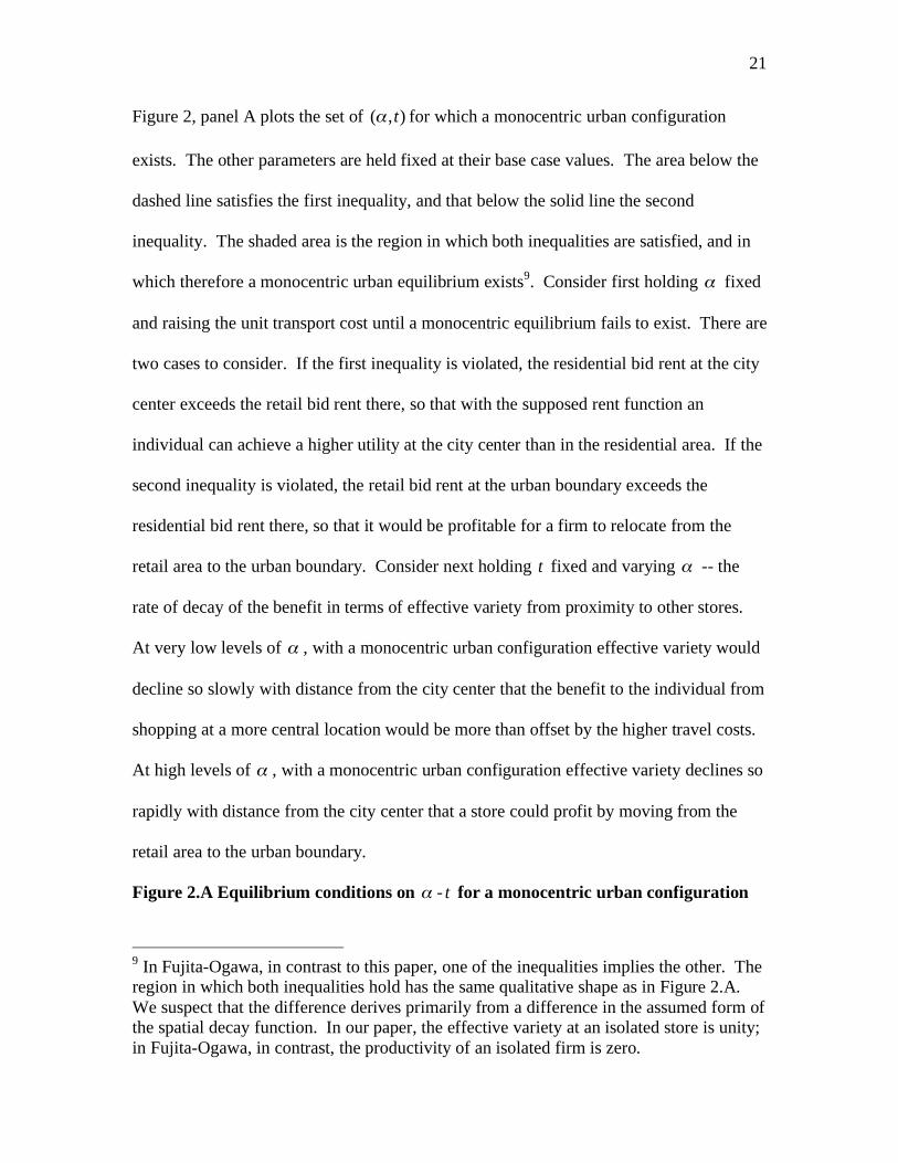
Figure 2, panel A plots the set of ),( t for which a monocentric urban configuration

exists. The other parameters are held fixed at their base case values. The area below the

dashed line satisfies the first inequality, and that below the solid line the second

inequality. The shaded area is the region in which both inequalities are satisfied, and in

which therefore a monocentric urban equilibrium exists9. Consider first holding fixed

and raising the unit transport cost until a monocentric equilibrium fails to exist. There are

two cases to consider. If the first inequality is violated, the residential bid rent at the city

center exceeds the retail bid rent there, so that with the supposed rent function an

individual can achieve a higher utility at the city center than in the residential area. If the

second inequality is violated, the retail bid rent at the urban boundary exceeds the

residential bid rent there, so that it would be profitable for a firm to relocate from the

retail area to the urban boundary. Consider next holding t fixed and varying -- the

rate of decay of the benefit in terms of effective variety from proximity to other stores.

At very low levels of , with a monocentric urban configuration effective variety would

decline so slowly with distance from the city center that the benefit to the individual from

shopping at a more central location would be more than offset by the higher travel costs.

At high levels of , with a monocentric urban configuration effective variety declines so

rapidly with distance from the city center that a store could profit by moving from the

retail area to the urban boundary.

Figure 2.A Equilibrium conditions on - t for a monocentric urban configuration

9 In Fujita-Ogawa, in contrast to this paper, one of the inequalities implies the other. The

region in which both inequalities hold has the same qualitative shape as in Figure 2.A.

We suspect that the difference derives primarily from a difference in the assumed form of

the spatial decay function. In our paper, the effective variety at an isolated store is unity;

in Fujita-Ogawa, in contrast, the productivity of an isolated firm is zero.

22

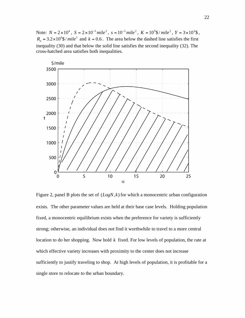
Note: 4102=N , 25

102 mileS = , 2510 miles = , 29

/$10 mileK = , $1034

=Y , 26

/$102.3 mileRa= and 6.0=k . The area below the dashed line satisfies the first

inequality (30) and that below the solid line satisfies the second inequality (32). The

cross-hatched area satisfies both inequalities.

Figure 2, panel B plots the set of ),( kLogN for which a monocentric urban configuration

exists. The other parameter values are held at their base case levels. Holding population

fixed, a monocentric equilibrium exists when the preference for variety is sufficiently

strong; otherwise, an individual does not find it worthwhile to travel to a more central

location to do her shopping. Now hold k fixed. For low levels of population, the rate at

which effective variety increases with proximity to the center does not increase

sufficiently to justify traveling to shop. At high levels of population, it is profitable for a

single store to relocate to the urban boundary.

23

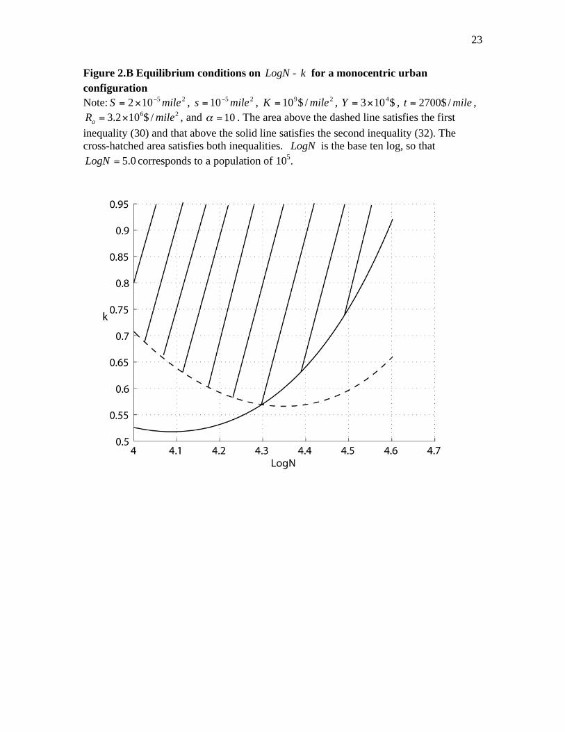
Figure 2.B Equilibrium conditions on LogN - k for a monocentric urban

configuration

Note: 25102 mileS = , 25

10 miles = , 29/$10 mileK = , $103

4=Y , milet /$2700= ,

26/$102.3 mileR

a= , and 10= . The area above the dashed line satisfies the first

inequality (30) and that above the solid line satisfies the second inequality (32). The

cross-hatched area satisfies both inequalities. LogN is the base ten log, so that

0.5=LogN corresponds to a population of 105.

24

4. Completely Mixed Urban Configuration

In a completely mixed urban configuration, retail and residential land uses are

interspersed so that each individual essentially has a store in his backyard. This section

determines the set of parameter values for which this configuration is an equilibrium.

Note that the completely mixed urban configuration and the monocentric urban

configuration are extreme cases; in one, stores are as centralized as possible, in the other

as decentralized as possible. Intuition therefore suggests that the parameter set for which

equilibria of both types exist may be empty, as it is in Fujita and Ogawa.

The city extends from b to b , with 2/)( sSNb += , with a proportion aSss =+ )/( of

the land at each location being allocated to retail and the rest to residential use. The

effective variety function is the same as for the monocentric city configuration, except

that axa =)( throughout the urban area, rather than equaling 1 in the retail area and 0 in

the residential area as was the case in the monocentric urban configuration. Thus,

For ],0[ bx :

0)}(exp{)}(exp{1)( >++= dyxykadyyxkaxvb

x

x

b

and

0)})(exp{)}((exp{)(' <+= xffxkaxv

0)})(exp{)}((exp{)('' <++= xffxkaxv . (33)

Also,

})exp{1)(/2(1)0( bkav += , })2exp{1)(/(1)( bkabv += (34)

25

Thus, the effective variety function declines monotonically from the city center and is

concave throughout the city.

• The retail bid-rent function

Eqs. (9) through (11) continue to apply.

• The residential bid-rent function

Everyone shops at her backyard store and therefore incurs no transport costs. Thus,

SxvUxpYUx /))(/)((),( = . (35)

• Equal rent conditions

Since retail and residential land co-exist at all urban locations, in equilibrium

)()()( xRxx == for ],0[ bx ,

where )(xR is the rent function, or

SxvUxpYKxsvUxp /))(/)(())(/(]1)([ = . (36)

Rewrite (36) as

)/1/(]/)()/(1[)( SsUxvSYsKsxp +++= . (36’)

Also, in equilibrium at the city boundary both the retail and residential bid rents equal

the agricultural bid rent:

SRbvUbpY a=)(/)( . (37)

Substituting (37) into (36’) evaluated at bx = yields

])()[(*KsSsRYbvU

a+= , (38)

which gives the equilibrium level of utility in terms of exogenous parameters.

Substituting (38) into (36’) would give an expression for )(xp in terms of only )(xv and

exogenous parameters. Now, insert (36’) into (35) to give the rent function:

26

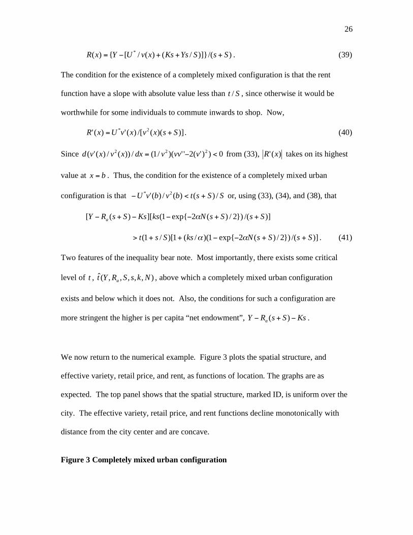
)/()]}/()(/[{)( *SsSYsKsxvUYxR +++= . (39)

The condition for the existence of a completely mixed configuration is that the rent

function have a slope with absolute value less than St / , since otherwise it would be

worthwhile for some individuals to commute inwards to shop. Now,

)])((/[)(')(' 2*SsxvxvUxR += . (40)

Since 0))'(2'')(/1(/))(/)('( 222<= vvvvdxxvxvd from (33), )(' xR takes on its highest

value at bx = . Thus, the condition for the existence of a completely mixed urban

configuration is that SSstbvbvU /)()(/)(' 2*+< or, using (33), (34), and (38), that

)]/(})2/)(2exp{1(][)([ SsSsNksKsSsRYa

+++

)]/(})2/)(2exp{1)(/(1)[/1( SsSsNksSst ++++> . (41)

Two features of the inequality bear note. Most importantly, there exists some critical

level of t , ),,,,,(ˆ NksSRYta

, above which a completely mixed urban configuration

exists and below which it does not. Also, the conditions for such a configuration are

more stringent the higher is per capita “net endowment”, KsSsRYa

+ )( .

We now return to the numerical example. Figure 3 plots the spatial structure, and

effective variety, retail price, and rent, as functions of location. The graphs are as

expected. The top panel shows that the spatial structure, marked ID, is uniform over the

city. The effective variety, retail price, and rent functions decline monotonically with

distance from the city center and are concave.

Figure 3 Completely mixed urban configuration

27

Note: 4102=N , 25

102 mileS = , 2510 miles = , 29

/$10 mileK = , $1034

=Y ,

milet /$2700= , 26/$102.3 mileR

a= , 10= , and 6.0=k .

Figure 4, panel A plots the set of ),( t for which a completely mixed urban equilibrium

exists. The other parameters are held at their base case levels.

28

Figure 4.A Equilibrium condition on - t for a completely mixed urban

configuration

Note: 4102=N , 25

102 mileS = , 2510 miles = , 29

/$10 mileK = , $1034

=Y , 26

/$102.3 mileRa= and 6.0=k . The cross-hatched area above the dashdot line

satisfies third inequality (42).

With this spatial configuration there is only one inequality that needs to be satisfied. The

set of parameter pairs satisfying the inequality, and for which therefore a completely

mixed urban equilibrium exists, is indicated by the cross-hatched area. Consider first

holding fixed and lowering the unit transport cost. Below a critical level of the unit

transport cost, a completely mixed urban equilibrium does not exist since, at some

locations at least, an individual can improve her utility by shopping at a more central

location, which offers greater product variety. Consider next holding t fixed and varying

. For low levels of , effective variety does not fall off sufficiently rapidly with

29

distance from the city center to make travel to shop at more central locations, with greater

retail variety, worthwhile, while for higher levels of effective variety does fall off

sufficiently rapidly to make it worthwhile.

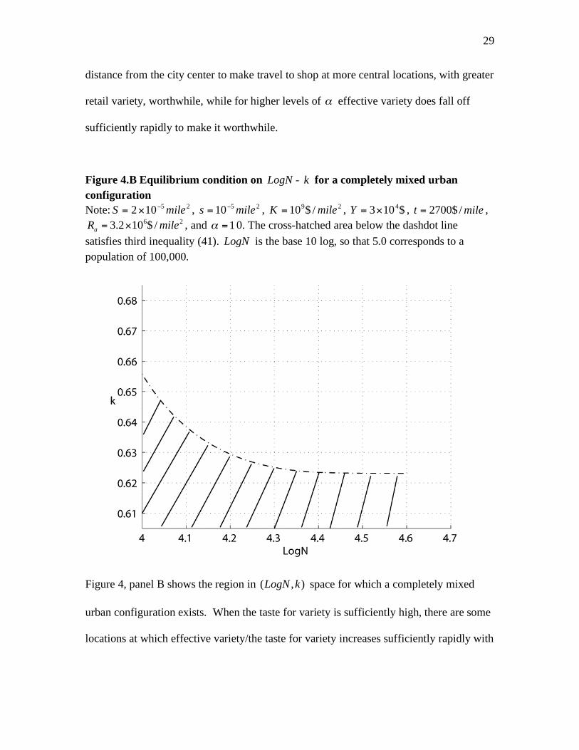
Figure 4.B Equilibrium condition on LogN - k for a completely mixed urban

configuration

Note: 25102 mileS = , 25

10 miles = , 29/$10 mileK = , $103

4=Y , milet /$2700= ,

26/$102.3 mileR

a= , and 1= 0. The cross-hatched area below the dashdot line

satisfies third inequality (41). LogN is the base 10 log, so that 5.0 corresponds to a

population of 100,000.

Figure 4, panel B shows the region in ),( kLogN space for which a completely mixed

urban configuration exists. When the taste for variety is sufficiently high, there are some

locations at which effective variety/the taste for variety increases sufficiently rapidly with

30

proximity to the city center to justify travel to shop, and for which therefore a completely

mixed equilibrium does not exist.

Figure 5 displays the region of ),( t space for which both the monocentric and

completely mixed equilibria co-exist. A monocentric equilibrium exists in the region

below the dashed and solid line and a completely mixed urban equilibrium in the region

above the dashdot line. In the small, cross-hatched region, which is centered on the

parameter values of the numerical example, both types of equilibria co-exist. We have

already provided some intuition for the shapes of the regions in this space for which each

of the two equilibria exist. Start at the point in the cross-hatched area corresponding to

the values of t and in the numerical example, and move SE to the area where neither

type of equilibrium exists. The monocentric equilibrium ceases to exist since the first

inequality is violated -- with a monocentric urban configuration, an individual can

achieve a higher level of utility at the center than in the residential area.

Figure 5 Equilibrium conditions on - t for monocentric/ completely mixed urban

configurations

Note: 4102=N , 25

102 mileS = , 2510 miles = , 29

/$10 mileK = , $1034

=Y , 26

/$102.3 mileRa= , 6.0=k . The area below the dashed and solid line satisfies the

monocentric equilibrium conditions,and that above dashdot line satisfies the completely

mixed equilibrium condition. The cross-hatched area satisfies both sets of equilibrium

conditions.

31

The completely mixed equilibrium ceases to exist since in the completely mixed

configuration it becomes worthwhile for the individual at the urban boundary to travel a

small distance towards the city center to shop; the cost of travel falls and the benefit

increases. Now, instead, move SW to the area where neither type of equilibrium exists.

The monocentric equilibrium ceases to exist since the second inequality ceases to be

satisfied -- with a monocentric urban configuration, it becomes profitable for a single

store to move from the retail area to the urban boundary; the decrease in the spatial decay

rate of proximity benefits causes the difference in the effective variety at the retail

location compared to the urban boundary to fall, and this effect more than offsets the

increased attractiveness of shopping in the retail area due to the decline in transport costs.

The completely mixed equilibrium ceases to exist because in a completely mixed urban

configuration it becomes worthwhile for the individual at the urban boundary to travel a

32

small distance towards the city center; the cost of travel falls by more than the benefit

does.

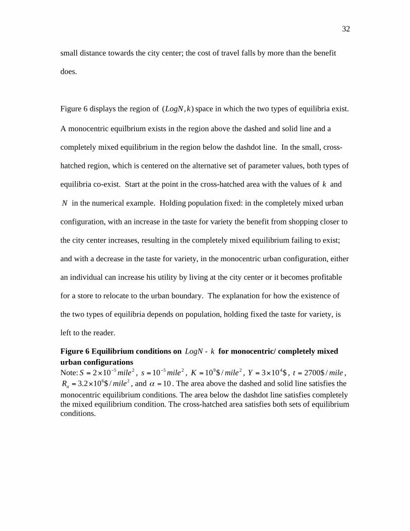
Figure 6 displays the region of ),( kLogN space in which the two types of equilibria exist.

A monocentric equilbrium exists in the region above the dashed and solid line and a

completely mixed equilibrium in the region below the dashdot line. In the small, cross-

hatched region, which is centered on the alternative set of parameter values, both types of

equilibria co-exist. Start at the point in the cross-hatched area with the values of k and

N in the numerical example. Holding population fixed: in the completely mixed urban

configuration, with an increase in the taste for variety the benefit from shopping closer to

the city center increases, resulting in the completely mixed equilibrium failing to exist;

and with a decrease in the taste for variety, in the monocentric urban configuration, either

an individual can increase his utility by living at the city center or it becomes profitable

for a store to relocate to the urban boundary. The explanation for how the existence of

the two types of equilibria depends on population, holding fixed the taste for variety, is

left to the reader.

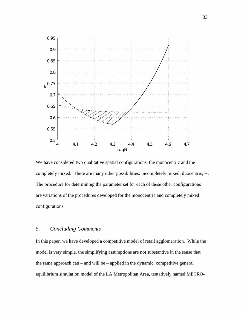
Figure 6 Equilibrium conditions on LogN - k for monocentric/ completely mixed

urban configurations

Note: 25102 mileS = , 25

10 miles = , 29/$10 mileK = , $103

4=Y , milet /$2700= ,

26/$102.3 mileR

a= , and 10= . The area above the dashed and solid line satisfies the

monocentric equilibrium conditions. The area below the dashdot line satisfies completely

the mixed equilibrium condition. The cross-hatched area satisfies both sets of equilibrium

conditions.

33

We have considered two qualitative spatial configurations, the monocentric and the

completely mixed. There are many other possibilities: incompletely mixed, duocentric, --.

The procedure for determining the parameter set for each of these other configurations

are variations of the procedures developed for the monocentric and completely mixed

configurations.

5. Concluding Comments

In this paper, we have developed a competitive model of retail agglomeration. While the

model is very simple, the simplifying assumptions are not substantive in the sense that

the same approach can – and will be – applied in the dynamic, competitive general

equilibrium simulation model of the LA Metropolitan Area, tentatively named METRO-

34

LA, which builds on Alex Anas’ RELU-TRAN model for Chicago (Anas and Liu, 2007),

and in the development of which Anas and Arnott are participating. In these concluding

comments, we describe briefly how this paper’s model could be extended for this

application.

One module of the LA model solves for the temporary (static) equilibrium for each

period. Each period inherits a stock of properties (vacant land and land with structures on

it) indexed by type and zone, as well as location potentials indexed by industry type and

zone, and the effective varieties indexed by zone. The temporary equilibrium is like a

static Arrow-Debreu competitive equilibrium with (commodity) transport costs10

, except

that: first, each household consumes property at only one location and incurs transport

costs, for commuting from its chosen residential location to its chosen work location, for

shopping, recreational activities, and so on 11

; second, retail goods are distinguished from

wholesale goods; third, the economy is endowed with structures, as well as conventional

factors of production; and fourth, agglomeration economies in production and retailing

are treated via industry-specific location potential functions and an effective variety

function12

. A temporary equilibrium is characterized by a market-clearing set of prices

10

Each household maximizes its utility and each firm maximizes its profits, taking prices

as fixed. There is potentially an arbitrarily large but finite number of types of individuals

and of retail and intermediate goods. 11

In the Arrow-Debreu model, the assumption of convex preferences would result in

households diversifying their housing consumption over locations, and people transport

costs are not treated. 12

An industry-specific location potential function can depend on proximity to firms in

other industries as well to firms in the same industry. The effective variety function can

be differentiated by type of retail good.

It is possible to introduce agglomeration economies in retailing on the production

as well as on the consumption side.

35

and the corresponding allocation. The location potential functions and effective variety

function can be solved for from the location pattern of the temporary equilibrium of one

period and then treated as exogenous in determining the next period’s temporary

equilibrium.

The second module links the time periods. The present is linked to the past via the

inheritance of real properties, location potential functions, and the effective variety

function13

. The present is linked to the future via real property markets. Economic

agents have perfect foresight, and the market value of a property equals the expected

present discounted value of future net rents14

. Between periods developers make profit-

maximizing conversion decisions, building on vacant land, demolishing structures,

allowing some existing properties to deteriorate and rehabilitating others, etc., which

moves the property stock forward from one period to the next15

. Currently,the

demography of the model is exogenous, but the aim is to make it responsive to economic

13

In the model of the paper, the effective variety function is determined as part of the

static equilibrium, taking as given the qualitative spatial configuration. In a

corresponding dynamic model, effective variety as a function of location could be

calculated as part of that period’s temporary equilibrium, taking as the starting point in

the computation the equilibrium effective variety function from the previous period,

which would generate some history dependence in the location pattern. METRO-LA

assumes instead that the locational potential functions and effective variety functions

calculated from one period’s temporary equilibrium are taken as exogenous in the next

period’s temporary equilibrium. This (substantive) simplifying assumption is made to

reduce computational costs. 14

A non-stationary, infinite horizon model can obviously not be solved exactly with a

computer, which has finite computational ability. The model must be truncated

somehow. In the LA model, the truncation is done by assuming that at some terminal

time the economy’s property values correspond to those of a stationary equilibrium. 15

Individual utilities and developer conversion costs are treated as idiosyncratic (in

particular, the logit algebra is employed) so as to smooth adjustment, which facilitates

computation.

36

conditions. The base industries grow according to the time path of export prices, which

are taken as exogenous.

Despite the higher complexity of the LA model, the economics of retail agglomeration

are essentially the same as those described in this paper. The essential component is the

effective variety function, which relates the attractiveness to individuals of shopping at

different locations to the spatial distribution of stores. Taking the spatial pattern of retail

location, as reflected in the effective variety function, and of retail prices as given,

individuals choose where to shop, trading off the greater variety of retail goods at larger

shopping centers against the higher prices there and (for most individuals) the higher

transport costs of traveling to a larger center. Stores choose where to locate trading off

the higher price they can charge at a larger center against the higher rent they must pay

there, and in equilibrium make zero profits. The spatial pattern of retail prices, as well as

the retail and residential bid-rent functions and the effective variety function, adjust

simultaneously to clear the location-specific markets for retail goods as well as the

location-specific land markets.

37

References

Anas, A. and Y.Liu. 2007. A regional economy, land use, and transportation model

(RELU-TRAN): Formulation, algorithm design, and testing. Journal of Regional

Science 47, 415-455.

Bell, D., T.-H. Ho, and C. Tang. 1998. Determining where to shop: Fixed and variable

costs of shopping. Journal of Market Research 35, 352-369.

Berry, B. 1967. Geography of Market Centers and Retail Distribution. Englewood Cliffs,

NJ: Prentice-Hall.

Brown, S. 1989. Retail location theory: The legacy of Harold Hotelling. Journal of

Retailing 65, 450-470.

Brown, S. 1993. Retail location theory: Evolution and evaluation. The International

Review of Retail, Distribution and Consumer Research 3, 185-229.

Bucklin, R. S. Gupta, and S. Siddarth. 1998. Determining segmentation in sales

response across consumer purchase behaviors. Journal of Marketing Research

35, 189-197.

Cadwaller, M. 1975. A behavioral model of consumer spatial decision making. Economic

Geography 51, 339-349.

Chen, D. 2007. Optimal retail location theory and shopping trip behavior: A general

summary and literature review. Mimeo.

Clark, I., D. Bennison, and J. Pal. 1997. Towards a contemporary perspective of retail

location. International Journal of Retail and Distribution Management 25, 59-69.

Craig, S., A. Ghosh, and S. McLafferty. 1984. Models of the retail location process: A

review. Journal of Retailing, 5-36.

Drezner, T. and Z. Drezner. 1996. Competitive facilities: Market share and location with

random utility. Journal of Regional Science 36, 1-15.

Eaton, B.C. 1976. Free entry in one-dimensional models – pure profits and multiple

equilibria. Journal of Regional Science 16, 21-33.

Eaton, B.C. and R. Lipsey1975. The principle of minimum differentiation reconsidered:

Some new developments in the theory of spatial competition. Review of

Economic Studies, 27-49.

Eaton, B.C. and R. Lipsey. 1979. Comparison shopping and the clustering of

homogeneous firms. Journal of Regional Science, 19, 421-435.

38

Eaton, C. and R. Lipsey. 1982. An economic theory of central places. Economic Journal

92, 56-72.

Eaton, B.C. and M. Wooders. 1985. Sophisticated entry in a model of spatial competition.

Rand Journal of Economics 16, 282-297.

Fujita, M. 1988. A monopolistic competition model of spatial agglomeration:

Differentiated product approach. Regional Science and Urban Economics 18,

87-124.

Fujita, M. and P. Krugman. 1995. When is the economy monocentric? Von Thünen and

Chamberlin unified. Regional Science and Urban Economics 25, 505-528.

Fujita, M. and H. Ogawa. 1982. Multiple equilibria and structural transition of non-

monocentric urban configurations. Regional Science and Urban Economics 12,

161-196.

Goldner, W. 1971. The Lowry Model heritage. Journal of the American Planning

Association 37, 100-110.

Harris, B. 1985. Urban simulation models in regional science. Journal of Regional

Science 25, 545-567.

Huff, D. 1964. Defining and estimating a trading area. Journal of Marketing 28, 34-38.

Huff, D. 1966. A programmed solution for approximating an optimum retail location.

Land Economics 42, 293-303.

Kohsaka, H. 1984. An optimization of the central place system in terms of multipurpose

shopping trip. Geographical Analysis 16, 250-268.

Lowry, I.S. 1964. A Model of Metropolis. Memorandum RM-4035-RC. Santa Monica:

The Rand Corporation.

Lowry, I.S. 1968. Seven models of urban development: A structural comparison. Urban

Development Models. Special Report 97, 121-163. Washington, DC: Highway

Research Board, National Research Council.

G.Weisbrod, R. Parcells, and C. Kern. 1984. A disaggregated model for predicting

shopping area market attraction. Journal of Retailing 60, 65-83.

Wilson A. 1974. Urban and Regional Models in Geography and Planning. New York:

Wiley.

Wilson, A. 1970. Entropy in Urban and Regional Modeling. London: Pion.