NBP Working Paper No. 336 Shocks to bank capital position: Do they matter for lending to firms and how they are channelled? Evidence from Senior Loan Officer Opinion Survey for Poland Ewa Wróbel

Welcome message from author
This document is posted to help you gain knowledge. Please leave a comment to let me know what you think about it! Share it to your friends and learn new things together.
Transcript

NBP Working Paper No. 336
Shocks to bank capital position: Do they matter for lending to firms and how they are channelled?Evidence from Senior Loan Officer Opinion Survey for Poland
Ewa Wróbel

Narodowy Bank PolskiWarsaw 2021
NBP Working Paper No. 336
Shocks to bank capital position: Do they matter for lending to firms and how they are channelled?Evidence from Senior Loan Officer Opinion Survey for Poland
Ewa Wróbel

Published by: Narodowy Bank Polski Education & Publishing Department ul. Świętokrzyska 11/21 00-919 Warszawa, Poland www.nbp.pl
ISSN 2084-624X
© Copyright Narodowy Bank Polski 2021
Ewa Wróbel – Narodowy Bank Polski; [email protected]
The author wishes to thank Ryszard Kokoszczyński, Mateusz Pipień, Tomasz Łyziak and an anonymous referee for helpful discussions and comments. The remaining errors are mine. The usual disclaimer applies.
ContentsAbstract 4
1. Introduction 5
2. Stylized facts 9
2.1. Banking sector and lending to corporates 9
2.2. Bank capital 11
2.3. Lending standards, terms and conditions 14
3. Related literature 16
4. Data and estimation method 19
4.1. The Survey 19
4.2 Non-survey data 20
4.3. Estimation method 21
5. Results 27
5.1. Impulse responses of standards, T&Cs to shocks to banks’ capital position 27
5.2. Impulse responses of investment and loans to shocks to banks’ capital position 29
5.3. Robustness checks 33
6. Summary and conclusions 35
References 37
Statistical Appendix 40
43
Shocks to bank capital position: Do they matter for lending to firmsand how they are channelled? Evidence from Senior Loan Officer
Opinion Survey for Poland
Ewa Wróbel*
Abstract
Basing on data from bank lending surveys, we show that shocks to capital position are an important driver of bank lending standards, terms and conditions. Standards for small and medium-sized enterprises are affected more than those for large entities. Shocks to capital are channelled to firms mostly through these terms and conditions which are related to loan price: average spreads and spreads on riskier loans. The third mostly used channel is required collateral. Adverse shocks to capital position result in a lower lending, in particular for real property acquisition and for financing working capital and on current account.
Key words: bank capital, bank lending survey, structural VAR
JEL: E44, E51, G21
*Narodowy Bank Polski, [email protected]. The author wishes to thank RyszardKokoszczyński, Mateusz Pipień, Tomasz Łyziak and an anonymous referee for helpful discussions and comments. The remaining errors are mine. The usual
disclaimer applies.
Narodowy Bank Polski4
Abstract

2
1. Introduction
Since the global financial crisis (GFC), capital requirements – a predetermined
fraction of loan amount that must be hold as equity – became a standard instrument in
the macro-prudential policy toolkit, supposed to increase the resilience of the banking
sector to adverse shocks and mitigate credit cycles. Basel III and CRD II and III
regulation in the EU, imposed on banks a requirement to build buffers of high-quality
capital, and resulted in a steady growth of banks’ capital and reserves. Thus, there is
a need to have a good grasp of impact of changes in bank capital on lending to the
non-financial sector and on the real sector activity.
Banks can increase capital in a few ways: accumulating the retained earnings, issuing
new equities, reducing lending and de-risking assets. If banks pursue either of the two
latter strategies, it is important to know whether the adjustment is realised through
price or the non-price dimensions of credit policy. If the required collateral rises,
small and medium-sized enterprises and sole proprietors, i.e. units which are the most
vulnerable to information asymmetry, may find it more difficult to have access to bank
credit. If, in turn, it is achieved through increased margins, this is an important
information for the monetary policy, as it operates through the same channel.
There is a number of papers which explore these topics. Some works provide evidence
that an increase in capital is financed from retained earnings, e.g. Cohen (2013), but
usually they show that banks transitorily curtail lending and change its structure, e.g.
Bridges et al. (2014), Kanngiesser et al. (2017). Bidder et al. (2019) find another
possible reaction. Although the study does not investigate banks increasing capital,
but those whose borrowers were hit by an adverse shock to the net worth, its
conclusions can be relevant for other shocks. Namely, banks tighten corporate lending
and mortgages that they would ultimately hold on their balance sheet. In the same
time, banks are induced to expand credit for mortgages to be securitized, particularly
those that are government-backed. Thus, while the effect of de-risking is
unambiguous, this may not be the case for the observed amounts of issued credits.
This paper analyses the impact of shocks to capital on lending standards, terms and
conditions as well as on various types of loans to corporates and sole proprietors. It
43
Shocks to bank capital position: Do they matter for lending to firmsand how they are channelled? Evidence from Senior Loan Officer
Opinion Survey for Poland
Ewa Wróbel*
Abstract
Basing on data from bank lending surveys, we show that shocks to capital position are an important driver of bank lending standards, terms and conditions. Standards for small and medium-sized enterprises are affected more than those for large entities. Shocks to capital are channelled to firms mostly through these terms and conditions which are related to loan price: average spreads and spreads on riskier loans. The third mostly used channel is required collateral. Adverse shocks to capital position result in a lower lending, in particular for real property acquisition and for financing working capital and on current account.
Key words: bank capital, bank lending survey, structural VAR
JEL: E44, E51, G21
*Narodowy Bank Polski, [email protected]. The author wishes to thank RyszardKokoszczyński, Mateusz Pipień, Tomasz Łyziak and an anonymous referee for helpful discussions and comments. The remaining errors are mine. The usual
disclaimer applies.
5NBP Working Paper No. 336
Chapter 1

3
verifies whether shocks to capital are transmitted through price or non-price channels.
Data on bank lending policy and capital position come from Senior Loan Officer
Opinion Survey (SLOOS).
Commercial banks which answer the SLOOS questionnaire, account for about 80-
90% of total loans to the non-financial sector. Data is weighted by individual bank’s
share in the market for a specific type of loan. Thus, it is possible to observe
developments in the credit market with respect to various types of loans (long- and
short-term) and agents (medium and small-sized corporates, SMEs, the large ones,
LEs, and households) with a relatively high precision. The survey shows the net
percent of responses, i.e. a difference between a tendency to tighten and weaken credit
policy (standards, terms and conditions – henceforth T&Cs). The same applies to
factors potentially driving credit policy.
By virtue of the construction of the questionnaire 1 , it brings information on
strengthening (weakening) of banks’ balance sheets if it indeed contributed to the
variations in credit policy. Put it another way, even if there were some changes in
bank capital, but perceived as minor or transitory, and in fact did not affect bank
decision on credit policy, they would not be reported in the questionnaire.
From the point of view of the goals of this paper, this feature may mean that we
dispose less noisy data as compared to the actual capital ratios. However, the survey
does not bring information whether the reported changes in the capital position result
from exogenous factors, like changes in regulations, or are endogenous.
There exists a plentiful evidence of reliability of bank lending survey data. Used
mostly in the monetary transmission literature, they serve to identify credit channel
operation. For example, Ciccarelli et al. (2015) and Couaillier (2015) show that
monetary policy shocks do affect bank lending policy. Lown and Morgan (2006) find
that in the US lending standards have an impact on loans, GDP and inflation. For
1 „If your bank’s lending policies (credit standards or terms) applied to corporate loans and credit lines have changed over the last three months, please indicate how the following factors have influenced the changes”.
Narodowy Bank Polski6
4
Poland, Wróbel (2018) shows that monetary policy has a bearing on banks’ lending
policy with respect to the corporate sector.
The paper makes use of structural vector autoregression models (SVARs henceforth)
and therefore accounts for dynamic relationships between variables and avoids the
endogeneity problem. The latter is binding since bank capital depends on
macroeconomic developments, monetary policy and lending. We build a set of
SVARs and identify shocks to bank capital through a non-recursive decomposition.
Models are over-identified. The restrictions are formally tested.
This way of proceeding has a twofold justification. Firstly, it introduces more
structure into models as compared to the usual Choleski decomposition. This includes
an explicit specification of loan demand and supply functions, capital position and
monetary policy rule equations. Moreover, because the restrictions are tested, the
models are more reliable. Secondly, the problem of the ordering of the variables is
avoided as it sometimes imposes implausible or at least questionable restrictions
related to time sequence of reactions of the endogenous variables.
The estimations bring two main observations. First, negative shocks to capital position
reduce investment (GFCF) and loans for the real property acquisition. Likewise, loans
to sole proprietors fall considerably. Credits on current account and for financing
working capital decline somewhat less. Point estimates for investment loans also
indicate a negative reaction, but it is not statistically significant. Secondly, after an
adverse shock to capital, banks tend to increase average spreads, spreads on riskier
loans and the required collateral. This finding conforms Tressel and Zhang (2016) for
the euro area. A relatively strong reaction of spreads on riskier loans and collateral as
well as the observed behaviour of various types of loans may suggest that shocks to
capital induce banks to de-risk their credit portfolio discouraging riskier customers.
The value added of this paper is twofold: it demonstrates that bank lending survey
data brings information which helps estimate the influence of macro-prudential policy
on the real sector and lending and shows that the main channels of this policy are
similar to these of the monetary policy.
7NBP Working Paper No. 336
Introduction

5
The paper is structured as follows: the next section shows stylized facts2, the third one
reviews the related literature. It is followed by a description of data and methodology.
The fifth section describes estimation results, while the sixth one summarizes and
concludes.
2 The related figures and tables are shown in the Statistical Appendix.
Narodowy Bank Polski8

6
2. Stylized facts
2.1. Banking sector and lending to corporates
In Poland, banking sector is the most important source of external financing for
corporates. Nonetheless, loans to firms related to GDP constitute a modest 13-17%.
Corporate bonds issued on the domestic market as well as new issues of shares on the
Warsaw Stock Exchange (WSE) play a minor role (Figure A1 in the Statistical
Appendix). Small and medium-sized enterprises (SMEs), particularly these belonging
to the segment of means of transport, to some extent replace bank loans with leasing.
To finance investment, firms rely mostly on their own funds: only 11-13% of
investment is financed with bank loans. Banks use flexible credit rates more
frequently than fixed rates.
Bank lending to the corporate sector comprises credits in the domestic and foreign
currencies (euro is by far the most important foreign currency in bank lending to the
corporate sector). Loans in foreign currencies represent some 26-30% of total loans
to firms; half of that amount was spent on investment outlays. Some 40% of SMEs
and almost 50% of LEs having loans in foreign currencies are exporters, Tymoczko
(2013).
Since 2013, to facilitate access to bank lending, SMEs have been eligible for state aid
within the de minimis Portfolio Guarantee Facility. Under the programme, a state-
owned bank grants entities from the SMEs sector, on their request, guarantees to
secure the repayment of loans. The programme can be considered as a supplementary
collateral and this way it can make credit supply to SMEs more rigid in the case of
monetary policy tightening. Currently, about 45% of short-term and 37% of long-
term loans are extended to SMEs, GUS (2020).
Figure A2 shows allocation of loans. Manufacturing is the largest recipient of both,
short-term and long-term banking loans extended to LEs and SMEs. Electricity, gas
and steam supply, information and communication as well as administrative activities
are important recipients in the case of long-term loans to LEs, whereas in the case of
long-term loans to SMEs the largest beneficiaries are real estate, transportation and
storage, administrative activities and construction. Short-term loans, besides
9NBP Working Paper No. 336
Chapter 2

7
manufacturing go to trade and repair and in the case of LEs to supply of electricity,
whereas in the case of SMEs – to construction and administrative activities. However,
indebtedness of sections of the economy (F01 GUS data) measured either as the ratio
of short-term or long-term loans to firms’ assets shows a somewhat different picture:
the most short-indebted are trade and repair, manufacturing and three divisions of
services: (i) administrative and support service activities, (ii) education and (iii) health
and social assistance. Producers of services, such as accommodation and catering,
health and social assistance, culture and recreation are the most long-term indebted,
followed by manufacturing and supply of water.
Because riskiness of sections and divisions of the non-financial sector can have some
bearing on lending standards, terms and conditions, we have examined data from
business surveys on the general climate and financial situation (Statistical Office). We
assume that indices of their variation can approximate riskiness. Tables A1 and A2
show descriptive statistics of the “general climate” and “financial situation”.
Coefficients of variation of the perceived climate are highly diversified across sectors
and sections. The highest are for administrative activities, trade and repair, transport
and storage. The respective coefficients for the financial situation vary less; in this
case the highest scores are observed for three sections of services: information and
communication, accommodation and catering and professional and scientific
activities. In all these sectors and sections but information and communication, SMEs
play important role. The share of their revenues and investment in the total amount of
revenues and investment of the non-financial enterprises ranges from about 60 to
82%3. SMEs and sole proprietors are mostly producers of services (about 36% of
them, they also operate in trade and repair (about 31%). Another two considerable
fractions of SMEs and sole proprietors function in construction (about 14%) and
manufacturing (11%), GUS (2015). In turn, LEs operate mostly in industry (almost
52% of them), but they are also active in services (about 31%); about 14% of LEs are
present in trade and repair, PARP, (2019).
3 Only the share of SMEs in transport and storage in total investment of this sector is much lower, amounting to some 30%.
Narodowy Bank Polski10

8
Services is the sector of a relatively high income elasticity of demand, displaying
higher volatility than others and in the same time populated by SMEs. Because SMEs
are riskier borrowers due to information asymmetry, this sector is supposedly more
vulnerable to the restrictive credit policy. Trade and repair seems to be vulnerable to
credit tightening rather because it is populated by SMEs than because of demand
volatility. Thus, some sectors can be more vulnerable because of inherently higher
risk, whereas other because they are populated by SMEs. We expect that after a shock
to capital, more banks will change their lending policy with respect to SMEs and sole
proprietors than LEs.
2.2 Bank capital
Capital ratios are cyclical, as depicted in Figure A3. Cyclical part of capital ratios and
capital position from SLOOS4 as well as those of investment, were obtained from HP-
detrending. Trends of the first two variables approximate long-term process of
regulatory policy, whereas the last one represents investment potential. Capital ratios
were declining in time of booms and increasing with rising risks of busts. “Gaps” of
capital ratios lag behind these obtained from SLOOS data by about one quarter,
especially in the subperiod ending in 2011.
In general, over the sample, Polish banking system was well capitalized (Figure A4,
Figure A5). The average capital ratio remained high, only just before the financial
crisis and in 2009 it oscillated around 11%. This was due to regulatory changes which
reduced capital requirements against large exposures and general interest rate risk.
In Poland, the post-crisis reform of prudential regulations started even before the
official adoption of the macro-prudential framework in 2015. This pre-2015 policy
comprised more restrictive policy with respect to capital requirements and risk
weights of exposures in currencies other than the obligor’s income. Most of new
regulations dealt with loans to households, because a large part of loans for housing
was extended in foreign currencies.
4 We have detrended accumulated data on capital position from SLOOS.
11NBP Working Paper No. 336
Stylized facts

9
In 2014 Poland began implementing the CRR/CRD IV package. This caused a further
increase in the required levels of regulatory capital, strengthened by a cautious
approach of the national supervisory authorities regarding the rules for determining
capital ratios. Besides exposures arising from foreign currency housing loans, it was
related to payment of dividends. Moreover, the increase in capital ratios was due to a
limited scale of implementation of advanced methods of estimating risk exposures.
The process of increases of the required capital has become even stronger since 2015.
Banks involved in housing loans in foreign currencies extended to unhedged
households were subject to surcharges. Those considered as systematically important
institutions (OSII) had to hold adequate capital buffers. Also, a newly imposed
conservation buffer was gradually phased in. It amounted to 1.25% of the total risk
exposure in 2016 and to 2.25% in 2019. Since the beginning of 2018, a systemic risk
buffer at the rate of 3% has been introduced to prevent and mitigate long-term non-
cyclical systemic risk.
The usual practice of the regulator in Poland is to pre-announce changes in the macro-
prudential instruments well before their formal implementation. This makes it easier
and smoother for banks to adjust. As a result, changes in capital requirements resulting
from the macroprudential policy can hardly be considered as unexpected. However,
in the paper, we may in fact capture the effects of announcements of changes imposed
by regulators, since it uses survey data.
Capital ratios are closely related to holdings of treasury bonds in banks’ portfolios and
to loans extended to the corporate sector, Figure A4. To check this relationship more
formally, we have built a bivariate error correction model (both variables are
integrated of order one). An exogenous dummy captures the impact of a tax on banks’
assets, introduced in 2016. Johansen test shows the existence of a cointegrating
relationship between banks’ holdings of treasury bonds expressed as per cent of
nominal GDP and the capital ratio5. In the long-run, an increase in the capital ratio
by 1 pp. leads to an increase in such a measure of T-bonds held by banks by about 0.7
pp. The coefficient of error correction equal to -0.4 means that 40% of disequilibrium
5 Before 2014 – capital adequacy ratio (CAR) and total capital ratio (TCR) thereafter.
Narodowy Bank Polski12

10
tends to be eliminated within one quarter. Importantly, capital ratio passes weak
exogeneity test (Chi-square(1) =1.26, p.0.26). The dummy representing tax on assets
is positive and significant in the dynamic equation.
Johansen test shows that there is also a long-term relationship between capital ratios
and loans to the corporate sector related to GDP, but the estimate of the long-run
multiplier of the capital ratio, equal to 0.09, is much lower comparing to this obtained
in the model for the T-bonds. The speed of adjustment to equilibrium is however
similar (-0.37). In this case, capital ratio does not pass weak exogeneity test (Chi-
square(1) =18.38, p.0.00). This is because increasing lending requires more capital,
which is not necessarily offset by changes in the lending structure.
There exists a clear-cut relationship between capital ratio and data on capital position
reported in the survey. Figure A5 presents capital ratio (TCR) and accumulated data
from SLOOS. Johansen test points out that TCR and accumulated data from SLOOS
are cointegrated. However, the estimated coefficient at the error correction term is low
(-0.04). Changes in capital position from SLOOS are weakly exogenous with respect
to changes in the capital ratio. What is more, Granger causality test shows that data
from the survey “cause” changes in the capital ratio. We do not interpret such Granger
causality test as a pure causality between the two variables. We argue that data from
SLOOS are forward-looking. Credit officers deduce both macro-prudential
requirements and the necessary adjustments in capital resulting from current and
expected variations of the structure of their banks’ asset portfolio and the related risks.
Thus, data from the survey bring additional information on developments in capital
ratios.
To verify if the relationship standing behind Granger causality is stable, we applied
CUSUM and CUSUM of Squares Tests. They are suggestive of a general stability of
parameters. Chow break-point test applied to check whether there was a break in 2014
when macro-prudential policy started, rejects the structural break.
Data on capital position from SLOOS display 4 episodes when banks considerably
increased their concerns, Figure A6. The first one is related to the GFC. It started in
the late 2007, with the first disturbances in the world financial markets and culminated
13NBP Working Paper No. 336
Stylized facts

11
in the beginning of 2009. Then, credit officers signalled possible difficulties during
the European sovereign debt crisis. Another two episodes of a significant worsening
of capital position were reported in 2016 and 2019; the former was possibly related to
the expected falling profits due to the introduction of a new tax on banks’ assets6. This
is important, because in Poland, retained profits are the most important source of an
increase in banks’ capital: in years 2000-2015 it was by 56.5% on average, NBP
(2016). The latter incident of the worsening of capital position had presumably similar
reasons.
2.3. Lending standards, terms and conditions
Lending standards are understood as bank’s internal guidelines related to approving
loan applications (e.g. minimal expected rate of return on a business project). Lending
terms and conditions comprise spreads on average loans, spreads on riskier loans, non-
interest rate costs of loans, collateral requirements, maximum size and maturity.
Developments of lending standards, terms and conditions (T&Cs) are similar to those
reported on capital position. Standards on loans to SMEs have somewhat higher
variability than standards for LEs. It seems that in “good” times, banks tended to gain
more ground in the SMEs’ segment of the market, but in the “bad” ones, this riskier
segment was more vulnerable to tightening of credit policy.
Likewise, variability of average spread is higher than of other T&Cs, especially this
of maximum size and maturity, Figure A7, Figure A8. Spreads seem to be less
downward rigid than other T&Cs. To explain this phenomenon, we have examined
correlation of risk factors reported in the survey with lending terms and conditions
and variables from the real sector, such as changes in GDP and investment. Whereas
correlation between the last two variables and spread did not differ much comparing
to other lending terms and conditions, spreads turned out to reflect developments in
capital position and macroeconomic risk more than any other lending term. In
6 A tax on certain financial institutions, including banks, imposed in the early 2016, requires them to reimburse every month the equivalent of 0.0366% of their assets to the state budget. However, the holdings of treasury bonds are exempt from the taxation base. As a result, banks significantly increased their portfolios of government bonds in 2016Q1. Despite the tax, loans to the corporate sector increased as well, but at much slower rate.
Narodowy Bank Polski14

12
particular, two episodes of a considerable spreads fall (in 2011 and 2012) reflected
developments of capital position declared by credit officers. This suggests that banks
adjusted average spreads to changes in their lending capacities related to capital and
to the expected evolution in the NPV of projects resulting from developments in the
business cycle. Other lending terms and conditions, e.g. maturity or collateral, seem
to be more related to the quality of banks’ assets (the share of non-performing loans).
To verify how “soft” information on selected T&Cs from the survey corresponds to
“hard” statistical data, we compare data on average spread and spread on riskier loans
from SLOOS with margins over 3-month money market rate (WIBOR), calculated
using respectively: (i) interest rate on total new loans to the corporate sector, and (ii)
the rate on new loans to sole proprietors We take first differences of the statistical
data, since credit officers report on changes in T&Cs with respect to the previous
quarter. Sole proprietors are “more risky borrowers” although we are conscious that
the corporate sector also includes some riskier segments, e.g. construction or services
of high demand elasticity.
Figure A9 and A10 and Table A3 show the reported and calculated spreads and their
correlation coefficients in time t, t-1 and t+1. Correlation between spreads on loans
to sole proprietors and data from SLOOS is higher than this on loans for the corporate
sector. Nonetheless, also in the latter case, the correlation coefficient is significant.
Spreads from monetary statistics, for both corporates and sole proprietors are more
strongly correlated with data from SLOOS on spreads on riskier than on average loans.
This is surprising since we expected that spreads for corporates would be more closely
related to these on average loans. The highest correlation coefficients are obtained
for time t, however, there is also a strong correlation of spreads for the corporates and
sole proprietors in t+1 with SLOOS data in time t. Granger causality tests confirms
that SLOOS data “Granger cause” these from the monetary statistics.
15NBP Working Paper No. 336
Stylized facts

13
3. Related literature
There exists a vast theoretical and empirical literature on the impact of bank capital
on the real sector and lending. Since the implementation of the macro-prudential
policy in the aftermath of the GFC, the discussion has become even more vivid, as
many of these instruments are capital-based. The issues concern its bearing on the real
and financial sectors, effectiveness in curtailing loans, channels through which it
operates and interactions with the monetary policy.
Naturally, the discussion refers to the Modigliani-Miller theorem according to which
capital requirements have little influence on bank lending and investment. If, for some
reason, the requirements increase, banks willing to maintain lending can issue new
equity at a modest cost. The opposite view argues that if equity is scarce and its rising
is difficult and costly, banks may have to abandon some projects with a positive net
present value, since they consume too much of the regulatory capital. Thus, banks
reduce lending to the non-financial sector which results in a lower investment activity.
There are three strategies which banks may follow to adjust their capital: (i) issue new
equity, (ii) use the retained earnings, (iii) deleverage – this may mean reducing lending
and risk weights, i.e. changing the structure of lending or the structure of total assets
increasing the share of these which are safer, such as government securities.
The empirical evidence on the strategies adopted by banks in the aftermath of the GFC
crisis is mixed. Analysing a sample of 82 large global banks from advanced and
emerging economies, Cohen (2013) finds that retained earnings accounted for the bulk
of the increase in risk-weighted capital ratios over the period 2009–12, with reductions
in risk weights playing a lesser role. On average, banks continued to expand their
lending, though at a slower rate. Lower dividend pay-outs and wider lending spreads
contributed to banks’ ability to use retained earnings to build capital. Kanngiesser et
al. (2017) show that in the euro area banks rather tend to de-risk their portfolios, away
from loans which are more capital intensive and adjust lending (and hence RWAs) to
a larger extent than they increase the level of capital and reserves per se. A short
review of the recent results on the impact of capital on lending and output is provided
in Fender and Lewrick (2016).
Narodowy Bank Polski16
Chapter 3

14
Literature showing evidence on the specific channels of macroprudential policy
transmission, including behaviour of lending terms and conditions is scarcer. In
general, works which analyse behaviour of T&Cs show how they depend on the
riskiness of borrowers or how they are affected by monetary policy. In this first strand,
Strahan (1999) demonstrates that tighter non-price terms are applied in contracts of
riskier firms. Loans to small firms, firms with low ratings, and firms with little cash
available to service debt, are more likely to be small, to be secured by collateral, and
to have a short contractual maturity. In the analysis of maturity of credit lines for small
business Ortiz-Molina and Penas (2008) find that maturity and collateral are substitute
mechanisms in mitigating agency problems, and that maturity increases with collateral
pledges. Collateral types that better mitigate agency problems reduce the sensitivity
of loan maturity to informational asymmetries and risk. In the second strand, Black
and Rosen (2016) show that monetary policy tightening reduces the supply of
commercial loans by shortening loan maturity.
Tressel and Zhang (2016) analyse how macroprudential policy is channelled and find
that it is transmitted mainly through price margins. Our paper, although focusing on
lending to firms, and using another estimation strategy, confirms this finding.
Due to a short history of macro-prudential policy and its specific instruments, such as
countercyclical capital buffers, econometric analyses are difficult. Empirical papers
may analyse bearing of shocks to bank capital and extend the results on the effects of
capital-based macro-prudential instruments. Other resort to loan-level data and
investigate episodes of changing capital requirements, like a transition to Basel II, i.e.
from a homogenous requirement of 8% imposed on all loans, to a system of capital
requirements which differ both across borrowers of the same bank, and across banks
within a given firm, Fraisse, Lé, Thesmar (2017).
There are two other problems which make estimates non-trivial. Firstly, it is
endogeneity, since bank capital reacts to the monetary policy, lending and demand
conditions. Secondly, it is disentangling demand and supply of loans.
As discussed in Kangiesser et al. (2017), there exist broadly three ways of solving the
endogeneity problem: the first one is to isolate shocks to bank capital per se by
17NBP Working Paper No. 336
Related literature

15
estimating the response of banks to losses associated with real estate exposures or a
stock market collapse, the second one – to isolate regulatory shocks, e.g. resulting
from a stricter supervision. Finally, the third one is identification of shocks to bank
capital through a structural time series modelling, such as vector autoregression
model. The argument for using VAR model is that it captures dynamic interactions
between banking and macroeconomic variables, while imposing a modest set of
restrictions.
This paper is related to the latter strand of the literature. We use a set of classical
SVARs. In contrast to the earlier studies which employed Choleski decomposition,
e.g. Lown and Morgan (2006), we identify structural shocks using a non-recursive
decomposition. This way we avoid the problem of dubious assumptions related to the
time sequence of macroeconomic developments, inherent to Choleski decomposition,
and can test the over-identifying restrictions.
Recently, there has been a growing literature where structural shocks are identified
with sign restrictions or a combination of zero and sign restrictions imposed on the
impulse responses, e.g. Noss, Toffano (2016), Gambetti, Musso (2017), Kangiesser
et al. (2017), Meeks (2017), Kumamoto, Zhuo (2017). However, this procedure only
provides set identification (it does not identify a single SVAR, but a set, and thus a
set of shock-candidates. Moreover, the identified shocks can be a linear combination
of other shocks, Wolf (2019). Machine learning vector autoregressions make only first
steps in casual inference, Varner (2017).
The problem of disentangling demand and supply of credit can be alleviated by using
lending survey data, where banks explicitly report on them. This is what is done is
this paper. Bank lending surveys were primarily used in the monetary transmission
literature to check the existence of credit channels, e.g. Lown and Morgan (2006),
De Bondt et al. (2010), Maddaloni and Peydró (2013). Recently, they have also been
used in analyses of the effects of macro-prudential policy, e.g. Berrospide and Edge
(2010) who consider the effect of capital ratios on lending applying a variant of Lown
and Morgan’s (2006) VAR model, and – in contrast to other studies – find that these
effects are modest. The Euro area BLS is also used in Tressel and Zhang (2016).
Narodowy Bank Polski18

16
4. Data and estimation method
4.1. The Survey
In Poland, the Survey7 was launched in 2003. It is conducted by the central bank on
a quarterly basis. Loan officers answer a set of questions related to loan supply and
demand to the non-financial corporations and households. They declare whether credit
standards, terms and conditions have been (i) tightened considerably, (ii) tightened
somewhat, (iii) remained basically the same, (iv) eased somewhat, (v) eased
considerably. Standards are minimum standards of creditworthiness, set by banks, that
the borrower is required to meet to obtain a loan. Banks report also on lending terms
and conditions. This category comprises three price dimensions: average spread
(spreadt), spread on riskier loans (spread_riskt), and non-interest rate cost (ni_costt),
and the same number of non-price elements, namely the required collateral
(collateralt), maximum size (sizet) and maximum maturity (maturityt) of a loan.
Throughout the paper, a positive value of shocks to capital position means an adverse
innovation, i.e. a perceived deterioration of the capital position8.
Loan officers are requested to rate factors which potentially drive lending standards.
They comprise (i) risks related to the borrowers – macroeconomic risk, industry-
specific and related to the default of the largest borrowers of a bank, (ii) risk related
to the lenders – capital position and the share of non-performing loans in total loans),
and (iii) structural factors (competition from other banks and non-bank financial
institutions, as well as from market financing (debt/equity issues).
The possible array of answers ranks from (i) have contributed to tightening
considerably, (ii) have contributed to tightening somewhat, (iii) have basically not
contributed to any changes, (iv) have contributed somewhat to softening to (v) have
considerably contributed to softening.
27 banks, which currently respond to the survey, possess about 90 per cent of total
loans to the non-financial sector (extended in the domestic currency and in foreign
7 http://www.nbp.pl/homen.aspx?f=/en/systemfinansowy/kredytowy.html8 We have multiplied original survey data on capital, standards and lending terms and conditions by(-(-1) to make their influence on macroeconomic variables analogous to the interest rate.
19NBP Working Paper No. 336
Chapter 4

17
currencies to both corporates and households). The number of banks involved was
changing over the period covered by the survey, mostly due to mergers and
acquisitions.
The aggregation of data consists in the calculation of weighted percentages of
responses and the net percentage, i.e. the difference between the structures presenting
opposite trends, i.e. have contributed slightly and have contributed considerably to
tightening vs. have contributed slightly and have contributed considerably to
softening. The importance of banks in a given market segment is represented by the
share of loans outstanding of this bank in the loan portfolio of all banks that respond
to the survey, broken down by types of loans. Thus, a weight, corresponding to a given
bank’s share in a given market segment is assigned to particular responses.
The survey contains lending standards applied to large and small and medium sized
enterprises, on short-term loans or long-term loans, referred to as 𝑠𝑠𝑠𝑠𝑠𝑠𝑡𝑡𝑖𝑖,𝑗𝑗 , where i=1 if
the standards refer to LEs or i=2 if they refer to SMEs; j denotes loan maturity: j=1
for long-term loans, and j=2 for short-term loans.
4.2. Non-survey data
Besides data from SLOOS, which have been already presented in the section on the
stylized facts, we use data on investment, three types of loans to the corporates in the
domestic currency: (i) for investment, (ii) for real property acquisition (RPA
henceforth) and (iii) for financing current account and working capital (WC&CA).
We also examine loans to sole proprietors, who formally belong to the household
sector. WC&CA loans are treated as short-term and therefore used solely in models
with standards on short-term credits. In turn, credits for investment and RPA
correspond to standards on long-term loans9. Loans to sole proprietors are mostly
short-term. All loans are in real terms. They are calculated using investment price
9 We do not analyze credits dubbed as ‘other‘ since it would be impossible to ascribe them the proper maturity.
Narodowy Bank Polski20
18
deflator or GDP price deflator (2015=100) in the case of loans to sole proprietors.
These data are in log-levels to avoid the loss of information caused by differencing.
3-month money market interest rate, WIBOR, approximates monetary policy rate. In
the long-run it fully adjusts to the NBP reference rate10 and is frequently used by banks
as a benchmark to set retail lending rates, Chmielewski et al. (2020). In the robustness
checks, we also use POLONIA rate, i.e. the overnight reference rate, and two lending
rates: average rate on new credits to the corporates and on credit on current account.
Since Poland is a small open economy, we plug in two exogenous euro area variables,
namely 3-month Euribor and investment in the euro area (12 countries) to pin down
close trade and financial interrelationships. Details on sources and the construction of
variables are presented in the Statistical Appendix (Table A4). The estimations cover
the sample 2003Q4-2019Q2.
4.3. Estimation method
We use a suite of vector autoregression models (SVARs) and non-recursive
decompositions to show responses of investment and various types of loans to shocks
to changes in capital position reported by credit officers.
In the baseline setting, we have five endogenous variables: investment of the corporate
sector, credit volume11, capital position from SLOOS, the interest rate and credit
standards (or alternatively one of T&Cs). Such a set of variables makes it possible to
control for business cycle developments and monetary policy.
We build three groups of models. The first one contains investment loans, RPA loans
and long-term standards for either large or small and medium-sized enterprises. The
second one - short-term loans (WC&CA) and short-term standards, as before for LEs
10 The point estimate of the long-run adjustment coefficient is equal to 0.96, but the formal test does not reject H0 of full adjustment. 11 Although banks' credit policy concerns both loans in the domestic and in the foreign currencies, we leave aside the latter category. It blurs reactions of loans to the domestic interest rate since it depends rather on a spread between domestic and foreign interest rate and because to make the model well-specified, we would have had to introduce the exchange rate. Bearing on mind data shortness, we cannot expand our model by two variables more.
21NBP Working Paper No. 336
Data and estimation method

19
and SMEs. The last group is devoted solely to sole proprietors. In total, we have 32
models with various combinations of loans and lending standards or terms and
conditions. The necessary model parsimony has, however, two major drawbacks.
Firstly, it excludes a possibility to directly analyse interrelationships between various
types of loans. We can do it only indirectly, comparing responses from various
models. Secondly, since there is no lending rate in the models, the identification of
shocks to demand for loans can be problematic. We refer to this problem in the
robustness checks tentatively introducing the lending rate into selected models.
If the underlying structural model is as in (1)
(1) 𝐴𝐴𝑌𝑌𝑡𝑡 = 𝐶𝐶(𝐿𝐿)𝑌𝑌𝑡𝑡−1 + 𝐵𝐵𝑣𝑣𝑡𝑡,
where 𝑌𝑌𝑡𝑡 is a vector of endogenous variables, 𝐴𝐴 is a vector of contemporaneous
relations among the variables, 𝐶𝐶(𝐿𝐿) is a matrix of a finite order lag polynomial, and
𝑣𝑣𝑡𝑡 is a vector of structural disturbances, we can estimate a VAR model as the reduced
form of the underlying model:
(2) 𝑌𝑌𝑡𝑡 = 𝐴𝐴−1𝐶𝐶(𝐿𝐿)𝑌𝑌𝑡𝑡−1 + 𝑢𝑢𝑡𝑡,
where 𝑢𝑢𝑡𝑡 is a vector of VAR residuals, normally independently distributed with full
variance-covariance matrix Σ. The relation between the residuals and structural
innovations is:
(3) 𝐴𝐴𝑢𝑢𝑡𝑡 = 𝐵𝐵𝑣𝑣𝑡𝑡 and
(4) 𝐵𝐵−1𝐴𝐴𝑢𝑢𝑡𝑡 = 𝑣𝑣𝑡𝑡
To identify the structural shocks, it is necessary to impose restrictions on matrices A
and B in (4).
Although at first glance we might use Cholesky decomposition (he survey is released
with a one quarter lag), we employ a non-recursive factorization which allows a
simultaneous reaction of lending standards (or terms and conditions) and the short-
term interest rate. Namely, we argue that in fact central banks may have
contemporaneous information at least on some elements of banks’ credit policies, as
Narodowy Bank Polski22

20
they are provided on banks’ web sites. It is therefore conceivable that such information
is contemporaneously scrutinized, because since the GFC there has been a growing
understanding of potentially disastrous effects of disturbances in credit on the real
sector. That assumption seems plausible also for inflation targeting countries.12
We assume that owing to real and nominal rigidities investment (invt) reacts to
developments in monetary policy (it) and credit standards, terms and conditions with
a lag. Demand for loans (lt) depends on the scale variable, i.e. investment, and the
interest rate. Capital position (capitalt), which is supposed to cause changes in credit
standards, terms and conditions depends contemporaneously on the current state of
the economy and the related risks. They are approximated by investment activity of
the corporate sector. Moreover, capital position depends contemporaneously on
developments in loans, as each credit requires additional capital. Because Narodowy
Bank Polski conducts inflation targeting policy, the policy rule should respond to
developments in prices and the real sector. However, to preserve model parsimony,
we do not explicitly include prices. Thus, in the model, monetary policy rate responds
contemporaneously to developments in investment. As mentioned above, there is a
contemporaneous feedback between the interest rate and credit standards or
alternatively interest rate and credit terms and conditions. Besides, banks’ lending
policy is contemporaneously impacted by investment and perceived capital position.
The set of restrictions in matrices A and B is as in (5). To simplify the notation below,
we refer to all types of loans analysed in the paper as lt and to all lending standards,
terms and conditions, which approximate loan supply as supplyt.
(5)
[ 1 0 0 0 0𝛼𝛼21 1 0 𝛼𝛼24 0𝛼𝛼31 𝛼𝛼32 1 0 0𝛼𝛼41 0 0 1 𝛼𝛼45𝛼𝛼51 0 𝛼𝛼53 𝛼𝛼54 1 ]
[ 𝑢𝑢𝑡𝑡
𝑖𝑖𝑖𝑖𝑖𝑖
𝑢𝑢𝑡𝑡𝑙𝑙
𝑢𝑢𝑡𝑡𝑐𝑐𝑐𝑐𝑐𝑐𝑖𝑖𝑡𝑡𝑐𝑐𝑙𝑙
𝑢𝑢𝑡𝑡𝑖𝑖
𝑢𝑢𝑡𝑡𝑠𝑠𝑠𝑠𝑐𝑐𝑐𝑐𝑙𝑙𝑠𝑠 ]
=
[ 𝑣𝑣𝑡𝑡
𝑖𝑖𝑖𝑖𝑖𝑖
𝑣𝑣𝑡𝑡𝑙𝑙
𝑣𝑣𝑡𝑡𝑐𝑐𝑐𝑐𝑐𝑐𝑖𝑖𝑡𝑡𝑐𝑐𝑙𝑙
𝑣𝑣𝑡𝑡𝑖𝑖
𝑣𝑣𝑡𝑡𝑠𝑠𝑠𝑠𝑐𝑐𝑐𝑐𝑙𝑙𝑠𝑠 ]
.
The model is overidentified by one restriction. The restrictions are formally tested.
We obtain 5 shocks: to investment (aggregate demand shock), to credit demand, to
12 There is some evidence that inflation targeting countries, both developed and emerging markets, are responsive to credit conditions, Choi, Cook (2018).
23NBP Working Paper No. 336
Data and estimation method

21
capital position, to the monetary policy rate and to credit supply (a shock to standards
or terms and conditions).
Positive aggregate demand shocks are supposed to increase firms’ demand for loans;
in the short-run they may also lead to a less stringent banks’ lending policy, owing to
a lower risk perception.
The impact of shocks to loan demand on the model variables is more complicated and
ambiguous. These shocks need to be independent from developments in the real
sector and the interest rate. They may result from a change in borrowers’ preferences
with respect to the external financing, e.g. from a change in the role of retained
earnings in financing investment or using other sources of external financing. Besides,
shocks to demand for investment loans may reflect innovations to technology which
induces firms to invest in a novelty. Shocks to demand for loans for real property
acquisition may reflect a speculative bubble.
Shocks to demand for credit on current account may have somewhat different
properties. Firstly, in the case of existing credit lines, the interest rate, terms and
conditions remain largely fixed following adverse shocks. Thus, shocks to demand
for loans on current account may in principle affect the rate on new credit lines but
not on the existing ones. Secondly, to some extent, such shocks can be grasped by
draw-downs of the existing credit lines. Thus, if a firm has an unused limit and is
affected by an unexpected shock, such as a sudden drop in cash flows, observed during
COVID-19 outbreak, it can simply resort to the existing credit facility. A similar effect
may induce an arrival of short-lived opportunities to capture investment projects,
Martin and Santomero (1997). Berrospide and Meisenzahl (2015) find evidence that
during the financial crisis 2007-2009 in the US, firms used draw-downs to sustain
investment after an idiosyncratic liquidity shock.
Since loans on current account are less likely to undermine financial stability of a
given economy, in the case of an unexpected shock, monetary policy can be simply
accommodative. To some extent, in response to positive shocks to demand for credits
for investment, monetary policy may also tend to be accommodative, supposing that
investment will add to the potential. As a result, also the reactions of lending rates to
Narodowy Bank Polski24

22
such credit demand shocks are supposed to be relatively small. In contrast, central
bank reactions to shocks to demand for loans for real property acquisition, which may
lead to a bubble, are expected to be large and significant.
Lending rates may increase independently from the policy rate as a result of a higher
demand for loans. The size of the effect may depend on structural features of credit
market like competition or relationship lending. The former is supposed to curb the
response, whereas the latter may reduce the upward responsiveness and amplify that
which is downward.
Similar arguments can be applied to shocks to demand for loans to sole proprietors.
However, this group of customers is more risky, thus banks can be more eager to
increase interest rates after a positive credit demand shock.
Thus, since we analyse separately loans for investment, RPA, WC&CA and to sole
proprietors, in fact we identify four shocks to loan demand which probably do not
have uniform properties and impact on the model variables.
Monetary policy tightening is expected to make lending policy of banks more
stringent, curb lending and investment. However, empirical findings frequently
display credit puzzles after monetary tightening. One explanation is that an increase
in interest rates induces banks to re-balance their loans portfolio in favour of more
profitable and less risky short-term corporate loans, reducing the stock of loans to
households. Another explanation for this finding is that facing the upward pressure on
their cost of lending induced by monetary tightening, firms may be encouraged to
draw-down their pre-committed credit lines with banks. Lastly, demand for loans may
increase in an economic recession due to the need of firms to address the squeeze in
their cash flows, Giannone et al. (2019).
Finally, adverse shocks to banks’ lending policy are supposed to reduce lending to
corporates and have some bearing on investment, however, due to a relatively small
share of investment financed with bank loans, this fall can be minor.
Despite some ambiguity concerning the impact of loan demand shocks on other model
variables, impulse responses to all five shocks serve us as a robustness check of our
25NBP Working Paper No. 336
Data and estimation method

23
models. To have a further check of credit demand shocks identification, we re-specify
a few models (these containing lending standards), introducing a second interest rate.
This can ameliorate the estimates for two reasons. Firstly, because this allows for the
contemporaneous impact of developments in credits on the policy rate, as suggested
by the empirical findings for inflation targeting countries in Choi and Cook (2018).
Secondly, in the six-variable setting, demand for various types of credit is a function
of a specific lending rate: average rate on new loans for the corporates in the case of
investment and real property loans and on current account for credit lines and loans
for financing working capital. The enlarged model is used only to verify the impact
of credit demand shocks, since their identification looks a priori the most problematic.
The set of restrictions used in the enlarged model is as in (6):
(6)
[ 1 0 0 0 0 0𝛼𝛼21 1 0 0 𝛼𝛼25 0𝛼𝛼31 𝛼𝛼32 1 0 0 0𝛼𝛼41 𝛼𝛼42 0 1 0 𝛼𝛼460 0 0 𝛼𝛼54 1 0
𝛼𝛼61 𝛼𝛼62 𝛼𝛼63 𝛼𝛼64 0 1 ]
[ 𝑢𝑢𝑡𝑡
𝑖𝑖𝑖𝑖𝑖𝑖
𝑢𝑢𝑡𝑡𝑙𝑙
𝑢𝑢𝑡𝑡𝑐𝑐𝑐𝑐𝑐𝑐𝑖𝑖𝑡𝑡𝑐𝑐𝑙𝑙
𝑢𝑢𝑡𝑡𝑖𝑖
𝑢𝑢𝑡𝑡𝑖𝑖_𝑙𝑙𝑙𝑙𝑖𝑖𝑙𝑙
𝑢𝑢𝑡𝑡𝑠𝑠𝑠𝑠𝑐𝑐𝑐𝑐𝑙𝑙𝑠𝑠]
=
[ 𝑣𝑣𝑡𝑡
𝑖𝑖𝑖𝑖𝑖𝑖
𝑣𝑣𝑡𝑡𝑙𝑙
𝑣𝑣𝑡𝑡𝑐𝑐𝑐𝑐𝑐𝑐𝑖𝑖𝑡𝑡𝑐𝑐𝑙𝑙
𝑣𝑣𝑡𝑡𝑖𝑖
𝑣𝑣𝑡𝑡𝑖𝑖_𝑙𝑙𝑙𝑙𝑖𝑖𝑙𝑙
𝑣𝑣𝑡𝑡𝑠𝑠𝑠𝑠𝑐𝑐𝑐𝑐𝑙𝑙𝑠𝑠 ]
Where i_lend denotes either of the two lending rates. The model is overidentified by
3 restrictions.
Besides, in a series of other robustness checks, we have re-estimated the standard
models replacing WIBOR 3M rate with POLONIA rate, i.e. the rate which reflects
fluctuations of overnight prices of deposits in the interbank market and which is
officially targeted by the central bank. POLONIA gradually gains more and more
ground as a benchmark rate. Because it was introduced only in 2005, the missing data
for the period 2003Q4-2004Q4 were filled with WIBOR O/N rate.
Narodowy Bank Polski26

24
5. Results
The benchmark models are over-identified by one restriction. For all models, Chi-
square tests show that restrictions cannot be rejected, validating the adopted set of
assumptions. Figure 1 and Table 1 in the main body text bring the results. Responses
of investment and loans to shocks to capital are hump-shaped; investment returns to
the baseline somewhat faster than loans.
5.1.Impulse responses of standards, T&Cs to shocks to banks’ capital position
The reactions of lending standards and T&Cs are presented in Table 1. This makes
comparisons easier, since we estimate a considerable number of models. Shocks are
normalized across models to 15% (they usually ranged from 14.6% to 16%). The
responses and error bands are respectively recalculated. We show the responses on
impact and indicate, when it applies, which of them are statistically insignificant.
Shocks to capital position (worsening) lead banks to tighten credit policy. Responses
of standards for LEs and SMEs, as well as of T&Cs are all statistically significant with
exception of maximum size and maturity in models with WC&CA credits. The latter
results from the properties of these loans.
As expected, after an innovation, more banks tends to tighten standards for SMEs than
for LEs. This is particularly true in the case of standards on long-term loans. While a
typical reaction of standards for SMEs is 7.5-9.9%, this for LEs is around 4.9-6.4%,
depending on the model. This means that in response to shocks to capital, banks tend
to de-risk their credit portfolios.
After a shock to capital, more banks would tighten standards for LEs on WC&CA
loans are than those on long-term loans (however, we do not observe a similar pattern
in reactions with respect to shocks to the monetary policy). Such behaviour is
somewhat surprising, since in general, short-term loans carry less risk than the long-
term ones. Moreover, short-term credits are repaid out of a conversion of assets, unlike
long-term loans which require free cash flow from operations. Also, the size of short-
term loans is usually smaller. Long-term loans mean a more extensive relationship,
which reduces monitoring costs and risks. This might explain such a counterintuitive
23
models. To have a further check of credit demand shocks identification, we re-specify
a few models (these containing lending standards), introducing a second interest rate.
This can ameliorate the estimates for two reasons. Firstly, because this allows for the
contemporaneous impact of developments in credits on the policy rate, as suggested
by the empirical findings for inflation targeting countries in Choi and Cook (2018).
Secondly, in the six-variable setting, demand for various types of credit is a function
of a specific lending rate: average rate on new loans for the corporates in the case of
investment and real property loans and on current account for credit lines and loans
for financing working capital. The enlarged model is used only to verify the impact
of credit demand shocks, since their identification looks a priori the most problematic.
The set of restrictions used in the enlarged model is as in (6):
(6)
[ 1 0 0 0 0 0𝛼𝛼21 1 0 0 𝛼𝛼25 0𝛼𝛼31 𝛼𝛼32 1 0 0 0𝛼𝛼41 𝛼𝛼42 0 1 0 𝛼𝛼460 0 0 𝛼𝛼54 1 0
𝛼𝛼61 𝛼𝛼62 𝛼𝛼63 𝛼𝛼64 0 1 ]
[ 𝑢𝑢𝑡𝑡
𝑖𝑖𝑖𝑖𝑖𝑖
𝑢𝑢𝑡𝑡𝑙𝑙
𝑢𝑢𝑡𝑡𝑐𝑐𝑐𝑐𝑐𝑐𝑖𝑖𝑡𝑡𝑐𝑐𝑙𝑙
𝑢𝑢𝑡𝑡𝑖𝑖
𝑢𝑢𝑡𝑡𝑖𝑖_𝑙𝑙𝑙𝑙𝑖𝑖𝑙𝑙
𝑢𝑢𝑡𝑡𝑠𝑠𝑠𝑠𝑐𝑐𝑐𝑐𝑙𝑙𝑠𝑠]
=
[ 𝑣𝑣𝑡𝑡
𝑖𝑖𝑖𝑖𝑖𝑖
𝑣𝑣𝑡𝑡𝑙𝑙
𝑣𝑣𝑡𝑡𝑐𝑐𝑐𝑐𝑐𝑐𝑖𝑖𝑡𝑡𝑐𝑐𝑙𝑙
𝑣𝑣𝑡𝑡𝑖𝑖
𝑣𝑣𝑡𝑡𝑖𝑖_𝑙𝑙𝑙𝑙𝑖𝑖𝑙𝑙
𝑣𝑣𝑡𝑡𝑠𝑠𝑠𝑠𝑐𝑐𝑐𝑐𝑙𝑙𝑠𝑠 ]
Where i_lend denotes either of the two lending rates. The model is overidentified by
3 restrictions.
Besides, in a series of other robustness checks, we have re-estimated the standard
models replacing WIBOR 3M rate with POLONIA rate, i.e. the rate which reflects
fluctuations of overnight prices of deposits in the interbank market and which is
officially targeted by the central bank. POLONIA gradually gains more and more
ground as a benchmark rate. Because it was introduced only in 2005, the missing data
for the period 2003Q4-2004Q4 were filled with WIBOR O/N rate.
27NBP Working Paper No. 336
Chapter 5
25
phenomenon, providing that the impact of the interest rate shock would have a similar
property – but this is not the case. A possible explanation is that banks may want to
reduce the scope of a possible substitution of long-term loans by these on current
account. Borrowers that fear that obtaining investment loan may be more difficult,
will use draw-downs of the existing credit lines, whereas lenders would probably like
to curb demand for the new ones.
An alternative hypothesis is that riskier LEs tend to take rather short-term than long-
term loans. As demonstrated before, besides manufacturing and electricity and steam
supply, short-term loans extended to LEs, are allocated in trade and services, which
were indicated as more volatile in terms of economic climate and/or perceived
financial situation. Thus, although we do not have more convincing proofs, none of
these hypotheses can be rejected.
Responses of T&Cs show that after a shock to capital, banks mostly adjust average
spread and spread on riskier loans, i.e. rather price than non-price conditions.
Although these two kinds of T&Cs are used the most, there is a considerable
difference between them: the response of spreads amounts from about 10 to nearly
12%, depending on the model, this of spreads on riskier loans from about 5 to 6%. It
should be noted here, that it does not mean that average spreads increase more than
spreads on riskier loans, but that after an innovation to capital, more banks (asset-
weighted) tend to tighten average spreads than spread on riskier loans. The third
largest response is that of required collateral, followed by another price dimension of
credit policy, i.e. non-interest rate cost. Thus, it seems that banks react mostly
reducing the overall supply of credits, and as a second most frequently used strategy
– de-risk their loan portfolio. These results are in line with Tressel and Zhang (2016)
for the euro area.
Responses obtained from models which employ loans to sole proprietors display a
pattern suggesting that these borrowers are perceived as risky customers and seem to
be the most vulnerable to tightening of loan supply. The response of spread is the
highest of all obtained from our models, whereas this of spread on riskier loans is
close to that from model with RPA loans by the corporates. Responses of other T&Cs
Narodowy Bank Polski28

26
are more in line with those obtained for the corporate sector. This shows once again
that banks are willing to de-risk their portfolios.
Table 1. Responses of standards, T&Cs (in %) to a standardized 15% adverse shock to capital position.
𝑠𝑠𝑠𝑠𝑠𝑠𝑡𝑡𝑖𝑖,𝑗𝑗 Models with
investment loans
Models with RPA loans
Models with WC&CA
loans
Models with loans to sole proprietors
i=1, j=1 4.9 6.4 non-applicable non-applicablei=2, j=1 7.5 9.9 non-applicable 8.6i=1, j=2 non-
applicablenon-applicable
7.1 non-applicable
i=2, j=2 non-applicable
non-applicable
8.0 8.1
T&Csspreadt 10.4 11.8 10.8 12.8spread_riskt 5.3 5.9 5.1 5.8ni_costt 3.2 3.7 2.6 3.3collateralt 3.9 5.1 3.8 4.3sizet 2.8 3.8 insignificant 3.0maturityt 2.4 2.3 insignificant insignificant
Source: Own calculations. Note: i=1 stands for LEs, i=2 for SMEs, j=1 stands for long-term loans, j=2 for short-term loans.
5.2. Impulse responses of investment and loans to shocks to banks’ capital position
Besides inducing tighter credit policy of banks in terms of both, standards and T&Cs,
(adverse) shocks to capital position gradually increase the interest rate, which reaches
its maximum reaction of 0.2 pp. 4 quarters after the innovation (in models which were
used in robustness checks, the increase in POLONIA is smaller and amounts to 0.1
pp.). As a result, investment falls, followed by a reduction in loans for real property
acquisition and short-term loans for financing working capital and on current account.
Responses of investment loans, although negative, are statistically insignificant (we
use 95% confidence intervals).
In particular, impulse response functions depicting reaction of investment, obtained
from models which contained investment loans as a variable representing loans to the
non-financial firms, show a statistically significant effect starting from the 2nd quarter
after the shock. The maximum effect lies between 1 and 2% and shows up with a
29NBP Working Paper No. 336
Results
27
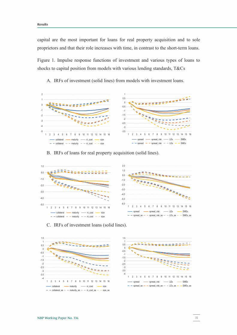
relatively long delay of some 8-11 quarters, Figure 1 (panel A depicts IRFs from 8
models which differ by standards and T&Cs). Models using other types of loans
produce similar results, thus for the sake of space limits, they are not presented here.
In the case of loans for real property acquisition, all models but one, namely this using
maximum size of loan as a variable representing lending T&Cs, give impulse response
functions which are statistically significant, either immediately after the innovation
(model with maximum maturity) or after 7-8 quarters, Figure 1, panel B.
Investment loans are less affected than RPA loans. Their fall is slower and smaller.
The point estimate of this reaction is comparable to that of short-term loans, but the
estimate is more uncertain. Reactions of short-term loans are also statistically
significant after 7-8 quarters and later on, matching a maximum reaction of
investment. Two models out of a total number of eight using this category of loans,
produce a temporary puzzle, i.e. loans increase despite a worsening of banks’ capital
position. The puzzle is not statistically significant, but it may mean that in fact there
exists some substitution of the long-term loans by these on current account, Figure 1
panel C&D.
Loans to sole proprietors, considered here as a separate category, tend to fall after a
shock to bank capital position. As in the case of other loans, this reaction is significant
after 7-8 quarters (Figure 1, panel E). It is relatively quick and large, comparable to
this of loans for real property acquisition for corporates. Thus, it seems that despite
de minimis programme, which can be considered as an additional collateral provided
to the smallest firms, they are the most vulnerable.
Responses of investment as well as of loans to shocks to capital display some
persistence. They return to the baseline after 36-40 quarters. These long-lasting
responses seem to be caused by persistence in reactions of the interest rate and
standards and T&Cs.
Decomposition of variance of loans to corporates and sole proprietors, Table 2,
provides information from a slightly different perspective: it confirms that shocks to
Narodowy Bank Polski30
2
1
0
-1
-2
-3
-4
-5
10.5
0-0.5
-1-1.5
-2-2.5
-3-3.5
21 10 11 12 13 14 15 163 4 5 6 7 8 9 21 10 11 12 13 14 15 163 4 5 6 7 8 9
1.51
0.50
-0.5
-1.5-2
-2.5-3
-4-3.5
-1
10.5
1.5
0-0.5
-1-1.5
-2-2.5
-3
-4-3.5
21 10 11 12 13 14 15 163 4 5 6 7 8 9
21 10 11 12 13 14 15 163 4 5 6 7 8 9
1.0
0.0
-1.0
-2.0
-3.0
-4.0
-5.021 10 11 12 13 14 15 163 4 5 6 7 8 9
2.0
1.0
0.0
-1.0
-4.0
-5.0
-3.0
-2.0
-6.021 10 11 12 13 14 15 163 4 5 6 7 8 9
collateral maturity ni_cost sizecollateral maturity ni_cost size
collateral maturity ni_cost sizecollateral maturity ni_cost size
collateral maturity ni_cost sizecollateral_se maturity_se ni_cost_se size_se
spread spread_risk LEs SMEsspread_risk LEs SMEsspread
spread spread_risk LEs SMEsspread_risk_se LEs_se SMEs_sespread_se
spread spread_risk LEs SMEsspread_risk_se LEs_se SMEs_sespread_se
28
capital are the most important for loans for real property acquisition and to sole
proprietors and that their role increases with time, in contrast to the short-term loans.
Figure 1. Impulse response functions of investment and various types of loans to
shocks to capital position from models with various lending standards, T&Cs
A. IRFs of investment (solid lines) from models with investment loans.
B. IRFs of loans for real property acquisition (solid lines).
C. IRFs of investment loans (solid lines).
31NBP Working Paper No. 336
Results

10.5
0-0.5
-1.5-2
-2.5-3
-4-3.5
-1
1.5
1
0.5
0
-0.5
-1.5
-2
-2.5
-1
1.51
0.50
-0.5
-1.5-2
-2.5-3
-1
10.5
0-0.5
-1.5-2
-2.5-3
-4-3.5
-1
collateral maturity ni_cost sizecollateral_se maturity_se ni_cost_se size_se
collateral maturity ni_cost sizecollateral_se maturity_se ni_cost_se size_se
spread spread_risk LEs SMEsspread_risk_se LEs_se SMEs_sespread_se
spread spread_risk std_short std_longspread_risk_se std_short_se std_long_sespread_se
21 10 11 12 13 14 15 163 4 5 6 7 8 9 21 10 11 12 13 14 15 163 4 5 6 7 8 9
21 10 11 12 13 14 15 163 4 5 6 7 8 9
21 10 11 12 13 14 15 163 4 5 6 7 8 9
29
D. IRFs of loans for working capital and on current account (solid lines).
E. IRF of loans to sole proprietors to shocks to capital (solid lines)
Horizontal axis shows quarters after the shock, vertical axis shows a change in the respective loans in %. “Collateral”, “maturity” mean a model with collateral or maturity as a variable representing T&Cs. SMEs or LEs mean the respective lending standards. Dashed lines are for the respective confidence intervals ± 2 S.E. Source: Own calculations.
Table 2. Variance decomposition of loans: the role of capital shocks, in %
Quarter after the shock
Investment loans
Loans for real property acquisition
Loans in current account and for working capital
Loan to sole proprietors
4 0.6 1.5 3.1 0.38 2.2 6.6 3.7 2.512 3.9 17.9 3.1 9.116 5.4 26.0 2.9 12.8
Source: Own calculations.
Narodowy Bank Polski32

30
5.3. Robustness checks
Positive shocks to aggregate demand obtained from the benchmark models increase
all types of loans. Better economic outlook improves the number of investment
projects which are considered as profitable in terms of expected net present value.
This induces banks to loose lending policy. However, there is some heterogeneity in
their reactions. In models containing loans on current account and for working capital,
all terms and conditions become less stringent; standards behave likewise, but in this
case we do not obtain a statistically significant reaction. In models with long-term
loans, either on investment or for real property acquisition, only some T&Cs are
loosened – in the case of loans for investment this is spread, whereas in the case of
loans for real property acquisition – spread, non-interest rate cost and maximum
maturity. Thus, it seems that bank policy with respect to WC&CA loans changes with
the business cycle, whereas it does somewhat less so in the case of loans for
investment. The policy with respect to RPA lending remains somewhere in between.
Positive shocks to demand for loans bring about diversified reactions of the
investigated variables, depending on the type of credit used in estimates. On one hand,
reactions obtained from models with RPA loans do not display any significant
reactions of either investment or the interest rate. On the other hand, those from
models using other types of loans show a fall in the interest rate. This is implausible
and – as expected – casts doubts whether our models properly identify shocks to credit
demand.
Responses to credit demand shocks obtained from the enlarged setting as in (6), show
that that in the case of these to credit on current account and for working capital, the
lending rate does not react at all for one to two quarters after the impulse and then
tends to fall; they also increase investment, but the effect is delayed. Shocks to demand
for investment loans increase lending rate by about 5 basis points for two quarters;
they leave investment practically intact. Finally, shocks to demand for loans for real
property acquisition, which are much larger than those to investment loans or
WC&CA loans, induce a statistically significant increase in both WIBOR rate and the
33NBP Working Paper No. 336
Results

31
lending rate by about 20 basis points 4 quarters after the impulse. As a result
investment tends to fall, but the effect is not significant.
Shocks to the monetary policy rate obtained from the benchmark models tend to
decrease investment and loans for real property acquisition. The reaction of loans for
investment, although usually negative, is not significant. Credit on current account
and for financing working capital temporarily increases, as in Giannone et al. (2019)
and falls only after some 4 quarters after the impulse; this may once again support the
hypothesis of a substitution between investment loans and credit on current account.
Loans for sole proprietors display behaviour similar to that of WC&CA loans.
Besides, interest rate shocks worsen capital position of banks and induce tightening
of lending standards, terms and conditions. The reactions of standards for SMEs are
larger than those for LEs.
Shocks to bank lending standards for SMEs (tightening) obtained from models with
investment loans induce a statistically significant decline of investment and
investment loans. Shocks to standards for LEs have a similar impact on investment,
but the reaction of loans, although negative, is not significant. Loans for real property
acquisition do not react to shocks to standards. Shocks to standards on short-term
loans, induce negative reactions of both investment and loans on current account and
for working capital, but they are not statistically significant.
All in all, besides shocks to demand for credit, other shocks identified in the
benchmark models induce impulse response functions which are consistent with the
economic theory or empirical findings in the literature.
Models employing POLONIA rate give smaller responses of investment and loans to
shocks to capital, since POLONIA itself increases less to these shocks. Nonetheless,
the responses are not qualitatively different comparing to the benchmark specification.
None of the dummy variables has a visible impact on the results.
Narodowy Bank Polski34

32
6. Summary and conclusions
In the paper, we show how shocks to bank capital, as reported in the Senior Loan
Officer Opinion Survey, conducted by Narodowy Bank Polski, affect bank lending
policy and activity of the real sector. We plug survey data into a suite of structural
vector autoregression models and examine reactions of various types of loans to the
corporate sector: for investment, for real property acquisition, loans on current
account and for financing working capital. To show reactions of the supposedly
riskiest firms, we also consider loans extended to sole proprietors, i.e. tiny business
run by the owner, seemingly suffering the most from the agency problem and
asymmetric information.
The estimates bring three major conclusions. Firstly, they show that shocks to capital
position affect lending standards on long-term and short-term loans for both, large
(LEs) and small and medium-sized enterprises (SMEs). They also have an impact on
all considered T&Cs: average spread, spread on riskier loans, collateral, non-interest
rate cost, maximum size and maturity of a loan. This means that shocks to capital lead
banks to reduce credit supply. Importantly, banks tend to react rather through these
T&Cs which are related to price, such as average spread and spread on riskier loans.
This has implications for the monetary policy. As shown in Wróbel (2018), monetary
policy shocks also affect lending standards, terms and conditions. Put it another way,
monetary shocks and shocks to capital are transmitted through the same channels.
Thus, there is a need for a good calibration of the two policies to avoid situations of a
too tight/too loose policy mix. For example, contractionary monetary policy increases
the price of credit and constraints credit availability to the new borrowers due to a fall
in value of collateral. Tightening of macroprudential policy through increased capital
ratio would result in the even higher spreads and lending cost, lower supply of loans
and changes in the structure of supply towards lower risk.
This leads us to the second conclusion, namely, to the pattern of bank responses to
shocks to capital. Our estimates show that following such innovations, more banks
tend to tighten credit policy with respect to SMEs than to LEs. Thus, banks apparently
intend to de-risk their credit portfolios. As a result, SMEs may face more problems
35NBP Working Paper No. 336
Chapter 6
33
with access to external financing and are more vulnerable to macro-prudential policy
than LEs. This also means that some sectors, such as services, which are more
populated by SMEs, can be more affected by macroprudential tightening that other
sectors.
Thirdly, we show that shocks to capital constrain lending, but to a diversified extent.
Loans for real property acquisition and these extended to sole proprietors display the
largest reactions. This is also an argument supporting our conclusion that banks de-
risk their credit portfolios. Moreover, shocks to capital do have real effects –
investment falls after a negative innovation to the capital position of banks. The effect
is transitory, but not negligible.
Narodowy Bank Polski36

34
References
Berrospide J. M., Edge R., (2010), The Effects of Bank Capital on Lending: What Do We Know, and What Does it Mean?, International Journal of Credit and Banking, vol. 6(4), 5-54.
Berrospide J. M., Meisenzahl R. R., (2015), The Real Effects of Credit Line Drawdowns, Finance and Economics Discussion Series Divisions of Research & Statistics and Monetary Affairs Federal Reserve Board, Washington, D.C.
Bidder R. M, Krainer J. R., Shapiro A. H., (2020), De-leveraging or de-risking? How banks cope with loss, Review of Economic Dynamics,https://doi.org/10.1016/j.red.2020.06.014.
Black L.K., Rosen R. J., (2016), Monetary Policy, Loan Maturity, and Credit Availability, International Journal of Central Banking, vol. 12(1), 199-230.
Bridges J., Gregory D., Nielsen M., Pezzini S., Radia A., and Spaltro M. (2014), The impact of capital requirements on bank lending, Working Paper, 486, Bank of England.
Choi W.W., Cook D. (2018), Policy Conflicts and Inflation Targeting: The Role of Credit Markets, IMF Working Paper WP 18/72, International Monetary Fund.
Ciccarelli M., Maddaloni A., Peydró (2015), Trusting the bankers. A new look at the credit channel of monetary policy, Review of Economic Dynamics, vol.18(4),979-1002.
Chmielewski T., Kocięcki A., Łyziak T., Przystupa J., Stanisławska E., Walerych M., Wróbel E. (2019), Monetary policy transmission mechanism in Poland, What do we know in 2019? NBP Working Paper, 329, Narodowy Bank Polski.
Cohen B.H. (2013), How have banks adjusted to higher capital requirements? BIS Quarterly Review, September, Bank for International Settlements.
Couaillier C. (2015): Do Loan Terms and Conditions Channel ECB’s Monetary Policy? Applying Bayesian and Panel VAR to the Bank Lending Survey,https://afse2016.sciencesconf.org/98953/document
De Bondt G., Maddaloni A., Peydró J-L., Scopel S. (2010), The euro area bank
lending survey matters. Empirical evidence for credit and output growth,
Working Paper, 1160, European Central Bank.
37NBP Working Paper No. 336
References

35
Fraisse H., Lé M., Thesmar D., (2017), The real effects of bank capital requirements,
Working Paper, 47, European Systemic Risk Board.
Fender I., Lewrick U., (2016), Adding it all up: the macroeconomic impact of Basel
III and outstanding reform issues, BIS Working Paper, 591, Bank for
International Settlements.
Gambetti L., Musso A., (2017), Loan Supply Shocks and the Business Cycle, Journal
of Applied Econometrics, 32(4), 764-782.
GUS (2015), Small and medium non-financial enterprises in Poland 2009-2013,
Studia i Analizy Statystyczne, Główny Urząd Statystyczny, Warszawa.
GUS (2020), Wyniki finansowe przedsiębiorstw niefinansowych I-XII 2019, Główny
Urząd Statystyczny, Warszawa.
Kanngiesser D., Martin R., Maurin L., Moccero D., (2017), Estimating the impact of shocks to bank capital in the euro area, Working Paper, 2077, European Central Bank.
Kumamoto M. Zhuo J., (2017), Bank Lending Channel in Transmission of the Monetary Policy in Japan, Applied Economics and Finance,4(2), 87-100.
Lown C., Morgan D. (2006), The credit cycle and the business cycle: new findings
using the loan officer opinion survey, Journal of Money Credit and Banking,
38(6), 1575-1597.
Maddaloni A., Peydró J-L., (2013), Monetary Policy, Macro-prudential Policy and Banking Stability. Evidence from the Euro Area, International Journal of Central Banking, 9(1), 121-169.
Martin J. S., Santomero A. M. (1997), Investment opportunities and corporate demand for lines of credit, Journal of Banking and Finance, 21(10), 1331-1350.
Meeks R. (2017), Capital regulation and the macroeconomy: Empirical evidence andmacroprudential policy, European Economic Review, 95(C), 125-141.
NBP (2016), Financial system in Poland, https://www.nbp.pl/en/systemfinansowy/fsd_2016.pdf.
Noss J., Toffano P. (2016), Estimating the impact of changes in aggregate bank capital requirements on lending and growth during an upswing, Journal of Banking and Finance, 62 (C), 15-27.
Narodowy Bank Polski38

36
Ortiz-Molina H., Penas M. F. (2008), Lending to small businesses: the role of loan maturity in addressing information problems, Small Business Economics, 30(4), 361-383.
PARP (2019), Raport o stanie sektora małych i średnich przedsiębiorstw w Polsce,https://www.parp.gov.pl/publications/publication/raport-o-stanie-sektora -malych-i-srednich-przedsiebiorstw-w-polsce
Strahan P. E. (1999), Borrower Risk and the Price and Nonprice Terms of Bank Loans, Staff Reports, 90, Federal Reserve Bank of New York.
Tressel Th., Zhang Y.S., (2016), Effectiveness and Channels of Macro-prudentialInstruments, Lessons from the Euro Area, IMF Working Paper, WP 16/4,International Monetary Fund.
Varner M.A. (2017), Vector Autoregressions with Machine Learning, Honors Theses. http://scarab.bates.edu/honorstheses/216.
Wolf Ch. K. (2019), SVAR (Mis)Identification and the Real Effects of Monetary Policy Shocks, mp_id_201907.pdf (princeton.edu)
Wróbel E. (2018), What is the impact of central bank on banks’ lending policy with respect to the corporate sector? Evidence from SLOOS for Poland, Bank and Credit, 49(6), 596-638.
Tymoczko I. (2018), Kredyty walutowe nie stanowią zagrożenia dla polskich firmhttps://www.obserwatorfinansowy.pl/forma/analizy-debata/analizy/kredyty -walutowe-nie-stanowia-zagrozenia-dla-polskich-przedsiebiorstw/
39NBP Working Paper No. 336
References

70605040302010
0
30
25
20
15
10
5
0
stocks issues on WSElong-term bonds issued on the domestic marketprivate equityleasing
2004
2005
2006
2007
2008
2009
2010
2011
2012
2013
2014
2015
2016
2017
2018
mining, q
uarring
manufac
turing
electri
city, ga
s…
water su
pply
constru
ction
trade, r
epair
transpo
rtation
…
accom
modation
…
informatio
n…
real es
tate…
profes
sional
…
adminis
trative
…
health,
socia
l work
02468
101214
mining, q
uarring
manufac
turing
electri
city, ga
s…
water su
pply
constru
ction
trade, r
epair
transpo
rtation
…
accom
modation
…
informatio
n…
real es
tate…
profes
sional
…
adminis
trative
…
health,
socia
l work
short-term loans of LEslong-term loans of LEs
short-term loans of SMEslong-term loans of SMEs
37
Statistical Appendix
1. Figures
Figure A1. Selected non-bank sources of the enterprise sector financing
PLN billion
Source: Financial System in Poland, NBP, various editions
Figure A2. Allocation of short-term and long-term loans to LEs (LH panel) SMEs (RH panel), 2019, in % of total short-term or long-term loans
Source: Own calculations, GUS data
05
1015202530
min
ing,
qua
rring
man
ufac
turin
gel
ectri
city
,gas
,…w
ater
sup
ply
cons
truct
ion
trade
, rep
air
trans
porta
tion,
…ac
com
mod
atio
n,…
info
rmat
ion,
…re
al e
stat
e…pr
ofes
sion
al,…
adm
inis
trativ
e…he
alth
, soc
ial w
ork
arts
, ent
airte
men
t
short-term loans of LEs
long-term loans of LEs
02468
101214
min
ing,
qua
rring
man
ufac
turin
gel
ectri
city
,gas
,…w
ater
sup
ply
cons
truct
ion
trade
, rep
air
trans
porta
tion,
…ac
com
mod
atio
n,…
info
rmat
ion,
…re
al e
stat
e…pr
ofes
sion
al,…
adm
inis
trativ
e…he
alth
, soc
ial w
ork
arts
, ent
airte
men
t
short-term loans of SMEs
long-term loans of SMEs
Narodowy Bank Polski40
Statistical Appendix

2
-2
1.5
-1.5
1
-1
0.5
-0.50
1210
-10
8
-8
6
-6
4
-4
2
-20
investment gap TCR* gap Capital_SLOOS gap
loans/GDP Debt securities/GDP TCR TCR (LH axis) capital, cumulated, SLOOS
capital
2003Q
4
25 21
19
17
15
13
11
9
7
20
15
10
0
5
25
20
15
10
0
5
00,2
-0,2
0,4
-0,4
0,6
-0,6
0,81
4,5
3,5
2,5
1,5
0
1
2
3
4
0,5
2005Q
1200
5Q4
2006Q
3200
7Q2
2008Q
1200
8Q4
2009Q
3201
0Q2
2011Q
1201
1Q4
2012Q
3201
3Q2
2014Q
1201
4Q4
2015Q
3201
6Q2
2017Q
1201
7Q4
2018Q
3201
9Q2
2003Q
4200
5Q1
2006Q
2200
7Q3
2008Q
4201
0Q1
2011Q
2201
2Q3
2013Q
4201
5Q1
2016Q
2201
7Q3
2018Q
4
2003Q
4200
5Q1200
6Q2200
7Q3200
8Q4201
0Q1201
1Q2201
2Q3201
3Q4201
5Q1201
6Q2201
7Q3201
8Q4
2005Q
1200
6Q2
2007Q
3200
8Q4
2010Q
1201
1Q2
2012Q
3201
3Q4
2015Q
1201
6Q2
2017Q
3201
8Q4
706050403020100
30
25
20
15
10
5
0
stocks issues on WSElong-term bonds issued on the domestic marketprivate equityleasing
2004
2005
2006
2007
2008
2009
2010
2011
2012
2013
2014
2015
2016
2017
2018
mining, q
uarring
manufac
turing
electri
city, ga
s…
water su
pply
constru
ction
trade, r
epair
transpo
rtation
…
accom
modation
…
informatio
n…
real es
tate…
profes
sional
…
adminis
trative
…
health,
socia
l work
02468
101214
mining, q
uarring
manufac
turing
electri
city, ga
s…
water su
pply
constru
ction
trade, r
epair
transpo
rtation
…
accom
modation
…
informatio
n…
real es
tate…
profes
sional
…
adminis
trative
…
health,
socia
l work
short-term loans of LEslong-term loans of LEs
short-term loans of SMEslong-term loans of SMEs
38
Figure A3. HP detrended: TCR*, accumulated responses on capital from SLOOS (LHaxis) and investment (RH axis)
* To the end of 2013 Capital Adequacy RatioSource: Own estimates
Figure A4. Bank loans to firms/GDP,debt securities/GDP (LH) and TCR*(RH axis), in %
Figure A5. TCR* (LH) and accumulated data on capital position from SLOOS(RH axis)
*To the end of 2013 Capital Adequacy RatioSource :NBP, PFSA, Eurostat
Figure A6. Capital position from SLOOS, change, q/q (1=100%)
Source: NBP
41NBP Working Paper No. 336
Statistical Appendix

-0.50
-0.25
0.00
0.25
0.50
0.75
1.00
-.6
-.4
-.2
.0
.2
.4
.6
-0.50
-0.25
0.00
0.25
0.50
0.75
1.00
-.6
-.4
-.2
.0
.2
.4
.6
2005:1
2006:1
2007:1
2008:1
2009:1
2010:1
2011:1
2012:1
2013:1
2014:1
2015:1
2016:1
2017:1
2018:1
2019:1
d(i_corp-i_mm), RHSspreadspread_riskier
2005:1
2006:1
2007:1
2008:1
2009:1
2010:1
2011:1
2012:1
2013:1
2014:1
2015:1
2016:1
2017:1
2018:1
2019:1
d(i_corp-i_mm), RHSspreadspread_riskier
2003Q
4200
5Q1200
6Q2
2007Q
3200
8Q4201
0Q1201
1Q2201
2Q3201
3Q4
2015Q
1201
6Q2201
7Q3
2018Q
4 2003Q
4200
5Q1200
6Q2
2007Q
3200
8Q4201
0Q1201
1Q2201
2Q3201
3Q4201
5Q1201
6Q2201
7Q3
2018Q
4
collateralmaturity size non-int rate costspread spread risk
0.8
-0.8
0.6
-0.6
0.4
-0.4
0.2
-0.20
10.80.6
-0.6
0.4
-0.4
0.2
-0.20
1
LEs shortLEs long SMEs shortSMEs long
39
Figure A7. Standards on short- and long-term loans for LEs and SMEs (1=100%)
Figure A8. Terms and conditions of lending to corporates (1=100%)
Source: NBP
Figure A9. Change in spread on loans to the corporate sector (RHS, in percentage points) and data on spreads from SLOOS (LHS, 1=100%)
Figure A10. Change in spread on loans to sole proprietors (RHS, in percentage points) and data on spreads from SLOOS (LHS, 1=100%)
-0.50
-0.25
0.00
0.25
0.50
0.75
1.00
-.6
-.4
-.2
.0
.2
.4
.6
2005
:1
2006
:1
2007
:1
2008
:1
2009
:1
2010
:1
2011
:1
2012
:1
2013
:1
2014
:1
2015
:1
2016
:1
2017
:1
2018
:1
2019
:1
d(i_corp-i_mm), RHSspreadspread_riskier
-0.50
-0.25
0.00
0.25
0.50
0.75
1.00
-.6
-.4
-.2
.0
.2
.4
.6
2005
:1
2006
:1
2007
:1
2008
:1
2009
:1
2010
:1
2011
:1
2012
:1
2013
:1
2014
:1
2015
:1
2016
:1
2017
:1
2018
:1
2019
:1
d(i_corp-i_mm), RHSspreadspread_riskier
Source: Own calculations, NBP data.
2. Tables
d(i_corp-i_mm), RHSspreadspread_riskier
d(i_sp-i_mm), RHSspreadspread_riskier
-0.50
-0.25
0.00
0.25
0.50
0.75
1.00
-.6
-.4
-.2
.0
.2
.4
.6
-0.50
-0.25
0.00
0.25
0.50
0.75
1.00
-.8
-.4
.0
.4
.8
2005:1
2006:1
2007:1
2008:1
2009:1
2010:1
2011:1
2012:1
2013:1
2014:1
2015:1
2016:1
2017:1
2018:1
2019:1
2005:1
2004:2
2006:1
2007:1
2008:1
2009:1
2010:1
2011:1
2012:1
2013:1
2014:1
2015:1
2016:1
2017:1
2018:1
2019:1
Narodowy Bank Polski42
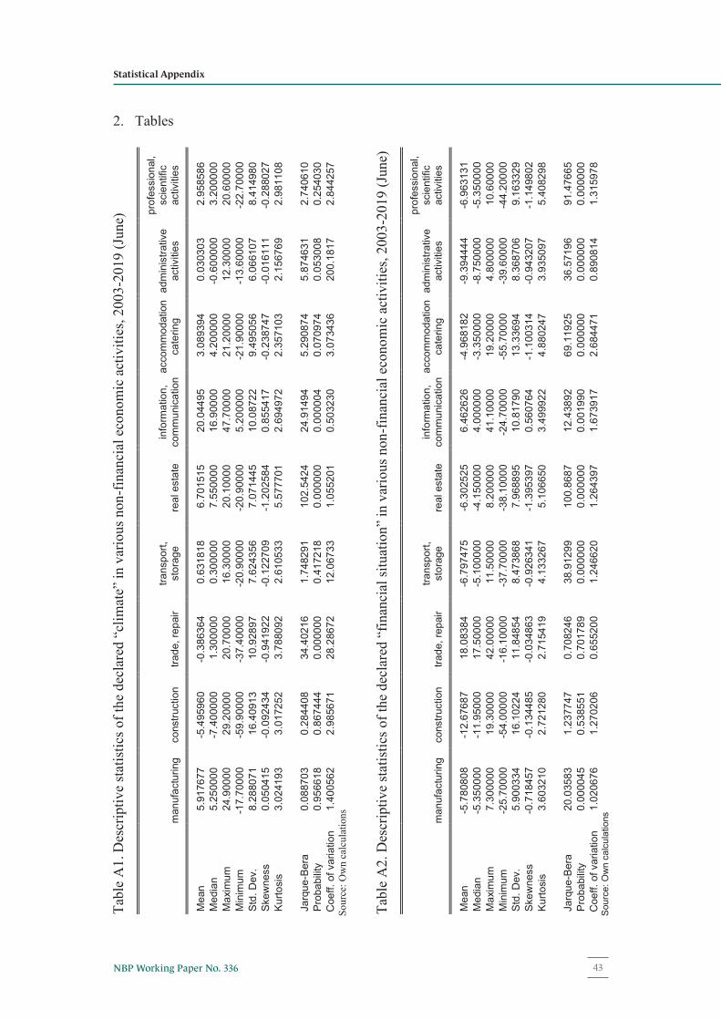
-0.50
-0.25
0.00
0.25
0.50
0.75
1.00
-.6
-.4
-.2
.0
.2
.4
.6
-0.50
-0.25
0.00
0.25
0.50
0.75
1.00
-.6
-.4
-.2
.0
.2
.4
.6
2005:1
2006:1
2007:1
2008:1
2009:1
2010:1
2011:1
2012:1
2013:1
2014:1
2015:1
2016:1
2017:1
2018:1
2019:1
d(i_corp-i_mm), RHSspreadspread_riskier
2005:1
2006:1
2007:1
2008:1
2009:1
2010:1
2011:1
2012:1
2013:1
2014:1
2015:1
2016:1
2017:1
2018:1
2019:1
d(i_corp-i_mm), RHSspreadspread_riskier
2003Q
4200
5Q1200
6Q2
2007Q
3200
8Q4201
0Q1201
1Q2201
2Q3201
3Q4
2015Q
1201
6Q2201
7Q3
2018Q
4 2003Q
4200
5Q1200
6Q2
2007Q
3200
8Q4201
0Q1201
1Q2201
2Q3201
3Q4201
5Q1201
6Q2201
7Q3
2018Q
4
collateralmaturity size non-int rate costspread spread risk
0.8
-0.8
0.6
-0.6
0.4
-0.4
0.2
-0.20
10.80.6
-0.6
0.4
-0.4
0.2
-0.20
1
LEs shortLEs long SMEs shortSMEs long
-0.50
-0.25
0.00
0.25
0.50
0.75
1.00
-.6
-.4
-.2
.0
.2
.4
.6
-0.50
-0.25
0.00
0.25
0.50
0.75
1.00
-.6
-.4
-.2
.0
.2
.4
.6
2005:1
2006:1
2007:1
2008:1
2009:1
2010:1
2011:1
2012:1
2013:1
2014:1
2015:1
2016:1
2017:1
2018:1
2019:1
d(i_corp-i_mm), RHSspreadspread_riskier
2005:1
2006:1
2007:1
2008:1
2009:1
2010:1
2011:1
2012:1
2013:1
2014:1
2015:1
2016:1
2017:1
2018:1
2019:1
d(i_corp-i_mm), RHSspreadspread_riskier
2003Q
4200
5Q1200
6Q2
2007Q
3200
8Q4201
0Q1201
1Q2201
2Q3201
3Q4
2015Q
1201
6Q2201
7Q3
2018Q
4 2003Q
4200
5Q1200
6Q2
2007Q
3200
8Q4201
0Q1201
1Q2201
2Q3201
3Q4201
5Q1201
6Q2201
7Q3
2018Q
4
collateralmaturity size non-int rate costspread spread risk
0.8
-0.8
0.6
-0.6
0.4
-0.4
0.2
-0.20
10.80.6
-0.6
0.4
-0.4
0.2
-0.20
1
LEs shortLEs long SMEs shortSMEs long
40
Tabl
e A
1.D
escr
iptiv
e sta
tistic
s of t
he d
ecla
red
“clim
ate”
in v
ario
us n
on-f
inan
cial
eco
nom
ic a
ctiv
ities
, 200
3-20
19 (J
une)
man
ufac
turin
gco
nstru
ctio
ntra
de, r
epai
rtra
nspo
rt,
stor
age
real
est
ate
info
rmat
ion,
co
mm
unic
atio
nac
com
mod
atio
n ca
terin
gad
min
istra
tive
activ
ities
prof
essi
onal
, sc
ient
ific
activ
ities
Mea
n5.
9176
77-5
.495
960
-0.3
8636
40.
6318
186.
7015
1520
.044
953.
0893
940.
0303
032.
9585
86M
edia
n5.
2500
00-7
.400
000
1.30
0000
0.30
0000
7.55
0000
16.9
0000
4.20
0000
-0.6
0000
03.
2000
00M
axim
um24
.900
0029
.200
0020
.700
0016
.300
0020
.100
0047
.700
0021
.200
0012
.300
0020
.600
00M
inim
um-1
7.70
000
-59.
9000
0-3
7.40
000
-20.
9000
0-2
0.90
000
5.20
0000
-21.
9000
0-1
3.60
000
-22.
7000
0St
d. D
ev.
8.28
8071
16.4
0913
10.9
2897
7.62
4356
7.07
1445
10.0
8722
9.49
5056
6.06
6107
8.41
4980
Skew
ness
0.05
0415
-0.0
9243
4-0
.941
922
-0.1
2270
9-1
.202
584
0.85
5417
-0.2
3874
7-0
.016
111
-0.2
8802
7Ku
rtosi
s3.
0241
933.
0172
523.
7880
922.
6105
335.
5777
012.
6949
722.
3571
032.
1567
692.
9811
08
Jarq
ue-B
era
0.08
8703
0.28
4408
34.4
0216
1.74
8291
102.
5424
24.9
1494
5.29
0874
5.87
4631
2.74
0610
Prob
abilit
y0.
9566
180.
8674
440.
0000
000.
4172
180.
0000
000.
0000
040.
0709
740.
0530
080.
2540
30C
oeff.
of v
aria
tion
1.40
0562
2.98
5671
28.2
8672
12.0
6733
1.05
5201
0.50
3230
3.07
3436
200.
1817
2.84
4257
Sour
ce: O
wn
calc
ulat
ions
Tabl
e A
2.D
escr
iptiv
e sta
tistic
s of t
he d
ecla
red
“fin
anci
al si
tuat
ion”
in v
ario
us n
on-f
inan
cial
eco
nom
ic a
ctiv
ities
, 200
3-20
19 (J
une)
man
ufac
turin
gco
nstru
ctio
ntra
de, r
epai
rtra
nspo
rt,
stor
age
real
est
ate
info
rmat
ion,
co
mm
unic
atio
nac
com
mod
atio
n ca
terin
gad
min
istra
tive
activ
ities
prof
essi
onal
, sc
ient
ific
activ
ities
Mea
n-5
.780
808
-12.
6768
718
.083
84-6
.797
475
-6.3
0252
56.
4626
26-4
.968
182
-9.3
9444
4-6
.963
131
Med
ian
-5.3
5000
0-1
1.95
000
17.5
0000
-5.1
0000
0-4
.150
000
4.00
0000
-3.3
5000
0-8
.750
000
-5.3
5000
0M
axim
um7.
3000
0019
.300
0042
.000
0011
.500
008.
2000
0041
.100
0019
.200
004.
8000
0010
.600
00M
inim
um-2
5.70
000
-54.
0000
0-1
6.10
000
-37.
7000
0-3
8.10
000
-24.
7000
0-5
5.70
000
-39.
6000
0-4
4.20
000
Std.
Dev
.5.
9003
3416
.102
2411
.848
548.
4738
687.
9688
9510
.817
9013
.336
948.
3687
069.
1633
29Sk
ewne
ss-0
.718
457
-0.1
3448
5-0
.034
863
-0.9
2634
1-1
.395
397
0.56
0764
-1.1
0031
4-0
.943
207
-1.1
4980
2Ku
rtosi
s3.
6032
102.
7212
802.
7154
194.
1332
675.
1066
503.
4999
224.
8802
473.
9350
975.
4082
98
Jarq
ue-B
era
20.0
3583
1.23
7747
0.70
8246
38.9
1299
100.
8687
12.4
3892
69.1
1925
36.5
7196
91.4
7665
Prob
abilit
y0.
0000
450.
5385
510.
7017
890.
0000
000.
0000
000.
0019
900.
0000
000.
0000
000.
0000
00C
oeff.
of v
aria
tion
1.02
0676
1.27
0206
0.65
5200
1.24
6620
1.26
4397
1.67
3917
2.68
4471
0.89
0814
1.31
5978
Sour
ce: O
wn
calc
ulat
ions
39
Figure A7. Standards on short- and long-term loans for LEs and SMEs (1=100%)
Figure A8. Terms and conditions of lending to corporates (1=100%)
Source: NBP
Figure A9. Change in spread on loans to the corporate sector (RHS, in percentage points) and data on spreads from SLOOS (LHS, 1=100%)
Figure A10. Change in spread on loans to sole proprietors (RHS, in percentage points) and data on spreads from SLOOS (LHS, 1=100%)
-0.50
-0.25
0.00
0.25
0.50
0.75
1.00
-.6
-.4
-.2
.0
.2
.4
.6
2005
:1
2006
:1
2007
:1
2008
:1
2009
:1
2010
:1
2011
:1
2012
:1
2013
:1
2014
:1
2015
:1
2016
:1
2017
:1
2018
:1
2019
:1
d(i_corp-i_mm), RHSspreadspread_riskier
-0.50
-0.25
0.00
0.25
0.50
0.75
1.00
-.6
-.4
-.2
.0
.2
.4
.6
2005
:1
2006
:1
2007
:1
2008
:1
2009
:1
2010
:1
2011
:1
2012
:1
2013
:1
2014
:1
2015
:1
2016
:1
2017
:1
2018
:1
2019
:1
d(i_corp-i_mm), RHSspreadspread_riskier
Source: Own calculations, NBP data.
2. Tables
43NBP Working Paper No. 336
Statistical Appendix
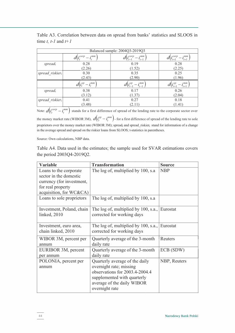
41
Table A3. Correlation between data on spread from banks’ statistics and SLOOS intime t, t-1 and t+1
Balanced sample: 2004Q3-2019Q3
( )mmt
corpt iid − ( )mm
tcorpt iid 11 −− − ( )mm
tcorpt iid 11 ++ −
spreadt 0.28 (2.26)
0.19 (1.52)
0.28 (2.25)
spread_riskiert 0.30 (2.43)
0.35 (2.90)
0.25 (1.96)
( )mmt
spt iid − ( )mm
tspt iid 11 −− − ( )mm
tspt iid 11 ++ −
spreadt 0.38 (3.12)
0.17 (1.37)
0.26 (2.04)
spread_riskiert 0.41 (3.48)
0.27 (2.11)
0.18 (1.41)
Note: ( )mmt
corpt iid − stands for a first difference of spread of the lending rate to the corporate sector over
the money market rate (WIBOR 3M), ( )mmt
spt iid − - for a first difference of spread of the lending rate to sole
proprietors over the money market rate (WIBOR 3M); spreadt and spread_riskiert stand for information of a changein the average spread and spread on the riskier loans from SLOOS; t-statistics in parentheses.
Source: Own calculations, NBP data.
Table A4. Data used in the estimates; the sample used for SVAR estimations coversthe period 2003Q4-2019Q2.
Variable Transformation SourceLoans to the corporate sector in the domestic currency (for investment, for real property acquisition, for WC&CA)
The log of, multiplied by 100, s.a NBP
Loans to sole proprietors The log of, multiplied by 100, s.a
Investment, Poland, chain linked, 2010
The log of, multiplied by 100, s.a., corrected for working days
Eurostat
Investment, euro area, chain linked, 2010
The log of, multiplied by 100, s.a., corrected for working days
Eurostat
WIBOR 3M, percent per annum
Quarterly average of the 3-monthdaily rate
Reuters
EURIBOR 3M, percent per annum
Quarterly average of the 3-monthdaily rate
ECB (SDW)
POLONIA, percent per annum
Quarterly average of the daily overnight rate; missing observations for 2003.4-2004.4 supplemented with quarterly average of the daily WIBOR overnight rate
NBP, Reuters
Narodowy Bank Polski44

41
Table A3. Correlation between data on spread from banks’ statistics and SLOOS intime t, t-1 and t+1
Balanced sample: 2004Q3-2019Q3
( )mmt
corpt iid − ( )mm
tcorpt iid 11 −− − ( )mm
tcorpt iid 11 ++ −
spreadt 0.28 (2.26)
0.19 (1.52)
0.28 (2.25)
spread_riskiert 0.30 (2.43)
0.35 (2.90)
0.25 (1.96)
( )mmt
spt iid − ( )mm
tspt iid 11 −− − ( )mm
tspt iid 11 ++ −
spreadt 0.38 (3.12)
0.17 (1.37)
0.26 (2.04)
spread_riskiert 0.41 (3.48)
0.27 (2.11)
0.18 (1.41)
Note: ( )mmt
corpt iid − stands for a first difference of spread of the lending rate to the corporate sector over
the money market rate (WIBOR 3M), ( )mmt
spt iid − - for a first difference of spread of the lending rate to sole
proprietors over the money market rate (WIBOR 3M); spreadt and spread_riskiert stand for information of a changein the average spread and spread on the riskier loans from SLOOS; t-statistics in parentheses.
Source: Own calculations, NBP data.
Table A4. Data used in the estimates; the sample used for SVAR estimations coversthe period 2003Q4-2019Q2.
Variable Transformation SourceLoans to the corporate sector in the domestic currency (for investment, for real property acquisition, for WC&CA)
The log of, multiplied by 100, s.a NBP
Loans to sole proprietors The log of, multiplied by 100, s.a
Investment, Poland, chain linked, 2010
The log of, multiplied by 100, s.a., corrected for working days
Eurostat
Investment, euro area, chain linked, 2010
The log of, multiplied by 100, s.a., corrected for working days
Eurostat
WIBOR 3M, percent per annum
Quarterly average of the 3-monthdaily rate
Reuters
EURIBOR 3M, percent per annum
Quarterly average of the 3-monthdaily rate
ECB (SDW)
POLONIA, percent per annum
Quarterly average of the daily overnight rate; missing observations for 2003.4-2004.4 supplemented with quarterly average of the daily WIBOR overnight rate
NBP, Reuters
Interest rate on credit on current account (outstanding amounts), per cent per annum
Quarterly average of monthly rate NBP
Average interest rate on new and renegotiated business, per cent per annum
Quarterly average of monthly rate NBP
Investment deflator,2010 =100
The log of, multiplied by 100, s.a. Eurostat
GDP deflator,2010 = 100
The log of, multiplied by 100, s.a. Eurostat
Lending standards(on long term andshort-term credits to:(i) LEs, and (ii) SMEs)
Multiplied by -100 NBP, SLOOS
Lending terms and conditions: spread, spread for riskier borrowers, non-interest rate cost, maximum size, maximum maturity, required collateral
Multiplied by -100 NBP (SLOOS)
Capital position of banks Multiplied by -100 NBP (SLOOS) Loans to the corporate sector, real terms
Loans to the corporate sector-investment deflator
Own calculations
Loans to sole proprietors, real
Loans to sole proprietors - GDP deflator
Own calculations
45NBP Working Paper No. 336
Statistical Appendix

www.nbp.pl
Related Documents


![Subcortical heterotopic gray matter brain malformationstheir normal position in the cortex (heterotopic gray matter brain malformations [HET]). The most commonly encoun-tered heterotopia](https://static.cupdf.com/doc/110x72/5e479a488e3f397a933aa426/subcortical-heterotopic-gray-matter-brain-malformations-their-normal-position-in.jpg)