Chapter 1 Problems 1-1 through 1-6 are for student research. No standard solutions are provided. 1-7 From Fig. 1-2, cost of grinding to 0.0005 in is 270%. Cost of turning to 0.003 in is 60%. Relative cost of grinding vs. turning = 270/60 = 4.5 times Ans. ______________________________________________________________________________ 1-8 C A = C B , 10 + 0.8 P = 60 + 0.8 P 0.005 P 2 P 2 = 50/0.005 P = 100 parts Ans. ______________________________________________________________________________ 1-9 Max. load = 1.10 P Min. area = (0.95) 2 A Min. strength = 0.85 S To offset the absolute uncertainties, the design factor, from Eq. (1-1) should be 2 1.10 1.43 . 0.85 0.95 d n A ns ______________________________________________________________________________ 1-10 (a) X 1 + X 2 : 1 2 1 1 2 2 1 2 1 2 1 2 error . x x X e X e e x x X X e e Ans (b) X 1 X 2 : 1 2 1 1 2 2 1 2 1 2 1 2 . x x X e X e e x x X X e e Ans (c) X 1 X 2 : 1 2 1 1 2 2 1 2 1 2 1 2 2 1 1 2 1 2 1 2 2 1 1 2 1 2 . xx X e X e e xx XX Xe Xe ee e e X e Xe XX Ans X X Chapter 1 Solutions - Rev. B, Page 1/6

Shigley's mechanical engineering design 9th edition solutions manual
Jan 17, 2017
Welcome message from author
This document is posted to help you gain knowledge. Please leave a comment to let me know what you think about it! Share it to your friends and learn new things together.
Transcript
Chapter 1 Problems 1-1 through 1-6 are for student research. No standard solutions are provided. 1-7 From Fig. 1-2, cost of grinding to 0.0005 in is 270%. Cost of turning to 0.003 in is
60%. Relative cost of grinding vs. turning = 270/60 = 4.5 times Ans. ______________________________________________________________________________ 1-8 CA = CB, 10 + 0.8 P = 60 + 0.8 P 0.005 P 2 P 2 = 50/0.005 P = 100 parts Ans. ______________________________________________________________________________ 1-9 Max. load = 1.10 P Min. area = (0.95)2A Min. strength = 0.85 S To offset the absolute uncertainties, the design factor, from Eq. (1-1) should be
2
1.101.43 .
0.85 0.95dn A ns
______________________________________________________________________________ 1-10 (a) X1 + X2:
1 2 1 1 2 2
1 2 1 2
1 2
error
.
x x X e X e
e x x X X
e e Ans
(b) X1 X2:
1 2 1 1 2 2
1 2 1 2 1 2 .
x x X e X e
e x x X X e e Ans
(c) X1 X2:
1 2 1 1 2 2
1 2 1 2 1 2 2 1 1 2
1 21 2 2 1 1 2
1 2
.
x x X e X e
e x x X X X e X e e e
e eX e X e X X Ans
X X
Chapter 1 Solutions - Rev. B, Page 1/6
(d) X1/X2:
1 1 1 1 1 1
2 2 2 2 2 2
1
2 2 1 1 1 2 1
2 2 2 2 1 2 1
1 1 1 1 2
2 2 2 1 2
1
1
11 1 then 1 1 1
1
Thus, .
x X e X e X
x X e X e X
e e e X e e e 2
2
e
X X e X X X X
x X X e ee Ans
x X X X X
X
______________________________________________________________________________
1-11 (a) x1 = 7 = 2.645 751 311 1 X1 = 2.64 (3 correct digits)
x2 = 8 = 2.828 427 124 7 X2 = 2.82 (3 correct digits) x1 + x2 = 5.474 178 435 8 e1 = x1 X1 = 0.005 751 311 1 e2 = x2 X2 = 0.008 427 124 7 e = e1 + e2 = 0.014 178 435 8 Sum = x1 + x2 = X1 + X2 + e = 2.64 + 2.82 + 0.014 178 435 8 = 5.474 178 435 8 Checks (b) X1 = 2.65, X2 = 2.83 (3 digit significant numbers) e1 = x1 X1 = 0.004 248 688 9 e2 = x2 X2 = 0.001 572 875 3 e = e1 + e2 = 0.005 821 564 2 Sum = x1 + x2 = X1 + X2 + e = 2.65 +2.83 0.001 572 875 3 = 5.474 178 435 8 Checks ______________________________________________________________________________
1-12 3
3
25 1016 10000.799 in .
2.5d
Sd A
n d
ns
Table A-17: d = 7
8in Ans.
Factor of safety:
3
37
8
25 103.29 .
16 1000S
n A
ns
______________________________________________________________________________
1-13 Eq. (1-5): R =1
n
ii
R = 0.98(0.96)0.94 = 0.88
Overall reliability = 88 percent Ans. ______________________________________________________________________________
Chapter 1 Solutions - Rev. B, Page 2/6
1-14 a = 1.500 0.001 in b = 2.000 0.003 in c = 3.000 0.004 in d = 6.520 0.010 in (a) d a b c w = 6.520 1.5 2 3 = 0.020 in = 0.001 + 0.003 + 0.004 +0.010 = 0.018 allt w t
w = 0.020 0.018 in Ans. (b) From part (a), wmin = 0.002 in. Thus, must add 0.008 in to d . Therefore, d = 6.520 + 0.008 = 6.528 in Ans. ______________________________________________________________________________ 1-15 V = xyz, and x = a a, y = b b, z = c c, V abc
V a a b b c c
abc bc a ac b ab c a b c b c a c a b a b c
The higher order terms in are negligible. Thus, V bc a ac b ab c
and, .V bc a ac b ab c a b c a b c
AnsV abc a b c a b c
For the numerical values given, 31.500 1.875 3.000 8.4375 inV
30.002 0.003 0.0040.00427 0.00427 8.4375 0.036 in
1.500 1.875 3.000
VV
V
V = 8.438 0.036 in3 Ans. ______________________________________________________________________________
Chapter 1 Solutions - Rev. B, Page 3/6
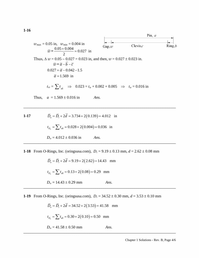
1-16 wmax = 0.05 in, wmin = 0.004 in
0.05 0.004
0.027 in2
w =
Thus, w = 0.05 0.027 = 0.023 in, and then, w = 0.027 0.023 in.
0.027 0.042 1.5
1.569 in
a b c
a
a
w =
tw = 0.023 = t
allt a + 0.002 + 0.005 ta = 0.016 in
Thus, a = 1.569 0.016 in Ans. ______________________________________________________________________________ 1-17 2 3.734 2 0.139 4.012 ino iD D d
all 0.028 2 0.004 0.036 in
oDt t
Do = 4.012 0.036 in Ans. ______________________________________________________________________________ 1-18 From O-Rings, Inc. (oringsusa.com), Di = 9.19 0.13 mm, d = 2.62 0.08 mm 2 9.19 2 2.62 14.43 mmo iD D d
all 0.13 2 0.08 0.29 mm
oDt t
Do = 14.43 0.29 mm Ans. ______________________________________________________________________________ 1-19 From O-Rings, Inc. (oringsusa.com), Di = 34.52 0.30 mm, d = 3.53 0.10 mm 2 34.52 2 3.53 41.58 mmo iD D d
all 0.30 2 0.10 0.50 mm
oDt t
Do = 41.58 0.50 mm Ans. ______________________________________________________________________________
Chapter 1 Solutions - Rev. B, Page 4/6
1-20 From O-Rings, Inc. (oringsusa.com), Di = 5.237 0.035 in, d = 0.103 0.003 in 2 5.237 2 0.103 5.443 ino iD D d
all 0.035 2 0.003 0.041 in
oDt t
Do = 5.443 0.041 in Ans. ______________________________________________________________________________ 1-21 From O-Rings, Inc. (oringsusa.com), Di = 1.100 0.012 in, d = 0.210 0.005 in 2 1.100 2 0.210 1.520 ino iD D d
all 0.012 2 0.005 0.022 in
oDt t
Do = 1.520 0.022 in Ans. ______________________________________________________________________________ 1-22 From Table A-2, (a) = 150/6.89 = 21.8 kpsi Ans. (b) F = 2 /4.45 = 0.449 kip = 449 lbf Ans. (c) M = 150/0.113 = 1330 lbf in = 1.33 kip in Ans. (d) A = 1500/ 25.42 = 2.33 in2 Ans. (e) I = 750/2.544 = 18.0 in4 Ans. (f) E = 145/6.89 = 21.0 Mpsi Ans. (g) v = 75/1.61 = 46.6 mi/h Ans. (h) V = 1000/946 = 1.06 qt Ans. ______________________________________________________________________________ 1-23 From Table A-2,
(a) l = 5(0.305) = 1.53 m Ans.
(b) = 90(6.89) = 620 MPa Ans.
(c) p = 25(6.89) = 172 kPa Ans.
Chapter 1 Solutions - Rev. B, Page 5/6
Chapter 1 Solutions - Rev. B, Page 6/6
(d) Z =12(16.4) = 197 cm3 Ans. (e) w = 0.208(175) = 36.4 N/m Ans. (f) = 0.001 89(25.4) = 0.0480 mm Ans. (g) v = 1200(0.0051) = 6.12 m/s Ans. (h) = 0.002 15(1) = 0.002 15 mm/mm Ans.
(i) V = 1830(25.43) = 30.0 (106) mm3 Ans.
______________________________________________________________________________ 1-24 (a) = M /Z = 1770/0.934 = 1895 psi = 1.90 kpsi Ans. (b) = F /A = 9440/23.8 = 397 psi Ans. (c) y =Fl3/3EI = 270(31.5)3/[3(30)106(0.154)] = 0.609 in Ans. (d) = Tl /GJ = 9740(9.85)/[11.3(106)( /32)1.004] = 8.648(102) rad = 4.95 Ans. ______________________________________________________________________________ 1-25 (a) =F / wt = 1000/[25(5)] = 8 MPa Ans. (b) I = bh3 /12 = 10(25)3/12 = 13.0(103) mm4 Ans. (c) I = d4/64 = (25.4)4/64 = 20.4(103) mm4 Ans. (d) =16T / d 3 = 16(25)103/[ (12.7)3] = 62.2 MPa Ans. ______________________________________________________________________________ 1-26 (a) =F /A = 2 700/[ (0.750)2/4] = 6110 psi = 6.11 kpsi Ans. (b) = 32Fa/ d 3 = 32(180)31.5/[ (1.25)3] = 29 570 psi = 29.6 kpsi Ans. (c) Z = (do
4 di4)/(32 do) = (1.504 1.004)/[32(1.50)] = 0.266 in3 Ans.
(d) k = (d 4G)/(8D 3 N) = 0.06254(11.3)106/[8(0.760)3 32] = 1.53 lbf/in Ans. ______________________________________________________________________________
Chapter 2 2-1 From Tables A-20, A-21, A-22, and A-24c, (a) UNS G10200 HR: Sut = 380 (55) MPa (kpsi), Syt = 210 (30) Mpa (kpsi) Ans. (b) SAE 1050 CD: Sut = 690 (100) MPa (kpsi), Syt = 580 (84) Mpa (kpsi) Ans. (c) AISI 1141 Q&T at 540C (1000F): Sut = 896 (130) MPa (kpsi), Syt = 765 (111) Mpa (kpsi) Ans. (d) 2024-T4: Sut = 446 (64.8) MPa (kpsi), Syt = 296 (43.0) Mpa (kpsi) Ans. (e) Ti-6Al-4V annealed: Sut = 900 (130) MPa (kpsi), Syt = 830 (120) Mpa (kpsi) Ans. ______________________________________________________________________________ 2-2 (a) Maximize yield strength: Q&T at 425C (800F) Ans. (b)Maximize elongation: Q&T at 650C (1200F) Ans. ______________________________________________________________________________ 2-3 Conversion of kN/m3 to kg/ m3 multiply by 1(103) / 9.81 = 102 AISI 1018 CD steel: Tables A-20 and A-5
3370 1047.4 kN m/kg .
76.5 102yS
Ans
2011-T6 aluminum: Tables A-22 and A-5
3169 1062.3 kN m/kg .
26.6 102yS
Ans
Ti-6Al-4V titanium: Tables A-24c and A-5
3830 10187 kN m/kg .
43.4 102yS
Ans
ASTM No. 40 cast iron: Tables A-24a and A-5.Does not have a yield strength. Using the ultimate strength in tension
342.5 6.89 1040.7 kN m/kg
70.6 102utS
Ans
______________________________________________________________________________ 2-4 AISI 1018 CD steel: Table A-5
6
630.0 10
106 10 in .0.282
EAns
2011-T6 aluminum: Table A-5
6
610.4 10
106 10 in .0.098
EAns
Ti-6Al-6V titanium: Table A-5
Chapter 2 - Rev. D, Page 1/19
6
616.5 10
103 10 in .0.160
EAns
No. 40 cast iron: Table A-5
6
614.5 10
55.8 10 in .0.260
EAns
______________________________________________________________________________ 2-5
22 (1 )
2
E GG v E v
G
From Table A-5
Steel:
30.0 2 11.5
0.304 .2 11.5
v A
ns
Aluminum:
10.4 2 3.90
0.333 .2 3.90
v A
ns
Beryllium copper:
18.0 2 7.0
0.286 .2 7.0
v A
ns
Gray cast iron:
14.5 2 6.0
0.208 .2 6.0
v A
ns
______________________________________________________________________________ 2-6 (a) A0 = (0.503)2/4, = Pi / A0 For data in elastic range, = l / l0 = l / 2
For data in plastic range, 0 0
0 0 0
1 1l l Al l
l l l A
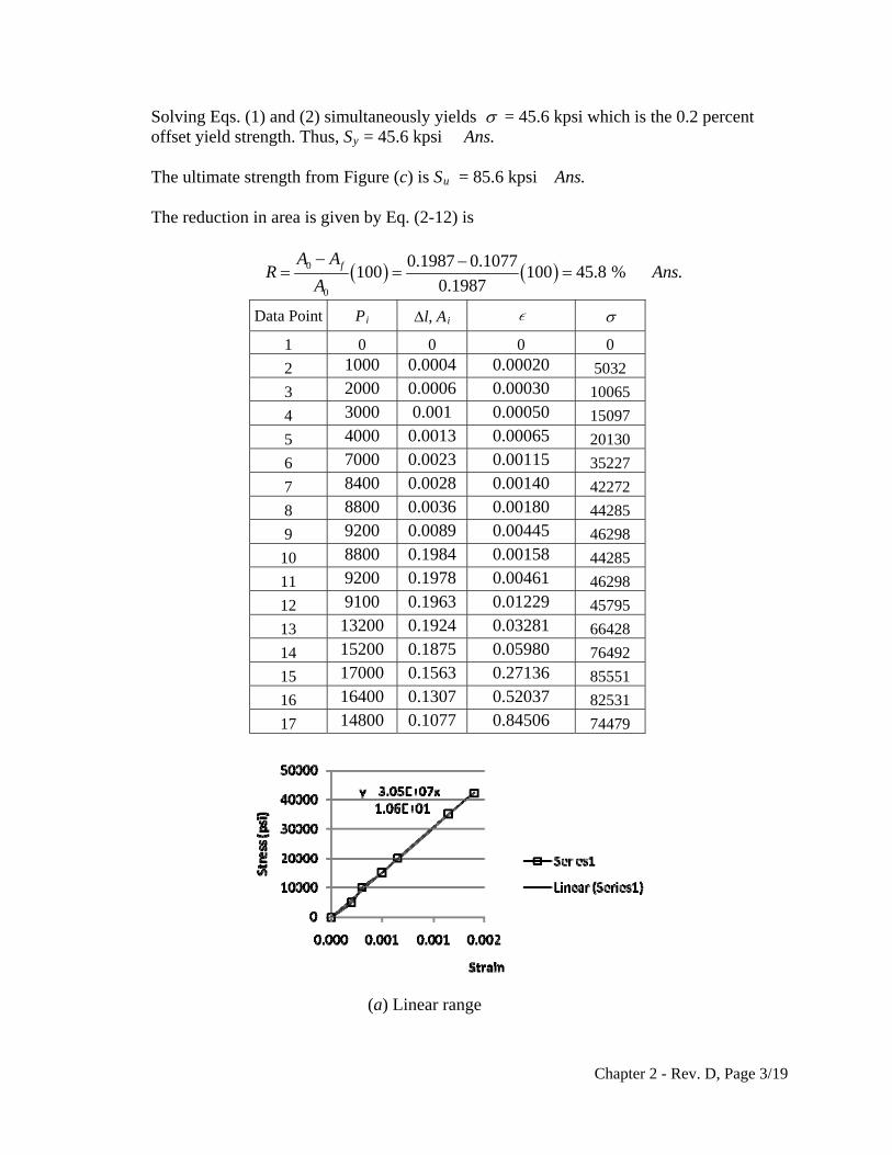
On the next two pages, the data and plots are presented. Figure (a) shows the linear part of the curve from data points 1-7. Figure (b) shows data points 1-12. Figure (c) shows the complete range. Note: The exact value of A0 is used without rounding off.
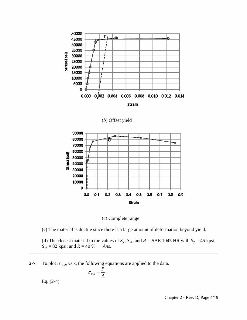
(b) From Fig. (a) the slope of the line from a linear regression is E = 30.5 Mpsi Ans. From Fig. (b) the equation for the dotted offset line is found to be = 30.5(106) 61 000 (1)
The equation for the line between data points 8 and 9 is = 7.60(105) + 42 900 (2)
Chapter 2 - Rev. D, Page 2/19
Solving Eqs. (1) and (2) simultaneously yields = 45.6 kpsi which is the 0.2 percent offset yield strength. Thus, Sy = 45.6 kpsi Ans.
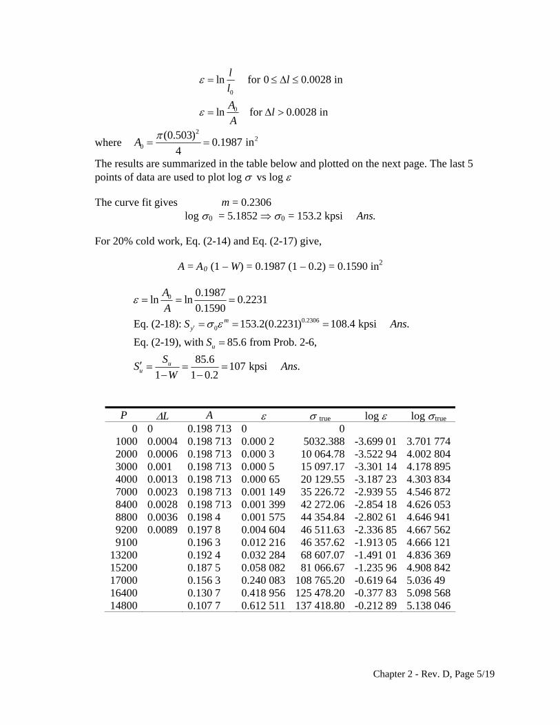
The ultimate strength from Figure (c) is Su = 85.6 kpsi Ans. The reduction in area is given by Eq. (2-12) is
0
0
0.1987 0.1077100 100 45.8 % .
0.1987fA A
R AnsA
Data Point Pi l, Ai
1 0 0 0 0
2 1000 0.0004 0.00020 5032
3 2000 0.0006 0.00030 10065
4 3000 0.001 0.00050 15097
5 4000 0.0013 0.00065 20130
6 7000 0.0023 0.00115 35227
7 8400 0.0028 0.00140 42272
8 8800 0.0036 0.00180 44285
9 9200 0.0089 0.00445 46298
10 8800 0.1984 0.00158 44285
11 9200 0.1978 0.00461 46298
12 9100 0.1963 0.01229 45795
13 13200 0.1924 0.03281 66428
14 15200 0.1875 0.05980 76492
15 17000 0.1563 0.27136 85551
16 16400 0.1307 0.52037 82531
17 14800 0.1077 0.84506 74479
(a) Linear range
Chapter 2 - Rev. D, Page 3/19
(b) Offset yield
(c) Complete range (c) The material is ductile since there is a large amount of deformation beyond yield. (d) The closest material to the values of Sy, Sut, and R is SAE 1045 HR with Sy = 45 kpsi,
Sut = 82 kpsi, and R = 40 %. Ans. ______________________________________________________________________________ 2-7 To plot true vs., the following equations are applied to the data.
true
P
A
Eq. (2-4)
Chapter 2 - Rev. D, Page 4/19
0
0
ln for 0 0.0028 in
ln for 0.0028 in
ll
l
Al
A
where 2
20
(0.503)0.1987 in
4A
The results are summarized in the table below and plotted on the next page. The last 5 points of data are used to plot log vs log
The curve fit gives m = 0.2306
log 0 = 5.1852 0 = 153.2 kpsi Ans. For 20% cold work, Eq. (2-14) and Eq. (2-17) give,
A = A0 (1 – W) = 0.1987 (1 – 0.2) = 0.1590 in2
0
0.23060
0.1987ln ln 0.2231
0.1590
Eq. (2-18): 153.2(0.2231) 108.4 kpsi .
Eq. (2-19), with 85.6 from Prob. 2-6,
85.6107 kpsi .
1 1 0.2
my
u
uu
A
A
S A
S
SS Ans
W
ns
P L A true log log true
0 0 0.198 713 0 0 1000 0.0004 0.198 713 0.000 2 5032.388 -3.699 01 3.701 7742000 0.0006 0.198 713 0.000 3 10 064.78 -3.522 94 4.002 8043000 0.001 0.198 713 0.000 5 15 097.17 -3.301 14 4.178 8954000 0.0013 0.198 713 0.000 65 20 129.55 -3.187 23 4.303 8347000 0.0023 0.198 713 0.001 149 35 226.72 -2.939 55 4.546 8728400 0.0028 0.198 713 0.001 399 42 272.06 -2.854 18 4.626 0538800 0.0036 0.198 4 0.001 575 44 354.84 -2.802 61 4.646 9419200 0.0089 0.197 8 0.004 604 46 511.63 -2.336 85 4.667 5629100 0.196 3 0.012 216 46 357.62 -1.913 05 4.666 121
13200 0.192 4 0.032 284 68 607.07 -1.491 01 4.836 36915200 0.187 5 0.058 082 81 066.67 -1.235 96 4.908 84217000 0.156 3 0.240 083 108 765.20 -0.619 64 5.036 49 16400 0.130 7 0.418 956 125 478.20 -0.377 83 5.098 56814800 0.107 7 0.612 511 137 418.80 -0.212 89 5.138 046
Chapter 2 - Rev. D, Page 5/19
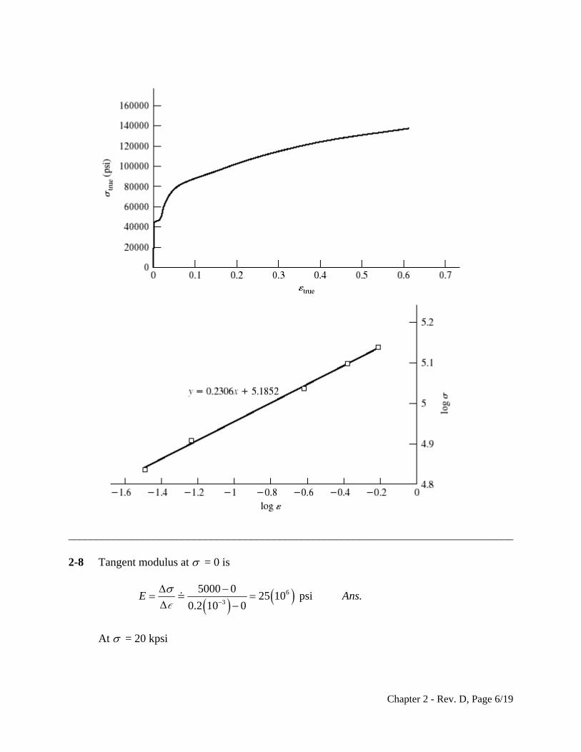
______________________________________________________________________________ 2-8 Tangent modulus at = 0 is
6
3
5000 025 10 psi
0.2 10 0E
Ans.
At = 20 kpsi
Chapter 2 - Rev. D, Page 6/19
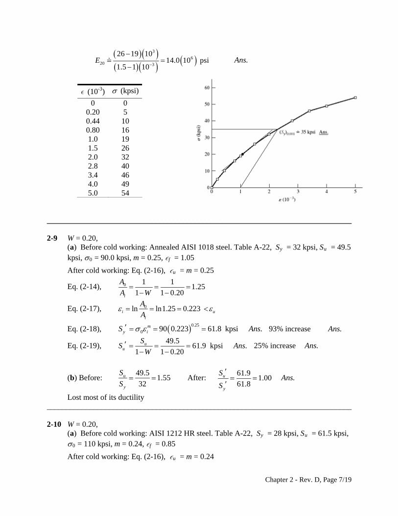
3
620 3
26 19 1014.0 10 psi
1.5 1 10E
Ans.
(10-3) (kpsi)
0 0 0.20 5 0.44 10 0.80 16 1.0 19 1.5 26 2.0 32 2.8 40 3.4 46 4.0 49 5.0 54
______________________________________________________________________________ 2-9 W = 0.20, (a) Before cold working: Annealed AISI 1018 steel. Table A-22, Sy = 32 kpsi, Su = 49.5
kpsi, 0 = 90.0 kpsi, m = 0.25, f = 1.05
After cold working: Eq. (2-16), u = m = 0.25
Eq. (2-14), 0 1 11.25
1 1 0.20i
A
A W
Eq. (2-17), 0ln ln1.25 0.223i ui
A
A
Eq. (2-18), S 93% increase Ans. 0.25
0 90 0.223 61.8 kpsi .my i Ans
Eq. (2-19), 49.5
61.9 kpsi .1 1 0.20
uu
SS A
W
ns 25% increase Ans.
(b) Before: 49.5
1.5532
u
y
S
S After:
61.91.00
61.8u
y
S
S
Ans.
Lost most of its ductility ______________________________________________________________________________ 2-10 W = 0.20, (a) Before cold working: AISI 1212 HR steel. Table A-22, Sy = 28 kpsi, Su = 61.5 kpsi,
0 = 110 kpsi, m = 0.24, f = 0.85
After cold working: Eq. (2-16), u = m = 0.24
Chapter 2 - Rev. D, Page 7/19
Eq. (2-14), 0 1 11.25
1 1 0.20i
A
A W
Eq. (2-17), 0ln ln1.25 0.223i ui
A
A
Eq. (2-18), 174% increase Ans. 0.24
0 110 0.223 76.7 kpsi .my iS A ns
Eq. (2-19), 61.5
76.9 kpsi .1 1 0.20
uu
SS A
W
ns 25% increase Ans.
(b) Before: 61.5
2.2028
u
y
S
S After:
76.91.00
76.7u
y
S
S
Ans.
Lost most of its ductility ______________________________________________________________________________ 2-11 W = 0.20, (a) Before cold working: 2024-T4 aluminum alloy. Table A-22, Sy = 43.0 kpsi, Su =
64.8 kpsi, 0 = 100 kpsi, m = 0.15, f = 0.18
After cold working: Eq. (2-16), u = m = 0.15
Eq. (2-14), 0 1 11.25
1 1 0.20i
A
A W
Eq. (2-17), 0ln ln1.25 0.223ii
A
A f Material fractures. Ans.
______________________________________________________________________________ 2-12 For HB = 275, Eq. (2-21), Su = 3.4(275) = 935 MPa Ans. ______________________________________________________________________________ 2-13 Gray cast iron, HB = 200. Eq. (2-22), Su = 0.23(200) 12.5 = 33.5 kpsi Ans. From Table A-24, this is probably ASTM No. 30 Gray cast iron Ans. ______________________________________________________________________________ 2-14 Eq. (2-21), 0.5HB = 100 HB = 200 Ans. ______________________________________________________________________________
Chapter 2 - Rev. D, Page 8/19
2-15 For the data given, converting HB to Su using Eq. (2-21)
HB Su (kpsi) Su2
(kpsi)
230 115 13225
232 116 13456
232 116 13456
234 117 13689
235 117.5 13806.25
235 117.5 13806.25
235 117.5 13806.25
236 118 13924
236 118 13924
239 119.5 14280.25
Su = 1172 Su2 = 137373
1172
117.2 117 kpsi .10
uu
SS A
N ns
Eq. (20-8),
102 2
2
1137373 10 117.2
1.27 kpsi .1 9u
u ui
S
S NSs A
N
ns
______________________________________________________________________________ 2-16 For the data given, converting HB to Su using Eq. (2-22)
HB Su (kpsi) Su2
(kpsi)
230 40.4 1632.16
232 40.86 1669.54
232 40.86 1669.54
234 41.32 1707.342
235 41.55 1726.403
235 41.55 1726.403
235 41.55 1726.403
236 41.78 1745.568
236 41.78 1745.568
239 42.47 1803.701
Su = 414.12 Su2 =17152.63
Chapter 2 - Rev. D, Page 9/19
414.12
41.4 kpsi .10
uu
SS A
N ns
Eq. (20-8),
102 2
2
117152.63 10 41.4
1.20 .1 9u
u ui
S
S NSs A
N
ns
______________________________________________________________________________
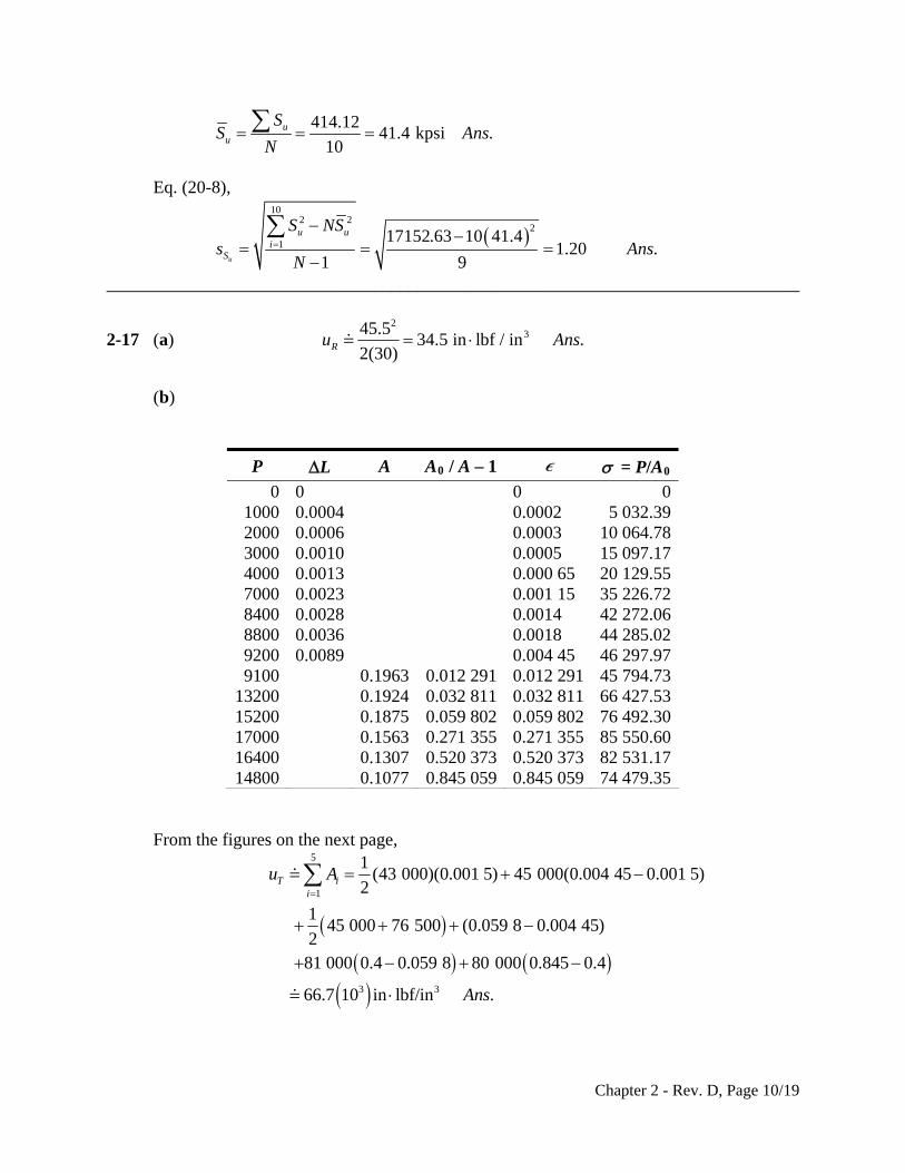
2-17 (a) 2
345.534.5 in lbf / in .
2(30)Ru A ns
(b)
P L A A0 / A – 1 = P/A0
0 0 0 0 1000 0.0004 0.0002 5 032.39 2000 0.0006 0.0003 10 064.78 3000 0.0010 0.0005 15 097.17 4000 0.0013 0.000 65 20 129.55 7000 0.0023 0.001 15 35 226.72 8400 0.0028 0.0014 42 272.06 8800 0.0036 0.0018 44 285.02 9200 0.0089 0.004 45 46 297.97 9100 0.1963 0.012 291 0.012 291 45 794.73
13200 0.1924 0.032 811 0.032 811 66 427.53 15200 0.1875 0.059 802 0.059 802 76 492.30 17000 0.1563 0.271 355 0.271 355 85 550.60 16400 0.1307 0.520 373 0.520 373 82 531.17 14800 0.1077 0.845 059 0.845 059 74 479.35
From the figures on the next page,
5
1
3 3
1(43 000)(0.001 5) 45 000(0.004 45 0.001 5)
2
145 000 76 500 (0.059 8 0.004 45)
281 000 0.4 0.059 8 80 000 0.845 0.4
66.7 10 in lbf/in .
T ii
u A
Ans
Chapter 2 - Rev. D, Page 10/19
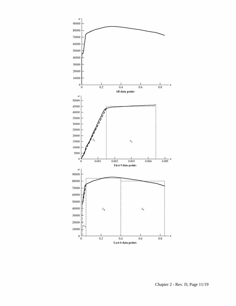
Chapter 2 - Rev. D, Page 11/19
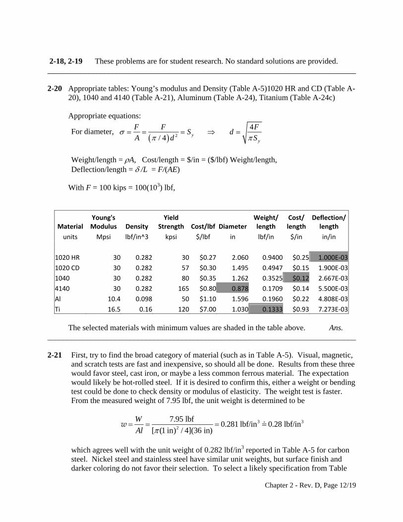
2-18, 2-19 These problems are for student research. No standard solutions are provided. ______________________________________________________________________________ 2-20 Appropriate tables: Young’s modulus and Density (Table A-5)1020 HR and CD (Table A-
20), 1040 and 4140 (Table A-21), Aluminum (Table A-24), Titanium (Table A-24c) Appropriate equations:
For diameter, 2
4
/ 4 yy
F FS d
F
A d S
Weight/length = A, Cost/length = $/in = ($/lbf) Weight/length, Deflection/length = /L = F/(AE) With F = 100 kips = 100(103) lbf,
Material Young's Modulus Density
Yield Strength Cost/lbf Diameter
Weight/ length
Cost/ length
Deflection/ length
units Mpsi lbf/in^3 kpsi $/lbf in lbf/in $/in in/in
1020 HR 30 0.282 30 $0.27 2.060 0.9400 $0.25 1.000E‐03
1020 CD 30 0.282 57 $0.30 1.495 0.4947 $0.15 1.900E‐03
1040 30 0.282 80 $0.35 1.262 0.3525 $0.12 2.667E‐03
4140 30 0.282 165 $0.80 0.878 0.1709 $0.14 5.500E‐03
Al 10.4 0.098 50 $1.10 1.596 0.1960 $0.22 4.808E‐03
Ti 16.5 0.16 120 $7.00 1.030 0.1333 $0.93 7.273E‐03
The selected materials with minimum values are shaded in the table above. Ans. ______________________________________________________________________________ 2-21 First, try to find the broad category of material (such as in Table A-5). Visual, magnetic,
and scratch tests are fast and inexpensive, so should all be done. Results from these three would favor steel, cast iron, or maybe a less common ferrous material. The expectation would likely be hot-rolled steel. If it is desired to confirm this, either a weight or bending test could be done to check density or modulus of elasticity. The weight test is faster. From the measured weight of 7.95 lbf, the unit weight is determined to be
3 32
7.95 lbf0.281 lbf/in 0.28 lbf/in
[ (1 in) / 4](36 in)
W
Al w
which agrees well with the unit weight of 0.282 lbf/in3 reported in Table A-5 for carbon steel. Nickel steel and stainless steel have similar unit weights, but surface finish and darker coloring do not favor their selection. To select a likely specification from Table
Chapter 2 - Rev. D, Page 12/19
A-20, perform a Brinell hardness test, then use Eq. (2-21) to estimate an ultimate strength of . Assuming the material is hot-rolled due to the
rough surface finish, appropriate choices from Table A-20 would be one of the higher carbon steels, such as hot-rolled AISI 1050, 1060, or 1080. Ans.
0.5 0.5(200) 100 kpsiu BS H
______________________________________________________________________________ 2-22 First, try to find the broad category of material (such as in Table A-5). Visual, magnetic,
and scratch tests are fast and inexpensive, so should all be done. Results from these three favor a softer, non-ferrous material like aluminum. If it is desired to confirm this, either a weight or bending test could be done to check density or modulus of elasticity. The weight test is faster. From the measured weight of 2.90 lbf, the unit weight is determined to be
3 32
2.9 lbf0.103 lbf/in 0.10 lbf/in
[ (1 in) / 4](36 in)
W
Al w
which agrees reasonably well with the unit weight of 0.098 lbf/in3 reported in Table A-5 for aluminum. No other materials come close to this unit weight, so the material is likely aluminum. Ans.
______________________________________________________________________________ 2-23 First, try to find the broad category of material (such as in Table A-5). Visual, magnetic,
and scratch tests are fast and inexpensive, so should all be done. Results from these three favor a softer, non-ferrous copper-based material such as copper, brass, or bronze. To further distinguish the material, either a weight or bending test could be done to check density or modulus of elasticity. The weight test is faster. From the measured weight of 9 lbf, the unit weight is determined to be
3 32
9.0 lbf0.318 lbf/in 0.32 lbf/in
[ (1 in) / 4](36 in)
W
Al w
which agrees reasonably well with the unit weight of 0.322 lbf/in3 reported in Table A-5 for copper. Brass is not far off (0.309 lbf/in3), so the deflection test could be used to gain additional insight. From the measured deflection and utilizing the deflection equation for an end-loaded cantilever beam from Table A-9, Young’s modulus is determined to be
33
4
100 2417.7 Mpsi
3 3 (1) 64 (17 / 32)
FlE
Iy
which agrees better with the modulus for copper (17.2 Mpsi) than with brass (15.4 Mpsi). The conclusion is that the material is likely copper. Ans.
______________________________________________________________________________ 2-24 and 2-25 These problems are for student research. No standard solutions are provided. ______________________________________________________________________________
Chapter 2 - Rev. D, Page 13/19
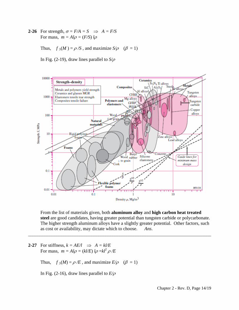
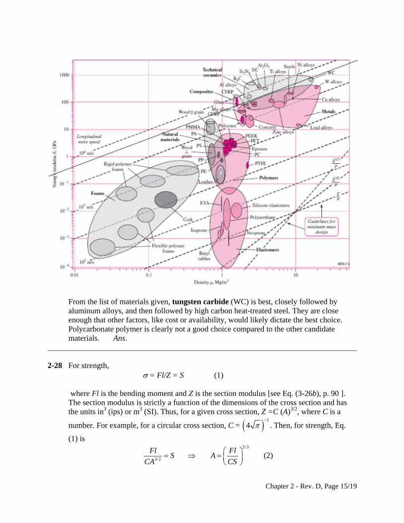
2-26 For strength, = F/A = S A = F/S For mass, m = Al = (F/S) l Thus, f 3(M ) = /S , and maximize S/ ( = 1) In Fig. (2-19), draw lines parallel to S/
From the list of materials given, both aluminum alloy and high carbon heat treated
steel are good candidates, having greater potential than tungsten carbide or polycarbonate. The higher strength aluminum alloys have a slightly greater potential. Other factors, such as cost or availability, may dictate which to choose. Ans.
______________________________________________________________________________ 2-27 For stiffness, k = AE/l A = kl/E For mass, m = Al = (kl/E) l =kl2 /E Thus, f 3(M) = /E , and maximize E/ ( = 1) In Fig. (2-16), draw lines parallel to E/
Chapter 2 - Rev. D, Page 14/19
From the list of materials given, tungsten carbide (WC) is best, closely followed by
aluminum alloys, and then followed by high carbon heat-treated steel. They are close enough that other factors, like cost or availability, would likely dictate the best choice. Polycarbonate polymer is clearly not a good choice compared to the other candidate materials. Ans.
______________________________________________________________________________ 2-28 For strength, = Fl/Z = S (1) where Fl is the bending moment and Z is the section modulus [see Eq. (3-26b), p. 90 ].
The section modulus is strictly a function of the dimensions of the cross section and has the units in3 (ips) or m3 (SI). Thus, for a given cross section, Z =C (A)3/2, where C is a
number. For example, for a circular cross section, C = 1
4
. Then, for strength, Eq.
(1) is
2/3
3/2
Fl FlS A
CA CS
(2)
Chapter 2 - Rev. D, Page 15/19
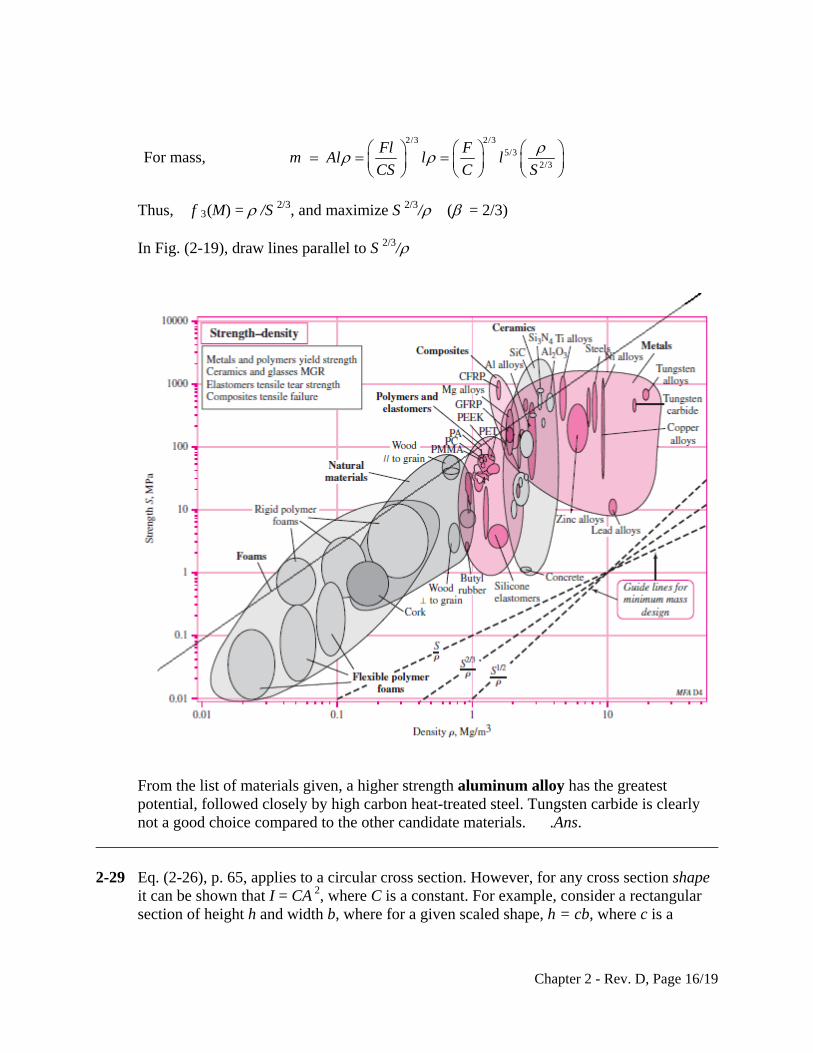
For mass, 2/3 2/3
5/32/3
Fl F
m Al l lCS C S
Thus, f 3(M) = /S 2/3, and maximize S 2/3/ ( = 2/3) In Fig. (2-19), draw lines parallel to S 2/3/
From the list of materials given, a higher strength aluminum alloy has the greatest
potential, followed closely by high carbon heat-treated steel. Tungsten carbide is clearly not a good choice compared to the other candidate materials. .Ans.
______________________________________________________________________________ 2-29 Eq. (2-26), p. 65, applies to a circular cross section. However, for any cross section shape
it can be shown that I = CA 2, where C is a constant. For example, consider a rectangular section of height h and width b, where for a given scaled shape, h = cb, where c is a
Chapter 2 - Rev. D, Page 16/19
constant. The moment of inertia is I = bh 3/12, and the area is A = bh. Then I = h(bh2)/12 = cb (bh2)/12 = (c/12)(bh)2 = CA 2, where C = c/12 (a constant).
Thus, Eq. (2-27) becomes
1/23
3
klA
CE
and Eq. (2-29) becomes
1/2
5/21/23
km Al l
C E
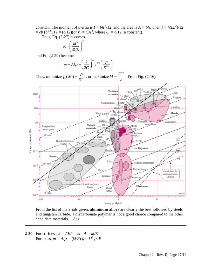
Thus, minimize 3 1/2f M
E
, or maximize
1/2EM
. From Fig. (2-16)
From the list of materials given, aluminum alloys are clearly the best followed by steels
and tungsten carbide. Polycarbonate polymer is not a good choice compared to the other candidate materials. Ans.
______________________________________________________________________________ 2-30 For stiffness, k = AE/l A = kl/E For mass, m = Al = (kl/E) l =kl2 /E
Chapter 2 - Rev. D, Page 17/19
So, f 3(M) = /E, and maximize E/ . Thus, = 1. Ans. ______________________________________________________________________________ 2-31 For strength, = F/A = S A = F/S For mass, m = Al = (F/S) l So, f 3(M ) = /S, and maximize S/ . Thus, = 1. Ans. ______________________________________________________________________________ 2-32 Eq. (2-26), p. 65, applies to a circular cross section. However, for any cross section shape
it can be shown that I = CA 2, where C is a constant. For example, consider a rectangular section of height h and width b, where for a given scaled shape, h = cb, where c is a constant. The moment of inertia is I = bh 3/12, and the area is A = bh. Then I = h(bh2)/12 = cb (bh2)/12 = (c/12)(bh)2 = CA 2, where C = c/12.
Thus, Eq. (2-27) becomes
1/23
3
klA
CE
and Eq. (2-29) becomes
1/2
5/21/23
km Al l
C E
So, minimize 3 1/2f M
E
, or maximize
1/2EM
. Thus, = 1/2. Ans.
______________________________________________________________________________ 2-33 For strength, = Fl/Z = S (1) where Fl is the bending moment and Z is the section modulus [see Eq. (3-26b), p. 90 ].
The section modulus is strictly a function of the dimensions of the cross section and has the units in3 (ips) or m3 (SI). Thus, for a given cross section, Z =C (A)3/2, where C is a
number. For example, for a circular cross section, C = 1
4
. Then, for strength, Eq. (1)
is
2/3
3/2
Fl FlS A
CA CS
(2)
For mass, 2/3 2/3
5/32/3
Fl F
m Al l lCS C S
So, f 3(M) = /S 2/3, and maximize S 2/3/. Thus, = 2/3. Ans. ______________________________________________________________________________ 2-34 For stiffness, k=AE/l, or, A = kl/E.
Chapter 2 - Rev. D, Page 18/19
Chapter 2 - Rev. D, Page 19/19
Thus, m = Al = (kl/E )l = kl 2 /E. Then, M = E / and = 1. From Fig. 2-16, lines parallel to E / for ductile materials include steel, titanium,
molybdenum, aluminum alloys, and composites. For strength, S = F/A, or, A = F/S. Thus, m = Al = F/Sl = Fl /S. Then, M = S/ and = 1. From Fig. 2-19, lines parallel to S/ give for ductile materials, steel, aluminum alloys,
nickel alloys, titanium, and composites. Common to both stiffness and strength are steel, titanium, aluminum alloys, and
composites. Ans.
Chapter 3
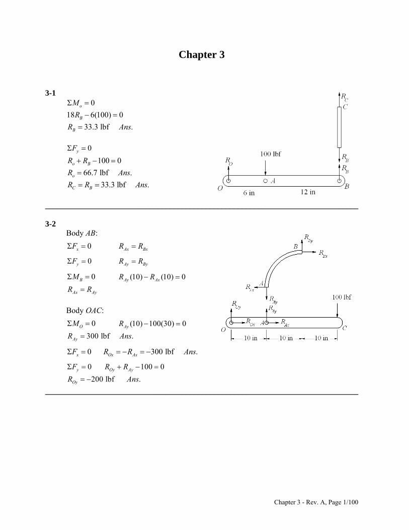
3-1
0oM
18 6(100) 0BR
33.3 lbf .BR Ans
0yF
100 0o BR R
66.7 lbf .oR Ans
33.3 lbf .C BR R A ns
______________________________________________________________________________ 3-2 Body AB:
0xF Ax BxR R
0yF Ay ByR R
0BM (10) (10) 0Ay AxR R
Ax AyR R
Body OAC:
0OM (10) 100(30) 0AyR
300 lbf .AyR Ans
0xF 300 lbf .Ox AxR R A ns
0yF 100 0Oy AyR R
200 lbf .OyR Ans
______________________________________________________________________________
Chapter 3 - Rev. A, Page 1/100
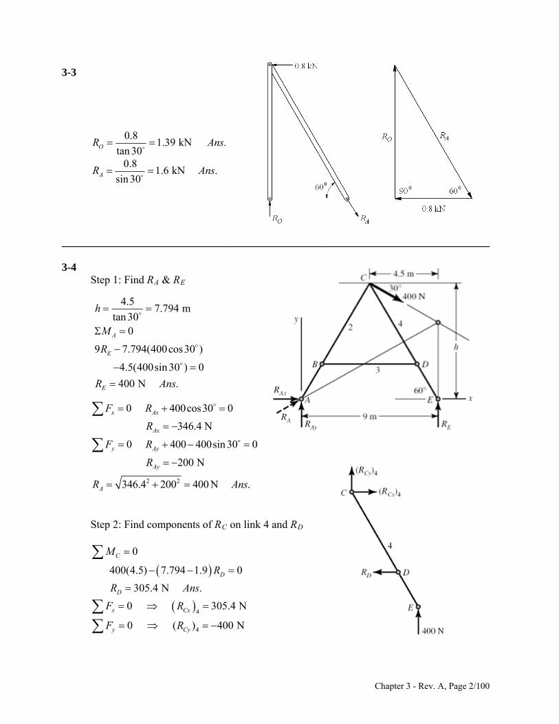
3-3
0.81.39 kN .
tan 30OR Ans
0.81.6 kN .
sin 30AR Ans
______________________________________________________________________________ 3-4 Step 1: Find RA & RE
4.57.794 m
tan 300
9 7.794(400cos30 )
4.5(400sin 30 ) 0
400 N .
A
E
E
h
M
R
R Ans
2 2
0 400cos30 0
346.4 N
0 400 400sin 30 0
200 N
346.4 200 400 N .
x Ax
Ax
y Ay
Ay
A
F R
R
F R
R
R Ans
Step 2: Find components of RC on link 4 and RD
4
4
0
400(4.5) 7.794 1.9 0
305.4 N .
0 305.4 N
0 ( ) 400 N
C
D
D
x Cx
y Cy
M
R
R Ans
F R
F R
Chapter 3 - Rev. A, Page 2/100
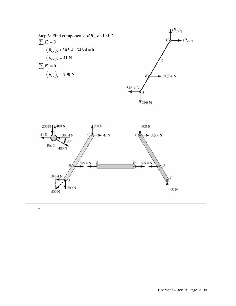
Step 3: Find components of RC on link 2
2
2
2
0
305.4 346.4 0
41 N
0
200 N
x
Cx
Cx
y
Cy
F
R
R
F
R
____________________________________________________________________________________________________________________
_
Chapter 3 - Rev. A, Page 3/100
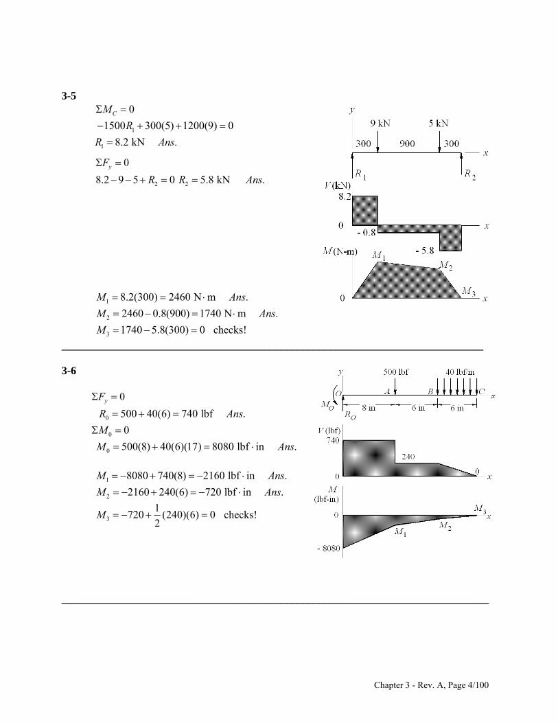
3-5
0CM 11500 300(5) 1200(9) 0R 1 8.2 kN .R Ans
0yF
28.2 9 5 0R 2 5.8 kN .R Ans
1 8.2(300) 2460 N m .M Ans
2 2460 0.8(900) 1740 N m .M Ans
3 1740 5.8(300) 0 checks!M _____________________________________________________________________________ 3-6
0yF
0 500 40(6) 740 lbf .R Ans
0 0M 0 500(8) 40(6)(17) 8080 lbf in .M Ans
1 8080 740(8) 2160 lbf in .M Ans
2 2160 240(6) 720 lbf in .M Ans
3
1720 (240)(6) 0 checks!
2M
______________________________________________________________________________
Chapter 3 - Rev. A, Page 4/100
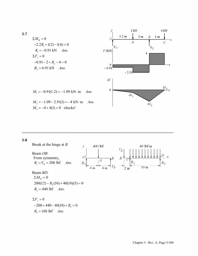
3-7
0BM
12.2 1(2) 1(4) 0R 1 0.91 kN .R Ans
0yF
20.91 2 4 0R
2 6.91 kN .R Ans
1 0.91(1.2) 1.09 kN m .M Ans
2 1.09 2.91(1) 4 kN m .M Ans 3 4 4(1) 0 checks!M ______________________________________________________________________________ 3-8 Break at the hinge at B Beam OB: From symmetry, 1 200 lbf .BR V Ans
Beam BD: 0DM 2200(12) (10) 40(10)(5) 0R 2 440 lbf .R Ans
0yF
3200 440 40(10) 0R 3 160 lbf .R Ans
Chapter 3 - Rev. A, Page 5/100
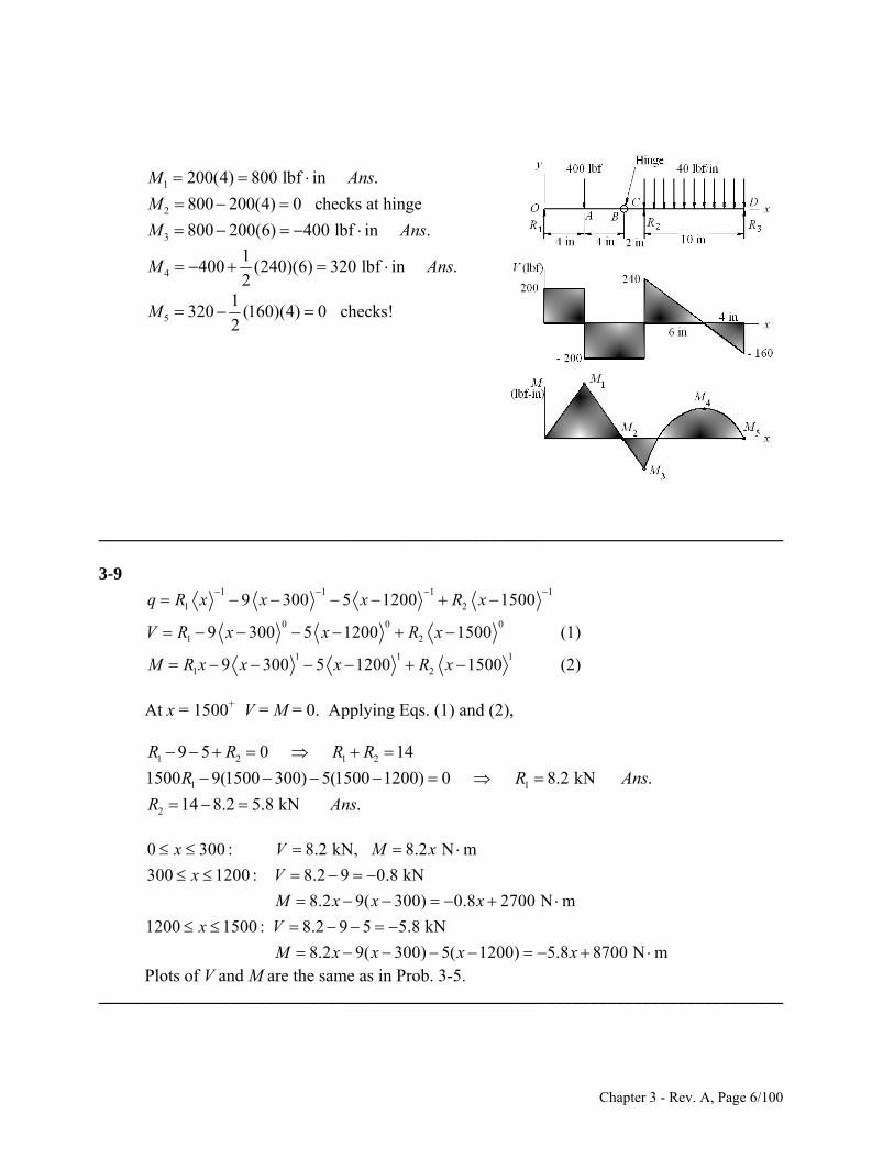
1 200(4) 800 lbf in .M Ans
2 800 200(4) 0 checks at hingeM
3 800 200(6) 400 lbf in .M Ans
4
1400 (240)(6) 320 lbf in .
2M Ans
5
1320 (160)(4) 0 checks!
2M
______________________________________________________________________________ 3-9
1 1 1
1 2
0 0 0
1 2
1 1 1
1 2
9 300 5 1200 1500
9 300 5 1200 1500 (1)
9 300 5 1200 1500 (2)
q R x x x R x
V R x x R x
M R x x x R x
1
At x = 1500+ V = M = 0. Applying Eqs. (1) and (2),
1 2 1 29 5 0 14R R R R
1 11500 9(1500 300) 5(1500 1200) 0 8.2 kN .R R A
2 14 8.2 5.8 kN .
ns
R Ans
0 300 : 8.2 kN, 8.2 N m
300 1200 : 8.2 9 0.8 kN
8.2 9( 300) 0.8 2700 N m
1200 1500 : 8.2 9 5 5.8 kN
8.2 9( 300
x V M x
x V
M x x x
x V
M x x
) 5( 1200) 5.8 8700 N mx x
Plots of V and M are the same as in Prob. 3-5. ______________________________________________________________________________
Chapter 3 - Rev. A, Page 6/100
3-10
1 2 1 0 0
0 0
1 0 1 1
0 0
1 2 2
0 0
500 8 40 14 40 20
500 8 40 14 40 20 (1)
500 8 20 14 20 20 (2)
at 20 in, 0, Eqs. (1) and (2) give
q R x M x x x x
V R M x x x x
M R x M x x x
x V M
R
0 0
20 0 0
500 40 20 14 0 740 lbf .
(20) 500(20 8) 20(20 14) 0 8080 lbf in .
R Ans
R M M
Ans
0 8 : 740 lbf, 740 8080 lbf in
8 14 : 740 500 240 lbf
740 8080 500( 8) 240 4080 lbf in
14 20 : 740 500 40( 14) 40 800 lbf
740 8080
x V M x
x V
M x x x
x V x x
M x
2 2500( 8) 20( 14) 20 800 8000 lbf inx x x x
Plots of V and M are the same as in Prob. 3-6. ______________________________________________________________________________ 3-11
1 1 1 1
1 2
0 0 0
1 2
1 1 1
1 2
2 1.2 2.2 4 3.2
2 1.2 2.2 4 3.2 (1)
2 1.2 2.2 4 3.2 (2)
q R x x R x x
V R x R x x
M R x x R x x
at x = 3.2+, V = M = 0. Applying Eqs. (1) and (2),
Solving Eqs. (3) and (4) simultaneously,
1 2 1 2
1 2 1 2
2 4 0 6 (3)
3.2 2(2) (1) 0 3.2 4 (4)
R R R R
R R R R
R1 = -0.91 kN, R2 = 6.91 kN Ans. 0 1.2 : 0.91 kN, 0.91 kN m
1.2 2.2 : 0.91 2 2.91 kN
0.91 2( 1.2) 2.91 2.4 kN m
2.2 3.2 : 0.91 2 6.91 4 kN
0.91 2(
x V M x
x V
M x x x
x V
M x x
1.2) 6.91( 2.2) 4 12.8 kN mx x
Plots of V and M are the same as in Prob. 3-7. ______________________________________________________________________________
Chapter 3 - Rev. A, Page 7/100
3-12
1 1 1 0 0 1
1 2 3
0 0 1 1 0
1 2 3
1 1 2 2 1
1 2 3
1
400 4 10 40 10 40 20 20
400 4 10 40 10 40 20 20 (1)
400 4 10 20 10 20 20 20 (2)
0 at 8 in 8 400(
q R x x R x x x R x
V R x R x x x R x
M R x x R x x x R x
M x R
18 4) 0 200 lbf .R Ans
at x = 20+, V =M = 0. Applying Eqs. (1) and (2),
2 3 2 3
22 2
200 400 40(10) 0 600
200(20) 400(16) (10) 20(10) 0 440 lbf .
R R R R
R R A
3 600 440 160 lbf .
ns
R Ans
0 4 : 200 lbf, 200 lbf in
4 10 : 200 400 200 lbf,
200 400( 4) 200 1600 lbf in
10 20 : 200 400 440 40( 10) 640 40 lbf
200 400( 4)
x V M x
x V
M x x x
x V x x
M x x
2 2440( 10) 20 10 20 640x x x
4800 lbf inx Plots of V and M are the same as in Prob. 3-8.
______________________________________________________________________________ 3-13 Solution depends upon the beam selected. ______________________________________________________________________________ 3-14
(a) Moment at center,
2
2
2
22 2 2 2 4
c
c
l ax
l l lM l a a
w wl
At reaction, 2 2rM aw
a = 2.25, l = 10 in, w = 100 lbf/in
2
100(10) 102.25 125 lbf in
2 4
100 2.25253 lbf in .
2
c
r
M
M Ans
(b) Optimal occurs when c rM M
Chapter 3 - Rev. A, Page 8/100
22 20.25 0
2 4 2
l l aa a al l
w w
Taking the positive root
2 21
4 0.25 2 1 0.207 .2 2
la l l l l A
ns
for l = 10 in, w = 100 lbf, a = 0.207(10) = 2.07 in 2
min 100 2 2.07 214 lbf inM
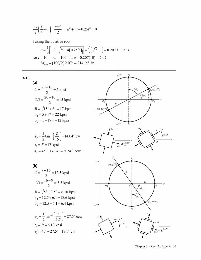
______________________________________________________________________________ 3-15
(a) 20 10
5 kpsi2
C
20 1015 kpsi
2CD
2 215 8 17 kpsiR
1 5 17 22 kpsi
2 5 17 12 kpsi
11 8tan 14.04 cw
2 15p
1 17 kpsi
45 14.04 30.96 ccws
R
(b) 9 16
12.5 kpsi2
C
16 93.5 kpsi
2CD
2 25 3.5 6.10 kpsiR
1 12.5 6.1 18.6 kpsi 2 12.5 6.1 6.4 kpsi
11 5tan 27.5 ccw
2 3.5p
1 6.10 kpsi
45 27.5 17.5 cws
R
Chapter 3 - Rev. A, Page 9/100
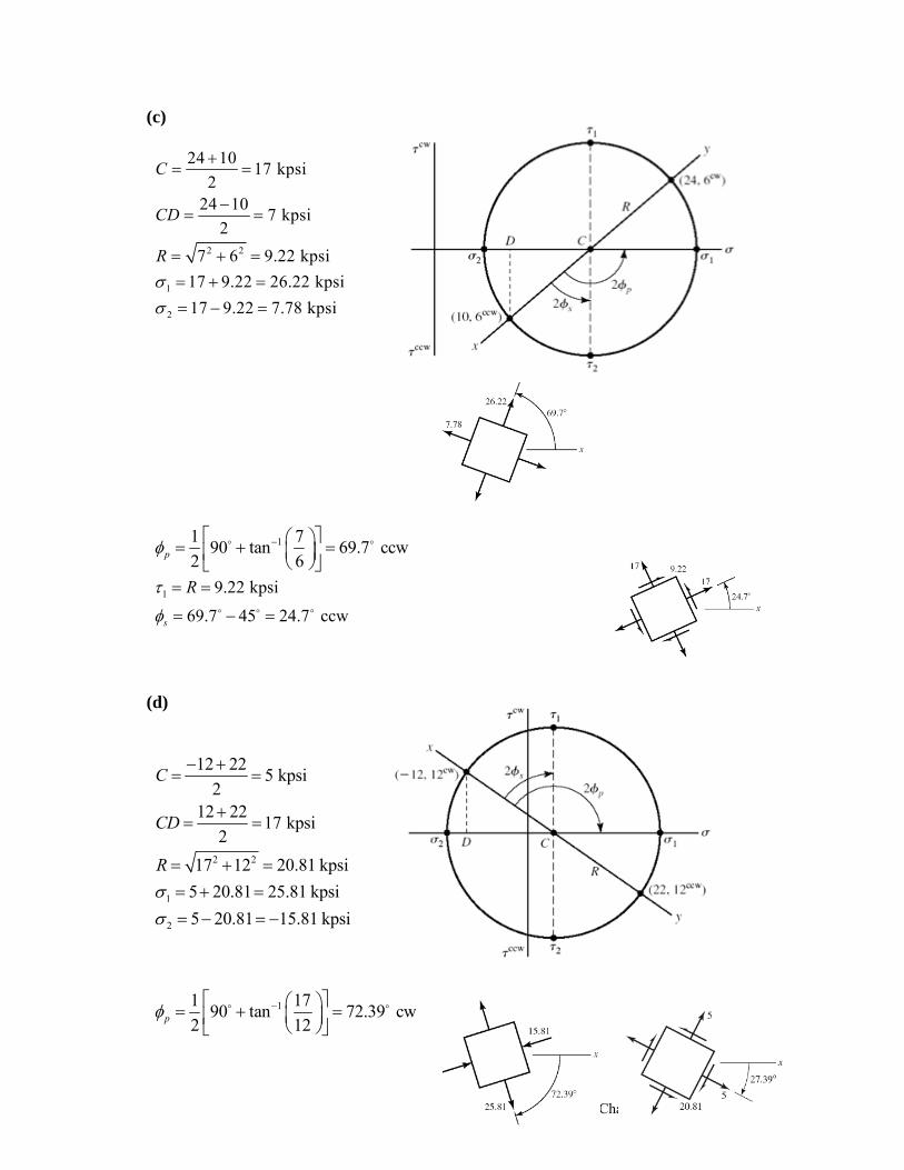
(c)
2 2
1
2
24 1017 kpsi
224 10
7 kpsi2
7 6 9.22 kpsi
17 9.22 26.22 kpsi
17 9.22 7.78 kpsi
C
CD
R
11 790 tan 69.7 ccw
2 6p
1 9.22 kpsi
69.7 45 24.7 ccws
R
(d)
2 2
1
2
12 225 kpsi
212 22
17 kpsi2
17 12 20.81 kpsi
5 20.81 25.81 kpsi
5 20.81 15.81 kpsi
C
CD
R
11 1790 tan 72.39 cw
2 12p
Chapter 3 - Rev. A, Page 10/100
1 20.81 kpsi
72.39 45 27.39 cws
R
______________________________________________________________________________
Chapter 3 - Rev. A, Page 11/100
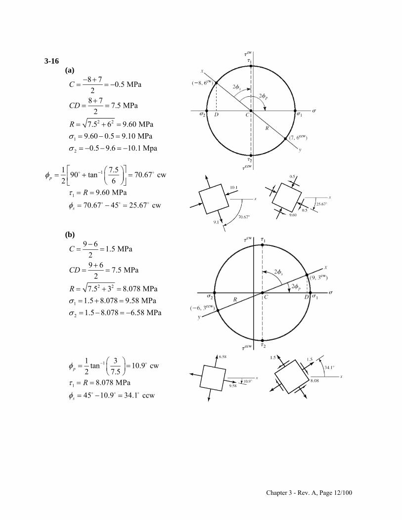
3-16
(a)
2 2
1
2
8 70.5 MPa
28 7
7.5 MPa2
7.5 6 9.60 MPa
9.60 0.5 9.10 MPa
0.5 9.6 10.1 Mpa
C
CD
R
11 7.590 tan 70.67 cw
2 6p
1 9.60 MPa
70.67 45 25.67 cws
R
(b)
2 2
1
2
9 61.5 MPa
29 6
7.5 MPa2
7.5 3 8.078 MPa
1.5 8.078 9.58 MPa
1.5 8.078 6.58 MPa
C
CD
R
11 3tan 10.9 cw
2 7.5p
1 8.078 MPa
45 10.9 34.1 ccws
R
Chapter 3 - Rev. A, Page 12/100
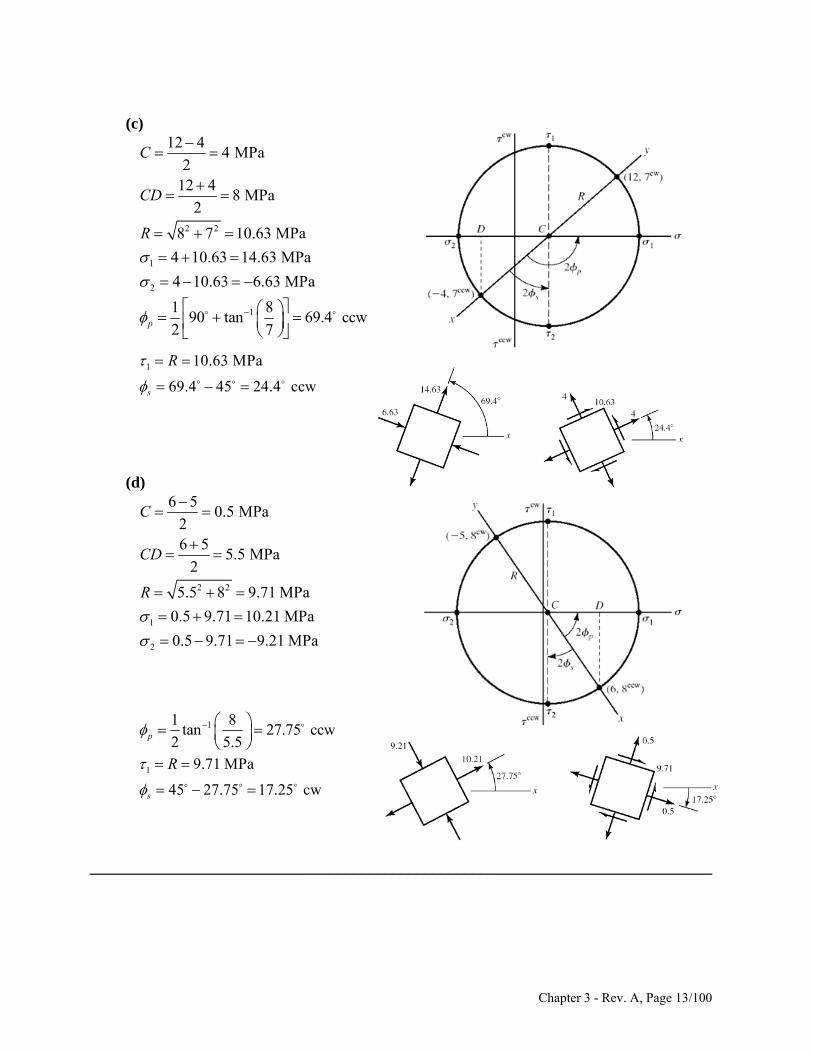
(c)
2 2
1
2
12 44 MPa
212 4
8 MPa2
8 7 10.63 MPa
4 10.63 14.63 MPa
4 10.63 6.63 MPa
C
CD
R
11 890 tan 69.4 ccw
2 7p
1 10.63 MPa
69.4 45 24.4 ccws
R
(d)
2 2
1
2
6 50.5 MPa
26 5
5.5 MPa2
5.5 8 9.71 MPa
0.5 9.71 10.21 MPa
0.5 9.71 9.21 MPa
C
CD
R
11 8tan 27.75 ccw
2 5.5p
1 9.71 MPa
45 27.75 17.25 cws
R
______________________________________________________________________________
Chapter 3 - Rev. A, Page 13/100
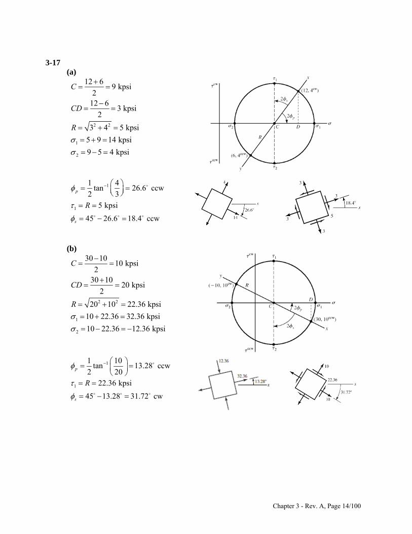
3-17
(a)
2 2
1
2
12 69 kpsi
212 6
3 kpsi2
3 4 5 kpsi
5 9 14 kpsi
9 5 4 kpsi
C
CD
R
11 4tan 26.6 ccw
2 3p
1 5 kpsi
45 26.6 18.4 ccws
R
(b)
2 2
1
2
30 1010 kpsi
230 10
20 kpsi2
20 10 22.36 kpsi
10 22.36 32.36 kpsi
10 22.36 12.36 kpsi
C
CD
R
11 10tan 13.28 ccw
2 20p
1 22.36 kpsi
45 13.28 31.72 cws
R
Chapter 3 - Rev. A, Page 14/100
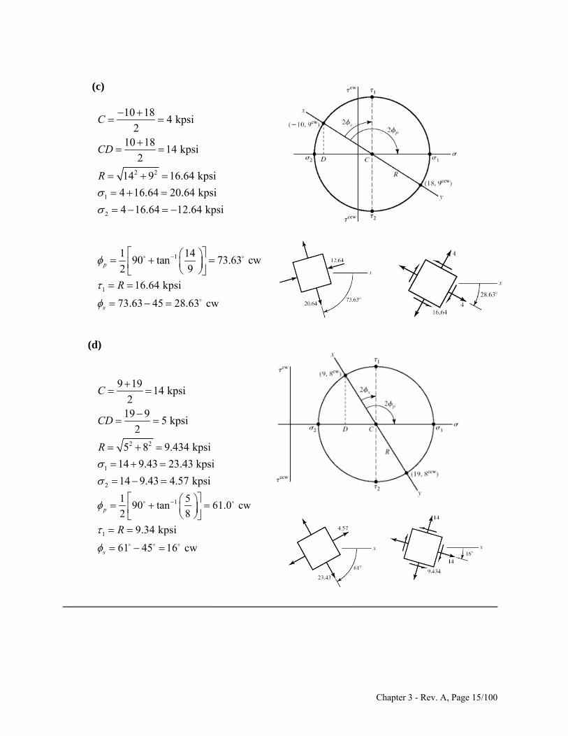
(c)
2 2
1
2
10 184 kpsi
210 18
14 kpsi2
14 9 16.64 kpsi
4 16.64 20.64 kpsi
4 16.64 12.64 kpsi
C
CD
R
11 1490 tan 73.63 cw
2 9p
1 16.64 kpsi
73.63 45 28.63 cws
R
(d)
2 2
1
2
9 1914 kpsi
219 9
5 kpsi2
5 8 9.434 kpsi
14 9.43 23.43 kpsi
14 9.43 4.57 kpsi
C
CD
R
11 590 tan 61.0 cw
2 8p
1 9.34 kpsi
61 45 16 cws
R
______________________________________________________________________________
Chapter 3 - Rev. A, Page 15/100
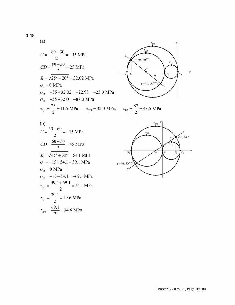
3-18
(a)
2 2
1
2
3
80 3055 MPa
280 30
25 MPa2
25 20 32.02 MPa
0 MPa
55 32.02 22.98 23.0 MPa
55 32.0 87.0 MPa
C
CD
R
1 2 2 3 1 3
23 8711.5 MPa, 32.0 MPa, 43.5 MPa
2 2
(b)
2 2
1
2
3
30 6015 MPa
260 30
45 MPa2
45 30 54.1 MPa
15 54.1 39.1 MPa
0 MPa
15 54.1 69.1 MPa
C
CD
R
1 3
1 2
2 3
39.1 69.154.1 MPa
239.1
19.6 MPa2
69.134.6 MPa
2
Chapter 3 - Rev. A, Page 16/100
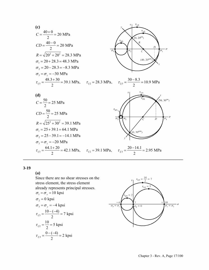
(c)
2 2
1
2
3
40 020 MPa
240 0
20 MPa2
20 20 28.3 MPa
20 28.3 48.3 MPa
20 28.3 8.3 MPa
30 MPaz
C
CD
R
1 3 1 2 2 3
48.3 30 30 8.339.1 MPa, 28.3 MPa, 10.9 MPa
2 2
(d)
2 2
1
2
3
5025 MPa
250
25 MPa2
25 30 39.1 MPa
25 39.1 64.1 MPa
25 39.1 14.1 MPa
20 MPaz
C
CD
R
1 3 1 2 2 3
64.1 20 20 14.142.1 MPa, 39.1 MPa, 2.95 MPa
2 2
______________________________________________________________________________ 3-19
(a) Since there are no shear stresses on the stress element, the stress element already represents principal stresses.
1
2
3
10 kpsi
0 kpsi
4 kpsi
x
y
1 3
1 2
2 3
10 ( 4)7 kpsi
210
5 kpsi20 ( 4)
2 kpsi2
Chapter 3 - Rev. A, Page 17/100
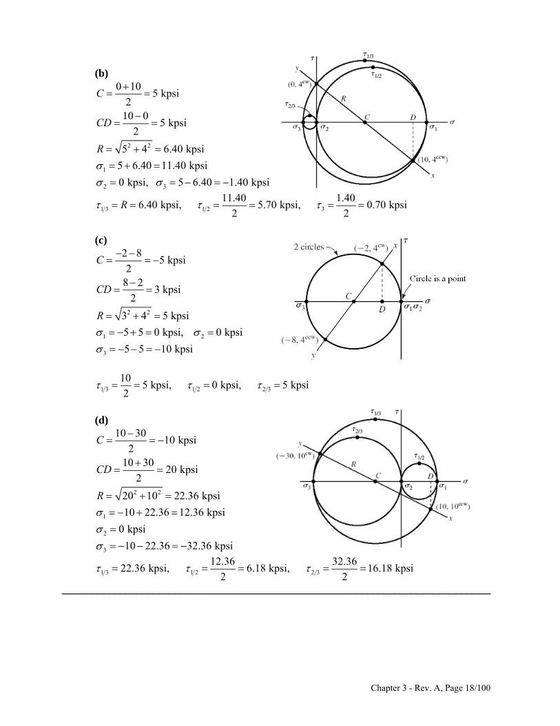
(b)
2 2
1
2 3
0 105 kpsi
210 0
5 kpsi2
5 4 6.40 kpsi
5 6.40 11.40 kpsi
0 kpsi, 5 6.40 1.40 kpsi
C
CD
R
1 3 1 2 3
11.40 1.406.40 kpsi, 5.70 kpsi, 0.70 kpsi
2 2R
(c)
2 2
1 2
3
2 85 kpsi
28 2
3 kpsi2
3 4 5 kpsi
5 5 0 kpsi, 0 kpsi
5 5 10 kpsi
C
CD
R
1 3 1 2 2 3
105 kpsi, 0 kpsi, 5 kpsi
2
(d)
2 2
1
2
3
10 3010 kpsi
210 30
20 kpsi2
20 10 22.36 kpsi
10 22.36 12.36 kpsi
0 kpsi
10 22.36 32.36 kpsi
C
CD
R
1 3 1 2 2 3
12.36 32.3622.36 kpsi, 6.18 kpsi, 16.18 kpsi
2 2
______________________________________________________________________________
Chapter 3 - Rev. A, Page 18/100
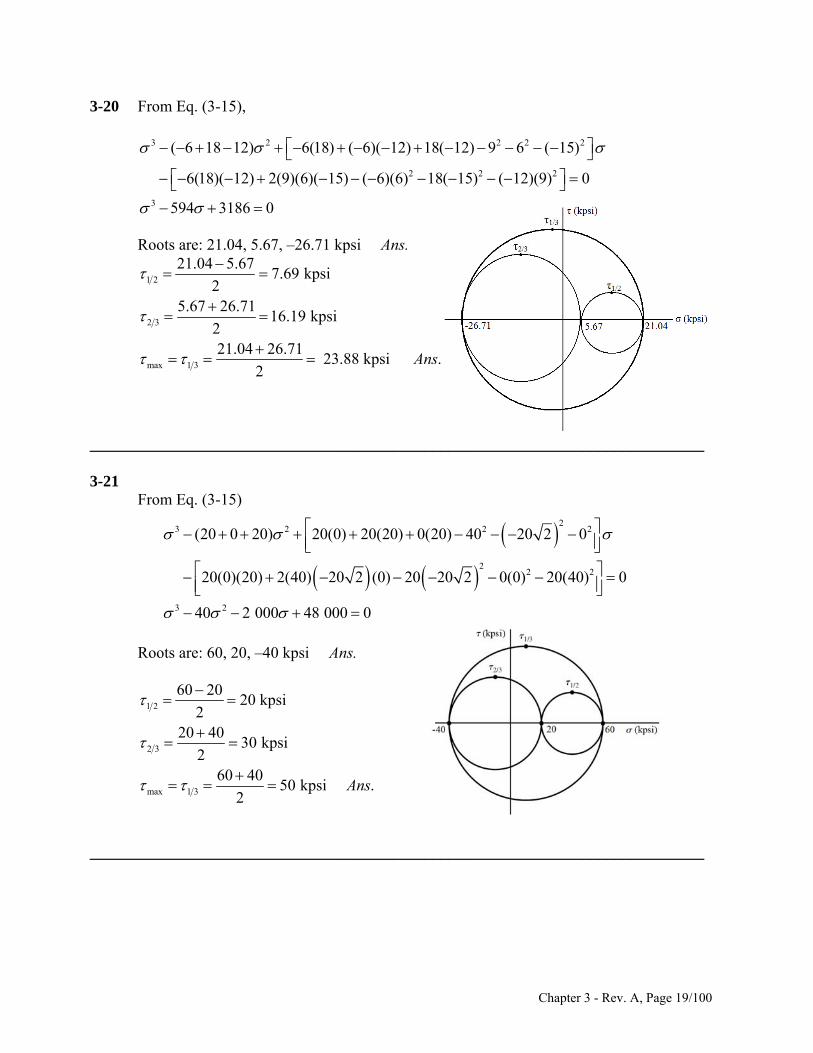
3-20 From Eq. (3-15),
3 2 2 2
2 2 2
3
( 6 18 12) 6(18) ( 6)( 12) 18( 12) 9 6 ( 15)
6(18)( 12) 2(9)(6)( 15) ( 6)(6) 18( 15) ( 12)(9) 0
594 3186 0
2
Roots are: 21.04, 5.67, –26.71 kpsi Ans.
1 2
2 3
max 1 3
21.04 5.677.69 kpsi
25.67 26.71
16.19 kpsi221.04 26.71
23.88 kpsi .2
Ans
_____________________________________________________________________________ 3-21 From Eq. (3-15)
23 2 2
22 2
3 2
(20 0 20) 20(0) 20(20) 0(20) 40 20 2 0
20(0)(20) 2(40) 20 2 (0) 20 20 2 0(0) 20(40) 0
40 2 000 48 000 0
2
Roots are: 60, 20, –40 kpsi Ans.
1 2
2 3
max 1 3
60 2020 kpsi
220 40
30 kpsi2
60 4050 kpsi .
2Ans
_____________________________________________________________________________
Chapter 3 - Rev. A, Page 19/100
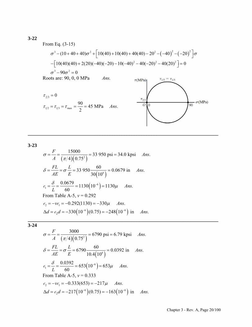
3-22
From Eq. (3-15)
2 23 2 2
2 2 2
3 2
(10 40 40) 10(40) 10(40) 40(40) 20 40 20
10(40)(40) 2(20)( 40)( 20) 10( 40) 40( 20) 40(20) 0
90 0
Roots are: 90, 0, 0 MPa Ans.
2 3
1 2 1 3 max
0
9045 MPa .
2Ans
_____________________________________________________________________________ 3-23
2
6
61
1500033 950 psi 34.0 kpsi .
4 0.75
6033 950 0.0679 in .
30 10
0.06791130 10 1130 .
60
FAns
A
FL LAns
AE E
AnsL
From Table A-5, v = 0.292
2 1
6 62
0.292(1130) 330 .
330 10 (0.75) 248 10 in .
v A
d d An
ns
s
_____________________________________________________________________________ 3-24
2
6
61
30006790 psi 6.79 kpsi .
4 0.75
606790 0.0392 in .
10.4 10
0.0392653 10 653 .
60
FAns
A
FL LAns
AE E
AnsL
From Table A-5, v = 0.333
2 1
6 62
0.333(653) 217 .
217 10 (0.75) 163 10 in .
v Ans
d d Ans
Chapter 3 - Rev. A, Page 20/100
_____________________________________________________________________________ 3-25
2
0.00010.0001
d d
d d
From Table A-5, v = 0.326, E = 119 GPa
621
6 91
2
6
0.0001306.7 10
0.326
and , so
= 306.7 10 (119) 10 36.5 MPa
0.0336.5 10 25 800 N 25.8 kN .
4
vFL F
AE AE
EL
F A An
s
Sy = 70 MPa > , so elastic deformation assumption is valid. _____________________________________________________________________________ 3-26
6
8(12)20 000 0.185 in .
10.4 10
FL LAns
AE E
_____________________________________________________________________________ 3-27
6
9
3140 10 0.00586 m 5.86 mm .
71.7 10
FL LAns
AE E
_____________________________________________________________________________ 3-28
6
10(12)15 000 0.173 in .
10.4 10
FL LAns
AE E
_____________________________________________________________________________ 3-29 With 0,z solve the first two equations of Eq. (3-19) simulatenously. Place E on the
left-hand side of both equations, and using Cramer’s rule,
2 2
1
1 1 1
1
x
y xx yx
E v
E EE vE
v v v
v
yv
Likewise,
Chapter 3 - Rev. A, Page 21/100
21
y x
y
E
v
From Table A-5, E = 207 GPa and ν = 0.292. Thus,
9
62 2
9
62
207 10 0.0019 0.292 0.000 7210 382 MPa .
1 1 0.292
207 10 0.000 72 0.292 0.001910 37.4 MPa .
1 0.292
x y
x
y
E vAns
v
Ans
_____________________________________________________________________________ 3-30 With 0,z solve the first two equations of Eq. (3-19) simulatenously. Place E on the
left-hand side of both equations, and using Cramer’s rule,
2 2
1
1 1 1
1
x
y xx yx
E v
E EE vE
v v v
v
yv
Likewise,
21
y x
y
E
v
From Table A-5, E = 71.7 GPa and ν = 0.333. Thus,
9
62 2
9
62
71.7 10 0.0019 0.333 0.000 7210 134 MPa .
1 1 0.333
71.7 10 0.000 72 0.333 0.001910 7.04 MPa .
1 0.333
x y
x
y
E vAns
v
Ans
_____________________________________________________________________________ 3-31
(a) 1 max 1 c ac
R F M R a Fl l
2
2 2
6 6
6
M ac bh lF F
bh bh l ac
Ans.
(b)
2 21 21( )( ) ( )
.( )( )
m m m mm
m m
b b h h l lF s s ss Ans
F a a c c s s
3-32
For equal stress, the model load varies by the square of the scale factor.
_____________________________________________________________________________
Chapter 3 - Rev. A, Page 22/100
2
1 max /2,
2 2 2 2x l
l l lR M l
w w
8
lww
(a)
2 2
2 2 2
6 6 3 4 .
8 4 3
M l Wl bhW A
bh bh bh l
w
ns
(b) 2 2
2( / )( / )( / ) 1( )( ).
/m m m m
m
W b b h h s ss An
W l l s
s
22 .m m ml s
s sl s
w ww w
Ans
For equal stress, the model load w varies linearly with the scale factor. _____ _____________
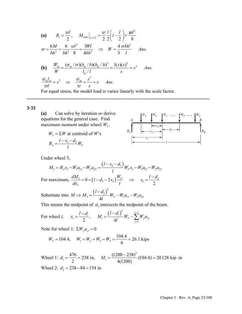
-33 (a) Can solve by iteration or derive
_ __________________________________________________________ 3
equations for the general case. Find maximum moment under wheel 3W .
W W at centroid of W’s T
3 3dA T
l xR W
l
Under wheel 3,
3 3
3 3 1 13 2 23 3 1 13 2 23A T
l x dM R x W a W a W x W a W a
l
For maximum, 3 33 3 3
3
0 22
TdM l dWl d x x
dx l
Substitute into 2
33 1 14 T
l d3 2 23M M W W a
l
W a
intersects the midpoint of the beam.
For wheel i,
This means the midpoint of 3d
2 1il dl d
1
,2 4
iiT j ji
ji ix M W W a
l
Note for wheel 1:
0j jiW a
1 2 3 4
104.4104.4, 26.1 kips
4TW W W W W
Wheel 1: 2
1 1
476 (1200 238)238 in, (104.4) 20128 kip in
2 4(1200)d M
Wheel 2: 238 84 154 ind 2
Chapter 3 - Rev. A, Page 23/100
2
2 max
(1200 154)(104.4) 26.1(84) 21605 kip in .
4(1200)M M A
ns
Check if all of the wheels are on the rail.
(b) max 600 77 523 in .x Ans
(c) See above sketch. (d) Inner axles
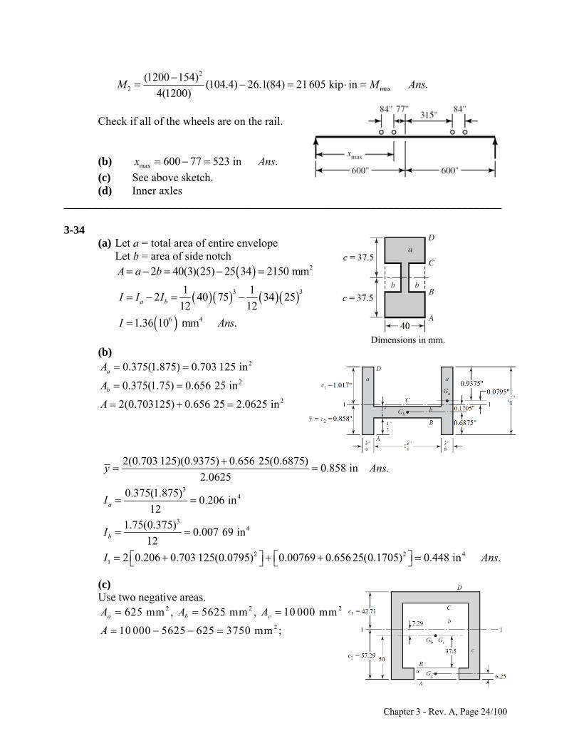
_____________________________________________________________________________ 3-34
(a) Let a = total area of entire envelope Let b = area of side notch
2
3 3
6 4
2 40(3)(25) 25 34 2150 mm
1 12 40 75 34 25
12 12
1.36 10 mm .
a b
A a b
I I I
I Ans
Dimensions in mm. (b)
2
2
2
0.375(1.875) 0.703 125 in
0.375(1.75) 0.656 25 in
2(0.703125) 0.656 25 2.0625 in
a
b
A
A
A
34
34
2 21
2(0.703 125)(0.9375) 0.656 25(0.6875)0.858 in .
2.0625
0.375(1.875)0.206 in
12
1.75(0.375)0.007 69 in
12
2 0.206 0.703 125(0.0795) 0.00769 0.656 25(0.1705) 0.448 in .
a
b
y A
I
I
4
ns
I Ans
(c) Use two negative areas.
2 2
2
625 mm , 5625 mm , 10 000 mm
10 000 5625 625 3750 mm ;
a b cA A A
A
2
Chapter 3 - Rev. A, Page 24/100
1
34
36 4
36 4
6.25 mm, 50 mm, 50 mm
10 000(50) 5625(50) 625(6.25)57.29 mm .
3750100 57.29 42.71 mm .
50(12.5)8138 mm
12
75(75)2.637 10 mm
12
100(100)8.333 10 in
12
a b c
a
b
c
y y y
y Ans
c Ans
I
I
I
2 26 2 61
6 41
8.333 10 10000(7.29) 2.637 10 5625 7.29 8138 625 57.29 6.25
4.29 10 in .
I
I Ans
(d)
2
2
2
4 0.875 3.5 in
2.5 0.875 2.1875 in
5.6875 in
2.9375 3.5 1.25(2.1875)2.288 in .
5.6875
a
b
a b
A
A
A A A
y Ans
3 2 3
4
1 1(4) 0.875 3.5 2.9375 2.288 0.875 2.5 2.1875 2.288 1.25
12 12
5.20 in .
I
I Ans
2
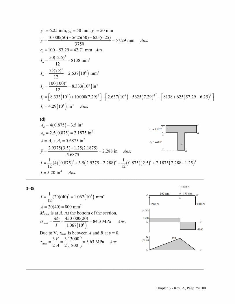
_____________________________________________________________________________ 3-35
3 5
2
1(20)(40) 1.067 10 mm
12
20(40) 800 mm
I
A
4
Mmax is at A. At the bottom of the section,
max 5
450 000(20)84.3 MPa .
1.067 10
McAns
I
Due to V, max is between A and B at y = 0.
max
3 3 30005.63 MPa .
2 2 800
VAns
A
_____________________________________________________________________________
Chapter 3 - Rev. A, Page 25/100
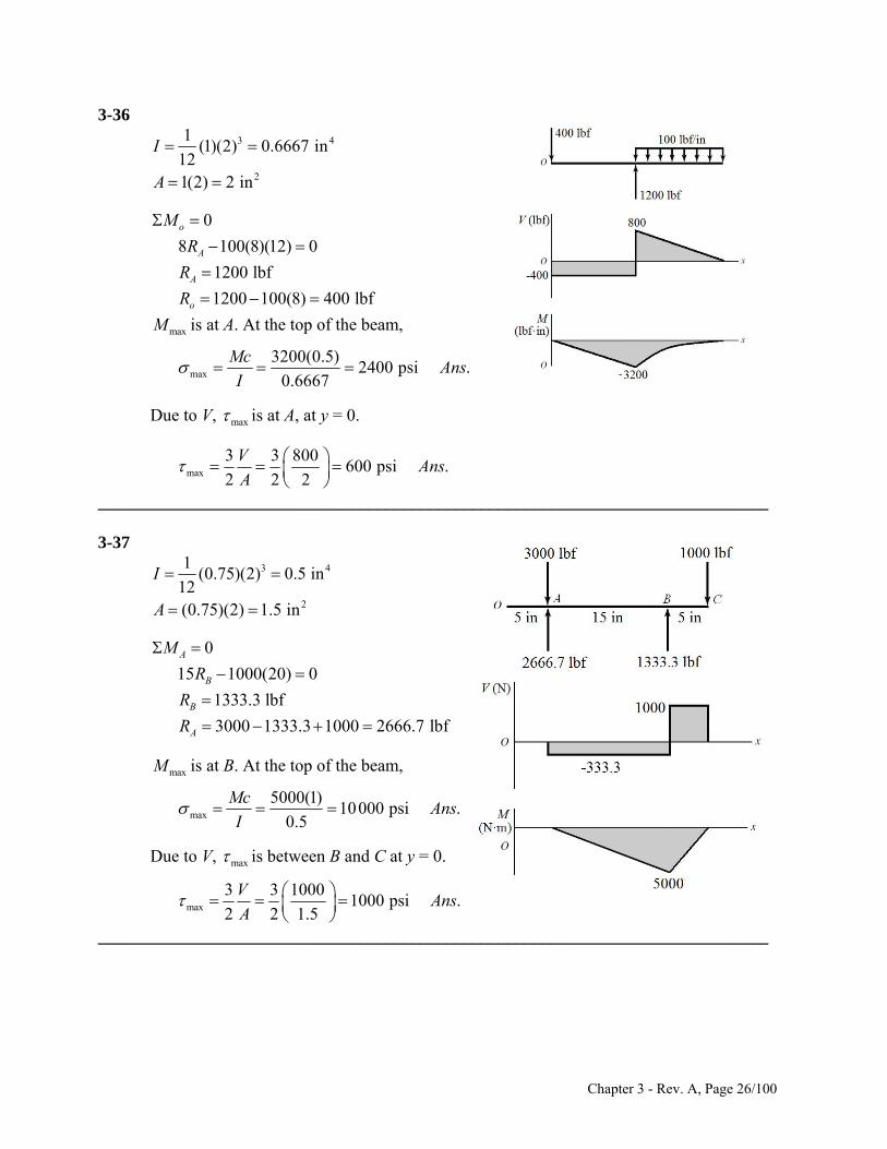
3-36 3 41
(1)(2) 0.6667 in12
I
21(2) 2 inA
0oM
8 100(8)(12) 0AR 1200 lbfAR 1200 100(8) 400 lbfoR
is at A. At the top of the beam, maxM
max
3200(0.5)2400 psi .
0.6667
McAns
I
Due to V, max is at A, at y = 0.
max
3 3 800600 psi .
2 2 2
VAns
A
_____________________________________________________________________________ 3-37
3 41(0.75)(2) 0.5 in
12I
2(0.75)(2) 1.5 inA
0AM
15 1000(20) 0BR 1333.3 lbfBR 3000 1333.3 1000 2666.7 lbfAR
is at B. At the top of the beam, maxM
max
5000(1)10000 psi .
0.5
McAns
I
Due to V, max is between B and C at y = 0.
max
3 3 10001000 psi .
2 2 1.5
VAns
A
_____________________________________________________________________________
Chapter 3 - Rev. A, Page 26/100
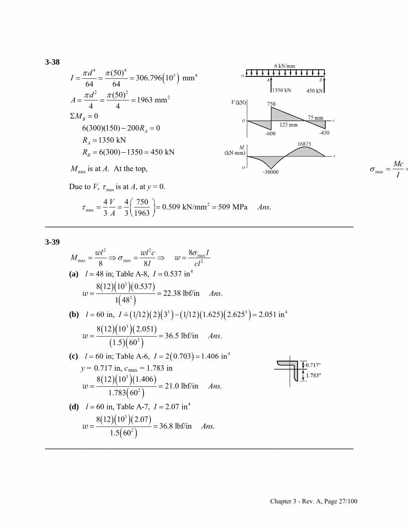
3-38
4 4
3 4(50)306.796 10 mm
64 64
dI
2 22(50)
1963 mm4 4
dA
0BM
6(300)(150) 200 0AR
1350 kNAR
6(300) 1350 450 kNBR
maxM is at A. At the top, max
Mc
I
Due to V, max is at A, at y = 0.
2max
4 4 7500.509 kN/mm 509 MPa .
3 3 1963
VAns
A
_____________________________________________________________________________ 3-39
2 2max
max max 2
8
8 8
Il l cM
I cl
w w
w
(a) 448 in; Table A-8, 0.537 inl I
3
2
8 12 10 0.53722.38 lbf/in .
1 48Ans w
(b) 3 360 in, 1 12 2 3 1 12 1.625 2.625 2.051 inl I 4
3
2
8 12 10 2.05136.5 lbf/in .
1.5 60Ans w
(c) 460 in; Table A-6, 2 0.703 1.406 inl I
y = 0.717 in, cmax = 1.783 in
3
2
8 12 10 1.40621.0 lbf/in .
1.783 60Ans w
(d)
460 in, Table A-7, 2.07 inl I
3
2
8 12 10 2.0736.8 lbf/in .
1.5 60Ans w
_____________________________________________________________________________
Chapter 3 - Rev. A, Page 27/100
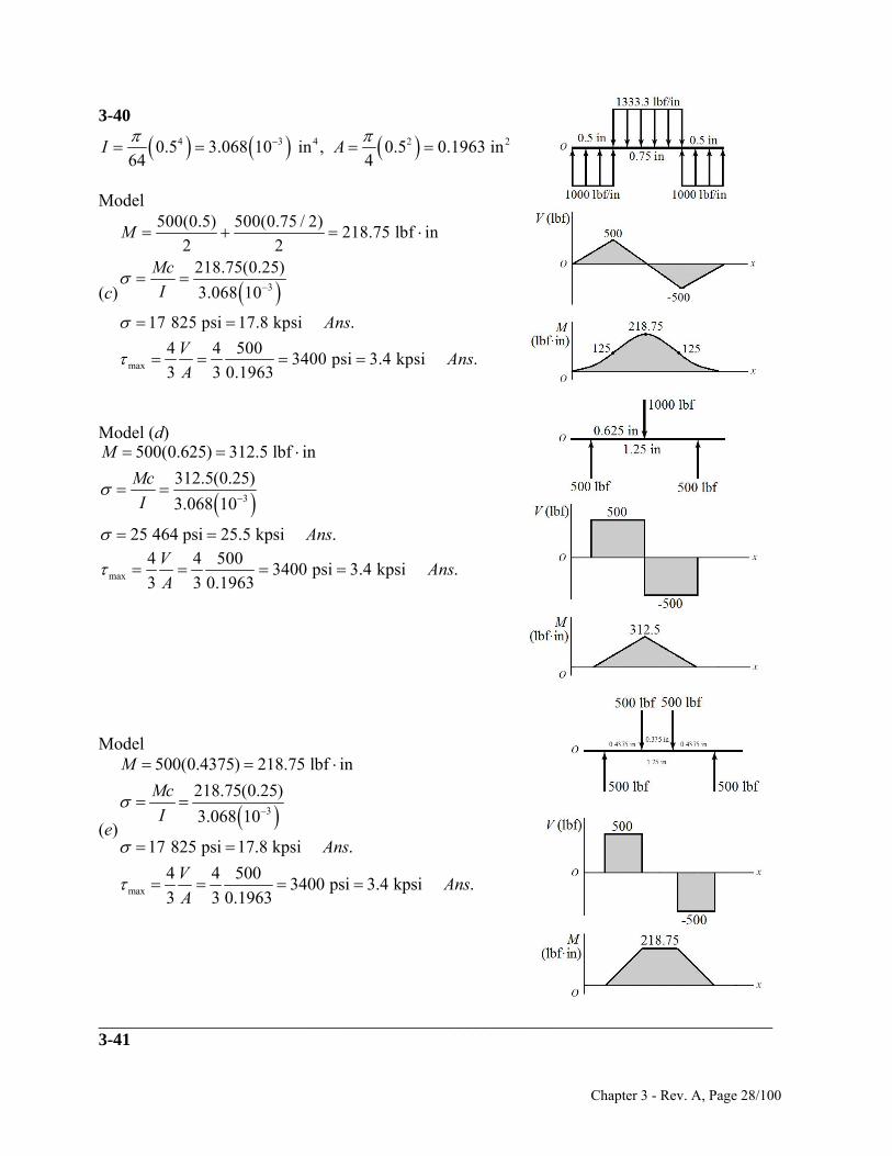
3-40
4 3 4 2 20.5 3.068 10 in , 0.5 0.1963 in64 4
I A
Model
(c) 3
max
500(0.5) 500(0.75 / 2)218.75 lbf in
2 2218.75(0.25)
3.068 10
17 825 psi 17.8 kpsi .
4 4 5003400 psi 3.4 kpsi .
3 3 0.1963
M
Mc
I
Ans
VAns
A
Model (d)
3
500(0.625) 312.5 lbf in
312.5(0.25)
3.068 10
25 464 psi 25.5 kpsi .
M
Mc
I
Ans
max
4 4 5003400 psi 3.4 kpsi .
3 3 0.1963
VAns
A
Model
(e) 3
max
500(0.4375) 218.75 lbf in
218.75(0.25)
3.068 10
17 825 psi 17.8 kpsi .
4 4 5003400 psi 3.4 kpsi .
3 3 0.1963
M
Mc
I
Ans
VAns
A
_____________________________________________________________________________ 3-41
Chapter 3 - Rev. A, Page 28/100
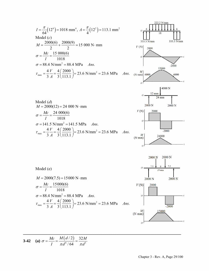
4 4 212 1018 mm , 12 113.1 mm64 4
I A 2
Model (c)
2
2max
2000(6) 2000(9)15 000 N mm
2 215 000(6)
1018
88.4 N/mm 88.4 MPa .
4 4 200023.6 N/mm 23.6 MPa .
3 3 113.1
M
Mc
I
Ans
VAns
A
Model (d)
2
2000(12) 24 000 N mm
24 000(6)
1018
141.5 N/mm 141.5 MPa .
M
Mc
I
Ans
2max
4 4 200023.6 N/mm 23.6 MPa .
3 3 113.1
VAns
A
Model (e)
2
2000(7.5) 15000 N mm
15000(6)
1018
88.4 N/mm 88.4 MPa .
M
Mc
I
Ans
2max
4 4 200023.6 N/mm 23.6 MPa .
3 3 113.1
VAns
A
_____________________________________________________________________________
4 3
/ 2 32
/ 64
M dMc M
I d d
3-42 (a)
Chapter 3 - Rev. A, Page 29/100
3 332 32(218.75)
0.420 in .(30 000)
Md A
ns
(b)
2 / 4
V V
A d
4 4(
500)0.206 in .
(15000)
Vd Ans
(c)
2
4 4
3 3 / 4
V V
A d
4 4 4 4(500)0.238 in .
3 3 (15000)
Vd A
ns
______________ __________________ ______________________________
_____________ _
_
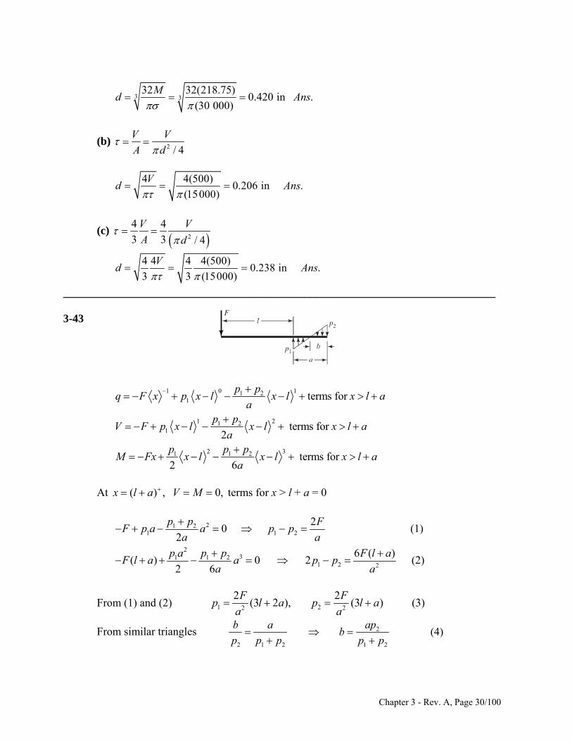
3-43
1 0 11 21
1 21 21
2 31 1 2
terms for
terms for 2
terms for 2 6
p pq F x p x l x l x l a
ap p
V F p x l x l x l aa
p p pM Fx x l x l x l a
a
terms for x > l + a = 0 At x ( ) , 0,l a V M
21 21 1 2
2
Fp p
231 1 2
1 2 2
0 (1)2
6 ( )( ) 0 2 (2)
2 6
p pF p a a
a a
p a p p F l aF l a a p p
a a
From (1) and (2) 1 22 2
2 2(3 2 ), (3 ) (3)
F Fp l a p l a
a a
From similar triang les 2
2 1 2 1 2
(4)apb a
bp p p p p
Chapter 3 - Rev. A, Page 30/100
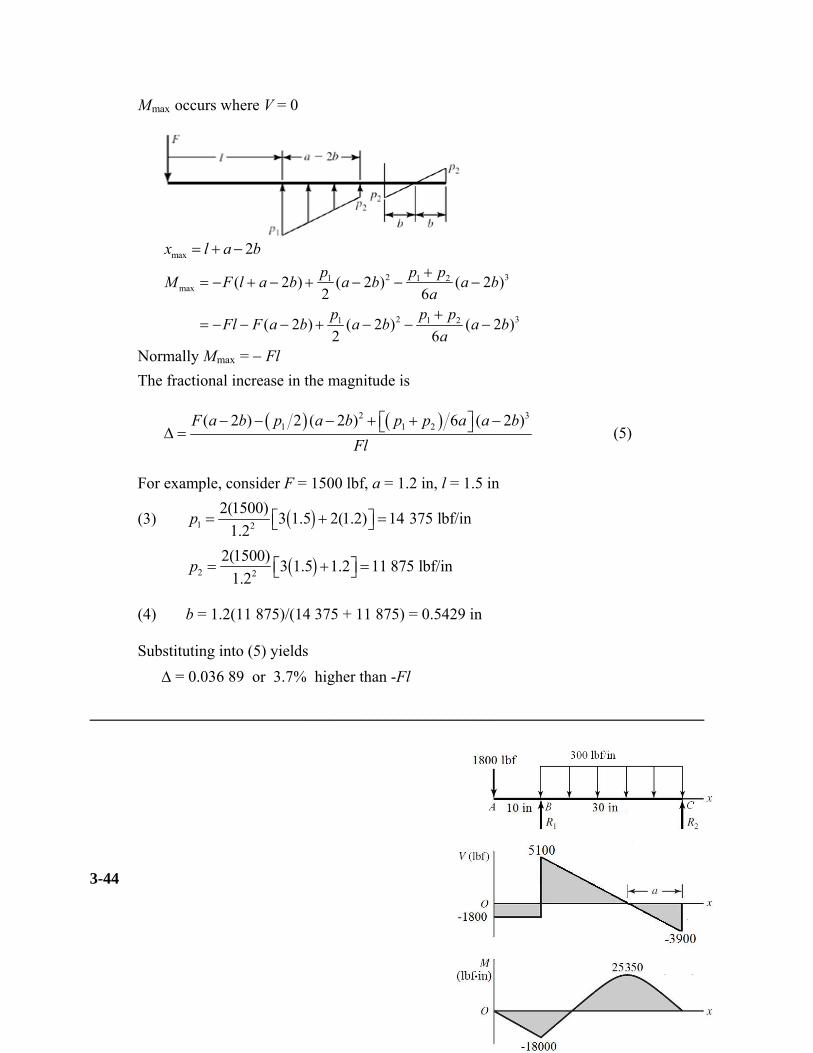
Mmax occurs where V = 0
max 2x l a b
2 31 1 2max
2 31 1 2
( 2 ) ( 2 ) ( 2 )2 6
( 2 ) ( 2 ) ( 2 )2 6
p p pM F l a b a b a b
ap p p
Fl F a b a b a ba
Normally Mmax = Fl
The fractional increase in the magnitude is
2 31 22 ( 2 ) 6 ( 2 )
(5)a b p p a a b
For example, consider F = 1500 lbf, a = 1.2 in, l = 1.5 in
(3)
1( 2 )F a b p
Fl
1 2
2(1500)3 1.5 2(1.2) 14 375 lbf/in
1.2p
2 2
2(1500)3 1.5 1.2 11 875 lbf/in
1.2p
(4) b = 1.2(11 875)/(14 375 + 11 875) = 0.5429 in Substituting into (5) yields
_____________________________________________________________________________
-44
= 0.036 89 or 3.7% higher than -Fl
3
Chapter 3 - Rev. A, Page 31/100
1
2
300(30)R
401800 6900 lbf
2 30300(30) 10
1800 3900 lbf2 30
390013 in
300
R
a
MB = 1800(10) = 18 000 lbfin
x = 27 in = (1/2)3900(13) = 25 350 lbfin
MB = 1800(10) = 18 000 lbfin
x = 27 in = (1/2)3900(13) = 25 350 lbfin MM
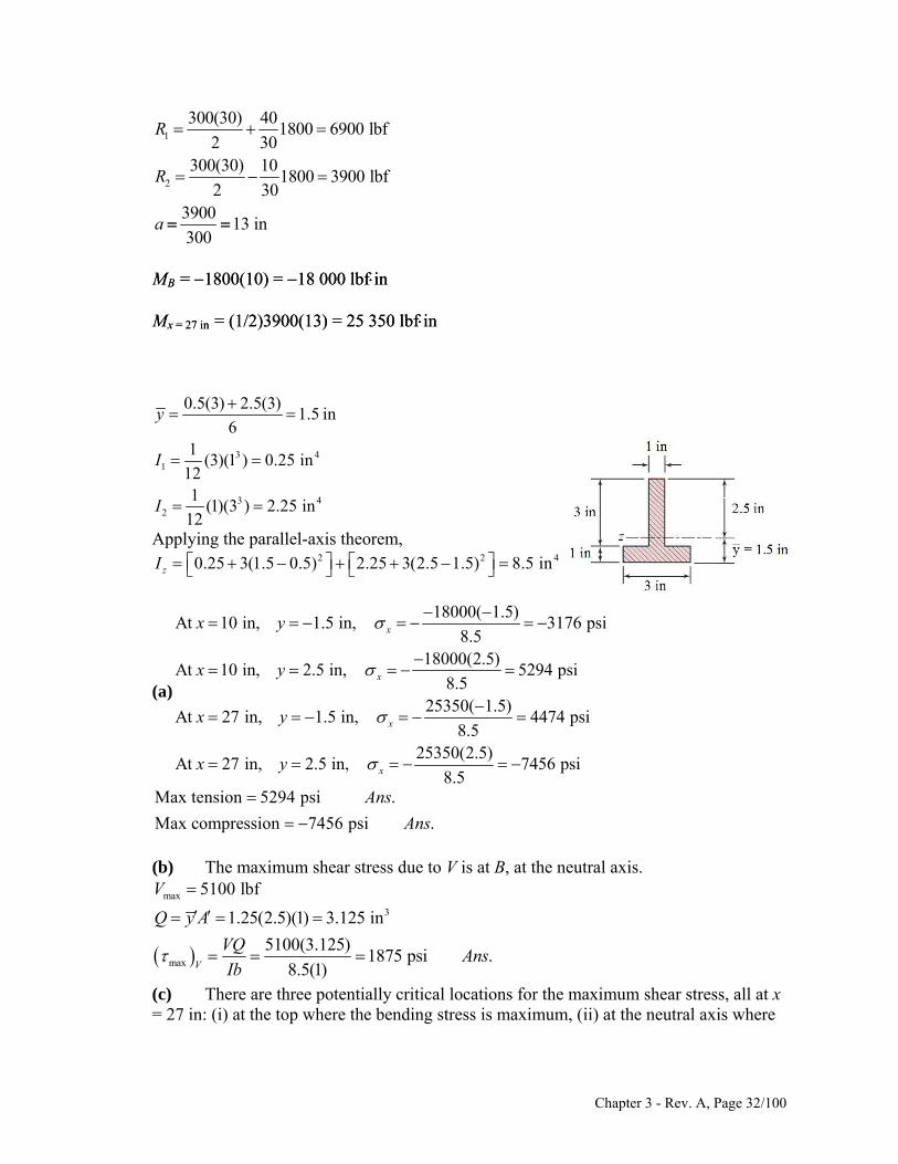
3 41
3 42
0.5(3) 2.5(3)1.5 in
61
(3)(1 ) 0.25 in 121
(1)(3 ) 2.25 in 12
y
I
I
Applying the parallel-axis theorem,
(a)
20.25 3(1.5 0.5) 2.25 3zI 2 4 (2.5 1.5) 8.5 in
18000( 1.5)At 10 in, 1.5 in, 3176 psi
8.518000(2.5)
At 10 in, 2.5 in, 5294 psi8.5
25350( 1.5)At 27 in, 1.5 in, 4474 psi
8.5
At 27 in, 2.5 in,
x
x
x
x
x y
x y
x y
x y
25350(2.5)
7456 psi8.5
Max tension 5294 psi .
Max compression 7456 psi .
Ans
Ans
aximum shear stress due to V is at B, at the neutral axis.
(b) The m max 5100 lbfV
3
max
1.25(2.5)(1) 3.125 in
5100(3.125)1875 psi .
8.5(1)V
Q y A
VQAns
Ib
(c) There are three potentially critical locations for the maximum shear stress, all at x = 27 in: (i) at the top where the bending stress is maximum, (ii) at the neutral axis where
Chapter 3 - Rev. A, Page 32/100
the transverse shear is maximum, or (iii) in the web just above the flange where bending stress and shear stress are in their largest combination. For (i):
The maximum bending stress was previously found to be 7456 psi, and the shear stress is zero. From Mohr’s circle,
maxmax
74563728 psi
2 2
For (ii):
The bending stress is zero, and the transverse shear stress was found previously to be 1875 psi. Thus, max = 1875 psi.
For (iii): The bending stress at y = – 0.5 in is
18000( 0.5)1059 psi
8.5x
The transverse shear stress is
3(1)(3)(1) 3.0 in
5100(3.0)1800 psi
8.5(1)
Q y A
VQ
Ib
From Mohr’s circle,
22
max
10591800 1876 psi
2
The critical location is at x = 27 in, at the top surface, where max = 3728 psi. Ans.
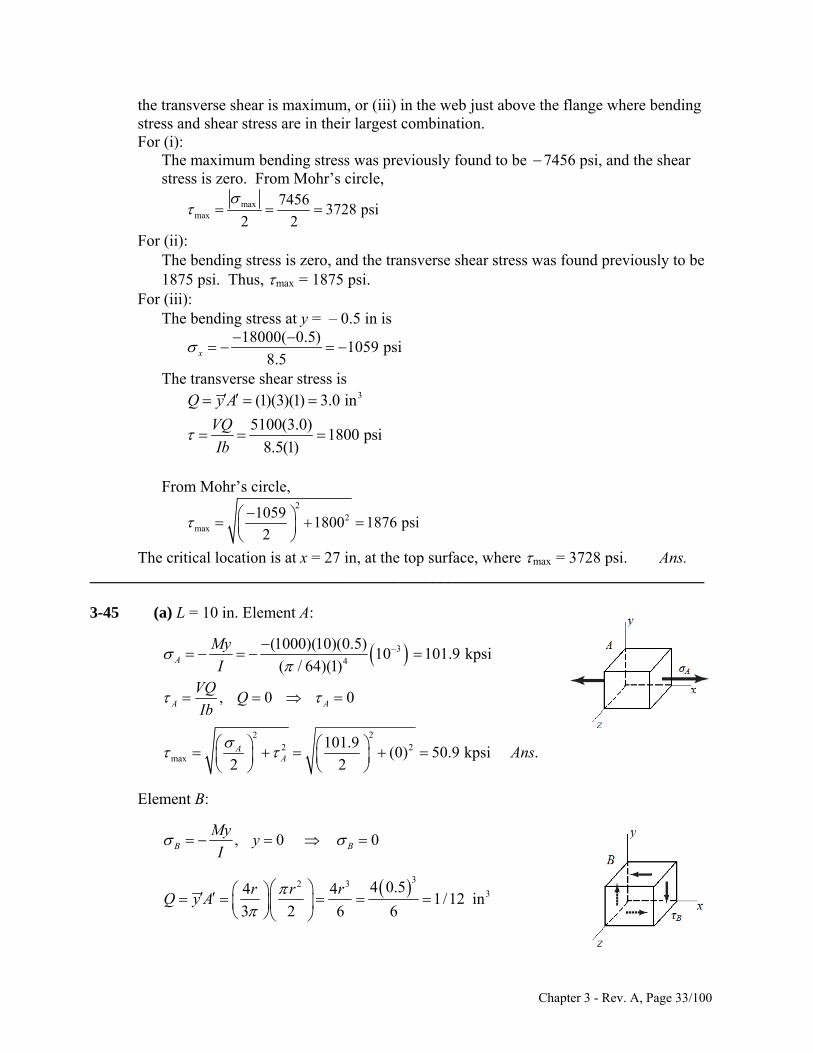
_____________________________________________________________________________ 3-45 (a) L = 10 in. Element A:
34
(1000)(10)(0.5)10 101.9 kpsi
( / 64)(1)A
My
I
, 0A A
VQQ 0
Ib
2 22 2
max
101.9(0) 50.9 kpsi .
2 2A
A Ans
Element B:
, 0 0B B
Myy
I
32 334 0.54 4
1/12 in3 2 6 6
r r rQ y A
Chapter 3 - Rev. A, Page 33/100
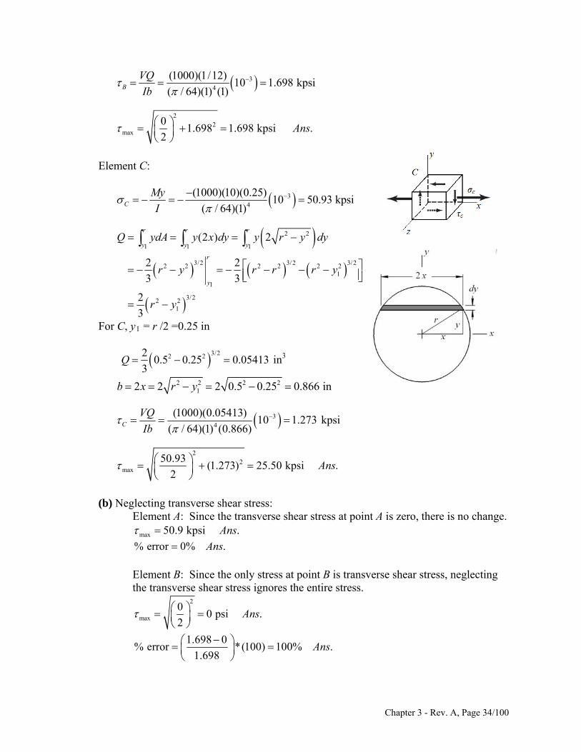
34
(1000)(1/12)10 1.698 kpsi
( / 64)(1) (1)B
VQ
Ib
22
max
01.698 1.698 kpsi .
2Ans
Element C:
34
(1000)(10)(0.25)10 50.93 kpsi
( / 64)(1)C
My
I
2 2
1 1 1
3/2 3/2 3/22 2 2 2 2 21
1
3/22 21
(2 ) 2
2 2
3 3
2
3
r r r
y y y
r
y
Q ydA y x dy y r y dy
r y r r r y
r y
For C, y1 = r /2 =0.25 in
3/22 220.5 0.25 0.05413
3Q in3
2 2 2 212 2 2 0.5 0.25 0.866 inb x r y
34
(1000)(0.05413)10 1.273 kpsi
( / 64)(1) (0.866)C
VQ
Ib
22
max
50.93(1.273) 25.50 kpsi .
2Ans
(b) Neglecting transverse shear stress: Element A: Since the transverse shear stress at point A is zero, there is no change.
max 50.9 kpsi .Ans
% error 0% .Ans
Element B: Since the only stress at point B is transverse shear stress, neglecting the transverse shear stress ignores the entire stress.
2
max
00 psi .
2Ans
1.698 0% error *(100) 100% .
1.698Ans
Chapter 3 - Rev. A, Page 34/100
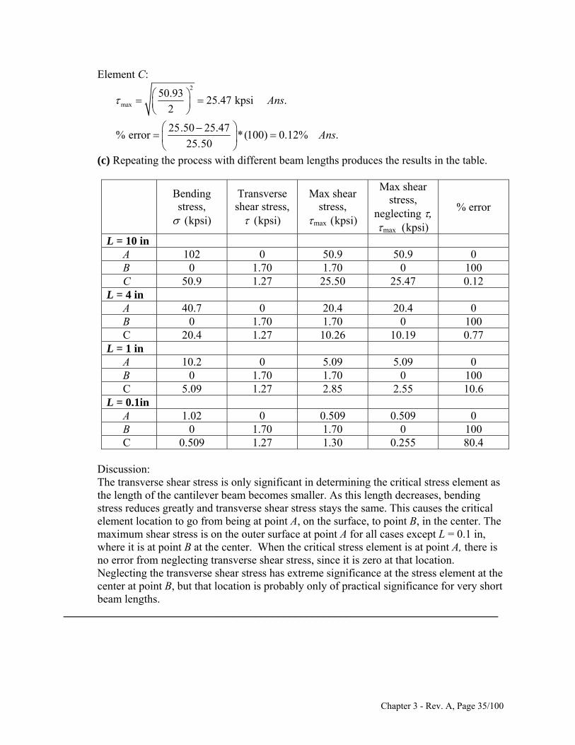
Element C: 2
max
50.9325.47 kpsi .
2Ans
25.50 25.47% error *(100) 0.12% .
25.50Ans
(c) Repeating the process with different beam lengths produces the results in the table.
Bending stress, kpsi)
Transverse shear stress, kpsi)
Max shear stress,
max kpsi)
Max shear stress,
neglecting max kpsi)
% error
L = 10 in A 102 0 50.9 50.9 0 B 0 1.70 1.70 0 100 C 50.9 1.27 25.50 25.47 0.12 L = 4 in A 40.7 0 20.4 20.4 0 B 0 1.70 1.70 0 100 C 20.4 1.27 10.26 10.19 0.77 L = 1 in A 10.2 0 5.09 5.09 0 B 0 1.70 1.70 0 100 C 5.09 1.27 2.85 2.55 10.6 L = 0.1in A 1.02 0 0.509 0.509 0 B 0 1.70 1.70 0 100 C 0.509 1.27 1.30 0.255 80.4
Discussion:
The transverse shear stress is only significant in determining the critical stress element as the length of the cantilever beam becomes smaller. As this length decreases, bending stress reduces greatly and transverse shear stress stays the same. This causes the critical element location to go from being at point A, on the surface, to point B, in the center. The maximum shear stress is on the outer surface at point A for all cases except L = 0.1 in, where it is at point B at the center. When the critical stress element is at point A, there is no error from neglecting transverse shear stress, since it is zero at that location. Neglecting the transverse shear stress has extreme significance at the stress element at the center at point B, but that location is probably only of practical significance for very short beam lengths.
_____________________________________________________________________________
Chapter 3 - Rev. A, Page 35/100
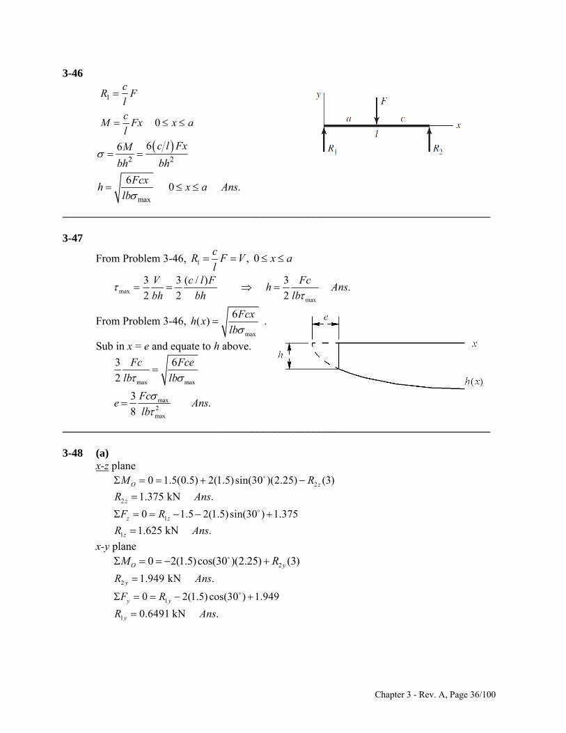
3-46
1
0
cR F
lc
M Fx x al
2 2
max
66
6 0 .
c l FxM
bh bh
Fcxh x
lb
a Ans
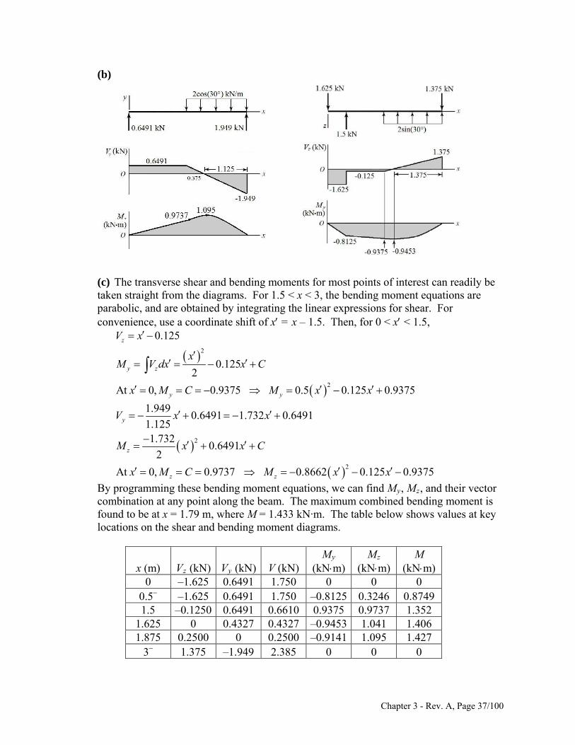
_____________________________________________________________________________ 3-47
From Problem 3-46, 1 , 0c
R F V x al
maxmax
3 3 ( / ) 3 .
2 2 2
V c l F Fch A
bh bh lb
ns
From Problem 3-46, max
6( )
Fcxh x .
lb
Sub in x = e and equate to h above.
max max
max2max
3 6
2
3 .
8
Fc Fce
lb lb
Fce A
lb
ns
_____________________________________________________________________________ 3-48 (a)
x-z plane
20 1.5(0.5) 2(1.5)sin(30 )(2.25) (3)O zM R
2 1.375 kN .zR Ans
10 1.5 2(1.5)sin(30 ) 1.375z zF R
1 1.625 kN .zR Ans
x-y plane
20 2(1.5)cos(30 )(2.25) (3)O yM R
2 1.949 kN .yR Ans
10 2(1.5) cos(30 ) 1.949y yF R
1 0.6491 kN .yR Ans
Chapter 3 - Rev. A, Page 36/100
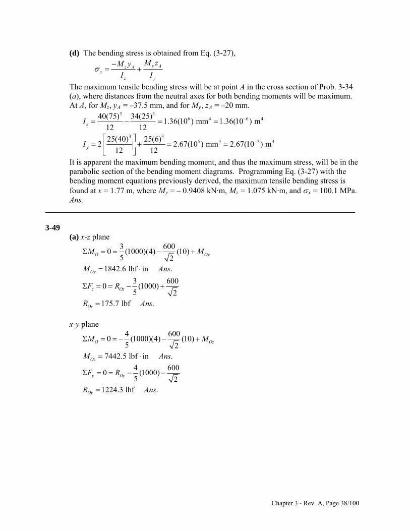
(b)
(c) The transverse shear and bending moments for most points of interest can readily be taken straight from the diagrams. For 1.5 < x < 3, the bending moment equations are parabolic, and are obtained by integrating the linear expressions for shear. For convenience, use a coordinate shift of x = x – 1.5. Then, for 0 < x < 1.5,
2
2
0.125
0.1252
At 0, 0.9375 0.5 0.125 0.9375
z
y z
y y
V x
xM V dx x C
x M C M x x
2
2
1.9490.6491 1.732 0.6491
1.1251.732
0.64912
At 0, 0.9737 0.8662 0.125 0.9375
y
z
z z
V x x
M x x C
x M C M x x
By programming these bending moment equations, we can find My, Mz, and their vector combination at any point along the beam. The maximum combined bending moment is found to be at x = 1.79 m, where M = 1.433 kN·m. The table below shows values at key locations on the shear and bending moment diagrams.
x (m) Vz (kN) Vy (kN) V (kN) My
(kNm) Mz
(kNm) M
(kNm) 0 –1.625 0.6491 1.750 0 0 0
0.5 –1.625 0.6491 1.750 –0.8125 0.3246 0.8749 1.5 –0.1250 0.6491 0.6610 0.9375 0.9737 1.352
1.625 0 0.4327 0.4327 –0.9453 1.041 1.406 1.875 0.2500 0 0.2500 –0.9141 1.095 1.427
3 1.375 –1.949 2.385 0 0 0
Chapter 3 - Rev. A, Page 37/100
(d) The bending stress is obtained from Eq. (3-27),
y Az Ax
z y
M zM y
I I
The maximum tensile bending stress will be at point A in the cross section of Prob. 3-34 (a), where distances from the neutral axes for both bending moments will be maximum. At A, for Mz, yA = –37.5 mm, and for My, zA = –20 mm.
3 36 4 640(75) 34(25)
1.36(10 ) mm 1.36(10 ) m12 12zI 4
3 35 4 725(40) 25(6)
2 2.67(10 ) mm 2.67(10 ) m12 12yI
4
It is apparent the maximum bending moment, and thus the maximum stress, will be in the parabolic section of the bending moment diagrams. Programming Eq. (3-27) with the bending moment equations previously derived, the maximum tensile bending stress is found at x = 1.77 m, where My = – 0.9408 kN·m, Mz = 1.075 kN·m, and x = 100.1 MPa. Ans.
_____________________________________________________________________________ 3-49 (a) x-z plane
3 6000 (1000)(4) (10)
5 2O OyM M
1842.6 lbf in .OyM Ans
3 60 (1000)
5 2z OzF R
00
175.7 lbf .OzR Ans
x-y plane
4 6000 (1000)(4) (10)
5 2O OzM M
7442.5 lbf in .OzM Ans
4 60 (1000)
5 2y OyF R
00
1224.3 lbf .OyR Ans
Chapter 3 - Rev. A, Page 38/100
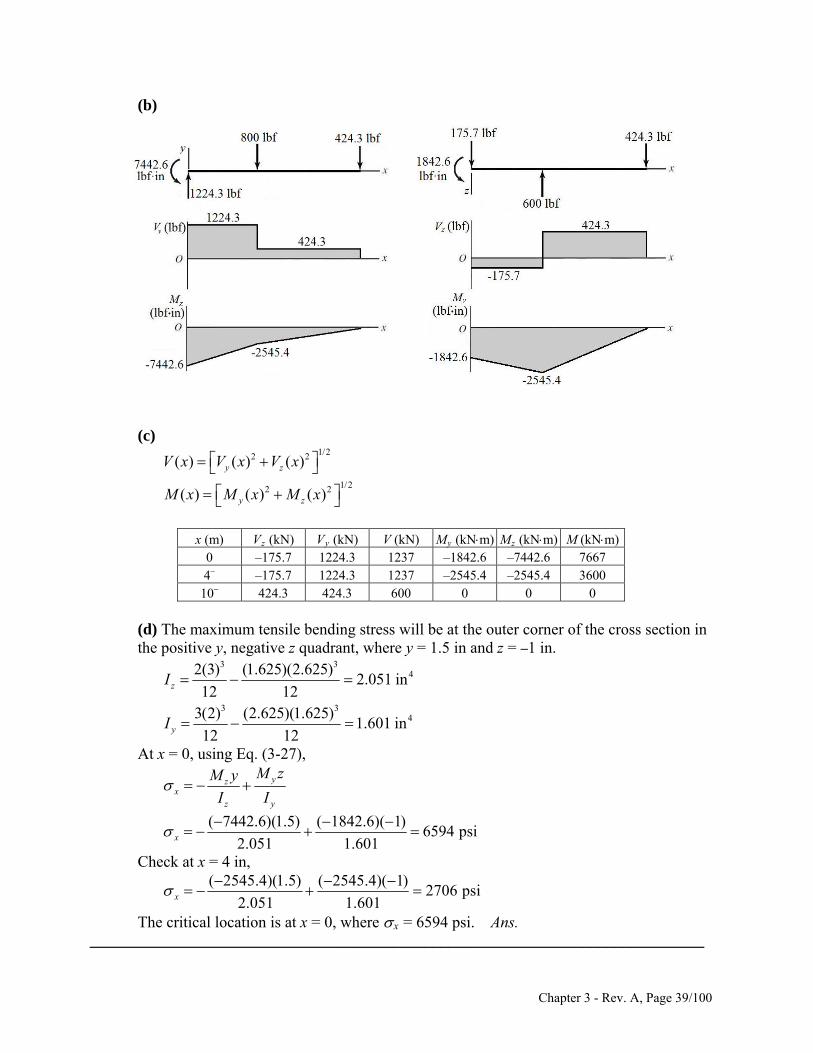
(b)
( (c)
1/22 2( ) ( ) ( )y zV x V x V x
1/22 2( ) ( ) ( )y zM x M x M x
x (m) Vz (kN) Vy (kN) V (kN) My (kNm) Mz (kNm) M (kNm) 0 –175.7 1224.3 1237 –1842.6 –7442.6 7667 4 –175.7 1224.3 1237 –2545.4 –2545.4 3600
10 424.3 424.3 600 0 0 0
(d) The maximum tensile bending stress will be at the outer corner of the cross section in
the positive y, negative z quadrant, where y = 1.5 in and z = –1 in. 3 3
42(3) (1.625)(2.625)2.051 in
12 12zI
3 343(2) (2.625)(1.625)
1.601 in12 12yI
At x = 0, using Eq. (3-27),
yzx
z y
M zM y
I I
( 7442.6)(1.5) ( 1842.6)( 1)6594 psi
2.051 1.601x
Check at x = 4 in, ( 2545.4)(1.5) ( 2545.4)( 1)
2706 psi2.051 1.601x
The critical location is at x = 0, where x = 6594 psi. Ans. _____________________________________________________________________________
Chapter 3 - Rev. A, Page 39/100
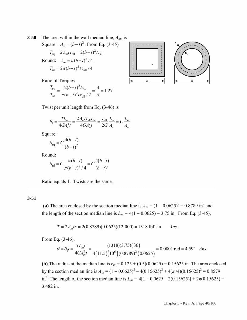
3-50 The area within the wall median line, Am, is
Square: 2( )mA b t . From Eq. (3-45) 2
sq all all2 2( )mT A t b t t
Round: 2( ) /mA b t 4
2rd all2 ( ) / 4T b t t
Ratio of Torques
2sq all
2rd all
2( ) 41.27
( ) / 2
T b t t
T b t t
Twist per unit length from Eq. (3-46) is
all all1 2 2
2
4 4 2m m m m
m m m
TL A t L L LC
GA t GA t G A Am
m
Square:
sq 2
4( )
( )
b tC
b t
Round:
rd 2 2
( ) 4(
( ) / 4 ( )
b t b tC C
b t b t
)
Ratio equals 1. Twists are the same. _____________________________________________________________________________ 3-51
(a) The area enclosed by the section median line is Am = (1 0.0625)2 = 0.8789 in2 and
the length of the section median line is Lm = 4(1 0.0625) = 3.75 in. From Eq. (3-45),
2 2(0.8789)(0.0625)(12 000) 1318 lbf in .mT A t Ans
From Eq. (3-46),
1 2 6 2
(1318)(3.75) 360.0801 rad 4.59 .
4 4 11.5 10 (0.8789) 0.0625m
m
TL ll A
GA t ns
(b) The radius at the median line is rm = 0.125 + (0.5)(0.0625) = 0.15625 in. The area enclosed
by the section median line is Am = (1 0.0625)2 – 4(0.15625)2 + 4(π /4)(0.15625)2 = 0.8579
in2. The length of the section median line is Lm = 4[1 – 0.0625 – 2(0.15625)] + 2π(0.15625) =
3.482 in.
Chapter 3 - Rev. A, Page 40/100
From Eq. (3-45), 2 2(0.8579)(0.0625)(12 000) 1287 lbf in .mT A t Ans
From Eq. (3-46),
1 2 6 2
(1287)(3.482) 360.0762 rad 4.37 .
4 4 11.5 10 (0.8579) 0.0625m
m
TL ll A
GA t ns
_____________________________________________________________________________
3-52
31
1 3
3
3i i
ii i
T GT
GL c
iL c
331
1 2 31
.3 i i
i
GT T T T L c Ans
From Eq. (3-47), G1c
G and 1 are constant, therefore the largest shear stress occurs when c is a maximum.
max 1 max .G c Ans _____________________________________________________________________________
3-53
(b) Solve part (b) first since the twist is needed for part (a).
max allow 12 6.89 82.7 MPa
6
max1 9
max
82.7 100.348 rad/m .
79.3 10 (0.003)Ans
Gc
(a)
9 331 1 1
1
0.348(79.3) 10 (0.020)(0.002 )1.47 N m .
3 3
GL cT A
ns
9 332 2 2
2
9 333 3 3
3
1 2 3
0.348(79.3) 10 (0.030)(0.003 )7.45 N m .
3 3
0.348(79.3) 10 (0)(0 )0 .
3 31.47 7.45 0 8.92 N m .
GL cT A
GL cT A
T T T T Ans
ns
ns
_____________________________________________________________________________
Chapter 3 - Rev. A, Page 41/100
3-54
(b) Solve part (b) first since the twist is needed for part (a).
3max1 6
max
120008.35 10 rad/in .
11.5 10 (0.125)Ans
Gc
(a)
3 6 331 1 1
1
3 6 332 2 2
2
3 6 333 3 3
3
1 2 3
8.35 10 11.5 10 0.75 0.06255.86 lbf in .
3 3
8.35 10 11.5 10 1 0.12562.52 lbf in .
3 3
8.35 10 11.5 10 0.625 0.06254.88 lbf in .
3 35.86 62.52 4
GL cT A
GL cT A
GL cT A
T T T T
.88 73.3 lbf in .Ans
ns
ns
ns
_____________________________________________________________________________
3-55
(b) Solve part (b) first since the twist is needed for part (a).
max allow 12 6.89 82.7 MPa
6
max1 9
max
82.7 100.348 rad/m .
79.3 10 (0.003)Ans
Gc
(a)
9 331 1 1
1
0.348(79.3) 10 (0.020)(0.002 )1.47 N m .
3 3
GL cT A
ns
9 332 2 2
2
9 333 3 3
3
1 2 3
0.348(79.3) 10 (0.030)(0.003 )7.45 N m .
3 3
0.348(79.3) 10 (0.025)(0.002 )1.84 N m .
3 31.47 7.45 1.84 10.8 N m .
GL cT A
GL cT A
T T T T Ans
ns
ns
_____________________________________________________________________________
3-56
(a) From Eq. (3-40), with two 2-mm strips,
6 22max
max
80 10 0.030 0.0023.08 N m
3 1.8 / ( / ) 3 1.8 / 0.030 / 0.002
2(3.08) 6.16 N m .
bcT
b c
T Ans
Chapter 3 - Rev. A, Page 42/100
From the table on p. 102, with b/c = 30/2 = 15, and has a value between 0.313 and 0.333.
From Eq. (3-40), 1
0.3213 1.8 / (30 / 2)
From Eq. (3-41),
3 3 9
3.08(0.3)0.151 rad .
0.321 0.030 0.002 79.3 10
6.1640.8 N m .
0.151t
TlAns
bc G
Tk Ans
From Eq. (3-40), with a single 4-mm strip,
6 22max
max
80 10 0.030 0.00411.9 N m .
3 1.8 / ( / ) 3 1.8 / 0.030 / 0.004
bcT A
b c
ns
Interpolating from the table on p. 102, with b/c = 30/4 = 7.5,
7.5 6(0.307 0.299) 0.299 0.305
8 6
From Eq. (3-41)
3 3 9
11.9(0.3)0.0769 rad .
0.305 0.030 0.004 79.3 10
11.9155 N m .
0.0769t
TlAns
bc G
Tk Ans
(b) From Eq. (3-47), with two 2-mm strips,
2 62
max
0.030 0.002 80 103.20 N m
3 32(3.20) 6.40 N m .
LcT
T Ans
3 3 9
3 3(3.20)(0.3)0.151 rad .
0.030 0.002 79.3 10
6.40 0.151 42.4 N m .t
TlAns
Lc G
k T Ans
From Eq. (3-47), with a single 4-mm strip,
2 62
max
0.030 0.004 80 1012.8 N m .
3 3
LcT A
ns
Chapter 3 - Rev. A, Page 43/100
3 3 9
3 3(12.8)(0.3)0.0757 rad .
0.030 0.004 79.3 10
12.8 0.0757 169 N m .t
TlAns
Lc G
k T Ans
The results for the spring constants when using Eq. (3-47) are slightly larger than when using
Eq. (3-40) and Eq. (3-41) because the strips are not infinitesimally thin (i.e. b/c does not equal
infinity). The spring constants when considering one solid strip are significantly larger (almost
four times larger) than when considering two thin strips because two thin strips would be able
to slip along the center plane. _____________________________________________________________________________
3-57
(a) Obtain the torque from the given power and speed using Eq. (3-44).
(40000)
9.55 9.55 152.8 N m2500
HT
n
max 3
16Tr T
J d
1 31 3
6max
16 152.8160.0223 m 22.3 mm .
70 10
Td A
ns
(b) (40000)
9.55 9.55 1528 N m250
HT
n
1 3
6
16(1528)0.0481 m 48.1 mm .
70 10d A
ns
_____________________________________________________________________________ 3-58
(a) Obtain the torque from the given power and speed using Eq. (3-42). 63025 63025(50)
1261 lbf in2500
HT
n
max 3
16Tr T
J d
1 31 3
max
16 1261160.685 in .
(20000)
Td A
ns
(b)
63025 63025(50)12610 lbf in
250
HT
n
1 316(12610)
1.48 in .(20000)
d A
ns
_____________________________________________________________________________
Chapter 3 - Rev. A, Page 44/100
3-59
6 33max
max 3
50 10 0.0316 265 N m
16 16
dTT
d
Eq. (3-44), 3265(2000)55.5 10 W 55.5 kW .
9.55 9.55
TnH A ns
_____________________________________________________________________________
3-60
3 6 33
4 94
16 110 10 0.020 173 N m
16 16
0.020 79.3 10 15180
32 32(173)
1.89 m .
TT d
d
Tl d Gl
JG T
l Ans
_____________________________________________________________________________ 3-61
3 33
4 4 6
16 30 000 0.75 2485 lbf in
16 1632 32(2485)(24)
0.167 rad 9.57 .0.75 11.5 10
TT d
dTl Tl
AnsJG d G
_____________________________________________________________________________ 3-62
(a) 4 4
max max max maxsolid hollow
( )
16 16o o
o o
J d J d dT T
r d r d
4i
44solid hollow
4 4solid
36% (100%) (100%) (100%) 65.6% .
40i
o
T T dT A
T d
ns
(b) 2 2solid hollow, o oW kd W k d d 2
i
22
solid hollow2 2
solid
36% (100%) (100%) (100%) 81.0% .
40i
o
W W dW A
W d
ns
_____________________________________________________________________________
3-63
(a) 44
4 maxmax max max
solid hollow 16 16
d xdJ d JT T
r d r d
44solid hollow
4soli
( )% (100%) (100%) (100%) .
d
T T xdT x
T d
Ans
Chapter 3 - Rev. A, Page 45/100
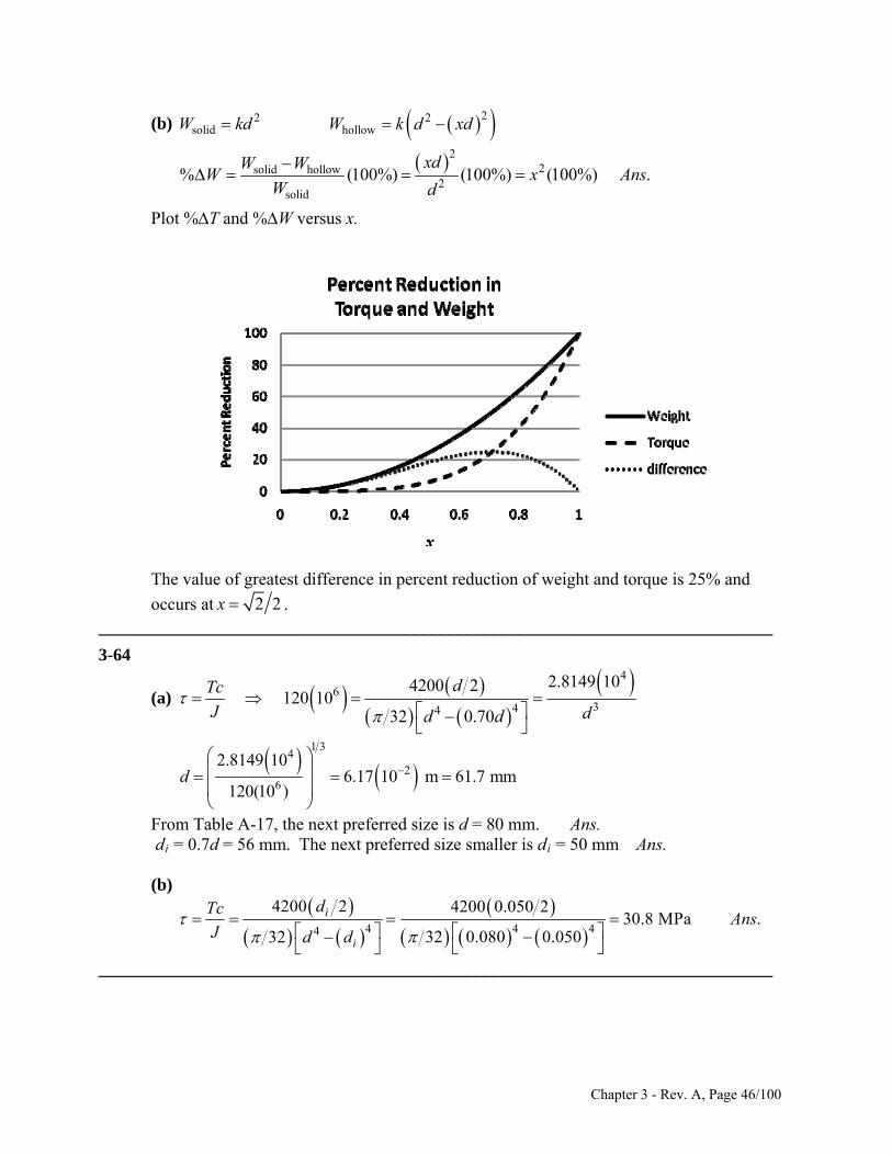
(b) 22 2solid hollow W kd W k d xd
22solid hollow
2solid
% (100%) (100%) (100%) .xdW W
W xW d
Ans
Plot %T and %W versus x.
The value of greatest difference in percent reduction of weight and torque is 25% and
occurs at 2 2x . _____________________________________________________________________________
3-64
(a)
46
344
2.8149 104200 2 120 10
32 0.70
dTc
J dd d
1 3
42
6
2.8149 106.17 10 m 61.7 mm
120(10 )d
d From Table A-17, the next preferred size is d = 80 mm. Ans.
i = 0.7d = 56 mm. The next preferred size smaller is di = 50 mm Ans.
(b)
4 4 44
4200 2 4200 0.050 230.8 MPa .
32 0.080 0.05032
i
i
dTcAns
J d d
_____________________________________________________________________________
Chapter 3 - Rev. A, Page 46/100
3-65
(1500)
9.55 9.55 1433 N m10
HT
n
1 31 3
3 6
16 143316 16 = 0.045 m 45 mm
80 10C
C
T Td
d
From Table A-17, select 50 mm. Ans.
(a) 6
start 3
16 2 1433117 10 Pa 117 MPa .
0.050Ans
(b) Design activity _____________________________________________________________________________
3-66
1 31 3
3
63 025 63 025(1)7880 lbf in
8
16 788016 16 = 1.39 in
15 000CC
HT
n
T Td
d
From Table A-17, select 1.40 in. Ans. _____________________________________________________________________________
3-67 For a square cross section with side length b, and a circular section with diameter d,
2 2square circular
4 2A A b d b d
From Eq. (3-40) with b = c,
3
max 2 3 3square
1.8 1.8 23 3 (4.8) 6.896
/ 1
T T T
bc b c b d d
3
T
For the circular cross section,
max 3 3circular
165.093
T T
d d
3max square
max circular3
6.8961.354
5.093
TdTd
The shear stress in the square cross section is 35.4% greater. Ans.
(b) For the square cross section, from the table on p. 102, β = 0.141. From Eq. (3-41),
Chapter 3 - Rev. A, Page 47/100
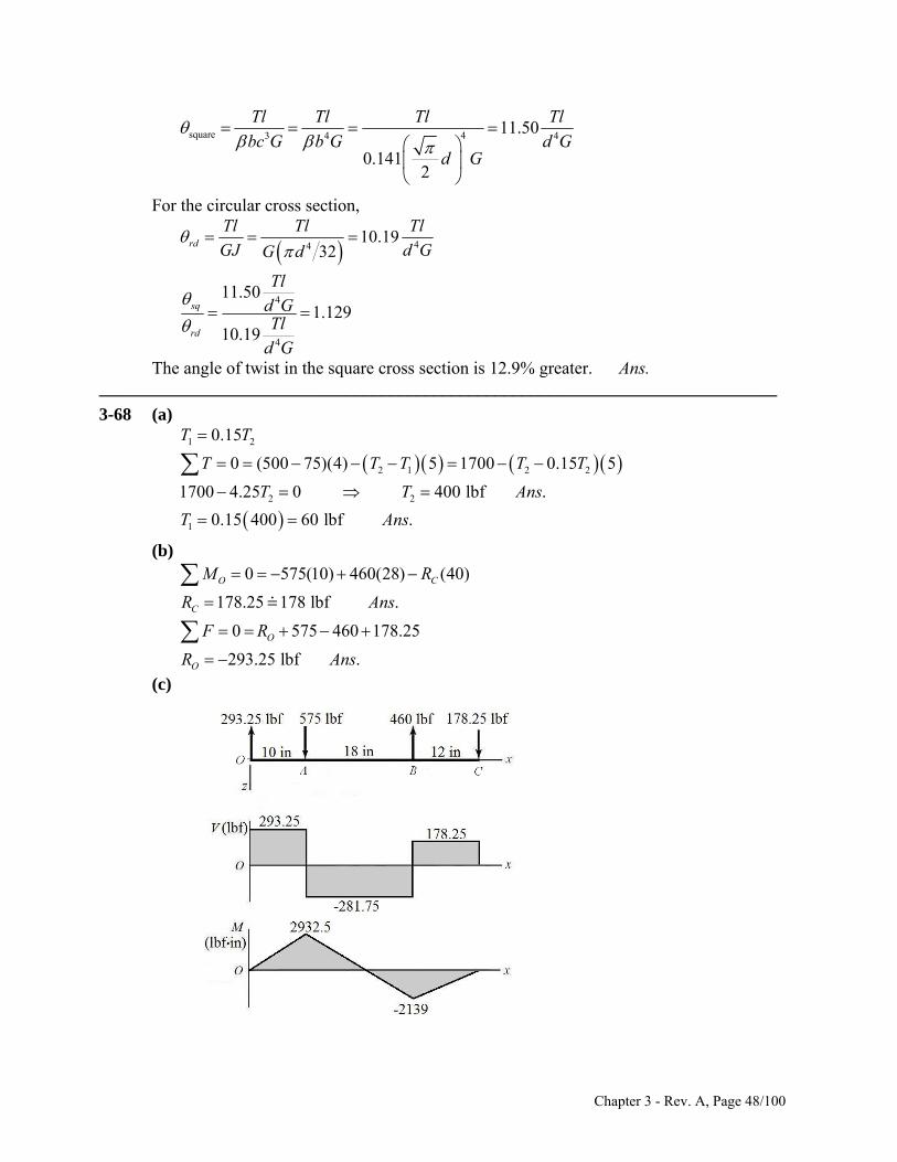
square 43 411.50
0.1412
Tl Tl Tl Tl
bc G b G d Gd G
4
For the circular cross section,
4410.19
32rd
Tl Tl Tl
GJ d GG d
4
4
11.501.129
10.19
sq
rd
Tld GTl
d G
The angle of twist in the square cross section is 12.9% greater. Ans. _____________________________________________________________________________
3-68 (a)
1 2
2 1 2 2
2 2
1
0.15
0 (500 75)(4) 5 1700 0.15 5
1700 4.25 0 400 lbf .
0.15 400 60 lbf .
T T
T T T T
T T Ans
T Ans
T
s
(b)
0 575(10) 460(28) (40)
178.25 178 lbf .
0 575 460 178.25
293.25 lbf .
O C
C
O
O
M R
R An
F R
R Ans
(c)
Chapter 3 - Rev. A, Page 48/100
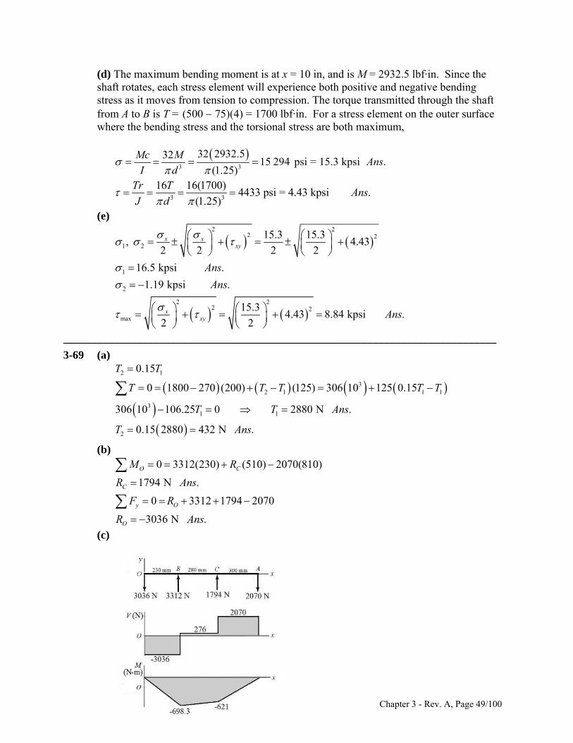
(d) The maximum bending moment is at x = 10 in, and is M = 2932.5 lbf·in. Since the shaft rotates, each stress element will experience both positive and negative bending stress as it moves from tension to compression. The torque transmitted through the shaft from A to B is T = (500 75)(4) = 1700 lbf·in. For a stress element on the outer surface where the bending stress and the torsional stress are both maximum,
3 3
32 2932.53215 294 psi = 15.3 kpsi .
(1.25)
Mc MAns
I d
3 3
16 16(1700)4433 psi = 4.43 kpsi .
(1.25)
Tr TAns
J d
(e)
2 22 2
1 2
1
2
2 22 2
max
15.3 15.3, 4.43
2 2 2 2
16.5 kpsi .
1.19 kpsi .
15.34.43 8.84 kpsi .
2 2
x xxy
xxy
Ans
Ans
Ans
_____________________________________________________________________________ 3-69 (a)
2 1
32 1 1 1
31 1
2
0.15
0 1800 270 (200) (125) 306 10 125 0.15
306 10 106.25 0 2880 N .
0.15 2880 432 N .
T T
T T T
T T Ans
T Ans
T T
(b)
0 3312(230) (510) 2070(810)
1794 N .
0 3312 1794 2070
3036 N .
O C
C
y O
O
M R
R Ans
F R
R Ans
(c)
Chapter 3 - Rev. A, Page 49/100
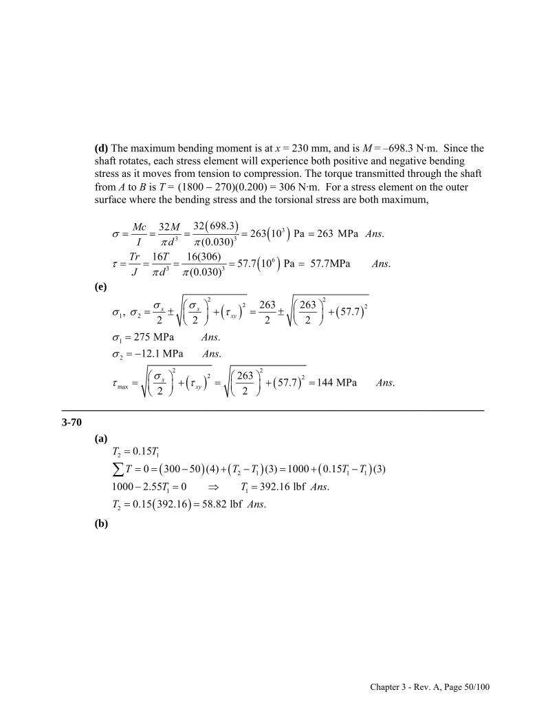
(d) The maximum bending moment is at x = 230 mm, and is M = –698.3 N·m. Since the shaft rotates, each stress element will experience both positive and negative bending stress as it moves from tension to compression. The torque transmitted through the shaft from A to B is T = (1800 270)(0.200) = 306 N·m. For a stress element on the outer surface where the bending stress and the torsional stress are both maximum,
3
3 3
32 698.332263 10 Pa 263 MPa .
(0.030)
Mc MAns
I d
63 3
16 16(306)57.7 10 Pa 57.7MPa .
(0.030)
Tr TAns
J d
(e)
2 22 2
1 2
1
2
2 22 2
max
263 263, 57.7
2 2 2 2
275 MPa .
12.1 MPa .
26357.7 144 MPa .
2 2
x xxy
xxy
Ans
Ans
Ans
_____________________________________________________________________________ 3-70
(a)
2 1
2 1 1 1
1 1
2
0.15
0 300 50 (4) (3) 1000 0.15 (3)
1000 2.55 0 392.16 lbf .
0.15 392.16 58.82 lbf .
T T
T T T
T T Ans
T Ans
T T
(b)
Chapter 3 - Rev. A, Page 50/100
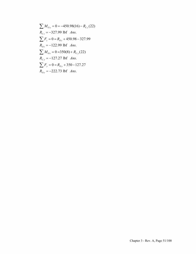
0 450.98(16) (22)
327.99 lbf .
0 450.98 327.99
122.99 lbf .
0 350(8) (22)
127.27 lbf .
0 350 127.27
222.73 lbf .
O y C z
C z
z O z
O z
O z C y
C y
y O y
O y
M R
R Ans
F R
R Ans
M R
R Ans
F R
R Ans
Chapter 3 - Rev. A, Page 51/100
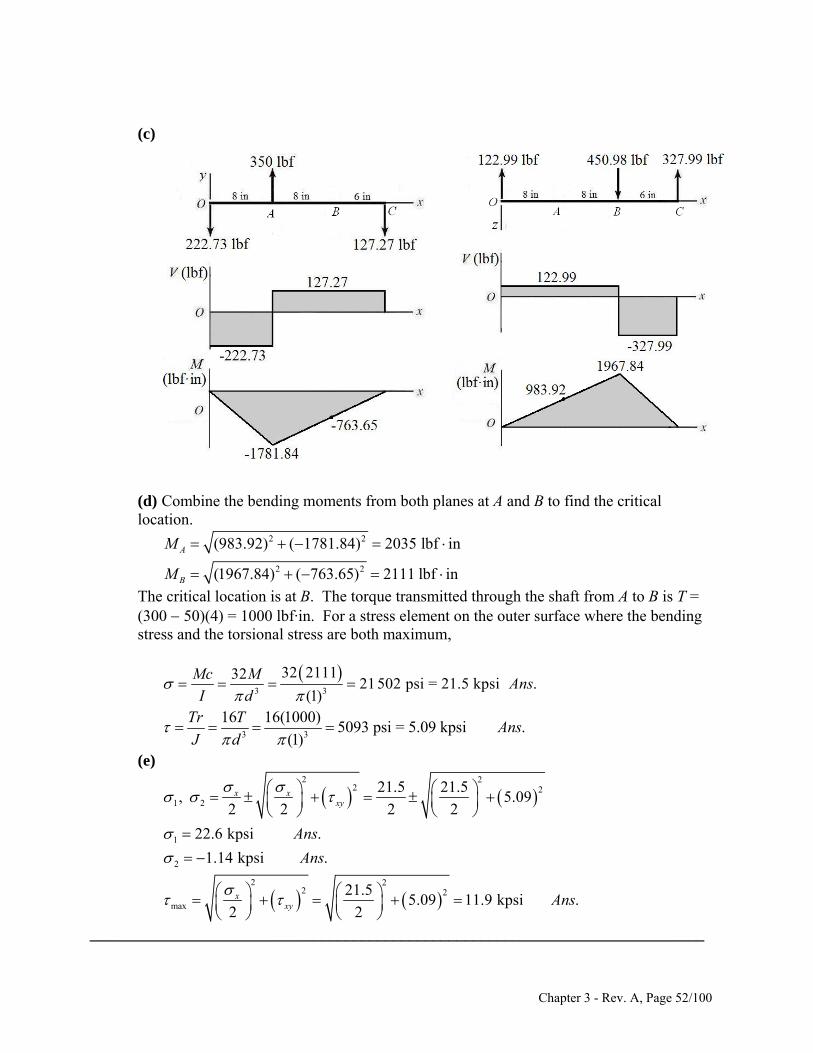
(c)
(d) Combine the bending moments from both planes at A and B to find the critical location.
2 2
2 2
(983.92) ( 1781.84) 2035 lbf in
(1967.84) ( 763.65) 2111 lbf in
A
B
M
M
The critical location is at B. The torque transmitted through the shaft from A to B is T = (300 50)(4) = 1000 lbf·in. For a stress element on the outer surface where the bending stress and the torsional stress are both maximum,
3 3
32 21113221502 psi = 21.5 kpsi .
(1)
Mc MAns
I d
3 3
16 16(1000)5093 psi = 5.09 kpsi .
(1)
Tr TAns
J d
(e)
2 22 2
1 2
1
2
2 22 2
max
21.5 21.5, 5.09
2 2 2 2
22.6 kpsi .
1.14 kpsi .
21.55.09 11.9 kpsi .
2 2
x xxy
xxy
Ans
Ans
Ans
_____________________________________________________________________________
Chapter 3 - Rev. A, Page 52/100
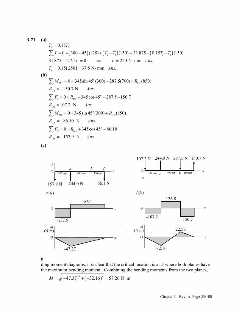
3-71 (a)
2 1
2 1 1 1
1 1
2
0.15
0 300 45 (125) (150) 31 875 0.15 (150)
31 875 127.5 0 250 N mm .
0.15 250 37.5 N mm .
T T
T T T T
T T Ans
T Ans
T
(b)
o
o
o
o
0 345sin 45 (300) 287.5(700) (850)
150.7 N .
0 345cos 45 287.5 150.7
107.2 N .
0 345sin 45 (300) (850)
86.10 N .
0 345cos 45 86.10
O y C z
C z
z O z
O z
O z C y
C y
y O y
O y
M R
R Ans
F R
R Ans
M R
R Ans
F R
R
157.9 N .Ans
(c)
(d) From the bending moment diagrams, it is clear that the critical location is at A where both planes have the maximum bending moment. Combining the bending moments from the two planes,
2 247.37 32.16 57.26 N mM
Chapter 3 - Rev. A, Page 53/100
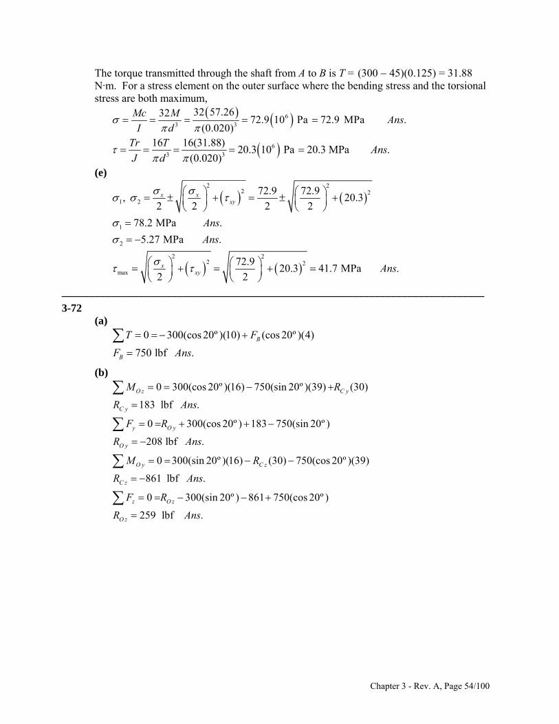
The torque transmitted through the shaft from A to B is T = (300 45)(0.125) = 31.88 N·m. For a stress element on the outer surface where the bending stress and the torsional stress are both maximum,
6
3 3
32 57.263272.9 10 Pa 72.9 MPa .
(0.020)
Mc MAns
I d
63 3
16 16(31.88)20.3 10 Pa 20.3 MPa .
(0.020)
Tr TAns
J d
(e)
2 22 2
1 2
1
2
2 22 2
max
72.9 72.9, 20.3
2 2 2 2
78.2 MPa .
5.27 MPa .
72.920.3 41.7 MPa .
2 2
x xxy
xxy
Ans
Ans
Ans
_____________________________________________________________________________ 3-72
(a)
0 300(cos 20º )(10) (cos 20º )(4)
750 lbf .B
B
T F
F Ans
(b)
0 300(cos 20º )(16) 750(sin 20º )(39) (30)
183 lbf .
0 300(cos 20º ) 183 750(sin 20º )
208 lbf .
0 300(sin 20º )(16) (30) 750(cos 20º )(39)
861 lbf .
0 300
O z C y
C y
y O y
O y
O y C z
C z
z O z
M R
R Ans
F R
R Ans
M R
R Ans
F R
(sin 20º ) 861 750(cos 20º )
259 lbf .O zR Ans
Chapter 3 - Rev. A, Page 54/100
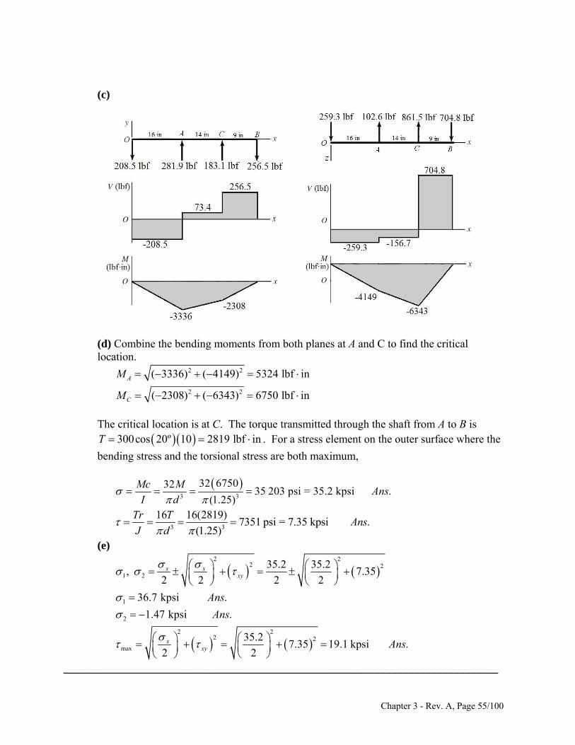
(c)
(d) Combine the bending moments from both planes at A and C to find the critical location.
2 2
2 2
( 3336) ( 4149) 5324 lbf in
( 2308) ( 6343) 6750 lbf in
A
C
M
M
The critical location is at C. The torque transmitted through the shaft from A to B is . For a stress element on the outer surface where the
bending stress and the torsional stress are both maximum,
300cos 20º 10 2819 lbf inT
3 3
32 67503235 203 psi = 35.2 kpsi .
(1.25)
Mc MAns
I d
3 3
16 16(2819)7351 psi = 7.35 kpsi .
(1.25)
Tr TAns
J d
(e)
2 22 2
1 2
1
2
2 22 2
max
35.2 35.2, 7.35
2 2 2 2
36.7 kpsi .
1.47 kpsi .
35.27.35 19.1 kpsi .
2 2
x xxy
xxy
Ans
Ans
Ans
_____________________________________________________________________________
Chapter 3 - Rev. A, Page 55/100
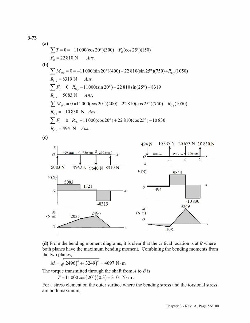
3-73
(a)
0 11000(cos 20º )(300) (cos 25º )(150)
22 810 N .B
B
T F
F Ans
(b)
0 11 000(sin 20º )(400) 22 810(sin 25º )(750) (1050)
8319 N .
O z C y
C y
M R
R Ans
0 11000(sin 20º ) 22 810sin(25º ) 8319
5083 N .
0 11 000(cos 20º )(400) 22 810(cos 25º )(750) (1050)
10 830 N .
0 11 000(cos 20º ) 22 810(cos 25º ) 10 830
494 N .
y O y
O y
O y C z
C z
z O z
O z
F R
R Ans
M R
R Ans
F R
R Ans
(c)
(d) From the bending moment diagrams, it is clear that the critical location is at B where both planes have the maximum bending moment. Combining the bending moments from the two planes,
2 22496 3249 4097 N mM
The torque transmitted through the shaft from A to B is . 11000cos 20º 0.3 3101 N mT For a stress element on the outer surface where the bending stress and the torsional stress are both maximum,
Chapter 3 - Rev. A, Page 56/100
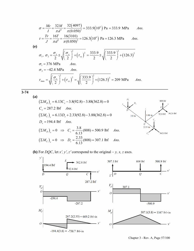
6
3 3
32 409732333.9 10 Pa 333.9 MPa .
(0.050)
Mc MAns
I d
63 3
16 16(3101)126.3 10 Pa 126.3 MPa .
(0.050)
Tr TAns
J d
(e)
2 22 2
1 2
1
2
2 22 2
max
333.9 333.9, 126.3
2 2 2 2
376 MPa .
42.4 MPa .
333.9126.3 209 MPa .
2 2
x xxy
xxy
Ans
Ans
Ans
_____________________________________________________________________________ 3-74
(a) 6.13 3.8(92.8) 3.88(362.8) 0D xz
M C
287.2 lbf .xC A ns
ns
6.13 2.33(92.8) 3.88(362.8) 0C xzM D
194.4 lbf .xD A
3.80 (808) 500.9 lbf .
6.13D zxM C Ans
2.330 (808) 307.1 lbf .
6.13C zxM D A ns
(b) For DQC, let x, y, z correspond to the original y, x, z axes.
Chapter 3 - Rev. A, Page 57/100
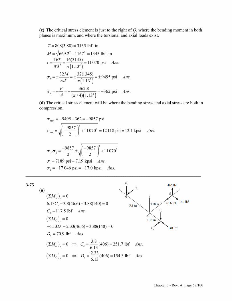
(c) The critical stress element is just to the right of Q, where the bending moment in both planes is maximum, and where the torsional and axial loads exist.
808(3.88) 3135 lbf inT
2 2669.2 1167 1345 lbf inM
3 3
16 16(3135)11 070 psi .
1.13
TAns
d
3 3
32 32(1345)9495 psi .
1.13b
MAns
d
2
362.8362 psi .
( / 4) 1.13a
FAns
A
(d) The critical stress element will be where the bending stress and axial stress are both in compression.
max 9495 362 9857 psi 2
2max
985711 070 12118 psi 12.1 kpsi .
2Ans
2
21 2
9857 9857, 11 070
2 2
1 7189 psi 7.19 kpsi .Ans
2 17 046 psi 17.0 kpsi .Ans
_____________________________________________________________________________
3-75 (a)
0
6.13 3.8(46.6) 3.88(140) 0
D z
x
M
C
ns
ns
117.5 lbf .xC A
0
6.13 2.33(46.6) 3.88(140) 0
C z
x
M
D
70.9 lbf .xD A
3.80 (406) 251.7 lbf .
6.13D zxM C A
ns
2.330 (406) 154.3 lbf .
6.13C zxM D A ns
Chapter 3 - Rev. A, Page 58/100
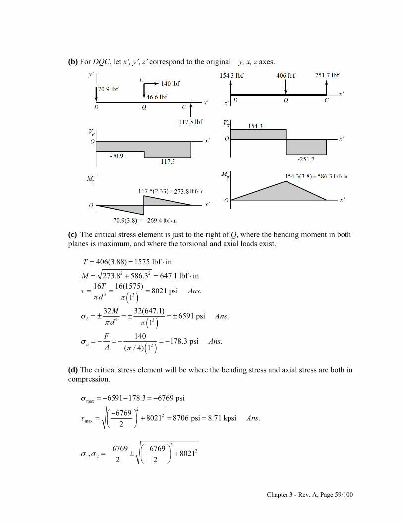
(b) For DQC, let x, y, z correspond to the original y, x, z axes.
(c) The critical stress element is just to the right of Q, where the bending moment in both planes is maximum, and where the torsional and axial loads exist.
406(3.88) 1575 lbf inT
2 2273.8 586.3 647.1 lbf inM
3 3
16 16(1575)8021 psi .
1
TAns
d
3 3
32 32(647.1)6591 psi .
1b
MAns
d
2
140178.3 psi .
( / 4) 1a
FAns
A
(d) The critical stress element will be where the bending stress and axial stress are both in compression.
max 6591 178.3 6769 psi 2
2max
67698021 8706 psi 8.71 kpsi .
2Ans
2
21 2
6769 6769, 8021
2 2
Chapter 3 - Rev. A, Page 59/100
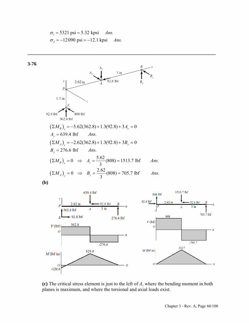
1 5321 psi 5.32 kpsi .Ans
2 12090 psi 12.1 kpsi .Ans
_____________________________________________________________________________
3-76 5.62(362.8) 1.3(92.8) 3 0B yz
M A
639.4 lbfyA Ans.
2.62(362.8) 1.3(92.8) 3 0A yzM B
276.6 lbfyB Ans.
5.620 (808) 1513.7 lbf
3B zyM A Ans.
2.620 (808) 705.7 lbf
3A zyM B Ans.
(b)
(c) The critical stress element is just to the left of A, where the bending moment in both planes is maximum, and where the torsional and axial loads exist.
Chapter 3 - Rev. A, Page 60/100
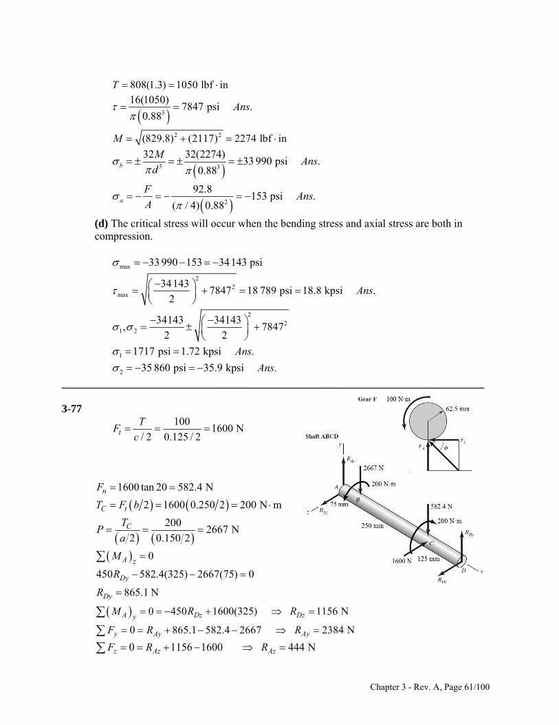
808(1.3) 1050 lbf inT
3
16(1050)7847 psi .
0.88Ans
2 2(829.8) (2117) 2274 lbf inM
3 3
32 32(2274)33 990 psi .
0.88b
MAns
d
2
92.8153 psi .
( / 4) 0.88a
FAns
A
(d) The critical stress will occur when the bending stress and axial stress are both in compression.
max 33 990 153 34143 psi 2
2max
341437847 18 789 psi 18.8 kpsi .
2Ans
22
1 2
34143 34143, 7847
2 2
1 1717 psi 1.72 kpsi .Ans
2 35 860 psi 35.9 kpsi .Ans
_____________________________________________________________________________
3-77
1001600 N
/ 2 0.125 / 2tT
Fc
1600 tan 20 582.4 N
2 1600 0.250 2 200 N m
2002667 N
2 0.150 2
n
C t
C
F
T F b
TP
a
0
450 582.4(325) 2667(75) 0
865.1 N
A z
Dy
Dy
M
R
R
0 450 1600(325)A DzyM R
0 865.1 582.4 2667y AyF R 0 1156 1600 z AzF R
1156 NDzR
2384 NAyR
444 NAzR
Chapter 3 - Rev. A, Page 61/100
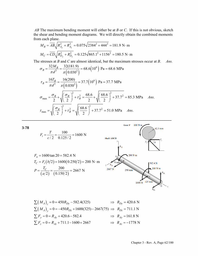
AB The maximum bending moment will either be at B or C. If this is not obvious, sketch the shear and bending moment diagrams. We will directly obtain the combined moments from each plane.
2 2 2 2
2 2 2 2
0.075 2384 444 181.9 N m
0.125 865.1 1156 180.5 N m
y z
y z
B A A
C D D
M AB R R
M CD R R
The stresses at B and C are almost identical, but the maximum stresses occur at B. Ans.
63 3
63 3
32 32(181.9)68.6 10 Pa 68.6 MPa
0.030
16 16(200)37.7 10 Pa 37.7 MPa
0.030
BB
BB
M
d
T
d
2 22 2
max68.6 68.6
37.7 85.3 MPa .2 2 2 2B B
B Ans
2 22 2
max68.6
37.7 51.0 MPa .2 2B
B Ans
_____________________________________________________________________________
3-78
100
1600 N/ 2 0.125 / 2tT
Fc
1600 tan 20 582.4 N
2 1600 0.250 2 200 N m
2002667 N
2 0.150 2
n
C t
C
F
T F b
TP
a
0 450 582.4(325) 420.6 N
0 450 1600(325) 2667(75) 711.1 N
0 420.6 582.4 161.8 N
0 711.1 1600 2667
A Dy Dyz
A Dz Dzy
y Ay Ay
z Az
M R R
M R R
F R R
F R
1778 NAzR
Chapter 3 - Rev. A, Page 62/100
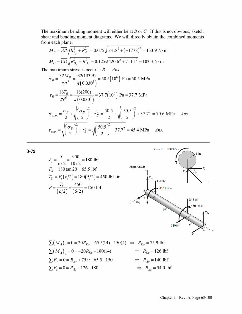
The maximum bending moment will either be at B or C. If this is not obvious, sketch shear and bending moment diagrams. We will directly obtain the combined moments from each plane.
22 2 2
2 2 2 2
0.075 161.8 1778 133.9 N m
0.125 420.6 711.1 103.3 N m
y z
y z
B A A
C D D
M AB R R
M CD R R
The maximum stresses occur at B. Ans.
63 3
63 3
32 32(133.9)50.5 10 Pa 50.5 MPa
0.030
16 16(200)37.7 10 Pa 37.7 MPa
0.030
BB
BB
M
d
T
d
2 22 2
max50.5 50.5
37.7 70.6 MPa .2 2 2 2B B
B Ans
2 22 2
max50.5
37.7 45.4 MPa .2 2B
B Ans
_____________________________________________________________________________
3-79
900180 lbf
/ 2 10 / 2tT
Fc
180 tan 20 65.5 lbf
2 180 5 2 450 lbf in
450150 lbf
2 6 2
n
C t
C
F
T F b
TP
a
0 20 65.5(14) 150(4) 75.9 lbf
0 20 180(14) 126 lbf
0 75.9 65.5 150 140 lbf
0 126 180
A Dy Dyz
A Dz Dzy
y Ay Ay
z Az
M R R
M R R
F R R
F R
54.0 lbfAzR
Chapter 3 - Rev. A, Page 63/100
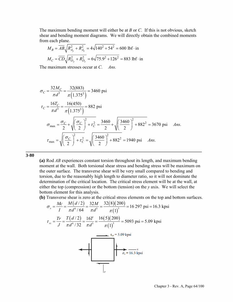
The maximum bending moment will either be at B or C. If this is not obvious, sketch shear and bending moment diagrams. We will directly obtain the combined moments from each plane.
2 2 2 2
2 2 2 2
4 140 54 600 lbf in
6 75.9 126 883 lbf in
y z
y z
B A A
C D D
M AB R R
M CD R R
The maximum stresses occur at C. Ans.
3 3
3 3
32 32(883)3460 psi
1.375
16 16(450)882 psi
1.375
CC
CC
M
d
T
d
2 22 2
max3460 3460
882 3670 psi .2 2 2 2C C
C Ans
2 22 2
max3460
882 1940 psi .2 2C
C Ans
_____________________________________________________________________________ 3-80
(a) Rod AB experiences constant torsion throughout its length, and maximum bending moment at the wall. Both torsional shear stress and bending stress will be maximum on the outer surface. The transverse shear will be very small compared to bending and torsion, due to the reasonably high length to diameter ratio, so it will not dominate the determination of the critical location. The critical stress element will be at the wall, at either the top (compression) or the bottom (tension) on the y axis. We will select the bottom element for this analysis. (b) Transverse shear is zero at the critical stress elements on the top and bottom surfaces.
34 3
/ 2 32 8 2003216 297 psi 16.3 kpsi
/ 64 1x
M dMc M
I d d
34 3
/ 2 16 5 200165093 psi 5.09 kpsi
/ 32 1xz
T dTr T
J d d
Chapter 3 - Rev. A, Page 64/100
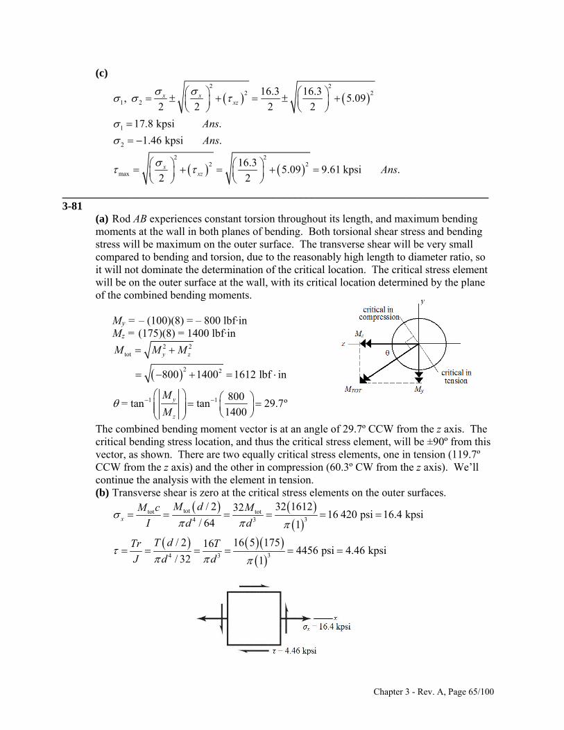
(c)
2 22 2
1 2
1
2
2 22 2
max
16.3 16.3, 5.09
2 2 2 2
17.8 kpsi .
1.46 kpsi .
16.35.09 9.61 kpsi .
2 2
x xxz
xxz
Ans
Ans
Ans
_____________________________________________________________________________ 3-81
(a) Rod AB experiences constant torsion throughout its length, and maximum bending moments at the wall in both planes of bending. Both torsional shear stress and bending stress will be maximum on the outer surface. The transverse shear will be very small compared to bending and torsion, due to the reasonably high length to diameter ratio, so it will not dominate the determination of the critical location. The critical stress element will be on the outer surface at the wall, with its critical location determined by the plane of the combined bending moments. My = – (100)(8) = – 800 lbf·in Mz = (175)(8) = 1400 lbf·in
2 2tot
2 2
1 1
800 1400 1612 lbf in
800= tan tan 29.7º
1400
y z
y
z
M M M
M
M
The combined bending moment vector is at an angle of 29.7º CCW from the z axis. The critical bending stress location, and thus the critical stress element, will be ±90º from this vector, as shown. There are two equally critical stress elements, one in tension (119.7º CCW from the z axis) and the other in compression (60.3º CW from the z axis). We’ll continue the analysis with the element in tension. (b) Transverse shear is zero at the critical stress elements on the outer surfaces.
tottot tot
34 3
/ 2 32 16123216 420 psi 16.4 kpsi
/ 64 1x
M dM c M
I d d
34 3
/ 2 16 5 175164456 psi 4.46 kpsi
/ 32 1
T dTr T
J d d
Chapter 3 - Rev. A, Page 65/100
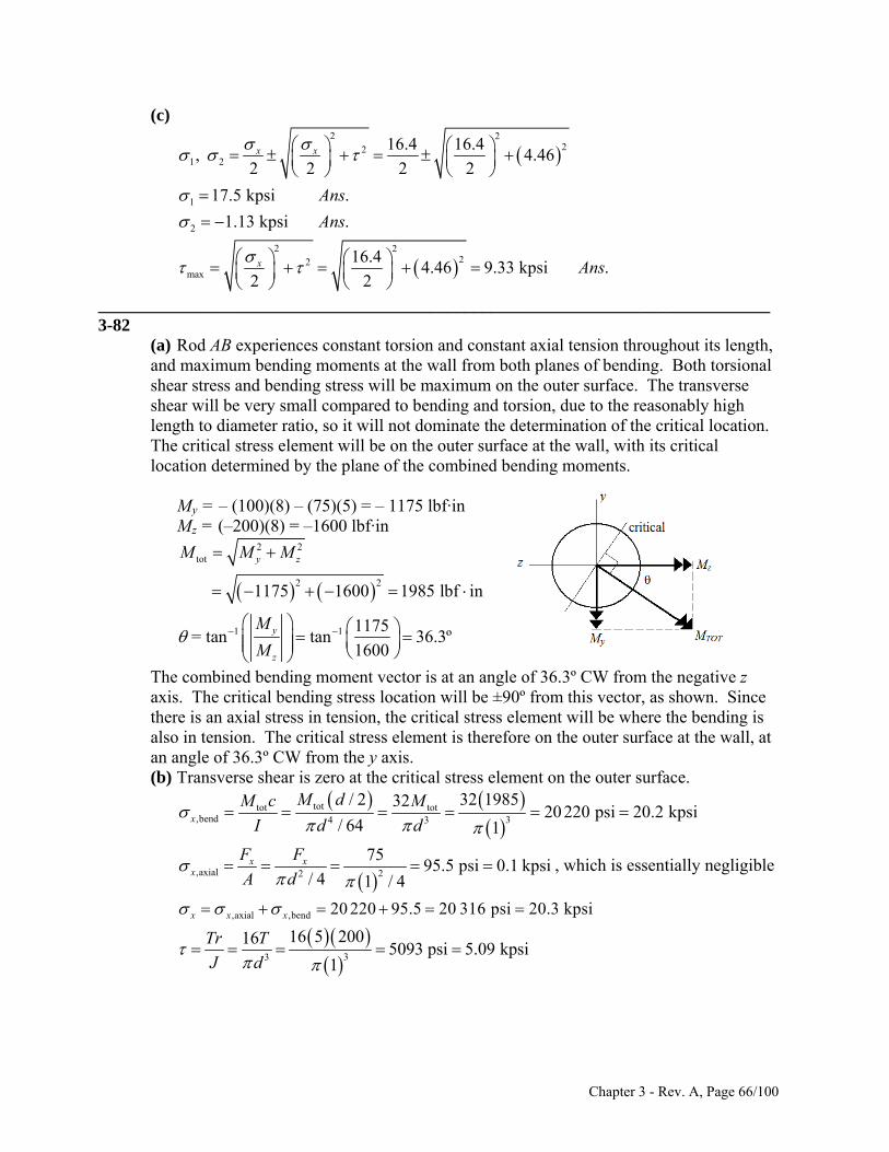
(c)
2 222
1 2
1
2
2 222
max
16.4 16.4, 4.46
2 2 2 2
17.5 kpsi .
1.13 kpsi .
16.44.46 9.33 kpsi .
2 2
x x
x
Ans
Ans
Ans
_____________________________________________________________________________ 3-82
(a) Rod AB experiences constant torsion and constant axial tension throughout its length, and maximum bending moments at the wall from both planes of bending. Both torsional shear stress and bending stress will be maximum on the outer surface. The transverse shear will be very small compared to bending and torsion, due to the reasonably high length to diameter ratio, so it will not dominate the determination of the critical location. The critical stress element will be on the outer surface at the wall, with its critical location determined by the plane of the combined bending moments. My = – (100)(8) – (75)(5) = – 1175 lbf·in Mz = (–200)(8) = –1600 lbf·in
2 2tot
2 2
1 1
1175 1600 1985 lbf in
1175= tan tan 36.3º
1600
y z
y
z
M M M
M
M
The combined bending moment vector is at an angle of 36.3º CW from the negative z axis. The critical bending stress location will be ±90º from this vector, as shown. Since there is an axial stress in tension, the critical stress element will be where the bending is also in tension. The critical stress element is therefore on the outer surface at the wall, at an angle of 36.3º CW from the y axis. (b) Transverse shear is zero at the critical stress element on the outer surface.
tottot tot
,bend 34 3
/ 2 32 19853220220 psi 20.2 kpsi
/ 64 1x
M dM c M
I d d
,axial 22
7595.5 psi 0.1 kpsi
/ 4 1 / 4x x
x
F F
A d
, which is essentially negligible
,axial ,bend 20 220 95.5 20 316 psi 20.3 kpsix x x
33
16 5 200165093 psi 5.09 kpsi
1
Tr T
J d
Chapter 3 - Rev. A, Page 66/100
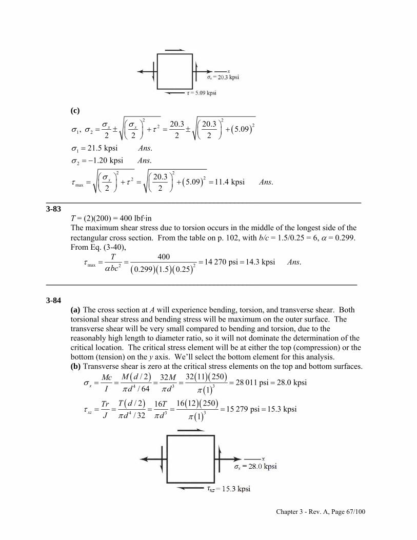
(c)
2 222
1 2
1
2
2 222
max
20.3 20.3, 5.09
2 2 2 2
21.5 kpsi .
1.20 kpsi .
20.35.09 11.4 kpsi .
2 2
x x
x
Ans
Ans
Ans
_____________________________________________________________________________ 3-83
T = (2)(200) = 400 lbf·in The maximum shear stress due to torsion occurs in the middle of the longest side of the rectangular cross section. From the table on p. 102, with b/c = 1.5/0.25 = 6, = 0.299. From Eq. (3-40),
max 22
40014 270 psi 14.3 kpsi .
0.299 1.5 0.25
TAns
bc
____________________________________________________________________________ 3-84
(a) The cross section at A will experience bending, torsion, and transverse shear. Both torsional shear stress and bending stress will be maximum on the outer surface. The transverse shear will be very small compared to bending and torsion, due to the reasonably high length to diameter ratio, so it will not dominate the determination of the critical location. The critical stress element will be at either the top (compression) or the bottom (tension) on the y axis. We’ll select the bottom element for this analysis. (b) Transverse shear is zero at the critical stress elements on the top and bottom surfaces.
34 3
/ 2 32 11 2503228 011 psi 28.0 kpsi
/ 64 1x
M dMc M
I d d
34 3
/ 2 16 12 2501615 279 psi 15.3 kpsi
/ 32 1xz
T dTr T
J d d
Chapter 3 - Rev. A, Page 67/100
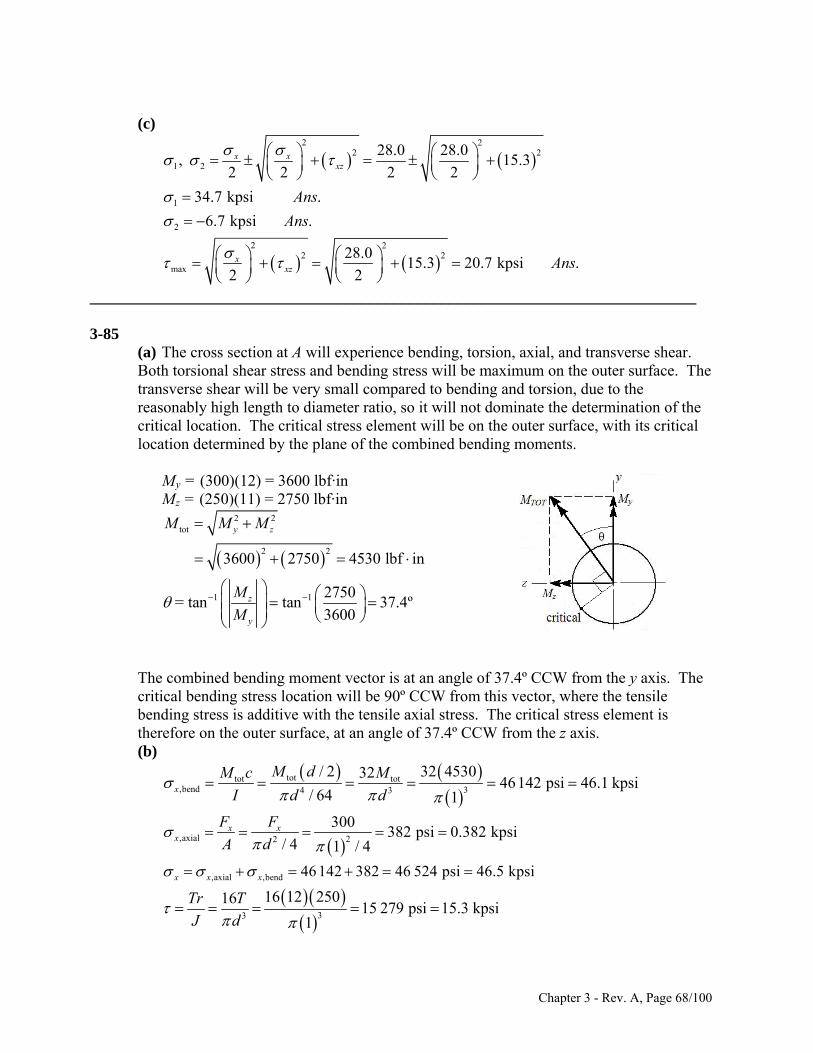
(c)
2 22 2
1 2
1
2
2 22 2
max
28.0 28.0, 15.3
2 2 2 2
34.7 kpsi .
6.7 kpsi .
28.015.3 20.7 kpsi .
2 2
x xxz
xxz
Ans
Ans
Ans
____________________________________________________________________________ 3-85
(a) The cross section at A will experience bending, torsion, axial, and transverse shear. Both torsional shear stress and bending stress will be maximum on the outer surface. The transverse shear will be very small compared to bending and torsion, due to the reasonably high length to diameter ratio, so it will not dominate the determination of the critical location. The critical stress element will be on the outer surface, with its critical location determined by the plane of the combined bending moments. My = (300)(12) = 3600 lbf·in Mz = (250)(11) = 2750 lbf·in
2 2tot
2 2
1 1
3600 2750 4530 lbf in
2750= tan tan 37.4º
3600
y z
z
y
M M M
M
M
The combined bending moment vector is at an angle of 37.4º CCW from the y axis. The critical bending stress location will be 90º CCW from this vector, where the tensile bending stress is additive with the tensile axial stress. The critical stress element is therefore on the outer surface, at an angle of 37.4º CCW from the z axis. (b)
tottot tot
,bend 34 3
/ 2 32 45303246142 psi 46.1 kpsi
/ 64 1x
M dM c M
I d d
,axial 22
300382 psi 0.382 kpsi
/ 4 1 / 4x x
x
F F
A d
,axial ,bend 46142 382 46 524 psi 46.5 kpsix x x
33
16 12 2501615 279 psi 15.3 kpsi
1
Tr T
J d
Chapter 3 - Rev. A, Page 68/100
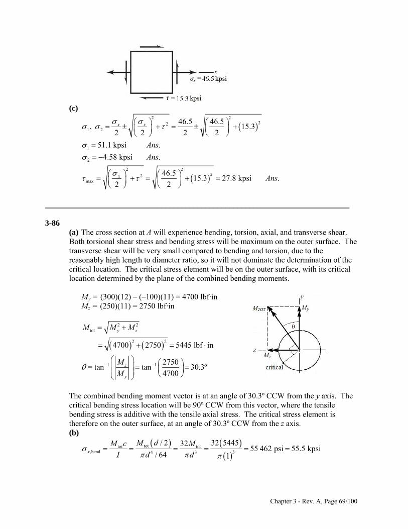
(c)
2 222
1 2
1
2
2 222
max
46.5 46.5, 15.3
2 2 2 2
51.1 kpsi .
4.58 kpsi .
46.515.3 27.8 kpsi .
2 2
x x
x
Ans
Ans
Ans
____________________________________________________________________________ 3-86
(a) The cross section at A will experience bending, torsion, axial, and transverse shear. Both torsional shear stress and bending stress will be maximum on the outer surface. The transverse shear will be very small compared to bending and torsion, due to the reasonably high length to diameter ratio, so it will not dominate the determination of the critical location. The critical stress element will be on the outer surface, with its critical location determined by the plane of the combined bending moments. My = (300)(12) – (–100)(11) = 4700 lbf·in Mz = (250)(11) = 2750 lbf·in
2 2tot
2 2
1 1
4700 2750 5445 lbf in
2750= tan tan 30.3º
4700
y z
z
y
M M M
M
M
The combined bending moment vector is at an angle of 30.3º CCW from the y axis. The critical bending stress location will be 90º CCW from this vector, where the tensile bending stress is additive with the tensile axial stress. The critical stress element is therefore on the outer surface, at an angle of 30.3º CCW from the z axis. (b)
tottot tot
,bend 34 3
/ 2 32 54453255 462 psi 55.5 kpsi
/ 64 1x
M dM c M
I d d
Chapter 3 - Rev. A, Page 69/100
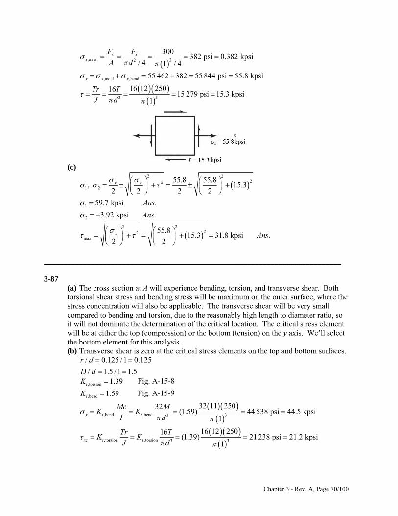
,axial 22
300382 psi 0.382 kpsi
/ 4 1 / 4x x
x
F F
A d
,axial ,bend 55 462 382 55 844 psi 55.8 kpsix x x
33
16 12 2501615 279 psi 15.3 kpsi
1
Tr T
J d
(c)
2 222
1 2
1
2
2 222
max
55.8 55.8, 15.3
2 2 2 2
59.7 kpsi .
3.92 kpsi .
55.815.3 31.8 kpsi .
2 2
x x
x
Ans
Ans
Ans
____________________________________________________________________________ 3-87
(a) The cross section at A will experience bending, torsion, and transverse shear. Both torsional shear stress and bending stress will be maximum on the outer surface, where the stress concentration will also be applicable. The transverse shear will be very small compared to bending and torsion, due to the reasonably high length to diameter ratio, so it will not dominate the determination of the critical location. The critical stress element will be at either the top (compression) or the bottom (tension) on the y axis. We’ll select the bottom element for this analysis. (b) Transverse shear is zero at the critical stress elements on the top and bottom surfaces.
/ 0.125 /1 0.125
/ 1.5 /1 1.5
r d
D d
Fig. A-15-8 ,torsion 1.39tK
Fig. A-15-9 ,bend 1.59tK
,bend ,bend 33
32 11 25032(1.59) 44 538 psi 44.5 kpsi
1x t t
Mc MK K
I d
,torsion ,torsion 33
16 12 25016(1.39) 21 238 psi 21.2 kpsi
1xz t t
Tr TK K
J d
Chapter 3 - Rev. A, Page 70/100
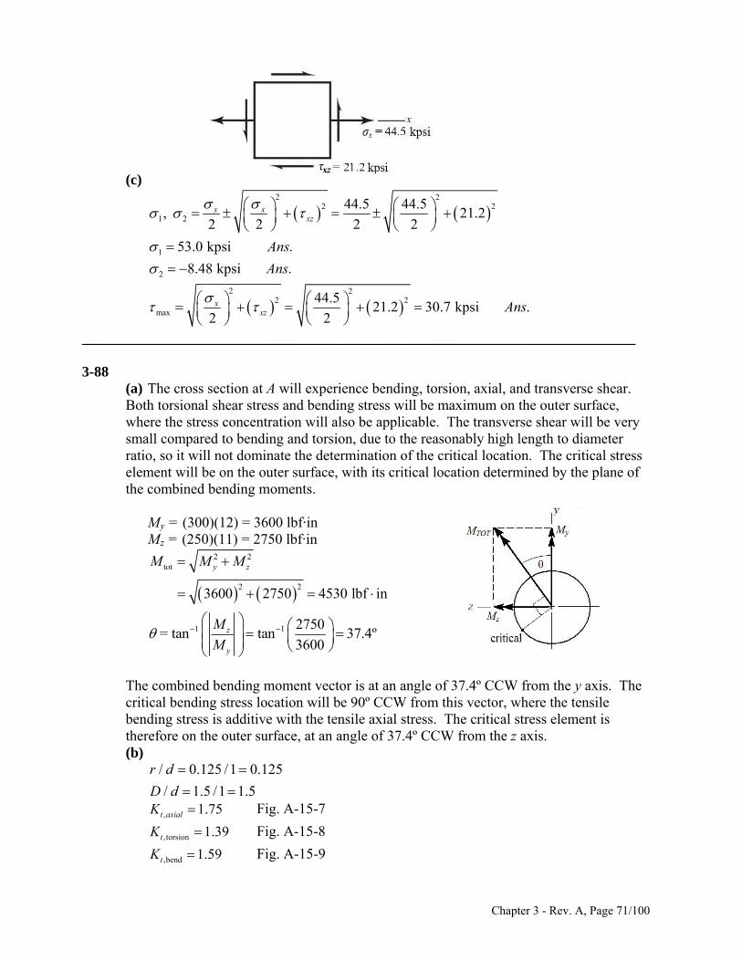
(c)
2 22 2
1 2
1
2
2 22 2
max
44.5 44.5, 21.2
2 2 2 2
53.0 kpsi .
8.48 kpsi .
44.521.2 30.7 kpsi .
2 2
x xxz
xxz
Ans
Ans
Ans
____________________________________________________________________________ 3-88
(a) The cross section at A will experience bending, torsion, axial, and transverse shear. Both torsional shear stress and bending stress will be maximum on the outer surface, where the stress concentration will also be applicable. The transverse shear will be very small compared to bending and torsion, due to the reasonably high length to diameter ratio, so it will not dominate the determination of the critical location. The critical stress element will be on the outer surface, with its critical location determined by the plane of the combined bending moments. My = (300)(12) = 3600 lbf·in Mz = (250)(11) = 2750 lbf·in
2 2tot
2 2
1 1
3600 2750 4530 lbf in
2750= tan tan 37.4º
3600
y z
z
y
M M M
M
M
The combined bending moment vector is at an angle of 37.4º CCW from the y axis. The critical bending stress location will be 90º CCW from this vector, where the tensile bending stress is additive with the tensile axial stress. The critical stress element is therefore on the outer surface, at an angle of 37.4º CCW from the z axis. (b)
/ 0.125 /1 0.125
/ 1.5 /1 1.5
r d
D d
Fig. A-15-7 , 1.75t axialK
Fig. A-15-8 ,torsion 1.39tK
Fig. A-15-9 ,bend 1.59tK
Chapter 3 - Rev. A, Page 71/100
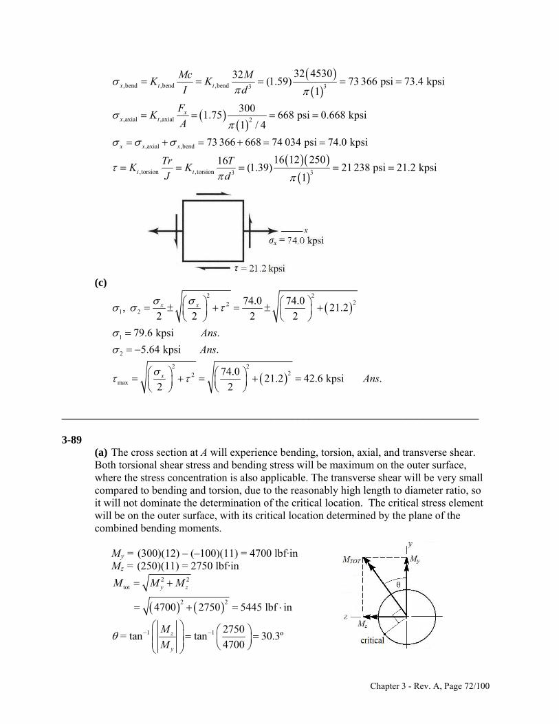
,bend ,bend ,bend 33
32 453032(1.59) 73 366 psi 73.4 kpsi
1x t t
Mc MK K
I d
,axial ,axial 2
3001.75 668 psi 0.668 kpsi
1 / 4x
x t
FK
A
,axial ,bend 73 366 668 74 034 psi 74.0 kpsix x x
,torsion ,torsion 33
16 12 25016(1.39) 21 238 psi 21.2 kpsi
1t t
Tr TK K
J d
(c)
2 222
1 2
1
2
2 222
max
74.0 74.0, 21.2
2 2 2 2
79.6 kpsi .
5.64 kpsi .
74.021.2 42.6 kpsi .
2 2
x x
x
Ans
Ans
Ans
____________________________________________________________________________ 3-89
(a) The cross section at A will experience bending, torsion, axial, and transverse shear. Both torsional shear stress and bending stress will be maximum on the outer surface, where the stress concentration is also applicable. The transverse shear will be very small compared to bending and torsion, due to the reasonably high length to diameter ratio, so it will not dominate the determination of the critical location. The critical stress element will be on the outer surface, with its critical location determined by the plane of the combined bending moments. My = (300)(12) – (–100)(11) = 4700 lbf·in Mz = (250)(11) = 2750 lbf·in
2 2tot
2 24700 2750 5445 lbf in
y zM M M
1 1 2750= tan tan 30.3º
4700z
y
M
M
Chapter 3 - Rev. A, Page 72/100
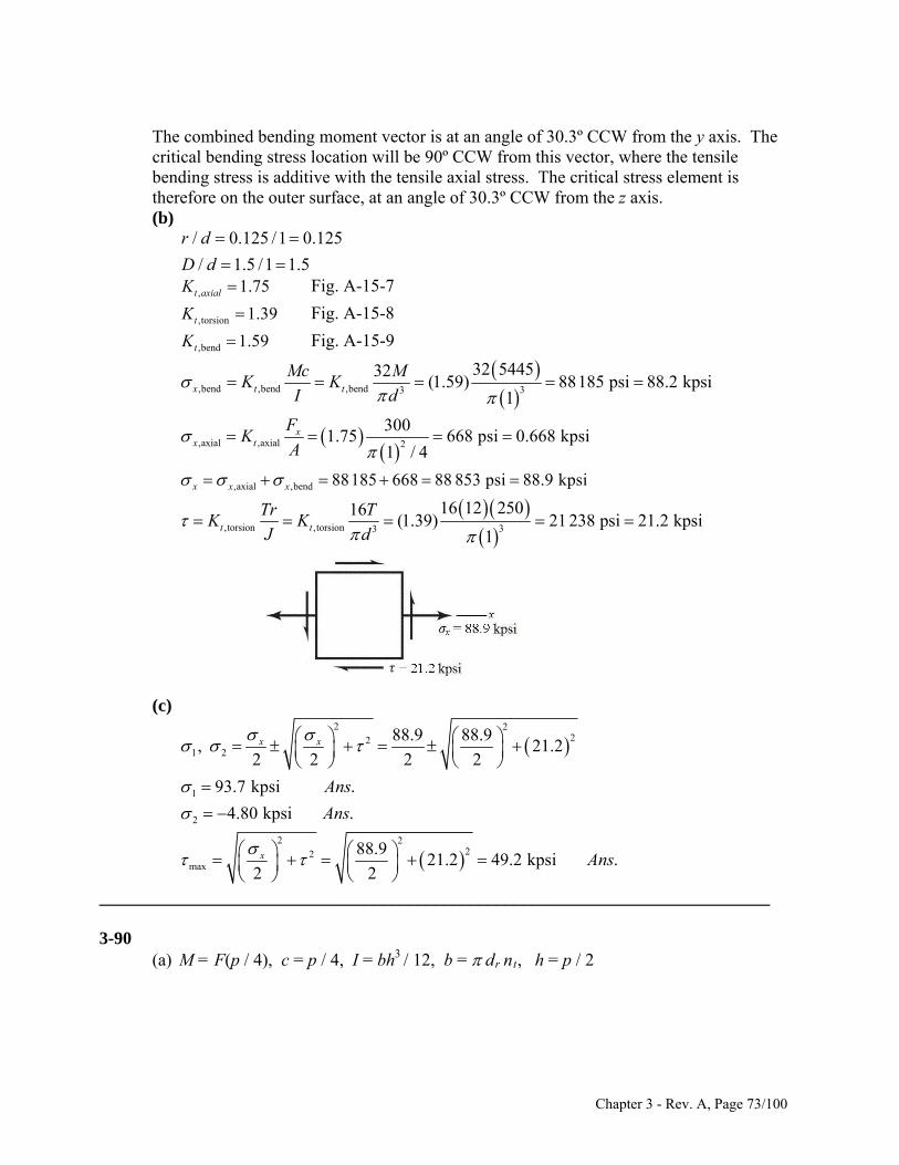
The combined bending moment vector is at an angle of 30.3º CCW from the y axis. The critical bending stress location will be 90º CCW from this vector, where the tensile bending stress is additive with the tensile axial stress. The critical stress element is therefore on the outer surface, at an angle of 30.3º CCW from the z axis. (b)
/ 0.125 /1 0.125
/ 1.5 /1 1.5
r d
D d
Fig. A-15-7 , 1.75t axialK
Fig. A-15-8 ,torsion 1.39tK
Fig. A-15-9 ,bend 1.59tK
,bend ,bend ,bend 33
32 544532(1.59) 88185 psi 88.2 kpsi
1x t t
Mc MK K
I d
,axial ,axial 2
3001.75 668 psi 0.668 kpsi
1 / 4x
x t
FK
A
,axial ,bend 88185 668 88 853 psi 88.9 kpsix x x
,torsion ,torsion 33
16 12 25016(1.39) 21 238 psi 21.2 kpsi
1t t
Tr TK K
J d
(c)
2 222
1 2
1
2
2 222
max
88.9 88.9, 21.2
2 2 2 2
93.7 kpsi .
4.80 kpsi .
88.921.2 49.2 kpsi .
2 2
x x
x
Ans
Ans
Ans
____________________________________________________________________________ 3-90
(a) M = F(p / 4), c = p / 4, I = bh3 / 12, b = dr nt, h = p / 2
Chapter 3 - Rev. A, Page 73/100

2
33
/ 4 / 4
/12 16 / 2 /12
6 .
b
r t
br t
F p pMc Fp
I bh d n p
FAns
d n p
(b) 2 2
4
/ 4ar r
F F FAns.
A d d
4 3
/ 2 16 .
/ 32r
tr r
T dTr TAns
J d d
(c) The bending stress causes compression in the x direction. The axial stress causes compression in the y direction. The torsional stress shears across the y face in the negative z direction.
(d) Analyze the stress element from part (c) using the equations developed in parts (a) and (b).
2 2
3 3
1.5 0.25 1.25 in
6 150064584 psi = 4.584 kpsi
1.25 2 0.25
4 15004= = 1222 psi = 1.222 kpsi
1.25
16 23516= = 612.8 psi = 0.6128 kpsi
1.25
r
x br t
y ar
yz tr
d d p
F
d n p
F
d
T
d
Use Eq. (3-15) for the three-dimensional stress element.
2 23 2
3 2
4.584 1.222 4.584 1.222 0.6128 4.584 0.6128 0
5.806 5.226 1.721 0
The roots are at 0.2543, – 4.584, and –1.476. Thus, the ordered principal stresses are 1 = 0.2543 kpsi, 2 = –1.476 kpsi, and 3 = – 4.584 kpsi. Ans. From Eq. (3-16), the principal shear stresses are
Chapter 3 - Rev. A, Page 74/100
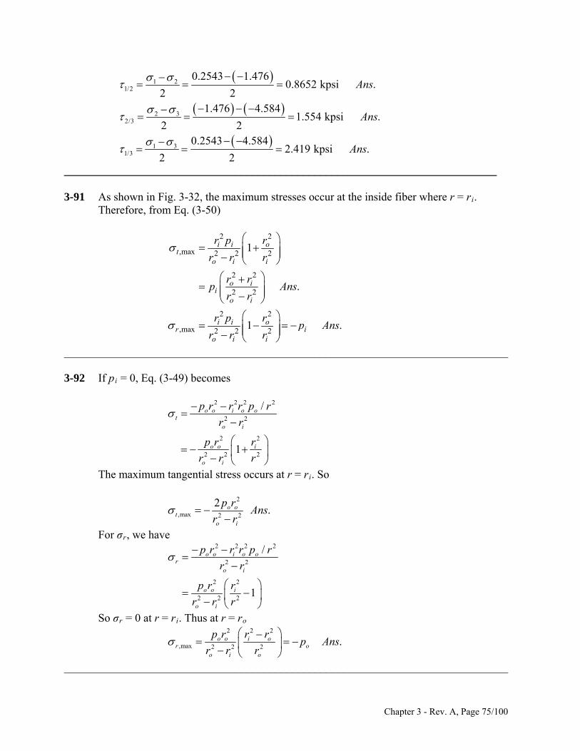
1 21/2
2 32/3
1 31/3
0.2543 1.4760.8652 kpsi .
2 21.476 4.584
1.554 kpsi .2 2
0.2543 4.5842.419 kpsi .
2 2
Ans
Ans
Ans
____________________________________________________________________________ 3-91 As shown in Fig. 3-32, the maximum stresses occur at the inside fiber where r = ri.
Therefore, from Eq. (3-50)
2 2
,max 2 2 2
2 2
2 2
2 2
,max 2 2 2
1
.
1 .
i i ot
o i i
o ii
o i
i i or i
o i i
r p r
r r r
r rp Ans
r r
r p rp Ans
r r r
______________________________________________________________________________ 3-92 If pi = 0, Eq. (3-49) becomes
2 2 2 2
2 2
2 2
2 2 2
/
1
o o i o ot
o i
o o i
o i
p r r r p r
r r
p r r
r r r
The maximum tangential stress occurs at r = ri. So
2
,max 2 2
2 .o o
to i
p rAns
r r
For σr, we have
2 2 2 2
2 2
2 2
2 2 2
/
1
o o i o or
o i
o o i
o i
p r r r p r
r r
p r r
r r r
So σr = 0 at r = ri. Thus at r = ro
2 2 2
,max 2 2 2 .o o i o
r oo i o
p r r rp Ans
r r r
______________________________________________________________________________
Chapter 3 - Rev. A, Page 75/100
3-93 The force due to the pressure on half of the sphere is resisted by the stress that is
distributed around the center plane of the sphere. All planes are the same, so
2
av 1 2
/ 4( ) .
4i i
ti
p d pdAns
d t t
The radial stress on the inner surface of the shell is, 3 = p Ans.
______________________________________________________________________________ 3-94 σt > σl > σr τmax = (σt − σr)/2 at r = ri
2 2 2 2 2
max 2 2 2 2 2 2 2 2
2 2 2 2
max2 2
11 1
2
3 2.75(10 000) 1597 psi .
3
i i o i i o o i
o i i o i i o i
o ii
o
r p r r p r r p
r r r r r r r r
r rp Ans
r
______________________________________________________________________________ 3-95 σt > σl > σr τmax = (σt − σr)/2 at r = ri
2 2 2 2 2 2 2
max 2 2 2 2 2 2 2 2 2 2 2
6max
6max
11 1
2
( ) (25 4)10100 91.7 mm
25 10
100 91.7 8.3 mm .
i i o i i o i i o o i
o i i o i i o i i o i
ii o
o i
r p r r p r r p r r p
r r r r r r r r r r r
pr r
t r r Ans
______________________________________________________________________________ 3-96 σt > σl > σr τmax = (σt − σr)/2 at r = ri
2 2 2 2 2 2 2
max 2 2 2 2 2 2 2 2 2 2 2
11 1
2i i o i i o i i o o i
o i i o i i o i i o i
r p r r p r r p r r p
r r r r r r r r r r r
2
2 2
4 (500)4129 psi .
4 3.75Ans
______________________________________________________________________________ 3-97 From Eq. (3-49) with pi = 0,
Chapter 3 - Rev. A, Page 76/100
2 2
2 2 2
2 2
2 2 2
1
1
o o it
o i
o o ir
o i
r p r
r r r
r p r
r r r
σt > σl > σr, and since σt and σr are negative, τmax = (σr − σt)/2 at r = ro
2 2 2 2 2 2 2
max 2 2 2 2 2 2 2 2 2 2
2 2 2 2
max2 2
11 1
2
3 2.75(10 000) 1900 psi .
2.75
o o i o o i o o i i o
o i o o i o o i o o i
o io
i
r p r r p r r p r r p
r r r r r r r r r r r
r rp Ans
r
2
______________________________________________________________________________ 3-98 From Eq. (3-49) with pi = 0,
2 2
2 2 2
2 2
2 2 2
1
1
o o it
o i
o o ir
o i
r p r
r r r
r p r
r r r
σt > σl > σr, and since σt and σr are negative, τmax = (σr − σt)/2 at r = ro
2 2 2 2 2 2 2
max 2 2 2 2 2 2 2 2 2 2
6
max6
max
11 1
2
25 10100 92.8 mm
( ) 25 4 10
100 92.8 7.2 mm .
o o i o o i o o i i o
o i o o i o o i o o i
i oo
o i
r p r r p r r p r r p
r r r r r r r r r r r
r rp
t r r Ans
2
______________________________________________________________________________ 3-99 From Eq. (3-49) with pi = 0,
2 2
2 2 2
2 2
2 2 2
1
1
o o it
o i
o o ir
o i
r p r
r r r
r p r
r r r
σt > σl > σr, and since σt and σr are negative, τmax = (σr − σt)/2 at r = ro
Chapter 3 - Rev. A, Page 77/100
2 2 2 2 2 2 2
max 2 2 2 2 2 2 2 2 2 2
2
2 2
11 1
2
3.75 (500)3629 psi .
4 3.75
o o i o o i o o i i o
o i o o i o o i o o i
r p r r p r r p r r p
r r r r r r r r r r r
Ans
2
______________________________________________________________________________ 3-100 From Table A-20, Sy=490 MPa From Eq. (3-49) with pi = 0,
2 2
2 2 21o o i
to i
r p r
r r r
Maximum will occur at r = ri
2 22 22,max
,max 2 2 2 2
0.8( 490) 25 19( )282.8 MPa .
2 2(25 )t o io o
t oo i o
r rr pp Ans
r r r
______________________________________________________________________________ 3-101 From Table A-20, Sy = 71 kpsi From Eq. (3-49) with pi = 0,
2 2
2 2 21o o i
to i
r p r
r r r
Maximum will occur at r = ri
2 2 2 22,max
,max 2 2 2 2
0.8( 71) 1 0.75212.4 kpsi .
2 2(1 )t o io o
t oo i o
r rr pp Ans
r r r
______________________________________________________________________________ 3-102 From Table A-20, Sy=490 MPa From Eq. (3-50)
2 2
2 2 21i i o
to i
r p r
r r r
Maximum will occur at r = ri
2 22 2
,max 2 2 2 2 2
2 2 2 2,max
2 2 2 2
1
( ) 0.8(490) (25 19 )105 MPa .
(25 19 )
i o ii i ot
o i i o i
t o ii
o i
p r rr p r
r r r r r
r rp Ans
r r
______________________________________________________________________________
Chapter 3 - Rev. A, Page 78/100

3-103 From Table A-20, Sy =71 MPa From Eq. (3-50)
2 2
2 2 21i i o
to i
r p r
r r r
Maximum will occur at r = ri
2 2 2 2
,max 2 2 2 2 2
2 2 2 2,max
2 2 2 2
( )1
( ) 0.8(71) (1 0.75 )15.9 ksi .
(1 0.75 )
i i o i o it
o i i o i
t o ii
o i
r p r p r r
r r r r r
r rp Ans
r r
______________________________________________________________________________ 3-104 The longitudinal stress will be due to the weight of the vessel above the maximum stress
point. From Table A-5, the unit weight of steel is s = 0.282 lbf/in3. The area of the wall is
Awall = ( /4)(3602 358.52) = 846. 5 in2
The volume of the wall and dome are Vwall = Awall h = 846.5 (720) = 609.5 (103) in3 Vdome = (2 /3)(1803 179.253) = 152.0 (103) in3 The weight of the structure on the wall area at the tank bottom is W = s Vtotal = 0.282(609.5 +152.0) (103) = 214.7(103) lbf
3
wall
214.7 10254 psi
846.5l
W
A
The maximum pressure will occur at the bottom of the tank, pi = water h. From Eq. (3-50) with ir r
2 2 2 2
2 2 2 2 2
2 2 2
2 2 2
1
1 ft 180 179.2562.4(55) 5708 5710 psi .
144 in 180 179.25
i i o o it i
o i i o i
r p r r rp
r r r r r
Ans
2 2 2
2 2 2 2
1 ft1 62.4(55) 23.8 psi .
144 ini i o
r io i i
r p rp Ans
r r r
Note: These stresses are very idealized as the floor of the tank will restrict the values calculated.
Chapter 3 - Rev. A, Page 79/100
Since 1 2 3, 1 = t = 5708 psi, 2 = r = 24 psi and3 = l = 254 psi. From Eq. (3-16),
1 3
1 2
2 3
5708 2542981 2980 psi
25708 24
2866 2870 psi .2
24 254115 psi
2
Ans
______________________________________________________________________________ 3-105 Stresses from additional pressure are, Eq. (3-51),
2
2 250psi
50 179.255963 psi
180 179.25l
(r)50 psi = 50 psi Eq. (3-50)
2 2
2 250psi
180 179.2550 11 975 psi
180 179.25t
Adding these to the stresses found in Prob. 3-104 gives t = 5708 + 11 975 = 17683 psi = 17.7 kpsi Ans. r = 23.8 50 = 73.8 psi Ans. l = 254 + 5963 = 5709 psi Ans. Note: These stresses are very idealized as the floor of the tank will restrict the values
calculated. From Eq. (3-16)
1 3
1 2
2 3
17 683 73.88879 psi
217 683 5709
5987 psi .2
5709 23.82866 psi
2
Ans
______________________________________________________________________________ 3-106 Since σt and σr are both positive and σt > σr
max max2t
From Eq. (3-55), t is maximum at r = ri = 0.3125 in. The term
Chapter 3 - Rev. A, Page 80/100
2
2 2 50003 0.282 3 0.29282.42 lbf/in
8 386 60 8
2 2
2 2 22max
0.3125 2.75 1 3(0.292)82.42 0.3125 2.75 0.3125
3 0.2920.3125
1260 psi
t
max1260
630 psi .2
Ans
Radial stress:
2 22 2 2
2i o
r i or r
k r r rr
Maxima:
2 2
32 2 0 0.3125(2.75) 0.927 ini or
i or rd
k r r r rdr r
2 2
2 22max
0.3125 2.7582.42 0.3125 2.75 0.927
0.927
490 psi .
r
Ans
2
______________________________________________________________________________ 3-107 = 2 (2000)/60 = 209.4 rad/s, = 3320 20 kg/m3, = 0.24, ri = 0.01 m, ro = 0.125 m Using Eq. (3-55)
2 22 2 23 0.24 1 3(0.24)
3320(209.4) 0.01 (0.125) (0.125) 0.01 (10)8 3 0.24
1.85 MPa .
t
Ans
6
______________________________________________________________________________ 3-108 = 2 (12 000)/60 = 1256.6 rad/s,
4 22 2
5 /166.749 10 lbf s / in
386 1 16 4 5 0.75
4
The maximum shear stress occurs at bore where max = t /2. From Eq. (3-55)
24 2 2 2 2
max
3 0.20 1 3(0.20)( ) 6.749(10 ) 1256.6 0.375 2.5 2.5 (0.375)
8 3 0.20
5360 psi
t
Chapter 3 - Rev. A, Page 81/100
max = 5360 / 2 = 2680 psi Ans. ______________________________________________________________________________ 3-109 = 2 (3500)/60 = 366.5 rad/s, mass of blade = m = V = (0.282 / 386) [1.25(30)(0.125)] = 3.425(103) lbfs2/in F = (m/2) 2r = [3.425(103)/2]( 366.52)(7.5) = 1725 lbf Anom = (1.25 0.5)(1/8) = 0.093 75 in2 nom = F/ Anom = 1725/0.093 75 = 18 400 psi Ans. Note: Stress concentration Fig. A-15-1 gives Kt = 2.25 which increases σmax and fatigue. ______________________________________________________________________________ 3-110 = 0.292, E = 207 GPa, ri = 0, R = 25 mm, ro = 50 mm
Eq. (3-57),
9 2 2 2
9 33 2
207(10 ) (0.05 0.025 )(0.025 0)10 3.105(10 ) (1)
2(0.025) (0.05 0)p
where p is in MPa and is in mm. Maximum interference,
max
1[50.042 50.000] 0.021 mm .
2Ans
Minimum interference,
min
1[50.026 50.025] 0.0005 mm .
2Ans
From Eq. (1) pmax = 3.105(103)(0.021) = 65.2 MPa Ans. pmin = 3.105(103)(0.0005) = 1.55 MPa Ans. ______________________________________________________________________________ 3-111 = 0.292, E = 30 Mpsi, ri = 0, R = 1 in, ro = 2 in Eq. (3-57),
6 2 2 2
73 2
30(10 ) (2 1 )(1 0)1.125(10 ) (1)
2(1 ) (2 0)p
where p is in psi and is in inches. Maximum interference,
Chapter 3 - Rev. A, Page 82/100
max
1[2.0016 2.0000] 0.0008 in .
2Ans
Minimum interference,
min
1[2.0010 2.0010] 0 .
2Ans
From Eq. (1), pmax = 1.125(107)(0.0008) = 9 000 psi Ans. pmin = 1.125(107)(0) = 0 Ans. ______________________________________________________________________________ 3-112 = 0.292, E = 207 GPa, ri = 0, R = 25 mm, ro = 50 mm
Eq. (3-57),
9 2 2 2
9 33 2
207(10 ) (0.05 0.025 )(0.025 0)10 3.105(10 ) (1)
2(0.025) (0.05 0)p
where p is in MPa and is in mm. Maximum interference,
max
1[50.059 50.000] 0.0295 mm .
2Ans
Minimum interference,
min
1[50.043 50.025] 0.009 mm .
2Ans
From Eq. (1) pmax = 3.105(103)(0.0295) = 91.6 MPa Ans. pmin = 3.105(103)(0.009) = 27.9 MPa Ans. ______________________________________________________________________________ 3-113 = 0.292, E = 30 Mpsi, ri = 0, R = 1 in, ro = 2 in Eq. (3-57),
6 2 2 2
73 2
30(10 ) (2 1 )(1 0)1.125(10 ) (1)
2(1 ) (2 0)p
where p is in psi and is in inches. Maximum interference,
max
1[2.0023 2.0000] 0.00115 in .
2Ans
Minimum interference,
Chapter 3 - Rev. A, Page 83/100
min
1[2.0017 2.0010] 0.00035 .
2Ans
From Eq. (1), pmax = 1.125(107)(0.00115) = 12 940 psi Ans. pmin = 1.125(107)(0.00035) = 3 938 Ans.
______________________________________________________________________________ 3-114 = 0.292, E = 207 GPa, ri = 0, R = 25 mm, ro = 50 mm
Eq. (3-57),
9 2 2 2
9 33 2
207(10 ) (0.05 0.025 )(0.025 0)10 3.105(10 ) (1)
2(0.025) (0.05 0)p
where p is in MPa and is in mm. Maximum interference,
max
1[50.086 50.000] 0.043 mm .
2Ans
Minimum interference,
min
1[50.070 50.025] 0.0225 mm .
2Ans
From Eq. (1) pmax = 3.105(103)(0.043) = 134 MPa Ans. pmin = 3.105(103)(0.0225) = 69.9 MPa Ans. ______________________________________________________________________________ 3-115 = 0.292, E = 30 Mpsi, ri = 0, R = 1 in, ro = 2 in Eq. (3-57),
6 2 2 2
73 2
30(10 ) (2 1 )(1 0)1.125(10 ) (1)
2(1 ) (2 0)p
where p is in psi and is in inches. Maximum interference,
max
1[2.0034 2.0000] 0.0017 in .
2Ans
Minimum interference,
min
1[2.0028 2.0010] 0.0009 .
2Ans
From Eq. (1),
Chapter 3 - Rev. A, Page 84/100
pmax = 1.125(107)(0.0017) = 19 130 psi Ans. pmin = 1.125(107)(0.0009) = 10 130 Ans. ______________________________________________________________________________ 3-116 From Table A-5, Ei = Eo = 30 Mpsi, i o ri = 0, R = 1 in, ro = 1.5 in
The radial interference is 12.002 2.000 0.001in .
2Ans
Eq. (3-57),
2 2 2 2 6 2 2 2
3 2 2 3 2
30 10 0.001 1.5 1 1 0
2 2 1 1.5 0
8333 psi 83.3 kpsi .
o i
o i
r R R rEp
R r r
Ans
The tangential stresses at the interface for the inner and outer members are given by Eqs. (3-58) and (3-59), respectively.
2 2 2 2
2 2 2 2
1 0( ) (8333) 8333 psi 8.33 kpsi .
1 0i
t i r Ri
R rp Ans
R r
2 2 2 2
2 2 2 2
1.5 1( ) (8333) 21 670 psi 21.7 kpsi .
1.5 1o
t o r Ro
r Rp Ans
r R
______________________________________________________________________________ 3-117 From Table A-5, Ei = 30 Mpsi, Eo =14.5 Mpsi, i o ri = 0, R = 1 in, ro = 1.5 in
The radial interference is 12.002 2.000 0.001in .
2Ans
Eq. (3-56),
2 2 2 2
2 2 2 2
2 2 2 2
2 2 2 26 6
1 1
0.0014599 psi .
1 1.5 1 1 1 01 0.211 0.292
1.5 1 1 014.5 10 30 10
o io i
o o i i
pr R R r
RE r R E R r
p Ans
The tangential stresses at the interface for the inner and outer members are given by Eqs. (3-58) and (3-59), respectively.
2 2 2 2
2 2 2 2
1 0( ) (4599) 4599 psi .
1 0i
t i r Ri
R rp Ans
R r
Chapter 3 - Rev. A, Page 85/100
2 2 2 2
2 2 2 2
1.5 1( ) (4599) 11960 psi .
1.5 1o
t o r Ro
r Rp Ans
r R
______________________________________________________________________________ 3-118 From Table A-5, Ei = Eo = 30 Mpsi, i o ri = 0, R = 0.5 in, ro = 1 in
The minimum and maximum radial interferences are
min
11.002 1.002 0.000 in .
2Ans
max
11.003 1.001 0.001in .
2Ans
Since the minimum interference is zero, the minimum pressure and tangential stresses are zero. Ans. The maximum pressure is obtained from Eq. (3-57).
2 2 2 2
3 2 2
6 2 2 2
3 2
2
30 10 0.001 1 0.5 0.5 022 500 psi
2 0.5 1 0
o i
o i
r R R rEp
R r r
p Ans
The maximum tangential stresses at the interface for the inner and outer members are given by Eqs. (3-58) and (3-59), respectively.
2 2 2 2
2 2 2 2
0.5 0( ) (22 500) 22 500 psi .
0.5 0i
t i r Ri
R rp Ans
R r
2 2 2 2
2 2 2 2
1 0.5( ) (22 500) 37 500 psi .
1 0.5o
t o r Ro
r Rp Ans
r R
______________________________________________________________________________ 3-119 From Table A-5, Ei = 10.4 Mpsi, Eo =30 Mpsi, i o ri = 0, R = 1 in, ro = 1.5 in
The minimum and maximum radial interferences are
min
1[2.003 2.002] 0.0005 in .
2Ans
max
1[2.006 2.000] 0.003 in .
2Ans
Eq. (3-56),
Chapter 3 - Rev. A, Page 86/100
2 2 2 2
2 2 2 2
2 2 2 2
2 2 2 26 6
6
1 1
1 1.5 1 1 1 01 0.292 0.333
1.5 1 1 030 10 10.4 10
6.229 10 psi .
o io i
o o i i
pr R R r
RE r R E R r
p
p Ans
6 6min min6.229 10 6.229 10 0.0005 3114.6 psi 3.11 kpsi .p Ans
6 6max max6.229 10 6.229 10 0.003 18 687 psi 18.7 kpsi .p Ans
The tangential stresses at the interface for the inner and outer members are given by Eqs. (3-58) and (3-59), respectively. Minimum interference:
2 2 2 2
min 2 2 2 2min
1 0( ) (3.11) 3.11 kpsi .
1 0i
t ii
R rp Ans
R r
2 2 2 2
min 2 2 2 2min
1.5 1( ) (3.11) 8.09 kpsi .
1.5 1o
t oo
r Rp Ans
r R
Maximum interference:
2 2 2 2
max 2 2 2 2max
1 0( ) (18.7) 18.7 kpsi .
1 0i
t ii
R rp Ans
R r
2 2 2 2
max 2 2 2 2max
1.5 1( ) (18.7) 48.6 kpsi .
1.5 1o
t oo
r Rp Ans
r R
______________________________________________________________________________ 3-120 20 mm, 37.5 mm, 57.5 mmi od r r
From Table 3-4, for R = 10 mm,
37.5 10 47.5 mmcr
2
2 2
1046.96772 mm
2 47.5 47.5 10nr
47.5 46.96772 0.53228 mmc ne r r
46.9677 37.5 9.4677 mmi n ic r r
57.5 46.9677 10.5323 mmo o nc r r 2 2/ 4 (20) / 4 314.16 mmA d 2
4000(47.5) 190 000 N mmcM Fr
Using Eq. (3-65) for the bending stress, and combining with the axial stress,
Chapter 3 - Rev. A, Page 87/100
4000 190 000(9.4677)300 MPa .
314.16 314.16(0.53228)(37.5)
4000 190 000(10.5323)195 MPa .
314.16 314.16(0.53228)(57.5)
ii
i
oo
o
McFAns
A Aer
McFAns
A Aer
______________________________________________________________________________ 3-121 0.75 in, 1.25 in, 2.0 ini od r r
From Table 3-4, for R = 0.375 in,
1.25 0.375 1.625 incr
2
2 2
0.3751.60307 in
2 1.625 1.625 0.375nr
1.625 1.60307 0.02193 inc ne r r
1.60307 1.25 0.35307 ini n ic r r
2.0 1.60307 0.39693 ino o nc r r 2 2/ 4 (0.75) / 4 0.44179 inA d 2
750(1.625) 1218.8 lbf incM Fr
Using Eq. (3-65) for the bending stress, and combining with the axial stress,
750 1218.8(0.35307)37 230 psi 37.2 kpsi .
0.44179 0.44179(0.02193)(1.25)
750 1218.8(0.39693)23 269 psi 23.3 kpsi .
0.44179 0.44179(0.02193)(2.0)
ii
i
oo
o
McFAns
A Aer
McFAns
A Aer
______________________________________________________________________________ 3-122 6 mm, 10 mm, 16 mmi od r r
From Table 3-4, for R = 3 mm,
10 3 13 mmcr
2
2 2
312.82456 mm
2 13 13 3nr
13 12.82456 0.17544 mmc ne r r
12.82456 10 2.82456 mmi n ic r r
16 12.82456 3.17544 mmo o nc r r 2 2/ 4 (6) / 4 28.2743 mmA d 2
300(13) 3900 N mmcM Fr
Using Eq. (3-65) for the bending stress, and combining with the axial stress,
Chapter 3 - Rev. A, Page 88/100
300 3900(2.82456)233 MPa .
28.2743 28.2743(0.17544)(10)
300 3900(3.17544)145 MPa .
28.2743 28.2743(0.17544)(16)
ii
i
oo
o
McFAns
A Aer
McFAns
A Aer
______________________________________________________________________________ 3-123 6 mm, 10 mm, 16 mmi od r r
From Table 3-4, for R = 3 mm,
10 3 13 mmcr
2
2 2
312.82456 mm
2 13 13 3nr
13 12.82456 0.17544 mmc ne r r
12.82456 10 2.82456 mmi n ic r r
16 12.82456 3.17544 mmo o nc r r 2 2/ 4 (6) / 4 28.2743 mmA d 2
The angle of the line of radius centers is
1 1/ 2 10 6 / 2sin sin 30
10 6 10
/ 2 sin 300 10 6 / 2 sin 30 1950 N mm
R d
R d R
M F R d
Using Eq. (3-65) for the bending stress, and combining with the axial stress,
sin 300sin 30 1950(2.82456)116 MPa .
28.2743 28.2743(0.17544)(10)
sin 300sin 30 1950(3.17544)72.7 MPa .
28.2743 28.2743(0.17544)(16)
ii
i
oo
o
McFAns
A Aer
McFAns
A Aer
Note that the shear stress due to the shear force is zero at the surface.
______________________________________________________________________________ 3-124 0.25 in, 0.5 in, 0.75 ini od r r
From Table 3-4, for R = 0.125 in,
0.5 0.125 0.625 incr
2
2 2
0.1250.618686 in
2 0.625 0.625 0.125nr
0.625 0.618686 0.006314 inc ne r r
0.618686 0.5 0.118686 ini n ic r r
0.75 0.618686 0.131314 ino o nc r r
Chapter 3 - Rev. A, Page 89/100
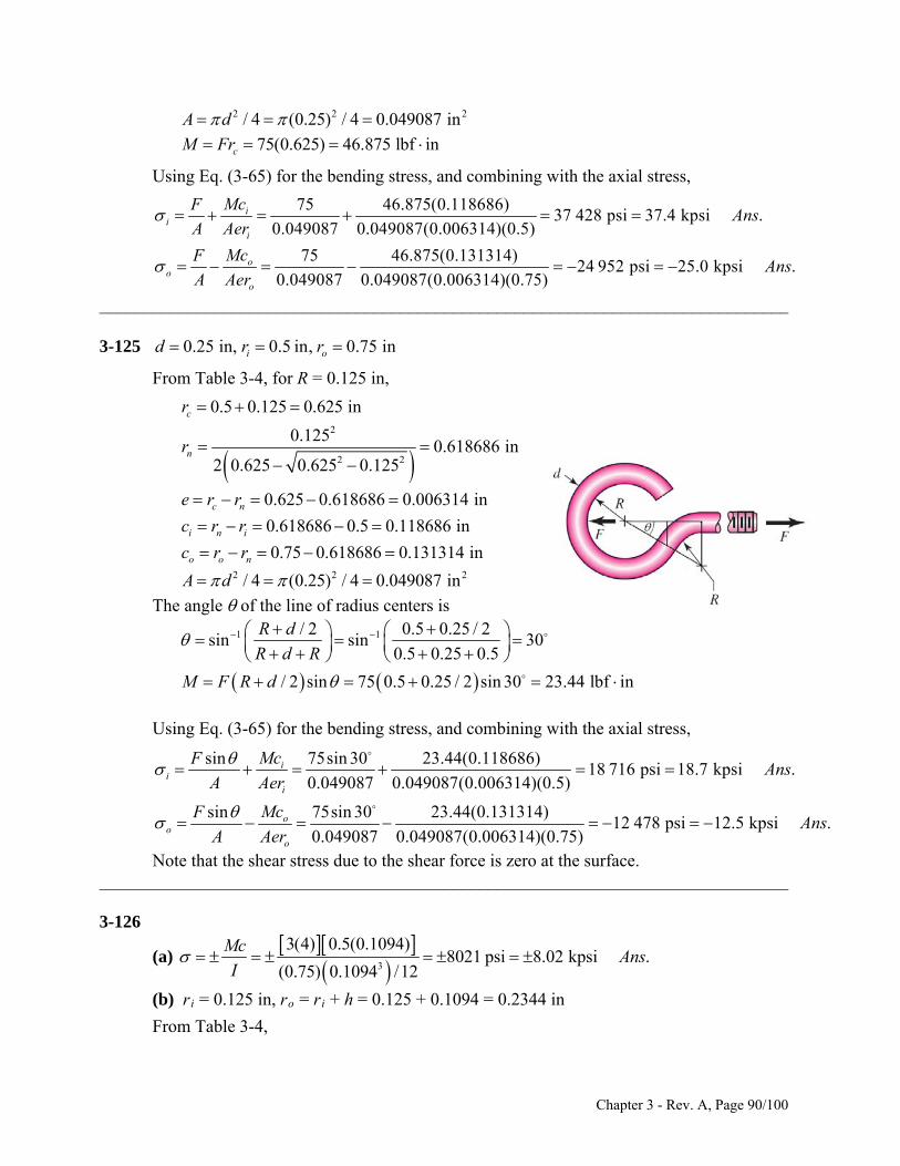
2 2/ 4 (0.25) / 4 0.049087 inA d 2
75(0.625) 46.875 lbf incM Fr
Using Eq. (3-65) for the bending stress, and combining with the axial stress,
75 46.875(0.118686)37 428 psi 37.4 kpsi .
0.049087 0.049087(0.006314)(0.5)
75 46.875(0.131314)24 952 psi 25.0 kpsi .
0.049087 0.049087(0.006314)(0.75)
ii
i
oo
o
McFAns
A Aer
McFAns
A Aer
______________________________________________________________________________ 3-125 0.25 in, 0.5 in, 0.75 ini od r r
From Table 3-4, for R = 0.125 in,
0.5 0.125 0.625 incr
2
2 2
0.1250.618686 in
2 0.625 0.625 0.125nr
0.625 0.618686 0.006314 inc ne r r
0.618686 0.5 0.118686 ini n ic r r
0.75 0.618686 0.131314 ino o nc r r 2 2/ 4 (0.25) / 4 0.049087 inA d 2
The angle of the line of radius centers is
1 1/ 2 0.5 0.25 / 2sin sin 30
0.5 0.25 0.5
/ 2 sin 75 0.5 0.25 / 2 sin 30 23.44 lbf in
R d
R d R
M F R d
Using Eq. (3-65) for the bending stress, and combining with the axial stress,
sin 75sin 30 23.44(0.118686)18 716 psi 18.7 kpsi .
0.049087 0.049087(0.006314)(0.5)
sin 75sin 30 23.44(0.131314)12 478 psi 12.5 kpsi
0.049087 0.049087(0.006314)(0.75)
ii
i
oo
o
McFAns
A Aer
McF
A Aer
.Ans
Note that the shear stress due to the shear force is zero at the surface. ______________________________________________________________________________ 3-126
(a)
3
3(4) 0.5(0.1094)8021 psi 8.02 kpsi .
(0.75) 0.1094 /12
McAns
I
(b) ri = 0.125 in, ro = ri + h = 0.125 + 0.1094 = 0.2344 in
From Table 3-4,
Chapter 3 - Rev. A, Page 90/100
0.125 (0.5)(0.1094) 0.1797 in
0.10940.174006 in
ln(0.2344 / 0.125)
0.1797 0.174006 0.005694 in
0.174006 0.125 0.049006 in
0.2344 0.174006 0.060394 in
0.75(0.1094) 0.08205
c
n
c n
i n i
o o n
r
r
e r r
c r r
c r r
A bh
2 in
3(4) 12 lbf inM
The negative sign on the bending moment is due to the sign convention shown in Fig. 3-34. Using Eq. (3-65),
12(0.049006)10 070 psi 10.1 kpsi .
0.08205(0.005694)(0.125)
12(0.060394)6618 psi 6.62 kpsi .
0.08205(0.005694)(0.2344)
ii
i
oo
o
McAns
Aer
McAns
Aer
(c) 10.1
1.26 .8.02
iiK Ans
6.620.825 .
8.02o
oK Ans
______________________________________________________________________________ 3-127
(a)
3
3(4) 0.5(0.1406)4856 psi 4.86 kpsi .
(0.75) 0.1406 /12
McAns
I
(b) ri = 0.125 in, ro = ri + h = 0.125 + 0.1406 = 0.2656 in
From Table 3-4, 0.125 (0.5)(0.1406) 0.1953 in
0.14060.186552 in
ln(0.2656 / 0.125)
0.1953 0.186552 0.008748 in
0.186552 0.125 0.061552 in
0.2656 0.186552 0.079048 in
0.75(0.1406) 0.10545
c
n
c n
i n i
o o n
r
r
e r r
c r r
c r r
A bh
2 in
3(4) 12 lbf inM
The negative sign on the bending moment is due to the sign convention shown in Fig. 3-34. Using Eq. (3-65),
Chapter 3 - Rev. A, Page 91/100
12(0.061552)6406 psi 6.41 kpsi .
0.10545(0.008748)(0.125)
12(0.079048)3872 psi 3.87 kpsi .
0.10545(0.008748)(0.2656)
ii
i
oo
o
McAns
Aer
McAns
Aer
(c) 6.41
1.32 .4.86
iiK Ans
3.870.80 .
4.86o
oK Ans
______________________________________________________________________________ 3-128
(a)
3
3(4) 0.5(0.1094)8021 psi 8.02 kpsi .
(0.75) 0.1094 /12
McAns
I
(b) ri = 0.25 in, ro = ri + h = 0.25 + 0.1094 = 0.3594 in
From Table 3-4, 0.25 (0.5)(0.1094) 0.3047 in
0.10940.301398 in
ln(0.3594 / 0.25)
0.3047 0.301398 0.003302 in
0.301398 0.25 0.051398 in
0.3594 0.301398 0.058002 in
0.75(0.1094) 0.08205 in
c
n
c n
i n i
o o n
r
r
e r r
c r r
c r r
A bh
2
3(4) 12 lbf inM The negative sign on the bending moment is due to the sign convention shown in Fig. 3-34. Using Eq. (3-65),
12(0.051398)9106 psi 9.11 kpsi .
0.08205(0.003302)(0.25)
12(0.058002)7148 psi 7.15 kpsi .
0.08205(0.003302)(0.3594)
ii
i
oo
o
McAns
Aer
McAns
Aer
(c) 9.11
1.14 .8.02
iiK Ans
7.150.89 .
8.02o
oK Ans
______________________________________________________________________________ 3-129 ri = 25 mm, ro = ri + h = 25 + 87 = 112 mm, rc = 25 + 87/2 = 68.5 mm The radius of the neutral axis is found from Eq. (3-63), given below.
Chapter 3 - Rev. A, Page 92/100

/n
Ar
dA r
For a rectangular area with constant width b, the denominator is
lno
i
ro
ri
rbdrb
r r
Applying this equation over each of the four rectangular areas,
45 54.5 92 1129 ln 31 ln 31 ln 9 ln 16.3769
25 45 82.5 92
dA
r
22 20(9) 31(9.5) 949 mmA
949
57.9475 mm16.3769/
n
Ar
dA r
68.5 57.9475 10.5525 mmc ne r r
57.9475 25 32.9475 mmi n ic r r
112 57.9475 54.0525 mmo o nc r r
M = 150F2 = 150(3.2) = 480 kN·mm We need to find the forces transmitted through the section in order to determine the axial stress. It is not immediately obvious which plane should be used for resolving the axial versus shear directions. It is convenient to use the plane containing the reaction force at the bushing, which assumes its contribution resolves entirely into shear force. To find the angle of this plane, find the resultant of F1 and F2.
1 2
1 2
1 22 2
2.4cos60 3.2cos0 4.40 kN
2.4sin 60 3.2sin 0 2.08 kN
4.40 2.08 4.87 kN
x x x
y y y
F F F
F F F
F
This is the pin force on the lever which acts in a direction
1 1 2.08tan tan 25.3
4.40y
x
F
F
On the surface 25.3° from the horizontal, find the internal forces in the tangential and normal directions. Resolving F1 into components,
2.4cos 60 25.3 1.97 kN
2.4sin 60 25.3 1.37 kN
t
n
F
F
The transverse shear stress is zero at the inner and outer surfaces. Using Eq. (3-65) for the bending stress, and combining with the axial stress due to Fn,
Chapter 3 - Rev. A, Page 93/100
3200 150 (32.9475)137064.6 MPa .
949 949(10.5525)(25)
3200 150 (54.0525)137021.7 MPa .
949 949(10.5525)(112)
n ii
i
n oo
o
F McAns
A Aer
F McAns
A Aer
______________________________________________________________________________ 3-130 ri = 2 in, ro = ri + h = 2 + 4 = 6 in, 2 0.5(4) 4 incr
2(6 2 0.75)(0.75) 2.4375 inA
Similar to Prob. 3-129,
3.625 60.75ln 0.75ln 0.682 920 in
2 4.375
dA
r
2.43753.56923 in
0.682 920( / )n
Ar
dA r
4 3.56923 0.43077 inc ne r r 3.56923 2 1.56923 ini n ic r r
6 3.56923 2.43077 ino o nc r r
6000(4) 24 000 lbf incM Fr
Using Eq. (3-65) for the bending stress, and combining with the axial stress,
6000 24 000(1.56923)20 396 psi 20.4 kpsi .
2.4375 2.4375(0.43077)(2)
6000 24 000(2.43077)6 799 psi 6.80 kpsi .
2.4375 2.4375(0.43077)(6)
ii
i
oo
o
McFAns
A Aer
McFAns
A Aer
______________________________________________________________________________ 3-131 ri = 12 in, ro = ri + h = 12 + 3 = 15 in, rc = 12 + 3/2 = 13.5 in
3 3(1.5 )(0.75) 1.988 in
4 4(1.5)(0.75) 3.534
I a b
A ab
4
20(3 1.5) 90 kip inM Since the radius is large compared to the cross section, assume Eq. 3-67 is applicable for the bending stress. Combining the bending stress and the axial stress,
20 90(1.5)(13.5)
82.1 kpsi .3.534 (1.988)(12)
i ci
i
Mc rFAns
A Ir
20 90(1.5)(13.5)
55.5 kpsi .3.534 1.988(15)
o co
o
Mc rFAns
A Ir
______________________________________________________________________________
Chapter 3 - Rev. A, Page 94/100
3-132 ri = 1.25 in, ro = ri + h = 1.25 + 0.5 + 1 + 0.5 = 3.25 in rc = (ri + ro) / 2 = (1.25 + 3.25)/2 = 2.25 in Ans.
For outer rectangle, ln o
i
rdAb
r r
For circle,
22
O2 2
OO
, 2 c c
A rA r
dA r r r r
2 2
O
2 ( )c c
dAr r r
r
Combine the integrals subtracting the circle from the rectangle
2 23.251.25ln 2 2.25 2.25 0.5 0.840 904 in
1.25
dA
r
2 21.25(2) (0.5 ) 1.714 60 in .A A ns
1.71460
2.0390 in .0.840904( / )
n
Ar A
dA r
ns
2.25 2.0390 0.2110 in .c ne r r Ans
2.0390 1.25 0.7890 ini n ic r r
3.25 2.0390 1.2110 ino o nc r r
2000(4.5 1.25 0.5 0.5) 13 500 lbf inM
2000 13 500(0.7890)
20 720 psi = 20.7 kpsi .1.7146 1.7146(0.2110)(1.25)
ii
i
McFAns
A Aer
2000 13 500(1.2110)12 738 psi 12.7 kpsi .
1.7146 1.7146(0.2110)(3.25)o
oo
McFAns
A Aer
______________________________________________________________________________ 3-133 From Eq. (3-68),
1 32
1 3 1 32 13
8 2 1
Ea KF F
d
Use 0.292, F in newtons, E in N/mm2 and d in mm, then 1/323 [(1 0.292 ) / 207 000]
0.036858 1/ 30
K
From Eq. (3-69),
1/3 1/31/3
max 2 1/3 2 2 2
3 3 3 3352 MPa
2 2 ( ) 2 2 (0.03685)
F F F Fp F
a KF K
Chapter 3 - Rev. A, Page 95/100
From Eq. (3-71), the maximum principal stress occurs on the surface where z = 0, and is
equal to – pmax.
1/3max max 352 MPa .z p F A ns
From Fig. 3-37,
1/3
max max0.3 106 MPa .p F A ns
______________________________________________________________________________ 3-134 From Eq. (3-68),
2 21 1 2 2
3
1 2
2 2
3
1 13
8 1 1
1 0.292 207 000 1 0.333 717003 100.0990 mm
8 1 25 1 40
E EFa
d d
a
From Eq. (3-69),
max 2 2
3 103487.2 MPa
2 2 0.0990
Fp
a
From Fig. 3-37, the maximum shear stress occurs at a depth of z = 0.48 a. 0.48 0.48 0.0990 0.0475 mm .z a A ns
The principal stresses are obtained from Eqs. (3-70) and (3-71) at a depth of z/a = 0.48.
1
1 2 2
1487.2 1 0.48 tan 1/ 0.48 1 0.333 101.3 MPa
2 1 0.48
3 2
487.2396.0 MPa
1 0.48
From Eq. (3-72),
1 3
max
101.3 396.0147.4 MPa .
2 2Ans
Note that if a closer examination of the applicability of the depth assumption from Fig. 3-37 is desired, implementing Eqs. (3-70), (3-71), and (3-72) on a spreadsheet will allow for calculating and plotting the stresses versus the depth for specific values of . For = 0.333 for aluminum, the maximum shear stress occurs at a depth of z = 0.492a with max = 0.3025 pmax.
Chapter 3 - Rev. A, Page 96/100
This gives max = 0.3025 pmax = (0.3025)(487.2) = 147.38 MPa. Even though the depth assumption was a little off, it did not have significant effect on the the maximum shear stress.
______________________________________________________________________________ 3-135 From the solution to Prob. 3-134, a = 0.0990 mm and pmax
= 487.2 MPa. Assuming applicability of Fig. 3-37, the maximum shear stress occurs at a depth of z = 0.48 a = 0.0475 mm. Ans. The principal stresses are obtained from Eqs. (3-70) and (3-71) at a depth of z/a = 0.48.
1
1 2 2
1487.2 1 0.48 tan 1/ 0.48 1 0.292 92.09 MPa
2 1 0.48
3 2
487.2396.0 MPa
1 0.48
From Eq. (3-72),
1 3
max
92.09 396.0152.0 MPa .
2 2Ans
Note that if a closer examination of the applicability of the depth assumption from Fig. 3-37 is desired, implementing Eqs. (3-70), (3-71), and (3-72) on a spreadsheet will allow for calculating and plotting the stresses versus the depth for specific values of . For = 0.292 for steel, the maximum shear stress occurs at a depth of z = 0.478a with max = 0.3119 pmax.
______________________________________________________________________________ 3-136 From Eq. (3-68),
2
3
1 2
2
3
2 13
8 1 1
2 1 0.292 207 0003 200.1258 mm
8 1 30 1
EFa
d d
a
From Eq. (3-69),
max 2 2
3 203603.4 MPa
2 2 0.1258
Fp
a
From Fig. 3-37, the maximum shear stress occurs at a depth of 0.48 0.48 0.1258 0.0604 mm .z a A ns
Also from Fig. 3-37, the maximum shear stress is
max max0.3 0.3(603.4) 181 MPa .p Ans
Chapter 3 - Rev. A, Page 97/100
_____________ ____________________________________ _____________________________
-137 Aluminum Plate-Ball interface: From Eq. (3-68), 3
3
1 2
2 6 2 6
3 1/33
8 1 1
1 0.292 30 10 1 0.333 10.4 1033.517 10 in
8 1 1 1
ad d
Fa F
rom Eq. (3-69),
2 21 1 2 21 13 E EF
F
4 1/3
max 223 1/3
3Fp
33.860 10 psi
2 2 3.517 10
FF
a F
By examination of Eqs. (3-70), (3-71), and (3-72), it can be seen that the only difference in the maximum shear stress for the plate and the ball will be due to poisson’s ratio in Eq.
(3-70). The larger poisson’s ratio will create the greater maximum shear stress, so the aluminum plate will be the critical element in this interface. Applying the equations for the aluminum plate,
4 1/3 1 1/3
1 2
13.86 10 1 0.48 tan 1/ 0.48 1 0.333 8025 psi
2 1 0.48F F
4 1/3
4 1/33 2
3.86 103.137 10 psi
1 0.48
FF
From Eq. (3-72),
1/3 4 1/3
4 1/31 3 max
8025 3.137 101.167 10 psi
2 2
F FF
omparing this stress to the allowable stress, and solving for F,
C
3
20 000 4
5.03 lbf1.167 10
F
able-Ball interface: From Eq. (3-68),
T
2 6 2 6
3 1/331 0.292 30 10 1 0.211 14.5 103
3.306 10 in8 1 1 1
Fa F
From Eq. (3-69),
Chapter 3 - Rev. A, Page 98/100
4 1/3max 22
3 1/3
3 34.369 10 psi
2 2 3.306 10
F Fp F
a F
The steel ball has a higher poisson’s ratio than the cast iron table, so it will dominate.
4 1/3 1 1/3
1 2
14.369 10 1 0.48 tan 1/ 0.48 1 0.292 8258 psi
2 1 0.48F F
4 1/3
4 1/33 2
4.369 103.551 10 psi
1 0.48
FF
From Eq. (3-72),
1/3 4 1/3
4 1/31 3max
8258 3.551 101.363 10 psi
2 2
F FF
Comparing this stress to the allowable stress, and solving for F,
3
4
20 0003.16 lbf
1.363 10F
The steel ball is critical, with F = 3.16 lbf. Ans. ______________________________________________________________________________ 3-138 v1 = 0.333, E1 = 10.4 Mpsi, l = 2 in, d1 = 1.25 in, v2 = 0.211, E2 = 14.5 Mpsi, d2 = –12 in.
With b = KcF1/2
1 22 6 2 6
4
1 0.333 10.4 10 1 0.211 14.5 102
(2) 1/1.25 1/12
2.336 10
cK
By examination of Eqs. (3-75), (3-76), and (3-77, it can be seen that the only difference in the maximum shear stress for the two materials will be due to poisson’s ratio in Eq. (3-75). The larger poisson’s ratio will create the greater maximum shear stress, so the aluminum roller will be the critical element in this interface. Instead of applying these equations, we will assume the poisson’s ratio for aluminum of 0.333 is close enough to 0.3 to make Fig. 3-39 applicable.
max max
max
0.3
400013 300 psi
p
p0.3
From Eq. (3-74), pmax = 2F / (bl ), so we have
Chapter 3 - Rev. A, Page 99/100
1 2
max 1 2
2 2
c c
F Fp
lK F lK
So,
2
max
24
2
(2)(2.336) 10 (13 300)
2
95.3 lbf .
clK pF
Ans
______________________________________________________________________________ 3-139 v = 0.292, E = 30 Mpsi, l = 0.75 in, d1 = 2(0.47) = 0.94 in, d2 = 2(0.62) = 1.24 in.
Eq. (3-73):
1 2
2 6
32 1 0.292 30 102(40)
1.052 10 in(0.75) 1/ 0.94 1/1.24
b
Eq. (3-74):
max 3
2 40232 275 psi 32.3 kpsi .
1.052 10 0.75
Fp Ans
bl
From Fig. 3-39,
max max0.3 0.3(32 275)=9682.5 psi 9.68 kpsi .p Ans ______________________________________________________________________________ 3-140 Use Eqs. (3-73) through (3-77).
1/22 21 1 2 2
1 2
(1 ) / (1 ) /2
(1/ ) (1/ )
E v EFb
l d d
1/22 6 2 62(600) (1 0.292 ) / (30(10 )) (1 0.292 ) / (30(10 ))
(2) 1/ 5 1/
0.007 631 inb
max
2 2(600)25 028 psi
(0.007 631)(2)
Fp
bl
Chapter 3 - Rev. A, Page 100/100
2
2max 2
2 1 2 0.292 25 028 1 0.786
7102 psi 7.10 kpsi .
x
z zp
b b
Ans
0.786
2
max 2 2
2
2 25 028 2 0.7861 0.7861
4 646 psi 4.65 kpsi .
y
zbpbz
b
Ans
2
21 2 1 2 0.786z
max
2 2
25 02819 677 psi 19.7 kpsi .
1 0.786z
pAns
z
21
b
max
4 646 19 6777 516 psi 7.52 kpsi .y z Ans
2 2
______________________________________________________________________________ 3-141 Use Eqs. (3-73) through (3-77).
1 22 2
1 1 2 2
1 2
1 12
1/ 1/
E EF
l d d
b
1 2
2 30.211 100 10
/
2 31 0.292 207 10 12(2000)
(40) 1/150 1
0.2583 mmb
max
2 2(2000)123.2 MPa
(0.2583)(40)
Fp
bl
2
2max 2
2 1 2 0.292 123.2 1 0.786
35.0 MPa .
x
z zp
b b
Ans
0.786
2
21 20.786
z
2
max 2 2
2
1 2 0.7862 123.2 2
1 0.7861
22.9 MPa .
y
zbpbz
b
Ans
max
2 2
123.296.9 MPa .
1 0.786z
pAns
z
21
b
Chapter 3 - Rev. A, Page 101/100
Chapter 3 - Rev. A, Page 102/100
max
22.9 96.937.0 MPa .
2 2y z Ans
______________________________________________________________________________ 3-142 Note to the Instructor: The first printing incorrectly had a width w = 1.25 mm instead of
w = 1.25 in. The solution presented here reflects the correction which will be made in subsequent printings. Use Eqs. (3-73) through (3-77).
1 22 2
1 1 2 2
1 2
1 12
1/ 1/
E EF
l d d
b
1 2
2 60.211 14.5 10 2 61 0.211 14.5 10 12(250)
(1.25) 1/ 3 1/
0.007 095 inb
max
2 2(250)17 946 psi
(0.007 095)(1.25)
Fp
bl
2
2max 2
2 1 2 0.211 17 946 1 0.786 0.
3 680 psi 3.68 kpsi .
x
z zp
b b
Ans
786
2
max 2 2
2
1 2 0.7862 17 946 2 0.786
1 0.7861
3 332 psi 3.33 kpsi .
y
zbpbz
b
Ans
2
21 2z
max
2 2
17 94614109 psi 14.1 kpsi .z
pAns
2
1 0.7861
zb
max
3 332 141095 389 psi 5.39 kpsi .
2 2y z Ans
______________________________________________________________________________
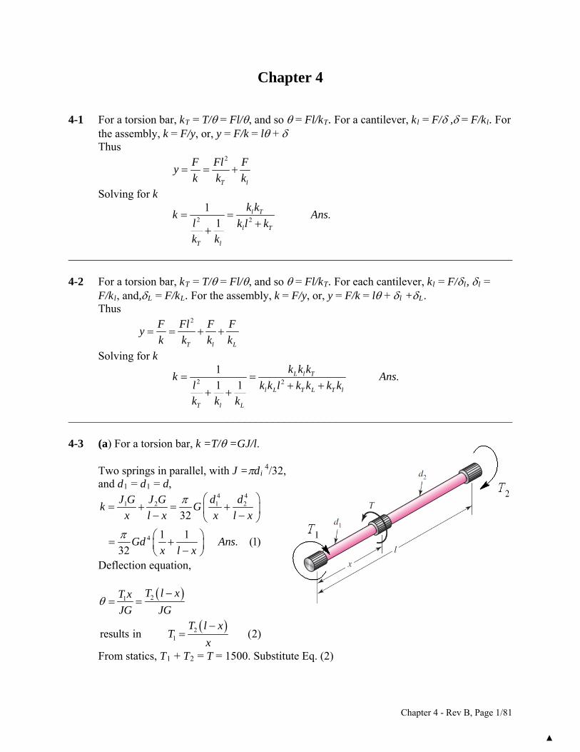
Chapter 4 4-1 For a torsion bar, kT = T/ = Fl/, and so = Fl/kT. For a cantilever, kl = F/ , = F/kl. For
the assembly, k = F/y, or, y = F/k = l + Thus
2
T l
F Fl Fy
k k k
Solving for k
2 2
1.
1l T
l T
T l
k kk A
l k l kk k
ns
______________________________________________________________________________ 4-2 For a torsion bar, kT = T/ = Fl/, and so = Fl/kT. For each cantilever, kl = F/l, l =
F/kl, and,L = F/kL. For the assembly, k = F/y, or, y = F/k = l + l +L. Thus
2
T l
F Fl F Fy
k k k k
L
Solving for k
2 2
1.
1 1L l T
l L T L T l
T l L
k k kk A
l k k l k k k kk k k
ns
______________________________________________________________________________ 4-3 (a) For a torsion bar, k =T/ =GJ/l. Two springs in parallel, with J =di
4/32, and d1 = d1 = d,
4 41 2 1 2
4
32
1 1. (1)
32
J G J G d dk G
x l x x l x
Gd Ansx l x
Deflection equation,
21
21results in (2)
T l xT x
JG JGT l x
Tx
From statics, T1 + T2 = T = 1500. Substitute Eq. (2)
Chapter 4 - Rev B, Page 1/81
2 2 21500 1500 . (3)l x x
T T T Ansx l
Substitute into Eq. (2) resulting in 1 1500 . (4)l x
T Anl
s
(b) From Eq. (1), 4 6 31 10.5 11.5 10 28.2 10 lbf in/rad .
32 5 10 5k A
ns
From Eq. (4), 1
10 51500 750 lbf in .
10T Ans
From Eq. (3), 2
51500 750 lbf in .
10T Ans
From either section, 3
3 3
16 15001630.6 10 psi 30.6 kpsi .
0.5i
i
TAns
d
______________________________________________________________________________ 4-4 Deflection to be the same as Prob. 4-3 where T1 = 750 lbfin, l1 = l / 2 = 5 in, and d1 = 0.5
in 1 = 2 =
1 2 31 2
4 44 4 4 1 2
1 2
4 6 750 5 4 660 10 (1)
0.532 32 32
T T T T
d dd G d G G
Or, 3 4
1 115 10 (2)T d
3 42 210 10 (3)T d
Equal stress, 1 2 1 21 2 3 3 3 3
1 2 1 2
16 16(4)
T T T T
d d d d
Divide Eq. (4) by the first two equations of Eq.(1) results in
1 23 31 2
2 11 2
4 41 2
1.5 (5)4 4
T Td d
d dT T
d d
Statics, T1 + T2 = 1500 (6) Substitute in Eqs. (2) and (3), with Eq. (5) gives
43 4 31 115 10 10 10 1.5 1500d d
Solving for d1 and substituting it back into Eq. (5) gives d1 = 0.388 8 in, d2 = 0.583 2 in Ans.
Chapter 4 - Rev B, Page 2/81
From Eqs. (2) and (3), T1 = 15(103)(0.388 8)4 = 343 lbfin Ans. T2 = 10(103)(0.583 2)4 = 1 157 lbfin Ans.
Deflection of T is
1 1
1 4 61
343 40.053 18 rad
/ 32 0.388 8 11.5 10
T l
J G
Spring constant is 3
1
150028.2 10 lbf in .
0.053 18
Tk Ans
The stress in d1 is
31
1 331
16 3431629.7 10 psi 29.7 kpsi .
0.388 8
TAns
d
The stress in d1 is
32
2 332
16 11571629.7 10 psi 29.7 kpsi .
0.583 2
TAns
d
______________________________________________________________________________ 4-5 (a) Let the radii of the straight sections be r1 = d1 /2 and r2 = d2 /2. Let the angle of the
taper be where tan = (r2 r1)/2. Thus, the radius in the taper as a function of x is r = r1 + x tan , and the area is A = (r1 + x tan )2. The deflection of the tapered portion
is
210 0 1 0
1 1 1
2 1
1 2 1 2 1 2
1 2
1
tan tantan
1 1 1
tan tan tan tan
tan
tan tan
4.
ll lF F dx Fdx
AE E E r xr x
F F
E r r l E r r
r rF F l Fl
E r r E r r r r E
FlAns
d d E
2
1
(b) For section 1,
41 2 2 6
1
4 4(1000)(2)3.40(10 ) in .
(0.5 )(30)(10 )
Fl FlAns
AE d E
For the tapered section,
46
1 2
4 4 1000(2)2.26(10 ) in .
(0.5)(0.75)(30)(10 )
FlAns
d d E
For section 2,
Chapter 4 - Rev B, Page 3/81
42 2 2 6
1
4 4(1000)(2)1.51(10 ) in .
(0.75 )(30)(10 )
Fl FlAns
AE d E
______________________________________________________________________________ 4-6 (a) Let the radii of the straight sections be r1 = d1 /2 and r2 = d2 /2. Let the angle of the
taper be where tan = (r2 r1)/2. Thus, the radius in the taper as a function of x is r = r1 + x tan , and the polar second area moment is J = ( /2) (r1 + x tan )4. The
angular deflection of the tapered portion is
4 30 0 1 1 0
33 31 11
2 23 3 3 31 1 2 22 1 2 1
3 3 3 3 3 31 2 2 1 1 2 1 2
2 1 2 1
3tan tan tan
2 1 1 2 1 1
3 tan 3 tantan tan
2 2 2
3 tan 3 3
32
3
ll lT T dx T
dxGJ G Gr x r x
T T
G r G r rr l
r r r rr r r rT T l Tl
G r r G r r r r G r r
T
32
2 21 1 2 2
3 31 2
.d d d dl
AnsG d d
(b) The deflections, in degrees, are For section 1,
1 4 4 6
1
180 32 180 32(1500)(2) 1802.44 deg .
(0.5 )11.5(10 )
Tl TlAns
GJ d G
For the tapered section,
2 21 1 2 2
3 31 2
2 2
6 3 3
( )32 180
3
(1500)(2) 0.5 (0.5)(0.75) 0.7532 1801.14 deg .
3 11.5(10 )(0.5 )(.75 )
Tl d d d d
Gd d
Ans
For section 2,
2 4 4 6
2
180 32 180 32(1500)(2) 1800.481 deg .
(0.75 )11.5(10 )
Tl TlAns
GJ d G
______________________________________________________________________________ 4-7 The area and the elastic modulus remain constant, however the force changes with respect
to x. From Table A-5 the unit weight of steel is = 0.282 lbf/in3, and the elastic modulus is E = 30 Mpsi. Starting from the top of the cable (i.e. x = 0, at the top).
F = (A)(lx)
Chapter 4 - Rev B, Page 4/81
22
260
0
0.282 500(12)1( ) 0.169 in
2 2 2(30)10
ll l
c o
Fdx ll x dx lx x
AE E E E
w
From the weight at the bottom of the cable,
2 2 6
4(5000) 500(12)45.093 in
(0.5 )30(10 )W
Wl Wl
AE d E
0.169 5.093 5.262 in .c W Ans
The percentage of total elongation due to the cable’s own weight
0.169
(100) 3.21% .5.262
Ans
______________________________________________________________________________ 4-8 Fy = 0 = R 1 F R 1 = F MA = 0 = M1 Fa M1 = Fa VAB = F, MAB =F (x a ), VBC = MBC = 0 Section AB:
2
1
1
2AB
F xF x a dx ax C
EI EI
(1)
AB = 0 at x = 0 C1 = 0
2 3
22 6AB
F x F x xy ax dx a
EI EI
2
2C (2)
yAB = 0 at x = 0 C2 = 0
2
3 .6AB
Fxy x a Ans
EI
Section BC:
3
10 0BC dx C
EI
From Eq. (1), at x = a (with C1 = 0), 2 2
( )2
F a Faa a
EI EI
2= C3. Thus,
2
2BC
Fa
EI
2 2
42 2BC
Fa Fay dx x C
EI EI (3)
Chapter 4 - Rev B, Page 5/81
From Eq. (2), at x = a (with C2 = 0), 3 2F a a 3
6 2 3
Fay a
EI EI
. Thus, from Eq. (3)
2 3Fa Fa 3
4 42 3 6
Faa C C
EI EI EI Substitute into Eq. (3)
2 3 2
3 .2 6 6BC
Fa Fa Fay x a x
EI EI EI Ans
maximum deflection occurs at x= l, The
2
max 3 .Fa
6y a l Ans
EI
MAB = R 1 x = Fx /2
:
= F /2, MBC = R 1 x F ( x l / 2) = F (l x) /2
______________________________________________________________________________ 4-9 MC = 0 = F (l /2) R1 l R1 = F /2 Fy = 0 = F /2 + R 2 F R 2 = F /2 Break at 0 x l /2: VAB = R 1 = F /2, Break at l /2 x l VBC = R 1 F = R 2
Section AB:
2
1 1
AB
Fx 2 4
F xdx C
EI EI
From symmetry, AB = 0 at x = l /2
2
2
1 1
20
4 1
lF
FlC C
EI EI
6. Thus,
2 2
2 2F x Fl Fx 4
4 16 16AB lEI EI EI
(1)
34x 2 2 2
2416 16 3AB
F Fy x l dx l x C
EI EI
Chapter 4 - Rev B, Page 6/81
at x = 0 C2 = 0, and, yAB = 0
2 24 348AB
Fxy x l
EI (2)
is not given, because with symmetry, Eq. (2) can be used in this region. The maximum deflection occurs at x =l /2,
yBC
22l
Fl 3
2max 4 3 .
48 2 48
Fly l Ans
EI EI
4-10 From Table A-6, for each angle, I = 207 cm4. Thus, I = 2(207) (104) = 4.14(106) mm4
From Table A-9, use beam 2 with F = 2500 N, a = 2000 mm, and l = 3000 mm; and beam
______________________________________________________________________________
1-1
3 with w = 1 N/mm and l = 3000 mm.
2 4
max ( 3 )Fa l
y a l w
6 8EI EI
2 4
3 6 3
2500(2000) (1)(3000)2000 3(3000)
6(207)10 (4.14)10 8(207)(10 )(4.14)(10 )
25.4 mm .Ans
6
)
= 2500(2000) [1(30002)/2] = 9.5(106) Nmm
rom Table A-6, from id to upper surface is y = 29 mm. From centroid to bottom is compressive at the bottom of
the beam at the wall. This stress is
2( / 2OM Fa l w
F centro
surface is y = 29.0 100= 71 mm. The maximum stress
6
max 6
9.5(10 )( 71)163 MPa .
4.14(10 )
MyAns
I
______________________________________________________________________________
Chapter 4 - Rev B, Page 7/81
4-11
14 10(450) (300) 465 lbf
20 206 10
(450) (300) 285 lbf20 20
O
C
R
R
M1 = 465(6)12 = 33.48(103) lbfin M2 = 33.48(103) +15(4)12 = 34.20(103) lbfin
3maxmax
34.2 15 2.28 in
MZ
Z Z
For deflections, use beams 5 and 6 of Table A-9
2 321 2
10ft
32 2 2
6 6
4 4
[ ( / 2)]2
6 2 2 48
450(72)(120) 300(240 )0.5 120 72 240
6(30)(10 ) (240) 48(30)(10 )
12.60 in / 2 6.30 in
x
F a l l F ll ly a l
EIl EI
I I
I I
Select two 5 in-6.7 lbf/ft channels from Table A-7, I = 2(7.49) = 14.98 in4, Z =2(3.00) =
6.00 in3
midspan
max
12.60 10.421 in
14.98 2
34.25.70 kpsi
6.00
y
______________________________________________________________________________
4-12 4 4(1.5 ) 0.2485 in64
I
From Table A-9 by superposition of beams 6 and 7, at x = a = 15 in, with b = 24 in and l = 39 in
2 2 2 2 3 3[ ] (26 24
Fba ay a b l la a )l
EIl EI
w
2 2 26
2 3 36
340(24)1515 24 39
6(30)10 (0.2485)39
(150 /12)(15)2(39)(15 ) 15 39 0.0978 in .
24(30)10 (0.2485)
Ay
Ans
At x = l /2 = 19.5 in
Chapter 4 - Rev B, Page 8/81
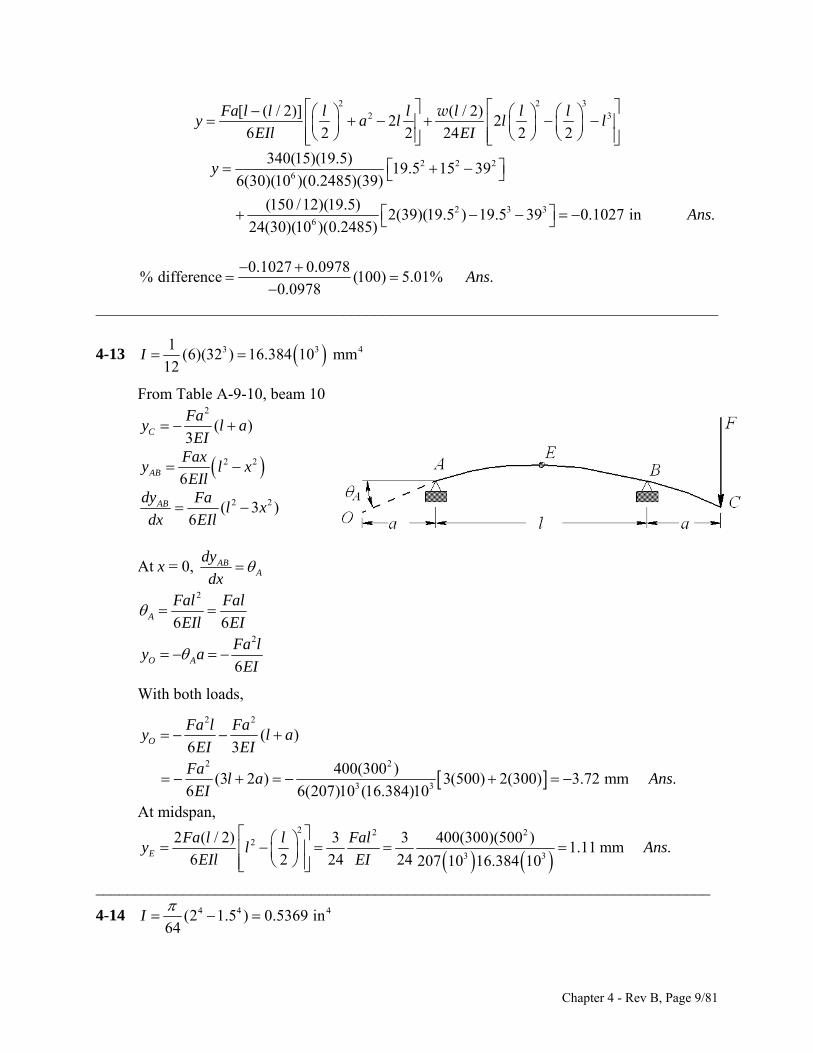
2 2
2 3[ ( / 2)] ( / 2)2 2
6 2 2 24 2 2
Fa l l l l l l ly a l l
EIl EI
w 3
l
2 2 26
2 3 36
340(15)(19.5)19.5 15 39
6(30)(10 )(0.2485)(39)
(150 /12)(19.5)2(39)(19.5 ) 19.5 39 0.1027 in .
24(30)(10 )(0.2485)
y
Ans
0.1027 0.0978
% difference (100) 5.01% .0.0978
Ans
______________________________________________________________________________
4-13 3 31(6)(32 ) 16.384 10 mm
12I 4
From Table A-9-10, beam 10
2
( )3C
Fay l a
EI
2 2
6AB
Faxy l x
EIl
2 2( 36
ABdy Fal x
dx EIl )
At x = 0, ABA
dy
dx
2
6 6A
Fal Fal
EIl EI
2
6O A
Fa ly a
EI
With both loads,
2 2
( )6 3O
Fa l Fay l a
EI EI
2 2
3 3
400(300 )(3 2 ) 3(500) 2(300) 3.72 mm .
6 6(207)10 (16.384)10
Fal a Ans
EI
At midspan,
2 2 22
3 3
2 ( / 2) 3 3 400(300)(500 )1.11 mm .
6 2 24 24 207 10 16.384 10E
Fa l l Faly l
EIl EI
Ans
_____________________________________________________________________________
4-14 4 4(2 1.5 ) 0.5369 in64
I 4
Chapter 4 - Rev B, Page 9/81
From Table A-5, E = 10.4 Mpsi From Table A-9, beams 1 and 2, by superposition
3 23 2
6 6
200 4(12) 300 2(12)( 3 ) 2(12) 3(4)(12)
3 6 3(10.4)10 (0.5369) 6(10.4)10 (0.5369)B A
B
F l F ay a l
EI EI
1.94 in .By Ans
______________________________________________________________________________ 4-15 From Table A-7, I = 2(1.85) = 3.70 in4 From Table A-5, E = 30.0 Mpsi From Table A-9, beams 1 and 3, by superposition
443 3
6 6
5 2(5 /12) (60 )( ) 150(60 )0.182 in .
3 8 3(30)10 (3.70) 8(30)10 (3.70)c
A
lFly Ans
EI EI
w w
______________________________________________________________________________
4-16 4
64I d
From Table A-5, 3207(10 ) MPaE From Table A-9, beams 5 and 9, with FC = FA = F, by superposition
3
2 2 3 2 21(4 3 ) 2 (4 3 )
48 24 48B
B BB
F l Fay a l I F l Fa a l
EI EI Ey
3 23
3 4
1550(1000 ) 2 375 (250) 4(250 ) 3(1000 )
48(207)10 2
53.624 10 mm
I 2
34 464 64
(53.624)10 32.3 mm .d I A
ns
______________________________________________________________________________ 4-17 From Table A-9, beams 8 (region BC for this beam with a = 0) and 10 (with a = a), by
superposition
3 2 2 2 2
3 2 2 2 2
3 26 6
13 2
6
AAB
A
M Faxy x lx l x l x
EIl EIl
.M x lx l x Fax l x AnEIl
s
3 2 2 2( )3 2 ( ) [( ) (3
6 6A
BC
x l
Md F x ly x lx l x x l x l a x l
dx EIl EI
)]
2( )( ) [( ) (3 )
6 6AM l F x l
]x l x l a x lEI EI
Chapter 4 - Rev B, Page 10/81
2( )( ) (3 )
6 A
x l.M l F x l a x l Ans
EI
______________________________________________________________________________ 4-18 Note to the instructor: Beams with discontinuous loading are better solved using
singularity functions. This eliminates matching the slopes and displacements at the discontinuity as is done in this solution.
1 10 22 2C
a a.M R l a l a R l a Ans
l
ww
2
2 20 22 2y
a aF l a R a R
l l w w
w .Ans
21 2 2 .V R
2 2AB
al a l a x a Ans
l l
w wwx = wx =
2
2 .2BC
aV R A
l
wns
2
212
2 2AB AB
xM V dx l ax a x C
l
w
210 at 0 0 2 .
2AB ABM x C M al a lx Al
wxns
2 2
22 2BC BC
a aM V dx dx x C
l l
w w
2 2
20 at ( ) .2 2BC BC
a aM x l C M l x Ans
l
w w
2 2 2 23
2 2 2 33
3 2 3 43 4
4
1 1 12
2 2 2
1 1 1
2 2 3
1 1 1 1
2 3 6 12
0 at 0 0
ABAB
AB AB
AB
M xdx al a lx dx alx a x lx C
EI EI l EI l
y dx alx a x lx C dxEI l
alx a x lx C x CEI l
y x C
31
3
w w
w
w
2 2
25
2 32 4 3 2
3 5 3
1 1 1( )
2 2 2
at
1 1 1 1 1 (1)
2 2 3 2 2 6
BCBC
AB BC
M a adx l x dx lx x C
EI EI l EI l
x a
a aala a la C la a C C C
EI l EI l
w w
w w w5
Chapter 4 - Rev B, Page 11/81
2 22 2 3
5 5
2 2
6 5
22 3 3
5
1 1 1 1 1
2 2 2 2 6
0 at 6
1 1 1 1( )
2 2 6 3
BC BC
BC
BC
a ay dx lx x C dx lx x C x
EI l EI l
a ly x l C C l
ay lx x l C x l
EI l
w w
w
w
6C
23 5 4 2 3 3
3 5
22 3
3 5
at
1 1 1 1 1 1( )
2 3 6 12 2 2 6 3
3 4 ( ) (2)24
AB BCy y x a
aala a la C a la a l C a l
l l
aC a la l C a l
l
w w
w
Substituting (1) into (2) yields 2
2 25 4
24
aC a
l
w l . Substituting this back into (2) gives
2
2 23 4 4
24
aC al a
l
wl . Thus,
3 2 3 4 3 4 2 24 2 4 424ABy alx a x lx a lx a x a l x
EIl
w
22 3 22 (2 ) 2 24AB
xy ax l a lx a l a .Ans
EIl
w
2 2 2 3 4 2 2 46 2 424BCy a lx a x a x a l x a l Ans.
EIl
w
This result is sufficient for yBC. However, this can be shown to be equivalent to
3 2 3 4 2 2 3 4
4
4 2 4 4 (24 24
( ) .24
BC
BC AB
y alx a x lx a l x a lx a x x aEIl EI
y y x a AnsEI
w w
w
4)
by expanding this or by solving the problem using singularity functions. ______________________________________________________________________________ 4-19 The beam can be broken up into a uniform load w downward from points A to C and a
uniform load upward from points A to B.
2 22 3 2 2 3 2
2 22 2 2 2
2 (2 ) 2 2 (2 ) 224 24
2 (2 ) 2 2 (2 ) 2 .24
AB
x xy bx l b lx b l b ax l a lx a l
EIl EIlx
bx l b b l b ax l a a l a AnsEIl
w w
w
a
23 4 2
3 2 3 4 2 2 3 4 4
2 (2 ) 224
4 2 4 4 ( )
BCy bx l b lx b x l bEIl
alx a x lx a l x a lx a x l x a Ans
w
.
Chapter 4 - Rev B, Page 12/81
3 2 3 4 2 2 3 4 4
3 2 3 4 2 2 3 4 4
4 4
4 2 4 4 ( )24
4 2 4 4 ( )24
( ) ( ) .24
CD
AB
y blx b x lx b l x b lx b x l x bEIl
alx a x lx a l x a lx a x l x aEIl
x b x a y AnsEI
w
w
w
______________________________________________________________________________ 4-20 Note to the instructor: See the note in the solution for Problem 4-18.
2
0 22 2y B B
a aF R a R l a A
l l w w
w .ns
For region BC, isolate right-hand element of length (l + a x)
2
, .2AB A BC
aV R V l a x An
l
ww s
2
2, .
2 2AB A BC
aM R x x M l a x Ans
l
w w
2
214AB AB
aEI M dx x C
l
w
2
31 212AB
aEIy x C x C
l
w
yAB = 0 at x = 0 C2 = 0 2
3112AB
aEIy x C x
l w
yAB = 0 at x = l 2
1 12
a lC
w
2 2 2 2
3 2 2 2 .12 12 12 12AB AB
a a l a x a xEIy x x l x y l x Ans
l l EIl w w w w 2
3
36BC BCEI M dx l a x w
C
4
3 424BCEIy l a x C x C w
yBC = 0 at x = l 4 4
3 4 4024 24
a aC l C C C l
w w3 (1)
AB = BC at x = l 2 2 3 2
3 34 12 6 6
a l a l aC C l
w w wa wa
Substitute C3 into Eq. (1) gives 2
24 4
24
aC a l l a
w. Substitute back into yBC
2 4 24
4 2 4
1
24 6 24 6
4 .24
BC
ly l a x x l a
EI
l a x a l x l a a AnsEI
w wa wa wa
w
l a
Chapter 4 - Rev B, Page 13/81
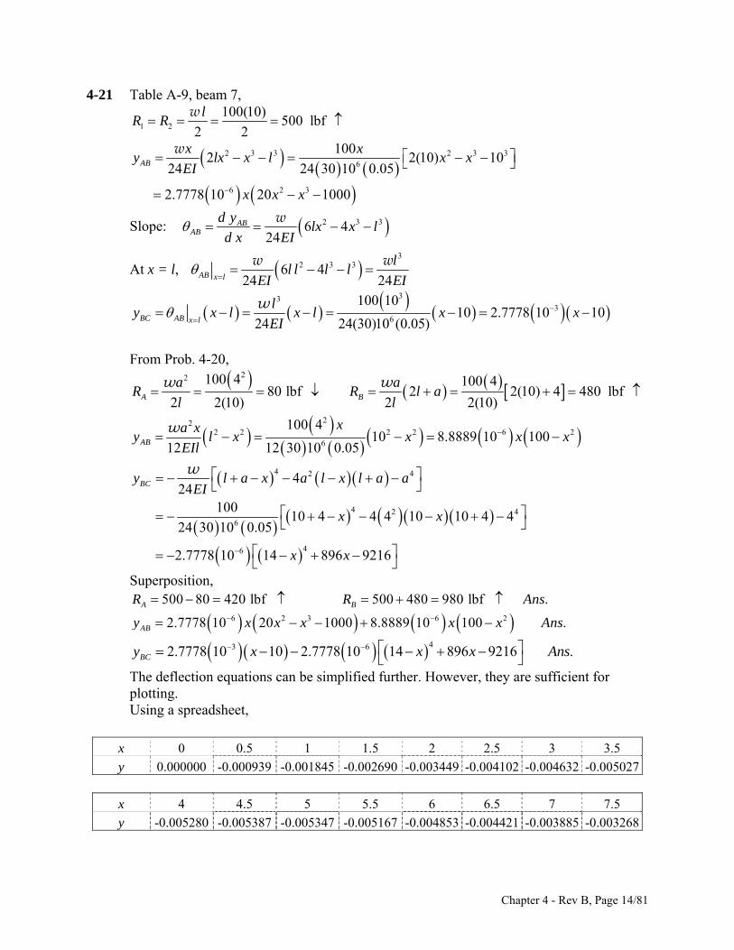
4-21 Table A-9, beam 7,
1 2
100(10)500 lbf
2 2
lR R
w
2 3 3 2 3 36
6 2 3
1002 2(10) 10
24 24 30 10 0.05
2.7778 10 20 1000
AB
x xy lx x l x x
EI
x x x
w
Slope: 2 3 36 424
ABAB
d ylx x l
d x EI
w
At x = l, 3
2 3 36 424 24AB x l
ll l l l
EI EI
w w
33
36
100 1010 2.7778 10 10
24 24(30)10 (0.05)BC AB x l
ly x l x l x x
EI
w
From Prob. 4-20,
22 100 4 100 480 lbf 2 2(10) 4 480 lbf
2 2(10) 2 2(10)A B
a aR R l a
l l w w
222 2 2 2 6 2
6
100 410 8.8889 10 100
12 12 30 10 0.05AB
xa xy l x x x
EIl
w x
4 2 4
4 2 46
46
424
10010 4 4 4 10 10 4 4
24 30 10 0.05
2.7778 10 14 896 9216
BCy l a x a l x l a aEI
x x
x x
w
Superposition, 500 80 420 lbf 500 480 980 lbf .A BR R A ns
6 2 3 6 22.7778 10 20 1000 8.8889 10 100 .ABy x x x x x Ans
43 62.7778 10 10 2.7778 10 14 896 9216 .BCy x x x Ans
The deflection equations can be simplified further. However, they are sufficient for plotting.
Using a spreadsheet,
x 0 0.5 1 1.5 2 2.5 3 3.5
y 0.000000 -0.000939 -0.001845 -0.002690 -0.003449 -0.004102 -0.004632 -0.005027
x 4 4.5 5 5.5 6 6.5 7 7.5
y -0.005280 -0.005387 -0.005347 -0.005167 -0.004853 -0.004421 -0.003885 -0.003268
Chapter 4 - Rev B, Page 14/81
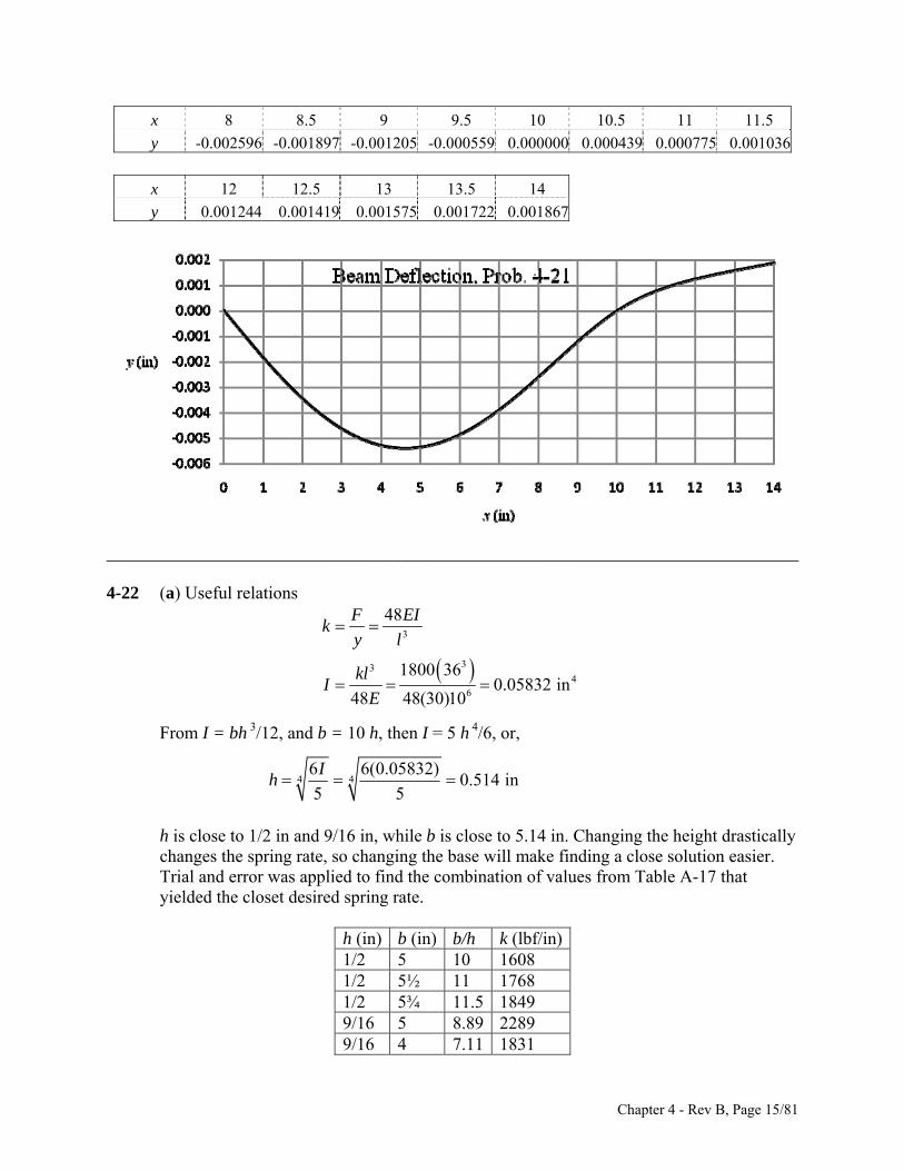
x 8 8.5 9 9.5 10 10.5 11 11.5
y -0.002596 -0.001897 -0.001205 -0.000559 0.000000 0.000439 0.000775 0.001036
x 12 12.5 13 13.5 14
y 0.001244 0.001419 0.001575 0.001722 0.001867
______________________________________________________________________________ 4-22 (a) Useful relations
3
334
6
48
1800 360.05832 in
48 48(30)10
F EIk
y l
klI
E
From I = bh 3/12, and b = 10 h, then I = 5 h 4/6, or,
4 4
6 6(0.05832)0.514 in
5 5
Ih
h is close to 1/2 in and 9/16 in, while b is close to 5.14 in. Changing the height drastically
changes the spring rate, so changing the base will make finding a close solution easier. Trial and error was applied to find the combination of values from Table A-17 that yielded the closet desired spring rate.
h (in) b (in) b/h k (lbf/in)1/2 5 10 1608 1/2 5½ 11 1768 1/2 5¾ 11.5 1849 9/16 5 8.89 2289 9/16 4 7.11 1831
Chapter 4 - Rev B, Page 15/81
h = ½ in, b = 5 ½ in should be selected because it results in a close spring rate and b/h is
still reasonably close to 10. (b)
3 45.5(0.5) /12 0.05729 inI
3
33
6
( / 4) 4 4(60)10 (0.05729) 1528 lbf
36 (0.25)
(1528) 360.864 in .
48 48(30)10 (0.05729)
Mc Fl c IF
I I lc
Fly A
EI
ns
______________________________________________________________________________ 4-23 From the solutions to Prob. 3-68, 1 260 lbf and 400 lbfT T
4 4
41198 in(1.25)
0.64 64
dI
From Table A-9, beam 6,
2 2 2 2 2 21 1 2 21 2
10in
2 2 26
2 2 26
( ) ( )6 6
( 575)(30)(10)10 30 40
6(30)10 (0.1198)(40)
460(12)(10)10 12 40 0.0332 in .
6(30)10 (0.1198)(40)
Ax
Fb x F b xz x b l x b l
EIl EIl
Ans
2 2 2 2 2 21 1 2 21 2
10in 10in
2 2 2 2 2 21 1 2 21 2
10in
2 2 26
( ) ( )6 6
(3 ) (3 )6 6
(575)(30)3 10 30 40
6(30)10 (0.1198)(40)
460(12)
6(30
A yx x
x
Fb x F b xd z dx b l x b l
dx dx EIl EIl
Fb F bx b l x b l
EIl EIl
2 2 2
6
4
3 10 12 40)10 (0.1198)(40)
6.02(10 ) rad .Ans
______________________________________________________________________________ 4-24 From the solutions to Prob. 3-69, 1 22880 N and 432 NT T
4 4
3 4(30)39.76 10 mm
64 64
dI
Chapter 4 - Rev B, Page 16/81
The load in between the supports supplies an angle to the overhanging end of the beam. That angle is found by taking the derivative of the deflection from that load. From Table A-9, beams 6 (subscript 1) and 10 (subscript 2),
2 beam10beam6A BC ACy a y (1)
1 1 2 2 2 2 21 11 1
2 21 11
2 6 36 6
6
BC C2
x lx l
F a l x F adx a lx lx x a l
dx EIl EIl
F al a
EIl
Equation (1) is thus
22 21 1 2 2
1 2 2
22 2
3 3 3 3
( )6 3
3312(230) 2070(300 )510 230 300 510 300
6(207)10 (39.76)10 (510) 3(207)10 (39.76)10
7.99 mm .
A
F a F ay l a a l a
EIl EI
Ans
The slope at A, relative to the z axis is
2
2
2 2 21 1 21 2
2 2 21 1 21 2 2
2 2 21 1 21 2 2
23 3
( )( ) ( ) (3 )
6 6
3( ) 3 ( ) (3 )6 6
( ) 3 26 6
3312(230)510 2
6(207)10 (39.76)10 (510)
A zx l a
x l a
F a F x ldl a x l a x l
EIl dx EI
F a Fl a x l a x l a x l
EIl EIF a F
l a a laEIl EI
2
23 3
30
20703(300 ) 2(510)(300)
6(207)10 (39.76)10
0.0304 rad .Ans
______________________________________________________________________________ 4-25 From the solutions to Prob. 3-70, 1 2392.16 lbf and 58.82 lbfT T
4 4
4(1)0.049 09 in
64 64
dI
From Table A-9, beam 6,
Chapter 4 - Rev B, Page 17/81
2 2 2 2 2 21 11 6
8in
( 350)(14)(8)8 14 22 0.0452 in .
6 6(30)10 (0.049 09)(22)Ax
F b xy x b l Ans
EIl
2 2 2 2 2 22 22 6
8in
( 450.98)(6)(8)( ) 8 6 22 0.0428 in .
6 6(30)10 (0.049 09)(22)Ax
F b xz x b l
EIl
Ans
The displacement magnitude is
2 2 2 20.0452 0.0428 0.0622 in .A Ay z Ans
11
2 2 2 2 2 21 1 1 11 1
2 2 26
(3 )6 6
( 350)(14)3 8 14 22 0.00242 rad .
6(30)10 (0.04909)(22)
A zx ax a
F b x F bd y d1x b l a b l
d x dx EIl EIl
Ans
11
2 2 2 2 2 22 2 2 22 1
2 2 26
( ) 36 6
(450.98)(6)3 8 6 22 0.00356 rad .
6(30)10 (0.04909)(22)
A yx ax a
F b x F bd z d2x b l a b l
d x dx EIl EIl
Ans
The slope magnitude is 220.00242 0.00356 0.00430 rad .A Ans
______________________________________________________________________________ 4-26 From the solutions to Prob. 3-71, 1 2250 N and 37.5 NT T
4 4
4(20)7 854 mm
64 64
dI
o1 1 2 2 2 2 2 2
1 3
300mm
345sin 45 (550)(300)( ) 300 550 850
6 6(207)10 (7 854)(850)
1.60 mm .
yA
x
F b xy x b l
EIl
Ans
2 2 2 2 2 21 1 2 2
1 2300mm
( ) ( )6 6
zA
x
F b x F b xz x b l x b l
EIl EIl
o
2 2 23
2 2 23
345cos 45 (550)(300)300 550 850
6(207)10 (7 854)(850)
287.5(150)(300)300 150 850 0.650 mm .
6(207)10 (7 854)(850)Ans
The displacement magnitude is 22 2 21.60 0.650 1.73 mm .A Ay z Ans
Chapter 4 - Rev B, Page 18/81
1 1
1 1 1 12 2 2 2 2 21 1
o
2 2 23
(3 )6 6
345sin 45 (550)3 300 550 850 0.00243 rad .
6(207)10 (7 854)(850)
y yA z
x a x a
F b x F bd y dx b l a b l
d x dx EIl EIl
Ans
1
11
2 2 2 2 2 21 1 2 21 2
2 2 2 2 2 21 1 2 21 1 1 2
o
2 2 23
3
6 6
3 36 6
345cos 45 (550)3 300 550 850
6(207)10 (7 854)(850)
287.5(150)
6(207)10 (7 85
zA y
x ax a
z
F b x F b xd z dx b l x b l
d x dx EIl EIl
F b F ba b l a b l
EIl EIl
2 2 2 43 300 150 850 1.91 10 rad .
4)(850)Ans
The slope magnitude is 2 20.00243 0.000191 0.00244 rad .A Ans
______________________________________________________________________________ 4-27 From the solutions to Prob. 3-72, 750 lbfBF
4 4
4(1.25)0.1198 in
64 64
dI
From Table A-9, beams 6 (subscript 1) and 10 (subscript 2)
1 1 2 22 2 2 2 21
16in
o o
2 2 2 2 26 6
6 6
300cos 20 (14)(16) 750sin 20 (9)(16)16 14 30 30 16
6(30)10 (0.119 8)(30) 6(30)10 (0.119 8)(30)
0.0805 in .
y yA
x
F b x F a xy x b l l x
EIl EIl
Ans
2 2 2 2 21 1 2 21
16in
o o
2 2 2 2 26 6
6 6
300sin 20 (14)(16) 750cos 20 (9)(16)16 14 30 30 16
6(30)10 (0.119 8)(30) 6(30)10 (0.119 8)(30)
0.1169 in .
z zA
x
F b x F a xz x b l l x
EIl EIl
Ans
The displacement magnitude is 22 2 20.0805 0.1169 0.142 in .A Ay z Ans
Chapter 4 - Rev B, Page 19/81
1 1
1 1 2 22 2 2 2 21
1 1 2 22 2 2 2 21 1 1
o
2 2 26
o
6
6 6
3 36 6
300cos 20 (14)3 16 14 30
6(30)10 (0.119 8)(30)
750sin 20 (9)3
6(30)10 (0.119 8)(30)
y yA z
x a x a
y y
F b x F a xd y dx b l l x
d x dx EIl EIl
F b F aa b l l a
EIl EIl
2 2 50 3 16 8.06 10 rad .Ans
11
2 2 2 2 21 1 2 21
2 2 2 2 21 1 2 21 1 1
o o
2 2 26 6
6 6
3 36 6
300sin 20 (14) 750cos 20 (9)3 16 14 30 3
6(30)10 (0.119 8)(30) 6(30)10 (0.119 8)(30)
z zA y
x ax a
z z
F b x F a xd z dx b l l x
d x dx EIl EIl
F b F aa b l l a
EIl EIl
2 20 3 16
0.00115 rad .Ans
The slope magnitude is 25 28.06 10 0.00115 0.00115 rad .A Ans
______________________________________________________________________________ 4-28 From the solutions to Prob. 3-73, FB = 22.8 (103) N
443 4
50306.8 10 mm
64 64
dI
From Table A-9, beam 6,
1 1 2 22 2 2 2 2 21 2
400mm
3 o
2 2 23 3
3 o
2 23 3
( ) ( )6 6
11 10 sin 20 (650)(400)400 650 1050
6(207)10 (306.8)10 (1050)
22.8 10 sin 25 (300)(400)400 300 1050
6(207)10 (306.8)10 (1050)
3.735
y yA
x
F b x F b xy x b l x b l
EIl EIl
mm .
2
Ans
Chapter 4 - Rev B, Page 20/81
2 2 2 2 2 21 1 2 21 2
400mm
3 o
2 2 23 3
3 o
2 2 23 3
( ) ( )6 6
11 10 cos 20 (650)(400)400 650 1050
6(207)10 (306.8)10 (1050)
22.8 10 cos 25 (300)(400)400 300 1050 1.791
6(207)10 (306.8)10 (1050)
z zA
x
F b x F b xz x b l x b l
EIl EIl
mm .Ans
The displacement magnitude is 22 2 23.735 1.791 4.14 mm .A Ay z Ans
11
2 2 2 2 2 21 1 2 21 2
1 1 2 22 2 2 2 2 21 1 1 2
3 o
2 2 23 3
3 o
6 6
3 36 6
11 10 sin 20 (650)3 400 650 1050
6(207)10 (306.8)10 (1050)
22.8 10 sin 25
z zA z
x ax a
y y
F b x F b xd y dx b l x b l
d x dx EIl EIl
F b F ba b l a b l
EIl EIl
2 2 23 3
(300)3 400 300 1050
6(207)10 (306.8)10 (1050)
0.00507 rad .Ans
11
2 2 2 2 2 21 1 2 21 2
2 2 2 2 2 21 1 2 21 1 1 2
3 o
2 2 23 3
3
6 6
3 36 6
11 10 cos 20 (650)3 400 650 1050
6(207)10 (306.8)10 (1050)
22.8 10 co
z zA y
x ax a
z z
F b x F b xd z dx b l x b l
d x dx EIl EIl
F b F ba b l a b l
EIl EIl
o
2 2 23 3
s 25 (300)3 400 300 1050
6(207)10 (306.8)10 (1050)
0.00489 rad .Ans
The slope magnitude is 2 20.00507 0.00489 0.00704 rad .A Ans
______________________________________________________________________________ 4-29 From the solutions to Prob. 3-68, T1 = 60 lbf and T2 = 400 lbf , and Prob. 4-23, I = 0.119 8
in4. From Table A-9, beam 6,
Chapter 4 - Rev B, Page 21/81
2 2 2 2 2 21 1 2 21 2
00
2 2 2 2 2 21 1 2 21 2 6
2 26
6 6
575(30)30 40
6 6 6(30)10 (0.119 8)(40)
460(12)12 40 0.00468 rad
6(30)10 (0.119 8)(40)
z zO y
xx
z z
F b x F b xd z dx b l x b l
d x dx EIl EIl
F b F bb l b l
EIl EIl
.Ans
1 1 2 22 2 2 21 2
2 2 2 2 2 21 1 2 21 2
2 2 2 21 1 2 21 2
2 2
2 26 6
6 2 3 6 2 36 6
6 6
575(10) 40 10
6(3
z zC y
x l x l
z z
x l
z z
F a l x F a l xd z dx a lx x a lx
d x dx EIl EIl
F a F alx l x a lx l x a
EIl EIl
F a F al a l a
EIl EIl
2 2
6 6
460(28) 40 280.00219 rad .
0)10 (0.119 8)(40) 6(30)10 (0.119 8)(40)Ans
______________________________________________________________________________ 4-30 From the solutions to Prob. 3-69, T1 = 2 880 N and T2 = 432 N, and Prob. 4-24, I = 39.76
(103) mm4. From Table A-9, beams 6 and 10
2 2 2 2 21 1 2 21
00
2 2 2 2 2 2 21 1 2 2 1 1 2 21 1
0
2 23 3
( ) ( )6 6
(3 ) ( 3 ) ( )6 6 6
3 312(280) 2 070(300)280 510
6(207)10 (39.76)10 (510)
O zxx
x
Fb x F a xd y dx b l l x
d x dx EIl EIl
Fb F a Fb F a lx b l l x b l
EIl EIl EIl EI
6
3 3
(510)
6(207)10 (39.76)10
0.0131 rad .Ans
2 2 2 21 1 2 21
2 2 2 2 2 2 21 1 2 2 1 1 2 21 1
23 3
( )( 2 ) ( )
6 6
(6 2 3 ) ( 3 ) ( )6 6 6
3 312(230)(510 230
6(207)10 (39.76)10 (510)
C zx lx l
x l
F a l x F a xd y dx a lx l x
d x dx EIl EIl
3
F a F a F alx l x a l x l a
F a l
EIl EIl EIl EI
23 3
2 070(300)(510))
3(207)10 (39.76)10
0.0191 rad .Ans
______________________________________________________________________________ 4-31 From the solutions to Prob. 3-70, T1 = 392.19 lbf and T2 = 58.82 lbf , and Prob. 4-25, I =
0.0490 9 in4. From Table A-9, beam 6
Chapter 4 - Rev B, Page 22/81
1 1 1 12 2 2 2 21 1
0 0
2 26
( )6 6
350(14)14 22 0.00726 rad .
6(30)10 (0.04909)(22)
y yO z
x x
F b x F bd y dx b l b l
d x dx EIl EIl
Ans
2 2 2 2 22 2 2 22 2
00
2 26
6 6
450.98(6)6 22
6(30)10 (0.04909)(22)
0.00624 rad .
z zO y
xx
F b x F bd z dx b l b l
d x dx EIl EIl
Ans
The slope magnitude is 220.00726 0.00624 0.00957 rad .O Ans
1 1 2 21
1 1 1 12 2 2 2 21 1
2 26
( )2
6
6 2 3 ( )6 6
350(8)22 8 0.00605 rad .
6(30)10 (0.0491)(22)
yC z
x l x l
y y
x l
F a l xd y dx a lx
d x dx EIl
F a F alx l x a l a
EIl EIl
Ans
2 22 22
2 2 2 2 22 2 2 22 2
2 26
( )2
6
6 2 36 6
450.98(16)22 16 0.00846 rad .
6(30)10 (0.04909)(22)
zC y
x lx l
z z
x l
F a l xd z dx a lx
d x dx EIl
F a F alx l x a l a
EIl EIl
Ans
The slope magnitude is 2 20.00605 0.00846 0.0104 rad .C Ans
______________________________________________________________________________ 4-32 From the solutions to Prob. 3-71, T1 =250 N and T1 =37.5 N, and Prob. 4-26, I = 7 854
mm4. From Table A-9, beam 6
1 1 1 12 2 2 2 21 1
0 0
o
2 23
( )6 6
345sin 45 (550)550 850 0.00680 rad .
6(207)10 (7 854)(850)
y yO z
x x
F b x F bd y dx b l b l
d x dx EIl EIl
Ans
Chapter 4 - Rev B, Page 23/81
2 2 2 2 2 21 1 2 21 2
00
o
2 2 2 2 2 21 1 2 21 2 3
2 23
6 6
345cos 45 (550)550 850
6 6 6(207)10 (7 854)(850)
287.5(150)150 850
6(207)10 (7 854)(850)
z zO y
xx
z z
F b x F b xd z dx b l x b l
d x dx EIl EIl
F b F bb l b l
EIl EIl
0.00316 rad .Ans
The slope magnitude is 2 20.00680 0.00316 0.00750 rad .O Ans
1 1 1 12 2 2 2 21 1
o1 1 2 2 2 2
1 3
( )2 6 2 3
6 6
345sin 45 (300)( ) 850 300 0.00558 rad .
6 6(207)10 (7 854)(850)
y yC z
x l x lx l
y
F a l x F ad y dx a lx lx l x a
d x dx EIl EIl
F al a Ans
EIl
2 2 2 21 1 2 21 2
o
2 2 2 2 2 21 1 2 21 2 3
3
( ) ( )2 2
6 6
345cos 45 (300)850 300
6 6 6(207)10 (7 854)(850)
287.5(700)
6(207)10 (7 854)(850
z zC y
x lx l
z z
F a l x F a l xd z dx a lx x a lx
d x dx EIl EIl
F a F al a l a
EIl EIl
2 2 5850 700 6.04 10 rad .)
Ans
The slope magnitude is 22 50.00558 6.04 10 0.00558 rad .C Ans
________________________________________________________________________ 4-33 From the solutions to Prob. 3-72, FB = 750 lbf, and Prob. 4-27, I = 0.119 8 in4. From
Table A-9, beams 6 and 10
1 1 2 22 2 2 2 21
0 0
1 1 2 2 1 1 2 22 2 2 2 2 2 21 1
0
o
2 26
6 6
3 36 6 6 6
300cos 20 (14) 750sin 214 30
6(30)10 (0.119 8)(30)
y yO z
x x
y y y y
x
F b x F a xd y dx b l l x
d x dx EIl EIl
F b F a F b F a lx b l l x b l
EIl EIl EIl EI
o
6
0 (9)(30)0.00751 rad .
6(30)10 (0.119 8)Ans
Chapter 4 - Rev B, Page 24/81
2 2 2 2 21 1 2 21
00
2 2 2 2 2 2 21 1 2 2 1 1 2 21 1
0
o
2 26
6 6
3 36 6 6 6
300sin 20 (14) 750cos14 30
6(30)10 (0.119 8)(30)
z zO y
xx
z z z z
x
F b x F a xd z dx b l l x
d x dx EIl EIl
F b F a F b F a lx b l l x b l
EIl EIl EIl EI
o
6
20 (9)(30)0.0104 rad .
6(30)10 (0.119 8)Ans
The slope magnitude is 2 20.00751 0.0104 0.0128 rad .O Ans
1 1 2 22 2 2 21
1 1 2 2 1 1 2 22 2 2 2 2 2 21 1
o
26
( )2
6 6
6 2 3 3 ( )6 6 6
300cos 20 (16)30
6(30)10 (0.119 8)(30)
y yC z
x l x l
y y y
x l
F a l x F a xd y dx a lx l x
dx dx EIl EIl
F a F a F a F a llx l x a l x l a
EIl EIl EIl EI
3y
o
26
750sin 20 (9)(30)16 0.0109 rad .
3(30)10 (0.119 8)Ans
2 2 2 21 1 2 21
2 2 2 2 2 2 21 1 2 2 1 1 2 21 1
o
26
( )2
6 6
6 2 3 36 6 6
300sin 20 (16)30 1
6(30)10 (0.119 8)(30)
z zC y
x lx l
z z z
x l
F a l x F a xd z dx a lx l x
d x dx EIl EIl
F a F a F a F a llx l x a l x l a
EIl EIl EIl EI
3z
o
26
750cos 20 (9)(30)6 0.0193 rad .
3(30)10 (0.119 8)Ans
The slope magnitude is 2 20.0109 0.0193 0.0222 rad .C Ans
______________________________________________________________________________ 4-34 From the solutions to Prob. 3-73, FB = 22.8 kN, and Prob. 4-28, I = 306.8 (103) mm4.
From Table A-9, beam 6
1 1 2 22 2 2 2 2 21 2
0 0
3 o
1 1 2 22 2 2 2 2 21 2 3 3
3 o
3
6 6
11 10 sin 20 (650)650 1050
6 6 6(207)10 (306.8)10 (1050)
22.8 10 sin 25 (300)
6(207)10 (
y yO z
x x
y y
F b x F b xd y dx b l x b l
d x dx EIl EIl
F b F bb l b l
EIl EIl
2 23
300 1050 0.0115 rad .306.8)10 (1050)
Ans
Chapter 4 - Rev B, Page 25/81
2 2 2 2 2 21 1 2 21 2
00
2 2 2 21 1 2 21 2
3 o
2 23 3
3 o
3
6 6
6 6
11 10 cos 20 (650)650 1050
6(207)10 (306.8)10 (1050)
22.8 10 cos 25 (300)
6(207)10
z zO y
xx
z z
F b x F b xd z dx b l x b l
d x dx EIl EIl
F b F bb l b l
EIl EIl
2 23
300 1050 0.00427 rad .(306.8)10 (1050)
Ans
The slope magnitude is 2 20.0115 0.00427 0.0123 rad .O Ans
1 1 2 22 2 2 21 2
1 1 2 22 2 2 2 2 21 2
3 o
1 1 2 22 2 2 21 2
( ) ( )2 2
6 6
(6 2 3 ) 6 2 36 6
11 10 sin 20 (4
6 6
y yC z
x l x l
y y
x l
y y
F a l x F a l xd y dx a lx x a lx
d x dx EIl EIl
F a F alx l x a lx l x a
EIl EIl
F a F al a l a
EIl EIl
2 23 3
3 o
2 23 3
00)1050 400
6(207)10 (306.8)10 (1050)
22.8 10 sin 25 (750)1050 750 0.0133 rad .
6(207)10 (306.8)10 (1050)Ans
2 2 2 21 1 2 21 2
2 2 2 2 2 21 1 2 21 2
3 o
2 2 2 21 1 2 21 2
( ) ( )2 2
6 6
6 2 3 6 2 36 6
11 10 cos 20 (40
6 6
z zC y
x lx l
z z
x l
z z
F a l x F a l xd z dx a lx x a lx
d x dx EIl EIl
F a F alx l x a lx l x a
EIl EIl
F a F al a l a
EIl EIl
2 23 3
3 o
2 23 3
0)1050 400
6(207)10 (306.8)10 (1050)
22.8 10 cos 25 (750)1050 750 0.0112 rad .
6(207)10 (306.8)10 (1050)Ans
The slope magnitude is 2 20.0133 0.0112 0.0174 rad .C Ans
______________________________________________________________________________ 4-35 The required new slope in radians is new = 0.06( /180) = 0.00105 rad. In Prob. 4-29, I = 0.119 8 in4, and it was found that the greater angle occurs at the bearing
at O where (O)y = 0.00468 rad. Since is inversely proportional to I,
Chapter 4 - Rev B, Page 26/81
new Inew = old Iold Inew = /64 = 4newd old Iold / new
or,
1/4
oldnew old
new
64d I
The absolute sign is used as the old slope may be negative.
1/4
new
64 0.004680.119 8 1.82 in .
0.00105d A
ns
______________________________________________________________________________ 4-36 The required new slope in radians is new = 0.06( /180) = 0.00105 rad. In Prob. 4-30, I = 39.76 (103) mm4, and it was found that the greater angle occurs at the
bearing at C where (C)y = 0.0191 rad. See the solution to Prob. 4-35 for the development of the equation
1/4
oldnew old
new
64d I
1/4
3new
64 0.019139.76 10 62.0 mm .
0.00105d A
ns
______________________________________________________________________________ 4-37 The required new slope in radians is new = 0.06( /180) = 0.00105 rad. In Prob. 4-31, I = 0.0491 in4, and the maximum slope is C = 0.0104 rad. See the solution to Prob. 4-35 for the development of the equation
1/4
oldnew old
new
64d I
1/4
new
64 0.01040.0491 1.77 in .
0.00105d A
ns
______________________________________________________________________________ 4-38 The required new slope in radians is new = 0.06( /180) = 0.00105 rad. In Prob. 4-32, I = 7 854 mm4, and the maximum slope is O = 0.00750 rad. See the solution to Prob. 4-35 for the development of the equation
Chapter 4 - Rev B, Page 27/81
1/4
oldnew old
new
64d I
1/4
new
64 0.007507 854 32.7 mm .
0.00105d A
ns
______________________________________________________________________________ 4-39 The required new slope in radians is new = 0.06( /180) = 0.00105 rad. In Prob. 4-33, I = 0.119 8 in4, and the maximum slope = 0.0222 rad. See the solution to Prob. 4-35 for the development of the equation
1/4
oldnew old
new
64d I
1/4
new
64 0.02220.119 8 2.68 in .
0.00105d A
ns
______________________________________________________________________________ 4-40 The required new slope in radians is new = 0.06( /180) = 0.00105 rad. In Prob. 4-34, I = 306.8 (103) mm4, and the maximum slope is C = 0.0174 rad. See the solution to Prob. 4-35 for the development of the equation
1/4
oldnew old
new
64d I
1/4
3new
64 0.0174306.8 10 100.9 mm .
0.00105d A
ns
______________________________________________________________________________ 4-41 IAB = 14/64 = 0.04909 in4, JAB = 2 IAB = 0.09818 in4, IBC = (0.25)(1.5)3/12 = 0.07031 in4,
ICD = (3/4)4/64 = 0.01553 in4. For Eq. (3-41), p. 102, b/c = 1.5/0.25 = 6 = 0.299. The deflection can be broken down into several parts 1. The vertical deflection of B due to force and moment acting on B (y1). 2. The vertical deflection due to the slope at B, B1, due to the force and moment acting on
B (y2 = CDB1 = 2B1).
Chapter 4 - Rev B, Page 28/81
3. The vertical deflection due to the rotation at B, B2, due to the torsion acting at B (y3 =
BC B1 = 5B1). 4. The vertical deflection of C due to the force acting on C (y4).
5. The rotation at C, C, due to the torsion acting at C (y3 = CDC = 2C). 6. The vertical deflection of D due to the force acting on D (y5). 1. From Table A-9, beams 1 and 4 with F = 200 lbf and MB = 2(200) = 400 lbfin
3 2
1 6 6
200 6 400 60.01467 in
3 30 10 0.04909 2 30 10 0.04909y
2. From Table A-9, beams 1 and 4
22
1
6
3 3 66 2 6
62 200 6 2 400 0.004074 rad
2 2 30 10 0.04909
B BB
x lx l
B
M x M xd Fx Fxx l x l
dx EI EI EI EI
lFl M
EI
y 2 = 2(0.004072) = 0.00815 in 3. The torsion at B is TB = 5(200) = 1000 lbfin. From Eq. (4-5)
2 6
1000 60.005314 rad
0.09818 11.5 10BAB
TL
JG
y 3 = 5(0.005314) = 0.02657 in 4. For bending of BC, from Table A-9, beam 1
3
4 6
200 50.00395 in
3 30 10 0.07031y
5. For twist of BC, from Eq. (3-41), p. 102, with T = 2(200) = 400 lbfin
3 6
400 50.02482 rad
0.299 1.5 0.25 11.5 10C
y 5 = 2(0.02482) = 0.04964 in 6. For bending of CD, from Table A-9, beam 1
3
6 6
200 20.00114 in
3 30 10 0.01553y
Chapter 4 - Rev B, Page 29/81
Summing the deflections results in
6
1
0.01467 0.00815 0.02657 0.00395 0.04964 0.00114 0.1041 in .D ii
y y A
ns
This problem is solved more easily using Castigliano’s theorem. See Prob. 4-71. ______________________________________________________________________________ 4-42 The deflection of D in the x direction due to Fz is from: 1. The deflection due to the slope at B, B1, due to the force and moment acting on B (x1 =
BC B1 = 5B1). 2. The deflection due to the moment acting on C (x2). 1. For AB, IAB = 14/64 = 0.04909 in4. From Table A-9, beams 1 and 4
22
1
6
3 3 66 2 6
62 100 6 2 200 0.002037 rad
2 2 30 10 0.04909
B BB
x lx l
B
M x M xd Fx Fxx l x l
dx EI EI EI EI
lFl M
EI
x 1 = 5( 0.002037) = 0.01019 in 2. For BC, IBC = (1.5)(0.25)3/12 = 0.001953 in4. From Table A-9, beam 4
2
2 6
2 100 50.04267 in
2 2 30 10 0.001953CM l
xEI
The deflection of D in the x direction due to Fx is from: 3. The elongation of AB due to the tension. For AB, the area is A = 12/4 = 0.7854 in2
53 6
150 63.82 10 in
0.7854 30 10AB
Flx
AE
4. The deflection due to the slope at B, B2, due to the moment acting on B (x1 = BC B2 = 5B2). With IAB = 0.04907 in4,
2 6
5 150 60.003056 rad
30 10 0.04909B
B
M l
EI
Chapter 4 - Rev B, Page 30/81
x4 = 5( 0.003056) = 0.01528 in 5. The deflection at C due to the bending force acting on C. With IBC = 0.001953 in4
33
5 6
150 50.10667 in
3 3 30 10 0.001953BC
Flx
EI
6. The elongation of CD due to the tension. For CD, the area is A = (0.752)/4 = 0.4418
in2
56 6
150 22.26 10 in
0.4418 30 10CD
Flx
AE
Summing the deflections results in
65
1
5
0.01019 0.04267 3.82 10
0.01528 0.10667 2.26 10 0.1749 in .
D ii
x x
Ans
______________________________________________________________________________ 4-43 JOA = JBC = (1.54)/32 = 0.4970 in4, JAB = (14)/32 = 0.09817 in4, IAB = (14)/64 = 0.04909 in4, and ICD = (0.754)/64 = 0.01553 in4.
6
250(12) 2 9 20.0260 rad .
11.5(10 ) 0.4970 0.09817 0.4970
OA BCAB
OA AB BC OA AB BC
l llTl Tl Tl T
GJ GJ GJ G J J J
Ans
Simplified
6
250(12)(13)
11.5 10 0.09817
0.0345 rad .
s
s
Tl
GJ
Ans
Simplified is 0.0345/0.0260 = 1.33 times greater Ans.
3 33 3
6 6
250 13 250 120.0345(12)
3 3 3(30)10 0.04909 3(30)10 0.01553
0.847 in .
y OC y CDD s CD
AB CD
D
F l F ly l
EI EI
y Ans
______________________________________________________________________________ 4-44 Reverse the deflection equation of beam 7 of Table A-9. Using units in lbf, inches
Chapter 4 - Rev B, Page 31/81
32 3 3 2 36
10 6 2 3
3000 /122 2 25 25 12
24 24 30 10 485
7.159 10 27 10 600 .
xxy lx x l x x
EI
x x x Ans
w
The maximum height occurs at x = 25(12)/2 = 150 in
10 6 2 3max 7.159 10 150 27 10 600 150 150 1.812 in .y Ans
______________________________________________________________________________ 4-45 From Table A-9-6,
2 2 2
6L
Fbxy x b l
EIl
3 2 2
6L
Fby x b x l x
EIl
2 2 236
Ldy Fbx b l
dx EIl
2 2
0 6L
x
Fb b ldy
dx EIl
Let 0
L
x
dy
dxand set
4
64
Ld
I . Thus,
1/4
2 232 .
3L
Fb b ld A
El
ns
For the other end view, observe beam 6 of Table A-9 from the back of the page, noting that a and b interchange as do x and –x
1/4
2 232 .
3R
Fa l ad A
El
ns
For a uniform diameter shaft the necessary diameter is the larger of and .L Rd d
______________________________________________________________________________ 4-46 The maximum slope will occur at the left bearing. Incorporating a design factor into the
solution for of Prob. 4-45, Ld
Chapter 4 - Rev B, Page 32/81
1/42 2
2 2
43
32
3
32(1.28)(3000)(200) 300 200
3 (207)10 (300)(0.001)
38.1 mm .
nFb l bd
El
d
d Ans
4
3 438.1
103.4 10 mm64
I
From Table A-9, beam 6, the maximum deflection will occur in BC where dyBC /dx = 0
2 2 2 2 22 0 3 6 2
6
Fa l xdx a lx x lx a l
dx EIl
0
2 2 2 23 6 300 100 2 300 0 600 63333 0x x x x
21600 600 4(1)63 333 463.3, 136.7 mm
2x
x = 136.7 mm is acceptable.
2 2max
136.7mm
3
2 23 3
26
3 10 100 300 136.7136.7 100 2 300 136.7 0.0678 mm .
6 207 10 103.4 10 300
x
Fa l xy x a lx
EIl
Ans
______________________________________________________________________________ 4-47 I = (1.254)/64 = 0.1198 in4. From Table A-9, beam 6
2 22 2 2 2 21 1 2 2
1 2
2
2 26
1/22
2 2 26
( )( 2 ) (
6 6
150(5)(20 8)8 5 2(20)(8)
6(30)10 0.1198 (20)
250(10)(8)8 10 20
6(30)10 0.1198 (20)
0.0120 in .
F a l x F b xx a lx x b l
EIl EIl
Ans
)
______________________________________________________________________________
Chapter 4 - Rev B, Page 33/81
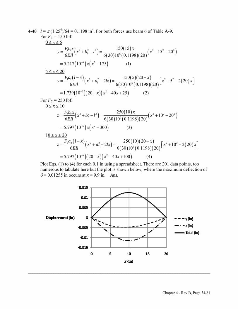
4-48 I = (1.254)/64 = 0.1198 in4. For both forces use beam 6 of Table A-9. For F1 = 150 lbf: 0 x 5
2 2 2 2 2 21 11 6
6 2
150 1515 20
6 6 30 10 0.1198 20
5.217 10 175 (1)
xFb xy x b l x
EIl
x x
5 x 20
1 1 2 2 2 21 6
6 2
150 5 202 5 2 20
6 6 30 10 0.1198 20
1.739 10 20 40 25 (2)
F a l x xx a lx x x
EIl
x x x
y
For F2 = 250 lbf: 0 x 10
2 2 2 2 2 22 22 6
6 2
250 1010 20
6 6 30 10 0.1198 20
5.797 10 300 (3)
xF b xz x b l x
EIl
x x
10 x 20
2 2 2 2 2 22 6
6 2
250 10 202 10 2 20
6 6 30 10 0.1198 20
5.797 10 20 40 100 (4)
F a l x xz x a lx x x
EIl
x x x
Plot Eqs. (1) to (4) for each 0.1 in using a spreadsheet. There are 201 data points, too numerous to tabulate here but the plot is shown below, where the maximum deflection of = 0.01255 in occurs at x = 9.9 in. Ans.
______________________________________________________________________________
Chapter 4 - Rev B, Page 34/81
4-49 The larger slope will occur at the left end. From Table A-9, beam 8
2 2 2
2 2 2
( 3 6 2 )6
(3 3 6 2 )6
BAB
AB B
M xy x a al l
EIldy M
x a al ldx EIl
With I
= d 4/64, the slope at the left bearing is
2 2
40
(3 6 2 )6 / 64
AB BA
x
dy Ma al l
dx E d l
Solving for d
2 2 244
6
32 32(1000)3 6 2 3(4 ) 6(4)(10) 2 10
3 3 (30)10 (0.002)(10)
0.461 in .
B
A
Md a al l
E l
Ans
2
______________________________________________________________________________ 4-50 From Table A-5, E = 10.4 Mpsi MO = 0 = 18 FBC 6(100) FBC = 33.33 lbf The cross sectional area of rod BC is A = (0.52)/4 = 0.1963 in2. The deflection at point B will be equal to the elongation of the rod BC.
5
6
33.33(12)6.79 10 in .
0.1963 30 10B
BC
FLy Ans
AE
______________________________________________________________________________ 4-51 MO = 0 = 6 FAC 11(100) FAC = 183.3 lbf
The deflection at point A in the negative y direction is equal to the elongation of the rod AC. From Table A-5, Es = 30 Mpsi.
4
2 6
183.3 123.735 10 in
0.5 / 4 30 10A
AC
FLy
AE
By similar triangles the deflection at B due to the elongation of the rod AC is
411 3 3( 3.735)10 0.00112 in
6 18A B
B A
y yy y
From Table A-5, Ea = 10.4 Mpsi
The bar can then be treated as a simply supported beam with an overhang AB. From Table A-9, beam 10
Chapter 4 - Rev B, Page 35/81
2 22
2
2 22
6 3
( )( ) 7 ( ) (3 ) (
3 6 3
77 3( ) 3 ( ) (3 ) | ( ) (2 3 ) ( )
6 3 6
7 100 5
6(10.4)10 0.25(2 ) /
BCB
x l a x l a
x l a
dy Fa d F x l Fay BD l a x l a x l l
dx EI dx EI EI
F Fa Fax l a x l a x l l a l a l a
EI EI EI EI
)
3
a
Fa
2
6 3
100 52(6) 3(5) (6 5)
12 3(10.4)10 0.25(2 ) /12
0.01438 in
yB = yB1 + yB2 = 0.00112 0.01438 = 0.0155 in Ans. ______________________________________________________________________________ 4-52 From Table A-5, E = 207 GPa, and G = 79.3 GPa.
2 23 3
4 43
2
4 4 4
3 / 32 / 32 3 / 64
32 2
3
OC AB AC ABAB ABB AB AB
OC AC AB OC AC
OC ACAB AB
OC AC AB
Fl l Fl lFl FlTl Tly l l
GJ GJ EI G d G d E d
l lFl l
Gd Gd Ed
4
The spring rate is k = F/ yB. Thus
12
4 4 4
12
3 4 3 4 3 4
32 2
3
32 200 2 200200 200
79.3 10 18 79.3 10 12 3 207 10 8
8.10 N/mm .
OC ACAB AB
OC AC AB
l ll lk
Gd Gd Ed
Ans
_____________________________________________________________________________ 4-53 For the beam deflection, use beam 5 of Table A-9.
1 2
1 21 2
2 31 21
2 32 1
1 1 2
2
, and 2 2
(4 3 )48
1(4 3 ) .
2 2 48
AB
AB
FR R
F F
k k
Fxy x x l
l EI
k k xy F x x l
k k k l EI
Ans
Chapter 4 - Rev B, Page 36/81
For BC, since Table A-9 does not have an equation (because of symmetry) an equation
will need to be developed as the problem is no longer symmetric. This can be done easily using beam 6 of Table A-9 with a = l /2
222 1
1 1 2
2 22 1
1 1 2
/ 22
2 2 4
14 8 .
2 2 48
BC
F l l xFk FkF ly x x
k k k l EIl
l xk k
lx
F x x l lxk k k l EI
Ans
______________________________________________________________________________ 4-54
1 2
1 21 2
2 21 21
2 22 12
1 1 2
, and ( )
, and ( )
( )6
( ) .6
AB
AB
Fa FR R l a
l lFa F
l alk lk
Faxy x l x
l EIl
a x axy F k a k l a l x
k l k k l EIl
Ans
21 21
22 12
1 1 2
( )( ) (3 )
6
( )( ) (3 ) .
6
BC
BC
F x ly x x l a x l
l EI
a x x ly F k a k l a x l a x l An
k l k k l EIs
______________________________________________________________________________ 4-55 Let the load be at x ≥ l/2. The maximum deflection will be in Section AB (Table A-9, beam 6)
2 2 2
6AB
Fbxy x b l
EIl
2 2 2 2 2 23 0 36
ABdy Fbx b l x b l
dx EIl 0
2 2 2
max, 0.577 .3 3
l b lx x l
Ans
For x l/2, min 0.577 0.423 .x l l l A ns
______________________________________________________________________________
Chapter 4 - Rev B, Page 37/81
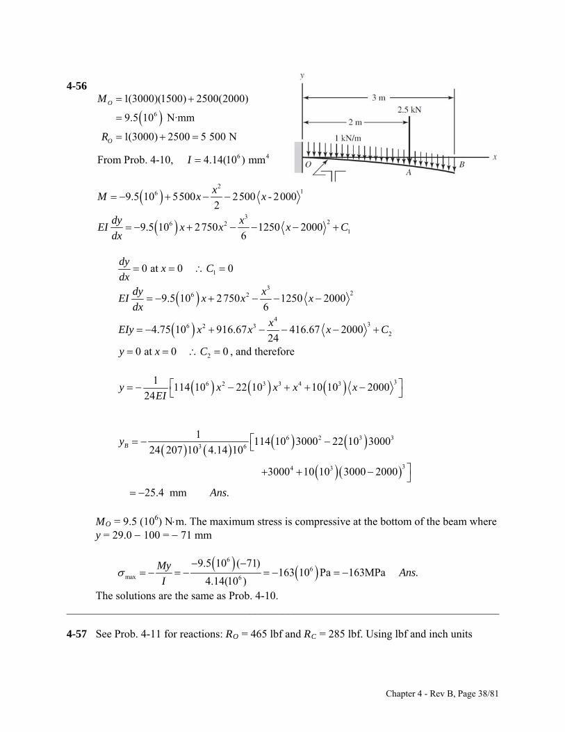
4-56
6
1(3000)(1500) 2500(2000)
9.5 10 N·mm
1(3000) 2500 5 500 N
O
O
M
R
6 4From Prob. 4-10, 4.14(10 ) mm I
2
169.5 10 5500 2500 - 20002
xM x x
3
26 219.5 10 2750 1250 2000
6
dy xEI x x x C
dx
10 at 0 0dy
x Cdx
326 2
436 2 3
2
9.5 10 2750 1250 20006
4.75 10 916.67 416.67 200024
dy xEI x x x
dx
xEIy x x x C
y , and therefore 20 at 0 0x C
36 2 3 3 4 31114 10 22 10 10 10 2000
24y x x x x
EI
6 2 3 33 6
34 3
1114 10 3000 22 10 3000
24 207 10 4.14 10
3000 10 10 3000 2000
25.4 mm .
By
Ans
MO = 9.5 (106) Nm. The maximum stress is compressive at the bottom of the beam where
y = 29.0 100 = 71 mm
6
6ma x 6
9.5 10 ( 71)163 10 Pa 163MPa .
4.14(10 )
MyAns
I
The solutions are the same as Prob. 4-10. ______________________________________________________________________________ 4-57 See Prob. 4-11 for reactions: RO = 465 lbf and RC = 285 lbf. Using lbf and inch units
Chapter 4 - Rev B, Page 38/81
M = 465 x 450 x 721 300 x 1201
2 22
1232.5 225 72 150 120dy
EI x x xdx
C
EIy = 77.5 x3 75 x 723 50 x 1203 C1x
y = 0 at x = 0 C2 = 0 y = 0 at x = 240 in 0 = 77.5(2403) 75(240 72)3 50(240 120)3 + C1 x C1 = 2.622(106) lbfin2
and, EIy = 77.5 x3 75 x 723 50 x 1203 2.622(106) x
Substituting y = 0.5 in at x = 120 in gives 30(106) I ( 0.5) = 77.5 (1203) 75(120 72)3 50(120 120)3 2.622(106)(120) I = 12.60 in4
Select two 5 in 6.7 lbf/ft channels; from Table A-7, I = 2(7.49) = 14.98 in4
midspan
12.60 10.421 in .
14.98 2y A
ns
The maximum moment occurs at x = 120 in where Mmax = 34.2(103) lbfin
3
max
34.2(10 )(2.5)5 710 psi
14.98
Mc
I O.K.
The solutions are the same as Prob. 4-17. ______________________________________________________________________________ 4-58 I = (1.54)/64 = 0.2485 in4, and w = 150/12 = 12.5 lbf/in.
1 2412.5 39 (340) 453.0 lbf
2 39OR
1212.5
453.0 340 152
M x x x
22 3
1
12.5226.5 170 15
6
dyEI x x x
dx C
33 4
1 275.5 0.5208 56.67 15EIy x x x C x C
20at 0 0y x C
Thus, 4 210 at 39 in 6.385(10 ) lbf iny x C
33 4 4175.5 0.5208 56.67 15 6.385 10y x x x x
EI
Evaluating at x = 15 in,
Chapter 4 - Rev B, Page 39/81
33 4 4
6
175.5 15 0.5208 15 56.67 15 15 6.385 10 (15)
30(10 )(0.2485)
0.0978 in .
Ay
Ans
33 4 4midspan 6
175.5 19.5 0.5208 19.5 56.67 19.5 15 6.385 10 (19.5)
30(10 )(0.2485)
0.1027 in .
y
Ans
5 % difference Ans. The solutions are the same as Prob. 4-12. ______________________________________________________________________________
4-59 I = 0.05 in4, 3 14 100 7 14 100
420 lbf and 980 lbf10 10A BR R
M = 420 x 50 x2 + 980 x 10 1
22 3
1210 16.667 490 10dy
EI x x xdx
C
33 4
1 270 4.167 163.3 10EIy x x x C x C
y = 0 at x = 0 C2 = 0 y = 0 at x = 10 in C1 = 2 833 lbfin2. Thus,
33 4
6
37 3 4
170 4.167 163.3 10 2833
30 10 0.05
6.667 10 70 4.167 163.3 10 2833 .
y x x x x
x x x x
Ans
The tabular results and plot are exactly the same as Prob. 4-21. ______________________________________________________________________________ 4-60 RA = RB = 400 N, and I = 6(323) /12 = 16 384 mm4. First half of beam, M = 400 x + 400 x 300 1
22
1200 200 300dy
EI x xdx
C
From symmetry, dy/dx = 0 at x = 550 mm 0 = 200(5502) + 200(550 – 300) 2 + C1 C1 = 48(106) N·mm2 EIy = 66.67 x3 + 66.67 x 300 3 + 48(106) x + C2
Chapter 4 - Rev B, Page 40/81
y = 0 at x = 300 mm C2 = 12.60(109) N·mm3. The term (EI)1 = [207(103)16 384] 1 = 2.949 (1010 ) Thus y = 2.949 (1010) [ 66.67 x3 + 66.67 x 300 3 + 48(106) x 12.60(109)] yO = 3.72 mm Ans. yx = 550 mm =2.949 (1010) [ 66.67 (5503) + 66.67 (550 300)3 + 48(106) 550 12.60(109)] = 1.11 mm Ans. The solutions are the same as Prob. 4-13. ______________________________________________________________________________ 4-61
1 1
2 2
10
10 ( )
B A A
A A A
M R l Fa M R M Fal
M M R l F l a R Fl Fa Ml
1
1 2AM R x M R x l
221 2 1
33 21 2
1 1
2 21 1 1
6 2 6
A
A
dyEI R x M x R x l C
dx
1 2EIy R x M x R x l C x C
y = 0 at x = 0 C2 = 0
y = 0 at x = l 21 1
1 1
6 2 AC R l M l . Thus,
33 2 2
1 2 1
1 1 1 1 1
6 2 6 6 2A AEIy R x M x R x l R l M l x
33 2 2 213 2
6 A A A Ay M Fa x M x l Fl Fa M x l Fal M l x Ans.EIl
In regions,
3 2 2 2
2 2 2 2
13 2
6
3 26
AB A A A
A
y M Fa x M x l Fal M l xEIlx
.M x lx l Fa l x AnsEIl
Chapter 4 - Rev B, Page 41/81
33 2 2 2
3 33 2 2 3 2
22
2
13 2
61
3 26
13
6
3 .6
BC A A A A
A
A
A
y M Fa x M x l Fl Fa M x l Fal M l xEIl
M x x l x l xl F ax l a x l axlEIl
M x l l Fl x l x l a x lEIlx l
M l F x l a x l AnsEI
The solutions reduce to the same as Prob. 4-17. ______________________________________________________________________________
4-62 1 1
10 2
2 2D
b aM R l b a l b b a R l b a
l
ww
2 2
1 2 2M R x x a x b
w w
3 32
1 1
1
2 6 6
dyEI R x x a x b
dx
w wC
4 43
1 1
1
6 24 24 2EIy R x x a x b C x C w w
y = 0 at x = 0 C2 = 0 y = 0 at x = l
4 431 1
1 1
6 24 24C R l l a l b
l
w w
4 43
4 43
4 43
4 42
1 12
6 2 24 24
1 12
6 2 24 24
2 224
2 2
b ay l b a x x a x b
EI l
b ax l b a l l a l
l l
b a l b a x l x a l x bEIl
.
b
x b a l b a l l a l b Ans
w w w
w w w
w
The above answer is sufficient. In regions,
Chapter 4 - Rev B, Page 42/81
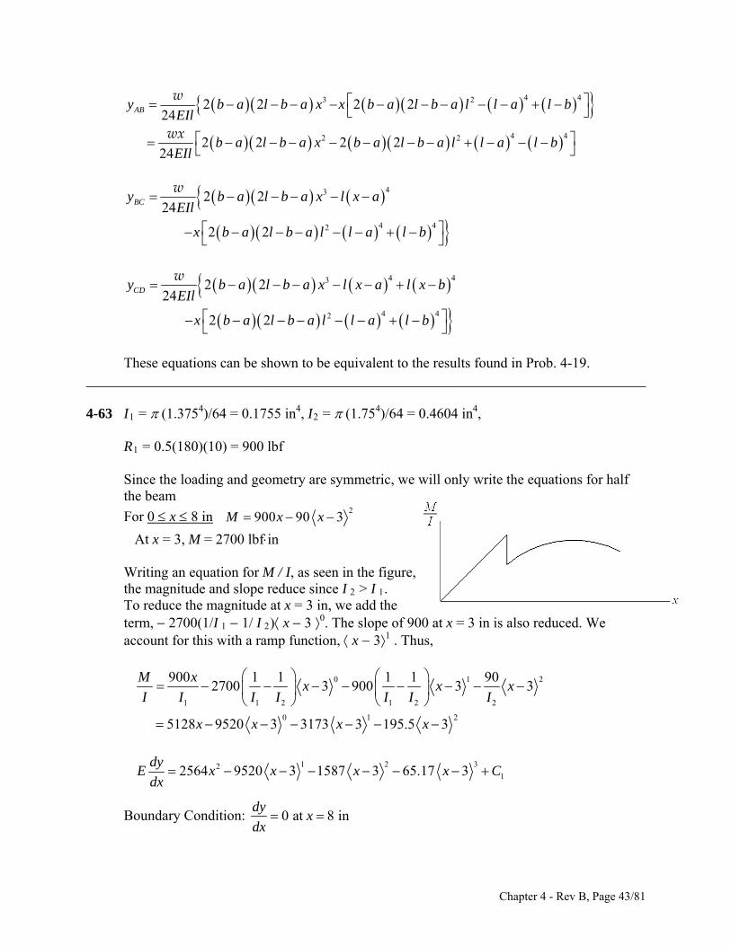
4 43 2
4 42 2
2 2 2 224
2 2 2 224
ABy b a l b a x x b a l b a l l a l bEIl
b a l b a x b a l b a l l a l bEIl
w
wx
43
4 42
2 224
2 2
BCy b a l b a x l x aEIl
x b a l b a l l a l b
w
4 43
4 42
2 224
2 2
CDy b a l b a x l x a l x bEIl
x b a l b a l l a l b
w
These equations can be shown to be equivalent to the results found in Prob. 4-19. ______________________________________________________________________________ 4-63 I1 = (1.3754)/64 = 0.1755 in4, I2 = (1.754)/64 = 0.4604 in4, R1 = 0.5(180)(10) = 900 lbf Since the loading and geometry are symmetric, we will only write the equations for half
the beam
For 0 x 8 in 2
900 90 3M x x
At x = 3, M = 2700 lbfin Writing an equation for M / I, as seen in the figure, the magnitude and slope reduce since I 2 > I 1. To reduce the magnitude at x = 3 in, we add the term, 2700(1/I 1 1/ I 2) x 3 0. The slope of 900 at x = 3 in is also reduced. We
account for this with a ramp function, x 31 . Thus,
0 1
1 1 2 1 2 2
0 1 2
900 1 1 1 1 902700 3 900 3 3
5128 9520 3 3173 3 195.5 3
M xx x
2x
I I I I I
x x x x
I I
1 22
12564 9520 3 1587 3 65.17 33dy
E x x x x Cdx
Boundary Condition: 0 at 8 indy
xdx
Chapter 4 - Rev B, Page 43/81
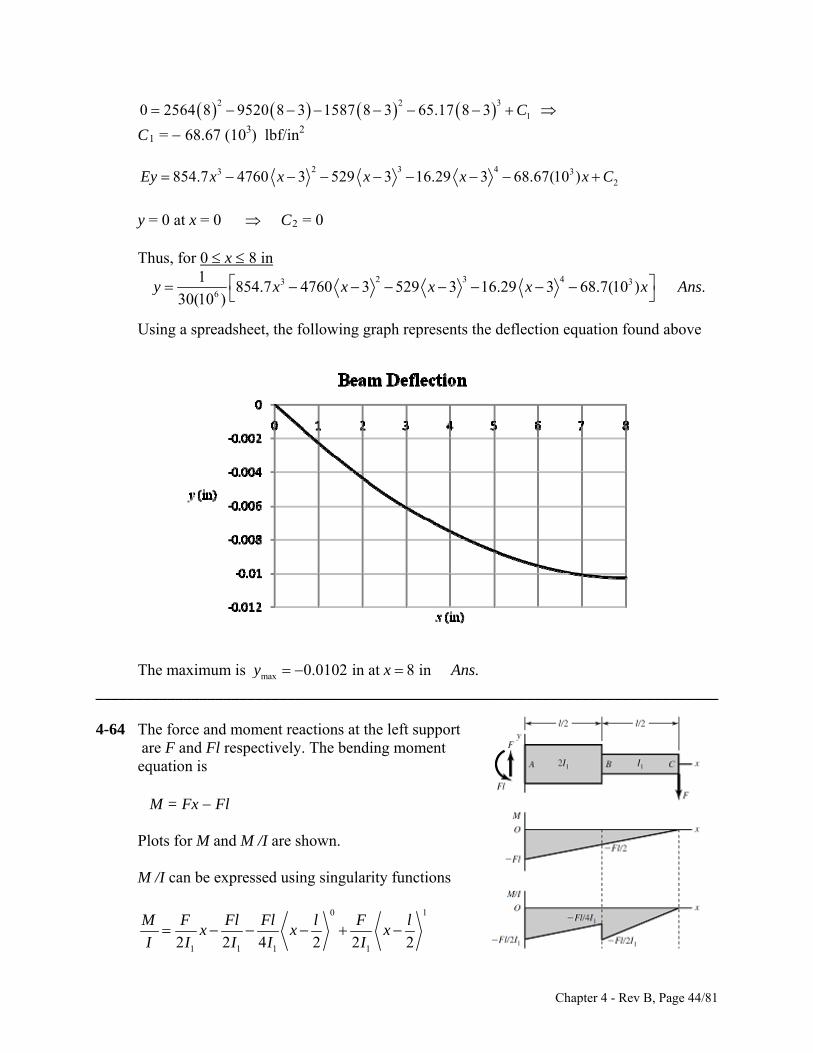
2 2
10 2564 8 9520 8 3 1587 8 3 65.17 8 3 C 3
C1 = 68.67 (103) lbf/in2
2 3 43 3
2854.7 4760 3 529 3 16.29 3 68.67(10 )Ey x x x x x C
y = 0 at x = 0 C2 = 0 Thus, for 0 x 8 in
2 3 43 3
6
1854.7 4760 3 529 3 16.29 3 68.7(10 ) .
30(10 )x x x x x Ans y
Using a spreadsheet, the following graph represents the deflection equation found above
The maximum is max 0.0102 in at 8 in .y x A ns
______________________________________________________________________________ 4-64 The force and moment reactions at the left support are F and Fl respectively. The bending moment equation is M = Fx Fl Plots for M and M /I are shown. M /I can be expressed using singularity functions
0 1
1 1 1 12 2 4 2 2 2
M F Fl Fl l F lx x x
I I I I I
Chapter 4 - Rev B, Page 44/81
where the step down and increase in slope at x = l /2 are given by the last two terms.
Integrate
1 2
21
1 1 1 14 2 4 2 4 2
dy F Fl Fl l F lE x x x x
dx I I I I C
dy/dx = 0 at x = 0 C1 = 0
2 3
3 22
1 1 1 112 4 8 2 12 2
F Fl Fl l F lEy x x x x C
I I I I
y = 0 at x = 0 C2 = 0
2 3
3 2
1
2 6 3 224 2 2
F ly x lx l x x
EI
l
3 2 3
/21 1
52 6 3 (0) 2(0) .
24 2 2 96x l
F l l Fly l l
EI EI
Ans
2 3 3
3 2
1 1
32 6 3 2
24 2 2 16x l
F l l Fly l l l l l x
EI EI
.Ans
The answers are identical to Ex. 4-10. ______________________________________________________________________________ 4-65 Place a dummy force, Q, at the center. The reaction, R1 = wl / 2 + Q / 2
2
2 2 2 2
Q x MM x
Q
wl w x
Integrating for half the beam and doubling the results
/2 /2 2
max
0 00
1 22
2 2 2
l l
Q
M xy M dx x
EI Q EI
wl w xdx
Note, after differentiating with respect to Q, it can be set to zero
/2/2 3 4
2max
0 0
5 .
2 2 3 4 384
ll x l xy x l x dx Ans
EI EI EI
w w w
______________________________________________________________________________ 4-66 Place a fictitious force Q pointing downwards at the end. Use the variable x originating at
the free end at positive to the left
2
2
x MM Qx x
Q
w
Chapter 4 - Rev B, Page 45/81
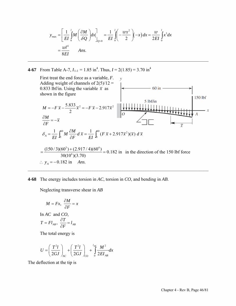
2
3max
0 00
4
1 1
2 2
.8
l l
Q
My M dx x dx x dx
EI Q EI EI
lAns
EI
wx w
w
0
l
______________________________________________________________________________ 4-67 From Table A-7, I1-1 = 1.85 in4. Thus, I = 2(1.85) = 3.70 in4
First treat the end force as a variable, F. Adding weight of channels of 2(5)/12 = 0.833 lbf/in. Using the variable x as shown in the figure
2 25.8332.917
2M F x x F x x
Mx
F
60 60 2
0 0
1 1( 2.917 )( ) A
MM d x F x x x d x
EI F EI
3 4
6
(150 / 3)(60 ) (2.917 / 4)(60 )0.182 in
30(10 )(3.70)
in the direction of the 150 lbf force
0.182 in .Ay Ans
______________________________________________________________________________ 4-68 The energy includes torsion in AC, torsion in CO, and bending in AB. Neglecting transverse shear in AB
, M
M Fx xF
In AC and CO,
, AB AB
TT Fl l
F
The total energy is
2 2 2
02 2 2
ABl
ABAC CO
T l T l MU d
GJ GJ EI
x
The deflection at the tip is
Chapter 4 - Rev B, Page 46/81
2
30 0
1AB ABl l
AC CO AC AB CO AB
AC CO AC CO AB
Tl Tl Tl l Tl lU T T M Mdx Fx dx
F GJ F GJ F EI F GJ GJ EI
2 23 3
4 4 4
2
4 4 4
3 / 32 / 32 3 / 64
32 2
3
AC AB CO AB AC AB CO ABAB AB
AC CO AB AC CO AB
AC COAB AB
AC CO AB
Tl l Tl l Fl l Fl lFl Fl
GJ GJ EI G d G d E d
l lFl l
Gd Gd Ed
1
2 4 4 4
1
2 3 4 3 4 3 4
2
32 3
2 200200 2008.10 N/mm .
32 200 79.3 10 18 79.3 10 12 3 207 10 8
AC CO AB
AB AC CO AB
l l lFk
l Gd Gd Ed
Ans
______________________________________________________________________________ 4-69 I1 = (1.3754)/64 = 0.1755 in4, I2 = (1.754)/64 = 0.4604 in4 Place a fictitious force Q pointing downwards at the midspan of the beam, x = 8 in
1
1 1(10)180 900 0.5
2 2R Q Q
For 0 x 3 in 900 0.5 0.5M
M Q x xQ
For 3 x 13 in 2900 0.5 90( 3) 0.5M
M Q x x xQ
By symmetry it is equivalent to use twice the integral from 0 to 8
8 3 822
1 20 0 30
3 833 4 3 2
1 20 3
3
3 3
6 61 2
1 12 900 900 90 3
300 1 1 9300 90( 2 )
4 2
120.2 108100 1 8100145.5 10 25.31 10
30 10 0.1755 30 10 0.4604
0.0102 in .
Q
M Mdx x dx x x x dx
EI Q EI EI
xx x x x
EI EI
EI EI
Ans
______________________________________________________________________________
Chapter 4 - Rev B, Page 47/81
4-70 I = (0.54)/64 = 3.068 (103) in4, J = 2 I = 6.136 (103) in4, A = (0.52)/4 = 0.1963 in2. Consider x to be in the direction of OA, y vertically upward, and z in the direction of AB. Resolve the force F into components in the x and y directions obtaining 0.6 F in the
horizontal direction and 0.8 F in the negative vertical direction. The 0.6 F force creates strain energy in the form of bending in AB and OA, and tension in OA. The 0.8 F force creates strain energy in the form of bending in AB and OA, and torsion in OA. Use the dummy variable x to originate at the end where the loads are applied on each segment,
0.6 F: AB 0.6 0.6M
M F x xF
OA 4.2 4.2M
M FF
0.6 0.6aa
FF F
F
0.8 F: AB 0.8 0.8M
M F x xF
OA 0.8 0.8M
M F x xF
5.6 5.6T
T FF
Once the derivatives are taken the value of F = 15 lbf can be substituted in. The deflection of B in the direction of F is*
6 3 6
27 12
6 3 6 30 0
72
6 3 60
1
0.6 15 15 5.6 15 150.6 5.6
0.1963 30 10 6.136 10 11.5 10
15 4.2150.6
30 10 3.068 10 30 10 3.068 10
15 150.8
30 10 3.068 10 30 10 3.06
a aB F
OAOA
F L FU TL T MM d x
F AE F JG F EI F
x d x d x
x d x
5
152
30
5 3
0.88 10
1.38 10 0.1000 6.71 10 0.0431 0.0119 0.1173
0.279 in .
x d x
Ans
Chapter 4 - Rev B, Page 48/81
*Note. This is not the actual deflection of point B. For this, dummy forces must be placed
B = 0.0831 i 0.2862 j 0.00770 k in
is
on B in the x, y, and z directions. Determine the energy due to each, take derivatives, and then substitute the values of Fx = 9 lbf, Fy = 12 lbf, and Fz = 0. This can be done separately and then use superposition. The actual deflections of B are
From this, the deflection of B in the direction of F 0.6 0.0831 0.8 0.2862 0.279 inB F
which agrees with our result. ____ ________________________________________________
-71 Strain energy. AB: Bending and torsion, BC: Bending and torsion, CD: Bending. 031 in4,
1) is in the form of =TL/(JG), where the equivalent of
Use the dummy variable
_ _________________________ 4 IAB = (14)/64 = 0.04909 in4, JAB = 2 IAB = 0.09818 in4, IBC = 0.25(1.53)/12 = 0.07
ICD = (0.754)/64 = 0.01553 in4. For the torsion of bar BC, Eq. (3-4J is Jeq = bc 3. With b/c = 1.5/0.25 = 6, JBC = bc 3 = 0.299(1.5)0.253 = 7.008 (103) in4.
x to originate at the end where the loads are applied on each
ing
segment,
AB: Bend 2 2M
M F x F xF
Torsion 5 5T
T FF
MM F x x
F
BC: Bending
Torsion 2 2T
T FF
CD: Bending M
M F x xF
62
6 3 6 60
5 22 2
6 60 0
4 4 4 5 6
1
5 6 2 5 15 2
0.09818 11.5 10 7.008 10 11.5 10 30 10 0.04909
1 1
30 10 0.07031 30 10 0.01553
1.329 10 2.482 10 1.141 10 1.98 10 5.72 10
5.207 10
D
U Tl T MM d x
F JG F EI FF F
2F x d
F x d x F x d x
F F F F F
4 45.207 10 200 0.104 in .F Ans
x
______________________________________________________________________________
Chapter 4 - Rev B, Page 49/81
4-72 AAB = (12)/4 = 0.7854 in2, IAB = (14)/64 = 0.04909 in4, IBC = 1.5 (0.253)/12 = 1.953 (103) in4, ACD = (0.752)/4 = 0.4418 in2, IAB = (0.754)/64 = 0.01553 in4. For (D )x let
F = Fx = 150 lbf and Fz = 100 lbf . Use the dummy variable x to originate at the end where the loads are applied on each segment,
CD: 0yy z
MM F x
F
1aa
FF F
F
BC: 2 yy z
MM F x F x
F
0aa z
FF F
F
AB: 5 2 yy z z
MM F F F x
F5
1aa
FF F
F
5
0
6
0
3 26 6 3
266
7
12
15 2 5
2 11 5 5
0.4418 30 10 330 10 1.953 10
6125 6 10 6 6 5 1
2 0.7854 30 1030 10 0.04909
1.509 10 7.112 1
aD zx
CD BC
az z
ABAB
z
zz
FU FLF x F x d x
F AE F EI
FFLF F F x d x
EI AE F
F FF
FFF F
F
4 4 4
4 7 4 4
0 4.267 10 1.019 10
1.019 10 2.546 10 8.135 10 5.286 10
z
z z
F F F
F F F
F
Substituting F = Fx = 150 lbf and Fz = 100 lbf gives 4 48.135 10 150 5.286 10 100 0.1749 in .D x
Ans
______________________________________________________________________________ 4-73 IOA = IBC = (1.54)/64 = 0.2485 in4, JOA = JBC = 2 IOA = 0.4970 in4, IAB = (14)/64 =
0.04909 in4, JAB = 2 IAB = 0.09818 in4, ICD = (0.754)/64 = 0.01553 in4 Let Fy = F, and use the dummy variable x to originate at the end where the loads are
applied on each segment,
Chapter 4 - Rev B, Page 50/81
OC: , 12 12M T
M F x x T FF F
DC: M
M F x xF
1D y
OC
U TL T MM d x
F JG F EI F
The terms involving the torsion and bending moments in OC must be split up because of the changing second-area moments.
22
6 6 60
11 13 122 2
6 6 62 11
4 3 7
4 5 3
12 4 12 9 112 12
0.4970 11.5 10 0.09818 11.5 10 30 10 0.2485
1 1 1
30 10 0.04909 30 10 0.2485 30 10 0.01553
1.008 10 1.148 10 3.58 10
2.994 10 3.872 10 1.2363 10
D y
F FF x d x
2
0
F x d x F x d x F x d x
F F F
F F F
3 32.824 10 2.824 10 250 0.706 in .F Ans
For the simplified shaft OC,
13 122 2
6 6 60 0
3 4 3 3 3
12 13 1 112
0.09818 11.5 10 30 10 0.04909 30 10 0.01553
1.6580 10 4.973 10 1.2363 10 3.392 10 3.392 10 250
0.848 in .
B y
FF x d x F x d x
F F F F
Ans
Simplified is 0.848/0.706 = 1.20 times greater Ans. ______________________________________________________________________________ 4-74 Place a dummy force Q pointing downwards at point B. The reaction at C is RC = Q + (6/18)100 = Q + 33.33 This is the axial force in member BC. Isolating the beam, we find that the moment is not a
function of Q, and thus does not contribute to the strain energy. Thus, only energy in the member BC needs to be considered. Let the axial force in BC be F, where
Chapter 4 - Rev B, Page 51/81
33.33 1F
F QQ
5
2 60 0
0 33.33 121 6.79 10 in
0.5 / 4 30 10B
BCQ Q
U FL FAns
Q AE Q
.
______________________________________________________________________________ 4-75 IOB = 0.25(23)/12 = 0.1667 in4 AAC = (0.52)/4 = 0.1963 in2 MO = 0 = 6 RC 11(100) 18 Q RC = 3Q + 183.3 MA = 0 = 6 RO 5(100) 12 Q RO = 2Q + 83.33 Bending in OB. BD: Bending in BD is only due to Q which when set to zero after differentiation
gives no contribution. AD: Using the variable x as shown in the figure above
100 7 7M
M x Q x xQ
OA: Using the variable x as shown in the figure above
2 83.33 2M
M Q xQ
x
Axial in AC:
3 183.3 3F
F QQ
Chapter 4 - Rev B, Page 52/81
0 0 0
56 2
6 00
563 2
6 00
3 7
1
183.3 12 13 100 7 2 83.33
0.1963 30 10
11.121 10 100 7 166.7
10.4 10 0.1667
1.121 10 5.768 10 100 129.2 166.
B
Q Q Q
U FL F MM dx
Q AE Q EI Q
x x d x x dxEI
x x d x x dx
7 72 0.0155 in .Ans
______________________________________________________________________________ 4-76 There is no bending in AB. Using the variable, rotating counterclockwise from B
sin sinM
M PR RP
cos cosrr
FF P
P
2
sin sin
2 sin
FF P
PMF
PRP
2 1 1
2 26(4) 24 mm , 40 (6) 43 mm, 40 (6) 37 mm,o iA r r
From Table 3-4, p.121, for a rectangular cross section
6
39.92489 mmln(43 / 37)nr
From Eq. (4-33), the eccentricity is e = R rn =40 39.92489 = 0.07511 mm From Table A-5, E = 207(103) MPa, G = 79.3(103) MPa From Table 4-1, C = 1.2 From Eq. (4-38)
2 2 2 2
0 0 0 0
1 r rMFF R F CF R FM M
d d dAeE P AE P AE P AG P
d
2 2 2 2
2 2 2
0 0 0 0
sin sin cos2 sinP R PR CPRPRd d d
AeE AE AE AG
2
d
3
3 3
(10)(40) 40 (207 10 )(1.2)1 2 1 2
4 4(24)(207 10 ) 0.07511 79.3 10
PR R EC
AE e G
0.0338 mm .Ans ______________________________________________________________________________
Chapter 4 - Rev B, Page 53/81
4-77 Place a dummy force Q pointing downwards at point A. Bending in AB is only due to Q which when set to zero after differentiation gives no contribution. For section BC use the variable, rotating counterclockwise from B
sin sin 1 sinM
M PR Q R R RQ
cos cosrr
FF P Q
Q
sin sinF
F P QQ
sin 1 sin sinMF PR QR P Q
2sin sin 1 sin 2 sin 1 sinMF
PR PR QRQ
But after differentiation, we can set Q = 0. Thus,
sin 1 2sinMF
PRQ
2 1 1
2 26(4) 24 mm , 40 (6) 43 mm, 40 (6) 37 mm,o iA r r
From Table 3-4, p.121, for a rectangular cross section
6
39.92489 mmln(43 / 37)nr
From Eq. (4-33), the eccentricity is e = R rn =40 39.92489 = 0.07511 mm From Table A-5, E = 207(103) MPa, G = 79.3(103) MPa From Table 4-1, C = 1.2 From Eq. (4-38)
2 2 2 2
2 2 2
2
0 0 0 0
22
0 0 0
2
0
2
1
sin 1 sin sin sin 1 2sin
cos
1 24 4 4
r rMFF R F CF R FM M
d d dAeE Q AE Q AE Q AG Q
PR PR PRd d d
AeE AE AECPR
dAG
PR PR PR
AeE AE
d
3
3 3
1 24 4 4
10 40 1.2 207 10401 2
24 207 10 4 0.07511 4 79.3 10
0.0766 mm .
CPR PR R CE
AE AG AE e G
Ans
______________________________________________________________________________
Chapter 4 - Rev B, Page 54/81
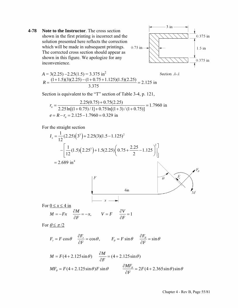
4-78 Note to the Instructor. The cross section shown in the first printing is incorrect and the solution presented here reflects the correction which will be made in subsequent printings. The corrected cross section should appear as shown in this figure. We apologize for any inconvenience.
A = 3(2.25) 2.25(1.5) = 3.375 in2
(1 1.5)(3)(2.25) (1 0.75 1.125)(1.5)(2.25)
2.125 in3.375
R
Section is equivalent to the “T” section of Table 3-4, p. 121,
2.25(0.75) 0.75(2.25)
1.7960 in2.25ln[(1 0.75) /1] 0.75ln[(1 3) / (1 0.75)]nr
2.125 1.7960 0.329 inne R r
For the straight section
3 2
23
4
1(2.25) 3 2.25(3)(1.5 1.125)
12
1 2.25(1.5) 2.25 1.5(2.25) 0.75 1.125
12 2
2.689 in
zI
For 0 x 4 in
, 1M V
x x V FM FF F
For /2
cos cos , sin sinrrF
FFF F F
F F
(4 2.125sin ) (4 2.125sin )
(4 2.125sin ) sin 2 (4 2.365sin )sin
MM F
FMF
MF F F FF
Chapter 4 - Rev B, Page 55/81
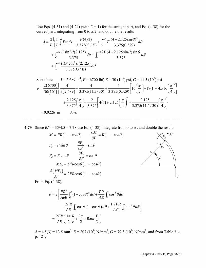
Use Eqs. (4-31) and (4-24) (with C = 1) for the straight part, and Eq. (4-38) for the curved part, integrating from 0 to π/2, and double the results
24 /22
0 0
2/2 /2
0 0
2/2
0
2 1 (4)(1) (4 2.125sin )
3.375( / ) 3.375(0.329)
sin (2.125) 2 (4 2.125sin )sin
3.375 3.375
(1) cos (2.125)
3.375( / )
FFx dx F d
E I G E
F Fd d
Fd
G E
Substitute I = 2.689 in4, F = 6700 lbf, E = 30 (106) psi, G = 11.5 (106) psi
3
6
2 6700 4 4 116 17(1) 4.516
3 2.689 3.375(11.5 / 30) 3.375(0.329) 2 430 10
2.125 2 2.1254 1 2.125
3.375 4 3.375 4 3.375 11.5 / 30 4
0.0226 in .Ans
______________________________________________________________________________ 4-79 Since R/h = 35/4.5 = 7.78 use Eq. (4-38), integrate from 0 to , and double the results
1 cos 1 cosM
M FR RF
sin sinrr
FF F
F
cos cosF
F FF
2 cos 1 cos
2 cos 1 cos
MF F R
MFFR
F
From Eq. (4-38),
22 2
0 0
2
0 0
2 (1 cos ) cos
2 1.2cos 1 cos sin
2 3 30.6
2 2
FR FRd d
AeE AE
FR FRd d
AE AG
FR R E
AE e G
A = 4.5(3) = 13.5 mm2, E = 207 (103) N/mm2, G = 79.3 (103) N/mm2, and from Table 3-4,
p. 121,
Chapter 4 - Rev B, Page 56/81
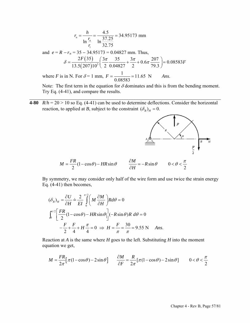
4.5
34.95173 mm37.25
lnln32.75
no
i
hr
r
r
and e = R rn = 35 34.95173 = 0.04827 mm. Thus,
3
2 35 3 35 3 2070.6 0.08583
13.5 207 10 2 0.04827 2 79.3
FF
where F is in N. For = 1 mm, 1
11.65 N .0.08583
F Ans
Note: The first term in the equation for dominates and this is from the bending moment. Try Eq. (4-41), and compare the results.
______________________________________________________________________________ 4-80 R/h = 20 > 10 so Eq. (4-41) can be used to determine deflections. Consider the horizontal
reaction, to applied at B, subject to the constraint ( ) 0.B H
(1 cos ) sin sin 02 2
FR MM HR R
H
By symmetry, we may consider only half of the wire form and use twice the strain energy Eq. (4-41) then becomes,
/2
0
2( ) 0B H
U MM Rd
H EI H
/2
0
(1 cos ) sin ( sin ) 02
FRHR R R d
30
0 9.55 N .2 4 4
F F FH H Ans
Reaction at A is the same where H goes to the left. Substituting H into the moment equation we get,
(1 cos ) 2sin [ (1 cos ) 2sin ] 02 2
FR M R
2M
F
Chapter 4 - Rev B, Page 57/81
2/2 2
20
3 /2 2 2 2 2 22 0
32 2 2
2
2 3
2 2[ (1 cos ) 2sin ]
4
( cos 4sin 2 cos 4 sin 4 sin cos ) 2
4 2 4 22 2 4 4
(3 8 4)
8
P
U M FRM Rd R d
P EI F EI
FRd
EI
FR
EI
FR
EI
2 3
3 4
(3 8 4) (30)(40 )0.224 mm .
8 207 10 2 / 64Ans
______________________________________________________________________________ 4-81 The radius is sufficiently large compared to the wire diameter to use Eq. (4-41) for the
curved beam portion. The shear and axial components will be negligible compared to bending.
Place a fictitious force Q pointing to the left at point A.
sin ( sin ) sinM
M PR Q R l R lQ
Note that the strain energy in the straight portion is zero since there is no real force in that section.
From Eq. (4-41),
/2 /2
0 00
2 2 2/2 2
6 40
1 1sin sin
1(5 )sin sin (5) 4
4 430 10 0.125 / 64
0.551 in .
Q
MM Rd PR R l Rd
EI Q EI
PR PRR l d R l
EI EI
Ans
______________________________________________________________________________ 4-82 Both the radius and the length are sufficiently large to use Eq. (4-41) for the curved beam
portion and to neglect transverse shear stress for the straight portion.
Straight portion: ABAB
MM Px x
P
Curved portion: (1 cos ) (1 cos )BCBC
MM P R l R l
P
From Eq. (4-41) with the addition of the bending strain energy in the straight portion of the wire,
Chapter 4 - Rev B, Page 58/81
/2
0 0
/2 22
0 0
3 /2 2 2 2
0
3 /2 2 2 2 2
0
3
1 1
(1 cos )
(1 2cos cos ) 2 (1 cos )3
cos 2 2 cos ( )3
3
lBCAB
AB BC
l
MMM dx M Rd
EI P EI P
P PRx dx R l d
EI EI
Pl PRR Rl l d
EI EI
Pl PRR R Rl R l d
EI EI
Pl P
EI
2 2 2
33 2 2
323 2
6 4
2 2 ( )4 2
2 2 ( )3 4 2
1 4(5 ) 5 2(5 ) 2(5)(4) 5 5 4
3 4 230 10 0.125 / 64
0.850 in .
RR R Rl R l
EI
P lR R R Rl R R l
EI
Ans
______________________________________________________________________________ 4-83 Both the radius and the length are sufficiently large to use Eq. (4-41) for the curved beam
portion and to neglect transverse shear stress for the straight portion. Place a dummy force, Q, at A vertically downward. The only load in the straight section is
the axial force, Q. Since this will be zero, there is no contribution. In the curved section
sin 1 cos 1 cosM
M PR QR RQ
From Eq. (4-41)
/2 /2
0 00
3 3/2
0
3
6 4
1 1sin 1 cos
1sin sin cos 1
2 2
1 50.174 in .
2 30 10 0.125 / 64
Q
M
3
M Rd PR R RdEI Q EI
PR PR PRd
EI EI EI
Ans
______________________________________________________________________________ 4-84 Both the radius and the length are sufficiently large to use Eq. (4-41) for the curved beam
portion and to neglect transverse shear stress for the straight portion.
Chapter 4 - Rev B, Page 59/81
Place a dummy force, Q, at A vertically downward. The load in the straight section is the
axial force, Q, whereas the bending moment is only a function of P and is not a function of Q. When setting Q = 0, there is no axial or bending contribution.
In the curved section
1 cos sin sinM
M P R l QR RQ
From Eq. (4-41)
/2 /2
0 00
/22 2
0
2
6 4
1 11 cos sin
1sin sin cos sin 2
2 2
1 55 2 4 0.452 in
2 30 10 0.125 / 64
Q
MM Rd P R l R Rd
EI Q EI
PR PR PR2
R R l d R l R REI EI EI
l
Since the deflection is negative, is in the opposite direction of Q. Thus the deflection is 0.452 in .Ans ______________________________________________________________________________ 4-85 Consider the force of the mass to be F, where F = 9.81(1) = 9.81 N. The load in AB is
tension
1ABAB
FF F
F
For the curved section, the radius is sufficiently large to use Eq. (4-41). There is no
bending in section DE. For section BCD, let be counterclockwise originating at D
sin sin 0M
M FR RF
Using Eqs. (4-29) and (4-41)
32
0 0
33 3
3 2 4
11 sin
409.81 80
2 2 207 10 2 / 4 2 2 / 64
6.067 mm .
AB
AB
FFl M Fl FRM Rd d
AE F EI F AE EI
Fl FR F l R
AE EI E A I
Ans
______________________________________________________________________________
Chapter 4 - Rev B, Page 60/81
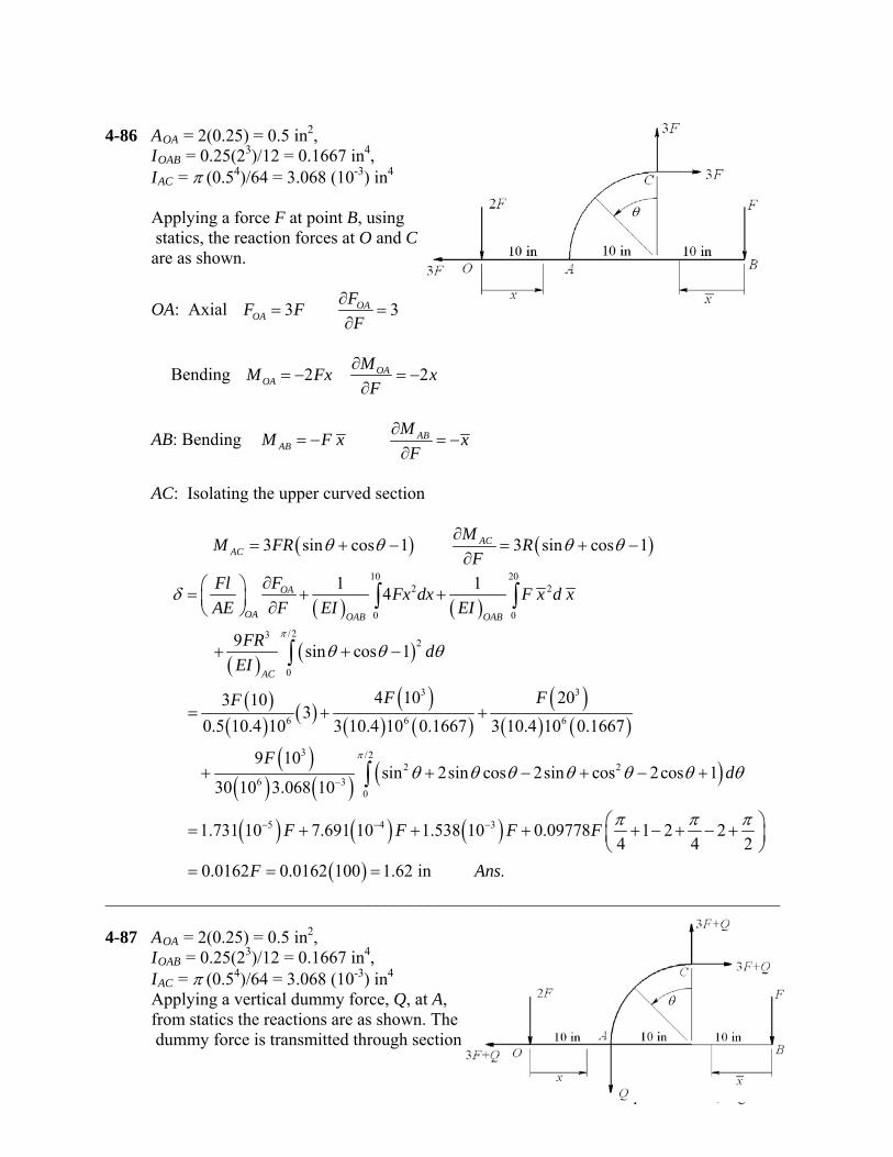
4-86 AOA = 2(0.25) = 0.5 in2, IOAB = 0.25(23)/12 = 0.1667 in4, IAC = (0.54)/64 = 3.068 (10-3) in4 Applying a force F at point B, using statics, the reaction forces at O and C are as shown.
OA: Axial 3 3OAOA
FF F
F
Bending 2 2OAOA
MM Fx x
F
AB: Bending ABAB
MM F x x
F
AC: Isolating the upper curved section
3 sin cos 1 3 sin cos 1ACAC
MM FR R
F
10 202 2
0 0
/232
0
3 3
6 6 6
3 /22 2
6 30
1 14
9sin cos 1
4 10 203 103
0.5 10.4 10 3 10.4 10 0.1667 3 10.4 10 0.1667
9 10sin 2sin cos 2sin cos 2cos 1
30 10 3.068 10
1
OA
OA OAB OAB
AC
FFlFx dx F x d x
AE F EI EI
FRd
EI
F FF
Fd
5 4 3.731 10 7.691 10 1.538 10 0.09778 1 2 24 4
0.0162 0.0162 100 1.62 in .
F F F F
F Ans
2
_____________________________________________________________________________ 4-87 AOA = 2(0.25) = 0.5 in2, IOAB = 0.25(23)/12 = 0.1667 in4, IAC = (0.54)/64 = 3.068 (10-3) in4 Applying a vertical dummy force, Q, at A, from statics the reactions are as shown. The dummy force is transmitted through section
Chapter 4 - Rev B, Page 61/81
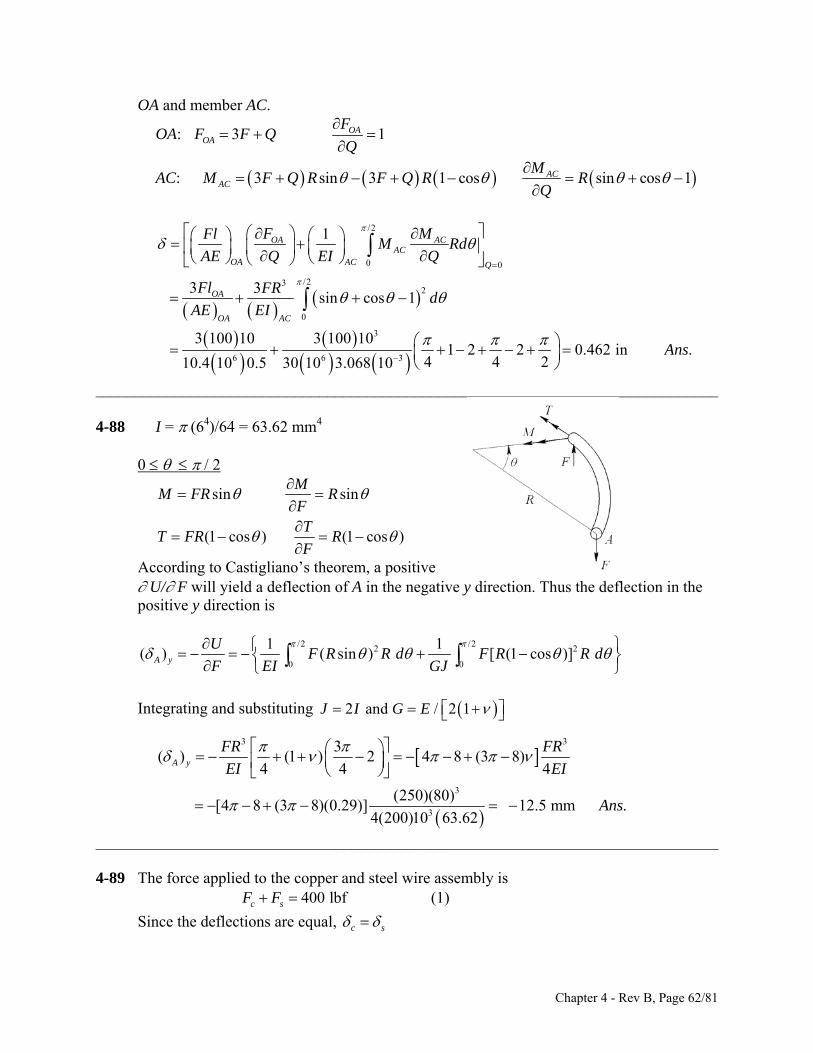
OA and member AC.
OA: 3 1OAOA
FF F Q
Q
AC: 3 sin 3 1 cos sin cos 1ACAC
MM F Q R F Q R R
Q
/2
0 0
/232
0
3
6 6 3
1
3 3sin cos 1
3 100 10 3 100 101 2 2 0.462 in .
4 4 210.4 10 0.5 30 10 3.068 10
OA ACAC
OA AC Q
OA
OA AC
F MFlM Rd
AE Q EI Q
Fl FRd
AE EI
Ans
______________________________________________________________________________ 4-88 I = (64)/64 = 63.62 mm4 0 / 2
sin sin
(1 cos ) (1 cos )
MM FR R
FT
T FR RF
According to Castigliano’s theorem, a positive U/ F will yield a deflection of A in the negative y direction. Thus the deflection in the
positive y direction is
/2 /22 2
0 0
1 1( ) ( sin ) [ (1 cos )]A y
U F R R d F R R d
F EI GJ
Integrating and substituting 2 and / 2 1J I G E
3 3
3
3
3( ) (1 ) 2 4 8 (3 8)
4 4 4
(250)(80)[4 8 (3 8)(0.29)] 12.5 mm .
4(200)10 63.62
A y
FR FR
EI EI
Ans
______________________________________________________________________________ 4-89 The force applied to the copper and steel wire assembly is (1) 400 lbfc sF F Since the deflections are equal, c s
Chapter 4 - Rev B, Page 62/81
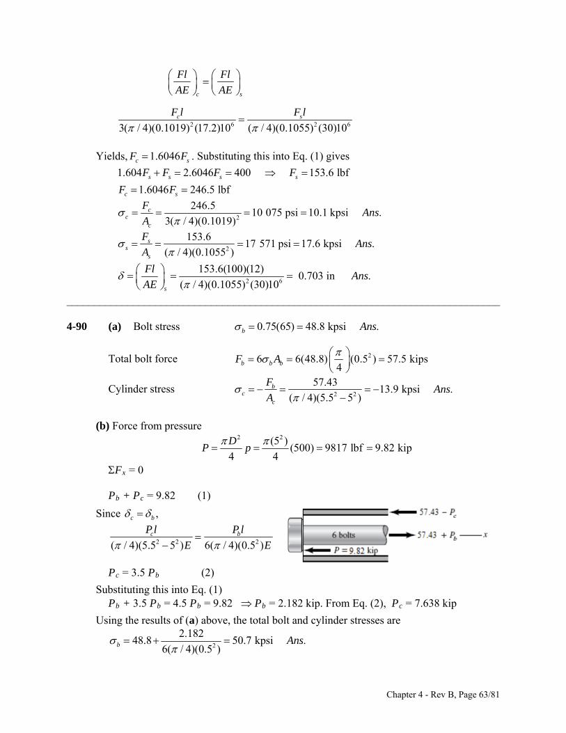
c s
Fl Fl
AE AE
2 6 23( / 4)(0.1019) (17.2)10 ( / 4)(0.1055) (30)10
c sF l F l
6
sF
Yields, . Substituting this into Eq. (1) gives 1.6046cF
1.604 2.6046 400 153.6 lbf
1.6046 246.5 lbfs s s s
c s
F F F F
F F
2
246.510 075 psi 10.1 kpsi .
3( / 4)(0.1019)c
cc
FAns
A
2
153.617 571 psi 17.6 kpsi .
( / 4)(0.1055 )s
ss
FAns
A
2 6
153.6(100)(12)0.703 in .
( / 4)(0.1055) (30)10s
FlAns
AE
______________________________________________________________________________ 4-90 (a) Bolt stress 0.75(65) 48.8 kpsi .b Ans
Total bolt force 26 6(48.8) (0.5 ) 57.5 kips4b b bF A
Cylinder stress 2 2
57.4313.9 kpsi .
( / 4)(5.5 5 )b
cc
FAns
A
(b) Force from pressure
2 2(5 )
(500) 9817 lbf 9.82 kip4 4
DP p
Fx = 0 Pb + Pc = 9.82 (1)
Since ,c b
2 2 2( / 4)(5.5 5 ) 6( / 4)(0.5 )
c bP l P l
E E
Pc = 3.5 Pb (2)
Substituting this into Eq. (1) Pb + 3.5 Pb = 4.5 Pb = 9.82 Pb = 2.182 kip. From Eq. (2), Pc = 7.638 kip
Using the results of (a) above, the total bolt and cylinder stresses are
2
2.18248.8 50.7 kpsi .
6( / 4)(0.5 )b Ans
Chapter 4 - Rev B, Page 63/81
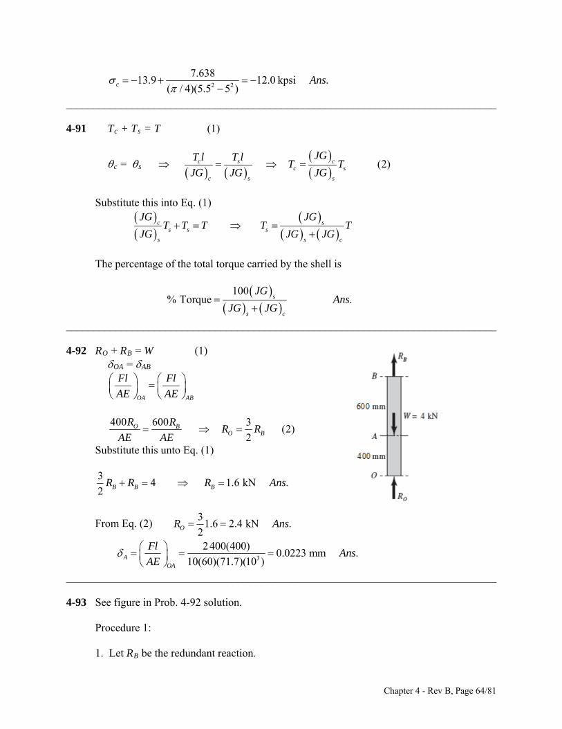
2 2
7.63813.9 12.0 kpsi .
( / 4)(5.5 5 )c Ans
______________________________________________________________________________ 4-91 Tc + Ts = T (1)
c = s
(2)c s cc s
c s s
JGT l T lT T
JG JG JG
Substitute this into Eq. (1)
c ss s s
s s
JG JGT T T T T
JG JG JG
c
The percentage of the total torque carried by the shell is
100
% Torque .s
s c
JGAns
JG JG
______________________________________________________________________________ 4-92 RO + RB = W (1) OA = AB
OA AB
Fl Fl
AE AE
400 600 3
(2)2
O BO B
R RR R
AE AE
Substitute this unto Eq. (1)
3
4 1.6 kN .2 B B BR R R Ans
From Eq. (2) 3
1.6 2.4 kN .2OR Ans
3
2400(400)0.0223 mm .
10(60)(71.7)(10 )A OA
FlAns
AE
______________________________________________________________________________ 4-93 See figure in Prob. 4-92 solution. Procedure 1: 1. Let RB be the redundant reaction.
Chapter 4 - Rev B, Page 64/81
2. Statics. RO + RB = 4 000 N RO = 4 000 RB (1)
3. Deflection of point B. 600 4000 400
0 (2B BB
R R
AE AE
)
4. From Eq. (2), AE cancels and RB = 1 600 N Ans. and from Eq. (1), RO = 4 000 1 600 = 2 400 N Ans.
3
2400(400)0.0223 mm .
10(60)(71.7)(10 )AOA
FlAns
AE
______________________________________________________________________________ 4-94 (a) Without the right-hand wall the deflection of point C would be
3 3
2 6 2 6
5 10 8 2 10 5
/ 4 0.75 10.4 10 / 4 0.5 10.4 10
0.01360 in 0.005 in Hits wall .
C
Fl
AE
Ans
(b) Let RC be the reaction of the wall at C acting to the left (). Thus, the deflection of
point C is now
3 3
2 6 2
6 2 2
5 10 8 2 10 5
/ 4 0.75 10.4 10 / 4 0.5 10.4 10
4 8 50.01360 0.005
10.4 10 0.75 0.5
C C
C
C
R R
R
6
or, 60.01360 4.190 10 0.005 2053 lbf 2.05 kip .C CR R A ns
Statics. Considering +, 5 000 RA 2 053 = 0 RA = 2 947 lbf = 2.95 kip Ans. Deflection. AB is 2 947 lbf in tension. Thus
32 6
8 2947 85.13 10 in .
/ 4 0.75 10.4 10A
B ABAB
RAns
A E
______________________________________________________________________________ 4-95 Since OA = AB,
(4) (6) 3
(1)2
OA ABOA AB
T TT T
JG JG
Chapter 4 - Rev B, Page 65/81
Statics. TOA + TAB = 200 (2) Substitute Eq. (1) into Eq. (2),
3 5200 80 lbf in .
2 2AB AB AB ABT T T T An s
From Eq. (1) 3 3
80 120 lbf in .2 2OA ABT T An s
0
4 6
80 6 1800.390 .
/ 32 0.5 11.5 10A Ans
max 3 3
16 120164890 psi 4.89 kpsi .
0.5OA
TAns
d
3
16 803260 psi 3.26 kpsi .
0.5AB Ans
______________________________________________________________________________ 4-96 Since OA = AB,
4 4
(4) (6)0.2963 (1)
/ 32 0.5 / 32 0.75OA AB
OA AB
T TT T
G G
Statics. TOA + TAB = 200 (2) Substitute Eq. (1) into Eq. (2),
0.2963 1.2963 200 154.3 lbf in .AB AB AB ABT T T T An s
From Eq. (1) 0.2963 0.2963 154.3 45.7 lbf in .OA ABT T Ans
0
4 6
154.3 6 1800.148 .
/ 32 0.75 11.5 10A Ans
max 3 3
16 45.7161862 psi 1.86 kpsi .
0.5OA
TAns
d
3
16 154.31862 psi 1.86 kpsi .
0.75AB Ans
______________________________________________________________________________
Chapter 4 - Rev B, Page 66/81
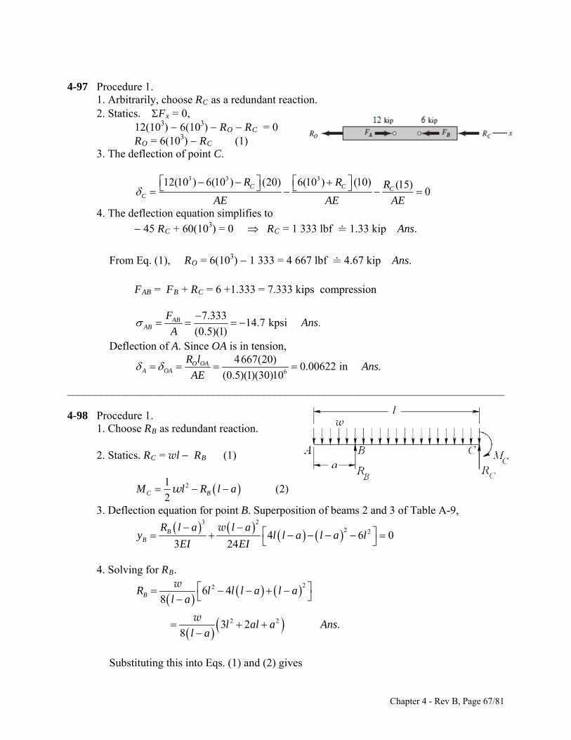
4-97 Procedure 1. 1. Arbitrarily, choose RC as a redundant reaction. 2. Statics. Fx = 0, 12(103) 6(103) RO RC = 0 RO = 6(103) RC (1) 3. The deflection of point C.
3 3 312(10 ) 6(10 ) (20) 6(10 ) (10) (15)
0C C C
C
R R R
AE AE AE
4. The deflection equation simplifies to 45 RC + 60(103) = 0 RC = 1 333 lbf 1.33 kip Ans.
From Eq. (1), RO = 6(103) 1 333 = 4 667 lbf 4.67 kip Ans.
FAB = FB + RC = 6 +1.333 = 7.333 kips compression
7.333
14.7 kpsi .(0.5)(1)
ABAB
FAns
A
Deflection of A. Since OA is in tension,
6
4667(20)0.00622 in .
(0.5)(1)(30)10O OA
A OA
R lAns
AE
______________________________________________________________________________ 4-98 Procedure 1. 1. Choose RB as redundant reaction. 2. Statics. RC = wl RB (1)
21(2)
2C BM l R l a w
3. Deflection equation for point B. Superposition of beams 2 and 3 of Table A-9,
3 22 24 6
3 24B
B
R l a l a0l l a l a l
EI EI
w
y
4. Solving for RB.
22
2 2
6 48
3 28
BR l l l a l al a
l al a Anl a
w
w.s
Substituting this into Eqs. (1) and (2) gives
Chapter 4 - Rev B, Page 67/81
2 25 10
8C B .R l R l al a Ansl a
w
w
2 2 212 .
2 8C BM l R l a l al a Ans w
w
______________________________________________________________________________ 4-99 See figure in Prob. 4-98 solution. Procedure 1. 1. Choose RB as redundant reaction. 2. Statics. RC = wl RB (1)
21(2)
2C BM l R l a w
3. Deflection equation for point B. Let the variable x start at point A and to the right. Using singularity functions, the bending moment as a function of x is
1 121
2 BB
MM x R x a x a
R
w
0
2 2
0
1
1 1 1 10 0
2 2
l
BB B
l l
B
a
U My M dx
R EI R
x dx x R x a x a dxEI EI
w w
or,
3 34 4 3 31 10
2 4 3 3BRa
l a l a l a a a w
Solving for RB gives
4 4 3 3 2 23 3 4 3 2
88B .R l a a l a l al a Ans
l al a
w w
From Eqs. (1) and (2)
2 25 10
8C B .R l R l al a Ansl a
w
w
2 2 212 .
2 8C BM l R l a l al a Ans w
w
Chapter 4 - Rev B, Page 68/81
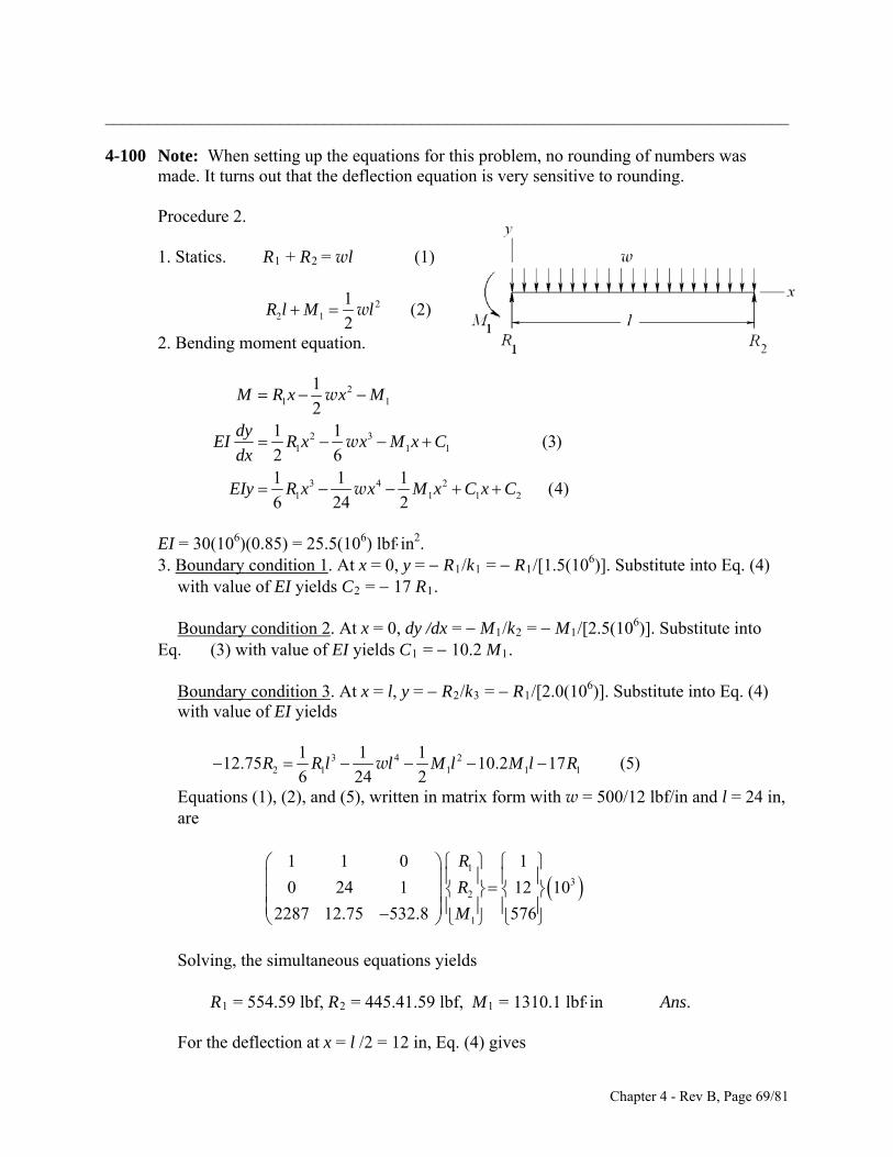
______________________________________________________________________________ 4-100 Note: When setting up the equations for this problem, no rounding of numbers was
made. It turns out that the deflection equation is very sensitive to rounding. Procedure 2. 1. Statics. R1 + R2 = wl (1)
22 1
1(2)
2R l M l w
2. Bending moment equation.
21 1
2 31 1 1
3 4 21 1 1
1
21 1
(3)2 61 1 1
(4)6 24 2
M R x x M
dy
2
R x x M x Cdx
EIy R x x M x C x C
w
w
w
EI
EI = 30(106)(0.85) = 25.5(106) lbfin2. 3. Boundary condition 1. At x = 0, y = R1/k1 = R1/[1.5(106)]. Substitute into Eq. (4)
with value of EI yields C2 = 17 R1. Boundary condition 2. At x = 0, dy /dx = M1/k2 = M1/[2.5(106)]. Substitute into
Eq. (3) with value of EI yields C1 = 10.2 M1. Boundary condition 3. At x = l, y = R2/k3 = R1/[2.0(106)]. Substitute into Eq. (4)
with value of EI yields
3 4 22 1 1 1 1
1 1 112.75 10.2 17 (5)
6 24 2R R l l M l M l R w
For the deflection at x = l /2 = 12 in, Eq. (4) gives
Equations (1), (2), and (5), written in matrix form with w = 500/12 lbf/in and l = 24 in, are
1
32
1
1 1 0 1
0 24 1 12 10
2287 12.75 532.8 576
R
R
M
Solving, the simultaneous equations yields R1 = 554.59 lbf, R2 = 445.41.59 lbf, M1 = 1310.1 lbfin Ans.
Chapter 4 - Rev B, Page 69/81
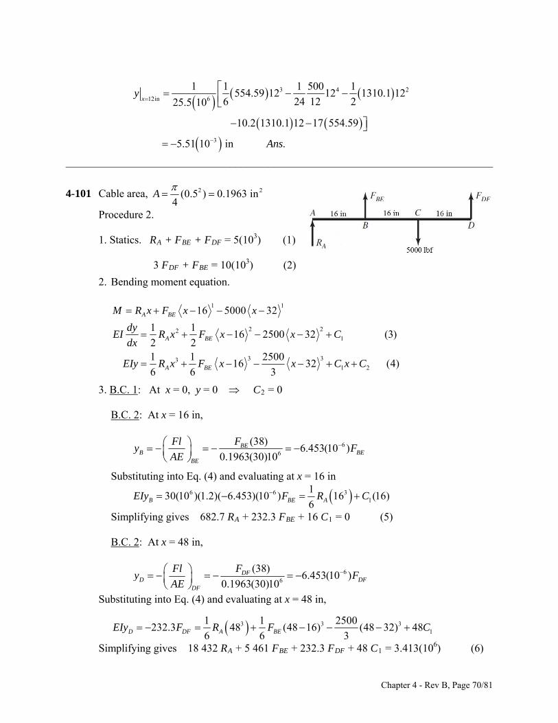
3 4
12in 6
3
1 1 1 500 1554.59 12 12 1310.1 12
6 24 12 225.5 10
10.2 1310.1 12 17 554.59
5.51 10 in .
xy
Ans
2
______________________________________________________________________________
-101 Cable area,
4 2 2(0.5 ) 0.1963 in4
A
Procedure 2.
1. Statics. RA + FBE + FDF = 5(103) (1)
3 FDF + FBE = 10(10 ) (2)
.
3
2 Bending moment equation.
1 1
16 5000 32A BEM R x F x x
2 221
3 331 2
1 116 2500 32 (3)
2 21 1 2500
16 32 (4)6 6 3
A BE
A BE
dyEI R x F x x C
dx
EIy R x F x x C x C
B.C. 1 3. : At x = 0, y = 0 C2 = 0
B.C. 2 : At x = 16 in,
66
(38)6.453(10 )
0.1963(30)10BE
B BEBE
FFly F
AE
Substituting into Eq. (4) and evaluating at x = 16 in
6 6 130(10 )(1.2)( 6.453)(10 ) 16EIy F R 3
1(16)6B BE A C
lifying gives 682.7 RA + 232.3 FBE + 16 C1 = 0 (5)
B.C. 2
Simp : At x = 48 in,
66
(38)6.453(10 )
0.1963(30)10DF
D DFDF
FFly F
AE
Substituting into Eq. (4) and evaluating at x = 48 in,
3 31
32500232.3 48 (48 16) (48 32) 48
6 6 3F A BE
1 1 E D DIy F R F C
plifying gives 18 432 RA + 5 461 FBE + 232.3 FDF + 48 C1 = 3.413(10 ) (6) Sim 6
Chapter 4 - Rev B, Page 70/81
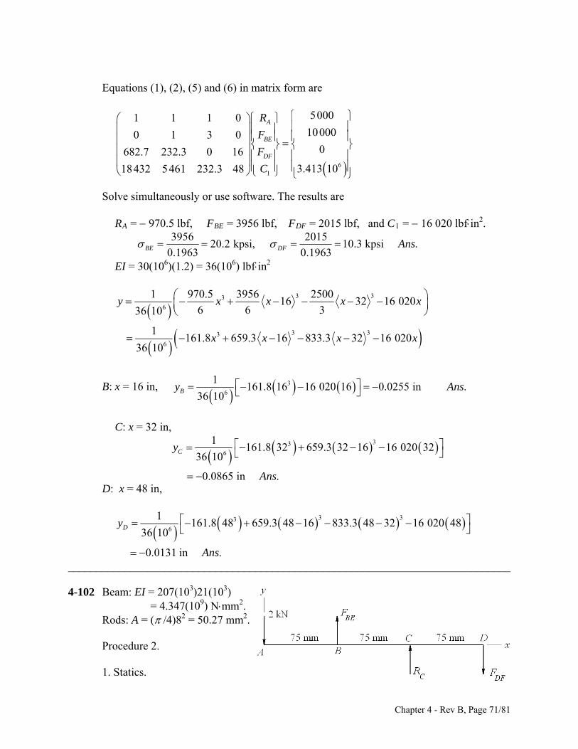
Equations (1), (2), (5) and (6) in matrix form are
61
50001 1 1 0100000 1 3 0
0682.7 232.3 0 16
3.413 1018432 5461 232.3 48
A
BE
DF
R
F
F
C
Solve simultaneously or use software. The results are
RA = 970.5 lbf, FBE = 3956 lbf, FDF = 2015 lbf, and C1 = 16 020 lbfin2.
3956 2015
20.2 kpsi, 10.3 kpsi .0.1963 0.1963BE DF Ans
EI = 30(106)(1.2) = 36(106) lbfin2
3 33
6
3 33
6
1 970.5 3956 250016 32 16 020
6 6 336 10
1161.8 659.3 16 833.3 32 16 020
36 10
y x x x x
x x x
x
B: x = 16 in,
3
6
1161.8 16 16 020 16 0.0255 in .
36 10By A ns
C: x = 32 in,
33
6
1161.8 32 659.3 32 16 16 020 32
36 10
0.0865 in .
C y
Ans
D: x = 48 in,
3 33
6
1161.8 48 659.3 48 16 833.3 48 32 16 020 48
36 10
0.0131 in .
D
Ans
______________________________________________________________________________
-102 Beam: EI = 207(10 )21(10 ) 2.
A
Procedure 2.
1. Statics.
y
3 34
= 4.347(109) Nmm Rods: = ( /4)82 = 50.27 mm2.
Chapter 4 - Rev B, Page 71/81
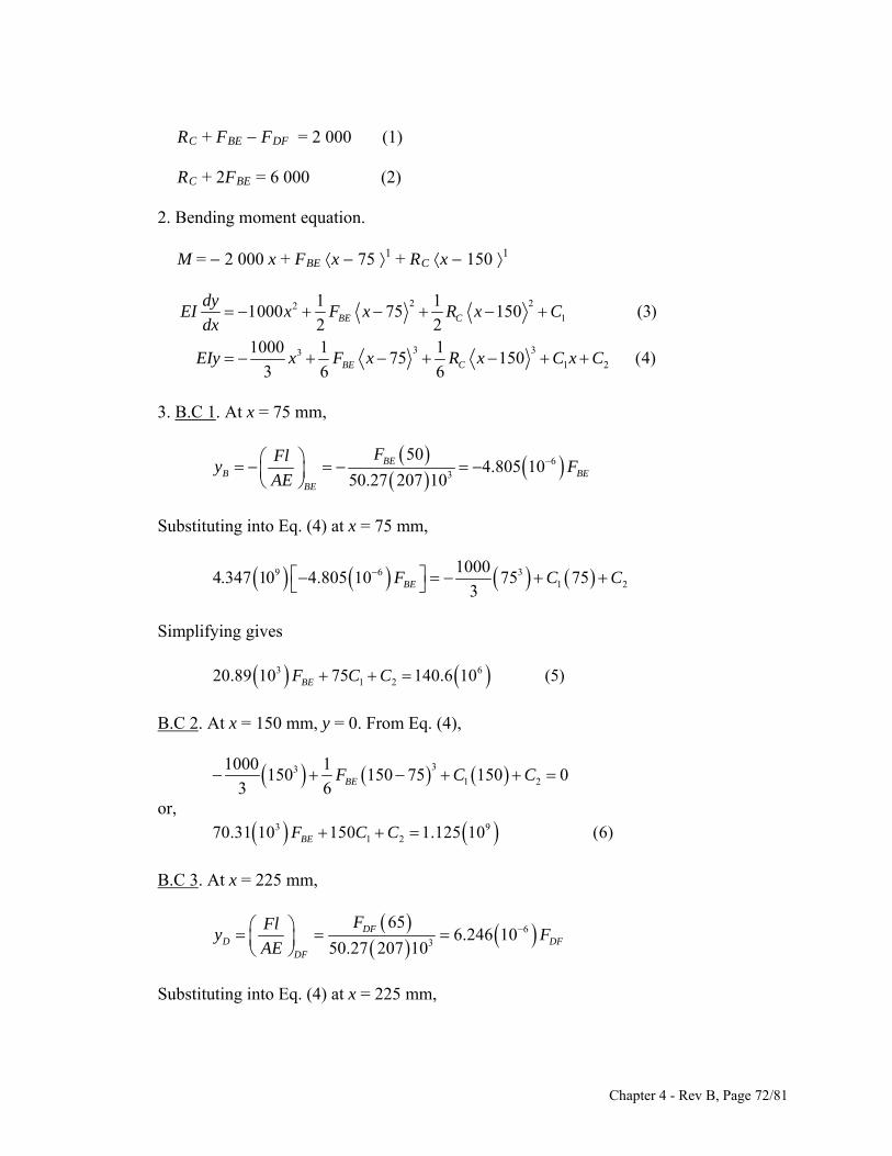
RC + FBE FDF = 2 000 (1)
RC + 2FBE = 6 000 (2)
2. Bending moment equation.
M = 2 000 x + FBE x 75 1 + RC x 150 1
2 221
3 331 2
1 11000 75 150 (3)
2 21000 1 1
75 150 (4)3 6 6
BE C
BE C
dyEI x F x R x C
dx
EIy x F x R x C x C
3. B.C 1 . At x = 75 mm,
63
504.805 10
50.27 207 10BE
B BEBE
FFly F
AE
Substituting into Eq. (4) at x = 75 mm,
9 6 31 2
10004.347 10 4.805 10 75 75
3BEF C C
Simplifying gives
3 6
1 220.89 10 75 140.6 10 (5)BEF C C
B.C 2. At x = 150 mm, y = 0. From Eq. (4),
331 2
1000 1150 150 75 150 0
3 6 BEF C C
or,
3 91 231 10 150 1.125 10 (6)BEF C C 70.
B.C 3. At x = 225 mm,
63
656.246 10
50.27 207 10DF
D DFDF
FFly F
AE
Substituting into Eq. (4) at x = 225 mm,
Chapter 4 - Rev B, Page 72/81
39 6 3
3
1 2
1000 14.347 10 6.246 10 225 225 75
3 61
225 150 2256
DF BE
C
F F
R C C
Simplifying gives 3 3 3 9
1 270.31 10 562.5 10 27.15 10 225 3.797 10 (7)C BE DFR F F C C
Equations (1), (2), (5), (6), and (7) in matrix form are
3
3
36
391
3 3 3 2 9
2 101 1 1 0 0
1 2 0 0 0 6 10
0 20.89 10 0 75 1 140.6 10
0 70.31 10 0 150 1 1.125 10
70.31 10 562.5 10 27.15 10 225 1 3.797 10
C
BE
DF
R
F
F
C
C
Solve simultaneously or use software. The results are RC = 2378 N, FBE = 4189 N, FDF = 189.2 N Ans. and C1 = 1.036 (107) Nmm2, C2 = 7.243 (108) Nmm3. The bolt stresses are BE = 4189/50.27 = 83.3 MPa, DF = 189/50.27= 3.8 MPa Ans. The deflections are
From Eq. (4) 8
9
17.243 10 0.167 mm .
4.347 10Ay A ns
For points B and D use the axial deflection equations*.
3
4189 500.0201 mm .
50.27 207 10BBE
Fly A
AE
ns
33
189 651.18 10 mm .
50.27 207 10DDF
Fly A
AE
ns
*Note. The terms in Eq. (4) are quite large, and due to rounding are not very accurate for calculating the very small deflections, especially for point D.
______________________________________________________________________________ 4-103 (a) The cross section at A does not rotate. Thus, for a single quadrant we have
Chapter 4 - Rev B, Page 73/81
0A
U
M
The bending moment at an angle to the x axis is
1 cos 12A
A
FR MM M
M
The rotation at A is
/2
0
10A
A A
U MM Rd
M EI M
Thus, /2
0
11 cos 1 0 0
2 2A A
FR FR FRM Rd M
EI
2 2
or,
2
12A
FRM
Substituting this into the equation for M gives
2
cos2
FRM
(1)
The maximum occurs at B where = /2
max .B
FRM M Ans
(b) Assume B is supported on a knife edge. The deflection of point D is U/ F. We will deal with the quarter-ring segment and multiply the results by 4. From Eq. (1)
2
cos2
M R
F
Thus,
2/2 /23 3
0 0
32
4 2cos
4
8 .4
D
U M FR FRM Rd d
F EI F EI EI
FRAns
EI
2
______________________________________________________________________________ 4-104
2
cr 2
44 4 41 where
64 64
C EIP
l
D dI D d K K
D
2 4
4cr 2
164
C E DP K
l
Chapter 4 - Rev B, Page 74/81
1/42
cr3 4
64.
1
P lD A
CE K
ns
______________________________________________________________________________
4-105 2 2 4 4 4 2 21 , 1 1 14 64 64
A D K I D K D K K , where K = d / D.
The radius of gyration, k, is given by
2
2 2116
I Dk K
A
From Eq. (4-46)
2 2 2 2
cr2 22 2 2 2 24/ 4 1 4 /16 1
y yy y
S l S lPS S
k CED K D K C
E
2 2 2 2
2 2cr 2 2 2
4 14 1
1
y
y
S l D KP D K S
D K C
E
2 2 2
2 2cr 2
4 11 4
1
y
y
S l KD K S P
K CE
1/22 2 2
cr2 2 2
1/22
cr2 2 2
4 14
1 1 1
2 .1 1
y
y y
y
y
S l KPD
S K K CE K S
S lPAns
S K CE K
______________________________________________________________________________
4-106 (a) 2 2
0.90, (0.75)(800) (0.5) 0 1373 N
0.9 0.5A BOM F
BOF
Using nd = 4, design for Fcr = nd FBO = 4(1373) = 5492 N
2 20.9 0.5 1.03 m, 165 MPayl S
In-plane:
1/21/2 3 /12
0.2887 0.2887(0.025) 0.007 218 m, 1.0I bh
k hA bh
C
1.03
142.70.007218
l
k
1/22 9
61
2 (207)(10 )157.4
165(10 )
l
k
Chapter 4 - Rev B, Page 75/81
Since use Johnson formula. 1( / ) ( / )l k l k Try 25 mm x 12 mm,
26
6cr 9
165 10 10.025(0.012) 165 10 (142.7) 29.1 kN
2 1(207)10P
This is significantly greater than the design load of 5492 N found earlier. Check out-of-plane.
Out-of-plane: 0.2887(0.012) 0.003 464 in, 1.2k C
1.03
297.30.003 464
l
k
Since use Euler equation. 1( / ) ( / )l k l k
2 9
cr 2
1.2 207 100.025(0.012) 8321 N
297.3P
This is greater than the design load of 5492 N found earlier. It is also significantly less than the in-plane Pcr found earlier, so the out-of-plane condition will dominate. Iterate the process to find the minimum h that gives Pcr greater than the design load.
With h = 0.010, Pcr = 4815 N (too small) h = 0.011, Pcr = 6409 N (acceptable) Use 25 mm x 11 mm. If standard size is preferred, use 25 mm x 12 mm. Ans.
(b) 6137310.4 10 Pa 10.4 MPa
0.012(0.011)b
P
dh
No, bearing stress is not significant. Ans. ______________________________________________________________________________ 4-107 This is an open-ended design problem with no one distinct solution. ______________________________________________________________________________ 4-108 F = 1500( /4)22 = 4712 lbf. From Table A-20, Sy = 37.5 kpsi Pcr = nd F = 2.5(4712) = 11 780 lbf (a) Assume Euler with C = 1
1/41/4 22 24 cr cr
2 3 3 6
64 11790 50641.193 in
64 1 30 10
P l P lI d d
C E CE
Use d = 1.25 in. The radius of gyration, k = ( I / A)1/2 = d /4 = 0.3125 in
Chapter 4 - Rev B, Page 76/81
1/21/2 2 62
31
2 6 4
cr 2
50160
0.3125
2 (1)30 102126 use Euler
37.5 10
30 10 / 64 1.2514194 lbf
50
y
l
k
l CE
k S
P
Since 14 194 lbf > 11 780 lbf, d = 1.25 in is satisfactory. Ans.
(b)
1/42
3 6
64 11780 160.675 in,
1 30 10d
so use d = 0.750 in
k = 0.750/4 = 0.1875 in
16
85.33 use Johnson0.1875
l
k
23
2 3cr 6
37.5 10 10.750 37.5 10 85.33 12748 lbf
4 2 1 30 10P
Use d = 0.75 in. (c)
( )
( )
141943.01 .
4712
127482.71 .
4712
a
b
n A
n A
ns
ns
______________________________________________________________________________ 4-109 From Table A-20, Sy = 180 MPa 4F sin = 2 943
735.8
sinF
In range of operation, F is maximum when = 15
max o
735.82843 N per bar
sin15F
Pcr = ndFmax = 3.50 (2 843) = 9 951 N l = 350 mm, h = 30 mm
Chapter 4 - Rev B, Page 77/81
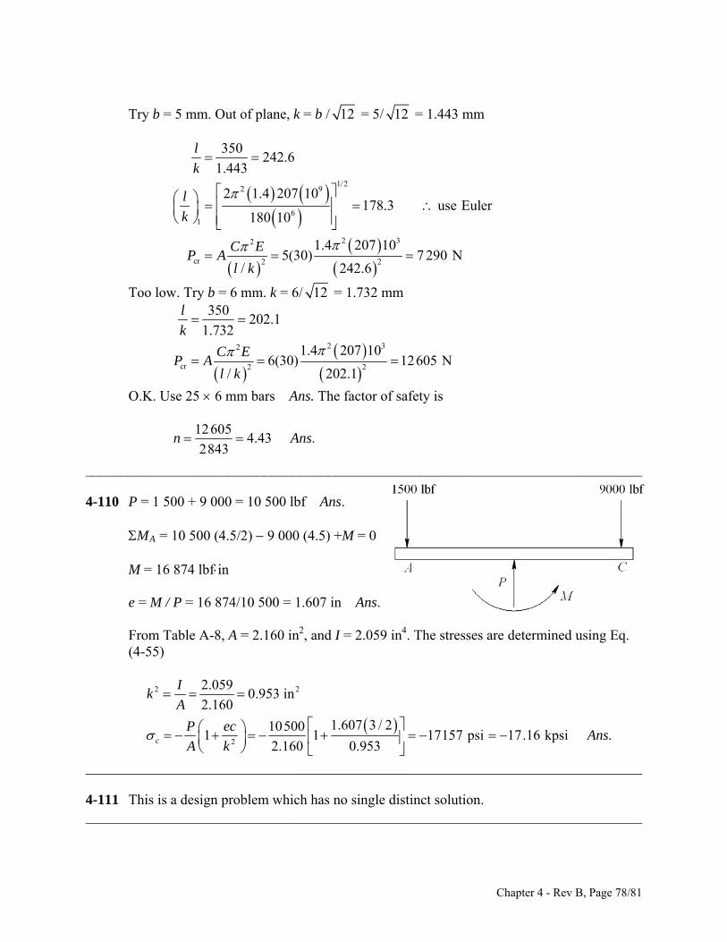
Try b = 5 mm. Out of plane, k = b / 12 = 5/ 12 = 1.443 mm
1/22 9
61
2 32
cr 2 2
350242.6
1.443
2 1.4 207 10178.3 use Euler
180 10
1.4 207 105(30) 7 290 N
/ 242.6
l
k
l
k
C EP A
l k
Too low. Try b = 6 mm. k = 6/ 12 = 1.732 mm
2 32
cr 2 2
350202.1
1.732
1.4 207 106(30) 12605 N
/ 202.1
l
k
C EP A
l k
O.K. Use 25 6 mm bars Ans. The factor of safety is
12605
4.43 .2843
n A ns
______________________________________________________________________________ 4-110 P = 1 500 + 9 000 = 10 500 lbf Ans. MA = 10 500 (4.5/2) 9 000 (4.5) +M = 0 M = 16 874 lbfin e = M / P = 16 874/10 500 = 1.607 in Ans. From Table A-8, A = 2.160 in2, and I = 2.059 in4. The stresses are determined using Eq.
(4-55)
2 2
2
2.0590.953 in
2.160
1.607 3 / 2105001 1 17157 psi 17.16 kpsi .
2.160 0.953c
Ik
A
P ecAns
A k
______________________________________________________________________________ 4-111 This is a design problem which has no single distinct solution. ______________________________________________________________________________
Chapter 4 - Rev B, Page 78/81
4-112 Loss of potential energy of weight = W (h + )
Increase in potential energy of spring = 21
2k
W (h + ) = 21
2k
or, 2 2 20
W Wh
k k . W = 30 lbf, k = 100 lbf/in, h = 2 in yields
2 0.6 1.2 = 0 Taking the positive root (see discussion on p. 192)
2max
10.6 ( 0.6) 4(1.2) 1.436 in .
2Ans
Fmax = k max = 100 (1.436) = 143.6 lbf Ans. ______________________________________________________________________________
4-113 The drop of weight W1 converts potential energy, W1 h, to kinetic energy 211
1
2
W
gv .
Equating these provides the velocity of W1 at impact with W2.
211 1 1
12
2
WW h gh
g v v (1)
Since the collision is inelastic, momentum is conserved. That is, (m1 + m2) v2 = m1 v1, where v2 is the velocity of W1 + W2 after impact. Thus
1 2 1 1 12 1 2 1
1 2 1 2
2W W W W W
ghg g W W W W
v v v v (2)
The kinetic and potential energies of W1 + W2 are then converted to potential energy of
the spring. Thus,
2 21 22 1 2
1 1
2 2
W WW W k
g
v
Substituting in Eq. (1) and rearranging results in
2
2 1 2 1
1 2
2 2W W W h
k W W k
0 (3)
Solving for the positive root (see discussion on p. 192)
2 2
1 2 1 2 1
1 2
12 4 8
2
W W W W W h
k k W
W k (4)
Chapter 4 - Rev B, Page 79/81
W1 = 40 N, W2 = 400 N, h = 200 mm, k = 32 kN/m = 32 N/mm.
2 21 40 400 40 400 40 200
2 4 8 29.06 mm .2 32 32 40 400 32
Ans
Fmax = k = 32(29.06) = 930 N Ans. ______________________________________________________________________________
4-114 The initial potential energy of the k1 spring is Vi = 21
1
2k a . The movement of the weight
W the distance y gives a final potential of Vf = 2 21
1
2 2k a y k y 2
1. Equating the two
energies give
22 21 1
1 1 1
2 2 2k a k a y k y 2
Simplifying gives 2
1 2 12 0k k y ak y
This has two roots, y = 0, 1
1 2
2k a
k k. Without damping the weight will vibrate between
these two limits. The maximum displacement is thus y max = 1
1 2
2k a
k k Ans.
With W = 5 lbf, k1 = 10 lbf/in, k2 = 20 lbf/in, and a = 0.25 in
max
2 0.25 100.1667 in .
10 20y Ans
______________________________________________________________________________
Chapter 4 - Rev B, Page 80/81
Chapter 6 6-1 Eq. (2-21): 3.4 3.4(300) 1020 MPaut BS H Eq. (6-8): 0.5 0.5(1020) 510 MPae utS S Table 6-2: 1.58, 0.085a b Eq. (6-19): 0.0851.58(1020) 0.877b
a utk aS
Eq. (6-20): 0.107 0.1071.24 1.24(10) 0.969bk d Eq. (6-18): (0.877)(0.969)(510) 433 MPa .e a b eS k k S Ans ______________________________________________________________________________ 6-2 (a) Table A-20: Sut = 80 kpsi
Eq. (6-8): 0.5(80) 40 kpsi .eS A ns
ns
ns
(b) Table A-20: Sut = 90 kpsi
Eq. (6-8): 0.5(90) 45 kpsi .eS A
(c) Aluminum has no endurance limit. Ans.
(d) Eq. (6-8): Sut > 200 kpsi, 100 kpsi .eS A
______________________________________________________________________________ 6-3 rev120 kpsi, 70 kpsiutS
Fig. 6-18: 0.82f
Eq. (6-8): 0.5(120) 60 kpsi e eS S
Eq. (6-14): 22 0.82(120)( )
161.4 kpsi60
ut
e
f Sa
S
Eq. (6-15): 1 1 0.82(120)
log log 0.07163 3 60
ut
e
f Sb
S
Eq. (6-16):
11/
0.0716rev 70
116 700 cycles .161.4
b
N Aa
ns
______________________________________________________________________________ 6-4 rev1600 MPa, 900 MPautS
Fig. 6-18: Sut = 1600 MPa = 232 kpsi. Off the graph, so estimate f = 0.77.
Eq. (6-8): Sut > 1400 MPa, so Se = 700 MPa
Eq. (6-14): 22 0.77(1600)( )
2168.3 MPa700
ut
e
f Sa
S
Chapter 6 - Rev. A, Page 1/66
Eq. (6-15): 1 1 0.77(1600)
log log 0.0818383 3 700
ut
e
f Sb
S
Eq. (6-16):
11/
0.081838rev 900
46 400 cycles .2168.3
b
N Aa
ns
______________________________________________________________________________
6-5 230 kpsi, 150 000 cyclesutS N
Fig. 6-18, point is off the graph, so estimate: f = 0.77
Eq. (6-8): Sut > 200 kpsi, so 100 kpsie eS S
Eq. (6-14): 22 0.77(230)( )
313.6 kpsi100
ut
e
f Sa
S
Eq. (6-15): 1 1 0.77(230)
log log 0.082743 3 100
ut
e
f Sb
S
Eq. (6-13): 0.08274313.6(150 000) 117.0 kpsi .bfS aN Ans
______________________________________________________________________________
6-6 = 160 kpsi 1100 MPautS
Fig. 6-18: f = 0.79
Eq. (6-8): 0.5(1100) 550 MPa e eS S
Eq. (6-14): 22 0.79(1100)( )
1373 MPa550
ut
e
f Sa
S
Eq. (6-15): 1 1 0.79(1100)
log log 0.066223 3 550
ut
e
f Sb
S
Eq. (6-13): 0.066221373(150 000) 624 MPa .bfS aN Ans
______________________________________________________________________________ 6-7
150 kpsi, 135 kpsi, 500 cyclesut ytS S N
Fig. 6-18: f = 0.798
From Fig. 6-10, we note that below 103 cycles on the S-N diagram constitutes the low-
cycle region, in which Eq. (6-17) is applicable.
Chapter 6 - Rev. A, Page 2/66
Eq. (6-17): log 0.798 /3log /3 150 500 122 kpsi .ff utS S N Ans
The testing should be done at a completely reversed stress of 122 kpsi, which is below
the yield strength, so it is possible. Ans. ______________________________________________________________________________ 6-8 The general equation for a line on a log Sf - log N scale is Sf = aNb, which is Eq. (6-13).
By taking the log of both sides, we can get the equation of the line in slope-intercept form.
log log logfS b N a
a
Substitute the two known points to solve for unknowns a and b. Substituting point (1, Sut),
log log(1) logutS b
From which . Substituting point uta S 3(10 , ) and ut utf S a S
3log log10 logut utf S b S
From which 1/ 3 logb f
(log )/3 3 1 10f
f utS S N N
N
N
______________________________________________________________________________ 6-9 Read from graph: From 3 610 ,90 and (10 ,50). bS aN
1 1
2 2
log log log
log log log
S a b
S a b
From which
1 2 2
2 1
log log log loglog
log /
S N S Na
N N1
6 3
6 3
log 90log10 log 50log10
log10 /10
2.2095
log 2.2095
0.0851 3 6
10 10 162.0 kpsi
log 50 / 900.0851
3
( ) 162 10 10 in kpsi .
a
f ax
a
b
S N N
Ans
Chapter 6 - Rev. A, Page 3/66
Check:
3
6
3 0.0851
10
6 0.0851
10
( ) 162(10 ) 90 kpsi
( ) 162(10 ) 50 kpsi
f ax
f ax
S
S
The end points agree. ______________________________________________________________________________ 6-10 d = 1.5 in, Sut = 110 kpsi Eq. (6-8): 0.5(110) 55 kpsieS Table 6-2: a = 2.70, b = 0.265 Eq. (6-19): 0.2652.70(110) 0.777b
a utk aS Since the loading situation is not specified, we’ll assume rotating bending or torsion so
Eq. (6-20) is applicable. This would be the worst case.
0.107 0.1070.879 0.879(1.5) 0.842
Eq. (6-18): 0.777(0.842)(55) 36.0 kpsi .b
e a b e
k d
S k k S Ans
______________________________________________________________________________ 6-11 For AISI 4340 as-forged steel, Eq. (6-8): Se = 100 kpsi Table 6-2: a = 39.9, b = 0.995 Eq. (6-19): ka = 39.9(260)0.995 = 0.158
Eq. (6-20): 0.107
0.750.907
0.30bk
Each of the other modifying factors is unity. Se = 0.158(0.907)(100) = 14.3 kpsi
For AISI 1040:
0.995
0.5(113) 56.5 kpsi
39.9(113) 0.362
0.907 (same as 4340)
e
a
b
S
k
k
Each of the other modifying factors is unity
0.362(0.907)(56.5) 18.6 kpsieS Not only is AISI 1040 steel a contender, it has a superior endurance strength. ______________________________________________________________________________
Chapter 6 - Rev. A, Page 4/66
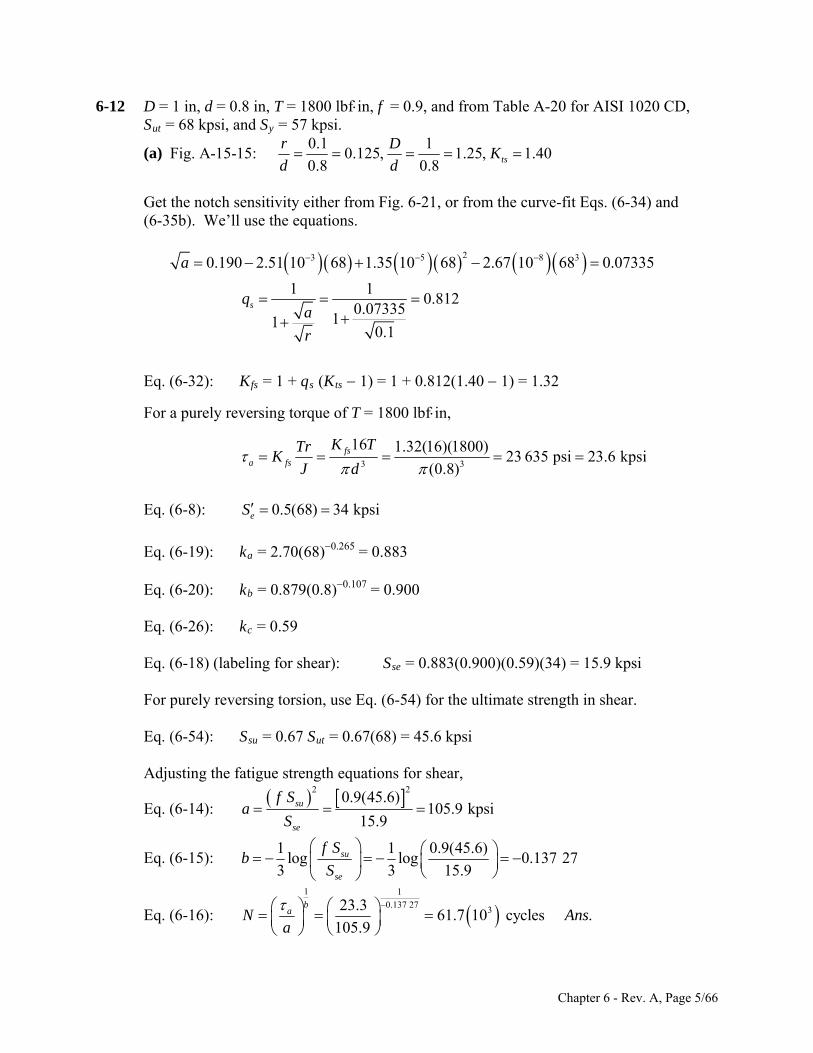
6-12 D = 1 in, d = 0.8 in, T = 1800 lbfin, f = 0.9, and from Table A-20 for AISI 1020 CD, Sut = 68 kpsi, and Sy = 57 kpsi.
(a) 0.1 1
Fig. A-15-15: 0.125, 1.25, 1.400.8 0.8 ts
r DK
d d
Get the notch sensitivity either from Fig. 6-21, or from the curve-fit Eqs. (6-34) and (6-35b). We’ll use the equations.
23 5 8 30.190 2.51 10 68 1.35 10 68 2.67 10 68 0.07335a
1 1
0.8120.07335
110.1
sqa
r
Eq. (6-32): Kfs = 1 + qs (Kts 1) = 1 + 0.812(1.40 1) = 1.32
For a purely reversing torque of T = 1800 lbfin,
3 3
16 1.32(16)(1800)23 635 psi 23.6 kpsi
(0.8)fs
a fs
K TTrK
J d
Eq. (6-8): 0.5(68) 34 kpsieS Eq. (6-19): ka = 2.70(68)0.265 = 0.883 Eq. (6-20): kb = 0.879(0.8)0.107 = 0.900 Eq. (6-26): kc = 0.59 Eq. (6-18) (labeling for shear): Sse = 0.883(0.900)(0.59)(34) = 15.9 kpsi For purely reversing torsion, use Eq. (6-54) for the ultimate strength in shear. Eq. (6-54): Ssu = 0.67 Sut = 0.67(68) = 45.6 kpsi Adjusting the fatigue strength equations for shear,
Eq. (6-14): 2 2
0.9(45.6)105.9 kpsi
15.9su
se
f Sa
S
Eq. (6-15): 1 1 0.9(45.6)
log log 0.137 273 3 15.9
su
se
f Sb
S
Eq. (6-16): 1 1
0.137 27323.3
61.7 10 cycles .105.9
baN A
a
ns
Chapter 6 - Rev. A, Page 5/66
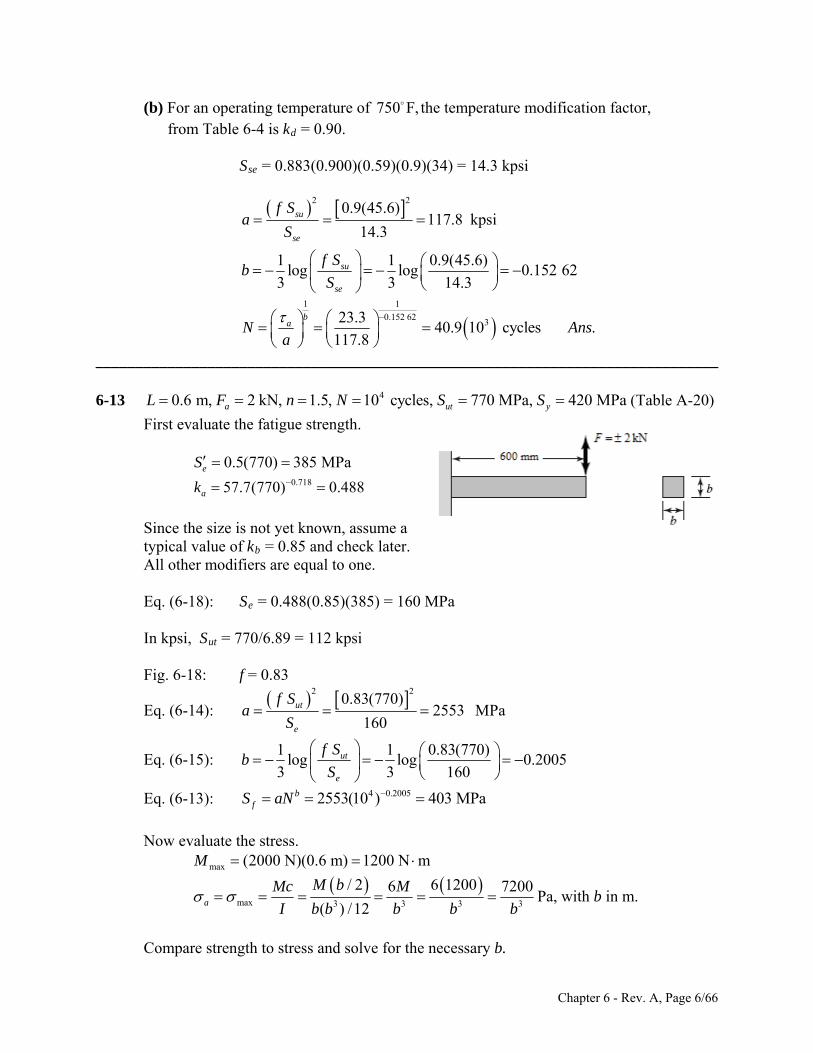
(b) For an operating temperature of 750 the temperature modification factor, F,
from Table 6-4 is kd = 0.90. Sse = 0.883(0.900)(0.59)(0.9)(34) = 14.3 kpsi
2 20.9(45.6)
117.8 kpsi14.3
1 1 0.9(45.6)log log 0.152 62
3 3 14.3
su
se
su
se
f Sa
S
f Sb
S
1 1
0.152 62323.3
40.9 10 cycles .117.8
baN A
a
ns
y
______________________________________________________________________________ 6-13 (Table A-20) 40.6 m, 2 kN, 1.5, 10 cycles, 770 MPa, 420 MPaa utL F n N S S First evaluate the fatigue strength.
0.5(770) 385 MPaeS
0.71857.7(770) 0.488ak Since the size is not yet known, assume a typical value of kb = 0.85 and check later. All other modifiers are equal to one. Eq. (6-18): Se = 0.488(0.85)(385) = 160 MPa In kpsi, Sut = 770/6.89 = 112 kpsi Fig. 6-18: f = 0.83
Eq. (6-14): 2 2
0.83(770)2553 MPa
160ut
e
f Sa
S
Eq. (6-15): 1 1 0.83(770)
log log 0.20053 3 160
ut
e
f Sb
S
Eq. (6-13): 4 0.20052553(10 ) 403 MPabfS aN
Now evaluate the stress.
max (2000 N)(0.6 m) 1200 N mM
max 3 3 3
/ 2 6 12006 7200
( ) /12a
M bMc M3I b b b b b
Pa, with b in m.
Compare strength to stress and solve for the necessary b.
Chapter 6 - Rev. A, Page 6/66
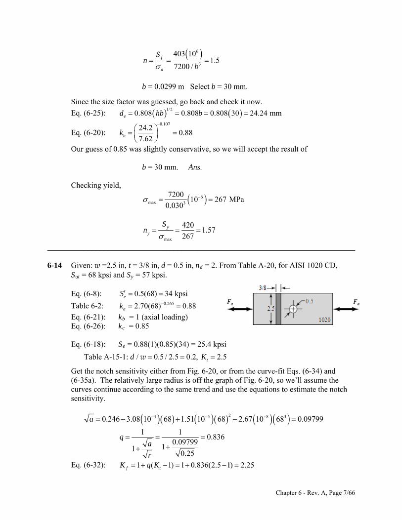
6403 10
fS3
1.57200 /a
nb
b = 0.0299 m Select b = 30 mm.
Since the size factor was guessed, go back and check it now.
Eq. (6-25): 1/20.808 0.808 0.808 30 24.24ed hb b mm
Eq. (6-20): 0.107
24.20.88
7.62bk
Our guess of 0.85 was slightly conservative, so we will accept the result of
b = 30 mm. Ans.
Checking yield,
6max 3
720010 267 MPa
0.030
max
4201.57
267y
y
Sn
______________________________________________________________________________
-14 Given: w =2.5 in, t = 3/8 in, d = 0.5 in, nd = 2. From Table A-20, for AISI 1020 CD,
Eq. (6-8):
b = 1 (axial loading)
Eq. (6-18): Se = 0.88(1)(0.85)(34) = 25.4 kpsi
notch sensitivity either from Fig. 6-20, or from the curve-fit Eqs. (6-34) and
h
6 Sut = 68 kpsi and Sy = 57 kpsi. 0.5(68) 34 kpsieS
Table 6-2: 88k 0.2652.70(68) 0. a
Eq. (6-21): k Eq. (6-26): kc = 0.85
Table A-15-1: / 0.5 / 2.5 0.2, 2.5td K w
Get the (6-35a). The relatively large radius is off the graph of Fig. 6-20, so we’ll assume the
curves continue according to the same trend and use the equations to estimate the notcsensitivity.
23 5 8 30.246 3.08 10 68 1.51 10 68 2.67 10 68 0.09799a
1 10.836
0.0979911
0.25
qa
r
Eq. (6-32): 1 ( 1) 1 0.836(2.5 1) 2.25f tK q K
Chapter 6 - Rev. A, Page 7/66
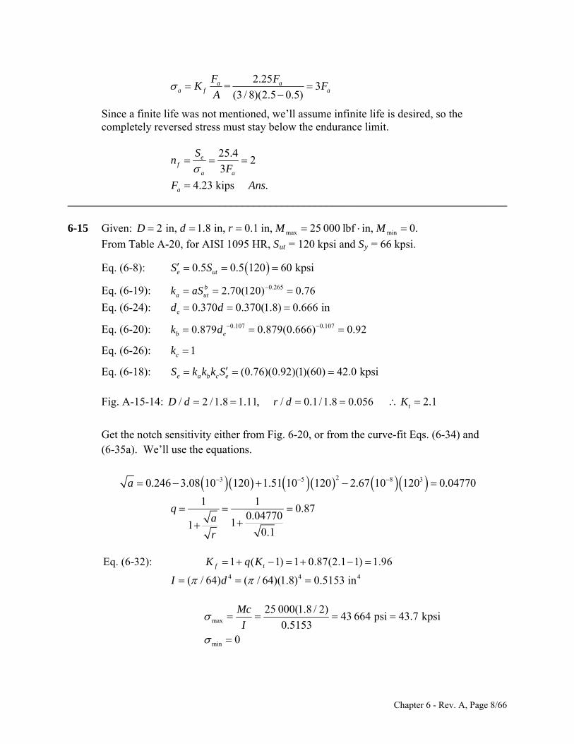
2.25= 3
(3 / 8)(2.5 0.5)a a
a f
F FK F
A
a
e life was not mentioned, we’ll assume infinite life is desired, so the
Since a finitcompletely reversed stress must stay below the endurance limit.
25.4
23
ef
a a
Sn
F
ns4.23 kips .aF A
____ __________ ___ ____________________ _________________________________________
ble A-20, for AISI 1095 HR, Sut = 120 kpsi and Sy = 66 kpsi.
-15 Given:6 max min2 in, 1.8 in, 0.1 in, 25 000 lbf in, 0.D d r M M
From Ta
(6-8): 0.5 0.5 120 60 kpsiS S Eq. e ut
Eq. (6-19): 0.2652.70(120) 0.76ba utk aS
Eq. (6-24): ie 0.370 0.370(1.8) 0.666 nd d
Eq. (6-20): 70.107 0.100.879 0.879(0.666) 0.92b ek d
Fig. A-15-14:
Eq. (6-26): 1ck
Eq. (6-18): (0.76)(0.92)(1)(60) 42.0 kpsie a b c eS k k k S
/ 2 /1.8 1.11, / 0.1 /1.8 0.056D d r d 2.1tK Get the notch sensitivity either from Fig. 6-20, or from the curve-fit Eqs. (6-34) and (6-35a). We’ll use the equations.
23 5 8 30.246 3.08 10 120 1.51 10 120 2.67 10 120 0.04770a
1 10.87
0.0477011
0.1
qa
r
Eq. (6-32):
1 ( 1) 1 0.87(2.1 1) 1.96f tK q K
4
4 4( / 64) ( / 64)(1.8) 0.5153 inI d
max
min
25 000(1.8 / 2)43 664 psi 43.7 kpsi
0.51530
Mc
I
Chapter 6 - Rev. A, Page 8/66
Eq. (6-36): max min43.7 0
1.96 42.8 kpsi2 2m fK
max min43.7 0
1.96 42.8 kpsi2 2a fK
Eq. (6-46): 1 42.8 42.8
42.0 120a m
f e utn S S
0.73 .fn A ns
A factor of safety less than unity indicates a finite life. Check for yielding. It is not necessary to include the stress concentration for static
yielding of a ductile material.
max
661.51 .
43.7y
y
Sn A
ns
______________________________________________________________________________ 6-16 From a free-body diagram analysis, the bearing reaction forces are found to be 2.1 kN at
the left bearing and 3.9 kN at the right bearing. The critical location will be at the shoulder fillet between the 35 mm and the 50 mm diameters, where the bending moment is large, the diameter is smaller, and the stress concentration exists. The bending moment at this point is M = 2.1(200) = 420 kN·mm. With a rotating shaft, the bending stress will be completely reversed.
2rev 4
420 (35 / 2)0.09978 kN/mm 99.8 MPa
( / 64)(35)
Mc
I
This stress is far below the yield strength of 390 MPa, so yielding is not predicted. Find
the stress concentration factor for the fatigue analysis. Fig. A-15-9: r/d = 3/35 = 0.086, D/d = 50/35 = 1.43, Kt =1.7 Get the notch sensitivity either from Fig. 6-20, or from the curve-fit Eqs. (6-34) and (6-35a). We’ll use the equations, with Sut = 470 MPa = 68.2 kpsi and r = 3 mm = 0.118
in.
2 33 5 80.246 3.08 10 68.2 1.51 10 68.2 2.67 10 68.2 0.09771a
1 10.78
0.0977111
0.118
qa
r
Eq. (6-32): 1 ( 1) 1 0.78(1.7 1) 1.55f tK q K
Chapter 6 - Rev. A, Page 9/66
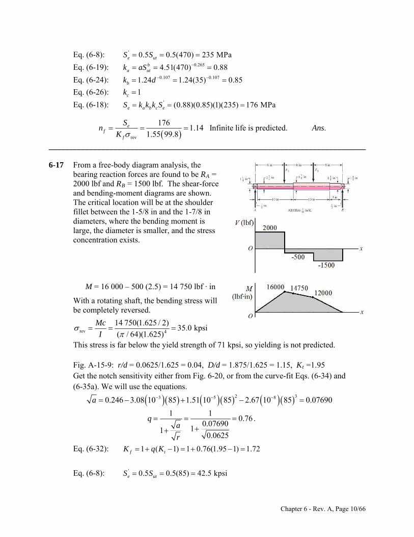
Eq. (6-8): ' 0.5 0.5(470) 235 MPae utS S
Eq. (6-19): 0.2654.51(470) 0.88ba utk aS
Eq. (6-24): 0.107 0.1071.24 1.24(35) 0.85bk d
Eq. (6-26): 1ck
Eq. (6-18): ' (0.88)(0.85)(1)(235) 176 MPae a b c eS k k k S
rev
1761.14 Infinite life is predicted. .
1.55 99.8e
ff
Sn A
K ns
______________________________________________________________________________ 6-17 From a free-body diagram analysis, the
bearing reaction forces are found to be RA = 2000 lbf and RB = 1500 lbf. The shear-force and bending-moment diagrams are shown. The critical location will be at the shoulder fillet between the 1-5/8 in and the 1-7/8 in diameters, where the bending moment is large, the diameter is smaller, and the stress concentration exists.
M = 16 000 – 500 (2.5) = 14 750 lbf · in
With a rotating shaft, the bending stress will be completely reversed.
rev 4
14 750(1.625 / 2)35.0 kpsi
( / 64)(1.625)
Mc
I
This stress is far below the yield strength of 71 kpsi, so yielding is not predicted. Fig. A-15-9: r/d = 0.0625/1.625 = 0.04, D/d = 1.875/1.625 = 1.15, Kt =1.95 Get the notch sensitivity either from Fig. 6-20, or from the curve-fit Eqs. (6-34) and (6-35a). We will use the equations.
2 33 5 80.246 3.08 10 85 1.51 10 85 2.67 10 85 0.07690a
1 10.76
0.0769011
0.0625
qa
r
.
Eq. (6-32):
1 ( 1) 1 0.76(1.95 1) 1.72f tK q K
Eq. (6-8): S S ' 0.5 0.5(85) 42.5 kpsie ut
Chapter 6 - Rev. A, Page 10/66
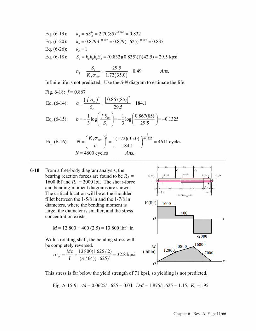
Eq. (6-19): 0.2652.70(85) 0.832ba utk aS
Eq. (6-20): 0.107 0.1070.879 0.879(1.625) 0.835bk d Eq. (6-26): 1ck
Eq. (6-18): ' (0.832)(0.835)(1)(42.5) 29.5 kpsie a b c eS k k k S
rev
29.50.49 .
1.72 35.0e
ff
Sn A
K ns
Infinite life is not predicted. Use the S-N diagram to estimate the life.
Fig. 6-18: f = 0.867
2 20.867(85)
Eq. (6-14): 184.129.5
1 1 0.867(85)Eq. (6-15): log log 0.1325
3 3 29.5
ut
e
ut
e
f Sa
S
f Sb
S
1 1
0.1325rev (1.72)(35.0)Eq. (6-16): 4611 cycles
184.1
bfK
Na
N = 4600 cycles Ans. ______________________________________________________________________________ 6-18 From a free-body diagram analysis, the
bearing reaction forces are found to be RA = 1600 lbf and RB = 2000 lbf. The shear-force and bending-moment diagrams are shown. The critical location will be at the shoulder fillet between the 1-5/8 in and the 1-7/8 in diameters, where the bending moment is large, the diameter is smaller, and the stress concentration exists.
M = 12 800 + 400 (2.5) = 13 800 lbf · in With a rotating shaft, the bending stress will
be completely reversed.
rev 4
13 800(1.625 / 2
)32.8 kpsi
( / 64)(1.625)
Mc
I
This stress is far below the yield strength of 71 kpsi, so yielding is not predicted. Fig. A-15-9: r/d = 0.0625/1.625 = 0.04, D/d = 1.875/1.625 = 1.15, Kt =1.95
Chapter 6 - Rev. A, Page 11/66
Get the notch sensitivity either from Fig. 6-20, or from the curve-fit Eqs. (6-34) and (6-35a). We will use the equations
2 33 5 80.246 3.08 10 85 1.51 10 85 2.67 10 85 0.07690a
1 10.76
0.0769011
0.0625
qa
r
Eq. (6-32):
1 ( 1) 1 0.76(1.95 1) 1.72f tK q K
Eq. (6-8): ' 0.5 0.5(85) 42.5 kpsie utS S
Eq. (6-19): 0.2652.70(85) 0.832ba utk aS
Eq. (6-20): 0.107 0.1070.879 0.879(1.625) 0.835bk d Eq. (6-26): 1ck
Eq. (6-18): ' (0.832)(0.835)(1)(42.5) 29.5 kpsie a b c eS k k k S
rev
29.50.52 .
1.72 32.8e
ff
Sn A
K ns
Infinite life is not predicted. Use the S-N diagram to estimate the life. Fig. 6-18: f = 0.867
2 20.867(85)
Eq. (6-14): 184.129.5
1 1 0.867(85)Eq. (6-15): log log 0.1325
3 3 29.5
ut
e
ut
e
f Sa
S
f Sb
S
1 1
0.1325rev (1.72)(32.8)Eq. (6-16): 7527 cycles
184.1
bfK
Na
N = 7500 cycles Ans. ______________________________________________________________________________ 6-19 Table A-20: 120 kpsi, 66 kpsiut yS S N = (950 rev/min)(10 hr)(60 min/hr) = 570 000 cycles One approach is to guess a diameter and solve the problem as an iterative analysis
problem. Alternatively, we can estimate the few modifying parameters that are dependent on the diameter and solve the stress equation for the diameter, then iterate to check the estimates. We’ll use the second approach since it should require only one iteration, since the estimates on the modifying parameters should be pretty close.
Chapter 6 - Rev. A, Page 12/66
First, we’ll evaluate the stress. From a free-body diagram analysis, the reaction forces at the bearings are R1 = 2 kips and R2 = 6 kips. The critical stress location is in the middle of the span at the shoulder, where the bending moment is high, the shaft diameter is smaller, and a stress concentration factor exists. If the critical location is not obvious, prepare a complete bending moment diagram and evaluate at any potentially critical locations. Evaluating at the critical shoulder,
2 kip 10 in 20 kip inM
rev 4 3 3 3
/ 2 32 2032 203.7kpsi
/ 64
M dMc M
I d d d d
Now we’ll get the notch sensitivity and stress concentration factor. The notch sensitivity depends on the fillet radius, which depends on the unknown diameter. For now, we’ll estimate a value for q = 0.85 from observation of Fig. 6-20, and check it later.
Fig. A-15-9: / 1.4 / 1.4, / 0.1 / 0.1, 1.65tD d d d r d d d K Eq. (6-32):
1 ( 1) 1 0.85(1.65 1) 1.55f tK q K
Now we will evaluate the fatigue strength.
'
0.265
0.5(120) 60 kpsi
2.70(120) 0.76
e
a
S
k
Since the diameter is not yet known, assume a typical value of k
b = 0.85 and check later. All other modifiers are equal to one.
Se = (0.76)(0.85)(60) = 38.8 kpsi Determine the desired fatigue strength from the S-N diagram. Fig. 6-18: f = 0.82
2 20.82(120)
Eq. (6-14): 249.638.8
1 1 0.82(120)Eq. (6-15): log log 0.1347
3 3 38.8
ut
e
ut
e
f Sa
S
f Sb
S
0.1347Eq. (6-13): 249.6(570 000) 41.9 kpsib
fS aN Compare strength to stress and solve for the necessary d.
Chapter 6 - Rev. A, Page 13/66
3
rev
d = 2.29 in
41.91.6
1.55 203.7 /f
ff
Sn
K d
Since the size factor and notch sensitivity were guessed, go back and check them now.
Eq. (6-20): 0.1570.1570.91 0.91 2.29 0.80bk d
Our guess of 0.85 was conservative. From Fig. 6-20 with r = d/10 = 0.229 in, we are off
the graph, but it appears our guess for q is low. Assuming the trend of the graph continues, we’ll choose q = 0.91 and iterate the problem with the new values of kb and q.
Intermediate results are Se = 36.5 kpsi, Sf = 39.6 kpsi, and Kf = 1.59. This gives
3
rev
39.61.6
1.59 203.7
d = 2.36 in Ans.
/f
ff
Sn
K d
a
A quick check of kb and q show that our estimates are still reasonable for this diameter. ______________________________________________________________________________ 6-20 40 kpsi, 60 kpsi, 80 kpsi, 15 kpsi, 25 kpsi, 0e y ut m a mS S S
Obtain von Mises stresses for the alternating, mid-range, and maximum stresses.
1/21/2 22 2 2
1/21/2 22 2 2
3 25 3 0 25.00 kpsi
3 0 3 15 25.98 kpsi
a a a
m m m
1/21/2 2 22 2max max max
1/22 2
3 3
25 3 15 36.06 kpsi
a m a m
max
601.66 .
36.06y
y
Sn A
ns
(a) Modified Goodman, Table 6-6
11.05 .
(25.00 / 40) (25.98 / 80)fn A
ns
(b) Gerber, Table 6-7
221 80 25.00 2(25.98)(40)
1 1 1.31 .2 25.98 40 80(25.00)fn A
ns
Chapter 6 - Rev. A, Page 14/66
(c) ASME-Elliptic, Table 6-8
2 2
11.32 .
(25.00 / 40) (25.98 / 60)fn A
ns
a
______________________________________________________________________________ 6-21 40 kpsi, 60 kpsi, 80 kpsi, 20 kpsi, 10 kpsi, 0e y ut m a mS S S
Obtain von Mises stresses for the alternating, mid-range, and maximum stresses.
1/21/2 22 2 2
1/21/2 22 2 2
3 10 3 0 10.00 kpsi
3 0 3 20 34.64 kpsi
a a a
m m m
1/21/2 2 22 2max max max
1/22 2
3 3
10 3 20 36.06 kpsi
a m a m
max
601.66 .
36.06y
y
Sn A
ns
(a) Modified Goodman, Table 6-6
11.46 .
(10.00 / 40) (34.64 / 80)fn A
ns
(b) Gerber, Table 6-7
221 80 10.00 2(34.64)(40)
1 1 1.74 .2 34.64 40 80(10.00)fn A
ns
(c) ASME-Elliptic, Table 6-8
2 2
11.59 .
(10.00 / 40) (34.64 / 60)fn A
ns
m
______________________________________________________________________________ 6-22 40 kpsi, 60 kpsi, 80 kpsi, 10 kpsi, 15 kpsi, 12 kpsi, 0e y ut a m aS S S
Obtain von Mises stresses for the alternating, mid-range, and maximum stresses.
1/21/2 22 2 2
1/21/2 22 2 2
3 12 3 10 21.07 kpsi
3 0 3 15 25.98 kpsi
a a a
m m m
Chapter 6 - Rev. A, Page 15/66
1/21/2 2 22 2max max max
1/22 2
3 3
12 0 3 10 15 44.93 kpsi
a m a m
max
601.34 .
44.93y
y
Sn A
ns
(a) Modified Goodman, Table 6-6
11.17 .
(21.07 / 40) (25.98 / 80)fn A
ns
(b) Gerber, Table 6-7
221 80 21.07 2(25.98)(40)
1 1 1.47 .2 25.98 40 80(21.07)fn A
ns
(c) ASME-Elliptic, Table 6-8
2 2
11.47 .
(21.07 / 40) (25.98 / 60)fn A
ns
a
______________________________________________________________________________ 6-23 40 kpsi, 60 kpsi, 80 kpsi, 30 kpsi, 0e y ut a m aS S S
Obtain von Mises stresses for the alternating, mid-range, and maximum stresses.
1/21/2 22 2 2
1/22 2
3 0 3 30 51.96 kpsi
3 0 kpsi
a a a
m m m
1/21/2 2 22 2max max max
1/22
3 3
3 30 51.96 kpsi
a m a m
max
601.15 .
51.96y
y
Sn A
ns
(a) Modified Goodman, Table 6-6
10.77 .
(51.96 / 40)fn A ns
(b) Gerber criterion of Table 6-7 is only valid for m > 0; therefore use Eq. (6-47).
Chapter 6 - Rev. A, Page 16/66
401 0
51.96a e
f fe a
Sn n
S.77 .Ans
(c) ASME-Elliptic, Table 6-8
2
10.77 .
(51.96 / 40)fn A ns
Since infinite life is not predicted, estimate a life from the S-N diagram. Since 'm = 0, the stress state is completely reversed and the S-N diagram is applicable for 'a.
Fig. 6-18: f = 0.875
Eq. (6-14): 22 0.875(80)( )
122.540
ut
e
f Sa
S
Eq. (6-15): 1 1 0.875(80)
log log 0.081013 3 40
ut
e
f Sb
S
Eq. (6-16):
11/
0.08101rev 51.96
39 600 cycles .122.5
b
N Aa
ns
a
______________________________________________________________________________ 6-24 40 kpsi, 60 kpsi, 80 kpsi, 15 kpsi, 15 kpsi, 0e y ut a m mS S S
Obtain von Mises stresses for the alternating, mid-range, and maximum stresses.
1/21/2 22 2 23 0 3 15 25.98 kpsia a a
1/21/2 22 2 23 15 3 0 15.00 kpsim m m
1/21/2 2 22 2max max max
1/22 2
3 3
15 3 15 30.00 kpsi
a m a m
max
602.00 .
30y
y
Sn A
ns
(a) Modified Goodman, Table 6-6
11.19 .
(25.98 / 40) (15.00 / 80)fn A
ns
(b) Gerber, Table 6-7
221 80 25.98 2(15.00)(40)
1 1 1.43 .2 15.00 40 80(25.98)fn A
ns
Chapter 6 - Rev. A, Page 17/66
(c) ASME-Elliptic, Table 6-8
2 2
11.44 .
(25.98 / 40) (15.00 / 60)fn A
ns
______________________________________________________________________________ 6-25 Given: . From Table A-20, for AISI 1040
CD, max min28 kN, 28 kNF F 590 MPa, 490 MPa, yS S ut
Check for yielding
2maxmax
28 000147.4 N/mm 147.4 MPa
10(25 6)
F
A
max
4903.32 .
147.4y
y
Sn A
ns
Determine the fatigue factor of safety based on infinite life Eq. (6-8): ' 0.5(590) 295 MPaeS
Eq. (6-19): 0.2654.51(590) 0.832ba utk aS
Eq. (6-21): 1 (axial)bk Eq. (6-26): 0.85ck
Eq. (6-18): ' (0.832)(1)(0.85)(295) 208.6 MPae a b c eS k k k S
Fig. 6-20: q = 0.83 Fig. A-15-1: t/ 0.24, 2.44d K w
1 ( 1) 1 0.83(2.44 1) 2.20f tK q K
max min
max min
28 000 28 0002.2 324.2 MPa
2 2(10)(25 6)
02
a f
m f
F FK
A
F FK
A
1 324.2 0
208.6 590
0.64 .
a m
f e ut
f
n S S
n Ans
Since infinite life is not predicted, estimate a life from the S-N diagram. Since m = 0, the stress state is completely reversed and the S-N diagram is applicable for a.
Sut = 590/6.89 = 85.6 kpsi Fig. 6-18: f = 0.87
Chapter 6 - Rev. A, Page 18/66
Eq. (6-14): 22 0.87(590)( )
1263208.6
ut
e
f Sa
S
Eq. (6-15): 1 1 0.87(590)
log log 0.13043 3 208.6
ut
e
f Sb
S
Eq. (6-16):
11/
0.1304rev 324.2
33 812 cycles 1263
b
Na
N = 34 000 cycles Ans.
________________________________________________________________________ 6-26 max min590 MPa, 490 MPa, 28 kN, 12 kNut yS S F F
Check for yielding
2maxmax
28 000147.4 N/mm 147.4 MPa
10(25 6)
F
A
max
4903.32 .
147.4y
y
Sn A
ns
Determine the fatigue factor of safety based on infinite life. From Prob. 6-25:
208.6 MPa, 2.2e fS K
max min
28 000 12 0002.2 92.63 MPa
2 2(10)(25 6)a f
F FK
A
max min 28 000 12 0002.2 231.6 MPa
2 2(10)(25 6)m f
F FK
A
Modified Goodman criteria:
1 92.63 231.6
208.6 590a m
f e utn S S
1.20 .fn A ns
Gerber criteria:
2 221
1 12
ut a m ef
m e ut a
S Sn
S S
22
1 590 92.63 2(231.6)(208.6)1 1
2 231.6 208.6 590(92.63)
1.49 .fn A ns
Chapter 6 - Rev. A, Page 19/66
ASME-Elliptic criteria:
2 2 2
1 1
( / ) ( / ) (92.63 / 208.6) (231.6 / 490)fa e m y
nS S
2
= 1.54 Ans. The results are consistent with Fig. 6-27, where for a mean stress that is about half of the
yield strength, the Modified Goodman line should predict failure significantly before the other two.
______________________________________________________________________________ 6-27 590 MPa, 490 MPaut yS S
(a) max min28 kN, 0 kNF F
Check for yielding
2maxmax
28 000147.4 N/mm 147.4 MPa
10(25 6)
F
A
max
4903.32 .
147.4y
y
Sn A
ns
From Prob. 6-25: 208.6 MPa, 2.2e fS K
max min
max min
28 000 02.2 162.1 MPa
2 2(10)(25 6)
28 000 02.2 162.1 MPa
2 2(10)(25 6)
a f
m f
F FK
A
F FK
A
1 162.1 162.1
208.6 590a m
f e utn S S
0.95 .fn A ns
Since infinite life is not predicted, estimate a life from the S-N diagram. First, find an equivalent completely reversed stress (See Ex. 6-12).
rev
162.1223.5 MPa
1 ( / ) 1 (162.1/ 590)a
m utS
Fig. 6-18: f = 0.87
Eq. (6-14): 22 0.87(590)( )
1263208.6
ut
e
f Sa
S
Chapter 6 - Rev. A, Page 20/66
Eq. (6-15): 1 1 0.87(590)
log log 0.13043 3 208.6
ut
e
f Sb
S
Eq. (6-16):
11/
0.1304rev 223.5
586 000 cycles . 1263
b
N Aa
ns
(b) max min28 kN, 12 kNF F
The maximum load is the same as in part (a), so max 147.4 MPa
3.32 .yn A ns
Factor of safety based on infinite life:
max min
max min
28 000 12 0002.2 92.63 MPa
2 2(10)(25 6)
28 000 12 0002.2 231.6 MPa
2 2(10)(25 6)
a f
m f
F FK
A
F FK
A
1 92.63 231.6
208.6 590a m
f e utn S S
1.20 .fn A ns
(c) max min12 kN, 28 kNF F
The compressive load is the largest, so check it for yielding.
minmin
28 000147.4 MPa
10(25 6)
F
A
min
4903.32 .
147.4yc
y
Sn A
ns
Factor of safety based on infinite life:
max min
max min
12 000 28 0002.2 231.6 MPa
2 2(10)(25 6)
12 000 28 0002.2 92.63 MPa
2 2(10)(25 6)
a f
m f
F FK
A
F FK
A
For m < 0, 208.6
0.90 .231.6
ef
a
Sn A
ns
Chapter 6 - Rev. A, Page 21/66
Since infinite life is not predicted, estimate a life from the S-N diagram. For a negative mean stress, we shall assume the equivalent completely reversed stress is the same as the actual alternating stress. Get a and b from part (a).
Eq. (6-16):
11/
0.1304rev 231.6
446 000 cycles . 1263
b
N Aa
ns
______________________________________________________________________________ 6-28 Eq. (2-21): Sut = 0.5(400) = 200 kpsi Eq. (6-8): ' 0.5(200) 100 kpsieS
Eq. (6-19): 0.71814.4(200) 0.321ba utk aS
Eq. (6-25): e 0.37 0.37(0.375) 0.1388 ind d
Eq. (6-20): 0.107 0.1070.879 0.879(0.1388) 1.09b ek d Since we have used the equivalent diameter method to get the size factor, and in doing so
introduced greater uncertainties, we will choose not to use a size factor greater than one. Let kb = 1.
Eq. (6-18): (0.321)(1)(100) 32.1 kpsieS
40 20 40 2010 lb 30 lb
2 2a mF F
3 3
3 3
32 32(10)(12)23.18 kpsi
(0.375)
32 32(30)(12)69.54 kpsi
(0.375)
aa
mm
M
d
M
d
(a) Modified Goodman criterion
1 23.18 69.54
32.1 200a m
f e utn S S
0.94 .fn A ns
Since infinite life is not predicted, estimate a life from the S-N diagram. First, find an equivalent completely reversed stress (See Ex. 6-12).
rev
23.1835.54 kpsi
1 ( / ) 1 (69.54 / 200)a
m utS
Fig. 6-18: f = 0.775
Eq. (6-14): 22 0.775(200)( )
748.432.1
ut
e
f Sa
S
Chapter 6 - Rev. A, Page 22/66
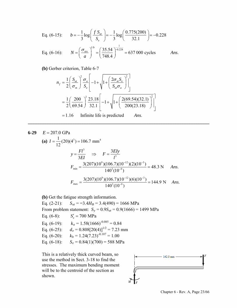
Eq. (6-15): 1 1 0.775(200)
log log 0.2283 3 32.1
ut
e
f Sb
S
Eq. (6-16):
11/
0.228rev 35.54
637 000 cycles . 748.4
b
N
Ansa
(b) Gerber criterion, Table 6-7
2 2
22
211 1
2
1 200 23.18 2(69.54)(32.1)1 1
2 69.54 32.1 200(23.18)
1.16 Infinite life is predicted .
ut a m ef
m e ut a
S Sn
S S
Ans
______________________________________________________________________________ 6-29 207.0 GPaE
(a) 3 41(20)(4 ) 106.7 mm
12I
3
3
3
3
Fl EIyy F
EI l
9 12 3
min 3 9
3(207)(10 )(106.7)(10 )(2)(10 )48.3 N .
140 (10 )F A
ns
9 12 3
max 3 9
3(207)(10 )(106.7)(10 )(6)(10 )144.9 N .
140 (10 )F A
ns
(b) Get the fatigue strength information. Eq. (2-21): Sut = =3.4HB = 3.4(490) = 1666 MPa From problem statement: Sy = 0.9Sut = 0.9(1666) = 1499 MPa
Eq. (6-8): 700 MPaeS
Eq. (6-19): ka = 1.58(1666)-0.085 = 0.84 Eq. (6-25): de = 0.808[20(4)]1/2 = 7.23 mm Eq. (6-20): kb = 1.24(7.23)-0.107 = 1.00 Eq. (6-18): Se = 0.84(1)(700) = 588 MPa This is a relatively thick curved beam, so
use the method in Sect. 3-18 to find the stresses. The maximum bending moment will be to the centroid of the section as shown.
Chapter 6 - Rev. A, Page 23/66
M = 142F N·mm, A = 4(20) = 80 mm2, h = 4 mm, ri = 4 mm, ro = ri + h = 8 mm, rc = ri + h/2 = 6 mm
Table 3-4: 4
5.7708 mmln( / ) ln(8 / 4)n
o i
hr
r r
6 5.7708 0.2292 mmc ne r r
5.7708 4 1.7708 mmi n ic r r
8 5.7708 2.2292 mmo o nc r r
Get the stresses at the inner and outer surfaces from Eq. (3-65) with the axial stresses added. The signs have been set to account for tension and compression as appropriate.
(142 )(1.7708)3.441 MPa
80(0.2292)(4) 80
(142 )(2.2292)2.145 MPa
80(0.2292)(8) 80
ii
i
oo
o
Mc F F FF
Aer A
Mc F F FF
Aer A
min
max
min
max
( ) 3.441(144.9) 498.6 MPa
( ) 3.441(48.3) 166.2 MPa
( ) 2.145(48.3) 103.6 MPa
( ) 2.145(144.9) 310.8 MPa
i
i
o
o
166.2 498.6
( ) 166.2 MPa2i a
166.2 498.6( ) 332.4 MPa
2i m
310.8 103.6
( ) 103.6 MPa2o a
310.8 103.6( ) 207.2 MPa
2o m
To check for yielding, we note that the largest stress is –498.6 MPa (compression) on the inner radius. This is considerably less than the estimated yield strength of 1499 MPa, so yielding is not predicted.
Check for fatigue on both inner and outer radii since one has a compressive mean stress
and the other has a tensile mean stress. Inner radius:
Since m < 0, 588
3.54166.2
ef
a
Sn
Chapter 6 - Rev. A, Page 24/66
Outer radius:
Since m > 0, we will use the Modified Goodman line.
103.6 207.21/
588 1666
3.33
a mf
e ut
f
nS S
n
Infinite life is predicted at both inner and outer radii. Ans. ______________________________________________________________________________ 6-30 From Table A-20, for AISI 1018 CD,
64 kpsi, 54 kpsiut yS S
Eq. (6-8): ' 0.5(64) 32 kpsieS
Eq. (6-19): 0.2652.70(64) 0.897ak Eq. (6-20): 1 (axial)bk Eq. (6-26): 0.85ck Eq. (6-18): (0.897)(1)(0.85)(32) 24.4 kpsieS Fillet: Fig. A-15-5: / 3.5 / 3 1.17, / 0.25 / 3 0.083, 1.85tD d r d K Use Fig. 6-20 or Eqs. (6-34) and (6-35a) for q. Estimate a little high since it is off the
graph. q = 0.85
1 ( 1) 1 0.85(1.85 1) 1.72f tK q K
maxmax
2
min
max min
max min
53.33 kpsi
3.0(0.5)
1610.67 kpsi
3.0(0.5)
3.33 ( 10.67)1.72 12.0 kpsi
2 2
3.33 ( 10.67)1.72 6.31 kpsi
2 2
a f
m f
F
h
K
K
w
min
545.06 Does not yield.
10.67y
y
Sn
Since the midrange stress is negative,
24.42.03
12.0e
fa
Sn
Chapter 6 - Rev. A, Page 25/66
Hole: Fig. A-15-1: 1/ 0.4 / 3.5 0.11 2.68td K w Use Fig. 6-20 or Eqs. (6-34) and (6-35a) for q. Estimate a little high since it is off the
graph. q = 0.85
1 0.85(2.68 1) 2.43fK
maxmax
1
minmin
1
53.226 kpsi
0.5(3.5 0.4)
1610.32 kpsi
0.5(3.5 0.4)
F
h d
F
h d
w
w
max min
max min
3.226 ( 10.32)2.43 16.5 kpsi
2 2
3.226 ( 10.32)2.43 8.62 kpsi
2 2
a f
m f
K
K
min
545.23 does not yield
10.32y
y
Sn
Since the midrange stress is negative,
24.41.48
16.5e
fa
Sn
Thus the design is controlled by the threat of fatigue at the hole with a minimum factor of safety of 1.48. .fn A ns
______________________________________________________________________________ 6-31 64 kpsi, 54 kpsiut yS S
Eq. (6-8): ' 0.5(64) 32 kpsieS
Eq. (6-19): 0.2652.70(64) 0.897ak
Eq. (6-20): 1 (axial)bk Eq. (6-26): 0.85ck Eq. (6-18): (0.897)(1)(0.85)(32) 24.4 kpsieS Fillet: Fig. A-15-5: / 2.5 /1.5 1.67, / 0.25 /1.5 0.17, 2.1tD d r d K Use Fig. 6-20 or Eqs. (6-34) and (6-35a) for q. Estimate a little high since it is off the
graph. q = 0.85
1 ( 1) 1 0.85(2.1 1) 1.94f tK q K
Chapter 6 - Rev. A, Page 26/66
maxmax
2
min
1621.3 kpsi
1.5(0.5)
45.33 kpsi
1.5(0.5)
F
h
w
max min
max min
21.3 ( 5.33)1.94 25.8 kpsi
2 2
21.3 ( 5.33)1.94 15.5 kpsi
2 2
a f
m f
K
K
max
542.54 Does not yield.
21.3y
y
Sn
Using Modified Goodman criteria,
1 25.8 15.5
24.4 64a m
f e utn S S
0.77fn
Hole: Fig. A-15-1: 1/ 0.4 / 2.5 0.16 2.55td K w Use Fig. 6-20 or Eqs. (6-34) and (6-35a) for q. Estimate a little high since it is off the
graph. q = 0.85
1 0.85(2.55 1) 2.32fK
maxmax
1
minmin
1
1615.2 kpsi
0.5(2.5 0.4)
43.81 kpsi
0.5(2.5 0.4)
F
h d
F
h d
w
w
max min
max min
15.2 ( 3.81)2.32 22.1 kpsi
2 2
15.2 ( 3.81)2.32 13.2 kpsi
2 2
a f
m f
K
K
max
543.55 Does not yield.
15.2y
y
Sn
Using Modified Goodman criteria
1 22.1 13.2
24.4 64a m
f e utn S S
0.90fn
Chapter 6 - Rev. A, Page 27/66
Thus the design is controlled by the threat of fatigue at the fillet with a minimum factor of safety of 0.77 .fn A ns
______________________________________________________________________________ 6-32
64 kpsi, 54 kpsiut yS S
From Prob. 6-30, the fatigue factor of safety at the hole is nf = 1.48. To match this at the fillet,
24.4
16.5 kpsi1.48
e ef a
a f
S Sn
n
where Se is unchanged from Prob. 6-30. The only aspect of a that is affected by the fillet radius is the fatigue stress concentration factor. Obtaining a in terms of Kf,
max min 3.33 ( 10.67)7.00
2 2a f f fK K K
Equating to the desired stress, and solving for Kf, 7.00 16.5 2.36a f fK K
Assume since we are expecting to get a smaller fillet radius than the original, that q will be back on the graph of Fig. 6-20, so we’ll estimate q = 0.8.
1 0.80( 1) 2.36 2.7f t tK K K
From Fig. A-15-5, with D / d = 3.5/3 = 1.17 and Kt = 2.6, find r / d. Choosing r / d = 0.03, and with d = w2 = 3.0,
2 0.03 0.03 3.0 0.09 in r w At this small radius, our estimate for q is too high. From Fig. 6-20, with r = 0.09, q
should be about 0.75. Iterating, we get Kt = 2.8. This is at a difficult range on Fig. A-15-5 to read the graph with any confidence, but we’ll estimate r / d = 0.02, giving r = 0.06 in. This is a very rough estimate, but it clearly demonstrates that the fillet radius can be relatively sharp to match the fatigue factor of safety of the hole. Ans.
______________________________________________________________________________ 6-33 60 kpsi, 110 kpsiy utS S
Inner fiber where 3 / 4 incr
3 30.84375
4 16(2)
3 30.65625
4 32
o
i
r
r
Table 3-4, p. 121,
Chapter 6 - Rev. A, Page 28/66
3 /160.74608 in
0.84375lnln
0.65625
no
i
hr
r
r
0.75 0.74608 0.00392 in
0.74608 0.65625 0.08983c n
i n i
e r r
c r r
23 30.035156 in
16 16A
Eq. (3-65), p. 119,
(0.08983)993.3
(0.035156)(0.00392)(0.65625)i
ii
Mc TT
Aer
where T is in lbf·in and i is in psi.
1( 993.3) 496.7
2496.7
m
a
T T
T
Eq. (6-8): ' 0.5 110 55 kpsieS
Eq. (6-19): 0.2652.70(110) 0.777ak
Eq. (6-25): 1/2
e 0.808 3 /16 3 /16 0.1515 ind Eq. (6-20): 0.107
0.879 0.1515 1.08 (round to 1)bk
Eq. (6-19): (0.777)(1)(55) 42.7 kpsieS For a compressive midrange component, / . Thus,a e fS n
42.70.4967
3T
28.7 lbf inT
Outer fiber where 2 .5 incr
32.5 2.59375
323
2.5 2.4062532
o
i
r
r
3 /162.49883
2.59375ln
2.40625
nr
2.5 2.49883 0.00117 in
2.59375 2.49883 0.09492 ino
e
c
Chapter 6 - Rev. A, Page 29/66
(0.09492)889.7 psi
(0.035156)(0.00117)(2.59375)
1(889.7 ) 444.9 psi
2
oo
o
m a
Mc TT
Aer
T T
(a) Using Eq. (6-46), for modified Goodman, we have
1
0.4449 0.4449 1
42.7 110 3
a m
e utS S n
T T
23.0 lbf in .T A ns (b) Gerber, Eq. (6-47), at the outer fiber,
2
2
1
3(0.4449 ) 3(0.4449 )1
42.7 110
a m
e ut
n n
S S
T T
28.2 lbf in .T A ns (c) To guard against yield, use T of part (b) and the inner stress.
602.14 .
0.9933(28.2)y
yi
Sn A
ns
______________________________________________________________________________ 6-34 From Prob. 6-33, 42.7 kpsi, 60 kpsi, and 110 kpsie y utS S S
(a) Assuming the beam is straight,
max 3 2 3
/ 2 6 6910.2
/12 (3 /16)
M hMc M TT
I bh bh
Goodman: 0.4551 0.4551 1
42.7 110 3
T T
22.5 lbf in .T A ns
(b) Gerber: 2
3(0.4551 ) 3(0.4551 )1
42.7 110
T T
27.6 lbf in .T A ns
Chapter 6 - Rev. A, Page 30/66
(c) max
602.39 .
0.9102(27.6)y
y
Sn A
ns
______________________________________________________________________________ 6-35 ,bend ,axial ,tors1.4, 1.1, 2.0, 300 MPa, 400 MPa, 200 MPaf f f y ut eK K K S S S
Bending: 0, 60 MPam a
Axial: 20 MPa, 0m a
Torsion: 25 MPa, 25 MPam a
Eqs. (6-55) and (6-56):
2 2
2 2
1.4(60) 0 3 2.0(25) 120.6 MPa
0 1.1(20) 3 2.0(25) 89.35 MPa
a
m
Using Modified Goodman, Eq. (6-46),
1 120.6 89.35
200 400a m
f e utn S S
1.21 .fn A ns
Check for yielding, using the conservative max a m ,
3001.43 .
120.6 89.35y
ya m
Sn A
ns
______________________________________________________________________________ 6-36 ,bend ,tors1.4, 2.0, 300 MPa, 400 MPa, 200 MPaf f y ut eK K S S S
Bending: max min150 MPa, 40 MPa, 55 MPa, 95 MPam a
Torsion: 90 MPa, 9 MPam a Eqs. (6-55) and (6-56):
2 2
2 2
1.4(95) 3 2.0(9) 136.6 MPa
1.4(55) 3 2.0(90) 321.1 MPa
a
m
Using Modified Goodman,
1 136.6 321.1
200 400a m
f e utn S S
0.67 .fn A ns
Check for yielding, using the conservative max a m ,
Chapter 6 - Rev. A, Page 31/66
3000.66 .
136.6 321.1y
ya m
Sn A
ns
Since the conservative yield check indicates yielding, we will check more carefully with
with max obtained directly from the maximum stresses, using the distortion energy
failure theory, without stress concentrations. Note that this is exactly the method used for static failure in Ch. 5.
2 2 2 2
max max max
max
3 150 3 90 9 227.8 MPa
3001.32 .
227.8y
y
Sn Ans
Since yielding is not predicted, and infinite life is not predicted, we would like to estimate a life from the S-N diagram. First, find an equivalent completely reversed stress (See Ex. 6-12).
rev
136.6692.5 MPa
1 ( / ) 1 (321.1/ 400)a
m utS
This stress is much higher than the ultimate strength, rendering it impractical for the S-N
diagram. We must conclude that the stresses from the combination loading, when increased by the stress concentration factors, produce such a high midrange stress that the equivalent completely reversed stress method is not practical to use. Without testing, we are unable to predict a life.
______________________________________________________________________________ 6-37 Table A-20: ut y64 kpsi, 54 kpsiS S
From Prob. 3-68, the critical stress element experiences = 15.3 kpsi and = 4.43 kpsi. The bending is completely reversed due to the rotation, and the torsion is steady, giving a = 15.3 kpsi, m = 0 kpsi, a = 0 kpsi, m = 4.43 kpsi. Obtain von Mises stresses for the alternating, mid-range, and maximum stresses.
1/21/2 22 2 2
1/21/2 22 2 2
1/21/2 22 2 2max max max
3 15.3 3 0 15.3 kpsi
3 0 3 4.43 7.67 kpsi
3 15.3 3 4.43 17.11 kpsi
a a a
m m m
Check for yielding, using the distortion energy failure theory.
max
543.16
17.11y
y
Sn
Obtain the modifying factors and endurance limit. Eq. (6-8): 0.5 64 32 kpsieS
Chapter 6 - Rev. A, Page 32/66
Eq. (6-19): 0.2652.70(64) 0.90ak
Eq. (6-20): 0.1070.879(1.25) 0.86bk Eq. (6-18): 0.90(0.86)(32) 24.8 kpsieS Using Modified Goodman,
1 15.3 7.67
24.8 64a m
f e utn S S
1.36 .fn A ns
______________________________________________________________________________ 6-38 Table A-20: ut y440 MPa, 370 MPaS S
From Prob. 3-69, the critical stress element experiences = 263 MPa and = 57.7 MPa. The bending is completely reversed due to the rotation, and the torsion is steady, giving a = 263 MPa, m = 0, a = 0 MPa, m = 57.7 MPa. Obtain von Mises stresses for the alternating, mid-range, and maximum stresses.
1/21/2 22 2 2
1/21/2 22 2 2
1/21/2 22 2 2max max max
3 263 3 0 263 MPa
3 0 3 57.7 99.9 MPa
3 263 3 57.7 281 MPa
a a a
m m m
Check for yielding, using the distortion energy failure theory.
max
3701.32
281y
y
Sn
Obtain the modifying factors and endurance limit. Eq. (6-8): 0.5 440 220 MPaeS
Eq. (6-19): 0.2654.51(440) 0.90ak
Eq. (6-20): 0.1071.24(30) 0.86bk
Eq. (6-18): 0.90(0.86)(220) 170 MPaeS Using Modified Goodman,
1 263 99.9
170 440a m
f e utn S S
Infinite life is not predicted. Ans. 0.56fn
______________________________________________________________________________
Chapter 6 - Rev. A, Page 33/66
6-39 Table A-20: ut y64 kpsi, 54 kpsiS S
From Prob. 3-70, the critical stress element experiences = 21.5 kpsi and = 5.09 kpsi. The bending is completely reversed due to the rotation, and the torsion is steady, giving a = 21.5 kpsi, m = 0 kpsi, a = 0 kpsi, m = 5.09 kpsi. Obtain von Mises stresses for the alternating, mid-range, and maximum stresses.
1/21/2 22 2 2
1/21/2 22 2 2
1/21/2 22 2 2max max max
3 21.5 3 0 21.5 kpsi
3 0 3 5.09 8.82 kpsi
3 21.5 3 5.09 23.24 kpsi
a a a
m m m
Check for yielding, using the distortion energy failure theory.
max
542.32
23.24y
y
Sn
Obtain the modifying factors and endurance limit.
0.2652.70(64) 0.90ak
0.1070.879(1) 0.88bk
0.90(0.88)(0.5)(64) 25.3 kpsieS Using Modified Goodman,
1 21.5 8.82
25.3 64a m
f e utn S S
1.01 .fn A ns
______________________________________________________________________________ 6-40 Table A-20: ut y440 MPa, 370 MPaS S
From Prob. 3-71, the critical stress element experiences = 72.9 MPa and = 20.3 MPa. The bending is completely reversed due to the rotation, and the torsion is steady, giving a = 72.9 MPa, m = 0 MPa, a = 0 MPa, m = 20.3 MPa. Obtain von Mises stresses for the alternating, mid-range, and maximum stresses.
1/21/2 22 2 2
1/21/2 22 2 2
1/21/2 22 2 2max max max
3 72.9 3 0 72.9 MPa
3 0 3 20.3 35.2 MPa
3 72.9 3 20.3 80.9 MPa
a a a
m m m
Check for yielding, using the distortion energy failure theory.
Chapter 6 - Rev. A, Page 34/66

max
3704.57
80.9y
y
Sn
Obtain the modifying factors and endurance limit. Eq. (6-8): 0.5 440 220 MPaeS
Eq. (6-19): 0.2654.51(440) 0.90ak
Eq. (6-20): 0.1071.24(20) 0.90bk
Eq. (6-18): 0.90(0.90)(220) 178.2 MPaeS Using Modified Goodman,
1 72.9 35.2
178.2 440a m
f e utn S S
2.04 .fn An s
______________________________________________________________________________ 6-41 Table A-20: ut y64 kpsi, 54 kpsiS S
From Prob. 3-72, the critical stress element experiences = 35.2 kpsi and = 7.35 kpsi. The bending is completely reversed due to the rotation, and the torsion is steady, giving a = 35.2 kpsi, m = 0 kpsi, a = 0 kpsi, m = 7.35 kpsi. Obtain von Mises stresses for the alternating, mid-range, and maximum stresses.
1/21/2 22 2 2
1/21/2 22 2 2
1/21/2 22 2 2max max max
3 35.2 3 0 35.2 kpsi
3 0 3 7.35 12.7 kpsi
3 35.2 3 7.35 37.4 kpsi
a a a
m m m
Check for yielding, using the distortion energy failure theory.
max
541.44
37.4y
y
Sn
Obtain the modifying factors and endurance limit. Eq. (6-8): 0.5(64) 32 kpsieS
Eq. (6-19): 0.2652.70(64) 0.90ak
Eq. (6-20): 0.1070.879(1.25) 0.86bk
Eq. (6-18): 0.90(0.86)(32) 24.8 kpsieS
Chapter 6 - Rev. A, Page 35/66
Using Modified Goodman,
1 35.2 12.7
24.8 64a m
f e utn S S
Infinite life is not predicted. Ans. 0.62fn
______________________________________________________________________________ 6-42 Table A-20: ut y440 MPa, 370 MPaS S
From Prob. 3-73, the critical stress element experiences = 333.9 MPa and = 126.3 MPa. The bending is completely reversed due to the rotation, and the torsion is steady, giving a = 333.9 MPa, m = 0 MPa, a = 0 MPa, m = 126.3 MPa. Obtain von Mises stresses for the alternating, mid-range, and maximum stresses.
1/21/2 22 2 2
1/21/2 22 2 2
1/21/2 22 2 2max max max
3 333.9 3 0 333.9 MPa
3 0 3 126.3 218.8 MPa
3 333.9 3 126.3 399.2 MPa
a a a
m m m
Check for yielding, using the distortion energy failure theory.
max
3700.93
399.2y
y
Sn
The sample fails by yielding, infinite life is not predicted. Ans. The fatigue analysis will be continued only to obtain the requested fatigue factor of
safety, though the yielding failure will dictate the life. Obtain the modifying factors and endurance limit. Eq. (6-8): 0.5(440) 220 MPaeS
Eq. (6-19): 0.2654.51(440) 0.90ak
Eq. (6-20): 0.1071.24(50) 0.82bk
Eq. (6-18): 0.90(0.82)(220) 162.4 MPaeS Using Modified Goodman,
1 333.9 218.8
162.4 440a m
f e utn S S
Infinite life is not predicted. Ans. 0.39fn
______________________________________________________________________________
Chapter 6 - Rev. A, Page 36/66
6-43 Table A-20: 64 kpsi, 54 kpsiut yS S From Prob. 3-74, the critical stress element experiences completely reversed bending
stress due to the rotation, and steady torsional and axial stresses.
,bend ,bend
,axial ,axial
9.495 kpsi, 0 kpsi
0 kpsi, 0.362 kpsi
0 kpsi, 11.07 kpsi
a m
a m
a m
Obtain von Mises stresses for the alternating, mid-range, and maximum stresses.
1/21/2 2 22 2
1/21/2 2 22 2
1/21/2 2 22 2max max max
3 9.495 3 0 9.495 kpsi
3 0.362 3 11.07 19.18 kpsi
3 9.495 0.362 3 11.07 21.56 kpsi
a a a
m m m
Check for yielding, using the distortion energy failure theory.
max
542.50
21.56y
y
Sn
Obtain the modifying factors and endurance limit. Eq. (6-8): 0.5(64) 32 kpsieS
Eq. (6-19): 0.2652.70(64) 0.90ak
Eq. (6-20): 0.1070.879(1.13) 0.87bk
Eq. (6-18): 0.90(0.87)(32) 25.1 kpsieS Using Modified Goodman,
1 9.495 19.18
25.1 64a m
f e utn S S
1.47 .fn A ns
______________________________________________________________________________ 6-44 Table A-20: ut y64 kpsi, 54 kpsiS S From Prob. 3-76, the critical stress element experiences completely reversed bending
stress due to the rotation, and steady torsional and axial stresses.
,bend ,bend
,axial ,axial
33.99 kpsi, 0 kpsi
0 kpsi, 0.153 kpsi
0 kpsi, 7.847 kpsi
a m
a m
a m
Chapter 6 - Rev. A, Page 37/66
Obtain von Mises stresses for the alternating, mid-range, and maximum stresses.
1/21/2 2 22 2
1/21/2 2 22 2
1/21/2 2 22 2max max max
3 33.99 3 0 33.99 kpsi
3 0.153 3 7.847 13.59 kpsi
3 33.99 0.153 3 7.847 36.75 kpsi
a a a
m m m
Check for yielding, using the distortion energy failure theory.
max
541.47
36.75y
y
Sn
Obtain the modifying factors and endurance limit. Eq. (6-8): 0.5(64) 32 kpsieS
Eq. (6-19): 0.2652.70(64) 0.90ak
Eq. (6-20): 0.1070.879(0.88) 0.89bk
Eq. (6-18): 0.90(0.89)(32) 25.6 kpsieS Using Modified Goodman,
1 33.99 13.59
25.6 64a m
f e utn S S
Infinite life is not predicted. Ans. 0.65fn
______________________________________________________________________________ 6-45 Table A-20: ut y440 MPa, 370 MPaS S
From Prob. 3-77, the critical stress element experiences = 68.6 MPa and = 37.7 MPa. The bending is completely reversed due to the rotation, and the torsion is steady, giving a = 68.6 MPa, m = 0 MPa, a = 0 MPa, m = 37.7 MPa. Obtain von Mises stresses for the alternating, mid-range, and maximum stresses.
1/21/2 22 2 2
1/21/2 22 2 2
1/21/2 22 2 2max max max
3 68.6 3 0 68.6 MPa
3 0 3 37.7 65.3 MPa
3 68.6 3 37.7 94.7 MPa
a a a
m m m
Check for yielding, using the distortion energy failure theory.
max
3703.91
94.7y
y
Sn
Chapter 6 - Rev. A, Page 38/66
Obtain the modifying factors and endurance limit. Eq. (6-8): 0.5(440) 220 MPaeS
Eq. (6-19): 0.2654.51(440) 0.90ak
Eq. (6-20): 0.1071.24(30) 0.86bk Eq. (6-18): 0.90(0.86)(220) 170 MPaeS Using Modified Goodman,
1 68.6 65.3
170 440a m
f e utn S S
1.81 .fn An s
______________________________________________________________________________ 6-46 Table A-20: 64 kpsi, 54 kpsiut yS S
From Prob. 3-79, the critical stress element experiences = 3.46 kpsi and = 0.882 kpsi. The bending is completely reversed due to the rotation, and the torsion is steady, giving a = 3.46 kpsi, m = 0, a = 0 kpsi, m = 0.882 kpsi. Obtain von Mises stresses for the alternating, mid-range, and maximum stresses.
1/21/2 22 2 2
1/21/2 22 2 2
1/21/2 22 2 2max max max
3 3.46 3 0 3.46 kpsi
3 0 3 0.882 1.53 kpsi
3 3.46 3 0.882 3.78 kpsi
a a a
m m m
Check for yielding, using the distortion energy failure theory.
max
5414.3
3.78y
y
Sn
Obtain the modifying factors and endurance limit. Eq. (6-8): 0.5(64) 32 kpsieS
Eq. (6-19): 0.2652.70(64) 0.90ak
Eq. (6-20): 0.1070.879(1.375) 0.85bk
Eq. (6-18): 0.90(0.85)(32) 24.5 kpsieS Using Modified Goodman,
Chapter 6 - Rev. A, Page 39/66
1 3.46 1.53
24.5 64a m
f e utn S S
Ans. 6.06fn
______________________________________________________________________________ 6-47 Table A-20: 64 kpsi, 54 kpsiut yS S
From Prob. 3-80, the critical stress element experiences = 16.3 kpsi and = 5.09 kpsi. Since the load is applied and released repeatedly, this gives max = 16.3 kpsi, min = 0 kpsi, max = 5.09 kpsi, min = 0 kpsi. Consequently,m = a = 8.15 kpsi, m = a = 2.55 kpsi.
For bending, from Eqs. (6-34) and (6-35a),
2 33 5 80.246 3.08 10 64 1.51 10 64 2.67 10 64 0.10373a
1 10.75
0.1037311
0.1
qa
r
Eq. (6-32):
1 ( 1) 1 0.75(1.5 1) 1.38f tK q K
For torsion, from Eqs. (6-34) and (6-35b),
2 33 5 80.190 2.51 10 64 1.35 10 64 2.67 10 64 0.07800a
1 10.80
0.0780011
0.1
qa
r
Eq. (6-32):
1 ( 1) 1 0.80(2.1 1) 1.88fs s tsK q K
Obtain von Mises stresses for the alternating and mid-range stresses from Eqs. (6-55) and
(6-56).
1/22 21.38 8.15 3 1.88 2.55 13.98 kpsi
13.98 kpsi
a
m a
Check for yielding, using the conservative max a m ,
541.93
13.98 13.98y
ya m
Sn
Obtain the modifying factors and endurance limit. Eq. (6-8): 0.5(64) 32 kpsieS
Eq. (6-19): 0.2652.70(64) 0.90ba utk aS
Chapter 6 - Rev. A, Page 40/66
Eq. (6-24): 0.370 0.370 1 0.370 ined d
Eq. (6-20): 0.107 0.1070.879 0.879(0.370) 0.98b ek d
Eq. (6-18):
(0.90)(0.98)(32) 28.2 kpsieS
Using Modified Goodman,
1 13.98 13.98
28.2 64a m
f e utn S S
1.40 .fn A ns
______________________________________________________________________________ 6-48 Table A-20: 64 kpsi, 54 kpsiut yS S
From Prob. 3-81, the critical stress element experiences = 16.4 kpsi and = 4.46 kpsi. Since the load is applied and released repeatedly, this gives max = 16.4 kpsi, min = 0 kpsi, max = 4.46 kpsi, min = 0 kpsi. Consequently,m = a = 8.20 kpsi, m = a = 2.23 kpsi.
For bending, from Eqs. (6-34) and (6-35a),
2 33 5 80.246 3.08 10 64 1.51 10 64 2.67 10 64 0.10373a
1 10.75
0.1037311
0.1
qa
r
Eq. (6-32):
1 ( 1) 1 0.75(1.5 1) 1.38f tK q K
For torsion, from Eqs. (6-34) and (6-35b),
2 33 5 80.190 2.51 10 64 1.35 10 64 2.67 10 64 0.07800a
1 10.80
0.0780011
0.1
qa
r
Eq. (6-32):
1 ( 1) 1 0.80(2.1 1) 1.88fs s tsK q K
Obtain von Mises stresses for the alternating and mid-range stresses from Eqs. (6-55) and
(6-56).
1/22 21.38 8.20 3 1.88 2.23 13.45 kpsi
13.45 kpsi
a
m a
Check for yielding, using the conservative max a m ,
Chapter 6 - Rev. A, Page 41/66
542.01
13.45 13.45y
ya m
Sn
Obtain the modifying factors and endurance limit. Eq. (6-8): 0.5(64) 32 kpsieS
Eq. (6-19): 0.2652.70(64) 0.90ba utk aS
Eq. (6-24): 0.370 0.370(1) 0.370 ined d
Eq. (6-20): 0.107 0.1070.879 0.879(0.370) 0.98b ek d Eq. (6-18):
(0.90)(0.98)(32) 28.2 kpsieS
Using Modified Goodman,
1 13.45 13.45
28.2 64a m
f e utn S S
1.46 .fn A ns
______________________________________________________________________________ 6-49 Table A-20: 64 kpsi, 54 kpsiut yS S From Prob. 3-82, the critical stress element experiences repeatedly applied bending,
axial, and torsional stresses of x,bend = 20.2 kpsi, x,axial = 0.1 kpsi, and = 5.09 kpsi.. Since the axial stress is practically negligible compared to the bending stress, we will simply combine the two and not treat the axial stress separately for stress concentration factor and load factor. This gives max = 20.3 kpsi, min = 0 kpsi, max = 5.09 kpsi, min = 0 kpsi. Consequently,m = a = 10.15 kpsi, m = a = 2.55 kpsi.
For bending, from Eqs. (6-34) and (6-35a),
2 33 5 80.246 3.08 10 64 1.51 10 64 2.67 10 64 0.10373a
1 10.75
0.1037311
0.1
qa
r
Eq. (6-32):
1 ( 1) 1 0.75(1.5 1) 1.38f tK q K
For torsion, from Eqs. (6-34) and (6-35b),
2 33 5 80.190 2.51 10 64 1.35 10 64 2.67 10 64 0.07800a
1 10.80
0.0780011
0.1
qa
r
Chapter 6 - Rev. A, Page 42/66
Eq. (6-32):
1 ( 1) 1 0.80(2.1 1) 1.88fs s tsK q K
Obtain von Mises stresses for the alternating and mid-range stresses from Eqs. (6-55) and
(6-56).
1/22 21.38 10.15 3 1.88 2.55 16.28 kpsi
16.28 kpsi
a
m a
Check for yielding, using the conservative max a m ,
541.66
16.28 16.28y
ya m
Sn
Obtain the modifying factors and endurance limit. Eq. (6-8): 0.5(64) 32 kpsieS
Eq. (6-19): 0.2652.70(64) 0.90ba utk aS
Eq. (6-24): 0.370 0.370(1) 0.370 ined d
Eq. (6-20): 0.107 0.1070.879 0.879(0.370) 0.98b ek d Eq. (6-18):
(0.90)(0.98)(32) 28.2 kpsieS
Using Modified Goodman,
1 16.28 16.28
28.2 64a m
f e utn S S
1.20 .fn A ns
____________________________________________________________________________ 6-50 Table A-20:
64 kpsi, 54 kpsiut yS S
From Prob. 3-83, the critical stress element on the neutral axis in the middle of the longest side of the rectangular cross section experiences a repeatedly applied shear stress of max = 14.3 kpsi, min = 0 kpsi. Thus, m = a = 7.15 kpsi. Since the stress is entirely shear, it is convenient to check for yielding using the standard Maximum Shear Stress theory.
max
/ 2 54 / 21.89
14.3y
y
Sn
Find the modifiers and endurance limit. Eq. (6-8): 0.5(64) 32 kpsieS
Eq. (6-19): 0.2652.70(64) 0.90ba utk aS
Chapter 6 - Rev. A, Page 43/66
The size factor for a torsionally loaded rectangular cross section is not readily available.
Following the procedure on p. 289, we need an equivalent diameter based on the 95 percent stress area. However, the stress situation in this case is nonlinear, as described on p. 102. Noting that the maximum stress occurs at the middle of the longest side, or with a radius from the center of the cross section equal to half of the shortest side, we will simply choose an equivalent diameter equal to the length of the shortest side.
0.25 ined
Eq. (6-20): 0.107 0.1070.879 0.879(0.25) 1.02b ek d We will round down to kb = 1. Eq. (6-26): 0.59ck Eq. (6-18): 0.9(1)(0.59)(32) 17.0 kpsiseS Since the stress is entirely shear, we choose to use a load factor kc = 0.59, and convert the
ultimate strength to a shear value rather than using the combination loading method of Sec. 6-14. From Eq. (6-54), Ssu = 0.67Su = 0.67 (64) = 42.9 kpsi.
Using Modified Goodman,
1 11.70 .
( / ) ( / ) (7.15 /17.0) (7.15 / 42.9)fa se m su
n AnsS S
______________________________________________________________________________ 6-51 Table A-20: 64 kpsi, 54 kpsiut yS S
From Prob. 3-84, the critical stress element experiences = 28.0 kpsi and = 15.3 kpsi. Since the load is applied and released repeatedly, this gives max = 28.0 kpsi, min = 0 kpsi, max = 15.3 kpsi, min = 0 kpsi. Consequently,m = a = 14.0 kpsi, m = a = 7.65 kpsi. From Table A-15-8 and A-15-9,
,bend ,tors
/ 1.5 /1 1.5, / 0.125 /1 0.125
1.60, 1.39t t
D d r d
K K
Eqs. (6-34) and (6-35), or Figs. 6-20 and 6-21: qbend = 0.78, qtors = 0.82 Eq. (6-32):
,bend bend ,bend
,tors tors ,tors
1 1 1 0.78 1.60 1 1.47
1 1 1 0.82 1.39 1 1.32
f t
f t
K q K
K q K
Obtain von Mises stresses for the alternating and mid-range stresses from Eqs. (6-55) and
(6-56).
Chapter 6 - Rev. A, Page 44/66
1/22 21.47 14.0 3 1.32 7.65 27.0 kpsi
27.0 kpsi
a
m a
Check for yielding, using the conservative max a m ,
541.00
27.0 27.0y
ya m
Sn
Since stress concentrations are included in this quick yield check, the low factor of safety is acceptable.
Eq. (6-8): 0.5(64) 32 kpsieS
Eq. (6-19): 0.2652.70(64) 0.897ba utk aS
Eq. (6-24): 0.370 0.370 1 0.370 ined d
Eq. (6-20): 0.107 0.1070.879 0.879(0.370) 0.978b ek d Eq. (6-18): (0.897)(0.978)(0.5)(64) 28.1 kpsieS
Using Modified Goodman,
1 27.0 27.0
28.1 64a m
f e utn S S
0.72 .fn A ns
Since infinite life is not predicted, estimate a life from the S-N diagram. First, find an
equivalent completely reversed stress (See Ex. 6-12).
rev
27.046.7 kpsi
1 ( / ) 1 (27.0 / 64)a
m utS
Fig. 6-18: f = 0.9
Eq. (6-14): 22 0.9(64)( )
118.0728.1
ut
e
f Sa
S
Eq. (6-15): 1 1 0.9(64)
log log 0.10393 3 28.1
ut
e
f Sb
S
Eq. (6-16):
11/
0.1039rev 46.7
7534 cycles 7500 cycles . 118.07
b
N Aa
ns
______________________________________________________________________________ 6-52 Table A-20: 64 kpsi, 54 kpsiut yS S
Chapter 6 - Rev. A, Page 45/66
From Prob. 3-85, the critical stress element experiences x,bend = 46.1 kpsi, x,axial = 0.382 kpsi and = 15.3 kpsi. The axial load is practically negligible, but we’ll include it to demonstrate the process. Since the load is applied and released repeatedly, this gives max,bend = 46.1 kpsi, min,bend = 0 kpsi, max,axial = 0.382 kpsi, min,axial = 0 kpsi, max = 15.3 kpsi, min = 0 kpsi. Consequently,m,bend = a,bend = 23.05 kpsi, m,axial = a,axial = 0.191 kpsi, m = a = 7.65 kpsi. From Table A-15-7, A-15-8 and A-15-9,
,bend ,tors ,axial
/ 1.5 /1 1.5, / 0.125 /1 0.125
1.60, 1.39, 1.75t t t
D d r d
K K K
Eqs. (6-34) and (6-35), or Figs. 6-20 and 6-21: qbend = qaxial =0.78, qtors = 0.82 Eq. (6-32):
,bend bend ,bend
,axial axial ,axial
,tors tors ,tors
1 1 1 0.78 1.60 1 1.47
1 1 1 0.78 1.75 1 1.59
1 1 1 0.82 1.39 1 1.32
f t
f t
f t
K q K
K q K
K q K
Obtain von Mises stresses for the alternating and mid-range stresses from Eqs. (6-55) and
(6-56).
1/22
20.1911.47 23.05 1.59 3 1.32 7.65 38.45 kpsi
0.85a
1/22 21.47 23.05 1.59 0.191 3 1.32 7.65 38.40 kpsim
Check for yielding, using the conservative max a m ,
540.70
38.45 38.40y
ya m
Sn
Since the conservative yield check indicates yielding, we will check more carefully with
with max obtained directly from the maximum stresses, using the distortion energy
failure theory, without stress concentrations. Note that this is exactly the method used for static failure in Ch. 5.
2 2 2 2
max max,bend max,axial max
max
3 46.1 0.382 3 15.3 53.5 kpsi
541.01 .
53.5y
y
Sn Ans
This shows that yielding is imminent, and further analysis of fatigue life should not be
interpreted as a guarantee of more than one cycle of life.
Chapter 6 - Rev. A, Page 46/66
Eq. (6-8): 0.5(64) 32 kpsieS
Eq. (6-19): 0.2652.70(64) 0.897ba utk aS
Eq. (6-24): 0.370 0.370 1 0.370 ined d
Eq. (6-20): 0.107 0.1070.879 0.879(0.370) 0.978b ek d Eq. (6-18): (0.897)(0.978)(0.5)(64) 28.1 kpsieS
Using Modified Goodman,
1 38.45 38.40
28.1 64a m
f e utn S S
0.51 .fn A ns
Since infinite life is not predicted, estimate a life from the S-N diagram. First, find an
equivalent completely reversed stress (See Ex. 6-12).
rev
38.4596.1 kpsi
1 ( / ) 1 (38.40 / 64)a
m utS
This stress is much higher than the ultimate strength, rendering it impractical for the S-N
diagram. We must conclude that the fluctuating stresses from the combination loading, when increased by the stress concentration factors, are so far from the Goodman line that the equivalent completely reversed stress method is not practical to use. Without testing, we are unable to predict a life.
______________________________________________________________________________ 6-53 Table A-20: 64 kpsi, 54 kpsiut yS S
From Prob. 3-86, the critical stress element experiences x,bend = 55.5 kpsi, x,axial = 0.382 kpsi and = 15.3 kpsi. The axial load is practically negligible, but we’ll include it to demonstrate the process. Since the load is applied and released repeatedly, this gives max,bend = 55.5 kpsi, min,bend = 0 kpsi, max,axial = 0.382 kpsi, min,axial = 0 kpsi, max = 15.3 kpsi, min = 0 kpsi. Consequently,m,bend = a,bend = 27.75 kpsi, m,axial = a,axial = 0.191 kpsi, m = a = 7.65 kpsi. From Table A-15-7, A-15-8 and A-15-9,
,bend ,tors ,axial
/ 1.5 /1 1.5, / 0.125 /1 0.125
1.60, 1.39, 1.75t t t
D d r d
K K K
Eqs. (6-34) and (6-35), or Figs. 6-20 and 6-21: qbend = qaxial =0.78, qtors = 0.82 Eq. (6-32):
,bend bend ,bend
,axial axial ,axial
,tors tors ,tors
1 1 1 0.78 1.60 1 1.47
1 1 1 0.78 1.75 1 1.59
1 1 1 0.82 1.39 1 1.32
f t
f t
f t
K q K
K q K
K q K
Chapter 6 - Rev. A, Page 47/66
Obtain von Mises stresses for the alternating and mid-range stresses from Eqs. (6-55) and (6-56).
1/222
1/22 2
0.1911.47 27.75 1.59 3 1.32 7.65 44.71 kpsi
0.85
1.47 27.75 1.59 0.191 3 1.32 7.65 44.66 kpsi
a
m
Since these stresses are relatively high compared to the yield strength, we will go ahead and check for yielding using the distortion energy failure theory.
2 2 2 2
max max,bend max,axial max
max
3 55.5 0.382 3 15.3 61.8 kpsi
540.87 .
61.8y
y
Sn Ans
This shows that yielding is predicted. Further analysis of fatigue life is just to be able to
report the fatigue factor of safety, though the life will be dictated by the static yielding failure, i.e. N = 1/2 cycle. Ans.
Eq. (6-8): 0.5 64 32 kpsieS
Eq. (6-19): 0.2652.70(64) 0.897ba utk aS
Eq. (6-24): 0.370 0.370 1 0.370 ined d
Eq. (6-20): 0.107 0.1070.879 0.879(0.370) 0.978b ek d Eq. (6-18): (0.897)(0.978)(0.5)(64) 28.1 kpsieS
Using Modified Goodman,
1 44.71 44.66
28.1 64a m
f e utn S S
0.44 .fn A ns
______________________________________________________________________________ 6-54 From Table A-20, for AISI 1040 CD, Sut = 85 kpsi and Sy = 71 kpsi. From the solution to
Prob. 6-17 we find the completely reversed stress at the critical shoulder fillet to be rev = 35.0 kpsi, producing a = 35.0 kpsi and m = 0 kpsi. This problem adds a steady torque which creates torsional stresses of
4
2500 1.625 / 22967 psi 2.97 kpsi, 0 kpsi
1.625 / 32m a
Tr
J
From Table A-15-8 and A-15-9, r/d = 0.0625/1.625 = 0.04, D/d = 1.875/1.625 = 1.15,
Kt,bend =1.95, Kt,tors =1.60
Chapter 6 - Rev. A, Page 48/66
Eqs. (6-34) and (6-35), or Figs. 6-20 and 6-21: qbend = 0.76, qtors = 0.81 Eq. (6-32):
,bend bend ,bend
,tors tors ,tors
1 1 1 0.76 1.95 1 1.72
1 1 1 0.81 1.60 1 1.49
f t
f t
K q K
K q K
Obtain von Mises stresses for the alternating and mid-range stresses from Eqs. (6-55) and
(6-56).
1/22 2
1/22 2
1.72 35.0 3 1.49 0 60.2 kpsi
1.72 0 3 1.49 2.97 7.66 kpsi
a
m
Check for yielding, using the conservative max a m ,
711.05
60.2 7.66y
ya m
Sn
From the solution to Prob. 6-17, Se = 29.5 kpsi. Using Modified Goodman,
1 60.2 7.66
29.5 85a m
f e utn S S
0.47 .fn A ns
Since infinite life is not predicted, estimate a life from the S-N diagram. First, find an equivalent completely reversed stress (See Ex. 6-12).
rev
60.266.2 kpsi
1 ( / ) 1 (7.66 / 85)a
m utS
Fig. 6-18: f = 0.867
2 20.867(85)
Eq. (6-14): 184.129.5
1 1 0.867(85)Eq. (6-15): log log 0.1325
3 3 29.5
ut
e
ut
e
f Sa
S
f Sb
S
11/
0.1325rev 66.2
Eq. (6-16): 2251 cycles 184.1
b
Na
N = 2300 cycles Ans. ______________________________________________________________________________
Chapter 6 - Rev. A, Page 49/66
6-55 From the solution to Prob. 6-18 we find the completely reversed stress at the critical shoulder fillet to be rev = 32.8 kpsi, producing a = 32.8 kpsi and m = 0 kpsi. This problem adds a steady torque which creates torsional stresses of
4
2200 1.625 / 22611 psi 2.61 kpsi, 0 kpsi
1.625 / 32m a
Tr
J
From Table A-15-8 and A-15-9, r/d = 0.0625/1.625 = 0.04, D/d = 1.875/1.625 = 1.15,
Kt,bend =1.95, Kt,tors =1.60
Eqs. (6-34) and (6-35), or Figs. 6-20 and 6-21: qbend = 0.76, qtors = 0.81 Eq. (6-32):
,bend bend ,bend
,tors tors ,tors
1 1 1 0.76 1.95 1 1.72
1 1 1 0.81 1.60 1 1.49
f t
f t
K q K
K q K
Obtain von Mises stresses for the alternating and mid-range stresses from Eqs. (6-55) and
(6-56).
1/22 21.72 32.8 3 1.49 0 56.4 kpsia
1/22 21.72 0 3 1.49 2.61 6.74 kpsim
Check for yielding, using the conservative max a m ,
711.12
56.4 6.74y
ya m
Sn
From the solution to Prob. 6-18, Se = 29.5 kpsi. Using Modified Goodman,
1 56.4 6.74
29.5 85a m
f e utn S S
0.50 .fn A ns
Since infinite life is not predicted, estimate a life from the S-N diagram. First, find an equivalent completely reversed stress (See Ex. 6-12).
rev
56.461.3 kpsi
1 ( / ) 1 (6.74 / 85)a
m utS
Fig. 6-18: f = 0.867
Chapter 6 - Rev. A, Page 50/66
2 20.867(85)
Eq. (6-14): 184.129.5
1 1 0.867(85)Eq. (6-15): log log 0.1325
3 3 29.5
ut
e
ut
e
f Sa
S
f Sb
S
11/
0.1325rev 61.3
Eq. (6-16): 4022 cycles 184.1
b
Na
N = 4000 cycles Ans.
______________________________________________________________________________ 6-56 min max55 kpsi, 30 kpsi, 1.6, 2 ft, 150 lbf , 500 lbfut y tsS S K L F F
Eqs. (6-34) and (6-35b), or Fig. 6-21: qs = 0.80 Eq. (6-32): 1 1 1 0.80 1.6 1 1.48fs s tsK q K
max min500(2) 1000 lbf in, 150(2) 300 lbf inT T
maxmax 3 3
16 16(1.48)(1000)11 251 psi 11.25 kpsi
(0.875)fsK T
d
minmin 3 3
16 16(1.48)(300)3375 psi 3.38 kpsi
(0.875)fsK T
d
max min
max min
11.25 3.387.32 kpsi
2 211.25 3.38
3.94 kpsi2 2
m
a
Since the stress is entirely shear, it is convenient to check for yielding using the standard
Maximum Shear Stress theory.
max
/ 2 30 / 21.33
11.25y
y
Sn
Find the modifiers and endurance limit. Eq. (6-8): 0.5(55) 27.5 kpsieS
Eq. (6-19): 0.71814.4(55) 0.81ak Eq. (6-24): 0.370(0.875) 0.324 ined
Eq. (6-20): 0.1070.879(0.324) 0.99bk
Eq. (6-26): 0.59ck
Eq. (6-18): 0.81(0.99)(0.59)(27.5) 13.0 kpsiseS
Chapter 6 - Rev. A, Page 51/66
Since the stress is entirely shear, we will use a load factor kc = 0.59, and convert the f
(a) Modified Goodman, Table 6-6
ultimate strength to a shear value rather than using the combination loading method oSec. 6-14. From Eq. (6-54), Ssu = 0.67Su = 0.67 (55) = 36.9 kpsi.
1 11.99 .
( / ) ( / ) (3.94 /13.0) (7.32 / 36.9)fa se m su
n AnsS S
(b) Gerber, Table 6-7
2 221
1 12
su a m sef
m se su a
S Sn
S S
22
1 36.9 3.94 2(7.32)(13.0)1 1
2 7.32 13.0 36.9(3.94)
ns
__ ________________ ____________________________________________
-57
From Eqs. (6-34) and (6-35a), or Fig. 6-20, with a notch radius of 0.1 in, q = 0.9. Thus,
2.49 .fn A
____ __________ __ 6 145 kpsi, 120 kpsiut yS S
with Kt = 3 from the problem statement,
1 ( 1) 1 0.9(3 1) 2.80f tK q K
max 2 2
4 2.80(4)( )2.476
(1.2)f
P PK P
d
1( 2.476 ) 1.238
2m a P P
max
0.3 6 1.20.54
4 4
f P D d PT P
From Eqs. ( 6-34) and (6-35b), or Fig. 6-21, with a notch radius of 0.1 in, Thus,
0.92.sq with Kts = 1.8 from the problem statement,
1 ( 1) 1 0.92fs s tsK q K (1.8 1) 1.74
max 3 3
16 16(1.74)(0.54 )2.769
(1.2)fsK T P
Pd
max 2.769
1.3852 2a m
PP
Eqs. (6-55) and (6-56):
Chapter 6 - Rev. A, Page 52/66
2 2 1/2 2 2 1/2
2 2 1/2 2 2 1/2
[( / 0.85) 3 ] [(1.238 / 0.85) 3(1.385 ) ] 2.81
[ 3 ] [( 1.238 ) 3(1.385 ) ] 2.70
a a a
m m m
P P
P P P
P
Eq. (6-8): 0.5(145) 72.5 kpsieS
Eq. (6-19):
0.2652.70(145) 0.722ak
Eq. (6-20): 0.1070.879(1.2) 0.862bk
Eq. (6-18): (0.722)(0.862)(72.5) 45.12 kpsieS
Modified Goodman: 1 2.81 2.70 1
45.12 145 3a m
f e ut
P P
n S S
4.12 kips .P A ns
Yield (conservative): 120
5.29 .(2.81)(4.12) (2.70)(4.12)
yy
a m
Sn A
ns
______________________________________________________________________________ 6-58 From Prob. 6-57, 2.80, 1.74, 45.12 kpsif f s eK K S
maxmax 2 2
4 4(18)2.80 44.56 kpsi
(1.2 )f
PK
d
minmin 2 2
4 4(4.5)2.80 11.14 kpsi
(1.2)f
PK
d
max max
6 1.20.3(18) 9.72 kip in
4 4
D dT f P
min min
6 1.20.3(4.5) 2.43 kip in
4 4
D dT f P
maxmax 3 3
16 16(9.72)1.74 49.85 kpsi
(1.2)f s
TK
d
minmin 3 3
16 16(2.43)1.74 12.46 kpsi
(1.2)f s
TK
d
44.56 ( 11.14)16.71 kpsi
2a
44.56 ( 11.14)27.85 kpsi
2m
49.85 12.4618.70 kpsi
2a
49.85 12.4631.16 kpsi
2m
Chapter 6 - Rev. A, Page 53/66
Eqs. (6-55) and (6-56):
2 2 1/2 2 2 1/2
2 2 1/2 2 2 1/2
[( / 0.85) 3 ] [(16.71/ 0.85) 3(18.70) ] 37.89 kpsi
[ 3 ] [( 27.85) 3(31.16) ] 60.73 kpsi
a a a
m m m
Modified Goodman: 1 37.89 60.73
45.12 145a m
f e utn S S
nf = 0.79 Since infinite life is not predicted, estimate a life from the S-N diagram. First, find an
equivalent completely reversed stress (See Ex. 6-12).
rev
37.8965.2 kpsi
1 ( / ) 1 (60.73 /145)a
m utS
Fig. 6-18: f = 0.8
2 2
0.8(145)Eq. (6-14): 298.2
45.12ut
e
f Sa
S
1 1 0.8(145)Eq. (6-15): log log 0.1367
3 3 45.12ut
e
f Sb
S
11/
0.1367rev 65.2
Eq. (6-16): 67 607 cycles 298.2
b
Na
N = 67 600 cycles Ans. ______________________________________________________________________________ 6-59 For AISI 1020 CD, From Table A-20, Sy = 390 MPa, Sut = 470 MPa. Given: Se = 175
MPa.
First Loading: 1 1
360 160 360 160260 MPa, 100 MPa
2 2m a
Goodman:
11
1
100223.8 MPa finite life
1 / 1 260 / 470a
a eem ut
SS
Chapter 6 - Rev. A, Page 54/66
2
1/0.127767
0.9 4701022.5 MPa
1750.9 4701
log 0.127 7673 175
223.8145 920 cycles
1022.5
a
b
N
Second loading: 2 2
320 200 320 20060 MPa, 260 MPa
2 2m a
2
260298.0 MPa
1 60 / 470a e
(a) Miner’s method: 1/0.127767
2
298.015 520 cycles
1022.5N
1 2 22
1 2
80 0001 1 7000 cycles .
145 920 15 520
n n nn A
N N ns
(b) Manson’s method: The number of cycles remaining after the first loading Nremaining =145 920 80 000 = 65 920 cycles Two data points: 0.9(470) MPa, 103 cycles 223.8 MPa, 65 920 cycles
2
2
2
32
2
2
2 0.151 997
1/ 0.151 997
2
100.9 470
223.8 65 920
1.8901 0.015170
log1.89010.151 997
log 0.015170
223.81208.7 MPa
65 920
298.010 000 cycles .
1208.7
b
b
b
a
a
b
a
n A
ns
______________________________________________________________________________ 6-60 Given: Se = 50 kpsi, Sut = 140 kpsi, f =0.8. Using Miner’s method,
Chapter 6 - Rev. A, Page 55/66
20.8 140
250.88 kpsi50
0.8 1401log 0.116 749
3 50
a
b
1/ 0.116 749
1 1
1/ 0.116 749
2 2
1/ 0.116 749
3 3
9595 kpsi, 4100 cycles
250.88
8080 kpsi, 17 850 cycles
250.88
6565 kpsi, 105 700 cycles
250.88
N
N
N
0.2 0.5 0.3
1 12 600 cycles .4100 17 850 105 700
N N NN Ans
______________________________________________________________________________ 6-61 Given: Sut = 530 MPa, Se = 210 MPa, and f = 0.9. (a) Miner’s method
20.9 530
1083.47 MPa210
0.9 5301log 0.118 766
3 210
a
b
1/ 0.118 766
1 1
350350 MPa, 13 550 cycles
1083.47N
1/ 0.118 766
2 2
1/ 0.118 766
3 3
260260 MPa, 165 600 cycles
1083.47
225225 MPa, 559 400 cycles
1083.47
N
N
31 2
1 2 3
1nn n
N N N
35000 50 000184 100 cycles .
13 550 165 600 559 400
nAns
(b) Manson’s method: The life remaining after the first series of cycling is NR1 = 13 550 5000 = 8550
cycles. The two data points required to define ,1eS are [0.9(530), 103] and (350, 8550).
Chapter 6 - Rev. A, Page 56/66
2
2
2
32
2
100.9 5301.3629 0.11696
350 8550
b
b
b
a
a
2
2 0.144 280
1/0.144 280
2
2
log 1.362 90.144 280
log 0.116 96
3501292.3 MPa
8550
26067 090 cycles
1292.3
67 090 50 000 17 090 cyclesR
b
a
N
N
3
2
3
33
3
100.9 5301.834 6 0.058 514
260 17 090
b
b
b
a
a
3 3 0.213 785
log 1.834 6 2600.213 785, 2088.7 MPa
log 0.058 514 17 090b a
1/0.213 785
3
22533 610 cycles .
2088.7N Ans
______________________________________________________________________________ 6-62 Given: Se = 45 kpsi, Sut = 85 kpsi, f = 0.86, and a = 35 kpsi and m = 30 kpsi for 12
(103) cycles.
Gerber equivalent reversing stress: rev 2 2
3539.98 kpsi
1 / 1 30 / 85a
m utS
(a) Miner’s method: rev < Se. According to the method, this means that the endurance limit has not been reduced and the new endurance limit is eS = 45 kpsi. Ans.
(b) Manson’s method: Again, rev < Se. According to the method, this means that the
material has not been damaged and the endurance limit has not been reduced. Thus, the new endurance limit is eS = 45 kpsi. Ans.
______________________________________________________________________________ 6-63 Given: Se = 45 kpsi, Sut = 85 kpsi, f = 0.86, and a = 35 kpsi and m = 30 kpsi for 12
(103) cycles.
Goodman equivalent reversing stress: rev
3554.09 kpsi
1 / 1 30 / 85a
m utS
Initial cycling
Chapter 6 - Rev. A, Page 57/66
20.86 85
116.00 kpsi45
0.86 851log 0.070 235
3 45
a
b
1/ 0.070 235
1 1
54.0954.09 kpsi, 52 190 cycles
116.00N
(a) Miner’s method (see discussion on p. 325): The number of remaining cycles at 54.09
kpsi is Nremaining = 52 190 12 000 = 40 190 cycles. The new coefficients are b = b, and a =Sf /N
b = 54.09/(40 190) 0.070 235 = 113.89 kpsi. The new endurance limit is
0.070 2356,1 113.89 10 43.2 kpsi .b
e eS a N An s
(b) Manson’s method (see discussion on p. 326): The number of remaining cycles at
54.09 kpsi is Nremaining = 52 190 12 000 = 40 190 cycles. At 103 cycles, Sf = 0.86(85) = 73.1 kpsi. The new coefficients are b = [log(73.1/54.09)]/log(103/40 190) = 0.081 540 and a = 1/ (Nremaining) b = 54.09/(40 190) 0.081 540 = 128.39 kpsi. The new endurance limit is
0.081 5406,1 128.39 10 41.6 kpsi .b
e eS a N An s
______________________________________________________________________________ 6-64 Given Sut =1030LN(1, 0.0508) MPa From Table 6-10: a = 1.58, b = 0.086, C = 0.120
Eq. (6-72) and Table 6-10): 0.0861.58 1030 1, 0.120 0.870 1, 0.120a
k LN LN
From Prob. 6-1: kb = 0.97 Eqs. (6-70) and (6-71): Se = [0.870LN(1, 0.120)] (0.97) [0.506(1030)LN(1,
0.138)] 0.870S e (0.97)(0.506)(1030) = 440 MPa
and, CSe (0.122 + 0.1382)1/2 = 0.183
Se =440LN(1, 0.183) MPa Ans. ______________________________________________________________________________
Chapter 6 - Rev. A, Page 58/66
6-65 A Priori Decisions: • Material and condition: 1020 CD, Sut = 68 LN(1, 0.28), and Sy = 57 LN(1, 0.058) kpsi • Reliability goal: R = 0.99 (z = 2.326, Table A-10) • Function: Critical location—hole • Variabilities:
1/22 2 2 2 2 2 1/2
2 2 1/2
2 2 2 2
2 2
0.058
0.125
0.138
(0.058 0.125 0.138 ) 0.195
0.10
0.20
(0.10 0.20 ) 0.234
0.195 0.2340.297
1 1 0.234
e
e
ka
kc
S
Se ka kc S
Kf
Fa
a
Se an
a
C
C
C
C C C C
C
C
C
C CC
C
Resulting in a design factor nf of,
Eq. (6-59): 2 2exp[ ( 2.326) ln(1 0.297 ) ln 1 0.297 ] 2.05fn
• Decision: Set nf = 2.05 Now proceed deterministically using the mean values:
Table 6-10: 0.2652.67 68 0.873ak
Eq. (6-21): kb = 1
Table 6-11: 0.07781.23 68 0.886ck
Eq. (6-70): 0.506 68 34.4 kpsieS
Eq. (6-71): 0.873 1 0.886 34.4 26.6 kpsieS
From Prob. 6-14, Kf = 2.26. Thus,
Chapter 6 - Rev. A, Page 59/66
2.5 0.5 2
2.05 2.26 3.80.331 in
2 2 26.6
a a aa f f f
e
f
f f a
e
F F FK K K
S
A t t
n K Ft
S
n
Decision: Use t = 3
8 in Ans.
______________________________________________________________________________ 6-66 Rotation is presumed. M and Sut are given as deterministic, but notice that is not;
therefore, a reliability estimation can be made. From Eq. (6-70): Se = 0.506(780)LN(1, 0.138) = 394.7 LN(1, 0.138) Table 6-13: ka = 4.45(780) 0.265LN(1, 0.058) = 0.762 LN(1, 0.058) Based on d = 32 6 = 26 mm, Eq. (6-20) gives
0.10726
0.8777.62bk
Conservatism is not necessary
2 2 1/2
0.762 1, 0.058 (0.877)(394.7) (1, 0.138)
263.8 MPa
(0.058 0.138 ) 0.150
263.8 (1, 0.150) MPa
e
e
Se
e
S
C
S LN LN
S LN
Fig. A-15-14: D/d = 32/26 = 1.23, r/d = 3/26 = 0.115. Thus, Kt 1.75, and Eq. (6-78)
and Table 6-15 gives
1.751.64
2 1.75 12 1 104 / 78011
1.75 3
tf
t
t
KK
K aK r
From Table 6-15, CKf = 0.15. Thus, K f = 1.64LN(1, 0.15) The bending stress is
3 3
6
32 32(160)1.64 (1, 0.15)
(0.026)
152 10 (1, 0.15) Pa 152 (1, 0.15) MPa
f
M
d
K LN
LN LN
From Eq. (5-43), p. 250,
Chapter 6 - Rev. A, Page 60/66
2
2
2 2
2 2
2 2
1ln
1
ln 1 1
ln 263.8 /152 1 0.15 / 1 0.152.61
ln 1 0.15 1 0.15
S
S
S
C
Cz
C C
From Table A-10, pf = 0.004 53. Thus, R = 1 0.004 53 = 0.995 Ans.
Note: The correlation method uses only the mean of Sut ; its variability is already included in the 0.138. When a deterministic load, in this case M, is used in a reliability estimate, engineers state, “For a Design Load of M, the reliability is 0.995.” They are, in fact, referring to a Deterministic Design Load.
______________________________________________________________________________ 6-67 For completely reversed torsion, ka and kb of Prob. 6-66 apply, but kc must also be
considered. utS = 780/6.89 = 113 kpsi
Eq. 6-74: kc = 0.328(113)0.125LN(1, 0.125) = 0.592LN(1, 0.125) Note 0.590 is close to 0.577.
2 2 2 1/2
0.762[ (1, 0.058)](0.877)[0.592 (1, 0.125)][394.7 (1, 0.138)]
0.762(0.877)(0.592)(394.7) 156.2 MPa
(0.058 0.125 0.138 ) 0.195
156.2 (1, 0.195) MPa
e a b c e
e
Se
e
k
S
C
S k k S
LN LN LN
S LN
Fig. A-15-15: D/d = 1.23, r/d = 0.115, then Kts 1.40. From Eq. (6-78) and
Table 7-8
1.401.34
2 1.40 12 1 104 / 78011
1.40 3
tsfs
ts
ts
KK
K aK r
From Table 6-15, CKf = 0.15. Thus, K fs = 1.34LN(1, 0.15) The torsional stress is
33
6
16 160161.34 (1, 0.15)
0.026
62.1 10 (1, 0.15) Pa 62.1 (1, 0.15) MPa
fs
T
d
K LN
LN LN
Chapter 6 - Rev. A, Page 61/66
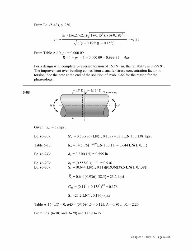
From Eq. (5-43), p. 250,
2 2
2 2
ln (156.2 / 62.1) (1 0.15 ) / (1 0.195 )3.75
ln[(1 0.195 )(1 0.15 )]z
From Table A-10, pf = 0.000 09
R = 1 pf = 1 0.000 09 = 0.999 91 Ans. For a design with completely-reversed torsion of 160 N · m, the reliability is 0.999 91.
The improvement over bending comes from a smaller stress-concentration factor in torsion. See the note at the end of the solution of Prob. 6-66 for the reason for the phraseology.
______________________________________________________________________________ 6-68 Given: Sut = 58 kpsi. Eq. (6-70): Se = 0.506(76) LN(1, 0.138) = 38.5 LN(1, 0.138) kpsi Table 6-13: ka = 14.5(76) 0.719 LN(1, 0.11) = 0.644 LN(1, 0.11) Eq. (6-24): de = 0.370(1.5) = 0.555 in Eq. (6-20): kb = (0.555/0.3)0.107 = 0.936 Eq. (6-70): Se = [0.644 LN(1, 0.11)](0.936)[38.5 LN(1, 0.138)] 0.644 0.936 38.5 23.2 kpsieS
CSe = (0.112 + 0.1382)1/2 = 0.176 Se =23.2 LN(1, 0.176) kpsi Table A-16: d/D = 0, a/D = (3/16)/1.5 = 0.125, A = 0.80 Kt = 2.20. From Eqs. (6-78) and (6-79) and Table 6-15
Chapter 6 - Rev. A, Page 62/66
2.20 (1, 0.10)
1.83 (1, 0.10)2 2.20 1 5 / 76
12.20 0.125
fK
LNLN
Table A-16:
3 33
net
net
(0.80)(1.5 )0.265 in
32 321.5
1.83 (1, 0.10)0.265
10.4 (1, 0.10) kpsi
10.4 kpsi
0.10
f
ADZ
M
Z
C
K LN
LN
Eq. (5-43), p. 250:
2 2
2 2
ln (23.2 /10.4) (1 0.10 ) / (1 0.176 )3.94
ln[(1 0.176 )(1 0.10 )]z
Table A-10: pf = 0.000 041 5 R = 1 pf = 1 0.000 041 5 = 0.999 96 Ans. ______________________________________________________________________________ 6-69 From Prob. 6-68: Se = 23.2 LN(1, 0.138) kpsi ka = 0.644LN(1, 0.11) kb = 0.936 Eq. (6-74): kc = 0.328(76)0.125LN(1, 0.125) = 0.564 LN(1, 0.125) Eq. (6-71): Se = [0.644LN(1, 0.11)](0.936)[ 0.564 LN(1, 0.125)][ 23.2 LN(1, 0.138)] 0.644 0.936 0.564 23.2 7.89 kpsieS
CSe = (0.112 +0.1252 + 0.1383)1/2 = 0.216 Table A-16: d/D = 0, a/D = (3/16)/1.5 = 0.125, A = 0.89, Kts = 1.64 From Eqs. (6-78) and(7-79), and Table 6-15
1.64 (1, 0.10)
1.40 (1, 0.10)2 1.64 1 5 / 76
11.64 3 / 32
f s
LNK LN
Chapter 6 - Rev. A, Page 63/66
Table A-16:
4 44
net
net
(0.89)(1.5 )0.4423 in
32 322(1.5)
1.40[ (1, 0.10)] 4.75 (1, 0.10) kpsi2 2 0.4423
aa f s
ADJ
T D
J
K LN LN
From Eq. (6-57):
2 2
2 2
ln(7.89 / 4.75) (1 0.10 ) / (1 0.216 )2.08
ln[(1 0.10 )(1 0.216 )]z
Table A-10, pf = 0.0188, R = 1 pf = 1 0.0188 = 0.981 Ans. ______________________________________________________________________________ 6-70 This is a very important task for the student to attempt before starting Part 3. It illustrates the drawback of the deterministic factor of safety method. It also identifies the a priori
decisions and their consequences. The range of force fluctuation in Prob. 6-30 is 16 to + 5 kip, or 21 kip. Let the
repeatedly-applied Fa be 10.5 kip. The stochastic properties of this heat of AISI 1018 CD are given in the problem statement.
Function Consequences Axial Fa = 10.5 kip Fatigue load CFa = 0
Ckc = 0.125 Overall reliability R ≥ 0.998;with twin fillets
0.998 0.999R
z = 3.09 CKf = 0.11
Cold rolled or machined surfaces
Cka = 0.058
Ambient temperature Ckd = 0 Use correlation method 0.138C
Stress amplitude CKf = 0.11 C a = 0.11
Significant strength Se 2 2 2 1/2(0.058 0.125 0.138 ) 0.195SeC
Choose the mean design factor which will meet the reliability goal. From Eq. (6-88)
2 2
2
2 2
0.195 0.110.223
1 0.11
exp ( 3.09) ln(1 0.223 ) ln 1 0.223
2.02
nC
n
n
Chapter 6 - Rev. A, Page 64/66
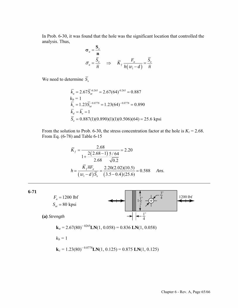
In Prob. 6-30, it was found that the hole was the significant location that controlled the
analysis. Thus,
1
ea
e aa f
S FK
n h d
S
n
weS
n
We need to determine eS
-0.265 -0.2652.67 2.67(64) 0.887a utk S
kb = 1 0.0778 0.07781.23 1.23(64) 0.890c utk S
1d ek k
0.887(1)(0.890)(1)(1)(0.506)(64) 25.6 kpsieS
From the solution to Prob. 6-30, the stress concentration factor at the hole is Kt = 2.68.
From Eq. (6-78) and Table 6-15
1
2.682.20
2 2.68 1 5 / 641
2.68 0.2
2.20(2.02)(10.5)0.588 .
3.5 0.4 (25.6)
f
f a
e
K
K nFh Ans
d S
w
______________________________________________________________________________ 6-71
1200 lbf
80 kpsia
ut
F
S
(a) Strength ka = 2.67(80) 0265LN(1, 0.058) = 0.836 LN(1, 0.058) kb = 1 kc = 1.23(80) 0.0778LN(1, 0.125) = 0.875 LN(1, 0.125)
Chapter 6 - Rev. A, Page 65/66
Chapter 6 - Rev. A, Page 66/66
2 2 2 1/2
0.506(80) (1, 0.138) 40.5 (1, 0.138) kpsi
0.836 (1, 0.058) (1) 0.875 (1, 0.125) 40.5 (1, 0.138)
0.836(1)(0.875)(40.5) 29.6 kpsi
(0.058 0.125 0.138 ) 0.195
e
e
e
Se
S
C
S LN LN
S LN LN LN
Stress: Fig. A-15-1; d/w = 0.75/1.5 = 0.5, Kt = 2.18. From Eqs. (6-78), (6-79) and Table 6-15
2.18 (1, 0.10)
1.96 (1, 0.10)2 2.18 1 5 / 80
12.18 0.375
f
LNK LN
2 2
2 2
2 2
2 2
, 0.10( )
1.96(1.2)12.54 kpsi
( ) (1.5 0.75)(0.25)
29.6 kpsi
ln ( / ) 1 1
ln 1 1
ln 29.6 /12.48 1 0.10 / 1 0.1953.9
ln 1 0.10 1 0.195
aa f
f aa
a e
a a S
S
FC
d t
K F
d t
S S
S C Cz
C C
Kw
w
From Table A-20, pf = 4.81(10 5) R = 1 4.81(10 5) = 0.999 955 Ans. (b) All computer programs will differ in detail. ______________________________________________________________________________ 6-72 to 6-78 Computer programs are very useful for automating specific tasks in the design
process. All computer programs will differ in detail.
Chapter 7 7-1 (a) DE-Gerber, Eq. (7-10):
2 2 2 24 3 4 (2.2)(70) 3 (1.8)(45) 338.4 N mf a fs aA K M K T
2 2 2 24 3 4 (2.2)(55) 3 (1.8)(35) 265.5 N mf m fs mB K M K T
1/31/22
6
6 6
2(265.5) 210 108(2)(338.4)1 1
210 10 338.4 700 10d
d = 25.85 (103) m = 25.85 mm Ans. (b) DE-elliptic, Eq. (7-12) can be shown to be
1/31/3 2 22 2
2 22 26 6
338.4 265.516 16(2)
210 10 560 10e y
n A Bd
S S
d = 25.77 (103) m = 25.77 mm Ans. (c) DE-Soderberg, Eq. (7-14) can be shown to be
1/31/3
6 6
16 16(2) 338.4 265.5
210 10 560 10e y
n A Bd
S S
d = 27.70 (103) m = 27.70 mm Ans. (d) DE-Goodman: Eq. (7-8) can be shown to be
1/31/3
6 6
16 16(2) 338.4 265.5
210 10 700 10e ut
n A Bd
S S
d = 27.27 (103) m = 27.27 mm Ans. ________________________________________________________________________ Criterion d (mm) Compared to DE-Gerber DE-Gerber 25.85 DE-Elliptic 25.77 0.31% Lower Less conservative DE-Soderberg 27.70 7.2% Higher More conservative DE-Goodman 27.27 5.5% Higher More conservative
______________________________________________________________________________ 7-2 This problem has to be done by successive trials, since Se is a function of shaft size. The
material is SAE 2340 for which Sut = 175 kpsi, Sy = 160 kpsi, and HB ≥ 370.
Chapter 7 - Rev. A, Page 1/45
Eq. (6-19), p. 287: 0.2652.70(175) 0.69ak Trial #1: Choose dr = 0.75 in Eq. (6-20), p. 288:
0.1070.879(0.75) 0.91bk
Eq. (6-8), p.282: 0.5 0.5 175 87.5 kpsie utS S Eq. (6-18), p. 287: Se = 0.69 (0.91)(87.5) = 54.9 kpsi 2 0.75 2 / 20 0.65rd d r D D D
0.75
1.15 in0.65 0.65
rdD
1.15
0.058 in20 20
Dr
Fig. A-15-14:
2 0.75 2(0.058) 0.808 inrd d r
0.808
1.080.75r
d
d
0.058
0.0770.75r
r
d
Kt = 1.9 Fig. 6-20, p. 295: r = 0.058 in, q = 0.90 Eq. (6-32), p. 295: Kf = 1 + 0.90 (1.9 – 1) = 1.81 Fig. A-15-15: Kts = 1.5 Fig. 6-21, p. 296: r = 0.058 in, qs = 0.92 Eq. (6-32), p. 295: Kfs = 1 + 0.92 (1.5 – 1) = 1.46 We select the DE-ASME Elliptic failure criteria, Eq. (7-12), with d as dr, and Mm = Ta = 0,
1/31/22 2
3 3
16(2.5) 1.81(600) 1.46(400)4 3
54.9 10 160 10rd
dr = 0.799 in
Trial #2: Choose dr = 0.799 in. 0.1070.879(0.799) 0.90bk
Se = 0.69 (0.90)(0.5)(175) = 54.3 kpsi
0.799
1.23 in0.65 0.65
rdD
r = D / 20 = 1.23/20 = 0.062 in
Chapter 7 - Rev. A, Page 2/45
Figs. A-15-14 and A-15-15:
2 0.799 2(0.062) 0.923 inrd d r
0.923
1.160.799r
d
d
0.062
0.0780.799r
r
d
With these ratios only slightly different from the previous iteration, we are at the limit of readability of the figures. We will keep the same values as before.
1.9, 1.5, 0.90, 0.92t ts sK K q q 1.81, 1.46f fsK K
Using Eq. (7-12) produces dr = 0.802 in. Further iteration produces no change. With dr = 0.802 in,
0.802
1.23 in0.65
0.75(1.23) 0.92 in
D
d
A look at a bearing catalog finds that the next available bore diameter is 0.9375 in. In nominal sizes, we select d = 0.94 in, D = 1.25 in, r = 0.0625 in Ans.
______________________________________________________________________________ 7-3 F cos 20(d / 2) = TA, F = 2 TA / ( d cos 20) = 2(340) / (0.150 cos 20) = 4824 N.
The maximum bending moment will be at point C, with MC = 4824(0.100) = 482.4 N·m. Due to the rotation, the bending is completely reversed, while the torsion is constant. Thus, Ma = 482.4 N·m, Tm = 340 N·m, Mm = Ta = 0.
For sharp fillet radii at the shoulders, from Table 7-1, Kt = 2.7, and Kts = 2.2. Examining Figs. 6-20 and 6-21 (pp. 295 and 296 respectively) with 560 MPa,utS conservatively
estimate q = 0.8 and These estimates can be checked once a specific fillet radius
is determined.
0.9.sq
Eq. (6-32): 1 0.8(2.7 1) 2.4fK
1 0.9(2.2 1) 2.1fsK
(a) We will choose to include fatigue stress concentration factors even for the static analysis to avoid localized yielding.
Eq. (7-15):
1/22 2
max 3 3
32 163f a fs mK M K T
d d
Chapter 7 - Rev. A, Page 3/45
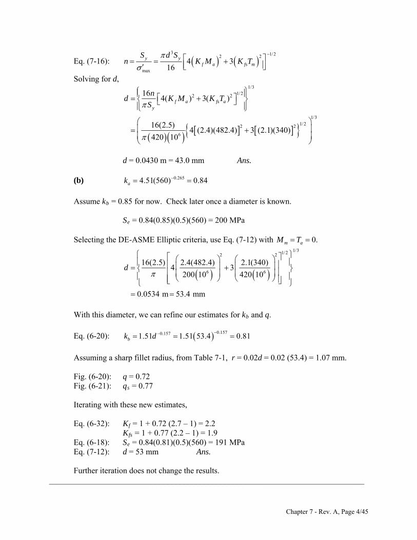
Eq. (7-16): 3 1/22 2
max
4 316
y yf a fs m
S d Sn K M K
T
Solving for d,
1/31/22 2
1/31/22 2
6
164( ) 3( )
16(2.5)4 (2.4)(482.4) 3 (2.1)(340)
420 10
f a fs ay
nd K M K T
S
d = 0.0430 m = 43.0 mm Ans.
(b) 0.2654.51(560) 0.84ak
Assume kb = 0.85 for now. Check later once a diameter is known. Se = 0.84(0.85)(0.5)(560) = 200 MPa
Selecting the DE-ASME Elliptic criteria, use Eq. (7-12) with 0.m aM T
1/31/22 2
6 6
16(2.5) 2.4(482.4) 2.1(340)4 3
200 10 420 10
0.0534 m 53.4 mm
d
With this diameter, we can refine our estimates for kb and q.
Eq. (6-20): 0.1570.1571.51 1.51 53.4 0.81bk d
Assuming a sharp fillet radius, from Table 7-1, r = 0.02d = 0.02 (53.4) = 1.07 mm. Fig. (6-20): q = 0.72 Fig. (6-21): qs = 0.77 Iterating with these new estimates,
Eq. (6-32): Kf = 1 + 0.72 (2.7 – 1) = 2.2 Kfs = 1 + 0.77 (2.2 – 1) = 1.9
Eq. (6-18): Se = 0.84(0.81)(0.5)(560) = 191 MPa Eq. (7-12): d = 53 mm Ans.
Further iteration does not change the results. _____________________________________________________________________________
Chapter 7 - Rev. A, Page 4/45
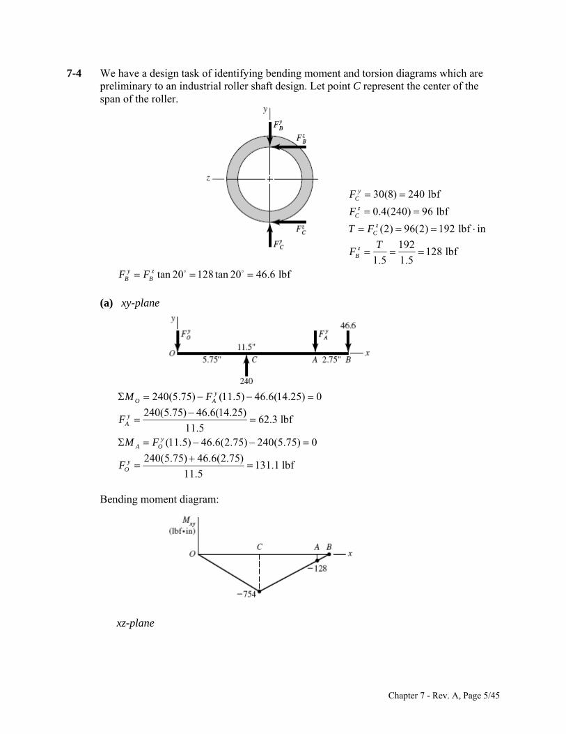
7-4 We have a design task of identifying bending moment and torsion diagrams which are preliminary to an industrial roller shaft design. Let point C represent the center of the span of the roller.
30(8) 240 lbfyCF
0.4(240) 96 lbfzCF
(2) 96(2) 192 lbf inzCT F
192128 lbf
1.5 1.5z
B
TF
tan 20 128 tan 20 46.6 lbfy z
B BF F
(a) xy-plane
240(5.75) (11.5) 46.6(14.25) 0y
O AM F 240(5.75) 46.6(14.25)
62.3 lbf11.5
yAF
(11.5) 46.6(2.75) 240(5.75) 0yA OM F
240(5.75) 46.6(2.75)131.1 lbf
11.5y
OF
Bending moment diagram:
xz-plane
Chapter 7 - Rev. A, Page 5/45
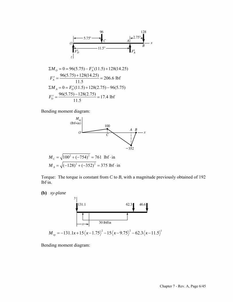
0 96(5.75) (11.5) 128(14.25)zO AM F
96(5.75) 128(14.25)
206.6 lbf11.5
zAF
0 (11.5) 128(2.75) 96(5.75)zA OM F
96(5.75) 128(2.75)17.4 lbf
11.5z
OF
Bending moment diagram:
2 2100 ( 754) 761 lbf inCM
2 2( 128) ( 352) 375 lbf inAM
Torque: The torque is constant from C to B, with a magnitude previously obtained of 192 lbf·in.
(b) xy-plane
2 2
131.1 15 1.75 15 9.75 62.3 11.5xyM x x x x 1
Bending moment diagram:
Chapter 7 - Rev. A, Page 6/45
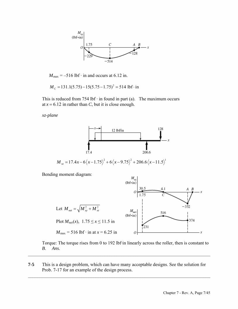
Mmax = –516 lbf · in and occurs at 6.12 in.
2131.1(5.75) 15(5.75 1.75) 514 lbf inCM
This is reduced from 754 lbf · in found in part (a). The maximum occurs at rather than C, but it is close enough. 6.12 inx
xz-plane
2 2
17.4 6 1.75 6 9.75 206.6 11.5xzM x x x x 1
Bending moment diagram:
Let 2 2net xy xzM M M
Plot Mnet(x), 1.75 ≤ x ≤ 11.5 in
Mmax = 516 lbf · in at x = 6.25 in Torque: The torque rises from 0 to 192 lbf·in linearly across the roller, then is constant to B. Ans.
______________________________________________________________________________ 7-5 This is a design problem, which can have many acceptable designs. See the solution for
Prob. 7-17 for an example of the design process. ______________________________________________________________________________
Chapter 7 - Rev. A, Page 7/45
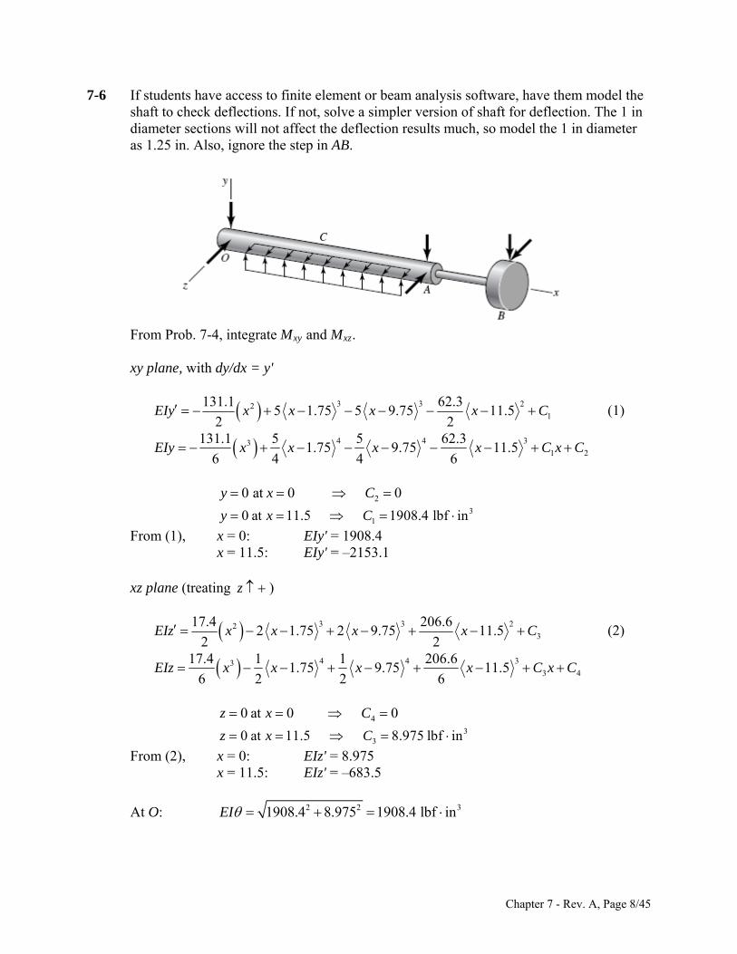
7-6 If students have access to finite element or beam analysis software, have them model the shaft to check deflections. If not, solve a simpler version of shaft for deflection. The 1 in diameter sections will not affect the deflection results much, so model the 1 in diameter as 1.25 in. Also, ignore the step in AB.
From Prob. 7-4, integrate Mxy and Mxz. xy plane, with dy/dx = y'
3 321
131.1 62.35 1.75 5 9.75 11.5
2 2
2EIy x x x x C (1)
4 4 331 2
131.1 5 5 62.31.75 9.75 11.5
6 4 4 6EIy x x x x C x C
20 at 0 0y x C
3
10 at 11.5 1908.4 lbf iny x C From (1), x = 0: EIy' = 1908.4 x = 11.5: EIy' = –2153.1
xz plane (treating ) z
3 323
17.4 206.62 1.75 2 9.75 11.5
2 2
2EIz x x x x C (2)
4 4 333 4
17.4 1 1 206.61.75 9.75 11.5
6 2 2 6EIz x x x x C x C
40 at 0 0z x C
330 at 11.5 8.975 lbf inz x C
From (2), x = 0: EIz' = 8.975 x = 11.5: EIz' = –683.5
At O: 2 21908.4 8.975 1908.4 lbf inEI 3
Chapter 7 - Rev. A, Page 8/45
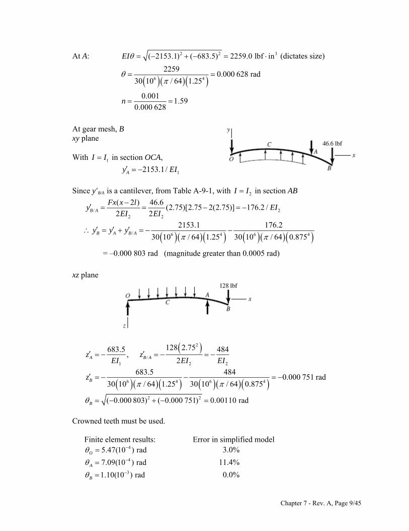
At A: 2 2( 2153.1) ( 683.5) 2259.0 lbf inEI 3 (dictates size)
6 4
22590.000 628 rad
30 10 / 64 1.25
0.001
1.590.000 628
n
At gear mesh, B xy plane
With 1I I in section OCA,
12153.1/Ay EI
Since y'B/A is a cantilever, from Table A-9-1, with 2I I in section AB
/ 22 2
( 2 ) 46.6(2.75)[2.75 2(2.75)] 176.2 /
2 2B A
Fx x ly E
EI EI
I
/ 6 4 6
2153.1 176.2
30 10 / 64 1.25 30 10 / 64 0.875B A B Ay y y
4
= –0.000 803 rad (magnitude greater than 0.0005 rad)
xz plane
2
/1 2
128 2.75683.5 484,
2A B Az z2EI EI
EI
6 4 6 4
683.5 4840.000 751 rad
30 10 / 64 1.25 30 10 / 64 0.875Bz
2 2( 0.000 803) ( 0.000 751) 0.00110 radB
Crowned teeth must be used.
Finite element results: Error in simplified model 45.47(10 ) radO
3.0% 47.09(10 ) radA
11.4% 31.10(10 ) radB
0.0%
Chapter 7 - Rev. A, Page 9/45
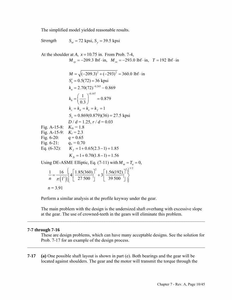
The simplified model yielded reasonable results.
Strength 72 kpsi, 39.5 kpsiut yS S
At the shoulder at A, From Prob. 7-4, 10.75 in.x
209.3 lbf in, 293.0 lbf in, 192 lbf inxy xzM M T
2 2( 209.3) ( 293) 360.0 lbf inM
0.5(72) 36 kpsieS
0.2652.70(72) 0.869ak
0.1071
0.8790.3bk
1c d e fk k k k
0.869(0.879)(36) 27.5 kpsieS D / d = 1.25, r / d = 0.03 Fig. A-15-8: Kts = 1.8 Fig. A-15-9: Kt = 2.3 Fig. 6-20: q = 0.65 Fig. 6-21: qs = 0.70 Eq. (6-32): 1 0.65(2.3 1) 1.85fK
1 0.70(1.8 1) 1.56fsK
Using DE-ASME Elliptic, Eq. (7-11) with 0,m aM T
1/22 2
3
1 16 1.85(360) 1.56(192)4 3
27 500 39 5001n
n = 3.91
Perform a similar analysis at the profile keyway under the gear.
The main problem with the design is the undersized shaft overhang with excessive slope at the gear. The use of crowned-teeth in the gears will eliminate this problem.
______________________________________________________________________________ 7-7 through 7-16
These are design problems, which can have many acceptable designs. See the solution for Prob. 7-17 for an example of the design process.
______________________________________________________________________________ 7-17 (a) One possible shaft layout is shown in part (e). Both bearings and the gear will be
located against shoulders. The gear and the motor will transmit the torque through the
Chapter 7 - Rev. A, Page 10/45
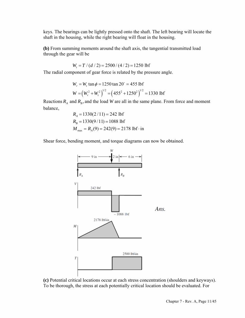
keys. The bearings can be lightly pressed onto the shaft. The left bearing will locate the shaft in the housing, while the right bearing will float in the housing.
(b) From summing moments around the shaft axis, the tangential transmitted load
through the gear will be
/ ( / 2) 2500 / (4 / 2) 1250 lbftW T d The radial component of gear force is related by the pressure angle.
tan 1250 tan 20 455 lbfr tW W
1/2 1/22 2 2 2455 1250 1330 lbfr tW W W
Reactions and ,A BR R and the load W are all in the same plane. From force and moment
balance,
1330(2 /11) 242 lbfAR
1330(9 /11) 1088 lbfBR
max (9) 242(9) 2178 lbf inAM R Shear force, bending moment, and torque diagrams can now be obtained.
(c) Potential critical locations occur at each stress concentration (shoulders and keyways).
To be thorough, the stress at each potentially critical location should be evaluated. For
Chapter 7 - Rev. A, Page 11/45
now, we will choose the most likely critical location, by observation of the loading situation, to be in the keyway for the gear. At this point there is a large stress concentration, a large bending moment, and the torque is present. The other locations either have small bending moments, or no torque. The stress concentration for the keyway is highest at the ends. For simplicity, and to be conservative, we will use the maximum bending moment, even though it will have dropped off a little at the end of the keyway.
(d) At the gear keyway, approximately 9 in from the left end of the shaft, the bending is
completely reversed and the torque is steady.
2178 lbf in 2500 lbf in 0a m mM T M aT
From Table 7-1, estimate stress concentrations for the end-milled keyseat to be Kt = 2.14 and Kts = 3.0. For the relatively low strength steel specified (AISI 1020 CD), roughly estimate notch sensitivities of q = 0.75 and qs = 0.80, obtained by observation of Figs. 6-20 and 6-21, assuming a typical radius at the bottom of the keyseat of r / d = 0.02 (p. 373), and a shaft diameter of up to 3 inches.
Eq. (6-32): 1 0.75(2.14 1) 1.9fK
1 0.8(3.0 1) 2.6fsK
Eq. (6-19): 0.2652.70(68) 0.883ak For estimating , guess 2 in.bk d
Eq. (6-20) 0.107(2 / 0.3) 0.816bk Eq. (6-18) 0.883(0.816)(0.5)(68) 24.5 kpsieS Selecting the DE-Goodman criteria for a conservative first design,
Eq. (7-8):
1/31/2 1/22 2
4 316 f a fs m
e ut
K M K Tnd
S S
1/31/2 1/22 2
4 1.9 2178 3 2.6 250016(1.5)
24 500 68 000d
1.57 in .d A ns
With this diameter, the estimates for notch sensitivity and size factor were conservative, but close enough for a first iteration until deflections are checked. Check yielding with this diameter.
Chapter 7 - Rev. A, Page 12/45
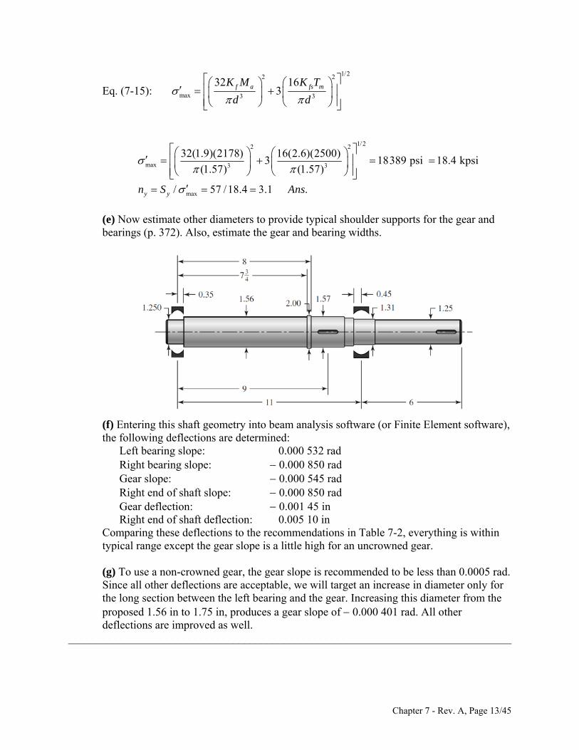
Eq. (7-15):
1/22 2
max 3 3
32 163f a fs mK M K T
d d
1/22 2
max 3 3
32(1.9)(2178) 16(2.6)(2500)3 18389 psi 18.4 kpsi
(1.57) (1.57)
max/ 57 /18.4 3.1 .y yn S Ans
(e) Now estimate other diameters to provide typical shoulder supports for the gear and
bearings (p. 372). Also, estimate the gear and bearing widths.
(f) Entering this shaft geometry into beam analysis software (or Finite Element software),
the following deflections are determined: Left bearing slope: 0.000 532 rad Right bearing slope: 0.000 850 rad Gear slope: 0.000 545 rad Right end of shaft slope: 0.000 850 rad Gear deflection: 0.001 45 in Right end of shaft deflection: 0.005 10 in
Comparing these deflections to the recommendations in Table 7-2, everything is within typical range except the gear slope is a little high for an uncrowned gear.
(g) To use a non-crowned gear, the gear slope is recommended to be less than 0.0005 rad. Since all other deflections are acceptable, we will target an increase in diameter only for the long section between the left bearing and the gear. Increasing this diameter from the proposed 1.56 in to 1.75 in, produces a gear slope of 0.000 401 rad. All other deflections are improved as well.
______________________________________________________________________________
Chapter 7 - Rev. A, Page 13/45
7-18 (a) Use the distortion-energy elliptic failure locus. The torque and moment loadings on the shaft are shown in the solution to Prob. 7-17. Candidate critical locations for strength:
Left seat keyway Right bearing shoulder Right keyway
Table A-20 for 1030 HR: 68 kpsi, 37.5 kpsi, 137ut y BS S H
Eq. (6-8): 0.5(68) 34.0 kpsieS
Eq. (6-19): 0.2652.70(68) 0.883ak 1c d ek k k
Left keyway See Table 7-1 for keyway stress concentration factors,
2.14Profile keyway
3.0t
ts
K
K
For an end-mill profile keyway cutter of 0.010 in radius, estimate notch sensitivities.
Fig. 6-20: 0.51q
Fig. 6-21: 0.57sq
Eq. (6-32): 1 ( 1) 1 0.57(3.0 1) 2.1fs s tsK q K
1 0.51(2.14 1) 1.6fK
Eq. (6-20): 0.107
1.8750.822
0.30bk
Eq. (6-18): 0.883(0.822)(34.0) 24.7 kpsieS
Eq. (7-11):
12 2 2
3
1 16 1.6(2178) 2.1(2500)4 3
(1.875 ) 24 700 37 500fn
nf = 3.5 Ans.
Right bearing shoulder
The text does not give minimum and maximum shoulder diameters for 03-series bearings (roller). Use D = 1.75 in.
0.030 1.750.019, 1.11
1.574 1.574
r D
d d
Fig. A-15-9: 2.4tK
Fig. A-15-8: 1.6tsK
Chapter 7 - Rev. A, Page 14/45
Fig. 6-20: 0.65q Fig. 6-21: 0.70sq
Eq. (6-32): 1 0.65(2.4 1) 1.91fK
1 0.70(1.6 1) 1.42fsK
0.453
2178 493 lbf in2
M
Eq. (7-11):
1/22 2
3
1 16 1.91(493) 1.42(2500)4 3
(1.574 ) 24 700 37 500fn
nf = 4.2 Ans. Right keyway
Use the same stress concentration factors as for the left keyway. There is no bending moment, thus Eq. (7-11) reduces to:
3 3
16 31 16 3(2.1)(2500)
1.5 (37 500)fs m
f y
K T
n d S
nf = 2.7 Ans. Yielding
Check for yielding at the left keyway, where the completely reversed bending is maximum, and the steady torque is present. Using Eq. (7-15), with Mm = Ta = 0,
1/22 2
max 3 3
1/22 2
3 3
32 163
32 1.6 2178 16 2.1 25003
1.875 1.875
8791 psi 8.79 kpsi
f a fs mK M K T
d d
max
37.54.3
8.79y
y
Sn
Ans.
Check in smaller diameter at right end of shaft where only steady torsion exists.
1/22
max 3
1/22
3
163
16 2.1 25003
1.5
13 722 psi 13.7 kpsi
fs mK T
d
Chapter 7 - Rev. A, Page 15/45
max
37.52.7
13.7y
y
Sn
Ans.
(b) One could take pains to model this shaft exactly, using finite element software.
However, for the bearings and the gear, the shaft is basically of uniform diameter, 1.875 in. The reductions in diameter at the bearings will change the results insignificantly. Use E = 30 Mpsi for steel.
To the left of the load, from Table A-9, case 6, p. 1015,
2 2 22 2 2
6 4
6 2
1449(2)(3 2 11 )(3 )
6 6(30)(10 )( / 64)(1.875 )(11)
2.4124(10 )(3 117)
ABAB
d y Fb xx b l
dx EIl
x
At x = 0 in: 42.823(10 ) rad At x = 9 in: 43.040(10 ) rad To the right of the load, from Table A-9, case 6, p. 1015,
2 23 6 26
BCBC
d y Fa 2x xl l adx EIl
At x = l = 11 in:
2 2
2 2 46 4
1449(9)(11 9 )4.342(10 ) rad
6 6(30)(10 )( / 64)(1.875 )(11)
Fal a
EIl
Obtain allowable slopes from Table 7-2.
Left bearing:
Allowable slope 0.0013.5 .
Actual slope 0.000 282 3fsn Ans
Right bearing:
0.00081.8 .
0.000 434 2fsn Ans
Gear mesh slope:
Table 7-2 recommends a minimum relative slope of 0.0005 rad. While we don’t know the slope on the next shaft, we know that it will need to have a larger diameter and be stiffer. At the moment we can say
0.00051.6 .
0.000 304fsn Ans
______________________________________________________________________________
Chapter 7 - Rev. A, Page 16/45
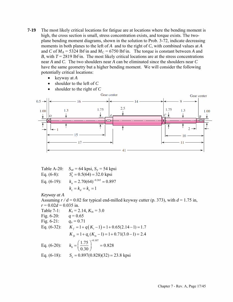
7-19 The most likely critical locations for fatigue are at locations where the bending moment is high, the cross section is small, stress concentration exists, and torque exists. The two-plane bending moment diagrams, shown in the solution to Prob. 3-72, indicate decreasing moments in both planes to the left of A and to the right of C, with combined values at A and C of MA = 5324 lbf·in and MC = 6750 lbf·in. The torque is constant between A and B, with T = 2819 lbf·in. The most likely critical locations are at the stress concentrations near A and C. The two shoulders near A can be eliminated since the shoulders near C have the same geometry but a higher bending moment. We will consider the following potentially critical locations:
keyway at A shoulder to the left of C shoulder to the right of C
Table A-20: Sut = 64 kpsi, Sy = 54 kpsi Eq. (6-8): 0.5(64) 32.0 kpsieS
Eq. (6-19): 0.2652.70(64) 0.897ak 1c d ek k k Keyway at A Assuming r / d = 0.02 for typical end-milled keyway cutter (p. 373), with d = 1.75 in, r = 0.02d = 0.035 in. Table 7-1: Kt = 2.14, Kts = 3.0 Fig. 6-20: q = 0.65 Fig. 6-21: qs = 0.71 Eq. (6-32):
1 1 1 0.65(2.14 1) 1.7f tK q K
1 ( 1) 1 0.71(3.0 1) 2.4fs s tsK q K
Eq. (6-20): 0.107
1.750.828
0.30bk
Eq. (6-18): 0.897(0.828)(32) 23.8 kpsieS
Chapter 7 - Rev. A, Page 17/45
We will choose the DE-Gerber criteria since this is an analysis problem in which we would like to evaluate typical expectations.
sing Eq. (7-9) with M = T = 0,
U m a
2 2
2 2
4 4 1.7 5324 18102 lbf in 18.10 kip in
3 3 2.4 2819 11 718 lbf in 11.72 kip in
f a
fs m
A K M
B K T
1/22
3
1/22
3
21 81 1
8 18.10 2 11.72 23.81 1
18.10 6475 .8
e
e ut
BSA
n d S AS
1. 23
oulder to the left of C 625 / 1.75 = 0.036, D / d = 2.5 / 1.75 = 1.43
: :
q = 0.71 Fig. 6-21: q = 0.76
q. (6-32):
n = 1.3
Sh r / d = 0.0 Fig. A-15-9 Kt = 2.2 Fig. A-15-8 Kts = 1.8 Fig. 6-20:
Es
1 1 1 0.71(2.2 1) 1.9f tK q K
1 ( 1) 1 .76(1.8 1) 1.6fs s tsK q K
00.107
1.750.828
0.30bk
Eq. (6-20):
Eq. (6-18): 0.897(0.828)(32) 23.8 kpsieS
For convenience, we will use the full value of the bending moment at C, even though it will be slightly less at the shoulder. Using Eq. (7-9) with Mm = Ta = 0,
2 2
2 2
4 4 1.9 6750 25 650 lbf in 25.65 kip in
3 3 1.6 2819 7812 lbf in 7.812 kip in
f a
fs m
A K M
B K T
1/22
3
1/22
21 81 1
8 25.65 2 7.812 23.81 1
25.65 643.8
e
e ut
BSA
n d S AS
31.75 2
Chapter 7 - Rev. A, Page 18/45
n = 0.96
oulder to the right of C 625 / 1.3 = 0.048, D / d = 1.75 / 1.3 = 1.35
: :
q = 0.71 Fig. 6-21: qs = 0.76
q. (6-32):
Sh r / d = 0.0 Fig. A-15-9 Kt = 2.0 Fig. A-15-8 Kts = 1.7 Fig. 6-20:
E 1 1 1 0.71(2.0 1) 1.7f tK q K
1 ( 1) 1 .76(1.7 1) 1.5fs s tsK q K
00.107
1.30.855Eq. (6-20):
0.30 Eq. (6-18): 0.897(0.855)(32) 24.5 kpsieS
bk
or convenience, we will use the full value of the bending moment at C, even though it will be slightly less at the shoulder. Using Eq. (7-9) with Mm = Ta = 0,
F
2 2
2 2
4 4 1.7 6750 22 950 lbf in 22.95 kip in
3 3 1.5 2819 7324 lbf in 7.324 kip in
f a
fs m
A K M
B K T
1/22
3
1/22
21 81 1
8 22.95 2 7.324 24.51 1
22.95 6424.5
e
e ut
BSA
n d S AS
31.3
The critical location is at the shoulder to the right of C, where n = 0.45 and finite life is
plicitly called for in the problem statement, a static check for yielding is
especially warranted with such a low fatigue factor of safety. Using Eq. (7-15), with Mm = Ta = 0,
n = 0.45
predicted. Ans.
Though not ex
1/22 2
max 3 3
1/22 2
3 3
32 163
32 1.7 6750 16 1.5 28193 55 845 psi 55.8 kpsi
1.3
f a fs mK M K T
d d
1.3
Chapter 7 - Rev. A, Page 19/45
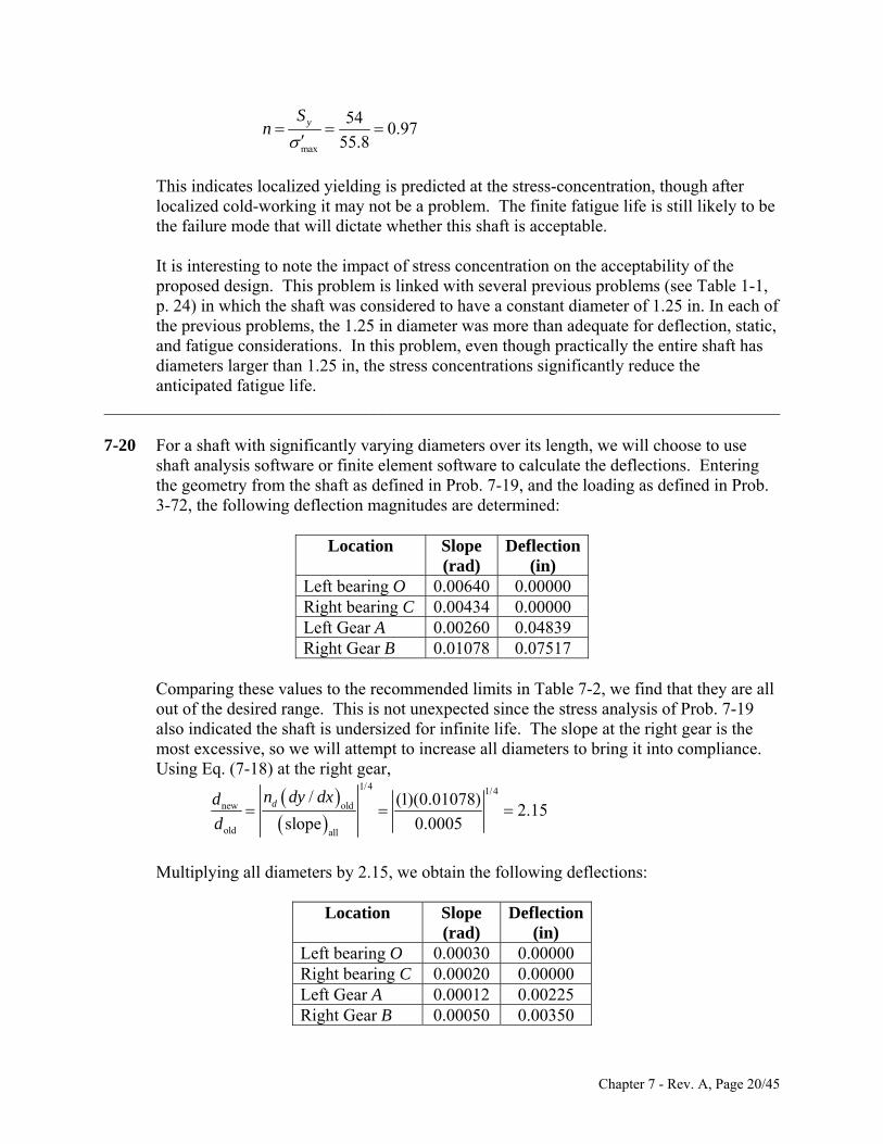
max
0.9755.8
yn
his indicates localized yielding is predicted at the stress-concentr
54S
ation, though after o be
f static,
7-20
te the deflections. Entering the geometry from the shaft as defined in - loading as defined in Prob. 3-72, the following defle itude te
D
Tlocalized cold-working it may not be a problem. The finite fatigue life is still likely tthe failure mode that will dictate whether this shaft is acceptable. It is interesting to note the impact of stress concentration on the acceptability of the proposed design. This problem is linked with several previous problems (see Table 1-1, p. 24) in which the shaft was considered to have a constant diameter of 1.25 in. In each othe previous problems, the 1.25 in diameter was more than adequate for deflection, and fatigue considerations. In this problem, even though practically the entire shaft has diameters larger than 1.25 in, the stress concentrations significantly reduce the anticipated fatigue life.
______________________________________________________________________________
For a shaft with significantly varying diameters over its length, we will choose to use shaft analysis software or finite element software to calcula
Prob. 7e
19, and the rmined: ction magn s are d
Location Slope (rad)
eflection(in)
Left bearing O 0.00640 0.00000 Right bearing C 0.00434 0.00000 Left Gear A 0.00260 0.04839 Right Gear B 0.01078 0.07517
Comparing these values to the recommended limits in Table 7-2, we find that they are allout of the desired range. This is not unexpected since the stress analysis of Prob. 7-19 also indicated the shaft is undersized for infinite life. The sl
ope at the right gear is the ost excessive, so we will attempt to increase all diameters to bring it into compliance. sing Eq. (7-18) at the right gear,
mU
1/4 1/4
new old
old all
2.15slope 0.0005d
/ (1)(0.01078)dn dy dxd
Multiplying all diameter e ob fo lections:
D
s by 2.15, w tain the llowing def
Location Slope (rad)
eflection(in)
Left bearing O 0.00030 0.00000 Right bearing C 0.00020 0.00000 Left Gear A 0.00012 0.00225 Right Gear B 0.00050 0.00350
Chapter 7 - Rev. A, Page 20/45
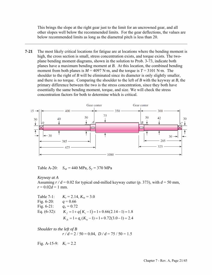
This brings the slope at the right gear just to the limit for an uncrowned gear, and all other slopes well below the recommended limits. For the gear deflections, the values are
______________________________________________________________________________ 7-21 is
o-
with the keyway at B, the rimary difference between the two is the stress concentration, since they both have
eyway at A d-milled keyway cutter (p. 373), with d = 50 mm,
Kt = 2.14, Kts = 3.0 Fig. 6-20: q = 0.66
ig. 6-21: qs = 0.72
e50 = 0.04, D / d = 75 / 50 = 1.5
:
below recommended limits as long as the diametral pitch is less than 20.
The most likely critical locations for fatigue are at locations where the bending moment high, the cross section is small, stress concentration exists, and torque exists. The twplane bending moment diagrams, shown in the solution to Prob. 3-73, indicate both planes have a maximum bending moment at B. At this location, the combined bending moment from both planes is M = 4097 N·m, and the torque is T = 3101 N·m. The shoulder to the right of B will be eliminated since its diameter is only slightly smaller, and there is no torque. Comparing the shoulder to the left of Bpessentially the same bending moment, torque, and size. We will check the stress concentration factors for both to determine which is critical.
Table A-20: Sut = 440 MPa, Sy = 370 MPa KAssuming r / d = 0.02 for typical enr = 0.02d = 1 mm. Table 7-1:
FEq. (6-32): 1fK q 1 1 0.66(2.14 1) 1.8tK
1 ( 1) 1 0.72(3.0 1) 2.4fs s tsK q K
Shoulder to th left of B r / d = 2 / Fig. A-15-9 Kt = 2.2
Chapter 7 - Rev. A, Page 21/45
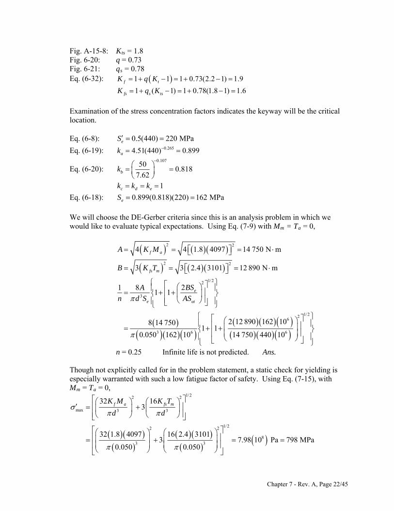
Fig. A-15-8:
F
Kts = 1.8 Fig. 6-20: q = 0.73
ig. 6-21: q = 0.78
n of the stress concentration f ctors indicates the keyway will be the critical
Eq. (6-19):
s
1 1 1 0.73(2.2 1) 1.9
fs s tsK q K
Eq. (6-32): f tK q K
1 ( 1) 1 0.78(1.8 1) 1.6
Examinatio alocation.
0.5(440) 220 MPaeS Eq. (6-8): 0.2654.51(440) 0.899ak
0.107
Eq. (6-20): 50
0.8187.62bk
We will choose the DE-Gerber criteria since this is an analysis problem in which we ould like to evaluate typical expectations. Using Eq. (7-9) with Mm a = 0,
1c d ek k k
Eq. (6-18): 0.899(0.818)(220) 162 MPaeS
w = T
2 2
2 2
4 4 1.8 4097 14 750 N m
3 3 2.4 3101 12 890 N m
f a
fs m
A K M
B K T
1/22
3
1/226
3 6 6
21 81 1
08 14
0.050 162 10 14 750 440 10
e
e ut
BSA
n d S AS
2 12 890 162 17501 1
n = 0.25 Infinite life is not predicted. Ans.
Though not explicitly called for in the problem statement, a static check for yielding is especially warranted with such a low fatigue factor of safety. Using Eq. (7-15), with Mm = Ta = 0,
1/22 2
max 3 3
1/22 2
83 3
32 163
32 1.8 4097 16 2.4 31013 7.98 10 Pa 798 MPa
050 0.050
f a fs mK M K T
d d
0.
Chapter 7 - Rev. A, Page 22/45
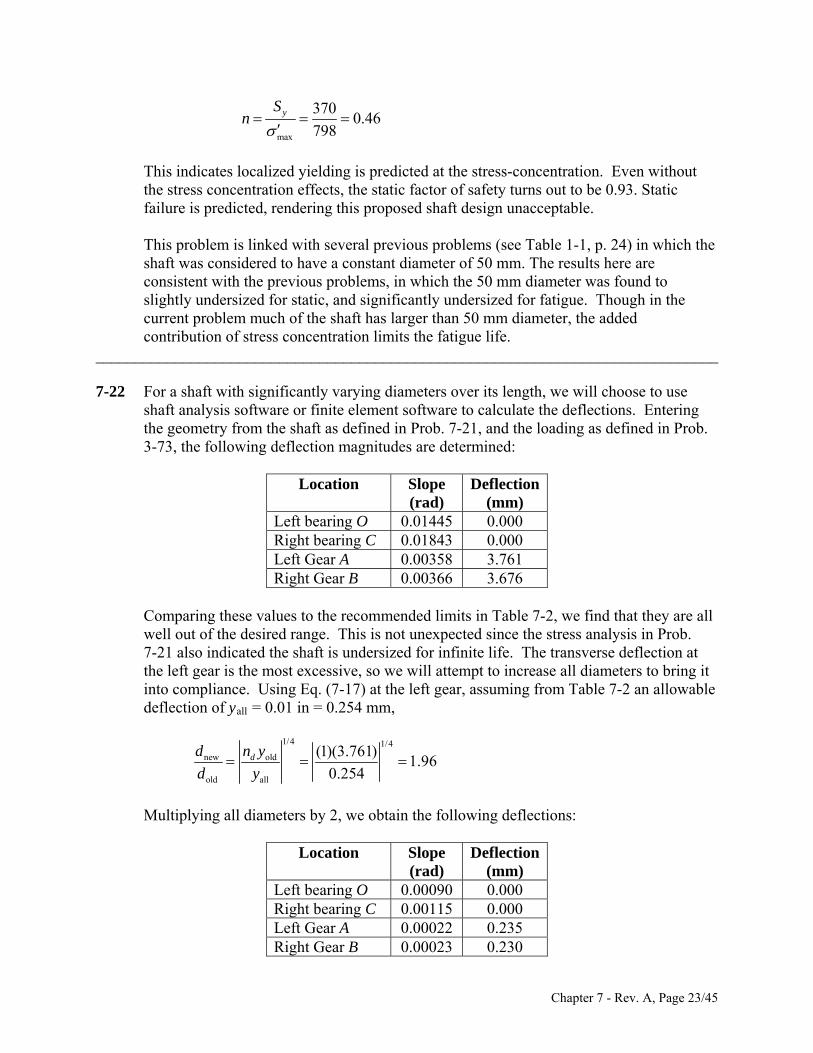
max
3700.46
798yS
n
This indicates localized yielding is predicted at the stress-concentration. Even without the stress concentration effects, the static factor of safety turns out to be 0.93. Static failure is predicted, rendering this proposed shaft design unacceptable. This problem is linked with several previous problems (see Table 1-1, p. 24) in which shaft was considered to have a constant diameter of 50 mm. The results here ar
the e
______________________________________________________________________________ -22 th, we will choose to use
shaft analysis software o ment s t e deflections. Entering the geometry from the shaft as defined in -2 ading as defined in Prob. 3-73, the following itud erm
De n
consistent with the previous problems, in which the 50 mm diameter was found to slightly undersized for static, and significantly undersized for fatigue. Though in the current problem much of the shaft has larger than 50 mm diameter, the added contribution of stress concentration limits the fatigue life.
For a shaft with significantly varying diameters over its leng7r finite ele oftware
7o calculate th1, and the lo
iProb.
deflection magn es are det ned:
Location Slope (rad)
flectio(mm)
Left bearing O 0.01445 0.000 Right bearing C 0.01843 0.000 Left Gear A 0.00358 3.761 Right Gear B 0.00366 3.676
Comparing these values to the recommended limits in Table 7-2, we find that they are all well out of the desired range. This is not unexpected since the stress analysis in Prob. -21 also indicated the shaft is undersize7
the lefd for infinite life. The transverse deflection at
t gear is the most excessive, so we will attempt to increase all diameters to bring it to compliance. Using Eq. (7-17) at the left gear, assuming from Table 7-2 an allowable
yall = 0.01 in = 0.254 mm, indeflection of
1/4 1/4
new old (1)(3.761)1.96dd n y
old alld y
Multiplying all diam btai wi :
De n
0.254
eters by 2, we o n the follo ng deflections
Location Slope (rad)
flectio(mm)
Left bearing O 0.00090 0.000 Right bearing C 0.00115 0.000 Left Gear A 0.00022 0.235 Right Gear B 0.00023 0.230
Chapter 7 - Rev. A, Page 23/45
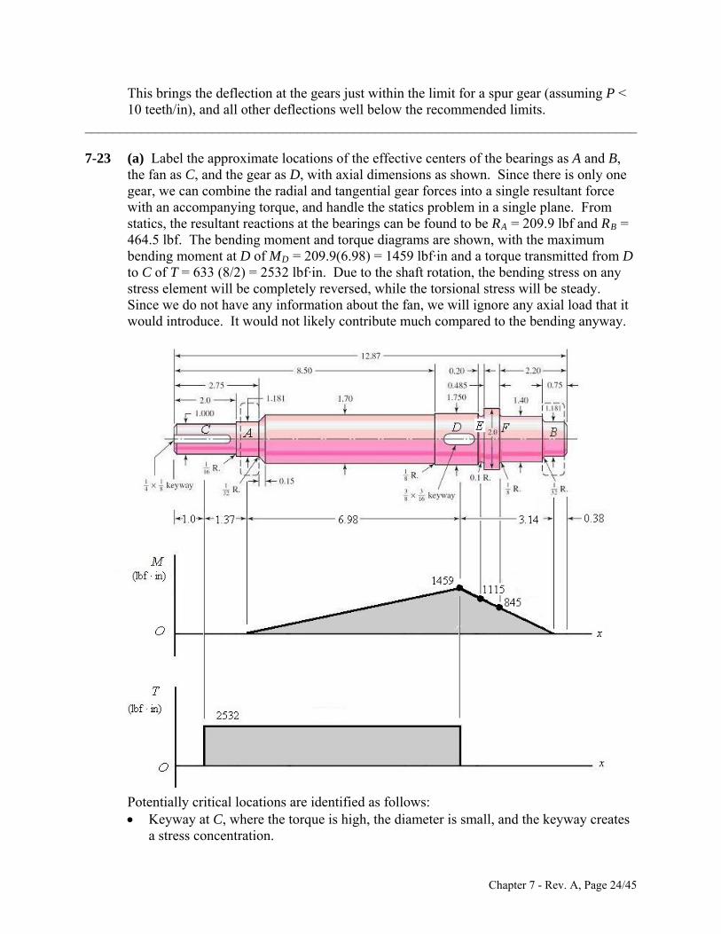
This brings the deflection at the gears just within the limit for a spur gear (assuming P <
______________________________________________________________________________ 7-23 ,
stress element will be completely reversed, while the torsional stress will be steady. Since we do not have any information about the fan, we will ignore any axial load that it would introduce. It would not likely contribute much compared to the bending anyway.
10 teeth/in), and all other deflections well below the recommended limits.
(a) Label the approximate locations of the effective centers of the bearings as A and Bthe fan as C, and the gear as D, with axial dimensions as shown. Since there is only one gear, we can combine the radial and tangential gear forces into a single resultant forcewith an accompanying torque, and handle the statics problem in a single plane. From statics, the resultant reactions at the bearings can be found to be RA = 209.9 lbf and RB =464.5 lbf. The bending moment and torque diagrams are shown, with the maximum bending moment at D of MD = 209.9(6.98) = 1459 lbf·in and a torque transmitted from D to C of T = 633 (8/2) = 2532 lbf·in. Due to the shaft rotation, the bending stress on any
Potentially critical locations are identified as follows: Keyway at C, where the torque is high, the diameter is small, and the keyway creates
a stress concentration.
Chapter 7 - Rev. A, Page 24/45
Keyway at D, where the bending moment is maximum, the torque is high, and thekeyway creates a stress concentration.
. eter is smaller than at D or E, the bending moment is
The shoulder to the left of D can be eliminated since the change in diameter is very ill undoubtedly be much less than at D.
Sut = 68 kpsi, Sy = 57 kpsi
ince there is only steady torsion here, only a static check needs to be performed. We’ll aximum shear stress theory.
Groove at E, where the diameter is smaller than at D, the bending moment is still high, and the groove creates a stress concentration. There is no torque here, though
Shoulder at F, where the diamstill moderate, and the shoulder creates a stress concentration. There is no torque here, though.
slight, so that the stress concentration w
Table A-20: q. (6-8): 0.5(68) 34.0 kpsieS E
0.2652.70(68) 0.883ak Eq. (6-19):
Keyway at C Suse the m
4
2532 1.00 / 212.9 kpsi
1.00 / 32
Tr
J
/ 2 57 / 22.21
12.9y
y
SnEq. (5-3):
ssuming r / d = 0.02 for typical end-milled keyway cutter (p. 373), with d = 1.75 in,
Kts = 3.0 q = 0.66
Fig. 6-21: qs = 0.72 q. (6-32):
A
Keyway at D
r = 0.02d = 0.035 in. Table 7-1: Kt = 2.14, Fig. 6-20:
E 1 1 1 0.66(2.14 1) 1.8f tK q K
1 ( 1) 1 .72(3.0 1) 2.4fs s tsK q K
00.107
1.750.828
0.30bk
Eq. (6-20):
Eq. (6-18): 0.883(0.828)(34.0) 24.9 kpsieS
We will choose the DE-Gerber criteria since this is an analysis problem in which we
ould like to evaluate typical expectations. Using Eq. (7-9) with Mm = Ta = 0, w
Chapter 7 - Rev. A, Page 25/45
2 2
2 2
4 4 1.8 1459 5252 lbf in 5.252 kip in
3 3 2.4 2532 10 525 lbf in 10.53 kip in
f a
fs m
A K M
B K T
1/22
3
1/22
3
21 81 1
8 5.252 2 10.53 24.91 1
5.252 681.75 24.9
e
e ut
BSA
n d S AS
n = 3.59 Ans.
roove at E he right of the
w and will likely not allow the stress flow to fully develop. (See the concept.)
r / d = 0.1 / 1.55 = 0.065, D / d = 1.75 / 1.55 = 1.13 : Kt = 2.1
Fig. 6-20: q = 0.76
GWe will assume Figs. A-15-14 is applicable since the 2 in diameter to tgroove is relatively narroFig.7-9 for stress flow
Fig. A-15-14
Eq. (6-32): ) 1 1 1 0.76(2.1 1 1.8f tK q K 0.107
1.550.839
0.30bk Eq. (6-20):
Using Eq. (7-9) with Mm = Ta = Tm = 0,
0.883(0.839)(34) 25.2 kpsieS Eq. (6-18):
2 24 4 1.8 1115 4122 lbf in 4.122 kip inf aA K M
B = 0
1/22
3
1/22
31.55 25.2
21 81 1
8 4.1221 1 0
e
e u
BSA
A
tn d S S
Ans.
F r / d = 0.125 / 1.40 = 0.089, D / d = 2.0 / 1.40 = 1.43
Kt = 1.7 Fig. 6-20: q = 0.78
n = 4.47 Shoulder at
Fig. A-15-9:
Chapter 7 - Rev. A, Page 26/45
Eq. (6-32): ) 1 1 1 0.78(1.7 1 1.5f tK q K 0.107
1.400.848
0.30bk
Eq. (6-20):
Eq. (6-18):
Using Eq. (7-9) with Mm = Ta = Tm = 0,
0.883(0.848)(34) 25.5 kpsieS
2 24 4 1.5 845 2535 lbf in 2.535 kip inf aA K M
B = 0
1/22
3
2.531 1 0
1.40 25.5
1/22
3
21 81 1 e
e ut
BSA
AS
n d S
8 5
n = 5.42 Ans.
(b) The deflection will not be much affected by the details of fillet radii, grooves, and keyways, so these can be A gnarrow 2.0 in diameter section, can be cted. ill model the shaft with the following three sections:
Section Diameter
(in) Length
(in)
ignored. lso, the sli ht diameter changes, as well as the
negle We w
1 1.00 2.90 2 1.70 7.77 3 1.40 2.20
The deflection problem can readily (though tediously) be solved with singularity functions. For example -7, p. the solution to Prob. 7-24. Alternatively, shaft analysis software or finite element software may be used. Using any of the methods, the results low
ation D
s, see Ex. 4 159, or
should be as fol s:
Loc Slope (rad)
eflection(in)
Left bearing A 0.000290 0.000000 Right bearing B 0.000400 0.000000 Fan C 0.000290 0.000404 Gear D 0.000146 0.000928
Chapter 7 - Rev. A, Page 27/45
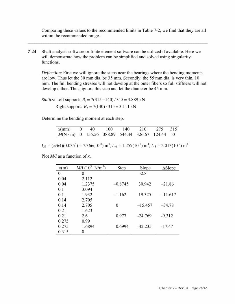
Comparing these values to the recommended limits in Table 7-2, we find that theywithin the r
are all ecommended range.
______________________________________________________________________________ 7-24
ill ignore the steps near the bearings where the bending moments w mm dia. be 35 mm. Secondly, the 55 mm dia. is very thin, 10 Th tresses will not develop at the outer fibers so full stiffness will not
iameter be 45 mm.
tatics: L ort
R r
100 140 210 275 315
Shaft analysis software or finite element software can be utilized if available. Here we will demonstrate how the problem can be simplified and solved using singularity functions. Deflection: First we ware lo . Thus let the 30mm. e full bending sdevelop either. Thus, ignore this step and let the d S eft supp : R1 15 140) / 315 889 7(3 3. kN
ight suppo t: 2 7(14 0R ) / 315 3.111 kN
Determine the bending moment at each step.
x(mm) 0 40M(N · m) 0 155.56 388.89 544.44 326.67 124.44 0
I35 = (/64)(0.0354) = 366(10 ) m4, I 0 = 1.257(1 , I45 = 2. -7) m4
Plot M/I nction
) M N/m3) Step
7. -84 0-7) m4 013(10
as a fu of x.
x(m /I (109 Slope Slope 0 0 52.8 0.04 2.112 0.04 1.2375 0.8745 21.86
4 1.162 11.617
05 0 15.457 34.78 0.21 1.623 0.21 2.6 0.977 -24.769 -9.312 0.275 0.99 0.275 1.6894 0.6994 -42.235 -17.47 0.315 0
– 30.942 –0.1 3.09 0.1 1.932 – 19.325 –0.14 2.705 0.14 2.7 – –
Chapter 7 - Rev. A, Page 28/45
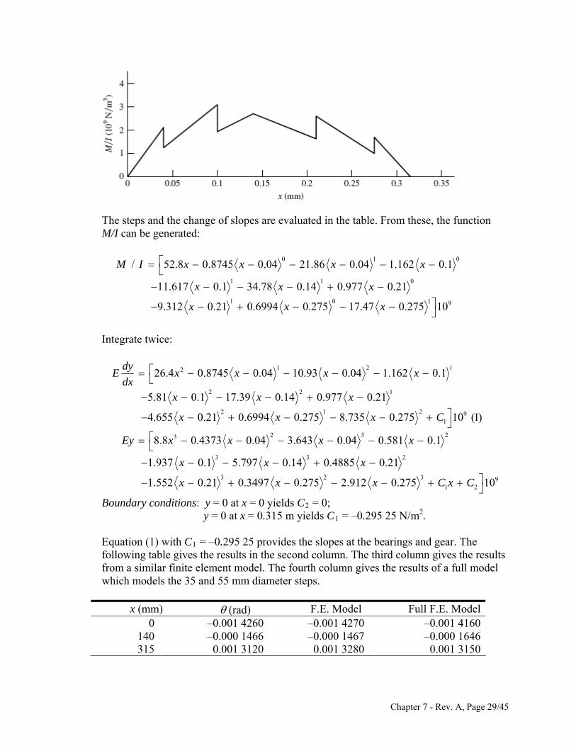
The steps and the change of slopes are evaluated in the table. From these, the function M/I can be generated:
0 1
1 1 0
1 0 9
/ 52.8 0.8745 0.04 21.86 0.04 1.162 0.1
11.617 0.1 34.78 0.14 0.977 0.21
9.312 0.21 0.6994 0.275 17.47 0.275 10
M I x x x x
x x x
x x x
0
1
Integrate twice:
1 2226.4 0.8745 0.04 10.93 0.04 1.162x x x x 1
3 2
0.1
0.04 0.581 0.1
7
Edx
x
x
dy
2 2 1
2 1 2 91
23
5.81 0.1 17.39 0.14 0.977 0.21
4.655 0.21 0.6994 0.275 8.735 0.275 10 (1)
8.8 0.4373 0.04 3.643
x x x
x x x C
Ey x x x
1.93 3 3 2
3 9
0.1 0.14 0.21
52 0. 0.2 0.275 10
x
x x x
Boundary conditions: y yields C2 y = 0 at x = 0.315 m yields C1 = –0.295 25 N/m2.
3 2 1 2C x C
5.797 0.4885 x
1.5 21 0.3497 75 2.912
= 0 at x = 0 = 0;
Equation (1) with C1 = –0.295 25 provides the slopes at the bearings and gear. The following table gives the results in the second column. The third column gives the resultsfrom a similar finite element model. The fourth column gives the results of a full model which models the 35 and 55 mm diameter steps.
x (mm) (rad) F.E. Model Full F.E. Model0 –0.001 4260 –0.001 4270 –0.001 4160
140 –0.000 1466 –0.000 1467 –0.000 1646315 0.001 3120 0.001 3280 0.001 3150
Chapter 7 - Rev. A, Page 29/45
The main discrepancy between the results is at the gear location (x = 140 mm). The larger value in the full model is caused by the stiffer 55 mm diameter step. As was stated arlier, this step is not as stiff as modeling implicates, so the exact answer is somewhere
between the full model and the simplified model which in any event is a small value. As xpected, modeling the 30 mm dia. as 35 mm does not affect the results much.
can be seen that the allowable slopes at the bearings are exceeded. Thus, either the load
ed or the shaft “beefed” up. If the allowable slope is 0.001 rad, then the aximum load should be Fmax = (0.001/0.001 426)7 = 4.91 kN. With a design factor this
would be reduced further. To increase the stiffness of th , E 8 f deflection (at = 0) to determine a multiplier to be used for all diameters.
e
e
Ithas to be reducm
e shaft apply q. (7-1 ) to the most o fendingx
1/4 1/4
new old
old
/ (1)(0.0014260)1.093
n dy dxd
d
orm a table:
allslope 0.001
d
F
Old d, mm 20.00 30.00 35.00 40.00 45.00 55.00 New ideal d, mm 21.86 32.79 38.26 43.72 49.19 60.12 Rounded up d, mm 22.00 34.00 40.00 44.00 50.00 62.00
Repeating the full finite element mo lts in del resu
x 940 : –1 1
5 .
stress concentrations and reduced shaft diameters, there are a number of at. A table of nominal stresses is given below. Note that torsion is only
f the 7 kN load. Using = 32 (d3) and = 16T/(d3),
0 275 300 330
= 0: = – .30 10-4 rad
x = 1 mm = .09 0-4 rad-4x = 31 mm: = 8 65 10 rad
This is well within our goal. Have the students try a goal of 0.0005 rad at the gears.
Strength: Due to looklocations to
to the right o M/
x (mm) 15 40 100 110 140 210 (MPa) 0 39.6 17.6 0
0 6 8.5 12.7 20.2 68.122.0 37.0 61.9 47.8 60.9 52.0
(MPa) 0 0 0 0 (MPa) 0 22.0 37.0 61.9 47.8 61.8 53.1 45.3 39.2 118.0
for Sy = 390 MPa
Eq. (6-19):
Table A-20 AISI 1020 CD steel: Sut = 470 MPa,
At x = 210 mm: 0.2654.51(470) 0.883ak
Chapter 7 - Rev. A, Page 30/45
Eq. (6-20): 0.107(40 / 7.62) 0.837bk
Eq. (6-18): Se = 0.883 (0.837)(0.5)(470) = 174 MPa D / d = 45 / 40 = 1.125, r / d = 2 / 40 = 0.05 Fig. A-15-8: Kts = 1.4 Fig. A-15-9: Kt = 1.9 Fig q = 0.75 Fig qs = 0.79
= 1 + 0.75(1.9 –1) = 1.68
ld check, from Eq. (7-11), with
. 6-20:
. 6-21: Eq. (6-32): Kf
K f s = 1 + 0.79(1.4 – 1) = 1.32
Choosing DE-ASME Elliptic to inherently include the yieMm = Ta = 0,
1/22 2
6
1.32(107)3
390 103 6
1.68(326.67)4
0.04 174 10n
1 16
At
The von Mises stress is the highest but it comes from the steady torque only.
Fig. 6-21: qs = 0.79 .42 – 1) = 1.33
1.98n
x = 330 mm:
D / d = 30 / 20 = 1.5, r / d = 2 / 20 = 0.1 Fig. A-15-9: Kts = 1.42
Eq. (6-32): Kf s = 1 + 0.79(1Eq. (7-11):
1 16 1.33(107)
3 6390 10n 3
n = 2.49
Note that since there is only a steady torque, Eq. (7-11) reduces to essentially the equivalent of the distortion energy failure theory.
s at x = 210 mm, the changes discussed for the slope criterion will
______________________________________________________________________________
7-2 se design tasks each student will travel different paths and almost all
The student gets a blank piece of paper, a statement of function, and some constraints
Check the other locations.
If worse-case i improve the strength issue.
5 and 7-26 With the
details will differ. The important points are
– explicit and implied. At this point in the course, this is a good experience. It is a good preparation for the capstone design course.
Chapter 7 - Rev. A, Page 31/45
The adequacy of their design must be demonstrated and possibly include a designer’s notebook.
Many of the fundaments of the course, based on this text and this course, are useful. .
Don’t let the students create a time sink for themselves. Tell them how far you want
______________________________________________________________________________ 7-27 oblem. This problem is a learning experience.
ollowing the task statement, the following guidance was added.
ting the temptation of putting pencil to paper, and decide what the problem really is.
ld implement it.
The students’ initial reaction is that he/she does not know much from the problem lowly the realization sets in that they do know some important things
that the designer did not. They knew how it failed, where it failed, and that the design wasn’t good enough; it was close, though.
Also, a fix at the bearing seat lead-in could transfer the problem to the shoulder fillet, and the problem may not be
tudents’ credit, they chose to keep the shaft geometry, and selected a new material to realize about
______________________________________________________________________________
-28
The student will find them useful and notice that he/she is doing it
them to go.
This task was once given as a final exam prF
Take the first half hour, resis
Take another twenty minutes to list several possible remedies. Pick one, and show your instructor how you wou
statement. Then, s
solved.
To many stwice the Brinell hardness.
7 In Eq. (7-22) set
4 2d d,
64 4I A
to obtain 2
4l d gE
(1)
or 2
2 gE
4ld
(2)
(a) From Eq. (1) and Table A-5
2 90.025 9.81(207)(10 )
.A3
883 rad/s 0.6 4 76.5 10
ns
Chapter 7 - Rev. A, Page 32/45
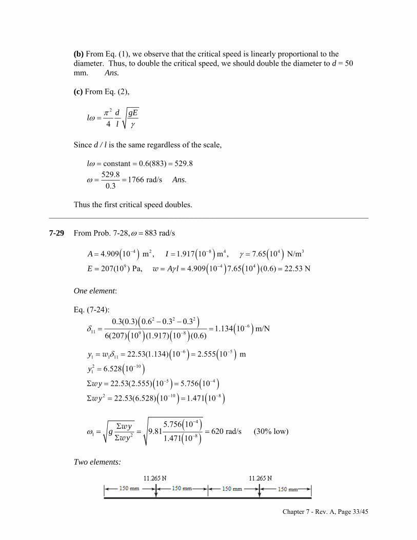
(b) From Eq. (1), we observe that the critical speed is linearly proportional to the diameter. Thus, to double the critical speed, we should double the diameter to d = 50 mm. Ans.
(c) From Eq. (2),
2 d gl
4
E
l
Since d / l is the same regardless of the scale,
constant 0.6(883) 529.8l 529.8
1766 rad/s .A0.3
ns
Thus the first critical speed doubles. ______________________________________________________________________________ 7-29 From Prob. 7-28,
883 rad/s
4 2 8 4 44.909 10 m , 1.917 10 m , 7.65 10 N/mA I 3
9 4 4207(10 ) Pa, 4.909 10 7.65 10 (0.6) 22.53 NE A l w
One element: Eq. (7-24):
2 2 2
611 9 8
0.3(0.3) 0.6 0.3 0.31.134 10 m/N
6(207) 10 (1.917) 10 (0.6)
6 51 1 11 22.53(1.134) 10 2.555 10 my w
2 11 6.528 10y 0
5 422.53(2.555) 10 5.756 10y w
2 1022.53(6.528) 10 1.471 10y w 8
4
1 2 8
5.756 109.81 620 rad/s
1.471 10
yg
y
ww
(30% low)
Two elements:
Chapter 7 - Rev. A, Page 33/45
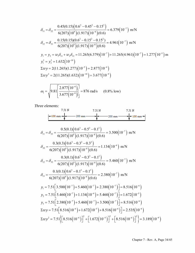
2 2 2
711 22 9 8
0.45(0.15) 0.6 0.45 0.156.379 10 m/N
6(207) 10 (1.917) 10 (0.6)
2 2 2
712 21 9 8
0.15(0.15)(0.6 0.15 0.15 )4.961 10 m/N
6(207) 10 (1.917) 10 (0.6)
7 71 2 1 11 2 12 11.265(6.379) 10 11.265(4.961) 10 1.277 10 my y w w 5
2 2 102 10 1 2 1.63y y
5 42(11.265)(1.277) 10 2.877 10y w
2 102(11.265)(1.632) 10 3.677 10y w 9
4
1 9
2.877 109.81 876 rad/s
3.677 10
(0.8% low)
Three elements:
2 2 2
711 33 9 8
0.5(0.1) 0.6 0.5 0.13.500 10 m/N
6(207) 10 (1.917) 10 (0.6)
2 2 2
622 9 8
0.3(0.3) 0.6 0.3 0.31.134 10 m/N
6(207) 10 (1.917) 10 (0.6)
2 2 2
712 32 9 8
0.3(0.1) 0.6 0.3 0.15.460 10 m/N
6(207) 10 (1.917) 10 (0.6)
2 2 2
713 9 8
0.1(0.1) 0.6 0.1 0.12.380 10 m/N
6(207) 10 (1.917) 10 (0.6)
7 7 71 7.51 3.500 10 5.460 10 2.380 10 8.516 10 6y
7 6 72 7.51 5.460 10 1.134 10 10 1.672 10y 55.460
7 7 73 7.51 2.380 10 5.460 10 3.500 10 8.516 10y 6
6 5 6 47.51 8.516 10 1.672 10 8.516 10 2.535 10y w
2 2 22 6 5 6 97.51 8.516 10 1.672 10 8.516 10 3.189 10y w
Chapter 7 - Rev. A, Page 34/45
42.535 109.81 883 ra
1 93.189 10
d/s
7-28. The point was to show that convergence is rapid using a static deflection beam equation. The method works because:
If a deflection curve is chosen which meets the boundary conditions of moment-free and deflection-free ends, as in this problem, the strain energy is not very sensitive to the equation used.
ation is available, and meets the moment-free and deflection-free ends, it works.
______________________________________________________________________________ 7-30 (a) For two bodies, Eq. (7-26) is
The result is the same as in Prob.
Since the static bending equ
2
1 11( 1/ )0
m 2 12
21 21 2 22( 1/ )
m
m m
Expanding the determinant yields,
2
1 1 11 2 22 1 2 11 22 12 212 2
1
1( ) ( ) 0m m m m
(1)
Eq. (1) has two roots 2 2
1 21 / and 1 / . Thus
2 2 2 21 2
1 1 1 1 0
or,
21 1
2
2 2 2 2 21 2 1 2
1 1 1 10
(2)
Equate the third terms of Eqs. (1) and (2), which must be identical.
2
1 2 11 22 12 21 1 1 2 11 22 12 212 2 2
1 1 1( ) ( )m m m m
1 2 2
and it follows that
Chapter 7 - Rev. A, Page 35/45
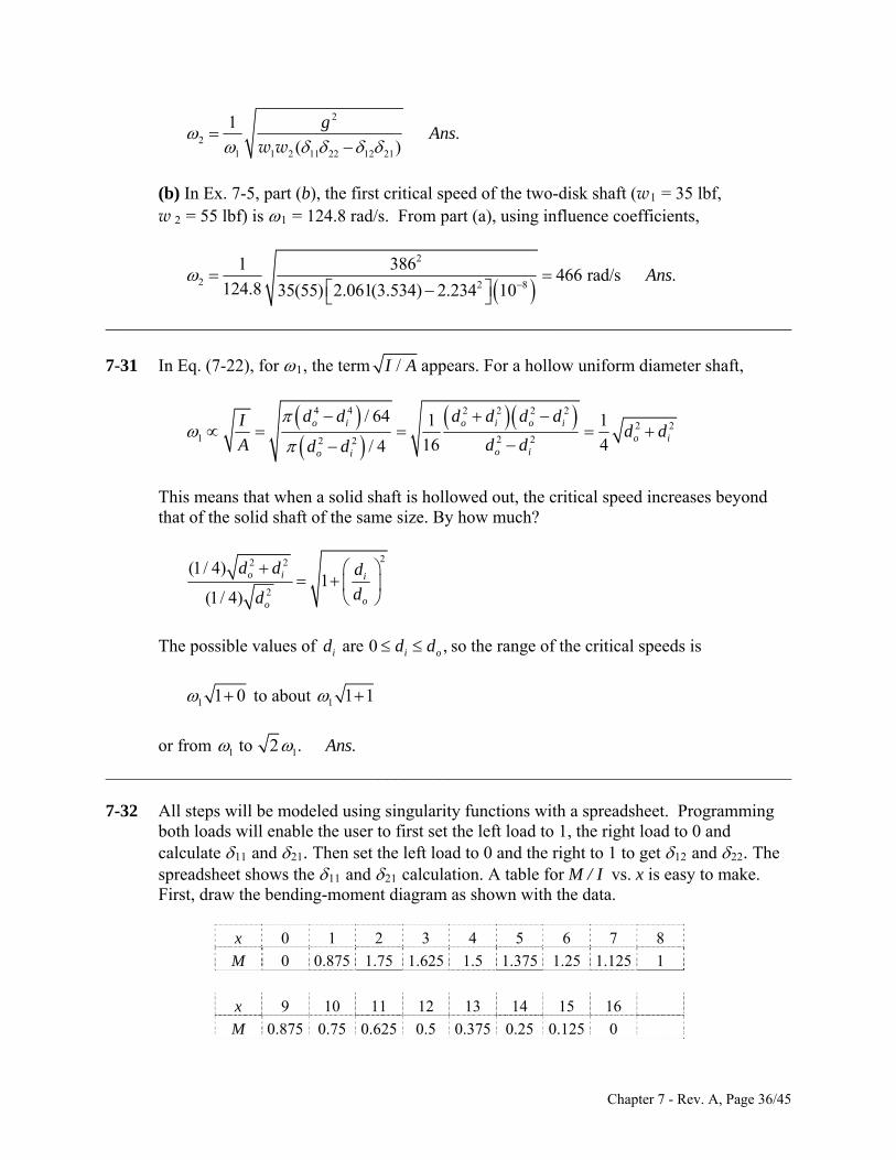
2
21 1 11 22 12
.( )
Ans
w w
2 21
1 g
(b) In Ex. 7-5, part (b), the first critical speed of the two-disk shaft (w1 = 35 lbf, w 2 = 55 lbf) is 1 = 124.8 rad/s. From part (a), using influence coefficients,
2
2 2 8
1 386466 rad/s .
124.8 35(55) 2.061(3.534) 2.234 10Ans
______________________________________________________________________________
7-31 In Eq. (7-22), for 1, the term /I A appears. For a hollow uniform diameter shaft,
4 2 2 2 2
2 2o o i o id d d d dId d
4
1 2 22 2
/ 64 1 1
16 4/ 4
i
o io io i
d
A d dd d
This means that when a solid shaft is hollowed out, the critical speed increases beyond
solid shaft of the same size. By how much? that of the
22 2
21
(1/ 4)
o i i
oodd
The possible values of are 0 ,i i od d d
(1/ 4) d d d
so the range of the critical speeds is
1 1 0 to about 1 1 1
or from 1 1to 2 . .Ans
______________________________________________________________________________ 7-32 All steps w b g t t pr s et. Programming
both loads will enable the user to first set the left load to 1, the right load to 0 and calculate 11 and 21. Then set the left load to 0 and the right to 1 to get 12 and 22. The spreadsheet shows the 11 and 21 calculation. A table for M / I vs. x is easy to make. First, draw the bending-moment diagram as shown with the data.
x 0 1 2 3 4 5 6 7 8
ill e modeled using sin ulari y func ions with a s ead he
M 0 0.875 1.75 1.625 1.5 1.375 1.25 1.125 1
x 9 10 11 12 13 14 15 16
M 0.875 0.75 0.625 0.5 0.375 0.25 0.125 0
Chapter 7 - Rev. A, Page 36/45
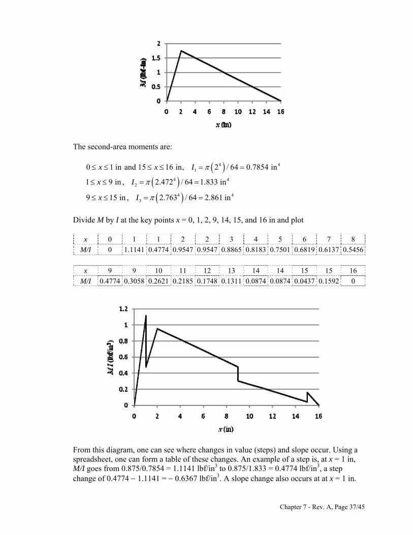
The second-area moments are: 4 4
10 1 in and 15 16 in, 2 / 64 0.7854 inx x I
4 42
4 43
1 9 in , 2.472 / 64 1.833 in
9 15 in , 2.763 / 64 2.861 in
x I
x I
Divide M by I at the key points x = 0, 1, 2, 9, 14, 15, and 16 in and plot
x 0 1 1 2 2 3 4 5 6 7 8
M/I 0 1.1141 0.4774 0.9547 0.9547 0.8865 0.8183 0.7501 0.6819 0.6137 0.5456
x 9 9 10 11 12 13 14 14 15 15 16
M/I 0.4774 0.3058 0.2621 0.2185 0.1748 0.1311 0.0874 0.0874 0.0437 0.1592 0
From this diagram, one can see where changes in value (steps) and slope occur. Using a
spreadsheet, one can form a table of these changes. An example of a step is, at x = 1 in, M/I goes from 0.875/0.7854 = 1.1141 lbf/in3 to 0.875/1.833 = 0.4774 lbf/in3, a step change of 0.4774 1.1141 = 0.6367 lbf/in3. A slope change also occurs at at x = 1 in.
Chapter 7 - Rev. A, Page 37/45
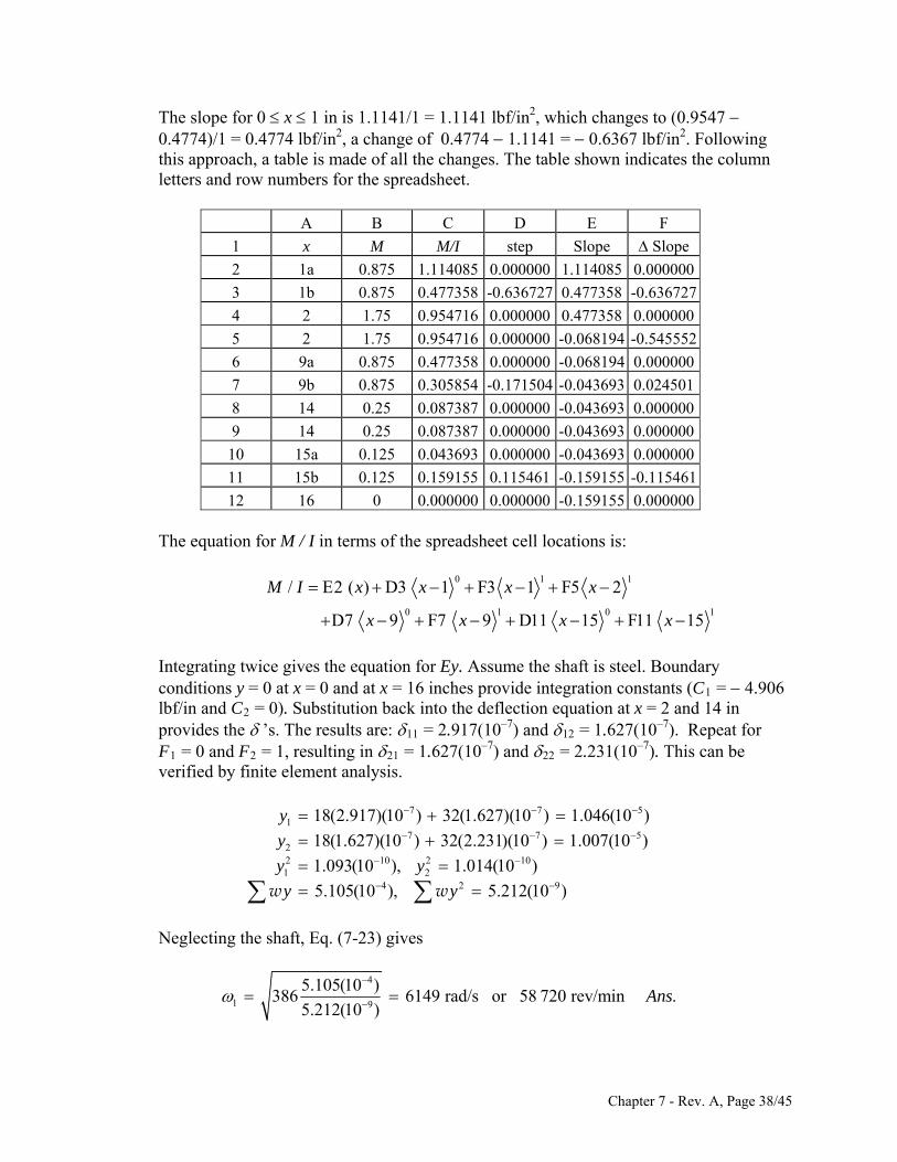
The slope for 0 x 1 in is 1.1141/1 = 1.1141 lbf/in2, which changes to (0.9547 0.4774)/1 = 0.4774 lbf/in2, a change of 0.4774 1.1141 = 0.6367 lbf/in2. Following this approach, a table is made of all the changes. The table shown indicates the column letters and row numbers for the spreadsheet.
A B C D E F
1 x M M/I step Slope Slope
2 1a 0.875 1.114085 0.000000 1.114085 0.000000
3 1b 0.875 0.477358 -0.636727 0.477358 -0.636727
4 2 1.75 0.954716 0.000000 0.477358 0.000000
5 2 1.75 0.954716 0.000000 -0.068194 -0.545552
6 9a 0.875 0.477358 0.000000 -0.068194 0.000000
7 9b 0.875 0.305854 -0.171504 -0.043693 0.024501
8 14 0.25 0.087387 0.000000 -0.043693 0.000000
9 14 0.25 0.087387 0.000000 -0.043693 0.000000
10 15a 0.125 0.043693 0.000000 -0.043693 0.000000
11 15b 0.125 0.159155 0.115461 -0.159155 -0.115461
12 16 0 0.000000 0.000000 -0.159155 0.000000 The equation for M / I in terms of the spreadsheet cell locations is:
0 1 1
0 1 0
/ E2 ( ) D3 1 F3 1 F5 2
D7 9 F7 9 D11 15 F11 15
M I x x x x
x x x x
1
5
5
Integrating twice gives the equation for Ey. Assume the shaft is steel. Boundary
conditions y = 0 at x = 0 and at x = 16 inches provide integration constants (C1 = 4.906 lbf/in and C2 = 0). Substitution back into the deflection equation at x = 2 and 14 in provides the ’s. The results are: 11 = 2.917(10–7) and 12 = 1.627(10–7). Repeat for
F1 = 0 and F2 = 1, resulting in 21 = 1.627(10–7) and 22 = 2.231(10–7). This can be verified by finite element analysis.
7 7
17 7
22 10 2 101 2
4 2 9
18(2.917)(10 ) 32(1.627)(10 ) 1.046(10 )
18(1.627)(10 ) 32(2.231)(10 ) 1.007(10 )
1.093(10 ), 1.014(10 )
5.105(10 ), 5.212(10 )
y
y
y y
y y
w w
Neglecting the shaft, Eq. (7-23) gives
4
1 9
5.105(10 )386 6149 rad/s or 58 720 rev/min .
5.212(10 )Ans
Chapter 7 - Rev. A, Page 38/45
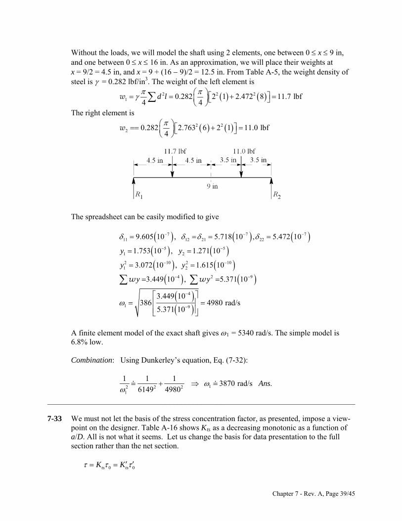
Without the loads, we will model the shaft using 2 elements, one between 0 x 9 in, and one between 0 x 16 in. As an approximation, we will place their weights at x = 9/2 = 4.5 in, and x = 9 + (16 9)/2 = 12.5 in. From Table A-5, the weight density of steel is = 0.282 lbf/in3. The weight of the left element is
2 2 21 0.282 2 1 2.472 8 11.7 lbf
4 4d l
w
The right element is
2 22 0.282 2.763 6 2 1 11.0 lbf
4
w
The spreadsheet can be easily modified to give
7 7
11 12 21 229.605 10 , 5.718 10 , 5.472 10 7
5 51 21.753 10 , 1.271 10y y
2 10 21 23.072 10 , 1.615 10y y 10
4 23.449 10 , 5.371 10y y w w 9
4
1 9
3.449 10386 4980 rad/s
5.371 10
A finite element model of the exact shaft gives 1 = 5340 rad/s. The simple model is 6.8% low. Combination: Using Dunkerley’s equation, Eq. (7-32):
12 2 21
1 1 13870 rad/s .
6149 4980Ans
______________________________________________________________________________ 7-33 We must not let the basis of the stress concentration factor, as presented, impose a view-
point on the designer. Table A-16 shows Kts as a decreasing monotonic as a function of a/D. All is not what it seems. Let us change the basis for data presentation to the full section rather than the net section.
0 0ts tsK K
Chapter 7 - Rev. A, Page 39/45
3 3
32 32ts ts
T TK K
AD D
Therefore
tsts
KK
A
Form a table:
tsK has the following attributes:
It exhibits a minimum; It changes little over a wide range; Its minimum is a stationary point minimum at a / D 0.100;
Our knowledge of the minima location is 0.075 ( / ) 0.125a D
We can form a design rule: In torsion, the pin diameter should be about 1/10 of the shaft diameter, for greatest shaft capacity. However, it is not catastrophic if one forgets the rule.
______________________________________________________________________________ 7-34 From the solution to Prob. 3-72, the torque to be transmitted through the key from the
gear to the shaft is T = 2819 lbf·in. From Prob. 7-19, the nominal shaft diameter supporting the gear is 1.00 in. From Table 7-6, a 0.25 in square key is appropriate for a 1.00 in shaft diameter. The force applied to the key is
2819
5638 lbf1.00 / 2
TF
r
Selecting 1020 CD steel for the key, with Sy = 57 kpsi, and using the distortion-energy theory, Ssy = 0.577 Sy = (0.577)(57) = 32.9 kpsi. Failure by shear across the key:
Chapter 7 - Rev. A, Page 40/45
1.1 5638 0.754 in
/ 0.25 32 900sy sy
sy
F F
A tlS S nF
n lF tl tS
Failure by crushing:
/ 2
F F
A t l
3
2 5638 1.12 0.870 in
2 / 0.25 57 10y y
y
S S Fnn l
F tl tS
Select ¼-in square key, 7/8 in long, 1020 CD steel. Ans.
______________________________________________________________________________ 7-35 From the solution to Prob. 3-73, the torque to be transmitted through the key from the
gear to the shaft is T = 3101 N·m. From Prob. 7-21, the nominal shaft diameter supporting the gear is 50 mm. To determine an appropriate key size for the shaft diameter, we can either convert to inches and use Table 7-6, or we can look up standard metric key sizes from the internet or a machine design handbook. It turns out that the recommended metric key for a 50 mm shaft is 14 x 9 mm. Since the problem statement specifies a square key, we will use a 14 x 14 mm key. For comparison, using Table 7-6 as a guide, for d = 50 mm = 1.97 in, a 0.5 in square key is appropriate. This is equivalent to 12.7 mm. A 14 x 14 mm size is conservative, but reasonable after rounding up to standard sizes.
The force applied to the key is
33101124 10 N
0.050 / 2
TF
r
Selecting 1020 CD steel for the key, with Sy = 390 MPa, and using the distortion-energy theory, Ssy = 0.577 Sy = 0.577(390) = 225 MPa. Failure by shear across the key:
3
6
1.1 124 10 0.0433 m 43.3 mm
/ 0.014 225 10sy sy
sy
F F
A tl
S S nFn l
F tl tS
Failure by crushing:
Chapter 7 - Rev. A, Page 41/45
/ 2
F F
A t
l
3
6
2 124 10 1.12 0.0500 m 50.0 mm
2 / 0.014 390 10y y
y
S S Fnn l
F tl tS
Select 14 mm square key, 50 mm long, 1020 CD steel. Ans. ______________________________________________________________________________ 7-36 Choose basic size D = d = 15 mm. From Table 7-9, a locational clearance fit is
designated as 15H7/h6. From Table A-11, the tolerance grades are D = 0.018 mm and d = 0.011 mm. From Table A-12, the fundamental deviation is F = 0 mm. Hole: Eq. (7-36): Dmax = D + D = 15 + 0.018 = 15.018 mm Ans. Dmin = D = 15.000 mm Ans.
Shaft: Eq. (7-37): dmax = d + F = 15.000 + 0 = 15.000 mm Ans. dmin = d + F – d = 15.000 + 0 – 0.011 = 14.989 mm Ans.
______________________________________________________________________________ 7-37 Choose basic size D = d = 1.75 in. From Table 7-9, a medium drive fit is designated as
H7/s6. From Table A-13, the tolerance grades are D = 0.0010 in and d = 0.0006 in. From Table A-14, the fundamental deviation is F = 0.0017 in. Hole: Eq. (7-36): Dmax = D + D = 1.75 + 0.0010 = 1.7510 in Ans. Dmin = D = 1.7500 in Ans.
Shaft: Eq. (7-38): dmin = d + F = 1.75 + 0.0017 = 1.7517 in Ans. dmax = d + F + d = 1.75 + 0.0017 + 0.0006 = 1.7523 in Ans.
______________________________________________________________________________ 7-38 Choose basic size D = d = 45 mm. From Table 7-9, a sliding fit is designated as H7/g6.
From Table A-11, the tolerance grades are D = 0.025 mm and d = 0.016 mm. From Table A-12, the fundamental deviation is F = –0.009 mm. Hole: Eq. (7-36): Dmax = D + D = 45 + 0.025 = 45.025 mm Ans. Dmin = D = 45.000 mm Ans.
Shaft: Eq. (7-37): dmax = d + F = 45.000 + (–0.009) = 44.991 mm Ans. dmin = d + F – d = 45.000 + (–0.009) – 0.016 = 44.975 mm Ans.
______________________________________________________________________________
Chapter 7 - Rev. A, Page 42/45
7-39 Choose basic size D = d = 1.250 in. From Table 7-9, a close running fit is designated as H8/f7. From Table A-13, the tolerance grades are D = 0.0015 in and d = 0.0010 in. From Table A-14, the fundamental deviation is F = –0.0010 in. Hole: Eq. (7-36): Dmax = D + D = 1.250 + 0.0015 = 1.2515 in Ans. Dmin = D = 1.2500 in Ans.
Shaft: Eq. (7-37): dmax = d + F = 1.250 + (–0.0010) = 1.2490 in Ans. dmin = d + F – d = 1.250 + (–0.0010) – 0.0010 = 1.2480 in Ans.
______________________________________________________________________________ 7-40 Choose basic size D = d = 35 mm. From Table 7-9, a locational interference fit is
designated as H7/p6. From Table A-11, the tolerance grades are D = 0.025 mm and d = 0.016 mm. From Table A-12, the fundamental deviation is F = 0.026 mm.
Hole: Eq. (7-36): Dmax = D + D = 35 + 0.025 = 35.025 mm Dmin = D = 35.000 mm The bearing bore specifications are within the hole specifications for a locational interference fit. Now find the necessary shaft sizes. Shaft: Eq. (7-38): dmin = d + F = 35 + 0.026 = 35.026 mm Ans. dmax = d + F + d = 35 + 0.026 + 0.016 = 35.042 mm Ans.
______________________________________________________________________________ 7-41 Choose basic size D = d = 1.5 in. From Table 7-9, a locational interference fit is
designated as H7/p6. From Table A-13, the tolerance grades are D = 0.0010 in and d = 0.0006 in. From Table A-14, the fundamental deviation is F = 0.0010 in.
Hole: Eq. (7-36): Dmax = D + D = 1.5000 + 0.0010 = 1.5010 in Dmin = D = 1.5000 in
The bearing bore specifications exactly match the requirements for a locational interference fit. Now check the shaft. Shaft: Eq. (7-38): dmin = d + F = 1.5000 + 0.0010 = 1.5010 in dmax = d + F + d = 1.5000 + 0.0010 + 0.0006 = 1.5016 in
Chapter 7 - Rev. A, Page 43/45
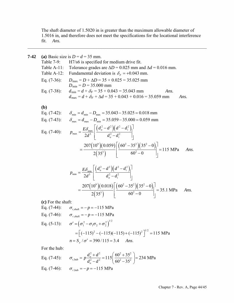
The shaft diameter of 1.5020 in is greater than the maximum allowable diameter of 1.5016 in, and therefore does not meet the specifications for the locational interference fit. Ans.
______________________________________________________________________________ 7-42 (a) Basic size is D = d = 35 mm.
Table 7-9: H7/s6 is specified for medium drive fit. Table A-11: Tolerance grades are D = 0.025 mm and d = 0.016 mm. Table A-12: Fundamental deviation is 0.043 mm.F
Eq. (7-36): Dmax = D + D = 35 + 0.025 = 35.025 mm Dmin = D = 35.000 mm Eq. (7-38): dmin = d + F = 35 + 0.043 = 35.043 mm Ans. dmax = d + F + d = 35 + 0.043 + 0.016 = 35.059 mm Ans.
(b) Eq. (7-42): min min max 35.043 35.025 0.018 mmd D
Eq. (7-43): max max min 35.059 35.000 0.059 mmd D
Eq. (7-40): 2 2 2 2
maxmax 3 2 22
o i
o i
d d d dEp
d d d
9 2 2 2
23
207 10 0.059 60 35 35 0115 MPa .
60 02 35Ans
2 2 2 2
minmin 3 2 22
o i
o i
d d d dEp
d d d
9 2 2 2
23
207 10 0.018 60 35 35 035.1 MPa .
60 02 35Ans
(c) For the shaft: Eq. (7-44): ,shaft 115 MPat p
Eq. (7-46): ,shaft 115 MPar p
Eq. (5-13): 1/22 21 1 2 2
1/22 2( 115) ( 115)( 115) ( 115) 115 MPa
/ 390 /115 3.4 .yn S Ans
For the hub:
Eq. (7-45): 2 2 2 2
,hub 2 2 2 2
60 35115 234 MPa
60 35o
to
d dp
d d
Eq. (7-46): ,hub 115 MPar p
Chapter 7 - Rev. A, Page 44/45
Eq. (5-13): 1/22 21 1 2 2
1/22 2(234) (234)( 115) ( 115) 308 MPa
/ 600 / 308 1.9 .yn S Ans
(d) A value for the static coefficient of friction for steel to steel can be obtained online or from a physics textbook as approximately f = 0.8. Eq. (7-49) 2
min( / 2)T f p ld
6 2( / 2)(0.8)(35.1) 10 (0.050)(0.035) 2700 N m .Ans
______________________________________________________________________________
Chapter 7 - Rev. A, Page 45/45
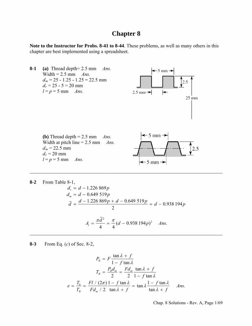
Chapter 8 Note to the Instructor for Probs. 8-41 to 8-44. These problems, as well as many others in this chapter are best implemented using a spreadsheet. 8-1 (a) Thread depth= 2.5 mm Ans. Width = 2.5 mm Ans. dm = 25 - 1.25 - 1.25 = 22.5 mm dr = 25 - 5 = 20 mm l = p = 5 mm Ans.
(b) Thread depth = 2.5 mm Ans.
Width at pitch line = 2.5 mm Ans. dm = 22.5 mm dr = 20 mm l = p = 5 mm Ans. ______________________________________________________________________________ 8-2 From Table 8-1,
1.226 8690.649 5191.226 869 0.649 519
0.938 1942
r
m
d d pd d p
d p d pd d
p
2
2( 0.938 194 ) .4 4t
dA d p
Ans
______________________________________________________________________________ 8-3 From Eq. (c) of Sec. 8-2,
tan
1 tantan
2 2 1 tan
R
R m mR
fP F
fP d Fd f
Tf
0 / (2 ) 1 tan 1 tantan .
/ 2 tan tanR m
T Fl f fe A
T Fd f fns
Chap. 8 Solutions - Rev. A, Page 1/69
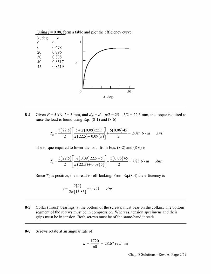
Using f = 0.08, form a table and plot the efficiency curve.
, deg. e 0 0 0 0.678 20 0.796 30 0.838 40 0.8517 45 0.8519
______________________________________________________________________________ 8-4 Given F = 5 kN, l = 5 mm, and dm = d p/2 = 25 5/2 = 22.5 mm, the torque required to
raise the load is found using Eqs. (8-1) and (8-6)
5 22.5 5 0.09 22.5 5 0.06 45
15.85 N m .2 22.5 0.09 5 2RT A
ns
The torque required to lower the load, from Eqs. (8-2) and (8-6) is
5 22.5 0.09 22.5 5 5 0.06 45
7.83 N m .2 22.5 0.09 5 2LT A
ns
Since TL is positive, the thread is self-locking. From Eq.(8-4) the efficiency is
5 5
0.251 .2 15.85
e Ans
______________________________________________________________________________ 8-5 Collar (thrust) bearings, at the bottom of the screws, must bear on the collars. The bottom
segment of the screws must be in compression. Whereas, tension specimens and their grips must be in tension. Both screws must be of the same-hand threads.
______________________________________________________________________________ 8-6 Screws rotate at an angular rate of
172028.67 rev/min
60n
Chap. 8 Solutions - Rev. A, Page 2/69
(a) The lead is 0.25 in, so the linear speed of the press head is
V = 28.67(0.25) = 7.17 in/min Ans. (b) F = 2500 lbf/screw
o
2 0.25 / 2 1.875 in
sec 1 / cos(29 / 2) 1.033md
Eq. (8-5):
2500(1.875) 0.25 (0.05)(1.875)(1.033)221.0 lbf · in
2 (1.875) 0.05(0.25)(1.033)RT
Eq. (8-6):
2500(0.08)(3.5 / 2) 350 lbf · in350 221.0 571 lbf · in/screw571(2)
20.04 lbf · in60(0.95)
20.04(1720)0.547 hp .
63 025 63 025
c
total
motor
TT
T
TnH A
ns
______________________________________________________________________________ 8-7 Note to the Instructor: The statement for this problem in the first printing of this edition
was vague regarding the effective handle length. For the printings to follow the statement “The overall length is 4.25 in.” will be replaced by “ A force will be applied to the handle at a radius of 1
23 in from the screw centerline.” We apologize if this has caused any
inconvenience.
3 3
3.5 in3.5
3 33.5 3.125
8 841 kpsi
32 32(3.125)41 000
(0.1875)8.49 lbf
y
y
LT F
M L F F
S
M FS
dF
F
ns
3.5(8.49) 29.7 lbf · in .T A (b) Eq. (8-5), 2 = 60 , l = 1/10 = 0.1 in, f = 0.15, sec = 1.155, p = 0.1 in
Chap. 8 Solutions - Rev. A, Page 3/69
clamp
clamp
clamp
30.649 519 0.1 0.6850 in
4(0.6850) 0.1 (0.15)(0.6850)(1.155)
2 (0.6850) 0.15(0.1)(1.155)0.075 86
29.7392 lbf .
0.075 86 0.075 86
m
R
R
R
d
FT
T F
TF A
ns
(c) The column has one end fixed and the other end pivoted. Base the decision on the
mean diameter column. Input: C = 1.2, D = 0.685 in, A = (0.6852)/4 = 0.369 in2, Sy = 41 kpsi, E = 30(106) psi, L = 6 in, k = D/4 =0.171 25 in, L/k = 35.04. From Eq. (4-45),
1/21/2 2 62
1
2 1.2 30 102131.7
41 000y
l CE
k S
From Eq. (4-46), the limiting clamping force for buckling is
2
clamp cr
23
3 36
1
2
41 10 10.369 41 10 35.04 14.6 10 lbf
2 1.2 30 10
yy
S lF P A S
k CE
Ans
(d) This is a subject for class discussion. ______________________________________________________________________________ 8-8 T = 8(3.5) = 28 lbf in
3 1
0.6667 in4 12md
l = 1
6 = 0.1667 in, =
029
2 = 14.50, sec 14.50 = 1.033
From Eqs. (8-5) and (8-6)
total
0.1667 0.15 0.6667 1.033 0.15 10.66670.1542
2 0.6667 0.15 0.1667 1.033 2
FFT F
28
182 lbf .0.1542
F Ans
_____________________________________________________________________________
Chap. 8 Solutions - Rev. A, Page 4/69
8-9 dm = 1.5 0.25/2 = 1.375 in, l = 2(0.25) = 0.5 in From Eq. (8-1) and Eq. (8-6)
3 32.2 10 (1.375) 2.2 10 (0.15)(2.25)0.5 (0.10)(1.375)
2 (1.375) 0.10(0.5) 2330 371 701 lbf · in
RT
Since n = V/l = 2/0.5 = 4 rev/s = 240 rev/min so the power is
701 240
2.67 hp .63 025 63 025
TnH A ns
______________________________________________________________________________ 8-10 dm = 40 4 = 36 mm, l = p = 8 mm From Eqs. (8-1) and (8-6)
36 8 (0.14)(36) 0.09(100)
2 (36) 0.14(8) 2(3.831 4.5) 8.33 N · m ( in kN)2 2 (1) 2 rad/s
3000477 N · m
2477
57.3 kN .8.33
F FT
F F Fn
H TH
T
F Ans
57.3(8)
0.153 .2 2 (477)
Fle A
T ns
______________________________________________________________________________ 8-11 (a) Table A-31, nut height H = 12.8 mm. L ≥ l + H = 2(15) + 12.8 = 42.8 mm. Rounding
up, L = 45 mm Ans. (b) From Eq. (8-14), LT = 2d + 6 = 2(14) +6 = 34 mm From Table 8-7, ld = L LT = 45 34 = 11 mm, lt = l ld = 2(15) 11 = 19 mm, Ad = (142) / 4 = 153.9 mm2. From Table 8-1, At = 115 mm2. From Eq. (8-17)
Chap. 8 Solutions - Rev. A, Page 5/69
153.9 115 207
874.6 MN/m .153.9 19 115 11
d tb
d t t d
A A Ek A
A l A l
ns
(c) From Eq. (8-22), with l = 2(15) = 30 mm
0.5774 207 140.57743 116.5 MN/m .
0.5774 0.5 0.5774 30 0.5 142ln 5 2ln 50.5774 2.5 0.5774 30 2.5 14
mk Ed
Ansl dl d
8-12 (a) Table A-31, nut height H = 12.8 mm. Table A-33, washer thickness t = 3.5 mm. Thus,
the grip is l = 2(15) + 3.5 = 33.5 mm. L ≥ l + H = 33.5 + 12.8 = 46.3 mm. Rounding up L = 50 mm Ans. (b) From Eq. (8-14), LT = 2d + 6 = 2(14) +6 = 34 mm From Table 8-7, ld = L LT = 50 34 = 16 mm, lt = l ld = 33.5 16 = 17.5 mm, Ad = (142) / 4 = 153.9 mm2. From Table 8-1, At = 115 mm2. From Eq. (8-17)
153.9 115 207
808.2 MN/m .153.9 17.5 115 16
d tb
d t t d
A A Ek A
A l A l
ns
(c) From Eq. (8-22)
0.5774 207 140.57742 969 MN/m .
0.5774 0.5 0.5774 33.5 0.5 142ln 5 2ln 50.5774 2.5 0.5774 33.5 2.5 14
m
Edk A
l dl d
ns
______________________________________________________________________________
Chap. 8 Solutions - Rev. A, Page 6/69
8-13 (a) Table 8-7, l = h + d /2 = 15 + 14/2 = 22 mm. L ≥ h + 1.5d = 36 mm. Rounding up L = 40 mm Ans. (b) From Eq. (8-14), LT = 2d + 6 = 2(14) +6 = 34 mm From Table 8-7, ld = L LT = 40 34 = 6 mm, lt = l ld = 22 6 = 16 mm Ad = (142) / 4 = 153.9 mm2. From Table 8-1, At = 115 mm2. From Eq. (8-17)
153.9 115 207
1 162.2 MN/m .153.9 16 115 6
d tb
d t t d
A A Ek A
A l A l
ns
(c) From Eq. (8-22), with l = 22 mm
0.5774 207 140.57743 624.4 MN/m .
0.5774 0.5 0.5774 22 0.5 142ln 5 2ln 50.5774 2.5 0.5774 22 2.5 14
m
Edk Ans
l dl d
______________________________________________________________________________ 8-14 (a) From Table A-31, the nut height is H = 7/16 in. L ≥ l + H = 2 + 1 + 7/16 = 3 7/16 in.
Rounding up, L = 3.5 in Ans. (b) From Eq. (8-13), LT = 2d + 1/4 = 2(0.5) + 0.25 = 1.25 in From Table 8-7, ld = L LT = 3.5 1.25 = 2.25 in, lt = l ld = 3 2.25 = 0.75 in Ad = (0.52)/4 = 0.1963 in2. From Table 8-2, At = 0.1419 in2. From Eq. (8-17)
0.1963 0.1419 30
1.79 Mlbf/in .0.1963 0.75 0.1419 2.25
d tb
d t t d
A A Ek A
A l A l
ns
Chap. 8 Solutions - Rev. A, Page 7/69
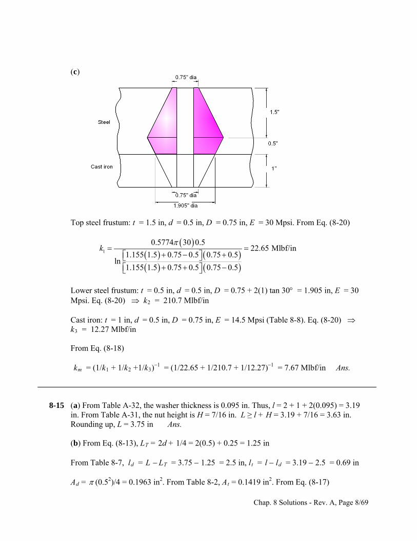
(c) Top steel frustum: t = 1.5 in, d = 0.5 in, D = 0.75 in, E = 30 Mpsi. From Eq. (8-20)
1
0.5774 30 0.522.65 Mlbf/in
1.155 1.5 0.75 0.5 0.75 0.5ln
1.155 1.5 0.75 0.5 0.75 0.5
k
Lower steel frustum: t = 0.5 in, d = 0.5 in, D = 0.75 + 2(1) tan 30 = 1.905 in, E = 30
Mpsi. Eq. (8-20) k2 = 210.7 Mlbf/in Cast iron: t = 1 in, d = 0.5 in, D = 0.75 in, E = 14.5 Mpsi (Table 8-8). Eq. (8-20) k3 = 12.27 Mlbf/in From Eq. (8-18) km = (1/k1 + 1/k2 +1/k3)1 = (1/22.65 + 1/210.7 + 1/12.27)1 = 7.67 Mlbf/in Ans. 8-15 (a) From Table A-32, the washer thickness is 0.095 in. Thus, l = 2 + 1 + 2(0.095) = 3.19
in. From Table A-31, the nut height is H = 7/16 in. L ≥ l + H = 3.19 + 7/16 = 3.63 in. Rounding up, L = 3.75 in Ans.
(b) From Eq. (8-13), LT = 2d + 1/4 = 2(0.5) + 0.25 = 1.25 in From Table 8-7, ld = L LT = 3.75 1.25 = 2.5 in, lt = l ld = 3.19 2.5 = 0.69 in Ad = (0.52)/4 = 0.1963 in2. From Table 8-2, At = 0.1419 in2. From Eq. (8-17)
Chap. 8 Solutions - Rev. A, Page 8/69
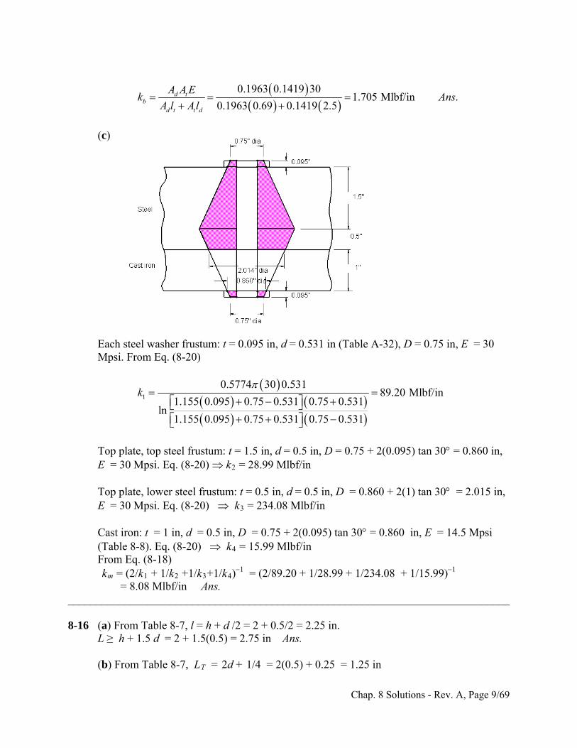
0.1963 0.1419 30
1.705 Mlbf/in .0.1963 0.69 0.1419 2.5
d tb
d t t d
A A Ek A
A l A l
ns
(c) Each steel washer frustum: t = 0.095 in, d = 0.531 in (Table A-32), D = 0.75 in, E = 30
Mpsi. From Eq. (8-20)
1
0.5774 30 0.53189.20 Mlbf/in
1.155 0.095 0.75 0.531 0.75 0.531ln
1.155 0.095 0.75 0.531 0.75 0.531
k
Top plate, top steel frustum: t = 1.5 in, d = 0.5 in, D = 0.75 + 2(0.095) tan 30 = 0.860 in,
E = 30 Mpsi. Eq. (8-20) k2 = 28.99 Mlbf/in Top plate, lower steel frustum: t = 0.5 in, d = 0.5 in, D = 0.860 + 2(1) tan 30 = 2.015 in,
E = 30 Mpsi. Eq. (8-20) k3 = 234.08 Mlbf/in Cast iron: t = 1 in, d = 0.5 in, D = 0.75 + 2(0.095) tan 30 = 0.860 in, E = 14.5 Mpsi
(Table 8-8). Eq. (8-20) k4 = 15.99 Mlbf/in From Eq. (8-18) km = (2/k1 + 1/k2 +1/k3+1/k4)1 = (2/89.20 + 1/28.99 + 1/234.08 + 1/15.99)1 = 8.08 Mlbf/in Ans. ______________________________________________________________________________ 8-16 (a) From Table 8-7, l = h + d /2 = 2 + 0.5/2 = 2.25 in. L ≥ h + 1.5 d = 2 + 1.5(0.5) = 2.75 in Ans. (b) From Table 8-7, LT = 2d + 1/4 = 2(0.5) + 0.25 = 1.25 in
Chap. 8 Solutions - Rev. A, Page 9/69
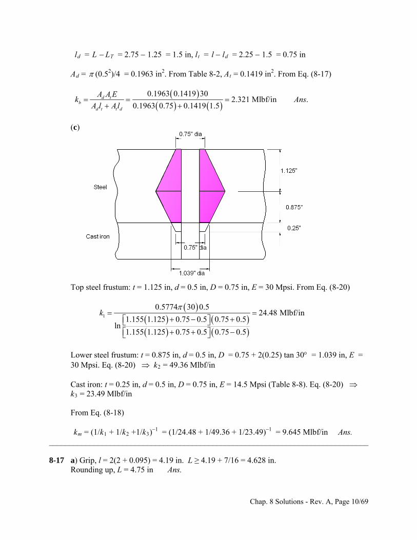
ld = L LT = 2.75 1.25 = 1.5 in, lt = l ld = 2.25 1.5 = 0.75 in Ad = (0.52)/4 = 0.1963 in2. From Table 8-2, At = 0.1419 in2. From Eq. (8-17)
0.1963 0.1419 30
2.321 Mlbf/in .0.1963 0.75 0.1419 1.5
d tbk
A l
d t t d
A A EAns
A l
(c) Top steel frustum: t = 1.125 in, d = 0.5 in, D = 0.75 in, E = 30 Mpsi. From Eq. (8-20)
1
0.5774 30 0.524.48 Mlbf/in
1.155 1.125 0.75 0.5 0.75 0.5ln
1.155 1.125 0.75 0.5 0.75 0.5
k
Lower steel frustum: t = 0.875 in, d = 0.5 in, D = 0.75 + 2(0.25) tan 30 = 1.039 in, E =
30 Mpsi. Eq. (8-20) k2 = 49.36 Mlbf/in Cast iron: t = 0.25 in, d = 0.5 in, D = 0.75 in, E = 14.5 Mpsi (Table 8-8). Eq. (8-20) k3 = 23.49 Mlbf/in From Eq. (8-18) km = (1/k1 + 1/k2 +1/k3)1 = (1/24.48 + 1/49.36 + 1/23.49)1 = 9.645 Mlbf/in Ans. ______________________________________________________________________________ 8-17 a) Grip, l = 2(2 + 0.095) = 4.19 in. L ≥ 4.19 + 7/16 = 4.628 in. Rounding up, L = 4.75 in Ans.
Chap. 8 Solutions - Rev. A, Page 10/69
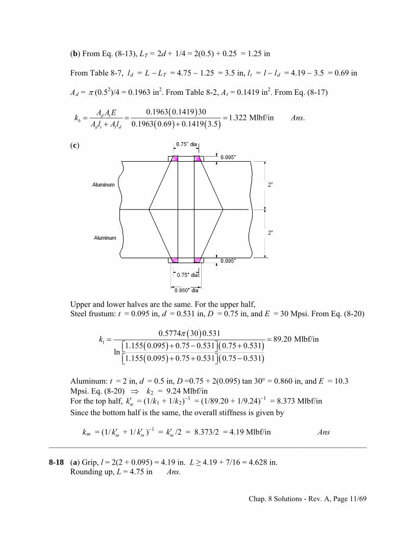
(b) From Eq. (8-13), LT = 2d + 1/4 = 2(0.5) + 0.25 = 1.25 in From Table 8-7, ld = L LT = 4.75 1.25 = 3.5 in, lt = l ld = 4.19 3.5 = 0.69 in Ad = (0.52)/4 = 0.1963 in2. From Table 8-2, At = 0.1419 in2. From Eq. (8-17)
0.1963 0.1419 30
1.322 Mlbf/in .0.1963 0.69 0.1419 3.5
d tbk
A l
d t t d
A A EAns
Al
(c) Upper and lower halves are the same. For the upper half, Steel frustum: t = 0.095 in, d = 0.531 in, D = 0.75 in, and E = 30 Mpsi. From Eq. (8-20)
1
0.5774 30 0.53189.20 Mlbf/in
1.155 0.095 0.75 0.531 0.75 0.531ln
1.155 0.095 0.75 0.531 0.75 0.531
k
Aluminum: t = 2 in, d = 0.5 in, D =0.75 + 2(0.095) tan 30 = 0.860 in, and E = 10.3
Mpsi. Eq. (8-20) k2 = 9.24 Mlbf/in For the top half, = (1/kmk 1 + 1/k2)1 = (1/89.20 + 1/9.24)1 = 8.373 Mlbf/in
Since the bottom half is the same, the overall stiffness is given by km = (1/ + 1/ k )mk m
1 = km /2 = 8.373/2 = 4.19 Mlbf/in Ans
______________________________________________________________________________ 8-18 (a) Grip, l = 2(2 + 0.095) = 4.19 in. L ≥ 4.19 + 7/16 = 4.628 in. Rounding up, L = 4.75 in Ans.
Chap. 8 Solutions - Rev. A, Page 11/69
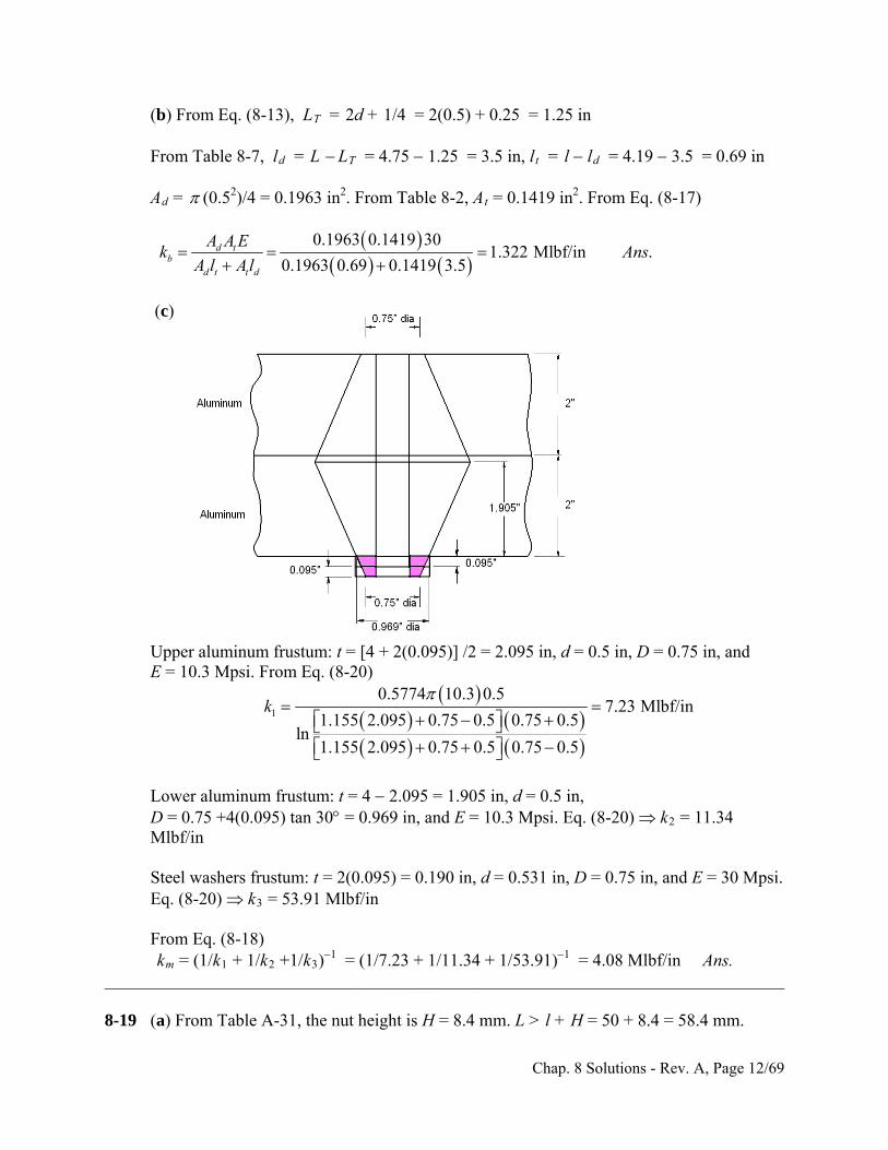
(b) From Eq. (8-13), LT = 2d + 1/4 = 2(0.5) + 0.25 = 1.25 in From Table 8-7, ld = L LT = 4.75 1.25 = 3.5 in, lt = l ld = 4.19 3.5 = 0.69 in Ad = (0.52)/4 = 0.1963 in2. From Table 8-2, At = 0.1419 in2. From Eq. (8-17)
0.1963 0.1419 30
1.322 Mlbf/in .0.1963 0.69 0.1419 3.5
d tbk
A l
d t t d
A A EAns
Al
(c) Upper aluminum frustum: t = [4 + 2(0.095)] /2 = 2.095 in, d = 0.5 in, D = 0.75 in, and E = 10.3 Mpsi. From Eq. (8-20)
1
0.5774 10.3 0.57.23 Mlbf/in
1.155 2.095 0.75 0.5 0.75 0.5ln
1.155 2.095 0.75 0.5 0.75 0.5
k
Lower aluminum frustum: t = 4 2.095 = 1.905 in, d = 0.5 in,
D = 0.75 +4(0.095) tan 30 = 0.969 in, and E = 10.3 Mpsi. Eq. (8-20) k2 = 11.34 Mlbf/in
Steel washers frustum: t = 2(0.095) = 0.190 in, d = 0.531 in, D = 0.75 in, and E = 30 Mpsi. Eq. (8-20) k3 = 53.91 Mlbf/in
From Eq. (8-18) km = (1/k1 + 1/k2 +1/k3)1 = (1/7.23 + 1/11.34 + 1/53.91)1 = 4.08 Mlbf/in Ans. ______________________________________________________________________________ 8-19 (a) From Table A-31, the nut height is H = 8.4 mm. L > l + H = 50 + 8.4 = 58.4 mm.
Chap. 8 Solutions - Rev. A, Page 12/69
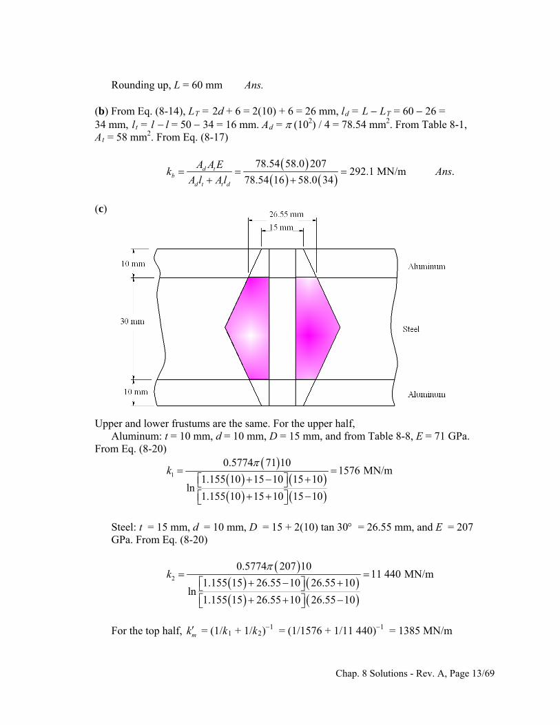
Rounding up, L = 60 mm Ans. (b) From Eq. (8-14), LT = 2d + 6 = 2(10) + 6 = 26 mm, ld = L LT = 60 26 = 34 mm, lt = l l = 50 34 = 16 mm. Ad = (102) / 4 = 78.54 mm2. From Table 8-1, At = 58 mm2. From Eq. (8-17)
78.54 58.0 207
292.1 MN/m .78.54 16 58.0 34
d tb
d t t d
A A Ek A
A l A l
ns
(c) Upper and lower frustums are the same. For the upper half, Aluminum: t = 10 mm, d = 10 mm, D = 15 mm, and from Table 8-8, E = 71 GPa.
From Eq. (8-20)
1
0.5774 71 101576 MN/m
1.155 10 15 10 15 10ln
1.155 10 15 10 15 10
k
Steel: t = 15 mm, d = 10 mm, D = 15 + 2(10) tan 30 = 26.55 mm, and E = 207
GPa. From Eq. (8-20)
2
0.5774 207 1011 440 MN/m
1.155 15 26.55 10 26.55 10ln
1.155 15 26.55 10 26.55 10
k
For the top half, = (1/kmk 1 + 1/k2)1 = (1/1576 + 1/11 440)1 = 1385 MN/m
Chap. 8 Solutions - Rev. A, Page 13/69
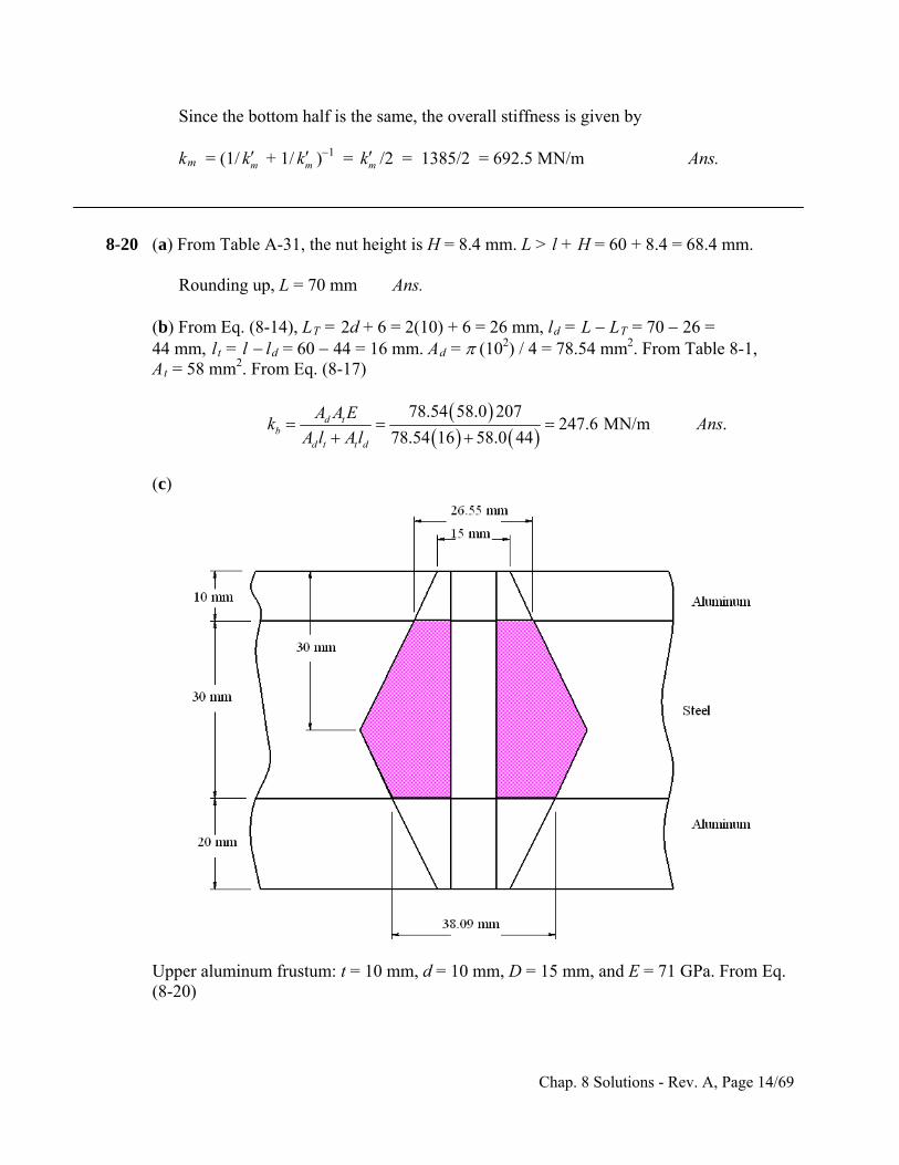
Since the bottom half is the same, the overall stiffness is given by km = (1/ + 1/ )mk mk 1 = mk /2 = 1385/2 = 692.5 MN/m Ans.
8-20 (a) From Table A-31, the nut height is H = 8.4 mm. L > l + H = 60 + 8.4 = 68.4 mm. Rounding up, L = 70 mm Ans. (b) From Eq. (8-14), LT = 2d + 6 = 2(10) + 6 = 26 mm, ld = L LT = 70 26 = 44 mm, lt = l ld = 60 44 = 16 mm. Ad = (102) / 4 = 78.54 mm2. From Table 8-1, At = 58 mm2. From Eq. (8-17)
78.54 58.0 207
247.6 MN/m .78.54 16 58.0 44
d tb
d t t d
A A Ek A
A l A l
ns
(c) Upper aluminum frustum: t = 10 mm, d = 10 mm, D = 15 mm, and E = 71 GPa. From Eq.
(8-20)
Chap. 8 Solutions - Rev. A, Page 14/69
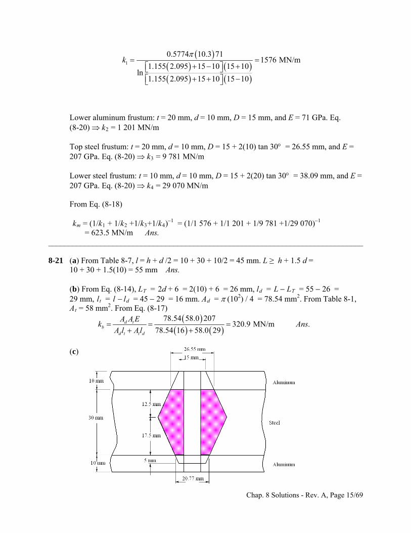
1
0.5774 10.3 711576 MN/m
1.155 2.095 15 10 15 10ln
1.155 2.095 15 10 15 10
k
Lower aluminum frustum: t = 20 mm, d = 10 mm, D = 15 mm, and E = 71 GPa. Eq.
(8-20) k2 = 1 201 MN/m
Top steel frustum: t = 20 mm, d = 10 mm, D = 15 + 2(10) tan 30 = 26.55 mm, and E =
207 GPa. Eq. (8-20) k
3 = 9 781 MN/m Lower steel frustum: t = 10 mm, d = 10 mm, D = 15 + 2(20) tan 30 = 38.09 mm, and E =
207 GPa. Eq. (8-20) k4 = 29 070 MN/m From Eq. (8-18) km = (1/k1 + 1/k2 +1/k3+1/k4)1 = (1/1 576 + 1/1 201 + 1/9 781 +1/29 070)1 = 623.5 MN/m Ans. ______________________________________________________________________________ 8-21 (a) From Table 8-7, l = h + d /2 = 10 + 30 + 10/2 = 45 mm. L ≥ h + 1.5 d = 10 + 30 + 1.5(10) = 55 mm Ans. (b) From Eq. (8-14), LT = 2d + 6 = 2(10) + 6 = 26 mm, ld = L LT = 55 26 = 29 mm, lt = l ld = 45 29 = 16 mm. Ad = (102) / 4 = 78.54 mm2. From Table 8-1, At = 58 mm2. From Eq. (8-17)
78.54 58.0 207
320.9 MN/m .78.54 16 58.0 29
d tbk
d t t d
A A EAns
A l A l
(c)
Chap. 8 Solutions - Rev. A, Page 15/69
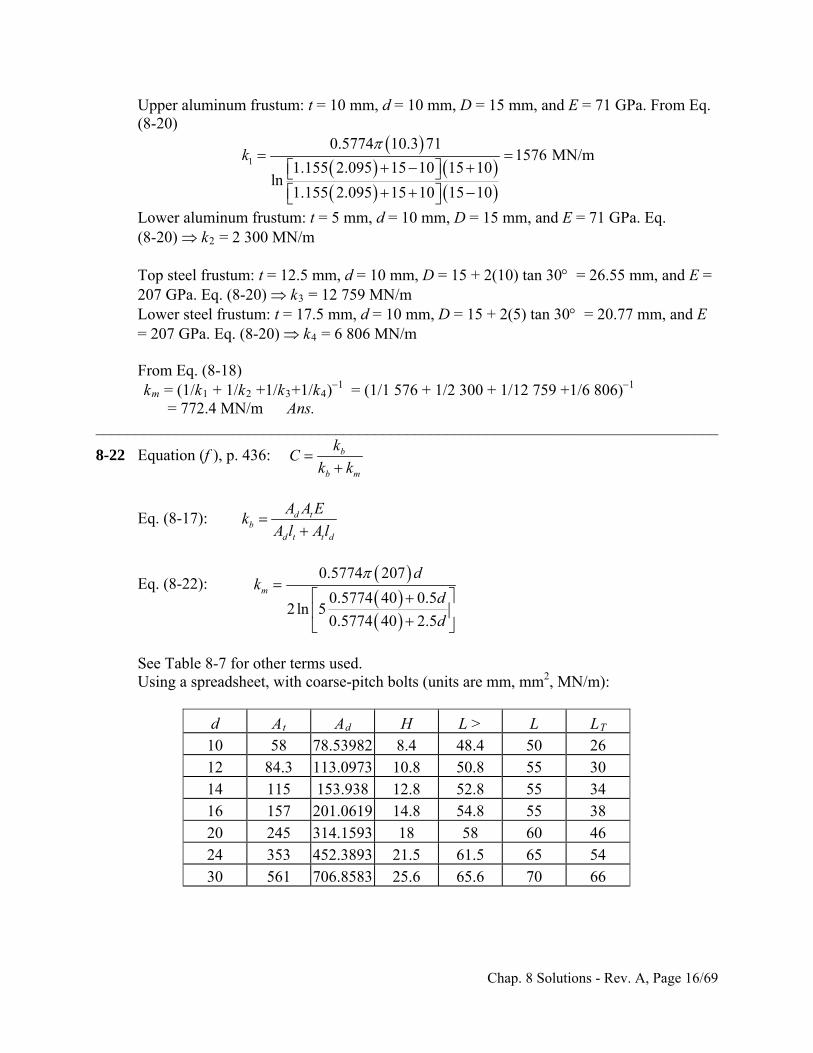
Upper aluminum frustum: t = 10 mm, d = 10 mm, D = 15 mm, and E = 71 GPa. From Eq. (8-20)
1
0.5774 10.3 711576 MN/m
1.155 2.095 15 10 15 10ln
1.155 2.095 15 10 15 10
k
Lower aluminum frustum: t = 5 mm, d = 10 mm, D = 15 mm, and E = 71 GPa. Eq. (8-20) k2 = 2 300 MN/m
Top steel frustum: t = 12.5 mm, d = 10 mm, D = 15 + 2(10) tan 30 = 26.55 mm, and E =
207 GPa. Eq. (8-20) k
3 = 12 759 MN/m Lower steel frustum: t = 17.5 mm, d = 10 mm, D = 15 + 2(5) tan 30 = 20.77 mm, and E
= 207 GPa. Eq. (8-20) k4 = 6 806 MN/m From Eq. (8-18) km = (1/k1 + 1/k2 +1/k3+1/k4)1 = (1/1 576 + 1/2 300 + 1/12 759 +1/6 806)1 = 772.4 MN/m Ans. ______________________________________________________________________________
8-22 Equation (f ), p. 436: b
b m
kC
k k
Eq. (8-17): d tb
d t t d
A A Ek
A l A l
Eq. (8-22):
0.5774 207
0.5774 40 0.52 ln 5
0.5774 40 2.5
m
dk
d
d
See Table 8-7 for other terms used. Using a spreadsheet, with coarse-pitch bolts (units are mm, mm2, MN/m):
d At Ad H L > L LT 10 58 78.53982 8.4 48.4 50 26 12 84.3 113.0973 10.8 50.8 55 30 14 115 153.938 12.8 52.8 55 34 16 157 201.0619 14.8 54.8 55 38 20 245 314.1593 18 58 60 46 24 353 452.3893 21.5 61.5 65 54 30 561 706.8583 25.6 65.6 70 66
Chap. 8 Solutions - Rev. A, Page 16/69
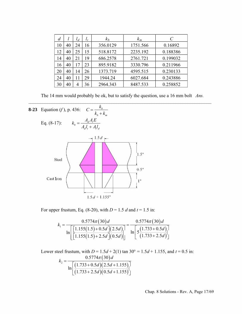
d l ld lt kb km C 10 40 24 16 356.0129 1751.566 0.16892 12 40 25 15 518.8172 2235.192 0.188386 14 40 21 19 686.2578 2761.721 0.199032 16 40 17 23 895.9182 3330.796 0.211966 20 40 14 26 1373.719 4595.515 0.230133 24 40 11 29 1944.24 6027.684 0.243886 30 40 4 36 2964.343 8487.533 0.258852
The 14 mm would probably be ok, but to satisfy the question, use a 16 mm bolt Ans. _____________________________________________________________________________
8-23 Equation (f ), p. 436: b
b m
kC
k k
Eq. (8-17): d tb
d t t d
A A Ek
A l A l
For upper frustum, Eq. (8-20), with D = 1.5 d and t = 1.5 in:
1
0.5774 30 0.5774 30
1.733 0.51.155 1.5 0.5 2.5ln 5ln
1.733 2.51.155 1.5 2.5 0.5
d dk
dd d
dd d
Lower steel frustum, with D = 1.5d + 2(1) tan 30 = 1.5d + 1.155, and t = 0.5 in:
2
0.5774 30
1.733 0.5 2.5 1.155ln
1.733 2.5 0.5 1.155
dk
d d
d d
Chap. 8 Solutions - Rev. A, Page 17/69
For cast iron frustum, let E = 14. 5 Mpsi, and D = 1.5 d, and t = 1 in:
3
0.5774 14.5
1.155 0.5ln 5
1.155 2.5
dk
d
d
Overall, km = (1/k1 +1/k2 +1/k3)1 See Table 8-7 for other terms used. Using a spreadsheet, with coarse-pitch bolts (units are in, in2, Mlbf/in):
d At Ad H L > L LT l 0.375 0.0775 0.110447 0.328125 3.328125 3.5 1 3 0.4375 0.1063 0.15033 0.375 3.375 3.5 1.125 3
0.5 0.1419 0.19635 0.4375 3.4375 3.5 1.25 3 0.5625 0.182 0.248505 0.484375 3.484375 3.5 1.375 3 0.625 0.226 0.306796 0.546875 3.546875 3.75 1.5 3 0.75 0.334 0.441786 0.640625 3.640625 3.75 1.75 3 0.875 0.462 0.60132 0.75 3.75 3.75 2 3
d ld lt kb k1 k2 k3 km C 0.375 2.5 0.5 1.031389 15.94599 178.7801 8.461979 5.362481 0.1613090.4375 2.375 0.625 1.383882 19.21506 194.465 10.30557 6.484256 0.175884
0.5 2.25 0.75 1.791626 22.65332 210.6084 12.26874 7.668728 0.1893830.5625 2.125 0.875 2.245705 26.25931 227.2109 14.35052 8.915294 0.201210.625 2.25 0.75 2.816255 30.03179 244.2728 16.55009 10.22344 0.2159760.75 2 1 3.988786 38.07191 279.7762 21.29991 13.02271 0.2344760.875 1.75 1.25 5.341985 46.7663 317.1203 26.51374 16.06359 0.24956
Use a 9
1612 UNC 3.5 in long bolt Ans.
______________________________________________________________________________
8-24 Equation (f ), p. 436: b
b m
kC
k k
Eq. (8-17): d tb
d t t d
A A Ek
A l A l
Chap. 8 Solutions - Rev. A, Page 18/69
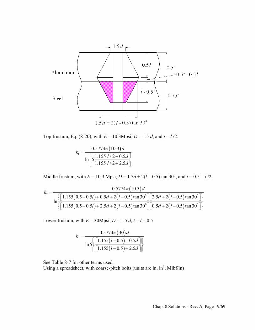
Top frustum, Eq. (8-20), with E = 10.3Mpsi, D = 1.5 d, and t = l /2:
1
0.5774 10.3
1.155 / 2 0.5ln 5
1.155 / 2 2.5
dk
l dl d
Middle frustum, with E = 10.3 Mpsi, D = 1.5d + 2(l 0.5) tan 30, and t = 0.5 l /2
2 0 0
0 0
0.5774 10.3
1.155 0.5 0.5 0.5 2 0.5 tan 30 2.5 2 0.5 tan 30ln
1.155 0.5 0.5 2.5 2 0.5 tan 30 0.5 2 0.5 tan 30
dk
l d l d l
l d l d l
Lower frustum, with E = 30Mpsi, D = 1.5 d, t = l 0.5
3
0.5774 30
1.155 0.5 0.5ln 5
1.155 0.5 2.5
dk
l d
l d
See Table 8-7 for other terms used. Using a spreadsheet, with coarse-pitch bolts (units are in, in2, Mlbf/in)
Chap. 8 Solutions - Rev. A, Page 19/69
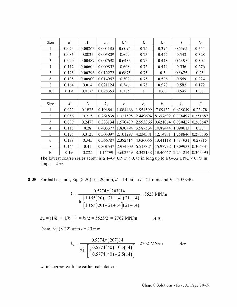
Size d At Ad L > L LT l ld 1 0.073 0.00263 0.004185 0.6095 0.75 0.396 0.5365 0.354 2 0.086 0.0037 0.005809 0.629 0.75 0.422 0.543 0.328 3 0.099 0.00487 0.007698 0.6485 0.75 0.448 0.5495 0.302 4 0.112 0.00604 0.009852 0.668 0.75 0.474 0.556 0.276 5 0.125 0.00796 0.012272 0.6875 0.75 0.5 0.5625 0.25 6 0.138 0.00909 0.014957 0.707 0.75 0.526 0.569 0.224 8 0.164 0.014 0.021124 0.746 0.75 0.578 0.582 0.172
10 0.19 0.0175 0.028353 0.785 1 0.63 0.595 0.37
Size d lt kb k1 k2 k3 km C 1 0.073 0.1825 0.194841 1.084468 1.954599 7.09432 0.635049 0.23478
2 0.086 0.215 0.261839 1.321595 2.449694 8.357692 0.778497 0.251687
3 0.099 0.2475 0.333134 1.570439 2.993366 9.621064 0.930427 0.263647
4 0.112 0.28 0.403377 1.830494 3.587564 10.88444 1.090613 0.27 5 0.125 0.3125 0.503097 2.101297 4.234381 12.14781 1.258846 0.285535
6 0.138 0.345 0.566787 2.382414 4.936066 13.41118 1.434931 0.28315
8 0.164 0.41 0.801537 2.974009 6.513824 15.93792 1.809923 0.306931
10 0.19 0.225 1.15799 3.602349 8.342138 18.46467 2.214214 0.343393 The lowest coarse series screw is a 164 UNC 0.75 in long up to a 632 UNC 0.75 in
long. Ans. ______________________________________________________________________________ 8-25 For half of joint, Eq. (8-20): t = 20 mm, d = 14 mm, D = 21 mm, and E = 207 GPa
1
0.5774 207 145523 MN/m
1.155 20 21 14 21 14ln
1.155 20 21 14 21 14
k
km = (1/k1 + 1/k1)1 = k1/2 = 5523/2 = 2762 MN/m Ans. From Eq. (8-22) with l = 40 mm
0.5774 207 142762 MN/m .
0.5774 40 0.5 142ln 5
0.5774 40 2.5 14
mk A
ns
which agrees with the earlier calculation.
Chap. 8 Solutions - Rev. A, Page 20/69
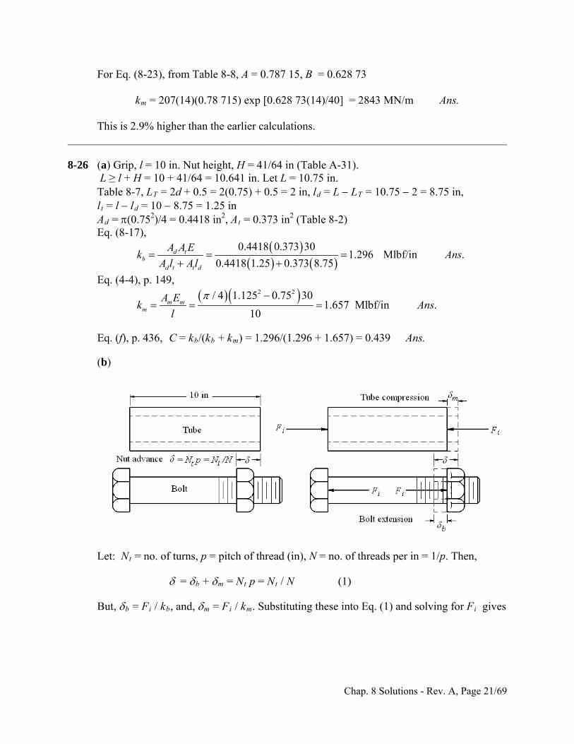
For Eq. (8-23), from Table 8-8, A = 0.787 15, B = 0.628 73 km = 207(14)(0.78 715) exp [0.628 73(14)/40] = 2843 MN/m Ans. This is 2.9% higher than the earlier calculations. ______________________________________________________________________________ 8-26 (a) Grip, l = 10 in. Nut height, H = 41/64 in (Table A-31). L ≥ l + H = 10 + 41/64 = 10.641 in. Let L = 10.75 in. Table 8-7, LT = 2d + 0.5 = 2(0.75) + 0.5 = 2 in, ld = L LT = 10.75 2 = 8.75 in, lt = l ld = 10 8.75 = 1.25 in Ad = (0.752)/4 = 0.4418 in2, At = 0.373 in2 (Table 8-2) Eq. (8-17),
0.4418 0.373 30
1.296 Mlbf/in .0.4418 1.25 0.373 8.75
d tb
d t t d
A A Ek A
A l Al
ns
Eq. (4-4), p. 149,
2 2/ 4 1.125 0.75 30
1.657 Mlbf/in .10
m mm
A Ek A
l
ns
Eq. (f), p. 436, C = kb/(kb + km) = 1.296/(1.296 + 1.657) = 0.439 Ans.
(b)
Let: Nt = no. of turns, p = pitch of thread (in), N = no. of threads per in = 1/p. Then,
= b + m = Nt p = Nt / N (1)
But, b = Fi / kb, and, m = Fi / km. Substituting these into Eq. (1) and solving for Fi gives
Chap. 8 Solutions - Rev. A, Page 21/69
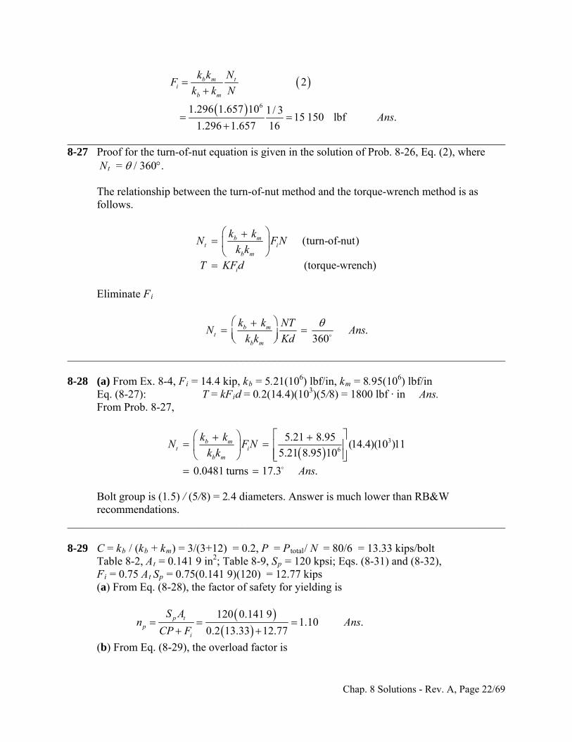
6
2
1.296 1.657 10 1/ 315 150 lbf .
1.296 1.657 16
b m ti
b m
k k NF
k k N
Ans
______________________________________________________________________________ 8-27 Proof for the turn-of-nut equation is given in the solution of Prob. 8-26, Eq. (2), where Nt = / 360. The relationship between the turn-of-nut method and the torque-wrench method is as
follows.
(turn-of-nut)
(torque-wrench)
b mt i
b m
i
k kN F N
k k
T KFd
Eliminate Fi
.360
b mt
b m
k k NTN A
k k Kd
ns
______________________________________________________________________________ 8-28 (a) From Ex. 8-4, Fi = 14.4 kip, kb = 5.21(106) lbf/in, km = 8.95(106) lbf/in Eq. (8-27): T = kFid = 0.2(14.4)(103)(5/8) = 1800 lbf · in Ans. From Prob. 8-27,
3
6
5.21 8.95(14.4)(10 )11
5.21 8.95 10
0.0481 turns 17.3 .
b mt i
b m
k kN F N
k k
Ans
Bolt group is (1.5) / (5/8) = 2.4 diameters. Answer is much lower than RB&W
recommendations. ______________________________________________________________________________ 8-29 C = kb / (kb + km) = 3/(3+12) = 0.2, P = Ptotal/ N = 80/6 = 13.33 kips/bolt Table 8-2, At = 0.141 9 in2; Table 8-9, Sp = 120 kpsi; Eqs. (8-31) and (8-32), Fi = 0.75 At Sp = 0.75(0.141 9)(120) = 12.77 kips (a) From Eq. (8-28), the factor of safety for yielding is
120 0.141 9
1.10 .0.2 13.33 12.77
p tp
i
S An A
CP F
ns
(b) From Eq. (8-29), the overload factor is
Chap. 8 Solutions - Rev. A, Page 22/69
120 0.141 9 12.77
1.60 .0.2 13.33
p t iL
S A Fn A
CP
ns
(c) From Eq. (803), the joint separation factor of safety is
0
12.771.20 .
1 13.33 1 0.2iF
n AP C
ns
______________________________________________________________________________ 8-30 1/2 13 UNC Grade 8 bolt, K = 0.20 (a) Proof strength, Table 8-9, Sp = 120 kpsi Table 8-2, At = 0.141 9 in2 Maximum, Fi = Sp At = 120(0.141 9) = 17.0 kips Ans. (b) From Prob. 8-29, C = 0.2, P = 13.33 kips Joint separation, Eq. (8-30) with n0 = 1 Minimum Fi = P (1 C) = 13.33(1 0.2) = 10.66 kips Ans. (c) iF = (17.0 + 10.66)/2 = 13.8 kips
Eq. (8-27), T = KFi d = 0.2(13.8)103(0.5)/12 = 115 lbf ft Ans. ______________________________________________________________________________ 8-31 (a) Table 8-1, At = 20.1 mm2. Table 8-11, Sp = 380 MPa. Eq. (8-31), Fi = 0.75 Fp = 0.75 At Sp = 0.75(20.1)380(103) = 5.73 kN
Eq. (f ), p. 436, 1
0.2781 2.6
b
b m
kC
k k
Eq. (8-28) with np = 1,
30.25 20.1 380 100.25
6.869 kN0.278
p t i p tS A F S AP
C C
Ptotal = NP = 8(6.869) = 55.0 kN Ans. (b) Eq. (8-30) with n0 = 1,
5.73
7.94 kN1 1 0.278
iFP
C
Ptotal = NP = 8(7.94) = 63.5 kN Ans. Bolt stress would exceed proof strength ______________________________________________________________________________ 8-32 (a) Table 8-2, At = 0.141 9 in2. Table 8-9, Sp = 120 kpsi. Eq. (8-31), Fi = 0.75 Fp = 0.75 At Sp = 0.75(0.141 9)120 = 12.77 kips
Eq. (f ), p. 436, 4
0.254 12
b
b m
kC
k k
Chap. 8 Solutions - Rev. A, Page 23/69
Eq. (8-28) with np = 1,
total
total
0.25
80 0.254.70
0.25 0.25 120 0.141 9
p t i p t
p t
S A F NS AP N
C C
P CN
S A
Round to N = 5 bolts Ans. (b) Eq. (8-30) with n0 = 1,
total
total
1
1 80 1 0.254.70
12.77
i
i
FP N
C
P CN
F
Round to N = 5 bolts Ans. ______________________________________________________________________________
8-33 Bolts: From Table A-31, the nut height is H = 10.8 mm. L ≥ l +H = 40 + 10.8 = 50.8
mm. Although Table A-17 indicates to go to 60 mm, 55 mm is readily available Round up to L = 55 mm Ans. Eq. (8-14): LT = 2d + 6 = 2(12) + 6 = 30 mm Table 8-7: ld = L LT = 55 30 = 25 mm, lt = l ld = 40 25 = 15 mm Ad = (122)/4 = 113.1 mm2, Table 8-1: At = 84.3 mm2 Eq. (8-17):
113.1 84.3 207
518.8 MN/m113.1 15 84.3 25
d tb
d t t d
A A Ek
A l A l
Members: Steel cyl. head: t = 20 mm, d = 12 mm, D = 18 mm, E = 207 GPa. Eq. (8-20),
1
0.5774 207 124470 MN/m
1.155 20 18 12 18 12ln
1.155 20 18 12 18 12
k
Cast iron: t = 20 mm, d = 12 mm, D = 18 mm, E = 100 GPa (from
Table 8-8). The only difference from k1 is the material k2 = (100/207)(4470) = 2159 MN/m Eq. (8-18): km = (1/4470 + 1/2159)1 = 1456 MN/m
Chap. 8 Solutions - Rev. A, Page 24/69
C = kb / (kb + km) = 518.8/(518.8+1456) = 0.263 Table 8-11: Sp = 650 MPa Assume non-permanent connection. Eqs. (8-31) and (8-32) Fi = 0.75 At Sp = 0.75(84.3)(650)103 = 41.1 kN The total external load is Ptotal = pg Ac, where Ac is the diameter of the cylinder which is
100 mm. The external load per bolt is P = Ptotal /N. Thus P = [6 (1002)/4](103)/10 = 4.712 kN/bolt Yielding factor of safety, Eq. (8-28):
3650 84.3 101.29 .
0.263 4.712 41.10p t
pi
S An A
CP F
ns
Overload factor of safety, Eq. (8-29):
3650 84.3 10 41.1011.1 .
0.263 4.712p t i
L
S A Fn A
CP
ns
Separation factor of safety, Eq. (8-30):
0
41.1011.8 .
1 4.712 1 0.263iF
n AP C
ns
______________________________________________________________________________ 8-34 Bolts: Grip, l = 1/2 + 5/8 = 1.125 in. From Table A-31, the nut height is H = 7/16 in. L ≥ l + H = 1.125 + 7/16 = 1.563 in. Round up to L = 1.75 in Ans. Eq. (8-13): LT = 2d + 0.25 = 2(0.5) + 0.25 = 1.25 in Table 8-7: ld = L LT = 1.75 1.25 = 0.5 in, lt = l ld = 1.125 0.5 = 0.625 in Ad = (0.52)/4 = 0.196 3 in2, Table 8-2: At = 0.141 9 in2 Eq. (8-17):
0.196 3 0.141 9 30
4.316 Mlbf/in0.196 3 0.625 0.141 9 0.5
d tb
d t t d
A A Ek
A l A l
Chap. 8 Solutions - Rev. A, Page 25/69
Members: Steel cyl. head: t = 0.5 in, d = 0.5 in, D = 0.75 in, E = 30 Mpsi. Eq. (8-20),
1
0.5774 30 0.533.30 Mlbf/in
1.155 0.5 0.75 0.5 0.75 0.5ln
1.155 0.5 0.75 0.5 0.75 0.5
k
Cast iron: Has two frusta. Midpoint of complete joint is at (1/2 + 5/8)/2 =
0.5625 in. Upper frustum, t = 0.5625 0.5 = 0.0625 in, d = 0.5 in, D = 0.75 + 2(0.5) tan 30 = 1.327 in, E = 14.5 Mpsi (from Table 8-8) Eq. (8-20) k2 = 292.7 Mlbf/in Lower frustum, t = 0.5625 in, d = 0.5 in, D = 0.75 in, E = 14.5 Mpsi Eq. (8-20) k3 = 15.26 Mlbf/in Eq. (8-18): km = (1/33.30 + 1/292.7 + 1/15.26)1 = 10.10 Mlbf/in C = kb / (kb + km) = 4.316/(4.316+10.10) = 0.299 Table 8-9: Sp = 85 kpsi Assume non-permanent connection. Eqs. (8-31) and (8-32) Fi = 0.75 At Sp = 0.75(0.141 9)(85) = 9.05 kips The total external load is Ptotal = pg Ac, where Ac is the diameter of the cylinder which is
3.5 in. The external load per bolt is P = Ptotal /N. Thus P = [1 500 (3.52)/4](103)/10 = 1.443 kips/bolt Yielding factor of safety, Eq. (8-28):
85 0.141 91.27 .
0.299 1.443 9.05p t
pi
S An A
CP F
ns
Overload factor of safety, Eq. (8-29):
85 0.141 9 9.05
6.98 .0.299 1.443
p t iL
S A Fn A
CPns
Separation factor of safety, Eq. (8-30):
Chap. 8 Solutions - Rev. A, Page 26/69
0
9.058.95 .
1 1.443 1 0.299iF
n AP C
ns
______________________________________________________________________________
-35 Bolts: Grip: l = 20 + 25 = 45 mm. From Table A-31, the nut height is H = 8.4 mm. m is
Round up to L = 55 mm Ans.
Eq. (8-14): LT = 2d + 6 = 2(10) + 6 = 26 mm
Table 8-7: ld = L LT = 55 26 = 29 mm, lt = l ld = 45 29 = 16 mm
Ad = (102)/4 = 78.5 mm2, Table 8-1: At = 58.0 mm2
Eq. (8-17):
8 L ≥ l +H = 45 + 8.4 = 53.4 mm. Although Table A-17 indicates to go to 60 mm, 55 m
readily available
78.5 58.0 207320.8 MN/m
78.5 16 58.0 29d t
bd t t d
A A Ek
A l A l
Members: Steel cyl. head: t = 20 mm, d = 10 mm, D = 15 mm, E = 207 GPa. Eq. (8-20),
1
0.5774 207 103503 MN/m
1.155 20 15 10 15 10ln
1.155 20 15 10 15 10
k
n: Has two frusta. Midpoint of complete joint is at (20 + 25)/2 = 22.5 mm
m Table 8-8),
Lower frustum, t = 22.5 mm, d = 10 mm, D = 15 mm, E = 100 GPa
Eq. (8-20) k3 = 1632 MN/m
Eq. (8-18): km = (1/3503 + 1/45 880 + 1/1632)1 = 1087 MN/m
C = kb / (kb + km) = 320.8/(320.8+1087) = 0.228
Table 8-11: Sp = 830 MPa ection. Eqs. (8-31) and (8-32)
Fi = 0.75 At Sp = 0.75(58.0)(830)103 = 36.1 kN
Cast iro Upper frustum, t = 22.5 20 = 2.5 mm, d = 10 mm, D = 15 + 2(20) tan 30 = 38.09 mm, E = 100 GPa (fro Eq. (8-20) k2 = 45 880 MN/m Assume non-permanent conn
Chap. 8 Solutions - Rev. A, Page 27/69
The total external load is Ptotal = pg Ac, where Ac is the diameter of the cylinder which is
P = [550 (0.82)/4]/36 = 7.679 kN/bolt
Yielding factor of safety, Eq. (8-28):
0.8 m. The external load per bolt is P = Ptotal /N. Thus
3830 58.0 101.27 .
0.228 7.679 36.1p t
pi
S An A
CP F
ns
Overload factor of safety, Eq. (8-29):
3830 58.0 10 36.16.88 .
0.228 7.679p t i
L
S A Fn A
CP
ns
Separation factor of safety, Eq. (8-30):
0
36.16.09 .
1 7.679 1 0.228iF
n AP C
ns
______________________________________________________________________________
-36 Bolts: Grip, l = 3/8 + 1/2 = 0.875 in. From Table A-31, the nut height is H = 3/8 in.
Let L = 1.25 in Ans.
Eq. (8-13): LT = 2d + 0.25 = 2(7/16) + 0.25 = 1.125 in
Table 8-7: ld = L LT = 1.25 1.125 = 0.125 in, lt = l ld = 0.875 0.125 =
Ad = (7/16) /4 = 0.150 3 in2, Table 8-2: At = 0.106 3 in2
Eq. (8-17),
8 L ≥ l + H = 0.875 + 3/8 = 1.25 in.
0.75 in
2
0.150 3 0.106 3 303.804 Mlbf/in
0.150 3 0.75 0.106 3 0.125dA
k tb
d t t d
A E
A l A l
Members: Steel cyl. head: t = 0.375 in, d = 0.4375 in, D = 0.65625 in, E = 30 Mpsi. Eq.
(8-20),
Chap. 8 Solutions - Rev. A, Page 28/69
1
0.5774 30 0.437531.40 Mlbf/in
1.155 0.375 0.65625 0.4375 0.65625 0.4375ln
1.155 0.375 0.65625 0.4375 0.65625 0.4375
k
Cast iron: Has two frusta. Midpoint of complete joint is at (3/8 + 1/2)/2 =
0.4375 in. Upper frustum, t = 0.4375 0.375 = 0.0625 in, d = 0.4375 in, D = 0.65625 + 2(0.375) tan 30 = 1.089 in, E = 14.5 Mpsi (from Table
8-8) Eq. (8-20) k2 = 195.5 Mlbf/in Lower frustum, t = 0.4375 in, d = 0.4375 in, D = 0.65625 in, E = 14.5
Mpsi Eq. (8-20) k3 = 14.08 Mlbf/in Eq. (8-18): km = (1/31.40 + 1/195.5 + 1/14.08)1 = 9.261 Mlbf/in C = kb / (kb + km) = 3.804/(3.804 + 9.261) = 0.291 Table 8-9: Sp = 120 kpsi Assume non-permanent connection. Eqs. (8-31) and (8-32) Fi = 0.75 At Sp = 0.75(0.106 3)(120) = 9.57 kips The total external load is Ptotal = pg Ac, where Ac is the diameter of the cylinder which is
3.25 in. The external load per bolt is P = Ptotal /N. Thus P = [1 200 (3.252)/4](103)/8 = 1.244 kips/bolt Yielding factor of safety, Eq. (8-28):
120 0.106 31.28 .
0.291 1.244 9.57p t
pi
S An A
CP F
ns
Overload factor of safety, Eq. (8-29):
120 0.106 3 9.57
8.80 .0.291 1.244
p t iL
S A Fn A
CPns
Separation factor of safety, Eq. (8-30):
Chap. 8 Solutions - Rev. A, Page 29/69
0
9.5710.9 .
1 1.244 1 0.291iF
n AP C
ns
______________________________________________________________________________
-37 From Table 8-7, h = t1 = 20 mm /2 = 26 mm
p to L = 40 mm
From Table 8-1, At = 84.3 mm2. Ad = (122)/4 = 113.1 mm2
8 For t2 > d, l = h + d /2 = 20 + 12 L ≥ h + 1.5 d = 20 + 1.5(12) = 38 mm. Round u LT = 2d + 6 = 2(12) + 6 = 30 mm ld = L LT = 40 20 = 10 mm lt = l ld = 26 10 = 16 mm Eq. (8-17),
113.1 84.3 207744.0 MN/m
113.1 16 84.3 10d t
bd t t d
A A Ek
A l A l
Similar to Fig. 8-21, we have three frusta. m, D = 18 mm, E = 207 GPa. Eq. (8-20)
Top frusta, steel: t = l / 2 = 13 mm, d = 12 m
1
0.5774 207 125 316 MN/m
1.155 13 18 12 18 12ln
1.155 13 18 12 18 12
k
Middle frusta, steel: t = 20 13 = 7 mm, d = 12 mm, D = 18 + 2(13 7) tan 30 = 24.93
Lower frusta, cast iron: t = 26 20 = 6 mm, d = 12 mm, D = 18 mm, E = 100 GPa (see
Eq. (8-18), km = (1/5 316 + 1/15 660 + 1/3 887)1 = 1 964 MN/m
C = kb / (kb + km) = 744.0/(744.0 + 1 964) = 0.275
Table 8-11: Sp = 650 MPa. From Prob. 8-33, P = 4.712 kN. Assume a non-permanent
Fi = 0.75 At Sp = 0.75(84.3)(650)103 = 41.1 kN
Yielding factor of safety, Eq. (8-28)
mm, E = 207 GPa. Eq. (8-20) k2 = 15 660 MN/m
Table 8-8). Eq. (8-20) k3 = 3 887 MN/m
connection. Eqs. (8-31) and (8-32),
3650 84.3 101.29 .
0.275 4.712 41.1p t
pi
S An A
CP F
ns
Overload factor of safety, Eq. (8-29)
Chap. 8 Solutions - Rev. A, Page 30/69
3650 84.3 10 41.110.7 .
0.275 4.712p t i
L
S A Fn A
CP
ns
r of safety, Eq. (8-30)
Separation facto
0
41.112.0 .
1 4.712 1 0.275iF
n AP C
ns
___________________________________________ ________________
1
.5/2 = 0.75 in 1.25 in
b = At E / l = 0.141 9(30)/0.75 =
in, D = 0.75 in, E = 30 Mpsi
__________________ _
-38 From Table 8-7, h = t = 0.5 in 8 For t2 > d, l = h + d /2 = 0.5 + 0 L ≥ h + 1.5 d = 0.5 + 1.5(0.5) = 1.25 in. Let L = LT = 2d + 0.25 = 2(0.5) + 0.25 = 1.25 in. All threaded.
2 From Table 8-1, At = 0.141 9 in . The bolt stiffness is k5.676 Mlbf/in
Similar to Fig. 8-21, we have three frusta. Top frusta, steel: t = l / 2 = 0.375 in, d = 0.5
1
0.5774 30 0.538.45 Mlk
bf/in
1.155 0.375 0.75 0.5 0.75 0.5ln
1.155 0.375 0.75 0.5 0.75 0.5
Middle frusta, steel: t = 0.5 0.375 = 0.125 in, d = 0.5 in,
d = 0.5 in, D = 0.75 in, E = 14.5 Mpsi.
m1 = 13.51 Mlbf/in
b b m
p e a non-permanent
i t p
D = 0.75 + 2(0.75 0.5) tan 30 = 1.039 in, E = 30 Mpsi. Eq. (8-20) k2 = 184.3 Mlbf/in
Lower frusta, cast iron: t = 0.75 0.5 = 0.25 in, Eq. (8-20) k3 = 23.49 Mlbf/in
Eq. (8-18), k = (1/38.45 + 1/184.3 + 1/23.49)
C = k / (k + k ) = 5.676 / (5.676 + 13.51) = 0.296
Table 8-9, S = 85 kpsi. From Prob. 8-34, P = 1.443 kips/bolt. Assum connection. Eqs. (8-31) and (8-32),
F = 0.75 A S = 0.75(0.141 9)(85) = 9.05 kips
Yielding factor of safety, Eq. (8-28)
85 0.141 91.27 .
0.296 1.443 9.05p t
pi
S An A
CP F
ns
Overload factor of safety, Eq. (8-29)
Chap. 8 Solutions - Rev. A, Page 31/69
85 0.141 9 9.05
7.05 .0.296 1.443
p t iL
S A Fn A
CP
ns
r of safety, Eq. (8-30)
Separation facto
0
9.058.91 .
1 1.443 1 0.296iF
n AP C
ns
__________________________________________ ________________
1
2 = 25 mm 35 mm
t2. Ad = (102)/4 = 78.5 mm2
__________________ __
-39 From Table 8-7, h = t = 20 mm 8 For t2 > d, l = h + d /2 = 20 + 10/ L ≥ h + 1.5 d = 20 + 1.5(10) = 35 mm. Let L = LT = 2d + 6 = 2(10) + 6 = 26 mm ld = L LT = 35 26 = 9 mm lt = l ld = 25 9 = 16 mm
From Table 8-1, A = 58.0 mm Eq. (8-17),
78.5 58.0 207530.1 MN/m
78.5 16 58.0 9d t
bd t t d
A A E k
A l A l
-21, we have three frusta. mm, D = 15 mm, E = 207 GPa. Eq. (8-20)
Similar to Fig. 8 Top frusta, steel: t = l / 2 = 12.5 mm, d = 10
1
0.5774 207 104 163 MN/mk
1.155 12.5 15 10 15 10ln
1.155 12.5 15 10 15 10
Middle frusta, steel: t = 20 12.5 = 7.5 mm, d = 10 mm, D = 15 + 2(12.5 7.5) tan 30 =
, E = 100 GPa (see
m1 = 1 562 MN/m
b b m
p = 830 MPa. From anent
i t p3 = 36.1 kN
20.77 mm, E = 207 GPa. Eq. (8-20) k2 = 10 975 MN/m
Lower frusta, cast iron: t = 25 20 = 5 mm, d = 10 mm, D = 15 mm Table 8-8). Eq. (8-20) k3 = 3 239 MN/m
Eq. (8-18), k = (1/4 163 + 1/10 975 + 1/3 239)
C = k / (k + k ) = 530.1/(530.1 + 1 562) = 0.253
Table 8-11: S Prob. 8-35, P = 7.679 kN/bolt. Assume a non-perm connection. Eqs. (8-31) and (8-32),
F = 0.75 A S = 0.75(58.0)(830)10
Yielding factor of safety, Eq. (8-28)
Chap. 8 Solutions - Rev. A, Page 32/69
3830p tS A
58.0 101.27 .
0.253 7.679 36.1pi
n AnsCP F
of safety, Eq. (8-29)
Overload factor
358.0 10 36.16.20 .
0.253 7.679p t i
Ln AnsCP
Separation factor of safety, Eq. (8-30)
830S A F
0
36.16.29 .
1 7.679 1 0.253iF
n Ans
P C
______________________________________________________________________________
For t2 > d, l = h + d /2 = 0.375 + 0.4375/2 = 0.59375 in ) = 1.031 in. Round up to L = 1.25 in
8-2: At = 0.106 3 in2
8-40 From Table 8-7, h = t1 = 0.375 in L ≥ h + 1.5 d = 0.375 + 1.5(0.4375 LT = 2d + 0.25 = 2(0.4375) + 0.25 = 1.125 in ld = L LT = 1.25 1.125 = 0.125 lt = l ld = 0.59375 0.125 = 0.46875 in Ad = (7/16)2/4 = 0.150 3 in2, Table Eq. (8-17),
0.150 3 0.106 3 30
5.724 Mlbf/in0.150 3 0.46875 0.106 3 0.125
d tb
d t t d
A A E k
A l A l
-21, we have three frusta. Top frusta, steel: t = l / 2 = 0.296875 in, d = 0.4375 in, D = 0.65625 in, E = 30 Mpsi Similar to Fig. 8
1k 0.5774 30 0.4375
35.52 Mlbf/in
1.155 0.296875 0.656255 0.4375 0.75 0.656255
ln1.155 0.296875 0.75 0.656255 0.75 0.656255
Middle frusta, steel: t = 0.375 0.296875 = 0.078125 in, d = 0.4375 in, D = 0.65625 + 2(0.59375 0.375) tan 30 = 0.9088 in, E = 30 Mpsi.
0.375 = 0.21875 in, d = 0.4375 in, D = 0.65625 in, E = 14.5 Mpsi. Eq. (8-20) k3 = 20.55 Mlbf/in
C = kb / (kb + km) = 5.724/(5.724 + 12.28) = 0.318
Eq. (8-20) k2 = 215.8 Mlbf/in Lower frusta, cast iron: t = 0.59375
Eq. (8-18), km = (1/35.52 + 1/215.8 + 1/20.55)1 = 12.28 Mlbf/in
Chap. 8 Solutions - Rev. A, Page 33/69
Table 8-9, Sp = 120 kpsi. From Prob. 8-34, P = 1.244 kips/bolt. Assume a non-permanent connection. Eqs. (8-31) and (8-32),
5(0.106 3)(120) = 9.57 kips
Fi = 0.75 At Sp = 0.7 Yielding factor of safety, Eq. (8-28)
12p tS An A
0 0.106 31.28 .
0.318 1.244 9.57pi
nsCP F
of safety, Eq. (8-29)
Overload factor
120p t iS A F 0.106 3 9.57
8.05 .0.318 1.244Ln Ans
CP
Separation factor of safety, Eq. (8-30)
0
9.5711.3 .
1 1.244 1 0.318iF
n Ans
P C
______________________________________________________________________________
What is presented here is one possible iterative approach. We will demonstrate this with
g using Eq. (8-18), yields km = 1 141 MN/m (see Prob. 8-33 for method of
e nut height in Table A-31. For the example, H = 8.4 mm. From this, L is
rounded up from the calculation of l + H = 40 + 8.4 = 48.4 mm to 50 mm. Next,
4 mm2.
for Db in Eq.
(8-34), the number of bolts are
8-41 This is a design problem and there is no closed-form solution path or a unique solution.
an example. 1. Select the diameter, d. For this example, let d = 10 mm. Using Eq. (8-20) on members,and combinincalculation.
2. Look up th
calculations are made for LT = 2(10) + 6 = 26 mm, ld = 50 26 = 24 mm, lt = 40 24 =16 mm. From step 1, Ad = (102)/4 = 78.54 mm2. Next, from Table 8-1, At = 78.5From Eq. (8-17), kb = 356 MN/m. Finally, from Eq. (e), p. 421, C = 0.238.
3. From Prob. 8-33, the bolt circle diameter is E = 200 mm. Substituting this
200
bDN
15.7
4 4 10d
p gives N = 16.
d on the solution to Prob. 8-33, the strength of ISO 9.8 was so high to give very large factors of safety for overload and separation. Try ISO 4.6
Rounding this u
4. Next, select a grade bolt. Base
Chap. 8 Solutions - Rev. A, Page 34/69
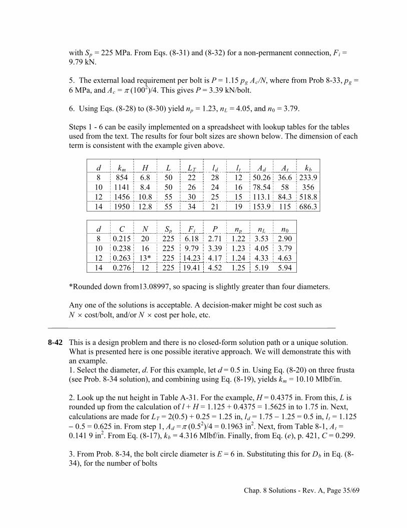
with Sp = 225 MPa. From Eqs. (8-31) and (8-32) for a non-permanent connection, Fi = 9.79 kN.
5. The ex ternal load requirement per bolt is P = 1.15 pg Ac/N, where from Prob 8-33, pg =
6 MPa, and A = (1002)/4. This gives P = 3.39 kN/bolt.
nd n0 = 3.79.
for the tables used from the text. The results for four bolt sizes are shown below. The dimension of each
lt Ad At kb
c
6. Using Eqs. (8-28) to (8-30) yield np = 1.23, nL = 4.05, a
Steps 1 - 6 can be easily implemented on a spreadsheet with lookup tables
term is consistent with the example given above.
d km H L LT ld 8 854 6.8 50 22 28 12 50.26 36.6 233.9 10 1 78.54 356 141 8.4 50 26 24 16 58 12 1456 10.8 55 30 25 15 113.1 84.3 518.8 14 1950 12.8 55 34 21 19 153.9 115 686.3
d C N S p F i P n p n L n 0
8 0.215 20 225 6.18 2.71 1.22 3.53 2.90
10 0.238 16 225 9.79 3.39 1.23 4.05 3.79
12 0.263 13* 225 14.23 4.17 1.24 4.33 4.63
14 0.276 12 225 19.41 4.52 1.25 5.19 5.94 *Rounded down from 89 g eters.
N cost/bolt, and/or N cost per hole, etc. ____ __
n. What is presented here is one possible iterative approach. We will demonstrate this with
4 solution), and combining using Eq. (8-19), yields km = 10.10 Mlbf/in.
rounded up from the calculation of l + H = 1.125 + 0.4375 = 1.5625 in to 1.75 in. Next,
34), for the number of bolts
13.0 97, so spacin is slightly greater than four diam Any one of the solutions is acceptable. A decision-maker might be cost such as _ _________________________________________________________________ 8-42 This is a design problem and there is no closed-form solution path or a unique solutio
an example. 1. Select the diameter, d. For this example, let d = 0.5 in. Using Eq. (8-20) on three frusta(see Prob. 8-3
2. Look up the nut height in Table A-31. For the example, H = 0.4375 in. From this, L is
calculations are made for LT = 2(0.5) + 0.25 = 1.25 in, ld = 1.75 1.25 = 0.5 in, lt = 1.125 0.5 = 0.625 in. From step 1, Ad = (0.52)/4 = 0.1963 in2. Next, from Table 8-1, At = 0.141 9 in2. From Eq. (8-17), kb = 4.316 Mlbf/in. Finally, from Eq. (e), p. 421, C = 0.299.
3. From Prob. 8-34, the bolt circle diameter is E = 6 in. Substituting this for Db in Eq. (8-
Chap. 8 Solutions - Rev. A, Page 35/69
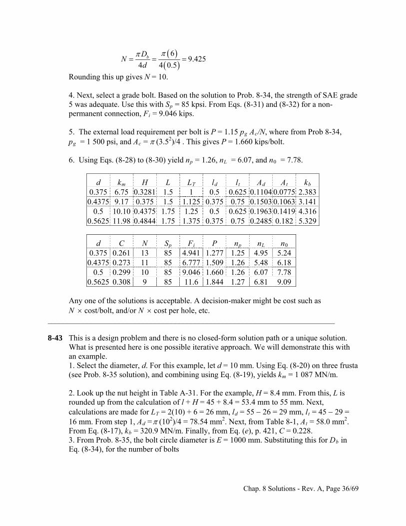
6
9.4254 4
bDN
d
0.5
Rounding this up gives N = 10.
4. Next, select a grade bolt. Based on the solution to Prob. 8-34, the strength of SAE grade = 85 kpsi. From Eqs. (8-31) and (8-32) for a non-
permanent connection, Fi = 9.046 kips.
4, s gives P = 1.660 kips/bolt.
b
5 was adequate. Use this with Sp
5. The external load requirement per bolt is P = 1.15 pg Ac/N, where from Prob 8-3pg = 1 500 psi, and Ac = (3.52)/4 . Thi
6. Using Eqs. (8-28) to (8-30) yield np = 1.26, nL = 6.07, and n0 = 7.78.
d km H L LT ld lt Ad At k0.375 6.75 0.3281 1.5 1 0.5 0.625 0.1104 0.0775 2.383 0.4375 9.17 0.375 1.5 1.125 0.375 0.75 0.1503 0.1063 3.141
0.5 10.10 0.4375 1.75 1.25 0.1963 0.1419 4.316 0.5 0.6250.5625 11.98 0.4844 1.75 1.375 0.375 0.75 0.2485 0.182 5.329
d C N Sp Fi P np nL n 0
0.375 0.261 13 85 4.941 1.277 1.25 4.95 5.24
0.4375 0.273 11 85 6.777 1.509 1.26 5.48 6.18
0.5 0.299 9.046 1.660 1.26 6.07 7.78 10 85
0.5625 0.308 9 85 11.6 1.844 1.27 6.81 9.09 Any on th io ac a d - r b such as N c r N cos r h t_______________________________________________________________________
solution path or a unique solution. ith
an example. ta
calculations are made for L = 2(10) + 6 = 26 mm, l = 55 26 = 29 mm, l = 45 29 =
e of e solut ns is cept ble. A ecision make might e costost/bolt, and/o t pe ole, e c.
_ 8-43 This is a design problem and there is no closed-form
What is presented here is one possible iterative approach. We will demonstrate this w
1. Select the diameter, d. For this example, let d = 10 mm. Using Eq. (8-20) on three frus(see Prob. 8-35 solution), and combining using Eq. (8-19), yields km = 1 087 MN/m.
2. Look up the nut height in Table A-31. For the example, H = 8.4 mm. From this, L is rounded up from the calculation of l + H = 45 + 8.4 = 53.4 mm to 55 mm. Next,
T d t
16 mm. From step 1, Ad = (102)/4 = 78.54 mm2. Next, from Table 8-1, At = 58.0 mm2. From Eq. (8-17), kb = 320.9 MN/m. Finally, from Eq. (e), p. 421, C = 0.228. 3. From Prob. 8-35, the bolt circle diameter is E = 1000 mm. Substituting this for Db in Eq. (8-34), for the number of bolts
Chap. 8 Solutions - Rev. A, Page 36/69
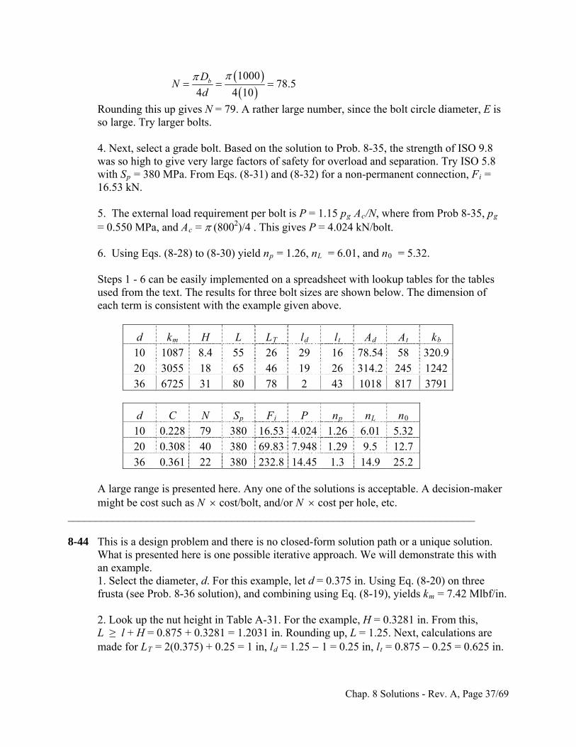
1000
78.54 4 10
bDN
d
Rounding this up gives N = 79. A rather large number, since the bolt circle diameter, E is ger bolts.
rge factors of safety for overload and separation. Try ISO 5.8 with Sp = 380 MPa. From Eqs. (8-31) and (8-32) for a non-permanent connection, Fi =
a, and Ac = (8002)/4 . This gives P = 4.024 kN/bolt.
Steps 1 - 6 can be easily implemented on a spreadsheet with lookup tables for the tables
mension of each term is consistent with the example given above.
so large. Try lar
4. Next, select a grade bolt. Based on the solution to Prob. 8-35, the strength of ISO 9.8 was so high to give very la
16.53 kN.
5. The external load requirement per bolt is P = 1.15 pg Ac/N, where from Prob 8-35, pg
= 0.550 MP 6. Using Eqs. (8-28) to (8-30) yield np = 1.26, nL = 6.01, and n0 = 5.32.
used from the text. The results for three bolt sizes are shown below. The di
d km H L LT ld lt Ad At kb 10 1087 8.4 55 26 29 16 78.54 58 320.9 20 3055 18 65 46 19 26 314.2 245 1242 36 6725 31 80 78 2 43 1018 817 3791
d C N Sp Fi P np nL n0
1 0 0.2 8 2 7 9 380 16.53 4.024 1.26 6. 1 0 5. 2 3
20 0.308 40 380 69.83 7.948 1.29 12.7 9.5
36 0.361 22 380 232.8 14.45 1.3 14.9 25.2 A large range e he n l i ep A decision-maker
might be cost such as co lt o r h tc_______________________________________________________________________
8-44 r a unique solution. ith
an example.
.
made for L = 2(0.375) + 0.25 = 1 in, l = 1.25 1 = 0.25 in, l = 0.875 0.25 = 0.625 in.
is pres nted re. A y one of the so utions s acc table.N st/bo , and/or N c st pe ole, e .
_
This is a design problem and there is no closed-form solution path oWhat is presented here is one possible iterative approach. We will demonstrate this w
1. Select the diameter, d. For this example, let d = 0.375 in. Using Eq. (8-20) on three frusta (see Prob. 8-36 solution), and combining using Eq. (8-19), yields km = 7.42 Mlbf/in
2. Look up the nut height in Table A-31. For the example, H = 0.3281 in. From this, L ≥ l + H = 0.875 + 0.3281 = 1.2031 in. Rounding up, L = 1.25. Next, calculations are
T d t
Chap. 8 Solutions - Rev. A, Page 37/69
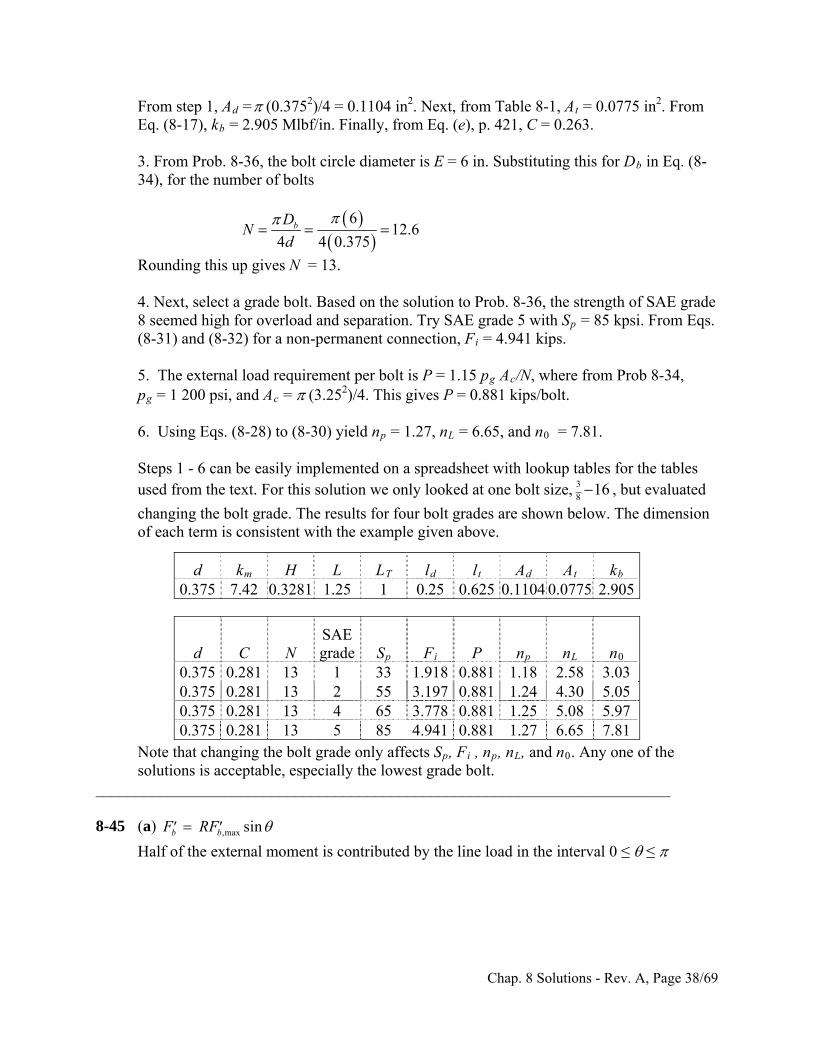
From step 1, Ad = (0.3752)/4 = 0.1104 in2. Next, from Table 8-1, At = 0.0775 in2. FromEq. (8-17), k
for Db in Eq. (8-
34), for the number of bolts
b = 2.905 Mlbf/in. Finally, from Eq. (e), p. 421, C = 0.263.
3. From Prob. 8-36, the bolt circle diameter is E = 6 in. Substituting this
6
12.64 4 0.375
bDN
d
p gives N = 13.
d on the solution to Prob. 8-36, the strength of SAE grade 8 seemed high for overload and separation. Try SAE grade 5 with Sp = 85 kpsi. From Eqs.
from Prob 8-34,
pg = 1 200 psi, and Ac = (3.25 )/4. This gives P = 0.881 kips/bolt.
.81.
for the tables used from the text. For this solution we only looked at one bolt size,
Rounding this u
4. Next, select a grade bolt. Base
(8-31) and (8-32) for a non-permanent connection, Fi = 4.941 kips.
5. The external load requirement per bolt is P = 1.15 pg Ac/N, where 2
6. Using Eqs. (8-28) to (8-30) yield np = 1.27, nL = 6.65, and n0 = 7 Steps 1 - 6 can be easily implemented on a spreadsheet with lookup tables
3
8
changing the bolt grade. The results for four bolt grades are shown below. The dimensionof each term is consistent with the example given above.
16 , but evaluated
Note t he t gr onl fe , d n of the solutio le eci the lowest grade bolt.
hat changing t bol ade y af cts Sp, Fi , np nL, an n0. A y one ns is acceptab , esp ally
________________________________________________________________________
ment is contributed by the line load in the interval 0 ≤ ≤
Ad At kb d km H L LT ld lt 0.375 7.42 0.3281 1.25 1 0.25 0.625 0.1104 0.0775 2.905
d C N grade S F P n n n SAE
p i p L 0
0.375 0.281 13 1 33 1.918 0.881 1.18 2.58 3.03 0. 5 0. 3.197 0.881 1 4 5.05 37 281 13 2 55 .24 .300.375 0.281 13 4 65 3.778 0.881 1.25 5.08 5.97 0.375 0.281 13 5 85 4.941 0.881 1.27 6.65 7.81
8-45 (a) ,max sinb bF RF
Half of the external mo
Chap. 8 Solutions - Rev. A, Page 38/69
2 2,max0 0
2,max
sin sin2
2 2
b b
b
MF R d F R d
MF R
2
from which ,max 2b
MF
R
2 2
1 1max 1 22
sin sin (cos - cos )b
M MF F R d R d
R R
Noting 1 = 75, 2 = 105,
max
12 000(cos 75 - cos105 ) 494 lbf .
(8 / 2)F A
ns
(b) max ,max 2
2 2( )b
M MF F R R
R N R
N
max
2(12 000)500 lbf .
(8 / 2)(12)F A ns
(c) F = Fmax sin
M = 2 Fmax R [(1) sin2 90 + 2 sin2 60 + 2 sin2 30 + (1) sin2 (0)] = 6FmaxR from which,
max
12 000500 lbf .
6 6(8 / 2)
MF A
R ns
The simple general equation resulted from part (b)
max
2MF
RN
________________________________________________________________________ 8-46 (a) From Table 8-11, Sp = 600 MPa. From Table 8-1, At = 353 mm2. Eq. (8-31): 30.9 0.9 353 600 10 190.6 kNi t pF A S
Table 8-15: K = 0.18 Eq. (8-27): T = K Fi d = 0.18(190.6)(24) = 823 Nm Ans.
Chap. 8 Solutions - Rev. A, Page 39/69
(b) Washers: t = 4.6 mm, d = 24 mm, D = 1.5(24) = 36 mm, E = 207 GPa. Eq. (8-20),
1
0.5774 207 2431 990 MN/m
1.155 4.6 36 24 36 24ln
1.155 4.6 36 24 36 24
k
Cast iron: t = 20 mm, d = 24 mm, D = 36 + 2(4.6) tan 30 = 41.31 mm, E = 135 GPa.
Eq. (8-20) k2 = 10 785 MN/m Steel joist: t = 20 mm, d = 24 mm, D = 41.31 mm, E = 207 GPa. Eq. (8-20) k3 = 16
537 MN/m Eq. (8-18): km = (2 / 31 990 + 1 / 10 785 +1 / 16 537)1 = 4 636 MN/m Bolt: l = 2(4.6) + 2(20) = 49.2 mm. Nut, Table A-31, H = 21.5 mm. L > 49.2 + 21.5 = 70.7
mm. From Table A-17, use L = 80 mm. From Eq. (8-14) LT = 2(24) + 6 = 54 mm, ld = 80 54 = 26 mm, lt = 49.2 26 = 23.2 mm From Table (8-1), At = 353 mm2, Ad = (242) / 4 = 452.4 mm2 Eq. (8-17):
452.4 353 207
1680 MN/m452.4 23.2 353 26
d tb
d t t d
A A Ek
A l A l
C = kb / (kb + km) = 1680 / (1680 + 4636) = 0.266, Sp = 600 MPa, Fi = 190.6 kN, P = Ptotal / N = 18/4 = 4.5 kN Yield: From Eq. (8-28)
3600 353 101.10 .
0.266 4.5 190.6p t
pi
S An A
CP F
ns
Load factor: From Eq. (8-29)
3600 353 10 190.617.7 .
0.266 4.5p t i
L
S A Fn A
CP
ns
Separation: From Eq. (8-30)
Chap. 8 Solutions - Rev. A, Page 40/69
0
190.657.7 .
1 4.5 1 0.266iF
n AP C
ns
m
As was stated in the text, bolts are typically preloaded such that the yielding factor of
safety is not much greater than unity which is the case for this problem. However, the other load factors indicate that the bolts are oversized for the external load.
______________________________________________________________________________ 8-47 (a) ISO M 20 2.5 grade 8.8 coarse pitch bolts, lubricated. Table 8-2, At = 245 mm2 Table 8-11, Sp = 600 MPa Fi = 0.90 At Sp = 0.90(245)600(103) = 132.3 kN Table 8-15, K = 0.18 Eq. (8-27), T = KFi d = 0.18(132.3)20 = 476 N m Ans. (b) Table A-31, H = 18 mm, L ≥ LG + H = 48 + 18 = 66 mm. Round up to L = 80 mm per
Table A-17.
2 6 2(20) 6 46 m
- 80 46 34 mm- 48 34 14 mm
T
d T
t d
L dl L Ll l l
Ad = (202) /4 = 314.2 mm2,
314.2(245)(207)1251.9 MN/m
314.2(14) 245(34)d t
bd t t d
A A Ek
A l Al
Members: Since all members are steel use Eq. (8-22) with E = 207 MPa, l = 48 mm, d =
20mm
0.5774 207 200.57744236 MN/m
0.5774 0.5 0.5774 48 0.5 202ln 5 2ln 50.5774 2.5 0.5774 48 2.5 20
m
Edk
l dl d
1251.9
0.2281251.9 4236
b
b m
kC
k k
P = Ptotal / N = 40/2 = 20 kN, Yield: From Eq. (8-28)
3600 245 101.07 .
0.228 20 132.3p t
pi
S An A
CP F
ns
Chap. 8 Solutions - Rev. A, Page 41/69
Load factor: From Eq. (8-29)
3600 245 10 132.33.22 .
0.228 20p t i
L
S A Fn A
CP
ns
Separation: From Eq. (8-30)
0
132.38.57 .
1 20 1 0.228iF
n AP C
ns
______________________________________________________________________________ 8-48 From Prob. 8-29 solution, Pmax =13.33 kips, C = 0.2, Fi = 12.77 kips, At = 0.141 9 in2
12.77
90.0 kpsi0.141 9
ii
t
F
A
Eq. (8-39),
0.2 13.33
9.39 kpsi2 2 0.141 9a
t
CP
A
Eq. (8-41), 9.39 90.0 99.39 kpsim a i
(a) Goodman Eq. (8-45) for grade 8 bolts, Se = 23.2 kpsi (Table 8-17), Sut = 150 kpsi (Table 8-9)
23.2 150 90.00.856 .
9.39 150 23.2e ut i
fa ut e
S Sn A
S S
ns
(b) Gerber Eq. (8-46)
2 2
2 2
14 2
2
1150 150 4 23.2 23.2 90.0 150 2 90.0 23.2 1.32 .
2 9.39 23.2
f ut ut e e i ut i ea e
n S S S S S SS
Ans
(c) ASME-elliptic Eq. (8-47) with Sp = 120 kpsi (Table 8-9)
2 2 2
2 2
2 2 2
2 2
23.2120 120 23.2 90 90 23.2 1.30 .
9.39 120 23.2
ef p p e i i e
a p e
Sn S S S S
S S
Ans
______________________________________________________________________________ 8-49 Attention to the Instructor. Part (d) requires the determination of the endurance strength,
Se, of a class 5.8 bolt. Table 8-17 does not provide this and the student will be required to estimate it by other means [see the solution of part (d)].
Per bolt, Pbmax = 60/8 = 7.5 kN, Pbmin = 20/8 = 2.5 kN
Chap. 8 Solutions - Rev. A, Page 42/69
1
0.2781 2.6
b
b m
kC
k k
(a) Table 8-1, At = 20.1 mm2; Table 8-11, Sp = 380 MPa Eqs. (8-31) and (8-32), Fi = 0.75 At Sp = 0.75(20.1)380(103) = 5.73 kN
Yield, Eq. (8-28),
3380 20.1 100.98 .
0.278 7.5 5.73p t
pi
S An A
CP F
ns
(b) Overload, Eq. (8-29),
3380 20.1 10 5.730.915 .
0.278 7.5p t i
L
S A Fn A
CP
ns
(c) Separation, Eq. (8-30), 0
5.731.06 .
1 7.5 1 0.278iF
n AP C
ns
(d) Goodman, Eq. (8-35),
3max min 0.278 7.5 2.5 10
34.6 MPa2 2 20.1
b ba
t
C P P
A
Eq. (8-36),
33
max min5.73 100.278 7.5 2.5 10
354.2 MPa2 2 20.1 20.1
b b im
t t
C P P F
A A
Table 8-11, Sut = 520 MPa, i = Fi /At = 5.73(103)/20.1 = 285 MPa We have a problem for Se. Table 8-17 does not list Se for class 5.8 bolts. Here, we will
estimate Se using the methods of Chapter 6. Estimate eS from the,
Eq. (6-8), p. 282, 0.5 0.5 520 260 MPae utS S .
Table 6-2, p. 288, a = 4.51, b = 0.265 Eq. (6-19), p. 287, 0.2654.51 520 0.860b
a utk aS
Eq. (6-21), p. 288, kb = 1 Eq. (6-26), p.290, kc = 0.85 The fatigue stress-concentration factor, from Table 8-16, is Kf = 2.2. For simple axial
loading and infinite-life it is acceptable to reduce the endurance limit by Kf and use the nominal stresses in the stress/strength/design factor equations. Thus,
Eq. (6-18), p. 287, Se = ka kb kc eS / Kf = 0.86(1)0.85(260) / 2.2 = 86.4 MPa
Eq. (8-38),
86.4 520 285
0.847 .520 34.6 86.4 354.2 285
e ut if
ut a e m i
S Sn A
S S
ns
It is obvious from the various answers obtained, the bolted assembly is undersized. This
can be rectified by a one or more of the following: more bolts, larger bolts, higher class bolts.
______________________________________________________________________________ 8-50 Per bolt, Pbmax = Pmax /N = 80/10 = 8 kips, Pbmin = Pmin /N = 20/10 = 2 kips C = kb / (kb + km) = 4/(4 + 12) = 0.25 (a) Table 8-2, At = 0.141 9 in2, Table 8-9, Sp = 120 kpsi and Sut = 150 kpsi
Chap. 8 Solutions - Rev. A, Page 43/69
Table 8-17, Se = 23.2 kpsi Eqs. (8-31) and (8-32), Fi = 0.75 At Sp i = Fi /At = 0.75 Sp = 0.75(120) =90 kpsi
Eq. (8-35),
max min 0.25 8 2
5.29 kpsi2 2 0.141 9
b ba
t
C P P
A
Eq. (8-36),
max min 0.25 8 2
90 98.81 kpsi2 2 0.141 9
b bm i
t
C P P
A
Eq. (8-38),
23.2 150 90
1.39 .150 5.29 23.2 98.81 90
e ut if
ut a e m i
S Sn A
S S
ns
______________________________________________________________________________ 8-51 From Prob. 8-33, C = 0.263, Pmax = 4.712 kN / bolt, Fi = 41.1 kN, Sp = 650 MPa, and At = 84.3 mm2 i = 0.75 Sp = 0.75(650) = 487.5 MPa
Eq. (8-39):
30.263 4.712 107.350 MPa
2 2 84.3at
CP
A
Eq. (8-40) 7.350 487.5 494.9 MPa2
im
t t
FCP
A A
(a) Goodman: From Table 8-11, Sut = 900 MPa, and from Table 8-17, Se = 140 MPa
Eq. (8-45):
140 900 487.57.55 .
7.350 900 140e ut i
fa ut e
S Sn A
S S
ns
(b) Gerber: Eq. (8-46):
2 2
2 2
14 2
2
1900 900 4 140 140 487.5 900 2 487.5 140
2 7.350 140
11.4 .
f ut ut e e i ut i ea e
n S S S S S SS
Ans
(c) ASME-elliptic: Eq. (8-47):
Chap. 8 Solutions - Rev. A, Page 44/69
2 2 2
2 2
2 2 2
2 2
140650 650 140 487.5 487.5 140 9.73 .
7.350 650 140
ef p p e i i e
a p e
Sn S S S S
S S
Ans
______________________________________________________________________________ 8-52 From Prob. 8-34, C = 0.299, Pmax = 1.443 kips/bolt,Fi = 9.05 kips, Sp = 85 kpsi, and At = 0.141 9 in2 0.75 0.75 85 63.75 kpsii pS
Eq. (8-37):
0.299 1.443
1.520 kpsi2 2 0.141 9a
t
CP
A
Eq. (8-38) 1.520 63.75 65.27 kpsi2m i
t
CP
A
(a) Goodman: From Table 8-9, Sut = 120 kpsi, and from Table 8-17, Se = 18.8 kpsi
Eq. (8-45):
18.8 120 63.755.01 .
1.520 120 18.8e ut i
fa ut e
S Sn A
S S
ns
(b) Gerber: Eq. (8-46):
2 2
2 2
14 2
2
1120 120 4 18.6 18.6 63.75 120 2 63.75 18.6
2 1.520 18.6
7.45 .
f ut ut e e i ut i ea e
n S S S S S SS
Ans
(c) ASME-elliptic: Eq. (8-47):
2 2 2
2 2
2 2 2
2 2
18.685 85 18.6 63.75 63.75 18.6 6.22 .
1.520 85 18.6
ef p p e i i e
a p e
Sn S S S S
S S
Ans
______________________________________________________________________________
Chap. 8 Solutions - Rev. A, Page 45/69
8-53 From Prob. 8-35, C = 0.228, Pmax = 7.679 kN/bolt, Fi = 36.1 kN, Sp = 830 MPa, and At = 58.0 mm2 i = 0.75 Sp = 0.75(830) = 622.5 MPa
Eq. (8-37):
30.228 7.679 1015.09 MPa
2 2 58.0at
CP
A
Eq. (8-38) 15.09 622.5 637.6 MPa2m i
t
CP
A
(a) Goodman: From Table 8-11, Sut = 1040 MPa, and from Table 8-17, Se = 162 MPa
Eq. (8-45):
162 1040 622.53.73 .
15.09 1040 162e ut i
fa ut e
S Sn A
S S
ns
(b) Gerber: Eq. (8-46):
2 2
2 2
14 2
2
11040 1040 4 162 162 622.5 1040 2 622.5 162
2 15.09 162
5.74 .
f ut ut e e i ut i ea e
n S S S S S SS
Ans
(c) ASME-elliptic: Eq. (8-47):
2 2 2
2 2
2 2 2
2 2
162830 830 162 622.5 622.5 162 5.62 .
15.09 830 162
ef p p e i i e
a p e
Sn S S S S
S S
Ans
______________________________________________________________________________ 8-54 From Prob. 8-36, C = 0.291, Pmax = 1.244 kips/bolt, Fi = 9.57 kips, Sp = 120 kpsi, and At = 0.106 3 in2 0.75 0.75 120 90 kpsii pS
Eq. (8-37):
0.291 1.244
1.703 kpsi2 2 0.106 3a
t
CP
A
Chap. 8 Solutions - Rev. A, Page 46/69
Eq. (8-38) 1.703 90 91.70 kpsi2m i
t
CP
A
(a) Goodman: From Table 8-9, Sut = 150 kpsi, and from Table 8-17, Se = 23.2 kpsi
Eq. (8-45):
23.2 150 904.72 .
1.703 150 23.2e ut i
fa ut e
S Sn A
S S
ns
(b) Gerber: Eq. (8-46):
2 2
2 2
14 2
2
1150 150 4 23.2 23.2 90 150 2 90 23.2
2 1.703 23.2
7.28 .
f ut ut e e i ut i ea e
n S S S S S SS
Ans
(c) ASME-elliptic: Eq. (8-47):
2 2 2
2 2
2 2 2
2 2
23.2120 120 23.2 90 90 23.2 7.24 .
1.703 120 18.6
ef p p e i i e
a p e
Sn S S S S
S S
Ans
______________________________________________________________________________ 8-55 From Prob. 8-51, C = 0.263, Se = 140 MPa, Sut = 900 MPa, At = 84.4 mm2, i =
487.5 MPa, and Pmax = 4.712 kN. Pmin = Pmax / 2 = 4.712/2 = 2.356 kN
Eq. (8-35):
3max min 0.263 4.712 2.356 10
3.675 MPa2 2 84.3a
t
C P P
A
Eq. (8-36):
Chap. 8 Solutions - Rev. A, Page 47/69
max min
3
2
0.263 4.712 2.356 10487.5 498.5 MPa
2 84.3
m it
C P P
A
Eq. (8-38):
140 900 487.5
11.9 .900 3.675 140 498.5 487.5
e ut if
ut a e m i
S Sn A
S S
ns
______________________________________________________________________________ 8-56 From Prob. 8-52, C = 0.299, Se = 18.8 kpsi, Sut = 120 kpsi, At = 0.141 9 in2, i = 63.75
kpsi, and Pmax = 1.443 kips Pmin = Pmax / 2 = 1.443/2 = 0.722 kips
Eq. (8-35):
max min 0.299 1.443 0.722
0.760 kpsi2 2 0.141 9a
t
C P P
A
Eq. (8-36):
max min
2
0.299 1.443 0.72263.75 66.03 kpsi
2 0.141 9
m it
C P P
A
Eq. (8-38):
18.8 120 63.75
7.89 .120 0.760 18.8 66.03 63.75
e ut if
ut a e m i
S Sn Ans
S S
______________________________________________________________________________ 8-57 From Prob. 8-53, C = 0.228, Se = 162 MPa, Sut = 1040 MPa, At = 58.0 mm2, i = 622.5
MPa, and Pmax = 7.679 kN. Pmin = Pmax / 2 = 7.679/2 = 3.840 kN
Eq. (8-35):
3max min 0.228 7.679 3.840 10
7.546 MPa2 2 58.0a
t
C P P
A
Chap. 8 Solutions - Rev. A, Page 48/69
Eq. (8-36):
max min
3
2
0.228 7.679 3.840 10622.5 645.1 MPa
2 58.0
m it
C P P
A
Eq. (8-38):
162 1040 622.5
5.88 .1040 7.546 162 645.1 622.5
e ut if
ut a e m i
S Sn A
S S
ns
______________________________________________________________________________ 8-58 From Prob. 8-54, C = 0.291, Se = 23.2 kpsi, Sut = 150 kpsi, At = 0.106 3 in2, i = 90
kpsi, and Pmax = 1.244 kips Pmin = Pmax / 2 = 1.244/2 = 0.622 kips
Eq. (8-35):
max min 0.291 1.244 0.622
0.851 kpsi2 2 0.106 3a
t
C P P
A
Eq. (8-36):
max min
2
0.291 1.244 0.62290 92.55 kpsi
2 0.106 3
m it
C P P
A
Eq. (8-38):
23.2 150 90
7.45 .150 0.851 23.2 92.55 90
e ut if
ut a e m i
S Sn A
S S
ns
______________________________________________________________________________ 8-59 Let the repeatedly-applied load be designated as P. From Table A-22, Sut = 93.7 kpsi.
Referring to the Figure of Prob. 3-122, the following notation will be used for the radii of Section AA.
ri = 1.5 in, ro = 2.5 in, rc = 2.0 in From Table 3-4, p. 121, with R = 0.5 in
Chap. 8 Solutions - Rev. A, Page 49/69
2 2
2 2 2 2
2 2
0.51.968 246 in
2 2 2 2 0.5
2.0 1.968 246 0.031 754 in- 2.5 1.968 246 0.531 754 in- 1.968 246 1.5 0.468 246 in
(1 ) / 4 0.7854 in
n
c c
c n
o o n
i n i
Rr
r r R
e r rc r rc r r
A
If P is the maximum load
2
2(0.468)1 1 26.29
0.785 4 0.031 754(1.5)
26.29413.15
2 2
c
c ii
i
ia m
M Pr P
P r c PP
A er
PP
(a) Eye: Section AA, Table 6-2, p. 288, a = 14.4 kpsi, b = 0.718 Eq. (6-19), p. 287, 0.71814.4(93.7) 0.553ak Eq. (6-23), p. 289, de = 0.370 d Eq. (6-20), p. 288,
0.107
0.370.978
0.30bk
Eq. (6-26), p. 290, kc = 0.85 Eq. (6-8), p. 282, 0.5 0.5 93.7 46.85 kpsie utS S
Eq. (6-18) p. 287, Se = 0.553(0.978)0.85(46.85) = 21.5 kpsi From Table 6-7, p. 307, for Gerber
2 2
211 1
2ut a m e
fm e ut a
S Sn
S S
With m = a,
2 22 21 2 1 93.7 2(21.5) 1.5571 1 1 1
2 2 13.15 (21.5) 93.7ut e
fa e ut
S Sn
S S P
P
where P is in kips.
Chap. 8 Solutions - Rev. A, Page 50/69
Thread: Die cut. Table 8-17 gives Se = 18.6 kpsi for rolled threads. Use Table 8-16 to find
Se for die cut threads Se = 18.6(3.0/3.8) = 14.7 kpsi
Table 8-2, At = 0.663 in2, = P/At = P /0.663 = 1.51 P, a = m = /2 = 0.755 P From Table 6-7, Gerber
2 22 21 2 1 93.7 2(14.7) 19.011 1 1 1
2 2 0.755 (14.7) 93.7ut e
fa e ut
S Sn
S S P
P
Comparing 1910/P with 19 200/P, we conclude that the eye is weaker in fatigue. Ans. (b) Strengthening steps can include heat treatment, cold forming, cross section change (a
round is a poor cross section for a curved bar in bending because the bulk of the material is located where the stress is small). Ans.
(c) For nf = 2
31.557 10779 lbf, max. load .
2P A ns
______________________________________________________________________________ 8-60 Member, Eq. (8-22) with E =16 Mpsi, d = 0.75 in, and l = 1.5 in
0.5774 16 0.750.577413.32 Mlbf/in
0.5774 0.5 0.5774 1.5 0.5 0.752ln 5 2ln 50.5774 2.5 0.5774 1.5 2.5 0.75
m
Edk
l dl d
Bolt, Eq. (8-13), LT = 2d + 0.25 = 2(0.75) + 0.25 = 1.75 in l = 1.5 in ld = L LT = 2.5 1.75 = 0.75 in lt = l ld = 1.5 0.75 = 0.75 in Table 8-2, At = 0.373 in2 Ad = (0.752)/4 = 0.442 in2 Eq. (8-17),
Chap. 8 Solutions - Rev. A, Page 51/69
0.442 0.373 30
8.09 Mlbf/in0.442 0.75 0.373 0.75
d tb
d t t d
A A Ek
A l A l
8.09
0.3788.09 13.32
b
b m
kC
k k
Eq. (8-35),
max min 0.378 6 4
1.013 kpsi2 2 0.373a
t
C P P
A
Eq.(8-36),
max min 0.378 6 4 25
72.09 kpsi2 2 0.373 0.373
im
t t
C P P F
A A
(a) From Table 8-9, Sp = 85 kpsi, and Eq. (8-51), the yielding factor of safety is
85
1.16 .72.09 1.013
pp
m a
Sn A
ns
(b) From Eq. (8-29), the overload factor of safety is
max
85 0.373 252.96 .
0.378 6p t i
L
S A Fn A
CP
ns
(c) From Eq. (8-30), the factor of safety based on joint separation is
0
max
256.70 .
1 6 1 0.378iF
n AP C
ns
(d) From Table 8-17, Se = 18.6 kpsi; Table 8-9, Sut = 120 kps; the preload stress is i = Fi / At = 25/0.373 = 67.0 kpsi; and from Eq. (8-38)
18.6 120 67.0
4.56 .120 1.013 18.6 72.09 67.0
e ut if
ut a e m i
S Sn A
S S
ns
______________________________________________________________________________ 8-61 (a) Table 8-2, At = 0.1419 in2 Table 8-9, Sp = 120 kpsi, Sut = 150 kpsi Table 8-17, Se = 23.2 kpsi Eqs. (8-31) and (8-32), i = 0.75 Sp = 0.75(120) = 90 kpsi
Chap. 8 Solutions - Rev. A, Page 52/69
40.2
4 160.2
0.705 kpsi2 2(0.141 9)
b
b m
at
kC
k kCP P
PA
Eq. (8-45) for the Goodman criterion,
23.2(150 90) 11.42 5.70 kips
0.705 (150 23.2)e ut i
fa ut e
S Sn P
S S P P
.Ans
(b) Fi = 0.75At Sp = 0.75(0.141 9)120 = 12.77 kips Yield, Eq. (8-28),
120 0.141 9
1.22 .0.2 5.70 12.77
p tp
i
S An A
CP F
ns
Load factor, Eq. (8-29), - 120(0.141 9) 12.77
3.74 .0.2(5.70)
p t iL
S A Fn A
CP
ns
Separation load factor, Eq. (8-30)
0
12.772.80 .
(1 - ) 5.70(1 0.2)iF
n AP C
ns
______________________________________________________________________________ 8-62 Table 8-2, At = 0.969 in2 (coarse), At = 1.073 in2 (fine) Table 8-9, Sp = 74 kpsi, Sut = 105 kpsi Table 8-17, Se = 16.3 kpsi Coarse thread, Fi = 0.75 At Sp = 0.75(0.969)74 = 53.78 kips i = 0.75 Sp = 0.75(74) = 55.5 kpsi
0.30
0.155 kpsi2 2(0.969)a
t
CP PP
A
Gerber, Eq. (8-46),
2 2
2 2
14 2
2
1 64.28105 105 4 16.3 16.3 55.5 105 2 55.5 16.3
2 0.155 16.3
f ut ut e e i ut i ea e
n S S S S S SS
P P
With nf =2,
Chap. 8 Solutions - Rev. A, Page 53/69
64.2832.14 kip .
2P A ns
Fine thread, Fi = 0.75 At Sp = 0.75(1.073)74 = 59.55kips i = 0.75 Sp = 0.75(74) = 55.5 kpsi
0.32
0.149 kpsi2 2(1.073)a
t
CP PP
A
The only thing that changes in Eq. (8-46) is a. Thus,
0.155 64.28 66.87
2 33.43 kips .0.149fn P
P P Ans
Percent improvement,
33.43 32.14(100) 4% .
32.14Ans
______________________________________________________________________________ 8-63 For an M 30 × 3.5 ISO 8.8 bolt with P = 65 kN/bolt and C = 0.28 Table 8-1, At = 561 mm2 Table 8-11, Sp = 600 MPa, Sut = 830 MPa Table 8-17, Se = 129 MPa Eq. (8-31), Fi = 0.75Fp = 0.75 At Sp = 0.75(5610600(103) = 252.45 kN i = 0.75 Sp = 0.75(600) = 450 MPa
Eq. (8-39),
30.28 65 1016.22 MPa
2 2 561at
CP
A
Gerber, Eq. (8-46),
2 2
2 2
14 2
2
1830 830 4 129 129 450 830 2 450 129
2 16.22 129
4.75 .
f ut ut e e i ut i ea e
n S S S S S SS
Ans
The yielding factor of safety, from Eq. (8-28) is
Chap. 8 Solutions - Rev. A, Page 54/69
3600 561 101.24 .
0.28 65 252.45p t
pi
S An A
CP F
ns
From Eq. (8-29), the load factor is
3600 561 10 252.454.62 .
0.28 65p t i
L
S A Fn A
CP
ns
The separation factor, from Eq. (8-30) is
0
252.455.39 .
1 65 1 0.28iF
n AP C
ns
______________________________________________________________________________ 8-64 (a) Table 8-2, At = 0.077 5 in2 Table 8-9, Sp = 85 kpsi, Sut = 120 kpsi Table 8-17, Se = 18.6 kpsi Unthreaded grip,
2
2 2 2 2 2
(0.375) (30)0.245 Mlbf/in per bolt .
4(13.5)
[( 2 ) - ] (4.75 - 4 ) 5.154 in4 4
5.154(30) 12.148 Mlbf/in/bolt. .
12 6
db
m
mm
A Ek A
l
A D t D
A Ek A
l
ns
ns
(b) Fi = 0.75 At Sp = 0.75(0.0775)(85) = 4.94 kip
2
0.75 0.75(85) 63.75 kpsi
2000(4) 4189 lbf/bolt
6 40.245
0.1020.245 2.148
0.102(4.189)2.77 kpsi
2 2(0.0775)
i p
b
b m
at
S
P pA
kC
k kCP
A
From Eq. (8-46) for Gerber fatigue criterion,
2 2
2 2
14 2
2
1120 120 4 18.6 18.6 63.75 120 2 63.75 18.6 4.09 .
2 2.77 18.6
f ut ut e e i ut i ea e
n S S S S S SS
Ans
Chap. 8 Solutions - Rev. A, Page 55/69
(c) Pressure causing joint separation from Eq. (8-30)
0
2
1(1 )
4.945.50 kip
1 1 0.1025.50
6 2.63 kpsi .(4 ) / 4
i
i
Fn
P CF
PC
Pp Ans
A
______________________________________________________________________________ 8-65 From the solution of Prob. 8-64, At = 0.077 5 in2, Sut = 120 kpsi, Se = 18.6 kpsi, C =
0.102, i = 63.75 kpsi Pmax = pmaxA = 2 (42)/4 = 25.13 kpsi, Pmin = pminA = 1.2 (42)/4 = 15.08 kpsi,
Eq. (8-35),
max min 0.102 25.13 15.08
6.61 kpsi2 2 0.077 5a
t
C P P
A
Eq. (8-36),
max min 0.102 25.13 15.08
63.75 90.21 kpsi2 2 0.077 5m i
t
C P P
A
Eq. (8-38),
18.6 120 63.75
0.814 .120 6.61 18.6 90.21 63.75
e ut if
ut a e m i
S Sn A
S S
ns
This predicts a fatigue failure. ______________________________________________________________________________ 8-66 Members: Sy = 57 kpsi, Ssy = 0.577(57) = 32.89 kpsi. Bolts: SAE grade 5, Sy = 92 kpsi, Ssy = 0.577(92) = 53.08 kpsi Shear in bolts,
2
2(0.25 )2 0.0982 in
4sA
0.0982(53.08)
2.61 kips2
s sys
A SF
n
Bearing on bolts, Ab = 2(0.25)0.25 = 0.125 in2
0.125(92)
5.75 kips2
b ycb
A SF
n
Bearing on member,
Chap. 8 Solutions - Rev. A, Page 56/69
0.125(57)
3.56 kips2bF
Tension of members, At = (1.25 0.25)(0.25) = 0.25 in2
0.25(57)7.13 kip
2min(2.61, 5.75, 3.56, 7.13) 2.61 kip .
tF
F Ans
The shear in the bolts controls the design. ______________________________________________________________________________ 8-67 Members, Table A-20, Sy = 42 kpsi Bolts, Table 8-9, Sy = 130 kpsi, Ssy = 0.577(130) = 75.01 kpsi Shear of bolts,
2
25 /162 0.1534 in
4sA
5
32.6 kpsi0.1534
s
s
F
A
75.01
2.30 .32.6
sySn A
ns
Bearing on bolts, Ab = 2(0.25)(5/16) = 0.1563 in2
5
32.0 kpsi0.1563b
130
4.06 .32.0
y
b
Sn A
ns
Bearing on members,
42
1.31 .32
y
b
Sn A
ns
Tension of members, At = [2.375 2(5/16)](1/4) = 0.4375 in2
5
11.4 kpsi0.4375t
Chap. 8 Solutions - Rev. A, Page 57/69
42
3.68 .11.4
y
t
Sn A
ns
______________________________________________________________________________ 8-68 Members: Table A-20, Sy = 490 MPa, Ssy = 0.577(490) = 282.7 MPa Bolts: Table 8-11, ISO class 5.8, Sy = 420 MPa, Ssy = 0.577(420) = 242.3 MPa Shear in bolts,
2
2(20 )2 628.3 mm
4sA
3628.3(242.3)10
60.9 kN2.5
s sys
A SF
n
Bearing on bolts, Ab = 2(20)20 = 800 mm2
3800(420)10
134 kN2.5
b ycb
A SF
n
Bearing on member,
3800(490)10
157 kN2.5bF
Tension of members, At = (80 20)(20) = 1 200 mm2
31 200(490)10235 kN
2.5min(60.9, 134, 157, 235) 60.9 kN .
tF
F A
ns
The shear in the bolts controls the design. ______________________________________________________________________________ 8-69 Members: Table A-20, Sy = 320 MPa Bolts: Table 8-11, ISO class 5.8, Sy = 420 MPa, Ssy = 0.577(420) = 242.3 MPa Shear of bolts, As = (202)/4 = 314.2 mm2
390 1095.48 MPa
3 314.2s
242.3
2.54 .95.48
sy
s
Sn A
ns
Bearing on bolt, Ab = 3(20)15 = 900 mm2
Chap. 8 Solutions - Rev. A, Page 58/69
390 10
100 MPa900b
420
4.2 .100
y
b
Sn A
ns
Bearing on members,
320
3.2 .100
y
b
Sn A
ns
Tension on members,
390 1046.15 MPa
15[190 3 20 ]
3206.93 .
46.15
t
y
t
F
A
Sn A
ns
______________________________________________________________________________ 8-70 Members: Sy = 57 kpsi Bolts: Sy = 100 kpsi, Ssy = 0.577(100) = 57.7 kpsi Shear of bolts,
2
21/ 43 0.1473 in
4A
5
33.94 kpsi0.1473s
s
F
A
57.7
1.70 .33.94
sy
s
Sn A
ns
Bearing on bolts, Ab = 3(1/4)(5/16) = 0.2344 in2
5
21.3 kpsi0.2344b
b
F
A
100
4.69 .21.3
y
b
Sn A
ns
Bearing on members, Ab = 0.2344 in2 (From bearing on bolts calculation) b = 21.3 kpsi (From bearing on bolts calculation)
Chap. 8 Solutions - Rev. A, Page 59/69
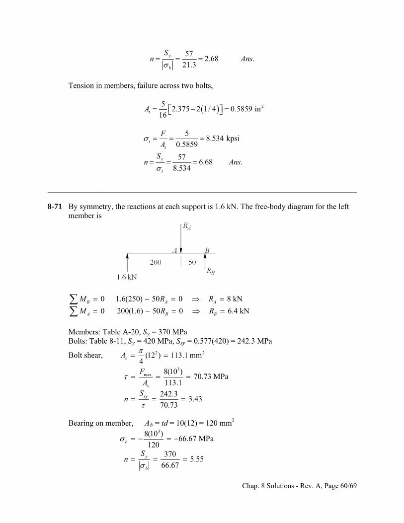
57
2.68 .21.3
y
b
Sn A
ns
Tension in members, failure across two bolts,
252.375 2 1/ 4 0.5859 in
16tA
5
8.534 kpsi0.5859t
t
F
A
57
6.68 .8.534
y
t
Sn A
ns
B
______________________________________________________________________________ 8-71 By symmetry, the reactions at each support is 1.6 kN. The free-body diagram for the left
member is
0 1.6(250) 50 0 8 kN
0 200(1.6) 50 0 6.4 kNB A A
A B
M R R
M R R
Members: Table A-20, Sy = 370 MPa Bolts: Table 8-11, Sy = 420 MPa, Ssy = 0.577(420) = 242.3 MPa
Bolt shear, 2 2(12 ) 113.1 mm4sA
3max 8(10 )
70.73 MPa113.1
242.33.43
70.73
s
sy
F
AS
n
Bearing on member, Ab = td = 10(12) = 120 mm2
38(10 )66.67 MPa
120370
5.5566.67
b
y
b
Sn
Chap. 8 Solutions - Rev. A, Page 60/69
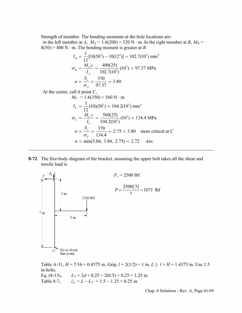
Strength of member. The bending moments at the hole locations are: in the left member at A, MA = 1.6(200) = 320 N · m. In the right member at B, MB =
8(50) = 400 N · m. The bending moment is greater at B
3 3 3
33
1[10(50 ) 10(12 )] 102.7(10 ) mm
12400(25)
(10 ) 97.37 MPa102.7(10 )
3703.80
97.37
B
AB
A
y
A
I
M c
IS
n
4
At the center, call it point C, MC = 1.6(350) = 560 N · m
3 3 4
33
1(10)(50 ) 104.2(10 ) mm
12560(25)
(10 ) 134.4 MPa104.2(10 )
3702.75 3.80 more critical at
134.4min(3.04, 3.80, 2.75) 2.72 .
C
CC
C
y
C
I
M c
IS
n C
n A
ns
______________________________________________________________________________ 8-72 The free-body diagram of the bracket, assuming the upper bolt takes all the shear and
tensile load is Fs = 2500 lbf
2500 3
1071 lbf7
P
Table A-31, H = 7/16 = 0.4375 in. Grip, l = 2(1/2) = 1 in. L ≥ l + H = 1.4375 in. Use 1.5
in bolts. Eq. (8-13), LT = 2d + 0.25 = 2(0.5) + 0.25 = 1.25 in Table 8-7, ld = L LT = 1.5 1.25 = 0.25 in
Chap. 8 Solutions - Rev. A, Page 61/69
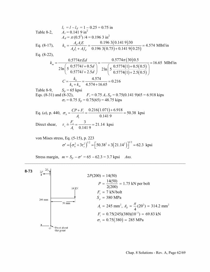
lt = l ld = 1 0.25 = 0.75 in Table 8-2, At = 0.141 9 in2 Ad = (0.52) /4 = 0.196 3 in2
Eq. (8-17),
0.196 3 0.141 9 30
4.574 Mlbf/in0.196 3 0.75 0.141 9 0.25
d tb
d t t d
A A Ek
A l A l
Eq. (8-22),
0.5774 30 0.50.577416.65 Mlbf/in
0.5774 0.5 0.5774 1 0.5 0.52ln 5 2ln 5
0.5774 2.5 0.5774 1 2.5 0.5
m
Edk
l dl d
4.574
0.2164.574 16.65
b
b m
kC
k k
Table 8-9, Sp = 65 kpsi Eqs. (8-31) and (8-32), Fi = 0.75 At Sp = 0.75(0.141 9)65 = 6.918 kips i = 0.75 Sp = 0.75(65) = 48.75 kips
Eq. (a), p. 440, 0.216 1.071 6.918
50.38 kpsi0.141 9
ib
t
CP F
A
Direct shear, 3
21.14 kpsi0.141 9
ss
t
F
A
von Mises stress, Eq. (5-15), p. 223
1/21/22 2 2 23 50.38 3 21.14 62.3 kpsib s
Stress margin, m = Sp = 65 62.3 = 3.7 kpsi Ans. ______________________________________________________________________________ 8-73
2 2
3
2 (200) 14(50)14(50)
1.75 kN per bolt2(200)7 kN/bolt380 MPa
245 mm , (20 ) 314.2 mm4
0.75(245)(380)(10 ) 69.83 kN
0.75 380 285 MPa
s
p
t d
i
i
P
P
FS
A A
F
2
Chap. 8 Solutions - Rev. A, Page 62/69
3
3
2 2 1/ 2
0.25(1.75) 69.83(10 ) 287 MPa
245
7(10 )22.3 MPa
314.2
[287 3(22.3 )] 290 MPa380 290 90 MPa
ib
t
s
d
p
CP F
A
F
A
m S
Stress margin, m = Sp = 380 90 = 90 MPa Ans. ______________________________________________________________________________ 8-74 Using the result of Prob. 5-67 for lubricated assembly (replace 0.2 with 0.18 per Table 8-15)
2
0.18x
f TF
d
With a design factor of nd gives
0.18 0.18(3)(1000)
7162 2 (0.12)
d xn F d dT d
f
or T/d = 716. Also,
(0.75 )
0.18(0.75)(85 000)11 475
p t
t
t
TK S A
dA
A
Form a table Size At T/d = 11 475At n 14 - 28 0.0364 417.70 1.755
16 - 24 0.058 665.55 2.8 38 24 0.0878 1007.50 4.23
where the factor of safety in the last column of the table comes from
2 ( / ) 2 (0.12)( / )0.0042( / )
0.18 0.18(1000)x
f T d T dn T
Fd
Select a "3
8 - 24 UNF cap screw. The setting is given by
T = (11 475At )d = 1007.5(0.375) = 378 lbf · in
Given the coarse scale on a torque wrench, specify a torque wrench setting of 400 lbf · in. Check the factor of safety
Chap. 8 Solutions - Rev. A, Page 63/69
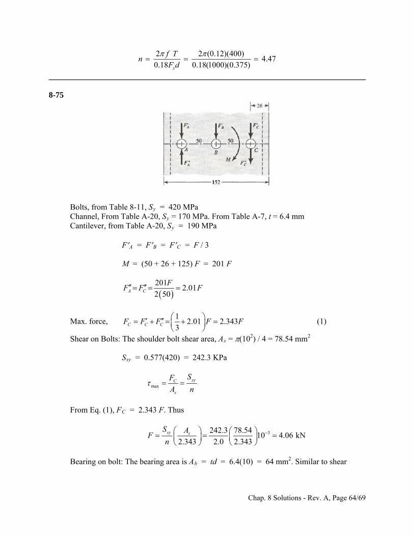
2 2 (0.12)(400)4.47
0.18 0.18(1000)(0.375)x
f Tn
F d
______________________________________________________________________________ 8-75 Bolts, from Table 8-11, Sy = 420 MPa Channel, From Table A-20, Sy = 170 MPa. From Table A-7, t = 6.4 mm Cantilever, from Table A-20, Sy = 190 MPa FA = FB = FC = F / 3 M = (50 + 26 + 125) F = 201 F
2012.01
2 50A C
FF F F
Max. force, 1
2.01 2.3433C C CF F F F F
(1)
Shear on Bolts: The shoulder bolt shear area, As = (102) / 4 = 78.54 mm2 Ssy = 0.577(420) = 242.3 KPa
maxsyC
s
SF
A n
From Eq. (1), FC = 2.343 F. Thus
3242.3 78.5410 4.06 kN
2.343 2.0 2.343sy s
S AF
n
Bearing on bolt: The bearing area is Ab = td = 6.4(10) = 64 mm2. Similar to shear
Chap. 8 Solutions - Rev. A, Page 64/69
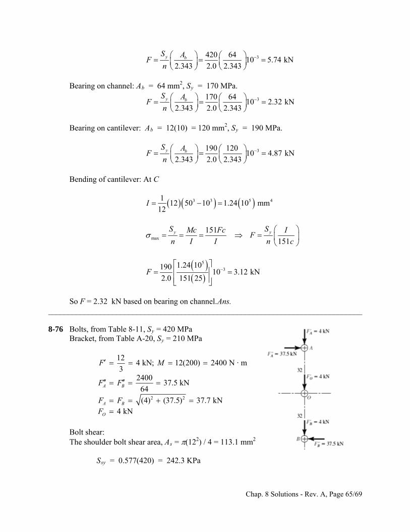
3420 6410 5.74 kN
2.343 2.0 2.343y b
S AF
n
Bearing on channel: Ab = 64 mm2, Sy = 170 MPa.
3170 6410 2.32 kN
2.343 2.0 2.343y b
S AF
n
Bearing on cantilever: Ab = 12(10) = 120 mm2, Sy = 190 MPa.
3190 12010 4.87 kN
2.343 2.0 2.343y b
S AF
n
Bending of cantilever: At C
3 3 5112 50 10 1.24 10 mm
12I 4
max
151
151y yS SMc Fc I
Fn I I n c
5
31.24 10190
10 3.12 kN2.0 151 25
F
So F = 2.32 kN based on bearing on channel. Ans. ______________________________________________________________________________ 8-76 Bolts, from Table 8-11, Sy = 420 MPa Bracket, from Table A-20, Sy = 210 MPa
2 2
124 kN; 12(200) 2400 N · m
32400
37.5 kN64
(4) (37.5) 37.7 kN4 kN
A B
A B
O
F M
F F
F FF
Bolt shear: The shoulder bolt shear area, As = (122) / 4 = 113.1 mm2 Ssy = 0.577(420) = 242.3 KPa
Chap. 8 Solutions - Rev. A, Page 65/69
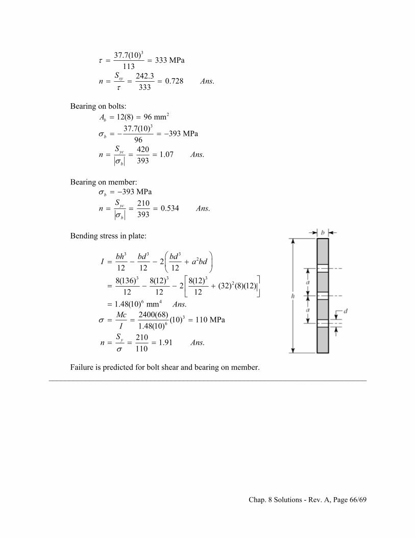
337.7(10)333 MPa
113242.3
0.728 .333
sySn A
ns
Bearing on bolts:
2
3
12(8) 96 mm
37.7(10)393 MPa
96420
1.07 .393
b
b
yc
b
A
Sn A
ns
Bearing on member:
393 MPa
2100.534 .
393
b
yc
b
Sn Ans
Bending stress in plate:
3 3 32
3 3 32
6 4
36
212 12 12
8(136) 8(12) 8(12)2 (32) (8)(
12 12 12
1.48(10) mm .2400(68)
(10) 110 MPa1.48(10)
2101.91 .
110y
bh bd bdI a bd
AnsMc
IS
n Ans
12)
Failure is predicted for bolt shear and bearing on member. ______________________________________________________________________________
Chap. 8 Solutions - Rev. A, Page 66/69
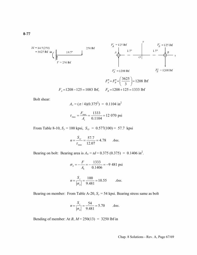
8-77
3625
1208 lbf3
1208 125 1083 lbf, 1208 125 1333 lbf
A B
A B
F F
F F
Bolt shear: As = ( / 4)(0.3752) = 0.1104 in2
maxmax
133312 070 psi
0.1104s
F
A
From Table 8-10, Sy = 100 kpsi, Ssy = 0.577(100) = 57.7 kpsi
max
57.74.78 .
12.07syS
n A
ns
Bearing on bolt: Bearing area is Ab = td = 0.375 (0.375) = 0.1406 in2.
1333
9 481 psi0.1406b
b
F
A
100
10.55 .9.481
y
b
Sn A
ns
Bearing on member: From Table A-20, Sy = 54 kpsi. Bearing stress same as bolt
54
5.70 .9.481
y
b
Sn A
ns
Bending of member: At B, M = 250(13) = 3250 lbfin
Chap. 8 Solutions - Rev. A, Page 67/69
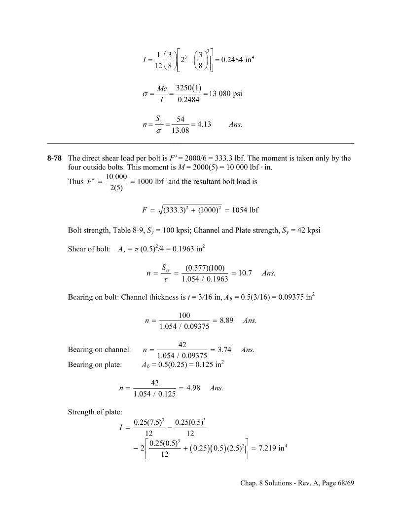
3
3 41 3 32 0.2484 in
12 8 8I
3250 1
13 080 psi0.2484
Mc
I
54
4.13 .13.08
ySn A
ns
______________________________________________________________________________ 8-78 The direct shear load per bolt is F = 2000/6 = 333.3 lbf. The moment is taken only by the
four outside bolts. This moment is M = 2000(5) = 10 000 lbf · in.
Thus 10 000
1000 lbf2(5)
F and the resultant bolt load is
2 2(333.3) (1000) 1054 lbfF
Bolt strength, Table 8-9, Sy = 100 kpsi; Channel and Plate strength, Sy = 42 kpsi Shear of bolt: As = (0.5)2/4 = 0.1963 in2
(0.577)(100)
10.7 .1.054 / 0.1963
sySn A
ns
Bearing on bolt: Channel thickness is t = 3/16 in, Ab = 0.5(3/16) = 0.09375 in2
1008.89 .
1.054 / 0.09375n A ns
Bearing on channel: 42
3.74 .1.054 / 0.09375
n A ns
Bearing on plate: Ab = 0.5(0.25) = 0.125 in2
42
4.98 .1.054 / 0.125
n A ns
Strength of plate:
3 3
32 4
0.25(7.5) 0.25(0.5)
12 120.25(0.5)
2 0.25 0.5 (2.5) 7.219 in12
I
Chap. 8 Solutions - Rev. A, Page 68/69
5000 lbf · in per plate5000(3.75)
2597 psi7.219
42 16.2 .
2.597
MMc
I
n Ans
______________________________________________________________________________ 8-79 to 8-81 Specifying bolts, screws, dowels and rivets is the way a student learns about such
components. However, choosing an array a priori is based on experience. Here is a chance for students to build some experience.
Chap. 8 Solutions - Rev. A, Page 69/69
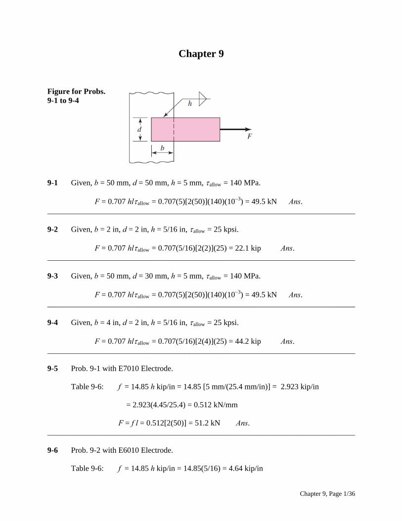
Chapter 9 Figure for Probs. 9-1 to 9-4 9-1 Given, b = 50 mm, d = 50 mm, h = 5 mm, allow = 140 MPa. F = 0.707 hlallow = 0.707(5)[2(50)](140)(103) = 49.5 kN Ans. ______________________________________________________________________________ 9-2 Given, b = 2 in, d = 2 in, h = 5/16 in, allow = 25 kpsi. F = 0.707 hlallow = 0.707(5/16)[2(2)](25) = 22.1 kip Ans. ______________________________________________________________________________ 9-3 Given, b = 50 mm, d = 30 mm, h = 5 mm, allow = 140 MPa. F = 0.707 hlallow = 0.707(5)[2(50)](140)(103) = 49.5 kN Ans. ______________________________________________________________________________ 9-4 Given, b = 4 in, d = 2 in, h = 5/16 in, allow = 25 kpsi. F = 0.707 hlallow = 0.707(5/16)[2(4)](25) = 44.2 kip Ans. ______________________________________________________________________________ 9-5 Prob. 9-1 with E7010 Electrode. Table 9-6: f = 14.85 h kip/in = 14.85 [5 mm/(25.4 mm/in)] = 2.923 kip/in = 2.923(4.45/25.4) = 0.512 kN/mm F = f l = 0.512[2(50)] = 51.2 kN Ans. ______________________________________________________________________________ 9-6 Prob. 9-2 with E6010 Electrode. Table 9-6: f = 14.85 h kip/in = 14.85(5/16) = 4.64 kip/in
Chapter 9, Page 1/36
F = f l = 4.64[2(2)] = 18.6 kip Ans. ______________________________________________________________________________ 9-7 Prob. 9-3 with E7010 Electrode. Table 9-6: f = 14.85 h kip/in = 14.85 [5 mm/(25.4 mm/in)] = 2.923 kip/in = 2.923(4.45/25.4) = 0.512 kN/mm F = f l = 0.512[2(50)] = 51.2 kN Ans. ______________________________________________________________________________ 9-8 Prob. 9-4 with E6010 Electrode. Table 9-6: f = 14.85 h kip/in = 14.85(5/16) = 4.64 kip/in F = f l = 4.64[2(4)] = 37.1 kip Ans. ______________________________________________________________________________ 9-9 Table A-20: 1018 CD: Sut = 440 MPa, Sy = 370 MPa 1018 HR: Sut = 400 MPa, Sy = 220 MPa Cold-rolled properties degrade to hot-rolled properties in the neighborhood of the weld. Table 9-4:
all min(0.30 , 0.40 )
min[0.30(400), 0.40(220)]min(120, 88) 88 MPa
ut yS S
for both materials. Eq. (9-3): F = 0.707hlall = 0.707(5)[2(50)](88)(103) = 31.1 kN Ans. ______________________________________________________________________________ 9-10 Table A-20: 1020 CD: Sut = 68 kpsi, Sy = 57 kpsi 1020 HR: Sut = 55 kpsi, Sy = 30 kpsi Cold-rolled properties degrade to hot-rolled properties in the neighborhood of the weld. Table 9-4:
all min(0.30 , 0.40 )
min[0.30(55), 0.40(30)]min(16.5, 12.0) 12.0 kpsi
ut yS S
for both materials. Eq. (9-3): F = 0.707hlall = 0.707(5/16)[2(2)](12.0) = 10.6 kip Ans. ______________________________________________________________________________
Chapter 9, Page 2/36
9-11 Table A-20: 1035 HR: Sut = 500 MPa, Sy = 270 MPa 1035 CD: Sut = 550 MPa, Sy = 460 MPa Cold-rolled properties degrade to hot-rolled properties in the neighborhood of the weld. Table 9-4:
all min(0.30 , 0.40 )
min[0.30(500), 0.40(270)]min(150, 108) 108 MPa
ut yS S
for both materials. Eq. (9-3): F = 0.707hlall = 0.707(5)[2(50)](108)(103) = 38.2 kN Ans. ______________________________________________________________________________ 9-12 Table A-20: 1035 HR: Sut = 72 kpsi, Sy = 39.5 kpsi 1020 CD: Sut = 68 kpsi, Sy = 57 kpsi, 1020 HR: Sut = 55 kpsi, Sy = 30 kpsi Cold-rolled properties degrade to hot-rolled properties in the neighborhood of the weld. Table 9-4:
all min(0.30 , 0.40 )
min[0.30(55), 0.40(30)]min(16.5, 12.0) 12.0 kpsi
ut yS S
for both materials. Eq. (9-3): F = 0.707hlall = 0.707(5/16)[2(4)](12.0) = 21.2 kip Ans. ______________________________________________________________________________ 9-13
Eq. (9-3):
32 100 102141 MPa .
5 2 50 50
FAns
hl
______________________________________________________________________________ 9-14
Eq. (9-3):
2 402
22.6 kpsi .5 /16 2 2 2
FAns
hl
______________________________________________________________________________
9-15 Eq. (9-3):
32 100 102177 MPa .
5 2 50 30
FAns
hl
______________________________________________________________________________
9-16 Eq. (9-3):
2 402
15.1 kpsi .5 /16 2 4 2
FAns
hl
______________________________________________________________________________
Chapter 9, Page 3/36
9-17 b = d =50 mm, c = 150 mm, h = 5 mm, and allow = 140 MPa. (a) Primary shear, Table 9-1, Case 2 (Note: b and d are interchanged between problem
figure and table figure. Note, also, F in kN and in MPa):
3102.829
1.414 5 50y
FVF
A
Secondary shear, Table 9-1:
2 22 2
3 350 3 50 503
83.33 10 mm6 6u
d b dJ
J = 0.707 h Ju = 0.707(5)(83.33)(103) = 294.6(103) mm4
3
3
175 10 2514.85
294.6 10y
x y
FMrF
J
2 22 2max 14.85 2.829 14.85 23.1x y y F F (1)
allow 1406.06 kN .
23.1 23.1F Ans
(b) For E7010 from Table 9-6, allow = 21 kpsi = 21(6.89) = 145 MPa 1020 HR bar: Sut = 380 MPa, Sy = 210 MPa 1015 HR support: Sut = 340 MPa, Sy = 190 MPa Table 9-3, E7010 Electrode: Sut = 482 MPa, Sy = 393 MPa The support controls the design. Table 9-4: allow = min(0.30Sut, 0.40Sy ) =min[0.30(340), 0.40(190) = min(102, 76) = 76 MPa The allowable load, from Eq. (1) is
allow 763.29 kN .
23.1 23.1F Ans
______________________________________________________________________________ 9-18 b = d =2 in, c = 6 in, h = 5/16 in, and allow = 25 kpsi.
Chapter 9, Page 4/36
(a) Primary shear, Table 9-1(Note: b and d are interchanged between problem figure and table figure. Note, also, F in kip and in kpsi):
1.1321.414 5 /16 2y
V FF
A
Secondary shear, Table 9-1:
2 22 2
32 3 2 23
5.333 in6 6u
d b dJ
J = 0.707 h Ju = 0.707(5/16)(5.333) = 1.178 in4
7 1
5.9421.178
yx y
Mr FF
J
2 22 2max 5.942 1.132 5.942 9.24x y y F F (1)
allow 252.71 kip .
9.24 9.24F Ans
(b) For E7010 from Table 9-6, allow = 21 kpsi 1020 HR bar: Sut = 55 kpsi, Sy = 30 kpsi 1015 HR support: Sut = 50 kpsi, Sy = 27.5 kpsi Table 9-3, E7010 Electrode: Sut = 70 kpsi, Sy = 57 kpsi The support controls the design. Table 9-4: allow = min(0.30Sut, 0.40Sy ) =min[0.30(50), 0.40(27.5) = min(15, 11) = 11 kpsi The allowable load, from Eq. (1) is
allow 111.19 kip .
9.24 9.24F Ans
______________________________________________________________________________ 9-19 b =50 mm, c = 150 mm, d = 30 mm, h = 5 mm, and allow = 140 MPa. (a) Primary shear, Table 9-1, Case 2 (Note: b and d are interchanged between problem
figure and table figure. Note, also, F in kN and in MPa):
Chapter 9, Page 5/36
3102.829
1.414 5 50y
FVF
A
Secondary shear, Table 9-1:
2 22 2
3 350 3 30 503
43.33 10 mm6 6u
d b dJ
J = 0.707 h Ju = 0.707(5)(43.33)(103) = 153.2(103) mm4
3
3
175 10 1517.13
153.2 10y
x
FMrF
J
3
3
175 10 2528.55
153.2 10x
y
FMrF
J
2 22 2max 17.13 2.829 28.55 35.8x y y F F (1)
allow 1403.91 kN .
35.8 35.8F Ans
(b) For E7010 from Table 9-6, allow = 21 kpsi = 21(6.89) = 145 MPa 1020 HR bar: Sut = 380 MPa, Sy = 210 MPa 1015 HR support: Sut = 340 MPa, Sy = 190 MPa Table 9-3, E7010 Electrode: Sut = 482 MPa, Sy = 393 MPa The support controls the design. Table 9-4: allow = min(0.30Sut, 0.40Sy ) =min[0.30(340), 0.40(190) = min(102, 76) = 76 MPa The allowable load, from Eq. (1) is
allow 762.12 kN .
35.8 35.8F Ans
______________________________________________________________________________ 9-20 b = 4 in, c = 6 in, d = 2 in, h = 5/16 in, and allow = 25 kpsi.
Chapter 9, Page 6/36
(a) Primary shear, Table 9-1(Note: b and d are interchanged between problem figure and table figure. Note, also, F in kip and in kpsi):
0.56581.414 5 /16 4y
V FF
A
Secondary shear, Table 9-1:
2 22 2
34 3 2 43
18.67 in6 6u
d b dJ
J = 0.707 h Ju = 0.707(5/16)(18.67) = 4.125 in4
8 1
1.9394.125
yx
Mr FF
J
8 23.879
4.125x
y
FMrF
J
2 22 2max 1.939 0.5658 3.879 4.85x y y F F (1)
allow 255.15 kip .
4.85 4.85F Ans
(b) For E7010 from Table 9-6, allow = 21 kpsi 1020 HR bar: Sut = 55 kpsi, Sy = 30 kpsi 1015 HR support: Sut = 50 kpsi, Sy = 27.5 kpsi Table 9-3, E7010 Electrode: Sut = 70 kpsi, Sy = 57 kpsi The support controls the design. Table 9-4: allow = min(0.30Sut, 0.40Sy ) =min[0.30(50), 0.40(27.5) = min(15, 11) = 11 kpsi The allowable load, from Eq. (1) is
allow 112.27 kip .
4.85 4.85F Ans
______________________________________________________________________________
Chapter 9, Page 7/36
9-21 Given, b = 50 mm, c = 150 mm, d = 50 mm, h = 5 mm, allow = 140 MPa. Primary shear (F in kN, in MPa, A in mm2):
3101.414
1.414 5 50 50y
FVF
A
Secondary shear:
Table 9-1:
3 3
3 350 50166.7 10 mm
6 6u
b dJ
J = 0.707 h Ju = 0.707(5)166.7(103) = 589.2(103) mm4
3
3
175 10 (25)7.425
589.2 10y
x y
FMrF
J
Maximum shear:
2 22 2max 7.425 1.414 7.425 11.54x y y F F
140
12.1 kN .11.54 11.54
allowF Ans
______________________________________________________________________________ 9-22 Given, b = 2 in, c = 6 in, d = 2 in, h = 5/16 in, allow = 25 kpsi. Primary shear:
0.56581.414 5 /16 2 2y
V FF
A
Secondary shear:
Table 9-1: 3 3
32 210.67 in
6 6u
b dJ
J = 0.707 h Ju = 0.707(5/16)10.67 = 2.357 in4
7 (1)
2.9702.357
yx y
Mr FF
J
Maximum shear:
2 22 2max 2.970 0.566 2.970 4.618x y y F F
25
5.41 kip .4.618 4.618
allowF Ans
______________________________________________________________________________ 9-23 Given, b = 50 mm, c = 150 mm, d = 30 mm, h = 5 mm, allow = 140 MPa.
Chapter 9, Page 8/36
Primary shear (F in kN, in MPa, A in mm2):
3101.768
1.414 5 50 30y
FVF
A
Secondary shear:
Table 9-1:
3 3
3 350 3085.33 10 mm
6 6u
b dJ
J = 0.707 h Ju = 0.707(5)85.33(103) = 301.6(103) mm4
3
3
175 10 (15)8.704
301.6 10y
x
FMrF
J
3
3
175 10 (25)14.51
301.6 10x
y
FMrF
J
Maximum shear:
2 22 2max 8.704 1.768 14.51 18.46x y y F F
140
7.58 kN .18.46 18.46
allowF Ans
______________________________________________________________________________ 9-24 Given, b = 4 in, c = 6 in, d = 2 in, h = 5/16 in, allow = 25 kpsi. Primary shear:
0.37721.414 5 /16 4 2y
V FF
A
Secondary shear:
Table 9-1: 3 3
34 236 in
6 6u
b dJ
J = 0.707 h Ju = 0.707(5/16)36 = 7.954 in4
8 (1)
1.0067.954
yx
Mr FF
J
8 (2)
2.0127.954
xy
Mr FF
J
Maximum shear:
2 22 2max 1.006 0.3772 2.012 2.592x y y F F
Chapter 9, Page 9/36
25
9.65kip .2.592 2.592
allowF Ans
______________________________________________________________________________ 9-25 Given, b = 50 mm, d = 50 mm, h = 5 mm, E6010 electrode. A = 0.707(5)(50 +50 + 50) = 530.3 mm2 Member endurance limit: From Table A-20 for AISI 1010 HR, Sut = 320 MPa. Eq. 6-19 and Table 6-2, pp. 287, 288: ka = 272(320)0.995 = 0.875 kb = 1 (uniform shear), kc = 0.59 (torsion, shear), kd = 1 Eqs. (6-8) and (6-18): Se = 0.875(1)(0.59)(1)(0.5)(320) = 82.6 MPa Electrode endurance: E6010, Table 9-3, Sut = 427 MPa Eq. 6-19 and Table 6-2, pp. 287, 288: ka = 272(427)0.995 = 0.657 As before, kb = 1 (direct shear), kc = 0.59 (torsion, shear), kd = 1 Se = 0.657(1)(0.59)(1)(0.5)(427) = 82.8 MPa The members and electrode are basically of equal strength. We will use Se = 82.6 MPa.
For a factor of safety of 1, and with Kfs = 2.7 (Table 9-5)
3allow
82.6 530.316.2 10 N 16.2 kN .
2.7fs
AF Ans
K
______________________________________________________________________________ 9-26 Given, b = 2 in, d = 2 in, h = 5/16 in, E6010 electrode. A = 0.707(5/16)(2 +2 + 2) = 1.326 in2 Member endurance limit: From Table A-20 for AISI 1010 HR, Sut = 47 kpsi. Eq. 6-19 and Table 6-2, pp. 287, 288: ka = 39.9(47)0.995 = 0.865 kb = 1 (uniform shear), kc = 0.59 (torsion, shear), kd = 1 Eqs. (6-8) and (6-18): Se = 0.865(1)(0.59)(1)(0.5)(47) = 12.0 kpsi Electrode endurance: E6010, Table 9-3, Sut = 62 kpsi Eq. 6-19 and Table 6-2, pp. 287, 288: ka = 39.9(62)0.995 = 0.657
Chapter 9, Page 10/36
As before, kb = 1 (uniform shear), kc = 0.59 (torsion, shear), kd = 1 Se = 0.657(1)(0.59)(1)(0.5)(62) = 12.0 kpsi Thus the members and electrode are of equal strength. For a factor of safety of 1, and
with Kfs = 2.7 (Table 9-5)
allow
12.0 1.3265.89 kip .
2.7fs
AF Ans
K
______________________________________________________________________________ 9-27 Given, b = 50 mm, d = 30 mm, h = 5 mm, E7010 electrode. A = 0.707(5)(50 +50 + 30) = 459.6 mm2 Member endurance limit: From Table A-20 for AISI 1010 HR, Sut = 320 MPa. Eq. 6-19 and Table 6-2, pp. 287, 288: ka = 272(320)0.995 = 0.875 kb = 1 (direct shear), kc = 0.59 (torsion, shear), kd = 1 Eqs. (6-8) and (6-18): Se = 0.875(1)(0.59)(1)(0.5)(320) = 82.6 MPa Electrode endurance: E6010, Table 9-3, Sut = 482 MPa Eq. 6-19 and Table 6-2, pp. 287, 288: ka = 272(482)0.995 = 0.582 As before, kb = 1 (direct shear), kc = 0.59 (torsion, shear), kd = 1 Se = 0.582(1)(0.59)(1)(0.5)(482) = 82.7 MPa The members and electrode are basically of equal strength. We will use Se =82.6 MPa.
For a factor of safety of 1, and with Kfs = 2.7 (Table 9-5)
3allow
82.6 459.614.1 10 N 14.1 kN .
2.7fs
AF Ans
K
______________________________________________________________________________ 9-28 Given, b = 4 in, d = 2 in, h = 5/16 in, E7010 electrode. A = 0.707(5/16)(4 +4 + 2) = 2.209 in2 Member endurance limit: From Table A-20 for AISI 1010 HR, Sut = 47 kpsi. Eq. 6-19 and Table 6-2, pp. 287, 288: ka = 39.9(47)0.995 = 0.865 kb = 1 (direct shear), kc = 0.59 (torsion, shear), kd = 1
Chapter 9, Page 11/36
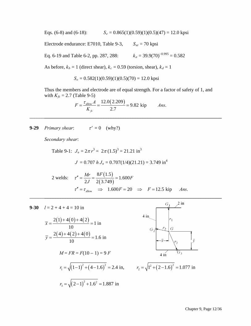
Eqs. (6-8) and (6-18): Se = 0.865(1)(0.59)(1)(0.5)(47) = 12.0 kpsi Electrode endurance: E7010, Table 9-3, Sut = 70 kpsi Eq. 6-19 and Table 6-2, pp. 287, 288: ka = 39.9(70)0.995 = 0.582 As before, kb = 1 (direct shear), kc = 0.59 (torsion, shear), kd = 1 Se = 0.582(1)(0.59)(1)(0.5)(70) = 12.0 kpsi Thus the members and electrode are of equal strength. For a factor of safety of 1, and
with Kfs = 2.7 (Table 9-5)
allow
12.0 2.2099.82 kip .
2.7fs
AF Ans
K
______________________________________________________________________________ 9-29 Primary shear: = 0 (why?) Secondary shear: Table 9-1: Ju = 2 r3 = 2 (1.5)3 = 21.21 in3 J = 0.707 h Ju = 0.707(1/4)(21.21) = 3.749 in4
2 welds:
8 1.5
1.6002 2 3.749
FMrF
J
allow 1.600 20 12.5 kip .F F Ans
______________________________________________________________________________ 9-30 l = 2 + 4 + 4 = 10 in
2 1 4 0 4 21 in
102 4 4 2 4 0
1.6 in10
x
y
M = FR = F(10 1) = 9 F
2 2 221 21 1 4 1.6 2.4 in, 1 2 1.6 1.077 inr r
2 23 2 1 1.6 1.887 inr
Chapter 9, Page 12/36
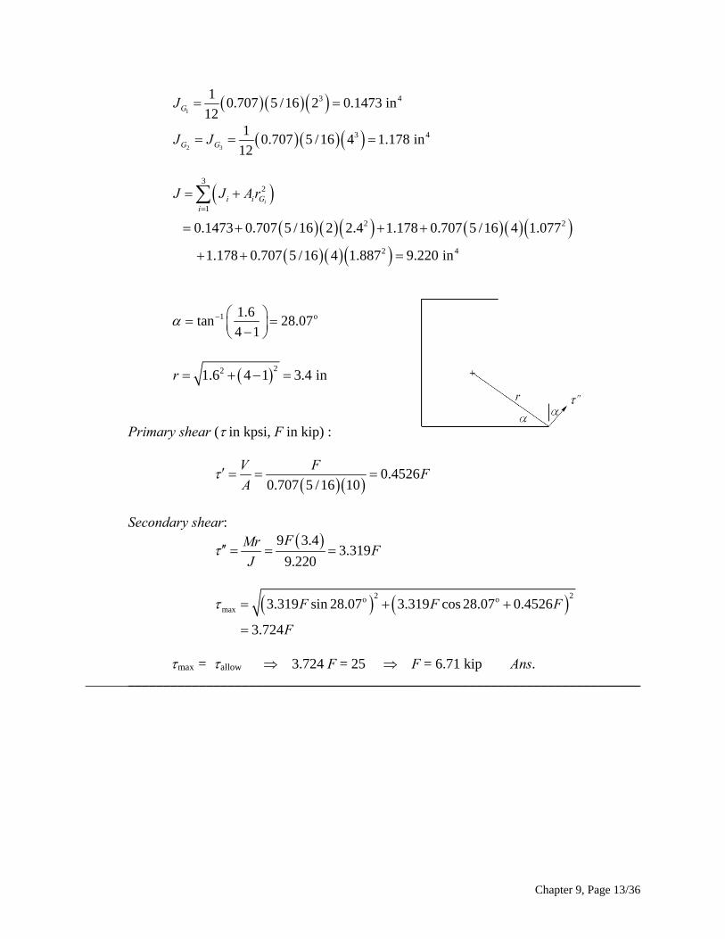
1
3 410.707 5 /16 2 0.1473 in
12GJ
2 3
3 410.707 5 /16 4 1.178 in
12G GJ J
32
1
2 2
2 4
0.1473 0.707 5 /16 2 2.4 1.178 0.707 5 /16 4 1.077
1.178 0.707 5 /16 4 1.887 9.220 in
ii i Gi
J J A r
1 o1.6tan 28.07
4 1
221.6 4 1 3.4 inr
Primary shear ( in kpsi, F in kip) :
0.45260.707 5 /16 10
V FF
A
Secondary shear:
9 3.4
3.3199.220
FMrF
J
2 2o omax 3.319 sin 28.07 3.319 cos 28.07 0.4526
3.724
F F
F
F
max = allow 3.724 F = 25 F = 6.71 kip Ans. ______________________________________________________________________________
Chapter 9, Page 13/36
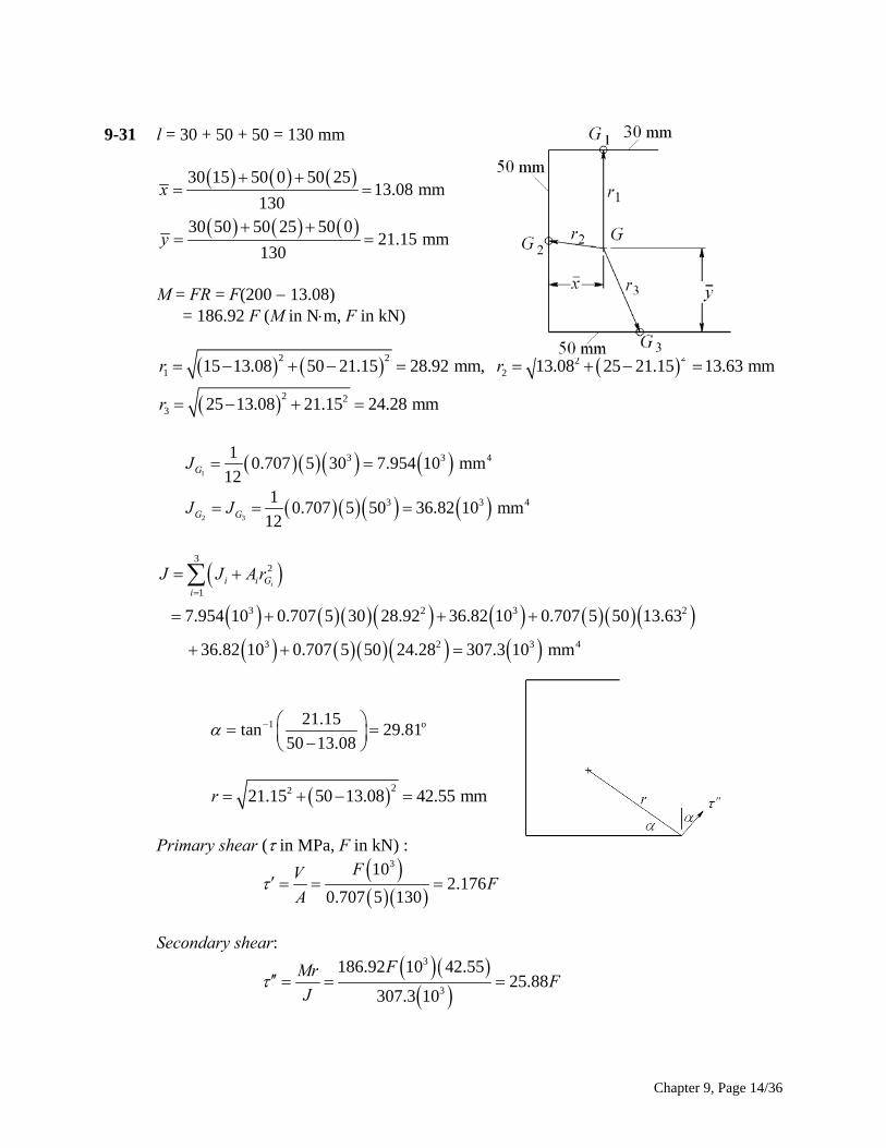
9-31 l = 30 + 50 + 50 = 130 mm
30 15 50 0 50 2513.08 mm
13030 50 50 25 50 0
21.15 mm130
x
y
M = FR = F(200 13.08) = 186.92 F (M in Nm, F in kN)
2 2 221 215 13.08 50 21.15 28.92 mm, 13.08 25 21.15 13.63 mmr r
2 23 25 13.08 21.15 24.28 mmr
1
3 310.707 5 30 7.954 10 mm
12GJ 4
2 3
3 310.707 5 50 36.82 10 mm
12G GJ J 4
2
32
1
3 2 3
3 2 3 4
7.954 10 0.707 5 30 28.92 36.82 10 0.707 5 50 13.63
36.82 10 0.707 5 50 24.28 307.3 10 mm
ii i Gi
J J A r
1 o21.15tan 29.81
50 13.08
2221.15 50 13.08 42.55 mmr
Primary shear ( in MPa, F in kN) :
3102.176
0.707 5 130
FVF
A
Secondary shear:
3
3
186.92 10 42.5525.88
307.3 10
FMrF
J
Chapter 9, Page 14/36
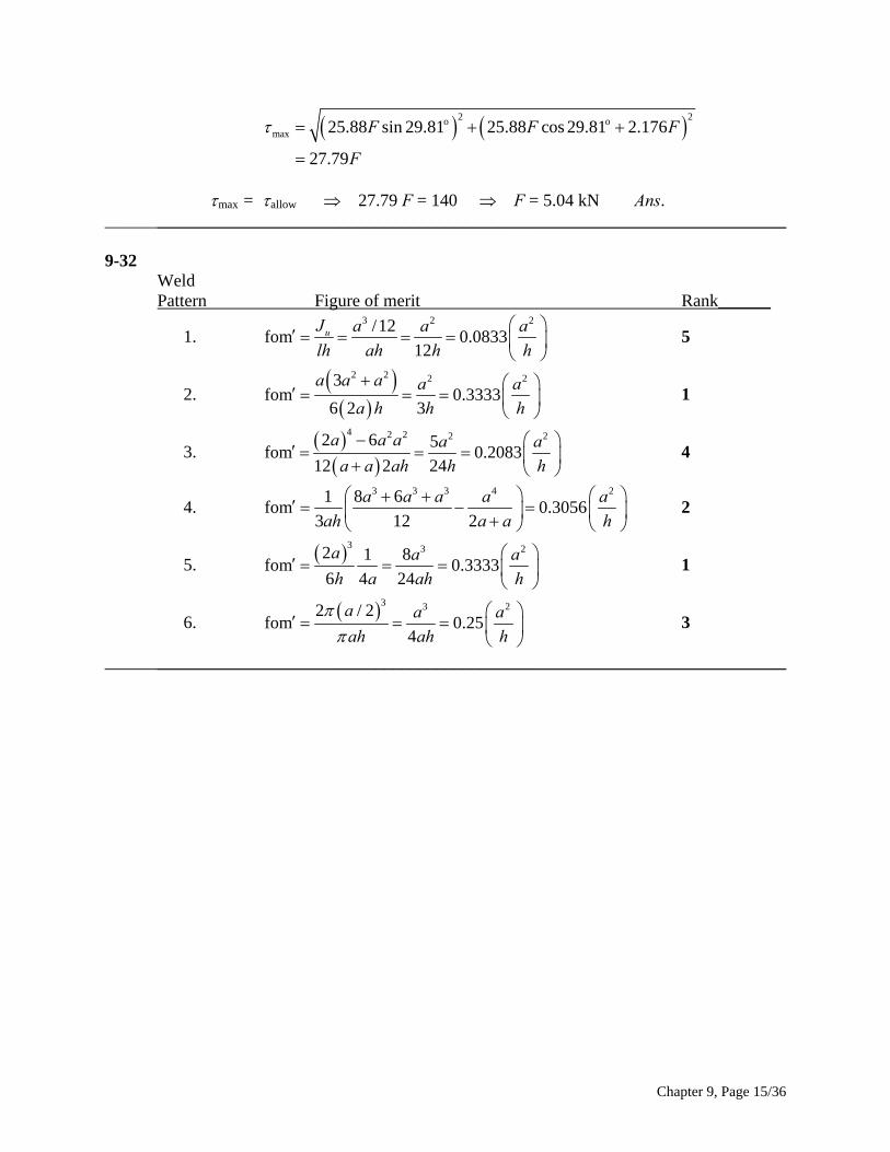
2 2o omax 25.88 sin 29.81 25.88 cos 29.81 2.176
27.79
F F
F
F
max = allow 27.79 F = 140 F = 5.04 kN Ans. ______________________________________________________________________________ 9-32 Weld Pattern Figure of merit Rank______
1. 3 2/12
fom 0.083312
uJ a a a
lh ah h h
2
5
2.
2 2 2 23fom 0.3333
6 2 3
a a a a
a h h h
a 1
3.
4 2 2 2 22 6 5fom 0.2083
12 2 24
a a a a a
a a ah h h
4
4. 3 3 3 4 21 8 6
fom 0.30563 12 2
a a a a a
ah a a h
2
5. 3 3 22 1 8
fom 0.33336 4 24
a a a
h a ah h
1
6. 3 3 22 / 2
fom 0.254
a a a
ah ah h
3
______________________________________________________________________________
Chapter 9, Page 15/36
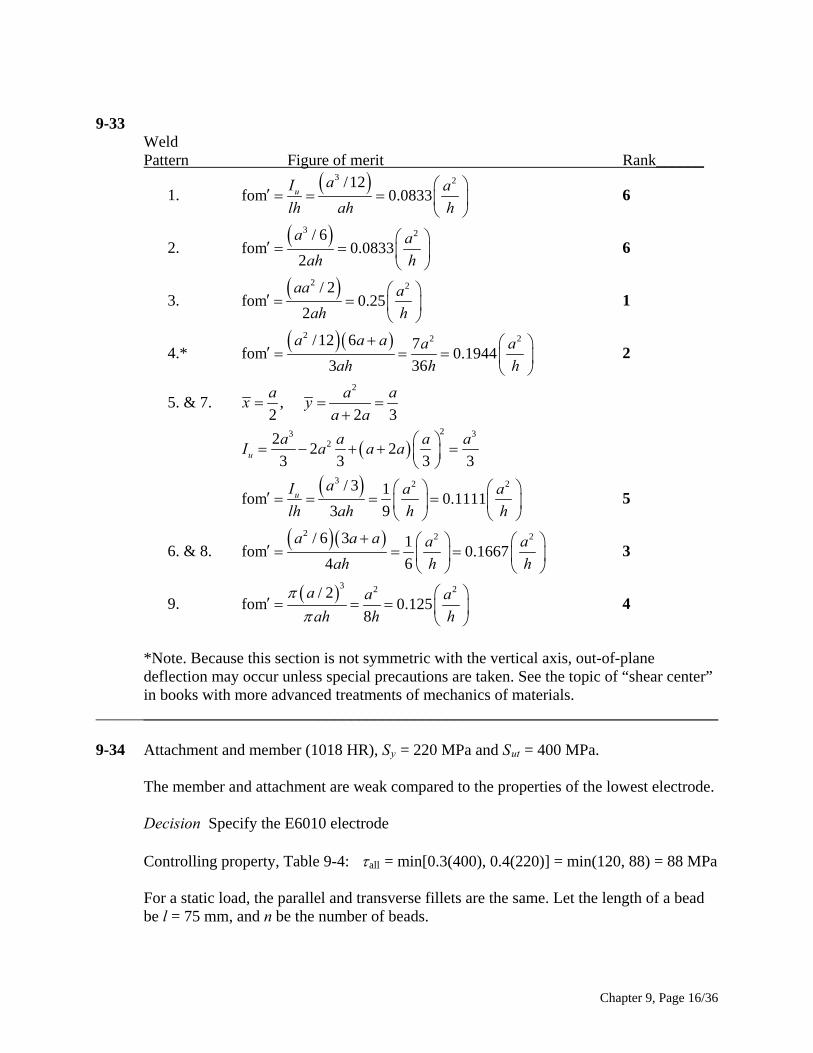
9-33 Weld Pattern Figure of merit Rank______
1. 3 2/12
fom 0.0833uaI a
lh ah h
6
2. 3 2/ 6
fom 0.08332
a a
ah h
6
3. 2 2/ 2
fom 0.252
aa a
ah h
1
4.* 2 2 2/12 6 7
fom 0.19443 36
a a a a
ah h h
a 2
5. & 7. 2
,2 2
a ax y
a a
3
a
23 3
222 2
3 3 3u
a a aI a a a
3
a
3 2 2/ 3 1
fom 0.11113 9
uaI a a
lh ah h h
5
6. & 8. 2 2 2/ 6 3 1
fom 0.16674 6
a a a a a
ah h h
3
9. 3 2 2/ 2
fom 0.1258
a a a
ah h h
4
*Note. Because this section is not symmetric with the vertical axis, out-of-plane
deflection may occur unless special precautions are taken. See the topic of “shear center” in books with more advanced treatments of mechanics of materials.
______________________________________________________________________________ 9-34 Attachment and member (1018 HR), Sy = 220 MPa and Sut = 400 MPa. The member and attachment are weak compared to the properties of the lowest electrode. Decision Specify the E6010 electrode Controlling property, Table 9-4: all = min[0.3(400), 0.4(220)] = min(120, 88) = 88 MPa For a static load, the parallel and transverse fillets are the same. Let the length of a bead
be l = 75 mm, and n be the number of beads.
Chapter 9, Page 16/36
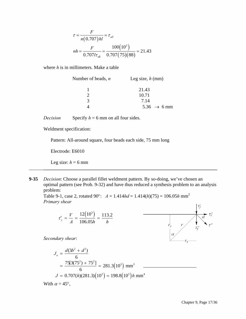
0.707 all
F
n hl
3
all
100 1021.43
0.707 0.707 75 88
Fnh
l
where h is in millimeters. Make a table Number of beads, n Leg size, h (mm) 1 21.43 2 10.71 3 7.14 4 5.36 6 mm Decision Specify h = 6 mm on all four sides. Weldment specification: Pattern: All-around square, four beads each side, 75 mm long Electrode: E6010 Leg size: h = 6 mm ______________________________________________________________________________ 9-35 Decision: Choose a parallel fillet weldment pattern. By so-doing, we’ve chosen an
optimal pattern (see Prob. 9-32) and have thus reduced a synthesis problem to an analysis problem:
Table 9-1, case 2, rotated 90: A = 1.414hd = 1.414(h)(75) = 106.05h mm2 Primary shear
312 10 113.2
106.05y V
A h h
Secondary shear:
2 2
2 23 3
3 3
(3 )
675[3(75 ) 75 ]
281.3 10 mm6
0.707( )(281.3) 10 198.8 10 mm
u
d b dJ
J h h
4
With = 45,
Chapter 9, Page 17/36
3o
3
22 2max
12 10 (187.5)(37.5)cos 45 424.4
198.8 10
1 684.9424.4 (113.2 424.4)
yx y
x y y
MrMr
J J hh
h h
2
Attachment and member (1018 HR): Sy = 220 MPa, Sut = 400 MPa Decision: Use E60XX electrode which is stronger
all
max all
min[0.3(400), 0.4(220)] 88 MPa684.9
88 MPa
684.97.78 mm
88
h
h
Decision: Specify 8 mm leg size Weldment Specifications: Pattern: Parallel horizontal fillet welds Electrode: E6010 Type: Fillet Length of each bead: 75 mm Leg size: 8 mm ______________________________________________________________________________ 9-36 Problem 9-35 solves the problem using parallel horizontal fillet welds, each 75 mm long
obtaining a leg size rounded up to 8 mm. For this problem, since the width of the plate is fixed and the length has not been
determined, we will explore reducing the leg size by using two vertical beads 75 mm long and two horizontal beads such that the beads have a leg size of 6 mm.
Decision: Use a rectangular weld bead pattern with a leg size of 6 mm (case 5 of Table 9-1 with b unknown and d = 75 mm). Materials: Attachment and member (1018 HR): Sy = 220 MPa, Sut = 400 MPa From Table 9-4, AISC welding code,
all = min[0.3(400), 0.4(220)] = min(120, 88) = 88 MPa Select a stronger electrode material from Table 9-3. Decision: Specify E6010 Solving for b: In Prob. 9-35, every term was linear in the unknown h. This made solving
for h relatively easy. In this problem, the terms will not be linear in b, and so we will use an iterative solution with a spreadsheet.
Throat area and other properties from Table 9-1: A = 1.414(6)(b + 75) = 8.484(b + 75) (1)
Chapter 9, Page 18/36
3
75
6u
bJ
, J = 0.707 (6) Ju = 0.707(b +75)3 (2)
Primary shear ( in MPa, h in mm):
312 10(3)y
V
A A
Secondary shear (See Prob. 9-35 solution for the definition of ) :
3
3
3
3
22max
12 10 150 / 2 (37.5)cos cos (4)
0.707 75
12 10 150 / 2 ( / 2)sin sin (5)
0.707 75
(6)
yx
xy
y x y
Mr
JbMrMr
J J b
b bMr Mr
J J b
Enter Eqs. (1) to (6) into a spreadsheet and iterate for various values of b. A portion of the spreadsheet is shown below.
b (mm) A (mm2) J (mm4) 'y (Mpa) "y (Mpa) "x (Mpa)max
(Mpa)
41 984.144 1103553.5 12.19334 69.5254 38.00722 90.12492
42 992.628 1132340.4 12.08912 67.9566 38.05569 88.63156
43 1001.112 1161623.6 11.98667 66.43718 38.09065 87.18485 < 88 Mpa
44 1009.596 1191407.4 11.88594 64.96518 38.11291 85.7828 We see that b 43 mm meets the strength goal. Weldment Specifications: Pattern: Horizontal parallel weld tracks 43 mm long, vertical parallel weld tracks 75 mm
long Electrode: E6010 Leg size: 6 mm ______________________________________________________________________________ 9-37 Materials: Member and attachment (1018 HR): 32 kpsi, 58 kpsiy utS S
Table 9-4: all min[0.3(58), 0.4(32)] 12.8 kpsi
Chapter 9, Page 19/36
Decision: Use E6010 electrode. From Table 9-3: 50 kpsi, 62 kpsi,y utS S
all min[0.3(62), 0.4(50)] 20 kpsi
Decision: Since 1018 HR is weaker than the E6010 electrode, use all 12.8 kpsi
Decision: Use an all-around square weld bead track. l1 = 6 + a = 6 + 6.25 = 12.25 in
Throat area and other properties from Table 9-1:
1.414 ( ) 1.414( )(6 6) 16.97A h b d h h Primary shear
320 10 1179psi
16.97y
V F
A A h h
Secondary shear
3 33( ) (6 6)
288 in6 6u
b dJ
40.707 (288) 203.6 inJ h h
320 10 (6.25 3)(3) 2726psi
203.6y
x y
Mr
J h
h
2 2 2 2max
1 4762( ) 2726 (1179 2726) psix y y h h
Relate stress to strength
3
max all 3
4762 476212.8 10 0.372 in
12.8 10h
h
Decision:
Specify in leg size 3 / 8 Specifications:
Pattern: All-around square weld bead track Electrode: E6010 Type of weld: Fillet Weld bead length: 24 in Leg size: in 3 / 8Attachment length: 12.25 in
______________________________________________________________________________
Chapter 9, Page 20/36
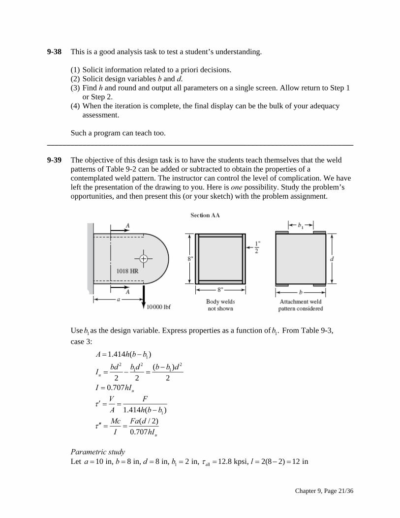
9-38 This is a good analysis task to test a student’s understanding. (1) Solicit information related to a priori decisions. (2) Solicit design variables b and d. (3) Find h and round and output all parameters on a single screen. Allow return to Step 1
or Step 2. (4) When the iteration is complete, the final display can be the bulk of your adequacy
assessment. Such a program can teach too. ______________________________________________________________________________ 9-39 The objective of this design task is to have the students teach themselves that the weld
patterns of Table 9-2 can be added or subtracted to obtain the properties of a contemplated weld pattern. The instructor can control the level of complication. We have left the presentation of the drawing to you. Here is one possibility. Study the problem’s opportunities, and then present this (or your sketch) with the problem assignment.
Use as the design variable. Express properties as a function of From Table 9-3, 1b 1.b
case 3:
11.414 ( )A h b b
2 22
1 1( )
2 2 2u
b d b b dbdI
0.707 uI hI
11.414 ( )
V F
A h b b
( / 2)
0.707 u
Mc Fa d
I hI
Parametric study Let 1 all10 in, 8 in, 8 in, 2 in, 12.8 kpsi, 2(8 2) 12 ina b d b l
Chapter 9, Page 21/36
21.414 (8 2) 8.48 inA h h 2 3(8 2)(8 / 2) 192 inuI
40.707( )(192) 135.7 inI h h
10 000 1179
psi8.48h h
10 000(10)(8 / 2) 2948
psi135.7h h
2 2max
1 31751179 2948 12 800 psi
h h
from which Do not round off the leg size – something to learn. 0.248 in.h
192
fom ' 64.5 in0.248(12)
uI
hl
28.48(0.248) 2.10 inA 4135.7(0.248) 33.65 inI
2 2
30.248vol 12 0.369 in
2 2
hl
33.65
eff 91.2 invol 0.369
I
1179
4754 psi0.248
2948
11 887 psi0.248
max
317512 800 psi
0.248
Now consider the case of uninterrupted welds,
1 0b 1.414( )(8 0) 11.31A h h
2 3(8 0)(8 / 2) 256 inuI
40.707(256) 181 inI h h
10 000 884
11.31h h
10 000(10)(8 / 2) 2210
181h h
2 2max all
1 2380884 2210
h h
max
all
23800.186 in
12 800h
Do not round off h.
Chapter 9, Page 22/36
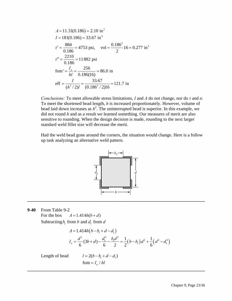
211.31(0.186) 2.10 inA 4181(0.186) 33.67 inI
2
3884 0.1864753 psi, vol 16 0.277 in
0.186 2
2210
11882 psi0.186
256
fom ' 86.0 in0.186(16)
uI
hl
2 2
33.67eff 121.7 in
( / 2) (0.186 / 2)16
I
h l
Conclusions: To meet allowable stress limitations, I and A do not change, nor do τ and σ.
To meet the shortened bead length, h is increased proportionately. However, volume of bead laid down increases as h2. The uninterrupted bead is superior. In this example, we did not round h and as a result we learned something. Our measures of merit are also sensitive to rounding. When the design decision is made, rounding to the next larger standard weld fillet size will decrease the merit.
Had the weld bead gone around the corners, the situation would change. Here is a follow
up task analyzing an alternative weld pattern.
______________________________________________________________________________ 9-40 From Table 9-2 For the box 1.414 ( )A h b d
Subtracting 1 1 from and from b b d d
1 11.414A h b b d d
3 22
2 31 11 1
1 1(3 )
6 6 2 2 6u
d b dd 3I b d b b d d d
Length of bead 1 12( )l b b d d fom /uI hl
______________________________________________________________________________
Chapter 9, Page 23/36
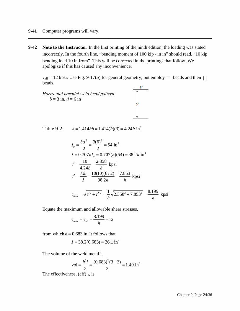
9-41 Computer programs will vary. ______________________________________________________________________________ 9-42 Note to the Instructor. In the first printing of the ninth edition, the loading was stated
incorrectly. In the fourth line, “bending moment of 100 kip ⋅ in in” should read, “10 kip
bending load 10 in from”. This will be corrected in the printings that follow. We apologize if this has caused any inconvenience.
all = 12 kpsi. Use Fig. 9-17(a) for general geometry, but employ beads and then
beads. Horizontal parallel weld bead pattern b = 3 in, d = 6 in Table 9-2: 21.414 1.414( )(3) 4.24 inA hb h h
2 2
33(6)54 in
2 2u
bdI
40.707 0.707( )(54) 38.2 inuI hI h h
10 2.358
kpsi4.24h h
10(10)(6 / 2) 7.853
kpsi38.2
Mc
I h h
2 2 2 2max
1 8.1992.358 7.853 kpsi
h h
Equate the maximum and allowable shear stresses.
max all
8.19912
h
from which It follows that 0.683 in.h
438.2(0.683) 26.1 inI The volume of the weld metal is
2 2
3(0.683) (3 3)vol 1.40 in
2 2
h l
The effectiveness, (eff)H, is
Chapter 9, Page 24/36
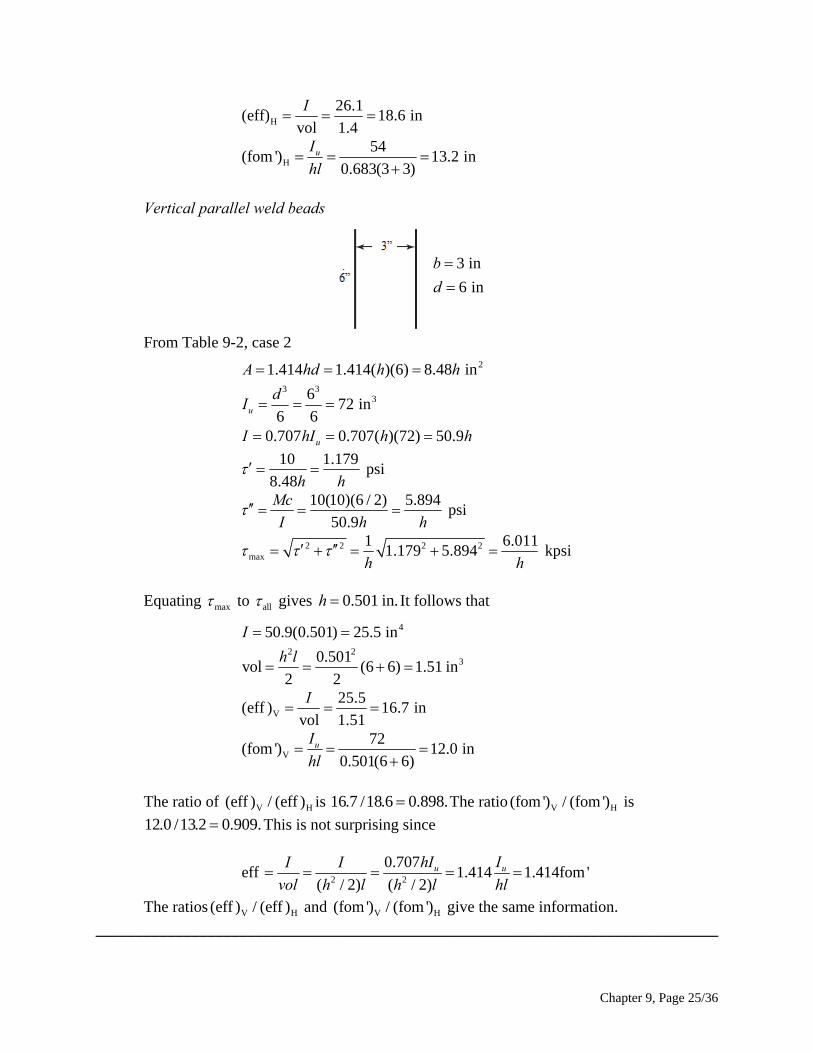
H
26.1(eff) 18.6 in
vol 1.4
I
H
54(fom ') 13.2 in
0.683(3 3)uI
hl
Vertical parallel weld beads
3 in
6 in
b
d
From Table 9-2, case 2
21.414 1.414( )(6) 8.48 inA hd h h
3 3
3672 in
6 6u
dI
0.707 0.707( )(72) 50.9uI hI h h
10 1.179
psi8.48h h
10(10)(6 / 2) 5.894
psi50.9
Mc
I h h
2 2 2 2max
1 6.0111.179 5.894 kpsi
h h
Equating max to all gives 0.501 in.h It follows that
450.9(0.501) 25.5 inI
2 2
30.501vol (6 6) 1.51 in
2 2
h l
V
25.5(eff ) 16.7 in
vol 1.51
I
V
72(fom') 12.0 in
0.501(6 6)uI
hl
The ratio of is 16V H(eff ) / (eff ) .7 /18.6 0.898. The ratio is
This is not surprising since V H(fom') / (fom ')
12.0 /13.2 0.909.
2 2
0.707eff 1.414 1.414fom'
( / 2) ( / 2)u uhI II I
vol h l h l hl
The ratios (e and give the same information. V Hff ) / (eff ) V(fom ') / (fom ')H
______________________________________________________________________________
Chapter 9, Page 25/36
9-43 F = 0, T = 15 kipin. Table 9-1: Ju = 2 r 3 = 2 (1)3 = 6.283 in3, J = 0.707(1/4) 6.283 = 1.111 in4
max
15 113.5 kpsi .
1.111
TrAns
J
______________________________________________________________________________ 9-44 F = 2 kip, T = 0. Table 9-2: A = 1.414 h r = 1.414 (1/4)(1) = 1.111 in2 Iu = r 3 = (1)3 = 3.142 in3, I = 0.707(1/4) 3.142 = 0.5553 in4
2
1.80 kpsi1.111
V
A
2 6 1
21.6 kpsi0.5553
Mr
I
max = ( 2 + 2)1/2 = (1.802 + 21.62)1/2 = 21.7 kpsi Ans. ______________________________________________________________________________ 9-45 F = 2 kip, T = 15 kipin. Bending: Table 9-2: A = 1.414 h r = 1.414 (1/4)(1) = 1.111 in2 Iu = r 3 = (1)3 = 3.142 in3, I = 0.707(1/4) 3.142 = 0.5553 in4
2
1.80 kpsi1.111
V
A
2 6 121.6 kpsi
0.5553M
Mr
I
Torsion: Table 9-1: Ju = 2 r 3 = 2 (1)3 = 6.283 in3, J = 0.707(1/4) 6.283 = 1.111 in4
15 113.5 kpsi
1.111T
Tr
J
Chapter 9, Page 26/36
2 22 2 2 2max 1.80 21.6 13.5 25.5 kpsi .
M TAns
______________________________________________________________________________ 9-46 F = 2 kip, T = 15 kipin. Bending: Table 9-2: A = 1.414 h r = 1.414 h (1) = 4.442h in2 Iu = r 3 = (1)3 = 3.142 in3, I = 0.707 h (3.142) = 2.221h in4
2 0.4502
kpsi4.442
V
A h h
2 6 1 5.403kpsi
2.221M
Mr
I h h
Torsion: Table 9-1: Ju = 2 r 3 = 2 (1)3 = 6.283 in3, J = 0.707 h (6.283) = 4.442 in4
15 1 3.377kpsi
4.442T
Tr
J h h
2 2 2
2 22max
0.4502 5.403 3.377 6.387kpsi
M T h h h h
max all
6.38720 0.319 in .h A
h ns
Should specify a 3
8in weld. Ans.
______________________________________________________________________________ 9-47 9 mm, 200 mm, 25mmh d b From Table 9-2, case 2:
A = 1.414(9)(200) = 2.545(103) mm2
3 3
6 32001.333 10 mm
6 6u
dI
I = 0.707h Iu = 0.707(9)(1.333)(106) = 8.484(106) mm4
Chapter 9, Page 27/36
3
3
25 109.82 MPa
2.545(10 )
F
A
M = 25(150) = 3750 Nm
36
3750(100)10 44.20 MPa
8.484(10 )
Mc
I
2 2 2 2max 9.82 44.20 45.3 MPa .Ans
______________________________________________________________________________ 9-48 Note to the Instructor. In the first printing of the ninth edition, the vertical dimension of
5 in should be to the top of the top plate. This will be corrected in the printings that follow. We apologize if this has caused any inconvenience.
h = 0.25 in, b = 2.5 in, d = 5 in. Table 9-2, case 5: A = 0.707h (b +2d) = 0.707(0.25)[2.5 + 2(5)] = 2.209 in2
2 252 in
2 2.5 2 5
dy
b d
32 2
3
2 2
22 2
3
2 52 5 2 2.5 2 5 2 33.33 in
3
u
dI d y b d y
3
I = 0.707 h Iu = 0.707(1/4)(33.33) = 5.891 in4 Primary shear:
2
0.905 kpsi2.209
F
A
Secondary shear (the critical location is at the bottom of the bracket): y = 5 2 = 3 in
2 5 3
5.093 kpsi5.891
My
I
2 2 2 2max 0.905 5.093 5.173 kpsi
all
max
183.48 .
5.173n Ans
______________________________________________________________________________
Chapter 9, Page 28/36
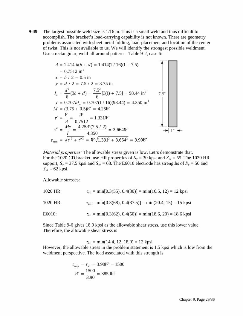
9-49 The largest possible weld size is 1/16 in. This is a small weld and thus difficult to accomplish. The bracket’s load-carrying capability is not known. There are geometry problems associated with sheet metal folding, load-placement and location of the center of twist. This is not available to us. We will identify the strongest possible weldment.
Use a rectangular, weld-all-around pattern – Table 9-2, case 6:
2
2 23
4
1.414 ( ) 1.414(1 / 16)(1 7.5)
0.7512 in/ 2 0.5 in/ 2 7.5 / 2 3.75 in
7.5(3 ) [3(1) 7.5] 98.44 in
6 60.707 0.707(1 / 16)(98.44) 4.350 in(3.75 0.5) 4.25
1.3310.7512
4
u
u
A h b d
x by d
dI b d
I hIM W W
V WW
AMc
I
2 2 2 2max
.25 (7.5 / 2)3.664
4.350
1.331 3.664 3.90
WW
W W
Materia
l properties: The allowable stress given is low. Let’s demonstrate that. For the 1020 CD bracket, use HR properties of Sy = 30 kpsi and Sut = 55. The 1030 HR
support, Sy = 37.5 kpsi and Sut = 68. The E6010 electrode has strengths of Sy = 50 and Sut = 62 kpsi. Allowable stresses: 1020 HR: all = min[0.3(55), 0.4(30)] = min(16.5, 12) = 12 kpsi 1020 HR: all = min[0.3(68), 0.4(37.5)] = min(20.4, 15) = 15 kpsi E6010: all = min[0.3(62), 0.4(50)] = min(18.6, 20) = 18.6 kpsi Since Table 9-6 gives 18.0 kpsi as the allowable shear stress, use this lower value. Therefore, the allowable shear stress is all = min(14.4, 12, 18.0) = 12 kpsi However, the allowable stress in the problem statement is 1.5 kpsi which is low from the
weldment perspective. The load associated with this strength is
max all 3.90 1500
1500385 lbf
3.90
W
W
Chapter 9, Page 29/36
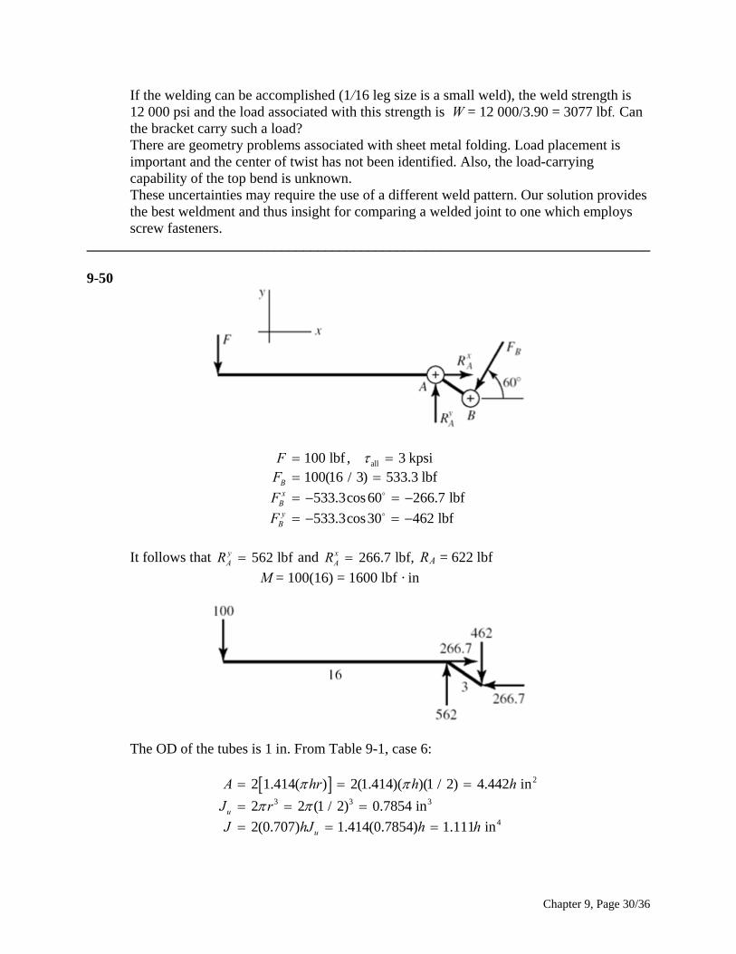
If the welding can be accomplished (1/16 leg size is a small weld), the weld strength is 12 000 psi and the load associated with this strength is W = 12 000/3.90 = 3077 lbf. Can
the bracket carry such a load? There are geometry problems associated with sheet metal folding. Load placement is
important and the center of twist has not been identified. Also, the load-carrying capability of the top bend is unknown.
These uncertainties may require the use of a different weld pattern. Our solution provides the best weldment and thus insight for comparing a welded joint to one which employs screw fasteners.
______________________________________________________________________________ 9-50
all100 lbf , 3 kpsi100(16 / 3) 533.3 lbf
533.3cos60 266.7 lbf
533.3cos30 462 lbf
Bx
By
B
FF
F
F
It follows that and R562 lbfy
AR 266.7 lbf,xAR A = 622 lbf
M = 100(16) = 1600 lbf · in
The OD of the tubes is 1 in. From Table 9-1, case 6:
2
3 3 3
4
2 1.414( ) 2(1.414)( )(1 / 2) 4.442 in
2 2 (1 / 2) 0.7854 in
2(0.707) 1.414(0.7854) 1.111 inu
u
A hr h
J r
J hJ h h
h
Chapter 9, Page 30/36
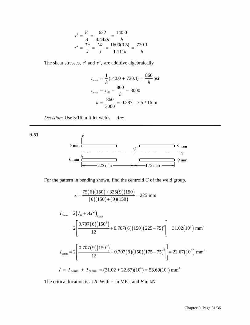
622 140.0
4.4421600(0.5) 720.1
1.111
V
A h hTc Mc
J J h h
The shear stresses, and , are additive algebraically
max
max all
1 860(140.0 720.1) psi
8603000
8600.287 5 / 16 in
3000
h h
h
h
Decision: Use 5/16 in fillet welds Ans. ______________________________________________________________________________ 9-51 For the pattern in bending shown, find the centroid G of the weld group.
75 6 150 325 9 150225 mm
6 150 9 150x
26mm 6mm
32 6 4
2
0.707 6 1502 0.707 6 150 225 75 31.02 10 mm
12
GI I Ax
32 6 4
9mm
0.707 9 1502 0.707 9 150 175 75 22.67 10 mm
12I
I = I 6 mm + I 9 mm = (31.02 + 22.67)(106) = 53.69(106) mm4
The critical location is at B. With in MPa, and F in kN
Chapter 9, Page 31/36
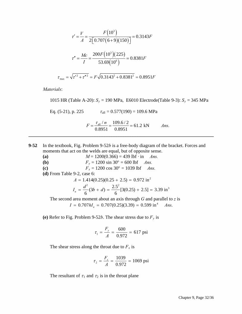
3100.3143
2 0.707 6 9 150
FVF
A
3
6
200 10 2250.8381
53.69 10
FMcF
I
2 2 2 2max 0.3143 0.8381 0.8951F F
Materials: 1015 HR (Table A-20): Sy = 190 MPa, E6010 Electrode(Table 9-3): Sy = 345 MPa Eq. (5-21), p. 225 all = 0.577(190) = 109.6 MPa
all / 109.6 / 261.2 kN .
0.8951 0.8951
nF Ans
______________________________________________________________________________ 9-52 In the textbook, Fig. Problem 9-52b is a free-body diagram of the bracket. Forces and
moments that act on the welds are equal, but of opposite sense. (a) M = 1200(0.366) = 439 lbf · in Ans. (b) Fy = 1200 sin 30 = 600 lbf Ans. (c) Fx = 1200 cos 30 = 1039 lbf Ans. (d) From Table 9-2, case 6:
2
2 23
1.414(0.25)(0.25 2.5) 0.972 in
2.5(3 ) [3(0.25) 2.5] 3.39 in
6 6u
A
dI b d
The second area moment about an axis through G and parallel to z is 40.707 0.707(0.25)(3.39) 0.599 in .uI hI Ans
(e) Refer to Fig. Problem 9-52b. The shear stress due to Fy is
1
600617 psi
0.972yF
A
The shear stress along the throat due to Fx is
2
10391069 psi
0.972xF
A
The resultant of 1 and 2 is in the throat plane
Chapter 9, Page 32/36
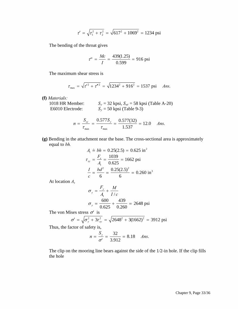
2 2 2 21 2 617 1069 1234 psi
The bending of the throat gives
439(1.25)916 psi
0.599
Mc
I
The maximum shear stress is
2 2 2 2max 1234 916 1537 psi .Ans
(f) Materials: 1018 HR Member: Sy = 32 kpsi, Sut = 58 kpsi (Table A-20) E6010 Electrode: Sy = 50 kpsi (Table 9-3)
max max
0.577 0.577(32)12.0 .
1.537sy yS S
n A
ns
(g) Bending in the attachment near the base. The cross-sectional area is approximately
equal to bh. 2
1
12 2
3
0.25(2.5) 0.625 in1039
1662 psi0.625
0.25(2.5)0.260 in
6 6
xxy
A bhF
A
I bd
c
At location A,
1 /600 439
2648 psi0.625 0.260
yy
y
F M
A I c
The von Mises stress is 2 2 2 23 2648 3(1662) 3912 psiy xy
Thus, the factor of safety is, 32
8.18 .3.912
ySn A
ns
The clip on the mooring line bears against the side of the 1/2-in hole. If the clip fills
the hole
Chapter 9, Page 33/36
3
12009600 psi
0.25(0.50)
32(10 )3.33 .
9600y
F
tdS
n A
ns
Further investigation of this situation requires more detail than is included in the task
statement. (h) In shear fatigue, the weakest constituent of the weld melt is 1018 HR with Sut = 58
kpsi, Eq. (6-8), p. 282, gives
0.504 0.504(58) 29.2 kpsie utS S
Eq. (6-19), p. 287: ka = 14.4(58)-0.718 = 0.780 For the size factor estimate, we first employ Eq. (6-25), p. 289, for the equivalent
diameter
0.808 0.707 0.808 0.707(2.5)(0.25) 0.537 ined hb
Eq. (6-20), p. 288, is used next to find kb
-0.107 -0.1070.537
0.9400.30 0.30
eb
dk
Eq.(6-26), p. 290: kc = 0.59 From Eq. (6-18), p. 287, the endurance strength in shear is
Sse = 0.780(0.940)(0.59)(29.2) = 12.6 kpsi
From Table 9-5, the shear stress-concentration factor is Kf s = 2.7. The loading is repeatedly-applied
max 1.5372.7 2.07 kpsi
2 2a m f sK
Table 6-7, p. 307: Gerber factor of safety nf, adjusted for shear, with Ssu = 0.67Sut
2
22
1 21 1
2
1 0.67(58) 2.07 2(2.07)(12.6)1 1 5.55 .
2 2.07 12.6 0.67(58)(2.07)
su a m sef
m se su a
S Sn
S S
Ans
Attachment metal should be checked for bending fatigue. ______________________________________________________________________________ 9-53 (a) Use b = d = 4 in. Since h = 5/8 in, the primary shear is
Chapter 9, Page 34/36
0.28291.414(5 / 8)(4)
FF
The secondary shear calculations, for a moment arm of 14 in give
2 23
4
4[3(4 ) 4 ]42.67 in
60.707 0.707(5 / 8)42.67 18.85 in
14 (2)1.485
18.85
u
u
yx y
J
J hJMr F
FJ
Thus, the maximum shear and allowable load are:
2 2max
all
1.485 (0.2829 1.485) 2.30925
10.8 kip .2.309 2.309
F F
F A
ns
The load for part (a) has increased by a factor of 10.8/2.71 = 3.99 Ans. (b) From Prob. 9-18b, all = 11 kpsi
allall
114.76 kip
2.309 2.309F
The allowable load in part (b) has increased by a factor of 4.76/1.19 = 4 Ans. ______________________________________________________________________________ 9-54 Purchase the hook having the design shown in Fig. Problem 9-54b. Referring to text Fig.
9-29a, this design reduces peel stresses. ______________________________________________________________________________ 9-55 (a)
/ 2/ 2 / 2
11/ 2 / 2
/ 2
1 1
1
1 cosh( )cosh( ) sinh( )
4 sinh( / 2)
[sinh( / 2) sinh( / 2)] [sinh( / 2) ( sinh( / 2))]
2 sinh( / 2)[2sinh( / 2)] .
4 sinh( / 2) 2
ll l
l ll
P x Adx A x dx x
l b lA A
l l l
A l P Pl An
bl l bl
l
s
(b) cosh( / 2)
( / 2) .4 sinh( / 2) 4 tanh( / 2)
P l Pl A
b l b lns
Chapter 9, Page 35/36
(c) ( / 2) 2 / 2
.4 tanh( / 2) tanh( / 2)
l P bl lK Ans
b l P l
For computer programming, it can be useful to express the hyperbolic tangent in
terms of exponentials: exp( / 2) exp( / 2)
.2 exp( / 2) exp( / 2)
l l lK A
l lns
______________________________________________________________________________ 9-56 This is a computer programming exercise. All programs will vary.
Chapter 9, Page 36/36
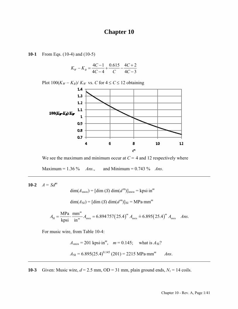
Chapter 10 10-1 From Eqs. (10-4) and (10-5)
4 1 0.615 4 2
4 4 4W B
C CK K
C C C 3
Plot 100(KW KB)/ KW vs. C for 4 C 12 obtaining
We see the maximum and minimum occur at C = 4 and 12 respectively where Maximum = 1.36 % Ans., and Minimum = 0.743 % Ans. ______________________________________________________________________________ 10-2 A = Sdm dim(Auscu) = [dim (S) dim(d m)]uscu = kpsiinm dim(ASI) = [dim (S) dim(d m)]SI = MPammm
SI uscu uscu uscu
MPa mm6.894757 25.4 6.895 25.4 .
kpsi in
mm m
mA A A A Ans
For music wire, from Table 10-4:
Auscu = 201 kpsiinm, m = 0.145; what is ASI?
_____________________________________________________________________________
0-3 Given: Music wire, d = 2.5 mm, OD = 31 mm, plain ground ends, Nt = 14 coils.
ASI = 6.895(25.4)0.145 (201) = 2215 MPammm Ans. _ 1
Chapter 10 - Rev. A, Page 1/41
(a) Table 10-1: Na = N 1 = 14 1 = 13 coils
Ls = d Nt = 2.5(14) = 35 mm
Table 10-4: m = 0.145, A = 2211 MPammm
Eq. (10-14):
t
0.145
22111936 MPa
2.5ut m
AS
d
Table 10-6: Ssy = 0.45(1936) = 871.2 MPa
D = OD d = 31 2.5 = 28.5 mm
C = D/d = 28.5/2.5 = 11.4
Eq. (10-5):
4 11.4 24 21.117
4 3 4 11.4 3B
CK
C
Eq. (10-7):
33 2.5 871.2167.9 N
8 8 1.117 28.5sy
sB
d SF
K D
Table 10-5): d = 2.5/25.4 = 0.098 in G = 81.0(103) MPa
Eq. (10-9):
4 34
3 3
2.5 81 101.314 N / mm
8 8 28.5 13a
d Gk
D N
0
167.935 162.8 mm .
1.314s
s
FL L A
k ns
(b) Fs = 167.9 N Ans.
(c) k = 1.314 N/mm Ans.
(d) 0 cr
149.9 mm0.5
L . Spring needs to be supported. Ans. 2.63 28.5
_____________________________________________________________________________
0-4 Given: Design load, F1 = 130 N.
4, N = 13 coils, Ssy = 871.2 MPa, Fs = 167.9 N,
Eq. (10-19): 3 ≤ Na ≤ 15 Na = 13 O.K.
_ 1 Referring to Prob. 10-3 solution, C = 11. a
L0 = 162.8 mm and (L0)cr = 149.9 mm. Eq. (10-18): 4 ≤ C ≤ 12 C = 11.4 O.K.
Chapter 10 - Rev. A, Page 2/41
Eq. (10-17): 1
167.91 1 0.29
130sF
F
Eq. (10-20): 0.15, 0.29 . .O K From Eq. (10-7) for static service
11 3 3
1
8 8(130)(28.5)1.117 674 MPa
(2.5)871.2
1.29674
B
sy
F DK
dS
n
Eq. (10-21): ns ≥ 1.2, n = 1.29 O.K.
1
167.9 167.9674 870.5 MPa
130 130/ 871.2 / 870.5 1
s
sy sS
Ssy/s ≥ (ns )d : Not solid-safe (but was the basis of the design). Not O.K. L0 ≤ (L0)cr: 162.8 149.9 Not O.K. Design is unsatisfactory. Operate over a rod? Ans. ______________________________________________________________________________ 10-5 Given: Oil-tempered wire, d = 0.2 in, D = 2 in, Nt = 12 coils, L0 = 5 in, squared ends. (a) Table 10-1: Ls = d (Nt + 1) = 0.2(12 + 1) = 2.6 in Ans. (b) Table 10-1: Na = Nt 2 = 12 2 = 10 coils Table 10-5: G = 11.2 Mpsi
Eq. (10-9):
4 64
3 3
0.2 11.2 1028 lbf/in
8 8 2 10
d Gk
D N
Fs = k ys = k (L0 Ls ) = 28(5 2.6) = 67.2 lbf Ans. (c) Eq. (10-1): C = D/d = 2/0.2 = 10
Eq. (10-5):
4 10 24 21.135
4 3 4 10 3B
CK
C
Eq. (10-7): 3
3 3
8 67.2 281.135 48.56 10 psi
0.2s B
FDK
d
Chapter 10 - Rev. A, Page 3/41
Table 10-4: m = 0.187, A = 147 kpsiinm
Eq. (10-14): 0.187
147198.6 kpsi
0.2ut m
AS
d
Table 10-6: Ssy = 0.50 Sut = 0.50(198.6) = 99.3 kpsi
99.3
2.04 .48.56
sys
s
Sn A
ns
______________________________________________________________________________ 10-6 Given: Oil-tempered wire, d = 4 mm, C = 10, plain ends, L0 = 80 mm, and at F = 50 N, y = 15 mm. (a) k = F/y = 50/15 = 3.333 N/mm Ans. (b) D = Cd = 10(4) = 40 mm OD = D + d = 40 + 4 = 44 mm Ans. (c) From Table 10-5, G = 77.2 GPa
Eq. (10-9):
4 34
3 3
4 77.2 1011.6 coils
8 8 3.333 40a
d GN
kD
Table 10-1: Nt = Na = 11.6 coils Ans. (d) Table 10-1: Ls = d (Nt + 1) = 4(11.6 + 1) = 50. 4 mm Ans. (e) Table 10-4: m = 0.187, A = 1855 MPammm
Eq. (10-14): 0.187
18551431 MPa
4ut m
AS
d
Table 10-6: Ssy = 0.50 Sut = 0.50(1431) = 715.5 MPa ys = L0 Ls = 80 50.4 = 29.6 mm Fs = k ys = 3.333(29.6) = 98.66 N
Eq. (10-5): 4 2 4(10) 2
1.1354 3 4(10) 3B
CK
C
Chapter 10 - Rev. A, Page 4/41
Eq. (10-7):
3 3
8 98.66 4081.135 178.2 MPa
4s
s B
F DK
d
715.5
4.02 .178.2
sys
s
Sn A
ns
______________________________________________________________________________ 10-7 Static service spring with: HD steel wire, d = 0.080 in, OD = 0.880 in, Nt = 8 coils, plain
and ground ends. Preliminaries Table 10-5: A = 140 kpsi · inm, m = 0.190
Eq. (10-14): 0.190
140226.2 kpsi
0.080ut m
AS
d
Table 10-6: Ssy = 0.45(226.2) = 101.8 kpsi Then, D = OD d = 0.880 0.080 = 0.8 in Eq. (10-1): C = D/d = 0.8/0.08 = 10
Eq. (10-5): 4 2 4(10) 2
1.1354 3 4(10) 3B
CK
C
Table 10-1: Na = Nt 1 = 8 1 = 7 coils Ls = dNt = 0.08(8) = 0.64 in Eq. (10-7) For solid-safe, ns = 1.2 :
3 33 0.08 101.8 10 / 1.2/
18.78 lbf8 8(1.135)(0.8)
sy ss
B
d S nF
K D
Eq. (10-9): 4 64
3 3
0.08 11.5 1016.43 lbf/in
8 8 0.8 7a
d Gk
D N
18.78
1.14 in16.43
ss
Fy
k
(a) L0 = ys + Ls = 1.14 + 0.64 = 1.78 in Ans.
(b) Table 10-1: 0 1.780.223 in .
8t
Lp A
N ns
(c) From above: Fs = 18.78 lbf Ans. (d) From above: k = 16.43 lbf/in Ans.
(e) Table 10-2 and Eq. (10-13): 0 cr
2.63 2.63(0.8)( ) 4.21 in
0.5
DL
Since L0 < (L0)cr, buckling is unlikely Ans. ______________________________________________________________________________ 10-8 Given: Design load, F1 = 16.5 lbf. Referring to Prob. 10-7 solution, C = 10, Na = 7 coils, Ssy = 101.8 kpsi, Fs = 18.78 lbf, ys = 1.14 in, L0 = 1.78 in, and (L0)cr = 4.208 in.
Chapter 10 - Rev. A, Page 5/41
Eq. (10-18): 4 ≤ C ≤ 12 C = 10 O.K. Eq. (10-19): 3 ≤ Na ≤ 15 Na = 7 O.K.
Eq. (10-17): 1
18.781 1 0.14
16.5sF
F
Eq. (10-20): 0.15, 0.14 . .not O K , but probably acceptable. From Eq. (10-7) for static service
311 3 3
1
8 8(16.5)(0.8)1.135 74.5 10 psi 74.5 kpsi
(0.080)101.8
1.3774.5
B
sy
F DK
dS
n
Eq. (10-21): ns ≥ 1.2, n = 1.37 O.K.
1
18.78 18.7874.5 84.8 kpsi
16.5 16.5/ 101.8 / 84.8 1.20
s
s sy sn S
Eq. (10-21): ns ≥ 1.2, ns = 1.2 It is solid-safe (basis of design). O.K. Eq. (10-13) and Table 10-2: L0 ≤ (L0)cr 1.78 in 4.208 in O.K. ______________________________________________________________________________ 10-9 Given: A228 music wire, sq. and grd. ends, d = 0.007 in, OD = 0.038 in, L0 = 0.58 in, Nt = 38 coils. D = OD d = 0.038 0.007 = 0.031 in Eq. (10-1): C = D/d = 0.031/0.007 = 4.429
Eq. (10-5):
4 4.429 24 21.340
4 3 4 4.429 3B
CK
C
Table (10-1): Na = Nt 2 = 38 2 = 36 coils (high) Table 10-5: G = 12.0 Mpsi
Eq. (10-9):
4 64
3 3
0.007 12.0 103.358 lbf/in
8 8 0.031 36a
d Gk
D N
Table (10-1): Ls = dNt = 0.007(38) = 0.266 in ys = L0 Ls = 0.58 0.266 = 0.314 in Fs = kys = 3.358(0.314) = 1.054 lbf
Eq. (10-7): 3
3 3
8 1.054 0.03181.340 325.1 10 psi
0.007s
s B
F DK
d
(1)
Table 10-4: A = 201 kpsiinm, m = 0.145
Chapter 10 - Rev. A, Page 6/41
Eq. (10-14): 0.145
201412.7 kpsi
0.007ut m
AS
d
Table 10-6: Ssy = 0.45 Sut = 0.45(412.7) = 185.7 kpsi s > Ssy, that is, 325.1 > 185.7 kpsi, the spring is not solid-safe. Return to Eq. (1) with Fs = kys and s = Ssy /ns, and solve for ys, giving
3 33 185.7 10 /1.2 0.007/0.149 in
8 8 1.340 3.358 0.031sy s
sB
S n dy
K kD
The free length should be wound to L0 = Ls + ys = 0.266 + 0.149 = 0.415 in Ans. This only addresses the solid-safe criteria. There are additional problems. ______________________________________________________________________________ 10-10 Given: B159 phosphor-bronze, sq. and grd. ends, d = 0.014 in, OD = 0.128 in, L0 = 0.50
in, Nt = 16 coils. D = OD d = 0.128 0.014 = 0.114 in Eq. (10-1): C = D/d = 0.114/0.014 = 8.143
Eq. (10-5):
4 8.143 24 21.169
4 3 4 8.143 3B
CK
C
Table (10-1): Na = Nt 2 = 16 2 = 14 coils Table 10-5: G = 6 Mpsi
Eq. (10-9):
4 64
3 3
0.014 6 101.389 lbf/in
8 8 0.114 14a
d Gk
D N
Table (10-1): Ls = dNt = 0.014(16) = 0.224 in ys = L0 Ls = 0.50 0.224 = 0.276 in Fs = kys = 1.389(0.276) = 0.3834 lbf
Eq. (10-7):
33 3
8 0.3834 0.11481.169 47.42 10 psi
0.014s
s B
F DK
d
(1)
Table 10-4: A = 145 kpsiinm, m = 0
Eq. (10-14): 0
145145 kpsi
0.014ut m
AS
d
Table 10-6: Ssy = 0.35 Sut = 0.35(135) = 47.25 kpsi s > Ssy, that is, 47.42 > 47.25 kpsi, the spring is not solid-safe. Return to Eq. (1) with Fs = kys and s = Ssy /ns, and solve for ys, giving
3 33 47.25 10 /1.2 0.014/0.229 in
8 8 1.169 1.389 0.114sy s
sB
S n dy
K kD
The free length should be wound to
Chapter 10 - Rev. A, Page 7/41
L0 = Ls + ys = 0.224 + 0.229 = 0.453 in Ans. ______________________________________________________________________________ 10-11 Given: A313 stainless steel, sq. and grd. ends, d = 0.050 in, OD = 0.250 in, L0 = 0.68 in,
Nt = 11.2 coils. D = OD d = 0.250 0.050 = 0.200 in Eq. (10-1): C = D/d = 0.200/0.050 = 4
Eq. (10-5):
4 4 24 21.385
4 3 4 4 3B
CK
C
Table (10-1): Na = Nt 2 = 11.2 2 = 9.2 coils Table 10-5: G = 10 Mpsi
Eq. (10-9):
4 64
3 3
0.050 10 10106.1 lbf/in
8 8 0.2 9.2a
d Gk
D N
Table (10-1): Ls = dNt = 0.050(11.2) = 0.56 in ys = L0 Ls = 0.68 0.56 = 0.12 in Fs = kys = 106.1(0.12) = 12.73 lbf
Eq. (10-7): 3
3 3
8 12.73 0.281.385 71.8 10 psi
0.050s
s B
F DK
d
Table 10-4: A = 169 kpsiinm, m = 0.146
Eq. (10-14): 0.146
169261.7 kpsi
0.050ut m
AS
d
Table 10-6: Ssy = 0.35 Sut = 0.35(261.7) = 91.6 kpsi
91.6
1.2871.8
sys
s
Sn
Spring is solid-safe (ns > 1.2) Ans.
______________________________________________________________________________ 10-12 Given: A227 hard-drawn wire, sq. and grd. ends, d = 0.148 in, OD = 2.12 in, L0 = 2.5 in,
Nt = 5.75 coils. D = OD d = 2.12 0.148 = 1.972 in Eq. (10-1): C = D/d = 1.972/0.148 = 13.32 (high)
Eq. (10-5):
4 13.32 24 21.099
4 3 4 13.32 3B
CK
C
Table (10-1): Na = Nt 2 = 5.75 2 = 3.75 coils Table 10-5: G = 11.4 Mpsi
Eq. (10-9):
4 64
3 3
0.148 11.4 1023.77 lbf/in
8 8 1.972 3.75a
d Gk
D N
Table (10-1): Ls = dNt = 0.148(5.75) = 0.851 in ys = L0 Ls = 2.5 0.851 = 1.649 in
Chapter 10 - Rev. A, Page 8/41
Fs = kys = 23.77(1.649) = 39.20 lbf
Eq. (10-7): 3
3 3
8 39.20 1.97281.099 66.7 10 psi
0.148s
s B
F DK
d
Table 10-4: A = 140 kpsiinm, m = 0.190
Eq. (10-14): 0.190
140201.3 kpsi
0.148ut m
AS
d
Table 10-6: Ssy = 0.35 Sut = 0.45(201.3) = 90.6 kpsi
90.6
1.3666.7
sys
s
Sn
Spring is solid-safe (ns > 1.2) Ans.
______________________________________________________________________________ 10-13 Given: A229 OQ&T steel, sq. and grd. ends, d = 0.138 in, OD = 0.92 in, L0 = 2.86 in, Nt = 12 coils. D = OD d = 0.92 0.138 = 0.782 in Eq. (10-1): C = D/d = 0.782/0.138 = 5.667
Eq. (10-5):
4 5.667 24 21.254
4 3 4 5.667 3B
CK
C
Table (10-1): Na = Nt 2 = 12 2 = 10 coils A229 OQ&T steel is not given in Table 10-5. From Table A-5, for carbon steels, G = 11.5 Mpsi.
Eq. (10-9):
4 64
3 3
0.138 11.5 10109.0 lbf/in
8 8 0.782 10a
d Gk
D N
Table (10-1): Ls = dNt = 0.138(12) = 1.656 in ys = L0 Ls = 2.86 1.656 = 1.204 in Fs = kys = 109.0(1.204) = 131.2 lbf
Eq. (10-7): 3
3 3
8 131.2 0.78281.254 124.7 10 psi
0.138s
s B
F DK
d
(1)
Table 10-4: A = 147 kpsiinm, m = 0.187
Eq. (10-14): 0.187
147212.9 kpsi
0.138ut m
AS
d
Table 10-6: Ssy = 0.50 Sut = 0.50(212.9) = 106.5 kpsi s > Ssy, that is, 124.7 > 106.5 kpsi, the spring is not solid-safe. Return to Eq. (1) with Fs = kys and s = Ssy /ns, and solve for ys, giving
3 33 106.5 10 /1.2 0.138/0.857 in
8 8 1.254 109.0 0.782sy s
sB
S n dy
K kD
The free length should be wound to
Chapter 10 - Rev. A, Page 9/41
L0 = Ls + ys = 1.656 + 0.857 = 2.51 in Ans. ______________________________________________________________________________ 10-14 Given: A232 chrome-vanadium steel, sq. and grd. ends, d = 0.185 in, OD = 2.75 in, L0 =
7.5 in, Nt = 8 coils. D = OD d = 2.75 0.185 = 2.565 in Eq. (10-1): C = D/d = 2.565/0.185 = 13.86 (high)
Eq. (10-5):
4 13.86 24 21.095
4 3 4 13.86 3B
CK
C
Table (10-1): Na = Nt 2 = 8 2 = 6 coils Table 10-5: G = 11.2 Mpsi.
Eq. (10-9):
4 64
3 3
0.185 11.2 1016.20 lbf/in
8 8 2.565 6a
d Gk
D N
Table (10-1): Ls = dNt = 0.185(8) = 1.48 in ys = L0 Ls = 7.5 1.48 = 6.02 in Fs = kys = 16.20(6.02) = 97.5 lbf
Eq. (10-7): 3
3 3
8 97.5 2.56581.095 110.1 10 psi
0.185s
s B
F DK
d
(1)
Table 10-4: A = 169 kpsiinm, m = 0.168
Eq. (10-14): 0.168
169224.4 kpsi
0.185ut m
AS
d
Table 10-6: Ssy = 0.50 Sut = 0.50(224.4) = 112.2 kpsi
112.2
1.02110.1
sys
s
Sn
Spring is not solid-safe (ns < 1.2)
Return to Eq. (1) with Fs = kys and s = Ssy /ns, and solve for ys, giving
3 33 112.2 10 /1.2 0.185/5.109 in
8 8 1.095 16.20 2.565sy s
sB
S n dy
K kD
The free length should be wound to L0 = Ls + ys = 1.48 + 5.109 = 6.59 in Ans. ______________________________________________________________________________ 10-15 Given: A313 stainless steel, sq. and grd. ends, d = 0.25 mm, OD = 0.95 mm, L0 = 12.1
mm, Nt = 38 coils. D = OD d = 0.95 0.25 = 0.7 mm Eq. (10-1): C = D/d = 0.7/0.25 = 2.8 (low)
Eq. (10-5):
4 2.8 24 21.610
4 3 4 2.8 3B
CK
C
Chapter 10 - Rev. A, Page 10/41
Table (10-1): Na = Nt 2 = 38 2 = 36 coils (high) Table 10-5: G = 69.0(103) MPa.
Eq. (10-9):
4 34
3 3
0.25 69.0 102.728 N/mm
8 8 0.7 36a
d Gk
D N
Table (10-1): Ls = dNt = 0.25(38) = 9.5 mm ys = L0 Ls = 12.1 9.5 = 2.6 mm Fs = kys = 2.728(2.6) = 7.093 N
Eq. (10-7): 3 3
8 7.093 0.781.610 1303 MPa
0.25s
s B
F DK
d
(1)
Table 10-4 (dia. less than table): A = 1867 MPammm, m = 0.146
Eq. (10-14): 0.146
18672286 MPa
0.25ut m
AS
d
Table 10-6: Ssy = 0.35 Sut = 0.35(2286) = 734 MPa s > Ssy, that is, 1303 > 734 MPa, the spring is not solid-safe. Return to Eq. (1) with Fs = kys and s = Ssy /ns, and solve for ys, giving
33 734 /1.2 0.25/1.22 mm
8 8 1.610 2.728 0.7sy s
sB
S n dy
K kD
The free length should be wound to L0 = Ls + ys = 9.5 + 1.22 = 10.72 mm Ans. This only addresses the solid-safe criteria. There are additional problems. ______________________________________________________________________________ 10-16 Given: A228 music wire, sq. and grd. ends, d = 1.2 mm, OD = 6.5 mm, L0 = 15.7 mm, Nt = 10.2 coils. D = OD d = 6.5 1.2 = 5.3 mm Eq. (10-1): C = D/d = 5.3/1.2 = 4.417
Eq. (10-5):
4 4.417 24 21.368
4 3 4 4.417 3B
CK
C
Table (10-1): Na = Nt 2 = 10.2 2 = 8.2 coils Table 10-5 (d = 1.2/25.4 = 0.0472 in): G = 81.7(103) MPa.
Eq. (10-9): 4 34
3 3
1.2 81.7 1017.35 N/mm
8 8 5.3 8.2a
d Gk
D N
Table (10-1): Ls = dNt = 1.2(10.2) = 12.24 mm ys = L0 Ls = 15.7 12.24 = 3.46 mm Fs = kys = 17.35(3.46) = 60.03 N
Chapter 10 - Rev. A, Page 11/41
Eq. (10-7):
3 3
8 60.03 5.381.368 641.4 MPa
1.2s
s B
F DK
d
(1)
Table 10-4: A = 2211 MPammm, m = 0.145
Eq. (10-14): 0.145
22112153 MPa
1.2ut m
AS
d
Table 10-6: Ssy = 0.45 Sut = 0.45(2153) = 969 MPa
969
1.51641.4
sys
s
Sn
Spring is solid-safe (ns > 1.2) Ans.
______________________________________________________________________________ 10-17 Given: A229 OQ&T steel, sq. and grd. ends, d = 3.5 mm, OD = 50.6 mm, L0 = 75.5 mm, Nt = 5.5 coils. D = OD d = 50.6 3.5 = 47.1 mm Eq. (10-1): C = D/d = 47.1/3.5 = 13.46 (high)
Eq. (10-5):
4 13.46 24 21.098
4 3 4 13.46 3B
CK
C
Table (10-1): Na = Nt 2 = 5.5 2 = 3.5 coils A229 OQ&T steel is not given in Table 10-5. From Table A-5, for carbon steels, G = 79.3(103) MPa.
Eq. (10-9):
4 34
3 3
3.5 79.3 104.067 N/mm
8 8 47.1 3.5a
d Gk
D N
Table (10-1): Ls = dNt = 3.5(5.5) = 19.25 mm ys = L0 Ls = 75.5 19.25 = 56.25 mm Fs = kys = 4.067(56.25) = 228.8 N
Eq. (10-7):
3 3
8 228.8 47.181.098 702.8 MPa
3.5s
s B
F DK
d
(1)
Table 10-4: A = 1855 MPammm, m = 0.187
Eq. (10-14): 0.187
18551468 MPa
3.5ut m
AS
d
Table 10-6: Ssy = 0.50 Sut = 0.50(1468) = 734 MPa
734
1.04702.8
sys
s
Sn
Spring is not solid-safe (ns < 1.2)
Return to Eq. (1) with Fs = kys and s = Ssy /ns, and solve for ys, giving
33 734 /1.2 3.5/48.96 mm
8 8 1.098 4.067 47.1sy s
sB
S n dy
K kD
The free length should be wound to
Chapter 10 - Rev. A, Page 12/41
L0 = Ls + ys = 19.25 + 48.96 = 68.2 mm Ans. ______________________________________________________________________________ 10-18 Given: B159 phosphor-bronze, sq. and grd. ends, d = 3.8 mm, OD = 31.4 mm, L0 = 71.4
mm, Nt = 12.8 coils. D = OD d = 31.4 3.8 = 27.6 mm Eq. (10-1): C = D/d = 27.6/3.8 = 7.263
Eq. (10-5):
4 7.263 24 21.192
4 3 4 7.263 3B
CK
C
Table (10-1): Na = Nt 2 = 12.8 2 = 10.8 coils Table 10-5: G = 41.4(103) MPa.
Eq. (10-9):
4 34
3 3
3.8 41.4 104.752 N/mm
8 8 27.6 10.8a
d Gk
D N
Table (10-1): Ls = dNt = 3.8(12.8) = 48.64 mm ys = L0 Ls = 71.4 48.64 = 22.76 mm Fs = kys = 4.752(22.76) = 108.2 N
Eq. (10-7):
3 3
8 108.2 27.681.192 165.2 MPa
3.8s
s B
F DK
d
(1)
Table 10-4 (d = 3.8/25.4 = 0.150 in): A = 932 MPammm, m = 0.064
Eq. (10-14): 0.064
932855.7 MPa
3.8ut m
AS
d
Table 10-6: Ssy = 0.35 Sut = 0.35(855.7) = 299.5 MPa
299.5
1.81165.2
sys
s
Sn
Spring is solid-safe (ns > 1.2) Ans.
______________________________________________________________________________ 10-19 Given: A232 chrome-vanadium steel, sq. and grd. ends, d = 4.5 mm, OD = 69.2 mm, L0 = 215.6 mm, Nt = 8.2 coils. D = OD d = 69.2 4.5 = 64.7 mm Eq. (10-1): C = D/d = 64.7/4.5 = 14.38 (high)
Eq. (10-5):
4 14.38 24 21.092
4 3 4 14.38 3B
CK
C
Table (10-1): Na = Nt 2 = 8.2 2 = 6.2 coils Table 10-5: G = 77.2(103) MPa.
Eq. (10-9):
4 34
3 3
4.5 77.2 102.357 N/mm
8 8 64.7 6.2a
d Gk
D N
Table (10-1): Ls = dNt = 4.5(8.2) = 36.9 mm
Chapter 10 - Rev. A, Page 13/41
ys = L0 Ls = 215.6 36.9 = 178.7 mm Fs = kys = 2.357(178.7) = 421.2 N
Eq. (10-7):
3 3
8 421.2 64.781.092 832 MPa
4.5s
s B
F DK
d
(1)
Table 10-4: A = 2005 MPammm, m = 0.168
Eq. (10-14): 0.168
20051557 MPa
4.5ut m
AS
d
Table 10-6: Ssy = 0.50 Sut = 0.50(1557) = 779 MPa s > Ssy, that is, 832 > 779 MPa, the spring is not solid-safe. Return to Eq. (1) with Fs = kys and s = Ssy /ns, and solve for ys, giving
33 779 /1.2 4.5/139.5 mm
8 8 1.092 2.357 64.7sy s
sB
S n dy
K kD
The free length should be wound to L0 = Ls + ys = 36.9 + 139.5 = 176.4 mm Ans. This only addresses the solid-safe criteria. There are additional problems. ______________________________________________________________________________ 10-20 Given: A227 HD steel. From the figure: L0 = 4.75 in, OD = 2 in, and d = 0.135 in. Thus
D = OD d = 2 0.135 = 1.865 in (a) By counting, Nt = 12.5 coils. Since the ends are squared along 1/4 turn on each end,
12.5 0.5 12 turns .4.75 / 12 0.396 in .
aN Ansp Ans
The solid stack is 13 wire diameters
Ls = 13(0.135) = 1.755 in Ans. (b) From Table 10-5, G = 11.4 Mpsi
4 64
3 3
0.135 (11.4) 106.08 lbf/in .
8 8 1.865 (12)a
d Gk A
D N ns
(c) Fs = k(L0 - Ls ) = 6.08(4.75 1.755)(10-3) = 18.2 lbf Ans. (d) C = D/d = 1.865/0.135 = 13.81
Chapter 10 - Rev. A, Page 14/41
3
3 3
4(13.81) 21.096
4(13.81) 38 8(18.2)(1.865)
1.096 38.5 10 psi 38.5 kpsi .0.135
B
ss B
K
F DK A
d
ns
______________________________________________________________________________
10-21 For the wire diameter analyzed, G = 11.75 Mpsi per Table 10-5. Use squared and ground ends. The following is a spread-sheet study using Fig. 10-3 for parts (a) and (b). For Na, k = Fmax /y = 20/2 = 10 lbf/in. For s, F = Fs = 20(1 + ) = 20(1 + 0.15) = 23 lbf.
(a) Spring over a Rod (b) Spring in a Hole Source Parameter Values Source Parameter Values
d 0.075 0.080 0.085 d 0.075 0.080 0.085 ID 0.800 0.800 0.800 OD 0.950 0.950 0.950 D 0.875 0.880 0.885 D 0.875 0.870 0.865 Eq. (10-1) C 11.667 11.000 10.412 Eq. (10-1) C 11.667 10.875 10.176 Eq. (10-9) Na 6.937 8.828 11.061 Eq. (10-9) Na 6.937 9.136 11.846 Table 10-1 Nt 8.937 10.828 13.061 Table 10-1 Nt 8.937 11.136 13.846 Table 10-1 Ls 0.670 0.866 1.110 Table 10-1 Ls 0.670 0.891 1.177 1.15y + Ls L0 2.970 3.166 3.410 1.15y + Ls L0 2.970 3.191 3.477 Eq. (10-13) (L0)cr 4.603 4.629 4.655 Eq. (10-
13) (L0)cr 4.603 4.576 4.550
Table 10-4 A 201.000 201.000 201.000 Table 10-4 A 201.000 201.000 201.000 Table 10-4 m 0.145 0.145 0.145 Table 10-4 m 0.145 0.145 0.145 Eq. (10-14) Sut 292.626 289.900 287.363 Eq. (10-
14) Sut 292.626 289.900 287.363
Table 10-6 Ssy 131.681 130.455 129.313 Table 10-6 Ssy 131.681 130.455 129.313 Eq. (10-5) KB 1.115 1.122 1.129 Eq. (10-5) KB 1.115 1.123 1.133 Eq. (10-7) s 135.335 112.948 95.293 Eq. (10-7) s 135.335 111.787 93.434 Eq. (10-3) ns 0.973 1.155 1.357 Eq. (10-3) ns 0.973 1.167 1.384 Eq. (10-22) fom 0.282 0.391 0.536 Eq. (10-
22) fom 0.282 0.398 0.555
For ns ≥ 1.2, the optimal size is d = 0.085 in for both cases. ______________________________________________________________________________ 10-22 In Prob. 10-21, there is an advantage of first selecting d as one can select from the
available sizes (Table A-28). Selecting C first, requires a calculation of d where then a size must be selected from Table A-28.
Consider part (a) of the problem. It is required that ID = D d = 0.800 in. (1) From Eq. (10-1), D = Cd. Substituting this into the first equation yields
0.800
1d
C (2)
Chapter 10 - Rev. A, Page 15/41
Starting with C = 10, from Eq. (2) we find that d = 0.089 in. From Table A-28, the closest diameter is d = 0.090 in. Substituting this back into Eq. (1) gives D = 0.890 in, with C = 0.890/0.090 = 9.889, which are acceptable. From this point the solution is the same as Prob. 10-21. For part (b), use
OD = D + d = 0.950 in. (3)
and, 0.800
1C
(4) d
(a) Spring over a rod (b) Spring in a Hole
Source Parameter Values Source Parameter Values C 10.000 10.5 C 10.000
Eq. (2) d 0.089 0.084 Eq. (4) d 0.086 Table A-28 d 0.090 0.085 Table A-28 d 0.085
Eq. (1) D 0.890 0.885 Eq. (3) D 0.865 Eq. (10-1) C 9.889 10.412 Eq. (10-1) C 10.176 Eq. (10-9) Na 13.669 11.061 Eq. (10-9) Na 11.846 Table 10-1 Nt 15.669 13.061 Table 10-1 Nt 13.846 Table 10-1 Ls 1.410 1.110 Table 10-1 Ls 1.177 1.15y + Ls L0 3.710 3.410 1.15y + Ls L0 3.477 Eq. (10-13) (L0)cr 4.681 4.655 Eq. (10-13) (L0)cr 4.550 Table 10-4 A 201.000 201.000 Table 10-4 A 201.000 Table 10-4 m 0.145 0.145 Table 10-4 m 0.145 Eq. (10-14) Sut 284.991 287.363 Eq. (10-14) Sut 287.363 Table 10-6 Ssy 128.246 129.313 Table 10-6 Ssy 129.313 Eq. (10-5) KB 1.135 1.128 Eq. (10-5) KB 1.135 Eq. (10-7) s 81.167 95.223 Eq. (10-7) s 93.643 ns = Ssy/s ns 1.580 1.358 ns = Ssy/s ns 1.381 Eq. (10-22) fom -0.725 -0.536 Eq. (10-22) fom -0.555
Again, for ns 1.2, the optimal size is = 0.085 in. Although this approach used less iterations than in Prob. 10-21, this was due to the initial
values picked and not the approach. ______________________________________________________________________________ 10-23 One approach is to select A227 HD steel for its low cost. Try L0 = 48 mm, then for y = 48 37.5 = 10.5 mm when F = 45 N. The spring rate is k = F/y = 45/10.5 = 4.286
N/mm. For a clearance of 1.25 mm with screw, ID = 10 + 1.25 = 11.25 mm. Starting with d = 2 mm, D = ID + d = 11.25 + 2 = 13.25 mm C = D/d = 13.25/2 = 6.625 (acceptable) Table 10-5 (d = 2/25.4 = 0.0787 in): G = 79.3 GPa
Chapter 10 - Rev. A, Page 16/41
Eq. (10-9): 4 4 3
3 3
2 (79.3)1015.9 coils
8 8(4.286)13.25a
d G
kD N
Assume squared and closed. Table 10-1: Nt = Na + 2 = 15.9 + 2 = 17.9 coils Ls = dNt = 2(17.9) =35.8 mm ys = L0 Ls = 48 35.8 = 12.2 mm Fs = kys = 4.286(12.2) = 52.29 N
Eq. (10-5):
4 6.625 24 2
1.213B
CK
4 3 4 6.625 3C
Eq. (10-7): 3
8 8(52.291.213s
s B
F DK
3
)13.25267.5 MPa
2d
Table 10-4: A = 1783 MPa · mmm, m = 0.190
Eq. (10-14): 0.190
17831563 MPa
2ut m
AS
d
Table 10-6: Ssy = 0.45Sut = 0.45(1563) = 703.3 MPa
703.3
2.63 1.2 . .267.5
sys
s
Sn O K
No other diameters in the given range work. So specify A227-47 HD steel, d = 2 mm, D = 13.25 mm, ID = 11.25 mm, OD = 15.25 mm, squared
and closed, Nt = 17.9 coils, Na = 15.9 coils, k = 4.286 N/mm, Ls = 35.8 mm, and L0 = 48 mm. Ans.
______________________________________________________________________________ 10-24 Select A227 HD steel for its low cost. Try L0 = 48 mm, then for y = 48 37.5 = 10.5 mm
when F = 45 N. The spring rate is k = F/y = 45/10.5 = 4.286 N/mm. For a clearance of 1.25 mm with screw, ID = 10 + 1.25 = 11.25 mm. D d = 11.25 (1) and, D =Cd (2) Starting with C = 8, gives D = 8d. Substitute into Eq. (1) resulting in d = 1.607 mm.
Selecting the nearest diameter in the given range, d = 1.6 mm. From this point, the calculations are shown in the third column of the spreadsheet output shown. We see that for d = 1.6 mm, the spring is not solid safe. Iterating on C we find that C = 6.5 provides acceptable results with the specifications
A227-47 HD steel, d = 2 mm, D = 13.25 mm, ID = 11.25 mm, OD = 15.25 mm, squared
Chapter 10 - Rev. A, Page 17/41
and closed, Nt = 17.9 coils, Na = 15.9 coils, k = 4.286 N/mm, Ls = 35.8 mm, and L0 = 48 mm. Ans.
Chapter 10 - Rev. A, Page 18/41
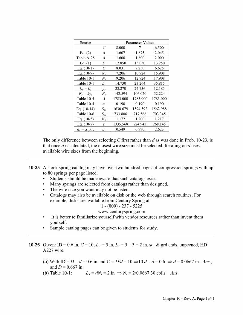
Source Parameter Values C 8.000 7 6.500
Eq. (2) d 1.607 1.875 2.045 Table A-28 d 1.600 1.800 2.000
Eq. (1) D 12.850 13.050 13.250 Eq. (10-1) C 8.031 7.250 6.625 Eq. (10-9) Na 7.206 10.924 15.908 Table 10-1 Nt 9.206 12.924 17.908 Table 10-1 Ls 14.730 23.264 35.815
L0 Ls ys 33.270 24.736 12.185 Fs = kys Fs 142.594 106.020 52.224
Table 10-4 A 1783.000 1783.000 1783.000 Table 10-4 m 0.190 0.190 0.190 Eq. (10-14) Sut 1630.679 1594.592 1562.988 Table 10-6 Ssy 733.806 717.566 703.345 Eq. (10-5) KB 1.172 1.200 1.217 Eq. (10-7) s 1335.568 724.943 268.145 ns = Ssy/s ns 0.549 0.990 2.623
The only difference between selecting C first rather than d as was done in Prob. 10-23, is
that once d is calculated, the closest wire size must be selected. Iterating on d uses available wire sizes from the beginning.
______________________________________________________________________________ 10-25 A stock spring catalog may have over two hundred pages of compression springs with up
to 80 springs per page listed. • Students should be made aware that such catalogs exist. • Many springs are selected from catalogs rather than designed. • The wire size you want may not be listed. • Catalogs may also be available on disk or the web through search routines. For
example, disks are available from Century Spring at 1 - (800) - 237 - 5225
www.centuryspring.com • It is better to familiarize yourself with vendor resources rather than invent them
yourself. • Sample catalog pages can be given to students for study. ______________________________________________________________________________ 10-26 Given: ID = 0.6 in, C = 10, L0 = 5 in, Ls = 5 3 = 2 in, sq. & grd ends, unpeened, HD
A227 wire. (a) With ID = D d = 0.6 in and C = D/d = 10 10 d d = 0.6 d = 0.0667 in Ans., and D = 0.667 in. (b) Table 10-1: Ls = dNt = 2 in Nt = 2/0.0667 30 coils Ans.
Chapter 10 - Rev. A, Page 19/41
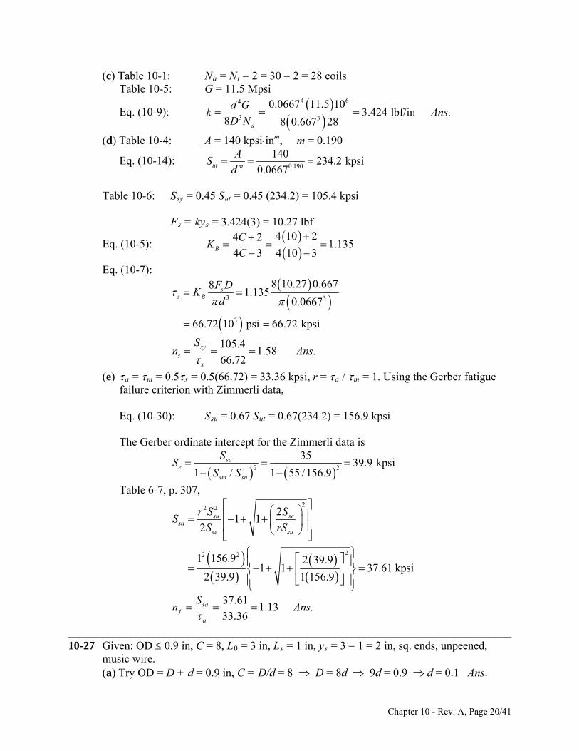
(c) Table 10-1: Na = Nt 2 = 30 2 = 28 coils Table 10-5: G = 11.5 Mpsi
Eq. (10-9): 4 64
3 3
0.0667 11.5 103.424 lbf/in .
8 8 0.667 28a
d Gk Ans
D N
(d) Table 10-4: A = 140 kpsiinm, m = 0.190
Eq. (10-14): 0.190
234.2 kpsi0.0667ut m
Sd
140A
Table 10-6: Ssy = 0.45 Sut = 0.45 (234.2) = 105.4 kpsi Fs = kys = 3.424(3) = 10.27 lbf
4 10 24 21.135
4 3 4 10 3B
CK
C
Eq. (10-5):
Eq. (10-7):
366.72 10 psi 66.72 kpsi
K
3 3
8 10.27 0.66781.135
0.0667s
s B
F D
d
105.41.58 .
66.72sy
s
n A s
Sns
(e) a = m = 0.5s = 0.5(66.72) = 33.36 kpsi, r = a / m = 1. Using the Gerber fatigue failure criterion with Zimmerli data,
Eq. (10-30): Ssu = 0.67 Sut = 0.67(234.2) = 156.9 kpsi The Gerber ordinate intercept for the Zimmerli data is
2 2
3539.9 kpsi
1 / 1 55 /156.9sa
e
sm su
SS
S S
Table 6-7, p. 307,
22 2 21 1
2
i
su sesa
se su
r S SS
S rS
22 21 156.9 2 39.91 1 37.61 kps
2 39.9 1 156.9 37.61
1.13 .33.36
saf
a
Sn Ans
______________________________________________________________________________ 10-27 Given: OD 0.9 in, C = 8, L0 = 3 in, Ls = 1 in, ys = 3 1 = 2 in, sq. ends, unpeened,
music wire. (a) Try OD = D + d = 0.9 in, C = D/d = 8 D = 8d 9d = 0.9 d = 0.1 Ans.
Chapter 10 - Rev. A, Page 20/41
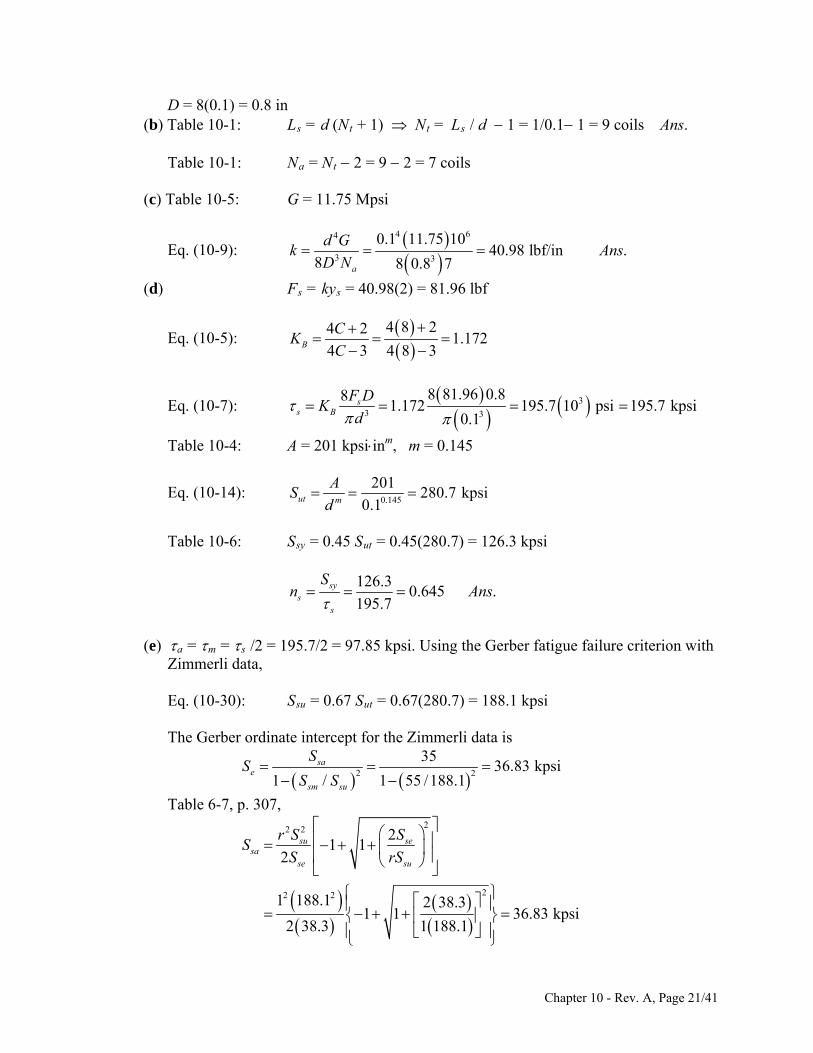
D = 8(0.1) = 0.8 in (b) Table 10-1: Ls = d (Nt + 1) Nt = Ls / d 1 = 1/0.1 1 = 9 coils Ans. Table 10-1: Na = Nt 2 = 9 2 = 7 coils (c) Table 10-5: G = 11.75 Mpsi
Eq. (10-9): 4 64
3 3
0.1 11.75 1040.98 lbf/in .
8 8 0.8 7a
d Gk Ans
D N
(d) Fs = kys = 40.98(2) = 81.96 lbf
Eq. (10-5): 4 8 24 2
1.1724 3 4 8 3B
CK
C
Eq. (10-7): 3
3 3
8 81.96 0.881.172 195.7 10 psi 195.7 kpsi
0.1s
s B
F DK
d
Table 10-4: A = 201 kpsiinm, m = 0.145
Eq. (10-14): 0.145
201280.7 kpsi
0.1ut m
A
d S
Table 10-6: Ssy = 0.45 Sut = 0.45(280.7) = 126.3 kpsi
126.30.645 .sy
s
Sn A
195.7s
ns
(e) a = m = s /2 = 195.7/2 = 97.85 kpsi. Using the Gerber fatigue failure criterion with
Zimmerli data, Eq. (10-30): Ssu = 0.67 Sut = 0.67(280.7) = 188.1 kpsi The Gerber ordinate intercept for the Zimmerli data is
2 2
/ 1 55 /188.1sm suS S
3536.83 kpsi
1sa
e
SS
Table 6-7, p. 307,
22 2
22 2
21 1
2
1 188.1 2 38.31 1 36.83 kpsi
2 38.3 1 188.1
su sesa
se su
r S SS
S rS
Chapter 10 - Rev. A, Page 21/41
36.830.376
97.85sa
a
.f
Sn Ans
Obviously, the spring is severely under designed and will fail statically and in fatigue.
Increasing C would improve matters. Try C = 12. This yields ns = 1.83 and nf = 1.00. ______________________________________________________________________________ 10-28 Note to the Instructor: In the first printing of the text, the wire material was incorrectly
identified as music wire instead of oil-tempered wire. This will be corrected in subsequent printings. We are sorry for any inconvenience.
Given: Fmax = 300 lbf, Fmin = 150 lbf, y = 1 in, OD = 2.1 0.2 = 1.9 in, C = 7,
unpeened, sq. & grd., oil-tempered wire. (a) D = OD d = 1.9 d (1) C = D/d = 7 D = 7d (2) Substitute Eq. (2) into (1) 7d = 1.9 d d = 1.9/8 = 0.2375 in Ans. (b) From Eq. (2): D = 7d = 7(0.2375) = 1.663 in Ans.
300 150150 lbf/in .
1
Fk A
y
(c) ns
(d) Table 10-5: G = 11.6 Mpsi
Eq. (10-9): 4 64
3 3
0.2375 11.6 106.69 coils
8 8 1.663 150a
d GN
D k
Table 10-1: Nt = Na + 2 = 8.69 coils Ans. (e) Table 10-4: A = 147 kpsiinm, m = 0.187
Eq. (10-14): 0.187
147192.3 kpsi
0.2375ut m
A
d S
Table 10-6: Ssy = 0.5 Sut = 0.5(192.3) = 96.15 kpsi
Eq. (10-5): 4 7 24 2
1.24 3 4 7 3B
CK
C
Chapter 10 - Rev. A, Page 22/41
Eq. (10-7): 3
8 ss B sy
F DK S
d
3 33 0.2375 96.15 10253.5 lbfsy
s
d SF
8 8 1.2 1.663BK D
ys = Fs / k = 253.5/150 = 1.69 in Table 10-1: Ls = Nt d = 8.46(0.2375) = 2.01 in L0 = Ls + ys = 2.01 + 1.69 = 3.70 in Ans. ______________________________________________________________________________ 10-29 For a coil radius given by:
2 11
-
2
R RR R
N
The torsion of a section is T = PR where dL = R d
23
0
32
2 110
24
2 11
2 10
4 4 2 22 1 1 2 1 2
2 1
4 2 21 2 1 24
1 1
2
1 2
4 2
( )2 ( ) 2
16 ( )
32
N
P
N
N
p
U TT dL PR d
P GJ P GJP R R
R dGJ N
P N R RR
GJ R R N
PN PNR R R R R R
GJ R R GJPN
J d R R R RGd
4
2 21 2 1 2
.16 ( )P
P d Gk Ans
N R R R R
______________________________________________________________________________ 10-30 Given: Fmin = 4 lbf, Fmax = 18 lbf, k = 9.5 lbf/in, OD 2.5 in, nf = 1.5. For a food service machinery application select A313 Stainless wire. Table 10-5: G = 10(106) psi Note that for 0.013 ≤ d ≤ 0.10 in A = 169, m = 0.146 0.10 < d ≤ 0.20 in A = 128, m = 0.263
18 4 18 4
7 lbf , 11 lbf , 7 / 112 2a m r
F F
Chapter 10 - Rev. A, Page 23/41
Try, 0.146
1690.080 in, 244.4 kpsi
(0.08)ut d S
Ssu = 0.67Sut = 163.7 kpsi, Ssy = 0.35Sut = 85.5 kpsi Try unpeened using Zimmerli’s endurance data: Ssa = 35 kpsi, Ssm = 55 kpsi
Gerber: 2 2
3539.5 kpsi
1 ( / ) 1 (55 / 163.7)sa
sesm su
S
S S
S
22 2
3 32 2
(7 / 11) (163.7) 2(39.5)1 1 35.0 kpsi
2(39.5) (7 / 11)(163.7)
/ 35.0 / 1.5 23.3 kpsi
8 8(7)(10 ) (10 ) 2.785 kpsi
(0.08 )
2(23.3) 2.785 2(23.3) 2.785
4(2.785) 4(2.785)
sa
sa f
a
S
S n
F
d
C
2
33 3
4 6
3
3(23.3)6.97
4(2.785)
6.97(0.08) 0.558 in4 2 4(6.97) 2
1.2014 3 4(6.97) 3
8 8(7)(0.558)1.201 (10 ) 23.3 kpsi
(0.08 )35 / 23.3 1.50 checks
10(10 )(0.0
8
B
aa B
f
a
D CdC
KC
F DK
dn
GdN
kD
4
3
max max
max
0
0
8)31.02 coils
8(9.5)(0.558)31.02 2 33 coils, 0.08(33) 2.64 in
/ 18 / 9.5 1.895 in(1 ) (1 0.15)(1.895) 2.179 in2.64 2.179 4.819 in
2.63(0.558)( ) 2.63 2.935 in
0.5
t s t
s
cr
s
N L dNy F k
y yL
DL
2 2 2 2
1.15(18 / 7) 1.15(18 / 7)(23.3) 68.9 kpsi/ 85.5 / 68.9 1.24
9.5(386)109 Hz
(0.08 )(0.558)(31.02)(0.283)
a
s sy s
a
kgf
d DN
n S
These steps are easily implemented on a spreadsheet, as shown below, for different
diameters.
Chapter 10 - Rev. A, Page 24/41
d1 d2 d3 d4
d 0.080 0.0915 0.1055 0.1205
m 0.146 0.146 0.263 0.263
A 169.000 169.000 128 128
Sut 244.363 239.618 231.257 223.311
Ssu 163.723 160.544 154.942 149.618
Ssy 85.527 83.866 80.940 78.159
Sse 39.452 39.654 40.046 40.469
Ssa 35.000 35.000 35.000 35.000
23.333 23.333 23.333 23.333
2.785 2.129 1.602 1.228
C 6.977 9.603 13.244 17.702
D 0.558 0.879 1.397 2.133
KB 1.201 1.141 1.100 1.074
a 23.333 23.333 23.333 23.333nf 1.500 1.500 1.500 1.500
Na 30.993 13.594 5.975 2.858
Nt 32.993 15.594 7.975 4.858
LS 2.639 1.427 0.841 0.585
ys 2.179 2.179 2.179 2.179
L0 4.818 3.606 3.020 2.764
(L0)cr 2.936 4.622 7.350 11.220
s 69.000 69.000 69.000 69.000
ns 1.240 1.215 1.173 1.133
f,(Hz) 108.895 114.578 118.863 121.775
The shaded areas depict conditions outside the recommended design conditions. Thus,
one spring is satisfactory. The specifications are: A313 stainless wire, unpeened, squared and ground, d = 0.0915 in, OD = 0.879 + 0.092 = 0.971 in, L0 = 3.606 in, and Nt = 15.59 turns Ans.
______________________________________________________________________________ 10-31 The steps are the same as in Prob. 10-23 except that the Gerber-Zimmerli criterion is
replaced with Goodman-Zimmerli:
1sa
sesm su
SS
S S
Chapter 10 - Rev. A, Page 25/41
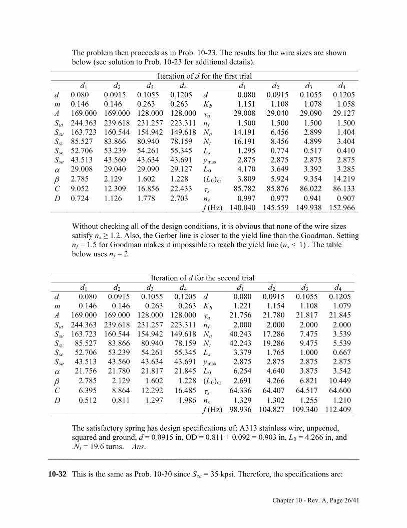
The problem then proceeds as in Prob. 10-23. The results for the wire sizes are shown below (see solution to Prob. 10-23 for additional details).
Iteration of d for the first trial d1 d2 d3 d4 d1 d2 d3 d4 d 0.080 0.0915 0.1055 0.1205 d 0.080 0.0915 0.1055 0.1205m 0.146 0.146 0.263 0.263 KB 1.151 1.108 1.078 1.058A 169.000 169.000 128.000 128.000 a 29.008 29.040 29.090 29.127Sut 244.363 239.618 231.257 223.311 nf 1.500 1.500 1.500 1.500Ssu 163.723 160.544 154.942 149.618 Na 14.191 6.456 2.899 1.404Ssy 85.527 83.866 80.940 78.159 Nt 16.191 8.456 4.899 3.404Sse 52.706 53.239 54.261 55.345 Ls 1.295 0.774 0.517 0.410Ssa 43.513 43.560 43.634 43.691 ymax 2.875 2.875 2.875 2.875 29.008 29.040 29.090 29.127 L0 4.170 3.649 3.392 3.285 2.785 2.129 1.602 1.228 (L0)cr 3.809 5.924 9.354 14.219C 9.052 12.309 16.856 22.433 s 85.782 85.876 86.022 86.133D 0.724 1.126 1.778 2.703 ns 0.997 0.977 0.941 0.907
f (Hz) 140.040 145.559 149.938 152.966
Without checking all of the design conditions, it is obvious that none of the wire sizes satisfy ns ≥ 1.2. Also, the Gerber line is closer to the yield line than the Goodman. Setting nf = 1.5 for Goodman makes it impossible to reach the yield line (ns < 1) . The table below uses nf = 2.
Iteration of d for the second trial d1 d2 d3 d4 d1 d2 d3 d4 d 0.080 0.0915 0.1055 0.1205 d 0.080 0.0915 0.1055 0.1205m 0.146 0.146 0.263 0.263 KB 1.221 1.154 1.108 1.079A 169.000 169.000 128.000 128.000 a 21.756 21.780 21.817 21.845Sut 244.363 239.618 231.257 223.311 nf 2.000 2.000 2.000 2.000Ssu 163.723 160.544 154.942 149.618 Na 40.243 17.286 7.475 3.539Ssy 85.527 83.866 80.940 78.159 Nt 42.243 19.286 9.475 5.539Sse 52.706 53.239 54.261 55.345 Ls 3.379 1.765 1.000 0.667Ssa 43.513 43.560 43.634 43.691 ymax 2.875 2.875 2.875 2.875 21.756 21.780 21.817 21.845 L0 6.254 4.640 3.875 3.542 2.785 2.129 1.602 1.228 (L0)cr 2.691 4.266 6.821 10.449C 6.395 8.864 12.292 16.485 s 64.336 64.407 64.517 64.600D 0.512 0.811 1.297 1.986 ns 1.329 1.302 1.255 1.210
f (Hz) 98.936 104.827 109.340 112.409 The satisfactory spring has design specifications of: A313 stainless wire, unpeened,
squared and ground, d = 0.0915 in, OD = 0.811 + 0.092 = 0.903 in, L0 = 4.266 in, and .Nt = 19.6 turns. Ans. ______________________________________________________________________________ 10-32 This is the same as Prob. 10-30 since Ssa = 35 kpsi. Therefore, the specifications are:
Chapter 10 - Rev. A, Page 26/41
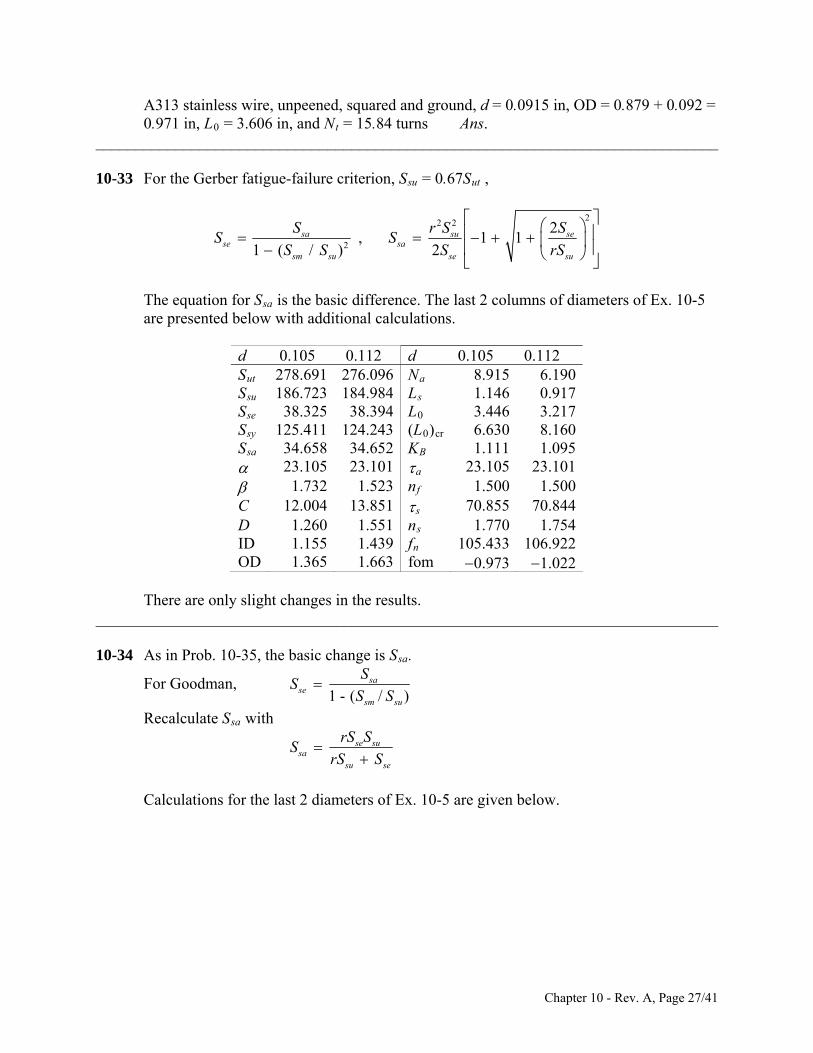
A313 stainless wire, unpeened, squared and ground, d = 0.0915 in, OD = 0.879 + 0.092 = 0.971 in, L0 = 3.606 in, and Nt = 15.84 turns Ans.
______________________________________________________________________________ 10-33 For the Gerber fatigue-failure criterion, Ssu = 0.67Sut ,
22 2
2
2, 1 1
1 ( / ) 2sa su se
se sasm su se su
S r S SS S
S S S rS
The equation for Ssa is the basic difference. The last 2 columns of diameters of Ex. 10-5
are presented below with additional calculations.
d 0.105 0.112 d 0.105 0.112 Sut 278.691 276.096 Na 8.915 6.190 Ssu 186.723 184.984 Ls 1.146 0.917 Sse 38.325 38.394 L0 3.446 3.217 Ssy 125.411 124.243 (L0)cr 6.630 8.160 Ssa 34.658 34.652 KB 1.111 1.095 23.105 23.101 a 23.105 23.101 1.732 1.523 nf 1.500 1.500 C 12.004 13.851 s 70.855 70.844 D 1.260 1.551 ns 1.770 1.754 ID 1.155 1.439 fn 105.433 106.922 OD 1.365 1.663 fom 0.973 1.022
There are only slight changes in the results. ______________________________________________________________________________ 10-34 As in Prob. 10-35, the basic change is Ssa.
For Goodman, 1 - ( / )
sase
sm su
SS S
S
Recalculate Ssa with
se susa
su se
rS SS
rS S
Calculations for the last 2 diameters of Ex. 10-5 are given below.
Chapter 10 - Rev. A, Page 27/41
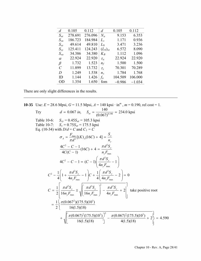
d 0.105 0.112 d 0.105 0.112 Sut 278.691 276.096 Na 9.153 6.353 Ssu 186.723 184.984 Ls 1.171 0.936 Sse 49.614 49.810 L0 3.471 3.236 Ssy 125.411 124.243 (L0)cr 6.572 8.090 Ssa 34.386 34.380 KB 1.112 1.096 22.924 22.920 a 22.924 22.920 1.732 1.523 nf 1.500 1.500 C 11.899 13.732 s 70.301 70.289 D 1.249 1.538 ns 1.784 1.768 ID 1.144 1.426 fn 104.509 106.000 OD 1.354 1.650 fom 0.986 1.034
There are only slight differences in the results. ______________________________________________________________________________ 10-35 Use: E = 28.6 Mpsi, G = 11.5 Mpsi, A = 140 kpsi · inm , m = 0.190, rel cost = 1.
Try 0.190
1400.067 , 234.0 kpsi
(0.067)utd in S
Table 10-6: Ssy = 0.45Sut = 105.3 kpsi Table 10-7: Sy = 0.75Sut = 175.5 kpsi Eq. (10-34) with D/d = C and C1 = C
max ySF2
22
max
22
max
[( ) (16 ) 4]
4 1(16 ) 4
4 ( 1)
4 1 ( 1) 14
A Ay
y
y
y
y
K Cd n
d SC CC
C C n F
d SC C C
n F
2 22
max max
1 11 1 2 0
4 4 4 4y y
y y
d S d SC C
n F n F
22 2 2
max max max
2 3
22 3 2 3
12 take positive root
2 16 16 4
1 (0.067 )(175.5)(10 )
2 16(1.5)(18)
(0.067) (175.5)(10 ) (0.067) (175.5)(10 )
16(1.5)(18) 4(
y y y
y y y
d S d S d SC
n F n F n F
2 4.590
1.5)(18)
Chapter 10 - Rev. A, Page 28/41
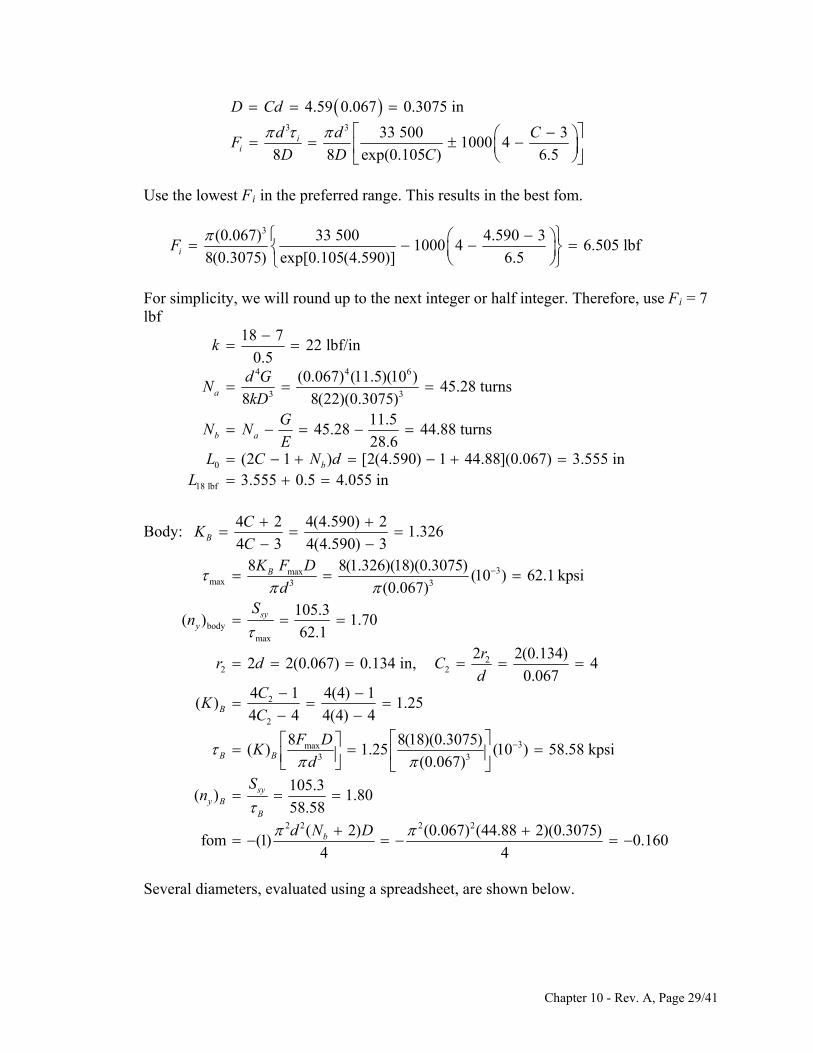
3 3
4.59 0.067 0.3075 in
33 500 31000 4
8 8 exp(0.105 ) 6.5i
i
D Cd
d d CF
D D C
Use the lowest Fi in the preferred range. This results in the best fom.
3(0.067) 33 500 4.590 31000 4 6.505 lbf
8(0.3075) exp[0.105(4.590)] 6.5iF
For simplicity, we will round up to the next integer or half integer. Therefore, use Fi = 7
lbf
4 4 6
3 3
0
18 lbf
18 722 lbf/in
0.5(0.067) (11.5)(10 )
45.28 turns8 8(22)(0.3075)
11.545.28 44.88 turns
28.6(2 1 ) [2(4.590) 1 44.88](0.067) 3.555 in3.555 0.5 4.055 in
a
b a
b
k
d GN
kDG
N NE
L C N dL
Body: 4 2 4(4.590) 2
1.3264 3 4(4.590) 3B
C
C
K
3maxmax 3 3
bodymax
22 2
2
2
8 8(1.326)(18)(0.3075)(10 ) 62.1 kpsi
(0.067)105.3
( ) 1.7062.1
2 2(0.134)2 2(0.067) 0.134 in, 4
0.0674 1 4(4) 1
( ) 1.254
( )
B
syy
B
K F D
dS
n
rr d C
dC
KC
F DK
max3
4 4(4) 4
8
B B d 38(18)(0.3075)
1.25 (10 ) 58.58 kpsi
( )
fom (1 0.1604 4
syy B
B
Sn
3
2 2 2 2
(0.067)
105.31.80
58.58
( 2) (0.067) (44.88 2)(0.3075)) bd N D
Several diameters, evaluated using a spreadsheet, are shown below.
Chapter 10 - Rev. A, Page 29/41
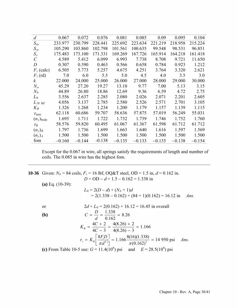
d 0.067 0.072 0.076 0.081 0.085 0.09 0.095 0.104Sut 233.977 230.799 228.441 225.692 223.634 221.219 218.958 215.224Ssy 105.290 103.860 102.798 101.561 100.635 99.548 98.531 96.851Sy 175.483 173.100 171.331 169.269 167.726 165.914 164.218 161.418C 4.589 5.412 6.099 6.993 7.738 8.708 9.721 11.650D 0.307 0.390 0.463 0.566 0.658 0.784 0.923 1.212Fi (calc) 6.505 5.773 5.257 4.675 4.251 3.764 3.320 2.621Fi (rd) 7.0 6.0 5.5 5.0 4.5 4.0 3.5 3.0k 22.000 24.000 25.000 26.000 27.000 28.000 29.000 30.000Na 45.29 27.20 19.27 13.10 9.77 7.00 5.13 3.15Nb 44.89 26.80 18.86 12.69 9.36 6.59 4.72 2.75L0 3.556 2.637 2.285 2.080 2.026 2.071 2.201 2.605L18 lbf 4.056 3.137 2.785 2.580 2.526 2.571 2.701 3.105KB 1.326 1.268 1.234 1.200 1.179 1.157 1.139 1.115max 62.118 60.686 59.707 58.636 57.875 57.019 56.249 55.031(ny)body 1.695 1.711 1.722 1.732 1.739 1.746 1.752 1.760B 58.576 59.820 60.495 61.067 61.367 61.598 61.712 61.712(ny)B 1.797 1.736 1.699 1.663 1.640 1.616 1.597 1.569(ny)A 1.500 1.500 1.500 1.500 1.500 1.500 1.500 1.500fom 0.160 0.144 -0.138 0.135 0.133 0.135 0.138 0.154
Except for the 0.067 in wire, all springs satisfy the requirements of length and number of
coils. The 0.085 in wire has the highest fom. ______________________________________________________________________________ 10-36 Given: Nb = 84 coils, Fi = 16 lbf, OQ&T steel, OD = 1.5 in, d = 0.162 in. D = OD d = 1.5 0.162 = 1.338 in (a) Eq. (10-39): L0 = 2(D d) + (Nb + 1)d = 2(1.338 0.162) + (84 + 1)(0.162) = 16.12 in Ans. or 2d + L0 = 2(0.162) + 16.12 = 16.45 in overall
1.3388.26
0.162
DC
d (b)
3 3
4 2 4(8.26) 21.166
4 3 4(8.26) 38 8(16)(1.338)
1.166 14 950 psi .(0.162)
B
ii B
CK
CF D
K Ansd
(c) From Table 10-5 use: G = 11.4(106) psi and E = 28.5(106) psi
Chapter 10 - Rev. A, Page 30/41
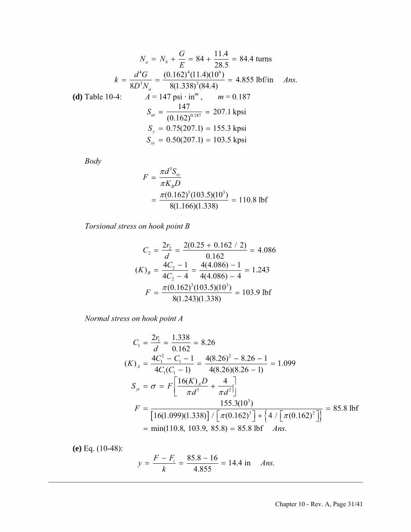
4 4 6
3 3
28.5(0.162) (11.4)(10 )
4.855 lb8 8(1.338) (84.4)a
Ed G
D N
11.484 84.4 turns
f/in .
a b
GN N
k Ans
(d) Table 10-4: A = 147 psi · inm , m = 0.187
0.187
147207.1 kpsi
(0.162)utS
0.75(207.1) 155.3 kpsi
0.50(207.1) 103.5 kpsiy
sy
S
S
Body
3
3 3(0.162) (103.5)(10 )
sy
B
d SF
K D
110.8 lbf8(1.166)(1.338)
Torsional stress on hook point B
22
2
2 2(0.25 0.162 / 2)4.086
0.1624 1 4(4.086) 1
( ) 1.243B
rC
dC
K2
3 3
4 4 4(4.086) 4
(0.162) (103.5)(10 )103.9 lbf
8(1.243)(1.338)
C
F
Normal stress on hook point A
11
2 21 1
1 1
2 1.3388.26
0.1624 1 4(8.26) 8.26 1
)4 ( 1) 4(8.26)(8.26 1)
16( ) 4
A
A
rC
dC C
KC C
K DS F
3 2
3
3 2
( 1.099
155.3(10 )85.8 lbf
16(1.099)(1.338) / (0.162) 4 / (0.162)
min(110.8, 103.9, 85.
yt d d
F
8) 85.8 lbf .Ans
(e) Eq. (10-48):
85.8 1614.4 in .
4.855iF F
y Ansk
______________________________________________________________________________
Chapter 10 - Rev. A, Page 31/41
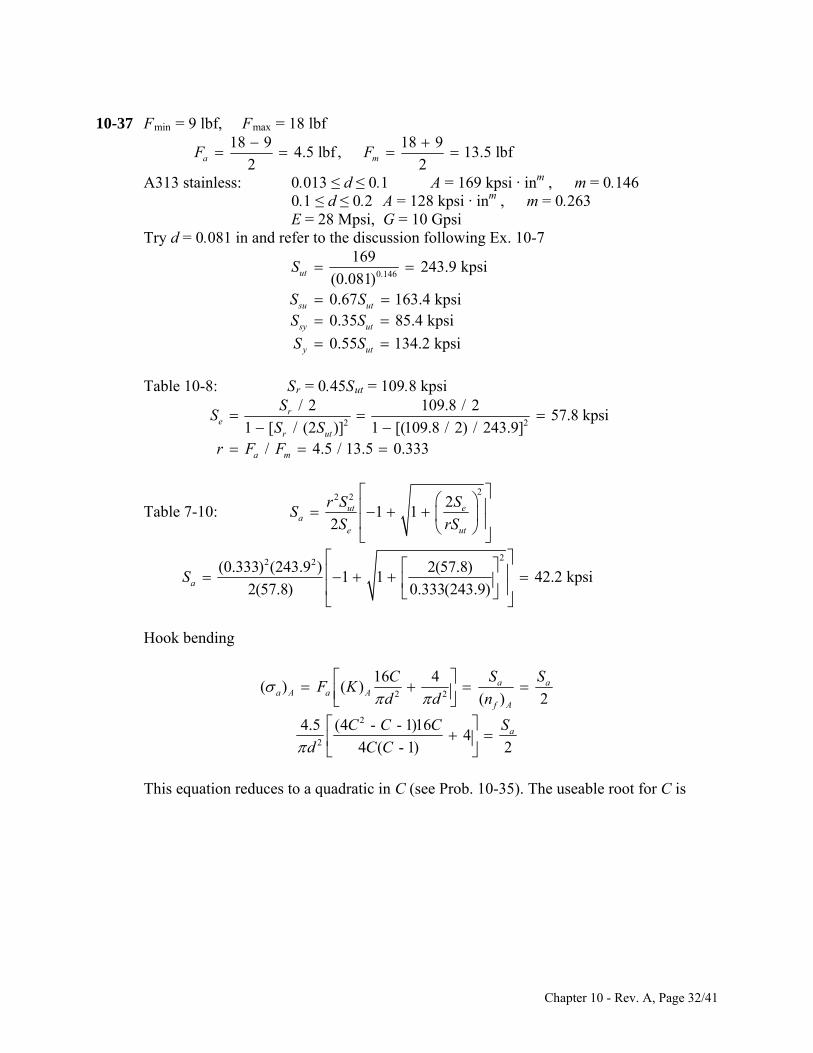
10-37 Fmin = 9 lbf, Fmax = 18 lbf
18 9 18 9
4.5 lbf , 13.5 lbf2 2a mF F
A313 stainless: 0.013 ≤ d ≤ 0.1 A = 169 kpsi · inm , m = 0.146 0.1 ≤ d ≤ 0.2 A = 128 kpsi · inm , m = 0.263 E = 28 Mpsi, G = 10 Gpsi Try d = 0.081 in and refer to the discussion following Ex. 10-7
0.146
169243.9 kpsi
(0.081)0.67 163.4 kpsi0.35 85.4 kpsi
ut
su ut
sy ut
S
S SS S
0.55 134.2 kpsiy utS S Table 10-8: Sr = 0.45Sut = 109.8 kpsi
2 2
/ 2 109.8 / 257.8 kpsi
1 [ / (2 )] 1 [(109.8 / 2) / 243.9]/ 4.5 / 13.5 0.333
re
r ut
S
S Sr F F
a m
S
2
2 2 21 1
2ut e
ae ut
r S SS
S rS
Table 7-10:
22 2(0.333) (243.9 ) 2(57.8)1 1 42.2 kpsi
2(57.8) 0.333(243.9)aS
Hook bending
2 2
2
2
16 4( ) ( )
( ) 2
4.5 (4 - - 1)164
4 ( - 1) 2
a aa A a A
f A
a
C S SF K
d d n
C C C S
d C C
This equation reduces to a quadratic in C (see Prob. 10-35). The useable root for C is
Chapter 10 - Rev. A, Page 32/41
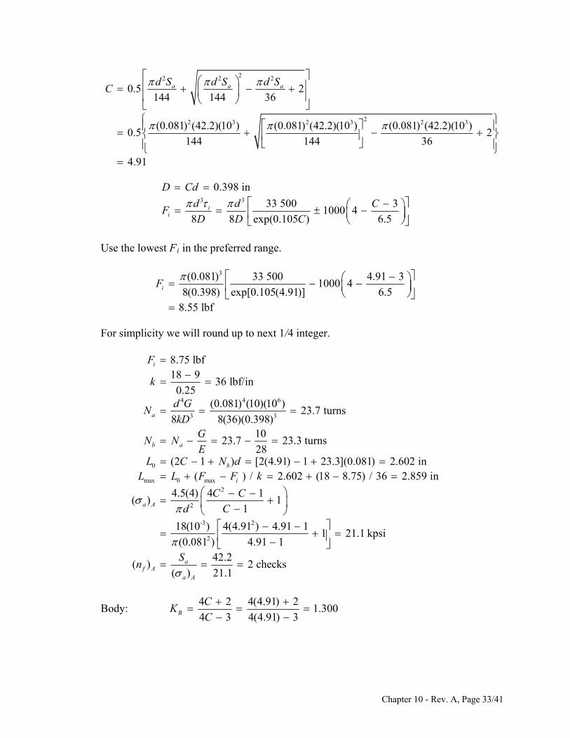
22 2 2
22 3 2 3
2144 36
(0.081) (42.2)(10 ) (0.081) (42.2)(10 )
a a ad S d S
2 3
0.5144
(0.081) (42.2)(10 )0.5 2
144 144 36
4.91
d SC
3 3 33 5001000 4
8 8 exp(0.105 ) 6id d
D D C
0.398 in
3
.5i
D Cd
CF
Use the lowest Fi in the preferred range.
3(0.081) 33 500 4.91 31000 4
8(0.398) exp[0.105(4.91)] 6.58.55 lbf
iF
For simplicity we will round up to next 1/4 integer.
4 4 6
8.75 lbf18 9
36 lbf/in0.25
(0.081) (10)(10 )
iF
k
d G
3 3
0
max 0 max
23.7 turns8 8(36)(0.398)
1023.7 23.3 turns
28(2 1 ) [2(4.91) 1 23.3](0.081) 2.602 in
( ) / 2.602 (18 8.75) / 36 2.
a
b a
b
i
NkD
GN N
EL C N d
L L F F k
2
2
859 in
4.5(4) 4 1( ) 1
1a A
C C
d C
-3 2
2
18(10 ) 4(4.91 ) 4.91 11 21.1 kpsi
(0.081 ) 4.91 142.2
( ) 2 checks( ) 21.1
af A
a A
Sn
Body: 4 2 4(4.91) 2
1.3004 3 4(4.91) 3B
CK
C
Chapter 10 - Rev. A, Page 33/41
33
8(1.300)(4.5)(0.398)(10 ) 11.16 kpsi
(0.081)13.5
(11.16) 33.47 kpsi4.5
a
mm a
a
F
F
The repeating allowable stress from Table 7-8 is
Ssr = 0.30Sut = 0.30(243.9) = 73.17 kpsi The Gerber intercept is
2
73.17 / 238.5 kpsi
1 [(73.17 / 2) / 163.4]seS
From Table 6-7, 22
body
1 163.4 11.16 2(33.47)(38.5)( ) 1 1 2.53fn
2 33.47 38.5 163.4(11.16)
Let r2 = 2d = 2(0.081) = 0.162
22
2 4(4) 14, ( ) 1.25
4(4) 4( ) 1.25
( ) (11.16) 10.73 kpsi1.30
( ) 1.25( ) (33.47) 32.18 kpsi
1.30
B
Ba B a
B
Bm B m
B
rC K
dK
KK
K
Table 10-8: (Ssr )B = 0.28Sut = 0.28(243.9) = 68.3 kpsi
2
22
68.3 / 2( ) 35.7 kpsi
1 [(68.3 / 2) / 163.4]
1 163.4 10.73 2(32.18)(35.7)( ) 1 1 2.51
2 32.18 35.7 163.4(10.73)
se B
f B
S
n
Yield Bending:
2max
max 2
2-3
2
4 (4 1)( ) 1
1
4(18) 4(4.91) 4.91 11 (10 ) 84.4 kpsi
(0.081 ) 4.91 1134.2
( ) 1.5984.4
A
y A
F C C
d C
n
Body:
Chapter 10 - Rev. A, Page 34/41
body
( / ) (8.75 / 4.5)(11.16) 21.7 kpsi /( ) 11.16 / (33.47 21.7) 0.948
0.948( ) ( ) (85.4 21.7) 31.0 kpsi
1 0.948 1( ) 31.0
( ) 2.7811.16
i i a a
a m i
sa y sy i
sa yy
a
F Fr
rS S
rS
n
Hook shear: Hook shear:
max
0.3 0.3(243.9) 73.2 kpsi
( ) ( ) 10.73 32.18 42.9 kpsi73.2
( ) 1.7142.9
sy ut
a B m B
y B
S S
n
2 2 2 27.6 ( 2) 7.6 (0.081) (23.3 2)(0.398)fom 1.239
4 4bd N D
A tabulation of several wire sizes follow
d 0.081 0.085 0.092 0.098 0.105 0.12 Sut 243.920 242.210 239.427 237.229 234.851 230.317 Ssu 163.427 162.281 160.416 158.943 157.350 154.312 Sr 109.764 108.994 107.742 106.753 105.683 103.643 Se 57.809 57.403 56.744 56.223 55.659 54.585 Sa 42.136 41.841 41.360 40.980 40.570 39.786 C 4.903 5.484 6.547 7.510 8.693 11.451 D 0.397 0.466 0.602 0.736 0.913 1.374 OD 0.478 0.551 0.694 0.834 1.018 1.494 Fi (calc) 8.572 7.874 6.798 5.987 5.141 3.637 Fi (rd) 8.75 9.75 10.75 11.75 12.75 13.75 k 36.000 36.000 36.000 36.000 36.000 36.000 Na 23.86 17.90 11.38 8.03 5.55 2.77 Nb 23.50 17.54 11.02 7.68 5.19 2.42 L0 2.617 2.338 2.127 2.126 2.266 2.918 L18 lbf 2.874 2.567 2.328 2.300 2.412 3.036 (a)A 21.068 20.920 20.680 20.490 20.285 19.893 (nf)A 2.000 2.000 2.000 2.000 2.000 2.000 KB 1.301 1.264 1.216 1.185 1.157 1.117 (a)body 11.141 10.994 10.775 10.617 10.457 10.177 (m)body 33.424 32.982 32.326 31.852 31.372 30.532 Ssr 73.176 72.663 71.828 71.169 70.455 69.095 Sse 38.519 38.249 37.809 37.462 37.087 36.371 (nf)body 2.531 2.547 2.569 2.583 2.596 2.616 (K)B 1.250 1.250 1.250 1.250 1.250 1.250 (a)B 10.705 10.872 11.080 11.200 11.294 11.391 (m)B 32.114 32.615 33.240 33.601 33.883 34.173 (Ssr)B 68.298 67.819 67.040 66.424 65.758 64.489 (Sse)B 35.708 35.458 35.050 34.728 34.380 33.717
Chapter 10 - Rev. A, Page 35/41
(nf)B 2.519 2.463 2.388 2.341 2.298 2.235 Sy 134.156 133.215 131.685 130.476 129.168 126.674 (A)max 84.273 83.682 82.720 81.961 81.139 79.573 (ny)A 1.592 1.592 1.592 1.592 1.592 1.592 i 21.663 23.820 25.741 27.723 29.629 31.097 r 0.945 1.157 1.444 1.942 2.906 4.703 (Ssy)body 85.372 84.773 83.800 83.030 82.198 80.611 (Ssa)y 30.958 32.688 34.302 36.507 39.109 40.832 (ny)body 2.779 2.973 3.183 3.438 3.740 4.012 (Ssy)B 73.176 72.663 71.828 71.169 70.455 69.095 (B)max 42.819 43.486 44.321 44.801 45.177 45.564 (ny)B 1.709 1.671 1.621 1.589 1.560 1.516 fom 1.246 1.234 1.245 1.283 1.357 1.639
optimal fom The shaded areas show the conditions not satisfied. ______________________________________________________________________________ 10-38 For the hook, M = FR sin, ∂M/∂F = R sin
3/ 2 2
0
1sin
2
FRF R R d
EI EI
F
The total deflection of the body and the two hooks
3 3 3 3
4 4 4
3 3
4 4
8 8 ( / 2)2
2 ( / 64)( )
8 8
b b
ab
FD N FR FD N F D
d G EI d G E d
FD G FD NN
d G E d GG
N N
Q.E.D.a b E
______________________________________________________________________________ 10-39 Table 10-5 (d = 4 mm = 0.1575 in): E = 196.5 GPa Table 10-4 for A227: A = 1783 MPa · mmm, m = 0.190
Eq. (10-14): 0.190
17831370 MPa
4ut m
AS
d
Eq. (10-57): Sy = all = 0.78 Sut = 0.78(1370) = 1069 MPa
Chapter 10 - Rev. A, Page 36/41
D = OD d = 32 4 = 28 mm C = D/d = 28/4 = 7
Eq. (10-43):
22 4 7 7 14 11.119
4 ( 1) 4(7)(7 1)i
C CK
C C
Eq. (10-44): 3
32i
FrK
d
At yield, Fr = My , = Sy. Thus,
3 33 4 1069 10y
y
d S
6.00 N · m32 32(1.119)i
MK
Count the turns when M = 0
2.5 yMN
k4
10.8
d Ek
DN where from Eq. (10-51):
Thus,
4
2.5/ (10.8 )
yMN
d E DN
Solving for N gives
4
2.5
1 [10.8 / ( )]
2.5y
NDM d E
42.413 turns
1 10.8(28)(6.00) / 4 (196.5)
This means (2.5 - 2.413)(360) or 31.3 from closed. Ans. Treating the hand force as in the middle of the grip,
3
max
87.5112.5 87.5 68.75 mm
26.00 10
87.3 N .68.75
y
r
MF Ans
r
______________________________________________________________________________ 10-40 The spring material and condition are unknown. Given d = 0.081 in and OD = 0.500, (a) D = 0.500 0.081 = 0.419 in Using E = 28.6 Mpsi for an estimate
Chapter 10 - Rev. A, Page 37/41
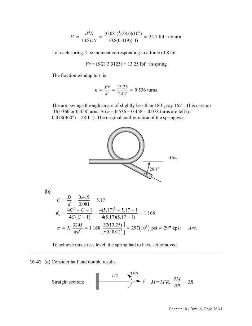
4 4 6(0.081) (28.6)(10 )24.7 lbf · in/turn
10.8 10.8(0.419)(11)
d Ek
DN
for each spring. The moment corresponding to a force of 8 lbf
Fr = (8/2)(3.3125) = 13.25 lbf · in/spring
The fraction windup turn is
13.25ns
Frn
k 0.536 tur
24.7
The arm swings through an arc of slightly less than 180, say 165. This uses up 165/360 or 0.458 turns. So n = 0.536 0.458 = 0.078 turns are left (or 0.078(360) = 28.1 ). The original configuration of the spring was
Ans.
(b)
33 3
1.1684 1 4(5.17)(5.17 1)
32 32(13.25)1.168 297 10 psi 297 kpsi .
i
i
C C
MK A
2 2
0.4195.17
0.0814 1 4(5.17) 5.17 1
(0.081)
DC
dC C
K
nsd
To achieve this stress level, the spring had to have set removed. ______________________________________________________________________________ 10-41 (a) Consider half and double results
Straight section: M = 3FR, 3M
RP
Chapter 10 - Rev. A, Page 38/41
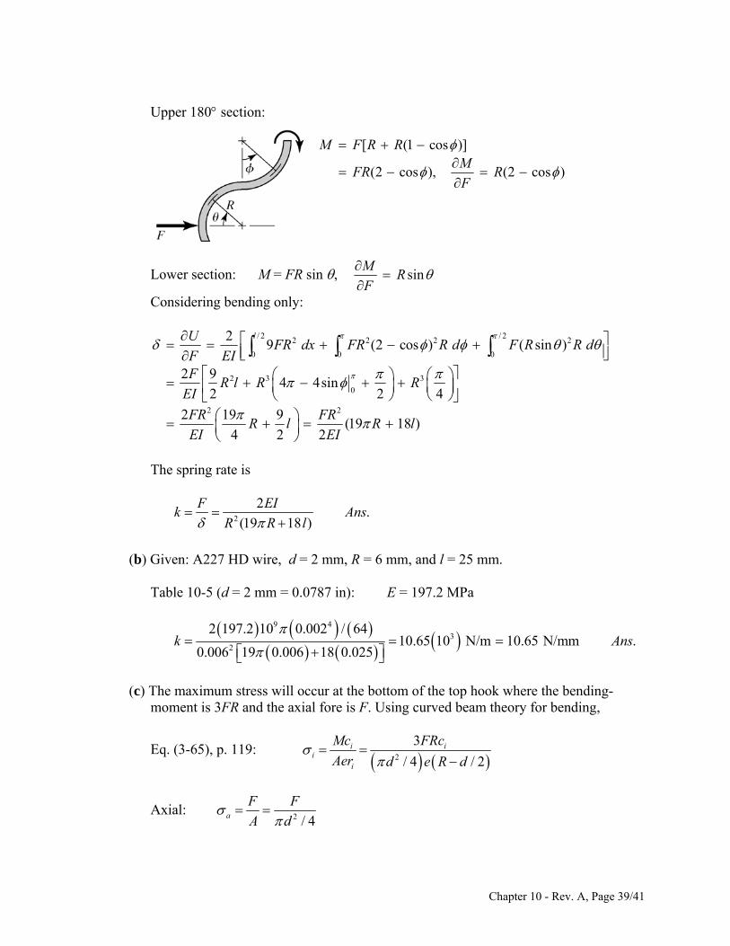
Upper 180 section:
[ (1 cos )]
s )
M F R R
(2 cos ), (2 coM
FR RF
Lower section: M = FR sin , sinM
R
F
Considering bending only:
/ 2 / 22 2 2 2
0
2 2
29 (2 cos ) ( sin )
2 9
4
2 19 9(19 18 )
4 2 2
lUFR dx FR R d F R R d
F EIF
R lEI
FR FRR l R l
EI EI
0 0
2 3 3
04 4sin
2 2R R
The spring rate is
2 (19
nsR R l
2.
18 )
F EIk A
(b) Given: A227 HD wire, d = 2 mm, R = 6 mm, and l = 25 mm. Table 10-5 (d = 2 mm = 0.0787 in): E = 197.2 MPa
310 N/m 10.65 N/mm .ns
9 4
2
2 197.2 10 0.002 / 6410.65
0.006 19 0.006 18 0.025k A
(c) The maximum stress will occur at the bottom of the top hook where the bending-
moment is 3FR and the axial fore is F. Using curved beam theory for bending,
Eq. (3-65), p. 119: 2
3
/ 4 / 2i i
ii
Mc FRc
Aer d e R d
Axial: F F
2 / 4a A d
Chapter 10 - Rev. A, Page 39/41
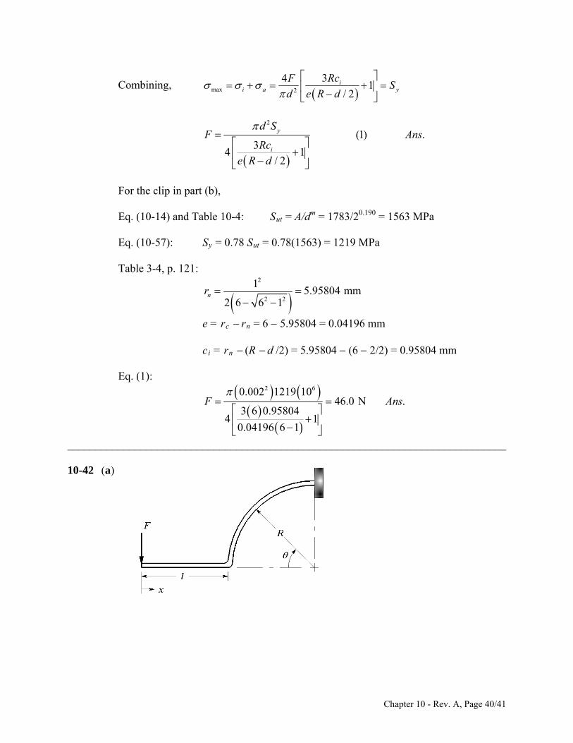
Combining, max 2
341
/ 2i
i a
RcFS
d e R d
y
2
(1) .3
4 1/ 2
y
i
d SF Ans
Rc
e R d
For the clip in part (b), Eq. (10-14) and Table 10-4: Sut = A/dm = 1783/20.190 = 1563 MPa Eq. (10-57): Sy = 0.78 Sut = 0.78(1563) = 1219 MPa Table 3-4, p. 121:
2
2 2
15.95804 mm
2 6 6 1nr
e = rc rn = 6 5.95804 = 0.04196 mm ci = rn (R d /2) = 5.95804 (6 2/2) = 0.95804 mm Eq. (1):
2 60.002 1219 1046.0 N .
3 6 0.958044 1
0.04196 6 1
F A
ns
______________________________________________________________________________ 10-42 (a)
Chapter 10 - Rev. A, Page 40/41
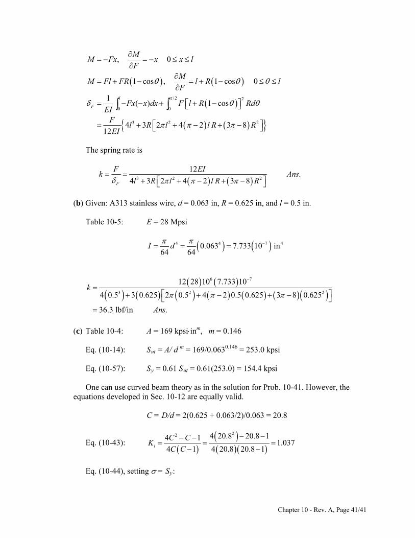
Chapter 10 - Rev. A, Page 41/41
/2 2
0 0
3 2 2
,
1 cos , 1 cos 0
1( ) 1 cos
4 3 2 4 2 3 812
l
F
MM Fx
F 0x x l
MM Fl FR l R l
F
Fx x dx F l R RdEI
Fl R l l R R
EI
The spring rate is
3 24 3 2F
2
12.
4 2 3 8
F EIns
l R l l R R
k A
(b) Given: A313 stainless wire, d = 0.063 in, R = 0.625 in, and l = 0.5 in. Table 10-5: E = 28 Mpsi
4 40.063 7.73364 64
I d 7 410 in
6 7
3 2 2
12 28 10 7.733 10
0.625k
4 0.5 3 0.625 2 0.5 4 2 0.5 0.625 3 8
36.3 lbf/in .Ans
(c) Table 10-4: A = 169 kpsiinm, m = 0.146 Eq. (10-14): Sut = A/ d m = 169/0.0630.146 = 253.0 kpsi Eq. (10-57): Sy = 0.61 Sut = 0.61(253.0) = 154.4 kpsi One can use curved beam theory as in the solution for Prob. 10-41. However, the
equations developed in Sec. 10-12 are equally valid. C = D/d = 2(0.625 + 0.063/2)/0.063 = 20.8
Eq. (10-43): 22 4 20.8 20.8 14 1
1.0374 1 4 20.8 20.8 1i
C C
C C
K
Eq. (10-44), setting = Sy:
Chapter 10 - Rev. A, Page 42/41
3
3 3
32 0.5 0.625321.037 154.4 10
0.063i y
FFrK S
d
Solving for F yields F = 3.25 lbf Ans. Try solving part (c) of this problem using curved beam theory. You should obtain the
same answer. ______________________________________________________________________________ 10-43 (a) M = Fx
2/ / / 6
M Fx Fx
I c I c bh
Constant stress,
2 6
(1) .6
Fx Fxh Ans
b
bh
At x = l,
6
/ .o o
Flh x l Ans
b
h h
(b) M = Fx, M / F = x
3/21/2
3/2 31 30 0 012
3/2 33/2
3 3
/ 1 12
/
2 12 8
3
l l l
oo
o o
M M F Fx x Fly dx dx x dx
EI E bh Ebh x l
Fl Fll
bh E bh E
3
3.
8obh EF
nsy l
k A
______________________________________________________________________________ 10-44 Computer programs will vary. ______________________________________________________________________________ 10-45 Computer programs will vary.
Chapter 11
11-1 For the deep-groove 02-series ball bearing with R = 0.90, the design life xD, in multiples
of rating life, is
6
10
60 25000 35060525 .
10D D D
DR
L nx Ans
L L
The design radial load is 1.2 2.5 3.0 kNDF
Eq. (11-6):
1/3
10 1/1.483
5253.0
0.02 4.459 0.02 ln 1/ 0.9C
C10 = 24.3 kN Ans. Table 11-2: Choose an 02-35 mm bearing with C10 = 25.5 kN. Ans.
Eq. (11-18):
1.4833525 3 / 25.5 0.02
exp 0.920 .4.459 0.02
R Ans
______________________________________________________________________________ 11-2 For the angular-contact 02-series ball bearing as described, the rating life multiple is
6
10
60 40000 520601248
10D D D
DR
L nx
L L
The design radial load is 1.4 725 1015 lbf 4.52 kNDF Eq. (11-6):
1/3
10 1/1.483
12481015
0.02 4.459 0.02 ln 1/ 0.9
10 930 lbf 48.6 kN
C
Table 11-2: Select an 02-60 mm bearing with C10 = 55.9 kN. Ans.
Eq. (11-18):
1.48331248 4.52 / 55.9 0.02
exp 0.945 .4.439
R Ans
______________________________________________________________________________
Chapter 11, Page 1/28

11-3 For the straight-roller 03-series bearing selection, xD = 1248 rating lives from Prob. 11-2 solution.
1.4 2235 3129 lbf 13.92 kNDF
3/10
10
124813.92 118 kN
1C
Table 11-3: Select an 03-60 mm bearing with C10 = 123 kN. Ans.
Eq. (11-18):
1.48310/31248 13.92 /123 0.02
exp 0.917 .4.459 0.02
R Ans
______________________________________________________________________________ 11-4 The combined reliability of the two bearings selected in Probs. 11-2 and 11-3 is 0.945 0.917 0.867 .R Ans
We can choose a reliability goal of 0.90 0.95 for each bearing. We make the selections, find the existing reliabilities, multiply them together, and observe that the reliability goal is exceeded due to the roundup of capacity upon table entry.
Another possibility is to use the reliability of one bearing, say R1. Then set the reliability
goal of the second as
21
0.90R
R
or vice versa. This gives three pairs of selections to compare in terms of cost, geometry
implications, etc. ______________________________________________________________________________
11-5 Establish a reliability goal of 0.90 0.95 for each bearing. For an 02-series angular contact ball bearing,
1/3
10 1/1.483
12481015
0.02 4.439 ln 1/ 0.95
12822 lbf 57.1 kN
C
Select an 02-65 mm angular-contact bearing with C10 = 63.7 kN.
1.48331248 4.52 / 63.7 0.02
exp 0.9624.439AR
Chapter 11, Page 2/28
For an 03-series straight roller bearing,
3/10
10 1/1.483
124813.92 136.5 kN
0.02 4.439 ln 1/ 0.95C
Select an 03-65 mm straight-roller bearing with C10 = 138 kN.
1.48310/31248 13.92 /138 0.02
exp 0.9534.439BR
The overall reliability is R = (0.962)(0.953) = 0.917, which exceeds the goal. ______________________________________________________________________________ 11-6 For the straight cylindrical roller bearing specified with a service factor of 1, R = 0.95 and
FR = 20 kN.
610
60 8000 95060456
10D D D
DR
L nx
L L
3/10
10 1/1.483
45620 145 kN .
0.02 4.439 ln 1/ 0.95C A
ns
______________________________________________________________________________ 11-7 Both bearings need to be rated in terms of the same catalog rating system in order to
compare them. Using a rating life of one million revolutions, both bearings can be rated in terms of a Basic Load Rating.
Eq. (11-3): 1/31/ 1/
6
3000 500 60602.0
10
8.96 kN
a a
A A AA A A
R R
L nC F F
L L
Bearing B already is rated at one million revolutions, so CB = 7.0 kN. Since CA > CB,
bearing A can carry the larger load. Ans. ______________________________________________________________________________ 11-8 FD = 2 kN, LD = 109 rev, R = 0.90
Eq. (11-3): 1/ 1/39
10 6
102 20 kN .
10
a
DD
R
LC F An
L
s
______________________________________________________________________________
Chapter 11, Page 3/28
11-9 FD = 800 lbf, D = 12 000 hours, nD = 350 rev/min, R = 0.90
Eq. (11-3): 1/31/
10 6
12 000 350 6060800 5050 lbf
10
a
D DD
R
nC F An
L
s
______________________________________________________________________________ 11-10 FD = 4 kN, D = 8 000 hours, nD = 500 rev/min, R = 0.90
Eq. (11-3): 1/31/
10 6
8 000 500 60604 24.9 kN
10
a
D DD
R
nC F An
L
s
______________________________________________________________________________ 11-11 FD = 650 lbf, nD = 400 rev/min, R = 0.95
D = (5 years)(40 h/week)(52 week/year) = 10 400 hours
Assume an application factor of one. The multiple of rating life is
6
10 400 400 60249.6
10D
DR
Lx
L
Eq. (11-6):
1/3
10 1/1.483
249.61 650
0.02 4.439 ln 1/ 0.95C
4800 lbf .Ans______________________________________________________________________________ 11-12 FD = 9 kN, LD = 108 rev, R = 0.99 Assume an application factor of one. The multiple of rating life is
8
6
10100
10D
DR
Lx
L
Eq. (11-6):
1/3
10 1/1.483
1001 9
0.02 4.439 ln 1/ 0.99C
69.2 kN .Ans______________________________________________________________________________ 11-13 FD = 11 kips, D = 20 000 hours, nD = 200 rev/min, R = 0.99
Assume an application factor of one. Use the Weibull parameters for Manufacturer 2 on p. 608.
Chapter 11, Page 4/28
The multiple of rating life is
6
20 000 200 60240
10D
DR
Lx
L
Eq. (11-6):
1/3
10 1/1.483
2401 11
0.02 4.439 ln 1/ 0.99C
113 kips .Ans ______________________________________________________________________________ 11-14 From the solution to Prob. 3-68, the ground reaction force carried by the bearing at C is
RC = FD = 178 lbf. Use the Weibull parameters for Manufacturer 2 on p. 608.
6
15000 1200 601080
10D
DR
Lx
L
Eq. (11-7):
1/
10 1/
0 0 1
a
Df D b
D
xC a F
x x R
1/3
10 1/1.483
10801.2 178
0.02 4.459 0.02 1 0.95
2590 lbf .
C
Ans
______________________________________________________________________________ 11-15 From the solution to Prob. 3-69, the ground reaction force carried by the bearing at C is
RC = FD = 1.794 kN. Use the Weibull parameters for Manufacturer 2 on p. 608.
6
15000 1200 601080
10D
DR
Lx
L
Eq. (11-7):
1/
10 1/
0 0 1
a
Df D b
D
xC a F
x x R
1/3
10 1/1.483
10801.2 1.794
0.02 4.459 0.02 1 0.95
26.1 kN .
C
Ans
______________________________________________________________________________ 11-16 From the solution to Prob. 3-70, RCz = –327.99 lbf, RCy = –127.27 lbf
1/22 2
327.99 127.27 351.8 lbfC DR F Use the Weibull parameters for Manufacturer 2 on p. 608.
Chapter 11, Page 5/28
6
15000 1200 601080
10D
DR
Lx
L
Eq. (11-7):
1/
10 1/1
a
Df D b
o o D
xC a F
x x R
1/3
10 1/1.483
10801.2 351.8
0.02 4.459 0.02 1 0.95
5110 lbf .
C
Ans
______________________________________________________________________________ 11-17 From the solution to Prob. 3-71, RCz = –150.7 N, RCy = –86.10 N
1/22 2
150.7 86.10 173.6 NC DR F Use the Weibull parameters for Manufacturer 2 on p. 608.
6
15000 1200 601080
10D
DR
Lx
L
Eq. (11-7):
1/
10 1/
0 0 1
a
Df D b
D
xC a F
x x R
1/3
10 1/1.483
10801.2 173.6
0.02 4.459 0.02 1 0.95
2520 N .
C
Ans
______________________________________________________________________________ 11-18 From the solution to Prob. 3-77, RAz = 444 N, RAy = 2384 N
1/22 2444 2384 2425 N 2.425 kNA DR F
Use the Weibull parameters for Manufacturer 2 on p. 608. The design speed is equal to the speed of shaft AD,
125191 95.5 rev/min
250F
D iC
dn n
d
6
12000 95.5 6068.76
10D
DR
Lx
L
Eq. (11-7):
1/
10 1/
0 0 1
a
Df D b
D
xC a F
x x R
Chapter 11, Page 6/28
1/3
10 1/1.483
68.761 2.425
0.02 4.459 0.02 1 0.95
11.7 kN .
C
Ans
______________________________________________________________________________ 11-19 From the solution to Prob. 3-79, RAz = 54.0 lbf, RAy = 140 lbf
1/22 254.0 140 150.1 lbfA DR F
Use the Weibull parameters for Manufacturer 2 on p. 608. The design speed is equal to the speed of shaft AD,
10280 560 rev/min
5F
D iC
dn n
d
6
14000 560 60470.4
10D
DR
Lx
L
Eq. (11-7):
1/
10 1/
0 0 1
a
Df D b
D
xC a F
x x R
3/10
10 1/1.483
470.41 150.1
0.02 4.459 0.02 1 0.98
1320 lbf .
C
Ans
______________________________________________________________________________ 11-20 (a) 3 kN, 7 kN, 500 rev/min, 1.2a r DF F n V From Table 11-2, with a 65 mm bore, C0 = 34.0 kN. Fa / C0 = 3 / 34 = 0.088 From Table 11-1, 0.28 e 3.0.
30.357
1.2 7a
r
F
VF
Since this is greater than e, interpolating Table 11-1 with Fa / C0 = 0.088, we obtain X2 = 0.56 and Y2 = 1.53. Eq. (11-9): 0.56 1.2 7 1.53 3 9.29 kNe i r i aF X VF Y F Ans.
Fe > Fr so use Fe. (b) Use Eq. (11-7) to determine the necessary rated load the bearing should have to carry
the equivalent radial load for the desired life and reliability. Use the Weibull parameters for Manufacturer 2 on p. 608.
Chapter 11, Page 7/28
6
10000 500 60300
10D
DR
Lx
L
Eq. (11-7):
1/
10 1/
0 0 1
a
Df D b
D
xC a F
x x R
1/3
10 1/1.483
3001 9.29
0.02 4.459 0.02 1 0.95
73.4 kN
C
From Table 11-2, the 65 mm bearing is rated for 55.9 kN, which is less than the
necessary rating to meet the specifications. This bearing should not be expected to meet the load, life, and reliability goals. Ans.
______________________________________________________________________________ 11-21 (a) 2 kN, 5 kN, 400 rev/min, 1a r DF F n V From Table 11-2, 30 mm bore, C10 = 19.5 kN, C0 = 10.0 kN Fa / C0 = 2 / 10 = 0.2 From Table 11-1, 0.34 e 0.38.
20.4
1 5a
r
F
VF
Since this is greater than e, interpolating Table 11-1, with Fa / C0 = 0.2, we obtain X2 =
0.56 and Y2 = 1.27. Eq. (11-9): 0.56 1 5 1.27 2 5.34 kNe i r i aF X VF Y F Ans.
Fe > Fr so use Fe. (b) Solve Eq. (11-7) for xD.
1/100 0 1
a
b
D Df D
Cx x x R
a F
3
1/1.48319.50.02 4.459 0.02 1 0.99
1 5.34Dx
10.66Dx
6
60
10D DD
DR
nLx
L
Chapter 11, Page 8/28
6 610 10.66 10444 h .
60 400 60
D
DD
xAns
n
______________________________________________________________________________ 11-22 98 kN, 0.9, 10 revr DF R L
Eq. (11-3): 1/ 1/39
10 6
108 80
10
a
DD
R
LC F
L
kN
From Table 11-2, select the 85 mm bore. Ans. ______________________________________________________________________________ 11-23 8 kN, 2 kN, 1, 0.99r aF F V R Use the Weibull parameters for Manufacturer 2 on p. 608.
6
10000 400 60240
10D
DR
Lx
L
First guess: Choose from middle of Table 11-1, X = 0.56, Y = 1.63 Eq. (11-9): 0.56 1 8 1.63 2 7.74 kNeF
Fe < Fr, so just use Fr as the design load.
Eq. (11-7):
1/
10 1/1
a
Df D b
o o D
xC a F
x x R
1/3
10 1/1.483
2401 8 82.5 kN
0.02 4.459 0.02 1 0.99C
From Table 11-2, try 85 mm bore with C10 = 83.2 kN, C0 = 53.0 kN Iterate the previous process: Fa / C0 = 2 / 53 = 0.038 Table 11-1: 0.22 e 0.24
2
0.251 8
a
r
Fe
VF
Interpolate Table 11-1 with Fa / C0 = 0.038 to obtain X2 = 0.56 and Y2 = 1.89. Eq. (11-9): 0.56(1)8 1.89(2) 8.26 > e rF F
Eq. (11-7):
1/3
10 1/1.483
2401 8.26 85.2 kN
0.02 4.459 0.02 1 0.99C
Chapter 11, Page 9/28
Table 11-2: Move up to the 90 mm bore with C10 = 95.6 kN, C0 = 62.0 kN. Iterate again: Fa / C0 = 2 / 62 = 0.032 Table 11-1: Again, 0.22 e 0.24
2
0.251 8
a
r
Fe
VF
Interpolate Table 11-1 with Fa / C0 = 0.032 to obtain X2 = 0.56 and Y2 = 1.95. Eq. (11-9): 0.56(1)8 1.95(2) 8.38 > e rF F
Eq. (11-7):
1/3
10 1/1.483
2401 8.38 86.4 kN
0.02 4.459 0.02 1 0.99C
The 90 mm bore is acceptable. Ans. ______________________________________________________________________________ 11-24 88 kN, 3 kN, 1.2, 0.9, 10 revr a DF F V R L First guess: Choose from middle of Table 11-1, X = 0.56, Y = 1.63 Eq. (11-9): 0.56 1.2 8 1.63 3 10.3 kNeF
e rF F
Eq. (11-3): 1/ 1/38
10 6
1010.3 47.8 kN
10
a
De
R
LC F
L
From Table 11-2, try 60 mm with C10 = 47.5 kN, C0 = 28.0 kN Iterate the previous process: Fa / C0 = 3 / 28 = 0.107 Table 11-1: 0.28 e 0.30
30.313
1.2 8a
r
Fe
VF
Interpolate Table 11-1 with Fa / C0 = 0.107 to obtain X2 = 0.56 and Y2 = 1.46 Eq. (11-9): 0.56 1.2 8 1.46 3 9.76 kN > e rF F
Eq. (11-3): 1/38
10 6
109.76 45.3 kN
10C
From Table 11-2, we have converged on the 60 mm bearing. Ans. ______________________________________________________________________________
Chapter 11, Page 10/28
11-25 10 kN, 5 kN, 1, 0.95r aF F V R Use the Weibull parameters for Manufacturer 2 on p. 608.
6
12000 300 60216
10D
DR
Lx
L
First guess: Choose from middle of Table 11-1, X = 0.56, Y = 1.63 Eq. (11-9): 0.56 1 10 1.63 5 13.75 kNeF
Fe > Fr, so use Fe as the design load.
Eq. (11-7):
1/
10 1/
0 0 1
a
Df D b
D
xC a F
x x R
1/3
10 1/1.483
2161 13.75 97.4 kN
0.02 4.459 0.02 1 0.95C
From Table 11-2, try 95 mm bore with C10 = 108 kN, C0 = 69.5 kN Iterate the previous process: Fa / C0 = 5 / 69.5 = 0.072 Table 11-1: 0.27 e 0.28
5
0.51 10
a
r
Fe
VF
Interpolate Table 11-1 with Fa / C0 = 0.072 to obtain X2 = 0.56 and Y2 = 1.62 1.63
Since this is where we started, we will converge back to the same bearing. The 95 mm
bore meets the requirements. Ans. ______________________________________________________________________________ 11-26 Note to the Instructor. In the first printing of the 9th edition, the design life was
incorrectly given to be 109 rev and will be corrected to 108 rev in subsequent printings. We apologize for the inconvenience.
9 kN, 3 kN, 1.2, 0.99r aF F V R Use the Weibull parameters for Manufacturer 2 on p. 608.
8
6
10100
10D
DR
Lx
L
First guess: Choose from middle of Table 11-1, X = 0.56, Y = 1.63
Chapter 11, Page 11/28
Eq. (11-9): 0.56 1.2 9 1.63 3 10.9 kNeF
Fe > Fr, so use Fe as the design load.
Eq. (11-7):
1/
10 1/
0 0 1
a
Df D b
D
xC a F
x x R
1/3
10 1/1.483
1001 10.9 83.9 kN
0.02 4.459 0.02 1 0.99C
From Table 11-2, try 90 mm bore with C10 = 95.6 kN, C0 = 62.0 kN. Try this bearing. Iterate the previous process: Fa / C0 = 3 / 62 = 0.048 Table 11-1: 0.24 e 0.26
3
0.2781.2 9
a
r
Fe
VF
Interpolate Table 11-1 with Fa / C0 = 0.048 to obtain X2 = 0.56 and Y2 = 1.79 Eq. (11-9): 0.56 1.2 9 1.79 3 11.4 kNe rF F
10
11.483.9 87.7 kN
10.9C
From Table 11-2, this converges back to the same bearing. The 90 mm bore meets the requirements. Ans.
______________________________________________________________________________ 11-27 (a) 1200 rev/min, 15 kh, 0.95, 1.2D Dn L R fa From Prob. 3-72, RCy = 183.1 lbf, RCz = –861.5 lbf.
1/222183.1 861.5 881 lbfC DR F
6
15000 1200 601080
10D
DR
Lx
L
Eq. (11-7):
1/3
10 1/1.483
10801.2 881
0.02 4.439 1 0.95C
12800 lbf 12.8 kips .Ans (b) Results will vary depending on the specific bearing manufacturer selected. A general
engineering components search site such as www.globalspec.com might be useful as a starting point.
______________________________________________________________________________
Chapter 11, Page 12/28
11-28 (a) 1200 rev/min, 15 kh, 0.95, 1.2D Dn L R fa From Prob. 3-72, ROy = –208.5 lbf, ROz = 259.3 lbf.
1/222259.3 208.5 333 lbfC DR F
6
15000 1200 601080
10D
DR
Lx
L
Eq. (11-7):
1/3
10 1/1.483
10801.2 333
0.02 4.439 1 0.95C
4837 lbf 4.84 kips .Ans (b) Results will vary depending on the specific bearing manufacturer selected. A general
engineering components search site such as www.globalspec.com might be useful as a starting point.
______________________________________________________________________________ 11-29 (a) 900 rev/min, 12 kh, 0.98, 1.2D Dn L R fa From Prob. 3-73, RCy = 8.319 kN, RCz = –10.830 kN.
1/2228.319 10.830 13.7 kNC DR F
6
12000 900 60648
10D
DR
Lx
L
Eq. (11-7):
1/3
10 1/1.483
6481.2 13.7 204 kN .
0.02 4.439 1 0.98C A
ns
fa
(b) Results will vary depending on the specific bearing manufacturer selected. A general engineering components search site such as www.globalspec.com might be useful as a starting point.
______________________________________________________________________________ 11-30 (a) 900 rev/min, 12 kh, 0.98, 1.2D Dn L R From Prob. 3-73, ROy = 5083 N, ROz = 494 N.
1/22 25083 494 5106 N 5.1 kNC DR F
6
12000 900 60648
10D
DR
Lx
L
Eq. (11-7):
1/3
10 1/1.483
6481.2 5.1 76.1 kN .
0.02 4.439 1 0.98C A
ns
(b) Results will vary depending on the specific bearing manufacturer selected. A general engineering components search site such as www.globalspec.com might be useful as a starting point.
______________________________________________________________________________
Chapter 11, Page 13/28
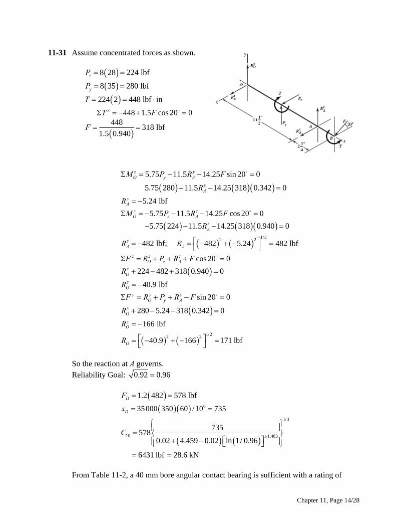
11-31 Assume concentrated forces as shown. 8 28 224 lbfzP
8 35 280 lbfyP
224 2 448 lbf inT
448 1.5 cos 20 0xT F
448
318 lbf1.5 0.940
F
5.75 11.5 14.25 sin 20 0z y
O y AM P R F
5.75 280 11.5 14.25 318 0.342 0yAR
5.24 lbfyAR
5.75 11.5 14.25 cos 20 0y zO z AM P R F
5.75 224 11.5 14.25 318 0.940 0zAR
1/22 2
482 lbf; 482 5.24 482 lbfzA AR R
cos 20 0z z zO z AF R P R F
224 482 318 0.940 0zOR
40.9 lbfzOR
sin 20 0y y yO y AF R P R F
280 5.24 318 0.342 0yOR
166 lbfyOR
1/22 2
40.9 166 171 lbfOR So the reaction at A governs.
Reliability Goal: 0.92 0.96 1.2 482 578 lbfDF
635000 350 60 /10 735Dx
1/3
10 1/1.483
735578
0.02 4.459 0.02 ln 1/ 0.96
6431 lbf 28.6 kN
C
From Table 11-2, a 40 mm bore angular contact bearing is sufficient with a rating of
Chapter 11, Page 14/28
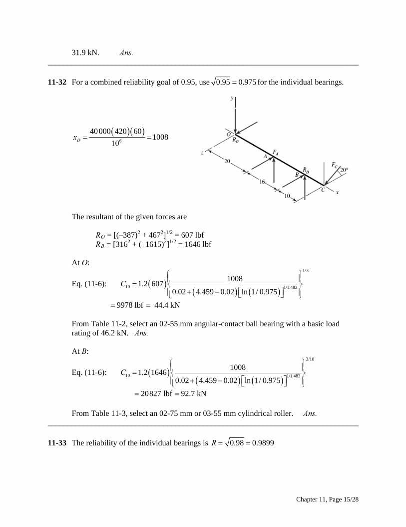
31.9 kN. Ans. ______________________________________________________________________________
1-32 For a combined reliability goal of 0.95, use
1 0.95 0.975 for the individual bearings.
6
40000 420 601008
10Dx
The resultant of the given forces are
RO = [(–387) + 467 ] = 607 lbf
At O:
Eq. (11-6):
2 2 1/2
RB = [3162 + (–1615)2]1/2 = 1646 lbf
1/3
10 1/1.483
10081.2 607
0.02 4.459 0.02 ln 1/ 0.975C
9978 lbf 44.4 kN
From Table 11-2, select an 02-55 mm angular-contact ball bearing with a basic load
At B:
Eq. (11-6):
rating of 46.2 kN. Ans.
3/10
10 1/1.483
10081.2 1646
0.02 4.459 0.02 ln 1/ 0.975C
20827 lbf 92.7 kN
From Table 11-3, select an 02-75 mm or 03-55 mm cylindrical roller. Ans. _____ _________
1-33 The reliability of the individual bearings is
_ _______________________________________________________________ 1 0.98 0.9899R
Chapter 11, Page 15/28
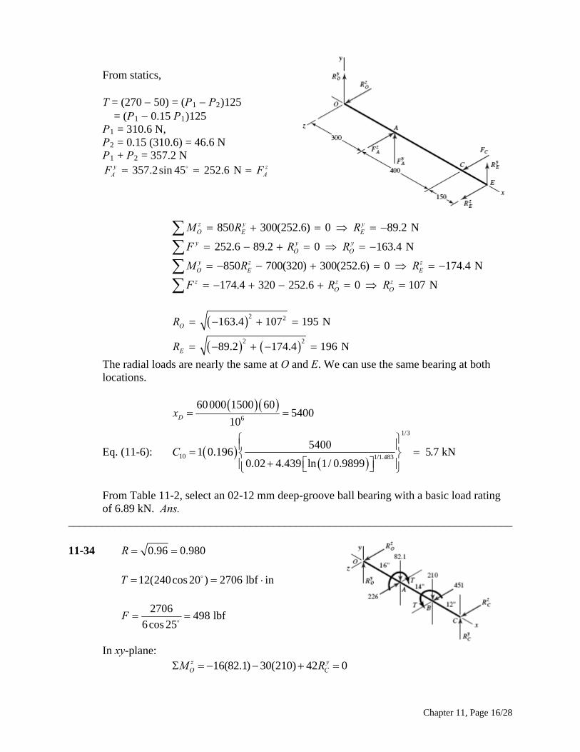
From statics, T = (270 50) = (P1 P2)125 = (P1 0.15 P1)125 P1 = 310.6 N, P2 = 0.15 (310.6) = 46.6 N P1 + P2 = 357.2 N
357.2sin 45 252.6 Ny zA AF F
zR
850 300(252.6) 0 89.2 Nz y y
O E EM R R 252.6 89.2 0 163.4 Ny y y
O OF R R 850 700(320) 300(252.6) 0 174.4 Ny z z
O E EM R R 174.4 320 252.6 0 107 Nz z
O OF R
2 2
2 2
163.4 107 195 N
89.2 174.4 196 N
O
E
R
R
The radial loads are nearly the same at O and E. We can use the same bearing at both locations.
6
60000 1500 605400
10Dx
Eq. (11-6):
1/3
10 1/1.483
54001 0.196 5.7 kN
0.02 4.439 ln 1/ 0.9899C
From Table 11-2, select an 02-12 mm deep-groove ball bearing with a basic load rating
of 6.89 kN. Ans. ______________________________________________________________________________
11-34 0.96 0.980R
12(240cos 20 ) 2706 lbf inT
2706
498 lbf6cos 25
F
In xy-plane:
16(82.1) 30(210) 42 0z y
O CM R
Chapter 11, Page 16/28
181 lbfyCR
82.1 210 181 111.1 lbfyOR
In xz-plane: 16(226) 30(451) 42 0y z
O CM R 236 lbfz
CR
226 451 236 11 lbfzOR
1/22 2111.1 11 112 lbf .OR Ans
1/22 2181 236 297 lbf .CR Ans
6
50000 300 60900
10Dx
1/3
10 1/1.483
9001.2 112
0.02 4.439 ln 1/ 0.980
1860 lbf 8.28 kN
OC
1/3
10 1/1.483
9001.2 297
0.02 4.439 ln 1/ 0.980
4932 lbf 21.9 kN
CC
Bearing at O: Choose a deep-groove 02-17 mm. Ans. Bearing at C: Choose a deep-groove 02-35 mm. Ans. ______________________________________________________________________________ 11-35 Shafts subjected to thrust can be constrained by bearings, one of which supports the
thrust. The shaft floats within the endplay of the second (roller) bearing. Since the thrust force here is larger than any radial load, the bearing absorbing the thrust (bearing A) is heavily loaded compared to bearing B. Bearing B is thus likely to be oversized and may not contribute measurably to the chance of failure. If this is the case, we may be able to obtain the desired combined reliability with bearing A having a reliability near 0.99 and bearing B having a reliability near 1. This would allow for bearing A to have a lower
capacity than if it needed to achieve a reliability of 0.99 . To determine if this is the case, we will start with bearing B.
Bearing B (straight roller bearing)
6
30000 500 60900
10Dx
1/22 236 67 76.1 lbf 0.339 kNrF
Try a reliability of 1 to see if it is readily obtainable with the available bearings.
Chapter 11, Page 17/28
Eq. (11-6):
3/10
10 1/1.483
9001.2 0.339 10.1 kN
0.02 4.439 ln 1/1.0C
The smallest capacity bearing from Table 11-3 has a rated capacity of 16.8 kN.
Therefore, we select the 02-25 mm straight cylindrical roller bearing. Ans. Bearing at A (angular-contact ball) With a reliability of 1 for bearing B, we can achieve the combined reliability goal of 0.99
if bearing A has a reliability of 0.99.
1/22 236 212 215 lbf 0.957 kNrF
555 lbf 2.47 kNaF Trial #1: Tentatively select an 02-85 mm angular-contact with C10 = 90.4 kN and C0 = 63.0 kN.
0
2.470.0392
63.0aF
C
6
30000 500 60900
10Dx
Table 11-1: Interpolating, X2 = 0.56, Y2 = 1.88 Eq. (11-9): 0.56 0.957 1.88 2.47 5.18 kNeF
Eq. (11-6):
1/3
10 1/1.483
9001.2 5.18
0.02 4.439 ln 1/ 0.99C
99.54 kN 90.4 kN Trial #2: Tentatively select a 02-90 mm angular-contact ball with C10 = 106 kN and C0 = 73.5 kN.
0
2.470.0336
73.5aF
C
Table 11-1: Interpolating, X2 = 0.56, Y2 = 1.93 0.56 0.957 1.93 2.47 5.30 kNeF
1/3
10 1/1.483
9001.2 5.30 102 kN < 106 kN O.K.
0.02 4.439 ln 1/ 0.99C
Chapter 11, Page 18/28
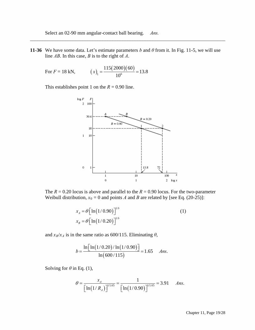
Select an 02-90 mm angular-contact ball bearing. Ans. ______________________________________________________________________________ 11-36 We have some data. Let’s estimate parameters b and θ from it. In Fig. 11-5, we will use
line AB. In this case, B is to the right of A.
For F = 18 kN, 61
115 2000 6013.8
10x
This establishes point 1 on the R = 0.90 line.
The R = 0.20 locus is above and parallel to the R = 0.90 locus. For the two-parameter
Weibull distribution, x0 = 0 and points A and B are related by [see Eq. (20-25)]:
(1) 1/ln 1/ 0.90
b
Ax
1/ln 1/ 0.20
b
Bx and xB/xA is in the same ratio as 600/115. Eliminating θ,
ln ln 1/ 0.20 / ln 1/ 0.90
1.65 .ln 600 /115
b A ns
Solving for θ in Eq. (1),
1/1.65 1/1.65
13.91 .
ln 1/ ln 1/ 0.90
A
A
xAns
R
Chapter 11, Page 19/28
Therefore, for the data at hand,
1.65
exp3.91
xR
Check R at point B: xB = (600/115) = 5.217
1.65
5.217exp 0.20
3.91R
Note also, for point 2 on the R = 0.20 line,
2
log 5.217 log 1 log log 13.8mx
272mx
______________________________________________________________________________ 11-37 This problem is rich in useful variations. Here is one. Decision: Make straight roller bearings identical on a given shaft. Use a reliability goal of
(0.99)1/6 = 0.9983. Shaft a
1/22 2239 111 264 lbf 1.175 kNrAF
1/22 2502 1075 1186 lbf 5.28 kNrBF
Thus the bearing at B controls.
6
10000 1200 60720
10Dx
1/1.4830.02 4.439 ln 1/ 0.9983 0.08026
0.3
10
7201.2 5.28 97.2 kN
0.080 26C
Select either an 02-80 mm with C10 = 106 kN or an 03-55 mm with C10 = 102 kN. Ans. Shaft b
1/22 2874 2274 2436 lbf or 10.84 kNrCF
1/22 2393 657 766 lbf or 3.41 kNrDF
The bearing at C controls.
Chapter 11, Page 20/28
6
10000 240 60144
10Dx
0.3
10
1441.2 10.84 123 kN
0.080 26C
Select either an 02-90 mm with C10 = 142 kN or an 03-60 mm with C10 = 123 kN. Ans. Shaft c
1/22 21113 2385 2632 lbf or 11.71 kNrEF
1/22 2417 895 987 lbf or 4.39 kNrFF
The bearing at E controls.
6
10000 80 6048
10Dx
0.3
10
481.2 11.71 95.7 kN
0.080 26C
Select an 02-80 mm with C10 = 106 kN or an 03-60 mm with C10 = 123 kN. Ans. ______________________________________________________________________________ 11-38 Express Eq. (11-1) as 1 1 10 10
a aF L C L K For a ball bearing, a = 3 and for an 02-30 mm angular contact bearing, C10 = 20.3 kN.
3 6 920.3 10 8.365 10K
At a load of 18 kN, life L1 is given by:
9
61 3
1
8.365 101.434 10 rev
18a
KL
F
For a load of 30 kN, life L2 is:
9
62 3
8.365 100.310 10 rev
30L
In this case, Eq. (6-57) – the Palmgren-Miner cycle-ratio summation rule – can be
expressed as
Chapter 11, Page 21/28
1 2
1 2
1l l
L L
Substituting,
26 6
200 0001
1.434 10 0.310 10
l
62 0.267 10 rev .l A ns
______________________________________________________________________________ 11-39 Total life in revolutions Let: l = total turns f1 = fraction of turns at F1 f2 = fraction of turns at F2 From the solution of Prob. 11-38, L1 = 1.434(106) rev and L2 = 0.310(106) rev. Palmgren-Miner rule:
1 2 1 2
1 2 1 2
1l l f l f l
L L L L
from which
1 1 2 2
1
/ /l
f L f L
6 6
1
0.40 / 1.434 10 0.60 / 0.310 10
451 585 rev .
l
Ans
Total life in loading cycles 4 min at 2000 rev/min = 8000 rev/cycle
6 min at 2000 rev/min = 12 000 rev/cycle
Total rev/cycle = 8000 + 12 000 = 20 000
451585rev22.58 cycles .
20000 rev/cycleAns
Chapter 11, Page 22/28
Total life in hours
min 22.58 cycles10 3.76 h .
cycle 60 min/hAns
______________________________________________________________________________ 11-40 560 lbfrAF 1095 lbfrBF 200 lbfaeF
6
40 000 400 6010.67
90 10D
DR
Lx
L
0.90 0.949R
Eq. (11-15): 0.47 5600.47
175.5 lbf1.5
rAiA
A
FF
K
Eq. (11-15): 0.47 10950.47
343.1 lbf1.5
rBiB
B
FF
K
?iA iB aeF F F
175.5 lbf 343.1 200 543.1 lbf, so Eq. (11-16) applies. We will size bearing B first since its induced load will affect bearing A, but is not itself
affected by the induced load from bearing A [see Eq. (11-16)]. From Eq. (11-16b), FeB = FrB = 1095 lbf.
Eq. (11-7):
3/10
1/1.5
10.671.4 1095 3607 lbf
4.48 1 0.949RBF
Ans.
Select cone 32305, cup 32305, with 0.9843 in bore, and rated at 3910 lbf with K = 1.95. Ans.
With bearing B selected, we re-evaluate the induced load from bearing B using the actual
value for K.
Eq. (11-15): 0.47 10950.47
263.9 lbf1.95
rBiB
B
FF
K
Find the equivalent radial load for bearing A from Eq. (11-16), which still applies. Eq. (11-16a): 0.4eA rA A iB aeF F K F F
0.4 560 1.5 263.9 200 920 lbfeAF
Chapter 11, Page 23/28
eA rAF F
Eq. (11-7):
3/10
1/1.5
10.671.4 920 3030 lbf
4.48 1 0.949RAF
Tentatively select cone M86643, cup M86610, with 1 in bore, and rated at 3250 lbf with
K = 1.07. Iterating with the new value for K, we get FeA = 702 lbf and FrA = 2312 lbf. Ans.
By using a bearing with a lower K, the rated load decreased significantly, providing a
higher than requested reliability. Further examination with different combinations of bearing choices could yield additional acceptable solutions.
______________________________________________________________________________ 11-41 The thrust load on shaft CD is from the axial component of the force transmitted through
the bevel gear, and is directed toward bearing C. By observation of Fig. 11-14, direct mounted bearings would allow bearing C to carry the thrust load. Ans.
From the solution to Prob. 3-74, the axial thrust load is Fae = 362.8 lbf, and the bearing
radial forces are FCx = 287.2 lbf, FCz = 500.9 lbf, FDx = 194.4 lbf, and FDz = 307.1 lbf. Thus, the radial forces are
2 2287.2 500.9 577 lbfrCF
2 2194.4 307.1 363 lbfrDF
The induced loads are
Eq. (11-15): 0.47 5770.47
181 lbf1.5
rCiC
C
FF
K
Eq. (11-15): 0.47 3630.47
114 lbf1.5
rDiD
D
FF
K
Check the condition on whether to apply Eq. (11-16) or Eq. (11-17), where bearings C and D are substituted, respectively, for labels A and B in the equations.
?iC iD aeF F F
181 lbf 114 362.8 476.8 lbf, so Eq.(11-16) applies Eq. (11-16a): 0.4eC rC C iD aeF F K F F
,0.4 577 1.5 114 362.8 946 lbf so use rC eCF F
Assume for tapered roller bearings that the specifications for Manufacturer 1 on p. 608
are applicable.
Chapter 11, Page 24/28
8
6
101.11
90 10D
DR
Lx
L
0.90 0.949R
Eq. (11-7):
3/10
1/1.5
1.111 946 1130 lbf .
4.48 1 0.949RCF Ans
Eq. (11-16b): 363 lbfeD rDF F
Eq. (11-7):
3/10
1/1.5
1.111 363 433 lbf .
4.48 1 0.949RDF Ans
______________________________________________________________________________ 11-42 The thrust load on shaft AB is from the axial component of the force transmitted through
the bevel gear, and is directed to the right. By observation of Fig. 11-14, indirect mounted bearings would allow bearing A to carry the thrust load. Ans.
From the solution to Prob. 3-76, the axial thrust load is Fae = 92.8 lbf, and the bearing
radial forces are FAy = 639.4 lbf, FAz = 1513.7 lbf, FBy = 276.6 lbf, and FBz = 705.7 lbf. Thus, the radial forces are
2 2639.4 1513.7 1643 lbfrAF
2 2276.6 705.7 758 lbfrBF
The induced loads are
Eq. (11-15): 0.47 16430.47
515 lbf1.5
rAiA
A
FF
K
Eq. (11-15): 0.47 7580.47
238 lbf1.5
rBiB
B
FF
K
Check the condition on whether to apply Eq. (11-16) or Eq. (11-17). ?iA iB aeF F F
515 lbf 238 92.8 330.8 lbf, so Eq.(11-17) applies Notice that the induced load from bearing A is sufficiently large to cause a net axial force
to the left, which must be supported by bearing B. Eq. (11-17a): 0.4eB rB B iA aeF F K F F
,0.4 758 1.5 515 92.8 937 lbf so use rB eBF F
Assume for tapered roller bearings that the specifications for Manufacturer 1 on p. 608
are applicable.
Chapter 11, Page 25/28
6
6
500 105.56
90 10D
DR
Lx
L
0.90 0.949R
Eq. (11-7):
3/10
1/1.5
5.561 937 1810 lbf .
4.48 1 0.949RBF Ans
Eq. (11-16b): 1643 lbfeA rAF F
Eq. (11-7):
3/10
1/1.5
5.561 1643 3180 lbf .
4.48 1 0.949RAF Ans
______________________________________________________________________________ 11-43 The lower bearing is compressed by the axial load, so it is designated as bearing A.
25 kNrAF 12 kNrBF 5 kNaeF
Eq. (11-15): 0.47 250.47
7.83 kN1.5
rAiA
A
FF
K
Eq. (11-15): 0.47 120.47
3.76 kN1.5
rBiB
B
FF
K
Check the condition on whether to apply Eq. (11-16) or Eq. (11-17) ?iA iB aeF F F
7.83 kN 3.76 5 8.76 kN, so Eq.(11-16) applies Eq. (11-16a): 0.4eA rA A iB aeF F K F F
,0.4 25 1.5 3.76 5 23.1 kN so use rA rAF F
6
60 min 8 hr 5 day 52 weeks250 rev/min 5 yrs
hr day week yr
156 10 rev
DL
Assume for tapered roller bearings that the specifications for Manufacturer 1 on p. 608 are applicable.
Eq. (11-3):
3/103/10 6
6
156 101.2 25 35.4 kN .
90 10D
RA f DR
LF a F An
L
s
Eq. (11-16b): 12 kNeB rBF F
Chapter 11, Page 26/28
Eq. (11-3): 3/10
1561.2 12 17.0 kN .
90RBF Ans
______________________________________________________________________________ 11-44 The left bearing is compressed by the axial load, so it is properly designated as bearing A. 875 lbfrAF 625 lbfrBF 250 lbfaeF Assume K = 1.5 for each bearing for the first iteration. Obtain the induced loads.
Eq. (11-15): 0.47 8750.47
274 lbf1.5
rAiA
A
FF
K
Eq. (11-15): 0.47 6250.47
196 lbf1.5
rBiB
B
FF
K
Check the condition on whether to apply Eq. (11-16) or Eq. (11-17). ?iA iB aeF F F
274 lbf 196 250 lbf, so Eq.(11-16) applies We will size bearing B first since its induced load will affect bearing A, but it is not
affected by the induced load from bearing A [see Eq. (11-16)]. From Eq. (11-16b), FeB = FrB = 625 lbf.
Eq. (11-3):
3/103/10
6
90 000 150 601 625
90 10D
RB f DR
LF a F
L
1208 lbf RBF
Select cone 07100, cup 07196, with 1 in bore, and rated at 1570 lbf with K = 1.45. Ans.
With bearing B selected, we re-evaluate the induced load from bearing B using the actual
value for K.
Eq. (11-15): 0.47 6250.47
203 lbf1.45
rBiB
B
FF
K
Find the equivalent radial load for bearing A from Eq. (11-16), which still applies.
Chapter 11, Page 27/28
Eq. (11-16a): 0.4eA rA A iB aeF F K F F
0.4 875 1.5 203 250 1030 lbf
eA rAF F
Eq. (11-3):
3/103/10
6
90 000 150 601 1030
90 10D
RA f DR
LF a F
L
1990 lbf RAF Any of the bearings with 1-1/8 in bore are more than adequate. Select cone 15590, cup
15520, rated at 2480 lbf with K = 1.69. Iterating with the new value for K, we get FeA = 1120 lbf and FrA = 2160 lbf. The selected bearing is still adequate. Ans.
______________________________________________________________________________
Chapter 11, Page 28/28
Chapter 12 12-1 Given: dmax = 25 mm, bmin = 25.03 mm, l/d = 1/2, W = 1.2 kN, = 55 mPas, and N =
1100 rev/min.
min maxmin
25.03 250.015 mm
2 2
b dc
r 25/2 = 12.5 mm
r/c = 12.5/0.015 = 833.3 N = 1100/60 = 18.33 rev/s P = W/ (ld) = 1200/ [12.5(25)] = 3.84 N/mm2 = 3.84 MPa
Eq. (12-7):
32
2
6
55 10 18.33833.3 0.182
3.84 10
r NS
c P
Fig. 12-16: h0 /c = 0.3 h0 = 0.3(0.015) = 0.0045 mm Ans. Fig. 12-18: f r/c = 5.4 f = 5.4/833.3 = 0.006 48 T =f Wr = 0.006 48(1200)12.5(103) = 0.0972 Nm Hloss = 2 TN = 2 (0.0972)18.33 = 11.2 W Ans. Fig. 12-19: Q/(rcNl) = 5.1 Q = 5.1(12.5)0.015(18.33)12.5 = 219 mm3/s Fig. 12-20: Qs /Q = 0.81 Qs = 0.81(219) = 177 mm3/s Ans. ______________________________________________________________________________ 12-2 Given: dmax = 32 mm, bmin = 32.05 mm, l = 64 mm, W = 1.75 kN, = 55 mPas, and N =
900 rev/min.
min maxmin
32.05 320.025 mm
2 2
b dc
r 32/2 = 16 mm
r/c = 16/0.025 = 640 N = 900/60 = 15 rev/s
Chapter 12, Page 1/26
Draft
P = W/ (ld) = 1750/ [32(64)] = 0.854 MPa l/d = 64/32 = 2
Eq. (12-7): 32
255 10 15
640 0.7970.854
r NS
c P
Eq. (12-16), Figs. 12-16, 12-19, and 12-21 l/d y y1 y1/2 y1/4 yl/d
h0/c 2 0.98 0.83 0.61 0.36 0.92
P/pmax 2 0.84 0.54 0.45 0.31 0.65
Q/rcNl 2 3.1 3.45 4.2 5.08 3.20
h0 = 0.92 c = 0.92(0.025) = 0.023 mm Ans. pmax = P / 0.065 = 0.854/0.65 = 1.31 MPa Ans. Q = 3.20 rcNl = 3.20(16)0.025(15)64 = 1.23 (103) mm3/s Ans. ______________________________________________________________________________ 12-3 Given: dmax = 3.000 in, bmin = 3.005 in, l = 1.5 in, W = 800 lbf, N = 600 rev/min, and
SAE 10 and SAE 40 at 150F.
min maxmin
3.005 3.0000.0025 in
2 23.000 / 2 1.500 in
/ 1.5 / 3 0.5/ 1.5 / 0.0025 600
600 / 60 10 rev/s800
177.78 psi1.5(3)
b dc
rl dr cN
WP
ld
Fig. 12-12: SAE 10 at 150F, 1.75 reynµ µ
2 62 1.75(10 )(10)
600 0.0354177.78
r NS
c P
Figs. 12-16 and 12-21: h0/c = 0.11 and P/pmax = 0.21
0
max
0.11(0.0025) 0.000 275 in .177.78 / 0.21 847 psi .
h Ap Ans
ns
Fig. 12-12: SAE 40 at 150F, 4.5 reynµ µ
Chapter 12, Page 2/26
Draft
0 max
0
max
4.50.0354 0.0910
1.75/ 0.19, / 0.275
0.19(0.0025) 0.000 475 in .177.78 / 0.275 646 psi .
S
h c P ph Ap A
nsns
______________________________________________________________________________ 12-4 Given: dmax = 3.250 in, bmin = 3.256 in, l = 3.25 in, W = 800 lbf, and N = 1000 rev/min.
min maxmin
3.256 3.2500.003
2 23.250 / 2 1.625 in
/ 3 / 3.250 0.923/ 1.625 / 0.003 542
1000 / 60 16.67 rev/s800
82.05 psi3(3.25)
b dc
rl dr cN
WP
ld
Fig. 12-14: SAE 20W at 150F, = 2.85 reyn
2 6
2 2.85(10 )(16.67)542 0.1701
82.05
r NS
c P
From Eq. (12-16), and Figs. 12-16 and 12-21:
l/d y y1 y1/2 y1/4 yl/d
ho/c 0.923 0.85 0.48 0.28 0.15 0.46
P/pmax 0.923 0.83 0.45 0.32 0.22 0.43
max
0.46 0.46(0.003) 0.001 38 in .82.05
191 psi .0.43 0.43
oh c AP
p A
ns
ns
Fig. 12-14: SAE 20W-40 at 150F, = 4.4 reyn
62 4.4(10 )(16.67)
542 0.26382.05
S
From Eq. (12-16), and Figs. 12-16 and 12-21:
l/d y y1 y1/2 y1/4 yl/d
ho/c 0.923 0.91 0.6 0.38 0.2 0.58
P/pmax 0.923 0.83 0.48 0.35 0.24 0.46
Chapter 12, Page 3/26
Draft
0
max
0.58 0.58(0.003) 0.001 74 in .8205 82.05
178 psi .0.46 0.46
h c A
p A
ns
ns
______________________________________________________________________________ 12-5 Given: dmax = 2.000 in, bmin = 2.0024 in, l = 1 in, W = 600 lbf, N = 800 rev/min, and SAE
20 at 130F.
min maxmin
2.0024 20.0012 in
2 22
1 in, / 1 / 2 0.502 2
/ 1 / 0.0012 833800 / 60 13.33 rev/s
600300 psi
2(1)
b dc
dr l d
r cN
WP
ld
Fig. 12-12: SAE 20 at 130F, 3.75 reynµ µ
2 6
2 3.75(10 )(13.3)833 0.115
300
r NS
c P
From Figs. 12-16, 12-18 and 12-19:
0
0
/ 0.23, / 3.8, / ( ) 5.30.23(0.0012) 0.000 276 in .3.8
0.004 56833
h c r f c Q rcNlh A
f
ns
The power loss due to friction is
3
2 2 (0.004 56)(600)(1)(13.33)
778(12) 778(12)0.0245 Btu/s .5.35.3(1)(0.0012)(13.33)(1)
0.0848 in / s .
f WrNH
AnsQ rcNl
Ans
______________________________________________________________________________ 12-6 Given: dmax = 25 mm, bmin = 25.04 mm, l/d = 1, W = 1.25 kN, = 50 mPas, and N =
1200 rev/min.
Chapter 12, Page 4/26
Draft
min maxmin
2
25.04 250.02 mm
2 2/ 2 25 / 2 12.5 mm, / 1
/ 12.5 / 0.02 6251200 / 60 20 rev/s
12502 MPa
25
b dc
r d l dr cN
WP
ld
For µ = 50 MPa · s, 2 3
26
50(10 )(20)625 0.195
2(10 )
r NS
c P
From Figs. 12-16, 12-18 and 12-20:
0
0
/ 0.52, / 4.5, / 0.570.52(0.02) 0.0104 mm .4.5
0.0072625
0.0072(1.25)(12.5) 0.1125 N · m
sh c f r c Q Qh A
f
T f Wr
ns
The power loss due to friction is H = 2πT N = 2π (0.1125)(20) = 14.14 W Ans. Qs = 0.57Q The side flow is 57% of Q Ans. ______________________________________________________________________________ 12-7 Given: dmax = 1.25 in, bmin = 1.252 in, l = 2 in, W = 620 lbf, = 8.5 reyn, and N =
1120 rev/min.
min maxmin
2 62
1.252 1.250.001 in
2 2/ 2 1.25 / 2 0.625 in
/ 0.625 / 0.001 6251120 / 60 18.67 rev/s
620248 psi
1.25(2)
8.5(10 )(18.67)625 0.250
248/ 2 / 1.25 1.6
b dc
r dr cN
WP
ld
r NS
c Pl d
From Eq. (12-16), and Figs. 12-16, 12-18, and 12-19
Chapter 12, Page 5/26
Draft
l/d y y1 y1/2 y1/4 yl/d
h0/c 1.6 0.9 0.58 0.36 0.185 0.69
fr/c 1.6 4.5 5.3 6.5 8 4.92
Q/rcNl 1.6 3 3.98 4.97 5.6 3.59 h0 = 0.69 c = 0.69(0.001) =0.000 69 in Ans. f = 4.92/(r/c) = 4.92/625 = 0.007 87 Ans. Q = 1.6 rcNl = 1.6(0.625) 0.001(18.57) 2 = 0.0833 in3/s Ans. ______________________________________________________________________________ 12-8 Given: dmax = 75.00 mm, bmin = 75.10 mm, l = 36 mm, W = 2 kN, N = 720 rev/min, and
SAE 20 and SAE 40 at 60C.
min maxmin
75.10 750.05 mm
2 2/ 36 / 75 0.48 0.5 (close enough)
/ 2 75 / 2 37.5 mm/ 37.5 / 0.05 750
720 / 60 12 rev/s2000
0.741 MPa75(36)
b dc
l dr dr cN
WP
ld
Fig. 12-13: SAE 20 at 60C, µ = 18.5 MPa · s
2 32
6
18.5(10 )(12)750 0.169
0.741(10 )
r NS
c P
From Figures 12-16, 12-18 and 12-21:
0 m
0
/ 0.29, / 5.1, / 0.3150.29(0.05) 0.0145 mm .5.1 / 750 0.0068
0.0068(2)(37.5) 0.51 N · m
h c f r c P ph Anf
T f Wr
ax
s
The heat loss rate equals the rate of work on the film Hloss = 2πT N = 2π(0.51)(12) = 38.5 W Ans. pmax = 0.741/0.315 = 2.35 MPa Ans. Fig. 12-13: SAE 40 at 60C, µ = 37 MPa · s
Chapter 12, Page 6/26
Draft
S = 0.169(37)/18.5 = 0.338 From Figures 12-16, 12-18 and 12-21:
0 m
0
loss
max
/ 0.42, / 8.5, / 0.380.42(0.05) 0.021 mm .8.5 / 750 0.0113
0.0113(2)(37.5) 0.85 N · m2 2 (0.85)(12) 64 W .0.741 / 0.38 1.95 MPa .
h c f r c P ph AnsfT f WrH TN Ansp A
ax
ns
_____________________________________________________________________________ 12-9 Given: dmax = 56.00 mm, bmin = 56.05 mm, l = 28 mm, W = 2.4 kN, N = 900 rev/min, and
SAE 40 at 65C.
min maxmin
56.05 560.025 mm
2 2/ 2 56 / 2 28 mm
/ 28 / 0.025 1120/ 28 / 56 0.5, 900 / 60 15 rev/s
24001.53 MPa
28(56)
b dc
r dr cl d N
P
Fig. 12-13: SAE 40 at 65C, µ = 30 MPa · s
2 32
6
30(10 )(15)1120 0.369
1.53(10 )
r NS
c P
From Figures 12-16, 12-18, 12-19 and 12-20:
0
0
/ 0.44, / 8.5, / 0.71, / ( ) 4.850.44(0.025) 0.011 mm .8.5 / 1000 0.007 59
0.007 59(2.4)(28) 0.51 N · m2 2 (0.51)(15) 48.1 W .
4.85 4.85(28)(0.0
sh c f r c Q Q Q rcNlh AnsfT f WrH TN Ans
Q rcNl
3
3
25)(15)(28) 1426 mm /s
0.71(1426) 1012 mm /s .sQ Ans
_____________________________________________________________________________ 12-10 Consider the bearings as specified by minimum f : 0
0, b
d
ttd b
maximum W: 00, b
d
ttd b
Chapter 12, Page 7/26
Draft
d and differing only in d and .
ig. µ = 1.38(106) reyn
/448) = 0.185(106)
Preliminaries:
2
/ 1
/ ( ) 700 / (1.25 ) 448 psi3600 / 60 60 rev/s
l d
P W ldN
Fig. 12-16:
minimum f :
S 0.08 maximum W: 0.20S
F 12-12:
µN/P = 1.38(106)(60 Eq. (12-7):
/
r S
c µN
P
m
For minimu f :
6
0.08 658
0.185(10 )0.625 / 658 0.000 950 0.001 in
r
cc
If this is c min,
b d = 2(0.001) = 0.002 in
The median clearance is
0.0012 2
d b d bt t t tminc c
ran nge for this bearing is
and the clea ce ra
2dtc bt
which is a function only of the tolerances.
For maximum W:
6
0.2 1040
0.185(10 )0.625 / 1040 0.000 600 0.0005 in
r
cc
If this is cmin
Chapter 12, Page 8/26
Draft
min
min
2 2(0.0005) 0.001 in
0.00052 2
2
d b d b
d b
b d ct t t t
c c
t tc
The difference (mean) in clearance between the two clearance ranges, crange, is
range 0.001 0.00052 2
0.0005 in
d b d bt t t tc
For the minimum f bearing
b d = 0.002 in
d = b 0.002 in
d = b 0.001 in
For the same b, tb and td, we need to change the journal diameter by 0.001 in.
Increasing d of the minimum friction bearing by 0.001 in, defines of the maximum
_____________________________________________________________________________
2-11 Given: SAE 40, N = 10 rev/s, Ts = 140F, l/d = 1, d = 3.000 in, b = 3.003 in, W = 675
or For the maximum W bearing
0.001 ( 0.002)0.001 in
d d b b
d load bearing. Thus, the clearance range provides for bearing dimensions which are attainable in manufacturing. Ans.
1
lbf.
min maxmin
3.003 30.0015 in
2 2/ 2 3 / 2 1.5 in
/ 1.5 / 0.0015 1000675
75 psi3(3)
b dc
r dr c
WP
ld
Trial #1: Fr om Figure 12-12 for T = 160°F, µ = 3.5 µ reyn,
2 62
2(160 140) 40
3.5(10 )(10)1000 0.4667
75
T F
r NS
c P
From Fig. 12-24,
Chapter 12, Page 9/26
Draft
29.700.349 109 6.009 40(0.4667) 0.047 467(0.4667) 3.16
753.16 3.16 24.4 F
9.70 9.70
T
PP
T
Discrepancy = 40 24.4 = 15.6°F
Trial #2: T = 150°F, µ = 4.5 µ reyn,
6
2
2(150 140) 20
4.5 10 101000 0.6
75
T F
S
From Fig. 12-24,
29.70
0.349 109 6.009 40(0.6) 0.047 467(0.6) 3.97
753.97 3.97 30.7 F
9.70 9.70
T
PP
T
Discrepancy = 20 30.7 = 10.7°F
Trial #3: T = 154°F, µ = 4 µ reyn,
6
2
2(154 140) 28
4 10 101000 0.533
75
T F
S
From Fig. 12-24,
29.70
0.349 109 6.009 40(0.533) 0.047 467(0.533) 3.57
753.57 3.57 27.6 F
9.70 9.70
T
PP
T
Discrepancy = 28 27.6 = 0.4°F O.K.
T = 140 +28/2 = 154°F Ans.
s 12-16, 12-18, to 12-20:
av
2 av
) 140/ 2 154 (28 / 2) 168
0.4
FT T T FS
1 av / 2 154 (28 / 2T T T
From Figure
Chapter 12, Page 10/26
Draft
0
0
loss
0.75, 11, 3.6, 0.33
0.75(0.0015) 0.00113 in .11
0.0111000
0.0075(3)(40) 0.9 N · m2 0.011 675 1.5 102
0.075 Btu/s .778 12 778 12
3.6 3.
sh f r Q Q
c c rcN l Qh Ans
f
T f Wr
f WrNH A
Q rcN l
3
3
6(1.5)0.0015(10)3 0.243 in /s .
0.33(0.243) 0.0802 in /s .s
Ans
Q Ans
ns
_____________________________________________________________________________
2-12 Given: d = 2.5 in, b = 2.504 in, cmin = 0.002 in, W = 1200 lbf, SAE = 20, Ts = 110°F,
P = W/(ld) = 1200/(2.5) = 192 psi, N = 1120/60 = 18.67 rev/s
For a trial film temperature, let Tf = 150°F
Table 12-1: = 0.0136 exp[1271.6/(150 + 95)] = 2.441 reyn
Eq. (12-7):
1 N = 1120 rev/min, and l = 2.5 in.
2
62 2 2.441 10 18.672.5 / 20.927
0.002 192
r NS
c P
Fig. 12-24:
21920.349 109 6.009 40 0.0927 0.047 467 0.0927
9.7017.9 F
T
av
av
17.9110 119.0 F
2 2150 119.0 31.0 F
s
f
TT T
T T
which is not 0.1 or less, therefore try averaging for the new trial film temperature, let
new
150 119.0( ) 134.5 F
2fT
ing a spreadsheet (table also shows the first trial)
Proceed with additional trials us
Chapter 12, Page 11/26
Draft
Trial Tf ' S T Tav Tf Tav
New Tf
150.0 2.441 0.0927 17.9 119.0 31.0 134.5
134.5 3.466 0.1317 22.6 121.3 13.2 127.9
127.9 4.084 0.1551 25.4 122.7 5.2 125.3
125.3 4.369 0.1659 26.7 123.3 2.0 124.3
124.3 4.485 0.1704 27.2 123.6 0.7 124.0
124.0 4.521 0.1717 27.4 123.7 0.3 123.8
123.8 4.545 0.1726 27.5 123.7 0.1 123.8 Note that the convergence begins rapidly. There are ways to speed this, but at this point they would only add complexity. (a) 64.545(10 ), 0.1726µ S
From Fig. 12-16: 000.482, 0.482(0.002) 0.000 964 in
hh
c
From Fig. 12-17: = 56° Ans. (b) e = c h0 = 0.002 0.000 964 = 0.001 04 in Ans.
(c) From Fig. 12-18:
4.10, 4.10(0.002 /1.25) 0.006 56 .f r
f Ansc
(d) T = f Wr = 0.006 56(1200)(1.25) = 9.84 lbf · in
2 2 (9.84)(1120 / 60)0.124 Btu/s .
778(12) 778(12)
T NH Ans
(e) From Fig. 12-19: 4.16Q
rcNl
311204.16(1.25)(0.002) (2.5) 0.485 in /s .
60Q A
ns
From Fig. 12-20: 30.6, 0.6(0.485) 0.291 in /s .ss
QQ A
Q ns
(f) From Fig. 12-21: 2
maxmax
/ 1200 / 2.50.45, 427 psi .
0.45 0.45
W ldPp Ans
p
From Fig. 12-22: max
16 .p Ans
Chapter 12, Page 12/26
Draft
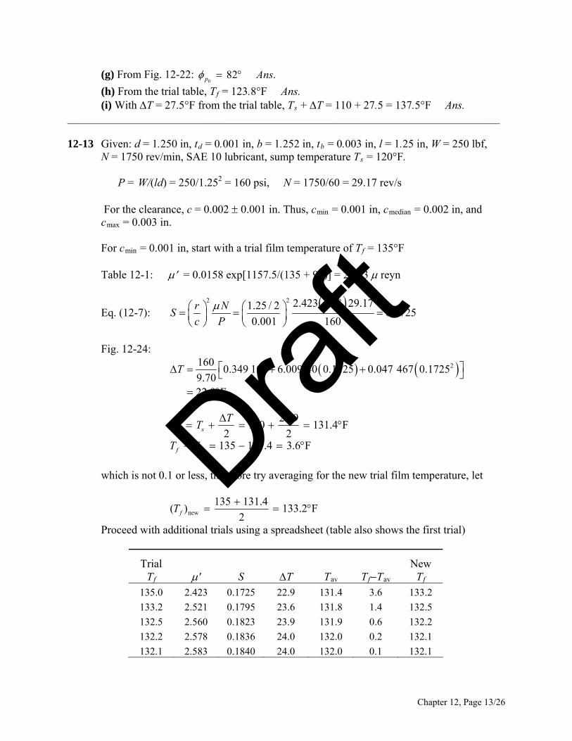
(g) From Fig. 12-22: 0
82 .p Ans
(h) From the trial tabl Ans. e, Tf = 123.8°F T = 110 + 27.5 = 137.5°F Ans.
_____
2-13 Given: d = 1.250 in, td = 0.001 in, b = 1.252 in, tb = 0.003 in, l = 1.25 in, W = 250 lbf,
P = W/(ld) = 250/1.25 = 160 psi, N = 1750/60 = 29.17 rev/s
For the clearance, c = 0.002 0.001 in. Thus, cmin = 0.001 in, cmedian = 0.002 in, and
For cmin = 0.001 in, start with a trial film temperature of Tf = 135°F
Table 12-1: = 0.0158 exp[1157.5/(135 + 95)] = 2.423 reyn
Eq. (12-7):
(i) With T = 27.5°F from the trial table, Ts +________________________________________________________________________ 1 N = 1750 rev/min, SAE 10 lubricant, sump temperature Ts = 120°F.
2 cmax = 0.003 in.
62 2 2.423 10 29.171.25 / 20.1725
0.001 160
r NS
c P
Fig. 12-24:
21600.349 109 6.009 40 0.1725 0.047 467 0.1725
9.7022.9 F
T
av
av
22.9120 131.4 F
2 2135 131.4 3.6 F
s
f
TT T
T T
which is not 0.1 or less, therefore try averaging for the new trial film temperature, let
new
135 131.4( ) 133.2 F
2fT
h additional trials using a spreadsheet (table also shows the first trial)
Trial ' S T Tav TfTav
New
Proceed wit
Tf Tf 1 2. 0.1 5 1 135.0 423 72 22.9 31.4 3.6 33.2
133.2 2.521 0.1795 23.6 131.8 1.4 132.5
132.5 2.560 0.1823 23.9 131.9 0.6 132.2
132.2 2.578 0.1836 24.0 132.0 0.2 132.1
132.1 2.583 0.1840 24.0 132.0 0.1 132.1
Chapter 12, Page 13/26
Draft
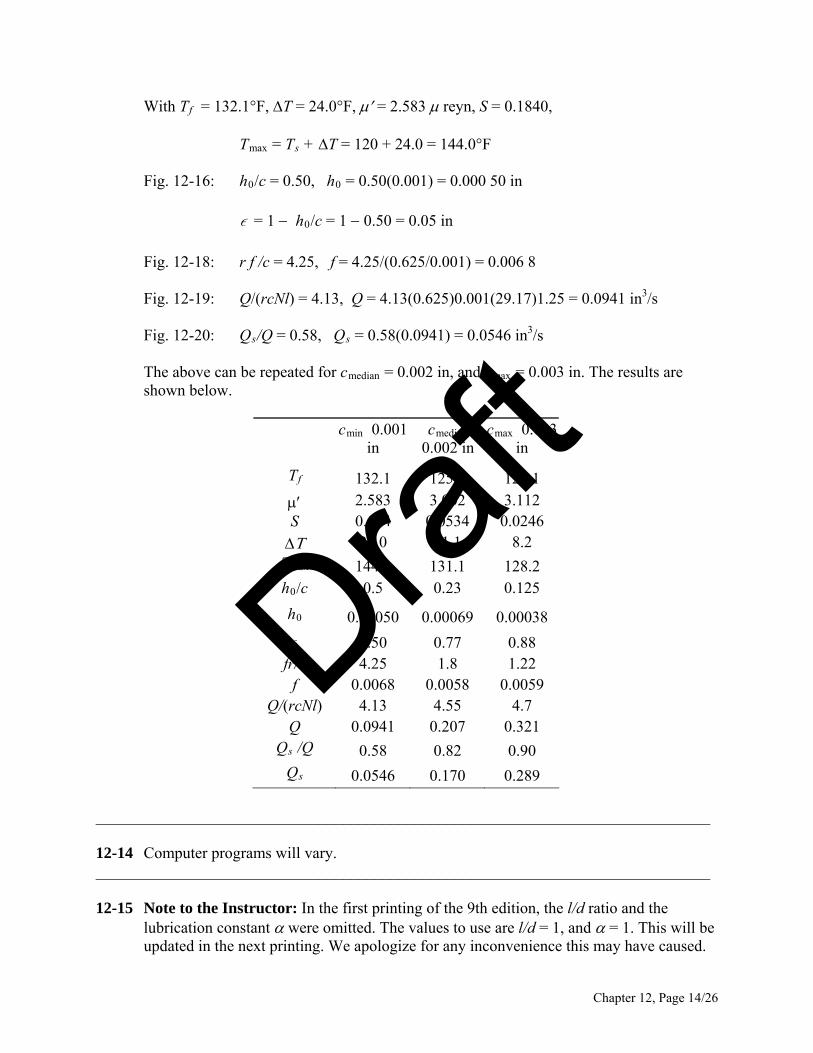
With Tf = 132.1°F, T = 24.0°F, = 2.583 reyn, S = 0.1840,
Tmax = Ts + T = 120 + 24.0 = 144.0°F
Fig. 12-16: h0/c = 0.50, h0 = 0.50(0.001) = 0.000 50 in
= 1 h0/c = 1 0.50 = 0.05 in
Fig. 12-18: r f /c = 4.25, f = 4.25/(0.625/0.001) = 0.006 8
Fig. 12-19: Q/(rcNl) = 4.13, Q = 4.13(0.625)0.001(29.17)1.25 = 0.0941 in3/s
Fig. 12-20: Qs/Q = 0.58, Qs = 0.58(0.0941) = 0.0546 in /s
The above can be repeated for cmedian = 0.002 in, and cmax = 0.003 in. The results are
cmin 0.001 cmedian
0.002 in cmax 0.003
3
shown below.
in in
T 132.1 125.6 124.1
1
0.00050 0.00069 0.00038
f
0.0068 0.0058 0.0059 Q/( )
0.0941 0.207 0.321 Q
0.0546 0.170
f
2.583 3.002 3.112 S 0.184 0.0534 0.0246
24.0 11.1 8.2 Tmax 144.0 131.1 28.2h0/c 0.5 0.23 0.125
h0
0.50 0.77 0.88 r/c 4.25 1.8 1.22 f rcNl 4.13 4.55 4.7 Q
s /Q 0.58 0.82 0.90 Qs 0.289
____________________________________________________________________________
2-14 Computer programs will vary. ______________________________________________
2-15 Note to the Instructor: In the first printing of the 9th edition, the l/d ratio and the ill be
_ 1_______________________________ 1
lubrication constant were omitted. The values to use are l/d = 1, and = 1. This wupdated in the next printing. We apologize for any inconvenience this may have caused.
Chapter 12, Page 14/26
Draft
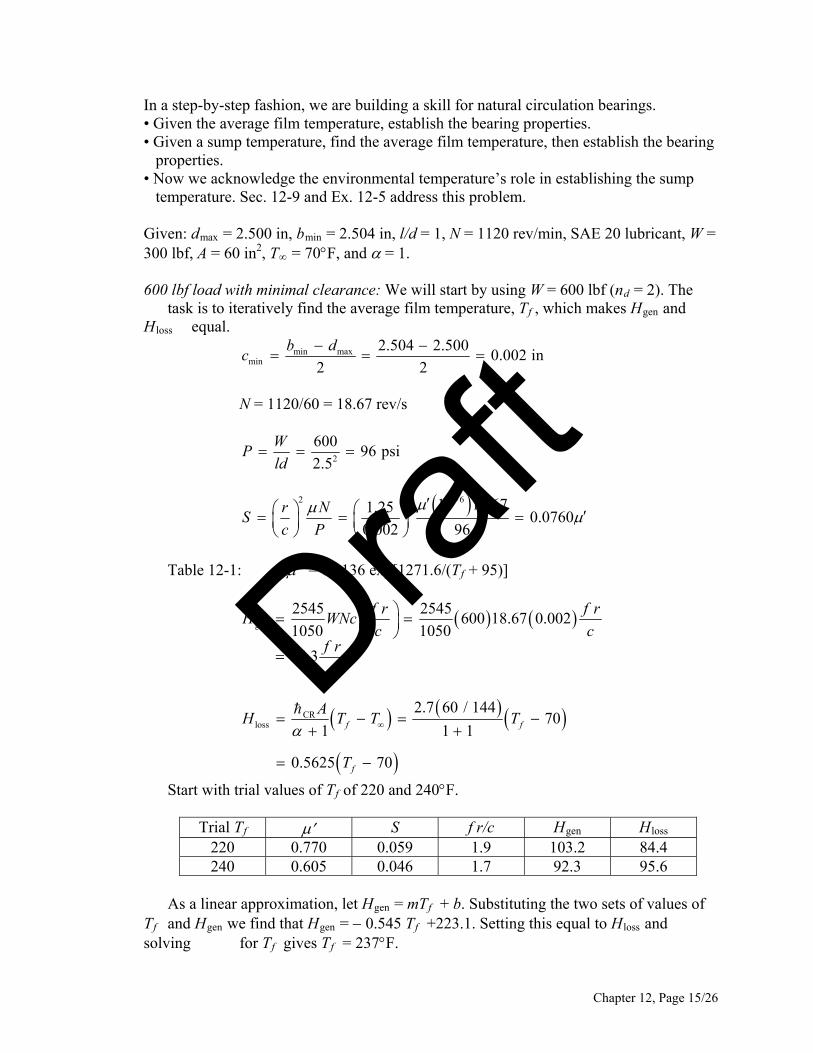
ring
nowledge the environmental temperature’s role in establishing the sump
Given: dmax = 2.500 in, bmin = 2.504 in, l/d = 1, N = 1120 rev/min, SAE 20 lubricant, W =
600 lbf load with minimal clearance: We will start by using W = 600 lbf (nd = 2). The
lo
In a step-by-step fashion, we are building a skill for natural circulation bearings. • Given the average film temperature, establish the bearing properties. • Given a sump temperature, find the average film temperature, then establish the bea properties. • Now we ack temperature. Sec. 12-9 and Ex. 12-5 address this problem.
300 lbf, A = 60 in2, T = 70F, and = 1.
task is to iteratively find the average film temperature, Tf , which makes Hgen and H ss equal.
min maxmin
2.504 2.5000.002 in
2 2
b dc
N = 1120/60 = 18.67 rev/s
2
60096 psi
2.5
WP
ld
62 2 10 18.671.250.0760
0.002 96
r NS
c P
Table 12-1: = 0.0136 exp[1271.6/(Tf + 95)]
gen
2545 2545600 18.67 0.002
1050 1050
54.3
f r fH WNc
c cf r
c
r
CRloss
2.7 60 / 14470
1 1 1
0.5625 70
f f
f
AH T T T
T
Start with trial values of Tf of 220 and 240F.
Trial Tf S f r/c Hgen Hloss
220 0.770 0. 9 05 1.9 103.2 84.4 240 0.605 0.046 1.7 92.3 95.6
As a linear approximation, let Hgen = mTf + b. Substituting the two sets of values of
f
T and Hgen we find that Hgen = 0.545 Tf +223.1. Setting this equal to Hloss and solving for Tf gives Tf = 237F.
Chapter 12, Page 15/26
Draft
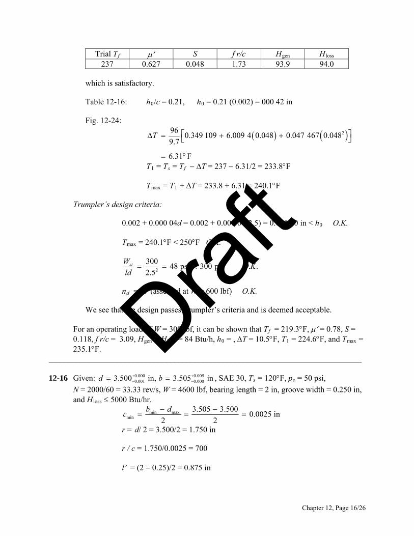
Tr S ial Tf f r/c Hgen Hloss
237 0.627 0. 8 04 1.73 93.9 94.0
which is satisfactory.
Table 12-16: h0/c = 0.21, h0 = 0.21 (0.002) = 000 42 in
Fig. 12-24:
2960.349 109 6.009 4 0.048 0.047 467 0.048
9.7
6.31 F
T
T1 = Ts = Tf T = 237 6.31/2 = 233.8F
Tmax = T1 + T = 233.8 + 6.31 = 240.1F
Trumpler’s design criteria:
0.002 + 0.000 04d = 0.002 + 0.000 04(2.5) = 0.000 30 in < h0 O.K.
Tmax = 240.1F < 250F O.K.
2
30048 psi 300 psi . .
2.5stW
O Kld
nd = 2 (assessed at W = 600 lbf) O.K.
We see that the design passes Trumpler’s criteria and is deemed acceptable.
For an operating load of W = 300 lbf, it can be shown that Tf = 219.3F, = 0.78, S =
_____________________________________________________________________________
2-16 Given: , SAE 30, Ts = 120F, ps = 50 psi,
0/60 = 33.33 rev/s, W = 4600 lbf, b 0.250 in,
0.118, f r/c = 3.09, Hgen = Hloss = 84 Btu/h, h0 = , T = 10.5F, T1 = 224.6F, and Tmax = 235.1F.
1 0.000 0.005
0.001 0.0003.500 in, 3.505 ind b
N = 200 earing length = 2 in, groove width =and Hloss 5000 Btu/hr.
minbc max
min
3.505 3.5000.0025 in
2 2
d
r = d/ 2 = 3.500/2 = 1.750 in
r / c = 1.750/0.0025 = 700
l = (2 0.25)/2 = 0.875 in
Chapter 12, Page 16/26
Draft
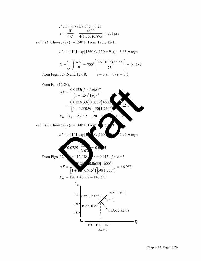
l / d = 0.875/3.500 = 0.25
4600W
P 751 psi4 4 1.750 0.875rl
Trial #1: Choose (Tf )1 = 150°F. From Table 12-1,
= 0.0141 exp[1360.0/(150 + 95)] = 3.63 µ reyn
2 62 3.63(10 )(33.33)
700 0.0789751
r NS
c P
From Figs. 12-16 and 12-18: = 0.9, f r/ c = 3.6
From Eq. (12-24),
2
2 4
2
2 4
0.012T
3( / )
1 1.5
0.0123 3.6 0.0789 460071.2 F
1 1.5(0.9) 50 1.750
s
f r c SW
p r
Tav = Ts + T / 2 = 120 + 71.2/2 = 155.6F
Trial #2: Choose (Tf )2 = 160°F. From Table 12-1
= 0.0141 exp[1360.0/(160 + 95)] = 2.92 µ reyn
2.92
0.0789 0.06353.63
S
From Figs. 12-16 and 12-18: = 0.915, f r/ c =3
20.0123 3 0.0635 46002 4
46.9 F1 1.5 0.915 50 1.750
T
Tav = 120 + 46.9/2 = 143.5F
Chapter 12, Page 17/26
Draft
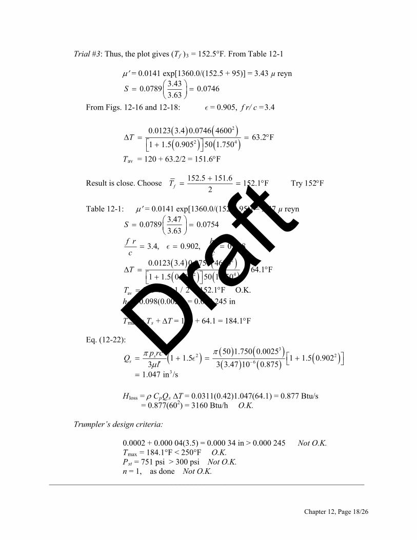
Trial #3: Thus, the plot gives (Tf )3 = 152.5°F. From Table 12-1
= 0.0141 exp[1360.0/(152.5 + 95)] = 3.43 µ reyn
3.430.0789 0.0746
3.63S
gs. 12-16 and 12-18: = 0.905, f r/ c =3.4
From Fi
2
2 4
0.0123 3.4 0.0746 460063.2 F
1 1.5 0.905 50 1.750T
Tav = 120 + 63.2/2 = 151.6F 152.5 151.6
152.1 F Try 152 F2fT
Result is close. Choose
Table 12-1: = 0.0141 exp[1360.0/(152 + 95)] = 3.47 µ reyn
0
2
2 4
av
3.470.0789 0.0754S
3.63
3.4, 0.902, 0.098
0.0123 3.4 0.0754 460064.1 F
1 1.5 0.902 50 1.750
120 64.1 / 2 152.1 F O.K.
f r h
c c
T
T
h0 = 0.098(0.0025) = 0.000 245 in
Tmax = Ts + T = 120 + 64.1 = 184.1F
Eq. (12-22):
6
3
1 1.5 1 1.5 0.9023 3 3.47 10 0.875
1.047 in /s
sQl
332 2
50 1.750 0.0025sp rc
Hloss = CpQs T = 0.0311(0.42)1.047(64.1) = 0.877 Btu/s
0.0002 + 0.000 04(3.5) = 0.000 34 in > 0.000 245 Not O.K.
.
__ __ ____________________________________
= 0.877(602) = 3160 Btu/h O.K. Trumpler’s design criteria: Tmax = 184.1°F < 250°F O.K. Pst = 751 psi > 300 psi Not O.K n = 1, as done Not O.K. ____ __________ _______________________
Chapter 12, Page 18/26
Draft
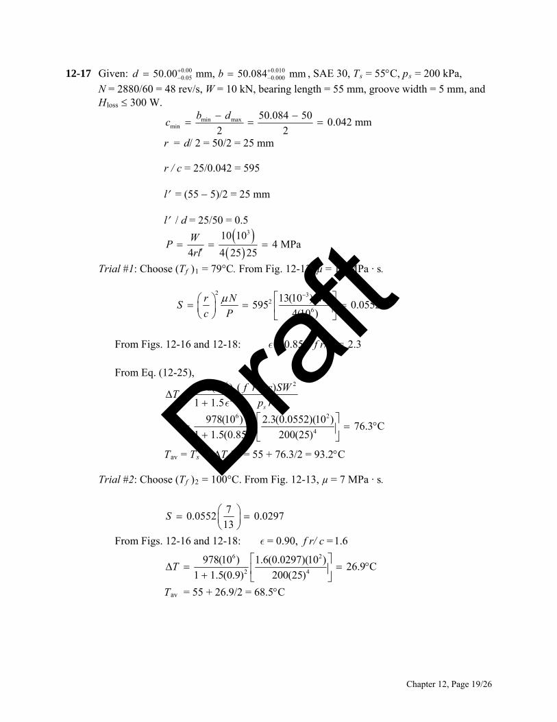
12-17 Given: 0.00 0.0100.05 0.00050.00 mm, 50.084 mmd b
, SAE 30, Ts = 55C, ps = 200 kPa,
N = 288 gth = 55 mm, groove width = 5 mm, 0/60 = 48 rev/s, W = 10 kN, bearing len and
Hloss 300 W.
min maxmin
50.084 500.042 mm
2 2
b dc
r = d/ 2 = 50/2 = 25 mm
r / c = 25/0.042 = 595
l = (55 5)/2 = 25 mm
l / d = 25/50 = 0.5
310 10W4 MPa
4 4 25 25P
rl
Trial #1: Choose (Tf )1 = 79°C. From Fig. 12-13, µ = 13 MPa · s.
2 32
6
13(10 )(48)595 0.0552
4(10 )
r NS
c P
From Figs. 12-16 and 12-18: = 0.85, f r/ c = 2.3
From Eq. (12-25),
6 2
2 4
6 2
2 4
978(1T
0 ) ( / )
1 1.5
978(10 ) 2.3(0.0552)(10 )76.3 C
1 1.5(0.85) 200(25)
s
f r c SW
p r
Tav = Ts + T / 2 = 55 + 76.3/2 = 93.2C
Trial #2: Choose (Tf )2 = 100°C. From Fig. 12-13, µ = 7 MPa · s.
7
0.0552 0.029713
S
From Figs. 12-16 and 12-18: = 0.90, f r/ c =1.6
6 2978(10 ) 1.6(0.0297)(10 ) 2 4
26.9 C1 1.5(0.9) 200(25)
T
Tav = 55 + 26.9/2 = 68.5C
Chapter 12, Page 19/26
Draft
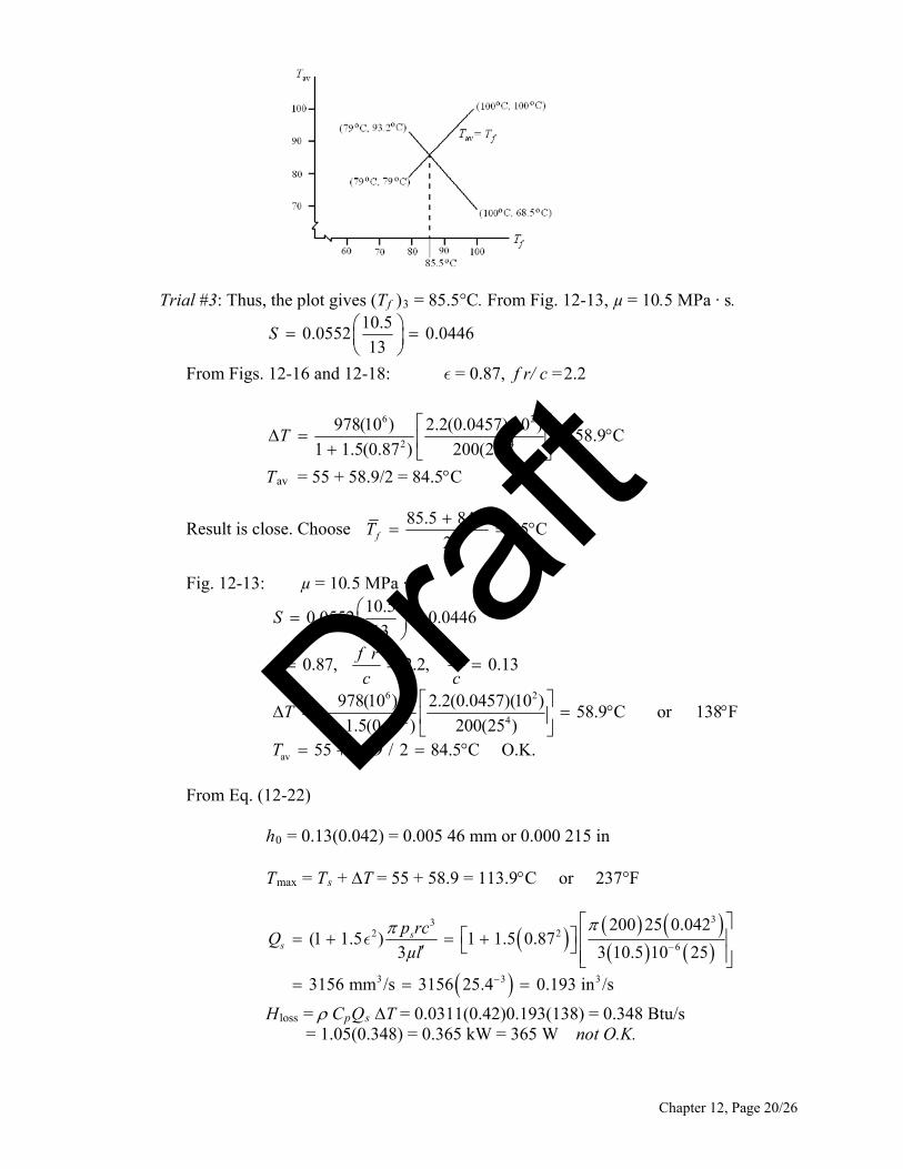
Trial #3: Thus, the plot gives (Tf )3 = 85.5°C. From Fig. 12-13, µ = 10.5 MPa · s.
10.50.0552 0.0446
13S
From Figs. 12-16 and 12-18: = 0.87, f r/ c =2.2
6 2
2 4
978(10 ) 2.2(0.0457)(10 )58.9 C
1 1.5(0.87 ) 200(25)T
Tav = 55 + 58.9/2 = 84.5C Result is close. Choose 85.5 84.5
85 C2fT
Fig. 12-13: µ = 10.5 MPa · s
0
6 2
2 4
av
10.50.0552 0.0446
13
0.87, 2.2, 0.13
978(10 ) 2.2(0.0457)(10 )58.9 C or 138 F
1 1.5(0.87 ) 200(25 )55 58.9 / 2 84.5 C O.K.
S
f r h
c c
T
T
From Eq. (12-22) h0 = 0.13(0.042) = 0.005 46 mm or 0.000 215 in Tmax = Ts + T = 55 + 58.9 = 113.9C or 237°F
332 2
6
3 3 3
200 25 0.042(1 1.5 ) 1 1.5 0.87
3 3 10.5 10 25
3156 mm /s 3156 25.4 0.193 in /s
ss
p rcQ
µl
Hloss = CpQs T = 0.0311(0.42)0.193(138) = 0.348 Btu/s = 1.05(0.348) = 0.365 kW = 365 W not O.K.
Chapter 12, Page 20/26
Draft
Trumpler’s design criteria: 0.0002 + 0.000 04(50/25.4) = 0.000 279 in > h0 Not O.K. Tmax = 237°F O.K. Pst = 4000 kPa or 581 psi > 300 psi Not O.K. n = 1, as done Not O.K. _____________________________________________________________________________ 12-18 So far, we’ve performed elements of the design task. Now let’s do it more completely. The values of the unilateral tolerances, tb and td , reflect the routine capabilities of the
bushing vendor and the in-house capabilities. While the designer has to live with these, his approach should not depend on them. They can be incorporated later.
First we shall find the minimum size of the journal which satisfies Trumpler’s constraint
of Pst ≤ 300 psi.
2
min
3002
300 2 / 600( / )
9001.73 in
2(300)(0.5)
st
WP
dlW W
dd l d l d
d
In this problem we will take journal diameter as the nominal value and the bushing bore
as a variable. In the next problem, we will take the bushing bore as nominal and the journal diameter as free.
To determine where the constraints are, we will set tb = td = 0, and thereby shrink the
design window to a point. We set d = 2.000 in b = d + 2cmin = d + 2c nd = 2 (This makes Trumpler’s nd ≤ 2 tight) and construct a table.
Chapter 12, Page 21/26
Draft
c b d *fT Tmax ho Pst Tmax n fom
0.0010 2.0020 2 215.50 312.0 -5.74 0.0011 2.0022 2 206.75 293.0 -6.06 0.0012 2.0024 2 198.50 277.0 -6.37 0.0013 2.0026 2 191.40 262.8 -6.66 0.0014 2.0028 2 185.23 250.4 -6.94 0.0015 2.0030 2 179.80 239.6 -7.20 0.0016 2.0032 2 175.00 230.1 -7.45 0.0017 2.0034 2 171.13 220.3 -7.65 0.0018 2.0036 2 166.92 213.9 -7.91 0.0019 2.0038 2 163.50 206.9 -8.12 0.0020 2.0040 2 160.40 200.6 -8.32
*Sample calculation for the first entry of this column. Iteration yields: 215.5 FfT
With 215.5 FfT , from Table 12-1
6 6
2 6
0.0136(10 )exp[1271.6 / (215.5 95)] 0.817(10 ) reyn900
3000 / 60 50 rev/s, 225 psi4
1 0.817(10 )(50)0.182
0.001 225
µ
N P
S
From Figs. 12-16 and 12-18: e = 0.7, f r/c = 5.5 Eq. (12–24):
2
2 4
av
0.0123(5.5)(0.182)(900 )191.6 F
[1 1.5(0.7 )](30)(1 )191.6 F
120 F 215.8 F 215.5 F2
FT
T
For the nominal 2-in bearing, the various clearances show that we have been in contact
with the recurving of (ho)min. The figure of merit (the parasitic friction torque plus the pumping torque negated) is best at c = 0.0018 in. For the nominal 2-in bearing, we will place the top of the design window at cmin = 0.002 in, and b = d + 2(0.002) = 2.004 in. At this point, add the b and d unilateral tolerances:
0.000 0.0030.001 0.0002.000 in, 2.004 ind b
Now we can check the performance at cmin , c , and cmax . Of immediate interest is the
fom of the median clearance assembly, 9.82, as compared to any other satisfactory bearing ensemble.
Chapter 12, Page 22/26
Draft
If a nominal 1.875 in bearing is possible, construct another table with tb = 0 and td = 0.
c b d fT Tmax ho Pst Tmax n fom
0.0020 1.879 1.875 157.2 194.30 7.36 0.0030 1.881 1.875 138.6 157.10 8.64 0.0035 1.882 1.875 133.5 147.10 9.05 0.0040 1.883 1.875 130.0 140.10 9.32 0.0050 1.885 1.875 125.7 131.45 9.59 0.0055 1.886 1.875 124.4 128.80 9.63 0.0060 1.887 1.875 123.4 126.80 9.64
The range of clearance is 0.0030 < c < 0.0055 in. That is enough room to fit in our
design window.
0.000 0.0030.001 0.0001.875 in, 1.881 ind b
The ensemble median assembly has a fom = 9.31. We just had room to fit in a design window based upon the (h0)min constraint. Further
reduction in nominal diameter will preclude any smaller bearings. A table constructed for a d = 1.750 in journal will prove this.
We choose the nominal 1.875-in bearing ensemble because it has the largest figure of
merit. Ans. _____________________________________________________________________________ 12-19 This is the same as Prob. 12-18 but uses design variables of nominal bushing bore b and
radial clearance c. The approach is similar to that of Prob. 12-18 and the tables will change slightly. In the
table for a nominal b = 1.875 in, note that at c = 0.003 in the constraints are “loose.” Set b = 1.875 in d = 1.875 2(0.003) = 1.869 in For the ensemble
0.003 0.0000.001 0.0011.875 in, 1.869 inb d
Analyze at cmin = 0.003, c = 0.004 in and cmax = 0.005 in At min loss0.003 in: 138.4, 3.160, 0.0297, 1035 Btu/hfc T µ S H and the
Trumpler conditions are met. At 0.004 in: 130 F,fc T = 3.872, S = 0.0205, Hloss = 1106 Btu/h, fom = 9.246
Chapter 12, Page 23/26
Draft
and the Trumpler conditions are O.K. At max 0.005 in: 125.68 F,fc T = 4.325, S = 0.014 66, Hloss = 1129 Btu/h
and the
Trumpler conditions are O.K. The ensemble figure of merit is slightly better; this bearing is slightly smaller. The
lubricant cooler has sufficient capacity. _____________________________________________________________________________ 12-20 Table 12-1: ( reyn) = 0 (106) exp [b / (T + 95)] b and T in F The conversion from reyn to mPas is given on p. 620. For a temperature of C degrees
Celsius, T = 1.8 C + 32. Substituting into the above equation gives (mPas) = 6.89 0 (106) exp [b / (1.8 C + 32+ 95)] = 6.89 0 (106) exp [b / (1.8 C + 127)] Ans. For SAE 50 oil at 70C, from Table 12-1, 0 = 0.0170 (106) reyn, and b = 1509.6F.
From the equation, = 6.89(0.0170) 106(106) exp {1509.6/[1.8(70) + 127]} = 45.7 mPas Ans. From Fig. 12-13, = 39 mPas Ans. The figure gives a value of about 15 % lower than the equation. _____________________________________________________________________________ 12-21 Originally
0.000 0.0030.001 0.0002.000 in, 2.005 ind b
Doubled,
0.000 0.0060.002 0.0004.000 in, 4.010 ind b
The radial load quadrupled to 3600 lbf when the analyses for parts (a) and (b) were
carried out. Some of the results are:
Part c S Tf f r/c Qs h0 /c e H loss h0 Trumpler
h0 f (a) 0.007 3.416 0.0310 135.1 0.1612 6.56 0.1032 0.897 9898 0.000 722 0.000 360 0.005 67 (b) 0.0035 3.416 0.0310 135.1 0.1612 0.870 0.1032 0.897 1237 0.000 361 0.000 280 0.005 67
The side flow Qs differs because there is a c3 term and consequently an 8-fold increase. Hloss is related by a 9898/1237 or an 8-fold increase. The existing h0 is related by a 2-fold
increase. Trumpler’s (h0)min is related by a 1.286-fold increase.
Chapter 12, Page 24/26
Draft
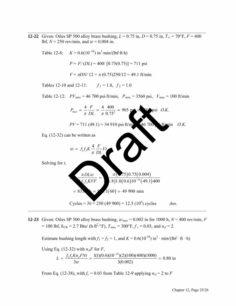
_____________________________________________________________________________ 12-22 Given: Oiles SP 500 alloy brass bushing, L = 0.75 in, D = 0.75 in, T = 70F, F = 400
lbf, N = 250 rev/min, and w = 0.004 in. Table 12-8: K = 0.6(1010) in3min/(lbffth) P = F/ (DL) = 400/ [0.75(0.75)] = 711 psi V = DN/ 12 = (0.75)250/12 = 49.1 ft/min Tables 12-10 and 12-11: f 1 = 1.8, f 2 = 1.0 Table 12-12: PVmax = 46 700 psift/min, Pmax = 3560 psi, Vmax = 100 ft/min
max 2
4 4 400905 psi 3560 psi . .
0.75
FP O
DLK
PV = 711 (49.1) = 34 910 psift/min < 46 700 psift/min O.K. Eq. (12-32) can be written as
1 2
4 Ff f K Vt
DLw
Solving for t,
101 2
0.75 0.75 0.004
4 4 1.8 1.0 0.6 10 49.1 400
833.1 h 833.1 60 49 900 min
DLt
f f KVF
w
Cycles = Nt = 250 (49 900) = 12.5 (106) cycles Ans. _____________________________________________________________________________ 12-23 Given: Oiles SP 500 alloy brass bushing, wmax = 0.002 in for 1000 h, N = 400 rev/min, F
= 100 lbf, CR = 2.7 Btu/ (hft2F), Tmax = 300F, f s = 0.03, and nd = 2.
Estimate bushing length with f1 = f2 = 1, and K = 0.6(10-10) in3 · min/(lbf · ft · h) Using Eq. (12-32) with ndF for F,
10
1 2 1(1)(0.6)(10 )(2)(100)(400)(1000)0.80 in
3 3(0.002)df f Kn FNt
L
w
From Eq. (12-38), with fs = 0.03 from Table 12-9 applying nd = 2 to F
Chapter 12, Page 25/26
Draft
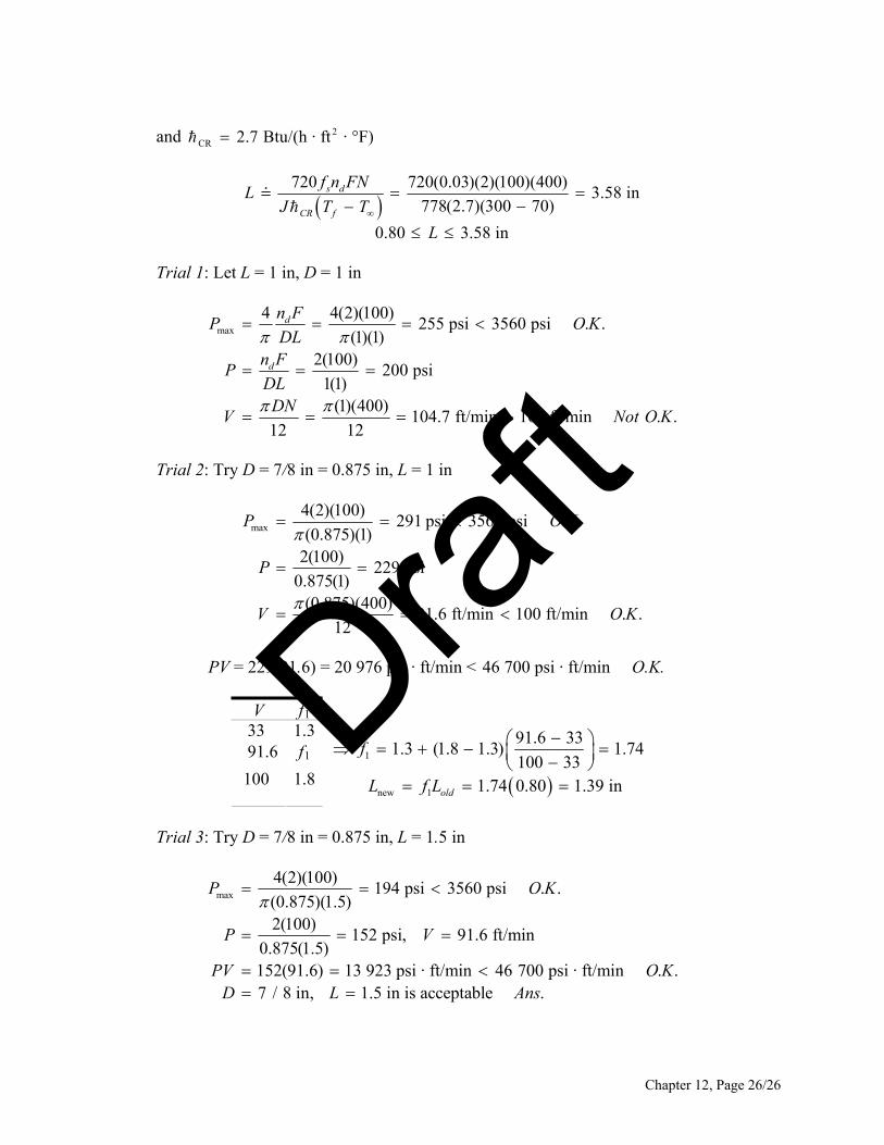
and 2
CR 2.7 Btu/(h · ft · °F)
720 720(0.03)(2)(100)(400)
3.58 in778(2.7)(300 70)
0.80 3.58 in
s d
CR f
f n FNL
J T T
L
Trial 1: Let L = 1 in, D = 1 in
max
4 4(2)(100)255 psi 3560 psi . .
(1)(1)2(100)
200 psi1(1)
(1)(400)104.7 ft/min 100 ft/min . .
12 12
d
d
n FP O
DLn F
PDLDN
V N
K
ot O K
Trial 2: Try D = 7/8 in = 0.875 in, L = 1 in
max
4(2)(100)291 psi 3560 psi . .
(0.875)(1)2(100)
229 psi0.875(1)
(0.875)(400)91.6 ft/min 100 ft/min . .
12
P O
P
V O
K
K
PV = 229(91.6) = 20 976 psi · ft/min < 46 700 psi · ft/min O.K.
V f1 33 1.3 91.6 f1
100 1.8 1
new 1
91.6 331.3 (1.8 1.3) 1.74
100 33 1.74 0.80 1.39 inold
f
L f L
Trial 3: Try D = 7/8 in = 0.875 in, L = 1.5 in
max
4(2)(100)194 psi 3560 psi . .
(0.875)(1.5)2(100)
152 psi, 91.6 ft/min0.875(1.5)152(91.6) 13 923 psi · ft/min 46 700 psi · ft/min . .7 / 8 in, 1.5 in is acceptable .
P O
P V
PV O KD L Ans
K
Chapter 12, Page 26/26
Draft

Chapter 12, Page 27/26
Suggestion: Try smaller sizes.
Draft
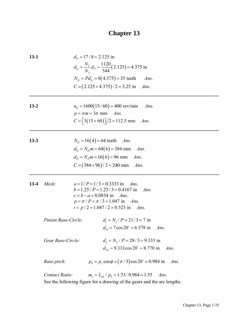
Chapter 13
13-1 17 / 8 2.125 inPd
2
3
11202.125 4.375 in
544G P
Nd d
N
8 4.375 35 teeth .G GN Pd An s
ns
ns
s
2.125 4.375 / 2 3.25 in .C A ______________________________________________________________________________ 13-2 1600 15 / 60 400 rev/min .Gn A 3 mm .p m An
3 15 60 2 112.5 mm .C A ns
ns
______________________________________________________________________________ 13-3 16 4 64 teeth .GN A
64 6 384 mm .G Gd N m An s
16 6 96 mm .P Pd N m An s
ns
sns
s
384 96 / 2 240 mm .C A ______________________________________________________________________________ 13-4 Mesh: 1/ 1/ 3 0.3333 in .a P An 1.25 / 1.25 / 3 0.4167 in .b P A 0.0834 in .c b a Ans / / 3 1.047 in .p P An / 2 1.047 / 2 0.523 in .t p Ans Pinion Base-Circle: 1 1 / 21/ 3 7 id N P n
1 7 cos 20 6.578 in .bd A ns
Gear Base-Circle: 2 2 / 28 / 3 9.333 ind N P
2 9.333cos 20 8.770 in .bd A ns
Base pitch: cos / 3 cos 20 0.984 in .b cp p A ns
Contact Ratio: / 1.53 / 0.984 1.55 .c ab bm L p Ans See the following figure for a drawing of the gears and the arc lengths.
Chapter 13, Page 1/35
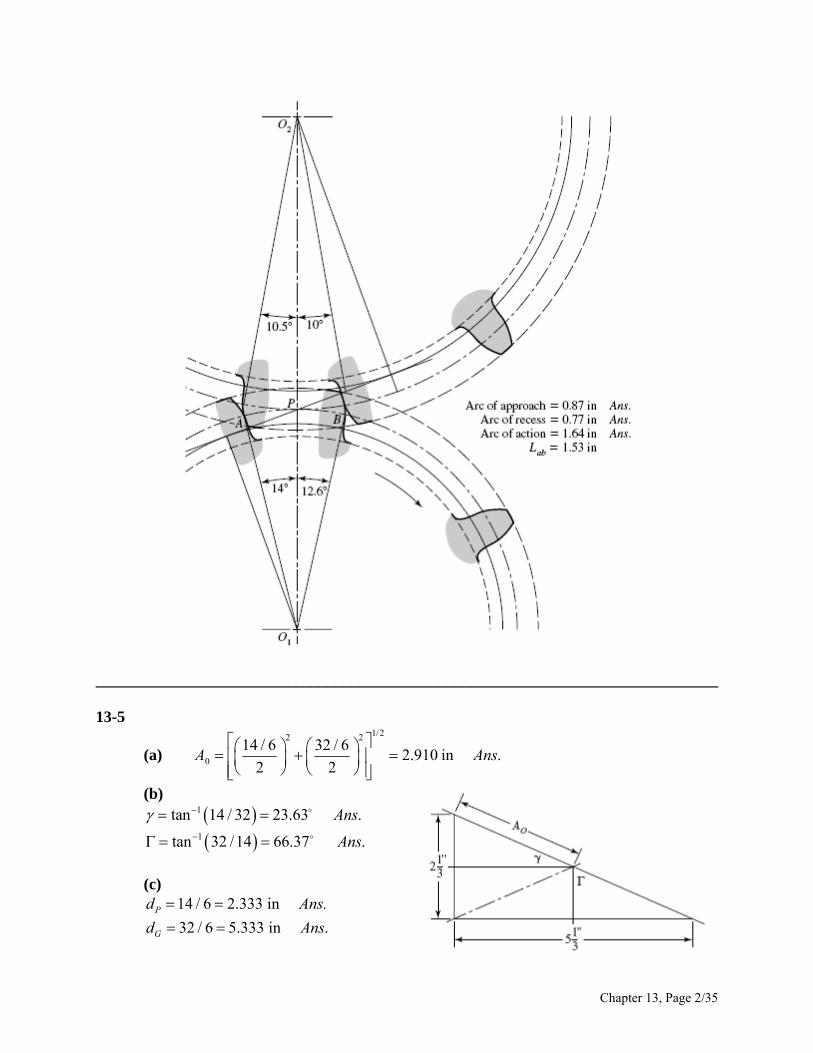
______________________________________________________________________________ 13-5
(a)
1/22 2
0
14 / 6 32 / 62.910 in .
2 2A Ans
(b) 1tan 14 / 32 23.63 .Ans
1tan 32 /14 66.37 .Ans
(c) Ans. 14 / 6 2.333 inPd 32 / 6 5.333 in .Gd A ns
Chapter 13, Page 2/35
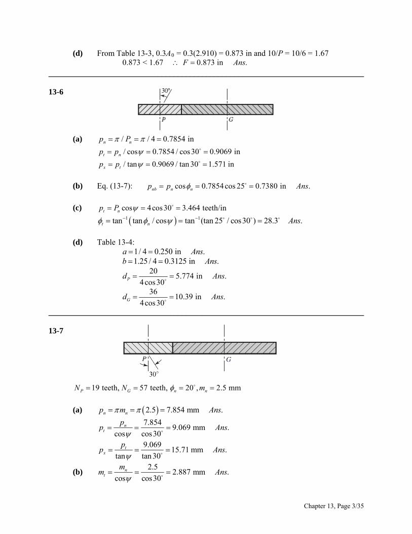
(d) From Table 13-3, 0.3A0 = 0.3(2.910) = 0.873 in and 10/P = 10/6 = 1.67 0.873 < 1.67 0.873 in .F Ans ______________________________________________________________________________ 13-6
(a) / / 4 0.7854 inn np P
/ cos 0.7854 / cos30 0.9069 int np p
/ tan 0.9069 / tan 30 1.571 inx tp p
(b) Eq. (13-7): cos 0.7854cos 25 0.7380 in .nb n np p A ns
(c) cos 4cos30 3.464 teeth/int np P
1 1tan tan / cos tan (tan 25 / cos30 ) 28.3 .t n Ans
(d) Table 13-4: 1/ 4 0.250 in .a A ns
ns 1.25 / 4 0.3125 in .b A
20
5.774 in .4cos30Pd A ns
36
10.39 in .4cos30Gd A ns
______________________________________________________________________________ 13-7
19 teeth, 57 teeth, 20 , 2.5 mmP G n nN N m
(a) 2.5 7.854 mm .n np m A ns
7.854
9.069 mm .cos cos30
nt
pp Ans
9.069
15.71 mm .tan tan 30
tx
pp Ans
(b) 2.5
2.887 mm .cos cos30
nt
mm A
ns
Chapter 13, Page 3/35
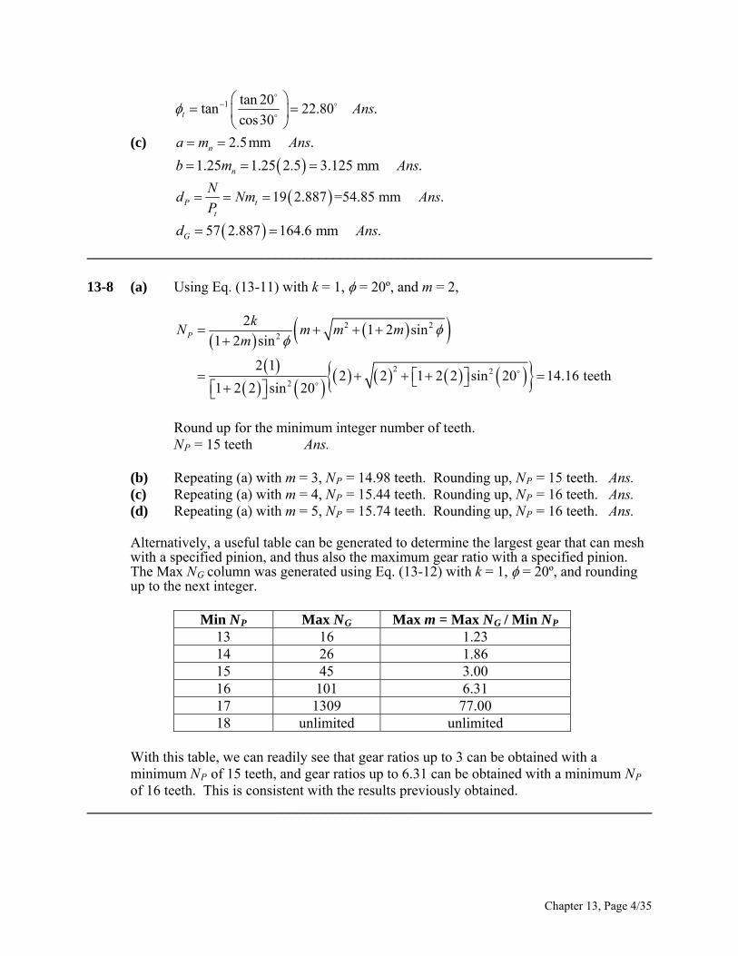
1 tan 20tan 22.80 .
cos30t Ans
(c) 2.5mm .na m Ans
1.25 1.25 2.5 3.125 mm .nb m A ns
19 2.887 =54.85 mm .P tt
Nd Nm
P Ans
57 2.887 164.6 mm .Gd A ns
______________________________________________________________________________ 13-8 (a) Using Eq. (13-11) with k = 1, = 20º, and m = 2,
2 22
2 2
2
21 2 sin
1 2 sin
2 12 2 1 2 2 sin 20 14.16 teeth
1 2 2 sin 20
P
kN m m m
m
Round up for the minimum integer number of teeth.
NP = 15 teeth Ans. (b) Repeating (a) with m = 3, NP = 14.98 teeth. Rounding up, NP = 15 teeth. Ans. (c) Repeating (a) with m = 4, NP = 15.44 teeth. Rounding up, NP = 16 teeth. Ans. (d) Repeating (a) with m = 5, NP = 15.74 teeth. Rounding up, NP = 16 teeth. Ans.
Alternatively, a useful table can be generated to determine the largest gear that can mesh with a specified pinion, and thus also the maximum gear ratio with a specified pinion. The Max NG column was generated using Eq. (13-12) with k = 1, = 20º, and rounding up to the next integer.
Min NP Max NG Max m = Max NG / Min NP
13 16 1.23 14 26 1.86 15 45 3.00 16 101 6.31 17 1309 77.00 18 unlimited unlimited
With this table, we can readily see that gear ratios up to 3 can be obtained with a minimum NP of 15 teeth, and gear ratios up to 6.31 can be obtained with a minimum NP of 16 teeth. This is consistent with the results previously obtained.
______________________________________________________________________________
Chapter 13, Page 4/35
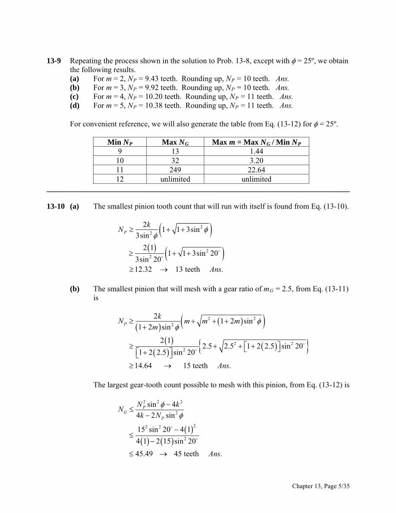
13-9 Repeating the process shown in the solution to Prob. 13-8, except with = 25º, we obtain
the following results. (a) For m = 2, NP = 9.43 teeth. Rounding up, NP = 10 teeth. Ans. (b) For m = 3, NP = 9.92 teeth. Rounding up, NP = 10 teeth. Ans. (c) For m = 4, NP = 10.20 teeth. Rounding up, NP = 11 teeth. Ans. (d) For m = 5, NP = 10.38 teeth. Rounding up, NP = 11 teeth. Ans.
For convenient reference, we will also generate the table from Eq. (13-12) for = 25º.
Min NP Max NG Max m = Max NG / Min NP 9 13 1.44 10 32 3.20 11 249 22.64 12 unlimited unlimited
______________________________________________________________________________ 13-10 (a) The smallest pinion tooth count that will run with itself is found from Eq. (13-10).
22
22
21 1 3sin
3sin
2 11 1 3sin 20
3sin 2012.32 13 teeth .
P
kN
Ans
(b) The smallest pinion that will mesh with a gear ratio of mG = 2.5, from Eq. (13-11)
is
2 22
2 2
2
21 2 sin
1 2 sin
2 12.5 2.5 1 2 2.5 sin 20
1 2 2.5 sin 20
14.64 15 teeth .
P
kN m m m
m
Ans
The largest gear-tooth count possible to mesh with this pinion, from Eq. (13-12) is
2 2 2
2
22 2
2
sin 4
4 2 sin
15 sin 20 4 1
4 1 2 15 sin 20
45.49 45 teeth .
PG
P
N kN
k N
Ans
Chapter 13, Page 5/35
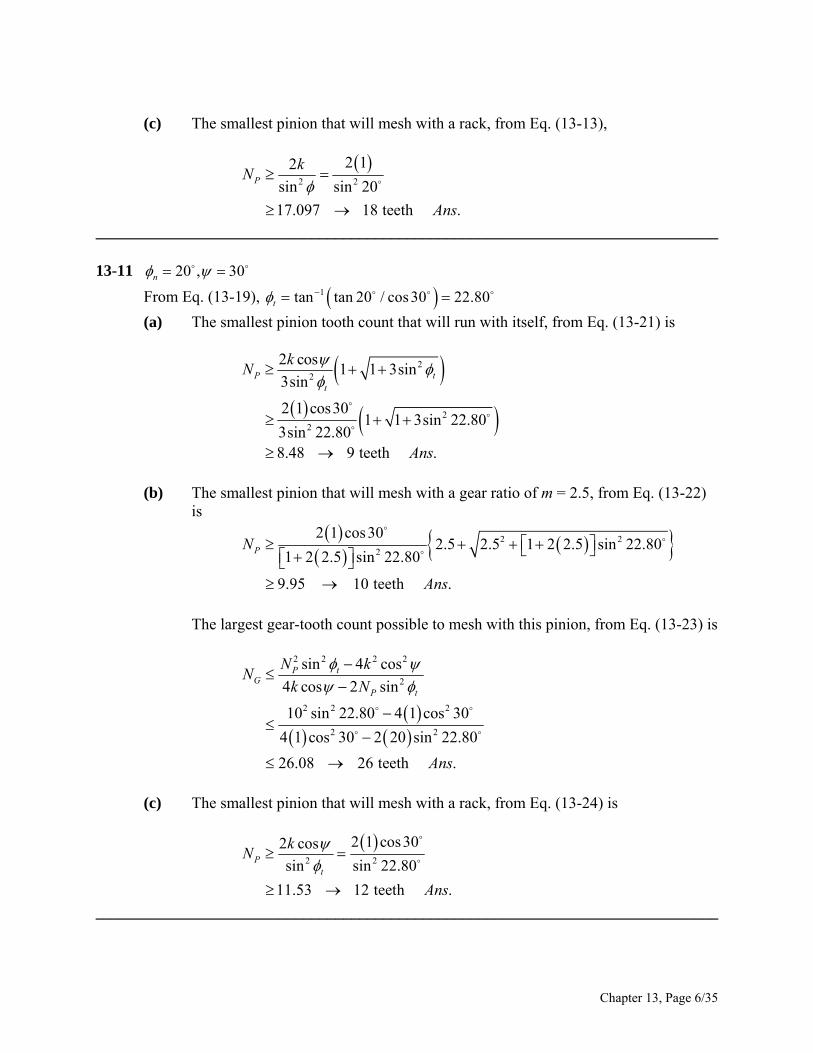
(c) The smallest pinion that will mesh with a rack, from Eq. (13-13),
2 2
2 12
sin sin 20
17.097 18 teeth .
P
kN
Ans
______________________________________________________________________________ 13-11 20 , 30n
From Eq. (13-19), 1tan tan 20 / cos30 22.80t
(a) The smallest pinion tooth count that will run with itself, from Eq. (13-21) is
22
22
2 cos1 1 3sin
3sin
2 1 cos301 1 3sin 22.80
3sin 22.808.48 9 teeth .
P tt
kN
Ans
(b) The smallest pinion that will mesh with a gear ratio of m = 2.5, from Eq. (13-22)
is
2 2
2
2 1 cos302.5 2.5 1 2 2.5 sin 22.80
1 2 2.5 sin 22.80
9.95 10 teeth .
PN
Ans
The largest gear-tooth count possible to mesh with this pinion, from Eq. (13-23) is
2 2 2 2
2
2 2 2
2 2
sin 4 cos
4 cos 2 sin
10 sin 22.80 4 1 cos 30
4 1 cos 30 2 20 sin 22.80
26.08 26 teeth .
P tG
P t
N kN
k N
Ans
(c) The smallest pinion that will mesh with a rack, from Eq. (13-24) is
2 2
2 1 cos302 cos
sin sin 22.80
11.53 12 teeth .
Pt
kN
Ans
______________________________________________________________________________
Chapter 13, Page 6/35
13-12 From Eq. (13-19), 1 1tan tan 20tan tan 22.796
cos cos30n
t
Program Eq. (13-23) on a computer using a spreadsheet or code, and increment NP. The first value of NP that can be doubled is NP = 10 teeth, where NG ≤ 26.01 teeth. So NG = 20 teeth will work. Higher tooth counts will work also, for example 11:22, 12:24, etc.
Use NP = 10 teeth, NG = 20 teeth Ans. Note that the given diametral pitch (tooth size) is not relevant to the interference problem. ______________________________________________________________________________
13-13 From Eq. (13-19), 1 1tan tan 20tan tan 27.236
cos cos 45n
t
Program Eq. (13-23) on a computer using a spreadsheet or code, and increment NP. The first value of NP that can be doubled is NP = 6 teeth, where NG ≤ 17.6 teeth. So NG = 12 teeth will work. Higher tooth counts will work also, for example 7:14, 8:16, etc.
Use NP = 6 teeth, NG = 12 teeth Ans. ______________________________________________________________________________ 13-14 The smallest pinion that will operate with a rack without interference is given by Eq. (13-
13).
2
2
sinP
kN
Setting k = 1 for full depth teeth, NP = 9 teeth, and solving for ,
1 1 2 12sin sin 28.126 .
9P
kAns
N
______________________________________________________________________________ 13-15
(a) Eq. (13-3): 3 mm .n np m Ans
Eq. (13-16): / cos 3 / cos 25 10.40 mm .t np p A ns
Eq. (13-17): / tan 10.40 / tan 25 22.30 mm .x tp p A ns
(b) Eq. (13-3): / 10.40 / 3.310 mm .t tm p Ans
Chapter 13, Page 7/35
Eq. (13-19): 1 1tan tan 20tan tan 21.88 .
cos cos 25n
t Ans
(c) Eq. (13-2): dp = mt Np = 3.310 (18) = 59.58 mm Ans. Eq. (13-2): dG = mt NG = 3.310 (32) = 105.92 mm Ans.
______________________________________________________________________________ 13-16 (a) Sketches of the figures are shown to
determine the axial forces by inspection.
The axial force of gear 2 on shaft a is in the negative z-direction. The axial force of gear 3 on shaft b is in the positive z-direction. Ans.
The axial force of gear 4 on shaft b is in the positive z-direction. The axial force of gear 5 on shaft c is in the negative z-direction. Ans.
(b) 5
12 16700 77.78 rev/min ccw .
48 36cn n Ans
(c) 2 12 / 12cos30 1.155 inPd
3 48 / 12cos30 4.619 inGd
1.155 4.619
2.887 in .2abC A
ns
ns
4 16 / 8cos 25 2.207 inPd
5 36 / 8cos 25 4.965 inGd
3.586 in .bcC A______________________________________________________________________________
13-17 20 8 20 4
40 17 60 51e
400 47.06 rev/min cw .
51dn A ns
______________________________________________________________________________
13-18 6 18 20 3 3
10 38 48 36 304e
9
31200 11.84 rev/min cw .
304n A ns
______________________________________________________________________________
Chapter 13, Page 8/35
13-19 (a) 12 1540 162 rev/min cw about . .
40 1cn x Ans
(b) 12 / 8cos 23 1.630 inPd
40 / 8cos 23 5.432 inGd
3.531 in .2
P Gd dAns
(c) 32
8 in at the large end of the teeth. .4
d A ns
______________________________________________________________________________ 13-20 Applying Eq. (13-30), e = (N2 / N3) (N4 / N5) = 45. For an exact ratio, we will choose to
factor the train value into integers, such that
N2 / N3 = 9 (1) N4 / N5 = 5 (2)
Assuming a constant diametral pitch in both stages, the geometry condition to satisfy the in-line requirement of the compound reverted configuration is N2 + N3 = N4 + N5 (3) With three equations and four unknowns, one free choice is available. It is necessary that all of the unknowns be integers. We will use a normalized approach to find the minimum free choice to guarantee integers; that is, set the smallest gear of the largest stage to unity, thus N3 = 1. From (1), N2 = 9. From (3), N2 + N3 = 9 + 1 = 10 = N4 + N5 Substituting N4 = 5 N5 from (2) gives
10 = 5 N5 + N5 = 6 N5
N5 = 10 / 6 = 5 / 3
To eliminate this fraction, we need to multiply the original free choice by a multiple of 3. In addition, the smallest gear needs to have sufficient teeth to avoid interference. From Eq. (13-11) with k = 1, = 20°, and m = 9, the minimum number of teeth on the pinion to avoid interference is 17. Therefore, the smallest multiple of 3 greater than 17 is 18. Setting N3 = 18 and repeating the solution of equations (1), (2), and (3) yields N2 = 162 teeth N3 = 18 teeth N4 = 150 teeth N5 = 30 teeth Ans.
______________________________________________________________________________
Chapter 13, Page 9/35
13-21 The solution to Prob. 13-20 applies up to the point of determining the minimum number of teeth to avoid interference. From Eq. (13-11), with k = 1, = 25°, and m = 9, the minimum number of teeth on the pinion to avoid interference is 11. Therefore, the smallest multiple of 3 greater than 11 is 12. Setting N3 = 12 and repeating the solution of equations (1), (2), and (3) yields N2 = 108 teeth N3 = 12 teeth N4 = 100 teeth N5 = 20 teeth Ans.
______________________________________________________________________________ 13-22 Applying Eq. (13-30), e = (N2 / N3) (N4 / N5) = 30. For an exact ratio, we will choose to
factor the train value into integers, such that
N2 / N3 = 6 (1) N4 / N5 = 5 (2)
Assuming a constant diametral pitch in both stages, the geometry condition to satisfy the in-line requirement of the compound reverted configuration is N2 + N3 = N4 + N5 (3) With three equations and four unknowns, one free choice is available. It is necessary that all of the unknowns be integers. We will use a normalized approach to find the minimum free choice to guarantee integers; that is, set the smallest gear of the largest stage to unity, thus N3 = 1. From (1), N2 = 6. From (3), N2 + N3 = 6 + 1 = 7 = N4 + N5 Substituting N4 = 5 N5 from (2) gives
7 = 5 N5 + N5 = 6 N5
N5 = 7 / 6
To eliminate this fraction, we need to multiply the original free choice by a multiple of 6. In addition, the smallest gear needs to have sufficient teeth to avoid interference. From Eq. (13-11) with k = 1, = 20°, and m = 6, the minimum number of teeth on the pinion to avoid interference is 16. Therefore, the smallest multiple of 3 greater than 16 is 18. Setting N3 = 18 and repeating the solution of equations (1), (2), and (3) yields N2 = 108 teeth N3 = 18 teeth N4 = 105 teeth N5 = 21 teeth Ans.
______________________________________________________________________________
Chapter 13, Page 10/35
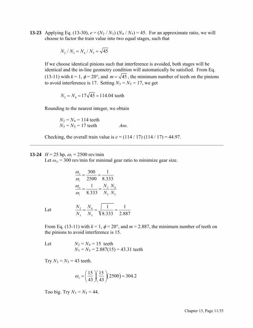
13-23 Applying Eq. (13-30), e = (N2 / N3) (N4 / N5) = 45. For an approximate ratio, we will choose to factor the train value into two equal stages, such that
2 3 4 5/ /N N N N 45
If we choose identical pinions such that interference is avoided, both stages will be identical and the in-line geometry condition will automatically be satisfied. From Eq.
(13-11) with k = 1, = 20°, and 45m , the minimum number of teeth on the pinions to avoid interference is 17. Setting N3 = N5 = 17, we get
2 4 17 45 114.04 teethN N
Rounding to the nearest integer, we obtain N2 = N4 = 114 teeth N3 = N5 = 17 teeth Ans. Checking, the overall train value is e = (114 / 17) (114 / 17) = 44.97.
______________________________________________________________________________ 13-24 H = 25 hp, i = 2500 rev/min Let ωo = 300 rev/min for minimal gear ratio to minimize gear size.
300 1
2500 8.333o
i
2 4
3 5
1
8.333o
i
N N
N N
Let 2 4
3 5
1 1
8.333 2.887
N N
N N
From Eq. (13-11) with k = 1, = 20°, and m = 2.887, the minimum number of teeth on the pinions to avoid interference is 15.
Let N2 = N4 = 15 teeth N3 = N5 = 2.887(15) = 43.31 teeth Try N3 = N5 = 43 teeth.
15 152500 304.2
43 43o
Too big. Try N3 = N5 = 44.
Chapter 13, Page 11/35
15 152500 290.55 rev/min
44 44o
N2 = N4 = 15 teeth, N3 = N5 = 44 teeth Ans. ______________________________________________________________________________ 13-25 (a) The planet gears act as keys and the wheel speeds are the same as that of the ring
gear. Thus, 3 900 16 / 48 300 rev/min .An n Ans
(b) 5 60, , 1F Ln n n n e
6 3001
0 300
n
6300 300n 6 600 rev/min .n A ns
(c) The wheel spins freely on icy surfaces, leaving no traction for the other wheel.
The car is stalled. Ans. ______________________________________________________________________________ 13-26 (a) The motive power is divided equally among four wheels instead of two. (b) Locking the center differential causes 50 percent of the power to be applied to the
rear wheels and 50 percent to the front wheels. If one of the rear wheels rests on a slippery surface such as ice, the other rear wheel has no traction. But the front wheels still provide traction, and so you have two-wheel drive. However, if the rear differential is locked, you have 3-wheel drive because the rear-wheel power is now distributed 50-50.
______________________________________________________________________________ 13-27 Let gear 2 be first, then nF = n2 = 0. Let gear 6 be last, then nL = n6 = –12 rev/min.
20 16 16
30 34 51L A
F A
n ne
n n
160 1
51A An n 2
12
17.49 rev/min (negative indicates cw) .35 / 51An A
ns
______________________________________________________________________________ 13-28 Let gear 2 be first, then nF = n2 = 0 rev/min. Let gear 6 be last, then nL = n6 = 85 rev/min.
Chapter 13, Page 12/35
20 16 16
30 34 51L A
F A
n ne
n n
160 85
51A An n
16
8551A An n
16
1 851An
5
85
123.9 rev/min16
151
An
The positive sign indicates the same direction as n6. 123.9 rev/min ccw .An Ans
______________________________________________________________________________ 13-29 The geometry condition is 5 2 3/ 2 / 2d d d 4d . Since all the gears are meshed, they
will all have the same diametral pitch. Applying d = N / P,
5 2 3/ (2 ) / (2 ) / /N P N P N P N 4 P
5 2 3 42 2 12 2 16 2 12 68 teeth .N N N N Ans
Let gear 2 be first, nF = n2 = 320 rev/min. Let gear 5 be last, nL = n5 = 0 rev/min.
12 16 12 3
16 12 68 17L A
F A
n ne
n n
17320 0
3A An n
3320 68.57 rev/min
14An
The negative sign indicates opposite of n2. 68.57 rev/min cw .An Ans
______________________________________________________________________________ 13-30 Let nF = n2, then nL = n7 = 0.
5
5
20 16 360.5217
16 30 46L
F
n ne
n n
5
5
00.5217
10
n
n
Chapter 13, Page 13/35
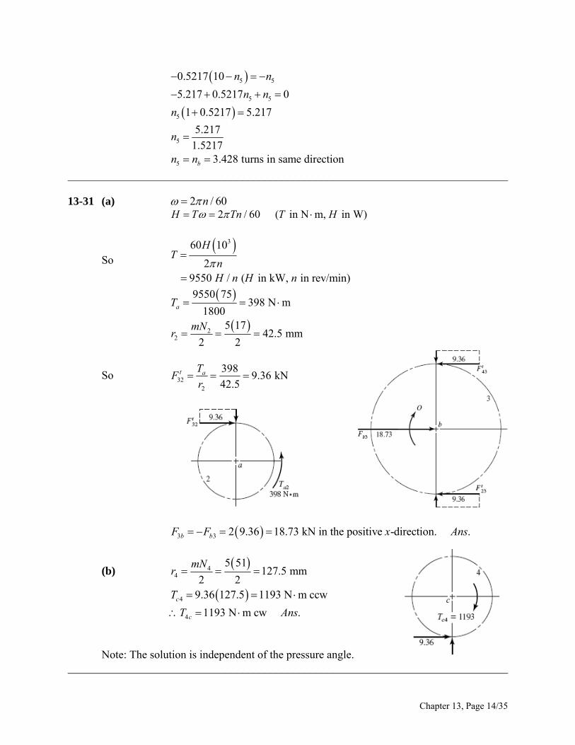
5 50.5217 10 n n
5 55.217 0.5217 0n n
5 1 0.5217 5.217n
5
5.217
1.5217n
5 3.428 turns in same directionbn n ______________________________________________________________________________ 13-31 (a) 2 / 60n 2 / 60 ( in N m, in W)H T Tn T H
So 360 10
29550 / ( in kW, in rev/min)
HT
nH n H n
9550 75
398 N m1800aT
2
2
5 1742.5 mm
2 2
mNr
So 322
3989.36 kN
42.5t aT
Fr
3 3 2 9.36 18.73 kN in the positive -direction. .b bF F x An s
(b) 4
4
5 51127.5 mm
2 2
mNr
4 9.36 127.5 1193 N m ccwcT
4 1193 N m cw .cT Ans
Note: The solution is independent of the pressure angle. ______________________________________________________________________________
Chapter 13, Page 14/35
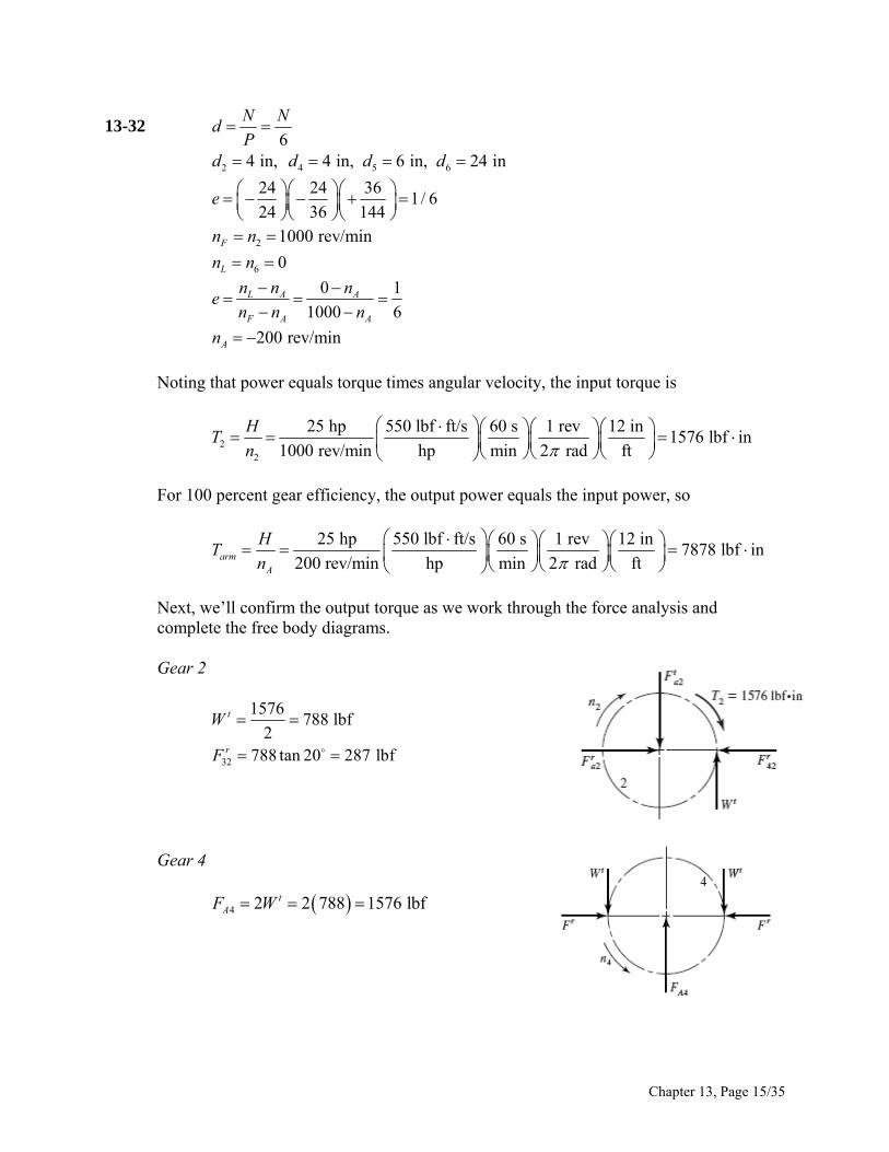
13-32 6
N Nd
P
2 4 5 64 in, 4 in, 6 in, 24 ind d d d
24 24 36
1/ 624 36 144
e
2 1000 rev/minFn n 6 0Ln n
0 1
1000 6L A A
F A A
n n ne
n n n
200 rev/minAn Noting that power equals torque times angular velocity, the input torque is
22
25 hp 550 lbf ft/s 60 s 1 rev 12 in1576 lbf in
1000 rev/min hp min 2 rad ft
HT
n
For 100 percent gear efficiency, the output power equals the input power, so
25 hp 550 lbf ft/s 60 s 1 rev 12 in
7878 lbf in200 rev/min hp min 2 rad ftarm
A
HT
n
Next, we’ll confirm the output torque as we work through the force analysis and complete the free body diagrams.
Gear 2
1576
788 lbf2
tW
32 788 tan 20 287 lbfrF
Gear 4
4 2 2 788 1576 lbft
AF W
Chapter 13, Page 15/35
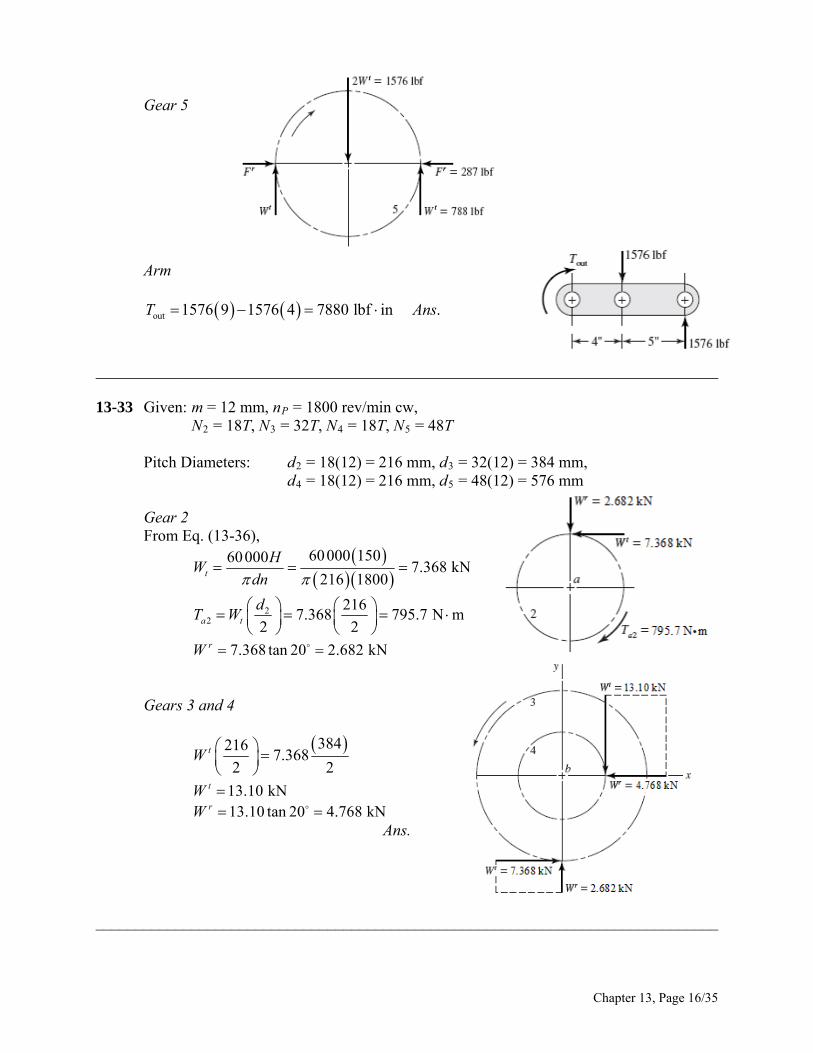
Gear 5 Arm
out 1576 9 1576 4 7880 lbf in .T A ns
______________________________________________________________________________ 13-33 Given: m = 12 mm, nP = 1800 rev/min cw,
N2 = 18T, N3 = 32T, N4 = 18T, N5 = 48T
Pitch Diameters: d2 = 18(12) = 216 mm, d3 = 32(12) = 384 mm, d4 = 18(12) = 216 mm, d5 = 48(12) = 576 mm
Gear 2
From Eq. (13-36),
60000 15060000
7.368 kN216 1800t
HW
dn
22
2167.368 795.7 N m
2 2a t
dT W
7.368 tan 20 2.682 kNrW
Gears 3 and 4
384216
7.3682 2
tW
13.10 kNtW W 13.10 tan 20 4.768 kNr
Ans. ______________________________________________________________________________
Chapter 13, Page 16/35
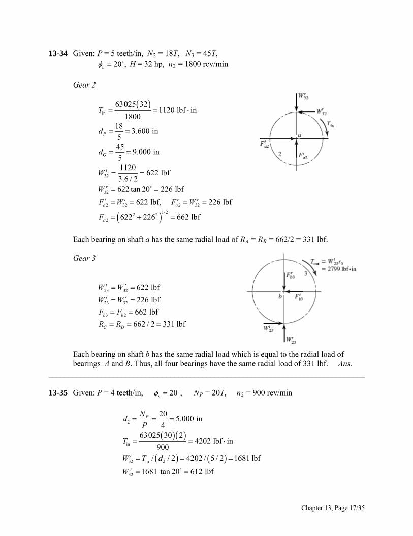
13-34 Given: P = 5 teeth/in, N2 = 18T, N3 = 45T, 20 ,n H = 32 hp, n2 = 1800 rev/min
Gear 2
in
63025 321120 lbf in
1800T
18
3.600 in5Pd
45
9.000 in5Gd
32
1120622 lbf
3.6 / 2tW
32 622 tan 20 226 lbfrW
2 32 2 32622 lbf, 226 lbft t r ra aF W F W
1/22 22 622 226 662 lbfaF
Each bearing on shaft a has the same radial load of RA = RB = 662/2 = 331 lbf. Gear 3
23 32 622 lbft tW W
23 32 226 lbfr rW W 3 2 662 lbfb bF F 662 / 2 331 lbfC DR R
Each bearing on shaft b has the same radial load which is equal to the radial load of bearings A and B. Thus, all four bearings have the same radial load of 331 lbf. Ans.
______________________________________________________________________________ 13-35 Given: P = 4 teeth/in, N20 ,n
P = 20T, n2 = 900 rev/min
2
205.000 in
4PN
dP
in
63025 30 24202 lbf in
900T
32 in 2/ / 2 4202 / 5 / 2 1681 lbft d W T
W 32 1681 tan 20 612 lbfr
Chapter 13, Page 17/35
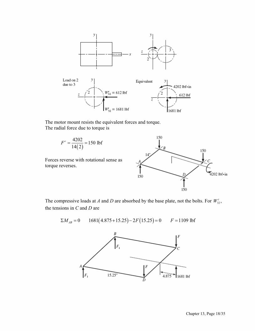
The motor mount resists the equivalent forces and torque.
The radial force due to torque is
4202150 lbf
14 2rF
Forces reverse with rotational sense as torque reverses.
The compressive loads at A and D are absorbed by the base plate, not the bolts. For
the tensions in C and D are 32 ,tW
0 1681 4.875 15.25 2 15.25 0 1109 lbfABM F F
Chapter 13, Page 18/35
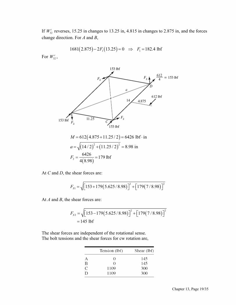
If reverses, 15.25 in changes to 13.25 in, 4.815 in changes to 2.875 in, and the forces
change direction. For A and B, 32tW
1 11681 2.875 2 13.25 0 182.4 lbfF F
For , 32rW
612 4.875 11.25 / 2 6426 lbf inM
2 214 / 2 11.25 / 2 8.98 ina
2
6426179 lbf
4 8.98F
At C and D, the shear forces are:
2 2
1 153 179 5.625 / 8.98 179 7 / 8.98SF
At A and B, the shear forces are:
2 2
2 153 179 5.625 / 8.98 179 7 / 8.98
145 lbf
SF
The shear forces are independent of the rotational sense. The bolt tensions and the shear forces for cw rotation are,
Chapter 13, Page 19/35
For ccw rotation,
______________________________________________________________________________ 13-36 (a) N2 = N4 = 15 teeth, N3 = N5 = 44 teeth
N N
P dd P
2 4
152.5 in .
6d d Ans
3 5
447.33 in .
6d d Ans
(b) 2 2
2 3
2.5 25001636 ft/min .
12 12i
d nV V V Ans
4 44 5
2.5 2500 15 / 44558 ft/min .
12 12o
d nV V V Ans
(c) Input gears:
33000 2533000 504.3 lbf 504 lbf .
1636tii
HW A
V ns
tan 504.3 tan 20 184 lbf .ri tiW W Ans
504.3
537 lbf .cos cos 20
tii
WW A
ns
Output gears:
33000 2533000 1478 lbf .
558too
HW A
V ns
tan 1478 tan 20 538 lbf .ro toW W Ans
1478
1573 lbf .cos 20 cos 20
too
WW A ns
(d) 2 2.5504.3 630 lbf in .
2 2i ti
dT W Ans
Chapter 13, Page 20/35
(e) 2 2
44 44630 5420 lbf in .
15 15o iT T Ans
______________________________________________________________________________ 13-37 35 hp, 1200 rev/min, =20iH n
2 4 3 516 teeth, 48 teeth, 10 teeth/inN N N N P
(a) 2intermediate 3 4
3
161200 400 rev/min
48i
Nn n n n
N Ans.
2 4
3 5
16 161200 133.3 rev/min
48 48o i
N Nn n
N N
Ans.
(b) N N
P dd P
2 4
161.6 in .
10d d Ans
3 5
484.8 in .
10d d Ans
2 22 3
1.6 1200502.7 ft/min .
12 12i
d nV V V Ans
4 44 5
1.6 400167.6 ft/min .
12 12o
d nV V V Ans
(c) 33000 35
33000 2298 lbf lbf .502.7ti
i
HW A
V ns
tan 2298 tan 20 836.4 lbf .ri tiW W Ans
2298
2445 lbf .cos cos 20
tii
WW A
ns
33000 35
33000 6891 lbf .167.6to
o
HW A
V ns
tan 6891tan 20 2508 lbf .ro toW W Ans
6891
7333 lbf .cos 20 cos 20
too
WW A ns
(d) 2 1.62298 1838 lbf in .
2 2i ti
dT W Ans
(e) 2 2
48 481838 16 540 lbf in .
16 16o iT T Ans
______________________________________________________________________________
Chapter 13, Page 21/35
13-38 (a) For 2
,1
o
i
from Eq. (13-11), with m = 2, k = 1, 20
2 2
2
2 12 2 1 2 2 sin 20 14.16
1 2 2 sin 20PN
ns
So min 15 .PN A
(b) 15
1.875 teeth/in .8
NP Ans
d
(c) To transmit the same power with no change in pitch diameters, the speed and transmitted force must remain the same.
For A, with = 20°, WtA = FA cos20° = 300 cos20° = 281.9 lbf For A, with = 25°, same transmitted load, FA = WtA/cos25° = 281.9/cos25° = 311.0 lbf Ans.
Summing the torque about the shaft axis,
2 2
A BtA tB
d dW W
/ 2 20
281.9 704.75 lbf/ 2 8
A AtB tA tA
B B
d dW W W
d d
704.75
777.6 lbf .cos 25 cos 25
tBB
WF Ans
______________________________________________________________________________
13-39 (a) For 5
,1
o
i
from Eq. (13-11), with m = 5, k = 1, 20
2 2
2
2 15 5 1 2 5 sin 25 10.4
1 2 5 sin 25PN
ns
So min 11 .PN A
(b) 300
27.3 mm/tooth .11
dm Ans
N
(d) To transmit the same power with no change in pitch diameters, the speed and transmitted force must remain the same.
Chapter 13, Page 22/35
For A, with = 20°, WtA = FA cos20° = 11 cos20° = 10.33 kN For A, with = 25°, same transmitted load, FA = WtA/cos25° = 10.33 / cos 25° = 11.40 kN Ans.
Summing the torque about the shaft axis,
2 2
A BtA tB
d dW W
/ 2 600
11.40 22.80 kN/ 2 300
A AtB tA tA
B B
d dW W W
d d
22.80
25.16 kN .cos 25 cos 25
tBB
WF Ans
______________________________________________________________________________ 13-40 (a) Using Eq. (13-11) with k = 1, = 20º, and m = 2,
2 22
2 2
2
21 2 sin
1 2 sin
2 12 2 1 2 2 sin 20 14.16 teeth
1 2 2 sin 20
P
kN m m m
m
Round up for the minimum integer number of teeth.
NF = 15 teeth, NC = 30 teeth Ans.
(b) 125
8.33 mm/tooth .15
dm Ans
N
(c) 2 kW 1000 W rev 60 s
100 N m191 rev/min kW 2 rad min
HT
(d) From Eq. (13-36),
60 000 260 000
1.60 kN 1600 N125 191t
HW
dn Ans.
Or, we could have obtained Wt directly from the torque and radius,
Chapter 13, Page 23/35
100
1600 N / 2 0.125 / 2t
TW
d
tan 1600 tan 20 583 N .r tW W Ans
16001700 N .
cos cos 20tW
W A
ns
______________________________________________________________________________ 13-41 (a) Using Eq. (13-11) with k = 1, = 20º, and m = 2,
2 22
2 2
2
21 2 sin
1 2 sin
2 12 2 1 2 2 sin 20 14.16 teeth
1 2 2 sin 20
P
kN m m m
m
Round up for the minimum integer number of teeth.
NC = 15 teeth, NF = 30 teeth Ans.
(b) 30
3 teeth/in .10
NP Ans
d
(c) 1 hp 550 lbf ft/s 12 in rev 60 s
70 rev/min hp ft 2 rad min
HT
Ans. 900 lbf inT
(d) From Eqs. (13-34) and (13-35),
10 70183.3 ft/min
12 12
dnV
33000 1
33000 180 lbf183.3t
HW
V Ans.
tan 180 tan 20 65.5 lbf .r tW W Ans
180192 lbf .
cos cos 20tW
W A
ns
______________________________________________________________________________
13-42 (a) Eq. (13-14): 1 1 1 1.30tan tan tan 18.5
3.88P P
G G
N d
N d
Ans.
(b) Eq. (13-34): 2 1.30 600
408.4 ft/min12 12
dnV
Ans.
Chapter 13, Page 24/35
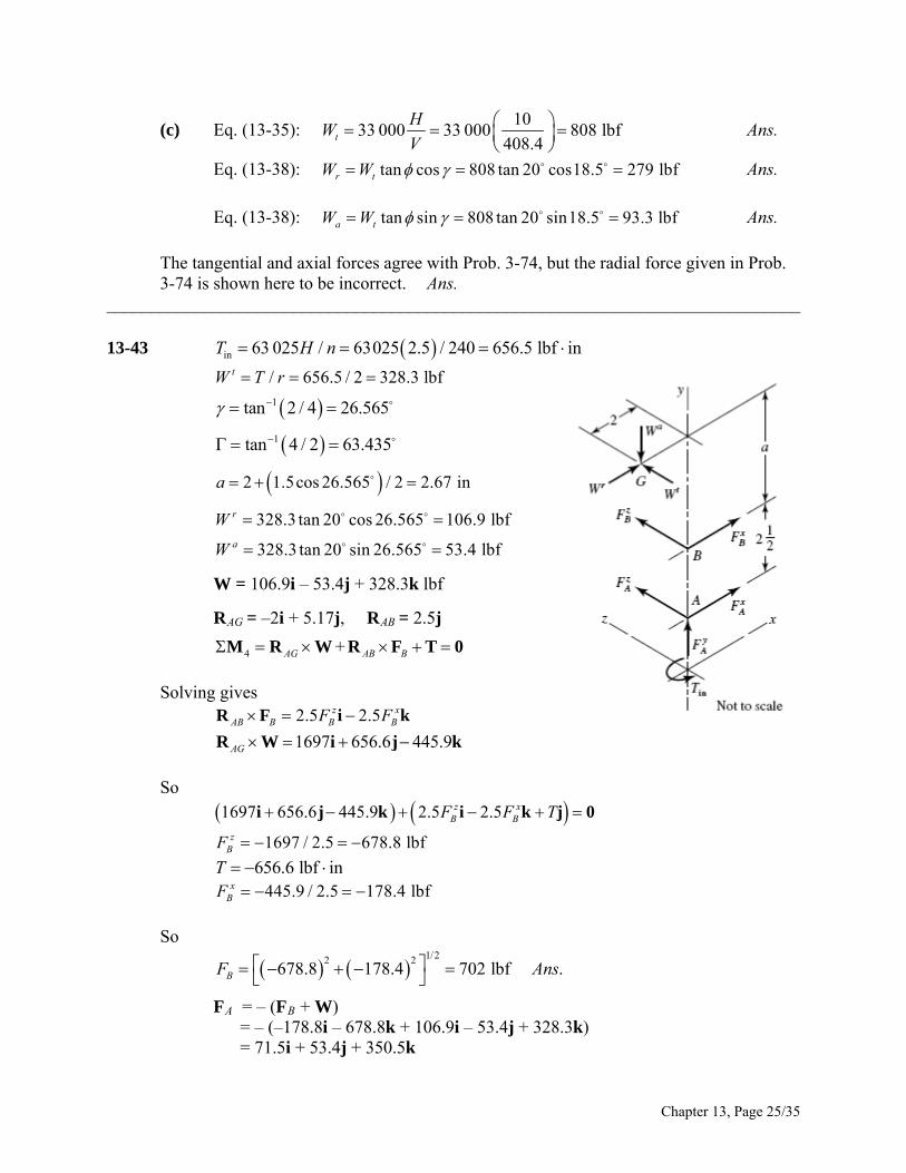
(c) Eq. (13-35): 10
33 000 33 000 808 lbf408.4t
HW
V
Ans.
Eq. (13-38): Ans. tan cos 808 tan 20 cos18.5 279 lbfr tW W
Eq. (13-38): Ans. tan sin 808 tan 20 sin18.5 93.3 lbfa tW W
The tangential and axial forces agree with Prob. 3-74, but the radial force given in Prob. 3-74 is shown here to be incorrect. Ans.
______________________________________________________________________________ 13-43 in 63 025 / 63025 2.5 / 240 656.5 lbf inT H n
0
k
/ 656.5 / 2 328.3 lbftW T r
1tan 2 / 4 26.565
1tan 4 / 2 63.435
2 1.5cos 26.565 / 2 2.67 ina
328.3 tan 20 cos 26.565 106.9 lbfrW
328.3 tan 20 sin 26.565 53.4 lbfaW
W = 106.9i – 53.4j + 328.3k lbf
RAG = –2i + 5.17j, RAB = 2.5j
4 +AG AB B M R W R F T
Solving gives 2.5 2.5z x
AB B B BF F R F i
1697 656.6 445.9AG R W i j k
So 1697 656.6 445.9 2.5 2.5z x
B BF F T i j k i k j 0
1697 / 2.5 678.8 lbfzBF
656.6 lbf inT 445.9 / 2.5 178.4 lbfx
BF So
1/22 2
678.8 178.4 702 lbf .BF Ans
FA = – (FB + W) = – (–178.8i – 678.8k + 106.9i – 53.4j + 328.3k) = 71.5i + 53.4j + 350.5k
Chapter 13, Page 25/35
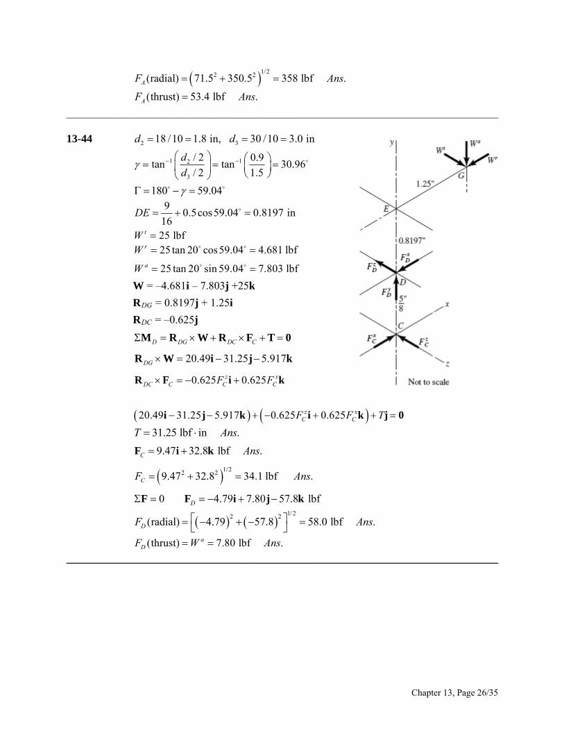
1/22 2(radial) 71.5 350.5 358 lbf .AF Ans
(thrust) 53.4 lbf .AF A ns
______________________________________________________________________________ 13-44 2 318 /10 1.8 in, 30 /10 3.0 ind d
1 12
3
/ 2 0.9tan tan 30.96
/ 2 1.5
d
d
180 59.04
9
0.5cos59.04 0.8197 in16
DE
W 25 lbft
W 25 tan 20 cos59.04 4.681 lbfr
W 25 tan 20 sin 59.04 7.803 lbfa
W = –4.681i – 7.803j +25k
RDG = 0.8197j + 1.25i
RDC = –0.625j
D DG DC C M R W R F T 0
20.49 31.25 5.917DG R W i j k
R F 0.625 0.625z xDC C C CF F i k
20.49 31.25 5.917 0.625 0.625z x
C CF F T i j k i k j 0
31.25 lbf in .T A ns
F i 9.47 32.8 lbf .C Ans k
1/22 29.47 32.8 34.1 lbf .CF Ans
0 4.79 7.80 57.8 lbfD F F i j k
1/22 2
(radial) 4.79 57.8 58.0 lbf .DF A ns
Ans (thrust) 7.80 lbf .aDF W
______________________________________________________________________________
Chapter 13, Page 26/35
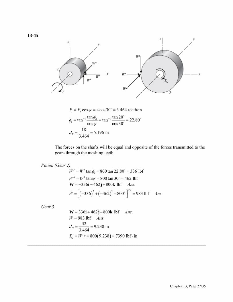
13-45
cos 4cos30 3.464 teeth/int nP P
1 1tan tan 20tan tan 22.80
cos cos30n
t
185.196 in
3.464Pd
The forces on the shafts will be equal and opposite of the forces transmitted to the gears through the meshing teeth.
Pinion (Gear 2) tan 800 tan 22.80 336 lbfr t
tW W
tan 800 tan 30 462 lbfa tW W
336 462 800 lbf .Ans W i j k
1/22 2 2336 462 800 983 lbf .W A ns
Gear 3 336 462 800 lbf .Ans W i j k 983 lbf .W A ns
32
9.238 in3.464Gd
800 9.238 7390 lbf intGT W r
______________________________________________________________________________
Chapter 13, Page 27/35
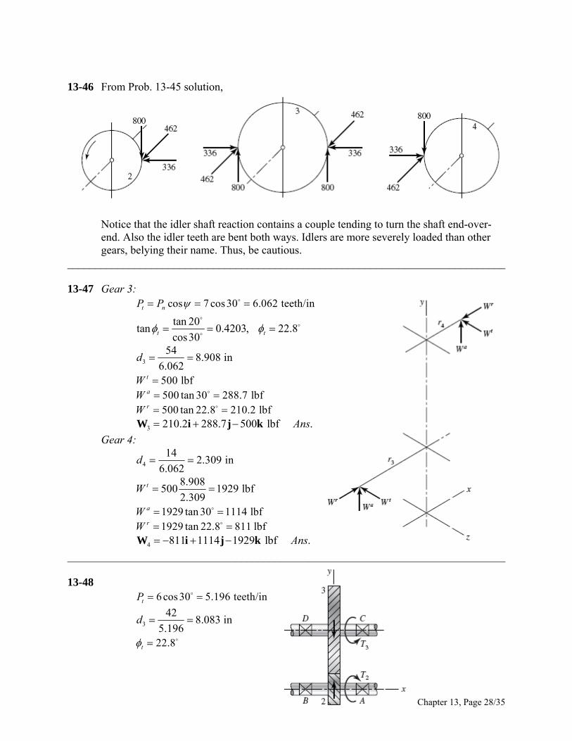
13-46 From Prob. 13-45 solution,
Notice that the idler shaft reaction contains a couple tending to turn the shaft end-over-end. Also the idler teeth are bent both ways. Idlers are more severely loaded than other gears, belying their name. Thus, be cautious.
______________________________________________________________________________ 13-47 Gear 3: cos 7 cos30 6.062 teeth/int nP P
tan 20
tan 0.4203, 22.8cos30t t
3
548.908 in
6.062d
500 lbftW 500 tan 30 288.7 lbfaW
500 tan 22.8 210.2 lbfrW
3 210.2 288.7 500 lbf .Ans W i j k
Gear 4:
4
142.309 in
6.062d
8.908
500 1929 lbf2.309
tW
1929 tan 30 1114 lbfaW
1929 tan 22.8 811 lbfrW
4 811 1114 1929 lbf .Ans W i j k
______________________________________________________________________________ 13-48 6cos30 5.196 teeth/intP
3
428.083 in
5.196d
22.8t
Chapter 13, Page 28/35
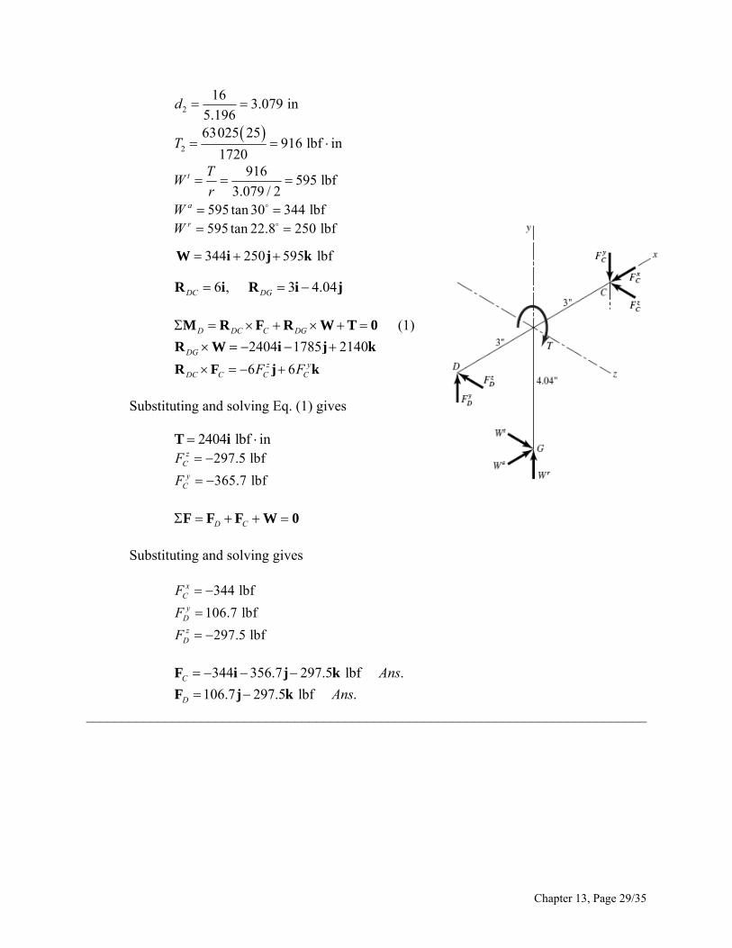
2
163.079 in
5.196d
2
63025 25916 lbf in
1720T
916
595 lbf3.079 / 2
t TW
r
595 tan 30 344 lbfaW
595 tan 22.8 250 lbfrW
344 250 595 lbf W i j k
6 , 3 4.04DC DG R i R i j
(1) D DC C DG M R F R W T 0
2404 1785 2140DG R W i j k
6 6z yDC C C CF F R F j k
Substituting and solving Eq. (1) gives 2404 lbf in T i 297.5 lbfz
CF
365.7 lbfyCF
D C F F F W 0
Substituting and solving gives 344 lbfx
CF
106.7 lbfyDF
297.5 lbfzDF
344 356.7 297.5 lbf .C Ans F i j k
106.7 297.5 lbf .D Ans F j k
______________________________________________________________________________
Chapter 13, Page 29/35
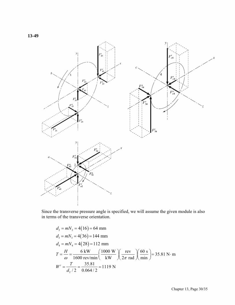
13-49
Since the transverse pressure angle is specified, we will assume the given module is also in terms of the transverse orientation.
2 2 4 16 64 mmd mN
3 3 4 36 144 mmd mN
4 4 4 28 112 mmd mN
6 kW 1000 W rev 60 s35.81 N m
1600 rev/min kW 2 rad min
HT
2
35.811119 N
/ 2 0.064 / 2t T
Wd
Chapter 13, Page 30/35
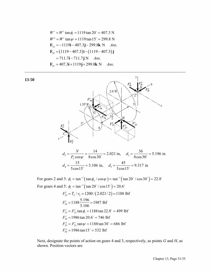
tan 1119 tan 20 407.3 Nr t
tW W
tan 1119 tan15 299.8 Na tW W
2 1119 407.3 299.8 N .a Ans F i j k
3 1119 407.3 1119 407.3
711.7 711.7 N .b
Ans
F i j
i j
4 407.3 1119 299.8 N .c Ans F i j k
______________________________________________________________________________ 13-50
2 3
14 362.021 in, 5.196 in
cos 8cos30 8cos30n
Nd d
P
4 5
15 453.106 in, 9.317 in
5cos15 5cos15d d
For gears 2 and 3: 1 1tan tan / cos tan tan 20 / cos30 22.8t n
For gears 4 and 5: 1tan tan 20 / cos15 20.6t
23 2 2/ 1200 / 2.021/ 2 1188 lbftF T r
54
5.1961188 1987 lbf
3.106tF
23 23 tan 1188 tan 22.8 499 lbfr ttF F
54 1986 tan 20.6 746 lbfrF
23 23 tan 1188 tan 30 686 lbfa tF F
a 54 1986 tan15 532 lbfF
Next, designate the points of action on gears 4 and 3, respectively, as points G and H, as shown. Position vectors are
Chapter 13, Page 31/35
1.553 3CG R j k
2.598 R 6.5CH j k
8.5CD R k
e Force vectors ar 54 1986 748 532 F i j k
F23 1188 500 686 i j k
x yC C CF F F i j
x y zD D D DF F F F i j k
Now, a summation of moments about bearing C gives
0
The terms for this equation are found to be
54 23C CG CH CD D M R F R F R F 54 1412 5961CG R F i j 3086k
23 5026 7722 3086CH R F i j k
8.5 8.5y xCD D D DF F R F i j
When these terms are placed back into the moment equation, the k terms, representing the shaft torque, cancel. The i and j terms give
3614
425 lbf .y
8.5DF Ans
13683
1610 lbf .8.5
xDF Ans
Next, we sum the forces to zero. 54 23C F F F F D 0
es
F
Substituting, giv 1987 746 532 1188 499 686y
CF xCF i j i j k i j k
1610 425 zDF i j k 0
Solving gives
1987 1188 1610 1565 lbf .xCF A ns
ns
ns
______________________________ ____________________________
746 499 425 672 lbf .yCF A
___________________ _
532 686 154 lbf .zDF A
Chapter 13, Page 32/35
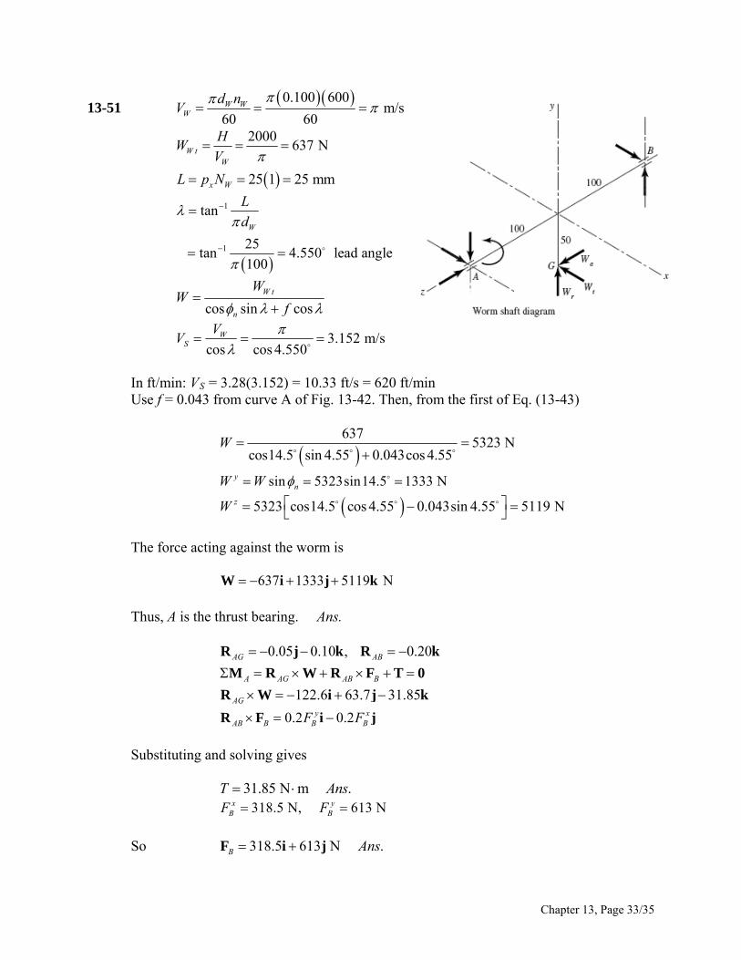
13-51 0.100 600
m/sW Wd nV
60 60W
2000
637 NW tW
HW
V
25 1 25 mmx WL p N
1
1
tan
25tan 4.550 lead angle
100
W
L
d
cos sin cos
W t
n
WW
f
3V .152 m/scos cos 4.550
WS
V
VS = 3.28(3.152) = 10.33 ft/s = 620 ft/min Use f = 0.043 from curve A of Fig. 13-42. Then, from the first of Eq. (13-43)
In ft/min:
6375323 NW
cos14.5 sin 4.55 0.043cos 4.55
W W sin 5323sin14.5 1333 Nyn
5323 cos14.5 cos 4.55 0.043 in 4.55 5119 Nz sW
against the worm is
rust bearing. Ans.
The force acting 637 1333 51 W i j 19 Nk Thus, A is the th 0.05 0.10 ,AG R j k 0.20AB R k
0 A AG AB B M R W R F T
122.6 63.7 31.85AG R W i j k
0.2 0.2y xAB B B BF F R F i j
Substituting and solving gives
Ans
31.85 N m T .
318.5 N, 613 Nx yB BF F
So 318.5 613 N .B Ans F i j
Chapter 13, Page 33/35
Or 1/22 2
613 318.5 691 N radialBF
A B F F W R 0
37 1333 5119 318.5 613
318.5 1946 5119 .A B
Ans
F W F i6 j k i j
i j k
Radial 318.5 1946 Nr
A F i j
1/22 2
318.5 1946 1972 NrAF
Thrust 5119 NaAF
___________________ ____________ _______________________________________________
3-52 From Prob. 13-51, 1
637G W i 1333 5119 Nj k
t xp p
So 48 25
382 mmGd xG
N p
D takes the thrust load.
0
Bearing
M R W RD DG G DC C F T
0.0725 0.191DG R i j
R i0.1075DC
The position vectors are in meters.
977.7 371.1 R W i 25.02DG G j k
0.1075 0.1075z yDC C C CF F R F j k
Putting it together and solving,
ns
977.7 N m .T Ans
233 3450 N, 3460 N .C CF A F j k
C G D F F W F 0
637 1566 1669 N .D C G Ans W i j k F F
Radial 1566 1669 Nr
D F j k
Or 2 1/2 21566 1669 2289 N (total radial)r
DF
tF i637 N (thrust)D
Chapter 13, Page 34/35
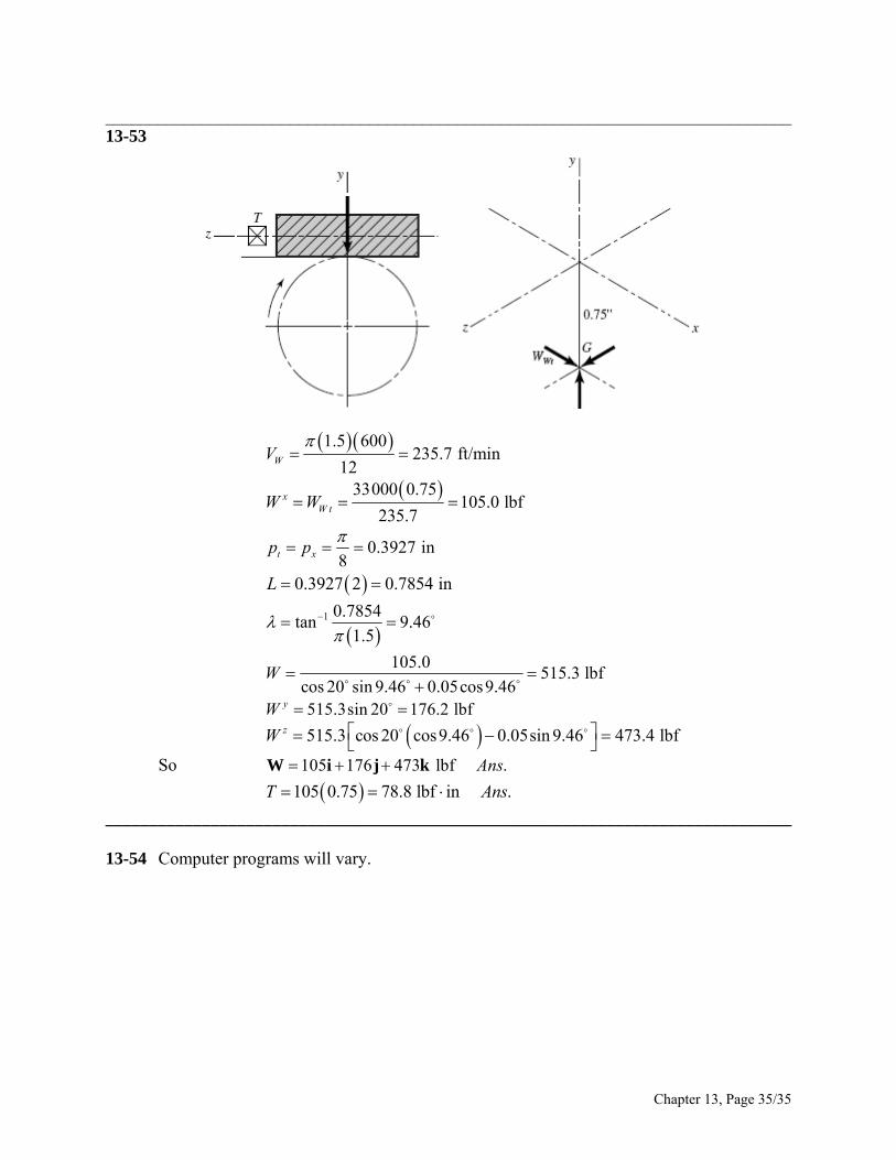
Chapter 13, Page 35/35
___________________ _____________________________________________ _____________ _13-53
1.5 600
235.7 ft/min12WV
33000 0.75105.0 lbf
235.7x
W tW W
0.3927 in8t xp p
0.3927 2 0.7854 inL
1 0.7854tan 9.46
1.5
105.0
515.3 lbfcos 20 sin 9.46 0.05cos9.46
W
515.3sin 20 176.2 lbfyW
515.3 cos 20 cos9.46 0.05sin 9.46 473.4 lbfzW
So 105 176 473 lbf .Ans W i j k
105 0.75 78.8 lbf in .T A ns
___________________________ ______________________________ ___________________ __ 3-54 Computer programs will vary. 1
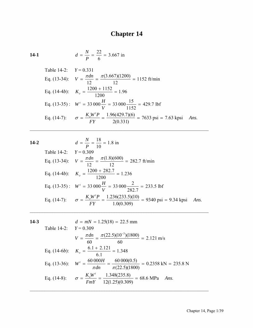
Chapter 14
14-1 22
3.667 in6
Nd
P
Table 14-2: Y = 0.331
Eq. (13-34): (3.667)(1200)
1152 ft/min12 12
dnV
Eq. (14-4b): 1200 1152
1.961200
K
v
Eq. (13-35) : 15
33 000 33 000 429.7 lbf1152
t HW
V
Eq. (14-7): 1.96(429.7)(6)
7633 psi 7.63 kpsi .2(0.331)
tK W PAns
FY v
________________________________________________________________________
14-2 18
1.8 in10
Nd
P
Table 14-2: Y = 0.309
Eq. (13-34): (1.8)(600)
282.7 ft/min12 12
dnV
Eq. (14-4b): 1200 282.7
1.2361200
K
v
Eq. (13-35) : 2
33 000 33 000 233.5 lbf282.7
t HW
V
Eq. (14-7): 1.236(233.5)(10)
9340 psi 9.34 kpsi .1.0(0.309)
tK W PAns
FY v
________________________________________________________________________ 14-3
1.25(18) 22.5 mmd mN Table 14-2: Y = 0.309
3(22.5)(10 )(1800)2.121 m/s
60 60
dnV
Eq. (14-6b): 6.1 2.121
1.3486.1
K
v
Eq. (13-36): 60 000 60 000(0.5)
0.2358 kN 235.8 N(22.5)(1800)
t HW
dn
Eq. (14-8): 1.348(235.8)
68.6 MPa .12(1.25)(0.309)
tK WAns
FmY v
________________________________________________________________________
Chapter 14, Page 1/39
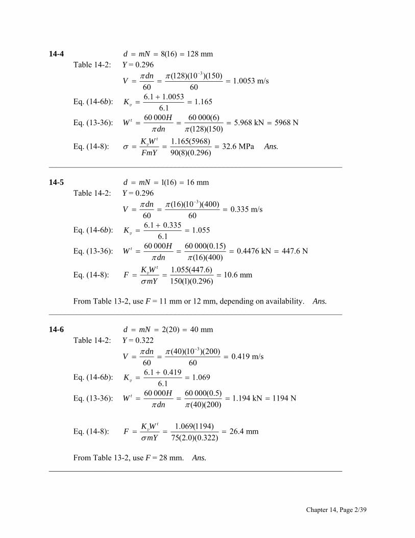
14-4 Y = 0.296
8(16) 128 mmd mN Table 14-2:
3(128)(10 )(150)1.0053 m/s
60 60
dnV
6.1 1.0053
1.1656.1
K
v Eq. (14-6b):
60 000 60 000(6)5.968 kN 5968 N
(128)(150)t H
Wdn
Eq. (13-36):
Eq. (14-8): 1.165(5968)
32.6 MPa .90(8)(0.296)
tK WAns
FmY v
________________________________________________________________________
4-5 Y = 0.296
1 1(16) 16 mmd mN Table 14-2:
3(16)(10 )(400)0.335 m/s
60 60
dnV
6.1 0.335
1.0556.1
K
v Eq. (14-6b):
60 000 60 000(0.15)0.4476 kN 447.6 N
(16)(400)t H
Wdn
Eq. (13-36):
Eq. (14-8): 1.055(447.6)
10.6 mm150(1)(0.296)
tK WF
mY v
From Table 13-2, use F = 11 mm or 12 mm, depending on availability. Ans. _____ ___
4-6 Y = 0.322
_ _______________________________________________________________ 1 2(20) 40 mmd mN Table 14-2:
3(40)(10 )(200)0.419 m/s
60 60
dnV
6.1 0.4191.069
6.1K
v Eq. (14-6b):
Eq. (13-36): 60 000 60 000(0.5)
1.194 kN 1194 N(40)(200)
t HW
dn
Eq. (14-8): 1.069(1194)
26.4 mm75(2.0)(0.322)
tK WF
mY v
From Table 13-2, use F = 28 mm. Ans.
_____ ________________________________ _ __________________________________
Chapter 14, Page 2/39
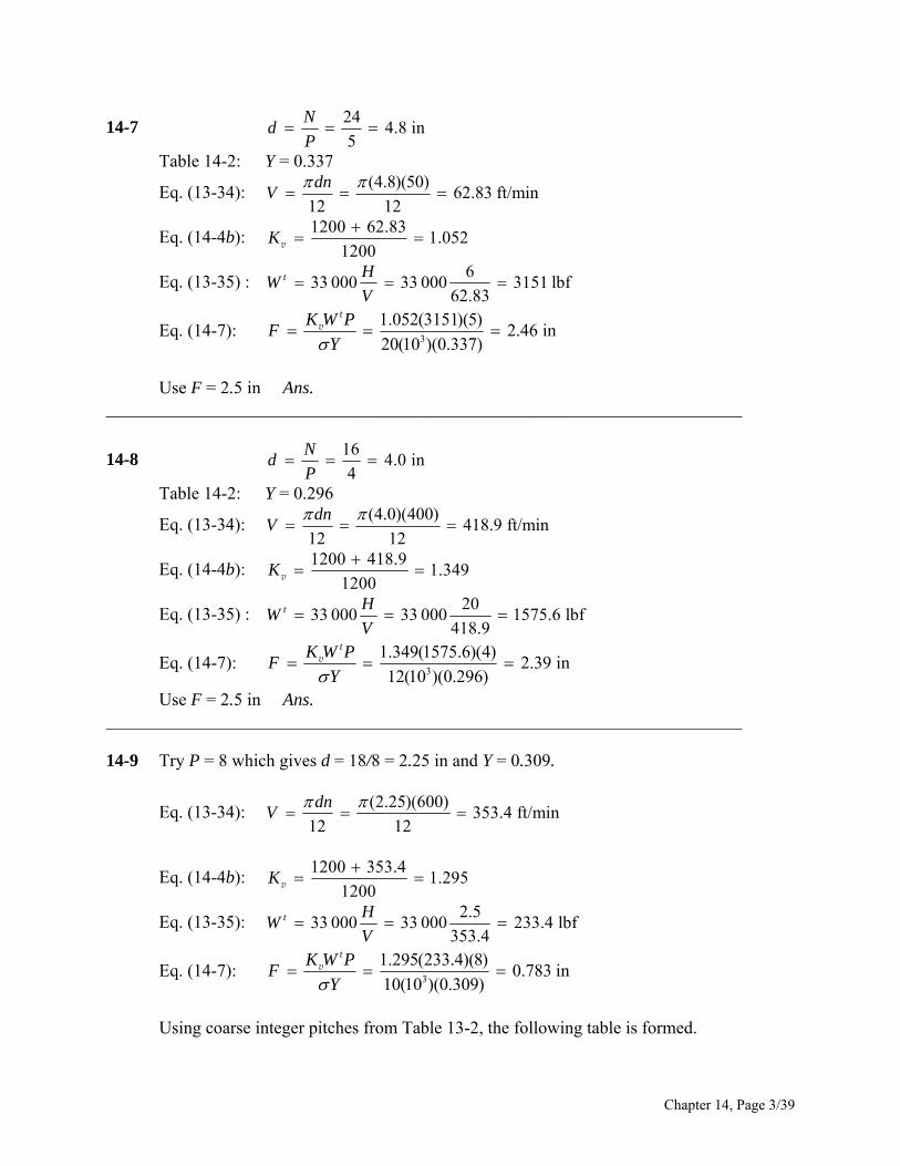
14-7 24
4.8 in5
Nd
P
Table 14-2: Y = 0.337 (4.8)(50)
62.83 ft/min12 12
dnV
Eq. (13-34):
Eq. (14-4b):
1200 62.831.052
1200K
v
Eq. (13-35) : 6
33 000 33 000 3151 lbf62.83
t HW
V
Eq. (14-7): 3
1.052(3151)(5)2.46 in
20(10 )(0.337)
tK W PF
Y v
Use F = 2.5 in Ans.
_______________________________________________
4-8
_________________________
116
4.0 in4
Nd
P
Table 14-2: Y = 0.296 (4.0)(400)
418.9 ft/min12 12
dnV
Eq. (13-34):
Eq. (14-4b):
1200 418.91.349
1200K
v
Eq. (13-35) : 20
33 000 33 000 1575.6 lbf418.9
t HW
V
Eq. (14-7): 3
1.349(1575.6)(4)2.39 in
12(10 )(0.296)
tK W PF
Y v
Use F = 2.5 in Ans. _______________________________________________
4-9 Try P = 8 which gives d = 18/8 = 2.25 in and Y = 0.309.
Eq. (13-34):
_________________________ 1
(2.25)(600)
353.4 ft/min12 12
dnV
1200 353.4
1.2951200
K
v Eq. (14-4b):
Eq. (13-35): 2.5
33 000 33 000 233.4 lbf353.4
t HW
V
Eq. (14-7): 3
1.295(233.4)(8)0.783 in
10(10 )(0.309)
tK W PF
Y v
Using coarse integer pitches from Table 13-2, the following table is formed.
Chapter 14, Page 3/39
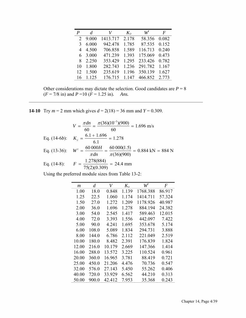
P d V Kv Wt F 2 9.000 1413.717 2.178 58.356 0.0823 6. 0 942.478 1.785 87.535 0.152
11
10 1.800 12 1.500
004 4.500 706.858 1.589 16.713 0.2406 3.000 471.239 1.393 75.069 0.4738 2.250 353.429 1.295 233.426 0.782
282.743 1.236 291.782 1.167235.619 1.196 350.139 1.627
16 1.125 176.715 1.147 466.852 2.773 Other considerat ta e G i re P = 8
(F = 7/8 in) and P =10 (F = 1.25 in). Ans. _____ _____
ions may dic te the sel ction. ood cand dates a _ _____________________________________________________________ 14-10 Try m = 2 mm which gives d = 2(18) = 36 mm and Y = 0.309.
3(36)(10 )(900)1.696 m/s
dnV
60 60
Eq. (14-6b): 6.1 1.696
1.2786.1
K
v
Eq. (13-36): 60 000 60 000(1.5)
0.884 kN 884 N(36)(900)
t HW
dn
Eq. (14-8): 1.278(884)
24.4 mm75(2)(0.309)
F
Using the prefer edr module sizes from Table 13-2:
Wt F m d V Kv 1.00 18.0 0.848 1.139 1768.388 86.917 1.25 22.5 1.060 1.174 1414.711 57.324
11
11 1
1
1.50 27.0 1.272 1.209 1178.926 40.987 2.00 36.0 1.696 1.278 884.194 24.382 3.00 54.0 2.545 1.417 589.463 12.015 4.00 72.0 3.393 1.556 442.097 7.422 5.00 90.0 4.241 1.695 353.678 5.174 6.00 08.0 5.089 1.834 294.731 3.888 8.00 44.0 6.786 2.112 221.049 2.519 0.00 180.0 8.482 2.391 176.839 1.824 2.00 216.0 0.179 2.669 147.366 1.414
16.00 288.0 3.572 3.225 110.524 0.961 20.00 360.0 16.965 3.781 88.419 0.721 25.00 450.0 21.206 4.476 70.736 0.547 32.00 576.0 27.143 5.450 55.262 0.406 40.00 720.0 33.929 6.562 44.210 0.313 50.00 900.0 42.412 7.953 35.368 0.243
Chapter 14, Page 4/39

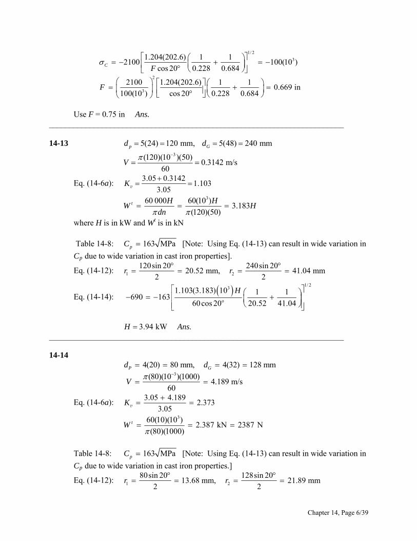
1/ 2
3
2
3
1.204(202.6) 1 12C
100 100(10 )cos 20 0.228 0.684
2100 1.204(202.6) 1 10.669 in
100(10 ) cos 20 0.228 0.684
F
F
Use F = 0.75 in Ans. ________________________________________________________________________
14-13 5(24pd ) 120 mm, 5(48) 240 mmGd
3(120)(10 )(50)
0.3142 m/s60
V
Eq. (14-6a): 3.05 0.3142
1.1033.05
K
v
360 000 60(10 )3.183
(120)(50)t H H
W Hdn
t
where H is in kW and W is in kN
Table 14-8:
163 MPapC
C
[Note: Using Eq. (14-13) can result in wide variation in
n properties].
p due to wide variation in cast iro
Eq. (14-12): 1 220.52 mm, 41.04 mm2
r 120sin 20 240sin 20
2r
1/ 231.103(3.183) 10 H
o
1 1690 163
60cos 20 20.52 41.04
Eq. (14-14):
3.94 kW .H Ans
________________________________________________________________________
4
14-1
3
4(20) 80 mm, 4(32) 128 mmP Gd d
(80)(10 )(1000)4.189 m/s
60V
Eq. (14-6a): 3.05 4.189
2.3733.05
K
v
360(10)(10 )2.387 kN 2387 N
(80)(1000)tW
Table 14-8: 163 MPapC [Note: Using Eq. (14-13) can result in wide variation in
Cp due to wide variation in cast iron properties.]
(14-12): 1 2
80sin 20 128sin 2013.68 mm, 21.89 mm
2 2r r
Eq.
Chapter 14, Page 6/39
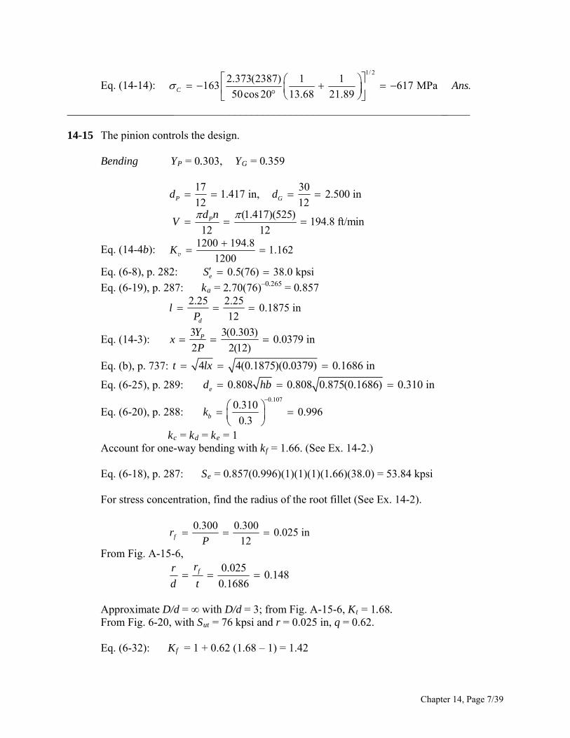
Eq. (14-14): 1/ 2
73(2387) 1 1163 617 MPa .
50cos 20 13.68C
2.3
21.89Ans
________________________________________________ ____
14-15 The pinion controls the design.
___________________ _
Bending YP = 0.303, YG = 0.359
17 301.417
12Pd
in, 2.500 in12
1 )194.8 ft/min
Gd
Eq. (14-4b):
( .417)(525
12 12Pd n
V
1200 194.81.162
1200K
v
Eq. (6-8), p. 282:
Eq. (6-19), p. 287: k = 2.70(76) = 0.857
0.5(76) 38.0 kpsieS –0.265
a
2.25 2.250.1875 i n
12d
lP
3 3(0.303)0.0379 in
2 Eq. (14-3):
2(12)PY
P
37:
x
4 4(0.1875)(0.0379) 0.1686 int lx Eq. (b), p. 7
0.808 0.808 0.875(0.1686) 0.310 ined hb Eq. (6-25), p. 289: 0.107
0.3100.996
0.3bk
Eq. (6-20), p. 288:
kc = kd = ke = 1 y bending with kf = 1.66. (See Ex. 14-2.)
Se = 0.857(0.996)(1)(1)(1)(1.66)(38.0) = 53.84 kpsi
i
Account for one-wa
Eq. (6-18), p. 287:
For stress co entration, find thnc e rad us of the root fillet (See Ex. 14-2).
0.300 0.3000.025 in
12frP
From Fig. A-15-6,
0.025
0.1480.1686
frr
d t
D/d = 3; from Fig. A-15-6, Kt = 1.68. ut 76 kpsi and r = 0.025 in, q = 0.62.
Eq. (6-32): Kf = 1 + 0.62 (1.68 – 1) = 1.42
Approximate D/d = ∞ with From Fig. 6-20, with S =
Chapter 14, Page 7/39
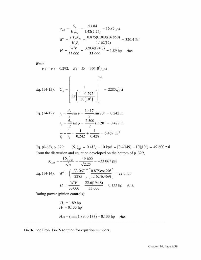
53.84eS16.85 psi
1.42(2.25)allf dK n
0.875(0.303)(16
(12t P allFY
WK P
850)320.4 lbf
1.162 )
320.4(194.8)1.89 hp .
33 000 33 000
dtW V
H Ans
v
Wear 1 = 2 = 0.292, E1 = E2 = 30(106) psi
1/ 2
2
6
Eq. (14-13): 1
C
2285 psi1 0.292
230 10
p
Eq. (14-12):
1
1.417sin sin 20 0.242 in
2 2Pd
r
2
2.500sin sin 20 0.428 in
2 2Gd
r
1
1 2
1 1 1 16.469 in
0.242 0.428r r
Eq. (6-68), p. 329:
From the discussion and equation developed on the bottom of p. 329,
83
10( ) 0.4 10 kpsi [0.4(149) 10](10 ) 49 600 psiC BS H
810,allC
49 60033 067 psi
2.25CS
n
Eq. (14-14): 2
33 067 0.875cos 2022.6 lbftW
2285 1.162(6.469)
22.6(194.8)
0.133 hp .33 000 33 000
tW VH A ns
i n controls):
H1 = 1.89 hp H2 = 0.133 hp
Hall = (min 1.89, 0.133) = 0.133 hp Ans. ___ __ __ _____ __________________________________________
4-16 See Prob. 14-15 solution for equation numbers.
Rating power (p nio
___ _ _ _ ____________ 1
Chapter 14, Page 8/39
Pinion controls: YP = 0.322, YG = 0.447 Bending d = 20/3 = 6.667 in, d = 100/3 = 33.333 in
P G
/ 12 (6.667)(870)V d n
0.265
0.5(113) 56.5 kpsi
2.70(113) 0.771
S
k
/ 12 1519 ft/min/ 6
2.25 / 2.25 / 3 0.75 in3(0.322) / [2(3)] 0.161 in
4(0.75)(0.161) 0.695 in
0.808 2.5(0.69
e
a
d
e
l Px
t
d
(1200 1519) 1200 2.26P
K
v
0.107
5) 1.065 in
(1.065 / 0.30) 0.8731
b
c d e
kk k k
kf = 1.66 (See Ex. 14-2.) 0.771(0.873)(1)(1)(1)(1.66)(56.5) 63.1 kpsieS
0.300 / 3 0.100 in 0.100
0.144frr
0.695
fr
d t
Kt = 1.75, q = 0.85, Kf = 1.64
63.125.7 kpsi
1.64(1.5)e
allf d
S
K n
all 2.5(0.322)(25
(3)t PFY
WK P
700)3043 lbf
2.266
/ 33 000 3043(1519) / 3 000 140 hp .d
t
H 3 W V Ans
v
Wear
Eq. (14-13):
1/ 2
2
6
12285 psi
1 0.2922
30 10
pC
Eq. (14-12): r1 = (6.667/2) sin 20° = 1.140 in r2 = (33.333/2) sin 20° = 5.700 in
Eq. (6-68), p. 329: SC = [0.4(262) – 10](103) = 94 800 psi
,allC C d/ 94 800 /S n 1.5 77 400 psi
Chapter 14, Page 9/39
2
,all
1 2
2
cos 1
1 / 1 /
77 400 2.5cos 20 1
2285 2.266 1 / 1.140 1 / 5.7001130 lbf
Ct
p
FW
C K r r
v
1130(1519)
52.0 hp .33 000 33 000
tW VH A ns
les (revolutions of the pinion), the power based on wear is 52.0 hp.
ns
________________________________________________________________________
75 mm, NP = 16 milled teeth,
For 108 cyc Rating power (pinion controls):
140 hpH 1
2
rated
52.0 hpmin(140, 52.0) 52.0 hp .
HH A
4-17 See Prob. 14-15 solution for equation numbers. 1
Given: = 20°, n = 1145 rev/min, m = 6 mm, F = NG = 30T, Sut = 900 MPa, HB = 260, nd = 3, YP = 0.296, and YG = 0.359.
Pinion bending
3
6(16) 96 mm6(30) 180 mm
(96)(10 )(1145)5.76 m/s
60 (60)
Pd mN P
G
P
d
d nV
6.1 5.761.944
6.1K
v
0.265
0.107
0.5(900) 450 MPa
4.51(900) 0.7442.25 2.25(6) 13.5 mm3 / 2 3(0.296)6 / 2 2.664 mm
4 4(13.5)(2.664) 12.0 mm
0.808 75(12.0) 24.23 mm
24.230.884
7.621
e
a
e
b
c d e
S
kl mx Ym
t lx
d
k
k k k
f
(1.66)(450) 491.3 MPa k = 1.66 (See Ex. 14-2)
r/d = rf /t = 1.8/12 = 0.15, Kt = 1.68, q = 0.86, Kf = 1.58
0.744(0.884)(1)(1)(1)eS
0.300 0.300(6) 1.8 mmfr m
Chapter 14, Page 10/39
all
491.3239.2 MPa
1.58 1.3e
f d
S
K n
Eq. (14-8): all 75(0.296)(6)(239.2)16 390 N
1.944t FYm
WK
v
Eq. (13-36): 16.39 (96)(1145)
94.3 kW .60 000 60 000
tW dnH A
ns
Wear: Pinion and gear Eq. (14-12): r1 = (96/2) sin 20 = 16.42 mm r2 = (180/2) sin 20 = 30.78 mm
Eq. (14-13):
1/ 2
2
3
1190 MPa
1 0.2922
207 10
pC
Eq. (6-68), p. 329: SC = 6.89[0.4(260) – 10] = 647.7 MPa
,all
647.7/ 568 MPa
1.3C C dS n
Eq. (14-14):
2
,all
1 2
cos 1
1 / 1 /Ct
p
FW
C K r
v r
2 o568 75cos 20 13469 N
190 1.944 1 / 16.42 1 / 30.78
Eq. (13-36): 3.469 (96)(1145)
20.0 kW60 000 60 000
tW dnH
Thus, wear controls the gearset power rating; H = 20.0 kW. Ans. ________________________________________________________________________ 14-18 NP = 17 teeth, NG = 51 teeth
172.833 in
651
8.500 in6
P
G
Nd
P
d
/ 12 (2.833)(1120) / 12 830.7 ft/minPV d n
Eq. (14-4b): Kv = (1200 + 830.7)/1200 = 1.692
Chapter 14, Page 11/39
all
90 00045 000 psi
2y
d
S
n
Table 14-2: YP = 0.303, YG = 0.410
Eq. (14-7): all 2(0.303)(45 000)2686 lbf
1.692(6)t PFY
WK P
v
Eq. (13-35): 2686(830.7)
67.6 hp33 000 33 000
tW VH
Based on yielding in bending, the power is 67.6 hp. (a) Pinion fatigue Bending Eq. (2-121), p. 41: Sut = 0.5 HB = 0.5(232) = 116 kpsi Eq. (6-8), p. 282: 0.5 0.5(116) 58 kpsie utS S
Eq. (6-19), p. 287: 0.2652.70(116) 0.766ak
Table 13-1, p. 696: 1 1.25 2.25 2.25
0.375 in6d d d
lP P P
Eq. (14-3): 3 3(0.303)
0.0758 in2 2(6)
PYx
P
Eq. (b), p. 737: 4 4(0.375)(0.0758) 0.337 int lx
Eq. (6-25), p. 289: 0.808 0.808 2(0.337) 0.663 ined F t
Eq. (6-20), p. 288: 0.107
0.6630.919
0.30bk
kc = kd = ke = 1 Account for one-way bending with kf = 1.66. (See Ex. 14-2.) Eq. (6-18): 0.766(0.919)(1)(1)(1)(1.66)(58) 67.8 kpsieS For stress concentration, find the radius of the root fillet (See Ex. 14-2).
0.300 0.3000.050 in
6frP
Fig. A-15-6: 0.05
0.1480.338
frr
d t
Estimate D/d = ∞ by setting D/d = 3, Kt = 1.68.
Chapter 14, Page 12/39
Fig. 6-20, p. 295: q = 0.86 Eq. (6-32), p. 295: 1 (0.86)(1.68 1) 1.58fK
all
67.821.5 kpsi
1.58(2)e
f d
S
K n
all 2(0.303)(21500)1283 lbf
1.692(6)t P
d
FYW
K P
v
1283(830.7)
32.3 hp .33 000 33 000
tW VH A ns
(b) Pinion fatigue Wear
Eq. (14-13): 1/ 2
2 6
12285 psi
2 [(1 - 0.292 ) / 30(10 )]pC
Eq. (14-12): o1
2.833sin sin 20 0.485 in
2 2Pd
r
o2
8.500sin sin 20 1.454 in
2 2Gd
r
1 2
1 1 1 12.750 in
0.485 1.454r r
Eq. (6-68): 810
( ) 0.4 10 kpsiC BS H
In terms of gear notation C = [0.4(232) – 10]103 = 82 800 psi We will introduce the design factor of nd = 2 and because it is a contact stress apply it
to the load Wt by dividing by 2 . (See p. 329.)
,all
82 80058 548 psi
2 2c
C
Solve Eq. (14-14) for Wt:
2 o
all
58 548 2cos 20265 lbf
2285 1.692(2.750)
265(830.7)6.67 hp .
33 000 33 000
t
t
W
W VH A
ns
(c) Gear fatigue due to bending and wear
For 108 cycles (turns of pinion), the allowable power is 6.67 hp.
Chapter 14, Page 13/39
Bending
3 3(0.4103)0.1026 in
2 2(6)GY
xP
Eq. (14-3):
4 4(0.375)(0.1026) 0.392 int lx Eq. (b), p. 737:
Eq. (6-25): 0.808 0.808 2(0.392) 0.715 ined F t
Eq. (6-20): 0.107
0.7150.911
0.30bk
k = kd = ke = 1 . 14-2.)
c
kf = 1.66. (See Ex Eq. (6-18): 0.766(0.911)(1)(1)(1)(1eS .66)(58) 67.2 kpsi
0.0500.128
0.392frr
d t
Fig. 6-20: q = 0.82 Approximate D/d = ∞ by setting D/d = 3 for Fig. A-15-6; Kt = 1.80.
Eq. (6-32): 1 (K 0.82)(1.80 1) 1.66 f
all
67.220.2 kpsi
1.66(2)e
f d
S
K n
all 2(0.4103)(20 200)1633 lbf
1.692(6)t P
d
FYW
K P
v
all
1633(830.7)41.1 hp .
33 000 33 000
tW VH A ns
Wear
Since the material of the pinion and the gear are the same, and the contact stresses are
(d)
nion bending: H1 = 32.3 hp
1.1, 6.67) = 6.67 hp Ans. __ __ ___________
4-19 dP = 16/6 = 2.667 in, dG = 48/6 = 8 in
The gear is thus stronger than the pinion in bending.
the same, the allowable power transmission of both is the same. Thus, Hall = 6.67 hp for 108 revolutions of each. As yet, we have no way to establish SC for 108/3 revolutions.
Pi Pinion wear: H2 = 6.67 hp Gear bending: H3 = 41.1 hp Gear wear: H4 = 6.67 hp Power rating of the gear set is thus Hrated = min(32.3, 6.67, 4____ __________ ___________________________________________ 1
Chapter 14, Page 14/39
(2.667)(300)209.4 ft/minV
12
33 000(5)787.8 lbf
209.4tW
Assuming uniform loading, K = 1.
o2/36) 0.8255 Eq. (14-28): 6, 0.25(12Q B v
50 56(1 0.8255) 59.77A
Eq. (14-27):
0.8255
59.77 209.41.196
59.77K
v
Table 14-2:
ec. 14-10 with F = 2 in
0.296, 0.4056P GY Y
From Eq. (a), S
0.0535
0.0535
2 0.296( ) 1.192 1.088
6
2 0.4056( ) 1.192 1.097
6
s P
s G
K
K
4-30) with C = 1
From Eq. (1 mc
2C 0.0375 0.0125(2) 0.0625
10(2.667)1, 0.093 (Fig. 14 - 11), 1
1 1[0.0625(1) 0.093(1)] 1.156
p f
p m ma e
m
C C C
K
Assuming constant thickness of the gears → KB = 1
mG = NG/NP = 48/16 = 3
With N (pinion) = 10 cycles and N (gear) = 108/3, Fig. 14-14 provides the relations:
Fig. 14-6:
R = 0.85
(14-23):
8 8 0.0178( ) 1.3558(10 ) 0.977N PY 8 0.0178( ) 1.3558(10 / 3) 0.996N GY
0.27, 0.38P GJ J
Table 14-10: K KT = Cf = 1
o ocos 20 sin 20 3
0.12052(1) 3 1
I
Eq.
Table 14-8: 2300 psipC
Strength: Grade 1 steel with HBP = HBG = 200
Chapter 14, Page 15/39
Fig. 14-2: (St)P = (St)G = 77.3(200) + 12 800 = 28 260 psi
Fig. 14-5: (Sc)P = (Sc)G = 322(200) + 29 100 = 93 500 psi
Fig. 14-15: (ZN )P = 1.4488(10 ) = 0.948 3
Sec. 14-12: HBP/HBG = 1 CH = 1
Pinion tooth bending
8 –0.023 (ZN )G = 1.4488(108/3)–0.023 = 0.97
Eq. (14-15): ( ) t d m BP o s
P K KW K K K
F Jv
6 (1.156)(1)787.8(1)(1.196)(1.088)
2 0.2713 170 psi .Ans
Eq. (14-41): / ( )
( ) t N T RF P
S Y K KS
28 260(0.977) / [(1)(0.85)]
2.47 .13 170
Ans
Gear tooth bending
6 (1.156)(1) Eq. (14-15): ( ) 787.8(1)(1.196)(1.097) 9433 psi .
2 0.38G Ans
Eq. (14-41):
28 260(0.996) / [(1)(0.85)]( ) 3.51 .
9433F GS A ns
Pinion tooth wear
Eq. (14-16):
1/ 2
( ) ft mc P p o s
P P
CKC W K K K
d F I
v
1/ 2
1.156 12300 787.8(1)(1.196)(1.088)
2.667(2) 0.1205
98 760 psi .Ans
: Eq. (14-42)
/( ) 93 500(0.948) /[(1)(0.85)]
( ) 1.06 .98 760
c NSS A
T R
H Pc P
Z K Kns
Gear tooth wear
Chapter 14, Page 16/39
1/ 2 1/ 2( )
( )( )
s Gc G
K 1.097( ) (98 760) 99 170 psi .
1.088
93 500(0.973)(1) /[(1)(0.85)]) 1.08 .
99 170
c Ps P
G( H
Ans
ns
The hardness of the pinion and the gear should be increased. _______________________________________________________________________
K
S A
_ 14-20 dP = 2.5(20) = 50 mm, dG = 2.5(36) = 90 mm
3
3
(50)(10 )(100)0.2618 m/s
60 60P PV
60(120)458.4 N
(50)(10 )(100)t
d n
W
With no specific information given to indicate otherwise, assume
: = 0.8255 A = 50 + 56(1 – 0.8255) = 59.77
KB = Ko = Y = ZR = 1 Eq. (14-28) Qv = 6, B = 0.25(12 – 6)2/3
0.8255
Eq. (14-27):
59.77 200(0.2618)
59.77K
v 1.099
P 0.322, YG = 0.3775
units:
Table 14-2: Y =
Similar to Eq. (a) of Sec. 14-10 but for SI
0.053510.8433K mF Y s
bk
0.0535
( ) 0.8433 2.5(18) 0.322 1.003 use 1s PK 0.0535
( ) 0.8433 2.5(18) 0.3775 =1.007 use 1s GK
1
1818 / 25.4 0.709 in, 0.025 0.011
10(50)
mc e pm
pf
C C C
F C
(YN )P = 1.3558(108)–0.0178 = 0.977
(Y )G = 1.3558(108/1.8)–0.0178 = 0.987
38): YZ = 0.658 – 0.0759 ln(1 – 0.95) = 0.885
4 20.247 0.0167(0.709) 0.765(10 )(0.709 ) 0.259maC
1 1[0.011(1) 0.259(1)] 1.27HK
Fig. 14-14: N
Fig. 14-6: (YJ )P = 0.33, (YJ )G = 0.38 Eq. (14-
Chapter 14, Page 17/39
Eq. (14-23): o ocos 20 sin 20 1.8
0.1032(1) 1.8 1IZ
Table 14-8: 191 MPaEZ
Strength Grade 1 steel, BPH = HBG = 200
.9 MPa Fig. 14-5: (Sc)P = (Sc)G = 2.22(200) + 200 = 644 MPa
ding
Fig. 14-2: (St)P = (St)G = 0.533(200) + 88.3 = 194 Fig. 14-15: (ZN )P = 1.4488(108)–0.023 = 0.948
N G
Fig. 14-12: / 1 H H C
8 0.023( ) 1.4488(10 / 1.8) 0.961Z
1BP BG W HZ
Pinion tooth ben
1 Eq. (14-15): ( )P t H B
o st J P
K KW K K K
bm Y
v
1 1.27(1)458.4(1)(1.099)(1) 43.08 MPa .
18(2.5) 0.33Ans
194.9 0.977( ) 4.99 .
43.08 1(0.885)t N
F PZ P
S YS A
Y Y
Eq. (14-41) for SI: ns
Gear tooth bending
1 1.27(1)( )G 458.4(1)(1.099)(1) 37.42 MPa .
18(2.5) 0.38
194.9 0.987( ) 5.81 .
37.42 1(0.885)F G
Ans
S Ans
wear Pinion tooth
1
Eq. (14-16): ( )ct H R
P E o sI P
K ZZ W K K K
d b Z
vw
1.27 1191 458.4(1)(1.099)(1) 501.8 MPa .
50(18) 0.103Ans
644 0.948(1)( ) 1.37 .
501.8 1(0.885)c N W
H Pc Z P
S Z ZS A
Y Y
Eq. (14-42) for SI:
ns
Gear tooth wear
1/ 2 1/ 2
( ) 1( ) ( ) (501.8) 501.8 MPa .
( ) 1s G
c G c P
K
s P
AnsK
Chapter 14, Page 18/39
644 0.961(1)( ) 1.39 .
501.8 1(0.885)H GS A
ns
________________________________________________________________________ 14-21
cos 6cos30 5.196 teeth/int nP P
0.8255
16 483.079 in, (3.079) 9.238 in
5.196 16(3.079)(300)
241.8 ft/min12
33 000(5) 59.77 241.8682.3 lbf , 1.210
241.8 59.77
P G
t
d d
V
W K
v
From Prob. 14-19:
0.296, 0.40568, ( ) 1.097, 1
3, ( ) 0.977, ( ) 0.996, 0.85( ) ( ) 28 260 psi, 1, ( ) ( ) 93 500 psi
( ) 0.948, ( ) 0.973
G
s P s G B
G N P N G R
t P t G H c P c G
N P N G
Y YK K
m Y Y KS S C S S
Z Z
( ) 1.08P
K
, 2300 psipC
The pressure angle is:
1 tan 20tan 22.80
cos30t
3.079( ) cos 22.8 1.419 in, ( ) 3( ) 4.258 in
2b P b G b Pr r
r
Eq. (14-25):
1 / 1 / 6 0.167 inna P
1/ 2 1/ 22 22 23.079 9.238
0.167 1.419 0.167 4.2582
3.079 9.238sin 22.8
2 20.9479 2.1852 2.3865 0.7466 Conditions . . for useO K
2
Z
cos cos 20 0.4920 in
6Np n np
0.492
0.69370.95 0.95(0.7466)
NN
pm
Z Eq. (14-21):
Chapter 14, Page 19/39
Eq. (14-23): sin 22.8 cos 22.8 3
0.1932(0.6937) 3 1
I
Fig. 14-7: 0.45, 0.54P GJ J
Fig. 14-8: Corre . ctions are 0.94 and 0.98
0.45(0.94) 0.423, PJ 0.54(0.98) 0.529
21, 0.0375 0.0125(2) 0.0525
10(3.079)1, 0.093, 1
1 (1)[0.0525(1) 0.093(1)] 1.146
G
mc pf
pm ma e
m
J
C C
C C C
K
bending
Pinion tooth5.196 1.146(1)
( ) 682.3(1)(1.21)(1.088) 6323 psi .2 0.423
28 260(0.977) / [1(0.85)]( ) 5.14 .
6323
AP
F P
ns
S Ans
ending
Gear tooth b5.196 1.146(1)
( ) 682.3(1)(1.21)(1.097) 5097 psi .2 0.529
28 260(0.996) / [1(0.85)]( ) 6.50 .
5097
AG
F G
ns
S Ans
Pinion tooth wear 1/ 2
1.146 1( ) 230c P 0 682.3(1)(1.21)(1.088) 67 700 psi .
3.078(2) 0.193
93 500(0.948) / [(1)(0.85)]( ) 1.54 .
67 700H P
Ans
S Ans
e oth wear
G ar to
1/ 21.097
( ) (67 700) 67 980 psi .1.08893 500(0.973) /[(1)(0.85)]
( ) 1.57 .67 980
c G
H G
Ans
S Ans
________________________________________________________________________
both P G
14-2: YP = 0.303, YG = 0.4103
14-22 Given: R = 0.99 at 108 cycles, HB = 232 through-hardening Grade 1, core and case,
gears. N = 17T, N = 51T, Table
Chapter 14, Page 20/39
Fig. 14-6: JP = 0.292, JG = 0.396 d 17 / 6 = 2.833 in, dG = 51 / 6 = 8.500 in.
Fig. 14-14: YN = 1.6831(108)–0.0323 = 0.928
P = NP / P = Pinion bending From Fig. 14-2:
70.99( ) 77.3 12 800
77.3(232) 12 800 30 734 psit BS H
10
P / 12 (2.833)(1120 / 12) 830.7 ft/minV d n
all
1, 2, K K S S 230 734(0.928)
14 261 psi2(1)(1)
T R F H
2/35, 0.25(12 5) 0.9148Q B v
50 56(1 0.9148) 54.77A
0.9148
54.77 830.71.472
54.77K
v
0.0535
2 0.3031.192 1.089 use 1
6sK
)e
1 (m m f mc p f p m maK C C C C C C
1
0.0375 0.012510
20.0375 0.0125(2) 0.0581
10(2.833)
mc
pf
CF
C Fd
4 2
1
0.127 0.0158(2) 0.093(10 )(2 ) 0.1586pm
ma
C
C
Eq. (14-15):
1eC
1 1[0.0581(1) 0.1586(1)] 1.2171
m
B
KK
allt P
o s d m
FJW
BK K K P K K
v
2(0.292)(14 261)775 lbf
1(1.472)(1)(6)(1.217)(1)
775(830.7)19.5 hp
33 000 33 000
tW VH
Pinion wear
Chapter 14, Page 21/39
Fig. 14-15: ZN = 2.466N–0.056 = 2.466(108)–0.056 = 0.879
Eq. (14-23):
Gm 51 / 17 3
o ocos 20 sin 20 3
1.205, 12 3 1 HI C
Fig. 14-5: (S 70.99 10
) 322 29 100c BH
322 103 804 psi
(232) 29 100
,all
103 804(0.879)64 519 psi
2(1)(1)c
Eq. (14-16):
2
,allct P
p o s m
Fd IW
C K K K K C
v
f
264 519 2(2.833)(0.1205)
2300 1(1.472)(1)(1.2167)(1
)
300 lbf
300(830.7)7.55 hp
33 000 33 000
tW VH
The pinion controls, therefore Hrated = 7.55 hp Ans. ________________________________________________________________________
l = 2.25/ Pd, x = 3Y / 2Pd
14-23
0.107 0.0535
0.0535
2.25 3 3.6744 4
2t lx
P P P
3.674
d d d
0.808 0.808e 1.5487
1.5487 /0.8389
0.30
11.192 .
d d
db
d
sb d
YY
F Y d F t F Y
P P
F Y P F Yk
P
F YK Ans
k P
________________________________________________________________________ 14-24 YP = 0.331, YG = 0.422, JP = 0.345, JG = 0.410, Ko = 1.25. The service conditions are
adequately described by Ko. Set SF = SH = 1. dP = 22 / 4 = 5.500 in
dG = 60 / 4 = 15.000 in
Chapter 14, Page 22/39
(5.5)(1145)1649 ft/min
12V
Pinion bending
3
2 800 77.3(250) 12 800 32 125 psi
1.6831[3(10 )] 0.832N
70.99 109 0.032
1t B
Y
( ) 77.3S H
Eq. (14-17): all
32 125(0.832)26728 psi
1(1)(1)P
A
2/30.25(12 6) 0.8255B 50 56(1 0.8255) 59.77
0.8255
59.77 16491.534
59.77K
v
1, 1s mK C
0.0375 0.012510mc
FC F
d
3.25
0.0375 0.0125(3.25) 0.062210(5.5)
4 20.127 0.0158(3.25) 0.093(10 )(3.25 ) 0.178maC
1eC
mK 1 (1)[0.0622(1) 0.178(1)] 1.240m fC
1, 1B TK K
1
26 728(3.25)(0.345)3151 lbf
1.25(1.534)(1)(4)(1.240)tW Eq. (14-15):
1
3151(1649)157.5 hp
33 000H
Gear bending 2 23861 lbf and 192.9 hptW H By similar reasoning,
Pinion wear60 / 22 2.727Gm
o ocos 20 sin 20 2I
.7270.1176
2 1 2.727
0.99(S 710) 322(250) 29 100 109 600 psic
9 0.056( ) 2.466[3(10 )] 0.727N PZ 9 0.056( ) 2.466[3(10 ) / 2.727] 0.769N GZ
,all
109 600(0.727)( ) 79 679 psi
1(1)(1)c P
Chapter 14, Page 23/39
2
,all3
ct P
p o s m
Fd IW
C K K K K C
v
f
2
79 679 3.25(5.5)(0.1176)1061 lbf
2300 1.25(1.534)(1)(1.24)(1)
3
1061(1649)53.0 hp
33 000H
G r eaea w r Similarly,
? ______________________________________________________
14-24:
4 41182 lbf , 59.0 hptW H
Rating
rated 1 2 3 4min( , , , )min(157.5, 192.9, 53, 59) 53 hp .
H H H H HAns
Note differing capacities. Can these be equalized__________________ 14-25 From Prob.
1 23151 lbf , 3861 lbf ,t tW W
3 41061 lbf , 1182 lbft tW W 33 000 33 000(1.25)(40)
1000 lbf1649
oK H
V
Pinion bending: The factor of safety, based on load and stress, is
tW
1 3151( ) 3.15
1000 1000
t
F P
WS
Gear bending based on load and stress
2 3861( ) 3.86
1000 1000
t
F G
WS
Pinion wear
based on load: 33
106tW 11.06
1000 1000n
( ) 1.06 1.03H PS based on stress:
Gear wear
44
11821.18
1000 1000
tWn based on load:
Chapter 14, Page 24/39
( ) 1.18 1.09H GS based on stress:
Factors of safety are used to assess the relative threat of loss of function 3.15, 3.86, 1.06,
1.18 where the threat is from pinion wear. By comparison, the AGMA safety factors (SF)P, (SF)G, (SH)P, ( H)G
.86, 1.03, 1.09 or 3.15, 3.86, 1.061/2, 1.181/2
on concerning threat. Therefore
______________________________________ ____ ___________ 4-26 Solution summary from Prob. 14-24: n = 1145 rev/min, K = 1.25, Grade 1 materials,
=
min, K = 1.534, (K ) = (K ) = 1, (Y )P =
S are
3.15, 3 and the threat is again from pinion wear. Depending on the magnitude of the numbers,
using SF and SH as defined by AGMA, does not necessarily lead to the same conclusi be cautious.
_______________ __ __
1 o
NP = 22T, NG = 60T, mG = 2.727, YP = 0.331,YG = 0.422, JP = 0.345, JG = 0.410, Pd 4T /in, F = 3.25 in, Qv = 6, (Nc)P = 3(109), R = 0.99, Km = 1.240, KT = 1, KB = 1, dP = 5.500 in, dG = 15.000 in, V = 1649 ft/ v s P s G N
0.832, (YN )G = 0.859, KR = 1 Pinion HB: 250 core, 390 case
Gear HB: 250 core, 390 case
Bending
all( ) 26 728 pP
all
lGt
1 3151t
W 1
2 2
si ( ) 32 125 psi( ) 27 546 psi ( ) 32 125 psi
bf , 157.5 hp
3861 lbf , 192.9 hp
t P
t G
SS
H
W H
Wear
o20 , 0.1176, ( ) 0.727N PI Z
( ) 0.769, 2300 psiN G PZ C
( ) 322(390) 29 100 154 680 psic P cS S
,all
154 680(0.727)( ) 112 450 psi
1(1)(1)c P
,all
154 680(0.769)( ) 118 950 psi
1(1)(1)c G
2
3 3
112 450 2113(1649)(1061) 2113 lbf , 105.6 hp
79 679 33 000H
tW
2
4 4
118 950 2354(1649)(1182) 2354 lbf , 117.6 hp
109 600(0.769) 33 000tW H
Rated power
Chapter 14, Page 25/39
Hrated = min(157.5, 192.9, 105.6, 117.6) = 105.6 hp Ans.
Prob. 14-24: Hrated = min(157.5, 192.9, 53.0, 59.0) = 53 hp
roximately doubled. ________________ ________________________________
4-27 The gea obtain Brinell
580–600 case.
The rated power app_______________________ _
1 r and the pinion are 9310 grade 1, carburized and case-hardened to 285 core and Brinell
Table 14-3: 70.99 10
( ) 55 000 psitS
Modification of St by (YN )P = 0.832 produces
all( ) 45 657 psi,P
Similarly for (Y ) = 0.859 N G
all( ) 47 161 psi, andG
1 14569 lbf , 228 hptW H
2 25668 lbf , 283 hptW H
From Table 14-8, 2300pC psi. Also, from Table 14-6:
Modification of Sc by YN produces
70.99 10( ) 180 000 psicS
( ) sic G
,all
,all
( ) 130 525 psi
138 069 pc P
and
Rating Hrated = min(228, 283, 124, 138) = 124 hp Ans.
________________________________________________________
Grade 2, 9310 carburized and case-hardened to 285 core and 580 case in Prob. 14-27.
4 42767 lbf , tW H3 32489 lbf , 124.3 hp
138.2 hp
tW H
____ ____________
14-28
Chapter 14, Page 26/39
Summary:
Table 14-3: 70.99 10( ) 65 000 psitS
all
all
( ) 53 959 psi( ) 55 736 psi
P
G
and it follows that
t
1tW 1
2 2
5400 lbf , 270 hp
6699 lbf , 335 hp
H
W H
From Table 14-8, 2300 psi.pC Also, from Table 14-6:
cS 225 000 psi ,all( ) 181 285 psic P
,all( ) 191 762 psic G Consequently,
480 240 hptW H
3 3t
4 4
1 lbf ,
5337 lbf , 267 hpW H
Rating ___ __________
Hrated = min(270, 335, 240, 267) = 240 hp. Ans. __ ________________________________________________________
in, Ko = 1.25, NP = 22T, NG = 60T, mG = 2.727, dP = 2.75 in, dG = 7.5 in, YP = 0.331,YG = 0.422, JP = 0.335, JG = 0.405, P = 8T /in, F = 1.625 in, HB = 250,
e, both gears. Cm = 1, F/dP = 0.0591, Cf = 0.0419, Cpm = 1, Cma = 0.152, C = 1, K = 1.1942, KT = 1, KB = 1, Ks = 1,V = 824 ft/min, (YN )P = 0.8318, (YN )G =
I = 0.117 58
_ 14-29 Given: n = 1145 rev/m
case and core m
0.859, KR = 1,
all
all
( ) 26 668 psi( ) 27 546 psi
P
G
and it follows that
70.99 10( ) 32 125 psitS
1 1
2 2
879.3 lbf , 21.97 hp
1098 lbf , 27.4 hp
t
t
W H
W H
For wear
Chapter 14, Page 27/39
Rating Hrated = min(21.97, 27.4, 7.59, 8.50) = 7.59 hp
rated = 53 hp. Thus,
3tW
3
4 4
304 lbf , 7.59 hp
340 lbf , 8.50 hp
tW H
H
In Prob. 14-24, H
7.59 1 10.1432 , not .
53.0 6.98 8Ans
The transmitted load rating is
In Prob. 14-24
Thus
tW rated min(879.3, 1098, 304, 340) 304 lbf
rated 1061 lbftW
3040.2865
1 1, not .
1061 3.49 4Ans
__ _______________________________________ _______________
4-30 d = 4, JP = 0.345, JG = 0.410, Ko = 1.25
____ __________ __ 1 SP = SH = 1, P Bending
70.99 10( ) 13 000 psitS Table 14-4:
all all
13 000(1)( ) ( ) 13 000 psi
1(1)(1)P G
all 13 000(3.25)(0.345)t PFJ1 1533 lbf
1)W
1.25(1.534)(1)(4)(1.24)(o s d m BK K K P K K
v
1
1533(1649)76.6 hp
33 000H
2 1
2 1
/ 1533(0.410) / 0.345 1822 lbf/ 76.6(0.410) / 0.345 91.0 hp
t tG P
G P
W W J JH H J J
Wear
Table 14-8:
1960 psipC
70.99 ,all ,all10( ) 75 000 psi ( ) ( )c c PS c G Table 14-7:
Chapter 14, Page 28/39
2
,all3
2
3
4 3
4 3
( )
75 000 3.25(5.5)(0.1176)1295 lbf
1960 1.25(1.534)(1)(1.24)(1)
1295 lbf1295(1649)
64.7 hp33 000
pc Pt
p o s m f
t
t t
Fd IW
C K K K K C
W
W W
H H
v
Rating
Hrated = min(76.7, 94.4, 64.7, 64.7) = 64.7 hp Ans. Notice that the balance between bending and wear power is improved due to CI’s more
favorable Sc/St ratio. Also note that the life is 107 pinion revolutions which is (1/300) of 3(109). Longer life goals require power de-rating.
______________________________________________________
1 and B
__________________ 14-3 From Table A-24a, Eav = 11.8(106) Mpsi
For = 14.5 H = 156
6
1.4(81)51 693 psi
2sin14.5 / [11.8(10 )]CS
For = 20
6
1
.4(112)52S 008 psi
.8(10 )]0.32(156) 49.9 kpsiCS
The first two calculations were approximately 4 percent higher. __ ______________________________________ _________________
ll vary. ________________________________________________________________________
14-33
2sin 20 / [11C
____ __________ _ 14-32 Programs wi
( ) 0.977, ( ) 0.996N P N GY Y
( ) ( ) 82.3(250) 12 150 32 725 psit P t GS S
all
32 725(0.977)
( ) 37 615 psi1(0.85)P
1
37 615(1.5)(0.423)1558 lbftW
1(1.404)(1.043)(8.66)(1.208)(1)
1
1558(925)43.7 hp
33 000H
Chapter 14, Page 29/39
all
32 725(0.996)( ) 38 346 psi
1(0.85)G
2
38 346(1.5)(0.5346)2007 lbf
1(1.404)(1.043)(8.66)(1.208)(1)tW
2
2007(925)56.3 hp
33 000H
( ) 0.948, ( ) 0.973N P N GZ Z
Table 14-6: 70.99 10
( ) 150 000 psicS
,allow
0.948(1)( ) 150 000 167 294 psi
1(0.85)c P
2
3
167 294 1.963(1.5)(0.195)2074 lbf
2300 1(1.404)(1.043)tW
3
2074(925)58.1 hp
33 000H
,allow
0.973( ) (167 294) 171 706 psi
0.948c G
2
4
171 706 1.963(1.5)(0.195)2167 lbf
2300 1(1.404)(1.052)tW
4
2167(925)60.7 hp
33 000H
ns
Pinion bending is controlling. ________________________________________________________________________
14-34
rated min(43.7, 56.3, 58.1, 60.7) 43.7 p .H A h
8 0.0323( ) 1.6831(10 ) .928N PY 08 0.0323( ) 1.6831(10 / 3.059) 0.962N GY
Table 14-3: St = 55 000 psi
all
55 000(0.928)( ) 60 047 psiP
1(0.85)
1
60 047(1.5)(0.423)2487 lbf
1(1.404)(1.043)(8.66)(1.208)(1)tW
1 33 000
2487(925)69.7 hpH
all
0.962( ) (60 047) 62 247 psi
0.928G
Chapter 14, Page 30/39
2
62 247 0.5346(2487) 3258 lbf
60 047 0.423tW
2
3258(69.7) 91.3 hp
2487H
S = 180 000 psi
Table 14-6: c8 0.056( ) 2.466(10 ) 0.8790N PZ 8 0.056( ) 2.466(10 / 3.059) 0.9358N GZ
,all
180 000(0.8790)( ) 186 141 psi
1(0.85)c P
2
3
186 141tW 1.963(1.5)(0.195)
2568 lbf2300 1(1.404)(1.043
)
3
2568(925)72.0 hp
33 000H
,all
0.9358( ) (186 141) 198 169 psi
0.8790c G
2
4
198 169 1.043(2568) 2886 lbf
186 141 1.052tW
4
2886(925)80.9 hp
33 000H
h
rated min(69.7, 91.3, 72, 80.9) 69.7 p .H A ns
Pinion bending controlling __ _______________________________________ ________________
14-35 (YN)P = 0.928, (YN )G = 0.
St = 65 000 psi
____ __________ _
962 (See Prob. 14-34) Table 14-3:
all( )P 65 000(0.928)
70 965 psi 1(0.85)
1
70 965(1.5)(0.423)2939 lbftW
1(1.404)(1.043)(8.66)(1.208)
1 33 000H
2939(925)82.4 hp
all
65 000(0.962)( ) 73 565 psi
1(0.85)G
2
73 565 0.5346(2939) 3850 lbf
70 965 0.423tW
2
3850(82.4) 108 hp
2939H
Chapter 14, Page 31/39
Table 14-6: Sc = 225 000 psi ( ) 0.8790, ( ) 0.9358N P N GZ Z
,all
225 000(0.879)( ) 232 676 psi
1(0.85)c P
2
3
232 676 1.963(1.5)(0.195)4013 lbf
2300 1(1.404)(1.043)tW
3
4013(925)112.5 hp
33 000H
,all
0.9358( ) (232 676) 247 711 psi
0.8790c G
2
4
247 711 1.043(4013) 4509 lbf
232 676 1.052tW
4
4509(925)126 hp
33 000H
ns
The bending of the pinion is the controlling factor. ________________________________________________________________________
14-36 P = 2 teeth/in, d = 8 in, N dP = 8 (2) = 16 teeth
rated min(82.4, 108, 112.5, 126) 82.4 p .H A h
=
4 4 4 22
F pP
0 10(300)cos 20 4 cox BM F s20
FB = 750 lbf cos 20 750cos 20 705 lbft
BW F
n = 2400 / 2 = 1200 rev/min (8)(1200)
2513 ft/min12 12
dnV
ain ed factors, roughly in the o der presented in the textbook.
St = 102(300) + 16 400 = 47 000 psi
Sc = 349(300) + 34 300 = 139 000 psi J = 0.27
r We will obt all of the need
Fig. 14-2: Fig. 14-5: Fig. 14-6:
o ocos 20 sin 20 20.107
2(1) 2 1I
Eq. (14-23):
Table 14-8: 2300 psipC
Assume a typical quality number of 6. Eq. (14-28): 2/3 2 /30.25(12 ) 0.25(12 6)B Q v 0.8255
Chapter 14, Page 32/39
50 56(1 ) 50 56(1 0.8255) 59.77A B
Eq. (14-27):
0.8255
59.77 25131.65
59.77
B
A VK
A
ze factor, get the Lewis Form Factor from Table 14-2, Y = 0.296.
v
To estimate a si From Eq. (a), Sec. 14-10,
0.0535 0.0535
2 0.2961.192 1.192 1.23
2s
F YK
P
The load distribution factor is applicable for straddle-mounted gears, which is not the tter,
Eq. (14-31): C = 1 (uncrowned teeth)
case here since the gear is mounted outboard of the bearings. Lacking anything be
ution factor as a rough estimate. we will use the load distrib
mc
2
0.0375 0.0125(2 ) 0.1196
C Eq. (14-32):10(8)p f
Eq. (14-35): Ce = 1
cle factors, we need the desired number of load cycles.
(109) rev
0.8 Eq. 14-38:
Eq. (14-33): Cpm = 1.1 Fig. 14-11: Cma = 0.23 (commercial enclosed gear unit)
Eq. (14-30): 1 1[0.1196(1.1) 0.23mK (1)] 1.36
For the stress-cy N = 15 000 h (1200 rev/min)(60 min/h) = 1.1
9 Fig. 14-14: YN = 0. Fig. 14-15: ZN
=
0.658 0.0759ln 1 0.658 0.0759ln 1 0.95 0.885RK R
With no specific information given to indicate otherwise, assume Ko = KB = KT = Cf = 1
Tooth bending
Eq. (14-15): t KW K d m B
o s
P KK K
F Jv
2 (1.36)(1)705(1)(1.65)(1.23) 2294 psi
2 0.27
/ ( )t N T R Eq. (14-41): F
S Y K K
S
47 000(0.9) / [(1)(0.885)]20.8 .
2294Ans
Tooth wear
Chapter 14, Page 33/39
Eq. (14-16): 1/ 2
ft mc p o s
P
CKC W K K K
d F I
v
1/ 2
1.36 12300 705(1)(1.65)(1.23)
8(2 ) 0.107
43 750 psi
Since gear B is a pinion, CH is not used in Eq. (14-42) (see p. 761), where
/ ( )c N T R
Hc
S Z K KS
139 000(0.8) / [(1)(0.885)]2.9
43 750Ans
_ _____
4-37 m = 18.75 mm/tooth, d = 300 mm N = d/m = 300 / 18.75 = 16 teeth
____________________________ ______________________________________ 1
4 4 4 18.75 236 mmF b p m
F = 22.81 kN
0 300(11)cos 20 150 cos25x BM F
B
cos 25 22.81cos 25 20.67 kNtBW F
n = 1800 / 2 = 900 rev/min
(0.300)(900)
14.dn
V 14 m/s60 60
roughly in the order presented in the textbook.
+ 113 = 324 MPa Sc = 2.41(300) + 237 = 960 MPa
We will obtain all of the needed factors, Fig. 14-2: St = 0.703(300) Fig. 14-5: Fig. 14-6: J = YJ = 0.27
o ocos 20 sin 20 5
0.1342(1) 5 1II Z
Eq. (14-23):
Table 14-8: 191 MPaEZ
Assume a typical quality number of 6. 2/3 Eq. (14-28): 0.25(12B 2/3) 0.25(12 6) 0.8255Q v
50 56(1 ) 50 56(1 0.8255) 59.77A B
Eq. (14-27):
0.8255
59.77 200(14.14)2001.69
59.77
B
A VK
A
Form Factor from Table 14-2, Y = 0.296. Similar to Eq. (a) of Sec. 14-10 but for SI units:
v
To estimate a size factor, get the Lewis
Chapter 14, Page 34/39
0.053510.8433s
b
K mFk
Y
0.0535
0.8433 18.75(236) 0.296 1.28 sK
Convert the diameter and facewidth to inches for use in the load-distribution facto
r
= 9.29 in
: Cmc = 1 (uncrowned teeth)
Eq. (14-32):
equations. d = 300/25.4 = 11.81 in, F = 236/25.4 Eq. (14-31)
9.290.0375 0.0125(9.29) 0.1573
10(11.81)pfC
Eq. (14-33): Cpm = 1.1 Fig. 14-11: Cma = 0.27 (commercial enclosed gear unit)
sired number of load cycles.
h ( 0 rev/min)(60 min/h) = 6.48 (108) rev
5
Eq. (14-35): Ce = 1
Eq. (14-30): 1 1[0.1573(1.1) 0.27(1)] 1.4m HK K 4
For the stress-cycle factors, we need the de N = 12 000 90 Fig. 14-14: YN = 0.9 Fig. 14-15: ZN = 0.8
Eq. 14-38: 0.658 0.0759ln 1 0.658 0.0759ln 1 0.98 0.955RK R
With no specific information given to indicate otherwise, assume Ko = KB = KT = ZR = 1. Tooth bending
1t H Bo s
t J
K K Eq. (14-15): W K K K
bm Yv
1 (1.44)(1)20 670(1)(1.69)(1.28) 53.9 MPa
236(18.75) 0.27
/ ( )t N T R Eq. (14-41): F
S Y K K S
324(0.9) / [(1)(0.955)]5.66 .
53.9Ans
Tooth wear
Eq. (14-16): 1/ 2
1
t H Rc E o s
I
K ZZ W K K K
d b Z
v
w
Chapter 14, Page 35/39
1/ 2
1.44 1191 20 670(1)(1.69)(1.28)
300(236) 0.134
498 MPa
Since gear B is a pinion, CH is not used in Eq. (14-42) (see p. 761), where
/ ( )c N T R
Hc
S Z K KS
960(0.85) / [(1)(0.955)]1.72
498Ans
____________________________ _______________________________________ _____
4-38 From the solution to Prob. 13-40, n = 191 rev/min, Wt = 1600 N, d = 125 mm, , m = 8.33 mm/tooth.
1
N = 15 teeth 4 4 4 8.33 105 mmF b p m
(0.125)(191)1.25 m/s
60 60
dnV
tbook.
t
Sc = 225 kpsi = 1550 MPa J = YJ = 0.25
Eq. (14-23):
We will obtain all of the needed factors, roughly in the order presented in the tex
Table 14-3: S = 65 kpsi = 448 MPa Table 14-6: Fig. 14-6:
o ocos 20 sin 20 2
0.1072(1) 2 1II Z
Table 14-8: 191 MPaZ E
Assume a typical quality number of 6. Eq. (14-28): 0.25(12B 2/3 2 /3) 0.25(12 6) 0.8255Q v
)A B50 56(1 ) 50 56(1 0.8255 59.77 0.8255
59.77 200(1.25)20 Eq. (14-27):
0 1.21
59.77
B
A VK
A
v
To estimate a size factor, get the Lewis Form Factor from Table 14-2, Y = 0.290. ) of Sec. 14-10 but for SI units:
Similar to Eq. (a
0.053510.8433 sK m
b
F Yk
0.0535
0.8433 8.33(105) 0.290 1.17 sK
r Convert the diameter and facewidth to inches for use in the load-distribution facto
Chapter 14, Page 36/39
equations. d = 125/25.4 = 4.92 in, F = 105/25.4 = 4.13 in 1): C = 1 (uncrowned teeth) Eq. (14-3 mc
4.13
0.0375 0.0125(4.13) 0.098110(4.92)pfC Eq. (14-32):
Eq. (14-33): Cpm = 1 Cma = 0.32 (open gearing)
factors, we need the desired number of load cycles. in)(60 min/h) = 1.4 (108) rev
5
Fig. 14-11: Eq. (14-35): Ce = 1
Eq. (14-30): 1 1[0.0981(1) 0.32(1)] 1.4K K 2 m H
For the stress-cycle N = 12 000 h (191 rev/m Fig. 14-14: YN = 0.9 Fig. 14-15: ZN = 0.88
658 0.0759ln 1 0.658 0.0759ln 1 0.95 0.885R Eq. 14-38: 0.RK
With no specific information given to indicate otherwise, assume K = KB = KT = ZR = 1. o
Tooth bending
1 Eq. (14-15): t H B
st J
o
K K
bmvW K K KY
1 (1.42)(1)1600(1)(1.21)(1.17) 14.7 MPa
105(8.33) 0.25
H Since gear is a pinion, C is not used in Eq. (14-42) (see p. 761), where
/ ( )t N T R FSS Y K K
448(0.95) / [(1)(0.885)]32.7 .
14.7Ans
Tooth wear
Eq. (14-16): 1/ 2
K Z
1
t H Rc E o s
I
Z W K K Kd b Z
vw
1/ 2
1.42 1191 1600(1)(1.21)(1.17)
125(105) 0.107
289 MPa
Eq. (14-42): / ( )c N T R
Hc
S Z K K
S
1550(0.88) / [(1)(0.885)]5.33
289Ans
________________________________________________________________________
Chapter 14, Page 37/39
14-39 From the solution to Prob. 13-41, n = 2(70) = 140 rev/min, Wt = 180 lbf, d = 5 in /in.
N = 15 teeth, P = 3 teeth
4 4 4 4.2 in3
F pP
(5)(140)183.3 ft/min
12 12
dnV
ook.
St = 65 kpsi Table 14-6: Sc = 225 kpsi
J = 0.25
Eq. (14-23):
We will obtain all of the needed factors, roughly in the order presented in the textb
Table 14-3:
Fig. 14-6:
o ocos 20 sin 20 2
0.1072(1) 2 1
I
Table 14-8: 2300 psiC p
ber of 6. Assume a typical quality num Eq. (14-28): 0.25B 2/3 2 /3(12 ) 0.25(12 6) 0.8255Q v
.8A B50 56(1 ) 50 56(1 0 255) 59.77
Eq. (14-27):
0.8255
59.77 183.31.18
59.77
B
A VK
A
v
To estimate a size factor, get the Lewis Form Factor from Table 14-2, Y = 0.290. c. 14-10,
From Eq. (a), Se
0.0535 0.0535
4.2 0.2901.192 1.192 1.17
3s
F YK
P
Eq. (14-31): Cmc = 1 (uncrowned teeth) 4.2
Eq. (14-32): 0.0375 0.0125(4.2) 0.09910(5)pfC
Eq. (14-33): Cpm = 1 Fig. 14-11: Cma = 0.32 (Open gearing) Eq. (14-35): Ce = 1
factors, we need the desired number of load cycles. N = 14 000 h (140 rev/min)(60 min/h) = 1.2 (108) rev
5
Eq. (14-30): 1 1[0.099(1) 0.32(mK
1)] 1.42
For the stress-cycle
Fig. 14-14: YN = 0.9 Fig. 14-15: ZN = 0.88
658 0.0759ln 1 0.658 0.0759ln 1 0.98 0.955R Eq. 14-38: 0.K R
With no specific nf i ormation given to indicate otherwise, assume Ko = KB = KT = Cf = 1.
Chapter 14, Page 38/39
Tooth bending
Chapter 14, Page 39/39
Eq. (14-15): t d m BP K KK KoW K s F Jv
3 (1.42)(1)180(1)(1.18)(1.17) 1010 psi
4.2 0.25
/ ( )t N T R Eq. (14-41): FS
S Y K K
65 000(0.95) / [(1)(0.955)]64.0 .
1010Ans
Tooth wear
Eq. (14-16): 1/ 2
ft mc p o s
P
CKC W K K K
d F I
v
1/ 2
1.42 12300 180(1)(1.18)(1.17)
5(4.2) 0.107
28 800 psi
Since gear B is a pinion, CH is not used in Eq. (14-42) (see p. 761), where
/ ( )c N T RH
c
S Z K KS
225 000(0.88) / [(1)(0.955)]7.28
28 800 Ans
_______________________________________________________________________ _
Chapter 15
15-1 Given: Uncrowned, through-hardened 300 Brinell core and case, Grade 1, NC =
109 rev of pinion at R = 0.999, NP = 20 teeth, NG = 60 teeth, Qv = 6, Pd = 6 teeth/in, shaft angle = 90°, np = 900 rev/min, JP = 0.249 and JG = 0.216 (Fig. 15-7), F = 1.25 in, SF = SH = 1, Ko = 1.
Mesh dP = 20/6 = 3.333 in, dG = 60/6 = 10.000 in Eq. (15-7): vt = (3.333)(900/12) = 785.3 ft/min Eq. (15-6): B = 0.25(12 – 6)2/3 = 0.8255 A = 50 + 56(1 – 0.8255) = 59.77
Eq. (15-5):
0.8255
59.77 785.31.374
59.77K
v
Eq. (15-8): vt,max = [59.77 + (6 – 3)]2 = 3940 ft/min Since 785.3 < 3904, Kv = 1.374 is valid. The size factor for bending is: Eq. (15-10): Ks = 0.4867 + 0.2132 / 6 = 0.5222 For one gear straddle-mounted, the load-distribution factor is: Eq. (15-11): Km = 1.10 + 0.0036 (1.25)2 = 1.106 Eq. (15-15): (KL)P = 1.6831(109)–0.0323 = 0.862 (KL)G = 1.6831(109 / 3)–0.0323 = 0.893 Eq. (15-14): (CL)P = 3.4822(109)–0.0602 = 1 (CL)G = 3.4822(109 / 3)–0.0602 = 1.069 Eq. (15-19): KR = 0.50 – 0.25 log(1 – 0.999) = 1.25 (or Table 15-3)
1.25 1.118R RC K
Bending Fig. 15-13: 0.9 9 44(300) 2100 15 300 psit atS s
Eq. (15-4): all
15 300(0.862)( ) 10 551 psi
1(1)(1.25)at L
P tF T R
s Ks
S K K w
Chapter 15, Page 1/20
Eq. (15-3): all( )t P x PP
d o s m
FK JW
P K K K K
v
1
10 551(1.25)(1)(0.249)690 lbf
6(1)(1.374)(0.5222)(1.106)690(785.3)
16.4 hp33 000
H
Eq. (15-4): all
15 300(0.893)( ) 10 930 psi
1(1)(1.25)G
2
10 930(1.25)(1)(0.216)620 lbf
6(1)(1.374)(0.5222)(1.106)620(785.3)
14.8 hp .33 000
tGW
H A
ns
The gear controls the bending rating. ________________________________________________________________________ 15-2 Refer to Prob. 15-1 for the gearset specifications. Wear Fig. 15-12: sac = 341(300) + 23 620 = 125 920 psi For the pinion, CH = 1. From Prob. 15-1, CR = 1.118. Thus, from Eq. (15-2):
,all
,all
( )( )
125 920(1)(1)( ) 112 630 psi
1(1)(1.118)
ac L P Hc P
H T R
c P
s C C
S K C
For the gear, from Eq. (15-16),
1 0.008 98(300 / 300) 0.008 29 0.000 69
1 0.000 69(3 1) 1.001 38H
BC
From Prob. 15-1, (CL)G = 1.0685. Equation (15-2) thus gives
,all
,all
( )( )
125 920(1.0685)(1.001 38)( ) 120 511 psi
1(1)(1.118)
ac L G Hc G
H T R
c G
s C C
S K C
For steel: 2290 psipC
Chapter 15, Page 2/20
Eq. (15-9): 0.125(1.25) 0.4375 0.593 75sC Fig. 15-6: I = 0.083 Eq. (15-12): Cxc = 2
Eq. (15-1):
2
,all( )c Pt PP
p o m s
Fd IW
C K K K C C
v xc
2
3
2
4
112 630 1.25(3.333)(0.083)
2290 1(1.374)(1.106)(0.5937)(2)464 lbf464(785.3)
11.0 hp33 000
120 511 1.25(3.333)(0.083)
2290 1(1.374)(1.106)(0.593 75)(2)531 lbf531(785.3)
3
tG
H
W
H
12.6 hp3 000
The pinion controls wear: H = 11.0 hp Ans. The power rating of the mesh, considering the power ratings found in Prob. 15-1,
is H = min(16.4, 14.8, 11.0, 12.6) = 11.0 hp Ans. ________________________________________________________________________ 15-3 AGMA 2003-B97 does not fully address cast iron gears. However, approximate
comparisons can be useful. This problem is similar to Prob. 15-1, but not identical. We will organize the method. A follow-up could consist of completing Probs. 15-1 and 15-2 with identical pinions, and cast iron gears.
Given: Uncrowned, straight teeth, Pd = 6 teeth/in, NP = 30 teeth, NG = 60 teeth,
ASTM 30 cast iron, material Grade 1, shaft angle 90°, F = 1.25, nP = 900 rev/min, n = 20, one gear straddle-mounted, Ko = 1, JP = 0.268, JG = 0.228, SF
= 2, 2.HS
Mesh dP = 30/6 = 5.000 in, dG = 60/6 = 10.000 in vt = (5)(900 / 12) = 1178 ft/min Set NL = 107 cycles for the pinion. For R = 0.99, Table 15-7: sat = 4500 psi
Chapter 15, Page 3/20
Table 15-5: sac = 50 000 psi
Eq. (15-4): 4500(1)
2250 psi2(1)(1)
at Lt
F T R
s Ks
S K K w
The velocity factor Kv represents stress augmentation due to mislocation of tooth
profiles along the pitch surface and the resulting “falling” of teeth into engagement. Equation (5-67) shows that the induced bending moment in a
cantilever (tooth) varies directly with E of the tooth material. If only the material varies (cast iron vs. steel) in the same geometry, I is the same. From the Lewis equation of Section 14-1,
/
tM K W P
I c FY v
We expect the ratio CI/steel to be
CI
steel steel steel
( )
( )CI CIK E
K E
v
v
In the case of ASTM class 30, from Table A-24(a)
(ECI)av = (13 + 16.2)/2 = 14.7 kpsi
Then,
CI steel steel
14.7( ) ( ) 0.7( )
30K K v v Kv
Our modeling is rough, but it convinces us that (Kv)CI < (Kv)steel, but we are not
sure of the value of (Kv)CI. We will use Kv for steel as a basis for a conservative rating.
Eq. (15-6): B = 0.25(12 – 6)2/3 = 0.8255 A = 50 + 56(1 – 0.8255) = 59.77
Eq. (15-5):
0.8255
59.77 11781.454
59.77K
v
Pinion bending (all)P = swt = 2250 psi From Prob. 15-1, Kx = 1, Km = 1.106, Ks = 0.5222
Eq. (15-3): all( )t P x PP
d o s m
FK JW
P K K K K
v
2250(1.25)(1)(0.268)149.6 lbf
6(1)(1.454)(0.5222)(1.106)
Chapter 15, Page 4/20
1
149.6(1178)5.34 hp
33 000H
Gear bending
2
0.228149.6 127.3 lbf
0.268127.3(1178)
4.54 hp33 000
t t GG P
P
JW W
J
H
The gear controls in bending fatigue. H = 4.54 hp Ans. ________________________________________________________________________ 15-4 Continuing Prob. 15-3, Table 15-5: sac = 50 000 psi
,all
50 00035 355 psi
2t cs w
Eq. (15-1):
2
,allct P
p o m s
Fd IW
C K K K C C
v xc
Fig. 15-6: I = 0.86 From Probs. 15-1 and 15-2: Cs = 0.593 75, Ks = 0.5222, Km = 1.106, Cxc = 2
From Table 14-8: 1960 psipC
Thus, 2
35 355 1.25(5.000)(0.086)91.6 lbf
1960 1(1.454)(1.106)(0.59375)(2)tW
3 4
91.6(1178)3.27 hp
33 000H H
Rating Based on results of Probs. 15-3 and 15-4, H = min(5.34, 4.54, 3.27, 3.27) = 3.27 hp Ans. The mesh is weakest in wear fatigue. ________________________________________________________________________ 15-5 Uncrowned, through-hardened to 180 Brinell (core and case), Grade 1, 109 rev of
pinion at R = 0.999, NP = z1 = 22 teeth, NG = z2 = 24 teeth, Qv = 5, met = 4 mm,
shaft angle 90°, n1 = 1800 rev/min, SF = 1, 1,H FS S
= KT = K = 1 and
JP = YJ1 = 0.23,
JG = YJ2 = 0.205, F = b = 25 mm, Ko = KA 190 MPa .pC
Chapter 15, Page 5/20
Mesh d , = 4(24) = 96 mm
Eq. (15-7): vet = 5.236(10–5)(88)(1800) = 8.29 m/s
Eq. (15-6): B = 0.25(12 – 5) = 0.9148
P = de1 = mz1 = 4(22) = 88 mm dG = met z2
2/3 A = 50 + 56(1 – 0.9148) = 54.77
0.9148
54.77 200(8.29) Eq. (15-5): 1.663
Eq. (15-10): Ks = Yx = 0.4867 + 0.008 339(4) = 0.520
Eq. (15-11): with Kmb = 1 (both straddle-mounted),
Eq. (15-12): Cxc = Zxc = 2 (uncrowned)
Eq. (15-19): K = Y = 0.50 – 0.25 log (1 – 0.999) = 1.25
54.77K v
Km = KH = 1 + 5.6(10–6)(252) = 1.0035 From Fig. 15-8,
L GC Z
9 0.0602( ) ( ) 3.4822(10 ) 1.0L P NT PC Z 9 0.0602
0
( ) ( ) 3.4822[10 (22 / 24)] 1.0054NT G
R Z
1.25 1.118R Z ZC Z Y
Eq. (15-9): Zx = 0.004 92(25) + 0.4375 = 0.560
Wear of Pinion
Fig. 15-12: H lim = 2.35HB + 162.89 = 2.35(180) + 162.89 = 585.9 MPa
Eq. (15-2):
From Fig. 15-10, CH = Zw = 1 Fig. 15-6: I = ZI = 0.066
lim( ) ( )( ) H P NT P WZ Z
H PH ZS K Z
585.9(1)(1)524.1 MPa
1(1)(1.118)
Eq. (15-1):
2
1
1000t H e I
Pp A H
bd ZW
C K K K Z
v
x xcZ
t 1 xpresses Wt in kN. The constan 000 e
Chapter 15, Page 6/20
2524.1 25(88)(0.066)
0.591 kN190 1000(1)(1.663)(1.0035)(0.56)(2)
tPW
Eq. (13-36): 13
(88)(1tdnWH
800)(0.591)4.90 kW
60 000 60 000
Wear of Gear H lim = 585.9 MPa
585.9(1.0054)
( ) 526.9 MPa1(1)(1.118)
H G
4
( ) 526.90.591 0.594 kN
( )G PH P
W 524.1
(88)(1800)(0.594)4.93 kW
60 000
t t H G
H
Thus in wear, the pinion controls the power rating; H = 4.90 kW Ans. We will rate the gear set after solving Prob. 15-6.
__ ________________________________________________________
5-6
0HB + 14.48 = 0.30(180) + 14.48 = 68.5 MPa
Kx = Y = 1
8.29 m/s,
W
____ __________ 1 Refer to Prob. 15-5 for terms not defined below. Bending of Pinion
9 0.0323( ) ( ) 1.6831(10 ) 0.862K Y
9 0( ) ( ) 1.6831[10 (22 /L G NT GK Y .032324)] 0.864
L P NT P
Fig. 15-13: F lim = 0.3
Eq. (15-13): From Prob. 15-5: YZ = 1.25, vet =
x
10.52, 1.0035, Y 0.23H JY K
1, 1.663, 1, AK K K v
Eq. (5-4): lim 68.5(0.862)( )
1(1)(1.25)F NT
F P
Y
S K Y47.2 MPa
F Z
Eq. (5-3): 1( )
1000F P et Jt
PA x H
bm Y YW
K K Y K
v
47.2(25)(4)(1)(0.23)1.25 kN
1000(1)(1.663)(0.52)(1.0035)
Chapter 15, Page 7/20
1
88 1800 1.25
10.37 kW
60 000H
of Gear
Bending
lim 68.5 MPaF
68.5(0.864)( ) 47.3 MPa
1(1)(1.25)F G
47.3(25)(4)(1)(0.205)1.12 kN
1000(1)(1.663)(0.52)(1.0035)t
GW
2
88 1800 1.129.29 kW
60 000H
Rating of mesh is
Hrating = min(10.37, 9.29, 4.90, 4.93) = 4.90 kW Ans. wear controlling.
________________________________________________________________________
5-7
with pinion
1
(a) all( ) (F P Fall)G
P GS S
( / ) ( / )s K K K s K K K
( / ) ( / )at L T R P at L T R G
t td o s m x P d o s m x GW P K K K K FK J W P K K K K FK J
v v
s cancel except for sat , KL , and J, (sat)P(KL)P JP = (sat )G(KL)G JG
All term
From which
( ) ( )( ) (at P L P Ps K Js s )
( )P
at G at P GG G
Jm
K J J
L G
or = – 0.0323 as appropriate. This equation is the same as
ng
where = – 0.0178 Eq. (14-44). Ans.
(b) In bendi
all x at L xFK J s K FK J
11 11F d o s m F T R d o s mS P K K K K S K K P K K K K v v
(1)
tW
In wear 1/ 2
22 22
tac L U o m s xc
pH T R P
s C C W K K K C CC
S K C Fd I
v
Chapter 15, Page 8/20
Squaring and solving for Wt gives
2 2 2
2 2 2 2
22 22
t ac L H P
H T R P o m s xc
s C C Fd IW
S K C C K K K C C
v
(2)
Equating the right-hand sides of Eqs. (1) and (2) and canceling terms, and
R RC K and PddP = NP, we obtain recognizing that
2
11 11 1122 2
22
( )( )
( ) ( )p H at L x T s xcac
L F H P s
sC S C N K I
C S s K K J K C C
For equal Wt in bending and wear
22
1FH
F F
SS
S S
So we get
( ) ( )( ) .
( )p at P L P P x T s xc
ac GL G H P s
C s K J K K C Cs A
C C N IK
ns
(c)
,all ,all( ) ( ) c cH P H G
c cP G
S S
g Substitutin in the right-hand equality gives
[ / ( )] [ / ( )]
/ ( ) / ( )
ac L R T P ac L
p o
C
C WH R T G
t tm s xc P p o m s xc P
P G
s C C K s C C K
K K K C C Fd I C W K K K C C Fd I
v v
Denominators cancel, leaving (sac)P(CL)P = (sac)G(CL)GCH
Solving for (s ) gives,
ac P
( )( )s
( ) (1)L G
ac P ac G H
Cs C
C
From Eq. (15-14),
( )L P
0.0602 0.06023.4822 and 3.4822 / .L L L L GP G
C N C N m
Thus,
0.0602 0.06021ac ac G H ac G HP G Gs s m C s m
C Ans.
transpose of Eq. (14-45). This equation is the
Chapter 15, Page 9/20
________________________________________________________________________
Given (HB)11 = 30 Brinell
Eq. (15-23): (sat ( 1 300 psi
15-8 0 )P = 44 300 +) 2 00 = 15
0.0323 0.03230.249
( ) ( )at G at Ps s 15 300 3 17 023 psi0.216
PG
G
Jm
J
21
17 023 2100( ) 339 Brinell .
44BH Ans
2290 15 300(0.862)(0.249)(1)(0.593 25)(2)( )
1.0685(1) 20(0.086)(0.5222)141 160 psi
ac Gs
22
141 160 23 600( ) 345 Brinell .
341BH Ans
0.0602 0.0602( ) ( ) 141 160(3 ) 1 150 811 psiac P ac G G Hs s m C
12
150 811 23 600( ) 373 Brinell .
341BH Ans
Core Case Pinion 300 373 Ans.Gear 339 345
______________________ ______ _ _ ______________________________ 15-9
core
_ _____ _____ _
Pinion
( ) 44(300) 2100 15 300 psiat Ps
all
15 300(0.862)( ) 10 551 psi
1(1)(1.25)P
10 551(1.25)(0.249)689.7 lbf
6(1)(1.374)(0.5222)(1.106)tW
Gear core
( ) 44(352) 2100 17 588 psiat Gs
all
17 588(0.893)( ) 12 565 psi
1(1)(1.25)G
12 565(1.25)(0.216)712.5 lbf
6(1)(1.374)(0.5222)(1.106)
Core Case Pinion (HB)11 (HB)12
Gear (H ) (H )B 21 B 22
tW
Chapter 15, Page 10/20

Pinion case 472( ) 341(372) 23 620 150 psiac Ps
,all
150 472(1)( ) 134 590 psi
1(1)(1.118)c P
2134 590 1.25(3.333)(0.086)
685.8 lbf2290 1(1.374)(1.106)(0.593 75)(2)
t
W
Gear case ( ) 341(344) 23 620 140 924 psiac Gs
,all
140 924(1.0685)(1)( ) 134 685 psi
1(1)(1.118)c G
2134 685 1.25(3.333)(0.086)
686.8 lbf2290 1(1.374)(1.106)(0.593 75 )(2)
W
oad would be
Pinion core
t
The rating l
rated min(689.7, 712.5, 685.8, 686.8) 685.8 lbftW which is slightly less than intended.
( ) 15 300 psi (as before)at Ps
all( ) 10 551 psi P (as before)
Gear core
689.7 lbf (as before)tW
( ) 44(339) 2100 17 016 psiat Gs
all
17 016(0.893)( ) 12 156 psi
1(1)(1.25)G
12 156(1.25)(0.216)689.3 lbf
6(1)(1.374)(0.5222)(1.106)tW
Pinion case ( ) 341(373) 23 620 150 813 psiac Ps
,all
150 813(1)( ) 134 895 psi
1(1)(1.118)c P
2134 895 1.25(3.333)(0.086)
689.0 lbf2290 1(1.374)(1.106)(0.593 75)(2)
t
W
Gear case ( ) 341(345) 23 620 141 265 psiac Gs
,all
141 265(1.0685)(1)( ) 135 010 psi
1(1)(1.118)c G
Chapter 15, Page 11/20
2135 010 1.25(3.333)(0.086)
690.1 lbf2290 1(1.1374)(1.106)(0.593 75)(2)
tW
ns developed within Prob. 15-7 are effective.
________________________________________________________________________
0 rating is 5.2 hp at 1200 re /min for a straight bevel gearset. Also JP = 0.241, JG = 0.201,
The equatio
15-1 The catalog vgiven: NP = 20 teeth, NG = 40 teeth, n = 20, F = 0.71 in,
P = 10 teeth/in, through-hardened to 300 Brinell-General d Industrial Service, and Qv = 5 uncrowned. Mesh
20 / 10 2.000 in, 40 / 10 4.000 inP Gd d
(2)(1200)628.3 ft/min
12 12P Pd n
t v
B = 0.25(12 – 5)2/3 = 0.9148 A = 50 + 56(1 – 0.9148) = 54.77
1, 1, 1o F HK S S
Eq. (15-6):
0.9148
Eq. (15-5): 54.77 628.3
1.412
= 1.25 + 0.0036(0.71)2 = 1.252, where Kmb = 1.25
9 –0.0323
1
9 –0.0602
10 reli
54.77K
v
Eq. (15-10): Ks = 0.4867 + 0.2132/10 = 0.508 Eq. (15-11): Km Eq. (15-15): (KL)P = 1.6831(10 ) = 0.862 (KL)G = 1.6831(109/2)–0.0323 = 0.88 Eq. (15-14): (CL)P = 3.4822(109)–0.0602 = 1.000 (CL)G = 3.4822(10 /2) = 1.043 Analyze for 9 pinion cycles at 0.999 ability. Eq. (15-19): K = 0.50 – 0.25 log(1 – 0.999) = 1R .25
1.25 8C K
1.11R R
Pinion: (sat )P = 44(300) + 2100 = 15 300 psi
Bending
Eq. (15-23):
Chapter 15, Page 12/20
15 300(0.862) Eq. (15-4): (s ) 10 551 psit P w
Eq. (15-3):
1(1)(1.25)
( )s FK J t P x Pt
d o s m
WP K K K K
w
v
1
10 551(0.71)(1)(0.241)201 lbf
10(1)(1.412)(0.508)(1.252)201(628.3)
3.8 hp33 000
H
Gear: (s ) = 15 300 psi at G
Eq. (15-4): 15 300(0.881)
( ) 10 783 psi1(1)(1.25)t Gs w
Eq. (15-3): 10 783(0.71)
10(tW
(1)(0.201)171.4 lbf
1)(1.412)(0.508)(1.252)
2
171.4(628.3)3.3 hp
33 000H
Wear Pinion:
( ) 1, 0.078, 2290 psi, 2
0.125(0.71) 0.4375 0.526 25H G p xc
s
C I C C
C
(sac)P = 341(300) + 23 620 = 125 920 psi Eq. (15-22):
,all
125 920(1)(1)( ) 112 630 psi
1(1)(1.118)c P
E ( -1q. 15 ):
2
,all( )c Pt P
p o m s xc
Fd IW
C K K K C C v
2112 630 0.71(2.000)(0.078)
2290 1(1.412)(1.252)(0.526 25)(2)144.0 lbf
3
144(628.3)2.7 hp
33 000H
Gear:
( ) 125 920 psiac Gs
,all
125 920(1.043)(1)( ) 117 473 psi
1(1)(1.118)c
2117 473 0.71(2.000)(0.078)
156.6 lbf2290 1(1.412)(1.252)(0.526 25)(2)
tW
Chapter 15, Page 13/20
4
156.6(628.3)3.0 hp
33 000H
Rating:
H = min(3.8, 3.3, 2.7, 3.0) = 2.7 hp
controls the power rating. While the basis of the catalog rating is istic (by a factor of 1.9).
_____ __________________________________________________________
5-11 From Ex. 15-1, the core hardness of both the pinion and gear is 180 Brinell. So
n Prob. 15-7, is
Pinion wearunknown, it is overly optim
_ ________ 1
(HB)11 and (HB)21 are 180 Brinell and the bending stress numbers are:
at G
The contact strength of the gear case, based upon the equation derived i
( ) 44(180) 2100 10 020 psiat Ps
( ) 10 020 psis
2 ( ) ( )( )
( )p H at P L P x P T s xc
ac GL G H F P s
C S s K K J K C Cs
C C S N IK
Substituting (s ) from above and the values of the remaining terms from
15-1, at P
Ex.
2
22
2290 1.5 10 020(1)(1)(0.216)(1)(0.575)(2)( )
1.32(1) 1.5 25(0.065)(0.529)
114 331 psi
114 331 23 620
) 266 Brinell341
ac G
B
s
The pinion contact strength is found using the relation from Prob. 15-7:
(H
0.0602 0.0602
12
( ) ( ) 114 331(1) (1) 114 331 psi114 331 23 600
( ) 266 Brinell341
ac P ac G G H
B
s s m C
H
Core CasePinion 180 266 Gear 180 266
Realization of hardnesses
The response of students to his par e ion would be a function of the extent to which heat-treatm c aterials and manufacturing prerequisites, and ho an ve it was. The most important
t t of th questent pro edures were covered in their m
w qu titati
Chapter 15, Page 14/20
Chapter 15, Page 15/20
bout it.
will meet or exceed core hardness in
the hot-rolled condition, then heat-treating to gain the additional 86 points of in
ay be too costly. In this case the material selection will be different.
ore hardness to 33–38 Rockwell C-scale (about 300–350 Brinell), which is too much.
_____ 5-12 Computer programs will vary.
________________________________________________________________________
in Sec. 15-5, p. 806, of the text. The decision set can be organized as follows:
• Function: H, Ko, rpm, mG, temp., NL, R
thing is to have the student think a The instructor can comment in class when students’ curiosity is heightened.
Options that will surface may include:
(a) Select a through-hardening steel which
Brinell hardness by bath-quenching, then tempering, then generating the teeththe blank.
(b) Flame or induction hardening are possibilities.
(c) The hardness goal for the case is sufficiently modest that carburizing and casehardening m
(d)The initial step in a nitriding process brings the c
_ __________________________________________________________________
1
15-13 A design program would ask the user to make the a priori decisions, as indicated
A priori decisions:
• Design factor: nd (SF = nd , H dS n )
• Tooth system: Involute, Straight Teeth, Crowning, n
v
• Gear hardness: (H ) , (HB)4
uations one needs, then arrange them before coding. Find s, express the consequences of the chosen hardnesses, and
.
• Straddling: Kmb • Tooth count: NP (NG = mGNP) Design decisions: • Pitch and Face: Pd , F • Quality number: Q • Pinion hardness: (HB)1, (HB)3 B 2
First, gather all of the eq
the required hardnesseallow for revisions as appropriate
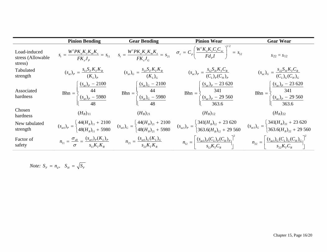
Pinion Bending Gear Bending Pinion Wear Gear Wear
Load-induced stress (Allowable stress)
11
to m s
t
W PK K K Ks s
FK J v
x P
21
to m s
t
W PK K K Ks s
FK J v
x G
1/ 2
12
to s xc
c pP
W K K C CC s
Fd I
v
s22 = s12
Tabulated strength
11( )( )
F T Rat P
L P
s S K Ks
K 21( )
( )F T R
at GL G
s S K Ks
K 12( )
( ) ( )H T R
ac PL P H P
s S K Cs
C C 22( )
( ) ( )H T R
ac GL G H G
s S K Cs
C C
Associated hardness
( ) 2100
44Bhn( ) 5980
48
at P
at P
s
s
( ) 2100
44Bhn( ) 5980
48
at G
at G
s
s
( ) 23 620
341Bhn( ) 29 560
363.6
ac P
ac P
s
s
( ) 23 620
341Bhn( ) 29 560
363.6
ac P
ac P
s
s
Chosen hardness
(HB)11 ( ( (HB)21 HB)12 HB)22
221
22
341( ) 23 620( )
363.6( ) 29 560B
ac GB
Hs
H
New tabulated strength
111
11
44( ) 2100( )
48( ) 5980B
at PB
Hs
H
211
21
44( ) 2100( )
48( ) 5980B
at GB
Hs
H
121
12
341( ) 23 620( )
363.6( ) 29 560B
ac PB
Hs
H
Factor of safety
all 111
11
( ) ( )at P L P
T R
s Kn
s K K
121
21
( ) ( )at G L G
T R
s Kn
s K K
2
112
12
( ) ( ) ( )ac P L P H P
T R
s C Cn
s K C
2
122
22
( ) ( ) ( )ac G L G H G
T R
s C Cn
s K C
Note: , F d H FS n S S
Chapter 15, Page 16/20
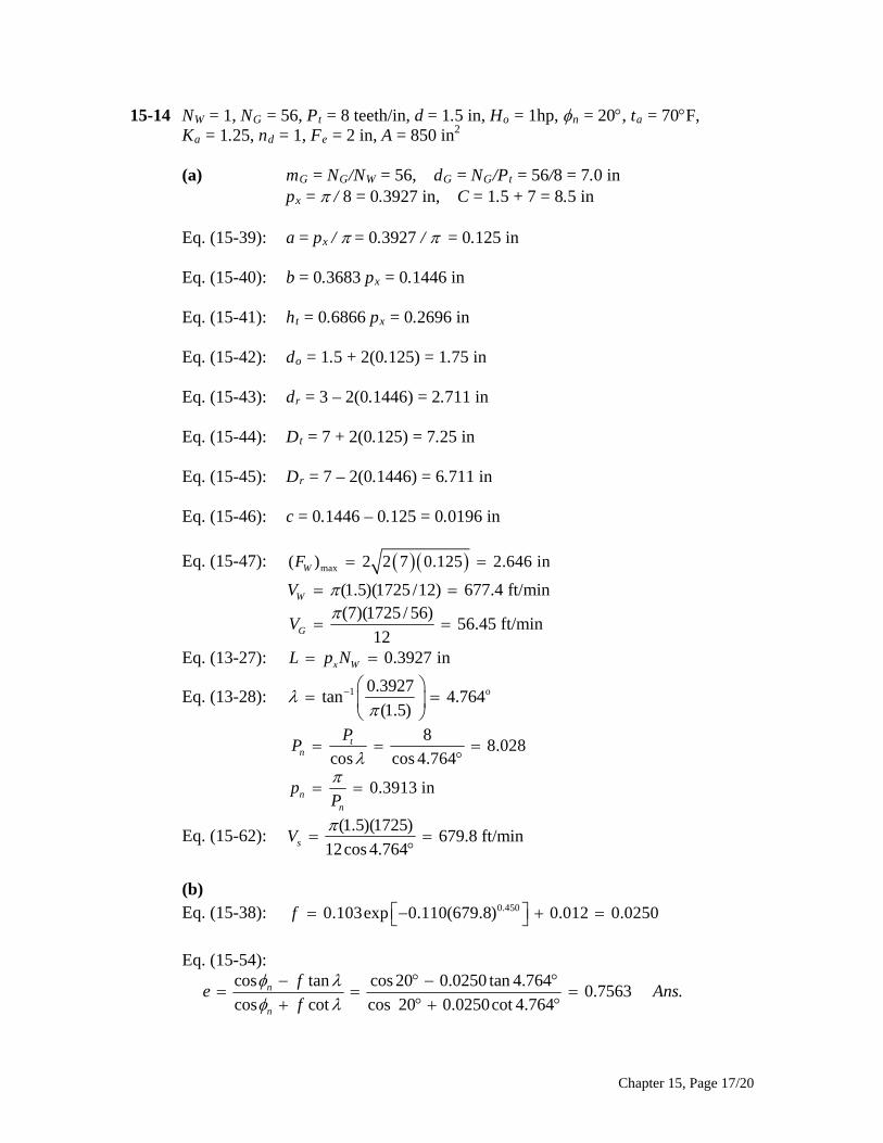
15-14 NW = 1, NG = 56, Pt = 8 teeth/in, d = 1.5 in, Ho = 1hp, n = 20, ta = 70F, Ka = 1.25, nd = 1, Fe = 2 in, A = 850 in2 (a) mG = NG/NW = 56, dG = NG/Pt = 56/8 = 7.0 in px = / 8 = 0.3927 in, C = 1.5 + 7 = 8.5 in Eq. (15-39): a = px / = 0.3927 / = 0.125 in Eq. (15-40): b = 0.3683 px = 0.1446 in Eq. (15-41): ht = 0.6866 px = 0.2696 in Eq. (15-42): do = 1.5 + 2(0.125) = 1.75 in Eq. (15-43): dr = 3 – 2(0.1446) = 2.711 in Eq. (15-44): Dt = 7 + 2(0.125) = 7.25 in Eq. (15-45): Dr = 7 – 2(0.1446) = 6.711 in Eq. (15-46): c = 0.1446 – 0.125 = 0.0196 in
Eq. (15-47): max( ) 2 2 7 0.125 2.646 inWF
(1.5)(1725 /12) 677.4 ft/min(7)(1725 / 56)
56.45 ft/min12
W
G
V
V
Eq. (13-27): 0.3927 inx WL p N
Eq. (13-28): 1 o0.3927tan 4.764
(1.5)
88.028
cos cos 4.764
0.3913 in
tn
nn
PP
pP
Eq. (15-62): (1.5)(1725)
679.8 ft/min12cos 4.764sV
(b) Eq. (15-38): 0.4500.103exp 0.110(679.8) 0.012 0.0250f Eq. (15-54):
cos tan cos 20 0.0250 tan 4.7640.7563 .
cos cot cos 20 0.0250cot 4.764n
n
fe A
fns
Chapter 15, Page 17/20
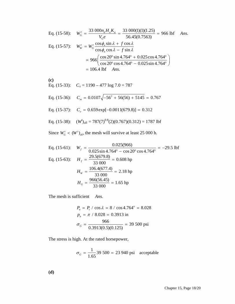
Eq. (15-58): 33 000 33 000(1)(1)(1.25)
966 lbf .56.45(0.7563)
t d o aG
G
n H KW Ans
V e
Eq. (15-57): cos sin cos
cos cos sint t n
W Gn
fW W
f
cos 20 sin 4.764 0.025cos 4.764966
cos 20 cos 4.764 0.025sin 4.764106.4 lbf .Ans
(c)
5-33): Cs = 1190 – 477 log 7.0 = 787
Eq. (15-36):
Eq. (1
20.0107 56 56(56) 5145 0.767mC
Eq. (15-37):
Eq. (15-38): (Wt)all = 787(7)0.8(2)(0.767)(0.312) = 1787 lbf
Since the mesh will survive at least 25 000 h.
Eq. (15-61):
0.659exp[ 0.0011(679.8)] 0.312C v
all( ) ,t t
GW W
0.025(966)29.5 lbf
0.025sin 4.764 cos 20 cos 4.764fW
Eq. (15-63): 29.5(679.8)
0.608 hp33 000fH
106.4(677.4)2.18 hp
33 000966(56.45)
1.65 hp33 000
W
G
H
H
The mesh is sufficient Ans.
o/ cos 8 / cos 4.764 8.028n tP P
/ 8.028 0.3913 innp
96639 500 psi
0.3913(0.5)(0.125)G
The stress is high. At the rated horsepower,
1
39 500 23 940 psi acceptable1.65G
(d)
Chapter 15, Page 18/20
Eq. (15-52): Amin = 43.2(8.5)1.7 = 1642 in2 < 1700 in2
Eq. (15-49): Hloss = 33 000(1 – 0.7563)(2.18) = 17 530 ft · lbf/min
Assuming a fan exists on the worm shaft,
Eq. (15-50):
2 o17250.13 0.568 ft · lbf/(min · in · F)
3939CR
Eq. (15-51): o17 53070 88.2 F .
0.568(1700)st A ns
________________________________________________________________________
Chapter 15, Page 19/20
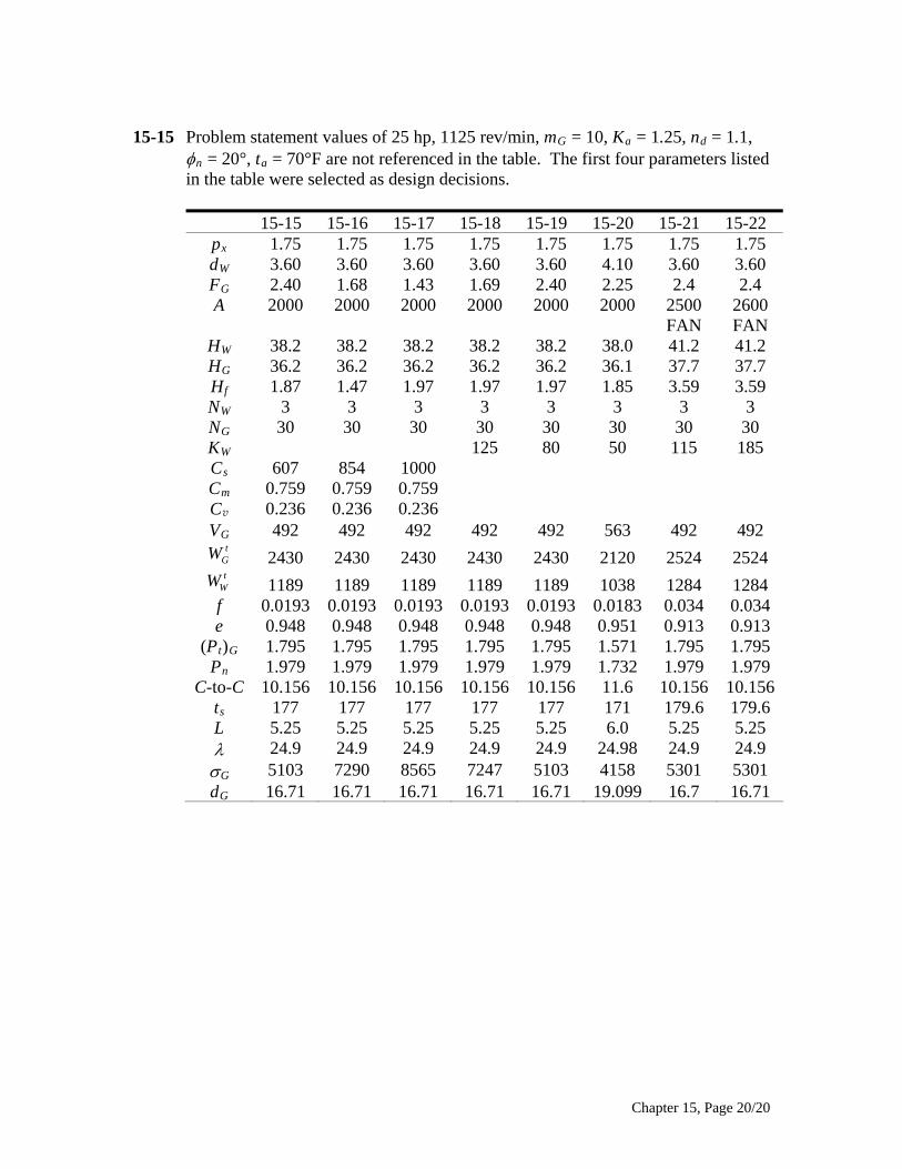
15-15 Problem statement values of 25 hp, 1125 rev/min, mG = 10, Ka = 1.25, nd = 1.1,
n = 20°, ta = 70°F are not referenced in the table. The first four parameters listed in the table were selected as design decisions.
15-15 15-16 15-17 15-18 15-19 15-20 15-21 15-22
px 1.75 1.75 1.75 1.75 1.75 1.75 1.75 1.75 dW 3.60 3.60 3.60 3.60 3.60 4.10 3.60 3.60 FG 2.40 1.68 1.43 1.69 2.40 2.25 2.4 2.4 A 2000 2000 2000 2000 2000 2000 2500 2600 FAN FAN
HW 38.2 38.2 38.2 38.2 38.2 38.0 41.2 41.2 HG 36.2 36.2 36.2 36.2 36.2 36.1 37.7 37.7 Hf 1.87 1.47 1.97 1.97 1.97 1.85 3.59 3.59 NW 3 3 3 3 3 3 3 3 NG 30 30 30 30 30 30 30 30 KW 125 80 50 115 185 Cs 607 854 1000 Cm 0.759 0.759 0.759 Cv 0.236 0.236 0.236 VG 492 492 492 492 492 563 492 492
tGW 2430 2430 2430 2430 2430 2120 2524 2524 t
WW 1189 1189 1189 1189 1189 1038 1284 1284 f 0.0193 0.0193 0.0193 0.0193 0.0193 0.0183 0.034 0.034 e 0.948 0.948 0.948 0.948 0.948 0.951 0.913 0.913
(Pt)G 1.795 1.795 1.795 1.795 1.795 1.571 1.795 1.795 Pn 1.979 1.979 1.979 1.979 1.979 1.732 1.979 1.979
C-to-C 10.156 10.156 10.156 10.156 10.156 11.6 10.156 10.156 ts 177 177 177 177 177 171 179.6 179.6 L 5.25 5.25 5.25 5.25 5.25 6.0 5.25 5.25 24.9 24.9 24.9 24.9 24.9 24.98 24.9 24.9 G 5103 7290 8565 7247 5103 4158 5301 5301 dG 16.71 16.71 16.71 16.71 16.71 19.099 16.7 16.71
Chapter 15, Page 20/20
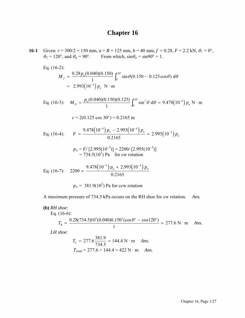
Chapter 16 16-1 Given: r = 300/2 = 150 mm, a = R = 125 mm, b = 40 mm, f = 0.28, F = 2.2 kN, 1 = 0,
2 = 120, and a = 90. From which, sina = sin90 = 1. Eq. (16-2):
120
0
4
0.28 (0.040)(0.150)sin (0.150 0.125cos )
1 2.993 10 N · m
af
a
pM d
p
Eq. (16-3): 120 2 4
0
(0.040)(0.150)(0.125)sin 9.478 10 N · m
1a
N a
pM d
p
c = 2(0.125 cos 30) = 0.2165 m
Eq. (16-4):
4 4
39.478 10 2.993 10
2.995 100.2165
a a
a
p pF p
pa = F/ [2.995(103)] = 2200/ [2.995(103)] = 734.5(103) Pa for cw rotation
Eq. (16-7): 4 49.478 10 2.993 10
22000.2165
a ap p
pa = 381.9(103) Pa for ccw rotation A maximum pressure of 734.5 kPa occurs on the RH shoe for cw rotation. Ans. (b) RH shoe: Eq. (16-6):
3 2 o o0.28(734.5)10 (0.040)0.150 (cos0 cos120 )
277.6 N · m .1RT A
ns
LH shoe:
381.9
277.6 144.4 N · m .734.5LT A ns
Ttotal = 277.6 + 144.4 = 422 N · m Ans.
Chapter 16, Page 1/27
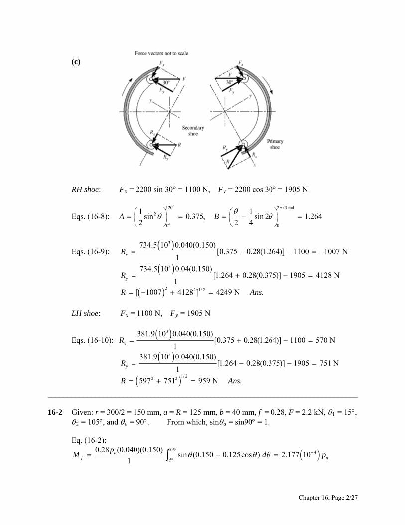
(c)
RH shoe: Fx = 2200 sin 30° = 1100 N, Fy = 2200 cos 30° = 1905 N
Eqs. (16-8):
o
o
120 2 /3 rad2
0 0
1 1sin 0.375, sin 2 1.264
2 2 4A B
Eqs. (16-9): 3734.5 10 0.040(0.150)
[0.375 0.28(1.264)] 1100 1007 N1xR
3
2 2 1/ 2
734.5 10 0.04(0.150)[1.264 0.28(0.375)] 1905 4128 N
1[ 1007 4128 ] 4249 N .
yR
R Ans
LH shoe: Fx = 1100 N, Fy = 1905 N
Eqs. (16-10): 3381.9 10 0.040(0.150)
[0.375 0.28(1.264)] 1100 570 N1xR
3
1/ 22 2
381.9 10 0.040(0.150)[1.264 0.28(0.375)] 1905 751 N
1
597 751 959 N .
yR
R Ans
______________________________________________________________________________ 16-2 Given: r = 300/2 = 150 mm, a = R = 125 mm, b = 40 mm, f = 0.28, F = 2.2 kN, 1 = 15, 2 = 105, and a = 90. From which, sina = sin90 = 1. Eq. (16-2):
105 4
15
0.28 (0.040)(0.150)sin (0.150 0.125cos ) 2.177 10
1a
f a
pM d p
Chapter 16, Page 2/27
Eq. (16-3): 105 2 4
15
(0.040)(0.150)(0.125)sin 7.765 10
1a
N a
pM d p
c = 2(0.125) cos 30° = 0.2165 m
Eq. (16-4):
4 4
37.765 10 2.177 10
2.581 100.2165
a a
a
p pF p
RH shoe: pa = 2200/ [2.581(10 3)] = 852.4 (103) Pa = 852.4 kPa on RH shoe for cw rotation Ans.
Eq. (16-6): 3 20.28(852.4)10 (0.040)(0.150 )(cos15 cos105 )
263 N · m1RT
LH shoe:
4 4
3
7.765 10 2.177 102200
0.2165479.1 10 Pa 479.1 kPa on LH shoe for ccw rotation .
a a
a
p p
p A
ns
3 2
total
0.28(479.1)10 (0.040)(0.150 )(cos15 cos105 )148 N · m
1263 148 411 N · m .
LT
T Ans
Comparing this result with that of Prob. 16-1, a 2.6% reduction in torque is obtained by
using 25% less braking material. ______________________________________________________________________________ 16-3 Given: 1 = 0°, 2 = 120°, a = 90°, sin a = 1, a = R = 3.5 in, b = 1.25 in, f = 0.30, F = 225 lbf, r = 11/2 = 5.5 in, counter-clockwise rotation. LH shoe: Eq. (16-2), with 1 = 0:
2
1
22 2
o 2
sin cos (1 cos ) sinsin sin 2
0.30 (1.25)5.5 3.55.5(1 cos120 ) sin 120
1 214.31 lbf · in
a af
a a
a
a
f p br f p br aM r a d r
p
p
Eq. (16-3), with 1 = 0:
2
1
2 22
1sin sin 2
sin sin 2 4
(1.25)5.5(3.5) 120 1sin 2(120 )
1 2 180 430.41 lbf · in
a aN
a a
a
a
p bra p braM d
p
p
Chapter 16, Page 3/27
oo2180
2 cos 2(5.5)cos30 9.526 in2
30.41 14.31225 1.690
9.526225 / 1.690 133.1 psi
a aa
a
c r
p pF p
p
Eq. (16-6):
2 21 2(cos cos ) 0.30(133.1)1.25(5.5 )
[1 ( 0.5)]sin 1
2265 lbf · in 2.265 kip · in .
aL
a
f p brT
Ans
RH shoe:
30.41 14.31225 4.694
9.526225 / 4.694 47.93 psi
a aa
a
p pF p
p
47.93
2265 816 lbf ·in 0.816 kip·in133.1RT
Ttotal = 2.27 + 0.82 = 3.09 kip in Ans. ______________________________________________________________________________ 16-4 (a) Given: 1 = 10°, 2 = 75°, a = 75°, pa = 106 Pa, f = 0.24, b = 0.075 m (shoe width),
a = 0.150 m, r = 0.200 m, d = 0.050 m, c = 0.165 m. Some of the terms needed are evaluated here:
22 2 2
11 11
2
1
2
1
2
7575 2
1010
75 /180 rad2
10 /180 rad
1sin sin cos cos sin
2
1200 cos 150 sin 77.5 mm
2
1sin sin 2 0.528
2 4
sin cos 0.4514
A r d a d r a
B d
C d
Now converting to Pascals and meters, we have from Eq. (16-2),
60.24 10 (0.075)(0.200)(0.0775) 289 N · m
sin sin 75a
fa
f p brM A
Chapter 16, Page 4/27
From Eq. (16-3),
610 (0.075)(0.200)(0.150)(0.528) 1230 N · m
sin sin 75a
Na
p braM B
Finally, using Eq. (16-4), we have
1230 2895.70 kN .
165N fM M
F Ac
ns
(b) Use Eq. (16-6) for the primary shoe.
21 2
6 2
(cos cos )
sin
0.24 10 (0.075)(0.200) (cos 10 cos 75 )541 N · m
sin 75
a
a
fp brT
For the secondary shoe, we must first find pa. Substituting
6 6
6 63
1230 289 and into Eq. (16 - 7),
10 10(1230 / 10 ) (289 / 10 )
5.70 , solving gives 619 10 Pa165
N a f a
a aa
M p M p
p pp
Then
3 20.24 619 10 0.075 0.200 cos 10 cos 75335 N · m
sin 75T
so the braking capacity is Ttotal = 2(541) + 2(335) = 1750 N · m Ans. (c) Primary shoes:
63
63
sin
10 (0.075)0.200[0.4514 0.24(0.528)](10 ) 5.70 0.658 kN
sin 75
( )sin
10 (0.075)0.200[0.528 0.24(0.4514)] 10 0 9.88 kN
sin 75
ax x
a
ay y
a
p brR C f B F
p brR B f C F
Chapter 16, Page 5/27
Secondary shoes:
6
3
6
3
( )sin
0.619 10 0.075(0.200)[0.4514 0.24(0.528)] 10 5.70
sin 750.143 kN
( )sin
0.619 10 0.075(0.200)[0.528 0.24(0.4514)] 10 0
sin 754.03 kN
ax x
a
ay y
a
p brR C f B F
p brR B f C F
Note from figure that +y for secondary shoe is opposite to +y for primary shoe. Combining horizontal and vertical components,
2 2
0.658 0.143 0.801 kN9.88 4.03 5.85 kN
( 0.801) 5.855.90 kN .
H
V
RR
RAns
______________________________________________________________________________ 16-5 Given: Face width b = 1.25 in, F = 90 lbf, f = 0.25. Preliminaries: 1 = 45° tan1(6/8) = 8.13°, 2 = 98.13°, a = 90°, a = (62 + 82)1/2 = 10 in Eq. (16-2):
2
1
98.13
8.13
0.25 (1.25)6sin cos sin 6 10cos
sin 1
3.728 lbf · in
a af
a
a
f p br pM r a d d
p
Eq. (16-3):
2
1
98.132 2
8.13
(1.25)6(10)sin sin
sin 1
69.405 lbf · in
a aN
a
a
p bra pM d d
p
Eq. (16-4): Using Fc = MN Mf , we obtain 90(20) (69.405 3.728) 27.4 psi .a ap p A ns
Chapter 16, Page 6/27
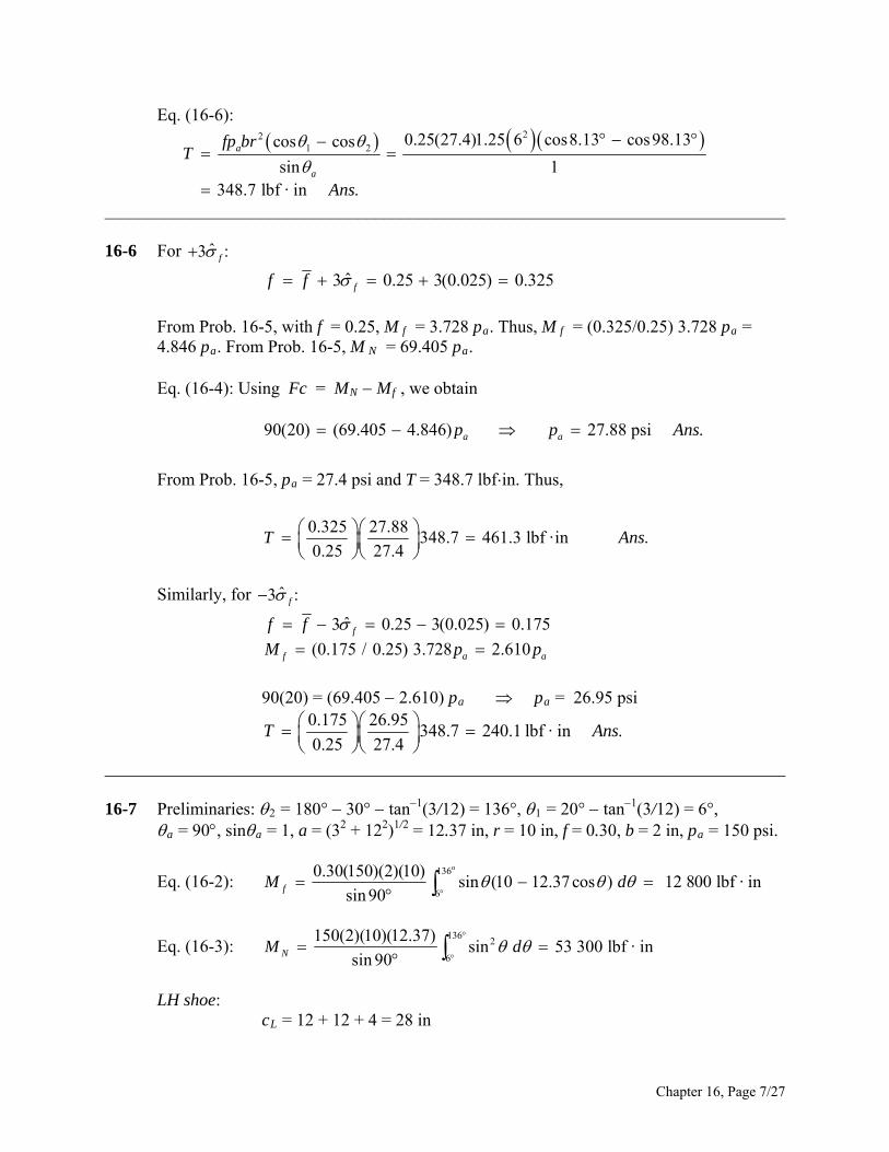
Eq. (16-6):
221 2
0.25(27.4)1.25 6 cos8.13 cos98.13cos cos
sin 1348.7 lbf · in .
a
a
fp brT
Ans
______________________________________________________________________________
16-6 For ˆ3 :f
ˆ3 0.25 3(0.025) 0.325ff f
From Prob. 16-5, with f = 0.25, M f = 3.728 pa. Thus, M f = (0.325/0.25) 3.728 pa =
4.846 pa. From Prob. 16-5, M N = 69.405 pa. Eq. (16-4): Using Fc = MN Mf , we obtain 90(20) (69.405 4.846) 27.88 psi .a ap p A ns
From Prob. 16-5, pa = 27.4 psi and T = 348.7 lbf⋅in. Thus,
0.325 27.88
348.7 461.3 lbf ·in .0.25 27.4
T A
ns
Similarly, for ˆ3 :f
ˆ3 0.25 3(0.025) 0.175
(0.175 / 0.25) 3.728 2.610f
f a a
f f
M p p
90(20) = (69.405 2.610) pa pa = 26.95 psi
0.175 26.95348.7 240.1 lbf · in .
0.25 27.4T A
ns
______________________________________________________________________________ 16-7 Preliminaries: 2 = 180° 30° tan1(3/12) = 136°, 1 = 20° tan1(3/12) = 6°, a = 90, sina = 1, a = (32 + 122)1/2 = 12.37 in, r = 10 in, f = 0.30, b = 2 in, pa = 150 psi.
Eq. (16-2): o136
6
0.30(150)(2)(10)sin (10 12.37cos ) 12 800 lbf · in
sin 90fM d
Eq. (16-3): 136
2
6
150(2)(10)(12.37)sin 53 300 lbf · in
sin 90NM d
LH shoe: cL = 12 + 12 + 4 = 28 in
Chapter 16, Page 7/27
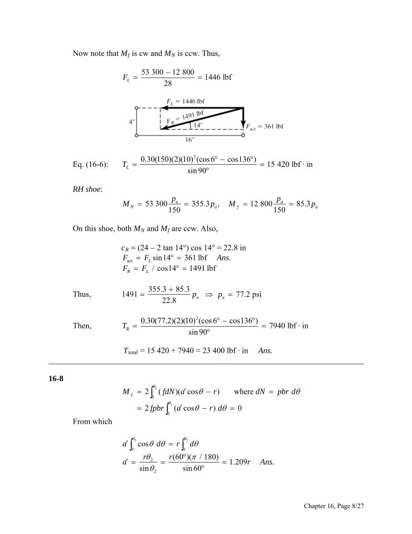
Now note that Mf is cw and MN is ccw. Thus,
53 300 12 8001446 lbf
28LF
Eq. (16-6): 20.30(150)(2)(10) (cos 6 cos136 )
15 420 lbf · insin 90LT
RH shoe:
53 300 355.3 , 12 800 85.3
150 150a a
N a f
p paM p M p
On this shoe, both MN and Mf are ccw. Also, cR = (24 2 tan 14°) cos 14° = 22.8 in
act sin14 361 lbf ./ cos14 1491 lbf
L
R L
F F AnsF F
Thus, 355.3 85.3
1491 77.2 psi22.8 a ap p
Then, 20.30(77.2)(2)(10) (cos6 cos136 )
7940 lbf · insin 90RT
Ttotal = 15 420 + 7940 = 23 400 lbf · in Ans. ______________________________________________________________________________ 16-8
2
2
0
0
2 ( )( cos ) where
2 ( cos ) 0
fM fdN a r dN pbr d
fpbr a r d
From which
2 2
0 0
2
2
cos
(60 )( / 180)1.209 .
sin sin 60
a d r d
r ra r
Ans
Chapter 16, Page 8/27
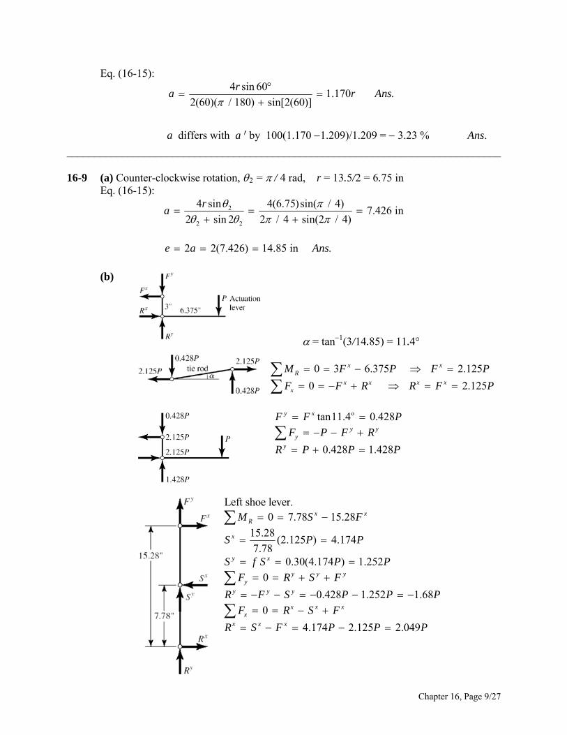
Eq. (16-15):
4 sin 601.170 .
2(60)( / 180) sin[2(60)]
ra r
Ans
a differs with a ¢ by 100(1.170 1.209)/1.209 = 3.23 % Ans.
______________________________________________________________________________ 16-9 (a) Counter-clockwise rotation, 2 = / 4 rad, r = 13.5/2 = 6.75 in Eq. (16-15):
2
2 2
4 sin 4(6.75)sin( / 4)7.426 in
2 sin 2 2 / 4 sin(2 / 4)
2 2(7.426) 14.85 in .
ra
e a Ans
(b)
= tan1(3/14.85) = 11.4°
0 3 6.375 2.125
0 2
x xR
x x x xx .125
M F P F
F F R R F
P
P
Potan11.4 0.428
0.428 1.428
y x
y yy
y
F F
F P F R
R P P
P
Left shoe lever. 0 7.78 15.28
15.28(2.125 ) 4.174
7.780.30(4.174 ) 1.252
0
0.428 1.252 1.68
0
4.174 2.125 2.049
x xR
x
y x
y y yy
y y y
x x xx
x x x
M S F
S P P
S f S P P
F R S F
R F S P P
F R S F
P
R S F P P P
Chapter 16, Page 9/27
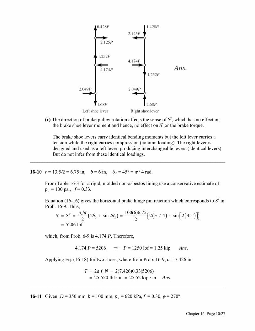
(c) The direction of brake pulley rotation affects the sense of Sy, which has no effect on
The brake shoe levers carry identical bending moments but the left lever carries a
ers).
______________________________________________________________________________
6-10 r = 13.5/2 = 6.75 in, b = 6 in, 2 = 45° = / 4 rad.
From Table 16-3 for a rigid, molded non-asbestos lining use a conservative estimate of
Equation (16-16) gives the horizontal brake hinge pin reaction which corresponds to Sx in
the brake shoe lever moment and hence, no effect on Sx or the brake torque.
tension while the right carries compression (column loading). The right lever is designed and used as a left lever, producing interchangeable levers (identical lev But do not infer from these identical loadings.
1 pa = 100 psi, f = 0.33.
Prob. 16-9. Thus,
2 2
100(6)6.752 sin 2 2 / 4 sin 2 45
2 25206 lbf
x apN S
br
which, from Prob. 6-9 is 4.174 P. Therefore,
4.174 P = 5206 P = 1250 lbf = 1.25 kip Ans.
Applying Eq. (16-18) for two shoes, where from Prob. 16-9, a = 7.426 in
______________________________________________________________________________
6-11 Given: D = 350 mm, b = 100 mm, pa = 620 kPa, f = 0.30, = 270.
2 2(7.426)0.33(5206)25 520 lbf · in 25.52 kip · in .
T a f NAns
1
Chapter 16, Page 10/27
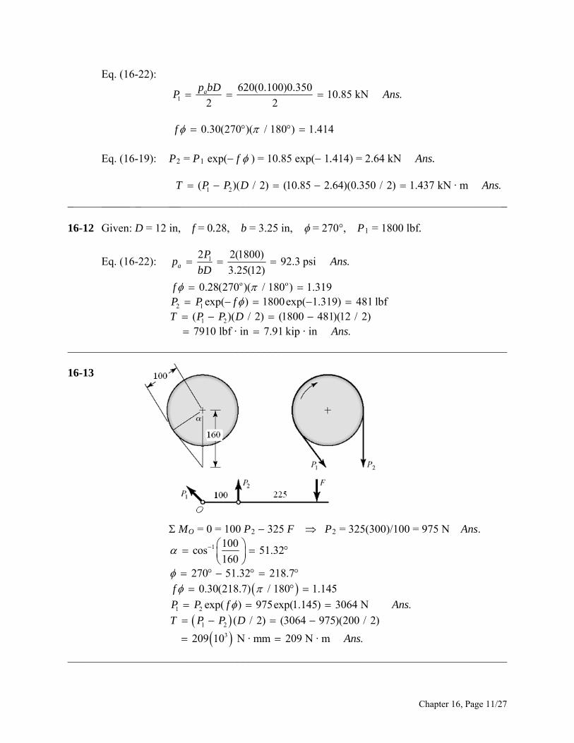
Eq. (16-22):
1
620(0.100)0.35010.85 kN .
2 2
0.30(270 )( / 180 ) 1.414
ap bDP Ans
f
Eq. (16-19): P2 = P1 exp( f ) = 10.85 exp( 1.414) = 2.64 kN Ans.
s
_____ _ _____ _________________________________________________________
6-12 Given: D = 12 in, f = 0.28, b = 3.25 in, = 270°, P1 = 1800 lbf.
Eq. (16-22):
1 2( )( / 2) (10.85 2.64)(0.350 / 2) 1.437 kN · m .T P P D An
_ _____ _ __ _ 1
12 2(1800)92.3 psi .
3.25(12)a
Pp Ans
bD
______________________________________________________________________________
3
Ans.
o o
2 1
1 2
0.28(270 )( / 180 ) 1.319exp( ) 1800exp( 1.319) 481 lbf
( )( / 2) (1800 481)(12 / 2)7910 lbf · in 7.91 kip · in .
fP P fT P P D
Ans
16-1 MO = 0 = 100 P2 325 F P2 = 325(300)/100 = 975 N
1 100cos 51.32
1 2
1 2
3
160270 51.32 218.7
0.30(218.7) / 180 1.145
exp( ) 975exp(1.145) 3064 N .
( / 2) (3064 975)(200 / 2)
209 10 N · mm 209 N · m .
f
P P f Ans
T P P D
Ans
______________________________________________________________________________
Chapter 16, Page 11/27
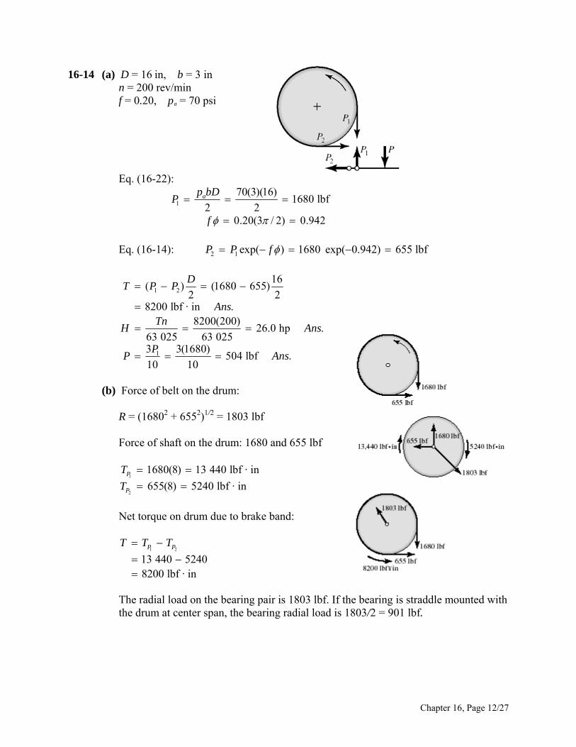
16-14 (a) D = 16 in, b = 3 in n = 200 rev/min f = 0.20, pa = 70 psi
Eq. (16-22):
1 1680 lbf2 2
aP 70(3)(16)p bD
f 0.20(3 / 2) 0.942
Eq. (16-14): P2 1 exp( ) 1680 exp( 0.942) 655 lbfP f
1 2
1 504 lbf .10 10
16( ) (1680 655)
2 28200 lbf · in .
8200(200)26.0 hp .
63 025 63 0253 3(1680)
DT P P
AnsTn
H Ans
P
(b) Force of belt on the drum:
R = (16802 + 6552)1/2 = 1803 lbf
shaft on the drum: 1680 and 655 lbf
Net torque on drum due to brake band:
r is 1803 lbf. If th the drum at center span, the bearing radial load is 1803
P Ans
Force of
1
2
1680(8) 13 440 lbf · in
655(8) 5240 lbf · inP
P
T
T
8200 lbf · in
1 2
13 440 5240P PT T T
The radial load on the bearing pai e bearing is straddle mounted with
/2 = 901 lbf.
Chapter 16, Page 12/27
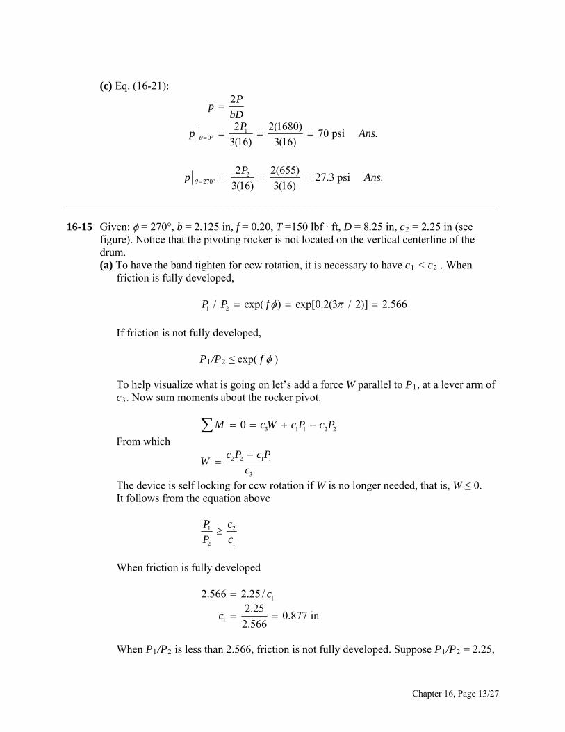
(c) Eq. (16-21):
10
2
2 2(1680)70 psi .
3(16) 3(16)
Pp
bDP
p Ans
2270 27.3 psi .
3(16) 3(16)
2 2(655)Pp Ans
______________________________________________________________________________ 16-15 Given: = 270°, b = 2.125 in, f = 0.20, T =150 lbf · ft, D = 8.25 in, c2 = 2.25 in (see
figure). Notice that the pivoting rocker is not located on the vertical centerline of the drum. (a) To have the band tighten for ccw rotation, it is necessary to have c1 < c2 . When friction is fully developed,
1 2/ exp( ) exp[0.2(3 / 2)] 2.566P P f
If friction is not fully developed, P1/P2 ≤ exp( f )
To help visualize what is going on let’s add a force W parallel to P1, at a lever arm of c3. Now sum moments about the rocker pivot.
23 1 1 20M c W c P c P
From which
2 2 1 1
3
c P c PW
c
The device is self locking for ccw rotation if W is no longer needed, that is, W ≤ 0. It follows from the equation above
1 2
2 1
P c
P c
When friction is fully developed
1
1
2.566 2.25 /2.25
0.877 in2.566
c
c
When P1/P2 is less than 2.566, friction is not fully developed. Suppose P1/P2 = 2.25,
Chapter 16, Page 13/27
then
1
2.251 in
2.25c
We don’t want to be at the point of slip, and we need the band to tighten.
21 2
1 2/
cc c
P P
When the developed friction is very small, P1/P2 → 1 and c1 → c2 Ans. (b) Rocker has c1 = 1 in
1 2
2 1 1ln(
P c
f
1 2
2.25
/ ) ln 2.250.172
3 / 2
P P
is ully developed, no slip.
2.25P c
Friction not f
11 2( )
D PT P P 2 1
2
DP
22 P
Solve for P2
21 2
1 2
1
2 2(150)(12)349 lbf
[( / ) 1] (2.25 1)(8.25)2.25 2.25(349) 785 lbf2 2(785)
89.6 psi .2.125(8.25)
TP
P P DP P
Pp Ans
bD
-fold.
(c) The torque ratio is 150(12)/100 or 18
2
1 2
34919.4 lbf
182.25 2.25(19.4) 43.6 lbf89.6
4.98 psi .18
P
P P
p Ans
Comment: As the torque opposed by the locked brake increases, P2 and P1 increase (although ratio is still 2.25), then p follows. The brake can self-destruct. Protection could be provided by a shear key.
__ __ ________________________________________________________
____ __________ ____ 16-16 Given: OD = 250 mm, ID = 175 mm, f = 0.30, F = 4 kN.
Chapter 16, Page 14/27
(a) From Eq. (16-23),
22 4000
2a 0.194 N/mm 194 kPa .
( ) (175)(250 175)
Fp Ans
d D d
Eq. (16-25): 34000(0.30)
( ) (250 175)10 127.5 N · m .4 4
FfT D d Ans
(b) From Eq. (16-26),
2
2 2( )a 2 2
4 4(4000)0.159 N/mm 159 kPa .
(250 175 )
Fp Ans
Eq. (16-27):
D d
33 3 3 3 3 3( ) (0.30)159 10 250 175 1012 12128 N · m .
aT f p D d
Ans
__ _________ ___
___ ___ _________________________________________________________
6-17 Given: OD = 6.5 in, ID = 4 in, f = 0.24, pa = 120 psi. (a) Eq. (16-23):
_ 1
(120)(4)( ) (6.5 4) 1885 lbf .
2 2 ap d
F
D d Ans
N sliding planes:
Eq. (16-24) with
2 2 2 2(0.24)(120)(4)( ) (6.5 4 )
8 87125 lbf · in .
afp dT D d N
Ans
(6)
2 2(0.24)(120 )
(6.5 )(6)8
d (b) T
d
d, in T, lbf · in
2 5191 3 6769 4 7125 Ans.5 5853 6 2545
(c) The torque-diameter curve exhibits a stationary point maximum in the range of
s nearly optimal proportions. diameter d. The clutch ha ______________________________________________________________________________ 16-18 (a) Eq. (16-24) with N sliding planes:
Chapter 16, Page 15/27
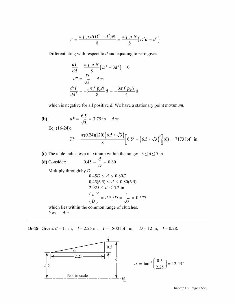
2 2
2 3( )
8 8a af
T D
p d D d N f p Nd d
respect to d and equating to zero gives
Differentiating with
2 2
2
2
3 08
*d .3
36
8 4
a
a a
dT f p ND d
ddD
Ans
d T f p N f p Nd d
dd
egative for all positive d. We have a stationary point maximum.
(b)
which is n
6.5* 3.75 in .
3d A ns
Eq. (16-24):
2(0.24)(120) 6.5 / 3
* 6.5T
2
6.5 / 3 (6) 7173 lbf · in8
(c) The table indicates a maximum within the range: 3 ≤ d ≤ 5 in
r:
0.45 0.80d
(d) ConsideD
Multiply through by D,
*
0.45 0.800.45(6.5) 0.80(6.5)2.925 5.2 in
1* / 0.577
3
D d Dd
d
dd D
D
which lies within the common range of clutches. Yes. Ans. ______________________________________________________________________________ 16-19 Given: d = 11 in, l = 2.25 in, = 1800 lbf · i D = 12 in, f = 0.28.
T n,
1 0.5 tan 12.532.25
Chapter 16, Page 16/27
Uniform wear
45):
Eq. (16-
2 2 8sin
af p dT D d
2 2(0.28) (11)1800 12 11 128.2
8sin12.531800
14.04 psi .128.2
aa
a
pp
p Ans
Eq. (16-44):
(14.04)11( ) (12 11) 243 lbf .
2 2ap d
F D d Ans
pressure
Uniform Eq. (16-48):
3 3
1 s
f pT
2 ina D d
3 3(0.28)1800 12 11 134.1
12sin12.531800
aa
p
13.42 psi .
134.1a
p
p Ans
Eq. (16-47):
2 2 2 2(13.42)(ap
) 12 11 242 lbf .4 4
F D d Ans
______________________________________________________________________________ 16-20 Uniform wear
Eq. (16-34):
2 22 1
1( )
2F = (
a i o iT f p r r r
2 1) pari (ro ri) Eq. (16-33):
Thus,
2 2
2 1(1 / 2)( ) a i o if p r r rT
2 1 ( ) ( )( )
/ 2 / 2 11 . . .
2 2 4
a i o i
o i
f FD f p r r r D
r r D d dO K Ans
D D D
Uniform pressure
Eq. (16-38):
3 32 1
1( )
3 a o iT f p r r
Chapter 16, Page 17/27
2 22 1
1( )
2 a o i Eq. (16-37): F p r r
Thus,
3 3 3 32 1
2 22 22 1
3 3 3
22 2
(1 / 3)( ) 2 ( / 2) ( / 2)
3 ( / 2) ( / 2)(1 / 2) ( )
2( / 2) 1 ( / ) 1 1 ( / ) . . .
3 1 ( / )3( / 2) 1 ( / )
a o i
a o i
f p r rT D
f FD D d Df p r r D
D d D d DO K Ans
d DD d D D
d
___ __________
__ ______________________________________________________________
_
6-211
3
2 / 60 2 500 / 60 52.4 rad/s
2(10 )38.2 N· m
52.4
n
HT
Key:
38.23.18 kN
12
TF
r
Average shear stress in key is
33.18(10 )13.2 MPa .
6(40)Ans
Average bearing stress is
33.18(10 )26.5 MPa .
3(40)b A
b
FAns
tire load. Let one jaw carry the en
1 26 4517.75 mm
2 2 238.2
2.15 kN17.75
av
av
r
TF
r
The bearing and shear stress estimates are
3
3
2
2.15 1022.6 MPa .
10(22.5 13)
2.15(10 )0.869 MPa .
10 0.25 (17.75)
b Ans
Ans
___________________________________________________ ___________________________
Chapter 16, Page 18/27
16-22
From Eq. (16-51),
1
2
2 / 60 2 (1600) / 60 167.6 rad/s0
n
21 2 1
1 2 1 2
2800(8)133.7 lbf · in · s
167.6 0
I I Tt
I I
Eq. (16-52):
2 2 61 21 2
1 2
133.7I I
(167.6 0) 1.877 10 lbf in
2 2E
I I
In Btu, Eq. (16-53): H = E / 9336 = 1.877(106) / 9336 = 201 Btu
:
6-54) Eq. (1
20141.9 F .
0.12(40)p
HT A
C W
ns
__ ________________________ _____________________________________
16-23
____ __________ _
1 2 260 240250 rev/min
2 Eq. (16-62): C
2
n nn
2 1) / = (n2 n1) / n = (260 240) / 250 = 0.08 Ans.
= 2 (250) / 60 = 26.18 rad/s
From Eq. (16-64):
s = (
3
22 12 2
6.75 10123.1 N · m · s
0.08(26.18)s
E EI
C
2 22 2 2 2
8 8(123.1)233.9 kg
8 1.5o io i
m II d d m
d d
1.4
Table A-5, cast iron unit weight = 70.6 kN/m3 = 70.6(103) / 9.81 = 7197 kg / m3. Volume: V = m / = 233.9 / 7197 = 0.0325 m3
2 2 2 2/ 4 1.5 1.4 / 4 0.2278o iV t d d t t
Equating the expressions for volume and solving for t,
0.03250.143 m 143 mm .
0.2278t A ns
Chapter 16, Page 19/27
______________________________________________________________________________ ) The useful work performed in one revolution of the crank shaft is
U = 320 (103) 200 (103) 0.15 = 9.6 (10
ict e total work done in one revolution is
U = 9.6(103) / (1 0.20) = 12.0(103) J
nk shaft stroke accounts for 7.5% of a crank shaft revolution, the energy fluctuation is
E2 E1 = 9.6(103) 12.0(103)(0.075) = 8.70(103) J Ans.
(b) For the flywheel,
16-24 (a
3) J
Accounting for fr ion, th
Since 15% of the cra
6(90) 540 rev/min2 2 (540)
56.5 rad/s60 60
nn
Since C = 0.10 s
q. (16-64): 3
22 12 2
8.70(10 )27.25 N · m · s
0.10(56.5)s
E EI
C
E
Assuming all the mass is concentrated at the effective diameter, d,
22 md
I mr
2 2
44 4(27.25)
75.7 kg .1.2
Ins
d
__ _________________________________________ ____________________
6-25 Use Ex. 16-6 and Table 16-6 data for one cylinder of a 3-cylinder engine.
m A
____ __________ _ 1
2 1
22 12 2
0.302400 rev/min or 251 rad/s3(3368)
804 lbf · in .
10 5900.560 in · lbf · s .
0.30(251 )
s
m
s
Cn
T Ans
E E
43(3531) 10 590 in · lbfE E
I
AnsC
_____ ___________________________
_ _____________________________________________
Chapter 16, Page 20/27
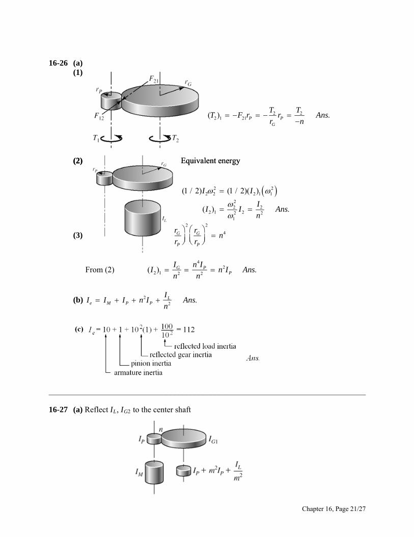
16-26 (a) (1)
2 22 1 21( ) P
G
T F rr
.P
T Tr Ans
n
Equivalent energy
Equivalent energy
(2) (2)
2 22 2 2 1 1
22 2
2 1 22 21
(1 / 2) (1 / 2)( )
( ) .
I I
II I Ans
n
(3) 2 2
4
2
G
P P P P P
rn
r
From (2)
G G G GI r m r
I r m r
4
2 2 1 2 2 P( ) .G PI n II n I Ans
(b)
n n
22
.Le M P P
II I I n I An
n
s
______________________________________________________________________________ 16-27 (a) Reflect IL, IG2 to the center shaft
Chapter 16, Page 21/27
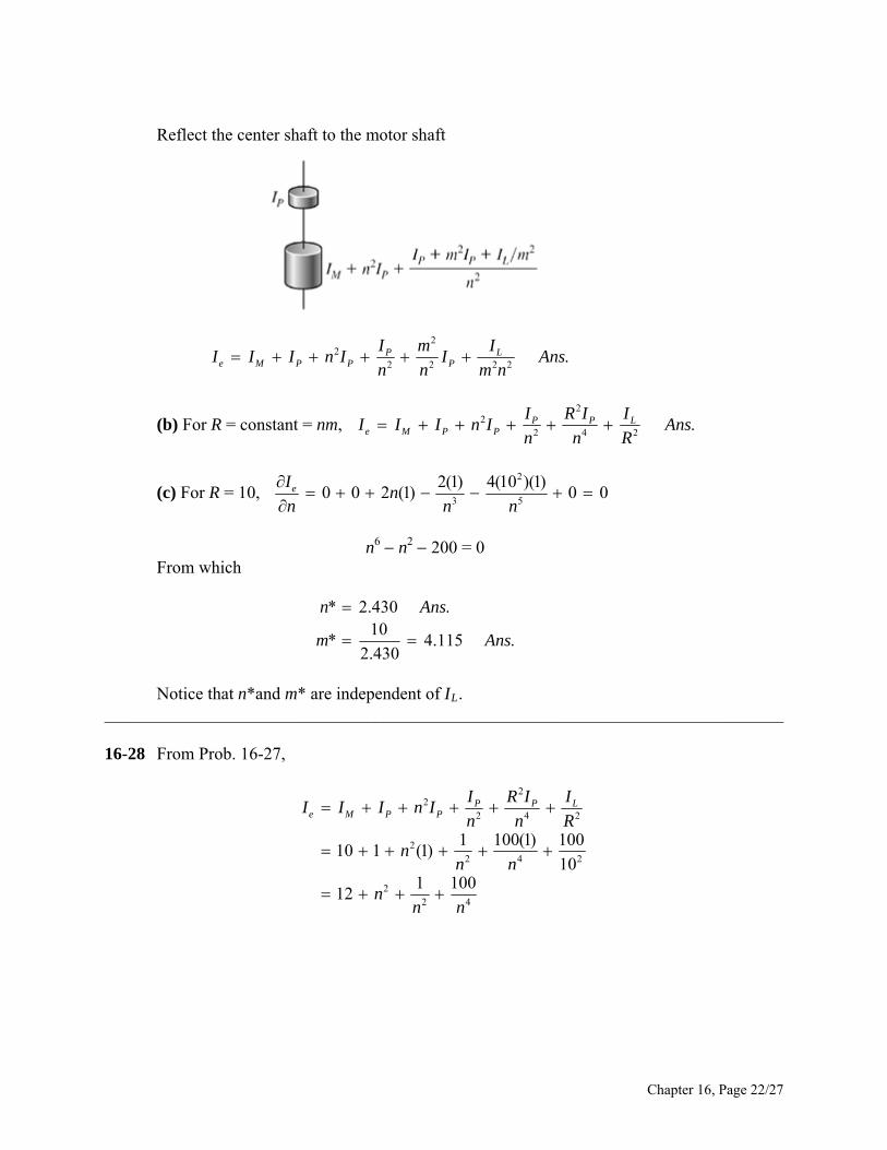
Reflect the center shaft to the motor shaft
22 P LI m I
2 2 2 2
.e M P P PI I I n I I Ansn n m n
(b) For R = constant = nm,
2
22 4 2
.P P Le M P P
I R I II I I n I An
n n s
= 10,
R
2
3 5
2(1) 4(10 )(1)0 0 2 (1) 0 0eI
nn n n
(c) For R
n6 n2 200 = 0
From which
* 2.430 .10
* 4.115 .2.430
n Ans
m A
ns
at n*and m* are independent of IL. _____________________________________________________________________________
6-28 From Prob. 16-27,
Notice th_ 1
22
2 4 2
2 4 2
2 4
101 100
12
2 1 100(1) 10010 1 (1)
2
P P Le M P P
I R I II I I n I
n n R
n n
nn n
n
Chapter 16, Page 22/27
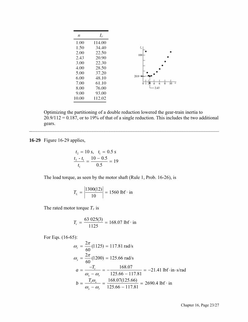
Optimizing the partitioning of a double reduction lowered the gear-train inertia to of that of a single reduction. This includes the two additional
gears. _____________________________________________________________________________
lies,
20.9/112 = 0.187, or to 19%
_ 16-29 Figure 16-29 app
2 110 , 0.5 t s t s
2 1-t t
1
10 0.519
0.5t
The load torque, as seen by the motor shaft (Rule 1, Prob. 16-26), is
1300(12)1560 lbf · in
10LT
ue Tr is
The rated motor torq
63 025(3)168.07 lbf · in
1125rT
For Eqs. (16-65):
2(1125) 117.81 rad/s
602
(1200) 125.66 rad/s60
168.0721.41 lbf in s/rad
125.66 117.81168.07(125.66)
2690.4 lbf · in125.66 117.81
r
s
r
s r
r s
s r
Ta
Tb
Chapter 16, Page 23/27
The linear portion of the squirrel-cage motor characteristic can now be expressed as TM = 21.41 + 2690.4 lbf · in Eq. (16-68):
19
22
1560 168.07168.07
1560T
T
One root is 168.07 which is for infinite time. The root for 10 s is desired. Use a
successive substitution method
T2 New T2
0.00 19.30 19.30 4.40
26.50 26.67
224.40 26.00 26.00 26.50
Continue until convergence to
T2 = 26.771 lbf ⋅ in
Eq. (16-69):
2 1 2
2
2max
min
max min
max
21.41(10 0.5)110.72 lbf · in · s
ln / ln(26.771 / 168.07)
26.771 2690.4124.41 rad/s .
21.41117.81 rad/s .
124.41 117.81121.11 rad/s
2
(
r
s
a t tI
T T
T bAns
aAns
C
T b
a
min
2 2
2 22 2
2 1
124.41 117.810.0545 .
) / 2 (124.4 117.81) / 21 1
(110.72)(117.81) 768 352 in · lbf2 21 1
(110.72)(124.41) 856 854 in · lbf2 2
856 854 768 352 88 502 in · lbf
r
A1
1
ns
E I
E I
E E E
Eq. (16-64):
2 20.0545(110.72)(121.11)88 508 in · lbf, close enough .
sE C IAns
Chapter 16, Page 24/27
During the punch
63 025H
(60 / 2 ) 1560(121.11)(60 / 2 )28.6 hp
63 025 63 25L
nT
H
eel is on
T
0 The gear train has to be sized for 28.6 hp under shock conditions since the flywh
the motor shaft. From Table A-18,
2 2 2 2o i
2 2
8 88 1
o i
o i
m W
2o
2i
8(386)( 10.72)
I d d
gIW
d d
If a mean diameter of the flywheel rim of 30 in is acceptable, try a rim thickness of 4 in
d dg
d d
2 2
30 (4 / 2) 28 in30 (4 / 2) 32 ino
8(386)(110.72)189.1 lbf
32 28
id
d
Rim volume V is given by
W
2 2 2 2(32 28 ) 188.54 4o i
l lV d d l
where l is the rim width as shown in Table A-18. The specific weight of cast iron is = 0.260 lbf / in3, therefore the volume of cast iron is
3189.1727.3 in
0.260
WV
Equating the volumes,
188.5 727.3727.3
3.86 in wide188.5
l
l
Proportions can be varied.
_____________________________________________________________________________
0 solution has I for the motor shaft flywheel as
_
16-3 Prob. 16-29
Chapter 16, Page 25/27
I = 110.72 lbf · in · s2
A flywheel located on the crank shaft needs an inertia of 102 I (Prob. 16-26, rule 2) I = 102(110.72) = 11 072 lbf · in · s2
inertia increase. On the other hand, the gear train has to transmit 3 hp under
A 100-fold shock conditions.
Stating the problem is most of the solution. Satisfy yourself that on the crankshaft:
1300(12) 15 600 lbf · in10(168.07) 1680.7 lbf · in117.81 / 10 11.781 rad/s125.66 / 10 12.566 rad/s
L
r
r
s
TT
19
22
21.41(100) 2141 lbf · in · s/rad2690.35(10) 26903.5 lbf · in
2141 26 903.5 lbf · inbT
15 600 1680.51680.6
15 600
M c
a
TT
0(26.67) = 266.7 lbf · in The root is 1
121.11
max
min
/ 10 12.111 rad/s0.0549 (same)
121.11 / 10 12.111 rad/s .117.81 / 10 11.781 rad/s .
sCAnsAns
-18 E1, E2, E and peak power are the same. From Table A
6
2 2 2 2 2 2
34.19 108 8(386)(11 072)
o i o i o i
gIW
d d d d d d
d di , but the gear ratio changed I. Scale up the flywheel in the Prob. 16-29 solution by a factor of 2.5. Thickness becomes 4(2.5) = 10 in.
Scaling will affect do an
30(2.5) 75 in75 (10 / 2) 80 in75 (10 / 2) 70 in
o
i
ddd
Chapter 16, Page 26/27
634.19 102 280 70
3026W
Chapter 16, Page 27/27
3
2 2
3026 lbf
11 638 in
11 638
W
V
Proportions can be varied. The weight has increased 3026/189.1 or about 16-fold while the moment of inertia I increased 100-fold. The gear train transmits a steady 3 hp. But the motor armature has its inertia magnified 100-fold, and during the punch there are deceleration stresses in the train. With no motor armature information, we cannot comment.
______________________________________________________________________________
1 the basis for a class discussion.
0.260
(80 70 ) 1178 4
V l l
9.88 in1178
l
16-3 This can be
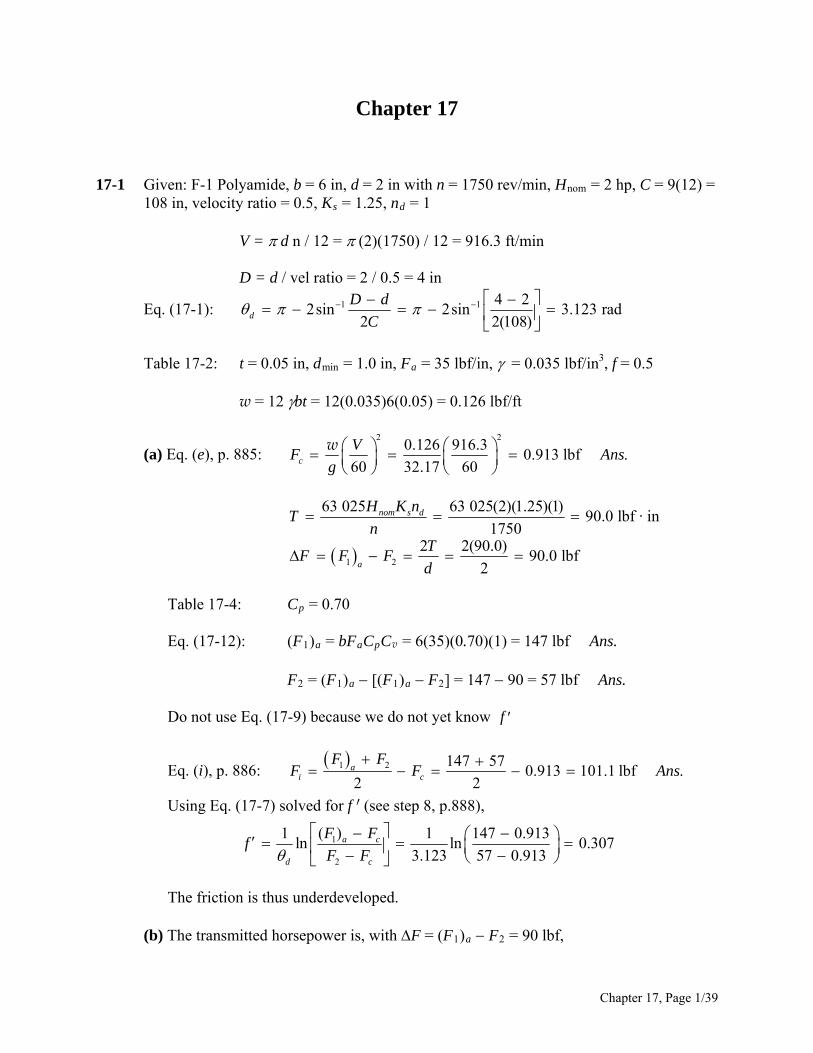
Chapter 17 17-1 Given: F-1 Polyamide, b = 6 in, d = 2 in with n = 1750 rev/min, Hnom = 2 hp, C = 9(12) =
108 in, velocity ratio = 0.5, Ks = 1.25, nd = 1 V = d n / 12 = (2)(1750) / 12 = 916.3 ft/min D = d / vel ratio = 2 / 0.5 = 4 in
Eq. (17-1): 1 1 4 22sin 2sin 3.123 rad
2 2(108)d
D d
C
Table 17-2: t = 0.05 in, dmin = 1.0 in, Fa = 35 lbf/in, = 0.035 lbf/in3, f = 0.5 w = 12 bt = 12(0.035)6(0.05) = 0.126 lbf/ft
(a) Eq. (e), p. 885: 2 2
0.126 916.30.913 lbf .
60 32.17 60c
VF Ans
g
w
1 2
63 025 63 025(2)(1.25)(1)90.0 lbf · in
17502 2(90.0)
90.0 lbf2
nom s d
a
H K nT
nT
F F Fd
Table 17-4: Cp = 0.70 Eq. (17-12): (F1)a = bFaCpCv = 6(35)(0.70)(1) = 147 lbf Ans. F2 = (F1)a [(F1)a F2] = 147 90 = 57 lbf Ans. Do not use Eq. (17-9) because we do not yet know f
Eq. (i), p. 886: 1 2 147 57
0.913 101.1 lbf .2 2
ai c
F FF F A
ns
Using Eq. (17-7) solved for f ¢ (see step 8, p.888),
1
2
1 ( ) 1 147 0.913ln ln 0.307
3.123 57 0.913a c
d c
F Ff
F F
The friction is thus underdeveloped. (b) The transmitted horsepower is, with F = (F1)a F2 = 90 lbf,
Chapter 17, Page 1/39
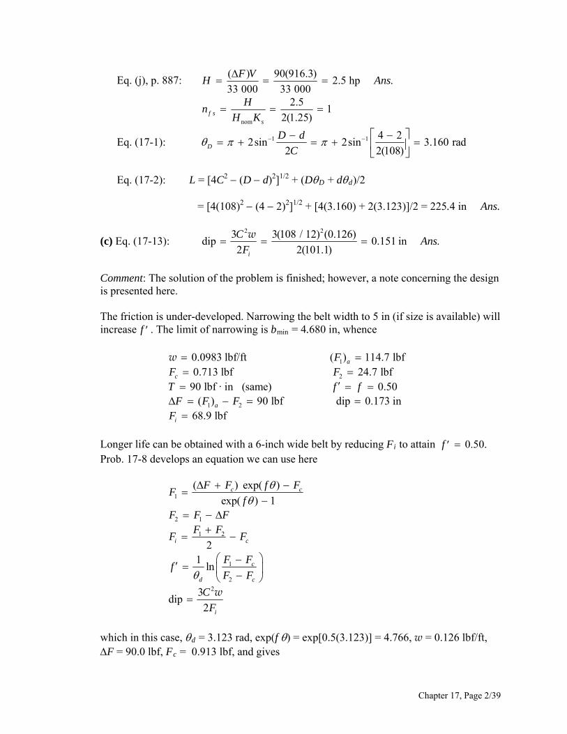
Eq. (j), p. 887: ( ) 90(916.3)
2.5 hp .33 000 33 000
F VH Ans
nom
2.51
2(1.25)f ss
Hn
H K
Eq. (17-1): 1 1 4 2
2sin 2sin 3.160 rad2 2(108)D
D d
C
Eq. (17-2): L = [4C2 (D d)2]1/2 + (DD + dd)/2 = [4(108)2 (4 2)2]1/2 + [4(3.160) + 2(3.123)]/2 = 225.4 in Ans.
(c) Eq. (17-13): 2 23 3(108 / 12) (0.126)
dip 0.151 in .2 2(101.1)i
CAns
F
w
Comment: The solution of the problem is finished; however, a note concerning the design
is presented here. The friction is under-developed. Narrowing the belt width to 5 in (if size is available) will
increase f . The limit of narrowing is bmin = 4.680 in, whence
1
2
1 2
0.0983 lbf/ft ( ) 114.7 lbf0.713 lbf 24.7 lbf
90 lbf · in (same) 0.50( ) 90 lbf
a
c
a
FF FT f
F F F
w
dip 0.173 in68.9 lbfiF
f
Longer life can be obtained with a 6-inch wide belt by reducing Fi to attain
Prob. 17-8 develops an equation we can use here 0.50.f
1
2 1
1 2
1
2
2
( ) exp( )
exp( ) 1
21
ln
3dip
2
c c
i c
c
d c
i
F F f FF
fF F F
F FF F
F Ff
F F
C
F
w
which in this case, d = 3.123 rad, exp(f ) = exp[0.5(3.123)] = 4.766, w = 0.126 lbf/ft,
F = 90.0 lbf, Fc = 0.913 lbf, and gives
Chapter 17, Page 2/39
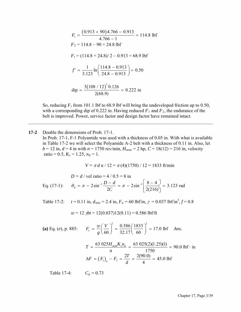
1
0.913 90 4.766 0.913114.8 lbf
4.766 1F
F2 = 114.8 90 = 24.8 lbf Fi = (114.8 + 24.8)/ 2 0.913 = 68.9 lbf
1 114.8 0.913
ln 0.503.123 24.8 0.913
f
2
3 108 / 12 0.126dip 0.222 in
2(68.9)
So, reducing F
i from 101.1 lbf to 68.9 lbf will bring the undeveloped friction up to 0.50,
with a corresponding dip of 0.222 in. Having reduced F1 and F2, the endurance of the belt is improved. Power, service factor and design factor have remained intact.
______________________________________________________________________________ 17-2 Double the dimensions of Prob. 17-1. In Prob. 17-1, F-1 Polyamide was used with a thickness of 0.05 in. With what is available
in Table 17-2 we will select the Polyamide A-2 belt with a thickness of 0.11 in. Also, let b = 12 in, d = 4 in with n = 1750 rev/min, Hnom = 2 hp, C = 18(12) = 216 in, velocity
ratio = 0.5, Ks = 1.25, nd = 1. V = d n / 12 = (4)(1750) / 12 = 1833 ft/min D = d / vel ratio = 4 / 0.5 = 8 in
Eq. (17-1): 1 1 8 42sin 2sin 3.123 rad
2 2(216)d
D d
C
Table 17-2: t = 0.11 in, dmin = 2.4 in, Fa = 60 lbf/in, = 0.037 lbf/in3, f = 0.8 w = 12 bt = 12(0.037)12(0.11) = 0.586 lbf/ft
(a) Eq. (e), p. 885: 2 2
0.586 183317.0 lbf .
60 32.17 60c
VF Ans
g
w
1 2
63 025 63 025(2)(1.25)(1)90.0 lbf · in
17502 2(90.0)
45.0 lbf4
nom s d
a
H K nT
nT
F F Fd
Table 17-4: Cp = 0.73
Chapter 17, Page 3/39
Eq. (17-12): (F1)a = bFaCpCv = 12(60)(0.73)(1) = 525.6 lbf Ans. F2 = (F1)a [(F1)a F2] = 525.6 45 = 480.6 lbf Ans.
Eq. (i), p. 886: 1 2 525.6 480.6
17.0 486.1 lbf .2 2
ai c
F FF F A
ns
Eq. (17-9):
1
2
1 ( ) 1 525.6 17.0ln ln 0.0297
3.123 480.6 17.0a c
d c
F Ff
F F
The friction is thus underdeveloped. (b) The transmitted horsepower is, with F = (F1)a F2 = 45 lbf,
nom
( ) 45(1833)2.5 hp .
33 000 33 0002.5
12(1.25)f s
s
F VH Ans
Hn
H K
Eq. (17-1): 1 1 8 42sin 2sin 3.160 rad
2 2(216)D
D d
C
Eq. (17-2): L = [4C2 (D d)2]1/2 + (DD + dd)/2 = [4(216)2 (8 4)2]1/2 + [8(3.160) + 4(3.123)]/2 = 450.9 in Ans.
(c) Eq. (17-13): 2 23 3(216 / 12) (0.586)
dip 0.586 in .2 2(486.1)i
CAns
F
w
______________________________________________________________________________ 17-3
As a design task, the decision set on p. 893 is useful. A priori decisions: • Function: Hnom = 60 hp, n = 380 rev/min, C = 192 in, Ks = 1.1 • Design factor: nd = 1 • Initial tension: Catenary • Belt material. Table 17-2: Polyamide A-3, Fa = 100 lbf/in, = 0.042 lbf/in3, f = 0.8 • Drive geometry: d = D = 48 in • Belt thickness: t = 0.13 in
Chapter 17, Page 4/39
Design variable: Belt width. Use a method of trials. Initially, choose b = 6 in
2 2
nom
1 1
(48)(380)4775 ft/min
12 1212 12(0.042)(6)(0.13) 0.393 lbf/ft
0.393(4775 / 60)77.4 lbf
32.1763 025 63 025(60)(1.1)(1)
10 946 lbf · in380
2 2(10 946)456.1 lbf
48( )
c
s d
a
dnV
bt
VF
gH K n
Tn
TF
dF F
ww
2 1
6(100)(1)(1) 600 lbf
600 456.1 143.9 lbfa pbF C C
F F F
v
Transmitted power H
1 2
1
2
( ) 456.1(4775)66 hp
33 000 33 000600 143.9
77.4 294.6 lbf2 2
1 1 600 77.4ln ln 0.656
143.9 77.4
i c
c
d c
F VH
F FF F
F Ff
F F
Eq. (17-2): L = [4(192)2 (48 48)2]1/2 + [48() + 48()] / 2 = 534.8 in Friction is not fully developed, so bmin is just a little smaller than 6 in (5.7 in). Not having a figure of merit, we choose the most narrow belt available (6 in). We can improve the design by reducing the initial tension, which reduces F1 and F2, thereby increasing belt
life (see the result of Prob. 17-8). This will bring f to 0.80
1
exp
exp 1
exp exp(0.80 ) 12.345
c cF F f FF
f
f
Therefore
1
2 1
1 2
(456.1 77.4)(12.345) 77.4573.7 lbf
12.345 1573.7 456.1 117.6 lbf
573.7 117.677.4 268.3 lbf
2 2i c
F
F F FF F
F F
These are small reductions since f is close to f , but improvements nevertheless.
Chapter 17, Page 5/39
1
2
1 1 573.7 77.4ln ln 0.80
117.6 77.4c
d c
F Ff
F F
2 23 3(192 / 12) (0.393)dip 0.562 in
2 2(268.3)i
C
F
w
______________________________________________________________________________ 17-4 From the last equation given in the problem statement,
0 2
0 2
0 2
0 2
1exp
1 2 / [ ( ) ]
21 exp 1
( )
2exp exp 1
( )
exp1 2
exp 1
fT d a a b
Tf
d a a b
Tf f
d a a b
fTb
a a d f
But 2T/d = 33 000Hd/V. Thus,
0 2
exp1 33 000 . . .
exp 1d
fHb Q
a a V f
E D
______________________________________________________________________________ 17-5 Refer to Ex. 17-1 on p. 890 for the values used below. (a) The maximum torque prior to slip is,
nom63 025 63 025(15)(1.25)(1.1)742.8 lbf · in .
1750s dH K n
T An
ns
The corresponding initial tension, from Eq. (17-9), is,
exp( ) 1 742.8 11.17 1148.1 lbf .
exp( ) 1 6 11.17 1i
T fF A
d f
ns
(b) See Prob. 17-4 statement. The final relation can be written
Chapter 17, Page 6/39
min 2
2
33 000 exp1
(12 / 32.174)( / 60) [exp 1]
1 33 000(20.6)(11.17)
100(0.7)(1) [12(0.042)(0.13)] / 32.174 (2749 / 60) 2749(11.17 1)
4.13 in .
a
a p
H fb
F C C t V V f
Ans
v
This is the minimum belt width since the belt is at the point of slip. The design must
round up to an available width. Eq. (17-1):
1 1
1 1
18 62sin 2sin
2 23.016 511 rad
18 62sin 2sin
2 23.266 674 rad
d
D
D d
C
D d
C
(96)
(96)
Eq. (17-2):
2 2 1/ 2 1[4(96) (18 6) ] [18(3.266 674) 6(3.016 511)]
2230.074 in .
L
Ans
(c) 2 2(742.8)
247.6 lbf6
TF
d
1 1
2 1
2 2
1 2
( ) 4.13(100)(0.70)(1) 289.1 lbf
289.1 247.6 41.5 lbf12 12(0.042)4.13(0.130) 0.271 lbf/ft
0.271 274917.7 lbf
60 32.17 60289.1 41.5
17.7 147.6 lb2 2
a a p
c
i c
F bF C C F
F F Fbt
VF
gF F
F F
v
w
w
f
Transmitted belt power H
nom
( ) 247.6(2749)20.6 hp
33 000 33 00020.6
1.115(1.25)fs
s
F VH
Hn
H K
Chapter 17, Page 7/39
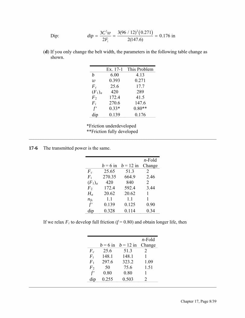
Dip: 22 3(96 / 12) 0.2713
0.176 in2 2(147.6)i
Cdip
F
w
(d) If you only change the belt width, the parameters in the following table change as
shown.
Ex. 17-1 This Problemb 6.00 4.13 w 0.393 0.271 Fc 25.6 17.7 (F1)a 420 289 F2 172.4 41.5 Fi 270.6 147.6 f 0.33* 0.80**
dip 0.139 0.176 *Friction underdeveloped **Friction fully developed ______________________________________________________________________________ 17-6 The transmitted power is the same.
b = 6 in b = 12 inn-Fold Change
Fc 25.65 51.3 2 Fi 270.35 664.9 2.46 (F1)a 420 840 2 F2 172.4 592.4 3.44 Ha 20.62 20.62 1 nfs 1.1 1.1 1 f 0.139 0.125 0.90
dip 0.328 0.114 0.34 If we relax Fi to develop full friction (f = 0.80) and obtain longer life, then
b = 6 in b = 12 inn-Fold Change
Fc 25.6 51.3 2 Fi 148.1 148.1 1 F1 297.6 323.2 1.09 F2 50 75.6 1.51 f 0.80 0.80 1
dip 0.255 0.503 2 ______________________________________________________________________________
Chapter 17, Page 8/39
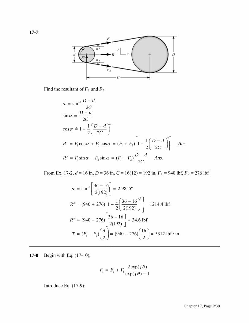
17-7
Find the resultant of F1 and F2:
1
2
2
1 2 1 2
1 2 1 2
sin2
sin2
1cos 1
2 2
1cos cos ( ) 1 .
2 2
sin sin ( ) .2
x
y
D d
CD d
CD d
C
D dR F F F F
C
D dR F F F F Ans
C
Ans
From Ex. 17-2, d = 16 in, D = 36 in, C = 16(12) = 192 in, F1 = 940 lbf, F2 = 276 lbf
1 o
2
1 2
36 16sin 2.9855
2(192)
1 36 16(940 276) 1 1214.4 lbf
2 2(192)
36 16(940 276) 34.6 lbf
2(192)
16( ) (940 276) 5312 lbf · in
2 2
x
y
R
R
dT F F
______________________________________________________________________________ 17-8 Begin with Eq. (17-10),
1
2exp( )
exp( ) 1c i
fF F F
f
Introduce Eq. (17-9):
Chapter 17, Page 9/39
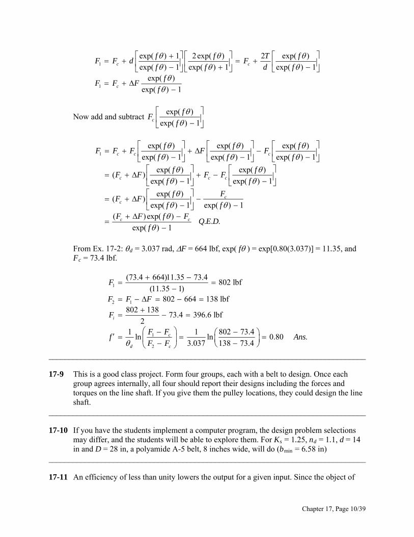
1
1
exp( ) 1 2exp( ) 2 exp( )
exp( ) 1 exp( ) 1 exp( ) 1exp( )
exp( ) 1
c c
c
f f TF F d F
f f d ff
F F Ff
f
Now add and subtract exp( )
exp( ) 1c
fF
f
1
exp( ) exp( ) exp( )
exp( ) 1 exp( ) 1 exp( ) 1
exp( ) exp( )( )
exp( ) 1 exp( ) 1
exp( )( )
exp( ) 1 exp( ) 1( )exp( )
ex
c c c
c c c
cc
c c
f fF F F F F
f f
f fF F F F
f f
f FF F
f fF F f F
f
f
. . .
p( ) 1Q E D
f
From Ex. 17-2: d = 3.037 rad, F = 664 lbf, exp( f ) = exp[0.80(3.037)] = 11.35, and Fc = 73.4 lbf.
1
2 1
1
2
(73.4 664)11.35 73.4802 lbf
(11.35 1)802 664 138 lbf
802 13873.4 396.6 lbf
21 1 802 73.4
ln ln 0.80 .3.037 138 73.4
i
c
d c
F
F F F
F
F Ff Ans
F F
______________________________________________________________________________ 17-9 This is a good class project. Form four groups, each with a belt to design. Once each
group agrees internally, all four should report their designs including the forces and torques on the line shaft. If you give them the pulley locations, they could design the line shaft.
______________________________________________________________________________ 17-10 If you have the students implement a computer program, the design problem selections
may differ, and the students will be able to explore them. For Ks = 1.25, nd = 1.1, d = 14 in and D = 28 in, a polyamide A-5 belt, 8 inches wide, will do (bmin = 6.58 in)
______________________________________________________________________________ 17-11 An efficiency of less than unity lowers the output for a given input. Since the object of
Chapter 17, Page 10/39
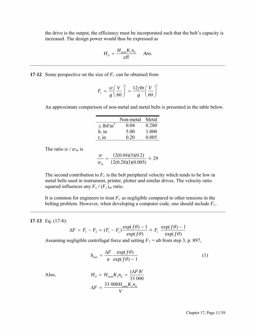
the drive is the output, the efficiency must be incorporated such that the belt’s capacity is increased. The design power would thus be expressed as
nom .eff
s dd
H K nH Ans
______________________________________________________________________________ 17-12 Some perspective on the size of Fc can be obtained from
2 212
60 60c
V btF
g g
w V
An approximate comparison of non-metal and metal belts is presented in the table below.
Non-metal Metal, lbf/in3 0.04 0.280b, in 5.00 1.000t, in 0.20 0.005
The ratio w / wm is
12(0.04)(5)(0.2)29
12(0.28)(1)(0.005)m
ww
The second contribution to Fc is the belt peripheral velocity which tends to be low in
metal belts used in instrument, printer, plotter and similar drives. The velocity ratio squared influences any Fc / (Fc)m ratio.
It is common for engineers to treat Fc as negligible compared to other tensions in the
belting problem. However, when developing a computer code, one should include Fc. ______________________________________________________________________________ 17-13 Eq. (17-8):
1 2 1 1
exp( ) 1 exp( ) 1( )
exp( ) exp( )c
f fF F F F F F
f f
Assuming negligible centrifugal force and setting F1 = ab from step 3, p. 897,
min
exp( ) (1)
exp( ) 1
F fb
a f
Also, nom
( )
33 000d s d
F VH H K n
nom33 000 s dH K nF
V
Chapter 17, Page 11/39
Substituting into Eq. (1), min
1 33 000 exp( ) .
exp( ) 1dH f
b Aa V f
ns
______________________________________________________________________________ 17-14 The decision set for the friction metal flat-belt drive is: A priori decisions • Function: Hnom = 1 hp, n = 1750 rev/min, VR = 2 , K15 in,C s = 1.2 , Np = 106 belt passes. • Design factor: nd = 1.05 • Belt material and properties: 301/302 stainless steel Table 17-8: Sy = 175 kpsi, E = 28 Mpsi, = 0.285 • Drive geometry: d = 2 in, D = 4 in • Belt thickness: t = 0.003 in Design variables: • Belt width, b • Belt loop periphery Preliminaries
nom 1(1.2)(1.05) 1.26 hp63 025(1.26)
45.38 lbf · in1750
d s dH H K n
T
A 15 in center-to-center distance corresponds to a belt loop periphery of 39.5 in. The 40 in loop available corresponds to a 15.254 in center distance.
1
1
4 22sin 3.010 rad
2(15.254)
4 22sin 3.273 rad
2(15.274)
d
D
For full friction development
exp( ) exp[0.35(3.010)] 2.868(2)(1750)
916.3 ft/s12 12175 kpsi
d
y
fdn
V
S
Eq. (17-15):
0.4076 0.407 6 6 314.17 10 14.17 10 10 51.212 10 psiy pS N
Chapter 17, Page 12/39
From selection step 3, p. 897, 6
32 2
1
28(10 )(0.003)51.212(10 ) (0.003)
(1 ) (1 0.285 )(2)16.50 lbf/in of belt width
( ) 16.50
f
a
Eta S t
d
F ab b
For full friction development, from Prob. 17-13,
min
exp( )
exp( ) 1
2 2(45.38)45.38 lbf
2
d
d
F fb
a f
TF
d
So
min
45.38 2.8684.23 in
16.50 2.868 1b
Decision #1: b = 4.5 in
1 1
2 1
1 2
( ) 16.5(4.5) 74.25 lbf74.25 45.38 28.87 lbf
74.25 28.8751.56 lbf
2 2
a
i
F F abF F F
F FF
Existing friction
1
2
nom
1 1 74.25ln ln 0.314
3.010 28.87
( ) 45.38(916.3)1.26 hp
33 000 33 0001.26
1.051(1.2)
d
t
tfs
s
Ff
F
F VH
Hn
H K
This is a non-trivial point. The methodology preserved the factor of safety corresponding
to nd = 1.1 even as we rounded bmin up to b. Decision #2 was taken care of with the adjustment of the center-to-center distance to
accommodate the belt loop. Use Eq. (17-2) as is and solve for C to assist in this. Remember to subsequently recalculate d and D .
______________________________________________________________________________
Chapter 17, Page 13/39
17-15 Decision set: A priori decisions • Function: Hnom = 5 hp, N = 1125 rev/min, VR = 3, K20 in,C s = 1.25, Np = 106 belt passes • Design factor: nd = 1.1
• Belt material: BeCu, Sy = 170 kpsi, E = 17 Mpsi, = 0.220 • Belt geometry: d = 3 in, D = 9 in • Belt thickness: t = 0.003 in Design decisions • Belt loop periphery • Belt width b Preliminaries:
nom 5(1.25)(1.1) 6.875 hp63 025(6.875)
385.2 lbf · in1125
d s dH H K n
T
Decision #1: Choose a 60-in belt loop with a center-to-center distance of 20.3 in.
1
1
9 32sin 2.845 rad
2(20.3)
9 32sin 3.438 rad
2(20.3)
d
D
For full friction development:
exp( ) exp[0.32(2.845)] 2.485(3)(1125)
883.6 ft/min12 1256.67 kpsi
d
f
fdn
V
S
From selection step 3, p. 897,
Chapter 17, Page 14/39
63
2 2
min
17(10 )(0.003)56.67(10 ) (0.003) 116.4 lbf/in
(1 ) (1 0.22 )(3)2 2(385.2)
256.8 lbf3
exp( ) 256.8 2.4853.69 in
exp( ) 1 116.4 2.485 1
tf
d
d
Ea S t
dT
FdF f
ba f
Decision #2: b = 4 in
1 1
2 1
1 2
( ) 116.4(4) 465.6 lbf465.6 256.8 208.8 lbf465.6 208.8
337.3 lbf2 2
a
i
F F abF F F
F FF
Existing friction
1
2
1 1 465.6ln ln 0.282
2.845 208.8
( ) 256.8(883.6)6.88 hp
33 000 33 0006.88
1.15(1.25) 5(1.25)
d
fs
Ff
F
F VH
Hn
Fi can be reduced only to the point at which 0.32.f f From Eq. (17-9)
exp( ) 1 385.2 2.485 1301.3 lbf
exp( ) 1 3 2.485 1d
id
T fF
d f
Eq. (17-10):
1
2 1
2exp( ) 2(2.485)301.3 429.7 lbf
exp( ) 1 2.485 1
429.7 256.8 172.9 lbf
di
d
fF F
f
F F F
and 0.32f f ______________________________________________________________________________ 17-16 This solution is the result of a series of five design tasks involving different belt
thicknesses. The results are to be compared as a matter of perspective. These design tasks are accomplished in the same manner as in Probs. 17-14 and 17-15 solutions.
The details will not be presented here, but the table is provided as a means of learning. Five groups of students could each be assigned a belt thickness. You can form a table
Chapter 17, Page 15/39

from their results or use the table given here.
Chapter 17, Page 16/39
t, in
0.002 0.003 0.005 0.008 0.010 b 4.000 3.500 4.000 1.500 1.500 CD 20.300 20.300 20.300 18.700 20.200 a 109.700 131.900 110.900 194.900 221.800 d 3.000 3.000 3.000 5.000 6.000 D 9.000 9.000 9.000 15.000 18.000 Fi 310.600 333.300 315.200 215.300 268.500 F1 439.000 461.700 443.600 292.300 332.700 F2 182.200 209.000 186.800 138.200 204.300 nf s 1.100 1.100 1.100 1.100 1.100 L 60.000 60.000 60.000 70.000 80.000 f 0.309 0.285 0.304 0.288 0.192
Fi 301.200 301.200 301.200 195.700 166.600 F1 429.600 429.600 429.600 272.700 230.800 F2 172.800 172.800 172.800 118.700 102.400 f 0.320 0.320 0.320 0.320 0.320
The first three thicknesses result in the same adjusted Fi, F1 and F2 (why?). We have no
figure of merit, but the costs of the belt and pulleys are about the same for these three thicknesses. Since the same power is transmitted and the belts are widening, belt forces are lessening.
______________________________________________________________________________ 17-17 This is a design task. The decision variables would be belt length and belt section, which
could be combined into one, such as B90. The number of belts is not an issue. We have no figure of merit, which is not practical in a text for this application. It is
suggested that you gather sheave dimensions and costs and V-belt costs from a principal vendor and construct a figure of merit based on the costs. Here is one trial.
Preliminaries: For a single V-belt drive with Hnom = 3 hp, n = 3100 rev/min, D = 12 in,
and d = 6.2 in, choose a B90 belt, Ks = 1.3 and nd = 1. From Table 17-10, select a circumference of 90 in. From Table 17-11, add 1.8 in giving
Lp = 90 + 1.8 = 91.8 in Eq. (17-16b):
220.25 91.8 (12 6.2) 91.8 (12 6.2) 2(12 6.2)
2 2
31.47 in
C
Chapter 17, Page 17/39
-1 12 6.22sin 2.9570 rad
2(31.47)d
exp( ) exp[0.5123(2.9570)] 4.5489(6.2)(3100)
5031.8 ft/min12 12
dfdn
V
Table 17-13:
180 180Angle (2.957 rad) 169.42d
The footnote regression equation of Table 17-13 gives K1 without interpolation:
K1 = 0.143 543 + 0.007 468(169.42°) 0.000 015 052(169.42°)2 = 0.9767 The design power is
Hd = HnomKsnd = 3(1.3)(1) = 3.9 hp From Table 17-14 for B90, K2 = 1. From Table 17-12 take a marginal entry of Htab = 4,
although extrapolation would give a slightly lower Htab. Eq. (17-17): Ha = K1K2Htab = 0.9767(1)(4) = 3.91 hp The allowable Fa is given by
63 025 63 025(3.91)25.6 lbf
( / 2) 3100(6.2 / 2)a
a
HF
n d
The allowable torque Ta is
25.6(6.2)79.4 lbf · in
2 2a
a
F dT
From Table 17-16, Kc = 0.965. Thus, Eq. (17-21) gives,
2 25031.8
0.965 24.4 lbf1000 1000c c
VF K
At incipient slip, Eq. (17-9) provides:
exp( ) 1 79.4 4.5489 120.0 lbf
exp( ) 1 6.2 4.5489 1i
T fF
d f
Eq. (17-10):
Chapter 17, Page 18/39
1
2exp( ) 2(4.5489)24.4 20 57.2 lbf
exp( ) 1 4.5489 1c i
fF F F
f
Thus, F2 = F1 Fa = 57.2 25.6 = 31.6 lbf
Eq. (17-26): (3.91)(1)
1.003 .3.9
a bfs
d
H Nn A
H ns
If we had extrapolated for Htab, the factor of safety would have been slightly less than
one. Life Use Table 17-16 to find equivalent tensions T1 and T2 .
1 1 1 1
2 1 2 1
576( ) 57.2 150.1 lbf
6.2576
( ) 57.2 105.2 lbf12
bb
bb
KT F F F
dK
T F F FD
From Table 17-17, K = 1193, b = 10.926, and from Eq. (17-27), the number of belt passes
is:
1
1 2
110.926 10.92691193 1193
6.72(10 ) passes150.1 105.2
b b
P
K KN
T T
From Eq. (17-28) for NP > 109,
910 (91.8)
720 720(5031.8)25 340 h .
P pN Lt
Vt A
ns
Suppose nf s was too small. Compare these results with a 2-belt solution.
tab
nom
4 hp/belt, 39.6 lbf · in/belt,12.8 lbf/belt, 3.91 hp/belt
2(3.91)2.0
3(1.3)
a
a a
b a b afs
d s
H TF H
N H N Hn
H H K
Also, F1 = 40.8 lbf/belt, F2 = 28.0 lbf/belt
Chapter 17, Page 19/39
1 2
1 210
9.99 lbf/belt, 24.4 lbf/belt( ) 92.9 lbf/belt, ( ) 48 lbf/belt
133.7 lbf/belt, 88.8 lbf/belt
2.39(10 ) passes, 605 600 h
i c
b b
P
F FF F
T T
N t
Initial tension of the drive: (Fi)drive = NbFi = 2(9.99) = 20 lbf ______________________________________________________________________________ 17-18 Given: two B85 V-belts with d = 5.4 in, D = 16 in, n = 1200 rev/min, and Ks = 1.25 Table 17-11: Lp = 85 + 1.8 = 86.8 in Eq. (17-17b):
220.25 86.8 (16 5.4) 86.8 (16 5.4) 2(16 5.4)
2 2
26.05 in .
C
Ans
Eq. (17-1):
-1 16 5.4180 2sin 156.5
2(26.05)d
From table 17-13 footnote: K1 = 0.143 543 + 0.007 468(156.5°) 0.000 015 052(156.5°)2 = 0.944 Table 17-14: K2 = 1
Belt speed: (5.4)(1200)
1696 ft/min12
V
Use Table 17-12 to interpolate for Htab.
tab
2.62 1.591.59 (1696 1000) 2.31 hp/belt
2000 1000H
Eq. (17-17) for two belts: 1 2 tab 0.944(1)(2)(2.31) 4.36 hpa bH K K N H
Assuming nd = 1,
Hd = KsHnomnd = 1.25(1)Hnom For a factor of safety of one,
Chapter 17, Page 20/39
nom
nom
4.36 1.254.36
3.49 hp .1.25
a dH HH
H A
ns
______________________________________________________________________________ 17-19 Given: Hnom = 60 hp, n = 400 rev/min, Ks = 1.4, d = D = 26 in on 12 ft centers. Design task: specify V-belt and number of strands (belts). Tentative decision: Use D360
belts. Table 17-11: Lp = 360 + 3.3 = 363.3 in Eq. (17-16b):
220.25 363.3 (26 26) 363.3 (26 26) 2(26 26)
2 2
140.8 in (nearly 144 in)
C
, , exp[0.5123 ] 5.0,
(26)(400)2722.7 ft/min
12 12
d D
dnV
Table 17-13: For = 180°, K1 = 1 Table 17-14: For D360, K2 = 1.10 Table 17-12: Htab = 16.94 hp by interpolation Thus, Ha = K1K2Htab = 1(1.1)(16.94) = 18.63 hp / belt Eq. (17-19): Hd = HnomKs nd = 60(1.4)(1) = 84 hp Number of belts, Nb
844.51
18.63d
ba
HN
H
Round up to five belts. It is left to the reader to repeat the above for belts such as C360
and E360.
Chapter 17, Page 21/39
63 025 63 025(18.63)225.8 lbf/belt
( / 2) 400(26 / 2)( ) 225.8(26)
2935 lbf · in/belt2 2
aa
aa
HF
n dF d
T
Eq. (17-21):
2 22722.7
3.498 3.498 25.9 lbf/belt1000 1000c
VF
At fully developed friction, Eq. (17-9) gives
exp( ) 1 2935 5 1169.3 lbf/belt
exp( ) 1 26 5 1i
T fF
d f
Eq. (17-10): 1
2exp( ) 2(5)25.9 169.3 308.1 lbf/belt
exp( ) 1 5 1c i
fF F F
f
2 1
308.1 225.8 82.3 lbf/belt
18.63 51.109 .
84
a
a bf s
d
F F F
H Nn A
H
ns
Life From Table 17-16,
1 2 1
5 680308.1 526.6 lbf
26bK
T T Fd
Eq. (17-27):
1
9
1 2
5.28 10 passesb b
P
K KN
T T
Thus, NP > 109 passes Ans.
Eq. (17-28): 910 (363.3)
720 720(2722.7)P pN L
tV
Thus, t > 185 320 h Ans. ______________________________________________________________________________ 17-20 Preliminaries: 14-in wide rim, H60 in,D nom = 50 hp, n = 875 rev/min, Ks = 1.2, nd = 1.1, mG = 875/170 = 5.147, 60 / 5.147 11.65 ind (a) From Table 17-9, an 11-in sheave exceeds C-section minimum diameter and
precludes D- and E-section V-belts. Decision: Use d = 11 in, C270 belts
Chapter 17, Page 22/39
Table 17-11: Lp = 270 + 2.9 = 272.9 in Eq. (17-16b):
220.25 272.9 (60 11) 272.9 (60 11) 2(60 11)
2 2
76.78 in
C
This fits in the range
3( ) 60 3(60 11) 60 in 213 inD C D d C C
1 60 112sin 2.492 rad 142.8
2(76.78)d
1 60 112sin 3.791 rad
2(76.78)D
exp(f d) = exp[0.5123(2.492)] = 3.5846 For the flat on flywheel, f = 0.13 (see p. 900), exp(f D) = exp[0.13(3.791)] = 1.637. The belt speed is
(11)(875)2520 ft/min
12 12
dnV
Table 17-13: K1 = 0.143 543 + 0.007 468(142.8°) 0.000 015 052(142.8°)2 = 0.903 Table 17-14: K2 = 1.15 For interpolation of Table 17-12, let x be entry for d = 11.65 in and n = 2000 ft/min, and y
be entry for d = 11.65 in and n = 3000 ft/min. Then,
6.74 7.17 6.74
7.01 hp at 2000 ft/min11.65 11 12 11
xx
and
8.11 8.84 8.11
8.58 hp at 3000 ft/min11.65 11 12 11
yy
Interpolating these for 2520 ft/min gives
tabtab
8.58 3000 25207.83 hp/belt
8.58 7.01 3000 2000
HH
Eq. (17-17): Ha = K1K2Htab = 0.903(1.15)(7.83) = 8.13 hp
Chapter 17, Page 23/39
Eq. (17-19): Hd = HnomKsnd = 50(1.2)(1.1) = 66 hp
Eq. (17-20): 66
8.1 belts8.13
db
a
HN
H
Decision: Use 9 belts. On a per belt basis,
63 025 63 025(8.13)
106.5 lbf/belt( / 2) 875(11 / 2)
aa
HF
n d
106.5(11)586.8 lbf · in per belt
2 2a
a
F dT
Table 17-16: Kc = 1.716
Eq. (17-21): 2 2
25201.716 1.716 10.9 lbf/belt
1000 1000c
VF
At fully developed friction, Eq. (17-9) gives
exp( ) 1 586.9 3.5846 194.6 lbf/belt
exp( ) 1 11 3.5846 1d
id
T fF
d f
Eq. (17-10):
1
2exp( ) 2(3.5846)10.9 94.6 158.8 lbf/belt
exp( ) 1 3.5846 1d
c id
fF F F
f
2 1
158.8 106.7 52.1 lbf/belt9(8.13)
1.11 . . .66
a
b af s
d
F F FN H
n OH
K Ans
Durability:
1
2
1 1 1
2 1 2
/ 1600 / 11 145.5 lbf/belt
/ 1600 / 60 26.7 lbf/belt
158.8 145.5 304.3 lbf/belt
158.8 26.7 185.5 lbf/belt
b b
b b
b
b
F K d
F K D
T F F
T F F
Eq. (17-27) with Table 17-17:
1 111.173 11.173
1 2
9 9
2038 2038
304.3 185.5
1.68 10 passes 10 passes .
b b
P
K KN
T T
Ans
Since NP is greater than 109 passes and is out of the range of Table 17-17, life from Eq.
(17-27) is
Chapter 17, Page 24/39
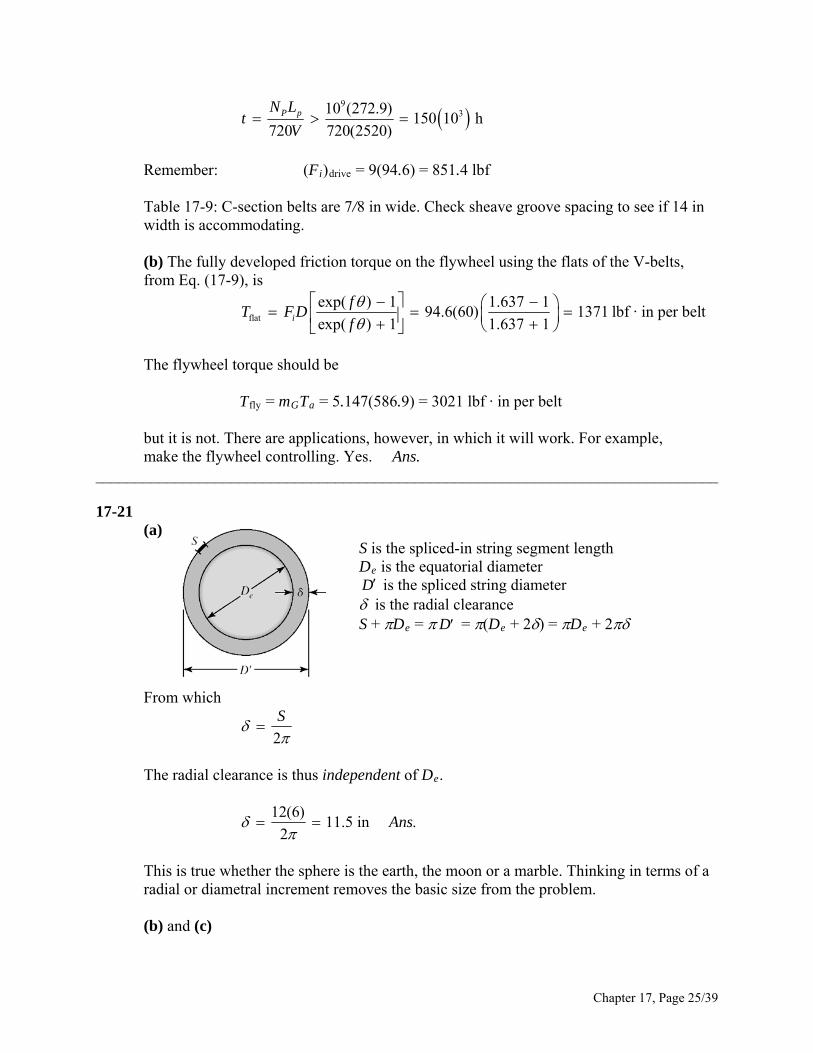
9
310 (272.9)150 10 h
720 720(2520)P pN L
tV
Remember: (Fi)drive = 9(94.6) = 851.4 lbf Table 17-9: C-section belts are 7/8 in wide. Check sheave groove spacing to see if 14 in
width is accommodating. (b) The fully developed friction torque on the flywheel using the flats of the V-belts,
from Eq. (17-9), is
flat
exp( ) 1 1.637 194.6(60) 1371 lbf · in per belt
exp( ) 1 1.637 1i
fT F D
f
The flywheel torque should be Tfly = mGTa = 5.147(586.9) = 3021 lbf · in per belt but it is not. There are applications, however, in which it will work. For example, make the flywheel controlling. Yes. Ans. ______________________________________________________________________________ 17-21 (a) S is the spliced-in string segment length De is the equatorial diameter
D is the spliced string diameter is the radial clearance
S + De = D = (De + 2) = De + 2
From which
2
S
The radial clearance is thus independent of De.
12(6)11.5 in .
2Ans
This is true whether the sphere is the earth, the moon or a marble. Thinking in terms of a
radial or diametral increment removes the basic size from the problem. (b) and (c)
Chapter 17, Page 25/39
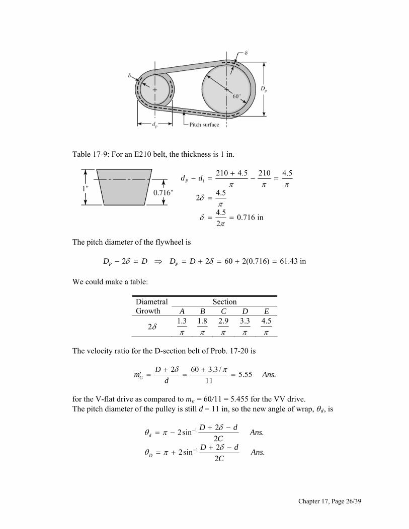
Table 17-9: For an E210 belt, the thickness is 1 in.
210 4.5 210 4.5
4.52
4.50.716 in
2
P id d
The pitch diameter of the flywheel is
2 2 60 2(0.716) 61.43 inP PD D D D
We could make a table:
Section Diametral Growth A B C D E
2 1.3
1.8
2.9
3.3
4.5
The velocity ratio for the D-section belt of Prob. 17-20 is
2 60 3.3 /5.55 .
11G
Dm A
dns
for the V-flat drive as compared to ma = 60/11 = 5.455 for the VV drive. The pitch diameter of the pulley is still d = 11 in, so the new angle of wrap, d, is
1
1
22sin .
22
2sin .2
d
D
D dAns
CD d
AnsC
Chapter 17, Page 26/39
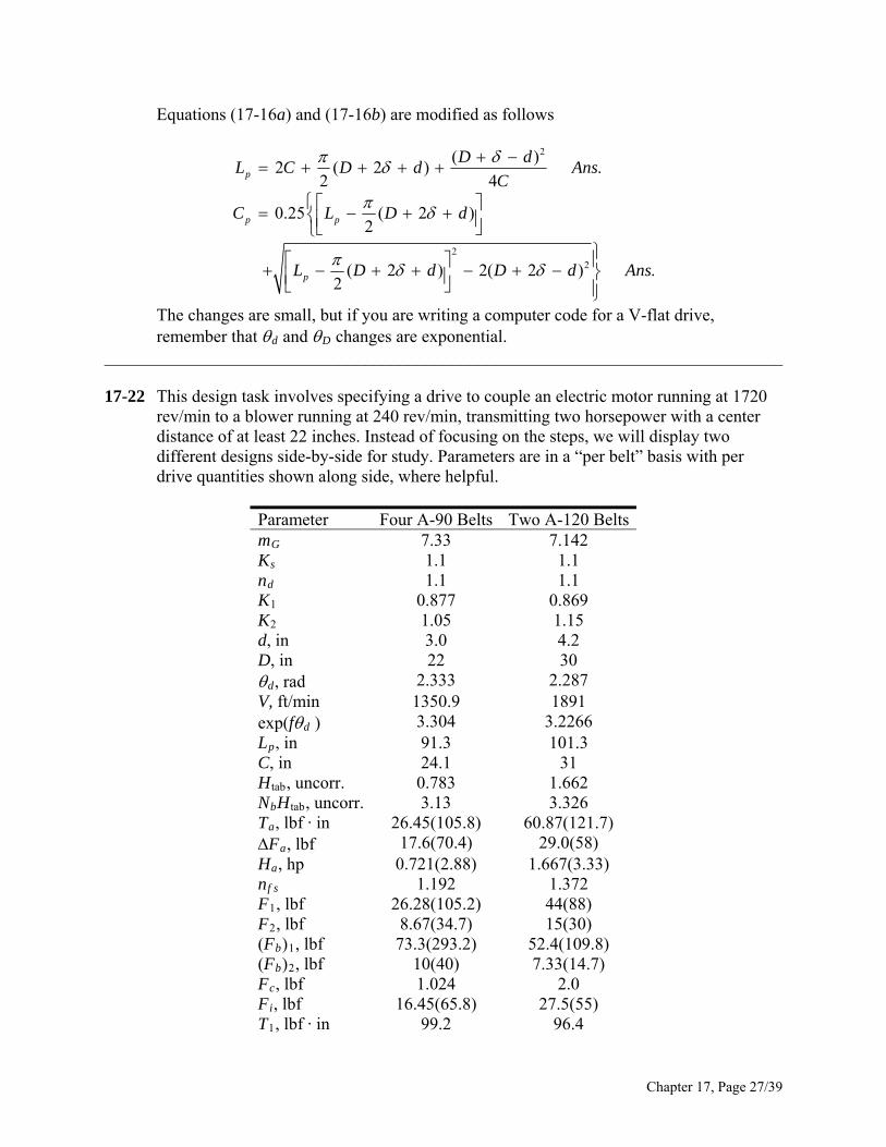
Equations (17-16a) and (17-16b) are modified as follows
2
22
( )2 ( 2 ) .
2 4
0.25 ( 2 )2
( 2 ) 2( 2 ) .2
p
p p
p
D dL C D d Ans
C
C L D d
L D d D d
Ans
The changes are small, but if you are writing a computer code for a V-flat drive, remember that d and D changes are exponential.
______________________________________________________________________________ 17-22 This design task involves specifying a drive to couple an electric motor running at 1720
rev/min to a blower running at 240 rev/min, transmitting two horsepower with a center distance of at least 22 inches. Instead of focusing on the steps, we will display two different designs side-by-side for study. Parameters are in a “per belt” basis with per drive quantities shown along side, where helpful.
Parameter Four A-90 Belts Two A-120 Belts mG 7.33 7.142 Ks 1.1 1.1 nd 1.1 1.1 K1 0.877 0.869 K2 1.05 1.15 d, in 3.0 4.2 D, in 22 30 d, rad 2.333 2.287 V, ft/min 1350.9 1891 exp(fd ) 3.304 3.2266 Lp, in 91.3 101.3 C, in 24.1 31 Htab, uncorr. 0.783 1.662 NbHtab, uncorr. 3.13 3.326 Ta, lbf · in 26.45(105.8) 60.87(121.7) Fa, lbf 17.6(70.4) 29.0(58) Ha, hp 0.721(2.88) 1.667(3.33) nf s 1.192 1.372 F1, lbf 26.28(105.2) 44(88) F2, lbf 8.67(34.7) 15(30) (Fb)1, lbf 73.3(293.2) 52.4(109.8) (Fb)2, lbf 10(40) 7.33(14.7) Fc, lbf 1.024 2.0 Fi, lbf 16.45(65.8) 27.5(55) T1, lbf · in 99.2 96.4
Chapter 17, Page 27/39
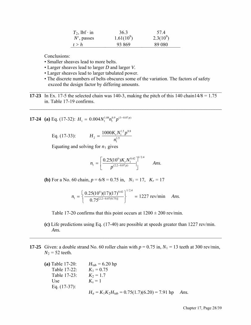
T2, lbf · in 36.3 57.4 , passesN 1.61(109) 2.3(109)
t > h 93 869 89 080 Conclusions: • Smaller sheaves lead to more belts. • Larger sheaves lead to larger D and larger V. • Larger sheaves lead to larger tabulated power. • The discrete numbers of belts obscures some of the variation. The factors of safety exceed the design factor by differing amounts. ______________________________________________________________________________ 17-23 In Ex. 17-5 the selected chain was 140-3, making the pitch of this 140 chain14/8 = 1.75
in. Table 17-19 confirms. ______________________________________________________________________________ 17-24 (a) Eq. (17-32):
1.08 0.9 (3 0.07 )1 1 10.004 pH N n p
Eq. (17-33): 1.5 0.81
2 1.51
1000 rK N pH
n
Equating and solving for n1 gives
1/ 2.46 0.421
1 (2.2 0.07 )
0.25(10 ) .r
p
K Nn A
p
ns
(b) For a No. 60 chain, p = 6/8 = 0.75 in, N1 = 17, Kr = 17
1/ 2.46 0.42
1 [2.2 0.07(0.75)]
0.25(10 )(17)(17)1227 rev/min .
0.75n A
ns
Table 17-20 confirms that this point occurs at 1200 ± 200 rev/min. (c) Life predictions using Eq. (17-40) are possible at speeds greater than 1227 rev/min.
Ans. ______________________________________________________________________________ 17-25 Given: a double strand No. 60 roller chain with p = 0.75 in, N1 = 13 teeth at 300 rev/min,
N2 = 52 teeth. (a) Table 17-20: Htab = 6.20 hp Table 17-22: K1 = 0.75 Table 17-23: K2 = 1.7 Use Ks = 1 Eq. (17-37): Ha = K1K2Htab = 0.75(1.7)(6.20) = 7.91 hp Ans.
Chapter 17, Page 28/39
(b) Eqs. (17-35) and (17-36) with L/p = 82
22
13 5282 49.5
2
52 1349.5 49.5 8 23.95
4 2
23.95(0.75) 17.96 in, round up to 18 in .
A
pC p
C A
ns
(c) For 30 percent less power transmission,
0.7(7.91) 5.54 hp63 025(5.54)
1164 lbf · in .300
H
T A
ns
Eq. (17-29):
o
0.753.13 in
sin(180 /13)1164
744 lbf .3.13 / 2
D
TF Ans
r
______________________________________________________________________________ 17-26 Given: No. 40-4 chain, N1 = 21 teeth for n = 2000 rev/min, N2 = 84 teeth, h = 20 000
hours. (a) Chain pitch is p = 4/8 = 0.500 in and 20 in.C Eq. (17-34):
2
1 21 22
2
2
2
2 4 /
2(20) 21 84 (84 21)135 pitches (or links)
0.5 2 4 (20 / 0.5)
N NL C N N
p p C p
L = 135(0.500) = 67.5 in Ans. (b) Table 17-20: Htab = 7.72 hp (post-extreme power) Eq. (17-40): Since K1 is required, the term is omitted (see p. 914). 3.75
1N
2.5
1/ 2.5
tab
7.72 (15 000)constant 18 399
13518 399(135)
6.88 hp .20 000
H Ans
Chapter 17, Page 29/39
(c) Table 17-22:
1.5
1
211.37
17K
Table 17-23: K2 = 3.3
1 2 tab 1.37(3.3)(6.88) 31.1 hp .aH K K H An s
(d) 1 21(0.5)(2000)1750 ft/min
12 12
N pnV
1
33 000(31.1)586 lbf .
1750F Ans
______________________________________________________________________________ 17-27 This is our first design/selection task for chain drives. A possible decision set:
A priori decisions • Function: Hnom, n1, space, life, Ks • Design factor: nd • Sprockets: Tooth counts N1 and N2, factors K1 and K2
Decision variables • Chain number • Strand count • Lubrication type • Chain length in pitches Function: Motor with Hnom = 25 hp at n = 700 rev/min; pump at n = 140 rev/min; mG = 700/140 = 5 Design Factor: nd = 1.1 Sprockets: Tooth count N2 = mGN1 = 5(17) = 85 teeth–odd and unavailable. Choose 84 teeth. Decision: N1 = 17, N2 = 84 Evaluate K1 and K2 Eq. (17-38): Hd = HnomKsnd Eq. (17-37): Ha = K1K2Htab Equate Hd to Ha and solve for Htab :
nomtab
1 2
s dK n HH
K K
Table 17-22: K1 = 1 Table 17-23: K2 = 1, 1.7, 2.5, 3.3 for 1 through 4 strands
Chapter 17, Page 30/39
tab2 2
1.5(1.1)(25) 41.25
(1)H
K K
Prepare a table to help with the design decisions:
Strands K2 tabH Chain No. Htab nf s
Lub. Type
1 1.0 41.3 100 59.4 1.58 B 2 1.7 24.3 80 31.0 1.40 B 3 2.5 16.5 80 31.0 2.07 B 4 3.3 12.5 60 13.3 1.17 B
Design Decisions We need a figure of merit to help with the choice. If the best was 4 strands of No. 60 chain, then Decision #1 and #2: Choose four strand No. 60 roller chain with nf s = 1.17.
1 2 tab
nom
1(3.3)(13.3)1.17
1.5(25)fss
K K Hn
K H
Decision #3: Choose Type B lubrication Analysis: Table 17-20: Htab = 13.3 hp Table 17-19: p = 0.75 in Try C = 30 in in Eq. (17-34):
21 2 2 1
2
2
2
2 ( )
2 4 /
17 84 (84 17)2(30 / 0.75)
2 4 (30 / 0.75)133.3
L C N N N N
p p C p
L = 0.75(133.3) = 100 in (no need to round)
Eq. (17-36) with p = 0.75 in: 1 2 17 84 10082.83
2 2 0.75
N N LA
p
Eq. (17-35):
22 2 1
22
84 2
0.75 84 1782.83 82.83 8 30.0 in
4 2
p N NC A A
Chapter 17, Page 31/39
Decision #4: Choose C = 30.0 in.
______________________________________________________________________________ 17-28 Follow the decision set outlined in Prob. 17-27 solution. We will form two tables, the
first for a 15 000 h life goal, and a second for a 50 000 h life goal. The comparison is useful.
Function: Hnom = 50 hp at n = 1800 rev/min, npump = 900 rev/min, mG = 1800/900 = 2, Ks = 1.2, life = 15 000 h, then repeat with life = 50 000 h Design factor: nd = 1.1 Sprockets: N1 = 19 teeth, N2 = 38 teeth Table 17-22 (post extreme):
1.5 1.5
11
191.18
17 17
NK
Table 17-23: K2 = 1, 1.7, 2.5, 3.3, 3.9, 4.6, 6.0 Decision variables for 15 000 h life goal:
nomtab
1 2 2 2
1 2 tab 2 tab 2 tab
nom
1.2(1.1)(50) 55.9 (1)
1.181.18
0.01971.2(50)
s d
f ss
K n HH
K K K KK K H K H
n KK H
H
Form a table for a 15 000 h life goal using these equations.
K2 H'tab Chain # Htab nf s Lub
1 55.90 120 21.6 0.423 C'
1.7 32.90 120 21.6 0.923 C'
2.5 22.40 120 21.6 1.064 C'
3.3 16.90 120 21.6 1.404 C'
3.9 14.30 80 15.6 1.106 C'
4.6 12.20 60 12.4 1.126 C'
6 9.32 60 12.4 1.416 C'
There are 4 possibilities where nf s ≥ 1.1 Decision variables for 50 000 h life goal From Eq. (17-40), the power-life tradeoff is:
Chapter 17, Page 32/39
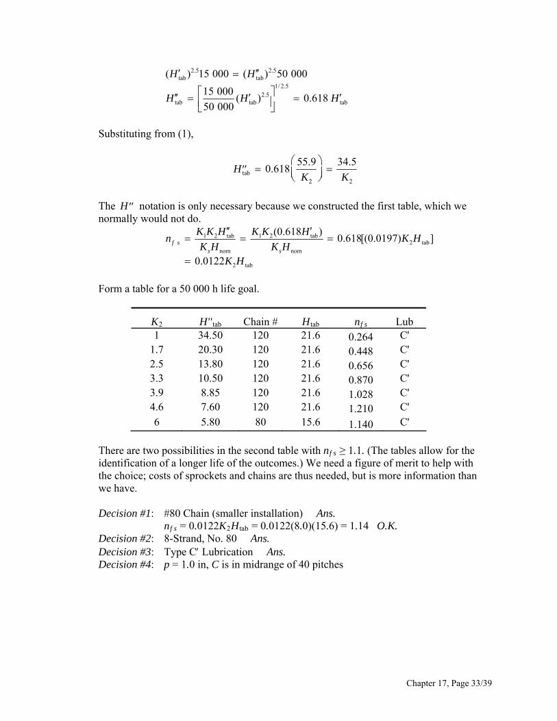
2.5 2.5tab tab
1/ 2.52.5
tab tab tab
( ) 15 000 ( ) 50 000
15 000( ) 0.618
50 000
H H
H H
H
Substituting from (1),
tab2 2
55.9 34.50.618H
K K
The H notation is only necessary because we constructed the first table, which we normally would not do.
1 2 tab 1 2 tab 2 tab
nom nom
2 tab
(0.618 )0.618[(0.0197) ]
0.0122
f ss s
K K H K K Hn K
K H K HK H
H
Form a table for a 50 000 h life goal.
K2 H''tab Chain # Htab nf s Lub 1 34.50 120 21.6 0.264 C'
1.7 20.30 120 21.6 0.448 C' 2.5 13.80 120 21.6 0.656 C' 3.3 10.50 120 21.6 0.870 C' 3.9 8.85 120 21.6 1.028 C' 4.6 7.60 120 21.6 1.210 C' 6 5.80 80 15.6 1.140 C'
There are two possibilities in the second table with nf s ≥ 1.1. (The tables allow for the identification of a longer life of the outcomes.) We need a figure of merit to help with the choice; costs of sprockets and chains are thus needed, but is more information than we have. Decision #1: #80 Chain (smaller installation) Ans. nf s = 0.0122K2Htab = 0.0122(8.0)(15.6) = 1.14 O.K. Decision #2: 8-Strand, No. 80 Ans. Decision #3: Type C Lubrication Ans. Decision #4: p = 1.0 in, C is in midrange of 40 pitches
Chapter 17, Page 33/39
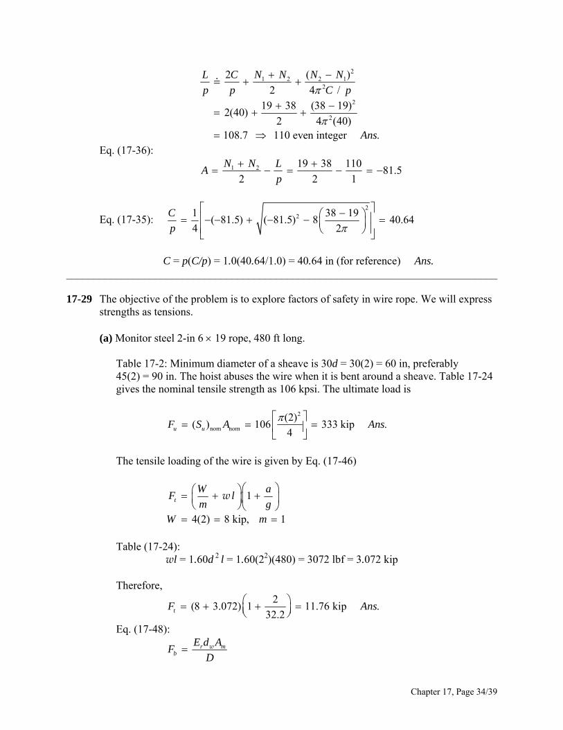
21 2 2 1
2
2
2
2 (
2 4 /
19 38 (38 19)2(40)
2 4 (40)108.7 110 even integer .
L C N N N N
p p C p
Ans
)
Eq. (17-36):
1 2 19 38 11081.5
2 2 1
N N LA
p
Eq. (17-35): 2
21 38 1( 81.5) ( 81.5) 8 40.64
4 2
C
p
9
C = p(C/p) = 1.0(40.64/1.0) = 40.64 in (for reference) Ans.
______________________________________________________________________________ 17-29 The objective of the problem is to explore factors of safety in wire rope. We will express
strengths as tensions.
(a) Monitor steel 2-in 6 19 rope, 480 ft long.
Table 17-2: Minimum diameter of a sheave is 30d = 30(2) = 60 in, preferably 45(2) = 90 in. The hoist abuses the wire when it is bent around a sheave. Table 17-24 gives the nominal tensile strength as 106 kpsi. The ultimate load is
2
nom nom
(2)( ) 106 333 kip .
4u uF S A Ans
The tensile loading of the wire is given by Eq. (17-46)
1
4(2) 8 kip, 1
t
W aF l
m gW m
w
Table (17-24): wl = 1.60d 2 l = 1.60(22)(480) = 3072 lbf = 3.072 kip Therefore,
2
(8 3.072) 1 11.76 kip .32.2tF Ans
Eq. (17-48):
r mb
E d AF
D w
Chapter 17, Page 34/39
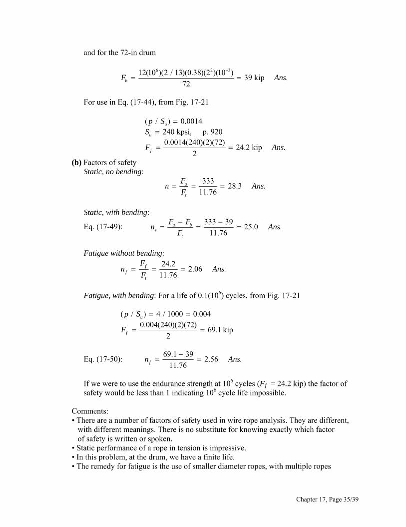
and for the 72-in drum
612(10 )
F
2 3(2 / 13)(0.38)(2 )(10 )39 kip .
72b Ans
in Eq. (17-44), from Fig. 17-21 For use
( / ) 0.0014up S
240 kpsi, p. 9200.0014(240)(2)(72)
24.2 kip .2
u
f
S
F Ans
(b) Factors of safety Static, no bending:
33328.3 .
11.76u
t
Fn A
F ns
Static, with bending:
333 3925.0 .
11.76u b
st
F Fn A
F Eq. (17-49): ns
Fatigue without bending:
24.22.06 .
11.ft
nF
76
fFAns
, with bending: For a life of 0.1(106) cycles, from Fig. 17-21
Fatigue
( / ) 4 / 1000 0.004up S 0.004(240)(2)(72)
69.1 kip2fF
50): 69.1 39
2.56 .11.76fn A Eq. (17- ns
If we were to use the endurance strength at 106 cycles (Ff = 24.2 kip) the factor of
safety would be less than 1 indicating 106 cycle life impossible.
ber of factors of safety used in wire rope analysis. They are different, ent meanings. There is no substitute for knowing exactly which factor
opes, with multiple ropes
Comments: • There are a num with differ of safety is written or spoken. • Static performance of a rope in tension is impressive.
have a finite life. • In this problem, at the drum, we• The remedy for fatigue is the use of smaller diameter r
Chapter 17, Page 35/39
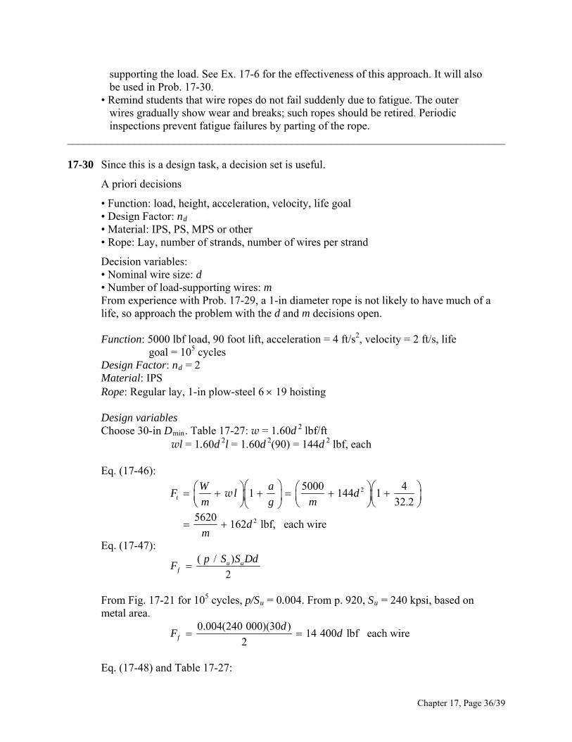
supporting the load. See Ex. 17-6 for the effectiveness of this approach. It will also
ar and breaks; such ropes should be retired. Periodic
______________________________________________________________________________
ight, acceleration, velocity, life goal
r of strands, number of wires per strand
pporting wires: m rob. 17-29, a 1-in diameter rope is not likely to have much of a
and m decisions open.
ity = 2 ft/s, life goal = 10 cycles
a ri plow-steel 6 19 hoisting
hoose 30-in D n. Table 17-27: w = 1.60d lbf/ft = 1.60d 2l = 1.60d 2(90) = 144d 2 lbf, each
:
be used in Prob. 17-30. • Remind students that wire ropes do not fail suddenly due to fatigue. The outer wires gradually show we inspections prevent fatigue failures by parting of the rope.
17-30 Since this is a design task, a decision set is useful.
A priori decisions
• Function: load, he• Design Factor: nd
• Material: IPS, PS, MPS or other • Rope: Lay, numbe
Decision variables: • Nominal wire size: d • Number of load-suFrom experience with Plife, so approach the problem with the d Function: 5000 lbf load, 90 foot lift, acceleration = 4 ft/s2, veloc
5 Design Factor: nd = 2 M te al: IPS Rope: Regular lay, 1-in Design variables
2C mi
wl Eq. (17-46)
2
2
5000 41 144 1
32.25620
162 lbf, each wire
t
W aF l d
m g m
dm
w
Eq. (17-47): ( / )
2u u
f
p S S DdF
7-21 for 105 cycles, p/Su = 0.004. From p. 920, Su = 240 kpsi, based on metal area. From Fig. 1
0.004(240 000)(30 )14 400 lbf each wire
dF d
2f
and Table 17-27: Eq. (17-48)
Chapter 17, Page 36/39
6 2
312 10 0.067 0.4
10 720 lbf, each wire30
mb
d dE d Aw w
F d
D
Eq. (17-45):
3
2
14 400 10 720
(5620 / ) 162f b
ft
F F d dn
F m
d
se a computer program to build a table similar to that of Ex. 17-6.
lternatively, we could recognize that 162 d 2 is small compared to 5620 / m, and We could uAtherefore eliminate the 162d 2 term.
3314 400 10 d
n d 720
(14 400 10 720 )5620 / 5620f
d md
m
Maximize nf ,
20 [14 400 3(10 720) ]5620
fn md
d
From which
14 400* 0.669 in
3(10 720)d
Back-substituting 3[14 400(0.669) 10 720(0.669 )] 1.14 m
5620f
mn
Thus nf = 1.14, 2.28, 3.42, 4.56 for m=1, 2, 3, 4 respectively. If we choose d = 0.50 in, then m = 2.
314 400(0.5) 10 720(0.5 )2.06n
2(5620 / 2) 162(0.5)f This exceeds nd = 2
in
s supporting load. Rope should be inspected weekly for any gns of fatigue (broken outer wires).
ght elevators in terms of velocity.
Decision #1: d = 1/2 Decision #2: m = 2 ropesi Comment: Table 17-25 gives n for frei
22( ) 106 000 83 252 lbf, each wire
dF S A d
nom nom
2
2
4
83 452(0.5)7.32
(5620 / 2) 162(0.5)
u u
u
t
Fn
F
Chapter 17, Page 37/39
By comparison, interpolation for 120 ft/min gives 7.08 - close. The category of construction hoists is not addressed in Table 17-25. We should investigate this before proceeding further.
______________________________________________________________________________ 17-31 2 ft/s2.
nom = 106 kpsi; Su = 240 kpsi (p. 920); Fig. 17-21: (p/Su)10 =
Given: 2000 ft lift, 72 in drum, 6 19 MS rope, cage and load 8000 lbf, accel. =
(a) Table 17-24: (Su) 6
0.0014
Eq. (17-44): / 0.0014(240) (72)
12.1 kip
2 2u u
fF d
p S S dD d
wl = 1.6d 2 2000(103) = 3.2d 2 kip
46):
Table 17-24:
( ) 1t
aF W l
g
w Eq. (17-
2 2
(8 3.2 ) 1d
2
32.28.5 3.4 kipd
Note that bending is not included.
2
12.1
8.5 3.4fF d
tF d
n
d, in n
0.500 0.650 1.000 1.020 1.500 1.124
1 5 ← maximum n Ans.1.6251.750
.12
.12 1 0
2.000 1.095
(b) Try m = s4 strand
Chapter 17, Page 38/39
2
2
2
8 23.2 1
4 32.22.12 3.4 kip12.1 kip
12.1
2.12 3.4
t
f
F d
dF d
dn
d
d, in n
0.5000 2.037 0.5625 2.130 0.6520 2.193 0.7500 2.250 ← maximum n Ans.0.8750 2.242 1.0000 2.192
Comparing tables, multiple ropes supporting the load increases the factor of safety, and reduces the corresponding wire rope diameter, a useful perspective.
______________________________________________________________________________
Chapter 17, Page 39/39
17-32
2
2
2 2
/( / ) (2 )
0( / )
adn
b m cddn b m cd a ad cd
dd b m cd
From which
* .
/ ( )*
( / ) [ / ( )] 2
bd Ans
mca b mc a m
n Ab m c b mc bc
.ns
These results agree closely with the Prob. 17-31 solution. The small differences are due
to rounding in Prob. 17-31. ______________________________________________________________________________ 17-33 From Prob. 17-32 solution:
1 2/
adn
b m cd
Solve the above equation for m
21
21 1
221
(1)/
/ (0) /0
/
bm
ad n cd
ad n ad b a n cddm
dd ad n cd
2
From which 1
* .2
ad A
cn ns
Substituting this result for d into Eq. (1) gives
1
2
4* .
bcnm A
a ns
______________________________________________________________________________ 17-34 Note to the Instructor. In the first printing of the ninth edition, the wording of this
problem is incorrect. It should read “ For Prob. 17-29 estimate the elongation of the rope if a 7000 lbf loaded mine cart is placed in the cage which weighs 1000 lbf. The results of Prob. 4-7 may be useful”. This will be corrected in subsequent printings. We apologize for any inconvenience encountered.
Chapter 17, Page 40/39
Table 17-27:
2 2 2
2 2
3
0.40 0.40(2 ) 1.6 in
12 Mpsi, 1.6 1.6(2 ) 6.4 lbf/ft6.4(480) 3072 lbf
/ 3072 / 1.6(480)12 0.333 lbf/in
m
r
m
A d
E dl
l A l
ww
w Treat the rest of the system as rigid, so that all of the stretch is due to the load of 7000 lbf,
the cage weighing 1000 lbf, and the wire’s weight. From the solution of Prob. 4-7,
2
1
2 2
6 6
2(1000 7000)(480)(12) 0.333(480 )12
1.6(12)(10 ) 2(12)(10 )
2.4 0.460 2.860 in .
Wl l
AE E
Ans
______________________________________________________________________________ 17-35 to 17-38 Computer programs will vary.
Chapter 17, Page 41/39
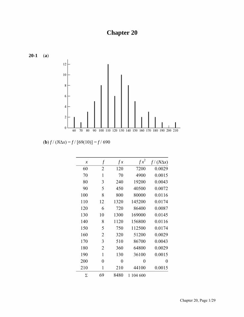
Chapter 20 20-1 (a)
(b) f / (Nx) = f / [69(10)] = f / 690
x f f x f x2 f / (Nx)60 2 120 7200 0.002970 1 70 4900 0.001580 3 240 19200 0.004390 5 450 40500 0.0072
100 8 800 80000 0.0116110 12 1320 145200 0.0174120 6 720 86400 0.0087130 10 1300 169000 0.0145140 8 1120 156800 0.0116150 5 750 112500 0.0174160 2 320 51200 0.0029170 3 510 86700 0.0043180 2 360 64800 0.0029190 1 130 36100 0.0015200 0 0 0 0210 1 210 44100 0.0015
69 8480 1 104 600
Chapter 20, Page 1/29
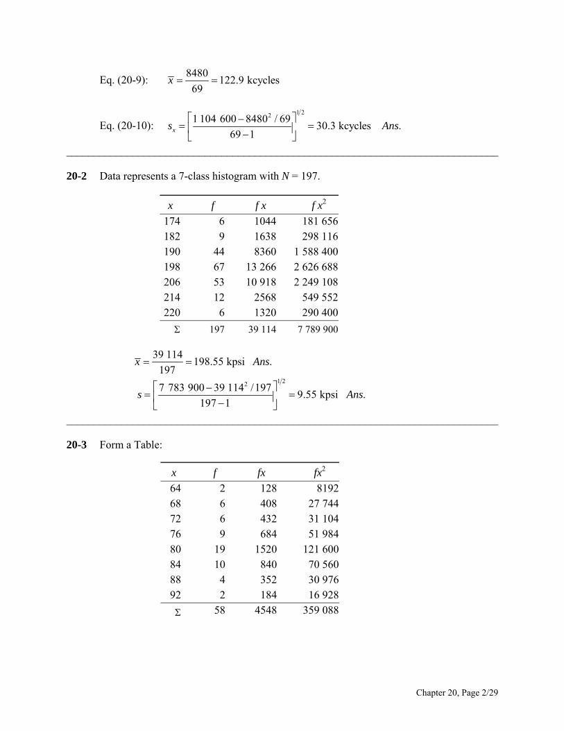
Eq. (20-9): 8480
122.9 kcycles69
x
Eq. (20-10): 1 221 104 600 8480 / 69
30.3 kcycles .69 1xs A
ns
______________________________________________________________________________ 20-2 Data represents a 7-class histogram with N = 197.
x f f x f x2
174 6 1044 181 656182 9 1638 298 116190 44 8360 1 588 400198 67 13 266 2 626 688206 53 10 918 2 249 108214 12 2568 549 552220 6 1320 290 400
197 39 114 7 789 900
39 114198.55 kpsi .
197x Ans
1 227 783 900 39 114 /197
9.55 kpsi .197 1
s A
ns
______________________________________________________________________________ 20-3 Form a Table:
x f fx fx2
64 2 128 819268 6 408 27 74472 6 432 31 10476 9 684 51 98480 19 1520 121 60084 10 840 70 56088 4 352 30 97692 2 184 16 928
58 4548 359 088
Chapter 20, Page 2/29
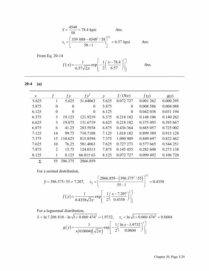
454878.4 kpsi .
58x Ans
1 22359 088 4548 / 586.57 kpsi .
58 1xs A
ns
From Eq. 20-14
21 1 78.4
exp .2 6.576.57 2
xf x A
ns
______________________________________________________________________________ 20-4 (a)
x f f y f y2 y f / (Nw) f (y) g(y) 5.625 1 5.625 31.64063 5.625 0.072 727 0.001 262 0.000 2955.875 0 0 0 5.875 0 0.008 586 0.004 0886.125 0 0 0 6.125 0 0.042 038 0.031 1946.375 3 19.125 121.9219 6.375 0.218 182 0.148 106 0.140 2626.625 3 19.875 131.6719 6.625 0.218 182 0.375 493 0.393 6676.875 6 41.25 283.5938 6.875 0.436 364 0.685 057 0.725 0027.125 14 99.75 710.7188 7.125 1.018 182 0.899 389 0.915 1287.375 15 110.625 815.8594 7.375 1.090 909 0.849 697 0.822 4627.625 10 76.25 581.4063 7.625 0.727 273 0.577 665 0.544 2517.875 2 15.75 124.0313 7.875 0.145 455 0.282 608 0.273 1388.125 1 8.125 66.015 63 8.125 0.072 727 0.099 492 0.106 720
55 396.375 2866.859 For a normal distribution,
1 222866.859 396.375 / 55
396.375 / 55 7.207, 0.435855 1yy s
2
1 1 7.207exp
2 0.43580.4358 2
xf y
For a lognormal distribution,
2 2ln 7.206 818 ln 1 0.060 474 1.9732, ln 1 0.060 474 0.0604xx s
21 1 ln 1.9732
exp2 0.06040.0604 2
xg y
x
Chapter 20, Page 3/29
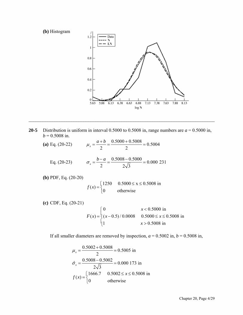
(b) Histogram
______________________________________________________________________________ 20-5 Distribution is uniform in interval 0.5000 to 0.5008 in, range numbers are a = 0.5000 in, b = 0.5008 in.
(a) Eq. (20-22) 0.5000 0.5008
0.50042 2x
a b
Eq. (20-23) 0.5008 0.5000
0.000 2312 2 3
x
b a
(b) PDF, Eq. (20-20)
1250 0.5000 x 0.5008 in( )
0 otherwisef x
(c) CDF, Eq. (20-21)
0 0.5000 in
( ) ( 0.5) / 0.0008 0.5000 0.5008 in
1 0.5008 in
x
F x x x
x
If all smaller diameters are removed by inspection, a = 0.5002 in, b = 0.5008 in,
0.5002 0.50080.5005 in
20.5008 0.5002
ˆ 0.000 173 in2 3
x
x
1666.7 0.5002 0.5008 in
( )0 otherwise
xf x
Chapter 20, Page 4/29
0 0.5002 in
( ) 1666.7( 0.5002) 0.5002 0.5008 in
1 0.5008 in
x
F x x x
x
______________________________________________________________________________
20-6 Dimensions produced are due to tool dulling and wear. When parts are mixed, the
distribution is uniform. From Eqs. (20-22) and (20-23),
3 0.6241 3 0.000 581 0.6231 in
3 0.6241 3 0.000 581 0.6251 in
x
x
a s
b s
We suspect the dimension was 0.623
in .0.625
Ans
______________________________________________________________________________ 20-7 F(x) = 0.555x – 33 mm. (a) Since F(x) is linear, distribution is uniform at x = a F(a) = 0 = 0.555(a) – 33 a = 59.46 mm. Therefore at x = b F(b) = 1= 0.555b – 33 b = 61.26 mm. Therefore,
0 59.46 mm
( ) 0.555 33 59.46 61.26 mm
1 61.26 mm
x
F x x x
x
The PDF is dF/dx, thus the range numbers are:
0.555 59.46 61.26 mm( ) .
0 otherwise
xf x A
ns
From the range numbers,
59.46 61.2660.36 mm .
261.26 59.46ˆ 0.520 mm .
2 3
x
x
Ans
Ans
Chapter 20, Page 5/29
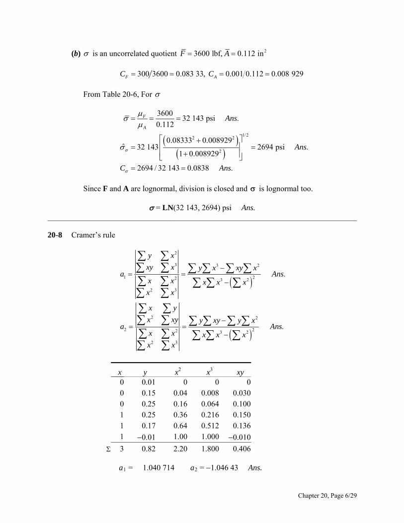
(b) is an uncorrelated quotient 23600 lbf, 0.112 inF A
300 3600 0.083 33, 0.001 0.112 0.008 929F AC C
From Table 20-6, For
1/22 2
2
360032 143 psi .
0.112
0.08333 0.008929ˆ 32 143 2694 psi .
1 0.008929
2694 / 32 143 0.0838 .
F
A
Ans
Ans
C Ans
Since F and A are lognormal, division is closed and is lognormal too.
= LN(32 143, 2694) psi Ans. ______________________________________________________________________________ 20-8 Cramer’s rule
2
3 3 2
1 22 3 2
2 3
2 2
2 22 3 2
2 3
.
.
y x
xy x y x xy xa A
x x x x xx x
x y
x xy y xy y xa A
x x x x xx x
ns
ns
x y x2 x3 xy
0 0.01 0 0 0
0 0.15 0.04 0.008 0.030
0 0.25 0.16 0.064 0.100
1 0.25 0.36 0.216 0.150
1 0.17 0.64 0.512 0.136
1 0.01 1.00 1.000 0.010
3 0.82 2.20 1.800 0.406 a1 = 1.040 714 a2 = 1.046 43 Ans.
Chapter 20, Page 6/29
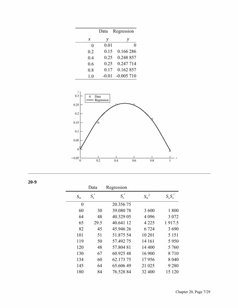
Data Regression
x y y
0 0.01 0
0.2 0.15 0.166 286
0.4 0.25 0.248 857
0.6 0.25 0.247 714
0.8 0.17 0.162 857
1.0 -0.01 -0.005 710
______________________________________________________________________________ 20-9
Data Regression
Su
Su
2
0 20.356 75
60 30 39.080 78 3 600 1 800
64 48 40.329 05 4 096 3 072
65 29.5 40.641 12 4 225 1 917.5
82 45 45.946 26 6 724 3 690
101 51 51.875 54 10 201 5 151
119 50 57.492 75 14 161 5 950
120 48 57.804 81 14 400 5 760
130 67 60.925 48 16 900 8 710
134 60 62.173 75 17 956 8 040
145 64 65.606 49 21 025 9 280
180 84 76.528 84 32 400 15 120
eS u eS S
eS
Chapter 20, Page 7/29
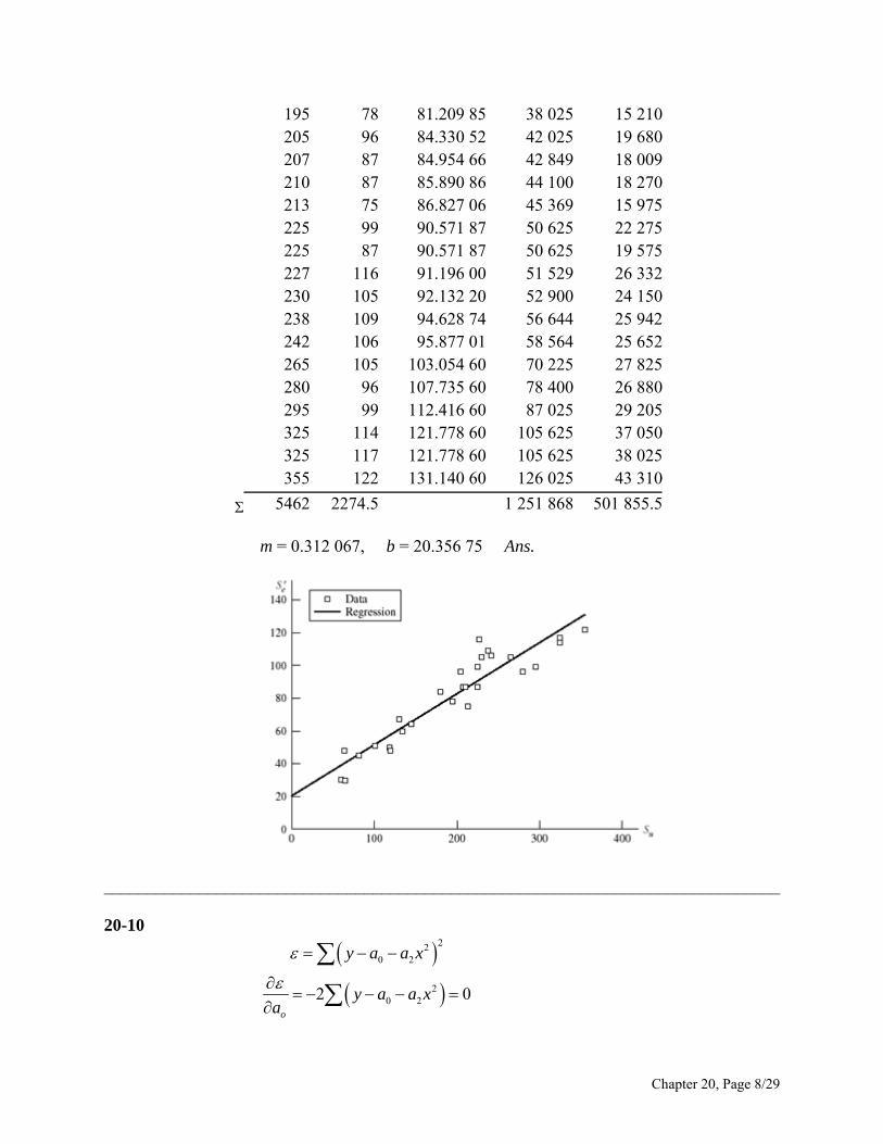
195 78 81.209 85 38 025 15 210
205 96 84.330 52 42 025 19 680
207 87 84.954 66 42 849 18 009
210 87 85.890 86 44 100 18 270
213 75 86.827 06 45 369 15 975
225 99 90.571 87 50 625 22 275
225 87 90.571 87 50 625 19 575
227 116 91.196 00 51 529 26 332
230 105 92.132 20 52 900 24 150
238 109 94.628 74 56 644 25 942
242 106 95.877 01 58 564 25 652
265 105 103.054 60 70 225 27 825
280 96 107.735 60 78 400 26 880
295 99 112.416 60 87 025 29 205
325 114 121.778 60 105 625 37 050
325 117 121.778 60 105 625 38 025
355 122 131.140 60 126 025 43 310
5462 2274.5 1 251 868 501 855.5
m = 0.312 067, b = 20.356 75 Ans.
______________________________________________________________________________ 20-10
220 2
20 22 0
o
y a a x
y a a xa
Chapter 20, Page 8/29
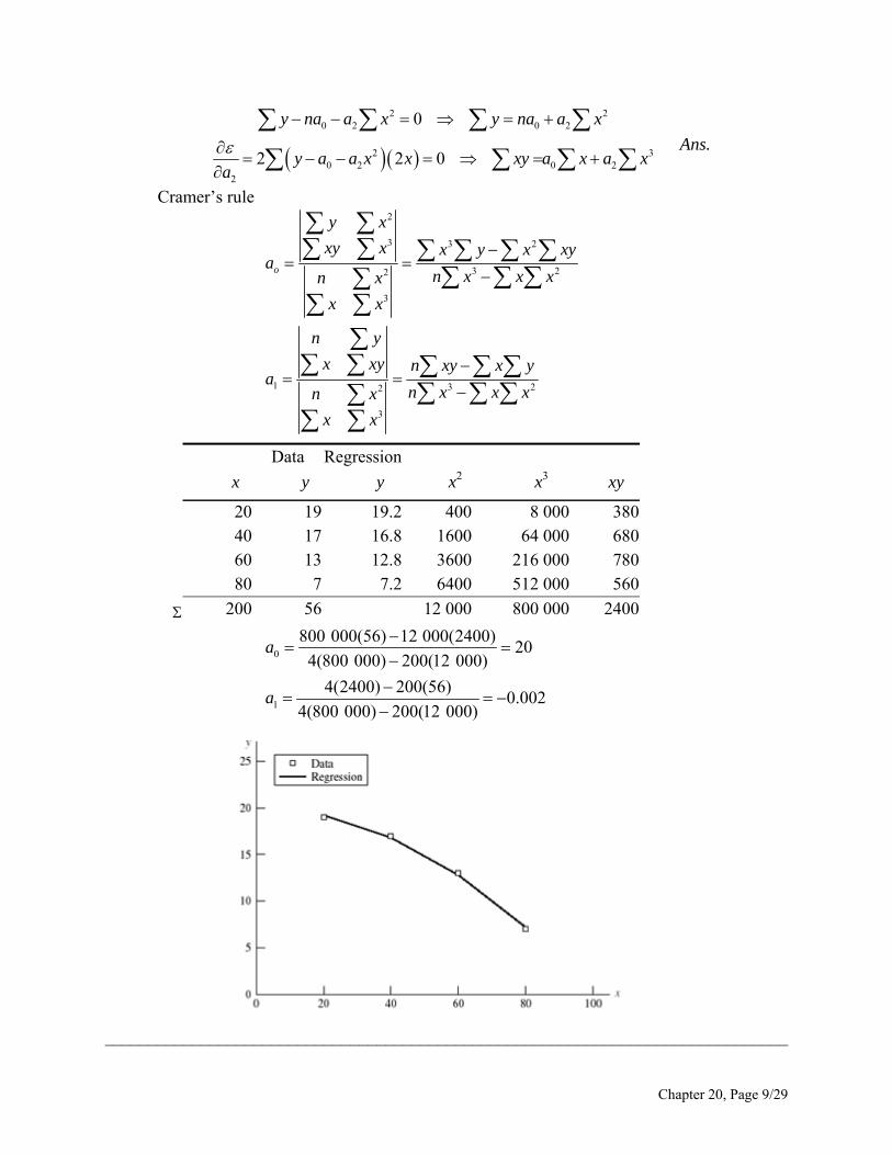
2 20 2 0 2
2 30 2 0 2
2
0
2 2 0
y na a x y na a x
y a a x x xy a x a xa
Ans.
Cramer’s rule
2
3 3 2
3 22
3
1 3 22
3
o
y x
xy x x y x xa
n x x xn x
x x
n y
x xy n xy x ya
n x x xn x
x x
y
Data Regression
x y y x2 x3 xy
20 19 19.2 400 8 000 380
40 17 16.8 1600 64 000 680
60 13 12.8 3600 216 000 780
80 7 7.2 6400 512 000 560
200 56 12 000 800 000 2400
0
1
800 000(56) 12 000(2400)20
4(800 000) 200(12 000)
4(2400) 200(56)0.002
4(800 000) 200(12 000)
a
a
______________________________________________________________________________
Chapter 20, Page 9/29
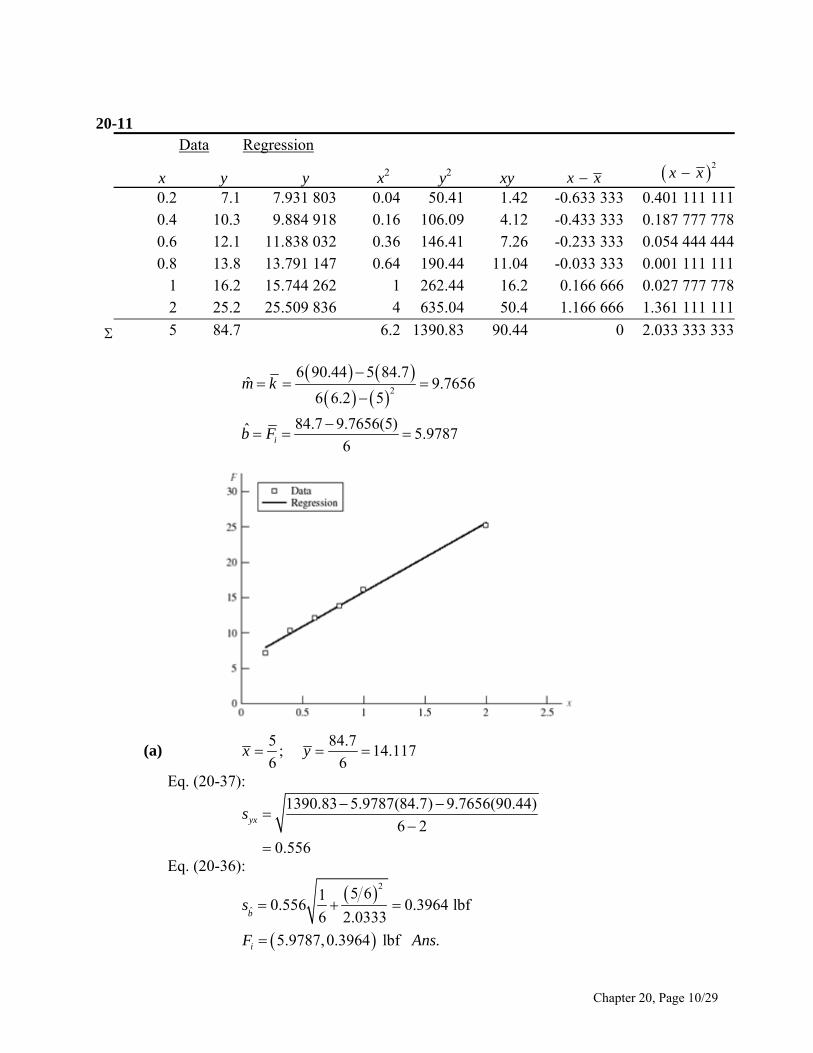
20-11
Data Regression
x y y x2 y2 xy x x 2x x
0.2 7.1 7.931 803 0.04 50.41 1.42 -0.633 333 0.401 111 111
0.4 10.3 9.884 918 0.16 106.09 4.12 -0.433 333 0.187 777 778
0.6 12.1 11.838 032 0.36 146.41 7.26 -0.233 333 0.054 444 444
0.8 13.8 13.791 147 0.64 190.44 11.04 -0.033 333 0.001 111 111
1 16.2 15.744 262 1 262.44 16.2 0.166 666 0.027 777 778
2 25.2 25.509 836 4 635.04 50.4 1.166 666 1.361 111 111
5 84.7 6.2 1390.83 90.44 0 2.033 333 333
2
6 90.44 5 84.7ˆ 9.7656
6 6.2 5
84.7 9.7656(5)ˆ 5.97876i
m k
b F
(a) 5 84.7
; 14.1176 6
x y
Eq. (20-37):
1390.83 5.9787(84.7) 9.7656(90.44)
6 20.556
yxs
Eq. (20-36):
2
ˆ
5 610.556 0.3964 lbf
6 2.0333
5.9787,0.3964 lbf .
b
i
s
F A
ns
Chapter 20, Page 10/29
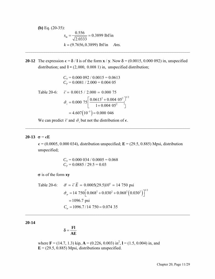
(b) Eq. (20-35):
ˆ
0.5560.3899 lbf/in
2.0333(9.7656,0.3899) lbf/in .
ms
k A
ns
______________________________________________________________________________ 20-12 The expression = / l is of the form x / y. Now = (0.0015, 0.000 092) in, unspecified
distribution; and unspecified distribution; (2,000, 0.008 1) in,l = Cx = 0.000 092 / 0.0015 = 0.0613 Cy = 0.0081 / 2.000 = 0.004 05 Table 20-6: 0.0015 / 2.000 0.000 75
1/22 2
2
5
0.0613 0.004 05ˆ 0.000 75
1 0.004 05
4.607 10 0.000 046
We can predict and ̂ but not the distribution of .
______________________________________________________________________________ 20-13 = E
= (0.0005, 0.000 034), distribution unspecified; E = (29.5, 0.885) Mpsi, distribution
unspecified; Cx = 0.000 034 / 0.0005 = 0.068 Cy = 0.0885 / 29.5 = 0.03 is of the form xy Table 20-6: 60.0005(29.5)10 14 750 psiE
1/22 2 2 2ˆ 14 750 0.068 0.030 0.068 0.030
1096.7 psi
1096.7 /14 750 0.074 35C
______________________________________________________________________________ 20-14
Fl
AE
where F = (14.7, 1.3) kip, A = (0.226, 0.003) in2, l = (1.5, 0.004) in, and E = (29.5, 0.885) Mpsi, distributions unspecified.
Chapter 20, Page 11/29
CF = 1.3 / 14.7 = 0.0884; CA = 0.003 / 0.226 = 0.0133; Cl = 0.004 / 1.5 = 0.00267; CE =0.885 / 29.5 = 0.03
1 1
FlFl
AE A E
Table 20-6:
6
1 1/ 1 1
1 114 700(1.5) 0.003 31 in. .
0.226 29.5 10
F l A E F l A E
Ans
For the standard deviation, using the first-order terms in Table 20-6,
1 2 1 22 2 2 2 2 2 2 2
1 22 2 2 2
ˆ
ˆ 0.003 31 0.0844 0.002 67 0.0133 0.03
0.000 313 in .
F l A E F l A E
F lC C C C C C C C
AE
Ans
COV: ˆ / 0.000 313/ 0.003 31 0.0945 .C A ns
Force COV dominates. There is no distributional information on . ______________________________________________________________________________
20-15 M = (15 000, 1350) lbf ⋅ in, distribution unspecified; d = (2.00, 0.005) in, distribution
unspecified.
3
32
M
d
CM = 1350 / 15 000 = 0.09, Cd = 0.005 / 2.00 = 0.0025 is of the form x/y3, Table 20-6. Mean: 15 000 lbf inM
2 23 3 3
1 1 11 6 1 6 0.0025 0.125 in *
2xCd d
3
* Note: 3 3
1 1
d d
Chapter 20, Page 12/29
3
32 32(15 000)(0.125)
19 099 psi .
M
dAns
Standard Deviation:
3 3
1 22 2 2ˆ / 1M d d
C C C
Table 20-6:
3
1 22 22
1 22 2 2
3 3(0.0025) 0.0075
ˆ 3 1 3
19 099 0.09 0.0075 1 0.0075
1725 psi .
dd
M d d
C C
C C C
Ans
COV:
17250.0903 .
19 099C A ns
Stress COV dominates. No information of distribution of . ______________________________________________________________________________ 20-16
Fraction discarded is +. The area under the PDF was unity. Having discarded +
fraction, the ordinates to the truncated PDF are multiplied by a.
1
1a
New PDF, g(x), is given by
1 2( ) 1 ( )
0 otherwise
f x xg x
x x
A more formal proof: g(x) has the property
Chapter 20, Page 13/29
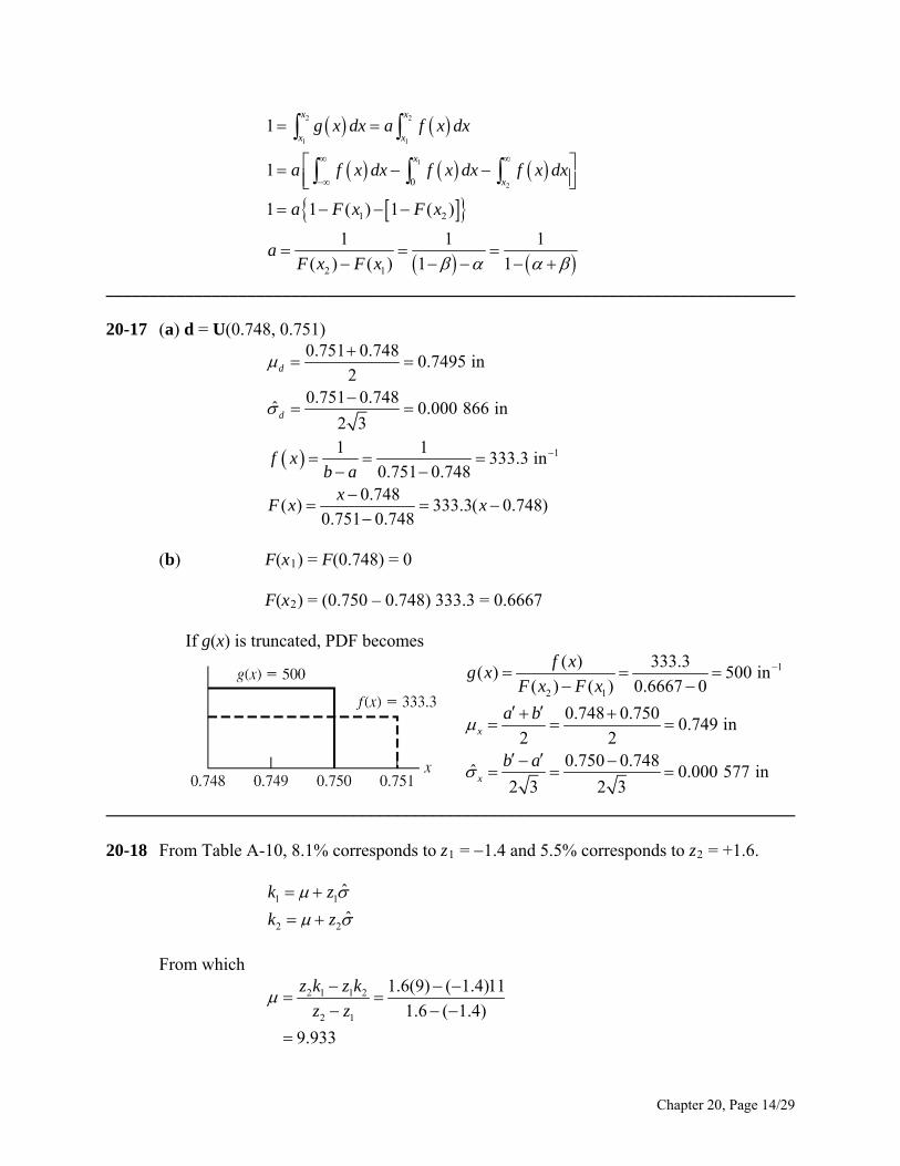
2 2
1 1
1
20
1 2
2 1
1
1
1 1 ( ) 1 ( )
1 1
( ) ( ) 1 1
x x
x x
x
x
g x dx a f x dx
a f x dx f x dx f x dx
a F x F x
aF x F x
1
______________________________________________________________________________ 20-17 (a) d = U(0.748, 0.751)
1
0.751 0.7480.7495 in
20.751 0.748
ˆ 0.000 866 in2 31 1
333.3 in0.751 0.748
0.748( ) 333.3( 0.748)
0.751 0.748
d
d
f xb a
xF x x
(b) F(x1) = F(0.748) = 0 F(x2) = (0.750 – 0.748) 333.3 = 0.6667 If g(x) is truncated, PDF becomes
1
2 1
( ) 333.3( ) 500 in
( ) ( ) 0.6667 0
0.748 0.7500.749 in
2 20.750 0.748
ˆ 0.000 577 in2 3 2 3
x
x
f xg x
F x F x
a b
b a
______________________________________________________________________________ 20-18 From Table A-10, 8.1% corresponds to z1 = 1.4 and 5.5% corresponds to z2 = +1.6.
1 1
2 2
ˆ
ˆ
k z
k z
From which
2 1 1 2
2 1
1.6(9) ( 1.4)11
1.6 ( 1.4)
9.933
z k z k
z z
Chapter 20, Page 14/29
2 1
2 1
11 9ˆ 0.6667
1.6 ( 1.4)
k k
z z
The original density function is
21 1 9.933
( ) exp .2 0.66670.6667 2
kf k A
ns
______________________________________________________________________________ 20-19 From Prob. 20-1, = 122.9 kcycles and ̂ = 30.3 kcycles.
10 1010
10 10
122.9ˆ 30.3
122.9 30.3
x xz
x z
From Table A-10, for 10 percent failure, z10 = 1.282
x10 = 122.9 + 30.3(1.282) = 84.1 kcycles Ans. ______________________________________________________________________________ 20-20
x f f x f x2 f / (Nw) f (x) 60 2 120 7200 0.002899 0.00039970 1 70 4900 0.001449 0.00120680 3 240 19200 0.004348 0.00300990 5 450 40500 0.007246 0.006204
100 8 800 80000 0.011594 0.010567110 12 1320 145200 0.017391 0.014871120 6 720 86400 0.008696 0.017292130 10 1300 169000 0.014493 0.016612140 8 1120 156800 0.011594 0.013185150 5 750 112500 0.007246 0.008647160 2 320 51200 0.002899 0.004685170 3 510 86700 0.004348 0.002097180 2 360 64800 0.002899 0.000776190 1 190 36100 0.001449 0.000237200 0 0 0 0 5.98E-05210 1 210 44100 0.001449 1.25E-05 69 8480
x = 122.8986 sx = 22.887 19
Chapter 20, Page 15/29
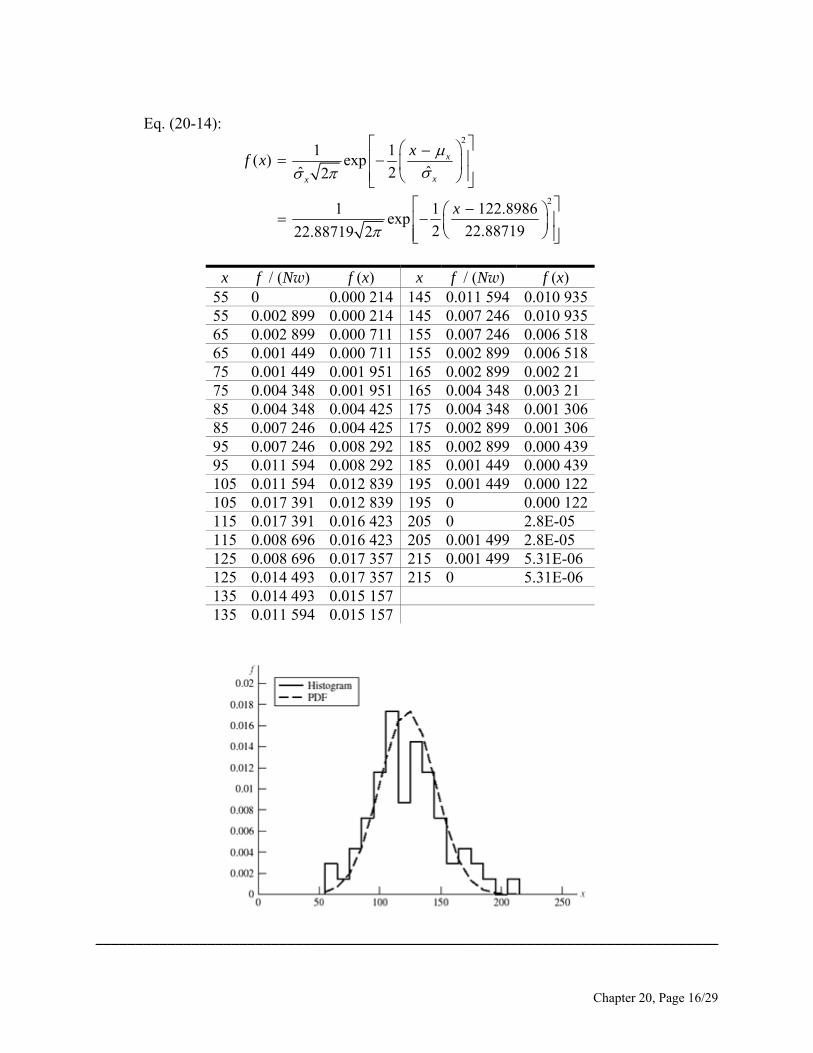
Eq. (20-14):
2
2
1 1( ) exp
ˆˆ 22
1 1 122.8986exp
2 22.8871922.88719 2
x
xx
xf x
x
x f / (Nw) f (x) x f / (Nw) f (x)
55 0 0.000 214 145 0.011 594 0.010 935 55 0.002 899 0.000 214 145 0.007 246 0.010 935 65 0.002 899 0.000 711 155 0.007 246 0.006 518 65 0.001 449 0.000 711 155 0.002 899 0.006 518 75 0.001 449 0.001 951 165 0.002 899 0.002 21 75 0.004 348 0.001 951 165 0.004 348 0.003 21 85 0.004 348 0.004 425 175 0.004 348 0.001 306 85 0.007 246 0.004 425 175 0.002 899 0.001 306 95 0.007 246 0.008 292 185 0.002 899 0.000 439 95 0.011 594 0.008 292 185 0.001 449 0.000 439 105 0.011 594 0.012 839 195 0.001 449 0.000 122 105 0.017 391 0.012 839 195 0 0.000 122 115 0.017 391 0.016 423 205 0 2.8E-05 115 0.008 696 0.016 423 205 0.001 499 2.8E-05 125 0.008 696 0.017 357 215 0.001 499 5.31E-06 125 0.014 493 0.017 357 215 0 5.31E-06 135 0.014 493 0.015 157 135 0.011 594 0.015 157
______________________________________________________________________________
Chapter 20, Page 16/29
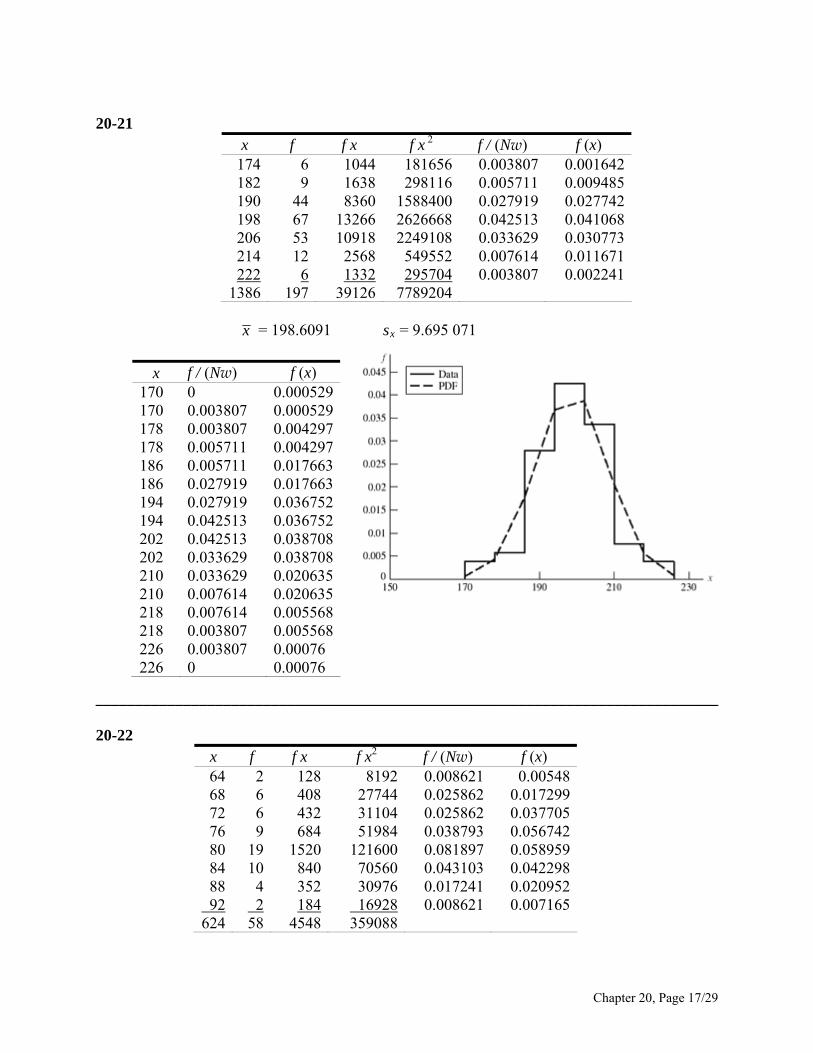
20-21
x f f x f x 2 f / (Nw) f (x) 174 6 1044 181656 0.003807 0.001642 182 9 1638 298116 0.005711 0.009485 190 44 8360 1588400 0.027919 0.027742 198 67 13266 2626668 0.042513 0.041068 206 53 10918 2249108 0.033629 0.030773 214 12 2568 549552 0.007614 0.011671 222 6 1332 295704 0.003807 0.002241
1386 197 39126 7789204
x = 198.6091 sx = 9.695 071
x f / (Nw) f (x) 170 0 0.000529170 0.003807 0.000529178 0.003807 0.004297178 0.005711 0.004297186 0.005711 0.017663186 0.027919 0.017663194 0.027919 0.036752194 0.042513 0.036752202 0.042513 0.038708202 0.033629 0.038708210 0.033629 0.020635210 0.007614 0.020635218 0.007614 0.005568218 0.003807 0.005568226 0.003807 0.00076 226 0 0.00076
______________________________________________________________________________ 20-22
x f f x f x2 f / (Nw) f (x) 64 2 128 8192 0.008621 0.0054868 6 408 27744 0.025862 0.01729972 6 432 31104 0.025862 0.03770576 9 684 51984 0.038793 0.05674280 19 1520 121600 0.081897 0.05895984 10 840 70560 0.043103 0.04229888 4 352 30976 0.017241 0.020952
92 2 184 16928 0.008621 0.007165624 58 4548 359088
Chapter 20, Page 17/29
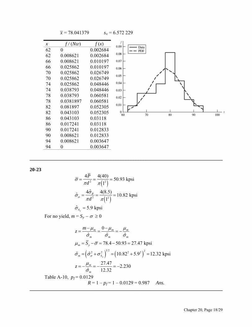
x = 78.041379 sx = 6.572 229
x f / (Nw) f (x) 62 0 0.00268462 0.008621 0.00268466 0.008621 0.01019766 0.025862 0.01019770 0.025862 0.02674970 0.025862 0.02674974 0.025862 0.04844674 0.038793 0.04844678 0.038793 0.06058178 0.0381897 0.06058182 0.081897 0.05230582 0.043103 0.05230586 0.043103 0.03118 86 0.017241 0.03118 90 0.017241 0.01283390 0.008621 0.01283394 0.008621 0.00364794 0 0.003647
______________________________________________________________________________ 20-23
2 2
2 2
4 4(40)50.93 kpsi
1
ˆ4 4(8.5)ˆ 10.82 kpsi 1
ˆ 5.9 kpsiy
P
S
P
d
d
For no yield, m = Sy 0
1 2 22 2 2 2
0ˆ ˆ ˆ
78.4 50.93 27.47 kpsi
ˆ ˆ 10.82 5.9 12.32 kpsi
27.472.230
ˆ 12.32
y
m m m
m m m
m y
m S
m
m
mz
S
z
Table A-10, pf = 0.0129 R = 1 – pf = 1 – 0.0129 = 0.987 Ans.
______________________________________________________________________________
Chapter 20, Page 18/29
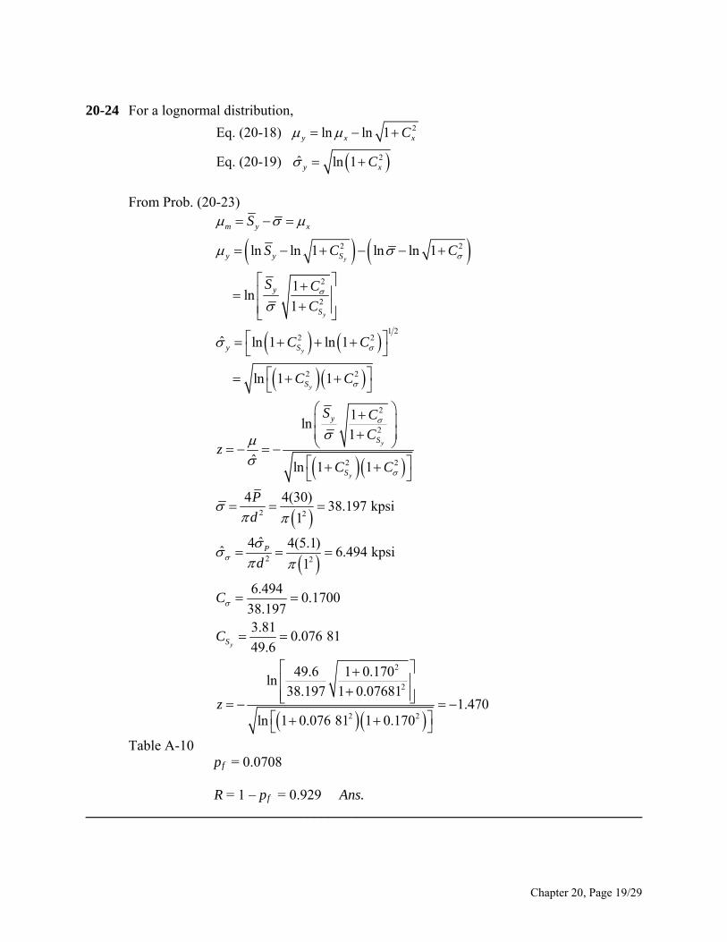
20-24 For a lognormal distribution,
2
2
Eq. (20-18) ln ln 1
ˆEq. (20-19) ln 1
y x x
y x
C
C
From Prob. (20-23)
2 2
2
2
1 22 2
2 2
2
2
2 2
2 2
2
ln ln 1 ln ln 1
1ln
1
ˆ ln 1 ln 1
ln 1 1
1ln
1
ˆ ln 1 1
4 4(30)38.197 kpsi
1
ˆ4 4(5.ˆ
y
y
y
y
y
y
m y x
y y S
y
S
y S
S
y
S
S
P
S
S C C
S C
C
C C
C C
S C
Cz
C C
P
d
d
2
2
2
2 2
1)6.494 kpsi
1
6.4940.1700
38.1973.81
0.076 8149.6
49.6 1 0.170ln
38.197 1 0.076811.470
ln 1 0.076 81 1 0.170
yS
C
C
z
Table A-10 pf = 0.0708 R = 1 – pf = 0.929 Ans. ______________________________________________________________________________
Chapter 20, Page 19/29
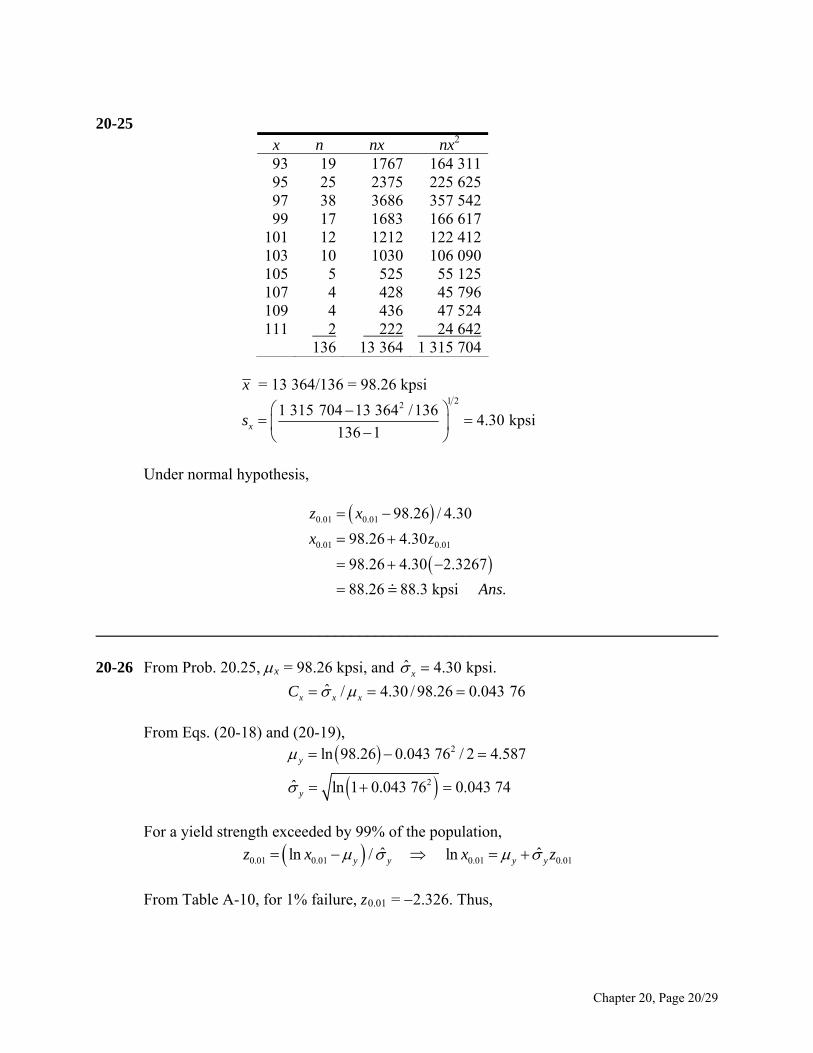
20-25
x n nx nx2
93 19 1767 164 31195 25 2375 225 62597 38 3686 357 54299 17 1683 166 617
101 12 1212 122 412103 10 1030 106 090105 5 525 55 125107 4 428 45 796109 4 436 47 524111 2 222 24 642
136 13 364 1 315 704
x = 13 364/136 = 98.26 kpsi
1 221 315 704 13 364 /1364.30 kpsi
136 1xs
Under normal hypothesis,
0.01 0.01
0.01 0.01
98.26 / 4.30
98.26 4.30
98.26 4.30 2.3267
88.26 88.3 kpsi .
z x
x z
Ans
______________________________________________________________________________ 20-26 From Prob. 20.25, x = 98.26 kpsi, and ˆ 4.30 kpsi.x
ˆ / 4.30 / 98.26 0.043 76x x xC
From Eqs. (20-18) and (20-19),
2
2
ln 98.26 0.043 76 / 2 4.587
ˆ ln 1 0.043 76 0.043 74
y
y
For a yield strength exceeded by 99% of the population,
0.01 0.01 0.01 0.01ˆ ˆln / lny y y yz x x z
From Table A-10, for 1% failure, z0.01 = 2.326. Thus,
Chapter 20, Page 20/29
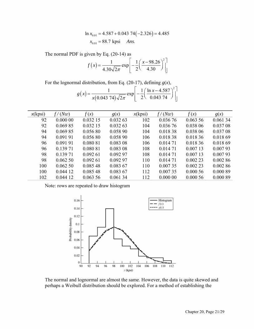
0.01
0.01
ln 4.587 0.043 74 2.326 4.485
88.7 kpsi .
x
x Ans
The normal PDF is given by Eq. (20-14) as
2
1 1 98.26exp
2 4.304.30 2
xf x
For the lognormal distribution, from Eq. (20-17), defining g(x),
21 1 ln 4.587
exp2 0.043 740.043 74 2
xg x
x
x(kpsi) f / (Nw) f (x) g(x) x(kpsi) f / (Nw) f (x) g(x)
92 0.000 00 0.032 15 0.032 63 102 0.036 76 0.063 56 0.061 3492 0.069 85 0.032 15 0.032 63 104 0.036 76 0.038 06 0.037 0894 0.069 85 0.056 80 0.058 90 104 0.018 38 0.038 06 0.037 0894 0.091 91 0.056 80 0.058 90 106 0.018 38 0.018 36 0.018 6996 0.091 91 0.080 81 0.083 08 106 0.014 71 0.018 36 0.018 6996 0.139 71 0.080 81 0.083 08 108 0.014 71 0.007 13 0.007 9398 0.139 71 0.092 61 0.092 97 108 0.014 71 0.007 13 0.007 9398 0.062 50 0.092 61 0.092 97 110 0.014 71 0.002 23 0.002 86
100 0.062 50 0.085 48 0.083 67 110 0.007 35 0.002 23 0.002 86100 0.044 12 0.085 48 0.083 67 112 0.007 35 0.000 56 0.000 89102 0.044 12 0.063 56 0.061 34 112 0.000 00 0.000 56 0.000 89
Note: rows are repeated to draw histogram
The normal and lognormal are almost the same. However, the data is quite skewed and
perhaps a Weibull distribution should be explored. For a method of establishing the
Chapter 20, Page 21/29
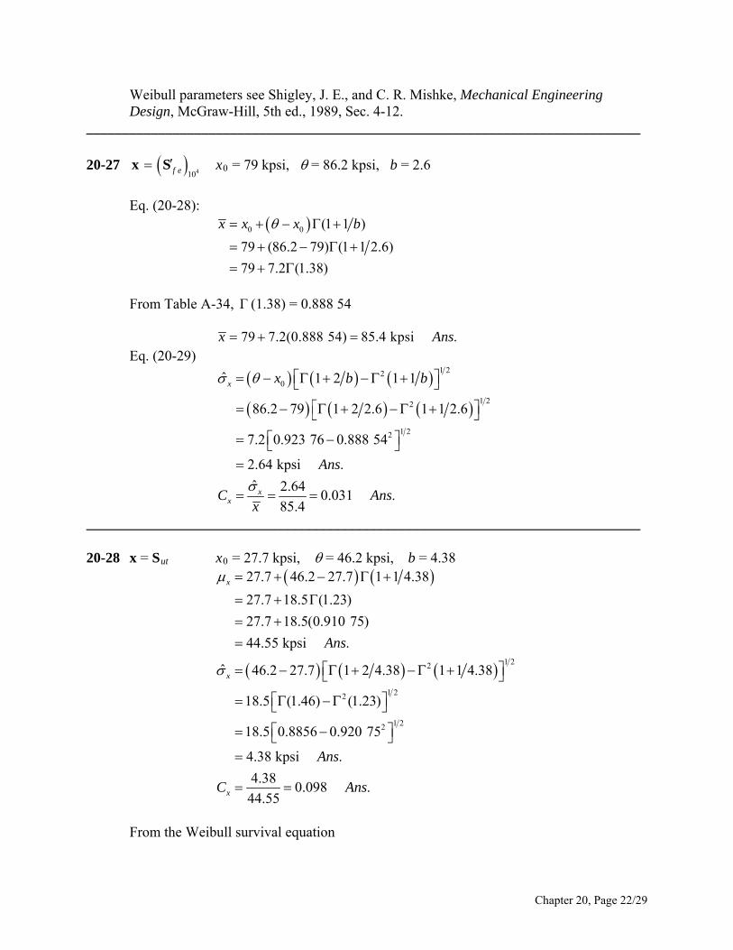
Weibull parameters see Shigley, J. E., and C. R. Mishke, Mechanical Engineering Design, McGraw-Hill, 5th ed., 1989, Sec. 4-12.
_____________________________________________________________________________
20-27 x 410f ex S 0 = 79 kpsi, = 86.2 kpsi, b = 2.6
Eq. (20-28):
0 0 (1 1 )
79 (86.2 79) (1 1 2.6)
79 7.2 (1.38)
x x x b
From Table A-34, Γ (1.38) = 0.888 54
79 7.2(0.888 54) 85.4 kpsi .x Ans Eq. (20-29)
1 220
1 22
1 22
ˆ 1 2 1 1
86.2 79 1 2 2.6 1 1 2.6
7.2 0.923 76 0.888 54
2.64 kpsi .
ˆ 2.640.031 .
85.4
x
xx
x b b
Ans
C Ansx
_____________________________________________________________________________ 20-28 x = Sut x0 = 27.7 kpsi, = 46.2 kpsi, b = 4.38
1 22
1 22
1 22
27.7 46.2 27.7 1 1 4.38
27.7 18.5 (1.23)
27.7 18.5(0.910 75)
44.55 kpsi .
ˆ 46.2 27.7 1 2 4.38 1 1 4.38
18.5 (1.46) (1.23)
18.5 0.8856 0.920 75
4.38 kpsi .
4.38
4
x
x
x
Ans
Ans
C
0.098 .4.55
Ans
From the Weibull survival equation
Chapter 20, Page 22/29
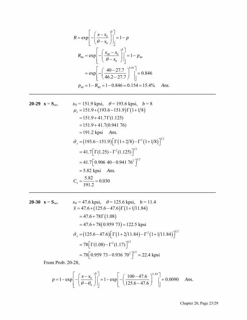
0
0
exp 1
bx x
R px
40 040 40
0
4.38
40 40
exp 1
40 27.7exp 0.846
46.2 27.7
1 1 0.846 0.154 15.4% .
bx x
R px
p R A
ns
_____________________________________________________________________________ 20-29 x = Sut, x0 = 151.9 kpsi, = 193.6 kpsi, b = 8
1 22
1 22
1 22
151.9 193.6 151.9 1 1 8
151.9 41.7 (1.125)
151.9 41.7(0.941 76)
191.2 kpsi .
ˆ 193.6 151.9 1 2 8 1 1 8
41.7 (1.25) (1.125)
41.7 0.906 40 0.941 76
5.82 kpsi .
5.8
x
x
x
Ans
Ans
C
2
0.030191.2
_____________________________________________________________________________ 20-30 x = Sut, x0 = 47.6 kpsi, = 125.6 kpsi, b = 11.4
1 22
1 22
1 22
47.6 125.6 47.6 1 1 11.84
47.6 78 1.08
47.6 78 0.959 73 122.5 kpsi
ˆ 125.6 47.6 1 2 11.84 1 1 11.84
78 (1.08) (1.17)
78 0.959 73 0.936 70 22.4 kpsi
x
x
From Prob. 20-28,
11.84
0
0
100 47.61 exp 1 exp 0.0090 .
125.6 47.6
bx x
p Ans
Chapter 20, Page 23/29
y = Sy, y0 = 64.1 kpsi, = 81.0 kpsi, b = 3.77
1 2
1 22
3.77
0
0
64.1 (81.0 64.1) 1 1 3.77
64.1 16.9 (1.27)
64.1 16.9(0.902 50) 79.35 kpsi
(81 64.1) (1 2 3.77) 1 1 3.77
16.9 0.887 57 0.902 50 4.57 kpsi
1 exp
70 64.11 exp
81
y
y
y yp
y
3.77
0.019 .64.1
Ans
_____________________________________________________________________________ 20-31 x = Sut = W[122.3, 134.6, 3.64] kpsi, p(x > 120) = 1 = 100% since x0 > 120 kpsi
3.64133 122.3
( 133) exp134.6 122.3
0.548 54.8% .
p x
Ans
_____________________________________________________________________________ 20-32 Using Eqs. (20-28) and (20-29) and Table A-34,
0 0
20
1 1 36.9 133.6 36.9 1 1 2.66
=122.85 kcycles
ˆ 1 2 1 1 34.79 kcycles
n
n
n n b
n b b
For the Weibull density function, Eq. (20-27),
2.66 1 2.66
2.66 36.9 36.9( ) exp
133.6 36.9 133.6 36.9 133.6 36.9W
n nf n
For the lognormal distribution, Eqs. (20-18) and (20-19) give,
2
2
ln 122.85 34.79 122.85 2 4.771
ˆ 1 34.79 122.85 0.2778
y
y
From Eq. (20-17), the lognormal PDF is
Chapter 20, Page 24/29
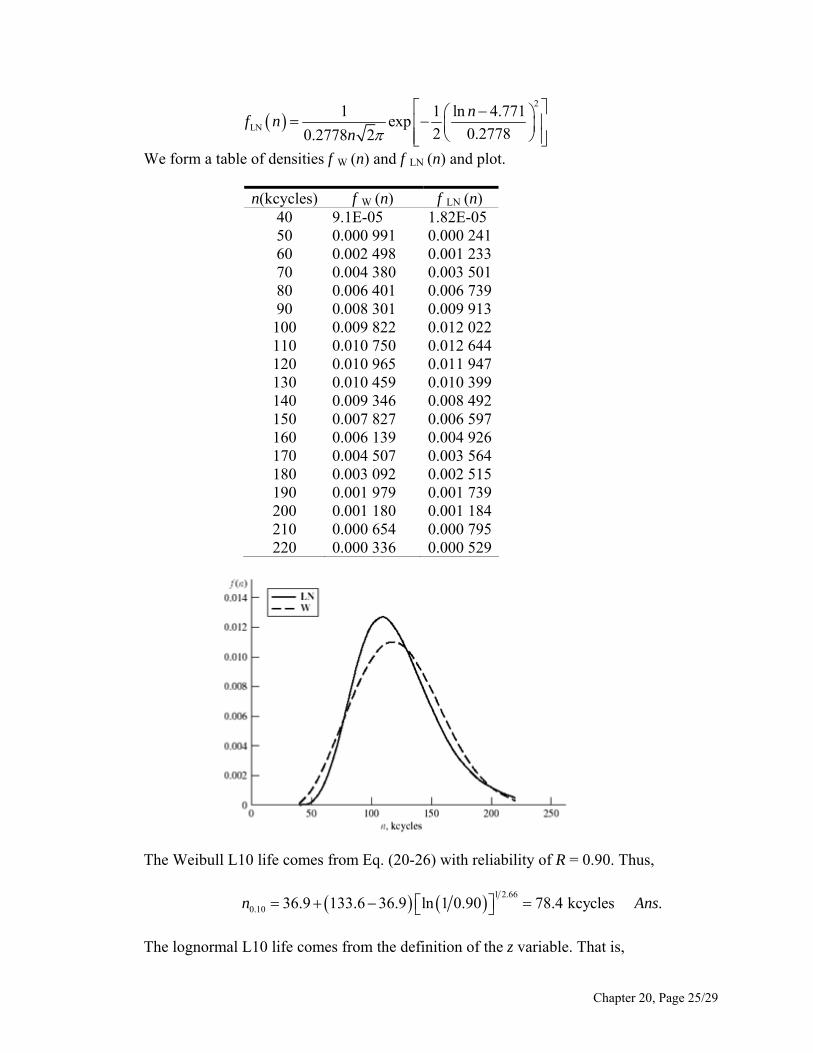
2
LN
1 1 ln 4.771exp
2 0.27780.2778 2
nf n
n
We form a table of densities f W (n) and f LN (n) and plot.
n(kcycles) f W (n) f LN (n) 40 9.1E-05 1.82E-05 50 0.000 991 0.000 24160 0.002 498 0.001 23370 0.004 380 0.003 50180 0.006 401 0.006 73990 0.008 301 0.009 913100 0.009 822 0.012 022110 0.010 750 0.012 644120 0.010 965 0.011 947130 0.010 459 0.010 399140 0.009 346 0.008 492150 0.007 827 0.006 597160 0.006 139 0.004 926170 0.004 507 0.003 564180 0.003 092 0.002 515190 0.001 979 0.001 739200 0.001 180 0.001 184210 0.000 654 0.000 795220 0.000 336 0.000 529
The Weibull L10 life comes from Eq. (20-26) with reliability of R = 0.90. Thus,
1 2.66
0.10 36.9 133.6 36.9 ln 1 0.90 78.4 kcycles .n A ns
The lognormal L10 life comes from the definition of the z variable. That is,
Chapter 20, Page 25/29
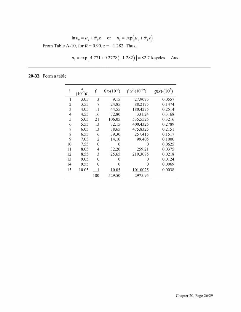
0 0ˆ ˆln or expy y y yn z n z
From Table A-10, for R = 0.90, z = 1.282. Thus,
0 exp 4.771 0.2778 1.282 82.7 kcycles .n A ns
_____________________________________________________________________________ 20-33 Form a table
i x
(105)L fi fi x⋅(105) fi x
2⋅(1010) g(x)⋅(105)
1 3.05 3 9.15 27.9075 0.0557 2 3.55 7 24.85 88.2175 0.1474 3 4.05 11 44.55 180.4275 0.2514 4 4.55 16 72.80 331.24 0.3168 5 5.05 21 106.05 535.5525 0.3216 6 5.55 13 72.15 400.4325 0.2789 7 6.05 13 78.65 475.8325 0.2151 8 6.55 6 39.30 257.415 0.1517 9 7.05 2 14.10 99.405 0.1000
10 7.55 0 0 0 0.0625 11 8.05 4 32.20 259.21 0.0375 12 8.55 3 25.65 219.3075 0.0218 13 9.05 0 0 0 0.0124 14 9.55 0 0 0 0.0069 15 10.05 1 10.05 101.0025 0.0038 100 529.50 2975.95
Chapter 20, Page 26/29
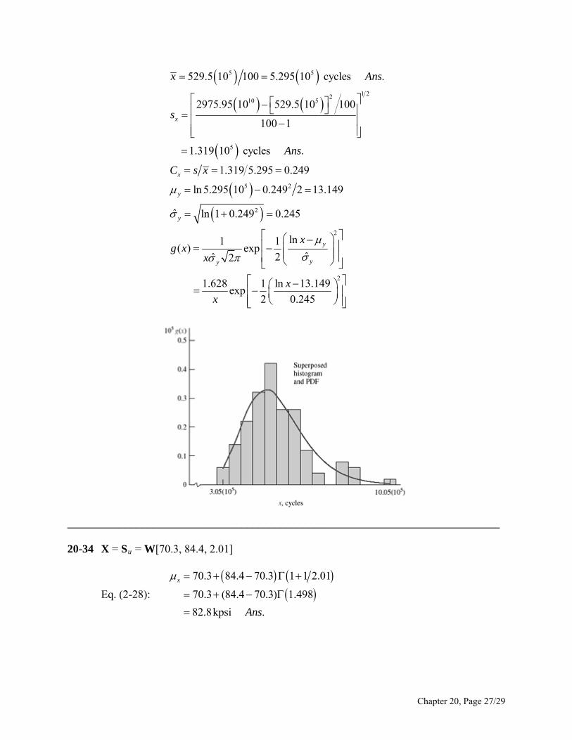
5 5
1 2210 5
5
5 2
2
529.5 10 100 5.295 10 cycles .
2975.95 10 529.5 10 100
100 1
1.319 10 cycles .
1.319 5.295 0.249
ln 5.295 10 0.249 2 13.149
ˆ ln 1 0.249 0.245
l1 1( ) exp
2ˆ 2
x
x
y
y
y
x Ans
s
Ans
C s x
g xx
2
2
n
ˆ
1.628 1 ln 13.149exp
2 0.245
y
y
x
x
x
_____________________________________________________________________________ 20-34 X = Su = W[70.3, 84.4, 2.01]
Eq. (2-28):
70.3 84.4 70.3 1 1 2.01
70.3 (84.4 70.3) 1.498
82.8kpsi .
x
Ans
Chapter 20, Page 27/29
Eq. (2-29):
1 22
1 22
ˆ (84.4 70.3) (1 2 2.01) (1 1 2.01)
ˆ 14.1 0.997 91 0.886 17
6.502 kpsi
6.5020.079 .
82.8
x
x
xC Ans
_____________________________________________________________________________ 20-35 Take the Weibull equation for the standard deviation
1 22
0ˆ (1 2 ) (1 1 )x x b b
and the mean equation solved for 0x x
0 0 1 1x x x b
and divide the first by the second,
1 22
0
1 2 1 1ˆ
1 1x
b b
x x b
2
1 24.21 0.2763
49 33.8 1 1
bR
b
Make a table and solve for b iteratively
0
0
4.068 Using MathCad .
49 33.833.8
(1 1/ ) 1 1/ 4.068
49.8 kpsi .
b A
x xx
b
Ans
b 1 + 2/b 1 + 1/b 1 2 b 1 1 b R
3 1.67 1.33 0.903 30 0.893 38 0.363 4 1.5 1.25 0.886 23 0.906 40 0.280 4.1 1.49 1.24 0.885 95 0.908 52 0.271
ns
_____________________________________________________________________________ 20-36 x = Sy = W[34.7, 39, 2.93] kpsi
Chapter 20, Page 28/29
1 22
1 22
1 22
34.7 39 34.7 1 1 2.93 34.7 4.3 1.34
34.7 4.3 0.892 22 38.5 kpsi
ˆ 39 34.7 1 2 2.93 1 1 2.93
4.3 1.68 1.34
4.3 0.905 00 0.892 22 1.42 kpsi .
1.42 38.5 0.037 .
x
x
x
Ans
C Ans
_____________________________________________________________________________
x (Mrev) f f x f x2
1 11 11 11 2 22 44 88 3 38 114 342 4 57 228 912 5 31 155 775 6 19 114 684 7 15 105 735 8 12 96 768 9 11 99 891 10 9 90 900 11 7 77 847 12 5 60 720Sum 78 237 1193 7673
20-37
6 6
212 6
6
1193 10 / 237 5.034 10 cycles
7673 10 1193 10 / 237ˆ 2.658 10 cycles
237 12.658 / 5.034 0.528
x
x
xC
From Eqs. (20-18) and (20-19),
6 2
2
ln 5.034 10 0.528 / 2 15.292
ˆ ln 1 0.528 0.496
y
y
From Eq. (20-17), defining g(x),
21 1 ln 15.292
( ) exp2 0.4960.496 2
xg x
x
x (Mrev) f / (Nw) g(x)(106)0.5 0.000 00 0.000 11
Chapter 20, Page 29/29
Chapter 20, Page 30/29
lnˆln 15.292 0.496
ˆy
y yy
xz x z z
L10 life, where 10% of bearings fail, from Table A-10, z = 1.282. Thus,
0.5 0.046414 0.000 11 1.5 0.046414 0.052 03 1.5 0.092827 0.052 03 2.5 0.092827 0.169 92 2.5 0.160338 0.169 92 3.5 0.160338 0.207 54 3.5 0.240506 0.207 54 4.5 0.240506 0.178 47 4.5 0.130802 0.178 47 5.5 0.130802 0.131 58 5.5 0.080 17 0.13158 6.5 0.080 17 0.090 11 6.5 0.063 29 0.090 11 7.5 0.063 29 0.059 53 7.5 0.050 63 0.059 53 8.5 0.050 63 0.038 69 8.5 0.046 41 0.038 69 9.5 0.046 41 0.025 01 9.5 0.037 97 0.025 01 10.5 0.037 97 0.016 18 10.5 0.029 54 0.016 18 11.5 0.029 54 0.010 51 11.5 0.021 10 0.010 51 12.5 0.021 10 0.006 87 12.5 0.000 00 0.006 87
ln x = 15.292 + 0.496(1.282) = 14.66 x = 2.33 (106) rev Ans.
Related Documents


![[Solution Manual] Shigley's Mechanical Engineering Design 7th com](https://static.cupdf.com/doc/110x72/55379ef7550346b82d8b458f/solution-manual-shigleys-mechanical-engineering-design-7th-com.jpg)
