Shift scheduling in a Nursing Home using Simulated Annealing Research Paper Business Analytics Marloes Boxelaar Supervisor Dr. René Bekker May 2017

Welcome message from author
This document is posted to help you gain knowledge. Please leave a comment to let me know what you think about it! Share it to your friends and learn new things together.
Transcript

Shift scheduling in a Nursing Home
using
Simulated Annealing
Research Paper Business Analytics
Marloes Boxelaar
Supervisor Dr. René Bekker
May 2017

2
Research Paper
Vrije Universiteit Amsterdam
Faculty of Sciences
Business Analytics
De Boelelaan 1081a
1081 HV Amsterdam
The Netherlands
May 2017

3
Preface The research paper is part of the compulsory courses within the Master Business Analytics at the
Vrije Universiteit (VU) Amsterdam. From the VU, I would like to thank Dr. René Bekker for his
guidance and knowledge. I also want to thank Dennis Moeke, who provided the data, and Ruben van
de Geer who gave preliminary guidelines for the discrete event simulation.
Almere, May 2017

4
Abstract For dependent elderly a key quality indicator is the extent to which they live the life they prefer. As such, it is important that they receive care at the moments of their preference. The goal of this paper is to provide a scheduling algorithm in which clients preferences are met as much as possible, given a certain staffing capacity. This paper develops and test a discrete event simulation model combined with an optimization algorithm to examine the optimum for full-time and flexible shift nurses-staffing schedules. The data for this paper consists of scheduled and unscheduled care requests, the former being obtained from a Dutch nursing home and elaborated upon by previous research; the latter being derived from expert judgement. This paper makes use of a search optimization algorithm called simulated annealing. This is a method which attempts to find the best solution to a given problem within a reasonable timeframe, while escaping local optimums. With this, this paper endeavours to answer the following question; “Is it possible to schedule nurses optimally in a nursing home using simulated annealing?”. The results conclude that flexible scheduling is both cheaper and reduces the resident’s waiting time during the day with almost 19 percent. While this method is effective in the optimization process of nurse staffing, as it provided clear results with applicable outcomes, it should be noted that minimal variability of daily activities is a prerequisite for any desirable outcome for this specific dataset.
5
Contents Preface ..................................................................................................................................................... 3
Abstract ................................................................................................................................................... 4
Chapter 1 ................................................................................................................................................. 7
Introduction ......................................................................................................................................... 7
1.1 Background ................................................................................................................................ 7
1.2 Research question ..................................................................................................................... 7
1.3 Structure of the paper ............................................................................................................... 8
Chapter 2 ................................................................................................................................................. 9
Data description .................................................................................................................................. 9
2.1 Scheduled data .......................................................................................................................... 9
2.2 Unscheduled data .................................................................................................................... 10
Chapter 3 ............................................................................................................................................... 12
Staff scheduling ................................................................................................................................. 12
3.1 Shift types ................................................................................................................................ 12
3.2 Expected staff capacity ............................................................................................................ 12
3.3 Shift length scenarios .............................................................................................................. 13
3.4 Available staff .......................................................................................................................... 13
Chapter 4 ............................................................................................................................................... 14
Discrete event simulation .................................................................................................................. 14
4.1 Background .............................................................................................................................. 14
4.2 Assumptions ............................................................................................................................ 14
4.3 Implementation ....................................................................................................................... 14
Chapter 5 ............................................................................................................................................... 16
Simulated annealing .......................................................................................................................... 16
5.1 Introduction ............................................................................................................................. 16
5.2 Methodology & Implementation ............................................................................................ 16
Chapter 6 ............................................................................................................................................... 21
Results ............................................................................................................................................... 21
6.1 Performance analysis .............................................................................................................. 21
6.2 Search progression of simulated annealing ............................................................................ 22
6.3 With peak at 17:00 .................................................................................................................. 22
6.4 Without peak at 17:00 ............................................................................................................. 26
Chapter 7 ............................................................................................................................................... 31
Conclusions & Recommendations ..................................................................................................... 31
7.1 Conclusions .............................................................................................................................. 31

6
7.2 Research question ................................................................................................................... 32
7.3. Further research ..................................................................................................................... 32
Appendix ................................................................................................................................................ 33
I. Shift types ................................................................................................................................... 33
II. Implemented flowchart of simulated annealing ....................................................................... 34
III. Calculation of the number of possibilities per scenario option ............................................... 35
V. Selected shifts ........................................................................................................................... 37
References ............................................................................................................................................. 38

7
Chapter 1
Introduction In this chapter, the subject and the aim of this research will be introduced. The first section of this
chapter will give some background on the problem of nurse staffing in nursing homes. The next
section will describe the research question and the final section will define the structure of this
paper.
1.1 Background Recently a Dutch news program has paid much attention to the issue of nurse staffing in Dutch
nursing homes [9]. In light of this, little research has been dedicated to nursing staff optimization. As
of yet, the problem of finding good nurse schedules has not been solved. Each of the nursing homes
is struggling to find the balance between sufficient staff to maintain the well-being of the residents
and the recent budgeted costs. The government wants to implement a minimum nursing staff on
duty in January 2019. Research has to be done into the minimum number of nursing staff necessary
to provide quality of service to the residents.
Mostly elderly people become residents of a nursing home. This group of the age 65 years and older
is increasing every year [12]. In these homes, nursing demand fluctuates during the day, as the level
of staff necessary depends on daily nursing activities as well as the distribution of workload across
the day. In case of rushing hours, it is possible that the quality of care provided to residents may
suffer. When the waiting time becomes too long it can affect the well-being of the residents of the
nursing home. The challenge is to find the optimum between waiting time and nurse staffing within
the tightening healthcare budget. This is called the balance between effectiveness and efficiency in
the health care [7]. To find this balance it is necessary to have insight in the nursing activities and the
waiting times for the residents. This means that all data are to be recorded over an extended period
of time and in multiple nursing homes. These real-life data are helpful to get an answer to the
question of an optimal number of staffing before the upcoming regulation. The goal is to find this
optimum with the use of a mathematical model.
This paper makes use of discrete event simulation in order to simulate scheduled care [11] and
unscheduled care [2]. Using simulated annealing (a search algorithm) we determine the number of
staff needed for a large department at a nursing home. The goal is to examine the optimum between
(flexible) staff scheduling and waiting time of the residents.
1.2 Research question
To investigate the possibility of finding an optimal nurse schedule in a nursing home using simulated
annealing, the following research question is defined:
“Is it possible to schedule nurses optimally in a nursing home using simulated annealing?”
With optimal scheduling we mean finding an optimum between the resident’s waiting time and
nurse staffing within a predefined staff capacity. In this research we will consider next to full-time
scheduling, also the possibility of scheduling nurses more flexible.

8
1.3 Structure of the paper The next chapters of this paper will stepwise describe the method used to answer the research
question. In chapter two, the data will be described. Chapter three will outline the staff scheduling
used for the nursing department. Chapter four focuses on the defined model for the discrete event
simulation. Chapter five is about the implemented optimization algorithm simulated annealing. In
chapter six, the results will be presented. The final chapter will give the conclusions and
recommendations.
9
Chapter 2
Data description The data for this research exists of scheduled and unscheduled care data for a nursing home. In this
chapter we will discuss each dataset separately.
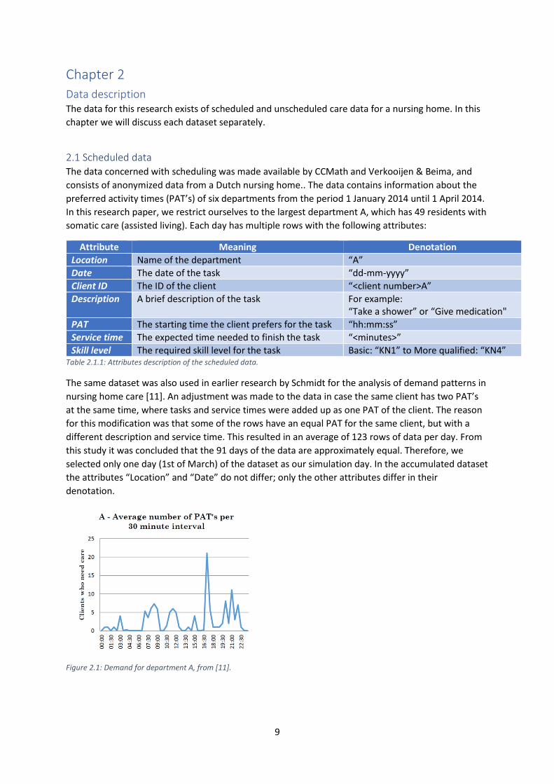
2.1 Scheduled data
The data concerned with scheduling was made available by CCMath and Verkooijen & Beima, and
consists of anonymized data from a Dutch nursing home.. The data contains information about the
preferred activity times (PAT’s) of six departments from the period 1 January 2014 until 1 April 2014.
In this research paper, we restrict ourselves to the largest department A, which has 49 residents with
somatic care (assisted living). Each day has multiple rows with the following attributes:
Attribute Meaning Denotation
Location Name of the department “A”
Date The date of the task “dd-mm-yyyy”
Client ID The ID of the client “<client number>A”
Description A brief description of the task For example: “Take a shower” or “Give medication"
PAT The starting time the client prefers for the task “hh:mm:ss”
Service time The expected time needed to finish the task “<minutes>”
Skill level The required skill level for the task Basic: “KN1” to More qualified: “KN4” Table 2.1.1: Attributes description of the scheduled data.
The same dataset was also used in earlier research by Schmidt for the analysis of demand patterns in
nursing home care [11]. An adjustment was made to the data in case the same client has two PAT’s
at the same time, where tasks and service times were added up as one PAT of the client. The reason
for this modification was that some of the rows have an equal PAT for the same client, but with a
different description and service time. This resulted in an average of 123 rows of data per day. From
this study it was concluded that the 91 days of the data are approximately equal. Therefore, we
selected only one day (1st of March) of the dataset as our simulation day. In the accumulated dataset
the attributes “Location” and “Date” do not differ; only the other attributes differ in their
denotation.
Figure 2.1: Demand for department A, from [11].

10
Schmidt has also identified the night shift to be a quiet period; no more than approximately four
clients within a 30-minute interval need care (see figure 2.1). Therefore, we will focus only on the
care process during daytime (07:00 - 23:00 hours). Another remarkable point from the analysis of
demand was the large peak at 17:00, where many residents take medication.
For the discrete event simulation, we need to know when a client has a PAT and their corresponding
service time. Therefore, we will only use the following attributes: “Client ID”, “PAT” and “Service
time”. During daytime the selected simulation day has the following number of PAT’s with a
corresponding total service time:
Simulation day Number of PAT’s
Total service time
Mean of the service time
Standard deviation of the
service time
1 March 2014 117 24,65 hours 12,64 minutes 8,68 minutes Table 2.1.2: Number of PAT’s, the total service time, the mean and standard deviation of the service time for the selected simulation day.
In practice, the service time of each PAT of a client will differ from day to day. For calculating this
value we will use a log-normal distribution. The reason for choosing this distribution is that it is often
used to generate durations, based on the shape of the distribution/density. This distribution function
requires the parameters mean (µ) and standard deviation (σ):
𝜇 = 𝑙𝑛
(
𝑚
√1+ 𝑣𝑚2)
(1)
𝜎 = √𝑙𝑛 (1 +𝑣
𝑚2 )
(2)
with m the mean and v the variance of the random variable X. The value m is equal to the service
time at a PAT of a client. The variance can be determined using the function for the quadratic
variance coefficient of the random variable X:
𝐶𝑥2 =
𝑉𝑎𝑟(𝑋)
𝐸(𝑋)2=
𝑣
𝑚2 (3)
In order to define a reasonable value for 𝐶𝑥2, multiple runs were done using Crystal Ball in Microsoft
Excel. This resulted in a reasonable range of durations for a value of 0,05. With this known it is
possible to generate for each simulation day a different service time value for each PAT.
2.2 Unscheduled data The unscheduled activities are unexpected tasks, such as assistance with toileting. This process is
generated using an exponential distribution for the interarrival times and a log-normal distribution
for the service time of an activity. According to [8] on average every two hours one resident at a
nursing department with somatic care has an emergency. With the 49 clients at department A, we
expect an average of 24,5 clients per 60 minutes (arrival rate) who need suddenly help. The
exponential parameter of the interarrival times is defined by the 1/arrival rate.
From the analysis of Van Eeden [2], an unscheduled task has on average a duration of 2,56 minutes.
Using this time-value for the mean (m) in equation 1, we have defined the first parameter of the log-
normal distribution of the service time. The squared coefficient of variation of the service time is

11
assumed to be 1. Knowing this value we can define with equation 2 the other parameter (standard
deviation) of the chosen distribution. For every simulation run, different arrivals times and mean care
delivery times will be generated.
The expected number of unscheduled activities and corresponding task duration is defined as
follows:
Simulation day Number of emergencies
Total service time
1 March 2014 392 16,73 hours Table 2.2: Number of expected emergencies and total expected service time.

12
Chapter 3
Staff scheduling In this chapter, we will define which staff schedules we will use for the discrete event simulation and
simulated annealing algorithm. We will first start with describing the shift types, followed by the
expected staff capacity and the shift length scenarios. At the end we will define how to transform a
staff schedule to the number of nurses needed per time interval.
3.1 Shift types
The total waiting time at the nursing department depends on the selected staff schedule. For
scheduling employees, one can use different shift starting times and lengths. In this research, we will
look at full-time and more flexible shifts during the daytime. We will use 8-hour, 4-hour and 2-hour
shifts. Each of these shifts can start every 30 minutes, which will result in a total of 71 different shift
types (see Appendix I). Each shift length has a cost value. When taking into account that a flexible
shift is more expensive per hour than a full-time shift, then we will define the following (simplified)
costs:
Shift Costs per hour (in euro)
Total costs (in euro)
8-hour 1 8
4-hour 1.1 4.4
2-hour 1.2 2.4 Table 3.1: Simplified costs per shift.
3.2 Expected staff capacity To determine the expected capacity of the staff we first need to know what the total amount of work
is during daytime. On a simulation day we have a combination of scheduled and unscheduled events.
Adding the expected service times of both the datasets from chapter 2 “Data description” will result
in the minimum amount of staffing hours needed:
The amount of work at daytime:
Scheduled 24,65 hours Unscheduled 16,73 hours +
Total: 41,38 hours Figure 3.2: The minimum amount of work at department A during daytime.
In practice more staff is needed, because the scheduled and unscheduled events are not equally
spread over the day. For defining the minimum working potential at the nursing department we will
use the following formula:
𝑠𝑡𝑎𝑓𝑓 𝑢𝑡𝑖𝑙𝑖𝑧𝑎𝑡𝑖𝑜𝑛 = 𝑎𝑚𝑜𝑢𝑛𝑡 𝑜𝑓 𝑤𝑜𝑟𝑘
𝑐𝑎𝑝𝑎𝑐𝑖𝑡𝑦 (4)
With a staff utilization of 75%, a minimum capacity of 55,2 nursing hours is needed. Therefore, the
maximum possible staff hours will be set to 56. When using the lowest costs per hour (see table 3.1),
the expected staffing budget will have a value of 56 euro.

13
3.3 Shift length scenarios The nurse schedules that we will define within the calculated budget (see paragraph 3.2) exists of the
following shift combinations:
Figure 3.3: Shift length scenarios for the nursing home at department A.
3.4 Available staff The prime resource (the nurses) are not constantly available, like machines within a company. To define the amount of staff during each 30-minute interval, we will use a part of the mathematical formulation of [5]. For our problem we let k denote a possible shift, and 𝑥𝑘 the number of nurses that are scheduled for shift type k. In figure 3.4 an illustration of the used schedule notation can be found. For satisficing the minimum staffing requirement per time interval t we express the following function:
∑𝑎𝑡𝑘 ∗
𝑘
𝑥𝑘 (5)
with 𝑎𝑡𝑘 the constraint matrix:
𝑎𝑡𝑘 = {1, 𝑠ℎ𝑖𝑓𝑡 𝑘 𝑤𝑜𝑟𝑘𝑠 𝑑𝑢𝑟𝑖𝑛𝑔 𝑖𝑛𝑡𝑒𝑟𝑣𝑎𝑙 𝑡0, 𝑜𝑡ℎ𝑒𝑟𝑤𝑖𝑠𝑒
(6)
Figure 3.4: Schedule notation for the number of nurses to be scheduled (𝑥𝑘) for each shift k.
14
Chapter 4
Discrete event simulation The first section of this chapter will give background information on discrete event simulation. The
next section will define the assumptions and the last section will describe the implementation of the
process at the nursing department.
4.1 Background Discrete event simulation (DES) is a technique for simulating a system where state changes (events)
happen at specific points in simulated time. It is assumed that between two consecutive events no
state change takes place. DES is used in a large number of industries (ex. manufacturing and retail)
and for various processes (ex. transportation and healthcare). With a simulation model one can
quickly analyse how a process behaves over time (ex. determine the efficiency of waiting queues or
the effect on the system when an unforeseen failure takes place).
4.2 Assumptions In order to define boundaries for the discrete event simulation we will define the following
assumptions for the combined datasets of chapter 2 “Data description”:
Assumptions for the scheduled & unscheduled data
1. A simulation day is between 07:00 - 23:00 hours (daytime) 2. Scheduled events are ordered First-Come-First-Served (FCFS) 3. Unscheduled events are ordered FCFS 4. Unscheduled events have priority 5. Events after the simulation day have priority for events during the night shift 6. System is non-preemptive 7. No difference in skill level of a staff member is needed 8. Travel time of a staff member is already part of the service time
Figure 4.2: Defined assumptions for the discrete event simulation.
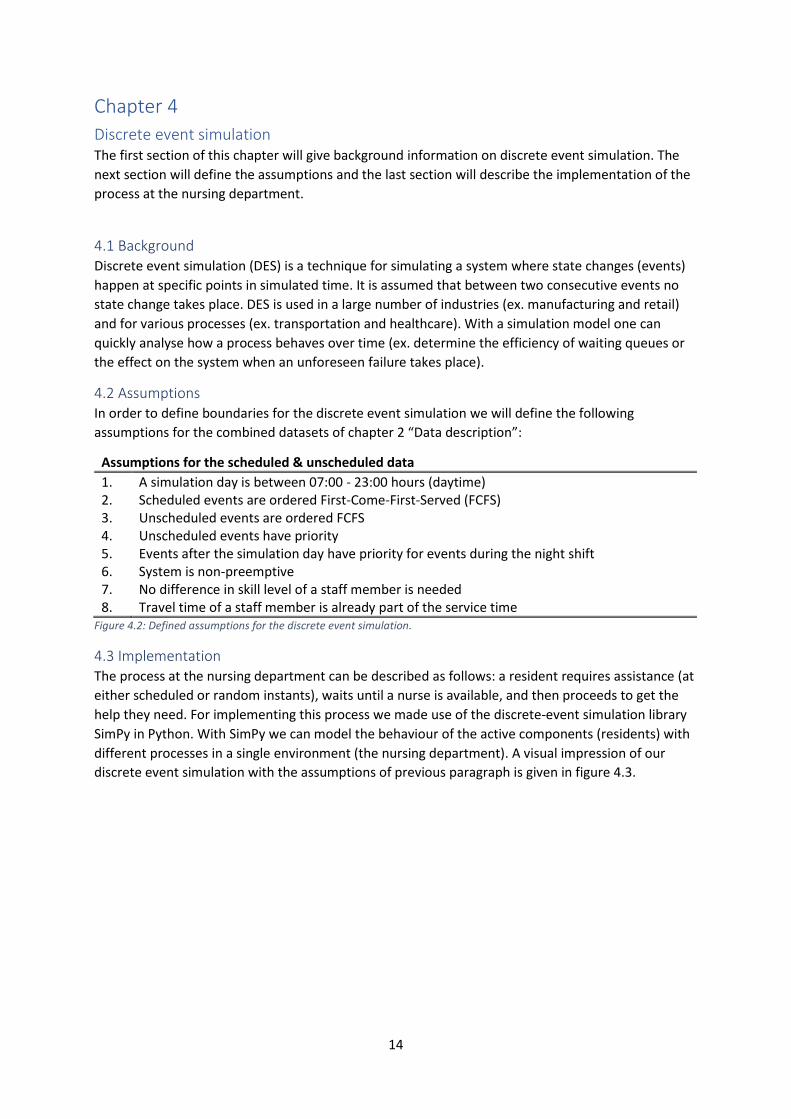
4.3 Implementation The process at the nursing department can be described as follows: a resident requires assistance (at
either scheduled or random instants), waits until a nurse is available, and then proceeds to get the
help they need. For implementing this process we made use of the discrete-event simulation library
SimPy in Python. With SimPy we can model the behaviour of the active components (residents) with
different processes in a single environment (the nursing department). A visual impression of our
discrete event simulation with the assumptions of previous paragraph is given in figure 4.3.

15
Figure 4.3: Illustration of the discrete event simulation of the scheduled (PAT) and unscheduled (emergencies) events.
The arrivals in the system are the PAT’s and the starting times of the emergencies during a simulation
day. When entering the system each event has a resident’s ID, starting time and service duration.
During the simulation the system will continually check the number of k available nurses at that
moment, and will give priority to the events that are classified as an emergency. When the resident
leaves the system (its care request is fulfilled), the waiting time will be calculated and stored in an
array. At the beginning of a simulation (at time 7:00) the nurses will be scheduled according to their
working times. In the simulation the nurses are “activated” the moment the starting time is reached,
and will “deactivate” when their workday is finished. A nurse will always complete a started task, also
if it is outside her/his working hours. At the end of the simulation the value of the cost function
(result of waiting time function, defined in chapter 5) will be returned. The simulation end is at time
23:00, plus the time needed to finish the remaining daily activities in the night shift.

16
Chapter 5
Simulated annealing The first section of this chapter will introduce the optimization algorithm simulated annealing. The
other section will define the method and implementation of this algorithm.
5.1 Introduction
The complexity of optimization problems makes it hard to find an adequate solution to a problem in
a reasonable amount of time. In order to do so, a search algorithm is needed. Multiple search
algorithms are developed for solving optimization problems. For this research we focus on the
algorithm simulated annealing (SA), which is a part of a controlled random technique for solving
bound-constrained and unconstrained optimization problems (see figure 5.1).
Figure 5.1: Taxonomy of search techniques, from [13] modified for the purposes of this paper.
In 1953 Metropolis et al. [6] created the method SA for simulating the real process of metals
annealing. This is a process where molten metal (at a high temperature) is slowly cooled down to a
point where it will have a minimum state of energy. In terms of the simulation, the temperature is
defined as the decreasing value of the objective function for minimization problems. Characteristic of
SA is that it is defined into two phases: exploration and exploitation. The first is used at the beginning
stage to escape local optima, and the other one is used later to find the best solution within the
current region. Large problems have already been successfully solved using this annealing technique.
For example the Traveling Salesman Problem [4] or – more in-line with the research this paper is
executing - a medical staff scheduling problem [10].
5.2 Methodology & Implementation For scheduling the nurses at the department using simulated annealing we made use of the method
from the study of medical staff scheduling, as mentioned at the end of previous section. While this
study did not take the waiting time into consideration (for the sake of simplicity), we used this study
as a guideline for scheduling the nurses.
The process of simulated annealing, starting at a high temperature and ending with a low
temperature is illustrated with figure 5.2.1. At the first iteration step a random solution with a
corresponding cost value (𝐶𝑐𝑢𝑟𝑟𝑒𝑛𝑡) will be generated. During the second iteration, a neighbour
solution with corresponding costs (𝐶𝑛𝑒𝑤) will be computed and compared. When the new costs have
SEARCH TECHNIQUES
CALCULUS BASED
DIRECT INDIRECT
RANDOM
GUIDED
Tabu searchSimulated Annealing
EVOLUTIONARY ALGORITHMS
NEURAL NETWORKS
NON-GUIDED
ENUMERATIVES
GUIDED NON-GUIDED

17
a lower value, then the new solution will be accepted (𝐶𝑐𝑢𝑟𝑟𝑒𝑛𝑡 = 𝐶𝑛𝑒𝑤) . Otherwise, it will keep the
current solution or it can still adopt the new solution with a probability of 𝑒−(∆𝐶
𝑡𝑒𝑚𝑝). This probability is
known as the Boltzmann distribution, where the difference between the two costs values (∆𝐶 =
𝐶𝑛𝑒𝑤 − 𝐶𝑐𝑢𝑟𝑟𝑒𝑛𝑡) is divided by the temperature at that moment. Here the value of the current
temperature depends on the cooling schedule, which will be defined later in this section. Using the
acceptance probability SA can escape local optima (hill climbing). This convergence behaviour is
repeated until the final temperature is reached.
Figure 5.2.1: Convergence of the simulated annealing process, from [1] modified for the purposes of this paper.
In order to describe the implementation of the used algorithm, we will walk step-by-step through the
four key components of simulated annealing. For an illustration of the SA process see the flowchart
in Appendix II.
(1) Hard & soft constraints:
For succeeding in the goal to schedule the nurses such that the waiting times of the residents are
minimized, we followed the framework used by Rosocha et al. [10]. Rosocha defined a categorization
of hard and soft constraints as follows: “… soft constraints define medical staff preferences directly
connected to the quality of work, physical severity, psychic, and work-life balance, hard constraints
are linked to legal and working regulations” (page 2, [10]). During the SA process of making a
schedule, all hard constraints need to be satisfied. Soft constraints, on the other hand, need to be
included as much as possible, however they are not an imperative. For the scheduling problem of this
research we define in figure 5.2.2 the hard constraints. Next to the legal and working regulations of
the nurse schedule, we also set a minimum coverage demand for the nursing department. The
reason for this modification is that there should be always a staff member available at each moment
of time. We choose to select at least two nurses available, because of the high number of residents
at the department. This adjustment will also have a positive effect on the size of the search space of
SA.

18
Figure 5.2.2: Hard constraints for the simulated annealing algorithm at department A.
Instead of focusing on the life of the quality of medical staff as proposed by Rosocha, we used the
resident’s waiting time during daytime and the remaining waiting time for the night shift (above the
allowed value of five remaining activities) as our soft constraints (see figure 5.2.3).
Figure 5.2.3: Soft constraints for the simulated annealing algorithm at department A.
(2) Cost function:
A simulation day (between 07:00 – 23:00 hours), plus the time to finish the daily activities during the
nightshift will result in a value for the cost function of a selected schedule. In order to find an optimal
schedule were the weighted sum of violations of soft constraints (see figure 5.2.3) is minimized, we
will define the following objective function:
𝑀𝑖𝑛𝑖𝑚𝑖𝑧𝑒 𝑤1𝔼𝑊 + 𝑤2𝔼𝑊𝑟𝑒𝑚𝑎𝑖𝑛𝑖𝑛𝑔 (7)
where 𝔼𝑊 is the expected total waiting time during a day and 𝔼𝑊𝑟𝑒𝑚𝑎𝑖𝑛𝑖𝑛𝑔 is the expected
remaining waiting time for the night shift. A higher penalty value will be given to the remaining
activities for the night shift. Therefore, we will give the following values to the weights: 𝑤1 = 1
and 𝑤2 = 2.
(3) Neighbourhood structure:
A neighbour structure consists of a set of neighbouring solutions for each possible solution. The
structure of a solution is defined as the number of nurses scheduled for each shift type, that is 𝑥𝑘
(see figure 3.4). During simulated annealing new schedules will be generated using a method named
Simple Searching Neighbourhood (SNN). This method will randomly choose a scheduled nurse of the
current schedule, and will place this nurse to a randomly chosen position of the same shift length. If
the new schedule is valid (does not violate the hard constraints of figure 5.2.2), then this schedule
will be used for the simulated annealing process. Otherwise, a new schedule will be generated until a
valid schedule is found.
(4) Cooling schedule:
For finding acceptable solutions with simulated annealing a good cooling schedule needs to be
defined. This schedule exists of the following five key parameters: initial temperature, final
temperature, the cooling factor, the number of iterations at each temperature and the temperature
to start the exploitation-phase. Each of this parameters are described as follows:
19
• Initial temperature (𝑻𝟎)
Known as the starting temperature of the simulated annealing process. It allows the search
process to almost any neighbouring state when the temperature is high enough. However, if
this value is too high at the beginning the search can change in a random search. If the initial
temperature is too low, the final results becomes (almost) equal to the first result.
• Final temperature (𝑻𝒔𝒕𝒐𝒑)
The value of this parameter is usually close to zero. The lower the final temperature is the
longer the running time will be to complete the simulated annealing process.
• Cooling factor (𝜶)
Once the initial and final temperature are defined, the cooling factor specifies the level the
temperature decreases. The higher the value of α is, the more iterations steps are needed
(longer running time), but the better the system will stabilise.
• Number of iterations at each temperature (𝑵𝒑)
This parameter will define the number of repetitions needed before the temperature is
lowered by the cooling factor. For a low value of the initial temperature, 𝑁𝑝 needs to be large
enough for exploring the local optimum fully. While less iteration steps are needed for a
higher starting temperature.
• Temperature to start the exploitation-phase (𝑻𝒆𝒙𝒑𝒍𝒐𝒊𝒕𝒂𝒕𝒊𝒐𝒏)
Used for starting the local search (exploitation) of the simulated annealing process. Usual
activated at a temperature close to 𝑇𝑠𝑡𝑜𝑝. The exploitation-phase is in our case a shift that
differ only 30 minutes in the starting time of the random selected shift (according to the
previously defined neighbourhood structure).
Defining these values is a contentious topic. When selecting values which are too high for the initial
temperature, 𝛼 and 𝑁𝑝; the running time can become infinite. The process for defining which cooling
schedule is optimal is a technique reliant on “trail-and-error”. [3], Hendriks at the TU Delft in the
Netherlands performed comprehensive trial-and-error tests, to determine the optimal parameters of
the cooling schedule. He concludes that “… SA is able to return a global minimum, with high
probability, if the starting temperature 𝑇0 is chosen highly enough, and the cooling happens slowly
enough (Np and α large enough).” (page 43, [3]).
Figure 5.3.5 describes the parameters values as put forth by Hendriks, and as adopted by this paper
(underlined). The other parameters (coloured grey) are not required, or implemented otherwise for
the nurse scheduling problem. An adjustment for this paper was made to the value of the parameter
𝑁𝑝. Instead of using a total number of 1000 repetitions per temperature, this value was set to 50.
The reason for this modification is the expected long running time needed to complete the SA
process. A reasonable good schedule needs 6,5 seconds for the discrete event simulation (see
paragraph 6.1 for more details of the analysis of the simulation performance). The running time looks
short, but this discrete event simulation needs to be repeated multiple times to finish the total
simulated annealing process of just one shift length scenario. When using the parameters as
proposed by Hendriks, the expected running time per scenario option can be calculated by: “time of
the discrete event simulation” x “number of repetitions per temperature value (𝑁𝑝)” x “total number
of temperature steps needed” = 6,5 seconds x 1000 x 136 = 884.000 seconds ≈ 10,2 days. The value

20
of the last parameter is determined by the number of steps needed to go from the initial
temperature to the final temperature. At each step a change of 5 percent (cooling factor) of the
current temperature will be taken.
According to the experiments done by Hendriks on the number of repetitions (see figure 5.3.6), the
duration of the one run with a value 50 for 𝑁𝑝, still resulted in a high number of returned global
minima. The expected running time will then be of a reasonable value of 11,3 hours. For the nurse
scheduling we added a parameter for the exploitation phase. The selected parameter values for our
SA algorithm are defined in figure 5.3.7.
Parameter chosen value
𝐴0 𝑂𝐼 𝑥 𝐽 (𝑧𝑒𝑟𝑜 𝑚𝑎𝑡𝑟𝑖𝑥)
𝑇0 500 𝑇𝑠𝑡𝑜𝑝 0,5
𝛼 0,95 𝑁𝑝 1000
k 1
Weights for ∋ CAN-D0 Figure 5.3.5: Parameters used to find global minimum for the simulated annealing process of [3]. With the selected parameters for our research paper underlined.
Variation on 𝑵𝒑 # returning a global minimum out of 100 runs
duration of 1 run (seconds)
no variations (𝑁𝑝 = 1000) 100 41
𝑁𝑝 = 500 100 21
𝑁𝑝 = 250 98 11
𝑁𝑝 = 50 78 2
𝑁𝑝 = 10 18 < 1
Figure 5.3.6: Variations of the number of repetitions 𝑁𝑝 on table 5.3.5, both from [3].
Parameter chosen value
𝑇0 500
𝑇𝑠𝑡𝑜𝑝 0,5
𝛼 0,95 𝑁𝑝 50
𝑇𝑒𝑥𝑝𝑙𝑜𝑖𝑡𝑎𝑡𝑖𝑜𝑛 0,6
Figure 5.3.7: Chosen parameter values for the simulated annealing process of this research.

21
Chapter 6
Results In this chapter the results of the four scenarios (see section 3.3) of the simulated annealing process
will be presented. The first section will describe the number of simulation runs needed, the total
running time and the total number of shift possibilities. The next section will define the search
progression of the simulated annealing algorithm. The final two sections will present the impact of
the nurse scheduling with scheduling medicines at 17:00 (with peak) instead of not scheduling
medicines at 17:00 (without peak).
6.1 Performance analysis For each schedule the arrivals (unscheduled) and the service times (scheduled and unscheduled) of
the residents are randomly generated. Therefore, multiple runs are needed to obtain sufficiently
accurate results for the discrete event simulation. The determining factor for the number of runs
needed is the variability of the value of the objective function (see equation 7). Using a confidence
level of 95% for a different number of simulation runs resulted in the following table:
Number of simulation runs
Half-width of the 95% confidence error
(relative)
Simulation runtime (in seconds)
5 0,07785 0,67
10 0,05117 1,27
25 0,05108 3,14
50 0,04440 6,50
100 0,02976 12,21 Table 6.1.1: Performance results per number of simulation runs (for a reasonable good schedule).
In order to get an acceptable result within a reasonable time we chose to select the total of 50
simulation runs. Each run was computed on an Intel I7 CPU, 8GB RAM, with an implementation in the
Integrated Development Environment PyCharm (version 2016.3), using the programming language
Python (version 2.7) combined with the discrete-event simulation library SimPy (version 3.0.10). The
total running time for each shift length scenario in section 3.3 (one SA process) had a running time of
11 hours. The total number of possibilities (with repetition and where order is irrelevant) can be
calculated with the following formula:
(𝑟 + 𝑛 − 1
𝑟) =
(𝑟 + 𝑛 − 1)!
𝑟! (𝑛 − 1)! (8)
where n is the number of shifts to choose from, and we choose r intervals of them. Determining the
number of all possibilities (when using Brute Force) for each scenario option will give the results
presented in table 6.1.2. For the most flexible option D is the number of possibilities very high, so
when using Brute Force the running time will take a long time. Therefore, simulated annealing is
preferred to find a good solution in a reasonable amount of time, especially for option D.
Option A Option B Option C Option D
Number of possibilities 245.157 74.667 79.108 1.350.074 Table 6.1.2: Number of possibilities per scenario option (including states outside the feasible region), see Appendix III for the calculation.

22
6.2 Search progression of simulated annealing A characteristic trace of the search progression of simulated annealing is shown in figure 6.2 (for
scenario option A with peak at 17:00; see Appendix IV for the other options). At the beginning (high
temperature) all possible parameter values are allowed to be explored, resulting in large fluctuations
in the costs value. While after a large number of iteration steps the search algorithm will set the cost
value longer fixed on one minimum. Where each iteration step exists of 50 runs of a simulation day
with the same schedule.
Figure 6.2: Simulated annealing search progression of scenario option A (with peak at 17:00).
6.3 With peak at 17:00 In this section the results will be presented on the impact of the nurse scheduling with scheduling
medicines at 17:00 (with peak). See Appendix V for the final selected shifts of each scenario option.
Value of cost function:
In order to succeed in minimizing the waiting time during the day and the remaining waiting time for
the night shift, the objective function (see equation 7) needs to be as low as possible. According to
table 6.3.1 the three flexible scenario options are preferred over the full-time option A. This is
remarkable, because the flexible options have less staffing hours; where option B is the best scenario
of the flexible schedules. Theoretically speaking, option C should be better than option B (same
number of working hours, but more flexibility). This is perhaps due to the random process of finding
an accepted schedule that satisfies the minimum level of nurses constraint.
Option A Option B Option C Option D
Total costs 3841 3158 3323 3175 Table 6.3.1: Costs per scenario option (with peak).
Average waiting times:
Shown in table 6.3.2 is the average waiting time per resident during day and night. The night shift is
divided into two values, one with the remaining activities for the night shift above 5 and the other
smaller or equal to 5. According to the results in the table the overall average waiting times are the
shortest for scenario option B during the day. Excluding the data of the first five remaining activities
for the night shift resulted in a higher average waiting time for all options, because these values will
not be part of the objective function (see equation 7). Notable is that option A and C have the highest

23
values in this category, while for the other categories (daytime and night (with remaining activities >
5)) all options are almost equal. With option D for the night (with remaining activities > 5) is almost
twice as much as the rest.
Option A Option B Option C Option D
Daytime 7,58 min 6,17 min 6,47 min 6,23 min
Night (remaining activities <= 5) 43,94 min 29,19 min 41,22 min 29,67 min
Night (remaining activities > 5) 10,45 min 13,87 min 12,54 min 23,26 min Table 6.3.2: Average waiting times per scenario option (with peak).
Average waiting time & staffing level per interval:
In this section the result of the average waiting time during the day is combined with the result of the
number of staff available at each time interval. The first four figures will show both results per
scenario option. The other two figures will show a combined version of each result for all options.
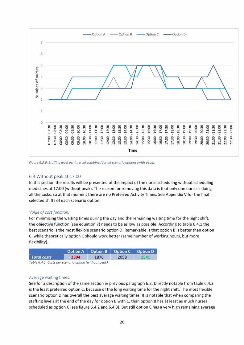
From figure 6.3.6 we see that all options start and end with the minimum predefined staffing
capacity of two nurses. The full-time scenario option A (see figure 6.3.1) has more staff capacity
planned earlier in the morning than the three other options. Remarkable for all options is that per
interval the average waiting time is almost equal (see figure 6.3.5) and that the staffing level is
always the highest in the afternoon (see figure 6.3.6). The only exception for the average waiting
time is option D during lunch time. The reason is that less nurses are scheduled in the morning shift.
Therefore, the accumulating nursing activities still had to be done during lunch time.
Figure 6.3.1: Average waiting time per interval of scenario option A (with peak).

24
Figure 6.3.2: Average waiting time per interval of scenario option B (with peak).
Figure 6.3.3: Average waiting time per interval of scenario option C (with peak).

25
Figure 6.3.4: Average waiting time per interval of scenario option D (with peak).
Figure 6.3.5: Average waiting time combined for all scenario options (with peak).
0
5
10
15
20
25
30
35
07
:00
- 0
7:3
0
07
:30
- 0
8:0
0
08
:00
- 0
8:3
0
08
:30
- 0
9:0
0
09
:00
- 0
9:3
0
09
:30
- 1
0:0
0
10
:00
- 1
0:3
0
10
:30
- 1
1:0
0
11
:00
- 1
1:3
0
11
:30
- 1
2:0
0
12
:00
- 1
2:3
0
12
:30
- 1
3:0
0
13
:00
- 1
3:3
0
13
:30
- 1
4:0
0
14
:00
- 1
4:3
0
14
:30
- 1
5:0
0
15
:00
- 1
5:3
0
15
:30
- 1
6:0
0
16
:00
- 1
6:3
0
16
:30
- 1
7:0
0
17
:00
- 1
7:3
0
17
:30
- 1
8:0
0
18
:00
- 1
8:3
0
18
:30
- 1
9:0
0
19
:00
- 1
9:3
0
19
:30
- 2
0:0
0
20
:00
- 2
0:3
0
20
:30
- 2
1:0
0
21
:00
- 2
1:3
0
21
:30
- 2
2:0
0
22
:00
- 2
2:3
0
22
:30
- 2
3:0
0
Ave
rage
wai
tin
g ti
me
(in
min
ute
s)
Time
Option A Option B Option C Option D
26
Figure 6.3.6: Staffing level per interval combined for all scenario options (with peak).
6.4 Without peak at 17:00 In this section the results will be presented of the impact of the nurse scheduling without scheduling
medicines at 17:00 (without peak). The reason for removing this data is that only one nurse is doing
all the tasks, so at that moment there are no Preferred Activity Times. See Appendix V for the final
selected shifts of each scenario option.
Value of cost function:
For minimizing the waiting times during the day and the remaining waiting time for the night shift,
the objective function (see equation 7) needs to be as low as possible. According to table 6.4.1 the
best scenario is the most flexible scenario option D. Remarkable is that option B is better than option
C, while theoretically option C should work better (same number of working hours, but more
flexibility).
Option A Option B Option C Option D
Total costs 2394 1876 2058 1541 Table 6.4.1: Costs per scenario option (without peak).
Average waiting times:
See for a description of the same section in previous paragraph 6.3. Directly notable from table 6.4.2
is the least preferred option C, because of the long waiting time for the night shift. The most flexible
scenario option D has overall the best average waiting times. It is notable that when comparing the
staffing levels at the end of the day for option B with C, than option B has at least as much nurses
scheduled as option C (see figure 6.4.2 and 6.4.3). But still option C has a very high remaining average
0
1
2
3
4
5
6
7
07
:00
- 0
7:3
0
07
:30
- 0
8:0
0
08
:00
- 0
8:3
0
08
:30
- 0
9:0
0
09
:00
- 0
9:3
0
09
:30
- 1
0:0
0
10
:00
- 1
0:3
0
10
:30
- 1
1:0
0
11
:00
- 1
1:3
0
11
:30
- 1
2:0
0
12
:00
- 1
2:3
0
12
:30
- 1
3:0
0
13
:00
- 1
3:3
0
13
:30
- 1
4:0
0
14
:00
- 1
4:3
0
14
:30
- 1
5:0
0
15
:00
- 1
5:3
0
15
:30
- 1
6:0
0
16
:00
- 1
6:3
0
16
:30
- 1
7:0
0
17
:00
- 1
7:3
0
17
:30
- 1
8:0
0
18
:00
- 1
8:3
0
18
:30
- 1
9:0
0
19
:00
- 1
9:3
0
19
:30
- 2
0:0
0
20
:00
- 2
0:3
0
20
:30
- 2
1:0
0
21
:00
- 2
1:3
0
21
:30
- 2
2:0
0
22
:00
- 2
2:3
0
22
:30
- 2
3:0
0
Nu
mb
er o
f n
urs
es
Time
Option A Option B Option C Option D
27
waiting time. We thought that maybe the random process was affecting this result, but after multiple
random runs almost the same unexplainable value came as a result.
Option A Option B Option C Option D
Daytime 4,89 min 3,81 min 4,07 min 3,11 min
Night (remaining activities <= 5) 46,01 min 49,03 min 70,62 min 20,10 min
Night (remaining activities > 5) 10,22 min 14,32 min 58,36 min 20,88 min Table 6.4.2: Average waiting times per scenario option (without peak).
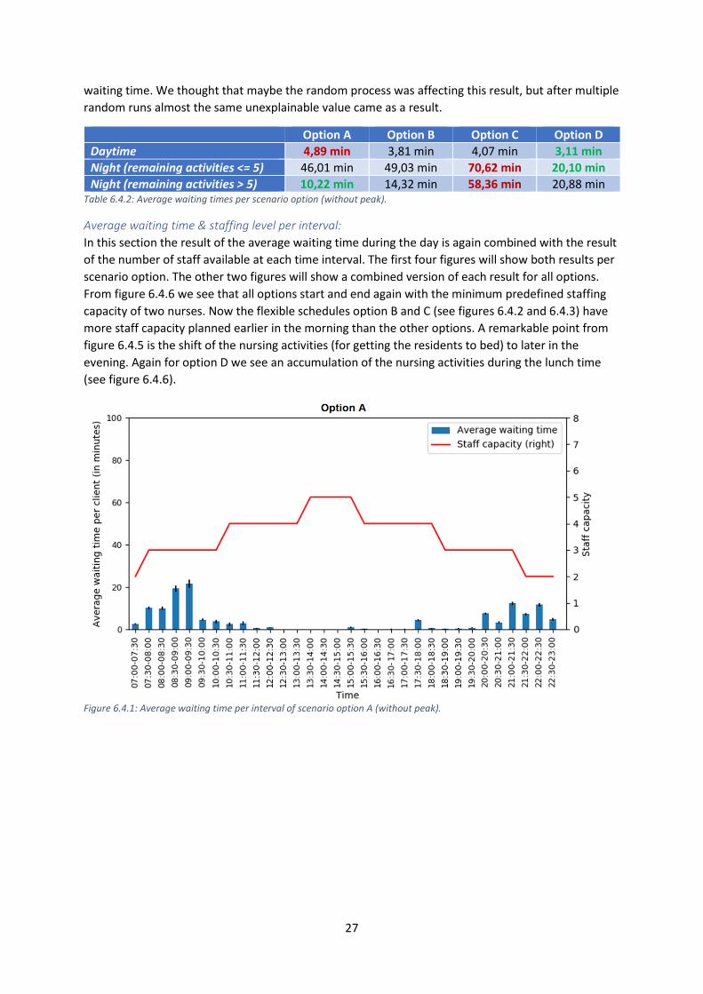
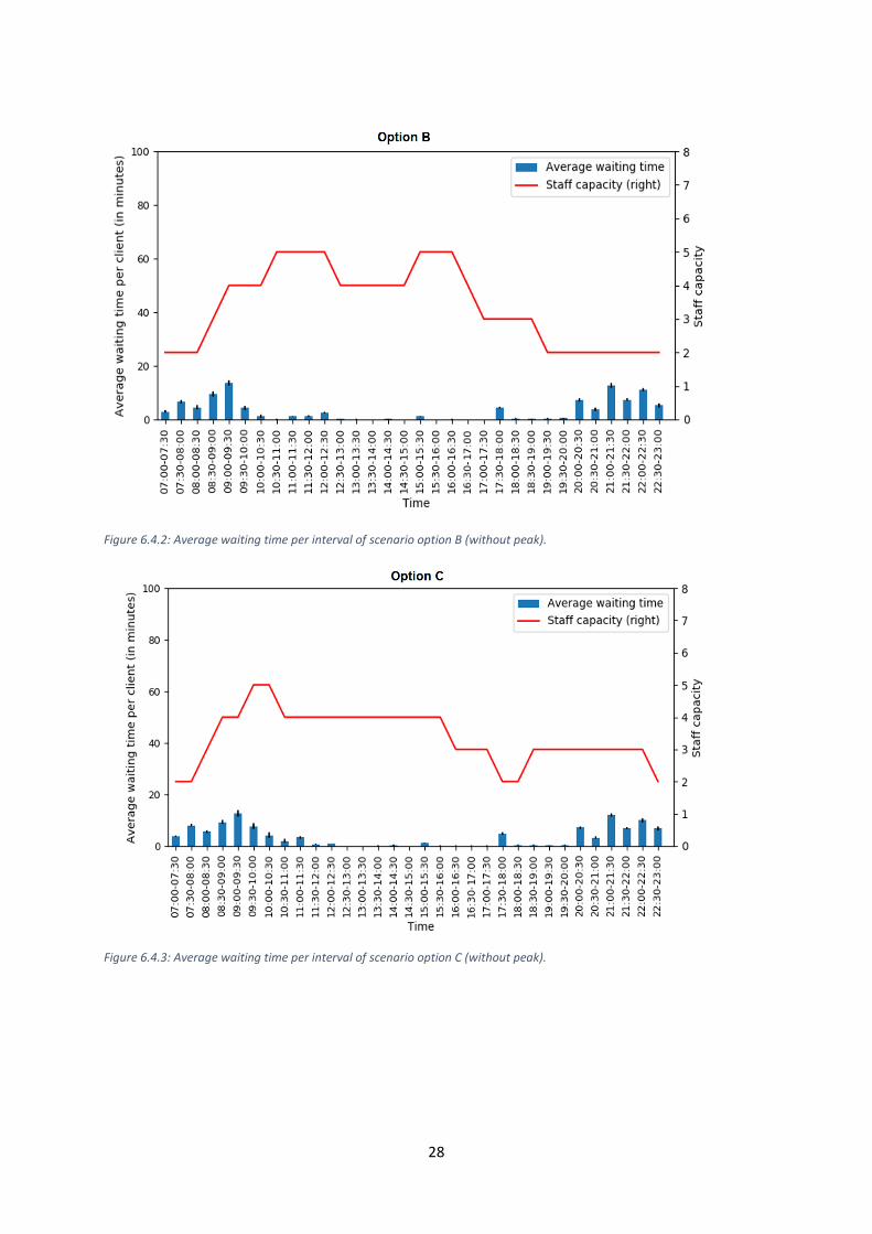
Average waiting time & staffing level per interval:
In this section the result of the average waiting time during the day is again combined with the result
of the number of staff available at each time interval. The first four figures will show both results per
scenario option. The other two figures will show a combined version of each result for all options.
From figure 6.4.6 we see that all options start and end again with the minimum predefined staffing
capacity of two nurses. Now the flexible schedules option B and C (see figures 6.4.2 and 6.4.3) have
more staff capacity planned earlier in the morning than the other options. A remarkable point from
figure 6.4.5 is the shift of the nursing activities (for getting the residents to bed) to later in the
evening. Again for option D we see an accumulation of the nursing activities during the lunch time
(see figure 6.4.6).
Figure 6.4.1: Average waiting time per interval of scenario option A (without peak).
28
Figure 6.4.2: Average waiting time per interval of scenario option B (without peak).
Figure 6.4.3: Average waiting time per interval of scenario option C (without peak).

29
Figure 6.4.4: Average waiting time per interval of scenario option D (without peak).

30
Figure 6.4.5: Average waiting time combined for all scenario options (without peak).
Figure 6.4.6: Staffing level per interval combined for all scenario options (without peak).
0
5
10
15
20
25
30
35
07
:00
- 0
7:3
0
07
:30
- 0
8:0
0
08
:00
- 0
8:3
0
08
:30
- 0
9:0
0
09
:00
- 0
9:3
0
09
:30
- 1
0:0
0
10
:00
- 1
0:3
0
10
:30
- 1
1:0
0
11
:00
- 1
1:3
0
11
:30
- 1
2:0
0
12
:00
- 1
2:3
0
12
:30
- 1
3:0
0
13
:00
- 1
3:3
0
13
:30
- 1
4:0
0
14
:00
- 1
4:3
0
14
:30
- 1
5:0
0
15
:00
- 1
5:3
0
15
:30
- 1
6:0
0
16
:00
- 1
6:3
0
16
:30
- 1
7:0
0
17
:00
- 1
7:3
0
17
:30
- 1
8:0
0
18
:00
- 1
8:3
0
18
:30
- 1
9:0
0
19
:00
- 1
9:3
0
19
:30
- 2
0:0
0
20
:00
- 2
0:3
0
20
:30
- 2
1:0
0
21
:00
- 2
1:3
0
21
:30
- 2
2:0
0
22
:00
- 2
2:3
0
22
:30
- 2
3:0
0
Ave
rage
wai
tin
g ti
me
(in
min
ute
s)
Time
Option A Option B Option C Option D
0
1
2
3
4
5
6
7
07
:00
- 0
7:3
0
07
:30
- 0
8:0
0
08
:00
- 0
8:3
0
08
:30
- 0
9:0
0
09
:00
- 0
9:3
0
09
:30
- 1
0:0
0
10
:00
- 1
0:3
0
10
:30
- 1
1:0
0
11
:00
- 1
1:3
0
11
:30
- 1
2:0
0
12
:00
- 1
2:3
0
12
:30
- 1
3:0
0
13
:00
- 1
3:3
0
13
:30
- 1
4:0
0
14
:00
- 1
4:3
0
14
:30
- 1
5:0
0
15
:00
- 1
5:3
0
15
:30
- 1
6:0
0
16
:00
- 1
6:3
0
16
:30
- 1
7:0
0
17
:00
- 1
7:3
0
17
:30
- 1
8:0
0
18
:00
- 1
8:3
0
18
:30
- 1
9:0
0
19
:00
- 1
9:3
0
19
:30
- 2
0:0
0
20
:00
- 2
0:3
0
20
:30
- 2
1:0
0
21
:00
- 2
1:3
0
21
:30
- 2
2:0
0
22
:00
- 2
2:3
0
22
:30
- 2
3:0
0
Nu
mb
er o
f st
aff
Time
Option A Option B Option C Option D
31
Chapter 7
Conclusions & Recommendations The first section of this chapter will present the conclusions of the results from chapter 6. The next
section will give answer to the defined research question. The final section will give some
recommendations to improve research based on nurse scheduling.
7.1 Conclusions The conclusions of the results of this paper are divided into the following four components:
(1) Performance analysis:
According to chapter 6.1, one run (50 simulation days with the same schedule) for the discrete event
simulation takes 6,5 seconds. The total running time of one simulated annealing process (for each
shift length scenario, see figure 3.3) takes 11 hours. When only using Brute Force, the number of
possibilities for the most flexible scenario option D has the highest value (see table 6.1.2). This will
result in a long computational time. Therefore, simulated annealing is especially preferred for option
D for finding a good solution in a reasonable amount of time.
(2) Staffing budget and cost value:
From both the tables 6.3.1 and 6.4.1 we can conclude that the flexible schedules are more preferred
than the full-time schedule (scenario option A). Option A has next to more staffing costs, also a
higher value for the cost function of the simulated annealing algorithm (equation 7). When the
medicines at 17:00 are scheduled (with peak), then the best flexible schedule is option B (see table
6.3.1). While option D is preferred when the medication at 17:00 is no part of the dataset (see table
6.4.1).
(3) Waiting time & staffing level (with peak at 17:00):
According to table 6.3.2 the overall average waiting times are the shortest for option B during the
day. Excluding the data of the first allowed five remaining activities for the night shift resulted in a
higher average waiting time for all options, because these values will not be part of the objective
function (see equation 7).
For all options is the average waiting time per interval almost equal (see figure 6.3.5). The only
exception is option D during lunch time. The reason is that less nurses are scheduled in the morning
shift (see figure 6.3.6). Therefore, the accumulating nursing activities still had to be done during
lunch time.
(4) Waiting time & staffing level (without peak at 17:00):
Directly notable from table 6.4.2 is the least preferred option C, because of the long waiting time for
the night shift. Figure 6.4.5 shows the shifting of the nursing activities (for getting the residents to
bed) to later in the evening. Again option D is an accumulation of the nursing activities during the
lunch time (see figure 6.4.6).

32
7.2 Research question Nursing homes are seeking for an optimum between the resident’s waiting time and nurse staffing
within a budget. Based on the described data with the made assumptions for the discrete event
simulation in chapter 4, and the conclusions from previous section we will answer the following
research question:
“Is it possible to schedule nurses optimally in a nursing home using simulated annealing?”
With simulated annealing it is possible to schedule nurses optimally in a nursing home if the daily
activities are approximately equal. The results conclude that flexible scheduling is both cheaper and
reduces resident waiting times. This annealing method is effective in the optimization process of
nurse staffing, as it provided clear results with applicable outcomes. The downside to this method is
one of time: the running time for the simulated annealing process (namely 11 hours per shift length
scenario) is not very practical. It is, however, unavoidable with this type of multifaceted research.
7.3. Further research For increasing the completeness of nurse scheduling for the nursing department it is recommended
to include the qualification levels. Also interesting is to do research of the effect on the resident’s
waiting time when spreading the Preferred Activity Time (PAT’s) more during the day. Now, most
residents have a scheduled task with a long service duration and low priority at the same time.
Future research should also consider generating varying shift scenarios within a certain budget; as
this paper chose to limit staff capacity scenarios to just four options. This would ensure a broader
range of outcomes, and perhaps lead to a better solution.

33
Appendix
I. Shift types
Figure I: Possible shift types.

34
II. Implemented flowchart of simulated annealing
Figure II: Flowchart of the medical staff scheduling algorithm, from [10] modified for the purposes of this paper.

35
III. Calculation of the number of possibilities per scenario option
Calculation Number of possibilities
Option A (7 + 17 − 1
7)
245.157
Option B (6 + 17 − 1
6) + (
1 + 25 − 1
1) + (
1 + 29 − 1
1) 74.667
Option C (6 + 17 − 1
6) + (
3 + 29 − 1
3) 79.108
Option D (4 + 17 − 1
4) + (
2 + 25 − 1
2) + (
6 + 29 − 1
6) 1.350.074
Table III: Calculation and the number of shift possibilities (including states outside the feasible region) per scenario option defined.

36
IV. Simulated annealing process
With peak at 17:00
Without peak at 17:00
Figure IV.2: Search progressions of the simulated annealing per scenario option (without peak).
Figure IV.1: Search progressions of the simulated annealing per scenario option (with peak).

37
V. Selected shifts
With peak at 17:00
Figure V.1: Selected shifts per scenario option (with peak).
Without peak at 17:00
Figure V.2: Selected shifts per scenario option (without peak).

38
References
[1] Dutta, J. 2013. Global Optimization Search Techniques. Computer Science & Engineering Calcutta University. 14. Retrieved from https://www.slideshare.net/idforjoydutta/simulated-annealing-24528483.
[2] Eeden, K., D. Moeke and R. Bekker. 2016. Care on demand in nursing homes: A Queueing theoretic approach. Health Care Management Science, 19, 227-240.
[3] Hendriks, W.H., F. van der Meulen. 2013, April 3. Multi skilled staff scheduling with simulated annealing. MSc Thesis Delft University of Technology.
[4] Johnson, D.S., and L.A. McGeoch. 1997. The traveling salesman problem: A case study, in Local Search in Combinatorial Optimization, Aarts, E.H.L., and Lenstra, J.K., John Wiley and Sons, Ltd., 215–310.
[5] Koole, G. 2010, March 30. Optimization of Business Processes: An Introduction to Applied Stochastic Modeling, 211-13.
[6] Metropolis, N. et al. 1953. Equation of state calculations by fast computing machines. Journal of Chemical Physics, 21(6), 1087-92.
[7] Moeke, D., G. Koole, and L. Verkooijen. 2014. Scale and skill-mix efficiencies in nursing home. Health Systems, 3, 18-28.
[8] Moeke, D., R. van der Geer, G. Koole, and R. Bekker. 2016. On the performance of small-scale living facilities in nursing homes: a simulation approach. Operations Research for Health Care, 11, 20-34.
[9] Nieuwsuur [Video file]. 2017, February 22. Retrieved from http://nos.nl/uitzending/22629-nieuwsuur.html.
[10] Rosocha, L., S. Vernerová, and R. Verner. 2015. Medical staff scheduling using simulated annealing. Quality Innovation Prosperity, 19, 1.
[11] Schmidt, B., and R. Bekker. 2014. Analysis of demand patterns in nursing home care. Research Paper Business Analytics VU University Amsterdam.
[12] Statistics Netherlands. 2014, December 18. Population forecasts 2014-2060. http://statline.cbs.nl/Statweb/publication/?DM=SLEN&PA=82683ENG&D1=3,13,16&D2=0&D3=0-1,6,11,16,21,26,31,36,41,l&LA=EN&HDR=T&STB=G1,G2&VW=T.
[13] Troya, J.M. Improving flexibility and efficiency by adding parallelism to genetic algorithms. Statistics and Computing 12(2), 91-114.
Related Documents


![Hybrid Sorting Immune Simulated Annealing Algorithm For ...programming and simulated annealing (AMPSA) [11] in job shop scheduling (JSP) for improving the makespan. Moreover, hybrid](https://static.cupdf.com/doc/110x72/60b8b8e6cc4e273663719cfd/hybrid-sorting-immune-simulated-annealing-algorithm-for-programming-and-simulated.jpg)


