Shear Test of High Performance Steel Hybrid Girders Organizational Results Research Report Prepared by University of Missouri-Columbia and Missouri Department of Transportation RI 99.026 OR 06.001 . . . . . . . . . . . . . . . . . . . . . . . . . . . . . . . . . . . . . . . . . July 2005 . . . . . . . . . . . . . . . . . . . . . . . . . . . . . . . . . . . . . . . . .

Welcome message from author
This document is posted to help you gain knowledge. Please leave a comment to let me know what you think about it! Share it to your friends and learn new things together.
Transcript

Shear Test of High Performance Steel Hybrid Girders
Organizational Results Research Report
Prepared by University of
Missouri-Columbia and
Missouri Department of
Transportation
RI 99.026OR 06.001
. . . . . . . . . . . . . . . . . . . . . . . . . . . . . . . . . . . . . . . . .July 2005
. . . . . . . . . . . . . . . . . . . . . . . . . . . . . . . . . . . . . . . . .

Draft Final Report
RI99-026
SHEAR TESTS OF HIGH PERFORMANCE STEEL HYBRID GIRDERS
Prepared for the Missouri Department of Transportation
Research Development & Technology
By: Michael G. Barker, PE University of Wyoming
formerly of the University of Missouri-Columbia
Submitted June 2005
The opinions, findings and conclusions expressed in this report are those of the principal investigator and the Missouri Department of Transportation. They are not necessarily those of the U.S. Department of Transportation or the Federal Highway Administration. This report does not constitute a standard, specification or regulation.
111

ACKNOWLEDGEMENTS
The author wishes to recognize the graduate students that worked on this project: auSTIN Hurst, John Schreiner, Courtney Rush, Ben Davis, Adam Zentz, and Tori Goessling. Special thanks are due to C.H. Cassil who dedicated himself to this project and made sure the testing was done with professionalism and care.
This work was part of a collaborative effort involving the American Iron and Steel Institute, the Federal Highway Administration, the Missouri Department of Transportation, and Georgia Tech University.
IV
EXECUTIVE SUMMARY
High Performance Steel, in particular HPS70W, has been used in hundreds of bridges across the United States. A large percentage of these bridges have used the HPS in the form of hybrid girder designs. Bridge studies have shown that the most beneficial use of HPS70W (70 ksi) is in the flanges of hybrid girders with 50 ksi webs. One limit with hybrid girder design, which decreases the beneficial aspects, is that tension field action (TF A) is not allowed when determining the shear capacity. This is a severe shear capacity penalty for using hybrid girders. Limiting hybrid shear capacities to the shear buckling capacity results in more transverse stiffeners required ( closer spacing) for a hybrid girder than that for a homogeneous girder. This not only increases material costs, but significantly increases fabrication costs.
The objective of this research is to validate the tension field action behavior in hybrid plate girders. The goal is to allow TF A in hybrid girders resulting in more economical design of steel bridges.
The work conducted for this research covers several topics in tension field action and moment-shear interaction of plate girders. The first effort concentrated on the original shear capacity theoretical derivations and the differences in using hybrid girders. In addition, two series of tests were designed and tested to determine the hybrid girder shear capacity and study the tension field behavior of homogeneous and hybrid girders. Series I test specimens were homogeneous and hybrid girders tested under high shear and low moment conditions. Series II test specimens were designed and tested to study the effect of moment-shear interaction. Finally, an array of practical bridge designs was developed to study the benefit of allowing TF A in hybrid girders.
This report includes a thorough presentation of tension field action and moment-shear interaction in plate girders, and in particular hybrid plate girders. It presents a comprehensive presentation on the test girders with a detailed analysis and examination of the test behaviors.
There are a few important results that may improve the design of hybrid steel girder bridges. Hybrid steel girders exhibit tension field action according to current AASHTO shear capacity provisions. Using the original moment-shear interaction derivations, this research has produced a theoretical lower-bound moment-shear interaction equation for hybrid girders that is equivalent to the current AASHTO moment-shear interaction requirement for homogeneous girders. However, the results of the experimental tests and analytical studies have also shown that there is no moment-shear interaction for these plate girders. The girders all demonstrated that the capacities exceeded expectations and that a moment-shear interaction reduction is not necessary.
V
TABLE OF CONTENTS
LIST OF FIGURES ......................................................................................................... viii LIST OF TABLES ............................................................................................................. xi
Chapter 1 - Introduction ...................................................................................................... 1 1.1 Problem Statement .............................................................................................. 1 1.2 Research Objective ............................................................................................. 3 1.3 Research Content ................................................................................................ 4 1.4 Results ................................................................................................................. 5 1.5 Report Organization ............................................................................................ 5
Chapter 2 - Tension Field Action ........................................................................................ 7 2.1 Introduction ......................................................................................................... 7 2.2 Hybrid Plate Girders ........................................................................................... 7 2.3 Shear Capacity .................................................................................................... 8
2.3.1 Shear Buckling Capacity ............................................................................. 9 2.3.2 Post-Buckling Shear Capacity .................................................................. 11 2.3.3 Basler's Shear Capacity Derivation .......................................................... 12 2.3.4 AASHTO's Tension Field Action Provisions .......................................... 26
2.4 Moment-Shear Interaction ................................................................................ 28 2.4.1 Basler' s Interaction Diagram .................................................................... 29 2.4.2 AASHTO's Interaction Diagram .............................................................. 35 2.4.3 Proposed Hybrid Moment-Shear Interaction Diagram ............................. 38
2.5 Summary ........................................................................................................... 45 Chapter 3 - Test Specimens and Theoretical Behavior ..................................................... 46
3.1 Introduction ....................................................................................................... 46 3.2 Series I Test Specimens .................................................................................... 48 3.3 Series II Test Specimens ................................................................................... 51
3.3.1 Test Girders ............................................................................................... 51 3.3.2 Test Design ............................................................................................... 54 3.3.3 Instrumentation ......................................................................................... 58
3.4 Summary of Test Specimens ............................................................................ 62 3.5 Theoretical Data Analysis ................................................................................. 62
3.5.1 Introduction ............................................................................................... 62 3.5.2 Theoretical Stress Analysis - Series II Tests ............................................ 63
3.5.2.1 Elastic Stresses ...................................................................................... 64 3.5.2.2 Postbuckling Stresses ............................................................................ 70 3.5.2.3 Example Calculation of Theoretical Stresses ....................................... 72
3.5.3 Experimental Stress Analysis ................................................................... 80 3.5.3.1 Rosette Strain Gauge Data .................................................................... 80 3.5.3.2 Linear Strain Gauge Data ...................................................................... 84 3.5.3.3 String Pot Data ...................................................................................... 85 3.5.3.4 Example Experimental Stress Calculations .......................................... 86
3.5.4 Summary Theoretical Behavior ................................................................ 89
Vl
3.6 Summary ........................................................................................................... 90 Chapter 4 - Experimental Results ..................................................................................... 91
4.1 Introduction ....................................................................................................... 91 4.2 Physical Observations ....................................................................................... 92
4.2.1 Experimental Shear Capacities ................................................................. 92 4.2.2 Moment-Shear Interaction ........................................................................ 95 4.2.3 Failure Mechanisms .................................................................................. 99 4.2.4 Experimental Web Buckling ................................................................... 103
4.2.4.1 String Pot Data .................................................................................... 104 4.2.4.2 Rosette Strain Gauge Data .................................................................. 105 4.2.4.3 Tension Field Anchorage Stresses ...................................................... 106 4.2.4.4 Postbuckling Stress Behavior ............................................................. 109 4.2.4.5 Results of Experimental Web Buckling Investigation ........................ 111
4.3 Elastic Stresses ................................................................................................ 113 4.4 Postbuckling Stresses ...................................................................................... 126 4.5 Impact of TF A in Hybrid Girders ................................................................... 14 7 4.6 Summary ......................................................................................................... 148
Chapter 5 - Summary and Conclusions .......................................................................... 149 5.1 Summary ......................................................................................................... 149 5.2 Project Conclusions and Recommendations ................................................... 152
References ....................................................................................................................... 153
Vll
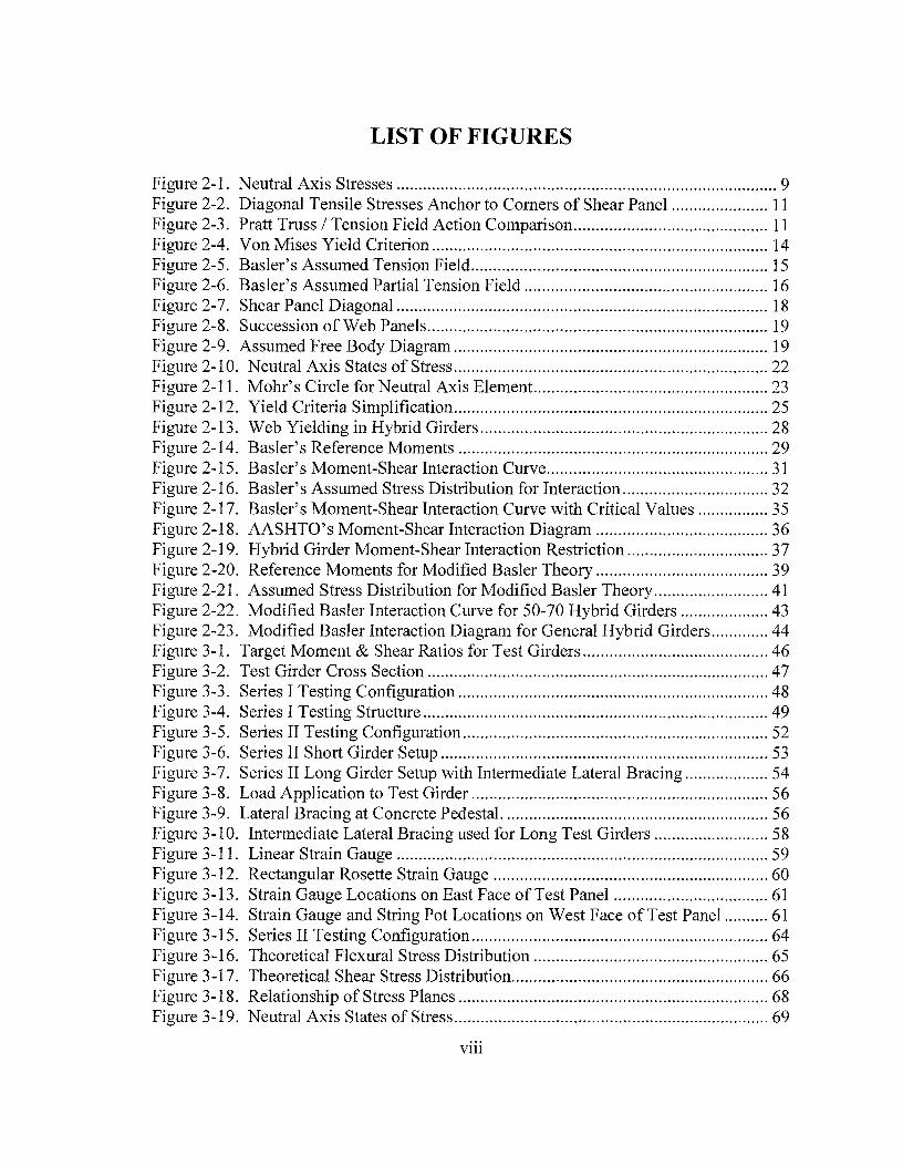
LIST OF FIGURES
Figure 2-1. Neutral Axis Stresses ...................................................................................... 9 Figure 2-2. Diagonal Tensile Stresses Anchor to Corners of Shear Panel ...................... 11 Figure 2-3. Pratt Truss I Tension Field Action Comparison ............................................ 11 Figure 2-4. Von Mises Yield Criterion ............................................................................ 14 Figure 2-5. Basler's Assumed Tension Field ................................................................... 15 Figure 2-6. Basler' s Assumed Partial Tension Field ....................................................... 16 Figure 2-7. Shear Panel Diagonal .................................................................................... 18 Figure 2-8. Succession of Web Panels ............................................................................. 19 Figure 2-9. Assumed Free Body Diagram ....................................................................... 19 Figure 2-10. Neutral Axis States of Stress ....................................................................... 22 Figure 2-11. Mohr's Circle for Neutral Axis Element ..................................................... 23 Figure 2-12. Yield Criteria Simplification ....................................................................... 25 Figure 2-13. Web Yielding in Hybrid Girders ................................................................. 28 Figure 2-14. Basler's Reference Moments ...................................................................... 29 Figure 2-15. Basler' s Moment-Shear Interaction Curve .................................................. 31 Figure 2-16. Basler's Assumed Stress Distribution for Interaction ................................. 32 Figure 2-17. Basler's Moment-Shear Interaction Curve with Critical Values ................ 35 Figure 2-18. AASHTO's Moment-Shear Interaction Diagram ....................................... 36 Figure 2-19. Hybrid Girder Moment-Shear Interaction Restriction ................................ 37 Figure 2-20. Reference Moments for Modified Basler Theory ....................................... 39 Figure 2-21. Assumed Stress Distribution for Modified Basler Theory .......................... 41 Figure 2-22. Modified Basler Interaction Curve for 50-70 Hybrid Girders .................... 43 Figure 2-23. Modified Basler Interaction Diagram for General Hybrid Girders ............. 44 Figure 3-1. Target Moment & Shear Ratios for Test Girders .......................................... 46 Figure 3-2. Test Girder Cross Section ............................................................................. 47 Figure 3-3. Series I Testing Configuration ...................................................................... 48 Figure 3-4. Series I Testing Structure .............................................................................. 49 Figure 3-5. Series II Testing Configuration ..................................................................... 52 Figure 3-6. Series II Short Girder Setup .......................................................................... 53 Figure 3-7. Series II Long Girder Setup with Intermediate Lateral Bracing ................... 54 Figure 3-8. Load Application to Test Girder ................................................................... 56 Figure 3-9. Lateral Bracing at Concrete Pedestal. ........................................................... 56 Figure 3-10. Intermediate Lateral Bracing used for Long Test Girders .......................... 58 Figure 3-11. Linear Strain Gauge .................................................................................... 59 Figure 3-12. Rectangular Rosette Strain Gauge .............................................................. 60 Figure 3-13. Strain Gauge Locations on East Face of Test Panel ................................... 61 Figure 3-14. Strain Gauge and String Pot Locations on West Face of Test Panel .......... 61 Figure 3-15. Series II Testing Configuration ................................................................... 64 Figure 3-16. Theoretical Flexural Stress Distribution ..................................................... 65 Figure 3-17. Theoretical Shear Stress Distribution .......................................................... 66 Figure 3-18. Relationship of Stress Planes ...................................................................... 68 Figure 3-19. Neutral Axis States of Stress ....................................................................... 69
Vlll

Figure 3-20. Mohr's Circle: Theoretical State of Stress at Gauge 1 (x-y Plane Shown). 75 Figure 3-21. Mohr's Circle: State of Stress at Web Buckling (u-v Plane Shown) .......... 78 Figure 3-22. States of Stress at Buckling and Failure (u-v Planes Shown) ..................... 79 Figure 3-23. Rosette Strain Gauge Directions ................................................................. 81 Figure 3-24. Anchorage ofTFA Stresses ........................................................................ 85 Figure 3-25. Mohr's Circles: State of Stress Comparison (x-y Planes Shown) .............. 88 Figure 4-1. Proposed Interaction Diagram ....................................................................... 95 Figure 4-2. Possible Interaction Diagrams ....................................................................... 96 Figure 4-3. Series II Interaction Design Values ............................................................... 96 Figure 4-4. Series II Ultimate Interaction Values ............................................................ 97 Figure 4-5. Typical Shear Failure Characteristics (Beam 6a) ........................................ 100 Figure 4-6. Tension Field Stress Direction Comparison for Shear Failure (Beam 6b) . 100 Figure 4-7. Moment Failure in Adjacent Shear Panel ................................................... 101 Figure 4-8. Combined Moment-Shear Behavior (Beam 8) ........................................... 102 Figure 4-9. Web Deflection vs. Applied Load ............................................................... 104 Figure 4-10. Raw Strain Data from Gauge Location 3-1.. ............................................. 106 Figure 4-11. Stiffener Stresses vs. Applied Load .......................................................... 107 Figure 4-12. Flange Stresses vs. Applied Load ............................................................. 108 Figure 4-13. Shear Stress vs. Applied Load (Basler u-v Plane) .................................... 110 Figure 4-14. Shear Stress vs. Applied Load (Rush u-v Plane) ...................................... 110 Figure 4-15. x-y Plane Stresses vs. Applied Load at Gauge 3 ....................................... 114 Figure 4-16. Principal Stresses vs. Applied Load for Gauge 3 ...................................... 115 Figure 4-17. Orientation of Principal Plane vs. Applied Load at Gauge 3 .................... 115 Figure 4-18. Mohr's Circle at Gauge 3 for 20 kip Applied Load .................................. 117 Figure 4-19. Mohr's Circle at Gauge 3 for 40 kip Applied Load .................................. 117 Figure 4-20. Mohr's Circle at Gauge 3 for 60 kip Applied Load .................................. 118 Figure 4-21. Mohr's Circle at Gauge 3 for 80 kip Applied Load .................................. 118 Figure 4-22. Cross Section Used To Calculate Flexural Stress Distribution ................. 120 Figure 4-23. Flexural Stress Distribution for 20 kip Applied Load ............................... 120 Figure 4-24. Flexural Stress Distribution 40 kip Applied Load .................................... 121 Figure 4-25. Flexural Stress Distribution for 60 kip Applied Load ............................... 121 Figure 4-26. Flexural Stress Distribution for 80 kip Applied Load ............................... 122 Figure 4-27. Flexural Stress Distribution for Beam 4 at 80 kip Applied Load ............. 123 Figure 4-28. Mid-span Flexural Stress Distribution of Simply Supported Deep Beam 124 Figure 4-29. Flexural Stress Distribution for Beam 4 at 160 kip Applied Load ........... 125 Figure 4-30. Theoretical u-v Plane Stresses for~= 16.8° ............................................. 127 Figure 4-31. Theoretical u-v Plane Stresses for~= 33.7° ............................................. 128 Figure 4-32. u-axis Normal Stress for~= 16.8° ............................................................ 128 Figure 4-33. u-axis Normal Stress for~= 33.7° ............................................................ 129 Figure 4-34. v-axis Normal Stress for~= 16.8° ............................................................ 129 Figure 4-35. v-axis Normal Stress for~= 33.7° ............................................................ 130 Figure 4-36. u-v Plane Shear Stress for~= 16.8° ......................................................... 130 Figure 4-37. u-v Plane Shear Stress for~= 33.7° ......................................................... 131 Figure 4-38. Major Principal Stress for~= 16.8° ......................................................... 132 Figure 4-39. Major Principal Stress for~= 33.7° ......................................................... 133
IX

Figure 4-40. Minor Principal Stress for ~ = 16.8° ......................................................... 133 Figure 4-41. Minor Principal Stress for ~ = 3 3. 7° ......................................................... 134 Figure 4-42. Orientation of Principal Plane for~= 16.8° ............................................. 134 Figure 4-43. Orientation of Principal Plane for~= 33.7° ............................................. 135 Figure 4-44. Mohr's Circle at 20 kip Applied Load ...................................................... 137 Figure 4-45. Mohr's Circle at 40 kip Applied Load ...................................................... 137 Figure 4-46. Mohr's Circle at 60 kip Applied Load ...................................................... 138 Figure 4-47. Mohr's Circle at 80 kip Applied Load ...................................................... 138 Figure 4-48. Mohr's Circle at 100 kip Applied Load .................................................... 139 Figure 4-49. Mohr's Circle at 120 kip Applied Load .................................................... 139 Figure 4-50. Mohr's Circle at 140 kip Applied Load .................................................... 140 Figure 4-51. Mohr's Circle at 160 kip Applied Load .................................................... 140 Figure 4-52. Mohr's Circle at 190 kip Applied Load (Failure) ..................................... 141 Figure4-53. Mohr's Circle at 180kipAppliedLoad .................................................... 141 Figure 4-54. Flexural Stress Distribution for 100 kip Applied Load ............................. 143 Figure 4-55. Flexural Stress Distribution for 120 kip Applied Load ............................. 143 Figure 4-56. Flexural Stress Distribution for 140 kip Applied Load ............................. 144 Figure 4-57. Flexural Stress Distribution for 160 kip Applied Load ............................. 144 Figure 4-58. Flexural Stress Distribution for 180 kip Applied Load ............................. 145 Figure 4-59. Flexural Stress Distribution for 190 kip Applied Load (Failure) .............. 145 Figure 4-60. Theoretical Flexural Stress Distribution from Superposition ................... 146 Figure 5-1. Test Results Compared to AASHTO & Proposed Moment-Shear Interactions
························· ........................................................................................................ 151
X
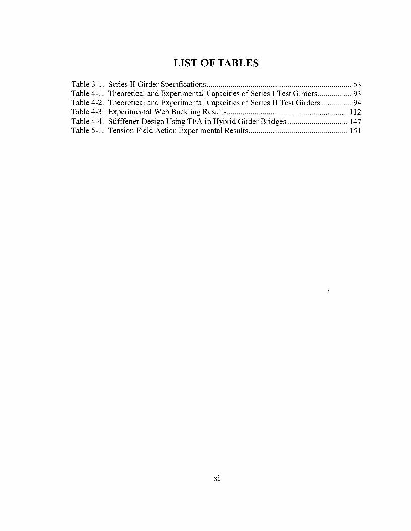
LIST OF TABLES
Table 3-1. Series II Girder Specifications ........................................................................ 53 Table 4-1. Theoretical and Experimental Capacities of Series I Test Girders ................. 93 Table 4-2. Theoretical and Experimental Capacities of Series II Test Girders ............... 94 Table 4-3. Experimental Web Buckling Results ............................................................ 112 Table 4-4. Stifffener Design Using TFA in Hybrid Girder Bridges .............................. 147 Table 5-1. Tension Field Action Experimental Results ................................................. 151
XI
Chapter 1 - Introduction
1.1 Problem Statement
With the advent of HPS70W steel (High Performance Steel with yield strength of
70 ksi), hundreds of bridges have been built using HPS. The AASHTO LRFD
Specifications (1998) have been updated to allow HPS70W steel in bridges. Studies have
shown that the current design specifications are adequate for HPS70W and the issues of
ductility and buckling are sufficiently considered (Barth et al. 2000). Therefore, bridges
have been built, and many more will be built, with HPS70W material. A majority of
these bridges will use hybrid girders.
Hybrid steel girders were a popular choice for bridge girders in years past. Using
50 ksi material for the flanges with a lower cost 36 ksi web material yielded more
economical results while still maintaining flexural capacities near a homogeneous 50 ksi
girder. Since that time, the cost gap between the two strength materials dwindled and the
economic benefit of hybrid girders vanished. However, with High Performance Steel,
hybrid design has become a common practice again. Bridge studies (Barker and Schrage
2000) have shown that the most beneficial use of HPS70W (70 ksi) is in the flanges of
hybrid girders with 50 ksi webs.
One limit with hybrid girder design, which decreases the beneficial aspects, is that
tension field action (TF A) is not allowed when determining the shear capacity. The
reasoning is that, in hybrid girders, the web yields near maximum moment, which may
affect the tension strut assumed for TF A. This is a severe shear capacity penalty when
using hybrid girders. Limiting hybrid shear capacities to the shear buckling capacity 1

results in more transverse stiffeners required ( closer spacing) for a hybrid girder than that
for a homogeneous girder. This not only increases material costs, but significantly
increases fabrication costs.
Tension field action is a type of shear behavior observable in transversely
stiffened girders. The slender web of a plate girder may buckle under applied load, after
which it can no longer resist shear in the traditional beam manner. Additional applied
shear beyond the shear buckling capacity of the web can be resisted through tension field
action, which includes formation of a tension strut diagonally across the buckled web
panel. This tension strut anchors to the transverse stiffeners and flanges that border the
shear panel, and the magnitude of vertical shear resistance is taken to be the vertical
component of the tension strut. The tension field action contribution to shear capacity
depends on the stiffener spacing, but can typically be equal in magnitude to the shear
buckling capacity. The total shear capacity of a stiffened girder is the sum of the shear
buckling capacity and the tension field action capacity. Thus, the use of tension field
action can significantly increase the shear design capacity of the girder.
A major concern with hybrid girders is that the lower strength web material may
yield before the nominal moment capacity of the girder is attained. The web yielding
problem leads to concerns about the ability of tension field action stresses to achieve
sufficient anchorage through the yielded web material. There has been little research
performed on this topic, so tension field action shear capacity is not allowed in the design
of hybrid plate girders according to AASHTO's (1998) Load and Resistance Factor
Design (LRFD) design code, and the design shear capacity of hybrid girders is limited to
the shear buckling capacity. Limiting the shear capacity of hybrid girders often results in
2

the use of thicker web panels and additional transverse stiffeners to increase the design
shear capacity of the hybrid girder. The ultimate result is a less economical hybrid
design.
1.2 Research Objective
The objective of this research is to validate the tension field action behavior in hybrid
plate girders. The goal is to allow TF A in hybrid girders resulting in more economical
design of steel bridges. Using thicker webs or extra transverse stiffeners would no longer
be necessary to obtain the required shear capacity, which would save material and labor
costs, as well as reduce weight and decrease the number a fatigue details on the girder.
The use of hybrid design can result in shallower girder depths, which will require less
material and labor costs for bridge approaches. The ultimate result of allowing tension
field action shear capacity to be used for hybrid design is the ability to achieve less
expensive, more efficient projects without sacrificing quality or safety.
Tension field action certainly does occur in transversely stiffened hybrid plate
girders, especially in situations where the flexural stresses are relatively low. If flexural
stresses are low, then there is no web yielding in the hybrid girder, and the tension field
should be no different than conventional homogeneous girders. However, as flexural
stresses increase and web yielding is possible, there may be some reduction in tension
field action capacity. The interaction between bending moment and shear capacity is also
investigated in this research.
3
1.3 Research Content
The work conducted for this research covers several endeavors. These topics will
be presented in this report as described in Section 1.4. The first effort concentrated on
the original shear capacity theoretical derivations (Basler 1961a) and the impact of using
hybrid girders. Proposed lower bound shear capacity procedures were developed that
represent the equivalent AASHTO equations for hybrid girders (Barker et al 2002, Hurst
2000). Hurst (2000) reformulates the original derivations to account for hybrid design
and develops new proposed moment-shear interaction equations.
Two series of tests were designed (Hurst 2000) and tested to determine the hybrid
girder shear capacity and study the tension field behavior of homogeneous and hybrid
girders. Series I test specimens were homogeneous and hybrid girders tested under high
shear and low moment conditions. Results from Series I testing are published in two
separate theses (Schreiner 2001, Rush 2001). Schreiner's thesis documents the testing
procedure and verifies that the hybrid girder's shear capacities were accurately predicted
by AASHTO's current tension field action design equations. Rush's thesis interprets the
experimental data and compares it to tension field action theory, concluding that tension
field action stresses are present in hybrid girders and reasonably predicted by theory.
Series II test specimens were designed and tested to study the effect of moment-shear
interaction. Results from Series II testing are published in two separate theses (Zentz
2002, Davis 2002). Davis' thesis documents the testing procedure and compares the
hybrid girder's shear capacities to AASHTO's current and Hurst's proposed tension field
action moment-shear interaction equations. Zentz's thesis interprets the experimental
4

data and compares it to tension field action theory, concluding that hybrid girders are
capable of developing tension field action stresses predicted by theory.
Finally, Goessling (2002) studied an array of practical bridge designs to study the
impact of allowing TF A in hybrid girders. The study included two- and three-span
bridges with varying span lengths, number of girders (girder spacing) and web
slenderness ratios. The results are presented in terms of number of transverse stiffeners
required with and without tension field action.
1.4 Results
This research, in conjunction with research at Georgia Tech (Aydemir 2000) found
that tension field action shear capacity is fully applicable to hybrid girders. The
AASHTO shear capacity equations are accurate for hybrid girders and that there is not a
moment-shear interaction for any plate girder, whether homogeneous or hybrid.
Allowing tension field action in hybrid plate girders and removing the moment-shear
interaction for all plate girder designs would be a major advancement for steel bridge
design.
1.5 Report Organization
This report will begin with background information concerning hybrid plate
girders, tension field action theory, and moment-shear interaction in Chapter 2. A
summary of the original derivation of the currently accepted tension field action theory
will be followed by presentation of AASHTO's (1998) Load and Resistance Factor
Design shear design capacity equations. Chapter 2 also presents Hurst's (2000)
derivation of a lower bound moment-shear interaction equation, in AASHTO format, that 5

considers hybrid action in plate girders. Although the final results show there should not
be any moment-shear interaction, the proposed hybrid moment-shear interaction is
presented to demonstrate the moment-shear interaction theory and to give a conservative
lower bound for moment-shear interaction in hybrid designs.
Chapter 3 presents the Series I & II test specimens, the test set-up, testing procedures
and theoretical experimental results for the test girders. Emphasis is placed on the Series
II tests since they constitute the most important part of this work. The Series I tests, high
shear and low moment, were expected to show applicable tension field action and the
results are a basis for the Series II tests. The Series II tests, the moment-shear interaction
tests, provide the important conclusions and results for this study.
Chapter 4 presents the experimental test analyses. Again, the Series II tests are
emphasized due to their importance. The experimental shear capacities from the Series I
tests have been shown to be comparable to those calculated by the current AASHTO
tension field action design equations (Schreiner 2001). To validate the tension field
action behavior, the experimental capacities and stress responses were compared to
tension field action theory (Rush 2001). The Series II tests are examined in detail in
Chapter 4. The experimental shear capacities were found to be adequately predicted by
current AASHTO tension field action design equations (Davis 2002). The experimental
stress behavior and tension action behavior is also shown to correspond with theory
(Zentz 2002). Chapter 4 includes an impact section that describes the savings that can be
realized using tension field action in hybrid plate girders and removing the moment-shear
interaction for all plate girders (Goessling 2002).
Chapter 5 presents the results and conclusions of the research efforts.
6

Chapter 2 - Tension Field Action
2.1 Introduction
The purpose of this chapter is to provide background information on the shear
strength of hybrid plate girders subject to concurrent shear and bending. Plate girders
and hybrid steel design are introduced, followed by current shear design equations. A
brief derivation of the shear design equations is given, and limitations of the current shear
design equations concerning hybrid plate girders are discussed. Moment-shear
interaction is explained and the current interaction equations presented, along with a
summary of the original derivation. The original derivation is modified to accommodate
hybrid girders. Finally, a proposed lower-bound moment-shear interaction diagram for
hybrid girders will be presented.
2.2 Hybrid Plate Girders
Plate girders are I-shaped steel girders built-up from flanges and webs cut from
steel plates and welded together. They are commonly used when the available hot-rolled
W-shapes are inadequate for a given span and loading. Currently, plate girders are
commonly used for bridges, but can also be used for special-purpose buildings where
long spans or high loadings are present. When properly designed and implemented, plate
girders are very efficient and cost-effective flexural members.
For any I-shaped section, the flanges provide the majority of the moment capacity
while the web provides shear resistance. Moment capacity of plate girders can be
increased by increasing the girder depth, increasing the amount of steel used in each
7

girder, or by improving the properties of the steel. However, using additional steel
increases the self-weight of the girder as well as the total steel costs. Indirect costs, such
as costs due to larger bridge approaches, can also arise by increasing the depth of the
girder.
Improving steel properties is a way to increase moment capacity without
additional girder weight or depth. High Performance Steel (HPS) has higher yield
strengths than conventional steels, thus conventional flexural members can be replaced
by smaller HPS members. However, there is currently a cost premium associated with
HPS, so homogeneous HPS sections are often uneconomical. Barker and Schrage (2000)
have shown that using a combination of conventional steel web and HPS flanges (hybrid
design) can be more economical than homogeneous sections of either 50 or 70 ksi steel.
The higher yield strength HPS flanges increase moment capacity while using the less
expensive conventional steel web saves material costs.
Plate girders are designed with slender webs in order to minimize material costs
while maintaining the distance between flanges. Web instability is a concern whenever
slender webs are used, so transverse stiffeners are welded to the web to increase capacity.
The transverse stiffeners, if properly spaced, create larger web buckling capacity and
allow for the development of tension field action shear capacity.
2.3 Shear Capacity
The shear capacity of a transversely stiffened plate girder is composed of two parts:
the shear buckling capacity and the post-buckling shear capacity. Theoretically, a
transversely stiffened plate girder initially resists shear in a beam type manner up to a
8
shear load level called the shear buckling capacity. Once the applied shear reaches the
shear buckling capacity, it is assumed that the web buckles and additional applied shear is
resisted through a post-buckling phenomenon known as tension field action (TF A) until
the nominal shear capacity of the plate girder is reached. The following discussions
explain the theory behind each mode of shear resistance, the capacities associated with
each mode, and give the current AASHTO design equations for shear capacity of
transversely stiffened plate girders.
2.3.1 Shear Buckling Capacity
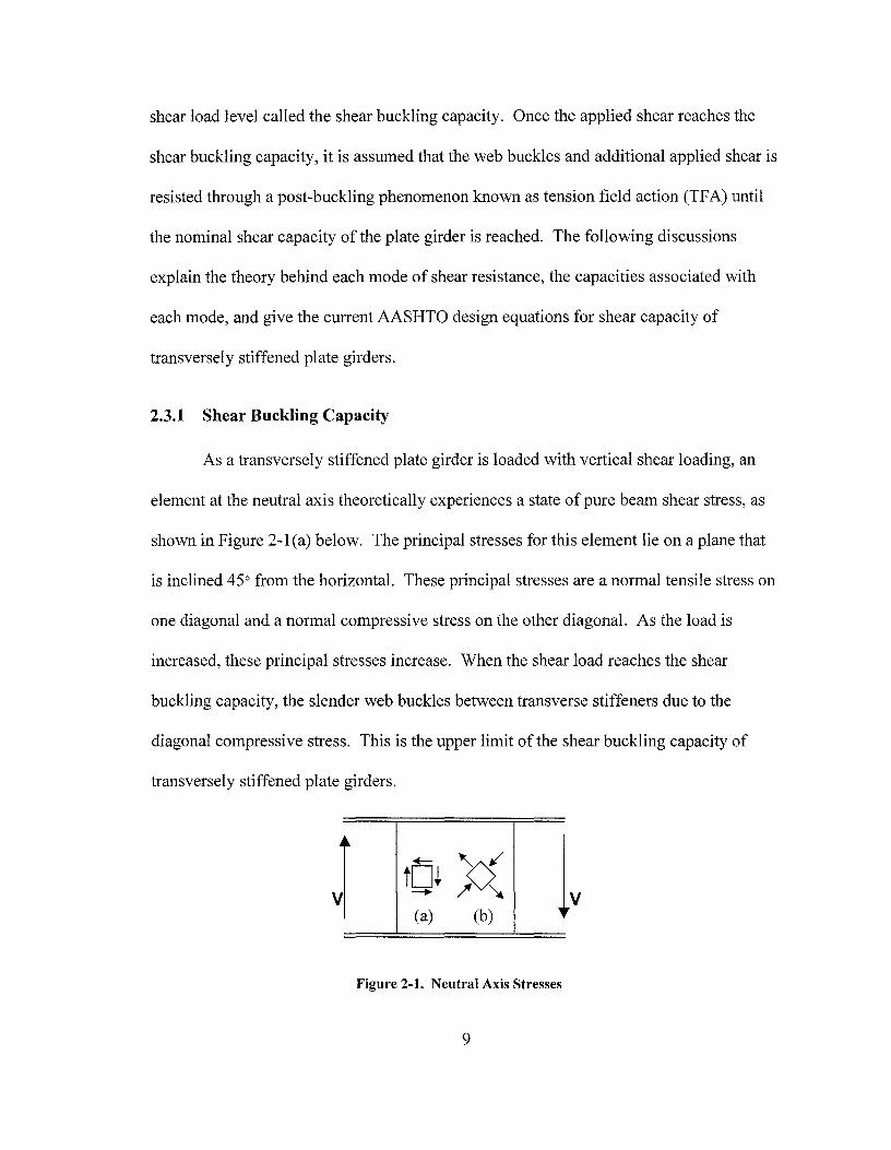
As a transversely stiffened plate girder is loaded with vertical shear loading, an
element at the neutral axis theoretically experiences a state of pure beam shear stress, as
shown in Figure 2-l(a) below. The principal stresses for this element lie on a plane that
is inclined 45° from the horizontal. These principal stresses are a normal tensile stress on
one diagonal and a normal compressive stress on the other diagonal. As the load is
increased, these principal stresses increase. When the shear load reaches the shear
buckling capacity, the slender web buckles between transverse stiffeners due to the
diagonal compressive stress. This is the upper limit of the shear buckling capacity of
transversely stiffened plate girders.
Figure 2-1. Neutral Axis Stresses
9

The shear buckling capacity used in AASHTO's LRFD (1998) design code is given as:
Where:
Ver = shear buckling capacity
C = ratio of shear buckling stress to shear yield strength
For elastic buckling:
Where:
E = modulus of elasticity of the material
Fyw = yield stress of web material
D = web depth
tw = web thickness
Where:
do = transverse stiffener spacing
Vp = plastic shear capacity= 0.6AwFyw
Where:
Aw = cross sectional area of web
10
Equation 2-1
Equation 2-2
Equation 2-3
Equation 2-4
2.3.2 Post-Buckling Shear Capacity
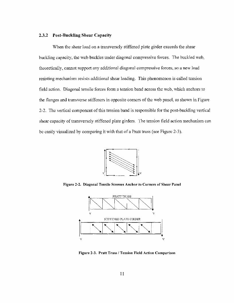
When the shear load on a transversely stiffened plate girder exceeds the shear
buckling capacity, the web buckles under diagonal compressive forces. The buckled web,
theoretically, cannot support any additional diagonal compressive forces, so a new load
resisting mechanism resists additional shear loading. This phenomenon is called tension
field action. Diagonal tensile forces form a tension band across the web, which anchors to
the flanges and transverse stiffeners in opposite corners of the web panel, as shown in Figure
2-2. The vertical component of this tension band is responsible for the post-buckling vertical
shear capacity of transversely stiffened plate girders. The tension field action mechanism can
be easily visualized by comparing it with that of a Pratt truss (see Figure 2-3).
Figure 2-2. Diagonal Tensile Stresses Anchor to Corners of Shear Panel
V V
STIFFENED PLATE GIRDER
V V
Figure 2-3. Pratt Truss I Tension Field Action Comparison
11

The post-buckling shear capacity, Vtfa, used in AASHTO's 1998 design code is given as:
Equation 2-5
The full shear capacity of a transversely stiffened plate girder is given by the sum of
the elastic shear capacity and the post-buckling shear capacity:
Equation 2-6
Where:
V n = nominal shear capacity of transversely stiffened plate girder
2.3.3 Basler's Shear Capacity Derivation
The current AASHTO design code equations relating to the shear capacity of
transversely stiffened plate girders are based on research by Basler (1961 a). A brief
summary of Basler's derivation follows.
Basler initially assumes the ultimate shear force of a transversely stiffened plate
girder can be described as the product of the plastic shear force and a nondimensional
function depending on the following parameters: stiffener spacing, web depth, web thickness,
yield stress, and modulus of elasticity. In mathematical form:
Equation 2-7
12

Where:
Vu = ultimate shear force
VP = plastic shear capacity
f = nondimensional function
d0 = transverse stiffener spacing
D = web depth
tw = web thickness
Fy = yield stress of the material
E = modulus of elasticity of the material
The plastic shear force is described as "the shear force for which unrestricted yielding
occurs" and is similar in concept to the plastic moment used in plastic analysis (Basler
1961a). The plastic shear force is calculated as the product of the shear yield stress and the
cross-sectional area of the web.
The Hencky - von Mises yield criterion is used to determine the shear yield stress, Ty,
For the case of yielding under pure shear, cr1 = -cr2 = Ty, where cr1 and cr2 are the major and
minor principal stresses, respectively. In this case, the yield criterion gives Ty= FY/ as /✓3
shown in Figure 2-4.
13
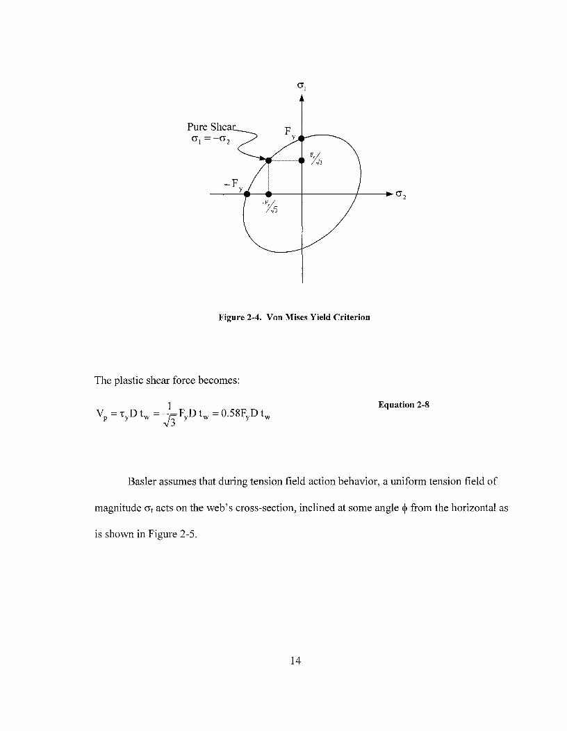
Pure Shea (}"I= -(}"2
-F y ---------f----------cr2
Figure 2-4. Von Mises Yield Criterion
The plastic shear force becomes:
Equation 2-8
Basler assumes that during tension field action behavior, a uniform tension field of
magnitude CTt acts on the web's cross-section, inclined at some angle~ from the horizontal as
is shown in Figure 2-5.
14
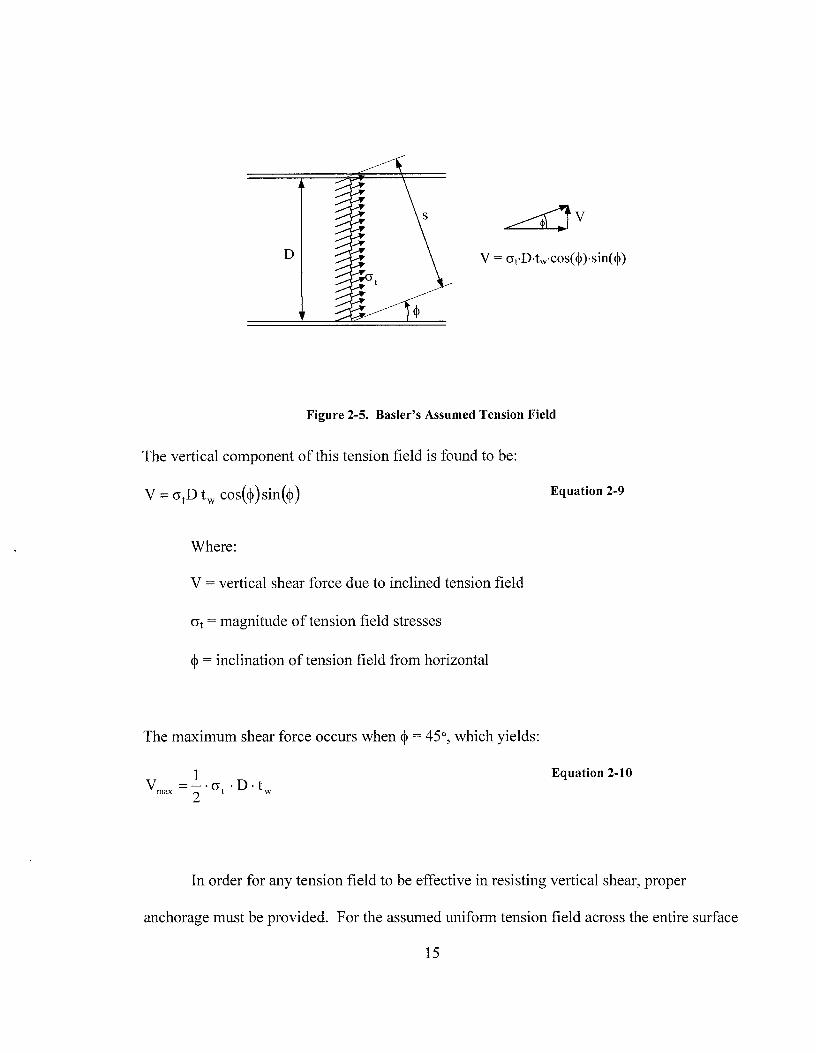
~v
D
Figure 2-5. Baster's Assumed Tension Field
The vertical component of this tension field is found to be:
Equation 2-9
Where:
V = vertical shear force due to inclined tension field
cr1 = magnitude of tension field stresses
~ = inclination of tension field from horizontal
The maximum shear force occurs when~= 45°, which yields:
Equation 2-10
In order for any tension field to be effective in resisting vertical shear, proper
anchorage must be provided. For the assumed uniform tension field across the entire surface
15
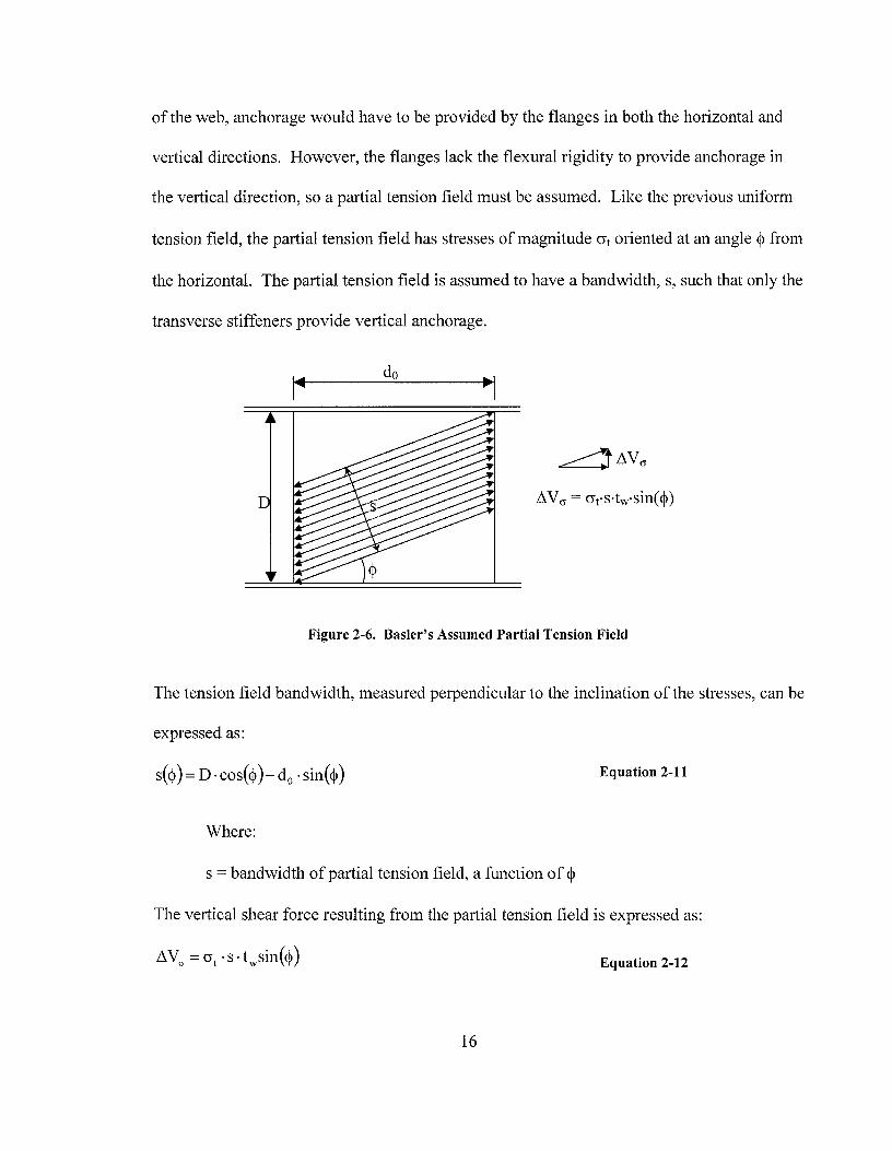
of the web, anchorage would have to be provided by the flanges in both the horizontal and
vertical directions. However, the flanges lack the flexural rigidity to provide anchorage in
the vertical direction, so a partial tension field must be assumed. Like the previous uniform
tension field, the partial tension field has stresses of magnitude <Jt oriented at an angle ~ from
the horizontal. The partial tension field is assumed to have a bandwidth, s, such that only the
transverse stiffeners provide vertical anchorage.
c::::::) /'j.Vcr
~ V cr = <JrS·tw•Sin( ~)
Figure 2-6. Basler's Assumed Partial Tension Field
The tension field bandwidth, measured perpendicular to the inclination of the stresses, can be
expressed as:
s(~) = D · cos(~ )-d0 ·sin(~) Equation 2-11
Where:
s = bandwidth of partial tension field, a function of~
The vertical shear force resulting from the partial tension field is expressed as:
Equation 2-12
16
Where:
Li V cr = vertical resultant shear force from partial tension field
Or, by substituting Equation 2-11 into Equation 2-12:
Equation 2-13
As the applied shear stresses continue to increase, the bandwidth associated with the
partial tension field must increase. This means that the inclination of the tension field must
decrease. At some point there is an optimum contribution of Li V cr to the shear force V cr•
Basler assumes that failure of the plate girder occurs when the Li V cr reaches a maximum
value. In order to find the inclination of the tension field at the ultimate shear load, Equation
2-13 is differentiated with respect to ~ and set equal to zero, as follows:
Equation 2-14
Which yields:
cr1 tw (D · cos(2~ )-d0 • sin(2~ )) = 0 Equation 2-15
Neither the tension field stress nor the web thickness is zero, so
D · cos(2~ )-d0 • sin(2~) = 0 Equation 2-16
Simplifying Equation 2-16 yields:
17
Equation 2-17
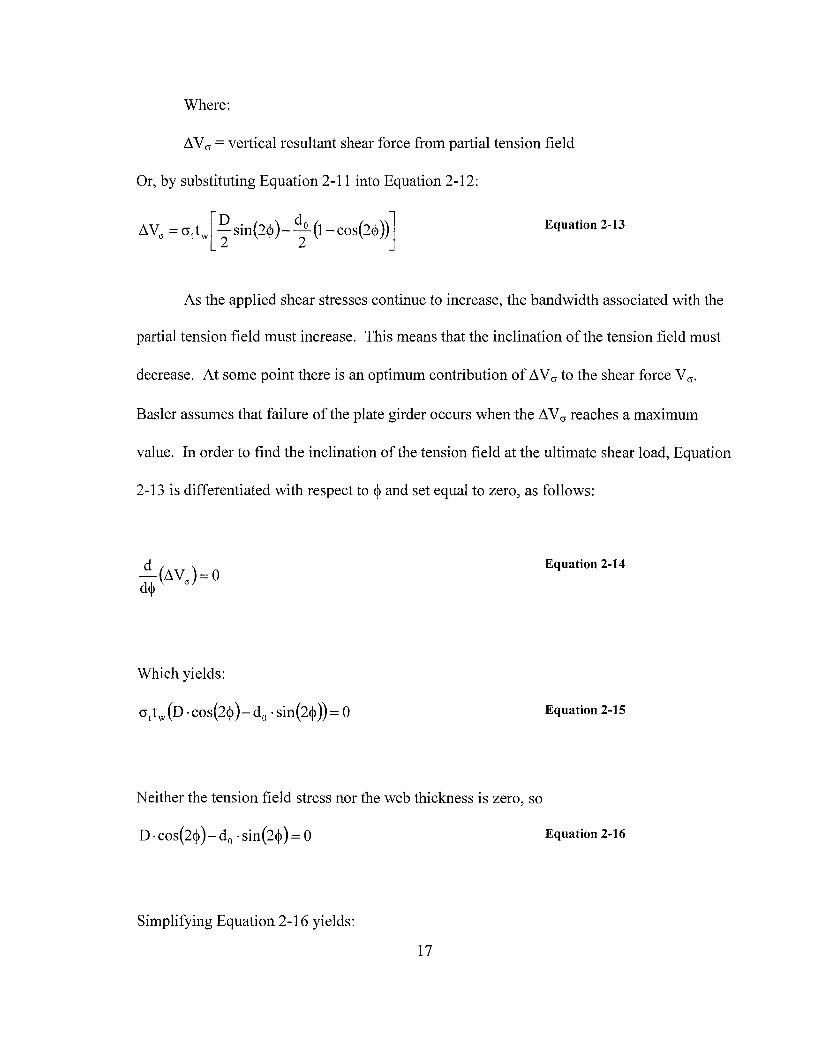
Equation 2-17 shows that the angle 2~ is equivalent to the angle between the panel
diagonal and the horizontal, as shown in Figure 2-7. Using that relationship, the following
quantities are readily obtained:
Equation 2-18
Equation 2-19
do
Figure 2-7. Shear Panel Diagonal
18
Next, Basler assumes a succession of web panels subject to a constant shear force, as
shown in Figure 2-8. A free body diagram (Figure 2-9) is taken by making cuts at A, B, and
C. Along cut A, the web is subjected to an unknown resultant, which is decomposed into a
normal force, F w, and a shear force component. The shear component is V cr/2 due to
symmetry. Flange force Fr also acts at section A. Similar force components act at cut B,
except the flange force changes by an amount ~Fr. At section C, the tension field stresses, cr1,
act at an inclination of <j>, which is defined in Equation 2-17. Vertical stiffener force Fs also
acts at cut C. Solving the system statically will yield an expression for V cr, the ultimate shear
force due to the partial tension field.
A B
Figure 2-8. Succession of Web Panels
d0-sin( <I>)
0
+--t==========::J---+- --+-Fr A B Fr +~Fr
Figure 2-9. Assumed Free Body Diagram
19

Considering horizontal equilibrium of the free body:
Equation 2-20
Summing moments around point 0:
Equation 2-21
Equating Equation 2-20 and Equation 2-21, and substituting Equation 2-18 for sin(2~) yields:
Equation 2-22
Equation 2-22 gives the vertical component of the tension field that occurs after web
buckling. Shear is resisted in a beam-type manner prior to web buckling, and the vertical
component of the tension field resists additional shear forces beyond the web-buckling load.
So, the ultimate shear capacity of the plate girder is due to both beam action (V 1 ) and tension
field action (V cr), and the ultimate shear load can be expressed as:
Equation 2-23
Basler then makes two assumptions in order to compute these components of shear
capacity. The first assumption is that the superposition of the beam and tension field
components is ultimately limited by the state of stress that fulfills the von Mises yield
criteria. The second assumption is that, prior to web buckling, applied shear is resisted
20
purely in a beam-type manner, but after that, V, remains constant and any postbuckling
contribution to shear capacity must be due to tension field action. Therefore, the maximum
beam-type shear resistance must correspond to the shear stress that will cause web buckling:
Equation 2-24
The shear buckling stress, taken from plate buckling theory, is given as:
Where:
v = Poisson's ratio
k = s~_ear buckling coefficient
Where:
k = 4.00 + 5·34
for do/D < 1
(dioY
Equation 2-25
Equation 2-26
Equation 2-27
Using the first assumption, the maximum tension field stress, cr1, can be computed.
This is the stress that can be added to the state of stress at web buckling that will fulfill the
yield criteria. For an element at the neutral axis, the state of stress at web buckling is pure
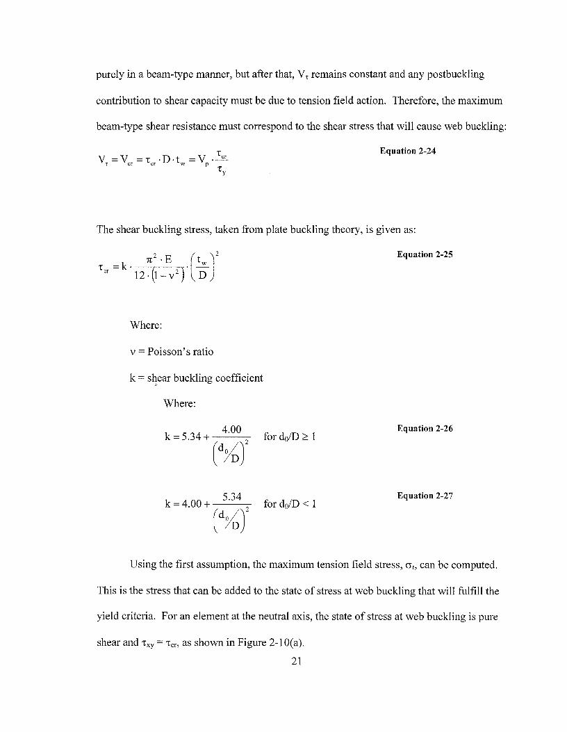
shear and 'txy = 'tcr, as shown in Figure 2-I0(a).
21
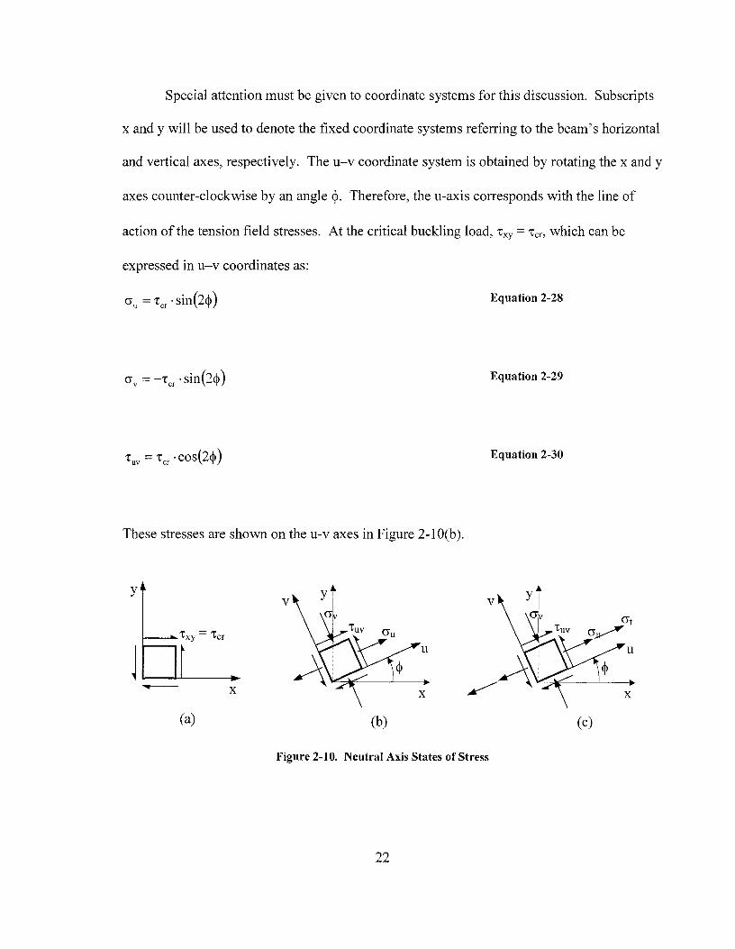
Special attention must be given to coordinate systems for this discussion. Subscripts
x and y will be used to denote the fixed coordinate systems referring to the beam's horizontal
and vertical axes, respectively. The u-v coordinate system is obtained by rotating the x and y
axes counter-clockwise by an angle~- Therefore, the u-axis corresponds with the line of
action of the tension field stresses. At the critical buckling load, 't'xy = 't'cr, which can be
expressed in u-v coordinates as:
Equation 2-28
Equation 2-29
Equation 2-30
These stresses are shown on the u-v axes in Figure 2-1 O(b ).
V
u
(a) (b) (c)
Figure 2-10. Neutral Axis States of Stress
22
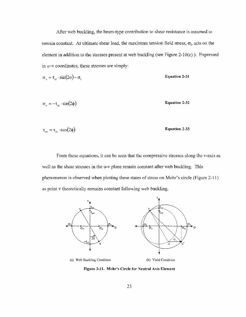
After web buckling, the beam-type contribution to shear resistance is assumed to
remain constant. At ultimate shear load, the maximum tension field stress, CTt, acts on the
element in addition to the stresses present at web buckling (see Figure 2-l0(c) ). Expressed
in u-v coordinates, these stresses are simply:
Equation 2-31
Equation 2-32
Equation 2-33
From these equations, it can be seen that the compressive stresses along the v-axis as
well as the shear stresses in the u-v plane remain constant after web buckling. This
phenomenon is observed when plotting these states of stress on Mohr's circle (Figure 2-11)
as point v theoretically remains constant following web buckling.
't
(J (J
(a) Web Buckling Condition (b) Yield Condition
Figure 2-11. Mohr's Circle for Neutral Axis Element
23

Substituting the ultimate state of stress described in the above equations into von Mises'
yield criteria:
Equation 2-34
The following solution is obtained:
Equation 2-35
The ultimate shear load is computed using Equation 2-22, Equation 2-23, and Equation 2-24.
Equation 2-36
Where crtfFy is given by Equation 2-35.
In order to simplify the computation, Basler approximates the von Mises yield
condition with a linear function. For any state of stress between pure shear and pure tension,
only a small portion of the yield criteria ellipse is needed (see Figure 2-12). This portion is
then approximated with a straight line with the following equation:
Equation 2-37
24

Pure Tension
Pure Shea
----,----1----1,------,..-----cr2 ·¼
Figure 2-12. Yield Criteria Simplification
For the limiting case of <I>= 45°, cru from Equation 2-31 and crv from Equation 2-32 become
principal stresses: cr1 = 'tcr + cr1 and cr2 = -'tcr• Substituting these values into the approximated
von Mises yield criteria from Equation 2-37, we obtain:
Equation 2-38
Basler states that using Equation 2-38 instead of Equation 2-35 even when <I> is not
equal to 45° will be conservative since the approximate method underestimates the tension
field stress, and the underestimation increases as <I> decreases. A lower value of <I>
corresponds to a panel with a larger aspect ratio, d0/D. In order for panels with large aspect
25

ratios to develop tension fields, larger shear displacements are required than those required
by shear panels with smaller aspect ratios. Therefore, this approximation is not only a way to
simplify computations, but also to provide an allowance for compatibility conditions for
longer shear panels (Basler 1961a).
The ultimate shear force can be calculated from Equation 2-36 and Equation 2-38 as:
Equation 2-39
2.3.4 AASHTO's Tension Field Action Provisions
Basler's tension field theory has been adopted by AASHTO (1998) LRFD for design.
For comparison, the design equation as published in AASHTO Article 6.10.6 for determining
the total shear capacity of a transversely stiffened plate girder is:
V =V · n p C + 0.87 · (1- C)
1+( dYoJ Equation 2-40
with C = 'tc/ty
AASHTO places three limitations on the tension field action provisions to ensure that
they are properly applied. First, tension field action shear capacity is not allowed in the
design of end panels of plate girders. The tension field anchors to the flanges and stiffeners
in opposite comers of the shear panel, and since end panels do not have an adjacent shear
panel one on side to anchor to, it is believed that the tension field cannot properly anchor to
26
the flange. Thus, without proper anchorage, the tension field cannot fully develop in end
panels of plate girders.
The second limitation is that tension field action shear capacity cannot be used for
This is to ensure that the dimensions of the plate girder are reasonable and will permit the
development of a tension field. This restriction keeps the shear panel from being too long,
which would reduce the angle of inclination of the tension field, making the vertical
component of the tension field negligible.
Finally, the third restriction imposed by AASHTO is that tension field action shear
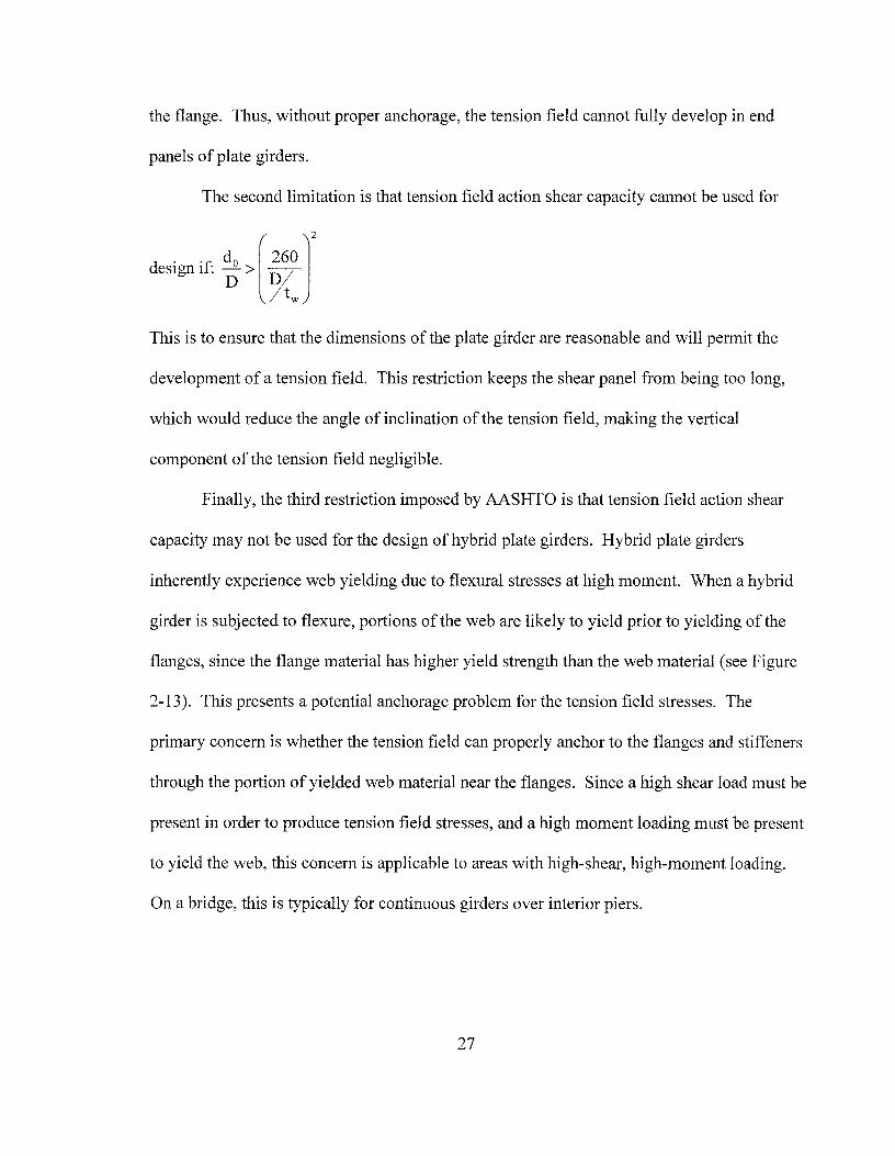
capacity may not be used for the design of hybrid plate girders. Hybrid plate girders
inherently experience web yielding due to flexural stresses at high moment. When a hybrid
girder is subjected to flexure, portions of the web are likely to yield prior to yielding of the
flanges, since the flange material has higher yield strength than the web material (see Figure
2-13). This presents a potential anchorage problem for the tension field stresses. The
primary concern is whether the tension field can properly anchor to the flanges and stiffeners
through the portion of yielded web material near the flanges. Since a high shear load must be
present in order to produce tension field stresses, and a high moment loading must be present
to yield the web, this concern is applicable to areas with high-shear, high-moment loading.
On a bridge, this is typically for continuous girders over interior piers.
27

Girder Cross-Section Flexural Stress Distribution Girder Side Elevation
Figure 2-13. Web Yielding in Hybrid Girders
For those instances, where the use of tension field action is disallowed, the girder is
restricted to the shear buckling capacity. The shear buckling capacity can typically be on the
order of about half of the full shear capacity utilizing tension field action. While the first two
of the three restrictions are straightforward, it seems counter-intuitive that a hybrid girder that
uses higher strength flanges would have about half the shear capacity of a homogeneous
girder of the same dimensions. To continue this investigation, the next section explores the
current moment-shear interaction theory as well as a proposed moment-shear interaction
curve for hybrid plate girders.
2.4 Moment-Shear Interaction
It is possible that the maximum bending moment and maximum shear occur at the
same location in a girder. In order to ensure that a given cross section is not expected to
28

resist its full moment capacity and full shear capacity concurrently, moment-shear interaction
reductions are included in current design practice (AASHTO 1998).
The accepted moment-shear interaction theory in AASHTO's 1998 design code is
also based on research performed by Basler (1961b). A brief summary ofBasler's derivation
and results will be presented here, followed by the actual interaction curve as published by
AASHTO. Also, a recently proposed (Barker et al 2002) lower-bound interaction diagram
for hybrid girders will be presented.
2.4.1 Basler's Interaction Diagram
Basler begins his moment-shear interaction derivation by defining several reference
moments, assuming a symmetrically proportioned girder (see Figure 2-14).
Figure 2-14. Baster's Reference Moments
The flange moment, Mr, is the moment carried by the flanges alone when fully yielded.
Equation 2-41
Where:
Mr= flange moment
29

Af = cross sectional area of one flange
The yield moment, My, is characterized by yielding at the centroid of the compression flange,
and has a linear flexural stress distribution.
M =F ·D·(A + Aw)=A ·F ·D•(l+ Aw] y y r 6 r y 6A f
Equation 2-42
The plastic moment, Mp, is the moment resistance provided by a fully yielded cross section.
Equation 2-43
In the following discussion, the applied moment, M, will be referred to in terms of the
yield moment, My, by means of the proportion M/My. This is necessary to give meaning to
the magnitude of the applied moment by comparing it with the girder's moment carrying
capacity, as well as to simplify the discussion by using nondimensional quantities. The
applied shear, V, will be expressed in terms of the ultimate shear force, Vn, in the proportion
V /V n for the same reasons. These ratios will be referred to as the relative ( or normalized)
moment and shear.
Basler's ultimate shear force is based on a web fully yielded in shear, and can be
expressed as:
Equation 2-44
30
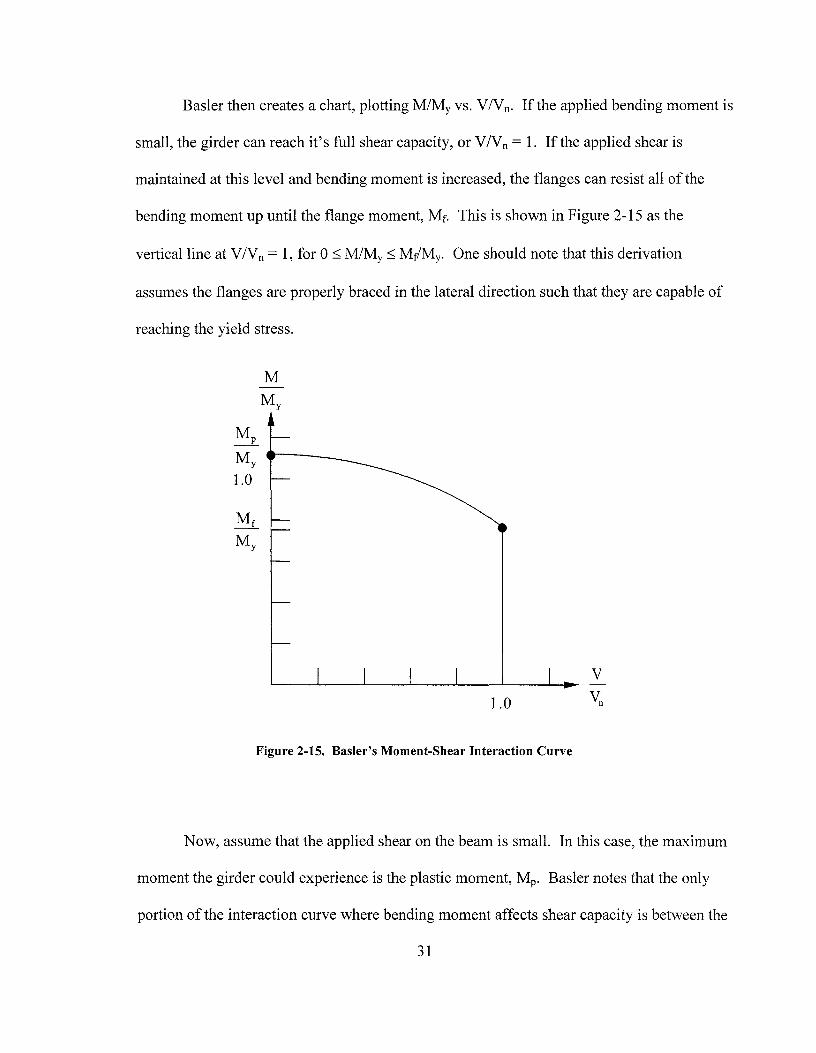
Basler then creates a chart, plotting M/My vs. V/Vn, If the applied bending moment is
small, the girder can reach it's full shear capacity, or VNn = 1. If the applied shear is
maintained at this level and bending moment is increased, the flanges can resist all of the
bending moment up until the flange moment, Mr. This is shown in Figure 2-15 as the
vertical line at V /V n = 1, for O ~ M/My ~ Mr/My, One should note that this derivation
assumes the flanges are properly braced in the lateral direction such that they are capable of
reaching the yield stress.
V
1.0
Figure 2-15. Basler's Moment-Shear Interaction Curve
Now, assume that the applied shear on the beam is small. In this case, the maximum
moment the girder could experience is the plastic moment, Mp, Basler notes that the only
portion of the interaction curve where bending moment affects shear capacity is between the
31
flange moment, Mr, and the plastic moment, Mp, so any interaction curve should pass through
those points. Also, since a small shear force would have little effect on the moment carrying
capacity of the girder, the interaction curve should be perpendicular to the M/My axis as V/Vn
tends toward zero. Basler suggests the following interaction curve equation:
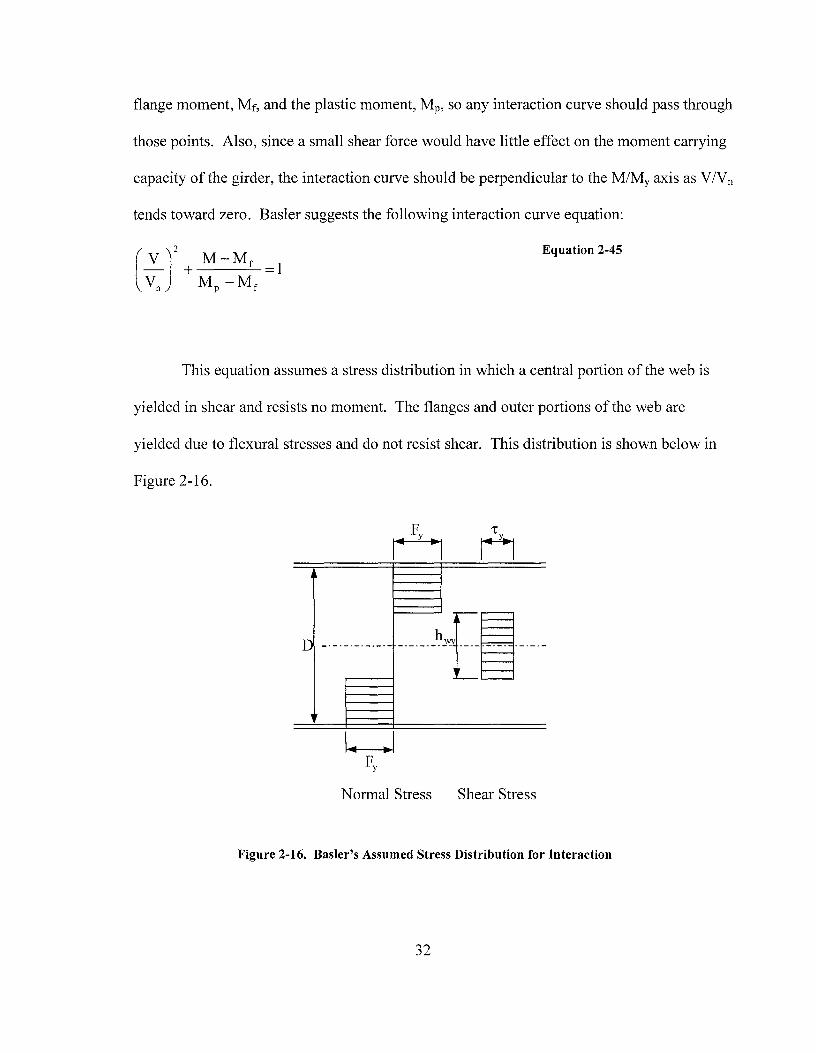
Equation 2-45
This equation assumes a stress distribution in which a central portion of the web is
yielded in shear and resists no moment. The flanges and outer portions of the web are
yielded due to flexural stresses and do not resist shear. This distribution is shown below in
Figure 2-16.
D ---------·--- ·-·-·- h{~·-·-·-,
I.. ..I FY
Normal Stress Shear Stress
Figure 2-16. Basler's Assumed Stress Distribution for Interaction
32
The height of the central "effective" portion of the web resisting shear is hwy, and it
provides the following shear strength:
Equation 2-46
Where:
Vn' = shear capacity of central portion of web
hwy = height of central portion of web yielded in shear
Dividing Equation 2-46 by Equation 2-44 and rearranging yields:
Equation 2-47
The remainder of the web and the flanges are resisting bending moment and carrying no
shear. The moment capacity provided by these portions of the cross section is:
Equation 2-48
Substituting Equation 2-47 into Equation 2-48 and rearranging yields:
Equation 2-49
33

Substitution of Equation 2-42 into Equation 2-49 gives:
Equation 2-50
It becomes obvious with Equation 2-50 that Basler's interaction curve is based on the ratio of
Awl Ar. Basler goes on to plot the interaction curve for various values of Awl Ar, noting that
most reasonably proportioned girders are in the range of Awl Ar '.S: 2. Using a value of2 for
Awl Ar, the following equation is obtained:
Equation 2-51
Equation 2-51 is then solved for 3 points to define the final curve (see Figure 2-17). First,
setting the shear to zero, the value of relative moment is calculated as 1.125. Next, setting
the relative shear to 1.0 yields a relative moment of 0.75. Finally, setting the relative
moment equal to one, the relative shear is calculated to be 1/✓3 ~ 0.6. Often, the geometry of
a plate girder does not allow the plastic moment to be attained. In this case, part of the
interaction curve will be cut off at the yield moment where MIMy = 1.0.
34
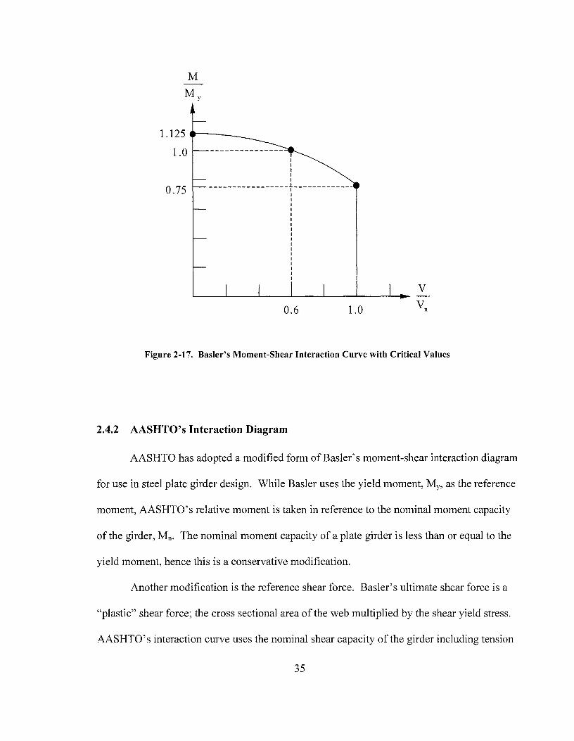
1.125 -----
1.0 I I I I I
0.75 _________________ ! ____________ _
0.6 1.0
V
Figure 2-17. Baster's Moment-Shear Interaction Curve with Critical Values
2.4.2 AASHTO's Interaction Diagram
AASHTO has adopted a modified form ofBasler's moment-shear interaction diagram
for use in steel plate girder design. While Basler uses the yield moment, My, as the reference
moment, AASHTO's relative moment is taken in reference to the nominal moment capacity
of the girder, Mn. The nominal moment capacity of a plate girder is less than or equal to the
yield moment, hence this is a conservative modification.
Another modification is the reference shear force. Basler's ultimate shear force is a
"plastic" shear force; the cross sectional area of the web multiplied by the shear yield stress.
AASHTO's interaction curve uses the nominal shear capacity of the girder including tension
35

field action as the reference shear. The nominal shear capacity of a plate girder is less than
or equal to the plastic shear force of the slender web panel, so this modification is also
conservative.
Since AASHTO uses the nominal moment capacity as the reference moment, the
relative moment is limited to a value of 1.0. This ensures that the moment capacity is not
exceeded, even at low shear loading. This modification also makes the interaction curve
easier to use, by replacing a large part of the curve with a straight line.
Finally, AASHTO notes that the remaining portion of the curve is nearly linear, and it
would be conservative and convenient to replace it with a straight line. So, the curve is
replaced with a straight line between the points where the curve formerly intersected the
limiting values of relative shear and moment ( see Figure 2-18).
0.6 1.0
Figure 2-18. AASHTO's Moment-Shear Interaction Diagram
36
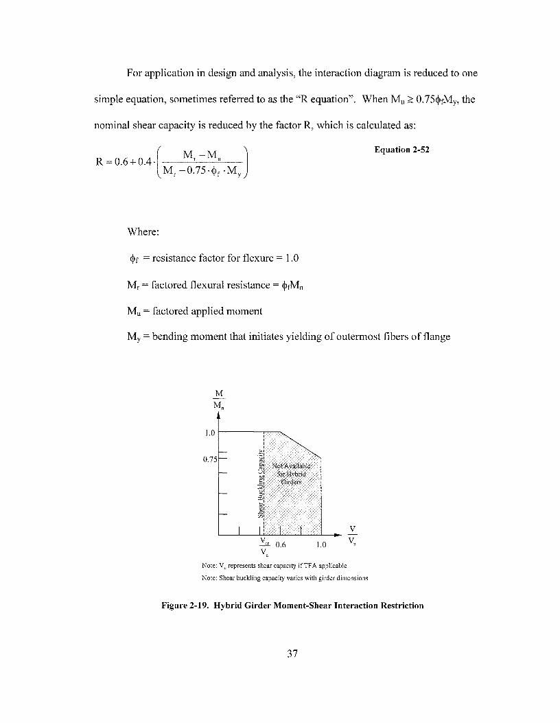
For application in design and analysis, the interaction diagram is reduced to one
simple equation, sometimes referred to as the "R equation". When Mu~ 0.75~fMy, the
nominal shear capacity is reduced by the factor R, which is calculated as:
Where:
~f = resistance factor for flexure = 1.0
Mr = factored flexural resistance = ~rMn
Mu = factored applied moment
Equation 2-52
My = bending moment that initiates yielding of outermost fibers of flange
M
1.0 1-----...... , ---I
0.75
I I
.f"l UI
gj·. N9fiv~ilabJ~'. . ~. · i4t::Hybtid .. :::, . ;:fht'¢ers =g:. ', ;:!I
o:l' ~r J,j, C/ll ,, , ,'
: ,:' 1,-,-·
Ver 0.6 v,,
1.0
Note: V,, represents shear capacity ifTFA applicable
V
Note: Shear buckling capacity varies with girder dimensions
Figure 2-19. Hybrid Girder Moment-Shear Interaction Restriction
37
As discussed in Section 2.3.4, AASHTO does not allow tension field action shear
capacity to be used in the design of hybrid plate girders. This results in a large part of the
moment-shear interaction diagram being unavailable to hybrid girders (see Figure 2-19).
While there may be justifiable concern for areas subjected to high shear and high moment
loading, the penalty as concerning the interaction diagram is very conservative. Consider a
hybrid plate girder that is subject to a high shear loading but small bending moment. This is
the situation for a simply supported bridge girder near an abutment. In this case, there is no
concern for web yielding, so tension field anchorage would not be a problem. The girder
should be able to attain its full shear capacity, including tension field action. The Series I
tests (Schreiner 2001 and Rush 2001) demonstrate TF A is applicable to hybrid girders
subject to low moment. The Series II tests and analyses (Zentz 2002 and Davis 2002) show
that tension field action is also applicable to hybrid girders subject to high moment. Hurst
(2000) developed a lower-bound conservative moment-shear interaction equation for hybrid
girders as is shown in the next section.
2.4.3 Proposed Hybrid Moment-Shear Interaction Diagram
With the intent to make hybrid designs more economical by utilizing tension field
action, and therefore reducing the required number of transverse stiffeners, a new moment
shear interaction diagram has been derived to accommodate hybrid girders. The interaction
curve was developed using Basler's original interaction equations and modifying them to
account for yield strength differences between the web and flanges (Hurst 2000). A brief
summary of Hurst's derivation follows.
38
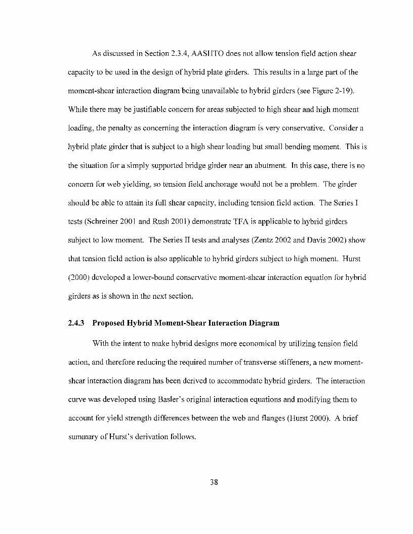
First, a ratio of the yield strengths of the flanges and web is defined:
Where:
Fyr = flange yield strength
Fyw = web yield strength
D
Equation 2-53
Figure 2-20. Reference Moments for Modified Basler Theory
Like Basler's derivation, some reference moments (Figure 2-20) are now defined.
The maximum bending moment that can be carried by the flanges alone is called the flange
moment, and denoted Mr. Approximating the distance between flange centroids as the web
depth, D, the flange moment can be expressed as:
Equation 2-54
39
The yield moment, denoted My, is defined as the moment that initiates yielding of the
centroid of the compression flange. Since we are dealing with a hybrid girder with Fyw::; Fyf,
the web will yield before the flange yield moment is reached. In order to account for the
nonlinear stress effects of web yielding, AASHTO's hybrid reduction factor, Rh, is applied
here.
Where:
A ·D Sx = section modulus :::::: Ar · D + ----'w'-----_
6
Equation 2-55
Substituting the approximated section modulus into Equation 2-55:
M = A · D · R • F · R ·(1 + Aw J y f 1--' yw h 6A f
Equation 2-56
Once again, a stress distribution is assumed such that a central portion of the web is
yielded due to shear stress and cannot resist any flexure. The remainder of the cross
section is yielded due to flexural stresses and provides no resistance to shear (see Figure
2-21 ).
40

I~ ~
Normal Stress Shear Stress
Figure 2-21. Assumed Stress Distribution for Modified Basler Theory
Through calculations identical to those leading up to Equation 2-4 7, the height of the
central portion of the web is again found to be:
Equation 2-57
The nominal moment capacity of the girder, which includes no contribution from the central
portion of the web, is calculated to be:
M' = A · A • F · D + t · (~) . F - t . (hwy 2
J . F n f 1--' yw w 4 yw w 4 yw
Equation 2-58
Substituting Equation 2-57 into Equation 2-58 and rearranging yields:
41
Equation 2-59
Substituting Equation 2-56into Equation 2-59 gives:
Equation 2-60
Again, assuming a practical upper limit of Awl Af = 2, Equation 2-60 becomes:
Equation 2-61
Equation 2-61 then simplifies as:
Equation 2-62
Equation 2-62 is the final equation for the proposed "Modified Basler Interaction
Curve" proposed by Hurst. This is the hybrid equivalent of Basler's interaction equation,
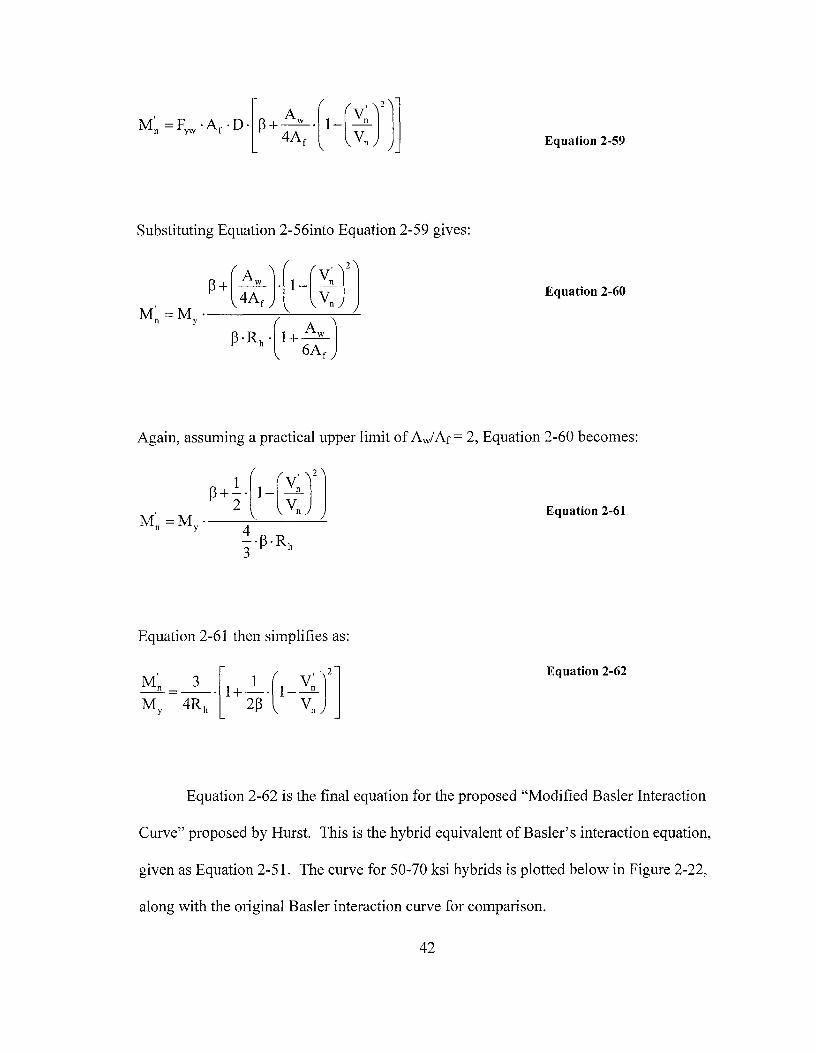
given as Equation 2-51. The curve for 50-70 ksi hybrids is plotted below in Figure 2-22,
along with the original Basler interaction curve for comparison.
42
1.0
0.75
I I I I I I
_____________ J __ l _______ -----' I I I I I I I I I I I I I I I I I I I I I I I I I I I I I I I I I I I
: I I I
0.5 0.6 1.0
Basler - Homogeneous
Modified Basler - Hybrid
V
Figure 2-22. Modified Basler Interaction Curve for 50-70 Hybrid Girders
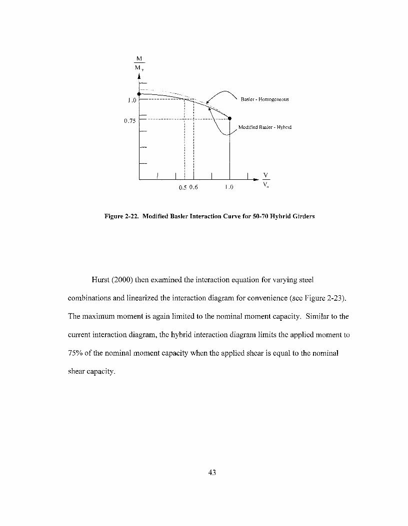
Hurst (2000) then examined the interaction equation for varying steel
combinations and linearized the interaction diagram for convenience (see Figure 2-23).
The maximum moment is again limited to the nominal moment capacity. Similar to the
current interaction diagram, the hybrid interaction diagram limits the applied moment to
75% of the nominal moment capacity when the applied shear is equal to the nominal
shear capacity.
43
M
1.0 i------~··· .................. •··• ..... ~ Basler - Homogeneous
0.75
Modified Basler - Hybrid
V
0.45 0.6 1.0
Figure 2-23. Modified Basler Interaction Diagram for General Hybrid Girders
The difference between the proposed hybrid interaction diagram and the currently
accepted homogeneous interaction diagram is apparent when the applied moment is taken
to be equal to the nominal moment capacity. At this load level there is a concern for web
yielding, and the normalized shear cannot attain the same level as that of a homogenous
girder (V/Vn = 0.6). Through a study ofreasonable steel combinations, a value ofV/Vn =
0.45 was selected as conservative and adequate as a limit when M/Mn = 1.0. For use in
design and analysis, the reduction equation in AASHTO for hybrid girders could be
expressed as:
Equation 2-63
44
When Mu~ 0.75~fMy, the nominal shear capacity of the hybrid girder is reduced by the
factor R, as calculated above, to account for moment-shear interaction.
2.5 Summary
The necessary background information concerning the strength of plate girders
subject to concurrent shear and bending has been presented, along with the limitations
imposed by AASHTO concerning hybrid girders. These limitations are believed to be
over-conservative, so a new moment-shear interaction curve for hybrid girders was
presented. In the following chapters, experimental testing to validate the proposed
interaction curve is documented. The test setup and procedure will be explained in the
next chapter.
45

Chapter 3 - Test Specimens and Theoretical Behavior
3.1 Introduction
Hurst (2000) outlined the experimental tension field action test setup, which is
designed to demonstrate tension field action in and the moment shear interaction behavior
of hybrid girders. In order to verify TF A and validate AASHTO' s or Hurst's proposed
hybrid moment-shear interaction curve, several tests are required with varying levels of
applied shear and bending moment. The designed tests plot on Hurst's interaction
diagram as shown in Figure 3-1. Tests 1 - 3 (two identical test 3 were planned, labeled
3a and 3b) are designated as Series I tests, described in Section 3.2. The remainder of the
tests are referred to as Series II and are described in Section 3 .3.
1 2
08
0.6
M/Mn
0.4
02
Test 7 (04, 1 O)
Tests (0 7, 1.0)
VN,
Tests 6 and 8 (1 o, 1.0)
Test 4 (1.0, 0.8)
Test 1 (0.43, 1.0)
Test2 (0.41, 1.0)
Test 3 (0 32, 1.0)
1.2
Figure 3-1. Target Moment & Shear Ratios for Test Girders
46
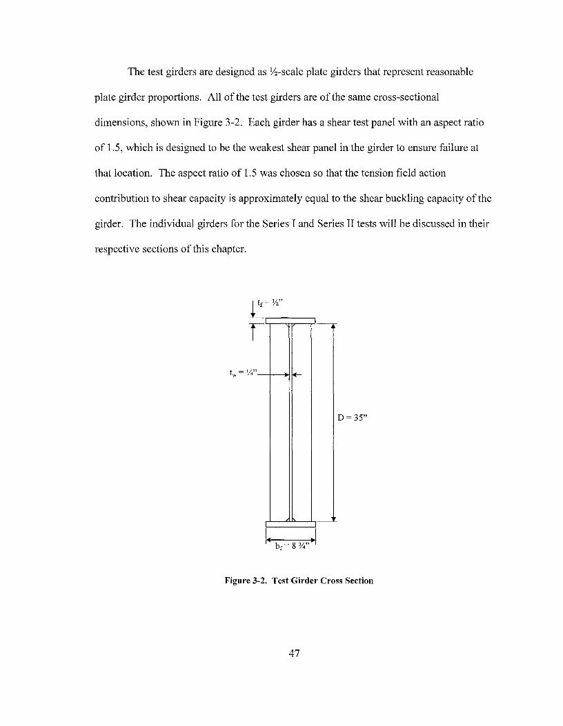
The test girders are designed as ½-scale plate girders that represent reasonable
plate girder proportions. All of the test girders are of the same cross-sectional
dimensions, shown in Figure 3-2. Each girder has a shear test panel with an aspect ratio
of 1.5, which is designed to be the weakest shear panel in the girder to ensure failure at
that location. The aspect ratio of 1.5 was chosen so that the tension field action
contribution to shear capacity is approximately equal to the shear buckling capacity of the
girder. The individual girders for the Series I and Series II tests will be discussed in their
respective sections of this chapter.
r_=½" I
' '
~~
D=35"
I I
Figure 3-2. Test Girder Cross Section
47

3.2 Series I Test Specimens
The objective of the Series I tests was to demonstrate that tension field action shear
capacity is applicable to hybrid girders subject to low moment-high shear loading. In
order to validate the experiment, the same setup and instrumentation was used to test both
homogeneous and hybrid girders. Four girders were included in Series I testing: two
identical 50-70 hybrid girders, one homogeneous 50 ksi girder, and one homogeneous 70
ksi girder. All four girders had identical dimensions and instrumentation.
Loading Diagram
Shear Force Diagram
Bending Moment Diagram
H
12"
p
pl
2P p
i Test Panel
1- 21" ~1•15 ¾.~I·
, .. l~.J ~ 21" 52 ½" 15¾" 21"
2P
J pl
42P
~ ~
-42P
Figure 3-3. Series I Testing Configuration
48
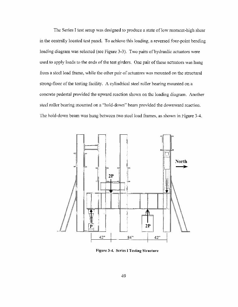
The Series I test setup was designed to produce a state of low moment-high shear
in the centrally located test panel. To achieve this loading, a reversed four-point bending
loading diagram was selected (see Figure 3-3). Two pairs of hydraulic actuators were
used to apply loads to the ends of the test girders. One pair of these actuators was hung
from a steel load frame, while the other pair of actuators was mounted on the structural
strong-floor of the testing facility. A cylindrical steel roller bearing mounted on a
concrete pedestal provided the upward reaction shown on the loading diagram. Another
steel roller bearing mounted on a "hold-down" beam provided the downward reaction.
The hold-down beam was hung between two steel load frames, as shown in Figure 3-4.
½~~~;1
2P
I' 1 c:t:J
·""=;,ili;==ll====-_=:_!, ? \ ·n- ~ r- -\
tl=====.===rr===;===!l'T
tl=======~='===!I:;=~==
2P
42" 84" 42"
Figure 3-4. Series I Testing Structure
49
North ~
Instrumentation of the test girder included bondable linear and rosette strain
gauges to record strains experienced by the girder. String potentiometers, or string pots,
were used to record lateral web deflections in the test panel throughout the test. The
actuators used to apply load to the test girders are equipped with load cells to record
applied load, as well as LVDT's to record deflection of each actuator. As the
instrumentation of the Series I girders is identical to that of the Series II girders, a
description of the test apparatus and instrumentation will be presented in the Series II
Sections 3.3.2 and 3.3.3.
Series I testing was performed in the spring of 2001 at the University of Missouri's
Remote Testing Facility (RTF). Results from Series I testing are published in two
separate theses (Schreiner 2001, Rush 2001 ). Schreiner' s thesis documents the testing
procedure and verifies that the hybrid girder's shear capacities were accurately predicted
by AASHTO's current tension field action design equations. Rush's thesis interprets the
experimental data and compares it to Basler's (1961a) tension field action theory,
concluding that tension field action stresses are present in hybrid girders and reasonably
predicted by Basler's theory. Note that these results only apply to low moment-high
shear loading. The more general case of combined shear and bending is investigated
herein with the Series II tests.
This chapter and Chapter 4 will concentrate on the Series II (tension field action
with moment-shear interaction) in the detailed presentation and anlyses. The Series II
tests demonstrate the behavior that justify the results and conclusions. Only the overall
results of the Series I tests will be presented. The Series I test results and detailed
analyses are contained in Schreiner (2001) and Rush (2001).
50

3.3 Series II Test Specimens
The objective of the Series II tests is to investigate tension field action behavior in
hybrid plate girders subject to combined shear and bending. Six test girders were
constructed and tested at the University of Missouri's Remote Testing Facility. The tests
are designated Tests 4- 8 on Figure 3-1, with two identical girders for Test 6, referred to
as Tests 6a and 6b. The following discussion will address the test girders, test design,
and instrumentation.
Series II testing was performed in the spring of 2002 at the University of Missouri's
Remote Testing Facility (RTF). Results from Series II testing are published in two
separate theses (Zentz 2002 and Davis 2002). Davis' thesis documents the testing
procedure and verifies that the hybrid girder's shear capacities were conservatively
predicted by AASHTO's current and Hurst's modified tension field action design
equations. Zentz's thesis interprets the experimental data and compares it to Basler's
(1961a and 1961b) tension field action theory, concluding that tension field action and
moment-shear interaction stresses in hybrid girders are reasonably predicted by Basler's
theory. Note that these results apply to moment-high shear interaction loading.
3.3.1 Test Girders
All Series II test girders are designed with the test panel adjacent to a central
bearing stiffener, as shown in Figure 3-5. Excluding the test panel, each girder uses a
short transverse stiffener spacing to ensure that the test panel is the weakest shear panel
in the girder.
51
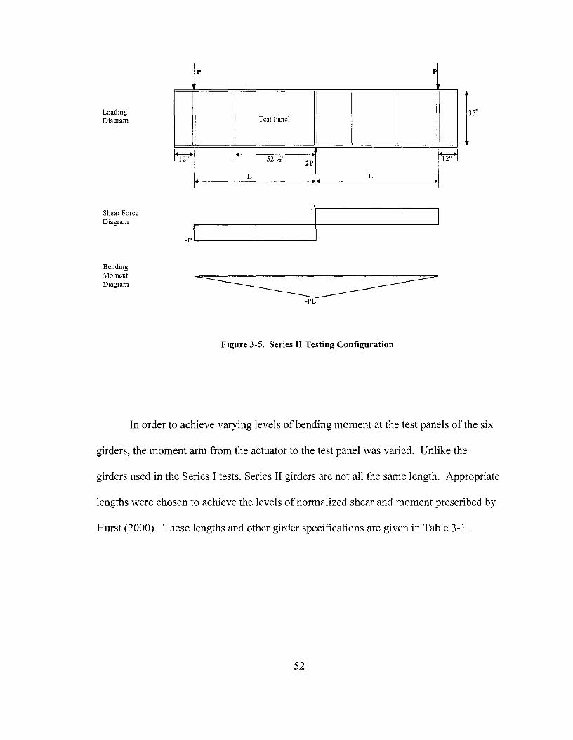
Loading Diagram
Shear Force Diagram
Bending Moment Diagram
p p
Test Panel } hr 52 ½"
2P 12"
1-4 _L -~1-4 _L _,j P·~---------~
-P ,__ _________ _,
-PL
Figure 3-5. Series II Testing Configuration
In order to achieve varying levels of bending moment at the test panels of the six
girders, the moment arm from the actuator to the test panel was varied. Unlike the
girders used in the Series I tests, Series II girders are not all the same length. Appropriate
lengths were chosen to achieve the levels of normalized shear and moment prescribed by
Hurst (2000). These lengths and other girder specifications are given in Table 3-1.
52
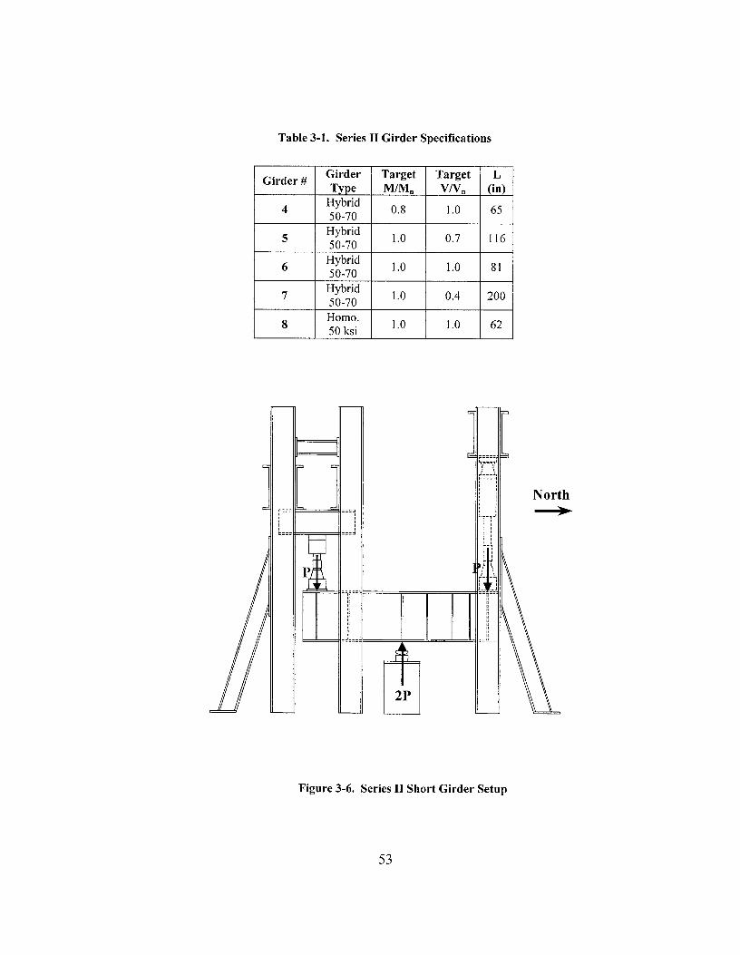
Table 3-1. Series II Girder Specifications
Girder# Girder Target Target L Tvoe M!Mn VN0 (in)
4 Hybrid
0.8 1.0 65 50-70
5 Hybrid
1.0 0.7 I I 6 50-70
6 Hybrid
1.0 1.0 81 50-70
7 Hybrid
1.0 0.4 200 50-70
8 Homo.
1.0 1.0 62 50 ksi
f===i!:=!===Si===~ ' ' ' ' ' ' ~--- ===:::!
' ' t \ ,L -~.
' '
r'l c;l1-r
- _,
6=c!!==l!IiF====;;===',r===;;=l!'I
2P
Figure 3-6. Series II Short Girder Setup
53
North )Ii

North --+-
Figure 3-7. Series II Long Girder Setup with Intermediate Lateral Bracing
3.3.2 Test Design
The general test setup for Series II testing includes two pairs of hydraulic
actuators hung from steel load frames, a cylindrical steel roller bearing mounted on a
concrete pedestal, and lateral bracing. General test setups for short and long girders are
shown in Figure 3-6 and Figure 3-7, respectively.
Each of the load frames consist of two W14x132 columns, connected near the top
by two specially designed cross beams. Three load frames are used for the Series II tests,
along with up to two pairs of diagonal braces for stability. These load frames are
fastened into the RTF's structural strong-floor. The strong-floor is an isolated, four-foot
thick, steel-reinforced concrete slab with threaded steel tie-down holes on a four-foot grid
pattern. Each tie-down hole has a rated uplift capacity of 120 kips.
The general setup remains the same for all of the Series II tests, but since the
lengths of the test girders vary, the setup must to be lengthened or shortened accordingly.
54
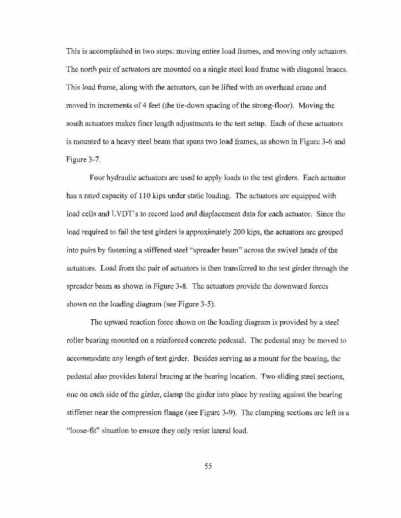
This is accomplished in two steps: moving entire load frames, and moving only actuators.
The north pair of actuators are mounted on a single steel load frame with diagonal braces.
This load frame, along with the actuators, can be lifted with an overhead crane and
moved in increments of 4 feet (the tie-down spacing of the strong-floor). Moving the
south actuators makes finer length adjustments to the test setup. Each of these actuators
is mounted to a heavy steel beam that spans two load frames, as shown in Figure 3-6 and
Figure 3-7.
Four hydraulic actuators are used to apply loads to the test girders. Each actuator
has a rated capacity of 110 kips under static loading. The actuators are equipped with
load cells and L VDT' s to record load and displacement data for each actuator. Since the
load required to fail the test girders is approximately 200 kips, the actuators are grouped
into pairs by fastening a stiffened steel "spreader beam" across the swivel heads of the
actuators. Load from the pair of actuators is then transferred to the test girder through the
spreader beam as shown in Figure 3-8. The actuators provide the downward forces
shown on the loading diagram (see Figure 3-5).
The upward reaction force shown on the loading diagram is provided by a steel
roller bearing mounted on a reinforced concrete pedestal. The pedestal may be moved to
accommodate any length of test girder. Besides serving as a mount for the bearing, the
pedestal also provides lateral bracing at the bearing location. Two sliding steel sections,
one on each side of the girder, clamp the girder into place by resting against the bearing
stiffener near the compression flange (see Figure 3-9). The clamping sections are left in a
"loose-fit" situation to ensure they only resist lateral load.
55
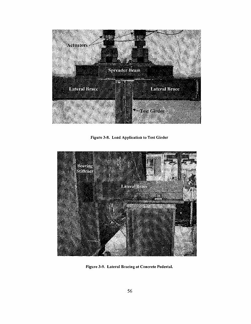
Figure 3-8. Load Application to Test Girder
Figure 3-9. Lateral Bracing at Concrete Pedestal.
56
Lateral bracing was provided to all test girders at the actuator locations. The
actuator lateral bracing not only needs to provide lateral support, but it also has to allow
vertical displacement. This is accomplished by using horizontal brace members between
the test girder and the load frame, with rollers on the outer end of the braces. Upper and
lower braces are provided at each end of the test girder. The upper lateral bracing system
consists of two braces, one on each side of the girder, as shown in Figure 3-8. The upper
braces fasten to the spreader beam on the actuators, and steel clips bolted to the braces
clamp the test girder in place. The lower lateral brace is a single piece with rollers on
each end. This brace is clamped directly to the test girder using steel clips like those used
on the upper bracing. The lateral bracing is tight-fit in the load frame, with the rollers
bearing on steel plates supported by the load frame.
While the lateral bracing provided only at loading points is sufficient for the
shorter test girders, additional lateral bracing is required for the two longer girders. For
this purpose, special intermediate lateral braces were installed. The intermediate braces
resemble C-clamps turned on their backs (see Figure 3-10). The braces are fastened to
the strong-floor using the floor's tie-down holes. The braces then fasten to the
compression flange of the test girder using sliding steel clamps. Lubricated bearing
plates allow vertical and axial deflections of the girder while restricting lateral
movement.
57
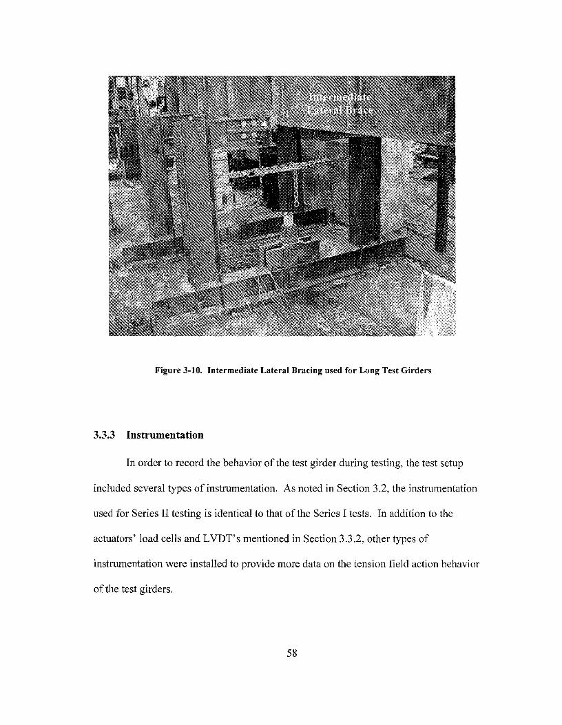
Figure 3-10. Intermediate Lateral Bracing used for Long Test Girders
3.3.3 Instrumentation
In order to record the behavior of the test girder during testing, the test setup
included several types of instrumentation. As noted in Section 3 .2, the instrumentation
used for Series II testing is identical to that of the Series I tests. In addition to the
actuators' load cells and L VDT' s mentioned in Section 3 .3 .2, other types of
instrumentation were installed to provide more data on the tension field action behavior
of the test girders.
58
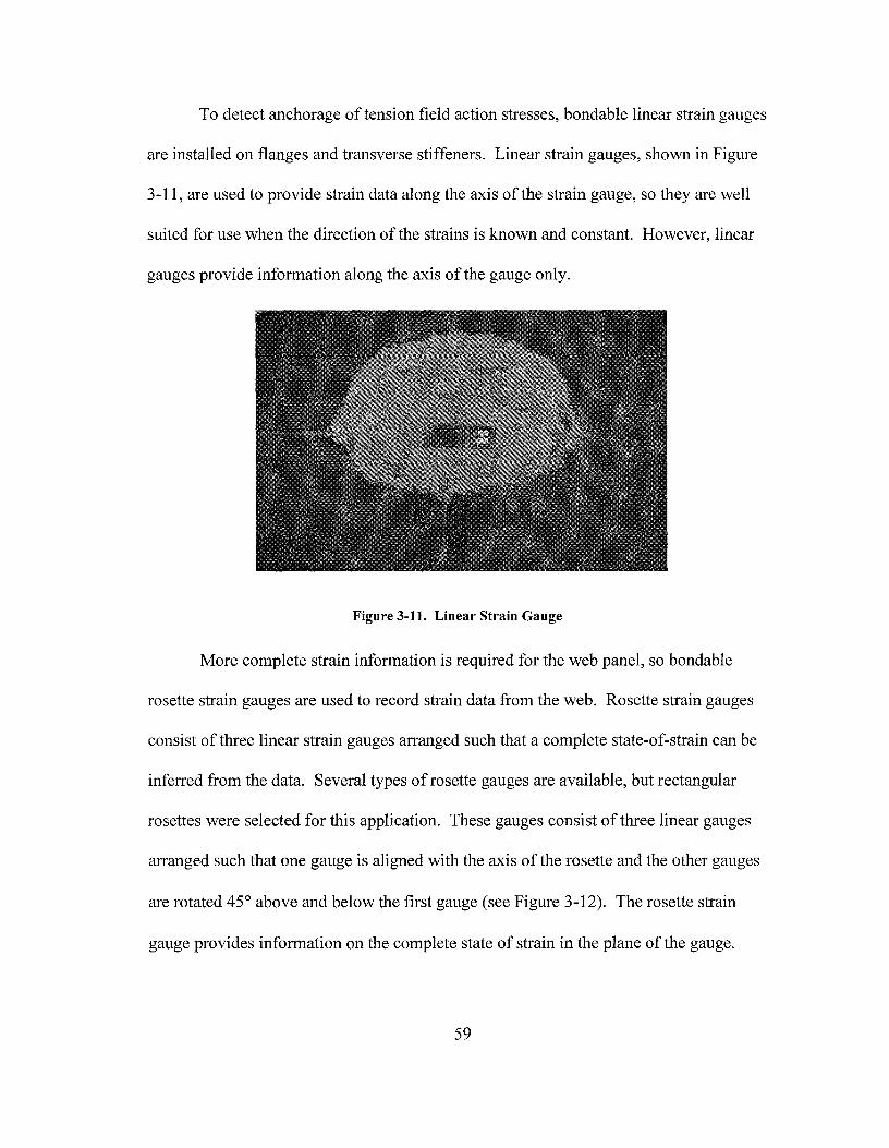
To detect anchorage of tension field action stresses, bondable linear strain gauges
are installed on flanges and transverse stiffeners. Linear strain gauges, shown in Figure
3-11, are used to provide strain data along the axis of the strain gauge, so they are well
suited for use when the direction of the strains is known and constant. However, linear
gauges provide information along the axis of the gauge only.
Figure 3-11. Linear Strain Gauge
More complete strain information is required for the web panel, so bondable
rosette strain gauges are used to record strain data from the web. Rosette strain gauges
consist of three linear strain gauges arranged such that a complete state-of-strain can be
inferred from the data. Several types of rosette gauges are available, but rectangular
rosettes were selected for this application. These gauges consist of three linear gauges
arranged such that one gauge is aligned with the axis of the rosette and the other gauges
are rotated 45° above and below the first gauge (see Figure 3-12). The rosette strain
gauge provides information on the complete state of strain in the plane of the gauge.
59

Figure 3-12. Rectangular Rosette Strain Gauge
In order to track the out-of-plane distortion expected due to web buckling, six
string pots were attached to the web panel. The string pots are mounted on a frame that is
attached to the test girder's flanges. This eliminates erroneous web deflection data due to
relative displacements between the web panel and the string pot.
Out-of-plane effects regarding strain gauges are resolved by mirroring the strain
gauge placement on either side of the test panel. By averaging the data taken from
gauges on either side of the test panel, out-of-plane effects due to web buckling can be
eliminated.
Strain gauge and string pot locations are shown in Figure 3-13 for the east face
and Figure 3-14 for the west face of the test panel.
60
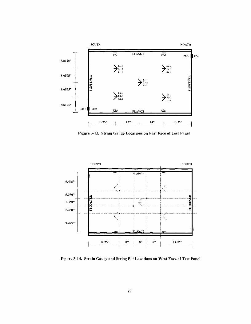
8.8125"
8.6875"
8.6875"
8.8125"
9.475"
5.350"
5.350"
5.350"
9.475"
SOUTH NORTH
EF-1 FLANGE EF-2 EB-31
➔El-! ➔ E2-l El-2 E2-2 El-3 E2-3
~ ~ la<
➔ E3-l la< z z
la< E3-2 la< I'-.
E3-3 I'-.
~ I'-.
i:: "' "'
➔E4-! ➔ ES-! E4-2 ES-2 E4-3 ES-3
EB-] I I EB-2 EF-3 FLANr.E ~
13.25" 13" 13" 13.25"
Figure 3-13. Strain Gauge Locations on East Face of Test Panel
NORTH
14.25" 8"
fLANGE i
1?1 ANr.li'
8"
SOUTH
! •••••
8" 14.25"
I EB-4
Figure 3-14. Strain Gauge and String Pot Locations on West Face of Test Panel
61

3.4 Summary of Test Specimens
Tension field action and existing and proposed hybrid moment-shear interaction
diagrams are to be verified by two series of tests. Series I tests investigate the presence
of tension field action stresses in hybrid plate girders subject to low moment-high shear
loading. Series II tests will determine the tension field action behavior of hybrid plate
girders subject to combined shear and bending. Using the testing procedures and data
from the instrumentation described in this chapter, the validity ofTFA and moment-shear
interaction will be demonstrated.
3.5 Theoretical Data Analysis
3.5.1 Introduction
The purpose of this section is to describe in detail the process used to interpret the
experimental data collected from Series II testing. In order to give meaning to the
experimental data, theoretical stress values are calculated for reference against the
experimental stresses. The theoretical stresses are calculated using Basler's (1961a)
tension field action theory as outlined in Chapter 2. Experimental stresses are calculated
from strain data recorded during testing. The methods used to calculate theoretical and
experimental stresses will be shown in detail and example calculations given. Using the
methods outlined in this chapter, the theoretical and experimental stresses will be
compared in Chapter 4 to determine the effectiveness of tension field action in hybrid
plate girders subject to concurrent bending and shear.
62
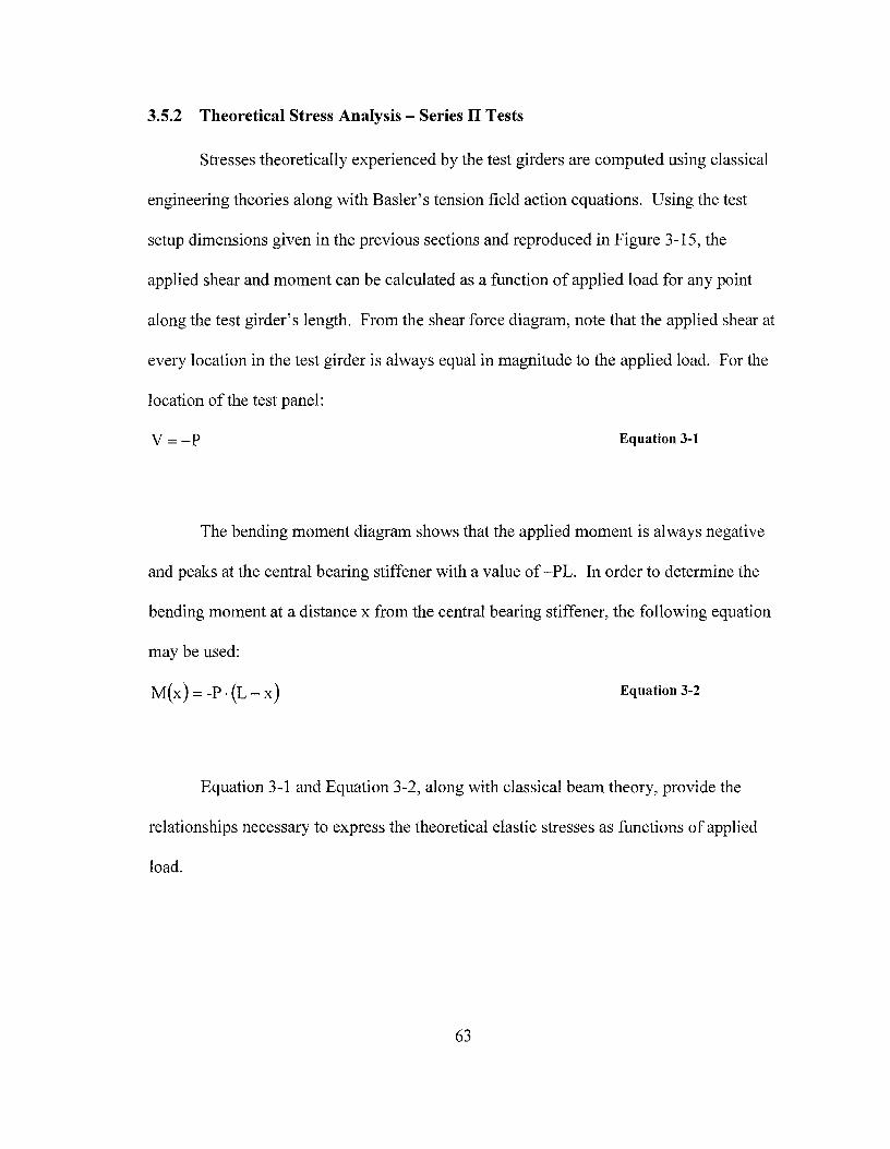
3.5.2 Theoretical Stress Analysis - Series II Tests
Stresses theoretically experienced by the test girders are computed using classical
engineering theories along with Basler's tension field action equations. Using the test
setup dimensions given in the previous sections and reproduced in Figure 3-15, the
applied shear and moment can be calculated as a function of applied load for any point
along the test girder's length. From the shear force diagram, note that the applied shear at
every location in the test girder is always equal in magnitude to the applied load. For the
location of the test panel:
V=-P Equation 3-1
The bending moment diagram shows that the applied moment is always negative
and peaks at the central bearing stiffener with a value of -PL. In order to determine the
bending moment at a distance x from the central bearing stiffener, the following equation
may be used:
M(x)= -P·(L-x) Equation 3-2
Equation 3-1 and Equation 3-2, along with classical beam theory, provide the
relationships necessary to express the theoretical elastic stresses as functions of applied
load.
63
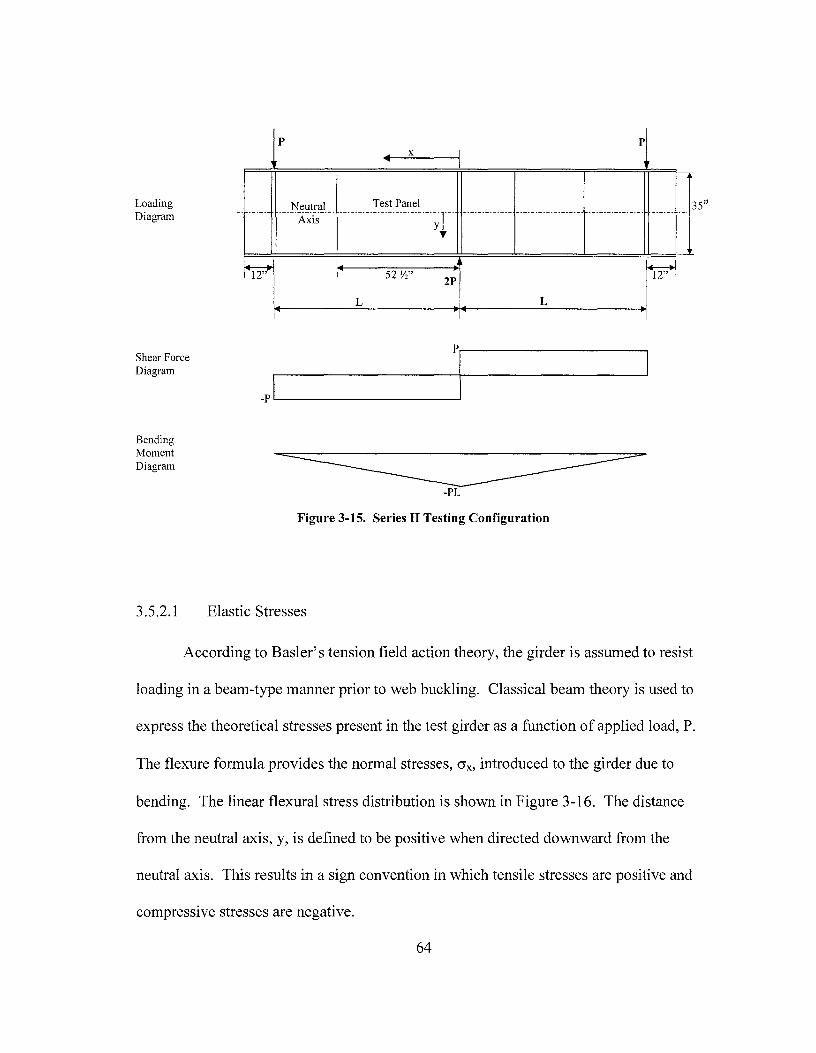
Loading Diagram
Shear Force Diagram
Bending Moment Diagram
3.5.2.1
p p X
Neutral Test Panel 35" -----A~f~---· ----------------------·-·; f. ' ,. 14 ► .r 52 ½"
2P
L ► 14
L
p
-P
-PL
Figure 3-15. Series II Testing Configuration
Elastic Stresses
According to Basler's tension field action theory, the girder is assumed to resist
loading in a beam-type manner prior to web buckling. Classical beam theory is used to
express the theoretical stresses present in the test girder as a function of applied load, P.
The flexure formula provides the normal stresses, crx, introduced to the girder due to
bending. The linear flexural stress distribution is shown in Figure 3-16. The distance
from the neutral axis, y, is defined to be positive when directed downward from the
neutral axis. This results in a sign convention in which tensile stresses are positive and
compressive stresses are negative.
64
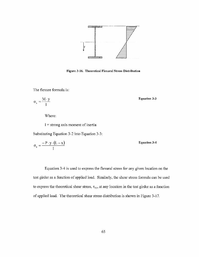
Figure 3-16. Theoretical Flexural Stress Distribution
The flexure formula is:
M•y (J =--
x I Equation 3-3
Where:
I = strong axis moment of inertia
Substituting Equation 3-2 into Equation 3-3:
-P·y·(L-x) (J =---~--
x I
Equation 3-4
Equation 3-4 is used to express the flexural stress for any given location on the
test girder as a function of applied load. Similarly, the shear stress formula can be used
to express the theoretical shear stress, Txy, at any location in the test girder as a function
of applied load. The theoretical shear stress distribution is shown in Figure 3-17.
65
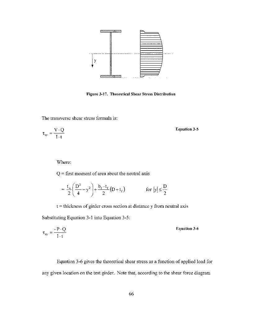
I
Figure 3-17. Theoretical Shear Stress Distribution
The transverse shear stress formula is:
V•Q 't =--
xy I· t
Where:
Q = first moment of area about the neutral axis
D for jyj:s;;-
2
Equation 3-5
t = thickness of girder cross section at distance y from neutral axis
Substituting Equation 3-1 into Equation 3-5:
-P·Q 't =--
xy I· t
Equation 3-6
Equation 3-6 gives the theoretical shear stress as a function of applied load for
any given location on the test girder. Note that, according to the shear force diagram
66
(Figure 3-15), this equation is valid only for the half of the girder containing the test
panel; the sign is reversed for the other half of the girder.
From the theoretical normal and shear stresses calculated above, the principal
stresses can be computed. Using the equation of Mohr's circle, and taking into account
that the vertical normal stress, cry, is theoretically zero, the principal stresses are:
(s__)2 +-r2 2 xy
Equation 3-7
Equation 3-8 (J
(J __ x -
2 - (s__)2 +-r2 2 xy 2
Where:
cr1 = major principal stress
cr2 = minor principal stress
The orientation of the major principal stress from the x-axis is given as:
Equation 3-9 if crx is a tensile stress
Equation 3-10 if crx is a compressive stress
0cr 1 is defined as the angle from the x-axis (longitudinal axis of girder) to the plane of the
major principal stress. Positive angles are counter-clockwise, negative angles are
clockwise.
The complete theoretical state of stress at any given level of loading prior to web
buckling can be defined either with x-y coordinate stresses or with principal stresses and
67

inclinations. The relationship of the x-y plane to the principal plane is best visualized by
plotting them together on Mohr's circle, as in Figure 3-18.
't x-y plane
u-v plane Principal plane
(j'
(j'
20crl
Figure 3-18. Relationship of Stress Planes
The theoretical stresses discussed in this section are limited to the elastic, or pre
buckling, load levels. The upper limit of elastic behavior is called the shear buckling
load, Ver (see derivation in Section 2.3.3). Basler's shear buckling load is calculated as:
Equation 3-11
Recall from Basler's derivation that the shear buckling load is the level of applied
shear that produces the shear buckling stress, "Ccr, which is sufficient to buckle the slender
68
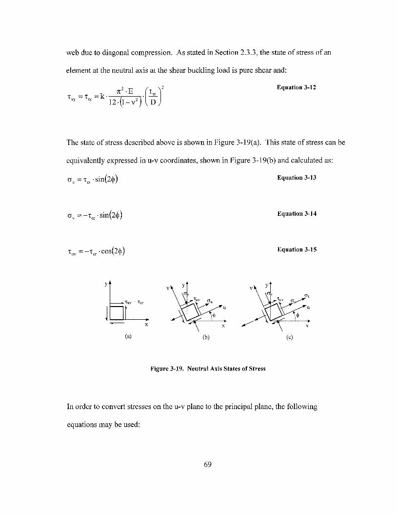
web due to diagonal compression. As stated in Section 2.3.3, the state of stress of an
element at the neutral axis at the shear buckling load is pure shear and:
Equation 3-12
The state of stress described above is shown in Figure 3-19( a). This state of stress can be
equivalently expressed in u-v coordinates, shown in Figure 3-19(b) and calculated as:
Equation 3-13
Equation 3-14
Equation 3-15
V
X
(a) (b) (c)
Figure 3-19. Neutral Axis States of Stress
In order to convert stresses on the u-v plane to the principal plane, the following
equations may be used:
69

Equation 3-16
Equation 3-17
The angle from the u-v plane to the principal plane is expressed as (0cr1-~ ), where
8cr1 is the angle from the x-y plane to the principal plane and~ is the angle from the x-y
plane to the u-v plane, as shown in Figure 3-18.
Equation 3-18 if <Ju:::: <Jv
Equation 3-19 if <Ju< <Jv
3.5.2.2 Postbuckling Stresses
Equation 3-12 gives the value of the maximum shear stress that an element at the
neutral axis will experience prior to web buckling. Following web buckling, the state of
stress caused by the shear buckling stress on the v-axis is assumed to remain constant
while tension field action stresses begin to form in the web in the direction of the u-axis,
which is rotated an angle~ from the x-axis. The maximum magnitude of tension field
action stress derived by Basler and stated in Section 2.3.3 as Equation 2-35 is:
Equation 3-20
70

The tension field stress, O"t, is the stress required to fulfill the von-Mises yield criterion
when added to the shear buckling stress. When expressed in u-v coordinates, O"t can be
directly added to the normal stress cru, resulting in the following state of stress, shown in
Figure 3-19( c ):
cru = 'rcr • Sin(2~ )+ CT 1 Equation 3-21
Equation 3-22
Equation 3-23
Note that Equation 3-20 gives only the maximum tension field stress. Basler's
tension field action theory does not specify how the incremental tension field stresses
develop in the web (i.e. linearly with applied load, etc.). Hence, the theoretical state of
stress is not explicitly defined for every given load level in the postbuckling region; only
the limiting states of stress at web buckling and failure are theoretically defined.
The state of stress at failure can be converted to the principal plane as before
using Equation 3-16 through Equation 3-19. From Basler' s derivation, the applied shear
required to fail the girder in shear is:
Equation 3-24
71
3.5.2.3 Example Calculation of Theoretical Stresses
In order to compare with experimental stresses, the theoretical stresses will be
calculated using the dimensions and properties of test Beam 6a. The girder is hybrid with
a total span length of 13.5 feet. The target values for relative moment and shear are both
1.0, which means that the girder is expected to reach its full shear and moment capacities
at approximately the same applied load. The given yield strengths are from tension tests
performed on samples of the steel plates that make up the plate girders (Schreiner 2001 ).
The properties are as follows:
Shear Span, L = 81"
Flange width, br = 8 ¾"
Flange thickness, tr= ½"
Flange yield strength, Fyr= 91.0 ksi
Web depth, D = 35"
Web thickness, tw = ¼"
Web yield strength, Fyw = 60.8 ksi
Modulus of Elasticity, E = 29,000 ksi (assumed)
Poisson's Ratio, v = 0.3 (assumed)
To calculate the theoretical state of stress in the web, an applied shear of P = 60
kips will be assumed. Note that this load level is less than the critical buckling load, so
tension field action stresses are theoretically absent. The stresses will be calculated at the
location of Gauge 1 (see Figure 3-13). Gauge 1 has the following coordinates, defined in
Figure 3-15: 72
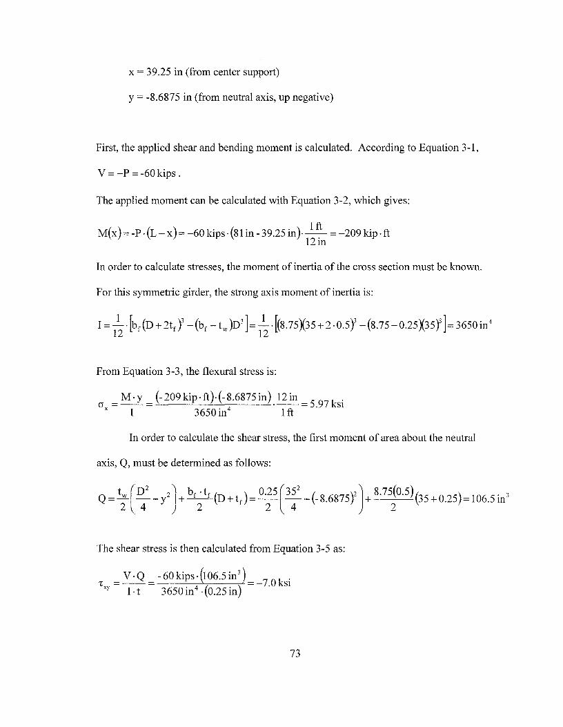
x = 3 9 .25 in ( from center support)
y = -8.6875 in (from neutral axis, up negative)
First, the applied shear and bending moment is calculated. According to Equation 3-1,
V = -P = -60kips.
The applied moment can be calculated with Equation 3-2, which gives:
M(x)= -P • (L-x)= -60 kips· (81 in -39.25 in)-~= -209 kip .ft 12m
In order to calculate stresses, the moment of inertia of the cross section must be known.
For this symmetric girder, the strong axis moment of inertia is:
From Equation 3-3, the flexural stress is:
cr = M·y = (-209kip•ft)·(-8.6875in)_ 12in = 5_97 ksi x I 3650in4 1 ft
In order to calculate the shear stress, the first moment of area about the neutral
axis, Q, must be determined as follows:
Q = ~(D2 -y2J+ br. tr (D + t )= 0.2
5 (
352 -(-8.6875)2]+
8·75
(0.5\35 + 0.25)= 106.5 in3
2 4 2 r 2 4 2
The shear stress is then calculated from Equation 3-5 as:
-r = V•Q = -60kips·(106.5in3)=_7_0 ksi
xy I·t 3650in4 ·(0.25in)
73
Since the vertical normal stress, cry, is theoretically zero, the complete state of
stress of an element located at Gauge 1 under an applied load of 60 kips is theoretically
known (see Figure 3-20). It may be desirable to express this state of stress on the
principal plane. The major principal stress can be found using Equation 3-7 as follows:
= ~ (~)2
2 = 5.97 ksi (5.97 ksi)2
(- 7 Ok .)2 = lO 6 k . CTI + +'txy ---+ --- + . Sl . Sl 2 2 2 2
Using Equation 3-8, the minor principal stress is found to be:
_ crx (crx )2
2 _ 5.97 ksi (5.97 ksi)2
( 7 Ok •)2 _ 4 62 k · CT --- - +'t ----- --- + - . Sl -- . Sl 2 2 2 xy 2 2
Since crx is positive, it is a tensile stress and Equation 3-9 can be used to calculate the
orientation of the principal plane.
8 _ 1 _1(2,:xyJ- 1 _1(2·(-7.0ksi))_ 33 50 1 ---•tan -- ----tan ----- -
cr 2 crx 2 5.97 ksi .
Theoretical stresses can also be calculated for locations on the flange. To
compare with experimental data, the flexural stress at the location of flange Gauge 1 will
be calculated. This gauge is located at:
X = 39.25"
y = -17.5"
Since flange Gauge 1 is located the same distance from the central bearing stiffener as
web Gauge 1, the applied moment at flange Gauge 1 is the same as that of web Gauge 1:
M(x) = -209 kip· ft
74
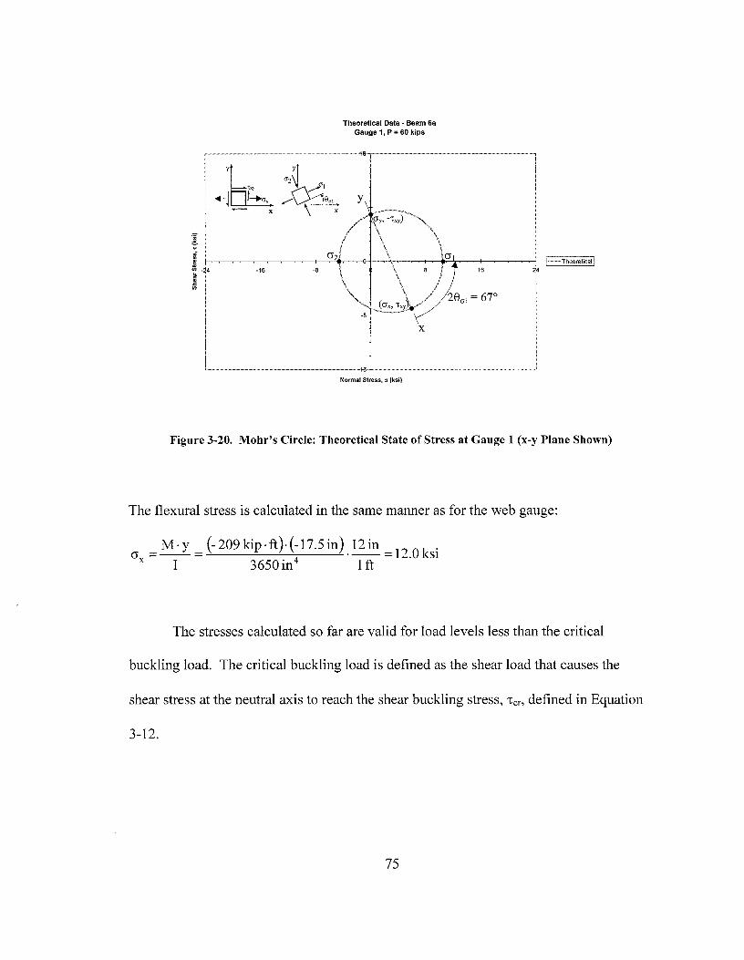
Theoretical Data - Beam Sa Gauge 1, P = 60 kips
~----------416-~-----------,
-16 -8
X
~-----------'!&--~----------~ Normal Stress, er (ksi)
I ~---Theoretical I
Figure 3-20. Mohr's Circle: Theoretical State of Stress at Gauge 1 (x-y Plane Shown)
The flexural stress is calculated in the same manner as for the web gauge:
0 = M-y = (-209kip-ft)·(-17.5in) _ 12in =l2_0ksi
x I 3650 in 4 1ft
The stresses calculated so far are valid for load levels less than the critical
buckling load. The critical buckling load is defined as the shear load that causes the
shear stress at the neutral axis to reach the shear buckling stress, Tcr, defined in Equation
3-12.
75
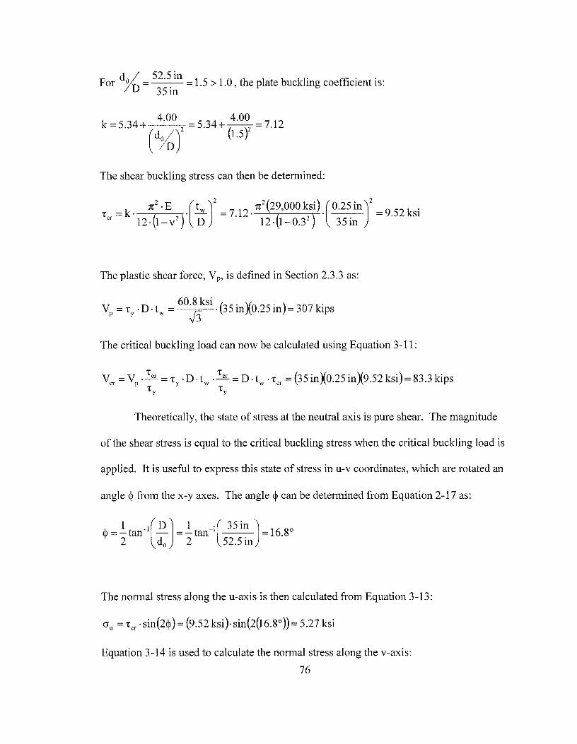
For dfo = 52
·~ in = 1.5 > 1.0, the plate buckling coefficient is: 35m
4.00 4.00 12 k=5.34+ (dfo)' =5.34+ (u)' =7.
The shear buckling stress can then be determined:
The plastic shear force, V p, is defined in Section 2.3 .3 as:
The critical buckling load can now be calculated using Equation 3-11:
Theoretically, the state of stress at the neutral axis is pure shear. The magnitude
of the shear stress is equal to the critical buckling stress when the critical buckling load is
applied. It is useful to express this state of stress in u-v coordinates, which are rotated an
angle~ from the x-y axes. The angle~ can be determined from Equation 2-17 as:
,1, 1 _,(DJ 1 _,(35in) 1680 '!'=-tan - =-tan --- = . 2 d0 2 52.5 in
The normal stress along the u-axis is then calculated from Equation 3-13:
cru = 'tcr · sin(2~) = (9.52 ksi)• sin(2(16.8° )) = 5.27 ksi
Equation 3-14 is used to calculate the normal stress along the v-axis:
76
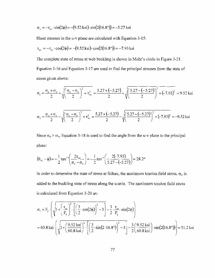
crv = -Tcr · sin(2~) = -(9.52 ksi)-sin(2(16.8°))= -5.27 ksi
Shear stresses in the u-v plane are calculated with Equation 3-15:
Tuv = -Tcr · cos(2~) = -(9.52 ksi)• cos(2(16.8°)) = -7.93 ksi
The complete state of stress at web buckling is shown in Mohr's circle in Figure 3-21.
Equation 3-16 and Equation 3-17 are used to find the principal stresses from the state of
stress given above:
cru+crv (cru-crv)2
2 5.27+(-5.27) (JI = --=---~+ --=---~ + T = ---"----'- +
2 2 UV 2 ( S.l? -t S.l?))' + (- 7.93 )' = 9.52 ksi
((ju-(jvJ2 2 _5.27+(-5.27)
2 +TUY - 2
Since cru > crv, Equation 3-18 is used to find the angle from the u-v plane to the principal
plane:
In order to determine the state of stress at failure, the maximum tension field stress, cr1, is
added to the buckling state of stress along the u-axis. The maximum tension field stress
is calculated from Equation 3-20 as:
cr, =F, { I+( f, J-[(%•sin(2$))' -3]-}f,•sin(2$)J
= 60.8 ksi J 1 + (9
·52
ks~ )2 •[(l. sin(2 -16.8°))
2
-3] _1(9·52
ks~)· sin(2(16.8°))1 = 51.2 ksi l 60.8 ks1 2 2 60.8 ks1 'j
77

Theoretical Data - Beam Sa Gauge 3, Web Buckling
; v:..v• t ... ~ f----,---~--.,......+--cr+---":,..--,-_,_,__,.--+-__ -,-J __ ..,.......,....
~ ~ 'o fil .c "'
-60 -30
2$- 34° -30
30 60 91)
~-----------so-~----------' Normal Stress, er {ksi)
I Basler Buckling I
Figure 3-21. Mohr's Circle: State of Stress at Web Buckling (u-v Plane Shown)
The shear load that will cause failure of the girder is calculated from Equation 3-24:
vu= VP. ~+ ✓3 -~•--;===1==
'ty 2 FY l +( dYof
=(307kips)J(9.52ksi)+ ✓3_(51.2ksi)· 1 l=207kips l 35.1 ksi 2 60.8 ksi ✓1 + (52.5 i½5
inl
The tension field stress is added to the u-axis buckling stress to determine the u-axis
stress at failure (Equation 3-21 ):
<>u = 'tcr · sin(2~ )+ <> 1 = 5.27 ksi + 51.2 ksi = 56.5 ksi
78
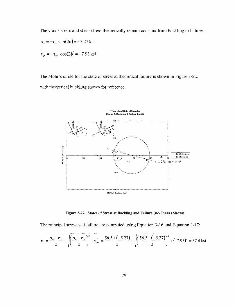
The v-axis stress and shear stress theoretically remain constant from buckling to failure:
The Mohr's circle for the state of stress at theoretical failure is shown in Figure 3-22,
with theoretical buckling shown for reference.
Theoretical Data • Beam 6a Gauge 3, Buckling & Failure Limits
Normal Stress, er (ksi)
Figure 3-22. States of Stress at Buckling and Failure (u-v Planes Shown)
The principal stresses at failure are computed using Equation 3-16 and Equation 3-17:
cr + cry cr = u +
l 2 (cru-crY)
2 2 _56.5+(-5.27)
2 +TUY - 2 + (56
·5-t5
·27)J +(-7.93)2 =57.4ksi
79
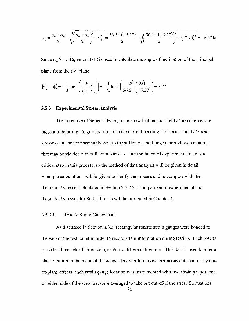
Since cru > crv, Equation 3-18 is used to calculate the angle of inclination of the principal
plane from the u-v plane:
fe ..1.)- 1 -1( 2i-uv J- 1 -1( 2(-7.93) J- 720 \ 1 -'I' ---tan --- ---tan ---~- - . cr 2 (Ju-(Jv 2 56.5-(-5.27)
3.5.3 Experimental Stress Analysis
The objective of Series II testing is to show that tension field action stresses are
present in hybrid plate girders subject to concurrent bending and shear, and that these
stresses can anchor reasonably well to the stiffeners and flanges through web material
that may be yielded due to flexural stresses. Interpretation of experimental data is a
critical step in this process, so the method of data analysis will be given in detail.
Example calculations will be given to clarify the process and to compare with the
theoretical stresses calculated in Section 3.5.2.3. Comparison of experimental and
theoretical stresses for Series II tests will be presented in Chapter 4.
3.5.3.1 Rosette Strain Gauge Data
As discussed in Section 3.3.3, rectangular rosette strain gauges were bonded to
the web of the test panel in order to record strain information during testing. Each rosette
provides three sets of strain data, each in a different direction. This data is used to infer a
state of strain in the plane of the gauge. In order to remove erroneous data caused by out
of-plane effects, each strain gauge location was instrumented with two strain gauges, one
on either side of the web that were averaged to take out out-of-plane stress fluctuations. 80

Therefore, six sets of strain data in three directions are used to determine the
experimental state of strain at each gauge location on the web of the test panel.
Each strain gauge was given a designation in order to distinctly identify the data
collected (Figures 3-13 and 3-14). The direction of strain recorded by each individual
gauge included in the rectangular rosette configuration is apparent from its designation.
The horizontal direction is designated as "2", whereas "l" is directed 45° clockwise from
horizontal. Direction "3" is 45° counter-clockwise from horizontal, as shown in Figure
3-23.
Directional strain gauges can be adversely affected by strains that act in directions
other than the direction of the gauge. This effect is called transverse sensitivity. The
errors due to the transverse sensitivity of rectangular rosette strain gauges in Series I
testing were found to be less than 1 % (Rush 2001 ). Therefore, transverse sensitivity
Figure 3-23. Rosette Strain Gauge Directions
corrections will not be included in Series II data analysis.
Out-of-plane effects such as web buckling are taken into consideration by
mirroring the strain gauge layout on either side of the web. It is assumed that if a gauge
reports compressive strains due to out-of-plane bending of the web, then the gauge on the
other side of the web will report tensile strains of the same magnitude. The data from
81
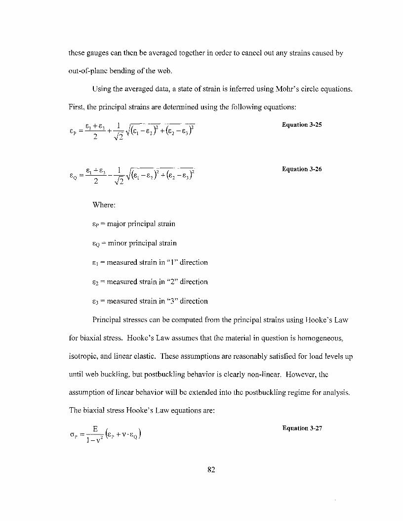
these gauges can then be averaged together in order to cancel out any strains caused by
out-of-plane bending of the web.
Using the averaged data, a state of strain is inferred using Mohr's circle equations.
First, the principal strains are determined using the following equations:
Equation 3-25
Equation 3-26
Where:
8p = major principal strain
8Q = minor principal strain
8 1 = measured strain in "1" direction
82 = measured strain in "2" direction
8 3 = measured strain in "3" direction
Principal stresses can be computed from the principal strains using Hooke's Law
for biaxial stress. Hooke's Law assumes that the material in question is homogeneous,
isotropic, and linear elastic. These assumptions are reasonably satisfied for load levels up
until web buckling, but postbuckling behavior is clearly non-linear. However, the
assumption of linear behavior will be extended into the postbuckling regime for analysis.
The biaxial stress Hooke's Law equations are:
Equation 3-27
82
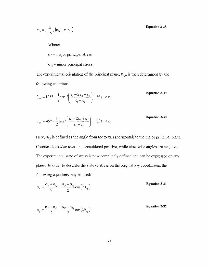
Equation 3-28
Where:
<Jp = major principal stress
cr0 = minor principal stress
The experimental orientation of the principal plane, 0xp, is then determined by the
following equations:
Equation 3-29
Equation 3-30
Here, 0xp is defined as the angle from the x-axis (horizontal) to the major principal plane.
Counter-clockwise rotation is considered positive, while clockwise angles are negative.
The experimental state of stress is now completely defined and can be expressed on any
plane. In order to describe the state of stress on the original x-y coordinates, the
following equations may be used:
crP +crQ crP -crQ ( ) CT =--~+----'-COS 20
X 2 2 ~
Equation 3-31
O"p-O"Q ( ) ---COS 20xp
2
Equation 3-32
83
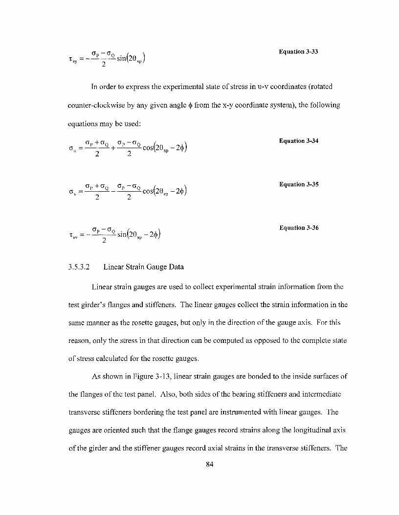
Equation 3-33
In order to express the experimental state of stress in u-v coordinates (rotated
counter-clockwise by any given angle~ from the x-y coordinate system), the following
equations may be used:
Equation 3-34
cr +cr cr -cr ( ) O"v = p Q - p Q COS 20xp -2~ 2 2
Equation 3-35
Equation 3-36
3.5.3.2 Linear Strain Gauge Data
Linear strain gauges are used to collect experimental strain information from the
test girder's flanges and stiffeners. The linear gauges collect the strain information in the
same manner as the rosette gauges, but only in the direction of the gauge axis. For this
reason, only the stress in that direction can be computed as opposed to the complete state
of stress calculated for the rosette gauges.
As shown in Figure 3-13, linear strain gauges are bonded to the inside surfaces of
the flanges of the test panel. Also, both sides of the bearing stiffeners and intermediate
transverse stiffeners bordering the test panel are instrumented with linear gauges. The
gauges are oriented such that the flange gauges record strains along the longitudinal axis
of the girder and the stiffener gauges record axial strains in the transverse stiffeners. The
84
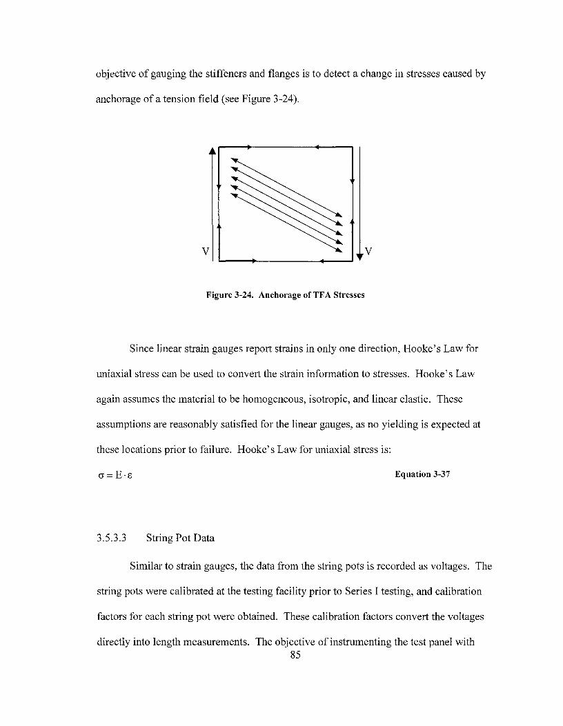
objective of gauging the stiffeners and flanges is to detect a change in stresses caused by
anchorage of a tension field (see Figure 3-24).
V V
Figure 3-24. Anchorage ofTFA Stresses
Since linear strain gauges report strains in only one direction, Hooke's Law for
uniaxial stress can be used to convert the strain information to stresses. Hooke's Law
again assumes the material to be homogeneous, isotropic, and linear elastic. These
assumptions are reasonably satisfied for the linear gauges, as no yielding is expected at
these locations prior to failure. Hooke's Law for uniaxial stress is:
cr = E • i:: Equation 3-37
3.5.3.3 String Pot Data
Similar to strain gauges, the data from the string pots is recorded as voltages. The
string pots were calibrated at the testing facility prior to Series I testing, and calibration
factors for each string pot were obtained. These calibration factors convert the voltages
directly into length measurements. The objective of instrumenting the test panel with 85

string pots is to track out-of-plane web deflections across the tension field as well as to
attempt to determine the load level that causes web buckling in the test girders. The
locations of the string pots are shown on the instrumentation layout diagram, Figure 3-14.
3.5.3.4 Example Experimental Stress Calculations
The following example calculations detail how the test data is reduced to
engineering terms. The following example is based on data taken from test Beam 6a at a
load level of P = 60 .1 kips. The equations used in this example are typical of all tests and
load levels. Below, recorded strain data from both rosette gauges at gauge location 1 (see
Figure 3-13) is given in micro-strains:
El-I: 1.71 µi:;
El-2: 303 w:
El-3: 436 µi:;
Wl-1: -374 µi:;
Wl-2: 108 µE
Wl-3: 248 µi:;
The data from opposite sides of the web panel is averaged to remove out-of-plane effects:
Al-1 = (El-1)+ (w1-1) = (1.71)+ (-374) = -186 µc = 81
2 2
The major principal strain is determined using Equation 3-25:
86
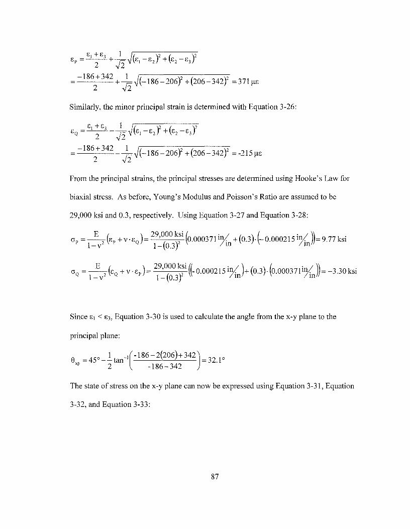
Similarly, the minor principal strain is determined with Equation 3-26:
From the principal strains, the principal stresses are determined using Hooke's Law for
biaxial stress. As before, Young's Modulus and Poisson's Ratio are assumed to be
29,000 ksi and 0.3, respectively. Using Equation 3-27 and Equation 3-28:
E ( ) 29,000 ksi ~ ·% ( ) ( ·% )~ . Cip =--2 Cp +V ·80 = ( )2 0.000371 lll. + 0.3 . -0.000215 m. = 9.77 ks1 1-V 1- 0.3 Ill Ill
E ( ) 29,000ksi~( ·n/) ( ) { ·n/ )~ · cr0 =
1_v2 s0 +v·sp = l-(o.
3)2 ~-0.000215 1~\n + 0.3 ·\0.00037l1~\n~=-3.30ks1
Since s1 < £3, Equation 3-30 is used to calculate the angle from the x-y plane to the
principal plane:
8 = 450 _ _!_tan-'(-186-2(206)+ 342) = 32_10 xp 2 -186-342
The state of stress on the x-y plane can now be expressed using Equation 3-31, Equation
3-32, and Equation 3-33:
87
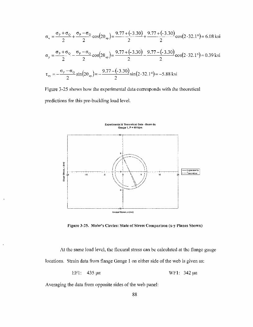
_<>r+cr0 <>r-<>o (20
)_9.77+(-3.30) 9.77+(-3.30) (2 .3210)_ 608 k. <>x ----+----'-COS xp -----'------'-+----'-----'---COS . - . SI 2 2 2 2
<>r -crQ sin(20xJ=- 9·77 -(- 3.30)sin(2·32.1°)=-5.88ksi 2 2
Figure 3-25 shows how the experimental data corresponds with the theoretical
predictions for this pre-buckling load level.
Experimental & Theoretical Data - Beam 6a Gauge 1, P = 60 kips
~---------1&--,-------------,
-16 -8 16
~---------<6··-~---------~ Normal Stress, er (ksi)
- Experimental
•½=,= Theoretical
Figure 3-25. Mohr's Circles: State of Stress Comparison (x-y Planes Shown)
At the same load level, the flexural stress can be calculated at the flange gauge
locations. Strain data from flange Gauge 1 on either side of the web is given as:
EFl: 435 µc
Averaging the data from opposite sides of the web panel:
88
WFl: 342 µc
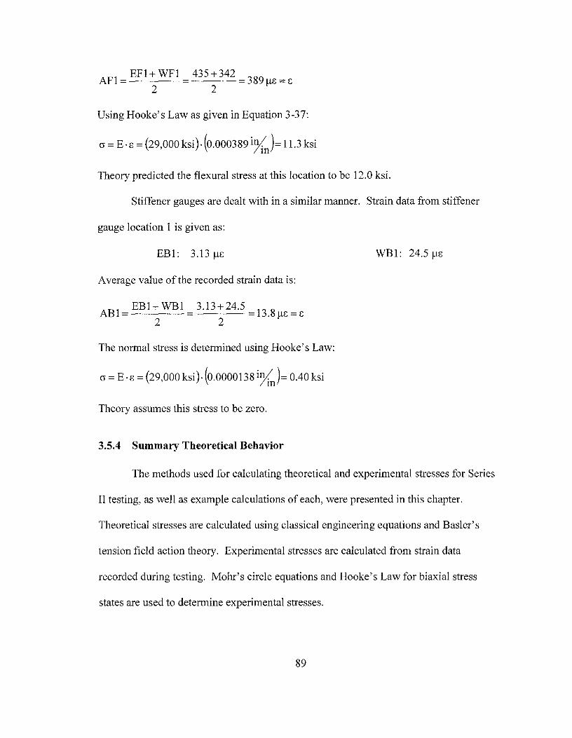
AFl= EFl+ WFl = 435+342 = 389 µs=c 2 2
Using Hooke's Law as given in Equation 3-37:
cr = E. s = (29,000 ksi). (o.000389 i1/in)= 11.3 ksi
Theory predicted the flexural stress at this location to be 12.0 ksi.
Stiffener gauges are dealt with in a similar manner. Strain data from stiffener
gauge location 1 is given as:
EBI: 3.13 µc
Average value of the recorded strain data is:
ABl= EBI+ WBl = 3.13+24.5 =l 3.Sµc=c 2 2
The normal stress is determined using Hooke's Law:
cr = E ·s = (29,000 ksi)-(0.0000138 i1/in)= 0.40 ksi
Theory assumes this stress to be zero.
3.5.4 Summary Theoretical Behavior
WBl: 24.5 µs
The methods used for calculating theoretical and experimental stresses for Series
II testing, as well as example calculations of each, were presented in this chapter.
Theoretical stresses are calculated using classical engineering equations and Basler' s
tension field action theory. Experimental stresses are calculated from strain data
recorded during testing. Mohr's circle equations and Hooke's Law for biaxial stress
states are used to determine experimental stresses.
89
Included in the analysis procedure is an assumption of linear-elastic material
behavior. While postbuckling behavior (yielding) is clearly non-linear, the assumption is
extended to the postbuckling regions for comparison purposes nonetheless.
In the next chapter, the stresses calculated from experimental data will be compared
with theory in an effort to determine if tension field action stresses are present and
effectively anchored.
3.6 Summary
Chapter 3 presented the Series I (low moment high shear) and Series II (high
moment high shear) test specimens and the test set up and procedures. They were
selected to demonstrate tension field action in hybrid girders and to examine the moment
shear interaction of hybrid girders. Chapter 3 also demonstrated theoretical and example
calculations to examine shear capacities and experimental stresses.
Chapter 4 will examine one of the Series II test girders in detail. Tension field
action and moment-shear interaction will be demonstrated, along with comparison of
experimental behavior to theoretical expectations. The equations demonstrated here will
be used in these analyses, but the reader is referred to Zentz (2002) for a complete
explanation of the procedures. Series I test results and analyses will not be shown here.
The reader is referred to Rush (200 I) for an equivalent presentation of the Series I tests.
90
Chapter 4 - Experimental Results
4.1 Introduction
The objective of this chapter is to determine the experimental tension field action
shear capacity of the Series II hybrid plate girders, verify that the capacity is indeed due
to tension field action stresses, and compare the results to theoretical values calculated
from Basler's tension field action theory. Through physical observation of the Series II
tests, the ultimate shear capacity and interaction characteristics of the test girders will be
investigated, and the tension field action contribution to shear resistance will be
quantified. The data taken from the tests will be used to investigate both the elastic and
postbuckling stresses present in the test girders in order to verify the presence of tension
field action. The Series I test girders will not be shown, except for overall behavior,
since the Series II tests demonstrate the topics to be covered. The reader is referred to
Rush (2001) and Schreiner (2001) for full details on the Series I test girders.
In order to maintain the flow of the text without repetition, experimental data will
primarily only be presented from Beam 6a throughout this chapter. Data for all of the
Series II test girders is included in the Results Volume (Zentz 2002), and will be referred
to whenever experimental results are presented. Also, many of the experimental data
graphs include vertical lines marked Ver, V n, My, or M0 • These lines represent the
theoretical load levels corresponding to the critical shear buckling load, nominal shear
capacity, yield moment, and nominal moment capacity, respectively.
91

4.2 Physical Observations
The physical observations of the experimental tests are considered prior to the
interpretation of test data. The first observation is the ultimate shear capacity of the test
girders, which has the potential to demonstrate that hybrid plate girders do exhibit tension
field action shear capacities that can be reasonably predicted by the current AASHTO
design codes. Next, the moment-shear interaction characteristics of the test girders are
considered, with the intention to define what special interaction reductions, if any, hybrid
plate girders might be subject to if tension field action capacity is allowed in their design.
The physical failure mechanisms of the test girders are explored in order to correctly
interpret the strain and deflection data taken from the tests. Finally, the experimental
tension field action contribution to shear capacity will be investigated.
4.2.1 Experimental Shear Capacities
The most important observation from Series II experimental testing is the
experimental shear capacity of each test girder. The experimental shear capacity has the
potential to show that hybrid plate girders do have shear capacities comparable to those
of similarly proportioned homogeneous girders. It will be left up to the experimental
stress analysis to verify that the shear capacity is due to tension field action behavior,
rather than some other mechanism.
The theoretical shear and moment capacities for the experimental test girders have
been calculated using AASHTO's 1998 LRFD design equations, including tension field
action for hybrid girders, and neglecting moment-shear interaction reductions. The
92
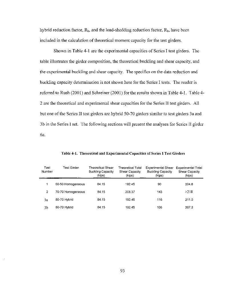
hybrid reduction factor, Rh, and the load-shedding reduction factor, Rb, have been
included in the calculation of theoretical moment capacity for the test girders.
Shown in Table 4-1 are the experimental capacities of Series I test girders. The
table illustrates the girder composition, the theoretical buckling and shear capacity, and
the experimental buckling and shear capacity. The specifics on the data reduction and
buckling capacity determination is not shown here for the Series I tests. The reader is
referred to Rush (2001) and Schreiner (2001) for the results shown in Table 4-1. Table 4-
2 are the theoretical and experimental shear capacities for the Series II test girders. All
but one of the Series II test girders are hybrid 50-70 girders similar to test girders 3a and
3b in the Series I set. The following sections will present the analyses for Series II girder
6a.
Table 4-1. Theoretical and Experimental Capacities of Series I Test Girders
Test Test Girder Theoretical Shear Theoretical Total Experimental Shear Experimental Total Number Buckling Capacity Shear Capacity Buckling Capacity Shear Capacity
(kips) (kips) (kips) (kips)
50-50 Homogeneous 84.15 192.45 90 204.8
2 70-70 Homogeneous 84.15 208.37 143 >218
3a 50-70 Hybrid 84.15 192.45 116 211.0
3b 50-70 Hybrid 84.15 192.45 106 207.3
93
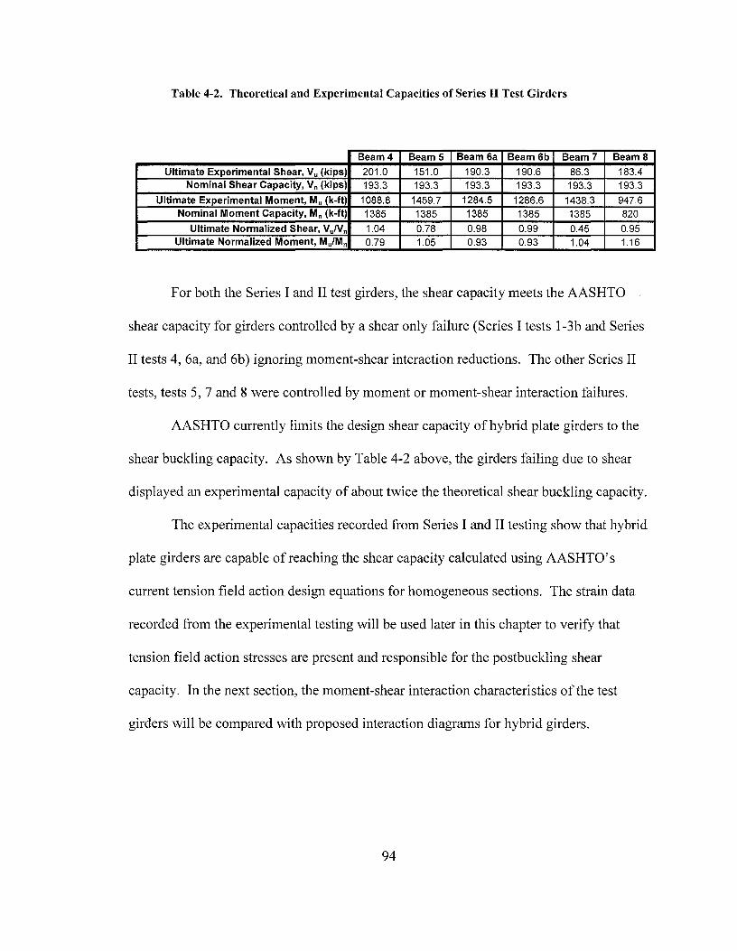
Table 4-2. Theoretical and Experimental Capacities of Series II Test Girders
Beam4 Beams Beam 6a Beam 6b Beam 7 Beams
Ultimate Experimental Shear, Vu (kips) 201.0 151.0 190.3 190.6 86.3 183.4 Nominal Shear Capacity, Vn (kips) 193.3 193.3 193.3 193.3 193.3 193.3
Ultimate Experimental Moment, Mu (k-ft) 1088.8 1459.7 1284.5 1286.6 1438.3 947.6 Nominal Moment Capacity, Mn (k-ft) 1385 1385 1385 1385 1385 820
Ultimate Normalized Shear, VuNn 1.04 0.78 0.98 0.99 0.45 0.95 Ultimate Normalized Moment, MJMn 0.79 1.05 0.93 0.93 1.04 1.16
For both the Series I and II test girders, the shear capacity meets the AASHTO
shear capacity for girders controlled by a shear only failure (Series I tests l-3b and Series
II tests 4, 6a, and 6b) ignoring moment-shear interaction reductions. The other Series II
tests, tests 5, 7 and 8 were controlled by moment or moment-shear interaction failures.
AASHTO currently limits the design shear capacity of hybrid plate girders to the
shear buckling capacity. As shown by Table 4-2 above, the girders failing due to shear
displayed an experimental capacity of about twice the theoretical shear buckling capacity.
The experimental capacities recorded from Series I and II testing show that hybrid
plate girders are capable of reaching the shear capacity calculated using AASHTO's
current tension field action design equations for homogeneous sections. The strain data
recorded from the experimental testing will be used later in this chapter to verify that
tension field action stresses are present and responsible for the postbuckling shear
capacity. In the next section, the moment-shear interaction characteristics of the test
girders will be compared with proposed interaction diagrams for hybrid girders.
94
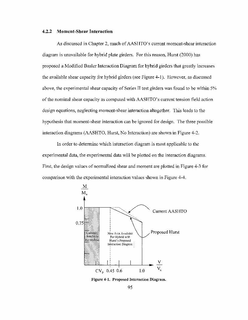
4.2.2 Moment-Shear Interaction
As discussed in Chapter 2, much of AASHTO's current moment-shear interaction
diagram is unavailable for hybrid plate girders. For this reason, Hurst (2000) has
proposed a Modified Basler Interaction Diagram for hybrid girders that greatly increases
the available shear capacity for hybrid girders (see Figure 4-1 ). However, as discussed
above, the experimental shear capacity of Series II test girders was found to be within 5%
of the nominal shear capacity as computed with AASHTO's current tension field action
design equations, neglecting moment-shear interaction altogether. This leads to the
hypothesis that moment-shear interaction can be ignored for design. The three possible
interaction diagrams (AASHTO, Hurst, No Interaction) are shown in Figure 4-2.
In order to determine which interaction diagram is most applicable to the
experimental data, the experimental data will be plotted on the interaction diagrams.
First, the design values of normalized shear and moment are plotted in Figure 4-3 for
comparison with the experimental interaction values shown in Figure 4-4.
M
1.0 i--,.,.......-,--=I·
I
0.75
Currentlf • AvaifauJe< :!zorHybi'ld
I I
I
I I I
I
I
I
New Area Available For Hybrid with Hurst's Proposed
Interaction Diagram
CVp 0.45 0.6
Current AASHTO
Proposed Hurst
V
1.0
Figure 4-1. Proposed Interaction Diagram.
95
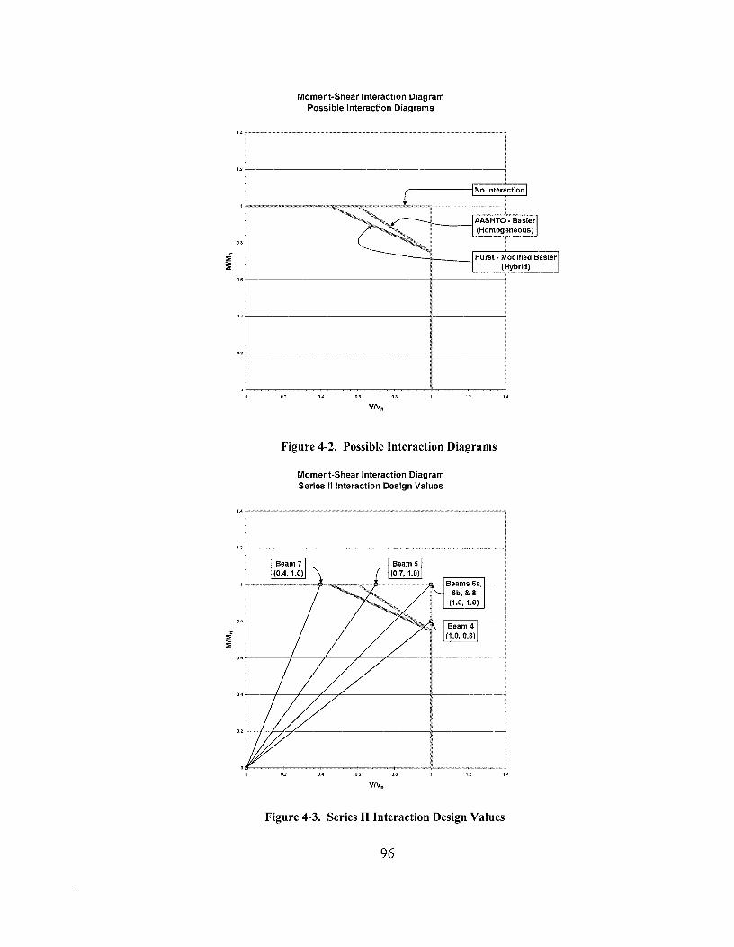
1.2
08
-:l :1l
06
0.4
0.2
Moment-Shear Interaction Diagram Possible Interaction Diagrams
0.4 0.6 08
No Interaction
AASHTO • Basler (Homogeneous)
l
Hurst - Modified Basler (Hybrid)
Figure 4-2. Possible Interaction Diagrams
Moment-Shear Interaction Diagram Series II Interaction Design Values
Figure 4-3. Series II Interaction Design Values
96

Moment-Shear Interaction Diagram Series II Experimental Interaction Values
Beam Sa (0.98, 0.93) Beam Sb
0_8 +------+ ~-/"--_T-----;7""1¾i~.;:r;:<=o.9=9=, o=.9=3);I
0 0.2 0.4 0.6 0.8
Beam4 (1.04, 0.79)
1.2 1.4
Figure 4-4. Series II Ultimate Interaction Values
From the experimental data shown in Figure 4-4, it appears that moment-shear
interaction can be ignored for design. With the exception of Beams 6a & 6b, all of the
test girders plot outside of the "no interaction" envelope, which indicates that those
beams have more capacity than would be calculated if interaction were considered. Table
4-2 shows that Beams 6a & 6b are less than 2% below the nominal shear capacity
(including TF A) at failure. This difference is within the uncertainty of shear design
(Aydemir 2000).
Recent research performed at the Georgia Institute of Technology recommends
that moment-shear interaction be removed from design criteria (Aydemir 2000).
Aydemir performed a parametric study of tension field action behavior in hybrid plate
97
girders using finite element analysis. The conclusion of the study was that only girders
with high depth of web in compression to web depth ratios (Dc/D :2: 0.65) experienced
any moment-shear interaction. The extent of the interaction for these girders was small
enough to suggest that the interaction be accounted for by adjustment of AASHTO
resistance factors ( ~ factors) rather than traditional moment-shear interaction reductions
(Aydemir 2000).
However, if the moment-shear interaction reduction is not removed from the
design requirements, Figure 4-4 shows that AASHTO's current moment-shear interaction
diagram for homogeneous girders is valid and conservative for the Series II hybrid test
girders. Hurst's proposed hybrid interaction diagram is also valid for the test girders as
shown, but is less conservative and more accurate than the current AASHTO
homogeneous interaction diagram.
The experimental capacities recorded from Series II testing show that hybrid plate
girders are capable of reaching the shear capacity calculated using AASHTO' s current
tension field action design equations for homogeneous sections. The moment-shear
interaction characteristics of the test girders suggest that the interaction reduction is
conservative or that the moment-shear interaction reduction may even be removed for all
plate girders.
The next section will investigate the observable failure mechanisms from the
Series II tests. Visual inspection of the failed test panels helps to properly interpret the
test data.
98
4.2.3 Failure Mechanisms
The observable failure mechanisms for Series II tests varied depending upon the
type of failure. Beams 4, 6a, and 6b failed in shear, while Beam 7 experienced failure
due to flexure. Beams 5 and 8 showed signs of a combined moment-shear failure. All of
the Series I test girders (Schreiner 2001) failed in a shear mode ( except the homogeneous
70 ksi girder which did not fail). Only the Series II test girders will be discussed here.
In general, the characteristics of each failure include lateral web buckling and
development of a tension strut, followed by formation of a plastic hinge in the
compression flange. Visual out-of-plane distortion was observed to begin at load levels
well below the theoretical buckling load. While theory assumes that buckling of the web
plate does not occur until the critical shear buckling stress is obtained, it is intuitive that
buckling of a slender plate with some initial curvature will begin as soon as a
compressive load is applied to the plate. Although each test was unique, out-of-plane
web distortion was visually apparent at load levels as low as 40 kips (about half of the
calculated shear buckling load). At high load levels, the diagonal strains across the shear
panel became large enough to cause shedding of mill scale, forming a visible tension strut
across the web. Eventually, a plastic hinge forms in the compression flange where the
tension strut anchors to the flange. When the hinge forms, end deflections of the girder
increase rapidly and the girder is considered failed.
A typical shear failure is shown in Figure 4-5. A tension strut running diagonally
from the upper corner of the test panel at the bearing stiffener to the opposite lower
corner of the panel characterizes a shear failure. Since the tension strut runs along the
diagonal of the test panel, it appears that the tension field stresses also act along the angle
99
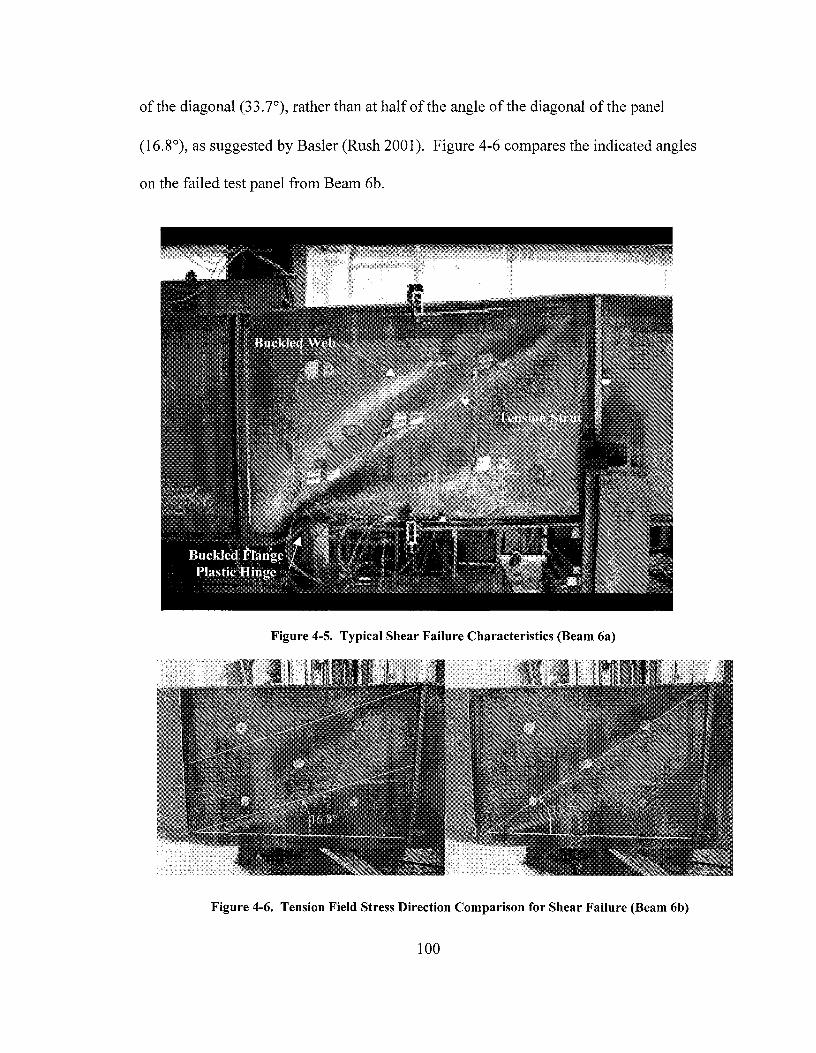
of the diagonal (33.7°), rather than at half of the angle of the diagonal of the panel
(16.8°), as suggested by Basler (Rush 2001). Figure 4-6 compares the indicated angles
on the failed test panel from Beam 6b.
Figure 4-5. Typical Shear Failure Characteristics (Beam 6a)
Figure 4-6. Tension Field Stress Direction Comparison for Shear Failure (Beam 6b)
100
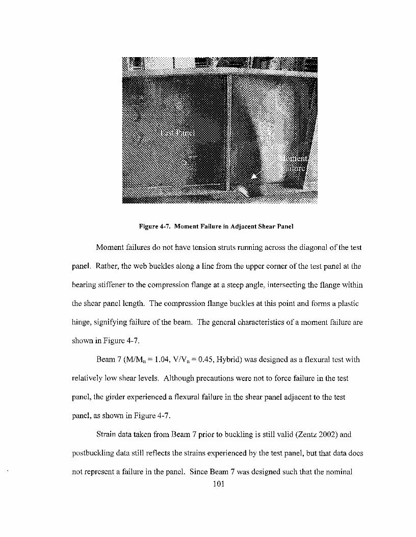
Figure 4-7. Moment Failure in Adjacent Shear Panel
Moment failures do not have tension struts running across the diagonal of the test
panel. Rather, the web buckles along a line from the upper corner of the test panel at the
bearing stiffener to the compression flange at a steep angle, intersecting the flange within
the shear panel length. The compression flange buckles at this point and forms a plastic
hinge, signifying failure of the beam. The general characteristics of a moment failure are
shown in Figure 4-7.
Beam 7 (M/Mn = 1.04, V/Vn = 0.45, Hybrid) was designed as a flexural test with
relatively low shear levels. Although precautions were not to force failure in the test
panel, the girder experienced a flexural failure in the shear panel adjacent to the test
panel, as shown in Figure 4-7.
Strain data taken from Beam 7 prior to buckling is still valid (Zentz 2002) and
postbuckling data still reflects the strains experienced by the test panel, but that data does
not represent a failure in the panel. Since Beam 7 was designed such that the nominal
101
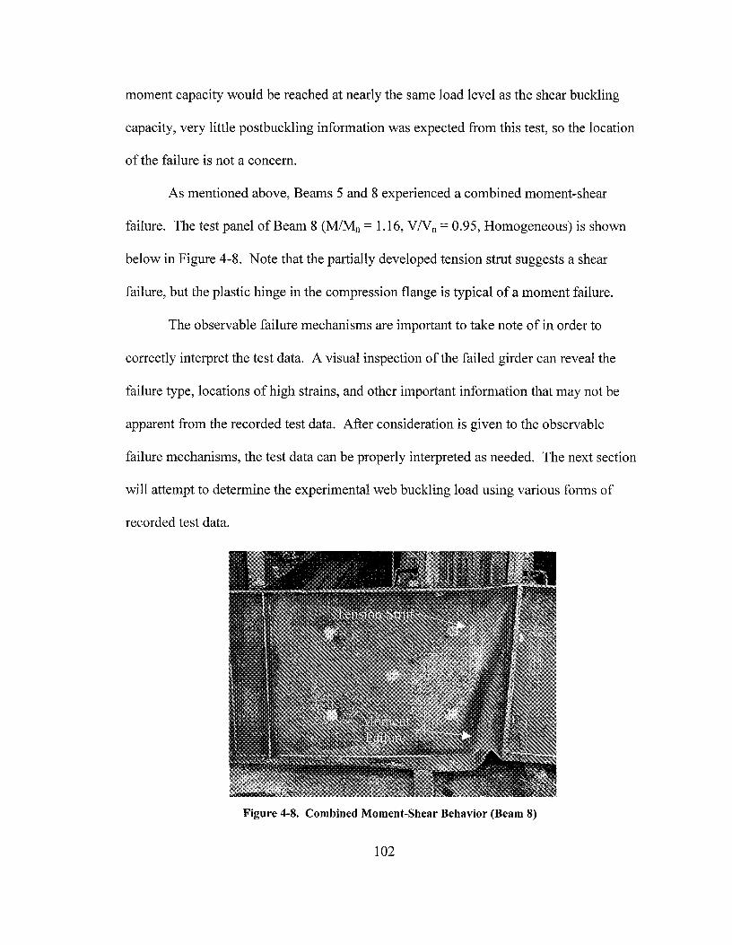
moment capacity would be reached at nearly the same load level as the shear buckling
capacity, very little postbuckling information was expected from this test, so the location
of the failure is not a concern.
As mentioned above, Beams 5 and 8 experienced a combined moment-shear
failure. The test panel of Beam 8 (M/Mn = 1.16, VNn = 0.95, Homogeneous) is shown
below in Figure 4-8. Note that the partially developed tension strut suggests a shear
failure, but the plastic hinge in the compression flange is typical of a moment failure.
The observable failure mechanisms are important to take note of in order to
correctly interpret the test data. A visual inspection of the failed girder can reveal the
failure type, locations of high strains, and other important information that may not be
apparent from the recorded test data. After consideration is given to the observable
failure mechanisms, the test data can be properly interpreted as needed. The next section
will attempt to determine the experimental web buckling load using various forms of
recorded test data.
Figure 4-8. Combined Moment-Shear Behavior (Beam 8)
102
4.2.4 Experimental Web Buckling
In an attempt to quantify the experimental tension field action contribution to total
shear capacity, an experimental shear buckling capacity is required. Once an
experimental shear buckling capacity is determined, any additional capacity beyond
buckling could be attributed to tension field action, provided the experimental strain
patterns agree with tension field action theory.
In the interest of brevity, Beam 6a (M/Mn = 0.93, VNn = 0.98, Hybrid) will be
used to present experimental and theoretical data for the remainder of the chapter. Full
data from all test girders is included in the Results Volume (Zentz 2002). Significant
data from other test girders is discussed and shown in this chapter when necessary.
As mentioned in Section 4.2.3, out-of-plane web buckling in the test girders was
visually noticeable at low load levels, prior to the theoretical critical buckling load. This
suggests a gradual transition from beam-type shear resistance to tension field action
behavior, rather than an abrupt switch from beam to TF A resistance as suggested by
theory. Therefore, it is likely that there is not a clearly defined experimental shear
buckling load, but it may be possible to determine an effective shear buckling load based
on the recorded data.
In the following sections, experimental web buckling will be investigated using a
variety of test data. First, string pot deflection data will be used in an attempt to
determine the experimental buckling load. Then the differences in data recorded by the
rosette strain gauges on either side of the web will be examined. Anchorage stresses
caused by the tension field may be useful in establishing the experimental buckling load,
so these will be explored, as well as postbuckling stress behavior in the web panel.
103
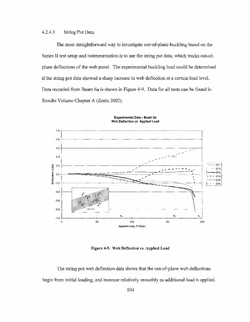
4.2.4.1 String Pot Data
The most straightforward way to investigate out-of-plane buckling based on the
Series II test setup and instrumentation is to use the string pot data, which tracks out-of
plane deflections of the web panel. The experimental buckling load could be determined
if the string pot data showed a sharp increase in web deflection at a certain load level.
Data recorded from Beam 6a is shown in Figure 4-9. Data for all tests can be found in
Results Volume Chapter A (Zentz 2002).
Experimental Data - Beam 6a Web Deflection vs. Applied Load
1.0 ,--------------------------------.
0.6 +--------------------------------l
,, I 0.2 +------------------,,,~.,-,---'-·· -----------
; 1_---=.,,,,,,.-i:=~~~§~2~====·=·-=/====~~~2~''"='=~'~-~=·---=---~--~,/ ~ Q.Q 1 ~ ' «« ~-~:_..~~•~,w,:S~~.:..,-:~ ;-Q)
~ -0.2 t--------------~~"'=~;;.:;;;;:=~-~"'=~----:--1 ·-------0.4
-0.6
-0.8 -- Tc~t Panel
0 50 100 150 200
Applied Load, P (kips)
Figure 4-9. Web Deflection vs. Applied Load
--SP1 -------SP2
--SP3
• • • SP4
-"-"''SP5 - - " SP6
The string pot web deflection data shows that the out-of-plane web deflections
begin from initial loading, and increase relatively smoothly as additional load is applied.
104

There are no sharp changes or discontinuities in the web deflection data that would
indicate a clear point of buckling. The gradual deflections, beginning at low load levels,
indicate a smooth transition from beam-type shear resistance to tension field action shear
resistance. Another attempt to determine the experimental buckling load using rosette
strain gauge data is presented in the next section.
4.2.4.2 Rosette Strain Gauge Data
As mentioned in Chapter 3, the rosette strain gauge layout is mirrored on either
side of the web of the test panel in order to eliminate out-of-plane effects. It may be
possible to use the raw strain data from either side of the web to determine the point of
experimental web buckling.
Theoretically, the strain data recorded from the east and west rosette at any
particular gauge location should be identical until web buckling. At the point of web
buckling, the strain data from the east and west rosette should theoretically diverge from
one another due to the curvature of the buckled web.
Web buckling is expected to be most pronounced in the center of the web of the
test panel, so rosette Gauge 3 will be used for this investigation. A change in strain due
to buckling is most likely to be recorded by a strain gauge oriented perpendicular to the
direction of buckling. Gauge direction 1 is most nearly perpendicular to the expected
direction of web buckling, so east and west gauge 3-1 will be used for this investigation.
Strain data from Beam 6a is shown in Figure 4-10. Data for all test girders can be found
in Results Volume Chapter B (Zentz 2002).
105

"
Experimental Data - Beam 6a Gauge 3-1 Strain vs. Applied Load
0.005 .-------------------------------,
0.004 +-----------------------------------j
0.003 +---------------------------~-J
,,/\, 0.002 +--------------------------o'"·-· ~·-------,
0.001 +--------------------~~------~-------,
·i 0.000 +---~--.. -._-.-.. -.. -.. -.• - .. -.-.. -.. -.• -.. ~.=-·~··~··~-------------------j
cii -----------------0.001 t---------------=-~-----------------l
-0.002 +----------------------=~=------------l
-0.003 ;-----------------~--___,__\ __ ___,
·0.004 +----------------------------~~-------,
\v. ·0.005 -~--~~~1---~----+---------~~~.---; M,
0 50 100 150 200
Applied Load, P (kips)
Figure 4-10. Raw Strain Data from Gauge Location 3-1
1--E3·11 ;······W3-1
The rosette strain gauge data shows that the strains recorded from the east and
west sides of the web panel begin to diverge at very low load levels. There are no sharp
discontinuities in the data that suggest a definite buckling load. The data agrees with the
theory of a gradual transition from beam to TF A shear resistance. Anchorage stresses
caused by the tension field will be inspected in the next section.
4.2.4.3 Tension Field Anchorage Stresses
According to Basler's tension field action theory, tension field action stresses
anchor to the stiffeners and flanges that make up the border of each shear panel.
Theoretically, the anchorage stresses tend to cause increased compressive stresses in both
106
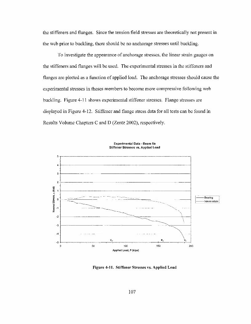
the stiffeners and flanges. Since the tension field stresses are theoretically not present in
the web prior to buckling, there should be no anchorage stresses until buckling.
To investigate the appearance of anchorage stresses, the linear strain gauges on
the stiffeners and flanges will be used. The experimental stresses in the stiffeners and
flanges are plotted as a function of applied load. The anchorage stresses should cause the
experimental stresses in theses members to become more compressive following web
buckling. Figure 4-11 shows experimental stiffener stresses. Flange stresses are
displayed in Figure 4-12. Stiffener and flange stress data for all tests can be found in
Results Volume Chapters C and D (Zentz 2002), respectively.
"iii
=-" ,,; "' I! 1i5 .. e 0 z
Experimental Data - Beam Sa Stiffener Stresses vs. Applied Load
5-r----------------------------,
4 ~------------------------------1
3 +------------------------------!
2
1
0
-1 ~
-2 ~ -3
~ -4
\ V,
-5
0 50 100 150 200
Applied Load, P (kips)
Figure 4-11. Stiffener Stresses vs. Applied Load
107
--Bearing - - - -- - - Intermediate

70
50
-30
-50
Experimental Data - Beam Sa Flange Stresses vs. Applied Load
Applied Load, P (kips)
... -.
i -. i . ···-- ! l F;. ·- -- I
Figure 4-12. Flange Stresses vs. Applied Load
The flange and stiffener data provides little information on the experimental
buckling load. Flange stresses appear to be linear, as predicted by beam theory, and
neither the flange nor stiffener data show any significant compressive discontinuities that
would indicate the introduction of anchorage stresses. Rather, it appears that any
compressive stresses due to tension field anchorage increase gradually from initial
loading, which again suggests a gradual transition from beam to TF A shear resistance.
108

4.2.4.4 Postbuckling Stress Behavior
The experimental web buckling load could potentially be determined through the
web stress behavior that occurs after buckling. As discussed in Chapter 2, Basler
assumes that once the critical shear buckling stress is reached, the shear on the u-v plane
remains constant. Basler derived the postbuckling stresses using an element at the neutral
axis, so the experimental investigation will use Gauge 3, located at the neutral axis in the
center of the test panel. Recall that Basler calculated the angle of inclination of the u-v
plane to be 16.8° for our test panel dimensions.
The experimental shear buckling load is calculated by the intersection of trend
lines that represent the initial slope of the shear stress plot and the stress level at which
the shear becomes constant (Zentz 2002). Figure 4-13 shows the determination of the
experimental shear buckling load for Basler's u-v plane. Data for all tests can be found
in Results Volume Chapter E (Zentz 2002).
As discussed in Section 4.2.3, it has been observed that the apparent angle of
tension field stresses is equal to the diagonal angle of the shear panel. The angle of
application of tension field stresses is how Basler defines the u-v plane, but that angle
was calculated to be half of the panel diagonal angle. During the analysis of Series I
tests, Rush (2001) found that the tension field stresses acted along the shear panel
diagonal and the experimental stresses more closely matched their theoretical values if~
is taken to be the angle of the panel diagonal. The Series II test analysis also includes
this investigation. The determination of the experimental shear buckling stress for
Rush's u-v plane is shown in Figure 4-14. Data for all tests is given in Results Volume
Chapter E (Zentz 2002).
109

Experimental Data • Beam Sa Gauge 3 - Shear Stress on u-v Plane (<I>= 1S.8°)
20 , __ ,
I I ' 15 -~ ~~
10
·;;; 5 ::.
> ., ui "' 0 E iii ~ .. "' .<: -5 U)
-10
I I I
V,, 110.8 M, Vnl
----------50 100 150 2•
-----------
0
--I~ -15
-20 l
Applied Load, P (kips)
Figure 4-13. Shear Stress vs. Applied Load (Basler u-v Plane)
Experimental Data • Beam Sa Gauge 3 • Shear Stress on u-v Plane (<I>= 33.7°)
20
15
10
·;;; 5 ::.
> ., ui 73.7 V,, V,
"' 0
! -D ~
50 I 100 150 .. "' .<: -5 U)
-10
-15
-20
Applied Load, P (kips)
Figure 4-14. Shear Stress vs. Applied Load (Rush u-v Plane)
110
As is apparent from the above charts, the inclination of the u-v plane has a
significant impact on the measured experimental buckling load. For~= 16.8°, the
experimental buckling load is found to be 110.8 kips, compared to 73. 7 kips for ~ =
33.7°. Recall that the theoretical buckling load was calculated to be 82.4 kips.
4.2.4.5 Results of Experimental Web Buckling Investigation
The original purpose of investigating the experimental web buckling load was to
be able to quantify the tension field action shear resistance of the hybrid test girders. It
was found that string pot deflections, discrepancies between rosette strain gauge data
from either side of the web, and anchorage stresses in the transverse stiffeners and
flanges did not show a clear experimental buckling load. Postbuckling stress patterns,
namely the constant shear stress on the u-v plane following buckling, were finally used to
estimate the experimental web buckling load. However, this method is sensitive to the
angle of inclination of the u-v plane. An investigation into the experimental inclination
of the u-v plane is included later in this chapter (see Section 4.4).
The results from the investigation into experimental web buckling for all Series II
test girders are shown in Table 4-3. Experimental buckling loads were found using the
method shown above for all test girders except Beam 8, for which no experimental
buckling load was found. For Beam 8, the shear stresses on the u-v plane increased
linearly almost until failure for both~= 16.8° and~= 33.7° without becoming constant
or changing slope significantly, so no experimental buckling load could be determined.
111
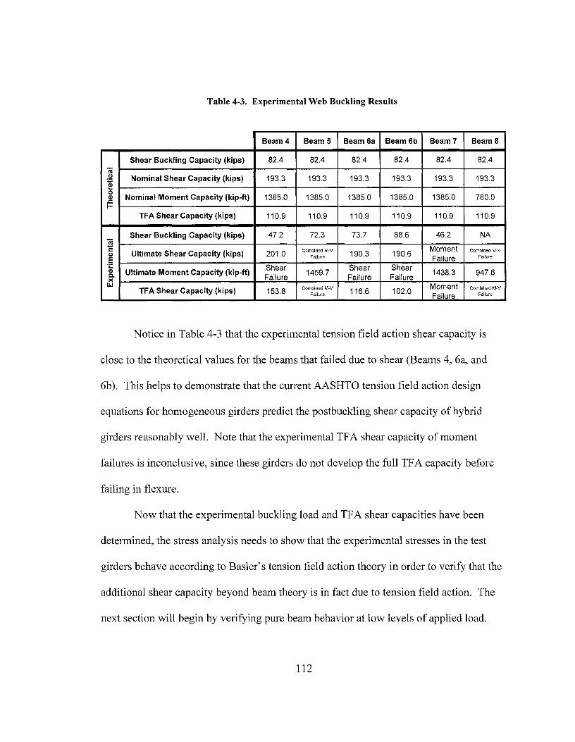
Table 4-3. Experimental Web Buckling Results
Beam4 Beams Beam 6a Beam 6b Beam7 Beam 8
Shear Buckling Capacity (kips) 82.4 82.4 82.4 82.4 82.4 82.4 cu t.) Nominal Shear Capacity (kips) 193.3 193.3 193.3 193.3 193.3 193.3 :;; f 0
Nominal Moment Capacity (kip-ft) 1385.0 1385.0 1385.0 1385.0 1385.0 780.0 Q) .c I-
TFA Shear Capacity (kips) 110.9 110.9 110.9 110.9 110.9 110.9
Shear Buckling Capacity (kips) 47.2 72.3 73.7 88.6 46.2 NA i C: Ultimate Shear Capacity (kips) 201.0 Combined M-V 190.3 190.6
Moment Combined M-V Q) Failure Failure Failure E ·;;: Shear Shear Shear Q) Ultimate Moment Capacity (kip-ft) 1459.7 1438.3 947.6 C. Failure Failure Failure >< w
TFA Shear Capacity (kips) Combined M-V Moment Combined M-V 153.8 Failure 116.6 102.0 Failure Failure
Notice in Table 4-3 that the experimental tension field action shear capacity is
close to the theoretical values for the beams that failed due to shear (Beams 4, 6a, and
6b ). This helps to demonstrate that the current AASHTO tension field action design
equations for homogeneous girders predict the postbuckling shear capacity of hybrid
girders reasonably well. Note that the experimental TF A shear capacity of moment
failures is inconclusive, since these girders do not develop the full TF A capacity before
failing in flexure.
Now that the experimental buckling load and TF A shear capacities have been
determined, the stress analysis needs to show that the experimental stresses in the test
girders behave according to Basler's tension field action theory in order to verify that the
additional shear capacity beyond beam theory is in fact due to tension field action. The
next section will begin by verifying pure beam behavior at low levels of applied load.
112
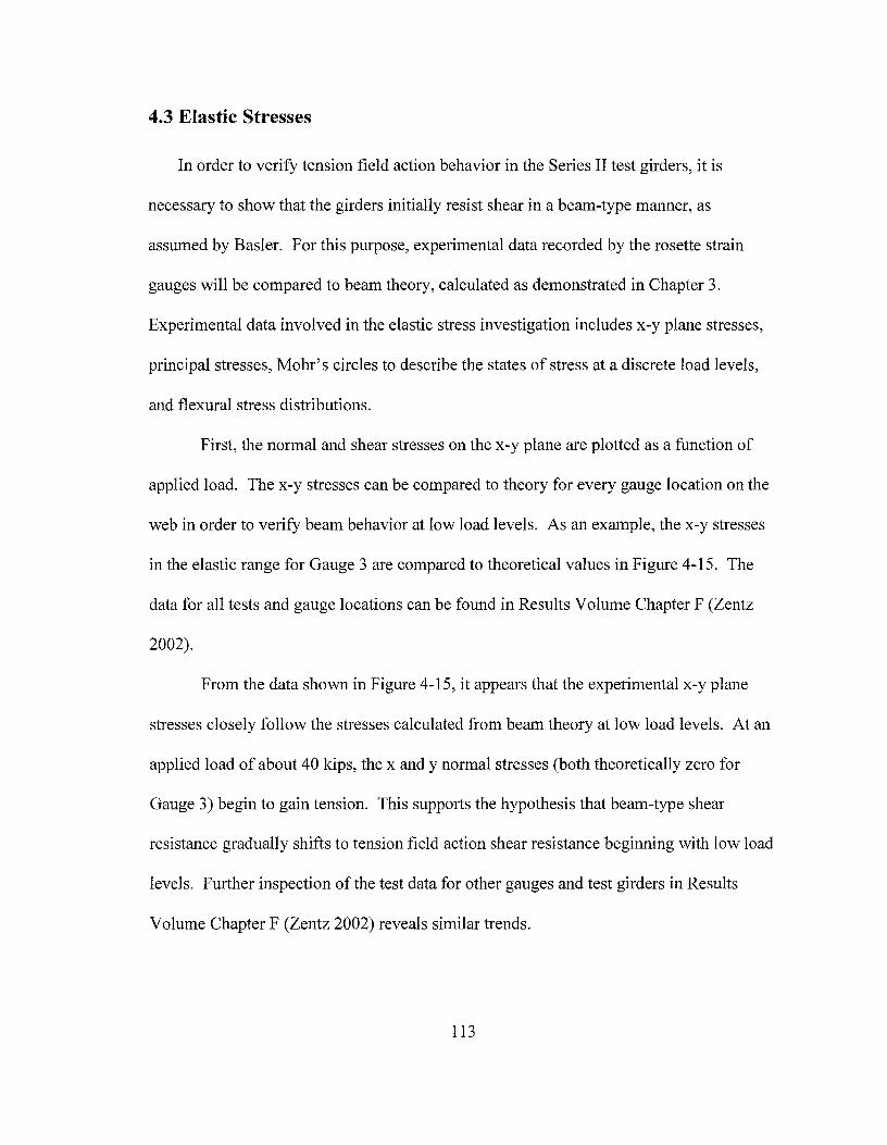
4.3 Elastic Stresses
In order to verify tension field action behavior in the Series II test girders, it is
necessary to show that the girders initially resist shear in a beam-type manner, as
assumed by Basler. For this purpose, experimental data recorded by the rosette strain
gauges will be compared to beam theory, calculated as demonstrated in Chapter 3.
Experimental data involved in the elastic stress investigation includes x-y plane stresses,
principal stresses, Mohr's circles to describe the states of stress at a discrete load levels,
and flexural stress distributions.
First, the normal and shear stresses on the x-y plane are plotted as a function of
applied load. The x-y stresses can be compared to theory for every gauge location on the
web in order to verify beam behavior at low load levels. As an example, the x-y stresses
in the elastic range for Gauge 3 are compared to theoretical values in Figure 4-15. The
data for all tests and gauge locations can be found in Results Volume Chapter F (Zentz
2002).
From the data shown in Figure 4-15, it appears that the experimental x-y plane
stresses closely follow the stresses calculated from beam theory at low load levels. At an
applied load of about 40 kips, the x and y normal stresses (both theoretically zero for
Gauge 3) begin to gain tension. This supports the hypothesis that beam-type shear
resistance gradually shifts to tension field action shear resistance beginning with low load
levels. Further inspection of the test data for other gauges and test girders in Results
Volume Chapter F (Zentz 2002) reveals similar trends.
113
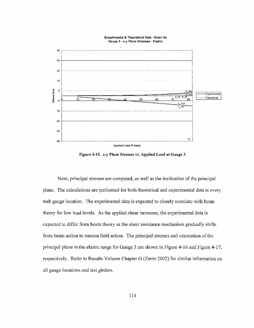
45
35
25
15
·;;; 5 ~
"' "' t -5 I 10 (/)
-15
-25
-35
-45
Experimental & Theoretical Data - Beam 6a Gauge 3 - x-y Plane Stresses - Elastic
'10 50 60
Applied Load, P {kips)
V ~~: cr ex :
70 cr, th. cr, th.
80
'tx exp. ·- · · · t)(; tn.· - - -
Figure 4-15. x-y Plane Stresses vs. Applied Load at Gauge 3
--Experimental
- - - - - -Theoretical
Next, principal stresses are computed, as well as the inclination of the principal
plane. The calculations are performed for both theoretical and experimental data at every
web gauge location. The experimental data is expected to closely correlate with beam
theory for low load levels. As the applied shear increases, the experimental data is
expected to differ from beam theory as the shear resistance mechanism gradually shifts
from beam action to tension field action. The principal stresses and orientation of the
principal plane in the elastic range for Gauge 3 are shown in Figure 4-16 and Figure 4-17,
respectively. Refer to Results Volume Chapter G (Zentz 2002) for similar information on
all gauge locations and test girders.
114
45
35
25
'iii 15 ~· ~
b ,ii
"' i 5 .. E -5 I 0 z oi C. ·;; C: -15 ·;: C.
-25
-35
-45
85
75
ci 65 1---.. ~
"' '" 55 C:
"' ;;: oi C. ·;; 45 C: •;: C.
0 C: 35 0 :;:
"' .5 0 .5 25
15
5 0
10
10
Experimental & Theoretical Data - Beam 6a Gauge 3 Principal Stresses - Elastic
-An 50 60
Applied Load, P (kips)
70 80
Figure 4-16. Principal Stresses vs. Applied Load for Gauge 3
20
Experimental & Theoretical Data - Beam 6a Gauge 3 - Inclination of Principal Plane - Elastic
30 40 50 60
Applied Load, P (kips)
v"
70 80
--Experimental
- - - - - - - Theoretical
--Experimental
- · · • • • Theoretical
Figure 4-17. Orientation of Principal Plane vs. Applied Load at Gauge 3
115

Once again, the experimental data closely correlates with beam theory for low
loads, but begins to gradually deviate from beam theory as the applied load increases. As
expected, the principal stresses begin to become more tensile than beam theory,
consistent with tension field action behavior. Also, the orientation of the principal plane
begins to decrease from the theoretical 45° as tension field stresses begin to develop in
the web along the u-axis. Data from Results Volume Chapter G (Zentz 2002) supports
these findings.
Another way to visualize the relationship of experimental stresses to theoretical
stresses is to use Mohr's circle. Mohr's circle is useful for displaying the complete state
of stress at a given load level. For the elastic region, the experimental Mohr's circle can
be compared to theory at every gauge location. As an example, the Mohr's circle for
stress at Gauge 3 is shown for load levels of 20, 40, 60, and 80 kips in Figure 4-18
through Figure 4-21. Mohr's circle data for other gauge locations and test girders can be
found in Results Volume Chapter H (Zentz 2002).
116
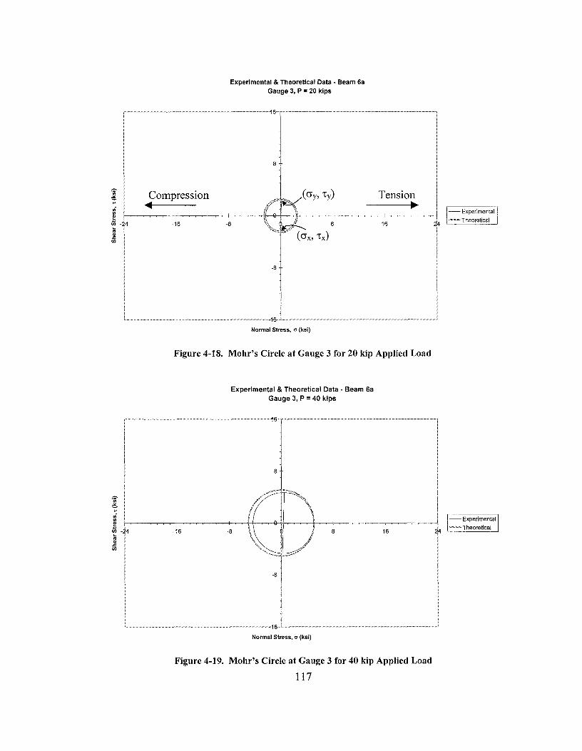
~ .., ui
Compression ◄
-16
Experimental & Theoretical Data - Beam Ga Gauge 3, P = 20 kips
8
Tension ►
-U,---A-l'--,----.-le~-~--+-~--~~~~
-8 8 16
--" ( O"x, 't'x)
-8
Normal Stress, cr (ksi)
Figure 4-18. Mohr's Circle at Gauge 3 for 20 kip Applied Load
Experimental & Theoretical Data - Beam 6a Gauge 3, P = 40 kips
8
- Experimental
4 ·-Theoretical
e 1--_ ~~--~+--~~~-~-+--~-i-,~~___,,__-4-,._~r--1--~-+-~----l--~-~----' - Experimental
-· -Theoretical ~ - '4 -16 -8 8 16
"' " .c VI
-8
'-----------------46···-'-------------------' Normal Stress, cr (ksi)
Figure 4-19. Mohr's Circle at Gauge 3 for 40 kip Applied Load
117
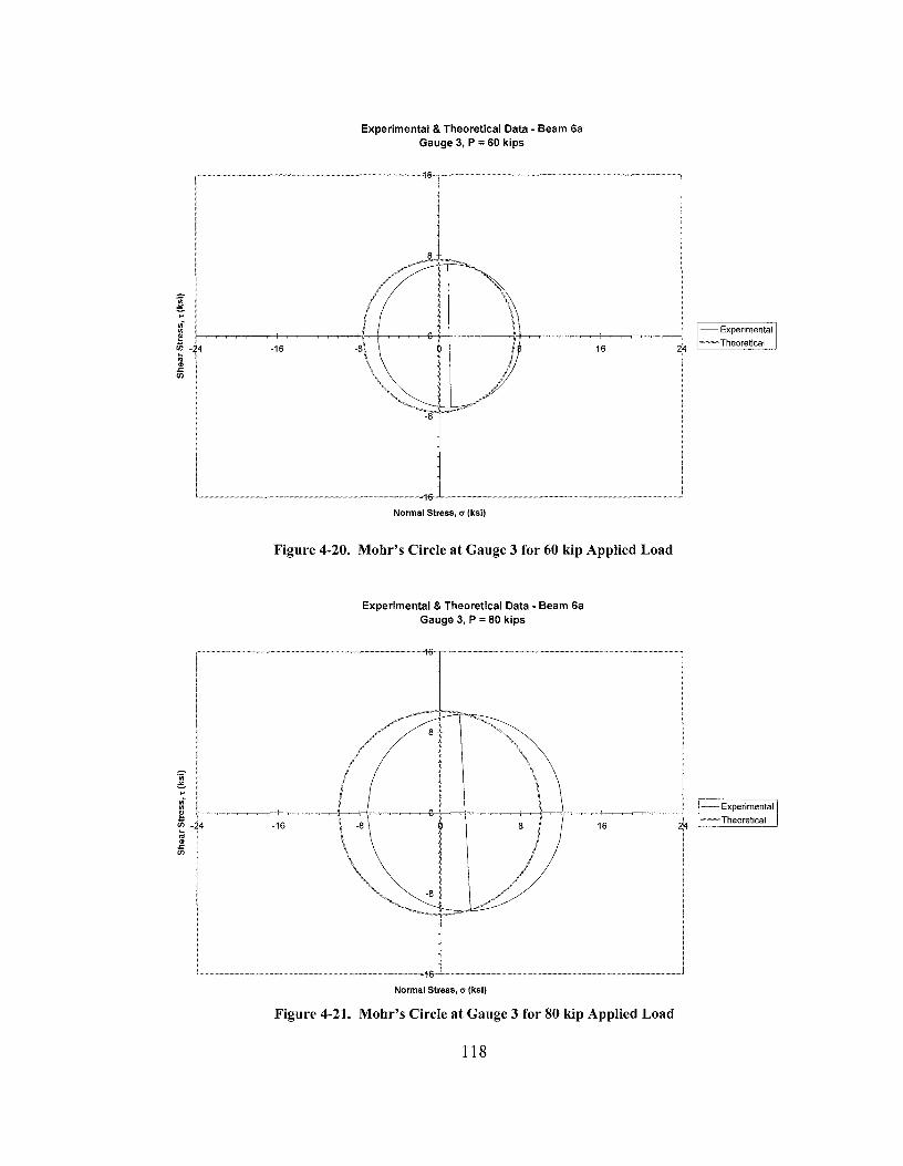
·;;; =-.. .. -"' g
-16
Experimental & Theoretical Data - Beam Ga Gauge 3, P = 60 kips
16
~------------------,£··.,__ ________________ _,
Nonmal Stress, er (ksi)
Figure 4-20. Mohr's Circle at Gauge 3 for 60 kip Applied Load
Experimental & Theoretical Data - Beam Ga Gauge 3, P = 80 kips
r---------------~46--,-------------------,
~ - 4 -16 -8 8 16
"' .. .c en
~--------------~46--~----------------~ Nonmal Stress, er (ksi)
Figure 4-21. Mohr's Circle at Gauge 3 for 80 kip Applied Load
118
- Experimental
---·-Theoretical
- Experimental
-·-Theoretical
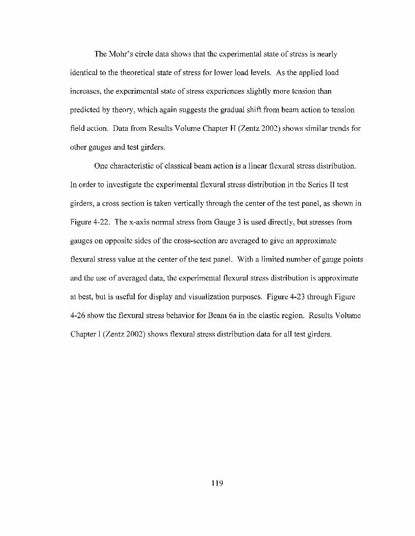
The Mohr's circle data shows that the experimental state of stress is nearly
identical to the theoretical state of stress for lower load levels. As the applied load
increases, the experimental state of stress experiences slightly more tension than
predicted by theory, which again suggests the gradual shift from beam action to tension
field action. Data from Results Volume Chapter H (Zentz 2002) shows similar trends for
other gauges and test girders.
One characteristic of classical beam action is a linear flexural stress distribution.
In order to investigate the experimental flexural stress distribution in the Series II test
girders, a cross section is taken vertically through the center of the test panel, as shown in
Figure 4-22. The x-axis normal stress from Gauge 3 is used directly, but stresses from
gauges on opposite sides of the cross-section are averaged to give an approximate
flexural stress value at the center of the test panel. With a limited number of gauge points
and the use of averaged data, the experimental flexural stress distribution is approximate
at best, but is useful for display and visualization purposes. Figure 4-23 through Figure
4-26 show the flexural stress behavior for Beam 6a in the elastic region. Results Volume
Chapter I (Zentz 2002) shows flexural stress distribution data for all test girders.
119
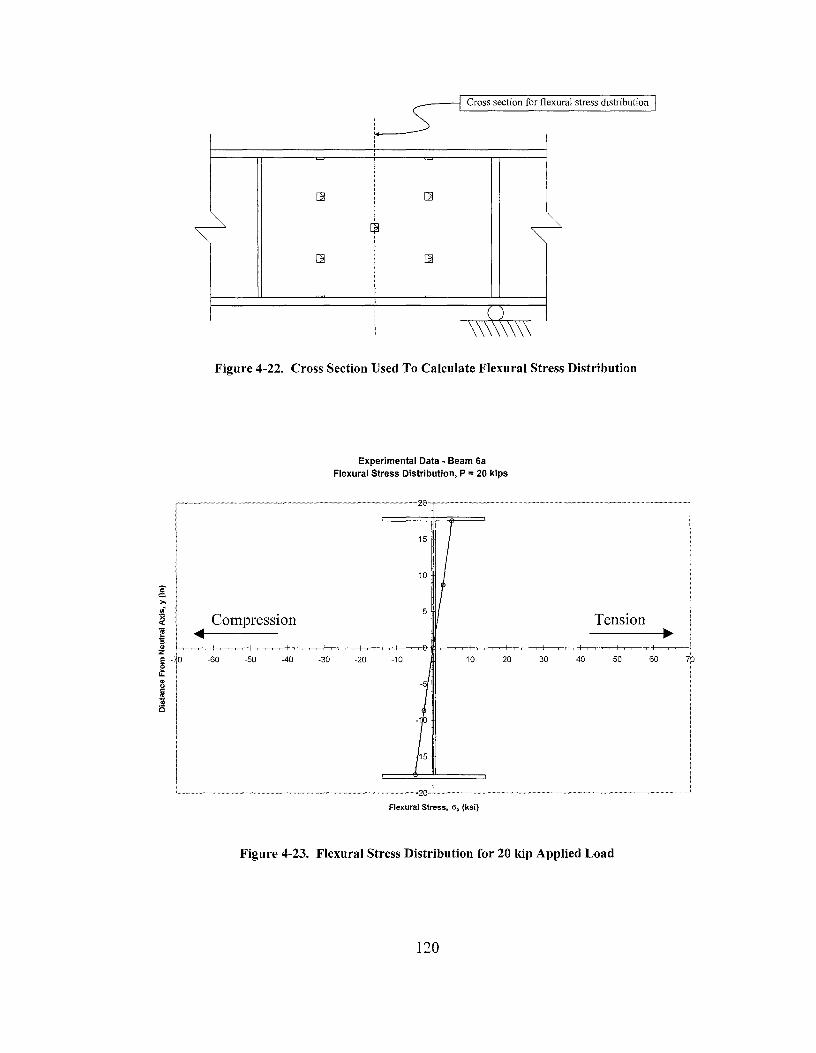
c C >, .. -~
' ' ' ' ' ' ' ' ' ' !
r
-------J Cross section for flexural stress distribution
Figure 4-22. Cross Section Used To Calculate Flexural Stress Distribution
Compression
Experimental Data - Beam Ga Flexural Stress Distribution, P = 20 kips
Tension ~ ... ◄------:i " z E - 0 -60 e u..
" " C:
~ c
+-r-~-r-+~~-.,-+--r-~~~-rlHIJ-~~~~~r-..-+~~-1-r~•
-50 -40 -30 -20 -10 10 20 30
Flexural Stress, cr, (ksi)
+-,---,----,--,--f--
40 50
Figure 4-23. Flexural Stress Distribution for 20 kip Applied Load
120
► 60 7b

Experimental Data - Beam 6a Flexural Stress Distribution, P = 40 kips
r-------------------i2tl··-,---------------------,
g >, ,,; ·;. <(
e '5 ., z E --0 e LL. ., " C:
!S ,,, i:5
-60 -50 -40 -30
15
-20 10 20 30 40 50 60 10
~------------------i20·-~-------------------~
g >, II)
~ e '5 ., z E - O e LL. ., " C:
* i:5
Flexural Stress, er, (ksi)
Figure 4-24. Flexural Stress Distribution 40 kip Applied Load
Experimental Data - Beam 6a Flexural Stress Distribution, P = 60 kips
15
10
+-~~--+--~~~-t-,-~-t--c~--1---r~-,-,f-,-~-----,-+-
-60 -50 -40 -30 -20 -10 10 20
-10
-15
30 40 50 60
~------------------i20··-'----------------------' Flexural Stress, er, (ksi)
Figure 4-25. Flexural Stress Distribution for 60 kip Applied Load
121

I >,
,,;
~ ~ ::,
" z E - O
~ g "' 'iii i5
-60 -50
Experimental Data - Beam Ga Flexural Stress Distribution, P = 80 kips
15
10
5
-40 -30 -20 -10
: -5
Theoretical~: -10
-15
10 20
Experimental
30 40 50 60
c..._ ______________ ..,,,o---'------------------'
Flexural Stress, "x (ksi)
Figure 4-26. Flexural Stress Distribution for 80 kip Applied Load
The experimental flexural stress distribution data is identical to data provided by
beam theory for low load levels. Notice that, as the applied load increases, the
experimental flexural stress at the center of the cross section is more tensile than the
theoretical value. This is the location where the tension strut will develop through this
cross section. Further discussion of this topic will be left until postbuckling stresses are
investigated in Section 4.4. Results are similar for other test girders, as shown in Results
Volume Chapter I (Zentz 2002), with the exception of Beam 4.
During the analysis of data from Beam 4, the flexural stress distribution showed
that the web stresses were not behaving as predicted. As shown in Figure 4-27, the
flexural stress at the center of the test panel, which is theoretically zero, becomes
122
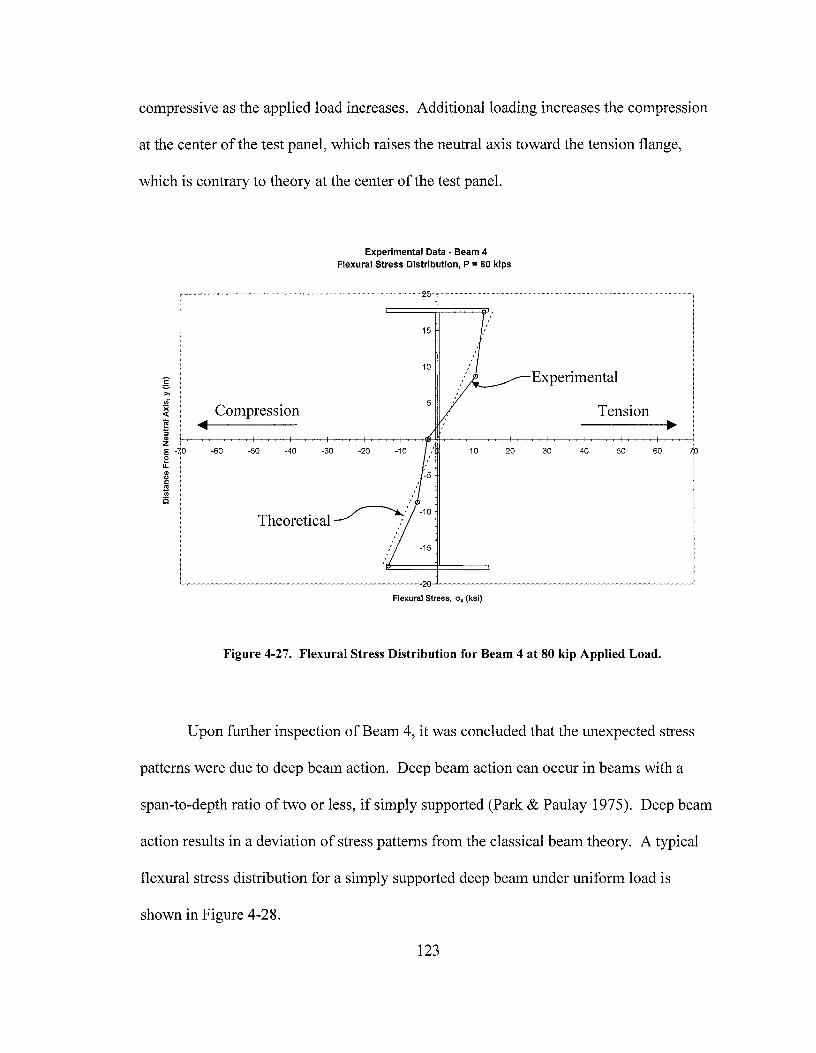
compressive as the applied load increases. Additional loading increases the compression
at the center of the test panel, which raises the neutral axis toward the tension flange,
which is contrary to theory at the center of the test panel.
g >,
,,;
Experimental Data - Beam 4 Flexural Stress Distribution, P = 80 kips
15
10
Experimental
~ Compression 5
Tension e ◄ ► j ~, ~~--+-,--,---+-,_-,-+ __ _,_,__-1-r~•-~·-,--J-r---r+------~~-+-,--,---+-,_-,-+_-r-.,-J
E -to -60 -50 -40 -30 -20 -10 10 20 30 40 50 60 7b e u.
" " C: ~ (/)
c
Theoretical ~:·
-15
~--------------20~--------------~ Flexural Stress, cr, (ksi)
Figure 4-27. Flexural Stress Distribution for Beam 4 at 80 kip Applied Load.
Upon further inspection of Beam 4, it was concluded that the unexpected stress
patterns were due to deep beam action. Deep beam action can occur in beams with a
span-to-depth ratio of two or less, if simply supported (Park & Paulay 1975). Deep beam
action results in a deviation of stress patterns from the classical beam theory. A typical
flexural stress distribution for a simply supported deep beam under uniform load is
shown in Figure 4-28.
123

Uniform Load, w
I I I I I I I I I I I I I I I I I I I I l
T Deep Beam Flexural Stress Distribution
Neutral Axis Shifts Beam Depth, h Tow,ml Te~;,. FIMgo l
1/h < 2.0 Simply Supported 1/h < 2.5 Continuous
i.-1◄1------ Span Length, I
Figure 4-28. Mid-span Flexural Stress Distribution of Simply Supported Deep Beam
Beam 4 has a shear span-to-depth ratio of 65"/36" = 1.81. The flexural stress
distribution for Beam 4 at a load of 160 is shown in Figure 4-29. The experimental
flexural stress distribution resembles the distribution for deep beams shown in Figure
4-28. It is believed that the stress patterns present in Beam 4 are due to deep beam
action. The interaction of deep beam action and tension field action is beyond the scope
of this thesis and will not be investigated here. However, the ultimate shear capacity is
still considered valid since the failure mechanism involved web buckling, formation of a
visible tension strut, and formation of a plastic hinge in the compression flange, which is
consistent with a tension field action shear failure.
124

g >,
.'!i. )( <(
'§ :i .. z ' E -to e 1L .. " C '9 .!!l C
-60 -50 -40 -30
Experimental Data - Beam 4 Flexural Stress Distribution, P = 160 kips
15
10
5
-20 10 20
-15
30 40 50 60
~-------------~20-•~----------------Flexural Stress, o-, (ksi)
Figure 4-29. Flexural Stress Distribution for Beam 4 at 160 kip Applied Load
it)
Several types of data from the elastic range have been presented in this section: x
y plane stresses, principal stresses, Mohr's circles, and flexural stress distributions. The
common trend from all this data is that the test girders behave in a beam manner for low
load levels. However, as applied load increases, the stress patterns begin to gradually
shift from beam behavior to tension field action behavior. This behavior is expected
since web buckling does not occur at a defined load level, but it rather slowly buckles
beginning with initial loading.
125

Basler assumes that transversely stiffened plate girders initially resist shear in a
beam-type manner, and then tension field action resists any shear load beyond the critical
buckling load. The experimental buckling loads have been determined and the elastic
beam stresses have been verified. The next section will investigate the presence of
tension field action stresses in the postbuckling region.
4.4 Postbuckling Stresses
The final step necessary to demonstrate the tension field action shear capacity of the
Series II test girders is to verify that the postbuckling stresses agree with Basler' s tension
field action theory. The data used to verify the postbuckling stresses includes u-v plane
stresses, principal stresses, Mohr's circles, and flexural stress distributions.
Basler's tension field action theory is derived using an element at the neutral axis,
so most of the experimental data used to compare with theory will come from Gauge 3,
located at the center of the test panel. Theory does not provide information in the
postbuckling region on the stress states of elements that are not located on the neutral
axis at the center of a shear panel. Therefore, strain data recorded from gauge locations
other than Gauge 3 is of limited usefulness, since there is no theoretical equivalent with
which to compare.
Recall from Chapter 2 that the theoretical web buckling load is defined as the load
that produces the critical shear buckling stress in an element at the neutral axis. To find
the state of stress at failure, the ultimate tension field stress, cr1, is added to the buckling
state of stress along the u-axis. Basler does not specify how the incremental tension field
stresses develop in the web (i.e. linearly, etc.), so for display purposes, the incremental
126
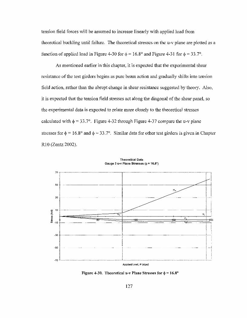
tension field forces will be assumed to increase linearly with applied load from
theoretical buckling until failure. The theoretical stresses on the u-v plane are plotted as a
function of applied load in Figure 4-30 for~= 16.8° and Figure 4-31 for~= 33.7°.
As mentioned earlier in this chapter, it is expected that the experimental shear
resistance of the test girders begins as pure beam action and gradually shifts into tension
field action, rather than the abrupt change in shear resistance suggested by theory. Also,
it is expected that the tension field stresses act along the diagonal of the shear panel, so
the experimental data is expected to relate more closely to the theoretical stresses
calculated with~= 33.7°. Figure 4-32 through Figure 4-37 compare the u-v plane
stresses for~= 16.8° and~= 33.7°. Similar data for other test girders is given in Chapter
Rl 0 (Zentz 2002).
Theoretical Data Gauge 3 u-v Plane Stresses (qi= 16.8°)
70
50
30
·;;; 10
~ V,
"' "' I!! D in -10
-30
-50
-70 ______________________ _,_ ___________________ _,__,
Applied Load, P (kips)
Figure 4-30. Theoretical u-v Plane Stresses for cp = 16.8°
127
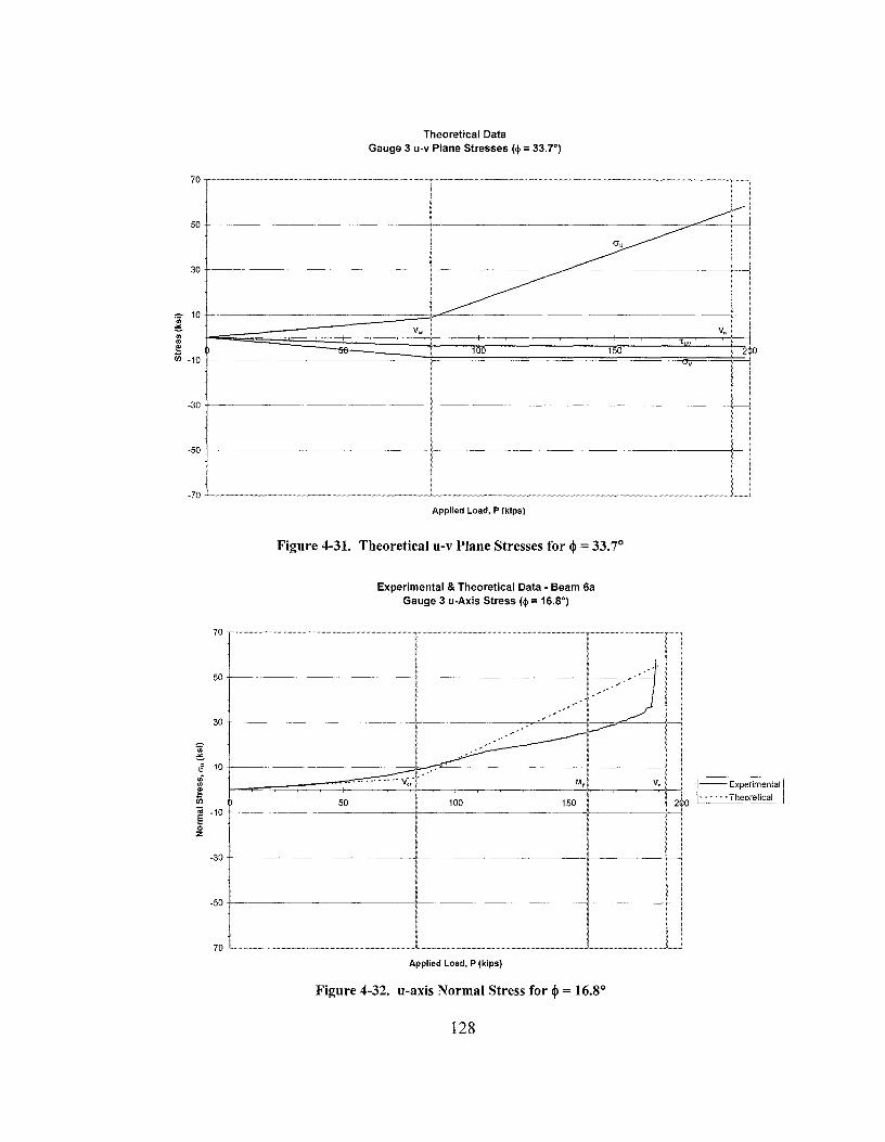
~ II) II)
E
70-r--------
10
Theoretical Data Gauge 3 u-v Plane Stresses (cj> = 33.7°)
V., V,
In -10 100 150
-30 +------------------+----~------------------1-----l
70
50
30
·;;; ~
e 10 ui II)
E In .; -10 e 0 z
-30
-50
-70
~-
--
Applied Load, P (kips)
Figure 4-31. Theoretical u-v Plane Stresses for cl>= 33.7°
Experimental & Theoretical Data - Beam 6a Gauge 3 u-Axis Stress (cj> = 16.8°)
!---.===;:==:;:::::::;:=:;·::·::::· ·::_· ~--~-·:_:·~-·::_·!_v,_~;ll·_· -~---+----------+-~M".'.J, L---~v':'-, LJ --Experimental
~ 100 150 l • • • • • • Theoretical
f" I
Applied Load, P (kips)
Figure 4-32. u-axis Normal Stress for cl>= 16.8°
128

70
50
30
·;;;
=--o 10 ,,; "' E iii .; -10 e 0 z
-30
-50
-70
70
50
30
·;;;
=-,; 10 ui "' E iii .. -10 e 0 z
-30
-50
-70
I 50
Experimental & Theoretical Data - Beam 6a Gauge 3 u-Axis Stress {cj) = 33.7°)
100 150
Applied Load, P (kips)
Figure 4-33. u-axis Normal Stress for <I>= 33.7°
Experimental & Theoretical Data - Beam 6a Gauge 3 v-Axis Stress {cj) = 16.8°)
Applied Load, P (kips)
Figure 4-34. v-axis Normal Stress for <I>= 16.8°
129
21 0
--Experimental
· · · · · · Theoretical
--Experimental
· · · · · • Theoretical

70
50
30
·.; ~ ., 10 ii ,,, ~ /ii ;;; -10 E 0 z
-30
-50
-70
70
50
30
·.; ~ ;; 10
ii ,,, ~ ~ -10 "' ., .c UJ
-30
-50
-70
Experimental & Theoretical Data - Beam 6a Gauge 3 v-Axis Stress (cl>= 33.7°)
V,,
Applied Load, P (kips)
Figure 4-35. v-axis Normal Stress for q, = 33.7°
Experimental & Theoretical Data - Beam 6a Gauge 3 u-v Plane Shear Stress (cl>= 16.8°)
Applied Load, P (kips)
Figure 4-36. u-v Plane Shear Stress for q, = 16.8°
130
V, --Experimental
• · · · · · Theoretical

·;;; -"
Experimental & Theoretical Data - Beam 6a Gauge 3 u-v Plane Shear Stress (<I>= 33.7°)
70 -.--------------.----------~~---~
} 10 +-------------+----------------le---------->--------1
:z"' Ver My Vn -- Experimental
~ 50 ,ou -···-·-···150--- 2~0 ······Theoretical :U -10 +--------------+--------------ll--~--.--,---1 ., .t: (f)
-50
-70 -'-----------~----------''----
Applied Load, P (kips)
Figure 4-37. u-v Plane Shear Stress for qi = 33. 7°
From the u-v plane stress data, it appears that the experimental data matches the
theoretical data reasonably well. As expected, the transition from beam action to tension
field action is more gradual for the experimental data than the theoretical data. Also, the
experimental data appears to more closely resemble the theoretical data for~= 33.7°.
This is especially true for the shear stress on the u-v plane, which was used to determine
the experimental web buckling load in Section 4.2.4. Data from Results Volume Chapter
J (Zentz 2002) gives similar results.
Next, principal stresses can be easily calculated from the u-v plane stresses above
and plotted against theoretical values. More importantly, the inclination of the principal
plane can also be computed and compared to theory. Since an element located at the
neutral axis is theoretically subject to pure shear prior to buckling, the inclination of the
131

principal plane for this element should theoretically be 45° from the horizontal (x-axis).
As tension field stresses become more prominent, the inclination of the principal plane
should asymptotically approach the angle at which the tension field stresses are acting.
This should verify the angle at which tension field stresses act. Figure 4-38 through
Figure 4-43 compare the principal stresses and angles for~= 16.8° and~= 33.7°.
Similar data for all test girders can be found in Results Volume Chapter K (Zentz 2002).
'iii ::. .; ,,; "' I!! 1ii ;;; C. ·;:; " ;f ~ 'io :;;
30
10
-10
-30
Experimental & Theoretical Data - Beam 6a Gauge 3 Major Principal Stress(~= 16.8°)
i...,ee;:::::::-;_::=::;:::::__--+-_~~..!._v~., ~-+---~-----+-_.:!_M14~---~vi" __j --Experimental
D 50 100 150 2~0 · · · · - · Theoretical
+---------------al-------~-------->---·---'---!
-50 ------------+--~--------½-----------1!~ -1
l -10 --··------------'----------·--'------"-! _,
Applied Load, P (kips)
Figure 4-38. Major Principal Stress for <I>= 16.8°
132
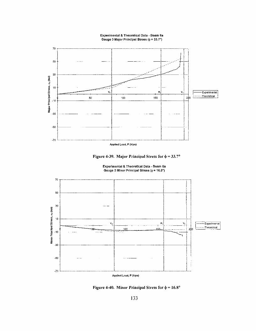
70
50
30 ·;;; =-.; ui 10 "' E iii ;;; Q. ·;:; C -10 ~ :s 'ii :;;
-30
D 50
Experimental & Theoretical Data - Beam 6a Gauge 3 Major Principal Stress (ip = 33.7°)
VcrJ
100 150
V,
I
-70 ~-------------~------------~-----~!~
70
50
30 ·;;; =-b ui
10 "' _g rJ)
;;; Q. ·;:;
-10 C ·c: a. ~
0 C
~ -30
-50
-70
Applied Load, P (kips)
Figure 4-39. Major Principal Stress for <I> = 33. 7°
Experimental & Theoretical Data - Beam 6a Gauge 3 Minor Principal Stress (ip = 16.8°)
-~-~··i I
100
-t----------------1---------------+--------r-
1 I ;
Applied Load, P (kips)
Figure 4-40. Minor Principal Stress for q> = 16.8°
133
--Experimental
· · · · · · Theoretical
--Experimental
· · · - - -Theoretical
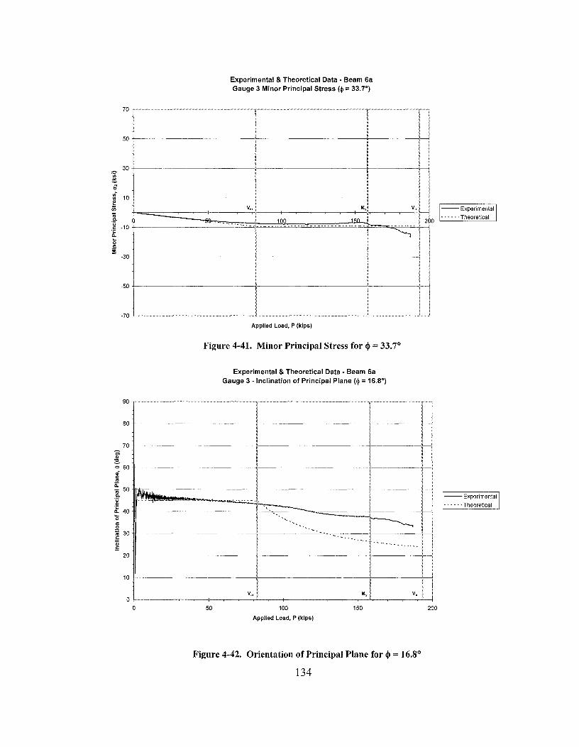
70
50
30 'iii
=-6 ,,;
10 "' ~ .; C. ·;:;
-10 C
~ ~ C
~ -30
-50
-70
90
80
70 ci " ~ <%> 60 .; C ., a: .; 50 C. ·;:; .5 n. 40 -0 C 0 :;:,
30 ., .5 u .!:
20
10
0
~ . e. -
Experimental & Theoretical Data - Beam 6a Gauge 3 Minor Principal Stress(<!>= 33.7°)
M,
Applied Load, P (kips)
Figure 4-41. Minor Principal Stress for q> = 33.7°
Experimental & Theoretical Data - Beam 6a Gauge 3 - Inclination of Principal Plane(<!>= 16.8°)
----ft-----~-----------l-~-~-- - - .-. -- . ·-. I!----------
0 50 100 150
Applied Load, P (kips)
Figure 4-42. Orientation of Principal Plane for q> = 16.8°
134
200
--Experimental
· · · · - · Theoretical
--Experimental
· · · · · · Theoretical
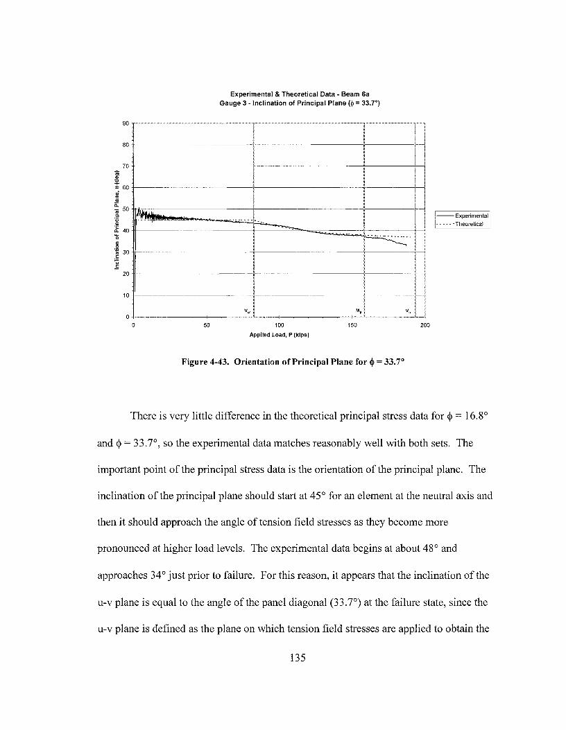
90
80
70 ci " ~ "' 60 ,,· C .. ii:
50 .; a. ·u C
;f 40 'o C 0 ,:, 30 .. . 5 u .5
20
10
0 0
11~. "· .L.
50
Experimental & Theoretical Data - Beam Ga Gauge 3 - Inclination of Principal Plane (<I>= 33.7°)
i__:.- ·-. - • - - -
100 150
Applied Load, P (kips)
Figure 4-43. Orientation of Principal Plane for <I>= 33.7°
200
--Experimental
· · · · · · Theoretical
There is very little difference in the theoretical principal stress data for~= 16.8°
and~= 33.7°, so the experimental data matches reasonably well with both sets. The
important point of the principal stress data is the orientation of the principal plane. The
inclination of the principal plane should start at 45° for an element at the neutral axis and
then it should approach the angle of tension field stresses as they become more
pronounced at higher load levels. The experimental data begins at about 48° and
approaches 34° just prior to failure. For this reason, it appears that the inclination of the
u-v plane is equal to the angle of the panel diagonal (33.7°) at the failure state, since the
u-v plane is defined as the plane on which tension field stresses are applied to obtain the
135
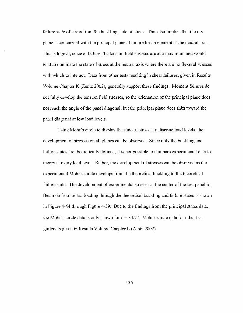
failure state of stress from the buckling state of stress. This also implies that the u-v
plane is concurrent with the principal plane at failure for an element at the neutral axis.
This is logical, since at failure, the tension field stresses are at a maximum and would
tend to dominate the state of stress at the neutral axis where there are no :flexural stresses
with which to interact. Data from other tests resulting in shear failures, given in Results
Volume Chapter K (Zentz 2002), generally support these findings. Moment failures do
not fully develop the tension field stresses, so the orientation of the principal plane does
not reach the angle of the panel diagonal, but the principal plane does shift toward the
panel diagonal at low load levels.
Using Mohr's circle to display the state of stress at a discrete load levels, the
development of stresses on all planes can be observed. Since only the buckling and
failure states are theoretically defined, it is not possible to compare experimental data to
theory at every load level. Rather, the development of stresses can be observed as the
experimental Mohr's circle develops from the theoretical buckling to the theoretical
failure state. The development of experimental stresses at the center of the test panel for
Beam 6a from initial loading through the theoretical buckling and failure states is shown
in Figure 4-44 through Figure 4-59. Due to the findings from the principal stress data,
the Mohr's circle data is only shown for~= 33.7°. Mohr's circle data for other test
girders is given in Results Volume Chapter L (Zentz 2002).
136

Experimental & Theoretical Data - Beam 6a Gauge 3, P = 20 kips (<I>= 33.7°)
i ... (crv, "Cv) I~ --. ~~~~---+----~ ~ - 'o : .r::: Cl)
-60 30 60
'---------------·-----R,&
-60
Normal Stress, a (ksi)
Figure 4-44. Mohr's Circle at 20 kip Applied Load
Experimental & Theoretical Data - Beam 6a Gauge 3, P = 40 kips (<I>= 33.7°)
-30
Normal Stress, a (ksi)
60
Figure 4-45. Mohr's Circle at 40 kip Applied Load
137
Basler Buckling
-- Basler Failure
- Experimental
Basler Buckling
--Basler Failure
- Experimental

-60 -30
Experimental & Theoretical Data - Beam 6a Gauge 3, P = 60 kips (<I>= 33.7°)
30 60
Basler Buckling , Basler Failure
9b -Experimental
'------------------fi,O"-'------------------_____, Normal Stress, " (ksi)
Figure 4-46. Mohr's Circle at 60 kip Applied Load
Experimental & Theoretical Data - Beam 6a Gauge 3, P = 80 kips (<I>= 33.7°)
'------------------,60--'-----------------Normal Stress, " (ksi)
Figure 4-47. Mohr's Circle at 80 kip Applied Load
138
Basler Buckling
Basler Failure
- Experimen~

Experimental & Theoretical Data - Beam 6a Gauge 3, P = 100 kips(~= 33.7°)
30
Basler Buckling
"""'"' Basler Failure
- Experimental
'-------------------f\O"-~----------------~
-60
Normal Stress, CJ (ksi)
Figure 4-48. Mohr's Circle at 100 kip Applied Load
Experimental & Theoretical Data - Beam 6a Gauge 3, P = 120 kips(~= 33.7°)
-30
Normal Stress, CJ (ksi)
60
Figure 4-49. Mohr's Circle at 120 kip Applied Load
139
Basler Buckling
--Basler Failure
9lO - Experimental

-60
Experimental & Theoretical Data - Beam 6a Gauge 3, P = 140 kips (<I>= 33.7°)
-30
Basler Buckling
-- - -· Basler Failure
- Experimental
---------------6·0··~----------------~
-60
Normal Stress, cr (ksi)
Figure 4-50. Mohr's Circle at 140 kip Applied Load
Experimental & Theoretical Data - Beam 6a Gauge 3, P = 160 kips (<I>= 33.7°)
-30
-----t>60-~--------------Normal Stress, cr (ksi)
Figure 4-51. Mohr's Circle at 160 kip Applied Load
140
· ·- Basler Buckling
••·• ····Basler Failure
9b - Experimental
·;;;
=-... qj II)
~ i
~ - 0
"' " .c rJl
-60 -30
Experimental & Theoretical Data - Beam Ga Gauge 3, P = 180 kips (<I>= 33.7°)
60
'-------------------nO·-~----------------~
·;;;
=-... qj II)
I!! ~ - 'o "' " .c rJl
-60
Normal Stress, CJ (ksi)
Figure 4-53. Mohr's Circle at 180 kip Applied Load
-30
Experimental & Theoretical Data - Beam Ga Gauge 3, P = 190 kips (Failure) (<I>= 33.7°)
Normal Stress, CJ (ksi)
Figure 4-52. Mohr's Circle at 190 kip Applied Load (Failure)
141
9D
Basler Buckling
---·Basler Failure
- Experimental
Basler Buckling
---·-· Basler Failure
The experimental Mohr's circle data agrees reasonably well with Basler's tension
field action theory using~= 33.7°. Note that the experimental v-axis state of stress
increases with applied load until it is nearly concurrent with the Basler buckling state of
stress, and then remains stationary, consistent with Basler's theory. Also notice that the
u-v plane approaches the principal plane as the girder nears failure. Data from other test
girders displays similar results (see Results Volume Chapter L (Zentz 2002)).
As with elastic stresses, the flexural stress distribution can also be a useful display
tool for postbuckling stresses. Even though it is qualitative, the flexural stress
distribution is useful for demonstrating the effect of tension field action stresses on the
cross section. With more gauge locations, it would also be possible to measure the
experimental tension field bandwidth as the tension field develops. However, with only a
few gauge locations as in the Series II tests, the bandwidth cannot be measured, but the
effects of the tension field on the flexural stress distribution can be visualized. Figure
4-54 through Figure 4-59 show development of flexural stresses from an applied load of
100 kips through failure. Refer to Section 4.3 for flexural stress data at lower levels of
applied load. Complete flexural stress data for all tests is given in Results Volume
Chapter I (Zentz 2002).
142

;[ >,
ui ·;. <(
~ :, 0,
z E e
LI.. 0,
" C
:I "' i5
~ >,
ui
~ e :i 0,
z
- 0 -60 -50 -40 -30
Experimental Data - Beam Ga Flexural Stress Distribution, P = 100 kips
15
10
5
-20 -10 10 20
-10
-15
30 40 50 60 70
~------------------20··-'--------------------~ Flexural Stress, er, (ksi)
Figure 4-54. Flexural Stress Distribution for 100 kip Applied Load
Experimental Data - Beam Ga Flexural Stress Distribution, P = 120 kips
~-------------------ii&·~------------------~
15
10
5
-+-·--r-+-----+------+--,--·➔-m~~
E - 0 e -60 -50 -40 -30 -20 -10 20 30 40 50 60 10 LI.. 0,
" C :I ,!/l C
-10
-15
'--------------------20·-'---------------------.J Flexural Stress, er, (ksi)
Figure 4-55. Flexural Stress Distribution for 120 kip Applied Load
143
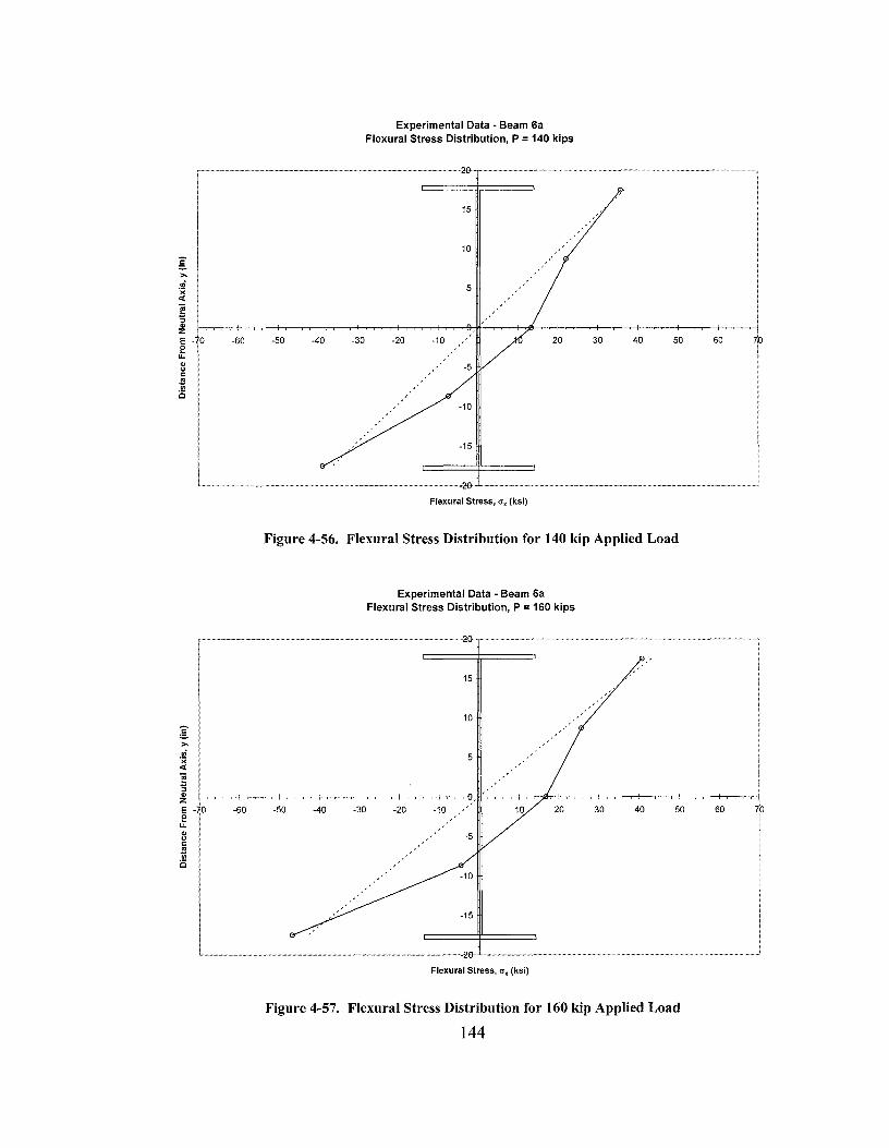
.i ~ ~ ::, ., z
Experimental Data - Beam 6a Flexural Stress Distribution, P = 140 kips
~-------------------20-.--------------------
15
10
E - 0 e
-60 -50 -40 -30 -20 -10 30 40 50 60 io LL ., " C
.B
.!!? C
;[ >,
,,;
~ ~ ::,
-5
-10
-15
'------------------------20--·-'--------------------_..J Flexural Stress, cr, (ksi)
Figure 4-56. Flexural Stress Distribution for 140 kip Applied Load
Experimental Data - Beam 6a Flexural Stress Distribution, P = 160 kips
~------------------0---------------------~
15
10
5
~ t-l ---+-----+-,---1--r-~-t--r--,-,1--,---.-+-r-r-l+-!!1-'.....----.--.-----.-T"-f/>,-+----l----+--.---+-r--t--r-~
E -70 -60 -50 -40 -30 -20 -10 10 20 30 40 50 60 10 e LL ., " C .B .!!? C
-5
-10
-15
'--------------------&·-'---------------------' Flexural Stress, cr, (ksi)
Figure 4-57. Flexural Stress Distribution for 160 kip Applied Load
144

g >, , .. ·;. <t °E '5 " z E • 0 e LL
" " C: .l!! <I)
i5
-60
Experimental Data • Beam 6a Flexural Stress Distribution, P = 180 kips
15
40 50 60 to
~--------------------'20·-~------------------~ Flexural Stress, er, (ksi)
Figure 4-58. Flexural Stress Distribution for 180 kip Applied Load
Experimental Data - Beam 6a Flexural Stress Distribution, P = 190 kips (Failure)
,--------------------0--.,-----------------------,
[ >,
.i >< <t
~ ::,
" Z I
E -70 e
LL
" " C:
~ i5
-60 -50 -40 -30
15
10
5
-20 -10 10 50 60 io
.5
~------------------,!}--~-------------------~ Flexural Stress, er, (ksi)
Figure 4-59. Flexural Stress Distribution for 190 kip Applied Load (Failure)
145

For a qualitative comparison, it is assumed that the flexural stress effects from
beam and tension field action can be superimposed. As shown in Figure 4-60, the linear
flexural stress distribution is added to the x-axis component of Basler's assumed tension
field, resulting in the flexural stress distribution shown. Given the few data points
available for the Series II tests, the theoretical distribution resembles the experimental
distribution as the girder nears failure.
Cross Section Tension Field Pure Beam Flexural Combined Flexural Stress Component of Flexural Stress
Tension Field Distribution
Figure 4-60. Theoretical Flexural Stress Distribution from Superposition
Experimental data including u-v plane stresses, principal stresses, Mohr's circles, and
flexural stress distributions have been used to verify the postbuckling stresses in the
Series II test girders. The stresses generally correspond reasonably well with Basler's
tension field action theory, with the exception that the angle of inclination of the u-v
plane was found to be equal to the diagonal angle of the shear panel.
146

4.5 Impact of TFA in Hybrid Girders
Goessling (2002) examined the impact of allowing tension field action and
eliminating the moment-shear interaction reduction on a suite of typical steel girder
bridges. She designed 16 bridges and determined the number of intermediate shear
stiffeners required for various bridge configurations (Table 4-4). The spans varied
between two and three with two different span length combinations each. She considered
girder spacing in terms of number of girders, and web slenderness ratios.
Table 4-4. Stifffener Design Using TFA in Hybrid Girder Bridges
50 ksi HPS70W Bridge # of Girders Steel Steel
2 Span tons tons
7 186.2
120'-120' 8
183.1
'· 1'.9i4 11
7 290.7
160'-160' 8
327.8
3 Span
D/tw NoTFA
#
TFA
#
# of Stiffeners saved
Stiffeners Stiffeners using TFA
120.9 42 28 14
120 80 48 32 "J,Bf~M-4'lf ap / E er ,:;:12
120 42 28 14
120 32 32 0
120.9 84 56
% Saved $ Saved . $200 per
using TFA stiffener
33.3% $2,800
40.0% $6,400 . 2S:6% $6,400
33.3% $2,800 33.3% $8,400
0.0% $0 42.9% $9,600
7 608.2 28 33.3% $5,600
120,_150,_120,1-------1-..a:·s;.,i;s:,:5::..:7-=a.'"">--i-:;.~~-1--:....:..::..---4_=~-1--__:__:;=---1--....:1=2a:::......_;,"'-·:c;µ,If[!J;w,i::.:i'5=.•~::.::-9.!!%:t-z:$2:.::5::=,2::::.oo~ 607.5 32 22.2% $6,400
!')';'\j''{','V .,! 1:40' 238 112 120 144 112
8 "'2648.'.h. 64;,irfi.i,)); .,,,,. '""'$""%+--=-$1-:-::2~.8:-::cO-:::-tO · •. '.; .. ,, 140 192 128
7 1100.6 120.7 56 28 28 50.0% $5,600
160'-200'-160'1-------1-="!:ili';0~7,:.5 .. ""9'""· ·F'l;:S:"",,,W;.i;<..._•;··;;... ·•+l·•-.:.14.:.;:0:..:;:J:..-;..il_.:;;15:;..;4~-l---4.:.;:2:..,_-1--....:1..:.;12::..\;;...\ =F'[!;'.=';%Wi'li.z:.::;~l.:.:.:%4-z:$2==2:.c.:,4::::.00~
8 1105.1 120 64 64 0 0.0% $0
Goessling compares the total number of stiffeners required, including bearing
stiffeners, for restricting the hybrid designs to the shear buckling capacity (no TF A) with
the reduced number required if TF A is allowed without a reduction for moment-shear
interaction. She assumes a stiffener cost of $200 per stiffener to arrive at a total savings.
In addition to fewer details and a more consistent design, the savings can be significant.
147
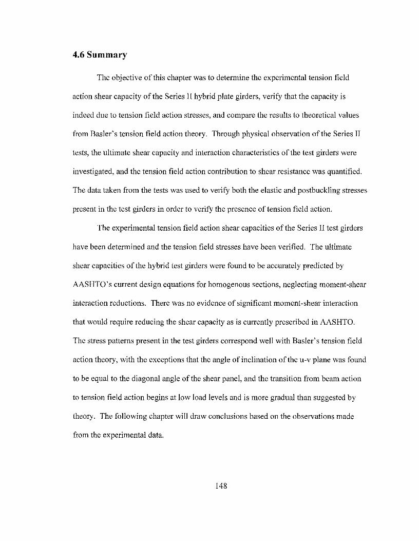
4.6 Summary
The objective of this chapter was to determine the experimental tension field
action shear capacity of the Series II hybrid plate girders, verify that the capacity is
indeed due to tension field action stresses, and compare the results to theoretical values
from Basler's tension field action theory. Through physical observation of the Series II
tests, the ultimate shear capacity and interaction characteristics of the test girders were
investigated, and the tension field action contribution to shear resistance was quantified.
The data taken from the tests was used to verify both the elastic and postbuckling stresses
present in the test girders in order to verify the presence of tension field action.
The experimental tension field action shear capacities of the Series II test girders
have been determined and the tension field stresses have been verified. The ultimate
shear capacities of the hybrid test girders were found to be accurately predicted by
AASHTO's current design equations for homogenous sections, neglecting moment-shear
interaction reductions. There was no evidence of significant moment-shear interaction
that would require reducing the shear capacity as is currently prescribed in AASHTO.
The stress patterns present in the test girders correspond well with Basler' s tension field
action theory, with the exceptions that the angle of inclination of the u-v plane was found
to be equal to the diagonal angle of the shear panel, and the transition from beam action
to tension field action begins at low load levels and is more gradual than suggested by
theory. The following chapter will draw conclusions based on the observations made
from the experimental data.
148

Chapter 5 - Summary and Conclusions
5.1 Summary
High Performance Steel, in particular HPS70W, has been used in hundreds of
bridges across the United States. A large percentage of these bridges have used the HPS
in the form of hybrid girder designs. Bridge studies (Barker and Schrage 2000) have
shown that the most beneficial use ofHPS70W (70 ksi) is in the flanges of hybrid girders
with 50 ksi webs. One limit with hybrid girder design, which decreases the beneficial
aspects, is that tension field action (TF A) is not allowed when determining the shear
capacity. This is a severe shear capacity penalty for using hybrid girders. Limiting
hybrid shear capacities to the shear buckling capacity results in more transverse stiffeners
required ( closer spacing) for a hybrid girder than that for a homogeneous girder. This not
only increases material costs, but significantly increases fabrication costs.
The objective of this research is to validate the tension field action behavior in hybrid
plate girders. The goal is to allow TF A in hybrid girders resulting in more economical
design of steel bridges.
The work conducted for this research covers several topics in tension field action
and moment-shear interaction of plate girders. The first effort concentrated on the
original shear capacity theoretical derivations (Basler 1961a) and the impact of using
hybrid girders. Proposed theoretical lower bound shear capacity procedures were
developed for moment-shear interaction that represent the equivalent AASHTO equations
for hybrid girders (Barker et al 2002, Hurst 2000).
149
Two series of tests were designed (Hurst 2000) and tested to determine the hybrid
girder shear capacity and study the tension field behavior of homogeneous and hybrid
girders. Series I test specimens were homogeneous and hybrid girders tested under high
shear and low moment conditions. Results from Series I testing are published in two
separate theses (Schreiner 2001, Rush 2001). Series II test specimens were designed and
tested to study the effect of moment-shear interaction. Results from Series II testing are
published in two separate theses (Zentz 2002, Davis 2002). Finally, Goessling (2002)
studied an array of practical bridge designs to study the impact of allowing TF A in hybrid
girders.
This report includes a thorough presentation of tension field action and moment
shear interaction in plate girders, and in particular hybrid plate girders. It presents a
comprehensive presentation on the Series II test girders with a detailed analysis and
examination of the test behaviors. The report only uses the overall results of the Series I
test girders.
In this Summary, there are a few important results that need to be presented
clearly. Hybrid steel girders exhibit tension field action according to current AASHTO
shear capacity provisions. Using the original moment-shear interaction derivations, this
research has produced a theoretical lower-bound moment-shear interaction equation for
hybrid girders that is equivalent to the current AASHTO moment-shear interaction
requirement for homogeneous girders. However, the results of the experimental tests
have also shown that there is no moment-shear interaction for these plate girders.
Aydemir (2000) agrees after many finite element analyses of a parametric suite of plate
girders. Table 5-1 summarizes the Series I and Series II test girder results. All of the
150

tests show that hybrid girders exhibit tension field action according to the current
AASHTO specifications. Figure 5-1 shows the test results plotted against the AASHTO
and proposed hybrid girder moment-shear interaction requirements. The girders all
demonstrated that the capacities exceeded expectations and that a moment-shear
interaction reduction is not necessary.
Table 5-1. Tension Field Action Experimental Results
BEAM Test V/Vn M/Mn Theoretical Experimental Remarks Girder Total Shear Shear Capacity (failure
Capacity (kips) (kips) mode)
- 1 50-50 1.07 193 205 Shear Cll 2 70-70 >1.05 208 >218 Shear (I) .....
Low I-< 3a 50-70 1.10 193 211 Shear (I) r:/)
3b 50-70 1.08 193 207 Shear 4 50-70 1.04 0.79 193 201 Shear
- 5 50-70 0.78 1.05 193 151 Moment -Cll 6a 50-70 0.98 0.93 193 190 Shear (I) ..... 6b 50-70 0.99 0.93 193 191 Shear I-<
(I) r:/)
7 50-70 0.45 1.04 193 86 Moment 8 50-50 0.95 1.16 193 183 Mom/Shear
1.2
50-70 50-70 ♦ 50-50
1 ♦ -Barker
50-70 -AASHTO 0 50-70 • 50-50
0.8 Current Extended • 50-70
50-70 Capacity Capacity • 70-70
C: 50-70 Hybrid • 50-70 I o.6
• 50-50 ♦ 50-50
• 50-70 0.4 ---50-10
• • 50-70 • 50-70 • 50-70
0.2 70-70 -- ♦ 50-70 No Fail ■ 50-70
0
0 0.2 0.4 0.6 0.8 1 1.2
VNn
Figure 5-1. Test Results Compared to AASHTO & Proposed Moment-Shear Interactions
151

5.2 Project Conclusions and Recommendations
This research, in conjunction with research at Georgia Tech (Aydemir 2000), found
that tension field action shear capacity is fully applicable to hybrid girders. The
AASHTO shear capacity equations are accurate for hybrid girders and that there is not a
moment-shear interaction for any plate girder, whether homogeneous or hybrid.
Allowing tension field action in hybrid plate girders and removing the moment-shear
interaction for all plate girder designs would be a major advancement for steel bridge
design.
152
References
AASHTO, (1998), LRFD Bridge Design Specifications, 2nd Edition, American
Association of State Highway and Transportation Officials, Washington, D.C.
Aydemir, Murat, (2000), "Moment Shear Interaction in HPS Hybrid Plate Girders,"
Master's Thesis, Georgia Institute of Technology.
Barker, M.G., and Schrage, S.D., (2000), "High Performance Steel Bridge Design and
Cost Comparison," Transportation Research Record No. 1740, Transportation
Research Board, Washington, D.C., pp 33-39.
Barker, M.G., Hurst, A.M., and White, D.W., (2002), "Tension Field Action in Hybrid
Steel Girders," AISC Engineering Journal, American Institute of Steel
Construction, Vol. 39, No. 1, 1st Quarter, pp 52-62.
Barth, K.E., White, D.W. and Bobb, B. (2000), "Negative Bending Resistance of HPS
70W Girders," Journal of Constructional Steel Research, 53(1), pp. 1-31.
Basler, Konrad, (1961a), "Strength of Plate Girders in Shear," ASCE J Struct. Div., Vol.
87, No. ST7, pp. 151-180.
Basler, Konrad, (1961b), "Strength of Plate Girders Under Combined Bending and
Shear," ASCE J Struct. Div., Vol. 87, No. ST7, pp. 181-197.
Davis, Benjamin, (2002), "Experimental Moment-Shear Interaction Testing of HPS
Hybrid Girders," Master's Thesis, University of Missouri- Columbia.
Goessling, Victoria, (2002), "Investigation of TF A in the Shear Design of Hybrid
Girders," Master's Thesis, University of Missouri - Columbia.
153

Hurst, Austin, (2000), "Tension Field Action in HPS Hybrid Plate Girders," Master's
Thesis, University of Missouri - Columbia.
Rush, Courtney, (2001), "Experimental Tension Field Action Behavior in HPS Plate
Girders," Master's Thesis, University of Missouri - Columbia.
Schreiner, John, (2001), "Experimental Testing of HPS Hybrid Plate Girders in Shear,"
Master's Thesis, University of Missouri - Columbia.
Zentz, Adam, (2002), "Experimental Moment-Shear Interaction and TF A Behavior in
Hybrid Plate Girders," Master's Thesis, University of Missouri-Columbia.
Zentz, Adam, (2002), "Data Results of TF A Girder Tests," Results Volume, University
of Missouri - Columbia.
154
Related Documents