1 Shear strength characterisation of in-pit mud to ensure lowwall stability Timothy Alexander Vangsness B. Eng A thesis submitted for the degree of Doctor of Philosophy at The University of Queensland in 2020 School of Civil Engineering Geotechnical Engineering Centre

Welcome message from author
This document is posted to help you gain knowledge. Please leave a comment to let me know what you think about it! Share it to your friends and learn new things together.
Transcript
1
Shear strength characterisation of in-pit mud to ensure lowwall stability
Timothy Alexander Vangsness
B. Eng
A thesis submitted for the degree of Doctor of Philosophy at
The University of Queensland in 2020
School of Civil Engineering
Geotechnical Engineering Centre
2
Abstract
Weakened basal spoil and in-pit ‘mud’ caused by heavy rainfall events and flooding have been
associated with open-cut strip mine lowwall failures, particularly in Australia’s Bowen Basin. Large-
scale lowwall failures cause considerable disruptions to mining associated with a loss of production,
damaged infrastructure, and the potential loss of life. The main objective of this research funded by
the Australian Coal Associated Research Program (ACARP) was to characterise this in-pit mud to
determine its parameters for use in design. An improved understanding of in-pit mud characteristics
will reduce the mud removal requirements, or remove them entirely, resulting in enhanced mine
safety and economics.
Thirteen samples of mud and six samples of spoil were obtained from three mines within the Bowen
Basin. The BMA Coal spoil shear strength framework was utilised for categorisation, with the
selection of materials ranging from competent to incompetent. Each sample was thoroughly
characterised with respect to its physical, chemical, mineralogical and geotechnical properties.
Physical, chemical and mineralogical testing involved measurement of the materials in situ moisture
content, specific gravity, pH, electrical conductivity, total suction, Emerson class, Atterberg limits,
X-ray diffraction, exchangeable cations, and cation exchange capacity. The particle size distributions
included dry sieving for material that did not agglomerate during drying at 60⁰, and wet sieving after
24 hours of soaking in a water bath without dispersant, followed by testing of the fine fraction without
dispersant.
Characterisation of the mud and spoil showed the majority of materials were dominated by Quartz,
Kaolinite, Illite-Smectite and Albite. High levels of sodium Smectite were associated with materials
having finer particle size distributions, higher liquid limits, and increased levels of degradation upon
exposure to water. Typically, the geotechnical competency of the mud was related to the competency
of the spoil it formed from.
Accelerated degradation testing results showed that the majority of degradation occurs within the first
24 hours. Wetting and drying cycles produced a faster rate of degradation than prolonged saturation.
From these results, the development of a modified slake durability testing methodology allowed for
rapid identification of highly degradable spoil prone to slaking and dispersion.
Geotechnical testing involved standard consolidation of the -2.36 mm fractions in a water bath, and
large slurry consolidometer consolidation of select mud samples at -19 mm, and direct shear testing
both as sampled, and after 24 hours of soaking in water. Spoil scalped to -19 mm was tested in a large
direct shear box measuring 300 x 300 x 200 mm. Mud samples were tested in a standard direct shear
box with dimensions of 60 x 60 x 30 mm, scalped to -6.7 mm.
3
Consolidation testing revealed the least settlement associated with the coarse-grained muds,
associated with stability in situ. Hydraulic conductivities calculated produced a range from 1.4x10⁻⁹
to 0.9x10⁻¹¹ m/s, with mud formed from more competent spoil typically having higher conductivities,
representative of the lower range of the material due to the effects of scalping. The large slurry
consolidometer simulating truck and shovel loading conditions determined significant pore pressures
develop in very fine-grained materials; however, negligible pressures developed within the coarse-
grained mud, highlighting the potential for safe loading in situ if managed correctly.
Shear strength testing indicated the majority of mud materials had significantly higher friction angles
than the 18⁰ that is typically assumed, with results ranging between 25⁰ and 36⁰. In contrast to the
tested spoil, the mud had lower average apparent cohesion measurements. Two mud materials with
significant degrees of degradation had friction angles lower than 15⁰, but relatively high values of
apparent cohesion. On average, dry material had higher shear strength values than wet material. The
influence of wetting and drying cycles on shear strength showed that the majority of strength
reduction occurs within the first cycle.
Correlations between the material characterisation results and the geotechnical testing allowed for the
development of a multivariate regression model to be developed, using the fractions of sand and
gravel to predict the shear strength of in-pit mud with an r2 of 0.87. This model allows for quick
estimations of mud friction angles using standardised, cheap testing methods.
2D slope stability modelling using Slide 7.0 revealed that using the parameters obtained during the
laboratory testing, there is potential for spoiling onto in-pit mud; typically found with material derived
from Category 3, competent spoil. The results highlighted the potentially conservative design that
results from the use of remoulded strength assumptions adopted from the BMA Coal spoil shear
strength framework.
This research has extensively characterised a range of in-pit muds, identifying material that has the
potential to be safely spoiled upon in-pit. It has also allowed for the rapid identification of material
prone to degradation and provided a model for predictions of shear strength with minimal testing
requirements. Application of these results will improve handling techniques, mine safety, and
treatment of in-pit mud.

4
Declaration by author
This thesis is composed of my original work, and contains no material previously published or written
by another person except where due reference has been made in the text. I have clearly stated the
contribution by others to jointly-authored works that I have included in my thesis.
I have clearly stated the contribution of others to my thesis as a whole, including statistical assistance,
survey design, data analysis, significant technical procedures, professional editorial advice, financial
support and any other original research work used or reported in my thesis. The content of my thesis
is the result of work I have carried out since the commencement of my higher degree by research
candidature and does not include a substantial part of work that has been submitted to qualify for the
award of any other degree or diploma in any university or other Tertiary institution. I have clearly
stated which parts of my thesis, if any, have been submitted to qualify for another award.
I acknowledge that an electronic copy of my thesis must be lodged with the University Library and,
subject to the policy and procedures of The University of Queensland, the thesis be made available
for research and study in accordance with the Copyright Act 1968 unless a period of embargo has
been approved by the Dean of the Graduate School.
I acknowledge that copyright of all material contained in my thesis resides with the copyright
holder(s) of that material. Where appropriate I have obtained copyright permission from the copyright
holder to reproduce material in this thesis and have sought permission from co-authors for any jointly
authored works included in the thesis.
5
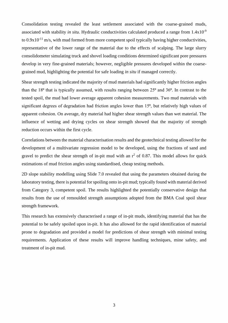
Publications included in this thesis
Vangsness, T.A., Williams, D.J., Ahn, J., Miles, B. (2018). Accelerated Degradation and Modified
Slake Durability Testing of Clay Mineral-rich Coal Mine Spoil. Tailings and Mine Waste Conference
2018. – partially incorporated as Chapter 6.0
Contributor Statement of Contribution
Vangsness, T.A. Laboratory Testing (60%)
Wrote and edited paper (80%)
Williams, D.J. Wrote and edited paper (20%)
Ahn, J Laboratory Testing (20%)
Miles, B Laboratory Testing (20%)
6
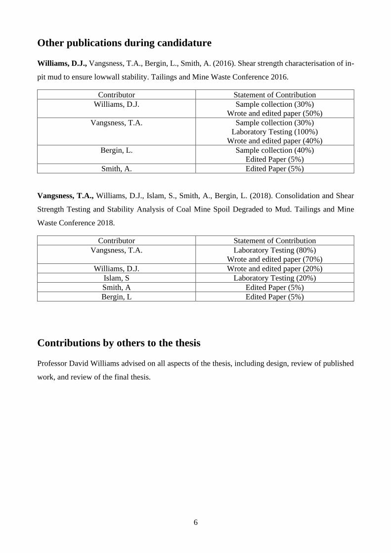
Other publications during candidature
Williams, D.J., Vangsness, T.A., Bergin, L., Smith, A. (2016). Shear strength characterisation of in-
pit mud to ensure lowwall stability. Tailings and Mine Waste Conference 2016.
Contributor Statement of Contribution
Williams, D.J. Sample collection (30%)
Wrote and edited paper (50%)
Vangsness, T.A. Sample collection (30%)
Laboratory Testing (100%)
Wrote and edited paper (40%)
Bergin, L. Sample collection (40%)
Edited Paper (5%)
Smith, A. Edited Paper (5%)
Vangsness, T.A., Williams, D.J., Islam, S., Smith, A., Bergin, L. (2018). Consolidation and Shear
Strength Testing and Stability Analysis of Coal Mine Spoil Degraded to Mud. Tailings and Mine
Waste Conference 2018.
Contributor Statement of Contribution
Vangsness, T.A. Laboratory Testing (80%)
Wrote and edited paper (70%)
Williams, D.J. Wrote and edited paper (20%)
Islam, S Laboratory Testing (20%)
Smith, A Edited Paper (5%)
Bergin, L Edited Paper (5%)
Contributions by others to the thesis
Professor David Williams advised on all aspects of the thesis, including design, review of published
work, and review of the final thesis.

7
Statement of parts of the thesis submitted to qualify for the award of
another degree
No works submitted towards another degree have been included in this thesis.
Research Involving Human or Animal Subjects
No animal or human subjects were involved in this research.
8
Acknowledgements
• Professor David Williams for his guidance, mentorship and council throughout my
undergraduate and postgraduate years;
• Stuart Whitton for his sharing his passion and insight into the world of soil;
• My mother, father, brother and sister for their never ending support, compassion, wisdom
and love;
• Adrian Smith of Pells Sullivan Meynink (PSM) for his guidance in project methodology and
help with interpretation of data;
• Leigh Bergin of BHP Mitsubishi Alliance (BMA) and all personnel that provided access and
collection to the researched materials;
• Mark Raven of CSIRO Land & Water for considerable input and advice with respect to the
mineralogical and geochemical analysis and interpretation.
• ACARP for its funding and support;
• The University of Queensland for access to and the use of their facilities;
• A number of undergraduate students who assisted in laboratory testing, particularly Jiwoo
Ahn, Ben Miles and Nick Hutley; and
• All members of my Academic board of supervisors.
Dicebat Bernardus Carnotensis nos esse quasi nanos, gigantium humeris
insidentes, ut possimus plura eis et remotiora videre, non utique proprii visus
acumine, aut eminentia corporis, sed quia in altum subvenimur et extollimur
magnitudine gigantea

9
Financial support
This research was supported by funding from the Australian Coal Association Research Program
(ACARP).
Keywords
Shear strength, flooding, spoil, degradation, weathering, consolidation, permeability, slope stability,
numerical simulation.
10
Australian and New Zealand Standard Research Classifications
(ANZSRC)
ANZSRC code: 090501, Civil Geotechnical Engineering, 100%
Fields of Research (FoR) Classification
FoR code: 0905, Civil Engineering, 100%
11
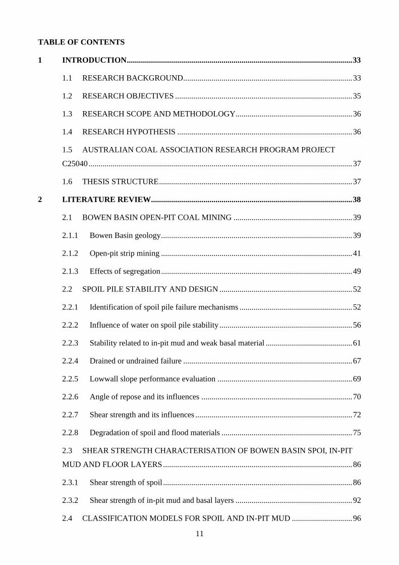
TABLE OF CONTENTS
1 INTRODUCTION ................................................................................................................ 33
1.1 RESEARCH BACKGROUND.................................................................................... 33
1.2 RESEARCH OBJECTIVES ........................................................................................ 35
1.3 RESEARCH SCOPE AND METHODOLOGY.......................................................... 36
1.4 RESEARCH HYPOTHESIS ....................................................................................... 36
1.5 AUSTRALIAN COAL ASSOCIATION RESEARCH PROGRAM PROJECT
C25040 ................................................................................................................................... 37
1.6 THESIS STRUCTURE ................................................................................................ 37
2 LITERATURE REVIEW.................................................................................................... 38
2.1 BOWEN BASIN OPEN-PIT COAL MINING ........................................................... 39
2.1.1 Bowen Basin geology ............................................................................................... 39
2.1.2 Open-pit strip mining ............................................................................................... 41
2.1.3 Effects of segregation ............................................................................................... 49
2.2 SPOIL PILE STABILITY AND DESIGN .................................................................. 52
2.2.1 Identification of spoil pile failure mechanisms ........................................................ 52
2.2.2 Influence of water on spoil pile stability .................................................................. 56
2.2.3 Stability related to in-pit mud and weak basal material ........................................... 61
2.2.4 Drained or undrained failure .................................................................................... 67
2.2.5 Lowwall slope performance evaluation ................................................................... 69
2.2.6 Angle of repose and its influences ........................................................................... 70
2.2.7 Shear strength and its influences .............................................................................. 72
2.2.8 Degradation of spoil and flood materials ................................................................. 75
2.3 SHEAR STRENGTH CHARACTERISATION OF BOWEN BASIN SPOI, IN-PIT
MUD AND FLOOR LAYERS .............................................................................................. 86
2.3.1 Shear strength of spoil .............................................................................................. 86
2.3.2 Shear strength of in-pit mud and basal layers .......................................................... 92
2.4 CLASSIFICATION MODELS FOR SPOIL AND IN-PIT MUD .............................. 96
12
2.4.1 BMA Coal State-of-the-Art framework for spoil categorisation ............................. 97
2.5 LITERATURE REVIEW COMMENTARY AND CONCLUSIONS ...................... 103
2.5.1 Spoil category expansion and refinement .............................................................. 103
2.5.2 Verification by testing ............................................................................................ 103
2.5.3 Material degradation considerations ...................................................................... 104
2.5.4 Consideration of in-pit mud parameters ................................................................. 104
3 MINE SITE OBSERVATIONS ........................................................................................ 105
3.1 PRELIMINARY SITE VISITS ................................................................................. 105
4 PROJECT PLAN AND RESEARCH METHODOLOGY ............................................ 109
4.1 SAMPLING METHODOLOGY ............................................................................... 109
4.2 SAMPLE IDENTIFICATION SYSTEM AND SAMPLING SUMMARY ............. 109
4.3 MATERIAL SAMPLING – MINE SITE A (26 APRIL 2015) ................................. 110
4.3.1 Mine Site A sampling locations ............................................................................. 110
4.3.2 Mine Site A samples............................................................................................... 111
4.4 MATERIAL SAMPLING – MINE SITE B (2 JUNE 2015) ..................................... 119
4.4.1 Mine Site B sampling locations.............................................................................. 119
4.4.2 Mine Site B samples ............................................................................................... 122
4.5 MATERIAL SAMPLING – MINE SITE C (3 JUNE 2015) ..................................... 128
4.5.1 Mine Site C Sampling locations ............................................................................. 128
4.5.2 Mine Site C samples ............................................................................................... 130
4.6 MATERIAL SAMPLING – MINE SITE A AND MINE SITE B (30 NOVEMBER
2016) 134
4.6.1 Mine Site A and Mine Site B sampling locations .................................................. 134
4.6.2 Mine Site A and Mine Site B samples ................................................................... 134
4.7 PHYSICAL AND CHEMICAL CHARACTERISATION ....................................... 137
4.7.1 As-sampled moisture content ................................................................................. 137
4.7.2 Specific gravity....................................................................................................... 137
13
4.7.3 Total suction ........................................................................................................... 137
4.7.4 Atterberg limits....................................................................................................... 137
4.7.5 Emerson class number ............................................................................................ 138
4.7.6 Chemical characterisation ...................................................................................... 139
4.7.7 X-ray diffraction ..................................................................................................... 139
4.7.8 Cation exchange capacity and exchangeable cations ............................................. 140
4.8 PARTICLE SIZE DISTRIBUTION .......................................................................... 142
4.9 DEGRADATION TESTING OF SPOIL ................................................................... 144
4.9.1 Varied saturation durations .................................................................................... 144
4.9.2 Multiple wetting and drying cycles ........................................................................ 144
4.9.3 Spoil degradation testing program ......................................................................... 144
4.10 GEOTECHNICAL CHARACTERISATION ............................................................ 147
4.10.1 Small-scale consolidometer testing ........................................................................ 147
4.10.2 Large slurry consolidometer ................................................................................... 147
4.10.3 Small-scale and large-scale shear strength testing ................................................. 148
5 MATERIAL CHARACTERISATION TEST RESULTS ............................................. 151
5.1 PHYSICAL CHARACTERISATION ....................................................................... 151
5.1.1 As-sampled moisture state...................................................................................... 151
5.1.2 Total suction ........................................................................................................... 153
5.1.3 Specific gravity....................................................................................................... 155
5.1.4 Particle size distributions........................................................................................ 157
5.2 GEOTECHNICAL CHARACTERISATION ............................................................ 172
5.2.1 Atterberg limits....................................................................................................... 172
5.2.2 Emerson class number ............................................................................................ 175
5.3 CHEMICAL CHARACTERISATION...................................................................... 177
5.3.1 pH, electrical conductivity and total dissolved solids ............................................ 177
5.4 MINERALOGICAL AND GEOCHEMICAL CHARACTERISATION ................. 180
14
5.4.1 X-Ray diffraction, cation exchange capacity and exchangeable cations ............... 180
5.5 MATERIAL CHARACTERISATION TEST CONCLUSIONS .............................. 186
6 DEGRADATION TEST RESULTS ................................................................................. 189
6.1 WETTING AND DRYING CYCLES, AND PROLONGED SATURATION ........ 189
6.1.1 Results of degradation testing of C3S-20 ............................................................... 190
6.1.2 Results of degradation testing of C3S-13 ............................................................... 194
6.1.3 Conclusions of prolonged saturation and wetting and drying cycle degradation testing
198
6.2 ACCELERATED DEGRADATION AND MODIFIED SLAKE DURABILITY
TESTING OF SPOIL ........................................................................................................... 200
6.2.1 Testing methodology and sampling ....................................................................... 200
6.2.2 Physical characterisation of spoil ........................................................................... 203
6.2.3 Degradation testing results ..................................................................................... 204
6.2.4 Discussion of degradation results ........................................................................... 208
6.2.5 Accelerated degradation conclusions ..................................................................... 213
7 CONSOLIDATION TEST RESULTS ............................................................................. 214
7.1 STANDARD CONSOLIDOMETER RESULTS ...................................................... 214
7.1.1 Discussion and conclusions of consolidometer test results .................................... 230
7.2 LARGE SLURRY CONSOLIDOMETER TEST RESULTS ................................... 232
7.2.1 Test results for C3M-08 ......................................................................................... 236
7.2.2 Test results for C3M-18 ......................................................................................... 239
7.2.3 Test results for C1M-02 ......................................................................................... 241
7.2.4 Test results for C1M-23 ......................................................................................... 244
7.2.5 Discussion and conclusions of slurry consolidometer test results ......................... 246
8 SHEAR STRENGTH TEST RESULTS .......................................................................... 250
8.1 SPOIL AND MUD DIRECT SHEAR TEST RESULTS .......................................... 250
8.1.1 Spoil material test results ....................................................................................... 250
8.1.2 Mud material test results ........................................................................................ 255
15
8.1.3 Conclusions of direct shear test results .................................................................. 260
8.2 INFLUENCE OF PIT FLOODING ON SPOIL AND MUD SHEAR STRENGTH 262
8.2.1 C3S-13 spoil and associated mud ........................................................................... 262
8.2.2 C3S-20 spoil and associated mud ........................................................................... 264
8.3 INFLUENCE OF DEGRADATION ON SPOIL SHEAR STRENGTH .................. 266
8.3.1 Conclusions of spoil degradation shear strength test results .................................. 276
9 IN-PIT MUD CATEGORISATION, SHEAR STRENGTH ESTIMATION, AND
LOWWALL STABILITY ................................................................................................. 277
9.1 CATEGORISATION AND SHEAR STRENGTH ESTIMATION OF IN-PIT MUD
277
9.1.1 Categorisation and shear strength estimation conclusions: .................................... 290
9.2 TESTING METHODOLOGY FOR CHARACTERISING IN-PIT MUD ............... 291
9.3 STABILITY MODELLING OF IN-PIT SPOIL AND MUD ................................... 292
9.3.1 Stability modelling conclusions: ............................................................................ 304
10 CONCLUSIONS AND RECOMMENDATIONS FOR FUTURE RESEARCH ......... 306
10.1 CONCLUSIONS AND SIGNIFICANT OUTCOMES ............................................. 306
10.1.1 Spoil and in-pit mud characterisation ..................................................................... 306
10.1.2 Degradation of spoil ............................................................................................... 307
10.1.3 Consolidation of spoil and mud.............................................................................. 308
10.1.4 Shear strength of spoil and mud ............................................................................. 309
10.1.5 Categorisation, shear strength estimation and modelling of in-pit mud ................ 309
10.2 RECOMMENDATIONS FOR FUTURE RESEARCH ............................................ 311
11 REFERENCES ................................................................................................................... 312
16
Tables
Table 2.1 Key dragline components for strip mining, (adapted from Prytherch 2012; Simmons 2009;
Williams 2015) ................................................................................................................................... 44
Table 2.2 Suggested Factor of Safety relationships for open-pit coal mining (adapted from Simmons
2009) .................................................................................................................................................. 70
Table 2.3 Properties related to strength and slake durability (adapted from McLemore et al. 2009) 80
Table 2.4 Results of statistical analysis of spoil density and triaxial shear strength data from Bowen
Basin spoil materials (adapted from Williams & Zou 1991) ............................................................. 86
Table 2.5 Shear strength parameters derived from direct shear testing (adapted from Naderian &
Williams 1996) ................................................................................................................................... 89
Table 2.6 Bowen Basin spoil shear strengths, (adapted from Simmons & McManus 2004) ............ 90
Table 2.7 Strengths for -2.36 mm spoil specimens tested dry in a 60 mm direct shear box, reproduced
(adapted from Hiung 2016) ................................................................................................................ 91
Table 2.8 Strengths for -2.36 mm spoil specimens tested wet in a 60 mm direct shear box, reproduced
(adapted from Hiung 2016) ................................................................................................................ 91
Table 2.9 Shear strength parameters of drained residual or remoulded Bowen Basin material ........ 94
Table 2.10 Shear strength parameters of undrained Bowen Basin basal material ............................. 95
Table 2.11 Typical shear strength parameter ranges for soil (adapted from Dorador et al. 2017) .... 96
Table 2.12 BMA design parameters for Category 1 to 4 spoil in unsaturated, saturated and remoulded
states, (adapted from Simmons & McManus 2004) .......................................................................... 99
Table 4.1 Spoil and Mud Identification Details ............................................................................... 109
Table 4.2 Mine Site A sampling details ........................................................................................... 111
Table 4.3 Mine Site B sampling details ........................................................................................... 122
Table 4.4 Mine Site C samples ........................................................................................................ 130
Table 4.5 Mine Site B and Mine Site A samples (2016) ................................................................. 135
Table 4.6 Summary of physical and chemical characterisation testing ........................................... 139
Table 4.7 Summary of mineralogical and geochemical characterisation testing ............................. 141
Table 4.8 Summary of Particle Size Distribution Testing ............................................................... 143
Table 4.9 Summary of degradation testing program ........................................................................ 146
17
Table 4.10 Summary of geotechnical testing ................................................................................... 150
Table 5.1 As-sampled gravimetric moisture content of all spoil and mud samples ........................ 152
Table 5.2 As-sampled moisture state of -2.36 mm scalped spoil samples....................................... 153
Table 5.3 Specific gravity of all spoil and mud samples ................................................................. 155
Table 5.4 D90, D50, D10, Cu and Cc for Category 3 spoil wet and dry sieving .................................. 158
Table 5.5 D90, D50, D10, Cu and Cc for Category 2 spoil wet and dry sieving .................................. 159
Table 5.6 D90, D50, D10, Cu and Cc for Category 1 spoil wet and dry sieving .................................. 160
Table 5.7 D90, D50, D10, Cu and Cc for Category 3 mud wet sieving ............................................... 163
Table 5.8 D90, D50, D10, Cu and Cc for Category 2 desiccated mud wet and dry sieving ................. 165
Table 5.9 D90, D50, D10, Cu and Cc for Category 1 mud wet sieving ............................................... 166
Table 5.10 Atterberg limits and plasticity index for all spoil and mud samples.............................. 172
Table 5.11 Emerson class test results for all spoil samples ............................................................. 175
Table 5.12 pH, electrical conductivity and total dissolved solids for all spoil and mud samples ... 177
Table 5.13 Mineralogical analysis via X-ray diffraction for all spoil and mud samples, excluding
amorphous materials ........................................................................................................................ 181
Table 5.14 Exchangeable cations and cation exchange capacity of all spoil and mud samples ...... 183
Table 6.1 Degradation of C3S-20 subjected to prolonged soaking ................................................. 191
Table 6.2 Degradation of C3S-20 subjected to wetting and drying cycles ...................................... 192
Table 6.3 Degradation of C3S-13 subjected to prolonged soaking ................................................. 194
Table 6.4 Degradation of C3S-13 subjected to wetting and drying cycles ...................................... 195
Table 6.5 Spoil physical characterisation ........................................................................................ 203
Table 6.6 D90, D50 and D10 before and after degradation testing of fresh spoil ............................... 205
Table 6.7 X-ray diffraction analysis for all spoil samples ............................................................... 209
Table 6.8 Exchangeable cations and cation exchange capacity of all spoil samples ....................... 209
Table 6.9 Key mineralogical and geochemical characteristics of spoil samples ............................. 212
Table 7.1 Initial and final conditions for all spoil specimens tested ................................................ 214
Table 7.2 Initial and final conditions for all mud specimens tested ................................................ 215
18
Table 7.3 Settlement for all spoil specimens tested ......................................................................... 217
Table 7.4 Settlement for all mud specimens tested .......................................................................... 218
Table 7.5 Final void ratio and compression index values for all spoil and mud specimens tested . 221
Table 7.6 Coefficient of Consolidation values for all spoil and mud specimens tested .................. 224
Table 7.7 Coefficient of volume change for all spoil and mud specimens tested............................ 225
Table 7.8 Hydraulic conductivity for all spoil and mud specimens tested ...................................... 228
Table 7.9 Slurry consolidometer test results for C3M-08 ................................................................ 237
Table 7.10 Slurry consolidometer test results for C3M-18 .............................................................. 239
Table 7.11 Slurry consolidometer test results for C1M-02 .............................................................. 242
Table 7.12 Slurry consolidometer test results for C1M-23 .............................................................. 244
Table 7.13 End of testing state for all slurry consolidometer specimens tested .............................. 248
Table 8.1 BMA shear strength parameters for different categories and mobilisation modes .......... 250
Table 8.2 Direct shear strength results for spoil tested dry and wet ................................................ 251
Table 8.3 Direct shear strength results for mud tested dry and wet ................................................. 256
Table 8.4 Direct shear strength test results of C3S-13 and associated muds .................................. 263
Table 8.5 Direct shear strength test results for C3S-20 and associated mud ................................... 264
Table 8.6 Direct shear strength test results for all spoil tested dry, wet and degraded .................... 269
Table 9.1 BMA shear strength parameters for categories and mobilisation modes ........................ 279
Table 9.2 Wet sieved particle size distributions for all mud samples .............................................. 280
Table 9.3 Direct shear strength test results for mud tested wet ....................................................... 282
Table 9.4 Mud gravel and sand-size fraction correlated to friction angle and shear strength ......... 285
Table 9.5 Multivariate regression statistics for prediction of friction angle using Gravel and Sand %
for -6.7 mm fraction of mud............................................................................................................. 286
Table 9.6 Comparison of laboratory tested friction angle and shear strength and predicted values using
multivariate analysis ........................................................................................................................ 287
Table 9.7 BMA shear strength parameters for categories and mobilisation modes ........................ 292
Table 9.8 Direct shear strength of spoil tested dry and wet ............................................................. 293
Table 9.9 Direct shear strength of mud tested dry and wet .............................................................. 293
19
Table 9.10 Slide 7.0 model geometry and assumptions ................................................................... 295
Table 9.11 Factor of safety for all spoil samples with different materials at toe of lowwall ........... 298
Table 9.12 Factor of safety for spoil with associated mud at the toe of lowwall ............................ 300
Table 9.13 Factor of safety for Category 3 spoil with laboratory tested muds at the toe of lowwall
.......................................................................................................................................................... 302
20
Figures
Figure 1.1 Rainfall anomaly for Queensland (adapted from http://www.bom.gov.au/) .................... 34
Figure 1.2 – BMA Spoil Strength Categories (adapted from Simmons and McManus, 2004) ......... 35
Figure 2.1 Map of basins within eastern Australia (left), and a conceptual model for the evolution of
the Bowen Basin (right) (adapted from Fielding et al. 1996) ............................................................ 40
Figure 2.2 Box cut, strip cuts and spoil piles (adapted from Humphrey 1984) ................................. 42
Figure 2.3 Blasted overburden in a strip mine (adapted from Prytherch 2012) ................................. 43
Figure 2.4 Typical strip coal mine highwall (left) and lowwall (right) in the Bowen Basin ............. 44
Figure 2.5 Dragline dimensional extents (adapted from Prytherch 2012) ......................................... 46
Figure 2.6 Dragline working bench instability (adapted from ‘Norwich Park Dragline Recovery’
2008) .................................................................................................................................................. 46
Figure 2.7 Dragline lowwall construction, (adapted from Duran 2013) ............................................ 47
Figure 2.8 A view of a truck and shovel operation in Hunter Valley Region in NSW (adapted from
Mitra & Onargan 2012)...................................................................................................................... 48
Figure 2.9 Schematic section of dragline spoil dump fabric and phreatic surface (adapted from
Simmons & McManus 2004) ............................................................................................................. 49
Figure 2.10 Schematic section of truck spoil dump fabric and phreatic surface (adapted from
Simmons & McManus 2004) ............................................................................................................. 50
Figure 2.11 Truck end dumping in the Bowen Basin ........................................................................ 50
Figure 2.12 Conceptual model of the particle-size distribution of a rock pile (adapted from McLemore
et al. 2009).......................................................................................................................................... 51
Figure 2.13 Schematic structure of a spoil pile formed by haul trucks end-dumping from a tip-head
(adapted from Williams 2015) ........................................................................................................... 51
Figure 2.14 Rainfall anomalies for Queensland’s Bowen Basin (adapted from
http://www.bom.gov.au) .................................................................................................................... 52
Figure 2.15 Geometric features of five surveyed spoil failures (adapted from Richards et al. 1981)53
Figure 2.16 Variables involved in two-wedge limit equilibrium analysis (adapted from Richards et al.
1981) .................................................................................................................................................. 54
Figure 2.17 Superficial failure mechanism (adapted from Simmons & McManus 2004) ................. 55
21
Figure 2.18 Two-wedge dump failure due to weak floor material (adapted from Poulsen et al. 2014)
............................................................................................................................................................ 56
Figure 2.19 Intermediate scale multi-wedge failure (adapted from Simmons & McManus 2004) ... 56
Figure 2.20 A sacrificial flooded pit within the Bowen Basin........................................................... 57
Figure 2.21 Conceptual hydrogeological model of a stockpile (adapted from Beale 2017) ............. 58
Figure 2.22 Hydrostratigraphy of segregated dumps – terraced construction (adapted from Smith et
al. 1995) ............................................................................................................................................. 59
Figure 2.23 Three-zone model for moisture conditions within spoil dumps (adapted from Simmon &
Fityus 2016) ....................................................................................................................................... 60
Figure 2.24 Spoiling into in-pit mud, adapted from (Prytherch 2012) .............................................. 62
Figure 2.25 Mud cleanout via the key bridge method (adapted from Prytherch 2012) ..................... 63
Figure 2.26 Potential geotechnical hazards for dragline in-pit bench operations (adapted from
Simmons 2009) .................................................................................................................................. 63
Figure 2.27 In-pit mud-dam storage observed in the Bowen Basin................................................... 64
Figure 2.28 Geotechnical instabilities related to weak basal material (adapted from Prytherch 2012)
............................................................................................................................................................ 66
Figure 2.29 Concept of mechanism by which undrained behaviour is invoked at base of spoil pile
(adapted from Duran 2013) ................................................................................................................ 68
Figure 2.30 Annual probability of failure versus consequence for various engineering structures
(adapted from Whitman 1984) ........................................................................................................... 69
Figure 2.31 Angle of repose of granular materials (adapted from Simons & Albertson 1960)......... 71
Figure 2.32 Schematic frequency distribution for natural hillslope angles in the United Kingdom
(adapted from Carson & Petley 1970) ............................................................................................... 72
Figure 2.33 Standard direct shear apparatus ...................................................................................... 73
Figure 2.34 Shear characteristics of dense and loose sands (adapted from Jackson 2015) ............... 74
Figure 2.35 Peak and residual shear strength and Coulomb envelopes (adapted from Jackson 2015)
............................................................................................................................................................ 74
Figure 2.36 Factors affecting weathering (adapted from Lan et al. 2003) ......................................... 76
Figure 2.37 Degradation of stable aggregate due to slaking and dispersion ...................................... 77
22
Figure 2.38 Weak cementation of spoil within the Bowen Basin ...................................................... 78
Figure 2.39 Slaking of clay-rich mine spoil from the Bowen Basin.................................................. 79
Figure 2.40 Erosion of dispersive spoil pile observed within the Bowen Basin ............................... 83
Figure 2.41 Scheme for determining class numbers of aggregates (adapted from Emerson 1967) .. 83
Figure 2.42 The influence of remoulding water content on dispersion (left), and influence of
exchangeable sodium on dispersion (right) (adapted from Seedsman & Emerson 1985) ................. 84
Figure 2.43 Effect of saturation on the shear strength of Bowen Basin spoil and a comparison with
other values determined either experimentally or by back-analysis of spoil pile instability (adapted
from Seedsman et al. 1988) ................................................................................................................ 87
Figure 2.44 Compilation of the strength of rockfill as measured in large triaxial tests (adapted from
Leps 1970), compared with direct shear values for coal mine spoil (adapted from Seedsman et al.
1988) .................................................................................................................................................. 88
Figure 2.45 Calculated shear strength of 100m deep spoil pile using average shear strength parameters
(adapted from Kho et al. 2013) .......................................................................................................... 90
Figure 2.46 Comparison of friction angle and cohesion for Boyd et al. (1978), Seedsman et al. (1988),
Simmons & McManus (2004) and Hiung (2016) .............................................................................. 92
Figure 2.47 Shear strength of bulk spoil (a) unsaturated – as sampled; (b) saturated (adapted from
Richards et al. 1981) .......................................................................................................................... 93
Figure 2.48 Spoil categories and attributes (adapted from Simmons & McManus 2004)................. 98
Figure 2.49 Spoil structure attribute to be used with Figure 2.48 (adapted from Simmons & McManus
2004) .................................................................................................................................................. 98
Figure 2.50 Degradation of dry Category 3 spoil (left) to mud (right) .............................................. 99
Figure 2.51 Conceptual strength modes for spoil (adapted from Simmons & McManus 2004) ..... 100
Figure 2.52 Conceptual strength modes for spoil modified to explain the linear shear strength
approximation adopted in framework (adapted from Bradfield et al. 2013) ................................... 100
Figure 2.53 Mohr Diagram showing framework linear fit with respect to actual strength envelope (not
to scale) (adapted from Bradfield et al. 2013) ................................................................................. 101
Figure 3.1 Mine Site C Ramp 23, spoil failure and draglining into mud producing slumping of spoil
and bow-waving of mud .................................................................................................................. 105
Figure 3.2 Mine Site C Ramp 23, Category 3 (left) and Category 4 and 2 (right) spoil ................. 106
23
Figure 3.3 Mine Site C Ramp 22, flooded pit (~40 m deep) ........................................................... 106
Figure 3.4 Mine Site C Ramp 6S, floor mud from Category 3 spoil ............................................... 107
Figure 3.5 Mine Site B Ramp 11S, closed by flooding since late 2010 .......................................... 107
Figure 3.6 Mine Site B Ramp 5S, flooded pit surrounded by largely Category 3 overburden and spoil
.......................................................................................................................................................... 108
Figure 3.7 Mine Site B Ramp 5S, in-pit mud at base of Category 3 overburden and spoil lowwall
.......................................................................................................................................................... 108
Figure 4.1 Mine Site A sampling locations...................................................................................... 110
Figure 4.2 Mine Site A Ramp 10N sampling location C3M-01 ...................................................... 111
Figure 4.3 Mine Site A Ramp 10N sample C3M-01 ....................................................................... 112
Figure 4.4 Mine Site A Ramp 10N sampling location C1M-02 ...................................................... 112
Figure 4.5 Mine Site A Ramp 10N Sample C1M-02 ....................................................................... 113
Figure 4.6 Mine Site A Ramp 10N sampling location C3M-03 ...................................................... 113
Figure 4.7 Mine Site A Ramp 10N sample C3M-03 ....................................................................... 114
Figure 4.8 Mine Site A Ramp 10N sampling location C3M-04 ...................................................... 114
Figure 4.9 Mine Site A Ramp 10N sample C3M-04 ....................................................................... 115
Figure 4. 10 Mine Site A Ramp 10N sampling location C3M-05 ................................................... 115
Figure 4.11 Mine Site A Ramp 10N sample C3M-05 ..................................................................... 116
Figure 4.12 Mine Site A Ramp 10N sampling Location C2M-06 ................................................... 116
Figure 4.13 Mine Site A Ramp 10N sample C2M-06 ..................................................................... 117
Figure 4.14 Mine Site A Ramp 10N sampling Location C2M-07 ................................................... 117
Figure 4.15 Mine Site A Ramp 10N sample C2M-07 ..................................................................... 118
Figure 4.16 Mine Site B Ramp 5S sampling ................................................................................... 119
Figure 4.17 Mine Site B Ramp 5S sampling location C3M-08 ....................................................... 119
Figure 4.18 Mine Site B Ramp 5S sampling location C3S-10 ........................................................ 120
Figure 4.19 Mine Site B Ramp 5S sampling location C3M-12 ....................................................... 120
Figure 4.20 Mine Site B Ramp 5S sampling location C3S-13 ........................................................ 121
Figure 4.21 Mine Site B Ramp 5S sampling location C2S-16 ........................................................ 121
24
Figure 4.22 Mine Site B Ramp 5S sampling location C1S-17 ........................................................ 121
Figure 4.23 Mine Site B Ramp 5S Sample C3M-08 surface texture (with 20-cent coins for scale)
.......................................................................................................................................................... 122
Figure 4.24 Mine Site B Ramp 5S sampling location C3S-10 surface texture ................................ 123
Figure 4.25 Mine Site B Ramp 5S sample C3S-10 sieving to -53 mm ........................................... 123
Figure 4.26 Mine Site B Ramp 5S sample C3M-12 surface texture................................................ 124
Figure 4.27 Mine Site B Ramp 5S sample C3S-13 fine-grained surface texture ............................ 124
Figure 4.28 Mine Site B Ramp 5S sample C3S-13 coarser-grained below surface ........................ 125
Figure 4.29 Mine Site B Ramp 5S sample C3S-13: (a) -53 mm, and (b) +53 mm ......................... 125
Figure 4.30 Mine Site B Ramp 5S sample C3S-13: +53 mm .......................................................... 126
Figure 4.31 Mine Site B Ramp 5S sample C2S-16 agglomerated surface texture .......................... 126
Figure 4.32 Mine Site B Ramp 5S sample C1S-17.......................................................................... 127
Figure 4.33 Mine Site B Ramp 1N sample C1S-17 surface texture ................................................ 127
Figure 4.34 Mine Site C sampling location C3M-18 ....................................................................... 128
Figure 4.35 Mine Site C sampling location C3S-20 ........................................................................ 128
Figure 4.36 Mine Site C sampling location C3S-23 ........................................................................ 129
Figure 4.37 Mine Site C sampling location C2S-24 ........................................................................ 129
Figure 4.38 Mine Site C Ramp 6S sample C3M-18 surface crusting .............................................. 130
Figure 4.39 Mine Site C Ramp 6S sample C3S-20 surface PSD (with 22.9 cm diameter plates for
scale) ................................................................................................................................................ 131
Figure 4.40 Mine Site C Ramp 5S sample C3S-20: (a) -53 mm, and (b) +53 mm ......................... 131
Figure 4.41 Mine Site C Ramp 5S sample C3S-20 weighing + & -53 mm fractions ...................... 132
Figure 4.42 Mine Site C Ramp 5S sample C3S-20 +53 mm ........................................................... 132
Figure 4.43 Mine Site C Ramp 22 sample C1M-23 ........................................................................ 133
Figure 4.44 Mine Site C Ramp 14 sample C2S-24 .......................................................................... 133
Figure 4.45 Mine Site B Ramp 5S sampling location C3M-30 ....................................................... 134
Figure 4.46 Mine Site A Ramp 50S sampling location C3M-32 ..................................................... 134
Figure 4.47 Mine Site B Ramp 5S sample C3M-30 ........................................................................ 135
25
Figure 4.48 Mine Site A Ramp 50S sample C3M-32 ...................................................................... 136
Figure 4.49 Helium pycnometer ...................................................................................................... 137
Figure 4.50 WP4 dewpoint potential meter ..................................................................................... 138
Figure 4.51 Atterberg limit test apparatus ....................................................................................... 138
Figure 4.52 Wet sieving apparatus (left), addition of suspension solution to stack (top right), filtering
of sieved sample for drying and weighing (bottom right) ............................................................... 142
Figure 4.53 Agitation of 1000cc solution (left) & hydrometer analysis of solution with the control
cylinder and temperature gauge (right) ............................................................................................ 143
Figure 4.54 Slake durability apparatus ............................................................................................ 145
Figure 4.55 Schematics of consolidometer testing in a water bath (tested “wet”) .......................... 147
Figure 4.56 Large slurry consolidometer apparatus schematic........................................................ 148
Figure 4.57 Schematic of direct shear box shear strength test ......................................................... 149
Figure 4.58 Large-scale direct shear machine (300 mm x 300 mm x 200 mm high) ...................... 149
Figure 5.1 As-sampled moisture content of all spoil and mud samples .......................................... 153
Figure 5.2 As-sampled gravimetric moisture content and total suction of all spoil samples .......... 154
Figure 5.3 Specific gravity of all spoil and mud samples ................................................................ 156
Figure 5.4 Overall particle size distribution curves of Category 3 spoil -53 mm fraction .............. 157
Figure 5.5 Overall particle size distribution curves of Category 2 spoil -53 mm fraction .............. 159
Figure 5.6 Overall particle size distribution curves of Category 1 spoil -53 mm fraction .............. 160
Figure 5.7 Overall particle size distribution curves of all dry spoil -53 mm fraction ...................... 161
Figure 5.8 D90 values for all dry and wet sieved spoil samples ....................................................... 162
Figure 5.9 Overall particle size distribution curves of all spoil wet and dry -53 mm fraction ........ 162
Figure 5.10 Overall particle size distribution curves of all Category 3 mud samples -53 mm fraction
.......................................................................................................................................................... 163
Figure 5.11 Overall particle size distribution curves of Category 2 dried mud -53 mm fraction .... 164
Figure 5.12 Overall particle size distribution curves of all Category 1 mud -53 mm fraction ........ 165
Figure 5.13 Overall particle size distribution curves of all mud samples -53 mm fraction ............. 166
Figure 5.14 D90 values for all wet sieved spoil and mud samples ................................................... 167
26
Figure 5.15 Overall particle size distribution curves of all Category 3 spoil and mud samples -53 mm
fraction ............................................................................................................................................. 168
Figure 5.16 Overall particle size distribution curves of all Category 2 spoil and mud samples -53 mm
fraction ............................................................................................................................................. 168
Figure 5.17 Overall particle size distribution curves of all Category 1 spoil and mud samples -53 mm
fraction ............................................................................................................................................. 170
Figure 5.18 Overall particle size distribution curves Mine Site B R5S spoil and mud -53 mm fraction
.......................................................................................................................................................... 170
Figure 5.19 Overall particle size distribution curves Mine Site C R6S spoil and mud -53 mm fraction
.......................................................................................................................................................... 171
Figure 5.20 Overall particle size distribution curves Mine Site A mud -53 mm fraction ............... 171
Figure 5.21 As-sampled gravimetric moisture content and Atterberg limits of all spoil and mud
samples ............................................................................................................................................. 173
Figure 5.22 Plasticity chart for all spoil and mud samples .............................................................. 174
Figure 5.23 Liquid and plastic limits for all spoil and mud samples ............................................... 174
Figure 5.24 C3S-10 and C3S-13 Emerson class test results ............................................................ 176
Figure 5.25 C2S-16 and C1S-17 Emerson class test results ............................................................ 176
Figure 5.26 C3S-20 and C2S-24 Emerson class test results ............................................................ 176
Figure 5.27 Variation of gravimetric moisture content and electrical conductivity for all spoil and
mud samples ..................................................................................................................................... 178
Figure 5.28 Variation of gravimetric moisture content and pH for all spoil and mud samples ....... 179
Figure 5.29 Variation of pH and electrical conductivity for all spoil and mud samples ................. 179
Figure 5.30 Mineralogical analysis via X-ray diffraction for all spoil and mud samples ................ 182
Figure 5.31 Cation exchange capacity and exchangeable cations for all spoil and mud samples ... 184
Figure 5.32 Calculated levels of Smectite and Illite for all spoil and mud samples ........................ 185
Figure 5.33 Smectite cations present in all spoil and mud samples ................................................. 185
Figure 6.1 C3S-20 prolonged saturation preparation ....................................................................... 190
Figure 6.2 Plastic-wrapped to avoid evaporation during submersion .............................................. 190
Figure 6.3 Degradation of C3S-20 when subjected to prolonged saturation ................................... 191
27
Figure 6.4 Degradation of C3S-20 when subjected to wetting and drying cycles ........................... 192
Figure 6.5 Electrical conductivity measurements of C3S-20 for soaking duration and wet/dry cycles
.......................................................................................................................................................... 193
Figure 6.6 Comparison of wetting and drying cycles versus saturation duration for C3S-20 ......... 194
Figure 6.7 Degradation of C3S-13 when subjected to prolonged soaking ...................................... 195
Figure 6.8 Degradation of spoil sample C3S-13 subjected to wetting and drying cycles ............... 196
Figure 6.9 Electrical conductivity measurements of C3S-13 for saturation duration and wet/dry cycles
.......................................................................................................................................................... 197
Figure 6.10 Comparison of wetting and drying cycles versus soaking duration for C3S-13 .......... 197
Figure 6.11 Comparison of C3S-13 and C3S-20 during prolonged soaking and wetting and drying
cycles ................................................................................................................................................ 199
Figure 6.12 Spoil material C3S-13 .................................................................................................. 200
Figure 6.13 Spoil material C3S-20 .................................................................................................. 201
Figure 6.14 Spoil material C2S-16 .................................................................................................. 201
Figure 6.15 Spoil material C2S-24 .................................................................................................. 202
Figure 6.16 Spoil material C1S-17 .................................................................................................. 202
Figure 6.17 As-sampled moisture content and Atterberg limits ...................................................... 203
Figure 6.18 Plasticity index versus liquid limit for all spoil ............................................................ 204
Figure 6.19 Particle size distribution of C3S-13 before and after degradation................................ 206
Figure 6.20 Particle size distribution of C3M-20 before and after degradation .............................. 206
Figure 6.21 Particle size distribution of C2S-16 before and after degradation................................ 207
Figure 6.22 Particle size distribution of C3S-24 before and after degradation................................ 207
Figure 6.23 Particle size distribution of C3S-17 before and after degradation................................ 208
Figure 6.24 Influence of degradation method on particle size reduction ......................................... 211
Figure 6.25 Modified slake durability degradation analysis per cycle ............................................ 211
Figure 7.1 Final dry density for all spoil and mud specimens tested ............................................... 216
Figure 7.2 Initial and final void ratio for all spoil and mud specimens tested ................................. 217
Figure 7.3 Settlement for -4.7 mm all loose-placed spoil specimens tested wet ............................. 218
28
Figure 7.4 Settlement for -4.7 mm all loose-placed mud specimens tested wet .............................. 219
Figure 7.5 Comparison of settlement for -4.7 mm spoil and mud specimens tested wet ................ 220
Figure 7.6 Initial dry density versus settlement at 1,000 kPa stress for all spoil and mud specimens
tested ................................................................................................................................................ 220
Figure 7.7 Applied stress versus void ratio for all spoil specimens tested ...................................... 222
Figure 7.8 Applied stress versus void ratio for all mud specimens tested ....................................... 222
Figure 7.9 Compression index values for all spoil and mud specimens tested ................................ 223
Figure 7.10 Typical calculation of the coefficient of consolidation for an oedometer specimen .... 225
Figure 7.11 Void ratio versus coefficient of volume change for -4.7 mm spoil tested wet ............. 226
Figure 7.12 Void ratio versus coefficient of volume change for -4.7 mm mud specimens tested wet
.......................................................................................................................................................... 227
Figure 7.13 Comparison of void ratio versus coefficient of volume change for all -4.7 mm spoil and
mud specimens tested wet ................................................................................................................ 227
Figure 7.14 Hydraulic conductivity values for all spoil and mud specimens tested ........................ 229
Figure 7.15 Hydraulic conductivity at 1,000 kPa applied stress for all spoil and mud specimens tested
.......................................................................................................................................................... 230
Figure 7.16 C3M-08 sampling ......................................................................................................... 234
Figure 7.17 C3M-18 sampling ......................................................................................................... 235
Figure 7.18 C1M-02 sampling ......................................................................................................... 235
Figure 7.19 C1M-23 sampling ......................................................................................................... 235
Figure 7.20 Particle size distribution of samples tested in slurry consolidometer ........................... 236
Figure 7.21 Slurry consolidometer stress and pore water pressure plots for C3M-08 ..................... 237
Figure 7.22 Slurry consolidometer void ratio versus effective stress for C3M-08 .......................... 238
Figure 7.23 Slurry consolidometer hydraulic conductivity versus effective stress for C3M-08 ..... 238
Figure 7.24 Slurry consolidometer stress and pore water pressure plots for C3M-18 ..................... 240
Figure 7.25 Slurry consolidometer void ratio versus effective stress for C3M-18 .......................... 240
Figure 7.26 Slurry consolidometer hydraulic conductivity versus effective stress for C3M-18 ..... 241
Figure 7.27 Slurry consolidometer stress and pore water pressure plots for C1M-02 ..................... 242
29
Figure 7.28 Slurry consolidometer void ratio versus effective stress for C1S-02 ........................... 243
Figure 7.29 Slurry consolidometer hydraulic conductivity versus effective stress for C1M-02 ..... 243
Figure 7.30 Slurry consolidometer stress and pore water pressure data for C1S-23 ....................... 245
Figure 7.31 Slurry consolidometer void ratio versus effective stress plot for C1S-23 .................... 245
Figure 7.32 Slurry consolidometer hydraulic conductivity versus effective stress plot for C1S-23 246
Figure 7.33 Slurry consolidometer settlement versus time for all mud specimens tested ............... 247
Figure 8.1 Direct shear strength results for Category 3 spoil tested dry and wet ............................ 252
Figure 8.2 Direct shear strength results for Category 2 spoil tested dry and wet ............................ 253
Figure 8.3 Direct shear strength results for Category 1 spoil tested dry and wet ............................ 253
Figure 8.4 Apparent cohesion and friction angle for all spoil ......................................................... 254
Figure 8.5 Secant friction angle versus applied normal stress for Category 1, 2 and 3 spoil tested dry
and wet ............................................................................................................................................. 255
Figure 8.6 Direct shear strength results of Category 3 mud tested dry and wet .............................. 257
Figure 8.7 Direct shear strength results of Category 1 mud tested dry and wet .............................. 258
Figure 8.8 Direct shear strength results of Category 1 mud tested dry and wet .............................. 258
Figure 8.9 Friction angle and apparent cohesion for all mud specimens tested .............................. 259
Figure 8.10 Secant friction angle versus applied normal stress for Category 1, 2 and 3 mud samples
tested dry and wet ............................................................................................................................ 260
Figure 8.11 Comparison of spoil and mud apparent cohesion and friction angle ........................... 261
Figure 8.12 C3S-13, associated mud C3M-08 (lowwall) and C3M-30 (highwall) sampling locations
.......................................................................................................................................................... 262
Figure 8.13 Direct shear strength test results for C3S-13 spoil and associated C3M-08 mud ........ 263
Figure 8.14 C3S-20 and associated mud C3M-18 sampling locations ............................................ 264
Figure 8.15 Direct shear strength test results for C3S-20 spoil and associated C3M-18 mud ........ 265
Figure 8.16 C3S-13 as-sampled and after three wetting and drying cycles ..................................... 266
Figure 8.17 C3S-20 as-sampled and after three wetting and drying cycles ..................................... 267
Figure 8.18 C2S-16 as-sampled and after three wetting and drying cycles ..................................... 267
Figure 8.19 C2S-24 as-sampled and after three wetting and drying cycles ..................................... 267
30
Figure 8.20 C1S-17 as-sampled and after three wetting and drying cycles ..................................... 268
Figure 8.21 Particle size distribution for C3S-13 scalped to pass 6.7 mm and tested dry, soaked and
after wet/dry cycles .......................................................................................................................... 270
Figure 8.22 Direct shear strength results for C3S-13 scalped to pass 6.7 mm and tested dry, wet and
degraded ........................................................................................................................................... 270
Figure 8.23 Particle size distribution of C3S-20 scapled to pass 6.7 mm and tested dry, soaked and
after wet/dry cycles .......................................................................................................................... 271
Figure 8.24 Direct shear strength results for C3S-20 scalped to pass 6.7 mm and tested dry, wet and
degraded ........................................................................................................................................... 271
Figure 8.25 Particle size distribution of C3S-16 spoil scalped to pass 6.7 mm and tested dry, soaked
and after wet/dry cycles ................................................................................................................... 272
Figure 8.26 Direct shear strength results for C2S-16 scalped to pass 6.7 mm and tested dry, wet and
degraded ........................................................................................................................................... 273
Figure 8.27 Particle size distribution of C3S-24 scalped to pass 6.7 mm and tested dry, soaked and
after wet/dry cycles .......................................................................................................................... 273
Figure 8.28 Direct shear strength results for C2S-24 scalped to pass 6.7 mm and tested dry, wet and
degraded ........................................................................................................................................... 274
Figure 8.29 Particle size distribution of C3S-17 scalped to pass 6.7 mm and tested dry, soaked and
after wet/dry cycles .......................................................................................................................... 275
Figure 8.30 Direct shear strength results for C1S-17 scalped to pass 6.7 mm and tested dry, wet and
degraded ........................................................................................................................................... 275
Figure 9.1 Spoil Categories and Attributes (adapted from Simmons & McManus 2004)............... 278
Figure 9.2 Spoil Structure attribute to be used in association with Figure 9.1 (adapted from Simmons
& McManus 2004) ........................................................................................................................... 278
Figure 9.3 Coarse and fine fractions of degraded spoil ................................................................... 279
Figure 9.4 Overall particle size distribution curves of all mud samples .......................................... 281
Figure 9.5 Source material category compared with D90 ................................................................. 281
Figure 9.6 Apparent cohesion versus friction angle for all mud specimens .................................... 283
Figure 9.7 Secant friction angle versus applied normal stress for Category 1, 2 and 3 mud dry and wet
.......................................................................................................................................................... 284
31
Figure 9.8 A model for predicting the friction angle of in-pit mud ................................................. 288
Figure 9.9 Comparison of laboratory tested friction angle and predicted friction angle of mud
materials ........................................................................................................................................... 289
Figure 9.10 Comparison of laboratory tested shear strength and predicted shear strength assuming
zero cohesion for all mud samples ................................................................................................... 289
Figure 9.11 Two-wedge spoil pile failure mechanism (adapted from Philip et al. 1981) ............... 294
Figure 9.12 Dozer push lowwall geometry ...................................................................................... 295
Figure 9.13 Truck and shovel lowwall geometry ............................................................................ 296
Figure 9.14 Dragline lowwall geometry .......................................................................................... 296
Figure 9.15 Dragline lowwall with undercut toe geometry ............................................................. 296
Figure 9.16 Factor of safety for dragline lowwall with different base material at the toe ............... 299
Figure 9.17 Factor of Safety for Category 3 spoil with associated mud at the toe of a dragline lowwall
.......................................................................................................................................................... 300
Figure 9.18 Factor of safety for Category 3 spoil with different mud at the toe of lowwall ........... 303
Figure 9.19 Factor of safety comparison for Category 3 spoil against mud equivalent spoil with
different mud at toe of lowwall ........................................................................................................ 303

32
List of Abbreviations
ACARP – Australian Coal Association Research Program
ANZSRC – Australian and New Zealand Standard Research Classifications
BMA – BHP Mitsubishi Alliance
BOM – Bureau of Meteorology
CEC – Cation Exchange Capacity
CSIRO - Commonwealth Scientific and Industrial Research Organisation
D10 – Particle size 10% of material passes
EC – Electrical Conductivity
FOR – Fields of Research
FOS – Factor of Safety
LL – Liquid Limit
PI – Plasticity Index
PL – Plastic Limit
POF – Probability of Failure
PSD – Particle Size Distribution
PSM – Pells Sullivan Meynink
UDC – Utah Development Company
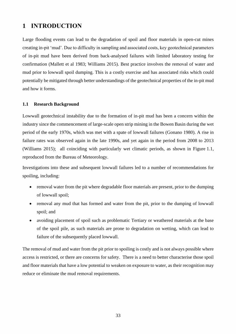
33
1 INTRODUCTION
Large flooding events can lead to the degradation of spoil and floor materials in open-cut mines
creating in-pit ‘mud’. Due to difficulty in sampling and associated costs, key geotechnical parameters
of in-pit mud have been derived from back-analysed failures with limited laboratory testing for
confirmation (Mallett et al 1983; Williams 2015). Best practice involves the removal of water and
mud prior to lowwall spoil dumping. This is a costly exercise and has associated risks which could
potentially be mitigated through better understandings of the geotechnical properties of the in-pit mud
and how it forms.
1.1 Research Background
Lowwall geotechnical instability due to the formation of in-pit mud has been a concern within the
industry since the commencement of large-scale open strip mining in the Bowen Basin during the wet
period of the early 1970s, which was met with a spate of lowwall failures (Gonano 1980). A rise in
failure rates was observed again in the late 1990s, and yet again in the period from 2008 to 2013
(Williams 2015); all coinciding with particularly wet climatic periods, as shown in Figure 1.1,
reproduced from the Bureau of Meteorology.
Investigations into these and subsequent lowwall failures led to a number of recommendations for
spoiling, including:
• removal water from the pit where degradable floor materials are present, prior to the dumping
of lowwall spoil;
• removal any mud that has formed and water from the pit, prior to the dumping of lowwall
spoil; and
• avoiding placement of spoil such as problematic Tertiary or weathered materials at the base
of the spoil pile, as such materials are prone to degradation on wetting, which can lead to
failure of the subsequently placed lowwall.
The removal of mud and water from the pit prior to spoiling is costly and is not always possible where
access is restricted, or there are concerns for safety. There is a need to better characterise those spoil
and floor materials that have a low potential to weaken on exposure to water, as their recognition may
reduce or eliminate the mud removal requirements.
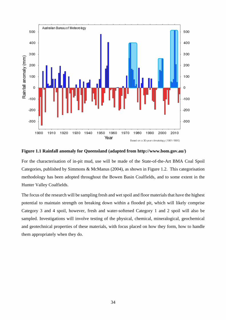
34
Figure 1.1 Rainfall anomaly for Queensland (adapted from http://www.bom.gov.au/)
For the characterisation of in-pit mud, use will be made of the State-of-the-Art BMA Coal Spoil
Categories, published by Simmons & McManus (2004), as shown in Figure 1.2. This categorisation
methodology has been adopted throughout the Bowen Basin Coalfields, and to some extent in the
Hunter Valley Coalfields.
The focus of the research will be sampling fresh and wet spoil and floor materials that have the highest
potential to maintain strength on breaking down within a flooded pit, which will likely comprise
Category 3 and 4 spoil, however, fresh and water-softened Category 1 and 2 spoil will also be
sampled. Investigations will involve testing of the physical, chemical, mineralogical, geochemical
and geotechnical properties of these materials, with focus placed on how they form, how to handle
them appropriately when they do.
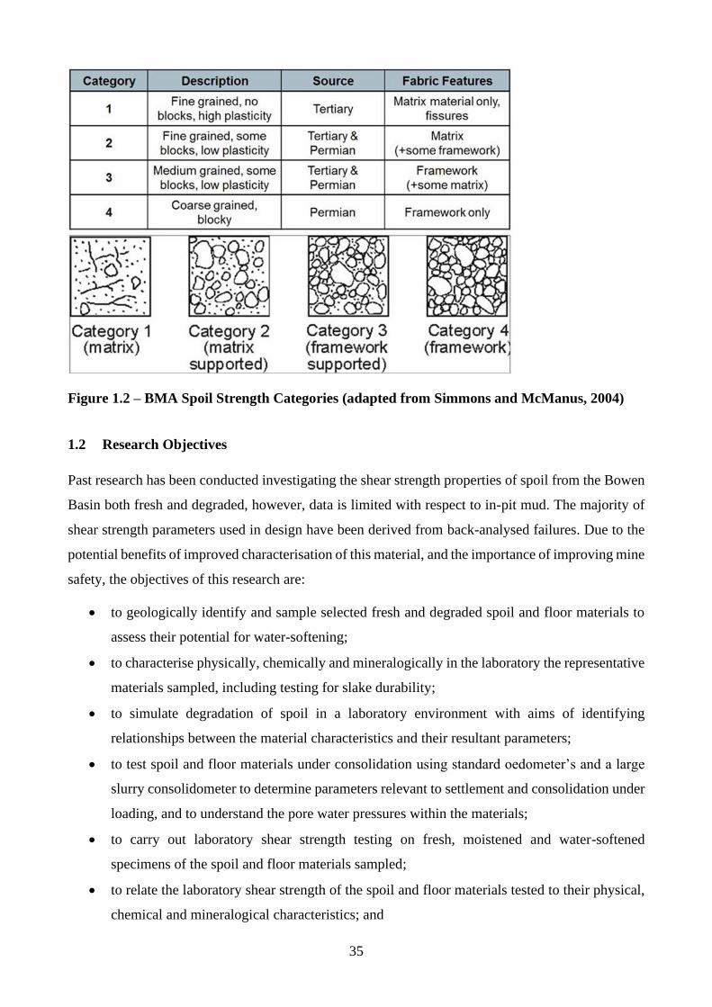
35
Figure 1.2 – BMA Spoil Strength Categories (adapted from Simmons and McManus, 2004)
1.2 Research Objectives
Past research has been conducted investigating the shear strength properties of spoil from the Bowen
Basin both fresh and degraded, however, data is limited with respect to in-pit mud. The majority of
shear strength parameters used in design have been derived from back-analysed failures. Due to the
potential benefits of improved characterisation of this material, and the importance of improving mine
safety, the objectives of this research are:
• to geologically identify and sample selected fresh and degraded spoil and floor materials to
assess their potential for water-softening;
• to characterise physically, chemically and mineralogically in the laboratory the representative
materials sampled, including testing for slake durability;
• to simulate degradation of spoil in a laboratory environment with aims of identifying
relationships between the material characteristics and their resultant parameters;
• to test spoil and floor materials under consolidation using standard oedometer’s and a large
slurry consolidometer to determine parameters relevant to settlement and consolidation under
loading, and to understand the pore water pressures within the materials;
• to carry out laboratory shear strength testing on fresh, moistened and water-softened
specimens of the spoil and floor materials sampled;
• to relate the laboratory shear strength of the spoil and floor materials tested to their physical,
chemical and mineralogical characteristics; and
36
• to develop testing protocols for the identification of degradable spoil and floor materials,
allowing for the development and improvement of design guidelines for enhancing the
geotechnical stability of lowwalls for both durable and water-softened spoil.
1.3 Research Scope And Methodology
To investigate the properties of in-pit mud, and the influences they have on stability, the methodology
is as follows:
• Representative mud and spoil sampling, with an emphasis on material likely to maintain
structure and strength during wetting;
• Laboratory physical and chemical characterisation testing;
• Laboratory mineralogical and geochemical testing;
• Laboratory geotechnical investigations including degradation, consolidation and shear
strength testing;
• Framework development to estimate in-pit mud parameters using relationships found between
the material characteristics and the geotechnical properties; and
• Stability modelling to determine the impact the tested spoil and mud properties have on
stability, and to provide insight into improvements of the current assumptions used by
industry.
1.4 Research Hypothesis
• Upon wetting, coal mine spoil and pit floors will exhibit varied degrees of degradation related
to the state of weathering, degree of blasting, time of exposure, and the geological and
mineralogical properties, resulting in a loss of shear strength;
• Wetting and drying cycles will increase the rate of degradation of coal mine spoil, affecting
materials with higher fractions of swelling clays more severely;
• The shear strength of in-pit mud will be related to the material source, allowing for the
identification of spoil that will not break down rapidly, and will be suitable for spoiling upon
if handled correctly; and
• Improved knowledge of the geotechnical properties of in-pit mud will allow for increases in
modelling accuracy and the development of in situ handling methodologies.
37
1.5 Australian Coal Association Research Program Project C25040
This research has been funded by the Australian Coal Association Research Program (ACARP)
Project C25040. It builds upon the related 4-year ACARP Project C19022 on the Implications of
Settlements of High Coal Mine Spoil on Stored Volume and Stability undertaken by Professor David
Williams of The University of Queensland (UQ) from 2010 to 2014, and the 3-year ACARP Project
C20019 on the Stability of very High Spoil Piles, undertaken by Dr John Simmons of Sherwood
Geotechnical and Research Services and Professor Stephen Fityus of the University of Newcastle.
Both of these projects involved the laboratory shear strength testing of a range of spoil materials,
including those that degrade on contact with water.
1.6 Thesis Structure
This thesis consists of multiple chapters investigating specific aspects of the characterisation and
testing of in-pit mud, and sampled spoil materials. The topics of each chapter are as follows:
• Section 1: A project introduction detailing scope and objectives;
• Section 2: A literature review including commentary;
• Section 3: Mine site observations of in-pit mud at numerous sites;
• Section 4: Material sampling, project plan and testing methodologies;
• Section 5: Physical, chemical, mineralogical and geochemical characterisation of spoil and
mud;
• Section 6: Degradation testing of spoil;
• Section 7: Standard consolidation and large slurry consolidation of spoil and mud;
• Section 8: Direct shear testing of spoil and mud;
• Section 9: Prediction of mud shear strength and implications of results on lowwall stability;
• Section 10: Conclusions and future research; and
• Section 11: References.
38
2 LITERATURE REVIEW
Weak foundations and floor materials below dumped spoil have been the cause for many significant
coal mine lowwall failures in the Bowen Basin (Nguyen & Welsh 1981; Richards et al. 1981;
Seedsman et al. 1988). There is a concern that mud produced by the degradation of in-pit spoil and
floor materials could cause instabilities in future lowwalls if spoil is placed on top. Characterisation
of degraded material is most often through the interpretation of back-analysed failures (Gonano 1980;
Seedsman et al. 1988). The locations of these weak materials often present safety issues with respect
to access. Furthermore, due to the rate of mining, economics and standard operating procedures,
degraded in-pit mud is rarely tested with strength parameters assumed for design. Another reason for
the limited information available is the reluctance of the mining community to make information
about lowwall failures public. There is currently work underway to improve knowledge of these
problematic materials and to better understand all the issues involved (Williams 2015; Simmon &
Fityus 2016).
Section 2.1 discusses the open-pit coal mining operations of the Bowen Basin in Australia. This
includes the geological aspects of coal formation, the methodology behind open-pit strip mining, and
the impacts typical handling processes have on the physical structure of a lowwall.
Section 2.2 investigates spoil pile stability and design within the Bowen Basin, reviewing the causes
of past failures and the derived parameters related to their occurrence. The review includes an
investigation into failure mechanisms, the occurrence and impact of water within a spoil pile, the
influential parameters of the spoil, and the degradation mechanisms that are associated with the
formation of in-pit mud.
Section 2.3 reviews the literature around shear strength characterisation of Bowen Basin spoil, in-pit
mud and basal layers within lowwalls. Results of past testing have been compiled in relation to the
strength of in-pit mud, highlighting areas that require further investigation.
Section 2.4 discusses the classification and State-of-the-Art categorisation of spoil and in-pit mud,
looking at standardised practice, and systems utilised by mines within the Bowen Basin for visual
categorisation.
Section 2.5 summarises the findings of the literature review, highlighting areas of research that will
improve the stability of lowwalls through improved classification and categorisation of in-pit mud.
39
2.1 Bowen Basin Open-pit Coal Mining
Commercial coal mining has taken place in the Bowen Basin since the 1890s, however, large-scale
mining has commenced since the mid to late 1970s (Richards et al. 1981). Due to the nature of the
coal formation, the size of the waste dumps created are also increasing. Spoil dump heights have
already reached above 350 m, with plans to go higher being implemented (Simmons 2009). The
stability of these dumps is dependent on a number of factors, including geometry, construction
methods, and the parameters of the spoil, which is largely influenced by its geological history. This
section focuses on the formation of coal measures and their relevance to lowwall stability.
2.1.1 Bowen Basin geology
The geology of Australia has been discussed in depth by Fielding et al. (1996) and Mallett et al (1983),
who both detail the large amount of valuable minerals within the Bowen Basin, particularly fossil
fuels. It contains the largest black coal reserves in Australia and is one of the world’s largest deposits.
Its general layout has been detailed in Figure 2.1. The Bowen Basin is up to 10 km thick, composed
of Permian and Triassic aged material (Fielding et al. 1996), situated in a sub-humid, sub-tropical
climate. The exposed formation is 550 to 600 km long, and 250 km wide. A comprehensive study on
the formation and sedimentological features of the Bowen Basin was conducted by Mallett et al
(1983). Of consideration for mining operations were the identification of weak lacustrine beds and
the presence of finely interbedded sequences vulnerable to damage during mine blasting. Steeply
dipping inter-seam units were also recognised as potential causes of instability.
2.1.1.1 Coal formation
The coal found in the Bowen Basin is created through the burial of peat mires in alluvial or estuarine
depositional systems, considered low energy environments. As these mires are buried beneath soil,
they become compressed under increasing temperature and pressure (Christoulas et al. 1987). The
biological and geological processes that take place result in the formation of peat, which then turns
into coal (Taylor et al. 2009). A conceptual model of the evolution of the Bowen Basin is shown in
Figure 2.1.
For the formation of commercially usable coal to occur, the range of acceptable temperatures and
pressures is quite small. This is important as it means the parameters of coal measures overburden
are related more to geological attributes than the geographical ones (Simmons & McManus, 2004).
2.1.1.2 Geotechnical considerations of coal measures
Coal measures define the carboniferous system in which coal forms. In a low energy environment,
the coal measures typically consist of fine- and coarse-grained sedimentary rocks, including but not
limited to claystone, mudstone, siltstone, shale and sandstone (Rayner & Hemingway 1974). These
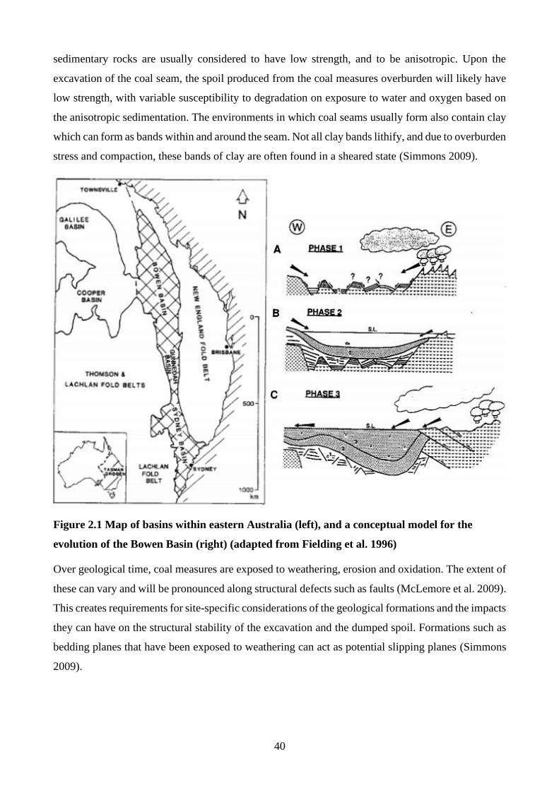
40
sedimentary rocks are usually considered to have low strength, and to be anisotropic. Upon the
excavation of the coal seam, the spoil produced from the coal measures overburden will likely have
low strength, with variable susceptibility to degradation on exposure to water and oxygen based on
the anisotropic sedimentation. The environments in which coal seams usually form also contain clay
which can form as bands within and around the seam. Not all clay bands lithify, and due to overburden
stress and compaction, these bands of clay are often found in a sheared state (Simmons 2009).
Figure 2.1 Map of basins within eastern Australia (left), and a conceptual model for the
evolution of the Bowen Basin (right) (adapted from Fielding et al. 1996)
Over geological time, coal measures are exposed to weathering, erosion and oxidation. The extent of
these can vary and will be pronounced along structural defects such as faults (McLemore et al. 2009).
This creates requirements for site-specific considerations of the geological formations and the impacts
they can have on the structural stability of the excavation and the dumped spoil. Formations such as
bedding planes that have been exposed to weathering can act as potential slipping planes (Simmons
2009).
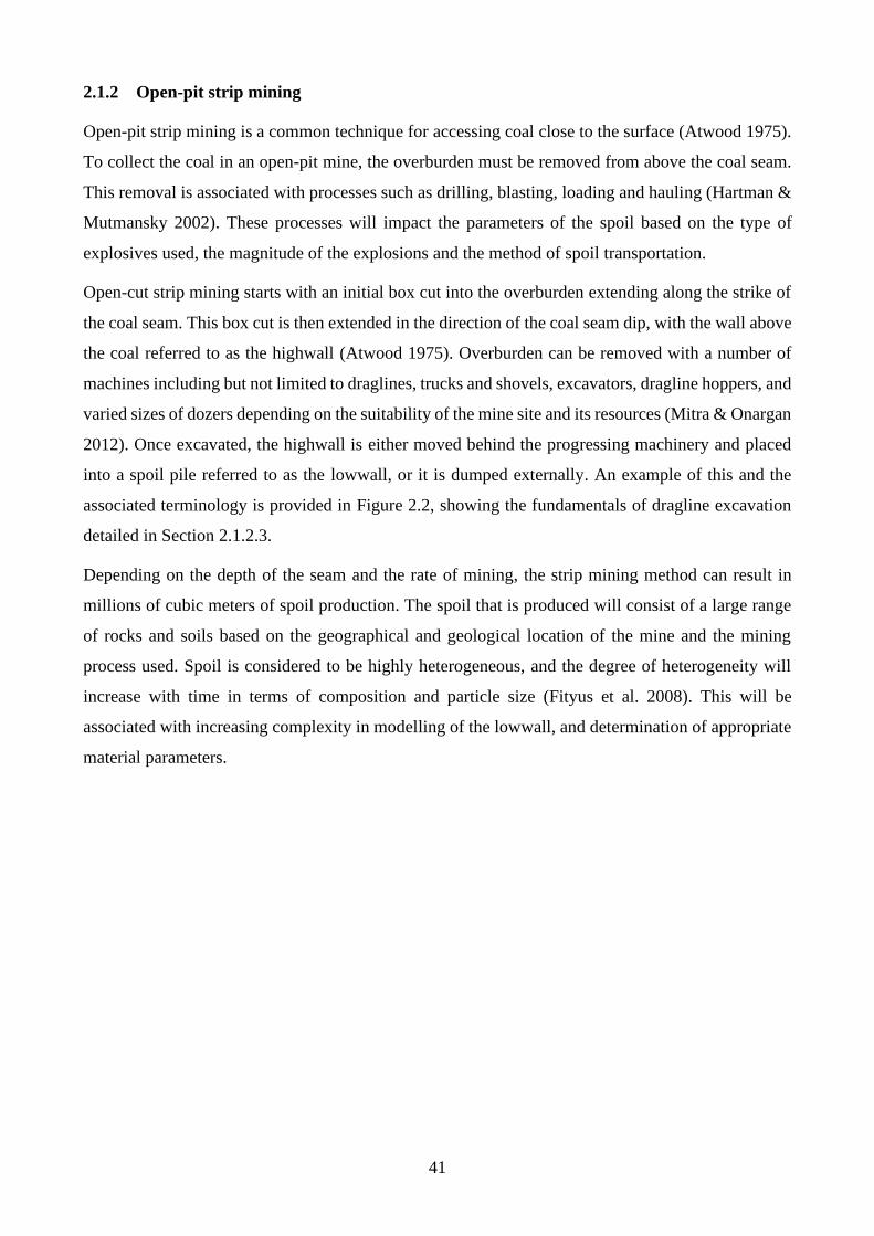
41
2.1.2 Open-pit strip mining
Open-pit strip mining is a common technique for accessing coal close to the surface (Atwood 1975).
To collect the coal in an open-pit mine, the overburden must be removed from above the coal seam.
This removal is associated with processes such as drilling, blasting, loading and hauling (Hartman &
Mutmansky 2002). These processes will impact the parameters of the spoil based on the type of
explosives used, the magnitude of the explosions and the method of spoil transportation.
Open-cut strip mining starts with an initial box cut into the overburden extending along the strike of
the coal seam. This box cut is then extended in the direction of the coal seam dip, with the wall above
the coal referred to as the highwall (Atwood 1975). Overburden can be removed with a number of
machines including but not limited to draglines, trucks and shovels, excavators, dragline hoppers, and
varied sizes of dozers depending on the suitability of the mine site and its resources (Mitra & Onargan
2012). Once excavated, the highwall is either moved behind the progressing machinery and placed
into a spoil pile referred to as the lowwall, or it is dumped externally. An example of this and the
associated terminology is provided in Figure 2.2, showing the fundamentals of dragline excavation
detailed in Section 2.1.2.3.
Depending on the depth of the seam and the rate of mining, the strip mining method can result in
millions of cubic meters of spoil production. The spoil that is produced will consist of a large range
of rocks and soils based on the geographical and geological location of the mine and the mining
process used. Spoil is considered to be highly heterogeneous, and the degree of heterogeneity will
increase with time in terms of composition and particle size (Fityus et al. 2008). This will be
associated with increasing complexity in modelling of the lowwall, and determination of appropriate
material parameters.
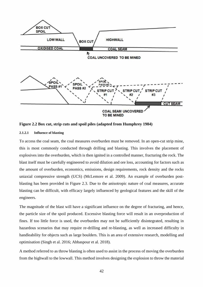
42
Figure 2.2 Box cut, strip cuts and spoil piles (adapted from Humphrey 1984)
2.1.2.1 Influence of blasting
To access the coal seam, the coal measures overburden must be removed. In an open-cut strip mine,
this is most commonly conducted through drilling and blasting. This involves the placement of
explosives into the overburden, which is then ignited in a controlled manner, fracturing the rock. The
blast itself must be carefully engineered to avoid dilution and ore loss, accounting for factors such as
the amount of overburden, economics, emissions, design requirements, rock density and the rocks
uniaxial compressive strength (UCS) (McLemore et al. 2009). An example of overburden post-
blasting has been provided in Figure 2.3. Due to the anisotropic nature of coal measures, accurate
blasting can be difficult, with efficacy largely influenced by geological features and the skill of the
engineers.
The magnitude of the blast will have a significant influence on the degree of fracturing, and hence,
the particle size of the spoil produced. Excessive blasting force will result in an overproduction of
fines. If too little force is used, the overburden may not be sufficiently disintegrated, resulting in
hazardous scenarios that may require re-drilling and re-blasting, as well as increased difficulty in
handleability for objects such as large boulders. This is an area of extensive research, modelling and
optimisation (Singh et al. 2016; Abbaspour et al. 2018).
A method referred to as throw blasting is often used to assist in the process of moving the overburden
from the highwall to the lowwall. This method involves designing the explosion to throw the material
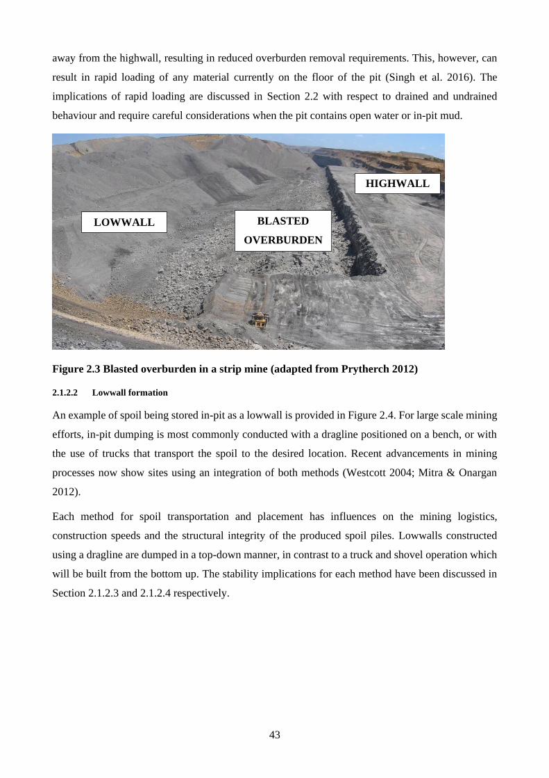
43
away from the highwall, resulting in reduced overburden removal requirements. This, however, can
result in rapid loading of any material currently on the floor of the pit (Singh et al. 2016). The
implications of rapid loading are discussed in Section 2.2 with respect to drained and undrained
behaviour and require careful considerations when the pit contains open water or in-pit mud.
Figure 2.3 Blasted overburden in a strip mine (adapted from Prytherch 2012)
2.1.2.2 Lowwall formation
An example of spoil being stored in-pit as a lowwall is provided in Figure 2.4. For large scale mining
efforts, in-pit dumping is most commonly conducted with a dragline positioned on a bench, or with
the use of trucks that transport the spoil to the desired location. Recent advancements in mining
processes now show sites using an integration of both methods (Westcott 2004; Mitra & Onargan
2012).
Each method for spoil transportation and placement has influences on the mining logistics,
construction speeds and the structural integrity of the produced spoil piles. Lowwalls constructed
using a dragline are dumped in a top-down manner, in contrast to a truck and shovel operation which
will be built from the bottom up. The stability implications for each method have been discussed in
Section 2.1.2.3 and 2.1.2.4 respectively.
HIGHWALL
LOWWALL BLASTED
OVERBURDEN
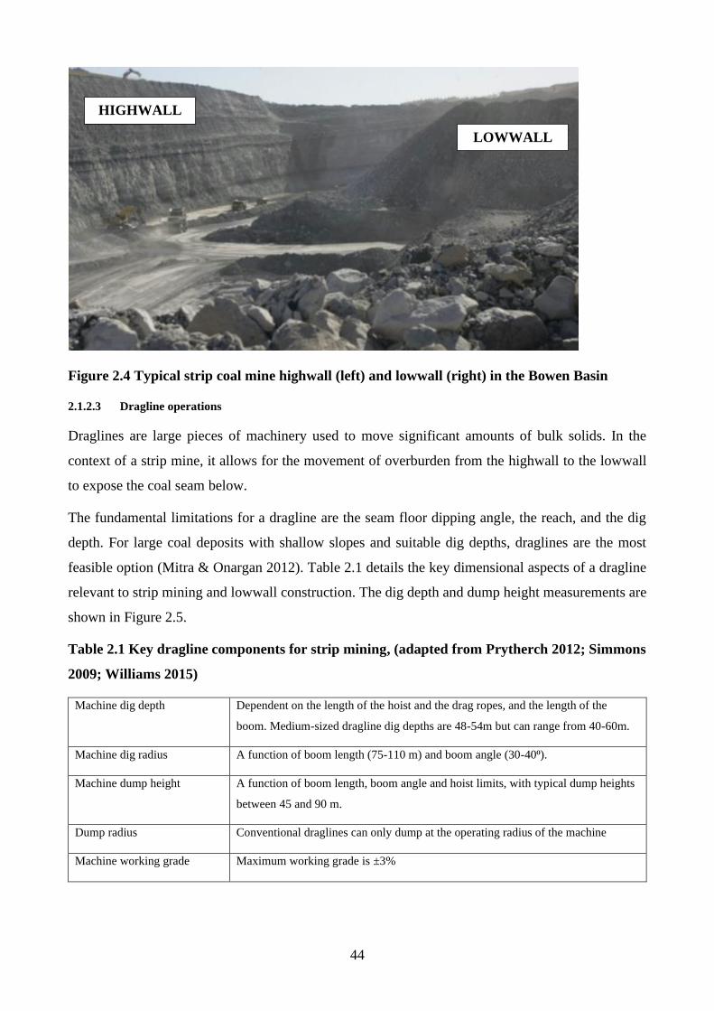
44
Figure 2.4 Typical strip coal mine highwall (left) and lowwall (right) in the Bowen Basin
2.1.2.3 Dragline operations
Draglines are large pieces of machinery used to move significant amounts of bulk solids. In the
context of a strip mine, it allows for the movement of overburden from the highwall to the lowwall
to expose the coal seam below.
The fundamental limitations for a dragline are the seam floor dipping angle, the reach, and the dig
depth. For large coal deposits with shallow slopes and suitable dig depths, draglines are the most
feasible option (Mitra & Onargan 2012). Table 2.1 details the key dimensional aspects of a dragline
relevant to strip mining and lowwall construction. The dig depth and dump height measurements are
shown in Figure 2.5.
Table 2.1 Key dragline components for strip mining, (adapted from Prytherch 2012; Simmons
2009; Williams 2015)
Machine dig depth Dependent on the length of the hoist and the drag ropes, and the length of the
boom. Medium-sized dragline dig depths are 48-54m but can range from 40-60m.
Machine dig radius A function of boom length (75-110 m) and boom angle (30-40⁰).
Machine dump height A function of boom length, boom angle and hoist limits, with typical dump heights
between 45 and 90 m.
Dump radius Conventional draglines can only dump at the operating radius of the machine
Machine working grade Maximum working grade is ±3%
HIGHWALL
LOWWALL
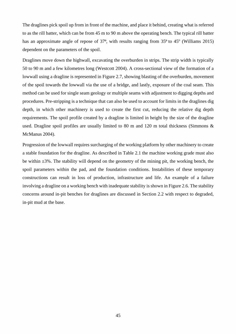
45
The draglines pick spoil up from in front of the machine, and place it behind, creating what is referred
to as the rill batter, which can be from 45 m to 90 m above the operating bench. The typical rill batter
has an approximate angle of repose of 37⁰, with results ranging from 35⁰ to 45o (Williams 2015)
dependent on the parameters of the spoil.
Draglines move down the highwall, excavating the overburden in strips. The strip width is typically
50 to 90 m and a few kilometres long (Westcott 2004). A cross-sectional view of the formation of a
lowwall using a dragline is represented in Figure 2.7, showing blasting of the overburden, movement
of the spoil towards the lowwall via the use of a bridge, and lastly, exposure of the coal seam. This
method can be used for single seam geology or multiple seams with adjustment to digging depths and
procedures. Pre-stripping is a technique that can also be used to account for limits in the draglines dig
depth, in which other machinery is used to create the first cut, reducing the relative dig depth
requirements. The spoil profile created by a dragline is limited in height by the size of the dragline
used. Dragline spoil profiles are usually limited to 80 m and 120 m total thickness (Simmons &
McManus 2004).
Progression of the lowwall requires surcharging of the working platform by other machinery to create
a stable foundation for the dragline. As described in Table 2.1 the machine working grade must also
be within ±3%. The stability will depend on the geometry of the mining pit, the working bench, the
spoil parameters within the pad, and the foundation conditions. Instabilities of these temporary
constructions can result in loss of production, infrastructure and life. An example of a failure
involving a dragline on a working bench with inadequate stability is shown in Figure 2.6. The stability
concerns around in-pit benches for draglines are discussed in Section 2.2 with respect to degraded,
in-pit mud at the base.
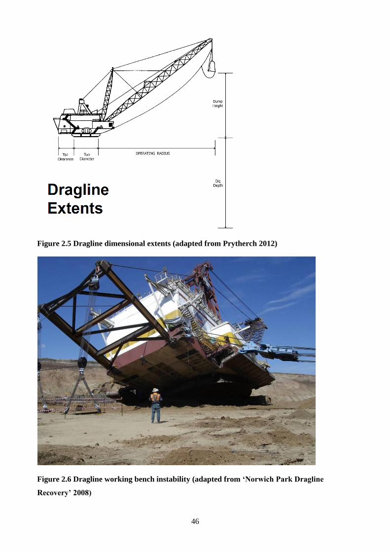
46
Figure 2.5 Dragline dimensional extents (adapted from Prytherch 2012)
Figure 2.6 Dragline working bench instability (adapted from ‘Norwich Park Dragline
Recovery’ 2008)
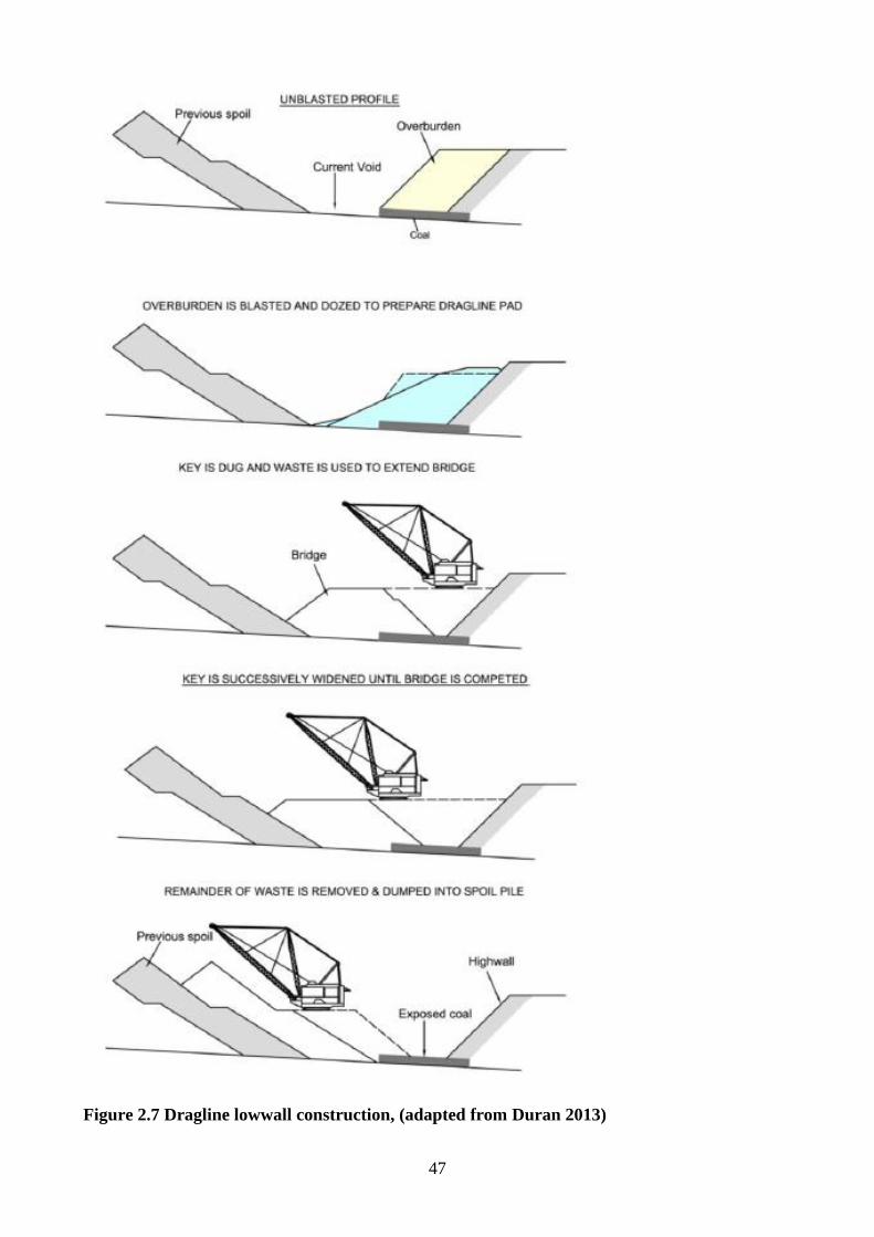
47
Figure 2.7 Dragline lowwall construction, (adapted from Duran 2013)
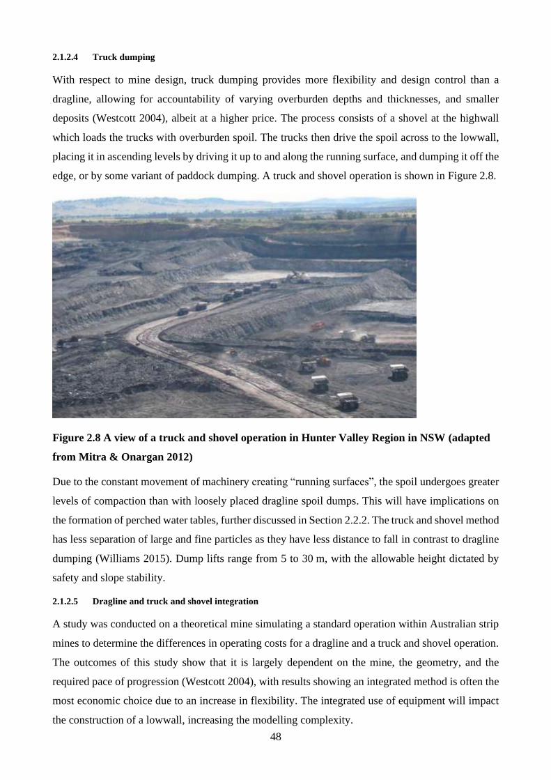
48
2.1.2.4 Truck dumping
With respect to mine design, truck dumping provides more flexibility and design control than a
dragline, allowing for accountability of varying overburden depths and thicknesses, and smaller
deposits (Westcott 2004), albeit at a higher price. The process consists of a shovel at the highwall
which loads the trucks with overburden spoil. The trucks then drive the spoil across to the lowwall,
placing it in ascending levels by driving it up to and along the running surface, and dumping it off the
edge, or by some variant of paddock dumping. A truck and shovel operation is shown in Figure 2.8.
Figure 2.8 A view of a truck and shovel operation in Hunter Valley Region in NSW (adapted
from Mitra & Onargan 2012)
Due to the constant movement of machinery creating “running surfaces”, the spoil undergoes greater
levels of compaction than with loosely placed dragline spoil dumps. This will have implications on
the formation of perched water tables, further discussed in Section 2.2.2. The truck and shovel method
has less separation of large and fine particles as they have less distance to fall in contrast to dragline
dumping (Williams 2015). Dump lifts range from 5 to 30 m, with the allowable height dictated by
safety and slope stability.
2.1.2.5 Dragline and truck and shovel integration
A study was conducted on a theoretical mine simulating a standard operation within Australian strip
mines to determine the differences in operating costs for a dragline and a truck and shovel operation.
The outcomes of this study show that it is largely dependent on the mine, the geometry, and the
required pace of progression (Westcott 2004), with results showing an integrated method is often the
most economic choice due to an increase in flexibility. The integrated use of equipment will impact
the construction of a lowwall, increasing the modelling complexity.
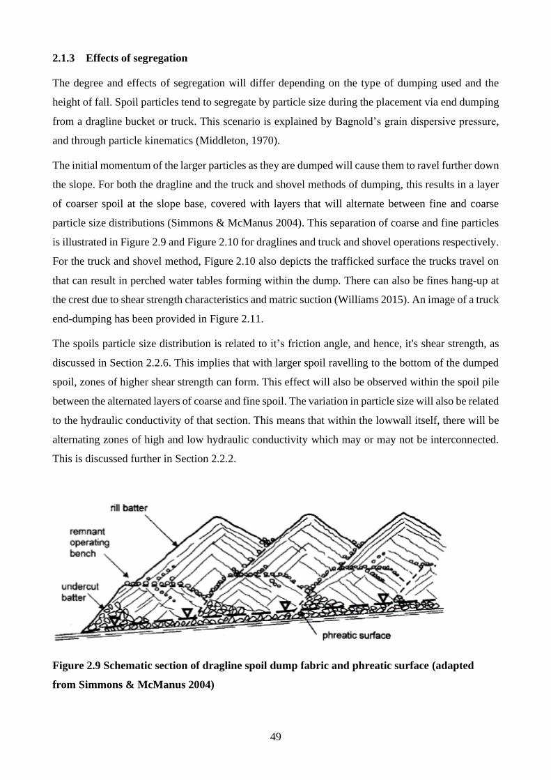
49
2.1.3 Effects of segregation
The degree and effects of segregation will differ depending on the type of dumping used and the
height of fall. Spoil particles tend to segregate by particle size during the placement via end dumping
from a dragline bucket or truck. This scenario is explained by Bagnold’s grain dispersive pressure,
and through particle kinematics (Middleton, 1970).
The initial momentum of the larger particles as they are dumped will cause them to ravel further down
the slope. For both the dragline and the truck and shovel methods of dumping, this results in a layer
of coarser spoil at the slope base, covered with layers that will alternate between fine and coarse
particle size distributions (Simmons & McManus 2004). This separation of coarse and fine particles
is illustrated in Figure 2.9 and Figure 2.10 for draglines and truck and shovel operations respectively.
For the truck and shovel method, Figure 2.10 also depicts the trafficked surface the trucks travel on
that can result in perched water tables forming within the dump. There can also be fines hang-up at
the crest due to shear strength characteristics and matric suction (Williams 2015). An image of a truck
end-dumping has been provided in Figure 2.11.
The spoils particle size distribution is related to it’s friction angle, and hence, it's shear strength, as
discussed in Section 2.2.6. This implies that with larger spoil ravelling to the bottom of the dumped
spoil, zones of higher shear strength can form. This effect will also be observed within the spoil pile
between the alternated layers of coarse and fine spoil. The variation in particle size will also be related
to the hydraulic conductivity of that section. This means that within the lowwall itself, there will be
alternating zones of high and low hydraulic conductivity which may or may not be interconnected.
This is discussed further in Section 2.2.2.
Figure 2.9 Schematic section of dragline spoil dump fabric and phreatic surface (adapted
from Simmons & McManus 2004)
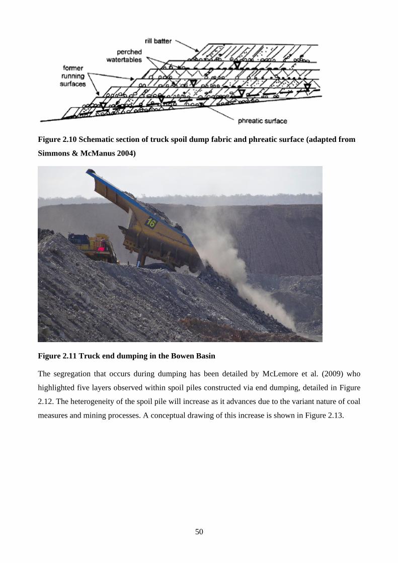
50
Figure 2.10 Schematic section of truck spoil dump fabric and phreatic surface (adapted from
Simmons & McManus 2004)
Figure 2.11 Truck end dumping in the Bowen Basin
The segregation that occurs during dumping has been detailed by McLemore et al. (2009) who
highlighted five layers observed within spoil piles constructed via end dumping, detailed in Figure
2.12. The heterogeneity of the spoil pile will increase as it advances due to the variant nature of coal
measures and mining processes. A conceptual drawing of this increase is shown in Figure 2.13.
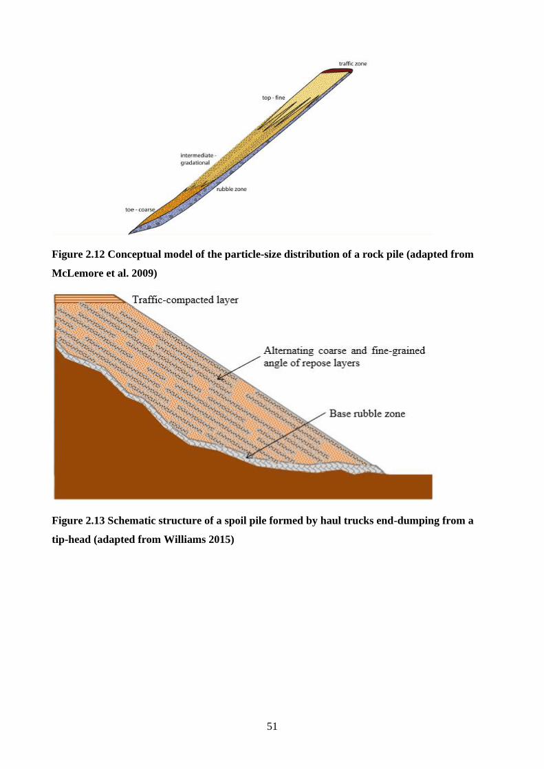
51
Figure 2.12 Conceptual model of the particle-size distribution of a rock pile (adapted from
McLemore et al. 2009)
Figure 2.13 Schematic structure of a spoil pile formed by haul trucks end-dumping from a
tip-head (adapted from Williams 2015)
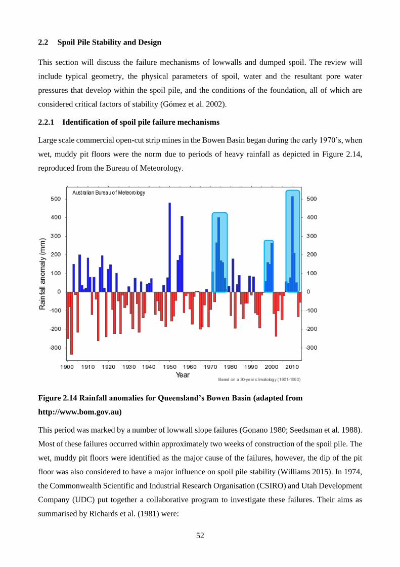
52
2.2 Spoil Pile Stability and Design
This section will discuss the failure mechanisms of lowwalls and dumped spoil. The review will
include typical geometry, the physical parameters of spoil, water and the resultant pore water
pressures that develop within the spoil pile, and the conditions of the foundation, all of which are
considered critical factors of stability (Gómez et al. 2002).
2.2.1 Identification of spoil pile failure mechanisms
Large scale commercial open-cut strip mines in the Bowen Basin began during the early 1970’s, when
wet, muddy pit floors were the norm due to periods of heavy rainfall as depicted in Figure 2.14,
reproduced from the Bureau of Meteorology.
Figure 2.14 Rainfall anomalies for Queensland’s Bowen Basin (adapted from
http://www.bom.gov.au)
This period was marked by a number of lowwall slope failures (Gonano 1980; Seedsman et al. 1988).
Most of these failures occurred within approximately two weeks of construction of the spoil pile. The
wet, muddy pit floors were identified as the major cause of the failures, however, the dip of the pit
floor was also considered to have a major influence on spoil pile stability (Williams 2015). In 1974,
the Commonwealth Scientific and Industrial Research Organisation (CSIRO) and Utah Development
Company (UDC) put together a collaborative program to investigate these failures. Their aims as
summarised by Richards et al. (1981) were:
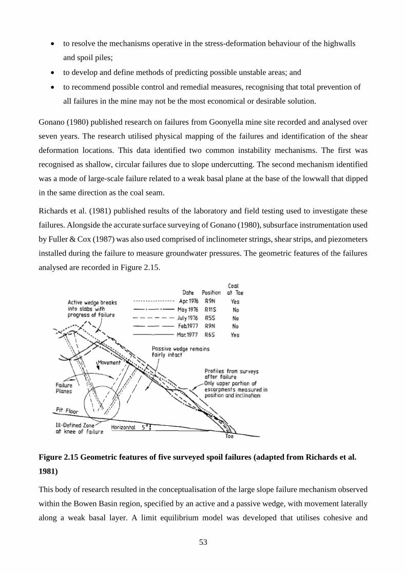
53
• to resolve the mechanisms operative in the stress-deformation behaviour of the highwalls
and spoil piles;
• to develop and define methods of predicting possible unstable areas; and
• to recommend possible control and remedial measures, recognising that total prevention of
all failures in the mine may not be the most economical or desirable solution.
Gonano (1980) published research on failures from Goonyella mine site recorded and analysed over
seven years. The research utilised physical mapping of the failures and identification of the shear
deformation locations. This data identified two common instability mechanisms. The first was
recognised as shallow, circular failures due to slope undercutting. The second mechanism identified
was a mode of large-scale failure related to a weak basal plane at the base of the lowwall that dipped
in the same direction as the coal seam.
Richards et al. (1981) published results of the laboratory and field testing used to investigate these
failures. Alongside the accurate surface surveying of Gonano (1980), subsurface instrumentation used
by Fuller & Cox (1987) was also used comprised of inclinometer strings, shear strips, and piezometers
installed during the failure to measure groundwater pressures. The geometric features of the failures
analysed are recorded in Figure 2.15.
Figure 2.15 Geometric features of five surveyed spoil failures (adapted from Richards et al.
1981)
This body of research resulted in the conceptualisation of the large slope failure mechanism observed
within the Bowen Basin region, specified by an active and a passive wedge, with movement laterally
along a weak basal layer. A limit equilibrium model was developed that utilises cohesive and
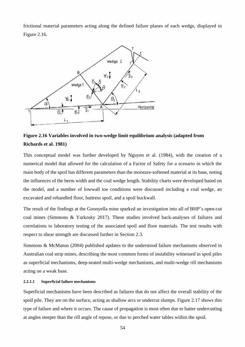
54
frictional material parameters acting along the defined failure planes of each wedge, displayed in
Figure 2.16.
Figure 2.16 Variables involved in two-wedge limit equilibrium analysis (adapted from
Richards et al. 1981)
This conceptual model was further developed by Nguyen et al. (1984), with the creation of a
numerical model that allowed for the calculation of a Factor of Safety for a scenario in which the
main body of the spoil has different parameters than the moisture-softened material at its base, noting
the influences of the berm width and the coal wedge length. Stability charts were developed based on
the model, and a number of lowwall toe conditions were discussed including a coal wedge, an
excavated and rehandled floor, buttress spoil, and a spoil buckwall.
The result of the findings at the Goonyella mine sparked an investigation into all of BHP’s open-cut
coal mines (Simmons & Yarkosky 2017). These studies involved back-analyses of failures and
correlations to laboratory testing of the associated spoil and floor materials. The test results with
respect to shear strength are discussed further in Section 2.3.
Simmons & McManus (2004) published updates to the understood failure mechanisms observed in
Australian coal strip mines, describing the most common forms of instability witnessed in spoil piles
as superficial mechanisms, deep-seated multi-wedge mechanisms, and multi-wedge rill mechanisms
acting on a weak base.
2.2.1.1 Superficial failure mechanisms
Superficial mechanisms have been described as failures that do not affect the overall stability of the
spoil pile. They are on the surface, acting as shallow arcs or undercut slumps. Figure 2.17 shows this
type of failure and where it occurs. The cause of propagation is most often due to batter undercutting
at angles steeper than the rill angle of repose, or due to perched water tables within the spoil.
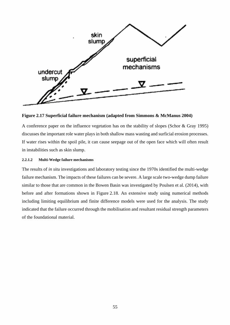
55
Figure 2.17 Superficial failure mechanism (adapted from Simmons & McManus 2004)
A conference paper on the influence vegetation has on the stability of slopes (Schor & Gray 1995)
discusses the important role water plays in both shallow mass wasting and surficial erosion processes.
If water rises within the spoil pile, it can cause seepage out of the open face which will often result
in instabilities such as skin slump.
2.2.1.2 Multi-Wedge failure mechanisms
The results of in situ investigations and laboratory testing since the 1970s identified the multi-wedge
failure mechanism. The impacts of these failures can be severe. A large scale two-wedge dump failure
similar to those that are common in the Bowen Basin was investigated by Poulsen et al. (2014), with
before and after formations shown in Figure 2.18. An extensive study using numerical methods
including limiting equilibrium and finite difference models were used for the analysis. The study
indicated that the failure occurred through the mobilisation and resultant residual strength parameters
of the foundational material.
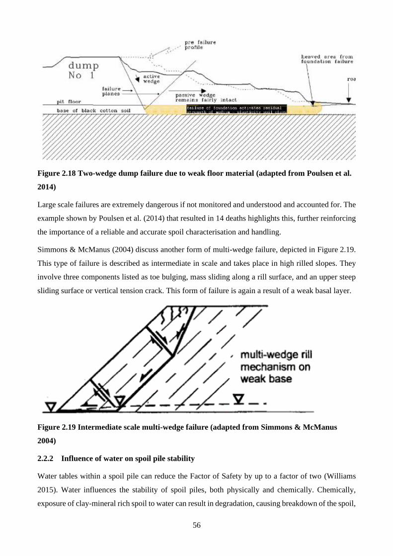
56
Figure 2.18 Two-wedge dump failure due to weak floor material (adapted from Poulsen et al.
2014)
Large scale failures are extremely dangerous if not monitored and understood and accounted for. The
example shown by Poulsen et al. (2014) that resulted in 14 deaths highlights this, further reinforcing
the importance of a reliable and accurate spoil characterisation and handling.
Simmons & McManus (2004) discuss another form of multi-wedge failure, depicted in Figure 2.19.
This type of failure is described as intermediate in scale and takes place in high rilled slopes. They
involve three components listed as toe bulging, mass sliding along a rill surface, and an upper steep
sliding surface or vertical tension crack. This form of failure is again a result of a weak basal layer.
Figure 2.19 Intermediate scale multi-wedge failure (adapted from Simmons & McManus
2004)
2.2.2 Influence of water on spoil pile stability
Water tables within a spoil pile can reduce the Factor of Safety by up to a factor of two (Williams
2015). Water influences the stability of spoil piles, both physically and chemically. Chemically,
exposure of clay-mineral rich spoil to water can result in degradation, causing breakdown of the spoil,
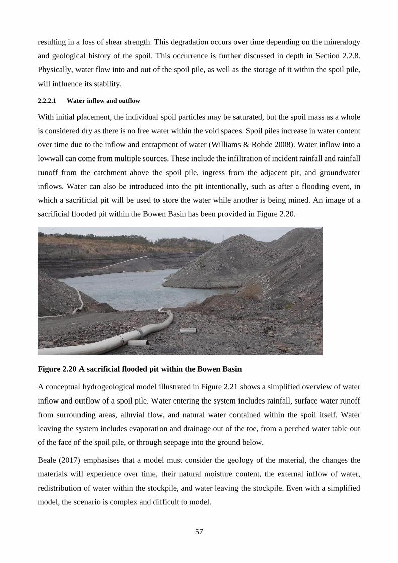
57
resulting in a loss of shear strength. This degradation occurs over time depending on the mineralogy
and geological history of the spoil. This occurrence is further discussed in depth in Section 2.2.8.
Physically, water flow into and out of the spoil pile, as well as the storage of it within the spoil pile,
will influence its stability.
2.2.2.1 Water inflow and outflow
With initial placement, the individual spoil particles may be saturated, but the spoil mass as a whole
is considered dry as there is no free water within the void spaces. Spoil piles increase in water content
over time due to the inflow and entrapment of water (Williams & Rohde 2008). Water inflow into a
lowwall can come from multiple sources. These include the infiltration of incident rainfall and rainfall
runoff from the catchment above the spoil pile, ingress from the adjacent pit, and groundwater
inflows. Water can also be introduced into the pit intentionally, such as after a flooding event, in
which a sacrificial pit will be used to store the water while another is being mined. An image of a
sacrificial flooded pit within the Bowen Basin has been provided in Figure 2.20.
Figure 2.20 A sacrificial flooded pit within the Bowen Basin
A conceptual hydrogeological model illustrated in Figure 2.21 shows a simplified overview of water
inflow and outflow of a spoil pile. Water entering the system includes rainfall, surface water runoff
from surrounding areas, alluvial flow, and natural water contained within the spoil itself. Water
leaving the system includes evaporation and drainage out of the toe, from a perched water table out
of the face of the spoil pile, or through seepage into the ground below.
Beale (2017) emphasises that a model must consider the geology of the material, the changes the
materials will experience over time, their natural moisture content, the external inflow of water,
redistribution of water within the stockpile, and water leaving the stockpile. Even with a simplified
model, the scenario is complex and difficult to model.
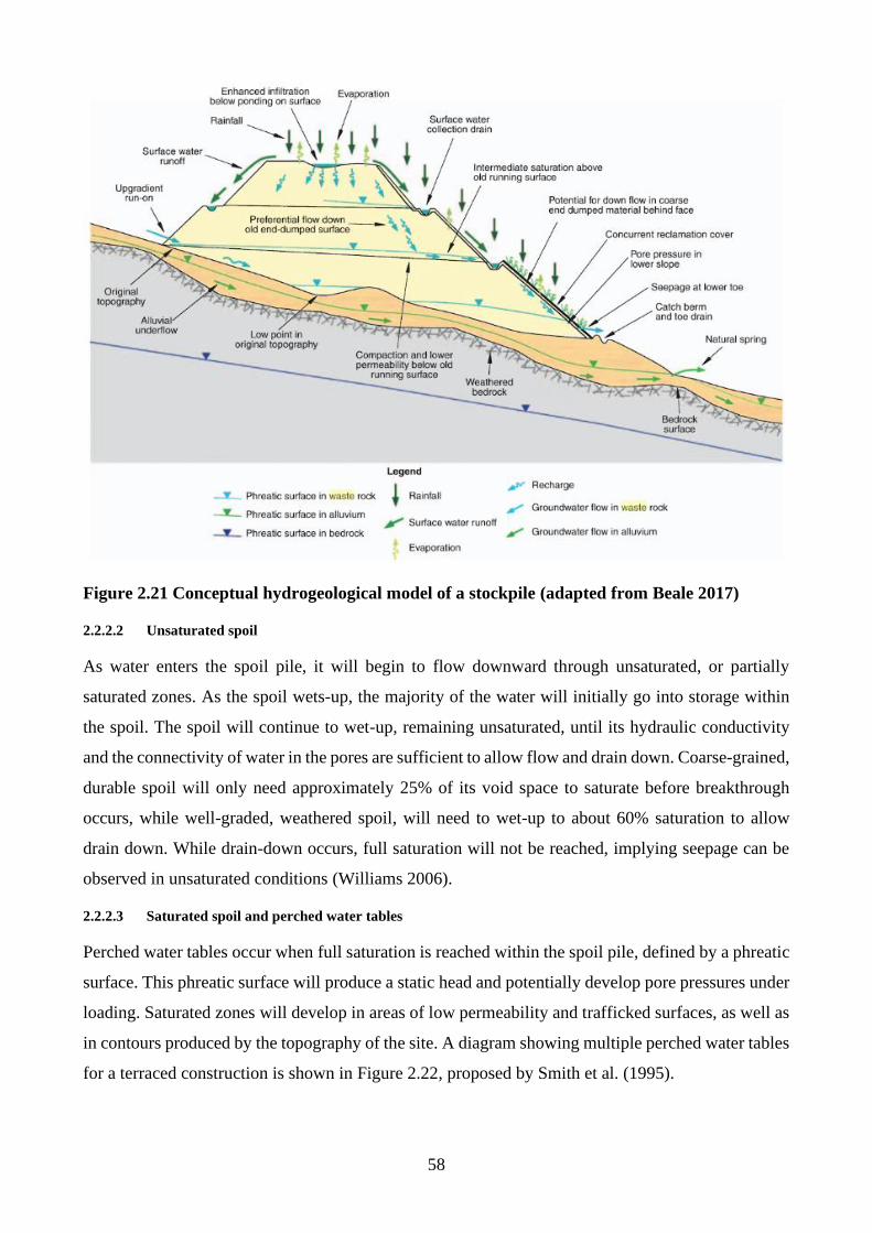
58
Figure 2.21 Conceptual hydrogeological model of a stockpile (adapted from Beale 2017)
2.2.2.2 Unsaturated spoil
As water enters the spoil pile, it will begin to flow downward through unsaturated, or partially
saturated zones. As the spoil wets-up, the majority of the water will initially go into storage within
the spoil. The spoil will continue to wet-up, remaining unsaturated, until its hydraulic conductivity
and the connectivity of water in the pores are sufficient to allow flow and drain down. Coarse-grained,
durable spoil will only need approximately 25% of its void space to saturate before breakthrough
occurs, while well-graded, weathered spoil, will need to wet-up to about 60% saturation to allow
drain down. While drain-down occurs, full saturation will not be reached, implying seepage can be
observed in unsaturated conditions (Williams 2006).
2.2.2.3 Saturated spoil and perched water tables
Perched water tables occur when full saturation is reached within the spoil pile, defined by a phreatic
surface. This phreatic surface will produce a static head and potentially develop pore pressures under
loading. Saturated zones will develop in areas of low permeability and trafficked surfaces, as well as
in contours produced by the topography of the site. A diagram showing multiple perched water tables
for a terraced construction is shown in Figure 2.22, proposed by Smith et al. (1995).
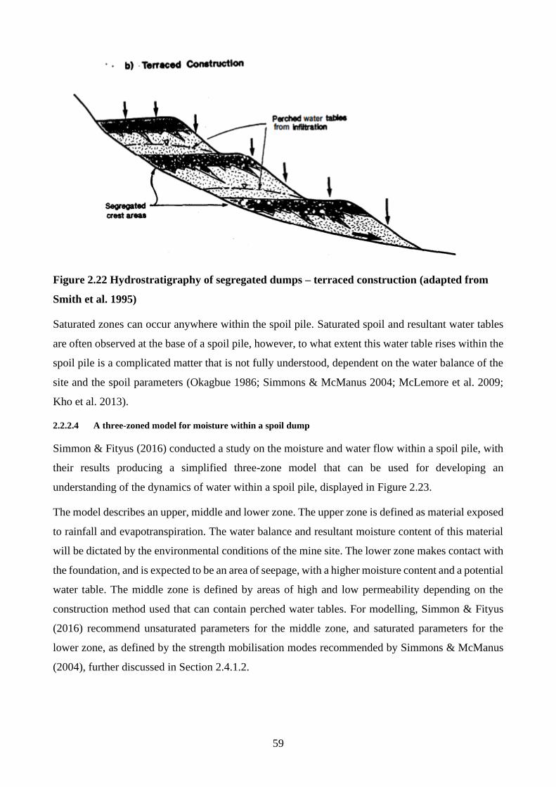
59
Figure 2.22 Hydrostratigraphy of segregated dumps – terraced construction (adapted from
Smith et al. 1995)
Saturated zones can occur anywhere within the spoil pile. Saturated spoil and resultant water tables
are often observed at the base of a spoil pile, however, to what extent this water table rises within the
spoil pile is a complicated matter that is not fully understood, dependent on the water balance of the
site and the spoil parameters (Okagbue 1986; Simmons & McManus 2004; McLemore et al. 2009;
Kho et al. 2013).
2.2.2.4 A three-zoned model for moisture within a spoil dump
Simmon & Fityus (2016) conducted a study on the moisture and water flow within a spoil pile, with
their results producing a simplified three-zone model that can be used for developing an
understanding of the dynamics of water within a spoil pile, displayed in Figure 2.23.
The model describes an upper, middle and lower zone. The upper zone is defined as material exposed
to rainfall and evapotranspiration. The water balance and resultant moisture content of this material
will be dictated by the environmental conditions of the mine site. The lower zone makes contact with
the foundation, and is expected to be an area of seepage, with a higher moisture content and a potential
water table. The middle zone is defined by areas of high and low permeability depending on the
construction method used that can contain perched water tables. For modelling, Simmon & Fityus
(2016) recommend unsaturated parameters for the middle zone, and saturated parameters for the
lower zone, as defined by the strength mobilisation modes recommended by Simmons & McManus
(2004), further discussed in Section 2.4.1.2.
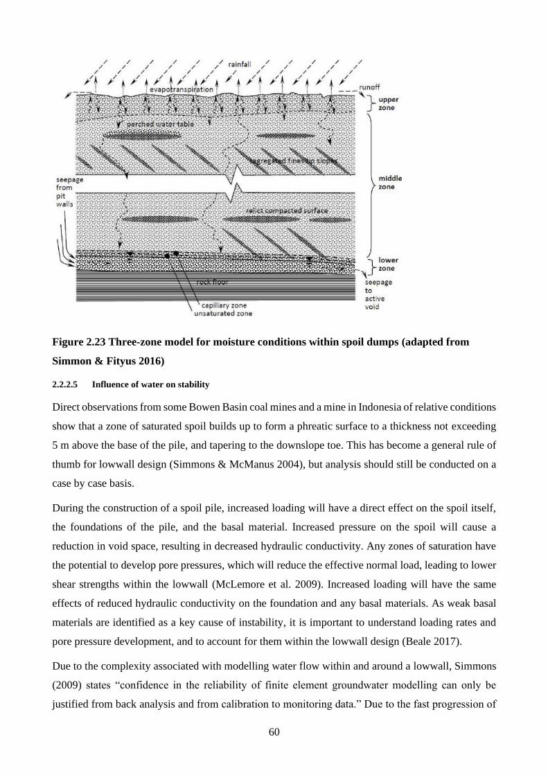
60
Figure 2.23 Three-zone model for moisture conditions within spoil dumps (adapted from
Simmon & Fityus 2016)
2.2.2.5 Influence of water on stability
Direct observations from some Bowen Basin coal mines and a mine in Indonesia of relative conditions
show that a zone of saturated spoil builds up to form a phreatic surface to a thickness not exceeding
5 m above the base of the pile, and tapering to the downslope toe. This has become a general rule of
thumb for lowwall design (Simmons & McManus 2004), but analysis should still be conducted on a
case by case basis.
During the construction of a spoil pile, increased loading will have a direct effect on the spoil itself,
the foundations of the pile, and the basal material. Increased pressure on the spoil will cause a
reduction in void space, resulting in decreased hydraulic conductivity. Any zones of saturation have
the potential to develop pore pressures, which will reduce the effective normal load, leading to lower
shear strengths within the lowwall (McLemore et al. 2009). Increased loading will have the same
effects of reduced hydraulic conductivity on the foundation and any basal materials. As weak basal
materials are identified as a key cause of instability, it is important to understand loading rates and
pore pressure development, and to account for them within the lowwall design (Beale 2017).
Due to the complexity associated with modelling water flow within and around a lowwall, Simmons
(2009) states “confidence in the reliability of finite element groundwater modelling can only be
justified from back analysis and from calibration to monitoring data.” Due to the fast progression of
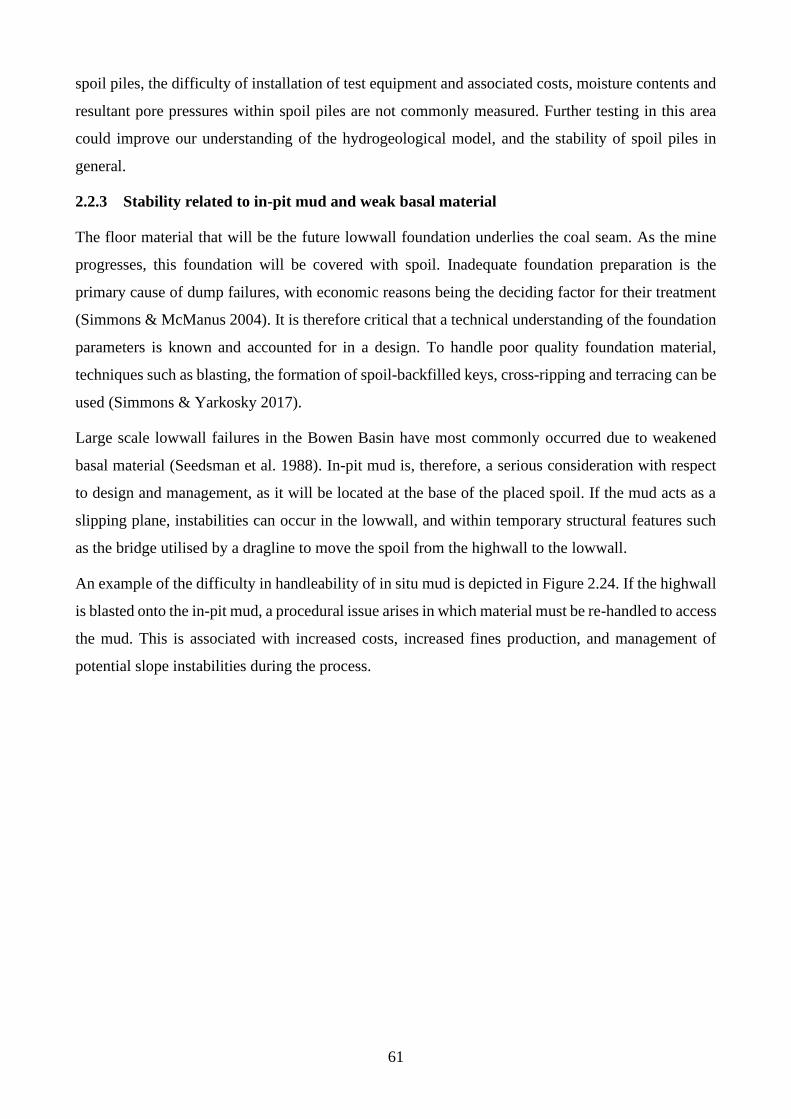
61
spoil piles, the difficulty of installation of test equipment and associated costs, moisture contents and
resultant pore pressures within spoil piles are not commonly measured. Further testing in this area
could improve our understanding of the hydrogeological model, and the stability of spoil piles in
general.
2.2.3 Stability related to in-pit mud and weak basal material
The floor material that will be the future lowwall foundation underlies the coal seam. As the mine
progresses, this foundation will be covered with spoil. Inadequate foundation preparation is the
primary cause of dump failures, with economic reasons being the deciding factor for their treatment
(Simmons & McManus 2004). It is therefore critical that a technical understanding of the foundation
parameters is known and accounted for in a design. To handle poor quality foundation material,
techniques such as blasting, the formation of spoil-backfilled keys, cross-ripping and terracing can be
used (Simmons & Yarkosky 2017).
Large scale lowwall failures in the Bowen Basin have most commonly occurred due to weakened
basal material (Seedsman et al. 1988). In-pit mud is, therefore, a serious consideration with respect
to design and management, as it will be located at the base of the placed spoil. If the mud acts as a
slipping plane, instabilities can occur in the lowwall, and within temporary structural features such
as the bridge utilised by a dragline to move the spoil from the highwall to the lowwall.
An example of the difficulty in handleability of in situ mud is depicted in Figure 2.24. If the highwall
is blasted onto the in-pit mud, a procedural issue arises in which material must be re-handled to access
the mud. This is associated with increased costs, increased fines production, and management of
potential slope instabilities during the process.
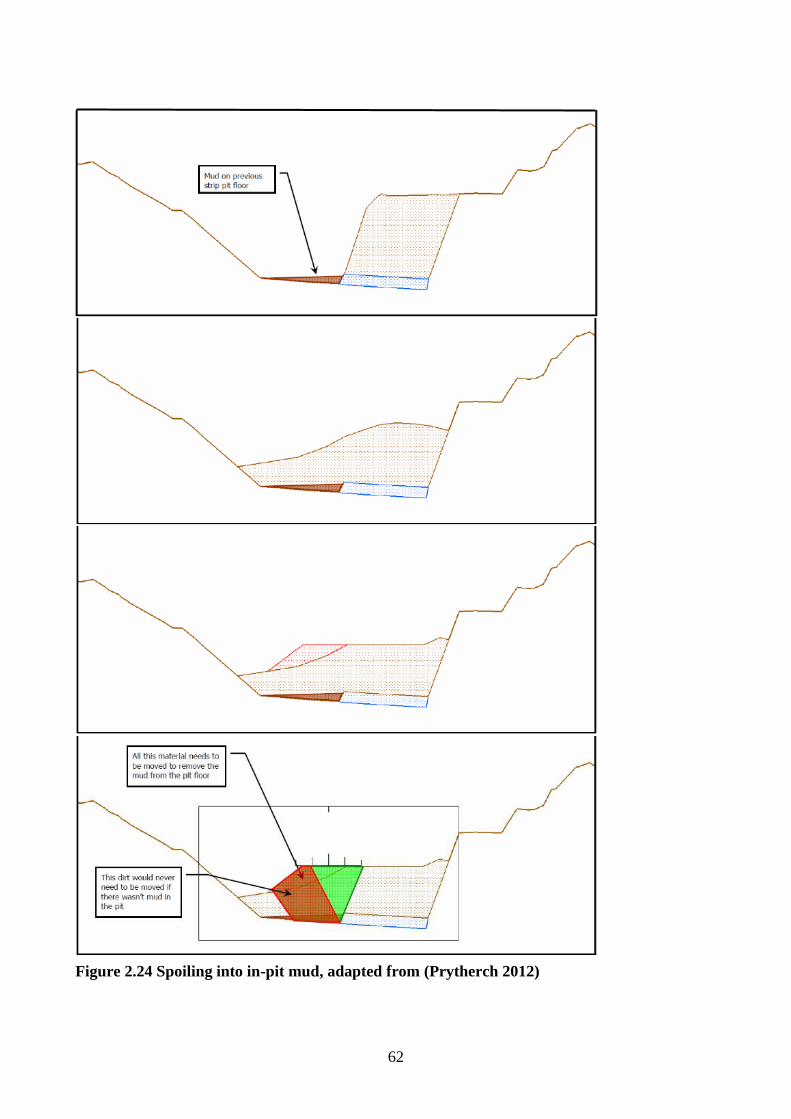
62
Figure 2.24 Spoiling into in-pit mud, adapted from (Prytherch 2012)
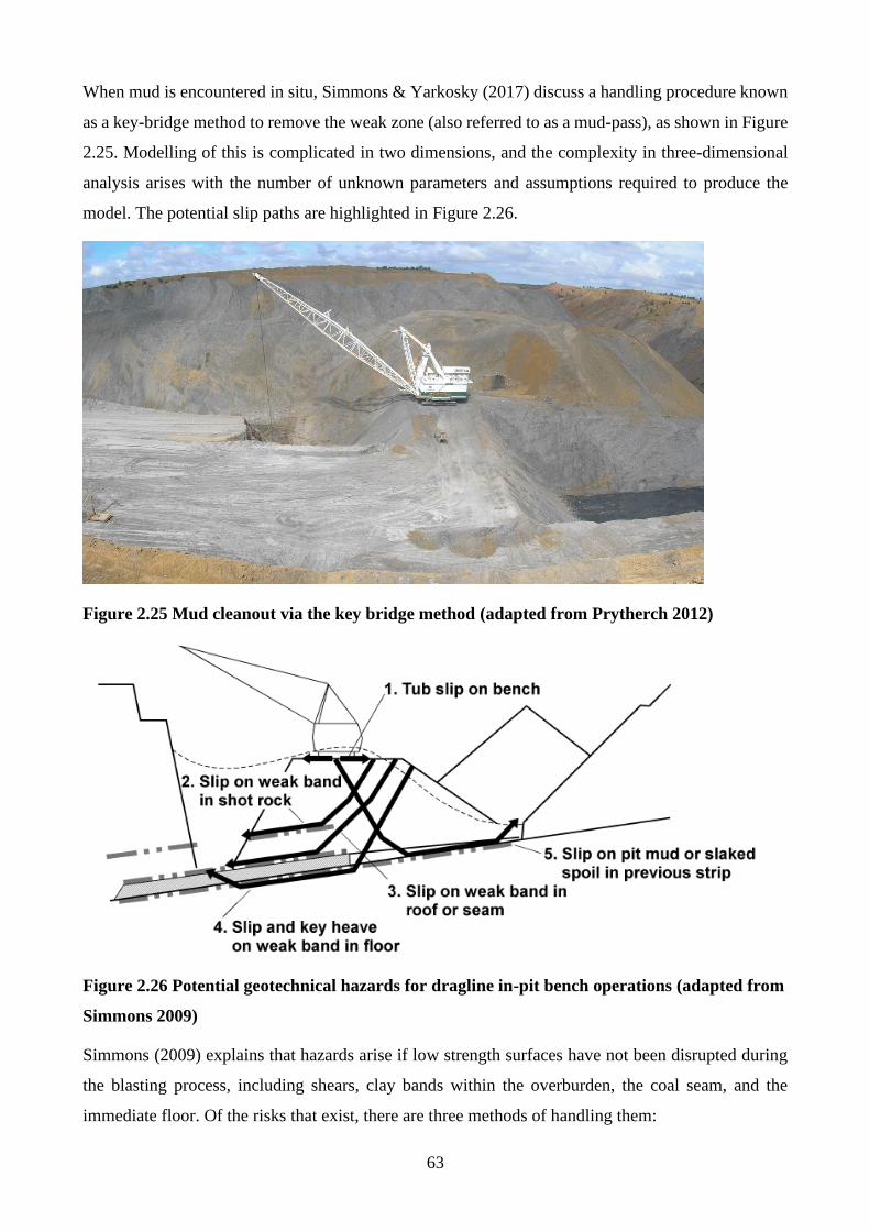
63
When mud is encountered in situ, Simmons & Yarkosky (2017) discuss a handling procedure known
as a key-bridge method to remove the weak zone (also referred to as a mud-pass), as shown in Figure
2.25. Modelling of this is complicated in two dimensions, and the complexity in three-dimensional
analysis arises with the number of unknown parameters and assumptions required to produce the
model. The potential slip paths are highlighted in Figure 2.26.
Figure 2.25 Mud cleanout via the key bridge method (adapted from Prytherch 2012)
Figure 2.26 Potential geotechnical hazards for dragline in-pit bench operations (adapted from
Simmons 2009)
Simmons (2009) explains that hazards arise if low strength surfaces have not been disrupted during
the blasting process, including shears, clay bands within the overburden, the coal seam, and the
immediate floor. Of the risks that exist, there are three methods of handling them:
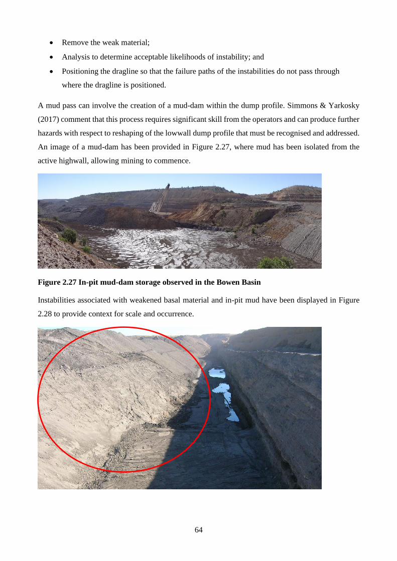
64
• Remove the weak material;
• Analysis to determine acceptable likelihoods of instability; and
• Positioning the dragline so that the failure paths of the instabilities do not pass through
where the dragline is positioned.
A mud pass can involve the creation of a mud-dam within the dump profile. Simmons & Yarkosky
(2017) comment that this process requires significant skill from the operators and can produce further
hazards with respect to reshaping of the lowwall dump profile that must be recognised and addressed.
An image of a mud-dam has been provided in Figure 2.27, where mud has been isolated from the
active highwall, allowing mining to commence.
Figure 2.27 In-pit mud-dam storage observed in the Bowen Basin
Instabilities associated with weakened basal material and in-pit mud have been displayed in Figure
2.28 to provide context for scale and occurrence.
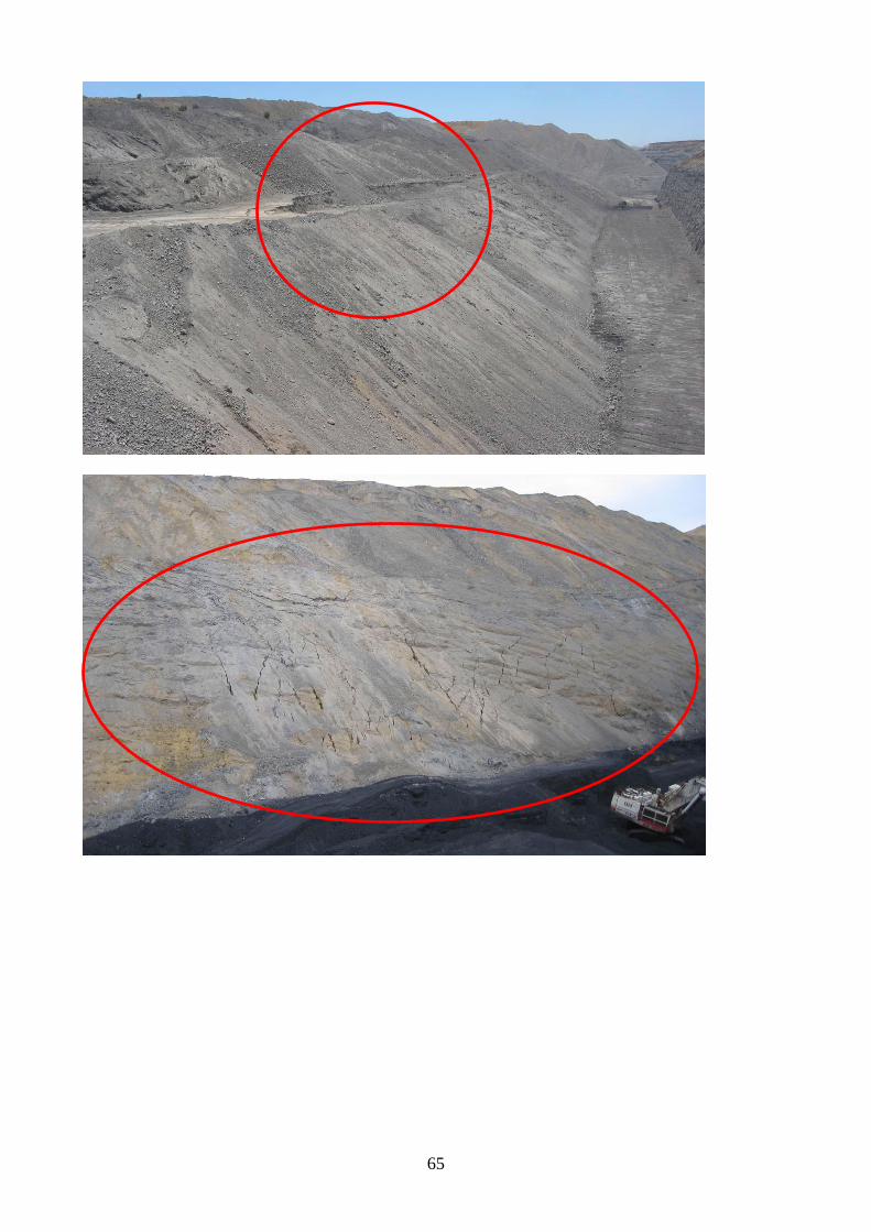
65
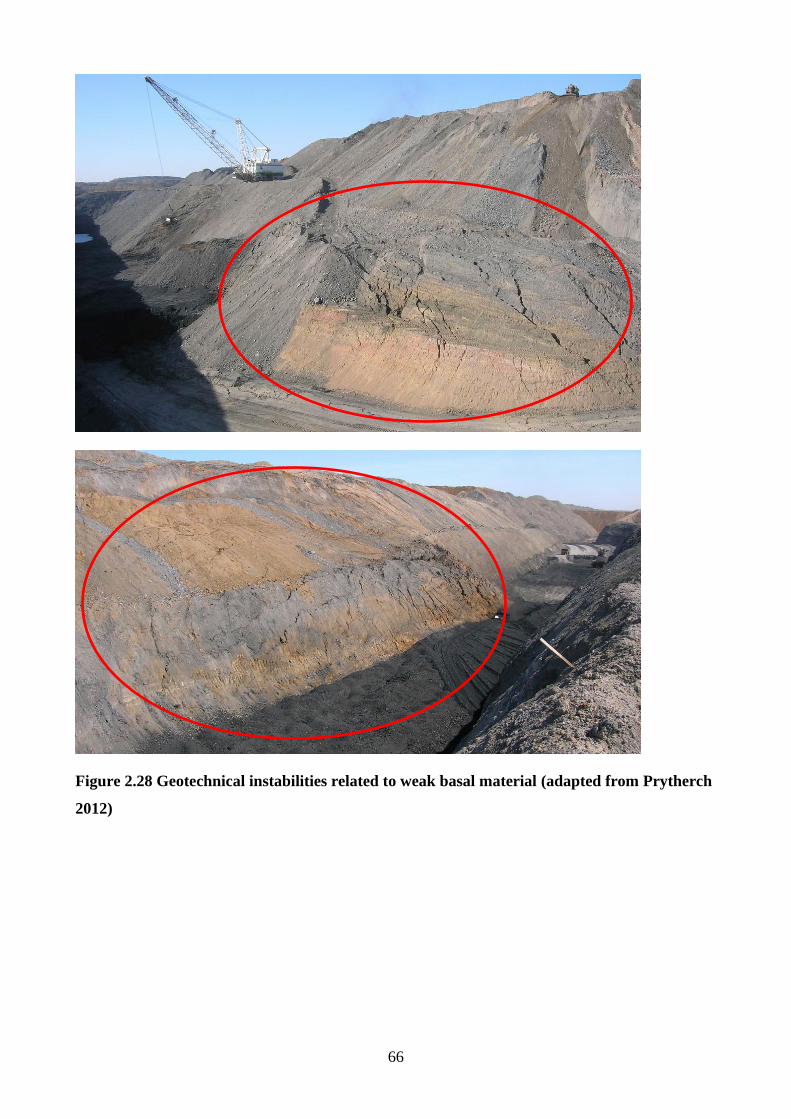
66
Figure 2.28 Geotechnical instabilities related to weak basal material (adapted from Prytherch
2012)
67
2.2.4 Drained or undrained failure
For coarse-grained spoil, large voids indicate drained conditions will exist, allowing water to flow
freely through the voids, with the stresses being held by the spoil framework. This contrasts with
undrained conditions, where the water in the voids cannot flow out fast enough, resulting in an
increase in pore pressures with no change in volume due to the incompressible nature of water. For
complex scenarios such as spoil piles, the internal spoil may be drained or undrained and can be
within these idealised conditions, acting in a partially drained manner (Williams 2015).
While typically drained conditions are observed, Duran (2013) investigated the behaviour of two
spoil piles in the Bowen Basin that appeared to exhibit undrained behaviour. Seven possible scenarios
were analysed involving weak basal material at the bottom of a spoil pile. One such scenario is
depicted in Figure 2.29, which shows the progression of a strip mine that was inundated with water.
The water within the pit was removed, and the next strip loading was placed against the previous
spoil pile. Upon completion of the strip, a large double wedge failure occurred, with shearing along
the previously saturated basal zone.
The failures were examined using the Morgenstern-Price method of slides. The models were
generated and calibrated with measurements recorded in situ to determine the best parameters to
represent the failure that occurred. It was found that for two scenarios, excellent matches existed
between the critical failure paths observed and undrained strength parameters. Duran (2013)
concludes that for undrained behaviour to be considered, the following aspects are required:
• Materials highly prone to slaking; and
• Previous spoil that has undergone flooding, with undrained behaviour applicable to areas
where additional spoil loading occurs in the current strip.
For investigations into in-pit mud, it is therefore critical to determine whether the material is likely
to exhibit drained or undrained conditions, as this will influence how the material should be tested in
the laboratory. Ideal conditions for maximum shear strength will be under drained conditions. It is,
therefore, most likely that in-pit muds with coarse-grained particle size distributions will have the
highest likelihood of ensuring stability.
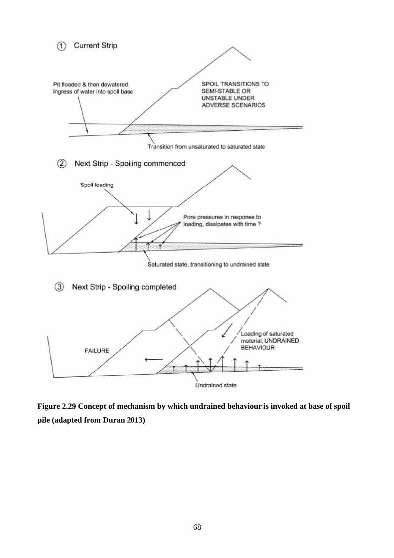
68
Figure 2.29 Concept of mechanism by which undrained behaviour is invoked at base of spoil
pile (adapted from Duran 2013)
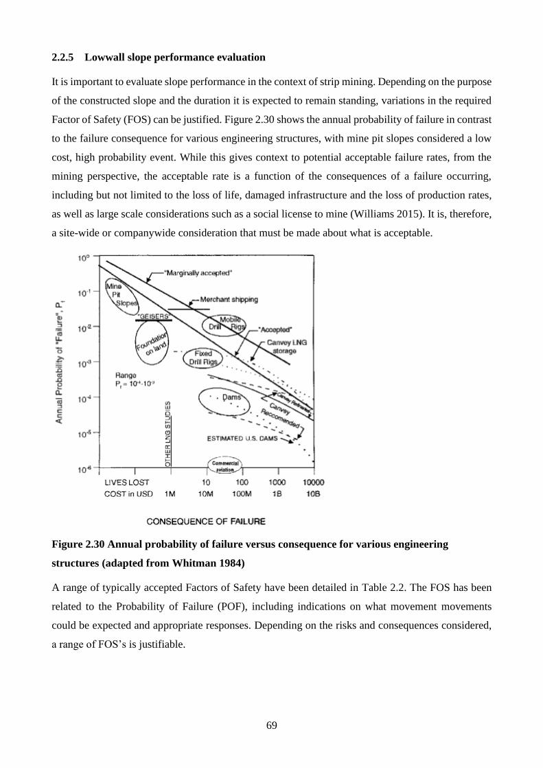
69
2.2.5 Lowwall slope performance evaluation
It is important to evaluate slope performance in the context of strip mining. Depending on the purpose
of the constructed slope and the duration it is expected to remain standing, variations in the required
Factor of Safety (FOS) can be justified. Figure 2.30 shows the annual probability of failure in contrast
to the failure consequence for various engineering structures, with mine pit slopes considered a low
cost, high probability event. While this gives context to potential acceptable failure rates, from the
mining perspective, the acceptable rate is a function of the consequences of a failure occurring,
including but not limited to the loss of life, damaged infrastructure and the loss of production rates,
as well as large scale considerations such as a social license to mine (Williams 2015). It is, therefore,
a site-wide or companywide consideration that must be made about what is acceptable.
Figure 2.30 Annual probability of failure versus consequence for various engineering
structures (adapted from Whitman 1984)
A range of typically accepted Factors of Safety have been detailed in Table 2.2. The FOS has been
related to the Probability of Failure (POF), including indications on what movement movements
could be expected and appropriate responses. Depending on the risks and consequences considered,
a range of FOS’s is justifiable.
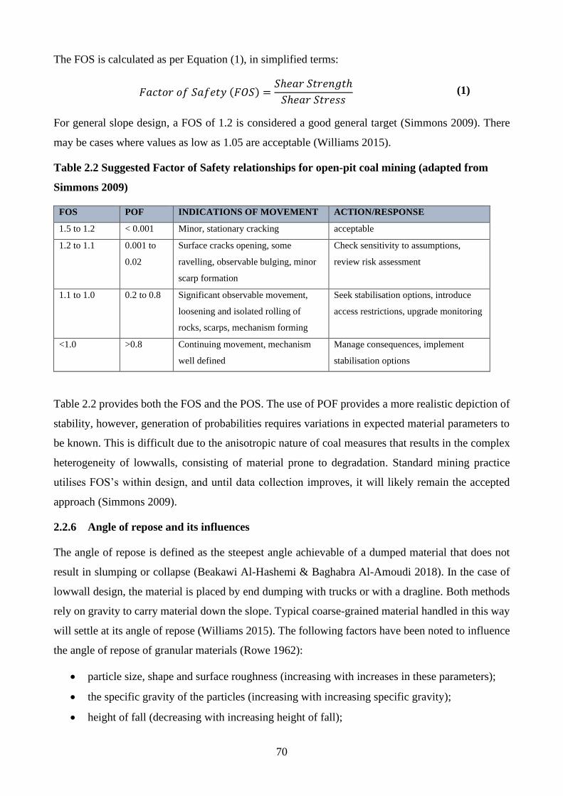
70
The FOS is calculated as per Equation (1), in simplified terms:
𝐹𝑎𝑐𝑡𝑜𝑟 𝑜𝑓 𝑆𝑎𝑓𝑒𝑡𝑦 (𝐹𝑂𝑆) =𝑆ℎ𝑒𝑎𝑟 𝑆𝑡𝑟𝑒𝑛𝑔𝑡ℎ
𝑆ℎ𝑒𝑎𝑟 𝑆𝑡𝑟𝑒𝑠𝑠 (1)
For general slope design, a FOS of 1.2 is considered a good general target (Simmons 2009). There
may be cases where values as low as 1.05 are acceptable (Williams 2015).
Table 2.2 Suggested Factor of Safety relationships for open-pit coal mining (adapted from
Simmons 2009)
FOS POF INDICATIONS OF MOVEMENT ACTION/RESPONSE
1.5 to 1.2 < 0.001 Minor, stationary cracking acceptable
1.2 to 1.1 0.001 to
0.02
Surface cracks opening, some
ravelling, observable bulging, minor
scarp formation
Check sensitivity to assumptions,
review risk assessment
1.1 to 1.0 0.2 to 0.8 Significant observable movement,
loosening and isolated rolling of
rocks, scarps, mechanism forming
Seek stabilisation options, introduce
access restrictions, upgrade monitoring
<1.0 >0.8 Continuing movement, mechanism
well defined
Manage consequences, implement
stabilisation options
Table 2.2 provides both the FOS and the POS. The use of POF provides a more realistic depiction of
stability, however, generation of probabilities requires variations in expected material parameters to
be known. This is difficult due to the anisotropic nature of coal measures that results in the complex
heterogeneity of lowwalls, consisting of material prone to degradation. Standard mining practice
utilises FOS’s within design, and until data collection improves, it will likely remain the accepted
approach (Simmons 2009).
2.2.6 Angle of repose and its influences
The angle of repose is defined as the steepest angle achievable of a dumped material that does not
result in slumping or collapse (Beakawi Al-Hashemi & Baghabra Al-Amoudi 2018). In the case of
lowwall design, the material is placed by end dumping with trucks or with a dragline. Both methods
rely on gravity to carry material down the slope. Typical coarse-grained material handled in this way
will settle at its angle of repose (Williams 2015). The following factors have been noted to influence
the angle of repose of granular materials (Rowe 1962):
• particle size, shape and surface roughness (increasing with increases in these parameters);
• the specific gravity of the particles (increasing with increasing specific gravity);
• height of fall (decreasing with increasing height of fall);
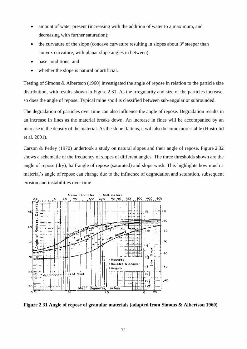
71
• amount of water present (increasing with the addition of water to a maximum, and
decreasing with further saturation);
• the curvature of the slope (concave curvature resulting in slopes about 3o steeper than
convex curvature, with planar slope angles in between);
• base conditions; and
• whether the slope is natural or artificial.
Testing of Simons & Albertson (1960) investigated the angle of repose in relation to the particle size
distribution, with results shown in Figure 2.31. As the irregularity and size of the particles increase,
so does the angle of repose. Typical mine spoil is classified between sub-angular or subrounded.
The degradation of particles over time can also influence the angle of repose. Degradation results in
an increase in fines as the material breaks down. An increase in fines will be accompanied by an
increase in the density of the material. As the slope flattens, it will also become more stable (Hustrulid
et al. 2001).
Carson & Petley (1970) undertook a study on natural slopes and their angle of repose. Figure 2.32
shows a schematic of the frequency of slopes of different angles. The three thresholds shown are the
angle of repose (dry), half-angle of repose (saturated) and slope wash. This highlights how much a
material’s angle of repose can change due to the influence of degradation and saturation, subsequent
erosion and instabilities over time.
Figure 2.31 Angle of repose of granular materials (adapted from Simons & Albertson 1960)
72
Figure 2.32 Schematic frequency distribution for natural hillslope angles in the United
Kingdom (adapted from Carson & Petley 1970)
2.2.7 Shear strength and its influences
The shear strength of a soil is described as the shear stress that can be resisted prior to deformation.
There are many models for the calculation of shear strength in soil mechanics, of which the most
commonly adopted for lowwall design with saturated conditions is determined as per Equation (2)
(Terzaghi 1936).
= 𝑐′ + (𝑛
− uw) 𝑡𝑎𝑛 ′ (2)
where:
= shear strength
c’ = apparent cohesion
n = normal stress on the failure plane
uw = pore-water pressure
(n – uw) = effective normal stress on failure plane
’ = effective friction angle
When plotted on a graph of shear strength in relation to normal stress, Mohr-Coulomb criterion can
be applied to determine the values of apparent cohesion and the effective friction angle, as defined
by the intercept of the y-axis and the strength envelope that intersects multiple Mohr circles
respectively. These relationships have been plotted in Figure 2.35.
The friction angle is a complex function of the (Hustrulid et al. 2001):
• particle size distribution (reducing with decreasing particle size);
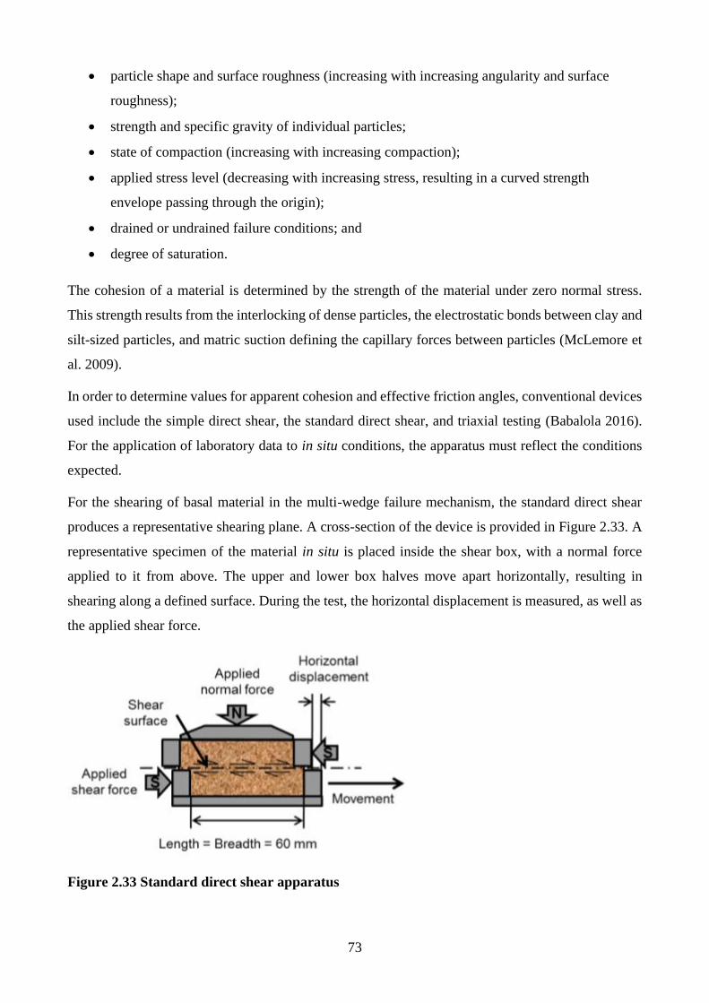
73
• particle shape and surface roughness (increasing with increasing angularity and surface
roughness);
• strength and specific gravity of individual particles;
• state of compaction (increasing with increasing compaction);
• applied stress level (decreasing with increasing stress, resulting in a curved strength
envelope passing through the origin);
• drained or undrained failure conditions; and
• degree of saturation.
The cohesion of a material is determined by the strength of the material under zero normal stress.
This strength results from the interlocking of dense particles, the electrostatic bonds between clay and
silt-sized particles, and matric suction defining the capillary forces between particles (McLemore et
al. 2009).
In order to determine values for apparent cohesion and effective friction angles, conventional devices
used include the simple direct shear, the standard direct shear, and triaxial testing (Babalola 2016).
For the application of laboratory data to in situ conditions, the apparatus must reflect the conditions
expected.
For the shearing of basal material in the multi-wedge failure mechanism, the standard direct shear
produces a representative shearing plane. A cross-section of the device is provided in Figure 2.33. A
representative specimen of the material in situ is placed inside the shear box, with a normal force
applied to it from above. The upper and lower box halves move apart horizontally, resulting in
shearing along a defined surface. During the test, the horizontal displacement is measured, as well as
the applied shear force.
Figure 2.33 Standard direct shear apparatus
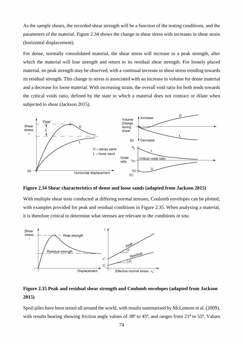
74
As the sample shears, the recorded shear strength will be a function of the testing conditions, and the
parameters of the material. Figure 2.34 shows the change in shear stress with increases in shear strain
(horizontal displacement).
For dense, normally consolidated material, the shear stress will increase to a peak strength, after
which the material will lose strength and return to its residual shear strength. For loosely placed
material, no peak strength may be observed, with a continual increase in shear stress trending towards
its residual strength. This change in stress is associated with an increase in volume for dense material
and a decrease for loose material. With increasing strain, the overall void ratio for both tends towards
the critical voids ratio, defined by the state in which a material does not contract or dilate when
subjected to shear (Jackson 2015).
Figure 2.34 Shear characteristics of dense and loose sands (adapted from Jackson 2015)
With multiple shear tests conducted at differing normal stresses, Coulomb envelopes can be plotted,
with examples provided for peak and residual conditions in Figure 2.35. When analysing a material,
it is therefore critical to determine what stresses are relevant to the conditions in situ.
Figure 2.35 Peak and residual shear strength and Coulomb envelopes (adapted from Jackson
2015)
Spoil piles have been tested all around the world, with results summarised by McLemore et al. (2009),
with results bearing showing friction angle values of 38⁰ to 45⁰, and ranges from 21⁰ to 55⁰. Values
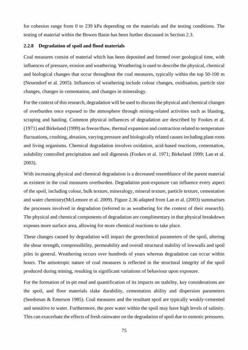
75
for cohesion range from 0 to 239 kPa depending on the materials and the testing conditions. The
testing of material within the Bowen Basin has been further discussed in Section 2.3.
2.2.8 Degradation of spoil and flood materials
Coal measures consist of material which has been deposited and formed over geological time, with
influences of pressure, erosion and weathering. Weathering is used to describe the physical, chemical
and biological changes that occur throughout the coal measures, typically within the top 50-100 m
(Neuendorf et al. 2005). Influences of weathering include colour changes, oxidisation, particle size
changes, changes in cementation, and changes in mineralogy.
For the context of this research, degradation will be used to discuss the physical and chemical changes
of overburden once exposed to the atmosphere through mining-related activities such as blasting,
scraping and hauling. Common physical influences of degradation are described by Fookes et al.
(1971) and Birkeland (1999) as freeze/thaw, thermal expansion and contraction related to temperature
fluctuations, crushing, abrasion, varying pressure and biologically related causes including plant roots
and living organisms. Chemical degradation involves oxidation, acid-based reactions, cementation,
solubility controlled precipitation and soil digenesis (Fookes et al. 1971; Birkeland 1999; Lan et al.
2003).
With increasing physical and chemical degradation is a decreased resemblance of the parent material
as existent in the coal measures overburden. Degradation post-exposure can influence every aspect
of the spoil, including colour, bulk texture, mineralogy, mineral texture, particle texture, cementation
and water chemistry(McLemore et al. 2009). Figure 2.36 adapted from Lan et al. (2003) summarises
the processes involved in degradation (referred to as weathering for the context of their research).
The physical and chemical components of degradation are complimentary in that physical breakdown
exposes more surface area, allowing for more chemical reactions to take place.
These changes caused by degradation will impact the geotechnical parameters of the spoil, altering
the shear strength, compressibility, permeability and overall structural stability of lowwalls and spoil
piles in general. Weathering occurs over hundreds of years whereas degradation can occur within
hours. The anisotropic nature of coal measures is reflected in the structural integrity of the spoil
produced during mining, resulting in significant variations of behaviour upon exposure.
For the formation of in-pit mud and quantification of its impacts on stability, key considerations are
the spoil, and floor materials slake durability, cementation ability and dispersion parameters
(Seedsman & Emerson 1985). Coal measures and the resultant spoil are typically weakly-cemented
and sensitive to water. Furthermore, the pore water within the spoil may have high levels of salinity.
This can exacerbate the effects of fresh rainwater on the degradation of spoil due to osmotic pressures.
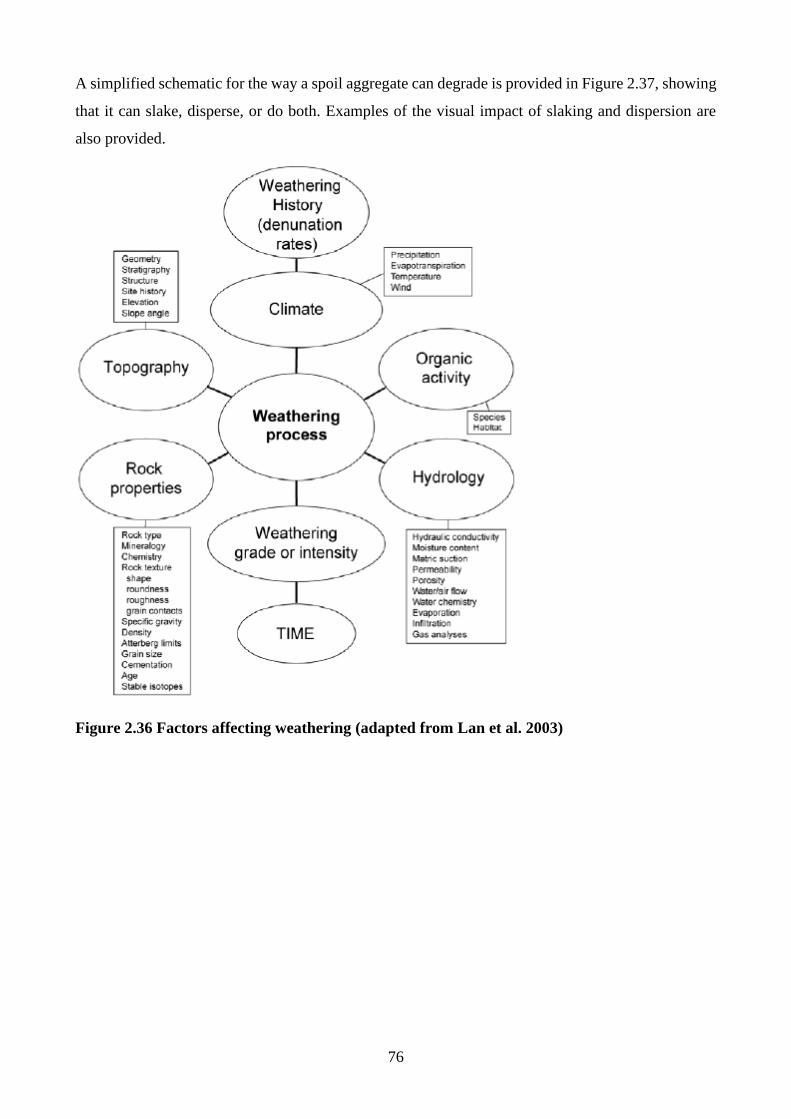
76
A simplified schematic for the way a spoil aggregate can degrade is provided in Figure 2.37, showing
that it can slake, disperse, or do both. Examples of the visual impact of slaking and dispersion are
also provided.
Figure 2.36 Factors affecting weathering (adapted from Lan et al. 2003)
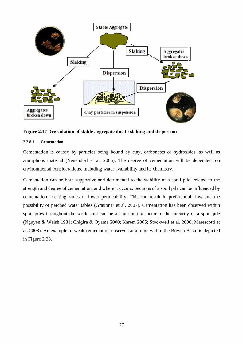
77
Figure 2.37 Degradation of stable aggregate due to slaking and dispersion
2.2.8.1 Cementation
Cementation is caused by particles being bound by clay, carbonates or hydroxides, as well as
amorphous material (Neuendorf et al. 2005). The degree of cementation will be dependent on
environmental considerations, including water availability and its chemistry.
Cementation can be both supportive and detrimental to the stability of a spoil pile, related to the
strength and degree of cementation, and where it occurs. Sections of a spoil pile can be influenced by
cementation, creating zones of lower permeability. This can result in preferential flow and the
possibility of perched water tables (Graupner et al. 2007). Cementation has been observed within
spoil piles throughout the world and can be a contributing factor to the integrity of a spoil pile
(Nguyen & Welsh 1981; Chigira & Oyama 2000; Karem 2005; Stockwell et al. 2006; Marescotti et
al. 2008). An example of weak cementation observed at a mine within the Bowen Basin is depicted
in Figure 2.38.
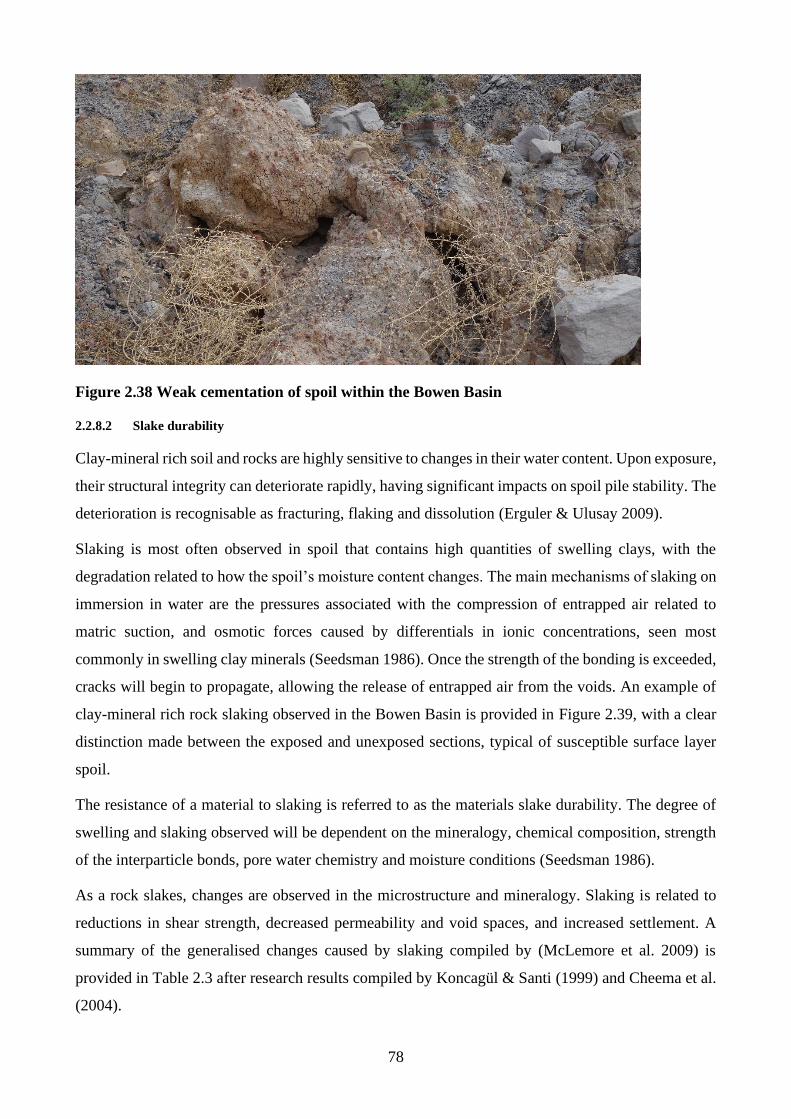
78
Figure 2.38 Weak cementation of spoil within the Bowen Basin
2.2.8.2 Slake durability
Clay-mineral rich soil and rocks are highly sensitive to changes in their water content. Upon exposure,
their structural integrity can deteriorate rapidly, having significant impacts on spoil pile stability. The
deterioration is recognisable as fracturing, flaking and dissolution (Erguler & Ulusay 2009).
Slaking is most often observed in spoil that contains high quantities of swelling clays, with the
degradation related to how the spoil’s moisture content changes. The main mechanisms of slaking on
immersion in water are the pressures associated with the compression of entrapped air related to
matric suction, and osmotic forces caused by differentials in ionic concentrations, seen most
commonly in swelling clay minerals (Seedsman 1986). Once the strength of the bonding is exceeded,
cracks will begin to propagate, allowing the release of entrapped air from the voids. An example of
clay-mineral rich rock slaking observed in the Bowen Basin is provided in Figure 2.39, with a clear
distinction made between the exposed and unexposed sections, typical of susceptible surface layer
spoil.
The resistance of a material to slaking is referred to as the materials slake durability. The degree of
swelling and slaking observed will be dependent on the mineralogy, chemical composition, strength
of the interparticle bonds, pore water chemistry and moisture conditions (Seedsman 1986).
As a rock slakes, changes are observed in the microstructure and mineralogy. Slaking is related to
reductions in shear strength, decreased permeability and void spaces, and increased settlement. A
summary of the generalised changes caused by slaking compiled by (McLemore et al. 2009) is
provided in Table 2.3 after research results compiled by Koncagül & Santi (1999) and Cheema et al.
(2004).
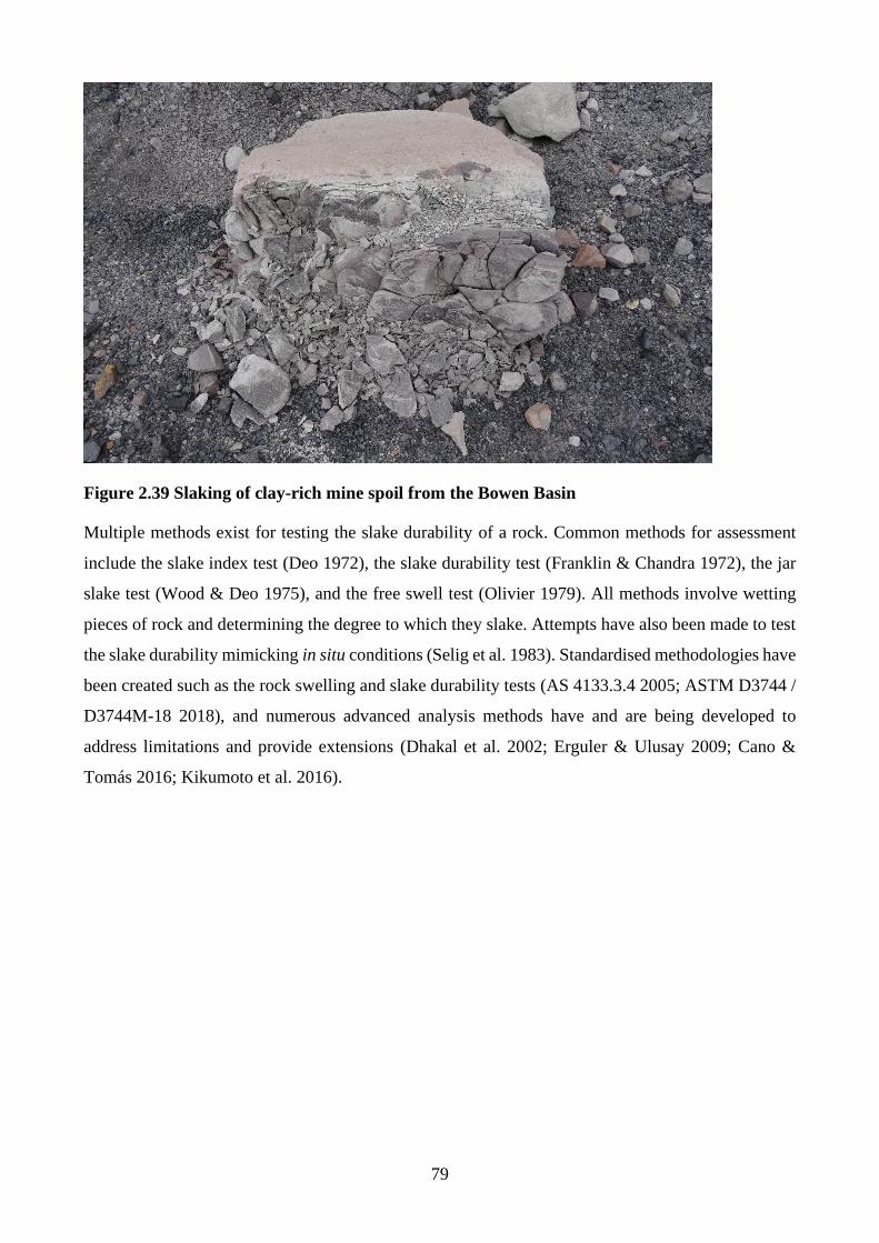
79
Figure 2.39 Slaking of clay-rich mine spoil from the Bowen Basin
Multiple methods exist for testing the slake durability of a rock. Common methods for assessment
include the slake index test (Deo 1972), the slake durability test (Franklin & Chandra 1972), the jar
slake test (Wood & Deo 1975), and the free swell test (Olivier 1979). All methods involve wetting
pieces of rock and determining the degree to which they slake. Attempts have also been made to test
the slake durability mimicking in situ conditions (Selig et al. 1983). Standardised methodologies have
been created such as the rock swelling and slake durability tests (AS 4133.3.4 2005; ASTM D3744 /
D3744M-18 2018), and numerous advanced analysis methods have and are being developed to
address limitations and provide extensions (Dhakal et al. 2002; Erguler & Ulusay 2009; Cano &
Tomás 2016; Kikumoto et al. 2016).
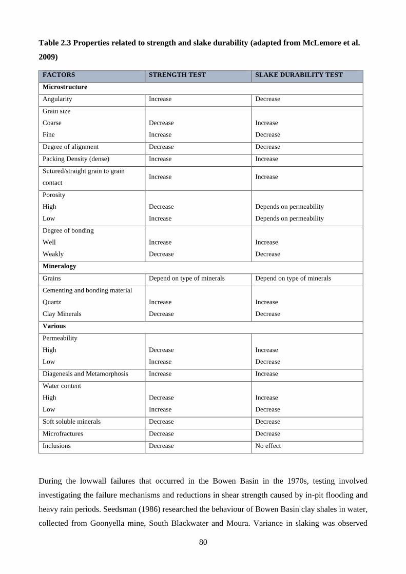
80
Table 2.3 Properties related to strength and slake durability (adapted from McLemore et al.
2009)
FACTORS STRENGTH TEST SLAKE DURABILITY TEST
Microstructure
Angularity Increase Decrease
Grain size
Coarse
Fine
Decrease
Increase
Increase
Decrease
Degree of alignment Decrease Decrease
Packing Density (dense) Increase Increase
Sutured/straight grain to grain
contact Increase Increase
Porosity
High
Low
Decrease
Increase
Depends on permeability
Depends on permeability
Degree of bonding
Well
Weakly
Increase
Decrease
Increase
Decrease
Mineralogy
Grains Depend on type of minerals Depend on type of minerals
Cementing and bonding material
Quartz
Clay Minerals
Increase
Decrease
Increase
Decrease
Various
Permeability
High
Low
Decrease
Increase
Increase
Decrease
Diagenesis and Metamorphosis Increase Increase
Water content
High
Low
Decrease
Increase
Increase
Decrease
Soft soluble minerals Decrease Decrease
Microfractures Decrease Decrease
Inclusions Decrease No effect
During the lowwall failures that occurred in the Bowen Basin in the 1970s, testing involved
investigating the failure mechanisms and reductions in shear strength caused by in-pit flooding and
heavy rain periods. Seedsman (1986) researched the behaviour of Bowen Basin clay shales in water,
collected from Goonyella mine, South Blackwater and Moura. Variance in slaking was observed
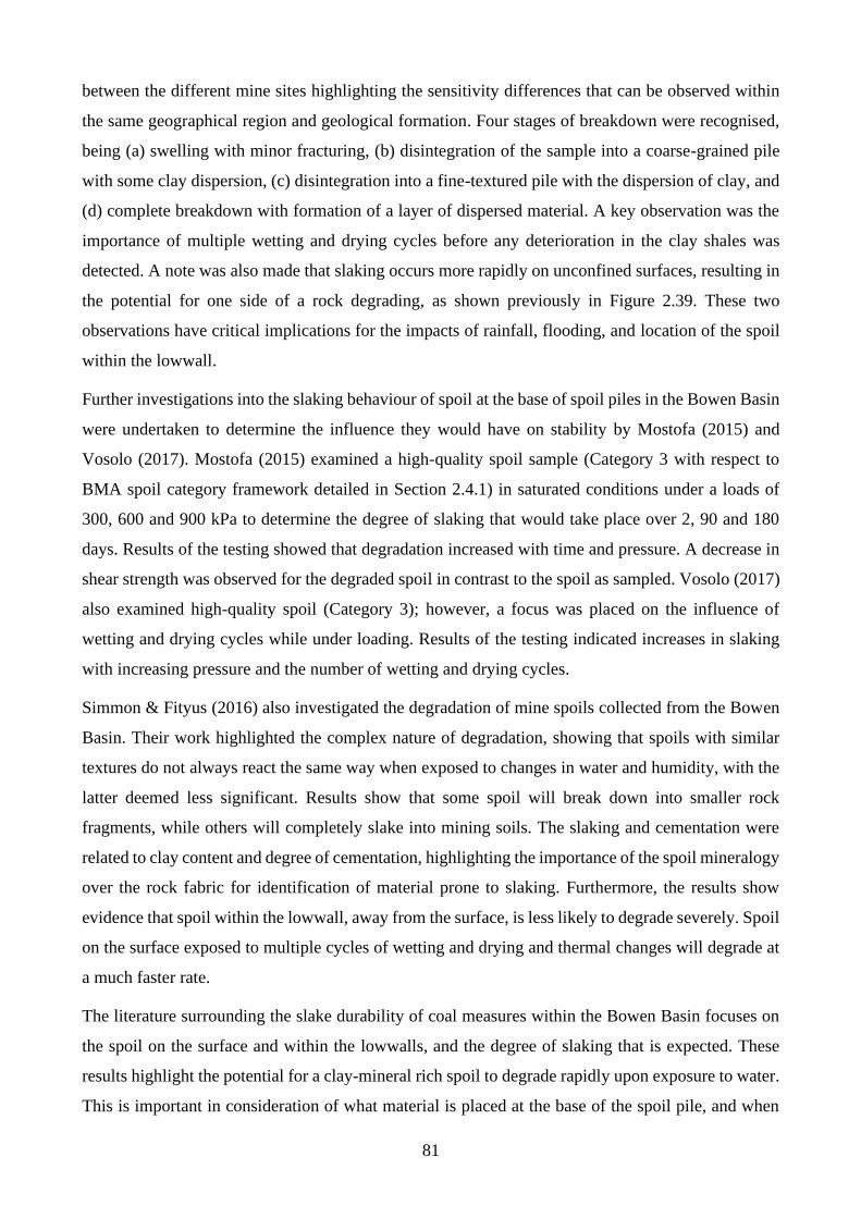
81
between the different mine sites highlighting the sensitivity differences that can be observed within
the same geographical region and geological formation. Four stages of breakdown were recognised,
being (a) swelling with minor fracturing, (b) disintegration of the sample into a coarse-grained pile
with some clay dispersion, (c) disintegration into a fine-textured pile with the dispersion of clay, and
(d) complete breakdown with formation of a layer of dispersed material. A key observation was the
importance of multiple wetting and drying cycles before any deterioration in the clay shales was
detected. A note was also made that slaking occurs more rapidly on unconfined surfaces, resulting in
the potential for one side of a rock degrading, as shown previously in Figure 2.39. These two
observations have critical implications for the impacts of rainfall, flooding, and location of the spoil
within the lowwall.
Further investigations into the slaking behaviour of spoil at the base of spoil piles in the Bowen Basin
were undertaken to determine the influence they would have on stability by Mostofa (2015) and
Vosolo (2017). Mostofa (2015) examined a high-quality spoil sample (Category 3 with respect to
BMA spoil category framework detailed in Section 2.4.1) in saturated conditions under a loads of
300, 600 and 900 kPa to determine the degree of slaking that would take place over 2, 90 and 180
days. Results of the testing showed that degradation increased with time and pressure. A decrease in
shear strength was observed for the degraded spoil in contrast to the spoil as sampled. Vosolo (2017)
also examined high-quality spoil (Category 3); however, a focus was placed on the influence of
wetting and drying cycles while under loading. Results of the testing indicated increases in slaking
with increasing pressure and the number of wetting and drying cycles.
Simmon & Fityus (2016) also investigated the degradation of mine spoils collected from the Bowen
Basin. Their work highlighted the complex nature of degradation, showing that spoils with similar
textures do not always react the same way when exposed to changes in water and humidity, with the
latter deemed less significant. Results show that some spoil will break down into smaller rock
fragments, while others will completely slake into mining soils. The slaking and cementation were
related to clay content and degree of cementation, highlighting the importance of the spoil mineralogy
over the rock fabric for identification of material prone to slaking. Furthermore, the results show
evidence that spoil within the lowwall, away from the surface, is less likely to degrade severely. Spoil
on the surface exposed to multiple cycles of wetting and drying and thermal changes will degrade at
a much faster rate.
The literature surrounding the slake durability of coal measures within the Bowen Basin focuses on
the spoil on the surface and within the lowwalls, and the degree of slaking that is expected. These
results highlight the potential for a clay-mineral rich spoil to degrade rapidly upon exposure to water.
This is important in consideration of what material is placed at the base of the spoil pile, and when
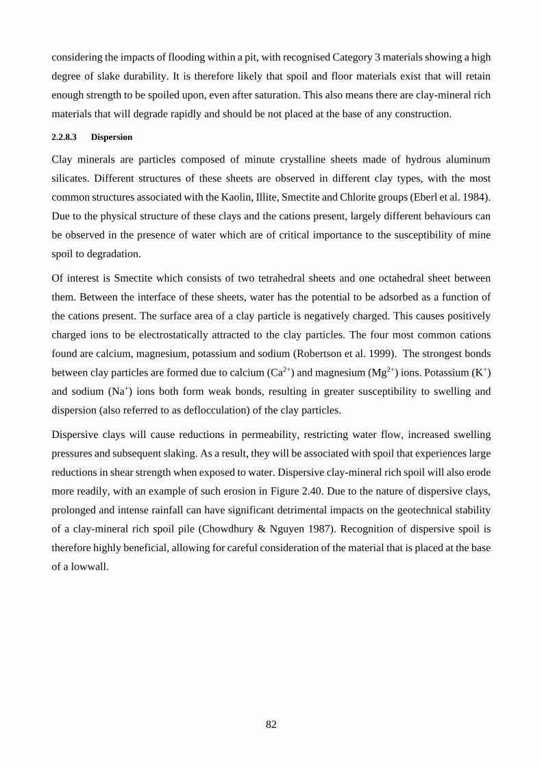
82
considering the impacts of flooding within a pit, with recognised Category 3 materials showing a high
degree of slake durability. It is therefore likely that spoil and floor materials exist that will retain
enough strength to be spoiled upon, even after saturation. This also means there are clay-mineral rich
materials that will degrade rapidly and should be not placed at the base of any construction.
2.2.8.3 Dispersion
Clay minerals are particles composed of minute crystalline sheets made of hydrous aluminum
silicates. Different structures of these sheets are observed in different clay types, with the most
common structures associated with the Kaolin, Illite, Smectite and Chlorite groups (Eberl et al. 1984).
Due to the physical structure of these clays and the cations present, largely different behaviours can
be observed in the presence of water which are of critical importance to the susceptibility of mine
spoil to degradation.
Of interest is Smectite which consists of two tetrahedral sheets and one octahedral sheet between
them. Between the interface of these sheets, water has the potential to be adsorbed as a function of
the cations present. The surface area of a clay particle is negatively charged. This causes positively
charged ions to be electrostatically attracted to the clay particles. The four most common cations
found are calcium, magnesium, potassium and sodium (Robertson et al. 1999). The strongest bonds
between clay particles are formed due to calcium (Ca2+) and magnesium (Mg2+) ions. Potassium (K+)
and sodium (Na+) ions both form weak bonds, resulting in greater susceptibility to swelling and
dispersion (also referred to as deflocculation) of the clay particles.
Dispersive clays will cause reductions in permeability, restricting water flow, increased swelling
pressures and subsequent slaking. As a result, they will be associated with spoil that experiences large
reductions in shear strength when exposed to water. Dispersive clay-mineral rich spoil will also erode
more readily, with an example of such erosion in Figure 2.40. Due to the nature of dispersive clays,
prolonged and intense rainfall can have significant detrimental impacts on the geotechnical stability
of a clay-mineral rich spoil pile (Chowdhury & Nguyen 1987). Recognition of dispersive spoil is
therefore highly beneficial, allowing for careful consideration of the material that is placed at the base
of a lowwall.
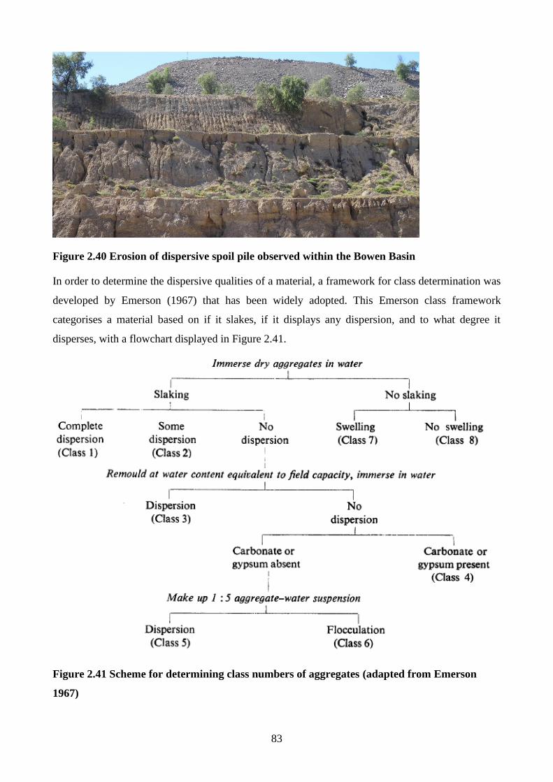
83
Figure 2.40 Erosion of dispersive spoil pile observed within the Bowen Basin
In order to determine the dispersive qualities of a material, a framework for class determination was
developed by Emerson (1967) that has been widely adopted. This Emerson class framework
categorises a material based on if it slakes, if it displays any dispersion, and to what degree it
disperses, with a flowchart displayed in Figure 2.41.
Figure 2.41 Scheme for determining class numbers of aggregates (adapted from Emerson
1967)
84
Due to the failures observed in the Bowen Basin in the 1970’s, Seedsman & Emerson (1985) looked
into the roles of clay-mineral rich spoil and the impacts they have on stability. The site focused on
was Goonyella mine, with the spoil noted to consist of Permian coal measures composed of
interbedded sandstones, siltstone and claystones. Seedsman & Emerson (1985) note that for clays to
disperse, the exchangeable sites of the clay must be occupied by sodium ions, however, there is also
the potential for material to disperse if reworked at water contents higher than their water content for
dispersion.
The analysis undertaken by Seedsman & Emerson (1985) involved six materials from slightly
weathered sandstone to mudstones, composed of Montmorillonite (a subclass of Smectite) and Illite.
Samples were classified as per the Emerson class testing detailed in Figure 2.41 and underwent a
comprehensive geochemical analysis.
Testing involved comparisons of the material as an intact chip to a pulverised condition with particle
size distributions passing 2 mm and 0.5 mm. The first intact chip showed dispersion of 3% in the
<20-micron fraction. Reduction of the aggregate particle size resulted in a 17% increase in measured
dispersed fines. Further reworking with water increasing dispersion to 95%. It was also determined
that swelling and dispersion could occur from osmotic pressures between the clay particles depending
on the strength of the attractive electrostatic forces, with the change in forces produced by variations
in the sodium cations identified as strong enough to disintegrate weak rock completely. For a sample
manipulated to contain more calcium ions, the required remoulding water content was significantly
increased, indicating the presence of calcium ions greatly reduce the dispersive potential of the clay.
The graphed results related to these findings are provided in Figure 2.42.
Figure 2.42 The influence of remoulding water content on dispersion (left), and influence of
exchangeable sodium on dispersion (right) (adapted from Seedsman & Emerson 1985)
85
From the investigations into coal measures overburden degradation, three key considerations were
drawn that will influence the degree and rate:
• Increased reworking will increase degradation;
• Increased water present during reworking will increase degradation; and
• Increased exchangeable sodium cation dominance will increase degradation.
These results imply that the more a material is reworked, the higher the chances are that it will degrade
on exposure to water. It is therefore critical that clay-mineral rich spoil with high exchangeable
sodium dominance is kept away from water, and any reworking is minimised. Upon saturation,
substantial degrees of degradation can be expected. These findings are in line with recent research
conducted by Simmon & Fityus (2016), with their degradation testing showing that the degree of
degradation was more dependent on the mineralogy of the material than the characteristic fragment
size or rock fabric.
2.2.8.4 Leaching
Leaching describes the process in which salts are removed from a material via hydraulic gradients or
through diffusion. It can cause significant changes in both the physical and the chemical properties
of clays, related to changes in pore water chemistry, removal of cementing agents, and resultant base
exchanges in the clay minerals. These can all be related to compressibility and decreases the shear
strength.
In the context of strip mining, this is likely to occur due to water movements within the spoil pile,
rainfall on the spoil, and in-pit flooding. Leaching lowers the materials liquid limit, plasticity index,
consolidation pressure, increases its compressibility, decreases its undisturbed and remoulded shear
strength, and increases sensitivity which is defined as the ratio of undisturbed shear strength to
remoulded shear strength (Brand & Brenner 1981). In the presence of swelling, dispersive clays,
leaching can occur rapidly. This highlights the importance of identifying spoil containing sensitive
swelling clays so it can be managed accordingly.
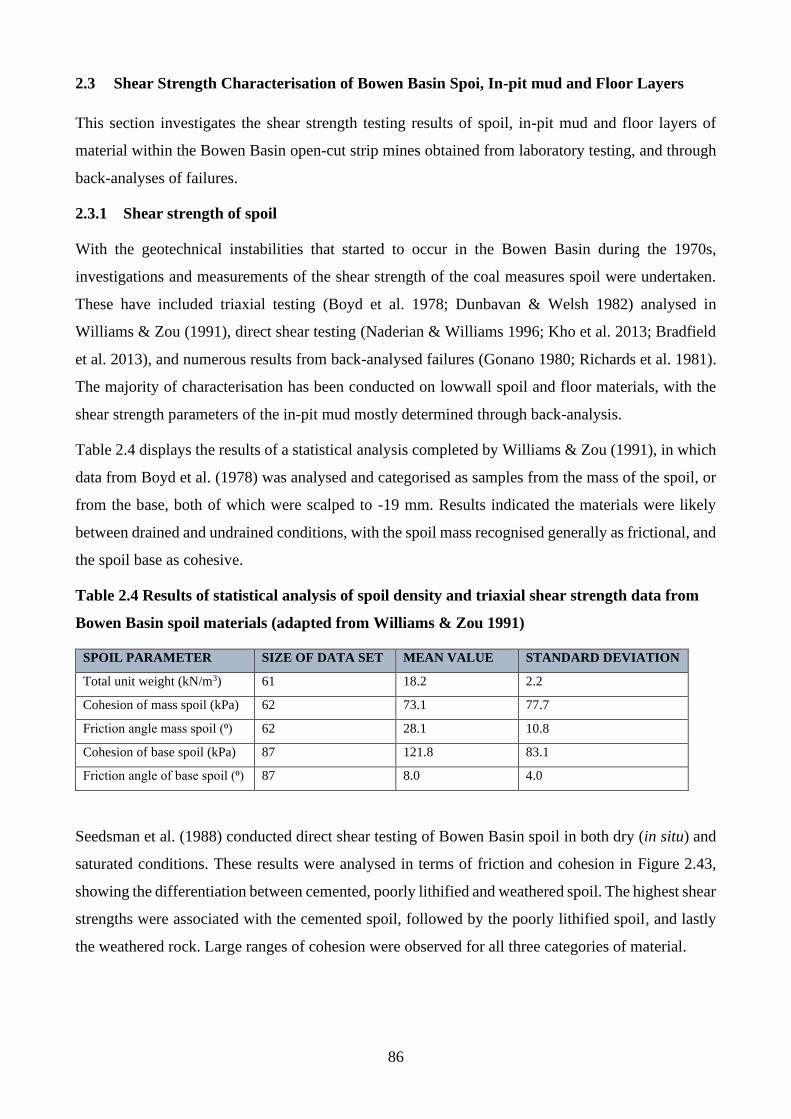
86
2.3 Shear Strength Characterisation of Bowen Basin Spoi, In-pit mud and Floor Layers
This section investigates the shear strength testing results of spoil, in-pit mud and floor layers of
material within the Bowen Basin open-cut strip mines obtained from laboratory testing, and through
back-analyses of failures.
2.3.1 Shear strength of spoil
With the geotechnical instabilities that started to occur in the Bowen Basin during the 1970s,
investigations and measurements of the shear strength of the coal measures spoil were undertaken.
These have included triaxial testing (Boyd et al. 1978; Dunbavan & Welsh 1982) analysed in
Williams & Zou (1991), direct shear testing (Naderian & Williams 1996; Kho et al. 2013; Bradfield
et al. 2013), and numerous results from back-analysed failures (Gonano 1980; Richards et al. 1981).
The majority of characterisation has been conducted on lowwall spoil and floor materials, with the
shear strength parameters of the in-pit mud mostly determined through back-analysis.
Table 2.4 displays the results of a statistical analysis completed by Williams & Zou (1991), in which
data from Boyd et al. (1978) was analysed and categorised as samples from the mass of the spoil, or
from the base, both of which were scalped to -19 mm. Results indicated the materials were likely
between drained and undrained conditions, with the spoil mass recognised generally as frictional, and
the spoil base as cohesive.
Table 2.4 Results of statistical analysis of spoil density and triaxial shear strength data from
Bowen Basin spoil materials (adapted from Williams & Zou 1991)
SPOIL PARAMETER SIZE OF DATA SET MEAN VALUE STANDARD DEVIATION
Total unit weight (kN/m3) 61 18.2 2.2
Cohesion of mass spoil (kPa) 62 73.1 77.7
Friction angle mass spoil (⁰) 62 28.1 10.8
Cohesion of base spoil (kPa) 87 121.8 83.1
Friction angle of base spoil (⁰) 87 8.0 4.0
Seedsman et al. (1988) conducted direct shear testing of Bowen Basin spoil in both dry (in situ) and
saturated conditions. These results were analysed in terms of friction and cohesion in Figure 2.43,
showing the differentiation between cemented, poorly lithified and weathered spoil. The highest shear
strengths were associated with the cemented spoil, followed by the poorly lithified spoil, and lastly
the weathered rock. Large ranges of cohesion were observed for all three categories of material.
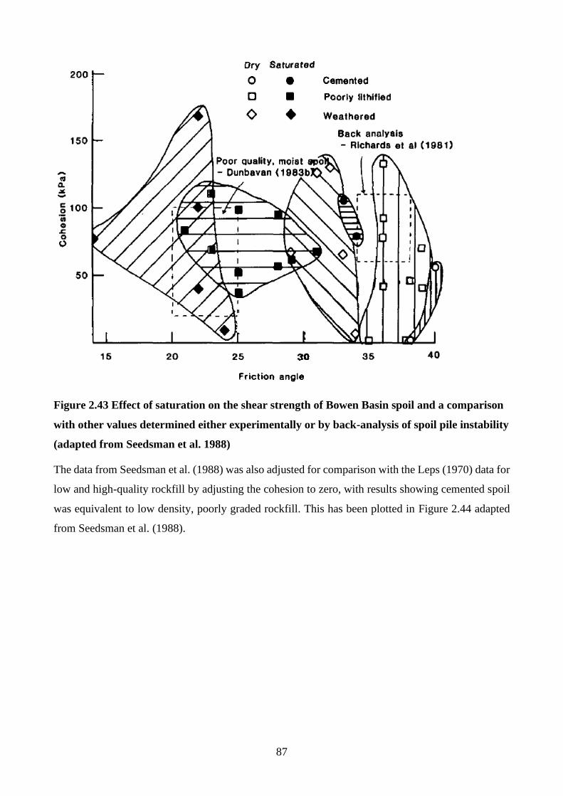
87
Figure 2.43 Effect of saturation on the shear strength of Bowen Basin spoil and a comparison
with other values determined either experimentally or by back-analysis of spoil pile instability
(adapted from Seedsman et al. 1988)
The data from Seedsman et al. (1988) was also adjusted for comparison with the Leps (1970) data for
low and high-quality rockfill by adjusting the cohesion to zero, with results showing cemented spoil
was equivalent to low density, poorly graded rockfill. This has been plotted in Figure 2.44 adapted
from Seedsman et al. (1988).
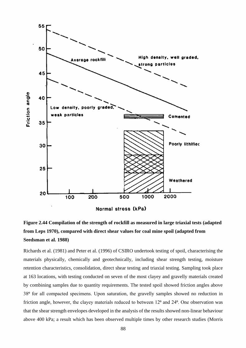
88
Figure 2.44 Compilation of the strength of rockfill as measured in large triaxial tests (adapted
from Leps 1970), compared with direct shear values for coal mine spoil (adapted from
Seedsman et al. 1988)
Richards et al. (1981) and Peter et al. (1996) of CSIRO undertook testing of spoil, characterising the
materials physically, chemically and geotechnically, including shear strength testing, moisture
retention characteristics, consolidation, direct shear testing and triaxial testing. Sampling took place
at 163 locations, with testing conducted on seven of the most clayey and gravelly materials created
by combining samples due to quantity requirements. The tested spoil showed friction angles above
38⁰ for all compacted specimens. Upon saturation, the gravelly samples showed no reduction in
friction angle, however, the clayey materials reduced to between 12⁰ and 24⁰. One observation was
that the shear strength envelopes developed in the analysis of the results showed non-linear behaviour
above 400 kPa; a result which has been observed multiple times by other research studies (Morris
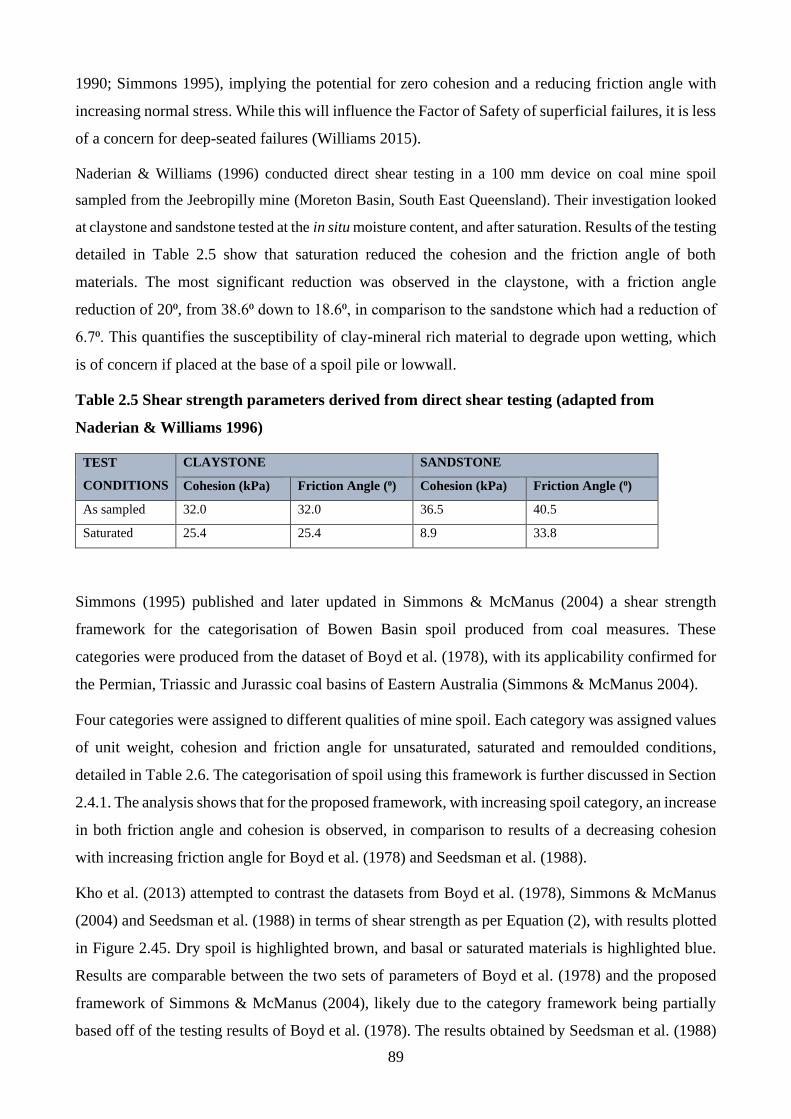
89
1990; Simmons 1995), implying the potential for zero cohesion and a reducing friction angle with
increasing normal stress. While this will influence the Factor of Safety of superficial failures, it is less
of a concern for deep-seated failures (Williams 2015).
Naderian & Williams (1996) conducted direct shear testing in a 100 mm device on coal mine spoil
sampled from the Jeebropilly mine (Moreton Basin, South East Queensland). Their investigation looked
at claystone and sandstone tested at the in situ moisture content, and after saturation. Results of the testing
detailed in Table 2.5 show that saturation reduced the cohesion and the friction angle of both
materials. The most significant reduction was observed in the claystone, with a friction angle
reduction of 20⁰, from 38.6⁰ down to 18.6⁰, in comparison to the sandstone which had a reduction of
6.7⁰. This quantifies the susceptibility of clay-mineral rich material to degrade upon wetting, which
is of concern if placed at the base of a spoil pile or lowwall.
Table 2.5 Shear strength parameters derived from direct shear testing (adapted from
Naderian & Williams 1996)
TEST
CONDITIONS
CLAYSTONE SANDSTONE
Cohesion (kPa) Friction Angle (⁰) Cohesion (kPa) Friction Angle (⁰)
As sampled 32.0 32.0 36.5 40.5
Saturated 25.4 25.4 8.9 33.8
Simmons (1995) published and later updated in Simmons & McManus (2004) a shear strength
framework for the categorisation of Bowen Basin spoil produced from coal measures. These
categories were produced from the dataset of Boyd et al. (1978), with its applicability confirmed for
the Permian, Triassic and Jurassic coal basins of Eastern Australia (Simmons & McManus 2004).
Four categories were assigned to different qualities of mine spoil. Each category was assigned values
of unit weight, cohesion and friction angle for unsaturated, saturated and remoulded conditions,
detailed in Table 2.6. The categorisation of spoil using this framework is further discussed in Section
2.4.1. The analysis shows that for the proposed framework, with increasing spoil category, an increase
in both friction angle and cohesion is observed, in comparison to results of a decreasing cohesion
with increasing friction angle for Boyd et al. (1978) and Seedsman et al. (1988).
Kho et al. (2013) attempted to contrast the datasets from Boyd et al. (1978), Simmons & McManus
(2004) and Seedsman et al. (1988) in terms of shear strength as per Equation (2), with results plotted
in Figure 2.45. Dry spoil is highlighted brown, and basal or saturated materials is highlighted blue.
Results are comparable between the two sets of parameters of Boyd et al. (1978) and the proposed
framework of Simmons & McManus (2004), likely due to the category framework being partially
based off of the testing results of Boyd et al. (1978). The results obtained by Seedsman et al. (1988)
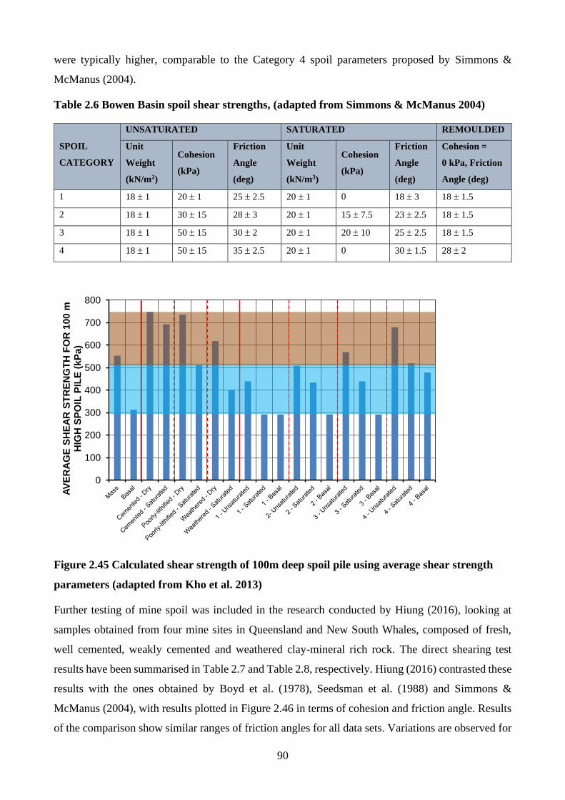
90
were typically higher, comparable to the Category 4 spoil parameters proposed by Simmons &
McManus (2004).
Table 2.6 Bowen Basin spoil shear strengths, (adapted from Simmons & McManus 2004)
SPOIL
CATEGORY
UNSATURATED SATURATED REMOULDED
Unit
Weight
(kN/m2)
Cohesion
(kPa)
Friction
Angle
(deg)
Unit
Weight
(kN/m3)
Cohesion
(kPa)
Friction
Angle
(deg)
Cohesion =
0 kPa, Friction
Angle (deg)
1 18 1 20 1 25 2.5 20 1 0 18 3 18 1.5
2 18 1 30 15 28 3 20 1 15 7.5 23 2.5 18 1.5
3 18 1 50 15 30 2 20 1 20 10 25 2.5 18 1.5
4 18 1 50 15 35 2.5 20 1 0 30 1.5 28 2
Figure 2.45 Calculated shear strength of 100m deep spoil pile using average shear strength
parameters (adapted from Kho et al. 2013)
Further testing of mine spoil was included in the research conducted by Hiung (2016), looking at
samples obtained from four mine sites in Queensland and New South Whales, composed of fresh,
well cemented, weakly cemented and weathered clay-mineral rich rock. The direct shearing test
results have been summarised in Table 2.7 and Table 2.8, respectively. Hiung (2016) contrasted these
results with the ones obtained by Boyd et al. (1978), Seedsman et al. (1988) and Simmons &
McManus (2004), with results plotted in Figure 2.46 in terms of cohesion and friction angle. Results
of the comparison show similar ranges of friction angles for all data sets. Variations are observed for
0
100
200
300
400
500
600
700
800
AV
ER
AG
E S
HE
AR
ST
RE
NG
TH
FO
R 1
00
m
HIG
H S
PO
IL P
ILE
(k
Pa)
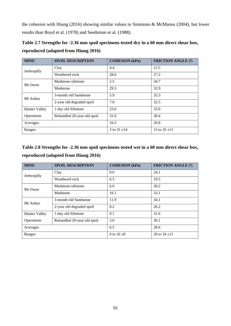
91
the cohesion with Hiung (2016) showing similar values to Simmons & McManus (2004), but lower
results than Boyd et al. (1978) and Seedsman et al. (1988).
Table 2.7 Strengths for -2.36 mm spoil specimens tested dry in a 60 mm direct shear box,
reproduced (adapted from Hiung 2016)
MINE SPOIL DESCRIPTION COHESION (kPa) FRICTION ANGLE (⁰)
Jeebropilly Clay 4.4 12.5
Weathered rock 28.6 27.2
Mt Owen Mudstone-siltstone 2.5 34.7
Mudstone 29.3 32.9
Mt Arthur 3-month old Sandstone 5.9 35.3
2-year old degraded spoil 7.0 32.5
Hunter Valley
Operations
1-day old Siltstone 23.6 33.0
Rehandled 20-year old spoil 31.0 30.4
Averages 16.5 29.8
Ranges 3 to 31 ±14 13 to 35 ±11
Table 2.8 Strengths for -2.36 mm spoil specimens tested wet in a 60 mm direct shear box,
reproduced (adapted from Hiung 2016)
MINE SPOIL DESCRIPTION COHESION (kPa) FRICTION ANGLE (⁰)
Jeebropilly Clay 0.0 24.1
Weathered rock 6.5 19.5
Mt Owen Mudstone-siltstone 6.0 30.2
Mudstone 16.1 33.1
Mt Arthur 3-month old Sandstone 11.9 34.1
2-year old degraded spoil 8.2 26.2
Hunter Valley
Operations
1-day old Siltstone 0.1 31.6
Rehandled 20-year old spoil 3.0 30.1
Averages 6.5 28.6
Ranges 0 to 16 ±8 20 to 34 ±11
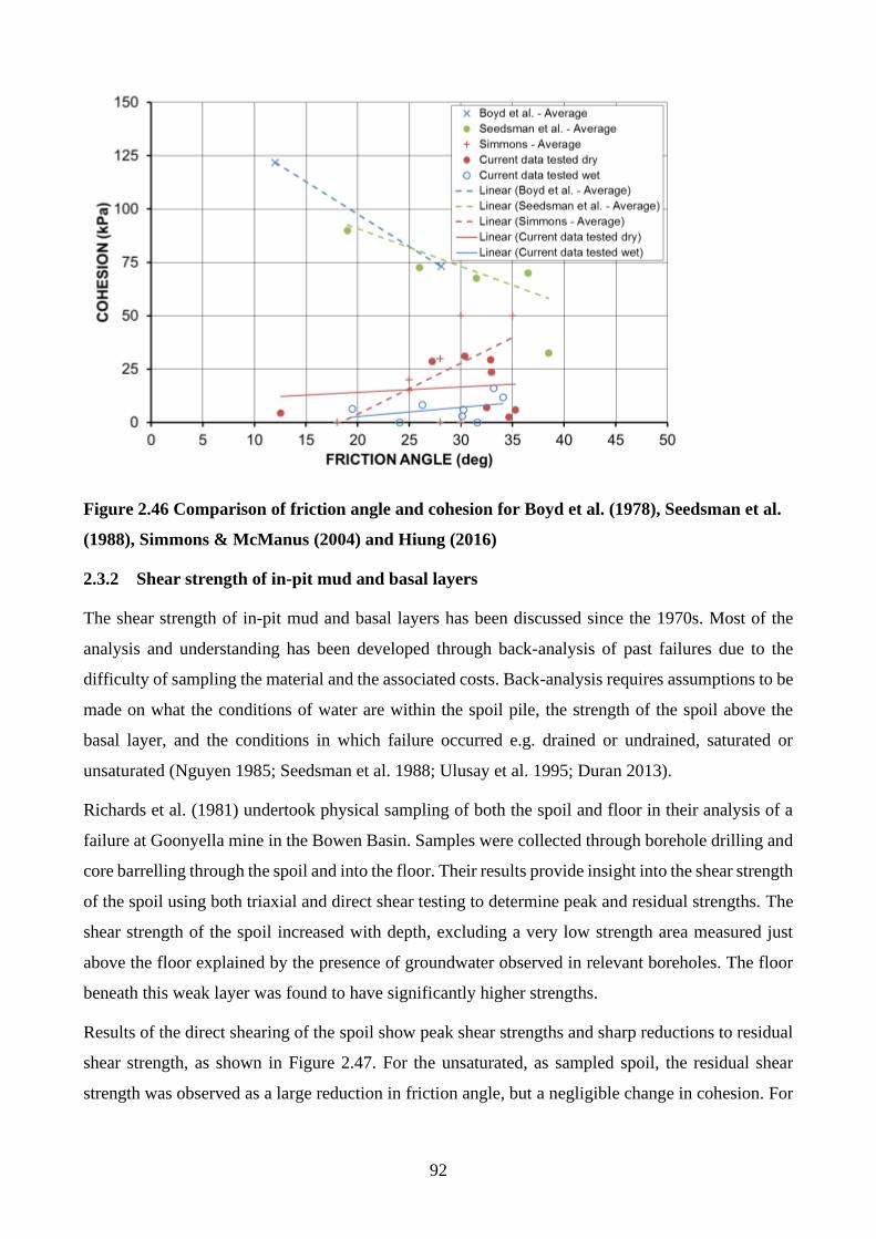
92
Figure 2.46 Comparison of friction angle and cohesion for Boyd et al. (1978), Seedsman et al.
(1988), Simmons & McManus (2004) and Hiung (2016)
2.3.2 Shear strength of in-pit mud and basal layers
The shear strength of in-pit mud and basal layers has been discussed since the 1970s. Most of the
analysis and understanding has been developed through back-analysis of past failures due to the
difficulty of sampling the material and the associated costs. Back-analysis requires assumptions to be
made on what the conditions of water are within the spoil pile, the strength of the spoil above the
basal layer, and the conditions in which failure occurred e.g. drained or undrained, saturated or
unsaturated (Nguyen 1985; Seedsman et al. 1988; Ulusay et al. 1995; Duran 2013).
Richards et al. (1981) undertook physical sampling of both the spoil and floor in their analysis of a
failure at Goonyella mine in the Bowen Basin. Samples were collected through borehole drilling and
core barrelling through the spoil and into the floor. Their results provide insight into the shear strength
of the spoil using both triaxial and direct shear testing to determine peak and residual strengths. The
shear strength of the spoil increased with depth, excluding a very low strength area measured just
above the floor explained by the presence of groundwater observed in relevant boreholes. The floor
beneath this weak layer was found to have significantly higher strengths.
Results of the direct shearing of the spoil show peak shear strengths and sharp reductions to residual
shear strength, as shown in Figure 2.47. For the unsaturated, as sampled spoil, the residual shear
strength was observed as a large reduction in friction angle, but a negligible change in cohesion. For
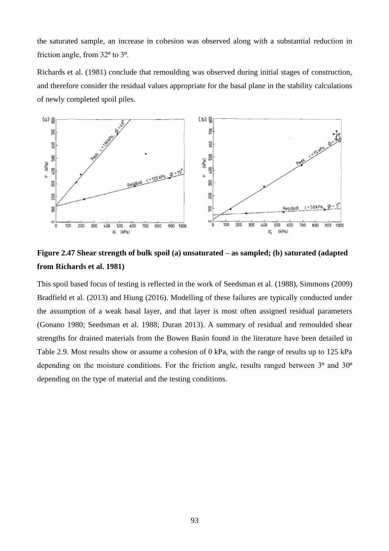
93
the saturated sample, an increase in cohesion was observed along with a substantial reduction in
friction angle, from 32⁰ to 3⁰.
Richards et al. (1981) conclude that remoulding was observed during initial stages of construction,
and therefore consider the residual values appropriate for the basal plane in the stability calculations
of newly completed spoil piles.
Figure 2.47 Shear strength of bulk spoil (a) unsaturated – as sampled; (b) saturated (adapted
from Richards et al. 1981)
This spoil based focus of testing is reflected in the work of Seedsman et al. (1988), Simmons (2009)
Bradfield et al. (2013) and Hiung (2016). Modelling of these failures are typically conducted under
the assumption of a weak basal layer, and that layer is most often assigned residual parameters
(Gonano 1980; Seedsman et al. 1988; Duran 2013). A summary of residual and remoulded shear
strengths for drained materials from the Bowen Basin found in the literature have been detailed in
Table 2.9. Most results show or assume a cohesion of 0 kPa, with the range of results up to 125 kPa
depending on the moisture conditions. For the friction angle, results ranged between 3⁰ and 30⁰
depending on the type of material and the testing conditions.
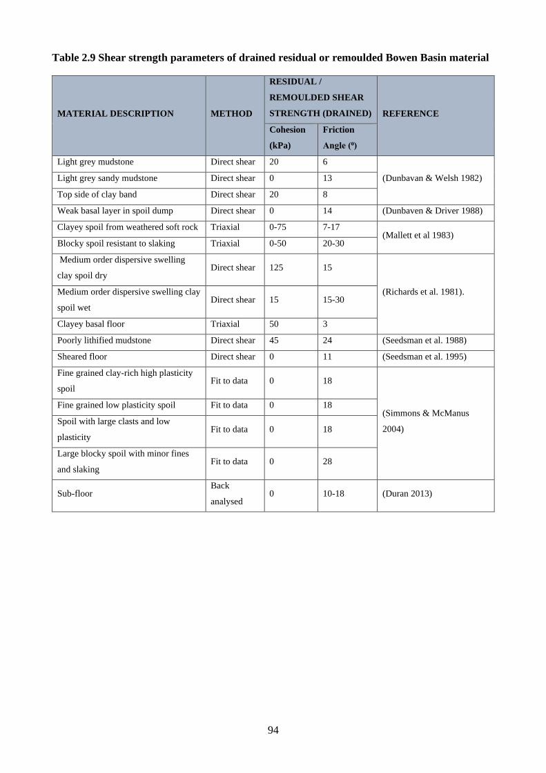
94
Table 2.9 Shear strength parameters of drained residual or remoulded Bowen Basin material
MATERIAL DESCRIPTION METHOD
RESIDUAL /
REMOULDED SHEAR
STRENGTH (DRAINED) REFERENCE
Cohesion
(kPa)
Friction
Angle (⁰)
Light grey mudstone Direct shear 20 6
(Dunbavan & Welsh 1982) Light grey sandy mudstone Direct shear 0 13
Top side of clay band Direct shear 20 8
Weak basal layer in spoil dump Direct shear 0 14 (Dunbaven & Driver 1988)
Clayey spoil from weathered soft rock Triaxial 0-75 7-17 (Mallett et al 1983)
Blocky spoil resistant to slaking Triaxial 0-50 20-30
Medium order dispersive swelling
clay spoil dry Direct shear 125 15
(Richards et al. 1981). Medium order dispersive swelling clay
spoil wet Direct shear 15 15-30
Clayey basal floor Triaxial 50 3
Poorly lithified mudstone Direct shear 45 24 (Seedsman et al. 1988)
Sheared floor Direct shear 0 11 (Seedsman et al. 1995)
Fine grained clay-rich high plasticity
spoil Fit to data 0 18
(Simmons & McManus
2004)
Fine grained low plasticity spoil Fit to data 0 18
Spoil with large clasts and low
plasticity Fit to data 0 18
Large blocky spoil with minor fines
and slaking Fit to data 0 28
Sub-floor Back
analysed 0 10-18 (Duran 2013)
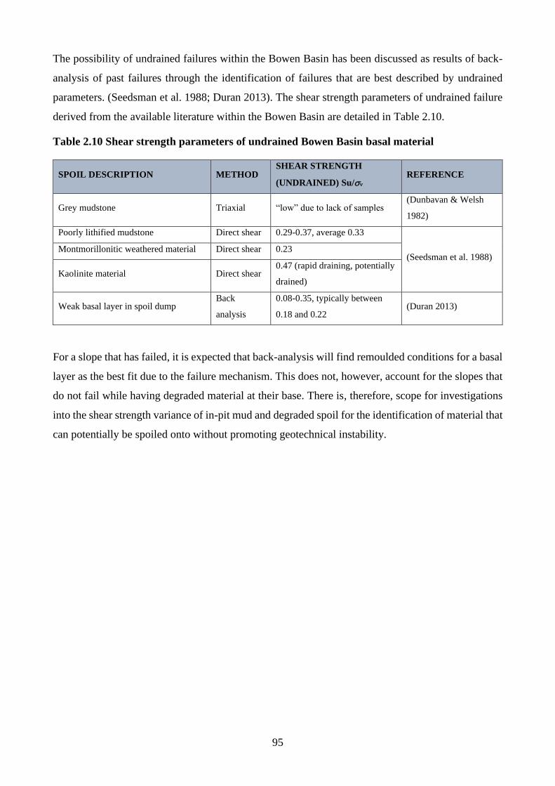
95
The possibility of undrained failures within the Bowen Basin has been discussed as results of back-
analysis of past failures through the identification of failures that are best described by undrained
parameters. (Seedsman et al. 1988; Duran 2013). The shear strength parameters of undrained failure
derived from the available literature within the Bowen Basin are detailed in Table 2.10.
Table 2.10 Shear strength parameters of undrained Bowen Basin basal material
SPOIL DESCRIPTION METHOD SHEAR STRENGTH
(UNDRAINED) Su/v REFERENCE
Grey mudstone Triaxial “low” due to lack of samples (Dunbavan & Welsh
1982)
Poorly lithified mudstone Direct shear 0.29-0.37, average 0.33
(Seedsman et al. 1988) Montmorillonitic weathered material Direct shear 0.23
Kaolinite material Direct shear 0.47 (rapid draining, potentially
drained)
Weak basal layer in spoil dump Back
analysis
0.08-0.35, typically between
0.18 and 0.22 (Duran 2013)
For a slope that has failed, it is expected that back-analysis will find remoulded conditions for a basal
layer as the best fit due to the failure mechanism. This does not, however, account for the slopes that
do not fail while having degraded material at their base. There is, therefore, scope for investigations
into the shear strength variance of in-pit mud and degraded spoil for the identification of material that
can potentially be spoiled onto without promoting geotechnical instability.
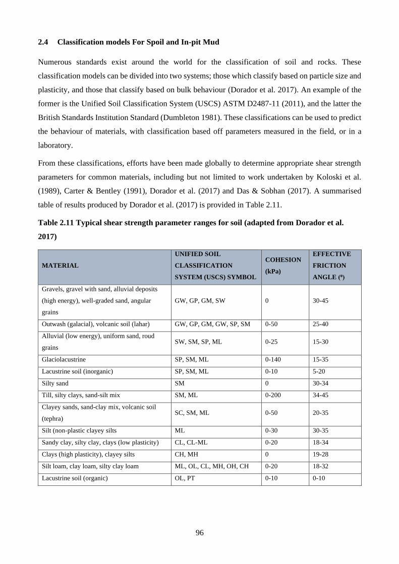
96
2.4 Classification models For Spoil and In-pit Mud
Numerous standards exist around the world for the classification of soil and rocks. These
classification models can be divided into two systems; those which classify based on particle size and
plasticity, and those that classify based on bulk behaviour (Dorador et al. 2017). An example of the
former is the Unified Soil Classification System (USCS) ASTM D2487-11 (2011), and the latter the
British Standards Institution Standard (Dumbleton 1981). These classifications can be used to predict
the behaviour of materials, with classification based off parameters measured in the field, or in a
laboratory.
From these classifications, efforts have been made globally to determine appropriate shear strength
parameters for common materials, including but not limited to work undertaken by Koloski et al.
(1989), Carter & Bentley (1991), Dorador et al. (2017) and Das & Sobhan (2017). A summarised
table of results produced by Dorador et al. (2017) is provided in Table 2.11.
Table 2.11 Typical shear strength parameter ranges for soil (adapted from Dorador et al.
2017)
MATERIAL
UNIFIED SOIL
CLASSIFICATION
SYSTEM (USCS) SYMBOL
COHESION
(kPa)
EFFECTIVE
FRICTION
ANGLE (⁰)
Gravels, gravel with sand, alluvial deposits
(high energy), well-graded sand, angular
grains
GW, GP, GM, SW 0 30-45
Outwash (galacial), volcanic soil (lahar) GW, GP, GM, GW, SP, SM 0-50 25-40
Alluvial (low energy), uniform sand, roud
grains SW, SM, SP, ML 0-25 15-30
Glaciolacustrine SP, SM, ML 0-140 15-35
Lacustrine soil (inorganic) SP, SM, ML 0-10 5-20
Silty sand SM 0 30-34
Till, silty clays, sand-silt mix SM, ML 0-200 34-45
Clayey sands, sand-clay mix, volcanic soil
(tephra) SC, SM, ML 0-50 20-35
Silt (non-plastic clayey silts ML 0-30 30-35
Sandy clay, silty clay, clays (low plasticity) CL, CL-ML 0-20 18-34
Clays (high plasticity), clayey silts CH, MH 0 19-28
Silt loam, clay loam, silty clay loam ML, OL, CL, MH, OH, CH 0-20 18-32
Lacustrine soil (organic) OL, PT 0-10 0-10
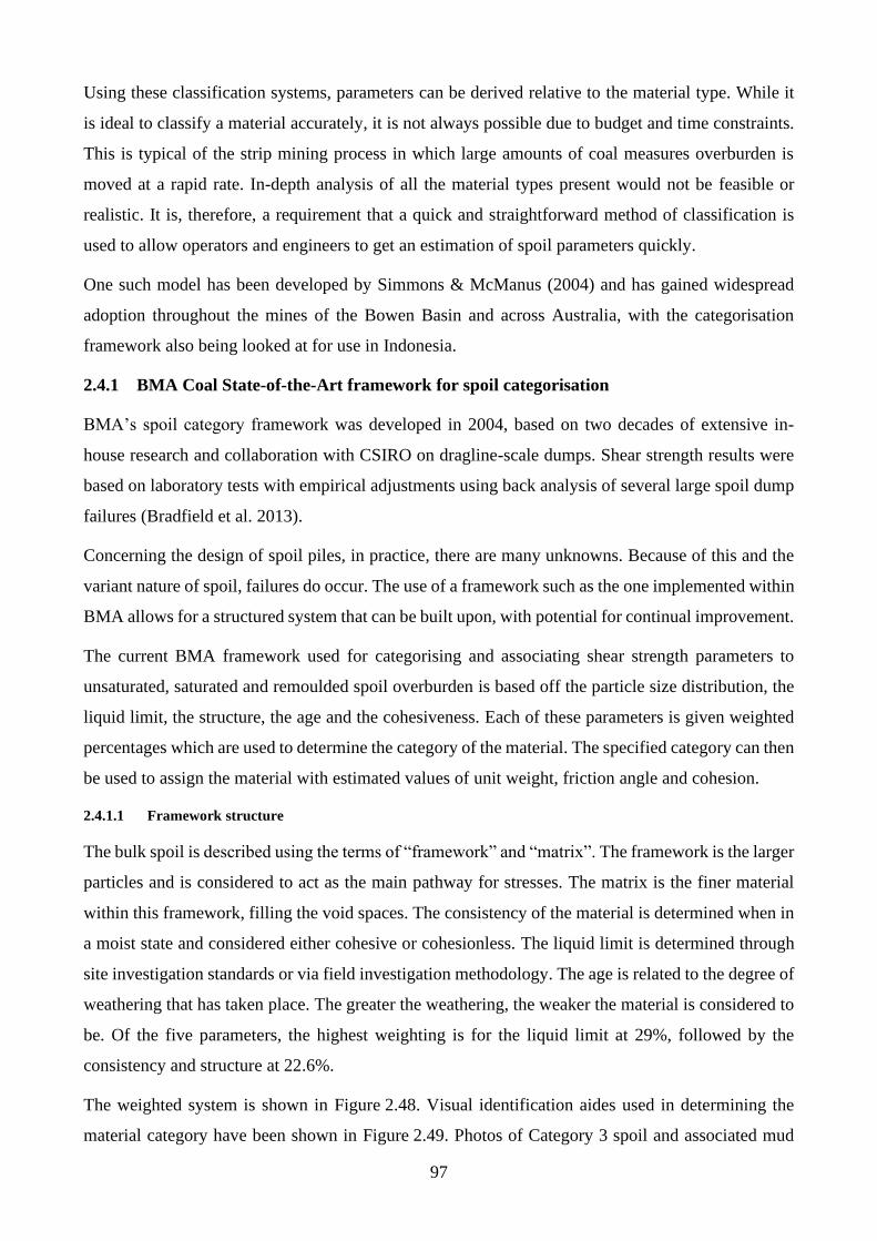
97
Using these classification systems, parameters can be derived relative to the material type. While it
is ideal to classify a material accurately, it is not always possible due to budget and time constraints.
This is typical of the strip mining process in which large amounts of coal measures overburden is
moved at a rapid rate. In-depth analysis of all the material types present would not be feasible or
realistic. It is, therefore, a requirement that a quick and straightforward method of classification is
used to allow operators and engineers to get an estimation of spoil parameters quickly.
One such model has been developed by Simmons & McManus (2004) and has gained widespread
adoption throughout the mines of the Bowen Basin and across Australia, with the categorisation
framework also being looked at for use in Indonesia.
2.4.1 BMA Coal State-of-the-Art framework for spoil categorisation
BMA’s spoil category framework was developed in 2004, based on two decades of extensive in-
house research and collaboration with CSIRO on dragline-scale dumps. Shear strength results were
based on laboratory tests with empirical adjustments using back analysis of several large spoil dump
failures (Bradfield et al. 2013).
Concerning the design of spoil piles, in practice, there are many unknowns. Because of this and the
variant nature of spoil, failures do occur. The use of a framework such as the one implemented within
BMA allows for a structured system that can be built upon, with potential for continual improvement.
The current BMA framework used for categorising and associating shear strength parameters to
unsaturated, saturated and remoulded spoil overburden is based off the particle size distribution, the
liquid limit, the structure, the age and the cohesiveness. Each of these parameters is given weighted
percentages which are used to determine the category of the material. The specified category can then
be used to assign the material with estimated values of unit weight, friction angle and cohesion.
2.4.1.1 Framework structure
The bulk spoil is described using the terms of “framework” and “matrix”. The framework is the larger
particles and is considered to act as the main pathway for stresses. The matrix is the finer material
within this framework, filling the void spaces. The consistency of the material is determined when in
a moist state and considered either cohesive or cohesionless. The liquid limit is determined through
site investigation standards or via field investigation methodology. The age is related to the degree of
weathering that has taken place. The greater the weathering, the weaker the material is considered to
be. Of the five parameters, the highest weighting is for the liquid limit at 29%, followed by the
consistency and structure at 22.6%.
The weighted system is shown in Figure 2.48. Visual identification aides used in determining the
material category have been shown in Figure 2.49. Photos of Category 3 spoil and associated mud
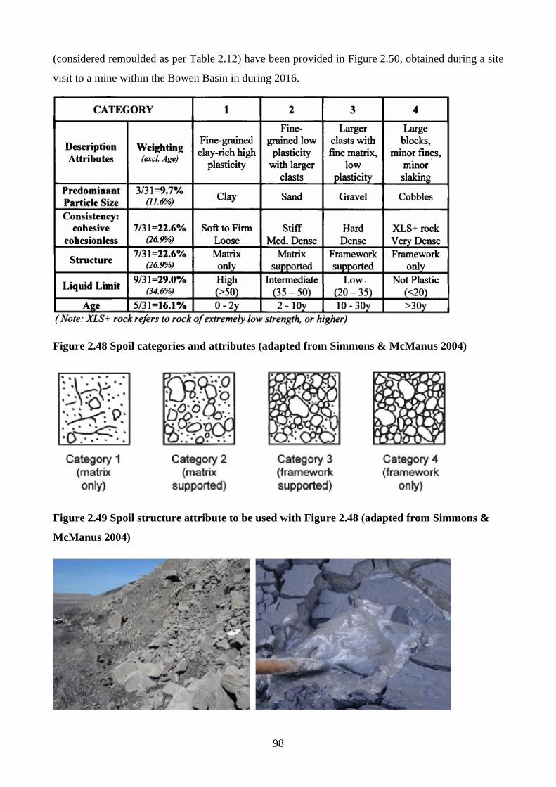
98
(considered remoulded as per Table 2.12) have been provided in Figure 2.50, obtained during a site
visit to a mine within the Bowen Basin in during 2016.
Figure 2.48 Spoil categories and attributes (adapted from Simmons & McManus 2004)
Figure 2.49 Spoil structure attribute to be used with Figure 2.48 (adapted from Simmons &
McManus 2004)
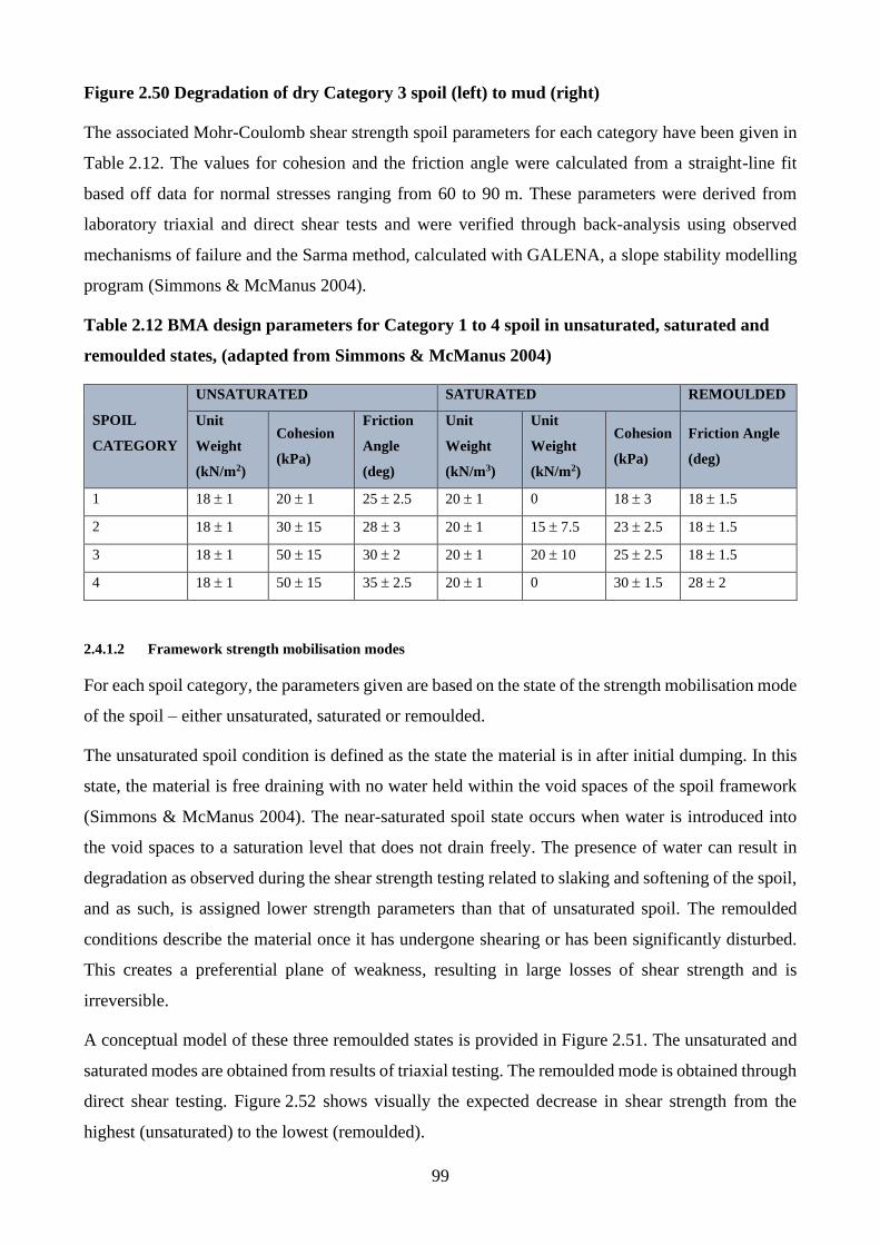
99
Figure 2.50 Degradation of dry Category 3 spoil (left) to mud (right)
The associated Mohr-Coulomb shear strength spoil parameters for each category have been given in
Table 2.12. The values for cohesion and the friction angle were calculated from a straight-line fit
based off data for normal stresses ranging from 60 to 90 m. These parameters were derived from
laboratory triaxial and direct shear tests and were verified through back-analysis using observed
mechanisms of failure and the Sarma method, calculated with GALENA, a slope stability modelling
program (Simmons & McManus 2004).
Table 2.12 BMA design parameters for Category 1 to 4 spoil in unsaturated, saturated and
remoulded states, (adapted from Simmons & McManus 2004)
SPOIL
CATEGORY
UNSATURATED SATURATED REMOULDED
Unit
Weight
(kN/m2)
Cohesion
(kPa)
Friction
Angle
(deg)
Unit
Weight
(kN/m3)
Unit
Weight
(kN/m2)
Cohesion
(kPa)
Friction Angle
(deg)
1 18 1 20 1 25 2.5 20 1 0 18 3 18 1.5
2 18 1 30 15 28 3 20 1 15 7.5 23 2.5 18 1.5
3 18 1 50 15 30 2 20 1 20 10 25 2.5 18 1.5
4 18 1 50 15 35 2.5 20 1 0 30 1.5 28 2
2.4.1.2 Framework strength mobilisation modes
For each spoil category, the parameters given are based on the state of the strength mobilisation mode
of the spoil – either unsaturated, saturated or remoulded.
The unsaturated spoil condition is defined as the state the material is in after initial dumping. In this
state, the material is free draining with no water held within the void spaces of the spoil framework
(Simmons & McManus 2004). The near-saturated spoil state occurs when water is introduced into
the void spaces to a saturation level that does not drain freely. The presence of water can result in
degradation as observed during the shear strength testing related to slaking and softening of the spoil,
and as such, is assigned lower strength parameters than that of unsaturated spoil. The remoulded
conditions describe the material once it has undergone shearing or has been significantly disturbed.
This creates a preferential plane of weakness, resulting in large losses of shear strength and is
irreversible.
A conceptual model of these three remoulded states is provided in Figure 2.51. The unsaturated and
saturated modes are obtained from results of triaxial testing. The remoulded mode is obtained through
direct shear testing. Figure 2.52 shows visually the expected decrease in shear strength from the
highest (unsaturated) to the lowest (remoulded).
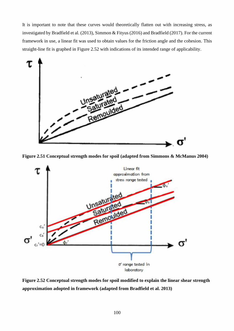
100
It is important to note that these curves would theoretically flatten out with increasing stress, as
investigated by Bradfield et al. (2013), Simmon & Fityus (2016) and Bradfield (2017). For the current
framework in use, a linear fit was used to obtain values for the friction angle and the cohesion. This
straight-line fit is graphed in Figure 2.52 with indications of its intended range of applicability.
Figure 2.51 Conceptual strength modes for spoil (adapted from Simmons & McManus 2004)
Figure 2.52 Conceptual strength modes for spoil modified to explain the linear shear strength
approximation adopted in framework (adapted from Bradfield et al. 2013)
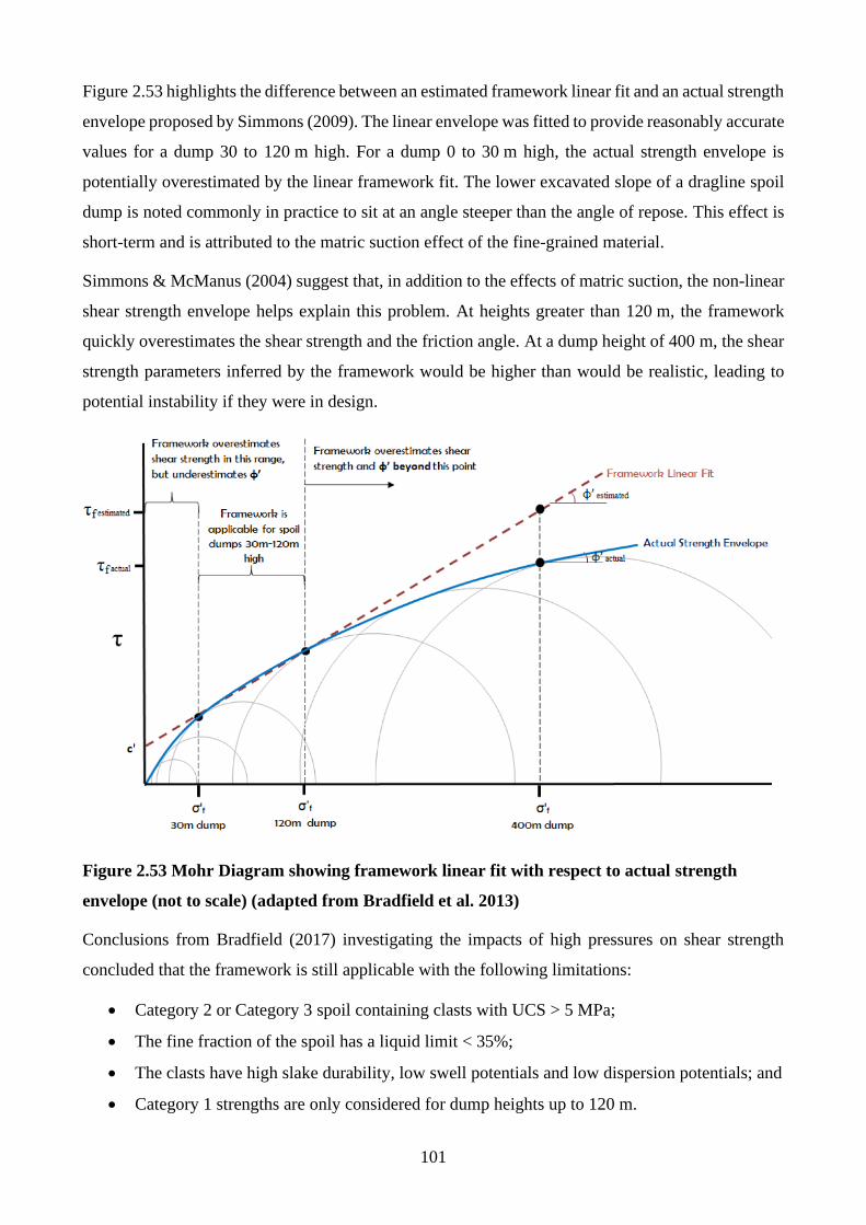
101
Figure 2.53 highlights the difference between an estimated framework linear fit and an actual strength
envelope proposed by Simmons (2009). The linear envelope was fitted to provide reasonably accurate
values for a dump 30 to 120 m high. For a dump 0 to 30 m high, the actual strength envelope is
potentially overestimated by the linear framework fit. The lower excavated slope of a dragline spoil
dump is noted commonly in practice to sit at an angle steeper than the angle of repose. This effect is
short-term and is attributed to the matric suction effect of the fine-grained material.
Simmons & McManus (2004) suggest that, in addition to the effects of matric suction, the non-linear
shear strength envelope helps explain this problem. At heights greater than 120 m, the framework
quickly overestimates the shear strength and the friction angle. At a dump height of 400 m, the shear
strength parameters inferred by the framework would be higher than would be realistic, leading to
potential instability if they were in design.
Figure 2.53 Mohr Diagram showing framework linear fit with respect to actual strength
envelope (not to scale) (adapted from Bradfield et al. 2013)
Conclusions from Bradfield (2017) investigating the impacts of high pressures on shear strength
concluded that the framework is still applicable with the following limitations:
• Category 2 or Category 3 spoil containing clasts with UCS > 5 MPa;
• The fine fraction of the spoil has a liquid limit < 35%;
• The clasts have high slake durability, low swell potentials and low dispersion potentials; and
• Category 1 strengths are only considered for dump heights up to 120 m.
102
2.4.1.3 Application of framework in practice
Simmons & McManus (2004) describe a test that was undertaken, in which 105 bulk samples were
collected. Two mine site personnel were required to categories the material visually. The results
showed different answers for 45 of the samples. The worksheet was then used to reattempt
categorisation of 13 bulk samples that were difficult to test previously. Again, using two personnel
with different levels of experience, there was 100% agreement on the categories of the samples.
103
2.5 Literature Review Commentary and Conclusions
The current BMA shear strength framework has been applied and used for hundreds of back-analysis
situations (Simmons & McManus 2004). It is a popular tool throughout the Australian coal industry
partially due to the movement of personnel between sites and companies. In its current state, it
provides adequate starting points for the categorisation of spoil. Application and adaption to
investigate the formation and potential categorisation of spoil that degrades into in-pit mud is of
consideration, with the following limitations and potential extensions identified.
2.5.1 Spoil category expansion and refinement
The current framework allows for the choice of four categories. The most common categories of
material found on site are Category 2 and 3, with Category 1 and 4 being relatively rare. Furthermore,
there is often variability within a spoil pile. This variability along with the high occurrence of
Category 2 and 3 material can make it challenging to identify which is which, and how to model the
spoil pile as a whole (Simmons & McManus 2004). As the classification is typically conducted
visually, it is crucial that different operators can obtain the same result consistently.
To account for this issue, one solution is to expand the selection of categories. This would involve
refining the parameters used to identify the material so that classifications can be more accurately
made. The introduction of more categories would also provide greater accuracy when investigating
failures using back analysis. The reason that this was not originally done was due to the data used to
create the framework. Review of the triaxial test data could not identify an alternative sorting that
was considered more reliable (Simmons & McManus 2004). More data collection, in collaboration
with past results, will allow for greater refinement and potential expansion of the current framework
categories.
2.5.2 Verification by testing
The authors of the original framework Simmons & McManus (2004) found that additional testing
was required for some clay-mineral rich lithologies. They state that the test results were not too
different from what the framework had suggested, however, acknowledged that this will not always
be the case.
While the framework has proven reliable for many typical cases, more data is always beneficial for
the less common materials and lithologies. Through more sampling and testing, refinement will be
possible. This is important for Category 1 material in particular, as it is not as common as the other
categories of materials and is often the most troublesome.
104
2.5.3 Material degradation considerations
The current framework was not designed to account for spoil susceptible to significant slaking. The
material will typically appear blocky initially, however once dumped, weathering can quickly induce
slaking. Williams (2015); Hiung (2016), Simmon & Fityus (2016), Mostofa (2015), Vosolo (2017)
and Bradfield (2017) have all investigated spoil from the Bowen Basin and the influence of saturation
on the particle size and shear strength, with results yet to be used in updating the framework.
Simmons & McManus (2004) discuss an observation of this occurrence in the field. The material at
the bottom of the spoil pile that was originally blocky underwent slaking, dispersion and inter-particle
void collapse. It is therefore important to have a means of identifying material susceptible to slaking
and to adapt the framework to account for this degraded state as witnessed with in-pit mud formations.
2.5.4 Consideration of in-pit mud parameters
Since the development of the BMA Coal shear strength framework, little consideration has been
found in the literature for the application of the framework to in-pit mud, and the parameters of in-pit
mud. This is due to a lack of testing, standard operating procedures requiring the removal of in-pit
mud, and remoulded strength parameters being assumed and assigned to in-pit mud for stability
modelling purposes.
The remoulded parameters used in the BMA Coal framework were obtained through the studies of
back-analysis of past failures such as in Seedsman & Emerson (1985). There is, therefore, room for
an investigation into the shear strength parameters of in-pit mud, and the potential variations that can
occur. The assumption of in-pit mud being assigned weak strength parameters is likely a combination
of conservative design to avoid failures, and the back-analysed strength parameters being low as only
failures are typically investigated. For scenarios in which the mud cannot be removed, and spoil is
placed on top, cases where no failure have occurred should also be investigated and added to the
literature. There is little data on this as the practice of spoiling onto mud in situ is frowned upon as
per standard operational procedures (Prytherch 2012).
Investigations into the classification of the physical, chemical and geotechnical properties relating to
in-pit mud and its formation will be highly beneficial towards ensuring lowwall stability post-flooding
events, and after periods of heavy rainfall. This is particularly beneficial for pits in which mud
removal is not an option. Testing of the causes and rates of degradation of spoil is also of interest,
with previous work (Emerson 1967; Seedsman & Emerson 1985; Seedsman 1986) highlighting key
identifiers such as the available exchangeable sodium cations and their relation to slake durability.
Through the correlation of in-pit mud parameters and the geotechnical parameters, significant
improvements in the modelling and handling of the mud can be made.
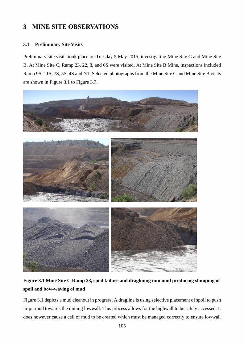
105
3 MINE SITE OBSERVATIONS
3.1 Preliminary Site Visits
Preliminary site visits took place on Tuesday 5 May 2015, investigating Mine Site C and Mine Site
B. At Mine Site C, Ramp 23, 22, 8, and 6S were visited. At Mine Site B Mine, inspections included
Ramp 9S, 11S, 7S, 5S, 4S and N1. Selected photographs from the Mine Site C and Mine Site B visits
are shown in Figure 3.1 to Figure 3.7.
Figure 3.1 Mine Site C Ramp 23, spoil failure and draglining into mud producing slumping of
spoil and bow-waving of mud
Figure 3.1 depicts a mud cleanout in progress. A dragline is using selective placement of spoil to push
in-pit mud towards the mining lowwall. This process allows for the highwall to be safely accessed. It
does however cause a cell of mud to be created which must be managed correctly to ensure lowwall
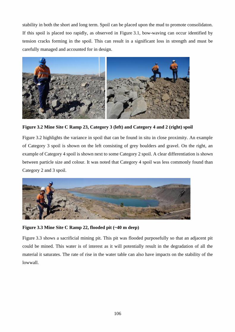
106
stability in both the short and long term. Spoil can be placed upon the mud to promote consolidaton.
If this spoil is placed too rapidly, as observed in Figure 3.1, bow-waving can occur identified by
tension cracks forming in the spoil. This can result in a significant loss in strength and must be
carefully managed and accounted for in design.
Figure 3.2 Mine Site C Ramp 23, Category 3 (left) and Category 4 and 2 (right) spoil
Figure 3.2 highlights the variance in spoil that can be found in situ in close proximity. An example
of Category 3 spoil is shown on the left consisting of grey boulders and gravel. On the right, an
example of Category 4 spoil is shown next to some Category 2 spoil. A clear differentiation is shown
between particle size and colour. It was noted that Category 4 spoil was less commonly found than
Category 2 and 3 spoil.
Figure 3.3 Mine Site C Ramp 22, flooded pit (~40 m deep)
Figure 3.3 shows a sacrificial mining pit. This pit was flooded purposefully so that an adjacent pit
could be mined. This water is of interest as it will potentially result in the degradation of all the
material it saturates. The rate of rise in the water table can also have impacts on the stability of the
lowwall.
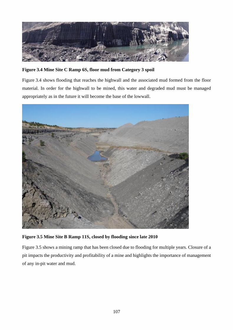
107
Figure 3.4 Mine Site C Ramp 6S, floor mud from Category 3 spoil
Figure 3.4 shows flooding that reaches the highwall and the associated mud formed from the floor
material. In order for the highwall to be mined, this water and degraded mud must be managed
appropriately as in the future it will become the base of the lowwall.
Figure 3.5 Mine Site B Ramp 11S, closed by flooding since late 2010
Figure 3.5 shows a mining ramp that has been closed due to flooding for multiple years. Closure of a
pit impacts the productivity and profitability of a mine and highlights the importance of management
of any in-pit water and mud.
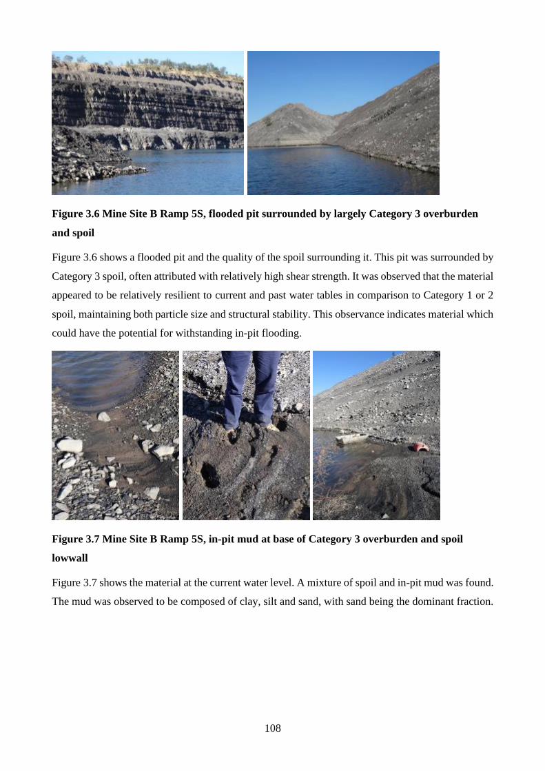
108
Figure 3.6 Mine Site B Ramp 5S, flooded pit surrounded by largely Category 3 overburden
and spoil
Figure 3.6 shows a flooded pit and the quality of the spoil surrounding it. This pit was surrounded by
Category 3 spoil, often attributed with relatively high shear strength. It was observed that the material
appeared to be relatively resilient to current and past water tables in comparison to Category 1 or 2
spoil, maintaining both particle size and structural stability. This observance indicates material which
could have the potential for withstanding in-pit flooding.
Figure 3.7 Mine Site B Ramp 5S, in-pit mud at base of Category 3 overburden and spoil
lowwall
Figure 3.7 shows the material at the current water level. A mixture of spoil and in-pit mud was found.
The mud was observed to be composed of clay, silt and sand, with sand being the dominant fraction.
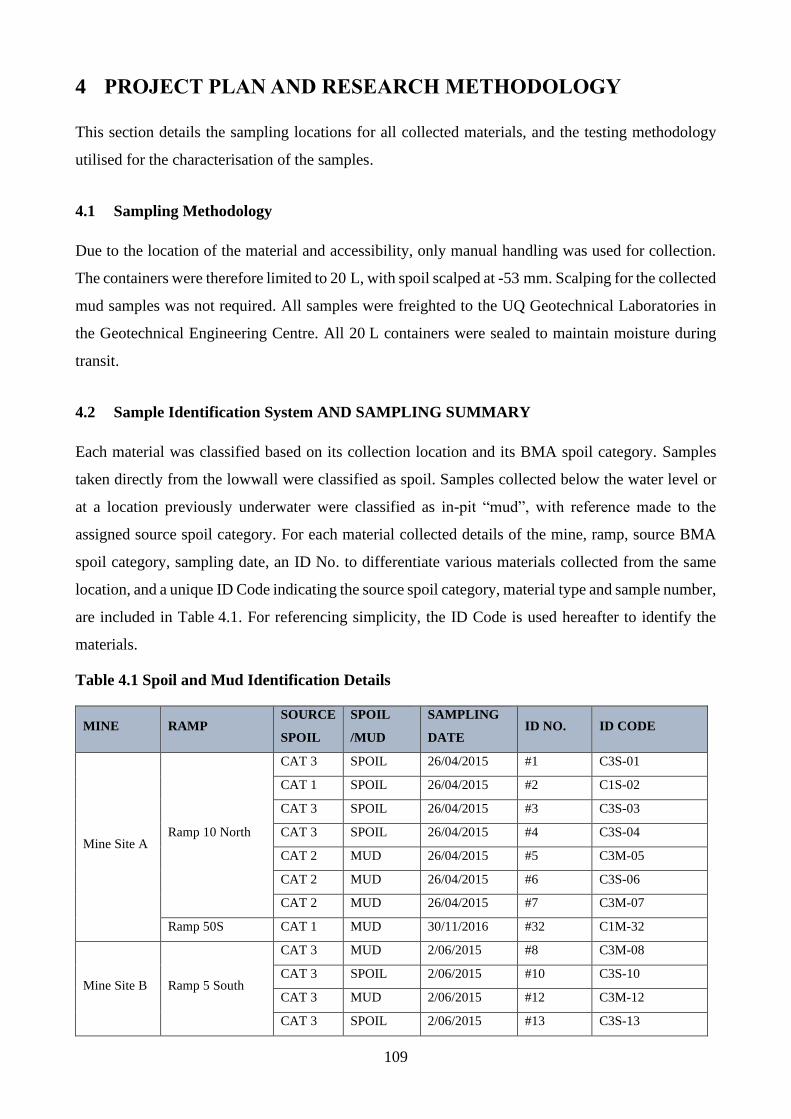
109
4 PROJECT PLAN AND RESEARCH METHODOLOGY
This section details the sampling locations for all collected materials, and the testing methodology
utilised for the characterisation of the samples.
4.1 Sampling Methodology
Due to the location of the material and accessibility, only manual handling was used for collection.
The containers were therefore limited to 20 L, with spoil scalped at -53 mm. Scalping for the collected
mud samples was not required. All samples were freighted to the UQ Geotechnical Laboratories in
the Geotechnical Engineering Centre. All 20 L containers were sealed to maintain moisture during
transit.
4.2 Sample Identification System AND SAMPLING SUMMARY
Each material was classified based on its collection location and its BMA spoil category. Samples
taken directly from the lowwall were classified as spoil. Samples collected below the water level or
at a location previously underwater were classified as in-pit “mud”, with reference made to the
assigned source spoil category. For each material collected details of the mine, ramp, source BMA
spoil category, sampling date, an ID No. to differentiate various materials collected from the same
location, and a unique ID Code indicating the source spoil category, material type and sample number,
are included in Table 4.1. For referencing simplicity, the ID Code is used hereafter to identify the
materials.
Table 4.1 Spoil and Mud Identification Details
MINE RAMP SOURCE
SPOIL
SPOIL
/MUD
SAMPLING
DATE ID NO. ID CODE
Mine Site A Ramp 10 North
CAT 3 SPOIL 26/04/2015 #1 C3S-01
CAT 1 SPOIL 26/04/2015 #2 C1S-02
CAT 3 SPOIL 26/04/2015 #3 C3S-03
CAT 3 SPOIL 26/04/2015 #4 C3S-04
CAT 2 MUD 26/04/2015 #5 C3M-05
CAT 2 MUD 26/04/2015 #6 C3S-06
CAT 2 MUD 26/04/2015 #7 C3M-07
Ramp 50S CAT 1 MUD 30/11/2016 #32 C1M-32
Mine Site B Ramp 5 South
CAT 3 MUD 2/06/2015 #8 C3M-08
CAT 3 SPOIL 2/06/2015 #10 C3S-10
CAT 3 MUD 2/06/2015 #12 C3M-12
CAT 3 SPOIL 2/06/2015 #13 C3S-13
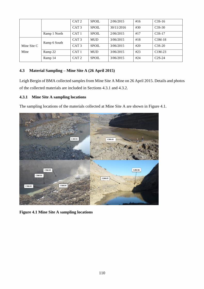
110
CAT 2 SPOIL 2/06/2015 #16 C3S-16
CAT 3 SPOIL 30/11/2016 #30 C3S-30
Ramp 1 North CAT 1 SPOIL 2/06/2015 #17 C3S-17
Mine Site C
Mine
Ramp 6 South CAT 3 MUD 3/06/2015 #18 C3M-18
CAT 3 SPOIL 3/06/2015 #20 C3S-20
Ramp 22 CAT 1 MUD 3/06/2015 #23 C1M-23
Ramp 14 CAT 2 SPOIL 3/06/2015 #24 C2S-24
4.3 Material Sampling – Mine Site A (26 April 2015)
Leigh Bergin of BMA collected samples from Mine Site A Mine on 26 April 2015. Details and photos
of the collected materials are included in Sections 4.3.1 and 4.3.2.
4.3.1 Mine Site A sampling locations
The sampling locations of the materials collected at Mine Site A are shown in Figure 4.1.
Figure 4.1 Mine Site A sampling locations
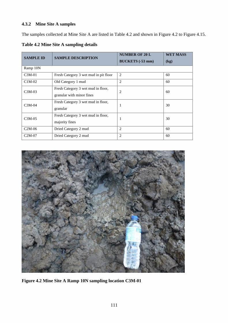
111
4.3.2 Mine Site A samples
The samples collected at Mine Site A are listed in Table 4.2 and shown in Figure 4.2 to Figure 4.15.
Table 4.2 Mine Site A sampling details
SAMPLE ID SAMPLE DESCRIPTION NUMBER OF 20 L
BUCKETS (-53 mm)
WET MASS
(kg)
Ramp 10N
C3M-01 Fresh Category 3 wet mud in pit floor 2 60
C1M-02 Old Category 1 mud 2 60
C3M-03 Fresh Category 3 wet mud in floor,
granular with minor fines 2 60
C3M-04 Fresh Category 3 wet mud in floor,
granular 1 30
C3M-05 Fresh Category 3 wet mud in floor,
majority fines 1 30
C2M-06 Dried Category 2 mud 2 60
C2M-07 Dried Category 2 mud 2 60
Figure 4.2 Mine Site A Ramp 10N sampling location C3M-01
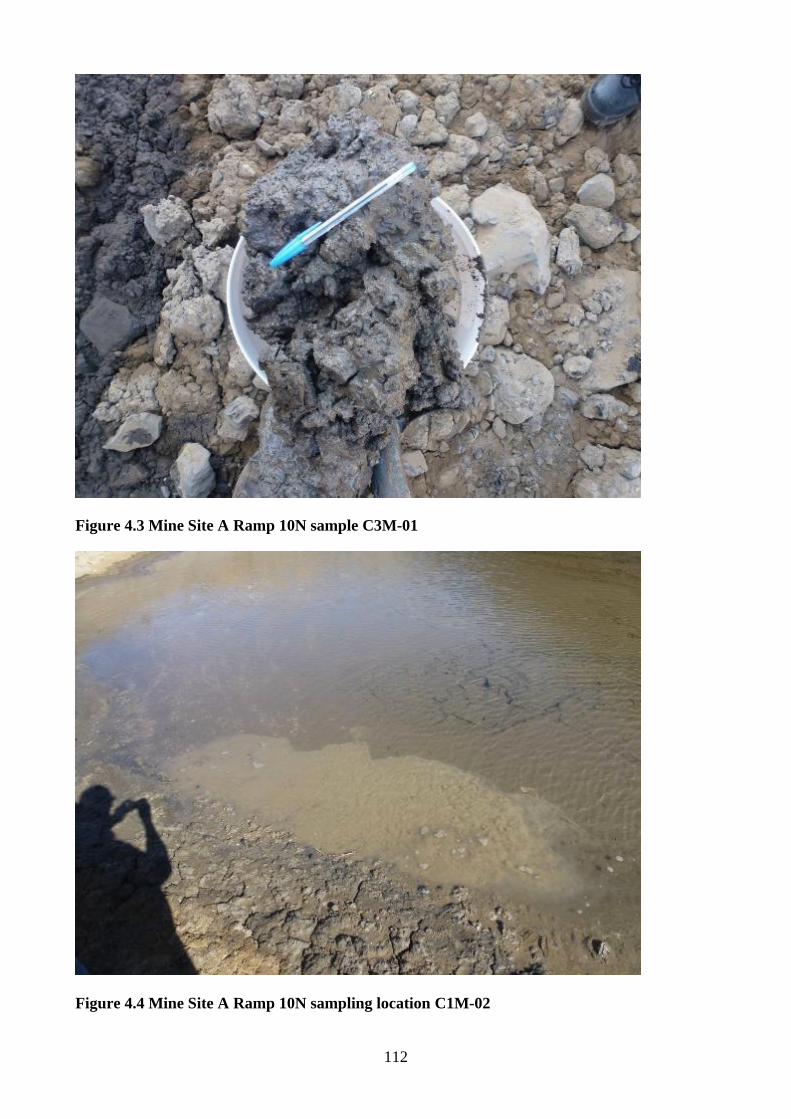
112
Figure 4.3 Mine Site A Ramp 10N sample C3M-01
Figure 4.4 Mine Site A Ramp 10N sampling location C1M-02
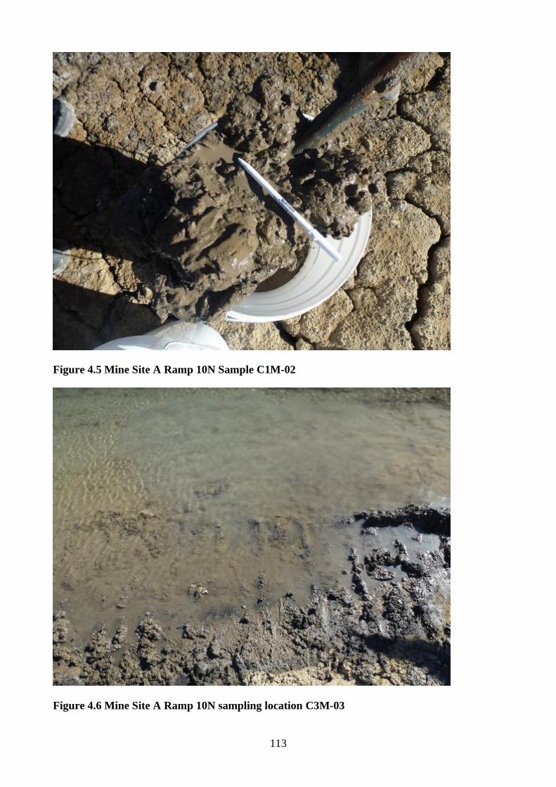
113
Figure 4.5 Mine Site A Ramp 10N Sample C1M-02
Figure 4.6 Mine Site A Ramp 10N sampling location C3M-03
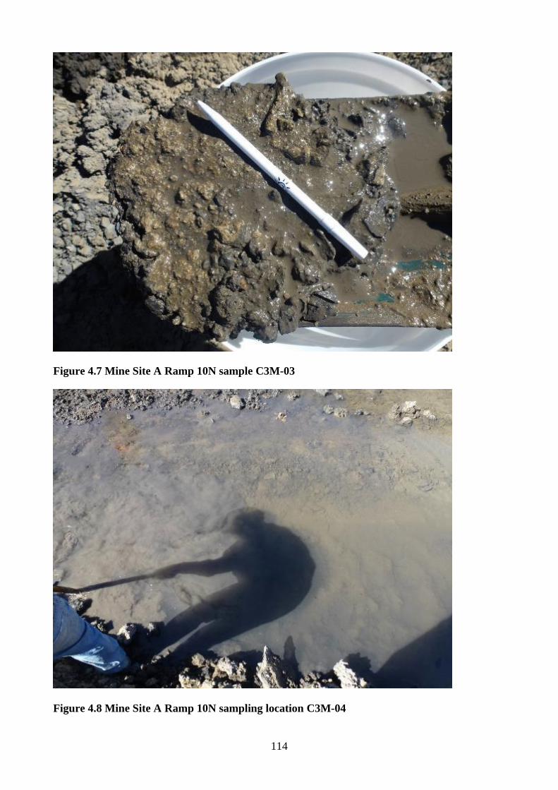
114
Figure 4.7 Mine Site A Ramp 10N sample C3M-03
Figure 4.8 Mine Site A Ramp 10N sampling location C3M-04
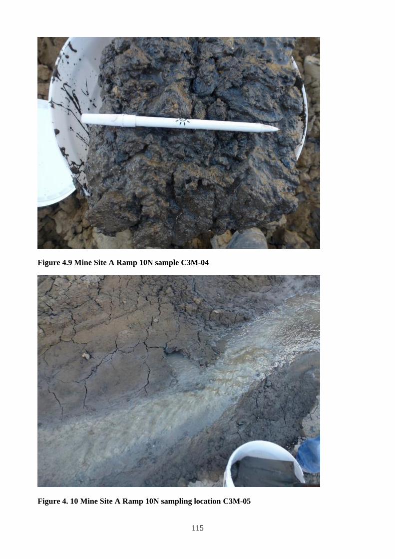
115
Figure 4.9 Mine Site A Ramp 10N sample C3M-04
Figure 4. 10 Mine Site A Ramp 10N sampling location C3M-05
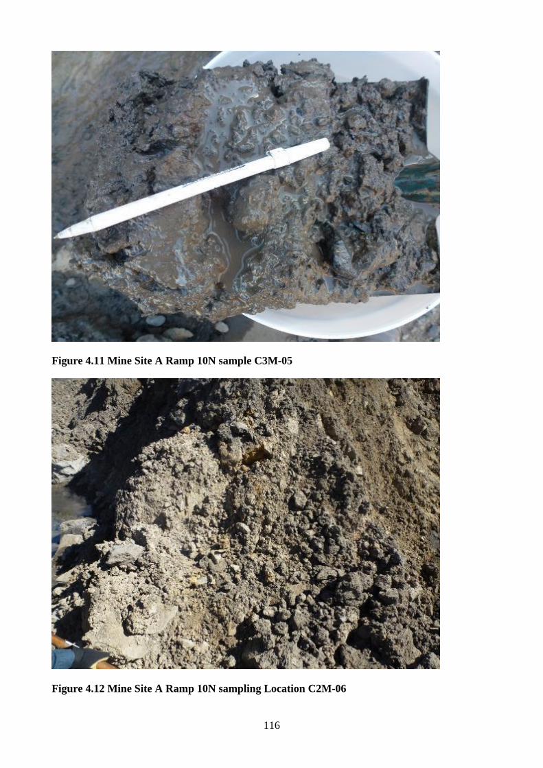
116
Figure 4.11 Mine Site A Ramp 10N sample C3M-05
Figure 4.12 Mine Site A Ramp 10N sampling Location C2M-06
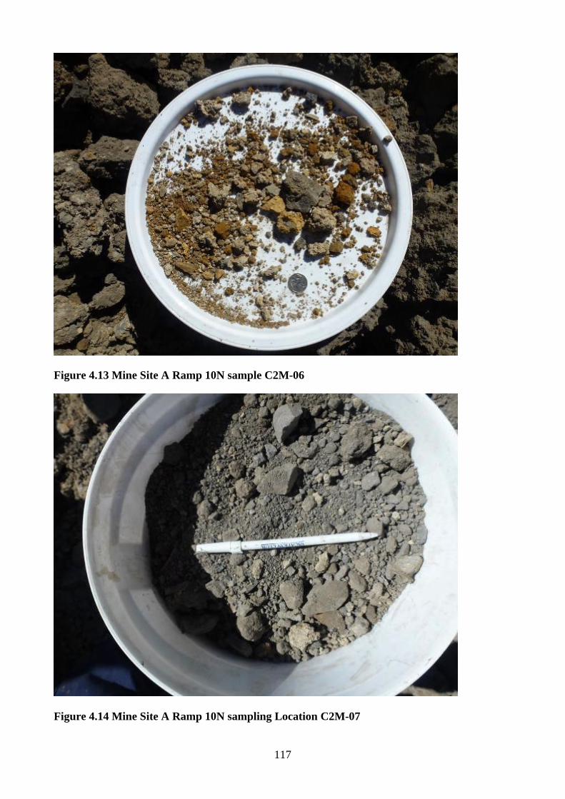
117
Figure 4.13 Mine Site A Ramp 10N sample C2M-06
Figure 4.14 Mine Site A Ramp 10N sampling Location C2M-07
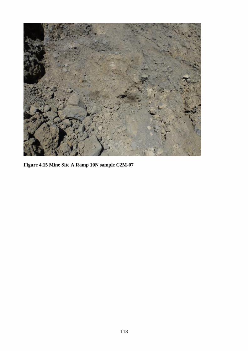
118
Figure 4.15 Mine Site A Ramp 10N sample C2M-07
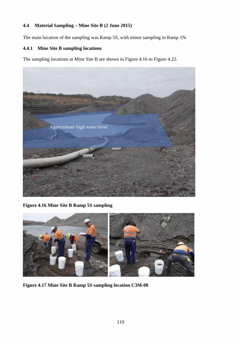
119
4.4 Material Sampling – Mine Site B (2 June 2015)
The main location of the sampling was Ramp 5S, with minor sampling in Ramp 1N.
4.4.1 Mine Site B sampling locations
The sampling locations at Mine Site B are shown in Figure 4.16 to Figure 4.22.
Figure 4.16 Mine Site B Ramp 5S sampling
Figure 4.17 Mine Site B Ramp 5S sampling location C3M-08
Approximate high water level
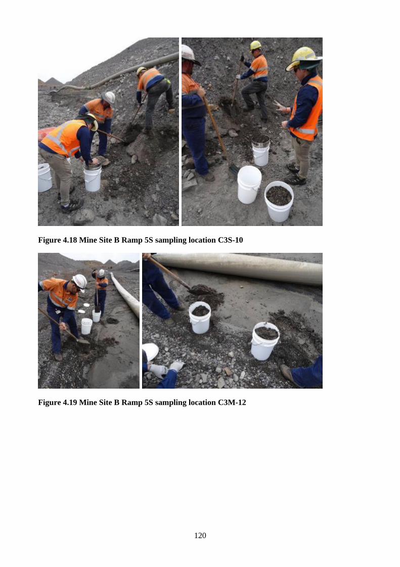
120
Figure 4.18 Mine Site B Ramp 5S sampling location C3S-10
Figure 4.19 Mine Site B Ramp 5S sampling location C3M-12
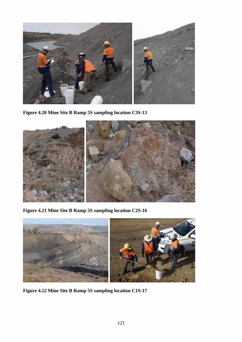
121
Figure 4.20 Mine Site B Ramp 5S sampling location C3S-13
Figure 4.21 Mine Site B Ramp 5S sampling location C2S-16
Figure 4.22 Mine Site B Ramp 5S sampling location C1S-17
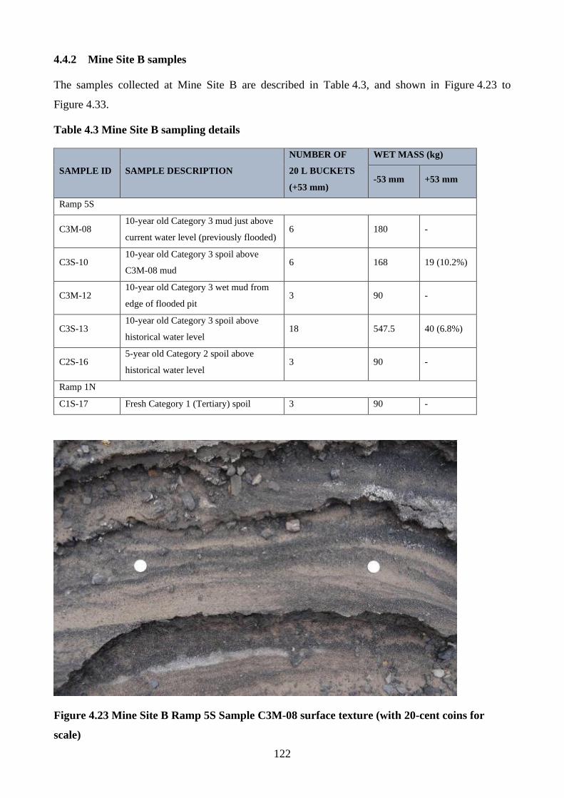
122
4.4.2 Mine Site B samples
The samples collected at Mine Site B are described in Table 4.3, and shown in Figure 4.23 to
Figure 4.33.
Table 4.3 Mine Site B sampling details
SAMPLE ID SAMPLE DESCRIPTION
NUMBER OF
20 L BUCKETS
(+53 mm)
WET MASS (kg)
-53 mm +53 mm
Ramp 5S
C3M-08 10-year old Category 3 mud just above
current water level (previously flooded) 6 180 -
C3S-10 10-year old Category 3 spoil above
C3M-08 mud 6 168 19 (10.2%)
C3M-12 10-year old Category 3 wet mud from
edge of flooded pit 3 90 -
C3S-13 10-year old Category 3 spoil above
historical water level 18 547.5 40 (6.8%)
C2S-16 5-year old Category 2 spoil above
historical water level 3 90 -
Ramp 1N
C1S-17 Fresh Category 1 (Tertiary) spoil 3 90 -
Figure 4.23 Mine Site B Ramp 5S Sample C3M-08 surface texture (with 20-cent coins for
scale)
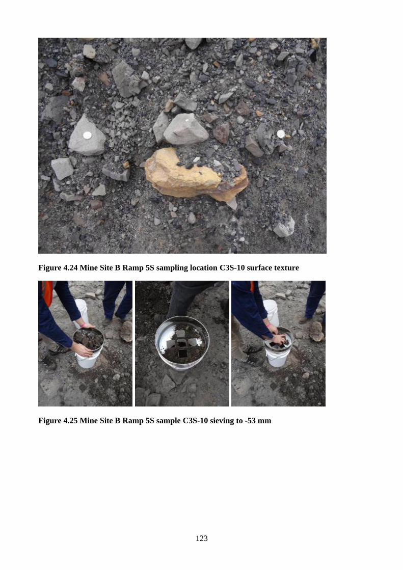
123
Figure 4.24 Mine Site B Ramp 5S sampling location C3S-10 surface texture
Figure 4.25 Mine Site B Ramp 5S sample C3S-10 sieving to -53 mm
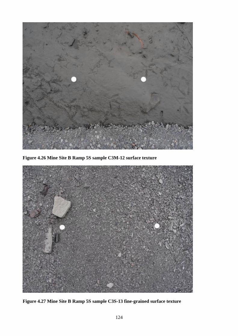
124
Figure 4.26 Mine Site B Ramp 5S sample C3M-12 surface texture
Figure 4.27 Mine Site B Ramp 5S sample C3S-13 fine-grained surface texture
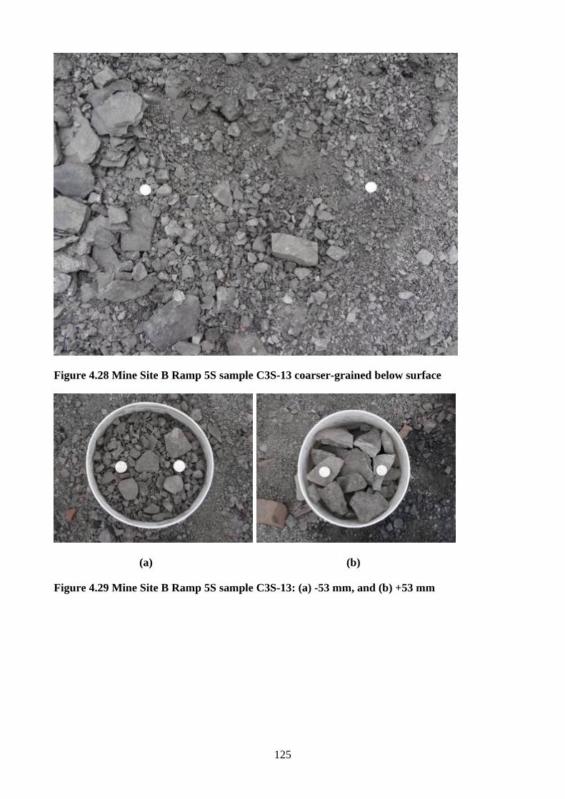
125
Figure 4.28 Mine Site B Ramp 5S sample C3S-13 coarser-grained below surface
(a) (b)
Figure 4.29 Mine Site B Ramp 5S sample C3S-13: (a) -53 mm, and (b) +53 mm
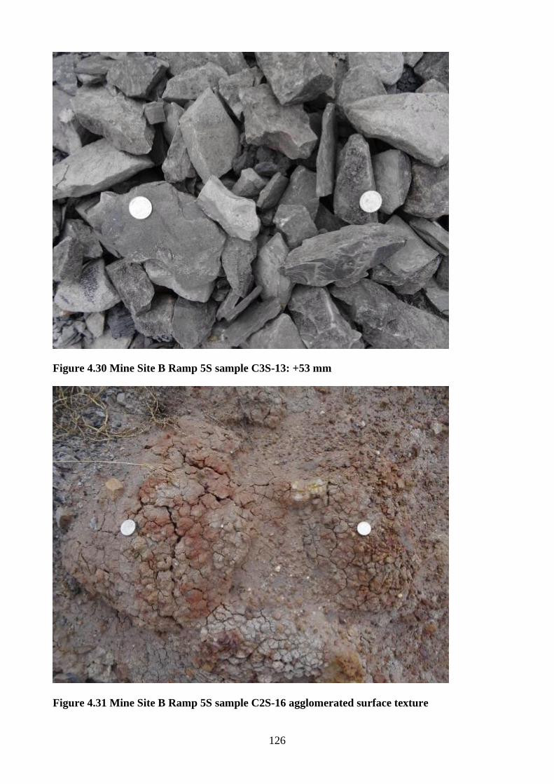
126
Figure 4.30 Mine Site B Ramp 5S sample C3S-13: +53 mm
Figure 4.31 Mine Site B Ramp 5S sample C2S-16 agglomerated surface texture
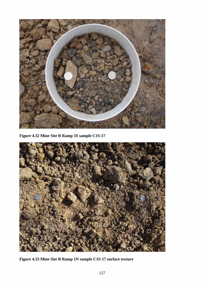
127
Figure 4.32 Mine Site B Ramp 5S sample C1S-17
Figure 4.33 Mine Site B Ramp 1N sample C1S-17 surface texture
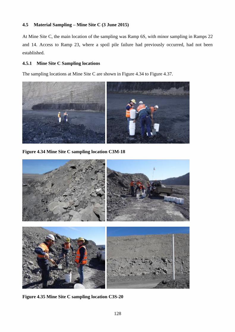
128
4.5 Material Sampling – Mine Site C (3 June 2015)
At Mine Site C, the main location of the sampling was Ramp 6S, with minor sampling in Ramps 22
and 14. Access to Ramp 23, where a spoil pile failure had previously occurred, had not been
established.
4.5.1 Mine Site C Sampling locations
The sampling locations at Mine Site C are shown in Figure 4.34 to Figure 4.37.
Figure 4.34 Mine Site C sampling location C3M-18
Figure 4.35 Mine Site C sampling location C3S-20

129
Figure 4.36 Mine Site C sampling location C3S-23
Figure 4.37 Mine Site C sampling location C2S-24
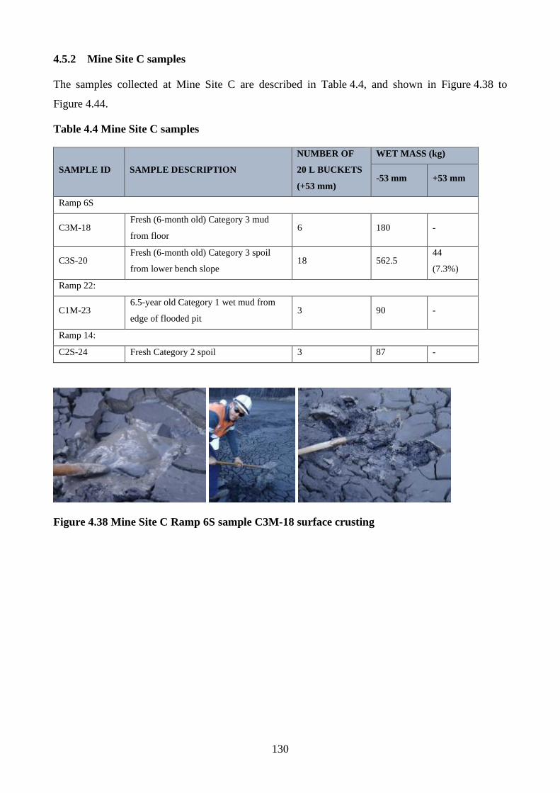
130
4.5.2 Mine Site C samples
The samples collected at Mine Site C are described in Table 4.4, and shown in Figure 4.38 to
Figure 4.44.
Table 4.4 Mine Site C samples
SAMPLE ID SAMPLE DESCRIPTION
NUMBER OF
20 L BUCKETS
(+53 mm)
WET MASS (kg)
-53 mm +53 mm
Ramp 6S
C3M-18 Fresh (6-month old) Category 3 mud
from floor 6 180 -
C3S-20 Fresh (6-month old) Category 3 spoil
from lower bench slope 18 562.5
44
(7.3%)
Ramp 22:
C1M-23 6.5-year old Category 1 wet mud from
edge of flooded pit 3 90 -
Ramp 14:
C2S-24 Fresh Category 2 spoil 3 87 -
Figure 4.38 Mine Site C Ramp 6S sample C3M-18 surface crusting
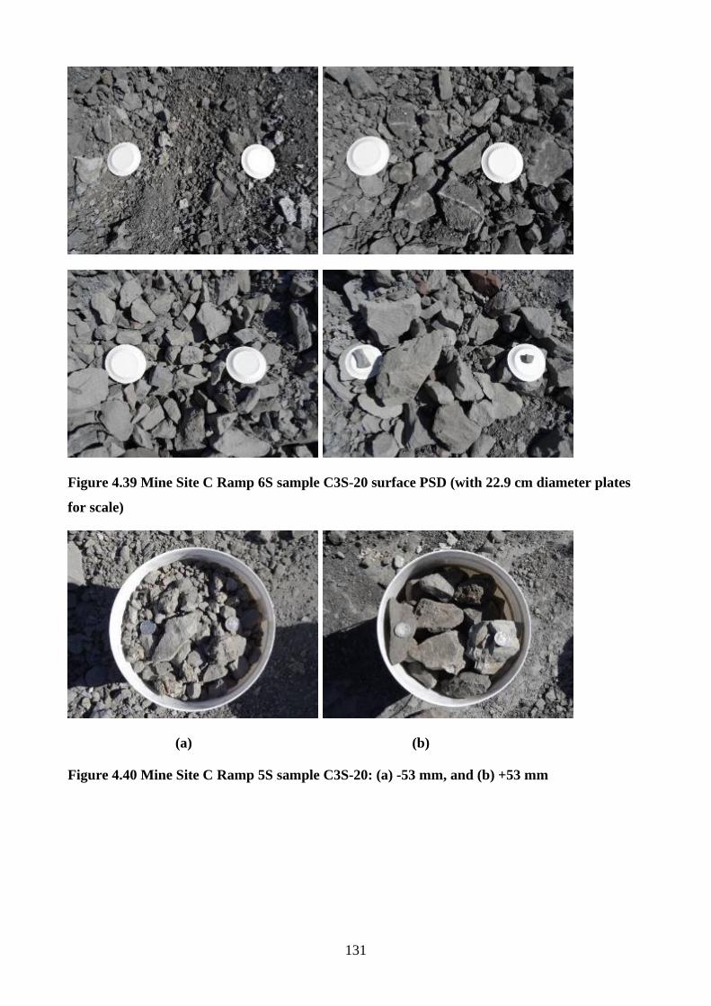
131
Figure 4.39 Mine Site C Ramp 6S sample C3S-20 surface PSD (with 22.9 cm diameter plates
for scale)
(a) (b)
Figure 4.40 Mine Site C Ramp 5S sample C3S-20: (a) -53 mm, and (b) +53 mm
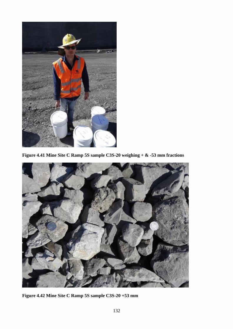
132
Figure 4.41 Mine Site C Ramp 5S sample C3S-20 weighing + & -53 mm fractions
Figure 4.42 Mine Site C Ramp 5S sample C3S-20 +53 mm
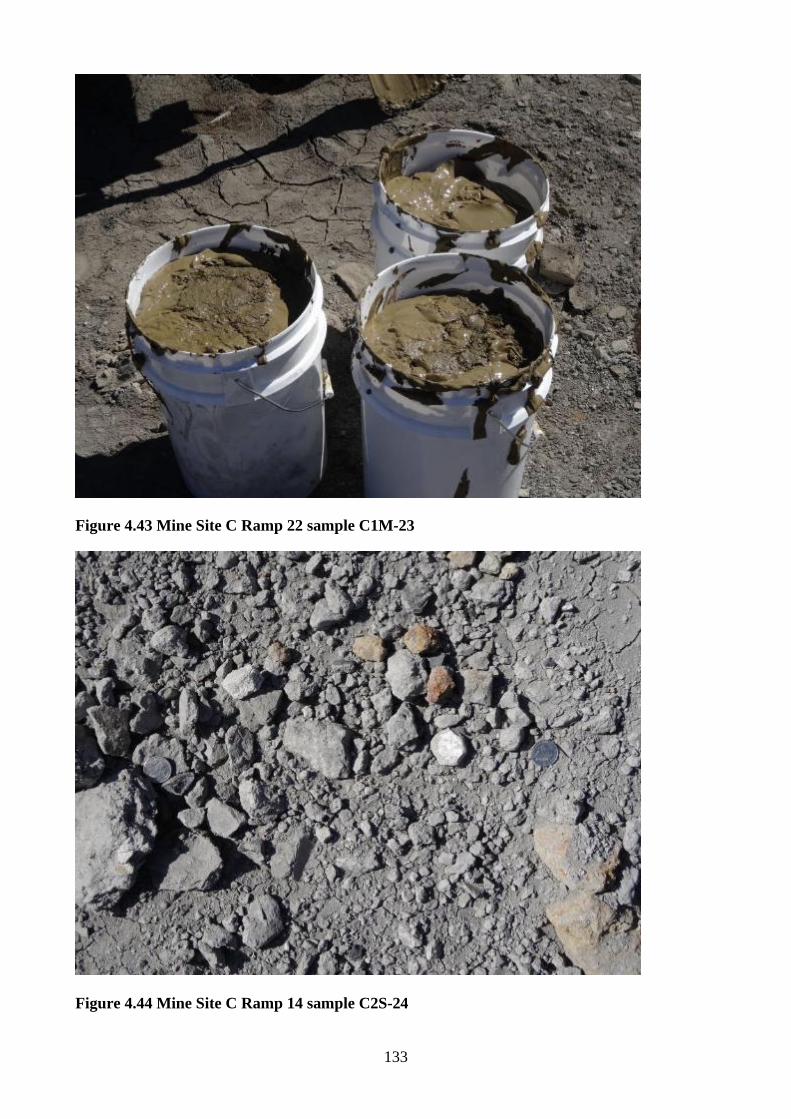
133
Figure 4.43 Mine Site C Ramp 22 sample C1M-23
Figure 4.44 Mine Site C Ramp 14 sample C2S-24
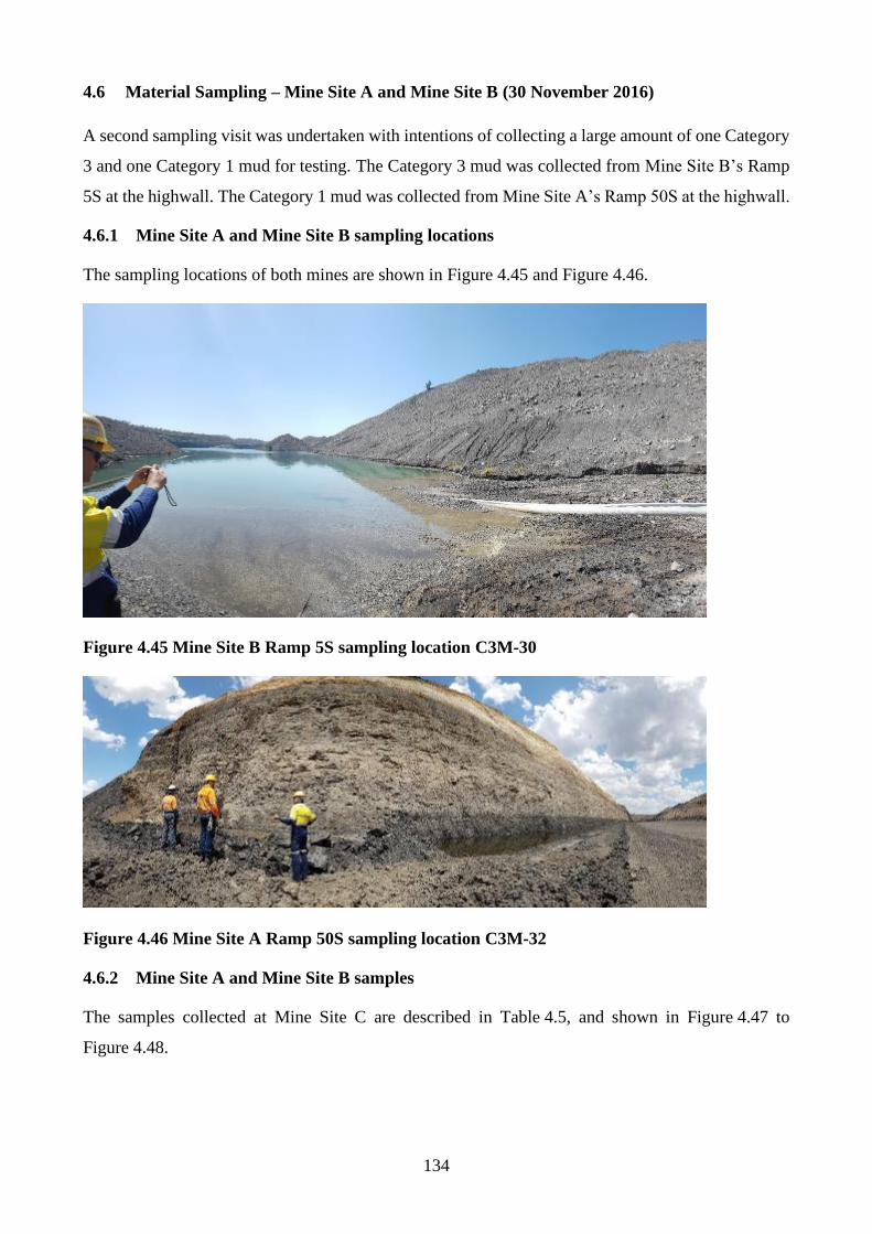
134
4.6 Material Sampling – Mine Site A and Mine Site B (30 November 2016)
A second sampling visit was undertaken with intentions of collecting a large amount of one Category
3 and one Category 1 mud for testing. The Category 3 mud was collected from Mine Site B’s Ramp
5S at the highwall. The Category 1 mud was collected from Mine Site A’s Ramp 50S at the highwall.
4.6.1 Mine Site A and Mine Site B sampling locations
The sampling locations of both mines are shown in Figure 4.45 and Figure 4.46.
Figure 4.45 Mine Site B Ramp 5S sampling location C3M-30
Figure 4.46 Mine Site A Ramp 50S sampling location C3M-32
4.6.2 Mine Site A and Mine Site B samples
The samples collected at Mine Site C are described in Table 4.5, and shown in Figure 4.47 to
Figure 4.48.
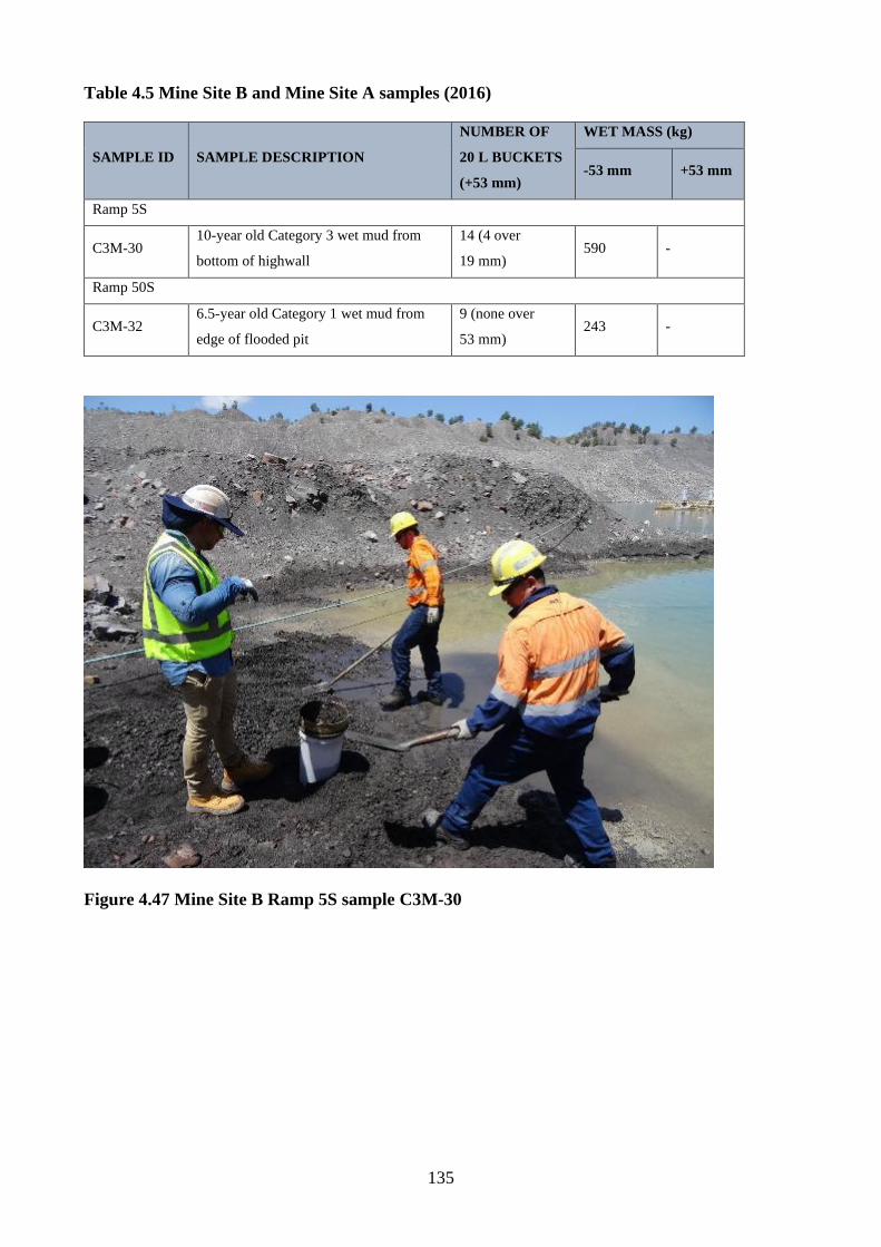
135
Table 4.5 Mine Site B and Mine Site A samples (2016)
SAMPLE ID SAMPLE DESCRIPTION
NUMBER OF
20 L BUCKETS
(+53 mm)
WET MASS (kg)
-53 mm +53 mm
Ramp 5S
C3M-30 10-year old Category 3 wet mud from
bottom of highwall
14 (4 over
19 mm) 590 -
Ramp 50S
C3M-32 6.5-year old Category 1 wet mud from
edge of flooded pit
9 (none over
53 mm) 243 -
Figure 4.47 Mine Site B Ramp 5S sample C3M-30
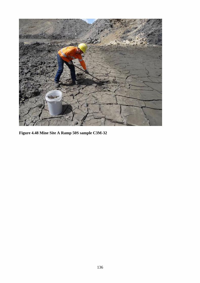
136
Figure 4.48 Mine Site A Ramp 50S sample C3M-32
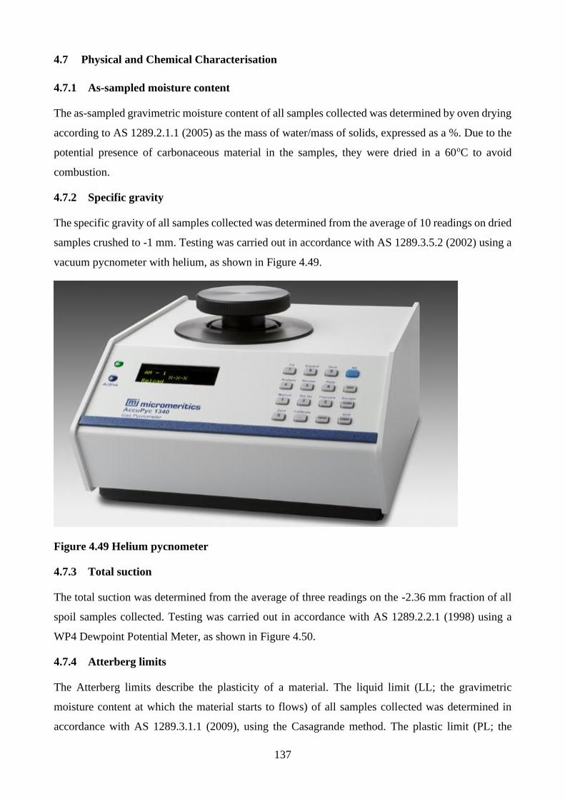
137
4.7 Physical and Chemical Characterisation
4.7.1 As-sampled moisture content
The as-sampled gravimetric moisture content of all samples collected was determined by oven drying
according to AS 1289.2.1.1 (2005) as the mass of water/mass of solids, expressed as a %. Due to the
potential presence of carbonaceous material in the samples, they were dried in a 60oC to avoid
combustion.
4.7.2 Specific gravity
The specific gravity of all samples collected was determined from the average of 10 readings on dried
samples crushed to -1 mm. Testing was carried out in accordance with AS 1289.3.5.2 (2002) using a
vacuum pycnometer with helium, as shown in Figure 4.49.
Figure 4.49 Helium pycnometer
4.7.3 Total suction
The total suction was determined from the average of three readings on the -2.36 mm fraction of all
spoil samples collected. Testing was carried out in accordance with AS 1289.2.2.1 (1998) using a
WP4 Dewpoint Potential Meter, as shown in Figure 4.50.
4.7.4 Atterberg limits
The Atterberg limits describe the plasticity of a material. The liquid limit (LL; the gravimetric
moisture content at which the material starts to flows) of all samples collected was determined in
accordance with AS 1289.3.1.1 (2009), using the Casagrande method. The plastic limit (PL; the
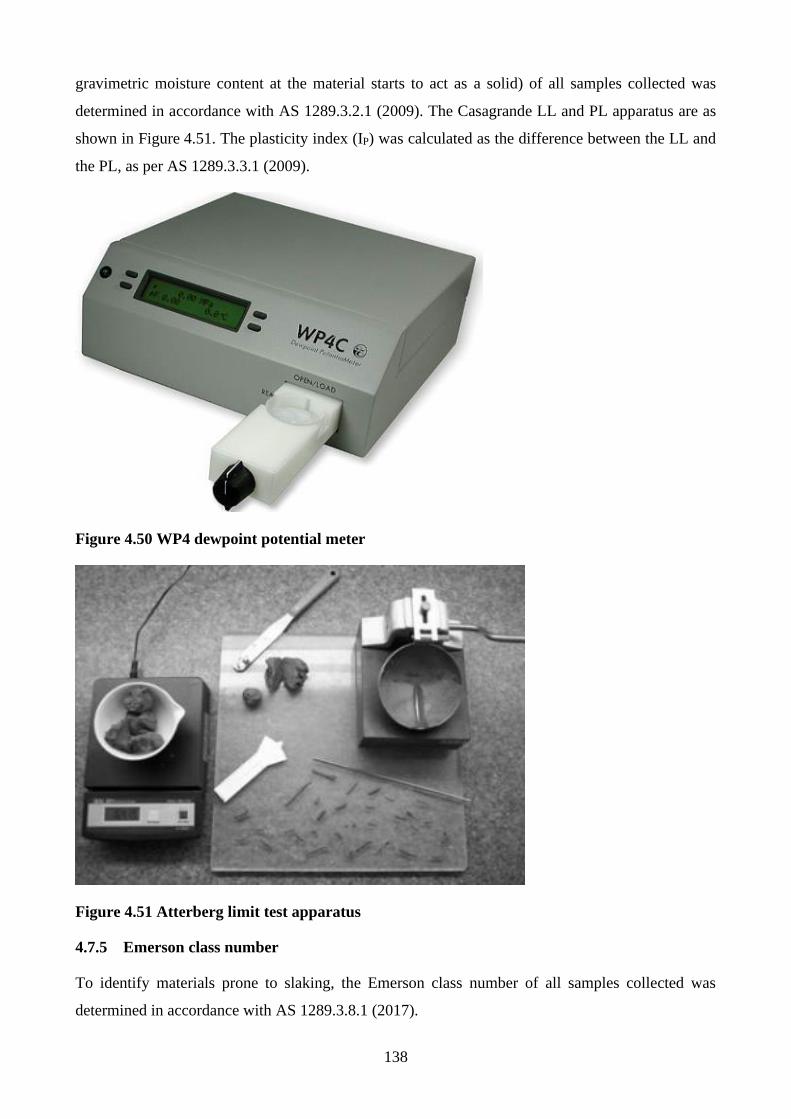
138
gravimetric moisture content at the material starts to act as a solid) of all samples collected was
determined in accordance with AS 1289.3.2.1 (2009). The Casagrande LL and PL apparatus are as
shown in Figure 4.51. The plasticity index (IP) was calculated as the difference between the LL and
the PL, as per AS 1289.3.3.1 (2009).
Figure 4.50 WP4 dewpoint potential meter
Figure 4.51 Atterberg limit test apparatus
4.7.5 Emerson class number
To identify materials prone to slaking, the Emerson class number of all samples collected was
determined in accordance with AS 1289.3.8.1 (2017).
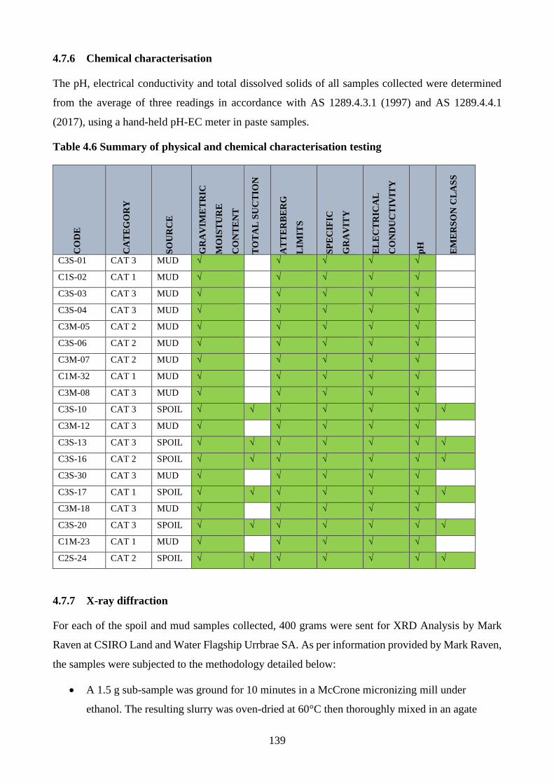
139
4.7.6 Chemical characterisation
The pH, electrical conductivity and total dissolved solids of all samples collected were determined
from the average of three readings in accordance with AS 1289.4.3.1 (1997) and AS 1289.4.4.1
(2017), using a hand-held pH-EC meter in paste samples.
Table 4.6 Summary of physical and chemical characterisation testing
CO
DE
CA
TE
GO
RY
SO
UR
CE
GR
AV
IME
TR
IC
MO
IST
UR
E
CO
NT
EN
T
TO
TA
L S
UC
TIO
N
AT
TE
RB
ER
G
LIM
ITS
SP
EC
IFIC
GR
AV
ITY
EL
EC
TR
ICA
L
CO
ND
UC
TIV
ITY
pH
EM
ER
SO
N C
LA
SS
C3S-01 CAT 3 MUD √ √ √ √ √
C1S-02 CAT 1 MUD √ √ √ √ √
C3S-03 CAT 3 MUD √ √ √ √ √
C3S-04 CAT 3 MUD √ √ √ √ √
C3M-05 CAT 2 MUD √ √ √ √ √
C3S-06 CAT 2 MUD √ √ √ √ √
C3M-07 CAT 2 MUD √ √ √ √ √
C1M-32 CAT 1 MUD √ √ √ √ √
C3M-08 CAT 3 MUD √ √ √ √ √
C3S-10 CAT 3 SPOIL √ √ √ √ √ √ √
C3M-12 CAT 3 MUD √ √ √ √ √
C3S-13 CAT 3 SPOIL √ √ √ √ √ √ √
C3S-16 CAT 2 SPOIL √ √ √ √ √ √ √
C3S-30 CAT 3 MUD √ √ √ √ √
C3S-17 CAT 1 SPOIL √ √ √ √ √ √ √
C3M-18 CAT 3 MUD √ √ √ √ √
C3S-20 CAT 3 SPOIL √ √ √ √ √ √ √
C1M-23 CAT 1 MUD √ √ √ √ √
C2S-24 CAT 2 SPOIL √ √ √ √ √ √ √
4.7.7 X-ray diffraction
For each of the spoil and mud samples collected, 400 grams were sent for XRD Analysis by Mark
Raven at CSIRO Land and Water Flagship Urrbrae SA. As per information provided by Mark Raven,
the samples were subjected to the methodology detailed below:
• A 1.5 g sub-sample was ground for 10 minutes in a McCrone micronizing mill under
ethanol. The resulting slurry was oven-dried at 60°C then thoroughly mixed in an agate
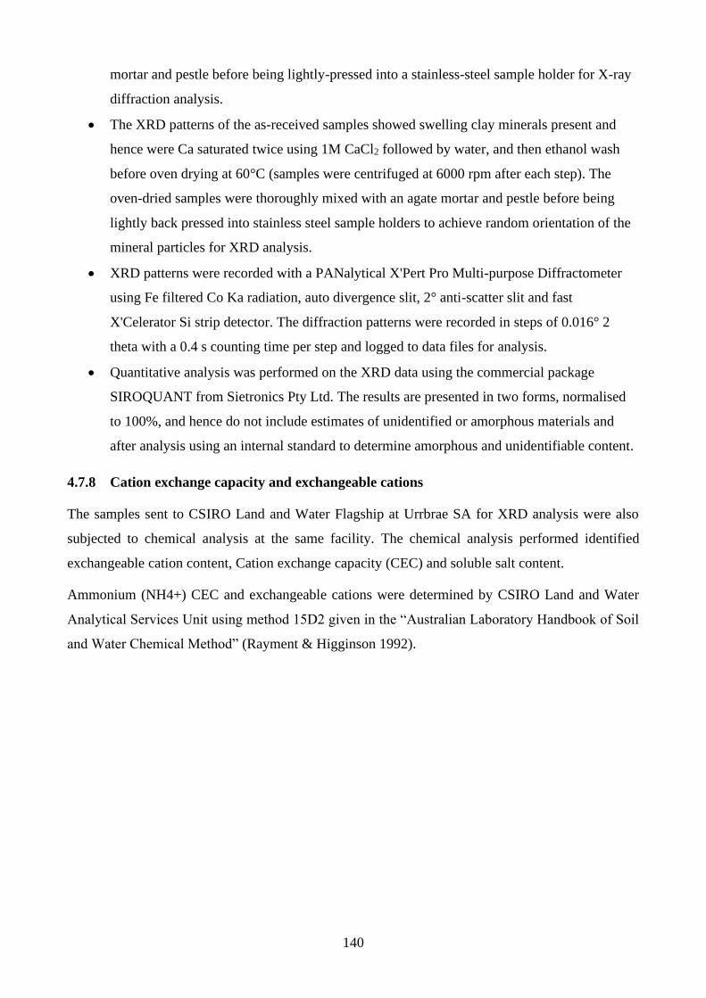
140
mortar and pestle before being lightly-pressed into a stainless-steel sample holder for X-ray
diffraction analysis.
• The XRD patterns of the as-received samples showed swelling clay minerals present and
hence were Ca saturated twice using 1M CaCl2 followed by water, and then ethanol wash
before oven drying at 60°C (samples were centrifuged at 6000 rpm after each step). The
oven-dried samples were thoroughly mixed with an agate mortar and pestle before being
lightly back pressed into stainless steel sample holders to achieve random orientation of the
mineral particles for XRD analysis.
• XRD patterns were recorded with a PANalytical X'Pert Pro Multi-purpose Diffractometer
using Fe filtered Co Ka radiation, auto divergence slit, 2° anti-scatter slit and fast
X'Celerator Si strip detector. The diffraction patterns were recorded in steps of 0.016° 2
theta with a 0.4 s counting time per step and logged to data files for analysis.
• Quantitative analysis was performed on the XRD data using the commercial package
SIROQUANT from Sietronics Pty Ltd. The results are presented in two forms, normalised
to 100%, and hence do not include estimates of unidentified or amorphous materials and
after analysis using an internal standard to determine amorphous and unidentifiable content.
4.7.8 Cation exchange capacity and exchangeable cations
The samples sent to CSIRO Land and Water Flagship at Urrbrae SA for XRD analysis were also
subjected to chemical analysis at the same facility. The chemical analysis performed identified
exchangeable cation content, Cation exchange capacity (CEC) and soluble salt content.
Ammonium (NH4+) CEC and exchangeable cations were determined by CSIRO Land and Water
Analytical Services Unit using method 15D2 given in the “Australian Laboratory Handbook of Soil
and Water Chemical Method” (Rayment & Higginson 1992).
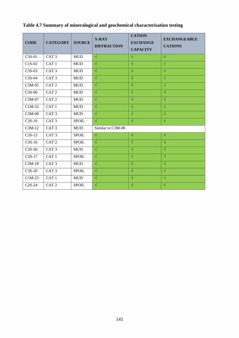
141
Table 4.7 Summary of mineralogical and geochemical characterisation testing
CODE CATEGORY SOURCE X-RAY
DIFFRACTION
CATION
EXCHANGE
CAPACITY
EXCHANGEABLE
CATIONS
C3S-01 CAT 3 MUD √ √ √
C1S-02 CAT 1 MUD √ √ √
C3S-03 CAT 3 MUD √ √ √
C3S-04 CAT 3 MUD √ √ √
C3M-05 CAT 2 MUD √ √ √
C3S-06 CAT 2 MUD √ √ √
C3M-07 CAT 2 MUD √ √ √
C1M-32 CAT 1 MUD √ √ √
C3M-08 CAT 3 MUD √ √ √
C3S-10 CAT 3 SPOIL √ √ √
C3M-12 CAT 3 MUD Similar to C3M-08
C3S-13 CAT 3 SPOIL √ √ √
C3S-16 CAT 2 SPOIL √ √ √
C3S-30 CAT 3 MUD √ √ √
C3S-17 CAT 1 SPOIL √ √ √
C3M-18 CAT 3 MUD √ √ √
C3S-20 CAT 3 SPOIL √ √ √
C1M-23 CAT 1 MUD √ √ √
C2S-24 CAT 2 SPOIL √ √ √
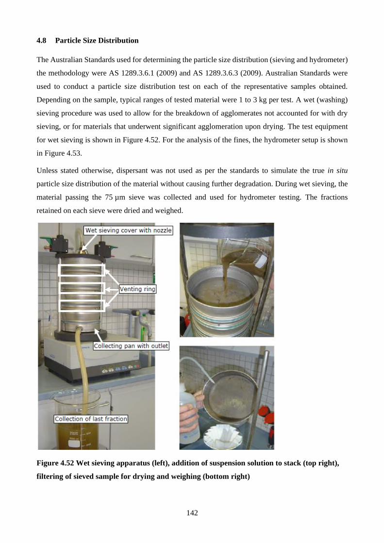
142
4.8 Particle Size Distribution
The Australian Standards used for determining the particle size distribution (sieving and hydrometer)
the methodology were AS 1289.3.6.1 (2009) and AS 1289.3.6.3 (2009). Australian Standards were
used to conduct a particle size distribution test on each of the representative samples obtained.
Depending on the sample, typical ranges of tested material were 1 to 3 kg per test. A wet (washing)
sieving procedure was used to allow for the breakdown of agglomerates not accounted for with dry
sieving, or for materials that underwent significant agglomeration upon drying. The test equipment
for wet sieving is shown in Figure 4.52. For the analysis of the fines, the hydrometer setup is shown
in Figure 4.53.
Unless stated otherwise, dispersant was not used as per the standards to simulate the true in situ
particle size distribution of the material without causing further degradation. During wet sieving, the
material passing the 75 µm sieve was collected and used for hydrometer testing. The fractions
retained on each sieve were dried and weighed.
Figure 4.52 Wet sieving apparatus (left), addition of suspension solution to stack (top right),
filtering of sieved sample for drying and weighing (bottom right)
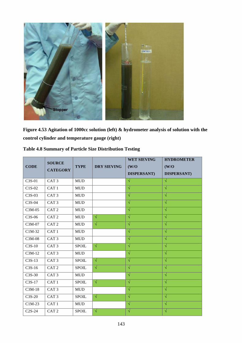
143
Figure 4.53 Agitation of 1000cc solution (left) & hydrometer analysis of solution with the
control cylinder and temperature gauge (right)
Table 4.8 Summary of Particle Size Distribution Testing
CODE SOURCE
CATEGORY TYPE DRY SIEVING
WET SIEVING
(W/O
DISPERSANT)
HYDROMETER
(W/O
DISPERSANT)
C3S-01 CAT 3 MUD √ √
C1S-02 CAT 1 MUD √ √
C3S-03 CAT 3 MUD √ √
C3S-04 CAT 3 MUD √ √
C3M-05 CAT 2 MUD √ √
C3S-06 CAT 2 MUD √ √ √
C3M-07 CAT 2 MUD √ √ √
C1M-32 CAT 1 MUD √ √
C3M-08 CAT 3 MUD √ √
C3S-10 CAT 3 SPOIL √ √ √
C3M-12 CAT 3 MUD √ √
C3S-13 CAT 3 SPOIL √ √ √
C3S-16 CAT 2 SPOIL √ √ √
C3S-30 CAT 3 MUD √ √
C3S-17 CAT 1 SPOIL √ √ √
C3M-18 CAT 3 MUD √ √
C3S-20 CAT 3 SPOIL √ √ √
C1M-23 CAT 1 MUD √ √
C2S-24 CAT 2 SPOIL √ √ √
144
4.9 Degradation Testing of Spoil
Two testing programs were conducted to investigate the degradation of fresh spoil. To understand
how spoil materials would behave under different conditions, the influence of prolonged saturation
and wetting and drying cycles were investigated. Once conditions were identified that would produce
appropriate degrees of in situ degradation, the methodologies were applied to all fresh spoils
collected, with methodologies discussed in Section 4.9.3.
4.9.1 Varied saturation durations
Prolonged saturation was used to determine how different durations of flooding would influence a
spoil sample, and at what rate the spoil degrades. To test the spoil, representative samples of 1.5 kg
were prepared for each material out of the -19 mm fraction. Each sample was exposed to different
durations of saturation, after which its particle size distribution was determined via wet sieving and
hydrometer analysis. During saturation, measurements were made of the electrical conductivity for
each sample, as well as the total dissolved salts.
4.9.2 Multiple wetting and drying cycles
Multiple wetting and drying cycles were used on representative samples of 1.5 kg of spoil out of the
-19 mm fraction. The aim of this testing was to determine how rainfall or flooding could degrade
spoil materials and at what rate. For each sample investigated, the particle size distribution was
analysed after three wetting and drying cycles had been completed. After each wetting cycle, the
electrical conductivity and total dissolved solids were measured.
4.9.3 Spoil degradation testing program
To simulate the degradation of the spoil materials on wetting-up, three methods of degradation with
tap water were used. Dry sieving was used to determine the particle size distribution of the as-sampled
spoil. This is the state it would be in on visual classification using the BMA framework. Submersion
with tap water over 24 hours was used to break down any loosely conglomerated particles. Wetting
and drying cycles were used to accelerate the rate of degradation and promote slaking of the material.
The modified slake durability test was used to reduce the time required for the material to degrade,
while still undergoing wetting and drying cycles in a reliable and repeatable manner.
4.9.3.1 24 Hour Saturation
A 1.5 kg representative sample of each spoil material was collected and submerged in tap water for
24 hours. To promote saturation, each sample was gently agitated to remove air pockets and wet-up
dry zones. Once submerged, each sample was covered with a lid to reduce evaporation and stored at
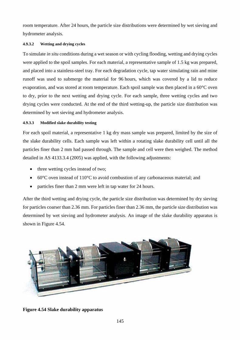
145
room temperature. After 24 hours, the particle size distributions were determined by wet sieving and
hydrometer analysis.
4.9.3.2 Wetting and drying cycles
To simulate in situ conditions during a wet season or with cycling flooding, wetting and drying cycles
were applied to the spoil samples. For each material, a representative sample of 1.5 kg was prepared,
and placed into a stainless-steel tray. For each degradation cycle, tap water simulating rain and mine
runoff was used to submerge the material for 96 hours, which was covered by a lid to reduce
evaporation, and was stored at room temperature. Each spoil sample was then placed in a 60°C oven
to dry, prior to the next wetting and drying cycle. For each sample, three wetting cycles and two
drying cycles were conducted. At the end of the third wetting-up, the particle size distribution was
determined by wet sieving and hydrometer analysis.
4.9.3.3 Modified slake durability testing
For each spoil material, a representative 1 kg dry mass sample was prepared, limited by the size of
the slake durability cells. Each sample was left within a rotating slake durability cell until all the
particles finer than 2 mm had passed through. The sample and cell were then weighed. The method
detailed in AS 4133.3.4 (2005) was applied, with the following adjustments:
• three wetting cycles instead of two;
• 60°C oven instead of 110°C to avoid combustion of any carbonaceous material; and
• particles finer than 2 mm were left in tap water for 24 hours.
After the third wetting and drying cycle, the particle size distribution was determined by dry sieving
for particles coarser than 2.36 mm. For particles finer than 2.36 mm, the particle size distribution was
determined by wet sieving and hydrometer analysis. An image of the slake durability apparatus is
shown in Figure 4.54.
Figure 4.54 Slake durability apparatus
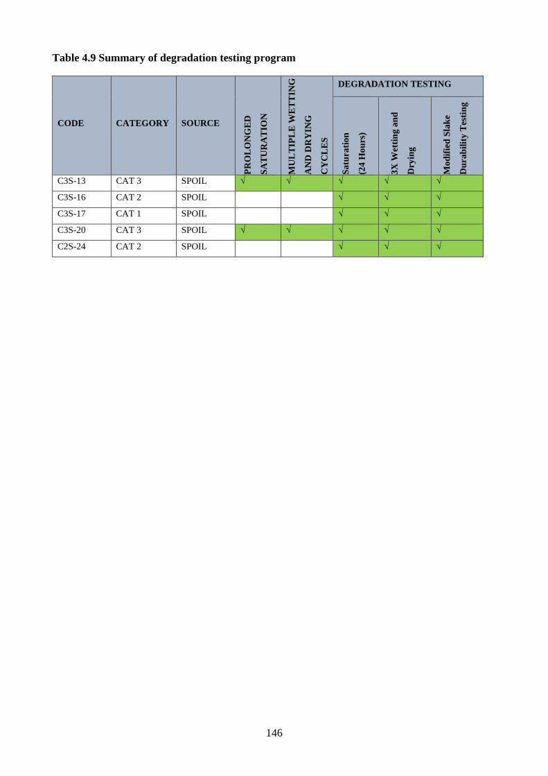
146
Table 4.9 Summary of degradation testing program
CODE CATEGORY SOURCE
PR
OL
ON
GE
D
SA
TU
RA
TIO
N
MU
LT
IPL
E W
ET
TIN
G
AN
D D
RY
ING
CY
CL
ES
DEGRADATION TESTING
Sa
tura
tio
n
(24
Ho
urs
)
3X
Wet
tin
g a
nd
Dry
ing
Mo
dif
ied
Sla
ke
Du
rab
ilit
y T
esti
ng
C3S-13 CAT 3 SPOIL √ √ √ √ √
C3S-16 CAT 2 SPOIL √ √ √
C3S-17 CAT 1 SPOIL √ √ √
C3S-20 CAT 3 SPOIL √ √ √ √ √
C2S-24 CAT 2 SPOIL √ √ √
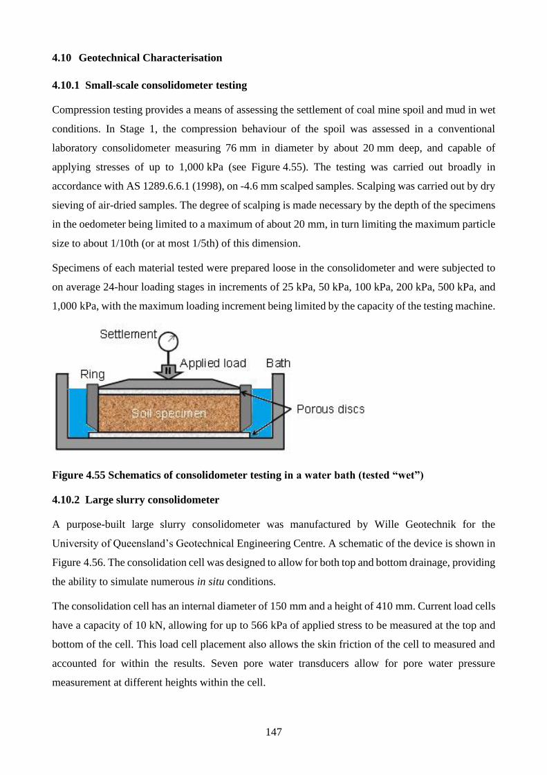
147
4.10 Geotechnical Characterisation
4.10.1 Small-scale consolidometer testing
Compression testing provides a means of assessing the settlement of coal mine spoil and mud in wet
conditions. In Stage 1, the compression behaviour of the spoil was assessed in a conventional
laboratory consolidometer measuring 76 mm in diameter by about 20 mm deep, and capable of
applying stresses of up to 1,000 kPa (see Figure 4.55). The testing was carried out broadly in
accordance with AS 1289.6.6.1 (1998), on -4.6 mm scalped samples. Scalping was carried out by dry
sieving of air-dried samples. The degree of scalping is made necessary by the depth of the specimens
in the oedometer being limited to a maximum of about 20 mm, in turn limiting the maximum particle
size to about 1/10th (or at most 1/5th) of this dimension.
Specimens of each material tested were prepared loose in the consolidometer and were subjected to
on average 24-hour loading stages in increments of 25 kPa, 50 kPa, 100 kPa, 200 kPa, 500 kPa, and
1,000 kPa, with the maximum loading increment being limited by the capacity of the testing machine.
Figure 4.55 Schematics of consolidometer testing in a water bath (tested “wet”)
4.10.2 Large slurry consolidometer
A purpose-built large slurry consolidometer was manufactured by Wille Geotechnik for the
University of Queensland’s Geotechnical Engineering Centre. A schematic of the device is shown in
Figure 4.56. The consolidation cell was designed to allow for both top and bottom drainage, providing
the ability to simulate numerous in situ conditions.
The consolidation cell has an internal diameter of 150 mm and a height of 410 mm. Current load cells
have a capacity of 10 kN, allowing for up to 566 kPa of applied stress to be measured at the top and
bottom of the cell. This load cell placement also allows the skin friction of the cell to measured and
accounted for within the results. Seven pore water transducers allow for pore water pressure
measurement at different heights within the cell.
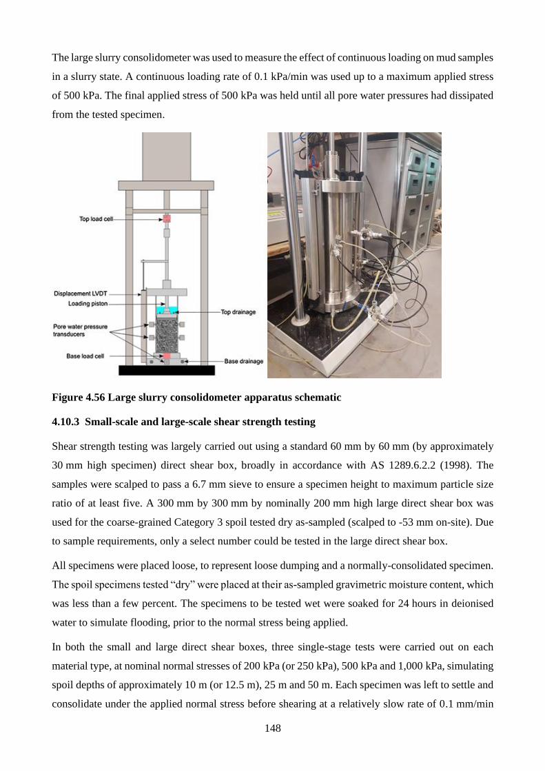
148
The large slurry consolidometer was used to measure the effect of continuous loading on mud samples
in a slurry state. A continuous loading rate of 0.1 kPa/min was used up to a maximum applied stress
of 500 kPa. The final applied stress of 500 kPa was held until all pore water pressures had dissipated
from the tested specimen.
Figure 4.56 Large slurry consolidometer apparatus schematic
4.10.3 Small-scale and large-scale shear strength testing
Shear strength testing was largely carried out using a standard 60 mm by 60 mm (by approximately
30 mm high specimen) direct shear box, broadly in accordance with AS 1289.6.2.2 (1998). The
samples were scalped to pass a 6.7 mm sieve to ensure a specimen height to maximum particle size
ratio of at least five. A 300 mm by 300 mm by nominally 200 mm high large direct shear box was
used for the coarse-grained Category 3 spoil tested dry as-sampled (scalped to -53 mm on-site). Due
to sample requirements, only a select number could be tested in the large direct shear box.
All specimens were placed loose, to represent loose dumping and a normally-consolidated specimen.
The spoil specimens tested “dry” were placed at their as-sampled gravimetric moisture content, which
was less than a few percent. The specimens to be tested wet were soaked for 24 hours in deionised
water to simulate flooding, prior to the normal stress being applied.
In both the small and large direct shear boxes, three single-stage tests were carried out on each
material type, at nominal normal stresses of 200 kPa (or 250 kPa), 500 kPa and 1,000 kPa, simulating
spoil depths of approximately 10 m (or 12.5 m), 25 m and 50 m. Each specimen was left to settle and
consolidate under the applied normal stress before shearing at a relatively slow rate of 0.1 mm/min
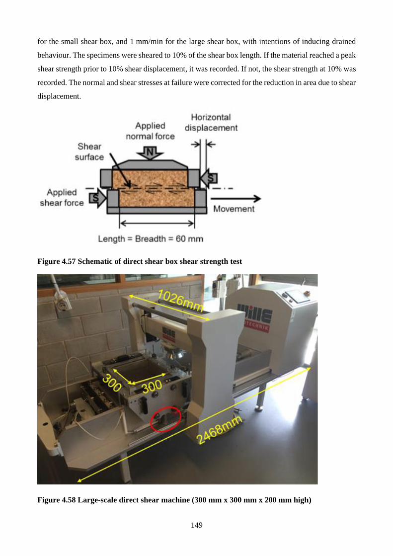
149
for the small shear box, and 1 mm/min for the large shear box, with intentions of inducing drained
behaviour. The specimens were sheared to 10% of the shear box length. If the material reached a peak
shear strength prior to 10% shear displacement, it was recorded. If not, the shear strength at 10% was
recorded. The normal and shear stresses at failure were corrected for the reduction in area due to shear
displacement.
Figure 4.57 Schematic of direct shear box shear strength test
Figure 4.58 Large-scale direct shear machine (300 mm x 300 mm x 200 mm high)
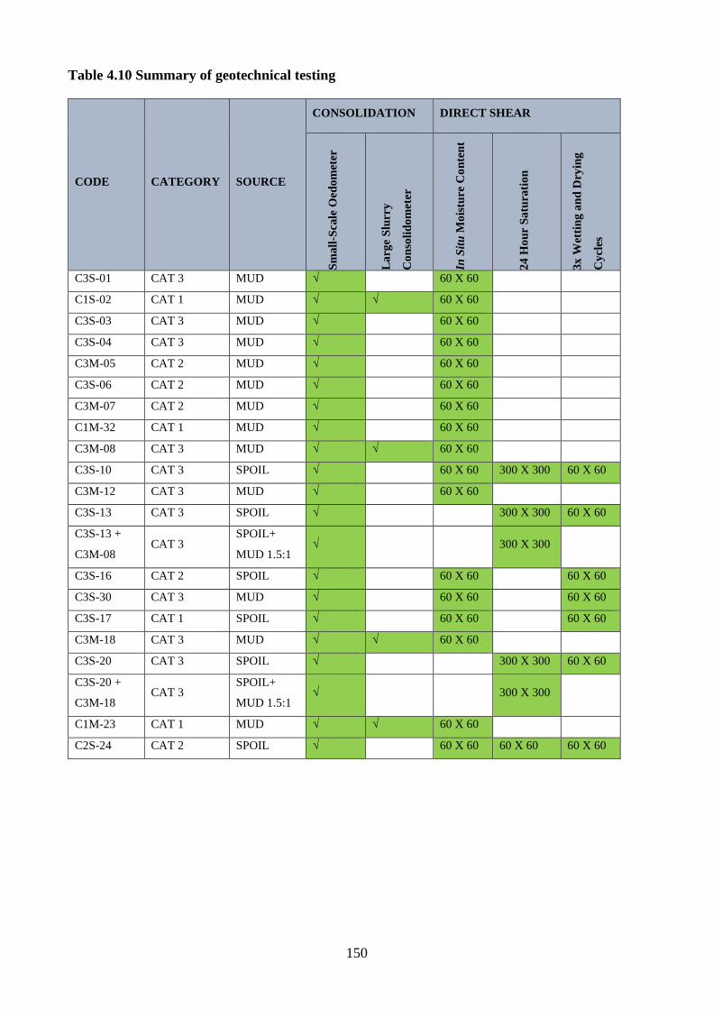
150
Table 4.10 Summary of geotechnical testing
CODE CATEGORY SOURCE
CONSOLIDATION DIRECT SHEAR
Sm
all
-Sca
le O
edo
met
er
La
rge
Slu
rry
Co
nso
lid
om
eter
In S
itu
Mo
istu
re C
on
ten
t
24
Ho
ur
Sa
tura
tio
n
3x
Wet
tin
g a
nd
Dry
ing
Cy
cles
C3S-01 CAT 3 MUD √ 60 X 60
C1S-02 CAT 1 MUD √ √ 60 X 60
C3S-03 CAT 3 MUD √ 60 X 60
C3S-04 CAT 3 MUD √ 60 X 60
C3M-05 CAT 2 MUD √ 60 X 60
C3S-06 CAT 2 MUD √ 60 X 60
C3M-07 CAT 2 MUD √ 60 X 60
C1M-32 CAT 1 MUD √ 60 X 60
C3M-08 CAT 3 MUD √ √ 60 X 60
C3S-10 CAT 3 SPOIL √ 60 X 60 300 X 300 60 X 60
C3M-12 CAT 3 MUD √ 60 X 60
C3S-13 CAT 3 SPOIL √ 300 X 300 60 X 60
C3S-13 +
C3M-08 CAT 3
SPOIL+
MUD 1.5:1 √ 300 X 300
C3S-16 CAT 2 SPOIL √ 60 X 60 60 X 60
C3S-30 CAT 3 MUD √ 60 X 60 60 X 60
C3S-17 CAT 1 SPOIL √ 60 X 60 60 X 60
C3M-18 CAT 3 MUD √ √ 60 X 60
C3S-20 CAT 3 SPOIL √ 300 X 300 60 X 60
C3S-20 +
C3M-18 CAT 3
SPOIL+
MUD 1.5:1 √ 300 X 300
C1M-23 CAT 1 MUD √ √ 60 X 60
C2S-24 CAT 2 SPOIL √ 60 X 60 60 X 60 60 X 60
151
5 MATERIAL CHARACTERISATION TEST RESULTS
A large testing program was conducted following the methodology detailed in Section 4.7, with aims
of characterising numerous spoil and mud materials collected from three mines within the Bowen
Basin. This chapter focuses on the physical, chemical, mineralogical and geochemical test results. All
spoil materials are discussed with respect to their assigned BMA spoil category. The mud materials
were labelled with respect to the category of their spoil source from which they formed.
5.1 Physical Characterisation
5.1.1 As-sampled moisture state
For each of the spoil and mud materials collected, the as-sampled gravimetric moisture content (mass
of water/mass of solids, expressed as a percentage) and total moisture content (mass of water/total
mass, expressed as a percentage) are given in Table 5.1. The moisture content was determined on the
-19 mm fraction to ensure accuracy and repeatability. Typically, the lowest gravimetric moisture
contents were obtained for the spoil materials collected above any previous flooding levels (1.1 to
3.3%). C3S-10, a spoil material that was previously below past flooding levels had a moisture content
of 9.5%, highlighting the spoils ability to retain moisture near the surface of the spoil pile post-
flooding. Moderate moisture contents were recorded for dried mud materials that had previously been
exposed to flooding (C2M-06 and C2M-07).
The as-sampled gravimetric moisture contents of the Category 3 muds ranged from 13.3 to 94.5%.
That of the Category 2 muds ranged from 4.5 to 12.9%, and that of the Category 1 muds ranged from
9.5 to 90.9%. The values given in Table 5.1 are also plotted in Figure 5.1.
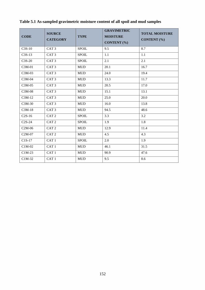
152
Table 5.1 As-sampled gravimetric moisture content of all spoil and mud samples
CODE SOURCE
CATEGORY TYPE
GRAVIMETRIC
MOISTURE
CONTENT (%)
TOTAL MOISTURE
CONTENT (%)
C3S-10 CAT 3 SPOIL 9.5 8.7
C3S-13 CAT 3 SPOIL 1.1 1.1
C3S-20 CAT 3 SPOIL 2.1 2.1
C3M-01 CAT 3 MUD 20.1 16.7
C3M-03 CAT 3 MUD 24.0 19.4
C3M-04 CAT 3 MUD 13.3 11.7
C3M-05 CAT 3 MUD 20.5 17.0
C3M-08 CAT 3 MUD 15.1 13.1
C3M-12 CAT 3 MUD 25.0 20.0
C3M-30 CAT 3 MUD 16.0 13.8
C3M-18 CAT 3 MUD 94.5 48.6
C2S-16 CAT 2 SPOIL 3.3 3.2
C2S-24 CAT 2 SPOIL 1.9 1.8
C2M-06 CAT 2 MUD 12.9 11.4
C2M-07 CAT 2 MUD 4.5 4.3
C1S-17 CAT 1 SPOIL 2.0 1.9
C1M-02 CAT 1 MUD 46.1 31.5
C1M-23 CAT 1 MUD 90.9 47.6
C1M-32 CAT 1 MUD 9.5 8.6
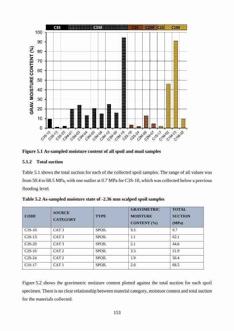
153
Figure 5.1 As-sampled moisture content of all spoil and mud samples
5.1.2 Total suction
Table 5.1 shows the total suction for each of the collected spoil samples. The range of all values was
from 50.4 to 68.5 MPa, with one outlier at 0.7 MPa for C3S-10, which was collected below a previous
flooding level.
Table 5.2 As-sampled moisture state of -2.36 mm scalped spoil samples
CODE SOURCE
CATEGORY TYPE
GRAVIMETRIC
MOISTURE
CONTENT (%)
TOTAL
SUCTION
(MPa)
C3S-10 CAT 3 SPOIL 9.5 0.7
C3S-13 CAT 3 SPOIL 1.1 62.1
C3S-20 CAT 3 SPOIL 2.1 44.6
C2S-16 CAT 2 SPOIL 3.3 51.9
C2S-24 CAT 2 SPOIL 1.9 50.4
C1S-17 CAT 1 SPOIL 2.0 68.5
Figure 5.2 shows the gravimetric moisture content plotted against the total suction for each spoil
specimen. There is no clear relationship between material category, moisture content and total suction
for the materials collected.
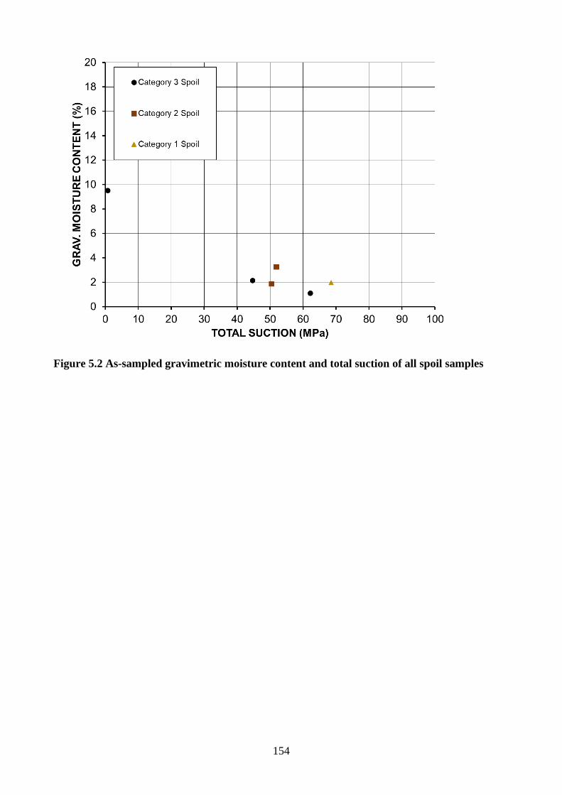
154
Figure 5.2 As-sampled gravimetric moisture content and total suction of all spoil samples
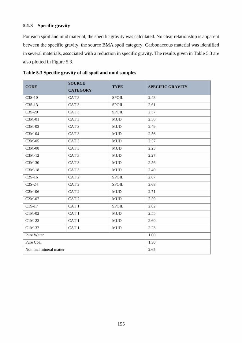
155
5.1.3 Specific gravity
For each spoil and mud material, the specific gravity was calculated. No clear relationship is apparent
between the specific gravity, the source BMA spoil category. Carbonaceous material was identified
in several materials, associated with a reduction in specific gravity. The results given in Table 5.3 are
also plotted in Figure 5.3.
Table 5.3 Specific gravity of all spoil and mud samples
CODE SOURCE
CATEGORY TYPE SPECIFIC GRAVITY
C3S-10 CAT 3 SPOIL 2.43
C3S-13 CAT 3 SPOIL 2.61
C3S-20 CAT 3 SPOIL 2.57
C3M-01 CAT 3 MUD 2.56
C3M-03 CAT 3 MUD 2.49
C3M-04 CAT 3 MUD 2.56
C3M-05 CAT 3 MUD 2.57
C3M-08 CAT 3 MUD 2.23
C3M-12 CAT 3 MUD 2.27
C3M-30 CAT 3 MUD 2.56
C3M-18 CAT 3 MUD 2.40
C2S-16 CAT 2 SPOIL 2.67
C2S-24 CAT 2 SPOIL 2.68
C2M-06 CAT 2 MUD 2.71
C2M-07 CAT 2 MUD 2.59
C1S-17 CAT 1 SPOIL 2.62
C1M-02 CAT 1 MUD 2.55
C1M-23 CAT 1 MUD 2.60
C1M-32 CAT 1 MUD 2.23
Pure Water 1.00
Pure Coal 1.30
Nominal mineral matter 2.65
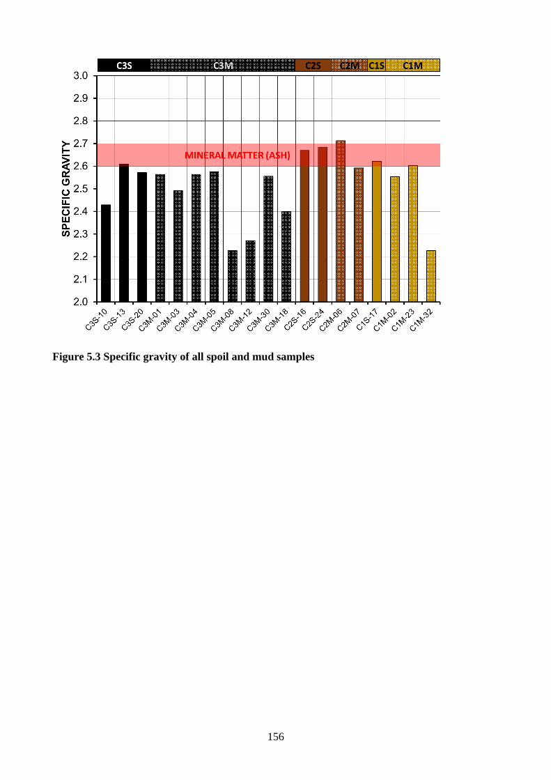
156
Figure 5.3 Specific gravity of all spoil and mud samples

157
5.1.4 Particle size distributions
All collected samples were analysed to determine their particle size distribution. For the spoil, both
wet and dry sieving were used to characterise the materials. The purpose of dry sieving was to
determine the in situ particle size distribution. Wet sieving was undertaken to breakdown any weakly
agglomerated fines that would not be identified during standardised dry sieving, and to promote
slaking in highly degradable material.
The particle size distributions of all the materials collected were analysed with respect to their BMA
spoil category, with results plotted in Figure 5.4 to Figure 5.20. For all materials, the D90, D50, D10,
Cu and Cc values were calculated and are given in Table 5.4 to Table 5.9. D90 values for all spoils
tested wet and dry, and all muds tested wet are plotted in Figure 5.8 and Figure 5.14, respectively.
Figure 5.4 Overall particle size distribution curves of Category 3 spoil -53 mm fraction
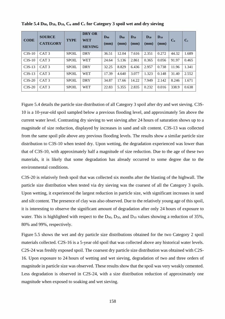
158
Table 5.4 D90, D50, D10, Cu and Cc for Category 3 spoil wet and dry sieving
CODE SOURCE
CATEGORY TYPE
DRY OR
WET
SIEVING
D90
(mm)
D60
(mm)
D50
(mm)
D30
(mm)
D10
(mm) Cu Cc
C3S-10 CAT 3 SPOIL DRY 36.51 12.04 7.616 2.351 0.272 44.32 1.689
C3S-10 CAT 3 SPOIL WET 24.64 5.136 2.861 0.365 0.056 91.97 0.465
C3S-13 CAT 3 SPOIL DRY 32.25 8.829 6.436 2.957 0.738 11.96 1.341
C3S-13 CAT 3 SPOIL WET 17.39 4.640 3.077 1.323 0.148 31.40 2.552
C3S-20 CAT 3 SPOIL DRY 34.87 17.66 14.22 7.949 2.142 8.246 1.671
C3S-20 CAT 3 SPOIL WET 22.83 5.355 2.835 0.232 0.016 338.9 0.638
Figure 5.4 details the particle size distribution of all Category 3 spoil after dry and wet sieving. C3S-
10 is a 10-year-old spoil sampled below a previous flooding level, and approximately 5m above the
current water level. Contrasting dry sieving to wet sieving after 24 hours of saturation shows up to a
magnitude of size reduction, displayed by increases in sand and silt content. C3S-13 was collected
from the same spoil pile above any previous flooding levels. The results show a similar particle size
distribution to C3S-10 when tested dry. Upon wetting, the degradation experienced was lower than
that of C3S-10, with approximately half a magnitude of size reduction. Due to the age of these two
materials, it is likely that some degradation has already occurred to some degree due to the
environmental conditions.
C3S-20 is relatively fresh spoil that was collected six months after the blasting of the highwall. The
particle size distribution when tested via dry sieving was the coarsest of all the Category 3 spoils.
Upon wetting, it experienced the largest reduction in particle size, with significant increases in sand
and silt content. The presence of clay was also observed. Due to the relatively young age of this spoil,
it is interesting to observe the significant amount of degradation after only 24 hours of exposure to
water. This is highlighted with respect to the D90, D50, and D10 values showing a reduction of 35%,
80% and 99%, respectively.
Figure 5.5 shows the wet and dry particle size distributions obtained for the two Category 2 spoil
materials collected. C2S-16 is a 5-year old spoil that was collected above any historical water levels.
C2S-24 was freshly exposed spoil. The coarsest dry particle size distribution was obtained with C2S-
16. Upon exposure to 24 hours of wetting and wet sieving, degradation of two and three orders of
magnitude in particle size was observed. These results show that the spoil was very weakly cemented.
Less degradation is observed in C2S-24, with a size distribution reduction of approximately one
magnitude when exposed to soaking and wet sieving.
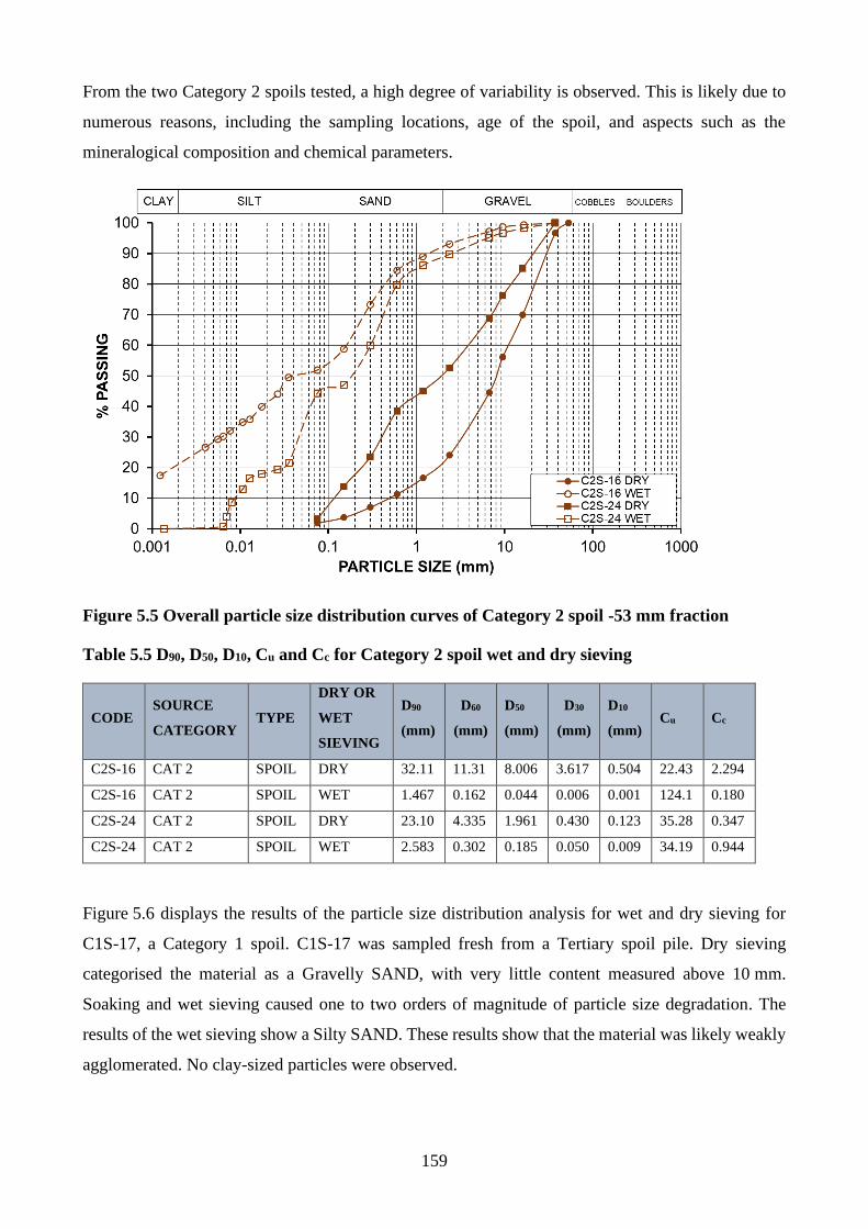
159
From the two Category 2 spoils tested, a high degree of variability is observed. This is likely due to
numerous reasons, including the sampling locations, age of the spoil, and aspects such as the
mineralogical composition and chemical parameters.
Figure 5.5 Overall particle size distribution curves of Category 2 spoil -53 mm fraction
Table 5.5 D90, D50, D10, Cu and Cc for Category 2 spoil wet and dry sieving
CODE SOURCE
CATEGORY TYPE
DRY OR
WET
SIEVING
D90
(mm)
D60
(mm)
D50
(mm)
D30
(mm)
D10
(mm) Cu Cc
C2S-16 CAT 2 SPOIL DRY 32.11 11.31 8.006 3.617 0.504 22.43 2.294
C2S-16 CAT 2 SPOIL WET 1.467 0.162 0.044 0.006 0.001 124.1 0.180
C2S-24 CAT 2 SPOIL DRY 23.10 4.335 1.961 0.430 0.123 35.28 0.347
C2S-24 CAT 2 SPOIL WET 2.583 0.302 0.185 0.050 0.009 34.19 0.944
Figure 5.6 displays the results of the particle size distribution analysis for wet and dry sieving for
C1S-17, a Category 1 spoil. C1S-17 was sampled fresh from a Tertiary spoil pile. Dry sieving
categorised the material as a Gravelly SAND, with very little content measured above 10 mm.
Soaking and wet sieving caused one to two orders of magnitude of particle size degradation. The
results of the wet sieving show a Silty SAND. These results show that the material was likely weakly
agglomerated. No clay-sized particles were observed.
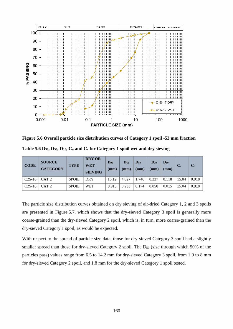
160
Figure 5.6 Overall particle size distribution curves of Category 1 spoil -53 mm fraction
Table 5.6 D90, D50, D10, Cu and Cc for Category 1 spoil wet and dry sieving
CODE SOURCE
CATEGORY TYPE
DRY OR
WET
SIEVING
D90
(mm)
D60
(mm)
D50
(mm)
D30
(mm)
D10
(mm) Cu Cc
C2S-16 CAT 2 SPOIL DRY 15.12 4.027 1.746 0.337 0.118 15.04 0.918
C2S-16 CAT 2 SPOIL WET 0.915 0.233 0.174 0.058 0.015 15.04 0.918
The particle size distribution curves obtained on dry sieving of air-dried Category 1, 2 and 3 spoils
are presented in Figure 5.7, which shows that the dry-sieved Category 3 spoil is generally more
coarse-grained than the dry-sieved Category 2 spoil, which is, in turn, more coarse-grained than the
dry-sieved Category 1 spoil, as would be expected.
With respect to the spread of particle size data, those for dry-sieved Category 3 spoil had a slightly
smaller spread than those for dry-sieved Category 2 spoil. The D50 (size through which 50% of the
particles pass) values range from 6.5 to 14.2 mm for dry-sieved Category 3 spoil, from 1.9 to 8 mm
for dry-sieved Category 2 spoil, and 1.8 mm for the dry-sieved Category 1 spoil tested.
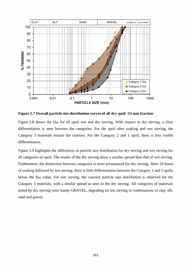
161
Figure 5.7 Overall particle size distribution curves of all dry spoil -53 mm fraction
Figure 5.8 shows the D90 for all spoil wet and dry sieving. With respect to dry sieving, a clear
differentiation is seen between the categories. For the spoil after soaking and wet sieving, the
Category 3 materials remain the coarsest. For the Category 2 and 1 spoil, there is less visible
differentiation.
Figure 5.9 highlights the differences in particle size distribution for dry sieving and wet sieving for
all categories of spoil. The results of the dry sieving show a smaller spread than that of wet sieving.
Furthermore, the distinction between categories is more pronounced for dry sieving. After 24 hours
of soaking followed by wet sieving, there is little differentiation between the Category 1 and 2 spoils
below the D90 value. For wet sieving, the coarsest particle size distribution is observed for the
Category 3 materials, with a similar spread as seen in the dry sieving. All categories of materials
tested by dry sieving were Sandy GRAVEL, degrading on wet sieving to combinations of clay, silt,
sand and gravel.
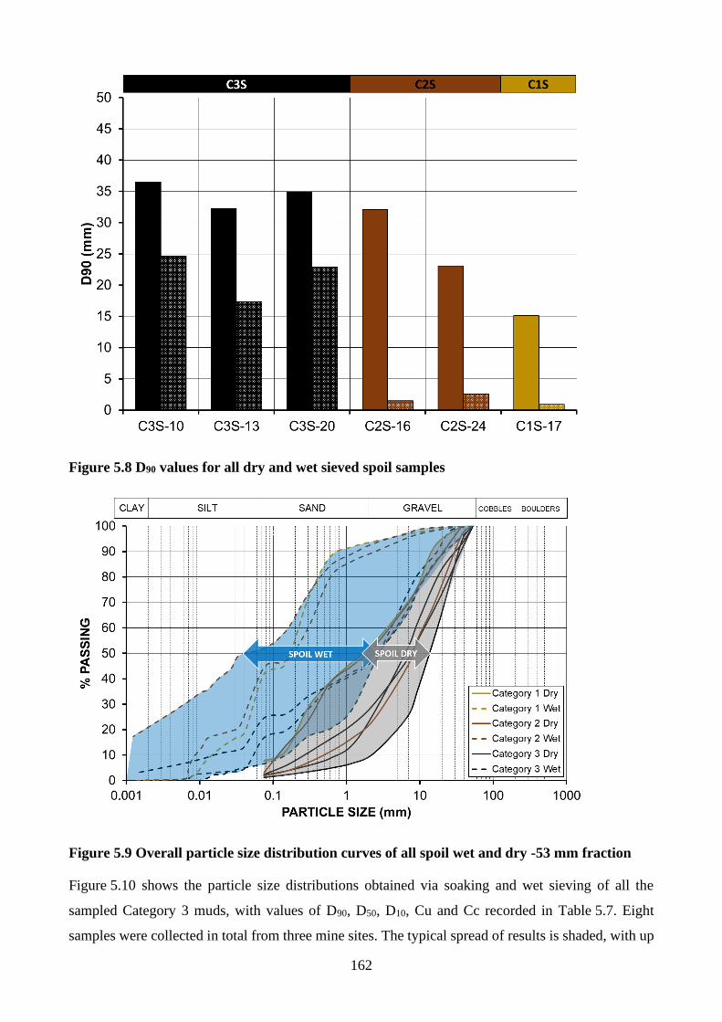
162
Figure 5.8 D90 values for all dry and wet sieved spoil samples
Figure 5.9 Overall particle size distribution curves of all spoil wet and dry -53 mm fraction
Figure 5.10 shows the particle size distributions obtained via soaking and wet sieving of all the
sampled Category 3 muds, with values of D90, D50, D10, Cu and Cc recorded in Table 5.7. Eight
samples were collected in total from three mine sites. The typical spread of results is shaded, with up
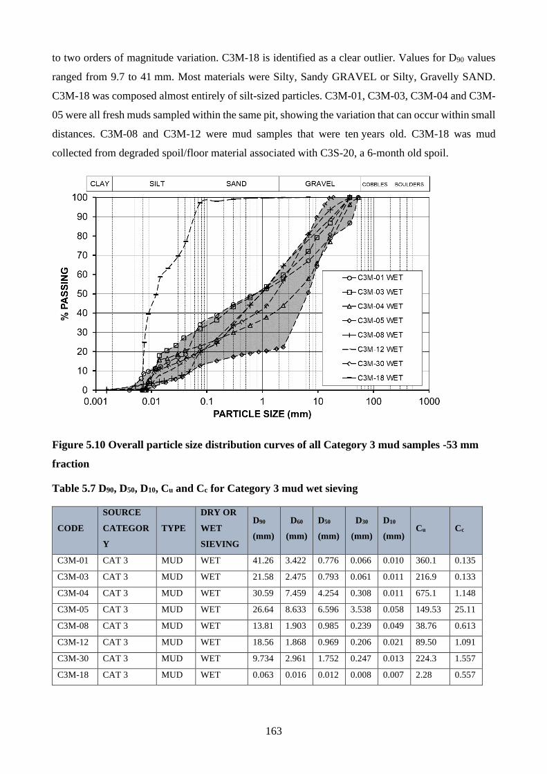
163
to two orders of magnitude variation. C3M-18 is identified as a clear outlier. Values for D90 values
ranged from 9.7 to 41 mm. Most materials were Silty, Sandy GRAVEL or Silty, Gravelly SAND.
C3M-18 was composed almost entirely of silt-sized particles. C3M-01, C3M-03, C3M-04 and C3M-
05 were all fresh muds sampled within the same pit, showing the variation that can occur within small
distances. C3M-08 and C3M-12 were mud samples that were ten years old. C3M-18 was mud
collected from degraded spoil/floor material associated with C3S-20, a 6-month old spoil.
Figure 5.10 Overall particle size distribution curves of all Category 3 mud samples -53 mm
fraction
Table 5.7 D90, D50, D10, Cu and Cc for Category 3 mud wet sieving
CODE
SOURCE
CATEGOR
Y
TYPE
DRY OR
WET
SIEVING
D90
(mm)
D60
(mm)
D50
(mm)
D30
(mm)
D10
(mm) Cu Cc
C3M-01 CAT 3 MUD WET 41.26 3.422 0.776 0.066 0.010 360.1 0.135
C3M-03 CAT 3 MUD WET 21.58 2.475 0.793 0.061 0.011 216.9 0.133
C3M-04 CAT 3 MUD WET 30.59 7.459 4.254 0.308 0.011 675.1 1.148
C3M-05 CAT 3 MUD WET 26.64 8.633 6.596 3.538 0.058 149.53 25.11
C3M-08 CAT 3 MUD WET 13.81 1.903 0.985 0.239 0.049 38.76 0.613
C3M-12 CAT 3 MUD WET 18.56 1.868 0.969 0.206 0.021 89.50 1.091
C3M-30 CAT 3 MUD WET 9.734 2.961 1.752 0.247 0.013 224.3 1.557
C3M-18 CAT 3 MUD WET 0.063 0.016 0.012 0.008 0.007 2.28 0.557
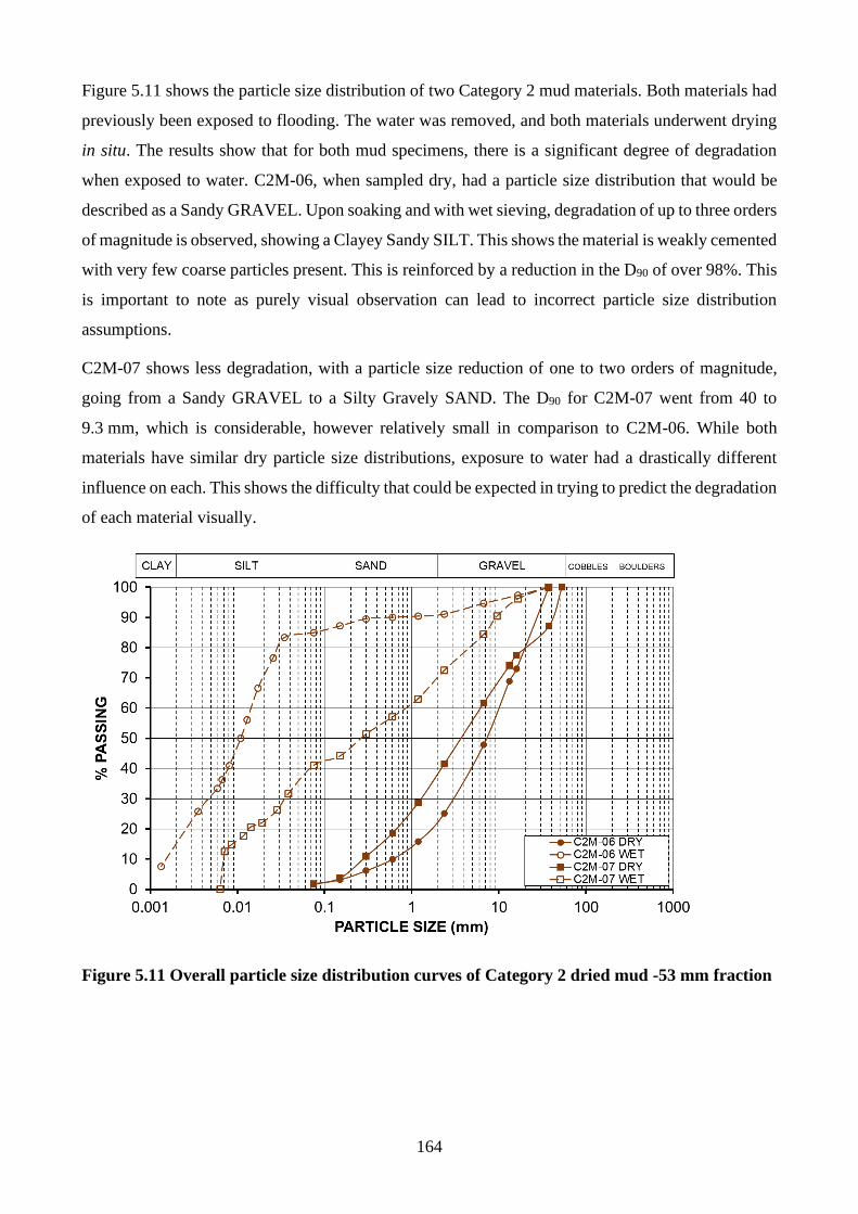
164
Figure 5.11 shows the particle size distribution of two Category 2 mud materials. Both materials had
previously been exposed to flooding. The water was removed, and both materials underwent drying
in situ. The results show that for both mud specimens, there is a significant degree of degradation
when exposed to water. C2M-06, when sampled dry, had a particle size distribution that would be
described as a Sandy GRAVEL. Upon soaking and with wet sieving, degradation of up to three orders
of magnitude is observed, showing a Clayey Sandy SILT. This shows the material is weakly cemented
with very few coarse particles present. This is reinforced by a reduction in the D90 of over 98%. This
is important to note as purely visual observation can lead to incorrect particle size distribution
assumptions.
C2M-07 shows less degradation, with a particle size reduction of one to two orders of magnitude,
going from a Sandy GRAVEL to a Silty Gravely SAND. The D90 for C2M-07 went from 40 to
9.3 mm, which is considerable, however relatively small in comparison to C2M-06. While both
materials have similar dry particle size distributions, exposure to water had a drastically different
influence on each. This shows the difficulty that could be expected in trying to predict the degradation
of each material visually.
Figure 5.11 Overall particle size distribution curves of Category 2 dried mud -53 mm fraction
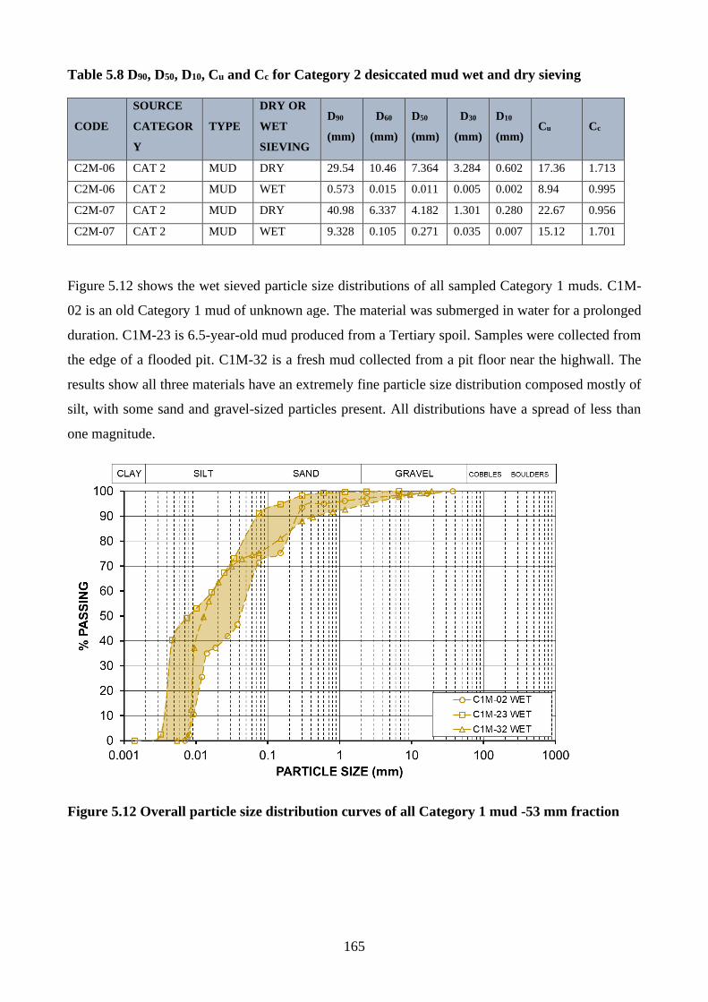
165
Table 5.8 D90, D50, D10, Cu and Cc for Category 2 desiccated mud wet and dry sieving
CODE
SOURCE
CATEGOR
Y
TYPE
DRY OR
WET
SIEVING
D90
(mm)
D60
(mm)
D50
(mm)
D30
(mm)
D10
(mm) Cu Cc
C2M-06 CAT 2 MUD DRY 29.54 10.46 7.364 3.284 0.602 17.36 1.713
C2M-06 CAT 2 MUD WET 0.573 0.015 0.011 0.005 0.002 8.94 0.995
C2M-07 CAT 2 MUD DRY 40.98 6.337 4.182 1.301 0.280 22.67 0.956
C2M-07 CAT 2 MUD WET 9.328 0.105 0.271 0.035 0.007 15.12 1.701
Figure 5.12 shows the wet sieved particle size distributions of all sampled Category 1 muds. C1M-
02 is an old Category 1 mud of unknown age. The material was submerged in water for a prolonged
duration. C1M-23 is 6.5-year-old mud produced from a Tertiary spoil. Samples were collected from
the edge of a flooded pit. C1M-32 is a fresh mud collected from a pit floor near the highwall. The
results show all three materials have an extremely fine particle size distribution composed mostly of
silt, with some sand and gravel-sized particles present. All distributions have a spread of less than
one magnitude.
Figure 5.12 Overall particle size distribution curves of all Category 1 mud -53 mm fraction
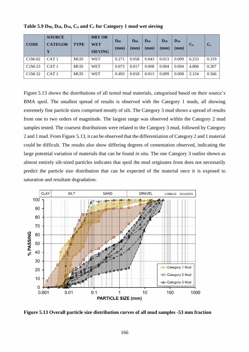
166
Table 5.9 D90, D50, D10, Cu and Cc for Category 1 mud wet sieving
CODE
SOURCE
CATEGOR
Y
TYPE
DRY OR
WET
SIEVING
D90
(mm)
D60
(mm)
D50
(mm)
D30
(mm)
D10
(mm) Cu Cc
C1M-02 CAT 1 MUD WET 0.271 0.058 0.043 0.013 0.009 6.233 0.319
C1M-23 CAT 1 MUD WET 0.073 0.017 0.008 0.004 0.004 4.806 0.307
C1M-32 CAT 1 MUD WET 0.493 0.018 0.013 0.009 0.008 2.154 0.566
Figure 5.13 shows the distributions of all tested mud materials, categorised based on their source’s
BMA spoil. The smallest spread of results is observed with the Category 1 muds, all showing
extremely fine particle sizes comprised mostly of silt. The Category 3 mud shows a spread of results
from one to two orders of magnitude. The largest range was observed within the Category 2 mud
samples tested. The coarsest distributions were related to the Category 3 mud, followed by Category
2 and 1 mud. From Figure 5.13, it can be observed that the differentiation of Category 2 and 1 material
could be difficult. The results also show differing degrees of cementation observed, indicating the
large potential variation of materials that can be found in situ. The one Category 3 outlier shown as
almost entirely silt-sized particles indicates that spoil the mud originates from does not necessarily
predict the particle size distribution that can be expected of the material once it is exposed to
saturation and resultant degradation.
Figure 5.13 Overall particle size distribution curves of all mud samples -53 mm fraction
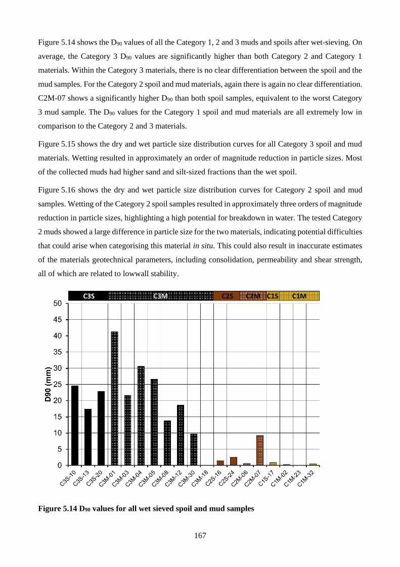
167
Figure 5.14 shows the D90 values of all the Category 1, 2 and 3 muds and spoils after wet-sieving. On
average, the Category 3 D90 values are significantly higher than both Category 2 and Category 1
materials. Within the Category 3 materials, there is no clear differentiation between the spoil and the
mud samples. For the Category 2 spoil and mud materials, again there is again no clear differentiation.
C2M-07 shows a significantly higher D90 than both spoil samples, equivalent to the worst Category
3 mud sample. The D90 values for the Category 1 spoil and mud materials are all extremely low in
comparison to the Category 2 and 3 materials.
Figure 5.15 shows the dry and wet particle size distribution curves for all Category 3 spoil and mud
materials. Wetting resulted in approximately an order of magnitude reduction in particle sizes. Most
of the collected muds had higher sand and silt-sized fractions than the wet spoil.
Figure 5.16 shows the dry and wet particle size distribution curves for Category 2 spoil and mud
samples. Wetting of the Category 2 spoil samples resulted in approximately three orders of magnitude
reduction in particle sizes, highlighting a high potential for breakdown in water. The tested Category
2 muds showed a large difference in particle size for the two materials, indicating potential difficulties
that could arise when categorising this material in situ. This could also result in inaccurate estimates
of the materials geotechnical parameters, including consolidation, permeability and shear strength,
all of which are related to lowwall stability.
Figure 5.14 D90 values for all wet sieved spoil and mud samples
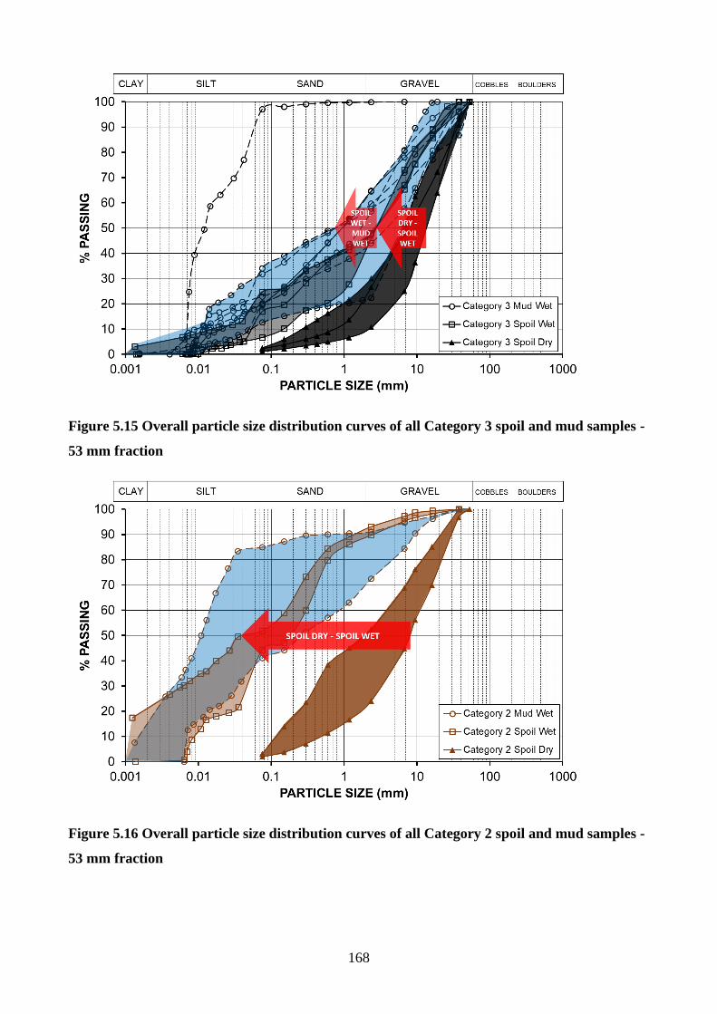
168
Figure 5.15 Overall particle size distribution curves of all Category 3 spoil and mud samples -
53 mm fraction
Figure 5.16 Overall particle size distribution curves of all Category 2 spoil and mud samples -
53 mm fraction
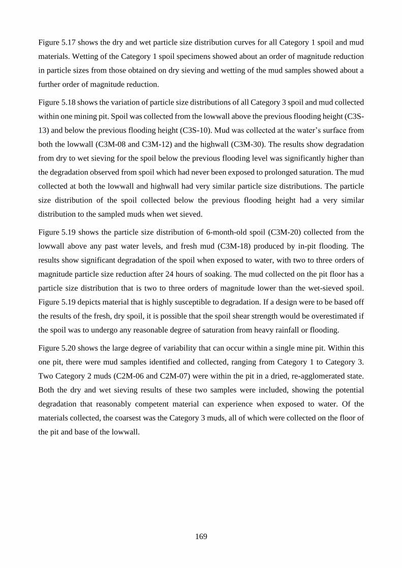
169
Figure 5.17 shows the dry and wet particle size distribution curves for all Category 1 spoil and mud
materials. Wetting of the Category 1 spoil specimens showed about an order of magnitude reduction
in particle sizes from those obtained on dry sieving and wetting of the mud samples showed about a
further order of magnitude reduction.
Figure 5.18 shows the variation of particle size distributions of all Category 3 spoil and mud collected
within one mining pit. Spoil was collected from the lowwall above the previous flooding height (C3S-
13) and below the previous flooding height (C3S-10). Mud was collected at the water’s surface from
both the lowwall (C3M-08 and C3M-12) and the highwall (C3M-30). The results show degradation
from dry to wet sieving for the spoil below the previous flooding level was significantly higher than
the degradation observed from spoil which had never been exposed to prolonged saturation. The mud
collected at both the lowwall and highwall had very similar particle size distributions. The particle
size distribution of the spoil collected below the previous flooding height had a very similar
distribution to the sampled muds when wet sieved.
Figure 5.19 shows the particle size distribution of 6-month-old spoil (C3M-20) collected from the
lowwall above any past water levels, and fresh mud (C3M-18) produced by in-pit flooding. The
results show significant degradation of the spoil when exposed to water, with two to three orders of
magnitude particle size reduction after 24 hours of soaking. The mud collected on the pit floor has a
particle size distribution that is two to three orders of magnitude lower than the wet-sieved spoil.
Figure 5.19 depicts material that is highly susceptible to degradation. If a design were to be based off
the results of the fresh, dry spoil, it is possible that the spoil shear strength would be overestimated if
the spoil was to undergo any reasonable degree of saturation from heavy rainfall or flooding.
Figure 5.20 shows the large degree of variability that can occur within a single mine pit. Within this
one pit, there were mud samples identified and collected, ranging from Category 1 to Category 3.
Two Category 2 muds (C2M-06 and C2M-07) were within the pit in a dried, re-agglomerated state.
Both the dry and wet sieving results of these two samples were included, showing the potential
degradation that reasonably competent material can experience when exposed to water. Of the
materials collected, the coarsest was the Category 3 muds, all of which were collected on the floor of
the pit and base of the lowwall.
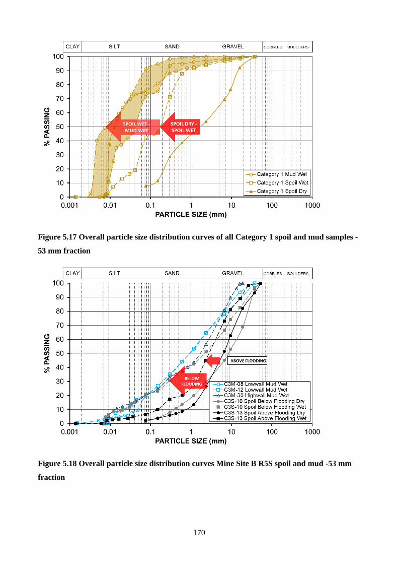
170
Figure 5.17 Overall particle size distribution curves of all Category 1 spoil and mud samples -
53 mm fraction
Figure 5.18 Overall particle size distribution curves Mine Site B R5S spoil and mud -53 mm
fraction
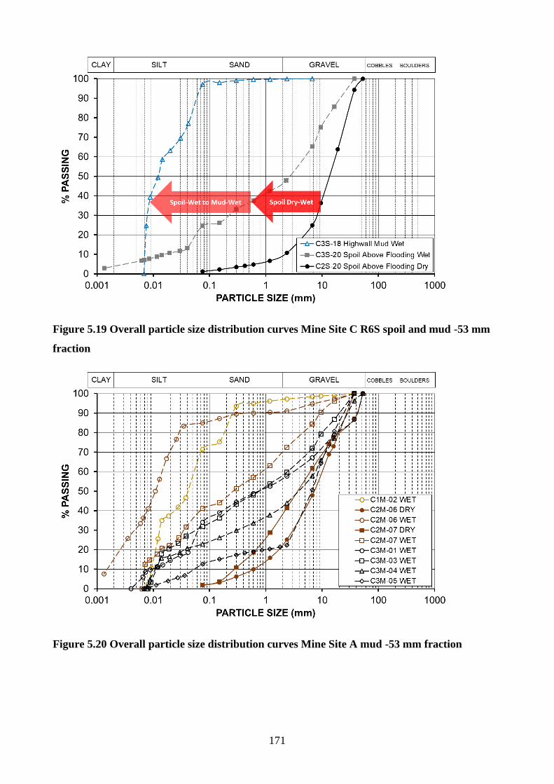
171
Figure 5.19 Overall particle size distribution curves Mine Site C R6S spoil and mud -53 mm
fraction
Figure 5.20 Overall particle size distribution curves Mine Site A mud -53 mm fraction
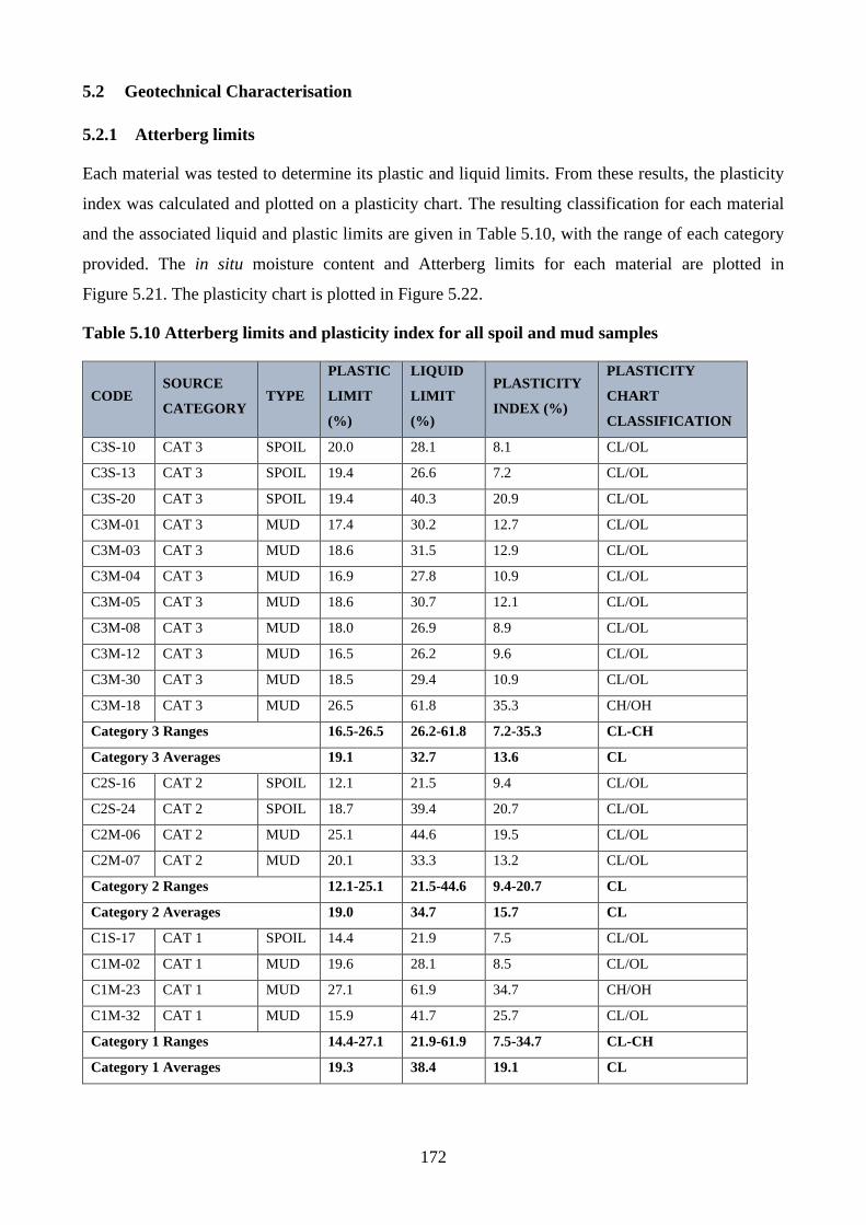
172
5.2 Geotechnical Characterisation
5.2.1 Atterberg limits
Each material was tested to determine its plastic and liquid limits. From these results, the plasticity
index was calculated and plotted on a plasticity chart. The resulting classification for each material
and the associated liquid and plastic limits are given in Table 5.10, with the range of each category
provided. The in situ moisture content and Atterberg limits for each material are plotted in
Figure 5.21. The plasticity chart is plotted in Figure 5.22.
Table 5.10 Atterberg limits and plasticity index for all spoil and mud samples
CODE SOURCE
CATEGORY TYPE
PLASTIC
LIMIT
(%)
LIQUID
LIMIT
(%)
PLASTICITY
INDEX (%)
PLASTICITY
CHART
CLASSIFICATION
C3S-10 CAT 3 SPOIL 20.0 28.1 8.1 CL/OL
C3S-13 CAT 3 SPOIL 19.4 26.6 7.2 CL/OL
C3S-20 CAT 3 SPOIL 19.4 40.3 20.9 CL/OL
C3M-01 CAT 3 MUD 17.4 30.2 12.7 CL/OL
C3M-03 CAT 3 MUD 18.6 31.5 12.9 CL/OL
C3M-04 CAT 3 MUD 16.9 27.8 10.9 CL/OL
C3M-05 CAT 3 MUD 18.6 30.7 12.1 CL/OL
C3M-08 CAT 3 MUD 18.0 26.9 8.9 CL/OL
C3M-12 CAT 3 MUD 16.5 26.2 9.6 CL/OL
C3M-30 CAT 3 MUD 18.5 29.4 10.9 CL/OL
C3M-18 CAT 3 MUD 26.5 61.8 35.3 CH/OH
Category 3 Ranges 16.5-26.5 26.2-61.8 7.2-35.3 CL-CH
Category 3 Averages 19.1 32.7 13.6 CL
C2S-16 CAT 2 SPOIL 12.1 21.5 9.4 CL/OL
C2S-24 CAT 2 SPOIL 18.7 39.4 20.7 CL/OL
C2M-06 CAT 2 MUD 25.1 44.6 19.5 CL/OL
C2M-07 CAT 2 MUD 20.1 33.3 13.2 CL/OL
Category 2 Ranges 12.1-25.1 21.5-44.6 9.4-20.7 CL
Category 2 Averages 19.0 34.7 15.7 CL
C1S-17 CAT 1 SPOIL 14.4 21.9 7.5 CL/OL
C1M-02 CAT 1 MUD 19.6 28.1 8.5 CL/OL
C1M-23 CAT 1 MUD 27.1 61.9 34.7 CH/OH
C1M-32 CAT 1 MUD 15.9 41.7 25.7 CL/OL
Category 1 Ranges 14.4-27.1 21.9-61.9 7.5-34.7 CL-CH
Category 1 Averages 19.3 38.4 19.1 CL
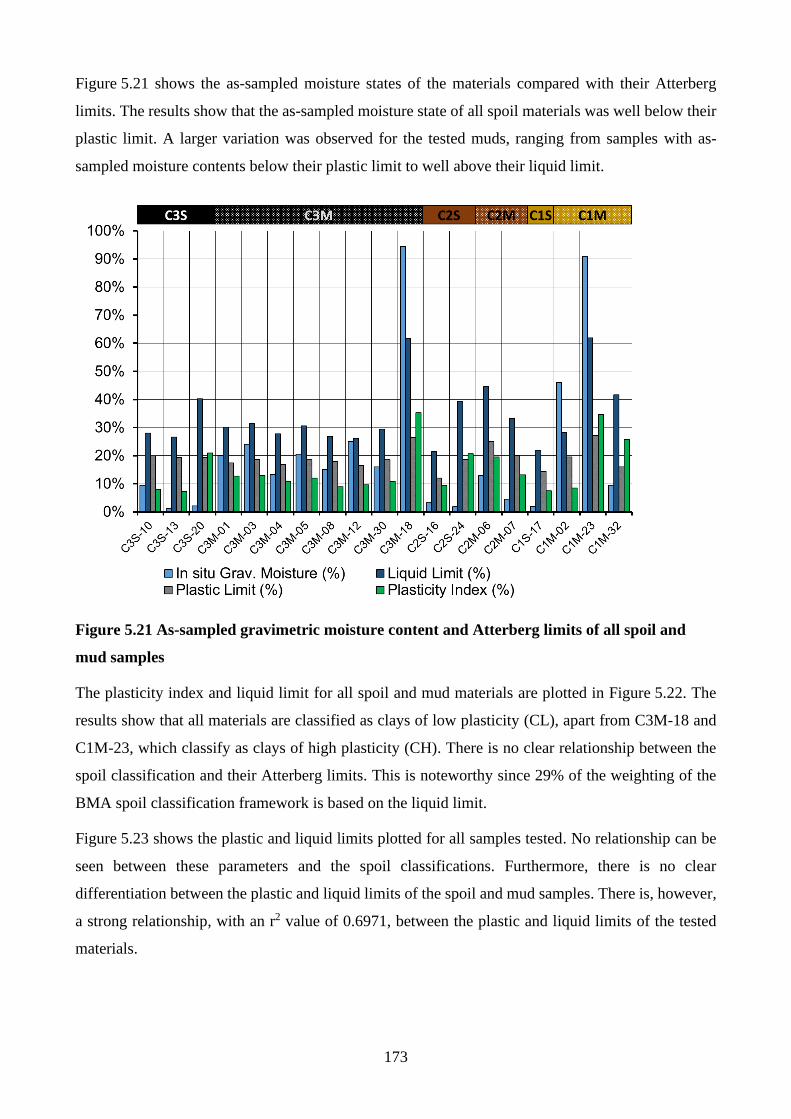
173
Figure 5.21 shows the as-sampled moisture states of the materials compared with their Atterberg
limits. The results show that the as-sampled moisture state of all spoil materials was well below their
plastic limit. A larger variation was observed for the tested muds, ranging from samples with as-
sampled moisture contents below their plastic limit to well above their liquid limit.
Figure 5.21 As-sampled gravimetric moisture content and Atterberg limits of all spoil and
mud samples
The plasticity index and liquid limit for all spoil and mud materials are plotted in Figure 5.22. The
results show that all materials are classified as clays of low plasticity (CL), apart from C3M-18 and
C1M-23, which classify as clays of high plasticity (CH). There is no clear relationship between the
spoil classification and their Atterberg limits. This is noteworthy since 29% of the weighting of the
BMA spoil classification framework is based on the liquid limit.
Figure 5.23 shows the plastic and liquid limits plotted for all samples tested. No relationship can be
seen between these parameters and the spoil classifications. Furthermore, there is no clear
differentiation between the plastic and liquid limits of the spoil and mud samples. There is, however,
a strong relationship, with an r2 value of 0.6971, between the plastic and liquid limits of the tested
materials.
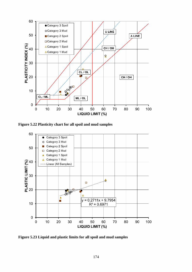
174
Figure 5.22 Plasticity chart for all spoil and mud samples
Figure 5.23 Liquid and plastic limits for all spoil and mud samples
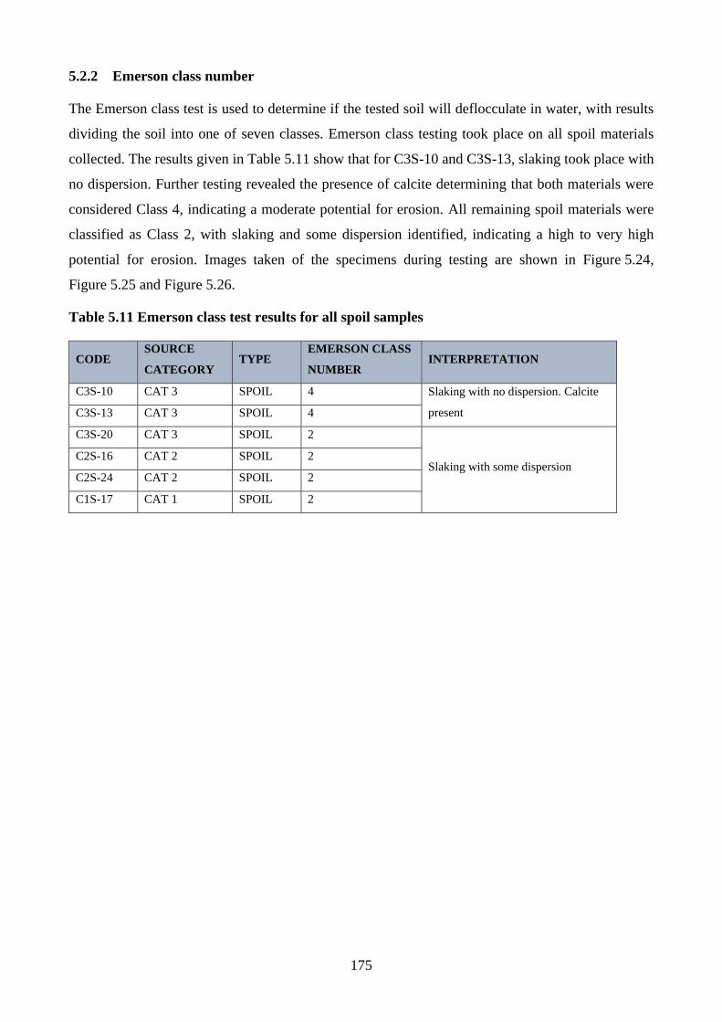
175
5.2.2 Emerson class number
The Emerson class test is used to determine if the tested soil will deflocculate in water, with results
dividing the soil into one of seven classes. Emerson class testing took place on all spoil materials
collected. The results given in Table 5.11 show that for C3S-10 and C3S-13, slaking took place with
no dispersion. Further testing revealed the presence of calcite determining that both materials were
considered Class 4, indicating a moderate potential for erosion. All remaining spoil materials were
classified as Class 2, with slaking and some dispersion identified, indicating a high to very high
potential for erosion. Images taken of the specimens during testing are shown in Figure 5.24,
Figure 5.25 and Figure 5.26.
Table 5.11 Emerson class test results for all spoil samples
CODE SOURCE
CATEGORY TYPE
EMERSON CLASS
NUMBER INTERPRETATION
C3S-10 CAT 3 SPOIL 4 Slaking with no dispersion. Calcite
present C3S-13 CAT 3 SPOIL 4
C3S-20 CAT 3 SPOIL 2
Slaking with some dispersion C2S-16 CAT 2 SPOIL 2
C2S-24 CAT 2 SPOIL 2
C1S-17 CAT 1 SPOIL 2
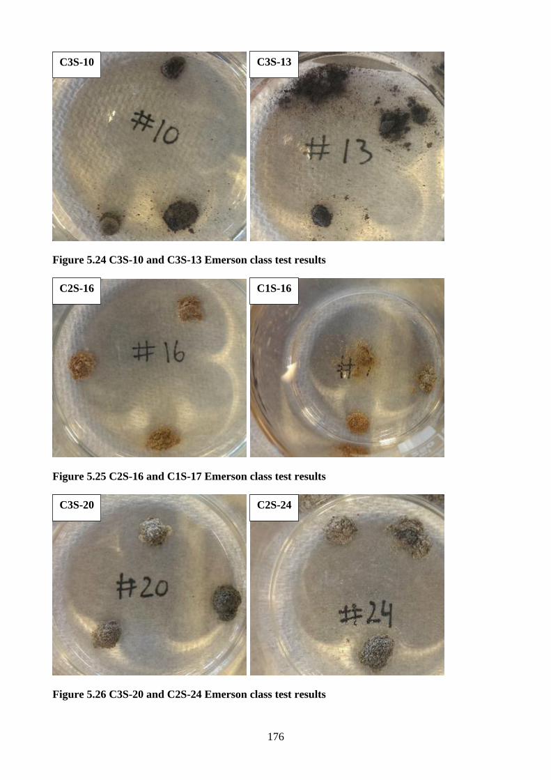
176
Figure 5.24 C3S-10 and C3S-13 Emerson class test results
Figure 5.25 C2S-16 and C1S-17 Emerson class test results
Figure 5.26 C3S-20 and C2S-24 Emerson class test results
C3S-10
C1S-16 C2S-16
C3S-13
C3S-20 C2S-24
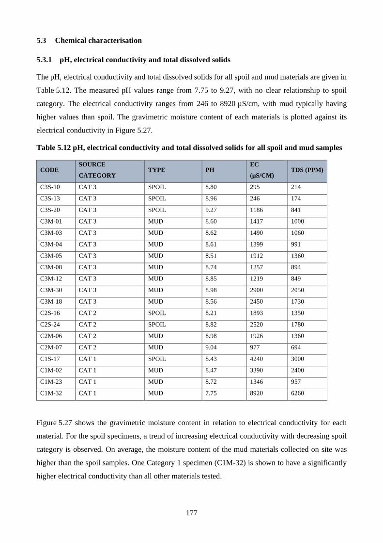
177
5.3 Chemical characterisation
5.3.1 pH, electrical conductivity and total dissolved solids
The pH, electrical conductivity and total dissolved solids for all spoil and mud materials are given in
Table 5.12. The measured pH values range from 7.75 to 9.27, with no clear relationship to spoil
category. The electrical conductivity ranges from 246 to 8920 µS/cm, with mud typically having
higher values than spoil. The gravimetric moisture content of each materials is plotted against its
electrical conductivity in Figure 5.27.
Table 5.12 pH, electrical conductivity and total dissolved solids for all spoil and mud samples
CODE SOURCE
CATEGORY TYPE PH
EC
(µS/CM) TDS (PPM)
C3S-10 CAT 3 SPOIL 8.80 295 214
C3S-13 CAT 3 SPOIL 8.96 246 174
C3S-20 CAT 3 SPOIL 9.27 1186 841
C3M-01 CAT 3 MUD 8.60 1417 1000
C3M-03 CAT 3 MUD 8.62 1490 1060
C3M-04 CAT 3 MUD 8.61 1399 991
C3M-05 CAT 3 MUD 8.51 1912 1360
C3M-08 CAT 3 MUD 8.74 1257 894
C3M-12 CAT 3 MUD 8.85 1219 849
C3M-30 CAT 3 MUD 8.98 2900 2050
C3M-18 CAT 3 MUD 8.56 2450 1730
C2S-16 CAT 2 SPOIL 8.21 1893 1350
C2S-24 CAT 2 SPOIL 8.82 2520 1780
C2M-06 CAT 2 MUD 8.98 1926 1360
C2M-07 CAT 2 MUD 9.04 977 694
C1S-17 CAT 1 SPOIL 8.43 4240 3000
C1M-02 CAT 1 MUD 8.47 3390 2400
C1M-23 CAT 1 MUD 8.72 1346 957
C1M-32 CAT 1 MUD 7.75 8920 6260
Figure 5.27 shows the gravimetric moisture content in relation to electrical conductivity for each
material. For the spoil specimens, a trend of increasing electrical conductivity with decreasing spoil
category is observed. On average, the moisture content of the mud materials collected on site was
higher than the spoil samples. One Category 1 specimen (C1M-32) is shown to have a significantly
higher electrical conductivity than all other materials tested.
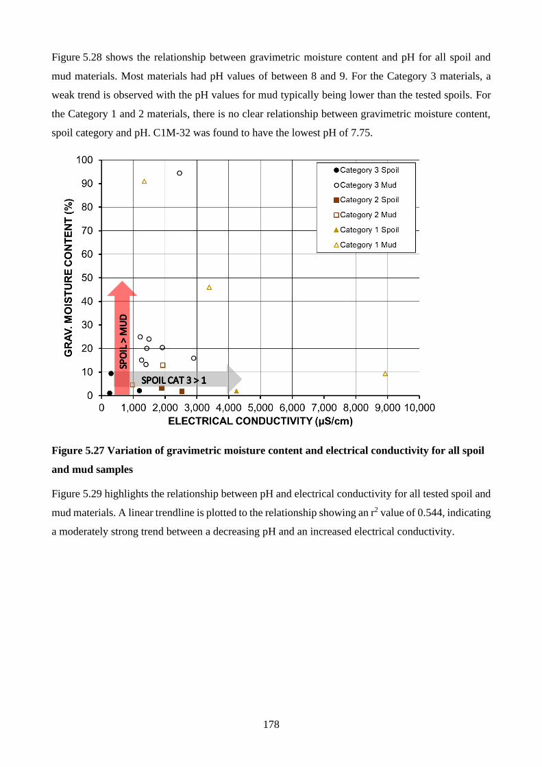
178
Figure 5.28 shows the relationship between gravimetric moisture content and pH for all spoil and
mud materials. Most materials had pH values of between 8 and 9. For the Category 3 materials, a
weak trend is observed with the pH values for mud typically being lower than the tested spoils. For
the Category 1 and 2 materials, there is no clear relationship between gravimetric moisture content,
spoil category and pH. C1M-32 was found to have the lowest pH of 7.75.
Figure 5.27 Variation of gravimetric moisture content and electrical conductivity for all spoil
and mud samples
Figure 5.29 highlights the relationship between pH and electrical conductivity for all tested spoil and
mud materials. A linear trendline is plotted to the relationship showing an r2 value of 0.544, indicating
a moderately strong trend between a decreasing pH and an increased electrical conductivity.
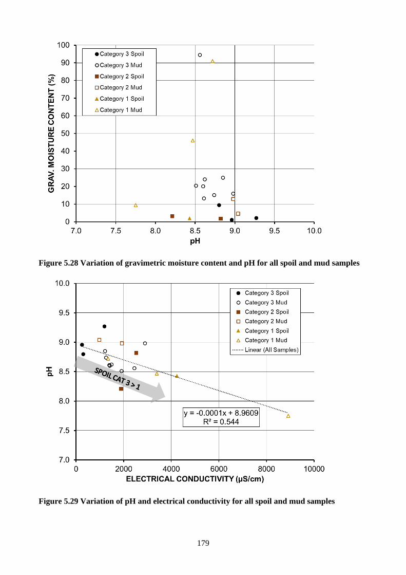
179
Figure 5.28 Variation of gravimetric moisture content and pH for all spoil and mud samples
Figure 5.29 Variation of pH and electrical conductivity for all spoil and mud samples
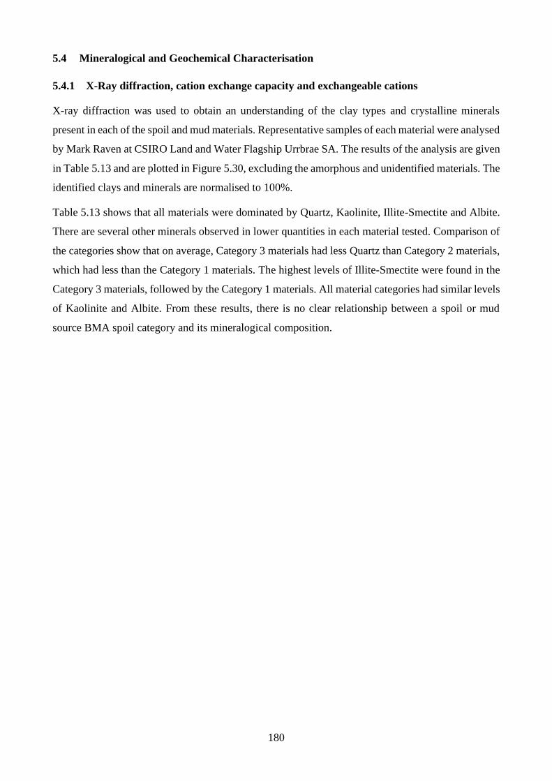
180
5.4 Mineralogical and Geochemical Characterisation
5.4.1 X-Ray diffraction, cation exchange capacity and exchangeable cations
X-ray diffraction was used to obtain an understanding of the clay types and crystalline minerals
present in each of the spoil and mud materials. Representative samples of each material were analysed
by Mark Raven at CSIRO Land and Water Flagship Urrbrae SA. The results of the analysis are given
in Table 5.13 and are plotted in Figure 5.30, excluding the amorphous and unidentified materials. The
identified clays and minerals are normalised to 100%.
Table 5.13 shows that all materials were dominated by Quartz, Kaolinite, Illite-Smectite and Albite.
There are several other minerals observed in lower quantities in each material tested. Comparison of
the categories show that on average, Category 3 materials had less Quartz than Category 2 materials,
which had less than the Category 1 materials. The highest levels of Illite-Smectite were found in the
Category 3 materials, followed by the Category 1 materials. All material categories had similar levels
of Kaolinite and Albite. From these results, there is no clear relationship between a spoil or mud
source BMA spoil category and its mineralogical composition.
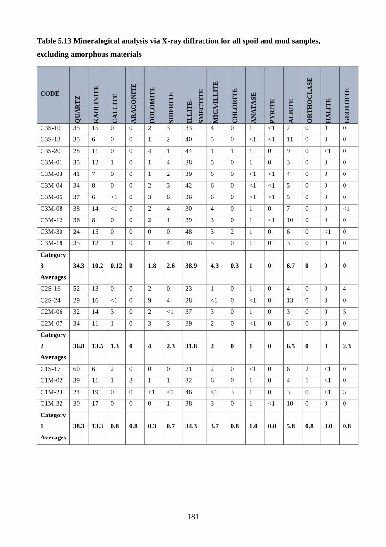
181
Table 5.13 Mineralogical analysis via X-ray diffraction for all spoil and mud samples,
excluding amorphous materials
CODE
QU
AR
TZ
KA
OL
INIT
E
CA
LC
ITE
AR
AG
ON
ITE
DO
LO
MIT
E
SID
ER
ITE
ILL
ITE
-
SM
EC
TIT
E
MIC
A/I
LL
ITE
CH
LO
RIT
E
AN
AT
AS
E
PY
RIT
E
AL
BIT
E
OR
TH
OC
LA
SE
HA
LIT
E
GE
OT
HIT
E
C3S-10 35 15 0 0 2 3 33 4 0 1 <1 7 0 0 0
C3S-13 35 6 0 0 1 2 40 5 0 <1 <1 11 0 0 0
C3S-20 28 11 0 0 4 1 44 1 1 1 0 9 0 <1 0
C3M-01 35 12 1 0 1 4 38 5 0 1 0 3 0 0 0
C3M-03 41 7 0 0 1 2 39 6 0 <1 <1 4 0 0 0
C3M-04 34 8 0 0 2 3 42 6 0 <1 <1 5 0 0 0
C3M-05 37 6 <1 0 3 6 36 6 0 <1 <1 5 0 0 0
C3M-08 38 14 <1 0 2 4 30 4 0 1 0 7 0 0 <1
C3M-12 36 8 0 0 2 1 39 3 0 1 <1 10 0 0 0
C3M-30 24 15 0 0 0 0 48 3 2 1 0 6 0 <1 0
C3M-18 35 12 1 0 1 4 38 5 0 1 0 3 0 0 0
Category
3
Averages
34.3 10.2 0.12 0 1.8 2.6 38.9 4.3 0.3 1 0 6.7 0 0 0
C2S-16 52 13 0 0 2 0 23 1 0 1 0 4 0 0 4
C2S-24 29 16 <1 0 9 4 28 <1 0 <1 0 13 0 0 0
C2M-06 32 14 3 0 2 <1 37 3 0 1 0 3 0 0 5
C2M-07 34 11 1 0 3 3 39 2 0 <1 0 6 0 0 0
Category
2
Averages
36.8 13.5 1.3 0 4 2.3 31.8 2 0 1 0 6.5 0 0 2.3
C1S-17 60 6 2 0 0 0 21 2 0 <1 0 6 2 <1 0
C1M-02 39 11 1 3 1 1 32 6 0 1 0 4 1 <1 0
C1M-23 24 19 0 0 <1 <1 46 <1 3 1 0 3 0 <1 3
C1M-32 30 17 0 0 0 1 38 3 0 1 <1 10 0 0 0
Category
1
Averages
38.3 13.3 0.8 0.8 0.3 0.7 34.3 3.7 0.8 1.0 0.0 5.8 0.8 0.0 0.8
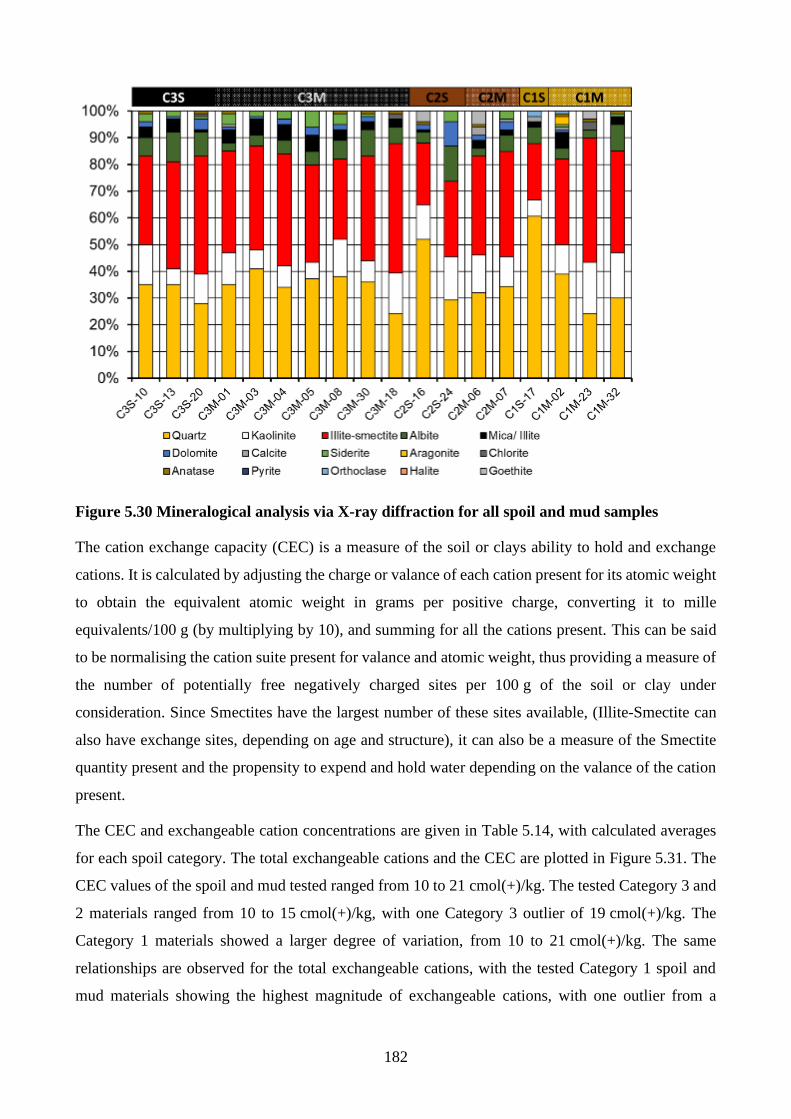
182
Figure 5.30 Mineralogical analysis via X-ray diffraction for all spoil and mud samples
The cation exchange capacity (CEC) is a measure of the soil or clays ability to hold and exchange
cations. It is calculated by adjusting the charge or valance of each cation present for its atomic weight
to obtain the equivalent atomic weight in grams per positive charge, converting it to mille
equivalents/100 g (by multiplying by 10), and summing for all the cations present. This can be said
to be normalising the cation suite present for valance and atomic weight, thus providing a measure of
the number of potentially free negatively charged sites per 100 g of the soil or clay under
consideration. Since Smectites have the largest number of these sites available, (Illite-Smectite can
also have exchange sites, depending on age and structure), it can also be a measure of the Smectite
quantity present and the propensity to expend and hold water depending on the valance of the cation
present.
The CEC and exchangeable cation concentrations are given in Table 5.14, with calculated averages
for each spoil category. The total exchangeable cations and the CEC are plotted in Figure 5.31. The
CEC values of the spoil and mud tested ranged from 10 to 21 cmol(+)/kg. The tested Category 3 and
2 materials ranged from 10 to 15 cmol(+)/kg, with one Category 3 outlier of 19 cmol(+)/kg. The
Category 1 materials showed a larger degree of variation, from 10 to 21 cmol(+)/kg. The same
relationships are observed for the total exchangeable cations, with the tested Category 1 spoil and
mud materials showing the highest magnitude of exchangeable cations, with one outlier from a
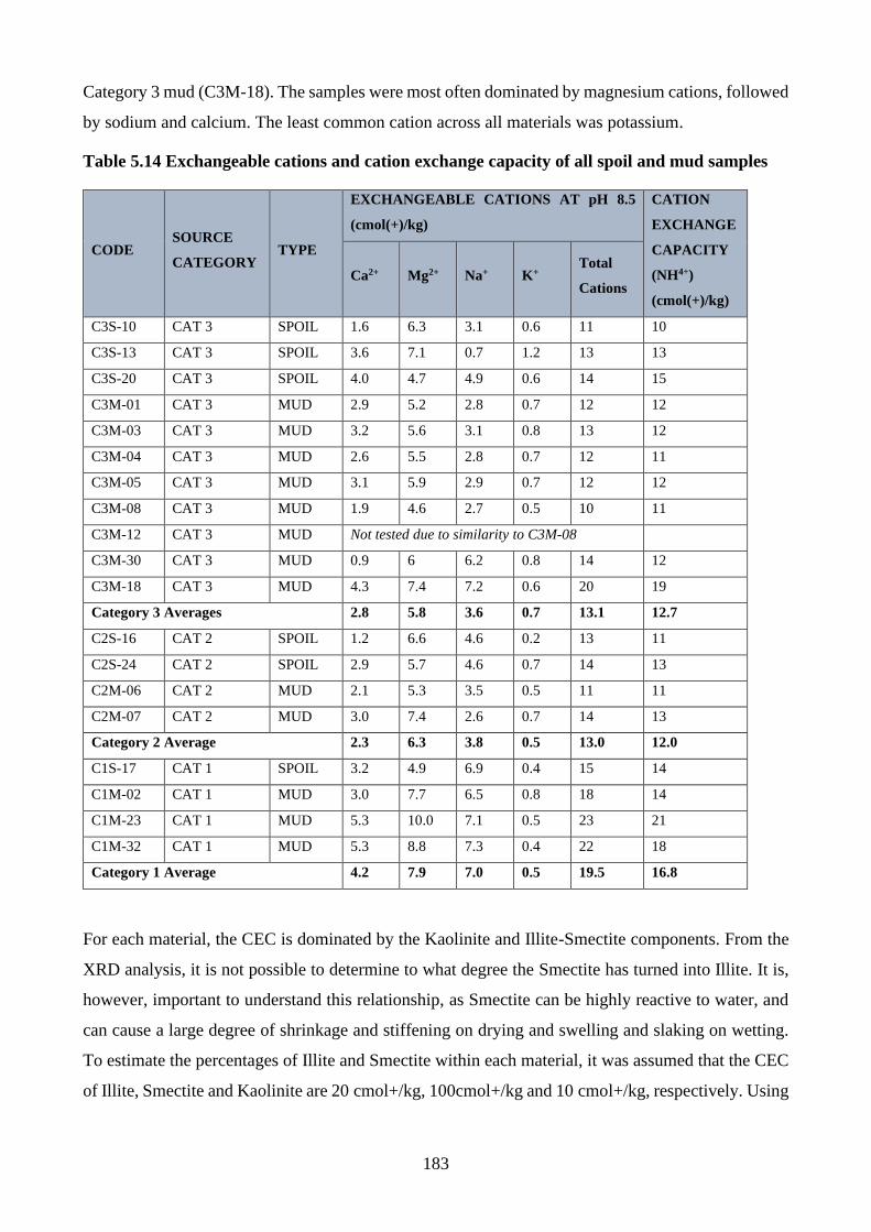
183
Category 3 mud (C3M-18). The samples were most often dominated by magnesium cations, followed
by sodium and calcium. The least common cation across all materials was potassium.
Table 5.14 Exchangeable cations and cation exchange capacity of all spoil and mud samples
CODE SOURCE
CATEGORY TYPE
EXCHANGEABLE CATIONS AT pH 8.5
(cmol(+)/kg)
CATION
EXCHANGE
CAPACITY
(NH4+)
(cmol(+)/kg)
Ca2+ Mg2+ Na+ K+ Total
Cations
C3S-10 CAT 3 SPOIL 1.6 6.3 3.1 0.6 11 10
C3S-13 CAT 3 SPOIL 3.6 7.1 0.7 1.2 13 13
C3S-20 CAT 3 SPOIL 4.0 4.7 4.9 0.6 14 15
C3M-01 CAT 3 MUD 2.9 5.2 2.8 0.7 12 12
C3M-03 CAT 3 MUD 3.2 5.6 3.1 0.8 13 12
C3M-04 CAT 3 MUD 2.6 5.5 2.8 0.7 12 11
C3M-05 CAT 3 MUD 3.1 5.9 2.9 0.7 12 12
C3M-08 CAT 3 MUD 1.9 4.6 2.7 0.5 10 11
C3M-12 CAT 3 MUD Not tested due to similarity to C3M-08
C3M-30 CAT 3 MUD 0.9 6 6.2 0.8 14 12
C3M-18 CAT 3 MUD 4.3 7.4 7.2 0.6 20 19
Category 3 Averages 2.8 5.8 3.6 0.7 13.1 12.7
C2S-16 CAT 2 SPOIL 1.2 6.6 4.6 0.2 13 11
C2S-24 CAT 2 SPOIL 2.9 5.7 4.6 0.7 14 13
C2M-06 CAT 2 MUD 2.1 5.3 3.5 0.5 11 11
C2M-07 CAT 2 MUD 3.0 7.4 2.6 0.7 14 13
Category 2 Average 2.3 6.3 3.8 0.5 13.0 12.0
C1S-17 CAT 1 SPOIL 3.2 4.9 6.9 0.4 15 14
C1M-02 CAT 1 MUD 3.0 7.7 6.5 0.8 18 14
C1M-23 CAT 1 MUD 5.3 10.0 7.1 0.5 23 21
C1M-32 CAT 1 MUD 5.3 8.8 7.3 0.4 22 18
Category 1 Average 4.2 7.9 7.0 0.5 19.5 16.8
For each material, the CEC is dominated by the Kaolinite and Illite-Smectite components. From the
XRD analysis, it is not possible to determine to what degree the Smectite has turned into Illite. It is,
however, important to understand this relationship, as Smectite can be highly reactive to water, and
can cause a large degree of shrinkage and stiffening on drying and swelling and slaking on wetting.
To estimate the percentages of Illite and Smectite within each material, it was assumed that the CEC
of Illite, Smectite and Kaolinite are 20 cmol+/kg, 100cmol+/kg and 10 cmol+/kg, respectively. Using
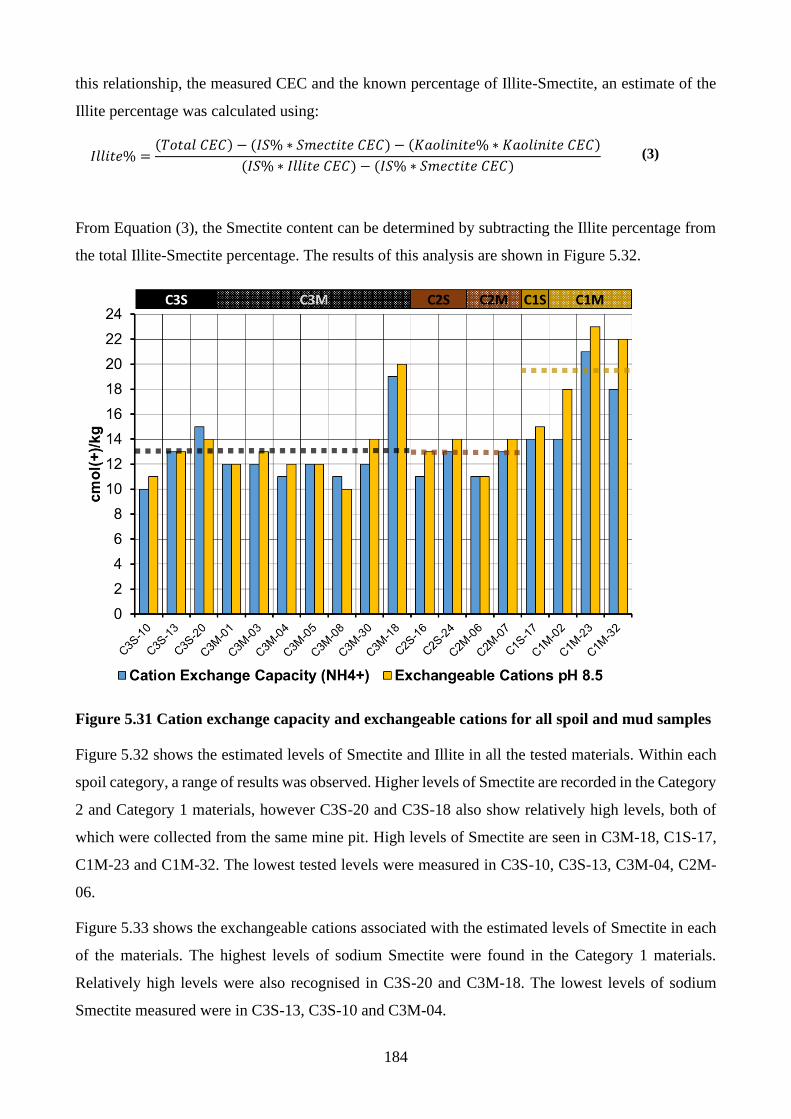
184
this relationship, the measured CEC and the known percentage of Illite-Smectite, an estimate of the
Illite percentage was calculated using:
𝐼𝑙𝑙𝑖𝑡𝑒% =(𝑇𝑜𝑡𝑎𝑙 𝐶𝐸𝐶) − (𝐼𝑆% ∗ 𝑆𝑚𝑒𝑐𝑡𝑖𝑡𝑒 𝐶𝐸𝐶) − (𝐾𝑎𝑜𝑙𝑖𝑛𝑖𝑡𝑒% ∗ 𝐾𝑎𝑜𝑙𝑖𝑛𝑖𝑡𝑒 𝐶𝐸𝐶)
(𝐼𝑆% ∗ 𝐼𝑙𝑙𝑖𝑡𝑒 𝐶𝐸𝐶) − (𝐼𝑆% ∗ 𝑆𝑚𝑒𝑐𝑡𝑖𝑡𝑒 𝐶𝐸𝐶) (3)
From Equation (3), the Smectite content can be determined by subtracting the Illite percentage from
the total Illite-Smectite percentage. The results of this analysis are shown in Figure 5.32.
Figure 5.31 Cation exchange capacity and exchangeable cations for all spoil and mud samples
Figure 5.32 shows the estimated levels of Smectite and Illite in all the tested materials. Within each
spoil category, a range of results was observed. Higher levels of Smectite are recorded in the Category
2 and Category 1 materials, however C3S-20 and C3S-18 also show relatively high levels, both of
which were collected from the same mine pit. High levels of Smectite are seen in C3M-18, C1S-17,
C1M-23 and C1M-32. The lowest tested levels were measured in C3S-10, C3S-13, C3M-04, C2M-
06.
Figure 5.33 shows the exchangeable cations associated with the estimated levels of Smectite in each
of the materials. The highest levels of sodium Smectite were found in the Category 1 materials.
Relatively high levels were also recognised in C3S-20 and C3M-18. The lowest levels of sodium
Smectite measured were in C3S-13, C3S-10 and C3M-04.
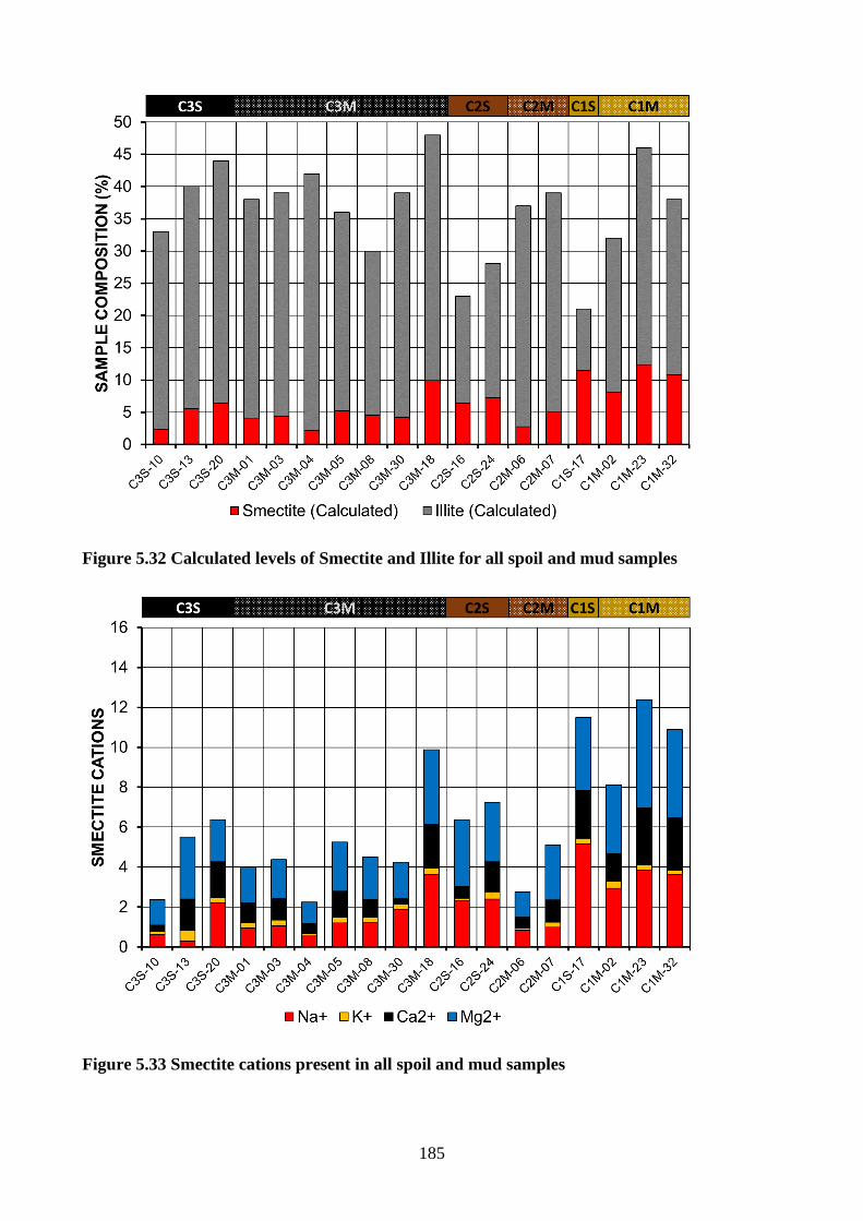
185
Figure 5.32 Calculated levels of Smectite and Illite for all spoil and mud samples
Figure 5.33 Smectite cations present in all spoil and mud samples
186
5.5 Material Characterisation Test Conclusions
An extensive material characterisation testing program of the collected spoil and mud materials was
conducted, investigating numerous physical, chemical, mineralogical and geochemical parameters.
The analysis of these results was related to the source BMA spoil category to determine its
applicability, limitations, and potential improvements for categorisation of in situ spoil and mud.
Each sampled material was tested for its as-sampled gravimetric moisture content. The results show
that spoil above any previous flooding levels had very low moisture contents, ranging from 1.1 to
3.3%, associated with no recent rainfall. Spoil collected from below a previous flooding level just
below the surface had a higher moisture content; however, it was still below the materials plastic
limit. These results highlight spoil’s ability to retain moisture below the surface, even when visually
the conditions appear dry. This indicates that once a spoil pile is inundated with water, it may not
readily drain. This is significant for the modelling of lowwalls with respect to consideration of
appropriate strength mobilisation modes, and where to apply saturated or unsaturated material
parameters.
Large variability in as-sampled moisture content was observed for the mud samples, ranging from
below their plastic limits to well above their liquid limits. For both the spoil and the mud samples,
there was no clear relationship between the spoil category and as-sampled moisture content, with
results largely influenced by the sampling locations and weather conditions.
The specific gravity of each spoil sample was determined, showing a range from 2.2 to 2.7, with the
majority between 2.4 and 2.6. Low specific gravities were associated with materials that were
observed to have trace amounts of carbonaceous material. There was no clear relationship between
specific gravity and the spoil category.
Each of the sampled spoils had their total suction calculated. For spoil collected above any previous
flooding levels, values ranged between 44 MPa and 68 MPa. For C3M-10, a spoil collected below a
previous flooding level, an average total suction of 0.7 MPa was recorded. There was no relationship
between the spoil category and the total suction, with results reflective of the materials history post-
excavation.
For all spoil materials sampled, and dried mud samples, dry sieving was conducted to determine the
materials in situ particle size distribution scalped at -53 mm. A clear distinction between the spoil
categories was identified, with the representative Category 3 spoil specimens being the coarsest,
followed by the Category 2 spoil, and lastly the Category 1. These results are clearly reflected in the
D90 results graphed in Figure 5.8 for the spoil, and Figure 5.14 for the mud. Wet sieving of the
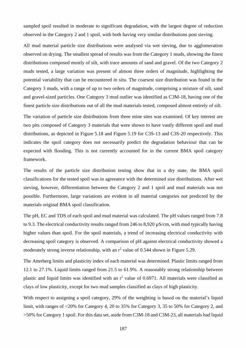
187
sampled spoil resulted in moderate to significant degradation, with the largest degree of reduction
observed in the Category 2 and 1 spoil, with both having very similar distributions post sieving.
All mud material particle size distributions were analysed via wet sieving, due to agglomeration
observed on drying. The smallest spread of results was from the Category 1 muds, showing the finest
distributions composed mostly of silt, with trace amounts of sand and gravel. Of the two Category 2
muds tested, a large variation was present of almost three orders of magnitude, highlighting the
potential variability that can be encountered in situ. The coarsest size distribution was found in the
Category 3 muds, with a range of up to two orders of magnitude, comprising a mixture of silt, sand
and gravel-sized particles. One Category 3 mud outlier was identified as C3M-18, having one of the
finest particle size distributions out of all the mud materials tested, composed almost entirely of silt.
The variation of particle size distributions from three mine sites was examined. Of key interest are
two pits composed of Category 3 materials that were shown to have vastly different spoil and mud
distributions, as depicted in Figure 5.18 and Figure 5.19 for C3S-13 and C3S-20 respectively. This
indicates the spoil category does not necessarily predict the degradation behaviour that can be
expected with flooding. This is not currently accounted for in the current BMA spoil category
framework.
The results of the particle size distribution testing show that in a dry state, the BMA spoil
classifications for the tested spoil was in agreeance with the determined size distributions. After wet
sieving, however, differentiation between the Category 2 and 1 spoil and mud materials was not
possible. Furthermore, large variations are evident in all material categories not predicted by the
materials original BMA spoil classification.
The pH, EC and TDS of each spoil and mud material was calculated. The pH values ranged from 7.8
to 9.3. The electrical conductivity results ranged from 246 to 8,920 µS/cm, with mud typically having
higher values than spoil. For the spoil materials, a trend of increasing electrical conductivity with
decreasing spoil category is observed. A comparison of pH against electrical conductivity showed a
moderately strong inverse relationship, with an r2 value of 0.544 shown in Figure 5.29.
The Atterberg limits and plasticity index of each material was determined. Plastic limits ranged from
12.1 to 27.1%. Liquid limits ranged from 21.5 to 61.9%. A reasonably strong relationship between
plastic and liquid limits was identified with an r2 value of 0.6971. All materials were classified as
clays of low plasticity, except for two mud samples classified as clays of high plasticity.
With respect to assigning a spoil category, 29% of the weighting is based on the material’s liquid
limit, with ranges of <20% for Category 4, 20 to 35% for Category 3, 35 to 50% for Category 2, and
>50% for Category 1 spoil. For this data set, aside from C3M-18 and C3M-23, all materials had liquid
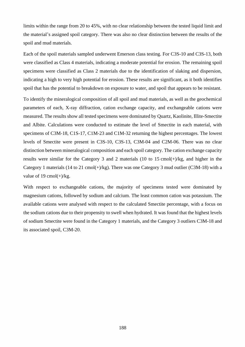
188
limits within the range from 20 to 45%, with no clear relationship between the tested liquid limit and
the material’s assigned spoil category. There was also no clear distinction between the results of the
spoil and mud materials.
Each of the spoil materials sampled underwent Emerson class testing. For C3S-10 and C3S-13, both
were classified as Class 4 materials, indicating a moderate potential for erosion. The remaining spoil
specimens were classified as Class 2 materials due to the identification of slaking and dispersion,
indicating a high to very high potential for erosion. These results are significant, as it both identifies
spoil that has the potential to breakdown on exposure to water, and spoil that appears to be resistant.
To identify the mineralogical composition of all spoil and mud materials, as well as the geochemical
parameters of each, X-ray diffraction, cation exchange capacity, and exchangeable cations were
measured. The results show all tested specimens were dominated by Quartz, Kaolinite, Illite-Smectite
and Albite. Calculations were conducted to estimate the level of Smectite in each material, with
specimens of C3M-18, C1S-17, C1M-23 and C1M-32 returning the highest percentages. The lowest
levels of Smectite were present in C3S-10, C3S-13, C3M-04 and C2M-06. There was no clear
distinction between mineralogical composition and each spoil category. The cation exchange capacity
results were similar for the Category 3 and 2 materials (10 to 15 cmol(+)/kg, and higher in the
Category 1 materials (14 to 21 cmol(+)/kg). There was one Category 3 mud outlier (C3M-18) with a
value of 19 cmol(+)/kg.
With respect to exchangeable cations, the majority of specimens tested were dominated by
magnesium cations, followed by sodium and calcium. The least common cation was potassium. The
available cations were analysed with respect to the calculated Smectite percentage, with a focus on
the sodium cations due to their propensity to swell when hydrated. It was found that the highest levels
of sodium Smectite were found in the Category 1 materials, and the Category 3 outliers C3M-18 and
its associated spoil, C3M-20.
189
6 DEGRADATION TEST RESULTS
To understand how clay mineral-rich spoil degrades to mud in situ, several degradation tests were
conducted. Section 6.1 details the results of testing two Category 3 spoils under different durations
of saturation, and different numbers of wetting and drying cycles. The results from these two sections
were used to determine at what rate these spoil specimens degrade, and to what extent, as well as the
implications this has for clay mineral-rich spoil in situ.
The spoil samples tested were C3S-13, a 10-year old Category 3 spoil, and C3S-20, a 6-month old
Category 3 spoil. The conclusions from the extended saturation and wetting and drying cycles were
then used to conduct a study involving multiple degradation techniques on all spoil materials that had
not been influenced by in-pit flooding prior to sampling. These test results are discussed in
Section 6.2, with comparisons made to each of the spoil’s physical and chemical parameters.
Through identification of material characteristics related to degradation, improvements can be made
with respect to their categorisation, and their handling. The use of a modified slaked durability test to
identify quickly spoil prone to degradation has also been discussed. The spoil materials examined
were C3S-13, C3S-16, C3S-17, C3S-20 and C3S-24.
6.1 Wetting and Drying Cycles, and Prolonged Saturation
The influence of wetting and drying cycles, as well as prolonged saturation, were investigated on two
Category 3 spoils. C3S-13 and C3S-20 were chosen, as a large difference was observed in the mud
that was formed during flooding in situ, and through the results of wet sieving after 24 hours, as
discussed in Section 1425.1.4. For both materials, several representative 1.5 kg specimens scalped to
-19 mm were prepared with known initial particle size distributions obtained via dry sieving. Each of
the representative specimens was then exposed to a set duration of submersion in tap water or a known
number of wetting and drying cycles.
Figure 6.1 shows the laboratory setup, with the spoil material placed within trays and submerged in
tap water. To ensure full submersion, each specimen was filled with 52% of the spoil’s dry mass.
Each specimen was covered with clear plastic to avoid evaporation during periods of soaking, as
shown in Figure 6.2.
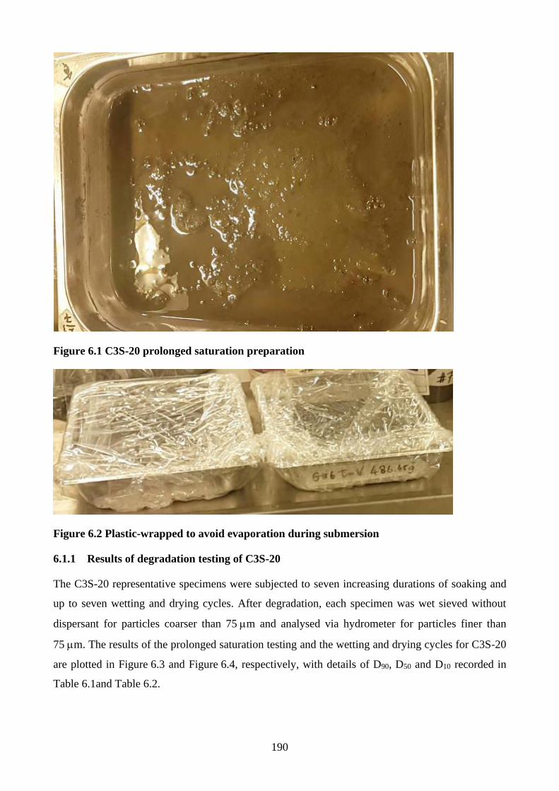
190
Figure 6.1 C3S-20 prolonged saturation preparation
Figure 6.2 Plastic-wrapped to avoid evaporation during submersion
6.1.1 Results of degradation testing of C3S-20
The C3S-20 representative specimens were subjected to seven increasing durations of soaking and
up to seven wetting and drying cycles. After degradation, each specimen was wet sieved without
dispersant for particles coarser than 75 m and analysed via hydrometer for particles finer than
75 m. The results of the prolonged saturation testing and the wetting and drying cycles for C3S-20
are plotted in Figure 6.3 and Figure 6.4, respectively, with details of D90, D50 and D10 recorded in
Table 6.1and Table 6.2.
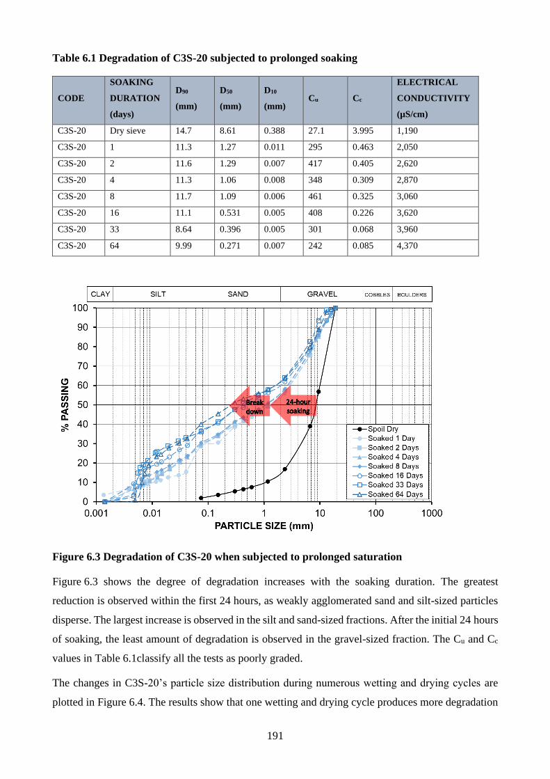
191
Table 6.1 Degradation of C3S-20 subjected to prolonged soaking
CODE
SOAKING
DURATION
(days)
D90
(mm)
D50
(mm)
D10
(mm) Cu Cc
ELECTRICAL
CONDUCTIVITY
(µS/cm)
C3S-20 Dry sieve 14.7 8.61 0.388 27.1 3.995 1,190
C3S-20 1 11.3 1.27 0.011 295 0.463 2,050
C3S-20 2 11.6 1.29 0.007 417 0.405 2,620
C3S-20 4 11.3 1.06 0.008 348 0.309 2,870
C3S-20 8 11.7 1.09 0.006 461 0.325 3,060
C3S-20 16 11.1 0.531 0.005 408 0.226 3,620
C3S-20 33 8.64 0.396 0.005 301 0.068 3,960
C3S-20 64 9.99 0.271 0.007 242 0.085 4,370
Figure 6.3 Degradation of C3S-20 when subjected to prolonged saturation
Figure 6.3 shows the degree of degradation increases with the soaking duration. The greatest
reduction is observed within the first 24 hours, as weakly agglomerated sand and silt-sized particles
disperse. The largest increase is observed in the silt and sand-sized fractions. After the initial 24 hours
of soaking, the least amount of degradation is observed in the gravel-sized fraction. The Cu and Cc
values in Table 6.1classify all the tests as poorly graded.
The changes in C3S-20’s particle size distribution during numerous wetting and drying cycles are
plotted in Figure 6.4. The results show that one wetting and drying cycle produces more degradation
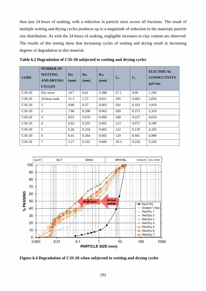
192
than just 24 hours of soaking, with a reduction in particle sizes across all fractions. The result of
multiple wetting and drying cycles produces up to a magnitude of reduction in the materials particle
size distribution. As with the 24 hours of soaking, negligible increases in clay content are observed.
The results of this testing show that increasing cycles of wetting and drying result in increasing
degrees of degradation in this material.
Table 6.2 Degradation of C3S-20 subjected to wetting and drying cycles
CODE
NUMBER OF
WETTING
AND DRYING
CYCLES
D90
(mm)
D50
(mm)
D10
(mm) Cu Cc
ELECTRICAL
CONDUCTIVITY
(µS/cm)
C3S-20 Dry sieve 14.7 8.61 0.388 27.1 4.00 1,190
C3S-20 24-hour soak 11.3 1.27 0.011 295 0.463 2,050
C3S-20 1 8.80 0.37 0.003 592 0.163 1,910
C3S-20 2 7.86 0.298 0.003 269 0.373 3,310
C3S-20 3 8.01 0.676 0.006 268 0.227 4,010
C3S-20 4 6.62 0.355 0.005 213 0.071 4,180
C3S-20 5 6.26 0.216 0.005 122 0.139 4,350
C3S-20 6 6.41 0.264 0.005 129 0.041 4,990
C3S-20 7 5.17 0.102 0.006 39.3 0.226 5,330
Figure 6.4 Degradation of C3S-20 when subjected to wetting and drying cycles
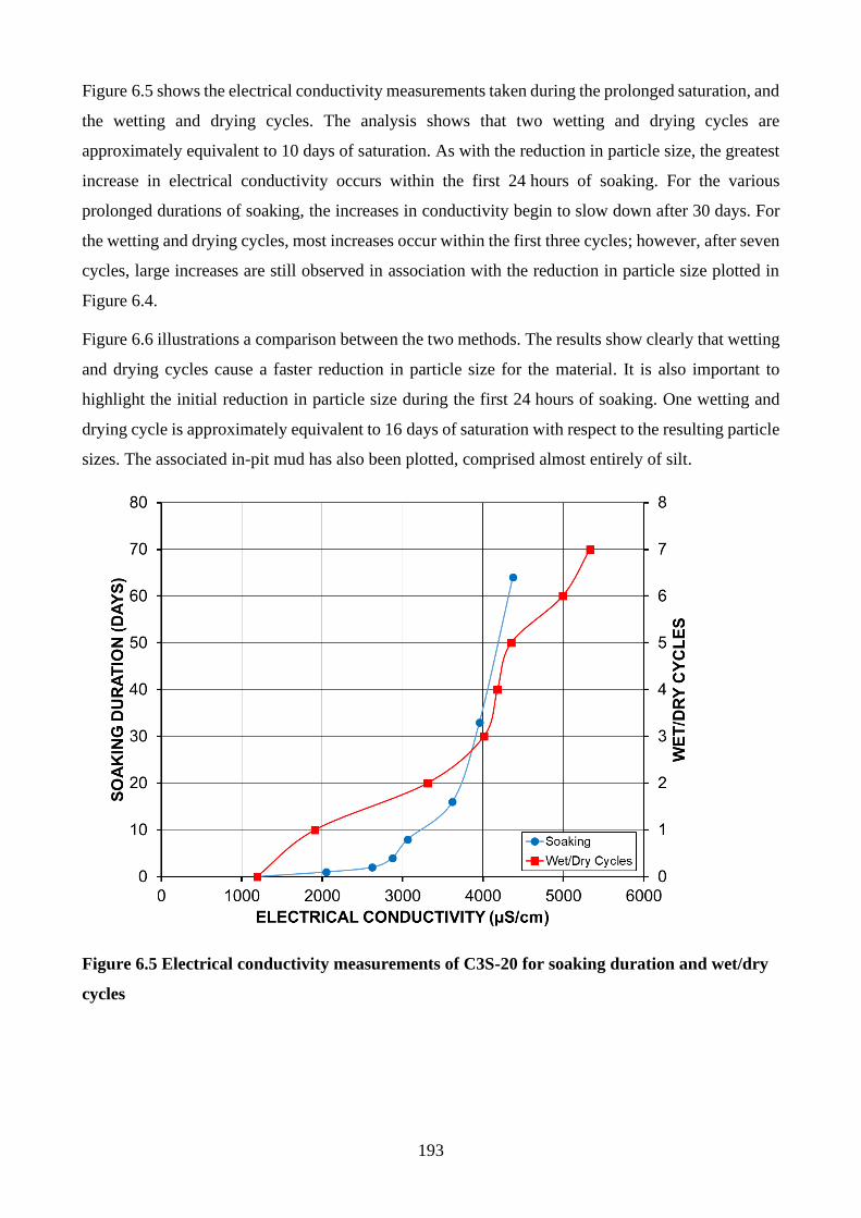
193
Figure 6.5 shows the electrical conductivity measurements taken during the prolonged saturation, and
the wetting and drying cycles. The analysis shows that two wetting and drying cycles are
approximately equivalent to 10 days of saturation. As with the reduction in particle size, the greatest
increase in electrical conductivity occurs within the first 24 hours of soaking. For the various
prolonged durations of soaking, the increases in conductivity begin to slow down after 30 days. For
the wetting and drying cycles, most increases occur within the first three cycles; however, after seven
cycles, large increases are still observed in association with the reduction in particle size plotted in
Figure 6.4.
Figure 6.6 illustrations a comparison between the two methods. The results show clearly that wetting
and drying cycles cause a faster reduction in particle size for the material. It is also important to
highlight the initial reduction in particle size during the first 24 hours of soaking. One wetting and
drying cycle is approximately equivalent to 16 days of saturation with respect to the resulting particle
sizes. The associated in-pit mud has also been plotted, comprised almost entirely of silt.
Figure 6.5 Electrical conductivity measurements of C3S-20 for soaking duration and wet/dry
cycles
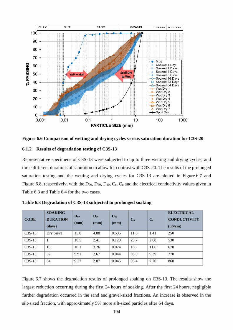
194
Figure 6.6 Comparison of wetting and drying cycles versus saturation duration for C3S-20
6.1.2 Results of degradation testing of C3S-13
Representative specimens of C3S-13 were subjected to up to three wetting and drying cycles, and
three different durations of saturation to allow for contrast with C3S-20. The results of the prolonged
saturation testing and the wetting and drying cycles for C3S-13 are plotted in Figure 6.7 and
Figure 6.8, respectively, with the D90, D50, D10, Cc, Cu and the electrical conductivity values given in
Table 6.3 and Table 6.4 for the two cases.
Table 6.3 Degradation of C3S-13 subjected to prolonged soaking
CODE
SOAKING
DURATION
(days)
D90
(mm)
D50
(mm)
D10
(mm) Cu Cc
ELECTRICAL
CONDUCTIVITY
(µS/cm)
C3S-13 Dry Sieve 15.0 4.88 0.535 11.8 1.41 250
C3S-13 1 10.5 2.41 0.129 29.7 2.68 530
C3S-13 16 10.1 3.26 0.024 185 11.6 670
C3S-13 32 9.91 2.67 0.044 93.0 9.39 770
C3S-13 64 9.27 2.87 0.045 95.4 7.70 860
Figure 6.7 shows the degradation results of prolonged soaking on C3S-13. The results show the
largest reduction occurring during the first 24 hours of soaking. After the first 24 hours, negligible
further degradation occurred in the sand and gravel-sized fractions. An increase is observed in the
silt-sized fraction, with approximately 5% more silt-sized particles after 64 days.
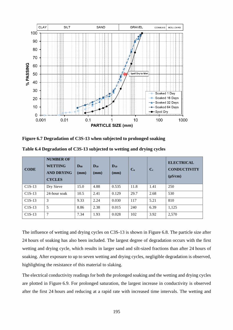
195
Figure 6.7 Degradation of C3S-13 when subjected to prolonged soaking
Table 6.4 Degradation of C3S-13 subjected to wetting and drying cycles
CODE
NUMBER OF
WETTING
AND DRYING
CYCLES
D90
(mm)
D50
(mm)
D10
(mm) Cu Cc
ELECTRICAL
CONDUCTIVITY
(µS/cm)
C1S-13 Dry Sieve 15.0 4.88 0.535 11.8 1.41 250
C1S-13 24-hour soak 10.5 2.41 0.129 29.7 2.68 530
C1S-13 3 9.33 2.24 0.030 117 5.21 810
C1S-13 5 8.86 2.38 0.015 240 6.39 1,125
C1S-13 7 7.34 1.93 0.028 102 3.92 2,570
The influence of wetting and drying cycles on C3S-13 is shown in Figure 6.8. The particle size after
24 hours of soaking has also been included. The largest degree of degradation occurs with the first
wetting and drying cycle, which results in larger sand and silt-sized fractions than after 24 hours of
soaking. After exposure to up to seven wetting and drying cycles, negligible degradation is observed,
highlighting the resistance of this material to slaking.
The electrical conductivity readings for both the prolonged soaking and the wetting and drying cycles
are plotted in Figure 6.9. For prolonged saturation, the largest increase in conductivity is observed
after the first 24 hours and reducing at a rapid rate with increased time intervals. The wetting and
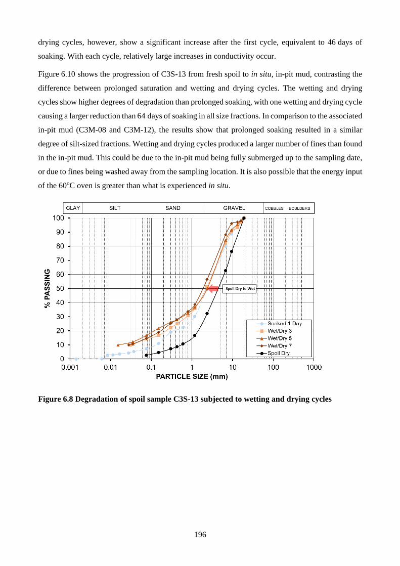
196
drying cycles, however, show a significant increase after the first cycle, equivalent to 46 days of
soaking. With each cycle, relatively large increases in conductivity occur.
Figure 6.10 shows the progression of C3S-13 from fresh spoil to in situ, in-pit mud, contrasting the
difference between prolonged saturation and wetting and drying cycles. The wetting and drying
cycles show higher degrees of degradation than prolonged soaking, with one wetting and drying cycle
causing a larger reduction than 64 days of soaking in all size fractions. In comparison to the associated
in-pit mud (C3M-08 and C3M-12), the results show that prolonged soaking resulted in a similar
degree of silt-sized fractions. Wetting and drying cycles produced a larger number of fines than found
in the in-pit mud. This could be due to the in-pit mud being fully submerged up to the sampling date,
or due to fines being washed away from the sampling location. It is also possible that the energy input
of the 60oC oven is greater than what is experienced in situ.
Figure 6.8 Degradation of spoil sample C3S-13 subjected to wetting and drying cycles
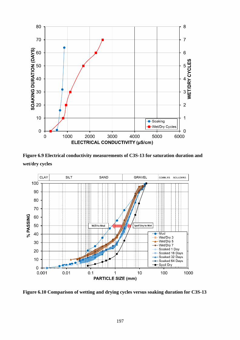
197
Figure 6.9 Electrical conductivity measurements of C3S-13 for saturation duration and
wet/dry cycles
Figure 6.10 Comparison of wetting and drying cycles versus soaking duration for C3S-13
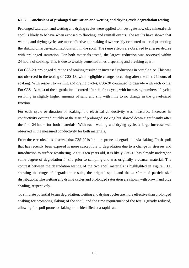
198
6.1.3 Conclusions of prolonged saturation and wetting and drying cycle degradation testing
Prolonged saturation and wetting and drying cycles were applied to investigate how clay mineral-rich
spoil is likely to behave when exposed to flooding, and rainfall events. The results have shown that
wetting and drying cycles are more effective at breaking down weakly cemented material promoting
the slaking of larger-sized fractions within the spoil. The same effects are observed to a lesser degree
with prolonged saturation. For both materials tested, the largest reduction was observed within
24 hours of soaking. This is due to weakly cemented fines dispersing and breaking apart.
For C3S-20, prolonged durations of soaking resulted in increased reductions in particle size. This was
not observed in the testing of C3S-13, with negligible changes occurring after the first 24 hours of
soaking. With respect to wetting and drying cycles, C3S-20 continued to degrade with each cycle.
For C3S-13, most of the degradation occurred after the first cycle, with increasing numbers of cycles
resulting in slightly higher amounts of sand and silt, with little to no change in the gravel-sized
fraction.
For each cycle or duration of soaking, the electrical conductivity was measured. Increases in
conductivity occurred quickly at the start of prolonged soaking but slowed down significantly after
the first 24 hours for both materials. With each wetting and drying cycle, a large increase was
observed in the measured conductivity for both materials.
From these results, it is observed that C3S-20 is far more prone to degradation via slaking. Fresh spoil
that has recently been exposed is more susceptible to degradation due to a change in stresses and
introduction to surface weathering. As it is ten years old, it is likely C3S-13 has already undergone
some degree of degradation in situ prior to sampling and was originally a coarser material. The
contrast between the degradation testing of the two spoil materials is highlighted in Figure 6.11,
showing the range of degradation results, the original spoil, and the in situ mud particle size
distributions. The wetting and drying cycles and prolonged saturation are shown with brown and blue
shading, respectively.
To simulate potential in situ degradation, wetting and drying cycles are more effective than prolonged
soaking for promoting slaking of the spoil, and the time requirement of the test is greatly reduced,
allowing for spoil prone to slaking to be identified at a rapid rate.
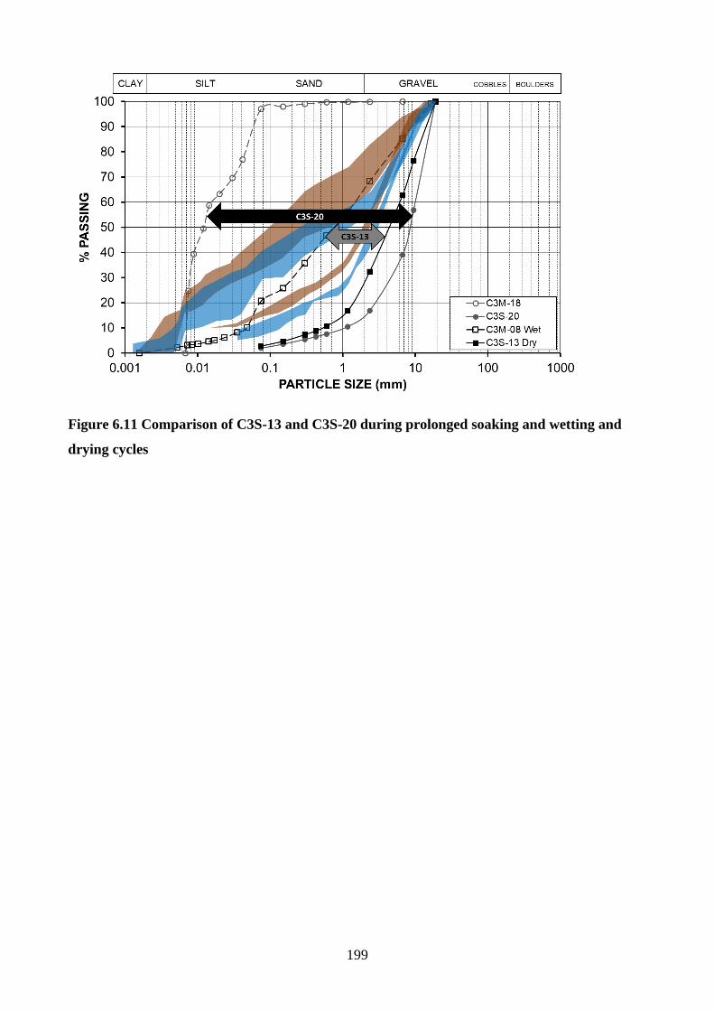
199
Figure 6.11 Comparison of C3S-13 and C3S-20 during prolonged soaking and wetting and
drying cycles
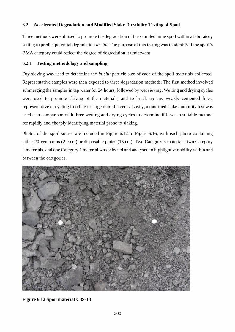
200
6.2 Accelerated Degradation and Modified Slake Durability Testing of Spoil
Three methods were utilised to promote the degradation of the sampled mine spoil within a laboratory
setting to predict potential degradation in situ. The purpose of this testing was to identify if the spoil’s
BMA category could reflect the degree of degradation it underwent.
6.2.1 Testing methodology and sampling
Dry sieving was used to determine the in situ particle size of each of the spoil materials collected.
Representative samples were then exposed to three degradation methods. The first method involved
submerging the samples in tap water for 24 hours, followed by wet sieving. Wetting and drying cycles
were used to promote slaking of the materials, and to break up any weakly cemented fines,
representative of cycling flooding or large rainfall events. Lastly, a modified slake durability test was
used as a comparison with three wetting and drying cycles to determine if it was a suitable method
for rapidly and cheaply identifying material prone to slaking.
Photos of the spoil source are included in Figure 6.12 to Figure 6.16, with each photo containing
either 20-cent coins (2.9 cm) or disposable plates (15 cm). Two Category 3 materials, two Category
2 materials, and one Category 1 material was selected and analysed to highlight variability within and
between the categories.
Figure 6.12 Spoil material C3S-13
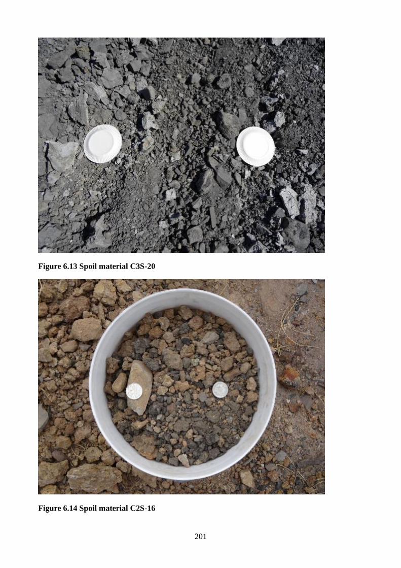
201
Figure 6.13 Spoil material C3S-20
Figure 6.14 Spoil material C2S-16
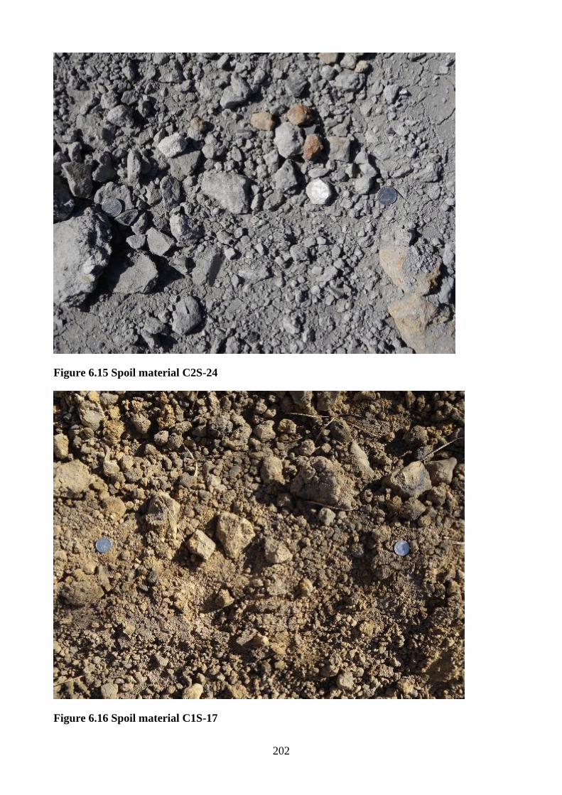
202
Figure 6.15 Spoil material C2S-24
Figure 6.16 Spoil material C1S-17
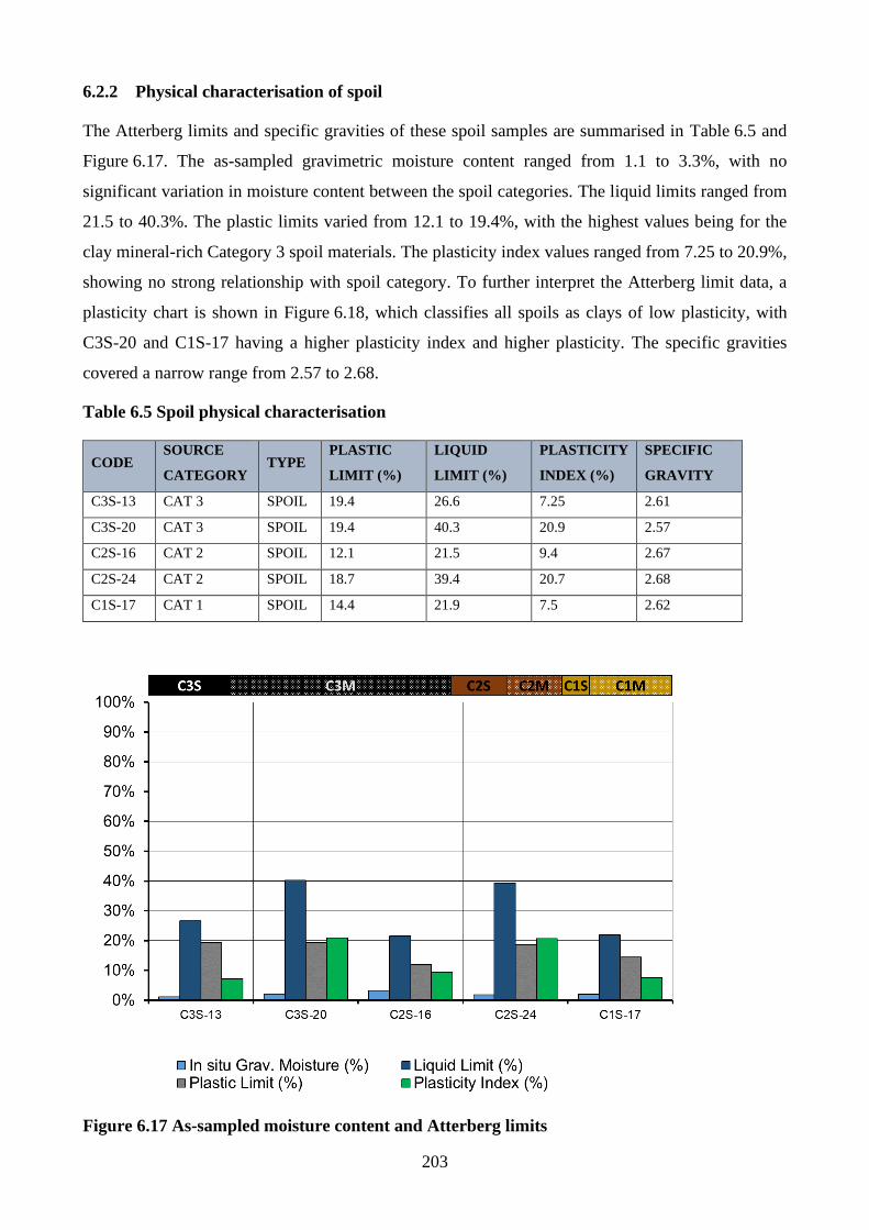
203
6.2.2 Physical characterisation of spoil
The Atterberg limits and specific gravities of these spoil samples are summarised in Table 6.5 and
Figure 6.17. The as-sampled gravimetric moisture content ranged from 1.1 to 3.3%, with no
significant variation in moisture content between the spoil categories. The liquid limits ranged from
21.5 to 40.3%. The plastic limits varied from 12.1 to 19.4%, with the highest values being for the
clay mineral-rich Category 3 spoil materials. The plasticity index values ranged from 7.25 to 20.9%,
showing no strong relationship with spoil category. To further interpret the Atterberg limit data, a
plasticity chart is shown in Figure 6.18, which classifies all spoils as clays of low plasticity, with
C3S-20 and C1S-17 having a higher plasticity index and higher plasticity. The specific gravities
covered a narrow range from 2.57 to 2.68.
Table 6.5 Spoil physical characterisation
CODE SOURCE
CATEGORY TYPE
PLASTIC
LIMIT (%)
LIQUID
LIMIT (%)
PLASTICITY
INDEX (%)
SPECIFIC
GRAVITY
C3S-13 CAT 3 SPOIL 19.4 26.6 7.25 2.61
C3S-20 CAT 3 SPOIL 19.4 40.3 20.9 2.57
C2S-16 CAT 2 SPOIL 12.1 21.5 9.4 2.67
C2S-24 CAT 2 SPOIL 18.7 39.4 20.7 2.68
C1S-17 CAT 1 SPOIL 14.4 21.9 7.5 2.62
Figure 6.17 As-sampled moisture content and Atterberg limits
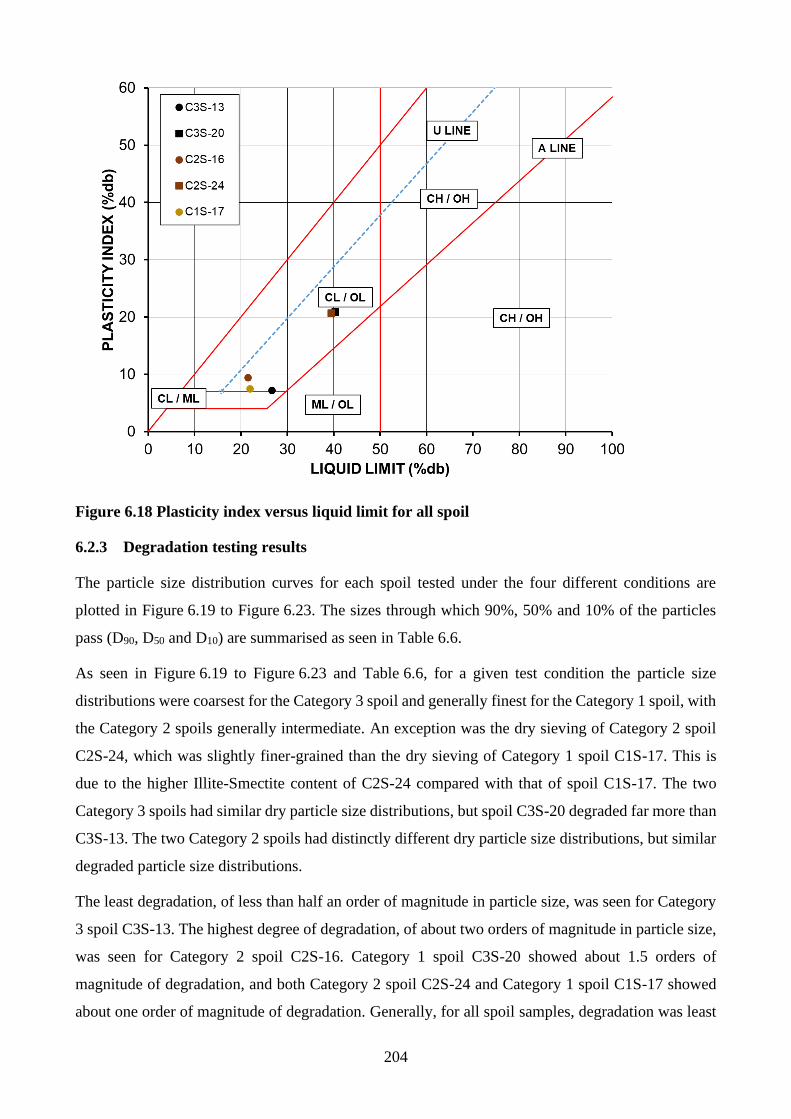
204
Figure 6.18 Plasticity index versus liquid limit for all spoil
6.2.3 Degradation testing results
The particle size distribution curves for each spoil tested under the four different conditions are
plotted in Figure 6.19 to Figure 6.23. The sizes through which 90%, 50% and 10% of the particles
pass (D90, D50 and D10) are summarised as seen in Table 6.6.
As seen in Figure 6.19 to Figure 6.23 and Table 6.6, for a given test condition the particle size
distributions were coarsest for the Category 3 spoil and generally finest for the Category 1 spoil, with
the Category 2 spoils generally intermediate. An exception was the dry sieving of Category 2 spoil
C2S-24, which was slightly finer-grained than the dry sieving of Category 1 spoil C1S-17. This is
due to the higher Illite-Smectite content of C2S-24 compared with that of spoil C1S-17. The two
Category 3 spoils had similar dry particle size distributions, but spoil C3S-20 degraded far more than
C3S-13. The two Category 2 spoils had distinctly different dry particle size distributions, but similar
degraded particle size distributions.
The least degradation, of less than half an order of magnitude in particle size, was seen for Category
3 spoil C3S-13. The highest degree of degradation, of about two orders of magnitude in particle size,
was seen for Category 2 spoil C2S-16. Category 1 spoil C3S-20 showed about 1.5 orders of
magnitude of degradation, and both Category 2 spoil C2S-24 and Category 1 spoil C1S-17 showed
about one order of magnitude of degradation. Generally, for all spoil samples, degradation was least
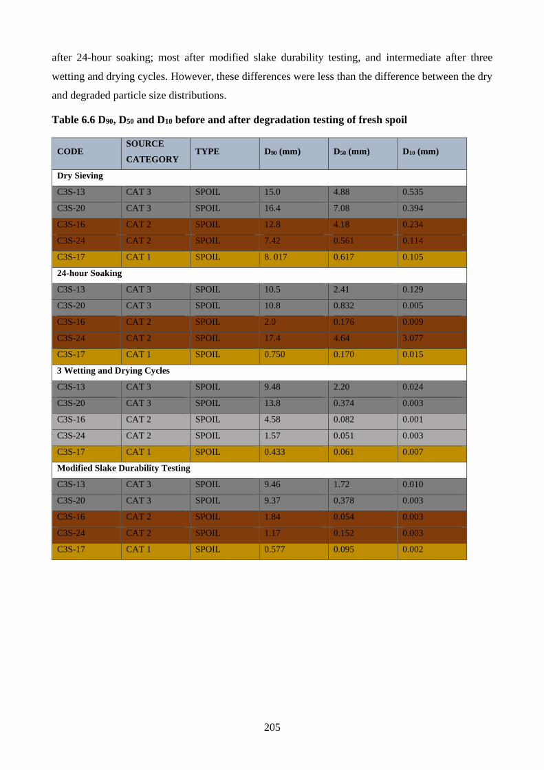
205
after 24-hour soaking; most after modified slake durability testing, and intermediate after three
wetting and drying cycles. However, these differences were less than the difference between the dry
and degraded particle size distributions.
Table 6.6 D90, D50 and D10 before and after degradation testing of fresh spoil
CODE SOURCE
CATEGORY TYPE D90 (mm) D50 (mm) D10 (mm)
Dry Sieving
C3S-13 CAT 3 SPOIL 15.0 4.88 0.535
C3S-20 CAT 3 SPOIL 16.4 7.08 0.394
C3S-16 CAT 2 SPOIL 12.8 4.18 0.234
C3S-24 CAT 2 SPOIL 7.42 0.561 0.114
C3S-17 CAT 1 SPOIL 8. 017 0.617 0.105
24-hour Soaking
C3S-13 CAT 3 SPOIL 10.5 2.41 0.129
C3S-20 CAT 3 SPOIL 10.8 0.832 0.005
C3S-16 CAT 2 SPOIL 2.0 0.176 0.009
C3S-24 CAT 2 SPOIL 17.4 4.64 3.077
C3S-17 CAT 1 SPOIL 0.750 0.170 0.015
3 Wetting and Drying Cycles
C3S-13 CAT 3 SPOIL 9.48 2.20 0.024
C3S-20 CAT 3 SPOIL 13.8 0.374 0.003
C3S-16 CAT 2 SPOIL 4.58 0.082 0.001
C3S-24 CAT 2 SPOIL 1.57 0.051 0.003
C3S-17 CAT 1 SPOIL 0.433 0.061 0.007
Modified Slake Durability Testing
C3S-13 CAT 3 SPOIL 9.46 1.72 0.010
C3S-20 CAT 3 SPOIL 9.37 0.378 0.003
C3S-16 CAT 2 SPOIL 1.84 0.054 0.003
C3S-24 CAT 2 SPOIL 1.17 0.152 0.003
C3S-17 CAT 1 SPOIL 0.577 0.095 0.002
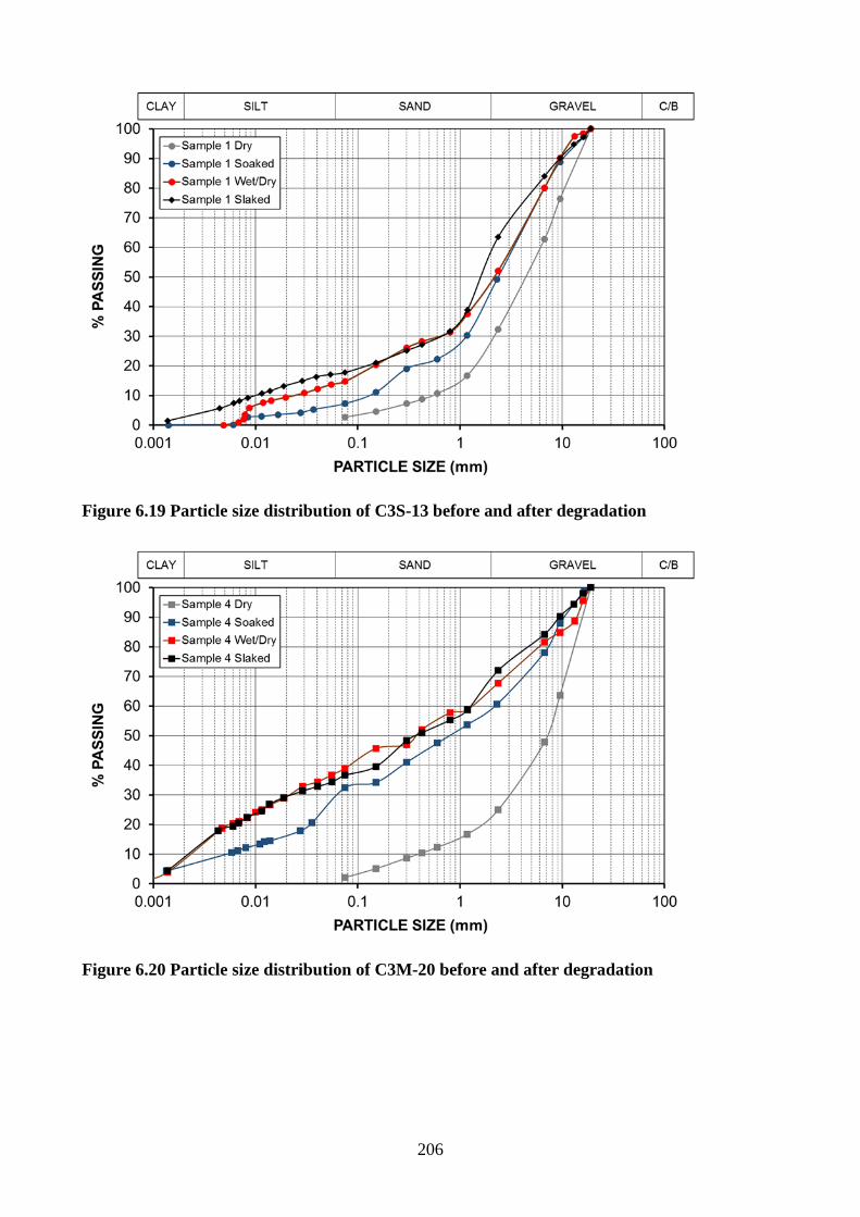
206
Figure 6.19 Particle size distribution of C3S-13 before and after degradation
Figure 6.20 Particle size distribution of C3M-20 before and after degradation
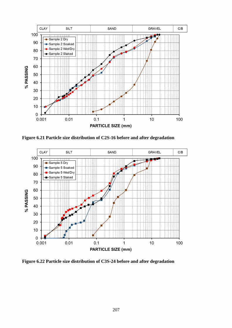
207
Figure 6.21 Particle size distribution of C2S-16 before and after degradation
Figure 6.22 Particle size distribution of C3S-24 before and after degradation
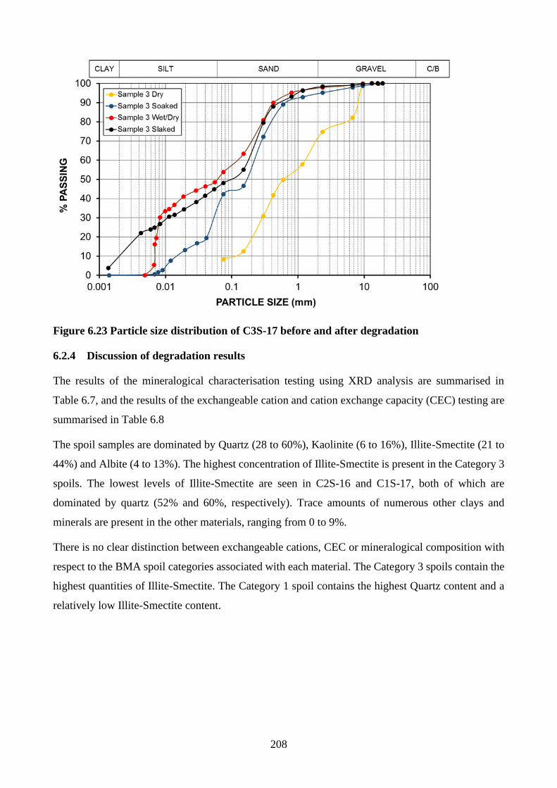
208
Figure 6.23 Particle size distribution of C3S-17 before and after degradation
6.2.4 Discussion of degradation results
The results of the mineralogical characterisation testing using XRD analysis are summarised in
Table 6.7, and the results of the exchangeable cation and cation exchange capacity (CEC) testing are
summarised in Table 6.8
The spoil samples are dominated by Quartz (28 to 60%), Kaolinite (6 to 16%), Illite-Smectite (21 to
44%) and Albite (4 to 13%). The highest concentration of Illite-Smectite is present in the Category 3
spoils. The lowest levels of Illite-Smectite are seen in C2S-16 and C1S-17, both of which are
dominated by quartz (52% and 60%, respectively). Trace amounts of numerous other clays and
minerals are present in the other materials, ranging from 0 to 9%.
There is no clear distinction between exchangeable cations, CEC or mineralogical composition with
respect to the BMA spoil categories associated with each material. The Category 3 spoils contain the
highest quantities of Illite-Smectite. The Category 1 spoil contains the highest Quartz content and a
relatively low Illite-Smectite content.
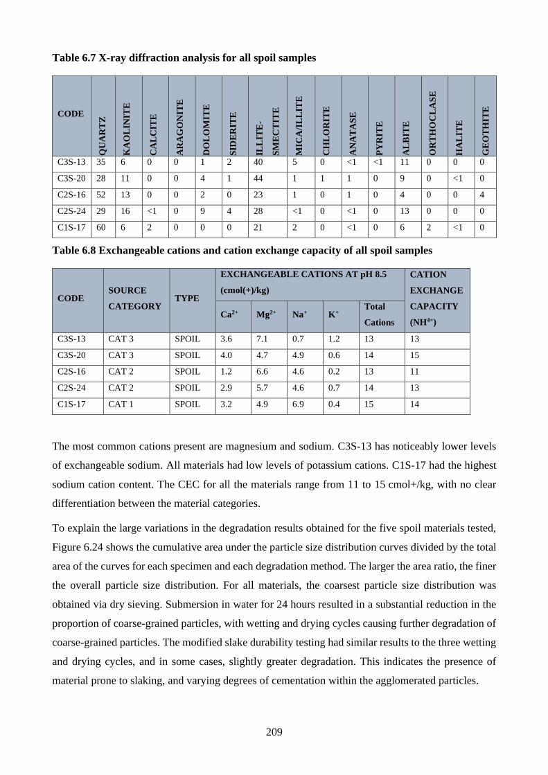
209
Table 6.7 X-ray diffraction analysis for all spoil samples
CODE
QU
AR
TZ
KA
OL
INIT
E
CA
LC
ITE
AR
AG
ON
ITE
DO
LO
MIT
E
SID
ER
ITE
ILL
ITE
-
SM
EC
TIT
E
MIC
A/I
LL
ITE
CH
LO
RIT
E
AN
AT
AS
E
PY
RIT
E
AL
BIT
E
OR
TH
OC
LA
SE
HA
LIT
E
GE
OT
HIT
E
C3S-13 35 6 0 0 1 2 40 5 0 <1 <1 11 0 0 0
C3S-20 28 11 0 0 4 1 44 1 1 1 0 9 0 <1 0
C2S-16 52 13 0 0 2 0 23 1 0 1 0 4 0 0 4
C2S-24 29 16 <1 0 9 4 28 <1 0 <1 0 13 0 0 0
C1S-17 60 6 2 0 0 0 21 2 0 <1 0 6 2 <1 0
Table 6.8 Exchangeable cations and cation exchange capacity of all spoil samples
CODE SOURCE
CATEGORY TYPE
EXCHANGEABLE CATIONS AT pH 8.5
(cmol(+)/kg)
CATION
EXCHANGE
CAPACITY
(NH4+) Ca2+ Mg2+ Na+ K+
Total
Cations
C3S-13 CAT 3 SPOIL 3.6 7.1 0.7 1.2 13 13
C3S-20 CAT 3 SPOIL 4.0 4.7 4.9 0.6 14 15
C2S-16 CAT 2 SPOIL 1.2 6.6 4.6 0.2 13 11
C2S-24 CAT 2 SPOIL 2.9 5.7 4.6 0.7 14 13
C1S-17 CAT 1 SPOIL 3.2 4.9 6.9 0.4 15 14
The most common cations present are magnesium and sodium. C3S-13 has noticeably lower levels
of exchangeable sodium. All materials had low levels of potassium cations. C1S-17 had the highest
sodium cation content. The CEC for all the materials range from 11 to 15 cmol+/kg, with no clear
differentiation between the material categories.
To explain the large variations in the degradation results obtained for the five spoil materials tested,
Figure 6.24 shows the cumulative area under the particle size distribution curves divided by the total
area of the curves for each specimen and each degradation method. The larger the area ratio, the finer
the overall particle size distribution. For all materials, the coarsest particle size distribution was
obtained via dry sieving. Submersion in water for 24 hours resulted in a substantial reduction in the
proportion of coarse-grained particles, with wetting and drying cycles causing further degradation of
coarse-grained particles. The modified slake durability testing had similar results to the three wetting
and drying cycles, and in some cases, slightly greater degradation. This indicates the presence of
material prone to slaking, and varying degrees of cementation within the agglomerated particles.
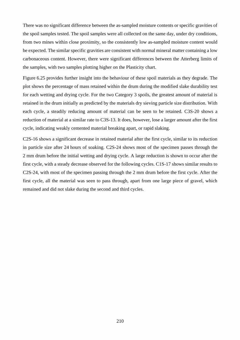
210
There was no significant difference between the as-sampled moisture contents or specific gravities of
the spoil samples tested. The spoil samples were all collected on the same day, under dry conditions,
from two mines within close proximity, so the consistently low as-sampled moisture content would
be expected. The similar specific gravities are consistent with normal mineral matter containing a low
carbonaceous content. However, there were significant differences between the Atterberg limits of
the samples, with two samples plotting higher on the Plasticity chart.
Figure 6.25 provides further insight into the behaviour of these spoil materials as they degrade. The
plot shows the percentage of mass retained within the drum during the modified slake durability test
for each wetting and drying cycle. For the two Category 3 spoils, the greatest amount of material is
retained in the drum initially as predicted by the materials dry sieving particle size distribution. With
each cycle, a steadily reducing amount of material can be seen to be retained. C3S-20 shows a
reduction of material at a similar rate to C3S-13. It does, however, lose a larger amount after the first
cycle, indicating weakly cemented material breaking apart, or rapid slaking.
C2S-16 shows a significant decrease in retained material after the first cycle, similar to its reduction
in particle size after 24 hours of soaking. C2S-24 shows most of the specimen passes through the
2 mm drum before the initial wetting and drying cycle. A large reduction is shown to occur after the
first cycle, with a steady decrease observed for the following cycles. C1S-17 shows similar results to
C2S-24, with most of the specimen passing through the 2 mm drum before the first cycle. After the
first cycle, all the material was seen to pass through, apart from one large piece of gravel, which
remained and did not slake during the second and third cycles.
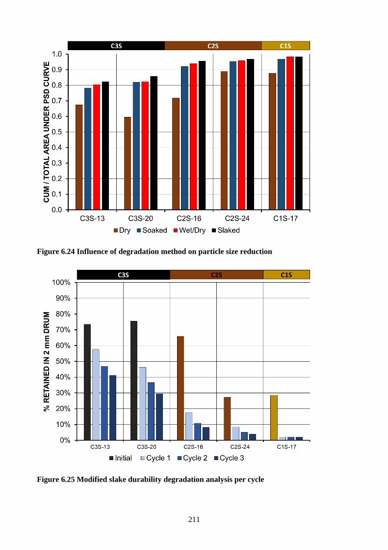
211
Figure 6.24 Influence of degradation method on particle size reduction
Figure 6.25 Modified slake durability degradation analysis per cycle
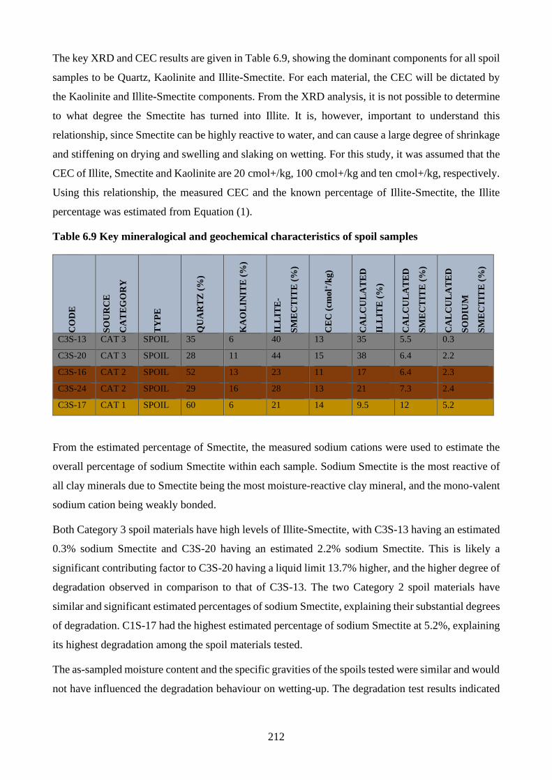
212
The key XRD and CEC results are given in Table 6.9, showing the dominant components for all spoil
samples to be Quartz, Kaolinite and Illite-Smectite. For each material, the CEC will be dictated by
the Kaolinite and Illite-Smectite components. From the XRD analysis, it is not possible to determine
to what degree the Smectite has turned into Illite. It is, however, important to understand this
relationship, since Smectite can be highly reactive to water, and can cause a large degree of shrinkage
and stiffening on drying and swelling and slaking on wetting. For this study, it was assumed that the
CEC of Illite, Smectite and Kaolinite are 20 cmol+/kg, 100 cmol+/kg and ten cmol+/kg, respectively.
Using this relationship, the measured CEC and the known percentage of Illite-Smectite, the Illite
percentage was estimated from Equation (1).
Table 6.9 Key mineralogical and geochemical characteristics of spoil samples
CO
DE
SO
UR
CE
CA
TE
GO
RY
TY
PE
QU
AR
TZ
(%
)
KA
OL
INIT
E (
%)
ILL
ITE
-
SM
EC
TIT
E (
%)
CE
C (
cmo
l+/k
g)
CA
LC
UL
AT
ED
ILL
ITE
(%
)
CA
LC
UL
AT
ED
SM
EC
TIT
E (
%)
CA
LC
UL
AT
ED
SO
DIU
M
SM
EC
TIT
E (
%)
C3S-13 CAT 3 SPOIL 35 6 40 13 35 5.5 0.3
C3S-20 CAT 3 SPOIL 28 11 44 15 38 6.4 2.2
C3S-16 CAT 2 SPOIL 52 13 23 11 17 6.4 2.3
C3S-24 CAT 2 SPOIL 29 16 28 13 21 7.3 2.4
C3S-17 CAT 1 SPOIL 60 6 21 14 9.5 12 5.2
From the estimated percentage of Smectite, the measured sodium cations were used to estimate the
overall percentage of sodium Smectite within each sample. Sodium Smectite is the most reactive of
all clay minerals due to Smectite being the most moisture-reactive clay mineral, and the mono-valent
sodium cation being weakly bonded.
Both Category 3 spoil materials have high levels of Illite-Smectite, with C3S-13 having an estimated
0.3% sodium Smectite and C3S-20 having an estimated 2.2% sodium Smectite. This is likely a
significant contributing factor to C3S-20 having a liquid limit 13.7% higher, and the higher degree of
degradation observed in comparison to that of C3S-13. The two Category 2 spoil materials have
similar and significant estimated percentages of sodium Smectite, explaining their substantial degrees
of degradation. C1S-17 had the highest estimated percentage of sodium Smectite at 5.2%, explaining
its highest degradation among the spoil materials tested.
The as-sampled moisture content and the specific gravities of the spoils tested were similar and would
not have influenced the degradation behaviour on wetting-up. The degradation test results indicated
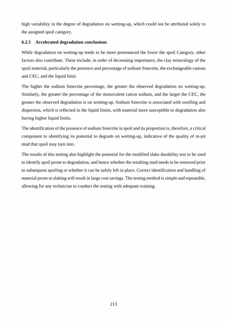
213
high variability in the degree of degradation on wetting-up, which could not be attributed solely to
the assigned spoil category.
6.2.5 Accelerated degradation conclusions
While degradation on wetting-up tends to be more pronounced the lower the spoil Category, other
factors also contribute. These include, in order of decreasing importance, the clay mineralogy of the
spoil material, particularly the presence and percentage of sodium Smectite, the exchangeable cations
and CEC, and the liquid limit.
The higher the sodium Smectite percentage, the greater the observed degradation on wetting-up.
Similarly, the greater the percentage of the monovalent cation sodium, and the larger the CEC, the
greater the observed degradation is on wetting-up. Sodium Smectite is associated with swelling and
dispersion, which is reflected in the liquid limits, with material more susceptible to degradation also
having higher liquid limits.
The identification of the presence of sodium Smectite in spoil and its proportion is, therefore, a critical
component to identifying its potential to degrade on wetting-up, indicative of the quality of in-pit
mud that spoil may turn into.
The results of this testing also highlight the potential for the modified slake durability test to be used
to identify spoil prone to degradation, and hence whether the resulting mud needs to be removed prior
to subsequent spoiling or whether it can be safely left in place. Correct identification and handling of
material prone to slaking will result in large cost savings. The testing method is simple and repeatable,
allowing for any technician to conduct the testing with adequate training.
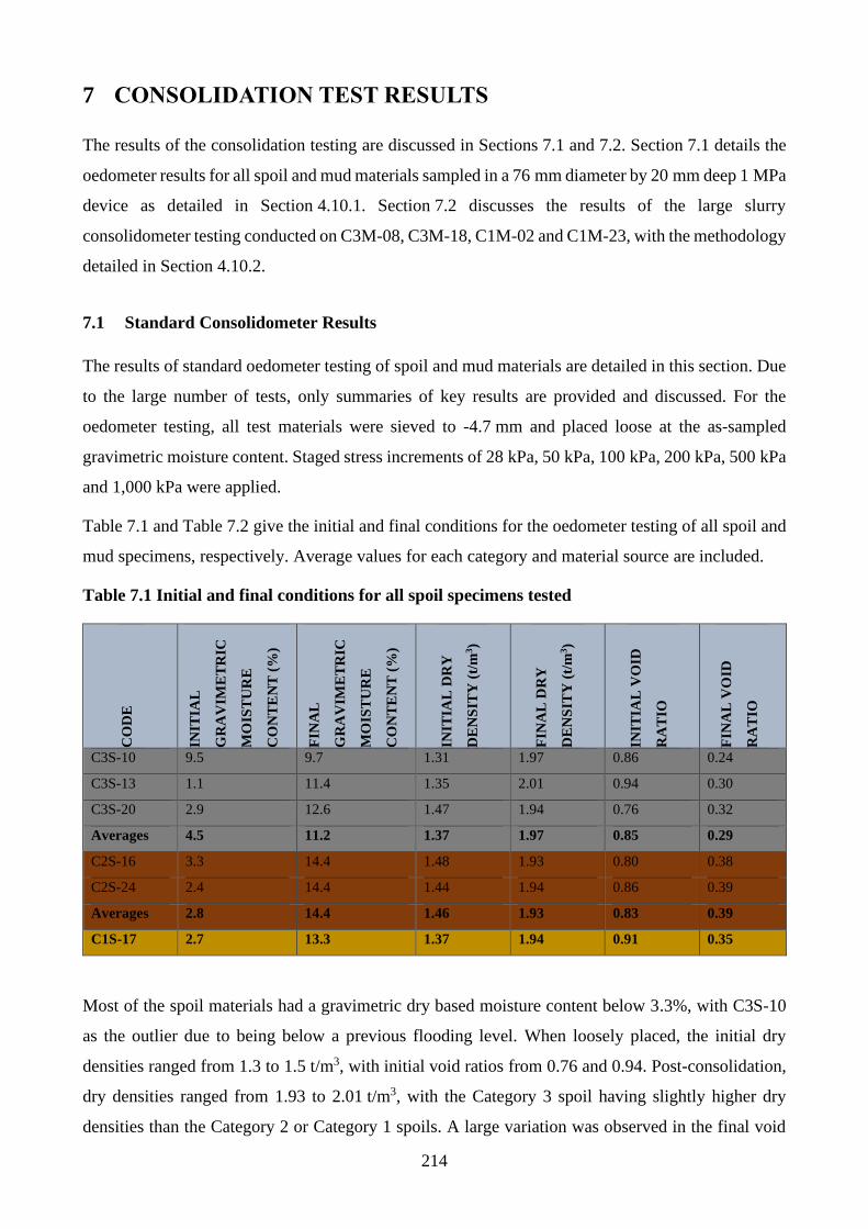
214
7 CONSOLIDATION TEST RESULTS
The results of the consolidation testing are discussed in Sections 7.1 and 7.2. Section 7.1 details the
oedometer results for all spoil and mud materials sampled in a 76 mm diameter by 20 mm deep 1 MPa
device as detailed in Section 4.10.1. Section 7.2 discusses the results of the large slurry
consolidometer testing conducted on C3M-08, C3M-18, C1M-02 and C1M-23, with the methodology
detailed in Section 4.10.2.
7.1 Standard Consolidometer Results
The results of standard oedometer testing of spoil and mud materials are detailed in this section. Due
to the large number of tests, only summaries of key results are provided and discussed. For the
oedometer testing, all test materials were sieved to -4.7 mm and placed loose at the as-sampled
gravimetric moisture content. Staged stress increments of 28 kPa, 50 kPa, 100 kPa, 200 kPa, 500 kPa
and 1,000 kPa were applied.
Table 7.1 and Table 7.2 give the initial and final conditions for the oedometer testing of all spoil and
mud specimens, respectively. Average values for each category and material source are included.
Table 7.1 Initial and final conditions for all spoil specimens tested
CO
DE
INIT
IAL
GR
AV
IME
TR
IC
MO
IST
UR
E
CO
NT
EN
T (
%)
FIN
AL
GR
AV
IME
TR
IC
MO
IST
UR
E
CO
NT
EN
T (
%)
INIT
IAL
DR
Y
DE
NS
ITY
(t/
m3)
FIN
AL
DR
Y
DE
NS
ITY
(t/
m3)
INIT
IAL
VO
ID
RA
TIO
FIN
AL
VO
ID
RA
TIO
C3S-10 9.5 9.7 1.31 1.97 0.86 0.24
C3S-13 1.1 11.4 1.35 2.01 0.94 0.30
C3S-20 2.9 12.6 1.47 1.94 0.76 0.32
Averages 4.5 11.2 1.37 1.97 0.85 0.29
C2S-16 3.3 14.4 1.48 1.93 0.80 0.38
C2S-24 2.4 14.4 1.44 1.94 0.86 0.39
Averages 2.8 14.4 1.46 1.93 0.83 0.39
C1S-17 2.7 13.3 1.37 1.94 0.91 0.35
Most of the spoil materials had a gravimetric dry based moisture content below 3.3%, with C3S-10
as the outlier due to being below a previous flooding level. When loosely placed, the initial dry
densities ranged from 1.3 to 1.5 t/m3, with initial void ratios from 0.76 and 0.94. Post-consolidation,
dry densities ranged from 1.93 to 2.01 t/m3, with the Category 3 spoil having slightly higher dry
densities than the Category 2 or Category 1 spoils. A large variation was observed in the final void
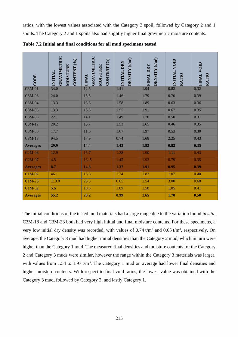
215
ratios, with the lowest values associated with the Category 3 spoil, followed by Category 2 and 1
spoils. The Category 2 and 1 spoils also had slightly higher final gravimetric moisture contents.
Table 7.2 Initial and final conditions for all mud specimens tested
CO
DE
INIT
IAL
GR
AV
IME
TR
IC
MO
IST
UR
E
CO
NT
EN
T (
%)
FIN
AL
GR
AV
IME
TR
IC
MO
IST
UR
E
CO
NT
EN
T (
%)
INIT
IAL
DR
Y
DE
NS
ITY
(t/
m3)
FIN
AL
DR
Y
DE
NS
ITY
(t/
m3)
INIT
IAL
VO
ID
RA
TIO
FIN
AL
VO
ID
RA
TIO
C3M-01 34.0 12.5 1.41 1.94 0.82 0.32
C3M-03 24.0 15.8 1.46 1.79 0.70 0.39
C3M-04 13.3 13.8 1.58 1.89 0.63 0.36
C3M-05 13.3 13.5 1.55 1.91 0.67 0.35
C3M-08 22.1 14.1 1.49 1.70 0.50 0.31
C3M-12 20.2 15.7 1.53 1.65 0.46 0.35
C3M-30 17.7 11.6 1.67 1.97 0.53 0.30
C3M-18 94.5 17.9 0.74 1.68 2.25 0.43
Averages 29.9 14.4 1.43 1.82 0.82 0.35
C2M-06 12.9 15.7 1.28 1.90 1.11 0.43
C2M-07 4.5 13. 5 1.45 1.92 0.79 0.35
Averages 8.7 14.6 1.37 1.91 0.95 0.39
C1M-02 46.1 15.8 1.24 1.82 1.07 0.40
C1M-23 113.8 26.3 0.65 1.54 3.00 0.68
C1M-32 5.6 18.5 1.09 1.58 1.05 0.41
Averages 55.2 20.2 0.99 1.65 1.70 0.50
The initial conditions of the tested mud materials had a large range due to the variation found in situ.
C3M-18 and C3M-23 both had very high initial and final moisture contents. For these specimens, a
very low initial dry density was recorded, with values of 0.74 t/m3 and 0.65 t/m3, respectively. On
average, the Category 3 mud had higher initial densities than the Category 2 mud, which in turn were
higher than the Category 1 mud. The measured final densities and moisture contents for the Category
2 and Category 3 muds were similar, however the range within the Category 3 materials was larger,
with values from 1.54 to 1.97 t/m3. The Category 1 mud on average had lower final densities and
higher moisture contents. With respect to final void ratios, the lowest value was obtained with the
Category 3 mud, followed by Category 2, and lastly Category 1.
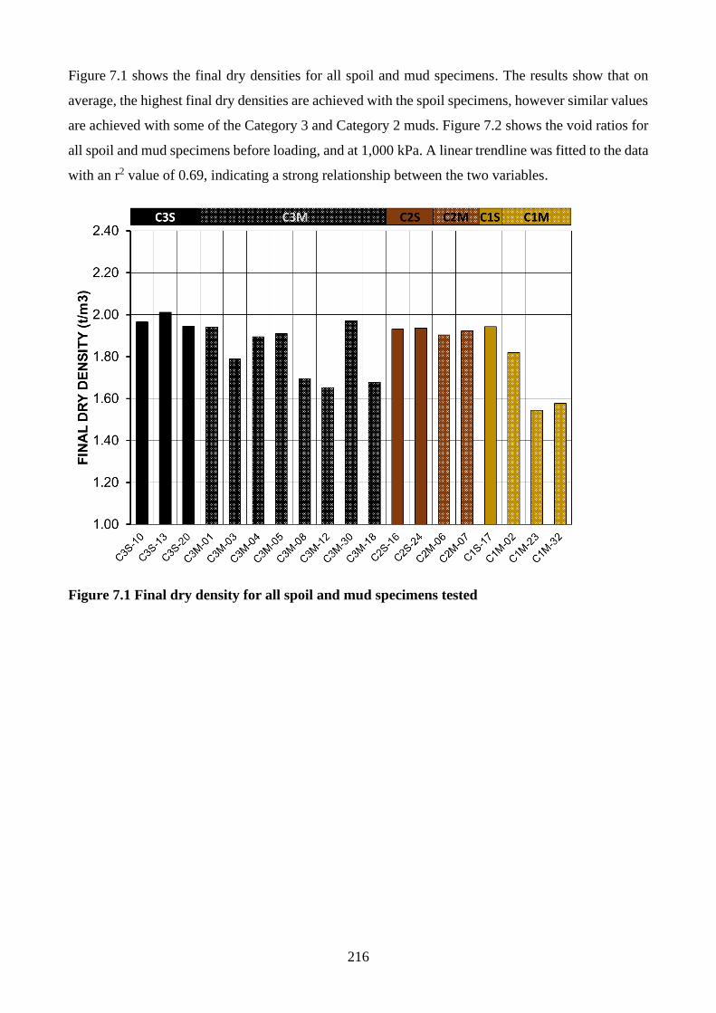
216
Figure 7.1 shows the final dry densities for all spoil and mud specimens. The results show that on
average, the highest final dry densities are achieved with the spoil specimens, however similar values
are achieved with some of the Category 3 and Category 2 muds. Figure 7.2 shows the void ratios for
all spoil and mud specimens before loading, and at 1,000 kPa. A linear trendline was fitted to the data
with an r2 value of 0.69, indicating a strong relationship between the two variables.
Figure 7.1 Final dry density for all spoil and mud specimens tested
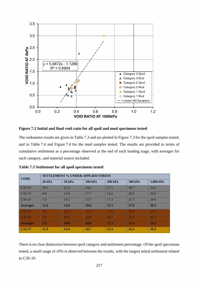
217
Figure 7.2 Initial and final void ratio for all spoil and mud specimens tested
The oedometer results are given in Table 7.3 and are plotted in Figure 7.3 for the spoil samples tested,
and in Table 7.4 and Figure 7.4 for the mud samples tested. The results are provided in terms of
cumulative settlement as a percentage observed at the end of each loading stage, with averages for
each category, and material source included.
Table 7.3 Settlement for all spoil specimens tested
CODE SETTLEMENT % UNDER APPLIED STRESS
28 kPa 50 kPa 100 kPa 200 kPa 500 kPa 1,000 kPa
C3S-10 18.1 21.2 24.2 27.1 30.7 33.4
C3S-13 8.9 13.0 17.7 22.6 28.5 33.0
C3S-20 7.9 10.2 13.7 17.3 21.7 24.6
Averages 11.6 14.8 18.6 22.3 27.0 30.3
C2S-16 7.0 11.2 15.1 17.8 20.6 23.1
C2S-24 7.6 10.4 12.8 16.7 22.2 25.4
Averages 7.3 10.8 14.0 17.3 21.4 24.2
C1S-17 11.0 14.4 18.7 22.4 26.5 29.4
There is no clear distinction between spoil category and settlement percentage. Of the spoil specimens
tested, a small range of 10% is observed between the results, with the largest initial settlement related
to C3S-10.
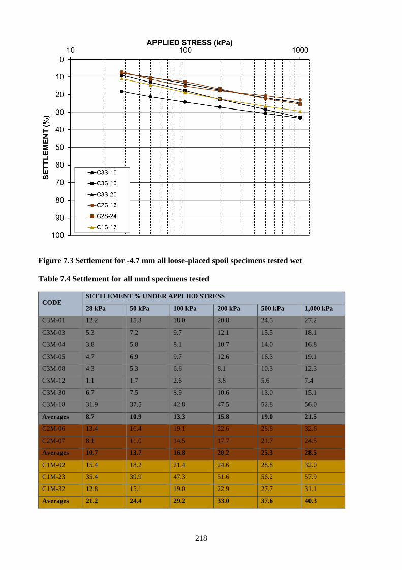
218
Figure 7.3 Settlement for -4.7 mm all loose-placed spoil specimens tested wet
Table 7.4 Settlement for all mud specimens tested
CODE SETTLEMENT % UNDER APPLIED STRESS
28 kPa 50 kPa 100 kPa 200 kPa 500 kPa 1,000 kPa
C3M-01 12.2 15.3 18.0 20.8 24.5 27.2
C3M-03 5.3 7.2 9.7 12.1 15.5 18.1
C3M-04 3.8 5.8 8.1 10.7 14.0 16.8
C3M-05 4.7 6.9 9.7 12.6 16.3 19.1
C3M-08 4.3 5.3 6.6 8.1 10.3 12.3
C3M-12 1.1 1.7 2.6 3.8 5.6 7.4
C3M-30 6.7 7.5 8.9 10.6 13.0 15.1
C3M-18 31.9 37.5 42.8 47.5 52.8 56.0
Averages 8.7 10.9 13.3 15.8 19.0 21.5
C2M-06 13.4 16.4 19.1 22.6 28.8 32.6
C2M-07 8.1 11.0 14.5 17.7 21.7 24.5
Averages 10.7 13.7 16.8 20.2 25.3 28.5
C1M-02 15.4 18.2 21.4 24.6 28.8 32.0
C1M-23 35.4 39.9 47.3 51.6 56.2 57.9
C1M-32 12.8 15.1 19.0 22.9 27.7 31.1
Averages 21.2 24.4 29.2 33.0 37.6 40.3
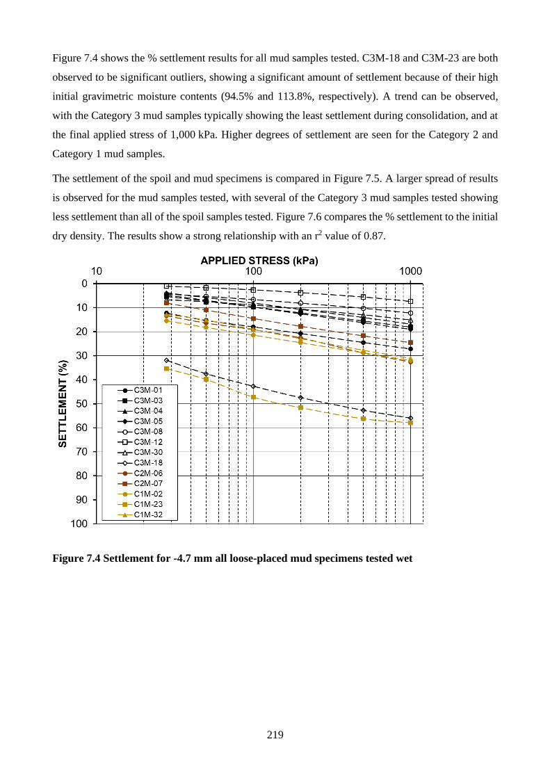
219
Figure 7.4 shows the % settlement results for all mud samples tested. C3M-18 and C3M-23 are both
observed to be significant outliers, showing a significant amount of settlement because of their high
initial gravimetric moisture contents (94.5% and 113.8%, respectively). A trend can be observed,
with the Category 3 mud samples typically showing the least settlement during consolidation, and at
the final applied stress of 1,000 kPa. Higher degrees of settlement are seen for the Category 2 and
Category 1 mud samples.
The settlement of the spoil and mud specimens is compared in Figure 7.5. A larger spread of results
is observed for the mud samples tested, with several of the Category 3 mud samples tested showing
less settlement than all of the spoil samples tested. Figure 7.6 compares the % settlement to the initial
dry density. The results show a strong relationship with an r2 value of 0.87.
Figure 7.4 Settlement for -4.7 mm all loose-placed mud specimens tested wet
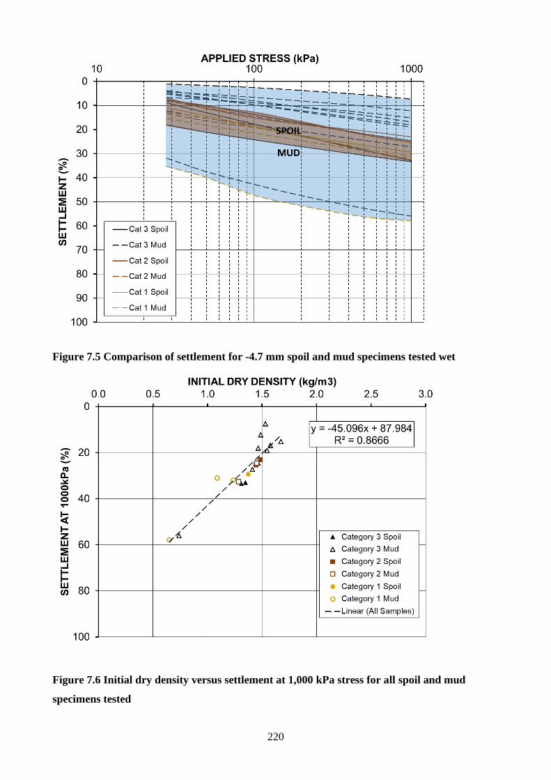
220
Figure 7.5 Comparison of settlement for -4.7 mm spoil and mud specimens tested wet
Figure 7.6 Initial dry density versus settlement at 1,000 kPa stress for all spoil and mud
specimens tested
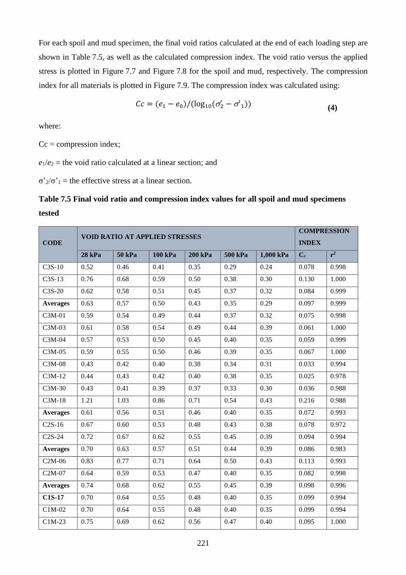
221
For each spoil and mud specimen, the final void ratios calculated at the end of each loading step are
shown in Table 7.5, as well as the calculated compression index. The void ratio versus the applied
stress is plotted in Figure 7.7 and Figure 7.8 for the spoil and mud, respectively. The compression
index for all materials is plotted in Figure 7.9. The compression index was calculated using:
𝐶𝑐 = (𝑒1 − 𝑒0)/(log10(2′ − ′
1)) (4)
where:
Cc = compression index;
e1/e2 = the void ratio calculated at a linear section; and
σ’2/σ’1 = the effective stress at a linear section.
Table 7.5 Final void ratio and compression index values for all spoil and mud specimens
tested
CODE VOID RATIO AT APPLIED STRESSES
COMPRESSION
INDEX
28 kPa 50 kPa 100 kPa 200 kPa 500 kPa 1,000 kPa Cc r2
C3S-10 0.52 0.46 0.41 0.35 0.29 0.24 0.078 0.998
C3S-13 0.76 0.68 0.59 0.50 0.38 0.30 0.130 1.000
C3S-20 0.62 0.58 0.51 0.45 0.37 0.32 0.084 0.999
Averages 0.63 0.57 0.50 0.43 0.35 0.29 0.097 0.999
C3M-01 0.59 0.54 0.49 0.44 0.37 0.32 0.075 0.998
C3M-03 0.61 0.58 0.54 0.49 0.44 0.39 0.061 1.000
C3M-04 0.57 0.53 0.50 0.45 0.40 0.35 0.059 0.999
C3M-05 0.59 0.55 0.50 0.46 0.39 0.35 0.067 1.000
C3M-08 0.43 0.42 0.40 0.38 0.34 0.31 0.033 0.994
C3M-12 0.44 0.43 0.42 0.40 0.38 0.35 0.025 0.978
C3M-30 0.43 0.41 0.39 0.37 0.33 0.30 0.036 0.988
C3M-18 1.21 1.03 0.86 0.71 0.54 0.43 0.216 0.988
Averages 0.61 0.56 0.51 0.46 0.40 0.35 0.072 0.993
C2S-16 0.67 0.60 0.53 0.48 0.43 0.38 0.078 0.972
C2S-24 0.72 0.67 0.62 0.55 0.45 0.39 0.094 0.994
Averages 0.70 0.63 0.57 0.51 0.44 0.39 0.086 0.983
C2M-06 0.83 0.77 0.71 0.64 0.50 0.43 0.113 0.993
C2M-07 0.64 0.59 0.53 0.47 0.40 0.35 0.082 0.998
Averages 0.74 0.68 0.62 0.55 0.45 0.39 0.098 0.996
C1S-17 0.70 0.64 0.55 0.48 0.40 0.35 0.099 0.994
C1M-02 0.70 0.64 0.55 0.48 0.40 0.35 0.099 0.994
C1M-23 0.75 0.69 0.62 0.56 0.47 0.40 0.095 1.000
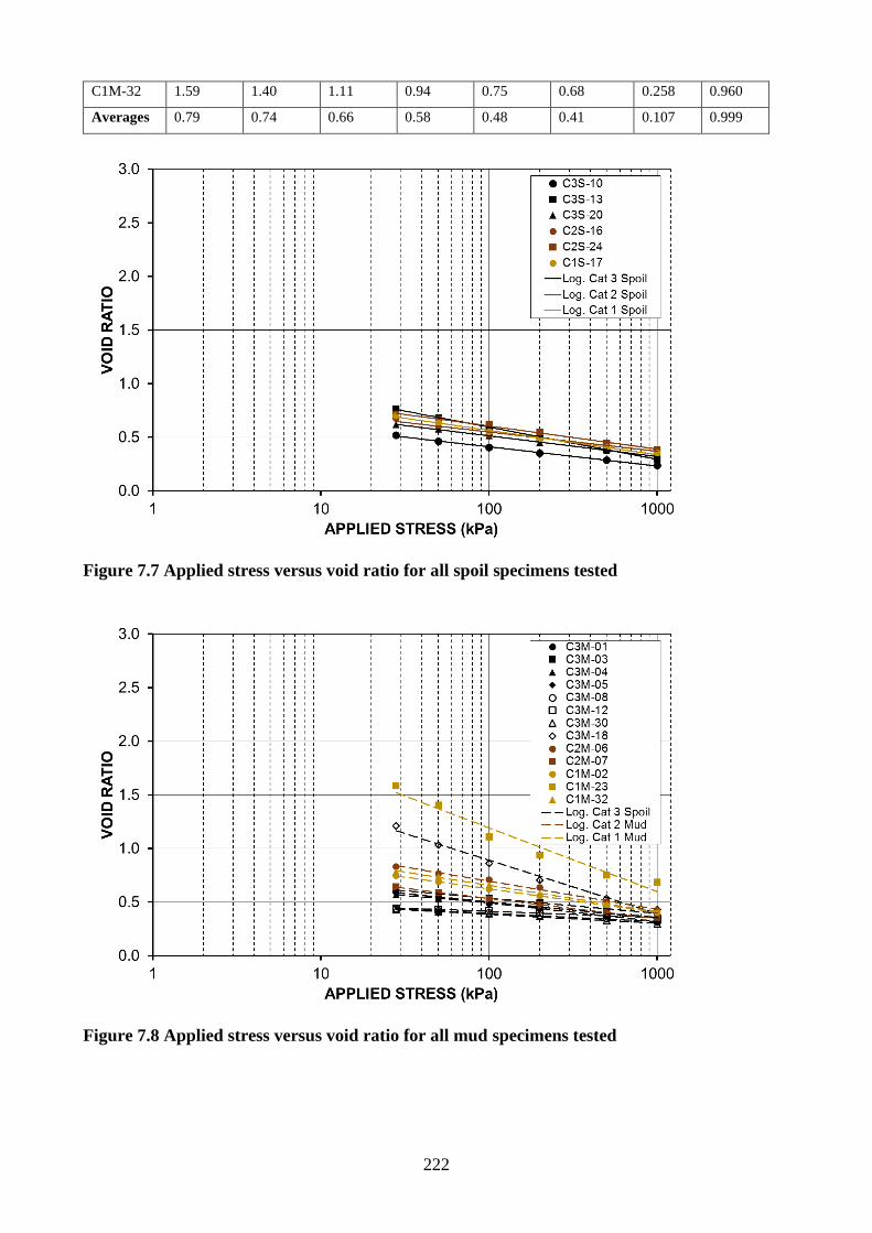
222
C1M-32 1.59 1.40 1.11 0.94 0.75 0.68 0.258 0.960
Averages 0.79 0.74 0.66 0.58 0.48 0.41 0.107 0.999
Figure 7.7 Applied stress versus void ratio for all spoil specimens tested
Figure 7.8 Applied stress versus void ratio for all mud specimens tested
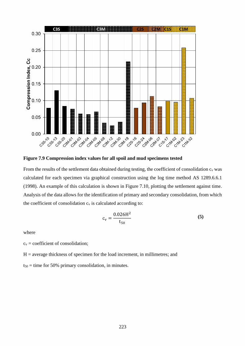
223
Figure 7.9 Compression index values for all spoil and mud specimens tested
From the results of the settlement data obtained during testing, the coefficient of consolidation cv was
calculated for each specimen via graphical construction using the log time method AS 1289.6.6.1
(1998). An example of this calculation is shown in Figure 7.10, plotting the settlement against time.
Analysis of the data allows for the identification of primary and secondary consolidation, from which
the coefficient of consolidation cv is calculated according to:
cv =
0.026H2
t50 (5)
where
cv = coefficient of consolidation;
H = average thickness of specimen for the load increment, in millimetres; and
t50 = time for 50% primary consolidation, in minutes.
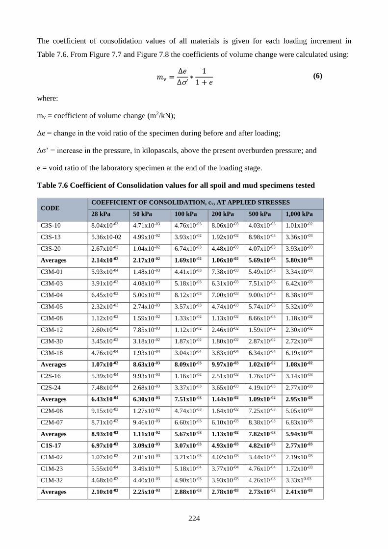
224
The coefficient of consolidation values of all materials is given for each loading increment in
Table 7.6. From Figure 7.7 and Figure 7.8 the coefficients of volume change were calculated using:
𝑚v =
∆𝑒
∆’∗
1
1 + 𝑒 (6)
where:
mv = coefficient of volume change (m2/kN);
∆e = change in the void ratio of the specimen during before and after loading;
∆σ’ = increase in the pressure, in kilopascals, above the present overburden pressure; and
e = void ratio of the laboratory specimen at the end of the loading stage.
Table 7.6 Coefficient of Consolidation values for all spoil and mud specimens tested
CODE COEFFICIENT OF CONSOLIDATION, cv, AT APPLIED STRESSES
28 kPa 50 kPa 100 kPa 200 kPa 500 kPa 1,000 kPa
C3S-10 8.04x10-03 4.71x10-03 4.76x10-03 8.06x10-03 4.03x10-03 1.01x10-02
C3S-13 5.36x10-02 4.99x10-02 3.93x10-02 1.92x10-02 8.98x10-03 3.36x10-03
C3S-20 2.67x10-03 1.04x10-02 6.74x10-03 4.48x10-03 4.07x10-03 3.93x10-03
Averages 2.14x10-02 2.17x10-02 1.69x10-02 1.06x10-02 5.69x10-03 5.80x10-03
C3M-01 5.93x10-04 1.48x10-03 4.41x10-03 7.38x10-03 5.49x10-03 3.34x10-03
C3M-03 3.91x10-03 4.08x10-03 5.18x10-03 6.31x10-03 7.51x10-03 6.42x10-03
C3M-04 6.45x10-03 5.00x10-03 8.12x10-03 7.00x10-03 9.00x10-03 8.38x10-03
C3M-05 2.32x10-03 2.74x10-03 3.57x10-03 4.74x10-03 5.74x10-03 5.32x10-03
C3M-08 1.12x10-02 1.59x10-02 1.33x10-02 1.13x10-02 8.66x10-03 1.18x10-02
C3M-12 2.60x10-02 7.85x10-03 1.12x10-02 2.46x10-02 1.59x10-02 2.30x10-02
C3M-30 3.45x10-02 3.18x10-02 1.87x10-02 1.80x10-02 2.87x10-02 2.72x10-02
C3M-18 4.76x10-04 1.93x10-04 3.04x10-04 3.83x10-04 6.34x10-04 6.19x10-04
Averages 1.07x10-02 8.63x10-03 8.09x10-03 9.97x10-03 1.02x10-02 1.08x10-02
C2S-16 5.39x10-04 9.93x10-03 1.16x10-02 2.51x10-02 1.76x10-02 3.14x10-03
C2S-24 7.48x10-04 2.68x10-03 3.37x10-03 3.65x10-03 4.19x10-03 2.77x10-03
Averages 6.43x10-04 6.30x10-03 7.51x10-03 1.44x10-02 1.09x10-02 2.95x10-03
C2M-06 9.15x10-03 1.27x10-02 4.74x10-03 1.64x10-02 7.25x10-03 5.05x10-03
C2M-07 8.71x10-03 9.46x10-03 6.60x10-03 6.10x10-03 8.38x10-03 6.83x10-03
Averages 8.93x10-03 1.11x10-02 5.67x10-03 1.13x10-02 7.82x10-03 5.94x10-03
C1S-17 6.97x10-03 3.09x10-03 3.07x10-03 4.93x10-03 4.82x10-03 2.77x10-03
C1M-02 1.07x10-03 2.01x10-03 3.21x10-03 4.02x10-03 3.44x10-03 2.19x10-03
C1M-23 5.55x10-04 3.49x10-04 5.18x10-04 3.77x10-04 4.76x10-04 1.72x10-03
C1M-32 4.68x10-03 4.40x10-03 4.90x10-03 3.93x10-03 4.26x10-03 3.33x10-03
Averages 2.10x10-03 2.25x10-03 2.88x10-03 2.78x10-03 2.73x10-03 2.41x10-03
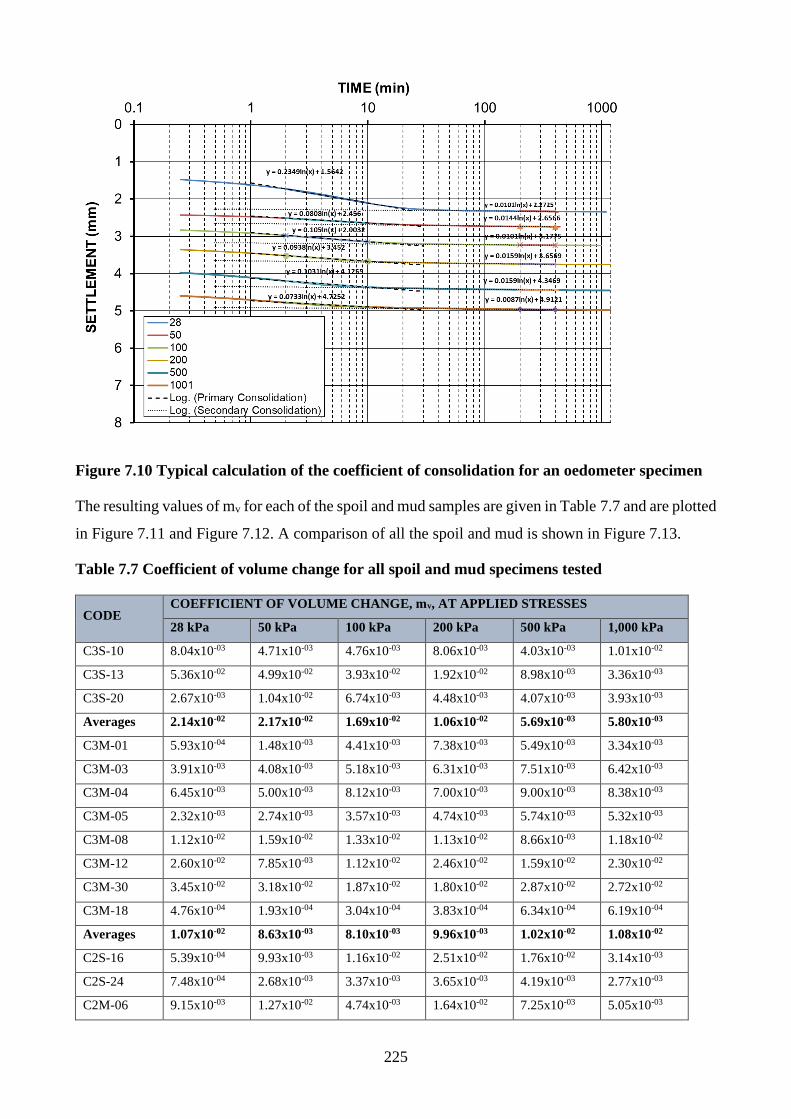
225
Figure 7.10 Typical calculation of the coefficient of consolidation for an oedometer specimen
The resulting values of mv for each of the spoil and mud samples are given in Table 7.7 and are plotted
in Figure 7.11 and Figure 7.12. A comparison of all the spoil and mud is shown in Figure 7.13.
Table 7.7 Coefficient of volume change for all spoil and mud specimens tested
CODE COEFFICIENT OF VOLUME CHANGE, mv, AT APPLIED STRESSES
28 kPa 50 kPa 100 kPa 200 kPa 500 kPa 1,000 kPa
C3S-10 8.04x10-03 4.71x10-03 4.76x10-03 8.06x10-03 4.03x10-03 1.01x10-02
C3S-13 5.36x10-02 4.99x10-02 3.93x10-02 1.92x10-02 8.98x10-03 3.36x10-03
C3S-20 2.67x10-03 1.04x10-02 6.74x10-03 4.48x10-03 4.07x10-03 3.93x10-03
Averages 2.14x10-02 2.17x10-02 1.69x10-02 1.06x10-02 5.69x10-03 5.80x10-03
C3M-01 5.93x10-04 1.48x10-03 4.41x10-03 7.38x10-03 5.49x10-03 3.34x10-03
C3M-03 3.91x10-03 4.08x10-03 5.18x10-03 6.31x10-03 7.51x10-03 6.42x10-03
C3M-04 6.45x10-03 5.00x10-03 8.12x10-03 7.00x10-03 9.00x10-03 8.38x10-03
C3M-05 2.32x10-03 2.74x10-03 3.57x10-03 4.74x10-03 5.74x10-03 5.32x10-03
C3M-08 1.12x10-02 1.59x10-02 1.33x10-02 1.13x10-02 8.66x10-03 1.18x10-02
C3M-12 2.60x10-02 7.85x10-03 1.12x10-02 2.46x10-02 1.59x10-02 2.30x10-02
C3M-30 3.45x10-02 3.18x10-02 1.87x10-02 1.80x10-02 2.87x10-02 2.72x10-02
C3M-18 4.76x10-04 1.93x10-04 3.04x10-04 3.83x10-04 6.34x10-04 6.19x10-04
Averages 1.07x10-02 8.63x10-03 8.10x10-03 9.96x10-03 1.02x10-02 1.08x10-02
C2S-16 5.39x10-04 9.93x10-03 1.16x10-02 2.51x10-02 1.76x10-02 3.14x10-03
C2S-24 7.48x10-04 2.68x10-03 3.37x10-03 3.65x10-03 4.19x10-03 2.77x10-03
C2M-06 9.15x10-03 1.27x10-02 4.74x10-03 1.64x10-02 7.25x10-03 5.05x10-03
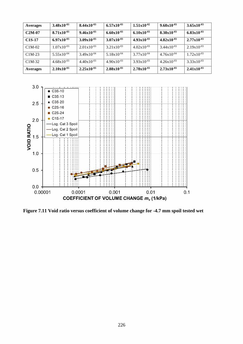
226
Averages 3.48x10-03 8.44x10-03 6.57x10-03 1.51x10-02 9.68x10-03 3.65x10-03
C2M-07 8.71x10-03 9.46x10-03 6.60x10-03 6.10x10-03 8.38x10-03 6.83x10-03
C1S-17 6.97x10-03 3.09x10-03 3.07x10-03 4.93x10-03 4.82x10-03 2.77x10-03
C1M-02 1.07x10-03 2.01x10-03 3.21x10-03 4.02x10-03 3.44x10-03 2.19x10-03
C1M-23 5.55x10-04 3.49x10-04 5.18x10-04 3.77x10-04 4.76x10-04 1.72x10-03
C1M-32 4.68x10-03 4.40x10-03 4.90x10-03 3.93x10-03 4.26x10-03 3.33x10-03
Averages 2.10x10-03 2.25x10-03 2.88x10-03 2.78x10-03 2.73x10-03 2.41x10-03
Figure 7.11 Void ratio versus coefficient of volume change for -4.7 mm spoil tested wet
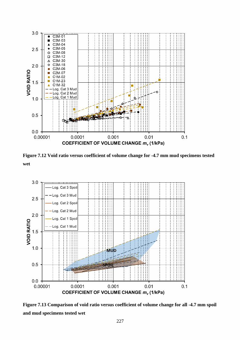
227
Figure 7.12 Void ratio versus coefficient of volume change for -4.7 mm mud specimens tested
wet
Figure 7.13 Comparison of void ratio versus coefficient of volume change for all -4.7 mm spoil
and mud specimens tested wet
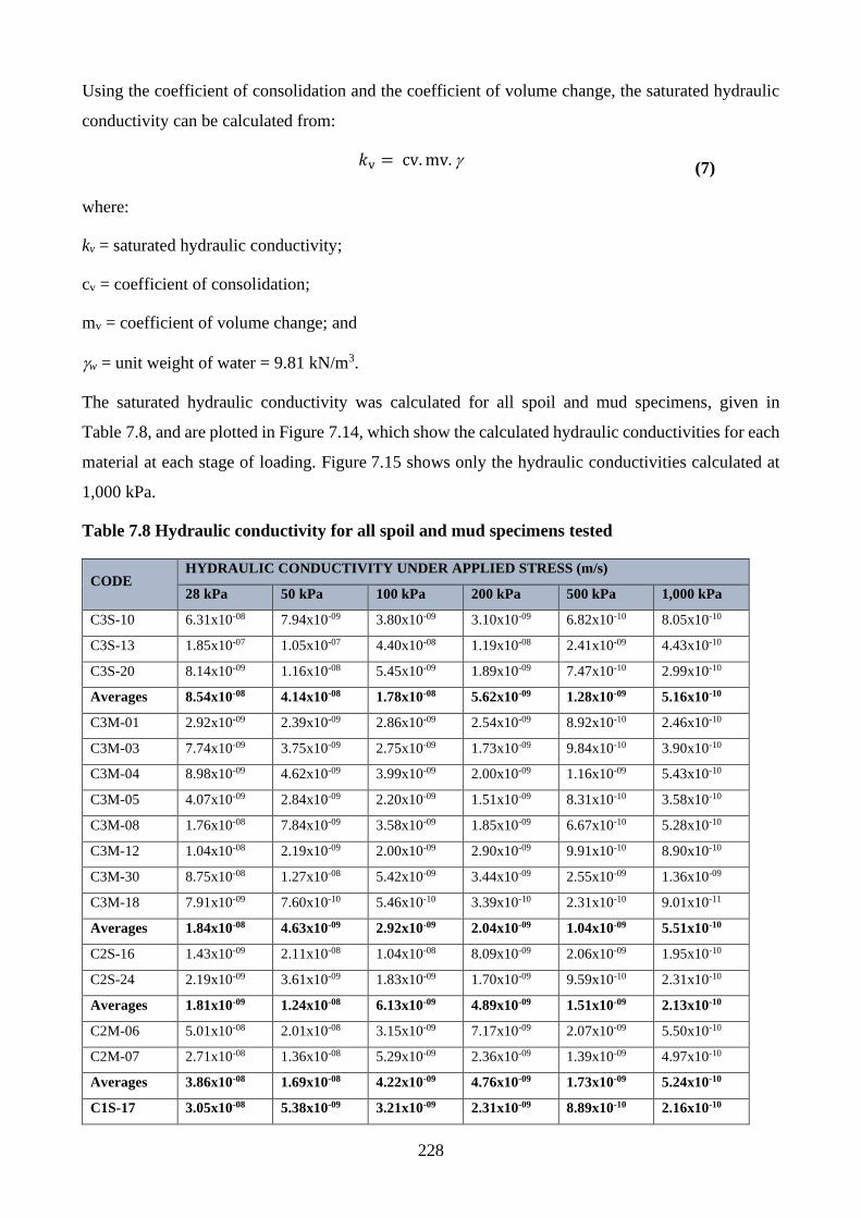
228
Using the coefficient of consolidation and the coefficient of volume change, the saturated hydraulic
conductivity can be calculated from:
𝑘v = cv. mv. (7)
where:
kv = saturated hydraulic conductivity;
cv = coefficient of consolidation;
mv = coefficient of volume change; and
w = unit weight of water = 9.81 kN/m3.
The saturated hydraulic conductivity was calculated for all spoil and mud specimens, given in
Table 7.8, and are plotted in Figure 7.14, which show the calculated hydraulic conductivities for each
material at each stage of loading. Figure 7.15 shows only the hydraulic conductivities calculated at
1,000 kPa.
Table 7.8 Hydraulic conductivity for all spoil and mud specimens tested
CODE HYDRAULIC CONDUCTIVITY UNDER APPLIED STRESS (m/s)
28 kPa 50 kPa 100 kPa 200 kPa 500 kPa 1,000 kPa
C3S-10 6.31x10-08 7.94x10-09 3.80x10-09 3.10x10-09 6.82x10⁻¹⁰ 8.05x10⁻¹⁰
C3S-13 1.85x10-07 1.05x10-07 4.40x10-08 1.19x10-08 2.41x10-09 4.43x10⁻¹⁰
C3S-20 8.14x10-09 1.16x10-08 5.45x10-09 1.89x10-09 7.47x10⁻¹⁰ 2.99x10⁻¹⁰
Averages 8.54x10-08 4.14x10-08 1.78x10-08 5.62x10-09 1.28x10-09 5.16x10⁻¹⁰
C3M-01 2.92x10-09 2.39x10-09 2.86x10-09 2.54x10-09 8.92x10⁻¹⁰ 2.46x10⁻¹⁰
C3M-03 7.74x10-09 3.75x10-09 2.75x10-09 1.73x10-09 9.84x10⁻¹⁰ 3.90x10⁻¹⁰
C3M-04 8.98x10-09 4.62x10-09 3.99x10-09 2.00x10-09 1.16x10-09 5.43x10⁻¹⁰
C3M-05 4.07x10-09 2.84x10-09 2.20x10-09 1.51x10-09 8.31x10⁻¹⁰ 3.58x10⁻¹⁰
C3M-08 1.76x10-08 7.84x10-09 3.58x10-09 1.85x10-09 6.67x10⁻¹⁰ 5.28x10⁻¹⁰
C3M-12 1.04x10-08 2.19x10-09 2.00x10-09 2.90x10-09 9.91x10⁻¹⁰ 8.90x10⁻¹⁰
C3M-30 8.75x10-08 1.27x10-08 5.42x10-09 3.44x10-09 2.55x10-09 1.36x10-09
C3M-18 7.91x10-09 7.60x10⁻¹⁰ 5.46x10⁻¹⁰ 3.39x10⁻¹⁰ 2.31x10⁻¹⁰ 9.01x10⁻¹¹
Averages 1.84x10-08 4.63x10-09 2.92x10-09 2.04x10-09 1.04x10-09 5.51x10⁻¹⁰
C2S-16 1.43x10-09 2.11x10-08 1.04x10-08 8.09x10-09 2.06x10-09 1.95x10⁻¹⁰
C2S-24 2.19x10-09 3.61x10-09 1.83x10-09 1.70x10-09 9.59x10⁻¹⁰ 2.31x10⁻¹⁰
Averages 1.81x10-09 1.24x10-08 6.13x10-09 4.89x10-09 1.51x10-09 2.13x10⁻¹⁰
C2M-06 5.01x10-08 2.01x10-08 3.15x10-09 7.17x10-09 2.07x10-09 5.50x10⁻¹⁰
C2M-07 2.71x10-08 1.36x10-08 5.29x10-09 2.36x10-09 1.39x10-09 4.97x10⁻¹⁰
Averages 3.86x10-08 1.69x10-08 4.22x10-09 4.76x10-09 1.73x10-09 5.24x10⁻¹⁰
C1S-17 3.05x10-08 5.38x10-09 3.21x10-09 2.31x10-09 8.89x10⁻¹⁰ 2.16x10⁻¹⁰
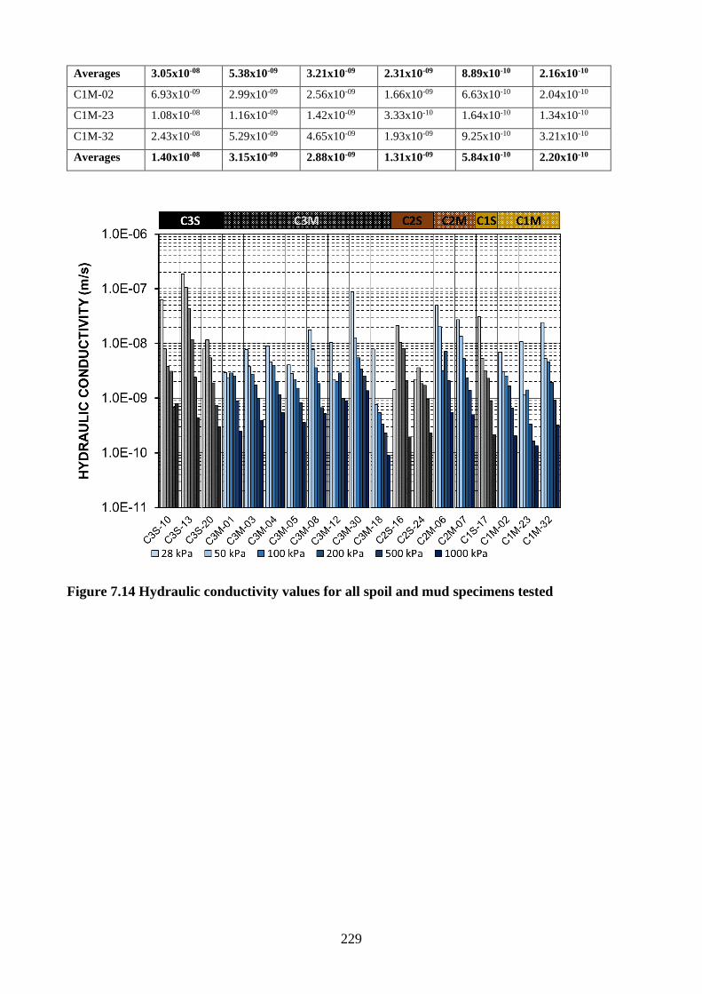
229
Averages 3.05x10-08 5.38x10-09 3.21x10-09 2.31x10-09 8.89x10⁻¹⁰ 2.16x10⁻¹⁰
C1M-02 6.93x10-09 2.99x10-09 2.56x10-09 1.66x10-09 6.63x10⁻¹⁰ 2.04x10⁻¹⁰
C1M-23 1.08x10-08 1.16x10-09 1.42x10-09 3.33x10⁻¹⁰ 1.64x10⁻¹⁰ 1.34x10⁻¹⁰
C1M-32 2.43x10-08 5.29x10-09 4.65x10-09 1.93x10-09 9.25x10⁻¹⁰ 3.21x10⁻¹⁰
Averages 1.40x10-08 3.15x10-09 2.88x10-09 1.31x10-09 5.84x10⁻¹⁰ 2.20x10⁻¹⁰
Figure 7.14 Hydraulic conductivity values for all spoil and mud specimens tested
230
Figure 7.15 Hydraulic conductivity at 1,000 kPa applied stress for all spoil and mud
specimens tested
From the materials tested, a large range of results for hydraulic conductivity were obtained. The
conductivities of all materials ranged from 1.4x10-09 to 0.9x10⁻¹¹ m/s, with values for both C3M-18
and C3M-23 being particularly low. At 1,000 kPa, the Category 3 spoil had higher hydraulic
conductivities than the Category 2 or 1 spoil materials. The Category 3 and 2 muds had similar values,
with slightly lower averages for the Category 1 mud.
It is important to note that these calculations are based off samples sieved to -2.36 mm. Based on the
material characterisation in Section 5.1.4, the coarser particles with the Category 3 spoil and mud
materials would have a large influence on the hydraulic conductivity of the material in situ.
7.1.1 Discussion and conclusions of consolidometer test results
All spoil and mud materials collected in situ were tested using a standard consolidometer. Each
specimen was soaked for 24 hours before consolidation. Initial dry densities of all spoil specimens
ranged from 1.3 to 1.5 t/m3 prior to consolidation, and from 1.9 to 2.0 t/m3 under an applied stress of
1,000 kPa. The lowest final void ratios were obtained by the Category 3 spoil. The same relationship
is seen reflected in the final moisture contents measured.
For the mud materials tested, the initial dry density mostly ranged from 1.3 to 1.6 t/m3, with the lowest
values for the Category 1 mud samples. C3M-18 and C1M-23 were both significant outliers with very
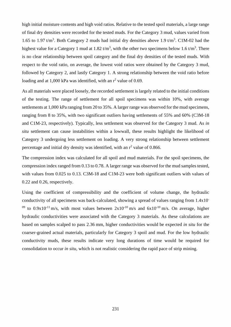
231
high initial moisture contents and high void ratios. Relative to the tested spoil materials, a large range
of final dry densities were recorded for the tested muds. For the Category 3 mud, values varied from
1.65 to 1.97 t/m3. Both Category 2 muds had initial dry densities above 1.9 t/m3. C1M-02 had the
highest value for a Category 1 mud at 1.82 t/m3, with the other two specimens below 1.6 t/m3. There
is no clear relationship between spoil category and the final dry densities of the tested muds. With
respect to the void ratio, on average, the lowest void ratios were obtained by the Category 3 mud,
followed by Category 2, and lastly Category 1. A strong relationship between the void ratio before
loading and at 1,000 kPa was identified, with an r2 value of 0.69.
As all materials were placed loosely, the recorded settlement is largely related to the initial conditions
of the testing. The range of settlement for all spoil specimens was within 10%, with average
settlements at 1,000 kPa ranging from 20 to 35%. A larger range was observed for the mud specimens,
ranging from 8 to 35%, with two significant outliers having settlements of 55% and 60% (C3M-18
and C1M-23, respectively). Typically, less settlement was observed for the Category 3 mud. As in
situ settlement can cause instabilities within a lowwall, these results highlight the likelihood of
Category 3 undergoing less settlement on loading. A very strong relationship between settlement
percentage and initial dry density was identified, with an r2 value of 0.866.
The compression index was calculated for all spoil and mud materials. For the spoil specimens, the
compression index ranged from 0.13 to 0.78. A larger range was observed for the mud samples tested,
with values from 0.025 to 0.13. C3M-18 and C1M-23 were both significant outliers with values of
0.22 and 0.26, respectively.
Using the coefficient of compressibility and the coefficient of volume change, the hydraulic
conductivity of all specimens was back-calculated, showing a spread of values ranging from 1.4x10-
09 to 0.9x10⁻¹¹ m/s, with most values between 2x10⁻¹⁰ m/s and 6x10⁻¹⁰ m/s. On average, higher
hydraulic conductivities were associated with the Category 3 materials. As these calculations are
based on samples scalped to pass 2.36 mm, higher conductivities would be expected in situ for the
coarser-grained actual materials, particularly for Category 3 spoil and mud. For the low hydraulic
conductivity muds, these results indicate very long durations of time would be required for
consolidation to occur in situ, which is not realistic considering the rapid pace of strip mining.
232
7.2 Large Slurry Consolidometer Test Results
Conventional consolidation equipment such as the standard consolidometer or Rowe cell are unable
to adequately handle slurry-like material. The standard consolidometer uses a thin specimen with a
height of 20 mm, loaded vertically. To load these specimens, a loading cap must be placed on top.
For a slurry, there is inadequate strength in the specimen to maintain the weight of the loading cap.
The Rowe cell can test slurry-like soils during consolidation; however, it has several limitations.
During consolidation, it is important to maintain a level surface. This can be difficult using a Rowe
cell as deformation of the specimen’s centre can cause bowing in the porous disk. It is also limited in
height, making it difficult to test slurries with high moisture contents (Umehara & Zen 1980).
Due to these limitations and for the recording of the desired measurements, a purpose-built large
slurry consolidometer was used to analyse a select number of muds during consolidation. A schematic
of the large slurry consolidometer was provided in Section 4.10.2, with design details and
methodology discussed. For this testing, drainage was only allowed from the top of the cell to
simulate upward drainage of the mud sitting on an impermeable pit floor. A loading rate of
0.1 kPa/min was applied, up to a maximum stress of 500 kPa. For each test, measurements of the
applied stress, stress measured at the base, pore water pressure readings along the column and at the
base, and settlement were taken.
While the applied stress and the stress at the base were recorded, the distribution of stress down the
length of the specimen is unknown, although the measured pore water pressures give some indication.
The average stress can be estimated using Equations (8) and (9):
σavg =σt − σb
2 (8)
σavg = σb +
1
3∗ (σt − σb) (9)
where:
σavg = the average stress within the specimen;
σt = the applied stress at the top of the specimen; and
σb = the measured stress at the base of the specimen.
Equations (8) and (9) assume linear and parabolic stress distributions within the specimen,
respectively. As drainage is only allowed from the top of the specimen, it is therefore assumed that
the closest fit is obtained using Equation (9). To determine the average effective stress, the following
equation was used:
233
σ′avg = σ𝑎𝑣𝑔 − 𝛽. 𝑢𝑏 (10)
where:
σ’avg = the average effective stress within the specimen;
β = average pore water pressure/pore water pressure at the base of the specimen; and
ub = measured pore water pressure at the base of the specimen.
For the calculations of average effective stress, several authors have suggested suitable values of β.
For the purposes of this research, values suggested by Janbu et al. (1980 and Leroueil et al. (1985)
were used to calculate the following conditions:
β = 0.67 if ub/σavg < 0.40;
β = 0.63+0.1×ub/σavg if 0.40 < ub/σavg <0.70;
β = 0.5409+0.2273×ub/σavg if 0.70 < ub/σavg <0.9.2; and
β = 0.75 if ub/σavg < 0.92.
Wall friction is usually ignored when the height to diameter ratio is greater than 0.4. The dimensions
of the large slurry consolidometer result in a height to diameter ratio of 2. It is important to consider
wall friction in the analysis of the test results. The loss of applied stress due to friction between the
piston and specimen and the wall was calculated using:
𝜇 = σt − σb (11)
μ = friction along the wall
σt = the applied stress at the top of the specimen
σb = the measured stress at the base of the specimen
The hydraulic conductivity of each specimen was calculated. Due to the constant rate of loading,
analysis of the hydraulic conductivity cannot be calculated using the standard method applied in
standard consolidation testing. Instead, the method proposed by Davison & Atkinson (1990) was
used:
𝑘 = (
𝑤
∗ 𝐻
2 ∗ 𝑢ℎ ) . (
∆ℎ
∆𝑡) (12)
where:
k = the hydraulic conductivity of the specimen;
γw = the unit weight of water;
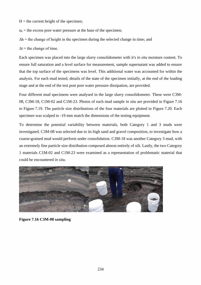
234
H = the current height of the specimen;
uh = the excess pore water pressure at the base of the specimen;
∆h = the change of height in the specimen during the selected change in time; and
∆t = the change of time.
Each specimen was placed into the large slurry consolidometer with it's in situ moisture content. To
ensure full saturation and a level surface for measurement, sample supernatant was added to ensure
that the top surface of the specimens was level. This additional water was accounted for within the
analysis. For each mud tested, details of the state of the specimen initially, at the end of the loading
stage and at the end of the test post pore water pressure dissipation, are provided.
Four different mud specimens were analysed in the large slurry consolidometer. These were C3M-
08, C3M-18, C1M-02 and C1M-23. Photos of each mud sample in situ are provided in Figure 7.16
to Figure 7.19. The particle size distributions of the four materials are plotted in Figure 7.20. Each
specimen was scalped to -19 mm match the dimensions of the testing equipment.
To determine the potential variability between materials, both Category 1 and 3 muds were
investigated. C3M-08 was selected due to its high sand and gravel composition, to investigate how a
coarse-grained mud would perform under consolidation. C3M-18 was another Category 3 mud, with
an extremely fine particle size distribution composed almost entirely of silt. Lastly, the two Category
1 materials C1M-02 and C1M-23 were examined as a representation of problematic material that
could be encountered in situ.
Figure 7.16 C3M-08 sampling
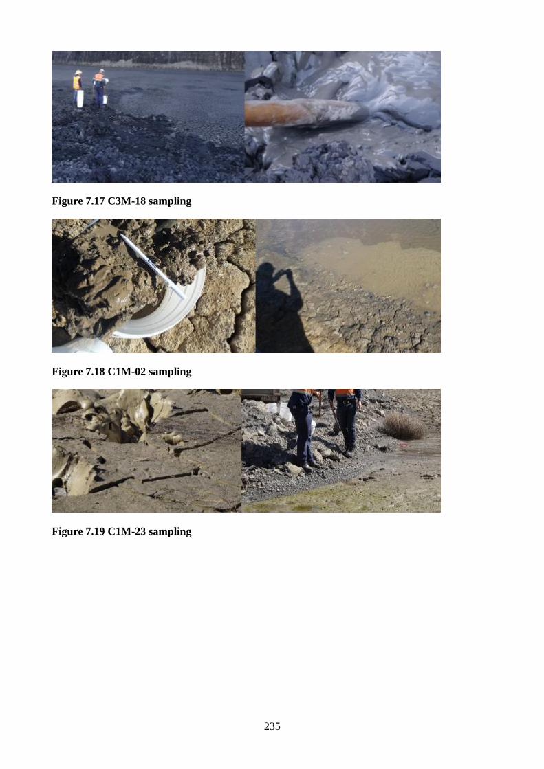
235
Figure 7.17 C3M-18 sampling
Figure 7.18 C1M-02 sampling
Figure 7.19 C1M-23 sampling
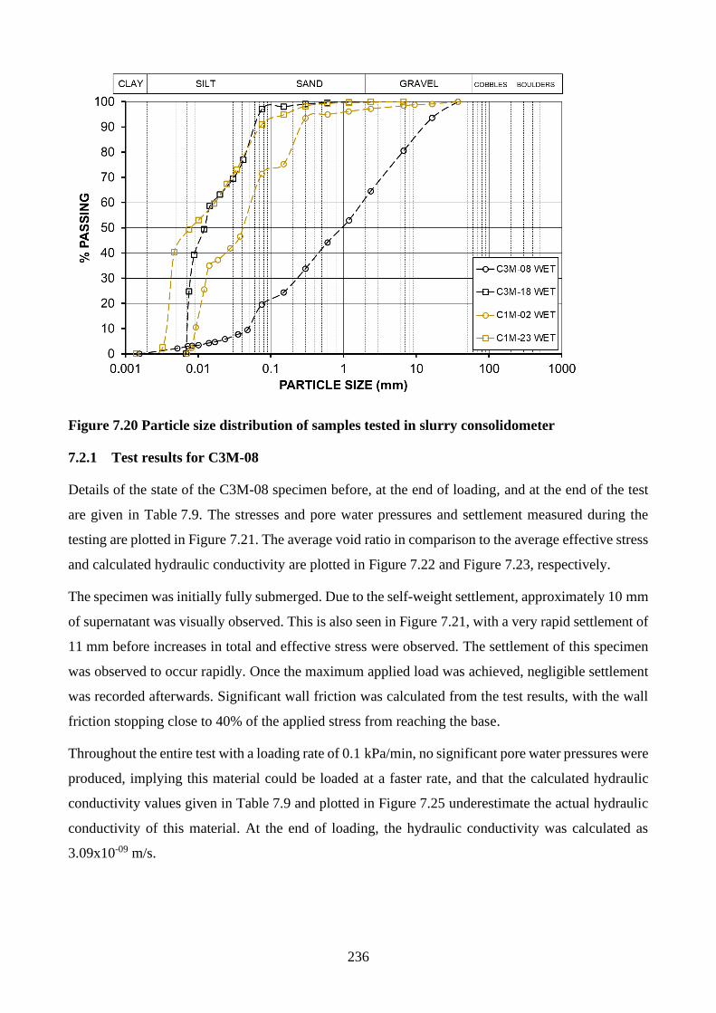
236
Figure 7.20 Particle size distribution of samples tested in slurry consolidometer
7.2.1 Test results for C3M-08
Details of the state of the C3M-08 specimen before, at the end of loading, and at the end of the test
are given in Table 7.9. The stresses and pore water pressures and settlement measured during the
testing are plotted in Figure 7.21. The average void ratio in comparison to the average effective stress
and calculated hydraulic conductivity are plotted in Figure 7.22 and Figure 7.23, respectively.
The specimen was initially fully submerged. Due to the self-weight settlement, approximately 10 mm
of supernatant was visually observed. This is also seen in Figure 7.21, with a very rapid settlement of
11 mm before increases in total and effective stress were observed. The settlement of this specimen
was observed to occur rapidly. Once the maximum applied load was achieved, negligible settlement
was recorded afterwards. Significant wall friction was calculated from the test results, with the wall
friction stopping close to 40% of the applied stress from reaching the base.
Throughout the entire test with a loading rate of 0.1 kPa/min, no significant pore water pressures were
produced, implying this material could be loaded at a faster rate, and that the calculated hydraulic
conductivity values given in Table 7.9 and plotted in Figure 7.25 underestimate the actual hydraulic
conductivity of this material. At the end of loading, the hydraulic conductivity was calculated as
3.09x10-09 m/s.
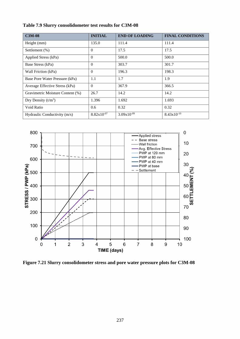
237
Table 7.9 Slurry consolidometer test results for C3M-08
C3M-08 INITIAL END OF LOADING FINAL CONDITIONS
Height (mm) 135.0 111.4 111.4
Settlement (%) 0 17.5 17.5
Applied Stress (kPa) 0 500.0 500.0
Base Stress (kPa) 0 303.7 301.7
Wall Friction (kPa) 0 196.3 198.3
Base Pore Water Pressure (kPa) 1.1 1.7 1.9
Average Effective Stress (kPa) 0 367.9 366.5
Gravimetric Moisture Content (%) 26.7 14.2 14.2
Dry Density (t/m3) 1.396 1.692 1.693
Void Ratio 0.6 0.32 0.32
Hydraulic Conductivity (m/s) 8.82x10-07 3.09x10-09 8.43x10⁻¹⁰
Figure 7.21 Slurry consolidometer stress and pore water pressure plots for C3M-08
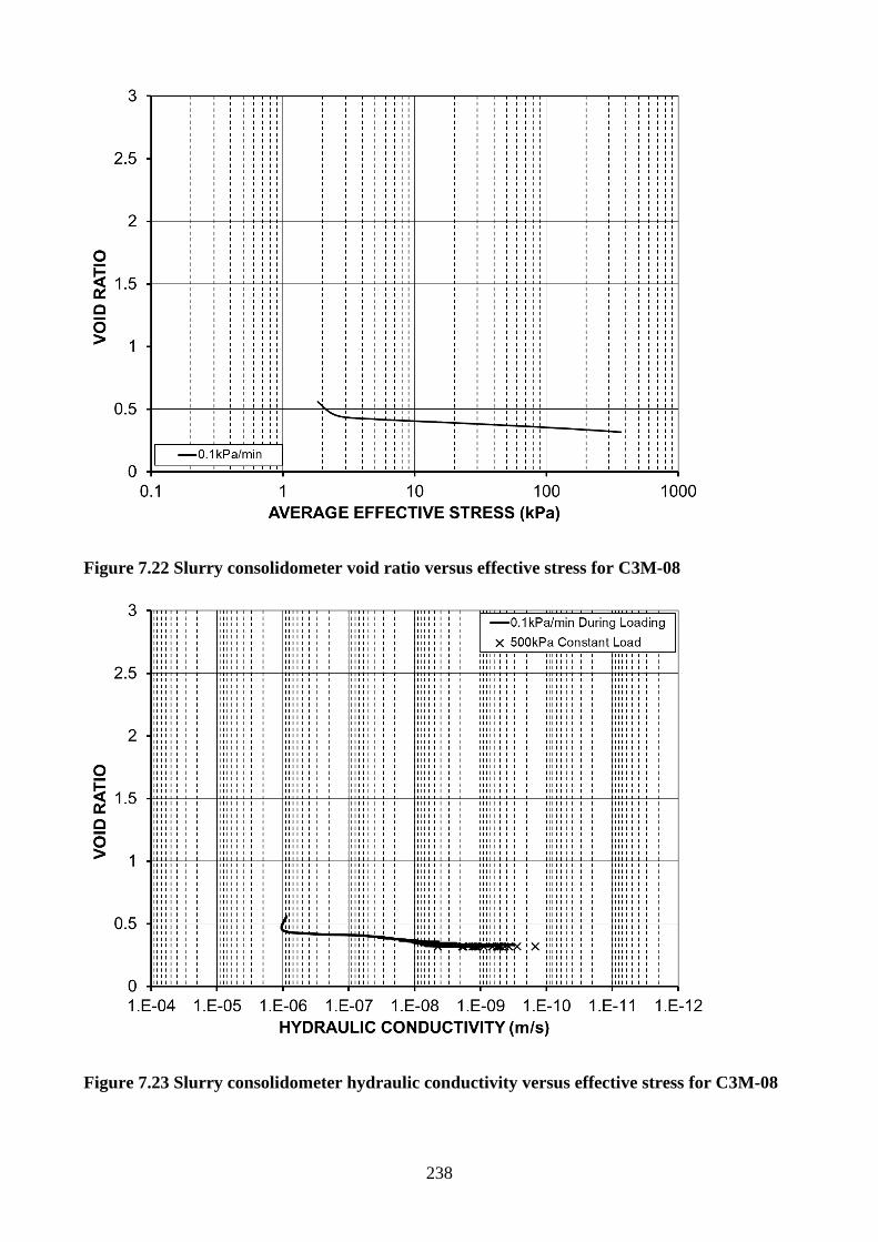
238
Figure 7.22 Slurry consolidometer void ratio versus effective stress for C3M-08
Figure 7.23 Slurry consolidometer hydraulic conductivity versus effective stress for C3M-08
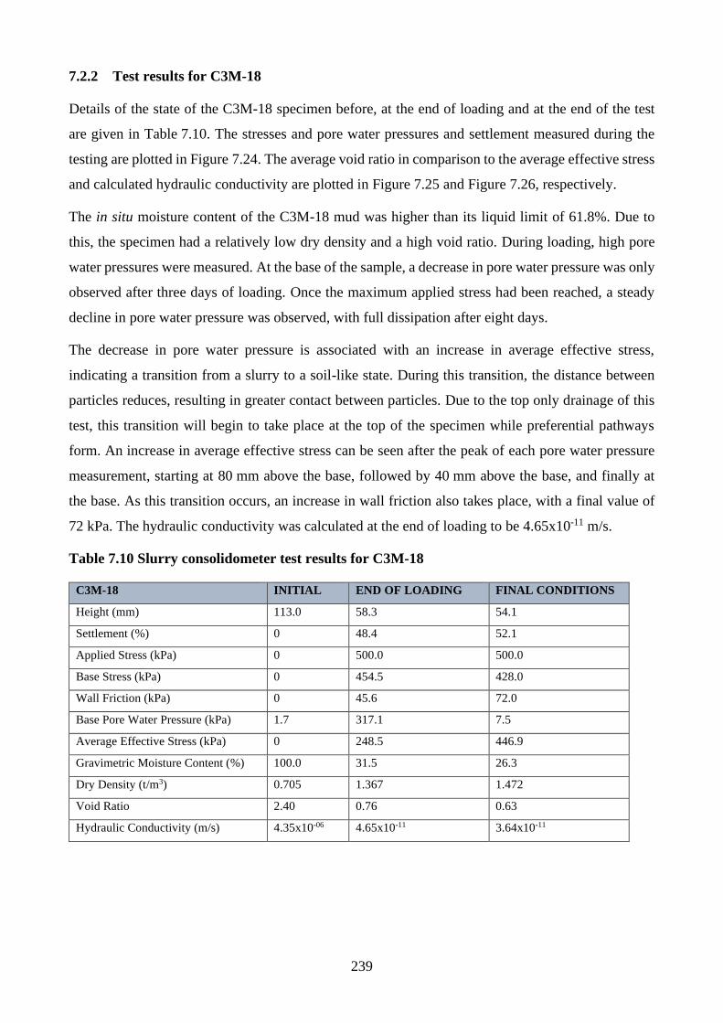
239
7.2.2 Test results for C3M-18
Details of the state of the C3M-18 specimen before, at the end of loading and at the end of the test
are given in Table 7.10. The stresses and pore water pressures and settlement measured during the
testing are plotted in Figure 7.24. The average void ratio in comparison to the average effective stress
and calculated hydraulic conductivity are plotted in Figure 7.25 and Figure 7.26, respectively.
The in situ moisture content of the C3M-18 mud was higher than its liquid limit of 61.8%. Due to
this, the specimen had a relatively low dry density and a high void ratio. During loading, high pore
water pressures were measured. At the base of the sample, a decrease in pore water pressure was only
observed after three days of loading. Once the maximum applied stress had been reached, a steady
decline in pore water pressure was observed, with full dissipation after eight days.
The decrease in pore water pressure is associated with an increase in average effective stress,
indicating a transition from a slurry to a soil-like state. During this transition, the distance between
particles reduces, resulting in greater contact between particles. Due to the top only drainage of this
test, this transition will begin to take place at the top of the specimen while preferential pathways
form. An increase in average effective stress can be seen after the peak of each pore water pressure
measurement, starting at 80 mm above the base, followed by 40 mm above the base, and finally at
the base. As this transition occurs, an increase in wall friction also takes place, with a final value of
72 kPa. The hydraulic conductivity was calculated at the end of loading to be 4.65x10⁻¹¹ m/s.
Table 7.10 Slurry consolidometer test results for C3M-18
C3M-18 INITIAL END OF LOADING FINAL CONDITIONS
Height (mm) 113.0 58.3 54.1
Settlement (%) 0 48.4 52.1
Applied Stress (kPa) 0 500.0 500.0
Base Stress (kPa) 0 454.5 428.0
Wall Friction (kPa) 0 45.6 72.0
Base Pore Water Pressure (kPa) 1.7 317.1 7.5
Average Effective Stress (kPa) 0 248.5 446.9
Gravimetric Moisture Content (%) 100.0 31.5 26.3
Dry Density (t/m3) 0.705 1.367 1.472
Void Ratio 2.40 0.76 0.63
Hydraulic Conductivity (m/s) 4.35x10-06 4.65x10⁻¹¹ 3.64x10⁻¹¹
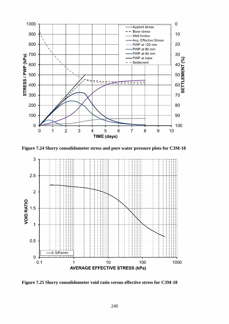
240
Figure 7.24 Slurry consolidometer stress and pore water pressure plots for C3M-18
Figure 7.25 Slurry consolidometer void ratio versus effective stress for C3M-18
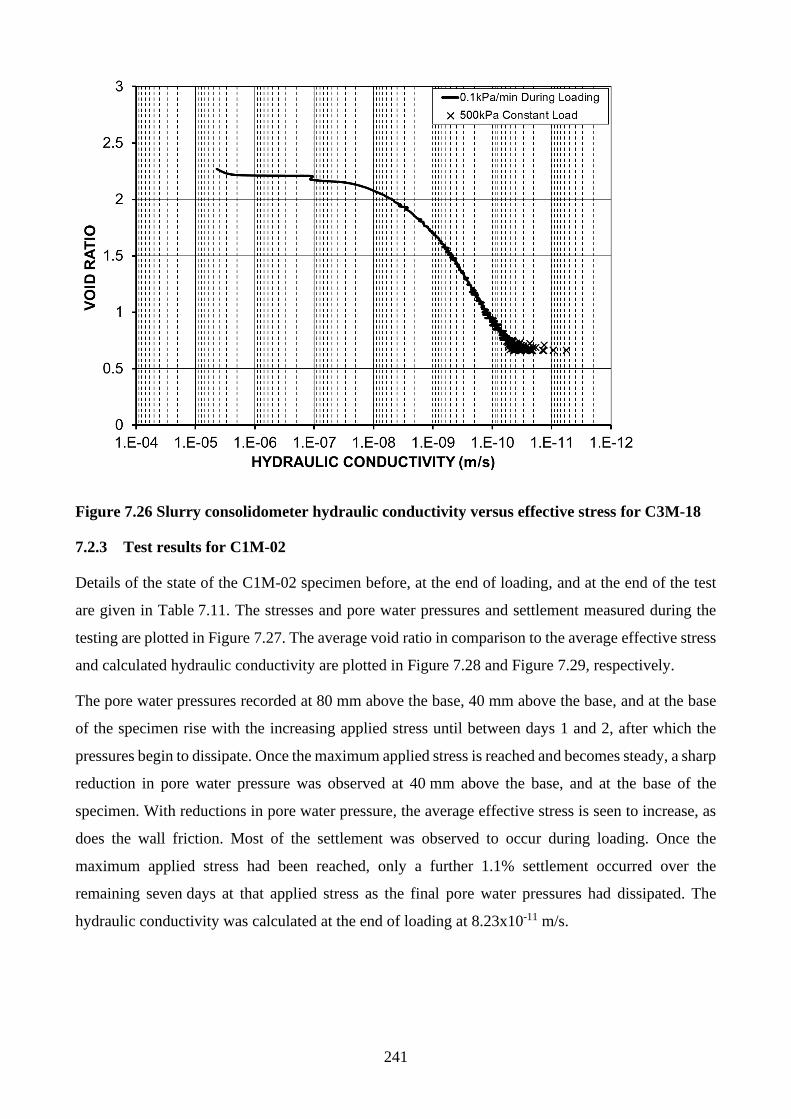
241
Figure 7.26 Slurry consolidometer hydraulic conductivity versus effective stress for C3M-18
7.2.3 Test results for C1M-02
Details of the state of the C1M-02 specimen before, at the end of loading, and at the end of the test
are given in Table 7.11. The stresses and pore water pressures and settlement measured during the
testing are plotted in Figure 7.27. The average void ratio in comparison to the average effective stress
and calculated hydraulic conductivity are plotted in Figure 7.28 and Figure 7.29, respectively.
The pore water pressures recorded at 80 mm above the base, 40 mm above the base, and at the base
of the specimen rise with the increasing applied stress until between days 1 and 2, after which the
pressures begin to dissipate. Once the maximum applied stress is reached and becomes steady, a sharp
reduction in pore water pressure was observed at 40 mm above the base, and at the base of the
specimen. With reductions in pore water pressure, the average effective stress is seen to increase, as
does the wall friction. Most of the settlement was observed to occur during loading. Once the
maximum applied stress had been reached, only a further 1.1% settlement occurred over the
remaining seven days at that applied stress as the final pore water pressures had dissipated. The
hydraulic conductivity was calculated at the end of loading at 8.23x10⁻¹¹ m/s.
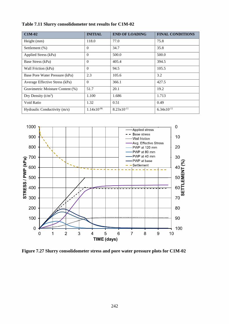
242
Table 7.11 Slurry consolidometer test results for C1M-02
C1M-02 INITIAL END OF LOADING FINAL CONDITIONS
Height (mm) 118.0 77.0 75.8
Settlement (%) 0 34.7 35.8
Applied Stress (kPa) 0 500.0 500.0
Base Stress (kPa) 0 405.4 394.5
Wall Friction (kPa) 0 94.5 105.5
Base Pore Water Pressure (kPa) 2.3 105.6 3.2
Average Effective Stress (kPa) 0 366.1 427.5
Gravimetric Moisture Content (%) 51.7 20.1 19.2
Dry Density (t/m3) 1.100 1.686 1.713
Void Ratio 1.32 0.51 0.49
Hydraulic Conductivity (m/s) 1.14x10-06 8.23x10⁻¹¹ 6.34x10⁻¹¹
Figure 7.27 Slurry consolidometer stress and pore water pressure plots for C1M-02
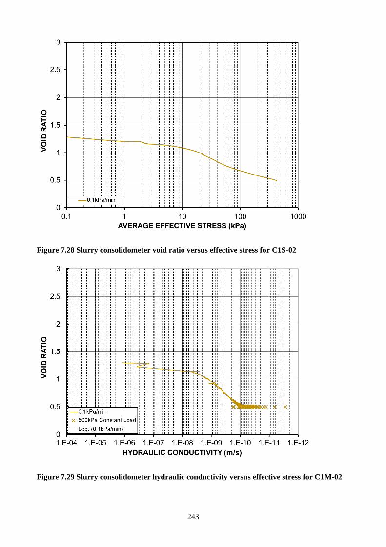
243
Figure 7.28 Slurry consolidometer void ratio versus effective stress for C1S-02
Figure 7.29 Slurry consolidometer hydraulic conductivity versus effective stress for C1M-02
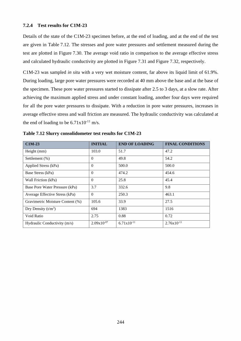
244
7.2.4 Test results for C1M-23
Details of the state of the C1M-23 specimen before, at the end of loading, and at the end of the test
are given in Table 7.12. The stresses and pore water pressures and settlement measured during the
test are plotted in Figure 7.30. The average void ratio in comparison to the average effective stress
and calculated hydraulic conductivity are plotted in Figure 7.31 and Figure 7.32, respectively.
C1M-23 was sampled in situ with a very wet moisture content, far above its liquid limit of 61.9%.
During loading, large pore water pressures were recorded at 40 mm above the base and at the base of
the specimen. These pore water pressures started to dissipate after 2.5 to 3 days, at a slow rate. After
achieving the maximum applied stress and under constant loading, another four days were required
for all the pore water pressures to dissipate. With a reduction in pore water pressures, increases in
average effective stress and wall friction are measured. The hydraulic conductivity was calculated at
the end of loading to be 6.71x10⁻¹¹ m/s.
Table 7.12 Slurry consolidometer test results for C1M-23
C1M-23 INITIAL END OF LOADING FINAL CONDITIONS
Height (mm) 103.0 51.7 47.2
Settlement (%) 0 49.8 54.2
Applied Stress (kPa) 0 500.0 500.0
Base Stress (kPa) 0 474.2 454.6
Wall Friction (kPa) 0 25.8 45.4
Base Pore Water Pressure (kPa) 3.7 332.6 9.8
Average Effective Stress (kPa) 0 250.3 463.1
Gravimetric Moisture Content (%) 105.6 33.9 27.5
Dry Density (t/m3) 694 1383 1516
Void Ratio 2.75 0.88 0.72
Hydraulic Conductivity (m/s) 2.09x10-07 6.71x10⁻¹¹ 2.76x10⁻¹¹
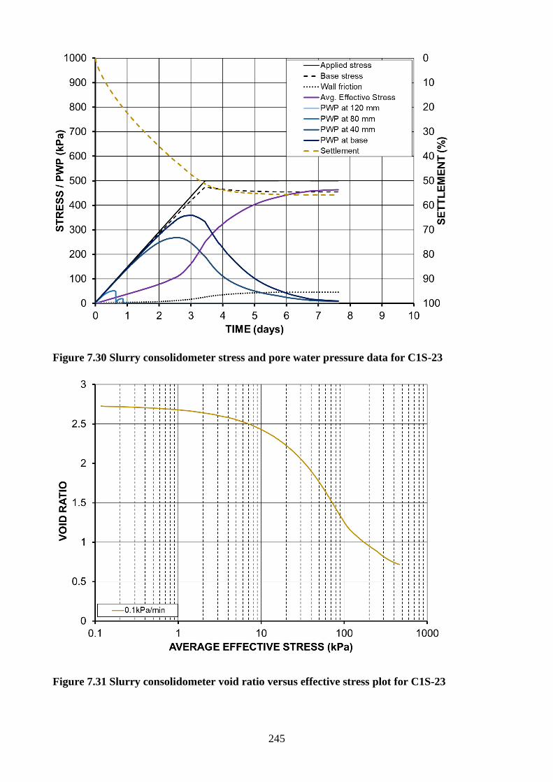
245
Figure 7.30 Slurry consolidometer stress and pore water pressure data for C1S-23
Figure 7.31 Slurry consolidometer void ratio versus effective stress plot for C1S-23
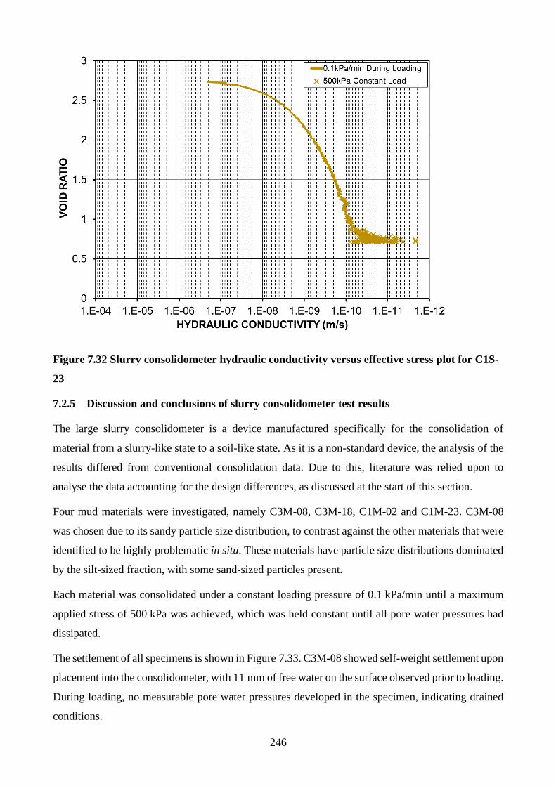
246
Figure 7.32 Slurry consolidometer hydraulic conductivity versus effective stress plot for C1S-
23
7.2.5 Discussion and conclusions of slurry consolidometer test results
The large slurry consolidometer is a device manufactured specifically for the consolidation of
material from a slurry-like state to a soil-like state. As it is a non-standard device, the analysis of the
results differed from conventional consolidation data. Due to this, literature was relied upon to
analyse the data accounting for the design differences, as discussed at the start of this section.
Four mud materials were investigated, namely C3M-08, C3M-18, C1M-02 and C1M-23. C3M-08
was chosen due to its sandy particle size distribution, to contrast against the other materials that were
identified to be highly problematic in situ. These materials have particle size distributions dominated
by the silt-sized fraction, with some sand-sized particles present.
Each material was consolidated under a constant loading pressure of 0.1 kPa/min until a maximum
applied stress of 500 kPa was achieved, which was held constant until all pore water pressures had
dissipated.
The settlement of all specimens is shown in Figure 7.33. C3M-08 showed self-weight settlement upon
placement into the consolidometer, with 11 mm of free water on the surface observed prior to loading.
During loading, no measurable pore water pressures developed in the specimen, indicating drained
conditions.
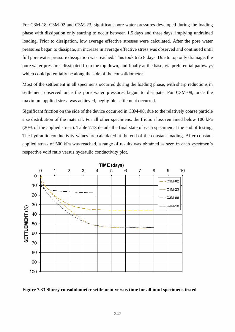
247
For C3M-18, C3M-02 and C3M-23, significant pore water pressures developed during the loading
phase with dissipation only starting to occur between 1.5 days and three days, implying undrained
loading. Prior to dissipation, low average effective stresses were calculated. After the pore water
pressures began to dissipate, an increase in average effective stress was observed and continued until
full pore water pressure dissipation was reached. This took 6 to 8 days. Due to top only drainage, the
pore water pressures dissipated from the top down, and finally at the base, via preferential pathways
which could potentially be along the side of the consolidometer.
Most of the settlement in all specimens occurred during the loading phase, with sharp reductions in
settlement observed once the pore water pressures begun to dissipate. For C3M-08, once the
maximum applied stress was achieved, negligible settlement occurred.
Significant friction on the side of the device occurred in C3M-08, due to the relatively coarse particle
size distribution of the material. For all other specimens, the friction loss remained below 100 kPa
(20% of the applied stress). Table 7.13 details the final state of each specimen at the end of testing.
The hydraulic conductivity values are calculated at the end of the constant loading. After constant
applied stress of 500 kPa was reached, a range of results was obtained as seen in each specimen’s
respective void ratio versus hydraulic conductivity plot.
Figure 7.33 Slurry consolidometer settlement versus time for all mud specimens tested
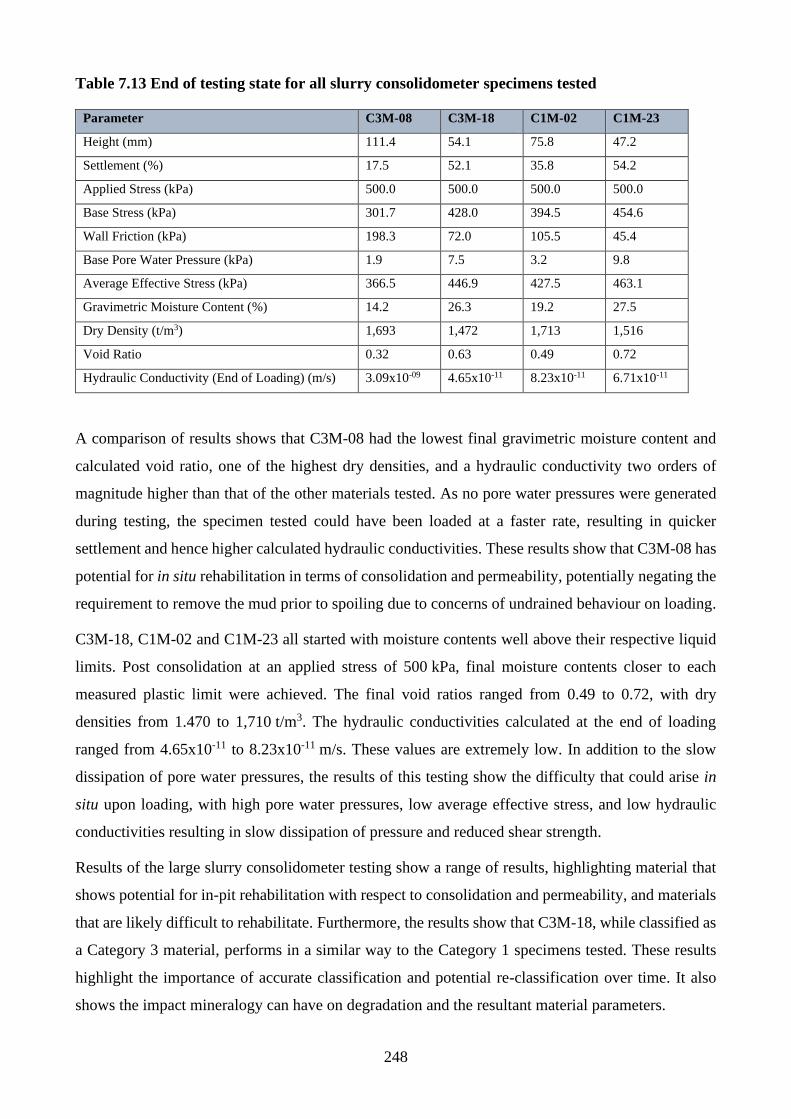
248
Table 7.13 End of testing state for all slurry consolidometer specimens tested
Parameter C3M-08 C3M-18 C1M-02 C1M-23
Height (mm) 111.4 54.1 75.8 47.2
Settlement (%) 17.5 52.1 35.8 54.2
Applied Stress (kPa) 500.0 500.0 500.0 500.0
Base Stress (kPa) 301.7 428.0 394.5 454.6
Wall Friction (kPa) 198.3 72.0 105.5 45.4
Base Pore Water Pressure (kPa) 1.9 7.5 3.2 9.8
Average Effective Stress (kPa) 366.5 446.9 427.5 463.1
Gravimetric Moisture Content (%) 14.2 26.3 19.2 27.5
Dry Density (t/m3) 1,693 1,472 1,713 1,516
Void Ratio 0.32 0.63 0.49 0.72
Hydraulic Conductivity (End of Loading) (m/s) 3.09x10-09 4.65x10⁻¹¹ 8.23x10⁻¹¹ 6.71x10⁻¹¹
A comparison of results shows that C3M-08 had the lowest final gravimetric moisture content and
calculated void ratio, one of the highest dry densities, and a hydraulic conductivity two orders of
magnitude higher than that of the other materials tested. As no pore water pressures were generated
during testing, the specimen tested could have been loaded at a faster rate, resulting in quicker
settlement and hence higher calculated hydraulic conductivities. These results show that C3M-08 has
potential for in situ rehabilitation in terms of consolidation and permeability, potentially negating the
requirement to remove the mud prior to spoiling due to concerns of undrained behaviour on loading.
C3M-18, C1M-02 and C1M-23 all started with moisture contents well above their respective liquid
limits. Post consolidation at an applied stress of 500 kPa, final moisture contents closer to each
measured plastic limit were achieved. The final void ratios ranged from 0.49 to 0.72, with dry
densities from 1.470 to 1,710 t/m3. The hydraulic conductivities calculated at the end of loading
ranged from 4.65x10⁻¹¹ to 8.23x10⁻¹¹ m/s. These values are extremely low. In addition to the slow
dissipation of pore water pressures, the results of this testing show the difficulty that could arise in
situ upon loading, with high pore water pressures, low average effective stress, and low hydraulic
conductivities resulting in slow dissipation of pressure and reduced shear strength.
Results of the large slurry consolidometer testing show a range of results, highlighting material that
shows potential for in-pit rehabilitation with respect to consolidation and permeability, and materials
that are likely difficult to rehabilitate. Furthermore, the results show that C3M-18, while classified as
a Category 3 material, performs in a similar way to the Category 1 specimens tested. These results
highlight the importance of accurate classification and potential re-classification over time. It also
shows the impact mineralogy can have on degradation and the resultant material parameters.
249
The results of the large slurry consolidometer testing used a constant loading rate of 0.1 kPa/min up
to 500 kPa to show the nature of the selected materials during consolidation. It is, however, important
to note that the conditions of the test setup should mimic the scenario expected in practice. The
method of loading of spoil onto the mud must be replicated. These tests were conducted at a rate of
144 kPa/day, equivalent to approximately 8 m of fill with a unit weight of 18 kN/m3. Draglines can
produce spoil piles of the order of 60 to 100m high and with lineal rates of advance along the strip of
10 m/day (Duran 2013).
These results, therefore, show that for C3M-18, C1M-02 and C1M-23, this rate of rise would produce
excessive pore pressures and likely result in instabilities. If these muds were encountered, careful
management methods would be required if the mud were to remain in situ such as truck and shovel
systems. For C3M-08, however, the results show the potential for truck and shovel loading without
the build-up of pore pressures, promoting the potential for this material to be left in-pit, potentially
saving millions of dollars in removal costs and associated issues.
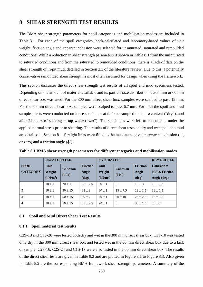
250
8 SHEAR STRENGTH TEST RESULTS
The BMA shear strength parameters for spoil categories and mobilisation modes are included in
Table 8.1. For each of the spoil categories, back-calculated and laboratory-based values of unit
weight, friction angle and apparent cohesion were selected for unsaturated, saturated and remoulded
conditions. While a reduction in shear strength parameters is shown in Table 8.1 from the unsaturated
to saturated conditions and from the saturated to remoulded conditions, there is a lack of data on the
shear strength of in-pit mud, detailed in Section 2.3 of the literature review. Due to this, a potentially
conservative remoulded shear strength is most often assumed for design when using the framework.
This section discusses the direct shear strength test results of all spoil and mud specimens tested.
Depending on the amount of material available and its particle size distribution, a 300 mm or 60 mm
direct shear box was used. For the 300 mm direct shear box, samples were scalped to pass 19 mm.
For the 60 mm direct shear box, samples were scalped to pass 6.7 mm. For both the spoil and mud
samples, tests were conducted on loose specimens at their as-sampled moisture content (“dry”), and
after 24 hours of soaking in tap water (“wet”). The specimens were left to consolidate under the
applied normal stress prior to shearing. The results of direct shear tests on dry and wet spoil and mud
are detailed in Section 8.1. Straight lines were fitted to the test data to give an apparent cohesion (c’,
or zero) and a friction angle (ɸ’).
Table 8.1 BMA shear strength parameters for different categories and mobilisation modes
SPOIL
CATEGORY
UNSATURATED SATURATED REMOULDED
Unit
Weight
(kN/m3)
Cohesion
(kPa)
Friction
Angle
(deg)
Unit
Weight
(kN/m3)
Cohesion
(kPa)
Friction
Angle
(deg)
Cohesion =
0 kPa, Friction
Angle (deg)
1 18 1 20 1 25 2.5 20 1 0 18 3 18 1.5
2 18 1 30 15 28 3 20 1 15 7.5 23 2.5 18 1.5
3 18 1 50 15 30 2 20 1 20 10 25 2.5 18 1.5
4 18 1 50 15 35 2.5 20 1 0 30 1.5 28 2
8.1 Spoil and Mud Direct Shear Test Results
8.1.1 Spoil material test results
C3S-13 and C3S-20 were tested both dry and wet in the 300 mm direct shear box. C3S-10 was tested
only dry in the 300 mm direct shear box and tested wet in the 60 mm direct shear box due to a lack
of sample. C2S-16, C2S-24 and C1S-17 were also tested in the 60 mm direct shear box. The results
of the direct shear tests are given in Table 8.2 and are plotted in Figure 8.1 to Figure 8.3. Also given
in Table 8.2 are the corresponding BMA framework shear strength parameters. A summary of the
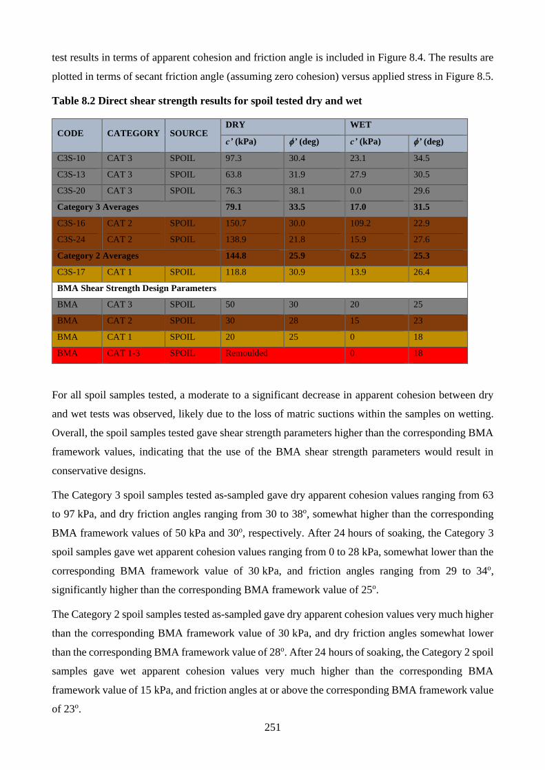
251
test results in terms of apparent cohesion and friction angle is included in Figure 8.4. The results are
plotted in terms of secant friction angle (assuming zero cohesion) versus applied stress in Figure 8.5.
Table 8.2 Direct shear strength results for spoil tested dry and wet
CODE CATEGORY SOURCE DRY WET
c’ (kPa) ’ (deg) c’ (kPa) ’ (deg)
C3S-10 CAT 3 SPOIL 97.3 30.4 23.1 34.5
C3S-13 CAT 3 SPOIL 63.8 31.9 27.9 30.5
C3S-20 CAT 3 SPOIL 76.3 38.1 0.0 29.6
Category 3 Averages 79.1 33.5 17.0 31.5
C3S-16 CAT 2 SPOIL 150.7 30.0 109.2 22.9
C3S-24 CAT 2 SPOIL 138.9 21.8 15.9 27.6
Category 2 Averages 144.8 25.9 62.5 25.3
C3S-17 CAT 1 SPOIL 118.8 30.9 13.9 26.4
BMA Shear Strength Design Parameters
BMA CAT 3 SPOIL 50 30 20 25
BMA CAT 2 SPOIL 30 28 15 23
BMA CAT 1 SPOIL 20 25 0 18
BMA CAT 1-3 SPOIL Remoulded 0 18
For all spoil samples tested, a moderate to a significant decrease in apparent cohesion between dry
and wet tests was observed, likely due to the loss of matric suctions within the samples on wetting.
Overall, the spoil samples tested gave shear strength parameters higher than the corresponding BMA
framework values, indicating that the use of the BMA shear strength parameters would result in
conservative designs.
The Category 3 spoil samples tested as-sampled gave dry apparent cohesion values ranging from 63
to 97 kPa, and dry friction angles ranging from 30 to 38o, somewhat higher than the corresponding
BMA framework values of 50 kPa and 30o, respectively. After 24 hours of soaking, the Category 3
spoil samples gave wet apparent cohesion values ranging from 0 to 28 kPa, somewhat lower than the
corresponding BMA framework value of 30 kPa, and friction angles ranging from 29 to 34o,
significantly higher than the corresponding BMA framework value of 25o.
The Category 2 spoil samples tested as-sampled gave dry apparent cohesion values very much higher
than the corresponding BMA framework value of 30 kPa, and dry friction angles somewhat lower
than the corresponding BMA framework value of 28o. After 24 hours of soaking, the Category 2 spoil
samples gave wet apparent cohesion values very much higher than the corresponding BMA
framework value of 15 kPa, and friction angles at or above the corresponding BMA framework value
of 23o.
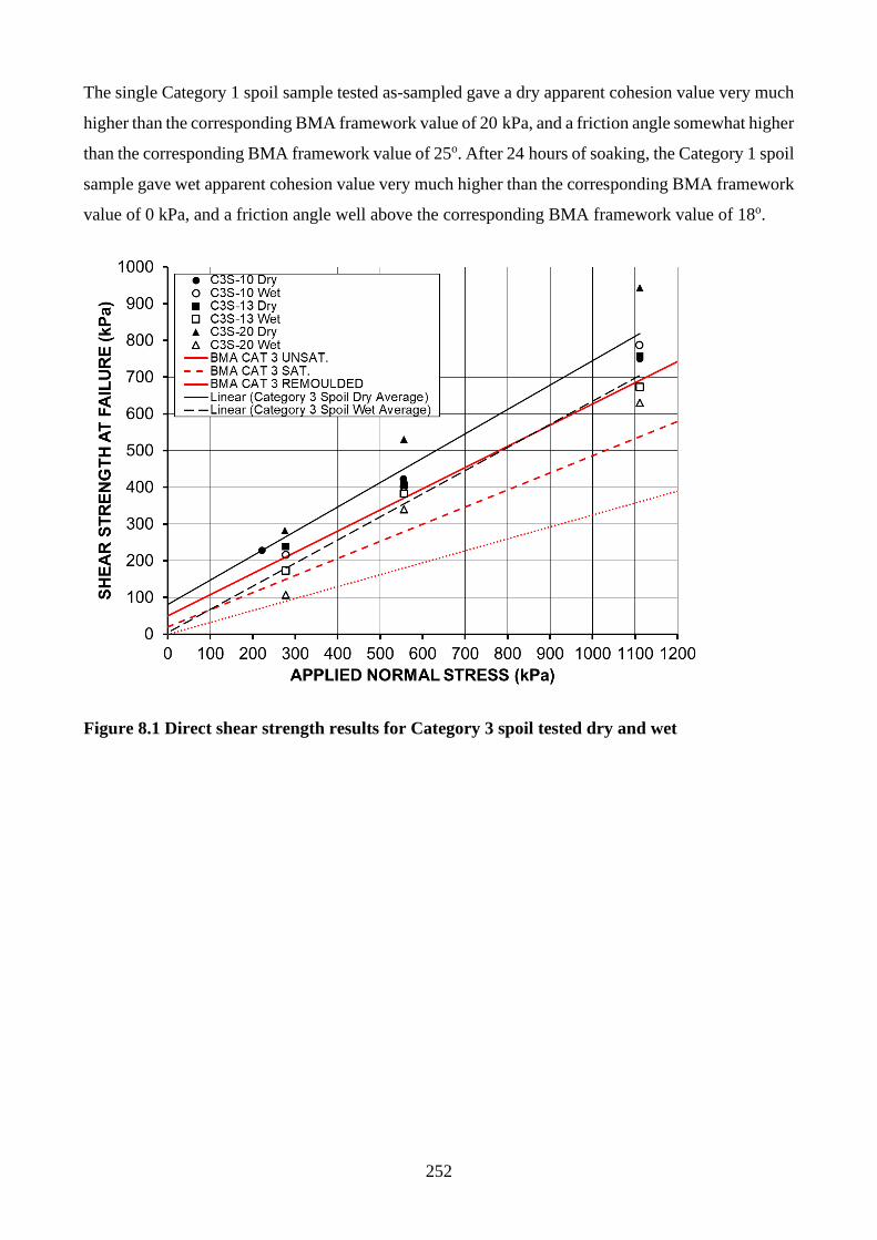
252
The single Category 1 spoil sample tested as-sampled gave a dry apparent cohesion value very much
higher than the corresponding BMA framework value of 20 kPa, and a friction angle somewhat higher
than the corresponding BMA framework value of 25o. After 24 hours of soaking, the Category 1 spoil
sample gave wet apparent cohesion value very much higher than the corresponding BMA framework
value of 0 kPa, and a friction angle well above the corresponding BMA framework value of 18o.
Figure 8.1 Direct shear strength results for Category 3 spoil tested dry and wet
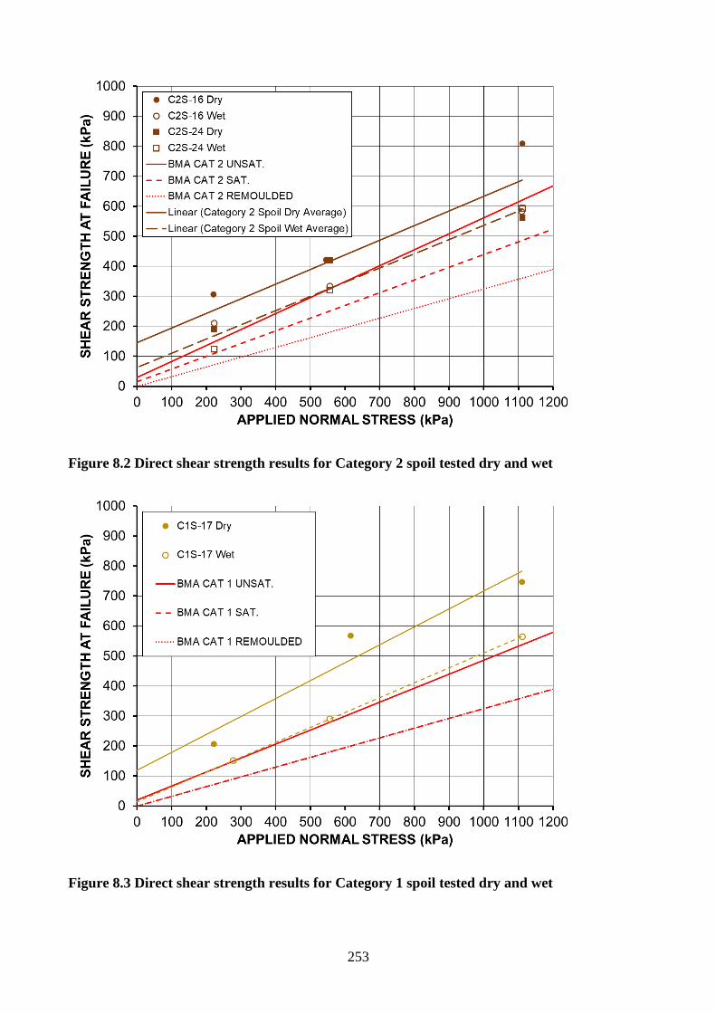
253
Figure 8.2 Direct shear strength results for Category 2 spoil tested dry and wet
Figure 8.3 Direct shear strength results for Category 1 spoil tested dry and wet
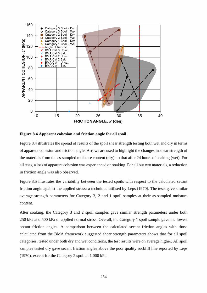
254
Figure 8.4 Apparent cohesion and friction angle for all spoil
Figure 8.4 illustrates the spread of results of the spoil shear strength testing both wet and dry in terms
of apparent cohesion and friction angle. Arrows are used to highlight the changes in shear strength of
the materials from the as-sampled moisture content (dry), to that after 24 hours of soaking (wet). For
all tests, a loss of apparent cohesion was experienced on soaking. For all but two materials, a reduction
in friction angle was also observed.
Figure 8.5 illustrates the variability between the tested spoils with respect to the calculated secant
friction angle against the applied stress; a technique utilised by Leps (1970). The tests gave similar
average strength parameters for Category 3, 2 and 1 spoil samples at their as-sampled moisture
content.
After soaking, the Category 3 and 2 spoil samples gave similar strength parameters under both
250 kPa and 500 kPa of applied normal stress. Overall, the Category 1 spoil sample gave the lowest
secant friction angles. A comparison between the calculated secant friction angles with those
calculated from the BMA framework suggested shear strength parameters shows that for all spoil
categories, tested under both dry and wet conditions, the test results were on average higher. All spoil
samples tested dry gave secant friction angles above the poor quality rockfill line reported by Leps
(1970), except for the Category 2 spoil at 1,000 kPa.
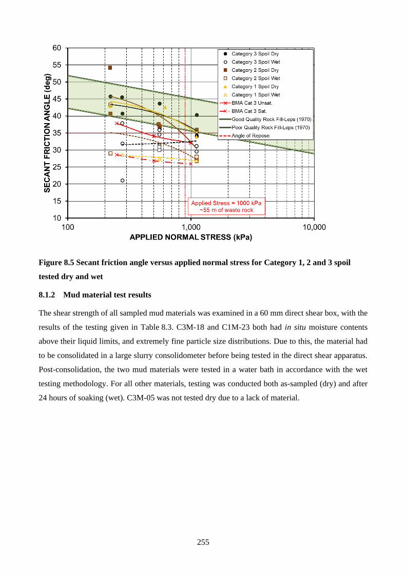
255
Figure 8.5 Secant friction angle versus applied normal stress for Category 1, 2 and 3 spoil
tested dry and wet
8.1.2 Mud material test results
The shear strength of all sampled mud materials was examined in a 60 mm direct shear box, with the
results of the testing given in Table 8.3. C3M-18 and C1M-23 both had in situ moisture contents
above their liquid limits, and extremely fine particle size distributions. Due to this, the material had
to be consolidated in a large slurry consolidometer before being tested in the direct shear apparatus.
Post-consolidation, the two mud materials were tested in a water bath in accordance with the wet
testing methodology. For all other materials, testing was conducted both as-sampled (dry) and after
24 hours of soaking (wet). C3M-05 was not tested dry due to a lack of material.
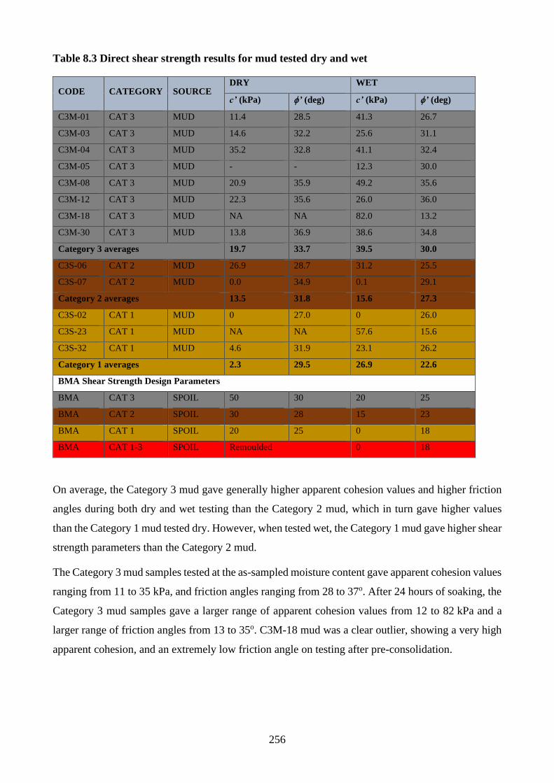
256
Table 8.3 Direct shear strength results for mud tested dry and wet
CODE CATEGORY SOURCE DRY WET
c’ (kPa) ’ (deg) c’ (kPa) ’ (deg)
C3M-01 CAT 3 MUD 11.4 28.5 41.3 26.7
C3M-03 CAT 3 MUD 14.6 32.2 25.6 31.1
C3M-04 CAT 3 MUD 35.2 32.8 41.1 32.4
C3M-05 CAT 3 MUD - - 12.3 30.0
C3M-08 CAT 3 MUD 20.9 35.9 49.2 35.6
C3M-12 CAT 3 MUD 22.3 35.6 26.0 36.0
C3M-18 CAT 3 MUD NA NA 82.0 13.2
C3M-30 CAT 3 MUD 13.8 36.9 38.6 34.8
Category 3 averages 19.7 33.7 39.5 30.0
C3S-06 CAT 2 MUD 26.9 28.7 31.2 25.5
C3S-07 CAT 2 MUD 0.0 34.9 0.1 29.1
Category 2 averages 13.5 31.8 15.6 27.3
C3S-02 CAT 1 MUD 0 27.0 0 26.0
C3S-23 CAT 1 MUD NA NA 57.6 15.6
C3S-32 CAT 1 MUD 4.6 31.9 23.1 26.2
Category 1 averages 2.3 29.5 26.9 22.6
BMA Shear Strength Design Parameters
BMA CAT 3 SPOIL 50 30 20 25
BMA CAT 2 SPOIL 30 28 15 23
BMA CAT 1 SPOIL 20 25 0 18
BMA CAT 1-3 SPOIL Remoulded 0 18
On average, the Category 3 mud gave generally higher apparent cohesion values and higher friction
angles during both dry and wet testing than the Category 2 mud, which in turn gave higher values
than the Category 1 mud tested dry. However, when tested wet, the Category 1 mud gave higher shear
strength parameters than the Category 2 mud.
The Category 3 mud samples tested at the as-sampled moisture content gave apparent cohesion values
ranging from 11 to 35 kPa, and friction angles ranging from 28 to 37o. After 24 hours of soaking, the
Category 3 mud samples gave a larger range of apparent cohesion values from 12 to 82 kPa and a
larger range of friction angles from 13 to 35o. C3M-18 mud was a clear outlier, showing a very high
apparent cohesion, and an extremely low friction angle on testing after pre-consolidation.
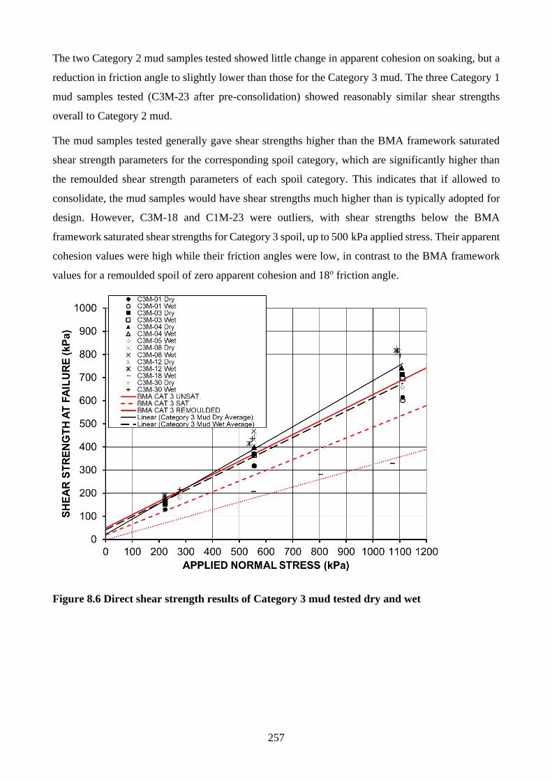
257
The two Category 2 mud samples tested showed little change in apparent cohesion on soaking, but a
reduction in friction angle to slightly lower than those for the Category 3 mud. The three Category 1
mud samples tested (C3M-23 after pre-consolidation) showed reasonably similar shear strengths
overall to Category 2 mud.
The mud samples tested generally gave shear strengths higher than the BMA framework saturated
shear strength parameters for the corresponding spoil category, which are significantly higher than
the remoulded shear strength parameters of each spoil category. This indicates that if allowed to
consolidate, the mud samples would have shear strengths much higher than is typically adopted for
design. However, C3M-18 and C1M-23 were outliers, with shear strengths below the BMA
framework saturated shear strengths for Category 3 spoil, up to 500 kPa applied stress. Their apparent
cohesion values were high while their friction angles were low, in contrast to the BMA framework
values for a remoulded spoil of zero apparent cohesion and 18o friction angle.
Figure 8.6 Direct shear strength results of Category 3 mud tested dry and wet
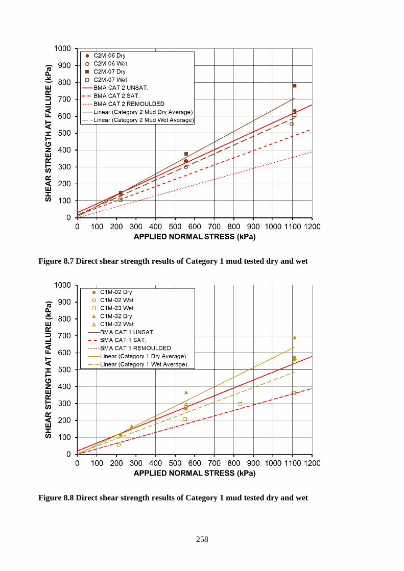
258
Figure 8.7 Direct shear strength results of Category 1 mud tested dry and wet
Figure 8.8 Direct shear strength results of Category 1 mud tested dry and wet
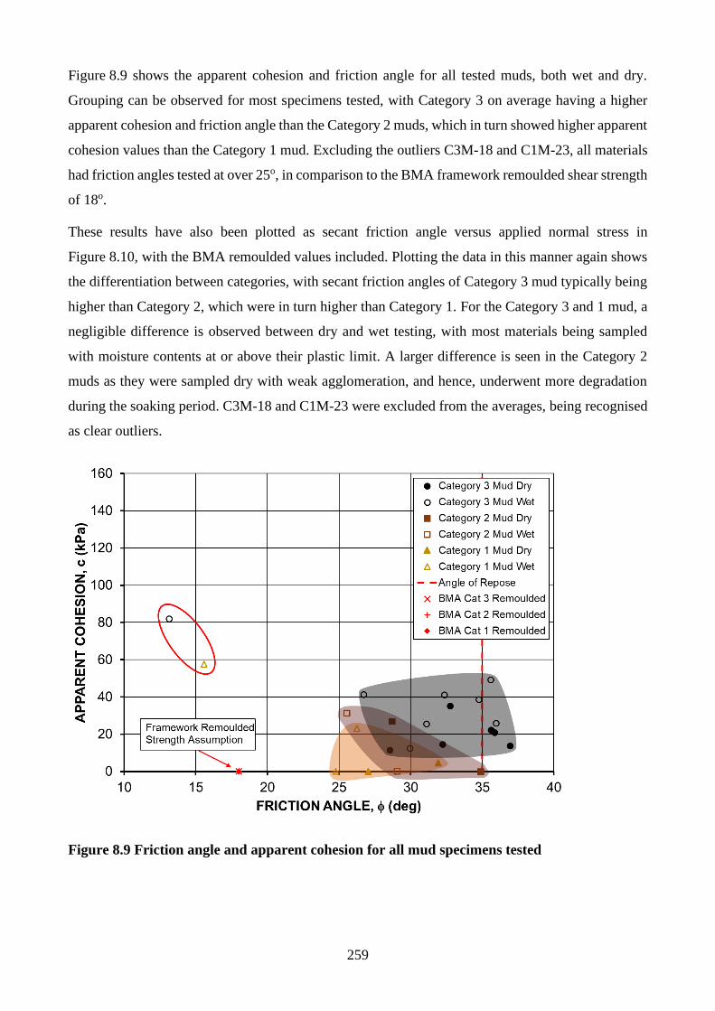
259
Figure 8.9 shows the apparent cohesion and friction angle for all tested muds, both wet and dry.
Grouping can be observed for most specimens tested, with Category 3 on average having a higher
apparent cohesion and friction angle than the Category 2 muds, which in turn showed higher apparent
cohesion values than the Category 1 mud. Excluding the outliers C3M-18 and C1M-23, all materials
had friction angles tested at over 25o, in comparison to the BMA framework remoulded shear strength
of 18o.
These results have also been plotted as secant friction angle versus applied normal stress in
Figure 8.10, with the BMA remoulded values included. Plotting the data in this manner again shows
the differentiation between categories, with secant friction angles of Category 3 mud typically being
higher than Category 2, which were in turn higher than Category 1. For the Category 3 and 1 mud, a
negligible difference is observed between dry and wet testing, with most materials being sampled
with moisture contents at or above their plastic limit. A larger difference is seen in the Category 2
muds as they were sampled dry with weak agglomeration, and hence, underwent more degradation
during the soaking period. C3M-18 and C1M-23 were excluded from the averages, being recognised
as clear outliers.
Figure 8.9 Friction angle and apparent cohesion for all mud specimens tested
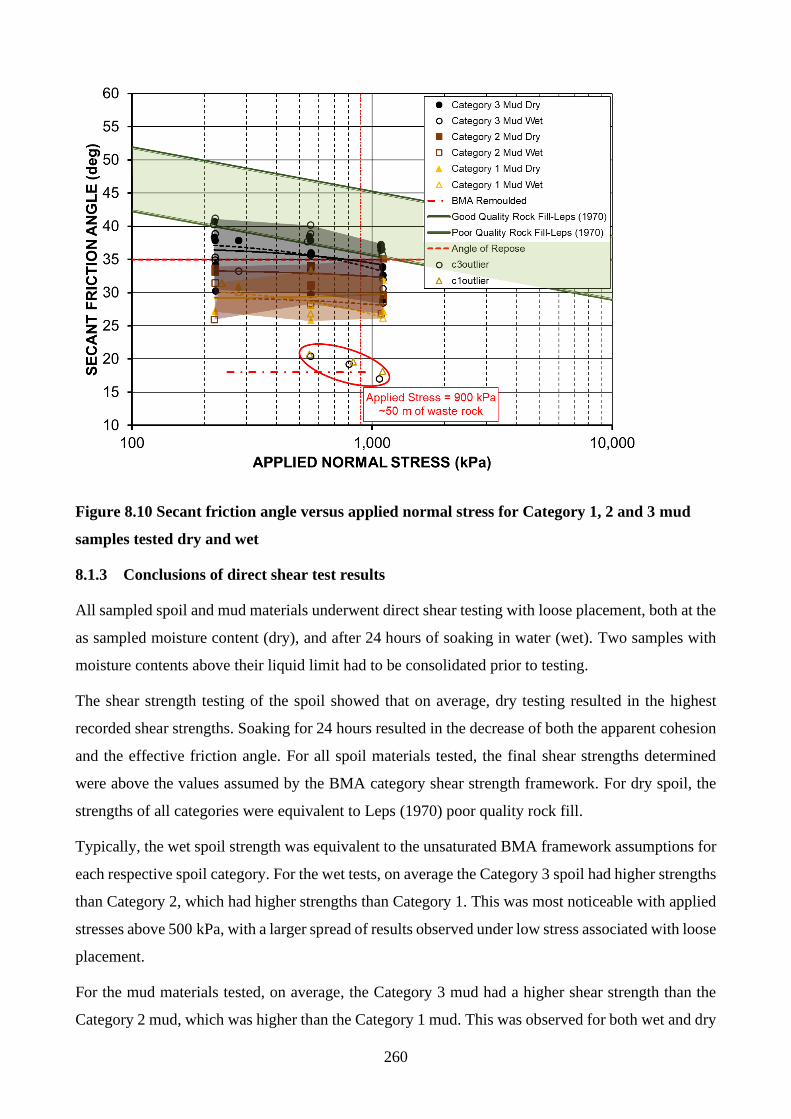
260
Figure 8.10 Secant friction angle versus applied normal stress for Category 1, 2 and 3 mud
samples tested dry and wet
8.1.3 Conclusions of direct shear test results
All sampled spoil and mud materials underwent direct shear testing with loose placement, both at the
as sampled moisture content (dry), and after 24 hours of soaking in water (wet). Two samples with
moisture contents above their liquid limit had to be consolidated prior to testing.
The shear strength testing of the spoil showed that on average, dry testing resulted in the highest
recorded shear strengths. Soaking for 24 hours resulted in the decrease of both the apparent cohesion
and the effective friction angle. For all spoil materials tested, the final shear strengths determined
were above the values assumed by the BMA category shear strength framework. For dry spoil, the
strengths of all categories were equivalent to Leps (1970) poor quality rock fill.
Typically, the wet spoil strength was equivalent to the unsaturated BMA framework assumptions for
each respective spoil category. For the wet tests, on average the Category 3 spoil had higher strengths
than Category 2, which had higher strengths than Category 1. This was most noticeable with applied
stresses above 500 kPa, with a larger spread of results observed under low stress associated with loose
placement.
For the mud materials tested, on average, the Category 3 mud had a higher shear strength than the
Category 2 mud, which was higher than the Category 1 mud. This was observed for both wet and dry
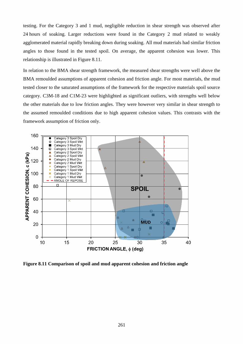
261
testing. For the Category 3 and 1 mud, negligible reduction in shear strength was observed after
24 hours of soaking. Larger reductions were found in the Category 2 mud related to weakly
agglomerated material rapidly breaking down during soaking. All mud materials had similar friction
angles to those found in the tested spoil. On average, the apparent cohesion was lower. This
relationship is illustrated in Figure 8.11.
In relation to the BMA shear strength framework, the measured shear strengths were well above the
BMA remoulded assumptions of apparent cohesion and friction angle. For most materials, the mud
tested closer to the saturated assumptions of the framework for the respective materials spoil source
category. C3M-18 and C1M-23 were highlighted as significant outliers, with strengths well below
the other materials due to low friction angles. They were however very similar in shear strength to
the assumed remoulded conditions due to high apparent cohesion values. This contrasts with the
framework assumption of friction only.
Figure 8.11 Comparison of spoil and mud apparent cohesion and friction angle
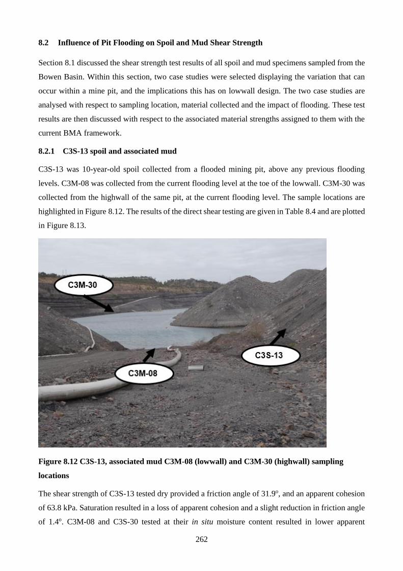
262
8.2 Influence of Pit Flooding on Spoil and Mud Shear Strength
Section 8.1 discussed the shear strength test results of all spoil and mud specimens sampled from the
Bowen Basin. Within this section, two case studies were selected displaying the variation that can
occur within a mine pit, and the implications this has on lowwall design. The two case studies are
analysed with respect to sampling location, material collected and the impact of flooding. These test
results are then discussed with respect to the associated material strengths assigned to them with the
current BMA framework.
8.2.1 C3S-13 spoil and associated mud
C3S-13 was 10-year-old spoil collected from a flooded mining pit, above any previous flooding
levels. C3M-08 was collected from the current flooding level at the toe of the lowwall. C3M-30 was
collected from the highwall of the same pit, at the current flooding level. The sample locations are
highlighted in Figure 8.12. The results of the direct shear testing are given in Table 8.4 and are plotted
in Figure 8.13.
Figure 8.12 C3S-13, associated mud C3M-08 (lowwall) and C3M-30 (highwall) sampling
locations
The shear strength of C3S-13 tested dry provided a friction angle of 31.9o, and an apparent cohesion
of 63.8 kPa. Saturation resulted in a loss of apparent cohesion and a slight reduction in friction angle
of 1.4o. C3M-08 and C3S-30 tested at their in situ moisture content resulted in lower apparent
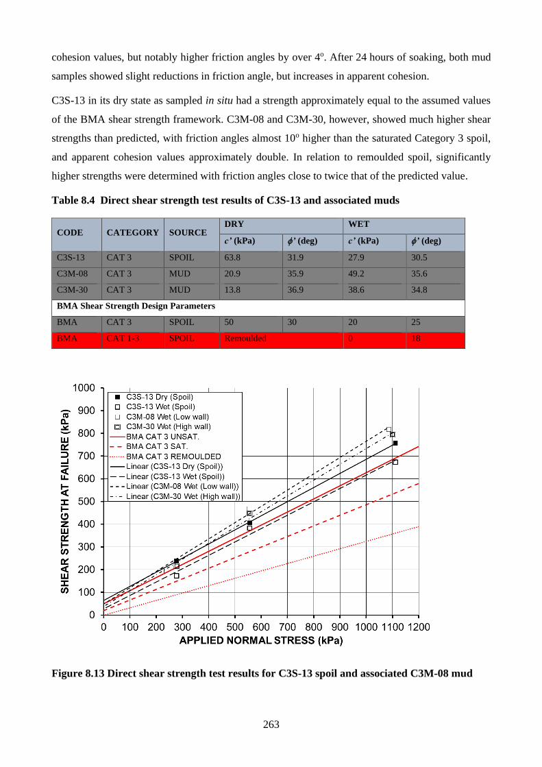
263
cohesion values, but notably higher friction angles by over 4o. After 24 hours of soaking, both mud
samples showed slight reductions in friction angle, but increases in apparent cohesion.
C3S-13 in its dry state as sampled in situ had a strength approximately equal to the assumed values
of the BMA shear strength framework. C3M-08 and C3M-30, however, showed much higher shear
strengths than predicted, with friction angles almost 10o higher than the saturated Category 3 spoil,
and apparent cohesion values approximately double. In relation to remoulded spoil, significantly
higher strengths were determined with friction angles close to twice that of the predicted value.
Table 8.4 Direct shear strength test results of C3S-13 and associated muds
CODE CATEGORY SOURCE DRY WET
c’ (kPa) ’ (deg) c’ (kPa) ’ (deg)
C3S-13 CAT 3 SPOIL 63.8 31.9 27.9 30.5
C3M-08 CAT 3 MUD 20.9 35.9 49.2 35.6
C3M-30 CAT 3 MUD 13.8 36.9 38.6 34.8
BMA Shear Strength Design Parameters
BMA CAT 3 SPOIL 50 30 20 25
BMA CAT 1-3 SPOIL Remoulded 0 18
Figure 8.13 Direct shear strength test results for C3S-13 spoil and associated C3M-08 mud
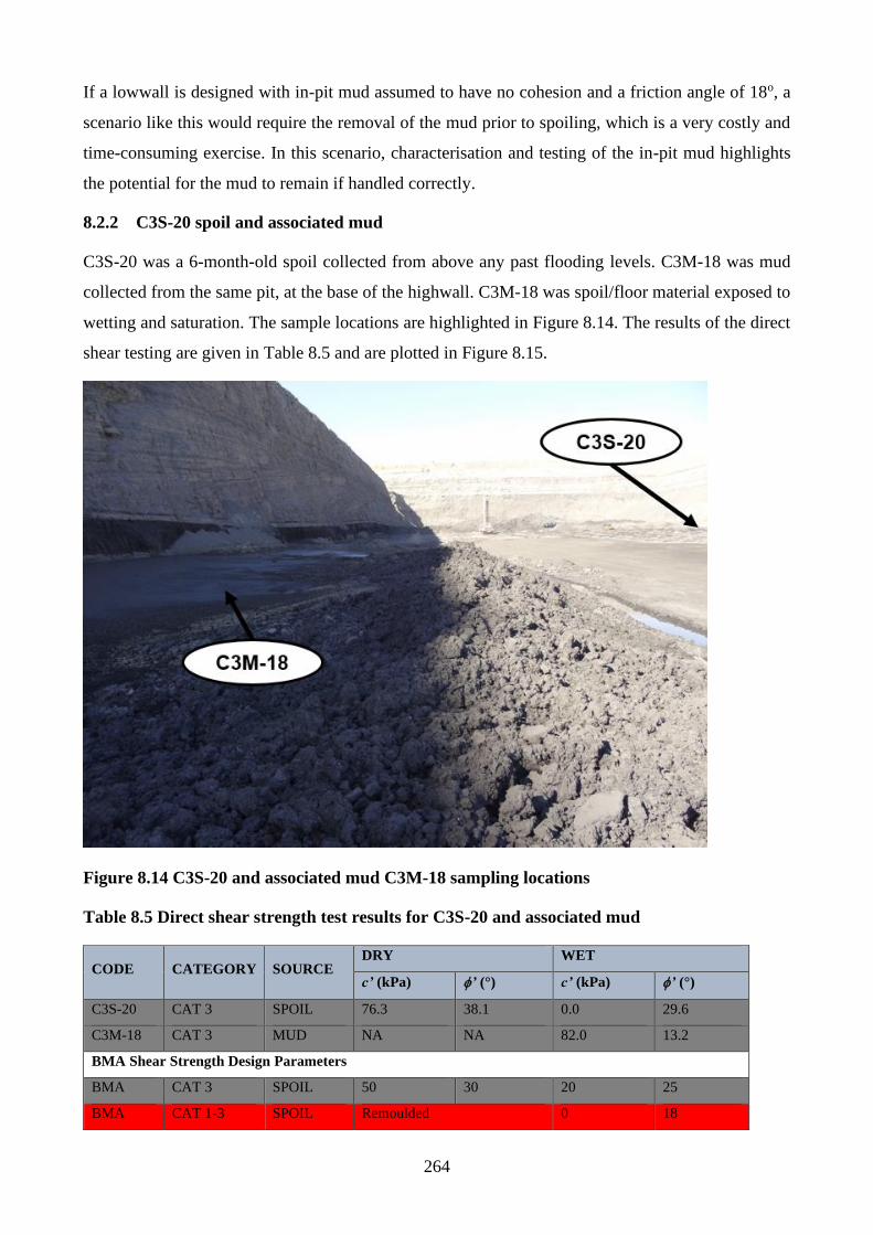
264
If a lowwall is designed with in-pit mud assumed to have no cohesion and a friction angle of 18o, a
scenario like this would require the removal of the mud prior to spoiling, which is a very costly and
time-consuming exercise. In this scenario, characterisation and testing of the in-pit mud highlights
the potential for the mud to remain if handled correctly.
8.2.2 C3S-20 spoil and associated mud
C3S-20 was a 6-month-old spoil collected from above any past flooding levels. C3M-18 was mud
collected from the same pit, at the base of the highwall. C3M-18 was spoil/floor material exposed to
wetting and saturation. The sample locations are highlighted in Figure 8.14. The results of the direct
shear testing are given in Table 8.5 and are plotted in Figure 8.15.
Figure 8.14 C3S-20 and associated mud C3M-18 sampling locations
Table 8.5 Direct shear strength test results for C3S-20 and associated mud
CODE CATEGORY SOURCE DRY WET
c’ (kPa) ’ (°) c’ (kPa) ’ (°)
C3S-20 CAT 3 SPOIL 76.3 38.1 0.0 29.6
C3M-18 CAT 3 MUD NA NA 82.0 13.2
BMA Shear Strength Design Parameters
BMA CAT 3 SPOIL 50 30 20 25
BMA CAT 1-3 SPOIL Remoulded 0 18
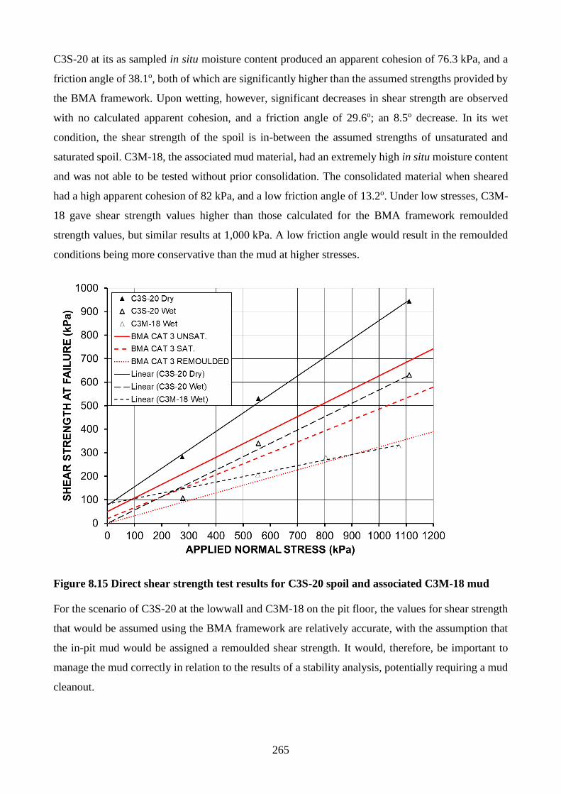
265
C3S-20 at its as sampled in situ moisture content produced an apparent cohesion of 76.3 kPa, and a
friction angle of 38.1o, both of which are significantly higher than the assumed strengths provided by
the BMA framework. Upon wetting, however, significant decreases in shear strength are observed
with no calculated apparent cohesion, and a friction angle of 29.6o; an 8.5o decrease. In its wet
condition, the shear strength of the spoil is in-between the assumed strengths of unsaturated and
saturated spoil. C3M-18, the associated mud material, had an extremely high in situ moisture content
and was not able to be tested without prior consolidation. The consolidated material when sheared
had a high apparent cohesion of 82 kPa, and a low friction angle of 13.2o. Under low stresses, C3M-
18 gave shear strength values higher than those calculated for the BMA framework remoulded
strength values, but similar results at 1,000 kPa. A low friction angle would result in the remoulded
conditions being more conservative than the mud at higher stresses.
Figure 8.15 Direct shear strength test results for C3S-20 spoil and associated C3M-18 mud
For the scenario of C3S-20 at the lowwall and C3M-18 on the pit floor, the values for shear strength
that would be assumed using the BMA framework are relatively accurate, with the assumption that
the in-pit mud would be assigned a remoulded shear strength. It would, therefore, be important to
manage the mud correctly in relation to the results of a stability analysis, potentially requiring a mud
cleanout.
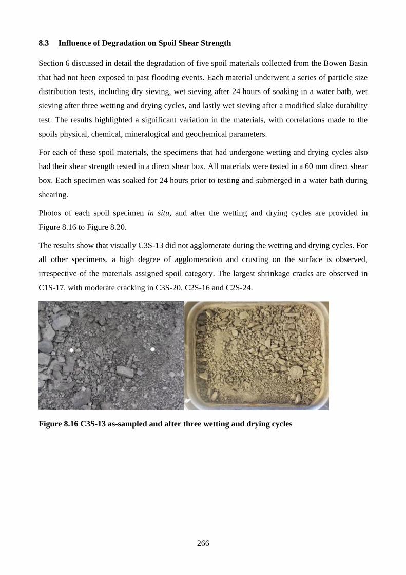
266
8.3 Influence of Degradation on Spoil Shear Strength
Section 6 discussed in detail the degradation of five spoil materials collected from the Bowen Basin
that had not been exposed to past flooding events. Each material underwent a series of particle size
distribution tests, including dry sieving, wet sieving after 24 hours of soaking in a water bath, wet
sieving after three wetting and drying cycles, and lastly wet sieving after a modified slake durability
test. The results highlighted a significant variation in the materials, with correlations made to the
spoils physical, chemical, mineralogical and geochemical parameters.
For each of these spoil materials, the specimens that had undergone wetting and drying cycles also
had their shear strength tested in a direct shear box. All materials were tested in a 60 mm direct shear
box. Each specimen was soaked for 24 hours prior to testing and submerged in a water bath during
shearing.
Photos of each spoil specimen in situ, and after the wetting and drying cycles are provided in
Figure 8.16 to Figure 8.20.
The results show that visually C3S-13 did not agglomerate during the wetting and drying cycles. For
all other specimens, a high degree of agglomeration and crusting on the surface is observed,
irrespective of the materials assigned spoil category. The largest shrinkage cracks are observed in
C1S-17, with moderate cracking in C3S-20, C2S-16 and C2S-24.
Figure 8.16 C3S-13 as-sampled and after three wetting and drying cycles
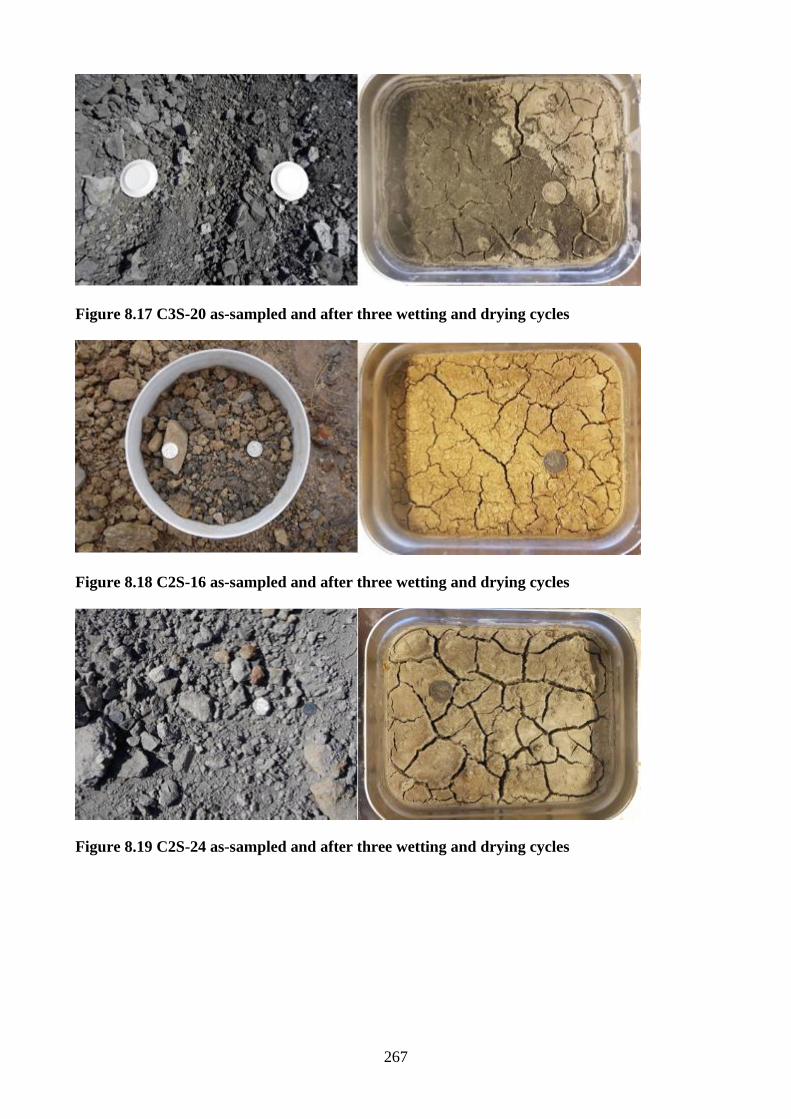
267
Figure 8.17 C3S-20 as-sampled and after three wetting and drying cycles
Figure 8.18 C2S-16 as-sampled and after three wetting and drying cycles
Figure 8.19 C2S-24 as-sampled and after three wetting and drying cycles
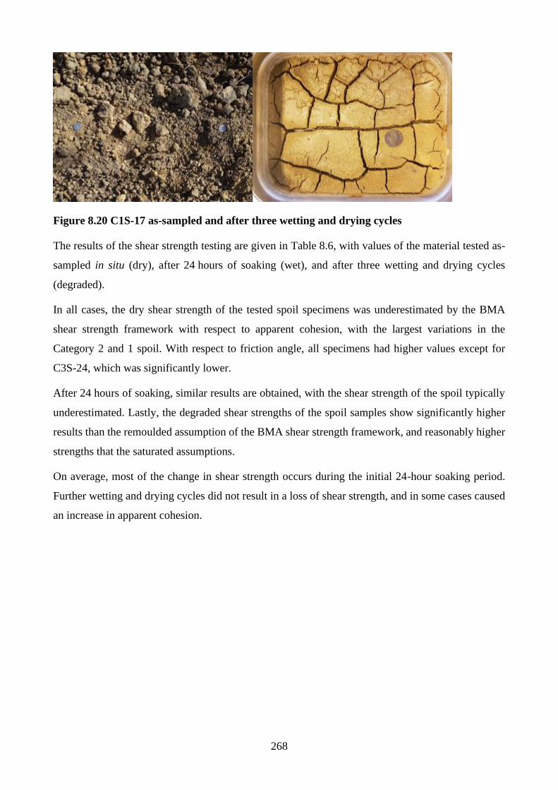
268
Figure 8.20 C1S-17 as-sampled and after three wetting and drying cycles
The results of the shear strength testing are given in Table 8.6, with values of the material tested as-
sampled in situ (dry), after 24 hours of soaking (wet), and after three wetting and drying cycles
(degraded).
In all cases, the dry shear strength of the tested spoil specimens was underestimated by the BMA
shear strength framework with respect to apparent cohesion, with the largest variations in the
Category 2 and 1 spoil. With respect to friction angle, all specimens had higher values except for
C3S-24, which was significantly lower.
After 24 hours of soaking, similar results are obtained, with the shear strength of the spoil typically
underestimated. Lastly, the degraded shear strengths of the spoil samples show significantly higher
results than the remoulded assumption of the BMA shear strength framework, and reasonably higher
strengths that the saturated assumptions.
On average, most of the change in shear strength occurs during the initial 24-hour soaking period.
Further wetting and drying cycles did not result in a loss of shear strength, and in some cases caused
an increase in apparent cohesion.
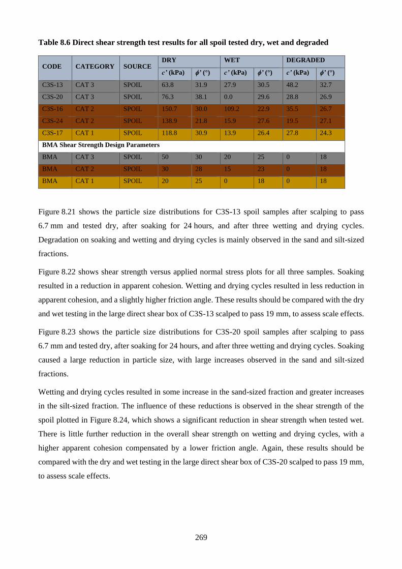
269
Table 8.6 Direct shear strength test results for all spoil tested dry, wet and degraded
CODE CATEGORY SOURCE DRY WET DEGRADED
c’ (kPa) ’ (°) c’ (kPa) ’ (°) c’ (kPa) ’ (°)
C3S-13 CAT 3 SPOIL 63.8 31.9 27.9 30.5 48.2 32.7
C3S-20 CAT 3 SPOIL 76.3 38.1 0.0 29.6 28.8 26.9
C3S-16 CAT 2 SPOIL 150.7 30.0 109.2 22.9 35.5 26.7
C3S-24 CAT 2 SPOIL 138.9 21.8 15.9 27.6 19.5 27.1
C3S-17 CAT 1 SPOIL 118.8 30.9 13.9 26.4 27.8 24.3
BMA Shear Strength Design Parameters
BMA CAT 3 SPOIL 50 30 20 25 0 18
BMA CAT 2 SPOIL 30 28 15 23 0 18
BMA CAT 1 SPOIL 20 25 0 18 0 18
Figure 8.21 shows the particle size distributions for C3S-13 spoil samples after scalping to pass
6.7 mm and tested dry, after soaking for 24 hours, and after three wetting and drying cycles.
Degradation on soaking and wetting and drying cycles is mainly observed in the sand and silt-sized
fractions.
Figure 8.22 shows shear strength versus applied normal stress plots for all three samples. Soaking
resulted in a reduction in apparent cohesion. Wetting and drying cycles resulted in less reduction in
apparent cohesion, and a slightly higher friction angle. These results should be compared with the dry
and wet testing in the large direct shear box of C3S-13 scalped to pass 19 mm, to assess scale effects.
Figure 8.23 shows the particle size distributions for C3S-20 spoil samples after scalping to pass
6.7 mm and tested dry, after soaking for 24 hours, and after three wetting and drying cycles. Soaking
caused a large reduction in particle size, with large increases observed in the sand and silt-sized
fractions.
Wetting and drying cycles resulted in some increase in the sand-sized fraction and greater increases
in the silt-sized fraction. The influence of these reductions is observed in the shear strength of the
spoil plotted in Figure 8.24, which shows a significant reduction in shear strength when tested wet.
There is little further reduction in the overall shear strength on wetting and drying cycles, with a
higher apparent cohesion compensated by a lower friction angle. Again, these results should be
compared with the dry and wet testing in the large direct shear box of C3S-20 scalped to pass 19 mm,
to assess scale effects.
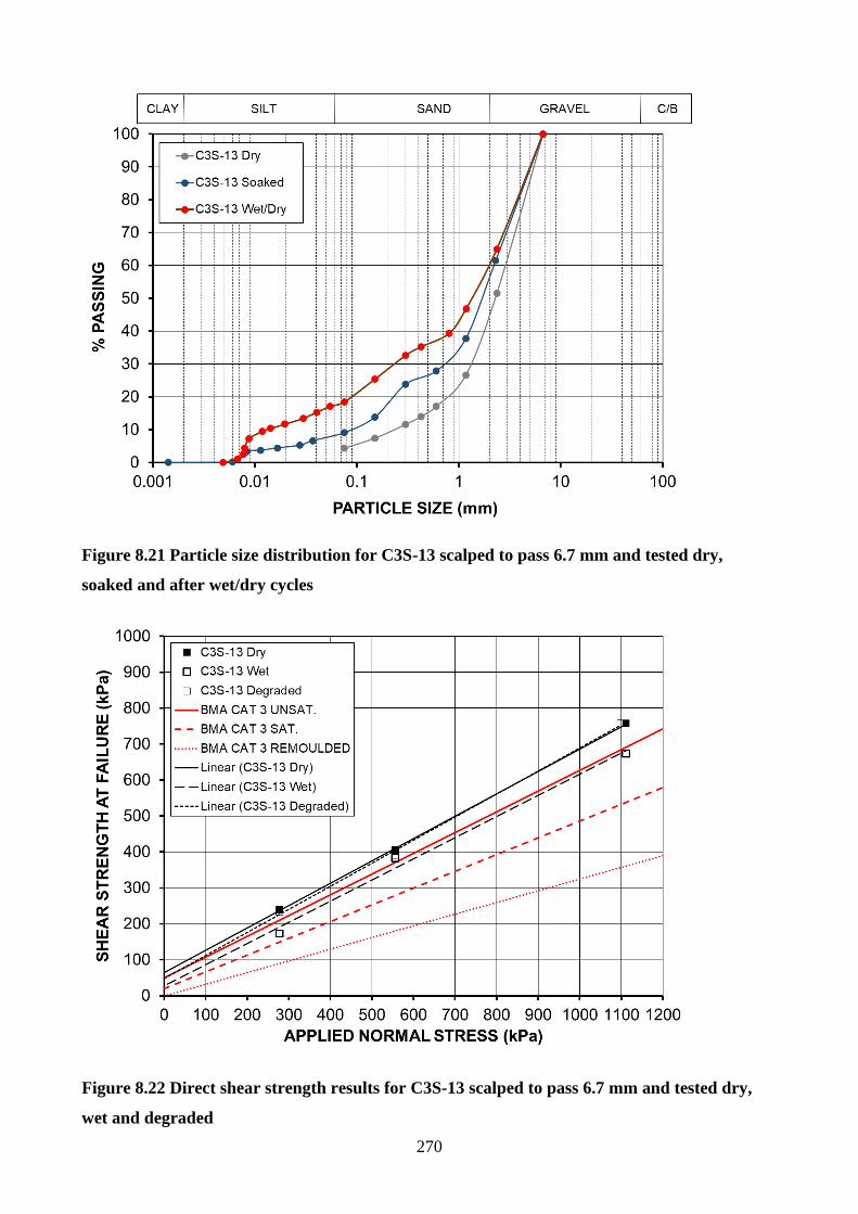
270
Figure 8.21 Particle size distribution for C3S-13 scalped to pass 6.7 mm and tested dry,
soaked and after wet/dry cycles
Figure 8.22 Direct shear strength results for C3S-13 scalped to pass 6.7 mm and tested dry,
wet and degraded
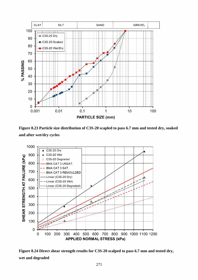
271
Figure 8.23 Particle size distribution of C3S-20 scapled to pass 6.7 mm and tested dry, soaked
and after wet/dry cycles
Figure 8.24 Direct shear strength results for C3S-20 scalped to pass 6.7 mm and tested dry,
wet and degraded
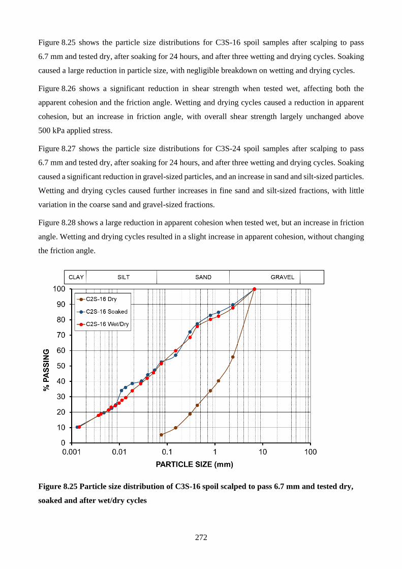
272
Figure 8.25 shows the particle size distributions for C3S-16 spoil samples after scalping to pass
6.7 mm and tested dry, after soaking for 24 hours, and after three wetting and drying cycles. Soaking
caused a large reduction in particle size, with negligible breakdown on wetting and drying cycles.
Figure 8.26 shows a significant reduction in shear strength when tested wet, affecting both the
apparent cohesion and the friction angle. Wetting and drying cycles caused a reduction in apparent
cohesion, but an increase in friction angle, with overall shear strength largely unchanged above
500 kPa applied stress.
Figure 8.27 shows the particle size distributions for C3S-24 spoil samples after scalping to pass
6.7 mm and tested dry, after soaking for 24 hours, and after three wetting and drying cycles. Soaking
caused a significant reduction in gravel-sized particles, and an increase in sand and silt-sized particles.
Wetting and drying cycles caused further increases in fine sand and silt-sized fractions, with little
variation in the coarse sand and gravel-sized fractions.
Figure 8.28 shows a large reduction in apparent cohesion when tested wet, but an increase in friction
angle. Wetting and drying cycles resulted in a slight increase in apparent cohesion, without changing
the friction angle.
Figure 8.25 Particle size distribution of C3S-16 spoil scalped to pass 6.7 mm and tested dry,
soaked and after wet/dry cycles
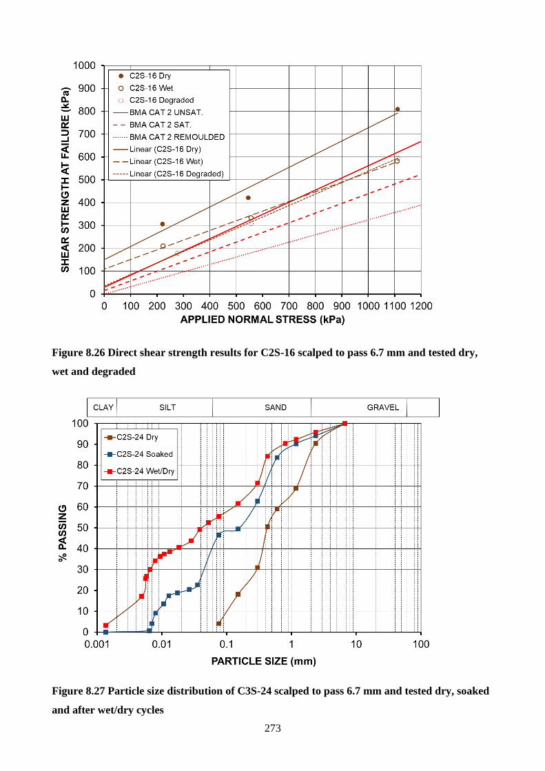
273
Figure 8.26 Direct shear strength results for C2S-16 scalped to pass 6.7 mm and tested dry,
wet and degraded
Figure 8.27 Particle size distribution of C3S-24 scalped to pass 6.7 mm and tested dry, soaked
and after wet/dry cycles
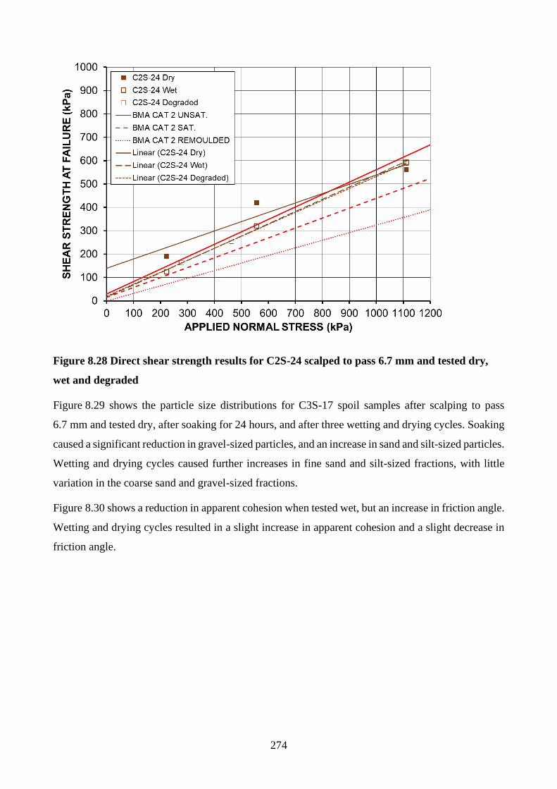
274
Figure 8.28 Direct shear strength results for C2S-24 scalped to pass 6.7 mm and tested dry,
wet and degraded
Figure 8.29 shows the particle size distributions for C3S-17 spoil samples after scalping to pass
6.7 mm and tested dry, after soaking for 24 hours, and after three wetting and drying cycles. Soaking
caused a significant reduction in gravel-sized particles, and an increase in sand and silt-sized particles.
Wetting and drying cycles caused further increases in fine sand and silt-sized fractions, with little
variation in the coarse sand and gravel-sized fractions.
Figure 8.30 shows a reduction in apparent cohesion when tested wet, but an increase in friction angle.
Wetting and drying cycles resulted in a slight increase in apparent cohesion and a slight decrease in
friction angle.
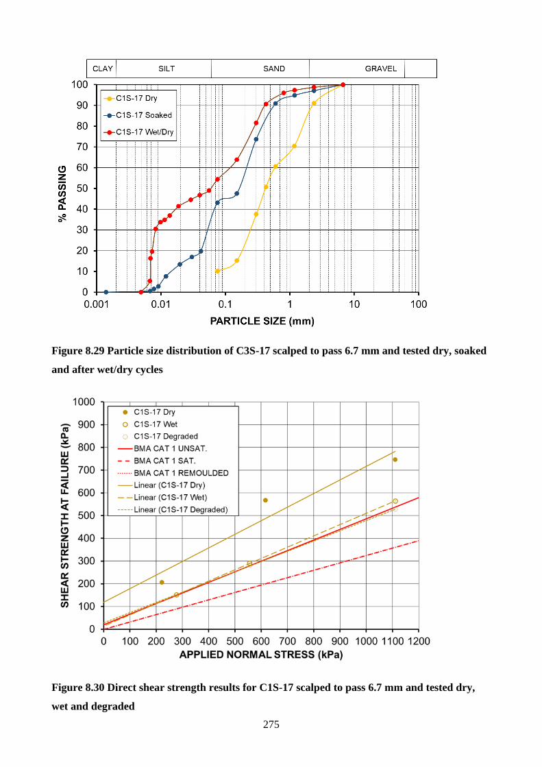
275
Figure 8.29 Particle size distribution of C3S-17 scalped to pass 6.7 mm and tested dry, soaked
and after wet/dry cycles
Figure 8.30 Direct shear strength results for C1S-17 scalped to pass 6.7 mm and tested dry,
wet and degraded
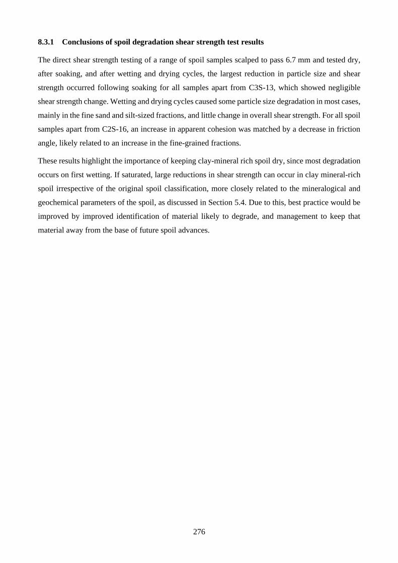
276
8.3.1 Conclusions of spoil degradation shear strength test results
The direct shear strength testing of a range of spoil samples scalped to pass 6.7 mm and tested dry,
after soaking, and after wetting and drying cycles, the largest reduction in particle size and shear
strength occurred following soaking for all samples apart from C3S-13, which showed negligible
shear strength change. Wetting and drying cycles caused some particle size degradation in most cases,
mainly in the fine sand and silt-sized fractions, and little change in overall shear strength. For all spoil
samples apart from C2S-16, an increase in apparent cohesion was matched by a decrease in friction
angle, likely related to an increase in the fine-grained fractions.
These results highlight the importance of keeping clay-mineral rich spoil dry, since most degradation
occurs on first wetting. If saturated, large reductions in shear strength can occur in clay mineral-rich
spoil irrespective of the original spoil classification, more closely related to the mineralogical and
geochemical parameters of the spoil, as discussed in Section 5.4. Due to this, best practice would be
improved by improved identification of material likely to degrade, and management to keep that
material away from the base of future spoil advances.
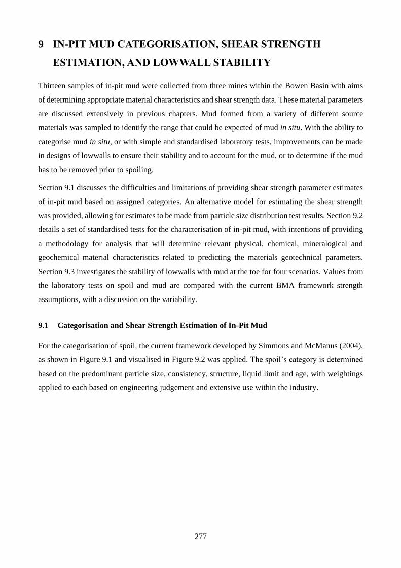
277
9 IN-PIT MUD CATEGORISATION, SHEAR STRENGTH
ESTIMATION, AND LOWWALL STABILITY
Thirteen samples of in-pit mud were collected from three mines within the Bowen Basin with aims
of determining appropriate material characteristics and shear strength data. These material parameters
are discussed extensively in previous chapters. Mud formed from a variety of different source
materials was sampled to identify the range that could be expected of mud in situ. With the ability to
categorise mud in situ, or with simple and standardised laboratory tests, improvements can be made
in designs of lowwalls to ensure their stability and to account for the mud, or to determine if the mud
has to be removed prior to spoiling.
Section 9.1 discusses the difficulties and limitations of providing shear strength parameter estimates
of in-pit mud based on assigned categories. An alternative model for estimating the shear strength
was provided, allowing for estimates to be made from particle size distribution test results. Section 9.2
details a set of standardised tests for the characterisation of in-pit mud, with intentions of providing
a methodology for analysis that will determine relevant physical, chemical, mineralogical and
geochemical material characteristics related to predicting the materials geotechnical parameters.
Section 9.3 investigates the stability of lowwalls with mud at the toe for four scenarios. Values from
the laboratory tests on spoil and mud are compared with the current BMA framework strength
assumptions, with a discussion on the variability.
9.1 Categorisation and Shear Strength Estimation of In-Pit Mud
For the categorisation of spoil, the current framework developed by Simmons and McManus (2004),
as shown in Figure 9.1 and visualised in Figure 9.2 was applied. The spoil’s category is determined
based on the predominant particle size, consistency, structure, liquid limit and age, with weightings
applied to each based on engineering judgement and extensive use within the industry.
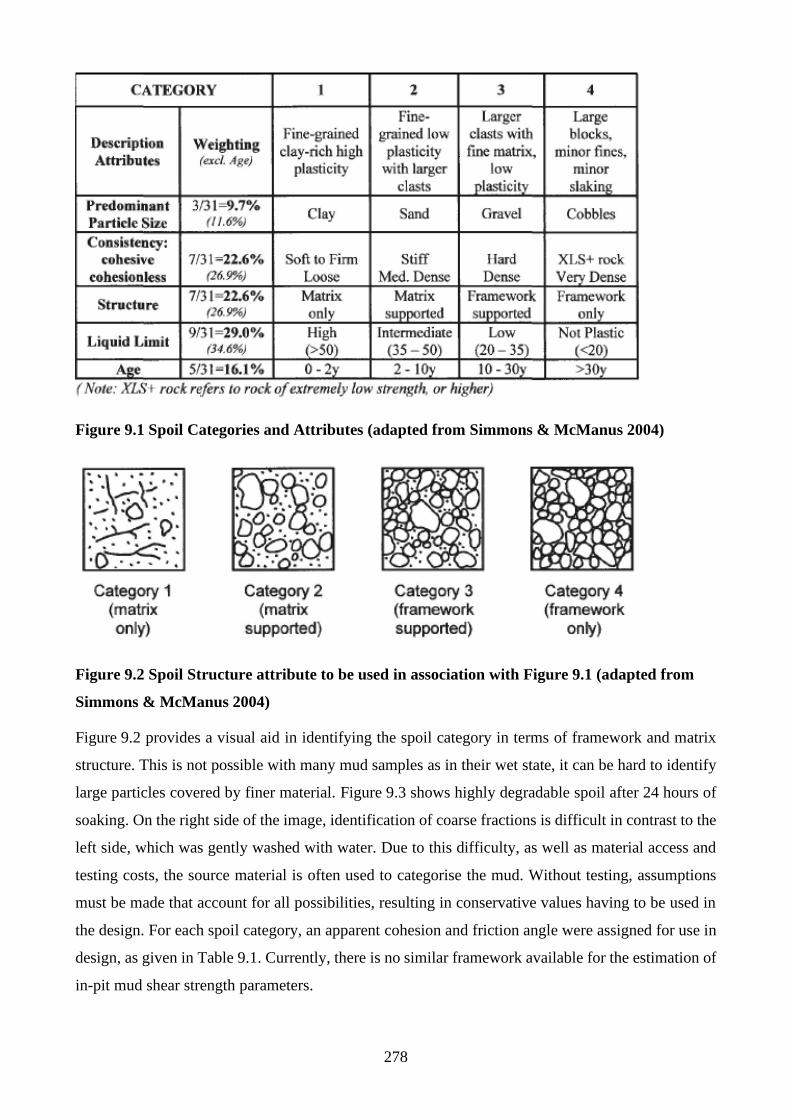
278
Figure 9.1 Spoil Categories and Attributes (adapted from Simmons & McManus 2004)
Figure 9.2 Spoil Structure attribute to be used in association with Figure 9.1 (adapted from
Simmons & McManus 2004)
Figure 9.2 provides a visual aid in identifying the spoil category in terms of framework and matrix
structure. This is not possible with many mud samples as in their wet state, it can be hard to identify
large particles covered by finer material. Figure 9.3 shows highly degradable spoil after 24 hours of
soaking. On the right side of the image, identification of coarse fractions is difficult in contrast to the
left side, which was gently washed with water. Due to this difficulty, as well as material access and
testing costs, the source material is often used to categorise the mud. Without testing, assumptions
must be made that account for all possibilities, resulting in conservative values having to be used in
the design. For each spoil category, an apparent cohesion and friction angle were assigned for use in
design, as given in Table 9.1. Currently, there is no similar framework available for the estimation of
in-pit mud shear strength parameters.
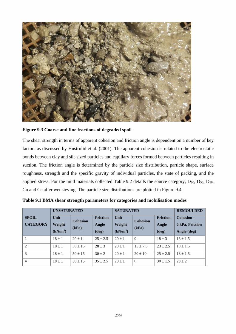
279
Figure 9.3 Coarse and fine fractions of degraded spoil
The shear strength in terms of apparent cohesion and friction angle is dependent on a number of key
factors as discussed by Hustrulid et al. (2001). The apparent cohesion is related to the electrostatic
bonds between clay and silt-sized particles and capillary forces formed between particles resulting in
suction. The friction angle is determined by the particle size distribution, particle shape, surface
roughness, strength and the specific gravity of individual particles, the state of packing, and the
applied stress. For the mud materials collected Table 9.2 details the source category, D90, D50, D10,
Cu and Cc after wet sieving. The particle size distributions are plotted in Figure 9.4.
Table 9.1 BMA shear strength parameters for categories and mobilisation modes
SPOIL
CATEGORY
UNSATURATED SATURATED REMOULDED
Unit
Weight
(kN/m3)
Cohesion
(kPa)
Friction
Angle
(deg)
Unit
Weight
(kN/m3)
Cohesion
(kPa)
Friction
Angle
(deg)
Cohesion =
0 kPa, Friction
Angle (deg)
1 18 1 20 1 25 2.5 20 1 0 18 3 18 1.5
2 18 1 30 15 28 3 20 1 15 7.5 23 2.5 18 1.5
3 18 1 50 15 30 2 20 1 20 10 25 2.5 18 1.5
4 18 1 50 15 35 2.5 20 1 0 30 1.5 28 2
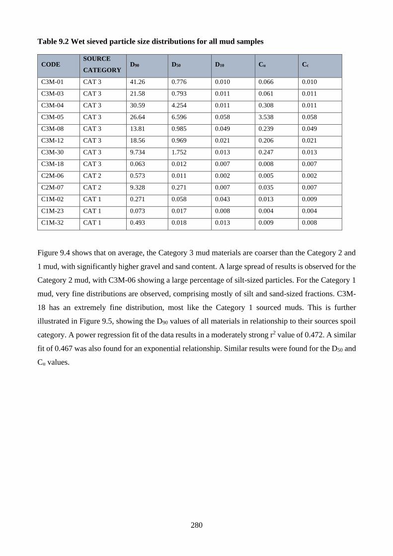
280
Table 9.2 Wet sieved particle size distributions for all mud samples
CODE SOURCE
CATEGORY D90 D50 D10 Cu Cc
C3M-01 CAT 3 41.26 0.776 0.010 0.066 0.010
C3M-03 CAT 3 21.58 0.793 0.011 0.061 0.011
C3M-04 CAT 3 30.59 4.254 0.011 0.308 0.011
C3M-05 CAT 3 26.64 6.596 0.058 3.538 0.058
C3M-08 CAT 3 13.81 0.985 0.049 0.239 0.049
C3M-12 CAT 3 18.56 0.969 0.021 0.206 0.021
C3M-30 CAT 3 9.734 1.752 0.013 0.247 0.013
C3M-18 CAT 3 0.063 0.012 0.007 0.008 0.007
C2M-06 CAT 2 0.573 0.011 0.002 0.005 0.002
C2M-07 CAT 2 9.328 0.271 0.007 0.035 0.007
C1M-02 CAT 1 0.271 0.058 0.043 0.013 0.009
C1M-23 CAT 1 0.073 0.017 0.008 0.004 0.004
C1M-32 CAT 1 0.493 0.018 0.013 0.009 0.008
Figure 9.4 shows that on average, the Category 3 mud materials are coarser than the Category 2 and
1 mud, with significantly higher gravel and sand content. A large spread of results is observed for the
Category 2 mud, with C3M-06 showing a large percentage of silt-sized particles. For the Category 1
mud, very fine distributions are observed, comprising mostly of silt and sand-sized fractions. C3M-
18 has an extremely fine distribution, most like the Category 1 sourced muds. This is further
illustrated in Figure 9.5, showing the D90 values of all materials in relationship to their sources spoil
category. A power regression fit of the data results in a moderately strong r2 value of 0.472. A similar
fit of 0.467 was also found for an exponential relationship. Similar results were found for the D50 and
Cu values.
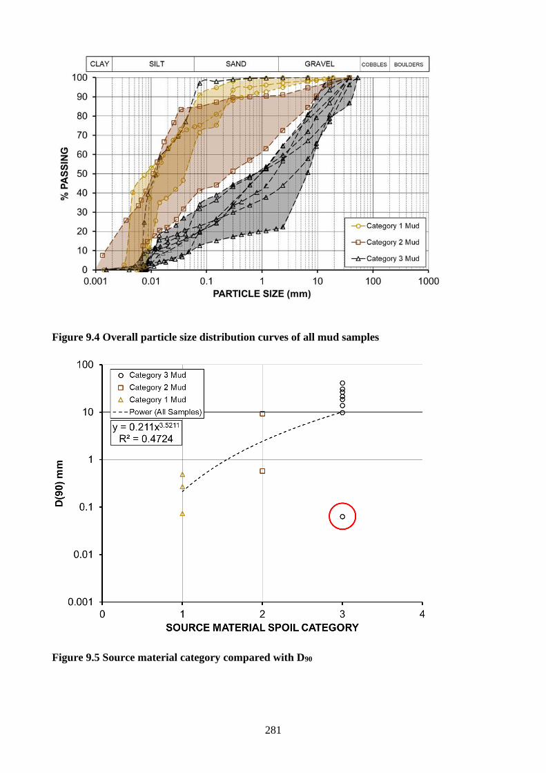
281
Figure 9.4 Overall particle size distribution curves of all mud samples
Figure 9.5 Source material category compared with D90
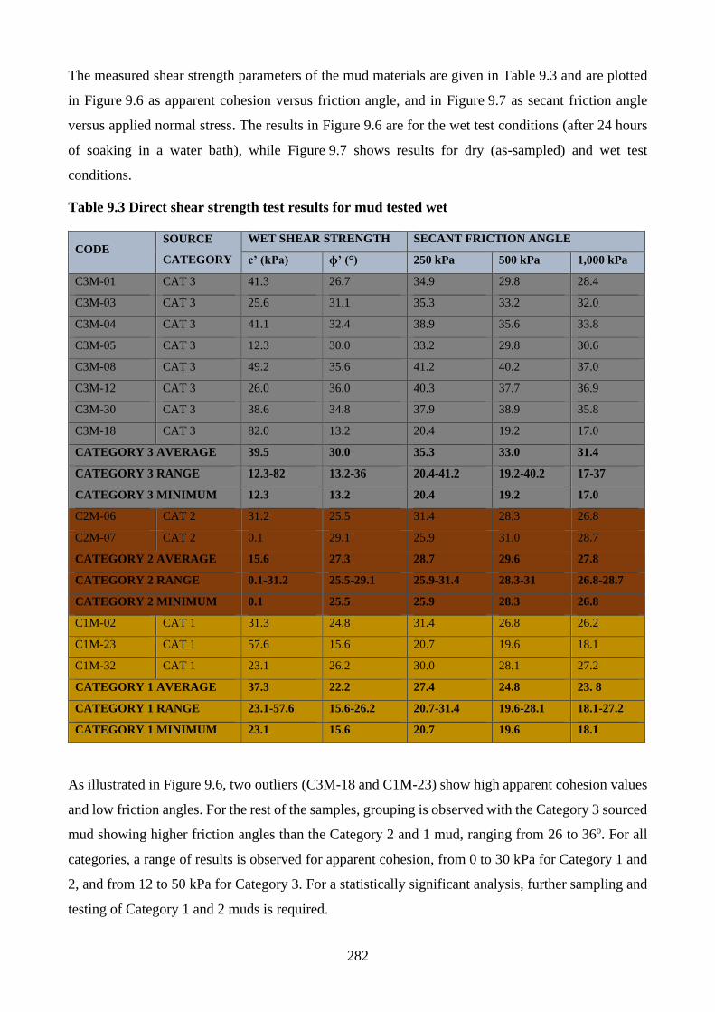
282
The measured shear strength parameters of the mud materials are given in Table 9.3 and are plotted
in Figure 9.6 as apparent cohesion versus friction angle, and in Figure 9.7 as secant friction angle
versus applied normal stress. The results in Figure 9.6 are for the wet test conditions (after 24 hours
of soaking in a water bath), while Figure 9.7 shows results for dry (as-sampled) and wet test
conditions.
Table 9.3 Direct shear strength test results for mud tested wet
As illustrated in Figure 9.6, two outliers (C3M-18 and C1M-23) show high apparent cohesion values
and low friction angles. For the rest of the samples, grouping is observed with the Category 3 sourced
mud showing higher friction angles than the Category 2 and 1 mud, ranging from 26 to 36o. For all
categories, a range of results is observed for apparent cohesion, from 0 to 30 kPa for Category 1 and
2, and from 12 to 50 kPa for Category 3. For a statistically significant analysis, further sampling and
testing of Category 1 and 2 muds is required.
CODE SOURCE
CATEGORY
WET SHEAR STRENGTH SECANT FRICTION ANGLE
c’ (kPa) ɸ’ (°) 250 kPa 500 kPa 1,000 kPa
C3M-01 CAT 3 41.3 26.7 34.9 29.8 28.4
C3M-03 CAT 3 25.6 31.1 35.3 33.2 32.0
C3M-04 CAT 3 41.1 32.4 38.9 35.6 33.8
C3M-05 CAT 3 12.3 30.0 33.2 29.8 30.6
C3M-08 CAT 3 49.2 35.6 41.2 40.2 37.0
C3M-12 CAT 3 26.0 36.0 40.3 37.7 36.9
C3M-30 CAT 3 38.6 34.8 37.9 38.9 35.8
C3M-18 CAT 3 82.0 13.2 20.4 19.2 17.0
CATEGORY 3 AVERAGE 39.5 30.0 35.3 33.0 31.4
CATEGORY 3 RANGE 12.3-82 13.2-36 20.4-41.2 19.2-40.2 17-37
CATEGORY 3 MINIMUM 12.3 13.2 20.4 19.2 17.0
C2M-06 CAT 2 31.2 25.5 31.4 28.3 26.8
C2M-07 CAT 2 0.1 29.1 25.9 31.0 28.7
CATEGORY 2 AVERAGE 15.6 27.3 28.7 29.6 27.8
CATEGORY 2 RANGE 0.1-31.2 25.5-29.1 25.9-31.4 28.3-31 26.8-28.7
CATEGORY 2 MINIMUM 0.1 25.5 25.9 28.3 26.8
C1M-02 CAT 1 31.3 24.8 31.4 26.8 26.2
C1M-23 CAT 1 57.6 15.6 20.7 19.6 18.1
C1M-32 CAT 1 23.1 26.2 30.0 28.1 27.2
CATEGORY 1 AVERAGE 37.3 22.2 27.4 24.8 23. 8
CATEGORY 1 RANGE 23.1-57.6 15.6-26.2 20.7-31.4 19.6-28.1 18.1-27.2
CATEGORY 1 MINIMUM 23.1 15.6 20.7 19.6 18.1
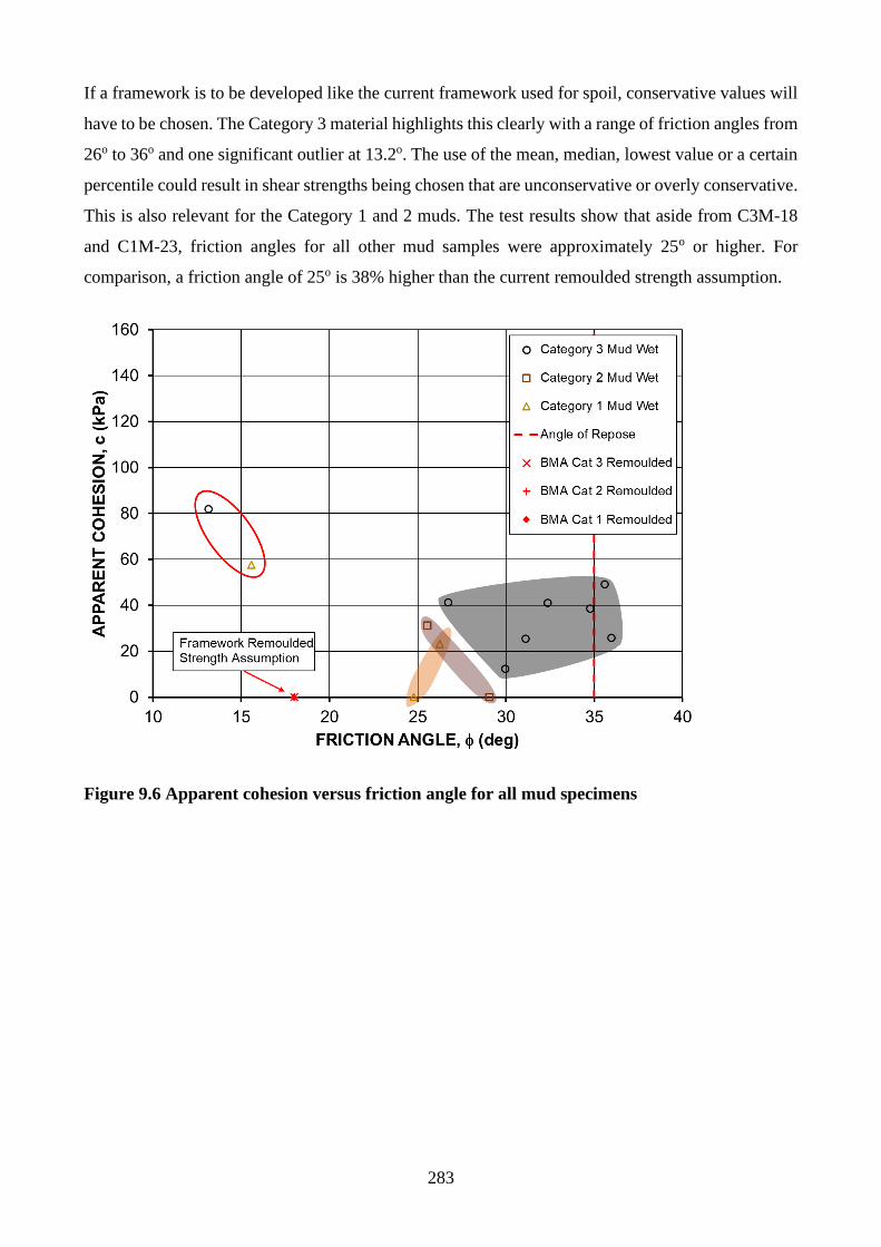
283
If a framework is to be developed like the current framework used for spoil, conservative values will
have to be chosen. The Category 3 material highlights this clearly with a range of friction angles from
26o to 36o and one significant outlier at 13.2o. The use of the mean, median, lowest value or a certain
percentile could result in shear strengths being chosen that are unconservative or overly conservative.
This is also relevant for the Category 1 and 2 muds. The test results show that aside from C3M-18
and C1M-23, friction angles for all other mud samples were approximately 25o or higher. For
comparison, a friction angle of 25o is 38% higher than the current remoulded strength assumption.
Figure 9.6 Apparent cohesion versus friction angle for all mud specimens
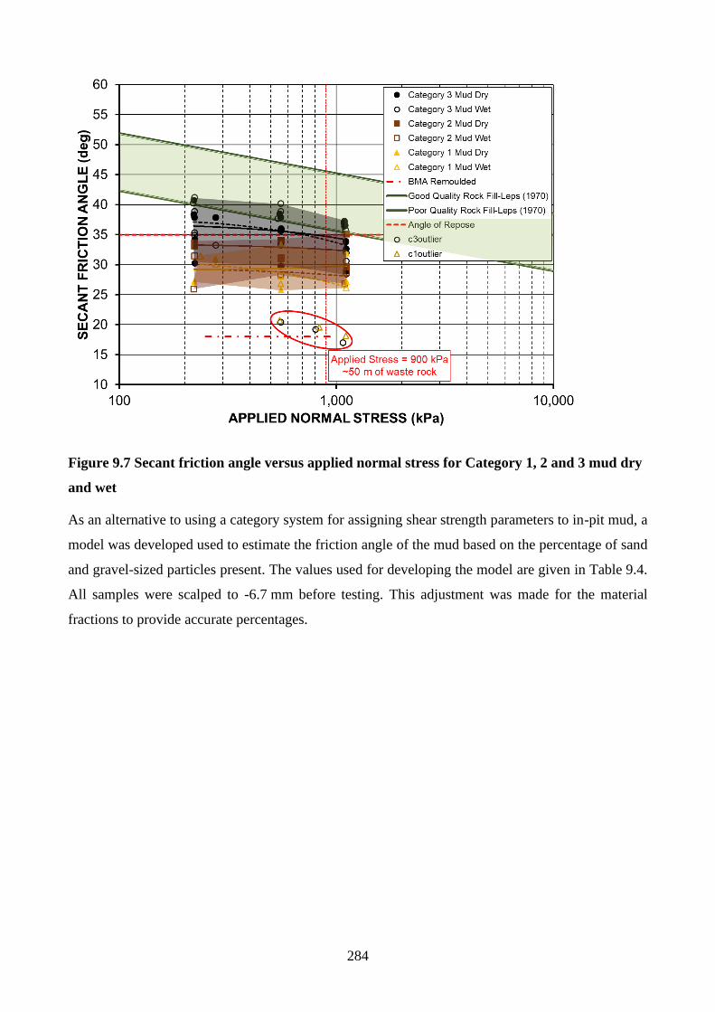
284
Figure 9.7 Secant friction angle versus applied normal stress for Category 1, 2 and 3 mud dry
and wet
As an alternative to using a category system for assigning shear strength parameters to in-pit mud, a
model was developed used to estimate the friction angle of the mud based on the percentage of sand
and gravel-sized particles present. The values used for developing the model are given in Table 9.4.
All samples were scalped to -6.7 mm before testing. This adjustment was made for the material
fractions to provide accurate percentages.
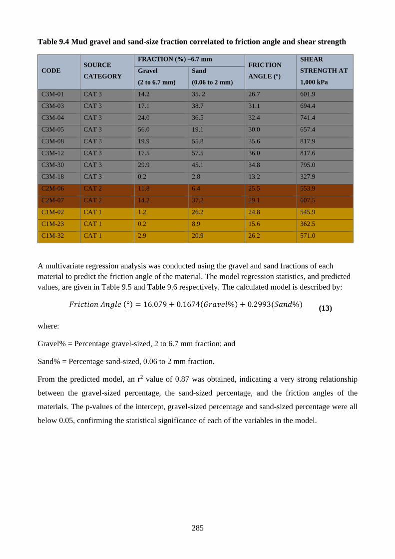
285
Table 9.4 Mud gravel and sand-size fraction correlated to friction angle and shear strength
A multivariate regression analysis was conducted using the gravel and sand fractions of each
material to predict the friction angle of the material. The model regression statistics, and predicted
values, are given in Table 9.5 and Table 9.6 respectively. The calculated model is described by:
𝐹𝑟𝑖𝑐𝑡𝑖𝑜𝑛 𝐴𝑛𝑔𝑙𝑒 (°) = 16.079 + 0.1674(𝐺𝑟𝑎𝑣𝑒𝑙%) + 0.2993(𝑆𝑎𝑛𝑑%) (13)
where:
Gravel% = Percentage gravel-sized, 2 to 6.7 mm fraction; and
Sand% = Percentage sand-sized, 0.06 to 2 mm fraction.
From the predicted model, an r2 value of 0.87 was obtained, indicating a very strong relationship
between the gravel-sized percentage, the sand-sized percentage, and the friction angles of the
materials. The p-values of the intercept, gravel-sized percentage and sand-sized percentage were all
below 0.05, confirming the statistical significance of each of the variables in the model.
CODE SOURCE
CATEGORY
FRACTION (%) –6.7 mm FRICTION
ANGLE (°)
SHEAR
STRENGTH AT
1,000 kPa
Gravel
(2 to 6.7 mm)
Sand
(0.06 to 2 mm)
C3M-01 CAT 3 14.2 35. 2 26.7 601.9
C3M-03 CAT 3 17.1 38.7 31.1 694.4
C3M-04 CAT 3 24.0 36.5 32.4 741.4
C3M-05 CAT 3 56.0 19.1 30.0 657.4
C3M-08 CAT 3 19.9 55.8 35.6 817.9
C3M-12 CAT 3 17.5 57.5 36.0 817.6
C3M-30 CAT 3 29.9 45.1 34.8 795.0
C3M-18 CAT 3 0.2 2.8 13.2 327.9
C2M-06 CAT 2 11.8 6.4 25.5 553.9
C2M-07 CAT 2 14.2 37.2 29.1 607.5
C1M-02 CAT 1 1.2 26.2 24.8 545.9
C1M-23 CAT 1 0.2 8.9 15.6 362.5
C1M-32 CAT 1 2.9 20.9 26.2 571.0
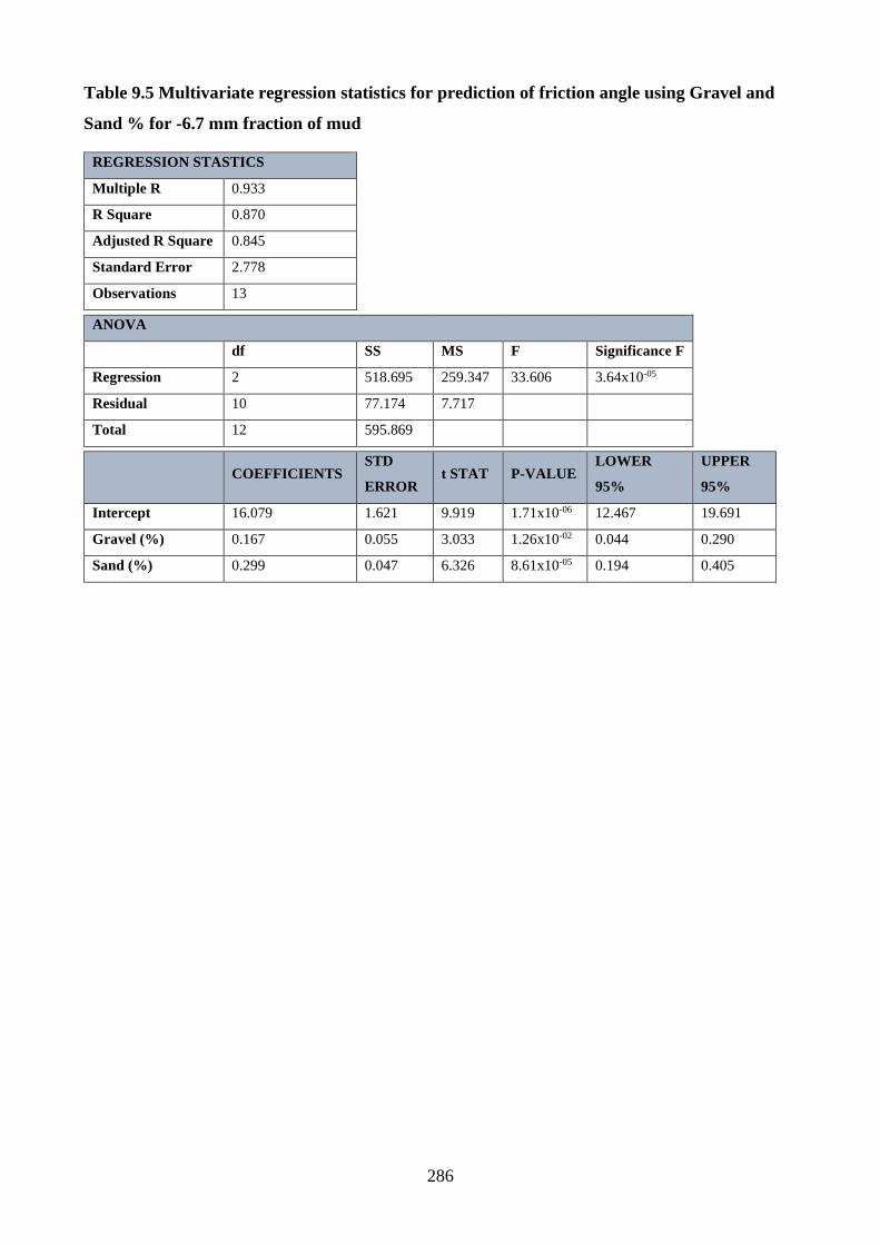
286
Table 9.5 Multivariate regression statistics for prediction of friction angle using Gravel and
Sand % for -6.7 mm fraction of mud
REGRESSION STASTICS
Multiple R 0.933
R Square 0.870
Adjusted R Square 0.845
Standard Error 2.778
Observations 13 ANOVA
df SS MS F Significance F
Regression 2 518.695 259.347 33.606 3.64x10-05
Residual 10 77.174 7.717
Total 12 595.869
COEFFICIENTS STD
ERROR t STAT P-VALUE
LOWER
95%
UPPER
95%
Intercept 16.079 1.621 9.919 1.71x10-06 12.467 19.691
Gravel (%) 0.167 0.055 3.033 1.26x10-02 0.044 0.290
Sand (%) 0.299 0.047 6.326 8.61x10-05 0.194 0.405
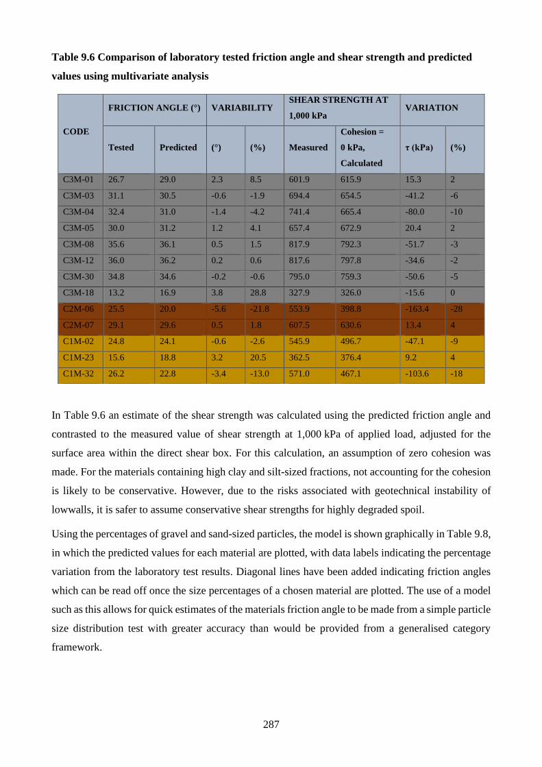
287
Table 9.6 Comparison of laboratory tested friction angle and shear strength and predicted
values using multivariate analysis
In Table 9.6 an estimate of the shear strength was calculated using the predicted friction angle and
contrasted to the measured value of shear strength at 1,000 kPa of applied load, adjusted for the
surface area within the direct shear box. For this calculation, an assumption of zero cohesion was
made. For the materials containing high clay and silt-sized fractions, not accounting for the cohesion
is likely to be conservative. However, due to the risks associated with geotechnical instability of
lowwalls, it is safer to assume conservative shear strengths for highly degraded spoil.
Using the percentages of gravel and sand-sized particles, the model is shown graphically in Table 9.8,
in which the predicted values for each material are plotted, with data labels indicating the percentage
variation from the laboratory test results. Diagonal lines have been added indicating friction angles
which can be read off once the size percentages of a chosen material are plotted. The use of a model
such as this allows for quick estimates of the materials friction angle to be made from a simple particle
size distribution test with greater accuracy than would be provided from a generalised category
framework.
CODE
FRICTION ANGLE (°) VARIABILITY SHEAR STRENGTH AT
1,000 kPa VARIATION
Tested Predicted (°) (%) Measured
Cohesion =
0 kPa,
Calculated
τ (kPa) (%)
C3M-01 26.7 29.0 2.3 8.5 601.9 615.9 15.3 2
C3M-03 31.1 30.5 -0.6 -1.9 694.4 654.5 -41.2 -6
C3M-04 32.4 31.0 -1.4 -4.2 741.4 665.4 -80.0 -10
C3M-05 30.0 31.2 1.2 4.1 657.4 672.9 20.4 2
C3M-08 35.6 36.1 0.5 1.5 817.9 792.3 -51.7 -3
C3M-12 36.0 36.2 0.2 0.6 817.6 797.8 -34.6 -2
C3M-30 34.8 34.6 -0.2 -0.6 795.0 759.3 -50.6 -5
C3M-18 13.2 16.9 3.8 28.8 327.9 326.0 -15.6 0
C2M-06 25.5 20.0 -5.6 -21.8 553.9 398.8 -163.4 -28
C2M-07 29.1 29.6 0.5 1.8 607.5 630.6 13.4 4
C1M-02 24.8 24.1 -0.6 -2.6 545.9 496.7 -47.1 -9
C1M-23 15.6 18.8 3.2 20.5 362.5 376.4 9.2 4
C1M-32 26.2 22.8 -3.4 -13.0 571.0 467.1 -103.6 -18
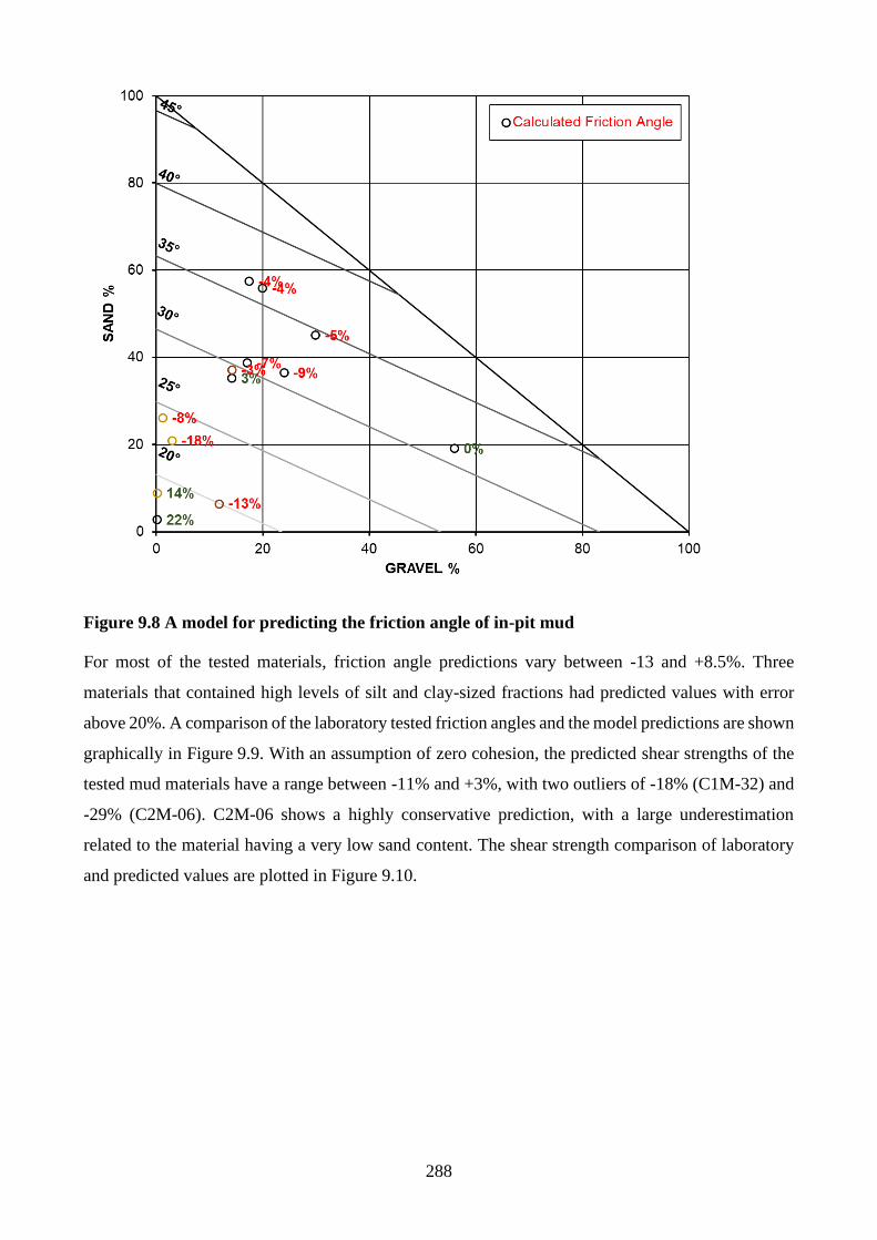
288
Figure 9.8 A model for predicting the friction angle of in-pit mud
For most of the tested materials, friction angle predictions vary between -13 and +8.5%. Three
materials that contained high levels of silt and clay-sized fractions had predicted values with error
above 20%. A comparison of the laboratory tested friction angles and the model predictions are shown
graphically in Figure 9.9. With an assumption of zero cohesion, the predicted shear strengths of the
tested mud materials have a range between -11% and +3%, with two outliers of -18% (C1M-32) and
-29% (C2M-06). C2M-06 shows a highly conservative prediction, with a large underestimation
related to the material having a very low sand content. The shear strength comparison of laboratory
and predicted values are plotted in Figure 9.10.
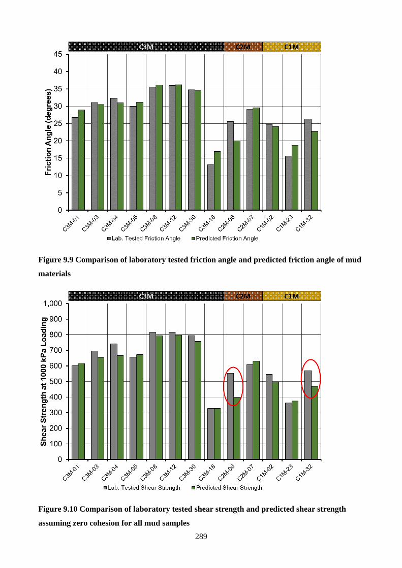
289
Figure 9.9 Comparison of laboratory tested friction angle and predicted friction angle of mud
materials
Figure 9.10 Comparison of laboratory tested shear strength and predicted shear strength
assuming zero cohesion for all mud samples
290
9.1.1 Categorisation and shear strength estimation conclusions:
This chapter has discussed the development of a model used to predict the friction angle of in-pit mud
based on the gravel and sand fractions of the material. The predicted friction angles show larger
variability for materials that contain large amounts of silt and clay-sized fractions. Overall, most
predictions varied between -13% and +8.5%. The statistical significance of the model was found to
be very high with an r2 value of 0.87, indicating a strong relationship between the parameters and the
friction angle. Each variable used in the multivariate regression was significant.
Calculations of the shear strength with an assumption of zero cohesion were compared with
laboratory-determined values. The largest variability above the laboratory-determined value was 3%.
For most materials, conservative results are calculated. For samples containing high amounts of silt
and clay, an increase is observed in the conservative nature of the predictions. For design, this is
desirable; however, improved accuracy is always beneficial.
To quickly estimate the shear strength of an in-pit mud material, this proposed model will provide
more accuracy than would be obtained based on an assumption of remoulded parameters from the
BMA spoil category framework.
By basing the predictions on material parameters that can be determined via wet sieving, estimations
can be made quickly and cheaply.
The key limitations and potential extensions of this model are:
• The sample size used for the multivariate regression analysis was 13. Future testing of in-pit
mud will allow for a larger sample size, which will be useful in improving the accuracy of
the model.
• As the model increases with inaccuracy in estimation of friction angle for materials with
high silt and clay content, its use for identification of material with more than 30% sand and
40% gravel is recommended.
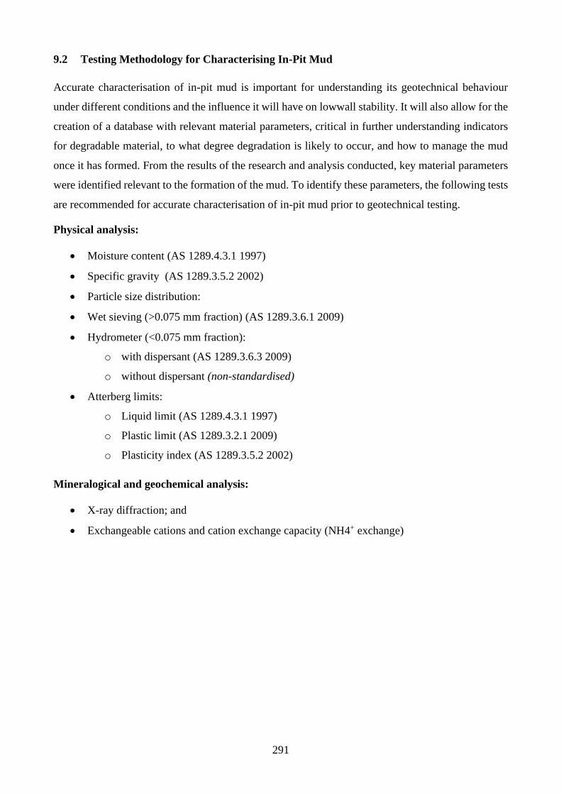
291
9.2 Testing Methodology for Characterising In-Pit Mud
Accurate characterisation of in-pit mud is important for understanding its geotechnical behaviour
under different conditions and the influence it will have on lowwall stability. It will also allow for the
creation of a database with relevant material parameters, critical in further understanding indicators
for degradable material, to what degree degradation is likely to occur, and how to manage the mud
once it has formed. From the results of the research and analysis conducted, key material parameters
were identified relevant to the formation of the mud. To identify these parameters, the following tests
are recommended for accurate characterisation of in-pit mud prior to geotechnical testing.
Physical analysis:
• Moisture content (AS 1289.4.3.1 1997)
• Specific gravity (AS 1289.3.5.2 2002)
• Particle size distribution:
• Wet sieving (>0.075 mm fraction) (AS 1289.3.6.1 2009)
• Hydrometer (<0.075 mm fraction):
o with dispersant (AS 1289.3.6.3 2009)
o without dispersant (non-standardised)
• Atterberg limits:
o Liquid limit (AS 1289.4.3.1 1997)
o Plastic limit (AS 1289.3.2.1 2009)
o Plasticity index (AS 1289.3.5.2 2002)
Mineralogical and geochemical analysis:
• X-ray diffraction; and
• Exchangeable cations and cation exchange capacity (NH4+ exchange)
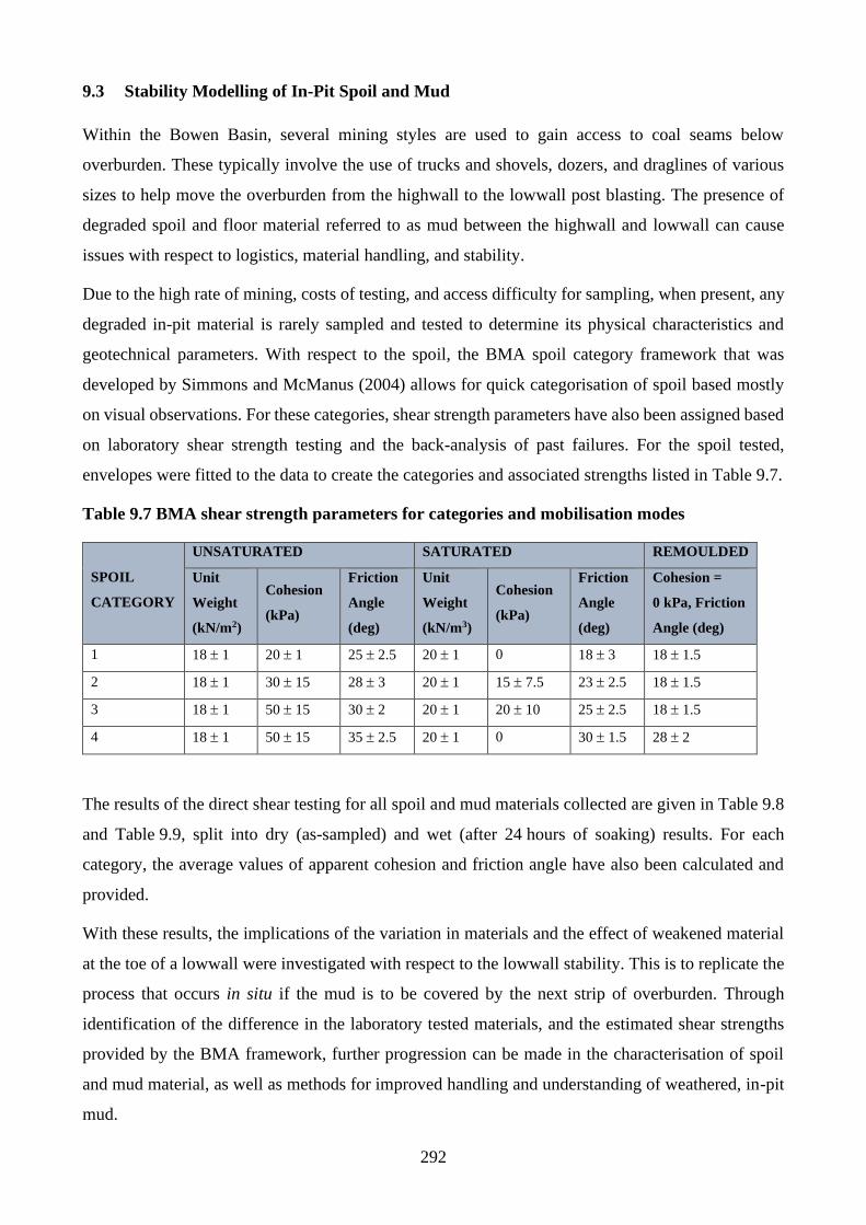
292
9.3 Stability Modelling of In-Pit Spoil and Mud
Within the Bowen Basin, several mining styles are used to gain access to coal seams below
overburden. These typically involve the use of trucks and shovels, dozers, and draglines of various
sizes to help move the overburden from the highwall to the lowwall post blasting. The presence of
degraded spoil and floor material referred to as mud between the highwall and lowwall can cause
issues with respect to logistics, material handling, and stability.
Due to the high rate of mining, costs of testing, and access difficulty for sampling, when present, any
degraded in-pit material is rarely sampled and tested to determine its physical characteristics and
geotechnical parameters. With respect to the spoil, the BMA spoil category framework that was
developed by Simmons and McManus (2004) allows for quick categorisation of spoil based mostly
on visual observations. For these categories, shear strength parameters have also been assigned based
on laboratory shear strength testing and the back-analysis of past failures. For the spoil tested,
envelopes were fitted to the data to create the categories and associated strengths listed in Table 9.7.
Table 9.7 BMA shear strength parameters for categories and mobilisation modes
SPOIL
CATEGORY
UNSATURATED SATURATED REMOULDED
Unit
Weight
(kN/m2)
Cohesion
(kPa)
Friction
Angle
(deg)
Unit
Weight
(kN/m3)
Cohesion
(kPa)
Friction
Angle
(deg)
Cohesion =
0 kPa, Friction
Angle (deg)
1 18 1 20 1 25 2.5 20 1 0 18 3 18 1.5
2 18 1 30 15 28 3 20 1 15 7.5 23 2.5 18 1.5
3 18 1 50 15 30 2 20 1 20 10 25 2.5 18 1.5
4 18 1 50 15 35 2.5 20 1 0 30 1.5 28 2
The results of the direct shear testing for all spoil and mud materials collected are given in Table 9.8
and Table 9.9, split into dry (as-sampled) and wet (after 24 hours of soaking) results. For each
category, the average values of apparent cohesion and friction angle have also been calculated and
provided.
With these results, the implications of the variation in materials and the effect of weakened material
at the toe of a lowwall were investigated with respect to the lowwall stability. This is to replicate the
process that occurs in situ if the mud is to be covered by the next strip of overburden. Through
identification of the difference in the laboratory tested materials, and the estimated shear strengths
provided by the BMA framework, further progression can be made in the characterisation of spoil
and mud material, as well as methods for improved handling and understanding of weathered, in-pit
mud.
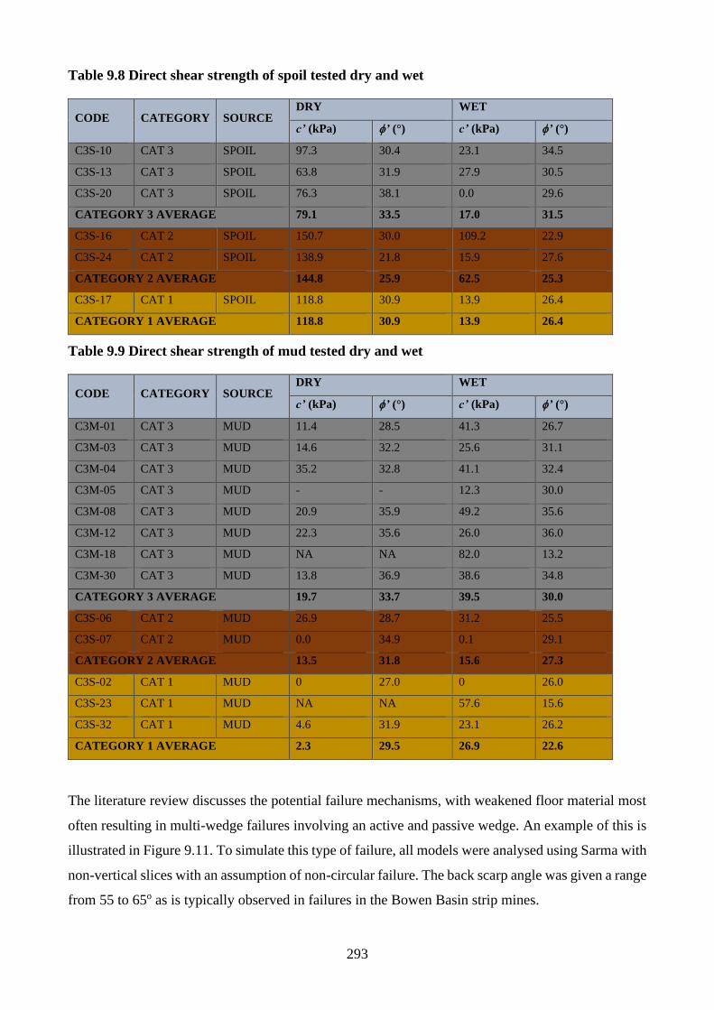
293
Table 9.8 Direct shear strength of spoil tested dry and wet
CODE CATEGORY SOURCE DRY WET
c’ (kPa) ’ (°) c’ (kPa) ’ (°)
C3S-10 CAT 3 SPOIL 97.3 30.4 23.1 34.5
C3S-13 CAT 3 SPOIL 63.8 31.9 27.9 30.5
C3S-20 CAT 3 SPOIL 76.3 38.1 0.0 29.6
CATEGORY 3 AVERAGE 79.1 33.5 17.0 31.5
C3S-16 CAT 2 SPOIL 150.7 30.0 109.2 22.9
C3S-24 CAT 2 SPOIL 138.9 21.8 15.9 27.6
CATEGORY 2 AVERAGE 144.8 25.9 62.5 25.3
C3S-17 CAT 1 SPOIL 118.8 30.9 13.9 26.4
CATEGORY 1 AVERAGE 118.8 30.9 13.9 26.4
Table 9.9 Direct shear strength of mud tested dry and wet
CODE CATEGORY SOURCE DRY WET
c’ (kPa) ’ (°) c’ (kPa) ’ (°)
C3M-01 CAT 3 MUD 11.4 28.5 41.3 26.7
C3M-03 CAT 3 MUD 14.6 32.2 25.6 31.1
C3M-04 CAT 3 MUD 35.2 32.8 41.1 32.4
C3M-05 CAT 3 MUD - - 12.3 30.0
C3M-08 CAT 3 MUD 20.9 35.9 49.2 35.6
C3M-12 CAT 3 MUD 22.3 35.6 26.0 36.0
C3M-18 CAT 3 MUD NA NA 82.0 13.2
C3M-30 CAT 3 MUD 13.8 36.9 38.6 34.8
CATEGORY 3 AVERAGE 19.7 33.7 39.5 30.0
C3S-06 CAT 2 MUD 26.9 28.7 31.2 25.5
C3S-07 CAT 2 MUD 0.0 34.9 0.1 29.1
CATEGORY 2 AVERAGE 13.5 31.8 15.6 27.3
C3S-02 CAT 1 MUD 0 27.0 0 26.0
C3S-23 CAT 1 MUD NA NA 57.6 15.6
C3S-32 CAT 1 MUD 4.6 31.9 23.1 26.2
CATEGORY 1 AVERAGE 2.3 29.5 26.9 22.6
The literature review discusses the potential failure mechanisms, with weakened floor material most
often resulting in multi-wedge failures involving an active and passive wedge. An example of this is
illustrated in Figure 9.11. To simulate this type of failure, all models were analysed using Sarma with
non-vertical slices with an assumption of non-circular failure. The back scarp angle was given a range
from 55 to 65o as is typically observed in failures in the Bowen Basin strip mines.
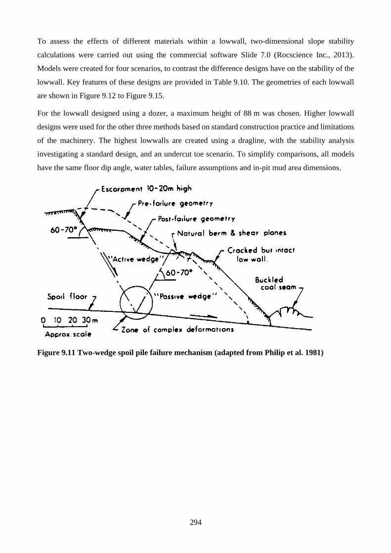
294
To assess the effects of different materials within a lowwall, two-dimensional slope stability
calculations were carried out using the commercial software Slide 7.0 (Rocscience Inc., 2013).
Models were created for four scenarios, to contrast the difference designs have on the stability of the
lowwall. Key features of these designs are provided in Table 9.10. The geometries of each lowwall
are shown in Figure 9.12 to Figure 9.15.
For the lowwall designed using a dozer, a maximum height of 88 m was chosen. Higher lowwall
designs were used for the other three methods based on standard construction practice and limitations
of the machinery. The highest lowwalls are created using a dragline, with the stability analysis
investigating a standard design, and an undercut toe scenario. To simplify comparisons, all models
have the same floor dip angle, water tables, failure assumptions and in-pit mud area dimensions.
Figure 9.11 Two-wedge spoil pile failure mechanism (adapted from Philip et al. 1981)
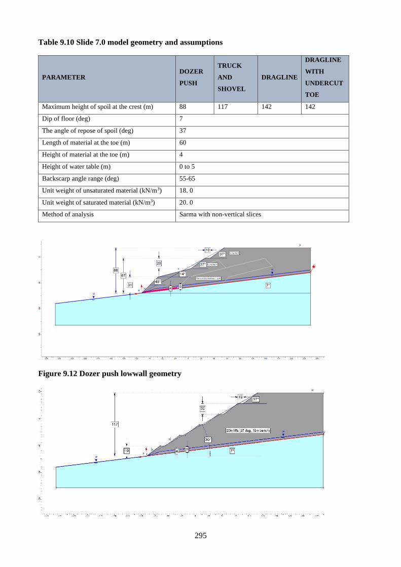
295
Table 9.10 Slide 7.0 model geometry and assumptions
PARAMETER DOZER
PUSH
TRUCK
AND
SHOVEL
DRAGLINE
DRAGLINE
WITH
UNDERCUT
TOE
Maximum height of spoil at the crest (m) 88 117 142 142
Dip of floor (deg) 7
The angle of repose of spoil (deg) 37
Length of material at the toe (m) 60
Height of material at the toe (m) 4
Height of water table (m) 0 to 5
Backscarp angle range (deg) 55-65
Unit weight of unsaturated material (kN/m3) 18. 0
Unit weight of saturated material (kN/m3) 20. 0
Method of analysis Sarma with non-vertical slices
Figure 9.12 Dozer push lowwall geometry
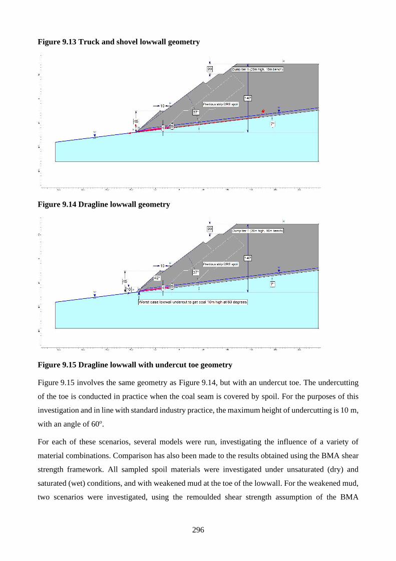
296
Figure 9.13 Truck and shovel lowwall geometry
Figure 9.14 Dragline lowwall geometry
Figure 9.15 Dragline lowwall with undercut toe geometry
Figure 9.15 involves the same geometry as Figure 9.14, but with an undercut toe. The undercutting
of the toe is conducted in practice when the coal seam is covered by spoil. For the purposes of this
investigation and in line with standard industry practice, the maximum height of undercutting is 10 m,
with an angle of 60o.
For each of these scenarios, several models were run, investigating the influence of a variety of
material combinations. Comparison has also been made to the results obtained using the BMA shear
strength framework. All sampled spoil materials were investigated under unsaturated (dry) and
saturated (wet) conditions, and with weakened mud at the toe of the lowwall. For the weakened mud,
two scenarios were investigated, using the remoulded shear strength assumption of the BMA
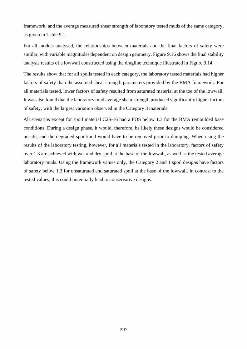
297
framework, and the average measured shear strength of laboratory tested muds of the same category,
as given in Table 9.1.
For all models analysed, the relationships between materials and the final factors of safety were
similar, with variable magnitudes dependent on design geometry. Figure 9.16 shows the final stability
analysis results of a lowwall constructed using the dragline technique illustrated in Figure 9.14.
The results show that for all spoils tested in each category, the laboratory tested materials had higher
factors of safety than the assumed shear strength parameters provided by the BMA framework. For
all materials tested, lower factors of safety resulted from saturated material at the toe of the lowwall.
It was also found that the laboratory mud average shear strength produced significantly higher factors
of safety, with the largest variation observed in the Category 3 materials.
All scenarios except for spoil material C2S-16 had a FOS below 1.3 for the BMA remoulded base
conditions. During a design phase, it would, therefore, be likely these designs would be considered
unsafe, and the degraded spoil/mud would have to be removed prior to dumping. When using the
results of the laboratory testing, however, for all materials tested in the laboratory, factors of safety
over 1.3 are achieved with wet and dry spoil at the base of the lowwall, as well as the tested average
laboratory muds. Using the framework values only, the Category 2 and 1 spoil designs have factors
of safety below 1.3 for unsaturated and saturated spoil at the base of the lowwall. In contrast to the
tested values, this could potentially lead to conservative designs.
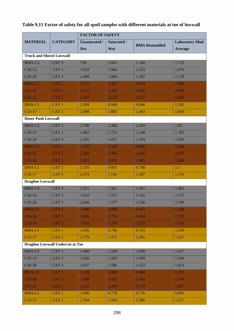
298
Table 9.11 Factor of safety for all spoil samples with different materials at toe of lowwall
MATERIAL CATEGORY
FACTOR OF SAFETY
Unsaturated /
Dry
Saturated /
Wet BMA Remoulded
Laboratory Mud
Average
Truck and Shovel Lowwall
BMA-C3 CAT 3 734 1.601 1.160 1.722
C3S-13 CAT 3 1.923 1.864 1.253 1.876
C3S-20 CAT 3 2.408 1.866 1.382 2.178
BMA-C2 CAT 2 1.511 1.353 1.034 1.486
C2S-16 CAT 2 2.232 2.141 1.662 2.068
C2S-24 CAT 2 1.707 1.623 1.517 1.620
BMA-C1 CAT 1 1.209 0.948 0.946 1.282
C1S-17 CAT 1 2.088 1.882 1.463 1.818
Dozer Push Lowwall
BMA-C3 CAT 3 1.708 1.386 1.043 1.65
C3S-13 CAT 3 1.992 1.712 1.148 1.783
C3S-20 CAT 3 2.455 1.657 1.294 1.959
BMA-C2 CAT 2 1.356 1.138 0.896 1.254
C2S-16 CAT 2 2.584 2.394 1.626 2.037
C2S-24 CAT 2 2.011 1.874 1.481 1.868
BMA-C1 CAT 1 1.105 0.801 0.798 1.1
C1S-17 CAT 1 2.374 1.741 1.397 1.710
Dragline Lowwall
BMA-C3 CAT 3 1.471 1.301 1.001 1.461
C3S-13 CAT 3 1.633 1.571 1.102 1.575
C3S-20 CAT 3 2.044 1.577 1.236 1.769
BMA-C2 CAT 2 1.280 1.090 0.872 1.196
C2S-16 CAT 2 1.886 1.793 1.454 1.725
C2S-24 CAT 2 1.431 1.379 1.272 1.376
BMA-C1 CAT 1 1.056 0.786 0.783 1.039
C1S-17 CAT 1 1.779 1.571 1.291 1.527
Dragline Lowwall Undercut at Toe
BMA-C3 CAT 3 1.468 1.298 1.008 1.457
C3S-13 CAT 3 1.626 1.595 1.099 1.569
C3S-20 CAT 3 2.037 1.586 1.233 1.813
BMA-C2 CAT 2 1.228 1.080 0.868 1.152
C2S-16 CAT 2 1.898 1.802 1.455 1.743
C2S-24 CAT 2 1.433 1.399 1.278 1.387
BMA-C1 CAT 1 1.006 0.778 0.776 0.993
C1S-17 CAT 1 1.794 1.594 1.286 1.517
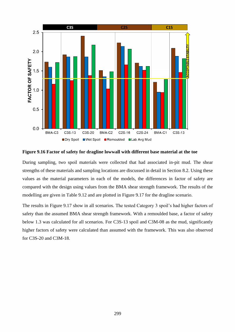
299
Figure 9.16 Factor of safety for dragline lowwall with different base material at the toe
During sampling, two spoil materials were collected that had associated in-pit mud. The shear
strengths of these materials and sampling locations are discussed in detail in Section 8.2. Using these
values as the material parameters in each of the models, the differences in factor of safety are
compared with the design using values from the BMA shear strength framework. The results of the
modelling are given in Table 9.12 and are plotted in Figure 9.17 for the dragline scenario.
The results in Figure 9.17 show in all scenarios. The tested Category 3 spoil’s had higher factors of
safety than the assumed BMA shear strength framework. With a remoulded base, a factor of safety
below 1.3 was calculated for all scenarios. For C3S-13 spoil and C3M-08 as the mud, significantly
higher factors of safety were calculated than assumed with the framework. This was also observed
for C3S-20 and C3M-18.
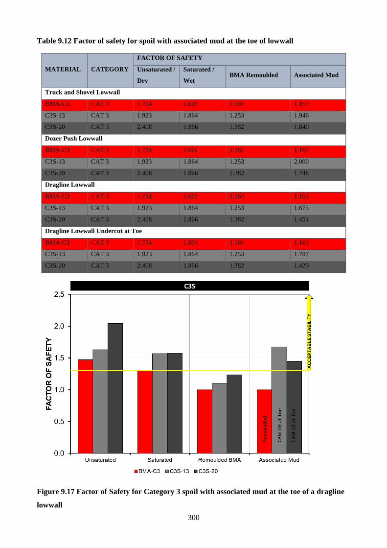
300
Table 9.12 Factor of safety for spoil with associated mud at the toe of lowwall
MATERIAL CATEGORY
FACTOR OF SAFETY
Unsaturated /
Dry
Saturated /
Wet BMA Remoulded Associated Mud
Truck and Shovel Lowwall
BMA-C3 CAT 3 1.734 1.601 1.160 1.160
C3S-13 CAT 3 1.923 1.864 1.253 1.946
C3S-20 CAT 3 2.408 1.866 1.382 1.840
Dozer Push Lowwall
BMA-C3 CAT 3 1.734 1.601 1.160 1.160
C3S-13 CAT 3 1.923 1.864 1.253 2.000
C3S-20 CAT 3 2.408 1.866 1.382 1.748
Dragline Lowwall
BMA-C3 CAT 3 1.734 1.601 1.160 1.160
C3S-13 CAT 3 1.923 1.864 1.253 1.675
C3S-20 CAT 3 2.408 1.866 1.382 1.451
Dragline Lowwall Undercut at Toe
BMA-C3 CAT 3 1.734 1.601 1.160 1.160
C3S-13 CAT 3 1.923 1.864 1.253 1.707
C3S-20 CAT 3 2.408 1.866 1.382 1.429
Figure 9.17 Factor of Safety for Category 3 spoil with associated mud at the toe of a dragline
lowwall
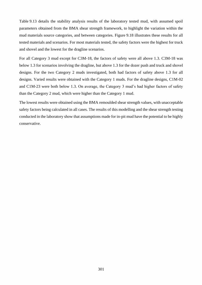
301
Table 9.13 details the stability analysis results of the laboratory tested mud, with assumed spoil
parameters obtained from the BMA shear strength framework, to highlight the variation within the
mud materials source categories, and between categories. Figure 9.18 illustrates these results for all
tested materials and scenarios. For most materials tested, the safety factors were the highest for truck
and shovel and the lowest for the dragline scenarios.
For all Category 3 mud except for C3M-18, the factors of safety were all above 1.3. C3M-18 was
below 1.3 for scenarios involving the dragline, but above 1.3 for the dozer push and truck and shovel
designs. For the two Category 2 muds investigated, both had factors of safety above 1.3 for all
designs. Varied results were obtained with the Category 1 muds. For the dragline designs, C1M-02
and C1M-23 were both below 1.3. On average, the Category 3 mud’s had higher factors of safety
than the Category 2 mud, which were higher than the Category 1 mud.
The lowest results were obtained using the BMA remoulded shear strength values, with unacceptable
safety factors being calculated in all cases. The results of this modelling and the shear strength testing
conducted in the laboratory show that assumptions made for in-pit mud have the potential to be highly
conservative.
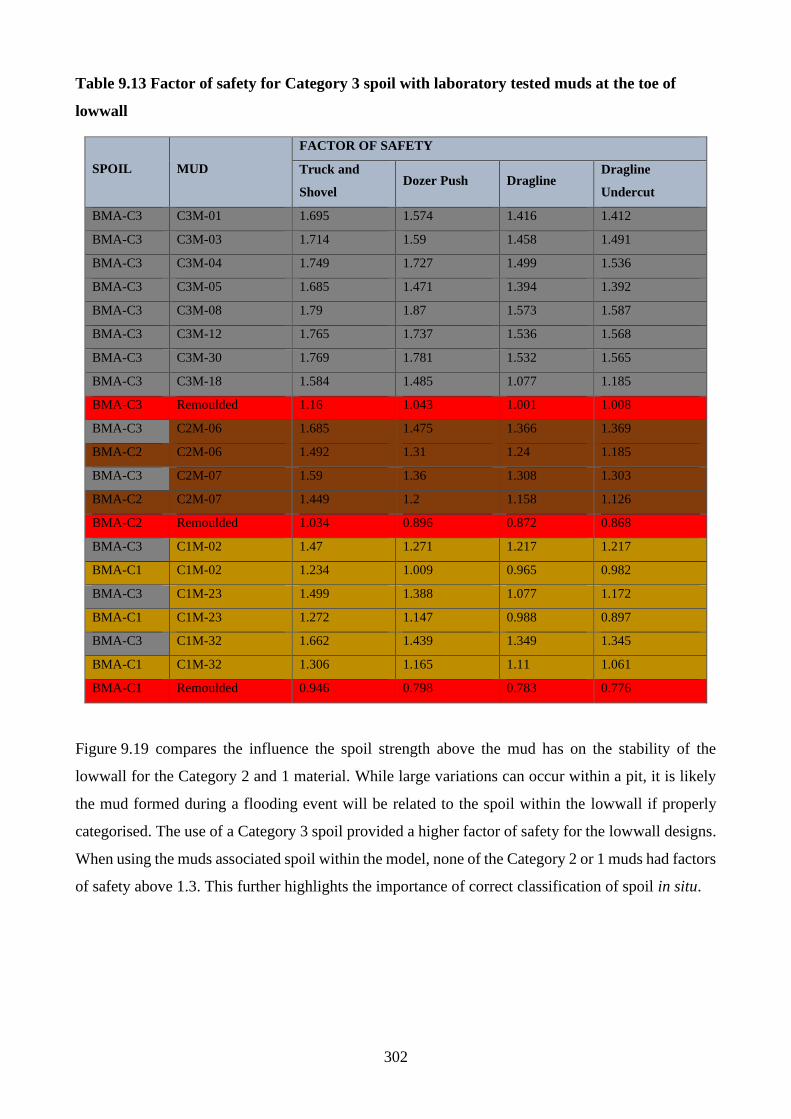
302
Table 9.13 Factor of safety for Category 3 spoil with laboratory tested muds at the toe of
lowwall
SPOIL MUD
FACTOR OF SAFETY
Truck and
Shovel Dozer Push Dragline
Dragline
Undercut
BMA-C3 C3M-01 1.695 1.574 1.416 1.412
BMA-C3 C3M-03 1.714 1.59 1.458 1.491
BMA-C3 C3M-04 1.749 1.727 1.499 1.536
BMA-C3 C3M-05 1.685 1.471 1.394 1.392
BMA-C3 C3M-08 1.79 1.87 1.573 1.587
BMA-C3 C3M-12 1.765 1.737 1.536 1.568
BMA-C3 C3M-30 1.769 1.781 1.532 1.565
BMA-C3 C3M-18 1.584 1.485 1.077 1.185
BMA-C3 Remoulded 1.16 1.043 1.001 1.008
BMA-C3 C2M-06 1.685 1.475 1.366 1.369
BMA-C2 C2M-06 1.492 1.31 1.24 1.185
BMA-C3 C2M-07 1.59 1.36 1.308 1.303
BMA-C2 C2M-07 1.449 1.2 1.158 1.126
BMA-C2 Remoulded 1.034 0.896 0.872 0.868
BMA-C3 C1M-02 1.47 1.271 1.217 1.217
BMA-C1 C1M-02 1.234 1.009 0.965 0.982
BMA-C3 C1M-23 1.499 1.388 1.077 1.172
BMA-C1 C1M-23 1.272 1.147 0.988 0.897
BMA-C3 C1M-32 1.662 1.439 1.349 1.345
BMA-C1 C1M-32 1.306 1.165 1.11 1.061
BMA-C1 Remoulded 0.946 0.798 0.783 0.776
Figure 9.19 compares the influence the spoil strength above the mud has on the stability of the
lowwall for the Category 2 and 1 material. While large variations can occur within a pit, it is likely
the mud formed during a flooding event will be related to the spoil within the lowwall if properly
categorised. The use of a Category 3 spoil provided a higher factor of safety for the lowwall designs.
When using the muds associated spoil within the model, none of the Category 2 or 1 muds had factors
of safety above 1.3. This further highlights the importance of correct classification of spoil in situ.
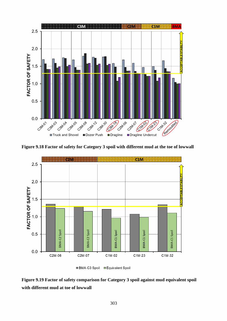
303
Figure 9.18 Factor of safety for Category 3 spoil with different mud at the toe of lowwall
Figure 9.19 Factor of safety comparison for Category 3 spoil against mud equivalent spoil
with different mud at toe of lowwall
304
9.3.1 Stability modelling conclusions:
The implications of spoiling onto in-pit mud were investigated with respect to four different lowwall
designs, produced using a truck and shovel, a dozer push, and a dragline with both standard and
undercut toes. The stability of each design was calculated using the assumed shear strength
parameters of spoil and mud obtained from the BMA shear strength framework and the associated
strength mobilisation mode as per recommended by Simmons (2009), with unsaturated conditions
assumed for spoil above the water table, and saturated conditions for spoil below. This was contrasted
with the shear strengths determined through laboratory testing.
Results of the stability analysis with respect to spoil in unsaturated, saturated and remoulded
conditions show that for all tested spoils, higher factors of safety were achieved using the laboratory
tested strength values highlighted in Figure 9.16. For all spoil materials tested, dry and wet conditions
produced factors of safety above 1.3. The assumption of a remoulded base at the toe of the lowwall
resulted in safety factors below 1.3 for all scenarios except for C2S-16.
Figure 9.16 shows that for calculations using the average shear strength of the laboratory tested muds
associated with the spoil assigned its BMA spoil category strength parameters, factors of safety for
all materials tested were above 1.3. This highlights the potential for conservative lowwall designs
based on assuming the BMA framework suggested remoulded shear strength parameters. It was also
observed that for Category 2 and 1 spoil using the BMA shear strength design values, all scenarios
produced factors of safety below 1.3.
Further analysis was conducted for two spoil materials with associated in-pit mud. The factors of
safety obtained using the laboratory tested spoil and mud shear strength parameters were significantly
higher than that of the remoulded assumptions, depicted in Figure 9.17.
A set of models were computed using BMA’s Category 3 spoil shear strength assumptions, and the
laboratory tested mud materials at the base of the toe of each lowwall design, with results plotted in
Figure 9.18. Except for one outlier, all Category 3 muds produced safety factors above 1.3 in all
scenarios. Lower safety factors were calculated for the Category 2 and 1 mud materials.
For the Category 2 and 1 material, models were computed using BMA spoil material strength values
associated with the material category of the laboratory tested mud. These results were contrasted to
the Factor of Safety generated if the spoil was incorrectly categorised as a Category 3 material. A
reduction in the safety factor was calculated, resulting in all the Category 2 and 1 scenarios having a
safety factor below 1.3. This highlights the importance of correct spoil and mud in situ categorisation.

305
The results of this modelling highlight the possibility of safety spoiling onto in situ mud. If the mud
has enough strength and can consolidate without the build-up of excess pore water pressures, the
factor of safety is not drastically influenced by its presence. This scenario is most like for in-pit mud
formed from Category 3 spoil, that exhibits limited slaking and dispersion. Assuming remoulded
conditions for in situ mud results in moderate to highly conservative designs, and for the tested
Category 3 mud, could result in unnecessary material handling and expenses.
306
10 CONCLUSIONS AND RECOMMENDATIONS FOR FUTURE
RESEARCH
The fundamental reason for this research was to investigate the parameters of in-pit mud and how
they influence the stability of lowwalls within an open-cut coal strip mining scenario. The objectives
were to identify spoil prone to degradation, determine parameters that predict its degradation, and
identify the geotechnical properties of the degraded mud both simulated and sampled. In addition to
this, the objectives included modelling of lowwalls to determine if mud could be spoiled upon in situ
if managed correctly.
10.1 Conclusions and Significant Outcomes
This research thesis has involved an extensive amount of laboratory testing, fully characterising 19
samples consisting of spoil and mud. Valuable contributions have been made to the understanding of
how mud is formed in situ, how it behaves once formed, and the impact it has on the stability of coal
strip mine lowwalls, and spoil piles in general. The degradation of spoil and its resultant strength have
also been investigated, with methods developed to identify degradable material in a laboratory setting
quickly. Lastly, a model has been developed allowing for quick predictions of the effective friction
angle of in-pit mud, and for an assumption of zero apparent cohesion, the shear strength of the
material in drained conditions using particle size distribution results.
10.1.1 Spoil and in-pit mud characterisation
Thirteen mud samples and six spoil samples were collected and analysed with respect to their
physical, chemical, mineralogical and geochemical parameters. The results of the testing were used
to identify relationships between the assigned BMA spoil categories of the materials and the results
determined in the laboratory.
The gravimetric moisture content of the sampled spoil varied from 1.1 to 3.3%, with one spoil
material collected below a previous flooding level having a moisture content of 9.5%, indicating the
ability for spoil to retain moisture at the surface post-flooding. Of the muds sampled, moisture
contents were recorded from below the plastic limit to above the liquid limit of the materials. The
specific gravities of all spoil and mud materials ranged from 2.2 to 2.7 t/m3, with lower values
associated with increases in carbonaceous material. The Atterberg limits were determined, with
plastic and liquid limit ranges of 12.1 to 27.1%, and 21.5 to 61.9%, respectively. All materials were
classified as clays of low plasticity excluding two outliers identified as clays of high plasticity. The
results indicate potential refinement of the current liquid limit ranges within the BMA spoil category
framework is required.
307
The measured pH for the spoil and mud ranged from 7.75 to 9.27, and the electrical conductivities
ranged from 246 to 8,920 µS/cm. There was no apparent relationship between the source materials
category and the measured results. All spoil materials had Emerson classes of 2 or 4, indicating
moderate and high to a very high potential for erosion, respectively. The implications of this show
that there is spoil that can degrade rapidly on exposure to water, irrespective of initial conditions such
as particle size.
All materials were dominated by quartz, Illite-Smectite, Albite and Kaolinite, with no clear
relationship between composition and source material category. The measured cation exchange
capacities were from 10 and 21 cmol+/kg. The most common exchangeable cations were magnesium,
sodium and calcium. An approximation of the presence of sodium Smectite was calculated, with
results showing the highest levels associated with Category 1 mud, and one Category 3 mud outlier.
With respect to particle size distribution, the Category 3 spoil was on average coarser than the
Category 2 spoil, which was, in turn, coarser than the Category 1 spoil. The same relationship was
observed with the mud formed from categorised source materials; however, less differentiation was
observed between the Category 1 and 2 source muds. Varying amounts of degradation were observed
during wet sieving within each category, indicating that categorisation of the material in a dry state
could lead to incorrect assumptions of the competence of the material.
10.1.2 Degradation of spoil
Five of the spoil samples had not been exposed to flooding prior to sampling. Each of these materials
was tested under multiple conditions to determine the degree of degradation experienced and to relate
the degradation to the materials physical, chemical and mineralogical parameters, with intentions of
being able to identify highly degradable material before it is wet up.
Two spoil samples underwent a series of prolonged saturation and wetting and drying cycle tests.
Wetting and drying cycles resulted in higher amounts of particle breakdown, indicating the clay-
mineral rich spoil’s potential for slaking, swelling and dispersion in scenarios of cycling flooding or
heavy rainfall. For both spoil materials, the largest degree of breakdown was observed within the first
24 hours of soaking. This has significant implications for ensuring degradable materials are kept away
from sources of water if possible. Increasing numbers of wetting and drying cycles were found to
cause large increases in the measured electrical conductivities of both materials.
Based on the degradation results, all spoil samples were then subjected to dry sieving, 24 hours of
soaking, three wetting and drying cycles, and a modified slake durability test. It was found that in
decreasing order of importance, the factors related to the degree of degradation were clay mineralogy
of the spoil, the exchangeable cations, the cation exchange capacity and the liquid limit. The results
308
of the modified slake durability test were found to be repeatable and showed potential for the method
to be used to quickly identify spoil prone to degradation in water.
10.1.3 Consolidation of spoil and mud
All spoil and mud samples underwent consolidation testing with loose placement to simulate in situ
conditions. Final dry densities under an applied stress of 1,000 kPa ranged from 1.65 to 1.97 t/m3 for
the tested spoil, with the highest densities obtained from the Category 3 specimens. Final dry densities
of the mud ranged from 1.54 to 1.97 t/m3, with no apparent relation to the source materials category.
On average, the lowest void ratios were found with the Category 3 mud, followed by the Category 2
and 1 mud.
For the spoil specimens tested, settlement ranged from 20 to 35%. For the mud specimens tested,
settlement generally ranged from 8 to 35%, with two significant outliers of 55% and 60%. Typically,
less settlement was observed for the Category 3 materials.
The compression index ranged from 0.13 to 0.78 for the spoil specimens tested, and generally much
flatter from 0.025 to 0.113 for the mud specimens tested. Two significant mud outliers had values of
0.216 and 0.258. Back-calculated hydraulic conductivities ranged from 1.4x10-09 to 0.9x10⁻¹¹ m/s
under an applied stress of 1,000 kPa. The Category 3 materials tested had on average higher hydraulic
conductivities than the Category 2 and 1 materials; however, considerable variability was observed.
In the absence of scalping, it is likely that typically, coarser particles in the Category 3 materials
would increase the hydraulic conductivity, suggesting that the calculated values are lower limits.
The large slurry consolidometer was used to analyse four mud samples. For mud with a fine-grained
particle size distribution, pore water pressures developed rapidly, with initial dissipation observed to
start after between 1.5 days and three days under a constant loading rate of 0.1 kPa/min. Full pore
water pressure dissipation took 6 to 8 days. One Category 3 mud, with a relatively coarse particle size
distribution of silt, gravel and sand, showed no pore water pressures. Hydraulic conductivity values
back-calculated from the dissipation of the pore water pressures reduced to 3.1x10-09 m/s towards the
end of loading, with higher conductivities likely with faster loading rates. The other three mud
specimens tested, having finer particle size distributions, gave much lower final hydraulic
conductivity values ranging from 4.7x10⁻¹¹ to 8.2x10⁻¹¹ m/s.
Results of the large slurry consolidometer show that coarse-grained muds show the most potential for
being spoiled onto in situ without developing detrimental pore water pressures, or without requiring
a long waiting period for pore pressures to dissipate. For the fine-grained muds tested, careful loading
would be required to allow for pore water pressure dissipation, using methods such as a dozer. If
309
loading is to occur too rapidly, the pore water pressures produced will drastically reduce the shear
strength of the material.
10.1.4 Shear strength of spoil and mud
All spoil and mud samples were tested both dry (as-sampled) and wet (after soaking for 24 hours in
a water bath prior to shearing). On average, the dry testing produced the largest shear strengths.
Soaking resulted in a decrease in both apparent cohesion and friction angle in most cases. Typically,
the shear strength of the spoil tested dry was higher than the shear strengths suggested by the BMA
Framework. The wet tested spoil was closer to the unsaturated BMA Framework shear strength,
indicating that for almost all cases, the BMA Framework was conservative to highly conservative.
On average, the Category 3 mud had higher shear strength than the Category 2 mud, which was higher
than the Category 1 mud. Two outliers were identified with extremely low friction angles of 12 to
15o, but high apparent cohesion values of up to 100 kPa. Most muds had friction angles above 25o,
with some up to 36o, with the highest values associated with Category 3 mud relatively high in sand
and gravel content. The majority of the tested materials had friction angles higher than the typical
assumption of 18o that is used in the industry, due to remoulded parameters being used for wet
conditions in the absence of laboratory testing results.
All spoil samples underwent wetting and drying cycles to cause degradation and to determine the
influence that would have on shear strength. The results show that the largest decrease in strength
occurs during the first 24 hours of wetting. After three wetting and drying cycles, the largest change
was observed in the silt and clay-sized fractions. The sand and gravel in most cases remained similar,
as did the tested shear strength. This indicates that once a spoil pile has been saturated, there will be
an irreversible loss of strength due to degradation.
10.1.5 Categorisation, shear strength estimation and modelling of in-pit mud
The use of the BMA Framework categories for in-pit mud and degraded material can lead to
conservative shear strengths used in design. Instead, a model was developed and proposed for the
estimation of in-pit mud friction angles. The model had an r2 value of 0.87, indicating a very strong
relationship using the gravel and sand-sized fractions to predict the friction angle of the mud.
Variability between the tested and predicted values for most in-pit mud materials ranged from -13%
to +8.5%, with increasing variability related to samples with higher percentages of silt and clay-sized
particles. Calculations using the predicted friction angles and an assumption of zero cohesion showed
that in comparison to the tested shear strength at 1,000 kPa stress, predictions were within 10%, with
the largest overestimation being 3% higher. Two materials underestimated the shear strength of the
material by up to 30%, both containing high silt and clay-sized fractions. With respect to design for
310
materials containing high silt and clay-sized fractions, conservative results are desirable as instability
can be highly dangerous and costly to remediate. Further sampling and testing would result in the
refinement of the model to improve shear strength estimates for fine-grained materials.
For the characterisation of in-pit mud and spoil, the recommended test methodology is provided for
materials to be characterised physically, chemically, mineralogically and geochemically. By
conducting these tests, significant parameters related to the geotechnical characteristics of the
material can be identified.
Four lowwall designs were analysed using the slope stability software Slide 7.0. The results of the
testing show that the laboratory tested shear strength parameters resulted in higher Factors of Safety
than the BMA framework suggested shear strengths. For all spoil materials tested, use of the BMA
framework remoulded shear strength parameters resulted in factors of safety below 1.3.
With the laboratory tested mud shear strengths applied at the base of the toe of the lowwall, factors
of safety greater than 1.3 were obtained for almost all materials tested. The results of the modelling
show potential for spoiling into in-pit mud if the shear strengths are given time to develop through
the dissipation of pore water pressures if they develop. Spoiling into in-pit mud is most possible for
mud formed from Category 3 spoil. For mud derived from spoil containing high silt and clay-sized
fractions, slow loading and extended periods between progressive strips would be required to allow
for adequate time for the pore water pressures to dissipate, likely requiring dozer or truck and shovel
operations rather than dragline or highwall blasting.
311
10.2 Recommendations for Future Research
Due to the continuous nature of strip mining and the potential risks associated with a weakened layer
at the base of a spoil pile, research into in-pit mud is critical in avoiding potential instabilities and
unnecessary costs. From the results of this project, and with future characterisation and modelling of
in-pit mud, there is potential for controlled spoiling onto in-pit mud. From this research project, the
following recommendations are made for future work.
Early identification of degradable material:
• Comparison of in-pit mud characterisation results to past borehole logs could allow for early
identification of poor-quality material, allowing it to be accounted for within design.
• Implementation of the modified slake durability test for analysing spoil, highlighting
material prone to degradation and comparing it to associated in-pit mud.
In-pit mud characterisation:
• Further categorisation of in-pit mud. The sample size for this project was 13, with a focus on
Category 3 materials. Future testing expanding the current set of results will allow for
refinement of material parameters and management techniques.
• Large slurry consolidation testing simulating spoiling into mud under different loading rates,
determining the impact of different spoil handling techniques on pore water pressures within
the mud, and the influence these have on stability.
Refinement of the proposed model for estimating in-pit mud friction angle:
• Refinement of the proposed model for predicting the friction angle of in-pit mud, with a
focus on improved accuracy for materials with high silt and clay-sized fractions.
Trial spoiling into mud and associated modelling:
• Trial spoiling into mud in situ is recommended, using dragline, truck and shove and dozing
methods to advance the spoil. There is potential for spoiling into in-pit mud if conducted at a
sufficiently slow rate, allowing excess pore water pressures to dissipate. A successful trial
could result in substantial cost savings in not having to remove in-pit mud.
• In association with a trial, consolidation and pore water pressure measurement would be
required during loading, and modelling of the results would be highly beneficial in
improving understanding of the response of the mud during loading.
312
11 REFERENCES
Abbaspour, H, Drebenstedt, C, Badroddin, M & Maghaminik, A 2018, ‘Optimized design of drilling
and blasting operations in open pit mines under technical and economic uncertainties by system
dynamic modelling’, International Journal of Mining Science and Technology, vol. 28, no. 6, pp.
839–848.
AS 1289.2.1.1 2005, ‘Methods of testing soils for engineering purposes - Soil moisture content tests
- Determination of the moisture content of a soil - Oven drying method (standard method)’, in
Standards Australia, Sydney: Standards Australia Limited.
AS 1289.2.2.1 1998, ‘Methods of testing soils for engineering purposes - Soil moisture content tests
- Determination of the total suction of a soil - Standard method’, in Standards Australia, Sydney:
Standards Australia Limited.
AS 1289.3.1.1 2009, ‘Methods of testing soils for engineering purposes - Soil classification tests -
Determination of the liquid limit of a soil - Four point Casagrande method’, in Standards Australia,
Sydney: Standards Australia Limited.
AS 1289.3.2.1 2009, ‘Methods of testing soils for engineering purposes - Soil classification tests -
Determination of the plastic limit of a soil - Standard method’, in Standards Australia, Sydney:
Standards Australia Limited.
AS 1289.3.3.1 2009, ‘Methods of testing soils for engineering purposes - Soil classification tests -
Calculation of the plasticity index of a soil’, in Standards Australia, Sydney: Standards Australia
Limited.
AS 1289.3.5.2 2002, ‘Methods of testing soils for engineering purposes Soil classification tests -
Determination of the soil particle density of combined soil fractions - Vacuum pycnometer method’,
in Standards Australia, Sydney: Standards Australia Limited.
AS 1289.3.6.1 2009, ‘Methods of testing soils for engineering purposes - Soil classification tests -
Determination of the particle size distribution of a soil - Standard method of analysis by sieving’, in
Standards Australia, Sydney: Standards Australia Limited.
AS 1289.3.6.3 2009, ‘Methods of testing soils for engineering purposes - Soil classification tests -
Determination of the particle size distribution of a soil - Standard method of fine analysis using a
hydrometer’, in Standards Australia, Sydney: Standards Australia Limited.
AS 1289.3.8.1 2017, ‘Methods of testing soils for engineering purposes - Soil classification tests -
Dispersion - Determination of Emerson class number of a soil’, in Standards Australia, Sydney:
Standards Australia Limited.
313
AS 1289.4.3.1 1997, ‘Methods of testing soils for engineering purposes - Soil chemical tests -
Determination of the pH value of a soil - Electrometric method’, in Standards Australia, Sydney:
Standards Australia Limited.
AS 1289.4.4.1 2017, ‘Methods of testing soils for engineering purposes - Soil chemical tests -
Determination of the electrical resistivity of a soil - Method for fine granular materials’, in Standards
Australia, Sydney: Standards Australia Limited.
AS 1289.6.2.2 1998, ‘Methods of testing soils for engineering purposes - Soil strength and
consolidation tests - Determination of shear strength of a soil - Direct shear test using a shear box’,
in Standards Australia, Sydney: Standards Australia Limited.
AS 1289.6.6.1 1998, ‘Methods of testing soils for engineering purposes - Soil strength and
consolidation tests - Determination of the one-dimensional consolidation properties of a soil -
Standard method’, in Standards Australia, Sydney: Standards Australia Limited.
AS 4133.3.4 2005, ‘Methods of testing rocks for engineering purposes - Rock swelling and slake
durability tests - Determination of the slake durability index of rock samples’, in Standards Australia,
Sydney: Standards Australia Limited.
ASTM D2487-11 2011, Standard Practice for Classification of Soils for Engineering Purposes
(Unified Soil Classification System), ASTM International, West Conshohocken, PA, accessed from
<www.astm.org>.
ASTM D3744 / D3744M-18 2018, Standard Test Method for Aggregate Durability Index, ASTM
International, West Conshohocken, PA, accessed from <www.astm.org>.
Atwood, G 1975, ‘The Strip-mining of Western Coal’, Scientific American, vol. 233, no. 6, pp. 23–
29.
Babalola, Z 2016, Direct shear and direct simple shear tests: a comparative study of the strength
parameters and their dependence on moisture and fines contents, University of Cape Town.
Beakawi Al-Hashemi, HM & Baghabra Al-Amoudi, OS 2018, ‘A review on the angle of repose of
granular materials’, Powder Technology, vol. 330, pp. 397–417.
Beale, G 2017, ‘Surface water and groundwater characterisation’, in Guidelines for Mine Waste
Dump and Stockpile Design, CSIRO Publishing, Collingwood, pp. 99–118.
Birkeland, P 1999, Soils and Geomorphology 3 edition., Oxford University Press, New York.
Boyd, GL, Komdeur, W & Richards, BG 1978, ‘Open strip pitwall instability at Goonyella mine -
causes and effects’, in Proceedings of The Australasian Institute of Mining and Metallurgy
314
Conference, The Australasian Institute of Mining and Metallurgy, Melbourne, Australia, pp. 139–
157.
Bradfield, L 2017, Reliable Shear Strength Estimation for Very-High Spoil Dumps, The University
of Newcastle.
Bradfield, L, Simmons, J & Fityus, S 2013, ‘Issues related to stability design of very high spoil
dumps’, in 13th Coal Operators’ Conference, The Australasian Institute of Mining and Metallurgy
and Mine Managers Association of Australia, University of Wollongong, pp. 376–386.
Brand, EW & Brenner, RP 1981, Soft clay engineering, Elsevier Science.
Cano, M & Tomás, R 2016, ‘Proposal of a New Parameter for the Weathering Characterization of
Carbonate Flysch-Like Rock Masses: The Potential Degradation Index (PDI)’, Rock Mechanics and
Rock Engineering, vol. 49, no. 7, pp. 2623–2640.
Carson, MA & Petley, DJ 1970, ‘The Existence of Threshold Hillslopes in the Denudation of the
Landscape’, Transactions of the Institute of British Geographers, no. 49, pp. 71–95.
Carter, M & Bentley, SP 1991, Correlations of soil properties, London Pentech.
Cheema, T, Al-Harthy, A, Al Aghbari, M & Al-Aufi, M 2004, ‘Influence of Grain Size and
Mineralogy on the Strength of Weak Rocks’, in Geotechnical Practice Publication, pp. 239–249.
Chigira, M & Oyama, T 2000, ‘Mechanism and effect of chemical weathering of sedimentary rocks’,
Developments in Geotechnical Engineering, vol. 55, pp. 267–278.
Chowdhury, RN & Nguyen, VU 1987, ‘Risk updating for rainfall-triggered spoil failures’,
Proceedings 2nd International Conference on Reclamation, Treatment and Utilisation of Coal
Mining Wastes, pp. 95–109.
Christoulas, S, Kalteziotis, N, Tsiambaos, G & Sabatakakis, N 1987, ‘Engineering Geology of Soft
Clays, Examples from Greece’, in Embankments on soft clays, Athens : Public Works Research
Center.
Das, B & Sobhan, K 2017, Principles of Geotechnical Engineering 9th edn, Cengage Learning US.
Davison, LR & Atkinson, JH 1990, ‘Continuous loading oedometer testing of soils’, Quarterly
Journal of Engineering Geology and Hydrogeology, vol. 23, no. 4, pp. 347–355.
Deo, P 1972, ‘Shales as Embankment Materials’, JTRP Technical Reports.
Dhakal, G, Yoneda, T, Kato, M & Kaneko, K 2002, ‘Slake durability and mineralogical properties of
some pyroclastic and sedimentary rocks’, Engineering Geology, vol. 65, no. 1, pp. 31–45.
315
Dorador, L, Cunning, J, Junqueira, F & Hawley, M 2017, ‘Material Characterisation’, in Guidelines
for Mine Waste Dump and Stockpile Design, CSIRO Publishing, Collingwood, pp. 79–97.
Dumbleton, MJ 1981, The British Soil Classification System for Engineering Purposes: Its
Development and Relation to Other Comparable Systems, Transport and Road Research Laboratory.
Dunbavan, M & Welsh, TC 1982, ‘Spoil Pile Instability, South Blackwater Mine Queensland’,
Commonwealth Scientific and Industrial Research Organisation, Institute of Energy and Energy
Resources, Division of Applied Geomechanics, vol. Report No. 35.
Dunbaven, M & Driver, IJ 1988, ‘Lowwall Stabilisation at Riverside Coal Mine’, Fifth Australia-
New Zealand Conference on Geomechanics: Prediction Versus Performance; Preprints of Papers,
p. 368.
Duran, A 2013, ‘Undrained behaviour in spoil piles’, in P Dight (ed), Proceedings of the 2013
International Symposium on Slope Stability in Open Pit Mining and Civil Engineering, Australian
Centre for Geomechanics, Perth, pp. 853–865.
Eberl, DD, Farmer, VC & Barrer, RM 1984, ‘Clay Mineral Formation and Transformation in Rocks
and Soils [and Discussion]’, Philosophical Transactions of the Royal Society of London. Series A,
Mathematical and Physical Sciences, vol. 311, no. 1517, pp. 241–257.
Emerson, WW 1967, ‘A classification of soil aggregates based on their coherence in water’, Soil
Research, vol. 5, no. 1, pp. 47–57.
Erguler, ZA & Ulusay, R 2009, ‘Assessment of physical disintegration characteristics of clay-bearing
rocks: Disintegration index test and a new durability classification chart’, Engineering Geology, vol.
105, no. 1, pp. 11–19.
Fielding, CR, Kassan, J, Draper, JJ & Geological Society of Australia. Australasian Sedimentologists
Group 1996, Geology of the Bowen and Surat Basins, Eastern Queensland / Christopher R. Fielding,
Jochen Kassan, John J. Draper., Geological Society of Australia, Springwood, N.S.W.
Fityus, S, Hancock, G & Wells, T 2008, ‘Geotechnical characteristics of coal mine spoil’, Australian
Geomechanics, vol. 43, no. 2, pp. 13–22.
Fookes, PG, Dearman, WR & Franklin, JA 1971, ‘Some engineering aspects of rock weathering with
field examples from Dartmoor and elsewhere’, Quarterly Journal of Engineering Geology and
Hydrogeology, vol. 4, no. 3, pp. 139–185.
Franklin, JA & Chandra, R 1972, ‘The slake-durability test’, International Journal of Rock Mechanics
and Mining Sciences & Geomechanics Abstracts, vol. 9, no. 3, pp. 325–328.
316
Fuller, PG & Cox, RHT 1987, Highwall and spoil pile failure processes identified by sub-surface
instramentation at Goonyella Mine, Commonwealth Scientific and Industrial Research Organisation
(CSIRO), Division of Applied Geomechanics.
Gómez, P, Díaz, M & Lorig, L 2002, ‘Stability analysis of waste dumps at Chuquicamata Mine,
Chile’, , vol. 20, pp. 61–68.
Gonano, LP 1980, An integrated report on slope failure mechanisms at Goonyella, November 1976,
Commonwealth Scientific and Industrial Research Organization, Institute of Earth Resources,
Division of Applied Geomechanics, Mt. Waverley, Vic.
Graupner, T, Kassahun, A, Rammlmair, D, A. Meima, J, Kock, D, Furche, M, Fiege, A, Schippers,
A & Melcher, F 2007, ‘Formation of sequences of cemented layers and hardpans within sulfide-
bearing mine tailings (mine district Freiberg, Germany)’, Applied Geochemistry, vol. 22, pp. 2486–
2508.
Hartman, HL & Mutmansky, JM 2002, Introductory Mining Engineering, John Wiley & Sons.
Hiung, AKK 2016, Bulking and Subsequent Self-Weight and Saturation Settlements, and
Geotechnical Stability of High Coal Mine Spoil Piles, The University of Queensland, School of Civil
Engineering.
Humphrey, J. D 1984, ‘The Fundamentals of the Dragline’, in Marion Division-Dresser Ind. Inc:
Marion, p. 29.
Hustrulid, WA, McCarter, MK & A, VZ, Dirk J (eds) 2001, Slope Stability in Surface Mining, Society
for Mining, Metallurgy, and Exploration, Littleton, Colo.
Jackson, R 2015, ‘Manual of Soil Laboratory TestingBook Review’, Environmental and Engineering
Geoscience, vol. 21, no. 3, pp. 247–248.
Janbu, N, Tokheim, O & Senneset, K 1980, ‘Consolidation tests with continuous loading’, Norvegian
Geotech Institute.
Karem, WA 2005, Development of a Predictive Model to Evaluate Mine Spoil Fills for Industrial
Development, University of Kentucky.
Kho, AK, Williams, DJ, Kaneko, N & Smith, NJW 2013, Shear strength parameters for assessing
geotechnical slope stability of open pit coal mine spoil based on laboratory tests, Australian Centre
for Geomechanics.
Kikumoto, M, Putra, AD & Fukuda, T 2016, ‘Slaking and deformation behaviour’, Géotechnique,
vol. 66, no. 9, pp. 771–785.
317
Koloski, JW, Schwarz, SD & Tubbs, DW 1989, ‘Geotechnical Properties of Geologic Materials’, in
Engineering Geology in Washington, Washington Division of Geology and Earth Resources, pp. 19–
26.
Koncagül, EC & Santi, PM 1999, ‘Predicting the unconfined compressive strength of the Breathitt
shale using slake durability, Shore hardness and rock structural properties’, International Journal of
Rock Mechanics and Mining Sciences, vol. 36, no. 2, pp. 139–153.
Lan, HX, Hu, RL, Yue, ZQ, Lee, CF & Wang, SJ 2003, ‘Engineering and geological characteristics
of granite weathering profiles in South China’, Journal of Asian Earth Sciences, vol. 21, no. 4, pp.
353–364.
Leps, TM 1970, ‘Review of Shearing Strength of Rockfill’, Journal of the Soil Mechanics and
Foundations Division, vol. 96, no. 4, pp. 1159–1170.
Leroueil, S, Kabbaj, M, Tavenas, F & Bouchard, R 1985, ‘Stress–strain–strain rate relation for the
compressibility of sensitive natural clays’, Géotechnique, vol. 35, no. 2, pp. 159–180.
Mallett et al, CW 1983, Stability of Spoil Piles and Highwalls in Deep Surface Mines,.
Marescotti, P, Carbone, C, De Capitani, L, Grieco, G, Lucchetti, G & Servida, D 2008, ‘Mineralogical
and geochemical characterisation of open-air tailing and waste-rock dumps from the Libiola Fe-Cu
sulphide mine (Eastern Liguria, Italy)’, Environmental Geology, vol. 53, pp. 1613–1626.
McLemore, VT, Fakhimi, A, van Zyl, D, Ayakwah, GF, Anim, K, Boakye, K, Ennin, F, Felli, P,
Fredlund, D, Gutierrez, LAF, Tachie-Menson, S & Viterbo, VC 2009, ‘Literature Review of Other
Rock Piles: Characterization, Weathering and Stability’, New Mexico Bureau of Geology and Mineral
Resources, p. 101.
Mitra, R & Onargan, T 2012, ‘Surface Coal Mining Methods in Australia’, in Mining Methods,
InTech.
Morris, PH 1990, The engineering properties and behaviour of coal tailings, The University of
Queensland, School of Civil Engineering, Australia.
Mostofa, MG 2015, Base material characterisation of spoil piles at BMA coal mines, Queensland
University of Technology.
Naderian, AR & Williams, DJ 1996, ‘Simulation of Open-cut Coal Mine Back-fill Behaviour’,
National Symposium on the Use of Recycled Materials in Engineering Construction: 1996;
Programme & Proceedings, p. 17.
Neuendorf, KKE, Mehl, JP & Jackson, JA 2005, Glossary of geology 5th edn, American Geological
Institute, Alexandria, VA.
318
Nguyen, VU 1985, ‘Discussion: Back calculations of slope failures by the secant method’,
Géotechnique, vol. 35, no. 3, pp. 386–388.
Nguyen, VU, Nemcik, JA & Chowdhury, RN 1984, ‘Some practical aspects of spoil pile stability by
the two-wedge model’, Mining Science and Technology, vol. 2, no. 1, pp. 57–68.
Nguyen, VU & Welsh, TC 1981, ‘Characteristics of Spoil Pile Failures In a Strip Coal Mine In
Tertiary And Permian Sediments’, in ISRM International Symposium, International Society for Rock
Mechanics and Rock Engineering.
‘Norwich Park Dragline Recovery’ 2008, accessed July 27, 2019, from
<http://www.miningmayhem.com/2009/09/norwich-park-dragline-recovery.html>.
Okagbue, CO 1986, ‘An investigation of landslide problems in spoil piles in a strip coal mining area,
West Virginia (U.S.A.)’, Engineering Geology, vol. 22, no. 4, pp. 317–333.
Olivier, HJ 1979, ‘Some aspects of the influence of mineralogy and moisture redistribution on the
weathering behaviour of mudrocks’, Proceedings of the 4th international conference on rock
mechanics, vol. 3, pp. 467–474.
Peter, P, Nefiodovas, A, Hignett, C, Wright, W, Wei, Y & Sheng, Y 1996, BHP Spoil Hydrology
Project Final Report, Geotechnical Testing of Spoil, Commonwealth Scientific and Industrial
Research Organisation (CSIRO).
Philip, MG, Boyd, GL & Eckersley, J 1981, ‘Stabilisation of large scale spoil piles in deep open strip
coal mines’, in Proceedings of Symposium on Strip Mining – 45 m and Beyond, The Australasian
Institute of Mining and Metallurgy, Melbourne, Australia., Central Queensland, pp. 119–129.
Poulsen, B, Khanal, M, Rao, AM, Adhikary, D & Balusu, R 2014, ‘Mine Overburden Dump Failure:
A Case Study’, Geotechnical and Geological Engineering, vol. 32, no. 2, pp. 297–309.
Prytherch, B 2012, ‘Goonyella Riverside Mine Dragline Operations’, in BHP Billiton Mitsubishi
Alliance Internal Documents.
Rayment, GE & Higginson, FR 1992, Australian Laboratory Handbook of Soil and Water Chemical
Method, Reed International Books Australia P/L, Trading as Inkata Press, Port Melbourne.
Rayner, DH & Hemingway, JE 1974, The Geology and Mineral Resources of Yorkshire, Yorkshire
Geological Society.
Richards, BG, Coulthard, MA & Toh, CT 1981, ‘Analysis of slope stability at Goonyella Mine’,
Canadian Geotechnical Journal, vol. 18, no. 2, pp. 179–194.
319
Robertson, GP, Sollins, P, Ellis, BG & Lajtha, K 1999, ‘Exchangeable ions, pH and cation exchange
capacity’, in Sollins, P. (Eds.), Standard Soil Methods in Long-term Ecological Research, Oxford
University Press, pp. 106–114.
Rowe, PW 1962, ‘The stress-dilatancy relation for static equilibrium of an assembly of particles in
contact’, Proceedings of the Royal Society of London. Series A. Mathematical and Physical Sciences,
vol. 269, no. 1339, pp. 500–527.
Schor, HJ & Gray, DH 1995, ‘Landform Grading and Slope Evolution’, Journal of Geotechnical
Engineering, vol. 121, no. 10, pp. 729–734.
Seedsman, R 1986, ‘The behaviour of clay shales in water’, Canadian Geotechnical Journal, vol. 23,
no. 1, pp. 18–22.
Seedsman, RW, Cameron, M & Peou, S 1995, ‘Geotechnical Investigations and Pit Wall Designs in
Faulted Ground at Eastern Creek South’, in Bowen Basin Symposium 1995, The Bowen Basin
Geologists Group and the Geological Society of Australia Incorporated Coal Geology Group, pp.
191–192.
Seedsman, RW & Emerson, WW 1985, ‘The role of clay-rich rocks in spoil pile failures at Goonyella
Mine, Queensland, Australia’, International Journal of Rock Mechanics and Mining Sciences &
Geomechanics Abstracts, vol. 22, no. 2, pp. 113–118.
Seedsman, RW, Richards, BG & Williams, DJ 1988, ‘The Possibility of Undrained Failure in Bowen
Basin Spoil Piles’, Fifth Australia-New Zealand Conference on Geomechanics: Prediction Versus
Performance; Preprints of Papers, p. 404.
Selig, E, Dusseault, M, Cimolini, P, Soderberg, H & Scafe, D 1983, ‘Rapid Index Tests for
Transitional Materials’, Geotechnical Testing Journal - GEOTECH TESTING J, vol. 6.
Simmon, J & Fityus, S 2016, The Stability of Very High Spoil Piles, Australian Coal Industries
Research Program.
Simmons, J 1995, ‘Slope stability for open pit coal mining’, in Australian Geomechanics, pp. 45–57.
Simmons, J 2009, Geotechnical Support for Open Pit Coal Mining, Australasian Institute of Mining
and Metallurgy, Carlton, Vic.
Simmons, J & McManus, D 2004, ‘Shear Strength Framework for Design of Dumped Spoil Slopes
for Open Pit Coal Mines’, in Advances in geotechnical engineering: The Skempton conference,
Conference Proceedings, Thomas Telford Publishing, pp. 981–991, accessed October 12, 2016, from
<http://www.icevirtuallibrary.com.ezproxy.library.uq.edu.au/doi/abs/10.1680/aigev2.32644.0026>.
320
Simmons, J & Yarkosky, R 2017, ‘Dragline spoils’, in M Hawley & J Cunning (eds), Guidelines for
Mine Waste Dump and Stockpile Design, CSIRO Publishing, Collingwood, pp. 233–256.
Simons, DB & Albertson, ML 1960, ‘Uniform Water Conveyance Channels in Alluvial Materials’,
Journal of the Hydraulics Division, vol. 86, no. 5, pp. 33–71.
Singh, PK, Roy, MP, Paswan, RK, Sarim, Md, Kumar, S & Ranjan Jha, R 2016, ‘Rock fragmentation
control in opencast blasting’, Journal of Rock Mechanics and Geotechnical Engineering, vol. 8, no.
2, pp. 225–237.
Smith, LA, López, DL, Beckie, R, Morin, K, Dawson, R & Price, W 1995, Hydrogeology of Waste
Rock Dumps, British Columbia Ministry of Energy, Mines and Petroleum Resources and CANMET.
Stockwell, J, Smith, L, Jambor, JL & Beckie, R 2006, ‘The relationship between fluid flow and
mineral weathering in heterogeneous unsaturated porous media: A physical and geochemical
characterization of a waste-rock pile’, Applied Geochemistry, vol. 21, no. 8, pp. 1347–1361.
Taylor, EL, Taylor, TN & Krings, M 2009, Paleobotany: The Biology and Evolution of Fossil Plants,
Academic Press.
Terzaghi, K 1936, ‘The shear resistance of saturated soils’, in The shear resistance of saturated soils,
International Conference Soil Mechanics Foundation Engineering, pp. 54–56.
Ulusay, R, Arikan, F, Yoleri, MF & Çaǧlan, D 1995, ‘Engineering geological characterization of coal
mine waste material and an evaluation in the context of back-analysis of spoil pile instabilities in a
strip mine, SW Turkey’, Engineering Geology, vol. 40, no. 1, pp. 77–101.
Umehara, Y & Zen, K 1980, ‘Constant Rate of Strain Consolidation for Very Soft Clayey Soils’,
Soils and Foundations, vol. 20, no. 2, pp. 79–95.
Vosolo, D 2017, Investigations on Geotechnical Engineering Properties of Coal Mine Spoil
Subjected to Slaking, Queensland University of Technology, School of Civil Engineering.
Westcott, P 2004, ‘Dragline or Truck/Shovel? Some Technical and Business Considerations’, in
University of New South Whales.
Whitman, RV 1984, ‘Evaluating Calculated Risk in Geotechnical Engineering’, Journal of
Geotechnical Engineering, vol. 110, no. 2, pp. 143–188.
Williams, D & Rohde, T 2008, ‘Rainfall infiltration into and seepage from rock dumps - A review’,
in A Fourie (ed), Proceedings of the First International Seminar on the Management of Rock Dumps,
Stockpiles and Heap Leach Pads, Australian Center for Geomechanics, Perth, Western Australia, pp.
79–89.
321
Williams, DJ 2006, ‘The case for revolutionary change to mine waste disposal rehabilitation’, in
Second International Seminar on Strategic versus Tactical Approahces to Mining, Australian Centre
for Geomechanics, Perth, Western Australia, pp. 1–10.
Williams, DJ 2015, Bulking and Subsequent Self-Weight and Saturation Settlements, and
Geotechnical Stability, of Deep Coal Mine Spoil Piles, Australian Coal Industry’s Research Program.,
Brisbane, Australia.
Williams, DJ & Zou, JZ 1991, ‘Stochastic finite element analysis of coal mine spoil pile stability’, in
Proceedings of 7th Conference of International Association for Computer Methods and Advances in
Geomechanics, Cairns, pp. 1411–1416.
Wood, L & Deo, P 1975, ‘A suggested system for classifying shale materials for embankments’,
International Journal of Rock Mechanics and Mining Sciences and Geomechanics Abstracts, vol. 12,
no. 8, pp. 39–55.
Related Documents