Sharing Data Through Plots with Plotly by Alex Johnson

Sharing data through plots with Plotly

Alex Johnson CTO, Plotly

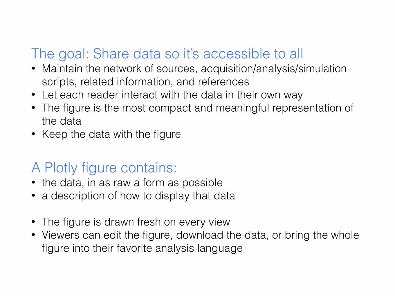
A Plotly figure contains: • the data, in as raw a form as possible • a description of how to display that data

• The figure is drawn fresh on every view • Viewers can edit the figure, download the data, or bring the whole

figure into their favorite analysis language

The goal: Share data so it’s accessible to all • Maintain the network of sources, acquisition/analysis/simulation

scripts, related information, and references • Let each reader interact with the data in their own way • The figure is the most compact and meaningful representation of

the data • Keep the data with the figure

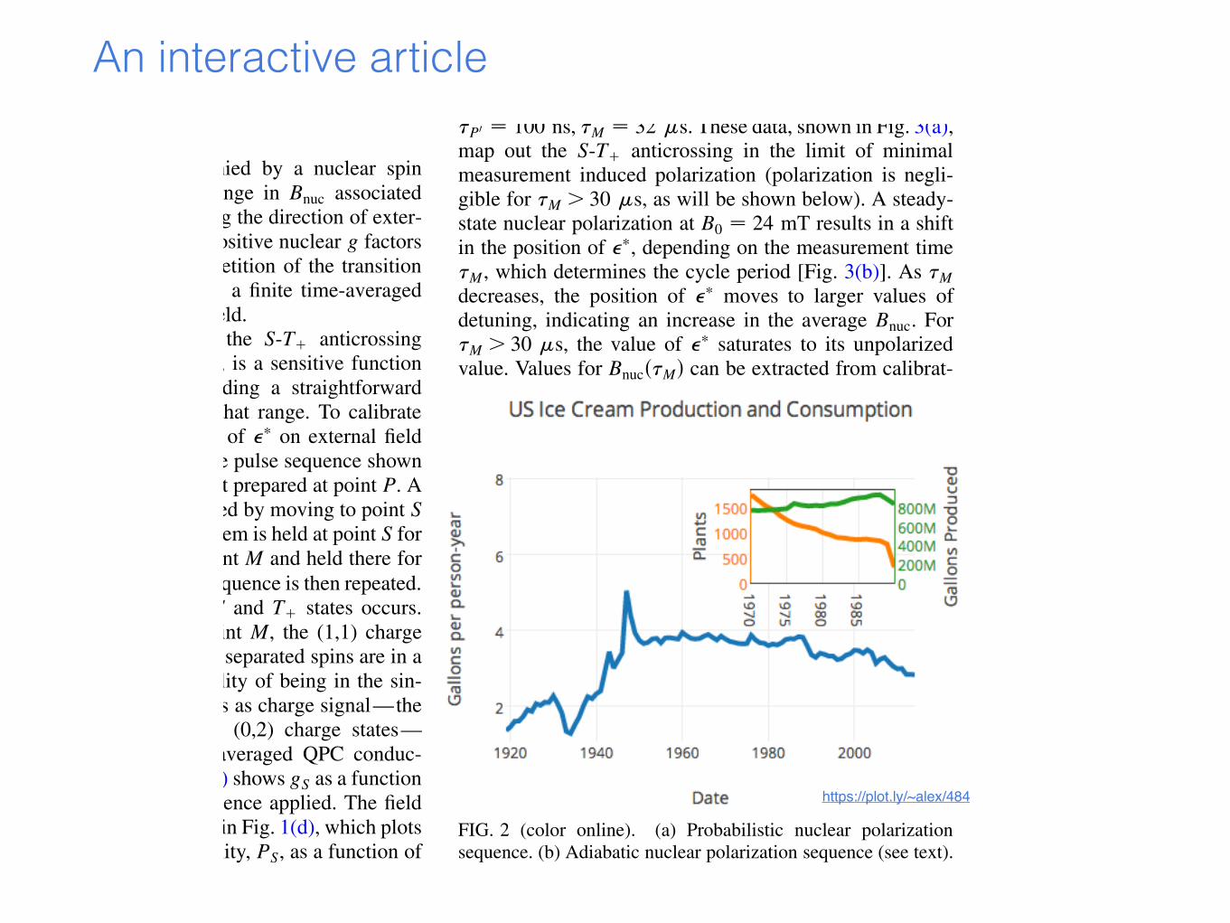
An interactive article

electron spin ‘‘flip’’ is accompanied by a nuclear spin‘‘flop’’ with !mI ! "1. The change in Bnuc associatedwith this flip-flop transition is along the direction of exter-nal field, taking into account the positive nuclear g factorsfor Ga and As [2]. The cyclic repetition of the transitionfrom S to T# can thereby lead to a finite time-averagedBnuc oriented along the external field.

The value of detuning where the S-T# anticrossingoccurs, denoted !$ [see Fig. 1(b)], is a sensitive functionof Btot for jBtotj % 80 mT, providing a straightforwardmeans of measuring Bnuc within that range. To calibratethe measurement, the dependence of !$ on external fieldamplitude B0 is measured using the pulse sequence shownin Fig. 1(c): The &0; 2'S state is first prepared at point P. Adelocalized singlet in (1,1) is created by moving to point S(detuning !S) via point P0. The system is held at point S fora time "S ( T$

2 then moved to point M and held there forthe longest part of the cycle. The sequence is then repeated.When !S ! !$, rapid mixing of S and T# states occurs.When the system is moved to point M, the (1,1) chargestate will return to (0,2) only if the separated spins are in asinglet configuration. The probability of being in the sin-glet state after time "S thus appears as charge signal—thedifference between the (1,1) and (0,2) charge states—detected by measuring the time-averaged QPC conduc-tance, gS [see Fig. 1(a)]. Figure 1(c) shows gS as a functionof VL and VR with this pulse sequence applied. The fielddependence of this signal is shown in Fig. 1(d), which plotsthe calibrated singlet state probability, PS, as a function of

B0 and !S. In Fig. 1(d), PS ) 0:7 at the S-T# degeneracy,corresponding to a probability of electron-nuclear flip-flopper cycle &1" PS' ) 0:3. The position of the anticrossing,!S ! !$, becomes more negative as B0 decreases towardzero [Fig. 1(d)], as expected from the level diagram,Fig. 1(b).

An alternative sequence that (in principle) deterministi-cally flips one nuclear spin per cycle and allows greatercontrol of the steady-state nuclear polarization is shown inFig. 2(b): In this case, the initial &0; 2'S is separated quickly()1 ns), to a value of detuning beyond the S-T# resonance,!S < !$. Since the time spent at the S-T# resonance duringthe pulse is short, the singlet is preserved with high proba-bility. Next, detuning is brought back toward zero,to a value !F, on a time scale slow compared to T$

2()100 ns). This converts S to T# and flips a nuclear spineach cycle. Detuning is then rapidly moved to the point M(again, over a time )1 ns). While slightly different, bothpulse sequences rely on bringing the S and T# states intoresonance; the otherwise large difference between nuclearand electron Zeeman energies would prevent flip-flop pro-cesses [23].

We begin by examining the statistical polarization se-quence shown in Fig. 2(a). We first measure PS as afunction of B0 and !S, with "S ! 100 ns, "P ! 300 ns,"P0 ! 100 ns, "M ! 32 #s. These data, shown in Fig. 3(a),map out the S-T# anticrossing in the limit of minimalmeasurement induced polarization (polarization is negli-gible for "M > 30 #s, as will be shown below). A steady-state nuclear polarization at B0 ! 24 mT results in a shiftin the position of !$, depending on the measurement time"M, which determines the cycle period [Fig. 3(b)]. As "Mdecreases, the position of !$ moves to larger values ofdetuning, indicating an increase in the average Bnuc. For"M > 30 #s, the value of !$ saturates to its unpolarizedvalue. Values for Bnuc&"M' can be extracted from calibrat-

Adiabatic nuclear polarizationProbabilistic nuclear polarization

Rapid Adiabatic Passage

Slow Adiabatic Passage

Prepare Singlet

Rapid Adiabatic Passage, S-T+ evolution

PS

Prepare Singlet

t= S

t=0

Rapid Adiabatic Passage, Projection

a) b)

t= S

t=0

1-PS

Ene

rgy

(0,2)S

0

(0,2)S T0

T+

T-E

nerg

y

(0,2)S

0

(0,2)S T0

T+

T-

Ene

rgy

(0,2)S

0

(0,2)S T0

T+

T-

Ene

rgy

(0,2)S

0

(0,2)S T0

T+

T-

Ene

rgy

(0,2)S

0

(0,2)S T0

T+

T-

S

Ene

rgy

(0,2)S

0

(0,2)S T0

T+

T-

F

FIG. 2 (color online). (a) Probabilistic nuclear polarizationsequence. (b) Adiabatic nuclear polarization sequence (see text).

FIG. 1 (color online). (a) SEM image of a device similar to theone used in this experiment. A QPC with conductance, gS, sensescharge on the double dot. (b) Energy levels near the (1,1)-(0,2)charge transition. (c) gS measured as a function of VL and VR. Apulse sequence used to polarize nuclei is superimposed on thecharge stability diagram (see text). The bright signal at point Mthat runs parallel to the ! ! 0 line is a result of Pauli-blocked&1; 1' !& 0; 2' charge transitions and reflects S-T# mixing atpoint S. (d) PS&"S ! 200 ns' as a function of !S and B0. Thefield dependent ‘‘spin funnel’’ corresponds to the S-T# anti-crossing position, !S ! !$.

PRL 100, 067601 (2008) P H Y S I C A L R E V I E W L E T T E R S week ending15 FEBRUARY 2008

067601-2

https://plot.ly/~alex/484

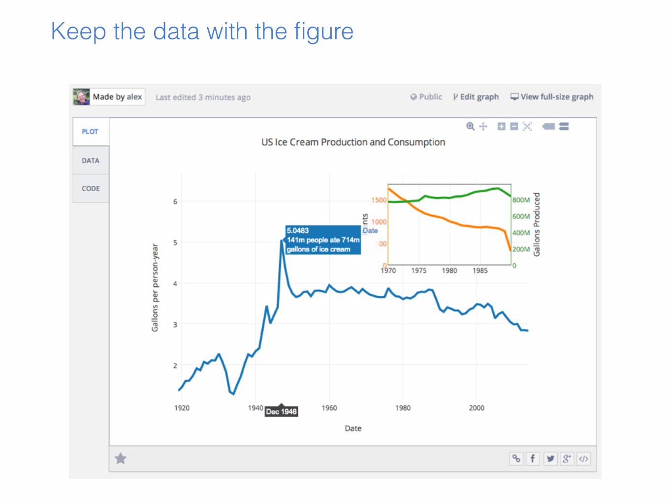
Keep the data with the figure

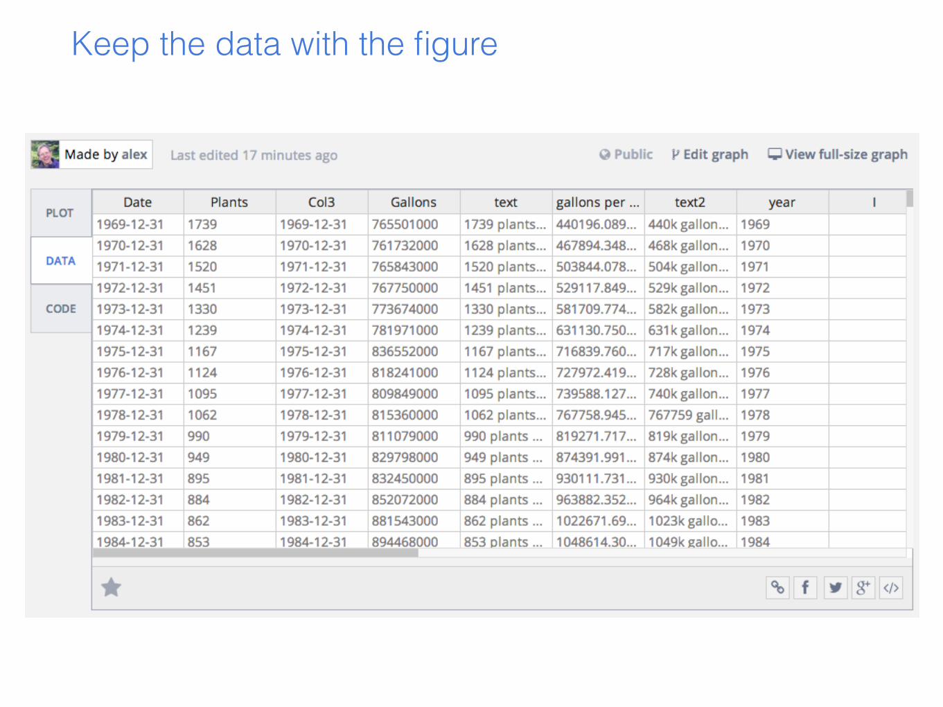
Keep the data with the figure

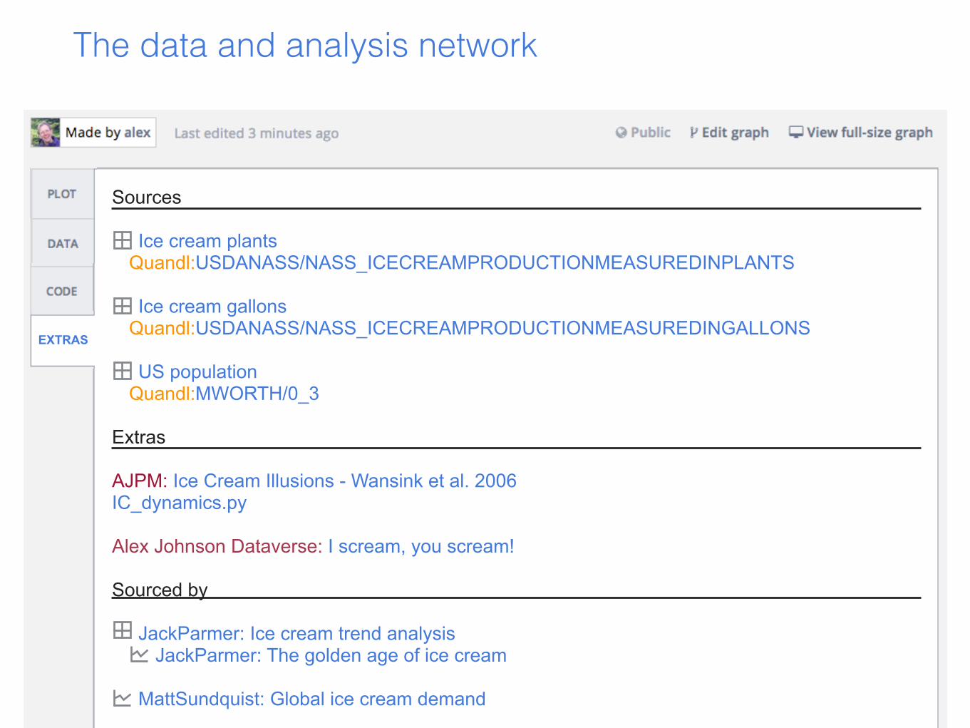
EXTRAS

Sources

Ice cream plants Quandl:USDANASS/NASS_ICECREAMPRODUCTIONMEASUREDINPLANTS

Ice cream gallons Quandl:USDANASS/NASS_ICECREAMPRODUCTIONMEASUREDINGALLONS

US population Quandl:MWORTH/0_3

Extras

AJPM: Ice Cream Illusions - Wansink et al. 2006 IC_dynamics.py

Alex Johnson Dataverse: I scream, you scream!

Sourced by

JackParmer: Ice cream trend analysis JackParmer: The golden age of ice cream

MattSundquist: Global ice cream demand

The data and analysis network

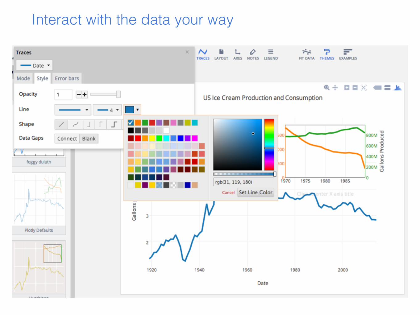
Interact with the data your way

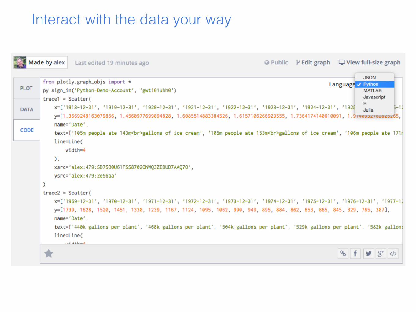
Interact with the data your way

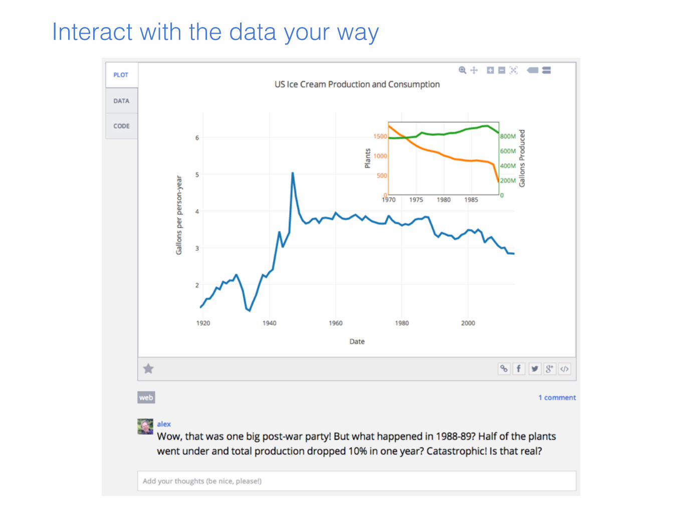
Interact with the data your way

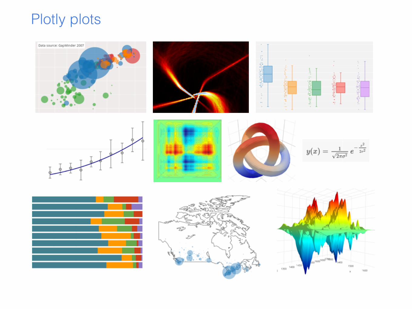
Plotly plots