Shape recognition and classification in electro-sensing

Shape recognition and classification inelectro-sensingHabib Ammari ∗, Thomas Boulier ∗ , Josselin Garnier †, and Han Wang ∗

∗Department of Mathematics and Applications, Ecole Normale Superieure, 45 Rue d’Ulm, 75005 Paris, France ([email protected], [email protected], [email protected]),

and †Laboratoire de Probabilites et Modeles Aleatoires & Laboratoire Jacques-Louis Lions, Universite Paris VII, 75205 Paris Cedex 13, France ([email protected]).

Submitted to Proceedings of the National Academy of Sciences of the United States of America

This paper aims at advancing the field of electro-sensing. It exhibitsthe physical mechanism underlying shape perception for weakly elec-tric fish. These fish orient themselves at night in complete darknessby employing their active electrolocation system. They generate astable, high-frequency, weak electric field and perceive the transder-mal potential modulations caused by a nearby target with differentadmittivity than the surrounding water. In this paper, we explainhow weakly electric fish might identify and classify a target, know-ing by advance that the latter belongs to a certain collection ofshapes. The fish is able to learn how to identify certain targets anddiscriminate them from all other targets. Our model of the weaklyelectric fish relies on differential imaging, i.e., by forming an imagefrom the perturbations of the field due to targets, and physics-basedclassification. The electric fish would first locate the target usinga specific location search algorithm. Then it could extract, fromthe perturbations of the electric field, generalized (or high-order)polarization tensors of the target. Computing, from the extractedfeatures, invariants under rigid motions and scaling yields shape de-scriptors. The weakly electric fish might classify a target by com-paring its invariants with those of a set of learned shapes. On theother hand, when measurements are taken at multiple frequencies,the fish might exploit the shifts and use the spectral content of thegeneralized polarization tensors to dramatically improve the stabilitywith respect to measurement noise of the classification procedurein electro-sensing. Surprisingly, it turns out that the first-order po-larization tensor at multiple frequencies could be enough for thepurpose of classification. A procedure to eliminate the backgroundfield in the case where the permittivity of the surrounding mediumcan be neglected, and hence improve further the stability of theclassification process, is also discussed.

weakly electric fish | electrolocation | shape classification | generalized polar-

ization tensors | shape descriptors | spectral induced polarization

IntroductionIn the turbid rivers of Africa and South America, some speciesof fish generate a stable, high frequency, weak electric field(0.1-10 kHz, ≤ 100 mV/cm) which is not enough for defensepurpose. In 1958, Lissmann and Machin [22] discovered thatthe emitted electrical signal is in fact used for active electro-sensing. The weakly electric fish have thousands of receptororgans at the surface of their skin. A nearby target with dif-ferent admittivity than the surrounding water is detected bymeasurements of the electric organ discharge modulations atthe receptor organs [13, 25]. Targets with large permittivitycause appreciable phase shifts, which can be measured by re-ceptors called T-type units [26]. It is an important input forthe fish, and thus it will be the central point in this paper forshape classification.

Active electro-sensing has driven an increasing number ofexperimental, behavioral, biological, and computational stud-ies since Lissmann and Machin’s work [11, 12, 15, 17, 23, 24,30, 36]. Behavioral experiments have shown that weakly elec-tric fish are able to locate a target [36] and discriminate be-tween targets with different shapes [35] or/and electric pa-rameters (conductivity and permittivity) [33]. The growinginterest in electro-sensing could be explained not only by thecuriosity of discovering a “sixth sense”, the electric percep-

tion, that is not accessible by our own senses, but also by po-tential bio-inspired applications in underwater robotics. It ischallenging to equip robots with electric perception and pro-vide them, by mimicking weakly electric fish, with imagingand classification capabilities in dark or turbid environments[18, 19, 21, 27, 28, 32, 33].

Mathematically speaking, the problem is to locate the tar-get and identify its shape and material parameters given thecurrent distribution over the skin. Due to the fundamentalill-posedness character of this imaging problem, it is very in-triguing to see how much information weakly electric fish areable to recover. The electric field due to the target is a com-plicated highly nonlinear function of its shape, admittivity,and distance from the fish. Thus, understanding analyticallythis electric sense is likely to give us insights in this regard[11, 12, 14, 15, 23, 27, 35]. While locating targets from theelectric field perturbations induced on the skin of the fish isnow understood (see [1, 21] and references therein), identify-ing and classifying their shapes is considered to be one of themost challenging problems in electro-sensing. Although theneuroethology of these fish has significantly been advancedlast years (see [16] and references therein), the neural mecha-nisms encoding the shape of a target is far beyond the scope ofour study. Rather, this work focuses on the physical feasibilityof such a process, which was not explained until now.

In [1], a rigorous model for the electro-location of a targetaround the fish was derived. Using the fact that the elec-tric current produced by the electric organ is time-harmonicwith a known fundamental frequency, a space-frequency lo-cation search algorithm was introduced. Its robustness withrespect to measurement noise and its sensitivity with respectto the number of frequencies, the number of sensors, and thedistance to the target were illustrated. In the case of disk-and ellipse-shaped targets, the conductivity, the permittivity,and the size of the targets can be reconstructed separatelyfrom multifrequency measurements. Such measurements havebeen used successfully in trans-admittance scanners of breasttumors [10, 20, 31].

In this paper, we tackle the challenging problem of shaperecognition and classification. In order to explain how theshape information is encoded in measured data, we first derivea multipolar expansion for the perturbations of the electricfield induced by a nearby target in terms of the characteris-

Reserved for Publication Footnotes

www.pnas.org — — PNAS Issue Date Volume Issue Number 1–11

tic size of the target. Our asymptotic expansion generalizesRasnow’s formula [29] in two directions: (i) it is a higher-order approximation of the effect of a nearby target and it isvalid for an arbitrary shape and admittivity contrast and (ii)it takes also into account the fish’s body. As it has been firstproved in [1], by postprocessing the measured data using layerpotentials associated only to the fish’s body, one can reducethe multipolar formula to the one in free space, i.e., withoutthe fish. Then we show how to identify and classify a target,knowing by advance that the latter belongs to a dictionaryof pre-computed shapes. The shapes considered in this paperhave been experimentally tested and results reported in [34].This idea comes naturally in mind when modeling behavioralexperiments such as in [33, 35, 36]. The pre-computed shapeswould then be a model for the fish’s memory (trained to rec-ognize specific shapes), and the experience of recognition pre-sented here would simulate the discrimination exercises thatare then imposed to them. We develop two algorithms forshape classification: one based on shape descriptors while thesecond is based on spectral induced polarizations. We first ex-tract, from the data, generalized (or high-order) polarizationtensors of the target (GPTs) [2]. These tensors, first intro-duced in [6], are intrinsic geometric quantities and constitutethe right class of features to represent the target shapes [5, 9].The shape features are encoded in the high-order polarizationtensors. The extraction of the GPTs can be achieved by aleast-squares method. The noise level in the reconstructedgeneralized polarization tensors depends on the angle of view.Larger is the angle of view, more stable is the reconstruc-tion. l1-regularization techniques could be used. Then wecompute from the extracted features invariants under rigidmotions and scaling. Comparing these invariants with thosein a dictionary of pre-computed shapes, we successfully clas-sify the target. Since the measurements are taken at multiplefrequencies, we make use of the spectral content of the gen-eralized polarization tensor in order to dramatically improvethe stability with respect to measurement noise of the physics-based classification procedure. In fact, we show numericallythat the first-order polarization tensor at multiple frequenciesis enough for the purpose of classification.

Feature extraction from induced current measurementsElectro-sensing model. Let us recall the nondimensionalizedmodel of electro-sensing: the body of the fish is Ω (of size oforder 1), an open bounded set in Rd, d = 2, 3, of class C1,α,0 < α < 1, with outward normal unit vector ν. The electricorgan is a dipole f placed at z0 ∈ Ω or a sum of point sourcesinside Ω satisfying the neutrality condition. We refer to [1]where the equations are nondimensionalized and the differentscales are identified. The fish’s skin is very thin and highlyresistive. Its effective thickness, that is, the skin thicknesstimes the contrast between the water and the skin conductiv-ities, is denoted by ξ and is of order 10−1 [11]. We assumethat the conductivity of the background medium is 1 and thatits permittivity is vanishing. Consider a target D = z + δB,where δ 1 is the characteristic size of D, z is its location,and B a smooth bounded domain containing the origin. Weassume that D is of complex admittivity k = σ + iεω, with ωbeing the operating frequency in the range [1, 10] and σ andε being respectively the conductivity and the permittivity ofthe target. It has been also shown in [1] that, in the presenceof D, the electric field u generated by the fish is the solution

of the following system:

∆u = f in Ω,

∇ · (1 + (k − 1)χD)∇u = 0 in Rd \ Ω,

∂u

∂ν

∣∣∣∣−

= 0 on ∂Ω,

u|+ − u|− = ξ∂u

∂ν

∣∣∣∣+

on ∂Ω

|u(x)| = O(|x|−d+1), |x| → ∞.

[1]

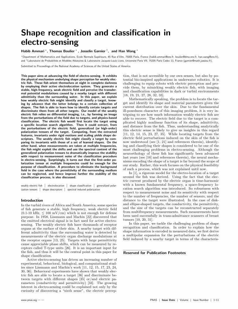
Here, χD is the characteristic function of D. Fig. 1 showsisopotentials with and without a target with zero permittiv-ity but different conductivity from the surrounding medium.Note that if the target’s admittivity depends on the frequency(i.e., if the permittivity is nonzero), then a phase shift in theelectrical potential is induced.

In a previous study [2], we have extracted the GPTs ofa target by multistatic measurements using arrays of sourcesand receptors. These GPTs were then arranged and comparedto a dictionary of already known shapes. This study aims atadapting this method to the electro-sensing problem.

Asymptotic formalism. The first step is to compute the GPTsfrom the measurements. In this regard, the next result willbe useful. Except when mentioned, we will fix in this sectionthe frequency ω, leading to a fixed complex admittivity k. Wewill need the following notation. For a multi-index α ∈ Nd,let xα = xα1

1 . . . xαdd , ∂α = ∂α1

1 . . . ∂αdd , with ∂j = ∂/∂xj . Let

G(x) be the Green function of the Laplacian in Rd which sat-isfies ∆G = δ (where δ is the Dirac function at the origin) andis given by

G(x) =

1

2πln |x|, d = 2,

− 1

4π

1

|x| , d = 3.

We denote the single and double layer potentials of a functionφ ∈ L2(∂Ω) as SΩ[φ] and DΩ[φ], where

SΩ[φ](x) :=

∫∂Ω

G(x− y)φ(y) dσ(y), x ∈ Rd, [2]

and

DΩ[φ](x) :=

∫∂Ω

∂G

∂ν(y)(x− y)φ(y) dσ(y), x ∈ Rd \∂Ω. [3]

We also define the boundary integral operator K∗Ω on L2(∂Ω)by

K∗Ω[φ](x) :=

∫∂Ω

∂G

∂ν(x)(x− y)φ(y) dσ(y), φ ∈ L2(∂Ω). [4]

−1 −0.5 0 0.5 1

−0.2

0

0.2

0.4

0.6

0.8

1

1.2

1.4

1.6

−2

−1.5

−1

−0.5

0

0.5

1

1.5

2

−1 −0.5 0 0.5 1

−0.2

0

0.2

0.4

0.6

0.8

1

1.2

1.4

1.6

−2

−1.5

−1

−0.5

0

0.5

1

1.5

2

(a) (b)

Fig. 1. Isopotentials without (a) and with (b) a target with σ = 5 and ε = 0.

2 www.pnas.org — — Footline Author

The operator K∗Ω is called the Neumann-Poincare operator.We assume that the target is away from the fish, i.e., the dis-tance between the fish and the target is much larger than thetarget’s characteristic size but smaller than the range of theelectrolocation which does not exceed two fish’s body lengths.The following theorem holds.Theorem 1. Let us define the function H : Rd → C by

H(x) = p(x) + SΩ

[∂u

∂ν

∣∣∣∣+

]− ξDΩ

[∂u

∂ν

∣∣∣∣+

], [5]

where p is the field created by the dipole f , i.e., ∆p = f in Rd.Then, for every integer K ≥ 1, the following expansion holds

u(x) = H(x) + δd−2K∑|α|=1

K−|α|+1∑|β|=1

(−1)|β|δ|α|+|β|

α!β!∂αH(z)

×Mαβ(λ,B)∂βG(x− z) +O(δd+K),[6]

uniformly for x ∈ ∂Ω, where z is the location of the target Dand

Mαβ(λ,B) :=

∫∂B

(λI −K∗B)−1[∂yα

∂ν]yβ dσ(y)

is the generalized polarization tensor (of order (α, β)) associ-ated with the domain B and the contrast λ = (k+1)/2(k−1);see [9]. Here, K∗B is the Neumann-Poincare operator associ-ated with B and I is the identity operator.

Let us make a few remarks. First, the definition of theGPTs still holds for complex-valued λ. However, some prop-erties are lost by this change; thus one has to study them morecarefully in this situation. Second, the function H, which iscomputed from the boundary measurements, still depends onδ but this is not important for our present study. Indeed,formula (6) could have been derived with U , the backgroundsolution in the absence of the target, instead of H and GR- the Green function associated to Robin conditions on ∂Ω -instead of G, but it is much easier to compute ∂αH(z) and∂βG(x−z) once z is known. This leads us to the third remark:the location z is supposed to be known from the algorithm de-veloped in [1]. Electrolocation algorithms are either based ona space-frequency approach in the case of multifrequency mea-surements or on the fish’s movement if only one frequency isused [1, 21]. Finally, it is worth mentioning that the knowl-edge of Mαβ(λ,B) for all α, β ∈ Nd determines uniquely Band λ [7, 8]. Moreover, the following scaling relation holds:

Mαβ(λ, δB) = δd−2+|α|+|β|Mαβ(λ,B).

We will follow the proof of [8, Theorem 4.8]. In a firststep, let us show the following formula.Lemma 2. For x ∈ Rd,

u(x) = H(x) + SD(λI −K∗D)−1

[∂H

∂ν

∣∣∣∣∂D

](x), [7]

where ν is the outward normal unit vector at ∂D and SD andK∗D are respectively defined by (2) and (4) with Ω replaced withD.

Proof. In [1, Section 4.1.2], it is shown that

u(x) = p(x) + SΩ[ψ](x) +DΩ[φ](x) + SD[φ](x),

where the functions ψ, φ ∈ L2(∂Ω) and φ ∈ L2(∂D) verifythe following system

φ = −ξψ on ∂Ω,(I

2−K∗Ω + ξ

∂DΩ

∂ν

)[ψ]− ∂

∂ν(SD[φ]) =

∂p

∂νon ∂Ω,

− ∂

∂ν(SΩ[ψ]) + ξ

∂

∂ν(DΩ[ψ]) + (λI −K∗D)[φ] =

∂p

∂νon ∂D.

The third line gives us

φ = (λI −K∗D)−1

[∂H

∂ν

∣∣∣∣∂D

],

and the jump formulas for the single and double layer poten-tials [9, Theorem 2.17] give us

ψ =∂u

∂ν

∣∣∣∣+

and φ = −u|+ + u|−,

so that, from the boundary conditions of the system (1), weobtain p+ SΩ[ψ] +DΩ[φ] = H and the lemma is proved.

We can now prove Theorem 1, using the arguments in [8,pp. 72-73]. Starting with formula (7), the proof relies on aTaylor expansion of H and the Green function involved in thesingle layer potential. Indeed, denoting

HK(x) =

K∑|α|=0

1

α!∂αH(z)(x− z)α,

a Taylor expansion gives us∥∥∥∥∂H∂ν − ∂HK∂ν

∥∥∥∥L2(∂D)

≤ CδK |∂D|1/2 ,

and from [8, Formula (4.10)], we have for any h ∈ L2(∂D)such that

∫∂D

h = 0:

∀x ∈ ∂Ω,∣∣SD(λI −K∗D)−1[h](x)

∣∣ ≤ Cδ |∂D|1/2 ‖h‖L2(∂D) .

Hence, using the fact that |∂D| = δd−1 |∂B|, we obtain∥∥∥∥SD(λI −K∗D)−1

[∂H

∂ν− ∂HK

∂ν

]∥∥∥∥L∞(∂Ω)

≤ Cδ |∂D|1/2∥∥∥∥∂H∂ν − ∂HK

∂ν

∥∥∥∥L2(∂D)

≤ Cδd+K .

Plugging this inequality into (7) enables us to write, forx ∈ ∂Ω,

u(x) = H(x) + SD(λI −K∗D)−1

[∂HK∂ν

](x) +O(δd+K).

By a change of variables y′ = (y − z)/δ, denoting φα(y′) =(λI − K∗B)−1[ν · ∇wα](y′) for y′ ∈ ∂B (where ν is here theoutward normal unit vector to ∂B), we have (see for examplethe arguments in [5, Section 3])

u(x)−H(x) =

K∑|α|=0

1

α!∂αH(z)δ|α|+d−2

×∫∂B

G(x− z − δy′)φα(y′)dσ(y) +O(δd+K).

We can now conclude by injecting a Taylor expansion of theGreen function

G(x− z − δy) =

∞∑|β|=0

(−δ)|β|

β!∂βG(x− z)yβ ,

in the integrand, giving

u(x)−H(x) = δd−2K∑|α|=0

K−|α|+1∑|β|=0

(−1)|β|δ|α|+|β|

α!β!∂αH(z)

×∂βG(x− z)∫∂B

yβφα(y)dσ(y) +O(δd+K).

The last term is Mαβ(λ,B) by definition [9]; it then sufficesto show that the terms with |α| = 0 or |β| = 0 vanish, whichis the case because

∫∂B

φα = 0 and φα = 0 if |α| = 0. Thus,Theorem 1 is proved.

Footline Author PNAS Issue Date Volume Issue Number 3

Data acquisition and reduction. Let us suppose that the fish ismoving, and let us take a sample of S ∈ N∗ different positions(Ωs)1≤s≤S . This gives us 2S different functions (us)1≤s≤S and

(Hs)1≤s≤S , leading us to the following data matrix

Q := (Qsr)1≤s≤S,1≤r≤R :=(us(x

(s)r )−Hs(x(s)

r ))

1≤s≤S,1≤r≤R,

[8]

where (x(s)r ∈ ∂Ωs)1≤r≤R are the receptors of the fish being

in the sth position. The choices of indices are motivated bythe fact that the different positions play the role of sources.

The goal of this subsection is to simplify this data set inorder to extract the GPTs (precisely, the contracted GPTs asit will be seen below). Indeed, from (6), one has

Qsr = δd−2K∑|α|=1

K−|α|+1∑|β|=1

(−1)|β|δ|α|+|β|

α!β!∂αHs(z)

×Mαβ(λ,B)∂βG(x(s)r − z) +O(δd+K).

[9]

As in [2], we will express this formula in terms of contractedGPTs (CGPTs), when the dimension of the space is d = 2.Let us first recall the definitions of these contracted GPTs.For a target B with contrast ratio λ, knowing the GPTsMαβ(λ,B) for all indices α and β such that |α| = m and|β| = n leads us to construct the following combinations,called CGPTs,

Mccmn =

∑|α|=m

∑|β|=n

amα anβMαβ ,

Mcsmn =

∑|α|=m

∑|β|=n

amα bnβMαβ ,

Mscmn =

∑|α|=m

∑|β|=n

bmα anβMαβ ,

Mssmn =

∑|α|=m

∑|β|=n

bmα bnβMαβ ,

where the real numbers amα and bmβ are defined by the followingrelation

(x1 + ix2)m =∑|α|=m

amα xα + i

∑|β|=m

bmβ xβ .

In the polar coordinates, x = rxeiθx , these coefficients also

verify the following characterization∑|α|=m

amα xα = rmx cosmθx and

∑|β|=m

bmβ xβ = rmx sinmθx.

This enables us to show [2, Appendix A.2] that

(−1)|α|

α!∂αG(x) =

−1

2π |α|

(a|α|α

cos |α| θxr|α|x

+ b|α|αsin |α| θxr|α|x

).

[10]From the definition of H, and with the help of the previousformula, one can prove the following lemma.Lemma 3. Let the source f be a dipole of moment ps placedat zs:

ps(x) = ps · ∇G(x− zs), [11]

Then, for any α ∈ N2, there exist two real numbers A|α|,s,zand B|α|,s,z such that

1

α!∂αHs(z) = A|α|,s,za

|α|α +B|α|,s,zb

|α|α .

Moreover, A|α|,s,z and B|α|,s,z can be expressed in the follow-ing way

Am,s,z =(−1)m

2πps ·

(φm+1(z − zs)ψm+1(z − zs)

)− 1

2πm

∫∂Ω

∂us∂ν

∣∣∣∣+

(y)φm(y − z)dσ(y),

− ξ

2π

∫∂Ω

(φm+1(y − z)ψm+1(y − z)

)· νy

∂us∂ν

∣∣∣∣+

(y) dσ(y),

Bm,s,z =(−1)m

2πps ·

(ψm+1(z − zs)−φm+1(z − zs)

)− 1

2πm

∫∂Ω

∂us∂ν

∣∣∣∣+

(y)ψm(y − z)dσ(y)

− ξ

2π

∫∂Ω

(ψm+1(y − z)−φm+1(y − z)

)· νy

∂us∂ν

∣∣∣∣+

(y) dσ(y),

where the functions φm and ψm are defined for x ∈ R2,x = (rx, θx) in the polar coordinates, by

φm(x) =cosmθxrmx

, ψm(x)=sinmθxrmx

.

Proof. Let us fix α ∈ N2 and define m = |α|. Let us recall thedefinition of H, given in (5)

Hs(x) = ps(x) + SΩs

[∂us∂ν

∣∣∣∣+

]− ξDΩs

[∂us∂ν

∣∣∣∣+

],

where ∆ps = fs in R2. From (11) it follows that

∂αps(x) = ps · ∇∂αG(x− zs).

Hence, (10) yields

(−1)|α|

α!∂αps(z) = amα

[−1

2πmps · ∇φm(z − zs)

]+bmα

[−1

2πmps · ∇ψm(z − zs)

].

Moreover, we have

∇φm = −m(

φm+1

ψm+1

), ∇ψm= −m

(ψm+1

−φm+1

).

In the same manner, from

SΩs

[∂us∂ν

∣∣∣∣+

](x) =

∫∂Ωs

∂us(y)

∂ν

∣∣∣∣+

G(y − x)dσ(y),

we can deduce

1

α!∂αSΩs

[∂us∂ν

∣∣∣∣+

](z)

=1

α!

∫∂Ωs

∂us∂ν

∣∣∣∣+

(y)(−1)|α|∂αG(y − z)dσ(y)

= amα

(∫∂Ωs

−1

2πm

∂us∂ν

∣∣∣∣+

(y)cosmθy−zrmy−z

dσ(y)

)

+bmα

(∫∂Ωs

−1

2πm

∂us∂ν

∣∣∣∣+

(y)sinmθy−zrmy−z

dσ(y)

).

Combining those two equations leads us to the desired result.


From (9), the data matrix is then expressed as follows

Qrs =

K+1∑|α|+|β|=1

(A|α|,s,za

|α|α +B|α|,s,zb

|α|α

)

×Mαβ(λ, δB)−a|β|β cos |β| θ

x(s)r −z

− b|β|β sin |β| θx(s)r −z

2π |β| r|β|x(s)r −z

+O(δK+2)

=

K+1∑m+n=1

(Am,s,z Bm,s,z

)︸︷︷︸Ssm

(Mccmn Mcs

mn

Mscmn Mss

mn

)︸︷︷︸

Mmn

×

(cosnθ

x(s)r −z

sinnθx(s)r −z

)−1

2πnrnx(s)r −z︸︷︷︸

G(s)nr

+O(δK+2)︸︷︷︸Ers

.

[12]Thus, defining the following matrices

M =

M11 M12 . . . M1K

M21 . ..

0... . .

.. .. ...

MK1 0 . . . 0

, E = (Ers)1≤r≤R,1≤s≤S ,

the problem is to recover the matrix M knowing the matrix

Q = L(M) + E,

where L is the linear operator defined by (12).Therefore, the CGPTs of the target D can be recon-

structed as the least-squares solution of the above linear sys-tem, i.e.,

M = argminM⊥ker(L)

‖Q− L(M)‖2F , [13]

where ker(L) denotes the kernel of L and ‖ · ‖F denotes theFrobenius norm of matrices [2].

Let us remark that, in the case of multifrequency measure-

ments (ω1, . . . , ωF ), we can reconstruct(M(f)

)1≤f≤F

from(Q(f)

)1≤f≤F

analogously.

It is worth mentioning that the location of the target de-tected by the fish may be different from the true one. More-over, the target may be rotated and hence, the reconstructedCGPTs correspond to a translated, scaled, and rotated targetB. In order to recognize the shape B, it is therefore funda-mental for the recognition procedure to have size invariance,rotational invariance, and translational invariance. This couldbe related to the behavioral experiments that have shownthat weakly electric fish categorize targets according to theirshapes but not according to sizes, locations, or orientations[34].

Recognition and classificationDepending on whether we consider multifrequency measure-ments or not, we will not identify the CGPTs in the sameway.

Fixed frequency setting: shape descriptor based classifica-tion. In [2], an algorithm based on shape descriptors was de-veloped for the recognition of a target in a more classical elec-trical sensing setup, (i.e., multiple sources/receptors placed onthe surface of a disk). In this paper, we apply this algorithmin the context of electro-sensing.

We recall here the concept and properties of shape de-scriptors in two dimensions [2]. For a double index mn, withm,n = 1, 2, . . ., we introduce the following complex combina-

tions, N(1) = (N (1)mn)m,n,N

(2) = (N (2)mn)m,n, of CGPTs:

N (1)mn(λ,D) = (Mcc

mn −Mssmn) + i(Mcs

mn +Mscmn),

N (2)mn(λ,D) = (Mcc

mn +Mssmn) + i(Mcs

mn −Mscmn).

[14]

Let

u =N (2)

12 (D)

2N (2)11 (D)

, T−uD = x− u, x ∈ D.

We define the following quantities which are translation in-variant:

J (1)(D) = N(1)(T−uD) = C−uN(1)(D)(C−u)t, [15]

J (2)(D) = N(2)(T−uD) = C−uN(2)(D)(C−u)t, [16]

with t being the transpose and the matrix C−u being a lowertriangular matrix with the m,n-th entry given by

C−umn =

(m

n

)(−u)m−n.

From J (1)(D) = (J (1)mm(D))m,n and J (2)(D) = (J (2)

mm(D))m,n,we define, for any indices m,n, the scaling invariant quanti-ties:

S(j)mn(D) =

J (j)mn(D)(

J (2)mm(D)J (2)

nn (D))1/2

, j = 1, 2. [17]

Finally, we introduce the CGPT-based shape descriptors

I(1) = (I(1)mn)m,n and I(2) = (I(2)

mn)m,n:

I(1)mn(D) = |S(1)

mn(D)|, I(2)mn(D) = |S(2)

mn(D)|, [18]

where | · | denotes the modulus of a complex number. Con-

structed in this way, I(1) and I(2) are invariant under trans-lation, rotation, and scaling. Only shape descriptors of order2, i.e., for m,n = 1, 2 will be used in the sequel. Shape de-scriptors in three dimensions were derived in [4].

Multifrequency setting: Spectral induced polarization basedclassification. When multiple frequencies are involved, we can

use the shape descriptors I(1)mn(D) and I(2)

mn(D) at frequenciesω1, . . . , ωF to enhance the stability of the classification. How-ever, as it will be shown later, this does not yield a very stableclassification procedure.

Here we rather focus on the first-order polarization tensor(PT), that is, the 2 × 2 complex matrix M(f)(D) associatedwith the target D and frequency f :

M(f)(D) :=

∫∂D

(σ + 1 + iωfε

2(σ − 1 + iωfε)I −K∗D

)−1

[ν]y dσ(y),

for f = 1, . . . , F . We will show that they are sufficient toidentify efficiently the targets. Note that it is not possible

to compute the shape descriptors I(1)mn(D) and I(2)

mn(D) basedonly on first-order PT, because they require at least second-order polarization tensors. This limits the use of shape de-scriptors in the limited-view case where the reconstruction ofhigher-order GPTs is not accurate [3].

Here we use the spectral content of the first-order PTs forrecognition. We have the following properties [9].


Proposition 4. For any scaling δ > 0, rotation angle θ ∈ Rand translation vector z ∈ R2, let us denote

D = z + δRθB := x = z + δRθu, u ∈ B ,

where

Rθ :=

(cos θ − sin θsin θ cos θ

),

is the rotation matrix of angle θ. Then,

M(f)(D) = δ2RθM(f)(B)RTθ . [19]

Hence, if we denote by τ(f)1 (D) and τ

(f)2 (D) the singular val-

ues of M(f)(D), we obtain

∀j ∈ 1, 2, τ (f)j (D) = δ2τ

(f)j (B).

This gives an idea for two algorithms:

1. The first one, matching the singular values of all the first-

order PT(M(f)

)1≤f≤F

, would be dependent of the char-

acteristic scale δ of the targets in the dictionary;2. The second one, independent of the scale of the target,

would match the following quantities

µ(f)j =

τ(f)j

τ(F )j

, [20]

for j = 1, 2 and f = 1, . . . , F − 1.

Some comments are in order. First, the reason why we con-sider the first one, even if it is scale-dependent, is because itis far more stable. Also, in some biological experiments, twotargets of different scales are considered as different [35]. Aquestion raised was then: how is it possible to discriminatebetween a nearby small target and an extended one situatedfar away? With the second algorithm, we have an answer.The last remark concerns equation (20). We could have alsoconsidered other scale-dependent ratios, such as

τ(f)j

τ(1)j

orτ

(f)j∑F

f ′=1 τ(f ′)j

,

but since τ(F )j happens to be the largest one (the frequen-

cies are sorted in increasing order), it is more stable to con-sider (20). It is worth mentioning that if there exists an integer

p > 2 such that R2π/pD = D, then M(f)(D) is proportionalto identity.

Background field elimination. We can also improve stabilityof reconstruction by eliminating the background field. Let usdenote by U(x) the background electric field (i.e., the solutionof (1) with k = 1). In [1, Proposition 2], we have proved thefollowing formula:

PΩ

(∂uf∂ν

∣∣∣∣+

− ∂U

∂ν

∣∣∣∣+

)≈ ∇U(z)TM(f)(D)∇z

(∂G

∂νx

),

[21]

where uf is u associated with the f th frequency, M(f)(D) isthe first-order polarization tensor at the f th frequency, andPΩ is the (real-valued) postprocessing operator given by

PΩ :=1

2I −K∗Ω − ξ

∂DΩ

∂ν,

with DΩ and K∗Ω being defined by (3) and (4); see [1]. Hence, ifthe emitted signal U is real-valued, then taking the imaginarypart leads us to

PΩ

[=m

(∂uf∂ν

∣∣∣∣+

)]≈ ∇U(z)T=mM(f)(D)∇z

(∂G

∂νx

).

[22]Note that in biological sciences, the restriction on U to be realis justified since the permittivities of water and the fish arenegligible [1]. Now, from (22), we can extract =mM(f)(D) bysolving a least-squares problem similar to (13). Then, we have

the singular values of the imaginary part of M(f)(D), whichwould be sufficient for shape recognition and classification.The goal of this procedure is to get rid off the computation of∂U/∂ν in (21), which is supposed to be performed numericallyin real-world applications, thus subject to errors. Note thatthe postprocessing operator PΩ makes the data independentof the shape of the fish’s body.

−1 0 1−1

−0.5

0

0.5

1

−1 0 1−1

−0.5

0

0.5

1

−0.5 0 0.5−0.5

0

0.5

−1 0 1−1

−0.5

0

0.5

1

−0.5 0 0.5

−0.5

0

0.5

−0.5 0 0.5

−0.5

0

0.5

−0.5 0 0.5

−0.4

−0.2

0

0.2

0.4

0.6

−1 0 1−1

−0.5

0

0.5

1

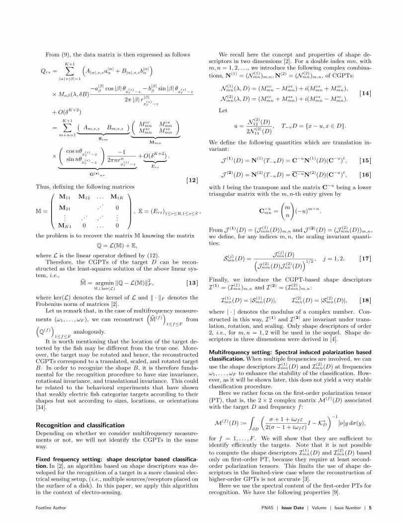
Fig. 2. The 8 elements of the dictionary. The dotted lines indicate a target with

different electrical parameters.

−1.5 −1 −0.5 0 0.5 1 1.5

−1.5

−1

−0.5

0

0.5

1

1.5

−3

−2

−1

0

1

2

3

−1.5 −1 −0.5 0 0.5 1 1.5

−1.5

−1

−0.5

0

0.5

1

1.5

−3

−2

−1

0

1

2

3

−1.5 −1 −0.5 0 0.5 1 1.5

−1.5

−1

−0.5

0

0.5

1

1.5

−3

−2

−1

0

1

2

3

−1.5 −1 −0.5 0 0.5 1 1.5

−1.5

−1

−0.5

0

0.5

1

1.5

−3

−2

−1

0

1

2

3

−1.5 −1 −0.5 0 0.5 1 1.5

−1.5

−1

−0.5

0

0.5

1

1.5

−3

−2

−1

0

1

2

3

−1.5 −1 −0.5 0 0.5 1 1.5

−1.5

−1

−0.5

0

0.5

1

1.5

−3

−2

−1

0

1

2

3

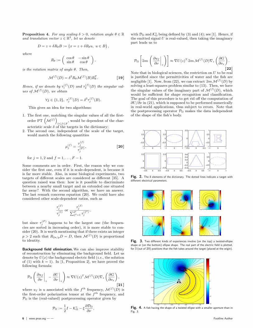
Fig. 3. Two different kinds of experiences involve (on the top) a twisted-ellipse

shape or (on the bottom) ellipse shape. The real part of the electric field is plotted,

for 3 (out of 20) positions that the fish takes around the target (placed at the origin).

−1.5 −1 −0.5 0 0.5 1 1.5

−1.5

−1

−0.5

0

0.5

1

1.5

−3

−2

−1

0

1

2

3

Fig. 4. A fish having the shape of a twisted ellipse with a smaller aperture than in

Fig. 3.


Because of the following relation which follows from (19)

M(f)(D) = O(δ2M(f)(B)),

taking the imaginary part would lead us to only compute∇U(z) in (22) and hence, the error made here would be mod-ulated by a factor of order δ2.

Numerical illustrationsIn this section, we illustrate the performance of the algorithmsdeveloped in the previous section. We use the CGPTs ob-tained in order to classify the targets. We present an examplewith fixed frequency, and another with multifrequency mea-surements. As it will be seen, the latter does not lead us to asignificantly more stable classification in the presence of noiseor for limited aperture. The errors in the reconstruction of thehigh-order polarization tensors due to measurement noise orthe limited-view aspect deteriorate the stability of the pro-posed algorithm. However, when, at multiple frequencies,only the first-order polarization tensor is used, we arrive ata very robust and efficient classification procedure.

For the sake of clarity, and due to the large numbers ofcomputations performed, the results are presented in the ap-pendix.

Setup and methods. We describe the dictionary as well as themeasurement systems. We consider two different shapes forthe fish: ellipses and twisted ellipses. Note that this vari-ety of shapes exists in nature. On the one hand, twisted el-lipses would represent electric eels (Electrophorus electricus),whereas on the other hand straight ellipses would look likeApteronotids [25]. This simplified representation shows thatthe principle of our algorithms can be generalized to any kindof fish’s shape (hence modeling, for example, electro-sensingfor Mormyrids as well). It also enhances the fact that, forbio-inspired engineering applications, the shape of the robotis not determining. Moreover, as we will see later, our simpli-fied representation is a good model to tackle aperture issues.

Dictionary

The dictionary D that we consider is composed by 8 differ-ent targets: a disk, an ellipse, the letter ’A’, the letter ’E’, arectangle, a square, a triangle, and an ellipse with differentelectrical parameters (see Fig. 2). Indeed, all the other tar-gets have conductivity σ = 2 and permittivity ε = 1 whereasthe last one has conductivity σ = 5 and permittivity ε = 2.Except when mentioned, the characteristic size of the targetwill not matter, and will be fixed to be of order 1.

Measurements

In each numerical experiment, one target of the dictionary isplaced at the origin, while the fish swims around it. As ithas been mentioned, we consider two different shapes for thefish’s body: ellipses and twisted ellipses. The measured datais built taking 20 positions of the fish around the target (seeFig. 3).

In Fig. 4, a smaller aperture than the one in Fig. 3 isconsidered.

The typical size of the target is δ = 0.3 while the fish isturning around a disk of radius R = 1; the twisted ellipse’ssemi-axes are a = 1.8 and b = 0.2 while the straight ellipse’ssemi axis are a = 1 and b = 0.2. The effective thickness ofthe skin is set at ξ = 0. The fish has 27 receptors uniformlydistributed on its skin, and the electric organ emits F = 10

frequencies, equally distributed from ω0 := 1 to Fω0. Again,we refer to [1] for nondimensionalization of the underlyingmodel equations with proper quantities and realistic values.

Classification

The recognition process is as follows. When measurements areacquired, we perform least-square reconstruction of the (first-or second-order) CGPT of the targets. From this CGPT, wecompute quantities of interest q (i.e. Shape Descriptors orsingular values or ratios of singular values). Then, for eachelement n in the dictionary D, we compute ‖q − qn‖, where qnis the - pre-computed - quantity of interest for the nth shape.This leads us to charts such as the ones presented in Figs. 5,6, and 7.

Framework for algorithms of multifrequency classifica-tion:

1: Input: the quantities of interest(q(f)

)1≤f≤F

calcu-

lated from the measurement of an unknown shape D;2: for Bn ∈ D do

3: en ←∑

1≤f≤F ‖q(Bn)(f)−q(f)‖2 where(q(Bn)(f)

)1≤f≤F

is the same type of quantities of interest of the shapeBn;

4: n← n+ 1;5: end for6: Output: the true dictionary element n∗ ← argminnen.

Stability analysis

First, let us explain what kind of noise is considered. Wewill add a random matrix (with Gaussian entries) to the datamatrix Q defined in (8). More precisely, we will consider

Q := Q + εW,

where W is a S×R matrix whose coefficients follow a Gaussiandistribution with mean 0 and variance 1. The real number εis the strength of the noise, and will be given in percentageof the fluctuations of Q, (i.e., maxs,r Qsr −mins,r Qsr). Therecognition procedure remains the same.

Stability analysis was then carried out empirically: foreach noise level, we performed Nstabil independent recognitionprocess (with Nstabil being precised for each experiment), andcomputed the ratio of good detection. The computation endswhen we reach the threshold of 12.5% probability of detectionthat corresponds to a uniform random choice of the object.This gives us Figs. 8 to 15.

Results and discussion. In this subsection, we compare the re-spective stability of our algorithms. Due to the large numberof situations and computations, only significant figures wereplotted, giving the following classification of recognition pro-cesses, according to their range of application.

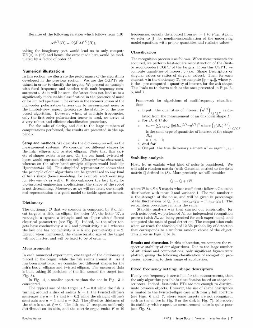
Fixed frequency setting: shape descriptors

If only one frequency is accessible for the measurements, thenthe only algorithm possible is classification based on shape de-scriptors. Indeed, first-order PTs are not enough to discrim-inate between objects. However, the use of shape descriptorsis limited to the twisted-ellipse case with nearly full aperture(see Figs. 6 and 7, where some targets are not recognized,such as the ellipse in Fig. 6 or the disk in Fig. 7). Moreover,its stability with respect to measurement noise is quite poor(see Fig. 8).


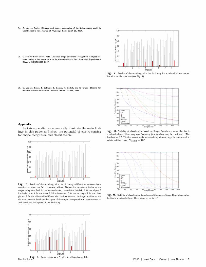
Multifrequency setting: spectral content of PTs

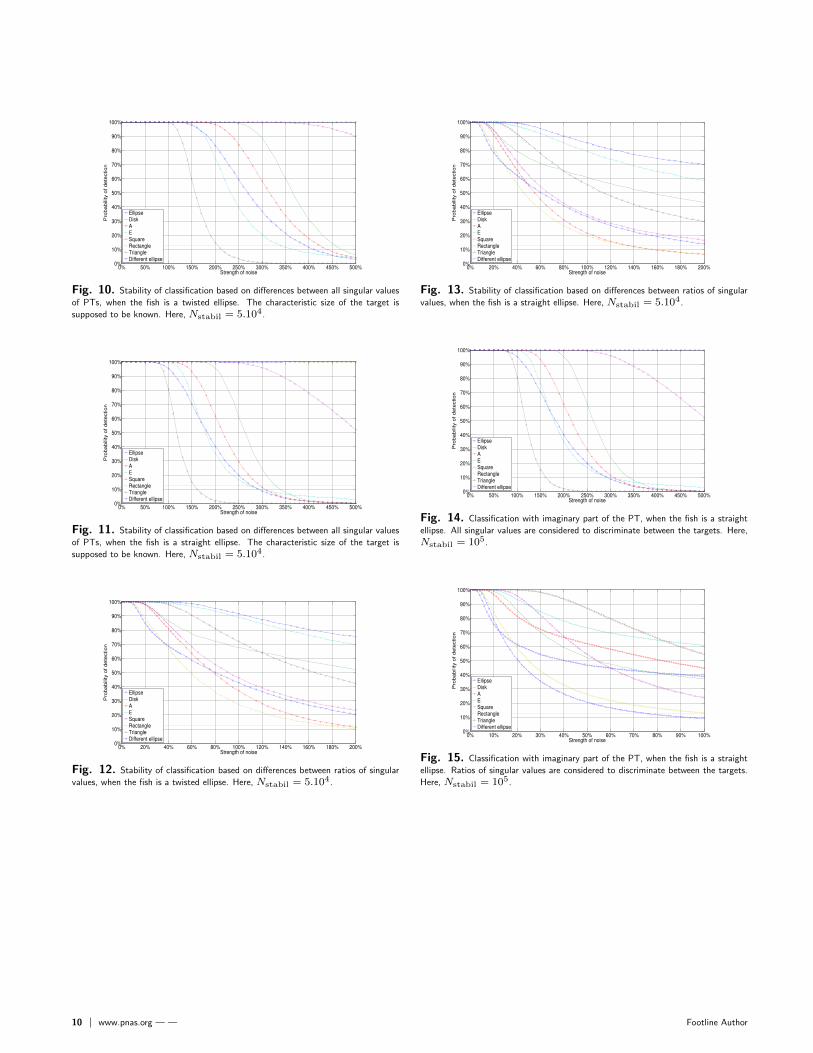
In the case of multifrequency measurements, shape descrip-tors do not increase their stability enough compared to sin-gular values (see Fig. 9). Hence, it is better to use singularvalues of the PTs (see Figs. 10 to 13). One can see that:

• considering all singular values (Figs. 10 and 11) is muchmore stable than considering ratios of singular values(Figs. 12 and 13);

• the aperture does not change very much the stability.

In this regard, the most stable algorithm is to recognize allsingular values when the fish is a twisted ellipse (Fig. 10),leading us to a probability of detection superior to 90% withnoise level of 125%. This is a huge gap when compared tothe recognition process with shape descriptors, allowing onlya few percents of noise. Note that the noise level is computedwith respect to the perturbation in the measurements Q givenby (8), which is of order of the target volume, see (9). Hence,a noise level of 125% remains small compared to the actualtransdermal potential u.

Background field elimination

We can see in Figs. 14 and 15 that taking the imaginary partof the measurements in order to avoid the computation of thebackground field does not significantly decrease the stabilityof the reconstruction based on spectral content. Since thereconstruction of CGPTs is very fast, the background fieldelimination technique would yield to real-time imaging.

Concluding remarksIn this paper, we have successfully exhibited the physicalmechanism underlying shape recognition and classification inactive electrolocation. We have shown that extracting gener-alized polarization tensors from the data and comparing in-variants with those of learned elements in a dictionary yieldsa classification procedure with a good performance in the full-view case and with moderate measurement noise level. How-ever, this shape descriptor based classification is instable inthe limited-view case and for higher noise level. When mea-surements at multiple frequencies are used, the stability ofour classification approach is significantly improved by usingphase shifts and keeping only the first-order polarization ten-sor. The resulting spectral induced polarization based classi-fication is very robust.

Our results open the door for the application of the ex-tended Kalman filter developed in [3] to show the feasibilityof a tracking of both location and orientation of a target fromperturbations of the electric field on the skin surface of thefish. It also remains to understand to what extent the spec-tral induced polarization approach could help us retrieve theelectric parameters of the target or locate and recognize mul-tiple targets.

ACKNOWLEDGMENTS. This work was supported by the ERC Advanced GrantProject MULTIMOD–267184.

1. H. Ammari, T. Boulier, and J. Garnier. Modeling active electrolocation in weakly

electric fish. To appear in SIAM Journal on Imaging Sciences, 2012.

2. H. Ammari, T. Boulier, J. Garnier, W. Jing, H. Kang, and H. Wang. Target identi-

fication using dictionary matching of generalized polarization tensors. Submitted to

Foundations of Computational Mathematics (arXiv:1204.3035), 2012.

3. H. Ammari, T. Boulier, J. Garnier, H. Kang, and H. Wang. Tracking of a mobile

target using generalized polarization tensors. Submitted to SIAM Journal on Imaging

Sciences (arXiv:1212.3544), 2012.

4. H. Ammari, D. Chung, H. Kang, and H. Wang. Invariance properties of generalized

polarization tensors and design of shape descriptors in three dimensions. Submitted

to Appl. Comput. Harmon. Anal. (arXiv:1212.3519), 2012.

5. H. Ammari, J. Garnier, H. Kang, M. Lim, and S. Yu. Generalized polarization tensors

for shape description. To appear in Numerische Mathematik, 2012.

6. H. Ammari and H. Kang. High-order terms in the asymptotic expansions of the

steady-state voltage potentials in the presence of conductivity inhomogeneities of

small diameter. SIAM J. Math. Anal., 34(5):1152–1166, 2003.

7. H. Ammari and H. Kang. Properties of generalized polarization tensors. SIAM Mul-

tiscale Model. Simul., 1:335–348, 2003.

8. H. Ammari and H. Kang. Reconstruction of small inhomogeneities from boundary mea-

surements, volume 1846 of Lecture Notes in Mathematics. Springer-Verlag, Berlin,

2004.

9. H. Ammari and H. Kang. Polarization and moment tensors, volume 162 of Applied

Mathematical Sciences. Springer, New York, 2007. With applications to inverse prob-

lems and effective medium theory.

10. H. Ammari, O. Kwon, J.K. Seo, and E.J. Woo. T-scan electrical impedance imaging

system for anomaly detection. SIAM J. Appl. Math., 65:252–266, 2004.

11. C. Assad. Electric field maps and boundary element simulations of electrolocation in

weakly electric fish. PhD thesis, California Institute of Technology, 1997.

12. D. Babineau, A. Longtin, and J.E. Lewis. Modeling the electric field of weakly electric

fish. Journal of experimental biology, 209(18):3636, 2006.

13. J. Bastian. Electrolocation i. how the electroreceptors of apteronotus albifrons code

for moving objects and other electrical stimuli. J Comp. Physiol. A, 144:397–411,

1981.

14. F. Boyer, P-B. Gossiaux, B. Jawad, V. Lebastard, and M. Porez. Model for a sensor

inspired by electric fish. IEEE Transactions on Robotics, 52(2):492–505, 2012.

15. R. Budelli and A.A. Caputi. The electric image in weakly electric fish: perception of

objects of complex impedance. Journal of Experimental Biology, 203(3):481, 2000.

16. T.H. Bullock, C.D. Hopkins, A.N. Popper, and R.F. Richard, editors. Electroreception.

Springer-Verlag, New York, 2005.

17. L. Chen, J.L. House, R. Krahe, and M.E. Nelson. Modeling signal and background

components of electrosensory scenes. Journal of Comparative Physiology A: Neu-

roethology, Sensory, Neural, and Behavioral Physiology, 191(4):331–345, 2005.

18. O.M. Curet, N.A. Patankar, G.V. Lauder, and M.A. MacIver. Aquatic maneuvering

with counter-propagating waves: a novel locomotive strategy. J. Royal Soc. Interface,

8:1041–1050, 2010.

19. B. Jawad, P.B. Gossiaux, F. Boyer, V. Lebastard, F. Gomez, N. Servagent, S. Bouvier,

A. Girin, and M. Porez. Sensor model for the navigation of underwater vehicles by

the electric sense. In Proc. of 2010 IEEE International Conference on Robotics and

Biomimetics (ROBIO), pages 879–884, 2010.

20. S. Kim, J. Lee, J.K. Seo, E.J. Woo, and H. Zribi. Multifrequency trans-admittance

scanner: mathematical framework and feasibility. SIAM J. Appl. Math., 69:22–36,

2008.

21. V. Lebastard, Ch. Chevallereau, A. Amrouche, B. Jawad, A. Girin, F. Boyer, and P-B.

Gossiaux. Underwater robot navigation around a sphere using electrolocation sense

and kalman filter. In 2010 IEEE/RSJ International Conference on Intelligent Robots

and Systems (IROS), pages 4225–4230, 2010.

22. H.W. Lissmann and K.E. Machin. The mechanism of object location in gymnarchus

niloticus and similar fish. Journal of Experimental Biology, 35(2):451, 1958.

23. M.A. Maciver. The computational neuroethology of weakly electric fish: body mod-

eling, motion analysis, and sensory signal estimation. PhD thesis, Citeseer, 2001.

24. M.A. MacIver, N.M. Sharabash, and M.E. Nelson. Prey-capture behavior in gymnotid

electric fish: motion analysis and effects of water conductivity. Journal of Experimental

Biology, 204(3):543, 2001.

25. P. Moller. Electric fish: history and behavior. Chapman and Hall, London, 1995.

26. M.E. Nelson. Target Detection, Image Analysis, and Modeling. Springer-Verlag, New

York, 2005.

27. M. Porez, V. Lebastard, A.J. Ijspeert, and F. Boyer. Multi-physics model of an electric

fish-like robot: Numerical aspects and application to obstacle avoidance. In Proc. of

2011 IEEE/RSJ International Conference on Intelligent Robots and Systems (IROS),

pages 1901–1906, 2011.

28. C.M. Postlethwaite, T.M. Psemeneki, J. Selimkhanov, M. Silber, and M.A. MacIver.

Optimal movement in the prey strikes of weakly electric fish: A case study of the

interplay of body plan and movement capability. J. Royal Soc. Interface, 6:417–433,

2009.

29. B. Rasnow. The effects of simple objects on the electric field of apteronotus. J Comp.

Physiol. A, 178:397–411, 1996.

30. B. Rasnow, C. Assad, M.E. Nelson, and J.M. Bower. Simulation and measurement of

the electric fields generated by weakly electric fish. In Advances in neural information

processing systems 1, pages 436–443. Morgan Kaufmann Publishers Inc., 1989.

31. B. Scholz. Towards virtual electrical breast biopsy: space-frequency music for trans-

admittance data. IEEE Transactions on Medical Imaging, 21(6):588–595, 2002.

32. J.R. Solberg, K.M. Lynch, and M.A. MacIver. Active electrolocation for underwater

target localization. Internat. J. Robotics Res., 27(5):529–548, 2008.

33. G. Von der Emde. Active electrolocation of objects in weakly electric fish. Journal of

experimental biology, 202(10):1205, 1999.


34. G. von der Emde. Distance and shape: perception of the 3-dimensional world by

weakly electric fish. Journal of Physiology Paris, 98:67–80, 2004.

35. G. von der Emde and S. Fetz. Distance, shape and more: recognition of object fea-

tures during active electrolocation in a weakly electric fish. Journal of Experimental

Biology, 210(17):3082, 2007.

36. G. Von der Emde, S. Schwarz, L. Gomez, R. Budelli, and K. Grant. Electric fish

measure distance in the dark. Science, 260:1617–1623, 1993.

Appendix

In this appendix, we numerically illustrate the main find-ings in this paper and show the potential of electro-sensingfor shape recognition and classification.

1 2 3 4 5 6 7 80

0.05

0.1

0.15

0.2

0.25

0.3

0.35

Shape Label

Dis

ta

nce

to

d

ictio

na

ry (A

.U

.)

Fig. 5. Results of the matching with the dictionary (differences between shape

descriptors), when the fish is a twisted ellipse. The red bar represents the bar of the

target being identified. In the x-coordinates, 1 stands for the disk, 2 for the ellipse, 3

for the letter A, 4 for the letter E, 5 for the square, 6 for the rectangle, 7 for the trian-

gle and 8 for the ellipse with different electrical parameters. In the y-coordinates, the

distance between the shape descriptor of the target - computed from measurements -

and the shape descriptors of the dictionary.

1 2 3 4 5 6 7 80

0.1

0.2

0.3

0.4

0.5

Shape Label

Dis

ta

nce

to

d

ictio

na

ry (A

.U

.)

Fig. 6. Same results as in 5, with an ellipse-shaped fish.

1 2 3 4 5 6 7 80

0.05

0.1

0.15

0.2

0.25

0.3

0.35

Shape Label

Dis

tan

ce

to

dic

tio

na

ry (

A.U

.)

Fig. 7. Results of the matching with the dictionary for a twisted ellipse shaped

fish with smaller aperture (see Fig. 4).

0% 0,5% 1% 1,5% 2% 2,5% 3% 3,5% 4% 4,5% 5%0%

10%

20%

30%

40%

50%

60%

70%

80%

90%

100%

Strength of noise

Pro

bability o

f dete

ction

EllipseDiskAESquareRectangleTriangleDifferent ellipse

Fig. 8. Stability of classification based on Shape Descriptors, when the fish is

a twisted ellipse. Here, only one frequency (the smallest one) is considered. The

threshold of 12.5% that corresponds to a randomly chosen target is represented in

red dotted line. Here, Nstabil = 105.

0% 2% 4% 6% 8% 10% 12% 14% 16% 18% 20%0%

10%

20%

30%

40%

50%

60%

70%

80%

90%

100%

Strength of noise

Pro

bability o

f dete

ction


Fig. 9. Stability of classification based on multifrequency Shape Descriptors, when

the fish is a twisted ellipse. Here, Nstabil = 5.104.


0% 50% 100% 150% 200% 250% 300% 350% 400% 450% 500%0%

10%

20%

30%

40%

50%

60%

70%

80%

90%

100%

Strength of noise

Pro

bability o

f dete

ction


Fig. 10. Stability of classification based on differences between all singular values

of PTs, when the fish is a twisted ellipse. The characteristic size of the target is

supposed to be known. Here, Nstabil = 5.104.

0% 50% 100% 150% 200% 250% 300% 350% 400% 450% 500%0%

10%

20%

30%

40%

50%

60%

70%

80%

90%

100%

Strength of noise

Pro

bability o

f dete

ction


Fig. 11. Stability of classification based on differences between all singular values

of PTs, when the fish is a straight ellipse. The characteristic size of the target is

supposed to be known. Here, Nstabil = 5.104.

0% 20% 40% 60% 80% 100% 120% 140% 160% 180% 200%0%

10%

20%

30%

40%

50%

60%

70%

80%

90%

100%

Strength of noise

Pro

bability o

f dete

ction


Fig. 12. Stability of classification based on differences between ratios of singular

values, when the fish is a twisted ellipse. Here, Nstabil = 5.104.

0% 20% 40% 60% 80% 100% 120% 140% 160% 180% 200%0%

10%

20%

30%

40%

50%

60%

70%

80%

90%

100%

Strength of noise

Pro

bability o

f dete

ction


Fig. 13. Stability of classification based on differences between ratios of singular

values, when the fish is a straight ellipse. Here, Nstabil = 5.104.

0% 50% 100% 150% 200% 250% 300% 350% 400% 450% 500%0%

10%

20%

30%

40%

50%

60%

70%

80%

90%

100%

Strength of noise

Pro

bability o

f dete

ction


Fig. 14. Classification with imaginary part of the PT, when the fish is a straight

ellipse. All singular values are considered to discriminate between the targets. Here,

Nstabil = 105.

0% 10% 20% 30% 40% 50% 60% 70% 80% 90% 100%0%

10%

20%

30%

40%

50%

60%

70%

80%

90%

100%

Strength of noise

Pro

bability o

f dete

ction


Fig. 15. Classification with imaginary part of the PT, when the fish is a straight

ellipse. Ratios of singular values are considered to discriminate between the targets.

Here, Nstabil = 105.


Shape recognition and classification in electro-sensing

Documents