Shallow Shear-Wave Seismic Analysis of Point Bar Deposits ...

Louisiana State University Louisiana State University

LSU Digital Commons LSU Digital Commons

LSU Master's Theses Graduate School

2017

Shallow Shear-Wave Seismic Analysis of Point Bar Deposits of Shallow Shear-Wave Seismic Analysis of Point Bar Deposits of

False River, Louisiana False River, Louisiana

Martial James Morrison Louisiana State University and Agricultural and Mechanical College

Follow this and additional works at: https://digitalcommons.lsu.edu/gradschool_theses

Part of the Earth Sciences Commons

Recommended Citation Recommended Citation Morrison, Martial James, "Shallow Shear-Wave Seismic Analysis of Point Bar Deposits of False River, Louisiana" (2017). LSU Master's Theses. 4407. https://digitalcommons.lsu.edu/gradschool_theses/4407

This Thesis is brought to you for free and open access by the Graduate School at LSU Digital Commons. It has been accepted for inclusion in LSU Master's Theses by an authorized graduate school editor of LSU Digital Commons. For more information, please contact [email protected].

i

SHALLOW SHEAR-WAVE SEISMIC ANALYSIS OF POINT BAR DEPOSITS OF FALSE RIVER, LOUISIANA

A Thesis

Submitted to the Graduate Faculty of the Louisiana State University and

Agricultural and Mechanical College in partial fulfillment of the

requirements for the degree of Master of Science

in

The Department of Geology and Geophysics

by Martial James Morrison

B.S., Louisiana State University, 2013 May 2017

ii

In memory of Amirhossein Javaheri, who began this program and project with me and assisted in building much of the field equipment we used to collect data. You are missed.

iii

ACKNOWLEDGEMENTS

I thank Dr. Juan Lorenzo for your guidance and thought-provoking ideas. I have

learned so much from you, about science as well as life. I thank my committee

members, Dr. Peter Clift and Dr. Kory Konsoer for your input. I thank AAPG (Mr. Ed

Picou) and GCAGS for helping to fund my research.

Thank-you to all past and present colleagues in my research group for all of your

ideas and support: Jie Shen, Derek Goff, Abah Omale, Amir Javaheri, Abby Maxwell,

Trudy Watkins, Ruhollah Keshvardoost, Nathan Benton, Adam Gostic, and Blake

Odom.

A final thank-you goes to my family and friends for all of the encouragement that I

needed in order to make it to this point. I appreciate everything that all of you do.

iv

TABLE OF CONTENTS

ACKNOWLEDGEMENTS ......................................................................................................................................................... iii

ABSTRACT ..................................................................................................................................................................................... v

CHAPTER 1 : INTRODUCTION AND GEOLOGICAL BACKGROUND.................................................................. 6 (1.1) POINT BAR FORMATION ............................................................................................................................................ 6 (1.2) POINT BAR STRUCTURE ............................................................................................................................................ 7 (1.3) GEOLOGICAL BACKGROUND ................................................................................................................................... 10 (1.4) PROBLEM ................................................................................................................................................................... 13 (1.5) HYPOTHESES............................................................................................................................................................. 13

CHAPTER 2 : PRIOR DATA AND EXPECTATIONS ................................................................................................ 14

CHAPTER 3 : METHODS .................................................................................................................................................. 16 (3.1) FIELD AREA............................................................................................................................................................... 16 (3.2) HORIZONTAL SHEAR (SH) WAVES ...................................................................................................................... 16 (3.3) MECHANICAL DESIGN OF ELECTRO-MECHANICAL SOURCE ............................................................................ 17 (3.4) SEISMIC DATA ACQUISITION.................................................................................................................................. 18 (3.5) SEISMIC PROCESSING .............................................................................................................................................. 23 (3.6) VELOCITY ANALYSIS ................................................................................................................................................ 37 (3.7) MIGRATION ............................................................................................................................................................... 48 (3.8) Τ-P INTERPRETATION ............................................................................................................................................. 49

CHAPTER 4 : RESULTS AND INTERPRETATIONS ............................................................................................... 54 (4.1) INTERPRETATION OF SEISMIC PROFILE .............................................................................................................. 58 (4.2) REFLECTOR DIP ....................................................................................................................................................... 58

CHAPTER 5 : DISCUSSION .............................................................................................................................................. 59 (5.1) SCALE DIFFERENCES & LIMITATIONS .................................................................................................................. 59 (5.2) UNIT BAR DEPOSITION MODEL ............................................................................................................................ 62 (5.3) RIVER CHUTE EROSIONAL MODEL ....................................................................................................................... 62 (5.4) WELL-LOG EVIDENCE ............................................................................................................................................. 62

CHAPTER 6 : CONCLUSIONS AND RECOMMENDATIONS ................................................................................ 70 (6.1) CONCLUSIONS ........................................................................................................................................................... 70 (6.2) RECOMMENDATIONS ............................................................................................................................................... 70

REFERENCES ............................................................................................................................................................................. 71

APPENDIX A: FIELD ACQUISITION OPTIMIZATION TESTS .................................................................................. 76 (A.1)SOURCE COMPARISON .................................................................................................................................................. 76 (A.2)GEOPHONE COMPARISON ............................................................................................................................................ 76 (A.3)SHOT SHELL COMPARISON.......................................................................................................................................... 83

APPENDIX B: STATIC CORRECTIONS ............................................................................................................................. 87

APPENDIX C: SEISMIC PROCESSING PROGRAMS ..................................................................................................... 91

VITA ............................................................................................................................................................................................ 127

v

ABSTRACT Current point-bar complex models do not include subsurface unit bars as a normal

feature. This study provides evidence for a potential buried unit bar amongst point-bar

sediments of the large-scale, modern-day False River point-bar complex of the Mississippi

River. We collect, process and interpret a two-dimensional, 150-m-long CMP seismic

reflection profile that cuts perpendicularly across a major discontinuity surface in the False

River point bar complex. The seismic source consists of a ground recoil device that fires a

shotgun shell horizontally, producing shear waves. Multiple field experiments

demonstrated which type of source and receiver provided the least amount of noise, with

the most coherent incoming signal from reflections. LiDAR data allow the ridge-swale

topography that exists above the point bar deposits to be readily mapped; this ridge-swale

topography gives clues to the relative history of the meander bend. Seismic methods allow

us to map the internal structure of the deposit, something that LiDAR cannot do. Gamma-

ray and electrical conductivity data have previously been collected in a well located along

our seismic line. These are correlated with the seismic data in order to assist with the

interpretation. We find a seismic boundary dipping in the opposite direction that we

anticipate in a point-bar complex. This may be a unit bar buried beneath many meters of

point bar sediment, or may be the result of an erosive event. Unit bars add to the

complexity of a point bar complex; they can lead to opposite-dipping boundaries than those

caused by IHS layers. Two different models are created that could have resulted in the

subsurface geometry seen in the seismic data. This study provides valuable insight into the

evolution of fine-grained river systems, both modern and ancient.

6

Chapter 1 : INTRODUCTION AND GEOLOGICAL BACKGROUND

(1.1) Point Bar Formation Point bar deposits are found along the inner (convex) bend of a meandering river.

The downstream and circular components of flow add together to make a three-dimensional flow pattern. Helicoidal water flow around the bend leads to the deposition of sediment along the bank (Figure 1.1)(Wolman and Leopold, 1957). Over time, the accumulation of sediment leads to the formation of large point bar deposits, often referred to as a point bar complex (Figure 1.2)(Hickin, 1974).

Figure 1.1: Cross-section view of a meandering river; arrows show flow direction of water around the bend. The spring-like helicoidal flow is produced from combining the downstream flow with the circular flow. Modified from Thomas et al., (1987).

7

Figure 1.2: Map view of a river meander migrating to the left. Point bar sediments are accreted along the convex bank of the river.

There are many hypotheses that explain the deposition of point-bar sediment. Several studies suggest that each scroll bar is formed during one flood event (Nanson, 1980; Nanson and Hickin, 1983). Others suggest that the erosion of the outer bank of the meander is the primary driving force in point-bar formation (van de Lageweg et al., 2014). An increase in river sediment flux does not lead to the deposition and outward building of point bars, unless the outer bank is experiencing erosion (van de Lageweg et al., 2014).

(1.2) Point Bar Structure

The depositional history of a meandering river bend can be interpreted from the structure of the point bar complex (Nanson, 1980). There are two components that make up a point bar complex: the external (surface) and internal (subsurface) sediment.

(1.2.1) External Geometry Ridge-and-swale topography, the surface expression of a point-bar complex, is

created during the deposition of a point bar (Gibling and Rust, 1993; van de Lageweg et al., 2014). Ridges are curvilinear features that extend along the previous location of the meander’s convex bank; swales are depressions, parallel to the ridges, which separate adjacent ridges (Figure 1.3)(Allen and Friend, 1968; Hickin, 1974). These features have been previously referred to as scroll bars, meander scrolls, and accretion topography (Lobeck, 1939; Fisk, 1952; Allen, 1965; Allen and Friend, 1968; Nanson, 1980). Overbank

sediments often deposit atop the ridge-swale topography (Gibling and Rust, 1993).

8

Figure 1.3: Cross-section A-A` (bottom) shows ridge-and-swale topography above dipping point-bar sediment. Map view (top) shows their curvilinear shape and lateral continuity. Modified from Gibling and Rust, (1993).

(1.2.2) Internal Geometry Thomas et al., (1987) suggested the classification scheme that is still used today for many point-bar features. Point bar deposits consist of a lower and upper bar, which are made of Inclined Stratification (IS), and Inclined Heterolithic Stratification (IHS), respectively. IHS deposits have three defining characteristics: (1) depositional dip relative to the horizontal, (2) lithologically heterogeneous composition, and (3) a variety of different layer thicknesses ranging from submillimeter to decimeter-thick units. Conversely, IS deposits are lithologically homogeneous, usually sand or sandstones (Thomas et al., 1987). Point bars tend to exhibit a fining upwards in grain size, as well as fining downstream within a meander bend (Figure 1.5)(Thomas et al., 1987). A layer of clay, silt, and mud overbank sediments can deposit atop the upper bar (Farrell, 1987). Upper point-bar deposits are also considered overbank deposits because they are the result of

post-depositional modification by overbank flooding as well as lateral accretion in channels

(Farrell, 1987). Inside IHS deposits of a point bar, larger-grained sandy sediments are inter-bedded with sediment of a smaller clast size, often silt, mud, or clay (Thomas et al., 1987; Hubbard et al., 2011). These smaller-grained beds penetrate down through the upper bar, stopping at the lower-bar IS, which is composed of clean sands (Figure 1.4)(Fustic et al., 2012).

9

Figure 1.4: Cross-section view of the current model of a point bar complex. Sand comprises

the majority of the point bar sediment; dark beds are fine-grained silt or clay. Reactivation

surfaces (squiggly lines) bound packages, or “sets” of point bars (Modified from Thomas et al.,

1987). Overbank deposits sit atop the point-bar complex. The middle IHS section sits atop the

lower bar, which consists primarily of clean sand.

Figure 1.5: Cross-section of a point bar complex, including the river that deposits the sediment. The two thick arrows show two separate coarse-to-fine sediment trends (Modified from Thomas et al., 1987).

10

(1.3) Geological Background

(1.3.1) Meandering and Braided Rivers The slope of the floodplain and sediment load of the river governs which type of river

will develop. Meandering occurs when a channel is flowing on a surface that is too steep for the

sediment load and water discharge transported by the river (Schumm and Khan, 1972). Rivers

with a cohesive floodplain develop into a meandering river, while non-cohesive floodplains lead

to channel widening which eventually results in braiding (van Dijk et al., 2013).

(1.3.2) Reactivation Surfaces Reactivation surfaces are bounding surfaces within point bar complexes that represent

erosion (Mowbray and Visser, 1984). These surfaces document major shifts in the orientation or

direction of flow of a meandering river. Both the point bar sediments as well as the reactivation

surfaces among these sediments should be investigated, in order to have a complete picture of the

process and timeline of a meander bend (Thomas et al., 1987; Musial et al., 2012).

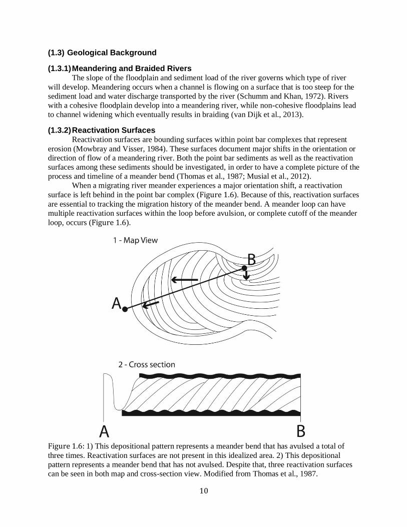
When a migrating river meander experiences a major orientation shift, a reactivation

surface is left behind in the point bar complex (Figure 1.6). Because of this, reactivation surfaces

are essential to tracking the migration history of the meander bend. A meander loop can have

multiple reactivation surfaces within the loop before avulsion, or complete cutoff of the meander

loop, occurs (Figure 1.6).

Figure 1.6: 1) This depositional pattern represents a meander bend that has avulsed a total of

three times. Reactivation surfaces are not present in this idealized area. 2) This depositional

pattern represents a meander bend that has not avulsed. Despite that, three reactivation surfaces

can be seen in both map and cross-section view. Modified from Thomas et al., 1987.

11

(1.3.3) Unit Bars Unit bars are single lobate ridges of sediment that are deposited among point bar deposits (Bridge et al., 1995). Bars are defined by Bridge et al. (2003) as within-channel depositional features with lengths proportional to the width of adjacent channels and with heights comparable to the bankfull channel depth. Overall, channel bars may be simple depositional forms called unit bars that have a relatively simple depositional history (Smith, 1974, 1978; Ashmore, 1982; Lunt and Bridge, 2004). Unit bars are known to exist in braided as well as meander environments (Reesink and Bridge, 2011), but literature on unit bars dominantly studies braided river environments (Smith, 1974; Smith et al., 2006; Cant and Walker, 1978; Best et al., 2003).

Figure 1.7: Map view of unit bars (see red arrows) from Sagavanirktok River, Alaska. These bars exist along a bend of the river. Modified from Lunt and Bridge, (2004).

12

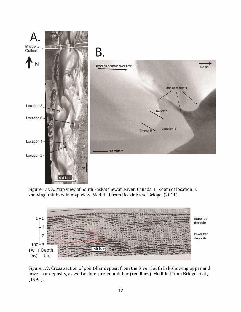
Figure 1.8: A. Map view of South Saskatchewan River, Canada. B. Zoom of location 3, showing unit bars in map view. Modified from Reesink and Bridge, (2011).

Figure 1.9: Cross section of point-bar deposit from the River South Esk showing upper and lower bar deposits, as well as interpreted unit bar (red lines). Modified from Bridge et al., (1995).

13

Figure 1.10: Cross section of point-bar deposits from the River South Esk showing upper and lower bar deposits, as well as interpreted unit bar (red lines). Modified from Bridge et al., (1995).

(1.4) Problem Large-scale, modern meandering rivers like the Mississippi River can take hundreds

of years to migrate and avulse (Blum and Roberts, 2012; Fisk, 1947). The physical journey of a meander bend from its first migration all the way to its avulsion is difficult to follow fully.

While it is accepted that unit bars exist in both meandering and braided river types, few models of point bar deposits include unit bars as a normal feature (Bridge et al., 1995). Rarer still are data that portray these bars inside a point bar complex.

The purpose of this thesis is to analyze the migration process of a large-scale meander

bend that was once part of the Mississippi River. I focus on an opposite-dipping reflector in the

subsurface, interpreted as a potential unit bar, located near a reactivation surface, in order to

better understand the creation of these bars by integrating seismic data with well data.

Ground penetrating radar (GPR) studies have previously imaged point bar complexes, but the heavy clay-based soils that exist in our study location are difficult to penetrate with GPR because the high conductivity of clay attenuates the signal (Leucci, 2007). No shallow shear-wave seismic survey has imaged a modern point bar complex.

(1.5) Hypotheses

• A meandering river can deposit sediment boundaries in geometries that are not included in current point-bar models.

• Mid-channel bars are covered by point-bar sediment, leading to subsurface unit bars. These bars create unexpected geometries in the subsurface of a point bar complex.

• Unit bars are more common than previous models of meandering rivers have shown.

14

Chapter 2 : PRIOR DATA AND EXPECTATIONS Three types of data are available for analysis: 1) LiDAR elevation data, 2) gamma-ray and conductivity well log data, and 3) shallow shear-wave seismic data. LiDAR (Light Detection And Ranging)(http://atlas.lsu.edu) data (Atlas, 2001) map ridge-swale topography surface expression of point bar deposits (Figure 2.1). The difference in elevation between the higher ridges and the low-lying swales vary 0.5 m in height on average. With LiDAR data, interpretation of the reactivation surfaces in the topographic data becomes simpler.

Well-logging tools measure different physical properties of sediment in a vertical profile at a location on the surface of Earth (Figure 2.2). Gamma-ray logs measure the natural radioactivity in formations and can be used for identifying lithologies and for correlating zones. Shale-free sandstones have low concentrations of radioactive isotopes and give low gamma readings. As shale content increases, the gamma-ray log response increases because of the concentration of radioactive isotopes in shale/clay (Asquith and Krygowski, 2004). The electrical conductivity of sediment measures the ability of the grains and interstitial fluids surrounding the grains to carry the flow of an electric current. Sediments with a high content of free charge such as shale/clay conducts electricity better (Revil and Glover, 1998). Gamma ray and electrical conductivity data have previously been collected in three main areas (north, southeast, and southwest) in the point bar complex, and their location (Table 2.1) influences our decision of where to collect seismic data (Figure 2.1). Well-log data is correlated with the seismic data in order to assist with the interpretation.

Figure 2.1: LiDAR data of False River point bar complex (Atlas, 2001). Interpreted reactivation surfaces are shown in yellow. Log locations are marked in red. Three areas are targeted during well-log data collection; all three of these areas (northwest, southwest, and southeast) lie near a reactivation surface. The red line, located near the northeastern group of wells, denotes the location of the seismic line.

15

Figure 2.2: A previous study on False River collected both gamma ray and conductivity well log data, both which generally decrease with depth (Lechnowskyj, 2013). A decrease in gamma ray and conductivity values both correlate with an increase in grain size.

I expect the IHS layers that exist in the upper point bar deposits to dip towards the meandering river. These layers cause multiple southward-dipping boundaries among point bar deposits in a seismic section (Thomas et al., 1987; Choi et al., 2004; Jablonski et al., 2014).

Table 2.1: Location of well log is shown. Well Latitude Longitude

J1 30°39'31.12"N 91°23'22.29"W

16

Chapter 3 : METHODS

(3.1) Field Area False River oxbow lake, once an active meandering branch of the Mississippi River, lies

about 35 km northwest of Baton Rouge (Figure 3.1)(Farrell, 1987). The Mississippi River

deposited a vast point bar complex before its avulsion in approximately 1700 A.D. (Sternberg,

1956). False River point bar sediments consist of Holocene bar sands (30-40 m) that overlie

Pleistocene gravels (Saucier, 1969). Overbank flows deposit the clay and silt sediments that

make up the upper-most section of the point bar complex.

Figure 3.1: Map of the state of Louisiana with a zoom on the False River oxbow lake and point

bar complex (Google, 2016). A yellow X denotes the location of the study site.

(3.2) Horizontal Shear (SH) Waves

Many different studies demonstrate the usefulness of S-waves over P-waves in near surface settings. SH-wave reflection studies avoid imaging the water table boundary that P-wave studies tend to emphasize, because SH-wave propagation is independent of fluids and gases filling pore space (Suyama et al., 1987; Goforth and Hayward, 1992; Young and Hoyos, 2001; Pugin et al., 2004; Haines and Ellefsen, 2010). SH-wave reflection studies are used in shallow sediments (0-100 m), where overburden Holocene alluvial and fluvial deposits exhibit low SH-wave velocities (100-200 m/s). Here, P-waves fail to image the top

17

50 m because of a lack of P-wave velocity or impedance contrast in the sediments (Wang et al., 2003). SH-waves have been used in numerous shallow-reflection studies (5-105m)(Woolery et al., 1993; Williams et al., 2000; Deidda and Balia, 2001; Wang et al., 2003).

Additionally, horizontally polarized shear waves (SH) do not convert to SV- or P-waves when reflecting off a horizontal boundary (Figure 3.2)(Liner, 2004). In the field, we do not always encounter perfectly horizontal boundaries, so we may experience small amounts of mode conversion. By using SH-waves and stacking shots with reversed polarity at each shotpoint, we can eliminate this conversion (Jolly, 1956; Woolery et al., 1993). By subtracting one gather from the other, P-waves cancel out while S-waves can double in amplitude (Stümpel et al., 1984).

Figure 3.2: Mode conversion cases for compressional (P), shear-vertical (SV) and shear-horizontal (SH) waves for elastic waves in solid media. In a P-wave, particles vibrate in the direction of wave propagation. In an S-wave, particles vibrate perpendicular to the direction of wave propagation. S-waves can be polarized in the vertical or horizontal plane. Modified from Liner, 2004.

(3.3) Mechanical Design of Electro-Mechanical Source An electro-mechanical shear source (Figure 3.3) produces seismic shear waves (SH) by recoil. A horizontally discharging 12-gauge shotgun shell provides a horizontal force, accelerating the device in the opposite direction of the expulsion of gas. A baseplate is coupled to the ground with eight steel spikes (5.1 cm long). A cradle that attaches to the baseplate holds an outer aluminum cylinder. The shotgun shell slides into an inner steel holder, which itself slides into the outer larger and thicker aluminum cylinder. The cannon can be set on the baseplate in either direction, allowing the shot to discharge in either direction, producing two shot gathers with opposite polarity shear waves.

18

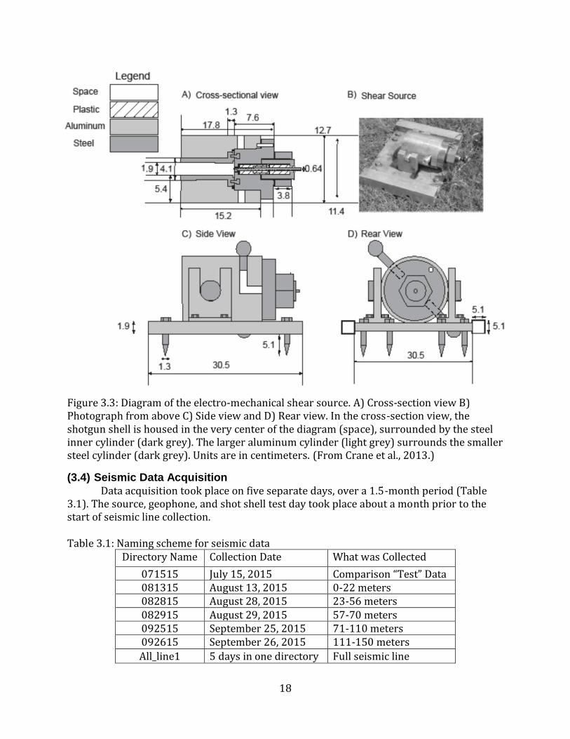
Figure 3.3: Diagram of the electro-mechanical shear source. A) Cross-section view B) Photograph from above C) Side view and D) Rear view. In the cross-section view, the shotgun shell is housed in the very center of the diagram (space), surrounded by the steel inner cylinder (dark grey). The larger aluminum cylinder (light grey) surrounds the smaller steel cylinder (dark grey). Units are in centimeters. (From Crane et al., 2013.)

(3.4) Seismic Data Acquisition

Data acquisition took place on five separate days, over a 1.5-month period (Table 3.1). The source, geophone, and shot shell test day took place about a month prior to the start of seismic line collection.

Table 3.1: Naming scheme for seismic data

Directory Name Collection Date What was Collected

071515 July 15, 2015 Comparison “Test” Data 081315 August 13, 2015 0-22 meters 082815 August 28, 2015 23-56 meters 082915 August 29, 2015 57-70 meters 092515 September 25, 2015 71-110 meters 092615 September 26, 2015 111-150 meters

All_line1 5 days in one directory Full seismic line

19

Seismic data are collected along an unpaved, compacted dirt pathway that lies directly over a major reactivation surface in the point bar complex. If geophones are not buried, a good vertical plant in compact soil will assure adequate coupling between the ground and receivers (Gadallah and Fisher, 2005). The path lies between two crop fields (Figures 3.4 & 3.5). Data are shotpoint, cdp-style (see Table 3.2 for acquisition parameters). Field notes record the time and position of each shot.

Table 3.2: Acquisition Parameters for the seismic data

Receiver 30 Hz Horizontal component Mark Products geophones; Roll-

along of 24 channels

Source Off-end electro-mechanical shear source to the north

FFFg & FFFFg black powder

Profile Length 150 meters

Geophone Spacing 1 meter

First Offset 1 meter

Seismograph Geometrics R-24 Seismograph

Line Orientation 190° azimuth

A tractor, tilling the field or workers within 0.5 miles from seismic sensors

generated noise near our study area. Other potential sources of noise in the area include trains and airplanes that both periodically pass over the point bar complex as well but we pause data acquisition during particularly noisy events. Low-frequency noise can be seen in our data (Figure 3.6).

For the first three days of data collection, we discharge four blasts at each shotpoint – two to the west and two to the east. We vertically stack the shots facing the same direction, in order to increase the signal; noise tends to cancel itself out during a stack. Following this, we subtract the two resulting gathers from one another, canceling out the P-waves while increasing S-wave. Reversing the direction of the source reverses the polarity of the S-wave, but not of the P-wave (Jolly, 1956). After investigating the data, discharging four shots at each shotpoint does not significantly improve our data quality compared to shooting twice at each shotpoint (Figure 3.7). By shooting once to the east and once to the west, we are able to double our data acquisition rate, so the final two days of data collection are collected in this manner.

We use a roll-along setup (Figure 3.8) in order to simplify and hasten our progress forwards over the full 150 meters.

20

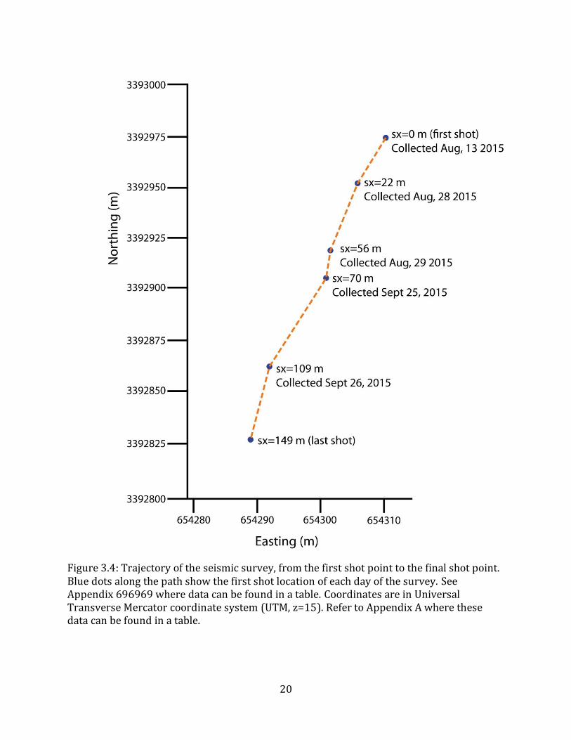
Figure 3.4: Trajectory of the seismic survey, from the first shot point to the final shot point. Blue dots along the path show the first shot location of each day of the survey. See Appendix 696969 where data can be found in a table. Coordinates are in Universal Transverse Mercator coordinate system (UTM, z=15). Refer to Appendix A where these data can be found in a table.

21

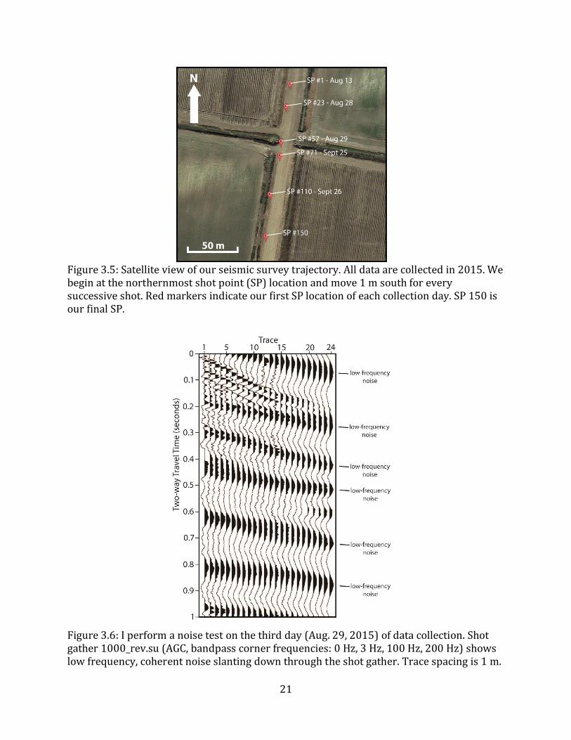
Figure 3.5: Satellite view of our seismic survey trajectory. All data are collected in 2015. We begin at the northernmost shot point (SP) location and move 1 m south for every successive shot. Red markers indicate our first SP location of each collection day. SP 150 is our final SP.

Figure 3.6: I perform a noise test on the third day (Aug. 29, 2015) of data collection. Shot gather 1000_rev.su (AGC, bandpass corner frequencies: 0 Hz, 3 Hz, 100 Hz, 200 Hz) shows low frequency, coherent noise slanting down through the shot gather. Trace spacing is 1 m.

22

Figure 3.7: We only need two shots per shot point location for the final two days of our seismic line acquisition. Four individual shot gathers are combined (2 shots to the west, 2 shots to the east; AGC, bandpass corner frequencies: 15 Hz, 30 Hz, 75 Hz, 150 Hz)(left), and the resulting shot gather has a comparable SNR to the gather created from two separate shots (1 shot to the west, 1 shot to the east; AGC, bandpass corner frequencies: 15 Hz, 30 Hz, 75 Hz, 150 Hz)(right). The amplitudes of the incoming reflection at 0.1 second are identical. Trace spacing is 1 m.

Figure 3.8: The roll-along switch allows us to mechanically select 24 geophones from a longer line of geophones. At each new shotpoint, the roll-along switch manually steps our active geophone group forward by one meter.

23

(3.5) Seismic Processing Seismic Unix version 43R6 (Cohen and Stockwell, 2014) processes the seismic data.

Seismic processing requires the introduction of much new terminology (Table 3.3). Every seismic trace is unique and identifiable by its corresponding trace headers (Table 3.4). Seismic Unix programs, often incorporated into Perl and Shell scripts, perform a myriad of different operations on the data (Table 3.5). See Appendix C for the code for these programs.

Table 3.3: Common Processing Terminology

Term Definition Trace The record of the data from one seismic (electromagnetic) channel. Gather A side-by-side display of seismic traces that have some acquisition

parameter in common. Gain Control Control for varying the amplification of an amplifier, used to compensate

for variations in input signal strength. Automatic Gain Control (AGC)

A type of gain control. AGC gradually restores the output to the same level after an increase or decrease in input amplitude.

Filter A part of a system that discriminates against some of the information entering it, usually on the basis of frequency.

Bandpass Filters Bandpass filters are often specified by listing their low-cut and high-cut component filters (Figure 3.9). The filter removes frequencies outside of a specified range.

Frequency-Wavenumber Filter (f-k)

Removing energy from seismic data by applying frequency, wavenumber, or velocity filters in the frequency-wavenumber domain. This filter removes linear seismic arrivals in the seismic traces.

Trace Header The identification information and tabulation of parameters that precedes data, as on magnetic tape.

Normal Moveout (NMO)

Normal moveout correction removes the effect of offset between a seismic source and geophone. After correction, each geophone appears to be in the same location as the source.

Common Depth Point Gather (CDP Gather)

Gather of traces that display data for the same midpoint, usually after correction for NMO and statics.

Bin The theoretical area on a rock and rock boundary that all the seismic rays bounce off.

Fold The number of traces that are in each CDP gather or the number of midpoints per bin.

Stack A composite record made by combining traces from different records. To stack is to sum all seismic traces at equal times within its unique CDP gather.

24

Table 3.4: Seismic trace headers that are set in our dataset

Header word Meaning tracl Trace sequence number within line (+1 every trace) tracr Trace sequence number within SEGY file (each new file starts

at 1) fldr Field record number (numbers the shot gathers beginning at

1001) tracf Trace number within field record trid Trace ID code (1=seismic data) sx Source coordinate (X location in Cartesian coordinate system) gx Geophone coordinate (X location in Cartesian coordinate

system) offset Straight-line distance from source to geophone (gx – sx) cdp Common depth point determined from offset and fold ns Number of samples in each seismic trace (ns=2001 samples) dt Sampling interval in micro-seconds (dt=500 μs)

Table 3.5: Program name and use, excluding programs in the main seismic workflow.

Program name Program Use susort Sort data on any trace header words. sufft Performs fast Fourier transform on the time traces,

converting them to complex frequency traces. sustack Stacks all traces in the same cdp gather. sufilter Applies a filter, most often a frequency-based bandpass,

on a seismic data set. NmoStack.pl Perl script that performs normal moveout and stacking

together on a seismic dataset. sugain Applies a gain, most often AGC, on a seismic data set.

Sufilter applies a zero-phase, sine-squared tapered filter to the dataset. This is a frequency-based bandpass filter. Bandpass filters work by selecting a subset of frequencies in a dataset and removing any frequency that does not lie inside that subset (Figure 3.9) (Kanasewich, 1981).

Data are saved in a directory that corresponds to the date of their collection. Figure 3.10 shows the directory path. With this directory structure, it is simple to coordinate which seismic datasets the program at hand operates on.

25

Table 3.6: Processing step, program that accomplishes step and purpose of each step are listed here in sequential order.

Processing Step Program Purpose 1) Import from Geometrics R-24 seismograph

2) Convert to SU (Seismic Unix) file format

Sseg2su.pl Converts seg2 (.dat) files to SU (.su) files. Data are collected and processed in different formats. This conversion to SU makes the data files compatible with the Seismic Unix processing package.

3) Subtract opposite-polarity shots

4to2shots.sh Suop2.sh

Eliminates P-wave signal and doubles S-wave signal in the seismic shot gathers.

4) Reverse trace polarity Reverse_polarity.pl Applies a common polarity correction to all traces.

5) Interpolate seismic traces suinterp Computes the averages of two adjacent seismic traces and inserts the resulting trace between the initial two.

6) Apply f-k filter Sudipfilt.pl Removes linear seismic noise events in the seismic shot gathers.

7) Set header geometry make_header_geometry.pl Assigns header words to every trace in the gathers. Each trace now has a unique identifier.

8) Apply top mute sumute Sets a user-specified area of seismic traces to zero.

9) Make CMPs Make_cmp.pl Calculates the CMP values for each trace using previously assigned trace header words.

10) Velocity Analysis IVA2.pl/IVA2.pm Performs a semblance analysis and calculates VRMS and Vint for each shot gather.

11 & 12) Stack and move out Nmostack.pl Applies a normal moveout correction to the gathers, and stacks adjacent traces having the same CMP header word.

13) Migration sustolt Performs Stolt (f-k) migration (Stolt, 1978) on stacked seismic data in the time domain.

26

Figure 3.9: The area below the trapezoid represents the frequencies that are allowed to “pass”, and remain in the data. The frequencies below the low cut (f1) and above the high cut (f4) of the corner frequencies (f1, f2, f3, f4) of the trapezoid are filtered out. Unwanted noise is generated if the slope from f1 to f2 and f3 to f4 is too steep.

Figure 3.10: Directory network for seismic data, saved on Zamin. Pl and sh programs act on data from the same corresponding date.

Frequency (Hz)

f1 f2 f3 f4

Am

pli

tud

e (%

)

/home/martm/FalseRiver/seismics/

data sh pl

core_1 tests core_1 tests core_1 tests

081315 081315 081315

082815 082815 082815

082915 082915 082915

092515 092515 092515

092615 092615 092615

All_line1 All_line1 All_line1

27

I include a processing flowchart (Figure 3.11) illustrating the processing steps that the seismic traces go through.

Figure 3.11: Flowchart for the processing steps for the seismic data, concluding with a stack of the data.

The interpretation of raw seismic data can be difficult, often because of the high levels of noise they can contain (Figure 3.12). To reduce this noise and increase the signal-to-noise ratio (SNR), we apply multiple stages of processing to our seismic data.

Step 1 & 2) After uploading the data to the Linux machine with Seismic Unix installed, I convert the files from SEG2 to SU format.

28

Step 3) I sum the two shot gathers whose blasts face the same direction that were collected at the same shot point location. I apply this same procedure for the two shot gathers whose blasts face the opposite direction. I subtract the one resulting shot gather from the second (Figure 3.13).

Step 4) The polarity of the traces in the seismic shot gathers is improperly reversed because of reversed wiring in the roll-along box. We reverse the polarity of the traces 13-24 in each gather, multiplying these traces by -1 (Figure 3.14).

Step 5) Aliasing is a phenomenon observed when the sample interval is not small enough to capture the higher range of frequencies in a signal. Aliasing can occur in space as well as time. Interpolation can reduce spatial aliasing in the seismic data that may exist because of sampling intervals that are too large in space. I interpolate a new trace between each pair of existing traces. Interpolation of my shot gathers creates 23 new traces in each; each gather now consists of 47 seismic traces. The final stack with the additional traces exhibits less spatial aliasing because we have increased the sampling interval in space (Figures 3.15 & 3.16).

Step 6) An f-k filter is used to eliminate unwanted linear noise in our seismic data. The Love wave propagates along the surface at a constant velocity, appearing as a linear event in the shot gathers. These high-amplitude Love waves constructively and destructively interfere with incoming reflection data. Noise is also found in larger offsets of our shot point gathers. These linear events have a negative slope. I filter data with slopes corresponding to the Love wave, as well as data with negative slopes (Figures 3.17 & 3.18).

Step 7) I assign trace headers to each trace in our study. Every single trace that is collected has a unique set of headers that allow it to be identified (Table 3.4). For example, trace headers delineate the position of each source and geophone on the ground (sx and gx), the shot gather each came from (fldr), and their distance away from the seismic source (offset). We also set these headers because future processing steps require that certain headers be set, in order to operate properly.

Step 8) In the raw shot gathers, the first seismic reflector is interpreted to appear at 0.1 second, so I mute everything shallower than this reflection. A shallow mute rids our data of incoming refractions as well as other shallow noise (Figure 3.19).

Step 9) I calculate and add the CMP numbers to the trace headers. This is important because stacking the data requires CMPs to be set.

I calculate the vertical resolution of the data to be approximately 0.7-1 m, using a velocity range of 150-225 m/s and a frequency of 55 Hz, the dominant frequency in our data.

29

Figure 3.12: Uninterpreted (left) and interpreted (right) unprocessed raw shot gather 10001.su (AGC, bandpass filter corner frequencies: 0 Hz, 3 Hz, 200 Hz, 400 Hz). Linear events are interpreted as the air blast and Love wave (blue), and hyperbolic events as reflections (orange, dotted). Multiples and Love-wave reflections arrive at a later time in our shot gathers (yellow). Trace spacing is 1 m.

30

Figure 3.13: Two vertically stacked west-facing-blast shot gathers are subtracted from two east-facing-blast shot gathers, and the resulting shot gather (10001.su)(AGC, bandpass corner frequencies: 0 Hz, 3 Hz, 100 Hz, 200 Hz)(left) shows more continuous reflections than a shot gather created from a single west-facing shot (AGC, bandpass corner frequencies: 0 Hz, 3 Hz, 100 Hz, 200 Hz)(right). Enhanced clarity is most easily seen inside the red box, particularly at the reflection at 0.1 seconds. Trace spacing is 1 m.

31

Figure 3.14: The polarity of traces 13-24 is reversed in shot gather 10001.su (AGC, bandpass filter corner frequencies: 15 Hz, 30 Hz, 75 Hz, 150 Hz)(left) when data is collected. I reverse the polarity of traces 13-24 to produce a new shot gather (right). Trace spacing is 1 m.

32

Figure 3.15: Increasing the sampling interval in our seismic data reduces aliasing in the final stack. I interpolate new traces between existing traces in the original shot gather (10001.su; AGC, bandpass corner frequencies: 15 Hz, 30 Hz, 65 Hz, 95 Hz)(left) in order to produce a new shot gather with more traces (10001_interp.su; AGC, bandpass corner frequencies: 15 Hz, 30 Hz, 65 Hz, 95 Hz)(right). Trace spacing before interpolation is 1 m; after interpolation is 0.5 m.

33

Figure 3.16: Increasing the sampling interval in our seismic data reduces aliasing in the final stack. I interpolate new traces between existing traces in the original shot gather (10001.su; AGC, bandpass corner frequencies: 15 Hz, 30 Hz, 65 Hz, 95 Hz) (left) in order to produce a new shot gather (10001_interp.su; AGC, bandpass corner frequencies: 15 Hz, 30 Hz, 65 Hz, 95 Hz) (right). Trace spacing before interpolation is 1 m; after interpolation is 0.5 m.

34

Figure 3.17: Linear seismic arrivals that are interpreted as surface-wave noise (e.g. Love wave or Love wave multiples) are filtered out of our dataset using an f-k filter. Love waves interfere with arrivals interpreted as reflections (left)(10001_interp.su)(AGC, bandpass filter corner frequencies: 25 Hz, 40 Hz, 65 Hz, 95 Hz). After f-k filtering (right)(10001_interp_fk2.su) (AGC, bandpass filter corner frequencies: 25 Hz, 40 Hz, 65 Hz, 95 Hz) the hyperbolic arrivals in the shot gather are more easily seen. Red ellipses highlight improved reflections. Trace spacing is 0.5 m.

35

Figure 3.18: Linear seismic arrivals that are interpreted as surface-wave noise (e.g. Love wave or Love wave multiples) are filtered out of our dataset using an f-k filter. Love waves interfere with arrivals interpreted as reflections (left)(10001_interp.su)(AGC, bandpass filter corner frequencies: 25 Hz, 40 Hz, 65 Hz, 95 Hz). After f-k filtering (right)(10001_interp_fk2.su) (AGC, bandpass filter corner frequencies: 25 Hz, 40 Hz, 65 Hz, 95 Hz) the hyperbolic arrivals in the shot gather are more easily seen. Red ellipses highlight improved reflections. Trace spacing is 0.5 m.

36

Figure 3.19: The shallowest reflection in the seismic data is interpreted around 0.1 second (red arrow). I apply a mute to the f-k filtered data (left)(10001_interp_fk2.su)(AGC, bandpass filter corner frequencies: 15 Hz, 30 Hz, 75 Hz, 150 Hz) that sets traces above my input muting line to zero (right)(10001_interp_fk2_mute.su)(AGC, bandpass filter corner frequencies: 15 Hz, 30 Hz, 75 Hz, 150 Hz). This eliminates noise from the air blast and allows us to focus primarily on the reflections in our data. Trace spacing is 0.5 m.

37

The SNR increases as the square root of the fold in each CDP gather (Liner, 2004). I create multiple stacks with different folds by altering the bin size for my reflection data. With increasing bin size, fold and the SNR both increase. Increasing the bin size beyond a fold of 72 leads to a less-clear image in the stack because traces are summed from multiple cdp locations instead of one. I first calculate CMPs from the trace headers (sx and gx) that I previously assigned. At this point I (Step10:) perform a velocity analysis. I then sort my shot gathers into CDP gathers, (Step 11:) apply a normal move out to the CDP gathers, and (Step 12:) stack of all the data files with various bin sizes (Figures 2.20 - 2.25) allowing us to compare them to one another. I perform a velocity analysis using CDP gathers with a max fold of 72. I use the same gathers for stacking.

(3.6) Velocity Analysis Step 10) The velocity analysis utilizes eight equally-spaced CDP gathers and

contains the first and last full-fold CDP gathers (Figure 3.26). A velocity model for our seismic section is created from our CMP gathers. I interpret RMS velocities (VRMS) using areas of high semblance in the CDP gather, and the Dix Formula calculates interval velocities (Vint) from the VRMS picks (Figure 3.27).

𝑉𝑖𝑛𝑡 = [[(𝑉𝑟𝑚𝑠𝑛)2𝑡𝑛 − (𝑉𝑟𝑚𝑠𝑛−1)2𝑡𝑛−1]

𝑡𝑛 − 𝑡𝑛−1]

12

Equation 3.1: Dix Formula where Vint is the interval velocity,

After velocity models are created for all eight gathers, I co-plot them to create a regional velocity profile along the seismic line (Figure 3.28).

38

Figure 3.20: A) A seismic stack with a maximum fold of 24 exhibits the lowest SNR of the stacks in the comparison. The SNR increases as the square of the fold, so a low fold correlates with a low SNR. B) The seismic fold along the length of the seismic line, which reaches a maximum 11 m from the edges of the profile.

39

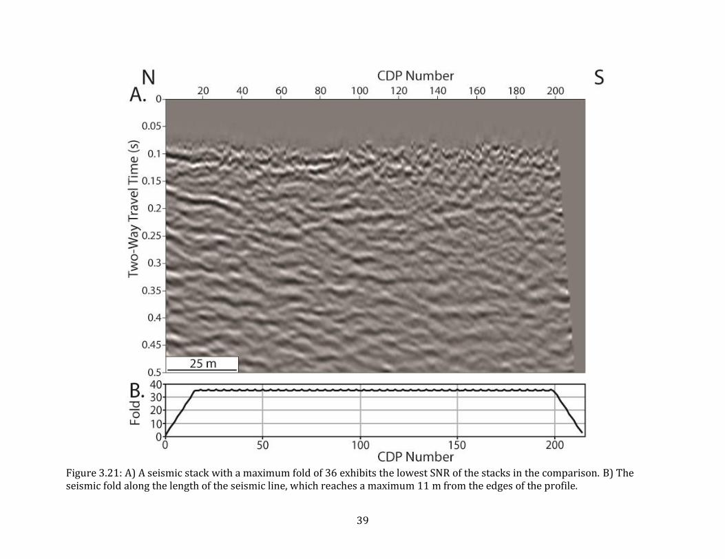
Figure 3.21: A) A seismic stack with a maximum fold of 36 exhibits the lowest SNR of the stacks in the comparison. B) The seismic fold along the length of the seismic line, which reaches a maximum 11 m from the edges of the profile.

40

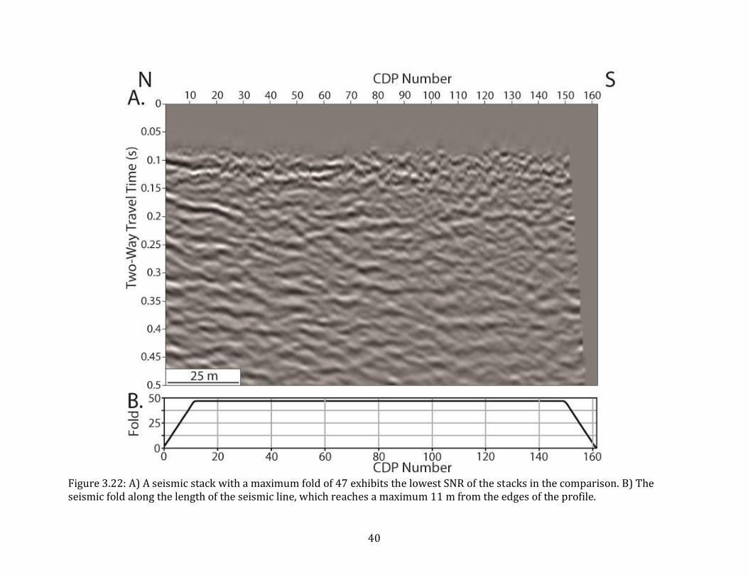
Figure 3.22: A) A seismic stack with a maximum fold of 47 exhibits the lowest SNR of the stacks in the comparison. B) The seismic fold along the length of the seismic line, which reaches a maximum 11 m from the edges of the profile.

41

Figure 3.23: A) A seismic stack with a maximum fold of 59 exhibits the lowest SNR of the stacks in the comparison. B) The seismic fold along the length of the seismic line, which reaches a maximum 11 m from the edges of the profile.

42

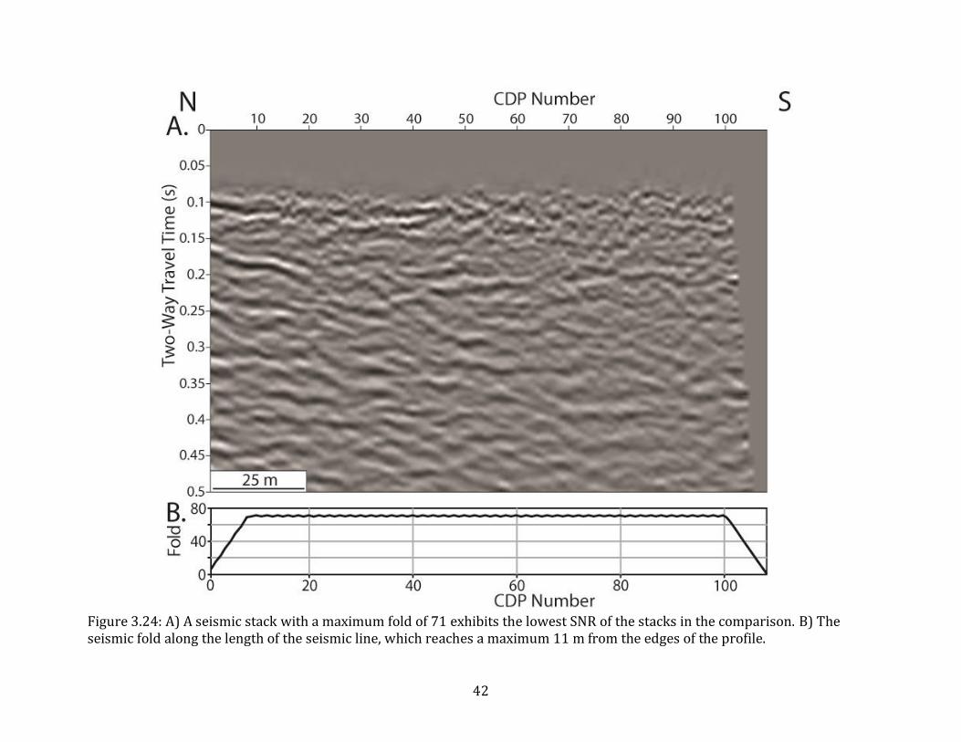
Figure 3.24: A) A seismic stack with a maximum fold of 71 exhibits the lowest SNR of the stacks in the comparison. B) The seismic fold along the length of the seismic line, which reaches a maximum 11 m from the edges of the profile.

43

Figure 3.25: A) A seismic stack with a maximum fold of 165 exhibits the lowest SNR of the stacks in the comparison. B) The seismic fold along the length of the seismic line, which reaches a maximum 11 m from the edges of the profile.

44

Figure 3.26: The UTM coordinate system shows the trajectory of the seismic survey. The velocity semblance analysis uses the CDP gathers that are labeled along the line.

45

Figure 3.27: RMS and interval velocities for selected CDPs (fold=72) along the seismic line.

46

Table 3.7: RMS velocity (m/s) and time (s) values that correspond to velocity model plots on the previous page.

CDP 12 CDP 24 CDP 36 CDP 48 Velocity Time Velocity Time Velocity Time Velocity Time 168.67 0.105541 154.16 0.137203 173.50 0.153034 149.61 0.168865 184.78 0.197889 173.50 0.274406 199.28 0.303430 177.00 0.253298 210.56 0.248021 218.61 0.369393 231.50 0.419525 222.11 0.361478 250.83 0.390501 292.72 0.551451 289.50 0.554090 284.94 0.567282 294.33 0.551451

CDP 60 CDP 72 CDP 84 CDP 96

Velocity Time Velocity Time Velocity Time Velocity Time 155.72 0.105541 167.21 0.1005382 151.74 0.091381 154.50 0.120758 228.22 0.343008 208.93 0.204476 169.79 0.142838 168.02 0.243855 241.11 0.430079 241.18 0.279981 194.02 0.235549 203.36 0.378837 307.17 0.620053 280.36 0.430582 227.49 0.327024 249.89 0.461902 302.80 0.521032 238.15 0.392046 281.07 0.587243 293.67 0.599687

47

Figure 3.28: RMS velocity model for seismic line. Isovelocity curves show lateral velocity changes along the length the seismic profile. Units are m/s. The velocity gradient varies little over the length of the profile. At around CDP location 24, the isovelocity lines are relatively deeper than elsewhere along the line.

0

0.1

0.2

0.3

0.4

0.5

0.6

0.7

12 24 36 48 60 72 84 96

Tw

o-W

ay T

rave

l T

ime

(s)

CDP Gather

Seismic Line Velocity Model

180

220

200

260

240

280

48

(3.7) Migration Step 13) Seismic migration moves dipping reflectors into their true subsurface positions and collapses diffractions to the hyperbolic apex, delineating detailed subsurface features such as fault planes. The goal of migration is to make the stacked section appear similar to the geologic cross-section along the seismic line (Yilmaz, 1987). There are different types of migration; each type is utilized in a different situation (Figure 3.29). Time migration is appropriate for our section because lateral velocity variations are mild to moderate (Liner, 2004).

Figure 3.29: Diagram shows which type of migration is ideal for a particular geologic region. From Liner, 2004. Post-stack time migration (boxed) is ideal for my seismic data, because of minimal structural complexity and mild to moderate lateral velocity variation.

Complex salt-dome structures in the Gulf of Mexico require migration of a more expensive and time-consuming nature (e.g. pre-stack and/or depth migration). False River’s simple structural elements and relatively consistent lateral velocity allow us to apply a poststack time migration on our data. Stolt migration (Stolt, 1978), or migration by Fourier transform can be applied to post or prestack time data. It is the fastest of all migration techniques (Liner, 2004).

49

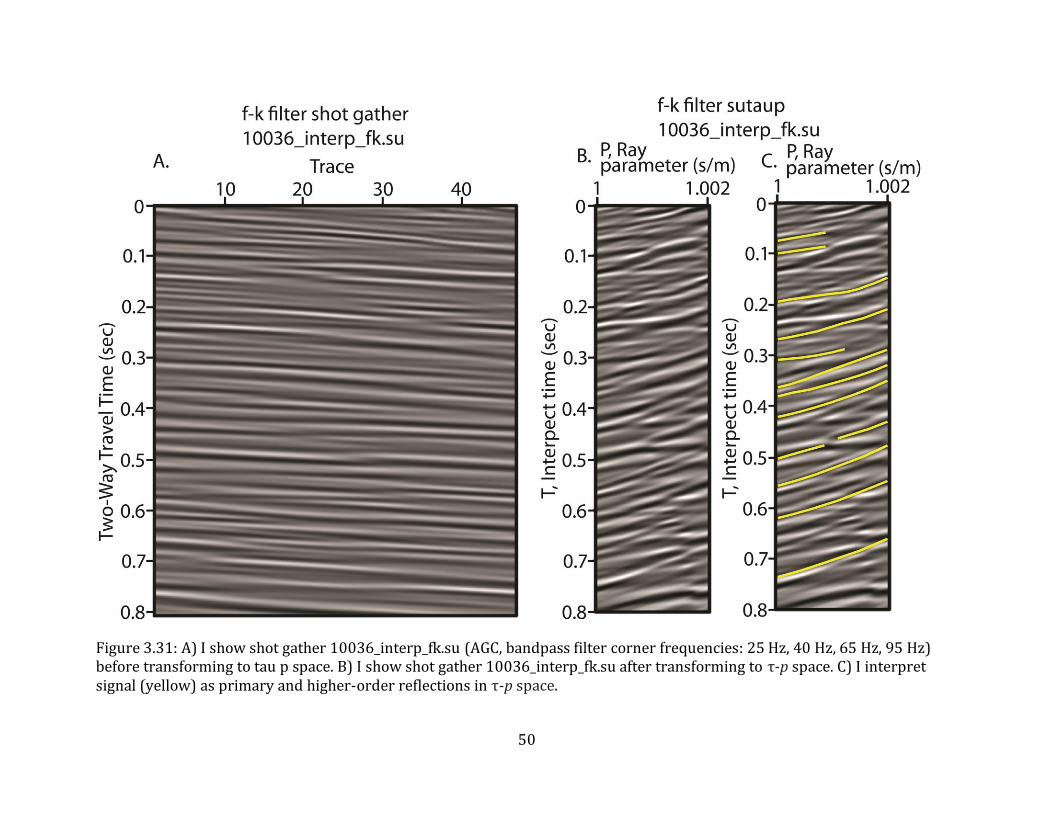
(3.8) τ-p Interpretation Seismic data can be described and plotted in terms of instantaneous slope and intercept time (Figure 3.30). In τ-p space, identifying true reflections and artifacts such as multiples in the gather becomes simpler (Diebold and Stoffa, 1981). I transform interpolated, f-k filtered shot gathers into τ-p space to help identify real reflectors among the multiples and noise in the seismic stack. Application of a confidence model to incoming seismic signal helps to accomplish this identification (Figures 2.31 – 2.34). Reflectors are interpreted in τ-p space as real reflectors, multiples/false reflectors, or uncertain. I indicate confidence of each reflector with a color (green = real reflector, high confidence; red = multiple/false reflector, high confidence; yellow = uncertain). A colored circle, located on each reflector, allows for visualization of what each reflector represents.

Figure 3.30: A) An end-on seismic record is f(x,t) where x=source-geophone distance (offset) and t=arrival time. B) Its tau-p transform is F(τ,p) where p=dt/dx=1/Va and τ=intercept time at x=0. Hyperbolic reflections transform into ellipses, straight events into points (the direct wave into P1, the head wave into P2). From Diebold and Stoffa, 1981.

50

Figure 3.31: A) I show shot gather 10036_interp_fk.su (AGC, bandpass filter corner frequencies: 25 Hz, 40 Hz, 65 Hz, 95 Hz) before transforming to tau p space. B) I show shot gather 10036_interp_fk.su after transforming to τ-p space. C) I interpret signal (yellow) as primary and higher-order reflections in τ-p space.

51

Figure 3.32: : A) Uninterpreted shot gather 10036_interp_fk.su after transforming to τ-p space. B) Interpreted shot gather 10036_interp_fk.su after transforming to τ-p space. C) I indicate confidence by a color (green = real reflector; red = multiple, noise, false reflector; yellow = uncertain) to each reflector corresponding to seismic reflections in B. The confidence measures how likely each reflector is real versus an artifact in the data.

52

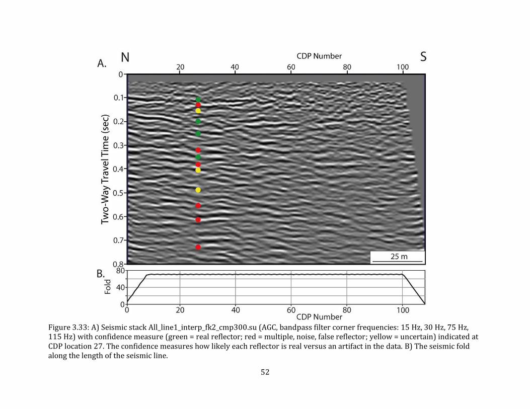
Figure 3.33: A) Seismic stack All_line1_interp_fk2_cmp300.su (AGC, bandpass filter corner frequencies: 15 Hz, 30 Hz, 75 Hz, 115 Hz) with confidence measure (green = real reflector; red = multiple, noise, false reflector; yellow = uncertain) indicated at CDP location 27. The confidence measures how likely each reflector is real versus an artifact in the data. B) The seismic fold along the length of the seismic line.

53

Figure 3.34: A) Seismic stack All_line1_interp_fk2_cmp300.su (AGC, bandpass filter corner frequencies: 15 Hz, 30 Hz, 75 Hz, 115 Hz) with confidence measurement (green = real reflector; red = multiple, noise, false reflector; yellow = uncertain) applied to every 9th CDP location. These confidence measurements allow real seismic reflectors to be followed and picked. B) The seismic fold along the length of the seismic line.

54

Chapter 4 : RESULTS AND INTERPRETATIONS Four real reflectors appear in the seismic section (Figure 4.2 -Figure 4.3): two shallow reflections before 0.2 seconds, a strong continuous reflector around 0.3 s that most likely represents the gravel Pleistocene boundary (Saucier, 1969), and one more reflector that appears to dip towards the north, the opposite dip direction of what we anticipate. The four reflectors in the seismic data are not very continuous, overall. The two shallowest reflectors are particularly discontinuous; this may be because of a buried culvert that passes under the seismic line above these reflectors. The dipping reflector does seem to be made up from pieces of smaller reflectors, but it traverses the entire seismic profile, except for one tough-to-interpret section near the well log (~cdp 65). Finally, the deepest, low frequency reflector has more continuity than the two shallow reflectors. All four reflectors exhibit dip, although some are quite minor. The continuous boundary dips to the north, while all other boundaries appear to dip in the opposite direction. The elevation profile posted above the seismic section is obtained from LiDAR data in the area.

55

Figure 4.1: A. The relative elevation along the surface of the seismic line, from LiDAR data. B. Uninterpreted seismic profile (AGC and bandpass filter corner frequencies: 15 Hz, 30 Hz, 65 Hz, 90 Hz) after stacking. The velocity model is used to create a rough depth scale, shown to the right of the seismic profile. I overlay well log location (green) on seismic data. C. The seismic fold along the length of the seismic line, which reaches a maximum 11 m from the edges of the profile.

56

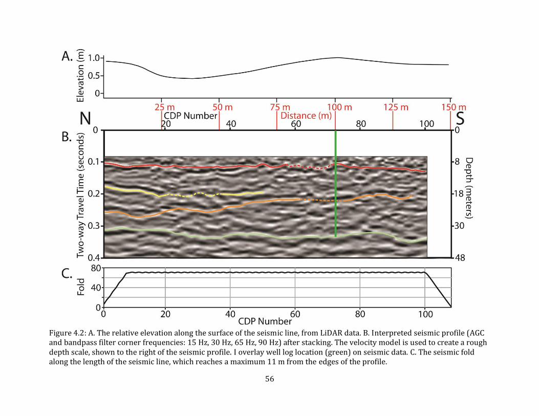
Figure 4.2: A. The relative elevation along the surface of the seismic line, from LiDAR data. B. Interpreted seismic profile (AGC and bandpass filter corner frequencies: 15 Hz, 30 Hz, 65 Hz, 90 Hz) after stacking. The velocity model is used to create a rough depth scale, shown to the right of the seismic profile. I overlay well log location (green) on seismic data. C. The seismic fold along the length of the seismic line, which reaches a maximum 11 m from the edges of the profile.

57

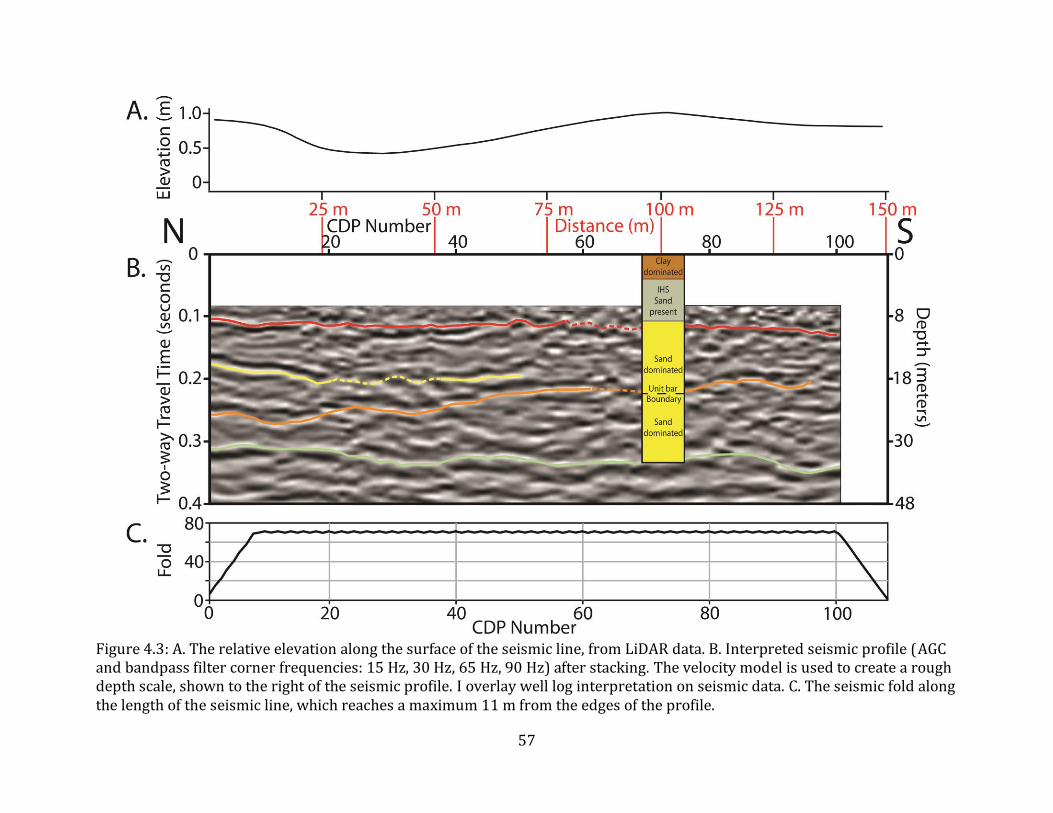
Figure 4.3: A. The relative elevation along the surface of the seismic line, from LiDAR data. B. Interpreted seismic profile (AGC and bandpass filter corner frequencies: 15 Hz, 30 Hz, 65 Hz, 90 Hz) after stacking. The velocity model is used to create a rough depth scale, shown to the right of the seismic profile. I overlay well log interpretation on seismic data. C. The seismic fold along the length of the seismic line, which reaches a maximum 11 m from the edges of the profile.

58

(4.1) Interpretation of Seismic Profile Interpreting the well log and seismic data allows four reflections to be identified in

the seismic stack (Figure 4.4). The shallowest represents the boundary between upper-bar IHS and lower-bar sands, and the deepest represents the boundary between point bar sands and the lower-lying Pleistocene gravels. Current point bar models consistently show these two major boundaries (Thomas et al., 1987; Hubbard et al., 2011).

Figure 4.4: Depositional, unit-bar interpretation of the profile, without seismic data. Well log location (green) samples through the dipping boundary. (4.2) Reflector Dip

The dipping reflector located between the shallowest and deepest reflectors dips at 4.4° ± 1°. The extent of the dipping reflector that we image is 18 m high, and 105 meters long (Figure 4.5).

Figure 4.5: Size of subsurface dipping reflector.

tan 𝜃 =8

105

𝜃 = arctan (8

105)

𝜃 = 4.4° ± 1°

59

Chapter 5 : DISCUSSION In this study, we find a seismic reflector with dip towards the north, opposite than the dip direction of IHS layers. Our data are consistent with data from the River South Esk, showing upper- and lower-bar deposits, as well as a reflector dipping in the opposite direction of IHS layers, away from the river (Bridge, 2003). Bridge interpreted this reflector as a unit bar buried beneath point bar sediments. Our dipping reflector may be a buried unit bar in the False River point bar complex, or it may be the result of an erosional event (e.g. a river chute).

Discontinuities in inclination may be associated with the occurrence of unit bars or with transitions from “lower-bar” deposits to “upper-bar” deposits (Bridge, 2003). I interpret this transition to occur at a shallower depth than where we see the dipping reflector, so this explanation doesn’t fit our seismic data. (5.1) Scale Differences & Limitations Previously studied unit bars inside point bar deposits have been on a much smaller scale. While maximum penetration depths in GRP studies from the South Saskatchewan River in Canada are from 3 m (Smith et al., 2006) to 1m (Reesink and Bridge, 2011), the False River point bar sediments exist down to 30-40 m. Additionally, GPR studies on the River South Esk only image down to ~5 m. One major limitation that stems from the difference in scale between other studies and ours is, while these other studies image the full lateral extent of the unit bar, my 150-m seismic line is not long enough to capture the full bar. Interpreting the dipping boundary as the top of a unit bar may be more difficult without being able to see the entire thing. Mid-channel bars and detached point bars north of False River are of similar size to this subsurface bar. I highlight two potential candidates in the Mississippi River that may one day be found beneath point bar sediments (Figures 5.1 & 5.2): (1) The tail of this point bar is physically separated from the mainland point bar. The velocity of the river water is practically zero between the mainland point-bar complex and the detached point bar, eventually leading to fine-grained sediment deposition. The width of the detached point bar (~93-146 m) is roughly the same size as the dipping layer in our seismic data. As the meandering river continues to migrate, point-bar deposition may continue on top of the detached point bar. (2) The point bar is completely detached from the mainland point-bar complex. The width of the island (~146 m) is comparable to the dipping boundary in our seismic stack.

60

Figure 5.1: The tail (downstream) end of the point bar (red outline) is separated from the mainland point-bar complex. This Mississippi River bend is located near the Arkansas/Mississippi border, northwest of Chatham, MS (UTM coordinates: 15S, 675035.83 m E, 3665937.10 m N). The lateral extent of the bar (yellow)(93-146 m) is comparable to the length of the dipping reflector that we can see in our seismic data (150 m).

61

Figure 5.2: The off-land point bar (red outline) is separated from the mainland point-bar complex. This Mississippi River bend is located near the Arkansas/Mississippi border, west of Refuge, MS (UTM coordinates: 15S, 670827.05 m E, 3686180.13 m N). Its lateral extent (yellow)(146 m) is comparable to the length of the dipping reflector that we can see in our seismic data (150 m).

62

The dipping boundary may be formed through deposition (unit bar) or erosion (river chute). I provide two models that outline an example of each type of process that may govern the formation of the unit bar. (5.2) Unit Bar Deposition Model – Potential Candidate #1

A depositional, lobate unit bar exhibits relatively continuous reflectors (Bridge et al., 1995). The interpreted IS surrounding the unit bar consists of trough cross-strata (Fustic et al., 2012) that largely lacks reflectors, continuous or discontinuous.

The outer bank of the migrating river first encounters an area of floodplain that is resistive to erosion. At this point, the unit bar is deposited in the Mississippi River as a point bar that detached from the mainland (Figure 5.3). The river continues its migration, eventually depositing point-bar sediment on top of the unit bar. Sedimentation preserves the unit bar in the point bar complex (Figures 5.4 & 5.5). (5.3) River Chute Erosional Model – Potential Candidate #2 If the dipping boundary represents the top of a unit bar, our well-log data samples the unit bar deposits. If the dipping boundary represents a surface created by erosion, our well-log data samples through the chute deposits that eventually deposit there. A meandering river first deposits point-bar sediment along its inner bank. A river chute forms cutting through the point bar complex (Figure 5.6). The chute erodes away point-bar sediment, resulting in a boundary that dips in the opposite direction than expected. This boundary remains after the river resumes migration and the chute has disappeared (Figures 5.7 & 5.8). (5.4) Well-log Evidence

The origin of the sediment beneath the dipping boundary can be inferred by considering its composition.

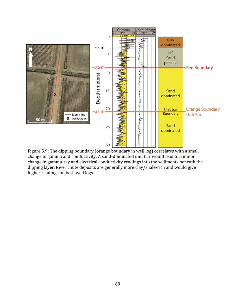
If a river chute cut through the point-bar complex, the sediment deposited by the river chute would contain more shale/clay and would lead to a higher reading on the gamma-ray and electrical conductivity well logs below the dipping boundary. Instead, the well logs appear to have similar readings above and below the dipping boundary, for both gamma-ray and electrical conductivity (Figure 5.9). This suggests the boundary represents a minor transition. A sand-on-sand transition, which can be interpreted as a unit bar, is more likely than shale/clay-rich section that was more likely deposited by a river chute cutting through the point-bar complex.

63

Figure 5.3: River model map view (top) showing point bar with tail detached (brown) from the mainland section of the point bar complex. Cross section A-A’ of river and unit bar deposition (bottom) also includes the detached section of the point-bar tail.

64

Figure 5.4: I show a cross-section view of a unit bar depositional model explaining a potential example of how the unit bar may have been deposited in the Mississippi River. Cross section of Mississippi River begins with detached point bar in the channel (brown). The first step (Figure 4.2) shows low water level. In step two, fine-grained sediment is deposited between the mainland and the detached point bar, and the water level rises. Meandering resumes in the third step, and point-bar sands deposit atop the unit-bar sediments. The river continues to migrate in step four, depositing point-bar sand atop the remainder of the unit-bar deposit.

65

Figure 5.5: Zoom-in view of the model shown in the previous figure. The boundary between fine-grained sediments and the unit bar deposit is dipping north, away from the migrating river. The IHS layers dip towards the river. This example portrays how a unit bar can be deposited in a point bar complex and lead to an opposite-dipping boundary.

66

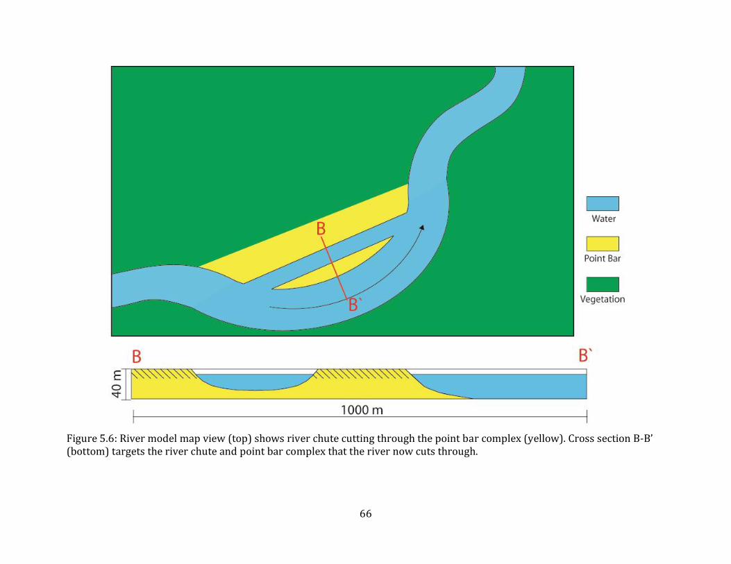
Figure 5.6: River model map view (top) shows river chute cutting through the point bar complex (yellow). Cross section B-B’ (bottom) targets the river chute and point bar complex that the river now cuts through.

67

Figure 5.7: I show a cross-section view of river chute erosional model. The first step shows an existing river and the point bar sediments it deposits. In step two, the river deposits more point bar sediment as it continues to migrate south. In step three, a chute develops north of the river, and cuts through the point bar complex. In step four, the chute dries out, leaving behind new sediments as the river continues to migrate.

68

Figure 5.8: Zoom-in view of the model shown in the previous figure. The boundary between chute deposits and the point bar sands is dipping north, away from the migrating river. The IHS layers dip towards the river. This example portrays how a unit bar can be deposited in a point bar complex and lead to an opposite-dipping boundary.

69

Figure 5.9: The dipping boundary (orange boundary in well log) correlates with a small change in gamma and conductivity. A sand-dominated unit bar would lead to a minor change in gamma-ray and electrical conductivity readings into the sediments beneath the dipping layer. River chute deposits are generally more clay/shale-rich and would give higher readings on both well logs.

70

Chapter 6 : CONCLUSIONS AND RECOMMENDATIONS (6.1) Conclusions

A 150-m seismic line overlies a reactivation surface in the False River point bar complex north of Baton Rouge, Louisiana. The seismic data were processed with the Colorado School of Mines Seismic Unix processing package and then interpreted, illuminating a possible subsurface unit bar buried beneath point bar sands.

A dipping reflector in the seismic data is interpreted as a possible subsurface unit bar, a geologic feature that leads to seismic boundaries with opposite dip than what is normally deposited in point bar complexes. Previous point-bar models from meandering rivers largely exclude unit bars and should include them in the future as a normal feature. Unit bar formation is a depositional process. Alternatively, an erosive river chute may have created this dipping boundary. (6.2) Recommendations

1. Extend my seismic line further north and south, to collect a greater extent of data along the dirt path. This way, the entire unit bar will be imaged and its full lateral and vertical extent will be known.

2. Perform new seismic studies across other reactivation surfaces in False River. Collect seismic lines longer than 150 meters, to increase the chances of finding another unit bar.

3. Collect two seismic lines orthogonal to one another at a reactivation surface, to increase the area we can study. This will increase our chances of finding more unit bars and uncover their true size and frequency.

4. Collect seismic over reactivation surfaces in other point bar complexes, to see their prevalence in a point bar complex created from a river of a different scale.

5. Address the connection between the presence of subsurface unit bars and major river shifts. Finding these bars in ancient river deposits allows us to consider how often the river shifted and evolved through its lifetime.

71

REFERENCES Allen, J. R. L. 1965, A Review of the Origin and Characteristics of Recent Alluvual Sediments.

Sedimentology, v. 5, no. 2, p. 91.

Allen, J. R. L., and P. F. Friend. 1968, Deposition of the Catskill facies, Appalachian region: with notes on some other Old Red Sandstone basins. Special Paper: Geological Society of America, v. 106, p. 21-74.

Ashmore, P. E. 1982, Laboratory modelling of gravel braided stream morphology. Earth Surface Processes and Landforms, v. 7, p. 201-225.

Asquith, G., and D. Krygowski. 2004, Basic Well Log Analysis. Second ed, AAPG Methods in Exploration Series 16: The American Association of Petroleum Geologists.

"Atlas: The Louisiana Statewide GIS." LSU Department of Geography and Anthropology. Baton Rouge, LA. http://atlas.lsu.edu.

Best, J. L., P. J. Ashworth, C. S. Bristow, and J. Roden. 2003, Three-dimensional sedimentary architecture of a large, mid-channel sand braid bar, Jamuna River, Bangladesh. Journal of Sedimentary Research, v. 73, no. 4, p. 516-530.

Blum, M. D., and H. H. Roberts. 2012, The Mississippi Delta Region: Past, Present, and Future. Annual Review of Earth and Planetary Sciences, Vol 40, v. 40, p. 655-683. doi: Doi 10.1146/Annurev-Earth-042711-105248.

Bridge, J. S. 2003, Rivers and Floodplains : forms, processes, and sedimentary record: Blackwell Publishing.

Bridge, J. S., J. Alexander, R. E. L. Collier, R. L. Gawthorpe, and J. Jarvis. 1995, Ground-Penetrating Radar and Coring Used to Study the Large-Scale Structure of Point-Bar Deposits in 3 Dimensions. Sedimentology, v. 42, no. 6, p. 839-852. doi: Doi 10.1111/J.1365-3091.1995.Tb00413.X.

Cant, D. J., and R. G. Walker. 1978, Fluvial processes and facies sequences in the sandy braided South Saskatchewan River, Canada. Sedimentology, v. 25, p. 625-648.

Choi, K. S., R. W. Dalrymple, S. S. Chun, and S. P. Kim. 2004, Sedimentology of modern, inclined heterolithic stratification (IHS) in the Macrotidal Han River delta, Korea. Journal of Sedimentary Research, v. 74, no. 5, p. 677-689. doi: Doi 10.1306/030804740677.

Cohen, J. K., and J. J. W. Stockwell. CWP/SU: Seismic Un*x Release No. 43R6: an open source software package for seismic research and processing, Center for Wave Phenomena, Colorado School of Mines 2014. Available from http://www.cwp.mines.edu/cwpcodes.

72

Crane, J. M., J. M. Lorenzo, and J. B. Harris. 2013, A new electrical and mechanically detonatable shear wave source for near surface (0-30m) seismic acquisition. Journal of Applied Geophysics, v. 91, p.

Deidda, G. P., and R. Balia. 2001, An ultra-shallow SH-wave seismic reflection experiment of a subsurface ground model. Geophysics, v. 66, p. 1097-1104.

Diebold, J. B., and P. L. Stoffa. 1981, The traveltime equation, tau-p mapping, and inversion of common midpoint data. Geophysics, v. 46, no. 3, p. 238-254.

Farrell, K. M. 1987, Sedimentology and facies architecture of overbank deposits of the Mississippi River, False River region, Louisiana. v., p.

Fisk, H. N. 1947, Fine-grained alluvial deposits and their effects on Mississippi River activity: Waterways Experiment Station.

Fisk, H. N. 1952, Mississippi River Valley geology in relation to river regime. Trans. Am. Soc. Civil Engs, v. 117, p. 667-689.

Fustic, M., S. M. Hubbard, R. Spencer, D. G. Smith, D. A. Leckie, B. Bennett, and S. Larter. 2012, Recognition of down-valley translation in tidally influenced meandering fluvial deposits, Athabasca Oil Sands (Cretaceous), Alberta, Canada. Marine and Petroleum Geology, v. 29, no. 1, p.

Gadallah, M. R., and R. L. Fisher. 2005, Applied Seismology: A Comprehensive Guide to Seismic Theory and Application.

Gibling, M., and B. Rust. 1993, Alluvial ridge-and-swale topography: a case study from the Morien Group of Atlantic Canada. Alluvial Sedimentation, Volume Special Publication, v. 17, p. 133-150.

Goforth, T., and C. Hayward. 1992, Seismic reflection investigations of a bedrock surface buried under alluvium. Geophysics, v. 57, p. 1217-1227.

Google, 2016, "Louisiana", 30.9843° N and 91.9623° W, Google Maps, September 18, 2016.

Haines, S. S., and K. J. Ellefsen. 2010, Shear-wave seismic reflection studies of unconsolidated sediments in the near surface. Geophysics, v. 75, no. 2, p. B59-B66.

Harris, J. B. 2009, Hammer-Impact SH-Wave Seismic Reflection Methods in Neotectonic Investigations: General Observations and Case Histories from the Mississippi Embayment, U.S.A.: Journal of Earth Science, v. 20, no. 3, p. 513-525. doi: 10.1007/s12583-009-0043-y.

Hickin, E. J. 1974, Development of Meanders in Natural River-Channels. American Journal of Science, v. 274, no. 4, p. 414-442.

73

Hubbard, S. M., D. G. Smith, H. Nielsen, D. A. Leckie, M. Fustic, R. J. Spencer, and L. Bloom. 2011, Seismic geomorphology and sedimentology of a tidally influenced river deposit, Lower Cretaceous Athabasca oil sands, Alberta, Canada. AAPG Bulletin, v. 95, no. 7, p. 1123-1145.

2014, A retrospective and prospective look at inclined heterolithic stratification of tidal-fluvial point bars of the middle McMurray Formation of Northeastern Alberta, Canada.

Jolly, R. N. 1956, Investigation of Shear Waves. Geophysics, v. 21, no. 4, p. 905-938.

Kanasewich, E. R. 1981, Time sequence analysis in geophysics. Vol. 3: Univ. Alberta Press.

Lechnowskyj, A. 2013, The Stratal Architecture of the False River Point Bar (Lower Mississippi River, LA), Louisiana State University.

Leucci, G. 2007, Ground Penetrating Radar: The Electromagnetic Signal Attenuation and Maximum Penetration Depth. Scholarly Research Exchange, v. 2008, p.

Liner, C. L. 2004, Elements of 3D Seismology. 2nd ed: PennWell Corporation.

Lobeck, A. K. 1939, Geomorphology, an introduction to the study of landscapes. v., p.

Lunt, I. A., and J. S. Bridge. 2004, Evolution and depositys of a gravelly braid bar, Sagavanirktok River, Alaska. Sedimentology, v. 51, p. 415-432.

Mowbray, T. d., and M. J. Visser. 1984, Reactivation surfaces in subtidal channel deposits, Oosterschelde, Southwest Netherlands. Journal of Sedimentary Petrology, v. 54, no. 3, p. 811-824.

Musial, G., J. Reynaud, M. Gingras, and H. Fenies. 2012, Subsurface and outcrop characterization of large tidally influenced point bars of the Cretaceous McMurray Formation (Alberta, Canada). Sedimentary Geology, v. 279, p. 156-172.

Nanson, G. C. 1980, Point-Bar and Floodplain Formation of the Meandering Beatton River, Northeastern British-Columbia, Canada. Sedimentology, v. 27, no. 1, p. 3-29. doi: Doi 10.1111/J.1365-3091.1980.Tb01155.X.

Nanson, G. C., and E. J. Hickin. 1983, Channel Migration and Incision on the Beatton River. Journal of Hydraulic Engineering, v. 109, p. 327-337. doi: 10.1061/(ASCE)0733-9429(1983)109:3(327).

Pugin, A., T. Larson, S. Sargent, J. McBride, and C. Bexfield. 2004, Near-surface mapping using SH-wave and P-wave land-streamer data acquisition in Ilinois, U.S.: The Leading Edge, v. 23, no. 7, p. 677-682.

74

Reesink, A., and J. Bridge. 2011, Evidence of Bedform Superimposition and Flow Unsteadiness In Unit-Bar Deposits, South Saskatchewan River, Canada. Journal of Sedimentary Research, v. 81, no. 11, p. 814-840.

Revil, A., and P. W. J. Glover. 1998, Nature of surface electrical conductivity in natural sands, sandstones, and clays. Geophysical Research Letters, v. 25, no. 5, p. 691-694.

Saucier, R. T. 1969, Geological investigation of the Mississippi River area, Artonish to Donaldsonville, LA. v., p.

Schumm, S. A., and H. R. Khan. 1972, Experimental Study of Channel Patterns. Geological Society of America (GSA) Bulletin, v. 83, p. 1755-1770.

Smith, G. H. S., P. J. Ashworth, J. L. Best, J. Woodward, and C. J. Simpson. 2006, The sedimentology and alluvial architecture of the sandy braided South Saskatchewan River, Canada. Sedimentology, v. 53, p. 413-434.

Smith, N. D. 1974, Sedimentology and Bar Formation in the Upper Kicking Horse River, a Braided Outwash Stream. Geology, v. 82, no. 2, p. 205-223.

Smith, N. D. 1978, Some comments on terminology for bars in shallow rivers. Fluvial Sedimentology, v., p. 85-88.

Sternberg, H. O. R. 1956, A contribution to the geomorphology of the False River area, Louisiana, Louisiana State University.

Stolt, R. H. 1978, Migration by Fourier Transform. Geophysics, v. 43, no. 1, p. 23-48.

Stümpel, H., S. Kähler, R. Meissner, and B. Milkereit. 1984, The Use of Seismic Shear Waves and Compresional Waves for Lithological Problems of Shallow Sediments. Geophysical Prospecting, v. 32, p. 662-675.

Suyama, K., T. Imai, H. Ohtomo, K. Ohta, and T. Takahashi. 1987, Delineation of structures in alluvium and diluvium using SH-wave reflection and VSP methods. Geophysical Prospecting, v. 1, p. 165-179.

Thomas, R. G., D. G. Smith, J. M. Wood, J. Visser, E. A. Calverley-Range, and E. H. Koster. 1987, Inclined heterolithic stratification; terminology, description, interpretation and significance. Sedimentary Geology, v. 53, no. 1-2, p. 123-179.

van de Lageweg, W. I., W. M. van Dijk, A. W. Baar, J. Rutten, and M. G. Kleinhans. 2014, Bank pull or bar push: What drives scroll-bar formation in meandering rivers? : Geology, v. 42, no. 4, p. 319-322. doi: Doi 10.1130/G35192.1.

van Dijk, W. M., W. I. van de Lageweg, and M. G. Kleinhans. 2013, Formation of a cohesive floodplain in a dynamic experimental meandering river. Earth Surface Processes and Landforms, v. 38, p. 1550-1565. doi: 10.1002/esp.3400.

75

Wang, Z., I. P. Madin, and E. Woolery. 2003, Shallow SH-wave seismic investigations of the Mt. Angel Fault, Northwest Oregon, USA. Tectonophysics, v. 368, p. 105-117.

Wiggins, R. A., K. L. Larner, and R. D. Wisecup. 1976, Resudial Statics Analysis as a General Linear Inverse Problem. Geophysics, v. 41, no. 5, p. 922-938.

Williams, R. A., W. J. Stephenson, A. D. Frankel, E. Cranswick, M. E. Meremonte, and J. K. Odum. 2000, Correlation of 1- to 10-Hz earthquake resonances with surface measurements of S-wave reflections and refractions in the upper 50 m. Bulletin of the Seismological Society of America, v. 90, p. 1323-1331.

Wolman, M. G., and L. B. Leopold. 1957, River Flood Plains: Some Observations On Their Formation. Geological Survey Professional Paper, v. 282-C, p.

Woolery, E., R. Street, Z. Wang, and J. Harris. 1993, Near-surface deformation in the New Madrid seismic zone as imaged by high resolution SH-wave seismic methods. Geophysical Research Letters, v. 20, p. 1615-1618.

Yilmaz, O. 1987, Seismic Data Processing. Edited by Edwin B Neitzel. Vol. Vol. 2, Investigations in Geophysics: Society of Exploration Geophysicists.

Young, R., and J. Hoyos. 2001, Near-surface, SH wave surveys in unconsolidated, alluvial sediments. The Leading Edge, v. 20, p. 936-948.

76

APPENDIX A: Field Acquisition Optimization Tests

Three preliminary field tests are performed in order to determine the seismic acquisition parameters that maximize the signal-noise ratio. We compare two different seismic sources, two different seismic receivers, and four different shot shells for the electro-mechanical seismic source. These tests are conducted at the field location in order to mimic the data collection for the seismic line.

(A.1)Source Comparison

We test two seismic sources to identify which produces the most reflections with the least amount of noise, in order to maximize the efficiency of our seismic survey. We also consider the repeatability of our sources, and the time of acquisition at each shotpoint. We compare a sledgehammer striking a metal plate (Harris, 2009) with a lightweight (17.9 kg), electro-mechanical recoil device (Crane et al., 2013) for SH-wave generation. The recoil device provides a constant repeatability, spectral content, and total output energy for every shot. Additionally, it can be operated by a single individual, and takes less time than the sledgehammer source. We compare a single strike of the I-Beam with a single shot from the electro-mechanical shear-source (Figures A.1 & A.2). To generate shear waves with the sledgehammer, we stand on a metal I-beam to improve coupling with the ground, and we strike the I-beam from a direction perpendicular to the line of geophones. The electro-mechanical shear source generates higher-frequency noise (150+ Hz), but leads to a greater number of continuous arrivals in the shallow regime. Alternatively, the hammer and I-beam generate deeper arrivals. The electro-mechanical source produces less Love waves; this may be a why shallower reflected arrivals are found in the gather. Data are compared in both the time and frequency domain. I compare the spectral content of both sources (Figure A.3). Sufft (Appendix C) performs a “fast Fourier transform” (fft) on the real time traces, converting them to complex frequency traces.

The electro-mechanical shear source produces more shallow reflections shown in the data. This is our area of interest. We use the electro-mechanical shear source for our 150-m survey because of its convenience, repeatability, speed, and efficiency.

(A.2)Geophone Comparison We test two different types of geophones for our survey. Mark Products, 28Hz horizontal geophones are compared with vertical 28Hz R.T. Clark geophones that are turned on their side in order to record horizontally-polarized shear waves. Our geophones measure ground motion in one dimension; vertical geophones can be oriented in any direction and will record motion in whichever direction they are facing. For this reason, “vertical” geophones can measure horizontal shear waves. Our first geophone experiment, performed on the campus of Louisiana State University (Figure A.4) utilizes the hammer source and three geophones of each type in a line (Figure A.5), and compares the overall response of the geophones to one another (Figure A.6).

77

Figure A.1: Field test shot gather collected with hammer source (left) and with the electro-mechanical shear source (right) (AGC, bandpass filter corner frequencies: 0 Hz, 3 Hz, 100 Hz, 200 Hz). Gathers are collected from same field location, using the same 24 R.T. Clark geophones. Interpreted reflections (red) appear deeper with the hammer source and shallower with the electro-mechanical shear source. Trace spacing is 1 m.

78

Figure A.2: Field test shot gathers collected with hammer source (left) and with the electro-mechanical shear source (right) (AGC, bandpass filter corner frequencies: 0 Hz, 3 Hz, 100 Hz, 200 Hz). Collected from same field location, with the same 24 R.T. Clark geophones. Trace spacing is 1 m.

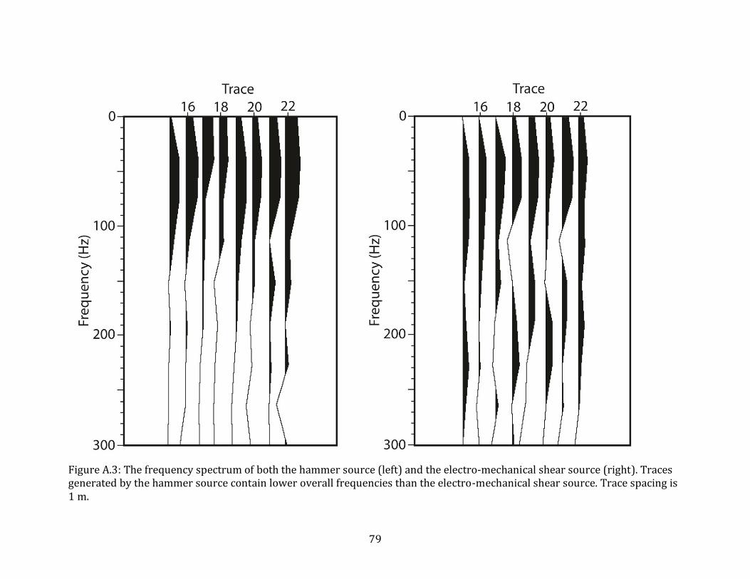
79

Figure A.3: The frequency spectrum of both the hammer source (left) and the electro-mechanical shear source (right). Traces generated by the hammer source contain lower overall frequencies than the electro-mechanical shear source. Trace spacing is 1 m.

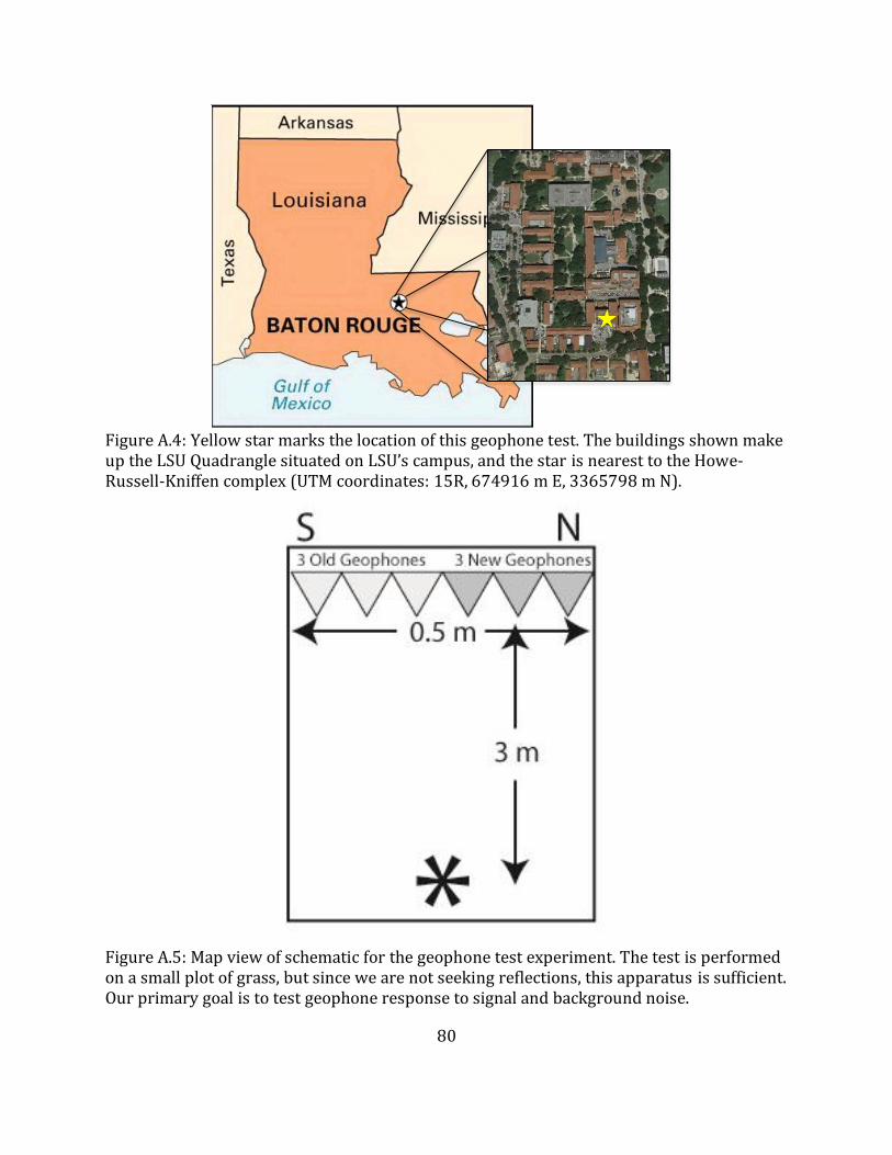
80

Figure A.4: Yellow star marks the location of this geophone test. The buildings shown make up the LSU Quadrangle situated on LSU’s campus, and the star is nearest to the Howe-Russell-Kniffen complex (UTM coordinates: 15R, 674916 m E, 3365798 m N).

Figure A.5: Map view of schematic for the geophone test experiment. The test is performed on a small plot of grass, but since we are not seeking reflections, this apparatus is sufficient. Our primary goal is to test geophone response to signal and background noise.

81

Figure A.6: This log plot of the frequency spectrum of RT Clark (traces 7-9) and Mark Products (traces 10-12) geophones suggests that the Mark Products geophones are more sensitive to frequencies 100-150 Hz while the RT Clark geophones show maximum sensitivity between 75-100 Hz. The similar amplitudes across the range of the plot suggest that the geophones aren’t so different, after all. The traces are not gained or filtered, in order to see the relative frequency spectrum.

100

200

300

400

500

7 8 9 10 11 12

0

Freq

uen

cy (

Hz)

Trace

50

150

250

350

450

R.T. Clark Mark Product

82

Figure A.7: These shot gathers compare the traces collected with R.T. Clark geophones (left) with the traces collected with Mark Product geophones (right)(AGC and bandpass filtered: 0 Hz, 3 Hz, 100 Hz, 200 Hz). The electro-mechanical source was used for all data collection. Reverberations (red) are more present in the shot gather collected with R.T. Clark geophones. Interpreted reflections (green) are more continuous in the Mark Product geophones. Trace spacing is 1 m.

83

After this preliminary test, I perform a second test at the False River study location. The R.T. Clark geophones produce shot gathers with more reverberations than the Mark Products geophones (Figure A.7). The incoming reflections can be picked out more easily in the shot gather recorded with Mark Products geophones.

(A.3)Shot Shell Comparison

The electro-mechanical shear source is loaded with 12-gauge shot shells. Black powder is used in every shot shell; it burns, forming gas that rapidly expands, forcing the shot out the end of the shell. The shot has been replaced with three different materials in our shells to generate the horizontal force that gives the cannon momentum: 1) iron oxide, 2) sand, and 3) a blank (no shot material). Candle wax keeps these materials securely inside the shell to allow for a good crimp (Figure A.8).

Figure A.8: Cross-section diagram of shotgun shell. We experimented with different types of shots and amounts of black powder (Table A.2).

Table A.1: Different shot shells we detonated and their responses in the field. Shot Makeup Black Powder

Weight Max Amplitudes Blast Characteristics

1 load black powder 1 load iron oxide

3.2 ± 0.3 g 1.4 Love wave 0.57 reflection

Loud and powerful

1 load black powder 1 load sand

3.2 ± 0.3 g 0.78 Love wave 0.33 reflection

Quieter and less powerful

1 load black powder 0 load iron oxide

3.2 ± 0.3 g 1.3 Love wave 0.61 reflection

Loud and less powerful

2 loads black powder 2 loads iron oxide

6.4 ± 0.05 g 2.5 Love wave 1.17 reflection

Louder and more powerful

Another test is performed in order to identify which material inside the shot shell

results in the most continuous reflections. We compare all four different shells (Figures A.9 & A.10). A multiple of the Love wave below the main Love wave can be seen in three out of

Primer

Candle wax

Very fine-grained iron oxide

Cork or paper wad

Black powder

3 inches

84

the four shot gathers. Reflection arrivals are difficult to interpret because this high-amplitude multiple interferes with incoming reflections. The shot with 1 load black powder and 1 load iron oxide produces the least Love wave multiple, allowing for the simplest interpretation of reflection arrivals. For this reason, we choose that makeup for our shells used during our 150 m line.

We use a multitude of different packing materials in our shells (Table A.2). No significant difference is seen in the source signature as we alter our materials. Changing our shell sealant from wax to wads allows for faster shot-to-shot progression, because we spend less time cleaning each shell before detonation.

GPS (UTM) locations (Table A.3) vary along our profile.

Table A.2: Different packing materials in the shotshells

Table A.3: Coordinates are shown in UTM (z=15) coordinate system. sx value Easting (m) Northing (m) 0 m 654310.5646 3392975.278 22 m 654306.9881 3392953.594 56 m 654302.475 3392919.296 70 m 654301.5213 3392905.659 109 m 654292.3276 3392867.791 149 m 654289.0171 3392827.480

Shot placement from northernmost shot location (m)

Black powder type Wad type

0-6 m FFFg powder, wax wads 7-21 m FFFFg powder cork wads

22-32 m FFFFg powder cork wads 33-55 m FFFFg powder fiber wads 56-69 m FFFFg powder fiber wads

70-109 m FFFFg powder fiber wads 110-149 m FFFFg powder fiber wads

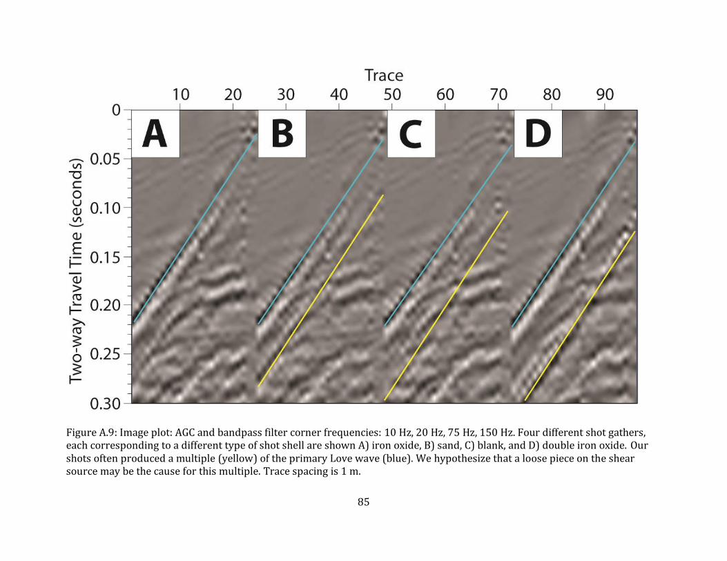
85

Figure A.9: Image plot: AGC and bandpass filter corner frequencies: 10 Hz, 20 Hz, 75 Hz, 150 Hz. Four different shot gathers, each corresponding to a different type of shot shell are shown A) iron oxide, B) sand, C) blank, and D) double iron oxide. Our shots often produced a multiple (yellow) of the primary Love wave (blue). We hypothesize that a loose piece on the shear source may be the cause for this multiple. Trace spacing is 1 m.

86

Figure A.10: Wiggle plot: AGC and bandpass filter corner frequencies: 10 Hz, 20 Hz, 75 Hz, 150 Hz. Four different shot gathers, each corresponding to a different type of shot shell are shown A) iron oxide, B) sand, C) blank, and D) double iron oxide. Our shots often produced a multiple (yellow) of the primary Love wave (blue). We hypothesize that a loose piece on the shear source may be the cause for this multiple. Trace spacing is 1 m.

87

APPENDIX B: Static Corrections

Two things can cause a flat layer to appear dipping in my seismic data: 1) surface elevation differences and 2) shallow velocity variations. Residual statics corrections are uniform time shifts that are applied to traces to compensate for time delays in the highly variable near-surface weathering zone (Wiggins et al., 1976). Near-surface velocity variation and topographic variation in the weathering zone can cause these time delays (Figure B.1).

Figure B.1: The effect of variable topography on a seismic stack is featured. A. Earth model with an elevation difference. B. The stacked section from this location contains a seismic boundary that dips. In the Earth model, that boundary is completely flat, but in the stack it exhibits a dip.

𝑣 =𝑑

𝑡

200 𝑚/𝑠 =30 𝑚

𝑡

𝑡 =30 𝑚

200 𝑚/𝑠

𝑡 = 0.15 𝑠

𝑣 =𝑑

𝑡

200 𝑚/𝑠 =20 𝑚

𝑡

𝑡 =20 𝑚

200 𝑚/𝑠

𝑡 = 0.10 𝑠

88

Seismic Unix includes Suresstat, a program that performs residual static correction to seismic data. The program calculates source and receiver statics and outputs each to an external file. The static corrections in the external files are applied to the original seismic data with a second program, Sustatic. Suresstat exists on Version 43 of Seismic Unix, but it does not run successfully. HOW TO RUN SURESSTAT: -Verify that Seismic Unix is completely up to date (V44 minimum) -Input seismic file must be nmo corrected and sorted into shot gathers -niter, or the number of iterations, should be ~20-25 -imax parameter must be greater than or equal to the largest shot (fldr), receiver (tracf) or cmp (cdp) number. -Program outputs two files, a source static correction file and receiver static correction file, both used by Sustatic. HOW TO RUN SUSTATIC: -Parameter hdrs must be equal to 3, to read external files -Include parameters sou_file and rec_file, the names of the external files -Include number of sources (ns), number of receivers (nr) and number of offsets (no) I include Statics.sh (Appendix C), a shell script that will sort the data, calculate the statics files, apply the statics and print the results to the screen (Figures B.2 & B.3) all at once.

89

Figure B.2: A) Static corrections are not applied to this migrated seismic stack (AGC, bandpass filter corner frequencies: 15 Hz, 30 Hz, 65 Hz, 90 Hz). I use this stack in the interpretation. B) The seismic fold along the length of the seismic line reaches a maximum 11 m from the edges of the profile.

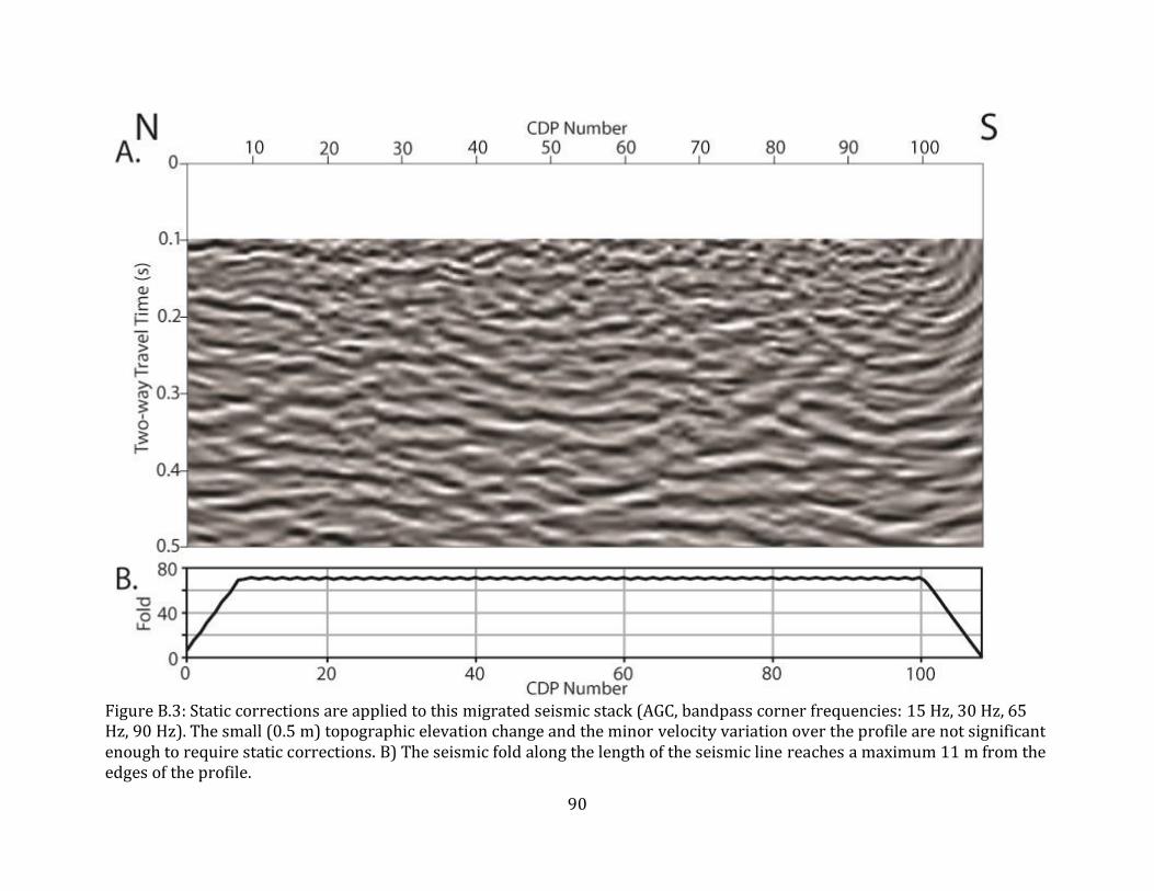
90

Figure B.3: Static corrections are applied to this migrated seismic stack (AGC, bandpass corner frequencies: 15 Hz, 30 Hz, 65 Hz, 90 Hz). The small (0.5 m) topographic elevation change and the minor velocity variation over the profile are not significant enough to require static corrections. B) The seismic fold along the length of the seismic line reaches a maximum 11 m from the edges of the profile.

91

APPENDIX C: Seismic Processing Programs The following appendix shows the seismic processing programs used to create the seismic stack from False River. The

12 processing steps (Table C.1) are listed with the programs that accomplish them as well as the input and output files for each program. I list the code for these programs. README found in home/martm/FalseRiver/seismics/data/core_1/All_line1/H/1/su contains a description of data files located in that directory.

Table C.1: Seismic processing steps and programs, as well as the input and output files for each program and step. Processing Step Program Input file Output file

Convert to SU Sseg2su.pl Subtract opposite polarity gathers

4to2shots.sh or 2to1shots.sh

1000_clean.su 10XX_clean.su

10001.su 10150.su

Reverse trace polarity

Reverse_polarity.pl 10001.su 10150.su

10001_rev.su 10150_rev.su

*Move 10001_rev.su-10150_rev.su to subdirectory All_line1. Remove ‘_rev’ extension from all files.* Interpolate seismic traces

suinterp 10001.su 10150.su

10001_interp.su 10150_interp.su

Apply f-k filter Sudipfilt.pl 10001_interp.su 10150_interp.su

10001_interp_fk2.su 10150_interp_fk2.su

Set header geometry

make_header_geometry.pl

10001_interp_fk2.su 10150_interp_fk2.su

10001_interp_fk2_tracr.su 10150_interp_fk2_tracr.su

Apply top mute sumute 10001_interp_fk2_tracr.su 10150_interp_fk2_tracr.su

10001_interp_fk2_mute.su 10150_interp_fk2_mute.su

*Concatenate 10001_interp_fk2_mute.su – 10150_interp_fk2_mute.su.* Make CMPs Make_CMP.pl All_line1_interp_fk2_mute.su All_line1_interp_fk2_mute_cmp300.su

*Sort data into CDP gathers before performing velocity analysis.* Velocity Analysis IVA2.pl/IVA2.pm All_line1_interp_fk2_mute_cmp300_cdp

sort.su Files for velocity analysis

Stack & Moveout NmoStack.pl All_line1_interp_fk2_mute_cmp300_cdpsort.su

All_line1_interp_fk2_mute_cmp300_cdp sort_nmocorrected_stack_unmig.su

Migration sustolt All_line1_interp_fk2_mute_cmp300_cdp sort_nmocorrected_stack_unmig.su

All_line1_interp_fk2_mute_cmp300_cdp sort_nmocorrected_stack_mig.su

92

########################## #Sseg2su# #This program converts our Seg2 data files to the SU file type. #Input the total number of files and first file name. ########################## #! /usr/bin/perl -w =pod =head1 DOCUMENTATION =head2 SYNOPSIS PROGRAM NAME: Sseg2su AUTHOR: Juan Lorenzo Purpose: File format conversion Data format change from Seg2 ("DAT") or geometrics format to su DATE: Aug 9, 2011 =head2 REQUIRES sioseis module =head2 EXAMPLE For example, total number of files =74 first file is ‘1000.su’ =cut # Use shell transparently to locate home directory before compilation my $library_location;

BEGIN { use Shell qw(echo);

93

$home_directory = ` echo \$HOME`; chomp $home_directory; $library_location = $home_directory.'/lsu/libAll'; } =pod LOAD GENERAL PERL LIBRARIES =cut use lib $library_location; # use library use lib '/usr/local/pl/libAll'; use System_Variables; my ($DATA_SEISMIC_SU) = System_Variables::DATA_SEISMIC_SU(); my ($DATA_SEISMIC_SEG2) = System_Variables::DATA_SEISMIC_SEG2(); # use library use lib './libAll'; use Sseg2su qw ($number_of_files $first_file_number); for ($i=1,$j=$first_file_number; $i <=$number_of_files; $i += 1,$j +=1){ $j_char = sprintf("%u",$j); $file_name[$i] = $j_char; } #START FOR LOOP for ($i=1; $i<=$number_of_files; $i++) { =pod Convert *dat file names to DAT file names for conversion by sioseis

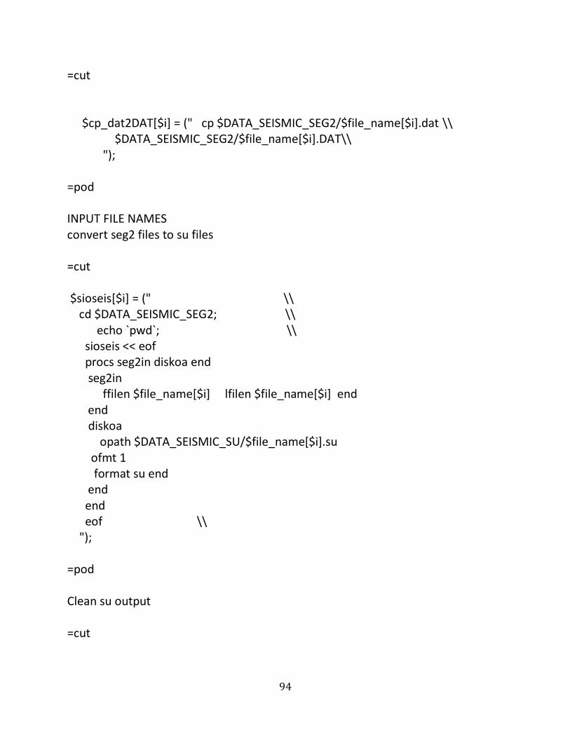
94

=cut $cp_dat2DAT[$i] = (" cp $DATA_SEISMIC_SEG2/$file_name[$i].dat \\ $DATA_SEISMIC_SEG2/$file_name[$i].DAT\\ "); =pod INPUT FILE NAMES convert seg2 files to su files =cut $sioseis[$i] = (" \\ cd $DATA_SEISMIC_SEG2; \\ echo `pwd`; \\ sioseis << eof procs seg2in diskoa end seg2in ffilen $file_name[$i] lfilen $file_name[$i] end end diskoa opath $DATA_SEISMIC_SU/$file_name[$i].su ofmt 1 format su end end end eof \\ "); =pod Clean su output =cut

95

$segyclean[$i] = (" segyclean \\ <$DATA_SEISMIC_SU/$file_name[$i].su \\ >$DATA_SEISMIC_SU/$file_name[$i]_clean.su \\ "); } # END FOR LOOP for ($i= 1 ; $i <= $number_of_files; $i += 1) { =pod DEFINE FLOW(S) =cut $flow[1][$i] = $cp_dat2DAT[$i]; $flow[2][$i] = $sioseis[$i]; $flow[3][$i] = $segyclean[$i]; =pod RUN FLOW(S) =cut system $flow[1][$i]; system 'echo', $flow[1][$i]; system $flow[2][$i]; system 'echo', $flow[2][$i]; system $flow[3][$i]; system 'echo', $flow[3][$i]; }

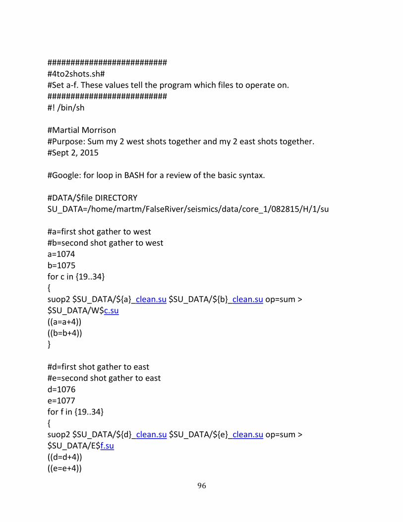
96

########################## #4to2shots.sh# #Set a-f. These values tell the program which files to operate on. ########################## #! /bin/sh #Martial Morrison #Purpose: Sum my 2 west shots together and my 2 east shots together. #Sept 2, 2015 #Google: for loop in BASH for a review of the basic syntax. #DATA/$file DIRECTORY SU_DATA=/home/martm/FalseRiver/seismics/data/core_1/082815/H/1/su #a=first shot gather to west #b=second shot gather to west a=1074 b=1075 for c in {19..34} { suop2 $SU_DATA/${a}_clean.su $SU_DATA/${b}_clean.su op=sum > $SU_DATA/W$c.su ((a=a+4)) ((b=b+4)) } #d=first shot gather to east #e=second shot gather to east d=1076 e=1077 for f in {19..34} { suop2 $SU_DATA/${d}_clean.su $SU_DATA/${e}_clean.su op=sum > $SU_DATA/E$f.su ((d=d+4)) ((e=e+4))

97

} #g & h control which output from the first two loops is used as input for this loop. g=h!!! #EX: g=1; h=1 ==> W1; E1. g=19 h=19 for i in {10019..10034} { suop2 $SU_DATA/W${g}.su $SU_DATA/E${h}.su op=diff > $SU_DATA/$i.su ((g=g+1)) ((h=h+1)) }

########################## #Reverse_polarity.pl# #Give the program the first and last file, and the number of shots. #Specify the traces that need to be multiplied by (-1). ########################## #! /usr/bin/perl use Moose; =pod =head1 DOCUMENTATION =head2 SYNOPSIS PROGRAM NAME: Reverse_polarity.pl AUTHOR: Juan Lorenzo Edited by: Martial Morrison DATE: Jan 27, 2016 DESCRIPTION: Reverse polarity of traces in a shot gather =head3 Steps are as follows:

98

=cut =pod 1. Use packages: (for subroutines) manage_files_by System_Variables (for subroutines) (for variable definitions) SeismicUnix (Seismic Unix modules) Use classes: flow message suximage =cut =pod LOAD GENERAL PERL LIBRARIES =cut use SU; use suop; =pod import system variables =cut my ($DATA_SEISMIC_SU) = System_Variables::DATA_SEISMIC_SU(); use SeismicUnix qw ($on $off $to $in $go $out);

99

=pod 2. Instantiate classes and declare variables =cut my $cat = new cat(); my $suxwigb = new suxwigb(); my $sugain = new sugain(); my $sufilter = new sufilter(); my $suop = new suop(); my $suwind = new suwind(); my $log = new message(); my $run = new flow(); my (@su_inbound, @su_outbound); my (@cat); my (@suop_in, @suop_inbound, @suop_outbound); my (@suwind_pos_outbound,@suwind_neg_outbound); my (@items,@flow); my (@ref_to_items); my (@sugain,@sufilter,@suxwigb); my (@suop, @suwind, @log,@run); my ($i); =pod Set file names: reverse file out raw file names in make a list of input files make a list of output files =cut

100

#my $first_file = 1001; #my $last_file = 1101; #my $num_shots = 100; #my $first_file = 10001; #my $last_file = 10022; #my $num_shots = 22; my $first_file = 10001; my $last_file = 10001; my $num_shots = 1; for ($i=$first_file; $i<=$last_file;$i++) { $su_inbound[$i] = $DATA_SEISMIC_SU.'/'.$i.'.su'; $su_outbound[$i] = $DATA_SEISMIC_SU.'/'.$i.'_rev'.'.su'; # $su_inbound[$i] = $DATA_SEISMIC_SU.'/'.$i.'_clean'.'.su'; # $su_outbound[$i] = $DATA_SEISMIC_SU.'/'.$i.'_clean'.'_rev'.'.su'; } for ($i=$first_file; $i<=$last_file; $i++) { $suwind_pos_outbound[$i] = $DATA_SEISMIC_SU.'/'.'.temp_positive_'.$i.' '; $suwind_neg_outbound[$i] = $DATA_SEISMIC_SU.'/'.'.temp_negative_'.$i.' '; } =pod make the patterns for selecting traces for the positive traces (traces 1 to 12 and 25 to 35 etc) for the negative traces (traces 13 to 24 and 36 to 48 etc) =cut $sugain -> clear(); $sugain -> agc($on);

101

$sugain -> wagc(0.1); $sugain[1] = $sugain->Step(); $sufilter -> clear(); $sufilter -> freq('3,6,100,160'); $sufilter[1] = $sufilter->Step(); $suxwigb -> clear(); $suxwigb -> absclip(1); $suxwigb -> windowtitle('uncorrected'); $suxwigb[1] = $suxwigb -> Step(); $suxwigb -> clear(); $suxwigb -> absclip(1); $suxwigb -> windowtitle('corrected'); $suxwigb[2] = $suxwigb -> Step(); $suwind -> clear(); $suwind -> setheaderword('tracr'); $suwind -> min(1); $suwind -> max(12); $suwind[1] = $suwind -> Step(); $suwind -> clear(); $suwind -> setheaderword('tracr'); $suwind -> min(13); $suwind -> max(24); $suwind[2] = $suwind -> Step(); $suop -> clear(); $suop -> neg(); $suop[1] = $suop -> Step(); $cat ->clear(); $cat[1] = $cat ->Step();

102

#print("cat is $cat[1] \n\n"); =pod =head4 Assemble the flows from the individual modules how to dereference a complicated array reference print("items are @{$ref_to_items[$i]}\n\n"); 1. extract positive traces (unchanged) 2. extract and make negative traces 3. concatenate the extracted positive (1) and negative (2) traces 4. view uncorrected data 5. view the results =cut for ($i=$first_file; $i <= $last_file; $i++){ $ref_to_items[$i] = [$suwind[1],$in,$su_inbound[$i], $out,$suwind_pos_outbound[$i] ]; $flow[$i][1] = $run ->modules($ref_to_items[$i]); $ref_to_items[$i] = [$suwind[2],$in,$su_inbound[$i], $to,$suop[1],$out,$suwind_neg_outbound[$i]]; $flow[$i][2] = $run ->modules($ref_to_items[$i]); $ref_to_items[$i] = [$cat[1],$suwind_pos_outbound[$i], $suwind_neg_outbound[$i],$out,$su_outbound[$i]]; $flow[$i][3] = $run ->modules($ref_to_items[$i]); $ref_to_items[$i] = [$sugain[1],$in,$su_inbound[$i], $to,$sufilter[1],$to,$suxwigb[1],$go]; $flow[$i][4] = $run ->modules($ref_to_items[$i]);

103

$ref_to_items[$i] = [$sugain[1],$in,$su_outbound[$i], $to,$sufilter[1],$to,$suxwigb[2],$go]; $flow[$i][5] = $run ->modules($ref_to_items[$i]); } =pod =head4 RUN FLOW(S) =cut for ($i=$first_file; $i <= $last_file; $i++) { $run->flow(\$flow[$i][1]); $run->flow(\$flow[$i][2]); $run->flow(\$flow[$i][3]); $run->flow(\$flow[$i][4]); $run->flow(\$flow[$i][5]); } =pod =head4 LOG FLOW(S) TO SCREEN AND FILE =cut for ($i=$first_file; $i <= $last_file; $i++) { print $flow[$i][1]."\n\n"; #$log->file($flow[$i][1]); print $flow[$i][2]."\n\n"; #$log->file($flow[$i][2]); print $flow[$i][3]."\n\n"; #$log->file($flow[$i][3]);

104

print $flow[$i][4]."\n\n"; #$log->file($flow[$i][4]); print $flow[$i][5]."\n\n"; #$log->file($flow[$i][5]); }

########################## #Sudipfilt.pl# #Specify four corner frequencies for the dip filter. ########################## #! /usr/bin/perl =pod =head1 DOCUMENTATION =head2 SYNOPSIS PROGRAM NAME: Sudipfilt.pl AUTHOR: Juan Lorenzo Edited by: Martial Morrison DATE: Jan 7, 2016 DESCRIPTION: f-k filter slopes from a dataset =cut =pod LOAD GENERAL PERL LIBRARIES =cut # library path use lib './libAll';

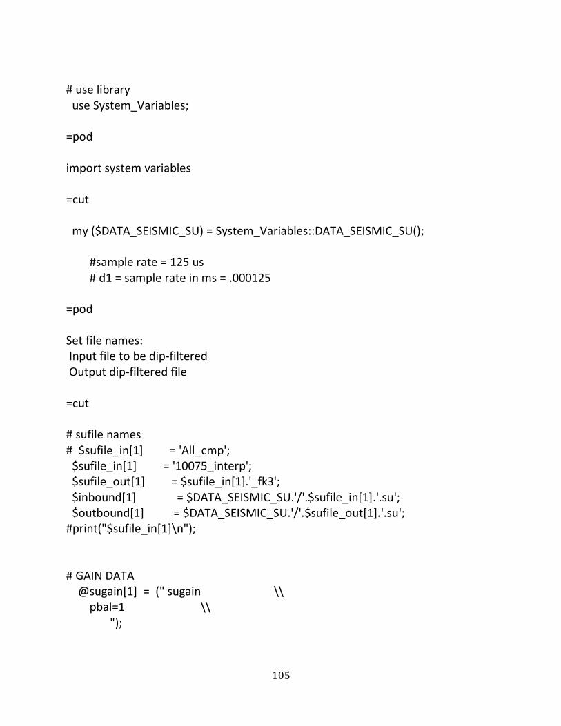
105

# use library use System_Variables; =pod import system variables =cut my ($DATA_SEISMIC_SU) = System_Variables::DATA_SEISMIC_SU(); #sample rate = 125 us # d1 = sample rate in ms = .000125 =pod Set file names: Input file to be dip-filtered Output dip-filtered file =cut # sufile names # $sufile_in[1] = 'All_cmp'; $sufile_in[1] = '10075_interp'; $sufile_out[1] = $sufile_in[1].'_fk3'; $inbound[1] = $DATA_SEISMIC_SU.'/'.$sufile_in[1].'.su'; $outbound[1] = $DATA_SEISMIC_SU.'/'.$sufile_out[1].'.su'; #print("$sufile_in[1]\n"); # GAIN DATA @sugain[1] = (" sugain \\ pbal=1 \\ ");

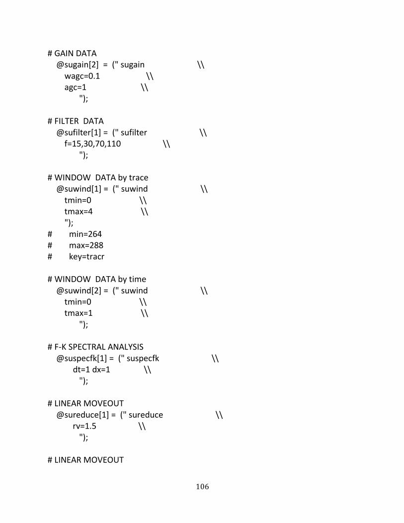
106

# GAIN DATA @sugain[2] = (" sugain \\ wagc=0.1 \\ agc=1 \\ "); # FILTER DATA @sufilter[1] = (" sufilter \\ f=15,30,70,110 \\ "); # WINDOW DATA by trace @suwind[1] = (" suwind \\ tmin=0 \\ tmax=4 \\ "); # min=264 # max=288 # key=tracr # WINDOW DATA by time @suwind[2] = (" suwind \\ tmin=0 \\ tmax=1 \\ "); # F-K SPECTRAL ANALYSIS @suspecfk[1] = (" suspecfk \\ dt=1 dx=1 \\ "); # LINEAR MOVEOUT @sureduce[1] = (" sureduce \\ rv=1.5 \\ "); # LINEAR MOVEOUT

107

@sureduce[2] = (" sureduce \\ rv=-1.5 \\ "); # APPLY DIP FILTER @sudipfilter[1] = (" sudipfilt \\ dt=1 dx=1 \\ amps=0,1,1,0,0,1 \\ slopes=0,2,5,7,50,55 \\ bias=0 \\ "); # slopes=0,2,7,12,30,34 \\ # APPLY DIP FILTER @sudipfilter[2] = (" sudipfilt \\ dt=1 dx=1 \\ amps=1,0,0,1 \\ bias=0 \\ slopes=50,100,175,250 \\ "); # DISPLAY DATA $suxwigb_windowtitle[1]=$sufile_in[1]; #key=offset \\ @suxwigb[1] = (" suxwigb \\ title=$sufile_in[1]' f=0,3,100,200 wagc=0.1' \\ windowtitle=$suxwigb_windowtitle[1] \\ label1='No. samples' \\ label2='No. traces' \\ d1=1 d2=1 f1=1 f2=1 \\ wbox=300 hbox=370 xbox=370 ybox=0 \\ n2tic=1 d2num=20 \\ va=1 \\

108

xcur=3 \\ clip=5 \\ "); #windowtitle='RAW' # DISPLAY DATA $suxwigb_windowtitle[2]=$sufile_in[1].'corrected'; #key=offset \\ @suxwigb[5] = (" suxwigb \\ title=$sufile_in[1]' f=0,3,100,200 wagc=0.1' \\ windowtitle=$suxwigb_windowtitle[2] \\ label1='No. samples' \\ label2='No. traces' \\ d1=1 d2=1 f1=1 f2=1 \\ wbox=300 hbox=370 xbox=370 ybox=440 \\ n2tic=1 d2num=20 \\ va=1 \\ xcur=3 \\ clip=5 \\ "); #windowtitle='f-k_applied' # DISPLAY DATA @suximage[1] = (" suximage \\ title=$sufile_in[1] \\ style=seismic \\ x1beg=0.5 x1end=0. \\ label1='Frequency (Hz) dt=1 Nf=0.5' \\ label2='k (1/m) dx=1 Nk=0.5' \\ n2tic=1 d2num=0.2 f2num=-0.5 \\ n1tic=1 d1num=0.1 \\ wbox=300 hbox=370 xbox=0 ybox=0 \\ "); # DISPLAY DATA

109

$suxwigb_windowtitle[3]=$sufile_in[1]; @suximage[2] = (" suximage \\ title=$sufile_in[1]' f=0,3,100,200 wagc=0.1' \\ label1='Time (s)' \\ label2='No. traces' \\ n2tic=1 d2num=20 \\ legend=1 \\ windowtitle=$suxwigb_windowtitle[3] \\ clip=3 \\ wbox=300 hbox=370 xbox=670 ybox=0 \\ "); # DISPLAY DATA @suximage[4] = (" suximage \\ title=$sufile_in[1] \\ x1beg=0.5 x1end=0. \\ label1='Frequency (Hz) dt=1 Nf=0.5' \\ label2='k (1/m) dx=1 Nk=0.5' \\ n2tic=1 d2num=0.2 f2num=-0.5 \\ n1tic=1 d1num=0.1 \\ wbox=300 hbox=370 xbox=0 ybox=440 \\ "); # DISPLAY DATA $suxwigb_windowtitle[4]=$sufile_in[1].'corrected'; @suximage[6] = (" suximage \\ title=$sufile_in[1]' f=0,3,100,200 wagc=0.1' \\ label1='Time (s)' \\ label2='No. traces' \\ n2tic=1 d2num=20 \\ legend=1 \\ windowtitle=$suxwigb_windowtitle[4] \\ wbox=300 hbox=370 xbox=670 ybox=440 \\

110

clip=3 \\ "); =pod =head4 Assemble the flows 1. Output frequency spectrum of original data to screen 2. Output wiggle plot of original data to screen 3. Output variable amplitude plot of original data to screen 4. Output frequency spectrum of f-k filtered data to screen 5. Output wiggle plot of f-k filtered data to screen 6. Output variable amplitude plot of f-k filtered data to screen 7. Output f-k filtered data file =cut # DEFINE FLOW(S) @flow[1] = (" \\ @suwind[2] \\ < @inbound[1] | \\ @sugain[2] | \\ @sufilter[1] | \\ @suspecfk[1] | \\ @suximage[1] \\ & \\ "); # DEFINE FLOW(S) @flow[2] = (" \\ @suwind[2] \\ < @inbound[1] | \\ @sugain[2] | \\ @sufilter[1] | \\ @suxwigb[1] \\ & \\ ");

111

# DEFINE FLOW(S) @flow[3] = (" \\ @suwind[2] \\ < @inbound[1] | \\ @sugain[2] | \\ @sufilter[1] | \\ @suximage[2] \\ & \\ "); # DEFINE FLOW(S) @flow[4] = (" \\ @suwind[2] \\ < @inbound[1] | \\ @sugain[2] | \\ @sufilter[1] | \\ @sudipfilter[1] | \\ @suspecfk[1] | \\ @suximage[4] \\ & \\ "); # DEFINE FLOW(S) @flow[5] = (" \\ @suwind[2] \\ < @inbound[1] | \\ @sugain[2] | \\ @sufilter[1] | \\ @sudipfilter[1] | \\ @suxwigb[5] \\ & \\ "); # DEFINE FLOW(S) @flow[6] = (" \\ @suwind[2] \\

112

< @inbound[1] | \\ @sugain[2] | \\ @sufilter[1] | \\ @sudipfilter[1] | \\ @suximage[6] \\ & \\ "); # DEFINE FLOW(S) @flow[7] = (" \\ @suwind[2] \\ < @inbound[1] | \\ @sugain[2] | \\ @sufilter[1] | \\ @sudipfilter[1] \\ > @outbound[1] \\ & \\ "); =pod =head4 RUN FLOW(S) =cut system @flow[1]; system 'echo', @flow[1]; system @flow[2]; system 'echo', @flow[2]; system @flow[3]; system 'echo', @flow[3]; system @flow[4]; system 'echo', @flow[4];

113

system @flow[5]; system 'echo', @flow[5]; system @flow[6]; system 'echo', @flow[6]; system @flow[7]; system 'echo', @flow[7];

########################## #Suinterp# #Specify a, the first file that will be interpolated as well as the full range of #files to be interpolated. ########################## #! /bin/sh #Martial Morrison #Purpose: Interpolate all gathers using suinterp. #Feb 1, 2016 #Google: for loop in BASH for a review of the basic syntax. #DATA/$file DIRECTORY SU_DATA=/home/martm/FalseRiver/seismics/data/core_1/All_line1/H/1/su #a=shot gather a=10001 for a in {10001..10150} { suinterp < $SU_DATA/${a}.su > $SU_DATA/${a}_interp.su ((a=a+1)) }

##########################

114

#make_header_geometry.pl# #Specify which header words to set, and what values to set them to. ########################## #!/usr/bin/perl =pod =head1 DOCUMENTATION =head2 SYNOPSIS PROGRAM NAME: make_header_geometry.pl AUTHOR: Juan Lorenzo DATE: Oct 27 2013 DESCRIPTION: Generate appropriate headers before generating CMPs (see Make_CMP.pl) Version: 1 =head2 USE =head3 NOTES We are using moose moose already declares that you need debuggers turned on so you don't need a line like the following: use warnings; (for subroutines) manage_files_by System_Variables (for subroutines) (for variable definitions) SeismicUnix (Seismic Unix modules) offset is defined as sx-gx

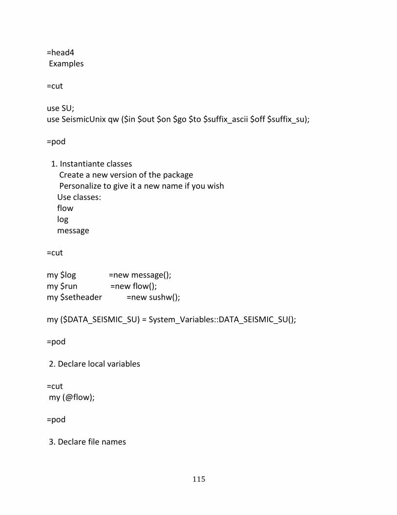
115

=head4 Examples =cut use SU; use SeismicUnix qw ($in $out $on $go $to $suffix_ascii $off $suffix_su); =pod 1. Instantiante classes Create a new version of the package Personalize to give it a new name if you wish Use classes: flow log message =cut my $log =new message(); my $run =new flow(); my $setheader =new sushw(); my ($DATA_SEISMIC_SU) = System_Variables::DATA_SEISMIC_SU(); =pod 2. Declare local variables =cut my (@flow); =pod 3. Declare file names

116

=cut # $file_in[1] ='All_line1_interp_fk2_mute_cmp300_nmo'; $file_in[1] ='All_line1_interp_fk2_mute_cmp'; $file_in[1] ='All_line1_interp_fk2_mute_cmp300_nmo_fldr'; $file_in[1] ='All_line1_interp_fk2_mute'; $sufile_in[1] =$file_in[1].$suffix_su; $inbound[1] =$DATA_SEISMIC_SU.'/'.$sufile_in[1]; $outbound[1] =$DATA_SEISMIC_SU.'/'.$file_in[1].'_tracf'.$suffix_su; =pod setheader set header values =cut #THIS IS FOR INTERPOLATED DATA # $setheader ->clear(); # $setheader ->name(tracl,tracf,tracr,sx,offset,gx,fldr,ep); # $setheader ->first_val(1,1,1,0,100,100,1,1); # $setheader ->intra_gather_inc(1,1,1,0,50,50,0,0); # $setheader ->inter_gather_inc(0,2,0,100,0,100,1,1); # $setheader ->gather_size(7050,47,47,47,47,47,47,47); # $setheader[1] =$setheader->Step(); #THIS IS FOR NON-INTERPOLATED DATA # $setheader ->clear(); # $setheader ->name(tracl,tracf,tracr,sx,offset,gx,fldr,ep); # $setheader ->first_val(1,1,1,0,100,100,1,1); # $setheader ->intra_gather_inc(1,1,1,0,50,50,0,0); # $setheader ->inter_gather_inc(0,0,0,100,0,100,1,1); # $setheader ->gather_size(3600,24,24,24,24,24,24,24); # $setheader[1] =$setheader->Step();

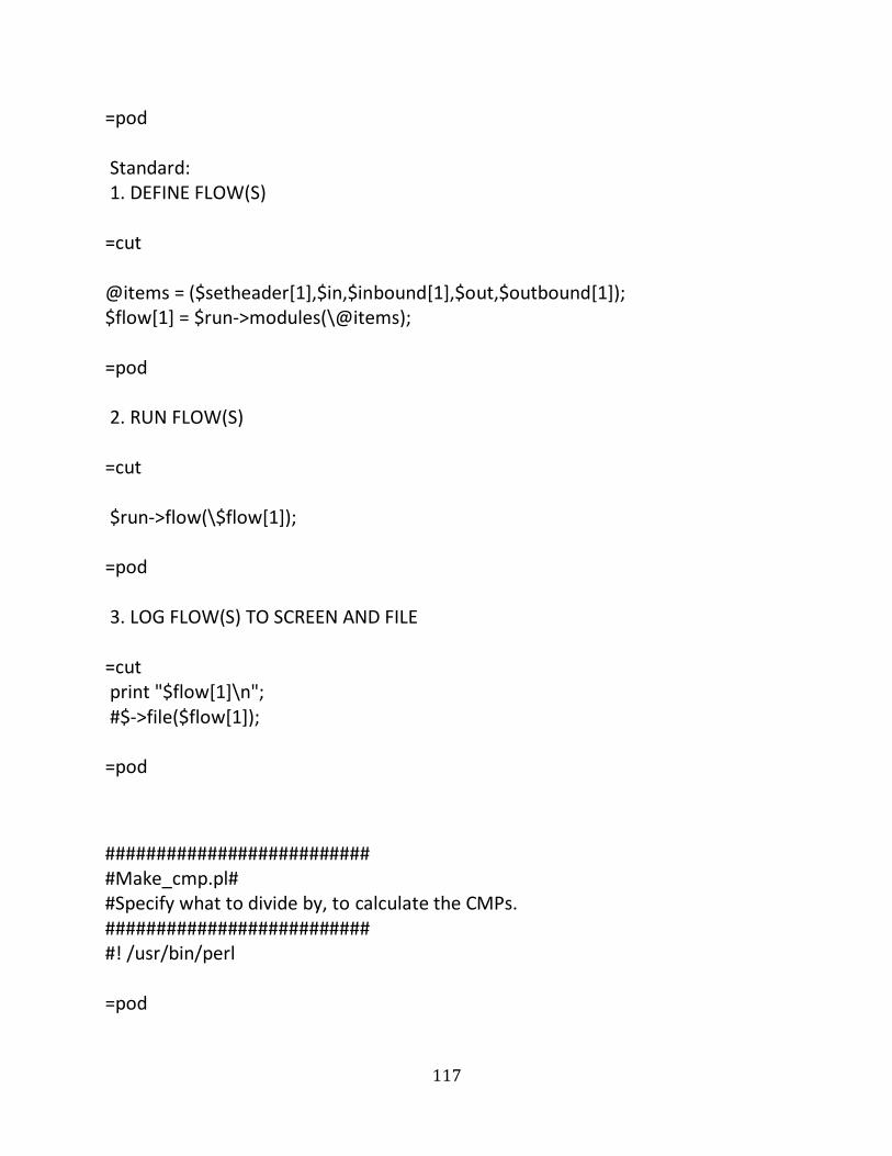
117

=pod Standard: 1. DEFINE FLOW(S) =cut @items = ($setheader[1],$in,$inbound[1],$out,$outbound[1]); $flow[1] = $run->modules(\@items); =pod 2. RUN FLOW(S) =cut $run->flow(\$flow[1]); =pod 3. LOG FLOW(S) TO SCREEN AND FILE =cut print "$flow[1]\n"; #$->file($flow[1]); =pod

########################## #Make_cmp.pl# #Specify what to divide by, to calculate the CMPs. ########################## #! /usr/bin/perl =pod

118

=head1 DOCUMENTATION =head2 SYNOPSIS PROGRAM NAME: Make_cmp.pl AUTHOR: Juan Lorenzo Edited by: Martial Morrison DATE: Oct. 25 2007 DATE: Nov 3 2013 DATE: Aug 26, 2015 Version 3 =cut =head2 DESCRIPTION Purpose: To generate CMP values in the headers, headers must already have the correct geometry values inserted for the seismic experiment (See header_geom.pl for this) We use the basic relation that CMP = (sx+gx)/2 where sx is the shot location, and gx is the receiver location. We use suchw to calculate the CMP using offset and other key words as input. value(key1) = (a + b * value(key2) + c * value(key3)) / d can be rewritten as: If we choose the first CMP to be equal to ,say, 101 then a = 304 a = ( 101 (first CMP number) + 51 * (absolute value of half the longest offset on the first shot gather))/2 You can choose other numbers to be the first CMP.

119

value(cdp) =(304 + 1 * value(sx) + 1 * value(gx) ) / 2 =cut =pod use the following libraries Some of these libraries or packages contain groups of subroutines for example: SU use lib explicitly locates packges =cut use Moose; use SeismicUnix qw ($in $on $go $to $out); use SU; =pod Declare local arrays Declare local scalars =cut my (@file_outbound,@file_inbound); my (@flow,@items,@makecmp); my ($log,$messages,$makecmp,$run); =pod create new instances of the classes =cut

120

$log = new message(); $run = new flow(); $makecmp = new suchw(); my ($DATA_SEISMIC_SU) = System_Variables::DATA_SEISMIC_SU(); my ($TEMP_DATA_SEISMIC_SU) = System_Variables::TEMP_DATA_SEISMIC_SU(); =pod Declare file names =cut # FOR INTERPOLATED DATA # $file_inbound[1] = $DATA_SEISMIC_SU.'/'.'All_line1_interp_fk2_mute_geom'.'.su'; # $file_outbound[1] = $DATA_SEISMIC_SU.'/'.'All_line1_interp_fk2_mute_cmp'.'.su'; # FOR NON-INTERPORLATED DATA # $file_inbound[1] = $DATA_SEISMIC_SU.'/'.'All_line1_fk_mute_geom'.'.su'; # $file_outbound[1] = $DATA_SEISMIC_SU.'/'.'All_line1_fk__mute_geom_cmp2'.'.su'; =pod =head3 Example in shell script suchw <$DATA_IN/1001_head_geom.su \ key1=cdp \ key2=sx \ key3=gx \ a=0 \ b=1 \

121

c=1 \ d=2 \ $DATA_OUT/all_geom_CMP.su =cut =pod =head3 set up suchw to calculate new header geometry variable to change here is “divide_all_by” to alter the max fold of your stack =cut $makecmp -> clear(); $makecmp -> result_header('cdp'); $makecmp -> first_header('sx'); $makecmp -> second_header('gx'); $makecmp -> multiply_hdr1_by(1); $makecmp -> multiply_hdr2_by(1); $makecmp -> divide_all_by(2); $makecmp[1] = $makecmp->Step(); =pod DEFINE FLOW(S) =cut @items = ($makecmp[1],$in,$file_inbound[1],$out,$file_outbound[1],$go); $flow[1] = $run->modules(\@items); =pod

122

RUN FLOW(S) =cut $run->flow(\$flow[1]); =pod LOG FLOW(S)TO SCREEN AND FILE =cut print "$flow[1]\n"; #$log->file($flow[1]);

########################## #Nmo_Stack.pl# #Specify the move-out velocity to apply before stacking. ########################## #! /usr/bin/perl # -w # PROGRAM NAME: NmoStack.pl # DATE: May 17, 2016 # AUTHOR: Martial Morrison # PURPOSE: Sort, normally move out and brute stack a large file with multiple shot gathers. # use library use lib '/usr/local/pl/libAll'; use manage_dirs_by; use manage_files_by; # use library use System_Variables; my ($DATA_SEISMIC_SU) = System_Variables::DATA_SEISMIC_SU();

123

my ($date) = Project_Variables::date(); my ($line) = Project_Variables::line(); my ($component) = Project_Variables::component(); $filesystem_in = $site.'-'.$monitoring_well.'-'.$preparation_well.'-'.$stage; # use library use SeismicUnix qw ($suffix_segy $suffix_su $suffix_bin $suffix_lsu); # sufile names # $sufile[1] = 'All_line1_interp_fk2_mute'; $sufile[1] = 'All_line1_interp_fk2_cmp700'; $sufile[1] = 'All_line1_interp_fk2_mute_cmp700'; $sufile[1] = 'All_line1_interp_fk2_mute_cmp300'; $sufile_in[1] = $sufile[1].$suffix_su; $sufile_inbound[1] = $DATA_SEISMIC_SU.'/'.$sufile_in[1]; # SUXIMAGE TITLE $suximage_title[1] = $sufile_inbound; # GAIN DATA $sugain[1] = (" sugain \\ pbal=0 \\ "); # GAIN DATA $sugain[2] = (" sugain \\ agc=1 \\ wagc=0.1 \\ "); # GAIN DATA $sugain[3] = (" sugain \\ tpow=1 \\ ");

124

# FILTER DATA $sufilter[1] = (" sufilter \\ f=15,30,75,110 \\ "); # WINDOW DATA $suwind[1] = (" suwind \\ tmin=0 \\ tmax=0.8 \\ "); # SORT DATA $susort[1] = (" susort \\ cdp \\ offset \\ "); # NORMAL MOVEOUT $vnmo[1]='11000'; $smute[1]='1.04'; $sunmo[1] = (" sunmo \\ vnmo=$vnmo[1] \\ smute=$smute[1] \\ "); # STACK $sustack[1] = (" sustack \\ "); # DISPLAY DATA $N=1; $suximage_windowtitle[$N] = $sufile[1]; $suximage_title[$N] = 'vnmo='.$vnmo[1]; $suximage_box_width[$N] = 500; $suximage_tlabel[$N] = 'TWTT\ \(s\)'; $suximage_xlabel[$N] = 'trace\ no.';

125

$suximage_clip[$N] = 3; $suximage[1] = (" suximage \\ windowtitle=$suximage_windowtitle[$N] \\ title=$suximage_title[$N] \\ legend=1 \\ clip=$suximage_clip[$N] \\ label1=$suximage_tlabel[$N] \\ label2=$suximage_xlabel[$N] \\ xbox=$suximage_X0[$N] \\ "); $N=2; $suxwigb_windowtitle[$N] = $sufile[1]; $suxwigb_title[$N] = 'unstacked'; $suxwigb_box_width[$N] = 500; $suxwigb_tlabel[$N] = 'TWTT\ \(s\)'; $suxwigb_xlabel[$N] = 'trace\ no.'; $suxwigb_X0[$N] = 725; $suxwigb_clip[$N] = 3; $suxwigb[1] = (" suxwigb \\ windowtitle=$suxwigb_windowtitle[$N] \\ title=$suxwigb_title[$N] \\ wbox=$suxwigb_box_width[$N] \\ label1=$suxwigb_tlabel[$N] \\ label2=$suxwigb_xlabel[$N] \\ xbox=$suxwigb_X0[$N] \\ clip=$suxwigb_clip[$N] \\ "); # STACKED $flow[1] = (" $susort[1] \\ < $sufile_inbound[1] | \\ $suwind[1] | \\ $sugain[2] | \\ $sufilter[1] | \\

126

$sunmo[1] | \\ $sustack[1] | \\ $suximage[1] \\ & \\ "); # UNSTACKED $flow[2] = (" $susort[1] \\ < $sufile_inbound[1] | \\ $suwind[1] | \\ $sugain[2] | \\ $sufilter[1] | \\ $sunmo[1] | \\ $suxwigb[1] \\ & \\ "); # RUN FLOWS system $flow[1]; system 'echo', $flow[1]; system $flow[2]; system 'echo', $flow[2];

127

VITA Martial Morrison was born is Katy, Texas, in 1990. He graduated from James E Taylor

High School in 2009, and then enrolled at Louisiana State University in Baton Rouge,

Louisiana. He pursued a Bachelor of Science degree in physics. While at LSU, he was

a member of the Golden Band from Tigerland marching band, and was also member of

the Bengal Brass ensemble that performed at other sporting events. He anticipates

graduating from LSU in May of 2017 with a Master of Science in geology, with a

geophysics specialization.