
Welcome message from author
This document is posted to help you gain knowledge. Please leave a comment to let me know what you think about it! Share it to your friends and learn new things together.
Transcript

Second Edition
SHALLOWFOUNDATIONSBearing Capacity and Settlement

CRC Press is an imprint of theTaylor & Francis Group, an informa business
Boca Raton London New York
Second Edition
Braja M. Das
SHALLOWFOUNDATIONSBearing Capacity and Settlement

CRC PressTaylor & Francis Group6000 Broken Sound Parkway NW, Suite 300Boca Raton, FL 33487-2742
© 2009 by Taylor & Francis Group, LLC CRC Press is an imprint of Taylor & Francis Group, an Informa business
No claim to original U.S. Government worksPrinted in the United States of America on acid-free paper10 9 8 7 6 5 4 3 2 1
International Standard Book Number-13: 978-1-4200-7006-4 (Hardcover)
This book contains information obtained from authentic and highly regarded sources. Reasonable efforts have been made to publish reliable data and information, but the author and publisher can-not assume responsibility for the validity of all materials or the consequences of their use. The authors and publishers have attempted to trace the copyright holders of all material reproduced in this publication and apologize to copyright holders if permission to publish in this form has not been obtained. If any copyright material has not been acknowledged please write and let us know so we may rectify in any future reprint.
Except as permitted under U.S. Copyright Law, no part of this book may be reprinted, reproduced, transmitted, or utilized in any form by any electronic, mechanical, or other means, now known or hereafter invented, including photocopying, microfilming, and recording, or in any information storage or retrieval system, without written permission from the publishers.
For permission to photocopy or use material electronically from this work, please access www.copy-right.com (http://www.copyright.com/) or contact the Copyright Clearance Center, Inc. (CCC), 222 Rosewood Drive, Danvers, MA 01923, 978-750-8400. CCC is a not-for-profit organization that pro-vides licenses and registration for a variety of users. For organizations that have been granted a photocopy license by the CCC, a separate system of payment has been arranged.
Trademark Notice: Product or corporate names may be trademarks or registered trademarks, and are used only for identification and explanation without intent to infringe.
Library of Congress Cataloging-in-Publication Data
Das, Braja M., 1941-Shallow foundations bearing capacity and settlement / Braja M. Das. -- 2nd ed.
p. cm.Includes bibliographical references and index.ISBN 978-1-4200-7006-4 (hardcover : alk. paper)1. Foundations. 2. Settlement of structures. 3. Soil mechanics. I. Title.
TA775.D2275 2009624.1’5--dc22 2009000683
Visit the Taylor & Francis Web site athttp://www.taylorandfrancis.com
and the CRC Press Web site athttp://www.crcpress.com

Dedication
To our granddaughter, Elizabeth Madison


Contents
Preface ................................................................................................................... xiiiAbout the Author .....................................................................................................xv
1Chapter Introduction ...............................................................................................................11.1 Shallow Foundations—General ........................................................................11.2 Types of Failure in Soil at Ultimate Load .........................................................11.3 Settlement at Ultimate Load ..............................................................................61.4 Ultimate and Allowable Bearing Capacities .....................................................8References ................................................................................................................ 10
2Chapter Ultimate Bearing Capacity Theories—Centric Vertical Loading ........................... 112.1 Introduction ................................................................................................... 112.2 Terzaghi’s Bearing Capacity Theory............................................................. 11
2.2.1 Relationship for Ppq (f ≠ 0, g = 0, q ≠ 0, c = 0) ................................ 132.2.2 Relationship for Ppc (f ≠ 0, g = 0, q = 0, c ≠ 0) ................................. 152.2.3 Relationship for Ppg (f ≠ 0, g ≠ 0, q = 0, c = 0) ................................. 172.2.4 Ultimate Bearing Capacity .............................................................. 19
2.3 Terzaghi’s Bearing Capacity Theory for Local Shear Failure ......................222.4 Meyerhof’s Bearing Capacity Theory ...........................................................24
2.4.1 Derivation of Nc and Nq (f ≠ 0, g = 0, po ≠ 0, c ≠ 0) .........................242.4.2 Derivation of Ng (f ≠ 0, g ≠ 0, po = 0, c = 0) .....................................29
2.5 General Discussion on the Relationships of Bearing Capacity Factors ............................................................................................ 35
2.6 Other Bearing Capacity Theories ................................................................. 382.7 Scale Effects on Ultimate Bearing Capacity ................................................. 412.8 Effect of Water Table .....................................................................................442.9 General Bearing Capacity Equation ............................................................. 452.10 Effect of Soil Compressibility .......................................................................502.11 Bearing Capacity of Foundations on Anisotropic Soils ................................ 53
2.11.1 Foundation on Sand (c = 0) .............................................................. 532.11.2 Foundations on Saturated Clay (f = 0 Concept) .............................. 552.11.3 Foundations on c–f Soil .................................................................. 58
2.12 Allowable Bearing Capacity with Respect to Failure ................................... 632.12.1 Gross Allowable Bearing Capacity .................................................. 632.12.2 Net Allowable Bearing Capacity .....................................................642.12.3 Allowable Bearing Capacity with Respect
to Shear Failure [qall(shear)] .................................................................652.13 Interference of Continuous Foundations in Granular Soil ............................68References ................................................................................................................ 74
3Chapter Ultimate Bearing Capacity under Inclined and Eccentric Loads ............................773.1 Introduction .....................................................................................................773.2 Foundations Subjected to Inclined Load .........................................................77
3.2.1 Meyerhof’s Theory (Continuous Foundation) ......................................773.2.2 General Bearing Capacity Equation .................................................... 793.2.3 Other Results for Foundations with Centric Inclined Load ................. 81
3.3 Foundations Subjected to Eccentric Load .......................................................853.3.1 Continuous Foundation with Eccentric Load ......................................85
3.3.1.1 Reduction Factor Method ......................................................853.3.1.2 Theory of Prakash and Saran ................................................86
3.3.2 Ultimate Load on Rectangular Foundation .........................................923.3.3 Ultimate Bearing Capacity of Eccentrically Obliquely
Loaded Foundations ........................................................................... 103References .............................................................................................................. 110
4Chapter Special Cases of Shallow Foundations .................................................................. 1114.1 Introduction ................................................................................................... 1114.2 Foundation Supported by Soil with a Rigid Rough Base
at a Limited Depth ......................................................................................... 1114.3 Foundation on Layered Saturated Anisotropic Clay (φ = 0) ......................... 1204.4 Foundation on Layered c – φ Soil—Stronger Soil Underlain
by Weaker Soil .............................................................................................. 1284.5 Foundation on Layered Soil—Weaker Soil Underlain
by Stronger Soil ............................................................................................. 1414.5.1 Foundations on Weaker Sand Layer Underlain
by Stronger Sand (c1 = 0, c2 = 0) ........................................................ 1414.5.2 Foundations on Weaker Clay Layer Underlain
by Strong Sand Layer (φ1 = 0, φ2 = 0) ................................................. 1434.6 Continuous Foundation on Weak Clay with a Granular Trench ................... 1454.7 Shallow Foundation Above a Void ................................................................ 1494.8 Foundation on a Slope ................................................................................... 1514.9 Foundation on Top of a Slope ........................................................................ 153
4.9.1 Meyerhof’s Solution ........................................................................... 1534.9.2 Solutions of Hansen and Vesic ........................................................... 1554.9.3 Solution by Limit Equilibrium and Limit Analysis ........................... 1564.9.4 Stress Characteristics Solution ........................................................... 158
References .............................................................................................................. 163
5Chapter Settlement and Allowable Bearing Capacity ......................................................... 1655.1 Introduction ................................................................................................... 1655.2 Stress Increase in Soil Due to Applied Load—Boussinesq’s Solution ......... 166
5.2.1 Point Load .......................................................................................... 1665.2.2 Uniformly Loaded Flexible Circular Area ........................................ 1685.2.3 Uniformly Loaded Flexible Rectangular Area .................................. 171

5.3 Stress Increase Due to Applied Load—Westergaard’s Solution ................... 1755.3.1 Point Load .......................................................................................... 1755.3.2 Uniformly Loaded Flexible Circular Area ........................................ 1765.3.3 Uniformly Loaded Flexible Rectangular Area .................................. 176
5.4 Elastic Settlement .......................................................................................... 1775.4.1 Flexible and Rigid Foundations ......................................................... 1775.4.2 Elastic Parameters .............................................................................. 1805.4.3 Settlement of Foundations on Saturated Clays .................................. 1815.4.4 Foundations on Sand—Correlation with Standard
Penetration Resistance ....................................................................... 1835.4.4.1 Terzaghi and Peck’s Correlation .......................................... 1845.4.4.2 Meyerhof’s Correlation ........................................................ 1845.4.4.3 Peck and Bazaraa’s Method ................................................. 1855.4.4.4 Burland and Burbidge’s Method .......................................... 186
5.4.5 Foundations on Granular Soil—Use of Strain Influence Factor........ 1895.4.6 Foundations on Granular Soil—Settlement Calculation Based
on Theory of Elasticity ...................................................................... 1935.4.7 Analysis of Mayne and Poulos Based on the Theory
of Elasticity—Foundations on Granular Soil .................................... 2015.4.8 Elastic Settlement of Foundations on Granular
Soil—Iteration Procedure ..................................................................2055.5 Primary Consolidation Settlement ................................................................208
5.5.1 General Principles of Consolidation Settlement ................................2085.5.2 Relationships for Primary Consolidation Settlement Calculation ..... 2105.5.3 Three-Dimensional Effect on Primary Consolidation
Settlement .......................................................................................... 2165.6 Secondary Consolidation Settlement ............................................................ 222
5.6.1 Secondary Compression Index .......................................................... 2225.6.2 Secondary Consolidation Settlement ................................................. 223
5.7 Differential Settlement ..................................................................................2245.7.1 General Concept of Differential Settlement ......................................2245.7.2 Limiting Value of Differential Settlement Parameters ......................225
References .............................................................................................................. 227
6Chapter Dynamic Bearing Capacity and Settlement ........................................................... 2296.1 Introduction ................................................................................................... 2296.2 Effect of Load Velocity on Ultimate Bearing Capacity ................................ 2296.3 Ultimate Bearing Capacity under Earthquake Loading................................ 2316.4 Settlement of Foundation on Granular Soil Due to Earthquake Loading .....2406.5 Foundation Settlement Due to Cyclic Loading—Granular Soil ...................242
6.5.1 Settlement of Machine Foundations ..................................................2446.6 Foundation Settlement Due to Cyclic Loading in Saturated Clay ................2506.7 Settlement Due to Transient Load on Foundation ......................................... 253References .............................................................................................................. 257
7Chapter Shallow Foundations on Reinforced Soil............................................................... 2597.1 Introduction ................................................................................................... 2597.2 Foundations on Metallic-Strip–Reinforced Granular Soil ............................ 259
7.2.1 Metallic Strips .................................................................................... 2597.2.2 Failure Mode ...................................................................................... 2597.2.3 Forces in Reinforcement Ties ............................................................ 2627.2.4 Factor of Safety Against Tie Breaking
and Tie Pullout ................................................................................... 2637.2.5 Design Procedure for a Continuous Foundation ................................265
7.3 Foundations on Geogrid-Reinforced Granular Soil ...................................... 2707.3.1 Geogrids ............................................................................................. 2707.3.2 General Parameters ............................................................................ 2727.3.3 Relationships for Critical Nondimensional Parameters
for Foundations on Geogrid-Reinforced Sand ................................... 2747.3.3.1 Critical Reinforcement–Depth Ratio ................................... 2767.3.3.2 Critical Reinforcement–Width Ratio ................................... 2767.3.3.3 Critical Reinforcement–Length Ratio ................................. 2767.3.3.4 Critical Value of u/B ............................................................ 277
7.3.4 BCRu for Foundations with Depth of Foundation Df Greater Than Zero ......................................................................... 2787.3.4.1 Settlement at Ultimate Load ................................................ 278
7.3.5 Ultimate Bearing Capacity of Shallow Foundations on Geogrid-Reinforced Sand .............................................................280
7.3.6 Tentative Guidelines for Bearing Capacity Calculation in Sand ............................................................................................... 281
7.3.7 Bearing Capacity of Eccentrically Loaded Strip Foundation ................................................................................ 282
7.3.8 Settlement of Foundations on Geogrid-Reinforced Soil Due to Cyclic Loading ....................................................................... 283
7.3.9 Settlement Due to Impact Loading ....................................................286References .............................................................................................................. 289
8Chapter Uplift Capacity of Shallow Foundations ................................................................ 2918.1 Introduction ................................................................................................... 2918.2 Foundations in Sand ...................................................................................... 291
8.2.1 Balla’s Theory .................................................................................... 2918.2.2 Theory of Meyerhof and Adams ........................................................2948.2.3 Theory of Vesic .................................................................................. 3018.2.4 Saeddy’s Theory.................................................................................3048.2.5 Discussion of Various Theories .........................................................306
8.3 Foundations in Saturated Clay (φ = 0 condition) ...........................................3098.3.1 Ultimate Uplift Capacity—General...................................................3098.3.2 Vesic’s Theory .................................................................................... 3108.3.3 Meyerhof’s Theory ............................................................................. 311
8.3.4 Modifications to Meyerhof’s Theory ................................................. 3118.3.5 Three-Dimensional Lower Bound Solution ....................................... 3158.3.6 Factor of Safety .................................................................................. 317
References .............................................................................................................. 317
Index ..................................................................................................................... 319

Preface
Shallow Foundations: Bearing Capacity and Settlement was originally published with a 1999 copyright and was intended for use as a reference book by university faculty members and graduate students in geotechnical engineering as well as by consulting engineers. During the last ten years, the text has served that constituency well. More recently there have been several requests to update the material and prepare a new edi-tion. This edition of the text has been developed in response to those requests.
The text is divided into eight chapters. Chapters 2, 3, and 4 present various theo-ries developed during the past 50 years for estimating the ultimate bearing capacity of shallow foundations under various types of loading and subsoil conditions. In this edition new details relating to the variation of the bearing capacity factor Ng published more recently have been added and compared in Chapter 2. This chapter also has a broader overview and discussion on shape factors as well as scale effects on the bearing capacity tests conducted on granular soils. Ultimate bearing capacity relationships for shallow foundations subjected to eccentric and inclined loads have been added in Chapter 3. Published results of recent laboratory tests relating to the ultimate bearing capacity of square and circular foundations on granular soil of lim-ited thickness underlain by a rigid rough base have been included in Chapter 4.
Chapter 5 discusses the principles for estimating the settlement of foundations—both elastic and consolidation. Westergaard’s solution for stress distribution caused by a point load and uniformly loaded flexible circular and rectangular areas has been added. Procedures to estimate the elastic settlement of foundations on granular soil have been fully updated and presented in a rearranged form. These procedures include those based on the correlation with standard penetration resistance, strain influence factor, and the theory of elasticity.
Chapter 6 discusses dynamic bearing capacity and associated settlement. Also included in this chapter are some details regarding permanent foundation settlement due to cyclic and transient loadings derived from experimental observations obtained from laboratory and field tests.
During the past 25 years, steady progress has been made to evaluate the possibil-ity of using reinforcement in granular soil to increase the ultimate and allowable bearing capacities of shallow foundations and also to reduce their settlement under various types of loading conditions. The reinforcement materials include galvanized steel strips and geogrids. Chapter 7 presents the state of the art on this subject.
Shallow foundations (such as transmission tower foundations) are on some occa-sions subjected to uplifting forces. The theories relating to the estimations of the ulti-mate uplift capacity of shallow foundations in granular and clay soils are presented in Chapter 8.
Example problems to illustrate the theories are given in each chapter.I am grateful to my wife, Janice, for typing the manuscript and preparing the
necessary artwork.

About the Author
Professor Braja M. Das received his Ph.D. in geotechnical engineering from the University of Wisconsin, Madison, USA. In 2006, after serving 12 years as dean of the College of Engineering and Computer Science at California State University, Sacramento, Professor Das retired and now lives in the Las Vegas, Nevada, area.
A fellow and life member in the American Society of Civil Engineers (ASCE), Professor Das served on the ASCE’s Shallow Foundations Committee, Deep Foundations Committee, and Grouting Committee. He was also a member of the ASCE’s editorial board for the Journal of Geotechnical Engineering. From 2000 to 2006, he was the coeditor of Geotechnical and Geological Engineering—An International Journal published by Springer in the Netherlands. Now an emeri-tus member of the Committee of Chemical and Mechanical Stabilization of the Transportation Research Board of the National Research Council of the United States, he served as committee chair from 1995 to 2001. He is also a life mem-ber of the American Society for Engineering Education. He was recently named the editor-in-chief of a new journal—the International Journal of Geotechnical Engineering—published by J. Ross Publishing of Florida (USA). The first issue of the journal was released in October 2007.
Dr. Das has received numerous awards for teaching excellence. He is the author of several geotechnical engineering text and reference books and has authored numer-ous technical papers in the area of geotechnical engineering. His primary areas of research include shallow foundations, earth anchors, and geosynthetics.

1
1 Introduction
1.1 Shallow FoundationS—General
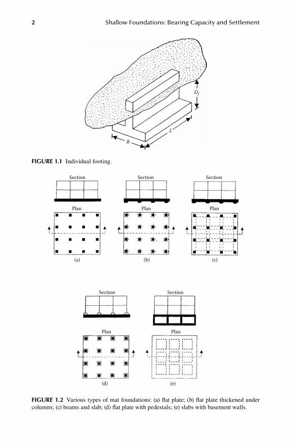
The lowest part of a structure that transmits its weight to the underlying soil or rock is the foundation. Foundations can be classified into two major categories—shallow foundations and deep foundations. Individual footings (Figure 1.1), square or rect-angular in plan, that support columns and strip footings that support walls and other similar structures are generally referred to as shallow foundations. Mat foundations, also considered shallow foundations, are reinforced concrete slabs of considerable structural rigidity that support a number of columns and wall loads. Several types of mat foundations are currently used. Some of the common types are shown schemati-cally in Figure 1.2 and include
1. Flat plate (Figure 1.2a). The mat is of uniform thickness. 2. Flat plate thickened under columns (Figure 1.2b). 3. Beams and slab (Figure 1.2c). The beams run both ways, and the columns
are located at the intersections of the beams. 4. Flat plates with pedestals (Figure 1.2d). 5. Slabs with basement walls as a part of the mat (Figure 1.2e). The walls act
as stiffeners for the mat.
When the soil located immediately below a given structure is weak, the load of the structure may be transmitted to a greater depth by piles and drilled shafts, which are considered deep foundations. This book is a compilation of the theoretical and experimental evaluations presently available in the literature as they relate to the load-bearing capacity and settlement of shallow foundations.
The shallow foundation shown in Figure 1.1 has a width B and a length L. The depth of embedment below the ground surface is equal to Df . Theoretically, when B/L is equal to zero (that is, L = ∞), a plane strain case will exist in the soil mass supporting the foundation. For most practical cases, when B/L ≤ 1/5 to 1/6, the plane strain theories will yield fairly good results. Terzaghi1 defined a shallow foundation as one in which the depth Df is less than or equal to the width B (Df /B ≤ 1). However, research studies conducted since then have shown that Df /B can be as large as 3 to 4 for shallow foundations.
1.2 typeS oF Failure in Soil at ultimate load
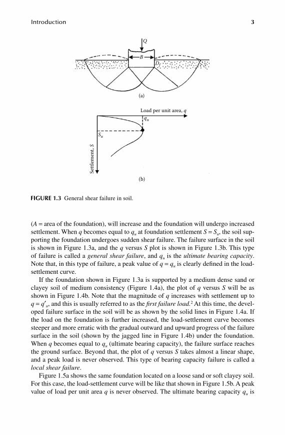
Figure 1.3 shows a shallow foundation of width B located at a depth of Df below the ground surface and supported by dense sand (or stiff, clayey soil). If this foundation is subjected to a load Q that is gradually increased, the load per unit area, q = Q/A
2 Shallow Foundations: Bearing Capacity and Settlement
Df
L
B
FiGure 1.1 Individual footing.
FiGure 1.2 Various types of mat foundations: (a) flat plate; (b) flat plate thickened under columns; (c) beams and slab; (d) flat plate with pedestals; (e) slabs with basement walls.
Section
Plan Plan Plan
Section
Section
(a) (b) (c)
(d) (e)
Plan Plan
Section
Section
Introduction 3
(A = area of the foundation), will increase and the foundation will undergo increased settlement. When q becomes equal to qu at foundation settlement S = Su, the soil sup-porting the foundation undergoes sudden shear failure. The failure surface in the soil is shown in Figure 1.3a, and the q versus S plot is shown in Figure 1.3b. This type of failure is called a general shear failure, and qu is the ultimate bearing capacity. Note that, in this type of failure, a peak value of q = qu is clearly defined in the load-settlement curve.
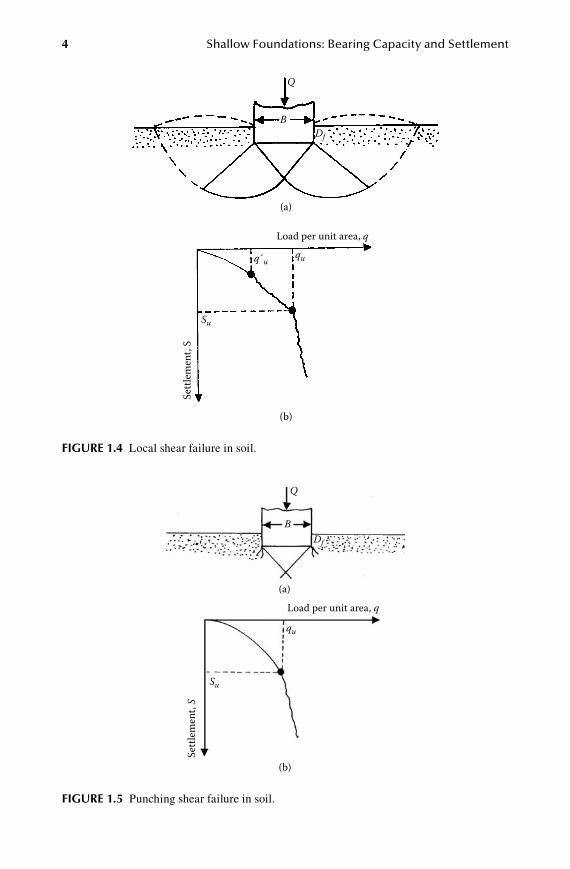
If the foundation shown in Figure 1.3a is supported by a medium dense sand or clayey soil of medium consistency (Figure 1.4a), the plot of q versus S will be as shown in Figure 1.4b. Note that the magnitude of q increases with settlement up to q = q′u, and this is usually referred to as the first failure load.2 At this time, the devel-oped failure surface in the soil will be as shown by the solid lines in Figure 1.4a. If the load on the foundation is further increased, the load-settlement curve becomes steeper and more erratic with the gradual outward and upward progress of the failure surface in the soil (shown by the jagged line in Figure 1.4b) under the foundation. When q becomes equal to qu (ultimate bearing capacity), the failure surface reaches the ground surface. Beyond that, the plot of q versus S takes almost a linear shape, and a peak load is never observed. This type of bearing capacity failure is called a local shear failure.
Figure 1.5a shows the same foundation located on a loose sand or soft clayey soil. For this case, the load-settlement curve will be like that shown in Figure 1.5b. A peak value of load per unit area q is never observed. The ultimate bearing capacity qu is
Load per unit area, qqu
Su
(a)
(b)
Settl
emen
t, S
Q
BDf
FiGure 1.3 General shear failure in soil.
4 Shallow Foundations: Bearing Capacity and Settlement
(a)
Q
BDf
Load per unit area, q
Settl
emen
t, S
Su
q´uqu
(b)
FiGure 1.4 Local shear failure in soil.
(a)
(b)
Settl
emen
t, S
Load per unit area, q
Q
BDf
qu
Su
FiGure 1.5 Punching shear failure in soil.
Introduction 5
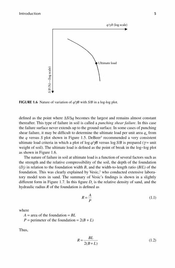
defined as the point where ΔS/Δq becomes the largest and remains almost constant thereafter. This type of failure in soil is called a punching shear failure. In this case the failure surface never extends up to the ground surface. In some cases of punching shear failure, it may be difficult to determine the ultimate load per unit area qu from the q versus S plot shown in Figure 1.5. DeBeer3 recommended a very consistent ultimate load criteria in which a plot of log q/gB versus log S/B is prepared (g = unit weight of soil). The ultimate load is defined as the point of break in the log−log plot as shown in Figure 1.6.
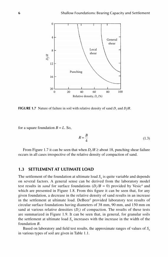
The nature of failure in soil at ultimate load is a function of several factors such as the strength and the relative compressibility of the soil, the depth of the foundation (Df) in relation to the foundation width B, and the width-to-length ratio (B/L) of the foundation. This was clearly explained by Vesic,2 who conducted extensive labora-tory model tests in sand. The summary of Vesic’s findings is shown in a slightly different form in Figure 1.7. In this figure Dr is the relative density of sand, and the hydraulic radius R of the foundation is defined as
R
AP
=
(1.1)
whereA = area of the foundation = BLP = perimeter of the foundation = 2(B + L)
Thus,
R
BLB L
=+2( )
(1.2)
q/γB (log scale)
S/B
(%)—
(log
scal
e)
Ultimate load
FiGure 1.6 Nature of variation of q/gB with S/B in a log-log plot.
6 Shallow Foundations: Bearing Capacity and Settlement
for a square foundation B = L. So,
R
B=4
(1.3)
From Figure 1.7 it can be seen that when Df /R ≥ about 18, punching shear failure occurs in all cases irrespective of the relative density of compaction of sand.
1.3 Settlement at ultimate load
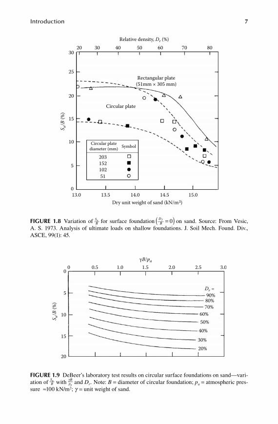
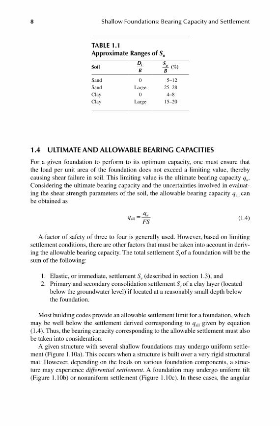
The settlement of the foundation at ultimate load Su is quite variable and depends on several factors. A general sense can be derived from the laboratory model test results in sand for surface foundations (Df /B = 0) provided by Vesic4 and which are presented in Figure 1.8. From this figure it can be seen that, for any given foundation, a decrease in the relative density of sand results in an increase in the settlement at ultimate load. DeBeer3 provided laboratory test results of circular surface foundations having diameters of 38 mm, 90 mm, and 150 mm on sand at various relative densities (Dr) of compaction. The results of these tests are summarized in Figure 1.9. It can be seen that, in general, for granular soils the settlement at ultimate load Su increases with the increase in the width of the foundation B.
Based on laboratory and field test results, the approximate ranges of values of Su in various types of soil are given in Table 1.1.
4
8
12
Df/R
16Punching
Relative density, Dr (%)
Localshear
Generalshear
0
200 20 40 60 80 100
FiGure 1.7 Nature of failure in soil with relative density of sand Dr and Df/R.
Introduction 7
30
25
20
15
S u/B
(%)
10
5
30
013.0 13.5 14.0 14.5 15.0
Dry unit weight of sand (kN/m3)
Circular plate
Circular platediameter (mm) Symbol
20315210251
Rectangular plate(51mm × 305 mm)
40 50Relative density, Dr (%)
60 7020 80
FiGure 1.8 Variation of SBu for surface foundation D
Bf =( )0 on sand. Source: From Vesic,
A. S. 1973. Analysis of ultimate loads on shallow foundations. J. Soil Mech. Found. Div., ASCE, 99(1): 45.
00 0.5 1.0 1.5
γB/pa
Dr =
S u/B
(%)
2.0 2.5
90%80%70%
60%50%40%
30%20%
3.0
5
10
15
20
FiGure 1.9 DeBeer’s laboratory test results on circular surface foundations on sand—vari-ation of S
Bu with γB
paand Dr . Note: B = diameter of circular foundation; pa = atmospheric pres-
sure ≈100 kN/m2; g = unit weight of sand.
8 Shallow Foundations: Bearing Capacity and Settlement
1.4 ultimate and allowable bearinG CapaCitieS
For a given foundation to perform to its optimum capacity, one must ensure that the load per unit area of the foundation does not exceed a limiting value, thereby causing shear failure in soil. This limiting value is the ultimate bearing capacity qu. Considering the ultimate bearing capacity and the uncertainties involved in evaluat-ing the shear strength parameters of the soil, the allowable bearing capacity qall can be obtained as
q
qFS
uall =
(1.4)
A factor of safety of three to four is generally used. However, based on limiting settlement conditions, there are other factors that must be taken into account in deriv-ing the allowable bearing capacity. The total settlement St of a foundation will be the sum of the following:
1. Elastic, or immediate, settlement Se (described in section 1.3), and 2. Primary and secondary consolidation settlement Sc of a clay layer (located
below the groundwater level) if located at a reasonably small depth below the foundation.
Most building codes provide an allowable settlement limit for a foundation, which may be well below the settlement derived corresponding to qall given by equation (1.4). Thus, the bearing capacity corresponding to the allowable settlement must also be taken into consideration.
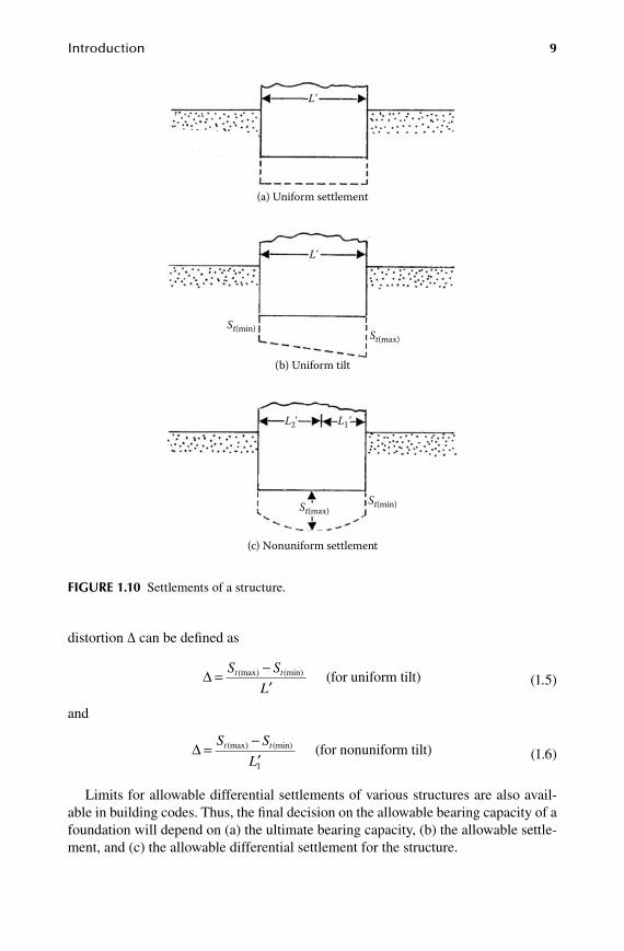
A given structure with several shallow foundations may undergo uniform settle-ment (Figure 1.10a). This occurs when a structure is built over a very rigid structural mat. However, depending on the loads on various foundation components, a struc-ture may experience differential settlement. A foundation may undergo uniform tilt (Figure 1.10b) or nonuniform settlement (Figure 1.10c). In these cases, the angular
table 1.1approximate ranges of Su
SoilDf
BSB
u ( )%
Sand 0 5–12Sand Large 25–28Clay 0 4–8Clay Large 15–20
Introduction 9
distortion Δ can be defined as
∆ = -
′S S
Lt t(max) (min) (for uniform tilt)
(1.5)
and
∆ = -′
S S
Lt t(max) (min)
1
(for nonuniform tilt)
(1.6)
Limits for allowable differential settlements of various structures are also avail-able in building codes. Thus, the final decision on the allowable bearing capacity of a foundation will depend on (a) the ultimate bearing capacity, (b) the allowable settle-ment, and (c) the allowable differential settlement for the structure.
(a) Uniform settlement
(c) Nonuniform settlement
(b) Uniform tilt
St(min)
St(min)St(max)
St(max)
L'
L'
L2' L1'
FiGure 1.10 Settlements of a structure.
10 Shallow Foundations: Bearing Capacity and Settlement
reFerenCeS
1. Terzaghi, K. 1943. Theoretical Soil Mechanics. New York: Wiley. 2. Vesic, A. S. 1973. Analysis of ultimate loads on shallow foundations. J. Soil Mech.
Found. Div., ASCE, 99(1): 45. 3. DeBeer, E. E. 1967. Proefondervindelijke bijdrage tot de studie van het gransdraagver-
mogen van zand onder funderingen op staal, Bepaling von der vormfactor sb. Annales des Travaux Publics de Belgique 6: 481.
4. Vesic, A. S. 1963. Bearing capacity of deep foundations in sand. Highway Res. Rec., National Research Council, Washington, D.C. 39:12.
11
2 Ultimate Bearing Capacity Theories—Centric Vertical Loading
2.1 introduCtion
Over the last 60 years, several bearing capacity theories for estimating the ultimate bearing capacity of shallow foundations have been proposed. This chapter summa-rizes some of the important works developed so far. The cases considered in this chapter assume that the soil supporting the foundation extends to a great depth and also that the foundation is subjected to centric vertical loading. The variation of the ultimate bearing capacity in anisotropic soils is also considered.
2.2 terzaGhi’S bearinG CapaCity theory
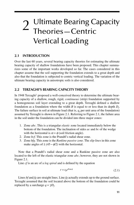
In 1948 Terzaghi1 proposed a well-conceived theory to determine the ultimate bear-ing capacity of a shallow, rough, rigid, continuous (strip) foundation supported by a homogeneous soil layer extending to a great depth. Terzaghi defined a shallow foundation as a foundation where the width B is equal to or less than its depth Df. The failure surface in soil at ultimate load (that is, qu per unit area of the foundation) assumed by Terzaghi is shown in Figure 2.1. Referring to Figure 2.1, the failure area in the soil under the foundation can be divided into three major zones:
1. Zone abc. This is a triangular elastic zone located immediately below the bottom of the foundation. The inclination of sides ac and bc of the wedge with the horizontal is a = f (soil friction angle).
2. Zone bcf. This zone is the Prandtl’s radial shear zone. 3. Zone bfg. This zone is the Rankine passive zone. The slip lines in this zone
make angles of ± (45 − f/2) with the horizontal.
Note that a Prandtl’s radial shear zone and a Rankine passive zone are also located to the left of the elastic triangular zone abc; however, they are not shown in Figure 2.1.
Line cf is an arc of a log spiral and is defined by the equation
r r e= 0
θ φtan
(2.1)
Lines bf and fg are straight lines. Line fg actually extends up to the ground surface. Terzaghi assumed that the soil located above the bottom of the foundation could be replaced by a surcharge q = g Df.
12 Shallow Foundations: Bearing Capacity and Settlement
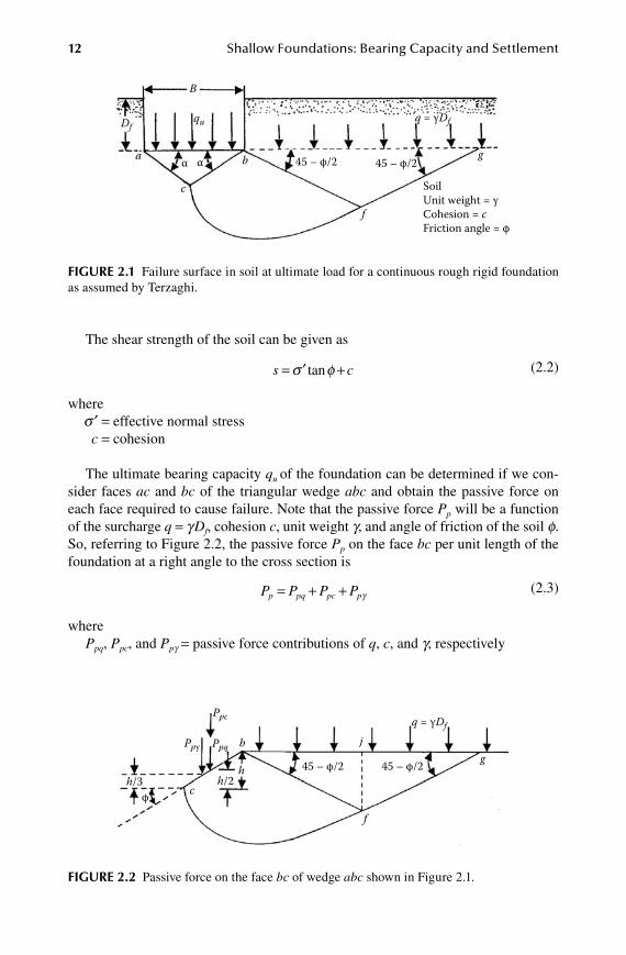
The shear strength of the soil can be given as
s c= ′ +σ φtan (2.2)
where s ′ = effective normal stress c = cohesion
The ultimate bearing capacity qu of the foundation can be determined if we con-sider faces ac and bc of the triangular wedge abc and obtain the passive force on each face required to cause failure. Note that the passive force Pp will be a function of the surcharge q = g Df, cohesion c, unit weight g, and angle of friction of the soil f. So, referring to Figure 2.2, the passive force Pp on the face bc per unit length of the foundation at a right angle to the cross section is
P P P Pp pq pc p= + + γ
(2.3)
wherePpq, Ppc, and Ppg = passive force contributions of q, c, and g, respectively
h/3 h/2
Ppγ Ppq j
Ppc
c
gb
h 45 – φ/2 45 – φ/2
q = γDf
φ
f
FiGure 2.2 Passive force on the face bc of wedge abc shown in Figure 2.1.
B
a
c
b g
f
α α 45 – φ/2
SoilUnit weight = γCohesion = cFriction angle = φ
45 – φ/2
quDfq = γDf
FiGure 2.1 Failure surface in soil at ultimate load for a continuous rough rigid foundation as assumed by Terzaghi.

Ultimate Bearing CapacityTheories—Centric Vertical Loading 13
It is important to note that the directions of Ppq, Ppc, and Ppg are vertical since the face bc makes an angle f with the horizontal, and Ppq, Ppc, and Ppg must make an angle f to the normal drawn to bc. In order to obtain Ppq, Ppc, and Ppg , the method of superposition can be used; however, it will not be an exact solution.
2.2.1 Relationship foR Ppq (f ≠ 0, g = 0, q ≠ 0, c = 0)
Consider the free body diagram of the soil wedge bcfj shown in Figure 2.2 (also shown in Figure 2.3). For this case, the center of the log spiral (of which cf is an arc) will be at point b. The forces per unit length of the wedge bcfj due to the surcharge q only are shown in Figure 2.3a, and they are
1. Ppq
2. Surcharge q 3. The Rankine passive force Pp(1)
4. The frictional resisting force F along the arc cf
The Rankine passive force Pp(1) can be expressed as
P qK H qHp p d d( ) tan1
2 452
= = +
φ
(2.4)
hh/2 Hd/2
Hd
qb
j
f
F
B
B/4
135 – φ/2
45 – φ/2
(a)
(b)
φ
φ φ
c
Ppq
Pp (1)
Ppq Ppq
FiGure 2.3 Determination of Ppq (f ≠ 0, g = 0, q ≠ 0, c = 0).
14 Shallow Foundations: Bearing Capacity and Settlement
where
H f jd =
Kp = Rankine passive earth pressure coefficient = tan2(45 + f/2)
According to the property of a log spiral defined by the equation r = r0eqtanf, the radial line at any point makes an angle f with the normal; hence, the line of action of the frictional force F will pass through b (the center of the log spiral as shown in Figure 2.3a). Taking the moment of all forces about point b:
P
Bq bj
bjP
Hpq p
d
4 2 21
=
+( ) ( )
(2.5)
let
bc r
B= =
0
2secφ (2.6)
From equation (2.1):
bf r r e= =-
1 0
34 2π φ φtan
(2.7)
So,
bj r= -
1 45
2cos
φ
(2.8)
and
H rd = -
1 45
2sin
φ
(2.9)
Combining equations (2.4), (2.5), (2.8), and (2.9):
P Bqr qr
pq
4
452
2
4521
2 212 2
=-
+
-
cos sinφ φ
+
tan2 452
2
φ
or
P
Bqrpq = -
445
212 2cos
φ
(2.10)
Now, combining equations (2.6), (2.7), and (2.10):
P qB epq =
-
-
sec cos
tan2
234 2 2 45
2φ φπ φ φ
=+
-
qBe
234 2
24 452
π φ φ
φ
tan
cos
(2.11)
Ultimate Bearing CapacityTheories—Centric Vertical Loading 15
Considering the stability of the elastic wedge abc under the foundation as shown in Figure 2.3b
q B Pq pq( )× =1 2
whereqq = load per unit area on the foundation, or
qP
Bq
eq
pq= =+
-
2
2 452
234 2
2
π φ φ
φ
tan
cos
=
N
q
q
qN
� ���� ����
(2.12)
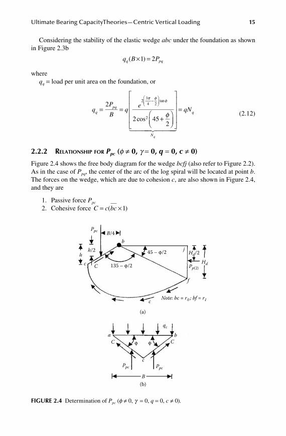
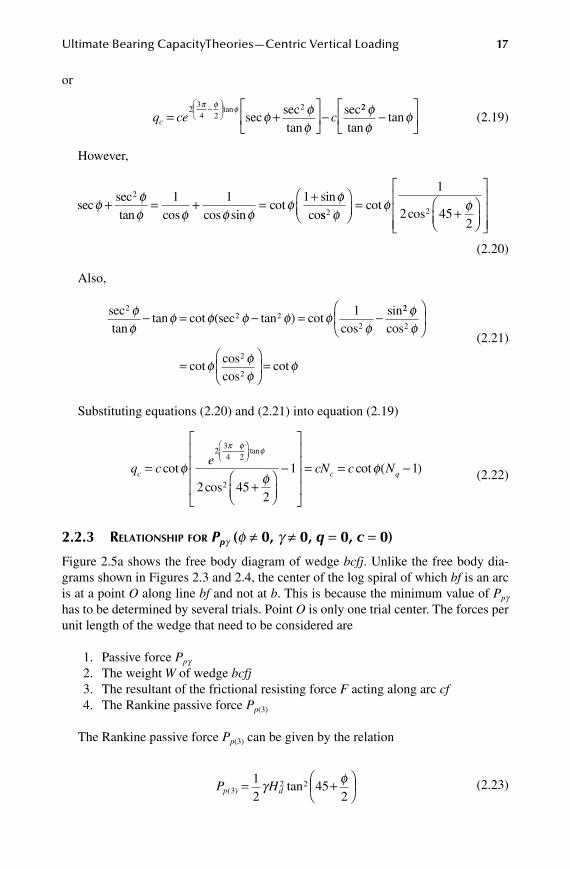
2.2.2 Relationship foR Ppc (f ≠ 0, g = 0, q = 0, c ≠ 0)
Figure 2.4 shows the free body diagram for the wedge bcfj (also refer to Figure 2.2). As in the case of Ppq, the center of the arc of the log spiral will be located at point b. The forces on the wedge, which are due to cohesion c, are also shown in Figure 2.4, and they are
1. Passive force Ppc
2. Cohesive force C c bc= ×( )1
h/2
B/4
135 – φ/2
φ φ
45 – φ/2
bj
f
c
aC C
B
c
b
Note: bc = r0 ; bf = r1
C
(a)
(b)
ch
Ppc
Hd
Hd/2
Pp(2)
Ppc Ppc
qc
FiGure 2.4 Determination of Ppc (f ≠ 0, g = 0, q = 0, c ≠ 0).
16 Shallow Foundations: Bearing Capacity and Settlement
3. Rankine passive force due to cohesion
P c K H cHp p d d( ) tan2 2 2 45
2= = +
φ
4. Cohesive force per unit area c along arc cf
Taking the moment of all the forces about point b:
PB
P rpc p4
452
22
1
= -
( )
sinφ
+ Mc
(2.13)
where
M c cf
cc = =moment due to cohesion along arc
2 tanφr r1
202-( )
(2.14)
So,
PB
cH rpc d4
2 452
451
= +
tan sinφ --
+
-( )φ
φ2
22 1
202c
r rtan
(2.15)
The relationships for Hd , r0 , and r1 in terms of B and f are given in equations (2.9), (2.6), and (2.7), respectively. Combining equations (2.6), (2.7), (2.9), and (2.15), and noting that sin2 (45 − f/2) × tan (45 + f/2) = ½ cos f,
P Bc epc =
-
(sec )costan
22
34 2
2φ φπ φ φ
+
-
Bc
e2
22
34 2
tansec
tan
φφ
π φ φ
(2.16)
Considering the equilibrium of the soil wedge abc (Figure 2.4b):
q B C Pc pc( ) sin× = +1 2 2φ
or
q B cB Pc pc= +sec sinφ φ 2
(2.17)
whereqc = load per unit area of the foundation
Combining equations (2.16) and (2.17):
q c e
cec = +
-
-
secsectan
tanφ φ
φ
π φ φ π φ2
34 2
2 234 2
- +tan sec
tantan
φ φφ
φcc
2
(2.18)
Ultimate Bearing CapacityTheories—Centric Vertical Loading 17
or
q ce cc = +
-
-
2
34 2
2π φ φφ φ
φtan
secsectan
sec22 φφ
φtan
tan-
(2.19)
However,
secsectan cos cos sin
cotsin
coφ φ
φ φ φ φφ φ+ = + = +2 1 1 1
sscot
cos2 2
1
2 452
φφ φ
=+
(2.20)
Also,
sectan
tan cot (sec tan ) cotcos
sin22 2
2
1φφ
φ φ φ φ φφ
- = - = -22
2
2
2
φφ
φ φφ
φ
cos
cotcoscos
cot
=
=
(2.21)
Substituting equations (2.20) and (2.21) into equation (2.19)
q ce
c =+
--
cot
cos
tan
φφ
π φ φ234 2
22 452
1 1
= = -cN c Nc qcot ( )φ
(2.22)
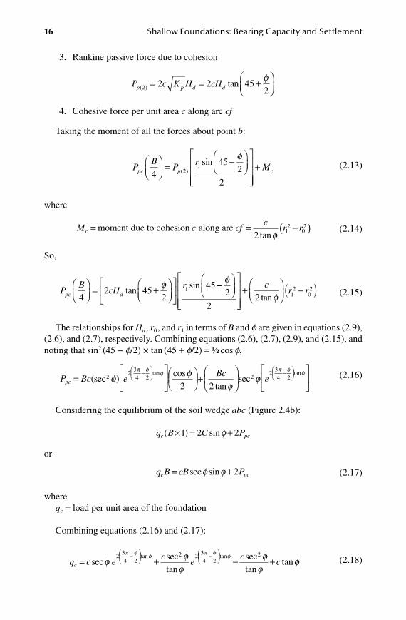
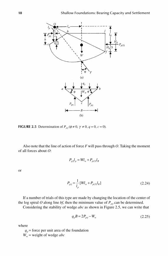
2.2.3 Relationship foR Ppg (f ≠ 0, g ≠ 0, q = 0, c = 0)
Figure 2.5a shows the free body diagram of wedge bcfj. Unlike the free body dia-grams shown in Figures 2.3 and 2.4, the center of the log spiral of which bf is an arc is at a point O along line bf and not at b. This is because the minimum value of Ppg has to be determined by several trials. Point O is only one trial center. The forces per unit length of the wedge that need to be considered are
1. Passive force Ppg 2. The weight W of wedge bcfj 3. The resultant of the frictional resisting force F acting along arc cf 4. The Rankine passive force Pp(3)
The Rankine passive force Pp(3) can be given by the relation
P Hp d( ) tan3
2 212
452
= +
γ φ
(2.23)
18 Shallow Foundations: Bearing Capacity and Settlement
Also note that the line of action of force F will pass through O. Taking the moment of all forces about O:
P l Wl P lp p w p Rγ = + ( )3
or
Pl
Wl P lpp
w p Rγ = +13[ ]( )
(2.24)
If a number of trials of this type are made by changing the location of the center of the log spiral O along line bf, then the minimum value of Ppg can be determined.
Considering the stability of wedge abc as shown in Figure 2.5, we can write that
q B P Wp wγ γ= -2
(2.25)
where qg = force per unit area of the foundation
Ww = weight of wedge abc
h
(a)
(b)
Wf
F
a
B
b
lpO
c
Ppγ
qγ
Ppγ Ppγ
Ww
c
b jlR
Hd/3Pp(3)
Hd
lw
φ
φ φ
h/3
FiGure 2.5 Determination of Ppg (f ≠ 0, g ≠ 0, q = 0, c = 0).
Ultimate Bearing CapacityTheories—Centric Vertical Loading 19
However,
W
Bw =
2
4γ φtan
(2.26)
So,
q
BP
Bpγ γ γ φ= -
12
4
2
tan
(2.27)
The passive force Ppg can be expressed in the form
P h K
BK B Kp p p pγ γ γ γγ γ φ γ φ= =
=1
212 2
18
22
2 2tantan
(2.28)
where Kpg = passive earth pressure coefficientSubstituting equation (2.28) into equation (2.27)
q
BB K
BB Kp pγ γ γγ φ γ φ γ= -
=1 1
4 412
12
2 22
2tan tan tan φφ φ γ γ-
=tan
212
BN
(2.29)
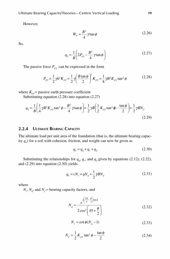
2.2.4 Ultimate BeaRing CapaCity
The ultimate load per unit area of the foundation (that is, the ultimate bearing capac-ity qu) for a soil with cohesion, friction, and weight can now be given as
q q q qu q c= + + γ
(2.30)
Substituting the relationships for qq, qc, and qg given by equations (2.12), (2.22), and (2.29) into equation (2.30) yields
q cN qN BNu c q= + + 1
2γ γ
(2.31)
whereNc, Nq, and Ng = bearing capacity factors, and
Ne
q =+
-
234 2
22 452
π φ φ
φ
tan
cos
(2.32)
N Nc q= -cot ( )φ 1
(2.33)
N K pγ γ φ φ= -1
2 22tan
tan
(2.34)

20 Shallow Foundations: Bearing Capacity and Settlement
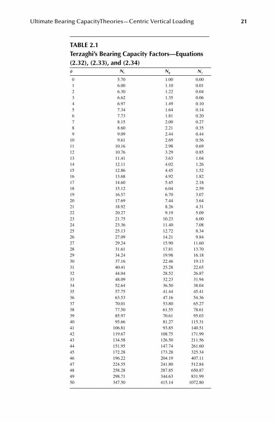
Table 2.1 gives the variations of the bearing capacity factors with soil friction angle f given by equations (2.32), (2.33), and (2.34). The values of Ng were obtained by Kumbhojkar.2
Krizek3 gave simple empirical relations for Terzaghi’s bearing capacity factors Nc, Nq, and Ng with a maximum deviation of 15%. They are as follows:
Nc = +
-228 4 3
40. φφ
(2.35a)
Nq = +
-40 540
φφ
(2.35b)
Nγ
φφ
=-
640
(2.35c)
wheref = soil friction angle, in degrees
Equations (2.35a), (2.35b), and (2.35c) are valid for f = 0 to 35°. Thus, substitut-ing equation (2.35) into (2.31),
q
c q Bu = + + + +
-= °( . ) ( )228 4 3 40 5 3
400
φ φ φγφ
φ(for to 35 )°
(2.36)
For foundations that are rectangular or circular in plan, a plane strain condition in soil at ultimate load does not exist. Therefore, Terzaghi1 proposed the following relationships for square and circular foundations:
q cN qN BNu c q= + +1 3 0 4. . γ γ (square foundation; pllan )B B×
(2.37)
and
q cN qN BNu c q= + +1 3 0 3. . γ γ (circular foundation; diameter )B
(2.38)
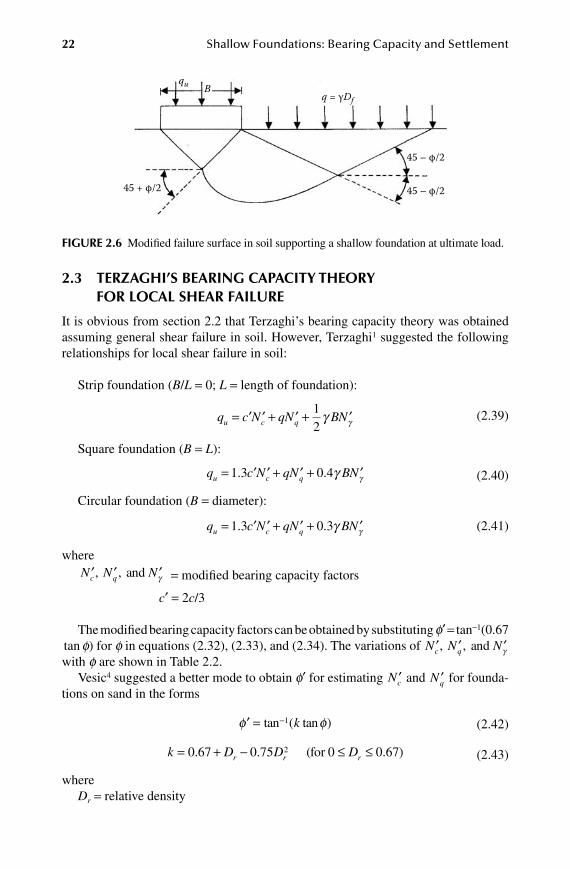
Since Terzaghi’s founding work, numerous experimental studies to estimate the ultimate bearing capacity of shallow foundations have been conducted. Based on these studies, it appears that Terzaghi’s assumption of the failure surface in soil at ultimate load is essentially correct. However, the angle a that sides ac and bc of the wedge (Figure 2.1) make with the horizontal is closer to 45 + f/2 and not f, as assumed by Terzaghi. In that case, the nature of the soil failure surface would be as shown in Figure 2.6.
The method of superposition was used to obtain the bearing capacity factors Nc, Nq, and Ng . For derivations of Nc and Nq, the center of the arc of the log spiral cf is located at the edge of the foundation. That is not the case for the derivation of Ng . In effect, two different surfaces are used in deriving equation (2.31); however, it is on the safe side.
Ultimate Bearing CapacityTheories—Centric Vertical Loading 21
table 2.1terzaghi’s bearing Capacity Factors—equations (2.32), (2.33), and (2.34)f Nc Nq Ng
0 5.70 1.00 0.00 1 6.00 1.10 0.01 2 6.30 1.22 0.04 3 6.62 1.35 0.06 4 6.97 1.49 0.10 5 7.34 1.64 0.14 6 7.73 1.81 0.20 7 8.15 2.00 0.27 8 8.60 2.21 0.35 9 9.09 2.44 0.4410 9.61 2.69 0.5611 10.16 2.98 0.6912 10.76 3.29 0.8513 11.41 3.63 1.0414 12.11 4.02 1.2615 12.86 4.45 1.5216 13.68 4.92 1.8217 14.60 5.45 2.1818 15.12 6.04 2.5919 16.57 6.70 3.0720 17.69 7.44 3.6421 18.92 8.26 4.3122 20.27 9.19 5.0923 21.75 10.23 6.0024 23.36 11.40 7.0825 25.13 12.72 8.3426 27.09 14.21 9.8427 29.24 15.90 11.6028 31.61 17.81 13.7029 34.24 19.98 16.1830 37.16 22.46 19.1331 40.41 25.28 22.6532 44.04 28.52 26.8733 48.09 32.23 31.9434 52.64 36.50 38.0435 57.75 41.44 45.4136 63.53 47.16 54.3637 70.01 53.80 65.2738 77.50 61.55 78.6139 85.97 70.61 95.0340 95.66 81.27 115.3141 106.81 93.85 140.5142 119.67 108.75 171.9943 134.58 126.50 211.5644 151.95 147.74 261.6045 172.28 173.28 325.3446 196.22 204.19 407.1147 224.55 241.80 512.8448 258.28 287.85 650.8749 298.71 344.63 831.9950 347.50 415.14 1072.80
22 Shallow Foundations: Bearing Capacity and Settlement
2.3 terzaGhi’S bearinG CapaCity theory For loCal Shear Failure
It is obvious from section 2.2 that Terzaghi’s bearing capacity theory was obtained assuming general shear failure in soil. However, Terzaghi1 suggested the following relationships for local shear failure in soil:
Strip foundation (B/L = 0; L = length of foundation):
q c N qN BNu c q= ′ ′ + ′ + ′1
2γ γ
(2.39)
Square foundation (B = L):
q c N qN BNu c q= ′ ′ + ′ + ′1 3 0 4. . γ γ (2.40)
Circular foundation (B = diameter):
q c N qN BNu c q= ′ ′ + ′ + ′1 3 0 3. . γ γ
(2.41)
where′ ′ ′N N Nc q, , and γ = modified bearing capacity factors
c′ = 2c/3
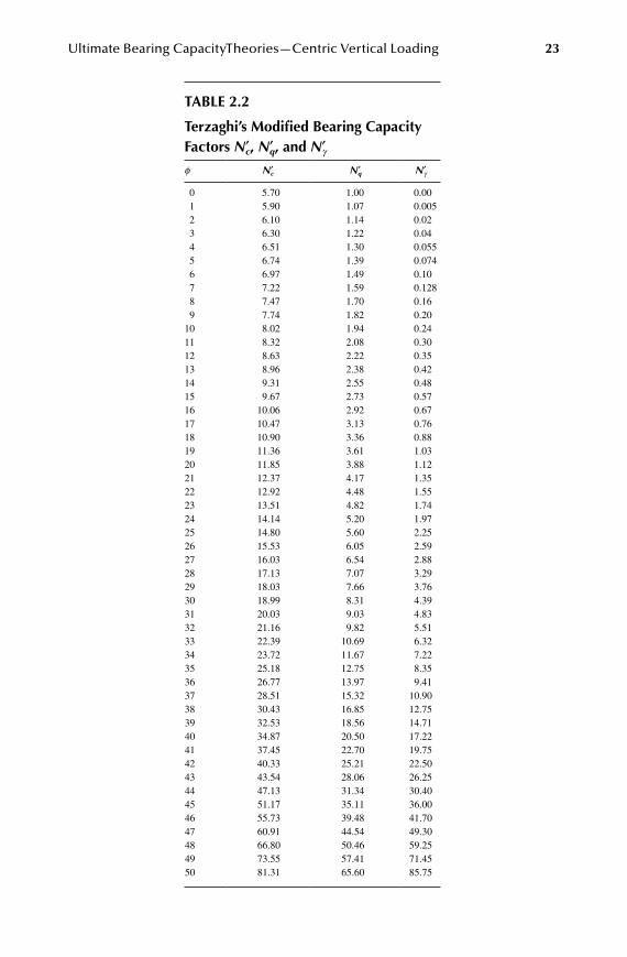
The modified bearing capacity factors can be obtained by substituting f′ = tan-1(0.67 tan f) for f in equations (2.32), (2.33), and (2.34). The variations of ′ ′ ′N N Nc q, , and γ with f are shown in Table 2.2.
Vesic4 suggested a better mode to obtain f′ for estimating ′Nc and ′Nq for founda-tions on sand in the forms
′ = -φ φtan ( tan )1 k (2.42)
k D D Dr r r= + - ≤ ≤0 67 0 75 0 672. . . )(for 0 (2.43)
whereDr = relative density
Bqu
q = γDf
45 – φ/2
45 – φ/245 + φ/2
FiGure 2.6 Modified failure surface in soil supporting a shallow foundation at ultimate load.
Ultimate Bearing CapacityTheories—Centric Vertical Loading 23
table 2.2
terzaghi’s modified bearing Capacity Factors N′c, N′q, and N′gf N′c N′q N′g
0 5.70 1.00 0.00 1 5.90 1.07 0.005 2 6.10 1.14 0.02 3 6.30 1.22 0.04 4 6.51 1.30 0.055 5 6.74 1.39 0.074 6 6.97 1.49 0.10 7 7.22 1.59 0.128 8 7.47 1.70 0.16 9 7.74 1.82 0.2010 8.02 1.94 0.2411 8.32 2.08 0.3012 8.63 2.22 0.3513 8.96 2.38 0.4214 9.31 2.55 0.4815 9.67 2.73 0.5716 10.06 2.92 0.6717 10.47 3.13 0.7618 10.90 3.36 0.8819 11.36 3.61 1.0320 11.85 3.88 1.1221 12.37 4.17 1.3522 12.92 4.48 1.5523 13.51 4.82 1.7424 14.14 5.20 1.9725 14.80 5.60 2.2526 15.53 6.05 2.5927 16.03 6.54 2.8828 17.13 7.07 3.2929 18.03 7.66 3.7630 18.99 8.31 4.3931 20.03 9.03 4.8332 21.16 9.82 5.5133 22.39 10.69 6.3234 23.72 11.67 7.2235 25.18 12.75 8.3536 26.77 13.97 9.4137 28.51 15.32 10.9038 30.43 16.85 12.7539 32.53 18.56 14.7140 34.87 20.50 17.2241 37.45 22.70 19.7542 40.33 25.21 22.5043 43.54 28.06 26.2544 47.13 31.34 30.4045 51.17 35.11 36.0046 55.73 39.48 41.7047 60.91 44.54 49.3048 66.80 50.46 59.2549 73.55 57.41 71.4550 81.31 65.60 85.75
24 Shallow Foundations: Bearing Capacity and Settlement
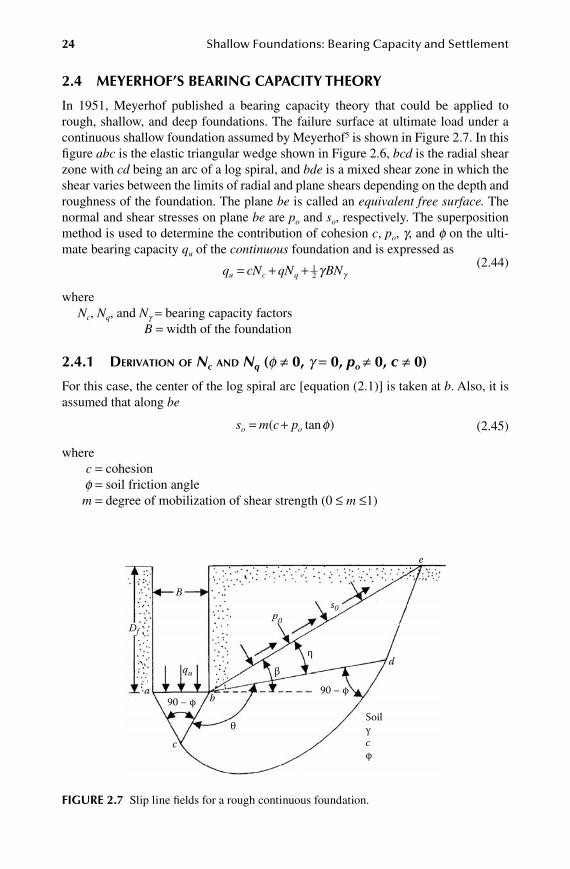
2.4 meyerhoF’S bearinG CapaCity theory
In 1951, Meyerhof published a bearing capacity theory that could be applied to rough, shallow, and deep foundations. The failure surface at ultimate load under a continuous shallow foundation assumed by Meyerhof5 is shown in Figure 2.7. In this figure abc is the elastic triangular wedge shown in Figure 2.6, bcd is the radial shear zone with cd being an arc of a log spiral, and bde is a mixed shear zone in which the shear varies between the limits of radial and plane shears depending on the depth and roughness of the foundation. The plane be is called an equivalent free surface. The normal and shear stresses on plane be are po and so, respectively. The superposition method is used to determine the contribution of cohesion c, po, g, and f on the ulti-mate bearing capacity qu of the continuous foundation and is expressed as
q cN qN BNu c q= + + 1
2 γ γ (2.44)
whereNc, Nq, and Ng = bearing capacity factors
B = width of the foundation
2.4.1 DeRivation of Nc anD Nq (f ≠ 0, g = 0, po ≠ 0, c ≠ 0)
For this case, the center of the log spiral arc [equation (2.1)] is taken at b. Also, it is assumed that along be
s m c po o= +( tan )φ (2.45)
where c = cohesion f = soil friction angle m = degree of mobilization of shear strength (0 ≤ m ≤1)
B
Df
qu
p0
s0
e
d
b
c
90 – φ90 – φ
Soilγcφ
θ
a
βη
FiGure 2.7 Slip line fields for a rough continuous foundation.

Ultimate Bearing CapacityTheories—Centric Vertical Loading 25
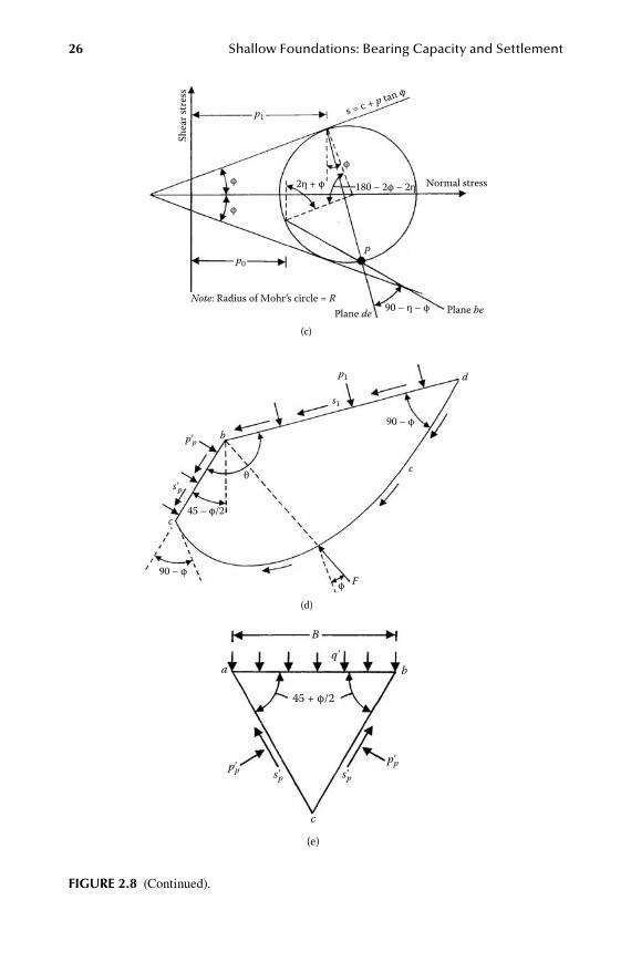
Now consider the linear zone bde (Figure 2.8a). Plastic equilibrium requires that the shear strength s1 under the normal stress p1 is fully mobilized, or
s c p1 1= + tanφ (2.46)
Figure 2.8b shows the Mohr’s circle representing the stress conditions on zone bde. Note that P is the pole. The traces of planes bd and be are also shown in the figure. For the Mohr’s circle,
R
s= 1
cosφ
(2.47)
whereR = radius of the Mohr’s circle
90 – φ
φ
φ
(a) Linear zone bde
Shea
r str
ess
90 + φ
e
90 – η – φ s0p0
p1
c
P
b
s1
s0
s1
2η + φ
φ2η
η
Normal stress
Plane bd
Note: Radius of Mohr’s circle = R
(b)Plane be
s = c + p tan φ
s1
p1
d
η
β
FiGure 2.8 Determination of Nq and Nc .
26 Shallow Foundations: Bearing Capacity and Settlement
P
p1
p0
p'p
s'p
p1 d
b
F
c
c
s1
φ 2η + φ
φ
φ
Shea
r str
ess
Normal stress
Plane de(c)
(d)
Plane beNote: Radius of Mohr’s circle = R
180 – 2φ – 2η
90 – η – φ
90 – φ
90 – φ
45 – φ/2
φ
θ
s = c + p tan φ
B
c
aq'
p'pp'p
s'p s'p
b
45 + φ/2
(e)
FiGure 2.8 (Continued).
Ultimate Bearing CapacityTheories—Centric Vertical Loading 27
Also,
s R
so = + = +
cos( )cos( )
cos2
21η φ η φφ
(2.48)
Combining equations (2.45), (2.46), and (2.48):
cos( )
costan
( tan )costan
21 1
η φ φφ
φ φ+ =+
= ++
sc p
m c pc p
o o
φφ (2.49)
Again, referring to the trace of plane de (Figure 2.8c),
s R1 = cosφ
R
c p=
+ 1 tan
cos
φφ
(2.50)
Note that
p R p R1 0 2+ = + +sin sin( )φ η φ
p R p
c po1
12 2= + - + =+
[sin( ) sin ]tan
cos[sin(η φ φ φ
φη + - +φ φ) sin ] po
(2.51)
Figure 2.8d shows the free body diagram of zone bcd. Note that the normal and shear stresses on the face bc are ′pp and ′sp, or
′ = + ′s c pp p tanφ
or
′ = ′ -p s cp p( )cotφ
(2.52)
Taking the moment of all forces about b,
p
rp
rMp c1
12
02
2 20
- ′
+ =
(2.53)
where
r bc0 =
r bd r e1 0= = θ φtan
(2.54)
It can be shown that
M
cr rc = -( )
2 12
02
tanφ (2.55)
28 Shallow Foundations: Bearing Capacity and Settlement
Substituting equations (2.54) and (2.55) into equation (2.53) yields
′ = + -p p e c ep 1
2 2 1θ φ θ φφtan tancot ( )
(2.56)
Combining equations (2.52) and (2.56)
′ = +s c p ep ( tan ) tan
12φ θ φ
(2.57)
Figure 2.8e shows the free body diagram of wedge abc. Resolving the forces in the vertical direction,
2 2
452
452
′+
+
+p
B
p
coscosφ
φ22 2
452
452
′+
+
s
B
p
cossinφ
φ == ′q B
whereq′ = load per unit area of the foundation, or
′ = ′ + ′ -
q p sp p cot 452φ
(2.58)
Substituting equations (2.51), (2.52), and (2.57) into equation (2.58) and further simplifying yields
′ = +- +
-
q c
e
N
cot( sin )
sin sin( )
tan
φ φφ η φ
θ φ11 2
12
cc
pe
o
� ����� �����
+ +-( sin ) tan1
1
2φ θ φ
sin sin( )φ η φ2 +
= +
N
c o q
q
cN p N
� ���� ����
(2.59)
whereNc, Nq = bearing capacity factors
The bearing capacity factors will depend on the degree of mobilization m of shear strength on the equivalent free surface. This is because m controls h. From equation (2.49)
cos( )
( tan )cos
tan2
1
η φ φ φφ
+ =+
+m c p
c po
For m = 0, cos(2h + f) = 0, or
η φ= -45
2 (2.60)
Ultimate Bearing CapacityTheories—Centric Vertical Loading 29
For m = 1, cos(2h + f) = cos f, or
η = 0 (2.61)
Also, the factors Nc and Nq are influenced by the angle of inclination of the equiva-lent free surface b. From the geometry of Figure 2.7,
θ β η φ= °+ - -135
2 (2.62)
From equation (2.60), for m = 0, the value of h is (45 – f/2). So,
θ β= °+ =90 0(for m )
(2.63)
Similarly, for m = 1 [since h = 0; equation (2.61)]:
θ β φ= °+ - =135
21(for m )
(2.64)
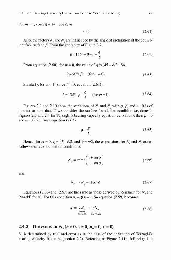
Figures 2.9 and 2.10 show the variations of Nc and Nq with f, b, and m. It is of interest to note that, if we consider the surface foundation condition (as done in Figures 2.3 and 2.4 for Terzaghi’s bearing capacity equation derivation), then b = 0 and m = 0. So, from equation (2.63),
θ π=
2 (2.65)
Hence, for m = 0, h = 45 – f/2, and q = π/2, the expressions for Nc and Nq are as follows (surface foundation condition):
N eq = +
-
π φ φφ
tan sinsin
11
(2.66)
and
N Nc q= -( ) cot1 φ
(2.67)
Equations (2.66) and (2.67) are the same as those derived by Reissner6 for Nq and Prandtl7 for Nc. For this condition po = gDf = q. So equation (2.59) becomes
′ = +q cN qNc q
Eq. (2.66) Eq. (2.67)
� �
(2.68)
2.4.2 DeRivation of Ng (f ≠ 0, g ≠ 0, po = 0, c = 0)
Ng is determined by trial and error as in the case of the derivation of Terzaghi’s bearing capacity factor Ng (section 2.2). Referring to Figure 2.11a, following is a
30 Shallow Foundations: Bearing Capacity and Settlement
step-by-step approach for the derivation of Ng :
1. Choose values for f and the angle b (such as +30°, +40°, −30°…). 2. Choose a value for m (such as m = 0 or m = 1). 3. Determine the value of q from equation (2.63) or (2.64) for m = 0 or
m = 1, as the case may be. 4. With known values of q and b, draw lines bd and be. 5. Select a trial center such as O and draw an arc of a log spiral connecting
points c and d. The log spiral follows the equation r = r0eqtanf. 6. Draw line de. Note that lines bd and de make angles of 90 – f due to the
restrictions on slip lines in the linear zone bde. Hence the trial failure sur-face is not, in general, continuous at d.
10,000
β (deg)+90
+60
+30
–30
0
1,000
100
Nc
10
10 10 20 30 40 50
Soil friction angle, φ (deg)
m = 0m = 1
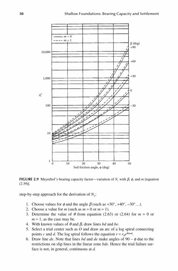
FiGure 2.9 Meyerhof’s bearing capacity factor—variation of Nc with b, f, and m [equation (2.59)].

Ultimate Bearing CapacityTheories—Centric Vertical Loading 31
7. Consider the trial wedge bcdf. Determine the following forces per unit length of the wedge at right angles to the cross section shown: (a) weight of wedge bcdf—W, and (b) Rankine passive force on the face df—Pp(R).
8. Take the moment of the forces about the trial center of the log spiral O, or
PWl P l
lp
w p R R
pγ =
+ ( )
(2.69)
wherePpg = passive force due to g and f only
10,000
β (deg)+90
+60
+30
–30
0
1,000
100
Nq
10
1 10 20 30 400 50Soil friction angle, φ (deg)
m = 0m = 1
FiGure 2.10 Meyerhof’s bearing capacity factor—variation of Nq with b, f, and m [equation (2.59)].
32 Shallow Foundations: Bearing Capacity and Settlement
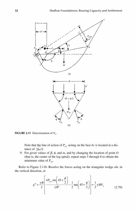
Note that the line of action of Ppg acting on the face bc is located at a dis-tance of 2 3bc/ .
9. For given values of b, f, and m, and by changing the location of point O (that is, the center of the log spiral), repeat steps 5 through 8 to obtain the minimum value of Ppg .
Refer to Figure 2.11b. Resolve the forces acting on the triangular wedge abc in the vertical direction, or
′′ =+
- +
q
BP
B
pγφ
γφγ
2
4 452 1
245
22
sin
tan
= 12
γ γBN (2.70)
B
Ppγ
Ppγ Ppγ
a
c
b
W
B
q"
f
e
dOlp
WW
lw
lRPp(R)
φ
θ
(a)
(b)
45 + φ/2
φ φ
β
η
FiGure 2.11 Determination of Ng .
Ultimate Bearing CapacityTheories—Centric Vertical Loading 33
where q″ = force per unit area of the foundation N g = bearing capacity factor
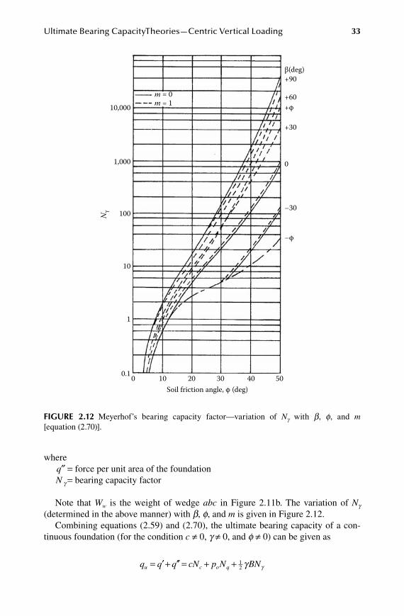
Note that Ww is the weight of wedge abc in Figure 2.11b. The variation of Ng (determined in the above manner) with b, f, and m is given in Figure 2.12.
Combining equations (2.59) and (2.70), the ultimate bearing capacity of a con-tinuous foundation (for the condition c ≠ 0, g ≠ 0, and f ≠ 0) can be given as
q q q cN p N BNu c o q= ′+ ′′ = + + 1
2 γ γ
10,000
1,000
100
10
Nγ
1
0.1 10 20 30 400 50Soil friction angle, φ (deg)
–φ
–30
+30
+φ+60
+90β(deg)
0
m = 0m = 1
FiGure 2.12 Meyerhof’s bearing capacity factor—variation of Ng with b, f, and m [equation (2.70)].
34 Shallow Foundations: Bearing Capacity and Settlement
table 2.3Variation of meyerhof’s bearing Capacity Factors Nc, Nq, and Ng [equations (2.66), (2.67), and (2.72)]f Nc Nq Ng
0 5.14 1.00 0.00 1 5.38 1.09 0.002 2 5.63 1.20 0.01 3 5.90 1.31 0.02 4 6.19 1.43 0.04 5 6.49 1.57 0.07 6 6.81 1.72 0.11 7 7.16 1.88 0.15 8 7.53 2.06 0.21 9 7.92 2.25 0.2810 8.35 2.47 0.3711 8.80 2.71 0.4712 9.28 2.97 0.6013 9.81 3.26 0.7414 10.37 3.59 0.9215 10.98 3.94 1.1316 11.63 4.34 1.3817 12.34 4.77 1.6618 13.10 5.26 2.0019 13.93 5.80 2.4020 14.83 6.40 2.8721 15.82 7.07 3.4222 16.88 7.82 4.0723 18.05 8.66 4.8224 19.32 9.60 5.7225 20.72 10.66 6.7726 22.25 11.85 8.0027 23.94 13.20 9.4628 25.80 14.72 11.1929 27.86 16.44 13.2430 30.14 18.40 15.6731 32.67 20.63 18.5632 35.49 23.18 22.0233 38.64 26.09 26.1734 42.16 29.44 31.1535 46.12 33.30 37.1536 50.59 37.75 44.4337 55.63 42.92 53.2738 61.35 48.93 64.0739 67.87 55.96 77.3340 75.31 64.20 93.6941 83.86 73.90 113.9942 93.71 85.38 139.3243 105.11 99.02 171.1444 118.37 115.31 211.4145 133.88 134.88 262.7446 152.10 158.51 328.7347 173.64 187.21 414.3248 199.26 222.31 526.4449 229.93 265.51 674.9150 266.89 319.07 873.84
Ultimate Bearing CapacityTheories—Centric Vertical Loading 35
The above equation is the same form as equation (2.44). Similarly, for surface foundation conditions (that is, b = 0 and m = 0), the ultimate bearing capacity of a continuous foundation can be given as
q q q cNu c= ′ + ′′ = +Eq. (2.68) Eq. (2.70 Eq. (2.67) )
� � � qqN BNq
Eq. (2.66)� + 1
2 γ γ
(2.71)
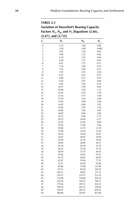
For shallow foundation designs, the ultimate bearing capacity relationship given by equation (2.71) is presently used. The variation of Ng for surface foundation con-ditions (that is, b = 0 and m = 0) is given in Figure 2.12. In 1963 Meyerhof8 suggested that Ng could be approximated as
N Nqγ φ= -( ) tan( . )Eq. (2.66)� 1 1 4
(2.72)
Table 2.3 gives the variations of Nc and Nq obtained from equations (2.66) and (2.67) and Ng obtained from equation (2.72).
2.5 General diSCuSSion on the relationShipS oF bearinG CapaCity FaCtorS
At this time, the general trend among geotechnical engineers is to accept the method of superposition as a suitable means to estimate the ultimate bearing capacity of shal-low rough foundations. For rough continuous foundations, the nature of the failure surface in soil shown in Figure 2.6 has also found acceptance, as have Reissner’s6 and Prandtl’s7 solutions for Nc and Nq, which are the same as Meyerhof’s5 solution for surface foundations, or,
N eq = +
-
π φ φφ
tan sinsin
11
(2.66)
and
N Nc q= -( ) cot1 φ
(2.67)
There has been considerable controversy over the theoretical values of Ng . Hansen9 proposed an approximate relationship for Ng in the form
N Ncγ φ=1 5 2. tan
(2.73)
In the preceding equation, the relationship for Nc is that given by Prandtl’s solution [equation (2.67)]. Caquot and Kerisel10 assumed that the elastic triangular soil wedge under a rough continuous foundation is of the shape shown in Figure 2.6. Using inte-gration of Boussinesq’s differential equation, they presented numerical values of Ng for various soil friction angles f. Vesic4 approximated their solutions in the form
N Nqγ φ= +2 1( ) tan
(2.74)
whereNq is given by equation (2.66)
36 Shallow Foundations: Bearing Capacity and Settlement
Equation (2.74) has an error not exceeding 5% for 20° < f < 40° compared to the exact solution. Lundgren and Mortensen11 developed numerical methods (using the theory of plasticity) for the exact determination of rupture lines as well as the bearing capacity factor (Ng) for particular cases. Chen12 also gave a solution for Ng in which he used the upper bound limit analysis theorem suggested by Drucker and Prager.13 Biarez et al.14 also recommended the following relationship for Ng :
N Nqγ φ= -1 8 1. ( ) tan
(2.75)
Booker15 used the slip line method and provided numerical values of Ng . Poulos et al.16 suggested the following expression that approximates the numerical results of Booker 15:
N eγ
φ≈ 0 1045 9 6. .
(2.76)
wheref is in radiansNg = 0 for f = 0
Recently Kumar17 proposed another slip line solution based on Lundgren and Mortensen’s failure mechanism.11 Michalowski18 also used the upper bound limit analysis theorem to obtain the variation of Ng . His solution can be approximated as
N eγ
φ φ= +( . . tan ) tan0 66 5 1
(2.77)
Hjiaj et al.19 obtained a numerical analysis solution for Ng. This solution can be approximated as
N eγ
π π φ πφ= +1
63
25
2( tan )(tan )
(2.78)
Martin20 used the method of characteristics to obtain the variations of Ng . Salgado21 approximated these variations in the form
N Nqγ φ= -( ) tan( . )1 1 32
(2.79)
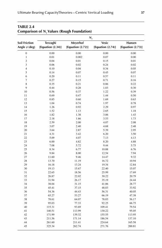
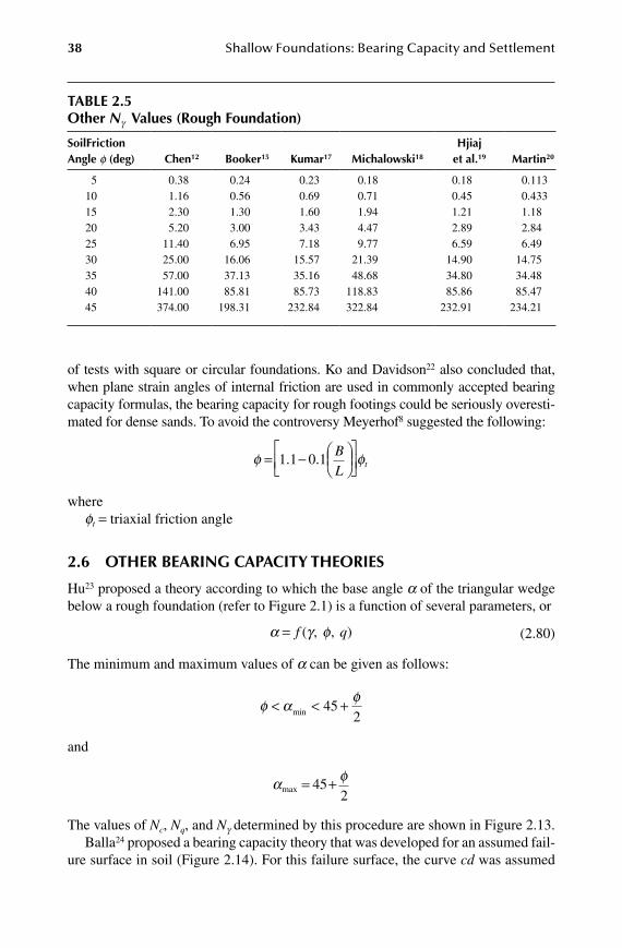
Table 2.4 gives a comparison of the Ng values recommended by Meyerhof,8 Terzaghi,1 Vesic,4 and Hansen.9 Table 2.5 compares the variations of Ng obtained by Chen,12 Booker,15 Kumar,17 Michalowski,18 Hjiaj et al.,19 and Martin.20
The primary reason several theories for Ng were developed, and their lack of cor-relation with experimental values, lies in the difficulty of selecting a representative value of the soil friction angle f for computing bearing capacity. The parameter f depends on many factors, such as intermediate principal stress condition, friction angle anisotropy, and curvature of the Mohr-Coulomb failure envelope.
It has been suggested that the plane strain soil friction angle fp, instead of ft, be used to estimate bearing capacity.9 To that effect Vesic4 raised the issue that this type of assumption might help explain the differences between the theoretical and experimen-tal results for long rectangular foundations; however, it does not help to interpret results
Ultimate Bearing CapacityTheories—Centric Vertical Loading 37
table 2.4Comparison of Ng Values (rough Foundation)
Ng
Soil Friction angle f (deg)
terzaghi [equation (2.34)]
meyerhof [equation (2.72)]
Vesic [equation (2.74)]
hansen [equation (2.73)]
0 0.00 0.00 0.00 0.00 1 0.01 0.002 0.07 0.00 2 0.04 0.01 0.15 0.01 3 0.06 0.02 0.24 0.02 4 0.10 0.04 0.34 0.05 5 0.14 0.07 0.45 0.07 6 0.20 0.11 0.57 0.11 7 0.27 0.15 0.71 0.16 8 0.35 0.21 0.86 0.22 9 0.44 0.28 1.03 0.3010 0.56 0.37 1.22 0.3911 0.69 0.47 1.44 0.5012 0.85 0.60 1.69 0.6313 1.04 0.74 1.97 0.7814 1.26 0.92 2.29 0.9715 1.52 1.13 2.65 1.1816 1.82 1.38 3.06 1.4317 2.18 1.66 3.53 1.7318 2.59 2.00 4.07 2.0819 3.07 2.40 4.68 2.4820 3.64 2.87 5.39 2.9521 4.31 3.42 6.20 3.5022 5.09 4.07 7.13 4.1323 6.00 4.82 8.20 4.8824 7.08 5.72 9.44 5.7525 8.34 6.77 10.88 6.7626 9.84 8.00 12.54 7.9427 11.60 9.46 14.47 9.3228 13.70 11.19 16.72 10.9429 16.18 13.24 19.34 12.8430 19.13 15.67 22.40 15.0731 22.65 18.56 25.99 17.6932 26.87 22.02 30.22 20.7933 31.94 26.17 35.19 24.4434 38.04 31.15 41.06 28.7735 45.41 37.15 48.03 33.9236 54.36 44.43 56.31 40.0537 65.27 53.27 66.19 47.3838 78.61 64.07 78.03 56.1739 95.03 77.33 92.25 66.7540 115.31 93.69 109.41 79.5441 140.51 113.99 130.22 95.0542 171.99 139.32 155.55 113.9543 211.56 171.14 186.54 137.1044 261.60 211.41 224.64 165.5845 325.34 262.74 271.76 200.81
38 Shallow Foundations: Bearing Capacity and Settlement
of tests with square or circular foundations. Ko and Davidson22 also concluded that, when plane strain angles of internal friction are used in commonly accepted bearing capacity formulas, the bearing capacity for rough footings could be seriously overesti-mated for dense sands. To avoid the controversy Meyerhof8 suggested the following:
φ φ= -
1 1 0 1. .BL
t
whereft = triaxial friction angle
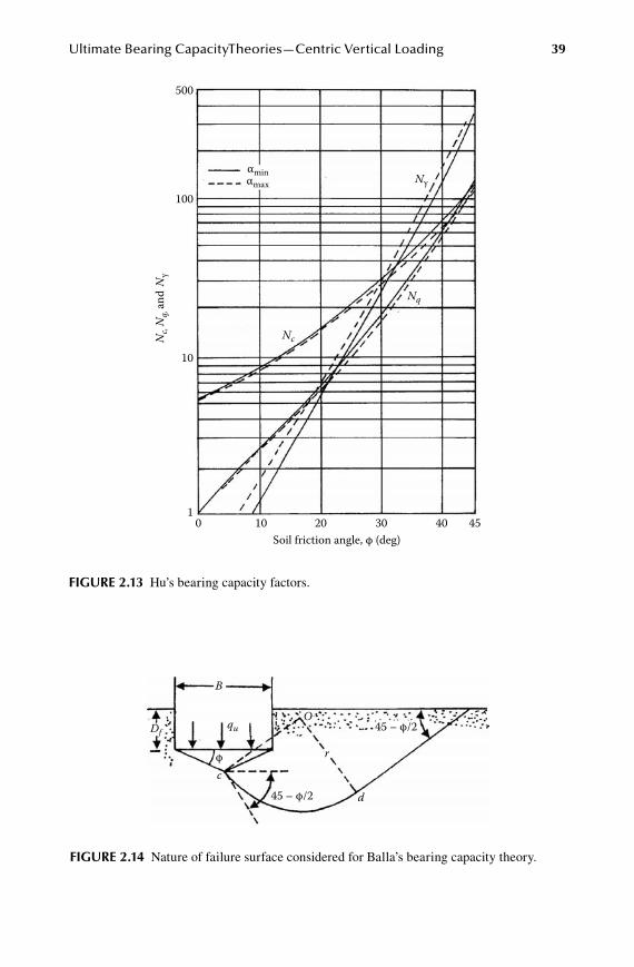
2.6 other bearinG CapaCity theorieS
Hu23 proposed a theory according to which the base angle a of the triangular wedge below a rough foundation (refer to Figure 2.1) is a function of several parameters, or
α γ φ= f q( , , ) (2.80)
The minimum and maximum values of a can be given as follows:
φ α φ< < +min 45
2
and
α φ
max = +452
The values of Nc, Nq, and Ng determined by this procedure are shown in Figure 2.13.Balla24 proposed a bearing capacity theory that was developed for an assumed fail-
ure surface in soil (Figure 2.14). For this failure surface, the curve cd was assumed
table 2.5other Ng Values (rough Foundation)
SoilFriction angle f (deg) Chen12 booker15 Kumar17 michalowski18
hjiaj et al.19 martin20
5 0.38 0.24 0.23 0.18 0.18 0.11310 1.16 0.56 0.69 0.71 0.45 0.43315 2.30 1.30 1.60 1.94 1.21 1.1820 5.20 3.00 3.43 4.47 2.89 2.8425 11.40 6.95 7.18 9.77 6.59 6.4930 25.00 16.06 15.57 21.39 14.90 14.7535 57.00 37.13 35.16 48.68 34.80 34.4840 141.00 85.81 85.73 118.83 85.86 85.4745 374.00 198.31 232.84 322.84 232.91 234.21
Ultimate Bearing CapacityTheories—Centric Vertical Loading 39
500
100
αmin Nγ
NcNc,
Nq,
and
Nγ
Nq
αmax
10
10 10 20
Soil friction angle, φ (deg)30 40 45
FiGure 2.13 Hu’s bearing capacity factors.
B
Dfqu
c
d
O
45 – φ/2
φ
45 – φ/2
r
FiGure 2.14 Nature of failure surface considered for Balla’s bearing capacity theory.
40 Shallow Foundations: Bearing Capacity and Settlement
5
5
4
3
2
1
015 1520 2030 3040 40
4
3
2
φ (deg) φ (deg)
φ (deg) φ (deg)
1
2.5
2.5
1.00.50.25
1.0
0.5
0.25
2.51.0
0.50.25
c/γB = 0
c/γB = 0c/γB = 0
c/γB = 0
Df /B = 0
Df/B = 1.0 Df /B = 1.5
Df /B = 0.5
ρ =
2r/B
ρ =
2r/B
015 20 30 40 15 20 30 40
∞
∞ ∞
∞
2.51.0
0.250.5
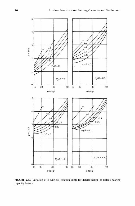
FiGure 2.15 Variation of r with soil friction angle for determination of Balla’s bearing capacity factors.
Ultimate Bearing CapacityTheories—Centric Vertical Loading 41
to be an arc of a circle having a radius r. The bearing capacity solution was obtained using Kötter’s equation to determine the distribution of the normal and tangential stresses on the slip surface. According to this solution for a continuous foundation,
q cN qN BNu c q= + + 1
2γ γ
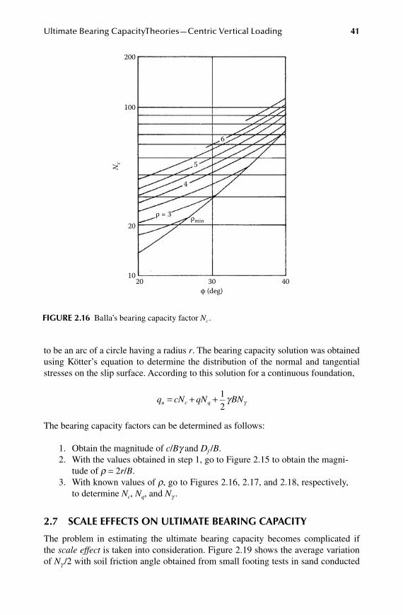
The bearing capacity factors can be determined as follows:
1. Obtain the magnitude of c/Bg and Df /B. 2. With the values obtained in step 1, go to Figure 2.15 to obtain the magni-
tude of r = 2r/B. 3. With known values of r, go to Figures 2.16, 2.17, and 2.18, respectively,
to determine Nc, Nq, and Ng .
2.7 SCale eFFeCtS on ultimate bearinG CapaCity
The problem in estimating the ultimate bearing capacity becomes complicated if the scale effect is taken into consideration. Figure 2.19 shows the average variation of Ng /2 with soil friction angle obtained from small footing tests in sand conducted
200
100
6
5
4
20ρ = 3 ρmin
Nc
1020 30 40
φ (deg)
FiGure 2.16 Balla’s bearing capacity factor Nc .

42 Shallow Foundations: Bearing Capacity and Settlement
in the laboratory at Ghent as reported by DeBeer.25 For these tests, the values of f were obtained from triaxial tests. This figure also shows the variation of Ng / 2 with f obtained from tests conducted in Berlin and reported by Muhs26 with footings having an area of 1 m2. The soil friction angles for these tests were obtained from direct shear tests. It is interesting to note that:
1. For loose sand, the field test results of Ng are higher than those obtained from small footing tests in the laboratory.
2. For dense sand, the laboratory tests provide higher values of Ng compared to those obtained from the field.
The reason for the above observations can partially be explained by the fact that, in the field, progressive rupture in the soil takes place during the loading process. For loose sand at failure, the soil friction angle is higher than at the beginning of loading due to compaction. The reverse is true in the case of dense sand.
Figure 2.20 shows a comparison of several bearing capacity test results in sand compiled by DeBeer,25 which are plots of Ng with gB. For any given soil, the magnitude of Ng decreases with B and remains constant for larger values of B.
100
10
6
5
4
Nq
520 30 40φ (deg)
ρmin
ρ = 3
FiGure 2.17 Balla’s bearing capacity factor Nq .

Ultimate Bearing CapacityTheories—Centric Vertical Loading 43
The reduction in Ng for larger foundations may ultimately result in a substantial decrease in the ultimate bearing capacity that can primarily be attributed to the following reasons:
1. For larger-sized foundations, the rupture along the slip lines in soil is pro-gressive, and the average shear strength mobilized (and thus f) along a slip line decreases with the increase in B.
2. There are zones of weakness that exist in the soil under the foundation. 3. The curvature of the Mohr-Coulomb envelope.
500
100
6
5
4
10
520 30 40
ρ = 3
ρmin
φ (deg)
Nγ
FiGure 2.18 Balla’s bearing capacity factor Ng .
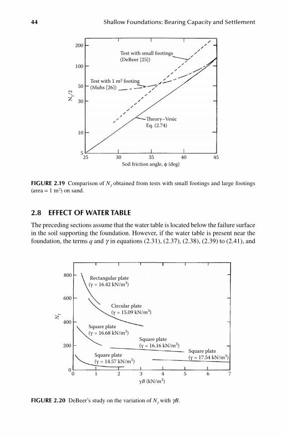
44 Shallow Foundations: Bearing Capacity and Settlement
2.8 eFFeCt oF water table
The preceding sections assume that the water table is located below the failure surface in the soil supporting the foundation. However, if the water table is present near the foundation, the terms q and g in equations (2.31), (2.37), (2.38), (2.39) to (2.41), and
200
100
Test with small footings(DeBeer [25])
Test with 1 m2 footing(Muhs [26])
Theory–VesicEq. (2.74)
Soil friction angle, φ (deg)
50
30
10
525 30 35 40 45
Nγ/
2
FiGure 2.19 Comparison of Ng obtained from tests with small footings and large footings (area = 1 m2) on sand.
800 Rectangular plate(γ = 16.42 kN/m3)
Circular plate(γ = 15.09 kN/m3)
Square plate(γ = 16.68 kN/m3)
Nγ
Square plate(γ = 16.16 kN/m3)
Square plate(γ = 14.57 kN/m3)
Square plate(γ = 17.54 kN/m3)
γB (kN/m2)
600
400
200
00 1 2 3 4 5 6 7
FiGure 2.20 DeBeer’s study on the variation of Ng with gB.
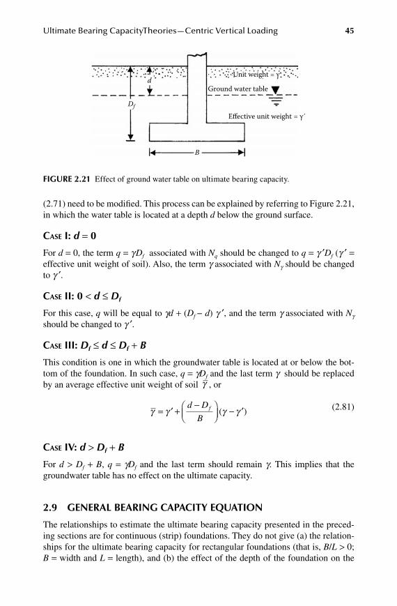
Ultimate Bearing CapacityTheories—Centric Vertical Loading 45
(2.71) need to be modified. This process can be explained by referring to Figure 2.21, in which the water table is located at a depth d below the ground surface.
Case i: d = 0
For d = 0, the term q = g Df associated with Nq should be changed to q = g ′Df (g ′ = effective unit weight of soil). Also, the term g associated with Ng should be changed to g ′.
Case ii: 0 < d ≤ Df
For this case, q will be equal to gd + (Df − d) g ′, and the term g associated with Ng should be changed to g ′.
Case iii: Df ≤ d ≤ Df + B
This condition is one in which the groundwater table is located at or below the bot-tom of the foundation. In such case, q = gDf and the last term g should be replaced by an average effective unit weight of soil γ , or
γ γ γ γ= ′ +
-
- ′d D
Bf ( )
(2.81)
Case iv: d > Df + B
For d > Df + B, q = gDf and the last term should remain g. This implies that the groundwater table has no effect on the ultimate capacity.
2.9 General bearinG CapaCity equation
The relationships to estimate the ultimate bearing capacity presented in the preced-ing sections are for continuous (strip) foundations. They do not give (a) the relation-ships for the ultimate bearing capacity for rectangular foundations (that is, B/L > 0; B = width and L = length), and (b) the effect of the depth of the foundation on the
Ground water table
Unit weight = γ
Effective unit weight = γ´
d
Df
B
FiGure 2.21 Effect of ground water table on ultimate bearing capacity.
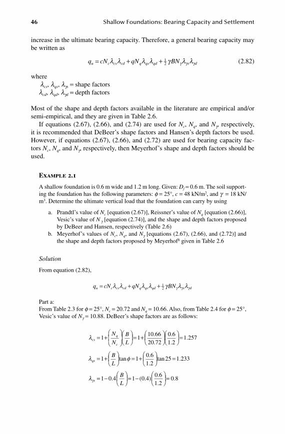
46 Shallow Foundations: Bearing Capacity and Settlement
increase in the ultimate bearing capacity. Therefore, a general bearing capacity may be written as
q cN qN BNu c cs cd q qs qd s d= + +l l l l γ l lγ γ γ
12
(2.82)
wherelcs, lqs, lgs = shape factors
lcd, lqd, lgd = depth factors
Most of the shape and depth factors available in the literature are empirical and/or semi-empirical, and they are given in Table 2.6.
If equations (2.67), (2.66), and (2.74) are used for Nc, Nq, and Ng, respectively, it is recommended that DeBeer’s shape factors and Hansen’s depth factors be used. However, if equations (2.67), (2.66), and (2.72) are used for bearing capacity fac-tors Nc, Nq, and Ng, respectively, then Meyerhof’s shape and depth factors should be used.
Example 2.1
A shallow foundation is 0.6 m wide and 1.2 m long. Given: Df = 0.6 m. The soil support-ing the foundation has the following parameters: f = 25°, c = 48 kN/m2, and g = 18 kN/m3. Determine the ultimate vertical load that the foundation can carry by using
a. Prandtl’s value of Nc [equation (2.67)], Reissner’s value of Nq [equation (2.66)], Vesic’s value of N g [equation (2.74)], and the shape and depth factors proposed by DeBeer and Hansen, respectively (Table 2.6)
b. Meyerhof’s values of Nc, Nq, and Ng [equations (2.67), (2.66), and (2.72)] and the shape and depth factors proposed by Meyerhof8 given in Table 2.6
Solution
From equation (2.82),
q cN qN BNu c cs cd q qs qd s d= + +l l l l γ l lγ γ γ
12
Part a:From Table 2.3 for f = 25°, Nc = 20.72 and Nq = 10.66. Also, from Table 2.4 for f = 25°, Vesic’s value of Ng = 10.88. DeBeer’s shape factors are as follows:
lcsq
c
N
NBL
= +
= +
1 1
10 6620 72
.
.0 61 2
1 257
1 10 6
.
..
tan.
=
= +
= +l φqs
BL 1 2
25 1 233
1 0 4 1 0
.tan .
. (
=
= -
= -lγs
BL
. )..
.40 61 2
0 8
=
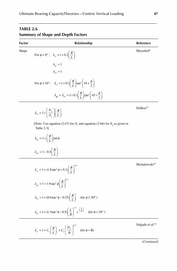
Ultimate Bearing CapacityTheories—Centric Vertical Loading 47
table 2.6Summary of Shape and depth Factors
Factor relationship reference
ShapeFor φ l
l
lγ
= ° = +
=
=
0 1 0 2
1
1
: .cs
qs
s
BL
For φ l φ
l
≥ ° = +
+
10 1 0 2 452
2: . tancs
BL
qqs s
BL
= = +
+
l φγ 1 0 1 45
22. tan
Meyerhof8
lcsq
c
N
N
B
L= +
1
[Note: Use equation (2.67) for Nc and equation (2.66) for Nq as given in Table 2.3]
l φqs
B
L= +
1 tan
lγ s
B
L= -
1 0 4.
DeBeer27
l φcs
B
L= + +
1 1 8 0 12
0 5
( . tan . ).
l φqs
B
L= +
1 1 9 2
0 5
. tan.
l φ φγ s
BL
= + -
≤1 0 6 0 25 302( . tan . ) (for °° )
l φγ s
L
BLB
= + -
-
1 1 3 0 52( . tan . )
1 5
e (for φ > °30 )
Michalowski28
l φcsf
CB
LC
D
B= +
+
=1 1 2 (for
0.5
00)
Salgado et al.29
(Continued)
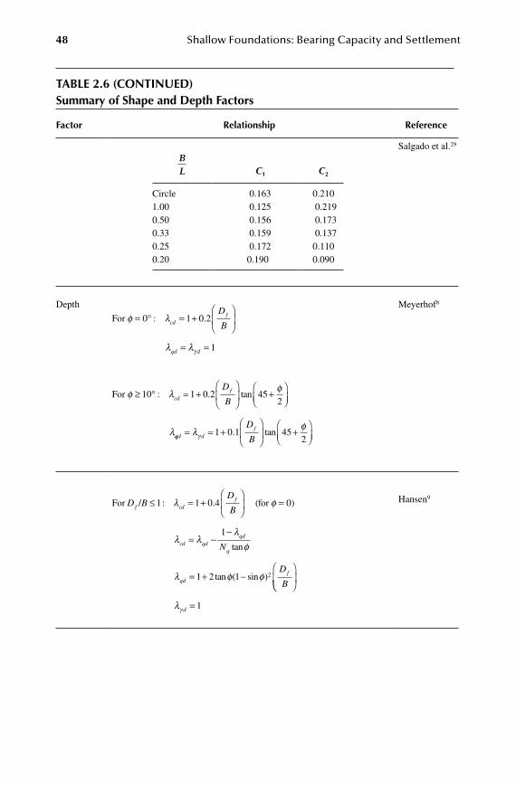
48 Shallow Foundations: Bearing Capacity and Settlement
table 2.6 (Continued)Summary of Shape and depth Factors
Factor relationship reference
BL C1 C2
Circle 0.163 0.2101.00 0.125 0.2190.50 0.156 0.1730.33 0.159 0.1370.25 0.172 0.1100.20 0.190 0.090
Salgado et al.29
Depth
For φ l
l lγ
= ° = +
= =
0 1 0 2
1
: .cdf
qd d
D
B
For φ l φ
l
≥ ° = +
+
10 1 0 2 452
: . tancdfD
B
qqd dfD
B= = +
+
l φγ 1 0 1 45
2. tan
Meyerhof8
For (forD BD
Bf cdf/ : . )≤ = +
=1 1 0 4 0l φ
lcd qdqd
q
qdf
N
D
B
= --
= + -
ll
φ
l φ φ
1
1 2 1 2
tan
tan ( sin )
=lγ d 1
Hansen9
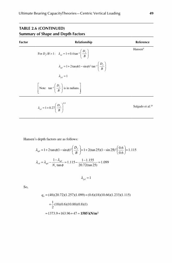
Ultimate Bearing CapacityTheories—Centric Vertical Loading 49
Hansen’s depth factors are as follows:
l φ φqdfD
B= + -
= + -1 2 1 1 2 25 1 22tan ( sin ) (tan )( sin 55
0 60 6
1 115
11 115
2)..
.
tan.
=
= --
=l ll
φcd qdqd
cN-- - =1 1 155
20 72 251 099
.. (tan )
.
lγ d = 1
So,
qu = +( )( . )( . )( . ) ( . )( )( .48 20 72 1 257 1 099 0 6 18 10 66 1 233 1 115
12
18 0 6 10 88 0 8
)( . )( . )
( )( . )( . )( . )+ ( )
. .
1
1373 9 163 96 47= + + ≈ 1585 kN/m2
table 2.6 (Continued)Summary of Shape and depth Factors
Factor relationship reference
For D BD
Bf cdf
qd
/ : . tan
ta
> = +
= +
-1 1 0 4
1 2
1l
l n ( sin ) tanφ φ
lγ
1
1
2 1-
=
-D
Bf
d
Note: is in radians.tan-
1
D
Bf
Hansen9
lcdfD
B= +
1 0 27
0 5
.
.
Salgado et al.29
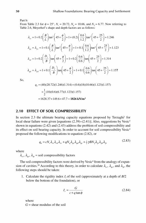
50 Shallow Foundations: Bearing Capacity and Settlement
Part b:From Table 2.3 for f = 25°, Nc = 20.72, Nq = 10.66, and Ng = 6.77. Now referring to Table 2.6, Meyerhof’s shape and depth factors are as follows:
l φcs
B
L= +
+
= +1 0 2 452
1 0 20 62. tan ( . ).
1 245
25
21 246
1 0
2
.tan .
+
=
= = +l lγqs s . tan ..
.1 45
21 0 1
0 6
1 22B
L
+
= +
φ +
=
= +
tan .
. t
2 4525
21 123
1 0 2lcdfD
Ban .
.
.tan45
21 0 2
0 6
0 645
25
2+
= +
+
φ
=
= = +
+
1 314
1 0 1 452
.
. tanl l φγqd d
fD
B
= +
+
=1 0 10 6
0 645
25
21 15.
.
.tan . 77
So,
qu = +( )( . )( . )( . ) ( . )( )( .48 20 72 1 246 1 314 0 6 18 10 66 1 123 1 157
12
18 0 6 6 77 1 123
)( . )( . )
( )( . )( . )( .+ )( . )
. . .
1 157
1628 37 149 6 47 7= + + ≈ 1826 kN/m2
2.10 eFFeCt oF Soil CompreSSibility
In section 2.3 the ultimate bearing capacity equations proposed by Terzaghi1 for local shear failure were given [equations (2.39)–(2.41)]. Also, suggestions by Vesic4 shown in equations (2.42) and (2.43) address the problem of soil compressibility and its effect on soil bearing capacity. In order to account for soil compressibility Vesic4 proposed the following modifications to equation (2.82), or
q cN qN BNu c cs cd cc q qs qd qc s d c= + +l l l l l l γ l l lγ γ γ γ
12
(2.83)
wherelcc, lqc, lgc = soil compressibility factors
The soil compressibility factors were derived by Vesic4 from the analogy of expan-sion of cavities.30 According to this theory, in order to calculate lcc, lqc, and lgc, the following steps should be taken:
1. Calculate the rigidity index Ir of the soil (approximately at a depth of B/2 below the bottom of the foundation), or
I
Gc q
r =+ tanφ
(2.84)
whereG = shear modulus of the soil
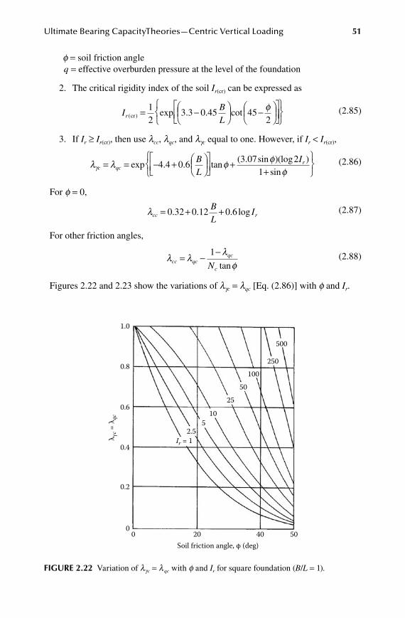
Ultimate Bearing CapacityTheories—Centric Vertical Loading 51
f = soil friction angleq = effective overburden pressure at the level of the foundation
2. The critical rigidity index of the soil Ir(cr) can be expressed as
IBL
r ( ) exp . . cotcr = -
-
12
3 3 0 45 452φ
(2.85)
3. If Ir ≥ Ir(cr), then use lcc, lqc, and lgc equal to one. However, if Ir < Ir(cr),
l l φ φγc qc
BL
= = - +
+exp . . tan( . sin
4 4 0 63 07 )(log )
sin2
1Ir
+
φ
(2.86)
For f = 0,
lcc r
BL
I= + +0 32 0 12 0 6. . . log
(2.87)
For other friction angles,
l l l
φcc qcqc
cN= -
-1
tan
(2.88)
Figures 2.22 and 2.23 show the variations of lgc = lqc [Eq. (2.86)] with f and Ir.
1.0
0.8
0.6
Ir = 12.5
510
2550
100
500
0.4
0.2
00 20
Soil friction angle, φ (deg) 40 50
λ γc =
λqc
250
FiGure 2.22 Variation of lgc = l qc with f and Ir for square foundation (B/L = 1).
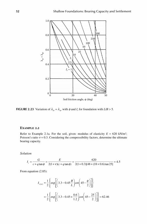
52 Shallow Foundations: Bearing Capacity and Settlement
Example 2.2
Refer to Example 2.1a. For the soil, given: modulus of elasticity E = 620 kN/m2; Poisson’s ratio n = 0.3. Considering the compressibility factors, determine the ultimate bearing capacity.
Solution
I
G
c q
E
c qr =+
=+ +
=+tan ( )( tan ) ( . )[φ ν φ2 1
620
2 1 0 3 48 + ×=
( . ) tan ].
18 0 6 254 5
From equation (2.85):
IB
Lr ( ) exp . . cotcr = -
-
1
23 3 0 45 45
2
φ
= - ×
1
23 3 0 45
0 6
1 2exp . .
.
. -
=cot .45
25
262 46
1.0
0.8
0.6
0.4
Ir = 1
0.2
2.55
1025
50100
250
500
00 20 40 50
Soil friction angle, φ (deg)
λ γc =
λqc
FiGure 2.23 Variation of lgc = l qc with f and Ir for foundation with L/B > 5.
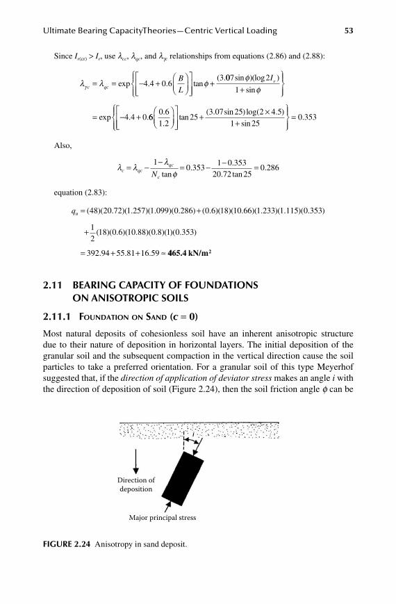
Ultimate Bearing CapacityTheories—Centric Vertical Loading 53
Since Ir(cr) > Ir, use lcc, lqc, and lgc relationships from equations (2.86) and (2.88):
l l φγ c qc
B
L= = - +
+exp . . tan( .
4 4 0 63 007 2
1
4 4 0
sin )(log )
sin
exp . .
φφ
Ir
+
= - + 660 6
1 225
3 07 25.
.tan
( . sin ) log(
+ 2 4 5
1 250 353
×+
=. )
sin.
Also,
l l
lφc qc
qc
cN= -
-= - - =
10 353
1 0 35320 72 25
0 28tan
..
. tan. 6
equation (2.83):
qu = +( )( . )( . )( . )( . ) ( . )(48 20 72 1 257 1 099 0 286 0 6 18 10 66 1 233 1 115 0 353
12
18 0 6
)( . )( . )( . )( . )
( )( . )+ ( . )( . )( )( . )
. . .
10 88 0 8 1 0 353
392 94 55 81 16 59= + + ≈ 4465.4 kN/m2
2.11 bearinG CapaCity oF FoundationS on aniSotropiC SoilS
2.11.1 foUnDation on sanD (c = 0)
Most natural deposits of cohesionless soil have an inherent anisotropic structure due to their nature of deposition in horizontal layers. The initial deposition of the granular soil and the subsequent compaction in the vertical direction cause the soil particles to take a preferred orientation. For a granular soil of this type Meyerhof suggested that, if the direction of application of deviator stress makes an angle i with the direction of deposition of soil (Figure 2.24), then the soil friction angle f can be
Direction ofdeposition
Major principal stress
FiGure 2.24 Anisotropy in sand deposit.
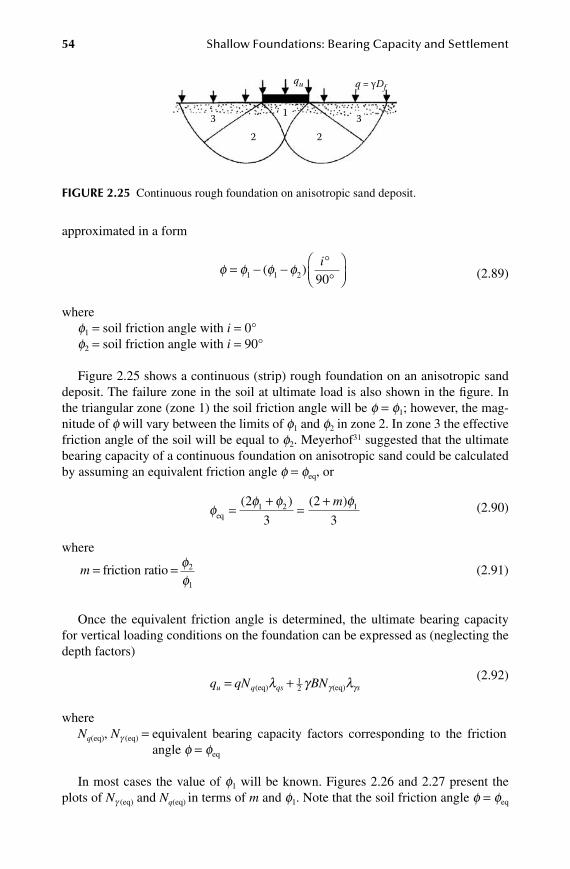
54 Shallow Foundations: Bearing Capacity and Settlement
approximated in a form
φ φ φ φ= - - °°
1 1 2 90
( )i
(2.89)
wheref1 = soil friction angle with i = 0°f2 = soil friction angle with i = 90°
Figure 2.25 shows a continuous (strip) rough foundation on an anisotropic sand deposit. The failure zone in the soil at ultimate load is also shown in the figure. In the triangular zone (zone 1) the soil friction angle will be f = f1; however, the mag-nitude of f will vary between the limits of f1 and f2 in zone 2. In zone 3 the effective friction angle of the soil will be equal to f2. Meyerhof31 suggested that the ultimate bearing capacity of a continuous foundation on anisotropic sand could be calculated by assuming an equivalent friction angle f = feq, or
φ
φ φ φeq =
+=
+( ) ( )2
3
2
31 2 1m
(2.90)
where
m = =friction ratioφφ
2
1
(2.91)
Once the equivalent friction angle is determined, the ultimate bearing capacity for vertical loading conditions on the foundation can be expressed as (neglecting the depth factors)
q qN BNu q qs s= +(eq) (eq)l γ lγ γ12
(2.92)
where Nq(eq), Ng (eq) = equivalent bearing capacity factors corresponding to the friction
angle f = feq
In most cases the value of f1 will be known. Figures 2.26 and 2.27 present the plots of Ng (eq) and Nq(eq) in terms of m and f1. Note that the soil friction angle f = feq
3 31
qu q = γDf
2 2
FiGure 2.25 Continuous rough foundation on anisotropic sand deposit.
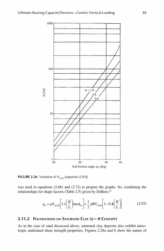
Ultimate Bearing CapacityTheories—Centric Vertical Loading 55
was used in equations (2.66) and (2.72) to prepare the graphs. So, combining the relationships for shape factors (Table 2.5) given by DeBeer,19
q qN
BL
BNu q= +
+ -(eq) eq (eq)1
12
1 0tan .φ γ γ 44BL
(2.93)
2.11.2 foUnDations on satURateD Clay (f = 0 ConCept)
As in the case of sand discussed above, saturated clay deposits also exhibit aniso-tropic undrained shear strength properties. Figures 2.28a and b show the nature of
1000
100
10
m = 1.00.8
0.6
Nγ(e
q)
120 30 40 45
Soil friction angle, φ1 (deg)
FiGure 2.26 Variation of Ng (eq) [equation (2.92)].
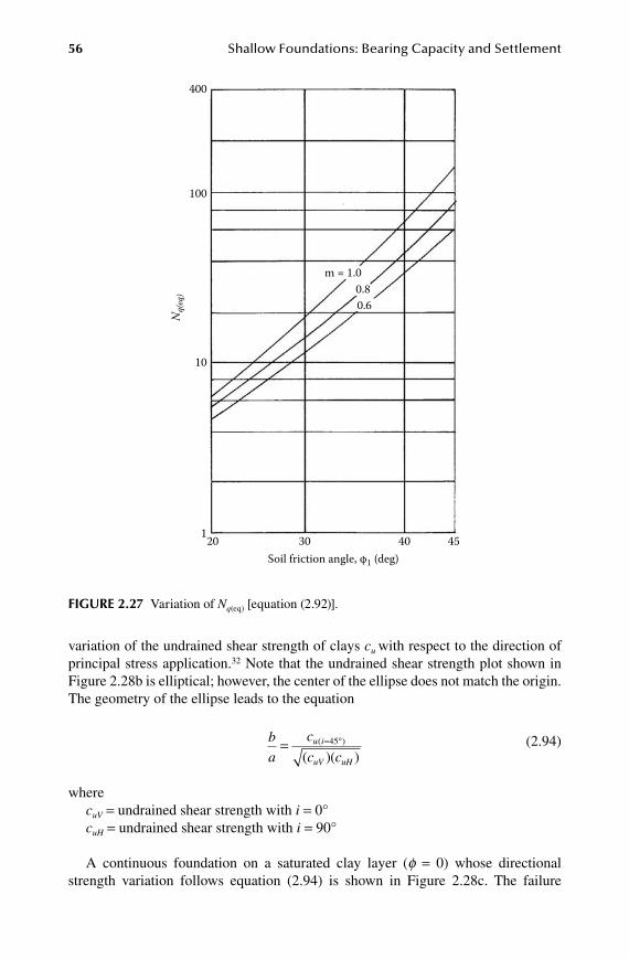
56 Shallow Foundations: Bearing Capacity and Settlement
variation of the undrained shear strength of clays cu with respect to the direction of principal stress application.32 Note that the undrained shear strength plot shown in Figure 2.28b is elliptical; however, the center of the ellipse does not match the origin. The geometry of the ellipse leads to the equation
ba
c
c cu i
uV uH
= = °( )
( )( )45
(2.94)
wherecuV = undrained shear strength with i = 0°cuH = undrained shear strength with i = 90°
A continuous foundation on a saturated clay layer (f = 0) whose directional strength variation follows equation (2.94) is shown in Figure 2.28c. The failure
400
100
10
m = 1.00.80.6
Nq(
eq)
120 30 40 45Soil friction angle, φ1 (deg)
FiGure 2.27 Variation of Nq(eq) [equation (2.92)].
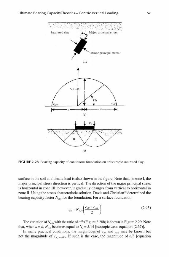
Ultimate Bearing CapacityTheories—Centric Vertical Loading 57
surface in the soil at ultimate load is also shown in the figure. Note that, in zone I, the major principal stress direction is vertical. The direction of the major principal stress is horizontal in zone III; however, it gradually changes from vertical to horizontal in zone II. Using the stress characteristic solution, Davis and Christian32 determined the bearing capacity factor Nc(i) for the foundation. For a surface foundation,
q N
c cu c i
uV uH= +
( )
2
(2.95)
The variation of Nc(i) with the ratio of a/b (Figure 2.28b) is shown in Figure 2.29. Note that, when a = b, Nc(i) becomes equal to Nc = 5.14 [isotropic case; equation (2.67)].
In many practical conditions, the magnitudes of cuV and cuH may be known but not the magnitude of cu(i = 45°). If such is the case, the magnitude of a/b [equation
Saturated clay Major principal stress
Minor principal stress
(a)
bcu(i = 45º)
2i
(b)
(c)
III IIIII
III
cuH
qu
a a
cuV
FiGure 2.28 Bearing capacity of continuous foundation on anisotropic saturated clay.
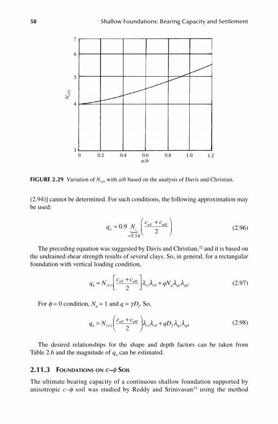
58 Shallow Foundations: Bearing Capacity and Settlement
(2.94)] cannot be determined. For such conditions, the following approximation may be used:
q Nc c
u cuV uH≈
+
=
0 92
5 14
..� (2.96)
The preceding equation was suggested by Davis and Christian,32 and it is based on the undrained shear strength results of several clays. So, in general, for a rectangular foundation with vertical loading condition,
q N
c cqNu c i
uV uHcs cd q qs qd= +
+( )2
l l l l (2.97)
For f = 0 condition, Nq = 1 and q = g Df. So,
q N
c cqDu c i
uV uHcs cd f qs qd= +
+( )
2l l l l
(2.98)
The desired relationships for the shape and depth factors can be taken from Table 2.6 and the magnitude of qu can be estimated.
2.11.3 foUnDations on c–f soil
The ultimate bearing capacity of a continuous shallow foundation supported by anisotropic c–f soil was studied by Reddy and Srinivasan33 using the method
7
6
5
4
30 0.2 0.4 0.6 0.8 1.0 1.2
a/b
Nc(
i)
FiGure 2.29 Variation of Nc(i) with a/b based on the analysis of Davis and Christian.

Ultimate Bearing CapacityTheories—Centric Vertical Loading 59
of characteristics. According to this analysis the shear strength of a soil can be given as
s c= ′ +σ φtan
It is assumed, however, that the soil is anisotropic only with respect to cohe-sion. As mentioned previously in this section, the direction of the major principal stress (with respect to the vertical) along a slip surface located below the founda-tion changes. In anisotropic soils, this will induce a change in the shearing resis-tance to the bearing capacity failure of the foundation. Reddy and Srinivasan33 assumed the directional variation of c at a given depth z below the foundation as (Figure 2.30a)
c c c c ii z H z V z H z( ) ( ) ( ) ( )[ ]cos= + - 2
(2.99)
whereci(z) = cohesion at a depth z when the major principal stress is inclined at an angle
i to the vertical (Figure 2.30b)
Minor principal stress
(a)
(c)(b)
Major principal stress
cV (z)
ci (z)
cH(z)
cV (z=0)cV (z)
1
z
α´
90 – i
90 – i
z
FiGure 2.30 Anisotropic clay soil—assumptions for bearing capacity evaluation.
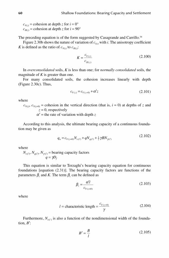
60 Shallow Foundations: Bearing Capacity and Settlement
cV(z) = cohesion at depth z for i = 0°cH(z) = cohesion at depth z for i = 90°
The preceding equation is of the form suggested by Casagrande and Carrillo.34
Figure 2.30b shows the nature of variation of ci(z) with i. The anisotropy coefficient K is defined as the ratio of cV(z) to cH(z):
Kc
cV z
H z
= ( )
( )
(2.100)
In overconsolidated soils, K is less than one; for normally consolidated soils, the magnitude of K is greater than one.
For many consolidated soils, the cohesion increases linearly with depth (Figure 2.30c). Thus,
c c zV z V z( ) ( )= + ′=0 α
(2.101)
wherecV(z), cV(z=0) = cohesion in the vertical direction (that is, i = 0) at depths of z and z = 0, respectively
a′ = the rate of variation with depth z
According to this analysis, the ultimate bearing capacity of a continuous founda-tion may be given as
q c N qN BNu V z c i q i i= + += ′ ′ ′( ) ( ) ( ) ( )0
12 γ γ
(2.102)
whereNc(i′), Nq(i′), Ng (i′) = bearing capacity factors
q = gDf
This equation is similar to Terzaghi’s bearing capacity equation for continuous foundations [equation (2.31)]. The bearing capacity factors are functions of the parameters bc and K. The term bc can be defined as
β αc
V z
lc
= ′=( )0
(2.103)
where
l
cV z= = =characteristic length ( )0
γ
(2.104)
Furthermore, Nc(i´) is also a function of the nondimensional width of the founda-tion, B′:
′ =B
B
l (2.105)
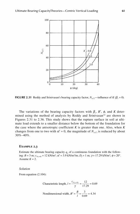
Ultimate Bearing CapacityTheories—Centric Vertical Loading 61
The variations of the bearing capacity factors with bc, B′, f, and K deter-mined using the method of analysis by Reddy and Srinivasan33 are shown in Figures 2.31 to 2.36. This study shows that the rupture surface in soil at ulti-mate load extends to a smaller distance below the bottom of the foundation for the case where the anisotropic coefficient K is greater than one. Also, when K changes from one to two with a′ = 0, the magnitude of Nc(i′) is reduced by about 30%–40%.
Example 2.3
Estimate the ultimate bearing capacity qu of a continuous foundation with the follow-ing: B = 3 m; cV(z=0) = 12 kN/m2; a′ = 3.9 kN/m2/m; Df = 1 m; g = 17.29 kN/m3; f = 20°. Assume K = 2.
Solution
From equation (2.104):
Characteristic length, lcV z= = ==( )
.0 12
17 290
γ.
..
69
3
0 694 34Nondimensional width, ′ = = =B
B
l
100
80
60
40
Nc(
i)
20
00 10 20 30
2.0
1.0
K = 0.8
40φ (deg)
FiGure 2.31 Reddy and Srinivasan’s bearing capacity factor, Nc(i′)—influence of K (bc = 0).
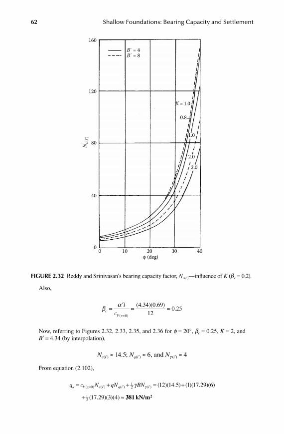
62 Shallow Foundations: Bearing Capacity and Settlement
Also,
β α
cV z
l
c= ′ = =
=( )
( . )( . ).
0
4 34 0 69
120 25
Now, referring to Figures 2.32, 2.33, 2.35, and 2.36 for f = 20°, bc = 0.25, K = 2, and B′ = 4.34 (by interpolation),
Nc(i′) ≈ 14.5; Nq(i′) ≈ 6, and Ng (i′) ≈ 4
From equation (2.102),
q c N qN BNu V z c i q i i= + + == ′ ′ ′( ) ( ) ( ) ( ) ( )(012 12 14γ γ . ) ( )( . )( )
( . )( )( )
5 1 17 29 6
17 29 3 412
+
+ ≈ 3381 kN/m2
160
120
B´ = 4B´ = 8
K = 1.0
0.8
1.0
2.0
2.0
80Nc(
i)
40
00 10 20 30 40
φ (deg)
FiGure 2.32 Reddy and Srinivasan’s bearing capacity factor, Nc(i′)—influence of K (bc = 0.2).
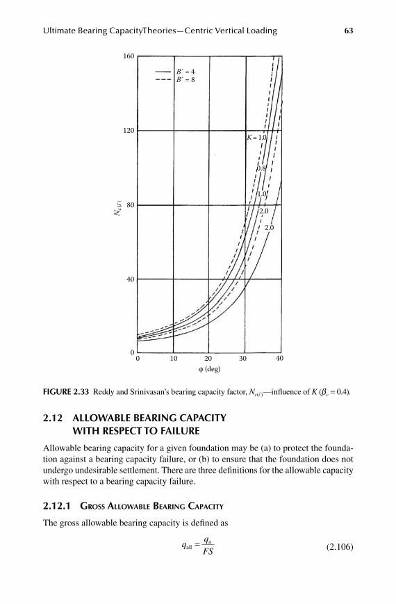
Ultimate Bearing CapacityTheories—Centric Vertical Loading 63
2.12 allowable bearinG CapaCity with reSpeCt to Failure
Allowable bearing capacity for a given foundation may be (a) to protect the founda-tion against a bearing capacity failure, or (b) to ensure that the foundation does not undergo undesirable settlement. There are three definitions for the allowable capacity with respect to a bearing capacity failure.
2.12.1 gRoss allowaBle BeaRing CapaCity
The gross allowable bearing capacity is defined as
q
qFS
uall =
(2.106)
160
120
B´ = 4B´ = 8
K = 1.0
0.8
1.0
2.0
2.0
80
Nc(
i)
40
00 10 20 30 40
φ (deg)
FiGure 2.33 Reddy and Srinivasan’s bearing capacity factor, Nc(i′)—influence of K (bc = 0.4).
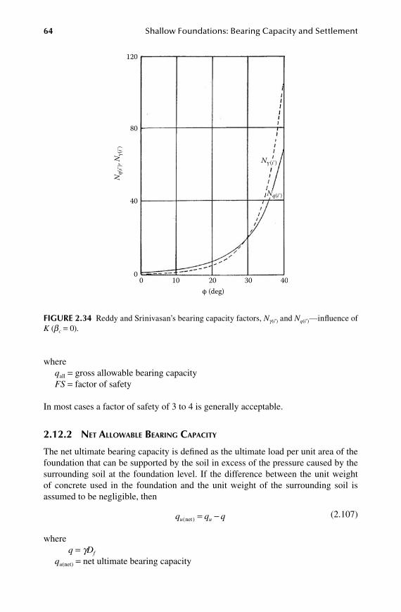
64 Shallow Foundations: Bearing Capacity and Settlement
where qall = gross allowable bearing capacityFS = factor of safety
In most cases a factor of safety of 3 to 4 is generally acceptable.
2.12.2 net allowaBle BeaRing CapaCity
The net ultimate bearing capacity is defined as the ultimate load per unit area of the foundation that can be supported by the soil in excess of the pressure caused by the surrounding soil at the foundation level. If the difference between the unit weight of concrete used in the foundation and the unit weight of the surrounding soil is assumed to be negligible, then
q q qu u( )net = -
(2.107)
where q = gDf
qu(net) = net ultimate bearing capacity
120
80
40
00 10 20 30 40
φ (deg)
Nq(
i), N
γ(i)
Nγ(i )
Nq(i )
FiGure 2.34 Reddy and Srinivasan’s bearing capacity factors, Ng(i′) and Nq(i′)—influence of K (bc = 0).
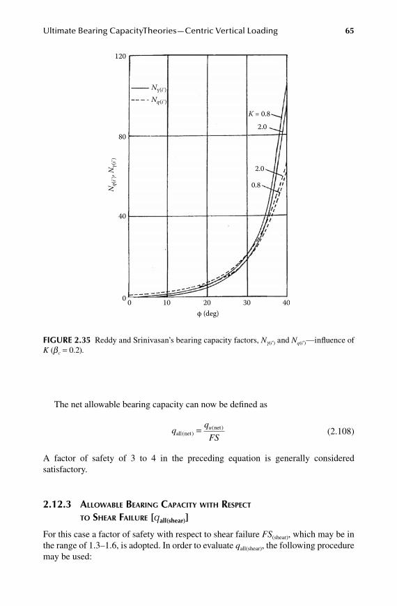
Ultimate Bearing CapacityTheories—Centric Vertical Loading 65
The net allowable bearing capacity can now be defined as
q
q
FSu
all netnet
( )( )=
(2.108)
A factor of safety of 3 to 4 in the preceding equation is generally considered satisfactory.
2.12.3 allowaBle BeaRing CapaCity with RespeCt to sheaR failURe [qall(shear)]
For this case a factor of safety with respect to shear failure FS(shear), which may be in the range of 1.3–1.6, is adopted. In order to evaluate qall(shear), the following procedure may be used:
120
80
40
0 0 10 20 30 40φ (deg)
Nq(
i), N
γ(i)
Nγ(i )
Nq(i )
2.0
2.0
0.8
K = 0.8
FiGure 2.35 Reddy and Srinivasan’s bearing capacity factors, Ng(i′) and Nq(i′)—influence of K (bc = 0.2).

66 Shallow Foundations: Bearing Capacity and Settlement
1. Determine the developed cohesion cd and the developed angle of friction fd as
cc
FSd =(shear)
(2.109)
φ φd FS
=
-tantan1
(shear)
(2.110)
2. The gross and net ultimate allowable bearing capacities with respect to shear failure can now be determined as [equation (2.82)]
q c N qN BNd c cs cd q qs qd sall(shear) gross
= + +l l l l γ lγ γ12 llγd
(2.111)
120
80
40
00 10 20 30 40
φ (deg)
Nq(
i), N
γ(i)
Nγ(i )
Nq(i )K = 0.8
2.0
2.00.8
FiGure 2.36 Reddy and Srinivasan’s bearing capacity factors, Ng(i′) and Nq(i′)—influence of K (bc = 0.4).

Ultimate Bearing CapacityTheories—Centric Vertical Loading 67
q q q c N qd c cs cdall(shear) net all(shear) gross
= - = +l l (N BNq qs qd s d- +1 12)l l γ l lγ γ γ
(2.112)
whereNc, Nq, and Ng = bearing capacity factors for friction angle fd
Example 2.4
Refer to Example 2.1, problem a.
a. Determine the gross allowable bearing capacity. Assume FS = 4. b. Determine the net allowable bearing capacity. Assume FS = 4. c. Determine the gross and net allowable bearing capacities with respect to shear
failure. Assume FS(shear) = 1.5.
Solution
Part aFrom Example 2.1, problem a, qu = 1585 kN/m2
q
qFS
uall = = ≈1585
4396.25 kN/m2
Part b
q
q q
FSu
all net( )
( . )( )=-
= - ≈1585 0 6 184
393.55 kN/m2
Part c
c
c
FSd = = =(shear)
2kN/m48
1 532
.
φ φd FS
=
- -tantan
tantan
.1 1 25
1 5(shear)
= °17 3.
For fd = 17.3°, Nc = 12.5, Nq = 4.8 (Table 2.3), and Ng = 3.6 (Table 2.4),
lcsq
c
N
N
B
L= +
= +
1 14 8
12 5
0 6.
.
.
1 21 192
1 10 6
1
..
tan.
.
=
= +
= +l φqs d
B
L 2217 3 1 156
1 0 4 1 0
=
= -
= -
tan . .
. .lγ s
B
L44
0 6
1 20 8
.
..
=
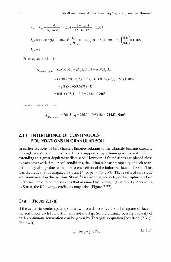
68 Shallow Foundations: Bearing Capacity and Settlement
l ll
φcd qdqd
c dN= -
-= - - =
11 308
1 1 30812 5 17 3
1tan
..
. tan ..
tan ( sin ) ( )(tan
387
1 2 1 1 2 12l φ φqd d dfD
B= + -
= + 7 3 1 17 3
0 60 6
1 308
1
2. )( sin . )..
.-
=
=lγd
From equation (2.111)
q c N qN BNd c cs cd q qs qd sall(shear) gross= + +l l l l γ lγ γ
12 llγd
= +( )( . )( . )( . ) ( . )( )( . )( .32 12 5 1 192 1 387 0 6 18 4 8 1 1156 1 308
18 0 6 3 6 0 8 1
661 3 7
12
)( . )
( )( . )( . )( . )( )
.
+
= + 8 4 15 6 755 3. . .+ = kN/m2
From equation (2.112):
q q
all(shear) net= - = - ≈761 5 755 3 0 6 18. . ( . )( ) 744.5 kN/m2
2.13 interFerenCe oF ContinuouS FoundationS in Granular Soil
In earlier sections of this chapter, theories relating to the ultimate bearing capacity of single rough continuous foundations supported by a homogeneous soil medium extending to a great depth were discussed. However, if foundations are placed close to each other with similar soil conditions, the ultimate bearing capacity of each foun-dation may change due to the interference effect of the failure surface in the soil. This was theoretically investigated by Stuart35 for granular soils. The results of this study are summarized in this section. Stuart35 assumed the geometry of the rupture surface in the soil mass to be the same as that assumed by Terzaghi (Figure 2.1). According to Stuart, the following conditions may arise (Figure 2.37):
Case 1 (figURe 2.37a)
If the center-to-center spacing of the two foundations is x ≥ x1, the rupture surface in the soil under each foundation will not overlap. So the ultimate bearing capacity of each continuous foundation can be given by Terzaghi’s equation [equation (2.31)]. For c = 0,
q qN BNu q= + 1
2 γ γ (2.113)

Ultimate Bearing CapacityTheories—Centric Vertical Loading 69
FiG
ur
e 2.
37 A
ssum
ptio
ns fo
r th
e fa
ilur
e su
rfac
e in
gra
nula
r so
il u
nder
two
clos
ely
spac
ed r
ough
con
tinu
ous
foun
dati
ons.
Not
e: a
1 =
f, a
2 =
45 –
f/2
, a3
= 18
0 –
f.
α 2
α 2α 2
α 2α 2
α 2α 2
(a)
(b)
α 2α 2
α 2α 2
α 2α 2
α 2α 1
α 1α 1
α 1
q u
q u
Bq u
q = γD
f
q = γD
f
B
BB
x =
x 1
x =
x 2
q u
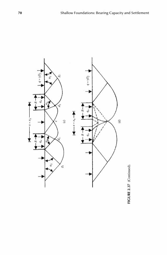
70 Shallow Foundations: Bearing Capacity and Settlement
α 2α 3
(c)
(d)
α 3α 2
g 1d 1
d 2g 2
e
B
BB
B
x =
x 3
x =
x 4
q u
q uq u
q uq
= γD
f
q =
γDf
FiG
ur
e 2.
37 (
Con
tinu
ed).
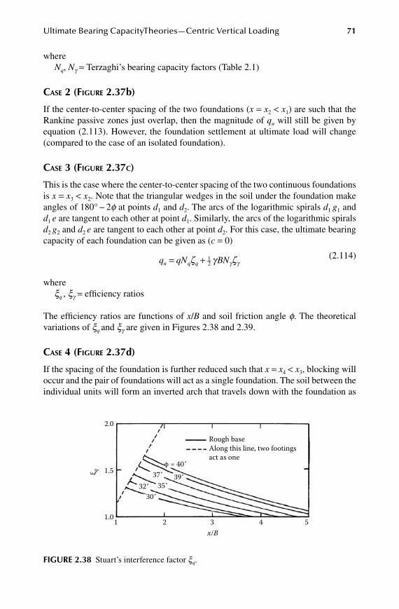
Ultimate Bearing CapacityTheories—Centric Vertical Loading 71
whereNq, Ng = Terzaghi’s bearing capacity factors (Table 2.1)
Case 2 (figURe 2.37b)
If the center-to-center spacing of the two foundations (x = x2 < x1) are such that the Rankine passive zones just overlap, then the magnitude of qu will still be given by equation (2.113). However, the foundation settlement at ultimate load will change (compared to the case of an isolated foundation).
Case 3 (figURe 2.37C)
This is the case where the center-to-center spacing of the two continuous foundations is x = x3 < x2. Note that the triangular wedges in the soil under the foundation make angles of 180° − 2f at points d1 and d2. The arcs of the logarithmic spirals d1 g1 and d1 e are tangent to each other at point d1. Similarly, the arcs of the logarithmic spirals d2 g2 and d2 e are tangent to each other at point d2. For this case, the ultimate bearing capacity of each foundation can be given as (c = 0)
q qN BNu q q= +ζ γ ζγ γ
12
(2.114)
wherexq , xg = efficiency ratios
The efficiency ratios are functions of x/B and soil friction angle f. The theoretical variations of xq and xg are given in Figures 2.38 and 2.39.
Case 4 (figURe 2.37d)
If the spacing of the foundation is further reduced such that x = x4 < x3, blocking will occur and the pair of foundations will act as a single foundation. The soil between the individual units will form an inverted arch that travels down with the foundation as
2.0
Rough baseAlong this line, two footingsact as one
1.5
1.01 2 3 4 5
ξ q
φ = 40˚37˚
32˚ 35˚39˚
30˚
x/B
FiGure 2.38 Stuart’s interference factor xq.

72 Shallow Foundations: Bearing Capacity and Settlement
the load is applied. When the two foundations touch, the zone of arching disappears and the system behaves as a single foundation with a width equal to 2B. The ultimate bearing capacity for this case can be given by equation (2.113), with B being replaced by 2B in the third term.
Das and Larbi-Cherif36 conducted laboratory model tests to determine the inter-ference efficiency ratios xq and xg of two rough continuous foundations resting on sand extending to a great depth. The sand used in the model tests was highly angular, and the tests were conducted at a relative density of about 60%. The angle of friction f at this relative density of compaction was 39°. Load-displacement curves obtained from the model tests were of the local shear type. The experi-mental variations of xq and xg obtained from these tests are given in Figures 2.40 and 2.41. From these figures it may be seen that, although the general trend of the experimental efficiency ratio variations is similar to those predicted by theory, there is a large variation in the magnitudes between the theory and experimen-tal results. Figure 2.42 shows the experimental variations of Su/B with x/B (Su = settlement at ultimate load). The elastic settlement of the foundation decreases with the increase in the center-to-center spacing of the foundation and remains constant at x > about 4B.
3.5
3.0
2.5
1.5
1.01 2 3 4
x/B5
2.0
ξ γ φ = 40˚
Rough baseAlong this line, two footingsact as one
39˚
37˚
35˚
32˚
30˚
FiGure 2.39 Stuart’s interference factor xg .
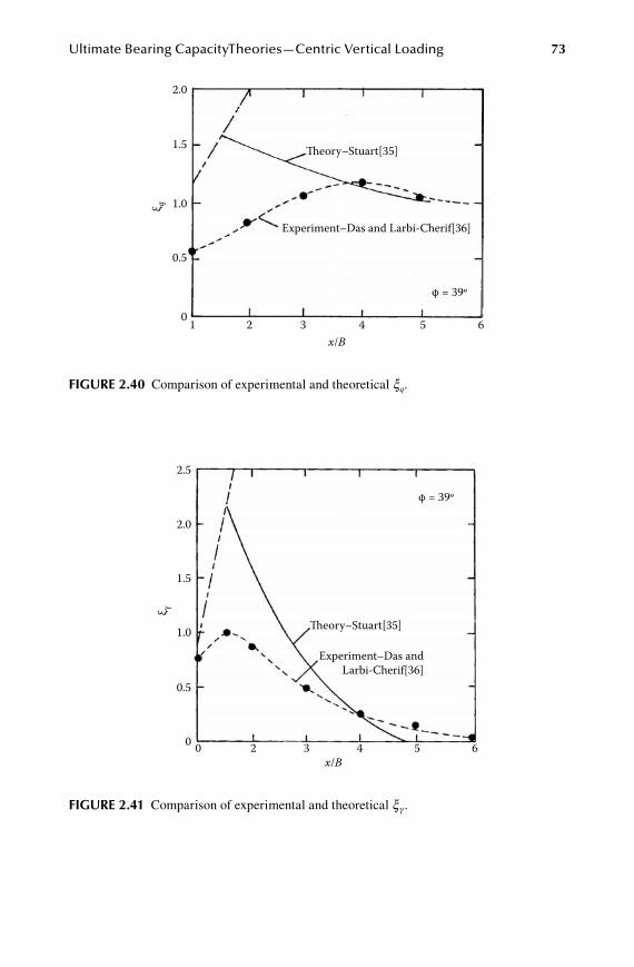
Ultimate Bearing CapacityTheories—Centric Vertical Loading 73
2.0
1.5
1.0
0.5
Theory–Stuart[35]
Experiment–Das and Larbi-Cherif[36]
0 21 3 4 5 6x/B
ξ q
φ = 39º
FiGure 2.40 Comparison of experimental and theoretical xq.
2.5
1.5
0.5
0 0 2 3 4 5x/B
6
2.0
1.0 Theory–Stuart[35]
Experiment–Das andLarbi-Cherif[36]
ξ γ
φ = 39º
FiGure 2.41 Comparison of experimental and theoretical xg .
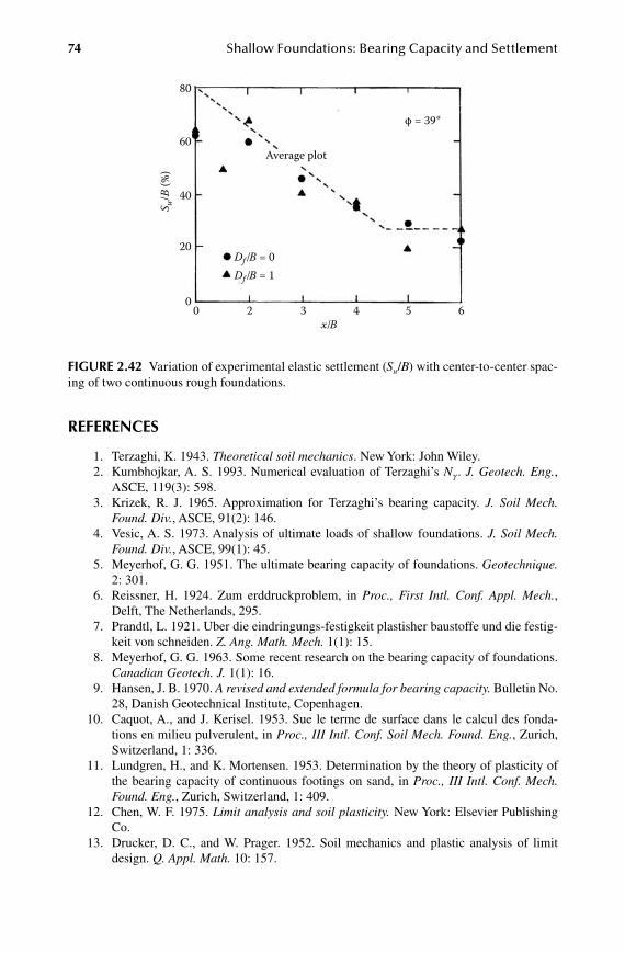
74 Shallow Foundations: Bearing Capacity and Settlement
reFerenCeS
1. Terzaghi, K. 1943. Theoretical soil mechanics. New York: John Wiley. 2. Kumbhojkar, A. S. 1993. Numerical evaluation of Terzaghi’s Ng . J. Geotech. Eng.,
ASCE, 119(3): 598. 3. Krizek, R. J. 1965. Approximation for Terzaghi’s bearing capacity. J. Soil Mech.
Found. Div., ASCE, 91(2): 146. 4. Vesic, A. S. 1973. Analysis of ultimate loads of shallow foundations. J. Soil Mech.
Found. Div., ASCE, 99(1): 45. 5. Meyerhof, G. G. 1951. The ultimate bearing capacity of foundations. Geotechnique.
2: 301. 6. Reissner, H. 1924. Zum erddruckproblem, in Proc., First Intl. Conf. Appl. Mech.,
Delft, The Netherlands, 295. 7. Prandtl, L. 1921. Uber die eindringungs-festigkeit plastisher baustoffe und die festig-
keit von schneiden. Z. Ang. Math. Mech. 1(1): 15. 8. Meyerhof, G. G. 1963. Some recent research on the bearing capacity of foundations.
Canadian Geotech. J. 1(1): 16. 9. Hansen, J. B. 1970. A revised and extended formula for bearing capacity. Bulletin No.
28, Danish Geotechnical Institute, Copenhagen. 10. Caquot, A., and J. Kerisel. 1953. Sue le terme de surface dans le calcul des fonda-
tions en milieu pulverulent, in Proc., III Intl. Conf. Soil Mech. Found. Eng., Zurich, Switzerland, 1: 336.
11. Lundgren, H., and K. Mortensen. 1953. Determination by the theory of plasticity of the bearing capacity of continuous footings on sand, in Proc., III Intl. Conf. Mech. Found. Eng., Zurich, Switzerland, 1: 409.
12. Chen, W. F. 1975. Limit analysis and soil plasticity. New York: Elsevier Publishing Co.
13. Drucker, D. C., and W. Prager. 1952. Soil mechanics and plastic analysis of limit design. Q. Appl. Math. 10: 157.
80
60
40
20
Average plot
Df /B = 0Df /B = 1
x/B
S u/B
(%)
00 2 3 4 5 6
φ = 39º
FiGure 2.42 Variation of experimental elastic settlement (Su/B) with center-to-center spac-ing of two continuous rough foundations.
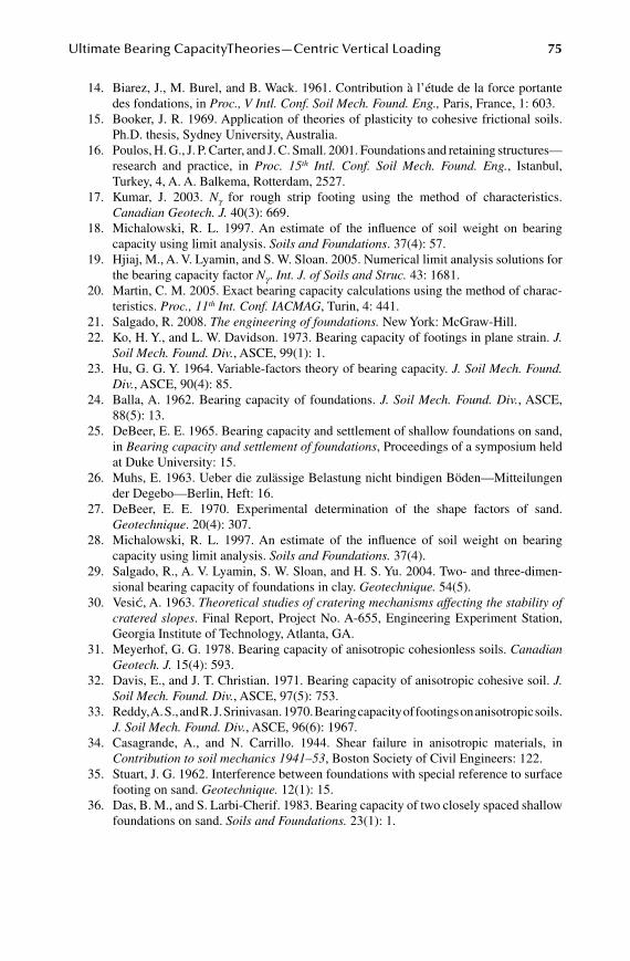
Ultimate Bearing CapacityTheories—Centric Vertical Loading 75
14. Biarez, J., M. Burel, and B. Wack. 1961. Contribution à l’étude de la force portante des fondations, in Proc., V Intl. Conf. Soil Mech. Found. Eng., Paris, France, 1: 603.
15. Booker, J. R. 1969. Application of theories of plasticity to cohesive frictional soils. Ph.D. thesis, Sydney University, Australia.
16. Poulos, H. G., J. P. Carter, and J. C. Small. 2001. Foundations and retaining structures— research and practice, in Proc. 15th Intl. Conf. Soil Mech. Found. Eng., Istanbul, Turkey, 4, A. A. Balkema, Rotterdam, 2527.
17. Kumar, J. 2003. Ng for rough strip footing using the method of characteristics. Canadian Geotech. J. 40(3): 669.
18. Michalowski, R. L. 1997. An estimate of the influence of soil weight on bearing capacity using limit analysis. Soils and Foundations. 37(4): 57.
19. Hjiaj, M., A. V. Lyamin, and S. W. Sloan. 2005. Numerical limit analysis solutions for the bearing capacity factor Ng . Int. J. of Soils and Struc. 43: 1681.
20. Martin, C. M. 2005. Exact bearing capacity calculations using the method of charac-teristics. Proc., 11th Int. Conf. IACMAG, Turin, 4: 441.
21. Salgado, R. 2008. The engineering of foundations. New York: McGraw-Hill. 22. Ko, H. Y., and L. W. Davidson. 1973. Bearing capacity of footings in plane strain. J.
Soil Mech. Found. Div., ASCE, 99(1): 1. 23. Hu, G. G. Y. 1964. Variable-factors theory of bearing capacity. J. Soil Mech. Found.
Div., ASCE, 90(4): 85. 24. Balla, A. 1962. Bearing capacity of foundations. J. Soil Mech. Found. Div., ASCE,
88(5): 13. 25. DeBeer, E. E. 1965. Bearing capacity and settlement of shallow foundations on sand,
in Bearing capacity and settlement of foundations, Proceedings of a symposium held at Duke University: 15.
26. Muhs, E. 1963. Ueber die zulässige Belastung nicht bindigen Böden—Mitteilungen der Degebo—Berlin, Heft: 16.
27. DeBeer, E. E. 1970. Experimental determination of the shape factors of sand. Geotechnique. 20(4): 307.
28. Michalowski, R. L. 1997. An estimate of the influence of soil weight on bearing capacity using limit analysis. Soils and Foundations. 37(4).
29. Salgado, R., A. V. Lyamin, S. W. Sloan, and H. S. Yu. 2004. Two- and three-dimen-sional bearing capacity of foundations in clay. Geotechnique. 54(5).
30. VesiĆ, A. 1963. Theoretical studies of cratering mechanisms affecting the stability of cratered slopes. Final Report, Project No. A-655, Engineering Experiment Station, Georgia Institute of Technology, Atlanta, GA.
31. Meyerhof, G. G. 1978. Bearing capacity of anisotropic cohesionless soils. Canadian Geotech. J. 15(4): 593.
32. Davis, E., and J. T. Christian. 1971. Bearing capacity of anisotropic cohesive soil. J. Soil Mech. Found. Div., ASCE, 97(5): 753.
33. Reddy, A. S., and R. J. Srinivasan. 1970. Bearing capacity of footings on anisotropic soils. J. Soil Mech. Found. Div., ASCE, 96(6): 1967.
34. Casagrande, A., and N. Carrillo. 1944. Shear failure in anisotropic materials, in Contribution to soil mechanics 1941–53, Boston Society of Civil Engineers: 122.
35. Stuart, J. G. 1962. Interference between foundations with special reference to surface footing on sand. Geotechnique. 12(1): 15.
36. Das, B. M., and S. Larbi-Cherif. 1983. Bearing capacity of two closely spaced shallow foundations on sand. Soils and Foundations. 23(1): 1.

77
3 Ultimate Bearing Capacity under Inclined and Eccentric Loads
3.1 introduCtion
Due to bending moments and horizontal thrusts transferred from the superstructure, shallow foundations are often subjected to eccentric and inclined loads. Under such circumstances the ultimate bearing capacity theories presented in Chapter 2 need some modification, and this is the subject of discussion in this chapter. The chapter is divided into two major parts. The first part discusses the ultimate bearing capaci-ties of shallow foundations subjected to centric inclined loads, and the second part is devoted to the ultimate bearing capacity under eccentric loading.
3.2 FoundationS SubjeCted to inClined load
3.2.1 meyeRhof’s theoRy (ContinUoUs foUnDation)
In 1953, Meyerhof1 extended his theory for ultimate bearing capacity under vertical loading (section 2.4) to the case with inclined load. Figure 3.1 shows the plastic zones in the soil near a rough continuous (strip) foundation with a small inclined load. The shear strength of the soil s is given as
s c= + ′σ φtan (3.1)
where c = cohesion s ′ = effective vertical stress f = angle of friction
The inclined load makes an angle a with the vertical. It needs to be pointed out that Figure 3.1 is an extension of Figure 2.7. In Figure 3.1, abc is an elastic zone, bcd is a radial shear zone, and bde is a mixed shear zone. The normal and shear stresses on plane be are po and so, respectively. Also, the unit base adhesion is ′ca. The solu-tion for the ultimate bearing capacity qu can be expressed as
q q cN p N BNu v u c o q( ) cos= = + +α γ γ
12
(3.2)

78 Shallow Foundations: Bearing Capacity and Settlement
whereNc, Nq, Ng = bearing capacity factors for inclined loading condition
g = unit weight of soil
Similar to equations (2.71), (2.59), and (2.70), we can write
q q q qu v u u v u v( ) ( ) ( )cos= = ′ + ′′α (3.3)
where
′ = + ≠ = ≠ ≠q cN p N pu v c o q o( ) ,(for 0, 0,φ γ 0 c 00) (3.4)
and
′′ = ≠ ≠ = =q BN p cu v o( )
12 γ φ γγ (for 0, 0, 0, 0 )) (3.5)
It was shown by Meyerhof1 in equation (3.4) that
N ec = + -- +
cotsin sin( )sin sin( )
tanφ φ ψ φφ η φ
θ1 21 2
2 φφ -
1 (3.6)
N ec = + -
- +1 21 2
2sin sin( )sin sin( )
tanφ ψ φφ η φ
θ φ (3.7)
Note that the horizontal component of the inclined load per unit area on the founda-tion ′qh cannot exceed the shearing resistance at the base, or
′ ≤ + ′q c qu h a u v( ) ( ) tanδ (3.8)
where ca = unit base adhesion d = unit base friction angle
In order to determine the minimum passive force per unit length of the foundation Ppg(min) (see Figure 2.11 for comparison) to obtain Ng , one can take a numerical step-by-step approach as shown by Caquot and Kerisel2 or a semi-graphical approach
FiGure 3.1 Plastic zones in soil near a foundation with an inclined load.
45 – φ/2
90 – φ
e
α
B
Df
θ
β ηψ
b a
c
d
s0p0
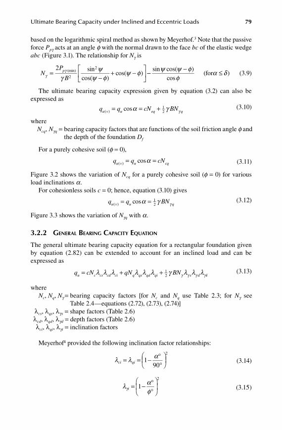
Ultimate Bearing Capacity under Inclined and Eccentric Loads 79
based on the logarithmic spiral method as shown by Meyerhof.3 Note that the passive force Ppg acts at an angle f with the normal drawn to the face bc of the elastic wedge abc (Figure 3.1). The relationship for Ng is
NP
Bp
γγ
γψ
ψ φψ φ=
-+ -
22
2(min) sin
cos( )cos( ) -- - ≤sin cos( )
cosψ ψ φ
φα δ(for ) (3.9)
The ultimate bearing capacity expression given by equation (3.2) can also be expressed as
q q cN BNu v u eq q( ) cos= = +α γ γ
12
(3.10)
whereNcq, Ngq = bearing capacity factors that are functions of the soil friction angle f and
the depth of the foundation Df
For a purely cohesive soil (f = 0),
q q cNu v u cq( ) cos= =α (3.11)
Figure 3.2 shows the variation of Ncq for a purely cohesive soil (f = 0) for various load inclinations a.
For cohesionless soils c = 0; hence, equation (3.10) gives
q q BNu v u q( ) cos= =α γ γ
12
(3.12)
Figure 3.3 shows the variation of Ngq with a.
3.2.2 geneRal BeaRing CapaCity eqUation
The general ultimate bearing capacity equation for a rectangular foundation given by equation (2.82) can be extended to account for an inclined load and can be expressed as
q cN qN BNu c cs cd ci q qs qd qi s d= + +l l l l l l γ l l lγ γ γ γ
12 ii
(3.13)
where Nc, Nq, Ng = bearing capacity factors [for Nc and Nq use Table 2.3; for Ng see
Table 2.4—equations (2.72), (2.73), (2.74)] lcs, lqs, lgs = shape factors (Table 2.6)lcd, lqd, lgd = depth factors (Table 2.6) lci, lqi, lgi = inclination factors
Meyerhof4 provided the following inclination factor relationships:
l l α
ci qi= = - °°
1
90
2
(3.14)
l α
φγi = - °°
1
2
(3.15)
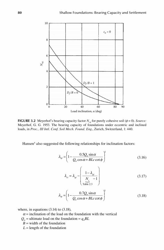
80 Shallow Foundations: Bearing Capacity and Settlement
Hansen5 also suggested the following relationships for inclination factors:
l αα φqi
u
u
QQ BLc
= -+
1
0 55
. sincos cot
(3.16)
l ll
ci qiqi
cN= -
--
1
1Table 2.3�
(3.17)
l αα φγi
u
u
QQ BLc
= -+
1
0 75
. sincos cot
(3.18)
where, in equations (3.14) to (3.18), a = inclination of the load on the foundation with the vertical Qu = ultimate load on the foundation = quBL B = width of the foundation L = length of the foundation
FiGure 3.2 Meyerhof’s bearing capacity factor Ncq for purely cohesive soil (f = 0). Source: Meyerhof, G. G. 1953. The bearing capacity of foundations under eccentric and inclined loads, in Proc., III Intl. Conf. Soil Mech. Found. Eng., Zurich, Switzerland, 1: 440.
10
8
6
4
Ncq
2
00 20 40
Load inclination, α (deg)60 80 90
ca = 0
Df /B = 1
Df /B = 0
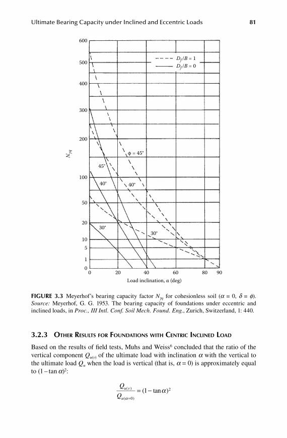
Ultimate Bearing Capacity under Inclined and Eccentric Loads 81
3.2.3 otheR ResUlts foR foUnDations with CentRiC inClineD loaD
Based on the results of field tests, Muhs and Weiss6 concluded that the ratio of the vertical component Qu(v) of the ultimate load with inclination a with the vertical to the ultimate load Qu when the load is vertical (that is, a = 0) is approximately equal to (1 – tan a)2:
Q
Qu v
u
( )
( )
( tan )α
α=
= -0
21
FiGure 3.3 Meyerhof’s bearing capacity factor Ngq for cohesionless soil (a = 0, d = f). Source: Meyerhof, G. G. 1953. The bearing capacity of foundations under eccentric and inclined loads, in Proc., III Intl. Conf. Soil Mech. Found. Eng., Zurich, Switzerland, 1: 440.
600
500
400
300
200
100
50
20
105
10
0 20 40Load inclination, α (deg)
60 80 90
Nγq
30°30°
40°40°
45°
φ = 45°
Df /B = 1Df /B = 0
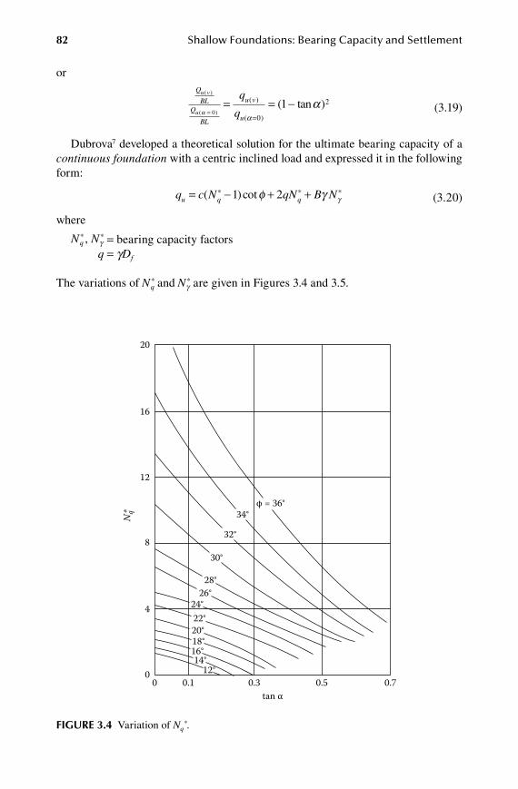
82 Shallow Foundations: Bearing Capacity and Settlement
or
Q
BLQ
BL
u v
u
u v
u
q
q
( )
( )
( )
( )
( tan )α
α
α=
=
= -0
0
21= (3.19)
Dubrova7 developed a theoretical solution for the ultimate bearing capacity of a continuous foundation with a centric inclined load and expressed it in the following form:
q c N qN B Nu q q= - + +( )cot* * *1 2φ γ γ (3.20)
where
N Nq
* *, γ = bearing capacity factors q = gDf
The variations of Nq* and Nγ
* are given in Figures 3.4 and 3.5.
FiGure 3.4 Variation of Nq*.
20
16
12
8
4
00 0.1 0.3 0.5 0.7
tan α
Nq*
φ = 36°34°
32°
30°
28°26°
24°22°20°18°16°14°
12°
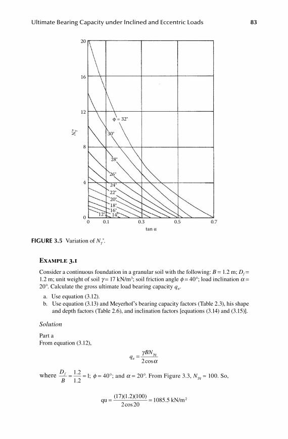
Ultimate Bearing Capacity under Inclined and Eccentric Loads 83
Example 3.1
Consider a continuous foundation in a granular soil with the following: B = 1.2 m; Df = 1.2 m; unit weight of soil g = 17 kN/m3; soil friction angle f = 40°; load inclination a = 20°. Calculate the gross ultimate load bearing capacity qu.
a. Use equation (3.12). b. Use equation (3.13) and Meyerhof’s bearing capacity factors (Table 2.3), his shape
and depth factors (Table 2.6), and inclination factors [equations (3.14) and (3.15)].
Solution
Part aFrom equation (3.12),
q
BNu
q=γ
αγ
2cos
where D
Bf = =1 2
1 21
.
.;
f = 40°; and a = 20°. From Figure 3.3, Ngq ≈ 100. So,
qu kN= =( )( . )( )
cos. /
17 1 2 1002 20
1085 5 2m
FiGure 3.5 Variation of Ng*.
20
16
12
8
4
00 0.1 0.3 0.5 0.7
tan α
Nγ*
φ = 32°
30°
28°
26°
24°22°20°18°16°
12° 14°
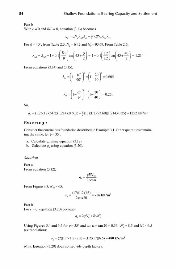
84 Shallow Foundations: Bearing Capacity and Settlement
Part bWith c = 0 and B/L = 0, equation (3.13) becomes
q qN BNu q qd qi d i= +l l γ l lγ γ γ
12
For f = 40°, from Table 2.3, Nq = 64.2 and Ng = 93.69. From Table 2.6,
l l φγqd d
fD
B= = +
+
= +1 0 1 452
1 0 11
. tan ...
tan .2
1 245
402
1 214
+
=
From equations (3.14) and (3.15),
l α
qi = - °°
= -
=1
901
2090
0 6052 2
.
l α
φγi = - °°
= -
=1 1
2040
0 252 2
. .
So,
qu = × +( . )( . )( . )( . ) ( )( . )1 2 17 64 2 1 214 0 605 17 1 21
2 ( . )( . )( . ) 93 69 1 214 0 25 1252= kN/m2
Example 3.2
Consider the continuous foundation described in Example 3.1. Other quantities remain-ing the same, let f = 35°.
a. Calculate qu using equation (3.12). b. Calculate qu using equation (3.20).
Solution
Part aFrom equation (3.12),
q
BNu
q=γ
αγ
2cos
From Figure 3.3, Ngq ≈ 65:
qu = ≈( )( . )( )
cos17 1 2 65
2 20706 kN/m2
Part bFor c = 0, equation (3.20) becomes
q qN B Nu q= +2 * *γ γ
Using Figures 3.4 and 3.5 for f = 35° and tan a = tan 20 = 0.36, Nq* ≈ 8.5 and Nγ
* ≈ 6.5 (extrapolation):
qu = × + ≈( )( . )( . ) ( . )( )( . )2 17 1 2 8 5 1 2 17 6 5 480 kN/m22
Note: Equation (3.20) does not provide depth factors.
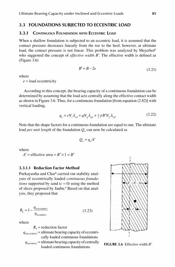
Ultimate Bearing Capacity under Inclined and Eccentric Loads 85
3.3 FoundationS SubjeCted to eCCentriC load
3.3.1 ContinUoUs foUnDation with eCCentRiC loaD
When a shallow foundation is subjected to an eccentric load, it is assumed that the contact pressure decreases linearly from the toe to the heel; however, at ultimate load, the contact pressure is not linear. This problem was analyzed by Meyerhof1 who suggested the concept of effective width B′. The effective width is defined as (Figure 3.6)
′ = -B B e2 (3.21)
wheree = load eccentricity
According to this concept, the bearing capacity of a continuous foundation can be determined by assuming that the load acts centrally along the effective contact width as shown in Figure 3.6. Thus, for a continuous foundation [from equation (2.82)] with vertical loading,
q cN qN B Nu c cd q qd d= + + ′l l γ lγ γ
12
(3.22)
Note that the shape factors for a continuous foundation are equal to one. The ultimate load per unit length of the foundation Qu can now be calculated as
Q q Au u= ′
whereA′ = effective area = B′ × 1 = B′
3.3.1.1 reduction Factor methodPurkayastha and Char8 carried out stability anal-yses of eccentrically loaded continuous founda-tions supported by sand (c = 0) using the method of slices proposed by Janbu.9 Based on that anal-ysis, they proposed that
Rq
qku
u
= -1 (
( )
eccentric)
centric
(3.23)
where Rk = reduction factor qu(eccentric) = ultimate bearing capacity of eccentri-
cally loaded continuous foundationsqu(centric) = ultimate bearing capacity of centrally
loaded continuous foundationsFiGure 3.6 Effective width B′.
B´ = B – 2e
B
e
86 Shallow Foundations: Bearing Capacity and Settlement
The magnitude of Rk can be expressed as
R a
eBk
k
=
(3.24)
where a and k are functions of the embedment ratio Df /B (Table 3.1).Hence, combining equations (3.23) and (3.24),
q q R qu u k u( ( ) ( )( )eccentric) centric centric= - =1 11-
aeB
k
(3.25)
where
q qN BN cu q qd d(centric) (Note:= + =l γ lγ γ
12 0) (3.26)
3.3.1.2 theory of prakash and SaranPrakash and Saran10 provided a comprehensive mathematical formulation to esti-mate the ultimate bearing capacity for rough continuous foundations under eccentric loading. According to this procedure, Figure 3.7 shows the assumed failure surface in a c–f soil under a continuous foundation subjected to eccentric loading. Let Qu be the ultimate load per unit length of the foundation of width B with an eccentricity e. In Figure 3.7 zone I is an elastic zone with wedge angles of y1 and y2. Zones II and III are similar to those assumed by Terzaghi (that is, zone II is a radial shear zone and zone III is a Rankine passive zone).
The bearing capacity expression can be developed by considering the equilib-rium of the elastic wedge abc located below the foundation (Figure 3.7b). Note that in Figure 3.7b the contact width of the foundation with the soil is equal to Bx1. Neglecting the self-weight of the wedge,
Q P P C Cu p m m a a= - + - + + ′cos( ) cos( ) sin sinψ φ ψ φ ψ ψ1 2 1 2 (3.27)
wherePp, Pm = passive forces per unit length of the wedge along the wedge faces bc and
ac, respectively
table 3.1Variations of a and k [equation (3.24)]
Df/B a k
0.00 1.862 0.730.25 1.811 0.7850.50 1.754 0.801.00 1.820 0.888
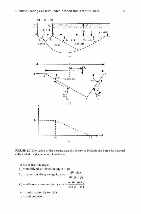
Ultimate Bearing Capacity under Inclined and Eccentric Loads 87
f = soil friction anglefm = mobilized soil friction angle (≤ f)
C bccBx
a = =adhesion along wedge face 1 2sins
ψiin( )ψ ψ1 2+
′ = =C acmcBx
a adhesion along wedge face 1 1sinψsin( )ψ ψ1 2+
m = mobilization factor (≤1)c = unit cohesion
FiGure 3.7 Derivation of the bearing capacity theory of Prakash and Saran for eccentri-cally loaded rough continuous foundation.
B
ea b
Be
a
C a Ca
ab
Bx1
Qu
c
Df
Qu
q = γDf
45 – φ/245 – φ/2Zone IIIZone IIZone I
(a)
ψ2 ψ1
ψ2ψ1
Center line
PmPp
(b)
φm φc
1.0
1/6 0.5e/B
(c)
x1
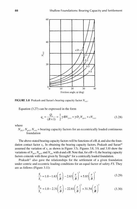
88 Shallow Foundations: Bearing Capacity and Settlement
Equation (3.27) can be expressed in the form
q
Q
BBN D N cNu
ue f q e c e=
×= + +
( ) ( ) ( ) ( )112
γ γγ (3.28)
whereNg(e), Nq(e), Nc(e) = bearing capacity factors for an eccentrically loaded continuous
foundation
The above-stated bearing capacity factors will be functions of e/B, f, and also the foun-dation contact factor x1. In obtaining the bearing capacity factors, Prakash and Saran10 assumed the variation of x1 as shown in Figure 3.7c. Figures 3.8, 3.9, and 3.10 show the variations of Ng(e), Nq(e), and Nc(e) with f and e/B. Note that, for e/B = 0, the bearing capacity factors coincide with those given by Terzaghi11 for a centrically loaded foundation.
Prakash12 also gave the relationships for the settlement of a given foundation under centric and eccentric loading conditions for an equal factor of safety FS. They are as follows (Figure 3.11):
S
SeB
eB
eB
e
o
= -
-
+
1 0 1 63 2 63 5 832
. . . .
3
(3.29)
S
SeB
eB
em
o
= -
-
+1 0 2 31 22 61 31 542
. . . .BB
3
(3.30)
FiGure 3.8 Prakash and Saran’s bearing capacity factor Nc(e) .
60
40
20
00 10 20 30 40
Friction angle, φ (deg)
Nc(
e)
0.4
0.3
0.2
0.1
e/B = 0
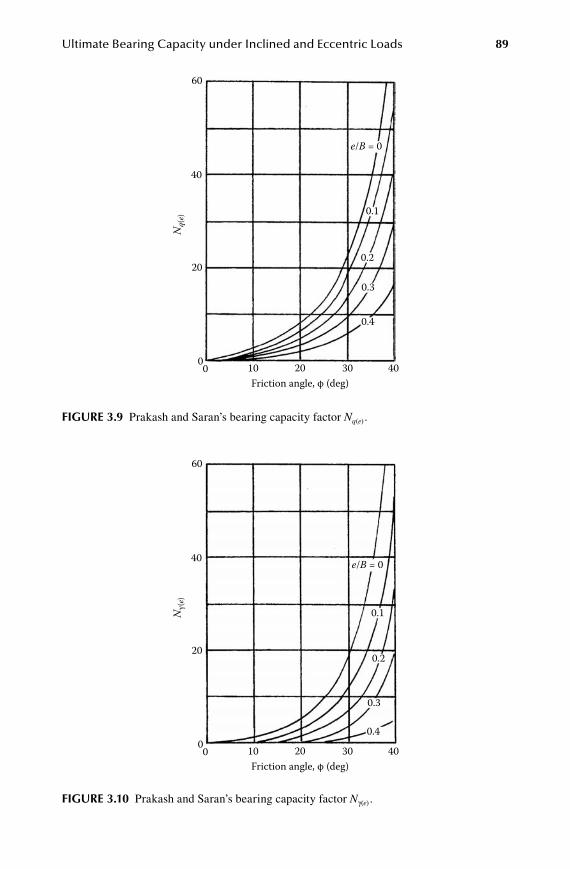
Ultimate Bearing Capacity under Inclined and Eccentric Loads 89
FiGure 3.9 Prakash and Saran’s bearing capacity factor Nq(e) .
60
40
20
00 10 20 30 40
Friction angle, φ (deg)
Nq(
e)
0.4
0.3
0.2
0.1
e/B = 0
FiGure 3.10 Prakash and Saran’s bearing capacity factor Nγ(e) .
60
40
20
00 10 20 30 40
Friction angle, φ (deg)
Nγ(
e)
0.4
0.3
0.2
0.1
e/B = 0
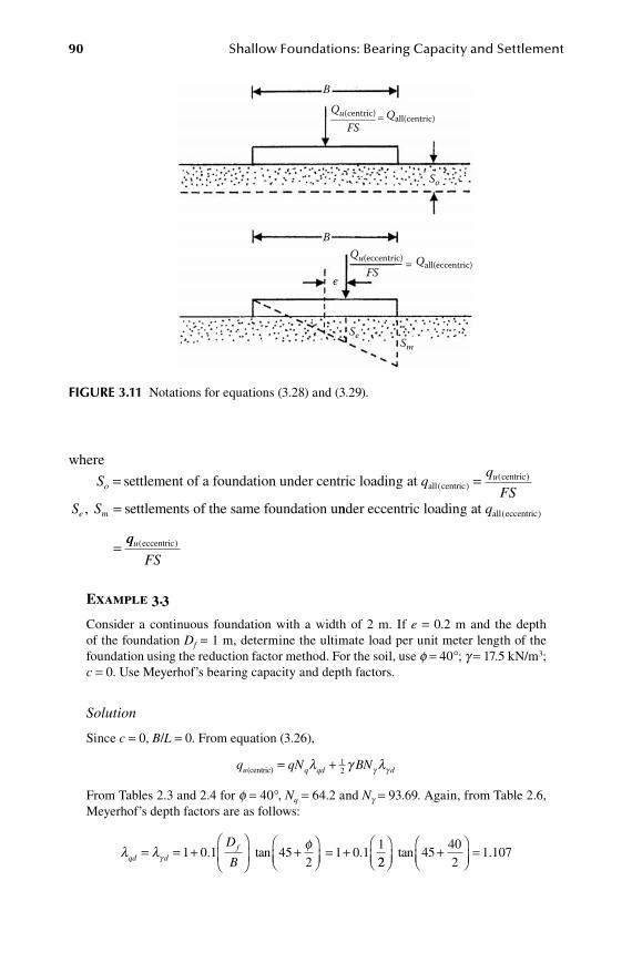
90 Shallow Foundations: Bearing Capacity and Settlement
where
So = settlement of a foundation under centric loading at all centriccentricq
q
FSu
( )( )=
S Se m, settlements of the same foundation u= nnder eccentric loading at all eccentricq ( )
FSu( )eccentric
Example 3.3
Consider a continuous foundation with a width of 2 m. If e = 0.2 m and the depth of the foundation Df = 1 m, determine the ultimate load per unit meter length of the foundation using the reduction factor method. For the soil, use f = 40°; g = 17.5 kN/m3; c = 0. Use Meyerhof’s bearing capacity and depth factors.
Solution
Since c = 0, B/L = 0. From equation (3.26),
q qN BNu q qd d(centric) = +l γ lγ γ
12
From Tables 2.3 and 2.4 for f = 40°, Nq = 64.2 and Ng = 93.69. Again, from Table 2.6, Meyerhof’s depth factors are as follows:
l l φγqd d
fD
B= = +
+
= +1 0 1 452
1 0 11
. tan .22
45402
+
=tan 1.107
FiGure 3.11 Notations for equations (3.28) and (3.29).
BQu(centric) Qall(centric)
FS=
B
e
SeSm
Qu(eccentric) Qall(eccentric)FS
=
So
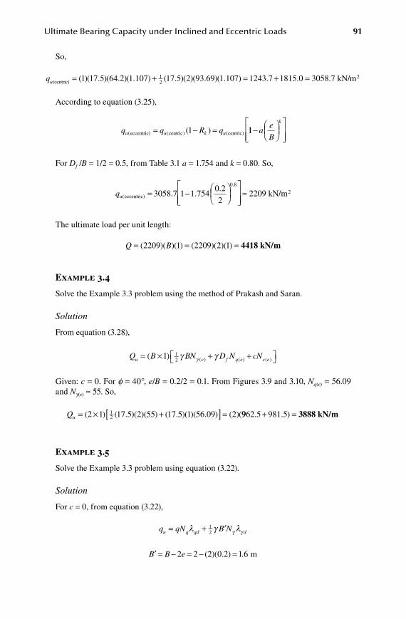
Ultimate Bearing Capacity under Inclined and Eccentric Loads 91
So,
qu(centric) = +( )( . )( . )( . ) ( . )1 17 5 64 2 1 107 17 512 ( )( . )( . ) . .2 93 69 1 107 1243 7 1815 0= + = 3058.7 kN/m2
According to equation (3.25),
q q R qu u k u( ( ) ( )( )eccentric) centric centric= - =1 11-
ae
B
k
For Df /B = 1/2 = 0.5, from Table 3.1 a = 1.754 and k = 0.80. So,
qu(
.
. ..
eccentric) = -
3058 7 1 1 754
0 2
2
0 8
≈ 2209 kN/m2
The ultimate load per unit length:
Q B= = =( )( )( ) ( )( )( )2209 1 2209 2 1 4418 kN/m
Example 3.4
Solve the Example 3.3 problem using the method of Prakash and Saran.
Solution
From equation (3.28),
Q B BN D N cNu e f q e c e= × + + ( ) ( ) ( ) ( )1 1
2 γ γγ
Given: c = 0. For f = 40°, e/B = 0.2/2 = 0.1. From Figures 3.9 and 3.10, Nq(e) = 56.09 and Ng(e) ≈ 55. So,
Qu = × +[ ] =( ) ( . )( )( ) ( . )( )( . ) ( )(2 1 17 5 2 55 17 5 1 56 09 21
2 9962 5 981 5. . )+ = 3888 kN/m
Example 3.5
Solve the Example 3.3 problem using equation (3.22).
Solution
For c = 0, from equation (3.22),
q qN B Nu q qd d= + ′l γ lγ γ
12
′ = - = - =B B e2 2 2 0 2 6( )( . ) .1 m
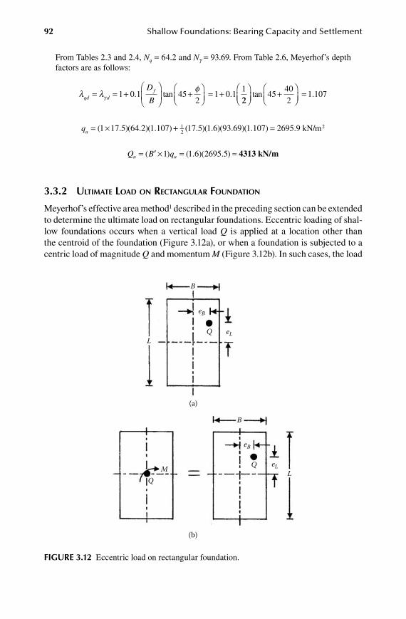
92 Shallow Foundations: Bearing Capacity and Settlement
From Tables 2.3 and 2.4, Nq = 64.2 and Ng = 93.69. From Table 2.6, Meyerhof’s depth factors are as follows:
l l φγqd d
fD
B= = +
+
= +1 0 1 452
1 0 11
. tan .22
45402
+
=tan 1.107
qu = × +( . )( . )( . ) ( . )( . )( .1 17 5 64 2 1 107 17 5 1 6 93 61
2 9 1 107)( . ) = 2695.9 kN/m2
Q B qu u= ′ × = ≈( ) ( . )( . )1 1 6 2695 5 4313 kN/m
3.3.2 Ultimate loaD on ReCtangUlaR foUnDation
Meyerhof’s effective area method1 described in the preceding section can be extended to determine the ultimate load on rectangular foundations. Eccentric loading of shal-low foundations occurs when a vertical load Q is applied at a location other than the centroid of the foundation (Figure 3.12a), or when a foundation is subjected to a centric load of magnitude Q and momentum M (Figure 3.12b). In such cases, the load
FiGure 3.12 Eccentric load on rectangular foundation.
B
L
L
Q
eB
eL
(a)
B
Q
QM
eB
eL
(b)
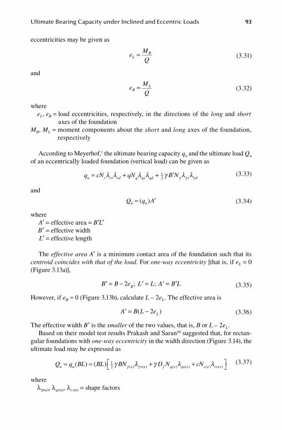
Ultimate Bearing Capacity under Inclined and Eccentric Loads 93
eccentricities may be given as
e
MQ
LB=
(3.31)
and
e
MQ
BL= (3.32)
where eL, eB = load eccentricities, respectively, in the directions of the long and short
axes of the foundation MB, ML = moment components about the short and long axes of the foundation,
respectively
According to Meyerhof,1 the ultimate bearing capacity qu and the ultimate load Qu of an eccentrically loaded foundation (vertical load) can be given as
q cN qN B Nu c cs cd q qs qd s d= + + ′l l l l γ l lγ γ γ
12
(3.33)
and
Q q Au u= ′( ) (3.34)
where A′ = effective area = B′L′ B′ = effective width L′ = effective length
The effective area A′ is a minimum contact area of the foundation such that its centroid coincides with that of the load. For one-way eccentricity [that is, if eL = 0 (Figure 3.13a)],
′ = - ′ = ′ = ′B B e L L A B LB2 ; ; (3.35)
However, if eB = 0 (Figure 3.13b), calculate L – 2eL. The effective area is
′ = -A B L eL( )2 (3.36)
The effective width B′ is the smaller of the two values, that is, B or L – 2eL.Based on their model test results Prakash and Saran10 suggested that, for rectan-
gular foundations with one-way eccentricity in the width direction (Figure 3.14), the ultimate load may be expressed as
Q q BL BL BN D Nu u e s e f q e qs e= = +( ) ( ) ( ) ( ) ( ) (
12 γ l γ lγ γ ) ( ) ( )+ cNc e cs el (3.37)
wherelgs(e), lqs(e), lcs(e) = shape factors
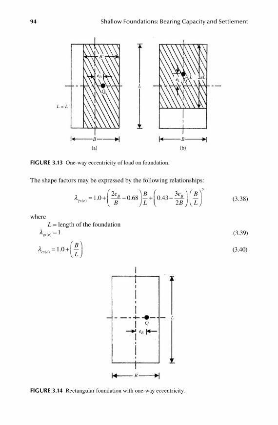
94 Shallow Foundations: Bearing Capacity and Settlement
The shape factors may be expressed by the following relationships:
lγ s e
B Be
BBL
e
B( ) . . .= + -
+ -
1 0
20 68 0 43
3
2
BL
2
(3.38)
whereL = length of the foundation
lqs e( ) =1 (3.39)
lcs e
BL( ) .= +
1 0 (3.40)
FiGure 3.13 One-way eccentricity of load on foundation.
B´
L
L = L´
L = 2eL
Q
Q
BB(a) (b)
eB eL
FiGure 3.14 Rectangular foundation with one-way eccentricity.
L
B
QeB
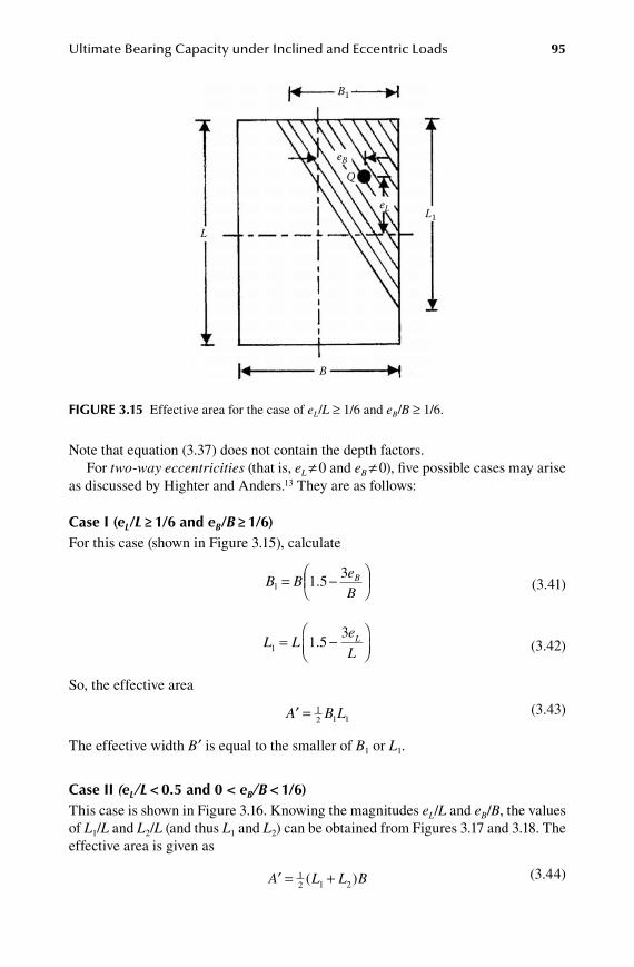
Ultimate Bearing Capacity under Inclined and Eccentric Loads 95
Note that equation (3.37) does not contain the depth factors.For two-way eccentricities (that is, eL ≠ 0 and eB ≠ 0), five possible cases may arise
as discussed by Highter and Anders.13 They are as follows:
Case i (eL/L ≥ 1/6 and eB/B ≥ 1/6)For this case (shown in Figure 3.15), calculate
B B
eB
B1 1 5
3= -
.
(3.41)
L L
e
LL
1 1 53
= -
. (3.42)
So, the effective area
′ =A B L1
2 1 1 (3.43)
The effective width B′ is equal to the smaller of B1 or L1.
Case ii (eL/L < 0.5 and 0 < eB/B < 1/6)This case is shown in Figure 3.16. Knowing the magnitudes eL/L and eB/B, the values of L1/L and L2/L (and thus L1 and L2) can be obtained from Figures 3.17 and 3.18. The effective area is given as
′ = +A L L B1
2 1 2( ) (3.44)
FiGure 3.15 Effective area for the case of eL/L ≥ 1/6 and eB/B ≥ 1/6.
L1
B1
Q
B
L
eB
eL
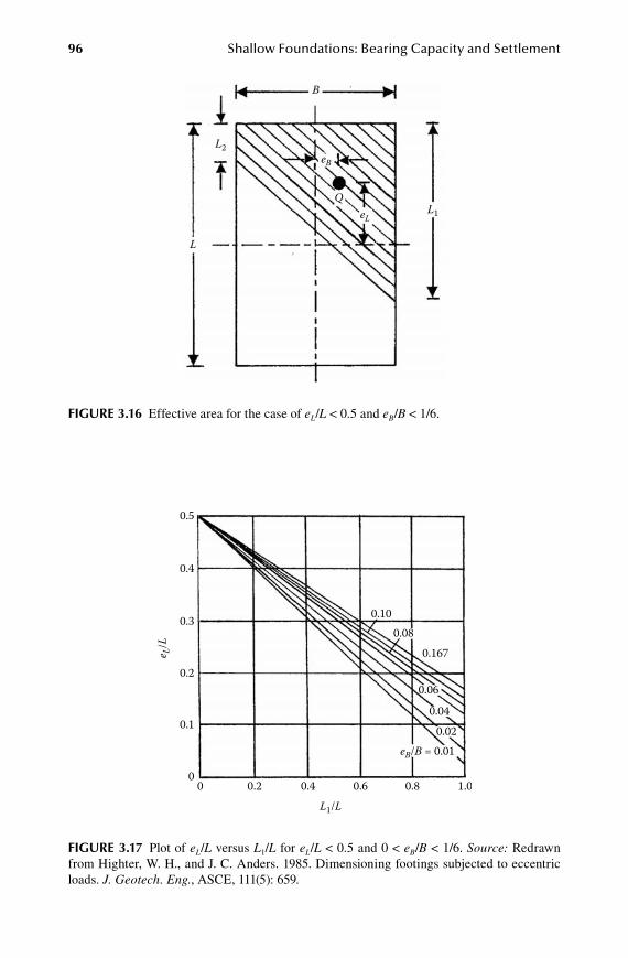
96 Shallow Foundations: Bearing Capacity and Settlement
FiGure 3.17 Plot of eL/L versus L1/L for eL/L < 0.5 and 0 < eB/B < 1/6. Source: Redrawn from Highter, W. H., and J. C. Anders. 1985. Dimensioning footings subjected to eccentric loads. J. Geotech. Eng., ASCE, 111(5): 659.
0.5
0.4
0.3
0.2
e L/L
L1/L
0.1
00 0.2 0.4 0.6 0.8 1.0
eB/B = 0.010.02
0.04
0.06
0.080.10
0.167
FiGure 3.16 Effective area for the case of eL/L < 0.5 and eB/B < 1/6.
B
L1
L2
Q
L
eB
eL

Ultimate Bearing Capacity under Inclined and Eccentric Loads 97
The effective length L′ is the larger of the two values L1 or L2. The effective width is equal to
′ = ′
′B
AL
(3.45)
Case iii (eL/L < 1/6 and 0 < eB/B < 0.5)Figure 3.19 shows the case under consideration. Knowing the magnitudes of eL/L and eB/B, the magnitudes of B1 and B2 can be obtained from Figures 3.20 and 3.21. So, the effective area can be obtained as
′ = +A B B L1
2 1 2( ) (3.46)
In this case, the effective length is equal to
′ =L L (3.47)
The effective width can be given as
′ = ′
BAL
(3.48)
FiGure 3.18 Plot of eL/L versus L2/L for eL/L < 0.5 and 0 < eB/B < 1/6. Source: Redrawn from Highter, W. H., and J. C. Anders. 1985. Dimensioning footings subjected to eccentric loads. J. Geotech. Eng., ASCE, 111(5): 659.
0.5
0.4
0.3
0.2
e L/L
L2/L
0.1
00 0.2 0.4 0.6 0.8 1.0
eB/B = 0.010.02
0.04
0.03
0.060.08
0.100.12
0.167
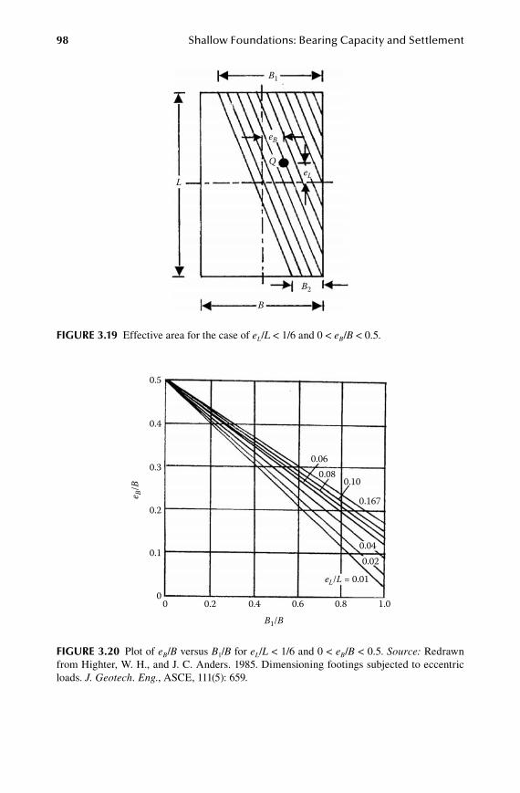
98 Shallow Foundations: Bearing Capacity and Settlement
FiGure 3.19 Effective area for the case of eL/L < 1/6 and 0 < eB/B < 0.5.
B2
B1
Q
B
L
eB
eL
FiGure 3.20 Plot of eB/B versus B1/B for eL/L < 1/6 and 0 < eB/B < 0.5. Source: Redrawn from Highter, W. H., and J. C. Anders. 1985. Dimensioning footings subjected to eccentric loads. J. Geotech. Eng., ASCE, 111(5): 659.
0.5
0.4
0.3
0.2
e B/B
B1/B
0.1
00 0.2 0.4 0.6 0.8 1.0
eL/L = 0.01
0.020.04
0.060.08
0.10
0.167
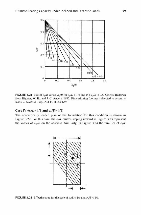
Ultimate Bearing Capacity under Inclined and Eccentric Loads 99
Case iV (eL/L < 1/6 and eB/B < 1/6)The eccentrically loaded plan of the foundation for this condition is shown in Figure 3.22. For this case, the eL/L curves sloping upward in Figure 3.23 represent the values of B2/B on the abscissa. Similarly, in Figure 3.24 the families of eL/L
FiGure 3.21 Plot of eB/B versus B2/B for eL/L < 1/6 and 0 < eB/B < 0.5. Source: Redrawn from Highter, W. H., and J. C. Anders. 1985. Dimensioning footings subjected to eccentric loads. J. Geotech. Eng., ASCE, 111(5): 659.
0.5
0.4
0.3
0.2
e B/B
B2/B
0.1
00 0.2 0.4 0.6 0.8 1.0
eL/L = 0.010.02
0.040.06
0.080.100.120.14
0.167
FiGure 3.22 Effective area for the case of eL/L < 1/6 and eB/B < 1/6.
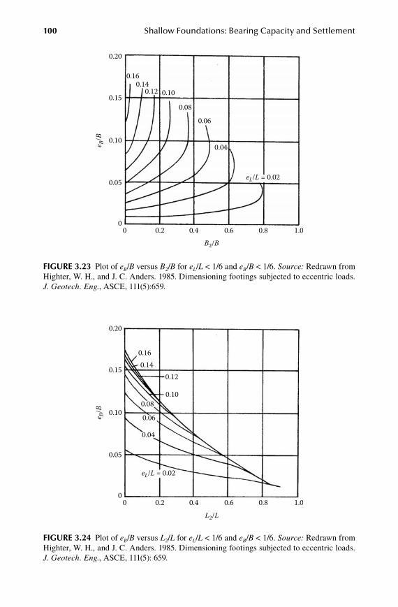
100 Shallow Foundations: Bearing Capacity and Settlement
FiGure 3.23 Plot of eB/B versus B2/B for eL/L < 1/6 and eB/B < 1/6. Source: Redrawn from Highter, W. H., and J. C. Anders. 1985. Dimensioning footings subjected to eccentric loads. J. Geotech. Eng., ASCE, 111(5):659.
0.20
0.15
0.10e B/B
B2/B
0.05
00 0.2 0.4 0.6 0.8 1.0
eL/L = 0.02
0.04
0.06
0.08
0.100.120.14
0.16
FiGure 3.24 Plot of eB/B versus L2/L for eL/L < 1/6 and eB/B < 1/6. Source: Redrawn from Highter, W. H., and J. C. Anders. 1985. Dimensioning footings subjected to eccentric loads. J. Geotech. Eng., ASCE, 111(5): 659.
0.20
0.15
0.10e B/B
L2/L
0.05
00 0.2 0.4 0.6 0.8 1.0
eL/L = 0.02
0.04
0.06
0.080.10
0.120.14
0.16
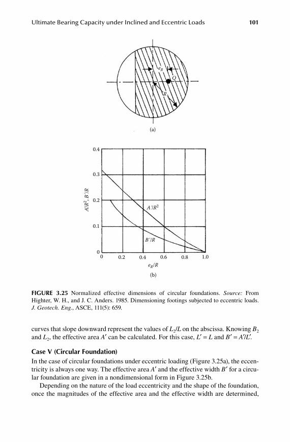
Ultimate Bearing Capacity under Inclined and Eccentric Loads 101
curves that slope downward represent the values of L2/L on the abscissa. Knowing B2 and L2, the effective area A′ can be calculated. For this case, L′ = L and B′ = A′/L′.
Case V (Circular Foundation)In the case of circular foundations under eccentric loading (Figure 3.25a), the eccen-tricity is always one way. The effective area A′ and the effective width B′ for a circu-lar foundation are given in a nondimensional form in Figure 3.25b.
Depending on the nature of the load eccentricity and the shape of the foundation, once the magnitudes of the effective area and the effective width are determined,
FiGure 3.25 Normalized effective dimensions of circular foundations. Source: From Highter, W. H., and J. C. Anders. 1985. Dimensioning footings subjected to eccentric loads. J. Geotech. Eng., ASCE, 111(5): 659.
0.4
0.3
0.2
A/R2 , B
/R
B /R
A /R2
eR/R
0.1
00 0.2 0.4 0.6 0.8 1.0
(b)
(a)
R
Q
eR
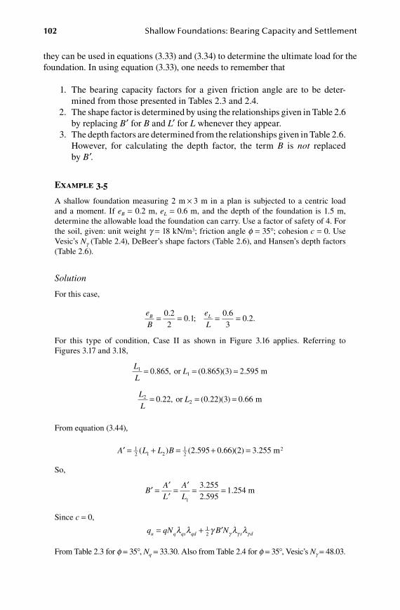
102 Shallow Foundations: Bearing Capacity and Settlement
they can be used in equations (3.33) and (3.34) to determine the ultimate load for the foundation. In using equation (3.33), one needs to remember that
1. The bearing capacity factors for a given friction angle are to be deter-mined from those presented in Tables 2.3 and 2.4.
2. The shape factor is determined by using the relationships given in Table 2.6 by replacing B′ for B and L′ for L whenever they appear.
3. The depth factors are determined from the relationships given in Table 2.6. However, for calculating the depth factor, the term B is not replaced by B′.
Example 3.5
A shallow foundation measuring 2 m × 3 m in a plan is subjected to a centric load and a moment. If eB = 0.2 m, eL = 0.6 m, and the depth of the foundation is 1.5 m, determine the allowable load the foundation can carry. Use a factor of safety of 4. For the soil, given: unit weight g = 18 kN/m3; friction angle f = 35°; cohesion c = 0. Use Vesic’s Ng (Table 2.4), DeBeer’s shape factors (Table 2.6), and Hansen’s depth factors (Table 2.6).
Solution
For this case,
e
B
e
LB L= = = =0 2
20 1
0 63
0 2.
. ;.
. .
For this type of condition, Case II as shown in Figure 3.16 applies. Referring to Figures 3.17 and 3.18,
L
LL1
10 865 0 865 3= = =. , ( . )( )or 2.595 m
L
LL2
20 22 0 22 3 0 66= = =. , ( . )( ) .or m
From equation (3.44),
′ = + = + =A L L B1
2 1 212 2 595 0 66 2( ) ( . . )( ) 3.255 m2
So,
′ = ′
′= ′ = =B
AL
AL1
3 2552 595..
1.254 m
Since c = 0,
q qN B Nu q qs qd s d= + ′l l γ l lγ γ γ
12
From Table 2.3 for f = 35°, Nq = 33.30. Also from Table 2.4 for f = 35°, Vesic’s Ng = 48.03.
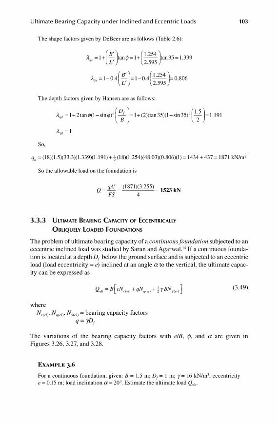
Ultimate Bearing Capacity under Inclined and Eccentric Loads 103
The shape factors given by DeBeer are as follows (Table 2.6):
l φqs
B
L= + ′
′
= +
1 1
1 254
2 5953tan
.
.tan 5 1 339= .
lγs
B
L= - ′
′
= -
=1 0 4 1 0 4
1 254
2 5950. .
.
...806
The depth factors given by Hansen are as follows:
l φ φqdfD
B= + -
= +1 2 1 1 2 352tan ( sin ) ( )(tan )(1 35
1 5
21 191
1
2-
=
=
sin ).
.
lγd
So,
qu = +( )( . )( . )( . )( . ) ( )( .18 1 5 33 3 1 339 1 191 18 1 212 554 48 03 0 806 1 1434 437 1871)( . )( . )( ) = + = kN/m2
So the allowable load on the foundation is
Q
qAFS
= ′ = ≈( )( . )1871 3 2554
1523 kN
3.3.3 Ultimate BeaRing CapaCity of eCCentRiCally oBliqUely loaDeD foUnDations
The problem of ultimate bearing capacity of a continuous foundation subjected to an eccentric inclined load was studied by Saran and Agarwal.14 If a continuous founda-tion is located at a depth Df below the ground surface and is subjected to an eccentric load (load eccentricity = e) inclined at an angle a to the vertical, the ultimate capac-ity can be expressed as
Q B cN qN BNc ei q ei eiult = + + ( ) ( ) ( )
12 γ γ
(3.49)
whereNc(ei), Nq(ei), Ng(ei) = bearing capacity factors
q = gDf
The variations of the bearing capacity factors with e/B, f, and a are given in Figures 3.26, 3.27, and 3.28.
Example 3.6
For a continuous foundation, given: B = 1.5 m; Df = 1 m; g = 16 kN/m3; eccentricity e = 0.15 m; load inclination a = 20°. Estimate the ultimate load Qult.
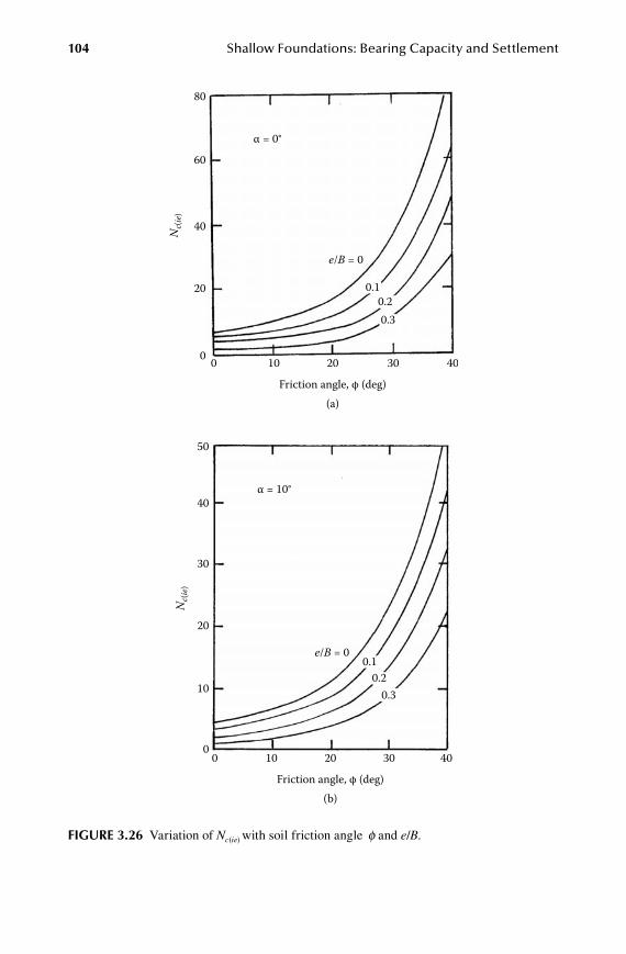
104 Shallow Foundations: Bearing Capacity and Settlement
80
60
40
20
0 0 10 20 30
0.30.2
0.1
e/B = 0
40
Nc(
ie)
Friction angle, φ (deg)(a)
α = 0°
FiGure 3.26 Variation of Nc(ie) with soil friction angle f and e/B.
40
50
30
20
10
00 10 20 30
0.30.2
0.1e/B = 0
40
Nc(
ie)
Friction angle, φ (deg)(b)
α = 10°
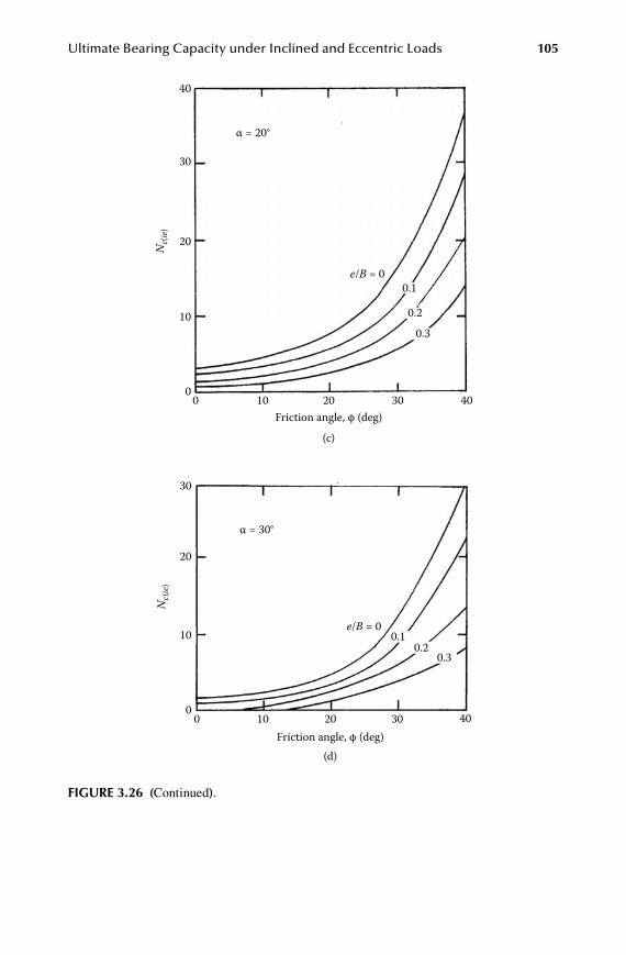
Ultimate Bearing Capacity under Inclined and Eccentric Loads 105
40
30
20
10
00 10 20 30
0.3
0.2
0.1e/B = 0
40
Nc(
ie)
Friction angle, φ (deg)
(c)
α = 20°
FiGure 3.26 (Continued).
30
20
10
00 10 20 30
0.30.2
0.1e/B = 0
40
Nc(
ie)
Friction angle, φ (deg)(d)
α = 30°

106 Shallow Foundations: Bearing Capacity and Settlement
80
60
40
20
00 10 20 30
0.30.2
0.1
e/B = 0
40
Nq(
ie)
Friction angle, φ (deg)(a)
α = 0°
FiGure 3.27 Variation of Nq(ie) with soil friction angle f and e/B.
40
50
30
20
10
00 10 20 30
0.3
0.2
0.1
e/B = 0
40
Nq(
ie)
Friction angle, φ (deg)(b)
α = 10°
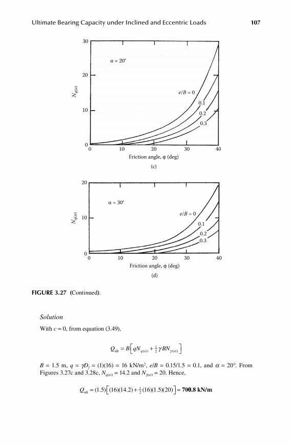
Ultimate Bearing Capacity under Inclined and Eccentric Loads 107
30
20
10
00 10 20 30
0.3
0.2
0.1
e/B = 0
40
Nq(
ie)
Friction angle, φ (deg)
(c)
α = 20°
Solution
With c = 0, from equation (3.49),
Q B qN BNq ei eiult = + ( ) ( )
12 γ γ
B = 1.5 m, q = gDf = (1)(16) = 16 kN/m2, e/B = 0.15/1.5 = 0.1, and a = 20°. From Figures 3.27c and 3.28c, Nq(ei) = 14.2 and Ng(ei) = 20. Hence,
Qult = + =( . ) ( )( . ) ( )( . )( )1 5 16 14 2 16 1 5 201
2 7000.8 kN/m
FiGure 3.27 (Continued).
20
10
00 10 20 30
0.30.2
0.1
e/B = 0
40
Nq(
ie)
Friction angle, φ (deg)
(d)
α = 30°
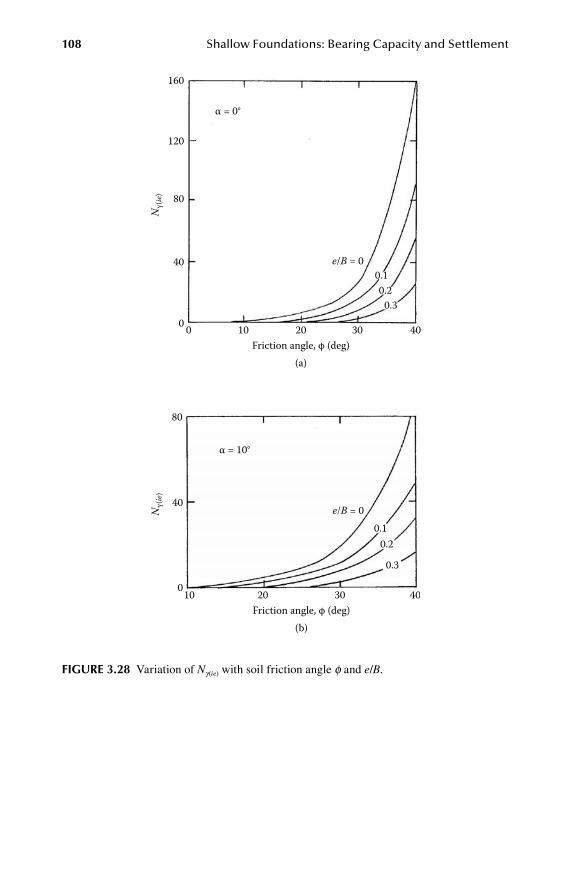
108 Shallow Foundations: Bearing Capacity and Settlement
160
120
80
40
0 0 10 20 30
0.30.2
0.1e/B = 0
40
Nγ(
ie)
Friction angle, φ (deg)(a)
α = 0°
FiGure 3.28 Variation of Ng(ie) with soil friction angle f and e/B.
80
40
010 20 30
0.3
0.20.1
e/B = 0
40
Nγ(
ie)
Friction angle, φ (deg)(b)
α = 10°
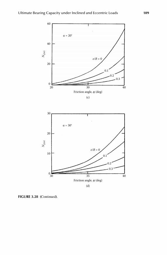
Ultimate Bearing Capacity under Inclined and Eccentric Loads 109
60
40
20
020 30
0.30.2
0.1
e/B = 0
40
Nγ(
ie)
Friction angle, φ (deg)
(c)
α = 20°
FiGure 3.28 (Continued).
30
20
10
030 35
0.30.2
0.1
e/B = 0
40
Nγ(
ie)
Friction angle, φ (deg)
(d)
α = 30°
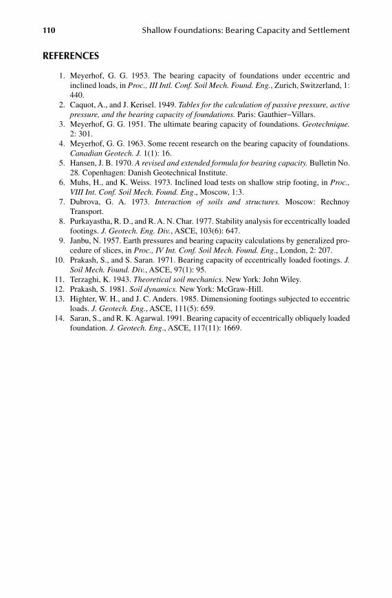
110 Shallow Foundations: Bearing Capacity and Settlement
reFerenCeS
1. Meyerhof, G. G. 1953. The bearing capacity of foundations under eccentric and inclined loads, in Proc., III Intl. Conf. Soil Mech. Found. Eng., Zurich, Switzerland, 1: 440.
2. Caquot, A., and J. Kerisel. 1949. Tables for the calculation of passive pressure, active pressure, and the bearing capacity of foundations. Paris: Gauthier−Villars.
3. Meyerhof, G. G. 1951. The ultimate bearing capacity of foundations. Geotechnique. 2: 301.
4. Meyerhof, G. G. 1963. Some recent research on the bearing capacity of foundations. Canadian Geotech. J. 1(1): 16.
5. Hansen, J. B. 1970. A revised and extended formula for bearing capacity. Bulletin No. 28. Copenhagen: Danish Geotechnical Institute.
6. Muhs, H., and K. Weiss. 1973. Inclined load tests on shallow strip footing, in Proc., VIII Int. Conf. Soil Mech. Found. Eng., Moscow, 1:3.
7. Dubrova, G. A. 1973. Interaction of soils and structures. Moscow: Rechnoy Transport.
8. Purkayastha, R. D., and R. A. N. Char. 1977. Stability analysis for eccentrically loaded footings. J. Geotech. Eng. Div., ASCE, 103(6): 647.
9. Janbu, N. 1957. Earth pressures and bearing capacity calculations by generalized pro-cedure of slices, in Proc., IV Int. Conf. Soil Mech. Found. Eng., London, 2: 207.
10. Prakash, S., and S. Saran. 1971. Bearing capacity of eccentrically loaded footings. J. Soil Mech. Found. Div., ASCE, 97(1): 95.
11. Terzaghi, K. 1943. Theoretical soil mechanics. New York: John Wiley.12. Prakash, S. 1981. Soil dynamics. New York: McGraw-Hill.13. Highter, W. H., and J. C. Anders. 1985. Dimensioning footings subjected to eccentric
loads. J. Geotech. Eng., ASCE, 111(5): 659.14. Saran, S., and R. K. Agarwal. 1991. Bearing capacity of eccentrically obliquely loaded
foundation. J. Geotech. Eng., ASCE, 117(11): 1669.

111
4 Special Cases of Shallow Foundations
4.1 introduCtion
The bearing capacity problems described in Chapters 2 and 3 assume that the soil supporting the foundation is homogeneous and extends to a great depth below the bottom of the foundation. They also assume that the ground surface is horizontal; however, this is not true in all cases. It is possible to encounter a rigid layer at a shal-low depth, or the soil may be layered and have different shear strength parameters. It may be necessary to construct foundations on or near a slope. Bearing capacity problems related to these special cases are described in this chapter.
4.2 Foundation Supported by Soil with a riGid rouGh baSe at a limited depth
Figure 4.1a shows a shallow rigid rough continuous foundation supported by soil that extends to a great depth. The ultimate bearing capacity of this foundation can be expressed (neglecting the depth factors) as (Chapter 2)
q cN qN BNu c q= + + 1
2 γ γ (4.1)
The procedure for determining the bearing capacity factors Nc, Nq, and Ng in homogeneous and isotropic soils was outlined in Chapter 2. The extent of the failure zone in soil at ultimate load qu is equal to D. The magnitude of D obtained during the evaluation of the bearing capacity factor Nc by Prandtl1 and Nq by Reissner2 is given in a nondimensional form in Figure 4.2. Similarly, the magnitude of D obtained by Lundgren and Mortensen3 during the evaluation of Ng is given in Figure 4.3.
If a rigid rough base is located at a depth of H < D below the bottom of the founda-tion, full development of the failure surface in soil will be restricted. In such a case, the soil failure zone and the development of slip lines at ultimate load will be as shown in Figure 4.1b. Mandel and Salencon4 determined the bearing capacity factors for such a case by numerical integration using the theory of plasticity. According to Mandel and Salencon’s theory, the ultimate bearing capacity of a rough continuous foundation with a rigid rough base located at a shallow depth can be given by the relation
q cN qN BNu c q= + +* * *1
2 γ γ (4.2)
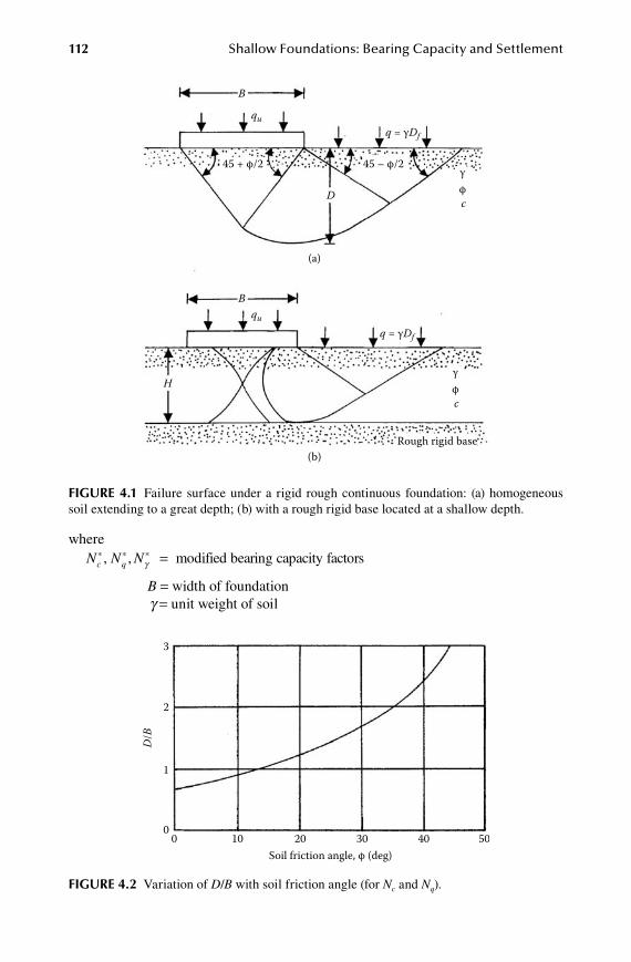
112 Shallow Foundations: Bearing Capacity and Settlement
whereN N Nc q
* * *, , modified bearing capacity fγ = actors
B = width of foundation g = unit weight of soil
FiGure 4.2 Variation of D/B with soil friction angle (for Nc and Nq).
3
2
1
00 10 20 30 40 50
Soil friction angle, φ (deg)
D/B
FiGure 4.1 Failure surface under a rigid rough continuous foundation: (a) homogeneous soil extending to a great depth; (b) with a rough rigid base located at a shallow depth.
45 + φ/2 45 – φ/2
φγ
B
H
q = γDf
q = γDf
Dc
φγ
c
qu
Bqu
(a)
(b)Rough rigid base
Special Cases of Shallow Foundations 113
Note that for H ≥ D, N*c = Nc, N*
q = Nq, and N*g = Ng (Lundgren and Mortensen).
The variations of Nc N*q, and N*
g with H/B and soil friction angle f are given in
Figures 4.4, 4.5, and 4.6, respectively.Neglecting the depth factors, the ultimate bearing capacity of rough circular and
rectangular foundations on a sand layer (c = 0) with a rough rigid base located at a shallow depth can be given as
q qN BNu q qs s= +* * * *l γ lγ γ
12
(4.3)
wherel*
qs, l*gs = modified shape factors
The above-mentioned shape factors are functions of H/B and f. Based on the work of Meyerhof and Chaplin5 and simplifying the assumption that the stresses and shear zones in radial planes are identical to those in transverse planes, Meyerhof6 evaluated the approximate values of l*
qs and l*
gs as
lqs m
B
L* = -
1 1 (4.4)
and
lγ s m
BL
* = -
1 2 (4.5)
whereL = length of the foundation
The variations of m1 and m2 with H/B and f are given in Figures 4.7 and 4.8.
FiGure 4.3 Variation of D/B with soil friction angle (for Ng).
3
2
1
00 10 20 30 40 50
Soil friction angle, φ (deg)
D/B

114 Shallow Foundations: Bearing Capacity and Settlement
Milovic and Tournier7 and Pfeifle and Das8 conducted laboratory tests to verify the theory of Mandel and Salencon.4 Figure 4.9 shows the comparison of the experi-mental evaluation of N*
g for a rough surface foundation (Df = 0) on a sand layer with theory. The angle of friction of the sand used for these tests was 43°. From Figure 4.9 the following conclusions can be drawn:
1. The value of N*g for a given foundation increases with the decrease in H/B.
2. The magnitude of H/B = D/B beyond which the presence of a rigid rough base has no influence on the N*
g value of a foundation is about 50%–75% more than that predicted by the theory.
3. For H/B between 0.5 to about 1.9, the experimental values of N*g are higher
than those predicted theoretically. 4. For H/B < about 0.6, the experimental values of N*
g are lower than those predicted by theory. This may be due to two factors: (a) the crushing of sand grains at such high values of ultimate load, and (b) the curvilinear nature of the actual failure envelope of soil at high normal stress levels.
FiGure 4.4 Mandel and Salencon’s bearing capacity factor Nc* [equation (4.2)].
H/B = 0.25
0.33
0.5
1.0
1.6
1.2
0.9
0.7
01
2
5
10
20
50
100
200
500
1000
2000
5000
10,000
10 20 30 40
D/B =2.4
Nc*
φ (deg)
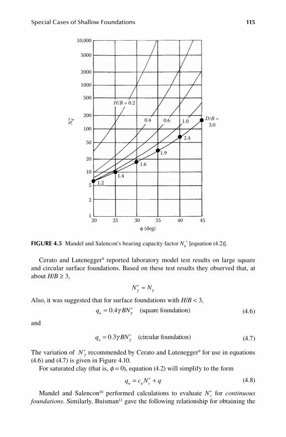
Special Cases of Shallow Foundations 115
Cerato and Lutenegger9 reported laboratory model test results on large square and circular surface foundations. Based on these test results they observed that, at about H/B ≥ 3,
N Nγ γ
* ≈
Also, it was suggested that for surface foundations with H/B < 3,
q BNu = 0 4. *γ γ (square foundation) (4.6)
and
q BNu = 0 3. *γ γ (circular foundation) (4.7)
The variation of N*g recommended by Cerato and Lutenegger9 for use in equations
(4.6) and (4.7) is given in Figure 4.10.For saturated clay (that is, f = 0), equation (4.2) will simplify to the form
q c N qu u c= +* (4.8)
Mandel and Salencon10 performed calculations to evaluate N*c for continuous
foundations. Similarly, Buisman11 gave the following relationship for obtaining the
FiGure 4.5 Mandel and Salencon’s bearing capacity factor Nq* [equation (4.2)].
H/B = 0.2
0.4 0.6 1.0
1.6
1.9
2.4
1.41.2
201
2
5
10
20
50
100
200
500
1000
2000
5000
10,000
25 30 35 40 45
D/B =3.0N
q*
φ (deg)

116 Shallow Foundations: Bearing Capacity and Settlement
FiGure 4.6 Mandel and Salencon’s bearing capacity factor Ng* [equation (4.2)].
H/B = 0.2
0.40.6
1.0
0.8
1.0
1.2
0.6
0.5
201
2
5
10
20
50
100
200
500
1000
2000
5000
10,000
25 30 35 40 45
D/B =1.5N
γ*
φ (deg)
FiGure 4.7 Variation of m1 (Meyerhof’s values) for use in the modified shape factor equation [equation (4.4)].
200
0.2
0.4
m1
0.6
0.8
1.0
25 30 40
2.0
1.00.6
0.4
0.2
H/B = 0.1
35 45φ (deg)
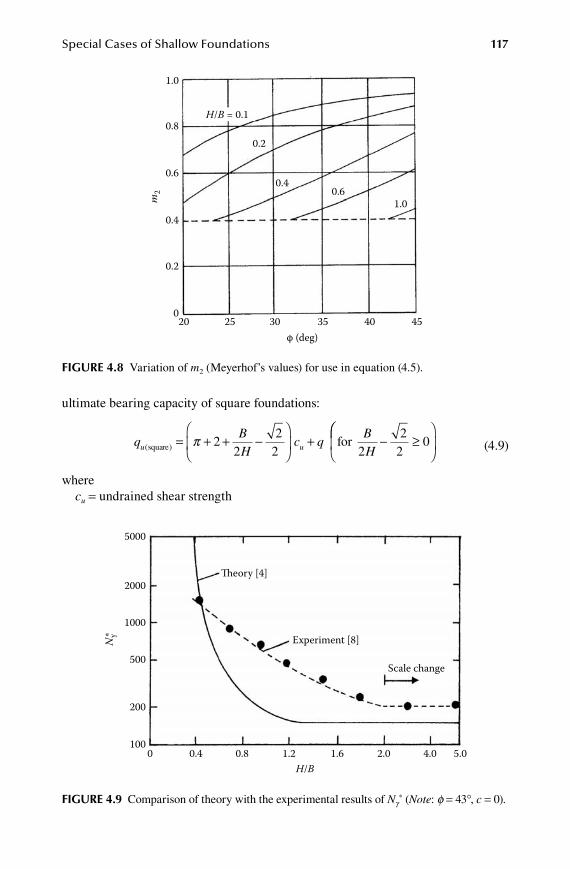
Special Cases of Shallow Foundations 117
ultimate bearing capacity of square foundations:
qBH
c qBHu u( )square for= + + -
+ - ≥π 2
22
2 22
20
(4.9)
wherecu = undrained shear strength
FiGure 4.8 Variation of m2 (Meyerhof’s values) for use in equation (4.5).
200
0.2
0.4
m2
0.6
0.8
1.0
25 30 40
1.00.6
0.4
0.2
H/B = 0.1
35 45φ (deg)
FiGure 4.9 Comparison of theory with the experimental results of Ng* (Note: f = 43°, c = 0).
Theory [4]
Experiment [8]
Scale change
0 0.4 0.8 1.2 1.6 2.0 4.0 5.0H/B
5000
2000
1000
500
200
100
Nγ*
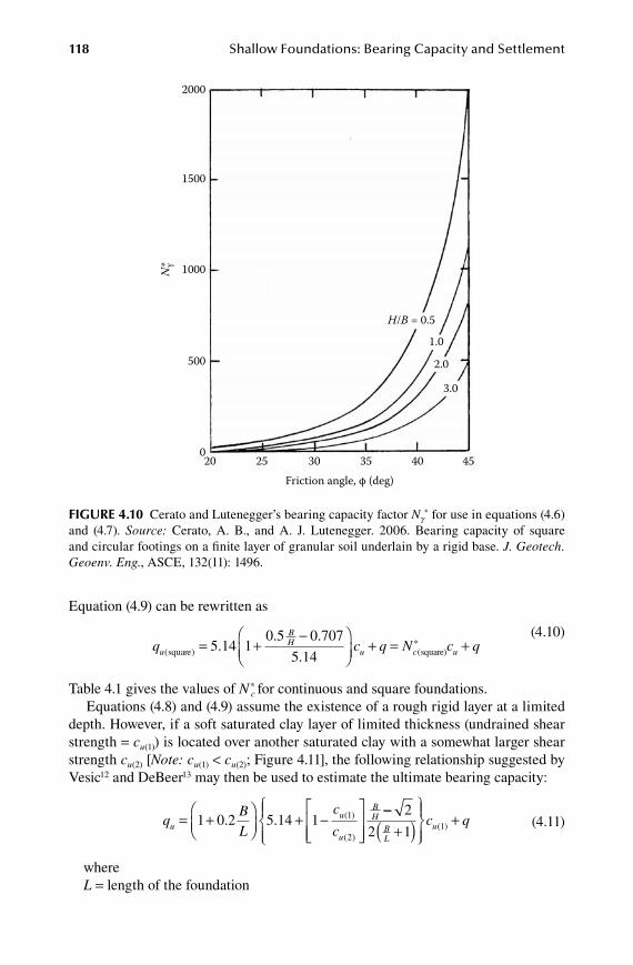
118 Shallow Foundations: Bearing Capacity and Settlement
Equation (4.9) can be rewritten as
q c qu
BH
u( ) .. .
.square = +-
+ =5 14 10 5 0 707
5 14N c qc u(
*square) +
(4.10)
Table 4.1 gives the values of N*c for continuous and square foundations.
Equations (4.8) and (4.9) assume the existence of a rough rigid layer at a limited depth. However, if a soft saturated clay layer of limited thickness (undrained shear strength = cu(1)) is located over another saturated clay with a somewhat larger shear strength cu(2) [Note: cu(1) < cu(2); Figure 4.11], the following relationship suggested by Vesic12 and DeBeer13 may then be used to estimate the ultimate bearing capacity:
qBL
c
cuu
u
BH= +
+ -
1 0 2 5 14 1 1
2
. . ( )
( )
--+( )
+
2
2 1 1BL
uc q( ) (4.11)
whereL = length of the foundation
FiGure 4.10 Cerato and Lutenegger’s bearing capacity factor Ng* for use in equations (4.6)
and (4.7). Source: Cerato, A. B., and A. J. Lutenegger. 2006. Bearing capacity of square and circular footings on a finite layer of granular soil underlain by a rigid base. J. Geotech. Geoenv. Eng., ASCE, 132(11): 1496.
2000
1500
1000
500
0
Nγ*
20 25 30 35 40 45Friction angle, φ (deg)
H/B = 0.5
1.0
2.0
3.0

Special Cases of Shallow Foundations 119
table 4.1Values of N*
c for Continuous and Square Foundations (f = 0 Condition)
BH
N*c
Squarea Continuousb
2 5.43 5.24 3 5.93 5.71 4 6.44 6.22 5 6.94 6.68 6 7.43 7.20 8 8.43 8.1710 9.43 9.05
a Buisman’s analysis. Source: From Buisman, A. S. K. 1940. Grond-mechanica. Delft: Waltman.
b Mandel and Salencon’s analysis. Source: From Mandel, J., and J. Salencon. 1969. Force portante d’un sol sur une assise rigide, in Proc., VII Int. Conf. Soil Mech. Found Engg., Mexico City, 2, 157.
FiGure 4.11 Foundation on a weaker clay underlain by a stronger clay layer (Note: cu(1) < cu(2)).
B
H
qu
cu (1)
q = γDf
Weaker clay layerφ1 = 0
cu (2)
Stronger clay layerφ2 = 0

120 Shallow Foundations: Bearing Capacity and Settlement
4.3 Foundation on layered Saturated aniSotropiC Clay (f = 0)
Figure 4.12 shows a shallow continuous foundation supported by layered saturated anisotropic clay. The width of the foundation is B, and the interface between the clay layers is located at a depth H measured from the bottom of the foundation. It is assumed that the clays are anisotropic with respect to strength following the Casagrande-Carillo relationship,14 or
c c c c iu i u h u v u h( ) ( ) ( ) ( )[ ]sin= + - 2 (4.12)
where Cu(i) = undrained shear strength at a given depth where the major principal
stress is inclined at an angle i with the horizontal cu(v), cu(h) = undrained shear strength for i = 90° and 0°, respectively
The ultimate bearing capacity of the continuous foundation can be given as
q c N qu u v c L= +-( ) ( )1 (4.13)
wherecu(v)-1 = undrained shear strength of the top soil layer when the major principal
stress is vertical q = g1Df
Df = depth of foundation g1 = unit weight of the top soil layer Nc(L) = bearing capacity factor
FiGure 4.12 Shallow continuous foundation on layered anisotropic clay.
Df
HB
Layer 1γ1φ1 = 0cu(i )–1
Layer 2γ2φ2 = 0cu(i)–2

Special Cases of Shallow Foundations 121
However, the bearing capacity factor Nc(L) will be a function of H/B and cu(v)-2/cu(v)-1, or
N fHB
c
cc Lu v
u v( )
( )
( )
,=
-
-
2
1
(4.14)
wherecu(v)-2 = undrained shear strength of the bottom clay layer when the major principal
stress is vertical
Reddy and Srinivasan15 developed a procedure to determine the variation of Nc(L). In developing their theory, they assumed that the failure surface was cylindri-cal when the center of the trial failure surface was at O, as shown in Figure 4.13. They also assumed that the magnitudes of cu(v) for the top clay layer [cu(v)-1] and the bottom clay layer [cu(v)-2] remained constant with depth z as shown in Figure 4.13b.
For equilibrium of the foundation, considering forces per unit length and taking the moment about point O in Figure 4.13a,
2 2 221
2
1
bq r b r c d r cu u i u i( sin ) [ ] [( ) ( )θ αθ
θ
- = +- -∫ 22
0
1
]dαθ
∫ (4.15)
where b = half-width of the foundation = B/2 r = radius of the trial failure circlecu(i)-1, cu(i)-2 = directional undrained shear strengths for layers 1 and 2, respectively
As shown in Figure 4.13, let y be the angle between the failure plane and the direction of the major principal stress. Referring to equation (4.12):Along arc AC,
c c c cu i u h u v u h( ) ( ) ( ) ( )[ ]sin ( )- - - -= + - +1 1 1 1
2 α ψ (4.16)
Along arc CE,
c c c cu i u h u v u h( ) ( ) ( ) ( )[ ]sin ( )- - - -= + - +2 2 2 2
2 α ψ (4.17)
Similarly, along arc DB,
c c c cu i u h u v u h( ) ( ) ( ) ( )[ ]sin ( )- - - -= + - -1 1 1 1
2 α ψ (4.18)
and along arc ED,
c c c cu i u h u v u h( ) ( ) ( ) ( )[ ]sin ( )- - - -= + - -2 2 2 2
2 α ψ (4.19)
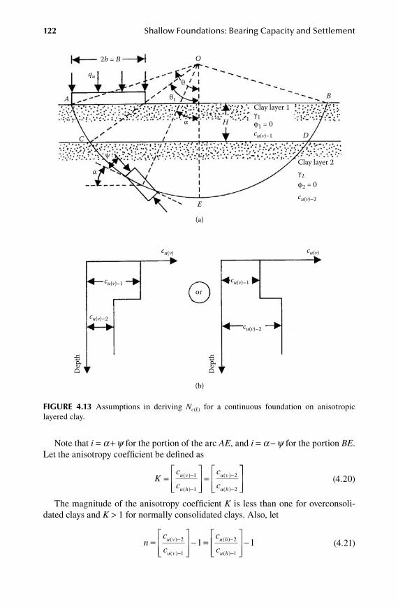
122 Shallow Foundations: Bearing Capacity and Settlement
Note that i = a + y for the portion of the arc AE, and i = a − y for the portion BE. Let the anisotropy coefficient be defined as
Kc
c
c
cu v
u h
u v
u h
=
=
-
-
-
-
( )
( )
( )
( )
1
1
2
2
(4.20)
The magnitude of the anisotropy coefficient K is less than one for overconsoli-dated clays and K > 1 for normally consolidated clays. Also, let
nc
c
c
cu v
u v
u h
u h
=
- =
-
-
-
-
( )
( )
( )
( )
2
1
2
1
1
-1 (4.21)
FiGure 4.13 Assumptions in deriving Nc(L) for a continuous foundation on anisotropic layered clay.
O2b = B
qu
A
C
H
E
D
BClay layer 1γ1φ1 = 0cu(v)–1
Clay layer 2γ2φ2 = 0cu(v)–2
(a)
θ
θ1
α
α
ψ
cu(v)
cu(v)–1
cu(v)–2
cu(v)
cu(v)–1
cu(v)–2
or
(b)
Dep
th
Dep
th
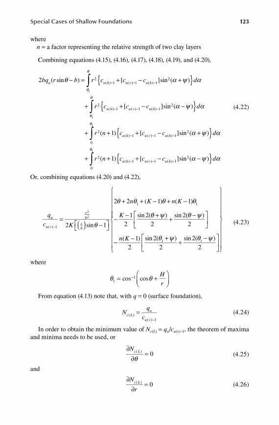
Special Cases of Shallow Foundations 123
wheren = a factor representing the relative strength of two clay layers
Combining equations (4.15), (4.16), (4.17), (4.18), (4.19), and (4.20),
2 21 1 1bq r b r c c cu u h u v u h( sin ) [ ]si( ) ( ) ( )θ - = + -- - - n ( )
[( ) ( ) ( )
2
21 1 1
1
α ψ αθ
θ
+{ }
+ + -
∫
- - -
d
r c c cu h u v u h ]sin ( )
( ) [( ) ( )
2
21 1
1
1
α ψ αθ
θ
-{ }
+ + +
∫
- -
d
r n c cu h u v - +{ }
+ + +
-
-
∫ c d
r n c
u h
u h
( )
( )
]sin ( )
( )
12
0
21
1
1
α ψ αθ
[ ]sin ( )( ) ( )c c du v u h- -- -{ }∫ 1 12
0
1
α ψ αθ
(4.22)
Or, combining equations (4.20) and (4.22),
q
c K
n K
u
u v
rb
rb( ) sin
( )
-
= ( ) -
+ + -
1
1
2
2
2 1
2 2 1
θ
θ θ θ θ
θ ψ θ ψ
+ -
- - + + -
n K
K
( )
sin ( sin (
1
12
2 2
1
)2
)2
-- - ++
-
n K( ) sin ( sin (12
2 21 1θ ψ θ ψ)
2
)
2
(4.23)
where
θ θ1
1= +
-cos cosH
r
From equation (4.13) note that, with q = 0 (surface foundation),
Nq
cc Lu
u v( )
( )
=-1
(4.24)
In order to obtain the minimum value of Nc(L) = qu/cu(v)-1, the theorem of maxima and minima needs to be used, or
∂∂
=Nc L( )
θ0 (4.25)
and
∂∂
=N
rc L( ) 0 (4.26)
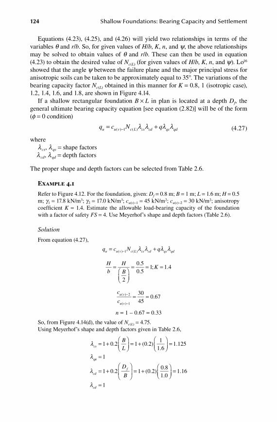
124 Shallow Foundations: Bearing Capacity and Settlement
Equations (4.23), (4.25), and (4.26) will yield two relationships in terms of the variables q and r/b. So, for given values of H/b, K, n, and y, the above relationships may be solved to obtain values of q and r/b. These can then be used in equation (4.23) to obtain the desired value of Nc(L) (for given values of H/b, K, n, and y). Lo16 showed that the angle y between the failure plane and the major principal stress for anisotropic soils can be taken to be approximately equal to 35°. The variations of the bearing capacity factor Nc(L) obtained in this manner for K = 0.8, 1 (isotropic case), 1.2, 1.4, 1.6, and 1.8, are shown in Figure 4.14.
If a shallow rectangular foundation B × L in plan is located at a depth Df, the general ultimate bearing capacity equation [see equation (2.82)] will be of the form (f = 0 condition)
q c N qu u v c L cs cd qs qd= +-( ) ( )1 l l l l (4.27)
wherel cs, l qs = shape factors
l cd, l qd = depth factors
The proper shape and depth factors can be selected from Table 2.6.
Example 4.1
Refer to Figure 4.12. For the foundation, given: Df = 0.8 m; B = 1 m; L = 1.6 m; H = 0.5 m; g1 = 17.8 kN/m3; g2 = 17.0 kN/m3; cu(v)-1 = 45 kN/m2; cu(v)-2 = 30 kN/m2; anisotropy coefficient K = 1.4. Estimate the allowable load-bearing capacity of the foundation with a factor of safety FS = 4. Use Meyerhof’s shape and depth factors (Table 2.6).
Solution
From equation (4.27),
q c N qu u v c L cs cd qs qd= +-( ) ( )1 l l l l
Hb
H
BK=
= = =
2
0 50 5
1 1 4..
; .
c
cu v
u v
( )
( )
.-
-
= =2
1
30
450 67
n = 1 – 0.67 = 0.33
So, from Figure 4.14(d), the value of Nc(L) = 4.75.Using Meyerhof’s shape and depth factors given in Table 2.6,
l
l
cs
q
BL
= +
= +
=1 0 2 1 0 21
1 61 125. ( . )
..
ss
cdfD
B
=
= +
= +
=
1
1 0 2 1 0 20 81 0
l . ( . )..
1 16
1
.
lcd =
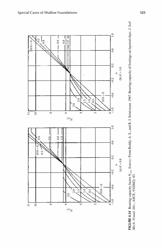
Special Cases of Shallow Foundations 125
FiG
ur
e 4.
14 B
eari
ng c
apac
ity
fact
or N
c(L)
. Sou
rce:
Fro
m R
eddy
, A. S
., an
d R
. J. S
rini
vasa
n. 1
967.
Bea
ring
cap
acit
y of
foot
ings
on
laye
red
clay
s. J
. Soi
l M
ech.
Fou
nd. D
iv.,
ASC
E, 9
3(SM
2): 8
3.
11 10 8 6 4 2 0
0.5
0.8
0.60.4
0.2
1.0
1.0
1.5
2.0
3.0 H
/b =
0
H/b
= 0
–1.0
–0.6
–0.2
0.2
0.6
1.0
n(a
) K =
0.8
Nc(L)
11 10 8 6 4 2 0
0.5
0.80.6
0.40.
2
1.0
1.0
1.52.0
3.0
H/b
= 0
H/b
= 0
–1.0
–0.6
–0.2
0.2
0.6
1.0
n(b
) K =
1.0
Nc(L)
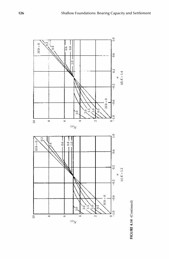
126 Shallow Foundations: Bearing Capacity and Settlement
10 8 6 4 2 0
0.5
0.8
0.6
0.4
0.2
1.0
1.0
1.5
2.0
3.0
H/b
= 0
H/b
= 0
–1.0
–0.6
–0.2
0.2
0.6
1.0
n(c
) K =
1.2
Nc(L)10 8 6 4 2 0
0.5
0.8
0.60.40.
2
1.0
1.0
1.5
2.0
3.0
H/b
= 0
H/b
= 0
–1.0
–0.6
–0.2
0.2
0.6
1.0
n(d
) K =
1.4
Nc(L)Fi
Gu
re
4.14
(C
onti
nued
)

Special Cases of Shallow Foundations 127
FiG
ur
e 4.
14 (
Con
tinu
ed)
9 8 6 4 2 0
0.5
0.8
0.60.
40.
2
1.0
1.0
1.52.0
3.0
H/b
= 0
H/b
= 0
–1.0
–0.6
–0.2
0.2
0.6
1.0
n(e
) K =
1.6
Nc(L)
9 8 6 4 2 0
0.5
0.8
0.6
0.4
0.2
1.0
1.0
1.5
2.5
3.0
H/b
= 0
H/b
= 0
–1.0
–0.6
–0.2
0.2
0.6
1.0
n(f
) K =
1.8
Nc(L)
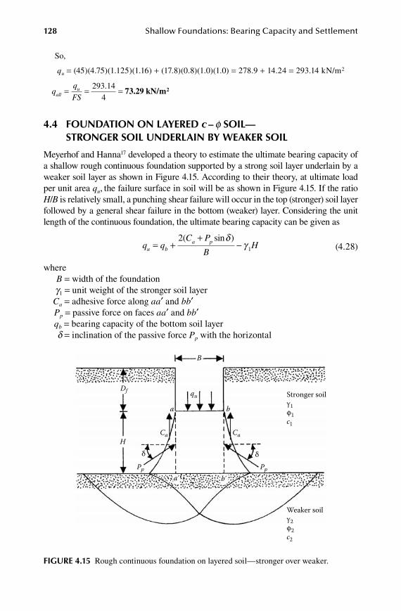
128 Shallow Foundations: Bearing Capacity and Settlement
So,
qu = (45)(4.75)(1.125)(1.16) + (17.8)(0.8)(1.0)(1.0) = 278.9 + 14.24 = 293.14 kN/m2
q
q
FSallu= = =293 14
4.
73.29 kN/m2
4.4 Foundation on layered c – f Soil— StronGer Soil underlain by weaKer Soil
Meyerhof and Hanna17 developed a theory to estimate the ultimate bearing capacity of a shallow rough continuous foundation supported by a strong soil layer underlain by a weaker soil layer as shown in Figure 4.15. According to their theory, at ultimate load per unit area qu, the failure surface in soil will be as shown in Figure 4.15. If the ratio H/B is relatively small, a punching shear failure will occur in the top (stronger) soil layer followed by a general shear failure in the bottom (weaker) layer. Considering the unit length of the continuous foundation, the ultimate bearing capacity can be given as
q q
C P
BHu b
a p= ++
-2
1
( sin )δγ (4.28)
where B = width of the foundation g1 = unit weight of the stronger soil layerCa = adhesive force along aa′ and bb′ Pp = passive force on faces aa′ and bb′ qb = bearing capacity of the bottom soil layer d = inclination of the passive force Pp with the horizontal
FiGure 4.15 Rough continuous foundation on layered soil—stronger over weaker.
Df
H
Pp
Ca Ca
a b
qu
δ
Pp
δ
B
Stronger soilγ1φ1c1
Weaker soilγ2φ2c2
a b
Special Cases of Shallow Foundations 129
Note that, in equation (4.28),
C c Ha a= (4.29)
whereca = unit adhesion
P HK
D HK
ppH
fpH=
+
1
2 12
1γδ
γδcos
( )( )cos
= +
12
12
12γ
δH
D
H
Kf pH
cos (4.30)
whereKpH = horizontal component of the passive earth pressure coefficient
Also,
q c N D H N BNb c f q= + + +2 2 1 2
12 2 2( ) ( ) ( )( )γ γ γ
(4.31)
where c2 = cohesion of the bottom (weaker) layer of soil g2 = unit weight of bottom soil layerNc(2), Nq(2), Ng(2) = bearing capacity factors for the bottom soil layer (that is, with
respect to the soil friction angle of the bottom soil layer f2)
Combining equations (4.28), (4.29), and (4.30),
q qc H
BH
D
H
Ku b
a f pH= + + +
22
12
12
12γ
coossin
δδ γ
γ
-
= + + +
BH
qc H
BH
Db
a
1
12
21
2 f pH
H
K
BH
-
tanδγ 1
(4.32)
Let
K KpH stan tanδ φ= 1 (4.33)
whereKs = punching shear coefficient
So,
q qc H
BH
D
H
K
BHu b
a f s= + + +
-
21
21
2 11γ φ γtan
(4.34)
The punching shear coefficient can be determined using the passive earth pres-sure coefficient charts proposed by Caquot and Kerisel.18 Figure 4.16 gives the varia-tion of Ks with q2/q1 and f1. Note that q1 and q2 are the ultimate bearing capacities of a continuous surface foundation of width B under vertical load on homogeneous beds of upper and lower soils, respectively, or
q c N BNc1 1 1
12 1 1= +( ) ( )γ γ
(4.35)

130 Shallow Foundations: Bearing Capacity and Settlement
whereNc(1), Ng(1) = bearing capacity factors corresponding to soil friction angle f1
q c N BNc2 2 2
12 2 2= +( ) ( )γ γ
(4.36)
If the height H is large compared to the width B (Figure 4.15), then the fail-ure surface will be completely located in the upper stronger soil layer, as shown in Figure 4.17. In such a case, the upper limit for qu will be of the following form:
q q c N qN BNu t c q= = + +1 1 1
12 1 1( ) ( ) ( )γ γ (4.37)
Hence, combining equations (4.34) and (4.37),
q qc H
BH
D
H
K
BH qu b
a f st= + + +
- ≤
21
21
2 11γ φ γtan
(4.38)
For rectangular foundations, the preceding equation can be modified as
q qBL
c H
BBL
Hu ba
a= + +
+ +
12
1 1l γ 22 111
2+
- ≤D
H
K
BH qf s
s t
tanφ l γ
(4.39)
FiGure 4.16 Meyerhof and Hanna’s theory—variation of Ks with f1 and q2/q1.
20 30 40 50
0
0.20.4
q2/q1 = 1.0
0
10
20
30
40
K s
φ1 (deg)
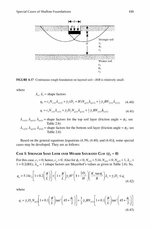
Special Cases of Shallow Foundations 131
where l a, l s = shape factors
q c N D H N BNb c cs f q qs= + + +2 2 2 1 2 2
12 2( ) ( ) ( ) ( )( )l γ l γ γ γl( ) ( )2 2s (4.40)
q c N D N BNt c cs f q qs= + +1 1 1 1 1 1
12 1 1( ) ( ) ( ) ( ) ( )l γ l γ γ llγ s( )1 (4.41)
l cs(1), l qs(1), lgs(1) = shape factors for the top soil layer (friction angle = f1; see Table 2.6)
l cs(2), l qs(2), lgs(2) = shape factors for the bottom soil layer (friction angle = f2; see Table 2.6)
Based on the general equations [equations (4.39), (4.40), and (4.41)], some special cases may be developed. They are as follows:
Case i: stRongeR sanD layeR oveR weakeR satURateD Clay (f2 = 0)
For this case, c1 = 0; hence, ca = 0. Also for f2 = 0, Nc(2) = 5.14, Ng(2) = 0, Nq(2) = 1, l cs = 1 + 0.2(B/L), l qs = 1 (shape factors are Meyerhof’s values as given in Table 2.6). So,
q cBL
BL
Hu = +
+ +
5 14 1 0 2 12 12. . γ 11
21
1+
+ ≤D
H
K
BD qf s
s f t
tanφ l γ (4.42)
where
q D NBLt f q= +
+
γ φ
1 12 11 0 1 45
2( ) . tan
+ +
+
12
1 0 1 4521 1
2 1γ φγBN
BL( ) . tan
(4.43)
FiGure 4.17 Continuous rough foundation on layered soil—H/B is relatively small.
Df
H
qu
B
Stronger soilγ1φ1c1
Weaker soilγ2φ2c2
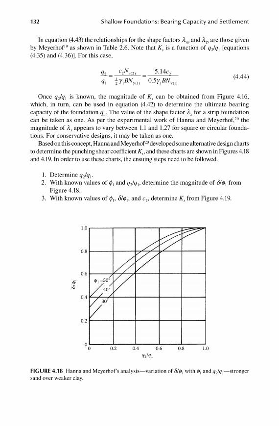
132 Shallow Foundations: Bearing Capacity and Settlement
In equation (4.43) the relationships for the shape factors l qs and lgs are those given by Meyerhof19 as shown in Table 2.6. Note that Ks is a function of q2/q1 [equations (4.35) and (4.36)]. For this case,
q
q
c N
BN
c
BNc2
1
2 2
12 1 1
2
1 1
5 14
0 5= =( )
( ) ( )
.
.γ γγ γ (4.44)
Once q2/q1 is known, the magnitude of Ks can be obtained from Figure 4.16, which, in turn, can be used in equation (4.42) to determine the ultimate bearing capacity of the foundation qu. The value of the shape factor l s for a strip foundation can be taken as one. As per the experimental work of Hanna and Meyerhof,20 the magnitude of l s appears to vary between 1.1 and 1.27 for square or circular founda-tions. For conservative designs, it may be taken as one.
Based on this concept, Hanna and Meyerhof20 developed some alternative design charts to determine the punching shear coefficient Ks, and these charts are shown in Figures 4.18 and 4.19. In order to use these charts, the ensuing steps need to be followed.
1. Determine q2/q1. 2. With known values of f1 and q2/q1, determine the magnitude of d/f1 from
Figure 4.18. 3. With known values of f1, d/f1, and c2, determine Ks from Figure 4.19.
FiGure 4.18 Hanna and Meyerhof’s analysis—variation of d/f1 with f1 and q2/q1—stronger sand over weaker clay.
0 0.2 0.4 0.6 0.8 1.0q2/q1
0
0.2
0.4
0.6
0.8
1.0
δ/φ 1 φ1 =50°
40°
30°

Special Cases of Shallow Foundations 133
FiGure 4.19 Hanna and Meyerhof’s analysis for coefficient of punching shear—stronger sand over weaker clay.
50
10
20
30
40
50
10 15 20
0.3
0.4
0.5
0.6
0.7
0.30.40.50.60.7
25 30 35
K s
0
10
20
30
K s
c2 (kN/m2)
5 10 15 20 25 30 35c2 (kN/m2)
δ/φ1 = 0.8
δ/φ1 = 0.8
(a) φ1 = 50°
(b) φ1 = 45°
0.30.4
0.5 0.60.710
0
20
K s
5 10 15 20 25 30 35c2 (kN/m2)
δ/φ1 = 0.8
(c) φ1 = 40°
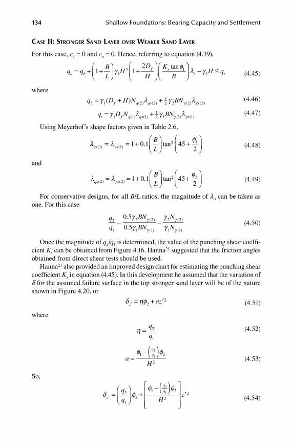
134 Shallow Foundations: Bearing Capacity and Settlement
Case ii: stRongeR sanD layeR oveR weakeR sanD layeR
For this case, c1 = 0 and ca = 0. Hence, referring to equation (4.39),
q qBL
HD
H
K
Bu bf s= + +
+
1 12
12 1γ φtan
- ≤l γs tH q1 (4.45)
where
q D H N BNb f q qs s= + +γ l γ lγ γ1 2 2
12 2 2 2( ) ( ) ( ) ( ) ( )
(4.46)
q D N BNt f q qs s= +γ l γ lγ γ1 1 1
12 1 1 1( ) ( ) ( ) ( )
(4.47)
Using Meyerhof’s shape factors given in Table 2.6,
l lφ
γqs s
B
L( ) ( ) . tan1 12 11 0 1 45
2= = +
+
(4.48)
and
l l φ
γqs s
BL( ) ( ) . tan2 2
2 21 0 1 452
= = +
+
(4.49)
For conservative designs, for all B/L ratios, the magnitude of l s can be taken as one. For this case
q
q
BN
BN
N
N2
1
2 2
1 1
2 2
1 1
0 5
0 5= =
.
.( )
( )
( )
( )
γγ
γγ
γ
γ
γ
γ (4.50)
Once the magnitude of q2/q1 is determined, the value of the punching shear coeffi-cient Ks can be obtained from Figure 4.16. Hanna21 suggested that the friction angles obtained from direct shear tests should be used.
Hanna21 also provided an improved design chart for estimating the punching shear coefficient Ks in equation (4.45). In this development he assumed that the variation of d for the assumed failure surface in the top stronger sand layer will be of the nature shown in Figure 4.20, or
δ ηφ′ = + ′z az2
2 (4.51)
where
η =
q
q2
1
(4.52)
a
H
q
q=- ( )φ φ1 2
2
2
1 (4.53)
So,
δ φφ φ
′ =
+- ( )
′z
q
q Hz2
12
1 2
22
2
1
(4.54)
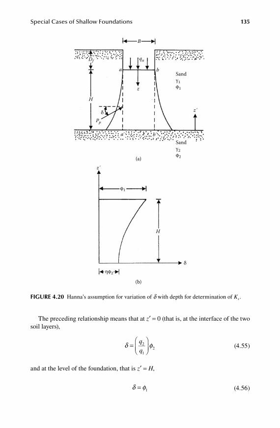
Special Cases of Shallow Foundations 135
The preceding relationship means that at z′ = 0 (that is, at the interface of the two soil layers),
δ φ=
q
q2
12 (4.55)
and at the level of the foundation, that is z′ = H,
δ φ= 1 (4.56)
FiGure 4.20 Hanna’s assumption for variation of d with depth for determination of Ks .
Df
H
H
Pp
a b
a b
qu
δ
δ
B
Sandγ1φ1
Sandγ2φ2
z
z´
z´(a)
(b)
ηφ2
φ1
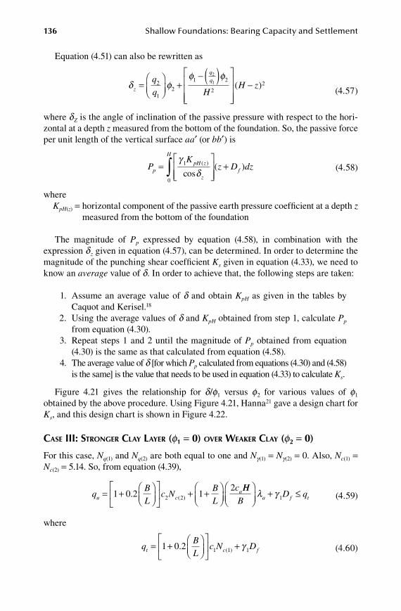
136 Shallow Foundations: Bearing Capacity and Settlement
Equation (4.51) can also be rewritten as
δ φφ φ
z
q
q HH z=
+- ( )
-2
12
1 2
2
2
1 ( )2
(4.57)
where dZ is the angle of inclination of the passive pressure with respect to the hori-zontal at a depth z measured from the bottom of the foundation. So, the passive force per unit length of the vertical surface aa′ (or bb′) is
PK
z D dzppH z
z
H
f=
+∫γ
δ1
0
( )
cos( ) (4.58)
whereKpH(z) = horizontal component of the passive earth pressure coefficient at a depth z
measured from the bottom of the foundation
The magnitude of Pp expressed by equation (4.58), in combination with the expression dz given in equation (4.57), can be determined. In order to determine the magnitude of the punching shear coefficient Ks given in equation (4.33), we need to know an average value of d. In order to achieve that, the following steps are taken:
1. Assume an average value of d and obtain KpH as given in the tables by Caquot and Kerisel.18
2. Using the average values of d and KpH obtained from step 1, calculate Pp from equation (4.30).
3. Repeat steps 1 and 2 until the magnitude of Pp obtained from equation (4.30) is the same as that calculated from equation (4.58).
4. The average value of d [for which Pp calculated from equations (4.30) and (4.58) is the same] is the value that needs to be used in equation (4.33) to calculate Ks.
Figure 4.21 gives the relationship for d/f1 versus f2 for various values of f1 obtained by the above procedure. Using Figure 4.21, Hanna21 gave a design chart for Ks, and this design chart is shown in Figure 4.22.
Case iii: stRongeR Clay layeR (f1 = 0) oveR weakeR Clay (f2 = 0)
For this case, Nq(1) and Nq(2) are both equal to one and Ng(1) = Ng(2) = 0. Also, Nc(1) = Nc(2) = 5.14. So, from equation (4.39),
qBL
c NBL
cu c
a= +
+ +
1 0 2 12
2 2. ( )
HH
BD qa f t
+ ≤l γ 1 (4.59)
where
qBL
c N Dt c f= +
+1 0 2 1 1 1. ( ) γ (4.60)
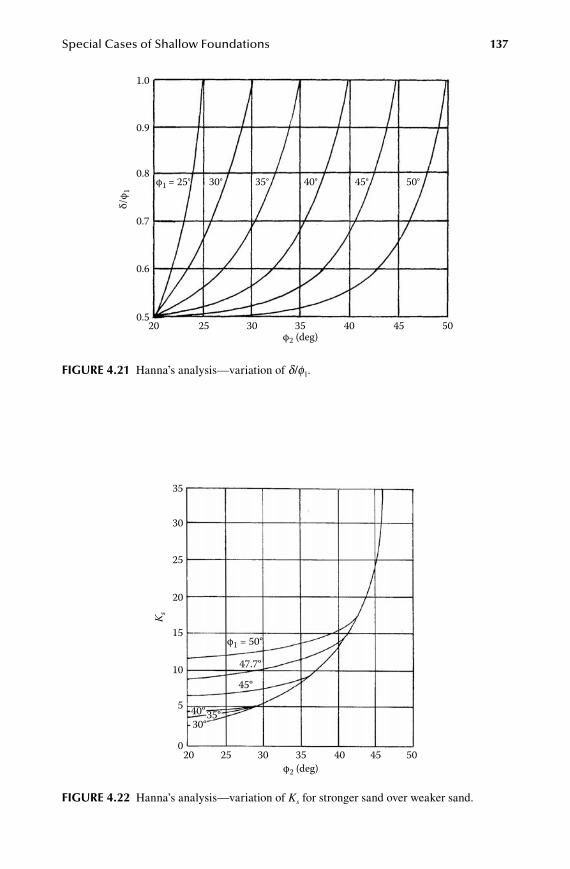
Special Cases of Shallow Foundations 137
FiGure 4.22 Hanna’s analysis—variation of Ks for stronger sand over weaker sand.
35
30
25
20
15
K s
10
5
020 25 30 35 40 45 50
φ1 = 50º
φ2 (deg)
47.7º
45º
40º 35º30º
FiGure 4.21 Hanna’s analysis—variation of d/f1.
20 25 30 35 40 45 50φ2 (deg)
φ1 = 25° 30° 35° 40° 45° 50°
δ/φ 1
0.5
0.6
0.7
0.8
0.9
1.0

138 Shallow Foundations: Bearing Capacity and Settlement
For conservative design the magnitude of the shape factor l a may be taken as one. The magnitude of the adhesion ca is a function of q2/q1. For this condition,
q
q
c N
c N
c
c
c
cc
c
2
1
2 2
1 1
2
1
2
1
5 14
5 14= = =( )
( )
.
. (4.61)
Figure 4.23 shows the theoretical variation of ca with q2/q1.17
Example 4.2
Refer to Figure 4.15. Let the top layer be sand and the bottom layer saturated clay. Given: H = 1.5 m. For the top layer (sand): g1 = 17.5 kN/m3; f1 = 40°; c1 = 0; for the bottom layer (saturated clay): g2 = 16.5 kN/m3; f2 = 0; c2 = 30 kN/m2; and for the foun-dation (continuous): B = 2 m; Df = 1.2 m. Determine the ultimate bearing capacity qu. Use the results shown in Figures 4.18 and 4.19.
Solution
For the continuous foundation BL = 0 and ls = 1, in equation 4.42 we obtain
q c HD
H
K
Buf s= + +
+5 14 12
2 12 1
1.tan
γφ
γ DD
HH
K
f
= + +
( . )( ) ( . )( )
( )( . )5 14 30 17 5 1
2 1 22 ss
sH KH
tan( . )( . )
. ..
40
217 5 1 2
175 2 7 342 12 42
+
= + +
(a)
To determine Ks, we need to obtain q2/q1. From equation (4.44),
q
q
c
BN2
1
2
1
5 14
0 5=
.
. ( )γ γ
FiGure 4.23 Analysis of Meyerhof and Hanna for the variation of ca/c1 with c2/c1.
1.0
0.9
0.8
0.7
c a/c
1
c2/c1
0.60 0.2 0.4 0.6 0.8 1.0
Special Cases of Shallow Foundations 139
From Table 2.3 for f1 = 40°, Meyerhof’s value of Ng(1) is equal to 93.7. So,
q
q2
1
5 14 300 5 17 5 2 93 7
0 094= =( . )( )( . )( . )( )( . )
.
Referring to Figure 4.18 for q2/q1 = 0.094 and f1 = 40°, the value of d/f1 = 0.42. With d/f1 = 0.42 and c2 = 30 kN/m2, Figure 4.19c gives the value of Ks = 3.89. Substituting this value into equation (a) gives
q H
Hqu t= + +
≤175 2 28 56 12 42. .
. (b)
From equation (4.43),
q D N
BLt f q= +
+
γ φ
1 12 11 0 1 45
2( ) . tan
+ +
+
12
1 0 1 4521 1
2 1γ φγBN
BL( ) . tan
(c)
For the continuous foundation B/L = 0. So,
q D N BNt f q= +γ γ γ1 1
12 1 1( ) ( )
For f1 = 40°, use Meyerhof’s values of Ng(1) = 93.7 and Nq(1) = 62.4 (Table 2.3). Hence,
qt = + =( . )( . )( . ) ( . )( )( . )17 5 1 2 62 4 17 5 2 93 7 13481
2 . . .2 1639 75 2987 95+ = kN/m2
If H = 1.5 m is substituted into equation (b),
qu = + +
=175 2 28 56 1 5 12 41 5
342 32. ( . )( . )..
. kN/m2
Since qu = 342.3 < qt, the ultimate bearing capacity is 342.3 kN/m2
Example 4.3
Refer to Figure 4.15, which shows a square foundation on layered sand. Given: H = 1.0 m. Also given for the top sand layer: g1 = 18 kN/m3; f1 = 40°; for the bottom sand layer: g2 = 16.5 kN/m3; f2 = 32°; and for the foundation: B × B = 1.5 m × 1.5 m; Df = 1.5 m. Estimate the ultimate bearing capacity of the foundation. Use Figure 4.22.
Solution
From equation (4.45),
q qB
LH
D
H
K
Bu bf s= + +
+
1 1
21
2 1γφtan
- ≤
≈
l γ
l
s t
s
H q1
1
Given: f1 = 40°; f2 = 32°. From Figure 4.22, Ks ≈ 5.75.From equation (4.46),
q D H N BNb f q qs s= + +γ l γ lγ γ1 2 2
12 2 2 2( ) ( ) ( ) ( ) ( )
140 Shallow Foundations: Bearing Capacity and Settlement
For f2 = 32°, Meyerhof’s bearing capacity factors are Ng(2) = 22.02 and Nq(2) = 23.18 (Table 2.3). Also from Table 2.6, Meyerhof’s shape factors
l l
φγqs s
B
L( ) ( ) . tan2 22 21 0 1 45
2= = +
+
= +
+
=1 0 11 5
1 545
32
21 3252( . )
.
.tan .
qb = + +( )( . )( . )( . ) ( . )( . )(18 1 5 1 23 18 1 3251
216 7 1 5 22 02 1 325 1382 1 365 4 1747 5. )( . ) . . .= + = kN/m2
Hence, from equation (4.45),
qu = + +
+ ×
1747 5 11 51 5
18 1 12 1 5
12.
.
.( )( )
.
- = +5 75 401 5
18 1 1747 5 463 2. tan
.( )( ) . . --
=
18
2192 7. kN/m2
CHECK
From equation (4.47),
q D H N BNt f q qs s= + +γ l γ lγ γ1 1 1
12 1 1 2( ) ( ) ( ) ( ) ( )
For f1 = 40°, Meyerhof’s bearing capacity factors are Nq(1) = 62.4 and Ng(1) = 93.69 (Table 2.3).
l l
φγqs s
B
L( ) ( ) . tan1 12 11 0 1 45
2= = +
+
= +
+
≈1 0 11 5
1 545
40
21 462( . )
.
.tan .
qt = + +( )( . )( . )( . ) ( )( . )( .18 1 5 1 64 2 1 46 18 1 5 93 61
2 9 1 46 4217 9 1846 6 6064 5)( . ) . . .= + = kN/m2
So, qu = 2192.7 kN/m2.
Example 4.4
Figure 4.24 shows a shallow foundation. Given: H = 1 m; undrained shear strength c1 (for f1 = 0 condition) = 80 kN/m 2; undrained shear strength c2 (for f2 = 0 condition) = 32 kN/m 2; g1 = 18 kN/m3; Df = 1 m; B = 1.5 m; L = 3 m. Estimate the ultimate bearing capacity of the foundation.
Solution
From equation (4.61),
q
q
c
c2
1
2
1
3280
0 4= = = .
From Figure 4.23 for q2/q1 = 0.4, ca/c1 = 0.9. So ca = (0.9)(80) = 72 kN/m 2. From equa-tion (4.60),
q
B
Lc N Dt c f= +
+ = +1 0 2 1 0 21
1 1 1. .( ) γ .( )( . ) ( )( ) .
5
380 5 14 18 1 470 32
+ = kN/m2.
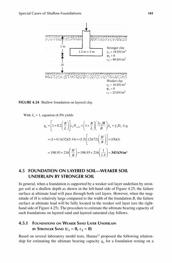
Special Cases of Shallow Foundations 141
With l s = 1, equation (4.59) yields
qBL
c NBL
cu c
a= +
+ +
1 0 2 12
2 2. ( )
HH
BD qa f t
+ ≤
= + +
l γ 1
1 0 1 32 5 14 1 5( . )( )( . ) ( . ) ( )( ) ( )( )
.
2 72 18 1
198 93 216
HB
HB
+
= +
= +
≈198 93 2161
1 5.
.343 kN/m2
4.5 Foundation on layered Soil—weaKer Soil underlain by StronGer Soil
In general, when a foundation is supported by a weaker soil layer underlain by stron-ger soil at a shallow depth as shown in the left-hand side of Figure 4.25, the failure surface at ultimate load will pass through both soil layers. However, when the mag-nitude of H is relatively large compared to the width of the foundation B, the failure surface at ultimate load will be fully located in the weaker soil layer (see the right-hand side of Figure 4.25). The procedure to estimate the ultimate bearing capacity of such foundations on layered sand and layered saturated clay follows.
4.5.1 foUnDations on weakeR sanD layeR UnDeRlain By stRongeR sanD (c1 = 0, c2 = 0)
Based on several laboratory model tests, Hanna22 proposed the following relation-ship for estimating the ultimate bearing capacity qu for a foundation resting on a
FiGure 4.24 Shallow foundation on layered clay.
1 m1.5 m × 3 m
Stronger clayγ1 = 18 kN/m3
φ2 = 0c2 = 80 kN/m2
Weaker clayγ1 = 16 kN/m3
φ1 = 0c1 = 32 kN/m2
H
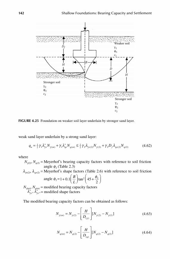
142 Shallow Foundations: Bearing Capacity and Settlement
weak sand layer underlain by a strong sand layer:
q N N Nu s m qs q m s= + ≤1
2 1 112 2 2 2γ l γ l γ lγ γ γ γ
*( )
*( ) ( ) ( ) ( ) ( )+ γ l2 2 2D Nf qs q (4.62)
where Ng(2), Nq(2) = Meyerhof’s bearing capacity factors with reference to soil friction
angle f2 (Table 2.3) lgs(2), l qs(2) = Meyerhof’s shape factors (Table 2.6) with reference to soil friction
angle f2 =1 0 1 452
2 2+
+
. tan
BL
φ
Ng(m), Nq(m) = modified bearing capacity factors
l lγ γs s
* *, , = modified shape factors
The modified bearing capacity factors can be obtained as follows:
N NH
DN Nmγ γ
γγ γ( ) ( )
( )( ) ( )[ ]= -
-2 2 1 (4.63)
N NH
DN Nq m q
qq q( ) ( )
( )( ) ( )[ ]= -
-2 2 1 (4.64)
FiGure 4.25 Foundation on weaker soil layer underlain by stronger sand layer.
Stronger soilγ2φ2c2
Stronger soilγ2φ2c2
Weaker soilγ1φ1c1
Df
HB
D
H
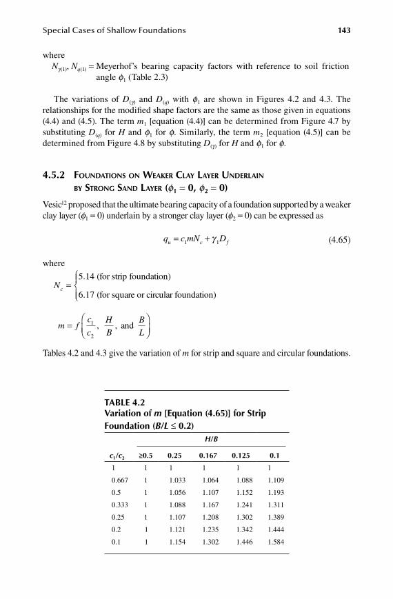
Special Cases of Shallow Foundations 143
whereNg(1), Nq(1) = Meyerhof’s bearing capacity factors with reference to soil friction
angle f1 (Table 2.3)
The variations of D(g) and D(q) with f1 are shown in Figures 4.2 and 4.3. The relationships for the modified shape factors are the same as those given in equations (4.4) and (4.5). The term m1 [equation (4.4)] can be determined from Figure 4.7 by substituting D(q) for H and f1 for f. Similarly, the term m2 [equation (4.5)] can be determined from Figure 4.8 by substituting D(g) for H and f1 for f.
4.5.2 foUnDations on weakeR Clay layeR UnDeRlain By stRong sanD layeR (f1 = 0, f2 = 0)
Vesic12 proposed that the ultimate bearing capacity of a foundation supported by a weaker clay layer (f1 = 0) underlain by a stronger clay layer (f2 = 0) can be expressed as
q c mN Du c f= +1 1γ (4.65)
where
Nc =5.14 (for strip foundation)
6.17 (for square or circular foundation)
m fc
c
H
B
B
L=
1
2
, , and
Tables 4.2 and 4.3 give the variation of m for strip and square and circular foundations.
table 4.2Variation of m [equation (4.65)] for Strip Foundation (B/L ≤ 0.2)
H/B
c1/c2 ≥0.5 0.25 0.167 0.125 0.1
1 1 1 1 1 1
0.667 1 1.033 1.064 1.088 1.109
0.5 1 1.056 1.107 1.152 1.193
0.333 1 1.088 1.167 1.241 1.311
0.25 1 1.107 1.208 1.302 1.389
0.2 1 1.121 1.235 1.342 1.444
0.1 1 1.154 1.302 1.446 1.584
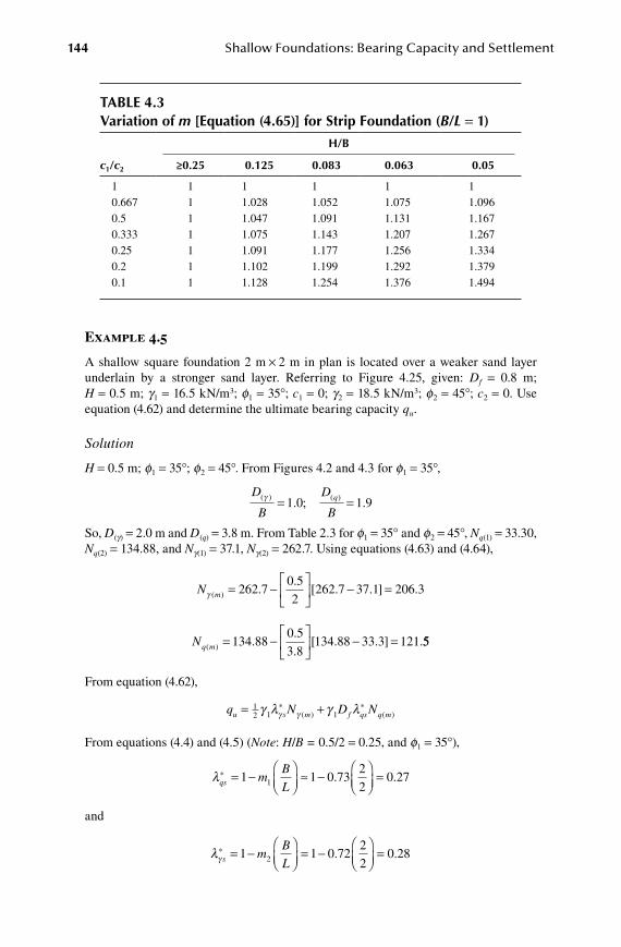
144 Shallow Foundations: Bearing Capacity and Settlement
Example 4.5
A shallow square foundation 2 m × 2 m in plan is located over a weaker sand layer underlain by a stronger sand layer. Referring to Figure 4.25, given: Df = 0.8 m; H = 0.5 m; g1 = 16.5 kN/m3; f1 = 35°; c1 = 0; g2 = 18.5 kN/m3; f2 = 45°; c2 = 0. Use equation (4.62) and determine the ultimate bearing capacity qu.
Solution
H = 0.5 m; f1 = 35°; f2 = 45°. From Figures 4.2 and 4.3 for f1 = 35°,
D
B
D
Bq( ) ( ). ; .γ = =1 0 1 9
So, D(g) = 2.0 m and D(q) = 3.8 m. From Table 2.3 for f1 = 35° and f2 = 45°, Nq(1) = 33.30, Nq(2) = 134.88, and Ng(1) = 37.1, Ng(2) = 262.7. Using equations (4.63) and (4.64),
N mγ ( ) .
.[ . . ] .= -
- =262 7
0 5
2262 7 37 1 206 3
Nq m( ) .
.
.[ . . ] .= -
- =134 88
0 5
3 8134 88 33 3 121 55
From equation (4.62),
q N D Nu s m f qs q m= +1
2 1 1γ l γ lγ γ*
( )*
( )
From equations (4.4) and (4.5) (Note: H/B = 0.5/2 = 0.25, and f1 = 35°),
lqs m
B
L* . .= -
≈ -
=1 1 0 732
20 271
and
lγ s m
B
L* . .= -
= -
=1 1 0 722
20 282
table 4.3Variation of m [equation (4.65)] for Strip Foundation (B/L = 1)
h/b
c1/c2 ≥0.25 0.125 0.083 0.063 0.05
1 1 1 1 1 10.667 1 1.028 1.052 1.075 1.0960.5 1 1.047 1.091 1.131 1.1670.333 1 1.075 1.143 1.207 1.2670.25 1 1.091 1.177 1.256 1.3340.2 1 1.102 1.199 1.292 1.3790.1 1 1.128 1.254 1.376 1.494
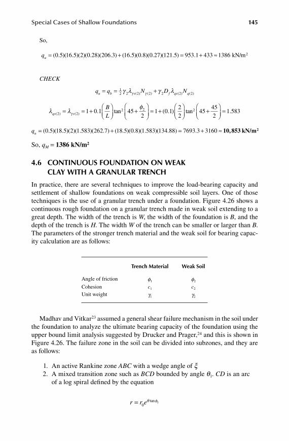
Special Cases of Shallow Foundations 145
So,
qu = +( . )( . )( )( . )( . ) ( . )( . )(0 5 16 5 2 0 28 206 3 16 5 0 8 0 27 121 5 953 1 433 1386. )( . ) .= + ≈ kN/m2
CHECK
q q N D Nu b s f qs q= = +1
2 2 2 2 2 2 2γ l γ lγ γ( ) ( ) ( ) ( )
l l
φγqs s
B
L( ) ( ) . tan2 22 21 0 1 45
2= = +
+
= +
+
=1 0 12
245
45
21 5832( . ) tan .
qu = +( . )( . )( )( . )( . ) ( . )( . )0 5 18 5 2 1 583 262 7 18 5 0 8 ( . )( . ) .1 583 134 88 7693 3 3160= + ≈ 10,853 kN/m2
So, qM = 1386 kN/m2
4.6 ContinuouS Foundation on weaK Clay with a Granular trenCh
In practice, there are several techniques to improve the load-bearing capacity and settlement of shallow foundations on weak compressible soil layers. One of those techniques is the use of a granular trench under a foundation. Figure 4.26 shows a continuous rough foundation on a granular trench made in weak soil extending to a great depth. The width of the trench is W, the width of the foundation is B, and the depth of the trench is H. The width W of the trench can be smaller or larger than B. The parameters of the stronger trench material and the weak soil for bearing capac-ity calculation are as follows:
trench material weak Soil
Angle of friction f1 f2
Cohesion c1 c2
Unit weight g1 g2
Madhav and Vitkar23 assumed a general shear failure mechanism in the soil under the foundation to analyze the ultimate bearing capacity of the foundation using the upper bound limit analysis suggested by Drucker and Prager,24 and this is shown in Figure 4.26. The failure zone in the soil can be divided into subzones, and they are as follows:
1. An active Rankine zone ABC with a wedge angle of x 2. A mixed transition zone such as BCD bounded by angle q1. CD is an arc
of a log spiral defined by the equation
r r e= 0
1θ φtan
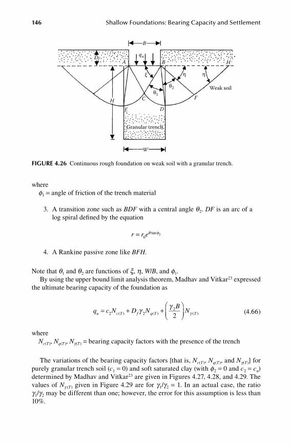
146 Shallow Foundations: Bearing Capacity and Settlement
wheref1 = angle of friction of the trench material
3. A transition zone such as BDF with a central angle q2. DF is an arc of a log spiral defined by the equation
r r e= 0
2θ φtan
4. A Rankine passive zone like BFH.
Note that q1 and q2 are functions of x, h, W/B, and f1.By using the upper bound limit analysis theorem, Madhav and Vitkar23 expressed
the ultimate bearing capacity of the foundation as
q c N D N
BNu c T f q T T= + +
2 2
2
2( ) ( ) ( )γ γγ (4.66)
whereNc(T), Nq(T), Ng(T) = bearing capacity factors with the presence of the trench
The variations of the bearing capacity factors [that is, Nc(T), Nq(T), and Ng(T)] for purely granular trench soil (c1 = 0) and soft saturated clay (with f2 = 0 and c2 = cu) determined by Madhav and Vitkar23 are given in Figures 4.27, 4.28, and 4.29. The values of Ng (T) given in Figure 4.29 are for g1/g2 = 1. In an actual case, the ratio g1/g2 may be different than one; however, the error for this assumption is less than 10%.
FiGure 4.26 Continuous rough foundation on weak soil with a granular trench.
Df A
H
H
W
E
C
B
D
F
B
qu
ξ
θ2
Granular trench
Weak soilθ1
η η
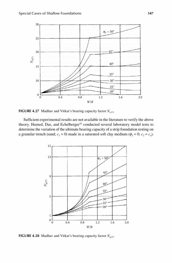
Special Cases of Shallow Foundations 147
Sufficient experimental results are not available in the literature to verify the above theory. Hamed, Das, and Echelberger25 conducted several laboratory model tests to determine the variation of the ultimate bearing capacity of a strip foundation resting on a granular trench (sand; c1 = 0) made in a saturated soft clay medium (f2 = 0; c2 = cu).
FiGure 4.27 Madhav and Vitkar’s bearing capacity factor Nc(T).
30
25
20
φ1 = 50º
45º
40º
35º
30º
25º20º
15
10
00 0.4 0.8 1.2
W/B
Nc(T
)
1.6 2.0
FiGure 4.28 Madhav and Vitkar’s bearing capacity factor Nq(T).
15
13
9
5
10
0 0.4 0.8W/B
Nq(
T)
1.2 1.6 2.0
φ1 = 50º
45º
40º
35º
30º25º20º
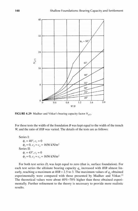
148 Shallow Foundations: Bearing Capacity and Settlement
For these tests the width of the foundation B was kept equal to the width of the trench W, and the ratio of H/B was varied. The details of the tests are as follows:
Series I:f1 = 40°, c1 = 0f2 = 0, c2 = cu = 1656 kN/m2
Series II:f1 = 43°, c1 = 0f2 = 0, c2 = cu = 1656 kN/m2
For both test series Df was kept equal to zero (that is, surface foundation). For each test series the ultimate bearing capacity qu increased with H/B almost lin-early, reaching a maximum at H/B ≈ 2.5 to 3. The maximum values of qu obtained experimentally were compared with those presented by Madhav and Vitkar.23 The theoretical values were about 40%−70% higher than those obtained experi-mentally. Further refinement to the theory is necessary to provide more realistic results.
FiGure 4.29 Madhav and Vitkar’s bearing capacity factor Ng(T).
40
32
24
16
8
Nγ(
T)
00 0.4 0.8 1.2 1.6 2.0
W/B
φ1 = 50º
45º
40º
35º
30º25º
20º
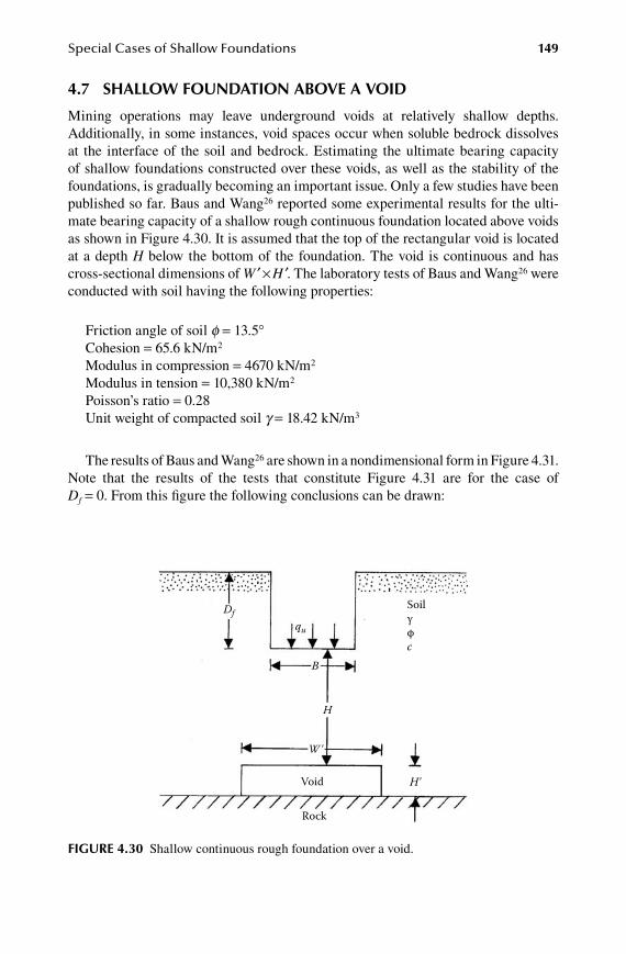
Special Cases of Shallow Foundations 149
4.7 Shallow Foundation aboVe a Void
Mining operations may leave underground voids at relatively shallow depths. Additionally, in some instances, void spaces occur when soluble bedrock dissolves at the interface of the soil and bedrock. Estimating the ultimate bearing capacity of shallow foundations constructed over these voids, as well as the stability of the foundations, is gradually becoming an important issue. Only a few studies have been published so far. Baus and Wang26 reported some experimental results for the ulti-mate bearing capacity of a shallow rough continuous foundation located above voids as shown in Figure 4.30. It is assumed that the top of the rectangular void is located at a depth H below the bottom of the foundation. The void is continuous and has cross-sectional dimensions of W ′ × H ′. The laboratory tests of Baus and Wang26 were conducted with soil having the following properties:
Friction angle of soil f = 13.5°Cohesion = 65.6 kN/m2
Modulus in compression = 4670 kN/m2
Modulus in tension = 10,380 kN/m2
Poisson’s ratio = 0.28Unit weight of compacted soil g = 18.42 kN/m3
The results of Baus and Wang26 are shown in a nondimensional form in Figure 4.31. Note that the results of the tests that constitute Figure 4.31 are for the case of Df = 0. From this figure the following conclusions can be drawn:
FiGure 4.30 Shallow continuous rough foundation over a void.
Dfqu
B
H
W'
H'
Soilγφc
Void
Rock

150 Shallow Foundations: Bearing Capacity and Settlement
1. For a given H/B, the ultimate bearing capacity decreases with the increase in the void width, W ′.
2. For any given W ′/B, there is a critical H/B ratio beyond which the void has no effect on the ultimate bearing capacity. For W ′/B = 10, the value of the critical H/B is about 12.
Baus and Wang26 conducted finite analysis to compare the validity of their experi-mental findings. In the finite element analysis, the soil was treated as an elastic– perfectly plastic material. They also assumed that Hooke’s law is valid in the elastic range and that the soil follows the von Mises yield criterion in the perfectly plastic range, or
f J J k= + = ′α 1 2 (4.67)
�f = 0 (4.68)
where f = yield function
α φ
φ=
+tan
( tan ) .9 12 0 5 (4.69)
′ =+
kc3
9 12 0 5( tan ) .φ (4.70) J1 = first stress invariant J2 = second stress invariant
FiGure 4.31 Experimental bearing capacity of a continuous foundation as a function of void size and location. Source: From Baus, R.L., and M.C. Wang. 1983. Bearing capacity of strip booking above void. J. Geotech. Eng., ASCE, 109(1):1.
100
80
60
40
20
01 5
23
5710
9 13H/B
W'/B = 1q u
(with
void
)q u
(with
out v
oid)
(%)
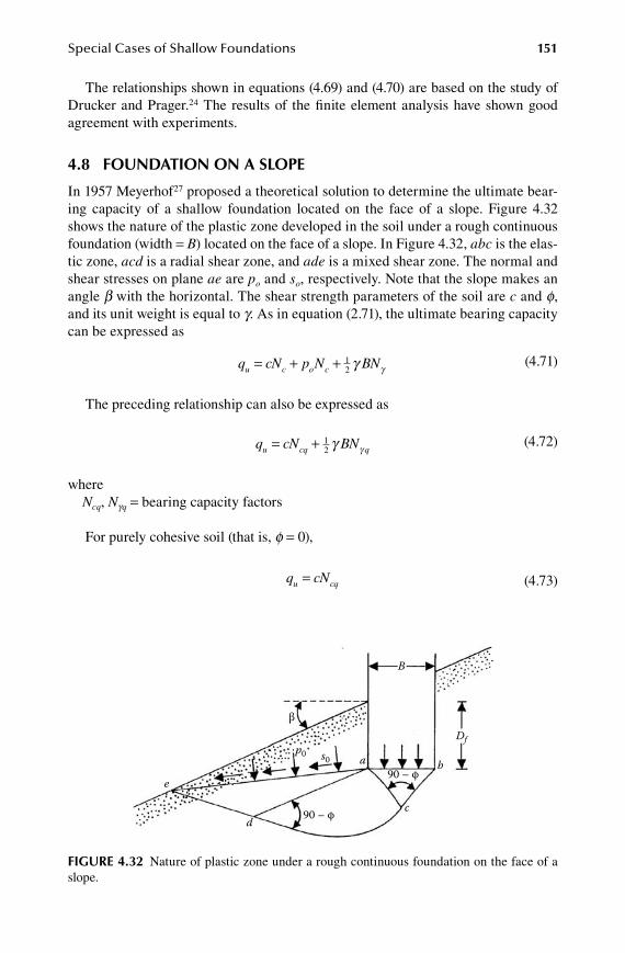
Special Cases of Shallow Foundations 151
The relationships shown in equations (4.69) and (4.70) are based on the study of Drucker and Prager.24 The results of the finite element analysis have shown good agreement with experiments.
4.8 Foundation on a Slope
In 1957 Meyerhof27 proposed a theoretical solution to determine the ultimate bear-ing capacity of a shallow foundation located on the face of a slope. Figure 4.32 shows the nature of the plastic zone developed in the soil under a rough continuous foundation (width = B) located on the face of a slope. In Figure 4.32, abc is the elas-tic zone, acd is a radial shear zone, and ade is a mixed shear zone. The normal and shear stresses on plane ae are po and so, respectively. Note that the slope makes an angle b with the horizontal. The shear strength parameters of the soil are c and f, and its unit weight is equal to g. As in equation (2.71), the ultimate bearing capacity can be expressed as
q cN p N BNu c o c= + + 1
2 γ γ (4.71)
The preceding relationship can also be expressed as
q cN BNu cq q= + 1
2 γ γ (4.72)
whereNcq, Ngq = bearing capacity factors
For purely cohesive soil (that is, f = 0),
q cNu cq= (4.73)
FiGure 4.32 Nature of plastic zone under a rough continuous foundation on the face of a slope.
90 – φ
90 – φ
β
e
d
a
c
b
B
Dfp0 s0

152 Shallow Foundations: Bearing Capacity and Settlement
Figure 4.33 shows the variation of Ncq with slope angle b and the slope stability number Ns. Note that
N
Hcs = γ (4.74)
whereH = height of the slope
In a similar manner, for a granular soil (c = 0),
q BNu q= 1
2 γ γ (4.75)
The variation of Ngq (for c = 0) applicable to equation (4.75) is shown in Figure 4.34.
FiGure 4.33 Variation of Meyerhof’s bearing capacity factor Ncq for a purely cohesive soil (foundation on a slope).
8
7
6
5
4
3
2
1
00 20 40 60
5.535
4
3
2
1
0
Ncq
Ns = 0
Df/B = 0Df/B = 1
80β (deg)
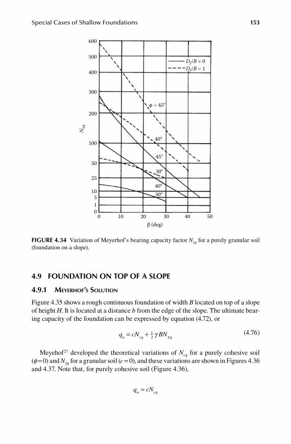
Special Cases of Shallow Foundations 153
4.9 Foundation on top oF a Slope
4.9.1 meyeRhof’s solUtion
Figure 4.35 shows a rough continuous foundation of width B located on top of a slope of height H. It is located at a distance b from the edge of the slope. The ultimate bear-ing capacity of the foundation can be expressed by equation (4.72), or
q cN BNu cq q= + 1
2 γ γ (4.76)
Meyehof27 developed the theoretical variations of Ncq for a purely cohesive soil (f = 0) and Ngq for a granular soil (c = 0), and these variations are shown in Figures 4.36 and 4.37. Note that, for purely cohesive soil (Figure 4.36),
q cNu cq=
FiGure 4.34 Variation of Meyerhof’s bearing capacity factor Ngq for a purely granular soil (foundation on a slope).
600
500
400
300
200
100
50
25
10510
0 10 20 30 40 50β (deg)
Df/B = 0Df/B = 1
Nγq
φ = 45º
40º
45º
30º
40º30º
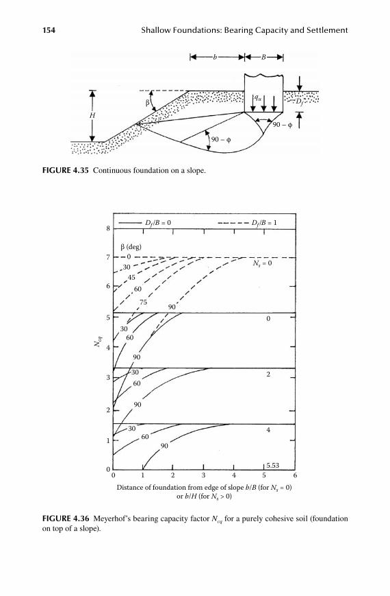
154 Shallow Foundations: Bearing Capacity and Settlement
FiGure 4.36 Meyerhof’s bearing capacity factor Ncq for a purely cohesive soil (foundation on top of a slope).
8Df /B = 0 Df /B = 1
Ns = 00
3045
60
75 900
2
4
5.53
Distance of foundation from edge of slope b/B (for Ns = 0)or b/H (for Ns > 0)
Ncq
3060
90
3060
90
3060
90
β (deg)7
6
5
4
3
2
1
00 1 2 3 4 5 6
FiGure 4.35 Continuous foundation on a slope.
H
b
qu Df
B
β
90 – φ
90 – φ

Special Cases of Shallow Foundations 155
and for granular soil (Figure 4.37),
q BNu q= 1
2 γ γ
It is important to note that, when using Figure 4.36, the stability number Ns should be taken as zero when B < H. If B ≥ H, the curve for the actual stability number should be used.
4.9.2 solUtions of hansen anD vesiC
Referring to the condition of b = 0 in Figure 4.35 (that is, the foundation is located at the edge of the slope), Hansen28 proposed the following relationship for the ultimate bearing capacity of a continuous foundation:
q cN qN BNu c c q q= + +l l γ lβ β γ γβ
12
(4.77)
FiGure 4.37 Meyerhof’s bearing capacity factor Ngq for a granular soil (foundation on top of a slope).
600
500
400
300
200
100
50
25
10510
0 1 2 3 4 5 6b/B
Df/B = 0
Nγq
Df/B = 1
β (deg)0
4020
400 40
20400 30
3030
30
0
φ (deg)

156 Shallow Foundations: Bearing Capacity and Settlement
where Nc, Nq, Ng = bearing capacity factors (see Table 2.3 for Nc and Nq and Table 2.4
for Ng)l cb, l qb, lg b = slope factors q = gDf
According to Hansen,28
l l ββ γβq = = -( tan )1 2
(4.78)
ll
φββ
cq q
q
N
N=
--
>1
10(for )
(4.79)
l β
πφβc = -
+=1
22
0(for ) (4.80)
For the f = 0 condition Vesic12 pointed out that, with the absence of weight due to the slope, the bearing capacity factor Ng has a negative value and can be given as
Nγ β= -2sin (4.81)
Thus, for the f = 0 condition with Nc = 5.14 and Nq = 1, equation (4.77) takes the form
q c D Bu f= -
+ - -( . ).
( tan ) sin5 14 12
5 141 2β γ β γ β β( tan )1 2-
or
q c D Bu f= - + - - -( . ) ( tan ) sin ( tan )5 14 2 1 12 2β γ β γ β β (4.82)
4.9.3 solUtion By limit eqUiliBRiUm anD limit analysis
Saran, Sud, and Handa29 provided a solution to determine the ultimate bearing capacity of shallow continuous foundations on the top of a slope (Figure 4.35) using the limit equilibrium and limit analysis approach. According to this theory, for a strip foundation,
q cN qN BNu c q= + + 1
2 γ γ (4.83)
whereNc, Nq, Ng = bearing capacity factors q = gDf
Referring to the notations used in Figure 4.35, the numerical values of Nc, Nq, and Ng are given in Table 4.4.
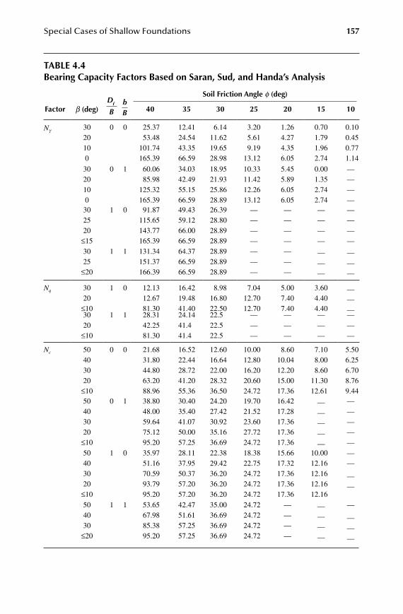
Special Cases of Shallow Foundations 157
table 4.4bearing Capacity Factors based on Saran, Sud, and handa’s analysis
D
Bf b
B
Soil Friction angle f (deg)
Factor b (deg) 40 35 30 25 20 15 10
Ng 3020100
0 0 25.3753.48
101.74165.39
12.4124.5443.3566.59
6.1411.6219.6528.98
3.205.619.19
13.12
1.264.274.356.05
0.701.791.962.74
0.100.450.771.14
3020100
0 1 60.0685.98
125.32165.39
34.0342.4955.1566.59
18.9521.9325.8628.89
10.3311.4212.2613.12
5.455.896.056.05
0.001.352.742.74
————
302520
≤15
1 0 91.87115.65143.77165.39
49.4359.1266.0066.59
26.3928.8028.8928.89
————
————
————
————
3025
≤20
1 1 131.34151.37166.39
64.3766.5966.59
28.8928.8928.89
———
———
———
———
Nq 3020
≤10
1 0 12.1312.6781.30
16.4219.4841.40
8.9816.8022.50
7.0412.7012.70
5.007.407.40
3.604.404.40
———
3020
≤10
1 1 28.3142.2581.30
24.1441.441.4
22.522.522.5
———
———
———
———
Nc 50403020
≤10
0 0 21.6831.8044.8063.2088.96
16.5222.4428.7241.2055.36
12.6016.6422.0028.3236.50
10.0012.8016.2020.6024.72
8.6010.0412.2015.0017.36
7.108.008.60
11.3012.61
5.506.256.708.769.44
50403020
≤10
0 1 38.8048.0059.6475.1295.20
30.4035.4041.0750.0057.25
24.2027.4230.9235.1636.69
19.7021.5223.6027.7224.72
16.4217.2817.3617.3617.36
—————
—————
50403020
≤10
1 0 35.9751.1670.5993.7995.20
28.1137.9550.3757.2057.20
22.3829.4236.2036.2036.20
18.3822.7524.7224.7224.72
15.6617.3217.3617.3617.36
10.0012.1612.1612.1612.16
——
——
504030
≤20
1 1 53.6567.9885.3895.20
42.4751.6157.2557.25
35.0036.6936.6936.69
24.7224.7224.7224.72
————
————
—
———
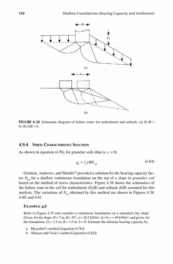
158 Shallow Foundations: Bearing Capacity and Settlement
4.9.4 stRess ChaRaCteRistiCs solUtion
As shown in equation (4.76), for granular soils (that is, c = 0)
q BNu q= 1
2 γ γ (4.84)
Graham, Andrews, and Shields30 provided a solution for the bearing capacity fac-tor Ngq for a shallow continuous foundation on the top of a slope in granular soil based on the method of stress characteristics. Figure 4.38 shows the schematics of the failure zone in the soil for embedment (Df/B) and setback (b/B) assumed for this analysis. The variations of Ngq obtained by this method are shown in Figures 4.39, 4.40, and 4.41.
Example 4.6
Refer to Figure 4.35 and consider a continuous foundation on a saturated clay slope. Given, for the slope: H = 7 m; b = 30°; g = 18.5 kN/m3; f = 0, c = 49 kN/m2; and given, for the foundation: Df = 1.5 m; B = 1.5 m; b = 0. Estimate the ultimate bearing capacity by:
a. Meyerhof’s method [equation (4.76)] b. Hansen and Vesic’s method [equation (4.82)]
FiGure 4.38 Schematic diagram of failure zones for embedment and setback: (a) Df /B > 0; (b) b/B > 0.
B
b
(a)
(b)
Df
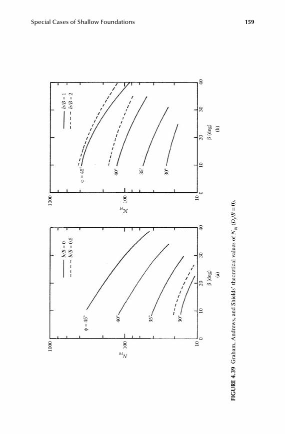
Special Cases of Shallow Foundations 159
FiG
ur
e 4.
39 G
raha
m, A
ndre
ws,
and
Shi
elds
’ th
eore
tica
l val
ues
of N
gq (D
f/B =
0).
1000 10
0 100
1020
30β
(deg
)40
(a)
φ =
45º
φ =
45º
40º
40º
35º
35º
30º
30º
Nγq
b/B
= 0
b/B
= 0.
5
1000 10
0 100
1020
30β
(deg
)40
(b)
Nγq
b/B
= 1
b/B
= 2

160 Shallow Foundations: Bearing Capacity and Settlement
1000 10
0
Nγq
100
1020
β (d
eg)
(a)
3040
φ =
45º
40º
35º
30º
b/B
= 0
b/B
= 0.
5
1000 10
0
Nγq
100
1020
β (d
eg)
(b)
3040
φ =
45º
40º
35º
30º
b/B
= 1
b/B
= 2
FiG
ur
e 4.
40 G
raha
m, A
ndre
ws,
and
Shi
elds
’ th
eore
tica
l val
ues
of N
gq (D
f/B =
0.5
).

Special Cases of Shallow Foundations 161
FiG
ur
e 4.
41 G
raha
m, A
ndre
ws,
and
Shi
elds
’ th
eore
tica
l val
ues
of N
gq (D
f/B =
1).
1000 10
0 1010
010
2030
40β
(deg
)
(a)
(b)
φ =
45º
40º
35º
30º b/
B =
0b/
B =
0.5
Nγq
1000 10
0 010
2030
40β
(deg
)
φ =
45º
40º
35º
30º b/
B =
1b/
B =
2
Nγq

162 Shallow Foundations: Bearing Capacity and Settlement
Solution
Part a:
q cNqu cq=
Given Df /B = 1.5/1.5 = 1; b/B = 0/1.5 = 0. Since H/B > 1, use Ns = 0.From Figure 4.36, for Df/B = 1; b/B = 0, b = 30°, and Ns = 0, the value of Ncq is about 5.85. So,
qu = (49)(5.85) = 286.7 kN/m2
Part b:From equation (4.82),
q c D Bu f= - + - - -
=
( . ) ( tan ) sin ( tan )5 14 2 1 12 2β γ β γ β β
5 14 280
30 49 18 5 1 5. ( ) ( ) ( . )( . )- ×
+π
( tan ) ( . )( . )(sin )( tan )1 30 18 5 1 5 30 1 302 2- - -
= 203 kN/m2
Example 4.7
Refer to Figure 4.35 and consider a continuous foundation on a slope of granular soil. Given, for the slope: H = 6 m; b = 30°; g = 16.8 kN/m3; f = 40°; c =0; and given, for the foundation: Df = 1.5 m; B = 1.5 m; b = 1.5 m. Estimate the ultimate bearing capacity by:
a. Meyerhof’s method [equation (4.76)] b. Saran, Sud, and Handa’s method [equation (4.83)] c. The stress characteristic solution [equation (4.84)]
Solution
Part a:For granular soil (c = 0), from equation (4.76),
q BNu q= 1
2 γ γ
Given: b/B = 1.5/1.5 = 1; Df /B = 1.5/1.5 = 1; f = 40°; and b = 30°. From Figure 4.37, Ngq ≈ 120. So,
qu = =1
2 16 8 1 5 120( . )( . )( ) 1512 kN/m2
Part b:For c = 0, from equation (4.83),
q qN BNu q= + 1
2 γ γ
For b/B = 1: Df/B = 1; f = 40°; and b = 30°. The value of Ng = 131.34 and the value of Nq = 28.31 (Table 4.4).
qu = +( . )( . )( . ) ( . )( . )( . )16 8 1 5 28 31 16 8 1 5 131 341
2 ≈≈ 2368 kN/m2
Special Cases of Shallow Foundations 163
Part c:From equation (4.84),
q BNu q= 1
2 γ γ
From Figure 4.41b, Ngq ≈ 110,
qu = =1
2 16 8 1 5 110( . )( . )( ) 1386 kN/m2
reFerenCeS
1. Prandtl, L. 1921. Uber die eindringungsfestigkeit plastisher baustoffe und die festig-keit von schneiden. Z. Ang. Math. Mech. 1(1): 15.
2. Reissner, H. 1924. Zum erddruckproblem, in Proc., I Intl. Conf. Appl. Mech., Delft, The Netherlands, 295.
3. Lundgren, H., and K. Mortensen. 1953. Determination by the theory of plasticity of the bearing capacity of continuous footings on sand, in Proc., III Int. Conf. Soil Mech. Found. Eng., Zurich, Switzerland, 1: 409.
4. Mandel, J., and J. Salencon. 1972. Force portante d’un sol sur une assise rigide (étude theorizue). Geotechnique 22(1): 79.
5. Meyerhof, G. G., and T. K. Chaplin. 1953. The compression and bearing capacity of cohesive soils. Br. J. Appl. Phys. 4: 20.
6. Meyerhof, G. G. 1974. Ultimate bearing capacity of footings on sand layer overlying clay. Canadian Geotech. J. 11(2): 224.
7. Milovic, D. M., and J. P. Tournier. 1971. Comportement de foundations reposant sur une coche compressible d´épaisseur limitée, in Proc., Conf. Comportement des Sols Avant la Rupture, Paris, France: 303.
8. Pfeifle, T. W., and B. M. Das. 1979. Bearing capacity of surface footings on sand layer resting on rigid rough base. Soils and Foundations 19(1): 1.
9. Cerato, A. B., and A. J. Lutenegger. 2006. Bearing capacity of square and circular footings on a finite layer of granular soil underlain by a rigid base. J. Geotech. Geoenv. Eng., ASCE, 132(11): 1496.
10. Mandel, J., and J. Salencon. 1969. Force portante d’un sol sur une assise rigide, in Proc., VII Int. Conf. Soil Mech. Found Eng., Mexico City, 2: 157.
11. Buisman, A. S. K. 1940. Grondmechanica. Delft: Waltman.12. Vesic, A. S. 1975. Bearing capacity of shallow foundations, in Foundation engineer-
ing handbook, ed. H. F. Winterkorn and H. Y. Fang, 121. New York: Van Nostrand Reinhold Co.
13. DeBeer, E. E. 1975. Analysis of shallow foundations, in Geotechnical modeling and applications, ed. S. M. Sayed, 212. Gulf Publishing Co. Houston, USA.
14. Casagrande, A., and N. Carrillo. 1954. Shear failure in anisotropic materials, in Contribution to soil mechanics 1941–53, Boston Society of Civil Engineers, 122.
15. Reddy, A. S., and R. J. Srinivasan. 1967. Bearing capacity of footings on layered clays. J. Soil Mech. Found. Div., ASCE, 93(SM2): 83.
16. Lo, K. Y. 1965. Stability of slopes in anisotropic soil. J. Soil Mech. Found. Div., ASCE, 91(SM4): 85.
17. Meyerhof, G. G., and A. M. Hanna. 1978. Ultimate bearing capacity of foundations on layered soils under inclined load. Canadian Geotech. J. 15(4): 565.
18. Caquot, A., and J. Kerisel. 1949. Tables for the calculation of passive pressure, active pressure, and bearing capacity of foundations. Paris: Gauthier-Villars.
164 Shallow Foundations: Bearing Capacity and Settlement
19. Meyerhof, G. G. 1963. Some recent research on the bearing capacity of foundations. Canadian Geotech. J. 1(1): 16.
20. Hanna, A. M., and G. G. Meyerhof. 1980. Design charts for ultimate bearing capacity for sands overlying clays. Canadian Geotech. J. 17(2): 300.
21. Hanna, A. M. 1981. Foundations on strong sand overlying weak sand. J. Geotech. Eng,, ASCE, 107(GT7): 915.
22. Hanna, A. M. 1982. Bearing capacity of foundations on a weak sand layer overlying a strong deposit. Canadian Geotech. J. 19(3): 392.
23. Madhav, M. R., and P. P. Vitkar. 1978. Strip footing on weak clay stabilized with a granular trench or pile. Canadian Geotech. J. 15(4): 605.
24. Drucker, D. C., and W. Prager. 1952. Soil mechanics and plastic analysis of limit design. Q. Appl. Math. 10: 157.
25. Hamed, J. T., B. M. Das, and W. F. Echelberger. 1986. Bearing capacity of a strip foundation on granular trench in soft clay. Civil Engineering for Practicing and Design Engineers 5(5): 359.
26. Baus, R. L., and M. C. Wang. 1983. Bearing capacity of strip footing above void. J. Geotech. Eng., ASCE, 109(GT1): 1.
27. Meyerhof, G. G. 1957. The ultimate bearing capacity of foundations on slopes, in Proc., IV Int. Conf. Soil Mech. Found. Eng., London, England, 1: 384.
28. Hansen, J. B. 1970. A revised and extended formula for bearing capacity, Bulletin 28. Copenhagen: Danish Geotechnical Institute.
29. Saran, S., V. K. Sud, and S. C. Handa. 1989. Bearing capacity of footings adjacent to slopes. J. Geotech. Eng., ASCE, 115(4): 553.
30. Graham, J., M. Andrews, and D. H. Shields. 1988. Stress characteristics for shallow footings in cohesionless slopes. Canadian Geotech. J. 25(2): 238.
165
5 Settlement and Allowable Bearing Capacity
5.1 introduCtion
Various theories relating to the ultimate bearing capacity of shallow foundations were presented in Chapters 2, 3, and 4. In section 2.12 a number of definitions for the allowable bearing capacity were discussed. In the design of any foundation, one must consider the safety against bearing capacity failure as well as against excessive settlement of the foundation. In the design of most foundations, there are specifica-tions for allowable levels of settlement. Refer to Figure 5.1, which is a plot of load per unit area q versus settlement S for a foundation. The ultimate bearing capacity is realized at a settlement level of Su. Let Sall be the allowable level of settlement for the foundation and qall(S) be the corresponding allowable bearing capacity. If FS is the factor of safety against bearing capacity failure, then the allowable bearing capacity is qall(b) = qu/FS. The settlement corresponding to qall(b) is S′. For founda-tions with smaller widths of B, S′ may be less than Sall; however, Sall < S′ for larger values of B. Hence, for smaller foundation widths, the bearing capacity controls; for larger foundation widths, the allowable settlement controls. This chapter describes the procedures for estimating the settlements of foundations under load and thus the allowable bearing capacity.
The settlement of a foundation can have three components: (a) elastic settlement Se, (b) primary consolidation settlement Sc, and (c) secondary consolidation settle-ment Ss.
The total settlement St can be expressed as
S S S St e c s= + +
For any given foundation, one or more of the components may be zero or negligible.Elastic settlement is caused by deformation of dry soil, as well as moist and sat-
urated soils, without any change in moisture content. Primary consolidation set-tlement is a time-dependent process that occurs in clayey soils located below the groundwater table as a result of the volume change in soil because of the expulsion of water that occupies the void spaces. Secondary consolidation settlement follows the primary consolidation process in saturated clayey soils and is a result of the plastic adjustment of soil fabrics. The procedures for estimating the above three types of settlements are discussed in this chapter.
Any type of settlement is a function of the additional stress imposed on the soil by the foundation. Hence, it is desirable to know the relationships for calculating the stress increase in the soil caused by application of load to the foundation. These
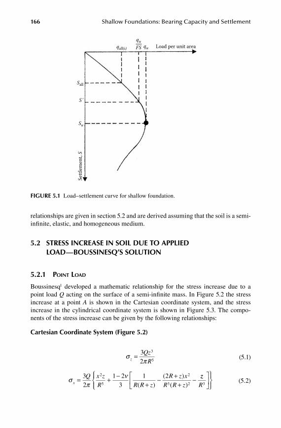
166 Shallow Foundations: Bearing Capacity and Settlement
relationships are given in section 5.2 and are derived assuming that the soil is a semi-infinite, elastic, and homogeneous medium.
5.2 StreSS inCreaSe in Soil due to applied load—bouSSineSq’S Solution
5.2.1 point loaD
Boussinesq1 developed a mathematic relationship for the stress increase due to a point load Q acting on the surface of a semi-infinite mass. In Figure 5.2 the stress increase at a point A is shown in the Cartesian coordinate system, and the stress increase in the cylindrical coordinate system is shown in Figure 5.3. The compo-nents of the stress increase can be given by the following relationships:
Cartesian Coordinate System (Figure 5.2)
σ
πz
QzR
= 32
3
5 (5.1)
σπ
νx
Q x zR R R z
R z xR R z
= + -+
- ++
-32
1 23
1 22
5
2
3 2( )( )
( )zz
R3
(5.2)
qall(s)
Sall
S´
Su
Settl
emen
t, S
Load per unit area qu
quFS
FiGure 5.1 Load–settlement curve for shallow foundation.
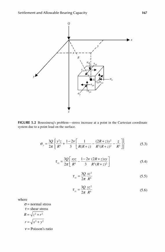
Settlement and Allowable Bearing Capacity 167
σπ
νy
Q y zR R R z
R z yR R z
= + -+
- ++
-32
1 23
1 22
5
2
3 2( )( )
( )zz
R3
(5.3)
τ
πν
xy
Q xyzR
R z xyR R z
= - - ++
32
1 23
25 3 2
( )( )
(5.4)
τ
πxz
Q xzR
= 32
2
5 (5.5)
τ
πyz
Q yzR
= 32
2
5 (5.6)
where s = normal stress t = shear stress
R z r= +2 2
r x y= +2 2
n = Poisson’s ratio
y
x
Q
x
y
R
A
zσz
σy
z
σx
τzy
τzx
τxyτyx
τyz
τxz
FiGure 5.2 Boussinesq’s problem—stress increase at a point in the Cartesian coordinate system due to a point load on the surface.

168 Shallow Foundations: Bearing Capacity and Settlement
Cylindrical Coordinate System (Figure 5.3)
σ
πz
QzR
= 32
3
5 (5.7)
σ
πν
r
Q zrR R R z
= - -+
2
3 1 22
5 ( ) (5.8)
σ
πνθ = -
+-
QR R z
zR2
1 21
3( )
( ) (5.9)
τ
πrz
QrzR
= 32
2
5 (5.10)
5.2.2 UnifoRmly loaDeD flexiBle CiRCUlaR aRea
Boussinesq’s solution for a point load can be extended to determine the stress increase due to a uniformly loaded flexible circular area on the surface of a semi-infinite mass (Figure 5.4). In Figure 5.4, the circular area has a radius R, and the
y
x
Q
x
y
R
A
z
r
σz
σθ
z
σr
τzr
τrz
FiGure 5.3 Boussinesq’s problem—stress increase at a point in the cylindrical coordinate system due to a point load on the surface.

Settlement and Allowable Bearing Capacity 169
uniformly distributed load per unit area is q. If the components of stress increase at a point A below the center are to be determined, then we consider an elemental area dA = rdqdr. The load on the elemental area is dQ = qrdqdr. This can be treated as a point load. Now the vertical stress increase dsz at A due to dQ can be obtained by substituting dQ for Q and r z2 2+ for R in equation (5.7). Thus,
d
z qrd drr z
zσ θπ
=+
32
3
2 2 5 2( ) /
The vertical stress increase due to the entire loaded area sz is then
σ σ θπ
θ
π
z z
r
R
dz qrd drr z
q= =+
===∫∫∫ 3
21
3
2 2 5 20
2
0( ) /
--+
zR z
3
2 2 3 2( ) / (5.11)
Similarly, the magnitudes of s q and sr below the center can be obtained as
σ σ ν ν
θrq z
R zz
R z= = + - +
++
+21 2
2 12 2 1 2
3
2 2 3 2
( )( ) ( )/ /
(5.12)
qdQ
dA dθ
dr
R
A
z
σz
σz
σθσr
r
FiGure 5.4 Stress increase below the center of a uniformly loaded flexible circular area.
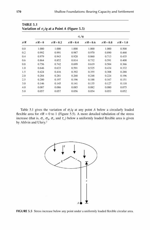
170 Shallow Foundations: Bearing Capacity and Settlement
Table 5.1 gives the variation of sz/q at any point A below a circularly loaded flexible area for r/R = 0 to 1 (Figure 5.5). A more detailed tabulation of the stress increase (that is, sz, s q, sr, and trz) below a uniformly loaded flexible area is given by Ahlvin and Ulery.2
table 5.1Variation of sz/q at a point A (Figure 5.5)
sz /q
z/R r/R = 0 r/R = 0.2 r/R = 0.4 r/R = 0.6 r/R = 0.8 r/R = 1.0
0.0 1.000 1.000 1.000 1.000 1.000 0.5000.2 0.992 0.991 0.987 0.970 0.890 0.4680.4 0.979 0.943 0.920 0.860 0.713 0.4350.6 0.864 0.852 0.814 0.732 0.591 0.4000.8 0.756 0.742 0.699 0.619 0.504 0.3661.0 0.646 0.633 0.591 0.525 0.434 0.3321.5 0.424 0.416 0.392 0.355 0.308 0.2882.0 0.284 0.281 0.268 0.248 0.224 0.1962.5 0.200 0.197 0.196 0.188 0.167 0.1513.0 0.146 0.145 0.141 0.135 0.127 0.1184.0 0.087 0.086 0.085 0.082 0.080 0.0755.0 0.057 0.057 0.056 0.054 0.053 0.052
FiGure 5.5 Stress increase below any point under a uniformly loaded flexible circular area.
q
rR
A
z

Settlement and Allowable Bearing Capacity 171
5.2.3 UnifoRmly loaDeD flexiBle ReCtangUlaR aRea
Figure 5.6 shows a flexible rectangular area of length L and width B subjected to a uniform vertical load of q per unit area. The load on the elemental area dA is equal to dQ = q dx dy. This can be treated as an elemental point load. The vertical stress increase dsz due to this at A, which is located at a depth z below the corner of the rectangular area, can be obtained by using equation (5.7), or
d
qz dxdyx y z
zσπ
=+ +
32
3
2 2 2 5 2( ) / (5.13)
Hence, the vertical stress increase at A due to the entire loaded area is
σ σπz z
x
L
y
B
dqz dxdyr z
qI= =+
===∫∫∫ 3
2
3
2 2 5 2
00( ) / (5.14)
where
I
mn m nm n m n
m nm
= + ++ + +
× + ++
14
2 11
22 2 0 5
2 2 2 2
2 2
2π( ) .
nnmn m n
m n m n21
2 2 0 5
2 2 2 212 1
1++ + +
+ - +
-tan
( ) .
(5.15)
mBz
=
n
Lz
=
Table 5.2 shows the variation of I with m and n. The stress below any other point C below the rectangular area (Figure 5.7) can be obtained by dividing it into four rect-angles as shown. For rectangular area 1, m1 = B1/z; n1 = L1/z. Similarly, for rectangles 2, 3,
y
xq
dA
dQ y
x
L
B
A(0,0,z)
z
FiGure 5.6 Stress increase below the corner of a uniformly loaded flexible rectangular area.
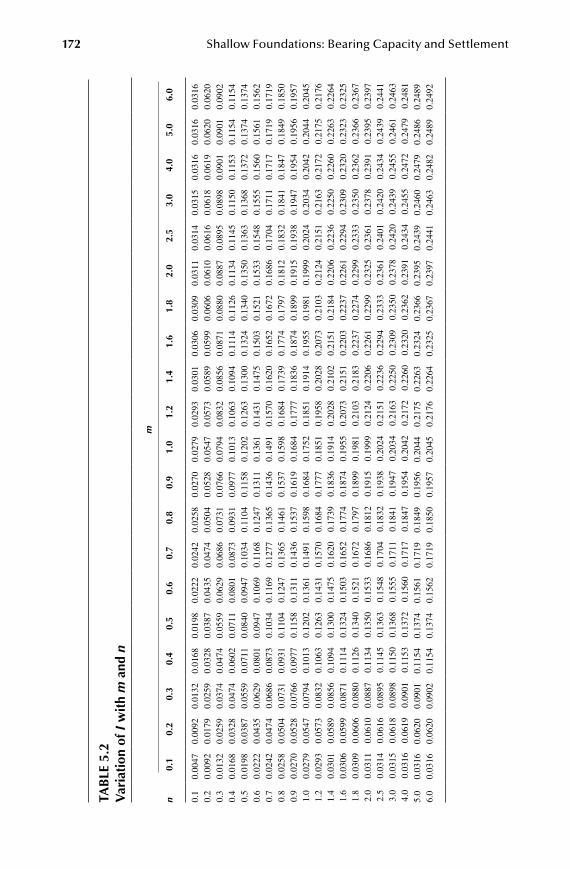
172 Shallow Foundations: Bearing Capacity and Settlement
tab
le 5
.2V
aria
tion
of I
wit
h m
and
n
m
n0.
10.
20.
30.
40.
50.
60.
70.
80.
91.
01.
21.
41.
61.
82.
02.
53.
04.
05.
06.
0
0.1
0.00
470.
0092
0.01
320.
0168
0.01
980.
0222
0.02
420.
0258
0.02
700.
0279
0.02
930.
0301
0.03
060.
0309
0.03
110.
0314
0.03
150.
0316
0.03
160.
0316
0.2
0.00
920.
0179
0.02
590.
0328
0.03
870.
0435
0.04
740.
0504
0.05
280.
0547
0.05
730.
0589
0.05
990.
0606
0.06
100.
0616
0.06
180.
0619
0.06
200.
0620
0.3
0.01
320.
0259
0.03
740.
0474
0.05
590.
0629
0.06
860.
0731
0.07
660.
0794
0.08
320.
0856
0.08
710.
0880
0.08
870.
0895
0.08
980.
0901
0.09
010.
0902
0.4
0.01
680.
0328
0.04
740.
0602
0.07
110.
0801
0.08
730.
0931
0.09
770.
1013
0.10
630.
1094
0.11
140.
1126
0.11
340.
1145
0.11
500.
1153
0.11
540.
1154
0.5
0.01
980.
0387
0.05
590.
0711
0.08
400.
0947
0.10
340.
1104
0.11
580.
1202
0.12
630.
1300
0.13
240.
1340
0.13
500.
1363
0.13
680.
1372
0.13
740.
1374
0.6
0.02
220.
0435
0.06
290.
0801
0.09
470.
1069
0.11
680.
1247
0.13
110.
1361
0.14
310.
1475
0.15
030.
1521
0.15
330.
1548
0.15
550.
1560
0.15
610.
1562
0.7
0.02
420.
0474
0.06
860.
0873
0.10
340.
1169
0.12
770.
1365
0.14
360.
1491
0.15
700.
1620
0.16
520.
1672
0.16
860.
1704
0.17
110.
1717
0.17
190.
1719
0.8
0.02
580.
0504
0.07
310.
0931
0.11
040.
1247
0.13
650.
1461
0.15
370.
1598
0.16
840.
1739
0.17
740.
1797
0.18
120.
1832
0.18
410.
1847
0.18
490.
1850
0.9
0.02
700.
0528
0.07
660.
0977
0.11
580.
1311
0.14
360.
1537
0.16
190.
1684
0.17
770.
1836
0.18
740.
1899
0.19
150.
1938
0.19
470.
1954
0.19
560.
1957
1.0
0.02
790.
0547
0.07
940.
1013
0.12
020.
1361
0.14
910.
1598
0.16
840.
1752
0.18
510.
1914
0.19
550.
1981
0.19
990.
2024
0.20
340.
2042
0.20
440.
2045
1.2
0.02
930.
0573
0.08
320.
1063
0.12
630.
1431
0.15
700.
1684
0.17
770.
1851
0.19
580.
2028
0.20
730.
2103
0.21
240.
2151
0.21
630.
2172
0.21
750.
2176
1.4
0.03
010.
0589
0.08
560.
1094
0.13
000.
1475
0.16
200.
1739
0.18
360.
1914
0.20
280.
2102
0.21
510.
2184
0.22
060.
2236
0.22
500.
2260
0.22
630.
2264
1.6
0.03
060.
0599
0.08
710.
1114
0.13
240.
1503
0.16
520.
1774
0.18
740.
1955
0.20
730.
2151
0.22
030.
2237
0.22
610.
2294
0.23
090.
2320
0.23
230.
2325
1.8
0.03
090.
0606
0.08
800.
1126
0.13
400.
1521
0.16
720.
1797
0.18
990.
1981
0.21
030.
2183
0.22
370.
2274
0.22
990.
2333
0.23
500.
2362
0.23
660.
2367
2.0
0.03
110.
0610
0.08
870.
1134
0.13
500.
1533
0.16
860.
1812
0.19
150.
1999
0.21
240.
2206
0.22
610.
2299
0.23
250.
2361
0.23
780.
2391
0.23
950.
2397
2.5
0.03
140.
0616
0.08
950.
1145
0.13
630.
1548
0.17
040.
1832
0.19
380.
2024
0.21
510.
2236
0.22
940.
2333
0.23
610.
2401
0.24
200.
2434
0.24
390.
2441
3.0
0.03
150.
0618
0.08
980.
1150
0.13
680.
1555
0.17
110.
1841
0.19
470.
2034
0.21
630.
2250
0.23
090.
2350
0.23
780.
2420
0.24
390.
2455
0.24
610.
2463
4.0
0.03
160.
0619
0.09
010.
1153
0.13
720.
1560
0.17
170.
1847
0.19
540.
2042
0.21
720.
2260
0.23
200.
2362
0.23
910.
2434
0.24
550.
2472
0.24
790.
2481
5.0
0.03
160.
0620
0.09
010.
1154
0.13
740.
1561
0.17
190.
1849
0.19
560.
2044
0.21
750.
2263
0.23
240.
2366
0.23
950.
2439
0.24
600.
2479
0.24
860.
2489
6.0
0.03
160.
0620
0.09
020.
1154
0.13
740.
1562
0.17
190.
1850
0.19
570.
2045
0.21
760.
2264
0.23
250.
2367
0.23
970.
2441
0.24
630.
2482
0.24
890.
2492
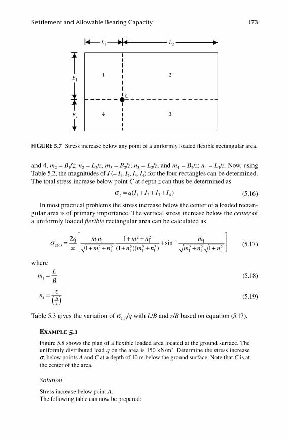
Settlement and Allowable Bearing Capacity 173
and 4, m2 = B1/z; n2 = L2/z, m3 = B2/z; n3 = L2/z, and m4 = B2/z; n4 = L1/z. Now, using Table 5.2, the magnitudes of I (= I1, I2, I3, I4) for the four rectangles can be determined. The total stress increase below point C at depth z can thus be determined as
σ z q I I I I= + + +( )1 2 3 4 (5.16)
In most practical problems the stress increase below the center of a loaded rectan-gular area is of primary importance. The vertical stress increase below the center of a uniformly loaded flexible rectangular area can be calculated as
σπz cq m n
m n
m nn m
( )( )(
=+ +
+ ++ +
21
11
1 1
12
12
12
12
12
12 nn
m
m n n12
1 1
12
12
121)
sin++ +
- (5.17)
where
m
LB1 = (5.18)
nzB12
= ( ) (5.19)
Table 5.3 gives the variation of sz(c)/q with L/B and z/B based on equation (5.17).
Example 5.1
Figure 5.8 shows the plan of a flexible loaded area located at the ground surface. The uniformly distributed load q on the area is 150 kN/m2. Determine the stress increase sz below points A and C at a depth of 10 m below the ground surface. Note that C is at the center of the area.
Solution
Stress increase below point A.The following table can now be prepared:
B2
C
B1
L1 L2
1 2
4 3
FiGure 5.7 Stress increase below any point of a uniformly loaded flexible rectangular area.
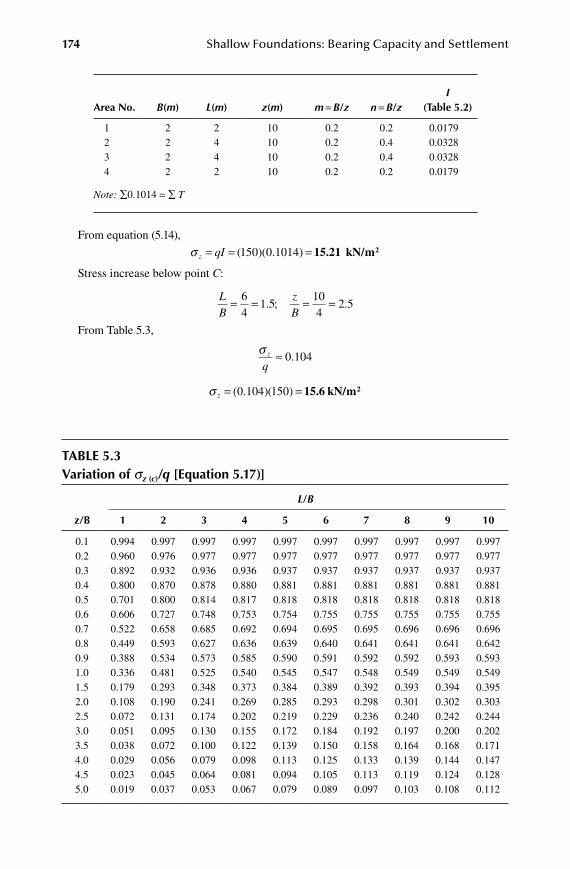
174 Shallow Foundations: Bearing Capacity and Settlement
area no. B(m) L(m) z(m) m = B/z n = B/zI
(table 5.2)
1 2 2 10 0.2 0.2 0.01792 2 4 10 0.2 0.4 0.03283 2 4 10 0.2 0.4 0.03284 2 2 10 0.2 0.2 0.0179
Note: ∑0.1014 = ∑ T
From equation (5.14),
σ z qI= = =( )( . )150 0 1014 15.21 kN/m2
Stress increase below point C:
LB
zB
= = = =64
1 5104
2 5. ; .
From Table 5.3,
σ z
q≈ 0 104.
σ z = =( . )( )0 104 150 15.6 kN/m2
table 5.3Variation of sz (c)/q [equation 5.17)]
L/B
z/b 1 2 3 4 5 6 7 8 9 10
0.1 0.994 0.997 0.997 0.997 0.997 0.997 0.997 0.997 0.997 0.9970.2 0.960 0.976 0.977 0.977 0.977 0.977 0.977 0.977 0.977 0.9770.3 0.892 0.932 0.936 0.936 0.937 0.937 0.937 0.937 0.937 0.9370.4 0.800 0.870 0.878 0.880 0.881 0.881 0.881 0.881 0.881 0.8810.5 0.701 0.800 0.814 0.817 0.818 0.818 0.818 0.818 0.818 0.8180.6 0.606 0.727 0.748 0.753 0.754 0.755 0.755 0.755 0.755 0.7550.7 0.522 0.658 0.685 0.692 0.694 0.695 0.695 0.696 0.696 0.6960.8 0.449 0.593 0.627 0.636 0.639 0.640 0.641 0.641 0.641 0.6420.9 0.388 0.534 0.573 0.585 0.590 0.591 0.592 0.592 0.593 0.5931.0 0.336 0.481 0.525 0.540 0.545 0.547 0.548 0.549 0.549 0.5491.5 0.179 0.293 0.348 0.373 0.384 0.389 0.392 0.393 0.394 0.3952.0 0.108 0.190 0.241 0.269 0.285 0.293 0.298 0.301 0.302 0.3032.5 0.072 0.131 0.174 0.202 0.219 0.229 0.236 0.240 0.242 0.2443.0 0.051 0.095 0.130 0.155 0.172 0.184 0.192 0.197 0.200 0.2023.5 0.038 0.072 0.100 0.122 0.139 0.150 0.158 0.164 0.168 0.1714.0 0.029 0.056 0.079 0.098 0.113 0.125 0.133 0.139 0.144 0.1474.5 0.023 0.045 0.064 0.081 0.094 0.105 0.113 0.119 0.124 0.1285.0 0.019 0.037 0.053 0.067 0.079 0.089 0.097 0.103 0.108 0.112
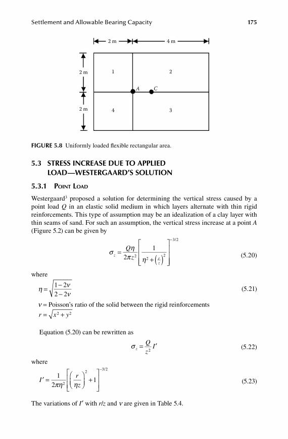
Settlement and Allowable Bearing Capacity 175
5.3 StreSS inCreaSe due to applied load—weSterGaard’S Solution
5.3.1 point loaD
Westergaard3 proposed a solution for determining the vertical stress caused by a point load Q in an elastic solid medium in which layers alternate with thin rigid reinforcements. This type of assumption may be an idealization of a clay layer with thin seams of sand. For such an assumption, the vertical stress increase at a point A (Figure 5.2) can be given by
σ ηπ η
zrz
Qz
=+ ( )
-
21
22
2
3 2/
(5.20)
where
η ν
ν= -
-1 22 2
(5.21)
n = Poisson’s ratio of the solid between the rigid reinforcements
r x y= +2 2
Equation (5.20) can be rewritten as
σ z
Qz
I= ′2
(5.22)
where
′ =
+
-
Irz
12
12
23 2
πη η
/
(5.23)
The variations of I′ with r/z and n are given in Table 5.4.
2 m
2 m 4 m
2 m
1 2
4 3
A C
FiGure 5.8 Uniformly loaded flexible rectangular area.
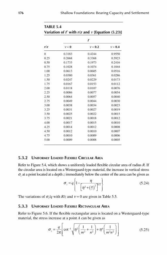
176 Shallow Foundations: Bearing Capacity and Settlement
5.3.2 UnifoRmly loaDeD flexiBle CiRCUlaR aRea
Refer to Figure 5.4, which shows a uniformly loaded flexible circular area of radius R. If the circular area is located on a Westergaard-type material, the increase in vertical stress sz at a point located at a depth z immediately below the center of the area can be given as
σ η
ηz
Rz
q= -+ ( )
1
2 2 1 2/ (5.24)
The variations of sz/q with R/z and n = 0 are given in Table 5.5.
5.3.3 UnifoRmly loaDeD flexiBle ReCtangUlaR aRea
Refer to Figure 5.6. If the flexible rectangular area is located on a Westergaard-type material, the stress increase at a point A can be given as
σπ
η ηz
qm n m n
= +
+
-
21 1 11 2
2 24
2 2cot
(5.25)
table 5.4Variation of I′ with r/z and n [equation (5.23)]
I′
r/z n = 0 n = 0.2 n = 0.4
0 0.3183 0.4244 0.95500.25 0.2668 0.3368 0.59230.50 0.1733 0.1973 0.24160.75 0.1028 0.1074 0.10441.00 0.0613 0.0605 0.05161.25 0.0380 0.0361 0.02861.50 0.0247 0.0229 0.01731.75 0.0167 0.0153 0.01122.00 0.0118 0.0107 0.00762.25 0.0086 0.0077 0.00542.50 0.0064 0.0057 0.00402.75 0.0049 0.0044 0.00303.00 0.0038 0.0034 0.00233.25 0.0031 0.0027 0.00193.50 0.0025 0.0022 0.00153.75 0.0021 0.0018 0.0012
4.00 0.0017 0.0015 0.00104.25 0.0014 0.0012 0.00084.50 0.0012 0.0010 0.00074.75 0.0010 0.0009 0.00065.00 0.0009 0.0008 0.0005
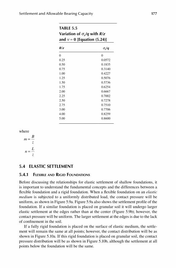
Settlement and Allowable Bearing Capacity 177
where
mBz
=
n
Lz
=
5.4 elaStiC Settlement
5.4.1 flexiBle anD RigiD foUnDations
Before discussing the relationships for elastic settlement of shallow foundations, it is important to understand the fundamental concepts and the differences between a flexible foundation and a rigid foundation. When a flexible foundation on an elastic medium is subjected to a uniformly distributed load, the contact pressure will be uniform, as shown in Figure 5.9a. Figure 5.9a also shows the settlement profile of the foundation. If a similar foundation is placed on granular soil it will undergo larger elastic settlement at the edges rather than at the center (Figure 5.9b); however, the contact pressure will be uniform. The larger settlement at the edges is due to the lack of confinement in the soil.
If a fully rigid foundation is placed on the surface of elastic medium, the settle-ment will remain the same at all points; however, the contact distribution will be as shown in Figure 5.10a. If this rigid foundation is placed on granular soil, the contact pressure distribution will be as shown in Figure 5.10b, although the settlement at all points below the foundation will be the same.
table 5.5Variation of sz/q with R/z and n = 0 [equation (5.24)]
R/z sz/q
0 00.25 0.05720.50 0.18350.75 0.31401.00 0.42271.25 0.50761.50 0.57361.75 0.62542.00 0.66672.25 0.70022.50 0.72782.75 0.75103.00 0.77064.00 0.82595.00 0.8600
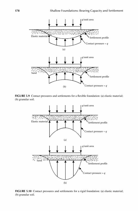
178 Shallow Foundations: Bearing Capacity and Settlement
Elastic material
q/unit area
Settlement profile
Contact pressure = q
Sand
q/unit area
(a)
(b)
Settlement profile
Contact pressure = q
FiGure 5.10 Contact pressures and settlements for a rigid foundation: (a) elastic material; (b) granular soil.
Elastic material
q/unit area
Settlement profile
Contact pressure = q
Sand
q/unit area
(a)
(b)
Settlement profile
Contact pressure = q
FiGure 5.9 Contact pressures and settlements for a flexible foundation: (a) elastic material; (b) granular soil.
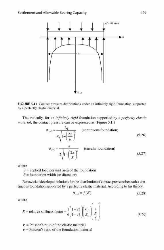
Settlement and Allowable Bearing Capacity 179
Theoretically, for an infinitely rigid foundation supported by a perfectly elastic material, the contact pressure can be expressed as (Figure 5.11)
σπ
zq
xB
= =
-
0 2
2
12
(continuous foundattion) (5.26)
σ zq
xB
= =
-
0 2
2 12
(circular foundationn) (5.27)
where q = applied load per unit area of the foundation B = foundation width (or diameter)
Borowicka4 developed solutions for the distribution of contact pressure beneath a con-tinuous foundation supported by a perfectly elastic material. According to his theory,
σ z f K= =0 ( ) (5.28)
where
K s
f
= = --
relative stiffness factor
16
11
2
2
νν
E
EtB
f
s
2
3
(5.29)
ns = Poisson’s ratio of the elastic material nf = Poisson’s ratio of the foundation material
q/unit area
x
B
σz=0
FiGure 5.11 Contact pressure distributions under an infinitely rigid foundation supported by a perfectly elastic material.

180 Shallow Foundations: Bearing Capacity and Settlement
t = thickness of the foundation Es, Ef = modulus of elasticity of the elastic material and foundation material,
respectively
Although soil is not perfectly elastic and homogeneous, the theory of elasticity may be used to estimate the settlements of shallow foundations at allowable loads. Judicious uses of these results have done well in the design, construction, and main-tenance of structures.
5.4.2 elastiC paRameteRs
Parameters such as the modulus of elasticity Es and Poisson’s ratio n for a given soil must be known in order to calculate the elastic settlement of a foundation. In most cases, if laboratory test results are not available, they are estimated from empirical correlations. Table 5.6 provides some suggested values for Poisson’s ratio.
Trautmann and Kulhawy5 used the following relationship for Poisson’s ratio (drained state):
ν φ= +0 1 0 3. . rel (5.30)
φ φ
reltcrelative friction angle= = - °° - °
2545 25
(0 rel≤ ≤φ 1) (5.31)
wherej tc = friction angle from drained triaxial compression test
A general range of the modulus of elasticity of sand Es is given in Table 5.7.A number of correlations for the modulus of elasticity of sand with the field stan-
dard penetration resistance N60 and cone penetration resistance qc have been made in the past. Schmertmann6 proposed that
E Ns (kN/m )2 = 766 60 (5.32)
table 5.6Suggested Values for poisson’s ratio
Soil type poisson’s ratio n
Coarse sand 0.15–0.20Medium loose sand 0.20–0.25Fine sand 0.25–0.30Sandy silt and silt 0.30–0.35Saturated clay (undrained) 0.50Saturated clay—lightly overconsolidated (drained)
0.2–0.4
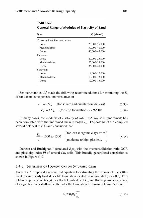
Settlement and Allowable Bearing Capacity 181
Schmertmann et al.7 made the following recommendations for estimating the Es of sand from cone penetration resistance, or
E qs c (for square and circular foun= 2 5. dations) (5.33)
E q L/ Bs c (for strip foundations; 1= ≥3 5. 0) (5.34)
In many cases, the modulus of elasticity of saturated clay soils (undrained) has been correlated with the undrained shear strength cu. D’Appolonia et al.8 compiled several field test results and concluded that
Ec
s
u
=1000 to 1500for lean inorganic claays from
moderate to high plasticity
(5.35)
Duncan and Buchignani9 correlated Es/cu with the overconsolidation ratio OCR and plasticity index PI of several clay soils. This broadly generalized correlation is shown in Figure 5.12.
5.4.3 settlement of foUnDations on satURateD Clays
Janbu et al.10 proposed a generalized equation for estimating the average elastic settle-ment of a uniformly loaded flexible foundation located on saturated clay (n = 0.5). This relationship incorporates (a) the effect of embedment Df, and (b) the possible existence of a rigid layer at a shallow depth under the foundation as shown in Figure 5.13, or,
S
qBE
es
= µ µ1 2 (5.36)
table 5.7General range of modulus of elasticity of Sand
type Es (kn/m2)
Coarse and medium coarse sand Loose 25,000–35,000 Medium dense 30,000–40,000 Dense 40,000–45,000Fine sand Loose 20,000–25,000 Medium dense 25,000–35,000 Dense 35,000–40,000Sandy silt Loose 8,000–12,000 Medium dense 10,000–12,000 Dense 12,000–15,000
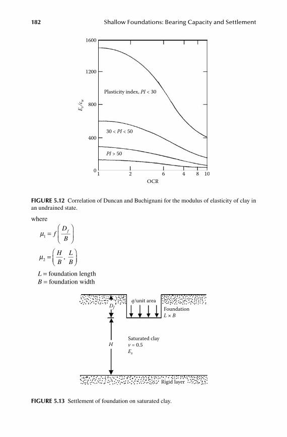
182 Shallow Foundations: Bearing Capacity and Settlement
where
µ1 =
f
D
Bf
µ2 =
HB
LB
,
L = foundation lengthB = foundation width
Plasticity index, PI < 30
30 < PI < 50
PI > 50
1600
1200
800
400
0 1 2 OCR
6 4 8 10
E s/c
u
FiGure 5.12 Correlation of Duncan and Buchignani for the modulus of elasticity of clay in an undrained state.
q/unit area
Saturated clayv = 0.5Es
FoundationL × B
Rigid layer
Df
H
FiGure 5.13 Settlement of foundation on saturated clay.
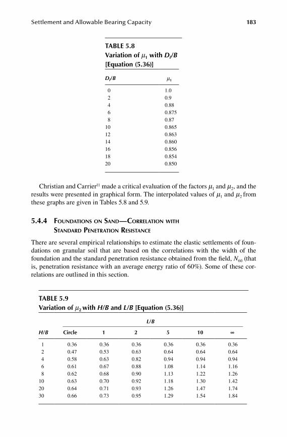
Settlement and Allowable Bearing Capacity 183
Christian and Carrier11 made a critical evaluation of the factors m1 and m2, and the results were presented in graphical form. The interpolated values of m1 and m2 from these graphs are given in Tables 5.8 and 5.9.
5.4.4 foUnDations on sanD—CoRRelation with stanDaRD penetRation ResistanCe
There are several empirical relationships to estimate the elastic settlements of foun-dations on granular soil that are based on the correlations with the width of the foundation and the standard penetration resistance obtained from the field, N60 (that is, penetration resistance with an average energy ratio of 60%). Some of these cor-relations are outlined in this section.
table 5.8Variation of m1 with Df/B [equation (5.36)]
Df/B m1
0 1.0 2 0.9 4 0.88 6 0.875 8 0.8710 0.86512 0.86314 0.86016 0.85618 0.85420 0.850
table 5.9Variation of m2 with H/B and L/B [equation (5.36)]
L/B
H/B Circle 1 2 5 10 ∞
1 0.36 0.36 0.36 0.36 0.36 0.36 2 0.47 0.53 0.63 0.64 0.64 0.64 4 0.58 0.63 0.82 0.94 0.94 0.94 6 0.61 0.67 0.88 1.08 1.14 1.16 8 0.62 0.68 0.90 1.13 1.22 1.2610 0.63 0.70 0.92 1.18 1.30 1.4220 0.64 0.71 0.93 1.26 1.47 1.7430 0.66 0.73 0.95 1.29 1.54 1.84
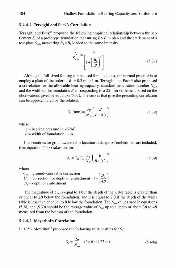
184 Shallow Foundations: Bearing Capacity and Settlement
5.4.4.1 terzaghi and peck’s Correlation
Terzaghi and Peck12 proposed the following empirical relationship between the set-tlement Se of a prototype foundation measuring B × B in plan and the settlement of a test plate Se(1) measuring B1 × B1 loaded to the same intensity:
S
S B
B
e
e( )11
2
4
1
=
+
(5.37)
Although a full-sized footing can be used for a load test, the normal practice is to employ a plate of the order of B1 = 0.3 m to 1 m. Terzaghi and Peck12 also proposed a correlation for the allowable bearing capacity, standard penetration number N60, and the width of the foundation B corresponding to a 25-mm settlement based on the observations given by equation (5.37). The curves that give the preceding correlation can be approximated by the relation,
S
qN
BB .
e (mm) =+
3
0 360
2
(5.38)
where q = bearing pressure in kN/m2
B = width of foundation in m
If corrections for groundwater table location and depth of embedment are included, then equation (5.38) takes the form,
S C C
qN
BB .
e W D=+
3
0 360
2
(5.39)
where CW = groundwater table correction CD = correction for depth of embedment =1
4-
D
Bf
Df = depth of embedment
The magnitude of CW is equal to 1.0 if the depth of the water table is greater than or equal to 2B below the foundation, and it is equal to 2.0 if the depth of the water table is less than or equal to B below the foundation. The N60 values used in equations (5.38) and (5.39) should be the average value of N60 up to a depth of about 3B to 4B measured from the bottom of the foundation.
5.4.4.2 meyerhof’s Correlation
In 1956, Meyerhof13 proposed the following relationships for Se:
S
qN
Be = ≤2
60
(for 1.22 m) (5.40a)

Settlement and Allowable Bearing Capacity 185
and
S
qN
BB .
Be =+
>30 360
2
(for 1.22 m) (5.40b)
where Se is in mm, B is in m, and q is in kN/m2.Note that equations (5.38) and (5.40b) are similar. In 1965, Meyerhof14 compared
the predicted and observed settlements of eight structures and proposed revisions to equations (5.40a) and (5.40b). According to these revisions,
S
. qN
Be ≈ ≤1 251 22
60
(for m). (5.41)
and
S
qN
BB .
Be =+
>20 360
2
(for 1.22 m) (5.42)
Comparing equations (5.40a) and (5.40b) with equations (5.41) and (5.42) it can be seen that, for similar settlement levels, the allowable pressure q is 50% higher for equations (5.41) and (5.42). If corrections for the location of the groundwater table and depth of embedment are incorporated into equations (5.41) and (5.42), we obtain
S C C
. qN
Be W D(mm) (for 1.22 m)= ≤1 25
60
(5.43)
and
S C C
qN
BB .
Be W D(mm) (for 1.22 m=+
>20 360
2
)) (5.44)
CW = 1 0. (5.45)
and
C .
D
BD
f= -1 04
(5.46)
5.4.4.3 peck and bazaraa’s method
The original work of Terzaghi and Peck12 as given in equation (5.38) was subse-quently compared to several field observations. It was found that the relationship provided by equation (5.38) is overly conservative (that is, observed field settlements were substantially lower than those predicted by the equation). Recognizing this fact, Peck and Bazaraa15 suggested the following revision to equation (5.39):
S C C
qN
BB .e W D=
+
20 31 60
2
( ) (5.47)
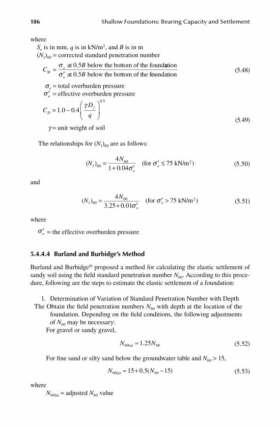
186 Shallow Foundations: Bearing Capacity and Settlement
where Se is in mm, q is in kN/m2, and B is in m (N1)60 = corrected standard penetration number
C
BW
o=σ at 0.5 below the bottom of the foundaation
at 0.5 below the bottom of the f′σ o B ooundation (5.48)
so = total overburden pressure ′σ o = effective overburden pressure
C . .D
qDf
.
= -
1 0 0 4
0 5γ
(5.49) g = unit weight of soil
The relationships for (N1)60 are as follows:
( ) (for 75 kN/m )1 60
2NN
. oo=
+ ′′ ≤
4
1 0 0460
σσ (5.50)
and
( ) (for 75 kN/m )1 60
2NN
. . oo=
+ ′′ >4
3 25 0 0160
σσ (5.51)
where
′σ o = the effective overburden pressure
5.4.4.4 burland and burbidge’s method
Burland and Burbidge16 proposed a method for calculating the elastic settlement of sandy soil using the field standard penetration number N60. According to this proce-dure, following are the steps to estimate the elastic settlement of a foundation:
1. Determination of Variation of Standard Penetration Number with DepthThe Obtain the field penetration numbers N60 with depth at the location of the
foundation. Depending on the field conditions, the following adjustments of N60 may be necessary:
For gravel or sandy gravel,
N N60(a) ≈ 1 25 60. (5.52)
For fine sand or silty sand below the groundwater table and N60 > 15,
N N60(a) ≈ + -15 0 5 1560. ( ) (5.53)
whereN60(a) = adjusted N60 value
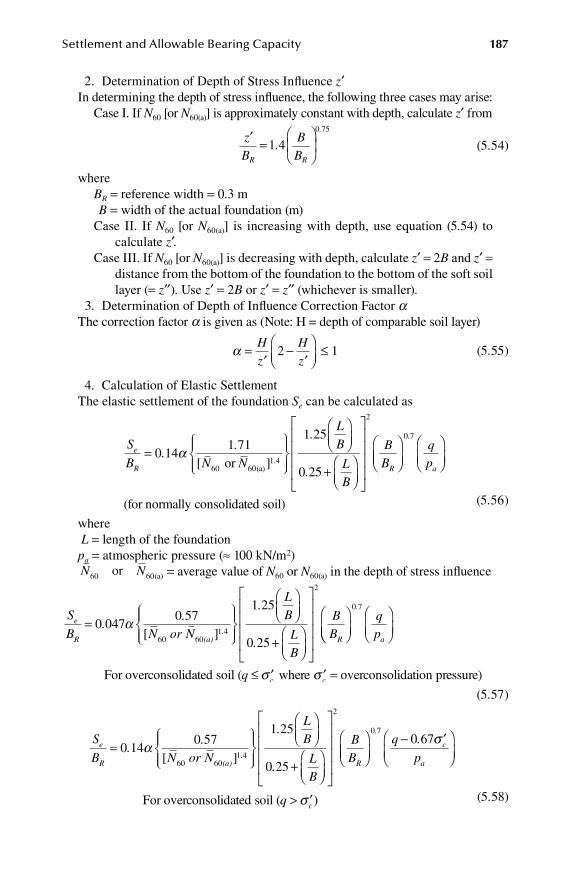
Settlement and Allowable Bearing Capacity 187
2. Determination of Depth of Stress Influence z′In determining the depth of stress influence, the following three cases may arise:
Case I. If N60 [or N60(a)] is approximately constant with depth, calculate z′ from
′ =
zB
.BBR R
.
1 40 75
(5.54)
whereBR = reference width = 0.3 m B = width of the actual foundation (m)Case II. If N60 [or N60(a)] is increasing with depth, use equation (5.54) to
calculate z′.Case III. If N60 [or N60(a)] is decreasing with depth, calculate z′ = 2B and z′ =
distance from the bottom of the foundation to the bottom of the soft soil layer (= z′′). Use z′ = 2B or z′ = z′′ (whichever is smaller).
3. Determination of Depth of Influence Correction Factor aThe correction factor a is given as (Note: H = depth of comparable soil layer)
α =
′-
′
≤Hz
Hz
2 1 (5.55)
4. Calculation of Elastic SettlementThe elastic settlement of the foundation Se can be calculated as
S
B.
.N N
e
R.
=
0 14
1 711
60 601 4
α[ ] or (a)
.LB
.LB
BBR
25
0 25
2
+
0 7.
a
qp
(for normally consolidated soil) (5.56)
where L = length of the foundationpa = atmospheric pressure (≈ 100 kN/m2)N N60 60or (a) = average value of N60 or N60(a) in the depth of stress influence
S
B.
.N or N
e
R (a).
=
0 047
0 57
60 601 4
α[ ]
1 25
0 25
2
.LB
.LB
BBR
+
0 7.
a
qp
For overconsolidated soil ( where overconsolidation pressuc cq ≤ ′ ′ =σ σ re)
(5.57)
S
B.
.N or N
e
R (a).
=
0 14
0 571
60 601 4
α[ ]
.LB
.LB
BBR
25
0 25
2
+
- ′
0 70 67
.
c
a
q .
p
σ
For overconsolidated soil ( )q c> ′σ (5.58)
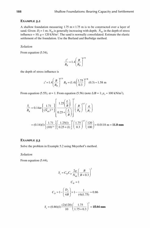
188 Shallow Foundations: Bearing Capacity and Settlement
Example 5.2
A shallow foundation measuring 1.75 m × 1.75 m is to be constructed over a layer of sand. Given: Df = 1 m; N60 is generally increasing with depth; N60 in the depth of stress influence = 10; q = 120 kN/m2. The sand is normally consolidated. Estimate the elastic settlement of the foundation. Use the Burland and Burbidge method.
Solution
From equation (5.54),
′ =
zB
.BBR R
.
1 40 75
the depth of stress influence is
′ =
=
z .
BB
BR
.
R
.
1 4 1 41 750 3
0 75 0 7
( . )..
55
0 3 1 58( . ) .≈ m
From equation (5.55), a = 1. From equation (5.56) (note L/B = 1; pa ≈ 100 kN/m2),
S
B.
.N
.LBe
R.
=
0 141 71
1 25
601 4
α( )
+
0 25
2
0 7
.LB
BB
q
R
.
pp
. .
a
.
=
( . )( )( )
( )0 14 1
1 7110
1 25 11 4 0 25 1
1 750 3
120100
2 0 7
.
.
+
( )
.. = =0.0118 m 11.8 mm
Example 5.3
Solve the problem in Example 5.2 using Meyerhof’s method.
Solution
From equation (5.44),
S C C
qN
BB .e W D=
+
20 360
2
CW = 1
CD
BDf= -
= - ≈1
41
14 1 75
0 86( )( . )
.
S
.e =+
=( . )( )( )( ) .
.0 86 1
2 12010
1 751 75 0 3
2
155.04 mm
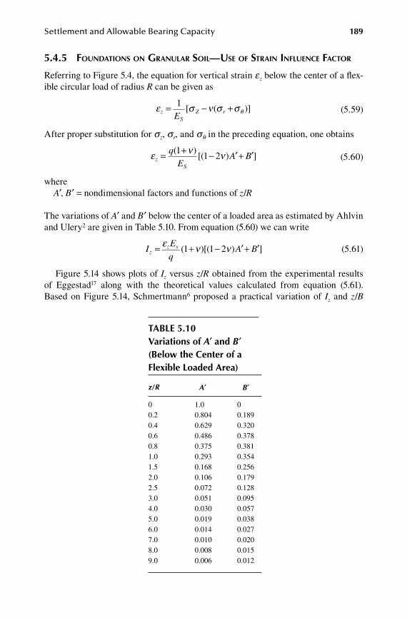
Settlement and Allowable Bearing Capacity 189
5.4.5 foUnDations on gRanUlaR soil—Use of stRain inflUenCe faCtoR
Referring to Figure 5.4, the equation for vertical strain ez below the center of a flex-ible circular load of radius R can be given as
ε σ ν σ σθz
SZ r
E= - +1
[ ( )] (5.59)
After proper substitution for sz, sr, and s q in the preceding equation, one obtains
ε ν νz
S
qE
A B= + - ′+ ′( )[( ) ]
11 2 (5.60)
whereA′, B′ = nondimensional factors and functions of z/R
The variations of A′ and B′ below the center of a loaded area as estimated by Ahlvin and Ulery2 are given in Table 5.10. From equation (5.60) we can write
I
Eq
A Bzz s= + - ′+ ′ε ν ν( )[( ) ]1 1 2 (5.61)
Figure 5.14 shows plots of Iz versus z/R obtained from the experimental results of Eggestad17 along with the theoretical values calculated from equation (5.61). Based on Figure 5.14, Schmertmann6 proposed a practical variation of Iz and z/B
table 5.10Variations of A′ and B′ (below the Center of a Flexible loaded area)
z/R A′ B′
0 1.0 00.2 0.804 0.1890.4 0.629 0.3200.6 0.486 0.3780.8 0.375 0.3811.0 0.293 0.3541.5 0.168 0.2562.0 0.106 0.1792.5 0.072 0.1283.0 0.051 0.0954.0 0.030 0.0575.0 0.019 0.0386.0 0.014 0.0277.0 0.010 0.0208.0 0.008 0.0159.0 0.006 0.012
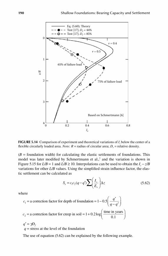
190 Shallow Foundations: Bearing Capacity and Settlement
(B = foundation width) for calculating the elastic settlements of foundations. This model was later modified by Schmertmann et al.,7 and the variation is shown in Figure 5.15 for L/B = 1 and L/B ≥ 10. Interpolations can be used to obtain the Iz – z/B variations for other L/B values. Using the simplified strain influence factor, the elas-tic settlement can be calculated as
S c c q qIE
zez
s
= - ′
∑1 2( ) ∆ (5.62)
where
c1 = a correction factor for depth of foundation = - ′
- ′
1 0 5.q
q q
c2 1= = +a correction factor for creep in soil 0 20 1
. log.
time in years
q′ = gDf
q = stress at the level of the foundation
The use of equation (5.62) can be explained by the following example.
Eq. (5.60); Theory
v = 0.4
v = 0.5
65% of failure load
0
1
2
3
4 0 0.2 0.4
Iz
0.6 0.8
z/R
75% of failure load
Based on Schmertmann [6]
Test [17]; Dr = 44%Test [17]; Dr = 85%
FiGure 5.14 Comparison of experiment and theoretical variations of Iz below the center of a flexible circularly loaded area. Note: R = radius of circular area; Dr = relative density.
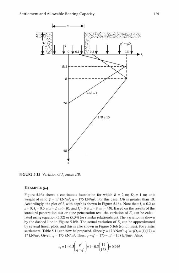
Settlement and Allowable Bearing Capacity 191
Example 5.4
Figure 5.16a shows a continuous foundation for which B = 2 m; Df = 1 m; unit weight of sand g = 17 kN/m3; q = 175 kN/m2. For this case, L/B is greater than 10. Accordingly, the plot of Iz with depth is shown in Figure 5.16a. Note that: Iz = 0.2 at z = 0; Iz = 0.5 at z = 2 m (= B), and Iz = 0 at z = 8 m (= 4B). Based on the results of the standard penetration test or cone penetration test, the variation of Es can be calcu-lated using equation (5.32) or (5.34) (or similar relationships). The variation is shown by the dashed line in Figure 5.16b. The actual variation of Es can be approximated by several linear plots, and this is also shown in Figure 5.16b (solid lines). For elastic settlement, Table 5.11 can now be prepared. Since g = 17 kN/m3, q′ = gDf = (1)(17) = 17 kN/m2. Given: q = 175 kN/m2. Thus, q − q′ = 175 − 17 = 158 kN/m2. Also,
c
qq q
1 1 0 5 1 0 517158
0 946= - ′- ′
= -
=. . .
B/2
0 0.1 0.2 0.5
q´ = γDf
Iz
L/B = 1
L/B ≥ 10
2B
4B
z
B
Df
B
q
FiGure 5.15 Variation of Iz versus z/B.

192 Shallow Foundations: Bearing Capacity and Settlement
Assume the time for creep is 10 years. Hence,
c2 1 0 2
0 11 4= +
=. log
..
10
Thus,
S c c q qI
Eze
z
s
= - ′
=∑1 2 0 946 1 4 158( ) ( . )( . )(∆ )( . ) .26 45 10 5534 8 105 5× = × ≈- - m 55.35 mm
1 m2 m
0
0 7,000 14,000Es (kN/m2)
Iz = 0.2Layer 1
2
3
4
5
1
2
3
4
5
6
7
8
z (m)(a) (b)
z
FiGure 5.16 Determination of elastic settlement of a continuous foundation by strain influ-ence factor method.
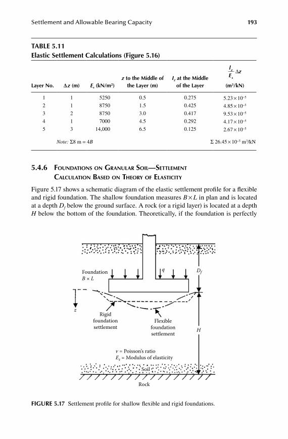
Settlement and Allowable Bearing Capacity 193
5.4.6 foUnDations on gRanUlaR soil—settlement CalCUlation BaseD on theoRy of elastiCity
Figure 5.17 shows a schematic diagram of the elastic settlement profile for a flexible and rigid foundation. The shallow foundation measures B × L in plan and is located at a depth Df below the ground surface. A rock (or a rigid layer) is located at a depth H below the bottom of the foundation. Theoretically, if the foundation is perfectly
table 5.11elastic Settlement Calculations (Figure 5.16)
layer no. Δz (m) Es (kn/m2)z to the middle of
the layer (m)Iz at the middle
of the layer
lE
zz
s
∆
(m3/kn)
1 1 5250 0.5 0.275 5.23 × 10⁻⁵
2 1 8750 1.5 0.425 4.85 × 10⁻⁵
3 2 8750 3.0 0.417 9.53 × 10⁻⁵
4 1 7000 4.5 0.292 4.17 × 10⁻⁵
5 3 14,000 6.5 0.125 2.67 × 10⁻⁵
Note: S8 m = 4B S 26.45 × 10⁻⁵ m3/kN
Rigidfoundationsettlement
v = Poisson’s ratioEs = Modulus of elasticity
Rock
Soil
Flexiblefoundationsettlement
FoundationB × L
q Df
H
z
FiGure 5.17 Settlement profile for shallow flexible and rigid foundations.

194 Shallow Foundations: Bearing Capacity and Settlement
flexible (Bowles18), the settlement may be expressed as
S q B
EI Ie
ss f= ′ ′ -
( )α ν1 2
(5.63)where
q = net applied pressure on the foundation n = Poisson’s ratio of soil Es = average modulus of elasticity of the soil under the foundation measured from
z = 0 to about z = 4B B’ = B/2 for center of foundation (= B for corner of foundation)
I Fs = = + -
-shape factor (Steinbrenner )19
11 21
νν
FF2
(5.64)
F
πA A1 0 1
1= +( )
(5.65)
F
nπ
A21
22= ′ -tan
(5.66)
A mm m n
m m n0
2 2 2
2 2
1 1
1 1= ′ + ′ + ′ + ′
′ + ′ + ′ +ln
( )
( )
(5.67)
Am m n
m m n1
2 2
2 2
1 1
1= ′ + ′ + + ′
′ + ′ + ′ +ln
( )
(5.68)
Am
n m n2 2 2 1
= ′′ + ′ + ′ +
(5.69)
I fD
BLB
ff= =
depth factor (Fox ) and20 , ,ν
(5.70)
a' = a factor that depends on the location on the foundation where settlement is being calculated
To calculate settlement at the center of the foundation, we use
′ =α 4 (5.71)
′ =m
LB
(5.72)
and
′ =( )
nHB2
(5.73)
To calculate settlement at a corner of the foundation,
′ =α 1 (5.74)
′ =m
LB
(5.75)
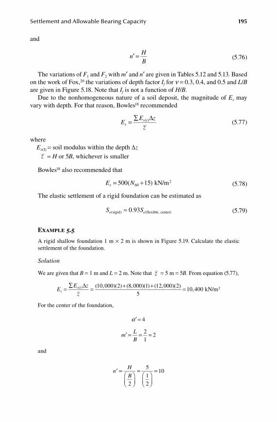
Settlement and Allowable Bearing Capacity 195
and
′ =n
HB
(5.76)
The variations of F1 and F2 with m′ and n′ are given in Tables 5.12 and 5.13. Based on the work of Fox,20 the variations of depth factor If for n = 0.3, 0.4, and 0.5 and L/B are given in Figure 5.18. Note that If is not a function of H/B.
Due to the nonhomogeneous nature of a soil deposit, the magnitude of Es may vary with depth. For that reason, Bowles18 recommended
E
E z
zs
s i= ∑ ( )∆ (5.77)
whereEs(I) = soil modulus within the depth Δz
z = H or 5B, whichever is smaller
Bowles18 also recommended that
E Ns = +500 1560( ) kN/m2 (5.78)
The elastic settlement of a rigid foundation can be estimated as
S Se e( ) .rigid (flexible, center)≈ 0 93 (5.79)
Example 5.5
A rigid shallow foundation 1 m × 2 m is shown in Figure 5.19. Calculate the elastic settlement of the foundation.
Solution
We are given that B = 1 m and L = 2 m. Note that z = 5 m = 5B. From equation (5.77),
E
E z
zs
s i= ∑ = + +( )∆ ( , )( ) ( , )( ) ( ,10 000 2 8 000 1 12 000)( ),
25
10 400= kN/m2
For the center of the foundation,
′ =α 4
′ = = =m
LB
21
2
and
′ =
=
=nH
B2
5
12
10
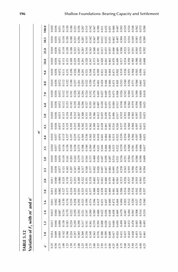
196 Shallow Foundations: Bearing Capacity and Settlement
tab
le 5
.12
Var
iati
on o
f F1
wit
h m
′ and
n′
m′
n′ 1
.0 1
.2 1
.41.
61.
82.
02.
53.
03.
54.
04.
55.
06.
07.
08.
09.
010
.025
.050
.510
0.0
0
.25
0.01
40.
013
0.01
20.
011
0.01
10.
011
0.01
00.
010
0.01
00.
010
0.01
00.
010
0.01
00.
010
0.01
00.
010
0.01
00.
010
0.01
00.
010
0
.50
0.04
90.
046
0.04
40.
042
0.04
10.
040
0.03
80.
038
0.03
70.
037
0.03
60.
036
0.03
60.
036
0.03
60.
036
0.03
60.
036
0.03
60.
036
0
.75
0.09
50.
090
0.08
70.
084
0.08
20.
080
0.07
70.
076
0.07
40.
074
0.07
30.
073
0.07
20.
072
0.07
20.
072
0.07
10.
071
0.07
10.
071
1
.00
0.14
20.
138
0.13
40.
130
0.12
70.
125
0.12
10.
118
0.11
60.
115
0.11
40.
113
0.11
20.
112
0.11
20.
111
0.11
10.
110
0.11
00.
110
1
.25
0.18
60.
183
0.17
90.
176
0.17
30.
170
0.16
50.
161
0.15
80.
157
0.15
50.
154
0.15
30.
152
0.15
20.
151
0.15
10.
150
0.15
00.
150
1
.50
0.22
40.
224
0.22
20.
219
0.21
60.
213
0.20
70.
203
0.19
90.
197
0.19
50.
194
0.19
20.
191
0.19
00.
190
0.18
90.
188
0.18
80.
188
1
.75
0.25
70.
259
0.25
90.
258
0.25
50.
253
0.24
70.
242
0.23
80.
235
0.23
30.
232
0.22
90.
228
0.22
70.
226
0.22
50.
223
0.22
30.
223
2
.00
0.28
50.
290
0.29
20.
292
0.29
10.
289
0.28
40.
279
0.27
50.
271
0.26
90.
267
0.26
40.
262
0.26
10.
260
0.25
90.
257
0.25
60.
256
2
.25
0.30
90.
317
0.32
10.
323
0.32
30.
322
0.31
70.
313
0.30
80.
305
0.30
20.
300
0.29
60.
294
0.29
30.
291
0.29
10.
287
0.28
70.
287
2
.50
0.33
00.
341
0.34
70.
350
0.35
10.
351
0.34
80.
344
0.34
00.
336
0.33
30.
331
0.32
70.
324
0.32
20.
321
0.32
00.
316
0.31
50.
315
2
.75
0.34
80.
361
0.36
90.
374
0.37
70.
378
0.37
70.
373
0.36
90.
365
0.36
20.
359
0.35
50.
352
0.35
00.
348
0.34
70.
343
0.34
20.
342
3
.00
0.36
30.
379
0.38
90.
396
0.40
00.
402
0.40
20.
400
0.39
60.
392
0.38
90.
386
0.38
20.
378
0.37
60.
374
0.37
30.
368
0.36
70.
367
3
.25
0.37
60.
394
0.40
60.
415
0.42
00.
423
0.42
60.
424
0.42
10.
418
0.41
50.
412
0.40
70.
403
0.40
10.
399
0.39
70.
391
0.39
00.
390
3
.50
0.38
80.
408
0.42
20.
431
0.43
80.
442
0.44
70.
447
0.44
40.
441
0.43
80.
435
0.43
00.
427
0.42
40.
421
0.42
00.
413
0.41
20.
411
3
.75
0.39
90.
420
0.43
60.
447
0.45
40.
460
0.46
70.
458
0.46
60.
464
0.46
10.
458
0.45
30.
449
0.44
60.
443
0.44
10.
433
0.43
20.
432
4
.00
0.40
80.
431
0.44
80.
460
0.46
90.
476
0.48
40.
487
0.48
60.
484
0.48
20.
479
0.47
40.
470
0.46
60.
464
0.46
20.
453
0.45
10.
451
4
.25
0.41
70.
440
0.45
80.
472
0.48
10.
484
0.49
50.
514
0.51
50.
515
0.51
60.
496
0.48
40.
473
0.47
10.
471
0.47
00.
468
0.46
20.
460
4
.50
0.42
40.
450
0.46
90.
484
0.49
50.
503
0.51
60.
521
0.52
20.
522
0.52
00.
517
0.51
30.
508
0.50
50.
502
0.49
90.
489
0.48
70.
487
4
.75
0.43
10.
458
0.47
80.
494
0.50
60.
515
0.53
00.
536
0.53
90.
539
0.53
70.
535
0.53
00.
526
0.52
30.
519
0.51
70.
506
0.50
40.
503
5
.00
0.43
70.
465
0.48
70.
503
0.51
60.
526
0.54
30.
551
0.55
40.
554
0.55
40.
552
0.54
80.
543
0.54
00.
536
0.53
40.
522
0.51
90.
519
5
.25
0.44
30.
472
0.49
40.
512
0.52
60.
537
0.55
50.
564
0.56
80.
569
0.56
90.
568
0.56
40.
560
0.55
60.
553
0.55
00.
537
0.53
40.
534
5
.50
0.44
80.
478
0.50
10.
520
0.53
40.
546
0.56
60.
576
0.58
10.
584
0.58
40.
583
0.57
90.
575
0.57
10.
568
0.58
50.
551
0.54
90.
548
5
.75
0.45
30.
483
0.50
80.
527
0.54
20.
555
0.57
60.
588
0.59
40.
597
0.59
70.
597
0.59
40.
590
0.58
60.
583
0.58
00.
565
0.58
30.
562
6
.00
0.45
70.
489
0.51
40.
534
0.55
00.
563
0.58
50.
598
0.60
60.
609
0.61
10.
610
0.60
80.
604
0.60
10.
598
0.59
50.
579
0.57
60.
575
6
.25
0.46
10.
493
0.51
90.
540
0.55
70.
570
0.59
40.
609
0.61
70.
621
0.62
30.
623
0.62
10.
618
0.61
50.
611
0.60
80.
592
0.58
90.
588
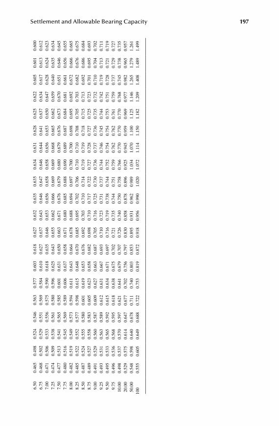
Settlement and Allowable Bearing Capacity 197
6
.50
0.46
50.
498
0.52
40.
546
0.56
30.
577
0.60
30.
618
0.62
70.
632
0.63
50.
635
0.63
40.
631
0.62
80.
625
0.62
20.
605
0.60
10.
600
6
.75
0.46
80.
502
0.52
90.
551
0.56
90.
584
0.61
00.
627
0.63
70.
643
0.64
60.
647
0.64
60.
644
0.64
10.
637
0.63
40.
617
0.61
30.
612
7
.00
0.47
10.
506
0.53
30.
556
0.57
50.
590
0.61
80.
635
0.64
60.
653
0.65
60.
658
0.65
80.
656
0.65
30.
650
0.64
70.
628
0.62
40.
623
7
.25
0.47
40.
509
0.53
80.
561
0.58
00.
596
0.62
50.
643
0.65
50.
662
0.66
60.
669
0.66
90.
668
0.66
50.
662
0.65
90.
640
0.63
50.
634
7
.50
0.47
70.
513
0.54
10.
565
0.58
50.
601
0.63
10.
650
0.66
30.
671
0.67
60.
679
0.68
00.
679
0.67
60.
673
0.67
00.
651
0.64
60.
645
7
.75
0.48
00.
516
0.54
50.
569
0.58
90.
606
0.63
70.
658
0.67
10.
680
0.68
50.
688
0.69
00.
689
0.68
70.
684
0.68
10.
661
0.65
60.
655
8
.00
0.48
20.
519
0.54
90.
573
0.59
40.
611
0.64
30.
664
0.67
80.
688
0.69
40.
697
0.70
00.
700
0.69
80.
695
0.69
20.
672
0.66
60.
665
8
.25
0.48
50.
522
0.55
20.
577
0.59
80.
615
0.64
80.
670
0.68
50.
695
0.70
20.
706
0.71
00.
710
0.70
80.
705
0.70
30.
682
0.67
60.
675
8
.50
0.48
70.
524
0.55
50.
580
0.60
10.
619
0.65
30.
676
0.69
20.
703
0.71
00.
714
0.71
90.
719
0.71
80.
715
0.71
30.
692
0.68
60.
684
8
.75
0.48
90.
527
0.55
80.
583
0.60
50.
623
0.65
80.
682
0.69
80.
710
0.71
70.
722
0.72
70.
728
0.72
70.
725
0.72
30.
701
0.69
50.
693
9
.00
0.49
10.
529
0.56
00.
587
0.60
90.
627
0.66
30.
687
0.70
50.
716
0.72
50.
730
0.73
60.
737
0.73
60.
735
0.73
20.
710
0.70
40.
702
9
.25
0.49
30.
531
0.56
30.
589
0.61
20.
631
0.66
70.
693
0.71
00.
723
0.73
10.
737
0.74
40.
746
0.74
50.
744
0.74
20.
719
0.71
30.
711
9
.50
0.49
50.
533
0.56
50.
592
0.61
50.
634
0.67
10.
697
0.71
60.
719
0.73
80.
744
0.75
20.
754
0.75
40.
753
0.75
10.
728
0.72
10.
719
9
.75
0.49
60.
536
0.56
80.
595
0.61
80.
638
0.67
50.
702
0.72
10.
735
0.74
40.
751
0.75
90.
762
0.76
20.
761
0.75
90.
737
0.72
90.
727
10.
000.
498
0.53
70.
570
0.59
70.
621
0.64
10.
679
0.70
70.
726
0.74
00.
750
0.75
80.
766
0.77
00.
770
0.77
00.
768
0.74
50.
738
0.73
5 2
0.00
0.52
90.
575
0.61
40.
647
0.67
70.
702
0.75
60.
797
0.83
00.
858
0.87
80.
896
0.92
50.
945
0.95
90.
969
0.97
70.
982
0.96
50.
957
50.
000.
548
0.59
80.
640
0.67
80.
711
0.74
00.
803
0.85
30.
895
0.93
10.
962
0.98
91.
034
1.07
01.
100
1.12
51.
146
1.26
51.
279
1.26
110
00.
555
0.60
50.
649
0.68
80.
722
0.75
30.
819
0.87
20.
918
0.95
60.
990
1.02
01.
072
1.11
41.
150
1.18
21.
209
1.40
81.
489
1.49
9
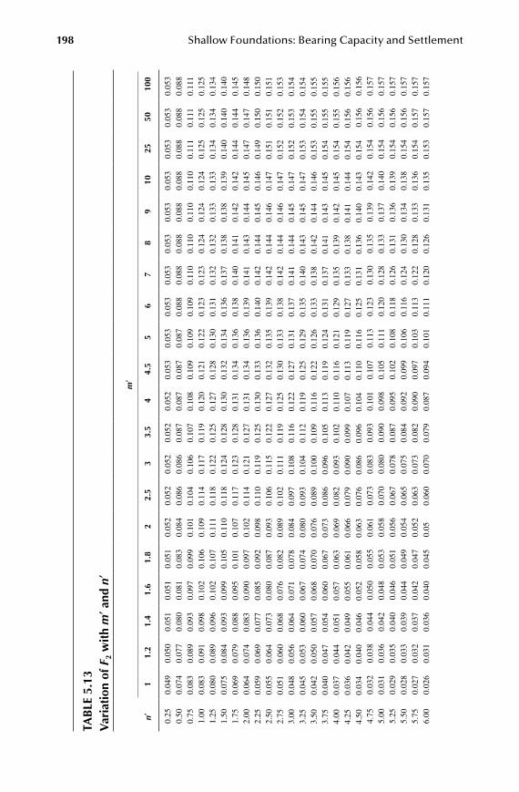
198 Shallow Foundations: Bearing Capacity and Settlement
tab
le 5
.13
Var
iati
on o
f F2
wit
h m
′ and
n′
m′
n′1
1.2
1.4
1.6
1.8
22.
53
3.5
44.
55
67
89
1025
5010
0
0.25
0.04
90.
050
0.05
10.
051
0.05
10.
052
0.05
20.
052
0.05
20.
052
0.05
30.
053
0.05
30.
053
0.05
30.
053
0.05
30.
053
0.05
30.
053
0.50
0.07
40.
077
0.08
00.
081
0.08
30.
084
0.08
60.
086
0.08
70.
087
0.08
70.
087
0.08
80.
088
0.08
80.
088
0.08
80.
088
0.08
80.
088
0.75
0.08
30.
089
0.09
30.
097
0.09
90.
101
0.10
40.
106
0.10
70.
108
0.10
90.
109
0.10
90.
110
0.11
00.
110
0.11
00.
111
0.11
10.
111
1.00
0.08
30.
091
0.09
80.
102
0.10
60.
109
0.11
40.
117
0.11
90.
120
0.12
10.
122
0.12
30.
123
0.12
40.
124
0.12
40.
125
0.12
50.
125
1.25
0.08
00.
089
0.09
60.
102
0.10
70.
111
0.11
80.
122
0.12
50.
127
0.12
80.
130
0.13
10.
132
0.13
20.
133
0.13
30.
134
0.13
40.
134
1.50
0.07
50.
084
0.09
30.
099
0.10
50.
110
0.11
80.
124
0.12
80.
130
0.13
20.
134
0.13
60.
137
0.13
80.
138
0.13
90.
140
0.14
00.
140
1.75
0.06
90.
079
0.08
80.
095
0.10
10.
107
0.11
70.
123
0.12
80.
131
0.13
40.
136
0.13
80.
140
0.14
10.
142
0.14
20.
144
0.14
40.
145
2.00
0.06
40.
074
0.08
30.
090
0.09
70.
102
0.11
40.
121
0.12
70.
131
0.13
40.
136
0.13
90.
141
0.14
30.
144
0.14
50.
147
0.14
70.
148
2.25
0.05
90.
069
0.07
70.
085
0.09
20.
098
0.11
00.
119
0.12
50.
130
0.13
30.
136
0.14
00.
142
0.14
40.
145
0.14
60.
149
0.15
00.
150
2.50
0.05
50.
064
0.07
30.
080
0.08
70.
093
0.10
60.
115
0.12
20.
127
0.13
20.
135
0.13
90.
142
0.14
40.
146
0.14
70.
151
0.15
10.
151
2.75
0.05
10.
060
0.06
80.
076
0.08
20.
089
0.10
20.
111
0.11
90.
125
0.13
00.
133
0.13
80.
142
0.14
40.
146
0.14
70.
152
0.15
20.
153
3.00
0.04
80.
056
0.06
40.
071
0.07
80.
084
0.09
70.
108
0.11
60.
122
0.12
70.
131
0.13
70.
141
0.14
40.
145
0.14
70.
152
0.15
30.
154
3.25
0.04
50.
053
0.06
00.
067
0.07
40.
080
0.09
30.
104
0.11
20.
119
0.12
50.
129
0.13
50.
140
0.14
30.
145
0.14
70.
153
0.15
40.
154
3.50
0.04
20.
050
0.05
70.
068
0.07
00.
076
0.08
90.
100
0.10
90.
116
0.12
20.
126
0.13
30.
138
0.14
20.
144
0.14
60.
153
0.15
50.
155
3.75
0.04
00.
047
0.05
40.
060
0.06
70.
073
0.08
60.
096
0.10
50.
113
0.11
90.
124
0.13
10.
137
0.14
10.
143
0.14
50.
154
0.15
50.
155
4.00
0.03
70.
044
0.05
10.
057
0.06
30.
069
0.08
20.
093
0.10
20.
110
0.11
60.
121
0.12
90.
135
0.13
90.
142
0.14
50.
154
0.15
50.
156
4.25
0.03
60.
042
0.04
90.
055
0.06
10.
066
0.07
90.
090
0.09
90.
107
0.11
30.
119
0.12
70.
133
0.13
80.
141
0.14
40.
154
0.15
60.
156
4.50
0.03
40.
040
0.04
60.
052
0.05
80.
063
0.07
60.
086
0.09
60.
104
0.11
00.
116
0.12
50.
131
0.13
60.
140
0.14
30.
154
0.15
60.
156
4.75
0.03
20.
038
0.04
40.
050
0.05
50.
061
0.07
30.
083
0.09
30.
101
0.10
70.
113
0.12
30.
130
0.13
50.
139
0.14
20.
154
0.15
60.
157
5.00
0.03
10.
036
0.04
20.
048
0.05
30.
058
0.07
00.
080
0.09
00.
098
0.10
50.
111
0.12
00.
128
0.13
30.
137
0.14
00.
154
0.15
60.
157
5.25
0.02
90.
035
0.04
00.
046
0.05
10.
056
0.06
70.
078
0.08
70.
095
0.10
20.
108
0.11
80.
126
0.13
10.
136
0.13
90.
154
0.15
60.
157
5.50
0.02
80.
033
0.03
90.
044
0.04
90.
054
0.06
50.
075
0.08
40.
092
0.09
90.
106
0.11
60.
124
0.13
00.
134
0.13
80.
154
0.15
60.
157
5.75
0.02
70.
032
0.03
70.
042
0.04
70.
052
0.06
30.
073
0.08
20.
090
0.09
70.
103
0.11
30.
122
0.12
80.
133
0.13
60.
154
0.15
70.
157
6.00
0.02
60.
031
0.03
60.
040
0.04
50.
050.
060
0.07
00.
079
0.08
70.
094
0.10
10.
111
0.12
00.
126
0.13
10.
135
0.15
30.
157
0.15
7

Settlement and Allowable Bearing Capacity 199
6.25
0.02
50.
030
0.03
40.
039
0.04
40.
048
0.05
80.
068
0.07
70.
085
0.09
20.
098
0.10
90.
118
0.12
40.
129
0.13
40.
153
0.15
70.
158
6.50
0.02
40.
029
0.03
30.
038
0.04
20.
046
0.05
60.
066
0.07
50.
083
0.09
00.
096
0.10
70.
116
0.12
20.
128
0.13
20.
153
0.15
70.
158
6.75
0.02
30.
028
0.03
20.
036
0.04
10.
045
0.05
50.
064
0.07
30.
080
0.08
70.
094
0.10
50.
114
0.12
10.
126
0.13
10.
153
0.15
70.
158
7.00
0.02
20.
027
0.03
10.
035
0.03
90.
043
0.05
30.
062
0.07
10.
078
0.08
50.
092
0.10
30.
112
0.11
90.
125
0.12
90.
152
0.15
70.
158
7.25
0.02
20.
026
0.03
00.
034
0.03
80.
042
0.05
10.
060
0.06
90.
076
0.08
30.
090
0.10
10.
110
0.11
70.
123
0.12
80.
152
0.15
70.
158
7.50
0.02
10.
025
0.02
90.
033
0.03
70.
041
0.05
00.
059
0.06
70.
074
0.08
10.
088
0.09
90.
108
0.11
50.
121
0.12
60.
152
0.15
60.
158
7.75
0.02
00.
024
0.02
80.
032
0.03
60.
039
0.04
80.
057
0.06
50.
072
0.07
90.
086
0.09
70.
106
0.11
40.
120
0.12
50.
151
0.15
60.
158
8.00
0.02
00.
023
0.02
70.
031
0.03
50.
038
0.04
70.
055
0.06
30.
071
0.07
70.
084
0.09
50.
104
0.11
20.
118
0.12
40.
151
0.15
60.
158
8.25
0.01
90.
023
0.02
60.
030
0.03
40.
037
0.04
60.
054
0.06
20.
069
0.07
60.
082
0.09
30.
102
0.11
00.
117
0.12
20.
150
0.15
60.
158
8.50
0.01
80.
022
0.02
60.
029
0.03
30.
036
0.04
50.
053
0.06
00.
067
0.07
40.
080
0.09
10.
101
0.10
80.
115
0.12
10.
150
0.15
60.
158
8.75
0.01
80.
021
0.02
50.
028
0.03
20.
035
0.04
30.
051
0.05
90.
066
0.07
20.
078
0.08
90.
099
0.10
70.
114
0.11
90.
150
0.15
60.
158
9.00
0.01
70.
021
0.02
40.
028
0.03
10.
034
0.04
20.
050
0.05
70.
064
0.07
10.
077
0.88
00.
097
0.10
50.
112
0.11
80.
149
0.15
60.
158
9.25
0.01
70.
020
0.02
40.
027
0.03
00.
033
0.04
10.
049
0.05
60.
063
0.06
90.
075
0.08
60.
096
0.10
40.
110
0.11
60.
149
0.15
60.
158
9.50
0.01
70.
020
0.02
30.
026
0.02
90.
033
0.04
00.
048
0.05
50.
061
0.06
80.
074
0.08
50.
094
0.10
20.
109
0.11
50.
148
0.15
60.
158
9.75
0.01
60.
019
0.02
30.
026
0.02
90.
032
0.03
90.
047
0.05
40.
060
0.06
60.
072
0.08
30.
092
0.10
00.
107
0.11
30.
148
0.15
60.
158
10.0
00.
016
0.01
90.
022
0.02
50.
028
0.03
10.
038
0.04
60.
052
0.05
90.
065
0.07
10.
082
0.09
10.
099
0.10
60.
112
0.14
70.
156
0.15
820
.00
0.00
80.
010
0.01
10.
013
0.01
40.
016
0.02
00.
024
0.02
70.
031
0.03
50.
039
0.04
60.
053
0.05
90.
065
0.07
10.
124
0.14
80.
156
50.0
00.
003
0.00
40.
004
0.00
50.
006
0.00
60.
008
0.01
00.
011
0.01
30.
014
0.01
60.
019
0.02
20.
025
0.02
80.
031
0.07
10.
113
0.14
210
0.00
0.00
20.
002
0.00
20.
003
0.00
30.
003
0.00
40.
005
0.00
60.
006
0.00
70.
008
0.01
00.
011
0.01
30.
014
0.01
60.
039
0.07
10.
113
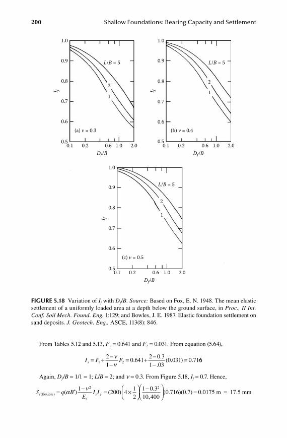
200 Shallow Foundations: Bearing Capacity and Settlement
From Tables 5.12 and 5.13, F1 = 0.641 and F2 = 0.031. From equation (5.64),
I F Fs = + -
-= + -
-=1 2
21
0 6412 0 31 03
0 031 0 71νν
..
.( . ) . 66
Again, Df/B = 1/1 = 1; L/B = 2; and n = 0.3. From Figure 5.18, If = 0.7. Hence,
S q B
EI Ie
ss f( ) ( ) ( )flexible = ′ - = ×
α ν1200 4
12
2
-
=1 0 3
10 4000 716 0 7
2.,
( . )( . ) 0.0175 m == 17.5 mm
1.0
0.9
0.8
0.7
0.6
I f
0.5 0.1
(a) v = 0.3
L/B = 5
2
1
0.2 0.6 1.0 2.0 Df/B
1.0
0.9
0.8
0.7
0.6
I f
0.5 0.1
(b) v = 0.4
L/B = 5
2
1
0.2 0.6 1.0 2.0Df/B
1.0
0.9
0.8
0.7
0.6
I f
0.5 0.1
(c) v = 0.5
L/B = 5
2
1
0.2 0.6 1.0 2.0 Df/B
FiGure 5.18 Variation of If with Df/B. Source: Based on Fox, E. N. 1948. The mean elastic settlement of a uniformly loaded area at a depth below the ground surface, in Proc., II Int. Conf. Soil Mech. Found. Eng. 1:129; and Bowles, J. E. 1987. Elastic foundation settlement on sand deposits. J. Geotech. Eng., ASCE, 113(8): 846.
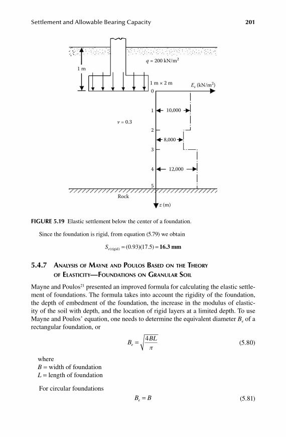
Settlement and Allowable Bearing Capacity 201
Since the foundation is rigid, from equation (5.79) we obtain
Se( ) ( . )( . )rigid = =0 93 17 5 16.3 mm
5.4.7 analysis of mayne anD poUlos BaseD on the theoRy of elastiCity—foUnDations on gRanUlaR soil
Mayne and Poulos21 presented an improved formula for calculating the elastic settle-ment of foundations. The formula takes into account the rigidity of the foundation, the depth of embedment of the foundation, the increase in the modulus of elastic-ity of the soil with depth, and the location of rigid layers at a limited depth. To use Mayne and Poulos’ equation, one needs to determine the equivalent diameter Be of a rectangular foundation, or
B
BLπ
e = 4 (5.80)
where B = width of foundationL = length of foundation
For circular foundations
B Be = (5.81)
1 m
1 m × 2 m Es (kN/m2)
10,000
0
1
2
3
4
5
z (m)Rock
8,000
v = 0.3
12,000
q = 200 kN/m2
FiGure 5.19 Elastic settlement below the center of a foundation.
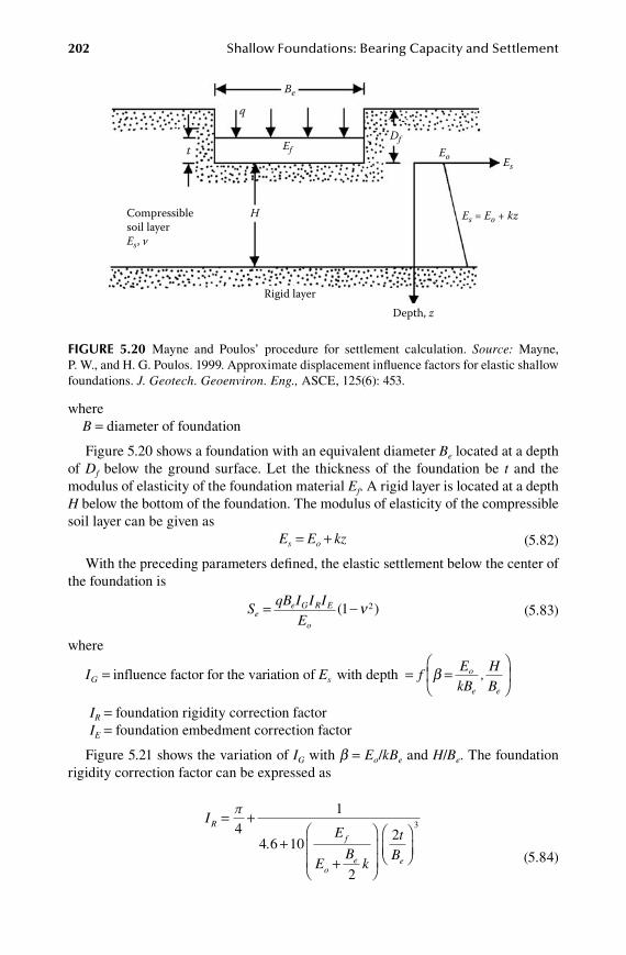
202 Shallow Foundations: Bearing Capacity and Settlement
where B = diameter of foundation
Figure 5.20 shows a foundation with an equivalent diameter Be located at a depth of Df below the ground surface. Let the thickness of the foundation be t and the modulus of elasticity of the foundation material Ef. A rigid layer is located at a depth H below the bottom of the foundation. The modulus of elasticity of the compressible soil layer can be given as
E E kzs o= + (5.82)
With the preceding parameters defined, the elastic settlement below the center of the foundation is
S
qB I I IE
ee G R E
o
= -( )1 2ν (5.83)
where
I EG s= influence factor for the variation of with depth = =
f
EkB
,HB
o
e e
β
IR = foundation rigidity correction factor IE = foundation embedment correction factor
Figure 5.21 shows the variation of IG with b = Eo/kBe and H/Be. The foundation rigidity correction factor can be expressed as
Iπ
.E
EB
k
tB
R
f
oe e
= +
++
41
4 6 10
2
23
(5.84)
Es = Eo + kz
EsEo
Df
Be
Ef
H
q
t
Compressiblesoil layerEs, v
Rigid layerDepth, z
FiGure 5.20 Mayne and Poulos’ procedure for settlement calculation. Source: Mayne, P. W., and H. G. Poulos. 1999. Approximate displacement influence factors for elastic shallow foundations. J. Geotech. Geoenviron. Eng., ASCE, 125(6): 453.
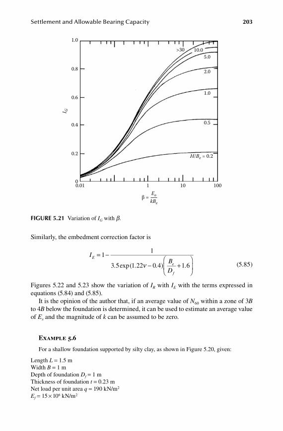
Settlement and Allowable Bearing Capacity 203
Similarly, the embedment correction factor is
I
. . .B
D.
E
e
f
= -- +
11
3 5 1 22 0 4 1 6exp( )ν (5.85)
Figures 5.22 and 5.23 show the variation of IR with IE with the terms expressed in equations (5.84) and (5.85).
It is the opinion of the author that, if an average value of N60 within a zone of 3B to 4B below the foundation is determined, it can be used to estimate an average value of Es and the magnitude of k can be assumed to be zero.
Example 5.6
For a shallow foundation supported by silty clay, as shown in Figure 5.20, given:
Length L = 1.5 mWidth B = 1 mDepth of foundation Df = 1 mThickness of foundation t = 0.23 mNet load per unit area q = 190 kN/m2
Ef = 15 × 106 kN/m2
0.010
0.2
0.4
I G
0.6
0.8
1.0
>30 10.05.0
2.0
1.0
0.5
H/Be = 0.2
β =EokBe
1 10 100
FiGure 5.21 Variation of IG with b.
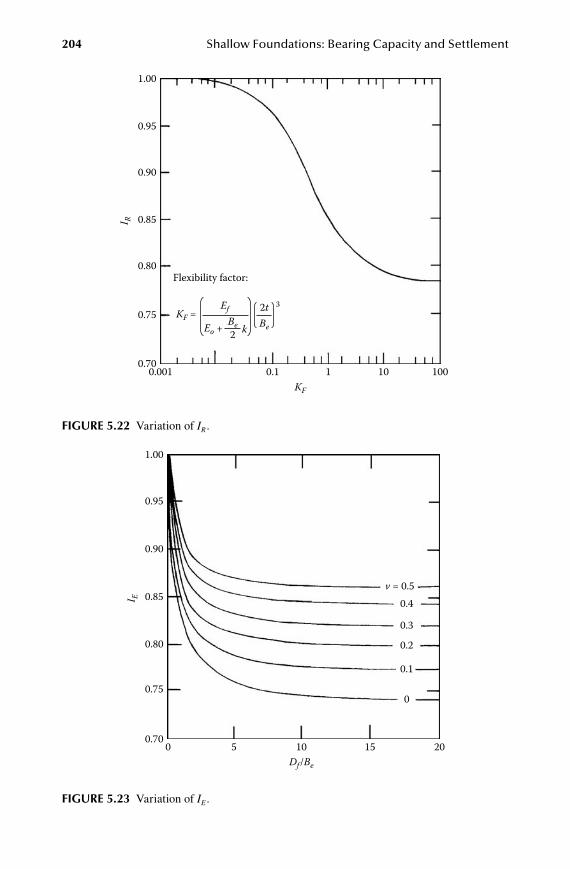
204 Shallow Foundations: Bearing Capacity and Settlement
1.00
0.95
0.90
0.85I E
0.80
0.75
0.700 5 10
v = 0.50.4
0.3
0.2
0.1
0
Df/Be
15 20
FiGure 5.23 Variation of IE .
0.001 0.70
0.75
0.85
0.80 Flexibility factor:
0.90
I R
0.95
1.00
1 0.1 10 100 KF
KF = Ef
Eo + k Be 2
2t Be
3
FiGure 5.22 Variation of IR .
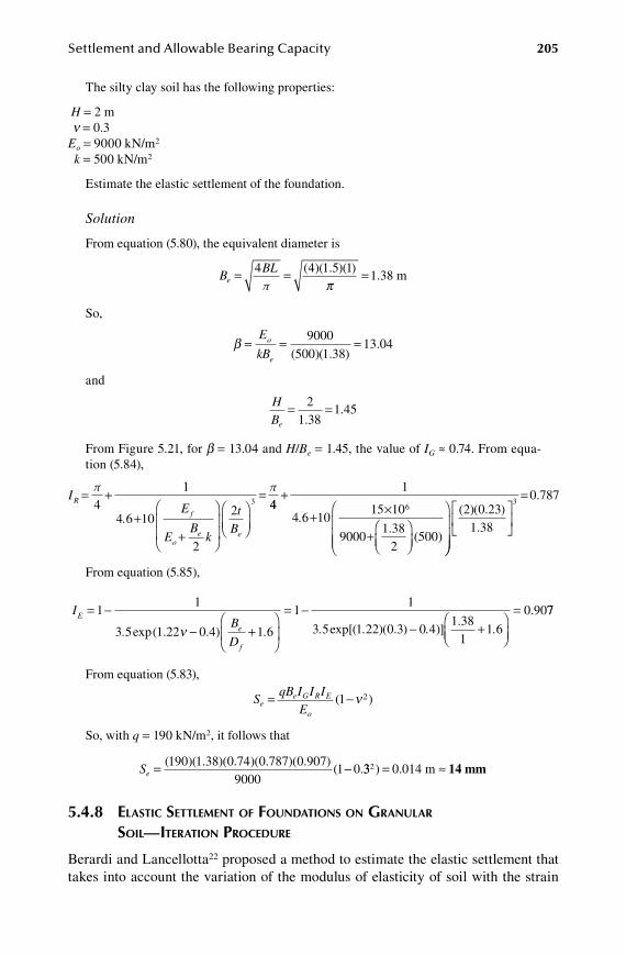
Settlement and Allowable Bearing Capacity 205
The silty clay soil has the following properties:
H = 2 m n = 0.3Eo = 9000 kN/m2
k = 500 kN/m2
Estimate the elastic settlement of the foundation.
Solution
From equation (5.80), the equivalent diameter is
B
BLπ
e = = =4 4 1 5 1( )( . )( )π
1.38 m
So,
β = = =
E
kBo
e
9000
500 1 3813 04
( )( . ).
and
HBe
= =21 38
1 45.
.
From Figure 5.21, for b = 13.04 and H/Be = 1.45, the value of IG ≈ 0.74. From equa-tion (5.84),
Iπ
.E
EB
k
tB
πR
f
oe e
= +
++
=4
1
4 6 10
2
23 44
1
4 6 1015 10
90001 38
2500
6+
+ ×
+
.
.( )
=( )( . )
.
.2 0 23
1 38
0 7873
From equation (5.85),
I
.B
D. .
E
e
f
= -
- +
= -11
3 5 1 6
11
3exp(1.22 0.4)ν 5 1 22 0 3 0 41 38
11 6
0 90
exp[( )( . ) )].
.
. . .- +
= 77
From equation (5.83),
S
qB I I IE
ee G R E
o
= -( )1 2ν
So, with q = 190 kN/m2, it follows that
Se = -( )( . )( . )( . )( . )
( .190 1 38 0 74 0 787 0 907
90001 0 332) = ≈0.014 m 14 mm
5.4.8 elastiC settlement of foUnDations on gRanUlaR soil—iteRation pRoCeDURe
Berardi and Lancellotta22 proposed a method to estimate the elastic settlement that takes into account the variation of the modulus of elasticity of soil with the strain
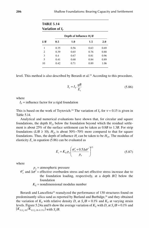
206 Shallow Foundations: Bearing Capacity and Settlement
level. This method is also described by Berardi et al.23 According to this procedure,
S I
qBE
e Fs
= (5.86)
whereIF = influence factor for a rigid foundation
This is based on the work of Tsytovich.24 The variation of IF for n = 0.15 is given in Table 5.14.
Analytical and numerical evaluations have shown that, for circular and square foundations, the depth H25 below the foundation beyond which the residual settle-ment is about 25% of the surface settlement can be taken as 0.8B to 1.3B. For strip foundations (L/B ≥ 10), H25 is about 50%−70% more compared to that for square foundations. Thus, the depth of influence Hi can be taken to be H25. The modulus of elasticity Es in equation (5.86) can be evaluated as
E K pp
s E ao
a
= ′ + ′
σ σ0 50 5
..
∆ (5.87)
where pa = atmospheric pressure
′σ o and Δs ′ = effective overburden stress and net effective stress increase due to the foundation loading, respectively, at a depth B/2 below the foundation
KE = nondimensional modulus number
Berardi and Lancellota22 reanalyzed the performance of 130 structures found on predominantly silica sand as reported by Burland and Burbidge,16 and they obtained the variation of KE with relative density Dr at Se/B = 0.1% and KE at varying strain levels. Figure 5.24a and b show the average variation of KE with Dr at Se/B = 0.1% and [ / ]( / ) ( / . %)K KE S B E S Be e =0 1 with Se/B.
table 5.14Variation of IF
depth of influence Hi/B
L/B 0.5 1.0 1.5 2.0
1 0.35 0.56 0.63 0.69 2 0.39 0.65 0.76 0.88 3 0.4 0.67 0.81 0.96 5 0.41 0.68 0.84 0.8910 0.42 0.71 0.89 1.06
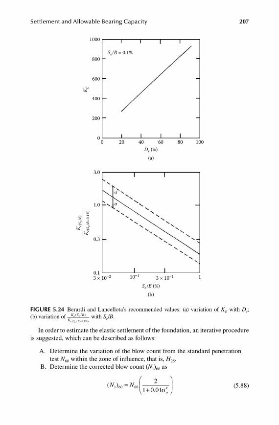
Settlement and Allowable Bearing Capacity 207
In order to estimate the elastic settlement of the foundation, an iterative procedure is suggested, which can be described as follows:
A. Determine the variation of the blow count from the standard penetration test N60 within the zone of influence, that is, H25.
B. Determine the corrected blow count (N1)60 as
( ).
N No
1 60 602
1 0 01=
+ ′
σ (5.88)
K e(S
e/B)
K e(S
e/B=
0.1%
)
1000
800
600
400
K E
200
00 20 40
Dr (%)
Se/B = 0.1%
(a)
60 80 100
3.0
1.0
0.3
0.13 × 10⁻² 3 × 10–110–1 1
Se/B (%)
σ
σ
(b)
FiGure 5.24 Berardi and Lancellota’s recommended values: (a) variation of KE with Dr; (b) variation of K S B
Ke e
e Se B
( / )
( / . %)=0 1with Se/B.

208 Shallow Foundations: Bearing Capacity and Settlement
where′σ o = vertical effective stress (kN/m2)
C. Determine the average corrected blow count from standard penetration test ( )N1 60 and, hence, the average relative density as
D
Nr =
1
0 5
60
.
(5.89)
D. With known Dr, determine KE S Be( / . %)=0 1 from Figure 5.24a and hence Es from equation (5.87) for Se/B = 0.1%.
E. With the known value of Es from step D, the magnitude of the elastic settlement Se can be calculated from equation (5.86).
F. If the calculated Se/B is not the same as the assumed Se/B, then use the calculated Se/B from step E and use Figure 5.24b to estimate a revisedKE S Be( / ). This value of KE S Be( / ) can now be used in equations (5.87) and (5.86) to obtain a revised Se. This iterative procedure can be continued until the assumed and calculated Se are the same.
5.5 primary ConSolidation Settlement
5.5.1 geneRal pRinCiples of ConsoliDation settlement
As explained in section 5.1, consolidation settlement is a time-dependent process that occurs due to the expulsion of excess pore water pressure in saturated clayey soils below the groundwater table and is created by the increase in stress created by the foundation load. For normally consolidated clay, the nature of the variation of the void ratio e with vertical effective stress s ′ is shown in Figure 5.25a. A similar plot for overconsolidated clay is also shown in Figure 5.25b. In this figure the pre-consolidation pressure is ′σ c. The slope of the e versus log s ′ plot for the normally consolidated portion of the soil is referred to as compression index Cc, or
Ce e
c c= -( ) ′ ≤ ′′
′
1 21
2
1log
)σσ
σ σ(for (5.90)
Similarly, the slope of the e versus log s ′ plot for the overconsolidated portion of the clay is called the swell index Cs, or
Ce e
s c= -( ) ′ ≤ ′′
′
3 44
4
3log
)σσ
σ σ(for (5.91)
For normally consolidated clays, Terzaghi and Peck25 gave a correlation for the compression index as
C LLc = -0 009 10. ( ) (5.92a)
whereLL = liquid limit

Settlement and Allowable Bearing Capacity 209
The preceding relation is reliable in the range of ±30% and should not be used for clays with sensitivity ratios greater than four.
Terzaghi and Peck25 also gave a similar correlation for remolded clays:
C LLc = -0 007 10. ( ) (5.92b)
Several other correlations for the compression index with the basic index proper-ties of soils have been made, and some of these are given below.26
C wc N= 0 01. (for Chicago clays) (5.93)
C LLc = -0 0046 9. ( ) (for Brazilian clays) (5.94)
C ec o= + -1 21 1 055 1 87. . ( . ) (for Motley clays, Sao Paulo city)� (5.95)
Void
ratio
, e
Effective stress, σ´ (log scale)(a)
Effective stress, σ´ (log scale)(b)
Void
ratio
, e
Slope Cs
(σ3, e3)
(σ1, e1)
(σ2, e2)
(σ4, e4)
(σ1, e1)
(σ2, e2)
σ c
Slope Cc
Slope Cc
FiGure 5.25 Nature of variation of void ratio with effective stress: (a) normally consoli-dated clay; (b) overconsolidated clay.

210 Shallow Foundations: Bearing Capacity and Settlement
C ec o= +0 208 0 0083. . (for Chicago clays)
(5.96)
C wc N= 0 0115.
(5.97)
wherewN = natural moisture content in percent eo = in situ void ratio
The swell index Cs for a given soil is about 1/4 to 1/5 Cc.
5.5.2 Relationships foR pRimaRy ConsoliDation settlement CalCUlation
Figure 5.26 shows a clay layer of thickness Hc. Let the initial void ratio before the construction of the foundation be eo, and let the average effective vertical stress on the clay layer be ′σ o. The foundation located at a depth Df is subjected to a net aver-age pressure increase of q. This will result in an increase in the vertical stress in the soil. If the vertical stress increase at any point below the center line of the foundation is Δs, the average vertical stress increase Δsav in the clay layer can thus be given as
∆ ∆σ σav =-
=
=
∫1
2 11
2
H Hdz
z H
z H
( ) (5.98)
Clay layereo
∆σ
∆σt
∆σm
∆σb
Ground water table
Hc
H2
H1
Dfq
z
FiGure 5.26 Primary consolidation settlement calculation.
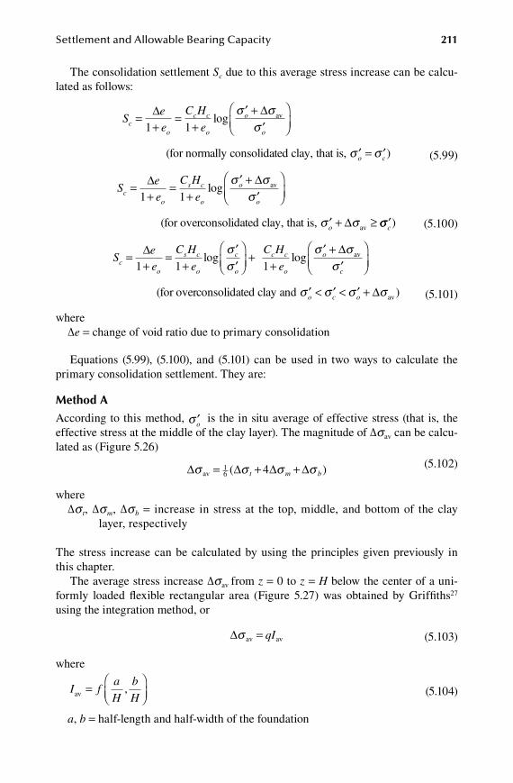
Settlement and Allowable Bearing Capacity 211
The consolidation settlement Sc due to this average stress increase can be calcu-lated as follows:
See
C H
eco
c c
o
o
o
=+
=+
′ +′
∆ ∆1 1
logσ σ
σav
(for normally consolidated clay, that is, ′σ o c= ′σ ) (5.99)
See
C H
eco
s c
o
o
o
=+
=+
′ +′
∆ ∆1 1
logσ σ
σav
(for overconsolidated clay, that is, av′ + ≥ ′σ σo ∆ σσ c) (5.100)
See
C H
e
C H
eco
s c
o
c
o
c c
o
=+
=+
′′
++
∆1 1 1
logσσ
log′ +
′
σ σσ
o
c
∆ av
(for overconsolidated clay and av′ < ′ < ′ +σ σ σ σo c o ∆ ) (5.101)
whereΔe = change of void ratio due to primary consolidation
Equations (5.99), (5.100), and (5.101) can be used in two ways to calculate the primary consolidation settlement. They are:
method a
According to this method, ′σ o is the in situ average of effective stress (that is, the effective stress at the middle of the clay layer). The magnitude of Δsav can be calcu-lated as (Figure 5.26)
∆ ∆ ∆ ∆σ σ σ σav = + +16 4( )t m b
(5.102)
whereΔs t, Δsm, Δsb = increase in stress at the top, middle, and bottom of the clay
layer, respectively
The stress increase can be calculated by using the principles given previously in this chapter.
The average stress increase Δsav from z = 0 to z = H below the center of a uni-formly loaded flexible rectangular area (Figure 5.27) was obtained by Griffiths27 using the integration method, or
∆σ av av= qI (5.103)
where
I fa
H
b
Hav =
,
(5.104)
a, b = half-length and half-width of the foundation
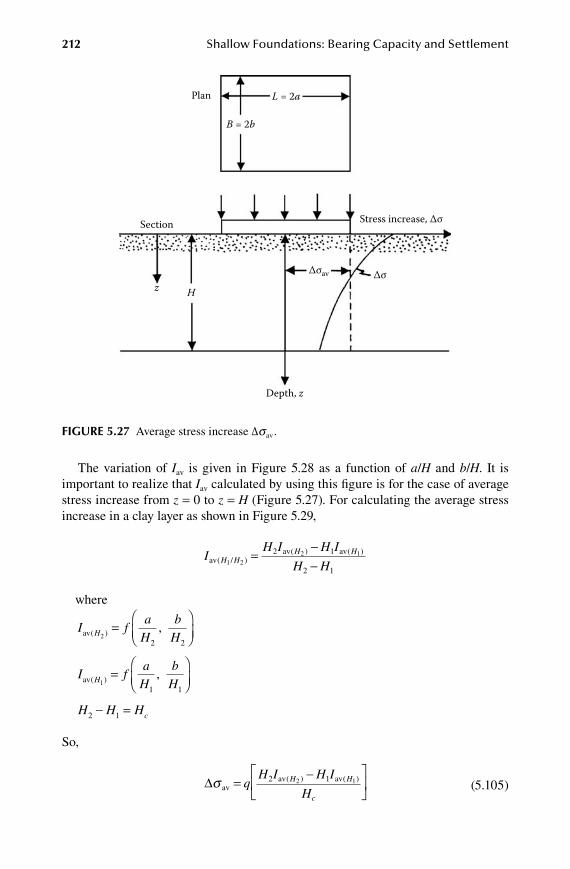
212 Shallow Foundations: Bearing Capacity and Settlement
The variation of Iav is given in Figure 5.28 as a function of a/H and b/H. It is important to realize that Iav calculated by using this figure is for the case of average stress increase from z = 0 to z = H (Figure 5.27). For calculating the average stress increase in a clay layer as shown in Figure 5.29,
I
H I H I
H HH H
H Hav
av av( / )
( ) ( )1 2
2 12 1
2 1
=--
where
I fa
Hb
HHav( ) ,2
2 2
=
I fa
Hb
HHav( ) ,1
1 1
=
H H Hc2 1- =
So,
∆σ avav av=
-
q
H I H I
HH H
c
2 12 1( ) ( ) (5.105)
Depth, z
Stress increase, ∆σ
∆σ ∆σav
Section
Plan
H
L = 2a
B = 2b
z
FiGure 5.27 Average stress increase Δsav .
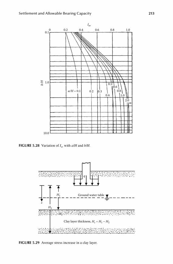
Settlement and Allowable Bearing Capacity 213
Clay layer thickness, Hc = H1 – H2
Ground water table
Hc
H2
H1
q
z
FiGure 5.29 Average stress increase in a clay layer.
0.1 0 0.2 0.4 0.6
Iav
0.8 1.0
1.0
a/H = 0.1 0.2 0.3 0.4
0.5 0.6
0.8 1.0
2.0
8
b/H
10.0
FiGure 5.28 Variation of Iav with a/H and b/H.
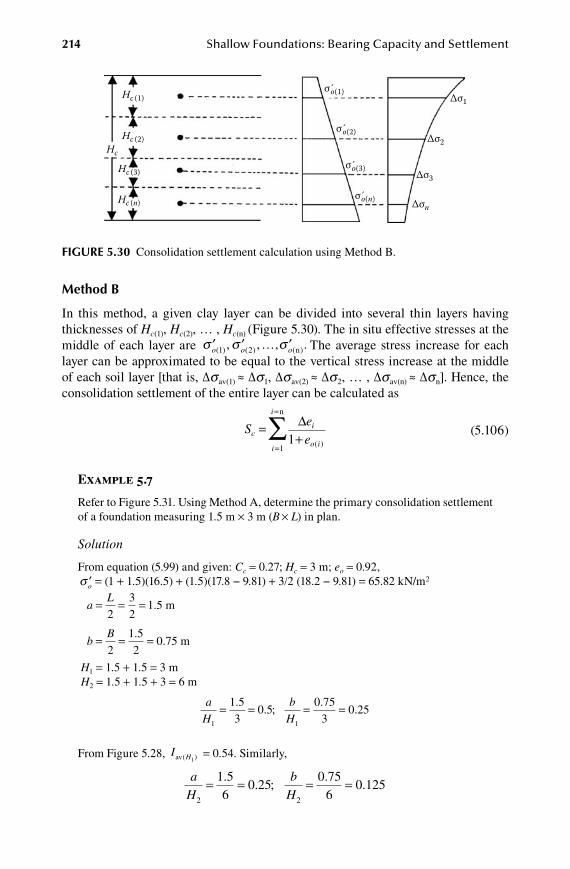
214 Shallow Foundations: Bearing Capacity and Settlement
method b
In this method, a given clay layer can be divided into several thin layers having thicknesses of Hc(1), Hc(2), … , Hc(n) (Figure 5.30). The in situ effective stresses at the middle of each layer are ′ ′ ′σ σ σo o o( ) ( ) ( ), , , .1 2 … n The average stress increase for each layer can be approximated to be equal to the vertical stress increase at the middle of each soil layer [that is, Δsav(1) ≈ Δs1, Δsav(2) ≈ Δs2, … , Δsav(n) ≈ Δsn]. Hence, the consolidation settlement of the entire layer can be calculated as
See
ci
o ii
i
=+
=
=
∑ ∆1
1 ( )
n
(5.106)
Example 5.7
Refer to Figure 5.31. Using Method A, determine the primary consolidation settlement of a foundation measuring 1.5 m × 3 m (B × L) in plan.
Solution
From equation (5.99) and given: Cc = 0.27; Hc = 3 m; eo = 0.92,′σ o = (1 + 1.5)(16.5) + (1.5)(17.8 − 9.81) + 3/2 (18.2 − 9.81) = 65.82 kN/m2
a
L= = =2
3
21.5 m
b
B= = =2
1 5
2
.0.75 m
H1 = 1.5 + 1.5 = 3 m H2 = 1.5 + 1.5 + 3 = 6 m
a
H
b
H1 1
1 5
30 5
0 75
30 25= = = =.
. ;.
.
From Figure 5.28, I Hav( )1 = 0.54. Similarly,
aH
bH2 2
1 56
0 250 75
60 125= = = =.
. ;.
.
Hc
Hc (1)σ o(1)
σ o(2)
σ o(3)
σ o(n) ∆σn
∆σ3
∆σ2
∆σ1
Hc (2)
Hc (3)
Hc (n)
FiGure 5.30 Consolidation settlement calculation using Method B.
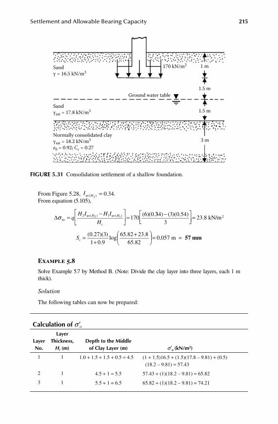
Settlement and Allowable Bearing Capacity 215
From Figure 5.28, I Hav( )2 = 0.34.
From equation (5.105),
∆σ av
av av=-
=q
H I H I
HH H
c
2 12 1 1706 0( ) ( ) ( )( .334 3 0 54
3) ( )( . )-
= 23.8 kN/m2
Sc =
++
=( . )( )
.log
. ..
0 27 31 0 9
65 82 23 865 82
0..057 m = 57 mm
Example 5.8
Solve Example 5.7 by Method B. (Note: Divide the clay layer into three layers, each 1 m thick).
Solution
The following tables can now be prepared:
Calculation of s ′o
layer no.
layer thickness,
Hi (m)depth to the middle
of Clay layer (m) s′o (kn/m2)
1 1 1.0 + 1.5 + 1.5 + 0.5 = 4.5 (1 + 1.5)16.5 + (1.5)(17.8 – 9.81) + (0.5) (18.2 – 9.81) = 57.43
2 1 4.5 + 1 = 5.5 57.43 + (1)(18.2 – 9.81) = 65.82
3 1 5.5 + 1 = 6.5 65.82 + (1)(18.2 – 9.81) = 74.21
Sand γ = 16.5 kN/m3
Sandγsat = 17.8 kN/m3
Ground water table
170 kN/m2 1 m
1.5 m
1.5 m
3 m Normally consolidated clayγsat = 18.2 kN/m3
e0 = 0.92; Cc = 0.27
FiGure 5.31 Consolidation settlement of a shallow foundation.

216 Shallow Foundations: Bearing Capacity and Settlement
Calculation of Δsav
layer no.
layer thickness
Hi (m)
depth to middle of layer from
bottom of Foundation, z (m) L/Ba z/B
∆σ ( )av b
q Δsavc
1 1 3.5 2 2.33 0.16 27.22 1 4.5 2 3.0 0.095 16.15
3 1 5.5 2 3.67 0.07 11.9
aB = 1.5 m; L = 3 m
bTable 5.3
cq = 170 kN/m2
SC H
ecc i
o
o i i
o i
=+
′ +′
=
∑ 1log
(
( )
( )
σ σσ
∆ av( )
0 27 1
1 0 9
57 43 27 2
57 43
6. )( )
.log
. .
.log
++
+ 5 82 16 15
65 82
74 21 11 9
74 21
. .
.log
. .
.
+
+ +
= + + =( . )( . . . )0 142 0 168 0 096 0 065 0.0047 m = 47 mm
5.5.3 thRee-Dimensional effeCt on pRimaRy ConsoliDation settlement
The procedure described in the preceding section is for one-dimensional consoli-dation and will provide a good estimation for a field case where the width of the foundation is large relative to the thickness of the compressible stratum Hc, and also when the compressible material lies between two stiffer soil layers. This is because the magnitude of horizontal strains is relatively less in the above cases.
In order to account for the three-dimensional effect, Skempton and Bjerrum28 proposed a correction to the one-dimensional consolidation settlement for normally consolidated clays. This can be explained by referring to Figure 5.32, which shows a circularly loaded area (diameter = B) on a layer of normally consolidated clay of thickness Hc. Let the stress increases at a depth z under the center line of the loaded area be Δs1 (vertical) and Δs3 (lateral). The increase in pore water pressure due to the increase in stress Δu can be given as
∆ ∆ ∆ ∆u A= + -σ σ σ3 1 3( ) (5.107)
whereA = pore water pressure parameter
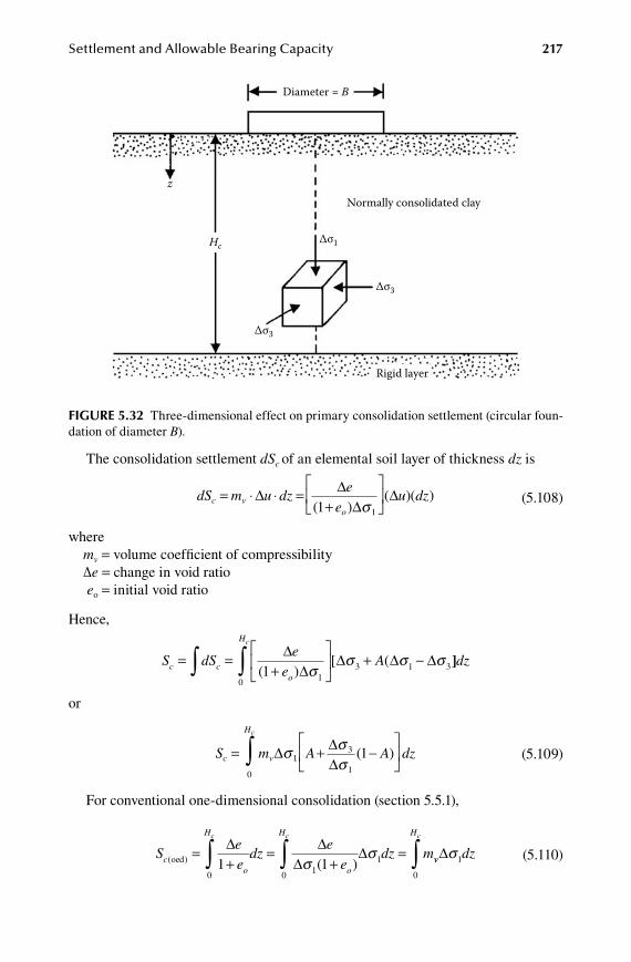
Settlement and Allowable Bearing Capacity 217
The consolidation settlement dSc of an elemental soil layer of thickness dz is
dS m u dze
eu dzc v
o
= ⋅ ⋅ =+
∆ ∆
∆∆
( )( )( )
1 1σ (5.108)
wheremv = volume coefficient of compressibilityΔe = change in void ratio eo = initial void ratio
Hence,
S dSe
eAc c
o
Hc
= =+
+ -∫ ∫ ∆
∆∆ ∆ ∆
( )[ (
1 10
3 1 3σσ σ σ ]]dz
or
S m A A dzc v
Hc
= + -
∫ ∆ ∆
∆σ σ
σ13
10
1( ) (5.109)
For conventional one-dimensional consolidation (section 5.5.1),
See
dze
edz mc
o
H
o
Hc c
( ) ( )oed =+
=+
=∫ ∫∆ ∆∆
∆1 1
0 10
1σσ vv
Hc
dz0
1∫ ∆σ (5.110)
Normally consolidated clay
Rigid layer
∆σ1
∆σ3
∆σ3
Diameter = B
z
Hc
FiGure 5.32 Three-dimensional effect on primary consolidation settlement (circular foun-dation of diameter B).
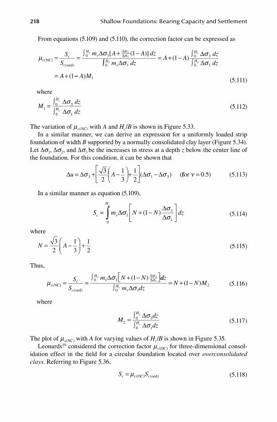
218 Shallow Foundations: Bearing Capacity and Settlement
From equations (5.109) and (5.110), the correction factor can be expressed as
µσ σ
σc
c
c
HvS
S
m A A dzc
(( )
[ ( )]NC)
oed
= =∫ + -0 1
31
1∆ ∆∆
∫∫= + - ∫
∫
= +
0 1
0 3
0 1
1
1
Hv
H
Hc
c
cm dzA A
dz
dz
A
∆∆∆σ
σσ
( )
( -- A M) 1 (5.111)
where
Mdz
dz
H
H
c
c10 3
0 1
=∫∫
∆∆
σσ
(5.112)
The variation of mc(NC) with A and Hc/B is shown in Figure 5.33.In a similar manner, we can derive an expression for a uniformly loaded strip
foundation of width B supported by a normally consolidated clay layer (Figure 5.34). Let Δs1, Δs2, and Δs3 be the increases in stress at a depth z below the center line of the foundation. For this condition, it can be shown that
∆ ∆ ∆ ∆u A= + -
+
-σ σ σ3 1 3
32
13
12
( ) (ffor ν = 0 5. ) (5.113)
In a similar manner as equation (5.109),
S m N N dzc v
Hc
= + -
∫ ∆
∆∆
σ σσ1
3
10
1( ) (5.114)
where
N A= -
+32
13
12
(5.115)
Thus,
µσ σ
σs
c
c
HvS
S
m N Nc
(( )
( )NC)
oed
= =∫ + - 0 1 1 3
1∆ ∆
∆ ddz
m dzN N M
Hv
c∫= + -
0 121
∆σ( ) (5.116)
where
Mdz
dz
H
H
c
c20 3
0 1
=∫∫
∆∆
σσ
(5.117)
The plot of ms(NC) with A for varying values of Hc/B is shown in Figure 5.35.Leonards29 considered the correction factor mc(OC) for three-dimensional consol-
idation effect in the field for a circular foundation located over overconsolidated clays. Referring to Figure 5.36,
S Sc c c= µ ( ) ( )OC oed (5.118)
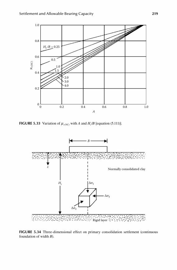
Settlement and Allowable Bearing Capacity 219
Hc/B = 0.25
0.5
1.01.5
2.03.04.0
1.0
0.8
0.6
µ c(N
C)
0.4
0.2
00 0.2 0.4
A0.6 0.8 1.0
FiGure 5.33 Variation of mc(NC) with A and Hc/B [equation (5.111)].
Normally consolidated clay
Rigid layer
∆σ1
∆σ3
∆σ2
B
z
Hc
FiGure 5.34 Three-dimensional effect on primary consolidation settlement (continuous foundation of width B).
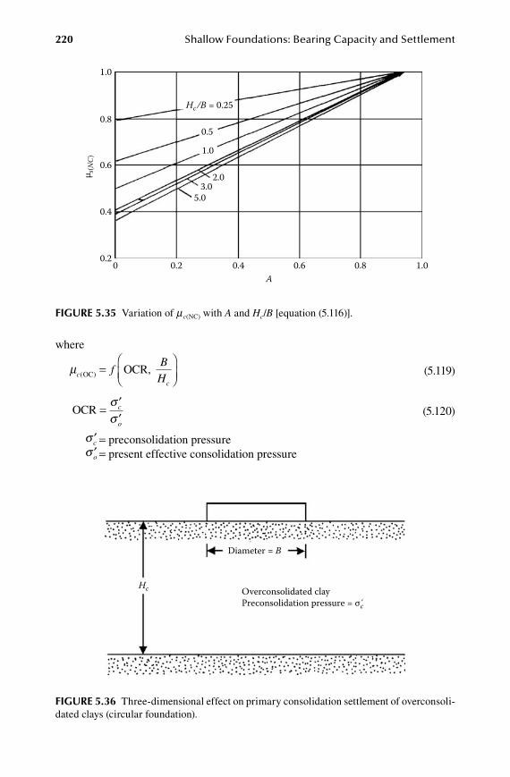
220 Shallow Foundations: Bearing Capacity and Settlement
where
µcc
fBH( )OC OCR,=
(5.119)
OCR =
′′
σσ
c
o
(5.120)
′σ c = preconsolidation pressure
′σ o = present effective consolidation pressure
Hc/B = 0.25
0.5
1.0
2.03.0
5.0
1.0
0.8
0.6
µ s(N
C)
0.4
0.20 0.2 0.4
A0.6 0.8 1.0
FiGure 5.35 Variation of mc(NC) with A and Hc/B [equation (5.116)].
Overconsolidated clayPreconsolidation pressure = σc
Diameter = B
Hc
FiGure 5.36 Three-dimensional effect on primary consolidation settlement of overconsoli-dated clays (circular foundation).
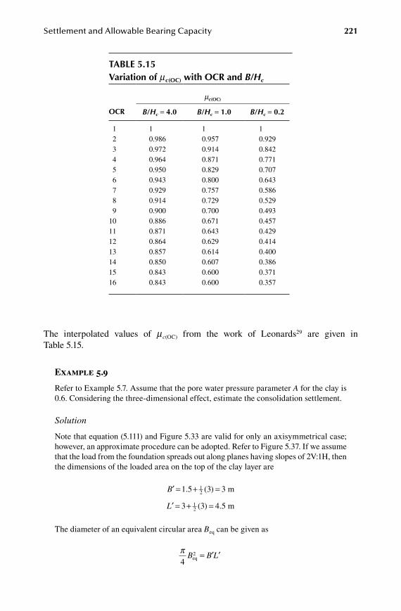
Settlement and Allowable Bearing Capacity 221
The interpolated values of mc(OC) from the work of Leonards29 are given in Table 5.15.
Example 5.9
Refer to Example 5.7. Assume that the pore water pressure parameter A for the clay is 0.6. Considering the three-dimensional effect, estimate the consolidation settlement.
Solution
Note that equation (5.111) and Figure 5.33 are valid for only an axisymmetrical case; however, an approximate procedure can be adopted. Refer to Figure 5.37. If we assume that the load from the foundation spreads out along planes having slopes of 2V:1H, then the dimensions of the loaded area on the top of the clay layer are
′ = + =B 1 5 312. ( ) 3 m
′ = + =L 3 312 ( ) 4.5 m
The diameter of an equivalent circular area Beq can be given as
π4
2B B Leq = ′ ′
table 5.15Variation of mc(oC) with oCr and B/Hc
mc(oC)
oCr B/Hc = 4.0 B/Hc = 1.0 B/Hc = 0.2
1 1 1 1 2 0.986 0.957 0.929 3 0.972 0.914 0.842 4 0.964 0.871 0.771 5 0.950 0.829 0.707 6 0.943 0.800 0.643 7 0.929 0.757 0.586 8 0.914 0.729 0.529 9 0.900 0.700 0.49310 0.886 0.671 0.45711 0.871 0.643 0.42912 0.864 0.629 0.41413 0.857 0.614 0.40014 0.850 0.607 0.38615 0.843 0.600 0.37116 0.843 0.600 0.357
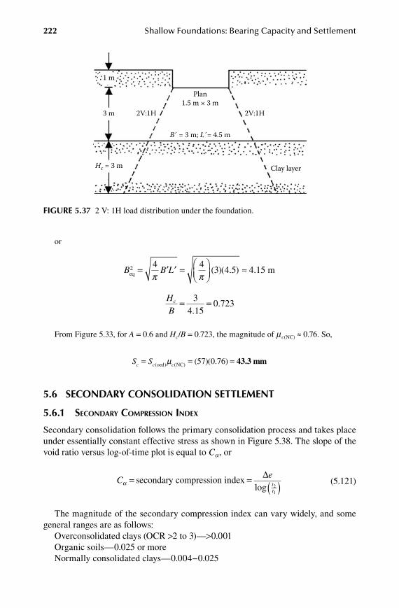
222 Shallow Foundations: Bearing Capacity and Settlement
or
B B Leq 4.15 m2 4 43 4 5= ′ ′ =
≈π π
( )( . )
HB
c = =34 15
0 723.
.
From Figure 5.33, for A = 0.6 and Hc/B = 0.723, the magnitude of mc(NC) ≈ 0.76. So,
S Sc c c= = =( ) ( ) ( )( . )oed NCµ 57 0 76 43.3 mm
5.6 SeCondary ConSolidation Settlement
5.6.1 seConDaRy CompRession inDex
Secondary consolidation follows the primary consolidation process and takes place under essentially constant effective stress as shown in Figure 5.38. The slope of the void ratio versus log-of-time plot is equal to Ca, or
Ce
tt
α = = ( )secondary compression index∆
log 21
(5.121)
The magnitude of the secondary compression index can vary widely, and some general ranges are as follows:
Overconsolidated clays (OCR >2 to 3)—>0.001Organic soils—0.025 or moreNormally consolidated clays—0.004−0.025
Plan1.5 m × 3 m
B´ = 3 m; L´= 4.5 m
Hc = 3 m Clay layer
3 m
1 m
2V:1H 2V:1H
FiGure 5.37 2 V: 1H load distribution under the foundation.

Settlement and Allowable Bearing Capacity 223
5.6.2 seConDaRy ConsoliDation settlement
The secondary consolidation settlement Ss can be calculated as
SC H
es
c
p
tt=
+ ( )α
121
log (5.122)
where ep = void ratio at the end of primary consolidationt2, t1 = time
In a majority of cases, secondary consolidation is small compared to primary consolidation settlement. It can, however, be substantial for highly plastic clays and organic soils.
Example 5.10
Refer to Example 5.7. Assume that the primary consolidation settlement is completed in 3 years. Also let Ca = 0.006. Estimate the secondary consolidation settlement at the end of 10 years.
Solution
From equation (5.122),
S
C He
tt
sc
p
=+
α
12
1
log
Primary consolidation
Secondary consolidation
∆e
t1 t2
Slope Cα
Void
ratio
, e
ep
FiGure 5.38 Secondary consolidation settlement.
224 Shallow Foundations: Bearing Capacity and Settlement
Given: Hc = 3 m, Ca = 0.006, t2 = 10 years, and t1 = 3 years. From equation (5.90),
Ce e
co p=
-
′′
logσσ
2
1
From Example 5.7, ′σ1 = 65.82 kN/m2, ′σ 2 = 65.82 + 23.8 = 89.62 kN/m2, Cc = 0.27, eo = 0.92. So,
0 270 92
89 6265 82
..
log..
=-
ep
ep = 0.884,
Ss =
+
≈ =( . )( )
.log
0 006 31 0 884
103
0.005 m 5 mm
5.7 diFFerential Settlement
5.7.1 geneRal ConCept of DiffeRential settlement
In most instances, the subsoil is not homogeneous and the load carried by various shallow foundations of a given structure can vary widely. As a result, it is reasonable to expect varying degrees of settlement in different parts of a given building. The differential settlement of various parts of a building can lead to damage of the super-structure. Hence, it is important to define certain parameters to quantify differential settlement and develop limiting values for these parameters for desired safe per-formance of structures. Burland and Worth30 summarized the important parameters relating to differential settlement. Figure 5.39 shows a structure in which various foundations at A, B, C, D, and E have gone through some settlement. The settlement at A is AA′, and at B it is BB′, … Based on this figure the definitions of the various parameters follow:
ST = total settlement of a given point ΔST = difference between total settlement between any two parts a = gradient between two successive points
β = =angular distortion
∆S
lT ij
ij
( )
(Note: lij = distance between points i and j)
w = tilt Δ = relative deflection (that is, movement from a straight line joining two refer-
ence points)
∆L = deflection ratio
Since the 1950s, attempts have been made by various researchers and building codes to recommend allowable values for the above parameters. A summary of some of these recommendations is given in the following section.
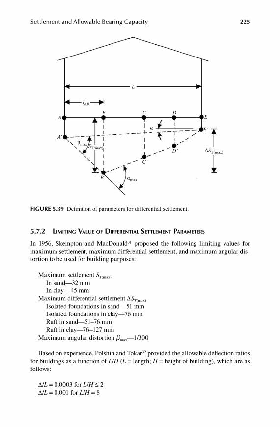
Settlement and Allowable Bearing Capacity 225
5.7.2 limiting valUe of DiffeRential settlement paRameteRs
In 1956, Skempton and MacDonald31 proposed the following limiting values for maximum settlement, maximum differential settlement, and maximum angular dis-tortion to be used for building purposes:
Maximum settlement ST(max)
In sand—32 mmIn clay—45 mm
Maximum differential settlement ΔST(max)
Isolated foundations in sand—51 mmIsolated foundations in clay—76 mmRaft in sand—51–76 mmRaft in clay—76–127 mm
Maximum angular distortion bmax—1/300
Based on experience, Polshin and Tokar32 provided the allowable deflection ratios for buildings as a function of L/H (L = length; H = height of building), which are as follows:
Δ/L = 0.0003 for L/H ≤ 2Δ/L = 0.001 for L/H = 8
B A
A
B
βmax
αmax
ST(max) ∆ST(max)
C
ω
C´
D
D´
E
E´
L
lAB
FiGure 5.39 Definition of parameters for differential settlement.
226 Shallow Foundations: Bearing Capacity and Settlement
The 1955 Soviet Code of Practice gives the following allowable values:
building type L/H Δ/L
Multistory buildings and civil dwellings ≤3 0.0003 (for sand)
0.0004 (for clay)
≥5 0.0005 (for sand)
0.0007 (for clay)One−story mills 0.001 (for sand and clay)
Bjerrum33 recommended the following limiting angular distortions (bmax) for various structures:
Category of potential damage bmax
Safe limit for flexible brick wall (L/H > 4)
1/150
Danger of structural damage to most buildings 1/150Cracking of panel and brick walls 1/150Visible tilting of high rigid buildings 1/250First cracking of panel walls 1/300Safe limit for no cracking of building 1/500Danger to frames with diagonals 1/600
Grant et al.34 correlated ST(max) and bmax for several buildings with the following results:
Soil type Foundation type CorrelationClay Isolated shallow foundation ST(max) (mm) = 30,000 bmax
Clay Raft ST(max) (mm) = 35,000 bmax
Sand Isolated shallow foundation ST(max) (mm) = 15,000 bmax
Sand Raft ST(max) (mm) = 18,000 bmax
Using the above correlations, if the maximum allowable value of bmax is known, the magnitude of the allowable ST(max) can be calculated.
The European Committee for Standardization provided values for limiting values for serviceability limit states35 and the maximum accepted foundation movements,36 and these are given in Table 5.16.

Settlement and Allowable Bearing Capacity 227
reFerenCeS
1. Boussinesq, J. 1883. Application des potentials a l’etude de l’equilibre et due mouve-ment des solides elastiques. Paris: Gauthier-Villars.
2. Ahlvin, R. G., and H. H. Ulery. 1962. Tabulated values for determining the complete pattern of stresses, strains, and deflections beneath a uniform load on a homogeneous half space. Highway Res. Rec., Bulletin 342: 1.
3. Westergaard, H. M. 1938. A problem of elasticity suggested by a problem in soil mechanics: Soft material reinforced by numerous strong horizontal sheets, in Contribution to the mechanics of solids, Stephen Timoshenko 60th anniversary vol. New York: Macmillan.
4. Borowicka, H. 1936. Influence of rigidity of a circular foundation slab on the distribu-tion of pressures over the contact surface, in Proc., I Int. Conf. Soil Mech. Found. Eng. 2: 144.
5. Trautmann, C. H., and F. H. Kulhawy. 1987. CUFAD—A computer program for com-pression and uplift foundation analysis and design, report EL-4540-CCM, 16. Palo Alto: Electric Power Research Institute.
6. Schmertmann, J. H. 1970. Static cone to compute settlement over sand. J. Soil Mech. Found. Div., ASCE, 96(8): 1011.
7. Schmertmann, J. H., J. P. Hartman, and P. R. Brown. 1978. Improved strain influence factor diagrams. J. Geotech. Eng. Div., ASCE, 104(8): 1131.
8. D’Appolonia, D. T., H. G. Poulos, and C. C. Ladd. 1971. Initial settlement of struc-tures on clay. J. Soil Mech. Found. Div., ASCE, 97(10): 1359.
9. Duncan, J. M., and A. L. Buchignani. 1976. An engineering manual for settlement studies, Department of Civil Engineering. Berkeley: University of California.
10. Janbu, N., L. Bjerrum, and B. Kjaernsli. 1956. Veiledning ved losning av fundamen-teringsoppgaver. Oslo: Norwegian Geotechnical Institute Publication 16.
11. Christian, J. T., and W. D. Carrier III. 1978. Janbu, Bjerrum and Kjaernsli’s chart reinterpreted. Canadian Geotech. J. 15(1): 124.
12. Terzaghi, K., and R. B. Peck. 1948. Soil mechanics in engineering practice. New York: Wiley.
table 5.16recommendation of european Committee for Standardization on differential Settlement parameters
item parameter magnitude Comments
Limiting values for serviceability35
ST 25 mm50 mm
Isolated shallow foundationRaft foundation
ΔST 5 mm Frames with rigid cladding10 mm Frames with flexible cladding20 mm Open frames
b 1/500 —
Maximum acceptable foundation movement36
ST
ΔST
5020
Isolated shallow foundationIsolated shallow foundation
b ≈1/500 —

228 Shallow Foundations: Bearing Capacity and Settlement
13. Meyerhof, G. G. 1956. Penetration tests and bearing capacity of cohesionless soils. J. Soil Mech. Found. Div., ASCE, 82(1): 1.
14. Meyerhof, G. G. 1965. Shallow foundations. J. Soil Mech. Found. Div., ASCE, 91(2): 21.
15. Peck, R. B., and A R. S. S. Bazaraa. 1969. Discussion of paper by D’Appolonia et al. J. Soil Mech. Found. Div., ASCE, 95(3): 305.
16. Burland, J. B., and M. C. Burbidge. 1985. Settlement of foundations on sand and gravel. Proc., Institution of Civil Engineers 78(1): 1325.
17. Eggestad, A. 1963. Deformation measurements below a model footing on the surface of dry sand, in Proc. Eur Conf. Soil Mech. Found. Eng. Weisbaden, W. Germany, 1: 223.
18. Bowles, J. E. 1987. Elastic foundation settlement on sand deposits. J. Geotech. Eng., ASCE, 113(8): 846.
19. Steinbrenner, W. 1934. Tafeln zur setzungsberschnung. Die Strasse 1: 121. 20. Fox, E. N. 1948. The mean elastic settlement of a uniformly loaded area at a depth
below the ground surface, in Proc., II Int. Conf. Soil Mech. Found. Eng. 1: 129. 21. Mayne, P. W., and H. G. Poulos. 1999. Approximate displacement influence factors
for elastic shallow foundations. J. Geotech. Geoenviron. Eng., ASCE 125(6): 453. 22. Berardi, R., and R. Lancellotta. 1991. Stiffness of granular soil from field perfor-
mance. Geotechnique 41(1): 149. 23. Berardi, R., M. Jamiolkowski, and R. Lancellotta. 1991. Settlement of shallow
foundations in sands: Selection of stiffness on the basis of penetration resistance. Geotechnical Engineering Congress 1991, Geotech. Special Pub. 27, ASCE, 185.
24. Tsytovich, N. A. 1951. Soil mechanics, ed. Stroitielstvo I. Archiketura, Moscow (in Russian).
25. Terzaghi, K., and R. B. Peck. 1967. Soil mechanics in engineering practice, 2nd Ed. New York: Wiley.
26. Azzouz, A. S., R. T. Krizek, and R. B. Corotis. 1976. Regression analysis of soil com-pressibility. Soils and Found. 16(2): 19.
27. Griffiths, D. V. 1984. A chart for estimating the average vertical stress increase in an elastic foundation below a uniformly loaded rectangular area. Canadian Geotech. J. 21(4): 710.
28. Skempton, A. W., and L. Bjerrum. 1957. A contribution to settlement analysis of foun-dations in clay. Geotechnique 7: 168.
29. Leonards, G. A. 1976. Estimating consolidation settlement of shallow foundations on overconsolidated clay. Transportation Research Board, Special Report 163, Washington, D.C.: 13.
30. Burland, J. B., and C. P. Worth. 1970. Allowable and differential settlement of struc-tures, including damage and soil-structure interaction, in Proc., Conf. on Settlement of Structures, Cambridge University, U.K.: 11.
31. Skempton, A. W., and D. H. MacDonald, D. H. 1956. The allowable settlement of buildings, in Proc., Institution of Civil Engineers, 5, Part III: 727.
32. Polshin, D. E., and R. A. Tokar. 1957. Maximum allowable non-uniform settlement of structures, in Proc., IV Int. Conf. Soil Mech. Found. Eng., London, 1: 402.
33. Bjerrum, L. 1963. Allowable settlement of structures, in Proc., European Conf. Soil Mech. Found. Eng., Weisbaden Germany, 3: 135.
34. Grant, R., J. T. Christian, and E. H. Vanmarcke. 1974. Differential settlement of build-ings. J. Geotech. Eng. Div., ASCE, 100(9): 973.
35. European Committee for Standardization. 1994. Basis of design and actions on struc-tures. Eurocode 1, Brussels, Belgium.
36. European Committee for Standardization. 1994. Geotechnical design, general rules—Part I. Eurocode 7, Brussels, Belgium.
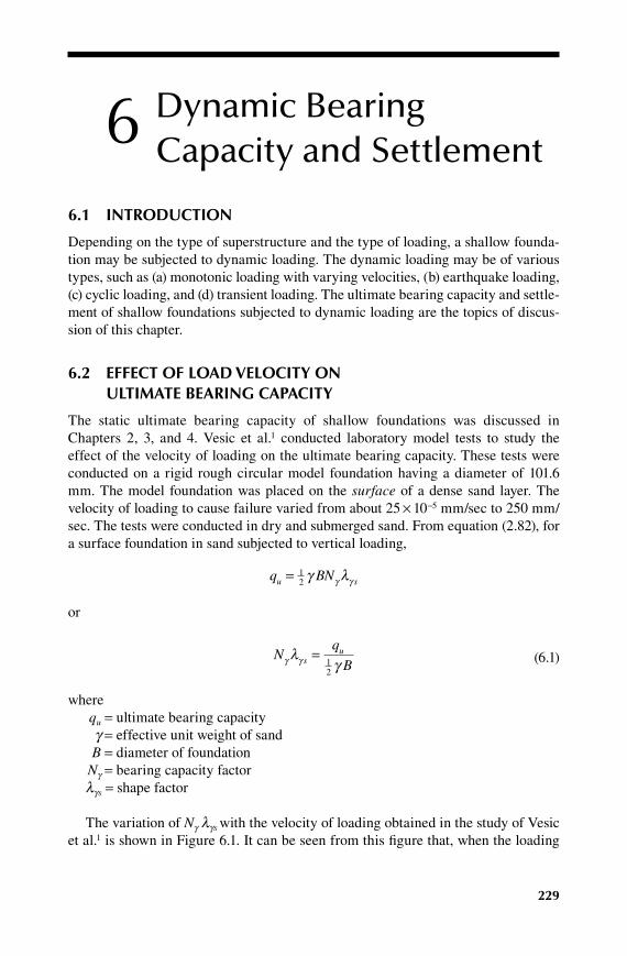
229
6 Dynamic Bearing Capacity and Settlement
6.1 introduCtion
Depending on the type of superstructure and the type of loading, a shallow founda-tion may be subjected to dynamic loading. The dynamic loading may be of various types, such as (a) monotonic loading with varying velocities, (b) earthquake loading, (c) cyclic loading, and (d) transient loading. The ultimate bearing capacity and settle-ment of shallow foundations subjected to dynamic loading are the topics of discus-sion of this chapter.
6.2 eFFeCt oF load VeloCity on ultimate bearinG CapaCity
The static ultimate bearing capacity of shallow foundations was discussed in Chapters 2, 3, and 4. Vesic et al.1 conducted laboratory model tests to study the effect of the velocity of loading on the ultimate bearing capacity. These tests were conducted on a rigid rough circular model foundation having a diameter of 101.6 mm. The model foundation was placed on the surface of a dense sand layer. The velocity of loading to cause failure varied from about 25 × 10-5 mm/sec to 250 mm/sec. The tests were conducted in dry and submerged sand. From equation (2.82), for a surface foundation in sand subjected to vertical loading,
q BNu s= 1
2 γ lγ γ
or
N
q
Bsu
γ γlγ
=12
(6.1)
where qu = ultimate bearing capacity g = effective unit weight of sand B = diameter of foundation Ng = bearing capacity factor lgs = shape factor
The variation of Ng lgs with the velocity of loading obtained in the study of Vesic et al.1 is shown in Figure 6.1. It can be seen from this figure that, when the loading
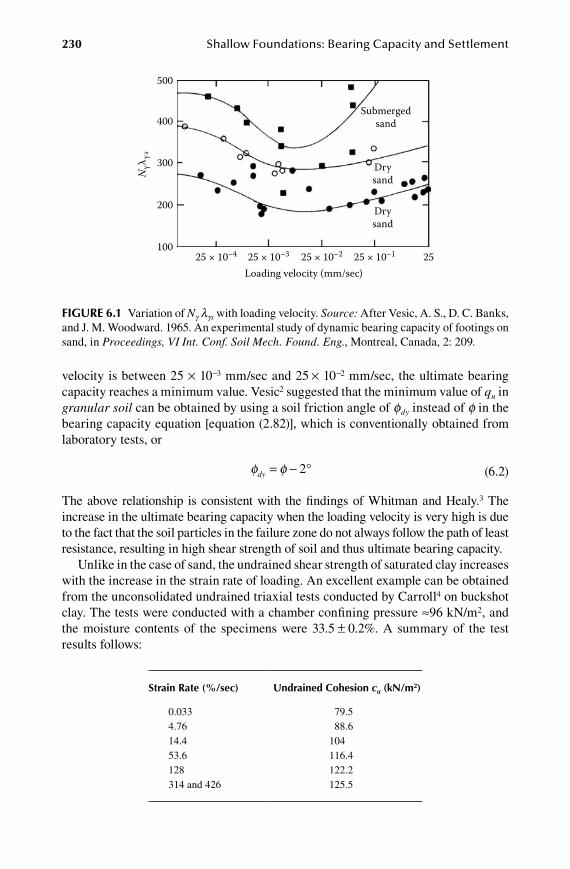
230 Shallow Foundations: Bearing Capacity and Settlement
velocity is between 25 × 10-3 mm/sec and 25 × 10-2 mm/sec, the ultimate bearing capacity reaches a minimum value. Vesic2 suggested that the minimum value of qu in granular soil can be obtained by using a soil friction angle of fdy instead of f in the bearing capacity equation [equation (2.82)], which is conventionally obtained from laboratory tests, or
φ φdy = - °2
(6.2)
The above relationship is consistent with the findings of Whitman and Healy.3 The increase in the ultimate bearing capacity when the loading velocity is very high is due to the fact that the soil particles in the failure zone do not always follow the path of least resistance, resulting in high shear strength of soil and thus ultimate bearing capacity.
Unlike in the case of sand, the undrained shear strength of saturated clay increases with the increase in the strain rate of loading. An excellent example can be obtained from the unconsolidated undrained triaxial tests conducted by Carroll4 on buckshot clay. The tests were conducted with a chamber confining pressure ≈96 kN/m2, and the moisture contents of the specimens were 33.5 ± 0.2%. A summary of the test results follows:
Strain rate (%/sec) undrained Cohesion cu (kn/m2)
0.033 79.54.76 88.614.4 10453.6 116.4128 122.2314 and 426 125.5
500
400
300
Nγλ
γs
200
100 25 × 10–4 25 × 10–3 25 × 10–2
Loading velocity (mm/sec)
Submerged sand
Dry sand
Dry sand
25 × 10–1 25
FiGure 6.1 Variation of Ng lgs with loading velocity. Source: After Vesic, A. S., D. C. Banks, and J. M. Woodward. 1965. An experimental study of dynamic bearing capacity of footings on sand, in Proceedings, VI Int. Conf. Soil Mech. Found. Eng., Montreal, Canada, 2: 209.
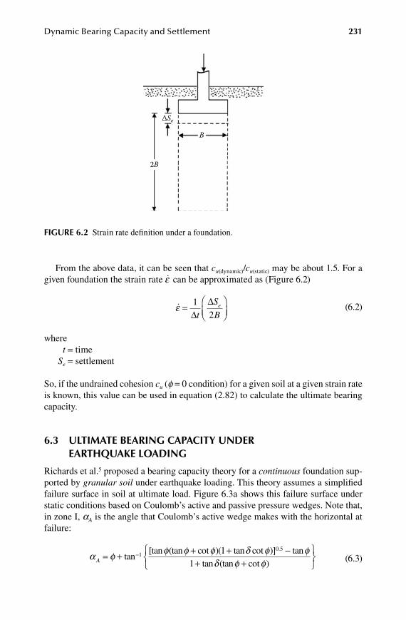
Dynamic Bearing Capacity and Settlement 231
From the above data, it can be seen that cu(dynamic)/cu(static) may be about 1.5. For a given foundation the strain rate �ε can be approximated as (Figure 6.2)
�ε =
12∆∆
t
S
Be
(6.2)
where t = time Se = settlement
So, if the undrained cohesion cu (f = 0 condition) for a given soil at a given strain rate is known, this value can be used in equation (2.82) to calculate the ultimate bearing capacity.
6.3 ultimate bearinG CapaCity under earthquaKe loadinG
Richards et al.5 proposed a bearing capacity theory for a continuous foundation sup-ported by granular soil under earthquake loading. This theory assumes a simplified failure surface in soil at ultimate load. Figure 6.3a shows this failure surface under static conditions based on Coulomb’s active and passive pressure wedges. Note that, in zone I, aA is the angle that Coulomb’s active wedge makes with the horizontal at failure:
α φ φ φ φ δ φ
A = + + + --tan[tan (tan cot )( tan cot )] .
10 51 tan
tan (tan cot )φ
δ φ φ1+ +
(6.3)
2B
B
∆Se
FiGure 6.2 Strain rate definition under a foundation.
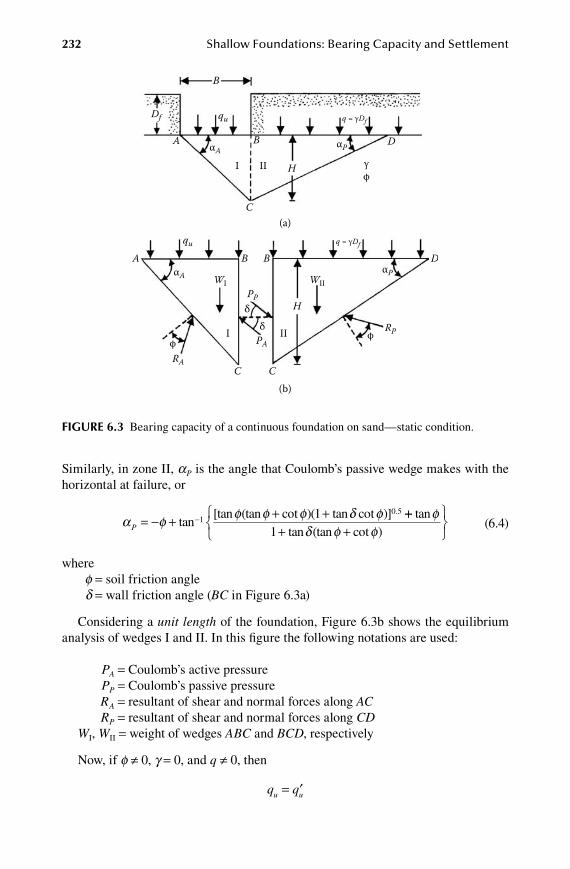
232 Shallow Foundations: Bearing Capacity and Settlement
Similarly, in zone II, aP is the angle that Coulomb’s passive wedge makes with the horizontal at failure, or
α φ φ φ φ δ φ
P = - + + +-tan[tan (tan cot )( tan cot )] .
10 51 ++
+ +
tantan (tan cot )
φδ φ φ1
(6.4)
where f = soil friction angle d = wall friction angle (BC in Figure 6.3a)
Considering a unit length of the foundation, Figure 6.3b shows the equilibrium analysis of wedges I and II. In this figure the following notations are used:
PA = Coulomb’s active pressure PP = Coulomb’s passive pressure RA = resultant of shear and normal forces along AC RP = resultant of shear and normal forces along CD
WI, WII = weight of wedges ABC and BCD, respectively
Now, if f ≠ 0, g = 0, and q ≠ 0, then
q qu u= ′
Df
D
qu
qu
q = γDf
q = γDf
γ φ
φ φ
H
A
A
C
C C
(a)
(b)
αA
αA αP
δ δ
RA
PP
RP
WI WII
H
PA
αP
I II
I II
B
B B
B
D
FiGure 6.3 Bearing capacity of a continuous foundation on sand—static condition.

Dynamic Bearing Capacity and Settlement 233
and
P PA Pcos cosδ δ= (6.5)
However,
P q K HA u Acosδ = ′
(6.6)
where
H BC= KA = horizontal component of Coulomb’s active earth pressure coefficient, or
K A =
+ +
cos
cossin( )sin
cos
2
2
1
φ
δ φ δ φδ
(6.7)
Similarly,
P qK HP Pcosδ = (6.8)
where KP = horizontal component of Coulomb’s passive earth pressure coefficient, or
KP =
- -
cos
cossin( )sin
cos
2
2
1
φ
δ φ δ φδ
(6.9)
Combining equations (6.5), (6.6), and (6.8),
′ = =q q
K
KqNu
P
Aq
(6.10)
whereNq = bearing capacity factor
Again, if f ≠ 0, g ≠ 0, and q = 0, then q qu u= ′′ :
P q HK H KA u A Acosδ γ= ′′ + 1
22
(6.11)
Also,
P H KP Pcosδ γ= 1
22
(6.12)
Equating the right-hand sides of equations (6.11) and (6.12),
′′ + =q HK H K H Ku A A P
12
2 12
2γ γ
′′= - q H K K
HKu P AA
12
2 1γ ( )
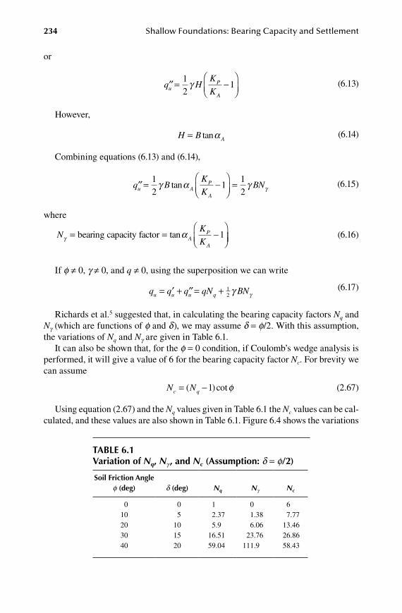
234 Shallow Foundations: Bearing Capacity and Settlement
or
′′= -
q HK
KuP
A
12
1γ
(6.13)
However,
H B A= tanα (6.14)
Combining equations (6.13) and (6.14),
′′= -
=q BK
KBNu A
P
A
12
112
γ α γ γtan
(6.15)
where
NK
KAP
Aγ α= = -
bearing capacity factor tan 1
(6.16)
If f ≠ 0, g ≠ 0, and q ≠ 0, using the superposition we can write
q q q qN BNu u u q= ′ + ′′= + 1
2 γ γ (6.17)
Richards et al.5 suggested that, in calculating the bearing capacity factors Nq and Ng (which are functions of f and d), we may assume d = f/2. With this assumption, the variations of Nq and Ng are given in Table 6.1.
It can also be shown that, for the f = 0 condition, if Coulomb’s wedge analysis is performed, it will give a value of 6 for the bearing capacity factor Nc. For brevity we can assume
N Nc q= -( )cot1 φ
(2.67)
Using equation (2.67) and the Nq values given in Table 6.1 the Nc values can be cal-culated, and these values are also shown in Table 6.1. Figure 6.4 shows the variations
table 6.1Variation of Nq, Ng , and Nc (assumption: d = f/2)
Soil Friction angle f (deg) d (deg) Nq Ng Nc
0 0 1 0 610 5 2.37 1.38 7.7720 10 5.9 6.06 13.4630 15 16.51 23.76 26.8640 20 59.04 111.9 58.43
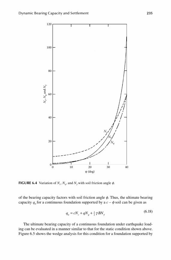
Dynamic Bearing Capacity and Settlement 235
of the bearing capacity factors with soil friction angle f. Thus, the ultimate bearing capacity qu for a continuous foundation supported by a c – f soil can be given as
q cN qN BNu c q= + + 1
2 γ γ (6.18)
The ultimate bearing capacity of a continuous foundation under earthquake load-ing can be evaluated in a manner similar to that for the static condition shown above. Figure 6.5 shows the wedge analysis for this condition for a foundation supported by
120
100
80
60
Nc,
Nq a
nd N
γ
40
20
0 0 10 20
φ (deg) 30 40
Nc
Nq
Nγ
FiGure 6.4 Variation of Nc, Nq, and Ng with soil friction angle f.

236 Shallow Foundations: Bearing Capacity and Settlement
granular soil. In Figure 6.5a note that aAE and aPE are, respectively, the angles that the Coulomb’s failure wedges would make for active and passive conditions, or
α α α δ θ α αAE = + + + + -
+-tan
( tan )[ tan( )cot ] tan121 1
1 tan( )(tan cot )δ θ α α+ +
(6.19)
and
α α α δ θ α αPE = - + + + - +-tan
( tan )[ tan( )cot ] tan121 1
1+ + +
tan( )(tan cot )δ θ α α
(6.20)
whereα φ θ= - (6.21)
θ =
--tan 1
1
k
kh
v
(6.22)
kh = horizontal coefficient of acceleration kv = vertical coefficient of acceleration
Df quE
quE
q = γDf
q = γDf
γφ
φφ
H
A
A
C
C C
(a)
(b)
αAE
αAEαPE
δδ
RA
PPE
RP
khWI
khquE khq
khWII
(1 – kv)WII(1 – kv)WI H
PAE
αPE D
I II
I II
B
B
B B D
FiGure 6.5 Bearing capacity of a continuous foundation on sand—earthquake condition.
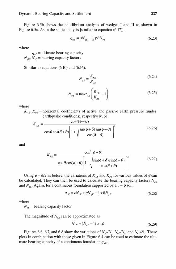
Dynamic Bearing Capacity and Settlement 237
Figure 6.5b shows the equilibrium analysis of wedges I and II as shown in Figure 6.5a. As in the static analysis [similar to equation (6.17)],
q qN BNuE qE E= + 1
2 γ γ
(6.23)
where quE = ultimate bearing capacityNqE, NgE = bearing capacity factors
Similar to equations (6.10) and (6.16),
N
K
KqEPE
AE
=
(6.24)
NK
KE AEPE
AEγ α= -
tan 1
(6.25)
whereKAE, KPE = horizontal coefficients of active and passive earth pressure (under
earthquake conditions), respectively, or
K AE = -
+ + + -
cos ( )
cos cos( )sin( )sin( )
2
1
φ θ
θ δ θ φ δ φ θcos( )δ θ+
2
(6.26)
and
KPE = -
+ - + -
cos ( )
cos cos( )sin( )sin( )
2
1
φ θ
θ δ θ φ δ φ θcos( )δ θ+
2
(6.27)
Using d = f/2 as before, the variations of KAE and KPE for various values of q can be calculated. They can then be used to calculate the bearing capacity factors NqE and NgE. Again, for a continuous foundation supported by a c – f soil,
q cN qN BNuE cE qE E= + + 1
2 γ γ
(6.28)
whereNcE = bearing capacity factor
The magnitude of NcE can be approximated as
N NcE qE≈ -( )cot1 φ
(6.29)
Figures 6.6, 6.7, and 6.8 show the variations of NgE/Ng , NqE/Nq, and NcE/Nc. These plots in combination with those given in Figure 6.4 can be used to estimate the ulti-mate bearing capacity of a continuous foundation quE.
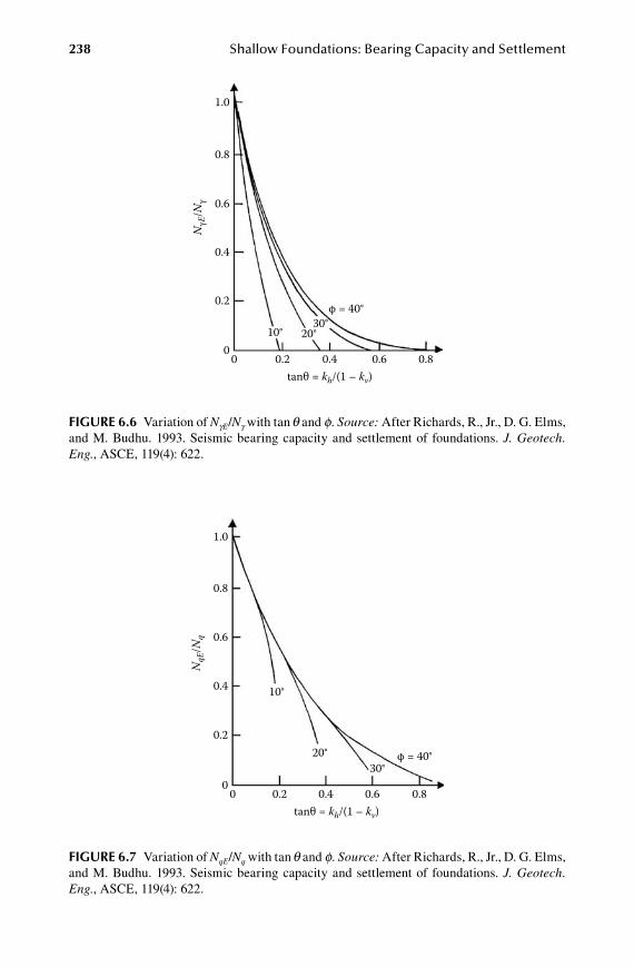
238 Shallow Foundations: Bearing Capacity and Settlement
1.0
0.8
0.6
0.4
NγE
/Nγ
0.2
00
10° 20°30°
φ = 40°
0.2 0.4tanθ = kh/(1 – kv)
0.6 0.8
FiGure 6.6 Variation of NgE/Ng with tan q and f. Source: After Richards, R., Jr., D. G. Elms, and M. Budhu. 1993. Seismic bearing capacity and settlement of foundations. J. Geotech. Eng., ASCE, 119(4): 622.
1.0
0.8
0.6
0.4
NqE
/Nq
0.2
00
10°
20°30°
φ = 40°
0.2 0.4tanθ = kh/(1 – kv)
0.6 0.8
FiGure 6.7 Variation of NqE/Nq with tan q and f. Source: After Richards, R., Jr., D. G. Elms, and M. Budhu. 1993. Seismic bearing capacity and settlement of foundations. J. Geotech. Eng., ASCE, 119(4): 622.

Dynamic Bearing Capacity and Settlement 239
Example 6.1
Consider a shallow continuous foundation. Given: B = 1.5 m; Df = 1 m; g = 17 kN/m3; f = 25°; c = 30 kN/m2; kh = 0.25; kv = 0. Estimate the ultimate bearing capacity quE.
Solution
From equation (6.28),
q cN qN BNuE cE qE E= + + 1
2 γ γ
For f = 25°, from Figure 6.4, Nc ≈ 20, Nq ≈ 10, and Ng ≈ 14. From Figures 6.6, 6.7, and 6.8, for tan q = kh/(1 – kv) = 0.25/(1 – 0) = 0.25,
N
NNcE
ccE= = =0 44 0 44 20 8 8. ; ( . )( ) .
N
NNqE
qqE= = =0 38 0 38 10 3 8. ; ( . )( ) .
N
NNE
cEγ
γ
= = =0 13 0 13 14 1 82. ; ( . )( ) .
1.0
0.8
0.6
0.4
NcE
/Nc
0.2
00
10° 20° 30° φ = 40°
0.2 0.4tanθ = kh/(1 – kv)
0.6 0.8
FiGure 6.8 Variation of NcE/Nc with tan q and f. Source: After Richards, R., Jr., D. G. Elms, and M. Budhu. 1993. Seismic bearing capacity and settlement of foundations. J. Geotech. Eng., ASCE, 119(4): 622.
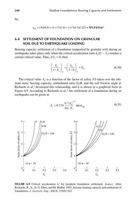
240 Shallow Foundations: Bearing Capacity and Settlement
So,
quE = + × +( )( . ) ( )( . ) ( )( . )( . )30 8 8 1 17 3 8 17 1 5 1 821
2 == 351.8 kN/m2
6.4 Settlement oF Foundation on Granular Soil due to earthquaKe loadinG
Bearing capacity settlement of a foundation (supported by granular soil) during an earthquake takes place only when the critical acceleration ratio kh/(1 – kv) reaches a certain critical value. Thus, if kv ≈ 0, then
k
k
kkh
v
hh1 1 0-
≈-
≈cr cr
*.
(6.30)
The critical value kh* is a function of the factor of safety FS taken over the ulti-
mate static bearing capacity, embedment ratio Df /B, and the soil friction angle f. Richards et al.5 developed this relationship, and it is shown in a graphical form in Figure 6.9. According to Richards et al.,5 the settlement of a foundation during an earthquake can be given as
SVAg
k
Aeh
AE=-
0 1742
4
. tan*
α
(6.31)
4 0 0.250.50
Df/B = 1.003
2
Stat
ic fa
ctor
of s
afet
y, FS
1
00
(a) φ = 10°
0.1 0.2 0.3 0.4k*
h
40
0.250.50
Df/B = 1.003
2
Stat
ic fa
ctor
of s
afet
y, FS
1
00
(b) φ = 20°
0.1 0.2 0.3 0.4k*
h
FiGure 6.9 Critical acceleration kh* for incipient foundation settlement. Source: After
Richards, R., Jr., D. G. Elms, and M. Budhu. 1993. Seismic bearing capacity and settlement of foundations. J. Geotech. Eng., ASCE, 119(4): 622.
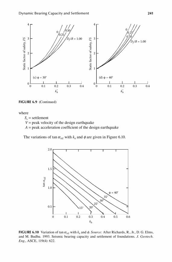
Dynamic Bearing Capacity and Settlement 241
where Se = settlement V = peak velocity of the design earthquake A = peak acceleration coefficient of the design earthquake
The variations of tan aAE with kh and f are given in Figure 6.10.
4
00.25
0.50
Df/B = 1.003
2
Stat
ic fa
ctor
of s
afet
y, FS
1
00
(c) φ = 30°
0.1 0.2 0.3 0.4k*
h
40
0.250.50
Df/B = 1.003
2
Stat
ic fa
ctor
of s
afet
y, FS
1
00
(d) φ = 40°
0.1 0.2 0.3 0.4k*
h
FiGure 6.9 (Continued)
2.0
1.5
1.0 tan
α AE
0.5
0
15°
35° 30°
25° 20°
φ = 40°
0.1 0.2 kh
0.3 0.4 0.5 0.6
FiGure 6.10 Variation of tan aAE with kh and f. Source: After Richards, R., Jr., D. G. Elms, and M. Budhu. 1993. Seismic bearing capacity and settlement of foundations. J. Geotech. Eng., ASCE, 119(4): 622.

242 Shallow Foundations: Bearing Capacity and Settlement
Example 6.2
Consider a shallow foundation on granular soil with B = 1.5 m; Df = 1 m; g = 16.5 kN/m3; f = 35°. If the allowable bearing capacity is 304 kN/m2, A = 0.32, and V = 0.35 m/s, determine the settlement the foundation may undergo.
Solution
From equation (6.17),
q qN BNu q= + 1
2 γ γ
From Figure 6.4 for f = 35°, Nq ≈ 30; Ng ≈ 42. So,
qu = × + ≈( . )( ) ( . )( . )( )1 16 5 30 16 5 1 5 42 10151
2 kN/m22
Given qall = 340 kN/m2,
FS
q
qu= = =all
1015340
2 98.
From Figure 6.9 for FS = 2.98 and Df/B = 1/1.5 = 0.67, the magnitude of kh* is about
0.28. From equation (6.31),
S
VAg
k
Aeh
AE=-
0 1742
4
. tan*
α
From Figure 6.10 for f = 35° and kh* = 0.28, tan aAE ≈ 0.95. So,
Se = ( . )
( .( . )( . )
.0 174
0 350 32 9 81
0 280
2m/s)m/s2 .
( . )32
0 954-
= =0.011 m 11 mm
6.5 Foundation Settlement due to CyCliC loadinG—Granular Soil
Raymond and Komos6 reported laboratory model test results on surface continuous foundations (Df = 0) supported by granular soil and subjected to a low-frequency (1 cps) cyclic loading of the type shown in Figure 6.11. In this figure, sd is the amplitude of the intensity of the cyclic load. The laboratory tests were conducted for foundation widths (B) of 75 mm and 228 mm. The unit weight of sand was 16.97 kN/m3. Since the settlement of the foundation Se after the first cycle of load application was pri-marily due to the placement of the foundation rather than the foundation behavior, it was taken to be zero (that is, Se = 0 after the first cycle load application). Figures 6.12 and 6.13 show the variation of Se (after the first cycle) with the number of load cycles, N, and sd/qu (qu = ultimate static bearing capacity). Note that (a) for a given number of load cycles, the settlement increased with the increase in sd/qu, and (b) for a given
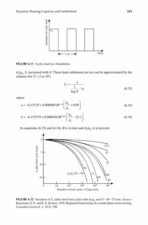
Dynamic Bearing Capacity and Settlement 243
sd/qu, Se increased with N. These load-settlement curves can be approximated by the relation (for N = 2 to 105)
Sa
Nb
e =-1
log (6.32)
where
a Bq
d
u
= - + +
0 15125 0 0000693 6 091 18. . ..σ
(6.33)
b Bq
d
u
= - + -
0 153579 0 0000363 23 10 821. . ..σ
(6.34)
In equations (6.33) and (6.34), B is in mm and sd/qu is in percent.
Inte
nsity
of c
yclic
load
1 sec
σd
Time
FiGure 6.11 Cyclic load on a foundation.
0
5
10
S e af
ter fi
rst c
ycle
(mm
)
15
0 10Number of load cycles, N (log scale)
σd/qu (%) = 90
84
7560
50
40
35
27
13.5
102 103 104 105
FiGure 6.12 Variation of Se (after first load cycle) with sd/qu and N—B = 75 mm. Source: Raymond, G. P., and F. E. Komos. 1978. Repeated load testing of a model plane strain footing. Canadian Geotech. J. 15(2): 190.
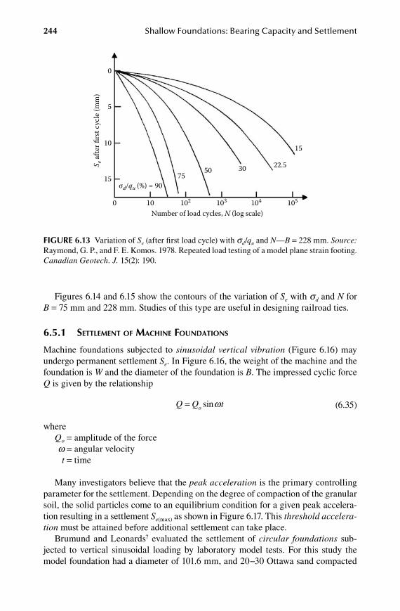
244 Shallow Foundations: Bearing Capacity and Settlement
Figures 6.14 and 6.15 show the contours of the variation of Se with sd and N for B = 75 mm and 228 mm. Studies of this type are useful in designing railroad ties.
6.5.1 settlement of maChine foUnDations
Machine foundations subjected to sinusoidal vertical vibration (Figure 6.16) may undergo permanent settlement Se. In Figure 6.16, the weight of the machine and the foundation is W and the diameter of the foundation is B. The impressed cyclic force Q is given by the relationship
Q Q to= sinω
(6.35)
where Qo = amplitude of the force w = angular velocity t = time
Many investigators believe that the peak acceleration is the primary controlling parameter for the settlement. Depending on the degree of compaction of the granular soil, the solid particles come to an equilibrium condition for a given peak accelera-tion resulting in a settlement Se(max) as shown in Figure 6.17. This threshold accelera-tion must be attained before additional settlement can take place.
Brumund and Leonards7 evaluated the settlement of circular foundations sub-jected to vertical sinusoidal loading by laboratory model tests. For this study the model foundation had a diameter of 101.6 mm, and 20−30 Ottawa sand compacted
0
5
10
S e af
ter fi
rst c
ycle
(mm
)
15
0 10Number of load cycles, N (log scale)
σd/qu (%) = 90
5075
30 22.5
15
102 103 104 105
FiGure 6.13 Variation of Se (after first load cycle) with sd/qu and N—B = 228 mm. Source: Raymond, G. P., and F. E. Komos. 1978. Repeated load testing of a model plane strain footing. Canadian Geotech. J. 15(2): 190.
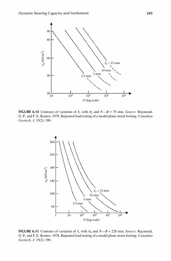
Dynamic Bearing Capacity and Settlement 245
40
σ d (k
N/m
2 )
20
60
80
90
10N (log scale)
2.5 mm 5 mm10 mm
Se = 15 mm
102 103 104 105
FiGure 6.14 Contours of variation of Se with sd and N—B = 75 mm. Source: Raymond, G. P., and F. E. Komos. 1978. Repeated load testing of a model plane strain footing. Canadian Geotech. J. 15(2): 190.
100
σ d (k
N/m
2 )
60
140
180
220
260
1 10N (log scale)
2.5 mm5 mm
10 mmSe = 15 mm
102 103 104 105
FiGure 6.15 Contours of variation of Se with sd and N—B = 228 mm. Source: Raymond, G. P., and F. E. Komos. 1978. Repeated load testing of a model plane strain footing. Canadian Geotech. J. 15(2): 190.
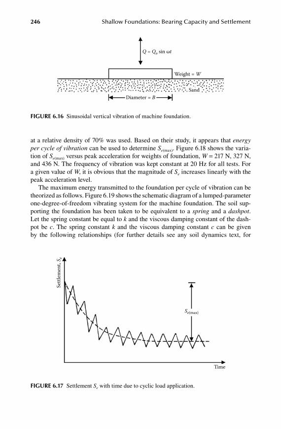
246 Shallow Foundations: Bearing Capacity and Settlement
at a relative density of 70% was used. Based on their study, it appears that energy per cycle of vibration can be used to determine Se(max). Figure 6.18 shows the varia-tion of Se(max) versus peak acceleration for weights of foundation, W = 217 N, 327 N, and 436 N. The frequency of vibration was kept constant at 20 Hz for all tests. For a given value of W, it is obvious that the magnitude of Se increases linearly with the peak acceleration level.
The maximum energy transmitted to the foundation per cycle of vibration can be theorized as follows. Figure 6.19 shows the schematic diagram of a lumped-parameter one-degree-of-freedom vibrating system for the machine foundation. The soil sup-porting the foundation has been taken to be equivalent to a spring and a dashpot. Let the spring constant be equal to k and the viscous damping constant of the dash-pot be c. The spring constant k and the viscous damping constant c can be given by the following relationships (for further details see any soil dynamics text, for
Q = Qo sin ωt
Weight = W
Diameter = BSand
FiGure 6.16 Sinusoidal vertical vibration of machine foundation.
Settl
emen
t, S e
Se(max)
Time
FiGure 6.17 Settlement Se with time due to cyclic load application.
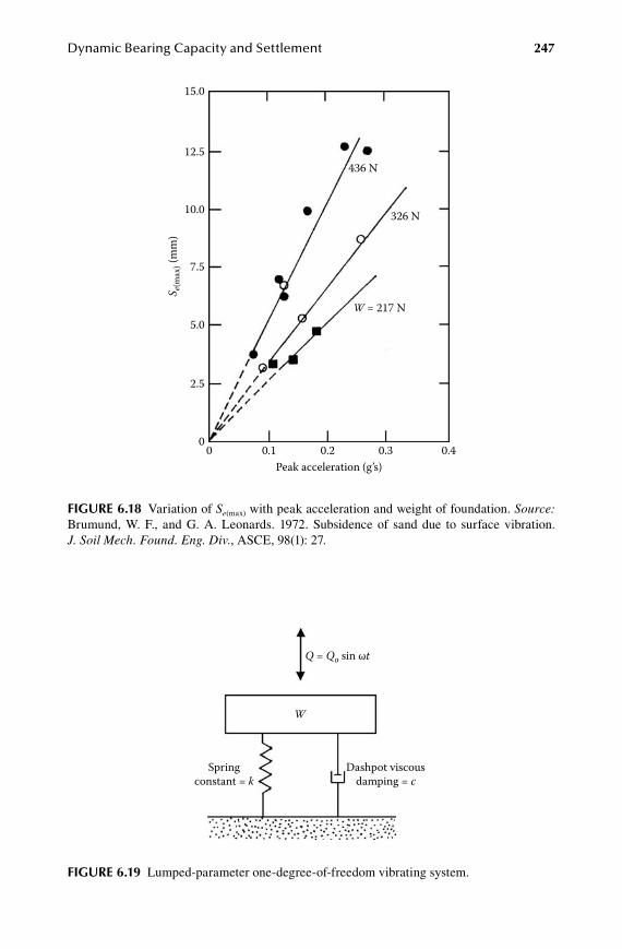
Dynamic Bearing Capacity and Settlement 247
15.0
12.5
10.0
S e(m
ax) (
mm
)
7.5
5.0
2.5
00 0.1 0.2 0.3 0.4
Peak acceleration (g’s)
W = 217 N
326 N
436 N
FiGure 6.18 Variation of Se(max) with peak acceleration and weight of foundation. Source: Brumund, W. F., and G. A. Leonards. 1972. Subsidence of sand due to surface vibration. J. Soil Mech. Found. Eng. Div., ASCE, 98(1): 27.
Q = Qo sin ωt
W
Spring constant = k
Dashpot viscousdamping = c
FiGure 6.19 Lumped-parameter one-degree-of-freedom vibrating system.
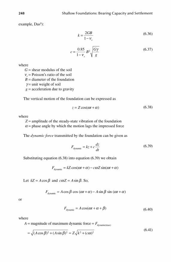
248 Shallow Foundations: Bearing Capacity and Settlement
example, Das8):
k
GB
s
=-
21 ν
(6.36)
c B
Ggs
=-
0 851
2.ν
γ
(6.37)
where G = shear modulus of the soil ns = Poisson’s ratio of the soil B = diameter of the foundation g = unit weight of soil g = acceleration due to gravity
The vertical motion of the foundation can be expressed as
z Z t= +cos( )ω α (6.38)
where Z = amplitude of the steady-state vibration of the foundation a = phase angle by which the motion lags the impressed force
The dynamic force transmitted by the foundation can be given as
F kz c
dzdtdynamic = +
(6.39)
Substituting equation (6.38) into equation (6.39) we obtain
F kZ t c Z tdynamic = + - +cos( ) sin( )ω α ω ω α
Let kZ A= cosβ and c Z Aω β= sin . So,
F A t A tdynamic = + - +cos cos ( ) sin sin ( )β ω α β ω α
or
F A tdynamic = + +cos( )ω α β
(6.40)
whereA F= =magnitude of maximum dynamic force dynamic(max)
= + = +( cos ) ( sin ) ( )A A Z k cβ β ω2 2 2 2
(6.41)
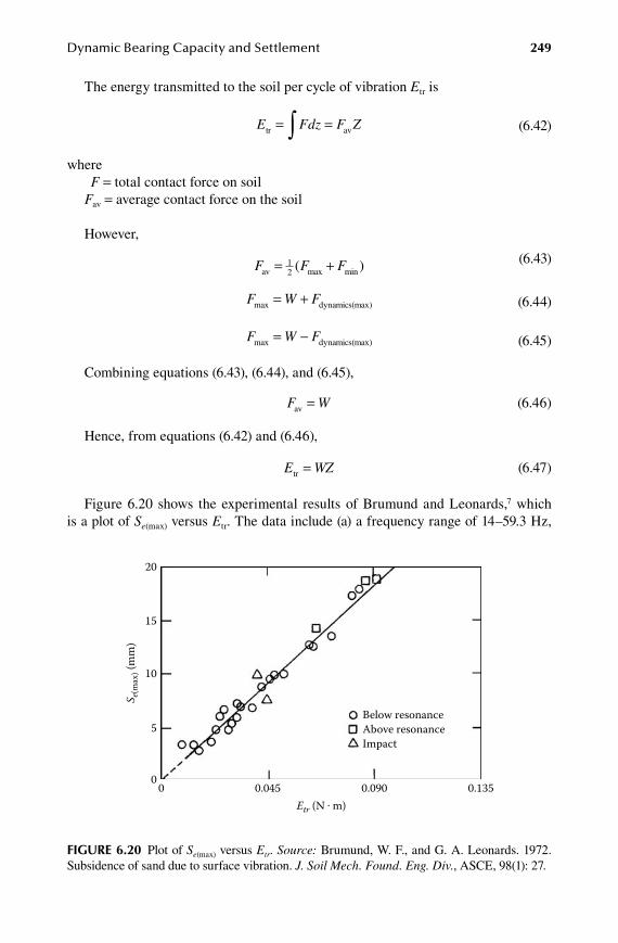
Dynamic Bearing Capacity and Settlement 249
The energy transmitted to the soil per cycle of vibration Etr is
E Fdz F Ztr av= =∫
(6.42)
where F = total contact force on soil Fav = average contact force on the soil
However,
F F Fav = +1
2 ( )max min (6.43)
F W Fmax dynamics(max)= +
(6.44)
F W Fmax dynamics(max)= -
(6.45)
Combining equations (6.43), (6.44), and (6.45),
F Wav =
(6.46)
Hence, from equations (6.42) and (6.46),
E WZtr =
(6.47)
Figure 6.20 shows the experimental results of Brumund and Leonards,7 which is a plot of Se(max) versus Etr. The data include (a) a frequency range of 14–59.3 Hz,
20
15
10
S e(m
ax) (
mm
)
5
00 0.045 0.090
Below resonanceAbove resonanceImpact
0.135Etr (N m)
FiGure 6.20 Plot of Se(max) versus Etr. Source: Brumund, W. F., and G. A. Leonards. 1972. Subsidence of sand due to surface vibration. J. Soil Mech. Found. Eng. Div., ASCE, 98(1): 27.

250 Shallow Foundations: Bearing Capacity and Settlement
(b) a range of W varying from 0.27qu to 0.55qu, (qu = static beaning capacity) and (c) the maximum downward dynamic force of 0.3W to 1.0W. The results show that Se(max) increases linearly with Etr. Figure 6.21 shows a plot of the experimental results of Se(max) against peak acceleration for different ranges of Etr. This clearly demon-strates that, if the value of the transmitted energy is constant, the magnitude of Se(max) remains constant irrespective of the level of peak acceleration.
6.6 Foundation Settlement due to CyCliC loadinG in Saturated Clay
Das and Shin9 provided small-scale model test results for the settlement of a continu-ous surface foundation (Df = 0) supported by saturated clay and subjected to cyclic loading. For these tests, the width of the model foundation B was 76.2 mm, and the average undrained shear strength of the clay was 11.9 kN/m2. The load to the founda-tion was applied in two stages (Figure 6.22):
Stage I—Application of a static load per unit area of qs = qu/FS (where qu = ultimate bearing capacity; FS = factor of safety) as shown in Figure 6.22a
Stage II—Application of a cyclic load, the intensity of which has an ampli-tude of sd as shown in Figure 6.22b
The frequency of the cyclic load was 1 Hz. Figure 6.22c shows the variation of the total load intensity on the foundation. Typical experimental plots obtained from these laboratory tests are shown by the dashed lines in Figure 6.23 (FS = 3.33; sd/qu = 4.38%, 9.38%, and 18.75%). It is important to note that Se in this figure refers to the
25
20
15
10 S e(m
ax) (
mm
)
5
0 0 0.4 0.8 1.2 1.6
Peak acceleration (g’s)
Frequency = 18.7 – 37.3 Hz Etr = 0.026 – 0.032 N · m
Frequency = 18 – 59.3 Hz Etr = 0.062 – 0.072 N · m
Frequency = 28 – 59.3 HzEtr = 0.081 – 0.087 N · m
FiGure 6.21 Se(max) versus peak acceleration for three levels of transmitted energy. Source: Brumund, W. F., and G. A. Leonards. 1972. Subsidence of sand due to surface vibration. J. Soil Mech. Found. Eng. Div., ASCE, 98(1): 27.

Dynamic Bearing Capacity and Settlement 251
settlement obtained due to cyclic load only (that is, after application of stage II load; Figure 6.22b). The general nature of these plots is shown in Figure 6.24. They consist of approximately three linear segments, and they are
1. An initial rapid settlement Se(r) (branch Oa). 2. A secondary settlement at a slower rate Se(s) (branch ab). The settlement
practically ceases after application of N = Ncr cycles of load. 3. For N > Ncr cycles of loading, the settlement of the foundation due to
cyclic load practically ceases (branch bc).
The linear approximations of Se with number of load cycles N are shown in Figure 6.23 (solid lines). Hence the total settlement of the foundation is
S S Se e r e s(max) ( ) ( )= +
(6.48)
Saturated clay
Load
per
uni
t are
a, q
B
(a)
(b) Time
qs
qs + σd
Saturated clay
Load
per
uni
t are
a, q
Load
per
uni
t are
a, q
B
(c)Time
Time
1 sec
1 sec
σd
FiGure 6.22 Load application sequence to observe foundation settlement in saturated clay due to cyclic loading based on laboratory model tests of Das and Shin. Source: Das, B. M., and E. C. Shin. 1996. Laboratory model tests for cyclic load-induced settlement of a strip foundation on a clayey soil. Geotech. Geol. Eng., London, 14: 213.
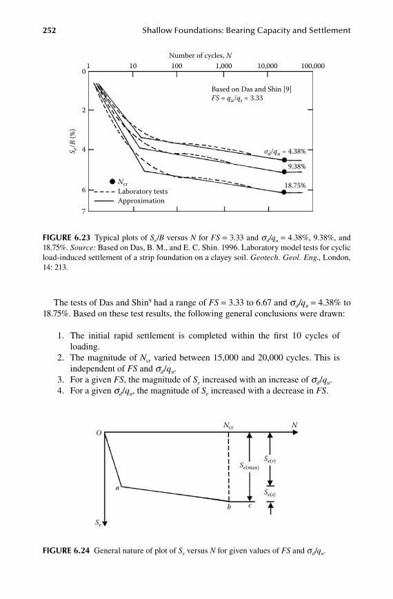
252 Shallow Foundations: Bearing Capacity and Settlement
The tests of Das and Shin9 had a range of FS = 3.33 to 6.67 and sd/qu = 4.38% to 18.75%. Based on these test results, the following general conclusions were drawn:
1. The initial rapid settlement is completed within the first 10 cycles of loading.
2. The magnitude of Ncr varied between 15,000 and 20,000 cycles. This is independent of FS and sd/qu.
3. For a given FS, the magnitude of Se increased with an increase of sd/qu. 4. For a given sd/qu, the magnitude of Se increased with a decrease in FS.
01 10 100 1,000
Number of cycles, N10,000 100,000
2
4S e/B
(%)
6NcrLaboratory tests
σd/qu = 4.38%
9.38%
18.75%
Based on Das and Shin [9]FS = qu/qs = 3.33
Approximation7
FiGure 6.23 Typical plots of Se/B versus N for FS = 3.33 and sd/qu = 4.38%, 9.38%, and 18.75%. Source: Based on Das, B. M., and E. C. Shin. 1996. Laboratory model tests for cyclic load-induced settlement of a strip foundation on a clayey soil. Geotech. Geol. Eng., London, 14: 213.
ONcr N
Se
Se(max)
b
a
c
Se(r)
Se(s)
FiGure 6.24 General nature of plot of Se versus N for given values of FS and sd/qu.
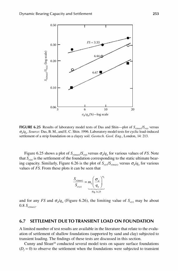
Dynamic Bearing Capacity and Settlement 253
Figure 6.25 shows a plot of Se(max)/Se(u) versus sd/qu for various values of FS. Note that Se(u) is the settlement of the foundation corresponding to the static ultimate bear-ing capacity. Similarly, Figure 6.26 is the plot of Se(r)/Se(max) versus sd/qu for various values of FS. From these plots it can be seen that
S
Sm
qe
e u
d
u
n
(max)
( )
=
1
1σ
Fig. 6.25� �� ��
and for any FS and sd/qu (Figure 6.26), the limiting value of Se(r) may be about 0.8 Se(max).
6.7 Settlement due to tranSient load on Foundation
A limited number of test results are available in the literature that relate to the evalu-ation of settlement of shallow foundations (supported by sand and clay) subjected to transient loading. The findings of these tests are discussed in this section.
Cunny and Sloan10 conducted several model tests on square surface foundations (Df = 0) to observe the settlement when the foundations were subjected to transient
σd/qu(%)—log scale
0.50
0.20
0.10
FS = 3.33
4.44
6.67
0.30S e
(max
)/Se(u)
(log
scal
e)
0.06 3 6 10 20
FiGure 6.25 Results of laboratory model tests of Das and Shin—plot of Se(max)/Se(u) versus sd/qu. Source: Das, B. M., and E. C. Shin. 1996. Laboratory model tests for cyclic load-induced settlement of a strip foundation on a clayey soil. Geotech. Geol. Eng., London, 14: 213.
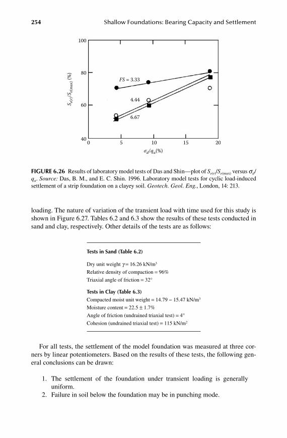
254 Shallow Foundations: Bearing Capacity and Settlement
loading. The nature of variation of the transient load with time used for this study is shown in Figure 6.27. Tables 6.2 and 6.3 show the results of these tests conducted in sand and clay, respectively. Other details of the tests are as follows:
tests in Sand (table 6.2)
Dry unit weight g = 16.26 kN/m3
Relative density of compaction = 96%
Triaxial angle of friction = 32°
tests in Clay (table 6.3)Compacted moist unit weight = 14.79 − 15.47 kN/m3
Moisture content = 22.5 ± 1.7%
Angle of friction (undrained triaxial test) = 4°
Cohesion (undrained triaxial test) = 115 kN/m2
For all tests, the settlement of the model foundation was measured at three cor-ners by linear potentiometers. Based on the results of these tests, the following gen-eral conclusions can be drawn:
1. The settlement of the foundation under transient loading is generally uniform.
2. Failure in soil below the foundation may be in punching mode.
σd/qu(%)
100
60
40
FS = 3.33
4.44
6.67
80S e
(r)/S
e(m
ax) (
%)
0 5 10 15 20
FiGure 6.26 Results of laboratory model tests of Das and Shin—plot of Se(r)/Se(max) versus sd/qu. Source: Das, B. M., and E. C. Shin. 1996. Laboratory model tests for cyclic load-induced settlement of a strip foundation on a clayey soil. Geotech. Geol. Eng., London, 14: 213.
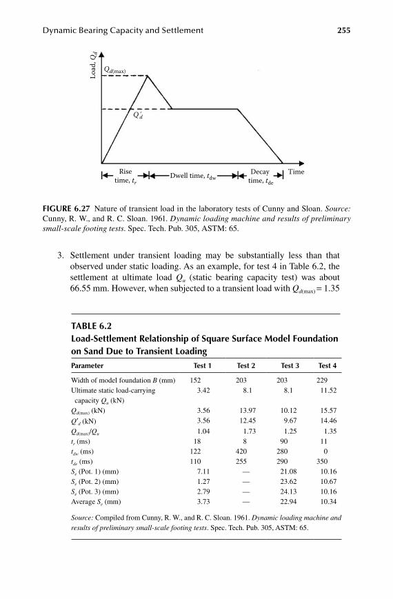
Dynamic Bearing Capacity and Settlement 255
3. Settlement under transient loading may be substantially less than that observed under static loading. As an example, for test 4 in Table 6.2, the settlement at ultimate load Qu (static bearing capacity test) was about 66.55 mm. However, when subjected to a transient load with Qd(max) = 1.35
table 6.2load-Settlement relationship of Square Surface model Foundation on Sand due to transient loading
parameter test 1 test 2 test 3 test 4
Width of model foundation B (mm) 152 203 203 229Ultimate static load-carrying capacity Qu (kN)
3.42 8.1 8.1 11.52
Qd(max) (kN) 3.56 13.97 10.12 15.57
Q′d (kN) 3.56 12.45 9.67 14.46
Qd(max)/Qu 1.04 1.73 1.25 1.35tr (ms) 18 8 90 11tdw (ms) 122 420 280 0tde (ms) 110 255 290 350Se (Pot. 1) (mm) 7.11 — 21.08 10.16Se (Pot. 2) (mm) 1.27 — 23.62 10.67Se (Pot. 3) (mm) 2.79 — 24.13 10.16Average Se (mm) 3.73 — 22.94 10.34
Source: Compiled from Cunny, R. W., and R. C. Sloan. 1961. Dynamic loading machine and results of preliminary small-scale footing tests. Spec. Tech. Pub. 305, ASTM: 65.
Qd(max)
Load
, Qd
Q d
Risetime, tr
Dwell time, tdwDecay
time, tde
Time
FiGure 6.27 Nature of transient load in the laboratory tests of Cunny and Sloan. Source: Cunny, R. W., and R. C. Sloan. 1961. Dynamic loading machine and results of preliminary small-scale footing tests. Spec. Tech. Pub. 305, ASTM: 65.
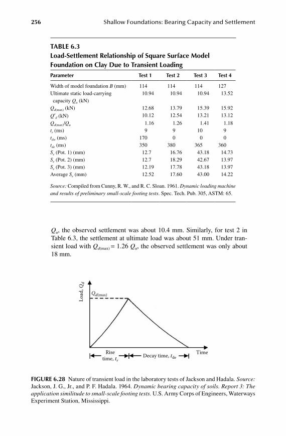
256 Shallow Foundations: Bearing Capacity and Settlement
Qu, the observed settlement was about 10.4 mm. Similarly, for test 2 in Table 6.3, the settlement at ultimate load was about 51 mm. Under tran-sient load with Qd(max) = 1.26 Qu, the observed settlement was only about 18 mm.
table 6.3load-Settlement relationship of Square Surface model Foundation on Clay due to transient loading
parameter test 1 test 2 test 3 test 4
Width of model foundation B (mm) 114 114 114 127Ultimate static load-carrying capacity Qu (kN)
10.94 10.94 10.94 13.52
Qd(max) (kN) 12.68 13.79 15.39 15.92
Q′d (kN) 10.12 12.54 13.21 13.12
Qd(max)/Qu 1.16 1.26 1.41 1.18tr (ms) 9 9 10 9tdw (ms) 170 0 0 0tde (ms) 350 380 365 360Se (Pot. 1) (mm) 12.7 16.76 43.18 14.73Se (Pot. 2) (mm) 12.7 18.29 42.67 13.97Se (Pot. 3) (mm) 12.19 17.78 43.18 13.97Average Se (mm) 12.52 17.60 43.00 14.22
Source: Compiled from Cunny, R. W., and R. C. Sloan. 1961. Dynamic loading machine and results of preliminary small-scale footing tests. Spec. Tech. Pub. 305, ASTM: 65.
Qd(max)
Load
, Qd
Risetime, tr
Decay time, tdeTime
FiGure 6.28 Nature of transient load in the laboratory tests of Jackson and Hadala. Source: Jackson, J. G., Jr., and P. F. Hadala. 1964. Dynamic bearing capacity of soils. Report 3: The application similitude to small-scale footing tests. U.S. Army Corps of Engineers, Waterways Experiment Station, Mississippi.
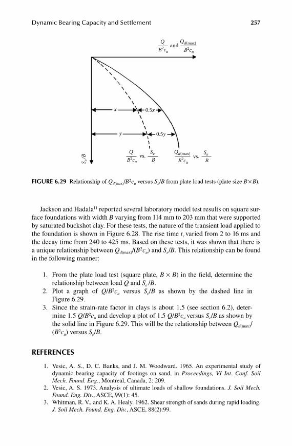
Dynamic Bearing Capacity and Settlement 257
Jackson and Hadala11 reported several laboratory model test results on square sur-face foundations with width B varying from 114 mm to 203 mm that were supported by saturated buckshot clay. For these tests, the nature of the transient load applied to the foundation is shown in Figure 6.28. The rise time tr varied from 2 to 16 ms and the decay time from 240 to 425 ms. Based on these tests, it was shown that there is a unique relationship between Qd(max)/(B2cu) and Se/B. This relationship can be found in the following manner:
1. From the plate load test (square plate, B × B) in the field, determine the relationship between load Q and Se /B.
2. Plot a graph of Q/B2cu versus Se/B as shown by the dashed line in Figure 6.29.
3. Since the strain-rate factor in clays is about 1.5 (see section 6.2), deter-mine 1.5 Q/B2cu and develop a plot of 1.5 Q/B2cu versus Se/B as shown by the solid line in Figure 6.29. This will be the relationship between Qd(max)/(B2cu) versus Se/B.
reFerenCeS
1. Vesic, A. S., D. C. Banks, and J. M. Woodward. 1965. An experimental study of dynamic bearing capacity of footings on sand, in Proceedings, VI Int. Conf. Soil Mech. Found. Eng., Montreal, Canada, 2: 209.
2. Vesic, A. S. 1973. Analysis of ultimate loads of shallow foundations. J. Soil Mech. Found. Eng. Div., ASCE, 99(1): 45.
3. Whitman, R. V., and K. A. Healy. 1962. Shear strength of sands during rapid loading. J. Soil Mech. Found. Eng. Div., ASCE, 88(2):99.
S e/B
x
y 0.5y
0.5x
vs.B2cu
QB
Se vs.B
SeB2cu
Qd(max)
andB2cu
QB2cu
Qd(max)
FiGure 6.29 Relationship of Qd(max)/B2cu versus Se/B from plate load tests (plate size B × B).
258 Shallow Foundations: Bearing Capacity and Settlement
4. Carroll, W. F. 1963. Dynamic bearing capacity of soils: Vertical displacement of spread footing on clay: Static and impulsive loadings, Technical Report 3-599, Report 5, U.S. Army Corps of Engineers, Waterways Experiment Station, Mississippi.
5. Richards, R., Jr., D. G. Elms, and M. Budhu. 1993. Seismic bearing capacity and settlement of foundations. J. Geotech. Eng., ASCE, 119(4): 622.
6. Raymond, G. P., and F. E. Komos. 1978. Repeated load testing of a model plane strain footing. Canadian Geotech. J. 15(2): 190.
7. Brumund, W. F., and G. A. Leonards. 1972. Subsidence of sand due to surface vibra-tion. J. Soil Mech. Found. Eng. Div., ASCE, 98(1): 27.
8. Das, B. M. 1993. Principles of soil dynamics. Boston, MA: PWS Publishers. 9. Das, B. M., and E. C. Shin. 1996. Laboratory model tests for cyclic load-induced
settlement of a strip foundation on a clayey soil. Geotech. Geol. Eng., London, 14: 213.
10. Cunny, R. W., and R. C. Sloan. 1961. Dynamic loading machine and results of pre-liminary small-scale footing tests. Spec. Tech. Pub. 305, ASTM: 65.
11. Jackson, J. G., Jr., and P. F. Hadala. 1964. Dynamic bearing capacity of soils. Report 3: The application similitude to small-scale footing tests. U.S. Army Corps of Engineers, Waterways Experiment Station, Mississippi.

259
7 Shallow Foundations on Reinforced Soil
7.1 introduCtion
Reinforced soil, or mechanically stabilized soil, is a construction material that consists of soil that has been strengthened by tensile elements such as metal strips, geotextiles, or geogrids. In the 1960s, the French Road Research Laboratory con-ducted extensive research to evaluate the beneficial effects of using reinforced soil as a construction material. Results of the early work were well documented by Vidal.1 During the last 40 years, many retaining walls and embankments were constructed all over the world using reinforced soil and they have performed very well.
The beneficial effects of soil reinforcement derive from (a) the soil’s increased tensile strength and (b) the shear resistance developed from the friction at the soil-reinforcement interfaces. This is comparable to the reinforcement of concrete struc-tures. At this time the design of reinforced earth is done with free-draining granular soil only. Thus, one avoids the effect of pore water pressure development in cohesive soil, which in turn controls the cohesive bond at the soil-reinforcement interfaces.
Since the mid-1970s a number of studies have been conducted to evaluate the possibility of constructing shallow foundations on reinforced soil to increase their load-bearing capacity and reduce settlement. In these studies, metallic strips and geogrids were used primarily as reinforcing material in granular soil. In the follow-ing sections the findings of these studies are summarized.
7.2 FoundationS on metalliC-Strip–reinForCed Granular Soil
7.2.1 metalliC stRips
The metallic strips used for reinforcing granular soil for foundation construction are usually thin galvanized steel strips. These strips are laid in several layers under the foundation. For any given layer, the strips are laid at a given center-to-center spacing. The galvanized steel strips are subject to corrosion at the rate of about 0.025 to 0.05 mm per year. Hence, depending on the projected service life of a given structure, allowances must be made for the rate of corrosion during the design process.
7.2.2 failURe moDe
Binquet and Lee2,3 conducted several laboratory tests and proposed a theory for designing a continuous foundation on sand reinforced with metallic strips. Figure 7.1 defines the general parameters in this design procedure. In Figure 7.1 the width of the continuous foundation is B. The first layer of reinforcement is placed at a distance

260 Shallow Foundations: Bearing Capacity and Settlement
u measured from the bottom of the foundation. The distance between each layer of reinforcement is h. It was experimentally shown2,3 that the most beneficial effect of reinforced earth is obtained when u/B is less than about two-thirds B and the number of layers of reinforcement N is greater than four but no more than six to seven. If the length of the ties (that is, reinforcement strips) is sufficiently long, failure occurs when the upper ties break. This phenomenon is shown in Figure 7.2.
Figure 7.3 shows an idealized condition for the development of a failure surface in reinforced earth that consists of two zones. Zone I is immediately below the founda-tion, which settles with the foundation during the application of load. In zone II the soil is pushed outward and upward. Points A1, A2, A3, … , and B1, B2, B3, … , which define the limits of zones I and II, are points at which maximum shear stress tmax occurs in the xz plane. The distance x = x′ of the points measured from the center line of the foundation where maximum shear stress occurs is a function of z/B. This is shown in a nondimensional form in Figure 7.4.
Reinforcementlayer
Sand
B
Df
u
h
h
h
hN
1
2
3
4
FiGure 7.1 Foundation on metallic-strip-reinforced granular soil.
Sand
Reinforcement
B
u
FiGure 7.2 Failure in reinforced earth by tie break (u/B < 2/3 and N ≥ 4).
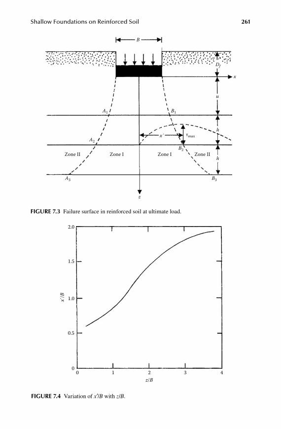
Shallow Foundations on Reinforced Soil 261
Zone II Zone II
τmax
Zone I Zone I
B
B1 A1
A2 x´
z
A3 B3
h
h
u
x
Df
B2
FiGure 7.3 Failure surface in reinforced soil at ultimate load.
2.0
1.5
1.0
0.5
x/B
00 1 2
z/B3 4
FiGure 7.4 Variation of x′/B with z/B.
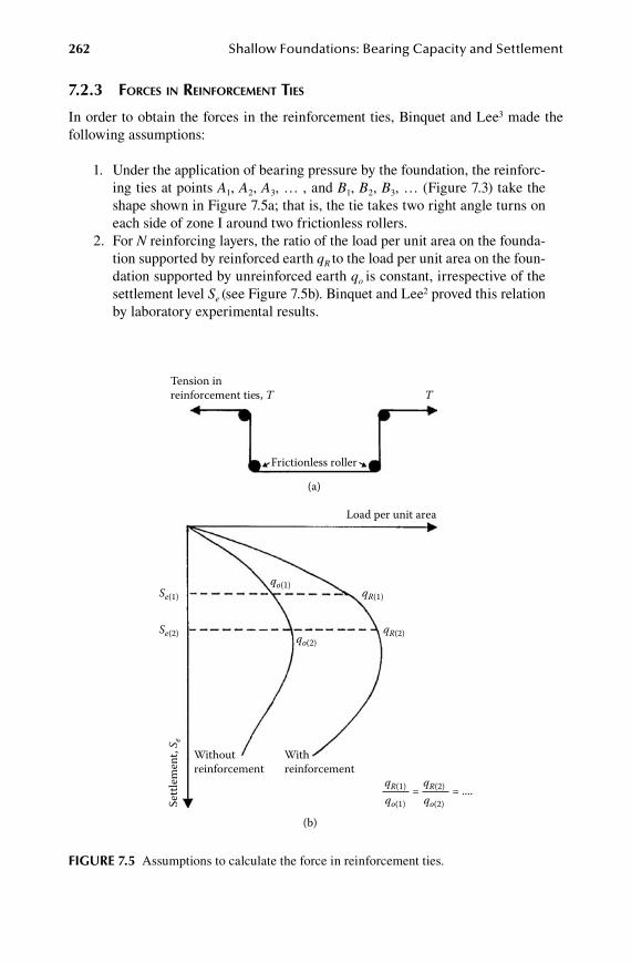
262 Shallow Foundations: Bearing Capacity and Settlement
7.2.3 foRCes in ReinfoRCement ties
In order to obtain the forces in the reinforcement ties, Binquet and Lee3 made the following assumptions:
1. Under the application of bearing pressure by the foundation, the reinforc-ing ties at points A1, A2, A3, … , and B1, B2, B3, … (Figure 7.3) take the shape shown in Figure 7.5a; that is, the tie takes two right angle turns on each side of zone I around two frictionless rollers.
2. For N reinforcing layers, the ratio of the load per unit area on the founda-tion supported by reinforced earth qR to the load per unit area on the foun-dation supported by unreinforced earth qo is constant, irrespective of the settlement level Se (see Figure 7.5b). Binquet and Lee2 proved this relation by laboratory experimental results.
Tension in reinforcement ties, T
Frictionless roller
Load per unit area
qo(1)
Without reinforcement
With reinforcement
= = ....
Se(1) qR(1)
qo(1)
qR(1)
Se(2)
Settl
emen
t, S e
qR(2) qo(2)
(a)
(b)
T
qo(2)
qR(2)
FiGure 7.5 Assumptions to calculate the force in reinforcement ties.
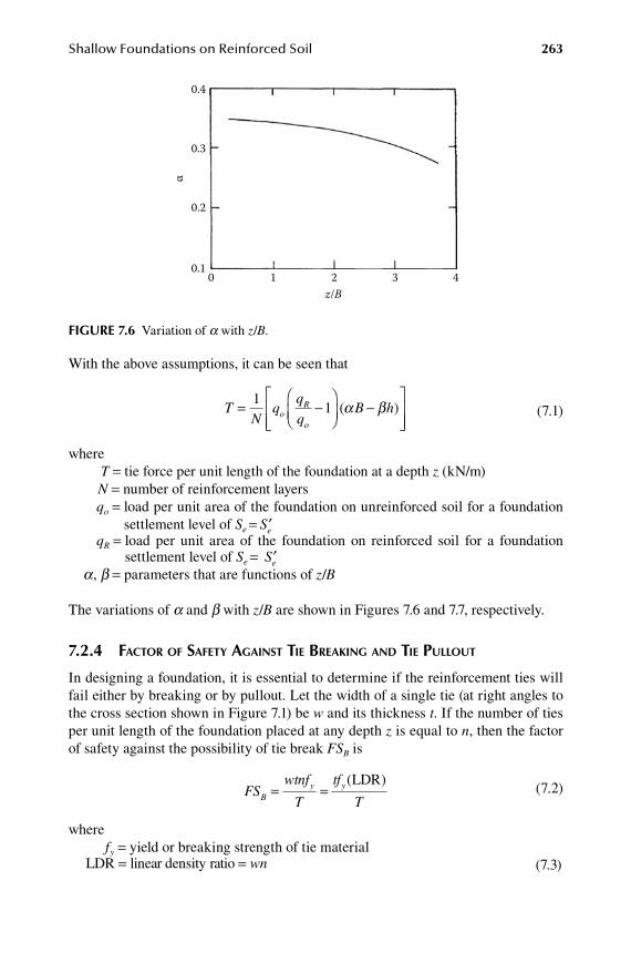
Shallow Foundations on Reinforced Soil 263
With the above assumptions, it can be seen that
TN
qB ho
R
o
= -
-
11 ( )α β (7.1)
whereT = tie force per unit length of the foundation at a depth z (kN/m)N = number of reinforcement layersqo = load per unit area of the foundation on unreinforced soil for a foundation
settlement level of Se = ′SeqR = load per unit area of the foundation on reinforced soil for a foundation
settlement level of Se = ′Se
a, b = parameters that are functions of z/B
The variations of a and b with z/B are shown in Figures 7.6 and 7.7, respectively.
7.2.4 faCtoR of safety against tie BReaking anD tie pUlloUt
In designing a foundation, it is essential to determine if the reinforcement ties will fail either by breaking or by pullout. Let the width of a single tie (at right angles to the cross section shown in Figure 7.1) be w and its thickness t. If the number of ties per unit length of the foundation placed at any depth z is equal to n, then the factor of safety against the possibility of tie break FSB is
FS
wtnf
T
tf
TBy y= =
( )LDR (7.2)
where fy = yield or breaking strength of tie materialLDR linear density ratio= = wn (7.3)
0.4
0.3
0.2
α
0.10 1 2
z/B3 4
FiGure 7.6 Variation of a with z/B.
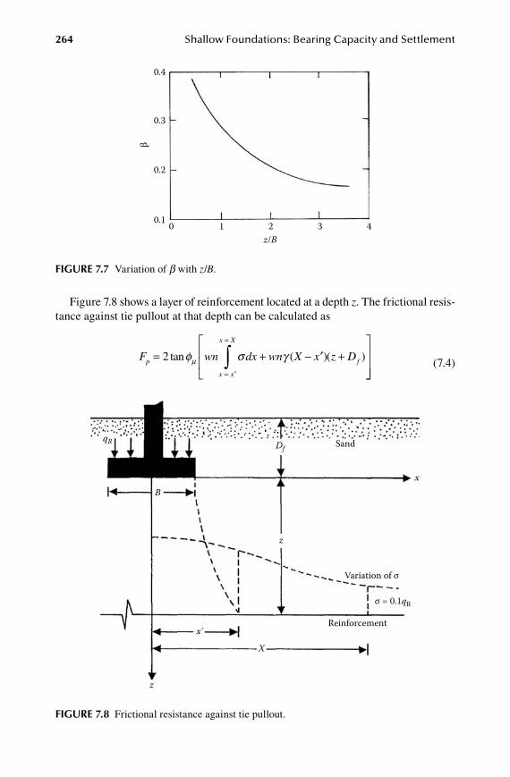
264 Shallow Foundations: Bearing Capacity and Settlement
Figure 7.8 shows a layer of reinforcement located at a depth z. The frictional resis-tance against tie pullout at that depth can be calculated as
F wn dx wn X x z Dp
x x
x X
f= + - ′ +
= ′
=
∫2 tan ( )( )φ σ γµ
(7.4)
0.4
0.3
0.2
β
0.1 0 1 2z/B
3 4
FiGure 7.7 Variation of b with z/B.
Variation of σ
Sand
Reinforcement
X
x B
z
z
x
σ = 0.1qR
qR Df
FiGure 7.8 Frictional resistance against tie pullout.
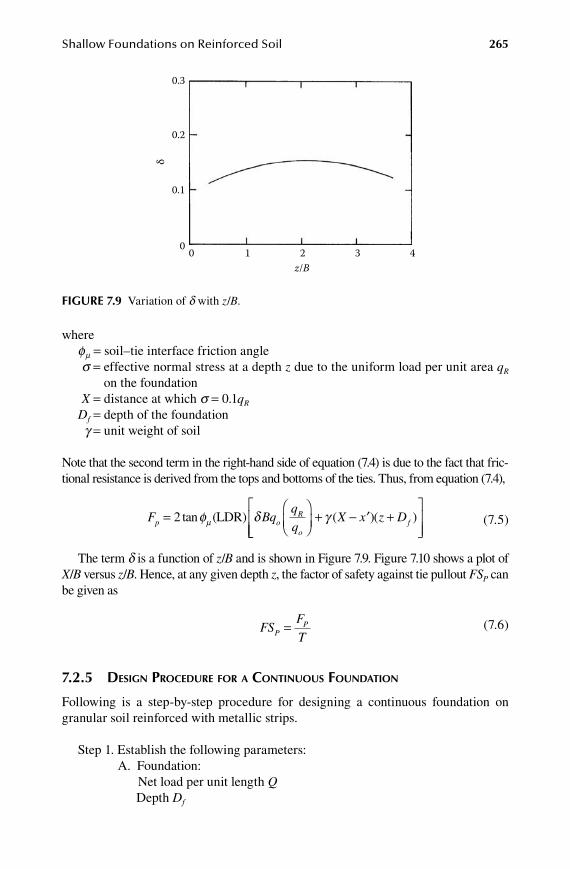
Shallow Foundations on Reinforced Soil 265
wheref m = soil–tie interface friction angle
s = effective normal stress at a depth z due to the uniform load per unit area qR on the foundation
X = distance at which s = 0.1qR
Df = depth of the foundationg = unit weight of soil
Note that the second term in the right-hand side of equation (7.4) is due to the fact that fric-tional resistance is derived from the tops and bottoms of the ties. Thus, from equation (7.4),
F Bqq
qX x z Dp o
R
of=
+ - ′ +
2 tan ( )( )φ δ γµ (LDR)
(7.5)
The term d is a function of z/B and is shown in Figure 7.9. Figure 7.10 shows a plot of X/B versus z/B. Hence, at any given depth z, the factor of safety against tie pullout FSP can be given as
FS
F
TPP= (7.6)
7.2.5 Design pRoCeDURe foR a ContinUoUs foUnDation
Following is a step-by-step procedure for designing a continuous foundation on granular soil reinforced with metallic strips.
Step 1. Establish the following parameters: A. Foundation:
Net load per unit length Q Depth Df
0.3
0.2
0.1
δ
0 0 1 2z/B
3 4
FiGure 7.9 Variation of d with z/B.
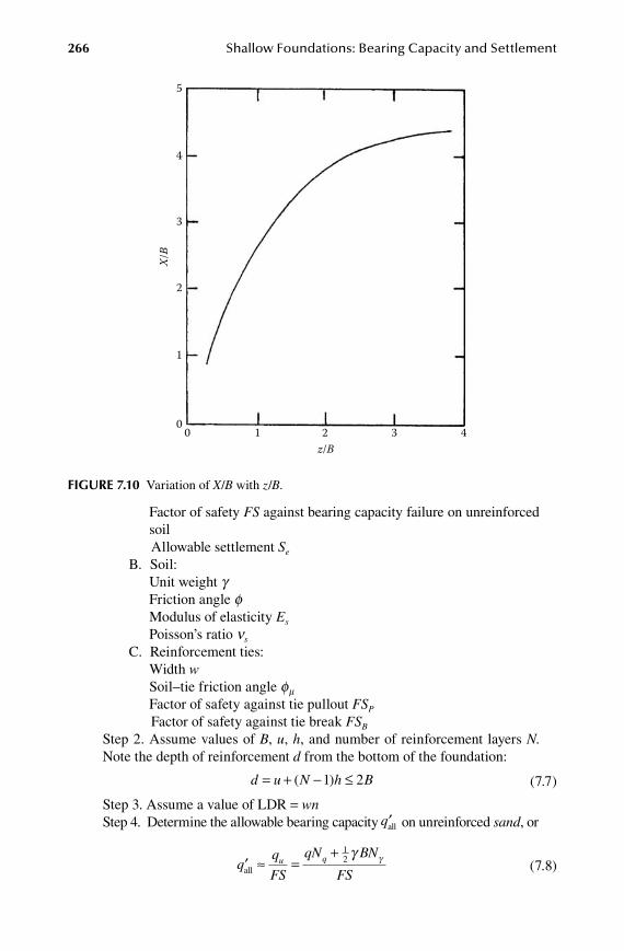
266 Shallow Foundations: Bearing Capacity and Settlement
Factor of safety FS against bearing capacity failure on unreinforced soil
Allowable settlement Se
B. Soil: Unit weight g Friction angle f Modulus of elasticity Es
Poisson’s ratio ns
C. Reinforcement ties: Width w Soil–tie friction angle f m Factor of safety against tie pullout FSP
Factor of safety against tie break FSB
Step 2. Assume values of B, u, h, and number of reinforcement layers N. Note the depth of reinforcement d from the bottom of the foundation:
d u N h B= + - ≤( )1 2 (7.7)
Step 3. Assume a value of LDR = wn Step 4. Determine the allowable bearing capacity ′qall on unreinforced sand, or
′ ≈ =
+q
q
FS
qN BN
FSu q
all
12 γ γ
(7.8)
5
4
3
X/B
2
1
00 1 2
z/B3 4
FiGure 7.10 Variation of X/B with z/B.

Shallow Foundations on Reinforced Soil 267
wherequ = ultimate bearing capacity on unreinforced soilq = gDf
Nq, Ng = bearing capacity factors (Table 2.3)
Step 5. Determine the allowable bearing capacity ′′qall based on allowable settlement as follows:
S q B
EIe
s(rigid) all= ′′ -( )1 2ν
or
′′ =
-q
E S
B Is e
all(rigid)
( )1 2ν (7.9)
The variation of I with L/B (L = length of foundation) is given in Table 7.1.Step 6. The smaller of the two allowable bearing capacities (that is, ′qall or ′′qall )
is equal to qo.Step 7. Calculate qR (load per unit area of the foundation on reinforced soil) as
q
QBR = (7.10)
Step 8. Calculate T for all layers of reinforcement using equation (7.1).Step 9. Calculate the magnitude of FP/T for each layer to see if FP/T ≥ FSP. If
FP/T < FSP, the length of the reinforcing strips may have to be increased by substituting X′ (>X) in equation (7.5) so that FP/T is equal to FSP.
Step 10. Use equation (7.2) to obtain the thickness of the reinforcement strips.Step 11. If the design is unsatisfactory, repeat steps 2 through 10.
table 7.1Variation of I with L/B
L/B I
1 0.8862 1.213 1.4094 1.5525 1.6636 1.7547 1.8318 1.8989 1.957
10 2.010
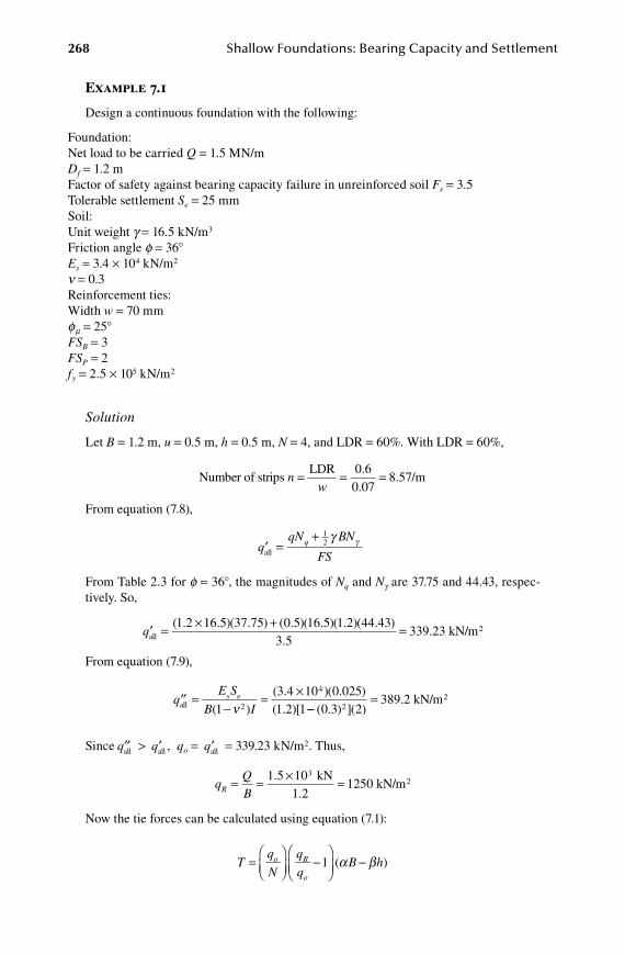
268 Shallow Foundations: Bearing Capacity and Settlement
Example 7.1
Design a continuous foundation with the following:
Foundation:Net load to be carried Q = 1.5 MN/mDf = 1.2 mFactor of safety against bearing capacity failure in unreinforced soil Fs = 3.5Tolerable settlement Se = 25 mmSoil:Unit weight g = 16.5 kN/m3
Friction angle f = 36°Es = 3.4 × 10⁴ kN/m2
n = 0.3Reinforcement ties:Width w = 70 mmf m = 25°FSB = 3FSP = 2fy = 2.5 × 10⁵ kN/m2
Solution
Let B = 1.2 m, u = 0.5 m, h = 0.5 m, N = 4, and LDR = 60%. With LDR = 60%,
Number of strips
LDRmn
w= = =0 6
0 078 57
..
. /
From equation (7.8),
′ =
+q
qN BN
FSq
all
12 γ γ
From Table 2.3 for f = 36°, the magnitudes of Nq and Ng are 37.75 and 44.43, respec-tively. So,
′ = × +
qall
( . . )( . ) ( . )( . )( . )(1 2 16 5 37 75 0 5 16 5 1 2 44. ).
433 5
= 339.23 kN/m2
From equation (7.9),
′′ =
-= ×
qE S
B Is e
all ( )( . )( . )( . )[13 4 10 0 0251 2 12
4
ν --=
( . ) ]( )0 3 22389.2 kN/m2
Since ′′qall > ′qall , qo = ′qall = 339.23 kN/m2. Thus,
q
QBR = = × =1 5 103. kN
1.21250 kN/m2
Now the tie forces can be calculated using equation (7.1):
T
q
N
q
qB ho R
o
=
-
-1 ( )α β

Shallow Foundations on Reinforced Soil 269
layer no.qN
o R
o
-
1
z (m) z/B aB − bh T (kn/m)
1 227.7 0.5 0.47 0.285 64.89 2 227.7 1.0 0.83 0.300 68.31 3 227.7 1.5 1.25 0.325 74.00 4 227.7 2.0 1.67 0.330 75.14
Note: B = 1.2 m; a from Figure 7.6; b from Figure 7.7; h = 0.5 m.
The magnitudes of FP/T for each layer are calculated in the following table. From equa-tions (7.5) and (7.6),
F
T TBq
q
qX x z Dp
oR
of=
+ - ′ +
2 tan( )(
φδ γµ (LDR)
))
layer
parameter 1 2 3 4
2tanφµ (LDR)(m/kN)
T0.0086 0.0082 0.0076 0.0075
z/B 0.47 0.83 1.25 1.67
d 0.12 0.14 0.15 0.16
δ Bqq
qoR
o
(kN/m) 180 210 225 240
X/B 1.4 2.3 3.2 3.6X (m) 1.68 2.76 3.84 4.32
x′/B 0.7 0.8 1.0 1.3
x′ (m) 0.84 0.96 1.2 1.56
γ ( )( )X x z Df
- ′ + (kN/m) 23.56 65.34 117.6 145.7FP/T 1.75 2.26 2.6 2.89
The minimum factor of safety FSP required is two. In all layers except layer 1, FP/T is greater than two. So we need to find a new value of x = X′ so that FP/T is equal to two. So, for layer 1,
F
T TBq
q
qX x z Dp
oR
of=
+ - ′ +
2 tan( )(
φδ γµ (LDR)
))
or
2 0 0086 180 16 5 0 84 0 5 1 2 2= + ′ - + ′ =. [ . ( . )( . . )]; .X X 771 m
Tie thickness t:
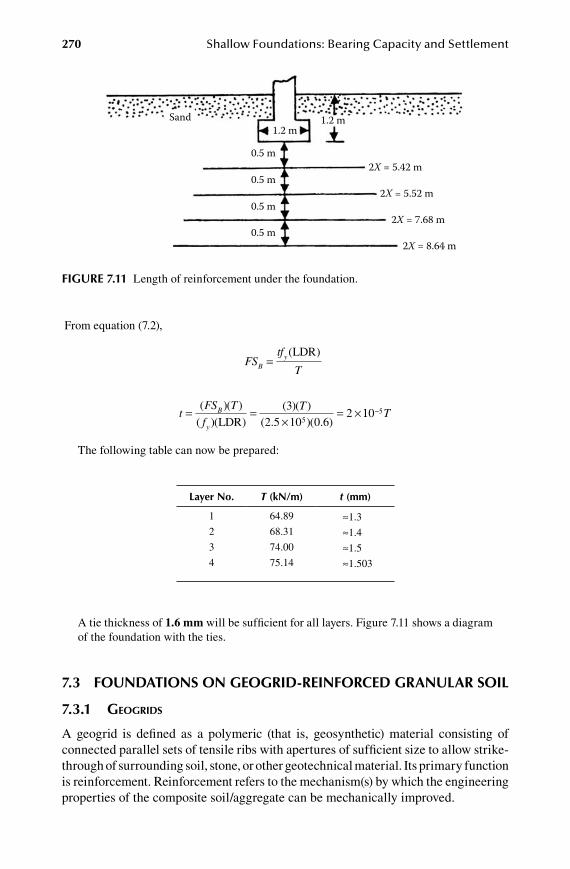
270 Shallow Foundations: Bearing Capacity and Settlement
From equation (7.2),
FS
tf
TBy=( )LDR
t
FS T
fTB
y
= =×
= ×( )( )
( )( )( )( )
( . )( . )LDR3
2 5 10 0 62
5110 5- T
The following table can now be prepared:
layer no. T (kn/m) t (mm)
1 64.89 ≈1.32 68.31 ≈1.43 74.00 ≈1.54 75.14 ≈1.503
A tie thickness of 1.6 mm will be sufficient for all layers. Figure 7.11 shows a diagram of the foundation with the ties.
7.3 FoundationS on GeoGrid-reinForCed Granular Soil
7.3.1 geogRiDs
A geogrid is defined as a polymeric (that is, geosynthetic) material consisting of connected parallel sets of tensile ribs with apertures of sufficient size to allow strike-through of surrounding soil, stone, or other geotechnical material. Its primary function is reinforcement. Reinforcement refers to the mechanism(s) by which the engineering properties of the composite soil/aggregate can be mechanically improved.
Sand1.2 m
1.2 m
0.5 m2X = 5.42 m
2X = 5.52 m
2X = 7.68 m
2X = 8.64 m
0.5 m
0.5 m
0.5 m
FiGure 7.11 Length of reinforcement under the foundation.
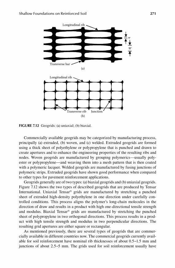
Shallow Foundations on Reinforced Soil 271
Commercially available geogrids may be categorized by manufacturing process, principally (a) extruded, (b) woven, and (c) welded. Extruded geogrids are formed using a thick sheet of polyethylene or polypropylene that is punched and drawn to create apertures and to enhance the engineering properties of the resulting ribs and nodes. Woven geogrids are manufactured by grouping polymerics—usually poly-ester or polypropylene—and weaving them into a mesh pattern that is then coated with a polymeric lacquer. Welded geogrids are manufactured by fusing junctions of polymeric strips. Extruded geogrids have shown good performance when compared to other types for pavement reinforcement applications.
Geogrids generally are of two types: (a) biaxial geogrids and (b) uniaxial geogrids. Figure 7.12 shows the two types of described geogrids that are produced by Tensar International. Uniaxial Tensar grids are manufactured by stretching a punched sheet of extruded high-density polyethylene in one direction under carefully con-trolled conditions. This process aligns the polymer’s long-chain molecules in the direction of draw and results in a product with high one-directional tensile strength and modulus. Biaxial Tensar grids are manufactured by stretching the punched sheet of polypropylene in two orthogonal directions. This process results in a prod-uct with high tensile strength and modulus in two perpendicular directions. The resulting grid apertures are either square or rectangular.
As mentioned previously, there are several types of geogrids that are commer-cially available in different countries now. The commercial geogrids currently avail-able for soil reinforcement have nominal rib thicknesses of about 0.5−1.5 mm and junctions of about 2.5−5 mm. The grids used for soil reinforcement usually have
Transverse bar
W
w
Transverse rib Junction
(a)
(b)
Longitudinal rib
Longitudinal rib
FiGure 7.12 Geogrids: (a) uniaxial; (b) biaxial.

272 Shallow Foundations: Bearing Capacity and Settlement
apertures that are rectangular or elliptical in shape. The dimensions of the apertures vary from about 25 to 160 mm. Geogrids are manufactured so that the open areas of the grids are greater than 50% of the total area. They develop reinforcing strength at low strain levels (such as 2%). Table 7.2 gives some properties of the Tensar biaxial geogrids that are currently available commercially.
7.3.2 geneRal paRameteRs
Since the mid-1980s, a number of laboratory model studies have been reported relating to the evaluation of the ultimate and allowable bearing capacities of shal-low foundations supported by soil reinforced with multiple layers of geogrids. The results obtained so far seem promising. The general parameters of the problem are defined in this section.
Figure 7.13 shows the general parameters of a rectangular surface foundation on a soil layer reinforced with several layers of geogrids. The size of the foundation is B × L (width × length) and the size of the geogrid layers is b × l (width × length). The first layer of geogrid is located at a depth u below the foundation, and the vertical distance between consecutive layers of geogrids is h. The total depth of reinforce-ment d can be given as
d u N h= + -( )1 (7.11)
whereN = number of reinforcement layers
The beneficial effects of reinforcement to increase the bearing capacity can be expressed in terms of a nondimensional parameter called the bearing capacity ratio
table 7.2properties of tensar biaxial Geogrids
Geogrid
property bX1100 bX1200 bX1300
Aperture size Machine direction 25 mm (nominal) 25 mm (nominal) 46 mm (nominal) Cross-machine direction 33 mm (nominal) 33 mm (nominal) 64 mm (nominal) Open area 70% (minimum) 70% (minimum) 75% (minimum) Junction thickness 2.9 mm (nominal) 4.0 mm (nominal) 4.4 mm (nominal)
Tensile modulus Machine direction 205 kN/m (nominal) 300 kN/m (nominal) 275 kN/m (nominal) Cross-machine direction 330 kN/m (nominal) 450 kN/m (nominal) 475 kN/m (nominal)
Material Polypropylene 99% (minimum) 99% (minimum) 98% (minimum) Carbon black 0.5% (minimum) 0.5% (minimum) 1.3% (minimum)
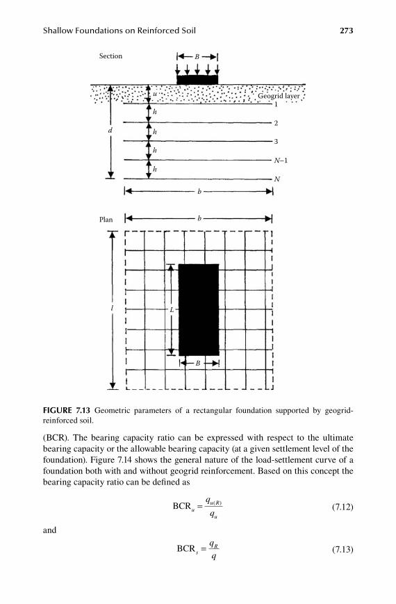
Shallow Foundations on Reinforced Soil 273
(BCR). The bearing capacity ratio can be expressed with respect to the ultimate bearing capacity or the allowable bearing capacity (at a given settlement level of the foundation). Figure 7.14 shows the general nature of the load-settlement curve of a foundation both with and without geogrid reinforcement. Based on this concept the bearing capacity ratio can be defined as
BCRu
u R
u
q
q= ( )
(7.12)
and
BCRs
Rq
q= (7.13)
B
d
u
h
h
h
h N
N–1
3
2
1 Geogrid layer
b
b
l L
B
Section
Plan
FiGure 7.13 Geometric parameters of a rectangular foundation supported by geogrid- reinforced soil.
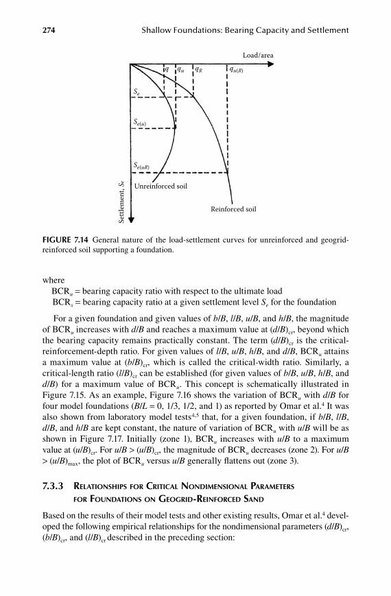
274 Shallow Foundations: Bearing Capacity and Settlement
whereBCRu = bearing capacity ratio with respect to the ultimate loadBCRs = bearing capacity ratio at a given settlement level Se for the foundation
For a given foundation and given values of b/B, l/B, u/B, and h/B, the magnitude of BCRu increases with d/B and reaches a maximum value at (d/B)cr, beyond which the bearing capacity remains practically constant. The term (d/B)cr is the critical-reinforcement-depth ratio. For given values of l/B, u/B, h/B, and d/B, BCRu attains a maximum value at (b/B)cr, which is called the critical-width ratio. Similarly, a critical-length ratio (l/B)cr can be established (for given values of b/B, u/B, h/B, and d/B) for a maximum value of BCRu. This concept is schematically illustrated in Figure 7.15. As an example, Figure 7.16 shows the variation of BCRu with d/B for four model foundations (B/L = 0, 1/3, 1/2, and 1) as reported by Omar et al.4 It was also shown from laboratory model tests4,5 that, for a given foundation, if b/B, l/B, d/B, and h/B are kept constant, the nature of variation of BCRu with u/B will be as shown in Figure 7.17. Initially (zone 1), BCRu increases with u/B to a maximum value at (u/B)cr. For u/B > (u/B)cr, the magnitude of BCRu decreases (zone 2). For u/B > (u/B)max, the plot of BCRu versus u/B generally flattens out (zone 3).
7.3.3 Relationships foR CRitiCal nonDimensional paRameteRs foR foUnDations on geogRiD-ReinfoRCeD sanD
Based on the results of their model tests and other existing results, Omar et al.4 devel-oped the following empirical relationships for the nondimensional parameters (d/B)cr, (b/B)cr, and (l/B)cr described in the preceding section:
Se
qu q qR qu(R)
Load/area
Se(u)
Se(uR)
Unreinforced soil
Settl
emen
t, Se
Reinforced soil
FiGure 7.14 General nature of the load-settlement curves for unreinforced and geogrid-reinforced soil supporting a foundation.

Shallow Foundations on Reinforced Soil 275
6
5
4
3
2
1 0 0.50 1.00 1.50
d/B
(d/B)cr
BCR u
B/L = 1
0.5
TENSAR BX 1100 geogridφ = 41°Relative density of sand = 70%Df = 0
0.333 0
2.00 2.33
FiGure 7.16 Variation of BCRu with d/B. Source: Based on the results of Omar, M. T., B. M. Das, S. C. Yen, V. K. Puri, and E. E. Cook. 1993. Ultimate bearing capacity of rectangular foundations on geogrid-reinforced sand. Geotech. Testing J., ASTM, 16(2): 246.
d/B, b/B, l/B
b/B, l/B, u/B, h/B constant
l/B, u/B, h/B, d/B constant
b/B, u/B, h/B, d/B constant
(d/B)cr
(b/B)cr
(l/B)cr
BCR u
FiGure 7.15 Definition of critical nondimensional parameters—(d/B)cr, (b/B)cr, and (l/B)cr .
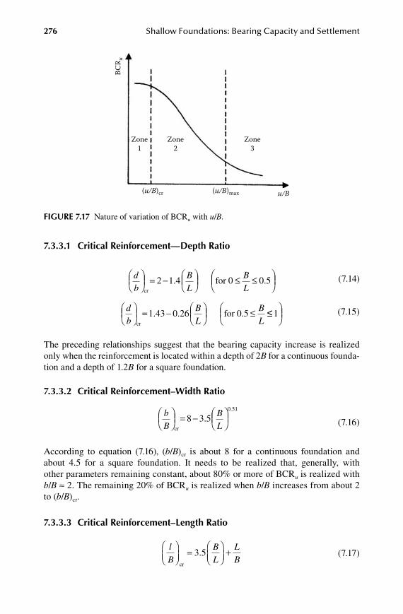
276 Shallow Foundations: Bearing Capacity and Settlement
7.3.3.1 Critical reinforcement—depth ratio
db
BL
BL
= -
≤ ≤
cr
for 02 1 4 0 5. . (7.14)
db
BL
BL
= -
≤
cr
for 0.51 43 0 26. . ≤≤
1 (7.15)
The preceding relationships suggest that the bearing capacity increase is realized only when the reinforcement is located within a depth of 2B for a continuous founda-tion and a depth of 1.2B for a square foundation.
7.3.3.2 Critical reinforcement–width ratio
bB
BL
= -
cr
0.51
8 3 5. (7.16)
According to equation (7.16), (b/B)cr is about 8 for a continuous foundation and about 4.5 for a square foundation. It needs to be realized that, generally, with other parameters remaining constant, about 80% or more of BCRu is realized with b/B ≈ 2. The remaining 20% of BCRu is realized when b/B increases from about 2 to (b/B)cr.
7.3.3.3 Critical reinforcement–length ratio
lB
BL
LB
=
+cr
3 5. (7.17)
BCR u
(u/B)cr (u/B)max u/B
Zone1
Zone2
Zone3
FiGure 7.17 Nature of variation of BCRu with u/B.

Shallow Foundations on Reinforced Soil 277
7.3.3.4 Critical Value of u/B
Figure 7.18 shows the laboratory model test results of Guido et al.,5 Akinmusuru and Akinbolade6 and Yetimoglu et al.7 for bearing capacity tests conducted on surface foundations supported by multi-layered reinforced sand. Details of these tests are given in Table 7.3. Based on the definition given in Figure 7.17, it appears from these test results that (u/B)max ≈ 0.9 to 1. From Figure 7.18 it may also be seen that (u/B)cr as defined by Figure 7.17 is about 0.25 to 0.5. An analysis of the test results of Schlosser et al.8 yields a value of (u/B)cr ≈ 0.4. Large-scale model tests by Adams and Collin9 showed that (u/B)cr is approximately 0.25.
table 7.3details of test parameters for plots Shown in Figure 7.18
Curve investigatortype of model
Foundationtype
of reinforcementparametric
details
1 Guido et al.5 Square Tensar BX1100 h/B = 0.25;2 Guido et al.5 Square Tensar BX1200 b/B = 3;3 Guido et al.5 Square Tensar BX1300 N = 34 Akinmusuru and
Akinbolade6
Square Rope fibers h/B = 0.5;b/B = 3; N = 5
5 Yetimoglu et al.7 Rectangular; B/L = 8;L = length of foundation
Terragrid GS100 b/B = 4; N = 1
6 Yetimoglu et al.7 Rectangular; B/L = 8;L = length of foundation
Terragrid GS100 h/B = 0.3;b/B = 4.5; N = 4
3.5
3.06
12
34
5
2.0
1.00 0.5
u/B1.0 1.5
BCR u
FiGure 7.18 Variation of BCRu with u/B from various published works (see Table 7.3 for details).

278 Shallow Foundations: Bearing Capacity and Settlement
7.3.4 BCRu foR foUnDations with Depth of foUnDation Df gReateR than ZeRo
To the best of the author’s knowledge, the only tests for bearing capacity of shallow foundations with Df > 0 are those reported by Shin and Das.10 These results were for laboratory model tests on a strip foundation in sand. The physical properties of the geogrid used in these tests are given in Table 7.4.
The model tests were conducted with d/B from 0 to 2.4, u/B = 0.4, h/B = 0.4, and b/B = 6 [≈ (b/B)cr]. The sand had relative densities Dr of 59% and 74%, and Df/B was varied from 0 to 0.75. The variation of BCRu with d/B, Df/B, and Dr is shown in Figure 7.19. From this figure the following observations can be made:
1. For all values of Df/B and Dr, the magnitude of (d/B)cr is about two for strip foundations.
2. For given b/B, Dr, u/B, and h/B, the magnitude of BCRu increases with Df/B.
Based on their laboratory model test results, Das and Shin10 have shown that the ratio of BCRs:BCRu for strip foundations has an approximate relationship with the embed-ment ratio (Df:B) for a settlement ratio Se:B less than or equal to 5%. This relationship is shown in Figure 7.20 and is valid for any values of d/B and b/B. The definition of BCRs was given in equation (7.13).
7.3.4.1 Settlement at ultimate load
As shown in Figure 7.14, a foundation supported by geogrid-reinforced sand shows a greater level of settlement at ultimate load qu(R). Huang and Hong11 analyzed the laboratory test results of Huang and Tatsuoka,12 Takemura et al.,13 Khing et al.,14 and
table 7.4physical properties of the Geogrid used by Shin and das for the results Shown in Figure 7.19
physical property Value
Polymer type PolypropyleneStructure BiaxialMass per unit area 320 g/m2
Aperture size 41 mm (MD) × 31 mm (CMD)Maximum tensile strength 14.5 kN/m (MD) × 20.5 kN/m (CMD)Tensile strength at 5% strain 5.5 kN/m (MD) × 16.0 kN/m (CMD)
Source: Shin, E. C., and B. M. Das. 2000. Experimental study of bearing capacity of a strip foundation on geogrid-reinforced sand. Geosynthetics Intl. 7(1): 59.
Note: CMD, cross-machine direction; MD, machine direction.
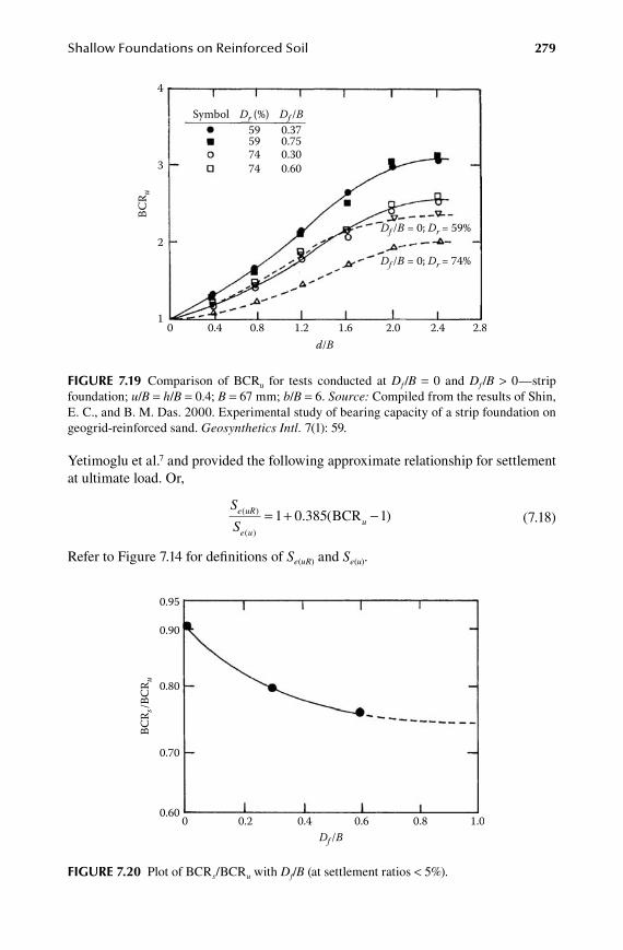
Shallow Foundations on Reinforced Soil 279
Yetimoglu et al.7 and provided the following approximate relationship for settlement at ultimate load. Or,
S
Se uR
e uu
( )
( )
. ( )= + -1 0 385 1BCR (7.18)
Refer to Figure 7.14 for definitions of Se(uR) and Se(u).
BCR u
4
Symbol Dr (%) Df /B59 0.3759 0.7574 0.3074 0.603
2
10 0.4 0.8 1.2 1.6 2.0
Df /B = 0; Dr = 74%
Df /B = 0; Dr = 59%
2.4 2.8d/B
FiGure 7.19 Comparison of BCRu for tests conducted at Df /B = 0 and Df /B > 0—strip foundation; u/B = h/B = 0.4; B = 67 mm; b/B = 6. Source: Compiled from the results of Shin, E. C., and B. M. Das. 2000. Experimental study of bearing capacity of a strip foundation on geogrid-reinforced sand. Geosynthetics Intl. 7(1): 59.
0.95
0.90
0.80
0.70
0.600 0.2 0.4 0.6
Df /B
BCR s
/BCR
u
0.8 1.0
FiGure 7.20 Plot of BCRs/BCRu with Df/B (at settlement ratios < 5%).
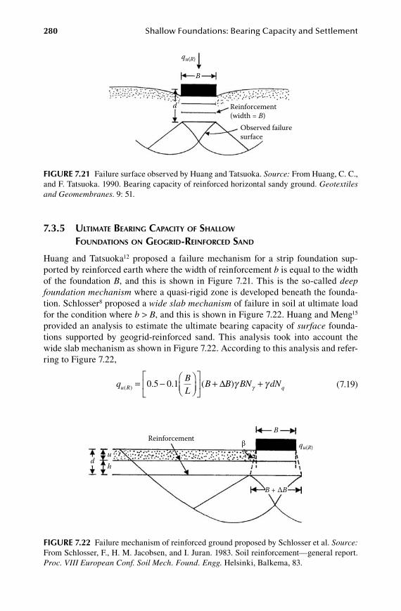
280 Shallow Foundations: Bearing Capacity and Settlement
7.3.5 Ultimate BeaRing CapaCity of shallow foUnDations on geogRiD-ReinfoRCeD sanD
Huang and Tatsuoka12 proposed a failure mechanism for a strip foundation sup-ported by reinforced earth where the width of reinforcement b is equal to the width of the foundation B, and this is shown in Figure 7.21. This is the so-called deep foundation mechanism where a quasi-rigid zone is developed beneath the founda-tion. Schlosser8 proposed a wide slab mechanism of failure in soil at ultimate load for the condition where b > B, and this is shown in Figure 7.22. Huang and Meng15 provided an analysis to estimate the ultimate bearing capacity of surface founda-tions supported by geogrid-reinforced sand. This analysis took into account the wide slab mechanism as shown in Figure 7.22. According to this analysis and refer-ring to Figure 7.22,
qBL
B B BN dNu R q( ) . . ( )= -
+ +0 5 0 1 ∆ γ γγ (7.19)
qu(R)
B
Reinforcement(width = B)
Observed failuresurface
d
FiGure 7.21 Failure surface observed by Huang and Tatsuoka. Source: From Huang, C. C., and F. Tatsuoka. 1990. Bearing capacity of reinforced horizontal sandy ground. Geotextiles and Geomembranes. 9: 51.
ReinforcementB
duh
qu(R)β
B + ∆B
FiGure 7.22 Failure mechanism of reinforced ground proposed by Schlosser et al. Source: From Schlosser, F., H. M. Jacobsen, and I. Juran. 1983. Soil reinforcement—general report. Proc. VIII European Conf. Soil Mech. Found. Engg. Helsinki, Balkema, 83.
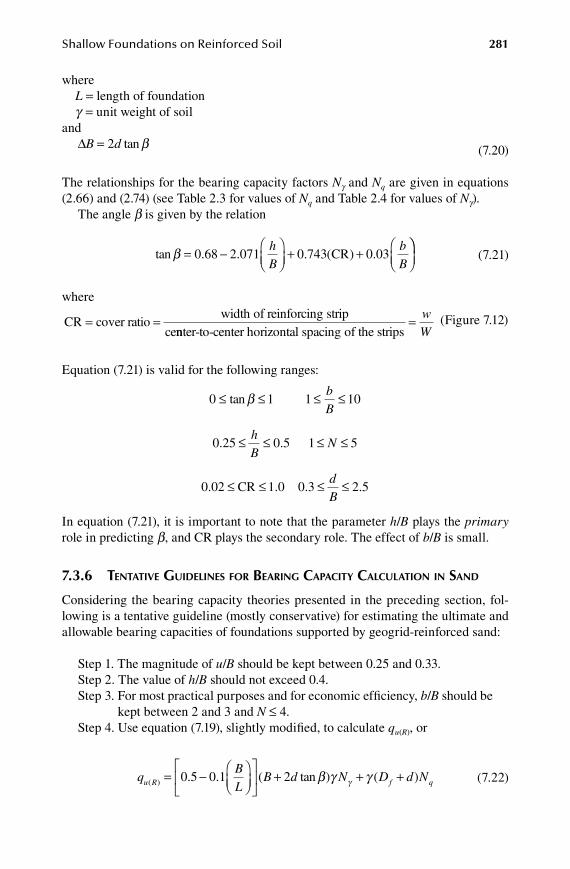
Shallow Foundations on Reinforced Soil 281
whereL = length of foundationg = unit weight of soil
and∆B d= 2 tan β (7.20)
The relationships for the bearing capacity factors Ng and Nq are given in equations (2.66) and (2.74) (see Table 2.3 for values of Nq and Table 2.4 for values of Ng).
The angle b is given by the relation
tan . . . ( ) .β = -
+ +
0 68 2 071 0 743 0 03hB
bB
CR
(7.21)
where
CR cover ratiowidth of reinforcing strip
ce= =
nnter-to-center horizontal spacing of the strips= w
W (Figure 7.12)
Equation (7.21) is valid for the following ranges:
0 1 1 10≤ ≤ ≤ ≤tan β b
B
0 25 0 5 1 5. .≤ ≤ ≤ ≤h
BN
0 02 1 0 0 3 2 5. . . .≤ ≤ ≤ ≤CR
dB
In equation (7.21), it is important to note that the parameter h/B plays the primary role in predicting b, and CR plays the secondary role. The effect of b/B is small.
7.3.6 tentative gUiDelines foR BeaRing CapaCity CalCUlation in sanD
Considering the bearing capacity theories presented in the preceding section, fol-lowing is a tentative guideline (mostly conservative) for estimating the ultimate and allowable bearing capacities of foundations supported by geogrid-reinforced sand:
Step 1. The magnitude of u/B should be kept between 0.25 and 0.33.Step 2. The value of h/B should not exceed 0.4.Step 3. For most practical purposes and for economic efficiency, b/B should be
kept between 2 and 3 and N ≤ 4.Step 4. Use equation (7.19), slightly modified, to calculate qu(R), or
qBL
B d Nu R( ) . . ( tan ) (= -
+ +0 5 0 1 2 β γ γγ D d Nf q+ ) (7.22)
282 Shallow Foundations: Bearing Capacity and Settlement
where
β ≈ -
+ +-tan . . .1 0 68 2 071 0 743
hB
bB
(CR) 0.03
(7.23)
Step 5. For determining qR at Se/B ≤ 5%, a. Calculation of BCRu = qu(R)/qu. The relationship for qu(R) is given in
equation (7.22). Also,
qBL
B N D Nu f q= -
+0 5 0 1. . γ γγ (7.24)
b. With known values of Df /B and using Figure 7.20, obtain BCRs/BCRu.
c. From steps a and b, obtain BCRs = qR/q. d. Estimate q from the relationships given in equations (5.43) and (5.44)
as
qS N
D
B
S N
De
f
e=
-
=-
60 60
1 25 14
0 8
1.
.
ff
B
B
4
≤(for 1.22 m) (7.25)
and
qS N
D
B
BB
e
f
=
-
+
=60
2
2 14
0 3 0. . .5
14
0 360S N
D
B
BB
Be
f-
+
>2
(for 1.22 m) (7.26)
whereq is in kN/m2, Se is in mm, Df and B are in mN60 = average field standard penetration number
e. Calculate qR = q(BCRs)
7.3.7 BeaRing CapaCity of eCCentRiCally loaDeD stRip foUnDation
Patra et al.16 conducted several model tests in the laboratory to determine the ulti-mate bearing capacity of eccentrically loaded strip foundations. The width of the foundation B was 80 mm for these tests. For geogrid reinforcement, u/B, h/B, and b/B were kept equal to 0.35, 0.25, and 5, respectively. The relative density of sand was 72% for all tests. Based on these test results, it was proposed that
q
qRu R e
u RKR
( )
( )
- = -1 (7.27)
where qu(R)−e and qu(R) = ultimate bearing capacity with load eccentricities e > 0 and
e = 0, respectively RKR = reduction factor
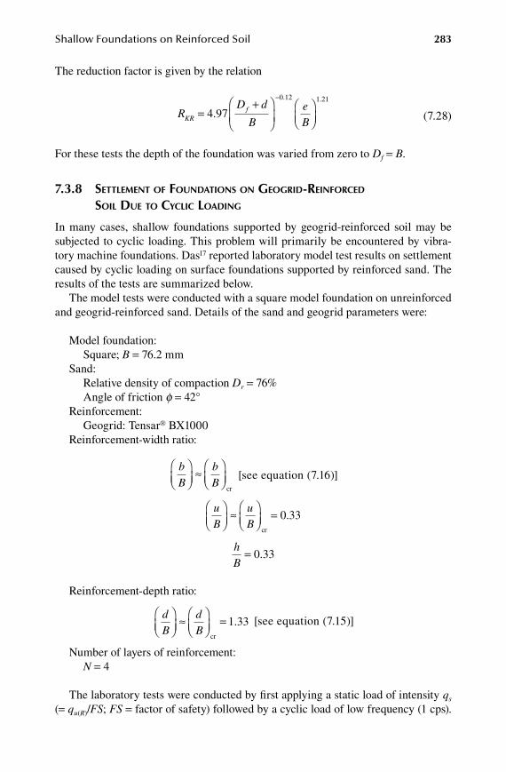
Shallow Foundations on Reinforced Soil 283
The reduction factor is given by the relation
RD d
BeBKR
f=+
-
4 97
0 12 1 21
.
. .
(7.28)
For these tests the depth of the foundation was varied from zero to Df = B.
7.3.8 settlement of foUnDations on geogRiD-ReinfoRCeD soil DUe to CyCliC loaDing
In many cases, shallow foundations supported by geogrid-reinforced soil may be subjected to cyclic loading. This problem will primarily be encountered by vibra-tory machine foundations. Das17 reported laboratory model test results on settlement caused by cyclic loading on surface foundations supported by reinforced sand. The results of the tests are summarized below.
The model tests were conducted with a square model foundation on unreinforced and geogrid-reinforced sand. Details of the sand and geogrid parameters were:
Model foundation:Square; B = 76.2 mm
Sand:Relative density of compaction Dr = 76%Angle of friction f = 42°
Reinforcement:Geogrid: Tensar BX1000
Reinforcement-width ratio:
bB
bB
≈
cr [see equation (7.16)]
uB
uB
≈
=cr
0 33.
hB
= 0 33.
Reinforcement-depth ratio:
dB
dB
≈
=cr
1 33. [see equation (7.15)]
Number of layers of reinforcement:N = 4
The laboratory tests were conducted by first applying a static load of intensity qs (= qu(R)/FS; FS = factor of safety) followed by a cyclic load of low frequency (1 cps).
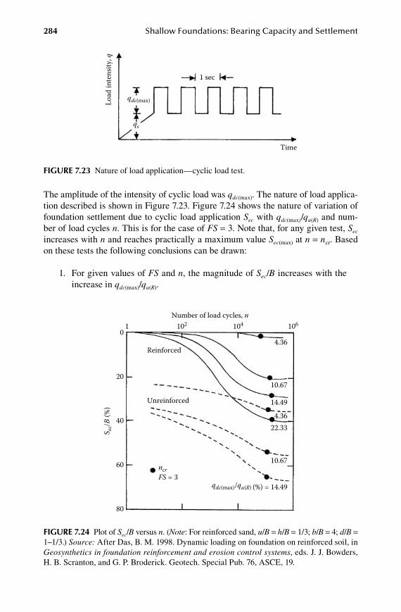
284 Shallow Foundations: Bearing Capacity and Settlement
The amplitude of the intensity of cyclic load was qdc(max). The nature of load applica-tion described is shown in Figure 7.23. Figure 7.24 shows the nature of variation of foundation settlement due to cyclic load application Sec with qdc(max)/qu(R) and num-ber of load cycles n. This is for the case of FS = 3. Note that, for any given test, Sec increases with n and reaches practically a maximum value Sec(max) at n = ncr. Based on these tests the following conclusions can be drawn:
1. For given values of FS and n, the magnitude of Sec/B increases with the increase in qdc(max)/qu(R).
1 sec
Time
qdc(max)
qs
Load
inte
nsity
, q
FiGure 7.23 Nature of load application—cyclic load test.
01 102
Number of load cycles, n
Reinforced
Unreinforced
ncrFS = 3
104 106
20
40
S ec/B
(%)
60
80
qdc(max)/qu(R) (%) = 14.49
10.67
22.334.36
4.36
14.49
10.67
FiGure 7.24 Plot of Sec/B versus n. (Note: For reinforced sand, u/B = h/B = 1/3; b/B = 4; d/B = 1−1/3.) Source: After Das, B. M. 1998. Dynamic loading on foundation on reinforced soil, in Geosynthetics in foundation reinforcement and erosion control systems, eds. J. J. Bowders, H. B. Scranton, and G. P. Broderick. Geotech. Special Pub. 76, ASCE, 19.
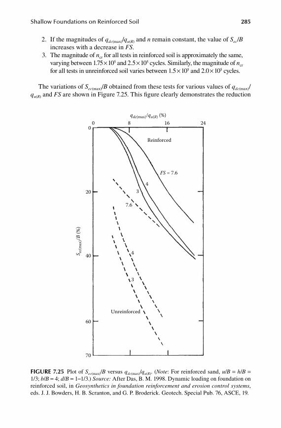
Shallow Foundations on Reinforced Soil 285
2. If the magnitudes of qdc(max)/qu(R) and n remain constant, the value of Sec/B increases with a decrease in FS.
3. The magnitude of ncr for all tests in reinforced soil is approximately the same, varying between 1.75 × 10⁵ and 2.5 × 10⁵ cycles. Similarly, the magnitude of ncr for all tests in unreinforced soil varies between 1.5 × 10⁵ and 2.0 × 10⁵ cycles.
The variations of Sec(max)/B obtained from these tests for various values of qdc(max)/qu(R) and FS are shown in Figure 7.25. This figure clearly demonstrates the reduction
00 8
qdc(max)/qu(R) (%)16 24
20
40S ec(
max
)/B (%
)
60
70
Unreinforced
3
4
7.6
Reinforced
34
FS = 7.6
FiGure 7.25 Plot of Sec(max)/B versus qdc(max)/qu(R). (Note: For reinforced sand, u/B = h/B = 1/3; b/B = 4; d/B = 1−1/3.) Source: After Das, B. M. 1998. Dynamic loading on foundation on reinforced soil, in Geosynthetics in foundation reinforcement and erosion control systems, eds. J. J. Bowders, H. B. Scranton, and G. P. Broderick. Geotech. Special Pub. 76, ASCE, 19.
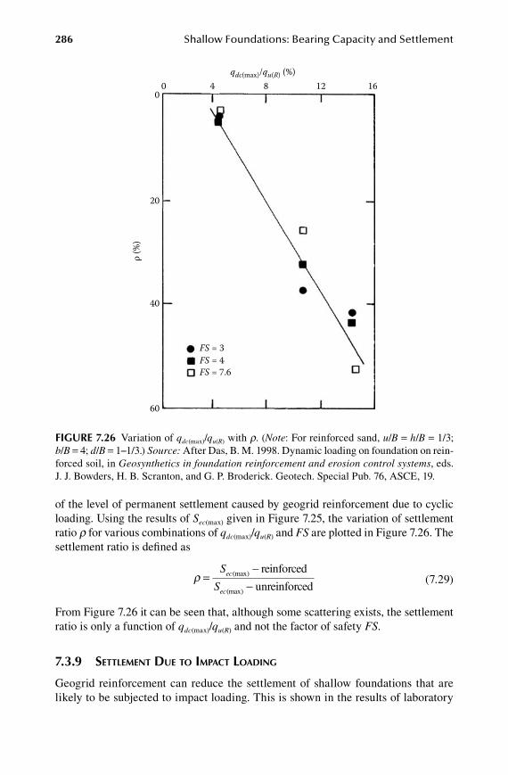
286 Shallow Foundations: Bearing Capacity and Settlement
of the level of permanent settlement caused by geogrid reinforcement due to cyclic loading. Using the results of Sec(max) given in Figure 7.25, the variation of settlement ratio r for various combinations of qdc(max)/qu(R) and FS are plotted in Figure 7.26. The settlement ratio is defined as
ρ =-
-S
Sec
ec
(max)
(max)
reinforced
unreinforced (7.29)
From Figure 7.26 it can be seen that, although some scattering exists, the settlement ratio is only a function of qdc(max)/qu(R) and not the factor of safety FS.
7.3.9 settlement DUe to impaCt loaDing
Geogrid reinforcement can reduce the settlement of shallow foundations that are likely to be subjected to impact loading. This is shown in the results of laboratory
00 84
qdc(max)/qu(R) (%)1612
20
40
ρ (%
)
60
FS = 3FS = 4FS = 7.6
FiGure 7.26 Variation of qdc(max)/qu(R) with r. (Note: For reinforced sand, u/B = h/B = 1/3; b/B = 4; d/B = 1−1/3.) Source: After Das, B. M. 1998. Dynamic loading on foundation on rein-forced soil, in Geosynthetics in foundation reinforcement and erosion control systems, eds. J. J. Bowders, H. B. Scranton, and G. P. Broderick. Geotech. Special Pub. 76, ASCE, 19.

Shallow Foundations on Reinforced Soil 287
model tests in sand reported by Das.17 The tests were conducted with a square sur-face foundation (Df = 0; B = 76.2 mm). Tensar BX1000 geogrid was used as rein-forcement. Following are the physical parameters of the soil and reinforcement:
Sand:Relative density of compaction = 76%Angle of friction f = 42°
Reinforcement:
uB
bB
hB
= = =0 33 4 0 33. ; ; .
Number of reinforcement layers N = 0, 1, 2, 3, and 4
The idealized shape of the impact load applied to the model foundation is shown in Figure 7.27, in which tr and td are the rise and decay times and qt(max) is the maxi-mum intensity of the impact load. For these tests the average values of tr and td were approximately 1.75 s and 1.4 s, respectively. The maximum settlements observed due to the impact loading Set(max) are shown in a nondimensional form in Figure 7.28. In this figure qu and Se(u), respectively, are the ultimate bearing capacity and the corre-sponding foundation settlement on unreinforced sand. From this figure it is obvious that
1. For a given value of qt(max)/qu, the foundation settlement decreases with an increase in the number of geogrid layers.
2. For a given number of reinforcement layers, the magnitude of Set(max)
increases with the increase in qt(max)/qu.
qt(max)
qu
tr td
Load
inte
nsity
, q
Time
FiGure 7.27 Nature of transient load.
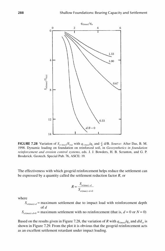
288 Shallow Foundations: Bearing Capacity and Settlement
The effectiveness with which geogrid reinforcement helps reduce the settlement can be expressed by a quantity called the settlement reduction factor R, or
RS
Set d
et d
= -
- =
(max)
(max) 0
whereSet(max)-d = maximum settlement due to impact load with reinforcement depth
of dSet(max)-d=0 = maximum settlement with no reinforcement (that is, d = 0 or N = 0)
Based on the results given in Figure 7.28, the variation of R with qt(max)/qu and d/dcr is shown in Figure 7.29. From the plot it is obvious that the geogrid reinforcement acts as an excellent settlement retardant under impact loading.
00 42
qt(max)/qu6
4
8S et(m
ax)/S
e(u)
12
14
d/B = 0
0.67
0.33
1.00
1.33
FiGure 7.28 Variation of Set (max)/Se(u) with qt (max)/qu and dB d/B. Source: After Das, B. M.
1998. Dynamic loading on foundation on reinforced soil, in Geosynthetics in foundation reinforcement and erosion control systems, eds. J. J. Bowders, H. B. Scranton, and G. P. Broderick. Geotech. Special Pub. 76, ASCE: 19.
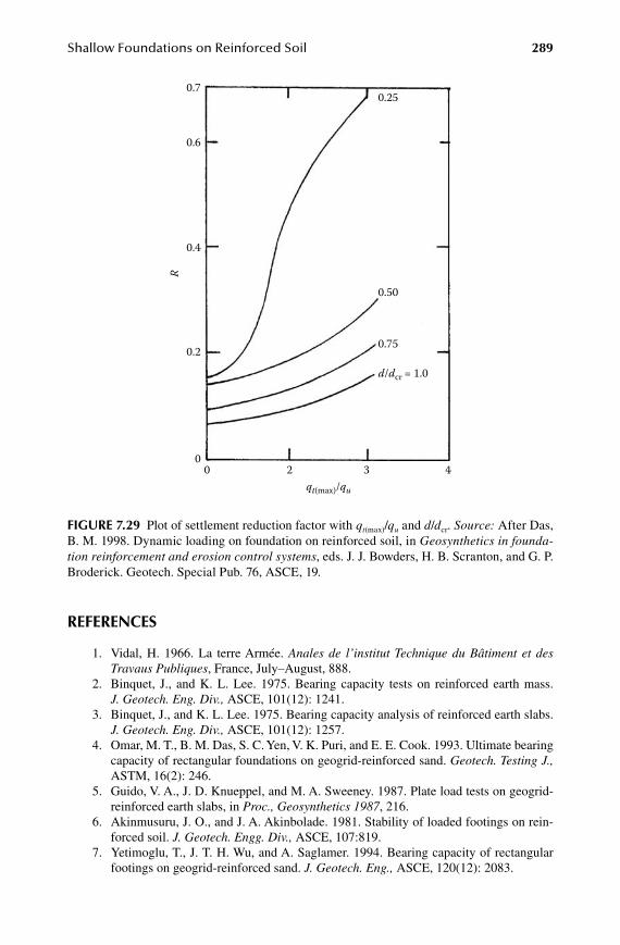
Shallow Foundations on Reinforced Soil 289
reFerenCeS
1. Vidal, H. 1966. La terre Armée. Anales de l’institut Technique du Bâtiment et des Travaus Publiques, France, July–August, 888.
2. Binquet, J., and K. L. Lee. 1975. Bearing capacity tests on reinforced earth mass. J. Geotech. Eng. Div., ASCE, 101(12): 1241.
3. Binquet, J., and K. L. Lee. 1975. Bearing capacity analysis of reinforced earth slabs. J. Geotech. Eng. Div., ASCE, 101(12): 1257.
4. Omar, M. T., B. M. Das, S. C. Yen, V. K. Puri, and E. E. Cook. 1993. Ultimate bearing capacity of rectangular foundations on geogrid-reinforced sand. Geotech. Testing J., ASTM, 16(2): 246.
5. Guido, V. A., J. D. Knueppel, and M. A. Sweeney. 1987. Plate load tests on geogrid-reinforced earth slabs, in Proc., Geosynthetics 1987, 216.
6. Akinmusuru, J. O., and J. A. Akinbolade. 1981. Stability of loaded footings on rein-forced soil. J. Geotech. Engg. Div., ASCE, 107:819.
7. Yetimoglu, T., J. T. H. Wu, and A. Saglamer. 1994. Bearing capacity of rectangular footings on geogrid-reinforced sand. J. Geotech. Eng., ASCE, 120(12): 2083.
0.7
qt(max)/qu
d/dcr = 1.0
0.75
0.50
0.25
0.6
0.4
0.2
00 2 3 4
R
FiGure 7.29 Plot of settlement reduction factor with qt(max)/qu and d/dcr. Source: After Das, B. M. 1998. Dynamic loading on foundation on reinforced soil, in Geosynthetics in founda-tion reinforcement and erosion control systems, eds. J. J. Bowders, H. B. Scranton, and G. P. Broderick. Geotech. Special Pub. 76, ASCE, 19.
290 Shallow Foundations: Bearing Capacity and Settlement
8. Schlosser, F., H. M. Jacobsen, and I. Juran. 1983. Soil reinforcement—general report. Proc. VIII European Conf. Soil Mech. Found. Engg. Helsinki, Balkema, 83.
9. Adams, M. T., and J. G. Collin. 1997. Large model spread footing load tests on geo-synthetic reinforced soil foundation. J. Geotech. Geoenviron. Eng., ASCE, 123(1): 66.
10. Shin, E. C., and B. M. Das. 2000. Experimental study of bearing capacity of a strip foundation on geogrid-reinforced sand. Geosynthetics Intl. 7(1): 59.
11. Huang, C. C., and L. K. Hong. 2000. Ultimate bearing capacity and settlement of foot-ings on reinforced sandy ground. Soils and Foundations 49(5): 65.
12. Huang, C. C., and F. Tatsuoka. 1990. Bearing capacity of reinforced horizontal sandy ground. Geotextiles and Geomembranes 9: 51.
13. Takemura, J., M. Okamura, N. Suesmasa, and T. Kimura. 1992. Bearing capacity and deformations of sand reinforced with geogrids. Proc., Int. Symp. Earth Reinforcement Practice, Fukuoka, Japan, 695.
14. Khing, K. H., B. M. Das, V. K. Puri, E. E. Cook, and S. C. Yen. 1992. Bearing capacity of two closely spaced strip foundations on geogrid-reinforced sand. Proc., Int. Symp. Earth Reinforcement Practice, Fukuoka, Japan, 619.
15. Huang, C. C., and F. Y. Meng. 1997. Deep footing and wide-slab effects on reinforced sandy ground. J. Geotech. Geoenviron. Eng., ASCE, 123(1): 30.
16. Patra, C. R., B. M. Das, M. Bohi, and E. C. Shin. 2006. Eccentrically loaded strip foundation on geogrid-reinforced sand. Geotextiles and Geomembranes 24: 254.
17. Das, B. M. 1998. Dynamic loading on foundation on reinforced soil, in Geosynthetics in foundation reinforcement and erosion control systems, eds. J. J. Bowders, H. B. Scranton, and G. P. Broderick. Geotech. Special Pub. 76, ASCE, 19.
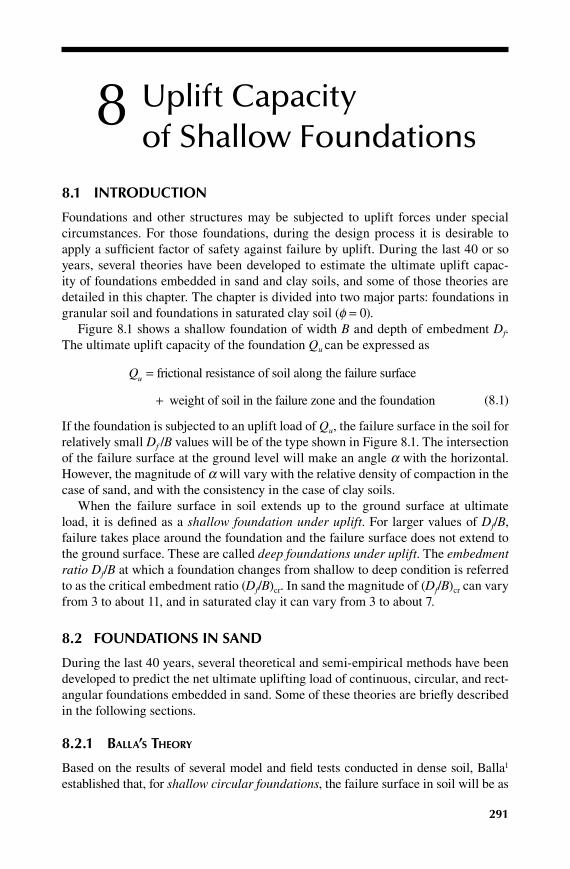
291
8 Uplift Capacity of Shallow Foundations
8.1 introduCtion
Foundations and other structures may be subjected to uplift forces under special circumstances. For those foundations, during the design process it is desirable to apply a sufficient factor of safety against failure by uplift. During the last 40 or so years, several theories have been developed to estimate the ultimate uplift capac-ity of foundations embedded in sand and clay soils, and some of those theories are detailed in this chapter. The chapter is divided into two major parts: foundations in granular soil and foundations in saturated clay soil (f = 0).
Figure 8.1 shows a shallow foundation of width B and depth of embedment Df. The ultimate uplift capacity of the foundation Qu can be expressed as
Qu = frictional resistance of soil along the failure surface
weight of soil in the fai+ lure zone and the foundation (8.1)
If the foundation is subjected to an uplift load of Qu, the failure surface in the soil for relatively small Df /B values will be of the type shown in Figure 8.1. The intersection of the failure surface at the ground level will make an angle a with the horizontal. However, the magnitude of a will vary with the relative density of compaction in the case of sand, and with the consistency in the case of clay soils.
When the failure surface in soil extends up to the ground surface at ultimate load, it is defined as a shallow foundation under uplift. For larger values of Df/B, failure takes place around the foundation and the failure surface does not extend to the ground surface. These are called deep foundations under uplift. The embedment ratio Df/B at which a foundation changes from shallow to deep condition is referred to as the critical embedment ratio (Df/B)cr. In sand the magnitude of (Df/B)cr can vary from 3 to about 11, and in saturated clay it can vary from 3 to about 7.
8.2 FoundationS in Sand
During the last 40 years, several theoretical and semi-empirical methods have been developed to predict the net ultimate uplifting load of continuous, circular, and rect-angular foundations embedded in sand. Some of these theories are briefly described in the following sections.
8.2.1 Balla’s theoRy
Based on the results of several model and field tests conducted in dense soil, Balla1 established that, for shallow circular foundations, the failure surface in soil will be as
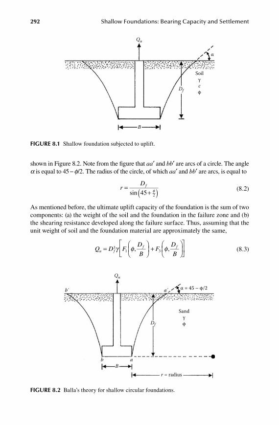
292 Shallow Foundations: Bearing Capacity and Settlement
shown in Figure 8.2. Note from the figure that aa′ and bb′ are arcs of a circle. The angle a is equal to 45 − f/2. The radius of the circle, of which aa′ and bb′ are arcs, is equal to
rDf=
+( )sin 45 2φ (8.2)
As mentioned before, the ultimate uplift capacity of the foundation is the sum of two components: (a) the weight of the soil and the foundation in the failure zone and (b) the shearing resistance developed along the failure surface. Thus, assuming that the unit weight of soil and the foundation material are approximately the same,
Q D F
D
BF
D
Bu f
f f=
+
3
1 3γ φ φ, , (8.3)
Qu
b
b a
a
Df
Br = radius
Sandγφ
α = 45 – φ/2
FiGure 8.2 Balla’s theory for shallow circular foundations.
Qu
Df
B
Soilγcφ
α
FiGure 8.1 Shallow foundation subjected to uplift.
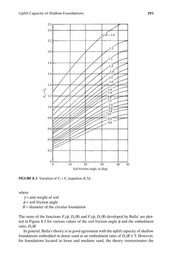
Uplift Capacity of Shallow Foundations 293
where g = unit weight of soil f = soil friction angleB = diameter of the circular foundation
The sums of the functions F1(f, Df /B) and F3(f, Df /B) developed by Balla1 are plot-ted in Figure 8.3 for various values of the soil friction angle f and the embedment ratio, Df /B.
In general, Balla’s theory is in good agreement with the uplift capacity of shallow foundations embedded in dense sand at an embedment ratio of Df /B ≤ 5. However, for foundations located in loose and medium sand, the theory overestimates the
0
0.2
0.4
0.6
0.8
1.0
1.2
1.4
1.6
1.8
2.0
2.2
2.5
2.4
0 10 20Soil friction angle, φ (deg)
F 1 +
F3
30 40 45
4.03.5
3.02.82.62.4
2.22.01.91.81.71.61.5
1.41.3
1.2
1.1
Df/B = 1.0
FiGure 8.3 Variation of F1 + F3 [equation (8.3)].

294 Shallow Foundations: Bearing Capacity and Settlement
ultimate uplift capacity. The main reason Balla’s theory overestimates the ultimate uplift capacity for Df /B > about 5 even in dense sand is because it is essentially a deep foundation condition, and the failure surface does not extend to the ground surface.
The simplest procedure to determine the embedment ratio at which the deep foun-dation condition is reached may be determined by plotting the nondimensional break-out factor Fq against Df /B as shown in Figure 8.4. The breakout factor is derived as
FQAD
qu
f
=γ (8.4)
whereA = area of the foundation.
The breakout factor increases with Df /B up to a maximum value of F Fq q= * at Df /B = (Df /B)cr. For Df /B > (Df /B)cr the breakout factor remains practically constant (that is, Fq
*).
8.2.2 theoRy of meyeRhof anD aDams
One of the most rational methods for estimating the ultimate uplift capacity of a shallow foundation was proposed by Meyerhof and Adams,2 and it is described in detail in this section. Figure 8.5 shows a continuous foundation of width B subjected to an uplifting force. The ultimate uplift capacity per unit length of the foundation is equal to Qu. At ultimate load the failure surface in soil makes an angle a with the horizontal. The magnitude of a depends on several factors, such as the relative density of compaction and the angle of friction of the soil, and it varies between 90° − 1/3 f and 90° − 2/3 f. Let us consider the free body diagram of the zone abcd. For stability consideration, the following forces per unit length of the foundation need to be considered: (a) the weight of the soil and concrete W and (b) the passive force P′p per unit length along the faces ad and bc. The force ′Pp is inclined at an
F q =
Qu/
γAD
f
Df/B
(Df/B)cr
Deepunderuplift
Shallowunderuplift
F*q
FiGure 8.4 Nature of variation of Fq with Df /B.
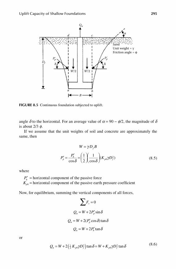
Uplift Capacity of Shallow Foundations 295
angle d to the horizontal. For an average value of a = 90 − f/2, the magnitude of d is about 2/3 f.
If we assume that the unit weights of soil and concrete are approximately the same, then
W D Bf= γ
′ = ′ =
P
PK Dp
hph f
cos cos( )
δ δγ1
21 2 (8.5)
where
′Ph = horizontal component of the passive forceKph = horizontal component of the passive earth pressure coefficient
Now, for equilibrium, summing the vertical components of all forces,
Fv =∑ 0
Q W Pu p= + ′2 sinδ
Q W Pu p= + ′2( cos ) tanδ δ
Q W Pu h= + ′2 tanδ
or
Q W K D W K Du ph f ph f= + ( ) = +2 1
22 2γ δ γ δtan tan (8.6)
Qu
DfPp Pp
W/2
a bB
δ δ
W/2
SandUnit weight = γFriction angle = φ
αd c
FiGure 8.5 Continuous foundation subjected to uplift.
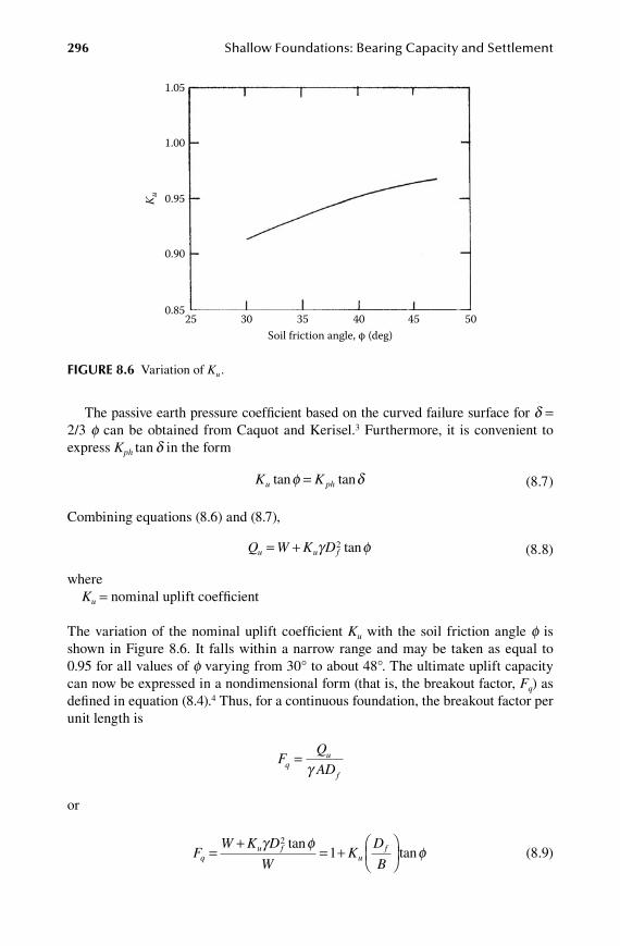
296 Shallow Foundations: Bearing Capacity and Settlement
The passive earth pressure coefficient based on the curved failure surface for d = 2/3 f can be obtained from Caquot and Kerisel.3 Furthermore, it is convenient to express Kph tan d in the form
K Ku phtan tanφ δ= (8.7)
Combining equations (8.6) and (8.7),
Q W K Du u f= + γ φ2 tan (8.8)
whereKu = nominal uplift coefficient
The variation of the nominal uplift coefficient Ku with the soil friction angle f is shown in Figure 8.6. It falls within a narrow range and may be taken as equal to 0.95 for all values of f varying from 30° to about 48°. The ultimate uplift capacity can now be expressed in a nondimensional form (that is, the breakout factor, Fq) as defined in equation (8.4).4 Thus, for a continuous foundation, the breakout factor per unit length is
FQ
ADqu
f
=γ
or
F
W K D
WK
D
Bq
u fu
f=+
= +
γ φ φ2
1tan
tan (8.9)
1.05
1.00
0.95
0.90
0.85
K u
25 30 35 40Soil friction angle, φ (deg)
45 50
FiGure 8.6 Variation of Ku .
Uplift Capacity of Shallow Foundations 297
For circular foundations, equation (8.8) can be modified to the form
Q W S BD Ku F f u= + π γ φ
22 tan (8.10)
W B Df≈ π γ
42 (8.11)
whereSF = shape factor B = diameter of the foundation
The shape factor can be expressed as
S m
D
BF
f= +
1 (8.12)
wherem = coefficient that is a function of the soil friction angle f
Thus, combining equations (8.10), (8.11), and (8.12) we obtain
Q B D mD
BBD Ku f
ff u= + +
π γ π γ4 2
12 2 tanφφ (8.13)
The breakout factor Fq can be given as
FQ
AD
B D mD
BBD
qu
f
ff
= =
+ +
γ
γ γπ π4
22 1 f u
f
f
K
B D
mD
B
D
2
42
1 2 1
tanφ
γ π( )
= + +
ffuB
K
tanφ (8.14)
For rectangular foundations having dimensions of B × L, the ultimate capacity can also be expressed as
Q W D S B L B Ku f F u= + + -γ φ2 2( ) tan (8.15)
The preceding equation was derived with the assumption that the two end por-tions of length B/2 are governed by the shape factor SF, while the passive pressure along the central portion of length L − B is the same as the continuous foundation. In equation (8.15),
W BLDf≈ γ (8.16)
and
S m
D
BF
f= +
1 (8.17)
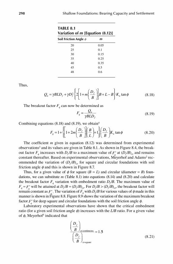
298 Shallow Foundations: Bearing Capacity and Settlement
Thus,
Q BLD D mD
BB L Bu f f
f= + +
+ -
γ γ 2 2 1
Ku tanφ (8.18)
The breakout factor Fq can now be determined as
FQ
BLDq
u
f
=γ (8.19)
Combining equations (8.18) and (8.19), we obtain4
F mD
BBL
qf= + +
+
1 1 2 1
D
BKf
u tanφ (8.20)
The coefficient m given in equation (8.12) was determined from experimental observations2 and its values are given in Table 8.1. As shown in Figure 8.4, the break-out factor Fq increases with Df /B to a maximum value of Fq
* at (Df /B)cr and remains constant thereafter. Based on experimental observations, Meyerhof and Adams2 rec-ommended the variation of (Df /B)cr for square and circular foundations with soil friction angle f and this is shown in Figure 8.7.
Thus, for a given value of f for square (B = L) and circular (diameter = B) foun-dations, we can substitute m (Table 8.1) into equations (8.14) and (8.20) and calculate the breakout factor Fq variation with embedment ratio Df /B. The maximum value of Fq = Fq
* will be attained at Df /B = (Df /B)cr. For Df /B > (Df /B)cr, the breakout factor will remain constant as Fq
*. The variation of Fq with Df /B for various values of f made in this manner is shown in Figure 8.8. Figure 8.9 shows the variation of the maximum breakout factor Fq
* for deep square and circular foundations with the soil friction angle f.Laboratory experimental observations have shown that the critical embedment
ratio (for a given soil friction angle f) increases with the L/B ratio. For a given value of f, Meyerhof5 indicated that
D
BD
B
f
f
≈cr-continuous
cr-square
1.55 (8.21)
table 8.1Variation of m [equation (8.12)]Soil Friction angle f m
20 0.0525 0.130 0.1535 0.2540 0.3545 0.548 0.6
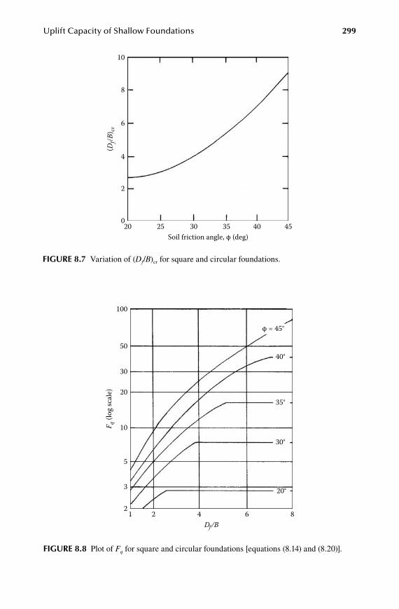
Uplift Capacity of Shallow Foundations 299
10
8
6
4
2
0
(Df/B
) cr
20 25 30 35Soil friction angle, φ (deg)
40 45
FiGure 8.7 Variation of (Df/B)cr for square and circular foundations.
100
φ = 45°
40°
35°
30°
20°
50
30
20
10F q (l
og sc
ale)
5
3
21 2 4
Df/B6 8
FiGure 8.8 Plot of Fq for square and circular foundations [equations (8.14) and (8.20)].
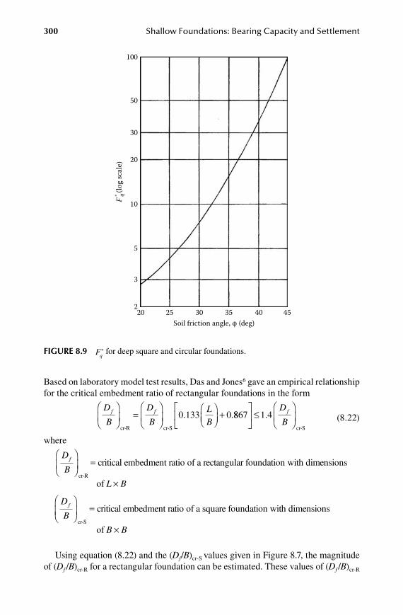
300 Shallow Foundations: Bearing Capacity and Settlement
Based on laboratory model test results, Das and Jones6 gave an empirical relationship for the critical embedment ratio of rectangular foundations in the form
D
B
D
BLB
f f
=
+cr-R cr-S
0 133 0. .8867 1 4
≤
.
D
Bf
cr-S
(8.22)
where
D
Bf
=
cr-R
critical embedment ratio of a rectangular foundation with dimensions
of L B×
D
Bf
=
cr-S
critical embedment ratio of a square foundation with dimensions
of B B×
Using equation (8.22) and the (Df/B)cr-S values given in Figure 8.7, the magnitude of (Df /B)cr-R for a rectangular foundation can be estimated. These values of (Df /B)cr-R
100
50
30
20
F* q (
log
scal
e)
10
5
2
3
20 25 30Soil friction angle, φ (deg)
35 40 45
FiGure 8.9 Fq* for deep square and circular foundations.
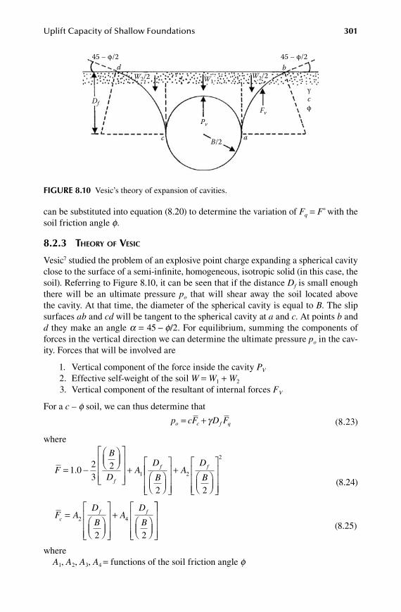
Uplift Capacity of Shallow Foundations 301
can be substituted into equation (8.20) to determine the variation of Fq = F* with the soil friction angle f.
8.2.3 theoRy of vesiC
Vesic7 studied the problem of an explosive point charge expanding a spherical cavity close to the surface of a semi-infinite, homogeneous, isotropic solid (in this case, the soil). Referring to Figure 8.10, it can be seen that if the distance Df is small enough there will be an ultimate pressure po that will shear away the soil located above the cavity. At that time, the diameter of the spherical cavity is equal to B. The slip surfaces ab and cd will be tangent to the spherical cavity at a and c. At points b and d they make an angle a = 45 − f/2. For equilibrium, summing the components of forces in the vertical direction we can determine the ultimate pressure po in the cav-ity. Forces that will be involved are
1. Vertical component of the force inside the cavity PV
2. Effective self-weight of the soil W = W1 + W2
3. Vertical component of the resultant of internal forces FV
For a c – f soil, we can thus determine that
p cF D Fo c f q= +γ (8.23)
where
F
B
DA
D
Bf
f= -
+
1 023
2
2
1.
+
AD
Bf
2
2
2 (8.24)
F AD
BA
D
Bcf f=
+
2 4
2 2
(8.25)
whereA1, A2, A3, A4 = functions of the soil friction angle f
45 – φ/2
γcφ
45 – φ/2b
ac
d
Df
W2/2
Pv
Fv
B/2
W2/2W1
FiGure 8.10 Vesic’s theory of expansion of cavities.
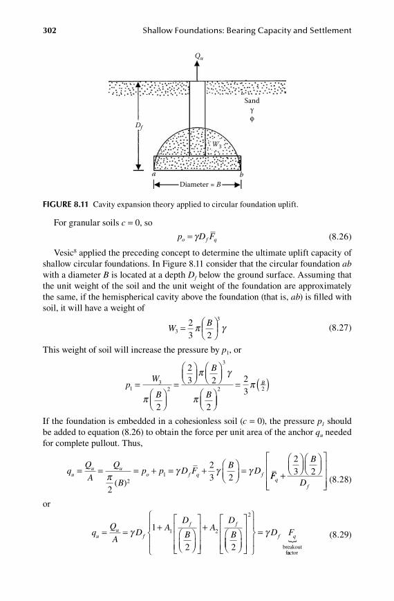
302 Shallow Foundations: Bearing Capacity and Settlement
For granular soils c = 0, so
p D Fo f q= γ (8.26)
Vesic8 applied the preceding concept to determine the ultimate uplift capacity of shallow circular foundations. In Figure 8.11 consider that the circular foundation ab with a diameter B is located at a depth Df below the ground surface. Assuming that the unit weight of the soil and the unit weight of the foundation are approximately the same, if the hemispherical cavity above the foundation (that is, ab) is filled with soil, it will have a weight of
W
B3
323 2
=
π γ (8.27)
This weight of soil will increase the pressure by p1, or
pW
B
B
B1
32
3
2
23 2
2
=
=
π
π γ
π
= ( )2 2
23
π B
If the foundation is embedded in a cohesionless soil (c = 0), the pressure p1 should be added to equation (8.26) to obtain the force per unit area of the anchor qu needed for complete pullout. Thus,
A
Q
Bp p D F
BDu
u uo f q f= = = + = +
=π
γ γ γ
2
23 22
1
( )FF
B
Dqf
+
23 2
(8.28)
or
AD A
D
BA
D
Buu
f
f f
= = +
+
γ 1
2 2
1 2
=
2
γ D Ff q
breakoutfaactor
� (8.29)
Sandγφ
Diameter = B
ac
Df
ba
Qu
W3
FiGure 8.11 Cavity expansion theory applied to circular foundation uplift.
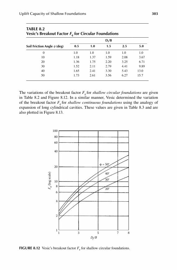
Uplift Capacity of Shallow Foundations 303
The variations of the breakout factor Fq for shallow circular foundations are given in Table 8.2 and Figure 8.12. In a similar manner, Vesic determined the variation of the breakout factor Fq for shallow continuous foundations using the analogy of expansion of long cylindrical cavities. These values are given in Table 8.3 and are also plotted in Figure 8.13.
table 8.2Vesic’s breakout Factor Fq for Circular Foundations
df/b
Soil Friction angle f (deg) 0.5 1.0 1.5 2.5 5.0
0 1.0 1.0 1.0 1.0 1.010 1.18 1.37 1.59 2.08 3.6720 1.36 1.75 2.20 3.25 6.7130 1.52 2.11 2.79 4.41 9.8940 1.65 2.41 3.30 5.43 13.050 1.73 2.61 3.56 6.27 15.7
100
8060
40
φ = 50°
40°
30°
20°
20
108
6
4
F q (l
og sc
ale)
2
11 3 5
Df/B7 8
FiGure 8.12 Vesic’s breakout factor Fq for shallow circular foundations.
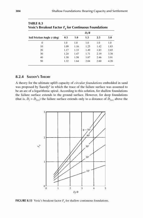
304 Shallow Foundations: Bearing Capacity and Settlement
8.2.4 saeDDy’s theoRy
A theory for the ultimate uplift capacity of circular foundations embedded in sand was proposed by Saeedy9 in which the trace of the failure surface was assumed to be an arc of a logarithmic spiral. According to this solution, for shallow foundations the failure surface extends to the ground surface. However, for deep foundations (that is, Df > Df(cr)) the failure surface extends only to a distance of Df(cr) above the
table 8.3Vesic’s breakout Factor Fq for Continuous Foundations
Df/B
Soil Friction angle f (deg) 0.5 1.0 1.5 2.5 5.0
0 1.0 1.0 1.0 1.0 1.010 1.09 1.16 1.25 1.42 1.8320 1.17 1.33 1.49 1.83 2.6530 1.24 1.47 1.71 2.19 3.3840 1.30 1.58 1.87 2.46 3.9150 1.32 1.64 2.04 2.60 4.20
3
φ = 50°
40°
30°
20°
10°
2
1
F q
00 1 2 3
Df/B4 5
FiGure 8.13 Vesic’s breakout factor Fq for shallow continuous foundations.
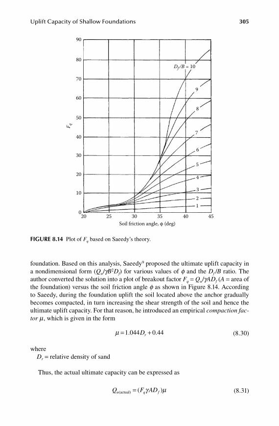
Uplift Capacity of Shallow Foundations 305
foundation. Based on this analysis, Saeedy9 proposed the ultimate uplift capacity in a nondimensional form (Qu/gB2Df) for various values of f and the Df /B ratio. The author converted the solution into a plot of breakout factor Fq = Qu/gADf (A = area of the foundation) versus the soil friction angle f as shown in Figure 8.14. According to Saeedy, during the foundation uplift the soil located above the anchor gradually becomes compacted, in turn increasing the shear strength of the soil and hence the ultimate uplift capacity. For that reason, he introduced an empirical compaction fac-tor m, which is given in the form
µ = +1 044 0 44. .Dr (8.30)
whereDr = relative density of sand
Thus, the actual ultimate capacity can be expressed as
Q F ADu q f(actual) = ( )γ µ (8.31)
90
80
70
60
50
40
30
20
10
0
Df /B = 10
8
9
7
123
4
5
6
F q
20 25 30 35 40 45Soil friction angle, φ (deg)
FiGure 8.14 Plot of Fq based on Saeedy’s theory.
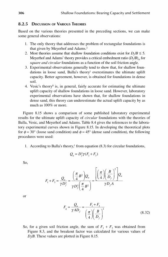
306 Shallow Foundations: Bearing Capacity and Settlement
8.2.5 DisCUssion of vaRioUs theoRies
Based on the various theories presented in the preceding sections, we can make some general observations:
1. The only theory that addresses the problem of rectangular foundations is that given by Meyerhof and Adams.2
2. Most theories assume that shallow foundation conditions exist for Df /B ≤ 5. Meyerhof and Adams’ theory provides a critical embedment ratio (Df /B)cr for square and circular foundations as a function of the soil friction angle.
3. Experimental observations generally tend to show that, for shallow foun-dations in loose sand, Balla’s theory1 overestimates the ultimate uplift capacity. Better agreement, however, is obtained for foundations in dense soil.
4. Vesic’s theory8 is, in general, fairly accurate for estimating the ultimate uplift capacity of shallow foundations in loose sand. However, laboratory experimental observations have shown that, for shallow foundations in dense sand, this theory can underestimate the actual uplift capacity by as much as 100% or more.
Figure 8.15 shows a comparison of some published laboratory experimental results for the ultimate uplift capacity of circular foundations with the theories of Balla, Vesic, and Meyerhof and Adams. Table 8.4 gives the references to the labora-tory experimental curves shown in Figure 8.15. In developing the theoretical plots for f = 30° (loose sand condition) and f = 45° (dense sand condition), the following procedures were used:
1. According to Balla’s theory,1 from equation (8.3) for circular foundations,
Q D F Fu f= +3
1 3γ ( )
So,
F FQ
D
B Q
D B
u
f
u
f
1 3 3
2
3 2
4
4
4+ = =
=
γ
π
γ π
π
BD
Q
D A
fu
f
2
γ
or
FQ
AD
F F
BD
qu
f
f
= =+
γ π
1 32
4 (8.32)
So, for a given soil friction angle, the sum of F1 + F3 was obtained from Figure 8.3, and the breakout factor was calculated for various values of Df/B. These values are plotted in Figure 8.15.
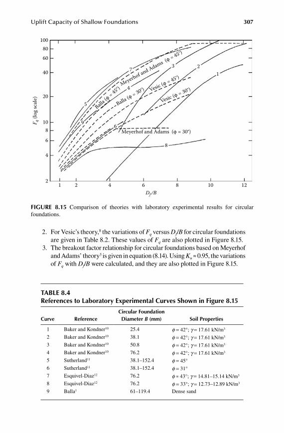
Uplift Capacity of Shallow Foundations 307
2. For Vesic’s theory,8 the variations of Fq versus Df/B for circular foundations are given in Table 8.2. These values of Fq are also plotted in Figure 8.15.
3. The breakout factor relationship for circular foundations based on Meyerhof and Adams’ theory3 is given in equation (8.14). Using Ku ≈ 0.95, the variations of Fq with Df/B were calculated, and they are also plotted in Figure 8.15.
table 8.4references to laboratory experimental Curves Shown in Figure 8.15
Curve referenceCircular Foundation diameter B (mm) Soil properties
1 Baker and Kondner10 25.4 f = 42°; g = 17.61 kN/m3
2 Baker and Kondner10 38.1 f = 42°; g = 17.61 kN/m3
3 Baker and Kondner10 50.8 f = 42°; g = 17.61 kN/m3
4 Baker and Kondner10 76.2 f = 42°; g = 17.61 kN/m3
5 Sutherland11 38.1–152.4 f = 45°6 Sutherland11 38.1–152.4 f = 31°7 Esquivel-Diaz12 76.2 f ≈ 43°; g = 14.81–15.14 kN/m3
8 Esquivel-Diaz12 76.2 f = 33°; g = 12.73–12.89 kN/m3
9 Balla1 61–119.4 Dense sand
10080
60
40
20
108
6
4
Balla (φ
= 45°)Meyerhof and Adams (φ
= 45°)
Balla (φ = 30°) Vesic (φ = 45°)
Vesic (φ = 30°)
5
7
4
3 2
9 6
2
8
1
F q (l
og sc
ale)
1 2 4 6 8 10 12Df /B
Meyerhof and Adams (φ = 30°)
FiGure 8.15 Comparison of theories with laboratory experimental results for circular foundations.
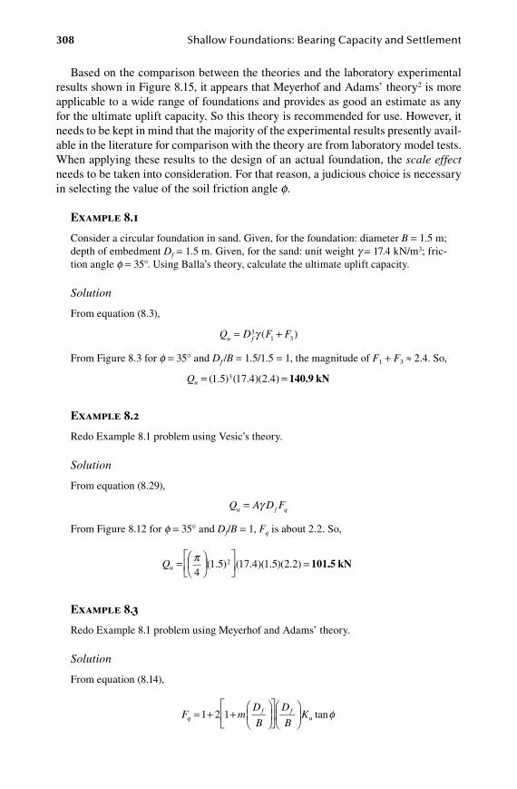
308 Shallow Foundations: Bearing Capacity and Settlement
Based on the comparison between the theories and the laboratory experimental results shown in Figure 8.15, it appears that Meyerhof and Adams’ theory2 is more applicable to a wide range of foundations and provides as good an estimate as any for the ultimate uplift capacity. So this theory is recommended for use. However, it needs to be kept in mind that the majority of the experimental results presently avail-able in the literature for comparison with the theory are from laboratory model tests. When applying these results to the design of an actual foundation, the scale effect needs to be taken into consideration. For that reason, a judicious choice is necessary in selecting the value of the soil friction angle f.
Example 8.1
Consider a circular foundation in sand. Given, for the foundation: diameter B = 1.5 m; depth of embedment Df = 1.5 m. Given, for the sand: unit weight g = 17.4 kN/m3; fric-tion angle f = 35°. Using Balla’s theory, calculate the ultimate uplift capacity.
Solution
From equation (8.3),
Q D F Fu f= +3
1 3γ ( )
From Figure 8.3 for f = 35° and Df /B = 1.5/1.5 = 1, the magnitude of F1 + F3 ≈ 2.4. So,
Qu = =( . ) ( . )( . )1 5 17 4 2 43 140.9 kN
Example 8.2
Redo Example 8.1 problem using Vesic’s theory.
Solution
From equation (8.29),
Q A D Fu f q= γ
From Figure 8.12 for f = 35° and Df/B = 1, Fq is about 2.2. So,
Qu =
=π4
1 5 17 4 1 5 2 22( . ) ( . )( . )( . ) 101..5 kN
Example 8.3
Redo Example 8.1 problem using Meyerhof and Adams’ theory.
Solution
From equation (8.14),
F m
D
B
D
BKq
f fu= + +
1 2 1 tanφ

Uplift Capacity of Shallow Foundations 309
For f = 35°, m = 0.25 (Table 8.1). So,
F . .q = + + =1 2 1 0 25 1 1 0 95 35 2 66[ ( )( )]( )( )(tan ) .
So,
Q F ADu q f= =
γ π( . )( . ) ( . ) (2 66 17 4
41 5 2 1 5. ) = 122.7 kN
8.3 FoundationS in Saturated Clay (φ = 0 Condition)
8.3.1 Ultimate Uplift CapaCity—geneRal
Theoretical and experimental research results presently available for determin-ing the ultimate uplift capacity of foundations embedded in saturated clay soil are rather limited. In the following sections, the results of some of the existing studies are reviewed.
Figure 8.16 shows a shallow foundation in saturated clay. The depth of the foun-dation is Df , and the width of the foundation is B. The undrained shear strength and the unit weight of the soil are cu and g, respectively. If we assume that the unit weights of the foundation material and the clay are approximately the same, then the ultimate uplift capacity can be expressed as8
Q A D c Fu f u c= +( )γ (8.33)
where A = area of the foundationFc = breakout factor g = saturated unit weight of the soil
Qu
Df
B
Saturated clayUnit weight = γUndrained shear strength = cu
FiGure 8.16 Shallow foundation in saturated clay subjected to uplift.
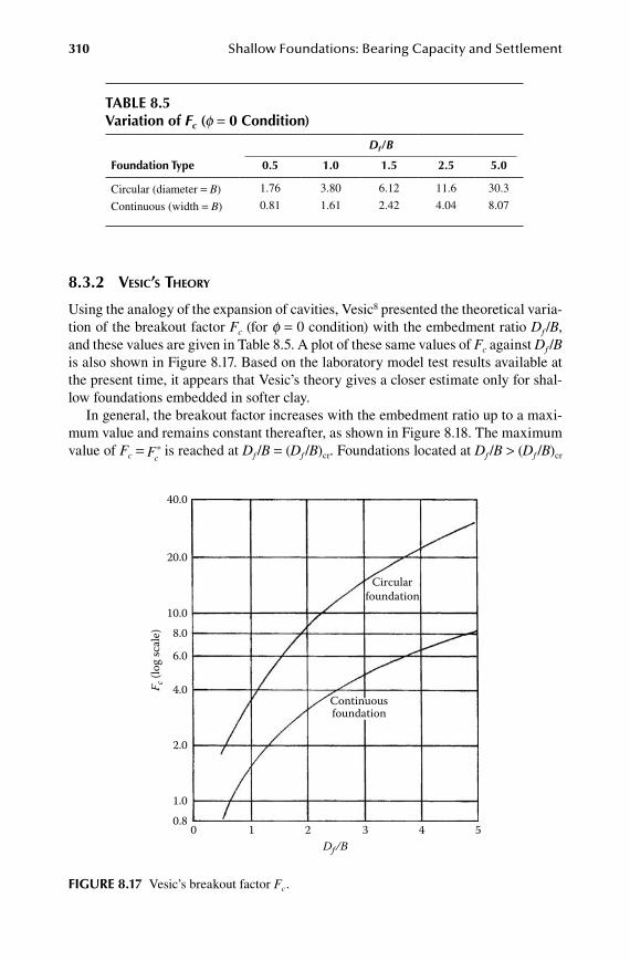
310 Shallow Foundations: Bearing Capacity and Settlement
8.3.2 vesiC’s theoRy
Using the analogy of the expansion of cavities, Vesic8 presented the theoretical varia-tion of the breakout factor Fc (for f = 0 condition) with the embedment ratio Df /B, and these values are given in Table 8.5. A plot of these same values of Fc against Df /B is also shown in Figure 8.17. Based on the laboratory model test results available at the present time, it appears that Vesic’s theory gives a closer estimate only for shal-low foundations embedded in softer clay.
In general, the breakout factor increases with the embedment ratio up to a maxi-mum value and remains constant thereafter, as shown in Figure 8.18. The maximum value of Fc = Fc
* is reached at Df /B = (Df /B)cr. Foundations located at Df /B > (Df /B)cr
table 8.5Variation of Fc (f = 0 Condition)
Df /B
Foundation type 0.5 1.0 1.5 2.5 5.0
Circular (diameter = B) 1.76 3.80 6.12 11.6 30.3
Continuous (width = B) 0.81 1.61 2.42 4.04 8.07
40.0
20.0
10.0
F c (l
og sc
ale) 8.0
6.0
4.0
2.0
1.00.8
0 1 2Df/B
3 4 5
Continuousfoundation
Circularfoundation
FiGure 8.17 Vesic’s breakout factor Fc .
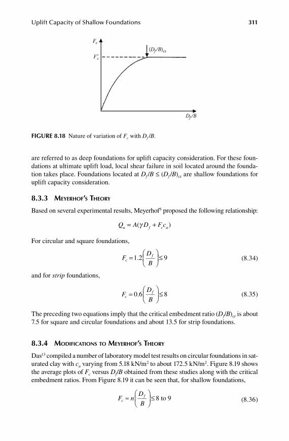
Uplift Capacity of Shallow Foundations 311
are referred to as deep foundations for uplift capacity consideration. For these foun-dations at ultimate uplift load, local shear failure in soil located around the founda-tion takes place. Foundations located at Df /B ≤ (Df /B)cr are shallow foundations for uplift capacity consideration.
8.3.3 meyeRhof’s theoRy
Based on several experimental results, Meyerhof5 proposed the following relationship:
Q A D F cu f c u= +( )γ
For circular and square foundations,
F
D
Bc
f=
≤1 2 9. (8.34)
and for strip foundations,
F
D
Bc
f=
≤0 6 8. (8.35)
The preceding two equations imply that the critical embedment ratio (Df/B)cr is about 7.5 for square and circular foundations and about 13.5 for strip foundations.
8.3.4 moDifiCations to meyeRhof’s theoRy
Das13 compiled a number of laboratory model test results on circular foundations in sat-urated clay with cu varying from 5.18 kN/m2 to about 172.5 kN/m2. Figure 8.19 shows the average plots of Fc versus Df/B obtained from these studies along with the critical embedment ratios. From Figure 8.19 it can be seen that, for shallow foundations,
F n
D
Bc
f≈
≤ 8 to 9 (8.36)
FiGure 8.18 Nature of variation of Fc with Df /B.
Fc
(Df/B)cr
Df /B
F *c
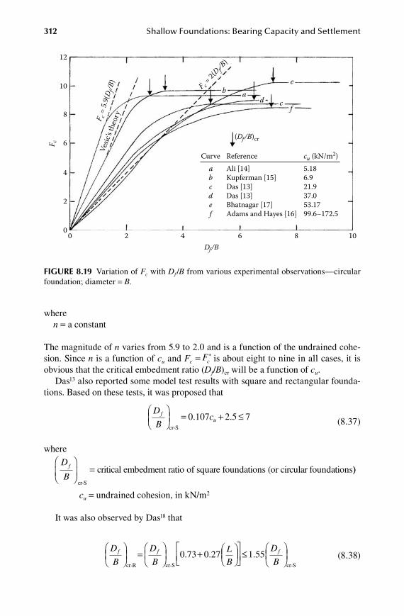
312 Shallow Foundations: Bearing Capacity and Settlement
wheren = a constant
The magnitude of n varies from 5.9 to 2.0 and is a function of the undrained cohe-sion. Since n is a function of cu and Fc = Fc
* is about eight to nine in all cases, it is obvious that the critical embedment ratio (Df/B)cr will be a function of cu.
Das13 also reported some model test results with square and rectangular founda-tions. Based on these tests, it was proposed that
D
Bcf
u
= + ≤
cr-S
70 107 2 5. . (8.37)
where
D
Bf
=
cr-S
critical embedment ratio of square foundations (or circular foundations))
cu = undrained cohesion, in kN/m2
It was also observed by Das18 that
D
B
D
BLB
f f
=
+
cr-R cr-S
0 73 0 27. .
≤
1 55.
D
Bf
cr-S
(8.38)
12
10
8
6
4
2
00 2
F c = 5.
9(D f/
B)Ve
sic’s
theo
ry
F c = 2(
D f/B)
4Df/B
b ad c
f
e
6 8 10
F c
(Df/B)cr
abcdef
Curve Reference cu (kN/m2)Ali [14]Kupferman [15]Das [13]Das [13]Bhatnagar [17]Adams and Hayes [16]
5.186.921.937.053.1799.6–172.5
FiGure 8.19 Variation of Fc with Df /B from various experimental observations—circular foundation; diameter = B.
Uplift Capacity of Shallow Foundations 313
where
D
Bf
=
cr-R
critical embedment ratio of rectangular foundations
L = length of foundation
Based on the above findings, Das18 proposed an empirical procedure to obtain the breakout factors for shallow and deep foundations. According to this procedure, a′ and b′ are two nondimensional factors defined as
′ =
α
D
BD
B
f
f
cr
(8.39)
and
′ =β F
Fc
c*
(8.40)
For a given foundation, the critical embedment ratio can be calculated using equa-tions (8.37) and (8.38). The magnitude of Fc
* can be given by the following empirical relationship:
F
BL
c-R* . .= +
7 56 1 44 (8.41)
where
Fc R-* = breakout factor for deep rectangular foundations
Figure 8.20 shows the experimentally derived plots (upper limit, lower limit, and average of b′ and a′). Following is a step-by-step procedure to estimate the ultimate uplift capacity.
1. Determine the representative value of the undrained cohesion cu. 2. Determine the critical embedment ratio using equations (8.37) and
(8.38). 3. Determine the Df /B ratio for the foundation. 4. If Df /B > (Df /B)cr as determined in step 2, it is a deep foundation. However,
if Df /B ≤ (Df /B)cr, it is a shallow foundation. 5. For Df /B > (Df /B)cr,
F F
BL
c c= = +
* . .7 56 1 44
Thus,
Q ABL
c Du u f= +
+
7 56 1 44. . γ (8.42)
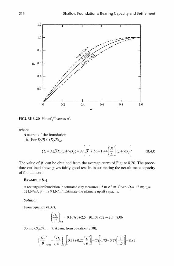
314 Shallow Foundations: Bearing Capacity and Settlement
whereA = area of the foundation
6. For Df/B ≤ (Df/B)cr,
Q A F c D ABL
u c u f= ′ + = ′ +
( ) . .*β γ β 7 56 1 44 +
c Du fγ (8.43)
The value of b′ can be obtained from the average curve of Figure 8.20. The proce-dure outlined above gives fairly good results in estimating the net ultimate capacity of foundations.
Example 8.4
A rectangular foundation in saturated clay measures 1.5 m × 3 m. Given: Df = 1.8 m; cu = 52 kN/m2; g = 18.9 kN/m3. Estimate the ultimate uplift capacity.
Solution
From equation (8.37),
D
Bcf
u
= + = + =
cr-S
(0.107)(52) 2.5 80 107 2 5. . ..06
So use (Df /B)cr-S = 7. Again, from equation (8.38),
D
B
D
BLB
f f
=
+
cr-R cr-S
0 73 0 27. .
= +
=( ) . ..
.7 0 73 0 273
1 58 89
1.2
1.0
0.8
0.6
0.4
0.2
0
β´
0 0.2 0.4α´
0.6 0.8 1.0
Upper lim
it
Lower limit
Average
FiGure 8.20 Plot of b′ versus a′.
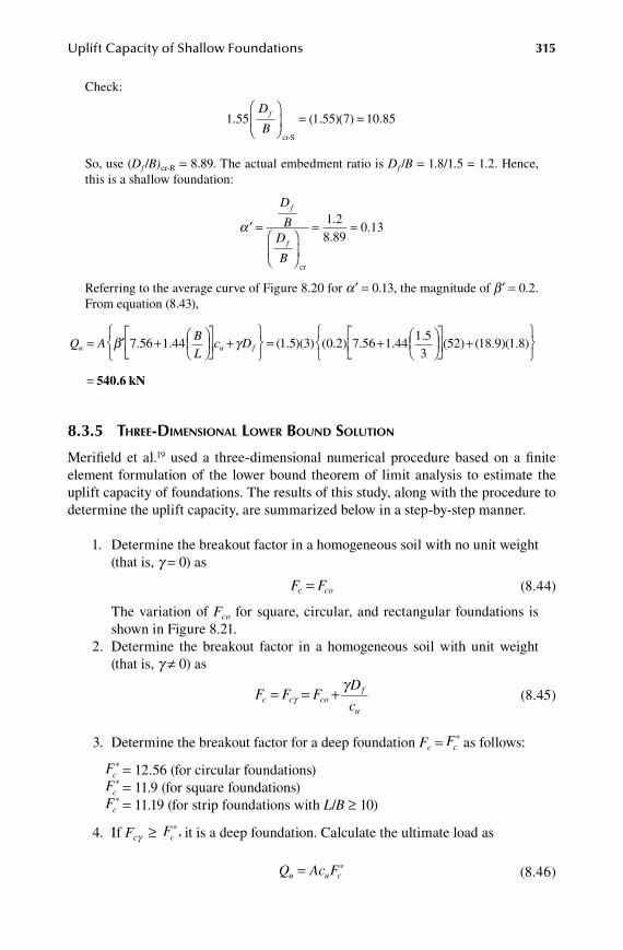
Uplift Capacity of Shallow Foundations 315
Check:
1 55 1 55 7 10 85. ( . )( ) .D
Bf
= =
cr-S
So, use (Df /B)cr-R = 8.89. The actual embedment ratio is Df /B = 1.8/1.5 = 1.2. Hence, this is a shallow foundation:
′ =
= =α
D
BD
B
f
f
cr
1 28 89
0 13..
.
Referring to the average curve of Figure 8.20 for a′ = 0.13, the magnitude of b′ = 0.2. From equation (8.43),
Q ABL
c Du u f= ′ +
+
=β γ7 56 1 44 1 5. . ( . )( ) ( . ) . ..
( ) ( . )(3 0 2 7 56 1 441 53
52 18 9 1+
+ . )8
= 540.6 kN
8.3.5 thRee-Dimensional loweR BoUnD solUtion
Merifield et al.19 used a three-dimensional numerical procedure based on a finite element formulation of the lower bound theorem of limit analysis to estimate the uplift capacity of foundations. The results of this study, along with the procedure to determine the uplift capacity, are summarized below in a step-by-step manner.
1. Determine the breakout factor in a homogeneous soil with no unit weight (that is, g = 0) as
F Fc co= (8.44)
The variation of Fco for square, circular, and rectangular foundations is shown in Figure 8.21.
2. Determine the breakout factor in a homogeneous soil with unit weight (that is, g ≠ 0) as
F F F
D
cc c co
f
u
= = +γγ
(8.45)
3. Determine the breakout factor for a deep foundation Fc = Fc* as follows:
Fc* = 12.56 (for circular foundations)
Fc* = 11.9 (for square foundations)
Fc* = 11.19 (for strip foundations with L/B ≥ 10)
4. If Fcg ≥ Fc*, it is a deep foundation. Calculate the ultimate load as
Q Ac Fu u c= * (8.46)
316 Shallow Foundations: Bearing Capacity and Settlement
However, if Fcg ≤ Fc*, it is a shallow foundation. Thus,
Q Ac Fu u c= γ (8.47)
Example 8.5
Solve the Example 8.4 problem using the procedure outlined in section 8.35.
Solution
Given: L/B = 3/1.5 = 2; Df/B = 1.8/1.5 = 1.2. From Figure 8.21, for L/B = 2 and Df/B = 1.2, the value of Fco ≈ 3.1:
F F
D
cc cof
uγ
γ= + = + =3 1
18 9 1 852
3 754.( . )( . )
.
For a foundation with L/B = 2, the magnitude of Fc* ≈ 11.5. Thus,
Fcg < Fc*
Hence,
Q Ac Fu u c= = × ≈γ ( . )( )( . )3 1 5 52 3 754 878 kN
13
12
10
8
6
4
2
00 2
CircleL/B = 1
2
46 8
∞
4Df/B
6 8 10
F co
FiGure 8.21 Numerical lower bound solution of Merifield et al.—plot of Fco versus Df /B for circular, square, and rectangular foundations. Source: Merifield, R. S., A. V. Lyamin, S. W. Sloan, and H. S. Yu. 2003. Three-dimensional lower bound solutions for stability of plate anchors in clay. J. Geotech. Geoenv. Eng., ASCE, 129(3): 243.

Uplift Capacity of Shallow Foundations 317
8.3.6 faCtoR of safety
In most cases of foundation design, it is recommended that a minimum factor of safety of 2 to 2.5 be used to arrive at the allowable ultimate uplift capacity.
reFerenCeS
1. Balla, A. 1961. The resistance to breaking out of mushroom foundations for pylons, in Proc., V Int. Conf. Soil Mech. Found. Eng., Paris, France, 1: 569.
2. Meyerhof, G. G., and J. I. Adams. 1968. The ultimate uplift capacity of foundations. Canadian Geotech. J. 5(4): 225.
3. Caquot, A., and J. Kerisel. 1949. Tables for calculation of passive pressure, active pressure, and bearing capacity of foundations. Paris: Gauthier-Villars.
4. Das, B. M., and G. R. Seeley. 1975. Breakout resistance of horizontal anchors. J. Geotech. Eng. Div., ASCE, 101(9): 999.
5. Meyerhof, G. G. 1973. Uplift resistance of inclined anchors and piles, in Proc., VIII Int. Conf. Soil Mech. Found. Eng., Moscow, USSR, 2.1: 167.
6. Das, B. M., and A. D. Jones. 1982. Uplift capacity of rectangular foundations in sand. Trans. Res. Rec. 884, National Research Council, Washington, D.C. 54.
7. Vesic, A. S. 1965. Cratering by explosives as an earth pressure problem, in Proc., VI Int. Conf. Soil Mech. Found. Eng., Montreal, Canada, 2: 427.
8. Vesic, A. S. 1971. Breakout resistance of objects embedded in ocean bottom. J. Soil Mech. Found. Div., ASCE 97(9): 1183.
9. Saeedy, H. S. 1987. Stability of circular vertical earth anchors. Canadian Geotech. J. 24(3): 452.
10. Baker, W. H., and R. L. Kondner. 1966. Pullout load capacity of a circular earth anchor buried in sand. Highway Res. Rec.108, National Research Council, Washington, D.C. 1.
11. Sutherland, H. B. 1965. Model studies for shaft raising through cohesionless soils, in Proc., VI Int. Conf. Soil Mech. Found. Eng., Montreal Canada, 2: 410.
12. Esquivel-Diaz, R. F. 1967. Pullout resistance of deeply buried anchors in sand. M.S. Thesis, Duke University, Durham, NC, USA.
13. Das, B. M. 1978. Model tests for uplift capacity of foundations in clay. Soils and Foundations, Japan 18(2): 17.
14. Ali, M. 1968. Pullout resistance of anchor plates in soft bentonite clay. M.S. Thesis, Duke University, Durham, NC, USA.
15. Kupferman, M. 1971. The vertical holding capacity of marine anchors in clay subjected to static and dynamic loading, M.S. Thesis, University of Massachusetts, Amherst, MA, USA.
16. Adams, J. K., and D. C. Hayes. 1967. The uplift capacity of shallow foundations. Ontario Hydro. Res. Quarterly 19(1): 1.
17. Bhatnagar, R. S. 1969. Pullout resistance of anchors in silty clay. M.S. Thesis, Duke University, Durham, NC, USA.
18. Das, B. M. 1980. A procedure for estimation of ultimate uplift capacity of foundations in clay. Soils and Foundations, Japan, 20(1): 77.
19. Merifield, R. S., A. V. Lyamin, S. W. Sloan, and H. S. Yu. 2003. Three-dimensional lower bound solutions for stability of plate anchors in clay. J. Geotech. Geoenv. Eng., ASCE, 129(3): 243.

319
a
Allowable bearing capacity, 8–9. See also Bearing capacity
foundations on geogrid-reinforced soil, 272–274
gross, 63–64net, 64–65shear failure and, 65–68
Allowable deflection ratios, 225Allowable settlement, 8–9, 165. See also
SettlementAngular distortion, limiting values for,
225–227Anisotropic clay
foundations on, 55–58, 59flayered saturated, foundations on, 120–128
Anisotropycoefficient, 122in sand, 53f
Applied load, stress increase due toBoussinesq’s solution, 166–174Westergaard’s solution, 175–177
Average vertical stress increase, consolidation settlement due to, 210–216
b
Balla’s uplift capacity theory, 291–294, 306Bearing capacity, 3. See also Allowable bearing
capacity; Ultimate bearing capacityBalla’s theory of, 38–41calculation of for geogrid-reinforced sand,
281–282during earthquakes, 240–242dynamic (See Dynamic loading)failure and, 63–68foundations on anisotropic soils, 53–63general equation for, 45–50
extension of for inclined loads, 79–80
Hu’s theory of, 38–39fMeyerhof’s theory of, 24–35Terzaghi’s theory of, 11–20ultimate and allowable, 8–9
Bearing capacity factorsderiving for continuous foundations on
anisotropic layered clay, 122flayered clays, 125–127f
relationships of, 35rough foundations, 37t–38tSaran, Sud, and Handa’s, 157tTerzaghi’s, 21tTerzaghi’s modified, 23tvariation of Meyerhof’s, 34tvariations of in anisotropic soils, 61–63
Bearing capacity ratio, 272–274Biaxial geogrids, 271–272Boussinesq
point load solution for stress increase due to applied load, 166–168
solution for stress increase below uniformly loaded flexible circular area, 168–170
Breakout factor, 303–304, 310Burland and Burbridge’s method for elastic
settlement, 186–188
C
C–S soil, foundations on, 58–63stronger soil underlain by weaker soil,
128–141Cartesian coordinate system for stress increase,
166–167Casagrande-Carillo relationship, 120Center-to-center spacing, continuous
foundations in granular soils and, 68–74
Centric inclined loads, 77. See also Inclined loads
foundations with, 81–84Circular foundations, 7f
normalized effective dimensions of, 101fon sand
cavity expansion theory applied to, 302fSaeddy’s theory of uplift forces on,
304–306Vesic’s breakout factor for, 303t
settlement of due to vertical sinusoidal loading, 244–245
shallow, uplift of, 291–294three-dimensional effect on primary
consolidation settlement of, 217fultimate bearing capacity of on sand
layer, 113under eccentric loading, 101–103uplift forces on, 297
Index
320 Shallow Foundations: Bearing Capacity and Settlement
Clayanisotropic
bearing capacity evaluation, 59ffoundations on, 55–58
load settlement due to transient loading, 254, 256t
saturated (See Saturated clay)settlement of, 208–210stronger over weaker layers of, 136–138weak, continuous foundations on, 145–148weaker underlain by strong sand layer,
foundations on, 143weaker underlain by stronger, foundations
on, 119fCohesionless soil, Meyerhof’s bearing capacity
factor for, 81fCohesive force, 15–17Cohesive soil
Meyerhof’s bearing capacity factor for, 80fvariation of Meyerhof’s bearing capacity
factor for, 152fCompaction factor, 305Compressibility, soil, 50–53Cone penetration resistance, 180–181Contact pressure, elastic settlement and,
177–180Continuous foundations. See also Rough
continuous foundationsdistribution of contact pressure beneath,
179–180eccentric load on, 85–92eccentrically obliquely loaded, ultimate
bearing capacity of, 103–109elastic settlement of, 192finterference of in granular soil, 68–74Meyerhof’s bearing capacity theory for,
24–35Meyerhof’s theory for inclined loads, 77–79on sand reinforced with metallic strips,
259–261design procedure for, 265–270
on slopes, 151–153, 154–155fon weak clay with a granular trench, 145–148settlement of on granular soil due to cyclic
loading, 242–250settlement of on saturated clay due to cyclic
loading, 250–253Terzaghi’s bearing capacity theory for, 11–21three-dimensional effect on primary
consolidation settlement of, 219fultimate bearing capacity of
on layered saturated anisotropic clay, 120under earthquake loading, 235–239under inclined loads, 82
uplift and, 295f
Coulomb’s active wedge, 231Coulomb’s passive wedge, 232Critical acceleration ratio, 240Critical reinforcement, 276Cyclic loading, 229
foundation settlement on granular soil due to, 242–250
foundation settlement on saturated clay due to, 250–253
settlement of foundation on geogrid-reinforced soil due to, 283–286
Cylindrical coordinate system for stress increase, 168
d
Dashpot constant, 246DeBeer’s shape factors, 46–47tDeep foundation mechanism, 280Deep foundations, classification of, 1Depth factors, Meyerhof’s, 90Deviator stress, direction of application of, 53Differential settlement, 8–9
general concept of, 224limiting value of parameters of, 225–227
Direction of application of deviator stress, 53
Drilled shafts, 1Dynamic loading, types of, 229
e
Earthquake loading, 229settlement of foundations on granular soil
due to, 240–242ultimate bearing capacity under, 231–240
Eccentric loadbearing capacity of strip foundations on
geogrid-reinforced sand, 282–283foundations subjected to, 85–109
Effective area, 93Effective stress, 211Effective width, 85Elastic parameters, 180–181Elastic settlement, 165, 177–208
calculating using strain influence factor, 189–193
calculations, 193tcontinuous foundations and, 72foundations on granular soil, iteration
procedure for, 205–208Mayne and Poulos analysis for determination
of, 201–205Elastic triangular zone, 11Elastic zone, eccentric loading and, 86–92

Index 321
Embedment, 158fEnergy per cycle of vibration, 246Equivalent free surface, 24European Committee for Standardization,
limiting values for serviceability, 226–227
Expansion of cavities, sand, Vesic’s theory of, 301–304
Extruded geogrids, 271
F
Factor of safetyfor allowable ultimate uplift capacity, 316gross allowable bearing capacity, 64net allowable bearing capacity, 65
Failure, 231allowable bearing capacity and, 63–68in metallic-strip reinforced granular soil,
259–261mechanism of reinforced soil, 280ftypes of in soil at ultimate load, 1–6
Failure surface, assumptions for in granular soil, 69–70f
Failure zones, 158fextent of in soil at ultimate load, 111
First failure load, 3Flexible circular area, uniformly loaded, stress
increase below, 168–170, 176–177Flexible foundations
elastic settlement of, 177–180on saturated clays, elastic settlement of,
181–183settlement profile for, 193f
Flexible rectangular area, uniformly loaded, stress increase below, 171–175
Frictional resistance, tie pullout and, 264f
G
General bearing capacity equation, 45–50inclined loads and, 79–80
General shear failure, 3Geogrid reinforcement
bearing capacity and, 281–283cyclic loading and, 283–286settlement due to impact loading and,
286–289settlement of foundations at ultimate load
and, 278–279Geogrids, 270–272
critical nondimensional parameters for, 274–278
general parameters of, 272–274use of for soil reinforcement, 259
Granular soil. See also Sandelastic settlement of foundations on,
183–188iteration procedure, 205–208
foundations onanalysis of Mayne and Poulos based on
theory of elasticity, 201–205settlement calculation based on theory of
elasticity, 193–201use of strain factor for calculating elastic
settlement for, 189–193interference of continuous foundations in, 68–74reinforcement of with geogrids, 270–289reinforcement of with metallic strips,
259–270 (See also Reinforced soil)settlement of foundations on due to cyclic
loading, 242–250settlement of foundations on due to
earthquake loading, 240–242stress characteristics solution for, 158ultimate bearing capacity on, 230
under earthquake loading, 231–240variation of Meyerhof’s bearing capacity
factor for, 153fGranular trenches, continuous foundations on
weak clay with, 145–148Gross allowable bearing capacity, 63–64Ground water table, effect of on ultimate
bearing capacity, 44–45
h
Hansen and Vasic, solution for foundation on top of a slope, 155–156
Hansen’s depth factors, 46, 48–49tHorizontal strains, 216Hu’s bearing capacity factors, 38–39f
i
Impact loading, settlement due to, 286–289Inclined loads. See also Centric inclined loads
foundations subjected to, 77–84plastic zones in soil near a foundation with,
78fInfluence correction factor, depth of, 187Iterative procedure, estimating elastic settlement
using, 205–208
l
Large footings, bearing capacity factors for, 42–43f
Layered saturated anisotropic clay, foundations on, 120–128

322 Shallow Foundations: Bearing Capacity and Settlement
Layered soilstronger over weaker, 128fweaker underlain by stronger, 141–145
Limit equilibrium and limit analysis approach, solution for foundation on top of a slope, 156–158
Load velocity, effect of on ultimate bearing capacity, 229–231
Local shear failure, 3, 4fTerzaghi’s bearing capacity theory for, 22
m
Machine foundations, settlement of, 244–250on geogrid-reinforced soil, 283–286
Mat foundations, 1, 2fMaximum angular distortion, limiting values
for, 225–227Maximum differential settlement, limiting
values for, 225–227Maximum settlement, limiting values for,
225–227Mayne and Poulos, elastic settlement analysis
method, 201–205Mechanically stabilized soil. See Reinforced
soilMetallic strips. See also Reinforcement ties
use of for soil reinforcement, 259–270Method of slices, 85Method of superposition. See Superposition
methodMeyerhof
bearing capacity factors of, 34tshape and depth, 46–48t, 50
bearing capacity theory of, 24–35correlation for elastic settlement, 184–185effective area method of, 90–92solution for foundation on top of a slope,
153–155theory for continuous foundations subject to
inclined loads, 77–79theory for uplift capacity, 311
modification of, 311–315Meyerhof and Adams’ theory of uplift capacity,
294–301, 306Modified shape factor equation, 113, 116fModulus of elasticity, 180–181
variation of with the strain level, 205–208Mohr’s circle, 25–27Monotonic loading, 229
n
Net allowable bearing capacity, 64–65Nonuniform settlement, 8–9f
Normally consolidated soilsanisotropy of, 60settlement of, 208–209
o
One-way eccentricity, 93–95Overconsolidated soils
anisotropy of, 60consolidation settlement due to stress increase
in, 211settlement of, 209fthree-dimensional consolidation effect on
primary consolidation settlement, 218, 220f
Overconsolidation ratio, 181
p
Passive earth pressure coefficient, 129Peak acceleration, 244Peck and Bazaraa’s method for elastic
settlement, 185–186Penetration resistance, 180–181Piles, 1Plane strain soil friction angle, use of
to estimate bearing capacity, 36Plastic zone, nature of on the face of a slope,
151fPlasticity index, 181Point load
Boussinesq’s solution for stress increase due to applied load, 175
Westergaard’s solution for vertical stress increase, 175
Poisson’s ratio, 180–181Pore water pressure, 216Prakash and Saran, theory of for bearing
capacity under eccentric loading, 86–92
Prandtl’s radial shear zone, 11Preconsolidation pressure, 208Primary consolidation settlement, 165
general principles of, 208–210one-dimensional, 211–216relationships for calculation of, 210–216three-dimensional effect on, 216–222
Progressive rupture, 42–43Punching shear coefficient, 129
determining for stronger sand over weaker clay, 132–133
determining for stronger sand over weaker sand, 134–136
Punching shear failure, 4f, 5, 128

Index 323
Purely cohesive soil, variation of Meyerhof’s bearing capacity factor for, 152f
Purely granular soil, variation of Meyerhof’s bearing capacity factor for, 152f
r
Radial shear zone, 11Rankine passive force, 13–15Rankine passive zone, 11Rectangular foundations
eccentric loading of, 92fone-way eccentricity, 94fultimate bearing capacity for, 45–50ultimate bearing capacity of on sand layer,
113ultimate load on, 92–101uplift forces on, 297
Reduction factor method, 85–86Reinforced soil, beneficial effects of, 259Reinforcement ties. See also Metallic strips
factor of safety against breaking and pullout of, 263–265
failure in due to tie break, 260fforces in, 262–263
Remolded clays, settlement of, 209–210Rigid foundations
elastic settlement of, 177–180, 193–195settlement profile for, 193f
Rigid rough continuous foundations, failure surface under, 112f
Rough continuous foundations. See also Continuous foundations
estimating ultimate bearing capacity for, 35
on layered soil, 131fon slopes, 151–153shallow rigid, 111slip line fields for, 24f
Rupture, 41–42. See also Progressive rupture
S
Saeddy’s theory of ultimate uplift capacity, 304–306
Sand. See also Granular soilbearing capacity factors in, 42bearing capacity of foundations on, 53–55foundations on, correlation with standard
penetration resistance, 183–188geogrid-reinforced, 274–278
bearing capacity calculations for, 281–282
bearing capacity of eccentrically loaded strip foundations on, 282–283
settlement of foundations on at ultimate load, 278–279
ultimate bearing capacity of shallow foundations on, 280–281
load settlement due to transient loading, 254–255t
modulus of elasticity of, 180–181settlement of ultimate load and, 6–8stronger layer of over weaker saturated clay,
131–133stronger over weaker layers of, 134–136uplift forces in foundations on, 291–309weaker layer underlain by stronger,
foundations on, 141–143Saturated clay
foundations on, 55–58, 59fsettlement of, 181–183settlement of due to cyclic loading,
250–253ultimate uplift capacity, 309–317
modulus of elasticity of, 181Scale effect, ultimate bearing capacity and,
41–44Secondary compression index, 222Secondary consolidation settlement, 165,
223–224Setback, 158fSettlement. See also specific types of settlement
at ultimate load, 6–8calculation of based on theory of elasticity,
193–201components of, 165determining, 8–10due to cyclic load, 251
on geogrid-reinforced soil, 283–286due to transient load, 253–257elastic, continuous foundations and, 72foundations on saturated clays, 181–183granular soil
due to cyclic loading, 242–250due to earthquake loading, 240–242
limiting values for, 225–227primary consolidation, 208–222under centric and eccentric loading
conditions, 88, 90Shallow foundations
above underground voids, 149–151classification of, 1consolidation settlement of, 215fcontinuous
on layered anisotropic clay, 120fVesic’s breakout factor for, 303–304t
rough, estimating ultimate bearing capacity for, 35
settlement of, dynamic loading and, 229
324 Shallow Foundations: Bearing Capacity and Settlement
settlement profile for, 193fTerzaghi’s bearing capacity theory for, 11–21ultimate bearing capacity of on geogrid-
reinforced sand, 280–281uplift forces on, 309f
Shape factors, 113Shear failure, 3. See also General shear failure;
Local shear failureallowable bearing capacity with respect to,
65–68punching, 128
Shear strength of soil, 12, 27–28Sinusoidal vertical vibration, 244Slip lines, 11
development of at ultimate load, 111use of to determine bearing capacity
factors, 36Slope stability number, 152Slopes
foundations on, 151–153foundations on top of, 153–163
Small footings, bearing capacity factors for, 42–43fSoil
cohesionless, Meyerhof’s bearing capacity factor for, 81f
compressibility, 50–53development of failure surface in, 111failure surface in, 38–39granular, interference of continuous
foundations in, 68–74plastic zones in, 78fpurely cohesive, Meyerhof’s bearing capacity
for, 80fshear strength of, 12stress increase in due to applied load,
Boussinesq’s solution for, 166–174stronger underlain by weaker, 128–141types of failure in at ultimate load, 1–6
Soil friction angledetermination of bearing capacity factors and,
36, 38variation of ultimate bearing capacities with,
104–109fSoviet Code of Practice (1995), deflection ratios,
226Spring constant, 246Square foundations
settlement of due to transient load on, 253–257
ultimate bearing capacity of at limited depth, 117
Stability analyses, eccentrically loaded continuous foundations, 85–86
Standard penetration number, variation of with depth, 186
Standard penetration resistance, 180–181correlation with foundations on sand,
183–188Strain influence factor, calculating elastic
settlement using, 189–193Stress characteristics, solution for foundation
on top of a slope, 158Stress increase
calculation of, 211–216due to applied load, Boussinesq’s solution for,
166–174Stress influence, depth of, 187Strip foundations
eccentrically loaded, bearing capacity of on geogrid reinforced sand, 282–283
limit equilibrium and limit analysis approach for, 156–158
shape factor for, 132three-dimensional effect on primary
consolidation settlement of, 218ultimate bearing capacity of, on a granular
trench, 147–148Stronger clay layer over weaker clay, 136–138Stronger sand layer over weaker sand layer,
134–136Stronger sand layer over weaker saturated clay,
131–133Stuart’s interference factors, 71–72fSuperposition method, 13, 24, 35
use of to obtain bearing capacity factors, 20
Surface foundation condition, 29Surface foundations, ultimate load and, 7f
t
Tensar geogrids, 271–272Terzaghi and Peck’s correlation for elastic
settlement, 184Terzaghi’s bearing capacity factors, 21t
modified, 23tTerzaghi’s bearing capacity theory, 11–20
local shear failure, 22Theorem of maxima and minima, 123Theory of elasticity
elastic settlement analysis of Mayne and Poulos based on, 201–205
settlement calculation based on, 193–201Three-dimensional lower bound solution,
estimating of uplift capacity using, 315–316
Threshold acceleration, 244Transient loading, 229, 287f
settlement of foundations due to, 253–257
Index 325
Triangular elastic zone, 11Two-way eccentricities, 95–101
u
Ultimate bearing capacity, 3, 8–9, 12, 19–20. See also Bearing capacity
eccentrically obliquely loaded foundations, 103–109
effect of load velocity on, 229–231effect of water table on, 44–45foundations on geogrid-reinforced soil,
272–274on layered c–S soil, 128Prakash and Saran theory of, 86–92
derivation of, 87frough continuous foundations, rigid rough
base, 111–119scale effects on, 41–44shallow continuous foundations
on geogrid-reinforced sand, 280–281
on top of a slope, 156–158under earthquake loading, 231–240under inclined load, 77–84
Ultimate loadcalculating per unit length, 85failure surface at
in reinforced soil, 261fweaker soil underlain by stronger,
141settlement at, 6–8settlement of foundations on geogrid-
reinforced sand at, 278–279types of failure in soil at, 1–6
Ultimate uplift capacity, 291. See also Uplift capacity
Underground voids, shallow foundations above, 149–151
Uniaxial geogrids, 271Uniform settlement, 8–9fUniform tilt, 8–9fUniformly loaded flexible areas
circular
Boussinesq’s solution for stress increase below, 168–170
Westergaard’s solution for stress increase below, 176
rectangularBoussinesq’s solution for stress increase
below, 171–175Westergaard’s solution for stress increase
below, 176–177Uplift capacity
sandBalla’s theory of, 291–294comparison of theories of, 306–309Meyerhof and Adams’ theory of, 294–301Saeddy’s theory of, 304–306Vesic’s theory of, 301–304
saturated clayMeyerhof’s theory for, 311–315Vesic’s theory for, 310–311
V
Velocity of loading. See Load velocityVertical stress increase. See also Stress increase
consolidation settlement due to, 210–216Westergaard’s solution for, 175
Vesic’s theory of cavity expansionsand, 301–304, 306–307saturated clay, 310–311
Vibrating system, lumped-parameter one-degree-of-freedom, 247f
Viscous damping constant, 246von Mises yield criterion, 150
w
Water table, effect of on ultimate bearing capacity, 44–45
Weaker soil underlain by stronger soil, foundations on, 141–145
Welded geogrids, 271Westergaard, point load solution for vertical
stress increase, 175Wide slab mechanism, 280Woven geogrids, 271

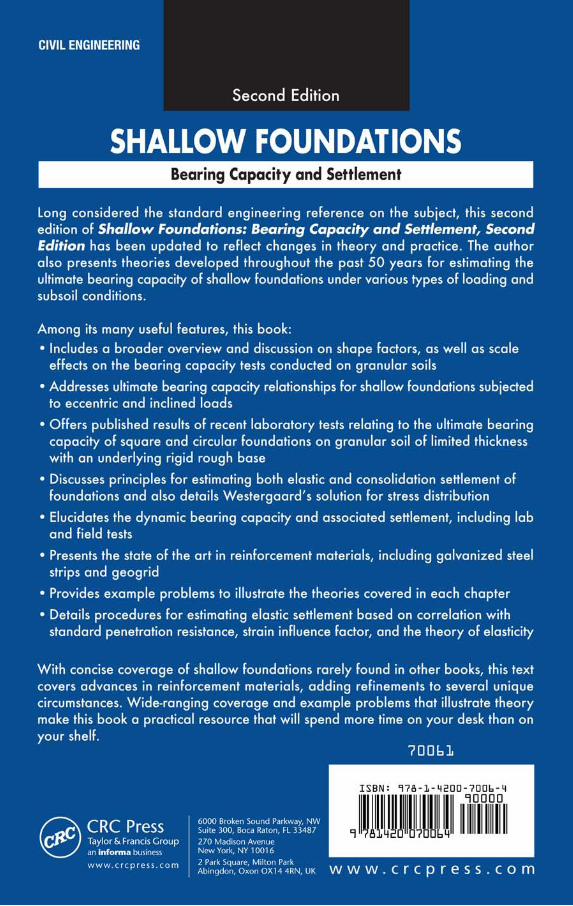
Related Documents


