Shadowing in Compton scattering on nuclei

arX

iv:1

003.

4188

v1 [

hep-

ph]

22

Mar

201

0

Shadowing in Compton scattering on nuclei

B.Z. Kopeliovich,∗ Ivan Schmidt,† and M. Siddikov‡

Departamento de Fısica, Centro de Estudios Subatomicos, y Centro Cientıfico - Tecnologico de Valparaıso,Universidad Tecnica Federico Santa Marıa, Casilla 110-V, Valparaıso, Chile

We evaluate the shadowing effect in deeply virtual and real Compton scattering on nuclei in theframework of the color dipole model. We rely on the soft photon wave function derived in theinstanton vacuum model, and employ the impact parameter dependent phenomenological elasticdipole amplitude. Both the effects of quark and the gluon shadowing are taken into account.

I. INTRODUCTION

Compton scattering, γ∗ + p → γ + p, with initial photons both real or virtual, has been a subject of intensivetheoretical and experimental investigation [1–16]. While in the case of deeply-virtual Compton scattering (DVCS),where the initial photon is highly-virtual, the QCD factorization has been proven [5, 7, 8] and the amplitude can beexpressed in terms of the generalized parton distributions (GPD) [1–15], in the case of real Compton scattering (RCS)the available theoretical tools are rather undeveloped.On the one hand, as it has been shown in [17, 18], for large momentum transfer ∆⊥ it is possible to factorize the

RCS amplitude [19, 20] and express it in terms of the distribution amplitudes of the proton. On the other hand, it ispossible to express the amplitude of the process via the minus 1st-moment of GPDs at zero skewedness [5, 21, 22].DVCS and RCS on a proton have been studied recently within the color dipole approach in [23, 24]. Here we extend

that study to nuclear targets. The DVCS process on a nuclear target has been measured at HERA by HERMEScollaboration [26] and may be also studied at the future Electron Ion Collider (EIC) and Large Hadron ElectronCollider (LHeC) [27, 28]. The Real Compton Scattering (RCS) may be measured at the LHC, as a subprocess inhadron-hadron collisions in ultraperipheral kinematics. Since both DVCS and RCS are studied in the high-energykinematics, the nuclear effects reveal themselves as shadowing corrections.The general framework for evaluation of the shadowing corrections is the Gribov-Glauber approach [29]. While in

the asymptotic high-energy (“frozen”) regime the shadowing corrections were studied in [25, 30], we use an approachwhich is also valid for intermediate energies. Also, we take into account the gluon shadowing corrections, which appearfor xB . 10−3 and give a sizeable contribution for xB ∼ 10−5.The paper is organized as follows. In Sections II we review the general formalism of the color dipole approach. In

Section III we discuss the frequently used frozen approximation which is valid for asymptotically large energies. InSection IV we discuss the method which will be used for calculations of nuclear shadowing effects and demonstratethat for asymptotically large energies it reproduces the results from Section III. In Section V we discuss the gluonshadowing and its effect on the DVCS and RCS observables. In Section VI the wavefunction of a real photon isevaluated in the instanton vacuum model. In Section VII we present the results of numerical evaluation, and inSection VIII we draw conclusions.

II. COLOR DIPOLE MODEL

The color dipole model is particularly efficient at high energies, where the dominant contribution to the Comptonamplitude comes from gluonic exchanges. Then the general expression for the Compton amplitude on a nucleon hasthe form,

A(ij)µν (s,∆) = e(i)µ e(j)ν

1ˆ

0

dβ1dβ2d2r1d

2r2Ψ(i)f (β2, ~r2)Ad (β1, ~r1;β2, ~r2; ∆)Ψ

(j)in (β1, ~r1) , (1)

∗Electronic address: [email protected]†Electronic address: [email protected]‡Electronic address: [email protected]

2

where e(i)µ is the photon polarization vector; β1,2 are the light-cone fractional momenta of the quark and antiquark, ~r1,2

are the transverse distances in the final and initial dipoles respectively; ∆ is the momentum transfer in the Compton

scattering, Ad(...) is the scattering amplitude of the dipole on the target (proton or nucleus), and Ψ(i)in(f) (β,~r) are the

wavefunctions of the initial and final photons in the polarization state i [31].At high energies in the small angle approximation, ∆/

√s≪ 1, the quark separation and fractional momenta β are

preserved, so,

Ad(

β1, ~r1;β2, ~r2;Q2,∆

)

≈ δ (β1 − β2) δ (~r1 − ~r2)

ˆ

d2b′ ei~∆~b′ℑmfN

qq(~r1,~b′, β1) (2)

ℑmfNqq(~r,

~b′, β) =1

12π

ˆ

d2k d2∆(

k + ∆2

)2 (k − ∆

2

)2αsF(

x,~k, ~∆)

ei~b′·~∆

×(

e−iβ~r·

(

~k−~∆2

)

− ei(1−β)~r·

(

~k−~∆2

))(

eiβ~r·

(

~k+~∆2

)

− e−i(1−β)~r·

(

~k+~∆2

))

, (3)

where

F(

x,~k, ~∆)

k2≡ Hg

(

x,~k, ~∆)

=1

2

ˆ

d2r eik·rˆ

dz−

2πeixP

+z− ×

×⟨

P ′

∣

∣

∣

∣

G+α

(

−z2, −~r

2

)

γ+L(

−z2− ~r

2,z

2+~r

2

)

G+α

(

z

2,~r

2

)∣

∣

∣

∣

P

⟩

(4)

is the gluon GPD of the target, P ′ = P + ∆,P = (P + P ′)/2, Gµν(x) is the gluon loop operator, L∞ (x, y) is theWilson factor required by gauge covariance. For this GPD we use a gaussian parameterization [55, 56, 66],

F(

x,~k, ~∆)

=3σ0(x)

16π2αs

(

k +∆

2

)2(

k − ∆

2

)2

R20(x) exp

(

−R20(x)

4

(

~k2 +~∆2

4

))

exp

(

−1

2B(x)∆2

)

, (5)

where σ0(x), R20(x), B(x) are the free parameters fixed from the DIS and πp scattering data. We shall discuss them

in more detail in Section VII. The parameterization (5) does not depend on the longitudinal momentum transfer anddecreases exponentially as a function of ∆2. Since the parameterization (5) is an effective one and is valid only in thesmall-x region, we do not assume that it satisfies general requirements, such as positivity [65] and polynomiality [3]constraints.The prefactor

(

k + ∆2

)2 (k − ∆

2

)2in (5) guarantees convergence of the integrals in the parameterization (2). In

the forward limit, the amplitude (2) reduces to the saturated parameterization of the dipole amplitude proposed byGolec-Biernat and Wusthoff (GBW) [53],

σd(β, r) = 2

ˆ

d2b′ ℑmfNqq(~r,

~b′, β) =1

6π

ˆ

d2k

k4αs

(

k2)

F(

x,~k,~0)

=σ0(x)

2

(

1− exp

(

− r2

R0(x)

))

(6)

Generally, the amplitude fNqq(...) involves nonperturbative physics, but the asymptotic behaviour for small r is con-

trolled by pQCD [32]:

fNqq(~r, ~∆, β)r→0 ∝ r2,

up to slowly varying corrections ∼ ln(r).Calculation of the differential cross section also involves the real part of scattering amplitude, whose relation to the

imaginary part is quite straightforward. According to [33], if the limit lims→∞

(

Imfsα

)

exists and is finite, then the real

and imaginary parts of the forward amplitude are related as

Re f(∆ = 0) = sα tan

[

π

2

(

α− 1 +∂

∂ ln s

)] ℑmf(∆ = 0)

sα. (7)

In the model under consideration the imaginary part of the forward dipole amplitude indeed has a power dependenceon energy, Imf(∆ = 0; s) ∼ sα, so (7) simplifies to

ReAℑmA = tan

(

π2 (α − 1)

)

≡ ǫ. (8)

3

This fixes the phase of the forward Compton amplitude, which we retain for nonzero momentum transfers, assumingsimilar dependences for the real and imaginary parts. Finally we arrive at,

A(ij)µν = (ǫ+ i)e(i)µ (q′)e(j)ν (q)

ˆ

d2r

1ˆ

0

dβ Ψ(i)f (β, r)Ψ

(j)in (β, r)ℑmfN

qq(~r, ~∆, β, s), (9)

For the cross-section of unpolarized Compton scattering, from (9) we obtain,

dσγpel

dt=

1 + ǫ2

16π

∑

ij

∣

∣

∣A(ij)

µν

∣

∣

∣

2

=

=1 + ǫ2

16π

∑

ij

∣

∣

∣

∣

∣

∣

ˆ

d2r

1ˆ

0

dβ Ψ(i)f (β, r)Ψ

(j)in (β, r)ℑmfN

qq(~r,~∆, β)

∣

∣

∣

∣

∣

∣

2

. (10)

III. NUCLEAR SHADOWING IN THE ”FROZEN” LIMIT

Nuclear shadowing signals the closeness of the unitarity limit. Hard reactions possess this feature only if they havea contribution from soft interactions. In DIS and DVCS the soft contribution arises from the so called aligned jetconfigurations [34], corresponding to qq fluctuations very asymmetric in sharing the photon momentum, β ≪ 1. Suchvirtual photon fluctuations, having large transverse separation, are the source of shadowing [40] .Calculation of nuclear shadowing simplifies considerably in the case of long coherence length [35], i.e. long lifetime of

the photon fluctuations, when it considerably exceeds the nuclear size. In this case Lorentz time dilation ”freezes” thetransverse size of the fluctuation during propagation though the nucleus. Then the Compton amplitude of coherentscattering, which leaves the nucleus intact, has the same form as Eq. (9) with a replacement of the nucleon Comptonamplitude by the nuclear one,

ℑmfNqq(r, β,∆) ⇒ ℑmfA

qq(r, β,∆) =

ˆ

d2b ei~∆·~b[

1− e−ℑmfNqq(r,β,∆=0)TA(b)

]

, (11)

where b is impact parameter of the photon-nucleus collision, TA(b) =´∞

−∞dz ρA(b, z) is the nuclear thickness function,

given by the integral of nuclear density along the direction of the collisions. In this expression we neglect the realpart of the amplitude which is particularly small for a coherent nuclear interaction.For incoherent Compton scattering, which results in nuclear fragmentation without particle production (quasielastic

scattering), the cross section has the form [36],

dσγAqel

dt= Bel e

Belt∑

ij

1ˆ

0

dβ

ˆ

d2rd2r′ Ψ(i)f (β, r) Ψ

(i)f (β, r′)Ψ

(j)in (β, r)Ψ

(j)in (β, r′)

× exp

[

1

2

(

σqq(r) − σqq(r′))

TA(b)

]

exp

[

σqq(r)σqq(r′)

16πBelTA(b)

]

− 1

≈ eBelt

16π

ˆ

d2b TA (b)

∣

∣

∣

∣

∣

∣

1ˆ

0

dβ d2r Ψf (β, r) σqq (r, s)Ψin (β, r) exp

[

−1

2σqq (r) TA (b]

)

∣

∣

∣

∣

∣

∣

2

. (12)

Here Bel is the t-slope of elastic dipole-nucleon amplitude. In this equation we treated the term quadratic in thedipole cross section as a small number and expanded the exponential in curly brackets.

IV. ONSET OF NUCLEAR SHADOWING

A. Coherent Compton scattering

The regime of frozen dipole size discussed in the previous section is valid only at very small xB in DVCS, or at highenergies in RCS. However, at medium small xB a dipole can ”breath”, i.e. vary its size, during propagation throughthe nucleus, and one should rely on a more sophisticated approach.

4

In this paper we employ the description of the onset of shadowing developed in [37] and based on the light-coneGreen function technique [38]. The propagation of a color dipole in a nuclear medium is described as motion in anabsorptive potential, i.e.

i∂W (z2, r2; z1, r1)

∂z2= −∆r2W (z2, r2; z1, r1)

να(1 − α)− iρA (z2, r2)σqq (r2)

2W (z2, r2; z1, r1) , (13)

where the Green function W (z2, r2; z1, r1) describes the probability amplitude for propagation of dipole state withsize r1 at the light-cone starting point z1 to the dipole state with size r2 at the light-cone point z2. Then the shadowingcorrection to the amplitude has the form

δA(s, ~∆⊥) =

ˆ

d2b ei~∆·~b⊥

ˆ

z1≤z2

dz1dz2 ρA(b, z1) ρA(b, z2)

1ˆ

0

dαd2r1d2r2 ×

Ψf (α, r2) σqq (r2) W (z2, r2; z1, r1)σqq (r1) Ψin (α, r1) eikmin(z2−z1),

where

kmin =Q2α(1− α) +m2

q

2να(1 − α).

Equation (13) is quite complicated and in the general case may be solved only numerically [39]. However in somecases an analytic solution is possible. For example, in the limit of long coherence length, lc ≫ RA, relevant forhigh-energy accelerators like LHC, one can neglect the “kinetic” term ∝ ∆r2W (z2, r2; z1, r1) in (13), and get theGreen function in the ”frozen” approximation [38],

W (z2, r2; z1, r1) = δ2 (r2 − r1) exp

−1

2σqq (r1)

z2ˆ

z1

dζ ρA (ζ, b)

. (14)

Then the shadowing correction (15) simplifies to

δA(s,∆⊥) =

ˆ

d2b ei~∆⊥·~b⊥

ˆ

z1≤z2

dz1dz2 ρA (z1, b) ρA (z2, b)

1ˆ

0

dα d2r σ2qq (r, b)× (15)

Ψf (α, r) exp

−1

2σqq (r)

z2ˆ

z1

dζρA (ζ, b)

Ψin (α, r) eikmin(z2−z1).

If we neglect the real part of the amplitude and the longitudinal momentum transfer kmin (which is justified forasymptotically large s), and average over polarizations, then taking the integral over z1,2 ”by parts” in (15), we getfor the elastic amplitude

A(s,∆⊥) = 2

ˆ

d2b ei~∆⊥·~b⊥

1ˆ

0

dα d2r Ψf (α, r)

1− exp

−1

2σqq (r)

+∞ˆ

−∞

dζρA (ζ, b)

Ψin (α, r) . (16)

Another case where an analytical solution is possible is when the effective dipole sizes are small and the functionσqq(r) may be approximated as

σqq(r) ≈ Cr2. (17)

This approximation cannot be precise even at high virtuality Q2 in DVCS, since there are contributions of thealigned jet configurations mentioned above, which permit large dipoles even for large Q2. Moreover, such alignedjet configurations of the dipole provide the main contribution to nuclear shadowing [40]. Nevertheless, for the sakeof simplicity we rely on this approximation in order to estimate the magnitude of the shadowing corrections. ThenEq. (13) yields for W (z2, r2; z1, r1) the well-known evolution operator of harmonic oscillator, although with complex

5

frequency

W (z2, r2; z1, r1) =a

2πi sin (ω∆z)exp

(

ia

2 sin (ω∆z)

[(

r21 + r22)

cos (ω∆z)− 2~r1 · ~r2]

)

, (18)

ω2 =−2iCρAνα(1 − α)

,

a2 = −iCρAνα(1 − α)/2

Notice that for DVCS in the kinematics of the HERMES experiment [26] the coherence length

lc ≈1

2mNxB∼ 1.7 fm

is comparable with the mean inter-nucleon spacing in nuclei and is much smaller than the radii of heavy nuclei.Therefore the frozen approximation employed in [25] cannot be used for an interpretation of HERMES data, insteadone should rely on the Green function method described above.

B. Incoherent scattering

In addition to the coherent processes which leave the recoil nucleus intact, a large contribution to photon productioncomes from incoherent Compton scattering, where the target nucleus breaks up. Using the missing mass techniqueone can select events γA→ γA∗ in which the nucleus breaks up to fragments without production of mesons. In thiscase one can employ completeness of the final states, which greatly simplifies the calculations.The analysis of such processes in electroproduction of vector mesons was done in [41], and its extension to the

DVCS and RCS is quite straightforward and yields

dσ

dt

∣

∣

∣

∣

∆⊥=0

=1

16π

ˆ

d2bdz ρA (b, z) |F1 (b, z)− F2 (b, z)|2 , (19)

F1 (b, z) =

1ˆ

0

dα d2r1 d2r2 Ψf (α,~r2)W (+∞, ~r2; z, ~r1)σqq (~r1, s)Ψin (α,~r1) , (20)

F2 (b, z) =

zˆ

−∞

dz2

1ˆ

0

dα d2r1 d2r2 d

2r3 Ψf (α,~r3)W (+∞, ~r3; z, ~r2)σqq (~r2, s)× (21)

W (z, ~r2; z2, ~r1) ρA (z2, b)σqq (~r1, s)Ψin (α,~r1) .

At sufficiently high energies one can rely on the frozen approximation introduced in the previous section, and thisformula may be simplified [42],

F1 (b, z) =

1ˆ

0

dαd2rΨf (α, r) σqq (r1, s)Ψin (α, r) exp

−1

2σqq (r)

+∞ˆ

z

dζρA (ζ, b)

, (22)

F2 (b, z) =

1ˆ

0

dαd2rΨf (α, r) × (23)

exp

−1

2σqq (r)

+∞ˆ

z

dζρA (ζ, b)

− exp

−1

2σqq (r)

+∞ˆ

−∞

dζρA (ζ, b)

σqq (r, s)Ψin (α, r) ,

Correspondingly the cross section (19) takes the form,

dσ

dt

∣

∣

∣

∣

∆⊥=0

=1

16π

ˆ

d2b TA (b)

∣

∣

∣

∣

∣

∣

1ˆ

0

dαd2rΨf (α, r) σqq (r, s) Ψin (α, r) exp

(

−1

2σqq (r) TA (b)

)

∣

∣

∣

∣

∣

∣

2

. (24)

6

This expression reproduces Eq. (12) derived in the ”frozen” limit. It is easy to see that in the limit of a transparentnucleus, σqqTA ≪ 1, the cross section Eq. (24) rises linearly with A. However in the limit of a very opaque nucleus(black disk limit), σqqTA ≫ 1, the absorptive exponential factor in (24) terminates the contribution of central impact

parameters, and dσ/dt|∆⊥=0 ∝ A1/3.In case of the approximation (17), we may use the explicit expression (18) for the Green function W (z2, ~r2; z1, ~r1)

to get

F1 (b, z) =

1ˆ

0

dαd2r1d2r2Ψf (α,~r2)

a

2πi sin (ω∆z)exp

(

ia

2 sin (ω∆z)

[(

r21 + r22)

cos (ω∆z)− 2~r1 · ~r2]

)

∆z=z∞−z

(25)

× σqq (~r1, s)Ψin (α,~r1) ,

F2 (b, z) =

zˆ

−∞

dz2

1ˆ

0

dα d2r1d2r2d

2r3Ψf (α,~r3)σqq (~r2, s) ρA (b, z2)σqq (~r1, s) (26)

× a

2πi sin (ω∆z)exp

(

ia

2 sin (ω∆z)

[(

r23 + r22)

cos (ω∆z)− 2~r3 · ~r2]

)

∆z=z∞−z2

× a

2πi sin (ω∆z)exp

(

ia

2 sin (ω∆z)

[(

r21 + r22)

cos (ω∆z)− 2~r1 · ~r2]

)

∆z=z2−z

Ψin (α,~r1) .

V. GLUON SHADOWING

It has been known since [43] that in addition to the quark shadowing inside nuclei there is also a shadowing ofgluons, which leads to attenuation of the gluon parton distributions. While nuclear shadowing of quarks is directlymeasured in DIS, the shadowing of gluons is poorly known from data [44, 45], mainly due to the relatively large errorbars in the nuclear structure functions and their weak dependence on the gluon distributions, which only comes viaevolution. The theoretical predictions for the gluon shadowing strongly depend on the implemented model–while forxB & 10−3 they all predict that the gluon shadowing is small, for xB . 10−3 the predictions vary in a wide range(see the review [45] and references therein). Since in this paper we also make predictions for the LHC energy range,the gluon shadowing corrections should be taken into account as well.In the framework of the color dipole model the gluon attenuation factor Rg was evaluated in the Gribov-Glauber

approach in [46]. It was found convenient to evaluate the gluon attenuation ratio Rg defined as

Rg

(

x,Q2, b)

=GA

(

x,Q2, b)

TA(b)GN (x,Q2, b),

where GN

(

x,Q2, b)

is the impact parameter dependent gluon GPD, relating it to the shadowing corrections in DISwith longitudinally polarized photons,

Rg

(

x,Q2, b)

≈ 1− ∆σγ∗pL

(

x,Q2, b)

TA(b)σγ∗pL (x,Q2)

, (27)

where ∆σγ∗pL = σγ∗A

L − Aσγ∗pL is the shadowing correction at impact parameter b, and σγ∗p

L

(

x,Q2)

is the totalphotoabsorption cross section for a longitudinal photon. The process with longitudinal photons is chosen because thealigned jets configurations are suppressed by powers of Q2, so that the average size of the dipole is small,

⟨

r2⟩

∼ 1/Q2,and nuclear shadowing mainly originates from gluons.As it was shown in [46],

∆σγ∗pL

(

x,Q2, b)

=

ˆ +∞

−∞

dz1

ˆ +∞

−∞

dz2Θ(z2 − z1) ρA (b, z1) ρA (b, z2) Γ(

x,Q2, z2 − z1)

, (28)

where ρA(b, z) is the nuclear density, and Γ(

x,Q2,∆z)

is defined as

Γ(

x,Q2,∆z)

= ℜeˆ 0.1

x

dαG

αG

16αem

(∑

Z2q

)

αs

(

Q2)

C2eff

3π2Q2b2×

7

×[(

1− 2ζ − ζ2)

e−ζ + ζ2(3 + ζ)E1(ζ)]

×[

t

w+

sinh (Ω∆z)

tln

(

1− t2

u2

)

+2t3

uw2+t sinh (Ω∆z)

w2+

4t3

w3

]

,

with

b2 = (0.65GeV )2+ αGQ

2,

Ω =iB

αG (1− αG) ν,

B =

√

b4 − iαG (1− αG) νCeffρA,

ν =Q2

2mNx,

ζ = ixmN∆z,

t =B

b2,

u = t cosh (Ω∆z) + sinh (Ω∆z) ,

w =(

1 + t2)

sinh (Ω∆z) + 2t cosh (Ω∆z) ,

For heavy nuclei we may rely on the hard sphere approximation, ρA(r) ≈ ρA(0)Θ (RA − r), and simplify (28) to:

∆σγ∗p(

x,Q2, b)

≈ ρ2A(0)

ˆ L

0

d∆z(L−∆z)Γ(

x,Q2,∆z)

,

where L = 2√

R2A − b2. For the total cross-section after integration over

´

d2b we may get

∆σγ∗p(

x,Q2)

=

ˆ

d2b∆σγ∗p(

x,Q2, b)

≈ πρ2A(0)

12

ˆ 2R

0

d∆zΓ(

x,Q2,∆z) (

16R3A − 12R2

A∆z +∆z3)

The results of evaluation of the gluon shadowing are presented in Section VII.

VI. WAVEFUNCTIONS FROM THE INSTANTON VACUUM

In this section we present briefly some details of evaluation of the wavefunction in the instanton vacuummodel (see [47–49] and references therein). The central object of the model is the effective action for the lightquarks in the instanton vacuum, which in the leading order in Nc has the form [48, 49]

S =

ˆ

d4x

(

N

Vlnλ+ 2Φ2(x)− ψ

(

p+ v −m− cLf ⊗ Φ · Γm ⊗ fL)

ψ

)

,

where Γm is one of the matrices, Γm = 1, i~τ , γ5, i~τγ5, ψ and Φ are the fields of constituent quarks and mesonsrespectively, N/V is the density of the instanton gas, v ≡ vµγ

µ is the external vector current corresponding to thephoton, L is the gauge factor,

L (x, z) = P exp

i

xˆ

z

dζµvµ(ζ)

, (29)

which provides the gauge covariance of the action, and f(p) is the Fourier transform of the zero-mode profile.In the leading order in Nc, we have the same Feynman rules as in perturbative theory, but with a momentum-

dependent quark mass µ(p) in the quark propagator

S(p) =1

p− µ(p) + i0. (30)

8

The mass of the constituent quark has a form

µ(p) = m+M f2(p),

where m ≈ 5 MeV is the current quark mass, M ≈ 350 MeV is the dynamical mass generated by the interaction withthe instanton vacuum background. Due to the presence of the instantons the coupling of a vector current to a quarkis also modified,

v ≡ vµγµ → V = v + V nonl,

V nonl ≈ −2Mf(p)df(p)

dpµvµ(q) +O

(

q2)

. (31)

Notice that for an arbitrary photon momentum q the expression for V nonl depends on the choice of the path in (29)and as a result one can find in the literature different expressions used for evaluations [31, 50–52]. In the limit p→ ∞the function f(p) falls off as ∼ 1

p3 , so for large p ≫ ρ−1, where ρ ≈ (600MeV )−1 is the mean instanton size, the

mass of the quark µ(p) ≈ m and vector current interaction vertex V ≈ v. However we would like to emphasize thatthe wavefunction Ψ(β, r) gets contribution from both the soft and the hard parts, so even in the large-Q limit theinstanton vacuum function is different from the well-known perturbative result.We have to evaluate the wavefunctions associated with the following matrix elements:

IΓ(β,~r) =

ˆ

dz−

2πei(β+

12 )q

−z+

⟨

0

∣

∣

∣

∣

ψ

(

−z2n− ~r

2

)

Γψ

(

z

2n+

~r

2

)∣

∣

∣

∣

γ(q)

⟩

, (32)

where Γ is one of the matrices Γ = γµ, γµγ5, σµν . In the leading order in Nc one can easily obtain

IΓ =

ˆ

d4p

(2π)4ei~p⊥~r⊥δ

(

p+ −(

β +1

2

)

q+)

Tr(

S(p)V S(p+ q)Γ)

. (33)

The evaluation of (33) is quite tedious but straightforward. Details of this evaluation may be found in [31].The overlap of the initial and final photon wavefunctions in (10) was evaluated according to

Ψ(i)∗(β, r,Q2 = 0)Ψ(i)(β, r,Q2) =∑

Γ

I∗Γ (β, r∗, 0) IΓ(

β, r,Q2)

, (34)

where summation is done over possible polarization states Γ = γµ, γµγ5, σµν . In the final state we should use

r∗µ = rµ+nµq′⊥·r⊥q+

= rµ−nµ∆⊥·r⊥

q+, which is related to the reference frame with q′⊥ = 0 in which the components (33)

were evaluated.

VII. NUMERICAL RESULTS

In this section we present the results of numerical calculations. In this paper we consider two processes–DVCSand RCS. While physically they differ only by the kinematics, the parameterizations used for scattering with softand hard photons are different. For example, for DVCS we have photons with large Q2–in this region we haveBjorken scaling, so all the model parameters such as basic cross-section σ0 and saturation radius R0 in Eq. (5).should depend on the Bjorken xB. A widely accepted parameterization which incorporates this features is the GBWparameterization [53]. On the contrary, for RCS when Q2 is vanishingly small, xB vanishes and thus all variablesshould depend on Mandelstam s. An example of such parameterization is KST parameterization introduced in [54–57].Up to the best of our knowledge there is no single parameterization which incorporates both asymptotic cases. Forthis reason for DVCS we used the GBW-style parameterization [53, 66] for the nonintegrated gluon density Eq.(5),which has a form

σ0(x) = 23.03mb = const, (35)

R0(x) = 0.4 fm× (x/x0)0.144, (36)

B(x) = Bγ∗p→ρp −1

8R2

0(x), (37)

where x0 = 3.04× 10−4, and Bγ∗p→ρp(x,Q2 ≫ 1GeV 2) ≈ 5GeV −2 [58].

9

Q2=5 GeV2

Q2=20 GeV2

A=40

A=208

10-110-210-310-4

xB

1

0.9

0.8

0.7

0.6

0.5

0.4

dσ A

/ dσ N

FA

2(t

)A=40A=208

xB=10-3

xB=10-5

5 10 15 20

Q2, GeV2

0.5

1

dσ A

/2 d

σ NF

A2(t

)

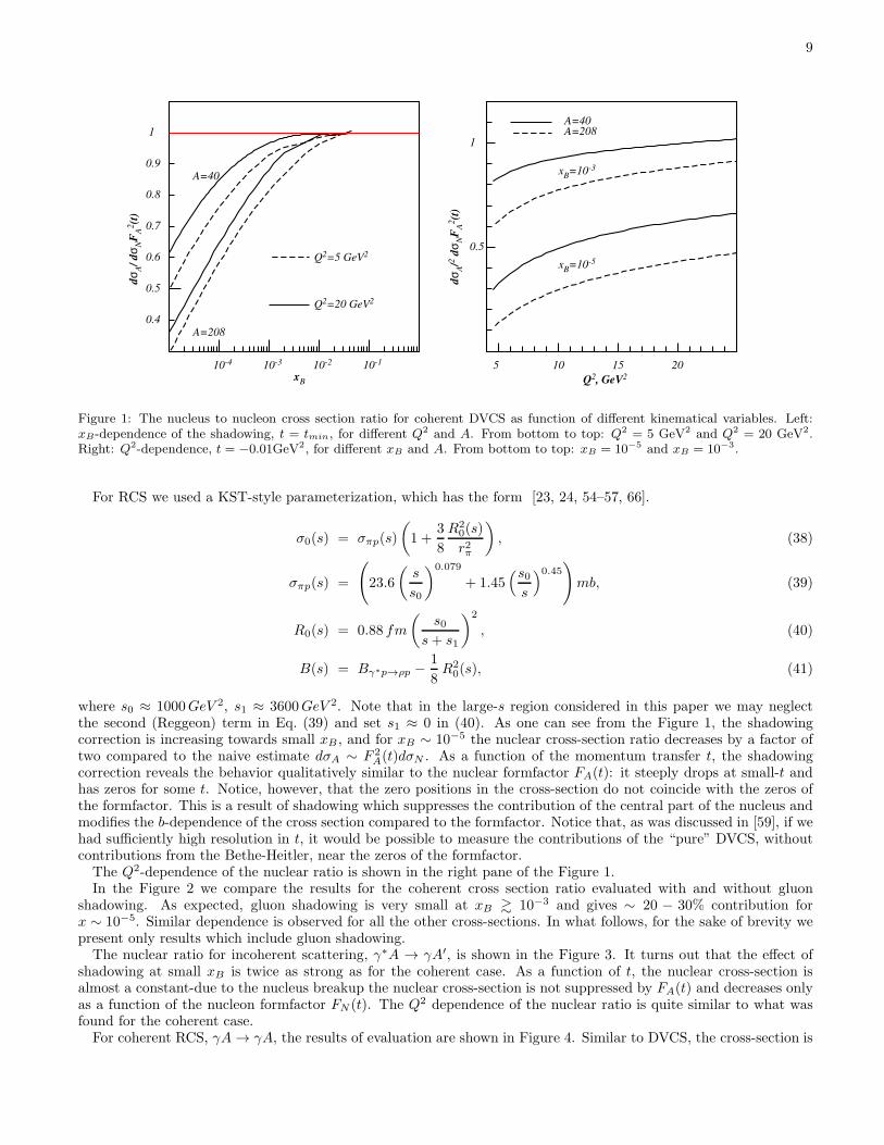
Figure 1: The nucleus to nucleon cross section ratio for coherent DVCS as function of different kinematical variables. Left:xB-dependence of the shadowing, t = tmin, for different Q2 and A. From bottom to top: Q2 = 5 GeV2 and Q2 = 20 GeV2.Right: Q2-dependence, t = −0.01GeV2, for different xB and A. From bottom to top: xB = 10−5 and xB = 10−3.

For RCS we used a KST-style parameterization, which has the form [23, 24, 54–57, 66].

σ0(s) = σπp(s)

(

1 +3

8

R20(s)

r2π

)

, (38)

σπp(s) =

(

23.6

(

s

s0

)0.079

+ 1.45(s0s

)0.45)

mb, (39)

R0(s) = 0.88 fm

(

s0s+ s1

)2

, (40)

B(s) = Bγ∗p→ρp −1

8R2

0(s), (41)

where s0 ≈ 1000GeV 2, s1 ≈ 3600GeV 2. Note that in the large-s region considered in this paper we may neglectthe second (Reggeon) term in Eq. (39) and set s1 ≈ 0 in (40). As one can see from the Figure 1, the shadowingcorrection is increasing towards small xB , and for xB ∼ 10−5 the nuclear cross-section ratio decreases by a factor oftwo compared to the naive estimate dσA ∼ F 2

A(t)dσN . As a function of the momentum transfer t, the shadowingcorrection reveals the behavior qualitatively similar to the nuclear formfactor FA(t): it steeply drops at small-t andhas zeros for some t. Notice, however, that the zero positions in the cross-section do not coincide with the zeros ofthe formfactor. This is a result of shadowing which suppresses the contribution of the central part of the nucleus andmodifies the b-dependence of the cross section compared to the formfactor. Notice that, as was discussed in [59], if wehad sufficiently high resolution in t, it would be possible to measure the contributions of the “pure” DVCS, withoutcontributions from the Bethe-Heitler, near the zeros of the formfactor.The Q2-dependence of the nuclear ratio is shown in the right pane of the Figure 1.In the Figure 2 we compare the results for the coherent cross section ratio evaluated with and without gluon

shadowing. As expected, gluon shadowing is very small at xB & 10−3 and gives ∼ 20 − 30% contribution forx ∼ 10−5. Similar dependence is observed for all the other cross-sections. In what follows, for the sake of brevity wepresent only results which include gluon shadowing.The nuclear ratio for incoherent scattering, γ∗A → γA′, is shown in the Figure 3. It turns out that the effect of

shadowing at small xB is twice as strong as for the coherent case. As a function of t, the nuclear cross-section isalmost a constant-due to the nucleus breakup the nuclear cross-section is not suppressed by FA(t) and decreases onlyas a function of the nucleon formfactor FN (t). The Q2 dependence of the nuclear ratio is quite similar to what wasfound for the coherent case.For coherent RCS, γA→ γA, the results of evaluation are shown in Figure 4. Similar to DVCS, the cross-section is

10

without gluons

with gluons

A=40

A=208

10-110-210-310-4

xB

1

0.9

0.8

0.7

0.6

0.5

0.4

dσ A

/ dσ N

FA

2(t

)A=40A=208

10-1

10-2

10-3

10-4

10-5

10-6

10-7

10-8

-t, GeV2

0.1 0.2 0.3 0.4

dσ A

/A2d

σ N

Figure 2: The nucleus to nucleon cross section ratio for coherent DVCS as function of different kinematical variables. Left:shadowing as function of Bjorken xB with and without gluon shadowing for different nuclei, t = tmin, Q

2 = 5GeV2. Right:t-dependence for different A. xB = 10−3, Q2 = 5GeV2.

Q2=5 GeV2

Q2=20 GeV2

A=40

A=208

10-110-210-310-4

xB

1

0.9

0.8

0.7

0.6

0.5

0.4

0.3

dσ A

/A d

σ N

A=40

A=208

Q2=20 GeV2

Q2=5 GeV2

1

0.9

0.8

0.7

0.6

0.5

0.4

0.3

0.2

0.1

-t×102, GeV25 10 15 20 25

dσ A

/A d

σ N

A=40A=208

5 10 15 20

Q2, GeV2

0.5

1

dσ A

/ A

dσ N

, x

B=

0.0

01, t=

-0.0

1 G

eV2

Figure 3: Dependence of the nuclear ratio for incoherent DVCS on different kinematical variables. Left: xB-dependence, center:t-dependence, right: Q2-dependence.

steeply falling with center of mass energy W (for DVCS xB ∝ 1/W 2 at fixed(

Q2, t)

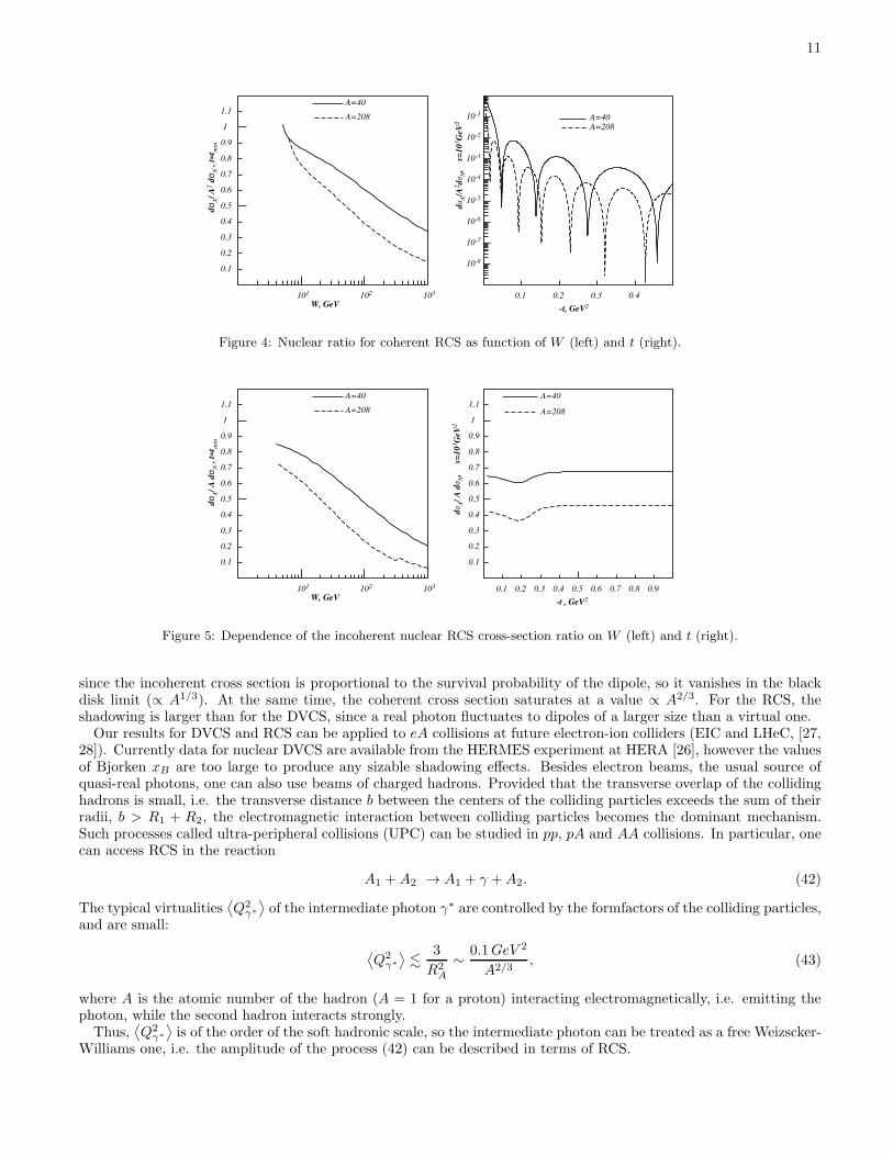
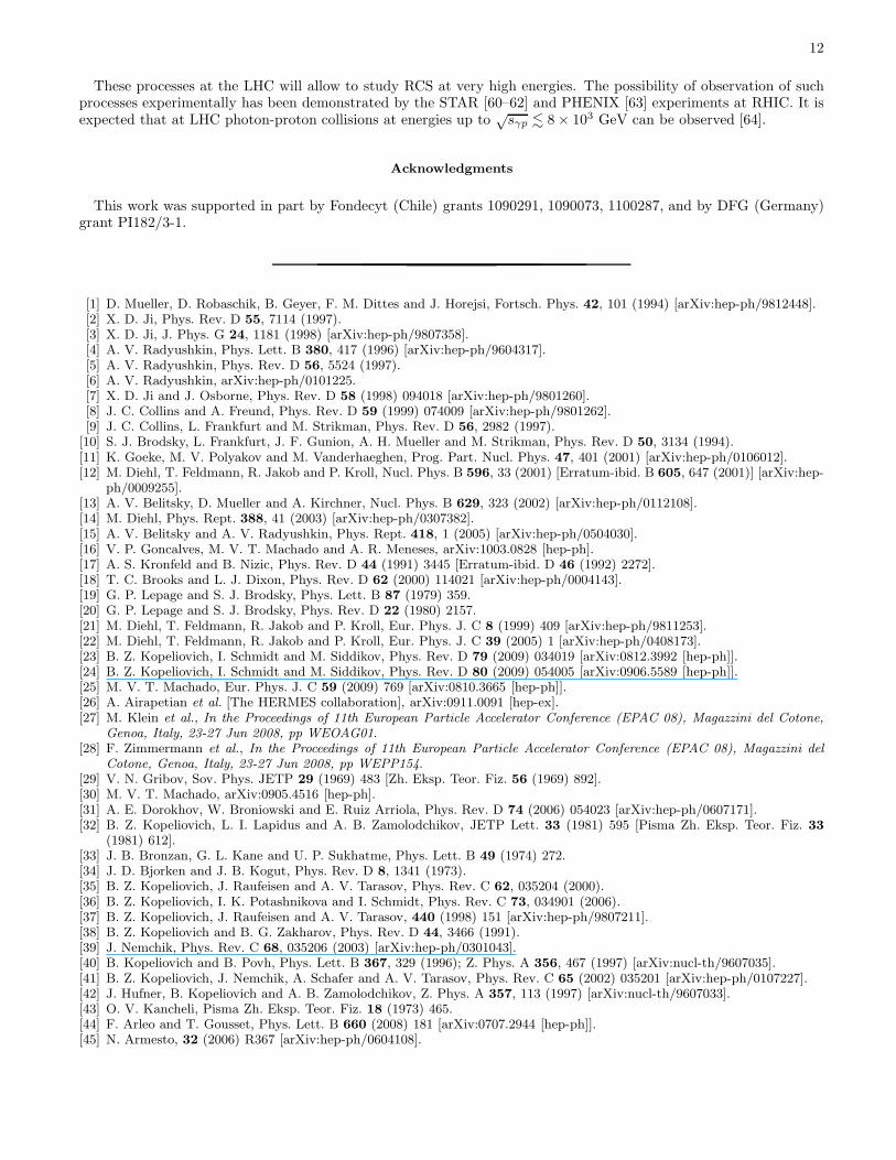
). As function of the momentumtransfer t, the shadowing correction reveals the behavior qualitatively similar to the case of coherent DVCS (see Fig. 1)It steeply decreases similar to the behavior of the nuclear formfactor FA(t).For the incoherent RCS, γA → γA′, the results of evaluation are shown in Figure 5. Similar to the coherent case,

the cross-section is decreasing as function of W , down to the values an order of magnitude smaller than would give asimple sum of the nucleon cross-sections. As function of t, the cross-section is almost constant because of absence ofthe nuclear formfactor.

VIII. CONCLUSIONS AND PROSPECTS

In this paper we considered DVCS and RCS on nuclear targets within the color dipole model. Results for thecoherent shadowing are presented in Section VII. We found that the magnitude of nuclear shadowing is large and isimportant for analysis of DVCS and RCS data. It may cause a substantial suppression of the nuclear DVCS cross-section. We observed that for incoherent case, the shadowing is stronger than for the coherent case. This happens

11

A=40

A=208

W, GeV

dσ A

/ A

2 d

σ N , t

=t m

in

101 102 103

1.1

1

0.9

0.8

0.7

0.6

0.5

0.4

0.3

0.2

0.1

A=40A=208

10-1

10-2

10-3

10-4

10-5

10-6

10-7

10-8

-t, GeV2

0.1 0.2 0.3 0.4

dσ A

/A2d

σ N, s

=10

3G

eV2

Figure 4: Nuclear ratio for coherent RCS as function of W (left) and t (right).

A=40

A=208

W, GeV

dσ A

/ A

dσ N

, t

=t m

in

101 102 103

1.1

1

0.9

0.8

0.7

0.6

0.5

0.4

0.3

0.2

0.1

A=40

A=2081.1

1

0.9

0.8

0.7

0.6

0.5

0.4

0.3

0.2

0.1

0.90.80.70.60.50.40.30.20.1

-t , GeV2

dσ A

/ A

dσ N

, s=

10

3G

eV2

Figure 5: Dependence of the incoherent nuclear RCS cross-section ratio on W (left) and t (right).

since the incoherent cross section is proportional to the survival probability of the dipole, so it vanishes in the blackdisk limit (∝ A1/3). At the same time, the coherent cross section saturates at a value ∝ A2/3. For the RCS, theshadowing is larger than for the DVCS, since a real photon fluctuates to dipoles of a larger size than a virtual one.Our results for DVCS and RCS can be applied to eA collisions at future electron-ion colliders (EIC and LHeC, [27,

28]). Currently data for nuclear DVCS are available from the HERMES experiment at HERA [26], however the valuesof Bjorken xB are too large to produce any sizable shadowing effects. Besides electron beams, the usual source ofquasi-real photons, one can also use beams of charged hadrons. Provided that the transverse overlap of the collidinghadrons is small, i.e. the transverse distance b between the centers of the colliding particles exceeds the sum of theirradii, b > R1 + R2, the electromagnetic interaction between colliding particles becomes the dominant mechanism.Such processes called ultra-peripheral collisions (UPC) can be studied in pp, pA and AA collisions. In particular, onecan access RCS in the reaction

A1 +A2 → A1 + γ +A2. (42)

The typical virtualities⟨

Q2γ∗

⟩

of the intermediate photon γ∗ are controlled by the formfactors of the colliding particles,and are small:

⟨

Q2γ∗

⟩

.3

R2A

∼ 0.1GeV 2

A2/3, (43)

where A is the atomic number of the hadron (A = 1 for a proton) interacting electromagnetically, i.e. emitting thephoton, while the second hadron interacts strongly.Thus,

⟨

Q2γ∗

⟩

is of the order of the soft hadronic scale, so the intermediate photon can be treated as a free Weizscker-Williams one, i.e. the amplitude of the process (42) can be described in terms of RCS.

12

These processes at the LHC will allow to study RCS at very high energies. The possibility of observation of suchprocesses experimentally has been demonstrated by the STAR [60–62] and PHENIX [63] experiments at RHIC. It isexpected that at LHC photon-proton collisions at energies up to

√sγp . 8× 103 GeV can be observed [64].

Acknowledgments

This work was supported in part by Fondecyt (Chile) grants 1090291, 1090073, 1100287, and by DFG (Germany)grant PI182/3-1.

[1] D. Mueller, D. Robaschik, B. Geyer, F. M. Dittes and J. Horejsi, Fortsch. Phys. 42, 101 (1994) [arXiv:hep-ph/9812448].[2] X. D. Ji, Phys. Rev. D 55, 7114 (1997).[3] X. D. Ji, J. Phys. G 24, 1181 (1998) [arXiv:hep-ph/9807358].[4] A. V. Radyushkin, Phys. Lett. B 380, 417 (1996) [arXiv:hep-ph/9604317].[5] A. V. Radyushkin, Phys. Rev. D 56, 5524 (1997).[6] A. V. Radyushkin, arXiv:hep-ph/0101225.[7] X. D. Ji and J. Osborne, Phys. Rev. D 58 (1998) 094018 [arXiv:hep-ph/9801260].[8] J. C. Collins and A. Freund, Phys. Rev. D 59 (1999) 074009 [arXiv:hep-ph/9801262].[9] J. C. Collins, L. Frankfurt and M. Strikman, Phys. Rev. D 56, 2982 (1997).

[10] S. J. Brodsky, L. Frankfurt, J. F. Gunion, A. H. Mueller and M. Strikman, Phys. Rev. D 50, 3134 (1994).[11] K. Goeke, M. V. Polyakov and M. Vanderhaeghen, Prog. Part. Nucl. Phys. 47, 401 (2001) [arXiv:hep-ph/0106012].[12] M. Diehl, T. Feldmann, R. Jakob and P. Kroll, Nucl. Phys. B 596, 33 (2001) [Erratum-ibid. B 605, 647 (2001)] [arXiv:hep-

ph/0009255].[13] A. V. Belitsky, D. Mueller and A. Kirchner, Nucl. Phys. B 629, 323 (2002) [arXiv:hep-ph/0112108].[14] M. Diehl, Phys. Rept. 388, 41 (2003) [arXiv:hep-ph/0307382].[15] A. V. Belitsky and A. V. Radyushkin, Phys. Rept. 418, 1 (2005) [arXiv:hep-ph/0504030].[16] V. P. Goncalves, M. V. T. Machado and A. R. Meneses, arXiv:1003.0828 [hep-ph].[17] A. S. Kronfeld and B. Nizic, Phys. Rev. D 44 (1991) 3445 [Erratum-ibid. D 46 (1992) 2272].[18] T. C. Brooks and L. J. Dixon, Phys. Rev. D 62 (2000) 114021 [arXiv:hep-ph/0004143].[19] G. P. Lepage and S. J. Brodsky, Phys. Lett. B 87 (1979) 359.[20] G. P. Lepage and S. J. Brodsky, Phys. Rev. D 22 (1980) 2157.[21] M. Diehl, T. Feldmann, R. Jakob and P. Kroll, Eur. Phys. J. C 8 (1999) 409 [arXiv:hep-ph/9811253].[22] M. Diehl, T. Feldmann, R. Jakob and P. Kroll, Eur. Phys. J. C 39 (2005) 1 [arXiv:hep-ph/0408173].[23] B. Z. Kopeliovich, I. Schmidt and M. Siddikov, Phys. Rev. D 79 (2009) 034019 [arXiv:0812.3992 [hep-ph]].[24] B. Z. Kopeliovich, I. Schmidt and M. Siddikov, Phys. Rev. D 80 (2009) 054005 [arXiv:0906.5589 [hep-ph]].[25] M. V. T. Machado, Eur. Phys. J. C 59 (2009) 769 [arXiv:0810.3665 [hep-ph]].[26] A. Airapetian et al. [The HERMES collaboration], arXiv:0911.0091 [hep-ex].[27] M. Klein et al., In the Proceedings of 11th European Particle Accelerator Conference (EPAC 08), Magazzini del Cotone,

Genoa, Italy, 23-27 Jun 2008, pp WEOAG01.[28] F. Zimmermann et al., In the Proceedings of 11th European Particle Accelerator Conference (EPAC 08), Magazzini del

Cotone, Genoa, Italy, 23-27 Jun 2008, pp WEPP154.[29] V. N. Gribov, Sov. Phys. JETP 29 (1969) 483 [Zh. Eksp. Teor. Fiz. 56 (1969) 892].[30] M. V. T. Machado, arXiv:0905.4516 [hep-ph].[31] A. E. Dorokhov, W. Broniowski and E. Ruiz Arriola, Phys. Rev. D 74 (2006) 054023 [arXiv:hep-ph/0607171].[32] B. Z. Kopeliovich, L. I. Lapidus and A. B. Zamolodchikov, JETP Lett. 33 (1981) 595 [Pisma Zh. Eksp. Teor. Fiz. 33

(1981) 612].[33] J. B. Bronzan, G. L. Kane and U. P. Sukhatme, Phys. Lett. B 49 (1974) 272.[34] J. D. Bjorken and J. B. Kogut, Phys. Rev. D 8, 1341 (1973).[35] B. Z. Kopeliovich, J. Raufeisen and A. V. Tarasov, Phys. Rev. C 62, 035204 (2000).[36] B. Z. Kopeliovich, I. K. Potashnikova and I. Schmidt, Phys. Rev. C 73, 034901 (2006).[37] B. Z. Kopeliovich, J. Raufeisen and A. V. Tarasov, 440 (1998) 151 [arXiv:hep-ph/9807211].[38] B. Z. Kopeliovich and B. G. Zakharov, Phys. Rev. D 44, 3466 (1991).[39] J. Nemchik, Phys. Rev. C 68, 035206 (2003) [arXiv:hep-ph/0301043].[40] B. Kopeliovich and B. Povh, Phys. Lett. B 367, 329 (1996); Z. Phys. A 356, 467 (1997) [arXiv:nucl-th/9607035].[41] B. Z. Kopeliovich, J. Nemchik, A. Schafer and A. V. Tarasov, Phys. Rev. C 65 (2002) 035201 [arXiv:hep-ph/0107227].[42] J. Hufner, B. Kopeliovich and A. B. Zamolodchikov, Z. Phys. A 357, 113 (1997) [arXiv:nucl-th/9607033].[43] O. V. Kancheli, Pisma Zh. Eksp. Teor. Fiz. 18 (1973) 465.[44] F. Arleo and T. Gousset, Phys. Lett. B 660 (2008) 181 [arXiv:0707.2944 [hep-ph]].[45] N. Armesto, 32 (2006) R367 [arXiv:hep-ph/0604108].

13

[46] B. Z. Kopeliovich, J. Raufeisen, A. V. Tarasov and M. B. Johnson, Phys. Rev. C 67 (2003) 014903 [arXiv:hep-ph/0110221].[47] T. Schafer and E. V. Shuryak, Rev. Mod. Phys. 70 (1998) 323 [arXiv:hep-ph/9610451].[48] D. Diakonov and V. Y. Petrov, Nucl. Phys. B 272 (1986) 457[49] D. Diakonov, M. V. Polyakov and C. Weiss, Nucl. Phys. B 461 (1996) 539 [arXiv:hep-ph/9510232].[50] I. V. Anikin, A. E. Dorokhov and L. Tomio, Phys. Part. Nucl. 31 (2000) 509 [Fiz. Elem. Chast. Atom. Yadra 31 (2000)

1023].[51] A. E. Dorokhov and W. Broniowski, Eur. Phys. J. C 32 (2003) 79 [arXiv:hep-ph/0305037].[52] K. Goeke, M. M. Musakhanov and M. Siddikov, Phys. Rev. D 76 (2007) 076007 [arXiv:0707.1997 [hep-ph]][53] K. J. Golec-Biernat and M. Wusthoff, Phys. Rev. D 59 (1999) 014017 [arXiv:hep-ph/9807513].[54] B.Z. Kopeliovich, A. Schafer and A.V. Tarasov, Phys. Rev. D62, 054022 (2000).[55] B. Z. Kopeliovich, H. J. Pirner, A. H. Rezaeian and I. Schmidt, Phys. Rev. D 77 (2008) 034011 [arXiv:0711.3010 [hep-ph]].[56] B. Z. Kopeliovich, A. H. Rezaeian and I. Schmidt, arXiv:0809.4327 [hep-ph], to appear in Phys. Rev. D.[57] B. Z. Kopeliovich, J. Nemchik and I. Schmidt, Phys. Rev. C 76 (2007) 025210 [arXiv:hep-ph/0703118].[58] S. Chekanov et al., (ZEUS Collaboration), PMC Phys. A1, 6 (2007) [arXiv:0708.1478 ].[59] K. Goeke, V. Guzey and M. Siddikov, Phys. Rev. C 79 (2009) 035210 [arXiv:0901.4711 [hep-ph]].[60] B. I. Abelev et al. [STAR Collaboration], Phys. Rev. C 77 (2008) 034910 [arXiv:0712.3320 [nucl-ex]].[61] J. Adams et al. [STAR Collaboration], Phys. Rev. C 70 (2004) 031902 [arXiv:nucl-ex/0404012].[62] C. Adler et al. [STAR Collaboration], Phys. Rev. Lett. 89 (2002) 272302 [arXiv:nucl-ex/0206004].[63] D. G. d’Enterria, arXiv:nucl-ex/0601001.[64] K. Hencken et al., Phys. Rept. 458 (2008) 1 [arXiv:0706.3356 [nucl-ex]].[65] P. V. Pobylitsa, Phys. Rev. D 65 (2002) 114015 [arXiv:hep-ph/0201030].[66] B. Z. Kopeliovich, I. K. Potashnikova, I. Schmidt and J. Soffer, Phys. Rev. D 78 (2008) 014031 [arXiv:0805.4534 [hep-ph]].