Shadow banking and financial stability under limited deposit ...

Working Paper Series No105 / December 2019

Shadow banking and financial stability under limited deposit insurance by Lukas Voellmy

Abstract

I study the relation between shadow banking and financial stability in an economy in whichbanks are susceptible to self-fulfilling runs and in which government-backed deposit insuranceis limited. Shadow banks issue only uninsured deposits while commercial banks issue both in-sured and uninsured deposits. The effect of shadow banking on financial stability is ambiguousand depends on the (exogenous) upper limit on insured deposits. If the upper limit on insureddeposits is high, then the presence of a shadow banking sector is detrimental to financial stabil-ity; shadow banking creates systemic instability that would not be present if all deposits wereheld in the commercial banking sector. In contrast, if the upper limit on insured deposits is low,then the presence of a shadow banking sector is beneficial from a financial stability perspec-tive; shadow banks absorb uninsured (and uninsurable) deposits from the commercial bankingsector, thereby shielding commercial banks from runs. While runs may occur in the shadowbanking sector, the situation without shadow banks and a larger amount of uninsured depositsheld at commercial banks is worse.

JEL-Codes: E44, G21, G28

Keywords: Shadow Banking, Deposit Insurance, Bank Runs, Financial Intermediation

1 Introduction

The recent decades have witnessed the growth of a so-called shadow banking sector in the United

States, which provides very short-term claims similar to bank deposits outside the traditional bank-

ing system (Poszar et al. 2010 and Ricks 2012 provide good overviews).1 Prominent examples of

shadow bank claims are money market mutual fund shares, overnight asset backed commercial pa-

per, or certain forms of repo.2 Since the financial crisis of 2007-08, and especially since the run on

money market mutual funds in September 20083, the shadow banking sector is widely thought to

pose a threat to financial stability.

In this paper, I present a theoretical argument why the financial stability implications of the shadow

banking sector should not be analyzed separately from the cap on deposit insurance at traditional

banks. Shadow banks cater mostly to institutional investors managing large cash-balances, who

have a preference for extremely safe, short-term assets (Poszar 2011). For instance, cash pools of

large non-financial corporations today commonly amount to several hundred million USD, a large

part of which is held in the form of shadow bank liabilities rather than traditional bank deposits

(Poszar 2011). Given the cap on deposit insurance, it is impossible or impracticable for these in-

stitutional cash pools to hold all of their funds in the form of insured bank deposits. In this context

of limited deposit insurance, shadow banks can have the effect of absorbing uninsured (and unin-

surable) short-term claims from the commercial banking sector. I show that this aspect of shadow

banking may be beneficial from a financial stability perspective and a flow of uninsured deposits

back into the commercial banking sector can be detrimental to aggregate financial stability.

1There is no universally accepted definition of the term shadow banking. Some understand the term broadly, encom-passing various sorts of financial intermediation outside the traditional banking system (e.g. FSB (2017)). Othersdefine shadow banking more narrowly as the provision of ‘money-like’ (or bank-deposit-like) liabilities outside thetraditional banking system (e.g. Poszar (2014)). This paper has the latter, narrow definition in mind.

2Short-term asset backed commercial paper has diminished in importance since the financial crisis. The moneymarket mutual fund industry is in flux after reforms enacted in 2016 (see Cipriani et al. (2017)).

3Schmidt et al. (2016) provide a detailed description of the run on money market mutual funds in 2008. Episodes thatcan be characterized as bank runs were also observed in other segments of the shadow banking system such as themarket for short-term asset backed commercial paper (Covitz et al. 2013, Kacperczyk and Schnabl 2010).

2

I take the deposit insurance scheme, and in particular the cap on deposit insurance, as exogenous

throughout the paper. Deriving the optimal level of the cap is not the subject of this paper. For a

given deposit insurance scheme in place, I derive the structure of the financial system for which

aggregate losses caused by systemic bank runs are minimized, and I compare it to the structure of

the financial system that results in a competitive equilibrium. In this sense, the paper speaks to a

regulator that cannot change the deposit insurance scheme in place.

Model Summary The model features banks that sell claims which are redeemable on demand

(‘deposits’) to households. Banks invest into riskless projects whose maturity exceeds the maturity

of deposits. The short-term nature of the claims issued by banks is taken as given. Households

choose at which banks to hold their deposits. In addition, households can choose to obtain deposit

insurance for a limited amount of deposits. The limit on insured deposits is given by an exogenous

parameter representing the cap on deposit insurance. The cap on deposit insurance amounts to a

rationing of deposit insurance; it implies that some fraction of deposits are ‘uninsurable’. The lower

the deposit insurance cap, the higher the amount of uninsurable deposits. The only dimension in

which banks differ from each other is the share of insured and uninsured deposits among the deposits

issued. If all deposits issued by a bank are uninsured, the bank is labelled a ‘shadow bank’. If some

(not necessarily all) of the deposits issued by a bank are insured by deposit insurance, the bank is

labelled a ‘commercial bank’.4

Since banks engage in maturity transformation, they are illiquid in an interim period, which opens

up the possibility of self-fulfilling bank runs in the spirit of Diamond and Dybvig (1983). Depos-

itors never have an incentive to run on their insured deposits, which means that only uninsured

deposits may potentially be withdrawn in a run. If a bank is hit by a run, it needs to sell assets on

a secondary market. The liquidation price of assets in the secondary market is decreasing in the

total amount of assets liquidated by banks (‘cash-in-the-market pricing’). An individual bank is

susceptible to a run if (i) the share of uninsured deposits at the bank is high and (ii) the liquidation

4In order to focus on the aspects most relevant for the theme of this paper, I abstract from other differences betweenshadow- and commercial banks. In reality, shadow- and commercial banks differ in more dimensions than just thefact that shadow bank liabilities are not explicitly protected by government-sponsored deposit insurance.

3

price of assets is low. The liquidation price itself depends on how many other banks are hit by a

run and sell assets, which introduces a systemic element to bank runs. The model abstracts from

fundamental risk, so that these self-fulfilling, systemic bank runs constitute the only source of risk

in the economy.

Main Results First I show that, for a given total amount of insured and uninsured deposits out-

standing in the economy, the set of banks that can potentially be affected by a systemic run depends

on the distribution of insured and uninsured deposits across banks. In general, the magnitude of

systemic bank runs is minimized if the financial system exhibits a dual structure, with one sector

that issues both insured and uninsured deposits (the commercial banking sector) and another sector

that issues only uninsured deposits (the shadow banking sector). While systemic runs may occur in

the shadow banking sector, the presence of the shadow banking sector also implies that the share

of insured deposits at commercial banks is relatively high, so that systemic runs do not encompass

the commercial banking sector. For this reason, a shadow banking sector can be beneficial from a

financial stability perspective if the deposit insurance cap is low, that is, if the share of uninsurable

deposits in the economy is high. To minimize aggregate losses caused by runs, the shadow bank-

ing sector should be set to the smallest size at which it absorbs enough of the uninsurable deposits

from the commercial banking sector such as to keep the commercial banking sector shielded from

systemic runs.

Next, I analyze the structure of the financial system that results in a competitive equilibrium and

compare it to the optimal allocation as described above. Households may face conflicting incen-

tives regarding the type of bank at which they hold deposits. On the one hand, the presence of

insured depositors who do not participate in runs reduces expected losses caused by runs for unin-

sured depositors at commercial banks. This gives households an incentive to hold uninsured (and

uninsurable) deposits at commercial banks rather than shadow banks. On the other hand, if the de-

posit insurance agency charges a fee on deposits issued by commercial banks, households have an

incentive to move into shadow banks in order to avoid the fee. The shadow banking sector tends to

be smaller than optimal if the share of uninsurable deposits is high (that is, if the deposit insurance

4

cap is low). Intuitively, if aggregate financial stability is low, households have an incentive to move

uninsurable deposits from the shadow banking sector into the more stable commercial banking sec-

tor, thereby increasing the share of uninsured deposits held at commercial banks, which causes the

commercial banking sector to become susceptible to runs as well. In contrast, the shadow banking

sector tends to be larger than optimal if the share of uninsurable deposits is low (that is, if the de-

posit insurance cap is high). In this case, the commercial banking sector will not be susceptible to

systemic runs even if most (or all) uninsurable deposits are held at commercial banks. In a compet-

itive equilibrium, households move deposits into the shadow banking sector in order to avoid the

fee on commercial bank deposits. The equilibrium size of the shadow banking sector is such that

shadow banks are susceptible to systemic runs and households are indifferent at the margin between

investing in shadow banks prone to runs and paying the fee on commercial bank deposits.

A regulator aiming to implement the optimal size of the shadow banking sector, taking as given

the deposit insurance cap in place, can achieve this with a two-pronged policy. First, impose a tax

on shadow bank deposits that mimics the fee charged on commercial bank deposits. This prevents

the shadow banking sector from growing too large relative to the optimal size. Second, impose a

marginal tax on uninsured commercial bank deposits that exceed a certain amount. This limits the

amount of uninsured deposits held at commercial banks and ensures that the shadow banking sector

is not too small relative to the optimal size.

Related Literature In a recent paper, Davila and Goldstein (2016) study the optimal level of the

cap on deposit insurance, including the case where runs have a systemic element as in the present

paper. Increasing the cap has the benefit of reducing expected losses caused by runs but entails

social costs such as deadweight losses of taxation. The present paper is complementary to Davila

and Goldstein (2016) by showing that the trade-offs studied in Davila and Goldstein (2016) can

be improved if, in addition to choosing the level of the cap, an appropriate distribution of insured

and uninsured deposits across banks can be implemented. Another closely related paper is Luck

and Schempp (2016) who study financial stability implications of the shadow banking sector in an

economy in which commercial banks issue insured- and shadow banks uninsured short-term claims.

5

The magnitude of systemic runs increases in the size of the shadow banking sector. The present

paper shows that some of the conclusions reached in Luck and Schempp (2016) regarding shadow

banking and financial stability may be reversed if deposit insurance is limited and commercial banks

issue both insured and uninsured deposits.

More generally, this paper is related to a recent theoretical literature studying the financial stability

implications of the shadow banking sector. Hanson et al. (2015) characterize shadow banking

and commercial banking as two different ways to provide riskless claims. Shadow banks create

riskless claims by investing in relatively liquid assets that can be liquidated immediately if bad

news arrive. In this sense the occurrence of fire sales in the shadow banking sector is inherent to

shadow banks’ business model. In Gertler et al. (2016) shadow banks are modelled as wholesale

banks that issue debt to other (retail) banks. Due to a relatively low degree of agency frictions

compared to retail banking, shadow banking can reduce the financial accelerator in the aftermath

of real shocks. However, high leverage in the shadow banking sector can also lead to instability in

the form of bank runs. Moreira and Savov (2017) characterize shadow banking as the provision

of risky claims which are information-insensitive and therefore provide liquidity services. This

leads to a socially desirable expansion of liquidity in normal times but makes the economy more

vulnerable to changes in aggregate uncertainty. Martin et al. (2014) study run equilibria on various

types of shadow banks, taking into account the specifics of the debt contracts used. Gennaioli et al.

(2013) focus on shadow banks’ role in the securitization process. While securitization allows for

gains from trade between risk averse buyers of securities and risk neutral financial intermediaries,

it also makes the financial system more vulnerable to aggregate shocks. Compared to the papers

mentioned above, the present paper highlights that, in the context of limited deposit insurance, the

presence or absence of a shadow banking sector affects the distribution of uninsurable short-term

claims across different financial institutions, with consequences for financial stability. This paper

abstracts of many issues relevant to shadow banking and should be seen as complementary to the

papers mentioned above.

6

Finally, this paper’s interest in the effect of deposit insurance design on the equilibrium structure of

a financial system populated (potentially) by both commercial banks and shadow banks is shared

by two recent papers by LeRoy and Singhania (2017) and Chrétien and Lyonnet (2017), albeit with

a somewhat different focus. LeRoy and Singhania (2017) study how deposit insurance pricing

affects equilibrium portfolio choices of commercial banks and shadow banks. In Chrétien and

Lyonnet (2017), the deposit insurance scheme allows commercial banks to issue riskless debt in

times of crisis, which enables them to act as a ‘buyer of last resort’ for assets usually held by

shadow banks. This leads to a complementarity between commercial banking and shadow banking,

and an extension of the deposit insurance scheme for commercial banks indirectly benefits shadow

banks as well. In order to focus on the aspects that are most relevant for the main theme of this

paper, I abstract from banks’ portfolio choices and treat the secondary market for banks’ assets as

exogenous.

The remainder of the paper is structured as follows. Section 2 describes the environment. Section

3 discusses run equilibria. Section 4 derives the optimal structure of the financial system. Sections

5 and 6 discuss the competitive equilibria of the economy, first for the case where deposit insurance

is costless for households (section 5) and then for the case where a fee is charged on commercial

bank deposits (section 6). Section 7 discusses how the optimal structure of the financial system can

be implemented in a competitive equilibrium.

2 The Model

The economy lasts for two periods, indexed by t=0,1. Period 1 is subdivided into beginning of

period and end of period. There is an infinitely divisible good used for consumption and investment.

Two types of agents populate the economy in period 0: A continuum of households, indexed by

h P H � r0, 1s and a continuum of banks, indexed by i P I � r0, 1s. Each household is born

with an endowment of one unit of good. Banks are born without endowment. At the beginning of

7

period 1, a continuum r0, 1s of agents called ‘outside investors’ are born, each with an endowment

of λS P p0, 1q units of good.

In period 0, there is a riskless, constant returns to scale investment technology that returns one

unit of good at the end of period 1 per unit of good invested in period 0. Investments cannot be

terminated prematurely at the beginning of period 1. There is no other storage technology between

periods 0 and 1.

Households maximize expected utility Erupc1qs, where c1 ¥ 0 is defined as total consumption dur-

ing period 1. Households are therefore indifferent about whether to consume at the beginning or at

the end of period 1. Utility up�q is strictly increasing, strictly concave and twice continuously dif-

ferentiable. Banks’ utility is strictly increasing in both period 0 and period 1 consumption. Outside

investors’ utility is strictly increasing in period 1 consumption.

For reasons that are outside of the model, households only save in the form of demand deposits,

which can be issued by banks in period 0. Banks can invest the proceeds from the sale of demand

deposits in period 0 into the investment technology. Demand deposits issued by any bank i:

(i) stipulate the return rpiq which the bank pays to depositors at the end of period 1, per unit

invested into the bank in period 0.5

(ii) allow depositors to withdraw an amount of good equal to the face value of the deposit al-

ready at the beginning of period 1. Depositors who withdraw early are served sequentially in

random order, as in Diamond and Dybvig (1983).

Since the investment technology pays out only at the end of period 1, banks are illiquid at the

beginning of period 1. If households withdraw early, banks need to raise good by selling claims to

the investment return to outside investors. Note that, since investments are fundamentally riskless,

losses incurred by banks are always related to liquidation losses incurred at the beginning of period

1. Households are indifferent about when to consume during period 1, and I assume they withdraw

early only if they have a strict incentive to do so.5Competition among banks is going to imply that rpiq � 1 for all banks.

8

The final element of the model is an exogenous scheme of limited deposit insurance. In period 0,

after having bought demand deposits from banks, households can choose for which deposits to ob-

tain deposit insurance. If households obtain deposit insurance for some of the deposits they bought,

they are guaranteed to receive an amount of good equal to the face value of the deposits at the end of

period 1. Whenever a bank is not able to pay out an amount of good corresponding to the face value

of the insured deposits at the end of period 1, deposit insurance makes up for the difference. The

total face value of insured deposits held by a household is limited to θ P r0, 1s, where θ represents

the ‘cap’ on deposit insurance. The cap amounts to a rationing of deposit insurance. Different to

real-world deposit insurance arrangements, the cap is a cap per person, without a specific limit on

insured deposits held at a certain bank.6 Depositors may choose to obtain deposit insurance for

some, but not all, of the deposits held at one particular bank. As a result, among the deposits issued

by a given bank, some may be insured by deposit insurance while others are not.

In the baseline version of the model, households can obtain deposit insurance for deposits issued

by all banks at no cost.7 Deposit insurance payments are financed by levying a lump-sum tax on

all households at the end of period 1.8 The deposit insurance agency remains passive as events

unfold. If banks have both insured and uninsured deposits outstanding at the end of period 1,

banks are allowed to pay their uninsured depositors first, thereby shifting losses (in case the bank

incurred losses) towards deposit insurance.9 I abstract from any further issues related to moral

hazard or asymmetric information; the face value of deposits sold in period 0 must be backed by a

corresponding amount of real investment and banks commit to pay depositors in period 1 whenever

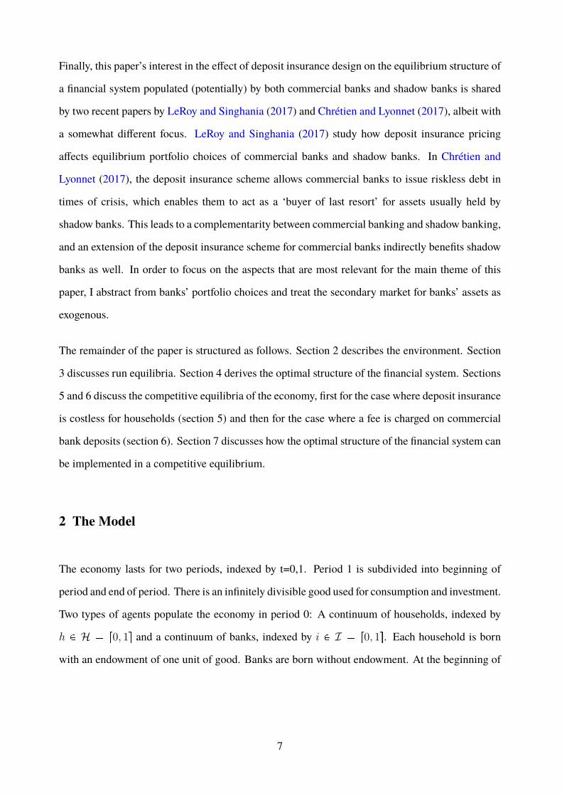
they can, rather than running away with the investment return. Figure 1 sketches the timeline.6Modelling the cap as a cap per person and bank would call for a richer model that endogenizes the number of banksthat offer insured deposits in equilibrium, for instance by introducing a fixed cost of opening a bank. See alsosection 6.

7In section 6, I discuss a version of the model where banks can choose whether or not get access to deposit insurance,and a fee is charged on all deposits issued by banks with access to deposit insurance.

8Consumption c1 equals the total return received during period 1 from a household’s investment into deposits (includ-ing any payment by deposit insurance in case some banks failed) minus taxes to deposit insurance. Since depositinsurance payments represent transfers from households to themselves, all households can pay the lump-sum tax ina symmetric allocation. In a hypothetical non-symmetric allocation in which some households’ consumption levelc1 would go to negative if they paid the entire tax, these households consume c1 � 0 and the tax will be increasedaccordingly for the remaining households.

9Without loss of generality, I assume banks always make use of this possibility. See Schilling (2018) for a settingwhere the deposit insurance agency acts strategically and sets its forbearance policy optimally for given levels ofdeposit insurance coverage.

9

Figure 1: Timeline.

3 Runs

When faced with withdrawals at the beginning of period 1, banks need to sell assets (claims to

investment return) to outside investors in order to pay out the depositors who withdraw.10 As in

Diamond and Dybvig (1983), orders of withdrawals are processed sequentially in random order

and depositors are paid out at face value.11 Let p denote the price, at the beginning of period 1, of

an asset that pays out one unit of good at the end of period 1. Since there is no discounting within

period 1, outside investors will buy assets at a price of p � 1 (the fundamental value) as long as their

endowment is sufficient to do so. Let λD denote the total fundamental value of all assets sold at the

beginning of period 1. If λD ¡ λS then outside investors’ aggregate endowment is not sufficient to

buy all assets sold in the beginning of period 1 at their fundamental value, and the market-clearing

price is determined by cash-in-the-market pricing a-la Allen and Gale (1994):

ppλDqloomoonliquidation

price

� min!

secondarymarketcapacityhkkikkjλS

λDloomoonassetssold

, 1)

(1)

From Diamond and Dybvig (1983) we know that the combination of payment-on-demand deposits

and liquidation losses can lead to self-fulfilling run equilibria. Liquidation losses occur whenever

assets trade below fundamental value. However, since depositors never have an incentive to with-10A ‘depositor’ is a household that holds deposits (insured or uninsured) at a bank.11The order of the line is determined independently at each bank, which allows households to diversify away idiosyn-

cratic risk regarding the order in the line by spreading their investment over many banks. See also the discussionin section 5 and footnote 20.

10

draw insured deposits early, susceptibility to runs depends also on the share of insured deposits

among the deposits issued by a bank.

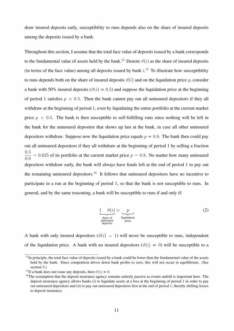
Throughout this section, I assume that the total face value of deposits issued by a bank corresponds

to the fundamental value of assets held by the bank.12 Denote ϑpiq as the share of insured deposits

(in terms of the face value) among all deposits issued by bank i.13 To illustrate how susceptibility

to runs depends both on the share of insured deposits ϑpiq and on the liquidation price p, consider

a bank with 50% insured deposits (ϑpiq � 0.5) and suppose the liquidation price at the beginning

of period 1 satisfies p   0.5. Then the bank cannot pay out all uninsured depositors if they all

withdraw at the beginning of period 1, even by liquidating the entire portfolio at the current market

price p   0.5. The bank is then susceptible to self-fulfilling runs since nothing will be left in

the bank for the uninsured depositor that shows up last at the bank, in case all other uninsured

depositors withdraw. Suppose now the liquidation price equals p � 0.8. The bank then could pay

out all uninsured depositors if they all withdraw at the beginning of period 1 by selling a fraction0.5

0.8� 0.625 of its portfolio at the current market price p � 0.8. No matter how many uninsured

depositors withdraw early, the bank will always have funds left at the end of period 1 to pay out

the remaining uninsured depositors.14 It follows that uninsured depositors have no incentive to

participate in a run at the beginning of period 1, so that the bank is not susceptible to runs. In

general, and by the same reasoning, a bank will be susceptible to runs if and only if:

1 � ϑpiqlooomooonshare ofuninsureddeposits

¡ ploomoonliquidation

price

(2)

A bank with only insured depositors (ϑpiq � 1) will never be susceptible to runs, independent

of the liquidation price. A bank with no insured depositors (ϑpiq � 0) will be susceptible to a

12In principle, the total face value of deposits issued by a bank could be lower than the fundamental value of the assetsheld by the bank. Since competition drives down bank profits to zero, this will not occur in equilibrium. (Seesection 5.)

13If a bank does not issue any deposits, then ϑpiq � 0.14The assumption that the deposit insurance agency remains entirely passive as events unfold is important here. The

deposit insurance agency allows banks (i) to liquidate assets at a loss at the beginning of period 1 in order to payout uninsured depositors and (ii) to pay out uninsured depositors first at the end of period 1, thereby shifting lossesto deposit insurance.

11

run whenever p   1, that is, whenever assets trade below fundamental value. Banks that are

hit by a run sell their entire portfolio on the secondary market. By cash-in-the-market pricing

(1), the liquidation price p thus depends on how many banks are hit by a run. This introduces a

systemic element to runs; the larger the number of banks hit by a run, the larger the number of

banks susceptible to a run.

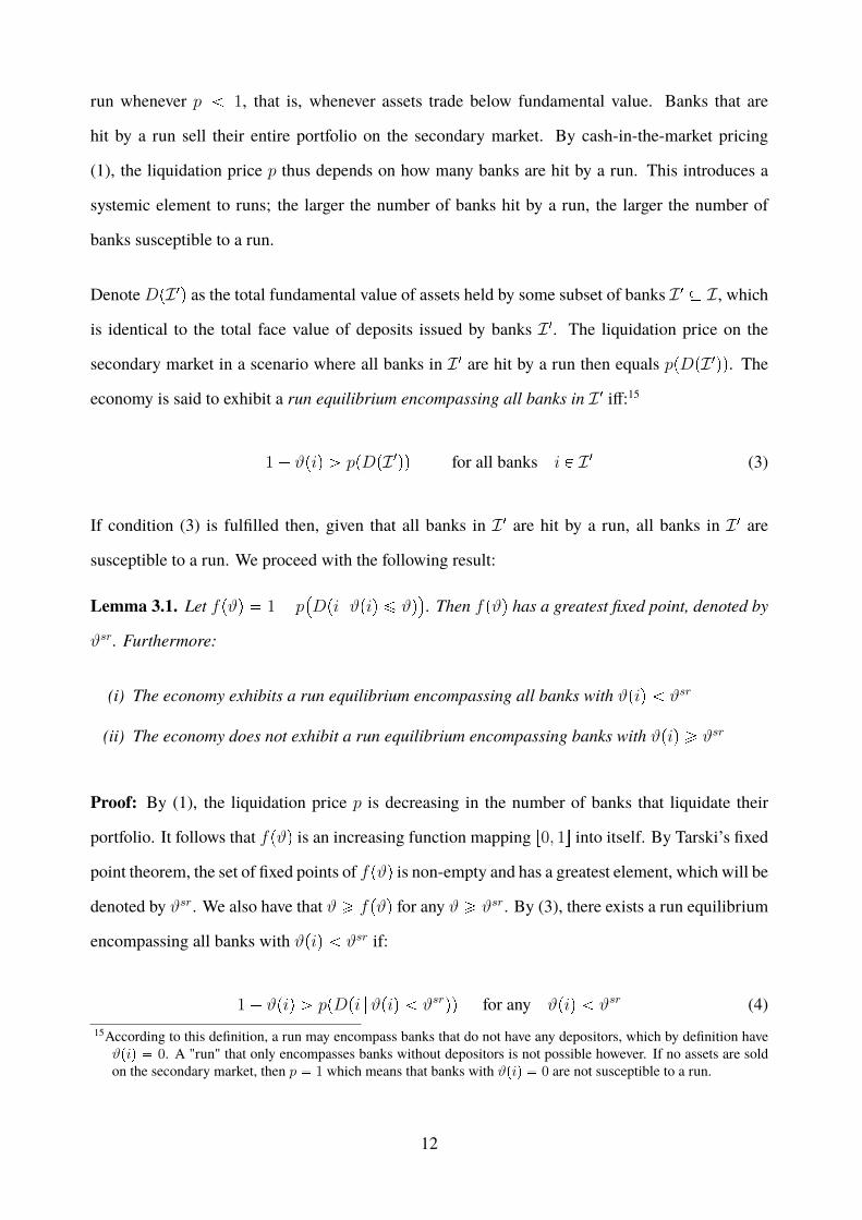
DenoteDpI 1q as the total fundamental value of assets held by some subset of banks I 1 � I, which

is identical to the total face value of deposits issued by banks I 1. The liquidation price on the

secondary market in a scenario where all banks in I 1 are hit by a run then equals ppDpI 1qq. The

economy is said to exhibit a run equilibrium encompassing all banks in I 1 iff:15

1 � ϑpiq ¡ ppDpI 1qq for all banks i P I 1 (3)

If condition (3) is fulfilled then, given that all banks in I 1 are hit by a run, all banks in I 1 are

susceptible to a run. We proceed with the following result:

Lemma 3.1. Let fpϑq � 1� p�Dpi |ϑpiq ¤ ϑq

�. Then fpϑq has a greatest fixed point, denoted by

ϑsr. Furthermore:

(i) The economy exhibits a run equilibrium encompassing all banks with ϑpiq   ϑsr

(ii) The economy does not exhibit a run equilibrium encompassing banks with ϑpiq ¥ ϑsr

Proof: By (1), the liquidation price p is decreasing in the number of banks that liquidate their

portfolio. It follows that fpϑq is an increasing function mapping r0, 1s into itself. By Tarski’s fixed

point theorem, the set of fixed points of fpϑq is non-empty and has a greatest element, which will be

denoted by ϑsr. We also have that ϑ ¥ fpϑq for any ϑ ¥ ϑsr. By (3), there exists a run equilibrium

encompassing all banks with ϑpiq   ϑsr if:

1 � ϑpiq ¡ ppDpi |ϑpiq   ϑsrqq for any ϑpiq   ϑsr (4)15According to this definition, a run may encompass banks that do not have any depositors, which by definition haveϑpiq � 0. A "run" that only encompasses banks without depositors is not possible however. If no assets are soldon the secondary market, then p � 1 which means that banks with ϑpiq � 0 are not susceptible to a run.

12

Rewriting condition 4 yields:

ϑpiq   1�ppDpi |ϑpiq   ϑsrqq ¤ 1�ppDpi |ϑpiq ¤ ϑsrqq � fpϑsrq � ϑsr for any ϑpiq   ϑsr

Hence condition 4 is fulfilled and the economy exhibits a run equilibrium encompassing all banks

with ϑpiq   ϑsr. Suppose next that, in contradiction to item (ii) in lemma 3.1, the economy exhibits

a run equilibrium encompassing a bank with ϑpiq � ϑ ¥ ϑsr. Then the economy exhibits a run

equilibrium encompassing all banks with ϑpiq ¤ ϑ. (This follows from the fact that, by (2), any

bank that is susceptible to a run at some liquidation price p1 will also be susceptible to run at

any liquidation price p2 ¤ p1). Repeating the same steps as before, the economy exhibits a run

equilibrium encompassing all banks with ϑpiq ¤ ϑ only if:

ϑpiq   1 � ppDpi |ϑpiq ¤ ϑqq � fpϑq for any ϑpiq ¤ ϑ (5)

Since ϑ ¥ fpϑq, condition 5 is violated and we arrive at a contradiction. �

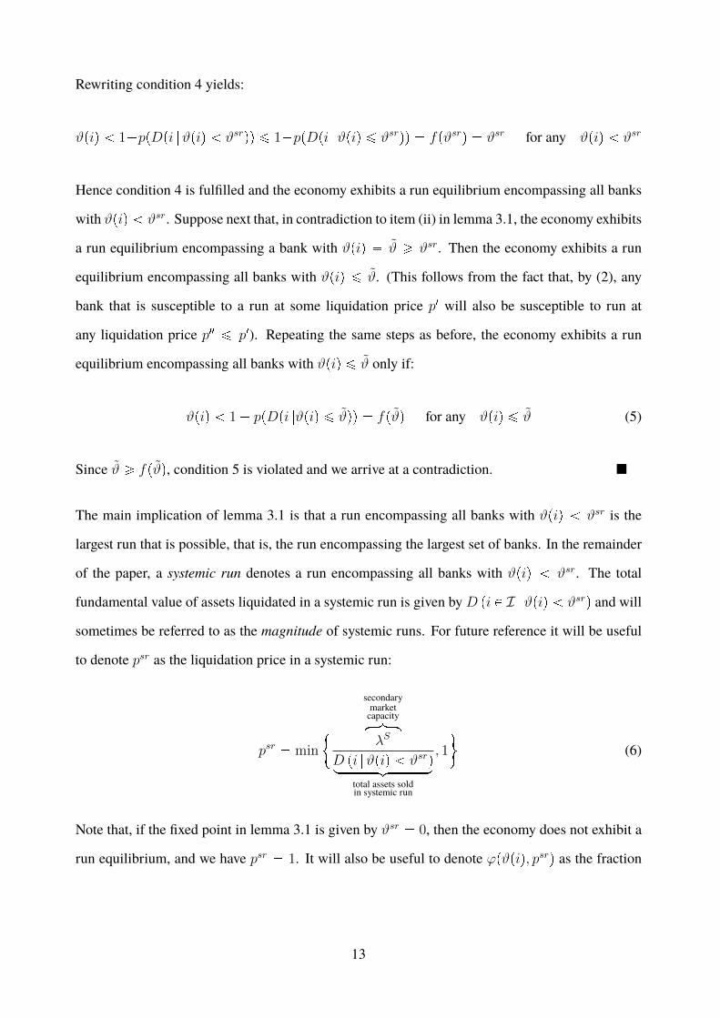
The main implication of lemma 3.1 is that a run encompassing all banks with ϑpiq   ϑsr is the

largest run that is possible, that is, the run encompassing the largest set of banks. In the remainder

of the paper, a systemic run denotes a run encompassing all banks with ϑpiq   ϑsr. The total

fundamental value of assets liquidated in a systemic run is given byD pi P I |ϑpiq   ϑsrq and will

sometimes be referred to as the magnitude of systemic runs. For future reference it will be useful

to denote psr as the liquidation price in a systemic run:

psr � min

"secondarymarketcapacityhkkikkjλS

D pi |ϑpiq   ϑsrqlooooooooomooooooooontotal assets soldin systemic run

, 1

*(6)

Note that, if the fixed point in lemma 3.1 is given by ϑsr � 0, then the economy does not exhibit a

run equilibrium, and we have psr � 1. It will also be useful to denote ϕpϑpiq, psrq as the fraction

13

of uninsured deposits that bank i can pay out in case of a systemic run:

ϕpϑpiq, psrq � min!

liquidationprice in runhkkikkjpsr

1 � ϑpiqlooomooonshare ofuninsureddeposits

, 1)

(7)

The fraction of uninsured deposits a bank can pay out in a systemic run increases in the share of

insured deposits at the bank, ϑpiq, and the liquidation price psr. If bank i is not susceptible to runs,

then we have ϕp�q � 1.

Equilibrium selection is driven by an exogenous sunspot variable ξ P t0, 1u that realizes at the

beginning of period 1. Households select the no-run equilibrium if ξ � 0 occurs and they select the

systemic run equilibrium if ξ � 1 occurs, in case the economy exhibits a systemic run equilibrium.16

ξ � 1 occurs with some probability πr ¡ 0 and ξ � 0 occurs with probability 1 � πr.

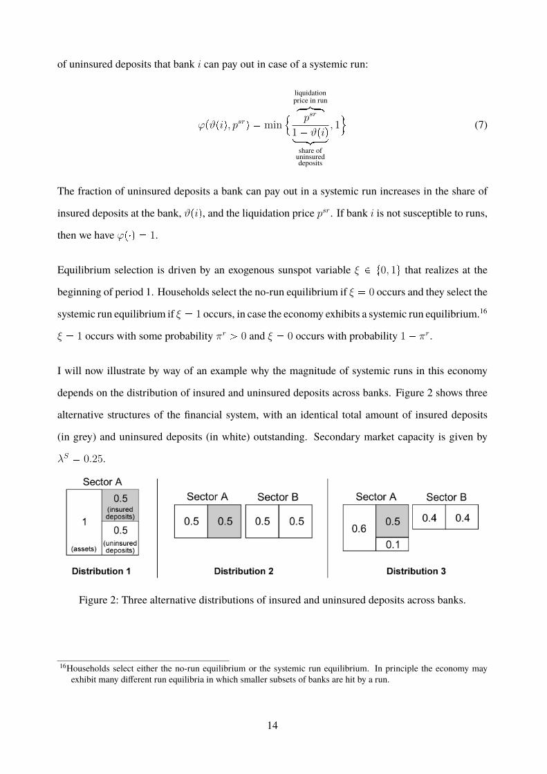
I will now illustrate by way of an example why the magnitude of systemic runs in this economy

depends on the distribution of insured and uninsured deposits across banks. Figure 2 shows three

alternative structures of the financial system, with an identical total amount of insured deposits

(in grey) and uninsured deposits (in white) outstanding. Secondary market capacity is given by

λS � 0.25.

Figure 2: Three alternative distributions of insured and uninsured deposits across banks.

16Households select either the no-run equilibrium or the systemic run equilibrium. In principle the economy mayexhibit many different run equilibria in which smaller subsets of banks are hit by a run.

14

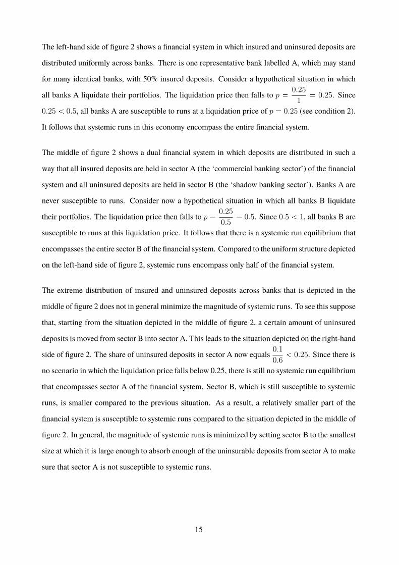
The left-hand side of figure 2 shows a financial system in which insured and uninsured deposits are

distributed uniformly across banks. There is one representative bank labelled A, which may stand

for many identical banks, with 50% insured deposits. Consider a hypothetical situation in which

all banks A liquidate their portfolios. The liquidation price then falls to p �0.25

1� 0.25. Since

0.25   0.5, all banks A are susceptible to runs at a liquidation price of p � 0.25 (see condition 2).

It follows that systemic runs in this economy encompass the entire financial system.

The middle of figure 2 shows a dual financial system in which deposits are distributed in such a

way that all insured deposits are held in sector A (the ‘commercial banking sector’) of the financial

system and all uninsured deposits are held in sector B (the ‘shadow banking sector’). Banks A are

never susceptible to runs. Consider now a hypothetical situation in which all banks B liquidate

their portfolios. The liquidation price then falls to p �0.25

0.5� 0.5. Since 0.5   1, all banks B are

susceptible to runs at this liquidation price. It follows that there is a systemic run equilibrium that

encompasses the entire sector B of the financial system. Compared to the uniform structure depicted

on the left-hand side of figure 2, systemic runs encompass only half of the financial system.

The extreme distribution of insured and uninsured deposits across banks that is depicted in the

middle of figure 2 does not in general minimize the magnitude of systemic runs. To see this suppose

that, starting from the situation depicted in the middle of figure 2, a certain amount of uninsured

deposits is moved from sector B into sector A. This leads to the situation depicted on the right-hand

side of figure 2. The share of uninsured deposits in sector A now equals0.1

0.6  0.25. Since there is

no scenario in which the liquidation price falls below 0.25, there is still no systemic run equilibrium

that encompasses sector A of the financial system. Sector B, which is still susceptible to systemic

runs, is smaller compared to the previous situation. As a result, a relatively smaller part of the

financial system is susceptible to systemic runs compared to the situation depicted in the middle of

figure 2. In general, the magnitude of systemic runs is minimized by setting sector B to the smallest

size at which it is large enough to absorb enough of the uninsurable deposits from sector A to make

sure that sector A is not susceptible to systemic runs.

15

4 Optimal Structure of the Financial System

In this section, I derive the structure of the financial system that maximizes welfare, taken as given

the deposit insurance cap θ. Welfare is defined as the integral over expected utility of households,

with equal weight given to all households. The structure of the financial system is given by two

integrable functions pδpiq, ϑpiqq, where δpiq : I Ñ R� denotes the face value of deposits issued by

bank i and, as before, ϑpiq : I Ñ r0, 1s denotes the share of insured deposits among the deposits

issued by bank i.

I impose two additional restrictions on the welfare maximization problem. First, all households

must receive an identical portfolio of deposits in period 0. This rules out the (arguably uninteresting)

allocation where each bank serves exactly one household, which would eliminate the coordination

problem inherent to bank runs. Second, the aggregate face value of deposits must be equal to

1, which implies that the entire period 0-endowment is invested, and the aggregate face value of

deposits equals the aggregate investment return. This is equivalent to saying that the aggregate

face value of deposits must be the same as in a competitive allocation (see section 5). This reflects

the fact that the present paper is concerned with the optimal distribution of insured and uninsured

deposits across banks, not with the optimal amount of short-term debt. It also implies that the

total face value of deposits issued by some set I 1 of banks must be identical (not lower) than the

fundamental value of assets held by these banks. As before DpI 1q �³I1δpiq di denotes the total

face value of deposits issued by banks I 1, which corresponds to the total fundamental value of assets

held by banks I 1.

The only uncertainty at the aggregate level stems from the realization of the sunspot variable ξ.

By a law of large numbers, idiosyncratic risk regarding the order in the line at individual banks

in case of a systemic run is eliminated, given that each depositor holds deposits at a continuum

of different banks.17 Consumption c1 of depositors is thus only subject to aggregate risk related

17There are well known technical problems with the law of large numbers in economies with a continuum of agents -see also footnote 20.

16

to the realization of ξ. If households select the no-run equilibrium (ξ � 0), then consumption

of households in period 1 is equal to the fundamental value (the end of period 1 return) of the

period 0 investment. If households select the systemic run equilibrium (ξ � 1), then consumption

of households equals the fundamental value of the period 0 investment minus losses caused by the

run. Total losses in a systemic run (from the point of households) are equal to the fundamental value

of claims sold to outside investors minus the amount outside investors pay for it. The latter simply

equals outside investors’ total endowment λS . Recall that a systemic run encompasses all banks

whose share of insured deposits is strictly below ϑsr, where ϑsr is the fixed point defined in lemma

3.1. Furthermore, any payments made by deposit insurance in period 1 represent transfers from

households to themselves, so that they cancel out in the aggregate. Consumption of households in

case of no run (ξ � 0) and a systemic run (ξ � 1) respectively can thus be expressed as:

cp0q � 1

cp1q � 1 � max! fundamental value of

assets sold in systemic runhkkkkkkkkkkkikkkkkkkkkkkjDpi P I|ϑpiq   ϑsrq�

secondarymarketcapacityhkkikkjλSlooooooooooooooooomooooooooooooooooon

total loss caused by systemic run

, 0) (8)

Note that if systemic runs cannot occur in the economy, then Dpi |ϑpiq   ϑsrq � 0 and we have

cp1q � 1. The optimal structure of the financial system is defined as any pδpiq, ϑpiqq solving:

maxpδpiq,ϑpiqq

expected utilityof householdshkkkkkikkkkkjErupc1pξqqs subject to

total face valueof depositshkkkkikkkkj»Iδpiq di � 1 and

face value ofinsured depositshkkkkkkkikkkkkkkj»Iϑpiq δpiq di ¤ θ (9)

It follows immediately from (8) and (9) that the optimal structure of the financial system is such

that it minimizes the total loss caused by a systemic run. We proceed with the following result:

Lemma 4.1. The optimal structure of the financial system satisfies

Dpi P I |ϑpiq � 0qloooooooooomoooooooooonface value of deposits issuedby banks with ϑpiq � 0

�Dpi P I |ϑpiq ¥ ϑsrqlooooooooooomooooooooooonface value of deposits issuedby banks with ϑpiq ¥ ϑsr

� 1.

17

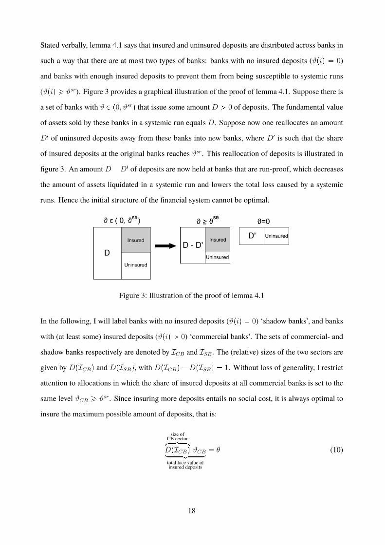
Stated verbally, lemma 4.1 says that insured and uninsured deposits are distributed across banks in

such a way that there are at most two types of banks: banks with no insured deposits (ϑpiq � 0)

and banks with enough insured deposits to prevent them from being susceptible to systemic runs

(ϑpiq ¥ ϑsr). Figure 3 provides a graphical illustration of the proof of lemma 4.1. Suppose there is

a set of banks with ϑ P p0, ϑsrq that issue some amountD ¡ 0 of deposits. The fundamental value

of assets sold by these banks in a systemic run equals D. Suppose now one reallocates an amount

D1 of uninsured deposits away from these banks into new banks, where D1 is such that the share

of insured deposits at the original banks reaches ϑsr. This reallocation of deposits is illustrated in

figure 3. An amountD�D1 of deposits are now held at banks that are run-proof, which decreases

the amount of assets liquidated in a systemic run and lowers the total loss caused by a systemic

runs. Hence the initial structure of the financial system cannot be optimal.

Figure 3: Illustration of the proof of lemma 4.1

In the following, I will label banks with no insured deposits (ϑpiq � 0) ‘shadow banks’, and banks

with (at least some) insured deposits (ϑpiq ¡ 0) ‘commercial banks’. The sets of commercial- and

shadow banks respectively are denoted by ICB and ISB. The (relative) sizes of the two sectors are

given by DpICBq and DpISBq, with DpICBq �DpISBq � 1. Without loss of generality, I restrict

attention to allocations in which the share of insured deposits at all commercial banks is set to the

same level ϑCB ¥ ϑsr. Since insuring more deposits entails no social cost, it is always optimal to

insure the maximum possible amount of deposits, that is:

size ofCB cectorhkkkikkkjDpICBq ϑCBloooooomoooooontotal face value ofinsured deposits

� θ (10)

18

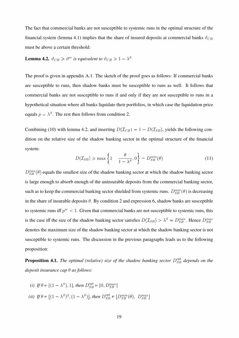
The fact that commercial banks are not susceptible to systemic runs in the optimal structure of the

financial system (lemma 4.1) implies that the share of insured deposits at commercial banks ϑCB

must be above a certain threshold:

Lemma 4.2. ϑCB ¥ ϑsr is equivalent to ϑCB ¥ 1 � λS

The proof is given in appendix A.1. The sketch of the proof goes as follows: If commercial banks

are susceptible to runs, then shadow banks must be susceptible to runs as well. It follows that

commercial banks are not susceptible to runs if and only if they are not susceptible to runs in a

hypothetical situation where all banks liquidate their portfolios, in which case the liquidation price

equals p � λS . The rest then follows from condition 2.

Combining (10) with lemma 4.2, and inserting DpICBq � 1 �DpISBq, yields the following con-

dition on the relative size of the shadow banking sector in the optimal structure of the financial

system:

DpISBq ¥ max

"1 �

θ

1 � λS, 0

*� Dmin

SB pθq (11)

DminSB pθq equals the smallest size of the shadow banking sector at which the shadow banking sector

is large enough to absorb enough of the uninsurable deposits from the commercial banking sector,

such as to keep the commercial banking sector shielded from systemic runs. DminSB pθq is decreasing

in the share of insurable deposits θ. By condition 2 and expression 6, shadow banks are susceptible

to systemic runs iff psr   1. Given that commercial banks are not susceptible to systemic runs, this

is the case iff the size of the shadow banking sector satisfies DpISBq ¡ λS � DmaxSB . Hence Dmax

SB

denotes the maximum size of the shadow banking sector at which the shadow banking sector is not

susceptible to systemic runs. The discussion in the previous paragraphs leads us to the following

proposition:

Proposition 4.1. The optimal (relative) size of the shadow banking sector DoptSB depends on the

deposit insurance cap θ as follows:

(i) If θ P rp1 � λSq, 1s, then DoptSB P r0, Dmax

SB s

(ii) If θ P rp1 � λSq2, p1 � λSqs, then DoptSB P rDmin

SB pθq, DmaxSB s

19

(iii) If θ P r0, p1 � λSq2s, then DoptSB � Dmin

SB pθq

According to proposition 4.1, the deposit insurance cap θ can be divided into three regions. The

three regions are also illustrated in Figure 4 further below, which depicts how the optimal size of

the shadow banking sector (green line/area) depends on the cap θ, for an economy with secondary

market capacity λS � 0.25. The dotted line in figure 4 is the 45�-line. Note that if no deposits are

insurable (θ � 0), then the relative size of the shadow banking sector equals 1 by definition.

Consider first region (i) in which the cap is at a relatively high level. From condition 11 we get

that DminSB pθq � 0, meaning that commercial banks are not susceptible to systemic runs even if all

uninsurable deposits remain in the commercial banking sector. Systemic runs do not occur in the

economy as long as the size of the shadow banking sector is within r0, DmaxSB s.18

Consider next the case where the cap is within the intermediate region (ii). For θ   p1 � λSq we

have that DminSB pθq � 1 �

θ

1 � λS¡ 0, which means that the relative size of the shadow banking

sector must be larger than zero in order to absorb enough uninsurable deposits from the commercial

banking sector. On the other hand, we have that DminSB pθq ¤ Dmax

SB , with strict inequality for θ ¡

p1 � λSq2. This means that systemic runs can be avoided in both the commercial- and the shadow

banking sector by setting the relative size of the shadow banking within rDminSB pθq, Dmax

SB s. If the cap

is within region (ii), systemic runs can therefore be avoided by setting the shadow banking sector

large enough to keep commercial banks shielded from systemic runs, but not too large, so that the

shadow banking sector itself is not susceptible to systemic runs either.

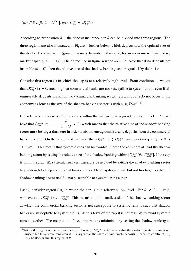
Lastly, consider region (iii) in which the cap is at a relatively low level. For θ   p1 � λSq2,

we have that DminSB pθq ¡ Dmax

SB . This means that the smallest size of the shadow banking sector

at which the commercial banking sector is not susceptible to systemic runs is such that shadow

banks are susceptible to systemic runs. At this level of the cap it is not feasible to avoid systemic

runs altogether. The magnitude of systemic runs is minimized by setting the shadow banking to

18Within this region of the cap, we have that 1 � θ   DmaxSB , which means that the shadow banking sector is not

susceptible to systemic runs even if it is larger than the share of uninsurable deposits. Hence the constraint (10)may be slack within this region of θ.

20

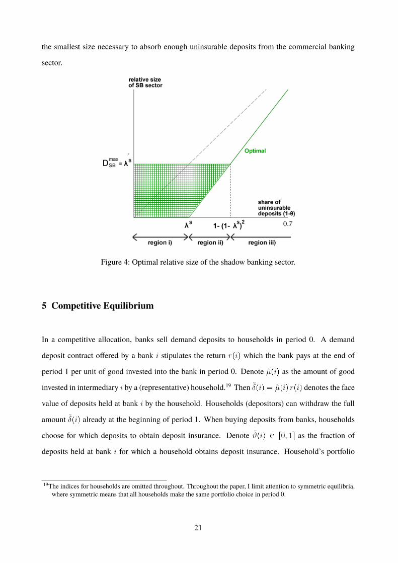
the smallest size necessary to absorb enough uninsurable deposits from the commercial banking

sector.

Figure 4: Optimal relative size of the shadow banking sector.

5 Competitive Equilibrium

In a competitive allocation, banks sell demand deposits to households in period 0. A demand

deposit contract offered by a bank i stipulates the return rpiq which the bank pays at the end of

period 1 per unit of good invested into the bank in period 0. Denote µpiq as the amount of good

invested in intermediary i by a (representative) household.19 Then δpiq � µpiq rpiq denotes the face

value of deposits held at bank i by the household. Households (depositors) can withdraw the full

amount δpiq already at the beginning of period 1. When buying deposits from banks, households

choose for which deposits to obtain deposit insurance. Denote ϑpiq P r0, 1s as the fraction of

deposits held at bank i for which a household obtains deposit insurance. Household’s portfolio

19The indices for households are omitted throughout. Throughout the paper, I limit attention to symmetric equilibria,where symmetric means that all households make the same portfolio choice in period 0.

21

choice in period 0 can then be expressed as choosing two integrable functions pδpiq, ϑpiqq subject

to the budget constraint and the cap on insured deposits.

An insured deposit held at bank i pays a riskless return of rpiq. An uninsured deposit held at bank

i pays a riskless return rpiq if the bank is not susceptible to runs. If the bank is susceptible to

runs, then the effective return to an uninsured deposit is risky and depends on the realization of

the sunspot variable ξ P t0, 1u. I again assume that, by some law of large numbers, households

diversify away any idiosyncratic risk regarding the order of the line at individual banks.20 Motivated

by this (and in order to circumvent issues of measurability), households do not take into account

idiosyncratic risk regarding the place in the line when making their portfolio decision; the return to

an uninsured deposit in case of a systemic run (ξ � 1) is taken to be equal to the expected return,

that is, rpiq times the probability that the deposit can be withdrawn in the run. Households’ utility

maximization problem is then to choose any portfolio pδpiq, ϑpiqq solving:21

maxpδpiq,ϑpiqq

expected utilityhkkkkkikkkkkjE rupc1pξqs subject to

budget constrainthkkkkkkkikkkkkkkj»I

δpiq

rpiqdi � 1 and

cap on deposit insurancehkkkkkkkkkkikkkkkkkkkkj»Iϑpiq δpiq di ¤ θ (12)

A (symmetric) equilibrium is a tuple pδpiq, ϑpiq, δpiq, ϑpiq, rpiqq so that: (i) households’ portfolio

choice pδpiq, ϑpiqq is such that households maximize expected utility according to (12); (ii) deposit

contracts rpiq offered by banks are such that no bank has a profitable deviation and (iii) the aggregate

structure of the financial system corresponds to individual choices, pδpiq, ϑpiqq � pδpiq, ϑpiqq.

First we can note that, since deposits at different banks are perfect substitutes, competition among

banks will drive banks’ profits to zero in equilibrium. This implies that the return paid by banks

in equilibrium equals the return to the investment technology, that is, rpiq � 1 for all banks in

equilibrium. This follows from the fact that banks face an infinitely elastic demand for insured

20 Intuitively, the return received from a portfolio of uninsured deposits in a systemic run by an individual householdh should be given by

³I Ipiq

hp1� ϑpiqq δpiq di where Ipiqh is random and takes the value 1 if household h is earlyin the line at bank i and can withdraw her deposits (or if bank i is not susceptible to runs) and 0 if household h islate in the line at bank i. Since the order of the line is random and independent at each bank, the sample path Ipiqhis generally not measurable. See, for instance, Uhlig (1996) and Al-Najjar (2004) for possible remedies.

21Since households attach no value to consumption in period 0, and utility is strictly increasing in period 1 consumption,it is without loss of generality to set the budget constraint to equality.

22

deposits and, by the usual argument of Bertrand, the only equilibrium is one in which all banks

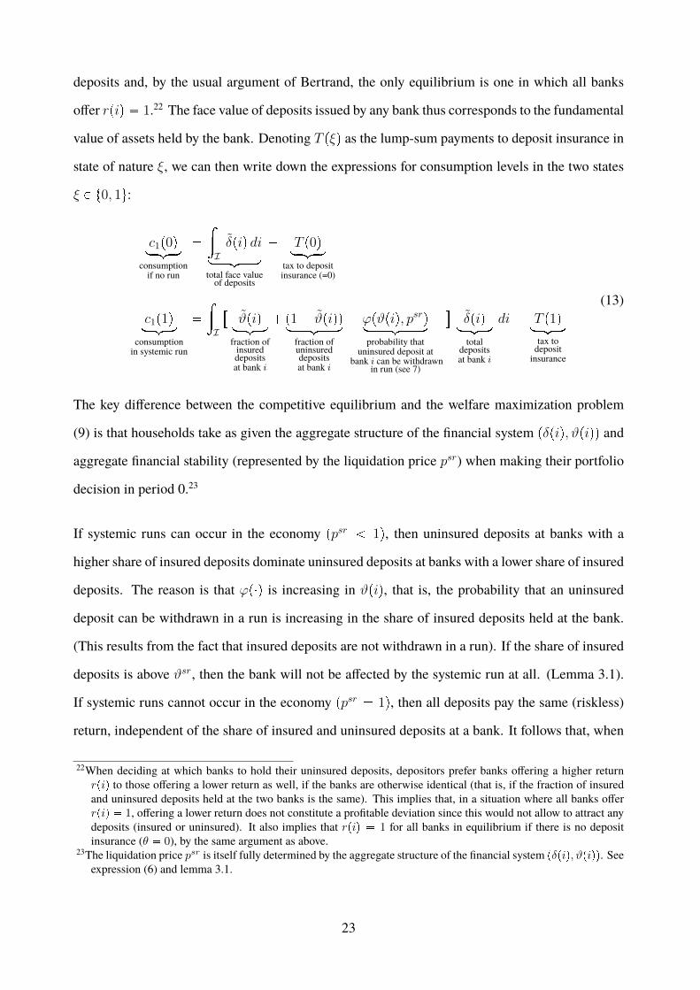
offer rpiq � 1.22 The face value of deposits issued by any bank thus corresponds to the fundamental

value of assets held by the bank. Denoting T pξq as the lump-sum payments to deposit insurance in

state of nature ξ, we can then write down the expressions for consumption levels in the two states

ξ P t0, 1u:

c1p0qloomoonconsumptionif no run

�

»Iδpiq diloooomoooon

total face valueof deposits

� T p0qloomoontax to depositinsurance (=0)

c1p1qloomoonconsumptionin systemic run

�

»I

�ϑpiqloomoon

fraction ofinsureddepositsat bank i

�p1 � ϑpiqqloooomoooonfraction ofuninsureddepositsat bank i

ϕpϑpiq, psrqlooooomooooonprobability that

uninsured deposit atbank i can be withdrawn

in run (see 7)

�δpiqloomoontotal

depositsat bank i

di� T p1qloomoontax todepositinsurance

(13)

The key difference between the competitive equilibrium and the welfare maximization problem

(9) is that households take as given the aggregate structure of the financial system pδpiq, ϑpiqq and

aggregate financial stability (represented by the liquidation price psr) when making their portfolio

decision in period 0.23

If systemic runs can occur in the economy ppsr   1q, then uninsured deposits at banks with a

higher share of insured deposits dominate uninsured deposits at banks with a lower share of insured

deposits. The reason is that ϕp�q is increasing in ϑpiq, that is, the probability that an uninsured

deposit can be withdrawn in a run is increasing in the share of insured deposits held at the bank.

(This results from the fact that insured deposits are not withdrawn in a run). If the share of insured

deposits is above ϑsr, then the bank will not be affected by the systemic run at all. (Lemma 3.1).

If systemic runs cannot occur in the economy ppsr � 1q, then all deposits pay the same (riskless)

return, independent of the share of insured and uninsured deposits at a bank. It follows that, when

22When deciding at which banks to hold their uninsured deposits, depositors prefer banks offering a higher returnrpiq to those offering a lower return as well, if the banks are otherwise identical (that is, if the fraction of insuredand uninsured deposits held at the two banks is the same). This implies that, in a situation where all banks offerrpiq � 1, offering a lower return does not constitute a profitable deviation since this would not allow to attract anydeposits (insured or uninsured). It also implies that rpiq � 1 for all banks in equilibrium if there is no depositinsurance (θ � 0), by the same argument as above.

23The liquidation price psr is itself fully determined by the aggregate structure of the financial system pδpiq, ϑpiqq. Seeexpression (6) and lemma 3.1.

23

choosing how to invest the uninsurable part of their endowment, households weakly prefer banks

with a higher share of insured deposits.24 In particular, households never have an incentive to invest

into ‘shadow banks’ with no insured depositors. This leads us to the following proposition:

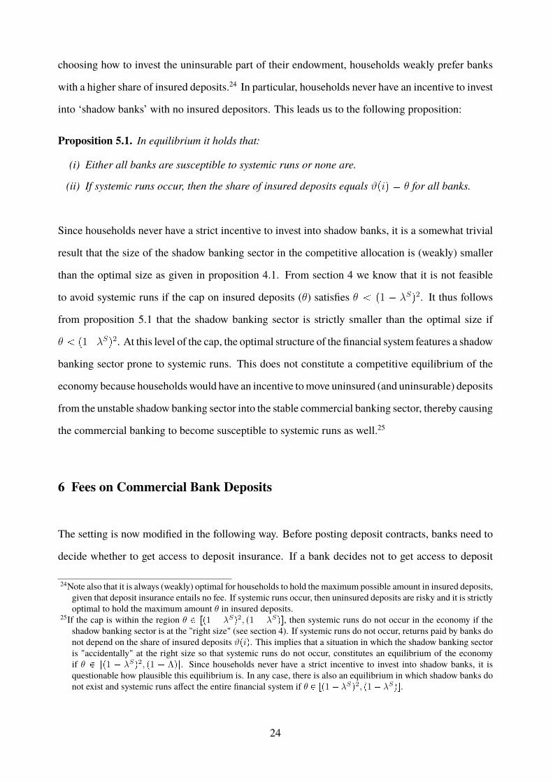
Proposition 5.1. In equilibrium it holds that:

(i) Either all banks are susceptible to systemic runs or none are.

(ii) If systemic runs occur, then the share of insured deposits equals ϑpiq � θ for all banks.

Since households never have a strict incentive to invest into shadow banks, it is a somewhat trivial

result that the size of the shadow banking sector in the competitive allocation is (weakly) smaller

than the optimal size as given in proposition 4.1. From section 4 we know that it is not feasible

to avoid systemic runs if the cap on insured deposits (θ) satisfies θ   p1 � λSq2. It thus follows

from proposition 5.1 that the shadow banking sector is strictly smaller than the optimal size if

θ   p1�λSq2. At this level of the cap, the optimal structure of the financial system features a shadow

banking sector prone to systemic runs. This does not constitute a competitive equilibrium of the

economy because householdswould have an incentive tomove uninsured (and uninsurable) deposits

from the unstable shadow banking sector into the stable commercial banking sector, thereby causing

the commercial banking to become susceptible to systemic runs as well.25

6 Fees on Commercial Bank Deposits

The setting is now modified in the following way. Before posting deposit contracts, banks need to

decide whether to get access to deposit insurance. If a bank decides not to get access to deposit

24Note also that it is always (weakly) optimal for households to hold the maximum possible amount in insured deposits,given that deposit insurance entails no fee. If systemic runs occur, then uninsured deposits are risky and it is strictlyoptimal to hold the maximum amount θ in insured deposits.

25If the cap is within the region θ P rp1 � λSq2, p1 � λSqs, then systemic runs do not occur in the economy if theshadow banking sector is at the "right size" (see section 4). If systemic runs do not occur, returns paid by banks donot depend on the share of insured deposits ϑpiq. This implies that a situation in which the shadow banking sectoris "accidentally" at the right size so that systemic runs do not occur, constitutes an equilibrium of the economyif θ P rp1 � λSq2, p1 � Λqs. Since households never have a strict incentive to invest into shadow banks, it isquestionable how plausible this equilibrium is. In any case, there is also an equilibrium in which shadow banks donot exist and systemic runs affect the entire financial system if θ P rp1 � λSq2, p1 � λSqs.

24

insurance, it will be labelled a ‘shadow bank’ and households cannot obtain deposit insurance for the

deposits issued by the bank. Banks that decide to get access to deposit insurance will be labelled

‘commercial banks’. Households can, but do not have to, obtain deposit insurance for deposits

issued by commercial banks. The cap on deposit insurance applies as before. Deposit insurance

charges a fee on all deposits issued by commercial banks, insured or uninsured. The setting studied

in this section is motivated by real-world institutional features; many deposit insurance schemes

require commercial banks to pay a fee on deposits.26 The focus of this section is to derive the

structure of the financial system that results in a competitive equilibrium under this institutional

framework, and compare it to the optimal structure of the financial system as derived in section 4.

Themain difference compared to section 5 is that households now have an incentive to hold deposits

at shadow banks instead of commercial banks in order to avoid the fee charged on commercial bank

deposits.

The fee on commercial bank deposits equals a fraction τ of the face value of deposits and is charged

directly on households after they have withdrawn the deposit from the bank. The results regarding

the optimal size of the shadow banking sector derived in section 4 are not affected by the fee.27

Deposit insurance payments can now be seen as being partly financed by fee revenue and partly by

lump-sum taxes if the fee revenue is not sufficient. Any fee revenue not used for deposit insurance

payments is rebated to households in a lump-sum fashion at the end of period 1.

The definition of the equilibrium in the economy with a fee on commercial bank deposits is analo-

gous to section 5 except for the explicit distinction between commercial banks and shadow banks.

Competition among banks again implies that all banks offer rpiq � 1 in equilibrium. Insured de-

posits at commercial banks pay a riskless return of p1 � τqrpiq � p1 � τq. Uninsured deposits at

commercial banks pay a return p1� τq if they can be withdrawn and zero otherwise. Shadow bank

deposits pay a return rpiq � 1 if they can be withdrawn from the bank and zero otherwise. Analo-

26In the U.S., all bank liabilities are included in the assessment base used to determine the fees banks need to pay tothe FDIC. Before the Dodd-Frank Act, the assesment base was total domestic deposits.

27In particular, the fee is set up in such a way that it does not affect the face value of outstanding deposits in period 1.If the fee were charged in period 0, or if it were charged on banks rather than directly on households, the aggregatefee revenue would affect the aggregate face value of outstanding deposits in period 1, even if by very little.

25

gous to before, the subsets of banks operating as commercial banks and shadow banks are denoted

by ICB and ISB respectively and the (relative) sizes of the two sectors are given by DpICBq and

DpISBq. I will sometimes say that a given sector is ‘unstable’ if it is susceptible to systemic runs

and ‘stable’ if it is not.

In a systemic run, a commercial bank i P ICB can pay out a fraction ϕpϑpiq, psrq of its uninsured

deposits, where ϕp�q is increasing in the share of insured deposits ϑpiq and the liquidation price psr

(see (7)). A shadow bank can pay out a fraction ϕp0, psrq � psr of deposits in case of a systemic

run. When choosing at which type of bank to hold uninsured deposits, households trade off the fee

τ charged on commercial bank deposits against higher losses caused by runs at shadow banks. We

then immediately get the following result:

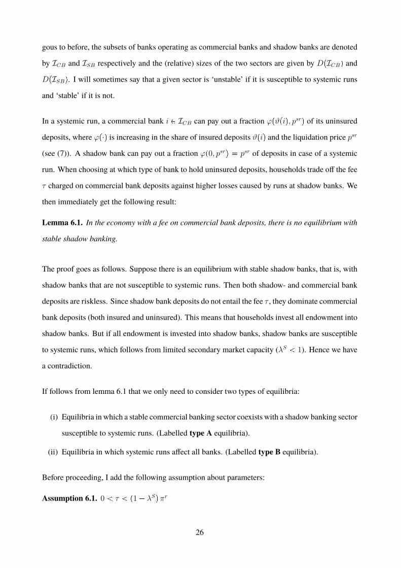
Lemma 6.1. In the economy with a fee on commercial bank deposits, there is no equilibrium with

stable shadow banking.

The proof goes as follows. Suppose there is an equilibrium with stable shadow banks, that is, with

shadow banks that are not susceptible to systemic runs. Then both shadow- and commercial bank

deposits are riskless. Since shadow bank deposits do not entail the fee τ , they dominate commercial

bank deposits (both insured and uninsured). This means that households invest all endowment into

shadow banks. But if all endowment is invested into shadow banks, shadow banks are susceptible

to systemic runs, which follows from limited secondary market capacity (λS   1). Hence we have

a contradiction.

If follows from lemma 6.1 that we only need to consider two types of equilibria:

(i) Equilibria in which a stable commercial banking sector coexists with a shadow banking sector

susceptible to systemic runs. (Labelled type A equilibria).

(ii) Equilibria in which systemic runs affect all banks. (Labelled type B equilibria).

Before proceeding, I add the following assumption about parameters:

Assumption 6.1. 0   τ   p1 � λSq πr

26

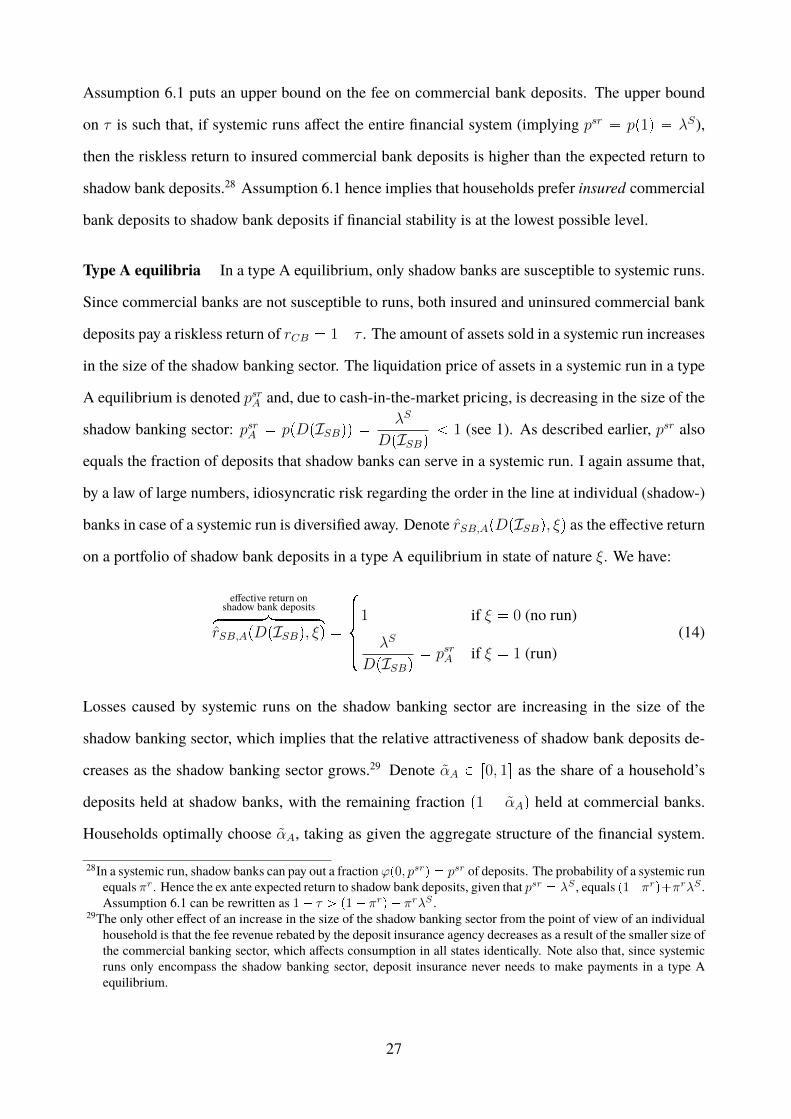
Assumption 6.1 puts an upper bound on the fee on commercial bank deposits. The upper bound

on τ is such that, if systemic runs affect the entire financial system (implying psr � pp1q � λS),

then the riskless return to insured commercial bank deposits is higher than the expected return to

shadow bank deposits.28 Assumption 6.1 hence implies that households prefer insured commercial

bank deposits to shadow bank deposits if financial stability is at the lowest possible level.

Type A equilibria In a type A equilibrium, only shadow banks are susceptible to systemic runs.

Since commercial banks are not susceptible to runs, both insured and uninsured commercial bank

deposits pay a riskless return of rCB � 1�τ . The amount of assets sold in a systemic run increases

in the size of the shadow banking sector. The liquidation price of assets in a systemic run in a type

A equilibrium is denoted psrA and, due to cash-in-the-market pricing, is decreasing in the size of the

shadow banking sector: psrA � ppDpISBqq �λS

DpISBq  1 (see 1). As described earlier, psr also

equals the fraction of deposits that shadow banks can serve in a systemic run. I again assume that,

by a law of large numbers, idiosyncratic risk regarding the order in the line at individual (shadow-)

banks in case of a systemic run is diversified away. Denote rSB,ApDpISBq, ξq as the effective return

on a portfolio of shadow bank deposits in a type A equilibrium in state of nature ξ. We have:

effective return onshadow bank depositshkkkkkkkkkikkkkkkkkkj

rSB,ApDpISBq, ξq �

$''&''%

1 if ξ � 0 (no run)

λS

DpISBq� psrA if ξ � 1 (run)

(14)

Losses caused by systemic runs on the shadow banking sector are increasing in the size of the

shadow banking sector, which implies that the relative attractiveness of shadow bank deposits de-

creases as the shadow banking sector grows.29 Denote αA P r0, 1s as the share of a household’s

deposits held at shadow banks, with the remaining fraction p1 � αAq held at commercial banks.

Households optimally choose αA, taking as given the aggregate structure of the financial system.

28In a systemic run, shadow banks can pay out a fractionϕp0, psrq � psr of deposits. The probability of a systemic runequals πr. Hence the ex ante expected return to shadow bank deposits, given that psr � λS , equals p1�πrq�πrλS .Assumption 6.1 can be rewritten as 1 � τ ¡ p1 � πrq � πrλS .

29The only other effect of an increase in the size of the shadow banking sector from the point of view of an individualhousehold is that the fee revenue rebated by the deposit insurance agency decreases as a result of the smaller size ofthe commercial banking sector, which affects consumption in all states identically. Note also that, since systemicruns only encompass the shadow banking sector, deposit insurance never needs to make payments in a type Aequilibrium.

27

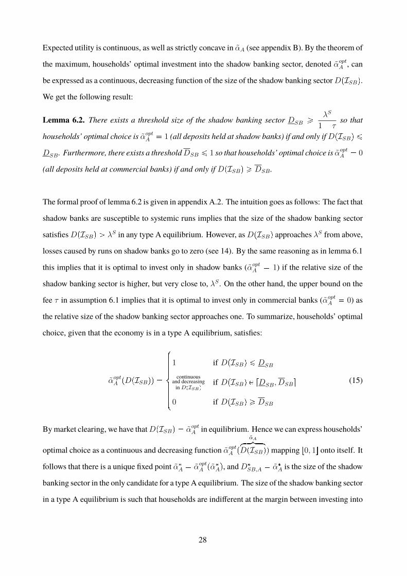
Expected utility is continuous, as well as strictly concave in αA (see appendix B). By the theorem of

the maximum, households’ optimal investment into the shadow banking sector, denoted αoptA , can

be expressed as a continuous, decreasing function of the size of the shadow banking sectorDpISBq.

We get the following result:

Lemma 6.2. There exists a threshold size of the shadow banking sector DSB ¥λS

1 � τso that

households’ optimal choice is αoptA � 1 (all deposits held at shadow banks) if and only ifDpISBq ¤

DSB. Furthermore, there exists a thresholdDSB ¤ 1 so that households’ optimal choice is αoptA � 0

(all deposits held at commercial banks) if and only if DpISBq ¥ DSB.

The formal proof of lemma 6.2 is given in appendix A.2. The intuition goes as follows: The fact that

shadow banks are susceptible to systemic runs implies that the size of the shadow banking sector

satisfiesDpISBq ¡ λS in any type A equilibrium. However, asDpISBq approaches λS from above,

losses caused by runs on shadow banks go to zero (see 14). By the same reasoning as in lemma 6.1

this implies that it is optimal to invest only in shadow banks (αoptA � 1) if the relative size of the

shadow banking sector is higher, but very close to, λS . On the other hand, the upper bound on the

fee τ in assumption 6.1 implies that it is optimal to invest only in commercial banks (αoptA � 0) as

the relative size of the shadow banking sector approaches one. To summarize, households’ optimal

choice, given that the economy is in a type A equilibrium, satisfies:

αoptA pDpISBqq �

$''''''&''''''%

1 if DpISBq ¤ DSB

continuousand decreasinginDpISBq

if DpISBq P rDSB, DSBs

0 if DpISBq ¥ DSB

(15)

Bymarket clearing, we have thatDpISBq � αoptA in equilibrium. Hence we can express households’

optimal choice as a continuous and decreasing function αoptA p

αAhkkikkjDpISBqqmapping r0, 1s onto itself. It

follows that there is a unique fixed point α�A � αoptA pα�Aq, andD�SB,A � α�A is the size of the shadow

banking sector in the only candidate for a type A equilibrium. The size of the shadow banking sector

in a type A equilibrium is such that households are indifferent at the margin between investing into

28

the shadow banking sector, which is prone to systemic runs, and paying the fee τ on commercial

bank deposits. Since αoptA p0q � 1 and αoptA p1q � 0, corner solutions are ruled out and we have

D�SB,A P pDSB, DSBq. It remains to check whether, at DpISBq � D�

SB,A, the economy is indeed

in a type A equilibrium, that is, in a situation in which shadow banks but not commercial banks

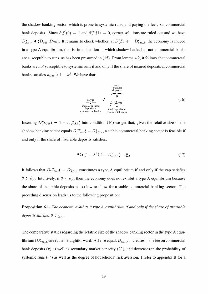
are susceptible to runs, as has been presumed in (15). From lemma 4.2, it follows that commercial

banks are not susceptible to systemic runs if and only if the share of insured deposits at commercial

banks satisfies ϑCB ¥ 1 � λS . We have that:

ϑCBloomoonshare of insured

deposits atcommercial banks

¤

totalinsurabledepositshkkikkjθ

DpICBqlooomooontotal deposits at

commercial banks

(16)

Inserting DpICBq � 1 � DpISBq into condition (16) we get that, given the relative size of the

shadow banking sector equals DpISBq � D�SB,A, a stable commercial banking sector is feasible if

and only if the share of insurable deposits satisfies:

θ ¥ p1 � λSqp1 �D�SB,Aq � θA (17)

It follows that DpISBq � D�SB,A constitutes a type A equilibrium if and only if the cap satisfies

θ ¥ θA. Intuitively, if θ   θA, then the economy does not exhibit a type A equilibrium because

the share of insurable deposits is too low to allow for a stable commercial banking sector. The

preceding discussion leads us to the following proposition:

Proposition 6.1. The economy exhibits a type A equilibrium if and only if the share of insurable

deposits satisfies θ ¥ θA.

The comparative statics regarding the relative size of the shadow banking sector in the type A equi-

librium (D�SB,A) are rather straightforward: All else equal,D�

SB,A increases in the fee on commercial

bank deposits (τ ) as well as secondary market capacity (λS), and decreases in the probability of

systemic runs (πr) as well as the degree of households’ risk aversion. I refer to appendix B for a

29

formal derivation of the comparative statics results. Note that changes in the deposit insurance cap

θ have no effect on the size of the shadow banking sector in a type A equilibrium as long as θ stays

above θA. If θ decreases below θA, the economy moves to a type B equilibrium, with an ambiguous

effect on the size of the shadow banking sector (see below).

Type B equilibria A type B equilibrium is an equilibrium in which all banks are susceptible to

systemic runs. This means that the total fundamental value of assets sold in a systemic run equals

λD � 1 and the liquidation price of assets in a systemic run equals psrB � pp1q � λS (see 1).

Different to a type A equilibrium, the magnitude of systemic runs does not depend on the size of

the shadow banking sector.

Insured commercial bank deposits pay a riskless return of 1�τ . The upper bound on τ (assumption

6.1) means that, in a situation in which systemic runs affect the entire financial system, insured

commercial bank deposits are preferred to uninsured deposits at any bank. Hence, different to a

type A equilibrium, in a type B equilibrium households will always hold the maximum possible

amount (θ) in insured commercial bank deposits. This implies that condition (16) is binding in a

type B equilibrium. The relevant choice of households is therefore how to allocate the uninsurable

part of their deposits between commercial banks and shadow banks. When deciding how to allocate

the uninsurable part of their deposits between commercial banks and shadow banks, households

again trade off the fee charged on uninsured commercial bank deposits against lower losses caused

by runs due to the presence of insured depositors.

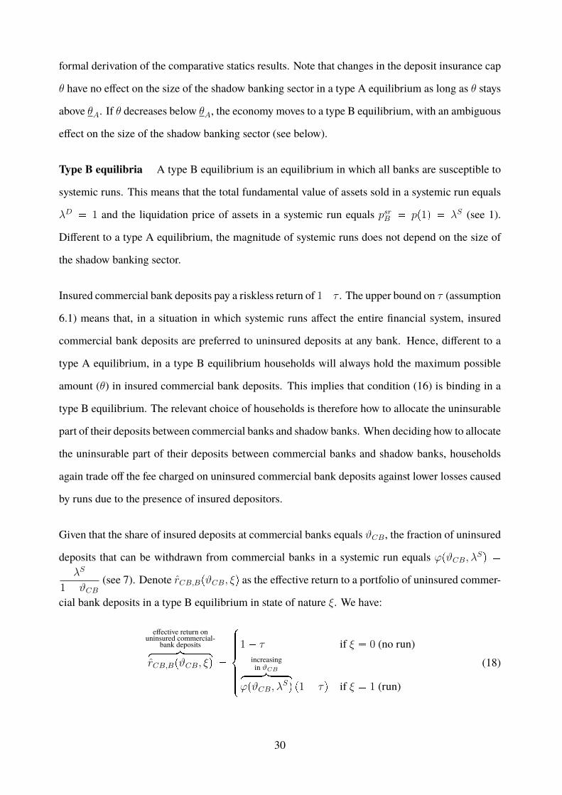
Given that the share of insured deposits at commercial banks equals ϑCB, the fraction of uninsured

deposits that can be withdrawn from commercial banks in a systemic run equals ϕpϑCB, λSq �λS

1 � ϑCB(see 7). Denote rCB,BpϑCB, ξq as the effective return to a portfolio of uninsured commer-

cial bank deposits in a type B equilibrium in state of nature ξ. We have:

effective return onuninsured commercial-

bank depositshkkkkkkkikkkkkkkjrCB,BpϑCB, ξq �

$''''&''''%

1 � τ if ξ � 0 (no run)increasingin ϑCBhkkkkkikkkkkj

ϕpϑCB, λSq p1 � τq if ξ � 1 (run)

(18)

30

The effective return to a portfolio of shadow bank deposits in a type B equilibrium is given by:

effective returnon shadow bank

depositshkkkikkkjrSB,Bpξq �

$'''&'''%

1 if ξ � 0 (no run)�λShkkkikkkj

ϕp0, λSq if ξ � 1 (run)

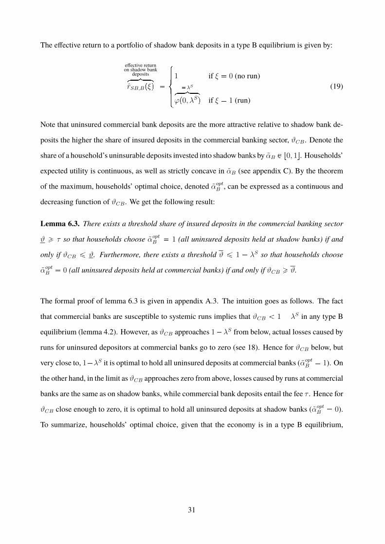
(19)

Note that uninsured commercial bank deposits are the more attractive relative to shadow bank de-

posits the higher the share of insured deposits in the commercial banking sector, ϑCB. Denote the

share of a household’s uninsurable deposits invested into shadow banks by αB P r0, 1s. Households’

expected utility is continuous, as well as strictly concave in αB (see appendix C). By the theorem

of the maximum, households’ optimal choice, denoted αoptB , can be expressed as a continuous and

decreasing function of ϑCB. We get the following result:

Lemma 6.3. There exists a threshold share of insured deposits in the commercial banking sector

ϑ ¥ τ so that households choose αoptB � 1 (all uninsured deposits held at shadow banks) if and

only if ϑCB ¤ ϑ. Furthermore, there exists a threshold ϑ ¤ 1 � λS so that households choose

αoptB � 0 (all uninsured deposits held at commercial banks) if and only if ϑCB ¥ ϑ.

The formal proof of lemma 6.3 is given in appendix A.3. The intuition goes as follows. The fact

that commercial banks are susceptible to systemic runs implies that ϑCB   1 � λS in any type B

equilibrium (lemma 4.2). However, as ϑCB approaches 1�λS from below, actual losses caused by

runs for uninsured depositors at commercial banks go to zero (see 18). Hence for ϑCB below, but

very close to, 1�λS it is optimal to hold all uninsured deposits at commercial banks (αoptB � 1). On

the other hand, in the limit as ϑCB approaches zero from above, losses caused by runs at commercial

banks are the same as on shadow banks, while commercial bank deposits entail the fee τ . Hence for

ϑCB close enough to zero, it is optimal to hold all uninsured deposits at shadow banks (αoptB � 0).

To summarize, households’ optimal choice, given that the economy is in a type B equilibrium,

31

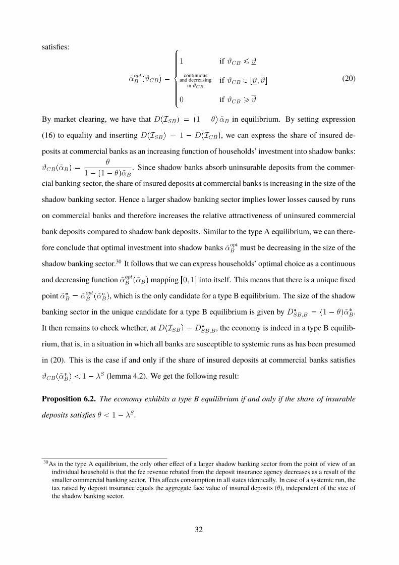
satisfies:

αoptB pϑCBq �

$''''''&''''''%

1 if ϑCB ¤ ϑ

continuousand decreasing

in ϑCB

if ϑCB P rϑ, ϑs

0 if ϑCB ¥ ϑ

(20)

By market clearing, we have that DpISBq � p1 � θq αB in equilibrium. By setting expression

(16) to equality and inserting DpISBq � 1 � DpICBq, we can express the share of insured de-

posits at commercial banks as an increasing function of households’ investment into shadow banks:

ϑCBpαBq �θ

1 � p1 � θqαB. Since shadow banks absorb uninsurable deposits from the commer-

cial banking sector, the share of insured deposits at commercial banks is increasing in the size of the

shadow banking sector. Hence a larger shadow banking sector implies lower losses caused by runs

on commercial banks and therefore increases the relative attractiveness of uninsured commercial

bank deposits compared to shadow bank deposits. Similar to the type A equilibrium, we can there-

fore conclude that optimal investment into shadow banks αoptB must be decreasing in the size of the

shadow banking sector.30 It follows that we can express households’ optimal choice as a continuous

and decreasing function αoptB pαBqmapping r0, 1s into itself. This means that there is a unique fixed

point α�B � αoptB pα�Bq, which is the only candidate for a type B equilibrium. The size of the shadow

banking sector in the unique candidate for a type B equilibrium is given by D�SB,B � p1 � θqα�B.

It then remains to check whether, at DpISBq � D�SB,B, the economy is indeed in a type B equilib-

rium, that is, in a situation in which all banks are susceptible to systemic runs as has been presumed

in (20). This is the case if and only if the share of insured deposits at commercial banks satisfies

ϑCBpα�Bq   1 � λS (lemma 4.2). We get the following result:

Proposition 6.2. The economy exhibits a type B equilibrium if and only if the share of insurable

deposits satisfies θ   1 � λS .

30As in the type A equilibrium, the only other effect of a larger shadow banking sector from the point of view of anindividual household is that the fee revenue rebated from the deposit insurance agency decreases as a result of thesmaller commercial banking sector. This affects consumption in all states identically. In case of a systemic run, thetax raised by deposit insurance equals the aggregate face value of insured deposits (θ), independent of the size ofthe shadow banking sector.

32

The proof is given in appendix A.4. Intuitively, if the share of insurable deposits is relatively high

(θ ¥ 1�λS), then there is no equilibrium inwhich systemic runs affect the entire financial system.

Next, I will show that if the cap θ is not too far below 1� λS , then only commercial banks (and no

shadow banks) exist in a type B equilibrium. To see this, note first that, if all uninsured deposits are

held at commercial banks (αB � 0) then the share of insured deposits at commercial banks equals

ϑCBp0q � θ. Now suppose we have θ P rϑ, 1 � λSq. Then it holds that ϑ ¤ ϑCBp0q   1 � λS .

This means that, in a situation in which all uninsurable deposits are held at commercial banks,

systemic runs affect the entire financial system. At the same time, since ϑCBp0q ¥ ϑ, it is optimal

for households to hold all uninsurable deposits at commercial banks in this situation. It follows

that the economy exhibits a type B equilibrium with only commercial banks and no shadow banks

if θ P rϑ, 1 � λSq, where ϑ may itself depend on θ. Intuitively, in a situation of low aggregate

financial stability in which the entire financial system is prone to systemic runs, it can be privately

optimal for households to hold all uninsured deposits at commercial banks rather than investing

into even less stable shadow banks. This is only true if the cap on deposit insurance, and hence the

share of insured deposits at commercial banks, is not all too low however. If ϑCBp0q � θ   ϑ,

then the stability provided by the (low) share of insured deposits at commercial banks does not

compensate for the fee on commercial bank deposits anymore and households will hold part of

their uninsurable deposits in shadow banks. This leads us to the following proposition whose proof

is given in appendix 6.3.

Proposition 6.3. There exists a θB, with 0   θB   1 � λS , so that the economy exhibits a type B

equilibrium with only commercial banks if and only θ P rθB, 1 � λSq.

Note next that, since θA   1� λS (see 17), the economy exhibits both a type A and a type B equi-

librium if the share of insurable deposits is within θ P rθA, 1�λSq. Expected utility of households

is higher in the type A equilibrium due to the smaller extent of systemic runs. Multiplicity of equi-

libria arises because households’ optimal portfolio choice depends on aggregate financial stability

(captured by the liquidation price psr) which in turn depends on households’ portfolio choices in

period 0.

33

To illustrate why the economy exhibits multiple equilibria for a certain range of the cap θ, suppose

that the cap is within θ P rθA, 1� λSq and all endowment is invested into commercial banks. Then

the share of insured deposits in the commercial banking sector equals ϑCB � θ   1 � λS and,

by lemma 4.2, the commercial banking sector, and therefore the entire financial system, is prone to

systemic runs. From proposition 6.3 we know that this situation may constitute a type B equilibrium

of the economy.31 Suppose now that, starting from an equilibrium with only commercial banks, a

large part of the uninsured (and uninsurable) deposits is moved at once from the commercial bank-

ing sector into a newly created shadow banking sector. If a large enough part of uninsured deposits

is moved from commercial banks into shadow banks, the share of insured deposits at commercial

banks (ϑCB) will become higher than 1 � λS , which implies that the commercial banking sector

will not be prone to systemic runs anymore. The resulting increase in aggregate financial stability

(captured by an increase in the liquidation price psr) lowers riskiness of both shadow bank deposits

and uninsured commercial bank deposits. However the effect is more pronounced for shadow bank

deposits, making shadow bank deposits relatively more attractive compared to uninsured commer-

cial bank deposits. This reflects the fact that the change in psr has a one-to-one effect on the effective

return to shadow bank deposits in a systemic run, while the effect on uninsured commercial bank

deposits is mitigated by the fact that insured depositors at commercial banks do not participate in

runs. As a result, given that aggregate financial stability (psr) has increased, it is now privately op-

timal for households to invest part of their endowment into shadow banks. The new situation with

a shadow banking sector and a smaller extent of systemic runs therefore constitutes an equilibrium

of the economy as well.

Figure (5) illustrates how the equilibrium of the economy with a fee on commercial bank deposits

depends on the deposit insurance cap θ, according to propositions 6.1 and 6.2.

Appendices B and C describe how to solve for the type A and type B equilibria. Consider the

following example:32

31Whether this is true for the entire range rθA, 1 � λSq depends on the position of θB relative to θA, which dependson parameters.

32I do not attempt to calibrate the model. One might argue that a more realistic parametrization would involve a lowerprobability of a run and a higher degree of risk aversion. This would lead to quantitatively similar results.

34

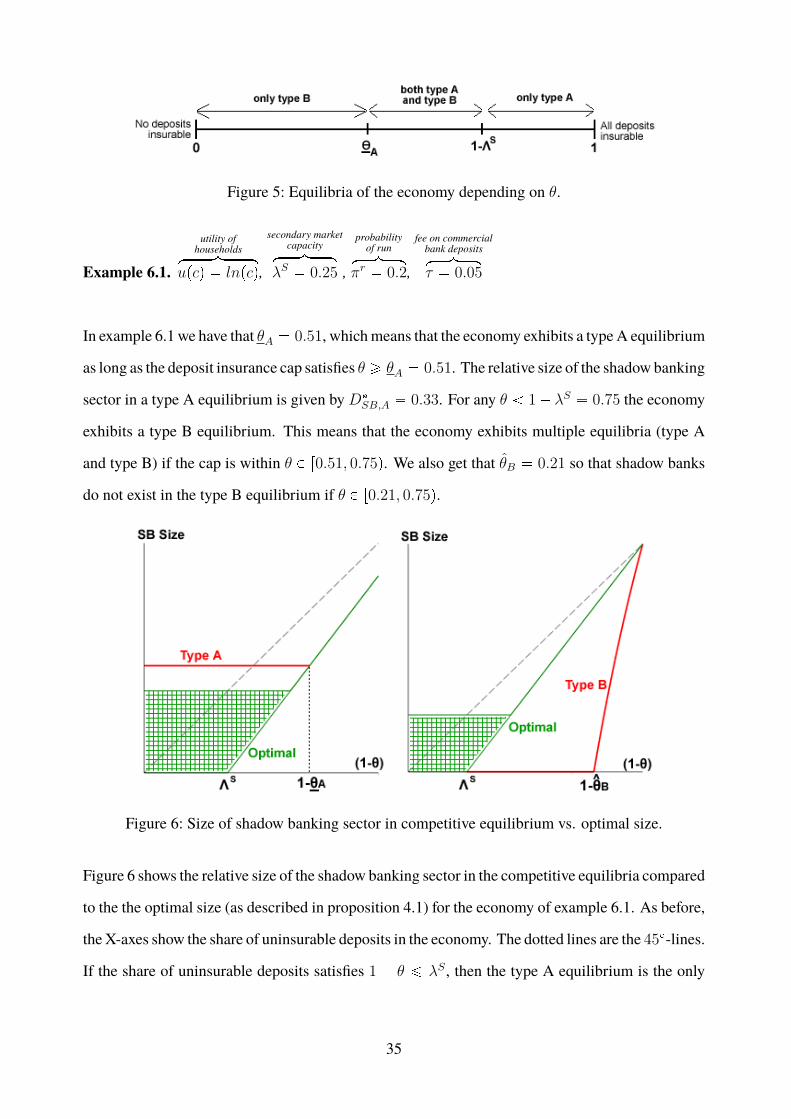
Figure 5: Equilibria of the economy depending on θ.

Example 6.1.

utility ofhouseholdshkkkkkkikkkkkkj

upcq � lnpcq,

secondary marketcapacityhkkkkikkkkj

λS � 0.25 ,

probabilityof runhkkkikkkj

πr � 0.2,

fee on commercialbank depositshkkkikkkjτ � 0.05

In example 6.1 we have that θA � 0.51, whichmeans that the economy exhibits a typeA equilibrium

as long as the deposit insurance cap satisfies θ ¥ θA � 0.51. The relative size of the shadow banking

sector in a type A equilibrium is given byD�SB,A � 0.33. For any θ   1� λS � 0.75 the economy

exhibits a type B equilibrium. This means that the economy exhibits multiple equilibria (type A

and type B) if the cap is within θ P r0.51, 0.75q. We also get that θB � 0.21 so that shadow banks

do not exist in the type B equilibrium if θ P r0.21, 0.75q.

Figure 6: Size of shadow banking sector in competitive equilibrium vs. optimal size.

Figure 6 shows the relative size of the shadow banking sector in the competitive equilibria compared

to the the optimal size (as described in proposition 4.1) for the economy of example 6.1. As before,

the X-axes show the share of uninsurable deposits in the economy. The dotted lines are the 45�-lines.

If the share of uninsurable deposits satisfies 1 � θ ¤ λS , then the type A equilibrium is the only

35

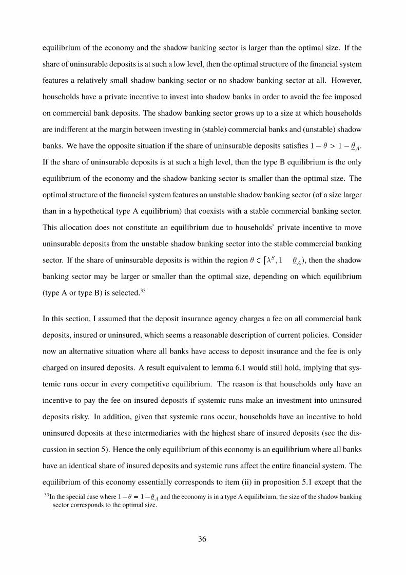
equilibrium of the economy and the shadow banking sector is larger than the optimal size. If the

share of uninsurable deposits is at such a low level, then the optimal structure of the financial system

features a relatively small shadow banking sector or no shadow banking sector at all. However,

households have a private incentive to invest into shadow banks in order to avoid the fee imposed

on commercial bank deposits. The shadow banking sector grows up to a size at which households

are indifferent at the margin between investing in (stable) commercial banks and (unstable) shadow

banks. We have the opposite situation if the share of uninsurable deposits satisfies 1� θ ¡ 1� θA.

If the share of uninsurable deposits is at such a high level, then the type B equilibrium is the only

equilibrium of the economy and the shadow banking sector is smaller than the optimal size. The

optimal structure of the financial system features an unstable shadow banking sector (of a size larger

than in a hypothetical type A equilibrium) that coexists with a stable commercial banking sector.

This allocation does not constitute an equilibrium due to households’ private incentive to move

uninsurable deposits from the unstable shadow banking sector into the stable commercial banking

sector. If the share of uninsurable deposits is within the region θ P rλS, 1 � θAq, then the shadow

banking sector may be larger or smaller than the optimal size, depending on which equilibrium

(type A or type B) is selected.33

In this section, I assumed that the deposit insurance agency charges a fee on all commercial bank

deposits, insured or uninsured, which seems a reasonable description of current policies. Consider

now an alternative situation where all banks have access to deposit insurance and the fee is only

charged on insured deposits. A result equivalent to lemma 6.1 would still hold, implying that sys-

temic runs occur in every competitive equilibrium. The reason is that households only have an

incentive to pay the fee on insured deposits if systemic runs make an investment into uninsured

deposits risky. In addition, given that systemic runs occur, households have an incentive to hold

uninsured deposits at these intermediaries with the highest share of insured deposits (see the dis-

cussion in section 5). Hence the only equilibrium of this economy is an equilibriumwhere all banks

have an identical share of insured deposits and systemic runs affect the entire financial system. The

equilibrium of this economy essentially corresponds to item (ii) in proposition 5.1 except that the33In the special case where 1�θ � 1�θA and the economy is in a type A equilibrium, the size of the shadow banking

sector corresponds to the optimal size.

36

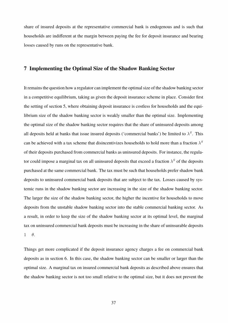
share of insured deposits at the representative commercial bank is endogenous and is such that

households are indifferent at the margin between paying the fee for deposit insurance and bearing

losses caused by runs on the representative bank.

7 Implementing the Optimal Size of the Shadow Banking Sector

It remains the question how a regulator can implement the optimal size of the shadow banking sector

in a competitive equilibrium, taking as given the deposit insurance scheme in place. Consider first

the setting of section 5, where obtaining deposit insurance is costless for households and the equi-

librium size of the shadow banking sector is weakly smaller than the optimal size. Implementing

the optimal size of the shadow banking sector requires that the share of uninsured deposits among

all deposits held at banks that issue insured deposits (‘commercial banks’) be limited to λS . This

can be achieved with a tax scheme that disincentivizes households to hold more than a fraction λS

of their deposits purchased from commercial banks as uninsured deposits. For instance, the regula-

tor could impose a marginal tax on all uninsured deposits that exceed a fraction λS of the deposits

purchased at the same commercial bank. The tax must be such that households prefer shadow bank

deposits to uninsured commercial bank deposits that are subject to the tax. Losses caused by sys-

temic runs in the shadow banking sector are increasing in the size of the shadow banking sector.

The larger the size of the shadow banking sector, the higher the incentive for households to move

deposits from the unstable shadow banking sector into the stable commercial banking sector. As

a result, in order to keep the size of the shadow banking sector at its optimal level, the marginal

tax on uninsured commercial bank deposits must be increasing in the share of uninsurable deposits

1 � θ.

Things get more complicated if the deposit insurance agency charges a fee on commercial bank

deposits as in section 6. In this case, the shadow banking sector can be smaller or larger than the

optimal size. A marginal tax on insured commercial bank deposits as described above ensures that

the shadow banking sector is not too small relative to the optimal size, but it does not prevent the

37

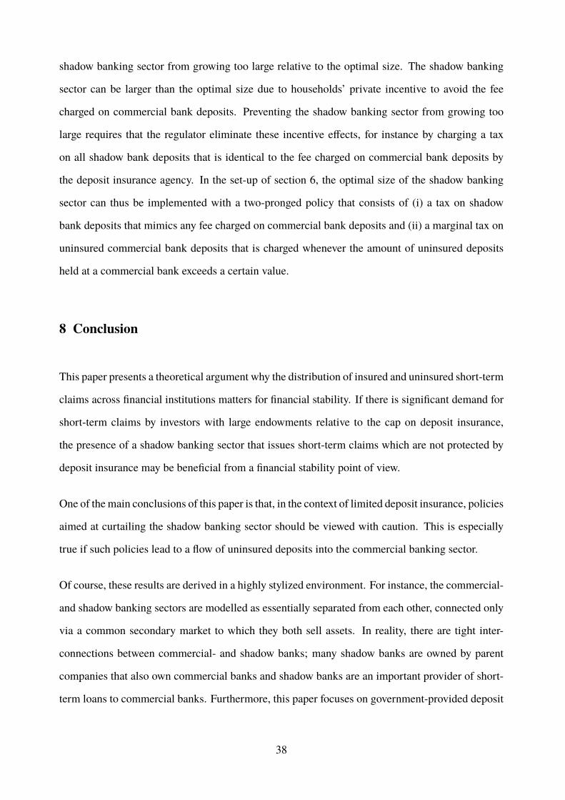
shadow banking sector from growing too large relative to the optimal size. The shadow banking

sector can be larger than the optimal size due to households’ private incentive to avoid the fee

charged on commercial bank deposits. Preventing the shadow banking sector from growing too

large requires that the regulator eliminate these incentive effects, for instance by charging a tax

on all shadow bank deposits that is identical to the fee charged on commercial bank deposits by

the deposit insurance agency. In the set-up of section 6, the optimal size of the shadow banking

sector can thus be implemented with a two-pronged policy that consists of (i) a tax on shadow

bank deposits that mimics any fee charged on commercial bank deposits and (ii) a marginal tax on

uninsured commercial bank deposits that is charged whenever the amount of uninsured deposits

held at a commercial bank exceeds a certain value.

8 Conclusion

This paper presents a theoretical argument why the distribution of insured and uninsured short-term

claims across financial institutions matters for financial stability. If there is significant demand for

short-term claims by investors with large endowments relative to the cap on deposit insurance,

the presence of a shadow banking sector that issues short-term claims which are not protected by

deposit insurance may be beneficial from a financial stability point of view.

One of themain conclusions of this paper is that, in the context of limited deposit insurance, policies

aimed at curtailing the shadow banking sector should be viewed with caution. This is especially

true if such policies lead to a flow of uninsured deposits into the commercial banking sector.

Of course, these results are derived in a highly stylized environment. For instance, the commercial-

and shadow banking sectors are modelled as essentially separated from each other, connected only

via a common secondary market to which they both sell assets. In reality, there are tight inter-

connections between commercial- and shadow banks; many shadow banks are owned by parent

companies that also own commercial banks and shadow banks are an important provider of short-

term loans to commercial banks. Furthermore, this paper focuses on government-provided deposit

38

insurance, abstracting from other government interventions such as the lender-of-last-resort or im-

plicit bail-out guarantees to commercial banks. Finally, the underlying causes of the demand for

short-term claims by investors with large endowments are not addressed. While such limitations

must be kept in mind, the paper does shed light on some aspects of shadow banking in the context

of limited deposit insurance that have not been analyzed so far.

39

References

Al-Najjar, Nabil (2004) “Aggregation and the Law of Large Numbers in Large Economies,” Gamesand Economic Behavior, Vol. 47(1), pp. 1–35.

Allen, Franklin and Douglas Gale (1994) “Limited Market Participation and Volatility of AssetPrices,” American Economic Review, Vol. 84(4), pp. 933–955.

Chrétien, Edouard and Victor Lyonnet (2017) “Traditional and Shadow Banks During the Crisis,”Working paper.

Cipriani, Marco, Gabriele La Spada, and Philip Mulder (2017) “Investors’ Appetite for Money-likeAssets: The Money Market Mutual Fund Industry after the 2014 Regulatory Reform,” FederalReserve Bank of New York Staff Reports No. 816.

Covitz, Daniel, Nellie Liang, and Gustavo A. Suarez (2013) “The Evolution of a Financial Crisis:Collapse of the Asset-Backed Commercial Paper Market,” The Journal of Finance, Vol. 68(3),pp. 815–848.

Davila, Eduardo and Itay Goldstein (2016) “Optimal Deposit Insurance,” Working Paper.

Diamond, Douglas W. and Philip H. Dybvig (1983) “Bank Runs, Deposit Insurance and Liquidity,”Journal of Political Economy, Vol. 91(3), pp. 401–419.

FSB (2017) “Global Shadow Banking Monitoring Report 2017,” http://www.fsb.org/

wp-content/uploads/P050318-1.pdf.

Gennaioli, Nicola, Andrei Shleifer, and Robert W. Vishny (2013) “A Model of Shadow Banking,”The Journal of Finance, Vol. 68(4), pp. 1331–1363.

Gertler, Mark, Nobuhiro Kiyotaki, and Andrea Prestipino (2016) “Wholesale Banking and BankRuns in Macroeconomic Modelling of Financial Crises,” in John Taylor and Harald Uhlig eds.Handbook of Macroeconomics, Volume 2B: Amsterdam: Elsevier, Chap. 17.

Hanson, Samuel G., Andrei Shleifer, Jeremy C. Stein, and Robert W. Vishny (2015) “Banks asPatient Fixed-Income Investors,” Journal of Financial Economics, Vol. 117(3), pp. 449–469.

Kacperczyk, Marcin and Philipp Schnabl (2010) “When Safe Proved Risky: Commercial PaperDuring the Financial Crisis of 2007-2009,” Journal of Economic Perspectives, Vol. 24(1), pp.29–50.

LeRoy, Stephen F. and Rish Singhania (2017) “Deposit Insurance and the Coexistence of Commer-cial and Shadow Banks,” Working paper.

Luck, Stephan and Paul Schempp (2016) “Banks, Shadow Banking, and Fragility,” Working Paper.

40

Martin, Antoine, David Skeie, and Ernst-Ludwig von Thadden (2014) “Repo Runs,” Review ofFinancial Studies, Vol. 27(4), pp. 957–989.

Moreira, Alan and Alexi Savov (2017) “The Macroeconomics of Shadow Banking,” The Journalof Finance, Vol. 72(6), pp. 2381–2432.

Poszar, Zoltan (2011) “Institutional Cash Pools and the Triffin Dilemma of the U.S. Banking Sys-tem,” IMF Working Papers No. 11/190.

(2014) “Shadow Banking: The Money View,” Oworking paper 14-04.

Poszar, Zoltan, Tobias Adrian, Adam Ashcraft, and Hayley Boesky (2010) “Shadow Banking,”Federal Reserve Bank of New York Staff Reports No. 458.

Ricks, Morgan (2012) “A Regulatory Design for Monetary Stability,” 65 Vanderbilt Law Review1287.

Schilling, Linda (2018) “Optimal Forbearance of Bank Resolution,” Becker Friedman InstituteWorking Paper 2018-15.

Schmidt, Lawrence, Allan Timmermann, and Russ Wermers (2016) “Runs on Money Market Mu-tual Funds,” American Economic Review, Vol. 106(9), pp. 2625–57.

Uhlig, Harald (1996) “A Law of Large Numbers for Large Economies,” Economic Theory, Vol.8(1), pp. 41–50.

41

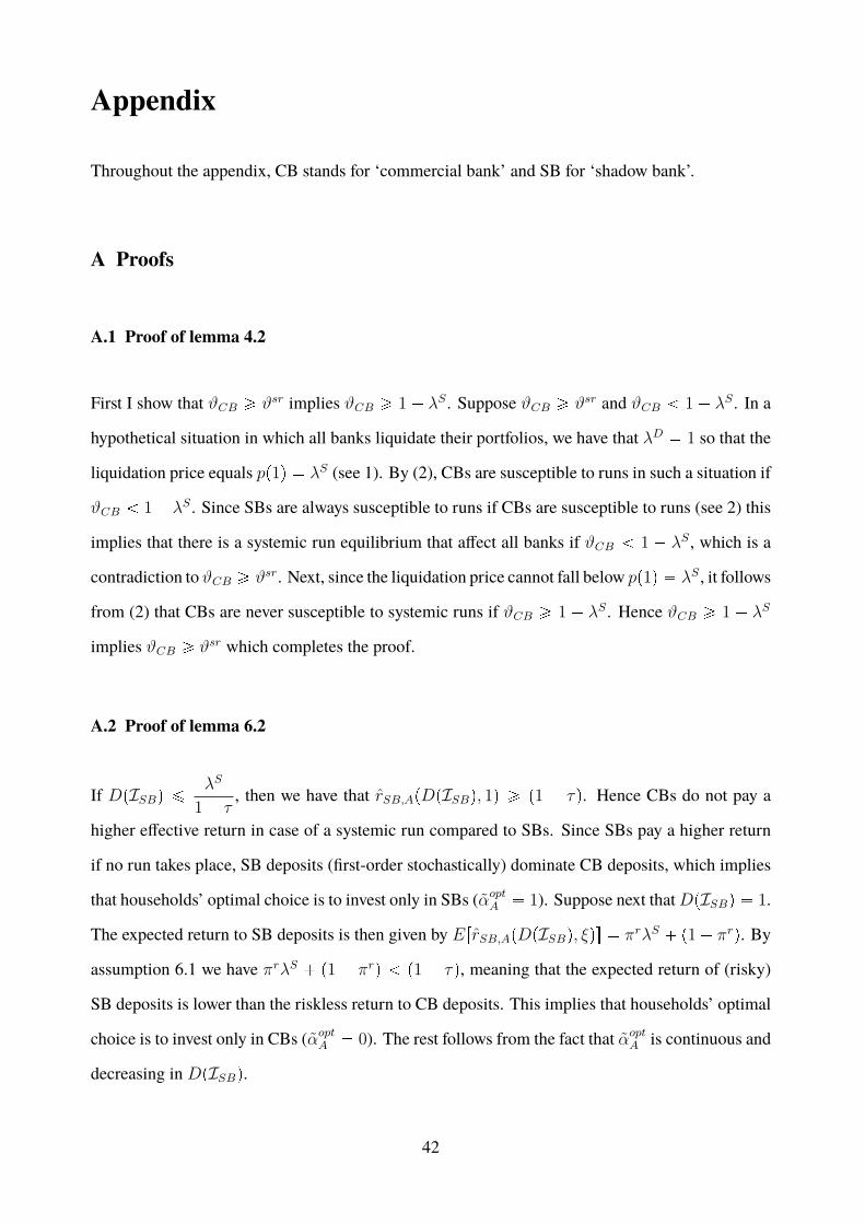
Appendix

Throughout the appendix, CB stands for ‘commercial bank’ and SB for ‘shadow bank’.

A Proofs

A.1 Proof of lemma 4.2

First I show that ϑCB ¥ ϑsr implies ϑCB ¥ 1 � λS . Suppose ϑCB ¥ ϑsr and ϑCB   1 � λS . In a

hypothetical situation in which all banks liquidate their portfolios, we have that λD � 1 so that the

liquidation price equals pp1q � λS (see 1). By (2), CBs are susceptible to runs in such a situation if

ϑCB   1� λS . Since SBs are always susceptible to runs if CBs are susceptible to runs (see 2) this

implies that there is a systemic run equilibrium that affect all banks if ϑCB   1 � λS , which is a

contradiction to ϑCB ¥ ϑsr. Next, since the liquidation price cannot fall below pp1q � λS , it follows

from (2) that CBs are never susceptible to systemic runs if ϑCB ¥ 1 � λS . Hence ϑCB ¥ 1 � λS

implies ϑCB ¥ ϑsr which completes the proof.

A.2 Proof of lemma 6.2

If DpISBq ¤λS

1 � τ, then we have that rSB,ApDpISBq, 1q ¥ p1 � τq. Hence CBs do not pay a

higher effective return in case of a systemic run compared to SBs. Since SBs pay a higher return

if no run takes place, SB deposits (first-order stochastically) dominate CB deposits, which implies

that households’ optimal choice is to invest only in SBs (αoptA � 1). Suppose next thatDpISBq � 1.

The expected return to SB deposits is then given by ErrSB,ApDpISBq, ξqs � πrλS � p1 � πrq. By

assumption 6.1 we have πrλS � p1 � πrq   p1 � τq, meaning that the expected return of (risky)

SB deposits is lower than the riskless return to CB deposits. This implies that households’ optimal

choice is to invest only in CBs (αoptA � 0). The rest follows from the fact that αoptA is continuous and

decreasing in DpISBq.

42

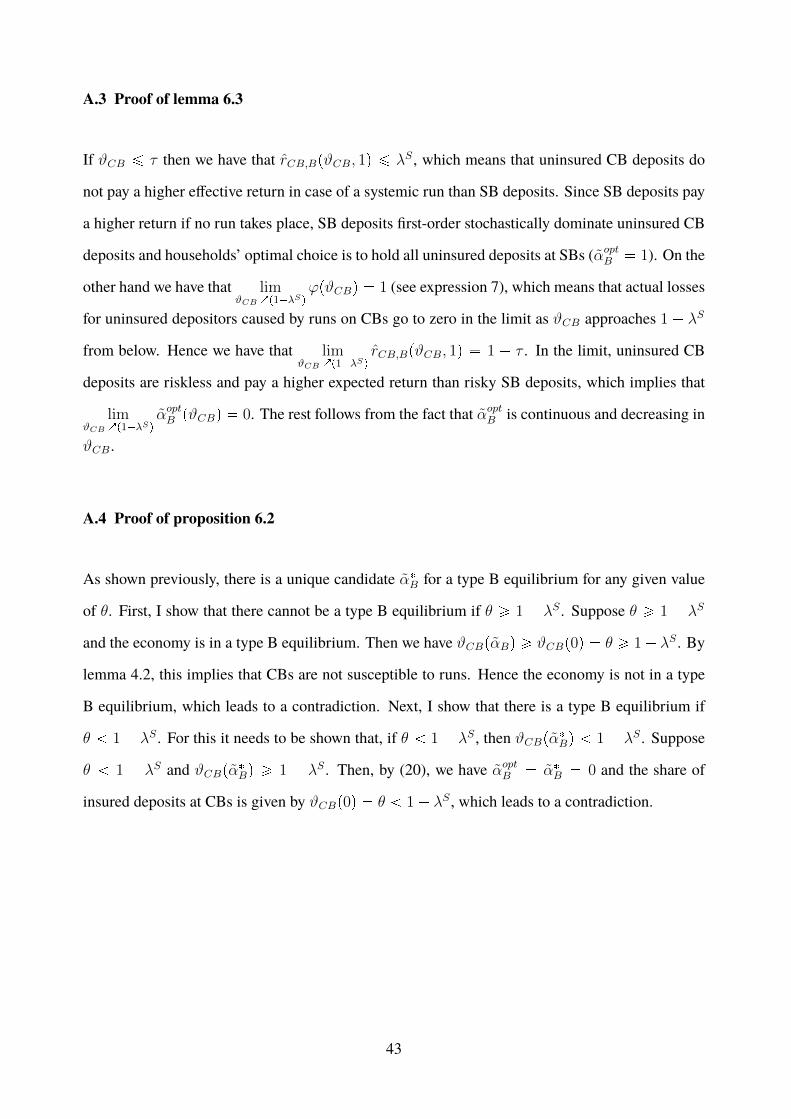
A.3 Proof of lemma 6.3

If ϑCB ¤ τ then we have that rCB,BpϑCB, 1q ¤ λS , which means that uninsured CB deposits do

not pay a higher effective return in case of a systemic run than SB deposits. Since SB deposits pay

a higher return if no run takes place, SB deposits first-order stochastically dominate uninsured CB

deposits and households’ optimal choice is to hold all uninsured deposits at SBs (αoptB � 1). On the

other hand we have that limϑCBÕp1�λSq

ϕpϑCBq � 1 (see expression 7), which means that actual losses

for uninsured depositors caused by runs on CBs go to zero in the limit as ϑCB approaches 1 � λS

from below. Hence we have that limϑCBÕp1�λSq

rCB,BpϑCB, 1q � 1 � τ . In the limit, uninsured CB

deposits are riskless and pay a higher expected return than risky SB deposits, which implies that

limϑCBÕp1�λSq

αoptB pϑCBq � 0. The rest follows from the fact that αoptB is continuous and decreasing in

ϑCB.

A.4 Proof of proposition 6.2

As shown previously, there is a unique candidate α�B for a type B equilibrium for any given value

of θ. First, I show that there cannot be a type B equilibrium if θ ¥ 1 � λS . Suppose θ ¥ 1 � λS

and the economy is in a type B equilibrium. Then we have ϑCBpαBq ¥ ϑCBp0q � θ ¥ 1� λS . By

lemma 4.2, this implies that CBs are not susceptible to runs. Hence the economy is not in a type

B equilibrium, which leads to a contradiction. Next, I show that there is a type B equilibrium if

θ   1 � λS . For this it needs to be shown that, if θ   1 � λS , then ϑCBpα�Bq   1 � λS . Suppose

θ   1 � λS and ϑCBpα�Bq ¥ 1 � λS . Then, by (20), we have αoptB � α�B � 0 and the share of

insured deposits at CBs is given by ϑCBp0q � θ   1 � λS , which leads to a contradiction.

43

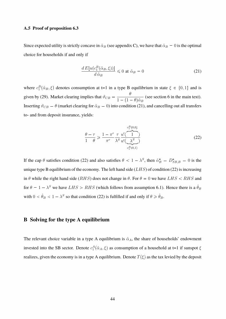
A.5 Proof of proposition 6.3

Since expected utility is strictly concave in αB (see appendix C), we have that αB � 0 is the optimal

choice for households if and only if

dErupcB1 pαB, ξqqs

d αB¤ 0 at αB � 0 (21)

where cB1 pαB, ξq denotes consumption at t=1 in a type B equilibrium in state ξ P t0, 1u and is

given by (29). Market clearing implies that ϑCB �θ

1 � p1 � θqαB(see section 6 in the main text).

Inserting ϑCB � θ (market clearing for αB � 0) into condition (21), and cancelling out all transfers

to- and from deposit insurance, yields:

θ � τ

1 � θ¥

1 � πr

πrτ

λSu1p

cB1 p0,0qhkkikkj1 q

u1p λSloomooncB1 p0,1q

q(22)

If the cap θ satisfies condition (22) and also satisfies θ   1 � λS , then α�B � D�SB,B � 0 is the

unique type B equilibrium of the economy. The left hand side (LHS) of condition (22) is increasing

in θ while the right hand side (RHS) does not change in θ. For θ � 0 we have LHS   RHS and

for θ � 1 � λS we have LHS ¡ RHS (which follows from assumption 6.1). Hence there is a θB

with 0   θB   1 � λS so that condition (22) is fulfilled if and only if θ ¥ θB.

B Solving for the type A equilibrium

The relevant choice variable in a type A equilibrium is αA, the share of households’ endowment

invested into the SB sector. Denote cA1 pαA, ξq as consumption of a household at t=1 if sunspot ξ

realizes, given the economy is in a type A equilibrium. Denote T pξq as the tax levied by the deposit

44

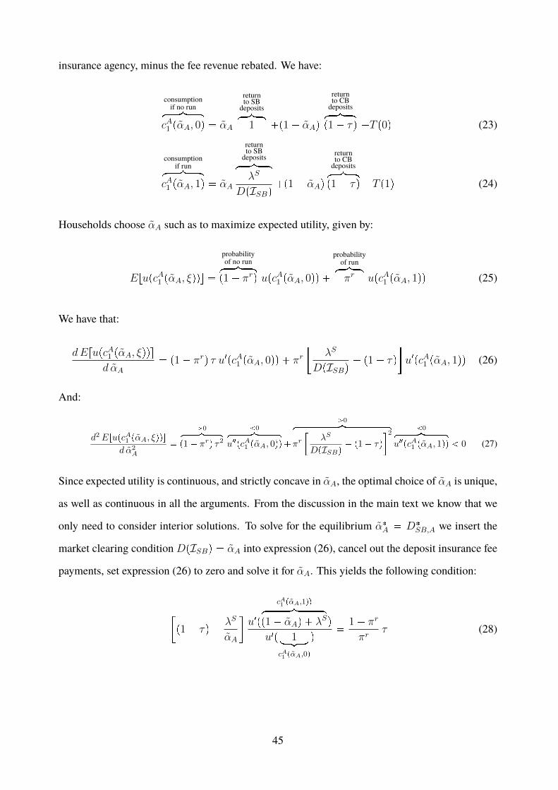
insurance agency, minus the fee revenue rebated. We have:

consumptionif no runhkkkkikkkkj

cA1 pαA, 0q � αA

returnto SB

depositshkkikkj1 �p1 � αAq

returnto CBdepositshkkikkjp1 � τq �T p0q (23)

consumptionif runhkkkkikkkkj

cA1 pαA, 1q � αA

returnto SB

depositshkkkikkkjλS

DpISBq�p1 � αAq

returnto CBdepositshkkikkjp1 � τq �T p1q (24)

Households choose αA such as to maximize expected utility, given by:

ErupcA1 pαA, ξqqs �

probabilityof no runhkkkikkkjp1 � πrq upcA1 pαA, 0qq �

probabilityof runhkkikkjπr upcA1 pαA, 1qq (25)

We have that:

dErupcA1 pαA, ξqqs

d αA� p1 � πrq τ u1pcA1 pαA, 0qq � πr

�λS

DpISBq� p1 � τq

�u1pcA1 pαA, 1qq (26)

And:

d2ErupcA1 pαA, ξqqs

d α2A

�

¡0hkkkkkikkkkkjp1 � πrq τ2

 0hkkkkkkkikkkkkkkju2pcA1 pαA, 0qq�

¡0hkkkkkkkkkkkkkkkikkkkkkkkkkkkkkkjπr

�λS

DpISBq� p1 � τq

�2  0hkkkkkkkikkkkkkkju2pcA1 pαA, 1qq   0 (27)

Since expected utility is continuous, and strictly concave in αA, the optimal choice of αA is unique,

as well as continuous in all the arguments. From the discussion in the main text we know that we

only need to consider interior solutions. To solve for the equilibrium α�A � D�SB,A we insert the

market clearing condition DpISBq � αA into expression (26), cancel out the deposit insurance fee

payments, set expression (26) to zero and solve it for αA. This yields the following condition:

�p1 � τq �

λS

αA

�u1p

cA1 pαA,1qqhkkkkkkkikkkkkkkjp1 � αAq � λSq

u1p 1loomooncA1 pαA,0q

q�

1 � πr

πrτ (28)

45

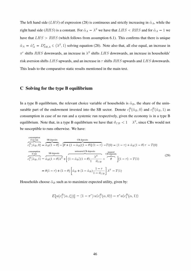
The left hand side (LHS) of expression (28) is continuous and strictly increasing in αA, while the

right hand side (RHS) is a constant. For αA � λS we have that LHS   RHS and for αA � 1 we

have that LHS ¡ RHS (which follows from assumption 6.1). This confirms that there is unique

αA � α�A � D�SB,A P pλS, 1q solving equation (28). Note also that, all else equal, an increase in

πr shifts RHS downwards, an increase in λS shifts LHS downwards, an increase in households’

risk aversion shifts LHS upwards, and an increase in τ shiftsRHS upwards and LHS downwards.

This leads to the comparative static results mentioned in the main text.

C Solving for the type B equilibrium

In a type B equilibrium, the relevant choice variable of households is αB, the share of the unin-surable part of the endowment invested into the SB sector. Denote cB1 pαB, 0q and cB1 pαB, 1q asconsumption in case of no run and a systemic run respectively, given the economy is in a type Bequilibrium. Note that, in a type B equilibrium we have that ϑCB   1 � λS , since CBs would notbe susceptible to runs otherwise. We have:

consumptionif no runhkkkkikkkkj

cB1 pαB , 0q �

SB depositshkkkkikkkkjαBp1 � θq�

CB depositshkkkkkkkkkkkkkkkkkkikkkkkkkkkkkkkkkkkkjrθ � p1 � αBqp1 � θqs p1 � τq �T p0q � p1 � τq � αBp1 � θq τ � T p0q

consumptionif runhkkkkikkkkj

cB1 pαB , 1q �

SB depositshkkkkkkikkkkkkjαBp1 � θqλS �

�uninsured CB depositshkkkkkkkkkkkkkkkikkkkkkkkkkkkkkkj

p1 � αBqp1 � θqλS

1 � ϑCB�

insuredCB depositshkkikkj

θ�p1 � τq � T p1q

� θp1 � τq � p1 � θq

�αB � p1 � αBq

1 � τ

1 � ϑCB

�λS � T p1q

(29)

Households choose αB such as to maximize expected utility, given by:

ErupcB1 pα, ξqqs � p1 � πrqupcB1 pα, 0qq � πrupcB1 pα, 1qq

46

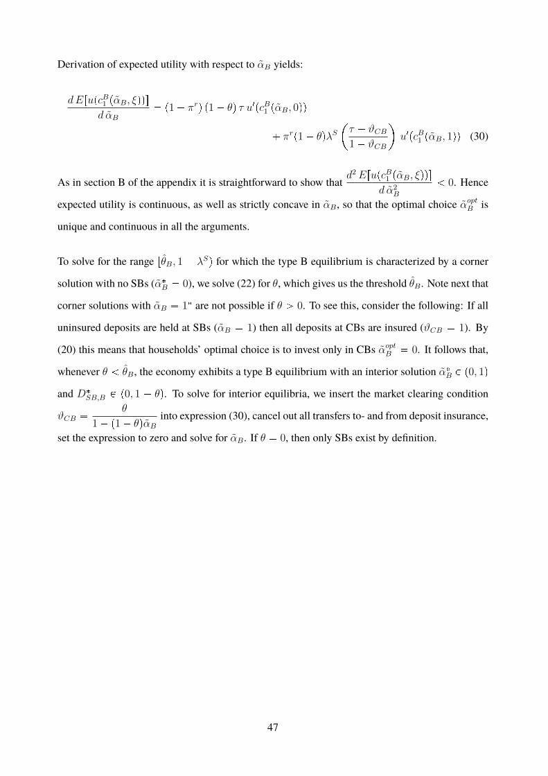
Derivation of expected utility with respect to αB yields:

dErupcB1 pαB, ξqqs

d αB� p1 � πrq p1 � θq τ u1pcB1 pαB, 0qq

� πrp1 � θqλS�τ � ϑCB1 � ϑCB

u1pcB1 pαB, 1qq (30)

As in section B of the appendix it is straightforward to show thatd2ErupcB1 pαB, ξqqs

d α2B

  0. Hence

expected utility is continuous, as well as strictly concave in αB, so that the optimal choice αoptB is

unique and continuous in all the arguments.

To solve for the range rθB, 1 � λSq for which the type B equilibrium is characterized by a corner

solution with no SBs (α�B � 0), we solve (22) for θ, which gives us the threshold θB. Note next that

corner solutions with αB � 1� are not possible if θ ¡ 0. To see this, consider the following: If all

uninsured deposits are held at SBs (αB � 1) then all deposits at CBs are insured (ϑCB � 1). By

(20) this means that households’ optimal choice is to invest only in CBs αoptB � 0. It follows that,

whenever θ   θB, the economy exhibits a type B equilibrium with an interior solution α�B P p0, 1q

and D�SB,B P p0, 1 � θq. To solve for interior equilibria, we insert the market clearing condition

ϑCB �θ

1 � p1 � θqαBinto expression (30), cancel out all transfers to- and from deposit insurance,

set the expression to zero and solve for αB. If θ � 0, then only SBs exist by definition.

47

I thank Aleksander Berentsen, Ina Bialova (discussant), Regis Breton, Fabrice Collard, Harris Dellas, Corinne Dubois (discussant), Leonardo Gambacorta (discussant), Zhiguo He, Marie Hoerova, Todd Keister, Ewelina Laskowska, Stephen F. LeRoy, Simone Manganelli, Antoine Martin, Dirk Niepelt and in particular Cyril Monnet for very helpful comments and suggestions on various versions of the paper. I also thank participants at the Biennial IADI Research Conference in Basel, Midwest Macro Meeting in Pittsburgh, SUERF & Bank of Finland colloquium on shadow banking in Helsinki, Verein fuer Socialpolitik Annual Conference in Vienna, Swiss Finance Institute Research Days in Gerzensee, Swiss Society for Economics and Statistics Annual Congress in Lausanne and Young Swiss Economist Meeting in Zurich. All errors are mine.

Lukas Voellmy Study Center Gerzensee, Gerzensee, Switzerland; email: [email protected]

Imprint and acknowledgements

© European Systemic Risk Board, 2019

Postal address 60640 Frankfurt am Main, Germany Telephone +49 69 1344 0 Website www.esrb.europa.eu

All rights reserved. Reproduction for educational and non-commercial purposes is permitted provided that the source is acknowledged.

Note: The views expressed in ESRB Working Papers are those of the authors and do not necessarily reflect the official stance of the ESRB, its member institutions, or the institutions to which the authors are affiliated.

ISSN 2467-0677 (pdf) ISBN 978-92-9472-119-8 (pdf) DOI 10.2849/875514 (pdf) EU catalogue No DT-AD-19-019-EN-N (pdf)