Seven Techniques for Data Dimensionality Reduction · PDF file2 Table of Contents Seven Techniques for Data Dimensionality Reduction Missing Values, Low Variance Filter, High Correlation

1

Seven Techniques for Data Dimensionality

Reduction Missing Values, Low Variance Filter, High Correlation Filter,

PCA, Random Forests, Backward Feature Elimination, and

Forward Feature Construction

Rosaria Silipo [email protected]

Iris Adae [email protected]

Aaron Hart [email protected]

Michael Berthold [email protected]

2

Table of Contents Seven Techniques for Data Dimensionality Reduction Missing Values, Low Variance Filter, High Correlation Filter, PCA, Random Forests, Backward Feature Elimination, and Forward Feature Construction .................................................................................................................................................. 1

Summary ....................................................................................................................................................... 3

The KDD Challenge........................................................................................................................................ 3

Reading Data and Selecting Target .............................................................................................................. 4

Reducing Input Dimensionality .................................................................................................................... 5

Setting the Baseline ...................................................................................................................................... 6

Seven Methods to Reduce Input Dimensionality ........................................................................................ 6

1. Removing Data Columns with Too Many Missing Values ............................................................... 6

2. Low Variance Filter ........................................................................................................................... 8

3. Reducing Highly Correlated Columns ............................................................................................... 9

4. Principal Component Analysis (PCA) .............................................................................................. 11

5. Dimensionality Reduction via Tree Ensembles (Random Forests) ................................................ 13

6. Backward Feature Elimination ....................................................................................................... 14

7. Forward Feature Construction ....................................................................................................... 17

Comparison of Techniques for Dimensionality Reduction ........................................................................ 18

Combining Dimensionality Reduction Techniques .................................................................................... 19

Conclusions ................................................................................................................................................. 21

3

Summary The recent explosion of data set size, in number of records as well as of attributes, has triggered the

development of a number of big data platforms as well as parallel data analytics algorithms. At the same

time though, it has pushed for the usage of data dimensionality reduction procedures.

This whitepaper explores some commonly used techniques for dimensionality reduction. It is an extract

from a larger project implemented on the 2009 KDD Challenge data sets for three classification tasks.

The particularity of one of those data sets is its very high dimensionality. Therefore, before proceeding

with any data analytics task, we needed to implement one or more dimensionality reduction techniques.

Dimensionality reduction is not only useful to speed up algorithm execution, but actually might help with

the final classification/clustering accuracy as well. Too much noisy or even faulty input data often lead to

a less than desirable algorithm performance. Removing un-informative or dis-informative data columns

might indeed help the algorithm find more general classification regions and rules and overall achieve

better performances on new data.

We used this project to explore a few of the state-of-the-art techniques to reduce the number of input

features in a data set and we decided to publish this information here for other data analysts. Keeping

the choice of the final classification algorithm to one side for now, our focus here is the dimensionality

reduction techniques that were evaluated for this project.

The workflows described in this whitepaper are available on the EXAMPLES server at

003_Preprocessing/003005_dimensionality_reduction.

Both small and large data sets from the 2009 KDD Challenge can be downloaded from

http://www.sigkdd.org/kdd-cup-2009-customer-relationship-prediction.

The KDD Challenge Every year the KDD conference (www.kdd.org) sets a data analytics challenge for its attendees: the KDD

cup. One of the most challenging cups was in 2009 and dealt with customer relationship prediction,

specifically with churn, appetency, and upselling prediction. Churn represents a contract severance by a

customer; appetency the propensity to buy a service or a product; and upselling the possibility of selling

additional side products to the main one. Now, all these three tasks – churn, appetency, and upselling

prediction – have been around quite some time in the data analytics community and solutions are

relatively well established. So, where was the challenge in this particular KDD cup?

The challenge was in the data structure and particularly in the number of input features. The data set

came from the CRM system of a big French telecommunications company. It is a well-known fact that

telco companies are practically drowning in data and while the analytics problems they are dealing with

do not really present exceptional challenges, the size of the data sets does. And this data set was no

exception, with 50K rows and 15K columns!

The web site offers two data sets: a “small” set to set up your analytics process with just a few more than

200 columns and still 50K records and a “large” one with almost 15K columns and 50K rows. The large

data set is contained in 5 separate files, each one with 10K records. The labels for the three prediction

tasks are located in three separate files: one with churn, one with appetency, and one with upselling

4

labels, indicating respectively whether a customer has churned, bought a product, or bought a second

side product. The reference key between the input data set and the label files is just the row index.

For more information about the challenge tasks and to download the original data files, see the KDD Cup

2009 web site http://www.sigkdd.org/kdd-cup-2009-customer-relationship-prediction.

Reading Data and Selecting Target Before reaching the pre-processing stage and the classification part, the first few blocks in the workflow

are about reading the data (“Reading all data” metanode) and selecting the target task ‒ as churn,

appetency, or upselling (“Target Selection” metanode).

Using Quickform nodes to produce a radio button list, the first metanode allows the user to choose

whether the small data set file, the large data set file, or the small data set from the database should be

read. The second metanode allows the user to select the classification task. The content of the “Reading

all data” metanode and the “Target Selection” metanode is shown in the Figs 1 and 2 below.

Figure 1. Content of “Reading all data” metanode with Quickform node controlling the switch and enabling different reading branches

Figure 2. Content of "Target Selection" metanode with Quickform node controlling Column Rename and

Column Filter nodes

Notice that a Quickform node inside a metanode builds the metanode configuration window. In the case

of the “Reading all Data” metanode, the metanode’s configuration window displays three radio buttons,

which can be seen in Fig. 3. The same radio button GUI would show up on a KNIME WebPortal during the

workflow execution. The output flow variable from the Quickform node is used to control a switch block

to read the selected data set.

In the “Target Selection” metanode, the Quickform node controls the Column Filter and the Column

Rename node to get rid of the unwanted targets and to rename the selected target with an anonymous

“Target” label.

5

Figure 3. Configuration Window of the “Reading all data” metanode generated by the String Radio Buttons Quickform

node

Figure 4. Configuration Window of the "Target Selection" metanode generated by the Single Selection Input Quickform

node

Reducing Input Dimensionality Data analytics solutions for churn detection, appetency and upselling evaluation are generally based on

supervised classification algorithms.

There are many algorithms available in KNIME for supervised classification: decision tree, naïve Bayes,

neural network, logistic regression, random forest, and more. Most of them though, due to their internal

learning algorithms, might find it difficult to deal with a very high number of columns. Notice that this is

not a KNIME specific problem. This is a problem inherent to the way the algorithms are designed and

therefore a transversal problem to all data analytics tools. Please note too that the problem is not the

size of the data set, but rather the number of input columns. Indeed, many data analytics algorithms

loop around the input columns, which makes the learning phase duration increase quickly together with

the number of columns and could become prohibitive.

Working with the 2009 KDD Cup data sets with 231 for the small and 15K data columns for the large data

set, it soon becomes apparent that the most important part of the work is to drastically reduce the data

set dimensionality to a more manageable size, but without compromising the subsequent classification

performance.

We started working with the “small” data set to evaluate a few classic dimensionality reduction

methods. The relatively small number of data columns allows for faster evaluation and comparison of

the different techniques. It was only after we had gained a clearer picture of the pros and cons of the

evaluated dimensionality reduction methods that we approached the “large” data set for a more realistic

analytics project. Here we used a cascade of the most promising techniques, as detected in the first

phase of the project on the smaller data set.

In this whitepaper, we concentrate on a few state-of-the-art methods to reduce input dimensionality

and examine how they might affect the final classification accuracy. In particular, we implement and

evaluate data columns reduction based on:

1. High number of missing values

2. Low variance

3. High correlation with other data columns

6

4. Principal Component Analysis (PCA)

5. First cuts in random forest trees

6. Backward feature elimination

7. Forward feature construction

The workflow evaluating and comparing these techniques on the small data set is named “Dim Reduction

Techniques”. The workflow applying a cascade of some of these methods is named “KDD Analysis on All

Data”. Both workflows can be found on the EXAMPLES server at

003_Preprocessing/003005_dimensionality_reduction.

Even though the workflow refers to a few classification algorithms to follow data dimensionality

reduction, we will not really explore the classification part in this whitepaper.

Setting the Baseline The goal of this whitepaper is to perform dimensionality reduction without damaging the classification

accuracy. The first thing to do is to set some baseline performance with which to compare possible

accuracy degradation.

With the original 231 data columns in the KDD small data set, the best accuracy (73%) is obtained by the

MLP neural network. This 73% accuracy is the value we need to preserve when adding some

dimensionality reduction processing to the pure classification phase.

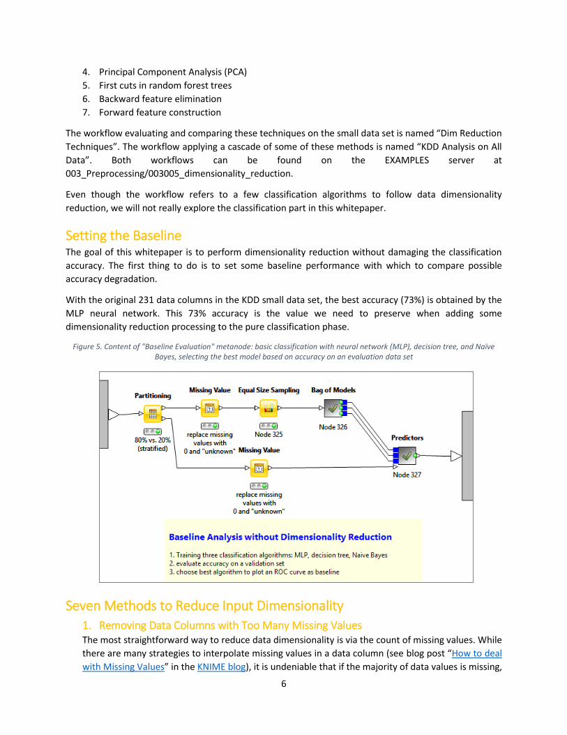
Figure 5. Content of "Baseline Evaluation" metanode: basic classification with neural network (MLP), decision tree, and Naïve Bayes, selecting the best model based on accuracy on an evaluation data set

Seven Methods to Reduce Input Dimensionality

1. Removing Data Columns with Too Many Missing Values The most straightforward way to reduce data dimensionality is via the count of missing values. While

there are many strategies to interpolate missing values in a data column (see blog post “How to deal

with Missing Values” in the KNIME blog), it is undeniable that if the majority of data values is missing,

7

the data column itself cannot carry that much information. In most cases, for example, if a data

column has only 5-10% of the possible values, it will likely not be useful for the classification of most

records. The goal, then, becomes to remove those data columns with too many missing values, i.e.

with more missing values in percent than a given threshold.

To count the number of missing values in all data columns, we can either use a Statistics or a

GroupBy node.

We used the Statistics node in the “KDD Analysis on All Data” workflow and the GroupBy node in the

“Dim Reduction Techniques” workflow.

The Statistics node produces three data tables at the output ports: a statistics table, a nominal

histogram table, and an occurrences table. The nominal histogram table contains the number of

missing values for each data column. In addition to other statistical measures, the statistics table

contains the total number of rows of the input data table. From these two data tables, a Math

Formula node calculates the ratio of missing values for each column as:

Ratio of missing values = number of missing values / total number of rows

If we use the GroupBy node, in the “Pattern Based Aggregation” tab, we set “.*” as the RegEx search

pattern for column names to count the missing values. After transposing the results, the Math

Formula node calculates the ratio of missing values, as described in the formula above.

A Rule Engine node followed by a Row Filter node or a Rule-based Row Filter node, in the two

workflows respectively, defines the rule for a too high missing value ratio (ratio > threshold value)

and then filters out those columns fitting the rule.

The threshold value selection is of course a crucial topic, since a too aggressive value will reduce

dimensionality at the expense of performance, while a too soft value might not get the best

reduction ratio. To find the best threshold value, we used an optimization loop and maximized the

classification algorithm accuracy on the test set. However, in some particular situations one

classification algorithm might perform better than others. To be on the safe side, we ran the

optimization loop on three possible classification algorithms ‒ neural network (MLP), decision tree,

and Naïve Bayes – selecting the best method accuracy as the value to be maximized.

After ascertaining the best threshold value from the optimization loop, we applied it to the original

data set to reduce the number of columns. Then we ran the three classification algorithms again and

we selected the best performing one to build the ROC curve.

Such a complex loop, though, can only run in a reasonable time on the small KDD data set. We used

the small data set as a test table to then export our findings to the large KDD data set.

Notice that this technique for data dimensionality reduction, based on the missing value ratio,

applies to both nominal and numerical columns.

The process of eliminating the data columns with too many missing values is contained in the

“Reduction based on Missing Values” metanode. The optimization loop to find the best threshold

value is contained in the “Best Threshold on Missing Values” metanode (Fig. 6). The procedure to

actually count the number of missing values and filter out the columns can be found in the “Column

Selection by Missing Values” metanode.

8

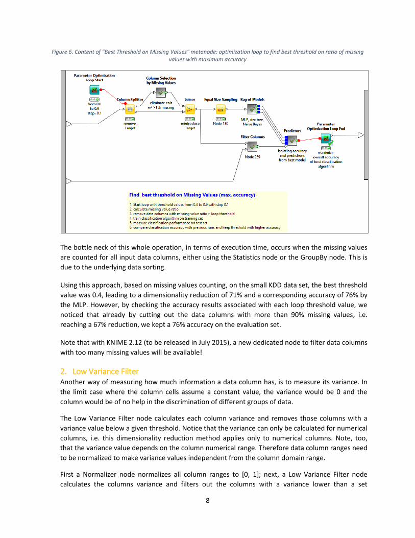
Figure 6. Content of "Best Threshold on Missing Values" metanode: optimization loop to find best threshold on ratio of missing values with maximum accuracy

The bottle neck of this whole operation, in terms of execution time, occurs when the missing values

are counted for all input data columns, either using the Statistics node or the GroupBy node. This is

due to the underlying data sorting.

Using this approach, based on missing values counting, on the small KDD data set, the best threshold

value was 0.4, leading to a dimensionality reduction of 71% and a corresponding accuracy of 76% by

the MLP. However, by checking the accuracy results associated with each loop threshold value, we

noticed that already by cutting out the data columns with more than 90% missing values, i.e.

reaching a 67% reduction, we kept a 76% accuracy on the evaluation set.

Note that with KNIME 2.12 (to be released in July 2015), a new dedicated node to filter data columns

with too many missing values will be available!

2. Low Variance Filter Another way of measuring how much information a data column has, is to measure its variance. In

the limit case where the column cells assume a constant value, the variance would be 0 and the

column would be of no help in the discrimination of different groups of data.

The Low Variance Filter node calculates each column variance and removes those columns with a

variance value below a given threshold. Notice that the variance can only be calculated for numerical

columns, i.e. this dimensionality reduction method applies only to numerical columns. Note, too,

that the variance value depends on the column numerical range. Therefore data column ranges need

to be normalized to make variance values independent from the column domain range.

First a Normalizer node normalizes all column ranges to [0, 1]; next, a Low Variance Filter node

calculates the columns variance and filters out the columns with a variance lower than a set

9

threshold. As for the previous method, the optimal threshold can be defined through an optimization

loop maximizing the classification accuracy on a validation set for the best out of three classification

algorithms: MLP, decision tree, and Naïve Bayes. Any remaining columns are finally de-normalized to

return to their original numerical range.

Metanode named “Reduction based on Low Variance” implements such an optimization loop with

the “best threshold on low variance” metanode and extracts the best threshold value to apply for

the final dimensionality reduction before the classification phase with the “rm columns with too low

variance” metanode. One level down, the metanode “Filter Low Variance Columns” contains the Low

Variance Filter node which calculates the column variance and performs the column reduction (Fig.

7).

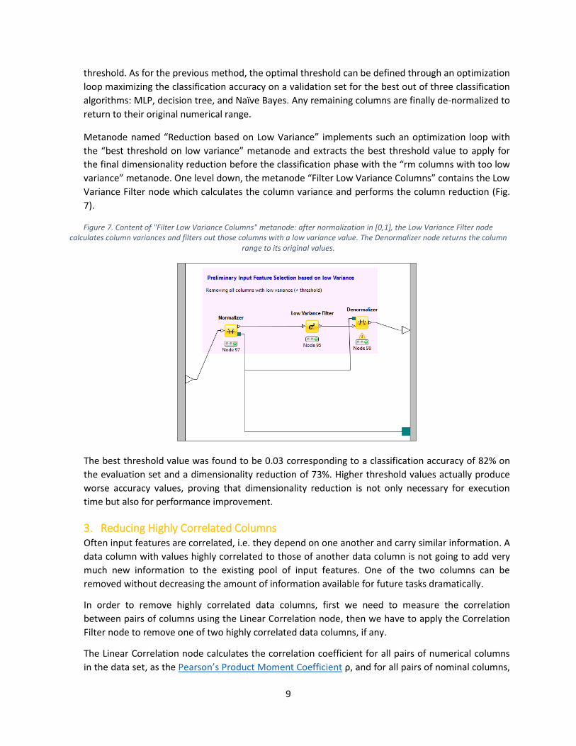
Figure 7. Content of "Filter Low Variance Columns" metanode: after normalization in [0,1], the Low Variance Filter node calculates column variances and filters out those columns with a low variance value. The Denormalizer node returns the column

range to its original values.

The best threshold value was found to be 0.03 corresponding to a classification accuracy of 82% on

the evaluation set and a dimensionality reduction of 73%. Higher threshold values actually produce

worse accuracy values, proving that dimensionality reduction is not only necessary for execution

time but also for performance improvement.

3. Reducing Highly Correlated Columns Often input features are correlated, i.e. they depend on one another and carry similar information. A

data column with values highly correlated to those of another data column is not going to add very

much new information to the existing pool of input features. One of the two columns can be

removed without decreasing the amount of information available for future tasks dramatically.

In order to remove highly correlated data columns, first we need to measure the correlation

between pairs of columns using the Linear Correlation node, then we have to apply the Correlation

Filter node to remove one of two highly correlated data columns, if any.

The Linear Correlation node calculates the correlation coefficient for all pairs of numerical columns

in the data set, as the Pearson’s Product Moment Coefficient ρ, and for all pairs of nominal columns,

10

as the Pearson's chi square value. No correlation coefficient is defined between a numerical and a

nominal data column.

The output table of the node is the correlation matrix, i.e. the matrix with the correlation coefficients

for all pairs of data columns. The correlation coefficient referring to a numerical and a nominal

column in the matrix has a missing value. The node also produces a color coded view of the

correlation matrix (see figure below) where values range from intense blue (+1 = full correlation),

white (0 = no correlation), to red (-1 = full inverse correlation). The matrix diagonal shows the

correlation of a data column with itself and this is, of course, a 1.0 correlation. The crosses indicate a

missing correlation value, e.g. for the combination of a numerical and a categorical column.

Figure 8. View of the Correlation Matrix from the Linear Correlation node

The Correlation Filter node uses this correlation matrix as input, identifies pairs of columns with a

high correlation (i.e. greater than a given threshold), and removes one of the two columns for each

identified pair. The correlation threshold can be set manually by means of a slide bar in the

configuration window of the Correlation Filter node. While moving the slide bar, you can evaluate

11

the number of remaining data columns corresponding to that particular threshold value with the

Calculate button. The lower the threshold the more aggressive the column filter.

As for the other techniques, we used an optimization loop in the “best threshold on high corr.”

Metanode, to find the best threshold value for the Correlation Filter node; best again in terms of

accuracy on the validation set.

Correlation coefficients for numerical columns are also dependent on the data range. Filtering highly

correlated data columns requires uniform data ranges again, which can be obtained with a

Normalizer node.

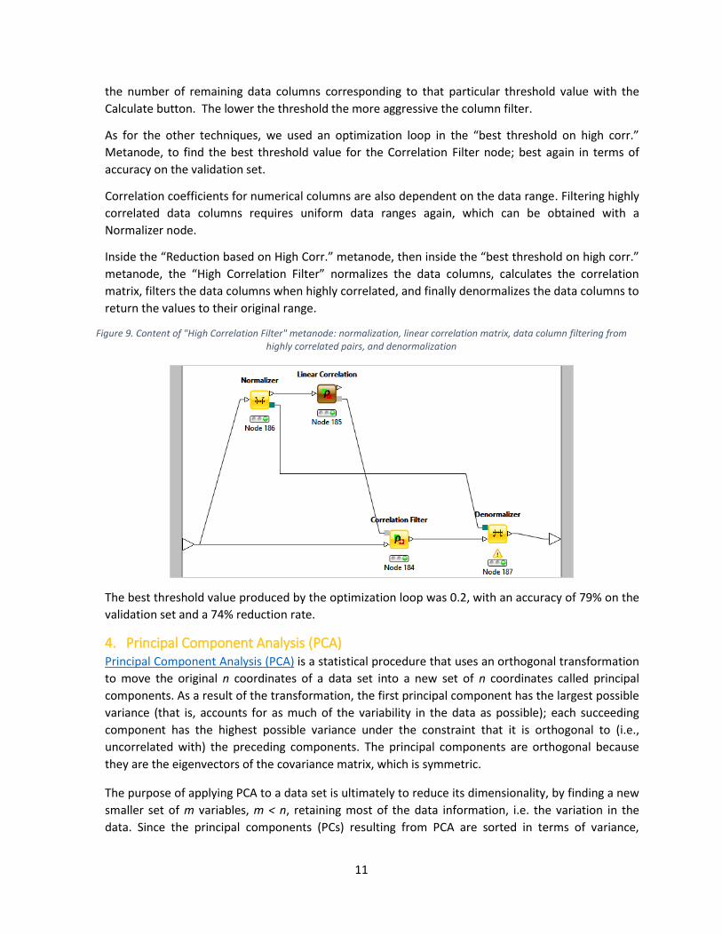
Inside the “Reduction based on High Corr.” metanode, then inside the “best threshold on high corr.”

metanode, the “High Correlation Filter” normalizes the data columns, calculates the correlation

matrix, filters the data columns when highly correlated, and finally denormalizes the data columns to

return the values to their original range.

Figure 9. Content of "High Correlation Filter" metanode: normalization, linear correlation matrix, data column filtering from highly correlated pairs, and denormalization

The best threshold value produced by the optimization loop was 0.2, with an accuracy of 79% on the

validation set and a 74% reduction rate.

4. Principal Component Analysis (PCA) Principal Component Analysis (PCA) is a statistical procedure that uses an orthogonal transformation

to move the original n coordinates of a data set into a new set of n coordinates called principal

components. As a result of the transformation, the first principal component has the largest possible

variance (that is, accounts for as much of the variability in the data as possible); each succeeding

component has the highest possible variance under the constraint that it is orthogonal to (i.e.,

uncorrelated with) the preceding components. The principal components are orthogonal because

they are the eigenvectors of the covariance matrix, which is symmetric.

The purpose of applying PCA to a data set is ultimately to reduce its dimensionality, by finding a new

smaller set of m variables, m < n, retaining most of the data information, i.e. the variation in the

data. Since the principal components (PCs) resulting from PCA are sorted in terms of variance,

12

keeping the first m PCs should also retain most of the data information, while reducing the data set

dimensionality.

Notice that the PCA transformation is sensitive to the relative scaling of the original variables. Data

column ranges need to be normalized before applying PCA. Also notice that the new coordinates

(PCs) are not real system-produced variables anymore. Applying PCA to your data set loses its

interpretability. If interpretability of the results is important for your analysis, PCA is not the

transformation for your project.

KNIME has 2 nodes to implement PCA transformation: PCA Compute and PCA Apply.

The PCA Compute node calculates the covariance matrix of the input data columns and its

eigenvectors, identifying the directions of maximal variance in the data space. The node outputs the

covariance matrix, the PCA model, and the PCA spectral decomposition of the original data columns

along the eigenvectors.

Each row in the spectral decomposition data table contains the projections of one eigenvector

(principal component) along the original coordinates, the corresponding eigenvalue being in the first

column. A high value of the eigenvalue indicates a high variance of the data on the corresponding

eigenvector. Eigenvectors (i.e. the data table rows) are sorted by decreasing eigenvalues, i.e.

variance. The PCA model produced at the last output port of the PCA Compute node contains the

eigenvalues and the eigenvector projections necessary to transform each data row from the original

space into the new PC space.

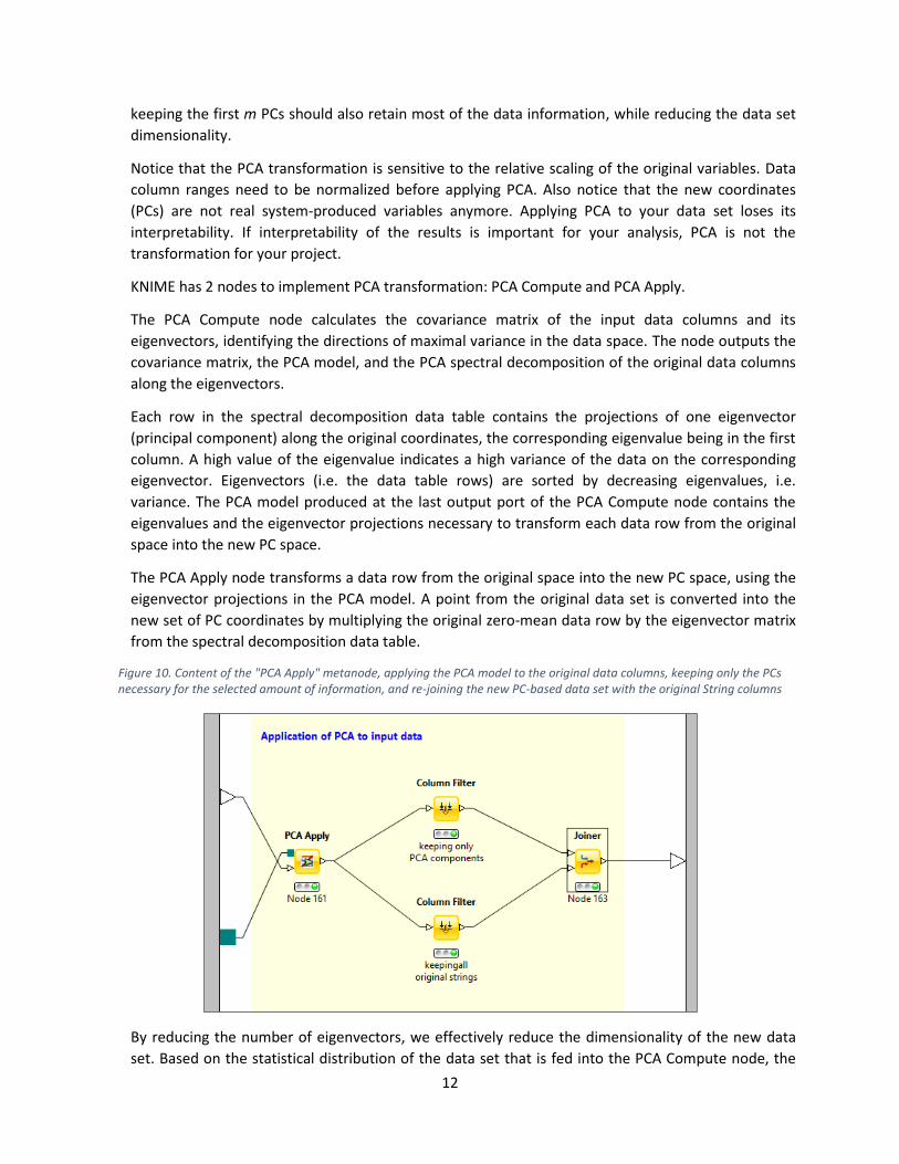
The PCA Apply node transforms a data row from the original space into the new PC space, using the

eigenvector projections in the PCA model. A point from the original data set is converted into the

new set of PC coordinates by multiplying the original zero-mean data row by the eigenvector matrix

from the spectral decomposition data table.

Figure 10. Content of the "PCA Apply" metanode, applying the PCA model to the original data columns, keeping only the PCs necessary for the selected amount of information, and re-joining the new PC-based data set with the original String columns

By reducing the number of eigenvectors, we effectively reduce the dimensionality of the new data

set. Based on the statistical distribution of the data set that is fed into the PCA Compute node, the

13

PCA Apply node calculates the dimensionality reduction (how many of the input features are kept)

with respect to the proposed information (variance) preservation rate. Usually, only a subset of all

PCs is necessary to keep 100% information from the original data set. The more tolerant the losing of

information, the higher the dimensionality reduction of the data space.

Notice that PCA is a numerical technique. This means the reduction process only affects the

numerical columns and does not act on the nominal columns. Also notice that PCA skips the missing

values. On a data set with many missing values, PCA will be less effective.

In the “PCA Apply” metanode, a PCA Apply node calculates the principal components of the original

normalized data rows. Since PCA applies only to numerical variables, string columns are ignored and

joined afterwards to the new set of PCs.

By allowing a loss of 4% of the original data set information, we were able to reduce the number of

columns from 231 to 87, with a 62% reduction rate and an accuracy of 74% on the evaluation set. To

keep accuracy over 70%, as in the other dimensionality reduction method, we decided to keep the

threshold on the remaining information at 96%.

5. Dimensionality Reduction via Tree Ensembles (Random Forests) Figure 11. Content of the "Tree Ensemble Features" metanode, comparing attribute usage in a Tree Ensemble model using

real and shuffled targets.

Decision Tree Ensembles, also referred to as random forests, are useful for feature selection in

addition to being effective classifiers. One approach to dimensionality reduction is to generate a

large and carefully constructed set of trees against a target attribute and then use each attribute’s

usage statistics to find the most informative subset of features.

Specifically, we can generate a set of very shallow trees, with each tree being trained on a small

fraction of the total number of attributes. Hence, first we trained e.g. 2000 trees. Each tree is

trained independently on 2 levels and 3 attributes: these settings provide for good feature selection

in a reasonable amount of time for this data set. If an attribute is often selected as best split, it is

most likely an informative feature to retain.

Once the tree ensemble is generated, we calculated a score for each attribute, by counting how

many times it has been selected for a split and at which rank (level) among all available attributes

(candidates) in the trees of the ensemble.

14

Score = #splits(lev. 0)/#candidates(lev. 0) + #splits(lev. 1)/#candidates(lev. 1)

This score tells us ‒ relative to the other attributes ‒ which are the most predictive.

At this point, one more step is needed to find out which features score higher than you would expect

by random chance. In order to identify the set of most predictive features in the ensemble, we

repeat the first two steps as already described above, but replace the real target column with a

shuffled version of the same column using the Target Shuffling node. We repeat this process many

times until a reliable estimate of the chance baseline score (“dummy” in Fig. 12) can be calculated.

Scores for an attribute against a real target with a value exceeding the chance baseline score can be

assumed to be useful in future model building. The plot below shows Var126, Var211, and Var28 as

the most reliably predictive attributes.

Figure12. Plot of attribute scores showing both real (target based) and dummy (shuffled target based) scores.

This techniques reduces the number of attributes from 231 to just 33 (86% reduction rate) while

keeping the accuracy at 76%.

6. Backward Feature Elimination The Backward Feature Elimination loop performs dimensionality reduction against a particular

machine learning algorithm.

The concept behind the Backward Feature Elimination technique is quite simple. At each iteration,

the selected classification algorithm is trained on n input features. Then we remove one input

15

feature at a time and train the same model on n-1 input features n times. Finally, the input feature

whose removal has produced the smallest increase in the error rate is removed, leaving us with n-1

input features. The classification is then repeated using n-2 features n-1 times and, again, the feature

whose removal produces the smallest disruption in classification performance is removed for good.

This gives us n-2 input features. The algorithm starts with all available N input features and continues

till only 1 last feature is left for classification. Each iteration k then produces a model trained on n-k

features and an error rate e(k). Selecting the maximum tolerable error rate, we define the smallest

number of features necessary to reach that classification performance with the selected machine

learning algorithm.

The “Backward Feature Elimination” metanode implements the Backward Feature Elimination

technique for dimensionality reduction. This metanode contains a loop (Backward Feature

Elimination loop) which trains and applies a classification algorithm. The default classification

algorithm is Naïve Bayes, but this can easily be changed with any other classification algorithm. The

Backward Feature Elimination End node calculates the error rate for the implemented classification

task and sends back control to the Backward Feature Elimination Start node, which controls the

input features to feed back into the classifier. The final list of input features and classification errors

is produced as a model at the output port of the Backward Feature Elimination End node.

The Backward Feature Elimination Filter finally visualizes the number of features kept at each

iteration and the corresponding error rate. Iterations are sorted by error rate. The user can manually

or automatically select the dimensionality reduction for the data set, depending on the tolerated

error.

The main drawback of this technique is the high number of iterations for very high dimensional data

sets, possibly leading to very long computation times. Already the small KDD data set, with just 231

input features, produces an unusable execution time. We therefore decided to apply it only after

some other dimensionality reduction had taken place, based for example on the number of missing

values as described above in this section.

Figure 13. Content of the "Backward Feature Elimination" metanode, including a Backward Feature Elimination loop, a decision tree, and a Backward Feature Elimination Filter node to summarize number of features and error rate per iteration

16

First, we reduced the number of columns from 231 to 77 based on columns having less than 90%

missing values. On the remaining 77 data columns we then ran the Backward Feature Elimination

algorithm contained in the “Backward Feature Elimination” metanode. A decision tree was used as

the classification algorithm.

Opening the configuration window of the Backward Elimination Filter node, we can see that

removing input features is actually beneficial in terms of classification performance. The error rate

on the training set in fact decreases to around 0.05 when only a few input features are used (Fig. 14).

Figure 143. Configuration window of the Backward Feature Elimination Filter node. This window shows the error rate and the number of features used at each iteration of the Backward Feature Elimination loop

The configuration window of the Backward Feature Elimination Filter shows Var28 and Var126 as the

two most informative input features. This gives an idea of the redundancy hidden in our data.

To remain in line with the accuracy values on the training set provided by the other algorithms, we

set the error threshold to 0.2 ‒ i.e. we expect 80% accuracy on the training set – in order to

automatically select the smallest number of input features fitting that criterion – i.e. 1 input feature

Var126. The dimensionality reduction rate here is massive, moving from the original 231 features to

just 1 (99% reduction rate), while the accuracy on the validation set is 94%.

Notice that even though we ran the backward feature elimination procedure on a decision tree, the

best performing algorithm on the validation data set was the neural network.

17

Even though the algorithm runs on only 77 features, it still takes quite some time (still circa 10 hours

on a quad-core laptop with 8GB RAM). Therefore make sure you run this part of the workflow on a

sufficiently performant machine.

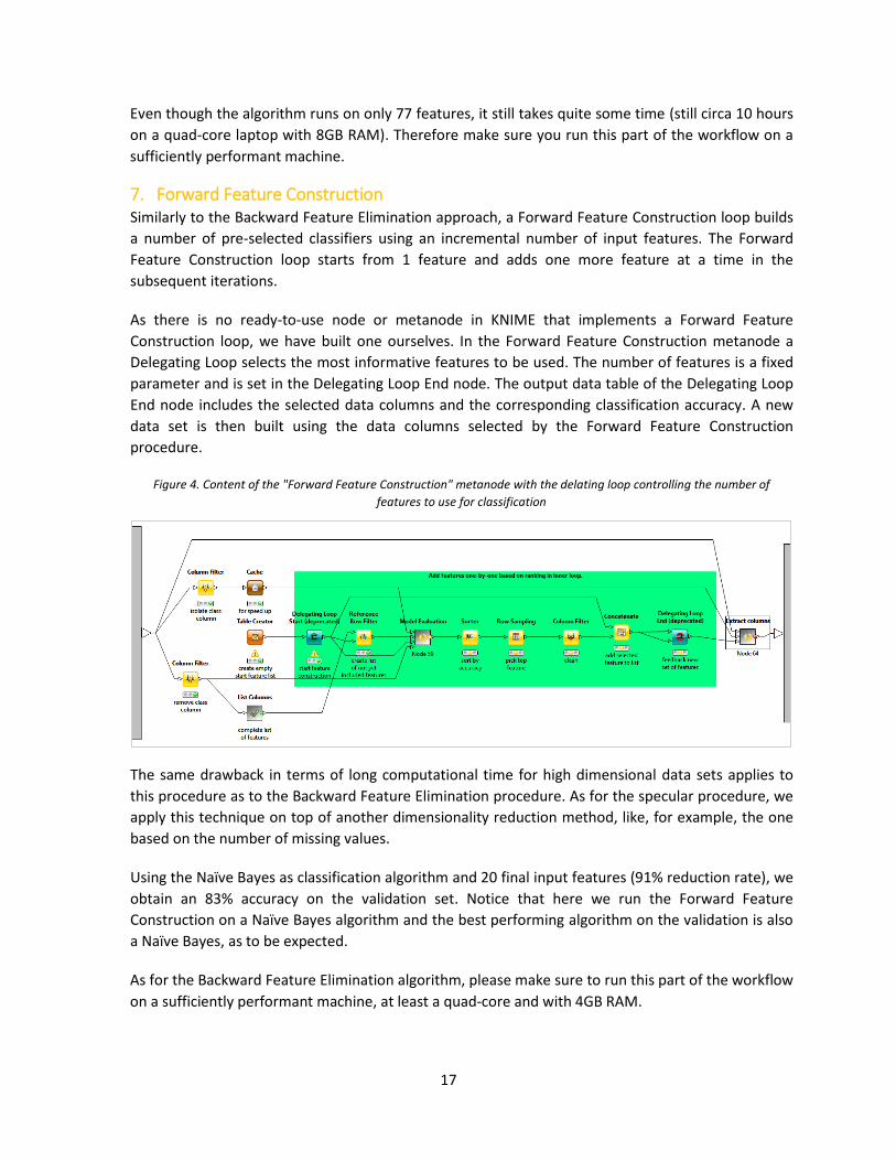
7. Forward Feature Construction Similarly to the Backward Feature Elimination approach, a Forward Feature Construction loop builds

a number of pre-selected classifiers using an incremental number of input features. The Forward

Feature Construction loop starts from 1 feature and adds one more feature at a time in the

subsequent iterations.

As there is no ready-to-use node or metanode in KNIME that implements a Forward Feature

Construction loop, we have built one ourselves. In the Forward Feature Construction metanode a

Delegating Loop selects the most informative features to be used. The number of features is a fixed

parameter and is set in the Delegating Loop End node. The output data table of the Delegating Loop

End node includes the selected data columns and the corresponding classification accuracy. A new

data set is then built using the data columns selected by the Forward Feature Construction

procedure.

Figure 4. Content of the "Forward Feature Construction" metanode with the delating loop controlling the number of

features to use for classification

The same drawback in terms of long computational time for high dimensional data sets applies to

this procedure as to the Backward Feature Elimination procedure. As for the specular procedure, we

apply this technique on top of another dimensionality reduction method, like, for example, the one

based on the number of missing values.

Using the Naïve Bayes as classification algorithm and 20 final input features (91% reduction rate), we

obtain an 83% accuracy on the validation set. Notice that here we run the Forward Feature

Construction on a Naïve Bayes algorithm and the best performing algorithm on the validation is also

a Naïve Bayes, as to be expected.

As for the Backward Feature Elimination algorithm, please make sure to run this part of the workflow

on a sufficiently performant machine, at least a quad-core and with 4GB RAM.

18

Comparison of Techniques for Dimensionality Reduction Accuracy alone might not be descriptive enough of the model performance, since it depends on the cut

on the model output. Usually the area under the curve of an ROC curve is assumed to be more

descriptive of the real predictive character of the model.

In order then, to produce the corresponding ROC curves, we piped the output results of the method

showing the best accuracy for each one of the evaluated dimensionality reduction techniques into an

ROC node (Fig. 16).

In general, the machine learning algorithm with the highest accuracy on the validation set is the neural

network and the area under the curve, which is generated in combination with one of the dimensionality

reduction techniques, is just over 80% independently from their accuracy value and around the baseline

ROC curve. Only the PCA analysis and the Forward Feature Construction method produce an area under

the curve of around 70%. This tells us that all evaluated dimensionality reduction techniques have a

comparable effect on model performance.

Figure16. ROC curves for all the evaluated dimensionality reduction techniques and the best performing machine learning

algorithm. The value of the area under the curve is shown in the legend.

19

In the table below, you can find a summary of all findings of this evaluation project.

The missing value ratio seems a safe starting point, since it obtains a good reduction rate without

compromising performances and applies to both numerical and nominal columns. The random forest

based method achieves the highest reduction rate, keeping a comparable area under the curve to the

baseline. Finally backward elimination and forward construction techniques produce great figures in

terms of accuracy but are less satisfying in terms of area under the curve, and show their specialization

around a specific algorithm and cutoff point. However, their reduction rate proved to be the highest we

found. PCA seems to perform the worst in the compromise between reduction rate and model

performance, but this might be due to the high number of missing values.

Dimensionality Reduction

Reduction Rate

Accuracy on validation set

Best Threshold

AuC Notes

Baseline 0% 73% - 81% -

Missing values ratio 71% 76% 0.4 82% -

Low Variance Filter 73% 82% 0.03 82% Only for numerical columns

High Correlation Filter

74% 79% 0.2 82% No correlation available between

numerical and nominal columns

PCA 62% 74% - 72% Only for numerical columns

Random Forest / Ensemble Trees

86% 76% - 82% -

Backward Feature Elimination + missing values ratio

99% 94% - 78% Backward Feature Elimination and Forward Feature Construction are

prohibitively slow on high dimensional data sets. Useful following other

dimensionality reduction techniques, like here the one based on the

number of missing values.

Forward Feature Construction + missing values ratio

91% 83% - 63%

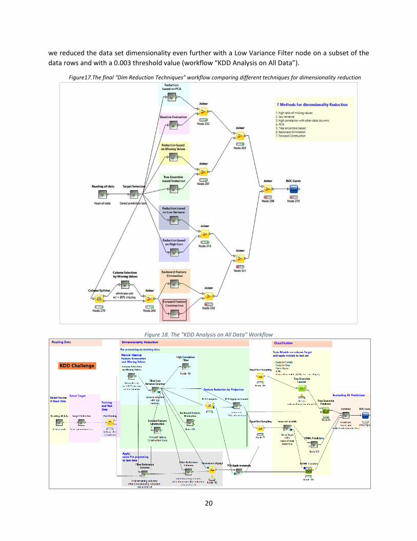
The full workflow comparing these seven different dimensionality reduction techniques, named “Dim

Reduction Techniques” is shown in Fig. 17.

Combining Dimensionality Reduction Techniques Moving to the large KDD data set, we face a completely different kind of problem: 15000 data columns

and 50000 data rows. The 15000 data columns in particular can deeply affect the workflow speed,

rendering execution of the optimization loops described in the sections above unfeasible even on a

subset of the original data set with a lower number of data rows.

Based on the experience with the small KDD data set, first we applied the method for dimensionality

reduction based on the number of missing values, using 90% as a very conservative threshold. After that,

20

we reduced the data set dimensionality even further with a Low Variance Filter node on a subset of the

data rows and with a 0.003 threshold value (workflow “KDD Analysis on All Data”).

Figure17.The final “Dim Reduction Techniques” workflow comparing different techniques for dimensionality reduction

Figure 18. The "KDD Analysis on All Data" Workflow

21

The missing values based approach, removing data columns with more than 90% missing values, reduced

the number of data columns from 150000 to 14578 (3% reduction). After applying the low variance filter,

removing data columns with a variance smaller than 0.003, the number of input columns was further

reduced from 14578 to 3511 (76% reduction).

Finally, the Principal Component Analysis was applied. By allowing a loss of 1% of the information

contained in the input data set, the data set dimensionality could be reduced from 3511 to 2136 data

columns (39% reduction). The total dimensionality reduction performed by the “KDD Analysis on All

Data” workflow amounted then to 86% (15000 original data columns to 2136 reduced ones).

We purposefully avoided using the Backward Feature Elimination and the Forward Feature Construction

loops, due to their long execution time.

Conclusions In this whitepaper, we explored some of the most commonly used techniques for dimensionality

reduction: removing data columns with too many missing values, removing low variance columns,

reducing highly correlated columns, applying Principal Component Analysis (PCA), investigating Random

Forests, Backward Feature Elimination, and Forward Feature Construction.

We showed how these techniques can be implemented within KNIME, either with pre-defined dedicated

nodes or with hand-made sub-workflows in meta-nodes. We also demonstrated how to use the

optimization loop to detect the best cutoffs for each technique on the selected data set. Finally, we

discussed the advantages and the drawbacks, in terms of calculation time, reduction strength, and

performance disturbance, for each evaluated technique.

With data sets becoming bigger and bigger in terms of dimensionality and a high number of features

meaning longer computational times yet no guarantee of better performances, the theme of

dimensionality reduction is currently increasing in popularity as a means to speed up execution times,

simplify problems, and optimize algorithm performances.