Session-Based Queueing Systems - VU · What is the performance of session-based queueing systems? ... - The SBQ can be nested In practice, this means that it should not matter what

Session-Based Queueing Systems

Modelling, Simulation, and Approximation

Jeroen Horters

Supervisor VU: Sandjai Bhulai

Executive Summary Companies often offer services that require multiple steps on the server side to complete. These

services often experience times of high demand, leading to a high server load. If nothing is done to

regulate this, this could result in services failing before full completion or, in the worst case, servers

crashing. To prevent these events, some actions must be taken. In session-based queuing systems

(SBQs), the amount of traffic on these systems is regulated by limiting the number of customers that

are active on the entire system, rather than on a per-queue basis. This system has been implemented

in several companies, without any scientific support.

The simulations show that adding sessions results in better performance for customers that manage

to get into the system, but also results in a significant blocking probability. It is hard to determine

whether this is an overall improvement of the system. The numerical approximation on Jackson

networks shows very similar results, but performs only faster than the simulation on very small

problems.

Contents Executive Summary ................................................................................................................................. 1

1. Introduction ..................................................................................................................................... 3

2. Background ...................................................................................................................................... 4

3. Approach ......................................................................................................................................... 6

4. Model .............................................................................................................................................. 7

4.1. Simulation ................................................................................................................................ 7

4.2. Approximation ......................................................................................................................... 9

5. Results ........................................................................................................................................... 11

5.1. Simulation .............................................................................................................................. 11

5.2. Approximation ....................................................................................................................... 13

6. Conclusion ..................................................................................................................................... 15

7. Literature ....................................................................................................................................... 16

8. Appendix ........................................................................................................................................ 17

A. Additional Results Simulation ................................................................................................... 17

B. Additional Results Approximation ............................................................................................. 21

1. Introduction Every day, the ING bank processes thousands of online transactions. These transactions on a

technical level consist of various steps. To prevent these transactions from failing halfway through

the process due to an overload of the servers, ING needs to put a system in place to control the

server load.

ING started using the Session-Based Queueing systems (SBQs) to solve the problem at hand. SBQs

are an extension of more traditional queueing models that involve blocking, where a single queue

has a limited number of positions in the queue. When all these spots are filled, additional customers

are blocked from the queue. SBQs use this property for an entire system of queues, where a limited

number of customers are allowed in the total system, more commonly referred to as the number of

sessions.

There is currently no academic literature available that describes these queueing models. So even

though they are used by some companies, not much is known about their performance. The purpose

of this research is to answer the following main question:

What is the performance of session-based queueing systems?

This paper will outline two different approaches to answer this question by using simulation as well

as by numerical approximation.

In Chapter 2, we take a more detailed look at the models that form the basis of the session-based

queueing model, as well as some other types of models that will be used in the remainder of this

research. Next, in Chapter 3 we formulate a general approach to answer the research question. In

Chapter 4, we construct the models needed to do the simulation and the numerical approximation.

Furthermore, Chapter 5 shows the results of these methods. Finally, Chapter 6 shows the conclusions

of this research and discusses the answer to the research question.

2. Background To understand the workings of SBQs, we will need to establish some basic knowledge about simpler

queueing systems. The most generic queueing model is commonly known as the M/M/1 model. In

this model, we assume that both the inter-arrival and handling times of the customers that enter the

system follow an exponential distribution. This leads to the arrivals following a so-called Poisson

Process (Koole, 2016, pp. 29-30). For the sake of not making this research any more complicated than

it needs to be, we will assume Poisson arrivals and exponential handling times for all models

described from this point forward.

The M/M/1 model is considered stable as long as the arrival rate is lower than the service rate, or in

a more general sense, the following equation holds:

𝜆

𝜇= 𝜌 < 1

Here, λ denotes the arrival rate, μ the service rate and ρ the load on the system. As long as this

equation holds, during simulation, the queue will never grow to a significant length and the queue is

guaranteed to go empty over time (Kijima, 1997). When this equation does not hold, the system

becomes unstable and the length of the queue will grow to infinity as time does. Also when arrival

and service rates are very close to each other, the system will encounter very high occupancy rates,

which is generally unwanted by service providers.

To prevent these server overloads from happening, we can limit the maximum queue length by

introducing a limited queue. If we apply this to the M/M/1 queue, we get a model that is called the

M/M/1/N system. This model works the same as the M/M/1 model with the exception that

customers are blocked when the maximum queue length has been reached. Even though this does

not seem like a complex extension of the basic model, there is no explicit solution to this system. We

can, however, model this system as a birth-death process and calculate waiting times from there in a

closed-form solution (Sharma & Gupta, 1982).

Since the SBQs are once again a more complicated extension to these M/M/1/N systems, we can

expect that there is no closed-form solution for the SBQs either. Therefore, we need to resort to

doing simulations. However, there is still a possibility that making a numerical approximation could

be possible.

When trying to construct a numerical approximation for SBQs, it quickly became apparent that this

would only be possible for systems that already have a closed-form solution when no sessions are in

place. The candidate subset of models that allowed for the most complex queueing networks were

the so-called Jackson networks.

A Jackson network is a collection of M/M/1 queues that not only have their arrivals from outside the

system, but also allow for networks to connect to one another. For each queue in the network, there

is a probability distribution r that describes where a customer is routed after service has ended in

that queue. This means that with a certain possibility, this customer is either leaving the system or

gets queued into another (or the same) queue within the network.

We can describe the stationary distribution of Jackson networks in the following way: Firstly, we

define new parameters γ for each queue which denote the actual inflow of customers into each

queue. This is simply the sum of the arrival rates plus the fractions of the inflows from other queues

as shown in the equation below. Since we have one of these equations for every queue, we can solve

this set of equations

𝛾𝑖 = 𝜆𝑖 + ∑ 𝛾𝑗𝑟𝑖𝑗

𝑉

𝑗=1

When all inflow parameters are known, we can now calculate the long-term probability of each state

of the system occurring. These probabilities are given by the following equations (Koole, 2016, pp.

78-80):

𝑃(𝑁1 = 𝑛1, … , 𝑁𝑣 = 𝑛𝑣) = ∏ 𝜋𝑖(𝑛𝑖)

𝑉

𝑖=1

𝜋𝑖(𝑛𝑖) = 𝑃(𝑁𝑖 = 𝑛𝑖) = (∑ ∏𝛾𝑖

𝜇𝑖(𝑗)

𝑛

𝑗=1

∞

𝑛=0

)−1 ∏𝛾𝑖

𝜇𝑖(𝑗)

𝑛𝑖

𝑗=1

Here, μi(j) denotes the service rate at queue I when there are j customers present. In our models, this

will be a constant rate. Because this is a probability distribution, the sum of all possible states is equal

to one. The difficulty in doing these calculations comes from the many possible combinations of

states for queues. However, because all queues are M/M/1, the calculations often boil down to

infinite products, which often have known limits. Also, when queues get long enough, the probability

of such a queue occurring gets very small and these states can be ignored when calculating average

wait times.

Finally, for these calculations to be correct, all the server load ratios for each queue must be smaller

than 1. In other words, each queue by itself must be stable for the system to be stable.

Now that we know what the session-based queueing models are derived from and we know exactly

how we can use Jackson models, we can start constructing an approach to test the performance of

SBQs.

3. Approach In order to run a good simulation, a capable software package needed to be chosen. A few different

possibilities were considered and ultimately Arena was chosen. Arena was primarily designed for

queueing models and there were multiple options to include the sessions into the different models.

Additionally, Arena provides the user with detailed reports on the statistics of the models after

simulating them, which would be very useful for the analysis.

Furthermore, it seemed relatively simple to create more complex networks, such as Jackson

networks in Arena. The only restriction seemed to be the maximum number of entities that Arena

can handle at the same time. This would however not be a problem, since the highest number of

sessions was lower than this number, guaranteeing that this limit would never be reached.

Because simulations usually take a long time to run, there was an incentive for a numerical

approximation. In order to accomplish such an approximation, sessions needed to be included in the

known numerical solution for Jackson networks. Afterward, this method had to be implemented in

some programming language. Due to previous experience with MatLab, it was chosen as the

programming language used for this part of the research.

4. Model

4.1. Simulation After deciding that Arena would be the most efficient software solution to create and simulate the

models in, some decisions regarding the design of the model had to be taken. For this particular

research, most models that were to be simulated were very simple models. However, the goal of the

actual modelling was to make the model as general as possible. The following properties are

essential to ensure a general SBQ model:

- Any model can have sessions added to turn it into an SBQ model

- The SBQ can be a submodel

- The SBQ can be nested

In practice, this means that it should not matter what queueing model we apply sessions to. We

should be able to apply sessions to only a part of a larger model or even apply sessions to a subset of

queues that already belong to a session-based model. Most of these properties are insignificant to

this specific paper, but they will make future research more efficient.

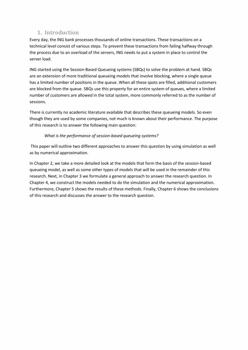
Since all queueing models use discrete-event simulation, we can observe the system at any moment

and know exactly how many customers are in which queue. There are never any travel times and

customers are never stuck between different elements of the system. Therefore, we can always

count the total number of customers in each separate

queue, which is denoted as Work In Progress (WIP) in

Arena. The WIP is simply the sum of the queue length

plus the customers that are being served.

As seen in Figure 2, we can always imagine a box that

surrounds the queues to which the sessions are applied.

Now we add a decision process anywhere where a line

enters this box. In this decision process, we check if the

sum of all WIPs of the queues within the box is smaller

than the number of sessions. If this is true, we allow the

customer into the box. Otherwise the customer is

rejected. By consistently adding this decision to all our

models we can add sessions in a very simple and intuitive way.

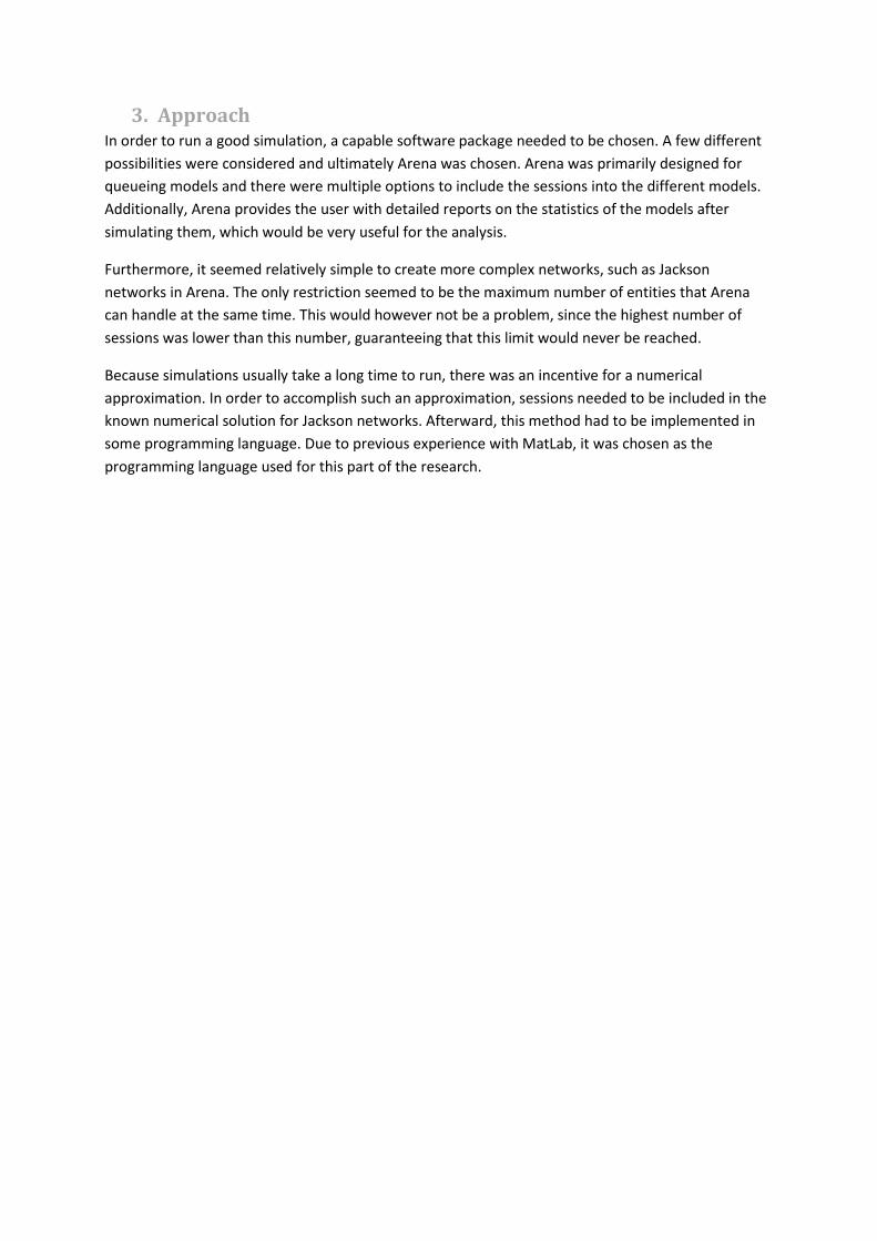
After being able to form all imaginable models into

SBQs, a subset of models needed to be picked for

simulation. There was one kind of model that

certainly had to be tested, namely the system with

multiple queues in series, which is what ING uses. This

model can be seen in Figure 3. The parallel model

from Figure 2 also seemed interesting. It can be

interpreted as a shared waiting room for multiple

general practitioners for example. There are only a

limited number of seats before people can no longer

take place in the waiting room. Very often a

Figure 1: Example of a model with three parallel queues

Figure 2: Example of a model with three queues in series.

practitioner’s office uses this notion of a shared waiting room, so it seemed interesting to model. For

both models, a different number of queues were simulated to see if the number of queues would

influence the results.

Lastly, a slightly more complicated Jackson network was

constructed. This network has five queues, two

different flows of customers into the network and some

queues that use randomness to route the customers

further into the system. Figure 4 shows the structure of

this model. The transition probabilities and service

rates can be seen in Table 3

μ Probability to transition to queue

1 2 3 4 5

1 3 0 0.3 0.4 0.3 0

2 4 0 0 0 0 0

3 4 0 0 0 0.5 0.5

4 3 0 0 0 0 0

5 3 0 1 0 0 0

Table 1: Service rates and transition probabilities for the Jackson model in Figure 4.

After making a selection of models that were to be tested, there were more choices to be made

before the simulation could be started. For each model, for each queue, arrival and service rates had

to be chosen. As seen in Table 3, values for the Jackson network’s service rates had been randomly,

but carefully chosen. For most other models, the initial values for λ and μ were set to 2 per hour and

3 per hour respectively. Using these values would ensure that there would be plenty of arrivals every

simulation, and simultaneously the load on the queues would not be too high. The arrival rates were

later varied between queues to look at the effect of higher loads and even overloaded systems,

where one or more queues have a value of ρ that is larger than one.

For all models, the simulated period was set to 20 days with a warmup period of 24 hours. This

warmup period has the purpose of removing the start of the simulation from the results. The

statistics for the start of the simulation are generally beneficial, as the system starts empty, so the

first customers will not encounter any waiting regardless of how unstable the system on average may

be.

The last parameter that was yet to be chosen was the value of k, the number of sessions. For all

models, the starting value for k was set very low, generally equal to the number of queues in the

system and then gradually brought up until there were rarely any blocked customers, at which point

the system will behave as if there were no sessions at all. It quickly became apparent that it would be

too time-consuming to test all values of k for all models, so larger increments were used, as

compared to when the value of k was higher. An example of the way different values for k were used

can be seen in Appendix A.

Figure 4: Example of a Jackson network.

4.2. Approximation To get a numerical approximation for the steady-state probabilities of a Jackson network with

sessions, we need to go through a number of steps. Firstly, we need to add the sessions to the

model. Then, we need to change the probability calculations accordingly. Finally, we have to ensure

that the probabilities still create a valid probability distribution.

Jackson networks are usually modelled as infinite Markov Chains. Each

state in the state space denotes a specific combination of customers in

each queue. The transition rates are then given by the arrival rates for

each queue for transitions into states with more customers and a

combination of the service rates and the probability table for the other

transitions. We can then calculate the steady-state probabilities using

the formulas described in Chapter 4.

Adding sessions to this model seems trivial initially. In each state, we

know exactly how many customers are in each queue, so we know the

total number of customers in the system for every state. We can then

remove every state and its incoming and outgoing transitions from the

state space where this number is larger than the number of allowed

sessions. For a system with two queues, a part of the remaining state-

space would look like Figure 5. There is, however, a problem with this

solution.

By removing all transitions belonging to the states that were removed, the model is no longer

complete. Along the now existing border where the number of customers is equal to k, the only

possible transitions are the transitions to a lower state. However, these are not the only events that

can occur when the system is in this state. Arrivals will still occur, except the customers are now

blocked from entering the system. This means that all transitions related to arriving customers are

one and the same transition from that state to itself. If these transitions would not exist and the

formulas for the full Jackson network would still hold, we would have a closed-form solution for the

Jackson SBQs.

However, these transitions do exist. Due to these transitions, the probabilities are different and the

formulas are no longer fully accurate. However, it would be impossible to add these transitions and

still have simple formulas to calculate the steady-state distribution with. Additionally, in most cases,

the probability density of these states is expected to be low, because they usually contain a high

number of customers. When the density in the removed nodes is low, the impact of the missing

transitions is also expected to be low. Taking all these statements in consideration, the decision was

made to ignore the transitions and only use the nodes where the number of customers is not larger

than the number of sessions.

Figure 5: A simplified representation of the edge of the statespace of a Jackson network. The transisions that were removed are crossed out in red.

If we apply this to the formulas for the steady-state distribution, we get the following equation for

each state:

𝑃(𝑁1 = 𝑛1, … , 𝑁𝑣 = 𝑛𝑣) = {∏ 𝜋𝑖(𝑛𝑖)

𝑉

𝑖=1

𝑤ℎ𝑒𝑛 𝑛1 + 𝑛2 + ⋯ + 𝑛𝑣 ≤ 𝑘

0 𝑜𝑡ℎ𝑒𝑟𝑤𝑖𝑠𝑒

Because we need the probabilities to form a distribution, we will need to add a final step to the

calculation. As you can imagine, by removing states from the original infinite state-space, we also

removed some of the original probability density, resulting in a total probability that is smaller than

1. To solve this problem, we simply calculate the sum of all probabilities after we calculate them and

then divide each probability by that sum to get the actual distribution.

It is imperative to realise that the resulting model and steady-state distribution are only an

approximation of the actual truncated Jackson model. The probabilities generated by this model will

not be fully accurate, but the expectation is that they are reasonably close.

5. Results

5.1. Simulation As mentioned in the chapter about modelling, a number of different SBQs were modelled and

simulated. In this chapter, the results of the parallel system with three queues and the more complex

Jackson network will be discussed in detail. Results from other systems can be found in Appendix A.

For most simulations, values for arrival and service rates were arbitrarily chosen, as long as the load

on each of the individual queues is smaller than 1. After choosing all other variables, the value for k,

the number of sessions was varied to observe the effect that sessions have on the system.

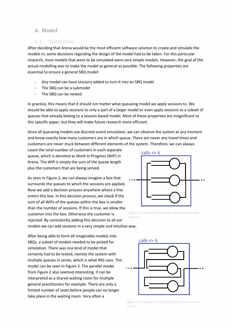
In Table 6 we see the results for the Jackson network. If we look at these results there are a number

of observations that can be done. The most intuitive result is that the average number of customers

in the system goes down as k goes down. This may not seem very remarkable by itself; however, the

number of average customers as a percentage of k does not remain constant. Due to the stability of

the system the average number of customers will converge to the value it would have if there were

no sessions in place at all.

Next, we see that both the occupancy and the average sojourn time for the system decrease as k

decreases. This was also according to expectation. When allowing fewer customers into the system,

the probability of long queues occurring will go down and so will the strain on the servers.

Furthermore, the customers that do make it into the system will encounter shorter queues on

average and will, therefore, have shorter sojourn times.

Lastly, adding the sessions to the queueing system will cause customers to get blocked from entering

the system. When the number of sessions is still relatively high, the number of blocked customers is

still very low, so is the impact on the sojourn time and occupancy. When the number of sessions gets

small enough, both the blocking probability goes up significantly as the occupancy and sojourn time

go down.

Sessions S Refused Served Total block % Occupancy

Total Occupancy

Av customers in system

6 1.29 2185 7424 22.74% 52% 39% 55% 51% 36% 46.6% 3.9904

8 1.46 1288 8237 13.52% 59% 43% 60% 57% 41% 52.0% 5.010842

10 1.6 772 8635 8.21% 60% 46% 63% 59% 42% 54.0% 5.756667

12 1.7 430 8992 4.56% 62% 47% 66% 63% 44% 56.4% 6.369333

14 1.85 375 9204 3.91% 64% 48% 69% 64% 46% 58.2% 7.09475

16 1.92 185 9436 1.92% 67% 50% 70% 64% 47% 59.6% 7.5488

18 1.91 75 9420 0.79% 65% 50% 68% 68% 47% 59.6% 7.49675

20 1.97 61 9391 0.65% 66% 58% 69% 65% 46% 60.8% 7.708446

∞ 2.19 0 9568 0.00% 67% 51% 70% 66% 47% 60.2% 8.7308 Table 6: Results of the simulation on the Jackson network as described in Chapter 4.

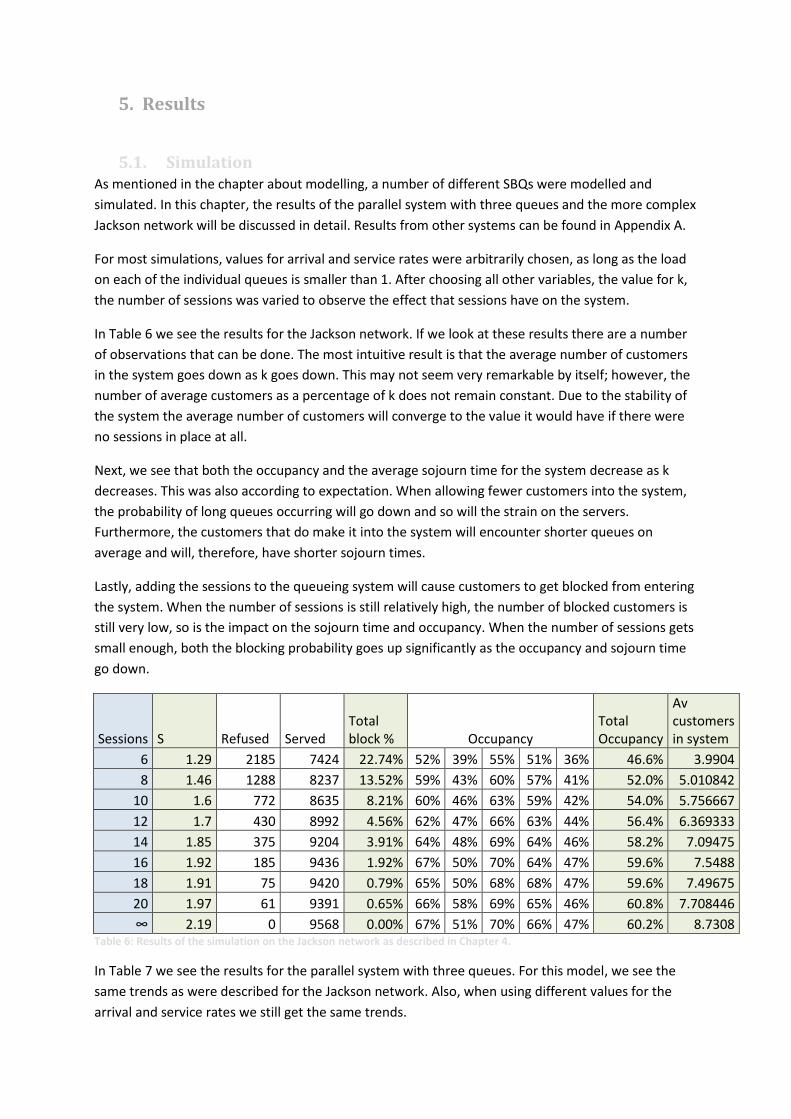
In Table 7 we see the results for the parallel system with three queues. For this model, we see the

same trends as were described for the Jackson network. Also, when using different values for the

arrival and service rates we still get the same trends.

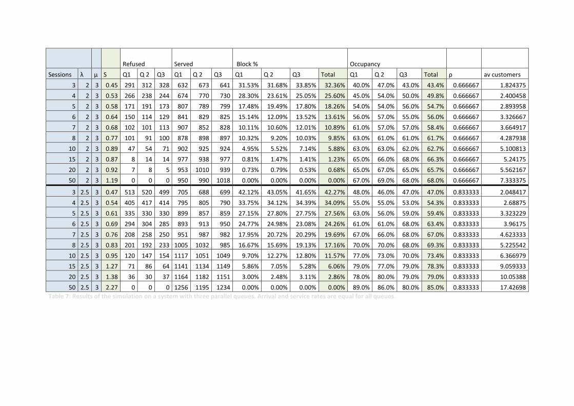
Refused Served Block % Occupancy

Sessions λ μ S Q1 Q 2 Q3 Q1 Q 2 Q3 Q1 Q 2 Q3 Total Q1 Q 2 Q3 Total ρ av customers

3 2 3 0.45 291 312 328 632 673 641 31.53% 31.68% 33.85% 32.36% 40.0% 47.0% 43.0% 43.4% 0.666667 1.824375

4 2 3 0.53 266 238 244 674 770 730 28.30% 23.61% 25.05% 25.60% 45.0% 54.0% 50.0% 49.8% 0.666667 2.400458

5 2 3 0.58 171 191 173 807 789 799 17.48% 19.49% 17.80% 18.26% 54.0% 54.0% 56.0% 54.7% 0.666667 2.893958

6 2 3 0.64 150 114 129 841 829 825 15.14% 12.09% 13.52% 13.61% 56.0% 57.0% 55.0% 56.0% 0.666667 3.326667

7 2 3 0.68 102 101 113 907 852 828 10.11% 10.60% 12.01% 10.89% 61.0% 57.0% 57.0% 58.4% 0.666667 3.664917

8 2 3 0.77 101 91 100 878 898 897 10.32% 9.20% 10.03% 9.85% 63.0% 61.0% 61.0% 61.7% 0.666667 4.287938

10 2 3 0.89 47 54 71 902 925 924 4.95% 5.52% 7.14% 5.88% 63.0% 63.0% 62.0% 62.7% 0.666667 5.100813

15 2 3 0.87 8 14 14 977 938 977 0.81% 1.47% 1.41% 1.23% 65.0% 66.0% 68.0% 66.3% 0.666667 5.24175

20 2 3 0.92 7 8 5 953 1010 939 0.73% 0.79% 0.53% 0.68% 65.0% 67.0% 65.0% 65.7% 0.666667 5.562167

50 2 3 1.19 0 0 0 950 990 1018 0.00% 0.00% 0.00% 0.00% 67.0% 69.0% 68.0% 68.0% 0.666667 7.333375

3 2.5 3 0.47 513 520 499 705 688 699 42.12% 43.05% 41.65% 42.27% 48.0% 46.0% 47.0% 47.0% 0.833333 2.048417

4 2.5 3 0.54 405 417 414 795 805 790 33.75% 34.12% 34.39% 34.09% 55.0% 55.0% 53.0% 54.3% 0.833333 2.68875

5 2.5 3 0.61 335 330 330 899 857 859 27.15% 27.80% 27.75% 27.56% 63.0% 56.0% 59.0% 59.4% 0.833333 3.323229

6 2.5 3 0.69 294 304 285 893 913 950 24.77% 24.98% 23.08% 24.26% 61.0% 61.0% 68.0% 63.4% 0.833333 3.96175

7 2.5 3 0.76 208 258 250 951 987 982 17.95% 20.72% 20.29% 19.69% 67.0% 66.0% 68.0% 67.0% 0.833333 4.623333

8 2.5 3 0.83 201 192 233 1005 1032 985 16.67% 15.69% 19.13% 17.16% 70.0% 70.0% 68.0% 69.3% 0.833333 5.225542

10 2.5 3 0.95 120 147 154 1117 1051 1049 9.70% 12.27% 12.80% 11.57% 77.0% 73.0% 70.0% 73.4% 0.833333 6.366979

15 2.5 3 1.27 71 86 64 1141 1134 1149 5.86% 7.05% 5.28% 6.06% 79.0% 77.0% 79.0% 78.3% 0.833333 9.059333

20 2.5 3 1.38 36 30 37 1164 1182 1151 3.00% 2.48% 3.11% 2.86% 78.0% 80.0% 79.0% 79.0% 0.833333 10.05388

50 2.5 3 2.27 0 0 0 1256 1195 1234 0.00% 0.00% 0.00% 0.00% 89.0% 86.0% 80.0% 85.0% 0.833333 17.42698

Table 7: Results of the simulation on a system with three parallel queues. Arrival and service rates are equal for all queues.

5.2. Approximation As for the simulations, for the results of the approximation we will mainly focus on the parallel model

with three queues. Like with the simulation, we see that the occupancy and the average number of

customers in the system increase when the number of sessions increases, while the blocking

probability decreases.

Furthermore, if we compare the results from the approximation in Table 8 and the results from the

simulation in Table 6, we can see that not only the trends, but also the values are very similar. For all

of the values, the difference is only a few percent. This also holds for the more complicated Jackson

network we described in the paper, as can be seen in Table 9. Once again, the values are very similar

to the simulation. Additional results for the numerical approximation for Jackson networks can be

found in Appendix B.

Even though we would like the results for both approaches to be equal, we see that there is still a

small difference between the simulation and the approximation. There are a few obvious causes for

this discrepancy. Firstly, the approximation is not perfect, as discussed earlier, due to the way the

state space is truncated. Additionally, any simulation will always result in some error due to

randomness. This error could be reduced by simulating for a longer period or taking the average over

a larger number of runs. Lastly, it could be the case that the two approaches do not represent the

same problem, even though they were constructed to model the same problem.

Sessions lambda mu block% occupancy av customers

3 2 3 34.33% 43.78% 1.87

4 2 3 25.56% 49.63% 2.42

5 2 3 19.26% 53.83% 2.91

6 2 3 14.62% 56.92% 3.36

7 2 3 11.13% 59.24% 3.77

8 2 3 8.49% 61.01% 4.13

10 2 3 4.92% 63.34% 4.72

15 2 3 1.19% 65.87% 5.57

20 2 3 0.26% 66.49% 5.88

50 2 3 0.00% 66.67% 6

3 2.5 3 43.01% 47.49% 2.09

4 2.5 3 34.97% 54.19% 2.76

5 2.5 3 28.97% 59.19% 3.41

6 2.5 3 24.35% 63.04% 4.04

7 2.5 3 20.69% 66.09% 4.65

8 2.5 3 17.73% 68.56% 5.24

10 2.5 3 13.27 72.28% 6.37

15 2.5 3 6.84% 77.63% 8.84

20 2.5 3 3.66% 80.29% 10.79

50 2.5 3 0.06% 83.28% 14.82

Table 8: Results of the approximation for the network with three parallel queues.

Sessions block Occupancy av customers

6 22.20% 51.89% 38.92% 54.48% 51.89% 36.32% 3.99

8 14.02% 57.32% 42.99% 61.09% 57.32% 40.12% 5

10 8.82% 60.79% 45.58% 63.83% 60.79% 42.55% 5.85

12 5.48% 63.01% 47.26% 66.16% 63.01% 44.11% 6.53

14 3.35% 64.43% 48.32% 67.65% 64.43% 45.10% 7.04

16 2.01% 65.33% 48.99% 68.59% 65.33% 45.73% 7.43

18 1.18% 65.88% 49.41% 69.17% 65.88% 46.11% 7.7

20 0.68% 66.21% 49.66% 69.52% 66.21% 46.35% 7.89

Lastly, we need to discuss the speed and the efficiency of the algorithm for the numerical

approximation. For the smaller models, the algorithm works extremely fast and it can calculate the

statistics for the model in a matter of seconds. However, due to the need for the different partitions,

the algorithm starts slowing down significantly when increasing both the number of queues and the

number of sessions. For example, calculating a model with six queues and around fifty sessions

already can take multiple minutes, depending on the size of the model.

Calculation times can be decreased for certain models by using clustering of similar queues and

several other mathematical tricks. However, for more complicated or larger models, which are

ultimately the models that companies such as ING would like to analyse, this numerical

approximation will be significantly slower than running simulations or perhaps not even possible due

to hardware restrictions.

Table 9: Results of the approximation for the Jackson network as defines in Chapter 4.

6. Conclusion Both the simulation and the numerical approximation of the SBQ models show that using a session-

based blocking method for a queueing system reduces the load on the system. The occupancy of the

agents goes down and customers that enter the system experience shorter sojourn times on

average. However, reducing the number of sessions also causes customers to be blocked from the

system at a significant rate. This means that the main research question cannot directly be answered

and it is up to the owner of the system to decide whether a lower occupancy or a larger number of

served customers hold a higher value to decide on the number of allowed sessions.

Moreover, when the different queues within the system are not very homogeneous and a subset of

queues experiences a higher load than the rest of the queues, using an SBQ approach might cause

the entire system to suffer from these higher load queues.

The numerical approximation gives very similar results to the simulation models and is significantly

faster for small systems. However, due to the nature of the approximation using partitions causing

exponential calculation times, it is not feasible to use this method for larger, more complex models.

Whether ING should continue using SBQs for their transaction servers depends on their relative cost

between blocked customers and the improved performance. The percentage of blocked customers is

not small enough to give a definitive answer to this problem.

7. Literature

Kijima, M. (1997). Markov Processes for Stochastic Modeling. Boston: Springer.

Koole, G. (2016). Optimisation of Business Processes. Amsterdam: MG Books.

Sharma, O. P., & Gupta, U. C. (1982, September). Transient Behaviour of an M/M/1/N Queue.

Stochastic Processes and their Applications, pp. 327-331.

8. Appendix

A. Additional Results Simulation

Refused Served Block % Occupancy

Sessions λ μ S Q1 Q 2 Q3 Q1 Q 2 Q3 Q1 Q 2 Q3 Total Q1 Q 2 Q3 Total ρ av customers

3 3 3 0.49 762 694 736 728 701 730 51.14% 49.75% 50.20% 50.38% 50.0% 47.0% 51.0% 49.4% 1 2.203979

4 3 3 0.56 614 592 606 840 860 813 42.23% 40.77% 42.71% 41.90% 57.0% 58.0% 55.0% 56.7% 1 2.931833

5 3 3 0.65 540 540 515 911 913 930 37.22% 37.16% 35.64% 36.68% 61.0% 62.0% 65.0% 62.7% 1 3.729375

6 3 3 0.72 461 491 475 972 988 970 32.17% 33.20% 32.87% 32.75% 68.0% 67.0% 66.0% 67.0% 1 4.395

7 3 3 0.84 441 409 494 1011 997 1038 30.37% 29.09% 32.25% 30.62% 71.0% 72.0% 69.0% 70.6% 1 5.3305

8 3 3 0.97 455 447 467 1037 1018 1049 30.50% 30.51% 30.80% 30.61% 75.0% 74.0% 74.0% 74.3% 1 6.272667

10 3 3 1.03 318 324 302 1142 1135 1121 21.78% 22.21% 21.22% 21.74% 78.0% 79.0% 75.0% 77.4% 1 7.291542

15 3 3 1.39 211 190 192 1277 1241 1218 14.18% 13.28% 13.62% 13.70% 85.0% 86.0% 83.0% 84.7% 1 10.81883

20 3 3 1.97 214 224 222 1263 1284 1208 14.49% 14.85% 15.52% 14.95% 88.0% 87.0% 85.0% 86.7% 1 15.41115

50 3 3 4.13 67 65 75 1364 1374 1422 4.68% 4.52% 5.01% 4.74% 93.0% 99.0% 97.0% 96.3% 1 35.79333

3 4 3 0.53 1239 1142 1234 715 790 736 63.41% 59.11% 62.64% 61.73% 48.0% 57.0% 51.0% 52.0% 1.333333 2.474438

4 4 3 0.6 1018 1126 1066 871 858 904 53.89% 56.75% 54.11% 54.94% 59.0% 61.0% 65.0% 61.7% 1.333333 3.29125

5 4 3 0.68 0.91 1021 922 1000 950 956 0.09% 51.80% 49.09% 40.08% 66.0% 63.0% 69.0% 65.9% 1.333333 4.116833

6 4 3 0.79 903 882 968 997 1020 1028 47.53% 46.37% 48.50% 47.48% 71.0% 71.0% 70.0% 70.7% 1.333333 5.011563

7 4 3 0.87 895 846 799 1090 1092 1028 45.09% 43.65% 43.73% 44.17% 75.0% 75.0% 69.0% 73.1% 1.333333 5.818125

8 4 3 0.99 841 840 866 1090 1125 1071 43.55% 42.75% 44.71% 43.67% 75.0% 68.0% 75.0% 72.6% 1.333333 6.777375

10 4 3 1.22 805 840 785 1093 1167 1157 42.41% 41.85% 40.42% 41.56% 78.0% 84.0% 80.0% 80.7% 1.333333 8.684875

15 4 3 1.7 710 677 678 1285 1176 1311 35.59% 36.54% 34.09% 35.38% 90.0% 85.0% 89.0% 88.1% 1.333333 13.35917

20 4 3 2.29 660 664 645 1269 1244 1287 34.21% 34.80% 33.39% 34.13% 87.0% 87.0% 88.0% 87.3% 1.333333 18.12917

50 4 3 5.6 618 599 585 1392 1288 1350 30.75% 31.74% 30.23% 30.90% 100.0% 91.0% 93.0% 94.8% 1.333333 47.01667 Table 10: Results of the simulation for the system with three parallel queues

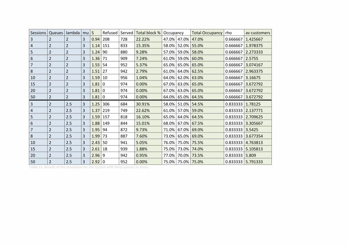
Sessions Queues lambda mu S Refused Served Total block % Occupancy Total Occupancy rho av customers

3 2 2 3 0.94 208 728 22.22% 47.0% 47.0% 47.0% 0.666667 1.425667

4 2 2 3 1.14 151 833 15.35% 58.0% 52.0% 55.0% 0.666667 1.978375

5 2 2 3 1.24 90 880 9.28% 57.0% 59.0% 58.0% 0.666667 2.273333

6 2 2 3 1.36 71 909 7.24% 61.0% 59.0% 60.0% 0.666667 2.5755

7 2 2 3 1.55 54 952 5.37% 65.0% 65.0% 65.0% 0.666667 3.074167

8 2 2 3 1.51 27 942 2.79% 61.0% 64.0% 62.5% 0.666667 2.963375

10 2 2 3 1.59 10 956 1.04% 64.0% 62.0% 63.0% 0.666667 3.16675

15 2 2 3 1.81 0 974 0.00% 67.0% 63.0% 65.0% 0.666667 3.672792

20 2 2 3 1.81 0 974 0.00% 67.0% 63.0% 65.0% 0.666667 3.672792

50 2 2 3 1.81 0 974 0.00% 64.0% 65.0% 64.5% 0.666667 3.672792

3 2 2.5 3 1.25 306 684 30.91% 58.0% 51.0% 54.5% 0.833333 1.78125

4 2 2.5 3 1.37 219 749 22.62% 61.0% 57.0% 59.0% 0.833333 2.137771

5 2 2.5 3 1.59 157 818 16.10% 65.0% 64.0% 64.5% 0.833333 2.709625

6 2 2.5 3 1.88 149 844 15.01% 68.0% 67.0% 67.5% 0.833333 3.305667

7 2 2.5 3 1.95 94 872 9.73% 71.0% 67.0% 69.0% 0.833333 3.5425

8 2 2.5 3 1.99 73 887 7.60% 73.0% 65.0% 69.0% 0.833333 3.677354

10 2 2.5 3 2.43 50 941 5.05% 76.0% 75.0% 75.5% 0.833333 4.763813

15 2 2.5 3 2.61 18 939 1.88% 75.0% 73.0% 74.0% 0.833333 5.105813

20 2 2.5 3 2.96 9 942 0.95% 77.0% 70.0% 73.5% 0.833333 5.809

50 2 2.5 3 2.92 0 952 0.00% 75.0% 75.0% 75.0% 0.833333 5.791333 Table 11: Results of the simulation for the system with three queues in series.

Sessions λ μ ρ S Refused Served Total block % Occupancy Total Occupancy

av Customers In System

6 2 3 3 3 3 0.7 0.7 0.7 0.7 2.47 1005 3778 21.01% 54.0% 54.0% 53.0% 52.0% 53.3% 3.888192

8 2 3 3 3 3 0.7 0.7 0.7 0.7 2.8 626 4090 13.27% 58.0% 57.0% 57.0% 57.0% 57.3% 4.771667

10 2 3 3 3 3 0.7 0.7 0.7 0.7 3.16 454 4331 9.49% 59.0% 61.0% 61.0% 62.0% 60.8% 5.702483

12 2 3 3 3 3 0.7 0.7 0.7 0.7 3.39 232 4479 4.92% 61.0% 63.0% 65.0% 62.0% 62.8% 6.326588

14 2 3 3 3 3 0.7 0.7 0.7 0.7 3.58 162 4647 3.37% 67.0% 65.0% 66.0% 64.0% 65.5% 6.931775

16 2 3 3 3 3 0.7 0.7 0.7 0.7 3.57 94 4587 2.01% 64.0% 64.0% 64.0% 64.0% 64.0% 6.823163

18 2 3 3 3 3 0.7 0.7 0.7 0.7 3.59 36 4602 0.78% 64.0% 64.0% 65.0% 64.0% 64.3% 6.883825

20 2 3 3 3 3 0.7 0.7 0.7 0.7 3.68 29 4613 0.62% 64.0% 64.0% 65.0% 64.0% 64.3% 7.073267

∞ 2 3 3 3 3 0.7 0.7 0.7 0.7 3.87 0 4679 0.00% 65.0% 66.0% 65.0% 66.0% 65.5% 7.544888

6 2 1.5 3 3 3 1.3 0.7 0.7 0.7 3.6 1647 3060 34.99% 84.0% 42.0% 43.0% 43.0% 53.0% 4.59

8 2 1.5 3 3 3 1.3 0.7 0.7 0.7 4.67 1544 3197 32.57% 92.0% 45.0% 44.0% 44.0% 56.3% 6.220829

10 2 1.5 3 3 3 1.3 0.7 0.7 0.7 5.56 1352 3443 28.20% 95.0% 49.0% 47.0% 49.0% 60.0% 7.976283

12 2 1.5 3 3 3 1.3 0.7 0.7 0.7 6.64 1340 3481 27.80% 97.0% 50.0% 49.0% 49.0% 61.3% 9.630767

14 2 1.5 3 3 3 1.3 0.7 0.7 0.7 7.59 1119 3590 23.76% 98.0% 51.0% 51.0% 50.0% 62.5% 11.35338

16 2 1.5 3 3 3 1.3 0.7 0.7 0.7 8.02 1292 3575 26.55% 99.0% 51.0% 49.0% 52.0% 62.8% 11.94646

18 2 1.5 3 3 3 1.3 0.7 0.7 0.7 9.92 1056 3670 22.34% 100.0% 53.0% 51.0% 52.0% 64.0% 15.16933

20 2 1.5 3 3 3 1.3 0.7 0.7 0.7 11.68 1244 3536 26.03% 100.0% 50.0% 49.0% 50.0% 62.3% 17.20853

∞ 2 1.5 3 3 3 1.3 0.7 0.7 0.7 ∞

100.0%

6 2 3 3 3 1.5 0.7 0.7 0.7 1.3 3.68 1756 3009 36.85% 43.0% 41.0% 42.0% 86.0% 53.0% 4.6138

8 2 3 3 3 1.5 0.7 0.7 0.7 1.3 4.58 1429 3230 30.67% 46.0% 43.0% 46.0% 91.0% 56.5% 6.163917

10 2 3 3 3 1.5 0.7 0.7 0.7 1.3 5.28 1225 3479 26.04% 49.0% 49.0% 50.0% 94.0% 60.5% 7.6538

12 2 3 3 3 1.5 0.7 0.7 0.7 1.3 6.9 1383 3427 28.75% 48.0% 48.0% 48.0% 98.0% 60.5% 9.852625

14 2 3 3 3 1.5 0.7 0.7 0.7 1.3 7.77 1187 3507 25.29% 50.0% 48.0% 49.0% 98.0% 61.3% 11.35391

16 2 3 3 3 1.5 0.7 0.7 0.7 1.3 8.99 1246 3560 25.93% 51.0% 50.0% 50.0% 99.0% 62.5% 13.33517

18 2 3 3 3 1.5 0.7 0.7 0.7 1.3 10.49 1261 3529 26.33% 49.0% 50.0% 50.0% 100.0% 62.3% 15.42467

20 2 3 3 3 1.5 0.7 0.7 0.7 1.3 11.83 1246 3450 26.53% 48.0% 47.0% 49.0% 100.0% 61.0% 17.00563

∞ 2 3 3 3 1.5 0.7 0.7 0.7 1.3 ∞

100.0%

6 2 2.2 3 3 3 0.9 0.7 0.7 0.7 2.8 1253 3480 26.47% 68.0% 48.0% 49.0% 48.0% 53.3% 4.06

8 2 2.2 3 3 3 0.9 0.7 0.7 0.7 3.31 870 3908 18.21% 75.0% 54.0% 54.0% 56.0% 59.8% 5.389783

10 2 2.2 3 3 3 0.9 0.7 0.7 0.7 3.75 638 4128 13.39% 80.0% 57.0% 57.0% 59.0% 63.3% 6.45

12 2 2.2 3 3 3 0.9 0.7 0.7 0.7 4.24 554 4276 11.47% 82.0% 59.0% 60.0% 61.0% 65.5% 7.554267

14 2 2.2 3 3 3 0.9 0.7 0.7 0.7 4.48 317 4448 6.65% 84.0% 62.0% 62.0% 63.0% 67.8% 8.302933

16 2 2.2 3 3 3 0.9 0.7 0.7 0.7 4.83 292 4466 6.14% 84.0% 63.0% 62.0% 64.0% 68.3% 8.987825

18 2 2.2 3 3 3 0.9 0.7 0.7 0.7 5.25 203 4584 4.24% 85.0% 66.0% 64.0% 64.0% 69.8% 10.0275

20 2 2.2 3 3 3 0.9 0.7 0.7 0.7 5.17 117 4566 2.50% 85.0% 64.0% 64.0% 65.0% 69.5% 9.835925

∞ 2 2.2 3 3 3 0.9 0.7 0.7 0.7 7.24 0 4727 0.00% 91.0% 65.0% 67.0% 67.0% 72.5% 14.25978 Table 12: Results of the simulation for the system with four queues in series.

Sessions λ μ ρ S Refused Served

Total block % Occupancy

Total Occupancy

Av customers in system

10 2 3 0.67 4.08 666 3968 14.37% 56.0% 55.0% 54.0% 55.0% 57.0% 54.0% 55.2% 6.7456

13 2 3 0.67 4.71 475 4349 9.85% 62.0% 61.0% 61.0% 61.0% 60.0% 61.0% 61.0% 8.534913

16 2 3 0.67 5.15 278 4505 5.81% 62.0% 46.0% 63.0% 63.0% 63.0% 64.0% 60.2% 9.666979

19 2 3 0.67 5.25 110 4591 2.34% 64.0% 64.0% 64.0% 65.0% 64.0% 65.0% 64.3% 10.04281

22 2 3 0.67 5.68 109 4649 2.29% 66.0% 66.0% 65.0% 65.0% 65.0% 64.0% 65.2% 11.00263

25 2 3 0.67 6.13 70 4909 1.41% 69.0% 69.0% 69.0% 68.0% 68.0% 70.0% 68.8% 12.5384

28 2 3 0.67 5.89 34 4722 0.71% 66.0% 66.0% 66.0% 64.0% 68.0% 65.0% 65.8% 11.58858

31 2 3 0.67 6.08 8 4802 0.17% 68.0% 68.0% 66.0% 67.0% 67.0% 67.0% 67.2% 12.16507

∞ 2 3 0.67 5.97 0 4711 0.00% 65.0% 67.0% 64.0% 66.0% 67.0% 66.0% 65.8% 11.71861 Table 13: Results of the simulation for the system with six queues in series.

B. Additional Results Approximation

Sessions lambda mu block occupancy av

customers

3 2 3 24.43% 50.38% 1.55

4 2 3 16.91% 55.39% 1.97

5 2 3 11.92% 58.72% 2.33

6 2 3 8.48% 61.01% 2.64

7 2 3 6.07% 62.62% 2.9

8 2 3 4.35% 63.76% 3.12

10 2 3 2.24% 65% 3.46

15 2 3 0.41% 66.39% 3.86

20 2 3 0.07% 66.66% 3.96

50 2 3 0.00% 66.67% 4

3 2.5 3 32.77% 56.03% 1.81

4 2.5 3 25.45% 62.13% 2.36

5 2.5 3 20.28% 66.43% 2.9

6 2.5 3 16.47% 69.61% 3.41

7 2.5 3 13.56% 72.03% 3.89

8 2.5 3 11.28% 73.93% 4.36

10 2.5 3 7.98% 76.69% 5.21

15 2.5 3 3.60% 80.33% 6.91

20 2.5 3 1.69% 81.93% 8.14

50 2.5 3 0.01% 83.32% 9.95

Table 14: Results of the numerical approximation for the system with three queues in series.

Sessions lambda mu Block Occupancy av customers

6 3 3 20.66% 52.90% 52.90% 52.90% 52.90% 3.86

8 3 3 13.10% 57.94% 57.94% 57.94% 57.94% 4.85

10 3 3 8.29% 61.14% 61.14% 61.14% 61.14% 5.68

12 3 3 5.19% 63.21% 63.21% 63.21% 63.21% 6.33

14 3 3 3.20% 64.53% 64.53% 64.53% 64.53% 6.84

16 3 3 1.94% 65.37% 65.37% 65.37% 65.37% 7.22

18 3 3 1.15% 65.90% 65.90% 65.90% 65.90% 7.49

20 3 3 0.67% 66.22% 66.22% 66.22% 66.22% 7.67

∞ 3 3 0.00% 66.66% 66.66% 66.66% 66.66% 7.9

6 3 2.2 3 25.42% 67.80% 49.72% 49.72% 49.72% 4.1

8 3 2.2 3 18.07% 74.49% 54.62% 54.62% 54.62% 5.33

10 3 2.2 3 13.18% 78.92% 57.88% 57.88% 57.88% 6.44

12 3 2.2 3 9.81% 81.99% 60.12% 60.12% 60.12% 7.45

14 3 2.2 3 7.42% 84.16% 61.72% 61.72% 61.72% 8.37

16 3 2.2 3 5.69% 85.74% 62.87% 62.87% 62.87% 9.21

18 3 2.2 3 4.41% 86.90% 63.73% 63.73% 63.73% 9.97

20 3 2.2 3 3.45% 87.77% 64.37% 64.37% 64.37% 10.66

∞ 3 2.2 3 25.42% 67.80% 49.72% 49.72% 49.72% 4.1 Table 15: Results of the numerical approximation for the system with four queues in series.

Sessions λ μ block Occupancy av customers

10 2 3 15.77% 56.16% 56.16% 56.16% 56.16% 56.16% 56.16% 6.95

13 2 3 9.32% 60.46% 60.46% 60.46% 60.46% 60.46% 60.46% 8.46

16 2 3 5.35% 63.10% 63.10% 63.10% 63.10% 63.10% 63.10% 9.64

19 2 3 2.96% 64.69% 64.69% 64.69% 64.69% 64.69% 64.69% 10.51

22 2 3 1.57% 65.62% 65.62% 65.62% 65.62% 65.62% 65.62% 11.12

Table 16: Results of the numerical approximation for the system with six queues in series.