HAL Id: tel-03371210 https://tel.archives-ouvertes.fr/tel-03371210v2 Submitted on 11 Oct 2021 HAL is a multi-disciplinary open access archive for the deposit and dissemination of sci- entific research documents, whether they are pub- lished or not. The documents may come from teaching and research institutions in France or abroad, or from public or private research centers. L’archive ouverte pluridisciplinaire HAL, est destinée au dépôt et à la diffusion de documents scientifiques de niveau recherche, publiés ou non, émanant des établissements d’enseignement et de recherche français ou étrangers, des laboratoires publics ou privés. Sequential Learning in a strategical environment Etienne Boursier To cite this version: Etienne Boursier. Sequential Learning in a strategical environment. Machine Learning [stat.ML]. Université Paris-Saclay, 2021. English. NNT: 2021UPASM034. tel-03371210v2

Welcome message from author
This document is posted to help you gain knowledge. Please leave a comment to let me know what you think about it! Share it to your friends and learn new things together.
Transcript
HAL Id: tel-03371210https://tel.archives-ouvertes.fr/tel-03371210v2
Submitted on 11 Oct 2021
HAL is a multi-disciplinary open accessarchive for the deposit and dissemination of sci-entific research documents, whether they are pub-lished or not. The documents may come fromteaching and research institutions in France orabroad, or from public or private research centers.
L’archive ouverte pluridisciplinaire HAL, estdestinée au dépôt et à la diffusion de documentsscientifiques de niveau recherche, publiés ou non,émanant des établissements d’enseignement et derecherche français ou étrangers, des laboratoirespublics ou privés.
Sequential Learning in a strategical environmentEtienne Boursier
To cite this version:Etienne Boursier. Sequential Learning in a strategical environment. Machine Learning [stat.ML].Université Paris-Saclay, 2021. English. NNT : 2021UPASM034. tel-03371210v2
Thès
e de
doc
tora
tNNT:2021UPA
SM034
Sequential Learning in astrategical environment
Thèse de doctorat de l’Université Paris-Saclay
Ecole Doctorale de Mathématique Hadamard (EDMH) n 574Spécialité de doctorat : Mathématiques appliquées
Unité de recherche : Centre Borelli (ENS Paris-Saclay), UMR 9010 CNRS
Référent : Ecole normale supérieure de Paris-Saclay
Thèse présentée et soutenue à Gif-sur-Yvette, le 30/09/2021, par
Etienne BOURSIER
Au vu des rapports de :
Alexandre Proutière RapporteurProfesseur, KTHNicolas Vieille RapporteurProfesseur, HEC
Composition du jury :
Nicolas Vieille PrésidentProfesseur, HECAlexandre Proutière RapporteurProfesseur, KTHSebastien Bubeck ExaminateurDirecteur de recherche, Microsoft ResearchRichard Combes ExaminateurProfesseur Assistant, Centrale Supelec L2SShie Mannor ExaminateurProfesseur, TechnionLucie Ménager ExaminatriceProfesseure, Université Paris 2Vianney Perchet DirecteurProfesseur, CREST, ENSAEMarco Scarsini InvitéProfesseur, LUISS

2

Remerciements
Tout d’abord, je tiens à remercier mon directeur de thèse, Vianney Perchet, qui m’a encadré
dès mon stage de fin d’études, et ce jusqu’à la fin de ma thèse, à mon plus grand plaisir. Tu
as toujours su me rebooster lorsque cela était nécessaire et susciter mon intérêt sur de nou-
veaux problèmes, et ce dès notre première rencontre lorsque nous parlions déjà de multiplayer
bandits et dilemme du prisonnier. Tu m’as également encouragé à participer à différents sémi-
naires/conférences et discuter avec de nombreux chercheurs, ce qui m’a amené à faire de nom-
breuses rencontres positives. Ta disponibilité et ton attention m’ont permis d’entrer dans le
monde de la recherche avec bienveillance et décontraction. Beaucoup de souvenirs resteront en
mémoire dont de longues séances au tableau, mais aussi les petits plaisirs comme les Pisco sour
cathedral à Lima ou lorsque nous nous plaignions mutuellement de certaines reviews.
Je remercie aussi Alexandre Proutière et Nicolas Vieille qui ont gentiment accepté d’être
rapporteurs pour cette thèse. Je ne vous ai pas facilité la tâche avec plus de 250 pages de lecture
pour l’été; vos commentaires éclairés ont clairement permis d’améliorer cette thèse. De plus, je
tiens à remercier Sebastien Bubeck, Richard Combes, Shie Mannor et Lucie Ménager pour avoir
accepté d’évaluer ma thèse. Vous compter au sein de mon jury de thèse est un honneur, tant vos
divers travaux ont pu influencer ma thèse et m’influenceront dans le futur.
J’ai eu la chance de collaborer à plusieurs reprises avec Marco Scarsini. Travailler avec
toi fut un réel plaisir, grâce notamment à ta bonne humeur et ton optimisme constants. Malgré
plusieurs tentatives infructueuses, j’espère avoir la chance de te rendre un jour visite à Rome.
Lors de ma thèse, j’ai eu la chance de travailler avec de nombreux autres chercheurs. Merci à
Emilie Kaufmann et Abbas Mehrabian qui ont accepté volontiers mon apport et mes suggestions
sur un travail déjà bien abouti. Au delà des riches interactions que nous avons pu avoir au labo,
dans les group meetings ou en dehors, je remercie aussi Pierre Perrault et Flore Sentenac pour
ces longues séances de réflexion toujours aussi intéressantes. Merci à Michal Valko pour les
divers échanges que nous avons pu avoir aux quatre coins du monde.
Malgré les restrictions sanitaires qui nous ont tenus à distance, j’ai rencontré de nombreuses
personnes géniales à l’ENS Paris-Saclay (anciennement Cachan). Merci donc à Matthieu, Mathilde,
3

4
Firas, Alice, Antoine, Pierre P., Xavier, Tristan, Rémy, Pierre H., Batiste, Marie, Ludovic, Amir,
Dimitri, Guillaume, Ioannis, Théo, Tina, Sylvain et ceux que j’oublie. Un merci particulier à
Myrto, co-bureau de toujours.
J’ai aussi échangé avec de nombreuses personnes en conférence lorsque celles-ci étaient
encore en présentiel. Je ne peux malheureusement pas toutes les citer, mais je salue en particulier
Lilian, Mario, Joon, Thomas, Claire et Quentin. C’est aussi à NeurIPS que j’ai rencontré Nicolas
Flammarion, avec qui je commence aujourd’hui mon post-doc. Merci de m’offrir cette chance.
Merci également à Alain Durmus, Alain Trouvé et Frédéric Pascal pour m’avoir permis
d’enseigner dans leurs cours: ce fut très formateur (et parfois une bonne piqûre de rappel per-
sonnelle).
Je remercie aussi tout le personnel administratif et en particulier Virginie, Véronique et Alina
qui m’ont, entre autres, permis d’assister aux différentes conférences et summer schools.
Une pensée particulière pour mes proches: mes parents et mes frères pour m’avoir supporté
ces 26 années et accompagné dans cette aventure; ainsi que tous mes amis1 pour les moments de
pressions (au Gobelet) et de décompression. Être si bien entouré est une chance que je chéris.
Je m’excuse d’avance auprès de ceux que j’aurais pu oublier, ma mémoire est malheureuse-
ment faillible.
Pour finir, merci à toi Zineb pour tout ce que tu m’apportes depuis tant d’années. T’avoir au
quotidien auprès de moi est un privilège.
1La liste est bien trop longue pour vous citer, mais vous vous reconnaîtrez.
Abstract
In sequential learning (or repeated games), data is acquired and treated on the fly and an al-
gorithm (or strategy) learns to behave as well as if it got in hindsight the state of nature, e.g.,
distributions of rewards. In many real life scenarios, learning agents are not alone and interact,
or interfere, with many others. As a consequence, their decisions have an impact on the others
and, by extension, on the generating process of rewards. We study how sequential learning algo-
rithms behave in strategic environments, when facing and interfering with each other. This thesis
considers different problems, where interactions between learning agents arise and it proposes
computationally efficient algorithms with good performance (small regret) guarantees for these
problems.
When agents are cooperative, the difficulty of the problem comes from its decentralized
aspect, as the different agents take decisions solely based on their observations. In this case,
we propose algorithms that not only coordinate the agents to avoid negative interference with
each other, but also leverage the interferences to transfer information between the agents, thus
reaching performances similar to centralized algorithms. With competing agents, we propose
algorithms with both satisfying performance and strategic (e.g., ε-Nash equilibria) guarantees.
This thesis mainly focuses on the problem of multiplayer bandits, which combines differ-
ent connections between learning agents in a formalized online learning framework. Both for
the cooperative and competing case, algorithms with performances comparable to the central-
ized case are proposed. Other sequential learning instances involving multiple agents are also
considered in this thesis. We propose a strategy reaching centralized performances for decen-
tralized queuing systems. In online auctions, we suggest to balance short and long term rewards
with a utility/privacy trade-off. It is formalized as an optimization problem, that is equivalent to
Sinkhorn divergence and benefits from the recent advances on Optimal Transport. We also study
social learning with reviews, when the quality of the product varies over time.
5
Contents
1 Introduction (version française) 91.1 Apprentissage en jeux répétés . . . . . . . . . . . . . . . . . . . . . . . . . . 9
1.2 Bandits stochastiques à plusieurs bras . . . . . . . . . . . . . . . . . . . . . . 13
1.3 Aperçu et Contributions . . . . . . . . . . . . . . . . . . . . . . . . . . . . . . 19
2 Introduction 232.1 Learning in repeated games . . . . . . . . . . . . . . . . . . . . . . . . . . . . 23
2.2 Stochastic Multi-Armed Bandits . . . . . . . . . . . . . . . . . . . . . . . . . 27
2.3 Outline and Contributions . . . . . . . . . . . . . . . . . . . . . . . . . . . . . 33
2.4 List of Publications . . . . . . . . . . . . . . . . . . . . . . . . . . . . . . . . 35
I Multiplayer Bandits 37
3 Multiplayer bandits: a survey 383.1 Introduction . . . . . . . . . . . . . . . . . . . . . . . . . . . . . . . . . . . . 39
3.2 Motivation for cognitive radio networks . . . . . . . . . . . . . . . . . . . . . 39
3.3 Baseline problem and first results . . . . . . . . . . . . . . . . . . . . . . . . . 41
3.4 Reaching centralized optimal regret . . . . . . . . . . . . . . . . . . . . . . . 44
3.5 Towards realistic considerations . . . . . . . . . . . . . . . . . . . . . . . . . 52
3.6 Related problems . . . . . . . . . . . . . . . . . . . . . . . . . . . . . . . . . 60
3.7 Summary table . . . . . . . . . . . . . . . . . . . . . . . . . . . . . . . . . . 65
4 SIC-MMAB: Synchronisation Involves Communication in Multiplayer Multi-ArmedBandits 684.1 Collision Sensing: achieving centralized performances by communicating through
collisions . . . . . . . . . . . . . . . . . . . . . . . . . . . . . . . . . . . . . 69
4.2 Without synchronization, the dynamic setting . . . . . . . . . . . . . . . . . . 77
6
Contents 7
4.A Experiments . . . . . . . . . . . . . . . . . . . . . . . . . . . . . . . . . . . . 83
4.B Omitted proofs . . . . . . . . . . . . . . . . . . . . . . . . . . . . . . . . . . 84
4.C On the inefficiency of SELFISH algorithm . . . . . . . . . . . . . . . . . . . . 94
5 A Practical Algorithm for Multiplayer Bandits when Arm Means Vary AmongPlayers 965.1 Contributions . . . . . . . . . . . . . . . . . . . . . . . . . . . . . . . . . . . 97
5.2 The M-ETC-Elim Algorithm . . . . . . . . . . . . . . . . . . . . . . . . . . . 100
5.3 Analysis of M-ETC-Elim . . . . . . . . . . . . . . . . . . . . . . . . . . . . . 104
5.4 Numerical Experiments . . . . . . . . . . . . . . . . . . . . . . . . . . . . . . 107
5.A Description of the Initialization Procedure and Followers’ Pseudocode . . . . . 109
5.B Practical Considerations and Additional Experiments . . . . . . . . . . . . . . 109
5.C Omitted proofs . . . . . . . . . . . . . . . . . . . . . . . . . . . . . . . . . . 112
6 Selfish Robustness and Equilibria in Multi-Player Bandits 1196.1 Problem statement . . . . . . . . . . . . . . . . . . . . . . . . . . . . . . . . 121
6.2 Statistic sensing setting . . . . . . . . . . . . . . . . . . . . . . . . . . . . . . 123
6.3 On harder problems . . . . . . . . . . . . . . . . . . . . . . . . . . . . . . . . 125
6.4 Full sensing setting . . . . . . . . . . . . . . . . . . . . . . . . . . . . . . . . 128
6.A Missing elements for Selfish-Robust MMAB . . . . . . . . . . . . . . . 134
6.B Collective punishment proof . . . . . . . . . . . . . . . . . . . . . . . . . . . 144
6.C Missing elements for SIC-GT . . . . . . . . . . . . . . . . . . . . . . . . . . 145
6.D Missing elements for RSD-GT . . . . . . . . . . . . . . . . . . . . . . . . . . 160
II Other learning instances 174
7 Decentralized Learning in Online Queuing Systems 1757.1 Introduction . . . . . . . . . . . . . . . . . . . . . . . . . . . . . . . . . . . . 176
7.2 Queuing Model . . . . . . . . . . . . . . . . . . . . . . . . . . . . . . . . . . 178
7.3 The case for a cooperative algorithm . . . . . . . . . . . . . . . . . . . . . . . 180
7.4 A decentralized algorithm . . . . . . . . . . . . . . . . . . . . . . . . . . . . . 182
7.5 Simulations . . . . . . . . . . . . . . . . . . . . . . . . . . . . . . . . . . . . 188
7.A General version of Theorem 7.5 . . . . . . . . . . . . . . . . . . . . . . . . . 190
7.B Efficient computation of φ . . . . . . . . . . . . . . . . . . . . . . . . . . . . 191
7.C Omitted Proofs . . . . . . . . . . . . . . . . . . . . . . . . . . . . . . . . . . 192
8 Contents
8 Utility/Privacy Trade-off as Regularized Optimal Transport 2118.1 Introduction . . . . . . . . . . . . . . . . . . . . . . . . . . . . . . . . . . . . 212
8.2 Some Applications . . . . . . . . . . . . . . . . . . . . . . . . . . . . . . . . 214
8.3 Model . . . . . . . . . . . . . . . . . . . . . . . . . . . . . . . . . . . . . . . 216
8.4 A convex minimization problem . . . . . . . . . . . . . . . . . . . . . . . . . 218
8.5 Sinkhorn Loss minimization . . . . . . . . . . . . . . . . . . . . . . . . . . . 222
8.6 Minimization schemes . . . . . . . . . . . . . . . . . . . . . . . . . . . . . . 223
8.7 Experiments and particular cases . . . . . . . . . . . . . . . . . . . . . . . . . 227
9 Social Learning in Non-Stationary Environments 2339.1 Introduction . . . . . . . . . . . . . . . . . . . . . . . . . . . . . . . . . . . . 234
9.2 Model . . . . . . . . . . . . . . . . . . . . . . . . . . . . . . . . . . . . . . . 237
9.3 Stationary Environment . . . . . . . . . . . . . . . . . . . . . . . . . . . . . . 240
9.4 Dynamical Environment . . . . . . . . . . . . . . . . . . . . . . . . . . . . . 243
9.5 Naive Learners . . . . . . . . . . . . . . . . . . . . . . . . . . . . . . . . . . 249
9.A Omitted proofs . . . . . . . . . . . . . . . . . . . . . . . . . . . . . . . . . . 251
9.B Continuous quality . . . . . . . . . . . . . . . . . . . . . . . . . . . . . . . . 257
Conclusion 265

Chapter 1
Introduction (version française)
1.1 Apprentissage en jeux répétés . . . . . . . . . . . . . . . . . . . . . . . . . . 9
1.2 Bandits stochastiques à plusieurs bras . . . . . . . . . . . . . . . . . . . . . . 13
1.2.1 Modèle et bornes inférieures . . . . . . . . . . . . . . . . . . . . . . . 14
1.2.2 Algorithmes de bandits classiques . . . . . . . . . . . . . . . . . . . . 15
1.3 Aperçu et Contributions . . . . . . . . . . . . . . . . . . . . . . . . . . . . . . 19
1.1 Apprentissage en jeux répétés
Les jeux répétés formalisent les différentes interactions se produisant entre des joueurs (ou
agents) participant à un jeu de manière répétée, à l’aide d’outils de théorie des jeux (Aumann et
al., 1995; Fudenberg and Maskin, 2009). De nombreuses applications motivent ce type de prob-
lème, dont les enchères pour les publicités en ligne, l’optimisation du trafic dans des réseaux
de transport, etc. Face à la recrudescence d’algorithmes d’apprentissage dans notre société,
il est crucial de comprendre comment ceux-ci intéragissent. Alors que les paradigmes clas-
siques d’apprentissage considèrent un seul agent dans un environnement fixe, cette hypothèse
semble erronée dans de nombreuses applications modernes. Des agents intelligents, qui sont
stratégiques et apprennent leur environnement, en effet intéragissent entre eux, influençant large-
ment l’issue finale. Cette thèse explore différentes interactions possibles entre des agents intel-
ligents dans un environnement stratégique et décrit les stratégies qui mènent typiquement à de
bonnes performances dans ces configurations. Aussi, elle quantifie les différentes inefficiences
en bien-être social qui résultent à la fois des considérations stratégiques, et d’apprentissage.
9

10 Chapter 1. Introduction (version française)
Les jeux répétés sont généralement formalisés comme suit. À chaque tour t ∈ [T ] :=1, . . . , T, chaque joueurm ∈ [M ] choisit individuellement une stratégie (un montant d’enchère
par exemple) sm ∈ Sm où Sm est l’espace de stratégie. Le joueur m reçoit alors le gain (pos-
siblement bruité) d’espérance umt (sss), où umt est sa fonction de gain associée à l’instant t et
sss ∈∏Mm=1 Sm est le profil stratégique de l’ensemble des joueurs. Dans la suite de cette thèse,
s−ms−ms−m représente le vector sss privé de sa m-ième composante.
Un joueur apprenant choisit à chaque nouveau tour sa stratégie, en fonction des ses précé-
dentes observations. Celles-ci peuvent en effet permettre d’estimer l’environnement du jeu, c’est
à dire les fonctions d’utilité umt , ainsi que le profil de stratégie des autres joueurs s−ms−ms−m.
Maximiser son propre gain dans un environnement fixé à un joueur est au cœur des théories
d’apprentissage et d’optimisation. Cela devient encore plus délicat lorsque plusieurs joueurs in-
téragissent entre eux dans des jeux répétés. Deux types d’interaction majeures entre ces joueurs
sont possibles. Premièrement, le gain d’un joueur à chaque tour ne dépend pas seulement de sa
propre action, mais également des actions des autres agents, et même potentiellement des issues
des tours précédents. Dans ce cas, les joueurs peuvent soit rivaliser, ou bien coopérer, selon la
nature du jeu. Deuxièmement, les joueurs peuvent aussi partager (dans une certaine mesure)
leurs observations entre eux, influençant leur estimation de l’environnement du jeu. Cela peut
soit accélérer l’apprentissage, ou biaiser l’estimation des différents paramètres.
Interaction dans les gains. Généralement, les fonctions de gain ut dépendent du profil com-
plet de stratégie des joueurs sss. Les objectifs des différents joueurs peuvent alors être antag-
onistes, puisqu’un profil donnant un gain conséquent à un certain joueur peut mener à des
gains infimes pour un autre joueur. Le cas extrême correspond aux jeux à somme nulle pour
deux joueurs, où les fonctions d’utilité vérifient u1 = −u2. Dans ce cas, les joueurs rivalisent
entre eux et tentent de maximiser leurs gains individuels. Dans un jeu à un seul tour (non
répété), les équilibres de Nash caractérisent des profils de stratégie intéressants pour des joueurs
stratégiques. Un joueur déviant unilatéralement d’un équilibre de Nash subit, par définition, une
diminution de gain.
Définition 1.1 (Equilibre de Nash). Un profil de stratégie sss est un équilibre de Nash pour le jeu
à un tour défini par les fonctions d’utilité (um)m∈[M ] si
∀m ∈ [M ],∀s′ ∈ Sm, um(s′, s−ms−ms−m) ≤ um(sm, s−ms−ms−m).
Dès lors ques les fonctions d’utilité um sont concaves et continues, l’existence d’un équilibre
de Nash est garantie par le théorème de point fixe de Brouwer. C’est par exemple le cas si Sm

1.1. Apprentissage en jeux répétés 11
est l’ensemble des distributions de probabilité sur un ensemble fini (qui est appelé ensembled’action dans la suite).
Cette première considération stratégique mène à une première inefficience dans les décisions
des joueurs, puisqu’ils maximisent leur gain individuel, au détriment du gain collectif. Le prix
de l’anarchie (Koutsoupias and Papadimitriou, 1999) mesure cette inefficience comme le ratio
de bien-être social entre la meilleure situation collective possible et le pire équilibre de Nash.
Bien qu’atteindre la meilleure situation collective semble illusoire pour des agents égoïstes,
considérer le pire équilibre de Nash peut être trop pessimiste. Le prix de la stabilité mesure
plutôt cette inefficience comme le ratio de bien-être social entre la meilleure situation possible
et le meilleur équilibre de Nash.
Apprendre les équilibres de jeux répétés est donc crucial, puisqu’ils reflètent le comporte-
ment des agents connaissant parfaitement leur environnement. En particulier, c’est au cœur de
nombreux problèmes en informatique et en économie (Fudenberg et al., 1998; Cesa-Bianchi
and Lugosi, 2006). Une seconde inefficience vient de cette considération, puisque les joueurs
doivent apprendre leur environnement et peuvent interférer l’un avec l’autre, ne convergeant po-
tentiellement pas ou vers un mauvais équilibre. Les équilibres corrélés sont définis similairement
aux équilibres de Nash, lorsque les stratégies (sm)m sont des distributions de probabilité dont
les réalisations jointes peuvent être corrélées. Il est connu que lorsque les fonctions d’utilité
sont constantes dans le temps umt = um, si tous les agents suivent des stratégies sans regret
interne, leurs actions convergent en moyenne vers l’ensemble des équilibres corrélées (Hart and
Mas-Colell, 2000; Blum and Monsour, 2007; Perchet, 2014). Cependant, on en sait beaucoup
moins lorsque les fonctions d’utilité umt dépendent aussi des issues des tours précédents, comme
dans le cas des systèmes de queues décentralisés, étudié dans le Chapitre 7.
De plus, déterminer un équilibre de Nash peut-être trop coûteux en pratique (Daskalakis et
al., 2009). C’est même le cas dans des jeux à somme nulle à deux joueurs, quand l’ensemble
d’action est continu. Par exemple dans le cas d’enchères répétées, une action d’enchère est une
fonction R+ → R+ qui à chaque valeur d’objet associe un montant d’enchère. Apprendre les
équilibres dans ce type de jeu semble alors déraisonnable et répondre de manière optimale à la
stratégie de l’adversaire peut mener à une course à l’armement sans fin entre les joueurs. Nous
proposons à la place au Chapitre 8 d’équilibrer entre le revenu à court terme obtenu en misant
de manière avide, et le revenu à long terme en maintenant une certaine asymétrie d’informations
entre les joueurs, qui est un aspect crucial des jeux répétés (Aumann et al., 1995).
Dans d’autres cas (par exemple l’allocation de ressources pour des réseaux radios ou infor-
matiques), les joueurs ont intérêt à coopérer entre eux. C’est par exemple le cas si les joueurs
répartissent équitablement le gain collectif entre eux, ou s’ils ont des intérêts communs en raison
12 Chapter 1. Introduction (version française)
des fonctions d’utilité (considèrez par exemple un jeu avec un prix d’anarchie égal à 1).
Dans les bandits à plusieurs joueurs, qui est l’axe de la Partie I, les joueurs choisissent un
canal de transmission. Mais si certains joueurs utilisent le même canal à un certain instant, une
collision se produit et aucune transmission n’est possible sur ce canal. Dans ce cas, les joueurs
ont intérêt à se coordonner entre eux pour éviter les collisions et efficacement transmettre sur
les différents canaux. En plus d’apprendre l’environnement du jeu, la difficulté vient aussi de la
coordination entre les joueurs, tout en étant décentralisés et ayant une communication limitée,
voire impossible. Lorsque les tours sont répétés, il devient cependant incertain si les joueurs
ont réellement intérêt à coopérer aveuglément. En particulier, un joueur pourrait avoir intérêt à
perturber le processus d’apprentissage des autres joueurs pour s’accorder le meilleur canal de
transmission. Ce type de comportement peut malgré tout être prévenu, comme montré dans le
Chapitre 6, en utilisant par exemple des stratégies punitives.
La coopération entre les joueurs semble encore plus encouragée dans les systèmes de queues
décentralisés. Dans ce problème, les fonctions d’utilité dépendent aussi des issues des tours
précédents. Leur conception assure que si un joueur a accumulé un plus petit gain que les
autres joueurs jusqu’ici, il devient alors favorisé dans le futur et a la priorité sur les autres
joueurs lorsqu’il accède à un serveur. Par conséquent, les joueurs ont aussi intérêt à partager
les ressources entre eux, afin de ne pas dégrader leurs propres gains futurs.
Interaction dans les observations. Même lorsque les fonctions d’utilité ne dépendent pas
des actions des autres joueurs, i.e. umt ne dépend que de sm, les joueurs peuvent intéragir en
partageant des informations/observations entre eux. Dans ce cas, les joueurs n’ont pas intérêt à
être compétitifs et ils partagent leurs informations uniquement pour que tous puissent apprendre
plus vite l’environnement du jeu. Un tel phénomène apparaît par exemple dans le cas de bandits
distribués, décrit en Section 3.6.1. Ce problème est similaire aux bandits à plusieurs joueurs, à
l’exception de deux différences: il n’y a pas de collision ici, comme les fonctions d’utilité ne
dépendent pas des actions des autre joueurs; et les joueurs sont assignés à un graphe et peuvent
envoyer des messages à leurs voisins dans ce graphe. Ils peuvent donc envoyer leurs observations
(ou une agrégation de ces observations) à leurs voisins, ce qui permet d’accélérer le processus
d’apprentissage.
Même dans le cas général de jeux où les fonctions d’utilité dépendent du profil de stratégie
complet sss, les joueurs coopératifs peuvent partager certaines informations afin d’accélérer l’apprentissage.
C’est typiquement ce qui nous permet d’atteindre une performance quasi-centralisée dans le
problème de bandits à plusieurs joueurs dans les Chapitres 4, 5 et 6.
Lorsque les joueurs coopèrent, le but est généralement de maximiser le revenu collectif.
Comme expliqué ci-dessus, une inefficience d’apprentissage peut alors apparaître en raison des

1.2. Bandits stochastiques à plusieurs bras 13
différentes interactions entre les joueurs. Lorsqu’ils sont centralisés, c’est à dire qu’un agent
central contrôle unilatéralement les décisions des autres joueurs, le problème est équivalent à
un cas à un seul joueur et cette inefficience vient simplement de la difficulté d’apprentissage
du problème. Mais lorsque les joueurs sont décentralisés, i.e. leurs décisions sont prises in-
dividuellement sans se concerter avec les autres, des difficultés supplémentaires apparaissent.
Par exemple, les observations/décisions ne peuvent être mutualisées. Le but principal dans ces
situations est alors de savoir si cette décentralisation apporte un coût supplémentaire, c’est à dire
si le meilleur bien-être social possible dans le cas décentralisé est plus petit que dans le cas cen-
tralisé. C’est en particulier l’objectif des Chapitres 4 et 7, qui montrent que la décentralisation
n’a globalement pas de coût, respectivement pour les problèmes de bandits à plusieurs joueurs
homogènes et les systèmes séquentiels de queues. Le Chapitre 5 suggère également que ce coût
est au maximum de l’ordre du nombre de joueurs pour le problème de bandits à plusieurs joueurs
hétérogènes.
L’apprentissage social considère un problème différent de jeux répétés, où à chaque tour,
un seul nouveau joueur ne joue que pour ce tour. Il choisit son action afin de maximiser son
revenu espéré, en se basant sur les actions des précédents joueurs (et potentiellement un re-
tour supplémentaire). Des comportements dits “de troupeau” peuvent alors se produire, où les
agents n’apprennent jamais correctement leur environnement et finissent par prendre des déci-
sions sous-optimales pour toujours. Ce type de problème illustre donc habilement comment des
agents peuvent prendre des décisions optimales à court terme, menant à de très mauvaises sit-
uations collectives. Le Chapitre 9 montre à l’inverse que cette inefficience d’apprentissage est
largement réduite lorsque les joueurs observent les revues des précédents consommateurs.
1.2 Bandits stochastiques à plusieurs bras
Les problèmes étudiés dans cette thèse sont complexes, puisqu’ils combinent des considérations
d’apprentissage et de théorie des jeux. Le cadre d’apprentissage séquentiel et tout particulière-
ment de Bandits à plusieurs bras semble parfaitement adapté. Tout d’abord, il définit un prob-
lème formel et relativement simple d’apprentissage, pour lequel des résultats théoriques sont
connus. De plus, son aspect séquentiel est similaire aux jeux répétés, et de nombreuses connex-
ions existent entre les jeux répétés et les bandits (voir par exemple Cesa-Bianchi and Lugosi,
2006). Le problème de bandits est effectivement un cas particulier de jeux répétés, où un seul
joueur joue contre la nature, qui génère les revenus de chaque bras.
Les bandits ont d’abord été introduits pour les essais cliniques (Thompson, 1933; Robbins,
1952) et ont été récemment popularisés pour ses applications aux systèmes de recommandation
14 Chapter 1. Introduction (version française)
en ligne. De nombreuses variations ont également été développées ces dernières années, incluant
les bandits contextuels, combinatoriaux ou lipschitziens par exemple (Woodroofe, 1979; Cesa-
Bianchi and Lugosi, 2012; Agrawal, 1995).
Cette section décrit rapidement le problème de bandits stochastiques, ainsi que les résultats
et algorithmes principaux pour ce problème classique. Ceux-ci inspireront les algorithmes et
résultats proposés tout au long de cette thèse. Nous renvoyons le lecteur à (Bubeck and Cesa-
Bianchi, 2012; Lattimore and Szepesvári, 2018; Slivkins, 2019) pour des revues complètes des
bandits.
1.2.1 Modèle et bornes inférieures
À chaque instant t ∈ [T ], l’agent tire un bras π(t) ∈ [K] parmi un ensemble fini d’actions, où T
est l’horizon du jeu. Lorsqu’il tire le bras k, il observe et reçoit le gain Xk(t) ∼ νk de moyenne
µk = E[Xk(t)], où νk ∈ P([0, 1]) est une distribution de probabilité sur [0, 1]. Cette observation
Xk(t) est alors utilisée par l’agent pour choisir le bras à tirer aux prochains tours.
Les variables aléatoires (Xk(t))t=1,...,T sont indépendantes, identiquement distribuées et
bornées dans [0, 1] dans la suite. Cependant, les résultats présentés dans cette section sont aussi
valides dans le cas plus général de variables sous-gaussiennes.
Dans la suite, x(k) désigne la k-ième statistique ordonnée du vecteur xxx ∈ Rn, i.e., x(1) ≥x(2) ≥ . . . ≥ x(n). Le but de l’agent est de maximiser son revenu cumulé. De manière équiva-
lente, il minimise son regret, défini comme la différence entre le revenu maximal espéré obtenu
par un agent connaissant a priori les distributions des bras et le revenu réellement accumulé par
l’agent jusqu’à l’horizon T . Formellement, le regret est défini par
R(T ) = Tµ(1) − E[T∑t=1
µπ(t)
],
où l’espérance est sur les actions π(t) de l’agent.
Le joueur n’observe que le gain Xk(t) du bras tiré et pas ceux associés aux bras non-tirés.
À cause de ce retour dit “bandit”, le joueur doit équilibrer entre l’exploration, c’est à dire
estimer les moyennes des bras en les tirant tous sufisamment, et l’exploitation, en tirant le bras
qui apparaît comme optimal. Ce compromis est au cœur des problèmes de bandits et est aussi
crucial dans les jeux répétés, comme il oppose élégamment revenus à court terme (exploitation)
et long terme (exploration).
Une configuration de problème est fixée par les distributions (νk)k∈[K].
Definition 1.1. Un agent (ou algorithme) est asymptotiquement fiable si pour toute configura-
tion de problème et α > 0, R(T ) = o (Tα).
1.2. Bandits stochastiques à plusieurs bras 15
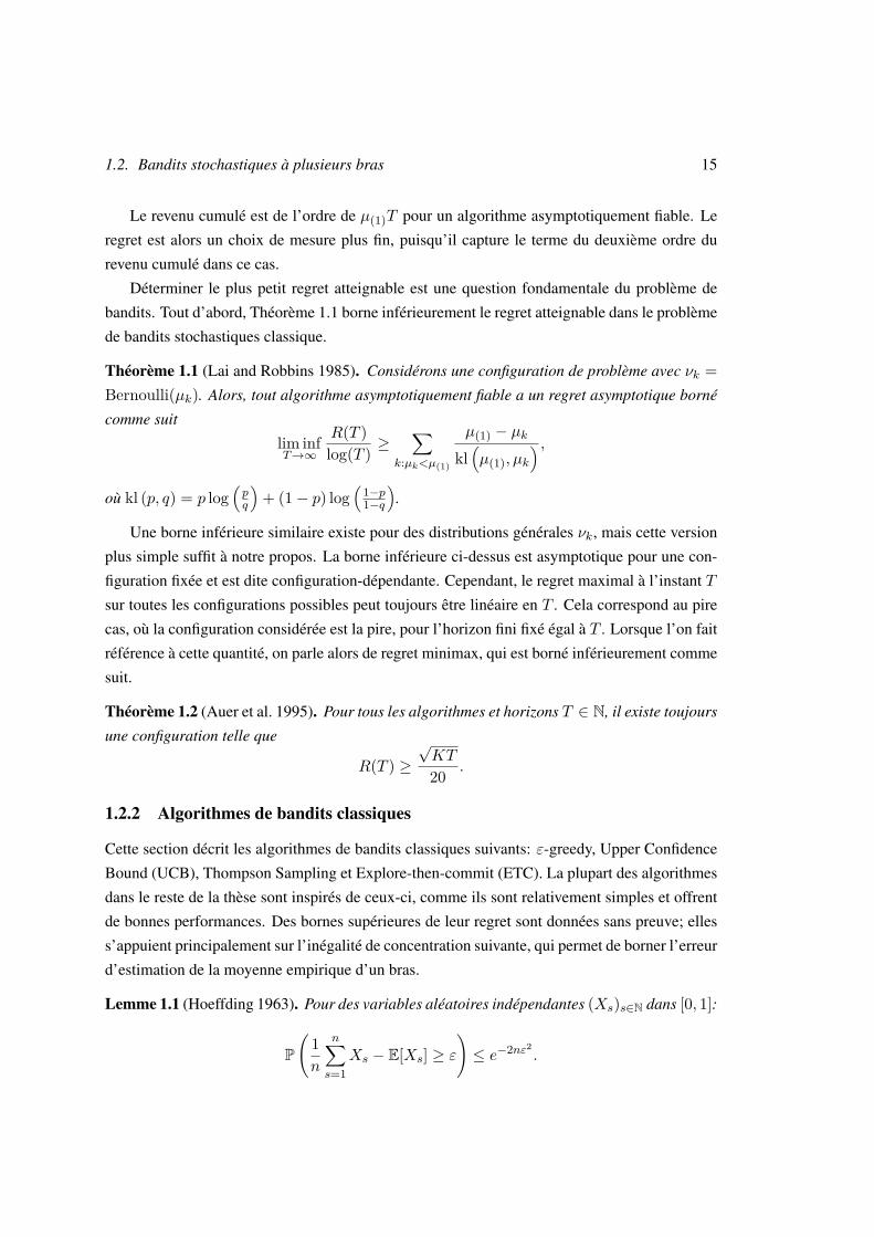
Le revenu cumulé est de l’ordre de µ(1)T pour un algorithme asymptotiquement fiable. Le
regret est alors un choix de mesure plus fin, puisqu’il capture le terme du deuxième ordre du
revenu cumulé dans ce cas.
Déterminer le plus petit regret atteignable est une question fondamentale du problème de
bandits. Tout d’abord, Théorème 1.1 borne inférieurement le regret atteignable dans le problème
de bandits stochastiques classique.
Théorème 1.1 (Lai and Robbins 1985). Considérons une configuration de problème avec νk =Bernoulli(µk). Alors, tout algorithme asymptotiquement fiable a un regret asymptotique borné
comme suit
lim infT→∞
R(T )log(T ) ≥
∑k:µk<µ(1)
µ(1) − µkkl(µ(1), µk
) ,où kl (p, q) = p log
(pq
)+ (1− p) log
(1−p1−q
).
Une borne inférieure similaire existe pour des distributions générales νk, mais cette version
plus simple suffit à notre propos. La borne inférieure ci-dessus est asymptotique pour une con-
figuration fixée et est dite configuration-dépendante. Cependant, le regret maximal à l’instant T
sur toutes les configurations possibles peut toujours être linéaire en T . Cela correspond au pire
cas, où la configuration considérée est la pire, pour l’horizon fini fixé égal à T . Lorsque l’on fait
référence à cette quantité, on parle alors de regret minimax, qui est borné inférieurement comme
suit.
Théorème 1.2 (Auer et al. 1995). Pour tous les algorithmes et horizons T ∈ N, il existe toujours
une configuration telle que
R(T ) ≥√KT
20 .
1.2.2 Algorithmes de bandits classiques
Cette section décrit les algorithmes de bandits classiques suivants: ε-greedy, Upper Confidence
Bound (UCB), Thompson Sampling et Explore-then-commit (ETC). La plupart des algorithmes
dans le reste de la thèse sont inspirés de ceux-ci, comme ils sont relativement simples et offrent
de bonnes performances. Des bornes supérieures de leur regret sont données sans preuve; elles
s’appuient principalement sur l’inégalité de concentration suivante, qui permet de borner l’erreur
d’estimation de la moyenne empirique d’un bras.
Lemme 1.1 (Hoeffding 1963). Pour des variables aléatoires indépendantes (Xs)s∈N dans [0, 1]:
P(
1n
n∑s=1
Xs − E[Xs] ≥ ε)≤ e−2nε2 .

16 Chapter 1. Introduction (version française)
Les notations suivantes sont utilisées dans le reste de la section:
• Nk(t) =∑t−1s=1 1 (π(s) = k) est le nombre de tirages du bras k jusqu’à l’instant t;
• µk(t) =∑t−1
s=1 1(π(s)=k)Xk(t)Nk(t) est la moyenne empirique du bras k avant l’instant t;
• ∆ = minµ(1) − µk > 0 | k ∈ [K] est l’écart de sous-optimalité et représente la
difficulté du problème.
Algorithme ε-greedy
L’algorithme ε-greedy décrit par Algorithme 1.1 est définie par une suite (εt)t ∈ [0, 1]N. Chaque
bras est d’abord tiré une fois. Ensuite à chaque tour t, l’algorithme explore avec probabilité εt,
auquel cas un bras est aléatoirement de manière uniforme. Sinon, l’algorithme exploite, i.e., le
bras avec la plus grande moyenne empirique est tiré.
Algorithme 1.1: ε-greedy
Entrées: (εt)t ∈ [0, 1]N1 pour t = 1, . . . ,K faire tirer le bras t
2 pour t = K + 1, . . . , T faire
tirer k ∼ U([K]) avec probabilité εt;tirer k ∈ arg maxi∈[K] µi(t) sinon.
Quand εt = 0 pour tout t, l’algorithme est appelé greedy (ou glouton), puisqu’il tire toujours
de manière “gloutonne” le meilleur bras empirique. L’algorithme greedy entraîne généralement
un regret de l’ordre de T , comme le meilleur bras peut-être sous-estimé dès son premier tirage
et n’est alors plus tiré.
En choisissant une suite (εt) appropriée, on obtient alors un regret sous-linéaire, comme
donné par le Théorème 1.3.
Théorème 1.3 (Slivkins 2019, Théorème 1.4). Pour une certaine constante universelle positive
c0, l’algorithme ε-greedy avec probabilités d’exploration εt =(K log(t)
t
)1/3a un regret borné
par
R(T ) ≤ c0K log(T )1/3T 2/3.
Si l’écart de sous-optimalité ∆ = minµ(1) − µk > 0 | k ∈ [K] est connu, la suite
εt = min(1, CK∆2t) pour une constante suffisamment large C donne un regret configuration-
dépendant logarithmique en T .

1.2. Bandits stochastiques à plusieurs bras 17
Algorithme UCB
Comme expliqué ci-dessus, choisir naïvement le meilleur bras empirique entraîne un regret con-
sidérable. Contrairement à greedy, l’algorithme UCB choisit le bras k maximisant µk(t)+Bk(t)à chaque instant, où le terme Bk(t) est une certaine borne de confiance. UCB, donné par
l’Algorithme 1.2 ci-dessous, biaise donc positivement les estimées des moyennes des bras.
Grâce à cela, le meilleur bras ne peut être sous-estimée (avec grande probabilité), évitant donc
les situations d’échec de l’algorithme greedy décrites ci-dessus.
Algorithme 1.2: UCB
1 pour t = 1, . . . ,K faire tirer le bras t2 pour t = K + 1, . . . , T faire tirer k ∈ arg maxi∈[K] µi(t) +Bi(t)
Théorème 1.4 borne le regret de l’algorithme UCB avec son choix de borne de confiance le
plus commun.
Théorème 1.4 (Auer et al. 2002a). L’algorithme UCB avec Bi(t) =√
2 log(t)Ni(t) verifie les bornes
de regret configuration-dépendante et minimax suivantes, pour certaines constantes universelles
positives c1, c2
R(T ) ≤∑
k:µk<µ(1)
8 log(T )µ(1) − µk
+ c1, (1.1)
R(T ) ≤ c2
√KT log(T ).
L’algorithme UCB a donc un regret configuration-dépendant optimal, à une constante multi-
plicative près, et lorsque les moyennes des bras ne sont pas arbitrairement proches de 0 ou 1. En
utilisant des bornes de confiance plus fines, un regret configuration-dépendant optimal est en fait
possible pour UCB (Garivier and Cappé, 2011). Dans la suite de cette thèse, une borne similaire
à l’Équation (1.1) est dite optimale à un facteur constant près par abus de notation.
Algorithme Thompson sampling
L’algorithme Thompson sampling décrit par Algorithme 1.3 adopte un point de vue Bayésien.
Pour une distribution a posteriori ppp des moyennes des bras µµµ, il échantillonne aléatoirement un
vecteur θ ∼ ppp et choisit un bras dans arg maxk∈[K] θk. La distribution a posteriori est alors
mise à jour en utilisant le gain observé, selon la règle de Bayes.
Théorème 1.5 (Kaufmann et al. 2012). Il existe une fonction f , dépendant uniquement du
vecteur des moyennes µµµ telle que pour toute configuration et ε > 0, le regret de l’algorithme
18 Chapter 1. Introduction (version française)
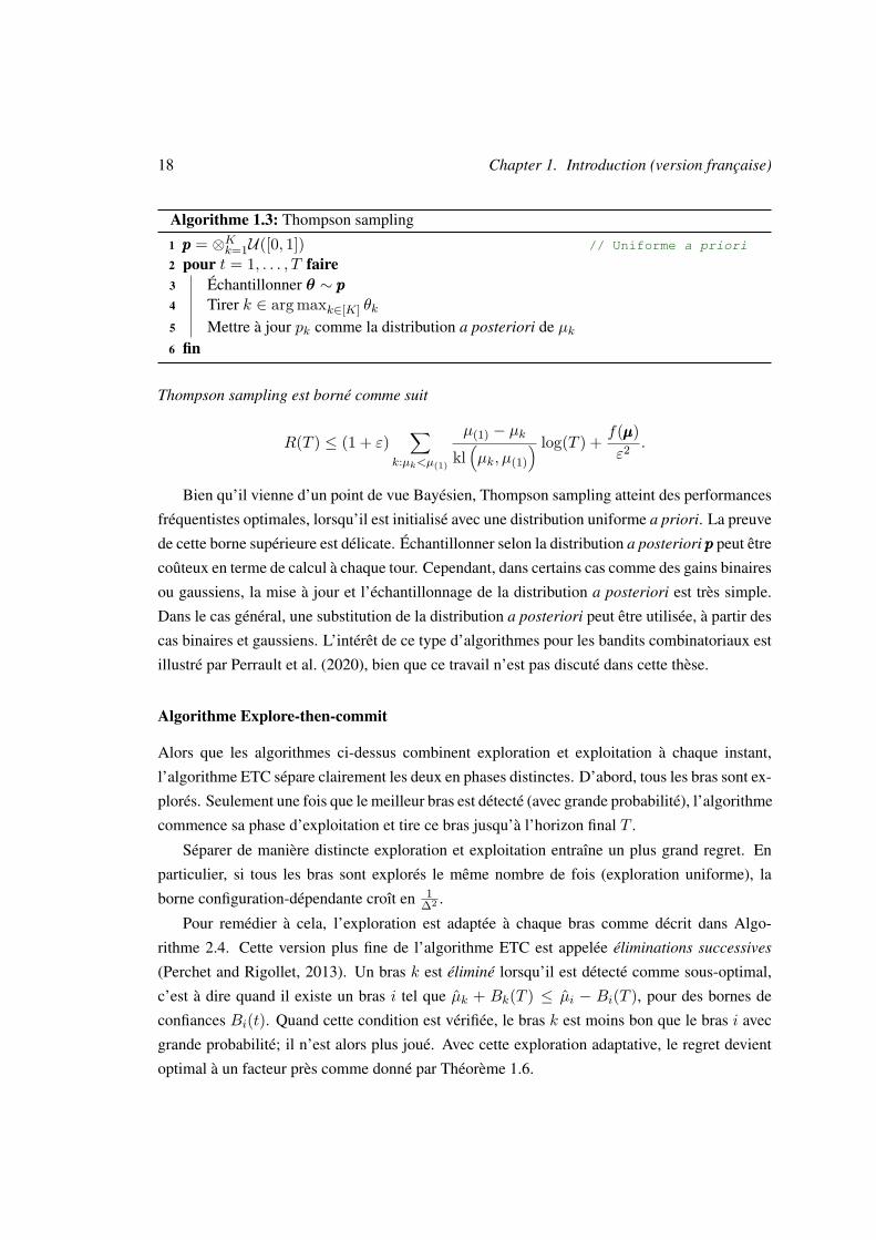
Algorithme 1.3: Thompson sampling
1 ppp = ⊗Kk=1U([0, 1]) // Uniforme a priori
2 pour t = 1, . . . , T faire3 Échantillonner θ ∼ ppp4 Tirer k ∈ arg maxk∈[K] θk5 Mettre à jour pk comme la distribution a posteriori de µk6 fin
Thompson sampling est borné comme suit
R(T ) ≤ (1 + ε)∑
k:µk<µ(1)
µ(1) − µkkl(µk, µ(1)
) log(T ) + f(µµµ)ε2 .
Bien qu’il vienne d’un point de vue Bayésien, Thompson sampling atteint des performances
fréquentistes optimales, lorsqu’il est initialisé avec une distribution uniforme a priori. La preuve
de cette borne supérieure est délicate. Échantillonner selon la distribution a posteriori ppp peut être
coûteux en terme de calcul à chaque tour. Cependant, dans certains cas comme des gains binaires
ou gaussiens, la mise à jour et l’échantillonnage de la distribution a posteriori est très simple.
Dans le cas général, une substitution de la distribution a posteriori peut être utilisée, à partir des
cas binaires et gaussiens. L’intérêt de ce type d’algorithmes pour les bandits combinatoriaux est
illustré par Perrault et al. (2020), bien que ce travail n’est pas discuté dans cette thèse.
Algorithme Explore-then-commit
Alors que les algorithmes ci-dessus combinent exploration et exploitation à chaque instant,
l’algorithme ETC sépare clairement les deux en phases distinctes. D’abord, tous les bras sont ex-
plorés. Seulement une fois que le meilleur bras est détecté (avec grande probabilité), l’algorithme
commence sa phase d’exploitation et tire ce bras jusqu’à l’horizon final T .
Séparer de manière distincte exploration et exploitation entraîne un plus grand regret. En
particulier, si tous les bras sont explorés le même nombre de fois (exploration uniforme), la
borne configuration-dépendante croît en 1∆2 .
Pour remédier à cela, l’exploration est adaptée à chaque bras comme décrit dans Algo-
rithme 2.4. Cette version plus fine de l’algorithme ETC est appelée éliminations successives
(Perchet and Rigollet, 2013). Un bras k est éliminé lorsqu’il est détecté comme sous-optimal,
c’est à dire quand il existe un bras i tel que µk + Bk(T ) ≤ µi − Bi(T ), pour des bornes de
confiances Bi(t). Quand cette condition est vérifiée, le bras k est moins bon que le bras i avec
grande probabilité; il n’est alors plus joué. Avec cette exploration adaptative, le regret devient
optimal à un facteur près comme donné par Théorème 1.6.
1.3. Aperçu et Contributions 19
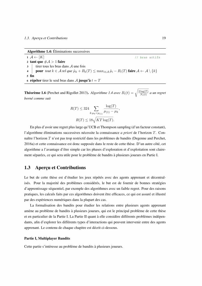
Algorithme 1.4: Éliminations successives
1 A ← [K] // bras actifs
2 tant que #A > 1 faire3 tirer tous les bras dans A une fois4 pour tout k ∈ A tel que µk +Bk(T ) ≤ maxi∈A µi −Bi(T ) faire A ← A \ k5 fin6 répéter tirer le seul bras dans A jusqu’à t = T
Théorème 1.6 (Perchet and Rigollet 2013). Algorithme 1.4 avec Bi(t) =√
2 log(T )Ni(t) a un regret
borné comme suit
R(T ) ≤ 324∑
k:µk<µ(1)
log(T )µ(1) − µk
,
R(T ) ≤ 18√KT log(T ).
En plus d’avoir une regret plus large qu’UCB et Thompson sampling (d’un facteur constant),
l’algorithme éliminations successives nécessite la connaissance a priori de l’horizon T . Con-
naître l’horizon T n’est pas trop restrictif dans les problèmes de bandits (Degenne and Perchet,
2016a) et cette connaissance est donc supposée dans le reste de cette thèse. D’un autre côté, cet
algorithme a l’avantage d’être simple car les phases d’exploration et d’exploitation sont claire-
ment séparées, ce qui sera utile pour le problème de bandits à plusieurs joueurs en Partie I.
1.3 Aperçu et Contributions
Le but de cette thèse est d’étudier les jeux répétés avec des agents apprenant et décentral-
isés. Pour la majorité des problèmes considérés, le but est de fournir de bonnes stratégies
d’apprentissage séquentiel, par exemple des algorithmes avec un faible regret. Pour des raisons
pratiques, les calculs faits par ces algorithmes doivent être efficaces, ce qui est assuré et illustré
par des expériences numériques dans la plupart des cas.
La formalisation des bandits pour étudier les relations entre plusieurs agents apprenant
amène au problème de bandits à plusieurs joueurs, qui est le principal problème de cette thèse
et en particulier de la Partie I. La Partie II quant à elle considère différents problèmes indépen-
dants, afin d’explorer les différents types d’interactions qui peuvent intervenir entre des agents
apprenant. Le contenu de chaque chapitre est décrit ci-dessous.
Partie I, Multiplayer Bandits
Cette partie s’intéresse au problème de bandits à plusieurs joueurs.

20 Chapter 1. Introduction (version française)
Chapitre 3, Multiplayer bandits: a survey. Ce chapitre présente le problème de bandits à
plusieurs joueurs et étudie de manière exhaustive l’état de l’art en bandits à plusieurs joueurs,
incluant les Chapitres 4, 5 et 6, ainsi que des travaux ultérieurs par différents auteurs.
Chapitre 4, SIC-MMAB: Synchronisation Involves Communication in Multiplayer Multi-Armed Bandits. Bien que les joueurs soient décentralisés, ils peuvent toujours communiquer
implicitement entre eux en utilisant les informations de collision comme des bits. Cette ob-
servation est ici exploitée pour proposer un algorithme décentralisé qui renforce les collisions
entre les joueurs pour établir une communication entre eux. Un regret similaire aux algorithmes
centralisés optimaux est alors atteint. Bien que quasi-optimal en théorie, cet algorithme n’est
pas satisfaisant, puisqu’un tel niveau de communication est très coûteux en pratique. Nous sug-
gérons que la formulation usuelle des bandits à plusieurs joueurs mène vers ce type d’algorithme
et en particulier l’hypothèse statique, selon laquelle les joueurs commencent et terminent tous
le jeu au même moment. Nous étudions ensuite un nouveau problème dynamique et proposons
un algorithme avec un regret logarithmique dans ce cas, sans utiliser de communication directe
entre les joueurs.
Chapitre 5, A Practical Algorithm for Multiplayer Bandits when Arm Means Vary AmongPlayers. Ce chapitre considère le cas hétérogène, où les moyennes de chaque bras varient selon
le joueur. Pour atteindre l’appariement optimal entre joueurs et bras, un niveau minimum de
communication est nécessaire entre les joueurs. Ce chapitre propose donc un algorithme efficace
pour le cas hétérogène à la fois en terme de regret et de calcul. Cela est réalisé en renforçant les
collisions parmi les joueurs et en améliorant le protocole de communication initialement proposé
dans le Chapitre 4.
Chapitre 6, Selfish Robustness and Equilibria in Multi-Player Bandits. Alors que la ma-
jorité des travaux sur le problème de bandits à plusieurs joueurs supposent des joueurs coopérat-
ifs, ce chapitre considère le cas de joueurs stratégiques, maximisant leur revenu individuel cu-
mulé de manière égoïste. Les algorithmes existants ne sont pas adaptés à ce contexte, comme
un joueur malveillant peut facilement interférer avec l’exploration des autres joueurs afin de
largement augmenter son propre revenu.
Nous proposons donc un premier algorithme, ignorant les collisions après l’initialisation,
qui est à la fois un O (log(T ))-équilibre de Nash (robuste aux joueurs égoïstes) et a un regret
collectif comparable aux algorithmes non-stratégiques. Lorsque les collisions sont observées,
les algorithmes existants peuvent en fait être adaptées en stratégies Grim-Trigger, qui sont aussi
des O (log(T ))-équilibres de Nash, tout en maintenant des garanties de regret similaires aux
1.3. Aperçu et Contributions 21
algorithmes coopératifs originaux. Avec des joueurs hétérogènes, l’appariement optimal ne peut
plus être atteint et nous minimisons alors une notion adaptée et pertinente de regret.
Partie II, Other learning instances
Cette partie étudie des problèmes indépendants qui illustrent les différents types d’interaction
entre des agents apprenant décrits en Section 1.1.
Chapitre 7, Decentralized Learning in Online Queuing Systems. Ce chapitre étudie le
problème séquentiel de systèmes de queues, initalement motivé par le routage de paquets dans
les réseaux informatiques. Dans ce problème, les queues reçoivent des paquets selon différents
taux et envoient répététivement leurs paquets aux serveurs, chacun d’entre eux ne pouvant traiter
au plus qu’un seul paquet à la fois. La stabilité du système (i.e., si le nombre de paquets restants
est borné) est d’un intérêt vital et est possible dans le cas centralisé dès lors que le ratio entre taux
de service et taux d’arrivée est strictement plus grand que 1. Avec des joueurs égoïstes, Gaitonde
and Tardos (2020a) ont montré que les queues minimisant leur regret sont stables lorsque ce ratio
est plus grand que 2. La minimisation du regret cependant mène à des comportements à court
terme et ignore les effets long terme dûs à la propriété de report propre à cet exemple de jeu
répété. En revanche, lorsque les joueurs minimisent des coûts à long terme, Gaitonde and Tar-
dos (2020b) ont montré que tous les équilibres de Nash sont stables tant que le ratio des taux est
plus grand que ee−1 , qui peut alors être vu comme le prix de l’anarchie pour ce jeu. Cependant,
le coût d’apprentissage reste inconnu et nous soutenons dans ce chapitre qu’un certain niveau de
coopération est nécessaire entre les queues pour garantir la stabilité avec un ratio plus petit que 2lorsqu’elles apprennent. Par conséquent, nous proposons un algorithme d’apprentissage décen-
tralisé, stable pour tout ratio plus grand que 1, ce qui implique que la décentralisation n’entraîne
pas de coût supplémentaire ici.
Chapitre 8, Utility/Privacy Trade-off as Regularized Optimal Transport. Dans les enchères
pour la publicité en ligne, le comissaire-priseur et les enchérisseurs sont répététivement en con-
currence. Déterminer les équilibres de Nash est ici trop coûteux en terme de calcul, comme les
espaces d’action sont continus. S’adapter aux nouvelles stratégies des autres joueurs mène à
une course à l’armement entre le comissaire-priseur et les enchérisseurs. À la place, ce chapitre
propose d’équilibrer naturellement le revenu à court terme, en maximisant sa propre utilité de
manière avide, et le revenu à long terme en cachant certaines informations privées dont la di-
vulgation pourrait être exploitée par les autres joueurs. Ce problème est formalisé par un cadre
Bayésien de compromis entre utilité et confidentialité, dont on montre qu’il est équivalent à un

22 Chapter 1. Introduction (version française)
problème de minimisation de divergence de Sinkhorn. Cette équivalence permet de calculer ce
minimum efficacement, en utilisant les différents outils développés par les théories de transport
optimal et d’optimisation.
Chapitre 9, Social Learning in Non-Stationary Environments. Ce chapitre considère l’apprentissage
social avec revues, où des consommateurs hétérogènes et Bayésiens décident l’un après l’autre
d’acheter un objet de qualité inconnue, en se basant sur les revues de précédents acheteurs. Les
précédents travaux supposent que la qualité de l’objet est constante dans le temps et montrent
que son estimée converge vers sa vraie valeur sous de faibles hypothèses. Ici, nous considérons
un modèle dynamique où la qualité peut changer par moments. Le coût supplémentaire dû à la
structure dynamique se révèle être logarithmique en le taux de changement de la qualité, dans
le cas de caractéristiques binaires. Cependant, l’écart entre les modèles statique et dynamique
lorsque les caractéristiques ne sont plus binaires demeure inconnu.
Chapter 2
Introduction
2.1 Learning in repeated games . . . . . . . . . . . . . . . . . . . . . . . . . . . . 23
2.2 Stochastic Multi-Armed Bandits . . . . . . . . . . . . . . . . . . . . . . . . . 27
2.2.1 Model and lower bounds . . . . . . . . . . . . . . . . . . . . . . . . . 28
2.2.2 Classical bandit algorithms . . . . . . . . . . . . . . . . . . . . . . . . 29
2.3 Outline and Contributions . . . . . . . . . . . . . . . . . . . . . . . . . . . . . 33
2.4 List of Publications . . . . . . . . . . . . . . . . . . . . . . . . . . . . . . . . 35
2.1 Learning in repeated games
Repeated games formalize the different interactions occurring between players (or agents) re-
peatedly taking part in a game instance, using game theoretical tools (Aumann et al., 1995;
Fudenberg and Maskin, 2009). Many applications derive from this kind of problem, including
bidding for online advertisement auctions, resource allocation in radio or computer networks,
minimizing travelling time in transportation networks, etc. Facing the surge of learning algo-
rithms in our society, it is of crucial interest to understand how these algorithms interact. While
the classical learning paradigms consider a single agent in a fixed environment, this assumption
seems inaccurate in many modern applications. Smart agents, which are strategic and learn their
environment, indeed interact between each other, highly influencing the final outcome. This
thesis aims at exploring these different possible interplays between learning agents in a strategic
environment and at describing the typical strategies that yield good performances in these set-
tings. It also measures the different inefficiencies in social welfare stemming from both strategic
23
24 Chapter 2. Introduction
and learning considerations.
Repeated games are generally formalized as follows. At each round t ∈ [T ] := 1, . . . , T,each player m ∈ [M ] individually chooses a strategy (a bidding amount for example) sm ∈ Sm
where Sm is the strategy space. She then receives a possibly noisy reward of expectation umt (sss)where umt is her associated reward function at time t and sss ∈
∏Mm=1 Sm is the strategy profile
of all players. In the following, s−ms−ms−m represents the vector sss, except for its m-th component.
A learning player chooses at each new round her strategy based on her past observations.
These observations can indeed help in estimating both the game environment, i.e., the utility
functions umt , and the other players strategy profile s−ms−ms−m.
Maximizing one’s sole reward in a single player, fixed environment is at the core of optimiza-
tion and learning theories and becomes even more intricate when several players are interacting
with each other in repeated games. Two major types of interaction between these players can
happen. First, the reward of a player at each round does not solely depend on her action, but
also on other agents’ actions and even potentially on past outcomes. In this case, players can
either compete or cooperate, depending on the game’s nature. Secondly, players can also share
(to some extent) their observations with each other, influencing their estimation of the game
environment. This can either lead to a faster global learning, or bias the parameters estimations.
Interaction in outcomes. Generally, the reward functions ut depend on the complete strategy
profile of the players sss. The different players objectives might then be antagonistic, as any
strategy profile yielding a large reward for some player can yield a low reward for another
player. The extreme case corresponds to zero-sum games for two players, where the utility
functions verify u1 = −u2. In this case, players compete with each other and aim at maximizing
their individual reward. In a single round game, Nash equilibria characterize interesting strategy
profiles for strategic players. A player unilaterally deviating from a Nash equilibrium indeed
suffers a decrease in her reward.
Definition 2.1 (Nash equilibrium). A strategy profile sss is a Nash equilibrium for the single round
game defined by the utility functions (um)m∈[M ] if
∀m ∈ [M ],∀s′ ∈ Sm, um(s′, s−ms−ms−m) ≤ um(sm, s−ms−ms−m).
As soon as the utility functions um are concave and continuous, the existence of a Nash
equilibrium is guaranteed by Brouwer fixed point theorem. It is for instance the case if Sm is
the set of probability distributions over some finite set (which is called the action space in the
following).
2.1. Learning in repeated games 25
This strategic consideration thus leads to a first inefficiency in the players’ decisions, as
they maximize their individual reward, at the expense of the collective reward. The price of
anarchy (Koutsoupias and Papadimitriou, 1999) measures this inefficiency as the social welfare
ratio between the best possible collective situation and the worst Nash equilibrium. Although
reaching the best collective outcome might be illusory for selfish agents, considering the worst
Nash equilibrium might be too pessimistic. Instead, the price of stability (Schulz and Moses,
2003) measures the inefficiency by the social welfare ratio between the best possible situation
and the best Nash equilibrium.
Learning equilibria in repeated games is thus of crucial interest, as they nicely reflect the
behavior of agents perfectly knowing their environment. It is in particular at the core of many
problems in computer science and economics (Fudenberg et al., 1998; Cesa-Bianchi and Lugosi,
2006). A second inefficiency stems from this consideration, as players need to learn their envi-
ronment and might interfere with each other, potentially converging to no or bad equilibria. A
correlated equilibrium is defined similarly to a Nash equilibrium, when the strategies (sm)m are
probability distributions whose joint realizations can be correlated. It is known that when the
utility functions are constant in time umt = um, if all agents follow no internal regret strategies,
their actions converge in average to the set of correlated equilibria (Hart and Mas-Colell, 2000;
Blum and Monsour, 2007; Perchet, 2014). Yet little is known when the utility functions umtalso depend on the outcomes of previous rounds as in decentralized queuing systems, which are
studied in Chapter 7.
Moreover, computing a Nash equilibrium might be too expensive in practice (Daskalakis et
al., 2009). It is even the case in two players zero-sum games when the action space is continuous.
For example in repeated auctions, a bidding action is a function R+ → R+ which for every
item value, returns some bidding amount. Learning equilibria in this kind of game thus seems
unreasonable and optimally responding to the adversary’s strategy leads to an endless arm race
between the players. We instead propose in Chapter 8 to balance between the short term revenue
earned by greedily bidding, and the long term revenue by maintaining some level of information
asymmetry between the players, which is a crucial aspect of repeated games (Aumann et al.,
1995).
In other cases (e.g., resource allocation in radio or computer networks), the players have an
interest in cooperating with each other. This for example happens if players equally split their
collective reward, or if they have common interests by design of the utility functions (assume
for example a game with a price of anarchy equal to 1).
In multiplayer bandits, which is the focus of Part I, the players choose a channel for trans-
mission. But if several players query the same server at some time step, a collision occurs and no
26 Chapter 2. Introduction
transmission happens on this channel. In this case, the players have interest in coordinating with
each other to avoid collisions and efficiently transmit on the different channels. Besides learning
the game environment, the difficulty here comes from coordinating the players with each other,
while being decentralized and limited in communication. When repeating the rounds, it however
becomes unclear whether players have an interest in blindly cooperating. Especially, a player
could have an interest in disturbing the learning process of other players in order to grant oneself
the best transmitting channel. This kind of behavior can however be prevented here as shown in
Chapter 6 using, for example, Grim-Trigger strategies.
Cooperation between the players seems even more strongly enforced in decentralized queu-
ing systems. In this problem, the utility functions also depend on the outcomes of previous
rounds. Their design actually ensures that if some player cumulated a smaller reward than the
other players, she gets favored in the future and is prioritized over the other players when query-
ing some server. Consequently, players also have interest in sharing the resources with each
other, to not degrade their future own rewards.
Interaction in observations. Even when the reward functions are independent of the other
players’ actions, i.e., umt only depends on sm, players can interact by sharing some informa-
tion/observations with each other. In that case, players have no interest in competing and they
only share their information to improve each other’s estimation of the game environment. Such a
phenomenon for example happens in distributed bandits, described in Section 3.6.1. This prob-
lem is similar to the multiplayer bandits except for two features: there are no collisions here, as
the utility functions do not depend on each other’s action, and players are assigned to a graph
and can send messages to their neighbours. They can thus send their observations (or an aggre-
gated function of these observations) to their neighbours, which allows to speed up the learning
process.
Even in general games where the utility functions depend on the whole strategy profile sss,
cooperative players can share some level of information in order to improve the learning rate.
This is typically what allows to reach near centralized performances in the multiplayer bandits
problem in Chapters 4 to 6.
When players are cooperating, the goal is generally to maximize the collective reward. As
explained above, some learning inefficiency might emerge because of the different interactions
between the players. When they are centralized, i.e., a central agent unilaterally controls the
decisions of all the players, this is equivalent to the single player instance and this inefficiency
solely comes from the learning difficulty of the problem. But when the players are decentralized,
that is their decisions are individually taken without consulting with each other, additional diffi-
culties arise, e.g., the observations/decisions cannot be mutualized. The main question in these
2.2. Stochastic Multi-Armed Bandits 27
settings is thus generally whether decentralization yields some additional cost, i.e., whether the
maximal attainable social welfare in the decentralized setting is smaller than in the centralized
setting. This is especially the focus of Chapters 4 and 7, which show that decentralization has
roughly no cost in homogeneous multiplayer bandits and online queuing systems, respectively.
Chapter 5 also suggests that this cost scales at most with the number of players in heterogeneous
multiplayer bandits.
Social learning considers a different instance of repeated games, where at each round, a new
single agent plays for this sole round. A player chooses her action to maximize her expected
reward, based on the former players’ actions (and potentially an additional feedback). Situations
of herding can then happen, where the agents never learn correctly their environment and end up
taking suboptimal decisions for ever. This problem instance thus nicely illustrates how myopic
agents can take decisions leading to bad collective situations. Chapter 9 on the other hand shows
that this learning inefficiency is largely mitigated under mild assumptions when players observe
the reviews of the previous consumers.
2.2 Stochastic Multi-Armed Bandits
The problems studied in this thesis are intricate as they combine both game theoretical and
learning considerations. The framework of sequential (or online) learning and especially Multi-Armed Bandits (MAB) seems well adapted. On the first hand, it defines a formal and rather
simple instance of learning, for which theoretical results are known. On the other hand, its
sequential aspect is similar to repeated games and many connections exist between repeated
games and MAB (see e.g., Cesa-Bianchi and Lugosi, 2006). MAB is indeed a particular instance
of repeated games, where a single agent plays against the nature, which generates the rewards
of each arm.
MAB was first introduced for clinical trials (Thompson, 1933; Robbins, 1952) and has been
recently popularised thanks to its applications to online recommendation systems. Many exten-
sions have also been developed in the past years, such as contextual, combinatorial or lipschitz
bandits for example (Woodroofe, 1979; Cesa-Bianchi and Lugosi, 2012; Agrawal, 1995).
This section shortly describes the stochastic MAB problem, as well as the main results and
algorithms for this classical instance, which will give insights for the proposed algorithms and
results all along this thesis. We refer the reader to (Bubeck and Cesa-Bianchi, 2012; Lattimore
and Szepesvári, 2018; Slivkins, 2019) for extensive surveys on MAB.
28 Chapter 2. Introduction
2.2.1 Model and lower bounds
At each time step t ∈ [T ], the agent pulls an arm π(t) ∈ [K] among a finite set of actions,
where T is the game horizon. When pulling the arm k, she observes and receives the reward
Xk(t) ∼ νk of mean µk = E[Xk(t)], where νk ∈ P([0, 1]) is a probability distribution on [0, 1].This observation Xk(t) is then used by the agent to choose the arm to pull in the next rounds.
The random variables (Xk(t))t=1,...,T are independent, identically distributed and bounded
in [0, 1] in the following. Yet, the results presented in this section also hold for the more general
class of sub-gaussian variables.
In the following, x(k) denotes the k-th order statistics of the vector xxx ∈ Rn, i.e., x(1) ≥x(2) ≥ . . . ≥ x(n). The goal of the agent is to maximize her cumulated reward. Equivalently,
she aims at minimizing her regret, which is the difference between the maximal expected reward
of an agent knowing beforehand the arms’ distributions and the actual earned reward until the
game horizon T . It is formally defined as
R(T ) = Tµ(1) − E[T∑t=1
µπ(t)
],
where the expectation holds over the actions π(t) of the agent.
The player only observes the reward Xk(t) of the pulled arm and not those associated to the
non-pulled arms. Because of this bandit feedback, the player must balance between exploration,
i.e., estimating the arm means by pulling all arms sufficiently, and exploitation, by pulling the
seemingly optimal arm. This trade-off is at the core of MAB and is also crucial in repeated
games, as it nicely opposes short term (exploitation) with long term (exploration) rewards.
A problem instance is fixed by the distributions (νk)k∈[K].
Definition 2.2. An agent (or algorithm) is asymptotically consistent if for every problem instance
and α > 0, R(T ) = o (Tα).
The cumulated reward is of order µ(1)T for an asymptotically consistent algorithm. The
regret is instead a more refined choice of measure, since it captures the second order term of the
cumulated reward in this case.
Determining the smallest achievable regret is a fundamental question for bandits problem.
First, Theorem 2.1 lower bounds the achievable regret in the classical stochastic MAB.
Theorem 2.1 (Lai and Robbins 1985). Consider a problem instance with Bernoulli distributions
νk = Bernoulli(µk), then any asymptotically consistent algorithm has an asymptotic regret
2.2. Stochastic Multi-Armed Bandits 29
bounded as follows
lim infT→∞
R(T )log(T ) ≥
∑k:µk<µ(1)
µ(1) − µkkl(µ(1), µk
) ,where kl (p, q) = p log
(pq
)+ (1− p) log
(1−p1−q
).
A similar lower bound holds for general distributions νk, but this simpler version is sufficient
for our purpose. The above lower bound holds asymptotically for a fixed instance and is referred
to as an instance dependent bound. However, the maximal regret incurred at time T over all
the possible instances might still be linear in T . This corresponds to the worst case, where the
considered instance is the worst for the fixed, finite horizon T . When specifying this quantity,
we instead refer to the minimax regret, which is lower bounded as follows.
Theorem 2.2 (Auer et al. 1995). For all algorithms and horizon T ∈ N, there exists a problem
instance such that
R(T ) ≥√KT
20 .
2.2.2 Classical bandit algorithms
This section describes the following classical bandit algorithms: ε-greedy, Upper Confidence
Bound (UCB), Thompson Sampling and Explore-then-commit (ETC). Most algorithms in the
following chapters will be inspired from them, as they are rather simple and yield good per-
formances. Upper bounds of their regret are provided without proofs; they mostly rely on the
following concentration inequality, which allows to bound the estimation error of the empirical
mean of an arm.
Lemma 2.1 (Hoeffding 1963). For independent random variables (Xs)s∈N in [0, 1]:
P(
1n
n∑s=1
Xs − E[Xs] ≥ ε)≤ e−2nε2 .
The following notations are used in the remaining of this section
• Nk(t) =∑t−1s=1 1 (π(s) = k) is the number of pulls on arm k until time t;
• µk(t) =∑t−1
s=1 1(π(s)=k)Xk(t)Nk(t) is the empirical mean of arm k before time t;
• ∆ = minµ(1) − µk > 0 | k ∈ [K] is the suboptimality gap and represents the hardness
of the problem.
30 Chapter 2. Introduction
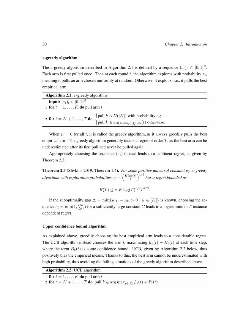
ε-greedy algorithm
The ε-greedy algorithm described in Algorithm 2.1 is defined by a sequence (εt)t ∈ [0, 1]N.
Each arm is first pulled once. Then at each round t, the algorithm explores with probability εt,
meaning it pulls an arm chosen uniformly at random. Otherwise, it exploits, i.e., it pulls the best
empirical arm.
Algorithm 2.1: ε-greedy algorithm
input: (εt)t ∈ [0, 1]N1 for t = 1, . . . ,K do pull arm t
2 for t = K + 1, . . . , T do
pull k ∼ U([K]) with probability εt;pull k ∈ arg maxi∈[K] µi(t) otherwise.
When εt = 0 for all t, it is called the greedy algorithm, as it always greedily pulls the best
empirical arm. The greedy algorithm generally incurs a regret of order T , as the best arm can be
underestimated after its first pull and never be pulled again.
Appropriately choosing the sequence (εt) instead leads to a sublinear regret, as given by
Theorem 2.3.
Theorem 2.3 (Slivkins 2019, Theorem 1.4). For some positive universal constant c0, ε-greedy
algorithm with exploration probabilities εt =(K log(t)
t
)1/3has a regret bounded as
R(T ) ≤ c0K log(T )1/3T 2/3.
If the suboptimality gap ∆ = minµ(1) − µk > 0 | k ∈ [K] is known, choosing the se-
quence εt = min(1, CK∆2t) for a sufficiently large constant C leads to a logarithmic in T instance
dependent regret.
Upper confidence bound algorithm
As explained above, greedily choosing the best empirical arm leads to a considerable regret.
The UCB algorithm instead chooses the arm k maximizing µk(t) + Bk(t) at each time step,
where the term Bk(t) is some confidence bound. UCB, given by Algorithm 2.2 below, thus
positively bias the empirical means. Thanks to this, the best arm cannot be underestimated with
high probability, thus avoiding the failing situations of the greedy algorithm described above.
Algorithm 2.2: UCB algorithm
1 for t = 1, . . . ,K do pull arm t2 for t = K + 1, . . . , T do pull k ∈ arg maxi∈[K] µi(t) +Bi(t)
2.2. Stochastic Multi-Armed Bandits 31
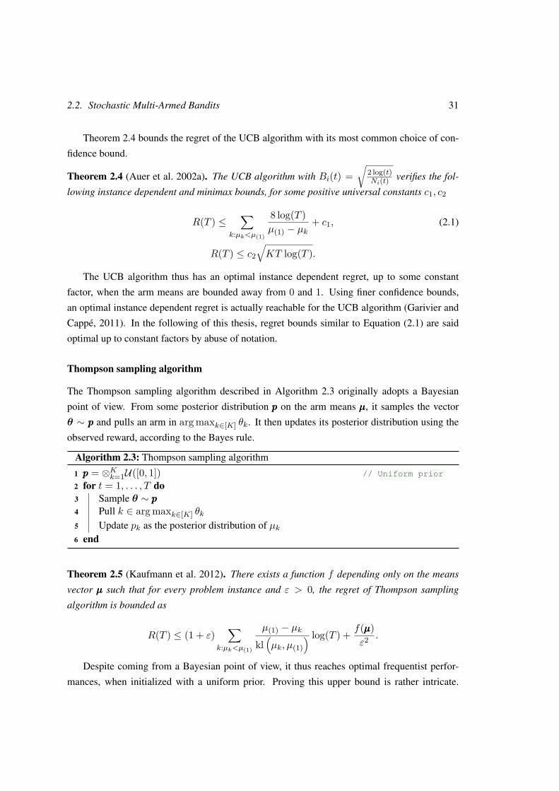
Theorem 2.4 bounds the regret of the UCB algorithm with its most common choice of con-
fidence bound.
Theorem 2.4 (Auer et al. 2002a). The UCB algorithm with Bi(t) =√
2 log(t)Ni(t) verifies the fol-
lowing instance dependent and minimax bounds, for some positive universal constants c1, c2
R(T ) ≤∑
k:µk<µ(1)
8 log(T )µ(1) − µk
+ c1, (2.1)
R(T ) ≤ c2
√KT log(T ).
The UCB algorithm thus has an optimal instance dependent regret, up to some constant
factor, when the arm means are bounded away from 0 and 1. Using finer confidence bounds,
an optimal instance dependent regret is actually reachable for the UCB algorithm (Garivier and
Cappé, 2011). In the following of this thesis, regret bounds similar to Equation (2.1) are said
optimal up to constant factors by abuse of notation.
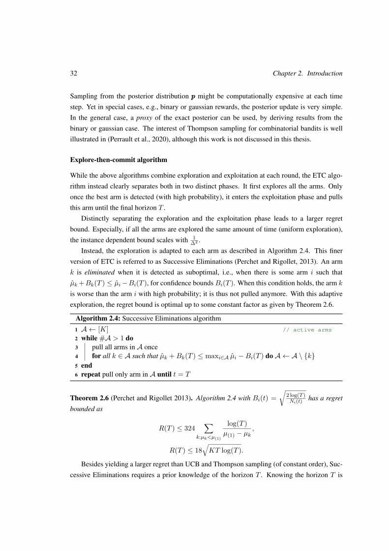
Thompson sampling algorithm
The Thompson sampling algorithm described in Algorithm 2.3 originally adopts a Bayesian
point of view. From some posterior distribution ppp on the arm means µµµ, it samples the vector
θ ∼ ppp and pulls an arm in arg maxk∈[K] θk. It then updates its posterior distribution using the
observed reward, according to the Bayes rule.
Algorithm 2.3: Thompson sampling algorithm
1 ppp = ⊗Kk=1U([0, 1]) // Uniform prior
2 for t = 1, . . . , T do3 Sample θ ∼ ppp4 Pull k ∈ arg maxk∈[K] θk5 Update pk as the posterior distribution of µk6 end
Theorem 2.5 (Kaufmann et al. 2012). There exists a function f depending only on the means
vector µµµ such that for every problem instance and ε > 0, the regret of Thompson sampling
algorithm is bounded as
R(T ) ≤ (1 + ε)∑
k:µk<µ(1)
µ(1) − µkkl(µk, µ(1)
) log(T ) + f(µµµ)ε2 .
Despite coming from a Bayesian point of view, it thus reaches optimal frequentist perfor-
mances, when initialized with a uniform prior. Proving this upper bound is rather intricate.
32 Chapter 2. Introduction
Sampling from the posterior distribution ppp might be computationally expensive at each time
step. Yet in special cases, e.g., binary or gaussian rewards, the posterior update is very simple.
In the general case, a proxy of the exact posterior can be used, by deriving results from the
binary or gaussian case. The interest of Thompson sampling for combinatorial bandits is well
illustrated in (Perrault et al., 2020), although this work is not discussed in this thesis.
Explore-then-commit algorithm
While the above algorithms combine exploration and exploitation at each round, the ETC algo-
rithm instead clearly separates both in two distinct phases. It first explores all the arms. Only
once the best arm is detected (with high probability), it enters the exploitation phase and pulls
this arm until the final horizon T .
Distinctly separating the exploration and the exploitation phase leads to a larger regret
bound. Especially, if all the arms are explored the same amount of time (uniform exploration),
the instance dependent bound scales with 1∆2 .
Instead, the exploration is adapted to each arm as described in Algorithm 2.4. This finer
version of ETC is referred to as Successive Eliminations (Perchet and Rigollet, 2013). An arm
k is eliminated when it is detected as suboptimal, i.e., when there is some arm i such that
µk +Bk(T ) ≤ µi−Bi(T ), for confidence bounds Bi(T ). When this condition holds, the arm k
is worse than the arm i with high probability; it is thus not pulled anymore. With this adaptive
exploration, the regret bound is optimal up to some constant factor as given by Theorem 2.6.
Algorithm 2.4: Successive Eliminations algorithm
1 A ← [K] // active arms
2 while #A > 1 do3 pull all arms in A once4 for all k ∈ A such that µk +Bk(T ) ≤ maxi∈A µi −Bi(T ) do A ← A \ k5 end6 repeat pull only arm in A until t = T
Theorem 2.6 (Perchet and Rigollet 2013). Algorithm 2.4 with Bi(t) =√
2 log(T )Ni(t) has a regret
bounded as
R(T ) ≤ 324∑
k:µk<µ(1)
log(T )µ(1) − µk
,
R(T ) ≤ 18√KT log(T ).
Besides yielding a larger regret than UCB and Thompson sampling (of constant order), Suc-
cessive Eliminations requires a prior knowledge of the horizon T . Knowing the horizon T is

2.3. Outline and Contributions 33
not too restrictive in bandits problem (Degenne and Perchet, 2016a) and is thus assumed in the
remaining of this thesis. On the other hand, Successivation Eliminations has the advantage of
being simple since it clearly separates both exploration and exploitation, which will be useful
for multiplayer bandits in Part I.
2.3 Outline and Contributions
The goal of this thesis is to study repeated games with decentralized learning agents. For most
of the considered problems, it aims at providing good sequential learning strategies, e.g., small
regret algorithms. For practical reasons, these strategies have to be computationally efficient,
which is ensured and illustrated by numerical experiments in most of the cases.
Using the MAB formalization to study relations between multiple learning agents leads to
the multiplayer bandits problem, which is the main focus of this thesis and particularly of Part I.
On the other hand, Part II considers different and independent problems, exploring the different
types of interactions that can happen between learning agents. The content of each chapter is
described below.
Part I, Multiplayer Bandits
This part focuses on the problem of multiplayer bandits.
Chapter 3, Multiplayer bandits: a survey. This chapter introduces the problem of multi-
player bandits and extensively reviews the multiplayer bandits literature, including Chapters 4
to 6 and subsequent works by different authors.
Chapter 4, SIC-MMAB: Synchronisation Involves Communication in Multiplayer Multi-Armed Bandits. Although players are decentralized, they can still implicitly communicate
with each other using collision information as bits. This observation is here leveraged to pro-
pose a decentralized algorithm that enforces collisions between players to allow communication
between them. It then achieves a regret bound similar to the smallest achievable regret in the
centralized case. Although theoretically efficient, this algorithm is not satisfying, as such a level
of communication is very costly in practice. We suggest that the usual formulation of the mul-
tiplayer bandits leads to this kind of algorithm and in particular the static assumption, which
assumes that all players start and end the game at the same time. We then study a new dynamic
setting and propose a logarithmic regret algorithm for this setting, using no direct communica-
tion between the players.
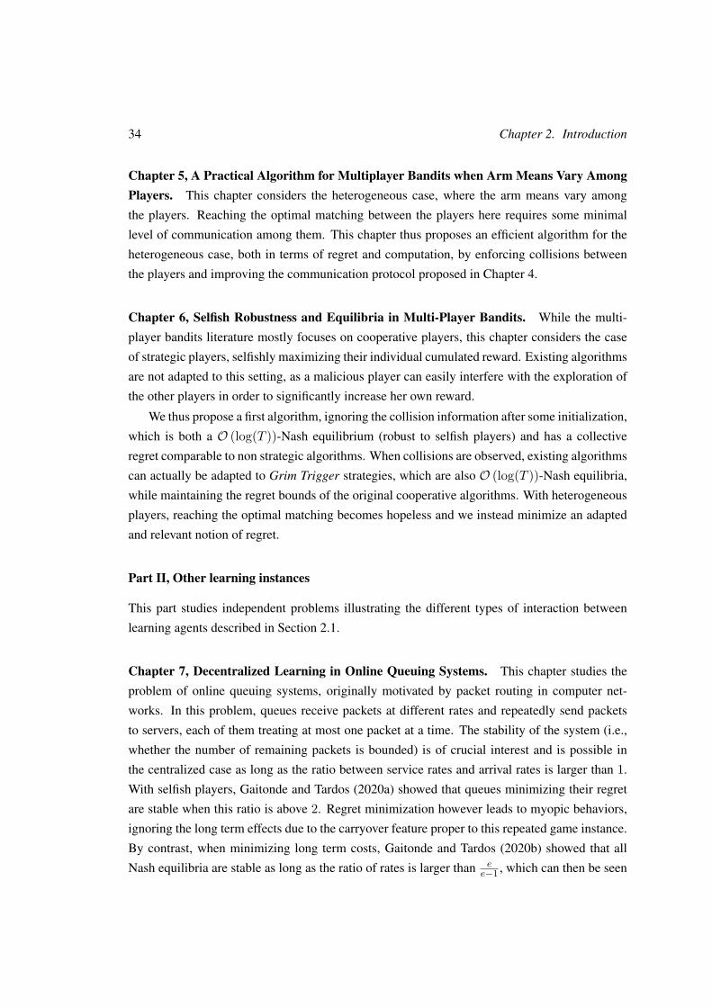
34 Chapter 2. Introduction
Chapter 5, A Practical Algorithm for Multiplayer Bandits when Arm Means Vary AmongPlayers. This chapter considers the heterogeneous case, where the arm means vary among
the players. Reaching the optimal matching between the players here requires some minimal
level of communication among them. This chapter thus proposes an efficient algorithm for the
heterogeneous case, both in terms of regret and computation, by enforcing collisions between
the players and improving the communication protocol proposed in Chapter 4.
Chapter 6, Selfish Robustness and Equilibria in Multi-Player Bandits. While the multi-
player bandits literature mostly focuses on cooperative players, this chapter considers the case
of strategic players, selfishly maximizing their individual cumulated reward. Existing algorithms
are not adapted to this setting, as a malicious player can easily interfere with the exploration of
the other players in order to significantly increase her own reward.
We thus propose a first algorithm, ignoring the collision information after some initialization,
which is both a O (log(T ))-Nash equilibrium (robust to selfish players) and has a collective
regret comparable to non strategic algorithms. When collisions are observed, existing algorithms
can actually be adapted to Grim Trigger strategies, which are also O (log(T ))-Nash equilibria,
while maintaining the regret bounds of the original cooperative algorithms. With heterogeneous
players, reaching the optimal matching becomes hopeless and we instead minimize an adapted
and relevant notion of regret.
Part II, Other learning instances
This part studies independent problems illustrating the different types of interaction between
learning agents described in Section 2.1.
Chapter 7, Decentralized Learning in Online Queuing Systems. This chapter studies the
problem of online queuing systems, originally motivated by packet routing in computer net-
works. In this problem, queues receive packets at different rates and repeatedly send packets
to servers, each of them treating at most one packet at a time. The stability of the system (i.e.,
whether the number of remaining packets is bounded) is of crucial interest and is possible in
the centralized case as long as the ratio between service rates and arrival rates is larger than 1.
With selfish players, Gaitonde and Tardos (2020a) showed that queues minimizing their regret
are stable when this ratio is above 2. Regret minimization however leads to myopic behaviors,
ignoring the long term effects due to the carryover feature proper to this repeated game instance.
By contrast, when minimizing long term costs, Gaitonde and Tardos (2020b) showed that all
Nash equilibria are stable as long as the ratio of rates is larger than ee−1 , which can then be seen
2.4. List of Publications 35
as the price of anarchy of the considered game. Yet the cost of learning remains unknown and
we argue in this chapter that some level of cooperation is required between the queues to ensure
stability with a ratio below 2 when learning. As a consequence, we propose a decentralized
learning strategy, that is stable for any ratio of rates larger than 1, implying that decentralization
yields no additional cost here.
Chapter 8, Utility/Privacy Trade-off as Regularized Optimal Transport. In online adver-
tisement auctions, the auctioneer and the bidders are repeatedly competing. Determining the
Nash equilibria is here too costly in terms of computation, as the action spaces are continuous.
Adapting to the new strategies of the other players leads to an arm race between the auctioneer
and the bidders. This chapter instead proposes to naturally balance between short term reward,
earned by greedily maximizing one’s utility, and long term reward by hiding some private in-
formation whose disclosure could be leveraged by the other players. This problem is generally
formalized as a Bayesian framework of utility/privacy trade-off, which is shown to be equivalent
to Sinkhorn divergence minimization. This equivalence leads to efficient computations of this
minimum, using the different tools developed in Optimal Transport and optimization theories.
Chapter 9, Social Learning in Non-Stationary Environments. This chapter considers so-
cial learning with reviews, where heterogeneous Bayesian consumers decide one after the other
whether to buy an item of unknown quality, based on the previous buyers’ reviews. Previous
works assume the item quality to be constant in time and show that its estimate converges to
its true value under mild assumptions. We here consider a dynamical model where the quality
might change at some point. The additional cost due to the dynamical structure is shown to
be logarithmic in the changing rate of the quality, in the case of binary features. Yet, the gap
between static and dynamical models when the features belong to more complex sets remains
unknown.
2.4 List of Publications
With the exception of Chapter 3, the chapters of this thesis are based either on publications in
proceedings of maching learning conferences or works currently submitted, as listed below.
Advances in Neural Information Processing Systems (NeurIPS)
• Chapter 4: “SIC-MMAB: Synchronisation Involves Communication in Multiplayer Multi-
Armed Bandits”, Etienne Boursier and Vianney Perchet (2019).

36 Chapter 2. Introduction
• Chapter 7: “Decentralized Learning in Online Queuing Systems”, Flore Sentenac∗, Eti-
enne Boursier∗ and Vianney Perchet (2021).
Conference on Learning Theory (COLT)
• Chapter 6: “Selfish robustness and equilibria in multi-player bandits”, Etienne Boursier
and Vianney Perchet (2020).
International Conference on Artificial Intelligence and Statistics (AISTATS)
• Chapter 5: “A Practical Algorithm for Multiplayer Bandits when Arm Means Vary Among
Players”, Etienne Boursier, Emilie Kaufmann, Abbas Mehrabian and Vianney Perchet
(2020).
• Chapter 8: “Utility/Privacy Trade-off through the lens of Optimal Transport”, Etienne
Boursier and Vianney Perchet (2020).
Working papers
• Chapter 9: “Social Learning from Reviews in Non-Stationary Environments”, Etienne
Boursier, Vianney Perchet and Marco Scarsini (2020).
The author also participated in the following published works, that are not discussed in this
thesis.
• “Statistical efficiency of thompson sampling for combinatorial semi-bandits”, Pierre Per-
rault, Etienne Boursier, Michal Valko and Vianney Perchet (NeurIPS 2020).
• “Making the most of your day: online learning for optimal allocation of time”, Etienne
Boursier, Tristan Garrec, Vianney Perchet and Marco Scarsini (NeurIPS 2021).
∗Equal contributions

Part I
Multiplayer Bandits
37

Chapter 3
Multiplayer bandits: a survey
3.1 Introduction . . . . . . . . . . . . . . . . . . . . . . . . . . . . . . . . . . . . 39
3.2 Motivation for cognitive radio networks . . . . . . . . . . . . . . . . . . . . . 39
3.3 Baseline problem and first results . . . . . . . . . . . . . . . . . . . . . . . . . 41
3.3.1 Model . . . . . . . . . . . . . . . . . . . . . . . . . . . . . . . . . . . 41
3.3.2 Centralized case . . . . . . . . . . . . . . . . . . . . . . . . . . . . . 43
3.3.3 Lower bound . . . . . . . . . . . . . . . . . . . . . . . . . . . . . . . 43
3.4 Reaching centralized optimal regret . . . . . . . . . . . . . . . . . . . . . . . 44
3.4.1 Coordination routines . . . . . . . . . . . . . . . . . . . . . . . . . . 45
3.4.2 Enhancing communication . . . . . . . . . . . . . . . . . . . . . . . . 47
3.4.3 No communication . . . . . . . . . . . . . . . . . . . . . . . . . . . . 51
3.5 Towards realistic considerations . . . . . . . . . . . . . . . . . . . . . . . . . 52
3.5.1 Non-stochastic rewards . . . . . . . . . . . . . . . . . . . . . . . . . . 53
3.5.2 Different collision models . . . . . . . . . . . . . . . . . . . . . . . . 56
3.5.3 Non-collaborative players . . . . . . . . . . . . . . . . . . . . . . . . 57
3.5.4 Dynamic case . . . . . . . . . . . . . . . . . . . . . . . . . . . . . . . 59
3.6 Related problems . . . . . . . . . . . . . . . . . . . . . . . . . . . . . . . . . 60
3.6.1 Multi-agent bandits . . . . . . . . . . . . . . . . . . . . . . . . . . . . 61
3.6.2 Competing bandits . . . . . . . . . . . . . . . . . . . . . . . . . . . . 62
3.6.3 Queuing systems . . . . . . . . . . . . . . . . . . . . . . . . . . . . . 64
3.7 Summary table . . . . . . . . . . . . . . . . . . . . . . . . . . . . . . . . . . 65
38
3.1. Introduction 39
3.1 Introduction
The problem of multiplayer bandits has known a recent interest. Motivated by cognitive radio
networks, it considers multiple decentralized players on a single Multi-Armed Bandits instance.
When several of them pull the same arm at some round, a collision occurs and causes a decrease
in the received reward, which makes the problem much more intricate.
Many works on multiplayer bandits thus emerged, considering different models, objectives
or algorithmic techniques. Because of the recency of the problem, the large diversity of the lit-
erature and the different communities involved (learning theory and communication networks),
gathering and structuring altogether the existing works remains missing.
The goal of this survey is thus multiple. It first aims at placing the current state of the art
in multiplayer bandits. It also aims at contextualizing altogether the existing works, according
to their studied models, their objectives and used techniques. Finally, this survey also provides
comprehensive explanations of the main existing algorithms and results.
For the sake of conciseness, this survey does not provide detailed proofs, but simple insights,
of the different presented results1. Similarly, it does not extensively describe the mentioned
algorithms but only describes them as simple and clear as possible.
Section 3.2 first presents the motivations leading to the design of the multiplayer bandits
model. The most classical version of multiplayer bandits is then described in Section 3.3, along
with a first base study including the centralized case and a lower bound of the incurred regret.
Section 3.4 then presents the different results known for this model. In particular, collision in-
formation can be abusively used to reach regrets similar to the centralized case. Section 3.5
then presents the several practical considerations that can be added to the model, in the hope
of leading to more natural algorithms. Finally, Section 3.6 mentions the Multi-agent bandits,
Competing bandits and Queuing Systems problems, which all bear similarities with Multiplayer
bandits, either in the model or in the used algorithms. Tables 3.3 and 3.4 in Section 3.7 summa-
rize the main results presented in this survey.
3.2 Motivation for cognitive radio networks
The concept of cognitive radio has been first developed by Mitola and Maguire (1999) and can
be defined as a radio capable of learning its environment and choosing dynamically the best
wireless channels for transmission. Especially, cognitive radio should lead to a more efficient
bandwidth usage rate. The concept of cognitive radio thus covers many different applications.
1The detailed proofs can be found in the corresponding cited papers.
40 Chapter 3. Multiplayer bandits: a survey
Two major cognitive radio models appear to be closely related to multiplayer bandits and each
of them still represent several different applications. We refer the reader to (Zhao and Sadler,
2007) for a survey on different cognitive radio models.
A first common approach to cognitive radio is Opportunistic Spectrum Access (OSA),
which considers licensed bands, where Primary Users (PU) have preferential access to desig-
nated channels (e.g., frequency bands). In practice, many of these bands remain largely unused
and Secondary Users (SU) then have the possibility to access these channels when let free by
the PUs. Assuming the SUs are equipped with a spectrum sensing capacity, they can first sense
the presence of a PU on a channel to give priority to PUs. If no PU is using the channel, SUs can
then decide to transmit on this channel. Such devices yet have limited capabilities; in particu-
lar, they proceed in a decentralized network and cannot sense different channels simultaneously.
This last restriction justifies the bandit feedback assumed in the considered models.
The second model related to multiplayer bandits is for Internet of Things (IoT) networks,
where the devices have even lower power capabilities and thus cannot sense the presence of
another user before transmitting. Moreover, there is no more licensed bands and all devices are
then SUs (no PU). Still, these devices can perform some form of learning as they determine
afterwards whether their transmission was successful. As a consequence, models for OSA and
IoT still share strong similarities, as shown in Section 3.3.1.
Using a Multi-Armed bandits model for cognitive radios was first suggested by Jouini et al.
(2009), Jouini et al. (2010), and Liu and Zhao (2008). In these first attempts in formalizing
the problem, a single SU (player) repeatedly chooses among a choice of K channels (arms) for
transmission. The success of transmission is then given by a random variable Xk(t) ∈ 0, 1,where the sequence (Xk(t))t can be i.i.d. (stochastic model) or a Markov chain for instance. A
successful transmission corresponds to Xk = 1, against Xk = 0 if transmission failed, e.g., the
channel was occupied by a PU. The goal of the SU is then to maximize its number of transmitted
bits, or in bandits lingo, to minimize its regret.
Shortly after, Liu and Zhao (2010) extended this model to multiple SUs, taking into account
the interaction between SUs in cognitive radio networks. The problem becomes more intricate as
SUs interfere when transmitting on the same channel. The event of multiple SUs simultaneously
using the same channel is called a collision.
Different proof-of-concepts later justified the use of Reinforcement Learning, and especially
Multi-Armed bandits model, for both OSA (Robert et al., 2014; Kumar et al., 2018b) and IoT
networks (Bonnefoi et al., 2017). We refer to (Marinho and Monteiro, 2012; Garhwal and
Bhattacharya, 2011) for surveys on the different research directions for cognitive radios and
to (Jouini, 2012; Besson, 2019) for more details on the link between OSA and Multi-Armed
3.3. Baseline problem and first results 41
bandits.
3.3 Baseline problem and first results
This section describes the classical model of multiplayer bandits and gives first results, which
are inferred from the centralized case.
3.3.1 Model
This section describes the general multiplayer bandits problem, with several variations of ob-
servation and arm means setting, as well as notations used all along this survey. Harder, more
realistic variations are discussed in Section 3.5. The model and notations described here will be
used in the remaining of Part I.
We consider a bandit problem with M players and K arms, where M ≤ K. To each
arm-player pair is associated an i.i.d. sequence of rewards (Xmk (t))t∈[T ], where Xm
k follows
a distribution in [0, 1] of mean µmk . At each round t ∈ [T ] := 1, . . . , T, all players pull
simultaneously an arm. We denote by πm(t) the arm pulled by player m at time t, who receives
the individual reward
rm(t) := Xmπm(t)(t) · (1− ηπm(t)(t)),
where ηk(t) = 1 (# m ∈ [M ] | πm(t) = k > 1) is the collision indicator.
The players are assumed to know the horizon T and use a common numbering of the arms.
A matching π ∈ M is an assignment of players to arms, i.e., mathematically, it is a one to
one function π : [M ]→ [K]. The (expected) utility of a matching is then defined as
U(π) :=M∑m=1
µmπ(m).
The performance of an algorithm is measured in terms of collective regret, which is the
difference between the maximal expected reward and the algorithm cumulative reward:
R(T ) := TU∗ −T∑t=1
M∑m=1
E[µmπm(t) · (1− ηπm(t)(t))],
where U∗ = maxπ∈M U(π) is the maximal utility. In the following, the problem difficulty is
related to the suboptimality gap ∆ where
∆(π) := U∗ − U(π)
42 Chapter 3. Multiplayer bandits: a survey
and ∆ := min ∆(π) | ∆(π) > 0 .
In contrast to the classical bandits problem where only the received reward at each time step
can be observed, algorithms might differ in the information observed at each time step, which
leads to four different settings2, described in Table 3.1 below.
Setting Full sensing Statisticsensing
Collisionsensing
No sensing
Feedback ηπm(t)(t) andXmπm(t)(t)
Xmπm(t)(t) andrm(t)
ηπm(t)(t) andrm(t)
rm(t)
Table 3.1: Different observation settings considered. Feedback represents the observation ofplayer m for round t
The different settings can be motivated by different applications, or purely for theoretical
purposes. For example, statistic sensing models the OSA problem, where SUs first sense the
presence of a PU before transmitting on the channel; while no sensing models IoT networks,
where devices have more limited capacities as explained in Section 3.2.
The no sensing setting is obviously the hardest one, since a 0 reward can either corresponds
to a low channel quality or a collision with another player.
This description corresponds to the heterogeneous setting, where the arm means vary among
the players. In practice, it can be due to several factors such as the presence of devices of
heterogeneous nature (especially in modern IoT networks) or the spatial aspect that may affect
signals quality.
In the following, the easier homogeneous setting is also considered, in which the arm means
are common to all players, i.e., µmk = µk for all m, k ∈ [M ] × [K]. In this case, the maximal
expected reward is given by
maxπ∈M
U(π) =M∑k=1
µ(k),
which largely facilitates the learning problem.
The statistics (Xmk (t)) can be either common or different between homogeneous players
depending on the literature. In the following, we consider by default common statistics between
players (i.e., Xmk (t) = Xk(t)) and precise when otherwise. Note that this has no influence in
both collision and no sensing settings.
2Bubeck and Budzinski (2020) also consider a fifth setting where only Xmπm(t)(t) is observed in order to com-
pletely ignore collision information.
3.3. Baseline problem and first results 43
3.3.2 Centralized case
To set baseline results, first consider in this section the easier centralized model, where all players
in the game described in Section 3.3.1 are controlled by a common central agent. It becomes
trivial for this central agent to avoid collisions between players as she unilaterally decides the
arms they pull. The difficulty is thus only to learn which is the optimal matching π in this
simplified setting.
Bandits with multiple plays. In the homogeneous setting where the arm means do not vary
across players, the centralized case reduces to bandits with multiple plays, where a single player
has to pull M arms among a set of K arms at each round. Anantharam et al. (1987a) introduced
this problem long before multiplayer bandits and provided an asymptotic lower bound for this
problem, given by Theorem 3.1 below.
Komiyama et al. (2015) later showed that a Thompson Sampling (TS) based algorithm
reaches this exact regret bound in the specific setting of multiple plays bandits.
Combinatorial bandits. More generally, multiple plays bandits as well as the heterogeneous
centralized setting are particular instances of combinatorial bandits (Gai et al., 2012), where the
central agent plays an action (representing several arms) a ∈ A and receives r(µµµ, a) for reward.
We here consider the simple case of linear reward r(µµµ, a) =∑k∈a µk.
In the homogeneous case,A was all the subsets of [K] of size M . In the heterogeneous case
however, MK arms are considered instead of K (one arm per pair (m, k)) and A represents the
set of matchings between players and arms.
Chen et al. (2013) proposed the CUCB algorithm, which yields a O(M2K
∆ log(T ))
re-
gret in the heterogeneous setting (Kveton et al., 2015). While CUCB performs well for any
correlation between the arms, Combes et al. (2015) leverages the independence of arms with
ESCB to reach a O(
log2(M)MK∆ log(T )
)regret in this specific setting. ESCB however suf-
fers from computational inefficiencies in general, as it requires to compute upper confidence
bounds for every action. Thompson Sampling strategies remedy this problem, while still hav-
ing O(
log2(M)MK∆ log(T )
)regret for independent arms (Wang and Chen, 2018). Degenne and
Perchet (2016b) and Perrault et al. (2020) respectively extended ESCB and combinatorial TS
for the intermediate case of neither independent nor fully correlated arms.
3.3.3 Lower bound
This section describes the different lower bounds known in multiplayer bandits, which are de-
rived from the centralized case.
44 Chapter 3. Multiplayer bandits: a survey
As mentioned in Section 3.3.2, Anantharam et al. (1987a) provided a lower bound for the
centralized homogeneous setting. This setting is obviously easier than the decentralized homo-
geneous multiplayer problem, so that this bound also holds for the latter.
Definition 3.1. An algorithm is asymptotically consistent if for every instance (given byµµµ,K,M )
and for every α > 0, R(T ) = o (Tα).
Theorem 3.1 (Anantharam et al. 1987a). For any asymptotically consistent algorithm and any
instance of homogeneous multiplayer bandits where arms follow Bernoulli distributions such
that µ(M) > µ(M+1),
lim infT→∞
R(T )log(T ) ≥
∑k>M
µ(k) − µ(M)
kl(µ(M), µ(k)
) .Combes et al. (2015) proved a lower bound for general combinatorial bandits, depending
on a problem constant c(µµµ,A), determined as the solution of an optimization problem. Luckily
for the specific case of matchings, its value is simplified. Especially, for some heterogeneous
problem instances, any asymptotically consistent algorithm regret is Ω(KM
∆ log(T ))
.
Note that the lower bound is tight in the homogeneous case, i.e., an algorithm matches this
regret bound, while there remains a log2(M) gap between the known lower and upper bounds in
the heterogeneous setting. In the centralized case, studying the heterogeneous setting is already
more intricate than the homogeneous one. This difference seems even larger when considering
decentralized algorithms as shown in the following sections.
It was first thought that the decentralized problem was harder than the centralized one, and
especially in the homogeneous setting that an additional M factor, the number of players, would
appear for all decentralized algorithms (Liu and Zhao, 2010; Besson and Kaufmann, 2018a).
This actually only holds if the players do not use any information from the collisions with other
players (Besson and Kaufmann, 2019), but as soon as the players use this information, only the
centralized bound holds.
3.4 Reaching centralized optimal regret
This section shows how this collision information has been used in the literature, from a coor-
dination tool to a communication tool between players, until reaching a near centralized perfor-
mance in theory. In the following, all algorithms are written from the point of view of a single
player to highlight their decentralized aspects.
3.4. Reaching centralized optimal regret 45
3.4.1 Coordination routines
The main challenge of multiplayer bandits comes from additional loss due to collisions between
players. The players cannot try solely to minimize their individual regret without considering the
multiplayer environment, as they would encounter a large amount of collisions. In this direction,
Besson and Kaufmann (2018a) studied the behavior of the SELFISH algorithm, where players
individually follow a UCB algorithm. Although it yields good empirical results on average,
players appear to incur a linear regret in some runs. Section 4.C proves the inefficiency of
SELFISH for machines with infinite precision. It yet remains to be proved for machines with
finite precision.
The first attempts at proposing algorithms for multiplayer bandits considered the homoge-
neous setting, as well as the existence of a pre-agreement between players (Anandkumar et al.,
2010). If players are assumed to have distinct ranks j ∈ [M ] beforehand, the player j then
just focuses on pulling the j-th best arm. Anandkumar et al. (2010) proposed a first algorithm
using an ε-greedy strategy. Instead of targeting the j-th best arm, players can instead rotate in
a delayed fashion on the M -best arms. For example, when player 1 targets the k-th best arm,
player j targets the kj-th best arm where kj = k + j − 1 (mod M). Liu and Zhao (2010) used
a UCB-strategy with rotation among players.
This kind of pre-agreement among players is however undesirable, and many works instead
suggested that the players use collision information for coordination. Especially, a significant
goal of multiplayer bandits is to orthogonalise players, i.e., reach a state where all players pull
different arms and no collision happens.
A first routine for orthogonalisation, called RAND ORTHOGONALISATION is given by Al-
gorithm 3.1 below. Each player pulls an arm uniformly at random among some set (the M -best
arms or all arms for instance). If she encounters no collision, she continues pulling this arm until
receiving a collision. As soon as she encounters a collision, she then restarts sampling uniformly
at random. After some time, all players end pulling different arms with high probability. Anand-
kumar et al. (2011) and Liu and Zhao (2010) used this routine when selecting an arm among the
set of the M largest UCB indexes to limit the number of collisions between players.
Avner and Mannor (2014) used a related procedure with an ε-greedy algorithm, but instead
of systematically resampling after a collision, players resample only with a small probability p.
When a player gives up an arm by resampling after colliding on it, she marks it as occupied and
stops trying to pull it for a long time.
Rosenski et al. (2016) later introduced a faster routine for orthogonalisation, MUSICAL
CHAIRS described by Algorithm 3.2. Players sample at random as RAND ORTHOGONALI-
SATION, but as soon as a player encounters no collision, she remains idle on this arm until the

46 Chapter 3. Multiplayer bandits: a survey
end of the procedure, even if she encounters new collisions afterwards. This routine is faster
since players do not restart each time they encounter a new collision.
Rosenski et al. (2016) used this routine with a simple Explore-then-Commit (ETC) algo-
rithm. Players first pull all arms log(T )/∆2 times so that they know the M best arms after-
wards, while sampling uniformly at random. Players then play musical chairs on the set of M
best arms and remain idle on their attributed arm until the end. Joshi et al. (2018) proposed a
similar strategy, but used MUSICAL CHAIRS directly at the beginning of the algorithm so that
players rotate over the arms even during the exploration, avoiding additional collisions.
Algorithm 3.1: RAND ORTHOGO-NALISATION
input: time T0, set S1 ηk(0)← 12 for t ∈ [T0] do3 if ηk(t− 1) = 1 then4 Sample k ∼ U(S)5 end6 Pull arm k
7 end
Algorithm 3.2: MUSICAL CHAIRS
input: time T0, set S1 stay← False2 for t ∈ [T0] do3 if not(stay) then4 Sample k ∼ U(S)5 end6 Pull arm k7 if ηk(t) = 0 then8 stay← True9 end
Besson and Kaufmann (2018a) adapted both routines with a UCB strategy. They show that
even in the statistic sensing setting where collisions are not directly observed, these routines can
be used for orthogonalisation. Lugosi and Mehrabian (2018) even used MUSICAL CHAIRS with
no sensing, but require the knowledge of a lower bound of µ(M). Indeed, for arbitrarily small
means, observing only zeros on an arm might not be due to collisions. While the ETC algo-
rithm proposed by Rosenski et al. (2016) assumes the knowledge of ∆, Lugosi and Mehrabian
(2018) removed this assumption by instead using a Successive Accept and Reject (SAR) algo-
rithm (Bubeck et al., 2013)3 with epochs of increasing sizes. At the end of each epoch, players
eliminate the arms that appear suboptimal and accept arms that appear optimal. The remaining
arms still have to be explored in the next phases. To avoid collisions on accepted arms, players
proceed to MUSICAL CHAIRS at the beginning of each new epoch.
Kumar et al. (2018a) proposed an ETC strategy based on MUSICAL CHAIRS. However,
they do not require the knowledge of M when assigning the M best arms to players, but instead
use a scheme where players improve their current arm when possible.
3It is a direct extension of the Successive Eliminations algorithm, that eliminates suboptimal arms similarly andaccept optimal arms as soon as they appear among the top-M arms (with high probability).
3.4. Reaching centralized optimal regret 47
With a few exceptions (Avner and Mannor, 2014; Kumar et al., 2018a), the presented algo-
rithms require the knowledge of the number of players M at some point, as the players must
exactly target the M best arms. While some of them assume M to be a priori known, others es-
timate it. Especially, uniform sampling rules are useful here, since the number of players can be
deduced from the collision probability (Anandkumar et al., 2011; Rosenski et al., 2016; Lugosi
and Mehrabian, 2018). Indeed, assume all players are sampling uniformly at random among all
arms. The probability to collide for a player at each round is exactly 1− (1− 1/K)M−1. If this
probability is estimated tightly enough, the number of players is then exactly estimated.
Joshi et al. (2018) proposed another routine to estimate M . If all players except one are
orthogonalized and rotate over the K arms while the remaining one stays idle on a single arm,
the number of collisions observed by this player during a window of K rounds is then M − 1.
Joshi et al. (2018) also proposed this routine with no sensing, in which case some lower bound
on µ has to be known similarly to (Lugosi and Mehrabian, 2018).
Heterogeneous setting. All the previous algorithms reach a sublinear regret in the homoge-
neous setting. Reaching the optimal matching in the heterogeneous setting is yet much harder
with decentralized algorithms and the first works on this topic thus only proposed solutions
reaching Pareto optimal matchings. A matching is Pareto optimal if no player can change her
assigned arm to increase her expected reward, without decreasing the expected reward of any
other player.
Avner and Mannor (2019) and Darak and Hanawal (2019) both proposed algorithms with
similar ideas to reach a Pareto optimal matching. First, the players are orthogonalized. The time
is then divided in several windows. In each window, with small probability p, a player becomes
a leader. The leader then suggests to switch with the player pulling her currently preferred arm
(in UCB index). If this player refuses, the leader then tries to switch for her second preferred
arm, and so on. This algorithm thus finally reaches a Pareto optimal matching when all arms are
well estimated.
3.4.2 Enhancing communication
The works of Section 3.4.1 used collision information as tool for coordination, i.e., to avoid
collisions between players. Yet, a richer level of information seems required to reach the optimal
allocation in the heterogeneous case. Indeed, the sole knowledge of other players preferences
order is not sufficient to compute the best matching between players and arms. Instead, players
need to be able to exchange detailed information on their arm means.
For this purpose, Kalathil et al. (2014) assumed that players were able to send real numbers
48 Chapter 3. Multiplayer bandits: a survey
to each others at some rounds. The players can then proceed to a Bertsekas Auction algorithm
(Bertsekas, 1992) by bidding on arms to end up with the optimal matching. Especially, the
algorithm works in epochs of doubling size. Each epoch starts by a decision phase, where
players bid according to UCB indexes of their arms. After this phase, players are attributed an
ε-optimal matching for these indexes and pull this matching for the remaining of the epoch. This
algorithm was later improved and adapted to ETC and Thompson sampling strategies (Nayyar
et al., 2016).
Although these works provide first algorithms with a sublinear regret in the heterogeneous
setting, they assume undesirable communication possibilities between players. Actually, this
kind of communication is possible through collision observations. In the following of this sec-
tion, we consider the collision sensing setting if not specified, so that a collision is systematically
detected.
Communication via Markov chains.
Bistritz and Leshem (2020) adapted a Markov chain dynamic (Marden et al., 2014) for multi-
player bandits to attribute the best matching to players. Here as well the algorithm works with
epochs of increasing sizes. Each epoch is divided in an exploration phase where players esti-
mate the arm means; a Game of Thrones (GoT) phase, in which players follow a Markov chain
dynamic to determine the best estimated matching; and an exploitation phase where players pull
the matching attributed by the GoT phase. This algorithm reaches a log1+δ(T ) regret for any
choice of parameter δ > 0 and even with several optimal matchings.
The main interest of the algorithm comes from the GoT phase, described in Algorithm 3.3,
which allows the players to determine the best matching using only collision information. In this
phase, players follow a decentralized game, where they tend to explore more when discontent
(state D) and still explore with a small probability when content (state C). When the routine
parameters ε and c are well chosen, players tend to visit more often the best matching according
to the estimated means µjk so far. In particular, each player, while content, pulls her assigned arm
in the optimal matching most often. This phase thus allows to estimate the optimal matching
between arms and players as proved by Bistritz and Leshem (2020).
Youssef et al. (2020) extended this algorithm to the multiple plays setting, where each player
can pull several arms at each round.
This algorithm is a very elegant way to assign the optimal matching to decentralized players.
However, it suffers from a large dependency in other problem parameters than T , as the GoT
phase requires the Markov chain to reach its stationary distribution. Moreover, the algorithm
requires a good tuning of the GoT parameters ε and c, which depends on the suboptimality gap
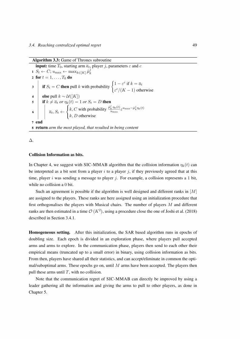
3.4. Reaching centralized optimal regret 49
Algorithm 3.3: Game of Thrones subroutineinput: time T0, starting arm at, player j, parameters ε and c
1 St ← C; umax ← maxk∈[K] µjk
2 for t = 1, . . . , T0 do
3 if St = C then pull k with probability
1− εc if k = at
εc/(K − 1) otherwise4 else pull k ∼ U([K])5 if k 6= at or ηk(t) = 1 or St = D then
6 at, St ←
k,C with probability µjkηk(t)
umaxεumax−µjkηk(t)
k,D otherwise7 end8 return arm the most played, that resulted in being content
∆.
Collision Information as bits.
In Chapter 4, we suggest with SIC-MMAB algorithm that the collision information ηk(t) can
be interpreted as a bit sent from a player i to a player j, if they previously agreed that at this
time, player i was sending a message to player j. For example, a collision represents a 1 bit,
while no collision a 0 bit.
Such an agreement is possible if the algorithm is well designed and different ranks in [M ]are assigned to the players. These ranks are here assigned using an initialization procedure that
first orthogonalises the players with Musical chairs. The number of players M and different
ranks are then estimated in a timeO(K2), using a procedure close the one of Joshi et al. (2018)
described in Section 3.4.1.
Homogeneous setting. After this initialization, the SAR based algorithm runs in epochs of
doubling size. Each epoch is divided in an exploration phase, where players pull accepted
arms and arms to explore. In the communication phase, players then send to each other their
empirical means (truncated up to a small error) in binary, using collision information as bits.
From then, players have shared all their statistics, and can accept/eliminate in common the opti-
mal/suboptimal arms. These epochs go on, until M arms have been accepted. The players then
pull these arms until T , with no collision.
Note that the communication regret of SIC-MMAB can directly be improved by using a
leader gathering all the information and giving the arms to pull to other players, as done in
Chapter 5.
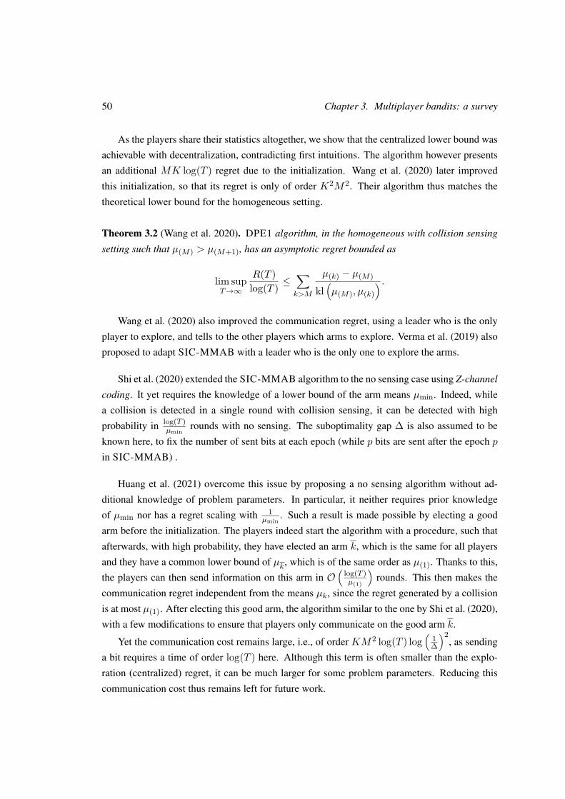
50 Chapter 3. Multiplayer bandits: a survey
As the players share their statistics altogether, we show that the centralized lower bound was
achievable with decentralization, contradicting first intuitions. The algorithm however presents
an additional MK log(T ) regret due to the initialization. Wang et al. (2020) later improved
this initialization, so that its regret is only of order K2M2. Their algorithm thus matches the
theoretical lower bound for the homogeneous setting.
Theorem 3.2 (Wang et al. 2020). DPE1 algorithm, in the homogeneous with collision sensing
setting such that µ(M) > µ(M+1), has an asymptotic regret bounded as
lim supT→∞
R(T )log(T ) ≤
∑k>M
µ(k) − µ(M)
kl(µ(M), µ(k)
) .Wang et al. (2020) also improved the communication regret, using a leader who is the only
player to explore, and tells to the other players which arms to explore. Verma et al. (2019) also
proposed to adapt SIC-MMAB with a leader who is the only one to explore the arms.
Shi et al. (2020) extended the SIC-MMAB algorithm to the no sensing case using Z-channel
coding. It yet requires the knowledge of a lower bound of the arm means µmin. Indeed, while
a collision is detected in a single round with collision sensing, it can be detected with high
probability in log(T )µmin
rounds with no sensing. The suboptimality gap ∆ is also assumed to be
known here, to fix the number of sent bits at each epoch (while p bits are sent after the epoch p
in SIC-MMAB) .
Huang et al. (2021) overcome this issue by proposing a no sensing algorithm without ad-
ditional knowledge of problem parameters. In particular, it neither requires prior knowledge
of µmin nor has a regret scaling with 1µmin
. Such a result is made possible by electing a good
arm before the initialization. The players indeed start the algorithm with a procedure, such that
afterwards, with high probability, they have elected an arm k, which is the same for all players
and they have a common lower bound of µk, which is of the same order as µ(1). Thanks to this,
the players can then send information on this arm in O(
log(T )µ(1)
)rounds. This then makes the
communication regret independent from the means µk, since the regret generated by a collision
is at most µ(1). After electing this good arm, the algorithm similar to the one by Shi et al. (2020),
with a few modifications to ensure that players only communicate on the good arm k.
Yet the communication cost remains large, i.e., of order KM2 log(T ) log(
1∆
)2, as sending
a bit requires a time of order log(T ) here. Although this term is often smaller than the explo-
ration (centralized) regret, it can be much larger for some problem parameters. Reducing this
communication cost thus remains left for future work.
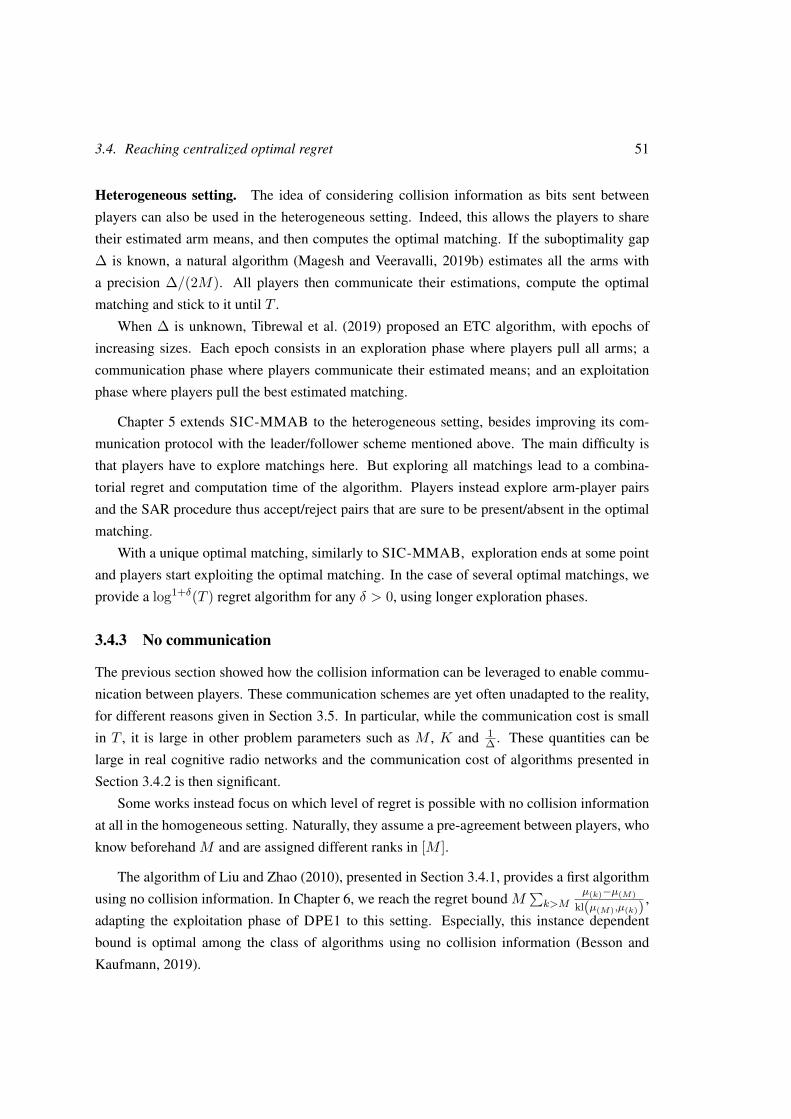
3.4. Reaching centralized optimal regret 51
Heterogeneous setting. The idea of considering collision information as bits sent between
players can also be used in the heterogeneous setting. Indeed, this allows the players to share
their estimated arm means, and then computes the optimal matching. If the suboptimality gap
∆ is known, a natural algorithm (Magesh and Veeravalli, 2019b) estimates all the arms with
a precision ∆/(2M). All players then communicate their estimations, compute the optimal
matching and stick to it until T .
When ∆ is unknown, Tibrewal et al. (2019) proposed an ETC algorithm, with epochs of
increasing sizes. Each epoch consists in an exploration phase where players pull all arms; a
communication phase where players communicate their estimated means; and an exploitation
phase where players pull the best estimated matching.
Chapter 5 extends SIC-MMAB to the heterogeneous setting, besides improving its com-
munication protocol with the leader/follower scheme mentioned above. The main difficulty is
that players have to explore matchings here. But exploring all matchings lead to a combina-
torial regret and computation time of the algorithm. Players instead explore arm-player pairs
and the SAR procedure thus accept/reject pairs that are sure to be present/absent in the optimal
matching.
With a unique optimal matching, similarly to SIC-MMAB, exploration ends at some point
and players start exploiting the optimal matching. In the case of several optimal matchings, we
provide a log1+δ(T ) regret algorithm for any δ > 0, using longer exploration phases.
3.4.3 No communication
The previous section showed how the collision information can be leveraged to enable commu-
nication between players. These communication schemes are yet often unadapted to the reality,
for different reasons given in Section 3.5. In particular, while the communication cost is small
in T , it is large in other problem parameters such as M , K and 1∆ . These quantities can be
large in real cognitive radio networks and the communication cost of algorithms presented in
Section 3.4.2 is then significant.
Some works instead focus on which level of regret is possible with no collision information
at all in the homogeneous setting. Naturally, they assume a pre-agreement between players, who
know beforehand M and are assigned different ranks in [M ].
The algorithm of Liu and Zhao (2010), presented in Section 3.4.1, provides a first algorithm
using no collision information. In Chapter 6, we reach the regret bound M∑k>M
µ(k)−µ(M)kl(µ(M),µ(k)) ,
adapting the exploitation phase of DPE1 to this setting. Especially, this instance dependent
bound is optimal among the class of algorithms using no collision information (Besson and
Kaufmann, 2019).
52 Chapter 3. Multiplayer bandits: a survey
Despite being asymptotically optimal, this algorithm suffers a considerable regret when the
suboptimality gap ∆ is close to 0. It indeed relies on the fact that if the arm rankings of the
players are the same, there is no collision, while the complementary event appears an order 1∆2
of rounds.
Bubeck et al. (2020a) instead focused on reaching a√T log(T ) minimax regret without
collision information. A preliminary work (Bubeck and Budzinski, 2020) proposed a first ge-
ometric solution for two players and three arms, before being extended to general numbers of
players and arms with combinatorial arguments. Their algorithm has 0 collision with high prob-
ability, using a colored partition of [0, 1]K , where a color gives a matching between players and
arms. Thus, the estimation µµµj of all arms by a player gives a point in [0, 1]K and consequently,
an arm to pull for this player. The key of the algorithm is that for close points in [0, 1]K , different
matchings might be assigned, but they do not overlap, i.e., if players have close estimations µµµj
and µµµi, they still pull different arms. Such a coloring implies that for some regions, players might
deliberately pull suboptimal arms, but at a small cost, to avoid collisions with other players.
Unfortunately, the algorithm of Bubeck et al. (2020a) still suffers a dependency MK11/2 in
the regret, which grows considerably with the number of channels K.
3.5 Towards realistic considerations
Section 3.4 proposes algorithms reaching very good regret guarantees for different settings.
Most of these algorithms are yet unrealistic, e.g., a large amount of communication occurs
between the players, while only a very small level of communication is possible between the
players in practice. The fact that good theoretical algorithms are actually bad in practice empha-
sizes that the model of Section 3.3.1 is not well designed. In particular, it might be too simple
with respect to the real problem of cognitive radio networks.
Section 3.4.3 suggests that this discrepancy might be due to the fact that the number of
secondary users and channels (M and K) is actually very large, and the dependency on these
terms is as significant as the dependency in T . This kind of question even appears in the bandits
literature for a single player (and a very large number of arms). Recent works showed that the
greedy algorithm actually performs very well in this single player setting, confirming a behavior
that might be observed in some real cases (Bayati et al., 2020; Jedor et al., 2021).
This section proposes other reasons for this discrepancy. Several simplifications are removed
in the multiplayer model, hoping that good theoretical algorithms in these new settings are also
reasonable in practice. First, the stochasticity of the rewardXk is questioned in Section 3.5.1 and
replaced by either Markovian, abruptly changing or adversarial rewards. The current collision
3.5. Towards realistic considerations 53
model is then relaxed in Section 3.5.2. It instead considers a more realistic and difficult model
where players only observe a decrease in reward when colliding. Section 3.5.3 considers non-
collaborative players, which can be either adversarial or strategic. A dynamic setting, where
secondary users do not enter or leave the network at the same instant, is finally considered in
Section 3.5.4.
3.5.1 Non-stochastic rewards
Most existing works in multiplayer bandits assume that the rewards Xk(t) are stochastic, i.e.,
they are drawn according to the same distribution at each round. This assumption might be too
simple for the problem of cognitive radio networks, and other settings can instead be adapted
from the bandits literature. It has indeed been the case for markovian rewards, abruptly changing
rewards and adversarial rewards, as described in this section.
Markovian rewards.
A first more complex model is given by markovian rewards. This model is rather natural in the
licensed band paradigm, where the presence probability of a primary user on a band might be
conditioned on its presence in the previous step. A primary user might indeed uses the band in
blocks, in which case the probability of occupation of a band for the next round is larger if it is
already occupied. In this model introduced by Anantharam et al. (1987b), the reward Xjk of arm
k for player j follows an irreducible, aperiodic, reversible Markov chain on a finite space. Given
the transition probability matrix P jk , if the last observed reward of arm k for player j is x, then
player j will observe x′ on this arm for the next pull with probability P jk (x, x′).
Given the stationary distribution pjk of the Markov chain represented by P jk , the expected
reward of arm k for player j is then equal to
µjk =∑x∈X
xpjk(x),
where X ⊂ [0, 1] is the state space. The regret then compares the performance of the algorithm
with the reward obtained by pulling the maximal matching with respect to µ at each round.
Anantharam et al. (1987b) proposed an optimal centralized algorithm for this setting, based
on a UCB strategy. Kalathil et al. (2014) later proposed a first decentralized algorithm for this
setting. Their algorithm follows the same lines as the algorithm described in Section 3.4.2 for the
stochastic case. Recall that it uses explicit communication between players to assign the arms
to pull. The only difference is that the UCB index has to be adapted to the markovian model.
The uncertainty is indeed larger in this setting, and the regret is thus larger as well. Bistritz and
54 Chapter 3. Multiplayer bandits: a survey
Leshem (2020) also showed that the GoT algorithm can be directly extended to this model, with
a proper tuning of its different parameters.
In a more recent work, Gafni and Cohen (2021) instead consider a restless Markov chain,
i.e., the state of an arm changes according to the Markov chain at each round, even when it is not
pulled. Using an ETC approach, they were thus able to reach a stable matching in a logarithmic
time. Their algorithm yet assumes the knowledge of the suboptimality gap ∆ and the uniqueness
of the stable (Pareto optimal) matching. The main difficulty of the restless setting is that the
exploration phase has to be carefully done in order to correctly estimate the expected reward of
each arm. This adds a dedicated random amount of time at the start of every exploration phase.
Abruptly changing rewards.
Although markovian rewards are closer to the reality, the resulting algorithms are very similar
to the stochastic case. Indeed, the goal is still to pull the arm with the expected mean overall,
while the change is just on its reward distribution.
A stronger model assumes instead that the expected rewards abruptly change over time, e.g.,
the mean vector µ is piecewise constant with the time, and each change is a breakpoint. It still
illustrates the fact that primary users might occupy the bands in blocks, but it here uses a harder,
frequentist point of view. Even in the single player case, this problem is far from being solved
(see e.g. Auer et al., 2019; Besson et al., 2020).
Wei and Srivastava (2018) considered this setting for the homogeneous multiplayer bandits
problem. Assuming a pre-agreement on the ranks of players, they propose an algorithm with
regret of order T1+ν
2 log(T ) where the number of breakpoints is O (T ν). Players use UCB
indices computed on sliding windows of length O(t
1−ν2)
, i.e., they compute the indices using
only the observations of the last t1−ν
2 rounds. Based on this, player k either rotates on the top-M
indices or focuses on the k-th best index to avoid collisions with other players.
Adversarial rewards.
The hardest model for rewards is the adversarial case, where the rewards are fixed by an adver-
sary. Although this model might be less motivated by cognitive radios, it has a strong theoretical
interest, as it considers the worst case sequence of generated rewards. In this case, the goal is to
provide a minimax regret bound that holds under any problem instance. For the homogeneous
stochastic case, we show in Chapter 4 that SIC-MMAB algorithm has a K√T log(T ) regret.
Bubeck et al. (2020b) showed that for an adaptive adversary, who chooses the rewardsXk(t)of the next round based on the previous decisions of the players, the lower bound is linear with
3.5. Towards realistic considerations 55
T . The literature thus focuses on an oblivious adversary, who chooses beforehand the sequences
of adversarial rewards Xk(t).
Bande and Veeravalli (2019) proposed a first algorithm based on the celebrated EXP.3 al-
gorithm. The EXP.3 algorithm pulls the arm k with a probability proportional to e−ηSk where
η is the learning rate and Sk is an estimator of∑s<tXk(s). Not all the terms of this sum are
observed, justifying the use of an estimator. To avoid collisions, Bande and Veeravalli (2019)
run EXP.3 in blocks of size√T . In each of these blocks, the players start by pulling with respect
to the probability distribution of EXP.3 until finding a free arm, thanks to collision sensing. Af-
terwards, the player keeps pulling this arm until the end of the block. This algorithm yields a
regret of order T 3/4. Dividing EXP.3 in blocks thus degrades the regret by a factor T 1/4 here.
Alatur et al. (2020) proposed a similar algorithm, with a leader-followers structure. At the
beginning of each block, the leader communicates to the followers the arms they have to pull for
this block, still using the probability distribution of EXP.3. Also, the size of each block is here
of order T 1/3, leading to a better regret scaling with T 2/3.
Shi and Shen (2020) later extended this algorithm to the no sensing setting. They introduce
the attackability of the adversary, which is the length of the longest possible sequence ofXk = 0on an arm. Knowing this quantity W , a bit can indeed be correctly sent in time W + 1. When
the attackability is of order Tα and α is known, the algorithm of Alatur et al. (2020) can then be
adapted and yields a regret of order T2+α
3 .
The problem is much harder when α is unknown. In this case, the players estimate α by
starting from 0 and increasing this quantity by ε at each communication failure. To keep the
players synchronized with the same estimate of α, the followers then report the communication
failure to the leader. These reports are crucial and can also fail because of 0 rewards. Shi and
Shen (2020) here use error detection code and randomized communication rounds to avoid such
situations.
Bubeck et al. (2020b) were the first to propose a√T regret algorithm for the collision sens-
ing setting, but only with two players. Their algorithm works as follows: a first player follows
a low switching strategy, e.g., she changes the arm to pull after a random number of times of
order√T , while the second player follows a high-switching strategy, given by EXP.3, on all
the arms except the one pulled by the first player. At each change of arm for the first player, a
communication round then occurs so that the second player is aware of the choice of the first
one.
This algorithm requires a shared randomness between the players, as the first player changes
her arm at random times. Yet, the players can choose a common seed during the initialization,
avoiding the need for this assumption.
56 Chapter 3. Multiplayer bandits: a survey
Bubeck et al. (2020b) also proposed a T 1− 12M algorithm for the no sensing setting. For two
players, the first, low-switching player runs an algorithm on the arms 2, . . . ,K and divide the
time in fixed blocks of length of order√T . Meanwhile on each block, the high-switching player
runs EXP.3 on an increasing set St starting from St = 1. At random times, this player pulls
arms not in St and adds them in the set St if they get a positive reward. The arm pulled by the
first player is then never added to St.
For more than two players, Bubeck et al. (2020b) generalize this algorithm using blocks of
different size for different players.
3.5.2 Different collision models
As shown in Section 3.4.2, the collision information allows communication between the different
players. The discrepancy between the theoretical and practical algorithms might then be due to
the collision model, which is here too strict as a collision systematically corresponds to a 0.
Non-zero collision reward. Depending on the used transmission protocol, the presence of
several users on the same channel does not necessarily lead to an absence of transmission in
practice, but only in a decrease of its quality. Moreover, the number of secondary users can
exceed the number of channels. This harder setting was introduced by Tekin and Liu (2012). In
the heterogeneous setting, when player j pulls an arm k, the expectation of the random variable
Xjk(t) also depends on the total number of players pulling this arm. The problem parameters are
then given by the functions µjk(m) which are the expectation of Xjk when exactly m players are
pulling the arm k. Naturally, the function µjk is non-increasing in m. The regret then compares
the cumulative reward with the one obtained by the best allocation of players through the dif-
ferent arms. Note that in this problem, there is no need to assume M ≤ K anymore as several
players can be assigned to the same arm without leading to 0 rewards on this arm.
Tekin and Liu (2012) proposed a first ETC algorithm, when players know the suboptimality
gap of the problem and always observe the number of players pulling the same arm as they do.
These assumptions are pretty strong and are not considered in the more recent literature.
Bande and Veeravalli (2019) also proposed an ETC algorithm, still with the prior knowledge
of the suboptimality gap. During the exploration, players pull all arms at random. The main
difficulty is that when players observe a reward, they do not know how many other players are
also pulling this arm. Bande and Veeravalli (2019) overcome this issue by assuming that the
decrease in mean rewards with the number of players is large enough with respect to the noise
in the reward. As a consequence, the observed rewards on a single arm can then be perfectly
clustered, where each cluster exactly corresponds to the observations for a given number of
3.5. Towards realistic considerations 57
players pulling the arm.
In practice, this assumption is actually very strong and means that the observed rewards
are almost noiseless. Magesh and Veeravalli (2019a) instead assume that all the players have
different ranks. Thanks to this, they can coordinate their exploration, so that all players can
explore each arm k with a known and fixed number of players m pulling it. Exploring for
all arms and all numbers of players m then allows the players to know their own expectations
µjk(m) for each k and m. From there, the players can reach the optimal allocation using a Game
of Thrones routine similar to Algorithm 3.3. This work thus extended the known results for this
routine to the harder setting of non-zero rewards in case of collision.
Bande et al. (2021) recently used a similar exploration for the homogeneous setting. In this
case, the allocation routine is not even needed as players can compute the optimal allocation
solely based on their own arm means.
When the arm mean is exactly inversely proportional, i.e., µjk(m) = µjk(1)m , Boyarski et al.
(2021) exploit this assumption to defer a simple O(log3+δ(T )
)regret algorithm. During the
exploration phase, all players first pull each arm k altogether and estimate µjk(M). From there,
they add a block where they pull the arm 1 with probability 12 , allowing to estimate M and thus
the whole functions µjk. The optimal matching is then assigned following a GoT subroutine.
Competing bandits. A recent stream of literature considers another collision model where
only one of the pulling players gets the arm reward, based on preferences of the arm. This
setting, introduced by Liu et al. (2020b), was initially not motivated by cognitive radio networks
and is thus discussed later in Section 3.6.2. An asymmetric collision model is also used for
decentralized queuing systems, which are discussed in Section 3.6.3 and studied in Chapter 7.
3.5.3 Non-collaborative players
Assuming perfectly collaborative players might be another oversimplification of the usual mul-
tiplayer bandits model. A short survey by Attar et al. (2012) presents the different security chal-
lenges for cognitive radio networks. Roughly, these threats are divided into two types: jamming
attacks and selfish players, which both appear as soon as players are no more fully cooperative.
Jammers. Jamming attacks can happen either from agents external to the network, or directly
within the network. Their goal is to deteriorate the performance of other agents as much as
possible. In the first case, it can be seen as malicious manipulations of the rewards generated on
each arm. Wang et al. (2015) then propose to consider the problem as an adversarial instance
and use EXP.3 algorithm in the centralized setting.
58 Chapter 3. Multiplayer bandits: a survey
Sawant et al. (2019) on the other side consider jammers directly within the network. The
jammers thus aim at causing a maximal loss of the other players by either pulling the best
arms or creating collisions. Without any restriction on the jammers’ strategy, they can perfectly
adapt to the other players’ strategy and cause tremendous losses. Because of this, the jammers’
strategy is restricted to pulling at random the top J-arms for any J ∈ [K], either in a centralized
(no collision between jammers) or decentralized way. The players then use an ETC algorithm,
where the exploration aims at estimating the arm means, but also both the number of players and
the number of jammers. Afterwards, they exploit by sequentially pulling the top J-arms where
J is chosen to maximize the earned reward.
Fairness. A first attempt at preventing from selfish behaviors is to ensure fairness of the al-
gorithms, as noted by Attar et al. (2012). A fair algorithm should not favor some player with
respect to another. In the homogeneous setting, a first definition of fairness is to guarantee the
same expected rewards to all players (Besson and Kaufmann, 2018a). Note that all symmetric
algorithms (i.e., no prior ranking of the players) ensure this property. A stronger notion would
be to guarantee the same asymptotic rewards to all players without expectation4, which can still
be easily reached by making the players sequentially pull all the top-M arms in the exploitation
phase.
The notion of fairness becomes complex in the heterogeneous setting, since it can be an-
tagonistic to the maximization of the collective reward. Bistritz et al. (2021) consider max-min
fairness, which is broadly used in the resource allocation literature. Instead of maximizing the
sum of players’ rewards, the goal is to maximize the minimal reward earned by each player at
each round. They propose an ETC algorithm which determines the largest possible γ such that
all players can earn at least γ at each round. For the allocation, the players follow a specific
Markov chain to determine whether players can all reach some given γ. If instead the objective
is for each player j to earn at least γj for some known and feasible vector γγγ, there is no need to
explore which is the largest possible γ and the regret becomes constant.
Selfish players. While jammers try to cause a huge loss to other players at any cost, selfish
players have a different objective: they maximize their own individual reward. In the algorithms
mentioned so far, a selfish player could largely improve her earned regret at the expense of the
other players. Chapter 6 proposes algorithms robust to selfish players, being a O(log(T ))-Nash
equilibrium. Without collision information, we adapt DPE1 without communication between
the players. The main difficulty comes from designing a robust initialization protocol to assign
4This notion is defined ex post, as opposed to the previous one which is ex ante.
3.5. Towards realistic considerations 59
ranks and estimate M . With collision information, we even show that robust communication
based algorithms are possible, thanks to a Grim Trigger strategy which punishes all players as
soon as a deviation from the collective strategy is detected. The centralized performances are
thus still possible with selfish players.
Reaching the optimal matching might not be possible in the heterogeneous case because
of the strategic feature of the players. Instead, we focus on reaching the average reward when
following the Random Serial Dictatorship algorithm, which has good strategic guarantees in this
setting (Abdulkadiroglu and Sönmez, 1998).
Brânzei and Peres (2019) consider a different strategic multiplayer bandits game. First, their
model is collisionless and players still earn some reward when pulling the same arm. Also, they
consider two players and a one armed bandit game, with a prior over the arm mean. Players
observe both their obtained reward and the choice of the other player.
They then compare the different Nash equilibria when players are either collaborative (max-
imizing sum of two rewards), neutral (maximizing their sole reward) and competitive (maximiz-
ing the difference between their reward and the other player’s reward). Players tend to explore
more when cooperative and less when competitive. A similar behavior is intuitive in the classi-
cal model of multiplayer bandits as selfish players would more aggressively appropriate the best
arms to keep them for a long time.
3.5.4 Dynamic case
Most of the multiplayer algorithms depend on a high level of synchronisation between the play-
ers. In particular, they assume that all players respectively start and end the game at times t = 1and t = T . This assumption actually makes the problem much simpler because it allows a
high level of synchronisation, while being unrealistic since secondary users enter and leave the
network at different time steps.
The dynamic model thus proposes a weaker level of synchronisation: the time step division
remains global and shared by all players, but players enter and leave the bandits instance at
different (unknown) times. This is different from asynchronicity, which corresponds to a het-
erogeneous time division between players and has been very little studied in theory (Bonnefoi
et al., 2017).
The MEGA algorithm of Avner and Mannor (2014) was the first proposed algorithm to deal
with this dynamic model. The exact same algorithm as the one described in Section 3.4.1 still
reaches a regret of order NT23 in this case, where N is the total number of players entering or
leaving the network.
In general, N is assumed to be sublinear in T as otherwise players would enter and leave
60 Chapter 3. Multiplayer bandits: a survey
the network too fast to learn the different problem parameters. Rosenski et al. (2016) propose to
divide the game duration into√NT epochs of equal size and run independently the MUSICAL
CHAIRS algorithm on each epoch. The number of failing epochs is at most N and their total
incurred regret is thus of order√NT . Finally, the total regret by this algorithm is of order√
NT K2 log(T )∆2 .
This technique can be used to adapt any static algorithm, but it requires the knowledge of
the number of entering/leaving players N , as well as a shared clock between players, to remain
synchronized on each epoch. Because it also works in time windows of size√T , the algorithm
of Bande and Veeravalli (2019) in the adversarial setting still has T34 regret guarantees in the
dynamic setting.
On the other hand, Bande and Veeravalli (2019) and Bande et al. (2021) propose to adapt
their static algorithms, with epochs of linearly increasing size. Players do not need to know N
here, but instead need a stronger shared clock, since they also need to know in which epoch they
currently are.
Besides requiring some strong assumption on either players’ knowledge or synchronisation,
this kind of technique also leads to large dependencies in T . Players indeed run independent
algorithms on a large number of time windows and thus suffer a considerable loss when summing
over all the epochs.
To avoid this kind of behavior, Chapter 4 considers a simpler dynamic setting, where players
can enter at any time but all leave the game at time T . We propose a no sensing ETC algorithm,
which requires no prior knowledge and no further assumption. The idea is that exploring uni-
formly at random is robust to the entering/committing of other players. The players then try to
commit on the best known available arm. This algorithm leads to a NK log(T )∆2 regret.
On the other hand, the algorithm by Darak and Hanawal (2019) recovers from the event
of entry/leave of a player after some time depending on the problem parameters. However,
if enter/leave events happen in a short time window, the algorithm has no guarantees. This
algorithm is thus adapted to another simpler dynamic setting, where the events of entering or
leaving of a new player are separated from a minimal duration.
3.6 Related problems
This section introduces related problems that have also been considered in the literature. All
these models consider a bandits game with multiple agents with some level of interaction be-
tween the agents. Because of these similarities with multiplayer bandits, methods and techniques
mentioned in this survey can be directly used or adapted to these related problems.
3.6. Related problems 61
The widely studied problem of multi-agent bandits is first mentioned. Section 3.6.2 then
introduces the problem of competing bandits, motivated by matching markets. Section 3.6.3
finally discusses the problem of queuing systems, motivated by packet routing to servers.
3.6.1 Multi-agent bandits
The multi-agent bandits problem (also called cooperative bandits and distributed bandits) in-
troduced by Awerbuch and Kleinberg (2008) considers a bandit game played by M players.
Motivated by distributed networks where agents can share their cumulated information, players
here encounter no collision when pulling the same arm: their goal is to collectively determine
the best arm. While running a single player algorithm such as UCB already yields regret guaran-
tees, players can improve their performance by collectively sharing some information. The way
players can communicate yet remains limited: they can only directly communicate with their
neighbours in a given graph G.
This problem has been widely studied in the past years, and we do not claim to provide an
extensive review of its literature.
Many algorithms are based on a gossip procedure, which is widely used in the more general
field of decentralized computation. Roughly, a player i updates its estimates xi by averaging
(potentially with different weights) the estimates xj of her neighbors j. Mathematically, the
estimated vector xxx is updated as follows:
xxx← Pxxx,
where P is a communication matrix. To respect the communication graph structure, Pi,j > 0 if
and only if the edge (i, j) is in G. P thus gives the weights used to average these estimates.
Szorenyi et al. (2013) propose an ε-greedy strategy with gossip based updates, while Land-
gren et al. (2016) propose gossip UCB algorithms. Their regret decomposes in two terms: a
centralized term approaching the regret incurred by a centralized algorithm and a term, which is
constant in T but depends on the spectral gap of the communication matrix P , which can be seen
as the delay to pass a message along the graph with the gossip procedure. Improving this graph
dependent term is thus the main focus of many works. Martínez-Rubio et al. (2018) propose a
UCB algorithm with gossip acceleration techniques, improving upon previous work (Landgren
et al., 2016).
Another common procedure is to elect a leader in the graph, who sends the arm (or distri-
bution) to pull to the other players. In particular, Wang et al. (2020) adapt the DPE1 algorithm
described in Section 3.4.2 to the multi-agent bandits problem. The leader is the only exploring
62 Chapter 3. Multiplayer bandits: a survey
player and sends her best empirical arm to the other players. Besides having an optimal regret
bound in T , the second term of the regret due to communication scales with the diameter of the
graph G. Moreover, this algorithm only requires for the players to send 1-bit messages at each
time step, while most multi-agent bandits work assume that the players can send real messages
with infinite precision.
In the adversarial setting, Bar-On and Mansour (2019) propose to elect local leaders who
send the distribution to play to their followers, based on EXP.3. Instead of focusing on the
collective regret as usually done, they provide good individual regret guarantees.
Another line of work assumes that a player observes the rewards of all her neighbors at each
time step. Cesa-Bianchi et al. (2019b) even assume to observe rewards of all players at distance
at most d, with a delay depending on the distance of the player. EXP.3 with smartly chosen
weights then allows to reach a small regret in the adversarial setting.
More recent works even assume that the players are asynchronous, i.e., players are active at
a given time step with some activation probability. This is for example similar to the model by
Bonnefoi et al. (2017) in the multiplayer setting. Cesa-Bianchi et al. (2020) then use an Online
Mirror Descent based algorithm for the adversarial setting. Della Vecchia and Cesari (2021)
extended this idea in the combinatorial setting, where players can pull multiple arms.
Similarly to multiplayer bandits, the problem of multi-agent bandits is wide and many di-
rections remain to be explored. For instance, Vial et al. (2020) recently proposed an algorithm
that is robust to malicious players. While malicious players cannot create collisions on purpose
here, they can still send corrupted information to their neighbors, leading to bad behaviors.
3.6.2 Competing bandits
The problem of competing bandits was first introduced by Liu et al. (2020b), motivated by decen-
tralized learning processes in matching markets. This model is very similar to the heterogeneous
multiplayer bandits: they only differ in their collision model. Here, arms also have preferences
over players: j k j′ means that the arm k prefers being pulled by the player j over j′. When
several players pull the same arm k, only the top-ranked player for arm k gets its reward, while
the others receive no reward. Mathematically the collision indicator is thus defined as:
ηjk(t) = 1(∃j′ k j such that πj
′(t) = k).
As often in bipartite matching problems, the goal is thus to reach a stable matching be-
tween players and arms. A matching is stable if every unmatched pair (j, k) would prefer to be
matched. Mathematically, this corresponds to the following definition.
3.6. Related problems 63
Definition 3.2. A matching π : [M ] → [K] is stable if for all j 6= j′, either µjπ(j) > µjπ(j′) or
j′ π(j′) j and for all unmatched arms k, µjπ(j) > µjk.
Several stable matchings can exist. Two different definitions of individual regret then appear.
First the optimal regret compares with the best possible arm for player j in a stable matching,
noted kj :
Rj(T ) = µjkjT −
T∑t=1
µjπj(t) · (1− η
jπj(t)(t)).
Similarly, the pessimal regret is defined with respect to the worst possible arm for player j
in a stable matching, noted kj :
Rj(T ) = µjkjT −
T∑t=1
µjπj(t) · (1− η
jπj(t)(t)).
Liu et al. (2020b) propose a centralized UCB algorithm, where at each time step, the players
send their UCB indexes to a central agent. This agent computes the optimal stable matching
based on these indexes using the celebrated Gale Shapley algorithm and the players then pull
according to the output of Gale Shapley algorithm. Although being natural, this algorithm only
reaches a logarithmic regret for the pessimal definition, but can still incur a linear optimal regret.
Cen and Shah (2021) showed that a logarithmic optimal regret is reachable for this algorithm,
if the platform can also choose transfers between the players and arms. The idea is to smartly
choose the transfers, so that the optimal matching is the only stable matching when taking into
account these transfers.
Liu et al. (2020b) also propose an ETC algorithm reaching a logarithmic optimal regret.
After the exploration, the central agent computes the Gale Shapley matching which is pulled
until T . A decentralized version of this algorithm is even possible, as Gale Shapley can be run in
times N2 in a decentralized way when observing the collision indicators ηjk. This decentralized
algorithm yet requires prior knowledge of ∆. Basu et al. (2021) extend this algorithm without
knowing ∆, but the regret is then of order log1+ε(T ) for a parameter ε.
Liu et al. (2020a) also propose a decentralized UCB algorithm with a collision avoidance
mechanism. Yet their algorithm requires for the players to observe the actions of all other play-
ers at each time step and only incurs a pessimal regret of order log2(T ), besides having an
exponential dependency in the number of players.
Because of the difficulty of the general problem, even with collision sensing, another line of
work focuses on simple instances of arm preferences. For example, when players are globally
ranked, i.e., all the arms have the same preference orders k, there is a unique stable matching.
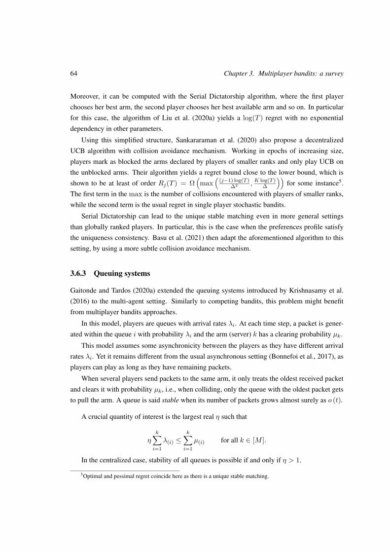
64 Chapter 3. Multiplayer bandits: a survey
Moreover, it can be computed with the Serial Dictatorship algorithm, where the first player
chooses her best arm, the second player chooses her best available arm and so on. In particular
for this case, the algorithm of Liu et al. (2020a) yields a log(T ) regret with no exponential
dependency in other parameters.
Using this simplified structure, Sankararaman et al. (2020) also propose a decentralized
UCB algorithm with collision avoidance mechanism. Working in epochs of increasing size,
players mark as blocked the arms declared by players of smaller ranks and only play UCB on
the unblocked arms. Their algorithm yields a regret bound close to the lower bound, which is
shown to be at least of order Rj(T ) = Ω(max
((j−1) log(T )
∆2 , K log(T )∆
))for some instance5.
The first term in the max is the number of collisions encountered with players of smaller ranks,
while the second term is the usual regret in single player stochastic bandits.
Serial Dictatorship can lead to the unique stable matching even in more general settings
than globally ranked players. In particular, this is the case when the preferences profile satisfy
the uniqueness consistency. Basu et al. (2021) then adapt the aforementioned algorithm to this
setting, by using a more subtle collision avoidance mechanism.
3.6.3 Queuing systems
Gaitonde and Tardos (2020a) extended the queuing systems introduced by Krishnasamy et al.
(2016) to the multi-agent setting. Similarly to competing bandits, this problem might benefit
from multiplayer bandits approaches.
In this model, players are queues with arrival rates λi. At each time step, a packet is gener-
ated within the queue i with probability λi and the arm (server) k has a clearing probability µk.
This model assumes some asynchronicity between the players as they have different arrival
rates λi. Yet it remains different from the usual asynchronous setting (Bonnefoi et al., 2017), as
players can play as long as they have remaining packets.
When several players send packets to the same arm, it only treats the oldest received packet
and clears it with probability µk, i.e., when colliding, only the queue with the oldest packet gets
to pull the arm. A queue is said stable when its number of packets grows almost surely as o (t).
A crucial quantity of interest is the largest real η such that
ηk∑i=1
λ(i) ≤k∑i=1
µ(i) for all k ∈ [M ].
In the centralized case, stability of all queues is possible if and only if η > 1.
5Optimal and pessimal regret coincide here as there is a unique stable matching.
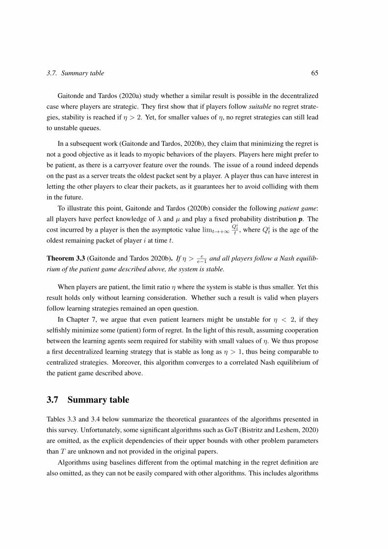
3.7. Summary table 65
Gaitonde and Tardos (2020a) study whether a similar result is possible in the decentralized
case where players are strategic. They first show that if players follow suitable no regret strate-
gies, stability is reached if η > 2. Yet, for smaller values of η, no regret strategies can still lead
to unstable queues.
In a subsequent work (Gaitonde and Tardos, 2020b), they claim that minimizing the regret is
not a good objective as it leads to myopic behaviors of the players. Players here might prefer to
be patient, as there is a carryover feature over the rounds. The issue of a round indeed depends
on the past as a server treats the oldest packet sent by a player. A player thus can have interest in
letting the other players to clear their packets, as it guarantees her to avoid colliding with them
in the future.
To illustrate this point, Gaitonde and Tardos (2020b) consider the following patient game:
all players have perfect knowledge of λ and µ and play a fixed probability distribution ppp. The
cost incurred by a player is then the asymptotic value limt→+∞Qitt , where Qit is the age of the
oldest remaining packet of player i at time t.
Theorem 3.3 (Gaitonde and Tardos 2020b). If η > ee−1 and all players follow a Nash equilib-
rium of the patient game described above, the system is stable.
When players are patient, the limit ratio η where the system is stable is thus smaller. Yet this
result holds only without learning consideration. Whether such a result is valid when players
follow learning strategies remained an open question.
In Chapter 7, we argue that even patient learners might be unstable for η < 2, if they
selfishly minimize some (patient) form of regret. In the light of this result, assuming cooperation
between the learning agents seem required for stability with small values of η. We thus propose
a first decentralized learning strategy that is stable as long as η > 1, thus being comparable to
centralized strategies. Moreover, this algorithm converges to a correlated Nash equilibrium of
the patient game described above.
3.7 Summary table
Tables 3.3 and 3.4 below summarize the theoretical guarantees of the algorithms presented in
this survey. Unfortunately, some significant algorithms such as GoT (Bistritz and Leshem, 2020)
are omitted, as the explicit dependencies of their upper bounds with other problem parameters
than T are unknown and not provided in the original papers.
Algorithms using baselines different from the optimal matching in the regret definition are
also omitted, as they can not be easily compared with other algorithms. This includes algorithms

66 Chapter 3. Multiplayer bandits: a survey
taking only a stable matching as baseline in the heterogeneous case, or algorithm which are
robust to jammers for instance.
Here is a list of the different notations used in Tables 3.3 and 3.4.
∆ = minU∗ − U(π) > 0 | π ∈M∆(m,k) = minU∗ − U(π) > 0 | π ∈M and π(m) = k∆(M) = mink≤M µ(k) − µ(k+1)
δ arbitrarily small positive constant
µ(k) k-th largest mean (homogeneous case)
M number of players simultaneously in the game
M set of matchings between arms and players
N total number of players entering/leaving the game (dynamic)
attackability length of longest time sequence with successive Xk(t) = 0rank different ranks are attributed beforehand to players
T horizon
U(π) =∑Mm=1 µ
mπ(m)
U∗ = maxπ∈M U(π)
Model Reference Prior knowledge Extra consideration Upper bound
Centralized CUCB [83] M -M∑m=1
K∑k=1
M log(T )∆(m,k)
Centralized CTS [237] M Independent armsM∑m=1
K∑k=1
log2(M) log(T )∆(m,k)
Coll. sensing dE3 [176] T,∆,M communicating players M3K2 log(T )∆2
Coll. sensing D-MUMAB[165] T,∆ unique optimal matching M log(T )∆2 + KM3 log( 1
∆ ) log(T )log(M)
Coll. sensing ELIM-ETC [61] T δ = 0 if unique optimal matchingK∑k=1
M∑m=1
(M2 log(T )
∆(m,k)
)1+δ
Table 3.3: Summary of presented algorithms in the heterogeneous setting. The last columnprovides the asymptotic upper bound, up to some universal multiplicative constant.
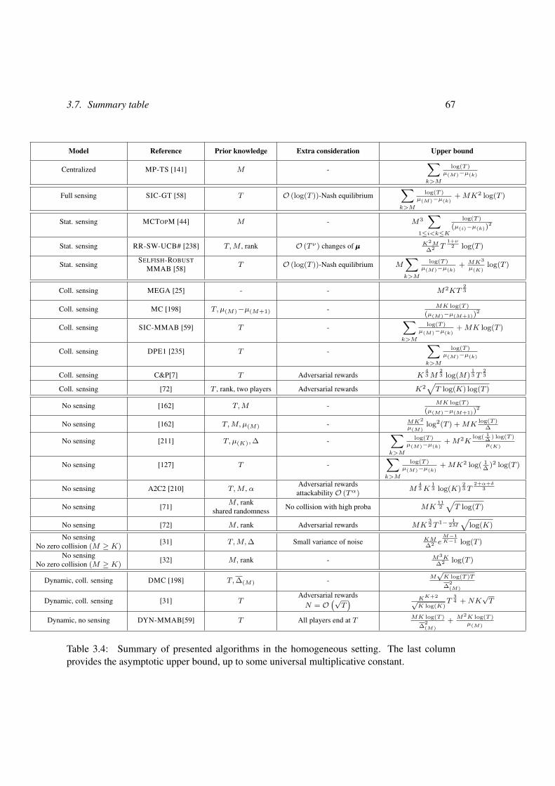
3.7. Summary table 67
Model Reference Prior knowledge Extra consideration Upper bound
Centralized MP-TS [141] M -∑k>M
log(T )µ(M)−µ(k)
Full sensing SIC-GT [58] T O (log(T ))-Nash equilibrium∑k>M
log(T )µ(M)−µ(k)
+MK2 log(T )
Stat. sensing MCTOPM [44] M - M3∑
1≤i<k≤K
log(T )(µ(i)−µ(k))2
Stat. sensing RR-SW-UCB# [238] T,M , rank O (T ν) changes of µµµ K2M∆2 T
1+ν2 log(T )
Stat. sensingSELFISH-ROBUST
MMAB [58] T O (log(T ))-Nash equilibrium M∑k>M
log(T )µ(M)−µ(k)
+ MK3
µ(K)log(T )
Coll. sensing MEGA [25] - - M2KT23
Coll. sensing MC [198] T, µ(M)−µ(M+1) - MK log(T )(µ(M)−µ(M+1))2
Coll. sensing SIC-MMAB [59] T -∑k>M
log(T )µ(M)−µ(k)
+MK log(T )
Coll. sensing DPE1 [235] T -∑k>M
log(T )µ(M)−µ(k)
Coll. sensing C&P[7] T Adversarial rewards K43M
23 log(M)
13 T
23
Coll. sensing [72] T , rank, two players Adversarial rewards K2√T log(K) log(T )
No sensing [162] T,M - MK log(T )(µ(M)−µ(M+1))2
No sensing [162] T,M, µ(M) - MK2
µ(M)log2(T ) +MK
log(T )∆
No sensing [211] T, µ(K),∆ -∑k>M
log(T )µ(M)−µ(k)
+M2Klog( 1
∆ ) log(T )µ(K)
No sensing [127] T -∑k>M
log(T )µ(M)−µ(k)
+MK2 log( 1∆ )2 log(T )
No sensing A2C2 [210] T,M , αAdversarial rewardsattackabilityO (Tα) M
43K
13 log(K)
23 T
2+α+δ3
No sensing [71]M , rank
shared randomness No collision with high proba MK112√T log(T )
No sensing [72] M , rank Adversarial rewards MK32 T 1− 1
2M√
log(K)No sensing
No zero collision (M ≥ K) [31] T,M,∆ Small variance of noise KM∆2 e
M−1K−1 log(T )
No sensingNo zero collision (M ≥ K) [32] M, rank - M3K
∆2 log(T )
Dynamic, coll. sensing DMC [198] T,∆(M) - M√K log(T )T∆2
(M)
Dynamic, coll. sensing [31] TAdversarial rewardsN = O
(√T) KK+2√
K log(K)T
34 +NK
√T
Dynamic, no sensing DYN-MMAB[59] T All players end at T MK log(T )∆2
(M)+ M2K log(T )
µ(M)
Table 3.4: Summary of presented algorithms in the homogeneous setting. The last columnprovides the asymptotic upper bound, up to some universal multiplicative constant.
Chapter 4
SIC-MMAB: Synchronisation InvolvesCommunication in MultiplayerMulti-Armed Bandits
This chapter presents a decentralized algorithm that achieves the same performance as acentralized one for homogeneous multiplayer bandits, by “hacking” the standard model witha communication protocol between players that deliberately enforces collisions, allowingthem to share their information at a negligible cost. This motivates the introduction of amore appropriate dynamic setting without sensing, where similar communication protocolsare no longer possible. However, we show that the logarithmic growth of the regret is stillachievable for this model with a new algorithm.
4.1 Collision Sensing: achieving centralized performances by communicating through
collisions . . . . . . . . . . . . . . . . . . . . . . . . . . . . . . . . . . . . . 69
4.1.1 Some preliminary notations . . . . . . . . . . . . . . . . . . . . . . . 70
4.1.2 Description of our protocol . . . . . . . . . . . . . . . . . . . . . . . . 70
4.1.3 In contradiction with lower bounds? . . . . . . . . . . . . . . . . . . . 76
4.2 Without synchronization, the dynamic setting . . . . . . . . . . . . . . . . . . 77
4.2.1 A logarithmic regret algorithm . . . . . . . . . . . . . . . . . . . . . . 78
4.2.2 A communication-less protocol . . . . . . . . . . . . . . . . . . . . . 78
4.2.3 DYN-MMAB description . . . . . . . . . . . . . . . . . . . . . . . . 80
4.A Experiments . . . . . . . . . . . . . . . . . . . . . . . . . . . . . . . . . . . . 83
4.B Omitted proofs . . . . . . . . . . . . . . . . . . . . . . . . . . . . . . . . . . 84
4.B.1 Regret analysis of SIC-MMAB . . . . . . . . . . . . . . . . . . . . . 84
68
4.1. Collision Sensing: achieving centralized performances by communicating throughcollisions 69
4.B.2 Regret analysis of DYN-MMAB . . . . . . . . . . . . . . . . . . . . . 89
4.C On the inefficiency of SELFISH algorithm . . . . . . . . . . . . . . . . . . . . 94
This chapter considers the homogeneous multiplayer bandits problem introduced in Sec-
tion 3.3.1 and presents the following contributions.
With collision sensing, Section 4.1 introduces a new decentralized algorithm that is “hack-
ing” the setting and induces communication between players through deliberate collisions. The
regret of this algorithm, called SIC-MMAB, reaches asymptotically (up to some universal con-
stant) the lower bound of the centralized problem, contradicting the previously believed lower
bounds. SIC-MMAB relies on the unrealistic assumption that all users start transmitting at the
very same time. It therefore appears that the assumption of synchronization has to be removed
for practical considerations.
Without synchronization or collision observations, Section 4.2 proposes the first algorithm
with a logarithmic regret. The dependencies in the gaps between arm means yet become quadratic.
We compare empirically SIC-MMAB with MCTOPM (Besson and Kaufmann, 2018a) on a
toy example in Section 4.A. Especially, it nicely illustrates how SIC-MMAB scales better with
the suboptimality gap and also confirms its smaller minimax regret bound.
Besson and Kaufmann (2018a) studied the SELFISH algorithm, consisting in unilaterally
following UCB algorithm, and conjectured that it leads to a linear regret with positive (constant)
probability. We prove this conjecture for agents with infinite calculus precision. Yet the question
remains open for machines with finite precision.
4.1 Collision Sensing: achieving centralized performances by com-municating through collisions
In this section, we consider the Collision Sensing model of Section 3.3.1 and prove that the
decentralized problem is almost as complex, in terms of regret growth, as the centralized one.
When players are synchronized, we provide an algorithm with an exploration regret similar
to the known centralized lower bound (Anantharam et al., 1987a). This algorithm strongly
relies on the synchronization assumption, which we leverage to allow communication between
players through observed collisions. The communication protocol is detailed and explained
in Section 4.1.2. This result also implies that the two lower bounds provided in the literature
(Besson and Kaufmann, 2018a; Liu and Zhao, 2010) are unfortunately not correct. Indeed, the
factor M that was supposed to be the cost of the decentralization in the regret should not appear.
Let us describe our algorithm SIC-MMAB. It consists of several phases.
70Chapter 4. SIC-MMAB: Synchronisation Involves Communication in Multiplayer Multi-Armed
Bandits
1. The initialization phase first estimates the number of players and assigns ranks among
them.
2. Players then alternate between exploration phases and communication phases.
(a) During the p-th exploration phase, each arm is pulled 2p times and its performance is
estimated in a Successive Accepts and Rejects fashion (Perchet and Rigollet, 2013;
Bubeck et al., 2013).
(b) During the communication phases, players communicate their statistics to each other
using collisions. Afterwards, the updated common statistics are known to all players.
3. The last phase, the exploitation one, is triggered for a player as soon as an arm is detected
as optimal and assigned to her. This player then pulls this arm until the final horizon T .
4.1.1 Some preliminary notations
Players that are not in the exploitation phase are called active. We denote, with a slight abuse of
notation, by [Mp] the set of active players during the p-th phase of exploration-communication
and by Mp ≤ M its cardinality. Notice that Mp is non increasing because players never leave
the exploitation phase.
Each arm among the top-M ones is called optimal and each other arm is sub-optimal. Arms
that still need to be explored (players cannot determine whether they are optimal or sub-optimal
yet) are active. We denote, with the same abuse of notation, the set of active arms by [Kp] of
cardinality Kp ≤ K. By construction of our algorithm, this set is common to all active players
at each stage.
Our algorithm is based on a protocol called sequential hopping (Joshi et al., 2018). It consists
of incrementing the index of the arm pulled by a specific player m: if she plays arm πm(t) at
time t, she will play πm(t+1) = πm(t)+1 (mod [Kp]) at time t+1 during the p-th exploration
phase.
4.1.2 Description of our protocol
As mentioned above, the SIC-MMAB algorithm consists of several phases. During the commu-
nication phase, players communicate with each other. At the end of this phase, each player thus
knows the statistics of all players on all arms, so that this decentralized problem becomes similar
to the centralized one. After alternating enough times between exploration and communication
phases, sub-optimal arms are eliminated and players are fixed to different optimal arms and will
exploit them until stage T . The complete pseudocode of SIC-MMAB is given by Algorithm 4.6.

4.1. Collision Sensing: achieving centralized performances by communicating throughcollisions 71
Initialization phase
The objective of the first phase is to estimate the number of players M and to assign internalranks to players. First, players follow the Musical Chairs algorithm (Rosenski et al., 2016), de-
scribed by Algorithm 4.1 below, during T0 := dK log(T )e steps in order to reach an orthogonalsetting, i.e., a position where they are all pulling different arms. The index of the arm pulled by
a player at stage T0 will then be her external rank.
Algorithm 4.1: MusicalChairs Protocolinput: [Kp] (active arms), T0 (time of procedure)
1 Initialize Fixed← −12 for T0 time steps do3 if Fixed = −1 then4 Sample k uniformly at random in [Kp] and play it in round t5 if ηk(t) = 0 (rk(t) > 0 for No Sensing setting) then Fixed← k // player
stays in arm k if no collision
6 end7 else Play Fixed8 end9 return Fixed // External rank
The second procedure, given by Algorithm 4.2, determines M and assigns a unique internal
rank in [M ] to each player. For example, if there are three players on arms 5, 7 and 2 at t = T0,
their external ranks are 5, 7 and 2 respectively, while their internal ranks are 2, 3 and 1. Roughly
speaking, the players follow each other sequentially hopping through all the arms so that players
with external ranks k and k′ collide exactly after a time k+k′. Each player then deduces M and
her internal rank from observed collisions during this procedure that lasts 2K steps.
Algorithm 4.2: Estimate_M Protocolinput: k ∈ [K] (external rank)
1 Initialize M ← 1, j ← 1 and π ← k // estimates of M and the internal rank
for 2k time steps do2 Pull π3 if ηπ(t) = 1 then hatM ← hatM + 1 and j ← j + 1 // increases if
collision
4 end5 for 2(K − k) time steps do6 π ← π + 1 (mod K) and pull π // sequential hopping
7 if ηπ(t) = 1 then hatM ← hatM + 1 // increases if collision
8 end9 return hatM, j
72Chapter 4. SIC-MMAB: Synchronisation Involves Communication in Multiplayer Multi-Armed
Bandits
In the next phases, active players will always know the set of active players [Mp]. This is
how the initial symmetry among players is broken and it allows the decentralized algorithm to
establish communication protocols.
Exploration phase
During the p-th exploration phase, active players sequentially hop among the active arms for
Kp2p steps. Each active arm is thus pulled 2p times by each active player. Using their internal
rank, players start and remain in an orthogonal setting during the exploration phase, which is
collision-free.
We denote by Bs = 3√
log(T )2s the error bound after s pulls and by Nk(p) (resp. Sk(p)) the
centralized number of pulls (resp. sum of rewards) for the arm k during the p first exploration
phases, i.e., Nk(p) =∑Mj=1N
jk(p) where Nm
k (p) is the number of pulls for the arm k by player
m during the p first exploration phases. During the communication phase, quantized rewards
Smk (p) will be communicated between active players as described in Section 4.1.2.After a succession of two phases (exploration and communication), an arm k is accepted if
#i ∈ [Kp]
∣∣ µk(p)−BNk(p) ≥ µi(p) +BNi(p)
≥ Kp −Mp,
where µk(p) =∑M
m=1 Smk (p)
Nk(p) is the centralized quantized empirical mean of the arm k1, which is
an approximation of µk(p) = Sk(p)Nk(p) . This inequality implies that k is among the top-Mp active
arms with high probability. In the same way, k is rejected if
#i ∈ [Kp]
∣∣ µi(p)−BNi(p) ≥ µk(p) +BNk(p)
≥Mp,
meaning that there are at least Mp active arms better than k with high probability. Notice that
each player j uses her own quantized statistics Sjk(p) to accept/reject an arm instead of the exact
ones Sjk(p). Otherwise, the estimations µk(p) would indeed differ between the players as well
as the sets of accepted and rejected arms. With Bernoulli distributions, the quantization becomes
unnecessary and the confidence bound can be chosen as Bs =√
2 log(T )/s.
Communication phase
In this phase, each active player communicates, one at a time, her statistics of the active arms
to all other active players. Each player has her own communicating arm, corresponding to her
internal rank. When the player j is communicating, she sends a bit at a time step to the player
l by deciding which arm to pull: a 1 bit is sent by pulling the communicating arm of player
1For a player m already exploiting since the pm-th phase, we instead use the last statistic Smk (p) = Smk (pm).

4.1. Collision Sensing: achieving centralized performances by communicating throughcollisions 73
l (a collision occurs) and a 0 bit by pulling her own arm. The main originality of SIC-MMAB
comes from this trick which allows implicit communication through collisions and is used in
subsequent papers as explained in Section 3.4.2. In an independent work, Tibrewal et al. (2019)
also proposed using similar communication protocols for the heterogeneous case.
As an arm is pulled 2n times by a single player during the n-th exploration phase, it has been
pulled 2p+1− 1 times in total at the end of the p-th phase and the statistic Sjk(p) is a real number
in [0, 2p+1− 1]. Players then send a quantized integer statistic Sjk(p) ∈ [2p+1− 1] to each other
in p + 1 bits, i.e., collisions. Let n = bSjk(p)c and d = Sjk(p) − n be the integer and decimal
parts of Sjk(p), the quantized statistic is then n + 1 with probability d and n otherwise, so that
E[Sjk(p)] = Sjk(p).
Algorithm 4.3: Receive Protocolinput: p (phase number), l (own internal rank), [Kp] (active arms)
1 s← 0 and π ← index of l-th active arm2 for n = 0, . . . , p do3 Pull π4 if ηπ(t) = 1 then s← s+ 2n // other player sends 15 end6 return s (statistic sent by other player)
Algorithm 4.4: Send Protocolinput: l (player receiving), s (statistics to send), p (phase number), j (own internal
rank), [Kp] (active arms)1 s← 0 and π ← index of the l-th active arm2 m← binary writing of s of length p+ 1, i.e., s =
∑pn=0mn2n
3 for n = 0, . . . , p do4 if mn = 1 then Pull the l-th active arm // send 15 else Pull the j-th active arm // send 06 end
An active player can have three possible statuses during the communication phase:
1. either she is receiving some other players’ statistics about the arm k. In that case, she
proceeds to Receive Protocol (see Algorithm 4.3).
2. Or she is sending her quantized statistics about arm k to player l (who is then receiving).
In that case, she proceeds to Send Protocol (see Algorithm 4.4) to send them in a time
p+ 1.
3. Or she is pulling her communicating arm, while waiting for other players to finish com-
municating statistics among them.

74Chapter 4. SIC-MMAB: Synchronisation Involves Communication in Multiplayer Multi-Armed
Bandits
Communicated statistics are all of length p + 1, even if they could be sent with shorter
messages, in order to maintain synchronization among players. Using their internal ranks, the
players can communicate in turn without interfering with each other. The general protocol for
each communication phase is described in Algorithm 4.5 below.
Algorithm 4.5: Communication Protocolinput: s (personal statistics of previous phases), p (phase number), j (own internal
rank), [Kp] (active arms), [Mp] (active players)
1 For all k, sample s[k] =bs[k]c+ 1 with probability s[k]− bs[k]cbs[k]c otherwise
// quantize
2 Define Ep := (i, l, k) ∈ [Mp]× [Mp]× [Kp] | i 6= l and set Sj ← s3 for (i, l, k) ∈ Ep do // Player i sends stats of arm k to player l
4 if i = j then Send (l, s[k], p, j, [Kp]) // sending player
5 else if l = j then Si[k]← Receive(p, j, [Kp]) // receiving player
6 else7 for p+ 1 rounds do pull j-th active arm // wait while others communicate
8 end9 end
10 return S
At the end of the communication phase, all active players know the statistics Sjk(p) and so
which arms to accept or reject. Rejected arms are removed right away from the set of active arms.
Thanks to the assigned ranks, accepted arms are assigned to one player each. The remaining
active players then update both sets of active players and arms as described in Algorithm 4.6,
Line 21.
This communication protocol uses the fact that a bit can be sent with a single collision.
Without sensing, this can not be done in a single time step, but communication is still somehow
possible. A bit can then be sent in log(T )µ(K)
steps with probability 1 − 1T . Using this trick, two
different algorithms relying on communication protocols were proposed No Sensing setting in
the conference version of this chapter (Boursier and Perchet, 2019).
Regret bound of SIC-MMAB
Theorem 4.1 bounds the expected regret incurred by SIC-MMAB and its proof is delayed to
Section 4.B.1.
Theorem 4.1. With the choice T0 = dK log(T )e, for any given set of parameters K, M and µµµ
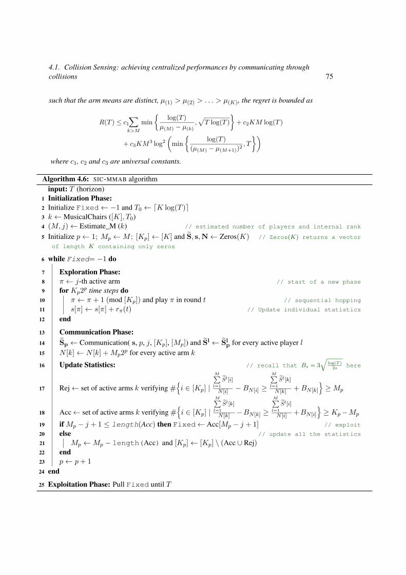
4.1. Collision Sensing: achieving centralized performances by communicating throughcollisions 75
such that the arm means are distinct, µ(1) > µ(2) > . . . > µ(K), the regret is bounded as
R(T ) ≤ c1∑k>M
min
log(T )µ(M) − µ(k)
,√T log(T )
+ c2KM log(T )
+ c3KM3 log2
(min
log(T )
(µ(M) − µ(M+1))2 , T
)where c1, c2 and c3 are universal constants.
Algorithm 4.6: SIC-MMAB algorithminput: T (horizon)
1 Initialization Phase:2 Initialize Fixed← −1 and T0 ← dK log(T )e3 k ←MusicalChairs ([K], T0)4 (M, j)← Estimate_M (k) // estimated number of players and internal rank
5 Initialize p← 1; Mp ←M ; [Kp]← [K] and S, s,N← Zeros(K) // Zeros(K) returns a vector
of length K containing only zeros
6 while Fixed= −1 do
7 Exploration Phase:8 π ← j-th active arm // start of a new phase
9 for Kp2p time steps do10 π ← π + 1 (mod [Kp]) and play π in round t // sequential hopping
11 s[π]← s[π] + rπ(t) // Update individual statistics
12 end
13 Communication Phase:14 Sp ← Communication( s, p, j, [Kp], [Mp]) and Sl ← Sl
p for every active player l15 N [k]← N [k] +Mp2p for every active arm k
16 Update Statistics: // recall that Bs = 3√
log(T )2s here
17 Rej← set of active arms k verifying #i ∈ [Kp] |
M∑l=1
Sl[i]
N [i] −BN [i] ≥
M∑l=1
Sl[k]
N [k] +BN [k]≥Mp
18 Acc← set of active arms k verifying #i ∈ [Kp] |
M∑l=1
Sl[k]
N [k] −BN [k] ≥
M∑l=1
Sl[i]
N [i] +BN [i]≥ Kp−Mp
19 if Mp − j + 1 ≤ length(Acc) then Fixed← Acc[Mp − j + 1] // exploit
20 else // update all the statistics
21 Mp ←Mp − length(Acc) and [Kp]← [Kp] \ (Acc ∪ Rej)22 end23 p← p+ 124 end
25 Exploitation Phase: Pull Fixed until T
76Chapter 4. SIC-MMAB: Synchronisation Involves Communication in Multiplayer Multi-Armed
Bandits
The first, second and third terms respectively correspond to the regret incurred by the ex-
ploration, initialization and communication phases, which dominate the regret due to low prob-
ability events of bad initialization or incorrect estimations. Notice that the minmax regret scales
with O(K√T log(T )).
Experiments on synthetic data are described in Section 4.A. They empirically confirm that SIC-
MMAB scales better than MCTopM (Besson and Kaufmann, 2018a) with the gaps ∆, besides
having a smaller minmax regret.
4.1.3 In contradiction with lower bounds?
Theorem 4.1 is in contradiction with the two lower bounds by Besson and Kaufmann (2018a)
and Liu and Zhao (2010), however SIC-MMAB respects the conditions required for both. It was
thought that the decentralized lower bound was Ω(M∑k>M
log(T )µ(M)−µ(k)
), while the centralized
lower bound was already known to be Ω(∑
k>Mlog(T )
µ(M)−µ(k)
)(Anantharam et al., 1987a). How-
ever, it appears that the asymptotic regret of the decentralized case is not that much different from
the latter, at least if players are synchronized. Indeed, SIC-MMAB takes advantage of this syn-
chronization to establish communication protocols as players are able to communicate through
collisions. The subsequent paper by Proutiere and Wang (2019) later improved the communi-
cation protocols of SIC-MMAB to obtain both initialization and communication costs constant
in T , confirming that the lower bound of the centralized case is also tight for the decentralized
model considered so far.
Liu and Zhao (2010) proved the lower bound “by considering the best case that they do not
collide”. This is only true if colliding does not provide valuable information and the policies just
maximize the losses at each round, disregarding the information gathered for the future. Our al-
gorithm is built upon the idea that the value of the information provided by collisions can exceed
in the long run the immediate loss in rewards (which is standard in dynamic programming or
reinforcement learning for instance). The mistake of Besson and Kaufmann (2018a) is found
in the proof of Lemma 12 after the sentence “We now show that second term in (25) is zero”.
The conditional expectation cannot be put inside/outside of the expectation as written and the
considered term, which corresponds to the difference of information given by collisions for two
different distributions, is therefore not zero.
These two lower bounds disregarded the amount of information that can be deduced from colli-
sions, while SIC-MMAB obviously takes advantage from this information.
Our exploration regret reaches, up to a constant factor, the lower bound of the centralized
problem (Anantharam et al., 1987a). Although it is sub-logarithmic in time, the communication
cost scales with KM3 and can thus be predominant in practice. Indeed for large networks, M3
4.2. Without synchronization, the dynamic setting 77
can easily be greater than log(T ) and the communication cost would then prevail over the other
terms. This highlights the importance of the parameter M in multiplayer MAB and future work
should focus on the dependency in both M and T instead of only considering asymptotic results
in T . The communication scheme of SIC-MMAB is improved in Chapter 5, which reduces its
total cost by a factor larger than M .
Synchronization is not a reasonable assumption for practical purposes and it also leads to
undesirable algorithms relying on communication protocols such as SIC-MMAB. We thus claim
that this assumption should be removed in the multiplayer MAB and the dynamic model should
be considered instead. However, this problem seems complex to model formally. Indeed, if
players stay in the game only for a very short period, learning is not possible. The difficulty to
formalize an interesting and nontrivial dynamic model may explain why most of the literature
focused on the static model so far.
4.2 Without synchronization, the dynamic setting
In the previous section, it was crucial that all exploration/communication phases start and end
at the same time for the SIC-MMAB algorithm. The synchronization assumption we leveraged
was the following.
Assumption 4.1 (Synchronization). Player i enters the bandit game at the time τi = 0 and stays
until the final horizon T . This is common knowledge to all players.
From now on, we no longer assume that players can communicate using synchronization.
This assumption is clearly unrealistic and should be alleviated, as radios do not start and end
transmitting simultaneously.
We instead assume in the following that players do not leave the game once they have started,
as formalized by Assumption 4.2 below.
Assumption 4.2 (Quasi-Asynchronization). Players enter at different times τi ∈ 0, . . . , T −1and stay until the final horizon T . The τi are unknown to all players (including i).
Yet, we mention that our results can also be adapted to the cases when players can leave the
game during specific intervals or share an internal synchronized clock (Rosenski et al., 2016). If
the time is divided in several intervals, DYN-MMAB can be run independently on each of these
intervals as suggested by Rosenski et al. (2016). In some cases, players will be leaving in the
middle of these intervals, leading to a large regret. But for any other interval, every player stays
until its end, thus satisfying Assumption 4.2.
78Chapter 4. SIC-MMAB: Synchronisation Involves Communication in Multiplayer Multi-Armed
Bandits
With quasi-asynchronicity2, the model is dynamic and several variants already exist (Rosen-ski et al., 2016). Denote by M(t) the set of players in the game at time t (unknown but notrandom). The total regret is then defined for the dynamic model (it is also valid for the staticone) by:
R(T ) :=T∑t=1
#M(t)∑k=1
µ(k) − Eµ
T∑t=1
∑m∈M(t)
rm(t)
.In this section, Assumption 4.2 holds. At each stage t = tj + τj , player j does not know t
but only tj (duration since joining). We denote by T j = T − τj the (known) time horizon of
player j. We also consider the more difficult No Sensing setting in this section.
4.2.1 A logarithmic regret algorithm
As synchronization no longer holds, we propose the DYN-MMAB algorithm, relying on differ-
ent tools than SIC-MMAB. The main ideas of DYN-MMAB are given in Section 4.2.2, while its
thorough description is given in 4.2.3.
The regret incurred by DYN-MMAB in the dynamic No Sensing model is given by Theo-
rem 4.2 and its proof is delayed to Section 4.B.2. We also mention that DYN-MMAB leads to
a Pareto optimal configuration in the more general problem where users’ reward distributions
differ (Avner and Mannor, 2014; Avner and Mannor, 2015; Avner and Mannor, 2019; Bistritz
and Leshem, 2018).
Theorem 4.2. In the dynamic setting, the regret incurred by DYN-MMAB is upper bounded as
follows:
R(T ) = O
M2K log(T )µ(M)
+ MK log(T )∆2
(M)
,where M = #M(T ) is the total number of players in the game and ∆(M) = min
i=1,...,M(µ(i) −
µ(i+1)).
4.2.2 A communication-less protocol
DYN-MMAB’s ideas are easy to understand but the upper bound proof is quite technical. This
section gives some intuitions about DYN-MMAB and its performance guarantees stated in Theo-
rem 4.2. A more detailed description is given in Section 4.2.3 below.
A player will only follow two different sampling strategies: either she samples uniformly at
random in [K] during the exploration phase; or she exploits an arm and pulls it until the final
2We prefer not to mention asynchronicity as players still use shared discrete time slots.
4.2. Without synchronization, the dynamic setting 79
horizon. In the first case, the exploration of the other players is not too disturbed by collisions
as they only change the mean reward of all arms by a common multiplicative term. In the
second case, the exploited arm will appear as sub-optimal to the other players, which is actually
convenient for them as this arm is now exploited.
During the exploration phase, a player will update a set of arms called Occupied ⊂ [K]and an ordered list of arms called Preferences ⊂ [K]. As soon as an arm is detected as
occupied (by another player), it is then added to Occupied (which is the empty set at the be-
ginning). If an arm is discovered to be the best one amongst those that are neither in Occupied
nor in Preferences, it is then added to Preferences (at the last position). An arm is
active for player j if it was neither added to Occupied nor to Preferences by this player
yet.To handle the fact that players can enter the game at anytime, we introduce the quantity
γj(t), the expected multiplicative factor of the means defined by
γj(t) = 1t
t+τj∑t′=1+τj
E[(1− 1
K)mt′−1
],
where mt is the number of players in their exploration phase at time t. The value of γj(t) is
unknown to the player and random but it only affects the analysis of DYN-MMAB and not how it
runs.
The objective of the algorithm is still to form estimates and confidence intervals of the per-
formances of arms. However, it might happen that the true mean µk does not belong to this
confidence interval. Indeed, this is only true for γj(t)µk, if the arm k is still free (not exploited).
This is the first point of Lemma 4.1 below. Notice that as soon as the confidence interval for the
arm i dominates the confidence interval for the arm k, then it must hold that γj(t)µi ≥ γj(t)µkand thus arm i is better than k.
The second crucial point is to detect when an arm k is exploited by another player. This de-
tection will happen if a player receives too many 0 rewards successively (so that it is statistically
very unlikely that this arm is not occupied). The number of zero rewards needed for player j to
disregard arm k is denoted by Ljk, which is sequentially updated during the process (following
the rule of Equation (4.1) in Section 4.2.3), so that Ljk ≥ 2e log(T j)/µk. As the probability of
observing a 0 reward on a free arm k is smaller than 1 − µk/e, no matter the current number
of players, observing Ljk successive 0 rewards on an unexploited arm happens with probability
smaller than 1(T j)2 .
The second point of Lemma 4.1 then states that an exploited arm will either be quickly
detected as occupied after observing Ljk zeros (if Ljk is small enough) or its average reward will
quickly drop because it now gives zero rewards (and it will be dominated by another arm after a
80Chapter 4. SIC-MMAB: Synchronisation Involves Communication in Multiplayer Multi-Armed
Bandits
relatively small number of pulls). The proof of Lemma 4.1 is delayed to Section 4.B.2.
Lemma 4.1. We denote by rjk(t) the empirical average reward of arm k for player j at stage
t+ τj .
1. For every player j and arm k, if k is still free at stage t+ τj , then
P[|rjk(t)− γ
j(t)µk| > 2
√6 K log(T j)
t
]≤ 4
(T j)2 .
We then say that the arm k is correctly estimated by player j if |rjk(t) − γj(t)µk| ≤2√
6 K log(T j)t holds as long as k is free.
2. On the other hand, if k is exploited by some player j′ 6= j at stage t0 +τj , then, condition-
ally on the correct estimation of all the arms by player j, with probability 1 − O(
1T j
):
• either k is added to Occupied at a stage at most t0 + τj +O(K log(T )
µk
)by player
j,
• or k is dominated by another unoccupied arm i (for player j) at stage at most
O(K log(T )
µ2i
)+ τj .
It remains to describe how players start exploiting arms. After some time (upper-bounded
by Lemma 4.10 in Section 4.B.2), an arm which is still free and such that all better arms are
occupied will be detected as the best remaining one. The player will try to occupy it, and this
happens as soon as she gets a positive reward from it: either she succeeds and starts exploiting it,
or she fails and assumes it is occupied by another player (this only takes a few number of steps,
see Lemma 4.1). In the latter case, she resumes exploring until she detects the next available
best arm. With high probability, the player will necessarily end up exploiting an arm while all
the better arms are already exploited by other players.
4.2.3 DYN-MMAB description
This section thoroughly describes DYN-MMAB algorithm. Its pseudocode is given in Algo-
rithm 4.7 below.
We first describe the rules explaining when a player adds an arm to Occupied or Preferences.
An arm k is added to Occupied (it may already be in Preferences) if only 0 rewards have
been observed during a whole block of Ljk pulls on arm k for player j. Such a block ends when
Ljk observations have been gathered on arm k and a new block is then restarted. Ljk is an esti-
mation of the required number of successive 0 to observe before considering an arm as occupied

4.2. Without synchronization, the dynamic setting 81
Algorithm 4.7: DYN-MMAB algorithminput: T j (personal horizon)
1 p← 1, Fixed← −1 and initialize Preferences, Occupied as empty lists2 N,Ntemp,S,Stemp ← Zeros(K) and define L as a vector of K elements equal to∞3 rinf [k]← 0 and rsup[k]← 1 for every arm k // Initialize the confidence
intervals
4 while Fixed = −1 do // Bj(t) = 2√
6 K log(T j)t
here
5 Pull k ∼ U([K]); N temp[k]← N temp[k] + 1 and N [k]← N [k] + 16 Stemp[k]← Stemp[k] + rk(t) and S[k]← S[k] + rk(t)7 For all arms i, rinf [i]←
(S[i]N [i] −B
j(t))
+and rsup[i]← min
(S[i]N [i] +Bj(t), 1
)8 L[k]← min
(2e log(T j)rinf [k] , L[k]
)9 if k = Preferences[p] and rk(t) > 0 then Fixed← k // no collision on
the arm to exploit
10 if Preferences[p] ∈ Occupied then p← p+ 1 // exploited by another
player
11 if Stemp[k] = 0 then // k is occupied
12 Add k to Occupied ; Reset Stemp[k], N temp[k]← 013 end14 if for some active arm i and all other active arms l, rinf [i] > rsup[l] then15 Add i to Preferences (last position) // i is better than all other
active arms
16 end17 if ∃l 6∈ Preferences[1 : p] such that rinf [l] > rsup[Preferences[p]] then18 Add Preferences[p] to Occupied// the mean of the available best
arm has significantly dropped
19 end20 end
21 Pull Fixed until T j // Exploitation phase
with high probability. Its value at stage t+τj , Ljk(t), is thus constantly updated using the current
estimation of a lower bound of µk:
Ljk(t+ 1)← min
2e log(T j)(rjk(t+ 1)−Bj(t+ 1)
)+
, Ljk(t)
and Ljk(0) = +∞, (4.1)
where rjk(t) is the empirical mean reward on the arm k at stage t + τj , Bj(t) = 2√
6 K log(T j)t ,
x+ = max(x, 0) and 2e log(T j)0 = +∞. This rule is described at Line 12 in Algorithm 4.7.
An active arm k is added to Preferences (at last position) if it is better than all other
82Chapter 4. SIC-MMAB: Synchronisation Involves Communication in Multiplayer Multi-Armed
Bandits
active arms, in term of confidence interval. This rule is described at Line 14 in Algorithm 4.7.
Another rule needs to be added to handle the possible case of an arm in Preferences
already exploited by another player. As soon as an arm k in Preferences becomes worse (in
terms of confidence intervals) than an active arm or an arm with a higher index in Preferences,
then k is added to Occupied. This rule is described at Line 18 in Algorithm 4.7.
Following these rules, as soon as there is an arm in Preferences, player j tries to occupy
the p-th arm in Preferences (starting with p = 1), yet she still continues to explore. As soon
as she encounters a positive reward on it, she occupies it and starts the exploitation phase. If
she does not end up occupying an optimal arm, this arm will be added to Occupied at some
point. The player then increments p and tries to occupy the next available best arm. This point
is described at lines 9-10 in Algorithm 4.7. Notice that Preferences can have more than p
elements, but the player must not exploit the q-th element of Preferences with q > p yet as
it can lead the player in exploiting a sub-optimal arm.
Appendix
4.A Experiments
We compare in Figure 4.1 the empirical performances of SIC-MMAB with the MCTopM algo-
rithm(Besson and Kaufmann, 2018a) on generated data3. We also compared with the MusicalChairs
algorithm (Rosenski et al., 2016), but its performance was irrelevant and out of scale. This is
mainly due to its scaling with 1/∆2, besides presenting large constant terms in its regret. Also,
its main advantage comes from its scaling with M , which is here small for computational rea-
sons. All the considered regret values are averaged over 200 runs. The experiments are run
with Bernoulli distributions. Thus, there is no need to quantize the sent statistics and a tighter
confidence bound Bs =√
2 log(T )s is used.
Figure 4.1a represents the evolution of the regret for both algorithms with the following
problem parameters: K = 9, M = 6, T = 5 × 10⁵. The means of the arms are linearly
distributed between 0.9 and 0.89, so the gap between two consecutive arms is 1.25× 10⁻³. The
switches between exploration and communication phases for SIC-MMAB are easily observable.
A larger horizon (near 40 times larger) is required for SIC-MMAB to converge to a constant
regret, but this alternation between the phases could not be visible for such a value of T .
Figure 4.1b represents the evolution of the final regret as a function of the gap ∆ between
two consecutive arms in a logarithmic scale. The problem parametersK,M and T are the same.
Although MCTopM seems to provide better results with larger values of ∆, SIC-MMAB seems to
have a smaller dependency in 1/∆. This confirms the theoretical results claiming that MCTopM
scales with ∆−2 while SIC-MMAB scales with ∆−1. This can be observed on the left part of
Figure 4.1b where the slope for MCTopM is approximately twice as large as for SIC-MMAB.
Also, a different behavior of the regret appears for very low values of ∆ which is certainly due
to the fact that the regret only depends on T for extremely small values of ∆ (minmax regret).
3The code is available at https://github.com/eboursier/sic-mmab.
83
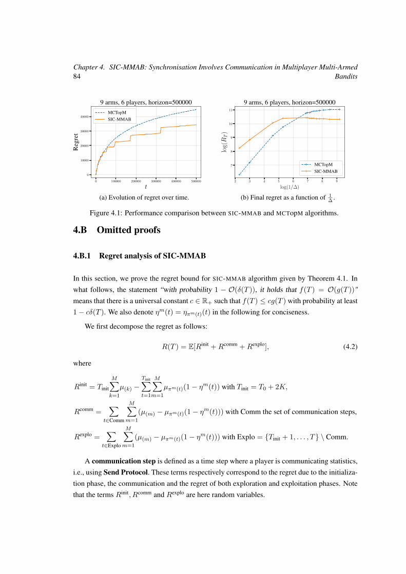
84Chapter 4. SIC-MMAB: Synchronisation Involves Communication in Multiplayer Multi-Armed
Bandits
0 100000 200000 300000 400000 500000
t
0
10000
20000
30000
40000
Reg
ret
9 arms, 6 players, horizon=500000MCTopMSIC-MMAB
(a) Evolution of regret over time.
2 3 4 5 6 7 8 9
log(1/∆)
7
8
9
10
11
log(RT
)
9 arms, 6 players, horizon=500000
MCTopMSIC-MMAB
(b) Final regret as a function of 1∆ .
Figure 4.1: Performance comparison between SIC-MMAB and MCTopM algorithms.
4.B Omitted proofs
4.B.1 Regret analysis of SIC-MMAB
In this section, we prove the regret bound for SIC-MMAB algorithm given by Theorem 4.1. In
what follows, the statement “with probability 1 − O(δ(T )), it holds that f(T ) = O(g(T ))"
means that there is a universal constant c ∈ R+ such that f(T ) ≤ cg(T ) with probability at least
1− cδ(T ). We also denote ηm(t) = ηπm(t)(t) in the following for conciseness.
We first decompose the regret as follows:
R(T ) = E[Rinit +Rcomm +Rexplo], (4.2)
where
Rinit = Tinit
M∑k=1
µ(k) −Tinit∑t=1
M∑m=1
µπm(t)(1− ηm(t)) with Tinit = T0 + 2K,
Rcomm =∑
t∈Comm
M∑m=1
(µ(m) − µπm(t)(1− ηm(t))) with Comm the set of communication steps,
Rexplo =∑
t∈Explo
M∑m=1
(µ(m) − µπm(t)(1− ηm(t))) with Explo = Tinit + 1, . . . , T \ Comm.
A communication step is defined as a time step where a player is communicating statistics,
i.e., using Send Protocol. These terms respectively correspond to the regret due to the initializa-
tion phase, the communication and the regret of both exploration and exploitation phases. Note
that the terms Rinit, Rcomm and Rexplo are here random variables.

4.B. Omitted proofs 85
Initialization analysis
The initialization regret is obviously bounded by M(T0 + 2K) as the initialization phase lasts
T0 + 2K steps. Lemma 4.2 provides the probability to reach an orthogonal setting at time T0. If
this orthogonal setting is reached, the initialization phase is successful. In that case, the players
then determine M and a unique internal rank using Algorithm 4.2. This is shown by observing
that players with external ranks k and k′ will exactly collide at round T0 + k + k′.
Lemma 4.2. After a time T0, all players pull different arms with probability at least 1 −M exp
(−T0K
).
Proof. As there is at least one arm that is not played by all the other players at each time step,
the probability of having no collision at time t for a single player j is lower bounded by 1K . It
thus holds:
P[∀t ≤ T0, η
j(t) = 1]≤(
1− 1K
)T0
≤ exp(−T0K
).
For a single player j, her probability to encounter only collisions until time T0 is at most
exp(−T0K
). The union bound over the M players then yields the desired result.
Exploration regret
This section aims at proving Lemma 4.3, which bounds the exploration regret.
Lemma 4.3. With probability 1−O(K log(T )
T +M exp(−T0K
)),
Rexplo = O(∑k>M
min log(T )µ(M) − µ(k)
,√T log(T )
).
The proof of Lemma 4.3 is divided in several auxiliary lemmas. It first relies on the correct-
ness of the estimations before taking the decision to accept or reject an arm.
Lemma 4.4. For each arm k and positive integer n, P[∃p ≤ n : |µk(p)− µk| ≥ BNk(p)] ≤ 4nT .
Proof. For each arm k and positive integer n, Hoeffding inequality gives the following, classical
inequality in MAB: P[∃p ≤ n : |µk(p) − µk| ≥√
2 log(T )Tk(p) ] ≤ 2n
T . It remains to bound the
estimation error due to quantization.
Notice that∑Mj=1(Sjk − bS
jkc) is the sum of M independent Bernoulli at each phase p.
Hoeffding inequality thus also claims that P[|∑Mj=1(Sjk(p) − S
jk(p))| ≥
√log(T )M
2 ] ≤ 2T . As
Nk(p) ≥ M , it then holds P[∃p ≤ n : |µjk(p) − µjk(p)| ≥
√log(T )2Nk(p) ] ≤ 2n
T . Using the triangle
inequality with this bound and the first Hoeffding inequality of the proof yields the final result.
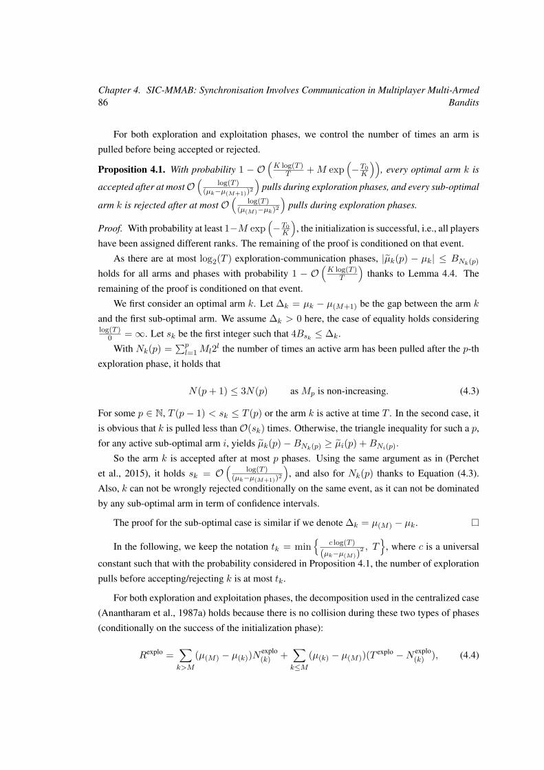
86Chapter 4. SIC-MMAB: Synchronisation Involves Communication in Multiplayer Multi-Armed
Bandits
For both exploration and exploitation phases, we control the number of times an arm is
pulled before being accepted or rejected.
Proposition 4.1. With probability 1 − O(K log(T )
T +M exp(−T0K
)), every optimal arm k is
accepted after at mostO(
log(T )(µk−µ(M+1))2
)pulls during exploration phases, and every sub-optimal
arm k is rejected after at most O(
log(T )(µ(M)−µk)2
)pulls during exploration phases.
Proof. With probability at least 1−M exp(−T0K
), the initialization is successful, i.e., all players
have been assigned different ranks. The remaining of the proof is conditioned on that event.
As there are at most log2(T ) exploration-communication phases, |µk(p) − µk| ≤ BNk(p)
holds for all arms and phases with probability 1 − O(K log(T )
T
)thanks to Lemma 4.4. The
remaining of the proof is conditioned on that event.
We first consider an optimal arm k. Let ∆k = µk − µ(M+1) be the gap between the arm k
and the first sub-optimal arm. We assume ∆k > 0 here, the case of equality holds consideringlog(T )
0 =∞. Let sk be the first integer such that 4Bsk ≤ ∆k.
With Nk(p) =∑pl=1Ml2l the number of times an active arm has been pulled after the p-th
exploration phase, it holds that
N(p+ 1) ≤ 3N(p) as Mp is non-increasing. (4.3)
For some p ∈ N, T (p− 1) < sk ≤ T (p) or the arm k is active at time T . In the second case, it
is obvious that k is pulled less than O(sk) times. Otherwise, the triangle inequality for such a p,
for any active sub-optimal arm i, yields µk(p)−BNk(p) ≥ µi(p) +BNi(p).
So the arm k is accepted after at most p phases. Using the same argument as in (Perchet
et al., 2015), it holds sk = O(
log(T )(µk−µ(M+1))2
), and also for Nk(p) thanks to Equation (4.3).
Also, k can not be wrongly rejected conditionally on the same event, as it can not be dominated
by any sub-optimal arm in term of confidence intervals.
The proof for the sub-optimal case is similar if we denote ∆k = µ(M) − µk.
In the following, we keep the notation tk = min
c log(T )(µk−µ(M))2 , T
, where c is a universal
constant such that with the probability considered in Proposition 4.1, the number of exploration
pulls before accepting/rejecting k is at most tk.
For both exploration and exploitation phases, the decomposition used in the centralized case
(Anantharam et al., 1987a) holds because there is no collision during these two types of phases
(conditionally on the success of the initialization phase):
Rexplo =∑k>M
(µ(M) − µ(k))Nexplo(k) +
∑k≤M
(µ(k) − µ(M))(T explo −N explo(k) ), (4.4)
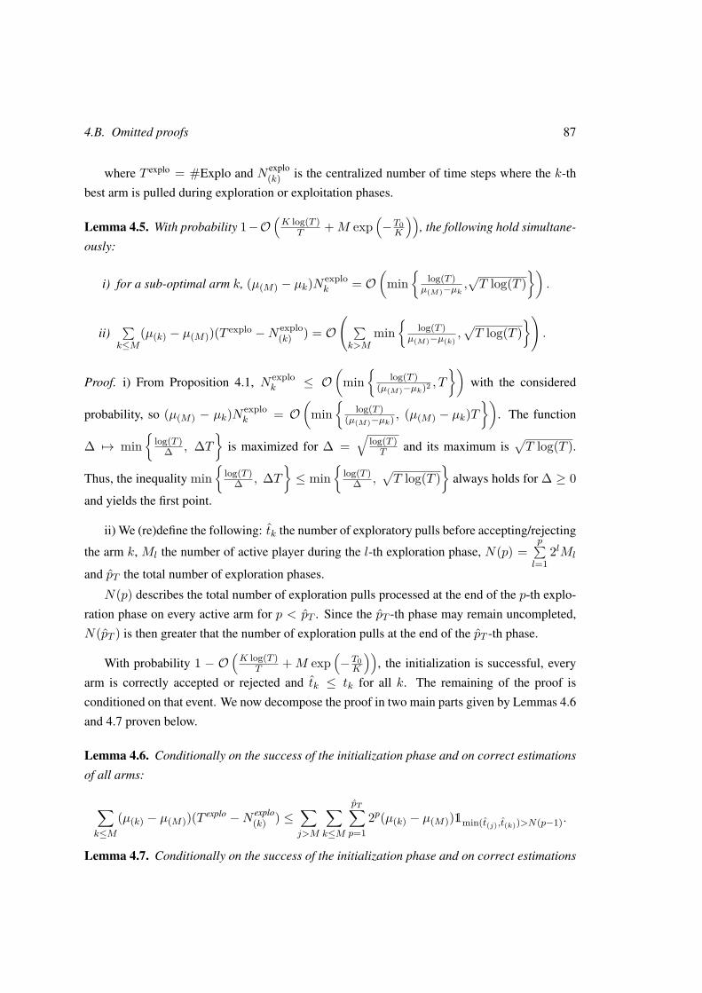
4.B. Omitted proofs 87
where T explo = #Explo and N explo(k) is the centralized number of time steps where the k-th
best arm is pulled during exploration or exploitation phases.
Lemma 4.5. With probability 1−O(K log(T )
T +M exp(−T0K
)), the following hold simultane-
ously:
i) for a sub-optimal arm k, (µ(M) − µk)Nexplok = O
(min
log(T )
µ(M)−µk,√T log(T )
).
ii)∑k≤M
(µ(k) − µ(M))(T explo −N explo(k) ) = O
( ∑k>M
min
log(T )µ(M)−µ(k)
,√T log(T )
).
Proof. i) From Proposition 4.1, N explok ≤ O
(min
log(T )
(µ(M)−µk)2 , T
)with the considered
probability, so (µ(M) − µk)N explok = O
(min
log(T )
(µ(M)−µk) , (µ(M) − µk)T)
. The function
∆ 7→ min
log(T )∆ , ∆T
is maximized for ∆ =
√log(T )T and its maximum is
√T log(T ).
Thus, the inequality min
log(T )∆ , ∆T
≤ min
log(T )
∆ ,√T log(T )
always holds for ∆ ≥ 0
and yields the first point.
ii) We (re)define the following: tk the number of exploratory pulls before accepting/rejecting
the arm k, Ml the number of active player during the l-th exploration phase, N(p) =p∑l=1
2lMl
and pT the total number of exploration phases.
N(p) describes the total number of exploration pulls processed at the end of the p-th explo-
ration phase on every active arm for p < pT . Since the pT -th phase may remain uncompleted,
N(pT ) is then greater that the number of exploration pulls at the end of the pT -th phase.
With probability 1 − O(K log(T )
T +M exp(−T0K
)), the initialization is successful, every
arm is correctly accepted or rejected and tk ≤ tk for all k. The remaining of the proof is
conditioned on that event. We now decompose the proof in two main parts given by Lemmas 4.6
and 4.7 proven below.
Lemma 4.6. Conditionally on the success of the initialization phase and on correct estimations
of all arms:
∑k≤M
(µ(k) − µ(M))(T explo −N explo(k) ) ≤
∑j>M
∑k≤M
pT∑p=1
2p(µ(k) − µ(M))1min(t(j),t(k))>N(p−1).
Lemma 4.7. Conditionally on the success of the initialization phase and on correct estimations
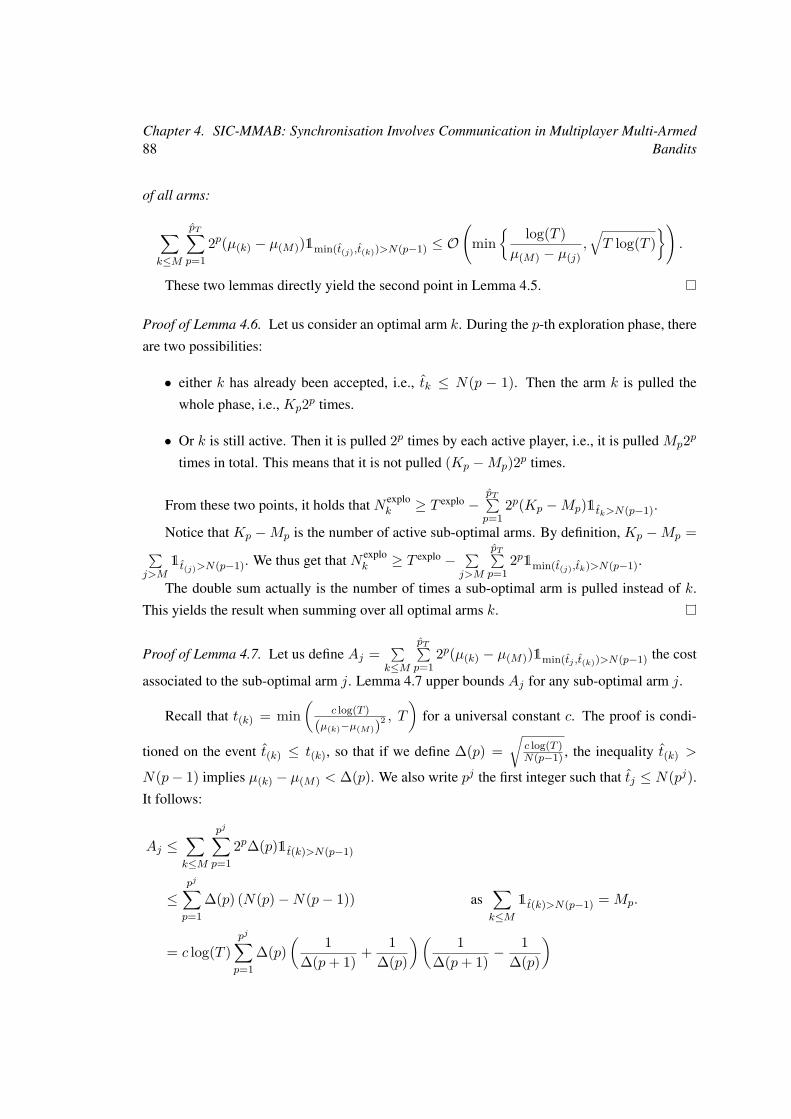
88Chapter 4. SIC-MMAB: Synchronisation Involves Communication in Multiplayer Multi-Armed
Bandits
of all arms:
∑k≤M
pT∑p=1
2p(µ(k) − µ(M))1min(t(j),t(k))>N(p−1) ≤ O(
min log(T )µ(M) − µ(j)
,√T log(T )
).
These two lemmas directly yield the second point in Lemma 4.5.
Proof of Lemma 4.6. Let us consider an optimal arm k. During the p-th exploration phase, there
are two possibilities:
• either k has already been accepted, i.e., tk ≤ N(p − 1). Then the arm k is pulled the
whole phase, i.e., Kp2p times.
• Or k is still active. Then it is pulled 2p times by each active player, i.e., it is pulled Mp2p
times in total. This means that it is not pulled (Kp −Mp)2p times.
From these two points, it holds that N explok ≥ T explo −
pT∑p=1
2p(Kp −Mp)1tk>N(p−1).
Notice that Kp −Mp is the number of active sub-optimal arms. By definition, Kp −Mp =∑j>M
1t(j)>N(p−1). We thus get that N explok ≥ T explo −
∑j>M
pT∑p=1
2p1min(t(j),tk)>N(p−1).
The double sum actually is the number of times a sub-optimal arm is pulled instead of k.
This yields the result when summing over all optimal arms k.
Proof of Lemma 4.7. Let us define Aj =∑k≤M
pT∑p=1
2p(µ(k) − µ(M))1min(tj ,t(k))>N(p−1) the cost
associated to the sub-optimal arm j. Lemma 4.7 upper bounds Aj for any sub-optimal arm j.
Recall that t(k) = min(
c log(T )(µ(k)−µ(M))2 , T
)for a universal constant c. The proof is condi-
tioned on the event t(k) ≤ t(k), so that if we define ∆(p) =√
c log(T )N(p−1) , the inequality t(k) >
N(p− 1) implies µ(k) − µ(M) < ∆(p). We also write pj the first integer such that tj ≤ N(pj).
It follows:
Aj ≤∑k≤M
pj∑p=1
2p∆(p)1t(k)>N(p−1)
≤pj∑p=1
∆(p) (N(p)−N(p− 1)) as∑k≤M
1t(k)>N(p−1) = Mp.
= c log(T )pj∑p=1
∆(p)( 1
∆(p+ 1) + 1∆(p)
)( 1∆(p+ 1) −
1∆(p)
)
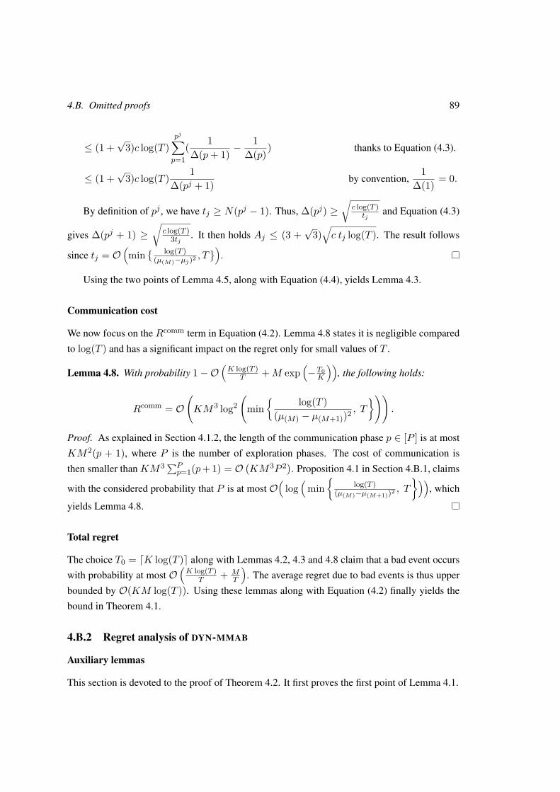
4.B. Omitted proofs 89
≤ (1 +√
3)c log(T )pj∑p=1
( 1∆(p+ 1) −
1∆(p)) thanks to Equation (4.3).
≤ (1 +√
3)c log(T ) 1∆(pj + 1) by convention,
1∆(1) = 0.
By definition of pj , we have tj ≥ N(pj − 1). Thus, ∆(pj) ≥√
c log(T )tj
and Equation (4.3)
gives ∆(pj + 1) ≥√
c log(T )3tj . It then holds Aj ≤ (3 +
√3)√c tj log(T ). The result follows
since tj = O(min
log(T )(µ(M)−µj)2 , T
).
Using the two points of Lemma 4.5, along with Equation (4.4), yields Lemma 4.3.
Communication cost
We now focus on the Rcomm term in Equation (4.2). Lemma 4.8 states it is negligible compared
to log(T ) and has a significant impact on the regret only for small values of T .
Lemma 4.8. With probability 1−O(K log(T )
T +M exp(−T0K
)), the following holds:
Rcomm = O(KM3 log2
(min
log(T )(µ(M) − µ(M+1))2 , T
)).
Proof. As explained in Section 4.1.2, the length of the communication phase p ∈ [P ] is at most
KM2(p + 1), where P is the number of exploration phases. The cost of communication is
then smaller than KM3∑Pp=1(p+ 1) = O
(KM3P 2). Proposition 4.1 in Section 4.B.1, claims
with the considered probability that P is at most O(
log(
min
log(T )(µ(M)−µ(M+1))2 , T
)), which
yields Lemma 4.8.
Total regret
The choice T0 = dK log(T )e along with Lemmas 4.2, 4.3 and 4.8 claim that a bad event occurs
with probability at most O(K log(T )
T + MT
). The average regret due to bad events is thus upper
bounded by O(KM log(T )). Using these lemmas along with Equation (4.2) finally yields the
bound in Theorem 4.1.
4.B.2 Regret analysis of DYN-MMAB
Auxiliary lemmas
This section is devoted to the proof of Theorem 4.2. It first proves the first point of Lemma 4.1.
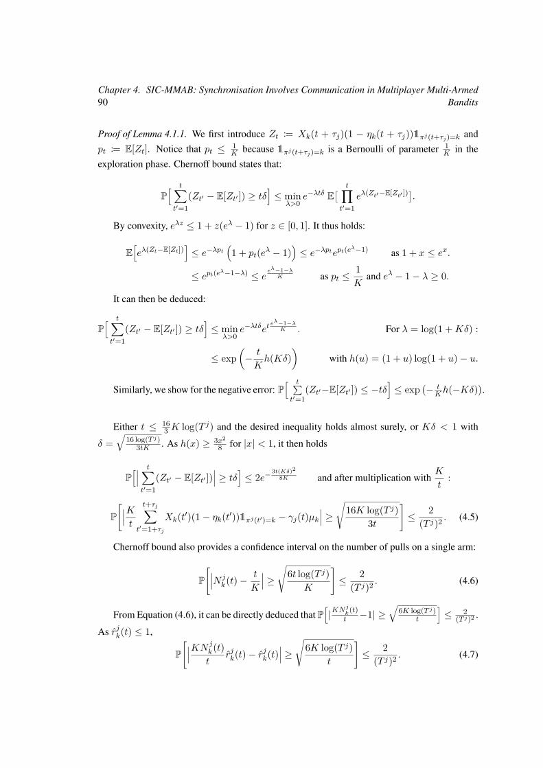
90Chapter 4. SIC-MMAB: Synchronisation Involves Communication in Multiplayer Multi-Armed
Bandits
Proof of Lemma 4.1.1. We first introduce Zt := Xk(t + τj)(1 − ηk(t + τj))1πj(t+τj)=k and
pt := E[Zt]. Notice that pt ≤ 1K because 1πj(t+τj)=k is a Bernoulli of parameter 1
K in the
exploration phase. Chernoff bound states that:
P[ t∑t′=1
(Zt′ − E[Zt′ ]) ≥ tδ]≤ min
λ>0e−λtδ E
[ t∏t′=1
eλ(Zt′−E[Zt′ ])].
By convexity, eλz ≤ 1 + z(eλ − 1) for z ∈ [0, 1]. It thus holds:
E[eλ(Zt−E[Zt])
]≤ e−λpt
(1 + pt(eλ − 1)
)≤ e−λptept(eλ−1) as 1 + x ≤ ex.
≤ ept(eλ−1−λ) ≤ eeλ−1−λ
K as pt ≤1K
and eλ − 1− λ ≥ 0.
It can then be deduced:
P[ t∑t′=1
(Zt′ − E[Zt′ ]) ≥ tδ]≤ min
λ>0e−λtδet
eλ−1−λK . For λ = log(1 +Kδ) :
≤ exp(− t
Kh(Kδ)
)with h(u) = (1 + u) log(1 + u)− u.
Similarly, we show for the negative error: P[ t∑t′=1
(Zt′−E[Zt′ ]) ≤ −tδ]≤ exp
(− tKh(−Kδ)
).
Either t ≤ 163 K log(T j) and the desired inequality holds almost surely, or Kδ < 1 with
δ =√
16 log(T j)3tK . As h(x) ≥ 3x2
8 for |x| < 1, it then holds
P[∣∣∣ t∑t′=1
(Zt′ − E[Zt′ ])∣∣∣ ≥ tδ] ≤ 2e−
3t(Kδ)28K and after multiplication with
K
t:
P[∣∣∣Kt
t+τj∑t′=1+τj
Xk(t′)(1− ηk(t′))1πj(t′)=k − γj(t)µk∣∣∣ ≥
√16K log(T j)
3t
]≤ 2
(T j)2 . (4.5)
Chernoff bound also provides a confidence interval on the number of pulls on a single arm:
P[∣∣∣N j
k(t)− t
K
∣∣∣ ≥√
6t log(T j)K
]≤ 2
(T j)2 . (4.6)
From Equation (4.6), it can be directly deduced that P[|KN
jk
(t)t −1| ≥
√6K log(T j)
t
]≤ 2
(T j)2 .
As rjk(t) ≤ 1,
P[∣∣∣KN j
k(t)t
rjk(t)− rjk(t)
∣∣∣ ≥√
6K log(T j)t
]≤ 2
(T j)2 . (4.7)
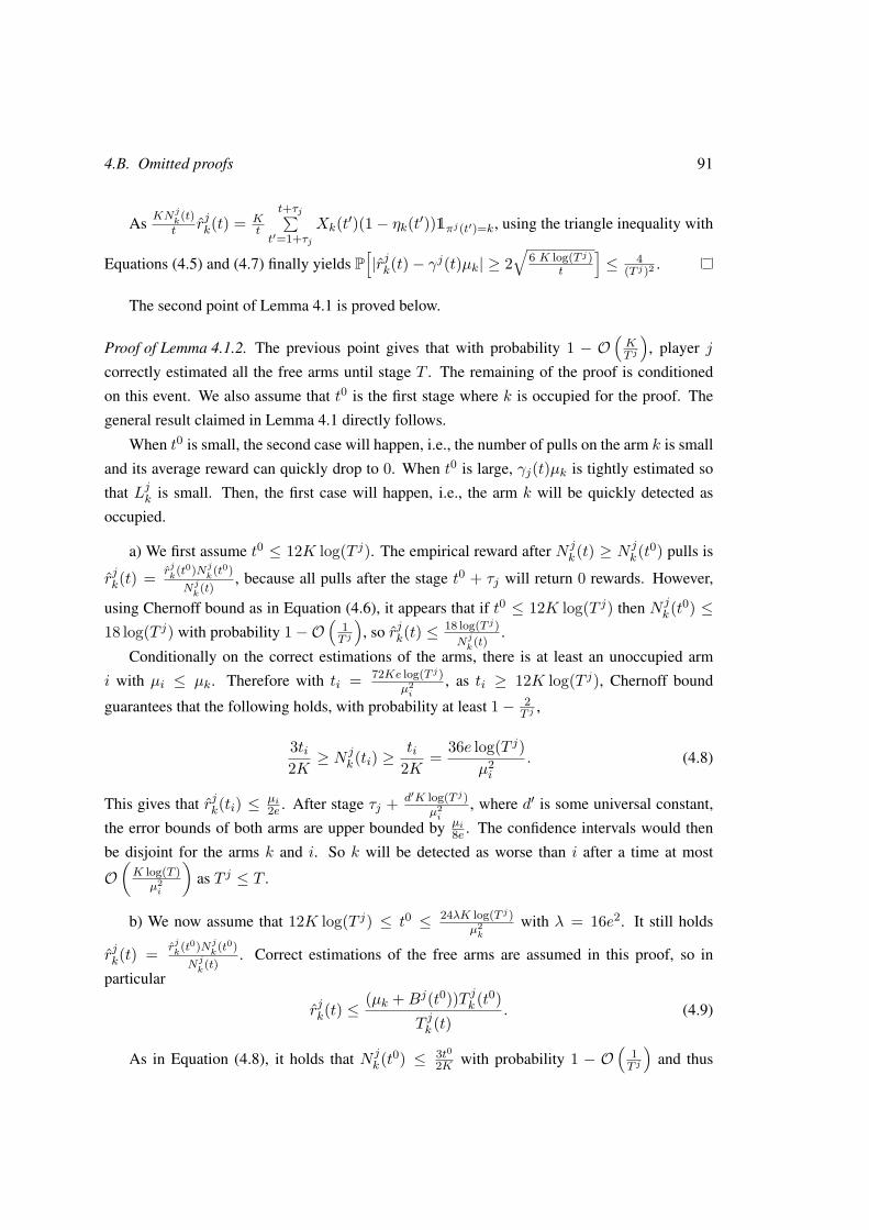
4.B. Omitted proofs 91
As KNjk
(t)t rjk(t) = K
t
t+τj∑t′=1+τj
Xk(t′)(1− ηk(t′))1πj(t′)=k, using the triangle inequality with
Equations (4.5) and (4.7) finally yields P[|rjk(t)− γj(t)µk| ≥ 2
√6 K log(T j)
t
]≤ 4
(T j)2 .
The second point of Lemma 4.1 is proved below.
Proof of Lemma 4.1.2. The previous point gives that with probability 1 − O(KT j
), player j
correctly estimated all the free arms until stage T . The remaining of the proof is conditioned
on this event. We also assume that t0 is the first stage where k is occupied for the proof. The
general result claimed in Lemma 4.1 directly follows.
When t0 is small, the second case will happen, i.e., the number of pulls on the arm k is small
and its average reward can quickly drop to 0. When t0 is large, γj(t)µk is tightly estimated so
that Ljk is small. Then, the first case will happen, i.e., the arm k will be quickly detected as
occupied.
a) We first assume t0 ≤ 12K log(T j). The empirical reward after N jk(t) ≥ N j
k(t0) pulls is
rjk(t) = rjk(t0)Nj
k(t0)
Njk
(t), because all pulls after the stage t0 + τj will return 0 rewards. However,
using Chernoff bound as in Equation (4.6), it appears that if t0 ≤ 12K log(T j) then N jk(t0) ≤
18 log(T j) with probability 1−O(
1T j
), so rjk(t) ≤
18 log(T j)Njk
(t).
Conditionally on the correct estimations of the arms, there is at least an unoccupied arm
i with µi ≤ µk. Therefore with ti = 72Ke log(T j)µ2i
, as ti ≥ 12K log(T j), Chernoff bound
guarantees that the following holds, with probability at least 1− 2T j
,
3ti2K ≥ N
jk(ti) ≥
ti2K = 36e log(T j)
µ2i
. (4.8)
This gives that rjk(ti) ≤µi2e . After stage τj + d′K log(T j)
µ2i
, where d′ is some universal constant,
the error bounds of both arms are upper bounded by µi8e . The confidence intervals would then
be disjoint for the arms k and i. So k will be detected as worse than i after a time at most
O(K log(T )
µ2i
)as T j ≤ T .
b) We now assume that 12K log(T j) ≤ t0 ≤ 24λK log(T j)µ2k
with λ = 16e2. It still holds
rjk(t) = rjk(t0)Nj
k(t0)
Njk
(t). Correct estimations of the free arms are assumed in this proof, so in
particular
rjk(t) ≤(µk +Bj(t0))T jk (t0)
T jk (t). (4.9)
As in Equation (4.8), it holds that N jk(t0) ≤ 3t0
2K with probability 1 − O(
1T j
)and thus
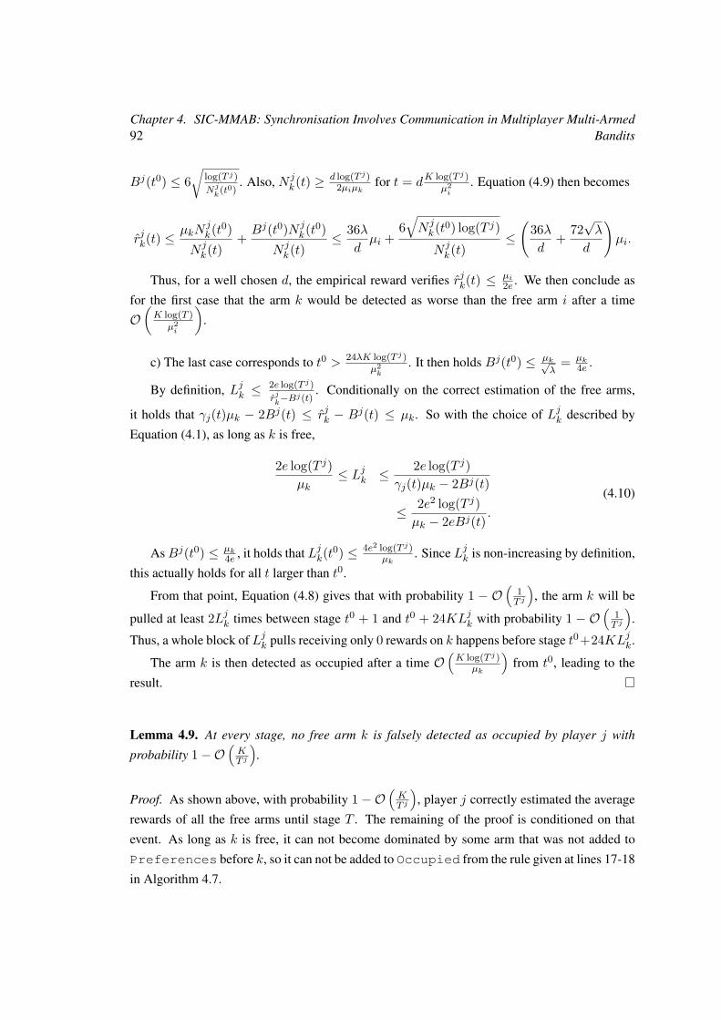
92Chapter 4. SIC-MMAB: Synchronisation Involves Communication in Multiplayer Multi-Armed
Bandits
Bj(t0) ≤ 6√
log(T j)Njk
(t0). Also, N j
k(t) ≥ d log(T j)2µiµk for t = dK log(T j)
µ2i
. Equation (4.9) then becomes
rjk(t) ≤µkN
jk(t0)
N jk(t)
+ Bj(t0)N jk(t0)
N jk(t)
≤ 36λdµi +
6√N jk(t0) log(T j)N jk(t)
≤(
36λd
+ 72√λ
d
)µi.
Thus, for a well chosen d, the empirical reward verifies rjk(t) ≤µi2e . We then conclude as
for the first case that the arm k would be detected as worse than the free arm i after a time
O(K log(T )
µ2i
).
c) The last case corresponds to t0 > 24λK log(T j)µ2k
. It then holds Bj(t0) ≤ µk√λ
= µk4e .
By definition, Ljk ≤2e log(T j)rjk−Bj(t)
. Conditionally on the correct estimation of the free arms,
it holds that γj(t)µk − 2Bj(t) ≤ rjk − Bj(t) ≤ µk. So with the choice of Ljk described by
Equation (4.1), as long as k is free,
2e log(T j)µk
≤ Ljk ≤ 2e log(T j)γj(t)µk − 2Bj(t)
≤ 2e2 log(T j)µk − 2eBj(t) .
(4.10)
AsBj(t0) ≤ µk4e , it holds that Ljk(t0) ≤ 4e2 log(T j)
µk. Since Ljk is non-increasing by definition,
this actually holds for all t larger than t0.
From that point, Equation (4.8) gives that with probability 1 − O(
1T j
), the arm k will be
pulled at least 2Ljk times between stage t0 + 1 and t0 + 24KLjk with probability 1 − O(
1T j
).
Thus, a whole block of Ljk pulls receiving only 0 rewards on k happens before stage t0+24KLjk.
The arm k is then detected as occupied after a time O(K log(T j)
µk
)from t0, leading to the
result.
Lemma 4.9. At every stage, no free arm k is falsely detected as occupied by player j with
probability 1−O(KT j
).
Proof. As shown above, with probability 1−O(KT j
), player j correctly estimated the average
rewards of all the free arms until stage T . The remaining of the proof is conditioned on that
event. As long as k is free, it can not become dominated by some arm that was not added to
Preferences before k, so it can not be added to Occupied from the rule given at lines 17-18
in Algorithm 4.7.

4.B. Omitted proofs 93
For the rule of Line 12, Equation (4.10) gives that
Ljk(t′) ≥ 2e log(T j)
µkat each stage t′ ≤ t. (4.11)
As in Section 4.B.1, the probability of detecting L successive 0 rewards on a free arm k is
then smaller than(1− µk
e
)L ≤ exp(−Lµk
e
).
Using this along with Equation (4.11) yields that with probability 1−O(
1(T j)2
), at least one
positive reward will be observed on arm k in a single block. The union bound over all blocks
yields the result.
Finally, Lemma 4.10 yields that, after some time, each player starts exploiting an arm while
all the better arms are already occupied by other players.
Lemma 4.10. We denote ∆(k) = mini=1,...,k
(µ(i) − µ(i+1)). With probability 1−O(KT j
), it holds
that for a single player j, there exists kj such that after a stage at most tkj + τj , she is exploiting
the kj-th best arm and all the better arms are also exploited by other players, where tkj =
O(K log(T )
∆2(kj)
+ kjK log(T )µ(kj)
).
Proof. Player j correctly estimates all the arms until stage T , with probability 1−O(KT j
). The
remaining of the proof is conditioned on that event. We define ti = cK log(T j)∆2
(i)+ i cK log(T j)
µ(i)for
some universal constant c and kj (random variable) defined as
kj = mini ∈ [K] | i-th best arm not exploited by another player at stage ti + τj
. (4.12)
k∗j (kj-th best arm) is the best arm not exploited by another player (than player j) after the
stage tkj + τj . The considered set is not empty as M ≤ K.
Lemma 4.9 gives that with probability 1 − O(KT j
), k∗j is not falsely detected as occupied
until stage T . All arms below k∗j will be detected as worse than k∗j after a time dK log(T j)∆2
(kj)for
some universal constant d.
By definition of kj , any arm i∗ better than k∗j is already occupied at stage ti+τj . Lemma 4.1,
gives that with probability 1 − O(
1T j
), either i∗ is detected as occupied after stage ti + τj +
d′K log(T j)µ(i)
or dominated by k∗j after stage d2K log(T j)∆2
(kj)+ τj for some universal constants d′ and
d2.
Thus the player detects the arm k∗j as optimal and starts trying to occupy k∗j at a stage at most
t = max(tkj−1 + d′K log(T j)
µ(kj),max(d, d2)K log(T j)
∆2(kj)
)+ τj with probability 1 −O
(KT j
)(where
t0 = 0).
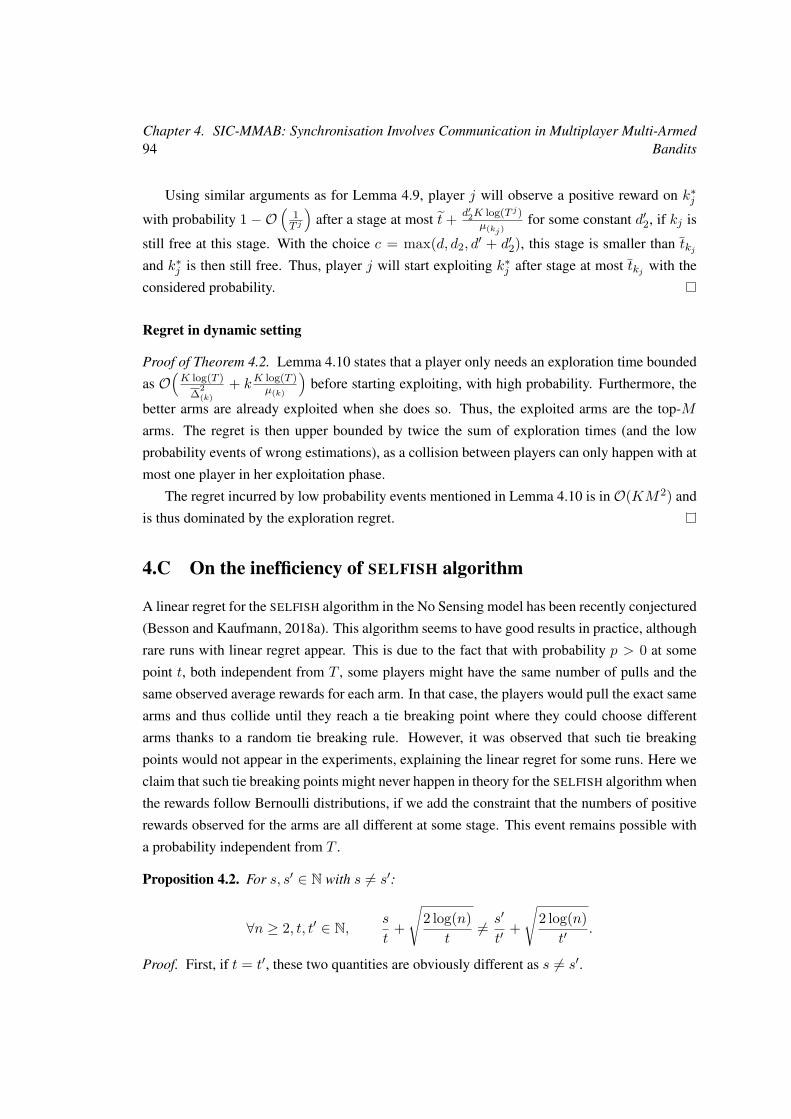
94Chapter 4. SIC-MMAB: Synchronisation Involves Communication in Multiplayer Multi-Armed
Bandits
Using similar arguments as for Lemma 4.9, player j will observe a positive reward on k∗jwith probability 1 − O
(1T j
)after a stage at most t + d′2K log(T j)
µ(kj)for some constant d′2, if kj is
still free at this stage. With the choice c = max(d, d2, d′ + d′2), this stage is smaller than tkj
and k∗j is then still free. Thus, player j will start exploiting k∗j after stage at most tkj with the
considered probability.
Regret in dynamic setting
Proof of Theorem 4.2. Lemma 4.10 states that a player only needs an exploration time bounded
as O(K log(T )
∆2(k)
+ kK log(T )µ(k)
)before starting exploiting, with high probability. Furthermore, the
better arms are already exploited when she does so. Thus, the exploited arms are the top-M
arms. The regret is then upper bounded by twice the sum of exploration times (and the low
probability events of wrong estimations), as a collision between players can only happen with at
most one player in her exploitation phase.
The regret incurred by low probability events mentioned in Lemma 4.10 is inO(KM2) and
is thus dominated by the exploration regret.
4.C On the inefficiency of SELFISH algorithm
A linear regret for the SELFISH algorithm in the No Sensing model has been recently conjectured
(Besson and Kaufmann, 2018a). This algorithm seems to have good results in practice, although
rare runs with linear regret appear. This is due to the fact that with probability p > 0 at some
point t, both independent from T , some players might have the same number of pulls and the
same observed average rewards for each arm. In that case, the players would pull the exact same
arms and thus collide until they reach a tie breaking point where they could choose different
arms thanks to a random tie breaking rule. However, it was observed that such tie breaking
points would not appear in the experiments, explaining the linear regret for some runs. Here we
claim that such tie breaking points might never happen in theory for the SELFISH algorithm when
the rewards follow Bernoulli distributions, if we add the constraint that the numbers of positive
rewards observed for the arms are all different at some stage. This event remains possible with
a probability independent from T .
Proposition 4.2. For s, s′ ∈ N with s 6= s′:
∀n ≥ 2, t, t′ ∈ N,s
t+
√2 log(n)
t6= s′
t′+
√2 log(n)
t′.
Proof. First, if t = t′, these two quantities are obviously different as s 6= s′.

4.C. On the inefficiency of SELFISH algorithm 95
We now assume st +
√2 log(n)
t = s′
t′ +√
2 log(n)t′ with t 6= t′.
This means that√
2 log(n)t −
√2 log(n)
t′ is a rational, i.e., for some rational p, log(n)(t + t′ −2√tt′) = 2p.
It then holds log(n)√tt′ = log(n) t+ t′
2 − p,
tt′ log2(n) = log2(n)( t+ t′
2 )2 − p(t+ t′) log(n) + p2,
log2(n)( t− t′
2 )2 − p(t+ t′) log(n) + p2 = 0.
Since ( t−t′2 )2 6= 0 and all the coefficients are in Q here, this would mean that log(n) is an
algebraic number. However, Lindemann–Weierstrass theorem implies that log(n) is transcen-
dental for any integer n ≥ 2. We thus have a contradiction.
The proof is only theoretical as computer are not precise enough to distinguish rationals from
irrationals. The advanced arguments are not applicable in practice. Still, this seems to confirm
the conjecture proposed by Besson and Kaufmann, 2018a: a tie breaking point is never reached,
or at least not before a very long period of time.
However, if the players are not synchronised (dynamic setting or asynchronous setting) or
if they are using confidence bounds of the form√
ηm log(n)t where ηm is some variable proper
to player m, this proof does not hold anymore. It thus remains unknown, whether slightly
modifying the SELFISH algorithm could lead to interesting regret guarantees.
Chapter 5
A Practical Algorithm for MultiplayerBandits when Arm Means Vary AmongPlayers
For the more challenging heterogeneous setting, arms may have different means for differ-ent players. This chapter proposes a new and efficient algorithm that combines the idea ofleveraging forced collisions for implicit communication and that of performing matchingeliminations. We present a finite-time analysis of our algorithm, giving the first sublinearminimax regret bound for this problem, and prove that if the optimal assignment of play-ers to arms is unique, our algorithm attains the optimal O (log(T )) regret, solving an openquestion raised at NeurIPS 2018 by Bistritz and Leshem (2018).
5.1 Contributions . . . . . . . . . . . . . . . . . . . . . . . . . . . . . . . . . . . 97
5.1.1 Context and related work . . . . . . . . . . . . . . . . . . . . . . . . . 98
5.2 The M-ETC-Elim Algorithm . . . . . . . . . . . . . . . . . . . . . . . . . . . 100
5.3 Analysis of M-ETC-Elim . . . . . . . . . . . . . . . . . . . . . . . . . . . . . 104
5.3.1 Sketch of Proof of Theorem 5.2 . . . . . . . . . . . . . . . . . . . . . 105
5.3.2 Proof of Theorem 5.1(b), Unique Optimal Matching . . . . . . . . . . 107
5.3.3 Proof of Theorem 5.1(c), Minimax Regret Bound . . . . . . . . . . . . 107
5.4 Numerical Experiments . . . . . . . . . . . . . . . . . . . . . . . . . . . . . . 107
5.A Description of the Initialization Procedure and Followers’ Pseudocode . . . . . 109
5.B Practical Considerations and Additional Experiments . . . . . . . . . . . . . . 109
5.B.1 Implementation Enhancements for M-ETC-Elim . . . . . . . . . . . . 109
5.B.2 Other Reward Distributions . . . . . . . . . . . . . . . . . . . . . . . 111
96
5.1. Contributions 97
5.C Omitted proofs . . . . . . . . . . . . . . . . . . . . . . . . . . . . . . . . . . 112
5.C.1 Regret Analysis in the Presence of a Unique Maximum Matching . . . 112
5.C.2 Minimax Regret Analysis . . . . . . . . . . . . . . . . . . . . . . . . 113
5.C.3 Proofs of Auxiliary Lemmas for Theorems 5.2 and 5.3 . . . . . . . . . 115
This chapter studies the heterogeneous collision sensing model described in Section 3.3.1,
for which each arm has a possibly different mean for each player.
Bistritz and Leshem (2018) proposed an algorithm with regret bounded by O(log2+κ(T )
)(for any constant κ), proved a lower bound of Ω(log T ) for any algorithm, and asked if there is
an algorithm matching this lower bound. We propose a new algorithm for this model, M-ETC-
Elim, which depends on a hyperparameter c, and we upper bound its regret byO(log1+1/c(T )
)for any c > 1. We also bound its worst-case regret byO
(√T log T
), which is the first sublinear
minimax bound for this problem. Moreover, if the optimal assignment of the players to the arms
is unique, we prove that instantiating M-ETC-Elim with c = 1 yields regret at mostO (log(T )),
which is optimal and answers affirmatively the open question mentioned above in this particular
case. We present a non-asymptotic regret analysis of M-ETC-Elim leading to nearly optimal
regret upper bounds, and also demonstrate the empirical efficiency of this new algorithm via
simulations.
This chapter is structured as follows. In Section 5.1, we present our contributions and put
them in perspective by comparison with the literature. We describe the M-ETC-Elim algorithm
in Section 5.2 and upper bound its regret in Section 5.3. Finally, we report in Section 5.4 results
from an experimental study demonstrating the competitive practical performance of M-ETC-
Elim.
5.1 Contributions
We propose an efficient algorithm for the heterogeneous multiplayer bandit problem achiev-
ing (quasi) logarithmic regret. The algorithm, called Multiplayer Explore-Then-Commit with
matching Elimination (M-ETC-Elim), is described in detail in Section 5.2. It combines the idea
of exploiting collisions for implicit communication, initially proposed in Chapter 4 for the ho-
mogeneous setting (which we have improved and adapted to our setting), with an efficient way
to perform “matching eliminations.”
M-ETC-Elim consists of several epochs combining exploration and communication, and
may end with an exploitation phase if a unique optimal matching has been found. The algorithm
depends on a parameter c controlling the epoch sizes and enjoys the following regret guarantees.
98Chapter 5. A Practical Algorithm for Multiplayer Bandits when Arm Means Vary Among
Players
Theorem 5.1. (a) The M-ETC-Elim algorithm with parameter c ∈ 1, 2, . . . satisfies
R(T ) = O
MK
(M2 log(T )
∆
)1+1/c .
(b) If the maximum matching is unique, M-ETC-Elim with c = 1 satisfies
R(T ) = O(M3K log(T )
∆
).
(c) Regardless of whether the optimal matching is unique or not, M-ETC-Elim with c = 1satisfies the minimax regret bound
R(T ) = O(M
32
√KT log(T )
).
We emphasize that we carry out a non-asymptotic analysis of M-ETC-Elim. The regret
bounds of Theorem 5.1 are stated with the O(·) notation for the ease of presentation and the
hidden constants depend on the chosen parameter c only. In Theorems 5.2, 5.3 and 5.4 we
provide the counterparts of these results with explicit constants.
A consequence of part (a) is that for a fixed problem instance, for any (arbitrarily small)
κ, there exists an algorithm (M-ETC-Elim with parameter c = d1/κe) with regret R(T ) =O((log(T ))1+κ). This quasi-logarithmic regret rate improves upon theO
(log2(T )
)regret rate
of (Bistritz and Leshem, 2018). Moreover, we provide additional theoretical guarantees for M-
ETC-Elim using the parameter c = 1: an improved analysis in the presence of a unique optimal
matching, which yields logarithmic regret (part (b)); and a problem-independent O(√T log T
)regret bound (part (c)), which supports the use of this particular parameter tuning regardless of
whether the optimal matching is unique. This is the first sublinear minimax regret bound for this
problem.
To summarize, we present a unified algorithm that can be used in the presence of either a
unique or multiple optimal matchings and get a nearly logarithmic regret in both cases, almost
matching the known logarithmic lower bound. Moreover, our algorithm is easy to implement,
performs well in practice and does not need problem-dependent hyperparameter tuning.
5.1.1 Context and related work
Our algorithm also leverages the ideas of arm elimination and communication through collisions
developed in Chapter 4, with the following enhancements. In our new communication protocol,
the followers only send each piece of information once, to the leader, instead of sending it to the
M − 1 other players. Then, while we used arm eliminations (coordinated between players) to
5.1. Contributions 99
reduce the regret in Chapter 4, we cannot employ the same idea for our heterogeneous problem,
as an arm that is bad for one player might be good for another player, and therefore cannot be
eliminated. M-ETC-Elim instead relies on matching eliminations.
As mentioned in Chapter 3, the fully distributed heterogeneous setting was first studied by
Bistritz and Leshem (2018), who proposed the Game-of-Thrones (GoT) algorithm and proved
its regret is bounded by O(log2+κ(T )
)for any given constant κ > 0, if its parameters are “ap-
propriately tuned’.’ In a more recent work (Bistritz and Leshem, 2020), the same authors provide
an improved analysis, showing the same algorithm (with slightly modified phase lengths) enjoys
quasi-logarithmic regret O(log1+κ(T )
). GoT is quite different from M-ETC-Elim: it proceeds
in epochs, each consisting of an exploration phase, a so-called GoT phase and an exploitation
phase. During the GoT phase, the players jointly run a Markov chain whose unique stochas-
tically stable state corresponds to a maximum matching of the estimated means. A parameter
ε ∈ (0, 1) controls the accuracy of the estimated maximum matching obtained after a GoT
phase. Letting c1, c2, c3 be the constants parameterizing the lengths of the phases, the improved
analysis of GoT (Bistritz and Leshem, 2020) upper bounds its regret by Mc32k0+1 + 2(c1 +c2)M log1+κ
2 (T/c3 + 2) . This upper bound is asymptotic as it holds for T large enough, where
“how large” is not explicitly specified and depends on ∆.1 Moreover, the upper bound is valid
only when the parameter ε is chosen small enough: ε should satisfy some constraints (Equations
(66)-(67)) also featuring ∆. Hence, a valid tuning of the parameter ε would require prior knowl-
edge of arm utilities. In contrast, we provide in Theorem 5.2 a non-asymptotic regret upper
bound for M-ETC-Elim, which holds for any choice of the parameter c controlling the epoch
lengths. Also, we show that if the optimal assignment is unique, M-ETC-Elim has logarithmic
regret. Besides, we also illustrate in Section 5.4 that M-ETC-Elim outperforms GoT in prac-
tice. Finally, GoT has several parameters to set (δ, ε, c1, c2, c3), while M-ETC-Elim has only
one integral parameter c, and setting c = 1 works very well in all our experiments.
If ∆ is known, an algorithm with similar ideas to M-ETC-Elim with O (log T ) regret was
presented independently in the work of Magesh and Veeravalli (2019b).
Finally, the independent work of Tibrewal et al. (2019) studies a slightly stronger feedback
model than ours: they assume each player in each round has the option of “observing whether
a given arm has been pulled by someone,” without actually pulling that arm (thus avoiding
collision due to this “observation”), an operation that is called “sensing.” Due to the stronger
feedback, communications do not need to be implicitly done through collisions and bits can be
broadcast to other players via sensing. Note that it is actually possible to send a single bit of
information from one player to all other players in a single round in their model, an action that1(Bistritz and Leshem, 2020, Theorem 4) requires T to be larger than c3(2k0 − 2), where k0 satisfies Equa-
tion (16), which features κ and ∆.
100Chapter 5. A Practical Algorithm for Multiplayer Bandits when Arm Means Vary Among
Players
requiresM−1 rounds in our model. Still, the algorithms proposed by Tibrewal et al. (2019) can
be modified to obtain algorithms for our setting, and M-ETC-Elim can also be adapted to their
setting. The two algorithms proposed by Tibrewal et al. (2019) share similarities with M-ETC-
Elim: they also have exploration, communication and exploitation phases, but they do not use
eliminations. Regarding their theoretical guarantees, a first remark is that those proved in Tibre-
wal et al. (2019) only hold in the presence of a unique optimal matching, whereas our analysis
of M-ETC-Elim applies in the general case. The second remark is that their regret bounds for
the case in which ∆ is unknown (Theorems 3(ii) and 4) feature exponential dependence on the
gap 1/∆, whereas our regret bounds have polynomial dependence. Finally, the first-order term
of their Theorem 4 has a quadratic dependence in 1/∆, whereas our Theorem 5.1(b) scales
linearly, which is optimal and allows us to get the O(√
log(T )T)
minimax regret bound for
M-ETC-Elim.
The best known lower bound in the centralized heterogeneous setting is Ω(KM
∆ log(T ))
as explained in Section 3.3.3 (Combes et al., 2015). Moreover, a minimax lower bound of
Ω(M√KT ) was given by Audibert et al. (2014) in the same setting. These lower bounds show
that the dependency in T,∆ and K obtained in Theorem 5.1(b),(c) are essentially not improv-
able, but that the dependency inM might be. However, finding an algorithm whose regrets attain
the available lower bounds for combinatorial semi-bandits is already hard even without the extra
challenge of decentralization.
5.2 The M-ETC-Elim Algorithm
Our algorithm relies on an initialization phase in which the players elect a leader in a distributed
manner. Then a communication protocol is set up, in which the leader and the followers have
different roles: followers explore some arms and communicate to the leader estimates of the arm
means, while the leader maintains a list of “candidate optimal matchings” and communicates to
the followers the list of arms that need exploration in order to refine the list, i.e. to eliminate some
candidate matchings. The algorithm is called Multiplayer Explore-Then-Commit with matching
Eliminations (M-ETC-Elim for short). Formally, each player executes Algorithm 5.1 below.
Algorithm 5.1: M-ETC-Elim with parameter cInput: Time horizon T , number of arms K
1 R,M ←− INIT(K, 1/KT )2 if R = 1 then LEADERALGORITHM(M) else FOLLOWERALGORITHM(R,M)
M-ETC-Elim requires as input the number of arms K (as well as a shared numbering of the
arms across the players) and the time horizon T (the total number of arm selections). However,
5.2. The M-ETC-Elim Algorithm 101
if the players know only an upper bound on T , our results hold with T replaced by that upper
bound as well. If no upper bound on T is known, the players can employ a simple doubling trick
(Besson and Kaufmann, 2018b): we execute the algorithm assuming T = 1, then we execute it
assuming T = 2 × 1, and so on, until the actual time horizon is reached. If the expected regret
of the algorithm for a known time horizon T is R(T ), then the expected regret of the modified
algorithm for unknown time horizon T would be R′(T ) ≤∑log2(T )i=0 R2i ≤ log2(T )×R(T ).
Initialization. The initialization procedure, similar to the initialization of SIC-MMAB de-
scribed in Section 4.1.2. It first outputs for each player a rank R ∈ [M ] as well as the value
of M , which is initially unknown to the players. This initialization phase relies on a “musical
chairs” phase after which the players end up on distinct arms, followed by a “sequential hopping”
protocol that permits them to know their ordering. For the sake of completeness, the initializa-
tion procedure is described in detail in Section 5.A. It corresponds to the same initialization as
SIC-MMAB and the following lemma has thus already been proven in Section 4.B.1.
Lemma 5.1. Fix δ0 > 0. With probability at least 1− δ0, if the M players run the INIT(K, δ0)procedure, which takes K log(K/δ0) + 2K − 2 < K log(e2K/δ0) many rounds, all players
learn M and obtain a distinct ranking from 1 to M .
Communication Phases. Once all players have learned their ranks, player 1 becomes the
leader and other players become the followers. The leader executes additional computations,
and communicates with the followers individually, while each follower communicates only with
the leader.
The leader and follower algorithms, described below, rely on several communication phases,
which start at the same time for every player. During communication phases, the default behavior
of each player is to pull her communication arm. It is crucial that these communication arms are
distinct: an optimal way to do so is for each player to use her arm in the best matching found
so far. In the first communication phase, such an assignment is unknown and players simply
use their ranking as communication arm. Suppose at a certain time the leader wants to send a
sequence of b bits t1, . . . , tb to the player with ranking i and communication arm ki. During the
next b rounds, for each j = 1, 2, . . . , b, if tj = 1, the leader pulls arm ki; otherwise, she pulls
her own communication arm k1, while all followers stick to their communication arms. Player
i can thus reconstruct these b bits after these b rounds, by observing the collisions on arm ki.
The converse communication between follower i and the leader is similar. The rankings are also
useful to know in which order communications should be performed, as the leader successively
communicates messages to the M − 1 followers, and then the M − 1 followers successively
communicate messages to the leader.
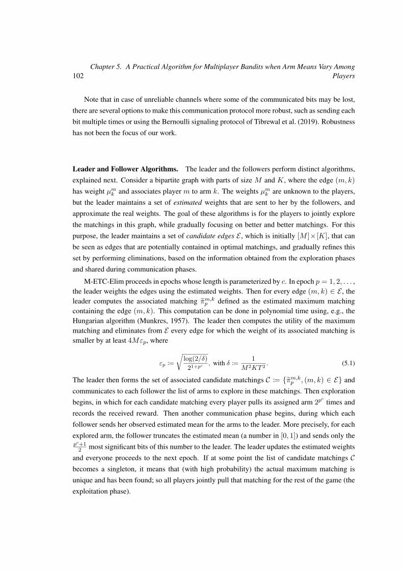
102Chapter 5. A Practical Algorithm for Multiplayer Bandits when Arm Means Vary Among
Players
Note that in case of unreliable channels where some of the communicated bits may be lost,
there are several options to make this communication protocol more robust, such as sending each
bit multiple times or using the Bernoulli signaling protocol of Tibrewal et al. (2019). Robustness
has not been the focus of our work.
Leader and Follower Algorithms. The leader and the followers perform distinct algorithms,
explained next. Consider a bipartite graph with parts of size M and K, where the edge (m, k)has weight µmk and associates player m to arm k. The weights µmk are unknown to the players,
but the leader maintains a set of estimated weights that are sent to her by the followers, and
approximate the real weights. The goal of these algorithms is for the players to jointly explore
the matchings in this graph, while gradually focusing on better and better matchings. For this
purpose, the leader maintains a set of candidate edges E , which is initially [M ]×[K], that can
be seen as edges that are potentially contained in optimal matchings, and gradually refines this
set by performing eliminations, based on the information obtained from the exploration phases
and shared during communication phases.
M-ETC-Elim proceeds in epochs whose length is parameterized by c. In epoch p = 1, 2, . . . ,the leader weights the edges using the estimated weights. Then for every edge (m, k) ∈ E , theleader computes the associated matching πm,kp defined as the estimated maximum matchingcontaining the edge (m, k). This computation can be done in polynomial time using, e.g., theHungarian algorithm (Munkres, 1957). The leader then computes the utility of the maximummatching and eliminates from E every edge for which the weight of its associated matching issmaller by at least 4Mεp, where
εp :=√
log(2/δ)21+pc , with δ := 1
M2KT 2 . (5.1)
The leader then forms the set of associated candidate matchings C := πm,kp , (m, k) ∈ E and
communicates to each follower the list of arms to explore in these matchings. Then exploration
begins, in which for each candidate matching every player pulls its assigned arm 2pc times and
records the received reward. Then another communication phase begins, during which each
follower sends her observed estimated mean for the arms to the leader. More precisely, for each
explored arm, the follower truncates the estimated mean (a number in [0, 1]) and sends only thepc+1
2 most significant bits of this number to the leader. The leader updates the estimated weights
and everyone proceeds to the next epoch. If at some point the list of candidate matchings Cbecomes a singleton, it means that (with high probability) the actual maximum matching is
unique and has been found; so all players jointly pull that matching for the rest of the game (the
exploitation phase).
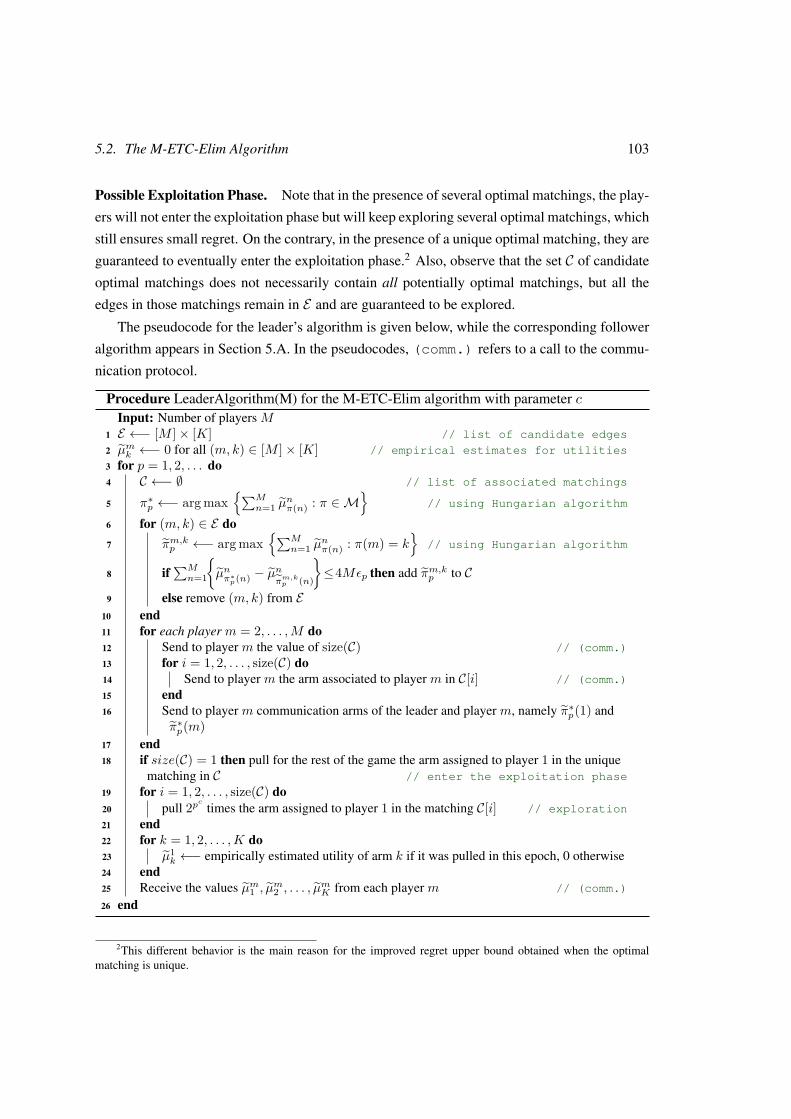
5.2. The M-ETC-Elim Algorithm 103
Possible Exploitation Phase. Note that in the presence of several optimal matchings, the play-
ers will not enter the exploitation phase but will keep exploring several optimal matchings, which
still ensures small regret. On the contrary, in the presence of a unique optimal matching, they are
guaranteed to eventually enter the exploitation phase.2 Also, observe that the set C of candidate
optimal matchings does not necessarily contain all potentially optimal matchings, but all the
edges in those matchings remain in E and are guaranteed to be explored.
The pseudocode for the leader’s algorithm is given below, while the corresponding follower
algorithm appears in Section 5.A. In the pseudocodes, (comm.) refers to a call to the commu-
nication protocol.
Procedure LeaderAlgorithm(M) for the M-ETC-Elim algorithm with parameter cInput: Number of players M
1 E ←− [M ]× [K] // list of candidate edges
2 µmk ←− 0 for all (m, k) ∈ [M ]× [K] // empirical estimates for utilities
3 for p = 1, 2, . . . do4 C ←− ∅ // list of associated matchings
5 π∗p ←− arg max∑M
n=1 µnπ(n) : π ∈M
// using Hungarian algorithm
6 for (m, k) ∈ E do7 πm,kp ←− arg max
∑Mn=1 µ
nπ(n) : π(m) = k
// using Hungarian algorithm
8 if∑Mn=1
µnπ∗p(n) − µ
n
πm,kp (n)
≤4Mεp then add πm,kp to C
9 else remove (m, k) from E10 end11 for each player m = 2, . . . ,M do12 Send to player m the value of size(C) // (comm.)
13 for i = 1, 2, . . . , size(C) do14 Send to player m the arm associated to player m in C[i] // (comm.)
15 end16 Send to player m communication arms of the leader and player m, namely π∗p(1) and
π∗p(m)17 end18 if size(C) = 1 then pull for the rest of the game the arm assigned to player 1 in the unique
matching in C // enter the exploitation phase
19 for i = 1, 2, . . . , size(C) do20 pull 2pc times the arm assigned to player 1 in the matching C[i] // exploration
21 end22 for k = 1, 2, . . . ,K do23 µ1
k ←− empirically estimated utility of arm k if it was pulled in this epoch, 0 otherwise24 end25 Receive the values µm1 , µ
m2 , . . . , µ
mK from each player m // (comm.)
26 end
2This different behavior is the main reason for the improved regret upper bound obtained when the optimalmatching is unique.
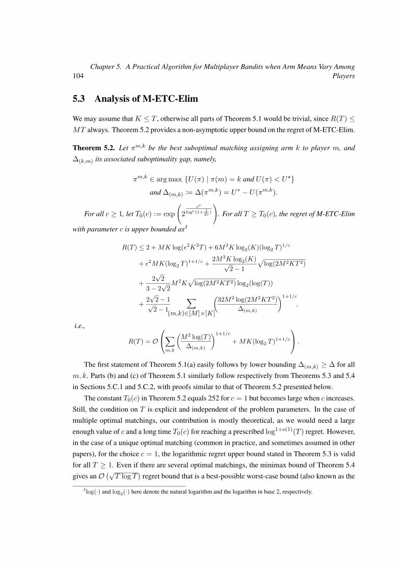
104Chapter 5. A Practical Algorithm for Multiplayer Bandits when Arm Means Vary Among
Players
5.3 Analysis of M-ETC-Elim
We may assume that K ≤ T , otherwise all parts of Theorem 5.1 would be trivial, since R(T ) ≤MT always. Theorem 5.2 provides a non-asymptotic upper bound on the regret of M-ETC-Elim.
Theorem 5.2. Let πm,k be the best suboptimal matching assigning arm k to player m, and
∆(k,m) its associated suboptimality gap, namely,
πm,k ∈ arg max U(π) | π(m) = k and U(π) < U?
and ∆(m,k) := ∆(πm,k) = U∗ − U(πm,k).
For all c ≥ 1, let T0(c) := exp(
2cc
logc(1+ 12c )
). For all T ≥ T0(c), the regret of M-ETC-Elim
with parameter c is upper bounded as3
R(T ) ≤ 2 +MK log(e2K2T ) + 6M2K log2(K)(log2 T )1/c
+ e2MK(log2 T )1+1/c + 2M3K log2(K)√2− 1
√log(2M2KT 2)
+ 2√
23− 2
√2M2K
√log(2M2KT 2) log2(log(T ))
+ 2√
2− 1√2− 1
∑(m,k)∈[M ]×[K]
(32M2 log(2M2KT 2)
∆(m,k)
)1+1/c
,
i.e.,
R(T ) = O
∑m,k
(M2 log(T )
∆(m,k)
)1+1/c
+MK(log2 T )1+1/c
.
The first statement of Theorem 5.1(a) easily follows by lower bounding ∆(m,k) ≥ ∆ for all
m, k. Parts (b) and (c) of Theorem 5.1 similarly follow respectively from Theorems 5.3 and 5.4
in Sections 5.C.1 and 5.C.2, with proofs similar to that of Theorem 5.2 presented below.
The constant T0(c) in Theorem 5.2 equals 252 for c = 1 but becomes large when c increases.
Still, the condition on T is explicit and independent of the problem parameters. In the case of
multiple optimal matchings, our contribution is mostly theoretical, as we would need a large
enough value of c and a long time T0(c) for reaching a prescribed log1+o(1)(T ) regret. However,
in the case of a unique optimal matching (common in practice, and sometimes assumed in other
papers), for the choice c = 1, the logarithmic regret upper bound stated in Theorem 5.3 is valid
for all T ≥ 1. Even if there are several optimal matchings, the minimax bound of Theorem 5.4
gives an O(√T log T
)regret bound that is a best-possible worst-case bound (also known as the
3log(·) and log2(·) here denote the natural logarithm and the logarithm in base 2, respectively.
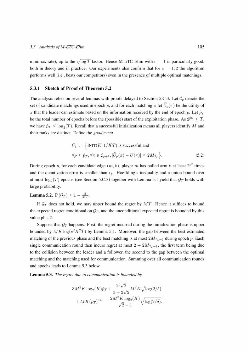
5.3. Analysis of M-ETC-Elim 105
minimax rate), up to the√
log T factor. Hence M-ETC-Elim with c = 1 is particularly good,
both in theory and in practice. Our experiments also confirm that for c = 1, 2 the algorithm
performs well (i.e., beats our competitors) even in the presence of multiple optimal matchings.
5.3.1 Sketch of Proof of Theorem 5.2
The analysis relies on several lemmas with proofs delayed to Section 5.C.3. Let Cp denote the
set of candidate matchings used in epoch p, and for each matching π let Up(π) be the utility of
π that the leader can estimate based on the information received by the end of epoch p. Let pTbe the total number of epochs before the (possible) start of the exploitation phase. As 2pcT ≤ T ,
we have pT ≤ log2(T ). Recall that a successful initialization means all players identify M and
their ranks are distinct. Define the good event
GT :=
INIT(K, 1/KT ) is successful and
∀p ≤ pT ,∀π ∈ Cp+1, |Up(π)− U(π)| ≤ 2Mεp. (5.2)
During epoch p, for each candidate edge (m, k), player m has pulled arm k at least 2pc times
and the quantization error is smaller than εp. Hoeffding’s inequality and a union bound over
at most log2(T ) epochs (see Section 5.C.3) together with Lemma 5.1 yield that GT holds with
large probability.
Lemma 5.2. P (GT ) ≥ 1− 2MT .
If GT does not hold, we may upper bound the regret by MT . Hence it suffices to bound
the expected regret conditional on GT , and the unconditional expected regret is bounded by this
value plus 2.
Suppose that GT happens. First, the regret incurred during the initialization phase is upper
bounded by MK log(e2K2T ) by Lemma 5.1. Moreover, the gap between the best estimated
matching of the previous phase and the best matching is at most 2Mεp−1 during epoch p. Each
single communication round then incurs regret at most 2 + 2Mεp−1, the first term being due
to the collision between the leader and a follower, the second to the gap between the optimal
matching and the matching used for communication. Summing over all communication rounds
and epochs leads to Lemma 5.3 below.
Lemma 5.3. The regret due to communication is bounded by
3M2K log2(K)pT + 2c√
23− 2
√2M2K
√log(2/δ)
+MK(pT )c+1 + 2M3K log2(K)√2− 1
√log(2/δ).
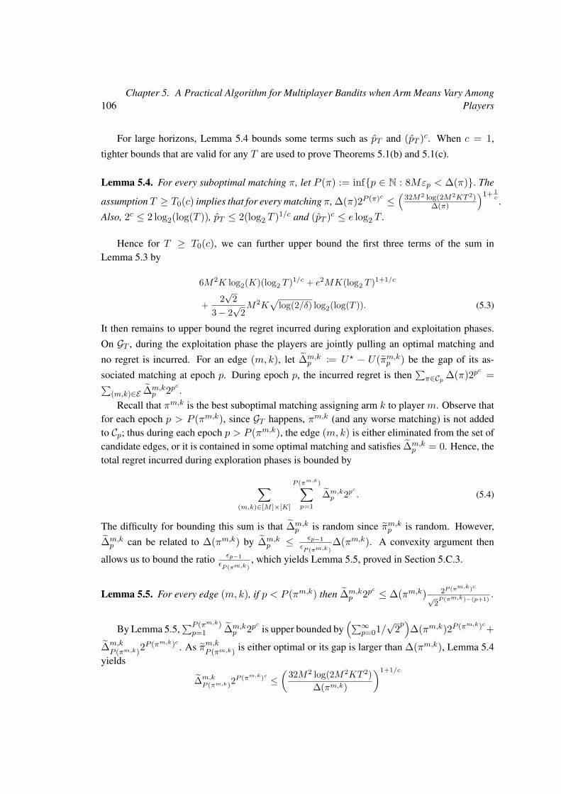
106Chapter 5. A Practical Algorithm for Multiplayer Bandits when Arm Means Vary Among
Players
For large horizons, Lemma 5.4 bounds some terms such as pT and (pT )c. When c = 1,
tighter bounds that are valid for any T are used to prove Theorems 5.1(b) and 5.1(c).
Lemma 5.4. For every suboptimal matching π, let P (π) := infp ∈ N : 8Mεp < ∆(π). The
assumption T ≥ T0(c) implies that for every matching π, ∆(π)2P (π)c ≤(
32M2 log(2M2KT 2)∆(π)
)1+ 1c .
Also, 2c ≤ 2 log2(log(T )), pT ≤ 2(log2 T )1/c and (pT )c ≤ e log2 T .
Hence for T ≥ T0(c), we can further upper bound the first three terms of the sum inLemma 5.3 by
6M2K log2(K)(log2 T )1/c + e2MK(log2 T )1+1/c
+ 2√
23− 2
√2M2K
√log(2/δ) log2(log(T )). (5.3)
It then remains to upper bound the regret incurred during exploration and exploitation phases.
On GT , during the exploitation phase the players are jointly pulling an optimal matching and
no regret is incurred. For an edge (m, k), let ∆m,kp := U? − U(πm,kp ) be the gap of its as-
sociated matching at epoch p. During epoch p, the incurred regret is then∑π∈Cp ∆(π)2pc =∑
(m,k)∈E ∆m,kp 2pc .
Recall that πm,k is the best suboptimal matching assigning arm k to player m. Observe thatfor each epoch p > P (πm,k), since GT happens, πm,k (and any worse matching) is not addedto Cp; thus during each epoch p > P (πm,k), the edge (m, k) is either eliminated from the set ofcandidate edges, or it is contained in some optimal matching and satisfies ∆m,k
p = 0. Hence, thetotal regret incurred during exploration phases is bounded by
∑(m,k)∈[M ]×[K]
P (πm,k)∑p=1
∆m,kp 2p
c
. (5.4)
The difficulty for bounding this sum is that ∆m,kp is random since πm,kp is random. However,
∆m,kp can be related to ∆(πm,k) by ∆m,k
p ≤ εp−1εP (πm,k)
∆(πm,k). A convexity argument then
allows us to bound the ratio εp−1εP (πm,k)
, which yields Lemma 5.5, proved in Section 5.C.3.
Lemma 5.5. For every edge (m, k), if p < P (πm,k) then ∆m,kp 2pc ≤ ∆(πm,k) 2P (πm,k)c
√2P (πm,k)−(p+1) .
By Lemma 5.5,∑P (πm,k)p=1 ∆m,k
p 2pc is upper bounded by(∑∞
p=01/√
2p)∆(πm,k)2P (πm,k)c+
∆m,kP (πm,k)2
P (πm,k)c . As πm,kP (πm,k) is either optimal or its gap is larger than ∆(πm,k), Lemma 5.4
yields
∆m,kP (πm,k)2
P (πm,k)c ≤(
32M2 log(2M2KT 2)∆(πm,k)
)1+1/c
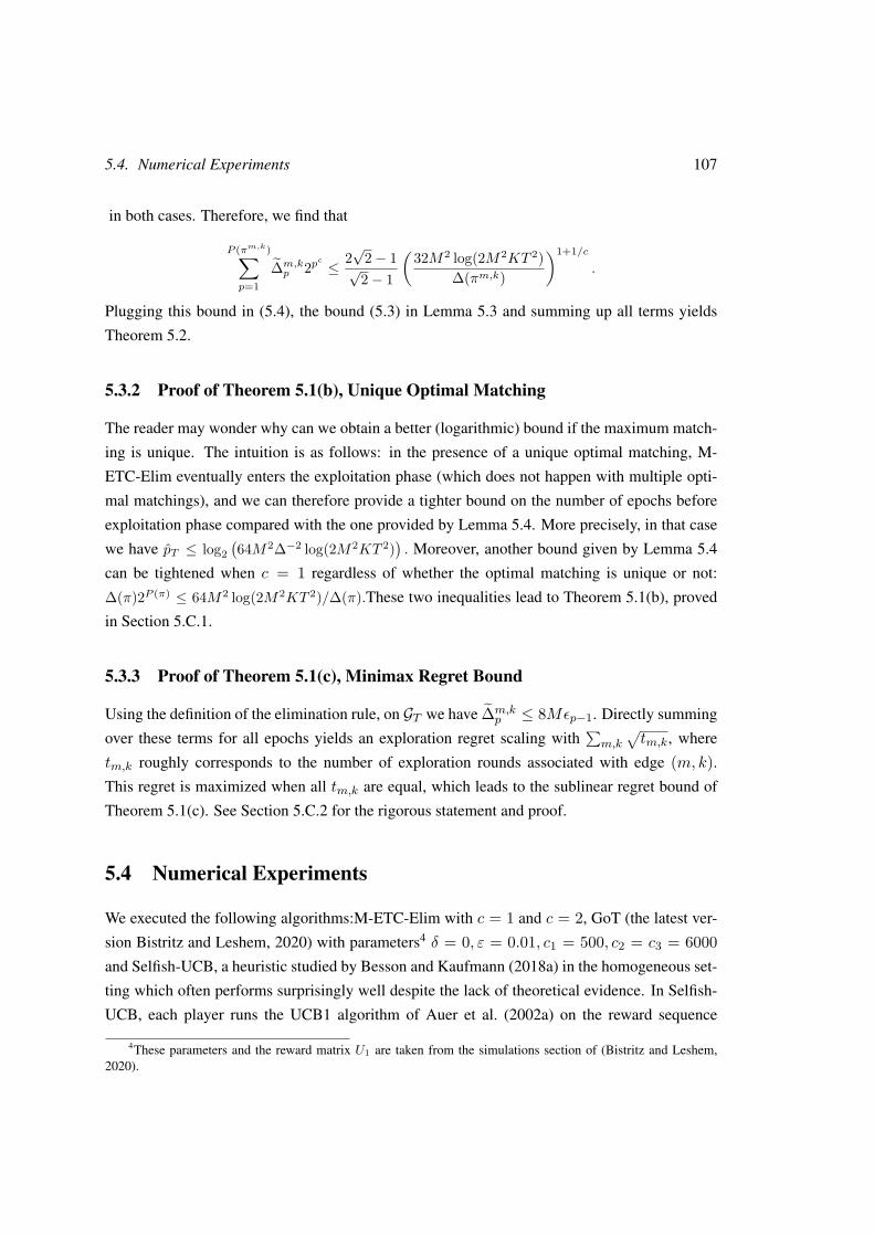
5.4. Numerical Experiments 107
in both cases. Therefore, we find that
P (πm,k)∑p=1
∆m,kp 2p
c
≤ 2√
2− 1√2− 1
(32M2 log(2M2KT 2)
∆(πm,k)
)1+1/c
.
Plugging this bound in (5.4), the bound (5.3) in Lemma 5.3 and summing up all terms yields
Theorem 5.2.
5.3.2 Proof of Theorem 5.1(b), Unique Optimal Matching
The reader may wonder why can we obtain a better (logarithmic) bound if the maximum match-
ing is unique. The intuition is as follows: in the presence of a unique optimal matching, M-
ETC-Elim eventually enters the exploitation phase (which does not happen with multiple opti-
mal matchings), and we can therefore provide a tighter bound on the number of epochs before
exploitation phase compared with the one provided by Lemma 5.4. More precisely, in that case
we have pT ≤ log2(64M2∆−2 log(2M2KT 2)
). Moreover, another bound given by Lemma 5.4
can be tightened when c = 1 regardless of whether the optimal matching is unique or not:
∆(π)2P (π) ≤ 64M2 log(2M2KT 2)/∆(π).These two inequalities lead to Theorem 5.1(b), proved
in Section 5.C.1.
5.3.3 Proof of Theorem 5.1(c), Minimax Regret Bound
Using the definition of the elimination rule, on GT we have ∆m,kp ≤ 8Mεp−1. Directly summing
over these terms for all epochs yields an exploration regret scaling with∑m,k
√tm,k, where
tm,k roughly corresponds to the number of exploration rounds associated with edge (m, k).
This regret is maximized when all tm,k are equal, which leads to the sublinear regret bound of
Theorem 5.1(c). See Section 5.C.2 for the rigorous statement and proof.
5.4 Numerical Experiments
We executed the following algorithms:M-ETC-Elim with c = 1 and c = 2, GoT (the latest ver-
sion Bistritz and Leshem, 2020) with parameters4 δ = 0, ε = 0.01, c1 = 500, c2 = c3 = 6000and Selfish-UCB, a heuristic studied by Besson and Kaufmann (2018a) in the homogeneous set-
ting which often performs surprisingly well despite the lack of theoretical evidence. In Selfish-
UCB, each player runs the UCB1 algorithm of Auer et al. (2002a) on the reward sequence
4These parameters and the reward matrix U1 are taken from the simulations section of (Bistritz and Leshem,2020).
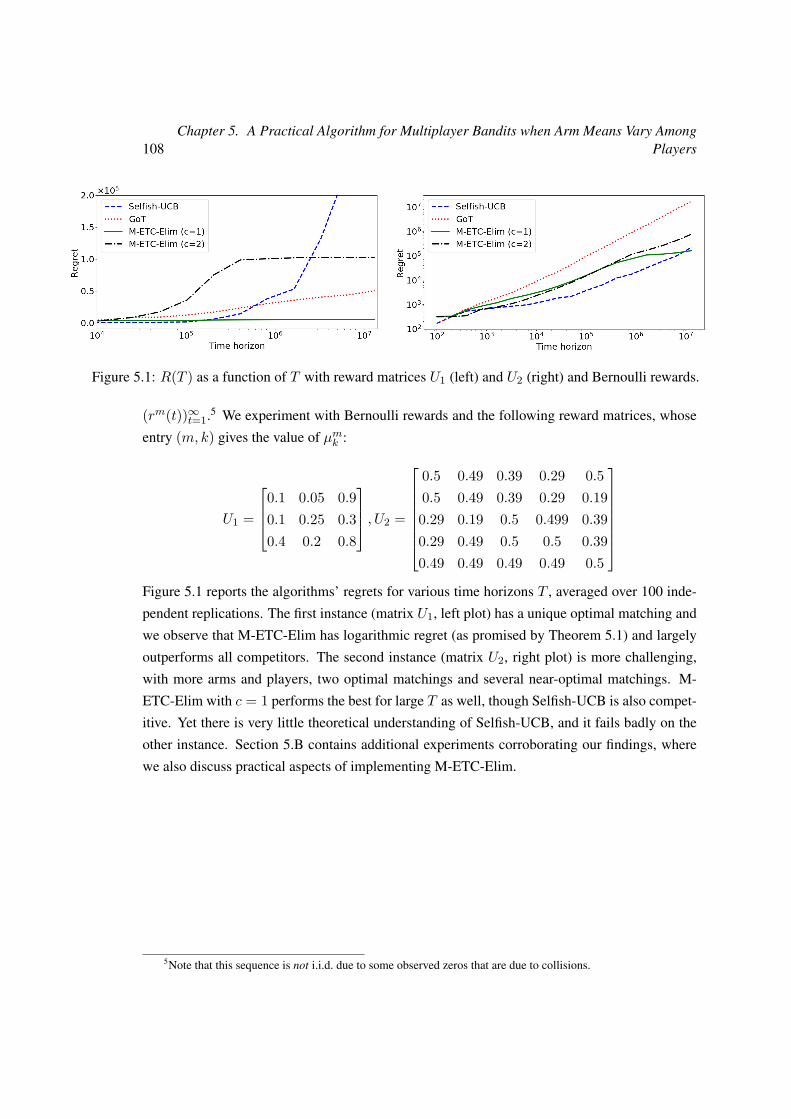
108Chapter 5. A Practical Algorithm for Multiplayer Bandits when Arm Means Vary Among
Players
Figure 5.1: R(T ) as a function of T with reward matrices U1 (left) and U2 (right) and Bernoulli rewards.
(rm(t))∞t=1.5 We experiment with Bernoulli rewards and the following reward matrices, whose
entry (m, k) gives the value of µmk :
U1 =
0.1 0.05 0.90.1 0.25 0.30.4 0.2 0.8
, U2 =
0.5 0.49 0.39 0.29 0.50.5 0.49 0.39 0.29 0.190.29 0.19 0.5 0.499 0.390.29 0.49 0.5 0.5 0.390.49 0.49 0.49 0.49 0.5
Figure 5.1 reports the algorithms’ regrets for various time horizons T , averaged over 100 inde-
pendent replications. The first instance (matrix U1, left plot) has a unique optimal matching and
we observe that M-ETC-Elim has logarithmic regret (as promised by Theorem 5.1) and largely
outperforms all competitors. The second instance (matrix U2, right plot) is more challenging,
with more arms and players, two optimal matchings and several near-optimal matchings. M-
ETC-Elim with c = 1 performs the best for large T as well, though Selfish-UCB is also compet-
itive. Yet there is very little theoretical understanding of Selfish-UCB, and it fails badly on the
other instance. Section 5.B contains additional experiments corroborating our findings, where
we also discuss practical aspects of implementing M-ETC-Elim.
5Note that this sequence is not i.i.d. due to some observed zeros that are due to collisions.
Appendix
5.A Description of the Initialization Procedure and Followers’ Pseu-docode
The pseudocode of the INIT(K, δ0) procedure, already presented in Chapter 4, is presented in
Algorithm 5.2 for the sake of completeness.
Next, we present the pseudocode that the followers execute in M-ETC-Elim. Recall that
(comm.) refers to a call to the communication protocol.
5.B Practical Considerations and Additional Experiments
5.B.1 Implementation Enhancements for M-ETC-Elim
In the implementation of M-ETC-Elim, the following enhancements significantly improve the
regret in practice (and have been used for the reported numerical experiments), but only by
constant factors in theory, hence we have not included them in the analysis for the sake of
brevity.
First, to estimate the means, the players are better off taking into account all pulls of the arms,
rather than just the last epoch. Note that after the exploration phase of epoch p, each candidate
edge has been pulledNp :=∑pi=1 2ic times. Thus, with probability at least 1−2 log2(T )/(MT ),
each edge has been estimated within additive error ≤ ε′p =√
log(M2TK)/2Np by Hoeffd-
ing’s inequality. The players then truncate these estimates using b := d− log2(0.1ε′p)e bits,
adding up to 0.1ε′p additive error due to quantization. They then send these b bits to the
leader. Now, the threshold for eliminating a matching would be 2.2Mε′p rather than 4M ×√log(2M2KT 2)/21+pc (compare with line 8 of the Leaderalgorithm presented on page 103).
The second enhancement is to choose the set C of matchings to explore more carefully. Say
that a matching is good if its estimated gap is at most 2.2Mε′p, and say an edge is candidate
(lies in E) if it is part of some good matching. There are at most MK candidate edges, and we
109
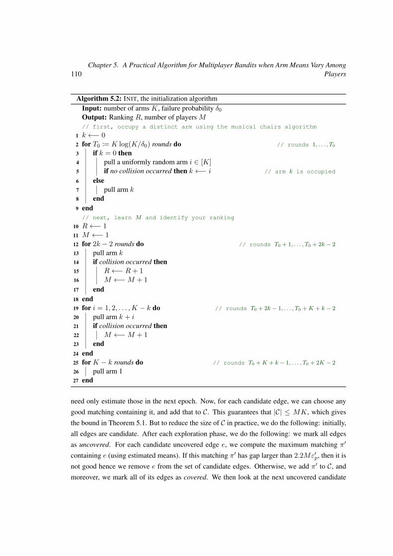
110Chapter 5. A Practical Algorithm for Multiplayer Bandits when Arm Means Vary Among
Players
Algorithm 5.2: INIT, the initialization algorithmInput: number of arms K, failure probability δ0Output: Ranking R, number of players M// first, occupy a distinct arm using the musical chairs algorithm
1 k ←− 02 for T0 := K log(K/δ0) rounds do // rounds 1, . . . , T0
3 if k = 0 then4 pull a uniformly random arm i ∈ [K]5 if no collision occurred then k ←− i // arm k is occupied
6 else7 pull arm k8 end9 end// next, learn M and identify your ranking
10 R←− 111 M ←− 112 for 2k − 2 rounds do // rounds T0 + 1, . . . , T0 + 2k − 213 pull arm k14 if collision occurred then15 R←− R+ 116 M ←−M + 117 end18 end19 for i = 1, 2, . . . ,K − k do // rounds T0 + 2k − 1, . . . , T0 +K + k − 220 pull arm k + i21 if collision occurred then22 M ←−M + 123 end24 end25 for K − k rounds do // rounds T0 +K + k − 1, . . . , T0 + 2K − 226 pull arm 127 end
need only estimate those in the next epoch. Now, for each candidate edge, we can choose any
good matching containing it, and add that to C. This guarantees that |C| ≤ MK, which gives
the bound in Theorem 5.1. But to reduce the size of C in practice, we do the following: initially,
all edges are candidate. After each exploration phase, we do the following: we mark all edges
as uncovered. For each candidate uncovered edge e, we compute the maximum matching π′
containing e (using estimated means). If this matching π′ has gap larger than 2.2Mε′p, then it is
not good hence we remove e from the set of candidate edges. Otherwise, we add π′ to C, and
moreover, we mark all of its edges as covered. We then look at the next uncovered candidate

5.B. Practical Considerations and Additional Experiments 111
Procedure Followeralgorithm(R,M) for the M-ETC-Elim algorithm with parameter cInput: Ranking R, number of players M
1 for p = 1, 2, . . . do2 Receive the value of size(C) // (comm.)
3 for i = 1, 2, . . . , size(C) do4 Receive the arm assigned to this player in C[i] // (comm.)
5 end6 Receive the communication arm of the leader and of this player7 if size(C) = 1 // (enter exploitation phase)
8 then9 pull for the rest of the game the arm assigned to this player in the unique
matching in C10 end11 for i = 1, 2, . . . , size(C) do12 pull 2pc times the arm assigned to this player in the matching C[i]13 end14 for k = 1, 2, . . . ,K do15 µRk ←− empirically estimated utility of arm k if arm k has been pulled in this
epoch, 0 otherwise16 Truncate µRk to µRk using the pc+1
2 most significant bits17 end18 Send the values µR1 , µ
R2 , . . . , µ
RK to the leader // (comm.)
19 end
edge, and continue similarly, until all candidate edges are covered. This guarantees that all the
candidate edges are explored, while the number of explored matchings could be much smaller
than the number of candidate edges, which results in faster exploration and a smaller regret in
practice.
To reduce the size of C even further, we do the following after each exploration phase: first,
find the maximum matching (using estimated means), add it to C, mark all its edges as covered,
and only then start looking for uncovered candidate edges as explained above.
5.B.2 Other Reward Distributions
In our model and analysis, we have assumed Xmk (t) ∈ [0, 1] for simplicity (this is a standard
assumption in online learning), but it is immediate to generalize the algorithm and its analysis
to reward distributions bounded in any known interval via a linear transformation. Also, we
can adapt our algorithm and analysis to subgaussian distributions with mean lying in a known
interval. A random variable X is σ-subgaussian if for all λ ∈ R we have E[eλ(X−EX)] ≤eσ
2λ2/2. This includes Gaussian distributions and distributions with bounded support. Suppose
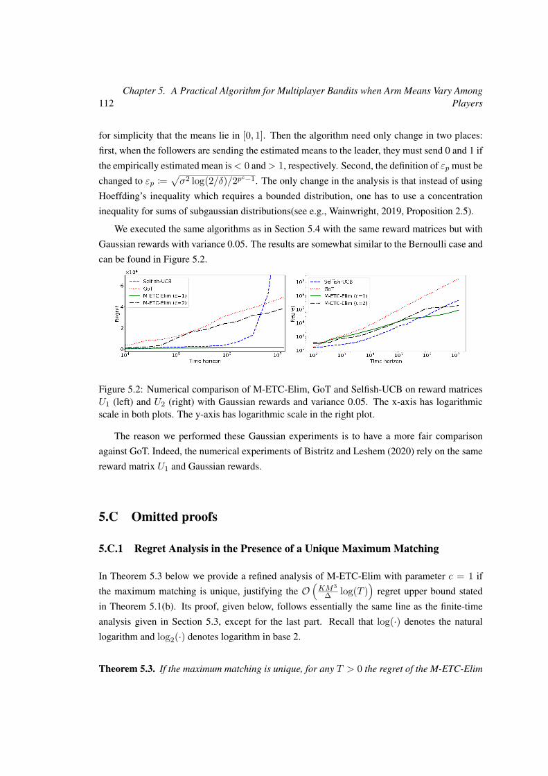
112Chapter 5. A Practical Algorithm for Multiplayer Bandits when Arm Means Vary Among
Players
for simplicity that the means lie in [0, 1]. Then the algorithm need only change in two places:
first, when the followers are sending the estimated means to the leader, they must send 0 and 1 if
the empirically estimated mean is< 0 and> 1, respectively. Second, the definition of εp must be
changed to εp :=√σ2 log(2/δ)/2pc−1. The only change in the analysis is that instead of using
Hoeffding’s inequality which requires a bounded distribution, one has to use a concentration
inequality for sums of subgaussian distributions(see e.g., Wainwright, 2019, Proposition 2.5).
We executed the same algorithms as in Section 5.4 with the same reward matrices but with
Gaussian rewards with variance 0.05. The results are somewhat similar to the Bernoulli case and
can be found in Figure 5.2.
Figure 5.2: Numerical comparison of M-ETC-Elim, GoT and Selfish-UCB on reward matricesU1 (left) and U2 (right) with Gaussian rewards and variance 0.05. The x-axis has logarithmicscale in both plots. The y-axis has logarithmic scale in the right plot.
The reason we performed these Gaussian experiments is to have a more fair comparison
against GoT. Indeed, the numerical experiments of Bistritz and Leshem (2020) rely on the same
reward matrix U1 and Gaussian rewards.
5.C Omitted proofs
5.C.1 Regret Analysis in the Presence of a Unique Maximum Matching
In Theorem 5.3 below we provide a refined analysis of M-ETC-Elim with parameter c = 1 if
the maximum matching is unique, justifying the O(KM3
∆ log(T ))
regret upper bound stated
in Theorem 5.1(b). Its proof, given below, follows essentially the same line as the finite-time
analysis given in Section 5.3, except for the last part. Recall that log(·) denotes the natural
logarithm and log2(·) denotes logarithm in base 2.
Theorem 5.3. If the maximum matching is unique, for any T > 0 the regret of the M-ETC-Elim
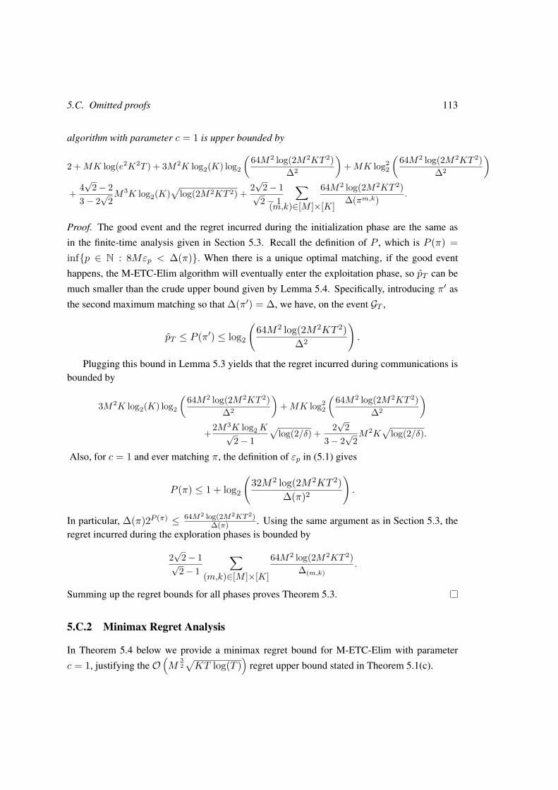
5.C. Omitted proofs 113
algorithm with parameter c = 1 is upper bounded by
2 +MK log(e2K2T ) + 3M2K log2(K) log2
(64M2 log(2M2KT 2)
∆2
)+MK log2
2
(64M2 log(2M2KT 2)
∆2
)+ 4√
2− 23− 2
√2M3K log2(K)
√log(2M2KT 2) + 2
√2− 1√2− 1
∑(m,k)∈[M ]×[K]
64M2 log(2M2KT 2)∆(πm,k) .
Proof. The good event and the regret incurred during the initialization phase are the same as
in the finite-time analysis given in Section 5.3. Recall the definition of P , which is P (π) =infp ∈ N : 8Mεp < ∆(π). When there is a unique optimal matching, if the good event
happens, the M-ETC-Elim algorithm will eventually enter the exploitation phase, so pT can be
much smaller than the crude upper bound given by Lemma 5.4. Specifically, introducing π′ as
the second maximum matching so that ∆(π′) = ∆, we have, on the event GT ,
pT ≤ P (π′) ≤ log2
(64M2 log(2M2KT 2)
∆2
).
Plugging this bound in Lemma 5.3 yields that the regret incurred during communications isbounded by
3M2K log2(K) log2
(64M2 log(2M2KT 2)
∆2
)+MK log2
2
(64M2 log(2M2KT 2)
∆2
)+2M3K log2K√
2− 1√
log(2/δ) + 2√
23− 2
√2M2K
√log(2/δ).
Also, for c = 1 and ever matching π, the definition of εp in (5.1) gives
P (π) ≤ 1 + log2
(32M2 log(2M2KT 2)
∆(π)2
).
In particular, ∆(π)2P (π) ≤ 64M2 log(2M2KT 2)∆(π) . Using the same argument as in Section 5.3, the
regret incurred during the exploration phases is bounded by
2√
2− 1√2− 1
∑(m,k)∈[M ]×[K]
64M2 log(2M2KT 2)∆(m,k)
.
Summing up the regret bounds for all phases proves Theorem 5.3.
5.C.2 Minimax Regret Analysis
In Theorem 5.4 below we provide a minimax regret bound for M-ETC-Elim with parameter
c = 1, justifying the O(M
32√KT log(T )
)regret upper bound stated in Theorem 5.1(c).
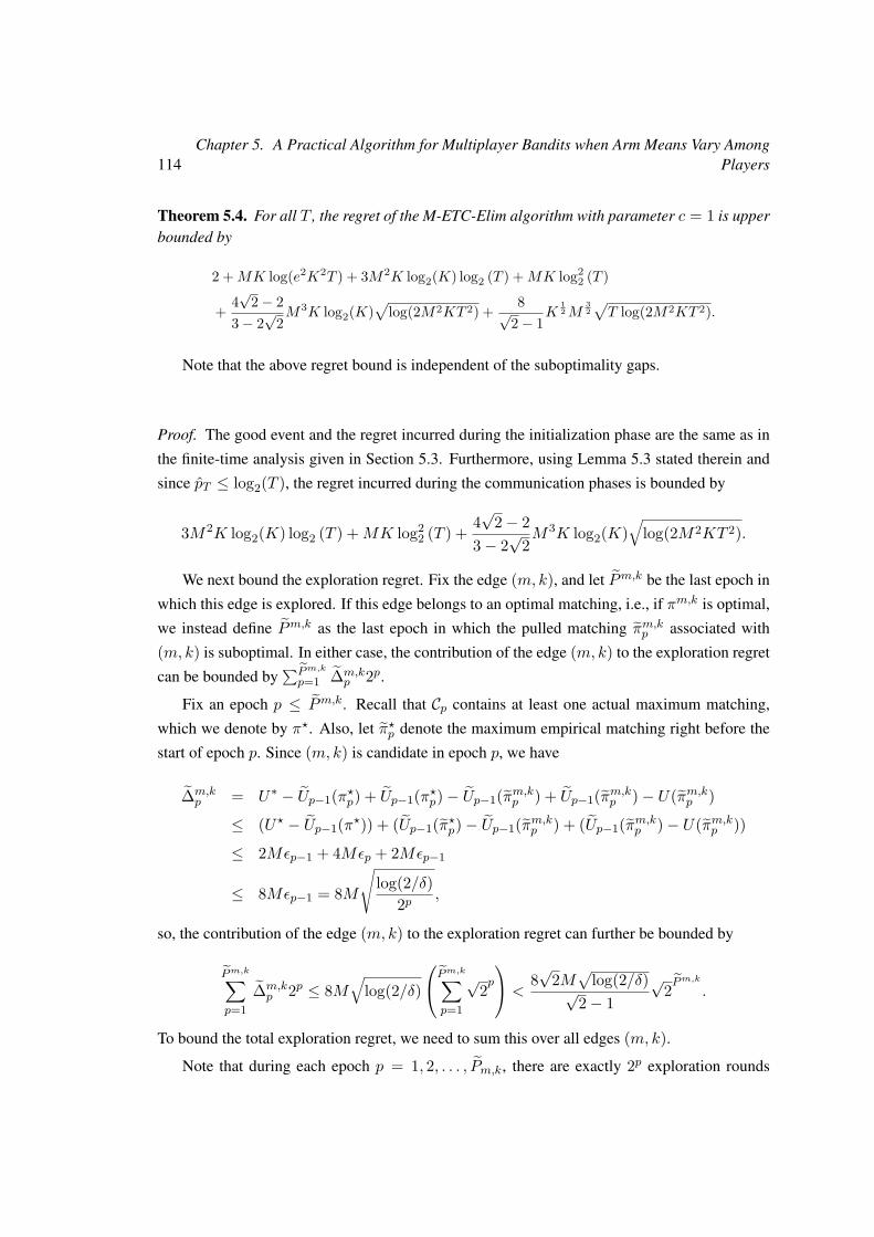
114Chapter 5. A Practical Algorithm for Multiplayer Bandits when Arm Means Vary Among
Players
Theorem 5.4. For all T , the regret of the M-ETC-Elim algorithm with parameter c = 1 is upperbounded by
2 +MK log(e2K2T ) + 3M2K log2(K) log2 (T ) +MK log22 (T )
+ 4√
2− 23− 2
√2M3K log2(K)
√log(2M2KT 2) + 8√
2− 1K
12M
32√T log(2M2KT 2).
Note that the above regret bound is independent of the suboptimality gaps.
Proof. The good event and the regret incurred during the initialization phase are the same as in
the finite-time analysis given in Section 5.3. Furthermore, using Lemma 5.3 stated therein and
since pT ≤ log2(T ), the regret incurred during the communication phases is bounded by
3M2K log2(K) log2 (T ) +MK log22 (T ) + 4
√2− 2
3− 2√
2M3K log2(K)
√log(2M2KT 2).
We next bound the exploration regret. Fix the edge (m, k), and let Pm,k be the last epoch in
which this edge is explored. If this edge belongs to an optimal matching, i.e., if πm,k is optimal,
we instead define Pm,k as the last epoch in which the pulled matching πm,kp associated with
(m, k) is suboptimal. In either case, the contribution of the edge (m, k) to the exploration regret
can be bounded by∑Pm,k
p=1 ∆m,kp 2p.
Fix an epoch p ≤ Pm,k. Recall that Cp contains at least one actual maximum matching,
which we denote by π?. Also, let π?p denote the maximum empirical matching right before the
start of epoch p. Since (m, k) is candidate in epoch p, we have
∆m,kp = U∗ − Up−1(π?p) + Up−1(π?p)− Up−1(πm,kp ) + Up−1(πm,kp )− U(πm,kp )
≤ (U? − Up−1(π?)) + (Up−1(π?p)− Up−1(πm,kp ) + (Up−1(πm,kp )− U(πm,kp ))
≤ 2Mεp−1 + 4Mεp + 2Mεp−1
≤ 8Mεp−1 = 8M
√log(2/δ)
2p ,
so, the contribution of the edge (m, k) to the exploration regret can further be bounded by
Pm,k∑p=1
∆m,kp 2p ≤ 8M
√log(2/δ)
Pm,k∑p=1
√2p <
8√
2M√
log(2/δ)√2− 1
√2P
m,k
.
To bound the total exploration regret, we need to sum this over all edges (m, k).
Note that during each epoch p = 1, 2, . . . , Pm,k, there are exactly 2p exploration rounds
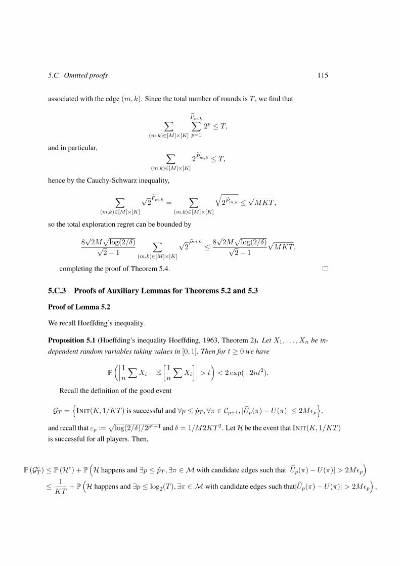
5.C. Omitted proofs 115
associated with the edge (m, k). Since the total number of rounds is T , we find that
∑(m,k)∈[M ]×[K]
Pm,k∑p=1
2p ≤ T,
and in particular, ∑(m,k)∈[M ]×[K]
2Pm,k ≤ T,
hence by the Cauchy-Schwarz inequality,
∑(m,k)∈[M ]×[K]
√2Pm,k =
∑(m,k)∈[M ]×[K]
√2Pm,k ≤
√MKT,
so the total exploration regret can be bounded by
8√
2M√
log(2/δ)√2− 1
∑(m,k)∈[M ]×[K]
√2P
m,k
≤ 8√
2M√
log(2/δ)√2− 1
√MKT,
completing the proof of Theorem 5.4.
5.C.3 Proofs of Auxiliary Lemmas for Theorems 5.2 and 5.3
Proof of Lemma 5.2
We recall Hoeffding’s inequality.
Proposition 5.1 (Hoeffding’s inequality Hoeffding, 1963, Theorem 2). Let X1, . . . , Xn be in-
dependent random variables taking values in [0, 1]. Then for t ≥ 0 we have
P(∣∣∣∣ 1n∑Xi − E
[ 1n
∑Xi
]∣∣∣∣ > t
)< 2 exp(−2nt2).
Recall the definition of the good event
GT =
INIT(K, 1/KT ) is successful and ∀p ≤ pT , ∀π ∈ Cp+1, |Up(π)− U(π)| ≤ 2Mεp.
and recall that εp :=√
log(2/δ)/2pc+1 and δ = 1/M2KT 2. LetH be the event that INIT(K, 1/KT )is successful for all players. Then,
P (GcT ) ≤ P (Hc) + P(H happens and ∃p ≤ pT , ∃π ∈M with candidate edges such that |Up(π)− U(π)| > 2Mεp
)≤ 1KT
+ P(H happens and ∃p ≤ log2(T ), ∃π ∈M with candidate edges such that|Up(π)− U(π)| > 2Mεp
),
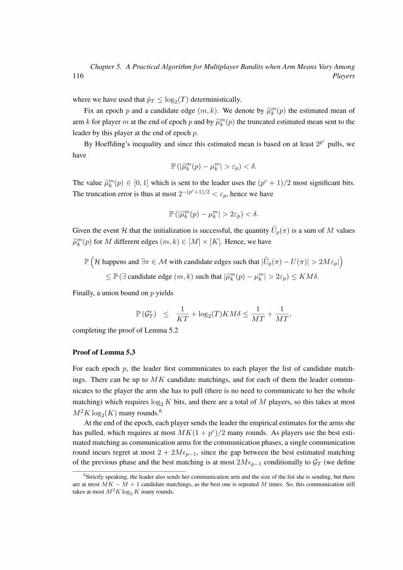
116Chapter 5. A Practical Algorithm for Multiplayer Bandits when Arm Means Vary Among
Players
where we have used that pT ≤ log2(T ) deterministically.
Fix an epoch p and a candidate edge (m, k). We denote by µmk (p) the estimated mean of
arm k for player m at the end of epoch p and by µmk (p) the truncated estimated mean sent to the
leader by this player at the end of epoch p.
By Hoeffding’s inequality and since this estimated mean is based on at least 2pc pulls, we
have
P (|µmk (p)− µmk | > εp) < δ.
The value µmk (p) ∈ [0, 1] which is sent to the leader uses the (pc + 1)/2 most significant bits.
The truncation error is thus at most 2−(pc+1)/2 < εp, hence we have
P (|µmk (p)− µmk | > 2εp) < δ.
Given the event H that the initialization is successful, the quantity Up(π) is a sum of M values
µmk (p) for M different edges (m, k) ∈ [M ]× [K]. Hence, we have
P(H happens and ∃π ∈M with candidate edges such that |Up(π)− U(π)| > 2Mεp|
)≤ P (∃ candidate edge (m, k) such that |µmk (p)− µmk | > 2εp) ≤ KMδ.
Finally, a union bound on p yields
P (GcT ) ≤ 1KT
+ log2(T )KMδ ≤ 1MT
+ 1MT
,
completing the proof of Lemma 5.2
Proof of Lemma 5.3
For each epoch p, the leader first communicates to each player the list of candidate match-
ings. There can be up to MK candidate matchings, and for each of them the leader commu-
nicates to the player the arm she has to pull (there is no need to communicate to her the whole
matching) which requires log2K bits, and there are a total of M players, so this takes at most
M2K log2(K) many rounds.6
At the end of the epoch, each player sends the leader the empirical estimates for the arms shehas pulled, which requires at most MK(1 + pc)/2 many rounds. As players use the best esti-mated matching as communication arms for the communication phases, a single communicationround incurs regret at most 2 + 2Mεp−1, since the gap between the best estimated matchingof the previous phase and the best matching is at most 2Mεp−1 conditionally to GT (we define
6Strictly speaking, the leader also sends her communication arm and the size of the list she is sending, but thereare at most MK −M + 1 candidate matchings, as the best one is repeated M times. So, this communication stilltakes at most M2K log2 K many rounds.
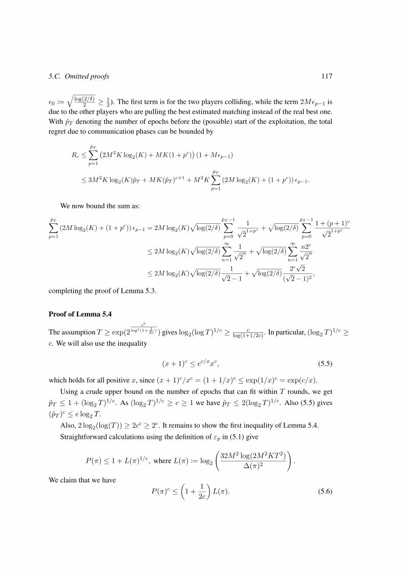
5.C. Omitted proofs 117
ε0 :=√
log(2/δ)2 ≥ 1
2 ). The first term is for the two players colliding, while the term 2Mεp−1 isdue to the other players who are pulling the best estimated matching instead of the real best one.With pT denoting the number of epochs before the (possible) start of the exploitation, the totalregret due to communication phases can be bounded by
Rc ≤pT∑p=1
(2M2K log2(K) +MK(1 + pc)
)(1 +Mεp−1)
≤ 3M2K log2(K)pT +MK(pT )c+1 +M2K
pT∑p=1
(2M log2(K) + (1 + pc)) εp−1.
We now bound the sum as:
pT∑p=1
(2M log2(K) + (1 + pc)) εp−1 = 2M log2(K)√
log(2/δ)pT−1∑p=0
1√
21+pc +√
log(2/δ)pT−1∑p=0
1 + (p+ 1)c√
21+pc
≤ 2M log2(K)√
log(2/δ)∞∑n=1
1√
2n+√
log(2/δ)∞∑n=1
n2c√
2n
≤ 2M log2(K)√
log(2/δ) 1√2− 1
+√
log(2/δ) 2c√
2(√
2− 1)2,
completing the proof of Lemma 5.3.
Proof of Lemma 5.4
The assumption T ≥ exp(2cc
logc(1+ 12c ) ) gives log2(log T )1/c ≥ c
log(1+1/2c) . In particular, (log2 T )1/c ≥c. We will also use the inequality
(x+ 1)c ≤ ec/xxc, (5.5)
which holds for all positive x, since (x+ 1)c/xc = (1 + 1/x)c ≤ exp(1/x)c = exp(c/x).
Using a crude upper bound on the number of epochs that can fit within T rounds, we get
pT ≤ 1 + (log2 T )1/c. As (log2 T )1/c ≥ c ≥ 1 we have pT ≤ 2(log2 T )1/c. Also (5.5) gives
(pT )c ≤ e log2 T .
Also, 2 log2(log(T )) ≥ 2cc ≥ 2c. It remains to show the first inequality of Lemma 5.4.
Straightforward calculations using the definition of εp in (5.1) give
P (π) ≤ 1 + L(π)1/c, where L(π) := log2
(32M2 log(2M2KT 2)
∆(π)2
).
We claim that we have
P (π)c ≤(
1 + 12c
)L(π). (5.6)

118Chapter 5. A Practical Algorithm for Multiplayer Bandits when Arm Means Vary Among
Players
Indeed, since ∆(π) ≤ M , we have L(π)1/c > (log2 log T )1/c ≥ clog(1+1/2c) and so (5.5)
with x = L(π)1/c gives (5.6). Hence,
∆(π)2P (π)c ≤ ∆(π)(
32M2 log(2M2KT 2)∆(π)2
)1+1/2c
≤(
32M2 log(2M2KT 2)∆(π)
)1+1/c
,
(5.7)
completing the proof of Lemma 5.4.
Proof of Lemma 5.5
For brevity we define, for this proof only, ∆ := ∆(πm,k), P := P (πm,k) and ∆p := ∆m,kp .
First, ∆ > 8MεP by definition of P . Also, ∆p ≤ 8Mεp−1 for every p ≤ P − 1, otherwise the
edge (m, k) would have been eliminated before epoch p. It then holds
∆p ≤εp−1εP
∆ =√
2Pc−(p−1)c∆. (5.8)
It comes from the convexity of x 7→ xc that (p+ 1)c + (p− 1)c − 2pc ≥ 0, and thus
P c + (p− 1)c − 2pc ≥ P c − (p+ 1)c ≥ P − (p+ 1).
It then follows
pc + P c − (p− 1)c
2 ≤ P c + p+ 1− P2 .
Plugging this in (5.8) gives
2pc∆p ≤2P c
√2P−(p+1) ∆,
completing the proof of Lemma 5.5.
Chapter 6
Selfish Robustness and Equilibria inMulti-Player Bandits
While the cooperative case where players maximize the collective reward (obediently fol-lowing some fixed protocol) has been mostly considered, robustness to malicious playersis a crucial and challenging concern of multiplayer bandits. Existing approaches consideronly the case of adversarial jammers whose objective is to blindly minimize the collectivereward.
We shall consider instead the more natural class of selfish players whose incentives are tomaximize their individual rewards, potentially at the expense of the social welfare. Weprovide the first algorithm robust to selfish players (a.k.a. Nash equilibrium) with a loga-rithmic regret, when the arm performance is observed. When collisions are also observed,Grim Trigger type of strategies enable some implicit communication-based algorithms andwe construct robust algorithms in two different settings: the homogeneous (with a regretcomparable to the centralized optimal one) and heterogeneous cases (for an adapted andrelevant notion of regret). We also provide impossibility results when only the reward isobserved or when arm means vary arbitrarily among players.
6.1 Problem statement . . . . . . . . . . . . . . . . . . . . . . . . . . . . . . . . 121
6.1.1 Considering selfish players . . . . . . . . . . . . . . . . . . . . . . . . 121
6.1.2 Limits of existing algorithms. . . . . . . . . . . . . . . . . . . . . . . 122
6.2 Statistic sensing setting . . . . . . . . . . . . . . . . . . . . . . . . . . . . . . 123
6.2.1 Description of Selfish-Robust MMAB . . . . . . . . . . . . . . . 123
6.2.2 Theoretical results . . . . . . . . . . . . . . . . . . . . . . . . . . . . 125
6.3 On harder problems . . . . . . . . . . . . . . . . . . . . . . . . . . . . . . . . 125
6.3.1 Hardness of no sensing setting . . . . . . . . . . . . . . . . . . . . . . 126
6.3.2 Heterogeneous model . . . . . . . . . . . . . . . . . . . . . . . . . . . 126
119
120 Chapter 6. Selfish Robustness and Equilibria in Multi-Player Bandits
6.4 Full sensing setting . . . . . . . . . . . . . . . . . . . . . . . . . . . . . . . . 128
6.4.1 Making communication robust . . . . . . . . . . . . . . . . . . . . . . 128
6.4.2 Homogeneous case: SIC-GT . . . . . . . . . . . . . . . . . . . . . . 129
6.4.3 Semi-heterogeneous case: RSD-GT . . . . . . . . . . . . . . . . . . . 131
6.A Missing elements for Selfish-Robust MMAB . . . . . . . . . . . . . . . 134
6.A.1 Thorough description of Selfish-Robust MMAB . . . . . . . . . 134
6.A.2 Proofs of Section 6.2 . . . . . . . . . . . . . . . . . . . . . . . . . . . 135
6.B Collective punishment proof . . . . . . . . . . . . . . . . . . . . . . . . . . . 144
6.C Missing elements for SIC-GT . . . . . . . . . . . . . . . . . . . . . . . . . . 145
6.C.1 Description of the algorithm . . . . . . . . . . . . . . . . . . . . . . . 146
6.C.2 Regret analysis . . . . . . . . . . . . . . . . . . . . . . . . . . . . . . 148
6.C.3 Selfish robustness of SIC-GT . . . . . . . . . . . . . . . . . . . . . . 156
6.D Missing elements for RSD-GT . . . . . . . . . . . . . . . . . . . . . . . . . . 160
6.D.1 Description of the algorithm . . . . . . . . . . . . . . . . . . . . . . . 160
6.D.2 Regret analysis . . . . . . . . . . . . . . . . . . . . . . . . . . . . . . 163
6.D.3 Selfish-robustness of RSD-GT . . . . . . . . . . . . . . . . . . . . . . 167
In most of the multiplayer bandits literature, as well as in Chapters 4 and 5, a crucial (yet
sometimes only implicitly stated) assumption is that all players follow cautiously and metic-
ulously some designed protocols and that none of them tries to free-ride the others by acting
greedily, selfishly or maliciously. The concern of designing multiplayer bandit algorithms ro-
bust to such players has been raised (Attar et al., 2012), but only addressed under the quite
restrictive assumption of adversarial players called jammers. Those try to perturb as much as
possible the cooperative players (Wang et al., 2015; Sawant et al., 2018; Sawant et al., 2019),
even if this is extremely costly to them as well. Because of this specific objective, they end up
using tailored strategies such as only attacking the top channels.
We focus instead on the construction of algorithms with “good” regret guarantees even if one
(or actually more) selfish player does not follow the common protocol but acts strategically in
order to manipulate the other players in the sole purpose of increasing her own payoff – maybe
at the cost of other players. This concept appeared quite early in the cognitive radio literature
(Attar et al., 2012), yet it is still not understood as robustness to selfish player is intrinsically
different (and even non-compatible) with robustness to jammers, as shown in Section 6.1.1. In
terms of game theory, we aim at constructing (ε-Nash) equilibria in this repeated game with
partial observations.
This chapter is organized as follows. Section 6.1 introduces notions and concepts of selfishness-
6.1. Problem statement 121
robust multiplayer bandits and showcases reasons for the design of robust algorithms. Besides its
state of the art regret guarantees when collisions are not directly observed, Selfish-Robust
MMAB, presented in Section 6.2, is also robust to selfish players. In the more complex settings
where only the reward is observed or the arm means vary among players, Section 6.3 shows that
no algorithm can guarantee both a sublinear regret and selfish-robustness. The latter case is due
to a more general result for random assignments. Instead of comparing the cumulated reward
with the best collective assignment in the heterogeneous case, it is then necessary to compare it
with a good and appropriate suboptimal assignment, leading to the new notion of RSD-regret.
When collisions are always observed, Section 6.4 proposes selfish-robust communication
protocols. Thanks to this, an adaptation of the work of Boursier and Perchet (2019) is possible
to provide a robust algorithm with a collective regret almost scaling as in the centralized case.
In the heterogeneous case, this communication – along with other new deviation control and
punishment protocols – is also used to provide a robust algorithm with a logarithmic RSD-regret.
Our contributions are thus diverse: on top of introducing notions of selfish-robustness, we
provide robust algorithms with state of the art regret bounds (w.r.t. non-robust algorithms) in
several settings. This is especially surprising when collisions are observed, since it leads to a
near centralized regret. Moreover, we show that such algorithms can not be designed in harder
settings. This leads to the new, adapted notion of RSD-regret in the heterogeneous case with
selfish players and we also provide a good algorithm in this case. These results of robustness
are even more intricate knowing they hold against any possible selfish strategy, in contrast to the
known results for jammer robust algorithms.
6.1 Problem statement
In this section, we introduce concepts and notions of robustness to selfish players (or equilibria
concepts) in the problem of multiplayer bandits introduced in Section 3.3.1.
6.1.1 Considering selfish players
As mentioned above, the literature focused on adversarial malicious players, a.k.a. jammers,
while considering selfish players instead of adversarial ones is as (if not more) crucial. These
two concepts of malicious players are fundamentally different. Jamming-robust algorithms must
stop pulling the best arm if it is being jammed. Against this algorithm, a selfish player could
therefore pose as a jammer, always pull the best arm and be left alone on it most of the time. On
the contrary, an algorithm robust to selfish players has to actually pull this best arm if jammed
122 Chapter 6. Selfish Robustness and Equilibria in Multi-Player Bandits
by some player in order to “punish” her so that she does not benefit from deviating from the
collective strategy.
We first introduce some game theoretic concepts before defining notions of robustness. Each
player j follows an individual strategy (or algorithm) sj ∈ S which determines her action at each
round given her past observations. As in Section 2.1, we denote by (s1, . . . , sM ) = s ∈ SM
the strategy profile of all players and by (s′, s−js−js−j) the strategy profile given by s except for the
j-th player whose strategy is replaced by s′. Let RewjT (sss) be the cumulative reward of player
j when players play the profile sss. As usual in game theory, we consider a single selfish player
– even if the algorithms we propose are robust to several selfish players assuming M is known
beforehand (its initial estimation can easily be tricked by several players).
Definition 6.1. A strategy profile sss ∈ SM is an ε-Nash equilibrium if for all s′ ∈ S andj ∈ [M ]:
E[RewjT (s′, s−js−js−j)] ≤ E[RewjT (sss)] + ε.
This simply states that a selfish player wins at most ε by deviating from sj . We now introduce
a more restrictive property of stability that involves two points: if a selfish player still were to
deviate, this would only incur a small loss to other players. Moreover, if the selfish player wants
to incur some considerable loss to the collective players (e.g., she is adversarial), then she also
has to incur a comparable loss to herself. Obviously, an ε-Nash equilibrium is (0, ε)-stable.
Definition 6.2. A strategy profile s ∈ SM is (α, ε)-stable if for all s′ ∈ S, l ∈ R+ and i, j ∈[M ]:
E[RewiT (s′, s−js−js−j)] ≤ E[RewiT (s)]− l =⇒ E[RewjT (s′, s−js−js−j)] ≤ E[RewjT (sss)] + ε− αl.
6.1.2 Limits of existing algorithms.
This section explains why existing algorithms are not robust to selfish players, i.e., are not even
o (T )-Nash equilibria. Besides justifying the design of new appropriate algorithms, this provides
some first insights on the way to achieve robustness.
Communication between players. Many recent algorithms rely on communication protocols
between players to gather their statistics. Facing an algorithm of this kind, a selfish player
would communicate fake statistics to the other players in order to keep the best arm for herself.
In case of collision, the colliding player(s) remains unidentified, so a selfish player could mod-
ify incognito the statistics sent by other players, making them untrustworthy. A way to make
such protocols robust to malicious players is proposed in Section 6.4. Algorithms relying on
communication can then be adapted in the Full Sensing setting.
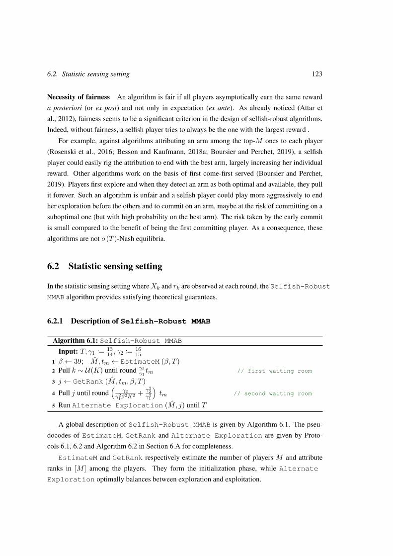
6.2. Statistic sensing setting 123
Necessity of fairness An algorithm is fair if all players asymptotically earn the same reward
a posteriori (or ex post) and not only in expectation (ex ante). As already noticed (Attar et
al., 2012), fairness seems to be a significant criterion in the design of selfish-robust algorithms.
Indeed, without fairness, a selfish player tries to always be the one with the largest reward .
For example, against algorithms attributing an arm among the top-M ones to each player
(Rosenski et al., 2016; Besson and Kaufmann, 2018a; Boursier and Perchet, 2019), a selfish
player could easily rig the attribution to end with the best arm, largely increasing her individual
reward. Other algorithms work on the basis of first come-first served (Boursier and Perchet,
2019). Players first explore and when they detect an arm as both optimal and available, they pull
it forever. Such an algorithm is unfair and a selfish player could play more aggressively to end
her exploration before the others and to commit on an arm, maybe at the risk of committing on a
suboptimal one (but with high probability on the best arm). The risk taken by the early commit
is small compared to the benefit of being the first committing player. As a consequence, these
algorithms are not o (T )-Nash equilibria.
6.2 Statistic sensing setting
In the statistic sensing setting whereXk and rk are observed at each round, the Selfish-Robust
MMAB algorithm provides satisfying theoretical guarantees.
6.2.1 Description of Selfish-Robust MMAB
Algorithm 6.1: Selfish-Robust MMAB
Input: T, γ1 := 1314 , γ2 := 16
151 β ← 39; M, tm ← EstimateM (β, T )2 Pull k ∼ U(K) until round γ2
γ1tm // first waiting room
3 j ← GetRank (M, tm, β, T )4 Pull j until round
(γ2
γ21β
2K2 + γ22γ2
1
)tm // second waiting room
5 Run Alternate Exploration (M, j) until T
A global description of Selfish-Robust MMAB is given by Algorithm 6.1. The pseu-
docodes of EstimateM, GetRank and Alternate Exploration are given by Proto-
cols 6.1, 6.2 and Algorithm 6.2 in Section 6.A for completeness.
EstimateM and GetRank respectively estimate the number of players M and attribute
ranks in [M ] among the players. They form the initialization phase, while Alternate
Exploration optimally balances between exploration and exploitation.
124 Chapter 6. Selfish Robustness and Equilibria in Multi-Player Bandits
Initialization phase
Let us first introduce the following quantities:
• T jk (t) = t′ ≤ t | πj(t′) = k and Xk(t′) > 0 are rounds when player j observed ηk.
• Cjk(t) = t′ ∈ T jk (t) | ηk(t′) = 1 are rounds when player j observed a collision.
• pjk(t) = #Cjk(t)
#T jk
(t)is the empirical probability to collide on the arm k for player j.
During the initialization, the players estimateM with large probability as given by Lemma 6.1
in Section 6.A.1. Players first pull uniformly at random in [K]. As soon as #T jk ≥ n for all
k ∈ [K] and some fixed n, player j ends the EstimateM protocol and estimates M as the
closest integer to 1 + log(1 −∑
kpjk(tM )
K )/ log(1 − 1K ). This estimation procedure is the same
as the one of Rosenski et al. (2016), except for the following features:
i) Collisions indicators are not always observed, as we consider statistic sensing here. For
this reason, the number of observations of ηk is random. The stopping criterion mink #T jk (t) ≥n ensures that players don’t need to know µ(K) beforehand, but they also do not end EstimateM
simultaneously. This is why a waiting room is needed, during which a player continues to pull
uniformly at random to ensure that all players are still pulling uniformly at random if some
player is still estimating M .
ii) The collision probability is not averaged over all arms, but estimated for each arm indi-
vidually, then averaged. This is necessary for robustness as explained in Section 6.A, despite
making the estimation longer.
Attribute ranks. After this first procedure, players then proceed to a Musical Chairs (Rosen-
ski et al., 2016) phase to attribute ranks among them as given by Lemma 6.2 in Section 6.A.1.
Players sample uniformly at random in [M ] and stop on an arm j as soon as they observe a
positive reward. The player’s rank is then j and only attributed to her. Here again, a waiting
room is required to ensure that all players are either pulling uniformly at random or only pulling
a specific arm (corresponding to their rank) during this procedure. During this second waiting
room, a player thus pulls the arm corresponding to her rank.
Exploration/exploitation
After the initialization, players know M and have different ranks. They enter the second phase,
where they follow Alternate Exploration, inspired by Proutiere and Wang (2019). Player
j sequentially pulls arms inMj(t), which is the ordered list of her M best empirical arms, un-
less she has to pull her M -th best empirical arm. In that case, she instead chooses at random
6.3. On harder problems 125
between actually pulling it or pulling an arm to explore (any arm not inMj(t) with an upper
confidence bound larger than the M -th best empirical mean, if there is any).
Since players proceed in a shifted fashion, they never collide whenMj(t) are the same for
all j. Having differentMj(t) happens in expectation a constant (in T ) amount of times, so that
the contribution of collisions to the regret is negligible.
6.2.2 Theoretical results
This section provides theoretical guarantees of Selfish-Robust MMAB. Theorem 6.1 first
presents guarantees in terms of regret. Its proof is given in Section 6.A.2.
Theorem 6.1. The collective regret of Selfish-Robust MMAB is bounded as
R(T ) ≤M∑k>M
µ(M) − µ(k)
kl(µ(k), µ(M))log(T ) +O
(MK3
µ(K)log(T )
).
It can also be noted from Lemma 6.3 in Section 6.A.2 that the regret due to Alternate
Exploration is M∑k>M
µ(M)−µ(k)kl(µ(k),µ(M))
log(T ) + o (log(T )), which is known to be optimal
for algorithms using no collision information (Besson and Kaufmann, 2019). Alternate
Exploration thus gives an optimal algorithm under this constraint, if M is already known
and ranks already attributed (as the O(·) term in the regret is the consequence of their estima-
tion).
On top of good regret guarantees, Selfish-Robust MMAB is robust to selfish behaviors
as highlighted by Theorem 6.2 (whose proof is deterred to Section 6.A.2).
Theorem 6.2. There exist α and ε satisfying
ε =∑k>M
µ(M)−µ(k)kl(µ(k),µ(M))
log(T ) +O(µ(1)µ(K)
K3 log(T )), α = µ(M)
µ(1)
such that playing Selfish-Robust MMAB is an ε-Nash equilibrium and is (α, ε)-stable
These points are proved for an omniscient selfish player (knowing all the parameters before-
hand). This is a very strong assumption and a real player would not be able to win as much by
deviating from the collective strategy. Intuitively, a selfish player would need to explore sub-
optimal arms as given by the known individual lower bounds. However, a selfish player can
actually decide to not explore but deduce the exploration of other players from collisions.
6.3 On harder problems
Following the positive results of the previous section (existence of robust algorithms) in the
homogeneous case with statistical sensing, we now provide in this section impossibility results
126 Chapter 6. Selfish Robustness and Equilibria in Multi-Player Bandits
for both no sensing and heterogeneous cases. By showing its limitations, it also suggests a
proper way to consider the heterogeneous problem in the presence of selfish players.
6.3.1 Hardness of no sensing setting
Theorem 6.3. In the no sensing setting, there is no individual strategy s such that for all problem
parameters (M,µµµ), if all players follow the strategy s, R(T ) = o (T ) and (s, s, . . . , s) is an
ε(T )-Nash equilibrium with ε(T ) = o (T ).
Proof. Consider a strategy sss verifying the first property and a problem instance (M,µµµ) where
the selfish player only pulls the best arm. Letµ′µ′µ′ be the mean vectorµµµwhere µ(1) is replaced by 0.
Then, because of the considered observation model, the cooperative players can not distinguish
the two worlds (M,µµµ) and (M − 1,µ′µ′µ′). Having a sublinear regret in the second world implies
o (T ) pulls on the arm 1 for the cooperative players. So in the first world, the selfish player
will have a reward in µ(1)T − o (T ), which is thus a linear improvement in comparison with
following sss if µ(1) > µ(2).
Theorem 6.3 is proved for a selfish players who knows the means µµµ beforehand, as the
notion of Nash equilibrium prevents against all possible strategies, which includes committing
to an arm for the whole game. The knowledge of µµµ is actually not needed, as a similar result
holds for a selfish player committing to an arm chosen at random when the best arm is K times
better than the second one. The question of existence of robust algorithms remains yet open if
we restrict selfish strategies to more reasonable algorithms.
6.3.2 Heterogeneous model
We consider the full sensing heterogeneous model described in Section 3.3.1 in this section.
A first impossibility result
Theorem 6.4. If the regret is compared with the optimal assignment, there is no strategy sss such
that, for all problem parameters µµµ, R(T ) = o (T ) and s is an ε(T )-Nash equilibrium with
ε(T ) = o (T ).
Proof. Assume sss satisfies these properties and consider a problem instance µµµ such that the self-
ish player unique best arm j1 has mean µj(1) = 1/2 and the difference between the optimal
assignment utility and the utility of the best one assigning arm j1 to j is 1/3.
Such an instance is of course possible. Consider a selfish player j playing exactly the strategy
sj but as if her reward vector µjµjµj was actually µ′jµ′jµ′j where µj(1) is replaced by 1 and all other µjk by
6.3. On harder problems 127
0, i.e., she fakes a second world µ′µ′µ′ in which the optimal assignment gives her the arm j1. In this
case, the sublinear regret assumption of sss implies that player j pulls j1 a time T − o (T ), while
in the true world, she would have pulled it o (T ) times. She thus earns an improvement at least
(µj(1) − µj(2))T − o (T ) w.r.t. playing sj , contradicting the Nash equilibrium assumption.
Random assignments
We now take a step back and describe “relevant” allocation procedures for the heterogeneous
case, when the vector of means µjµjµj is already known by player j.
An assignment is symmetric if, when µjµjµj = µiµiµi, players i and j get the same expected utility,
i.e., no player is a priori favored1. It is strategyproof if being truthful is a dominant strategy for
each player and Pareto optimal if no player can improve her own reward without decreasing the
reward of any other player. Theorem 6.4 is a consequence of Theorem 6.5 below.
Theorem 6.5 (Zhou 1990). ForM ≥ 3, there is no symmetric, Pareto optimal and strategyproof
random assignment algorithm.
Liu et al. (2020b) circumvent this assignment problem with player-preferences for arms.
Instead of assigning a player to a contested arm, the latter decides who gets to pull it, following
its preferences.
In the case of random assignment, Abdulkadiroglu and Sönmez (1998) proposed the Ran-
dom Serial Dictatorship (RSD) algorithm, which is symmetric and strategyproof. The algorithm
is rather simple: pick uniformly at random an ordering of the M players. Following this order,
the first player picks her preferred arm, the second one her preferred remaining arm and so on.
Svensson (1999) justified the choice of RSD for symmetric strategyproof assignment algorithms.
Adamczyk et al. (2014) recently studied efficiency ratios of such assignments: if Umax denotes
the expected social welfare of the optimal assignment, the expected social welfare of RSD is
greater than U2max/eM while no strategyproof algorithm can guarantee more than U2
max/M . As
a consequence, RSD is optimal up to a (multiplicative) constant and will serve as a benchmark
in the remaining.Instead of defining the regret in comparison with the optimal assignment as done in the
classical heterogeneous multiplayer bandits, we are indeed going to define it with respect toRSD to incorporate strategy-proofness constraints. Formally, the RSD-regret is defined as:
RRSD(T ) := TEσ∼U(SM )
[ M∑k=1
µσ(k)πσ(k)
]−
T∑t=1
M∑j=1
E[rjπj(t)(t)],
1The concept of fairness introduced above is stronger, as no player should be a posteriori favored.
128 Chapter 6. Selfish Robustness and Equilibria in Multi-Player Bandits
with SM the set of permutations over [M ] and πσ(k) the arm attributed by RSD to player σ(k)when the order of dictators is (σ(1), . . . , σ(M)). Mathematically, πσ is defined by:
πσ(1) = arg maxl∈[M ]
µσ(1)l and πσ(k + 1) = arg max
l∈[M ]l 6∈πσ(l′) | l′≤k
µσ(k+1)l .
6.4 Full sensing setting
This section focuses on the full sensing setting, where both ηk(t) andXk(t) are always observed
as we proved impossibility results for more complex settings. As seen in the previous chapters,
near optimal algorithms leverage the observation of collisions to enable some communication
between players by forcing them. Some of these communication protocols can be modified to
allow robust communication. This section is structured as follows. First, insights on two new
protocols are given for robust communications. Second, a robust adaptation of SIC-MMAB is
given, based on these two protocols. Third, they can also be used to reach a logarithmic RSD-
regret in the heterogeneous case.
6.4.1 Making communication robust
To have robust communication, two new complementary protocols are needed. The first one
allows to send messages between players and to detect when they have been corrupted by a
malicious player. If this has been the case, the players then use the second protocol to proceed to
a collective punishment, which forces every player to suffer a considerable loss for the remaining
of the game. Such punitive strategies are called “Grim Trigger” in game theory and are used to
deter defection in repeated games (Friedman, 1971; Axelrod and Hamilton, 1981; Fudenberg
and Maskin, 2009).
Back and forth messaging
Communication protocols in the collision sensing setting usually rely on the fact that collision
indicators can be seen as bits sent from a player to another one as follows. If player i sends
a binary message mi→j = (1, 0, . . . , 0, 1) to player j during a predefined time window, she
proceeds to the sequence of pulls (j, i, . . . , i, j), meaning she purposely collides with j to send
a 1 bit (reciprocally, not colliding corresponds to a 0 bit). A malicious player trying to corrupt
a message can only create new collisions, i.e., replace zeros by ones. The key point is that the
inverse operation is not possible.
6.4. Full sensing setting 129
If player j receives the (potentially corrupted) message mi→j , she repeats it to player i.
This second message can also be corrupted by the malicious player and player i receives mi→j .
However, since the only possible operation is to replace zeros by ones, there is no way to trans-
form back mi→j to mi→j if the first message had been corrupted. The player i then just has to
compare mi→j with mi→j to know whether or not at least one of the two messages has been
corrupted. We call this protocol back and forth communication.
In the following, other malicious communications are possible. Besides sending false in-
formation (which is managed differently), a malicious player can send different statistics to the
others, while they need to have the exact same statistics. To overcome this issue, players will
send to each other statistics sent to them by every player. If two players have received different
statistics by the same player, at least one of them automatically realizes it.
Collective punishment
The back and forth protocol detects if a malicious player interfered in a communication and,
in that case, a collective punishment is triggered (to deter defection). The malicious player
is yet unidentified and can not be specifically targeted. The punishment thus guarantees that
the average reward earned by each player is smaller than the average reward of the algorithm,
µM := 1M
∑Mk=1 µ(k).
A naive way to punish is to pull all arms uniformly at random. The selfish player then gets
the reward (1 − 1/K)M−1µ(1) by pulling the best arm, which can be larger than µM . A good
punishment should therefore pull arms more often the better they are.
During the punishment, players pull each arm k with probability 1 −(γ
∑M
l=1 µj(l)(t)
Mµjk(t)
) 1M−1
at least, where γ = (1− 1/K)M−1. Such a strategy is possible as shown by Lemma 6.13 in
Section 6.B. Assuming the arms are correctly estimated, i.e., the expected reward a selfish player
gets by pulling k is approximately µk(1− pk)M−1, with pk = max(1−
(γ µMµk
) 1M−1 , 0
).
If pk = 0, then µk is smaller than γµM by definition; otherwise, it necessarily holds
that µk(1 − pk)M−1 = γµM . As a consequence, in both cases, the selfish player earns at
most γµM , which involves a relative positive decrease of 1 − γ in reward w.r.t. following the
cooperative strategy. More details on this protocol are given by Lemma 6.21 in Section 6.C.3.
6.4.2 Homogeneous case: SIC-GT
In the homogeneous case, these two protocols can be incorporated in the SIC-MMAB algorithm
of Chapter 4 to provide SIC-GT, which is robust to selfish behaviors and still ensures a regret
comparable to the centralized lower bound.
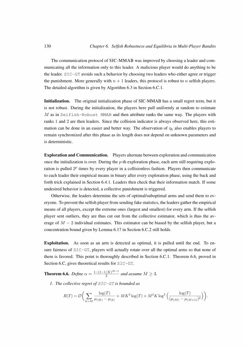
130 Chapter 6. Selfish Robustness and Equilibria in Multi-Player Bandits
The communication protocol of SIC-MMAB was improved by choosing a leader and com-
municating all the information only to this leader. A malicious player would do anything to be
the leader. SIC-GT avoids such a behavior by choosing two leaders who either agree or trigger
the punishment. More generally with n + 1 leaders, this protocol is robust to n selfish players.
The detailed algorithm is given by Algorithm 6.3 in Section 6.C.1.
Initialization. The original initialization phase of SIC-MMAB has a small regret term, but it
is not robust. During the initialization, the players here pull uniformly at random to estimate
M as in Selfish-Robust MMAB and then attribute ranks the same way. The players with
ranks 1 and 2 are then leaders. Since the collision indicator is always observed here, this esti-
mation can be done in an easier and better way. The observation of ηk also enables players to
remain synchronized after this phase as its length does not depend on unknown parameters and
is deterministic.
Exploration and Communication. Players alternate between exploration and communication
once the initialization is over. During the p-th exploration phase, each arm still requiring explo-
ration is pulled 2p times by every player in a collisionless fashion. Players then communicate
to each leader their empirical means in binary after every exploration phase, using the back and
forth trick explained in Section 6.4.1. Leaders then check that their information match. If some
undesired behavior is detected, a collective punishment is triggered.
Otherwise, the leaders determine the sets of optimal/suboptimal arms and send them to ev-
eryone. To prevent the selfish player from sending fake statistics, the leaders gather the empirical
means of all players, except the extreme ones (largest and smallest) for every arm. If the selfish
player sent outliers, they are thus cut out from the collective estimator, which is thus the av-
erage of M − 2 individual estimates. This estimator can be biased by the selfish player, but a
concentration bound given by Lemma 6.17 in Section 6.C.2 still holds.
Exploitation. As soon as an arm is detected as optimal, it is pulled until the end. To en-
sure fairness of SIC-GT, players will actually rotate over all the optimal arms so that none of
them is favored. This point is thoroughly described in Section 6.C.1. Theorem 6.6, proved in
Section 6.C, gives theoretical results for SIC-GT.
Theorem 6.6. Define α = 1−(1−1/K)M−1
2 and assume M ≥ 3.
1. The collective regret of SIC-GT is bounded as
R(T ) = O( ∑k>M
log(T )µ(M) − µ(k)
+MK2 log(T ) +M2K log2( log(T )
(µ(M) − µ(M+1))2
)).
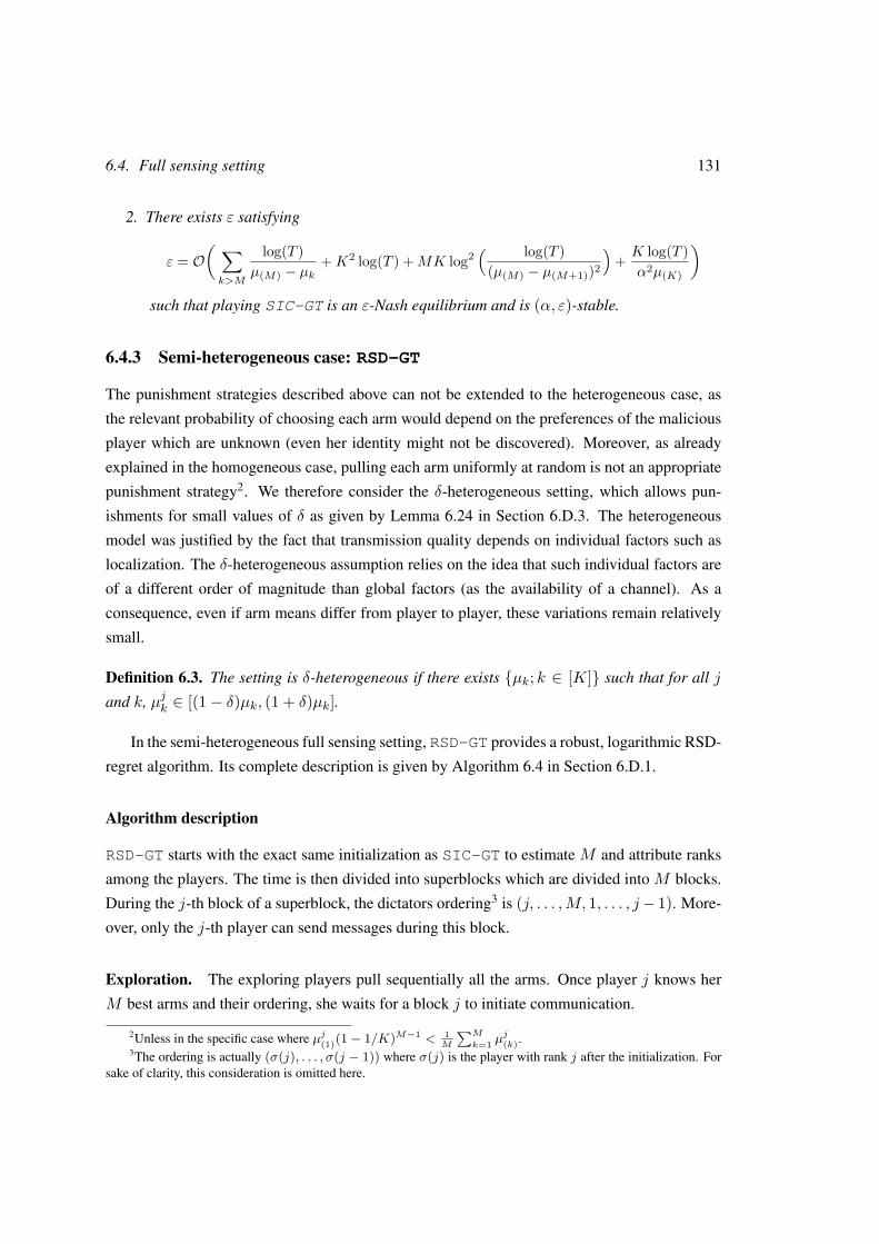
6.4. Full sensing setting 131
2. There exists ε satisfying
ε = O( ∑k>M
log(T )µ(M) − µk
+K2 log(T ) +MK log2( log(T )
(µ(M) − µ(M+1))2
)+ K log(T )
α2µ(K)
)such that playing SIC-GT is an ε-Nash equilibrium and is (α, ε)-stable.
6.4.3 Semi-heterogeneous case: RSD-GT
The punishment strategies described above can not be extended to the heterogeneous case, as
the relevant probability of choosing each arm would depend on the preferences of the malicious
player which are unknown (even her identity might not be discovered). Moreover, as already
explained in the homogeneous case, pulling each arm uniformly at random is not an appropriate
punishment strategy2. We therefore consider the δ-heterogeneous setting, which allows pun-
ishments for small values of δ as given by Lemma 6.24 in Section 6.D.3. The heterogeneous
model was justified by the fact that transmission quality depends on individual factors such as
localization. The δ-heterogeneous assumption relies on the idea that such individual factors are
of a different order of magnitude than global factors (as the availability of a channel). As a
consequence, even if arm means differ from player to player, these variations remain relatively
small.
Definition 6.3. The setting is δ-heterogeneous if there exists µk; k ∈ [K] such that for all j
and k, µjk ∈ [(1− δ)µk, (1 + δ)µk].
In the semi-heterogeneous full sensing setting, RSD-GT provides a robust, logarithmic RSD-
regret algorithm. Its complete description is given by Algorithm 6.4 in Section 6.D.1.
Algorithm description
RSD-GT starts with the exact same initialization as SIC-GT to estimate M and attribute ranks
among the players. The time is then divided into superblocks which are divided into M blocks.
During the j-th block of a superblock, the dictators ordering3 is (j, . . . ,M, 1, . . . , j− 1). More-
over, only the j-th player can send messages during this block.
Exploration. The exploring players pull sequentially all the arms. Once player j knows her
M best arms and their ordering, she waits for a block j to initiate communication.
2Unless in the specific case where µj(1)(1− 1/K)M−1 < 1M
∑M
k=1 µj(k).
3The ordering is actually (σ(j), . . . , σ(j − 1)) where σ(j) is the player with rank j after the initialization. Forsake of clarity, this consideration is omitted here.
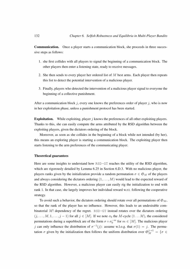
132 Chapter 6. Selfish Robustness and Equilibria in Multi-Player Bandits
Communication. Once a player starts a communication block, she proceeds in three succes-
sive steps as follows:
1. she first collides with all players to signal the beginning of a communication block. The
other players then enter a listening state, ready to receive messages.
2. She then sends to every player her ordered list of M best arms. Each player then repeats
this list to detect the potential intervention of a malicious player.
3. Finally, players who detected the intervention of a malicious player signal to everyone the
beginning of a collective punishment.
After a communication block j, every one knows the preferences order of player j, who is now
in her exploitation phase, unless a punishment protocol has been started.
Exploitation. While exploiting, player j knows the preferences of all other exploiting players.
Thanks to this, she can easily compute the arms attributed by the RSD algorithm between the
exploiting players, given the dictators ordering of the block.
Moreover, as soon as she collides in the beginning of a block while not intended (by her),
this means an exploring player is starting a communication block. The exploiting player then
starts listening to the arm preferences of the communicating player.
Theoretical guarantees
Here are some insights to understand how RSD-GT reaches the utility of the RSD algorithm,
which are rigorously detailed by Lemma 6.25 in Section 6.D.3. With no malicious player, the
players ranks given by the initialization provide a random permutation σ ∈ SM of the players
and always considering the dictators ordering (1, . . . ,M) would lead to the expected reward of
the RSD algorithm. However, a malicious player can easily rig the initialization to end with
rank 1. In that case, she largely improves her individual reward w.r.t. following the cooperative
strategy.
To avoid such a behavior, the dictators ordering should rotate over all permutations of SM ,
so that the rank of the player has no influence. However, this leads to an undesirable com-
binatorial M ! dependency of the regret. RSD-GT instead rotates over the dictators ordering
(j, . . . ,M, 1, . . . , j − 1) for all j ∈ [M ]. If we note σ0 the M -cycle (1 . . .M), the considered
permutations during a superblock are of the form σ σ−m0 for m ∈ [M ]. The malicious player
j can only influence the distribution of σ−1(j): assume w.l.o.g. that σ(1) = j. The permu-
tation σ given by the initialization then follows the uniform distribution over Sj→1M = σ ∈
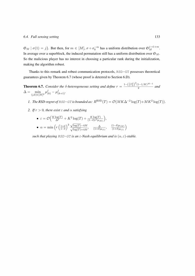
6.4. Full sensing setting 133
SM | σ(1) = j. But then, for m ∈ [M ], σ σ−m0 has a uniform distribution over Sj→1+mM .
In average over a superblock, the induced permutation still has a uniform distribution over SM .
So the malicious player has no interest in choosing a particular rank during the initialization,
making the algorithm robust.
Thanks to this remark and robust communication protocols, RSD-GT possesses theoretical
guarantees given by Theorem 6.7 (whose proof is deterred to Section 6.D).
Theorem 6.7. Consider the δ-heterogeneous setting and define r = 1−( 1+δ1−δ )
2(1−1/K)M−1
2 and
∆ = min(j,k)∈[M ]2
µj(k) − µj(k+1).
1. The RSD-regret of RSD-GT is bounded as: RRSD(T ) = O(MK∆−2 log(T )+MK2 log(T )
).
2. If r > 0, there exist ε and α satisfying
• ε = O(K log(T )
∆2 +K2 log(T ) + K log(T )(1−δ)r2µ(K)
),
• α = min(r(
1+δ1−δ
)3 √log(T )−4M√log(T )+4M
, ∆(1+δ)µ(1)
,(1−δ)µ(M)(1+δ)µ(1)
)such that playing RSD-GT is an ε-Nash equilibrium and is (α, ε)-stable.
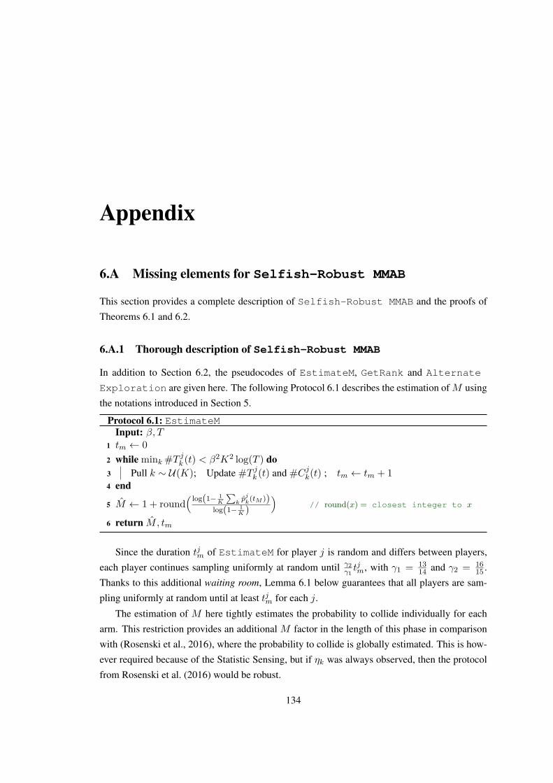
Appendix
6.A Missing elements for Selfish-Robust MMAB
This section provides a complete description of Selfish-Robust MMAB and the proofs of
Theorems 6.1 and 6.2.
6.A.1 Thorough description of Selfish-Robust MMAB
In addition to Section 6.2, the pseudocodes of EstimateM, GetRank and Alternate
Exploration are given here. The following Protocol 6.1 describes the estimation ofM using
the notations introduced in Section 5.
Protocol 6.1: EstimateMInput: β, T
1 tm ← 02 while mink #T jk (t) < β2K2 log(T ) do3 Pull k ∼ U(K); Update #T jk (t) and #Cjk(t) ; tm ← tm + 14 end
5 M ← 1 + round( log(1− 1
K
∑kpjk(tM ))
log(1− 1K )
)// round(x) = closest integer to x
6 return M, tm
Since the duration tjm of EstimateM for player j is random and differs between players,
each player continues sampling uniformly at random until γ2γ1tjm, with γ1 = 13
14 and γ2 = 1615 .
Thanks to this additional waiting room, Lemma 6.1 below guarantees that all players are sam-
pling uniformly at random until at least tjm for each j.
The estimation of M here tightly estimates the probability to collide individually for each
arm. This restriction provides an additional M factor in the length of this phase in comparison
with (Rosenski et al., 2016), where the probability to collide is globally estimated. This is how-
ever required because of the Statistic Sensing, but if ηk was always observed, then the protocol
from Rosenski et al. (2016) would be robust.
134
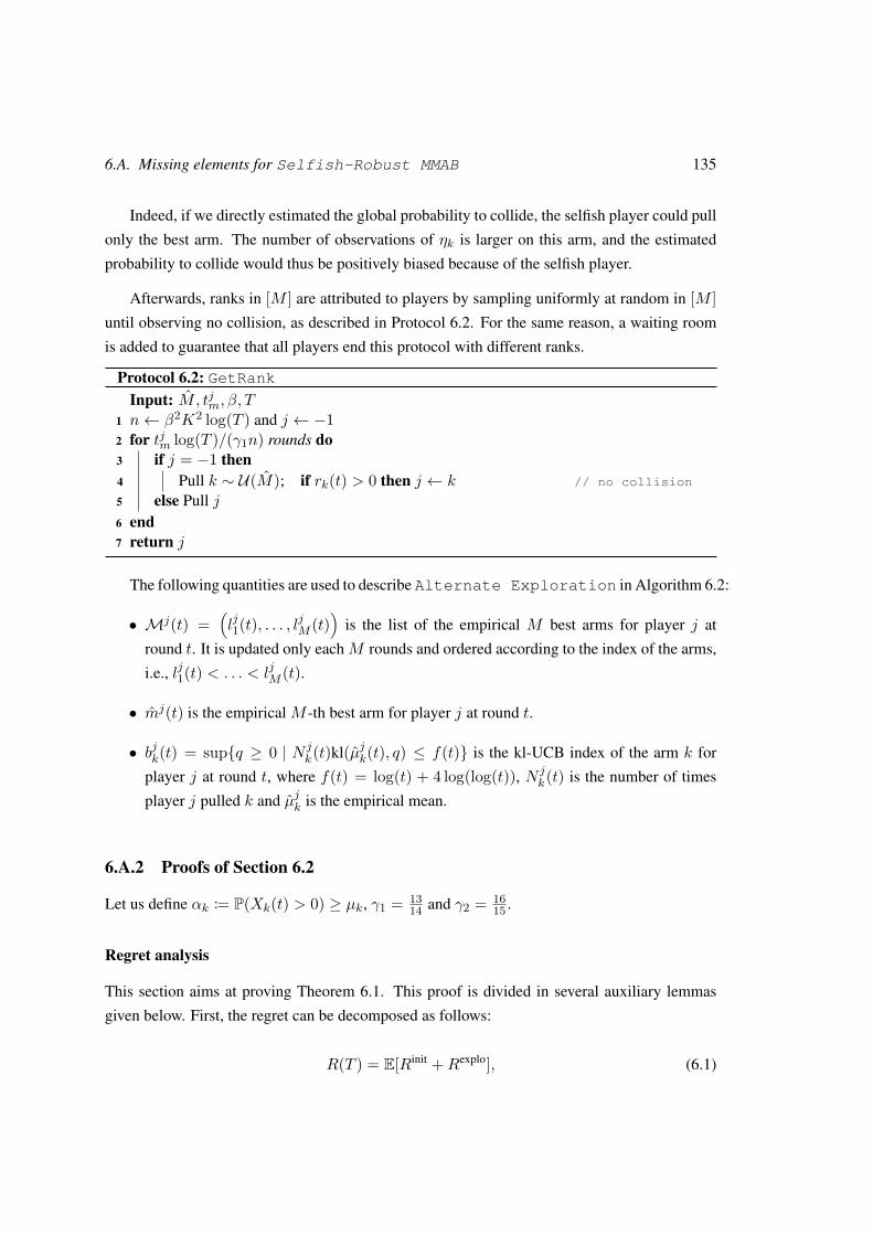
6.A. Missing elements for Selfish-Robust MMAB 135
Indeed, if we directly estimated the global probability to collide, the selfish player could pull
only the best arm. The number of observations of ηk is larger on this arm, and the estimated
probability to collide would thus be positively biased because of the selfish player.
Afterwards, ranks in [M ] are attributed to players by sampling uniformly at random in [M ]until observing no collision, as described in Protocol 6.2. For the same reason, a waiting room
is added to guarantee that all players end this protocol with different ranks.
Protocol 6.2: GetRankInput: M, tjm, β, T
1 n← β2K2 log(T ) and j ← −12 for tjm log(T )/(γ1n) rounds do3 if j = −1 then4 Pull k ∼ U(M); if rk(t) > 0 then j ← k // no collision
5 else Pull j6 end7 return j
The following quantities are used to describe Alternate Exploration in Algorithm 6.2:
• Mj(t) =(lj1(t), . . . , ljM (t)
)is the list of the empirical M best arms for player j at
round t. It is updated only each M rounds and ordered according to the index of the arms,
i.e., lj1(t) < . . . < ljM (t).
• mj(t) is the empirical M -th best arm for player j at round t.
• bjk(t) = supq ≥ 0 | N jk(t)kl(µjk(t), q) ≤ f(t) is the kl-UCB index of the arm k for
player j at round t, where f(t) = log(t) + 4 log(log(t)), N jk(t) is the number of times
player j pulled k and µjk is the empirical mean.
6.A.2 Proofs of Section 6.2
Let us define αk := P(Xk(t) > 0) ≥ µk, γ1 = 1314 and γ2 = 16
15 .
Regret analysis
This section aims at proving Theorem 6.1. This proof is divided in several auxiliary lemmas
given below. First, the regret can be decomposed as follows:
R(T ) = E[Rinit +Rexplo], (6.1)
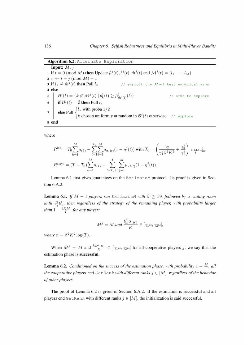
136 Chapter 6. Selfish Robustness and Equilibria in Multi-Player Bandits
Algorithm 6.2: Alternate Exploration
Input: M , j1 if t = 0 (mod M) then Update µj(t), bj(t), mj(t) andMj(t) = (l1, . . . , lM )2 π ← t+ j (mod M) + 13 if lπ 6= mj(t) then Pull lπ // exploit the M − 1 best empirical arms
4 else5 Bj(t) = k 6∈ Mj(t) | bjk(t) ≥ µ
jmj(t)(t) // arms to explore
6 if Bj(t) = ∅ then Pull lπ
7 else Pull
lπ with proba 1/2k chosen uniformly at random in Bj(t) otherwise // explore
8 end
where
Rinit = T0
M∑k=1
µ(k) −T0∑t=1
M∑j=1
µπj(t)(1− ηj(t)) with T0 =(
γ2γ2
1β2K2 + γ2
2γ2
1
)maxjtjm,
Rexplo = (T − T0)M∑k=1
µ(k) −T∑
t=T0+1
M∑j=1
µπj(t)(1− ηj(t)).
Lemma 6.1 first gives guarantees on the EstimateM protocol. Its proof is given in Sec-
tion 6.A.2.
Lemma 6.1. If M − 1 players run EstimateM with β ≥ 39, followed by a waiting room
until γ2γ1tjm, then regardless of the strategy of the remaining player, with probability larger
than 1− 6KMT , for any player:
M j = M andtjmα(K)K
∈ [γ1n, γ2n],
where n = β2K2 log(T ).
When M j = M and tjmα(K)K ∈ [γ1n, γ2n] for all cooperative players j, we say that the
estimation phase is successful.
Lemma 6.2. Conditioned on the success of the estimation phase, with probability 1 − MT , all
the cooperative players end GetRank with different ranks j ∈ [M ], regardless of the behavior
of other players.
The proof of Lemma 6.2 is given in Section 6.A.2. If the estimation is successful and all
players end GetRank with different ranks j ∈ [M ], the initialization is said successful.
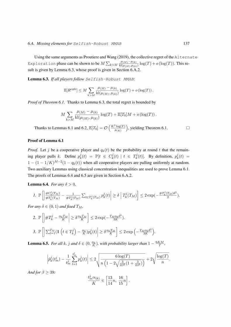
6.A. Missing elements for Selfish-Robust MMAB 137
Using the same arguments as Proutiere and Wang (2019), the collective regret of the Alternate
Exploration phase can be shown to be M∑k>M
µ(M)−µ(k)kl(µ(M),µ(k))
log(T ) + o (log(T )). This re-
sult is given by Lemma 6.3, whose proof is given in Section 6.A.2.
Lemma 6.3. If all players follow Selfish-Robust MMAB:
E[Rexplo] ≤M∑k>M
µ(M) − µ(k)
kl(µ(M), µ(k))log(T ) + o (log(T )) .
Proof of Theorem 6.1. Thanks to Lemma 6.3, the total regret is bounded by
M∑k>M
µ(M) − µ(k)kl(µ(M), µ(k))
log(T ) + E[T0]M + o (log(T )) .
Thanks to Lemmas 6.1 and 6.2, E[T0] = O(K3 log(T )µ(K)
), yielding Theorem 6.1.
Proof of Lemma 6.1
Proof. Let j be a cooperative player and qk(t) be the probability at round t that the remain-
ing player pulls k. Define pjk(t) = P[t ∈ Cjk(t) | t ∈ T jk (t)]. By definition, pjk(t) =1 − (1 − 1/K)M−2(1 − qk(t)) when all cooperative players are pulling uniformly at random.
Two auxiliary Lemmas using classical concentration inequalities are used to prove Lemma 6.1.
The proofs of Lemmas 6.4 and 6.5 are given in Section 6.A.2.
Lemma 6.4. For any δ > 0,
1. P[∣∣∣∣#Cjk(TM )
#T jk
(TM )− 1
#T jk
(TM )∑t∈T j
k(TM ) p
jk(t)
∣∣∣∣ ≥ δ ∣∣∣ T jk (TM )]≤ 2 exp(−#T j
k(TM )δ2
2 ).
For any δ ∈ (0, 1) and fixed TM ,
2. P[∣∣∣∣#T jk − αkTM
K
∣∣∣∣ ≥ δαkTMK ]≤ 2 exp(−TMαkδ
2
3K ).
3. P[∣∣∣∣∑TM
t=1(1(t ∈ T jk
)− αk
K )pjk(t)∣∣∣∣ ≥ δαkTMK ]
≤ 2 exp(−TMαkδ
2
3K
).
Lemma 6.5. For all k, j and δ ∈ (0, αkK ), with probability larger than 1− 6KMT ,
∣∣∣∣pjk(tjm)− 1tjm
tjm∑t=1
pjk(t)∣∣∣∣ ≤ 2
√√√√ 6 log(T )n(1− 2
√3
2β2 (1 + 32β2 )
) + 2
√log(T )n
.
And for β ≥ 39:tjmα(k)K
∈[13
14n,1615n
].
138 Chapter 6. Selfish Robustness and Equilibria in Multi-Player Bandits
Let ε = 2√
6 log(T )
n
(1−2√
32β2 (1+ 3
2β2 )) + 2
√log(T )n and pjk = 1
tjm
∑tjmt=1 p
jk(t) such that with prob-
ability at least 1− 6KMT ,
∣∣pjk− pjk∣∣ ≤ ε. The remaining of the proof is conditioned on this event.
By definition of n, ε = 1K f(β) where f(x) = 2
x
√6
1−2√
32x2 (1+ 3
2x2 )+ 2/x. Note that
f(x) ≤ 12e for x ≥ 39 and thus ε ≤ 1
2Ke for the considered β.
The last point of Lemma 6.5 yields that tjm ≤γ2γ1tj′m for any pair j, j′. All the cooperative
players are thus pulling uniformly at random until at least tjm, thanks to the additional waiting
room. Then,
1K
∑k
(1− pjk(t)) = (1− 1/K)M−2(1− 1K
∑k
qk(t)) = (1− 1/K)M−1.
When summing over k, it follows:
1K
∑k
(1− pjk)− ε ≤1K
∑k
(1− pjk) ≤ 1K
∑k
(1− pjk) + ε
(1− 1/K)M−1 − ε ≤ 1K
∑k
(1− pjk) ≤ (1− 1/K)M−1 + ε
M − 1 +log(1 + ε
(1−1/K)M−1 )log(1− 1/K) ≤
log(
1K
∑k(1− p
jk))
log(1− 1/K) ≤M − 1 +log(1− ε
(1−1/K)M−1 )log(1− 1/K)
M − 1 +log(1 + 1
2K )log(1− 1/K) ≤
log(
1K
∑k(1− p
jk))
log(1− 1/K) ≤M − 1 +log(1− 1
2K )log(1− 1/K)
The last line is obtained by observing that ε(1−1/K)M−1 is smaller than 1
2K .
Observing that max(
log(1−x/2)log(1−x) ,−
log(1+x/2)log(1−x)
)< 1/2 for any x > 0, the last line implies:
1 +log
(1K
∑k(1− p
jk))
log(1− 1/K) ∈ (M − 1/2,M + 1/2).
When rounding this quantity to the closest integer, we thus obtain M , which yields the first
part of Lemma 6.1. The second part is directly given by Lemma 6.5.
Proof of Lemma 6.2
The proof of Lemma 6.2 relies on two lemmas given below.
Lemma 6.6. Conditionally on the success of the estimation phase, when a cooperative player j
6.A. Missing elements for Selfish-Robust MMAB 139
proceeds to GetRank, all other cooperative players are either running GetRank or in a wait-
ing room4, i.e., they are not proceeding to Alternate Exploration yet.
Proof. Recall that γ1 = 13/14 and γ2 = 16/15. Conditionally on the success of the estimation
phase, for any pair (j, j′), γ2γ1tjm ≥ tj
′m. Let tjr = tjm
γ1K2β2 be the duration time of GetRank for
player j. For the same reason, γ2γ1tjr ≥ tj
′r . Player j ends GetRank at round tj = γ2
γ1tjm + tjr and
the second waiting room at round γ2γ1tj .
As γ2γ1tj ≥ tj
′, this yields that when a player ends GetRank, all other players are not
running Selfish-Robust MMAB yet. Because γ2γ1tjm ≥ tj
′m, when a player starts GetRank,
all other players also have already ended EstimateM. This yields Lemma 6.6.
Lemma 6.7. Conditionally on the success of the estimation phase, with probability larger
than 1− 1T , cooperative player j ends GetRank with a rank in [M ].
Proof. Conditionally on the success of the estimation phase and thanks to Lemma 6.5, tjr =tjm
γ1K2β2 ≥ K log(T )α(K)
. Moreover, at any round of GetRank, the probability of observing ηk(t) = 0is larger than α(K)
M . Indeed, the probability of observing ηk(t) is larger than α(K) with Statistic
sensing. Independently, the probability of having ηk = 0 is larger than 1/M since there is at
least an arm among [M ] not pulled by any other player. These two points yield, as M ≤ K:
P[player does not observe ηk(t) = 0 for tjr successive rounds] ≤(
1−α(K)M
)tjr≤ exp
(−α(K)t
jr
M
)
≤ 1T
Thus, with probability larger than 1 − 1T , player j observes ηk(t) = 0 at least once during
GetRank, i.e., she ends the procedure with a rank in [M ].
Proof of Lemma 6.2. Combining Lemmas 6.6 and 6.7 yields that the cooperative player j ends
GetRank with a rank in [M ] and no other cooperative player ends with the same rank. Indeed,
when a player gets the rank j, any other cooperative player has either no attributed rank (still
running GetRank or the first waiting room), or an attributed rank j′. In the latter case, thanks
to Lemma 6.6, this other player is either running GetRank or in the second waiting room,
meaning she is still pulling j′. Since the first player ends with the rank j, this means that she did
not encounter a collision when pulling j and especially, j 6= j′.
Considering a union bound among all cooperative players now yields Lemma 6.2.4Note that there is a waiting room before and after GetRank.
140 Chapter 6. Selfish Robustness and Equilibria in Multi-Player Bandits
Proof of Lemma 6.3
Let us denote T j0 =(
γ2γ2
1β2K2 + γ2
2γ2
1
)tjm such that player j starts running Alternate Exploration
at time T j0 . This section aims at proving Lemma 6.3. In this section, the initialization is assumed
to be successful. The regret due to an unsuccessful initialization is constant in T and thus
o (log(T )). We prove in this section, in case of a successful initialization, the following:
E[Rexplo] ≤M∑k>M
µ(M) − µ(k)kl(µ(M), µ(k))
log(T ) + o (log(T )) . (6.2)
This proof follows the same scheme as the regret proof from Proutiere and Wang (2019),
except that there is no leader here. Every bad event then happens independently for each indi-
vidual player. This adds a M factor in the regret compared to the follower/leader algorithm5
used by Proutiere and Wang (2019). For conciseness, we only give the main steps and refer to
the original Lemmas in (Proutiere and Wang, 2019) for their detailed proof.
We first recall useful concentration Lemmas which correspond to Lemmas 1 and 2 in (Proutiere
and Wang, 2019). They are respectively simplified versions of Lemma 5 in (Combes et al., 2015)
and Theorem 10 in (Garivier and Cappé, 2011).
Lemma 6.8. Let k ∈ [K], c > 0 and H be a (random) set such that for all t, t ∈ H is
Ft−1 measurable. Assume that there exists a sequence (Zt)t≥0 of binary random variables,
independent of all Ft, such that for t ∈ H , πj(t) = k if Zt = 1. Furthermore, if E[Zt] ≥ c for
all t, then: ∑t≥1
P[t ∈ H | |µjk(t)− µk| ≥ δ] ≤4 + 2c/δ2
c2 .
Lemma 6.9. If player j starts following Alternate Exploration at round T j0 + 1:
∑t>T j0
P[bjk(t) < µk] ≤ 15.
Let 0 < δ < δ0 := minkµ(k)−µ(k+1)
2 . Besides the definitions given in Section 6.A.1, define
the following:
• M∗ the list of the M -best arms, ordered according to their indices.
• Aj = t > T j0 | Mj(t) 6=M∗.
• Dj = t > T j0 | ∃k ∈Mj(t), |µjk(t)− µk| ≥ δ.
• Ej = t > T j0 | ∃k ∈M∗, bjk(t) < µk.
5Which is not selfish-robust.
6.A. Missing elements for Selfish-Robust MMAB 141
• Gj = t ∈ Aj \ Dj | ∃k ∈M∗ \Mj(t), |µjk(t)− µk| ≥ δ.
Lemma 6.10. If player j starts following Alternate Exploration at round T j0 + 1:
E[#(Aj ∪ Dj)] ≤ 8MK2(6K + δ−2).
Proof. Similarly to Proutiere and Wang (2019), we have (Aj ∪ Dj) ⊂ (Dj ∪ Ej ∪ Gj). We can
then individually bound E[#Dj ], E[#Ej ] and E[#Gj ], leading to Lemma 6.10. The detailed
proof is omitted here as it exactly corresponds to Lemmas 3 and 4 in (Proutiere and Wang,
2019).
Lemma 6.11. Consider a suboptimal arm k and define Hjk = t ∈ T j0 + 1, . . . , T \ (Aj ∪Dj) | πj(t) = k. It holds
E[#Hjk
]≤ log T + 4 log(log T )
kl(µk + δ, µ(M) − δ)+ 4 + 2δ−2.
Lemma 6.11 can be proved using the arguments of Lemma 5 in (Proutiere and Wang, 2019).
Proof of Lemma 6.3. If t ∈ Aj ∪ Dj , player j collides with at most one player j′ such that
t 6∈ Aj′ ∪ Dj′ .Otherwise, t 6∈ Aj ∪ Dj and player j collides with a player j′ only if t ∈ Aj′ ∪ Dj′ . Also,
she pulls a suboptimal arm k only on an exploration slot, i.e., instead of pulling the M -th best
arm. Thus, the regret caused by pulling a suboptimal arm k when t 6∈ Aj ∪ Dj is (µ(M) − µk)and this actually happens when t ∈ Hjk.
This discussion provides the following inequality, which concludes the proof of Lemma 6.3
when using Lemmas 6.10 and 6.11 and taking δ → 0.
E[Rexplo] ≤ 2
M∑j=1
E[#(Aj ∪ Dj)
]︸ ︷︷ ︸
collisions
+∑j≤M
∑k>M
(µ(M) − µ(k))E[#Hjk
]︸ ︷︷ ︸
pulls of suboptimal arms
.
Proof of Theorem 6.2
Proof. 1. Let us first prove the Nash equilibrium property. Assume that the player j is deviating
from Selfish-Robust MMAB and define E = [T0]∪( ⋃m∈[M ]\j
(Am∪Dm))
with the defi-
nitions of T0,Am andDm given in Section 6.A.26. Thanks to Lemmas 6.1 and 6.2, regardless of
6The max of T0 is here defined over all m ∈ [M ] \ j.
142 Chapter 6. Selfish Robustness and Equilibria in Multi-Player Bandits
the strategy of the selfish player, all other players successfully end the initialization after a time
T0 with probability 1−O(KM/T ). The remaining of the proof is conditioned on this event.
The selfish player earns at most µ(1)T0 during the initialization. Note that Alternate
Exploration never uses collision information, meaning that the behavior of the strategic
player during this phase does not change the behaviors of the cooperative players. Thus, the
optimal strategy during this phase for the strategic player is to pull the best available arm. Let
j be the rank of the strategic player7. For t 6∈ E , this arm is the k-th arm of M∗ with k =t + j (mod M) + 1. In a whole block of length M in [T ] \ E , the selfish player then earns at
most∑Mk=1 µ(k).
Over all, when a strategic player deviates from Alternate Exploration, she earns atmost:
E[RewjT (s′, s−js−js−j)] ≤ µ(1)(E [#E +M)] + T
M
M∑k=1
µ(k).
Note that we here add a factor µ(1) in the initialization regret. This is only because the true
loss of colliding is not 1 but µ(1). Also, the additional µ(1)M term is due to the fact that the last
block of length M of Alternate Exploration is not totally completed.
Thanks to Theorem 6.1, it also comes:
E[RewjT (sss)] ≥ T
M
M∑k=1
µ(k) −∑k>M
µ(M) − µ(k)
kl(µ(k), µ(M))log(T )−O
(µ(1)
K3
µ(K)log(T )
).
Lemmas 6.2 and 6.10 yield that E[#E ] = O(K3 log(T )µ(K)
), which concludes the proof.
2. We now prove the (α, ε)-stability of Selfish-Robust MMAB. Let ε′ = E[#E ] + M .
Note that this value is independent from the strategy of the deviating player j, since the setsAm
and Dm are independent from the actions of the player j. This is a consequence of the statistic
sensing assumption.
Consider that player j is playing a deviation strategy s′ ∈ S such that for some other playeri and l > 0:
E[RewiT (s′, s−js−js−j)] ≤ E[RewiT (sss)]− l − (ε′ +M).
We will first compare the reward of player j with her optimal possible reward. The only way for
the selfish player to influence the sampling strategy of another player is in modifying the rank
attributed to this other player. The total rewards of cooperative players with ranks j and j′ only
differ by at most ε′ + M in expectation, without considering the loss due to collisions with the
selfish player.7If the strategic player has no attributed rank, it is the only non-attributed rank in [M ].
6.A. Missing elements for Selfish-Robust MMAB 143
The only other way to cause regret to another player i is then to pull πi(t) at time t. This
incurs a loss at most µ(1) for player i, while this incurs a loss at least µ(M) for player j, in
comparison with her optimal strategy. This means that for incurring the additional loss l to the
player i, player j must suffer herself from a loss µ(M)µ(1)
compared to her optimal strategy s∗. Thus,
for α = µ(M)µ(1)
:
E[RewiT (s′, s−js−js−j)] ≤ E[Rewi
T (sss)]−l−(ε′+M) =⇒ E[RewjT (s′, s−js−js−j)] ≤ E[Rewj
T (s∗, s−js−js−j)]−αl
The first point of Theorem 6.2 yields for its given ε: E[RewjT (s∗, s−js−js−j)] ≤ E[Rewj
T (sss)] + ε.
Noting l1 = l + ε′ +M and ε1 = ε+ α(ε′ +M) = O(ε), we have shown:
E[RewiT (s′, s−js−js−j)] ≤ E[RewiT (sss)]− l1 =⇒ E[RewjT (s′, s−js−js−j)] ≤ E[RewjT (sss)] + ε1 − αl1.
Auxiliary lemmas
This section provides useful Lemmas for the proof of Lemma 6.1. We first recall a useful version
of Chernoff bound.
Lemma 6.12. For any independent variables X1, . . . , Xn in [0, 1] and δ ∈ (0, 1):
P(∣∣∣∣ n∑
i=1Xi − E[Xi]
∣∣∣∣ ≥ δ n∑i=1
E[Xi])≤ 2e−
δ2∑n
i=1 E[Xi]3 .
Proof of Lemma 6.4. 1. This is an application of Azuma-Hoeffding inequality on the variables
1(t ∈ Cjk(TM )
)| t ∈ T jk (TM ).
2. This is a consequence of Lemma 6.12 on the variables 1(t ∈ T jk
).
3. This is the same result on the variables 1(t ∈ T jk
)pjk(t) | Ft−1 where Ft−1 is the filtration
associated to the past events, using∑TMt=1 E[1
(t ∈ T jk
)pjk(t) | Ft−1] ≤ TMαk
K .
Proof of Lemma 6.5. From Lemma 6.4, it comes:
• P[∃t ≤ T,
∣∣∣pjk(t)− 1#T j
k
∑t′∈T j
kpjk(t′)
∣∣∣ ≥ 2√
log(T )#T j
k
]≤ 2
T ,
• P[∃t ≤ T,
∣∣∣K#T jk
αkt− 1
∣∣∣ ≥ √6 log(T )Kαkt
]≤ 2
T , (6.3)
144 Chapter 6. Selfish Robustness and Equilibria in Multi-Player Bandits
• P[∃t ≤ T,
∣∣∣ Kαkt∑t′∈T jkpjk(t′)−
1t
∑t′≤t p
jk(t′)
∣∣∣ ≥ √6 log(T )Kαkt
]≤ 2
T .
Noting that∑t′∈T j
kpjk(t′) ≤ #T jk , Equation (6.3) implies:
P
∃t ≤ T, ∣∣∣∣ Kαkt∑t′∈T j
k
pjk(t′)− 1
#T jk
∑t′∈T j
k
pjk(t′)∣∣∣∣ ≥
√6 log(T )K
αkt
≤ 2T.
Combining these three inequalities and making the union bound over all the players and
arms yield that with probability larger than 1− 6KMT :
∣∣∣∣pjk(tjm)− 1tjm
∑t≤tjm
pjk(t)∣∣∣∣ ≤ 2
√6 log(T )Kαkt
jm
+ 2
√√√√ log(T )#T jk (tjm)
. (6.4)
Moreover, under the same event, Equation (6.3) also gives that
T jk (tjm) ∈[αkt
jm
K−
√6αktjm log(T )
K,αkt
jm
K+
√6αktjm log(T )
K
].
Specifically, this yields n ≤ αktjm
K +√
6αktjm log(T )K , or equivalently tjmαk
K ≥ n−2√
3 log(T )2
√n+ 3 log(T )
2 .
Since n = β2K2 log(T ), this becomes tjmαkK ≥ n(1 − 2
√3
2β2K2
√1 + 3
2β2K2 ) and Equa-
tion (6.4) now rewrites into:
∣∣∣∣pjk(tjm)− 1tjm
∑t≤tjm
pjk(t)∣∣∣∣ ≤ 2
√√√√ 6 log(T )n(1− 2
√3
2β2K2 (1 + 32β2K2 )
) + 2
√log(T )n
Also, n ≥ αktjm
K −√
6 log(T )αktjmK for some k, which yields t
jmαkK ≤ n(1+ 3
β2K2 +2√
32β2K2
√1 + 3
2β2K2 ).
This relation then also holds for tjmα(K)K . We have therefore proved that:
n
(1− 2
√3
2β2
√1 + 3
2β2
)≤tjmα(k)K
≤ n(
1 + 3β2 + 2
√3
2β2
√1 + 3
2β2
).
For β ≥ 39, this gives the bound in Lemma 6.5.
6.B Collective punishment proof
Recall that the punishment protocol consists in pulling each arm k with probability at least
pjk = max(1 −
(γ
∑M
l=1 µj(l)
Mµjk
) 1M−1
, 0)
. Lemma 6.13 below guarantees that such a sampling
strategy is possible.
6.C. Missing elements for SIC-GT 145
Lemma 6.13. For pk = max(1−(γ∑M
l=1 µj(l)
Mµjk
) 1M−1
, 0)
with γ =(1− 1
K
)M−1:∑Kk=1 pk ≤ 1.
Proof. For ease of notation, define xk := µjk, xM :=∑M
l=1 x(l)M and S := k ∈ [K] | xk >
γxM = k ∈ [K] | pk > 0. We then get by concavity of x 7→ −x−1
M−1 ,
∑k∈S
pk = #S ×
1− (γxM )1
M−1∑k∈S
(xk)−1
M−1
#S
, (6.5)
≤ #S ×(
1−(γxMxS
) 1M−1
)with xS = 1
#S∑k∈S
xk. (6.6)
We distinguish two cases.
First, if #S ≤M , we then getMxM ≥ #SxS because S is a subset of theM best empirical
arms. The last inequality then becomes
∑k∈S
pk ≤ #S(
1−(γ
#SM
) 1M−1
).
Define g(x) = γM − x(1− x)M−1. For x ∈ (0, 1]:
g(x) ≥ 0 ⇐⇒ γ
xM≥ (1− x)M−1,
⇐⇒ 1−(
γ
xM
) 1M−1≤ x,
⇐⇒ 1x
(1−
(γ
xM
) 1M−1
)≤ 1.
Thus, g( 1#S ) ≥ 0 implies
∑k∈S pk ≤ 1. We now show that g is indeed non negative on
[0, 1]. x(1 − x)M−1 is maximized at 1M and is thus smaller than 1
M (1 − 1/M)M−1, and using
the fact that 1M (1− 1/M)M−1 ≤ γ
M for our choice of γ, we get the result for the first case.
The other case corresponds to #S > M . In this case, the M best empirical arms are all in S
and thus xM ≥ xS . Equation (6.6) becomes:
∑k∈S
pk ≤ #S(1− γ
1M−1
)≤ K(1− (1− 1/K)) = 1.
6.C Missing elements for SIC-GT
In this whole section, M is assumed to be at least 3.

146 Chapter 6. Selfish Robustness and Equilibria in Multi-Player Bandits
6.C.1 Description of the algorithm
This section provides a complete description of SIC-GT. The pseudocode of SIC-GT is given
in Algorithm 6.3 and relies on several auxiliary protocols, which are described by Algorithms 6.3
to 6.9.
Algorithm 6.3: SIC-GTInput: T, δ
1 M, j ← Initialize (T,K) and punish← False2 OptArms ← ∅, Mp ←M , [Kp]← [K] and p← 13 while not punish and #OptArms < M do4 for m = 0, . . . ,
⌈Kp2pMp
⌉− 1 do
5 ArmstoPull← OptArms ∪i ∈ [Kp]
∣∣ i−mMp (mod Kp) ∈ [Mp]
6 for M rounds do7 k ← j + t (mod M) + 1 and pull i the k-th element of ArmstoPull8 if N j
i (p) ≤ 2p then Update µji // N ji pulls on i by j this phase
9 if ηi = 1 then punish← True // collisionless exploration
10 end11 end12 (punish,OptArms, [Kp],Mp)← CommPhase (µj , j, p,OptArms , [Kp],Mp)13 p← p+ 114 end
15 if punish then PunishHomogeneous (p)16 else // exploitation phase
17 k ← j + t (mod M) + 1 and pull i, the k-th arm of OptArms18 if ηi = 1 then punish← True19 end
Protocol 6.5: ReceiveMeanInput: j, p
1 µ← 02 for n = 0, . . . , p do3 Pull j4 if ηj(t) = 1 then µ← µ+ 2−n5 end6 return µ // sent mean
Protocol 6.6: SendMeanInput: j, l, p, µ
1 m← dyadic writing of µ of lengthp+ 1, i.e., µ =
∑pn=0mn2−n
2 for n = 0, . . . , p do3 if mn = 1 then Pull l // send 14 else Pull j // send 05 end
Initialization phase. The purpose of the initialization phase is to estimate M and attribute
ranks in [M ] to all the players. This is done by Initialize, which is given in Algorithm 6.3.
It simply consists in pulling uniformly at random for a long time to infer M from the probability
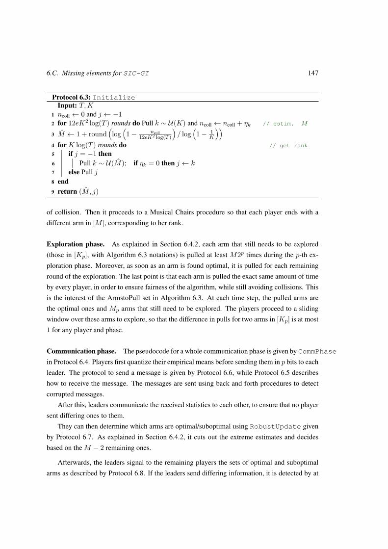
6.C. Missing elements for SIC-GT 147
Protocol 6.3: InitializeInput: T,K
1 ncoll ← 0 and j ← −12 for 12eK2 log(T ) rounds do Pull k ∼ U(K) and ncoll ← ncoll + ηk // estim. M
3 M ← 1 + round(log
(1− ncoll
12eK2 log(T )
)/ log
(1− 1
K
))4 for K log(T ) rounds do // get rank
5 if j = −1 then6 Pull k ∼ U(M); if ηk = 0 then j ← k7 else Pull j8 end9 return (M, j)
of collision. Then it proceeds to a Musical Chairs procedure so that each player ends with a
different arm in [M ], corresponding to her rank.
Exploration phase. As explained in Section 6.4.2, each arm that still needs to be explored
(those in [Kp], with Algorithm 6.3 notations) is pulled at least M2p times during the p-th ex-
ploration phase. Moreover, as soon as an arm is found optimal, it is pulled for each remaining
round of the exploration. The last point is that each arm is pulled the exact same amount of time
by every player, in order to ensure fairness of the algorithm, while still avoiding collisions. This
is the interest of the ArmstoPull set in Algorithm 6.3. At each time step, the pulled arms are
the optimal ones and Mp arms that still need to be explored. The players proceed to a sliding
window over these arms to explore, so that the difference in pulls for two arms in [Kp] is at most
1 for any player and phase.
Communication phase. The pseudocode for a whole communication phase is given by CommPhase
in Protocol 6.4. Players first quantize their empirical means before sending them in p bits to each
leader. The protocol to send a message is given by Protocol 6.6, while Protocol 6.5 describes
how to receive the message. The messages are sent using back and forth procedures to detect
corrupted messages.
After this, leaders communicate the received statistics to each other, to ensure that no player
sent differing ones to them.
They can then determine which arms are optimal/suboptimal using RobustUpdate given
by Protocol 6.7. As explained in Section 6.4.2, it cuts out the extreme estimates and decides
based on the M − 2 remaining ones.
Afterwards, the leaders signal to the remaining players the sets of optimal and suboptimal
arms as described by Protocol 6.8. If the leaders send differing information, it is detected by at

148 Chapter 6. Selfish Robustness and Equilibria in Multi-Player Bandits
Protocol 6.4: CommPhaseInput: µj , j, p,OptArms, [Kp],Mp
1 punish← False2 for K rounds do // receive punishment signal
3 Pull k = t+ j (mod K) + 1; if ηk = 1 then punish← True4 end
5 µjk ←
2−p(b2pµjkc+ 1
)with proba 2pµjk − b2pµ
jkc
2−pb2pµjkc otherwise// quantization
6 for (i, l, k) ∈ [M ]× 1, 2 × [K] such that i 6= l do // i sends µik to l
7 if j = i then // sending player
8 SendMean (j, l, p, µjk) and q ← ReceiveMean (j, p) // back and forth
9 if q 6= µjk then punish← True // corrupted message
10 else if j = l then µik ← ReceiveMean (j, p) and SendMean (j, i, p, µik)11 else Pull j // waiting for others
12 end13 for (i, l,m, k) ∈ (1, 2), (2, 1) × [M ]× [K] do // leaders check info match
14 if j = i then SendMean (j, l, p, µmk )15 else if j = l then16 q ← ReceiveMean (j, p); if q 6= µmk then punish← True // info differ
17 else Pull j // waiting for leaders
18 end19 if j ∈ 1, 2 then (Acc, Rej)← RobustUpdate (µ, p,OptArms , [Kp],Mp)20 else Acc, Rej← ∅ // arms to accept/reject
21 (punish, Acc)← SignalSet (Acc, j, punish)22 (punish, Rej)← SignalSet (Rej, j, punish)23 return (punish,OptArms ∪ Acc, [Kp] \ (Acc ∪ Rej) ,Mp −#Acc)
least one player.
If the presence of a malicious player is detected at some point of this communication phase,
then players signal to each other to trigger the punishment protocol described by Protocol 6.9.
Exploitation phase. If no malicious player perturbed the communication, players end up hav-
ing detected the M optimal arms. As soon as it is the case, they only pull these M arms in a
collisionless way until the end.
6.C.2 Regret analysis
This section aims at proving the first point of Theorem 6.6, using similar techniques as in (Bour-
sier and Perchet, 2019). The regret is first divided into three parts:
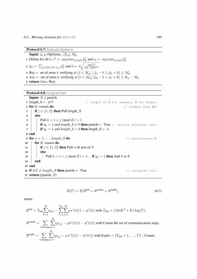
6.C. Missing elements for SIC-GT 149
Protocol 6.7: RobustUpdateInput: µ, p,OptArms , [Kp],Mp
1 Define for all k, ik ← arg maxj∈[M ] µjk and ik ← arg minj∈[M ] µ
jk
2 µk ←∑j∈[M ]\ik,ik µ
jk and b← 4
√log(T )
(M−2)2p+1
3 Rej← set of arms k verifying # i ∈ [Kp] | µi − b ≥ µk + b ≥Mp
4 Acc← set of arms k verifying # i ∈ [Kp] |µk − b ≥ µi + b ≥ Kp −Mp
5 return (Acc, Rej)
Protocol 6.8: SignalSetInput: S, j, punish
1 length_S← #S // length of S for leaders, 0 for others
2 for K rounds do // leaders send #S3 if j ∈ 1, 2 then Pull length_S4 else5 Pull k = t+ j (mod K) + 16 if ηk = 1 and length_S 6= 0 then punish← True // receive different info
7 if ηk = 1 and length_S = 0 then length_S← k
8 end9 for n = 1, . . . , length_S do // send/receive S
10 for K rounds do11 if j ∈ 1, 2 then Pull n-th arm of S12 else13 Pull k = t+ j (mod K) + 1; if ηk = 1 then Add k to S14 end15 end16 if #S 6= length_S then punish← True // corrupted info
17 return (punish, S)
R(T ) = E[Rinit +Rcomm +Rexplo], (6.7)
where
Rinit = Tinit
M∑k=1
µ(k) −Tinit∑t=1
M∑j=1
µπj(t)(1− ηj(t)) with Tinit = (12eK2 +K) log(T ),
Rcomm =∑
t∈Comm
M∑j=1
(µ(j) − µπj(t)(1− ηj(t))) with Comm the set of communication steps,
Rexplo =∑
t∈Explo
M∑j=1
(µ(j) − µπj(t)(1− ηj(t))) with Explo = Tinit + 1, . . . , T \ Comm.
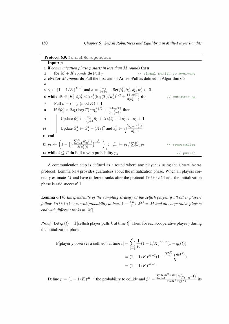
150 Chapter 6. Selfish Robustness and Equilibria in Multi-Player Bandits
Protocol 6.9: PunishHomogeneousInput: p
1 if communication phase p starts in less than M rounds then2 for M +K rounds do Pull j // signal punish to everyone
3 else for M rounds do Pull the first arm of ArmstoPull as defined in Algorithm 6.34
5 γ ← (1− 1/K)M−1 and δ = 1−γ1+3γ ; Set µjk, S
jk, s
jk, n
jk ← 0
6 while ∃k ∈ [K], δµjk < 2sjk(log(T )/njk)1/2 + 14 log(T )3(nj
k−1)
do // estimate µk
7 Pull k = t+ j (mod K) + 18 if δµjk < 2sjk(log(T )/njk)1/2 + 14 log(T )
3(njk−1)
then
9 Update µjk ←njk
njk+1µjk +Xk(t) and njk ← njk + 1
10 Update Sjk ← Sjk + (Xk)2 and sjk ←√
Sjk−(µj
k)2
njk−1
11 end
12 pk ←(
1−(γ
∑M
l=1 µj(l)(t)
Mµjk(t)
) 1M−1
)+
; pk ← pk/∑Kl=1 pl // renormalize
13 while t ≤ T do Pull k with probability pk // punish
A communication step is defined as a round where any player is using the CommPhase
protocol. Lemma 6.14 provides guarantees about the initialization phase. When all players cor-
rectly estimate M and have different ranks after the protocol Initialize, the initialization
phase is said successful.
Lemma 6.14. Independently of the sampling strategy of the selfish player, if all other players
follow Initialize, with probability at least 1 − 3MT : M j = M and all cooperative players
end with different ranks in [M ].
Proof. Let qk(t) = P[selfish player pulls k at time t]. Then, for each cooperative player j during
the initialization phase:
P[player j observes a collision at time t] =K∑k=1
1K
(1− 1/K)M−2(1− qk(t))
= (1− 1/K)M−2(1−∑Kk=1 qk(t)K
)
= (1− 1/K)M−1
Define p = (1 − 1/K)M−1 the probability to collide and pj =∑12eK2 log(T )
t=1 1(ηπj(t)=1
)12eK2 log(T ) its
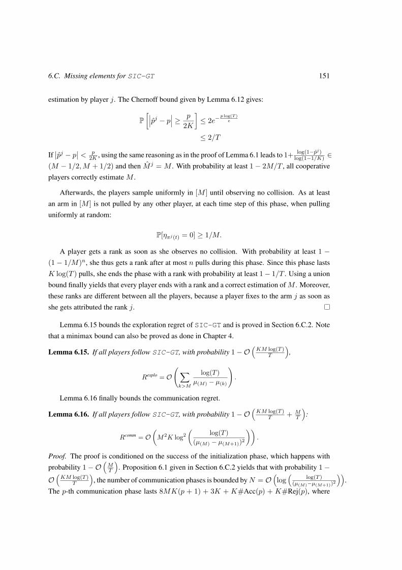
6.C. Missing elements for SIC-GT 151
estimation by player j. The Chernoff bound given by Lemma 6.12 gives:
P[∣∣∣pj − p∣∣∣ ≥ p
2K
]≤ 2e−
p log(T )e
≤ 2/T
If∣∣pj − p∣∣ < p
2K , using the same reasoning as in the proof of Lemma 6.1 leads to 1+ log(1−pj)log(1−1/K) ∈
(M − 1/2,M + 1/2) and then M j = M . With probability at least 1− 2M/T , all cooperative
players correctly estimate M .
Afterwards, the players sample uniformly in [M ] until observing no collision. As at least
an arm in [M ] is not pulled by any other player, at each time step of this phase, when pulling
uniformly at random:
P[ηπj(t) = 0] ≥ 1/M.
A player gets a rank as soon as she observes no collision. With probability at least 1 −(1 − 1/M)n, she thus gets a rank after at most n pulls during this phase. Since this phase lasts
K log(T ) pulls, she ends the phase with a rank with probability at least 1− 1/T . Using a union
bound finally yields that every player ends with a rank and a correct estimation ofM . Moreover,
these ranks are different between all the players, because a player fixes to the arm j as soon as
she gets attributed the rank j.
Lemma 6.15 bounds the exploration regret of SIC-GT and is proved in Section 6.C.2. Note
that a minimax bound can also be proved as done in Chapter 4.
Lemma 6.15. If all players follow SIC-GT, with probability 1−O(KM log(T )
T
),
Rexplo = O(∑k>M
log(T )µ(M) − µ(k)
).
Lemma 6.16 finally bounds the communication regret.
Lemma 6.16. If all players follow SIC-GT, with probability 1−O(KM log(T )
T + MT
):
Rcomm = O(M2K log2
(log(T )
(µ(M) − µ(M+1))2
)).
Proof. The proof is conditioned on the success of the initialization phase, which happens with
probability 1−O(MT
). Proposition 6.1 given in Section 6.C.2 yields that with probability 1−
O(KM log(T )
T
), the number of communication phases is bounded byN = O
(log
(log(T )
(µ(M)−µ(M+1))2
)).
The p-th communication phase lasts 8MK(p + 1) + 3K + K#Acc(p) + K#Rej(p), where
152 Chapter 6. Selfish Robustness and Equilibria in Multi-Player Bandits
Acc and Rej respectively are the accepted and rejected arms at the p-th phase. Their exact def-
initions are given in Algorithm 6.7. An arm is either accepted or rejected only once, so that∑Np=1 #Acc(p) + #Rej(p) = K. The total length of Comm is thus bounded by:
#Comm ≤N∑p=1
8MK(p+ 1) + 3K +K#Acc(p) +K#Rej(p)
≤ 8MK(N + 2)(N + 1)
2 + 3KN +K2
Which leads to Rcomm = O(M2K log2
(log(T )
(µ(M)−µ(M+1))2
))using the given bound for N .
Proof of Theorem 6.6. Using Lemmas 6.14 to 6.16 and Equation (6.7) it comes that with prob-ability 1−O
(KM log(T )
T
):
RT ≤ O
(∑k>M
log(T )µ(M) − µ(k)
+M2K log2(
log(T )(µ(M) − µ(M+1))2
)+MK2 log(T )
).
The regret incurred by the low probability event isO(KM2 log(T )), leading to Theorem 6.6.
Proof of Lemma 6.15
Lemma 6.15 relies on the following concentration inequality.
Lemma 6.17. Conditioned on the success of the initialization and independently of the means
sent by the selfish player, if all other players play cooperatively and send uncorrupted messages,
for any k ∈ [K]:P[∃p ≤ n, |µk(p)− µk| ≥ B(p)] ≤ 6nM
T
where B(p) = 4√
log(T )(M−2)2p+1 and µk(p) is the centralized mean of arm k at the end of phase p,
once the extremes have been cut out. It exactly corresponds to the µk of Protocol 6.7.
Proof. At the end of phase p, (2p+1 − 1) observations are used for each player j and arm k.
Hoeffding bound then gives: P[∣∣∣µjk(p)− µk∣∣∣ ≥ √ log(T )
2p+1
]≤ 2
T . The quantization only adds an
error of at most 2−p, yielding for every cooperative player:
P
∣∣∣µjk(p)− µk∣∣∣ ≥ 2
√log(T )2p+1
≤ 2T
(6.8)

6.C. Missing elements for SIC-GT 153
Assume w.l.o.g. that the selfish player has rank M . Hoeffding inequality also yields:
P
∣∣∣∣ 1M − 1
M−1∑j=1
µjk(p)− µk∣∣∣∣ ≥
√log(T )
(M − 1)2p+1
≤ 2T.
Since∑M−1j=1 2p(µjk(p)−µ
jk(p)) is the difference betweenM−1 Bernoulli variables and their
expectation, Hoeffding inequality yields P[∣∣∣ 1M−1
∑M−1j=1 (µjk − µ
jk(p))
∣∣∣ ≥ √ log(T )(M−1)2p+1
]≤ 2
T
and:
P
∣∣∣∣∣∣ 1M − 1
M−1∑j=1
µjk(p)− µk
∣∣∣∣∣∣ ≥ 2√
log(T )(M − 1)2p+1
≤ 4T. (6.9)
Using the triangle inequality combining Equations (6.8) and (6.9) yields for any j ∈ [M−1]:
P
∣∣∣ 1M − 2
∑j′∈[M−1]j′ 6=j
µjk(p)− µk∣∣∣ ≥ 4
√log(T )
(M − 2)2p+1
≤ P[M − 1M − 2
∣∣∣ 1M − 1
∑j′∈[M−1]
µjk(p)− µk∣∣∣
+ 1M − 2
∣∣∣µjk(p)− µk∣∣∣ ≥ 4√
log(T )(M − 2)2p+1
]
≤ P
∣∣∣ 1M − 1
M−1∑j=1
µjk(p)− µk∣∣∣ ≥ 2
√log(T )
(M − 1)2p+1
+ P
∣∣∣µjk(p)− µk∣∣∣ ≥ 2
√log(T )2p+1
≤ 6T. (6.10)
Moreover by construction, no matter what mean sent the selfish player,
minj∈[M−1]
1M − 2
∑j′∈[M−1]j′ 6=j
µjk(p) ≤ µk(p) ≤ maxj∈[M−1]
1M − 2
∑j′∈[M−1]j′ 6=j
µjk(p).
Indeed, assume that the selfish player sends a mean larger than all other players. Then her
mean as well as the minimal sent mean are cut out and µk(p) is then equal to the right term.
Conversely if she sends the smallest mean, µk(p) corresponds to the left term. Since µk(p) is
non-decreasing in µMk (p), the inequality also holds in the case where the selfish player sends
neither the smallest nor the largest mean.
Finally, using a union bound over all j ∈ [M − 1] with Equation (6.10) yields Lemma 6.17.
154 Chapter 6. Selfish Robustness and Equilibria in Multi-Player Bandits
Using classical MAB techniques then yields Proposition 6.1.
Proposition 6.1. Independently of the selfish player behavior, as long as the PunishHomogeneous
protocol is not used, with probability 1 − O(KM log(T )
T
), every optimal arm k is accepted
after at most O(
log(T )(µk−µ(M+1))2
)pulls and every sub-optimal arm k is rejected after at most
O(
log(T )(µ(M)−µk)2
)pulls during exploration phases.
Proof. The fact that the PunishHomogeneous protocol is not started just means that no cor-
rupted message is sent between cooperative players. The proof is conditioned on the success of
the initialization phase, which happens with probability 1−O(MT
). Note that there are at most
log2(T ) exploration phases. Thanks to Lemma 6.17, with probability 1 − O(KM log(T )
T
), the
inequality |µk(p)− µk| ≤ B(p) thus holds for any p. The remaining of the proof is conditioned
on this event. Especially, an optimal arm is never rejected and a suboptimal one never accepted.
First consider an optimal arm k and note ∆k = µk − µ(M+1) the optimality gap. Let pk be
the smallest integer p such that (M − 2)2p+1 ≥ 162 log(T )∆2k
. In particular, 4B(pk) ≤ ∆k, which
implies that the arm k is accepted at the end of the communication phase pk or before.
Necessarily, (M − 2)2pk+1 ≤ 2·162 log(T )∆2k
and especially, M2pk+1 = O(
log(T )∆2k
). Note that
the number of exploratory pulls on arm k during the p first phases is bounded by M(2p+1 + p)8,
leading to Proposition 6.1. The same holds for the sub-optimal arms with ∆k = µ(M)−µk.
In the following, we keep the notation tk = c log(T )(µk−µ(M))2 , where c is a universal constant,
such that with probability 1 − O(KMT
), every arm k is correctly accepted or rejected after a
time at most tk. All players are now assumed to play SIC-GT, e.g., there is no selfish player.Since there is no collision during exploration/exploitation (conditionally on the success of theinitialization phase), the following decomposition holds (Anantharam et al., 1987a):
Rexplo =∑k>M
(µ(M) − µ(k))T explo(k) +
∑k≤M
(µ(k) − µ(M))(T explo − T explo(k) ), (6.11)
where T explo = #Explo and T explo(k) is the centralized number of pulls on the k-th best arm during
exploration or exploitation.
Lemma 6.18. If all players follow SIC-GT, with probability 1−O(KM log(T )
T
), it holds:
• for k > M , (µ(M) − µ(k))Texplo(k) = O
(log(T )
µ(M)−µ(k)
).
8During the exploration phase p, each explored arm is pulled between M2p and M(2p + 1) times.
6.C. Missing elements for SIC-GT 155
•∑k≤M (µ(k) − µ(M))(T explo − T explo
(k) ) = O(∑
k>Mlog(T )
µ(M)−µk
).
Proof. With probability 1−O(KM log(T )
T
), Proposition 6.1 yields that every arm k is correctly
accepted or rejected at time at most tk. The remaining of the proof is conditioned on this event
and the success of the initialization phase. The first point of Lemma 6.18 is a direct consequence
of Proposition 6.1. It remains to prove the second point.
Let pk be the number of the phase at which the arm k is either accepted or rejected and let
Kp be the number of arms that still need to be explored at the beginning of phase p and Mp be
the number of optimal arms that still need to be explored. The following two key Lemmas are
crucial to obtain the second point.
Lemma 6.19. Under the assumptions of Lemma 6.18:
∑k≤M
(µ(k) − µ(M))(T explo − T explo(k) ) ≤
∑j>M
∑k≤M
min(p(k),p(j))∑p=1
(µ(k) − µ(M))2pM
Mp+ o (log(T )) .
Lemma 6.20. Under the assumptions of Lemma 6.18, for any j > M :
∑k≤M
min(p(k),p(j))∑p=1
(µ(k) − µ(M))2pM
Mp≤ O
(log(T )
µ(M) − µ(j)
).
Combining these two Lemmas with Equation (6.11) finally yields Lemma 6.15.
Proof of Lemma 6.19. Consider an optimal arm k. During the p-th exploration phase, either k
has already been accepted and is pulled M⌈Kp2pMp
⌉times; or k has not been accepted yet and is
pulled at least 2pM , i.e., is not pulled at most M(⌈
Kp2pMp
⌉− 2p
)times. This gives:
(µ(k) − µ(M))(T explo − T explo(k) ) ≤
pk∑p=1
(µ(k) − µ(M))M(⌈
Kp2p
Mp
⌉− 2p
),
≤pk∑p=1
(µ(k) − µ(M))M(Kp2p
Mp− 2p + 1
),
≤ pk(µ(k) − µ(M))M +pk∑p=1
(µ(k) − µ(M))(Kp −Mp)M
Mp2p.
We assumed that every arm k is correctly accepted or rejected after a time at most tk. This
implies that pk = o (log(T )). Moreover,Kp−Mp is the number of suboptimal arms not rejected
at phase p, i.e., Kp −Mp =∑j>M 1
(p ≤ p(j)
)and this proves Lemma 6.19.
156 Chapter 6. Selfish Robustness and Equilibria in Multi-Player Bandits
Proof of Lemma 6.20. For j > M , define Aj =∑k≤M
∑min(p(k),p(j))p=1 (µ(k) − µ(M))2p MMp
. We
want to show Aj ≤ O(
log(T )µ(M)−µ(j)
)with the considered conditions. Note N(p) = M(2p+1 − 1)
and ∆(p) =√
c log(T )N(p) . The inequality p(k) ≥ p then implies µ(k) − µ(M) < ∆(p), i.e.,
Aj ≤∑k≤M
p(j)∑p=1
2p∆(p)1(p ≤ p(k)
) MMp
=p(j)∑p=1
2p∆(p)M
≤p(j)∑p=1
∆(p)(N(p)−N(p− 1))
The equality comes because∑k≤M 1
(p ≤ p(k)
)is exactly Mp. Then from the definition of
∆(p):
Aj ≤ c log(T )p(j)∑p=1
∆(p)( 1
∆(p) + 1∆(p− 1)
)( 1∆(p) −
1∆(p− 1)
)
≤ (1 +√
2)c log(T )p(j)∑p=1
( 1∆(p) −
1∆(p− 1)
)≤ (1 +
√2)c log(T )/∆(p(j))
≤ (1 +√
2)√c log(T )N(p(j))
By definition, N(p(j)) is smaller than the number of exploratory pulls on the j-th best arm and
is thus bounded by c log(T )(µ(M)−µ(j))2 , leading to Lemma 6.20.
6.C.3 Selfish robustness of SIC-GT
In this section, the second point of Theorem 6.6 is proven. First Lemma 6.21 gives guarantees
for the punishment protocol. Its proof is given in Section 6.C.3.
Lemma 6.21. If the PunishHomogeneous protocol is started at time Tpunish by M − 1players, then for the remaining player j, independently of her sampling strategy:
E[RewjT |punish] ≤ E[Rewj
Tpunish+tp ] + αT − Tpunish − tp
M
M∑k=1
µ(k),
with tp = O(
K(1−α)2µ(K)
log(T ))
and α = 1+(1−1/K)M−1
2 .
Proof of the second point of Theorem 6.6 (Nash equilibrium). First fix Tpunish the time at which
the punishment protocol starts if it happens (and T if it does not). Before this time, the selfish
6.C. Missing elements for SIC-GT 157
player can not perturb the initialization phase, except by changing the ranks distribution. More-
over, the exploration/exploitation phase is not perturbed as well, as claimed by Proposition 6.1.
The optimal strategy then earns at most Tinit during the initialization and #Comm during the
communication. With probability 1 − O(KM log(T )
T
), the initialization is successful and the
concentration bound of Lemma 6.5 holds for each arm and player all the time. The following is
conditioned on this event.
Note that during the exploration, the cooperative players pull every arm the exact same
amount of times. Since the upper bound time tk to accept or reject an arm does not depend on
the strategy of the selfish player, Lemma 6.18 actually holds for any cooperative player j:
∑k≤M
(µ(k) − µ(M)
)(T explo
M− T j(k)
)= O
1M
∑k>M
log(T )µ(M) − µk
, (6.12)
where T j(k) is the number of pulls by player j on the k-th best arm during the exploration/exploitation.
The same kind of regret decomposition as in Equation (6.11) is possible for the regret of the self-
ish player j and especially:
Rexploj ≥
∑k≤M
(µ(k) − µ(M))(T explo
M− T j(k)
).
However, the optimal strategy for the selfish player is to pull the best available arm during
the exploration and especially to avoid collisions. This implies the constraint T j(k) ≤ T explo −∑j 6=j′ T
j′
(k). Using this constraint with Equation (6.12) yields Texplo
M −T j(k) ≥ −∑j 6=j′
T explo
M −T j′
(k)and then
Rexploj ≥ −O
∑k>M
log(T )µ(M) − µk
,which can be rewritten as
Rewexploj ≤ T explo
M
M∑k=1
µ(k) +O
∑k>M
log(T )µ(M) − µk
.Thus, for any strategy s′ when adding the low probability event of a failed exploration or initial-
ization,
E[Rewjtp+Tpunish
(s′, s−js−js−j)] ≤ (Tinit + #Comm + tp +O(KM log(T )))
+ E[Tpunish]− Tinit −#CommM
∑k≤M
µ(k) +O
∑k>M
log(T )µ(M) − µk
.
158 Chapter 6. Selfish Robustness and Equilibria in Multi-Player Bandits
Using Lemma 6.21, this yields:
E[RewjT (s′, s−js−js−j)] ≤ (Tinit + #Comm + tp +O(KM log(T )))
+ E[Tpunish]− Tinit −#CommM
∑k≤M
µ(k) +O
∑k>M
log(T )µ(M) − µk
+ α
T − E[Tpunish]M
M∑k=1
µ(k).
The right term is maximized when E[Tpunish] is maximized, i.e., when it is T . We then get:
E[RewjT (s′, s−js−js−j)] ≤ T
M
∑k≤M
µ(k) + ε,
where ε = O(∑
k>Mlog(T )
µ(M)−µk+K2 log(T )+MK log2
(log(T )
(µ(M)−µ(M+1))2
)+ K log(T )
(1−α)2µ(K)
).
Proof of the second point of Theorem 6.6 (stability). Define E the bad event that the initializa-
tion is not successful or that an arm is poorly estimated at some time. Let ε′ = TP[E ] +E[#Comm | ¬E ] +K log(T ). Then ε′ = O
(KM log(T ) +KM log2
(log(T )
(µ(M)−µ(M+1))2
)).
Assume that the player j is playing a deviation strategy s′ such that for some other player i
and l > 0:
E[RewiT (s′, s−js−js−j)] ≤ E[Rewi
T (sss)]− l − ε′
First fix Tpunish the time at which the punishment protocol starts. Let us now compare s′
with the individual optimal strategy for player j, s∗. Let ε′ take account of the communication
phases, the initialization and the low probability events.
The number of pulls by each player during exploration/exploitation is given by Equation (6.12)
unless the punishment protocol is started. Moreover, the selfish player causes at most a collision
during exploration/exploitation before initiating the punishment protocol, so the loss of player i
before punishment is at most 1 + ε′.
After Tpunish, Lemma 6.21 yields that the selfish player suffers a loss at least
(1− α)T−Tpunish−tpM
∑Mk=1 µ(k), while any cooperative player suffers at most T−Tpunish
M
∑Mk=1 µ(k).
The selfish player then suffers after Tpunish a loss at least (1 − α)((l − 1) − tp). Define
β = 1− α. We just showed:
E[RewiT (s′, s−js−js−j)] ≤ E[Rewi
T (sss)]−l−ε′ =⇒ E[RewjT (s′, s−js−js−j)] ≤ E[Rewj
T (s∗, s−js−js−j)]−β(l−1)+βtp
Moreover, thanks to the second part of Theorem 6.6, E[RewjT (s∗, s−js−js−j)] ≤ E[Rewj
T (sss)] + ε
6.C. Missing elements for SIC-GT 159
with ε = O(∑
k>Mlog(T )
µ(M)−µk+K2 log(T )+MK log2
(log(T )
(µ(M)−µ(M+1))2
)+ K log(T )
(1−α)2µ(K)
). Then
by defining l1 = l + ε′, ε1 = ε+ βtp + βε′ + 1 = O(ε), we get:
E[RewiT (s′, s−js−js−j)] ≤ E[Rewi
T (sss)]− l1 =⇒ E[RewjT (s′, s−js−js−j)] ≤ E[Rewj
T (sss)] + ε1 − βl1.
Proof of Lemma 6.21.
The punishment protocol starts by estimating all means µk with a multiplicative precision of δ.
This is possible thanks to Lemma 6.22, which corresponds to Theorem 9 in (Cesa-Bianchi et al.,
2019a) and Lemma 13 in (Berthet and Perchet, 2017).
Lemma 6.22. Let X1, . . . , Xn be n-i.i.d. random variables in [0, 1] with expectation µ and
define S2t = 1
t−1∑ts=1(Xs −Xt)2. For all δ ∈ (0, 1), if n ≥ n0, where
n0 =⌈
23δµ log(T )
(√9 1δ2 + 961
δ+ 85 + 3
δ+ 1
)⌉+ 2 = O
( 1δ2µ
log(T ))
and τ is the smallest time t ∈ 2, . . . , n such that
δXt ≥ 2St (log(T )/t)1/2 + 14 log(T )3(t− 1) ,
then, with probability at least 1− 3T :
1. τ ≤ n0,
2. (1− δ)Xτ < µ < (1 + δ)Xτ .
Proof of Lemma 6.21. The punishment protocol starts for all cooperative players at Tpunish. For
δ = 1−γ1+3γ , each player then estimates each arm. Lemma 6.22 gives that with probability at least
1− 3/T :
• the estimation ends after a time at most tp = O(
Kδ2µ(K)
log(T ))
,
• (1− δ)µjk ≤ µk ≤ (1 + δ)µjk.
The following is conditioned on this event. The last inequality can be reversed as µk1+δ ≤
µjk ≤µk
1−δ . Then, this implies for every cooperative player j
1− pjk ≤(γ
(1 + δ)∑Mm=1 µ(m)
(1− δ)Mµk
) 1M−1
.
160 Chapter 6. Selfish Robustness and Equilibria in Multi-Player Bandits
The expected reward that gets the selfish player j by pulling k after the time Tpunish + tp is
thus smaller than γ 1+δ1−δ
∑M
m=1 µ(m)M .
Note that γ 1+δ1−δ = 1+γ
2 = α. Considering the low probability event given by Lemma 6.22
adds a constant term that can be counted in tp. This finally yields the result of Lemma 6.21.
6.D Missing elements for RSD-GT
6.D.1 Description of the algorithm
This section provides a complete description of RSD-GT. Its pseudocode is given in Algo-
rithm 6.4. It relies on auxiliary protocols described by Algorithms 6.3 and 6.10 to 6.14.
Initialization phase. RSD-GT starts with the exact same initialization as SIC-GT, which is
given by Algorithm 6.3, to estimate M and attribute ranks among the players. Afterwards, they
start the exploration.
In the remaining of the algorithm, as already explained in Section 6.4.3, the time is divided
into superblocks, which are divided into M blocks of length 5K + MK + M2K. During the
j-th block of a superblock, the dictators ordering for RSD is (j, . . . ,M, 1, . . . , j−1). Moreover,
only the j-th player can send messages during this block if she is still exploring.
Exploration. The exploiting players sequentially pull all the arms in [K] to avoid collisions
with any other exploring player. Yet, they still collide with exploiting players.
RSD-GT is designed so that all players know at each round the M preferred arms of all
exploiting players and their order. The players thus know which arms are occupied by the
exploiting players during a block j. The communication arm is thus a common arm unoccupied
by any exploiting player. When an exploring player encounters a collision on this arm at the
beginning of the block, this means that another player signaled the start of a communication
block. In that case, the exploring player starts Listen, described by Algorithm 6.11, to receive
the messages of the communicating player.
On the other hand, when an exploring player j knows her M preferred arms and their order,
she waits for the next block j to initiate communication. She then proceeds to SignalPreferences,
given by Algorithm 6.13.
Communication block. In a communication block, the communicating player first collides
with each exploiting and exploring player to signal them the start of a communication block as
described by Algorithm 6.12. These collisions need to be done in a particular way given by
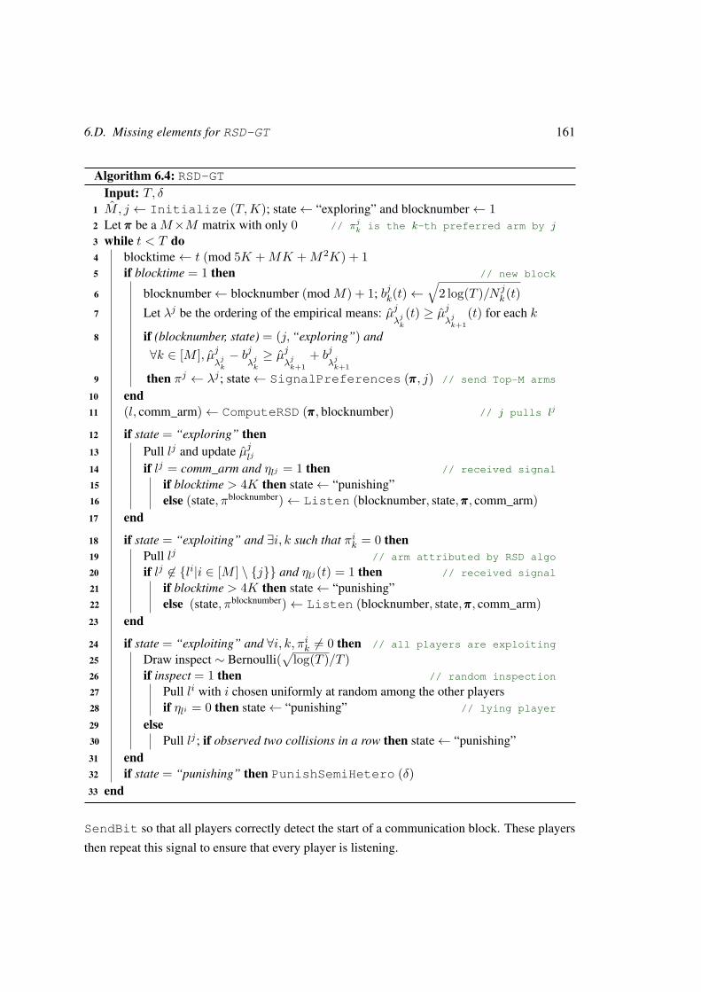
6.D. Missing elements for RSD-GT 161
Algorithm 6.4: RSD-GTInput: T, δ
1 M, j ← Initialize (T,K); state← “exploring” and blocknumber← 12 Let πππ be a M×M matrix with only 0 // πjk is the k-th preferred arm by j
3 while t < T do4 blocktime← t (mod 5K +MK +M2K) + 15 if blocktime = 1 then // new block
6 blocknumber← blocknumber (mod M) + 1; bjk(t)←√
2 log(T )/N jk(t)
7 Let λj be the ordering of the empirical means: µjλjk
(t) ≥ µjλjk+1
(t) for each k
8 if (blocknumber, state) = (j,“exploring”) and∀k ∈ [M ], µj
λjk
− bjλjk
≥ µjλjk+1
+ bjλjk+1
9 then πj ← λj ; state← SignalPreferences (πππ, j) // send Top-M arms
10 end11 (l, comm_arm)← ComputeRSD (πππ, blocknumber) // j pulls lj
12 if state = “exploring” then13 Pull lj and update µj
lj
14 if lj = comm_arm and ηlj = 1 then // received signal
15 if blocktime > 4K then state← “punishing”16 else (state, πblocknumber)← Listen (blocknumber, state,πππ, comm_arm)17 end
18 if state = “exploiting” and ∃i, k such that πik = 0 then19 Pull lj // arm attributed by RSD algo
20 if lj 6∈ li|i ∈ [M ] \ j and ηlj (t) = 1 then // received signal
21 if blocktime > 4K then state← “punishing”22 else (state, πblocknumber)← Listen (blocknumber, state,πππ, comm_arm)23 end
24 if state = “exploiting” and ∀i, k, πik 6= 0 then // all players are exploiting
25 Draw inspect ∼ Bernoulli(√
log(T )/T )26 if inspect = 1 then // random inspection
27 Pull li with i chosen uniformly at random among the other players28 if ηli = 0 then state← “punishing” // lying player
29 else30 Pull lj ; if observed two collisions in a row then state← “punishing”31 end32 if state = “punishing” then PunishSemiHetero (δ)33 end
SendBit so that all players correctly detect the start of a communication block. These players
then repeat this signal to ensure that every player is listening.
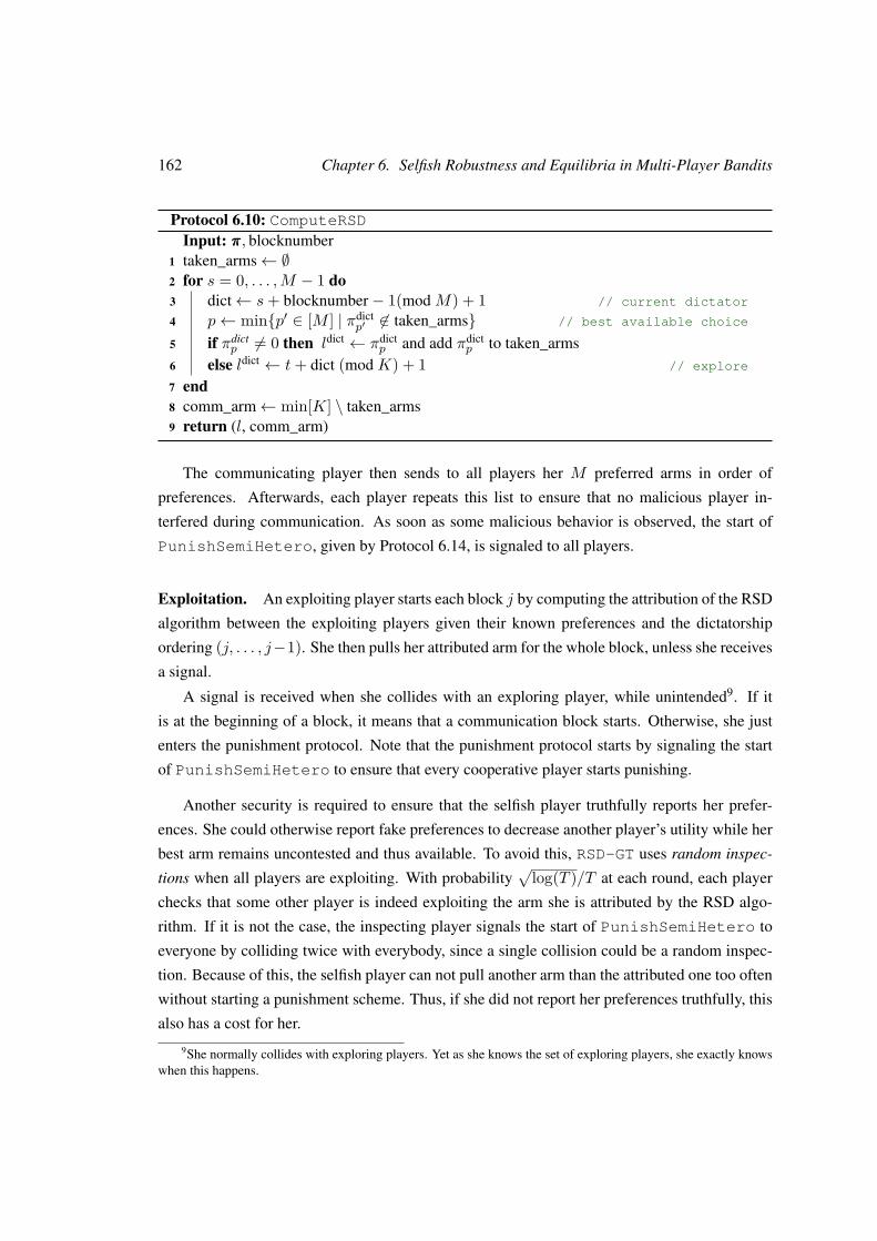
162 Chapter 6. Selfish Robustness and Equilibria in Multi-Player Bandits
Protocol 6.10: ComputeRSDInput: πππ, blocknumber
1 taken_arms← ∅2 for s = 0, . . . ,M − 1 do3 dict← s+ blocknumber− 1(mod M) + 1 // current dictator
4 p← minp′ ∈ [M ] | πdictp′ 6∈ taken_arms // best available choice
5 if πdictp 6= 0 then ldict ← πdict
p and add πdictp to taken_arms
6 else ldict ← t+ dict (mod K) + 1 // explore
7 end8 comm_arm← min[K] \ taken_arms9 return (l, comm_arm)
The communicating player then sends to all players her M preferred arms in order of
preferences. Afterwards, each player repeats this list to ensure that no malicious player in-
terfered during communication. As soon as some malicious behavior is observed, the start of
PunishSemiHetero, given by Protocol 6.14, is signaled to all players.
Exploitation. An exploiting player starts each block j by computing the attribution of the RSD
algorithm between the exploiting players given their known preferences and the dictatorship
ordering (j, . . . , j−1). She then pulls her attributed arm for the whole block, unless she receives
a signal.
A signal is received when she collides with an exploring player, while unintended9. If it
is at the beginning of a block, it means that a communication block starts. Otherwise, she just
enters the punishment protocol. Note that the punishment protocol starts by signaling the start
of PunishSemiHetero to ensure that every cooperative player starts punishing.
Another security is required to ensure that the selfish player truthfully reports her prefer-
ences. She could otherwise report fake preferences to decrease another player’s utility while her
best arm remains uncontested and thus available. To avoid this, RSD-GT uses random inspec-
tions when all players are exploiting. With probability√
log(T )/T at each round, each player
checks that some other player is indeed exploiting the arm she is attributed by the RSD algo-
rithm. If it is not the case, the inspecting player signals the start of PunishSemiHetero to
everyone by colliding twice with everybody, since a single collision could be a random inspec-
tion. Because of this, the selfish player can not pull another arm than the attributed one too often
without starting a punishment scheme. Thus, if she did not report her preferences truthfully, this
also has a cost for her.
9She normally collides with exploring players. Yet as she knows the set of exploring players, she exactly knowswhen this happens.
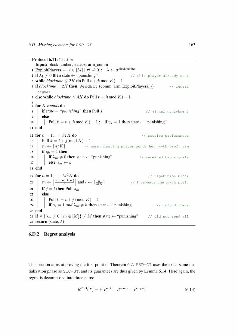
6.D. Missing elements for RSD-GT 163
Protocol 6.11: ListenInput: blocknumber, state,πππ, arm_comm
1 ExploitPlayers = i ∈ [M ] | πi1 6= 0; λ← πblocknumber
2 if λ1 6= 0 then state← “punishing” // this player already sent
3 while blocktime ≤ 2K do Pull t+ j(mod K) + 14 if blocktime = 2K then SendBit (comm_arm,ExploitPlayers, j) // repeat
signal
5 else while blocktime ≤ 4K do Pull t+ j(mod K) + 167 for K rounds do8 if state = “punishing” then Pull j // signal punishment
9 else10 Pull k = t+ j(mod K) + 1 ; if ηk = 1 then state← “punishing”11 end
12 for n = 1, . . . ,MK do // receive preferences
13 Pull k = t+ j(mod K) + 114 m← dn/Ke // communicating player sends her m-th pref. arm
15 if ηk = 1 then16 if λm 6= 0 then state← “punishing” // received two signals
17 else λm ← k
18 end
19 for n = 1, . . . ,M2K do // repetition block
20 m←⌈n (mod MK)
K
⌉and l← d n
MK e // l repeats the m-th pref.
21 if j = l then Pull λm22 else23 Pull k = t+ j (mod K) + 124 if ηk = 1 and λm 6= k then state← “punishing” // info differs
25 end26 if # λm 6= 0 | m ∈ [M ] 6= M then state← “punishing” // did not send all
27 return (state, λ)
6.D.2 Regret analysis
This section aims at proving the first point of Theorem 6.7. RSD-GT uses the exact same ini-
tialization phase as SIC-GT, and its guarantees are thus given by Lemma 6.14. Here again, the
regret is decomposed into three parts:
RRSD(T ) = E[Rinit +Rcomm +Rexplo], (6.13)
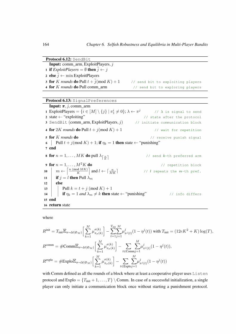
164 Chapter 6. Selfish Robustness and Equilibria in Multi-Player Bandits
Protocol 6.12: SendBitInput: comm_arm,ExploitPlayers, j
1 if ExploitPlayers = ∅ then j ← j
2 else j ← min ExploitPlayers3 for K rounds do Pull t+ j(mod K) + 1 // send bit to exploiting players
4 for K rounds do Pull comm_arm // send bit to exploring players
Protocol 6.13: SignalPreferencesInput: πππ, j, comm_arm
1 ExploitPlayers = i ∈ [M ] \ j | πi1 6= 0; λ← πj // λ is signal to send
2 state← “exploiting” // state after the protocol
3 SendBit (comm_arm,ExploitPlayers, j) // initiate communication block
4 for 2K rounds do Pull t+ j(mod K) + 1 // wait for repetition
5 for K rounds do // receive punish signal
6 Pull t+ j(mod K) + 1; if ηk = 1 then state← “punishing”7 end
8 for n = 1, . . . ,MK do pull λd nK e // send k-th preferred arm
9 for n = 1, . . . ,M2K do // repetition block
10 m←⌈n (mod MK)
K
⌉and l← d n
MK e // l repeats the m-th pref.
11 if j = l then Pull λm12 else13 Pull k = t+ j (mod K) + 114 if ηk = 1 and λm 6= k then state← “punishing” // info differs
15 end16 return state
where
Rinit = TinitEσ∼U(SM )
[ M∑k=1
µσ(k)πσ(k)
]−
Tinit∑t=1
M∑j=1
µjπj(t)(1− η
j(t)) with Tinit = (12eK2 +K) log(T ),
Rcomm = #CommEσ∼U(SM )
[ M∑k=1
µσ(k)πσ(k)
]−
∑t∈Comm
M∑j=1
µjπj(t)(1− η
j(t)),
Rexplo = #ExploEσ∼U(SM )
[ M∑k=1
µσ(k)πσ(k)
]−
∑t∈Explo
M∑j=1
µjπj(t)(1− η
j(t))
with Comm defined as all the rounds of a block where at least a cooperative player uses Listen
protocol and Explo = Tinit + 1, . . . , T \ Comm. In case of a successful initialization, a single
player can only initiate a communication block once without starting a punishment protocol.
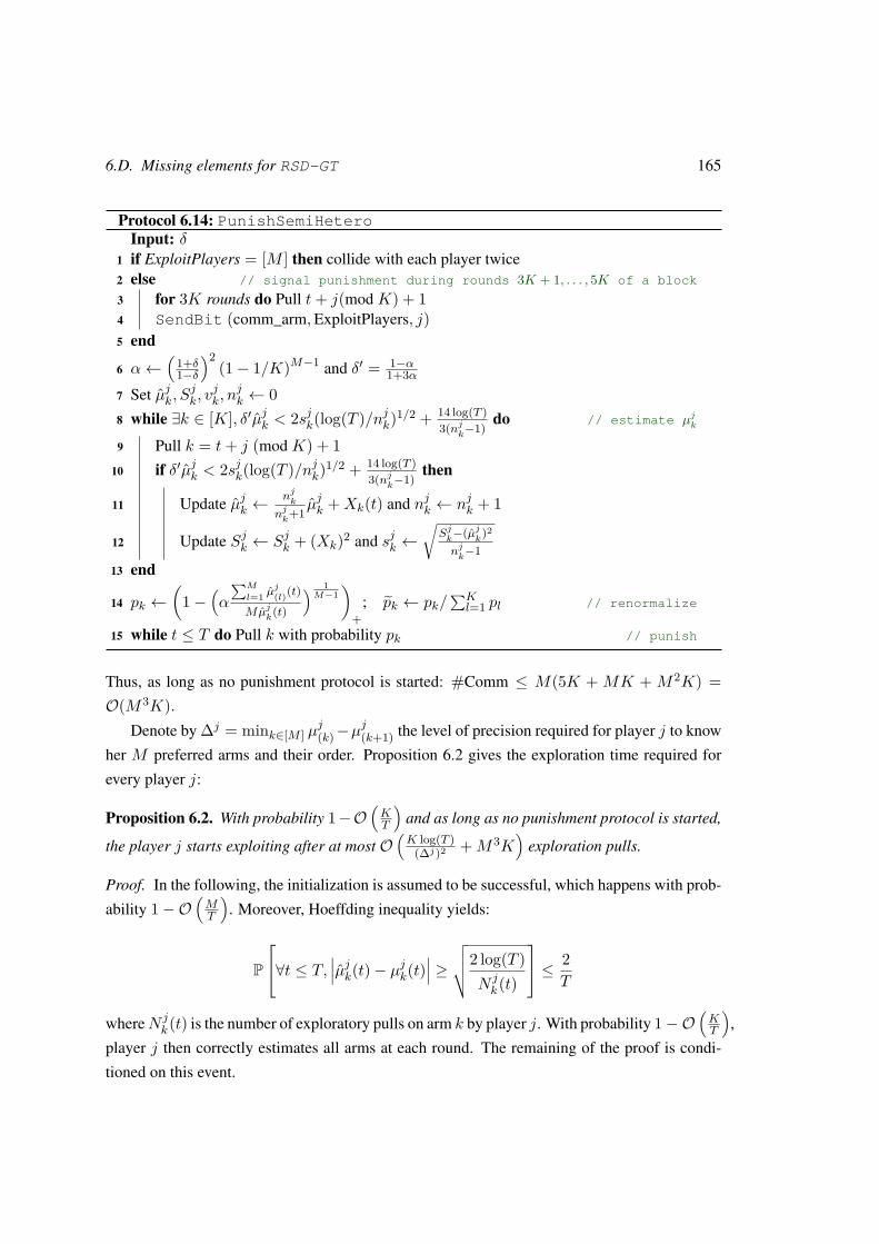
6.D. Missing elements for RSD-GT 165
Protocol 6.14: PunishSemiHeteroInput: δ
1 if ExploitPlayers = [M ] then collide with each player twice2 else // signal punishment during rounds 3K + 1, . . . , 5K of a block
3 for 3K rounds do Pull t+ j(mod K) + 14 SendBit (comm_arm,ExploitPlayers, j)5 end
6 α←(
1+δ1−δ
)2(1− 1/K)M−1 and δ′ = 1−α
1+3α
7 Set µjk, Sjk, v
jk, n
jk ← 0
8 while ∃k ∈ [K], δ′µjk < 2sjk(log(T )/njk)1/2 + 14 log(T )3(nj
k−1)
do // estimate µjk
9 Pull k = t+ j (mod K) + 110 if δ′µjk < 2sjk(log(T )/njk)1/2 + 14 log(T )
3(njk−1)
then
11 Update µjk ←njk
njk+1µjk +Xk(t) and njk ← njk + 1
12 Update Sjk ← Sjk + (Xk)2 and sjk ←√
Sjk−(µj
k)2
njk−1
13 end
14 pk ←(
1−(α
∑M
l=1 µj(l)(t)
Mµjk(t)
) 1M−1
)+
; pk ← pk/∑Kl=1 pl // renormalize
15 while t ≤ T do Pull k with probability pk // punish
Thus, as long as no punishment protocol is started: #Comm ≤ M(5K + MK + M2K) =O(M3K).
Denote by ∆j = mink∈[M ] µj(k)−µ
j(k+1) the level of precision required for player j to know
her M preferred arms and their order. Proposition 6.2 gives the exploration time required for
every player j:
Proposition 6.2. With probability 1−O(KT
)and as long as no punishment protocol is started,
the player j starts exploiting after at most O(K log(T )
(∆j)2 +M3K)
exploration pulls.
Proof. In the following, the initialization is assumed to be successful, which happens with prob-
ability 1−O(MT
). Moreover, Hoeffding inequality yields:
P
∀t ≤ T, ∣∣∣µjk(t)− µjk(t)∣∣∣ ≥√√√√2 log(T )
N jk(t)
≤ 2T
whereN jk(t) is the number of exploratory pulls on arm k by player j. With probability 1−O
(KT
),
player j then correctly estimates all arms at each round. The remaining of the proof is condi-
tioned on this event.
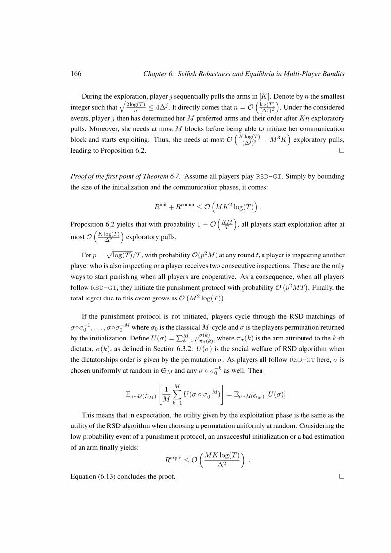
166 Chapter 6. Selfish Robustness and Equilibria in Multi-Player Bandits
During the exploration, player j sequentially pulls the arms in [K]. Denote by n the smallest
integer such that√
2 log(T )n ≤ 4∆j . It directly comes that n = O
(log(T )(∆j)2
). Under the considered
events, player j then has determined her M preferred arms and their order after Kn exploratory
pulls. Moreover, she needs at most M blocks before being able to initiate her communication
block and starts exploiting. Thus, she needs at most O(K log(T )
(∆j)2 +M3K)
exploratory pulls,
leading to Proposition 6.2.
Proof of the first point of Theorem 6.7. Assume all players play RSD-GT. Simply by bounding
the size of the initialization and the communication phases, it comes:
Rinit +Rcomm ≤ O(MK2 log(T )
).
Proposition 6.2 yields that with probability 1 − O(KMT
), all players start exploitation after at
most O(K log(T )
∆2
)exploratory pulls.
For p =√
log(T )/T , with probabilityO(p2M) at any round t, a player is inspecting another
player who is also inspecting or a player receives two consecutive inspections. These are the only
ways to start punishing when all players are cooperative. As a consequence, when all players
follow RSD-GT, they initiate the punishment protocol with probability O(p2MT
). Finally, the
total regret due to this event grows as O(M2 log(T )
).
If the punishment protocol is not initiated, players cycle through the RSD matchings of
σσ−10 , . . . , σσ−M0 where σ0 is the classicalM -cycle and σ is the players permutation returned
by the initialization. Define U(σ) =∑Mk=1 µ
σ(k)πσ(k), where πσ(k) is the arm attributed to the k-th
dictator, σ(k), as defined in Section 6.3.2. U(σ) is the social welfare of RSD algorithm when
the dictatorships order is given by the permutation σ. As players all follow RSD-GT here, σ is
chosen uniformly at random in SM and any σ σ−k0 as well. Then
Eσ∼U(SM )
[1M
M∑k=1
U(σ σ−M0 )]
= Eσ∼U(SM ) [U(σ)] .
This means that in expectation, the utility given by the exploitation phase is the same as the
utility of the RSD algorithm when choosing a permutation uniformly at random. Considering the
low probability event of a punishment protocol, an unsuccesful initialization or a bad estimation
of an arm finally yields:
Rexplo ≤ O(MK log(T )
∆2
).
Equation (6.13) concludes the proof.

6.D. Missing elements for RSD-GT 167
6.D.3 Selfish-robustness of RSD-GT
In this section, we prove the two last points of Theorem 6.7. Three auxiliary Lemmas are first
needed. They are proved in Section 6.D.3.
1. Lemma 6.23 compares the utility received by player j from the RSD algorithm with the
utility given by sequentially pulling her M best arms in the δ-heterogeneous setting.
2. Lemma 6.24 gives an equivalent version of Lemma 6.21, but for the δ-heterogeneous
setting.
3. Lemma 6.25 states that the expected utility of the assignment of any player during the
exploitation phase does not depend on the strategy of the selfish player. The intuition
behind this result is already given in Section 6.4.3.
In the case of several selfish players, they could actually fix the joint distribution of (σ−1(j), σ−1(j′)).
A simple rotation with aM -cycle is then not enough to recover a uniform distribution over
SM in average. A more complex rotation is then required and the dependence inM would
blow up with the number of selfish players.
Lemma 6.23. In the δ-heterogeneous case for every player j and permutation σ:
1M
M∑k=1
µj(k) ≤ Uj(σ) ≤ (1 + δ)2
(1− δ)2M
M∑k=1
µj(k),
where Uj(σ) := 1M
∑Mk=1 µ
j
πσσ−k0
(σk0σ−1(j)).
Following the notation of Section 6.3.2, πσ(σ−1(j)) is the arm attributed to player j by RSD
when the dictatorship order is given by σ. Uj(σ) is then the average utility of the exploitation
when σ is the permutation given by the initialization.
Lemma 6.24. Recall that γ = (1− 1/K)M−1. In the δ-heterogeneous setting with δ < 1−√γ1+√γ ,
if the punish protocol is started at time Tpunish by M − 1 players, then for the remaining playerj, independently of her sampling strategy:
E[RewjT |punishment] ≤ E[RewjTpunish+tp ] + αT − Tpunish − tp
M
M∑k=1
µj(k),
with tp = O(
K log(T )(1−δ)(1−α)2µ(K)
)and α = 1+( 1+δ
1−δ )2γ
2 .
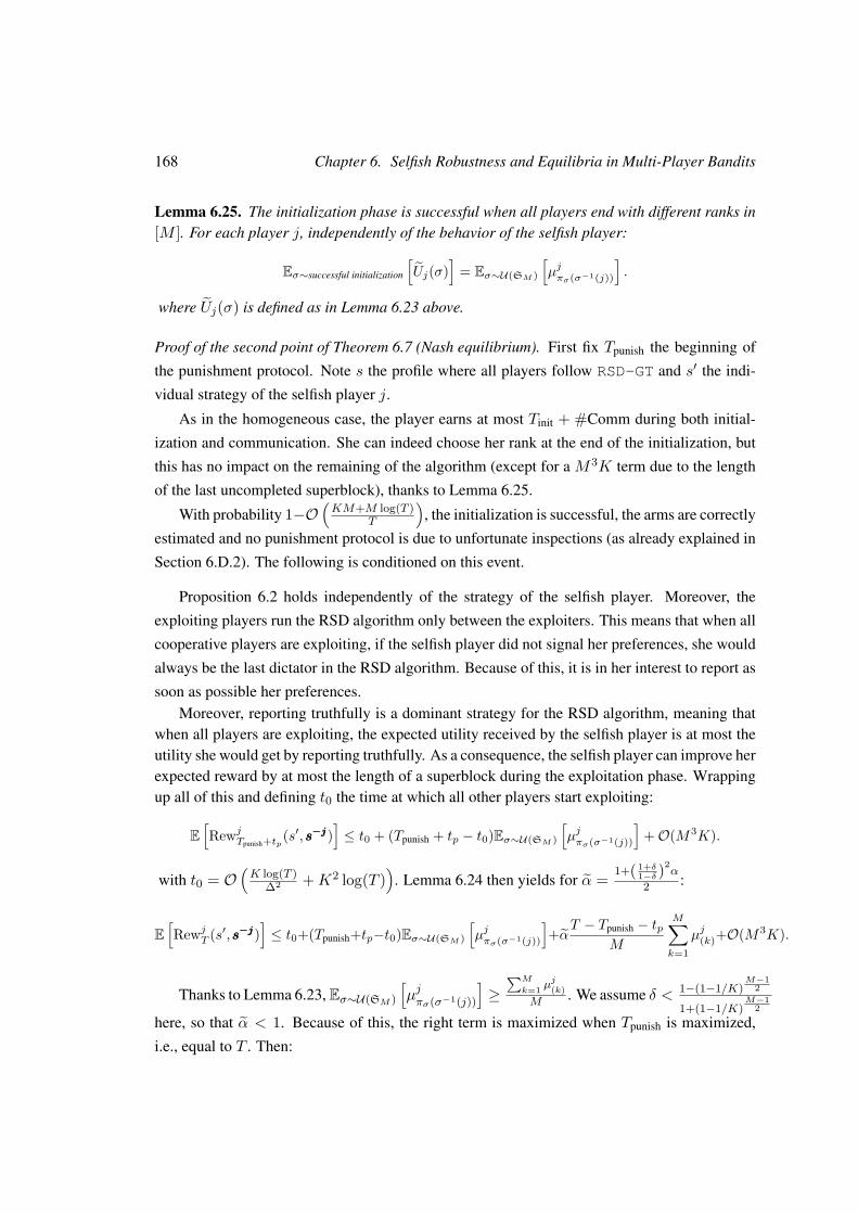
168 Chapter 6. Selfish Robustness and Equilibria in Multi-Player Bandits
Lemma 6.25. The initialization phase is successful when all players end with different ranks in[M ]. For each player j, independently of the behavior of the selfish player:
Eσ∼successful initialization
[Uj(σ)
]= Eσ∼U(SM )
[µjπσ(σ−1(j))
].
where Uj(σ) is defined as in Lemma 6.23 above.
Proof of the second point of Theorem 6.7 (Nash equilibrium). First fix Tpunish the beginning of
the punishment protocol. Note s the profile where all players follow RSD-GT and s′ the indi-
vidual strategy of the selfish player j.
As in the homogeneous case, the player earns at most Tinit + #Comm during both initial-
ization and communication. She can indeed choose her rank at the end of the initialization, but
this has no impact on the remaining of the algorithm (except for a M3K term due to the length
of the last uncompleted superblock), thanks to Lemma 6.25.
With probability 1−O(KM+M log(T )
T
), the initialization is successful, the arms are correctly
estimated and no punishment protocol is due to unfortunate inspections (as already explained in
Section 6.D.2). The following is conditioned on this event.
Proposition 6.2 holds independently of the strategy of the selfish player. Moreover, the
exploiting players run the RSD algorithm only between the exploiters. This means that when all
cooperative players are exploiting, if the selfish player did not signal her preferences, she would
always be the last dictator in the RSD algorithm. Because of this, it is in her interest to report as
soon as possible her preferences.Moreover, reporting truthfully is a dominant strategy for the RSD algorithm, meaning that
when all players are exploiting, the expected utility received by the selfish player is at most theutility she would get by reporting truthfully. As a consequence, the selfish player can improve herexpected reward by at most the length of a superblock during the exploitation phase. Wrappingup all of this and defining t0 the time at which all other players start exploiting:
E[RewjTpunish+tp(s′, s−js−js−j)
]≤ t0 + (Tpunish + tp − t0)Eσ∼U(SM )
[µjπσ(σ−1(j))
]+O(M3K).
with t0 = O(K log(T )
∆2 +K2 log(T ))
. Lemma 6.24 then yields for α = 1+( 1+δ1−δ )
2α
2 :
E[RewjT (s′, s−js−js−j)
]≤ t0+(Tpunish+tp−t0)Eσ∼U(SM )
[µjπσ(σ−1(j))
]+α
T − Tpunish − tpM
M∑k=1
µj(k)+O(M3K).
Thanks to Lemma 6.23, Eσ∼U(SM )[µjπσ(σ−1(j))
]≥∑M
k=1 µj(k)
M . We assume δ < 1−(1−1/K)M−1
2
1+(1−1/K)M−1
2
here, so that α < 1. Because of this, the right term is maximized when Tpunish is maximized,
i.e., equal to T . Then:
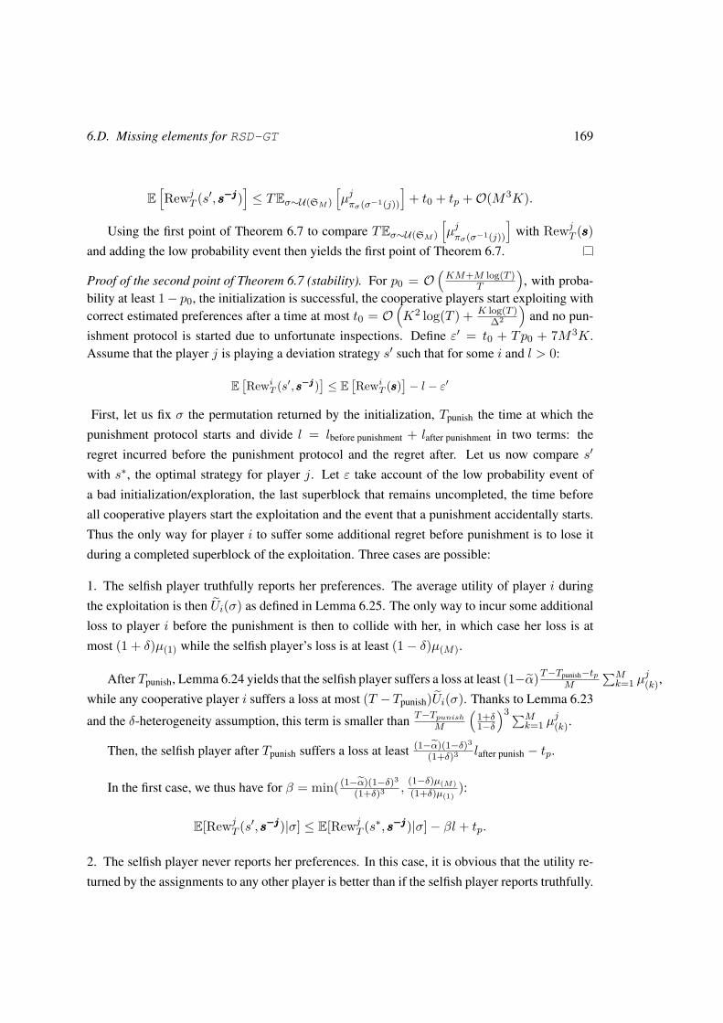
6.D. Missing elements for RSD-GT 169
E[Rewj
T (s′, s−js−js−j)]≤ TEσ∼U(SM )
[µjπσ(σ−1(j))
]+ t0 + tp +O(M3K).
Using the first point of Theorem 6.7 to compare TEσ∼U(SM )[µjπσ(σ−1(j))
]with Rewj
T (sss)and adding the low probability event then yields the first point of Theorem 6.7.
Proof of the second point of Theorem 6.7 (stability). For p0 = O(KM+M log(T )
T
), with proba-
bility at least 1− p0, the initialization is successful, the cooperative players start exploiting withcorrect estimated preferences after a time at most t0 = O
(K2 log(T ) + K log(T )
∆2
)and no pun-
ishment protocol is started due to unfortunate inspections. Define ε′ = t0 + Tp0 + 7M3K.Assume that the player j is playing a deviation strategy s′ such that for some i and l > 0:
E[RewiT (s′, s−js−js−j)
]≤ E
[RewiT (sss)
]− l − ε′
First, let us fix σ the permutation returned by the initialization, Tpunish the time at which the
punishment protocol starts and divide l = lbefore punishment + lafter punishment in two terms: the
regret incurred before the punishment protocol and the regret after. Let us now compare s′
with s∗, the optimal strategy for player j. Let ε take account of the low probability event of
a bad initialization/exploration, the last superblock that remains uncompleted, the time before
all cooperative players start the exploitation and the event that a punishment accidentally starts.
Thus the only way for player i to suffer some additional regret before punishment is to lose it
during a completed superblock of the exploitation. Three cases are possible:
1. The selfish player truthfully reports her preferences. The average utility of player i during
the exploitation is then Ui(σ) as defined in Lemma 6.25. The only way to incur some additional
loss to player i before the punishment is then to collide with her, in which case her loss is at
most (1 + δ)µ(1) while the selfish player’s loss is at least (1− δ)µ(M).
After Tpunish, Lemma 6.24 yields that the selfish player suffers a loss at least (1−α)T−Tpunish−tpM
∑Mk=1 µ
j(k),
while any cooperative player i suffers a loss at most (T −Tpunish)Ui(σ). Thanks to Lemma 6.23
and the δ-heterogeneity assumption, this term is smaller than T−TpunishM
(1+δ1−δ
)3∑Mk=1 µ
j(k).
Then, the selfish player after Tpunish suffers a loss at least (1−α)(1−δ)3
(1+δ)3 lafter punish − tp.
In the first case, we thus have for β = min( (1−α)(1−δ)3
(1+δ)3 ,(1−δ)µ(M)(1+δ)µ(1)
):
E[RewjT (s′, s−js−js−j)|σ] ≤ E[Rewj
T (s∗, s−js−js−j)|σ]− βl + tp.
2. The selfish player never reports her preferences. In this case, it is obvious that the utility re-
turned by the assignments to any other player is better than if the selfish player reports truthfully.

170 Chapter 6. Selfish Robustness and Equilibria in Multi-Player Bandits
Then the only way to incur some additional loss to player i before punishment is to collide with
her, still leading to a ratio of loss at mostµj(M)µi(1)
.
From there, it can be concluded as in the first case that for β = min( (1−α)(1−δ)3
(1+δ)3 ,(1−δ)µ(M)(1+δ)µ(1)
):
E[RewjT (s′, s−j)|σ] ≤ E[Rewj
T (s∗, s−j)|σ]− βl + tp.
3. The selfish player reported fake preferences. If these fake preferences never change the issue
of the ComputeRSD protocol, this does not change from the first case. Otherwise, for any block
where the final assignment is changed, the selfish player does not receive the arm she would get
if she reported truthfully. Denote by n the number of such blocks, by Nlie the number of times
player j did not pull the arm attributed by ComputeRSD during such a block before Tpunish and
by lb the loss incurred to player i on the other blocks.
As for the previous cases, the loss incurred by the selfish player during the blocks where the
assignment of ComputeRSD is unchanged is at least (1−δ)µ(M)(1+δ)µ(1)
lb.
Each time the selfish player pulls the attributed arm by ComputeRSD in a block where theassignment is changed, she suffers a loss at least ∆. The total loss for the selfish player is then(w.r.t. the optimal strategy s∗) at least:
(1− α)T − Tpunish − tp
M
M∑k=1
µj(k) +( nM
(Tpunish − t0)−Nlie
)∆ +
(1− δ)µ(M)
(1 + δ)µ(1)lb.
On the other hand, the loss for a cooperative player is at most:
T − Tpunish
M
(1 + δ
1− δ
)3 M∑k=1
µj(k) + n
M(Tpunish − t0)(1 + δ)µ(1) + lb.
Moreover, each time the selfish player does not pull the attributed arm by ComputeRSD,
she has a probability p = 1 − (1 − pM−1)M−1 ≥ p
2 for p =√
log(T )T , to receive a random
inspection and thus to trigger the punishment protocol. Because of this, Nlie follows a geometric
distribution of parameter p and E[Nlie] ≤ 2p .
When taking the expectations over Tpunish and Nlie, but still fixing σ and n, we get:
lselfish ≥ (1− α)T − E[Tpunish]− tpM
M∑k=1
µj(k) +(n
M
(E[Tpunish]− t0
)− 2/p
)∆ +
(1− δ)µ(M)(1 + δ)µ(1)
lb,
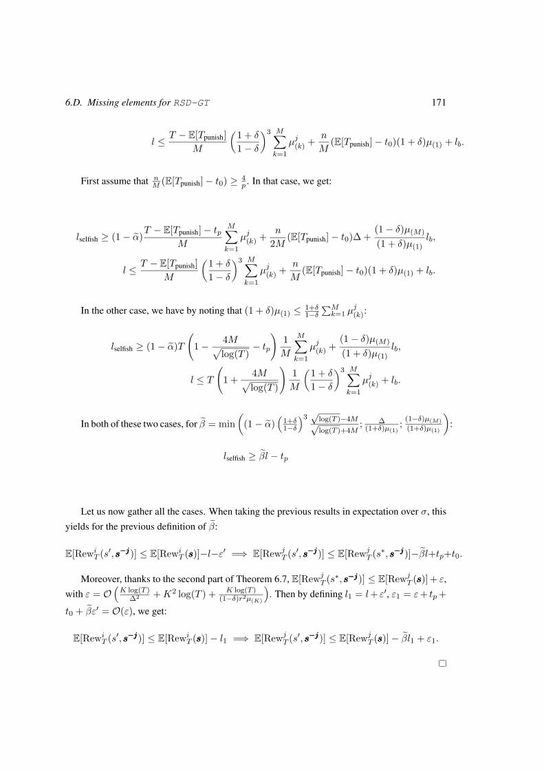
6.D. Missing elements for RSD-GT 171
l ≤T − E[Tpunish]
M
(1 + δ
1− δ
)3 M∑k=1
µj(k) + n
M(E[Tpunish]− t0)(1 + δ)µ(1) + lb.
First assume that nM (E[Tpunish]− t0) ≥ 4
p . In that case, we get:
lselfish ≥ (1− α)T − E[Tpunish]− tpM
M∑k=1
µj(k) + n
2M (E[Tpunish]− t0)∆ +(1− δ)µ(M)(1 + δ)µ(1)
lb,
l ≤T − E[Tpunish]
M
(1 + δ
1− δ
)3 M∑k=1
µj(k) + n
M(E[Tpunish]− t0)(1 + δ)µ(1) + lb.
In the other case, we have by noting that (1 + δ)µ(1) ≤ 1+δ1−δ
∑Mk=1 µ
j(k):
lselfish ≥ (1− α)T(
1− 4M√log(T )
− tp
)1M
M∑k=1
µj(k) +(1− δ)µ(M)(1 + δ)µ(1)
lb,
l ≤ T(
1 + 4M√log(T )
)1M
(1 + δ
1− δ
)3 M∑k=1
µj(k) + lb.
In both of these two cases, for β = min(
(1− α)(
1+δ1−δ
)3 √log(T )−4M√log(T )+4M
; ∆(1+δ)µ(1)
; (1−δ)µ(M)(1+δ)µ(1)
):
lselfish ≥ βl − tp
Let us now gather all the cases. When taking the previous results in expectation over σ, this
yields for the previous definition of β:
E[RewiT (s′, s−js−js−j)] ≤ E[Rewi
T (sss)]−l−ε′ =⇒ E[RewjT (s′, s−js−js−j)] ≤ E[Rewj
T (s∗, s−js−js−j)]−βl+tp+t0.
Moreover, thanks to the second part of Theorem 6.7, E[RewjT (s∗, s−js−js−j)] ≤ E[Rewj
T (sss)] + ε,
with ε = O(K log(T )
∆2 +K2 log(T ) + K log(T )(1−δ)r2µ(K)
). Then by defining l1 = l+ ε′, ε1 = ε+ tp +
t0 + βε′ = O(ε), we get:
E[RewiT (s′, s−js−js−j)] ≤ E[Rewi
T (sss)]− l1 =⇒ E[RewjT (s′, s−js−js−j)] ≤ E[Rewj
T (sss)]− βl1 + ε1.
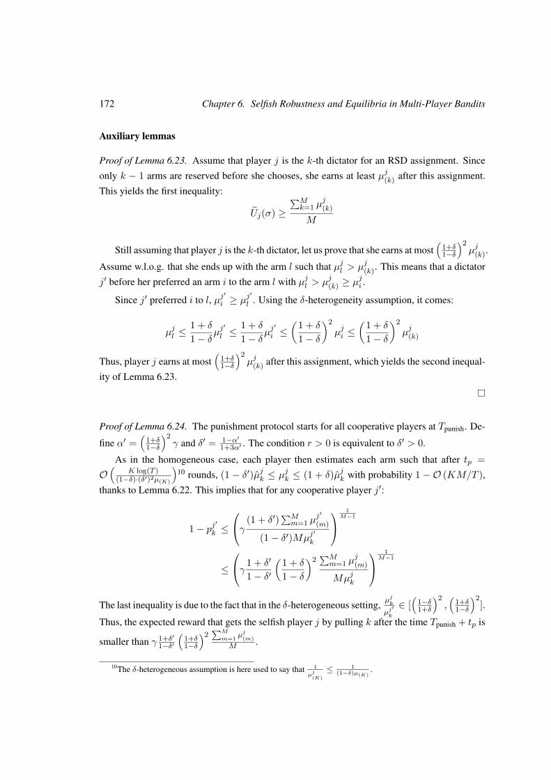
172 Chapter 6. Selfish Robustness and Equilibria in Multi-Player Bandits
Auxiliary lemmas
Proof of Lemma 6.23. Assume that player j is the k-th dictator for an RSD assignment. Since
only k − 1 arms are reserved before she chooses, she earns at least µj(k) after this assignment.
This yields the first inequality:
Uj(σ) ≥∑Mk=1 µ
j(k)
M
Still assuming that player j is the k-th dictator, let us prove that she earns at most(
1+δ1−δ
)2µj(k).
Assume w.l.o.g. that she ends up with the arm l such that µjl > µj(k). This means that a dictator
j′ before her preferred an arm i to the arm l with µjl > µj(k) ≥ µji .
Since j′ preferred i to l, µj′
i ≥ µj′
l . Using the δ-heterogeneity assumption, it comes:
µjl ≤1 + δ
1− δµj′
l ≤1 + δ
1− δµj′
i ≤(1 + δ
1− δ
)2µji ≤
(1 + δ
1− δ
)2µj(k)
Thus, player j earns at most(
1+δ1−δ
)2µj(k) after this assignment, which yields the second inequal-
ity of Lemma 6.23.
Proof of Lemma 6.24. The punishment protocol starts for all cooperative players at Tpunish. De-
fine α′ =(
1+δ1−δ
)2γ and δ′ = 1−α′
1+3α′ . The condition r > 0 is equivalent to δ′ > 0.
As in the homogeneous case, each player then estimates each arm such that after tp =O(
K log(T )(1−δ)·(δ′)2µ(K)
)10 rounds, (1 − δ′)µjk ≤ µjk ≤ (1 + δ)µjk with probability 1 −O (KM/T ),
thanks to Lemma 6.22. This implies that for any cooperative player j′:
1− pj′
k ≤
γ (1 + δ′)∑Mm=1 µ
j′
(m)
(1− δ′)Mµj′
k
1
M−1
≤
γ 1 + δ′
1− δ′(1 + δ
1− δ
)2∑Mm=1 µ
j(m)
Mµjk
1M−1
The last inequality is due to the fact that in the δ-heterogeneous setting, µjk
µj′k
∈ [(
1−δ1+δ
)2,(
1+δ1−δ
)2].
Thus, the expected reward that gets the selfish player j by pulling k after the time Tpunish + tp is
smaller than γ 1+δ′1−δ′
(1+δ1−δ
)2∑M
m=1 µj(m)
M .
10The δ-heterogeneous assumption is here used to say that 1µj
(K)≤ 1
(1−δ)µ(K).
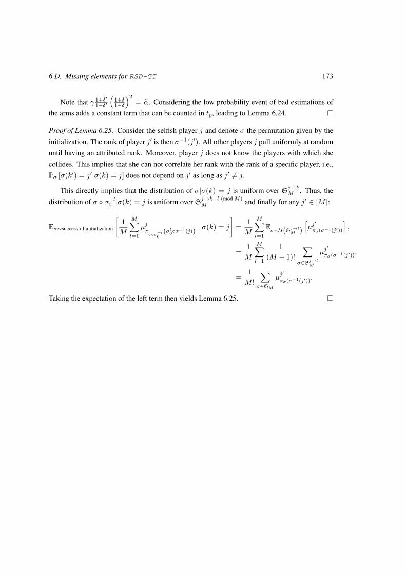
6.D. Missing elements for RSD-GT 173
Note that γ 1+δ′1−δ′
(1+δ1−δ
)2= α. Considering the low probability event of bad estimations of
the arms adds a constant term that can be counted in tp, leading to Lemma 6.24.
Proof of Lemma 6.25. Consider the selfish player j and denote σ the permutation given by the
initialization. The rank of player j′ is then σ−1(j′). All other players j pull uniformly at random
until having an attributed rank. Moreover, player j does not know the players with which she
collides. This implies that she can not correlate her rank with the rank of a specific player, i.e.,
Pσ [σ(k′) = j′|σ(k) = j] does not depend on j′ as long as j′ 6= j.
This directly implies that the distribution of σ|σ(k) = j is uniform over Sj→kM . Thus, the
distribution of σ σ−l0 |σ(k) = j is uniform over Sj→k+l (mod M)M and finally for any j′ ∈ [M ]:
Eσ∼successful initialization
[1M
M∑l=1
µjπσσ−l0
(σl0σ−1(j))
∣∣∣∣ σ(k) = j
]= 1M
M∑l=1
Eσ∼U
(Sj→lM
) [µj′πσ(σ−1(j′))
],
= 1M
M∑l=1
1(M − 1)!
∑σ∈Sj→lM
µj′
πσ(σ−1(j′)),
= 1M !
∑σ∈SM
µj′
πσ(σ−1(j′)).
Taking the expectation of the left term then yields Lemma 6.25.

Part II
Other learning instances
174

Chapter 7
Decentralized Learning in OnlineQueuing Systems
Motivated by packet routing in computer networks and resource allocation in radio net-works, online queuing systems are composed of queues receiving packets at different rates.Repeatedly, they send packets to servers, each of them treating only at most one packet at atime. In the centralized case, the number of accumulated packets remains bounded (i.e., thesystem is stable) as long as the ratio between service rates and arrival rates is larger than1. In the decentralized case, individual no-regret strategies ensures stability when this ratiois larger than 2. Yet, myopically minimizing regret disregards the long term effects due tothe carryover of packets to further rounds. On the other hand, minimizing long term costsleads to stable Nash equilibria as soon as the ratio exceeds e
e−1 . Stability with decentralizedlearning strategies with a ratio below 2 was a major remaining question. We first argue thatfor ratios up to 2, cooperation is required for stability of learning strategies, as selfish min-imization of policy regret, a patient notion of regret, might indeed still be unstable in thiscase. We therefore consider cooperative queues and propose the first learning decentralizedalgorithm guaranteeing stability of the system as long as the ratio of rates is larger than 1,thus reaching performances comparable to centralized strategies.
7.1 Introduction . . . . . . . . . . . . . . . . . . . . . . . . . . . . . . . . . . . . 176
7.1.1 Additional related work . . . . . . . . . . . . . . . . . . . . . . . . . 177
7.2 Queuing Model . . . . . . . . . . . . . . . . . . . . . . . . . . . . . . . . . . 178
7.3 The case for a cooperative algorithm . . . . . . . . . . . . . . . . . . . . . . . 180
7.4 A decentralized algorithm . . . . . . . . . . . . . . . . . . . . . . . . . . . . . 182
7.4.1 Choice of a dominant mapping . . . . . . . . . . . . . . . . . . . . . . 185
7.4.2 Choice of a Birkhoff von Neumann decomposition . . . . . . . . . . . 186
7.4.3 Stability guarantees . . . . . . . . . . . . . . . . . . . . . . . . . . . . 188
175
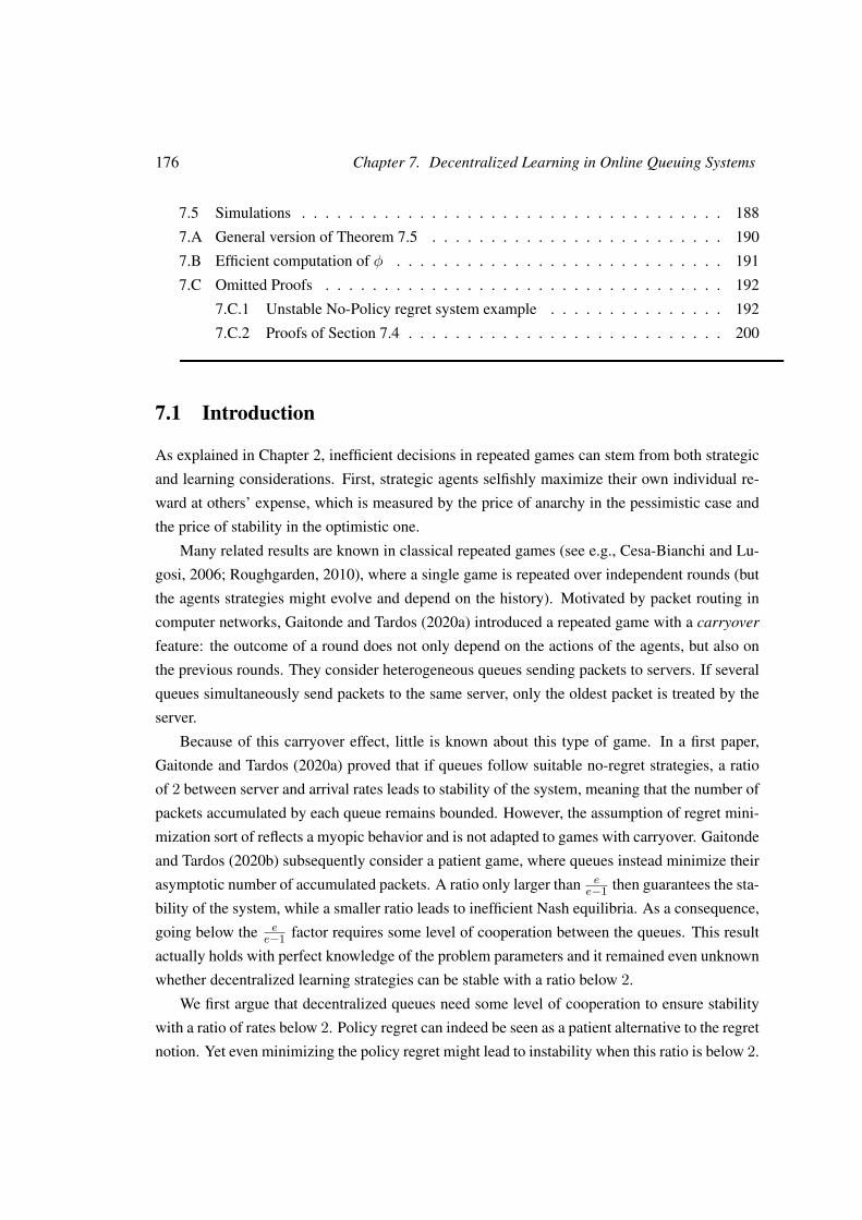
176 Chapter 7. Decentralized Learning in Online Queuing Systems
7.5 Simulations . . . . . . . . . . . . . . . . . . . . . . . . . . . . . . . . . . . . 188
7.A General version of Theorem 7.5 . . . . . . . . . . . . . . . . . . . . . . . . . 190
7.B Efficient computation of φ . . . . . . . . . . . . . . . . . . . . . . . . . . . . 191
7.C Omitted Proofs . . . . . . . . . . . . . . . . . . . . . . . . . . . . . . . . . . 192
7.C.1 Unstable No-Policy regret system example . . . . . . . . . . . . . . . 192
7.C.2 Proofs of Section 7.4 . . . . . . . . . . . . . . . . . . . . . . . . . . . 200
7.1 Introduction
As explained in Chapter 2, inefficient decisions in repeated games can stem from both strategic
and learning considerations. First, strategic agents selfishly maximize their own individual re-
ward at others’ expense, which is measured by the price of anarchy in the pessimistic case and
the price of stability in the optimistic one.
Many related results are known in classical repeated games (see e.g., Cesa-Bianchi and Lu-
gosi, 2006; Roughgarden, 2010), where a single game is repeated over independent rounds (but
the agents strategies might evolve and depend on the history). Motivated by packet routing in
computer networks, Gaitonde and Tardos (2020a) introduced a repeated game with a carryover
feature: the outcome of a round does not only depend on the actions of the agents, but also on
the previous rounds. They consider heterogeneous queues sending packets to servers. If several
queues simultaneously send packets to the same server, only the oldest packet is treated by the
server.
Because of this carryover effect, little is known about this type of game. In a first paper,
Gaitonde and Tardos (2020a) proved that if queues follow suitable no-regret strategies, a ratio
of 2 between server and arrival rates leads to stability of the system, meaning that the number of
packets accumulated by each queue remains bounded. However, the assumption of regret mini-
mization sort of reflects a myopic behavior and is not adapted to games with carryover. Gaitonde
and Tardos (2020b) subsequently consider a patient game, where queues instead minimize their
asymptotic number of accumulated packets. A ratio only larger than ee−1 then guarantees the sta-
bility of the system, while a smaller ratio leads to inefficient Nash equilibria. As a consequence,
going below the ee−1 factor requires some level of cooperation between the queues. This result
actually holds with perfect knowledge of the problem parameters and it remained even unknown
whether decentralized learning strategies can be stable with a ratio below 2.
We first argue that decentralized queues need some level of cooperation to ensure stability
with a ratio of rates below 2. Policy regret can indeed be seen as a patient alternative to the regret
notion. Yet even minimizing the policy regret might lead to instability when this ratio is below 2.
7.1. Introduction 177
An explicit decentralized cooperative algorithm called ADEQUA (A DEcentralized QUeuing
Algorithm) is thus proposed. It is the first decentralized learning algorithm guaranteeing stability
when this ratio is only larger than 1. ADEQUA does not require communication between the
queues, but uses synchronisation between them to accurately estimate the problem parameters
and avoid interference when sending packets. Our main result is given by Theorem 7.1 below,
whose formal version, Theorem 7.5 in Section 7.3, also provides bounds on the number of
accumulated packets.
Theorem 7.1. If the ratio between server rates and arrival rates is larger than 1 and all queues
follow ADEQUA, the system is strongly stable.
The remaining of the chapter is organised as follows. The model and existing results are
recalled in Section 7.2. Section 7.3 argues that cooperation is required to guarantee stability of
learning strategies when the ratio of rates is below 2. ADEQUA is then presented in Section 7.4,
along with insights for the proof of Theorem 7.1. Section 7.5 finally compares the behavior
of ADEQUA with no-regret strategies on toy examples and empirically confirms the different
known theoretical results.
7.1.1 Additional related work
Queuing theory includes applications in diverse areas such as computer science, engineering,
operation research (Shortle et al., 2018). Borodin et al. (1996) for example use the stability the-
orem of Pemantle and Rosenthal (1999), which was also used by Gaitonde and Tardos (2020a),
to study the problem of packet routing through a network. Our setting is the single-hop particular
instance of throughput maximization in wireless networks. Motivated by resource allocation in
multihop radio problem, packets can be sent through more general routing paths in the original
problem. Tassiulas and Ephremides (1990) proposed a first stable centralized algorithm, when
the service rates are known a priori. Stable decentralized algorithms were later introduced in
specific cases (Neely et al., 2008; Jiang and Walrand, 2009; Shah and Shin, 2012), when the re-
wards Xk(t) are observed before deciding which server to send the packet. The main challenge
is then of coordination, where queues avoid collisions with each other. The proposed algorithms
are thus not adapted to our setting, where both coordination between queues and learning the
service rates are required. We refer the reader to (Georgiadis et al., 2006) for an extended survey
on resource allocation in wireless networks.
Krishnasamy et al. (2016) first considered online learning for such queuing systems model,
in the simple case of a single queue. It is a particular instance of stochastic multi-armed bandits,
a celebrated online learning model, where the agent repeatedly takes an action within a finite
178 Chapter 7. Decentralized Learning in Online Queuing Systems
set and observes its associated reward. This model becomes intricate when considering multiple
queues, as they interfere when choosing the same server. It is then related to the multiplayer
bandits problem studied in Part I.
The collision model is here different as one of the players still gets a reward. It is thus even
more closely related to competing bandits (Liu et al., 2020b; Liu et al., 2020a), where arms
have preferences over the players and only the most preferred player pulling the arm actually
gets the reward. Arm preferences are here not fixed and instead depend on the packets’ ages.
While collisions can be used as communication tools between players in multiplayer bandits, this
becomes harder with an asymmetric collision model as in competing bandits. However, some
level of communication remains possible (Sankararaman et al., 2020; Basu et al., 2021). In
queuing systems, collisions are not only asymmetric, but depend on the age of the sent packets,
making such solutions unsuited.
While multiplayer bandits literature considers cooperative players, Chapter 6 showed that
cooperative algorithms could be made robust to selfish players. On the other hand, competing
bandits consider strategic players and arms as the goal is to reach a bipartite stable matching
between them. Despite being cooperative, ADEQUA also has strategic considerations as the
queues’ strategy converges to a correlated equilibrium of the patient game described in Sec-
tion 7.2.
An additional difficulty here appears as queues are asynchronous: they are not active at
each round, but only when having packets left. This is different from the classical notion of
asynchronicity (Bonnefoi et al., 2017), where players are active at each round with some fixed
probability. Communication schemes in multiplayer bandits rely on this synchronisation as-
sumption. While such a level of synchronisation is not available here, some lower level is still
used to avoid collisions between queues and to allow a limited exchange of information between
them.
7.2 Queuing Model
We consider a queuing system composed of N queues and K servers, associated with vectors of
arrival and service rates λ,µ, where at each time step t = 1, 2, . . . , the following happens:
• each queue i ∈ [N ] receives a new packet with probability λi ∈ [0, 1], that is marked with
the timestamp of its arrival time. If the queue currently has packet(s) on hold, it sends one
of them to a chosen server j based on its past observations.
• Each server j ∈ [K] attempts to clear the oldest packet it has received, breaking ties
uniformly at random. It succeeds with probability µj ∈ [0, 1] and otherwise sends it back
7.2. Queuing Model 179
to its original queue, as well as all other unprocessed packets.
At each time step, a queue only observes whether or not the packet sent (if any) is cleared
by the server. We note Qit the number of packets in queue i at time t. Given a packet-sending
dynamics, the system is stable if, for each i in [N ], Qit/t converges to 0 almost surely. It is
strongly stable, if for any r, t ≥ 0 and i ∈ [N ], E[(Qit)r] ≤ Cr, where Cr is an arbitrarily large
constant, depending on r but not t. Without ambiguity, we also say the policy or the queues are
(strongly) stable. Naturally, a strongly stable system is also stable (Gaitonde and Tardos, 2020a).
Without loss of generality, we assume K ≥ N (otherwise, we simply add fictitious servers
with 0 service rate). The key quantity of a system is its slack, defined as the largest real number
such that:k∑i=1
µ(i) ≥ ηk∑i=1
λ(i), ∀ k ≤ N.
We also denote by P ([K]) the set of probability distributions on [K] and by ∆ the margin of
the system defined by
∆ := mink∈[N ]
1k
k∑i=1
(µ(i) − λ(i)). (7.1)
Notice that the alternative system where λi = λi + ∆ and µk = µk has a slack 1. In that sense,
∆ is the largest margin between service and arrival rates that all queues can individually get in
the system. Note that if η > 1, then ∆ > 0. We now recall existing results for this problem,
summarized in Figure 7.1 below.
Theorem 7.2 (Marshall et al. 1979). For any instance, there exists a strongly stable centralized
policy if and only if η > 1.
Theorem 7.3 (Gaitonde and Tardos 2020a, informal). If η > 2, queues following appropriate
no regret strategies are strongly stable.
For each N > 0, there exists a system and a dynamic s.t. 2 > η > 2 − o(1/N), all queues
follow appropriate no-regret strategies, but they are not strongly stable.
In the above theorem, an appropriate no regret strategy is a strategy such that there exists
a partitioning of the time into successive windows, for which the incurred regret is o (w) with
high probability on each window of lengthw. This for example includes the EXP3.P.1 algorithm
(Auer et al., 2002b) where the k-th window has length 2k.
The patient queuing game G = ([N ], (ci)ni=1,µ,λ) is defined as follows. The strategy space
for each queue is P ([K]). Let p−i ∈ (P ([K]))N−1 denote the vector of fixed distributions for
all queues over servers, except for queue i. The cost function for queue i is defined as:
ci(pi,p−i) = limt→+∞
T it /t,
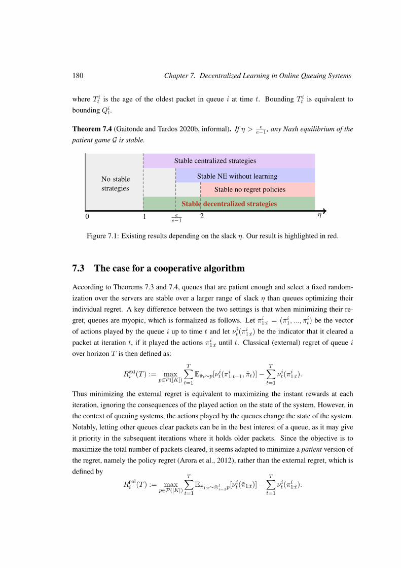
180 Chapter 7. Decentralized Learning in Online Queuing Systems
where T it is the age of the oldest packet in queue i at time t. Bounding T it is equivalent to
bounding Qit.
Theorem 7.4 (Gaitonde and Tardos 2020b, informal). If η > ee−1 , any Nash equilibrium of the
patient game G is stable.
η
No stablestrategies
Stable centralized strategies
Stable no regret policies
Stable NE without learning
Stable decentralized strategies
0 1 ee−1
2
Figure 7.1: Existing results depending on the slack η. Our result is highlighted in red.
7.3 The case for a cooperative algorithm
According to Theorems 7.3 and 7.4, queues that are patient enough and select a fixed random-
ization over the servers are stable over a larger range of slack η than queues optimizing their
individual regret. A key difference between the two settings is that when minimizing their re-
gret, queues are myopic, which is formalized as follows. Let πi1:t = (πi1, ..., πit) be the vector
of actions played by the queue i up to time t and let νit(πi1:t) be the indicator that it cleared a
packet at iteration t, if it played the actions πi1:t until t. Classical (external) regret of queue i
over horizon T is then defined as:
Rexti (T ) := max
p∈P([K])
T∑t=1
Eπt∼p[νit(πi1:t−1, πt)]−T∑t=1
νit(πi1:t).
Thus minimizing the external regret is equivalent to maximizing the instant rewards at each
iteration, ignoring the consequences of the played action on the state of the system. However, in
the context of queuing systems, the actions played by the queues change the state of the system.
Notably, letting other queues clear packets can be in the best interest of a queue, as it may give
it priority in the subsequent iterations where it holds older packets. Since the objective is to
maximize the total number of packets cleared, it seems adapted to minimize a patient version of
the regret, namely the policy regret (Arora et al., 2012), rather than the external regret, which is
defined by
Rpoli (T ) := max
p∈P([K])
T∑t=1
Eπ1:t∼⊗ti=1p[νit(π1:t)]−
T∑t=1
νit(πi1:t).
7.3. The case for a cooperative algorithm 181
That is, Rpoli (T ) is the expected difference between the number of packets queue i cleared and
the number of packets it would have cleared over the whole period by playing a fixed (possibly
random) action, taking into account how this change of policy would affect the state of the
system.
However, as stated in Proposition 7.1, optimizing this patient version of the regret rather than
the myopic one could not guarantee stability on a wider range of slack value. This suggests that
adding only patience to the learning strategy of the queues is not enough to go beyond a slack
of 2, and that any strategy beating that factor 2 must somewhat include synchronisation between
the queues.
Proposition 7.1. Consider the partition of the time t = 1, 2, . . . into successive windows, where
wk = k2 is the length of the k-th one. For any N ≥ 2, there exists an instance with 2N queues
and servers, with slack η = 2−O(
1N
), s.t., almost surely, each queue’s policy regret is o (wk)
on all but finitely many of the windows, but the system is not strongly stable.
Sketch of proof. Consider a system with 2N queues and servers with λi = 1/2N and µi =1/N−1/4N2 for all i ∈ [2N ]. The considered strategy profile is the following. For each k ≥ 0,
the kth time window is split into two stages. During the first stage, of length dαwke, queues 2iand 2i + 1 both play server 2i + t (mod 2N) at iteration t, for all i ∈ [N ]. During the second
stage of the time window, queue i plays server i + t (mod 2N) at iteration t. This counter
example, albeit very specific, illustrates well how when the queues are highly synchronised, it
is better to remain synchronized rather than deviate, even if the synchronisation is suboptimal in
terms of stability. The complete proof is provided in Section 7.C.1.
Queues following this strategy accumulate packets during the first stage, and clear more
packets than they receive during the second stage. The value of α is tuned so that the queues
still accumulate a linear portion of packets during each time window. For those appropriate α,
the system is unstable.
Now suppose that queue i deviates from the strategy and plays a fixed action p ∈ P ([K]).
In the first stage of each time window, queue i can clear a bit more packets than it would by not
deviating. However, during the second stage, it is no longer synchronised with the other queues
and collides with them a large number of times. Because of those collisions, it will accumulate
many packets. In the detailed analysis, we demonstrate that, in the end, for appropriate values
of α, queue i accumulates more packets than it would have without deviating.
According to Theorem 7.4, the factor ee−1 can be seen as the price of anarchy of the problem,
as for slacks below, the worst Nash equilibria might be unstable. On the other hand, it is known
that for any slack above 1, there exists a centralized stable strategy. This centralized strategy
actually consists in queues playing the same joint probability at each time step, independently
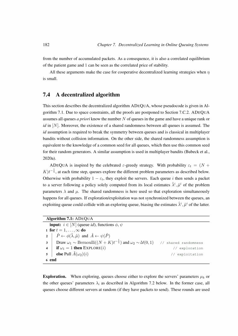
182 Chapter 7. Decentralized Learning in Online Queuing Systems
from the number of accumulated packets. As a consequence, it is also a correlated equilibrium
of the patient game and 1 can be seen as the correlated price of stability.
All these arguments make the case for cooperative decentralized learning strategies when η
is small.
7.4 A decentralized algorithm
This section describes the decentralized algorithm ADEQUA, whose pseudocode is given in Al-
gorithm 7.1. Due to space constraints, all the proofs are postponed to Section 7.C.2. ADEQUA
assumes all queues a priori know the numberN of queues in the game and have a unique rank or
id in [N ]. Moreover, the existence of a shared randomness between all queues is assumed. The
id assumption is required to break the symmetry between queues and is classical in multiplayer
bandits without collision information. On the other side, the shared randomness assumption is
equivalent to the knowledge of a common seed for all queues, which then use this common seed
for their random generators. A similar assumption is used in multiplayer bandits (Bubeck et al.,
2020a).
ADEQUA is inspired by the celebrated ε-greedy strategy. With probability εt = (N +K)t−
15 , at each time step, queues explore the different problem parameters as described below.
Otherwise with probability 1 − εt, they exploit the servers. Each queue i then sends a packet
to a server following a policy solely computed from its local estimates λi, µi of the problem
parameters λ and µ. The shared randomness is here used so that exploration simultaneously
happens for all queues. If exploration/exploitation was not synchronized between the queues, an
exploiting queue could collide with an exploring queue, biasing the estimates λi, µi of the latter.
Algorithm 7.1: ADEQUAinput: i ∈ [N ] (queue id), functions φ, ψ
1 for t = 1, . . . ,∞ do2 P ← φ(λ, µ) and A← ψ(P )3 Draw ω1 ∼ Bernoulli((N +K)t−
15 ) and ω2 ∼ U(0, 1) // shared randomness
4 if ω1 = 1 then EXPLORE(i) // exploration
5 else Pull A(ω2)(i) // exploitation
6 end
Exploration. When exploring, queues choose either to explore the servers’ parameters µk or
the other queues’ parameters λi as described in Algorithm 7.2 below. In the former case, all
queues choose different servers at random (if they have packets to send). These rounds are used
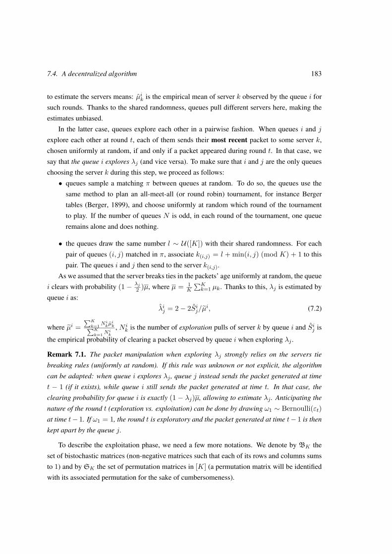
7.4. A decentralized algorithm 183
to estimate the servers means: µik is the empirical mean of server k observed by the queue i for
such rounds. Thanks to the shared randomness, queues pull different servers here, making the
estimates unbiased.
In the latter case, queues explore each other in a pairwise fashion. When queues i and j
explore each other at round t, each of them sends their most recent packet to some server k,
chosen uniformly at random, if and only if a packet appeared during round t. In that case, we
say that the queue i explores λj (and vice versa). To make sure that i and j are the only queues
choosing the server k during this step, we proceed as follows:
• queues sample a matching π between queues at random. To do so, the queues use the
same method to plan an all-meet-all (or round robin) tournament, for instance Berger
tables (Berger, 1899), and choose uniformly at random which round of the tournament
to play. If the number of queues N is odd, in each round of the tournament, one queue
remains alone and does nothing.
• the queues draw the same number l ∼ U([K]) with their shared randomness. For each
pair of queues (i, j) matched in π, associate k(i,j) = l + min(i, j) (mod K) + 1 to this
pair. The queues i and j then send to the server k(i,j).
As we assumed that the server breaks ties in the packets’ age uniformly at random, the queue
i clears with probability (1 − λj2 )µ, where µ = 1
K
∑Kk=1 µk. Thanks to this, λj is estimated by
queue i as:
λij = 2− 2Sij/µi, (7.2)
where µi =∑K
k=1 Nikµik∑K
k=1Nik
, N ik is the number of exploration pulls of server k by queue i and Sij is
the empirical probability of clearing a packet observed by queue i when exploring λj .
Remark 7.1. The packet manipulation when exploring λj strongly relies on the servers tie
breaking rules (uniformly at random). If this rule was unknown or not explicit, the algorithm
can be adapted: when queue i explores λj , queue j instead sends the packet generated at time
t − 1 (if it exists), while queue i still sends the packet generated at time t. In that case, the
clearing probability for queue i is exactly (1 − λj)µ, allowing to estimate λj . Anticipating the
nature of the round t (exploration vs. exploitation) can be done by drawing ω1 ∼ Bernoulli(εt)at time t− 1. If ω1 = 1, the round t is exploratory and the packet generated at time t− 1 is then
kept apart by the queue j.
To describe the exploitation phase, we need a few more notations. We denote by BK the
set of bistochastic matrices (non-negative matrices such that each of its rows and columns sums
to 1) and by SK the set of permutation matrices in [K] (a permutation matrix will be identified
with its associated permutation for the sake of cumbersomeness).
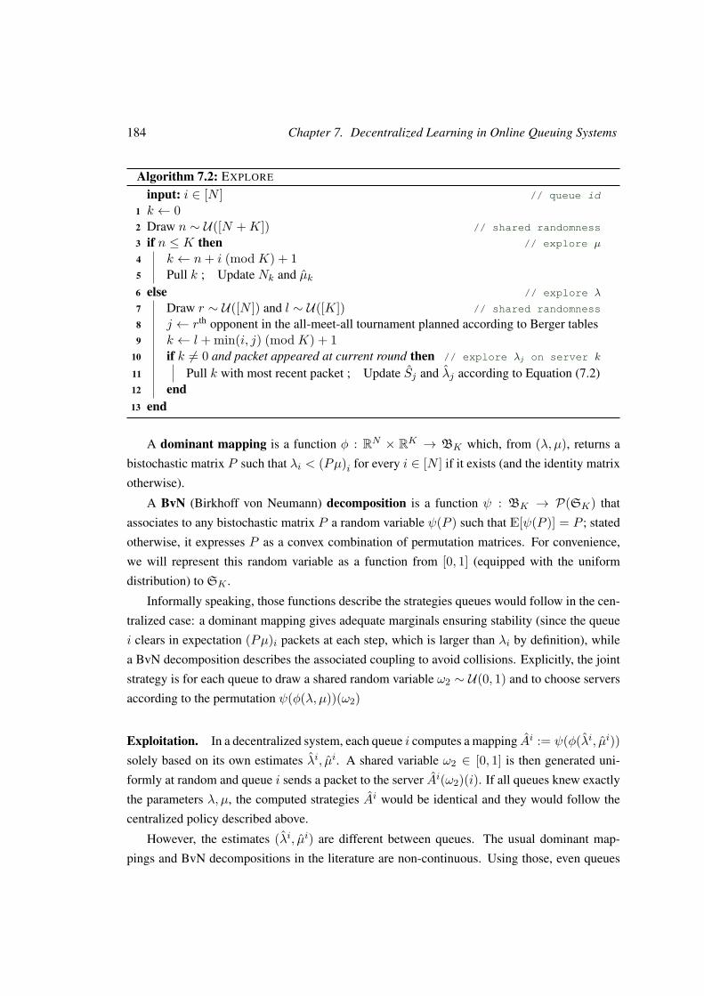
184 Chapter 7. Decentralized Learning in Online Queuing Systems
Algorithm 7.2: EXPLORE
input: i ∈ [N ] // queue id
1 k ← 02 Draw n ∼ U([N +K]) // shared randomness
3 if n ≤ K then // explore µ
4 k ← n+ i (mod K) + 15 Pull k ; Update Nk and µk6 else // explore λ
7 Draw r ∼ U([N ]) and l ∼ U([K]) // shared randomness
8 j ← rth opponent in the all-meet-all tournament planned according to Berger tables9 k ← l + min(i, j) (mod K) + 1
10 if k 6= 0 and packet appeared at current round then // explore λj on server k
11 Pull k with most recent packet ; Update Sj and λj according to Equation (7.2)12 end13 end
A dominant mapping is a function φ : RN × RK → BK which, from (λ, µ), returns a
bistochastic matrix P such that λi < (Pµ)i for every i ∈ [N ] if it exists (and the identity matrix
otherwise).
A BvN (Birkhoff von Neumann) decomposition is a function ψ : BK → P(SK) that
associates to any bistochastic matrix P a random variable ψ(P ) such that E[ψ(P )] = P ; stated
otherwise, it expresses P as a convex combination of permutation matrices. For convenience,
we will represent this random variable as a function from [0, 1] (equipped with the uniform
distribution) to SK .
Informally speaking, those functions describe the strategies queues would follow in the cen-
tralized case: a dominant mapping gives adequate marginals ensuring stability (since the queue
i clears in expectation (Pµ)i packets at each step, which is larger than λi by definition), while
a BvN decomposition describes the associated coupling to avoid collisions. Explicitly, the joint
strategy is for each queue to draw a shared random variable ω2 ∼ U(0, 1) and to choose servers
according to the permutation ψ(φ(λ, µ))(ω2)
Exploitation. In a decentralized system, each queue i computes a mapping Ai := ψ(φ(λi, µi))solely based on its own estimates λi, µi. A shared variable ω2 ∈ [0, 1] is then generated uni-
formly at random and queue i sends a packet to the server Ai(ω2)(i). If all queues knew exactly
the parameters λ, µ, the computed strategies Ai would be identical and they would follow the
centralized policy described above.
However, the estimates (λi, µi) are different between queues. The usual dominant map-
pings and BvN decompositions in the literature are non-continuous. Using those, even queues
7.4. A decentralized algorithm 185
with close estimates could have totally different Ai, and thus collide a large number of times,
which would impede the stability of the system. Regular enough dominant mappings and BvN
decompositions are required, to avoid this phenomenon. The design of φ and ψ is thus crucial
and appropriate choices are given in the following Sections 7.4.1 and 7.4.2. Nonetheless, they
can be used in some black-box fashion, so we provide for the sake of completeness sufficient
conditions for stability, as well as a general result depending on the properties of φ and ψ, in
Section 7.A.
Remark 7.2. The exploration probability t−15 gives the smallest theoretical dependency in ∆ in
our bound. A trade-off between the proportion of exploration rounds and the speed of learning
indeed appears in the proof of Theorem 7.1. Exploration rounds have to represent a small
proportion of the rounds, as the queues accumulate packets when exploring. On the other hand,
if queues explore more often, the regime where their number of packets decreases starts earlier.
A general stability result depending on the choice of this probability is given by Theorem 7.6 in
Section 7.A.
Yet in Section 7.5, taking a probability t−14 empirically performs better as it speeds up the
exploration.
7.4.1 Choice of a dominant mapping
Recall that a dominant mapping takes as inputs (λ, µ) and returns, if possible, a bistochastic
matrix P such that
λi <∑Kk=1 Pi,kµk for all i ∈ [N ].
The usual dominant mappings sort the vector λ and µ in descending orders (Marshall et al.,
1979). Because of this operation, they are non-continuous and we thus need to design a regular
dominant mapping satisfying the above property. Inspired by the log-barrier method, it is done
by taking the minimizer of a strongly convex program as follows
φ(λ, µ) = arg minP∈BK
maxi∈[N ]
− ln( K∑j=1
Pi,jµj − λi)
+ 12K ‖P‖
22. (7.3)
Although the objective function is non-smooth because of the max operator, it enforces
fairness between queues and leads to a better regularity of the arg min.
Remark 7.3. Computing φ requires solving a non-smooth strongly convex minimization prob-
lem. This cannot be computed exactly, but a good approximation can be quickly obtained using
the scheme described in Section 7.B. If this approximation error is small enough, it has no im-
pact on the stability bound of Theorem 7.5. It is thus ignored for simplicity, i.e., we assume in
the following that φ(λ, µ) is exactly computed at each step.
186 Chapter 7. Decentralized Learning in Online Queuing Systems
As required, φ always returns a matrix P satisfying that λ < Pµ if possible, since otherwise
the objective is infinite (and in that case we assume that φ returns the identity matrix). Moreover,
the objective function is 1K -strongly convex, which guarantees some regularity of the arg min,
namely local-Lipschitzness, leading to Lemma 7.1 below .
Lemma 7.1. For any (λ, µ) with positive margin ∆ (defined in Equation (7.1)), if ‖(λ− λ, µ−µ)‖∞ ≤ c1∆, for any c1 <
12√e+2 , then
‖φ(λ, µ)− φ(λ, µ)‖2 ≤c2K
∆ ‖(λ− λ, µ− µ)‖∞,
where c2 = 4(1−2c1)/
√e−2c1 . Moreover, denoting P = φ(λ, µ), it holds for any i ∈ [N ],
λi ≤∑Kk=1 Pi,kµk −
(1−2c1√
e− 2c1
)∆.
The first property guarantees that if the queues have close estimates, they also have close
bistochastic matrices P . Moreover, the second property guarantees that each queue should clear
its packets with a margin of order ∆, in absence of collisions.
7.4.2 Choice of a Birkhoff von Neumann decomposition
Given a bistochastic matrix P , Birkhoff algorithm returns a convex combination of permutation
matrices P [j] such that P =∑j z[j]P [j]. The classical version of Birkhoff algorithm is non-
continuous in its inputs. Yet it can be smartly modified as in ORDERED BIRKHOFF, described
in Algorithm 7.3, to get a regular BvN decomposition defined as follows for any ω ∈ (0, 1):
ψ(P )(ω) = P [jω] (7.4)
where P =∑j z[j]P [j] is the decomposition returned by ORDERED BIRKHOFF algorithm
and jω verifies∑j≤jω
z[j] ≤ ω <∑
j≤jω+1z[j].
For a matrix P in the following, its support is defined as supp(P ) = (i, j) | Pi,j 6= 0.Obviously Eω∼U(0,1)[ψ(P )(ω)] = P and permutations avoid collisions between queues. The
difference with the usual Birkhoff algorithm happens at Line 4. Birkhoff algorithm usually
computes any perfect matching in the graph induced by the support of P at the current iteration.
This is often done with the Hopcroft-Karp algorithm, while it is here done with the Hungarian
algorithm with respect to some cost matrix C. Although using the Hungarian algorithm slightly
increases the computational complexity of this step (K3 instead of K2.5), it ensures to output
the permutation matrices P [j] according to a fixed order defined below.
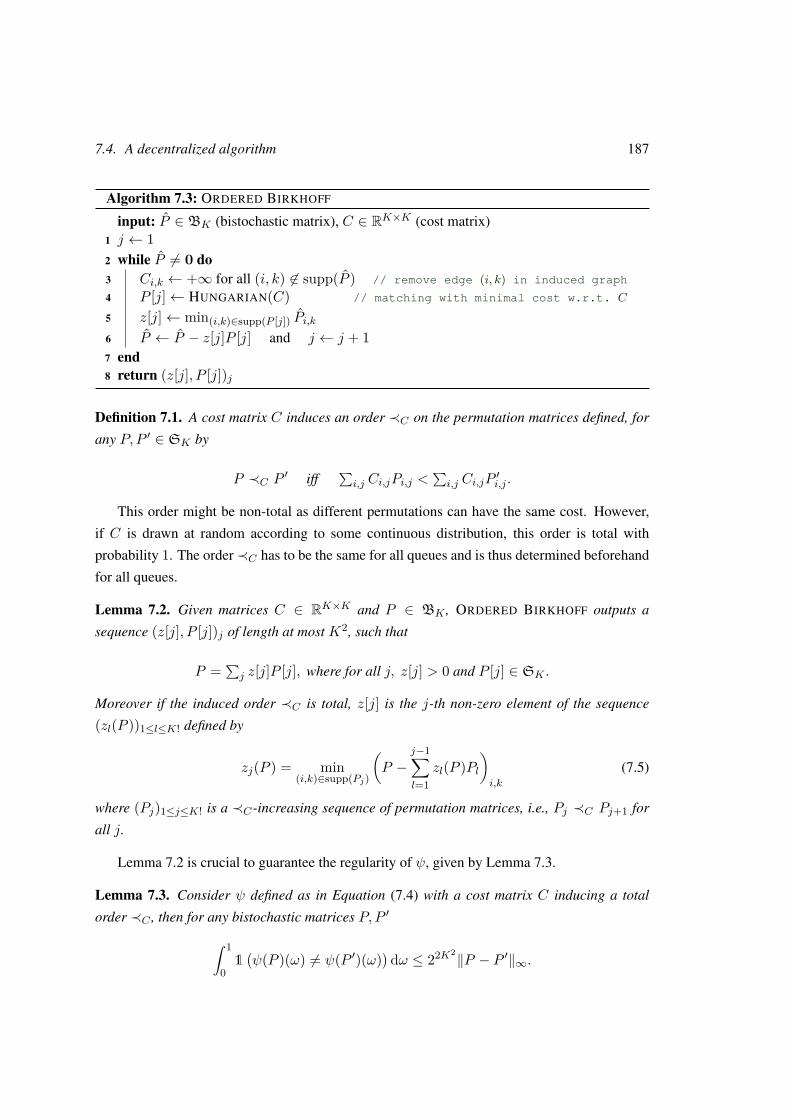
7.4. A decentralized algorithm 187
Algorithm 7.3: ORDERED BIRKHOFF
input: P ∈ BK (bistochastic matrix), C ∈ RK×K (cost matrix)1 j ← 12 while P 6= 0 do3 Ci,k ← +∞ for all (i, k) 6∈ supp(P ) // remove edge (i, k) in induced graph
4 P [j]← HUNGARIAN(C) // matching with minimal cost w.r.t. C
5 z[j]← min(i,k)∈supp(P [j]) Pi,k6 P ← P − z[j]P [j] and j ← j + 17 end8 return (z[j], P [j])j
Definition 7.1. A cost matrix C induces an order ≺C on the permutation matrices defined, for
any P, P ′ ∈ SK by
P ≺C P ′ iff∑i,j Ci,jPi,j <
∑i,j Ci,jP
′i,j .
This order might be non-total as different permutations can have the same cost. However,
if C is drawn at random according to some continuous distribution, this order is total with
probability 1. The order≺C has to be the same for all queues and is thus determined beforehand
for all queues.
Lemma 7.2. Given matrices C ∈ RK×K and P ∈ BK , ORDERED BIRKHOFF outputs a
sequence (z[j], P [j])j of length at most K2, such that
P =∑j z[j]P [j], where for all j, z[j] > 0 and P [j] ∈ SK .
Moreover if the induced order ≺C is total, z[j] is the j-th non-zero element of the sequence
(zl(P ))1≤l≤K! defined by
zj(P ) = min(i,k)∈supp(Pj)
(P −
j−1∑l=1
zl(P )Pl)i,k
(7.5)
where (Pj)1≤j≤K! is a ≺C-increasing sequence of permutation matrices, i.e., Pj ≺C Pj+1 for
all j.
Lemma 7.2 is crucial to guarantee the regularity of ψ, given by Lemma 7.3.
Lemma 7.3. Consider ψ defined as in Equation (7.4) with a cost matrix C inducing a total
order ≺C , then for any bistochastic matrices P, P ′∫ 1
01(ψ(P )(ω) 6= ψ(P ′)(ω)
)dω ≤ 22K2‖P − P ′‖∞.
188 Chapter 7. Decentralized Learning in Online Queuing Systems
Lemma 7.3 indeed ensures that the probability of collision between two queues remains
small when they have close estimates. Unfortunately, the regularity constant is exponential in
K2, which yields a similar dependency in the stability bound of Theorem 7.5. The existence of a
BvN decomposition with polynomial regularity constants remains unknown, even without com-
putational considerations. The design of a better BvN decomposition is left open for future work
and would directly improve the stability bounds, using the general result given by Theorem 7.6
in Section 7.A.
7.4.3 Stability guarantees
This section finally provides theoretical guarantees on the stability of the system when all queues
follow ADEQUA. The success of ADEQUA relies on the accurate estimation of all problem
parameters by the queues, given by Lemma 7.9 in Section 7.C.2. After some time τ , the queues
have tight estimations of the problem parameters. Afterwards, they clear their packets with a
margin of order ∆, thanks to Lemmas 7.1 and 7.3. This finally ensures the stability of the
system, as given by Theorem 7.5.
Theorem 7.5. For any η > 1, the system where all queues follow ADEQUA, for every queue i
and any r ∈ N, there exists a constant Cr depending only on r such that
E[(Qit)r] ≤ CrKN(
N52K
52 25K2
(min(1,Kµ)λ)54 ∆5
)r, for all t ∈ N.
As a consequence, for any η > 1, this decentralized system is strongly stable.
Despite yielding an exponential dependency in K2, this anytime bound leads to a first de-
centralized stability result when η ∈ (1, ee−1), which closes the stability gap left by previous
works. Moreover it can be seen in the proof that the asymptotic number of packets is much
smaller. It actually converges, in expectation, to the number of packets the queues would accu-
mulate if they were following a stable centralized strategy from the beginning. As already noted
by Krishnasamy et al. (2016) for a single queue, the number of packets first increases during the
learning phase and then decreases once the queues have tight enough estimations, until reaching
the same state as in the perfect knowledge centralized case. This is empirically confirmed in
Section 7.5.
7.5 Simulations
Figures 7.2 and 7.3 compare on toy examples the stability of queues, when either each of them
follows the no-regret strategy EXP3.P.1, or each queue follows ADEQUA. For practical con-
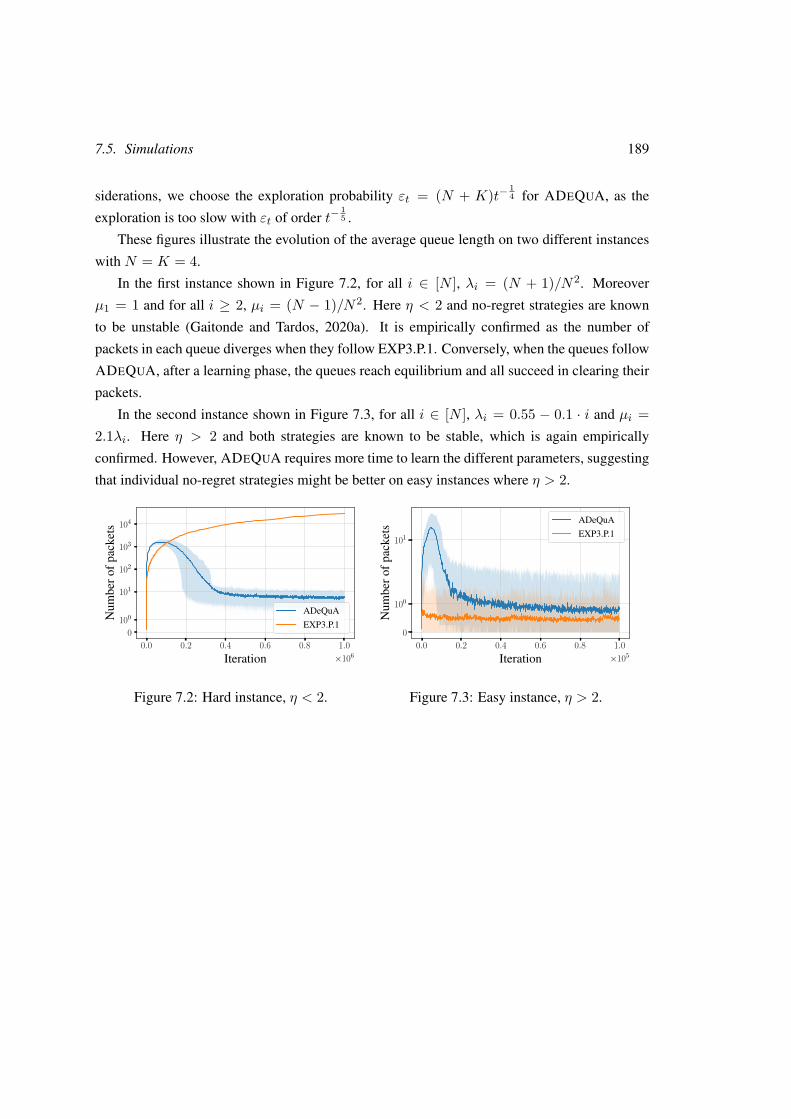
7.5. Simulations 189
siderations, we choose the exploration probability εt = (N + K)t−14 for ADEQUA, as the
exploration is too slow with εt of order t−15 .
These figures illustrate the evolution of the average queue length on two different instances
with N = K = 4.
In the first instance shown in Figure 7.2, for all i ∈ [N ], λi = (N + 1)/N2. Moreover
µ1 = 1 and for all i ≥ 2, µi = (N − 1)/N2. Here η < 2 and no-regret strategies are known
to be unstable (Gaitonde and Tardos, 2020a). It is empirically confirmed as the number of
packets in each queue diverges when they follow EXP3.P.1. Conversely, when the queues follow
ADEQUA, after a learning phase, the queues reach equilibrium and all succeed in clearing their
packets.
In the second instance shown in Figure 7.3, for all i ∈ [N ], λi = 0.55 − 0.1 · i and µi =2.1λi. Here η > 2 and both strategies are known to be stable, which is again empirically
confirmed. However, ADEQUA requires more time to learn the different parameters, suggesting
that individual no-regret strategies might be better on easy instances where η > 2.
0.0 0.2 0.4 0.6 0.8 1.0Iteration ×106
0100
101
102
103
104
Num
bero
fpac
kets
ADeQuAEXP3.P.1
Figure 7.2: Hard instance, η < 2.
0.0 0.2 0.4 0.6 0.8 1.0Iteration ×105
0
100
101
Num
bero
fpac
kets
ADeQuAEXP3.P.1
Figure 7.3: Easy instance, η > 2.
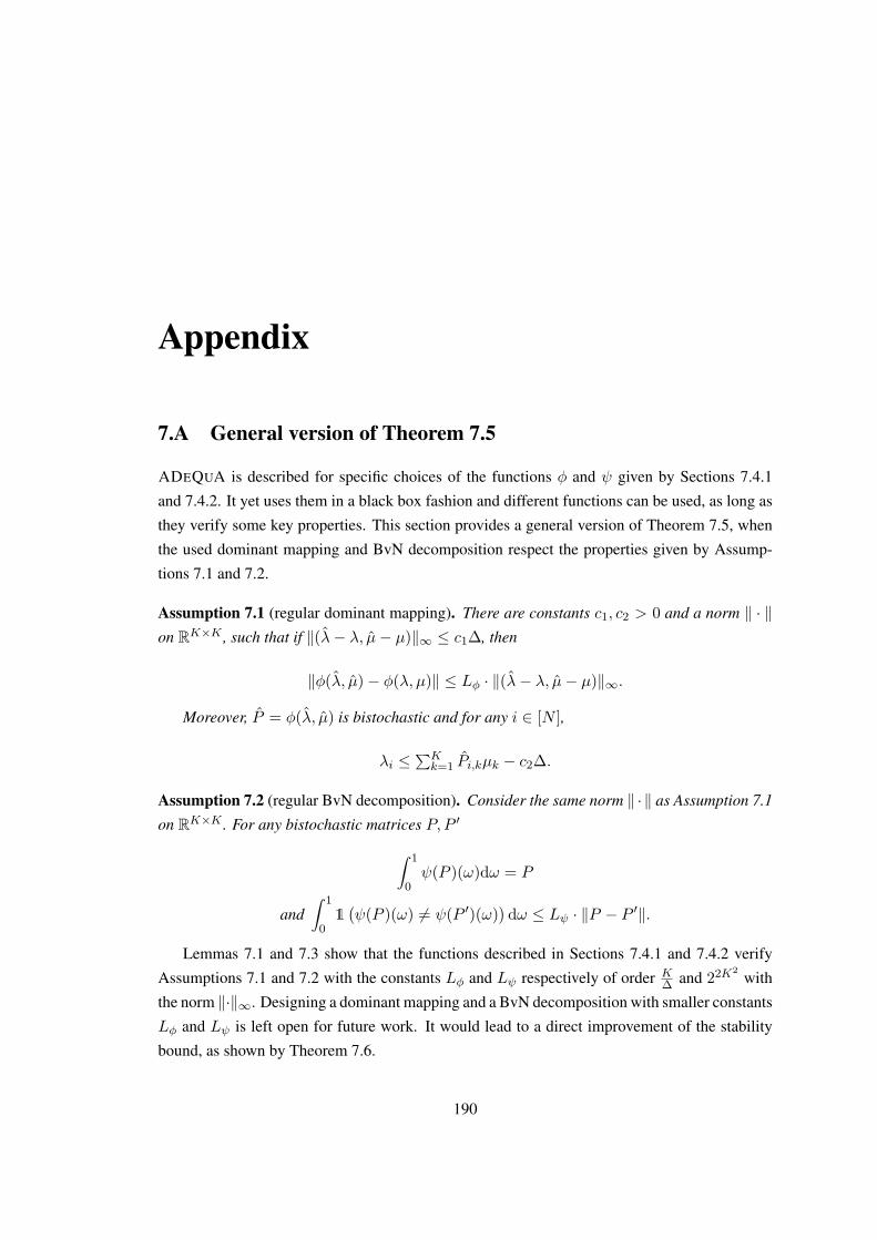
Appendix
7.A General version of Theorem 7.5
ADEQUA is described for specific choices of the functions φ and ψ given by Sections 7.4.1
and 7.4.2. It yet uses them in a black box fashion and different functions can be used, as long as
they verify some key properties. This section provides a general version of Theorem 7.5, when
the used dominant mapping and BvN decomposition respect the properties given by Assump-
tions 7.1 and 7.2.
Assumption 7.1 (regular dominant mapping). There are constants c1, c2 > 0 and a norm ‖ · ‖on RK×K , such that if ‖(λ− λ, µ− µ)‖∞ ≤ c1∆, then
‖φ(λ, µ)− φ(λ, µ)‖ ≤ Lφ · ‖(λ− λ, µ− µ)‖∞.
Moreover, P = φ(λ, µ) is bistochastic and for any i ∈ [N ],
λi ≤∑Kk=1 Pi,kµk − c2∆.
Assumption 7.2 (regular BvN decomposition). Consider the same norm ‖ · ‖ as Assumption 7.1
on RK×K . For any bistochastic matrices P, P ′∫ 1
0ψ(P )(ω)dω = P
and∫ 1
01(ψ(P )(ω) 6= ψ(P ′)(ω)
)dω ≤ Lψ · ‖P − P ′‖.
Lemmas 7.1 and 7.3 show that the functions described in Sections 7.4.1 and 7.4.2 verify
Assumptions 7.1 and 7.2 with the constants Lφ and Lψ respectively of order K∆ and 22K2
with
the norm ‖·‖∞. Designing a dominant mapping and a BvN decomposition with smaller constants
Lφ and Lψ is left open for future work. It would lead to a direct improvement of the stability
bound, as shown by Theorem 7.6.
190
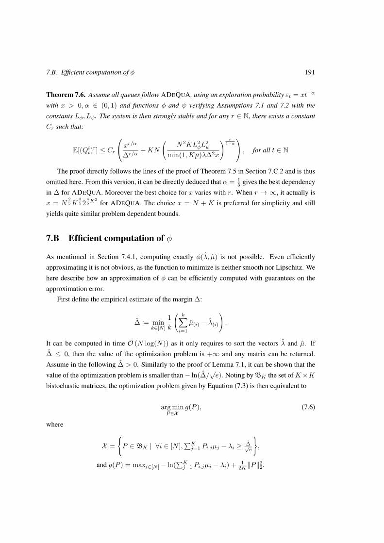
7.B. Efficient computation of φ 191
Theorem 7.6. Assume all queues follow ADEQUA, using an exploration probability εt = xt−α
with x > 0, α ∈ (0, 1) and functions φ and ψ verifying Assumptions 7.1 and 7.2 with the
constants Lφ, Lψ. The system is then strongly stable and for any r ∈ N, there exists a constant
Cr such that:
E[(Qit)r] ≤ Cr
xr/α
∆r/α+KN
(N2KL2
φL2ψ
min(1,Kµ)λ∆2x
) r1−α
, for all t ∈ N
The proof directly follows the lines of the proof of Theorem 7.5 in Section 7.C.2 and is thus
omitted here. From this version, it can be directly deduced that α = 15 gives the best dependency
in ∆ for ADEQUA. Moreover the best choice for x varies with r. When r → ∞, it actually is
x = N25K
35 2
45K
2for ADEQUA. The choice x = N + K is preferred for simplicity and still
yields quite similar problem dependent bounds.
7.B Efficient computation of φ
As mentioned in Section 7.4.1, computing exactly φ(λ, µ) is not possible. Even efficiently
approximating it is not obvious, as the function to minimize is neither smooth nor Lipschitz. We
here describe how an approximation of φ can be efficiently computed with guarantees on the
approximation error.
First define the empirical estimate of the margin ∆:
∆ := mink∈[N ]
1k
(k∑i=1
µ(i) − λ(i)
).
It can be computed in time O (N log(N)) as it only requires to sort the vectors λ and µ. If
∆ ≤ 0, then the value of the optimization problem is +∞ and any matrix can be returned.
Assume in the following ∆ > 0. Similarly to the proof of Lemma 7.1, it can be shown that the
value of the optimization problem is smaller than− ln(∆/√e). Noting by BK the set ofK×K
bistochastic matrices, the optimization problem given by Equation (7.3) is then equivalent to
arg minP∈X
g(P ), (7.6)
where
X =P ∈ BK | ∀i ∈ [N ],
∑Kj=1 Pi,jµj − λi ≥ ∆√
e
,
and g(P ) = maxi∈[N ]− ln(∑Kj=1 Pi,jµj − λi) + 1
2K ‖P‖22.

192 Chapter 7. Decentralized Learning in Online Queuing Systems
Thanks to this new constraint set, the objective function of Equation (7.6) is now (√e
∆ + 1)-
Lipschitz. We can now use classical results for Lipschitz strongly convex minimization to obtain
convergence rates of order 1t for the projected gradient descent algorithm (see e.g., Bubeck,
2014, Theorem 3.9). These results yet assume that the projection on the constraint set can
be exactly computed in a short time. This is not the case here, but it yet can be efficiently
approximated using interior point methods (see e.g., Bubeck, 2014, Section 5.3), which has a
linear convergence rate. If this approximation is good enough, similar convergence guarantees
than with exact projection can be shown similarly to the original proof.
Algorithm 7.4 then describes how to quickly estimate φ(λ, µ), where ΠX returns an ap-
proximation of the orthogonal projection on the set X and ∂g is a sub-gradient of g. It uses
an averaged value of the different iterates, as the last iterate does not have good convergence
guarantees.
Algorithm 7.4: Compute φinput: function g, constraint set X , P 0 ∈ X
1 P, P ← P 0
2 for t = 1, . . . , n do3 P ← ΠX
(P − 2N
(t+1)∂g(P ))
// approximated projection
4 P ← tt+2 P + 2
t+2P
5 end6 return P
In practice, the approximation can even be computed faster by initializing P 0 in Algo-
rithm 7.4 with the solution of the previous round t− 1.
7.C Omitted Proofs
7.C.1 Unstable No-Policy regret system example
Lemma 7.4. Consider the system where the queues play according to the policy described in
Algorithm 7.5 over successive windows of length wk = k2. If α > 1 − dN−d , the system is not
stable.
Proof. Note that the system is equivalent to a system where each queue or pair of queue would
always pick the same server. For simplicity, the analysis deals with that equivalent system.
Also, wlog, we analyse the subsystem with the two first queues and the two first servers. LetBit
i∈[n],t≥1 be the independent random variables indicating the arrival of a packet on queue i
at time t,Siti∈[n],t≥1 be the indicators that server j would clear a packet at iteration ` if one

7.C. Omitted Proofs 193
Algorithm 7.5: Unstable No-policy regret system exampleinput: wk, N , α, λ = (1/N, . . . , 1/N), µ = (2(N − d)/N2, . . . , 2(N − d)/N2)
1 for k = 1, . . . ,∞ do2 for t = 1, . . . , dαwke do3 Queues 2i and 2i+ 1 play server 2i+ t (mod N) // stage 1
4 end5 for t = dαwke+ 1, . . . , wk do6 Queue i plays server i+ t (mod N) // stage 2
7 end8 end
were sent to it. For each queue i ∈ [N ] and t ≥ 0, we have by Chernoff bound
Pr(∣∣∣∣∣∑
t=1Bit − λi`
∣∣∣∣∣ ≥ √` ln(`))≤ 2`2.
The same holds for each queue, thus the probability that this event happens for queue 1 or queue
2 is at most, 4`2 . As it is summable in `, The Borel-Cantelli Lemma implies that, for large enough
`, almost surely, for any i ∈ [2]:
∑`=1
Bit = λi`± O
(√`), (7.7)
where O hides poly-log factors in `
Let Wk =∑ki=1wi. Note that Wk = Θ
(k3) = Θ
(w
3/2k
). Again by Chernoff bound and
Borel-Cantelli, for large enough k, almost surely, for any i ∈ 1, 2:
Wk−1+dαwke∑t=Wk−1
Sit = µiαwk ± O (√wk) ,Wk∑
t=Wk−1+dαwkeSit = µi(1− α)wk ± O (√wk) . (7.8)
Thus, for any large enough k, the total number of packets in both queues at time Wk is
almost surely lower bounded as:
Q1Wk
+Q2Wk≥
Wk∑t=1
(B1t +B2
t )−Wk∑t=1
S1t −
k∑l=1
Wl∑t=Wl−1+dαwle
S2t
(7.9)
≥[ 2N− 2(N − d)
N2 − (1− α)2(N − d)N2
]Wk − O
(W
2/3k
)(7.10)
≥2 [α(N − d)− (N − 2d)]N2 Wk − O
(W
2/3k
)(7.11)
which is a diverging function of Wk. Note that this result also holds for any pair of queues
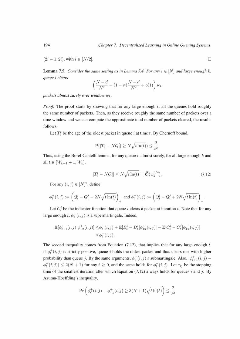
194 Chapter 7. Decentralized Learning in Online Queuing Systems
(2i− 1, 2i), with i ∈ [N/2].
Lemma 7.5. Consider the same setting as in Lemma 7.4. For any i ∈ [N ] and large enough k,
queue i clears (N − dN2 + (1− α)N − d
N2 + o(1))wk
packets almost surely over window wk.
Proof. The proof starts by showing that for any large enough t, all the queues hold roughly
the same number of packets. Then, as they receive roughly the same number of packets over a
time window and we can compute the approximate total number of packets cleared, the results
follows.
Let T ti be the age of the oldest packet in queue i at time t. By Chernoff bound,
P(|T ti −NQti| ≥ N√t ln(t)) ≤ 2
t2.
Thus, using the Borel-Cantelli lemma, for any queue i, almost surely, for all large enough k and
all t ∈ [Wk−1 + 1,Wk],
|T ti −NQti| ≤ N√t ln(t) = O(w3/4
k ). (7.12)
For any (i, j) ∈ [N ]2, define
φ+t (i, j) :=
(Qit −Q
jt − 2N
√t ln(t)
)+
and φ−t (i, j) :=(Qit −Q
jt + 2N
√t ln(t)
)−.
Let Cit be the indicator function that queue i clears a packet at iteration t. Note that for any
large enough t, φ+t (i, j) is a supermartingale. Indeed,
E[φ+t+1(i, j)|φ+
1:t(i, j)] ≤φ+t (i, j) + E[Bi
t −Bjt |φ+
1:t(i, j)]− E[Cit − Cjt |φ+
1:t(i, j)]
≤φ+t (i, j).
The second inequality comes from Equation (7.12), that implies that for any large enough t,
if φ+t (i, j) is strictly positive, queue i holds the oldest packet and thus clears one with higher
probability than queue j. By the same arguments, φ−t (i, j) a submartingale. Also, |φ+t+1(i, j)−
φ+t (i, j)| ≤ 2(N + 1) for any t ≥ 0, and the same holds for φ−t (i, j). Let τij be the stopping
time of the smallest iteration after which Equation (7.12) always holds for queues i and j. By
Azuma-Hoeffding’s inequality,
Pr(φ+` (i, j)− φ+
τij (i, j) ≥ 3(N + 1)√` ln(`)
)≤ 2`2
7.C. Omitted Proofs 195
and
Pr(φ−` (i, j)− φ+
τij (i, j) ≤ −3(N + 1)√` ln(`)
)≤ 2`2.
This, together with a union bound and Borel-Cantelli’s Lemma implies that almost surely,
for any large enough t, for any (i, j) ∈ [N ]2
Qit −Qjt = O
(√t). (7.13)
This with Equation (7.9) implies that for any large enough k, for any i ∈ [N ], almost surely,
QiWk≥ [α(N − d)− (N − 2d)]
N2 Wk − O(W
2/3k
).
This means that for any large enough k, every queue holds at least one packet over the whole
windowwk. This and Equation (7.8) is already enough to show that for any time-windowwk, for
any large enough k, the total number of packets cleared by every couple of queues (2i− 1, 2i),
i ∈ [N/2] is:
2(N − dN2 + (1− α)N − d
N2
)wk + O (√wk) .
During time window wk, according to Equation (7.7), both every queue receives αwk/N +O(w
3/4k
)packets almost surely for any large enough k. Equation (7.13) implies that for any
i ∈ [N/2]Q2i−1Wk−Q2i
Wk= O
(w
3/4k
)and Q2i−1
Wk−1−Q2i
Wk−1 = O(w
3/4k
).
Therefore, over each time-window wk, for any large enough k, each queue clears(N − dN2 + (1− α)N − d
N2 + o(1))wk
packets almost surely.
Lemma 7.6. Consider again the system where the queues play according to the policy described
in Algorithm 7.5 over successive windows of length wk = k2. If α < 1− 1N−1 , the queues have
no policy regret in all but finitely many of the windows.
Wlog, let us consider that queue 1 deviates, and plays at every iteration a server chosen from
the probability distribution p = (p1, ..., pN ), with pi the probability to play server i. To upper
bound the number of packets queue 1 clears over each time window, we can assume it always
has priority over queue 2 and ignore it in the analysis.
Before proving Lemma 7.6, we prove the following technical one.
Lemma 7.7. Consider that a queue deviates from the strategy considered in Lemma 7.6 and
plays at every iteration a server chosen from the probability distribution p = (p1, ..., pN ), with
196 Chapter 7. Decentralized Learning in Online Queuing Systems
pi the probability to play server i. For any large enough k, almost surely, the number of packets
the deviating queue clears of the first stage of the kth window is(12 + 1
N
) 2(N − d)N2 αwk + O
(w
3/4k
).
Proof. The proof starts by showing that for any large enough t, every non-deviating queue holds
approximately the same number of packets.
First note that for any large enough t, Equation (7.12) still holds surely for any queue i. For
any (i, j) ∈ 3, . . . , N2, define
φ+` (i, j) :=
(Qid`Ne −Q
jd`Ne − 4N
√d`Ne ln(d`Ne)
)+
and
φ−` (i, j) :=(Qid`Ne −Q
jd`Ne + 4N
√d`Ne ln(d`Ne)
)−.
For any interval [d`Ne, d(` + 1)Ne] where Equation (7.12) holds for queues 1, i and j, if
φ+` (i, j) is strictly positive, then
E
d(`+1)Ne∑t=d`Ne
Cjt − Cit∣∣∣∣φ+
1:t(i, j)
≤ 0.
Indeed, if φ+` (i, j) is strictly positive and Equation (7.12) holds, queue i holds the oldest packets
throughout the interval. Also, queue i and queue j collide with queue 1 the same number of
times over the interval in expectation, and if at one iteration of the interval, queue 1 holds
an older packet than queue i, it holds an older packet than queue j over the whole interval.
Thus φ+` (i, j) is a submartingale. By the same arguments, φ+
` (i, j) is a supermartingale. Also,
|φ+`+1(i, j) − φ+
` (i, j)| ≤ 4(N + 1)2 and the same holds for φ−` (i, j). Finishing with the same
arguments used to prove Equation (7.13), almost surely, for any (i, j) ∈ 3, . . . , N2,
Qit −Qjt = O
(√t). (7.14)
We now show that for any large enough t, queue 1 can not hold many more packets than the
non-deviating queues. Define
φ+t :=
(Q1t −max
i≥3Qit − 2N
√t ln(t)
)+.
Once again, at every iteration where φ+t is strictly positive and Equation (7.12) holds, queue 1
holds the oldest packet and thus has priority on whichever server it chooses. This implies that
for any large enough t, φ+t is a supermartingale. It also holds that for any t ≥ 0, |φ+
t+1 − φ+t | ≤

7.C. Omitted Proofs 197
2(N + 1). Thus, with the same arguments used to prove Equation (7.13), almost surely,(Q1t −max
i≥3Qit
)+
= O(√
t). (7.15)
With that at hand, we prove that for any large enough k, queue 1 doesn’t get priority often
over the other queues during the first stage of the kth window. For any i ∈ 2, . . . , N/2, pose:
ψi` = 12(Q2i−1d`Ne +Q2i
d`Ne
)−Q1
d`Ne −2(N − d)N3 (d`Ne −Wk−1)
For any ` s.t. d`Ne; d(`+ 1)N − 1e is included in the first phase of a window, we have
d(`+1)Ne−1∑t=d`Ne
E[C1t
∣∣∣∣ψ+1:`(i, j)
]≥d(`+1)Ne−1∑t=d`Ne
E[Sti1queue 1 and only queue 1 picks server i
∣∣∣∣ψ+1:`(i, j)
]
≥ N − dN
+ 2(N − d)N2
as well as
d(`+1)Ne−1∑t=d`Ne
E[1
2(C2it + C2i−1
t
) ∣∣∣∣ψ+1:`(i, j)
]≤d(`+1)Ne−1∑t=d`Ne
E[1
2Sti+t (mod N)
∣∣∣∣ψ+1:`(i, j)
]
≤ N − dN
.
Those two inequalities imply:
E[ψi`+1|ψ+1:`(i, j)] =ψ+
` (i, j) +d(`+1)Ne−1∑t=d`Ne
E[1
2(B2it −B2i−1
t )−B1t
∣∣∣∣ψ+1:`(i, j)
]
−d(`+1)Ne−1∑t=d`Ne
E[1
2(C2it − C2i−1
t )− C1t
∣∣∣∣ψ+1:`(i, j)
]− 2(N − d)
N2
≥ψ+` (i, j).
Thus, for any ` s.t. d`Ne; d(` + 1)N − 1e is included in the first phase of a window, ψi` is
a submartingale. Moreover, for any ` ≥ 0, |ψi`+1 − ψi`| ≤ 3N . Thus, by Azuma-Hoeffding’s
inequality, for any ` s.t.d`Ne; d(`+ 1)N − 1e ⊂ [Wk−1,Wk−1 + αwk],
Pr(ψi` − ψiWk
≤ −6N√`N ln(`N)
)≤ 1
(`N)2 .
Borel-Cantelli’s lemma implies, that for any large enough ` s.t.d`Ne; d(` + 1)N − 1e ⊂

198 Chapter 7. Decentralized Learning in Online Queuing Systems
[Wk−1,Wk−1 + αwk], almost surely:
ψi` ≥ ψiWk− 6N
√`N ln(`N).
This and Equation (7.15) applied at t = Wk, imply that for any large enough k, for any t ∈[Wk−1,Wk−1 + αwk],
12(Q2i−1t +Q2i
t
)≥Q1
d`Ne + 2(N − d)N3 (t−Wk−1) + ψiWk
− O(√t)
≥Q1d`Ne + 2(N − d)
N3 (t−Wk−1)− O(w3/4k ).
This and Equation (7.12) imply that during the first stage of the time window, queue 1 holds
younger packets than any other queues i ≥ 3 after at most O(w3/4k ) iterations.
By Chernoff bound and the Borel-Cantelli lemma again, for any large enough k, almost
surely, the number of packets queue 1 clears during the first stage of the kth window on servers
where it does not collide with other queues is:
Wk−1+αwk∑t=Wk−1+1
N∑i=1
Sti1queue 1 and only queue 1 picks server i = (12 + 1
N)2(N − d)
N2 αwk + O (√wk) .
Since we have shown that for any large enough k, almost surely, queue 1 does not have
priority over the other queues after at most O(w3/4k ) iterations, for any large enough k, almost
surely, the number of packets queue 1 clears of the first stage of the kth window is(12 + 1
N
) 2(N − d)N2 αwk + O
(w
3/4k
).
We are now ready to prove Lemma 7.6.
Proof. By Chernoff bound and the Borel-Cantelli lemma, almost surely for any large enough k,
the number of packets queue 1 clears during the second stage of the window on servers where it
does not collide with other queues is:
Wk−1∑t=Wk−1+αwk
N∑i=1
Sti1queue 1 and only queue 1 picks server i = 4(N − d)N3 (1− α)wk + O (√wk) .
(7.16)

7.C. Omitted Proofs 199
Suppose that during the second stage of the window, queue 1 never gets priority over another
queue. In that case, according to equation Equation (7.16) and Lemma 7.7, for any large enough
k, almost surely, the total number of packets cleared by queue 1 during the time window is(α
2 + 2− αN
) 2(N − d)N2 wk + O(w3/4
k ).
For any large enough k, if α ≤ 1 − 1N−1 this is smaller than the number of packets queue 1
would have cleared had it not deviated, according to Lemma 7.5.
On the other hand, suppose that queue gets priority over some other queue i at some iteration
τ of the second stage of the window. In that case, at that iteration, queue 1 holds the oldest
packets, which, according to Equation (7.12), implies
Qτ1 > Qτi − O(w3/4k )
During the second stage of the window, for any i ≥ 3, γit :=(Qti −Qt1 − 2N
√t ln(t)
)+
is a
supermartingale with bounded increments for any t where Equation (7.12) holds for queues 1and i. Indeed, in that case, if γit is strictly positive, queue i holds an older packet than queue 1,
and thus, whether they collide or not, it has a higher probability to clear a packet than queue 1.
Thus, by Azuma-Hoeffding and the Borel-cantelli lemma again, for any large enough k, almost
surely,
QWki −QWk
1 ≤ Qτi −Qτ1 + O(w3/4k ).
Thus it holds that QWk1 ≥ QWk
i − O(w3/4k ) for any i ≥ 2. This and Equation (7.15) imply that
all the queues clear approximately the same number of packets over those time windows for any
large enough k almost surely. Thus queue 1 clears[(2− α)(N − 2) + (α+ 4− 2α
N)] (N − d)
(N − 1)N2wk + O(w
3/4k
)packets almost surely, which again is smaller than the number of packets it would have cleared
had it not deviated.
Thus, the deviating queue clears almost surely less packets by time window than it would
have had it not deviated on all but finitely many of the time windows, which implies that it has
no policy regret on all but finitely many of the time windows.
200 Chapter 7. Decentralized Learning in Online Queuing Systems
7.C.2 Proofs of Section 7.4
Proof of Lemma 7.1
We want to show that if ‖(λ− λ, µ− µ)‖∞ ≤ c1∆, then
‖φ(λ, µ)− φ(λ, µ)‖2 ≤c2K
∆ ‖(λ− λ, µ− µ)‖∞, (7.17)
with the constants c1, c2 given in Lemma 7.1.
Recall that φ is defined as
φ(λ, µ) = arg minP∈BK
f(P, λ, µ),
where BK is the set of K ×K bistochastic matrices and f is defined as:
f(P, λ, µ) := maxi∈[N ]
− ln(K∑j=1
Pi,jµk − λi) + 12K ‖P‖
22
Let P ∗ and P ∗ be the minimizers of f with the respective parameters (λ, µ) and (λ, µ). They
are uniquely defined as f is 1K strongly convex.
As the property of Lemma 7.1 is symmetric, we can assume without loss of generality that
f(P ∗, λ, µ) ≥ f(P ∗, λ, µ).
Given the definition of ∆, we actually have the bound
− ln(∆) + 12 ≥ f(P ∗, λ, µ) ≥ − ln(∆).
The lower bound holds because the term in the ln is at most ∆ for at least one i. For the
upper bound, some matrix P ensures that the term in the ln is at least ∆ for all i and ‖P‖22 ≤ K.
Similarly for P ∗, it comes:
− ln((1− 2c1)∆) + 12 ≥ f(P ∗, λ, µ) ≥ − ln((1 + 2c1)∆).
As a consequence, it holds for any i ∈ [N ]:
− ln
K∑j=1
P ∗i,jµj − λi
≤ f(P ∗, λ, µ)
≤ − ln((1− 2c1)∆/√e)
K∑j=1
P ∗i,jµj − λi ≥ (1− 2c1)∆/√e.
7.C. Omitted Proofs 201
Note that for any i ∈ [N ],
K∑j=1
P ∗i,jµj − λi ≤K∑j=1
P ∗i,jµj − λi + 2‖(λ− λ, µ− µ)‖∞.
It then yields the second point of Lemma 7.1:
K∑j=1
P ∗i,jµj − λi ≥((1− 2c1)/
√e− 2c1
)∆
Moreover, it comes
− ln
K∑j=1
P ∗i,jµj − λi
≥ − ln
K∑j=1
P ∗i,jµj − λi
− ln(
1 + 2‖(λ− λ, µ− µ)‖∞∑Kj=1 P
∗i,jµj − λi
)
≥ − ln
K∑j=1
P ∗i,jµj − λi
− 2‖(λ− λ, µ− µ)‖∞((1− 2c1)/
√e− 2c1) ∆
Recall that for a 1K -strongly convex function g of global minimum x∗ and any x:
‖x− x∗‖2 ≤ 2K(g(x)− g(x∗))
As a consequence, it comes:
f(P ∗, λ, µ) ≥ f(P ∗, λ, µ)− 2‖(λ− λ, µ− µ)‖∞((1− 2c1)/
√e− 2c1) ∆
≥ f(P ∗, λ, µ)− 2‖(λ− λ, µ− µ)‖∞((1− 2c1)/
√e− 2c1) ∆ + 1
2K ‖P∗ − P ∗‖2.
Equation (7.17) then follows.
Proof of Lemma 7.2
The coefficient Ci,j is replaced by +∞ as soon as the whole weight Pi,j is exhausted. Thanks
to this, the HUNGARIAN algorithm does return a perfect matching with respect to the bipar-
tite graph with edges (i, j) where there remains some weight for Pi,j . Because of this, it can
be shown following the usual proof of Birkhoff algorithm (Birkhoff, 1946) that the sequence
(z[j], P [j]) is indeed of length at most K2 and is a valid decomposition of P .
Now assume that ≺C is a total order. At each iteration j of HUNGARIAN algorithm, denote
202 Chapter 7. Decentralized Learning in Online Queuing Systems
P j = P −∑j−1s=1 z[s]P [s] the remaining weights to attribute.
Let lj be such that P [j] = Plj for any iteration j of HUNGARIAN algorithm.
It can now be shown by induction that
P j = P −lj∑l=1
zl(P )Pl.
where zl(P ) are defined by Equation (7.5). Indeed, by definition
P j+1 = P j − z[j + 1]P [j + 1]
= P j − z[j + 1]Plj+1
The HUNGARIAN algorithm returns the minimal cost matching with respect to the modified
cost matrix C where the coefficients i, k such that P ji,k = 0 are replaced by +∞. Thanks
to this, Plj+1 is the minimal cost permutation matrix Pl (for ≺C) such that P ji,k > 0 for all
(i, k) ∈ supp(Pl).
This means that for any l < lj+1
min(i,k)∈supp(Pl)
(P j)i,k = 0.
Using the induction hypothesis, this implies that zl(P ) = 0 for any lj < l < lj+1. And finally,
this also implies that zlj+1(P ) = z[j + 1].
This finally concludes the proof as P j = 0 after the last iteration.
Proof of Lemma 7.3
For z and z′ the respective decompositions of P and P ′ defined in Lemma 7.2, then
∫ 1
01(ψ(P )(ω) 6= ψ(P ′)(ω)
)dω = Pω∼U(0,1)
(ψ(P )(ω) 6= ψ(P ′)(ω)
).
In the following, note A = ψ(P ) and A′ = ψ(P ′). It comes
∫ 1
01(ψ(P )(ω) 6= ψ(P ′)(ω)
)dω =
K!∑n=1
P(A = Pn and A′ 6= Pn)
= 12
K!∑n=1
P(A = Pn and A′ 6= Pn) + 12
K!∑n=1
P(A′ = Pn and A 6= Pn)
7.C. Omitted Proofs 203
= 12
K!∑n=1
vol
n−1∑j=1
zj(P ),n∑j=1
zj(P )
n−1∑j=1
zj(P ′),n∑j=1
zj(P ′)
,where vol denotes the volume of a set and A B = (A \ B) ∪ (B \ A) is the symmetric
difference of A and B. The last equality comes from the expression of ψ with respect to the
coefficients zj(P ), thanks to Lemma 7.2.
It is easy to show that
vol ([a, b] [c, d]) ≤ (|c− a|+ |d− b|)1 (b > a or c > d) .
The previous equality then leads to
∫ 1
01(ψ(P )(ω) 6= ψ(P ′)(ω)
)dω ≤ 1
2
K!∑n=1
∣∣∣∣∣∣n−1∑j=1
zj(P )− zj(P ′)
∣∣∣∣∣∣+∣∣∣∣∣∣n∑j=1
zj(P )− zj(P ′)
∣∣∣∣∣∣ ·
1(zn(P ) + zn(P ′) > 0
)≤
K!∑n=1
∣∣∣∣∣∣n∑j=1
zj(P )− zj(P ′)
∣∣∣∣∣∣1 (zn(P ) + zn(P ′) > 0).
(7.18)
The last inequality holds because∑kj=1 zj(P )− zj(P ′) is counted twice when zk(P ) + zk(P ′)
is positive: when n = k and for the next n such that the elements are counted in the sum.
Thanks to Lemma 7.2, only 2K2 elements zj(P ) and zj(P ′) are non-zero. Let kn be the
index of the n-th non-zero element of (zs(P )+zs(P ′))1≤s≤K!. Note that zs(P ′) can be non-zero
while zs(P ) is zero (or conversely). Let also
(ikn , jkn) ∈ arg min(i,j)∈supp(Pkn )
Pi,j −∑l<kn
zl(P )1 ((i, j) ∈ supp(Pkn))
(i′kn , j′kn) ∈ arg min
(i,j)∈supp(Pkn )P ′i,j −
∑l<kn
zl(P ′)1 ((i, j) ∈ supp(Pkn))
It then comes, thanks to Lemma 7.2
zkn(P )− zkn(P ′) ≤ Pi′kn,j′kn− P ′i′
kn,j′kn−∑l<kn
(zl(P )− zl(P ′))1((i′kn , j
′kn) ∈ supp(Pkn)
)≤ Pi′
kn,j′kn− P ′i′
kn,j′kn−∑l<n
(zkl(P )− zkl(P′))1
((i′kn , j
′kn) ∈ supp(Pkn)
)
204 Chapter 7. Decentralized Learning in Online Queuing Systems
The second inequality holds, because for l′ 6∈ kl | l < 2K2, the term in the sum is zero by
definition of the sequence kl.
A similar inequality holds for zkn(P ′)− zkn(P ), which leads to
|zkn(P )− zkn(P ′)| ≤ ‖P − P ′‖∞ +∑l<n
|zkl(P )− zkl(P′)|.
By induction, it thus holds
|zkn(P )− zkn(P ′)| ≤ 2n−1‖P − P ′‖∞.
We finally conclude using Equation (7.18)
∫ 1
01(ψ(P )(ω) 6= ψ(P ′)(ω)
)dω ≤
K!∑n=1
∣∣∣∣∣∣n∑j=1
zj(P )− zj(P ′)
∣∣∣∣∣∣1 (zn(P ) + zn(P ′) > 0)
≤∑n=1
∣∣∣∣∣∣kn∑j=1
zj(P )− zj(P ′)
∣∣∣∣∣∣≤∑n=1
∣∣∣∣∣n∑l=1
zkl(P )− zkl(P′)∣∣∣∣∣
≤2K2−1∑n=1
n∑j=1
2j−1‖P − P ′‖∞
≤ 22K2‖P − P ′‖∞.
In the fourth inequality, the last term of the sum is ignored. It is indeed 0 as z and z′ both
sum to 1.
Proof of Theorem 7.5
First recall below a useful version of Chernoff bound.
Lemma 7.8. For any independent variables X1, . . . , Xn in [0, 1] and δ ∈ (0, 1),
P(
n∑i=1
Xi ≤ (1− δ)n∑i=1
E[Xi])≤ e−
δ2∑n
i=1 E[Xi]2 .
We now prove the following concentration lemma.
Lemma 7.9. For any time t ≥ (N +K)5 and ε ∈ (0, 14),
P(|µik(t)− µk| ≥ ε
)≤ 3 exp
(−λi
(t
45 − 1
)ε2)
7.C. Omitted Proofs 205
P(|λij(t)− λj | ≥ ε
)≤ 6 exp
(−λiKµ
t45 − 1145 ε2
).
Proof.
Concentration for µ. Consider agent i in the following and denote by Nk(t) the number of
exploratory pulls of this agent on server k at time t. By definition, the probability to proceed to
an exploratory pull on the server k at round t is at least λi min(t−15 , 1
N+K ). The term λi here
appears as a pull is guaranteed if a packet appeared at the current time step. Yet the number of
exploratory pulls might be much larger in practice as queues should accumulate a large number
of uncleared packets at the beginning.
For t ≥ (N +K)5, it holds:
t∑n=1
min(n−15 ,
1N +K
) =(N+K)5∑n=1
1N +K
+t∑
n=(N+K)5+1n−
15
≥ (N +K)4 +∫ t
(N+K)5x−
15 dx− 1
≥ 14(5t
45 − (N +K)4 − 4
)≥ t
45 − 1.
Lemma 7.8 then gives for Nk(t):
P (Nk(t) ≤ (1− δ)E[Nk(t)]) ≤ exp(−δ
2E[Nk(t)]2
)
P(Nk(t) ≤ (1− δ)λi
(t
45 − 1
))≤ exp
−λiδ2(t
45 − 1
)2
.Which leads for δ = 1
2 to
P(Nk(t) ≤
λi2(t
45 − 1
))≤ exp
(−λi
t45 − 1
8
). (7.19)
The number of exploratory pulls and the observations on the server k are independent.
Thanks to this, Hoeffding’s inequality can be directly used as follows
P(|µik(t)− µk| ≥ ε | Nk(t)
)≤ 2 exp
(−2Nk(t)ε2
).

206 Chapter 7. Decentralized Learning in Online Queuing Systems
Using Equation (7.19) now gives the first concentration inequality for ε ≤ 14 ≤
12√
2 :
P(|µik(t)− µk| ≥ ε
)≤ 2 exp
(−λi
(t
45 − 1
)ε2)
+ exp(−λi
t45 − 1
8
)≤ 3 exp
(−λi
(t
45 − 1
)ε2).
Concentration for λ. Consider agent i in the following. First show a concentration inequal-
ity for µ. Denote by N(t) the total number of exploratory pulls on servers proceeded by player
i at round t, i.e., N(t) =∑Kk=1Nk(t). Similarly to Equation (7.19), it can be shown that
P(N(t) ≤ λiK
t45 − 1
2
)≤ exp
(−λiK
t45 − 1
8
).
Lemma 7.8 then gives for δ ∈ (0, 1):
P (|µ− µ| ≥ δµ) ≤ 2 exp(−λiKδ2µ
t45 − 1
8
)+ exp
(−λiK
t45 − 1
8
)
≤ 3 exp(−λiKδ2µ
t45 − 1
8
).
Note that |µ− µ| ≤ δµ implies | 1µ −1µ| ≤ δ
(1−δ)µ . So this gives the following inequality:
P(∣∣∣∣ 1µ − 1
µ
∣∣∣∣ ≥ δ
(1− δ)µ
)≤ 3 exp
(−λiKδ2µ
t45 − 1
8
). (7.20)
A concentration bound on Sij can be shown similarly for any δ ∈ (0, 1)
P(∣∣∣∣Sij(t)− (1− λj
2 )µ∣∣∣∣ ≥ δµ) ≤ 3 exp
(−λiKδ2µ
t45 − 1
8
). (7.21)
Now recall that the estimate of λj is defined by λj = 2 − 2Sijµ
. We then have the following
identity:
λj − λj = 2( 1µ− 1µ
)Sij + 2µ
((1− λj
2 )µ− Sij).
Since Sj ∈ [0, 1], it yields for ε ≤ 14 and x ∈ (0, 1):
P(∣∣∣λij(t)− λj∣∣∣ ≥ ε) ≤ P
(∣∣∣∣2( 1µ− 1µ
)Sij∣∣∣∣ ≥ xε or
∣∣∣∣ 2µ(
(1− λj2 )µ− Sj
)∣∣∣∣ ≥ (1− x)ε)
7.C. Omitted Proofs 207
≤ P(∣∣∣∣ 1µ − 1
µ
∣∣∣∣ ≥ xε
2Sij| Sij ≤ (1 + 1− x
8 )µ)
+ P(∣∣∣∣Sij(t)− (1− λj
2 )µ∣∣∣∣ ≥ (1− x)µε
2
)
≤ P(∣∣∣∣ 1µ − 1
µ
∣∣∣∣ ≥ δ
(1− δ)µ for δ = 4xε9
)+ P
(∣∣∣∣Sij(t)− (1− λj2 )µ
∣∣∣∣ ≥ (1− x)µε2
)Taking x = 9
17 leads to 4x9 = 1−x
2 and thus, using Equations (7.20) and (7.21):
P(∣∣∣λij(t)− λj∣∣∣ ≥ ε) ≤ 6 exp
(−λiK
( 817
)2µt
45 − 132 ε2
)
≤ 6 exp(−λiKµ
t45 − 1145 ε2
)
In the following, let c1 = 0.1 and c2 = 4(1−2c1)/
√e−2c1 ≈ 14. For a problem instance, let the
good event Et at time t be defined as
Et :=‖(λi − λ, µi − µ)‖∞ ≤
0.1∆2
2c222K2KN, ∀i ∈ [N ]
.
As ∆ is smaller than 1, the right hand term in the definition of Et is smaller than c1∆. Thanks
to Lemmas 7.1 and 7.3, Et then guarantees that any player will collide with another player with
probability at most 0.1∆, i.e., , ∀i ∈ [N ],
Pω∼U(0,1)(∃j ∈ [N ], Ait(ω) 6= Ajt (ω) | Et
)≤ 0.1∆.
Moreover, thanks to Lemma 7.1, under Et,
λi ≤K∑k=1
Pi,kµk −(1− 2c1√
e− 2c1
)∆.
These two last inequalities lead to the following lemma.
Lemma 7.10. For t ≥ 25K5
0.085∆5 , denote byHt the history of observations up to round t. Then
E[Sit | Et,Ht
]≥ λi + 0.1∆.
Proof. This is a direct consequence of the following decomposition:
E[Sit | Et,Ht
]≥
proba to exploit︷ ︸︸ ︷(1− (N +K)t−
15 )
proba to clear︷ ︸︸ ︷Pi,kµk −
collision proba︷ ︸︸ ︷P(∃j ∈ [N ], Ait(ω) 6= Ajt (ω)∃ | Et
)
208 Chapter 7. Decentralized Learning in Online Queuing Systems
≥ (1− (N +K)t−15 )(λi +
(1− 2c1√e− 2c1
)∆− 0.1∆)
≥ (1− (N +K)t−15 )(λi + 0.18∆).
The last inequality is given by c1 = 0.1 and it leads to
E[Sit | Et,Ht
]≥ λi + 0.18∆− (N +K)t−
15 .
For t ≥ 25K5
0.085∆5 , the last term is smaller than 0.08∆, giving Lemma 7.10.
Define the stopping time
τ := mint ≥ 25K5
0.085∆5 | ∀t ≥ s, Es holds
. (7.22)
Lemma 7.11. With probability 1, τ < +∞ and for any integer r ≥ 1,
E[τ r] = O(KN
(N
52K
52 25K2
(min(1,Kµ)λ)54 ∆5
)r),
where the O notation hides constant factors that only depend on r.
Proof. Define for this proof t0 =⌈
25K5
0.085∆5
⌉. By definition, if Et does not hold for t > t0, then
τ ≥ t. As a consequence, for any t > t0 and thanks to Lemma 7.9:
P(τ ≥ t) ≤ P(¬Et)
≤ (3eKN + 6eN2) exp(−ct
45),
where c = c0min(1,Kµ)λ∆4
N2K224K2 for some universal constant c0 ≤ 1. Note that∑∞t=0 P(τ = t) < +∞
by comparison. Borel-Cantelli lemma then implies that τ is finite with probability 1.
We can now bound the moments of τ :
E[τ r] = r
∫ ∞0
tr−1P (τ ≥ t) dt
≤ tr0 + (3eKN + 6eN2)r∫ ∞
0tr−1e−ct
45 dt.
Using the change of variable u = ct45 , it can be shown that∫ ∞
0tr−1e−ct
45 dt = 5
4c− 5r
4 Γ(5r
4
),
7.C. Omitted Proofs 209
where Γ denotes the Gamma function. It finally allows to conclude:
E[τ r] = O(K5r
∆5r +KNc−5r4
)
= O(KN
(N
52K
52 25K2
(min(1,Kµ)λ)54 ∆5
)r).
Let Xt be a random walk biased towards 0 with the following transition probabilities:
P(Xt+1 = Xt + 1) = p, P(Xt+1 = Xt − 1|Xt > 0) = q,
P(Xt+1 = Xt|Xt > 0) = 1− p− q, P(Xt+1 = Xt|Xt = 0) = 1− p,(7.23)
and X0 = 0.
Lemma 7.12. The non-asymptotic moments of the random walk defined by Equation (7.23) are
bounded. For any t > 0, r > 0:
E [(Xt)r] ≤r!
(ln (q/p))r .
Proof : Let π be the stationary distribution of the random walk. It verifies the following
system of equations:π(z) = pπ(z − 1) + qπ(z + 1) + (1− p− q)π(z), ∀z > 0
π(0) = (1− p)π(0) + qπ(1)∑π(z) = 1
which gives:
π(z) = q − pq
(p
q
)z.
Equivalently, π(z) = P(bY c = z) with Y an exponential random variable of parameter ln(q/p).
This gives:
EX∼π [(X)r] ≤ r!(ln (q/p))r .
Let Xt be the random walk with the same transition probabilities as Xt and X0 ∼ π. For
any t > 0, Xt ∼ π. Moreover, for any t > 0, Xt stochasticaly dominates Xt, which terminates
the proof.
Proof of Theorem 7.5. For τ the stopping time defined by Equation (7.22), Lemma 7.11 bounds
its moments as follows

210 Chapter 7. Decentralized Learning in Online Queuing Systems
E[τ r] = O(KN
(N
52K
52 25K2
(min(1,Kµ)λ)54 ∆5
)r).
Let
pi = λi(1− λi − 0.1∆) and qi = (λi + 0.1∆)(1− λi).
Let Xit be the random walk biased towards 0 with parameters pi and qi, with Xi
t = 0 for any
t ≤ 0. According to Lemma 7.10, past time τ , Qit is stochastically dominated by the random
process τ +Xit−τ . Thus, for any t > 0, for any r > 0
E[(Qti
)r] ≤ max(1, 2r−1)
(E[τ r] + E[(Xi
t−τ )r])
= O(KN
(N
52K
52 25K2
(min(1,Kµ)λ)54 ∆5
)r+ 1
ln(qi/pi)r
)
= O(KN
(N
52K
52 25K2
(min(1,Kµ)λ)54 ∆5
)r+ ∆−r
)
= O(KN
(N
52K
52 25K2
(min(1,Kµ)λ)54 ∆5
)r).
Chapter 8
Utility/Privacy Trade-off asRegularized Optimal Transport
Strategic information is valuable either by remaining private (for instance if it is sensitive)or, on the other hand, by being used publicly to increase some utility. These two objectivesare antagonistic and leaking this information by taking full advantage of it might be morerewarding than concealing it. Unlike classical solutions that focus on the first point, we con-sider instead agents that optimize a natural trade-off between both objectives. We formalizethis as an optimization problem where the objective mapping is regularized by the amountof information revealed to the adversary (measured as a divergence between the prior andposterior on the private knowledge). Quite surprisingly, when combined with the entropicregularization, the Sinkhorn loss naturally emerges in the optimization objective, making itefficiently solvable via better adapted optimization schemes. We empirically compare thesedifferent techniques on a toy example and apply them to preserve some privacy in onlinerepeated auctions.
8.1 Introduction . . . . . . . . . . . . . . . . . . . . . . . . . . . . . . . . . . . . 212
8.2 Some Applications . . . . . . . . . . . . . . . . . . . . . . . . . . . . . . . . 214
8.2.1 Online repeated auctions . . . . . . . . . . . . . . . . . . . . . . . . . 214
8.2.2 Learning through external servers . . . . . . . . . . . . . . . . . . . . 215
8.3 Model . . . . . . . . . . . . . . . . . . . . . . . . . . . . . . . . . . . . . . . 216
8.3.1 Toy Example . . . . . . . . . . . . . . . . . . . . . . . . . . . . . . . 216
8.3.2 General model . . . . . . . . . . . . . . . . . . . . . . . . . . . . . . 217
8.4 A convex minimization problem . . . . . . . . . . . . . . . . . . . . . . . . . 218
8.4.1 Discrete type space . . . . . . . . . . . . . . . . . . . . . . . . . . . . 219
8.5 Sinkhorn Loss minimization . . . . . . . . . . . . . . . . . . . . . . . . . . . 222
211
212 Chapter 8. Utility/Privacy Trade-off as Regularized Optimal Transport
8.5.1 Computing Sinkhorn loss . . . . . . . . . . . . . . . . . . . . . . . . . 223
8.6 Minimization schemes . . . . . . . . . . . . . . . . . . . . . . . . . . . . . . 223
8.6.1 Optimization methods . . . . . . . . . . . . . . . . . . . . . . . . . . 224
8.6.2 Different algorithms . . . . . . . . . . . . . . . . . . . . . . . . . . . 226
8.7 Experiments and particular cases . . . . . . . . . . . . . . . . . . . . . . . . . 227
8.7.1 Linear utility cost . . . . . . . . . . . . . . . . . . . . . . . . . . . . . 227
8.7.2 Minimize Sinkhorn loss on the toy example . . . . . . . . . . . . . . . 228
8.7.3 Comparing methods on the toy example . . . . . . . . . . . . . . . . . 229
8.7.4 Utility-privacy in repeated auctions . . . . . . . . . . . . . . . . . . . 230
8.1 Introduction
In many economic mechanisms and strategic games involving different agents, asymmetries of
information (induced by a private type, some knowledge on the hidden state of Nature, etc.) can
and should be leveraged to increase one’s utility. When these interactions between agents are
repeated over time, preserving some asymmetry (i.e., not revealing private information) can be
crucial to guarantee a larger utility in the long run. Indeed, the small short term utility of publicly
using information can be overwhelmed by the long term effect of revealing it (Aumann et al.,
1995).
Informally speaking, an agent should use, and potentially reveal some private information
only if she gets a subsequent utility increase in return. Keeping this information private is no
longer a constraint (as in other classical privacy concepts such as differential privacy Dwork
et al., 2006) but becomes part of the objective, which is then to decide how and when to use
it. For instance, it might happen that revealing everything is optimal or, on the contrary, that a
non-revealing policy is the best one. This is roughly similar to a poker player deciding whether
to bluff or not. In some situations, it might be interesting to focus solely on the utility even if
it implies losing the whole knowledge advantage, while in other situations, the immediate profit
for using this advantage is so small that playing independently of it (or bluffing) is better.
After a rigorous mathematical formulation of this utility vs. privacy trade-off, it appears that
this problem can be recast as a regularized optimal transport minimization. In the specific case
of entropic regularization, this problem has received a lot of interest in the recent years as it
induces a computationally tractable way to approximate an optimal transport distance between
distributions and has thus been used in many applications (Cuturi, 2013). Our work showcases
how the new Privacy Regularized Policy problem benefits in practice from this theory.
8.1. Introduction 213
Private Mechanisms. Differential privacy is the most widely used private learning framework
(Dwork, 2011; Dwork et al., 2006; Reed and Pierce, 2010) and ensures that any single element
of the whole dataset cannot be retrieved from the output of the algorithm. This constraint is often
too strong for economic applications (as illustrated before, it is sometimes optimal to disclose
publicly some private information). f -divergence privacy costs have thus been proposed in
recent literature as a promising alternative (Chaudhuri et al., 2019). These f -divergences, such
as Kullback-Leibler, are also used by economists to measure the cost of information from a
Bayesian perspective, as in the rational inattention literature (Sims, 2003; Matejka and McKay,
2015; Mackowiak and Wiederholt, 2015). It was only recently that this approach has been
considered to measure “privacy losses” in economic mechanisms (Eilat et al., 2019). This model
assumes that the designer of the mechanism has some prior belief on the unobserved and private
information. After observing the action of the player, this belief is updated and the cost of
information corresponds to the KL between the prior and posterior distributions of this private
information.
Optimal privacy preserving strategies with privacy constraints have been recently studied
in this setting under specific conditions (Eilat et al., 2019). Loss of privacy can however be
directly considered as a cost in the overall objective and an optimal strategy reveals information
only if it actually leads to a significant increase in utility. Meanwhile, constrained strategies
systematically reveal as much as allowed by the constraints, without incorporating the additional
cost of this revelation.
Optimal Transport. Finding an appropriate way to compare probability distributions is a ma-
jor challenge in learning theory. Optimal Transport manages to provide powerful tools to com-
pare distributions in metric spaces (Villani, 2008). As a consequence, it has received an increas-
ing interest these past years (Santambrogio, 2015), especially for generative models (Arjovsky et
al., 2017; Genevay et al., 2018; Salimans et al., 2018). However, such powerful distances often
come at the expense of heavy and intractable computations, which might not be suitable to learn-
ing algorithms. It was recently showcased that adding an entropic regularization term enables
fast computations of approximated distances using Sinkhorn algorithm (Sinkhorn, 1967; Cuturi,
2013). Since then, the Sinkhorn loss has also shown promising results for applications such as
generative models (Genevay et al., 2016; Genevay et al., 2018), domain adaptation (Courty et
al., 2014) and supervised learning (Frogner et al., 2015), besides having interesting theoretical
properties (Peyré and Cuturi, 2019; Feydy et al., 2019; Genevay et al., 2019).
Contributions and organization of the chapter. The new framework of Privacy Regularized
Policy is motivated by several applications, presented in Section 8.2 and is formalized in Sec-
214 Chapter 8. Utility/Privacy Trade-off as Regularized Optimal Transport
tion 8.3. This problem is mathematically formulated as some optimization problem (yet even-
tually in an infinite dimensional space), which is convex if the privacy cost is an f -divergence,
see Section 8.4. Also, if the private information space is discrete, this problem admits an op-
timal discrete distribution. The minimization problem then becomes dimensionally finite, but
non-convex.
If the Kullback-Leibler divergence between the prior and the posterior is considered for the
cost of information, the equivalence with a Sinkhorn loss minimization problem is shown in
Section 8.5. Although non-convex, this new problem formulation allows different optimization
techniques developed in Section 8.6 to efficiently compute partially revealing policies. Finally,
with a linear utility cost, the problem is equivalent to the minimization of the difference of
two convex functions. Using the theories of these specific problems, different optimization
methods can be compared, which illustrates the practical aspect of our new model. This is done
in Section 8.7, where we also compute partially revealing strategies for repeated auctions.
8.2 Some Applications
Our model is motivated by different applications described in this section: online repeated auc-
tions and learning models on external servers.
8.2.1 Online repeated auctions
When a website wants to sell an advertisement slot, firms such as Google or Criteo take part in
an auction to buy this slot for one of their customer, a process illustrated in Figure 8.1. As this
interaction happens each time a user lands on the website, this is no longer a one-time auction
problem, but repeated auctions where the seller and/or the competitor might observe not just one
bid, but a distribution of bids. As a consequence, if a firm were bidding truthfully, seller and
other bidders would have access to its true value distribution µ. This has two possible downsides.
First, if the value distribution µwas known to the auctioneer, she could maximize her revenue
at the expense of the bidder utility (Amin et al., 2013; Amin et al., 2014; Feldman et al., 2016;
Golrezaei et al., 2019), for instance with personalized reserve prices. Second, the auctioneer can
sometimes take part in the auction and becomes a direct concurrent of the bidder (this might be
a unique characteristic of online repeated auctions for ads). For instance, Google is both running
some auction platforms and bidding on some ad slots for their client. As a consequence, if the
distribution µ was perfectly known to some concurrent bidder, he could use it in the future, by
bidding more or less aggressively or by trying to conquer new markets.
It is also closely related to online pricing or repeated posted price auctions. When a user
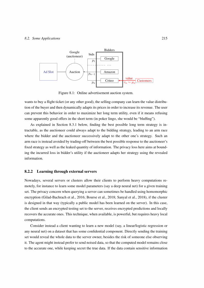
8.2. Some Applications 215
AuctionAd Slot
Google(auctioneer)
Criteo
Amazon
. . .
Biddersbids
p1
pn
pn−1
Customersvn ∼ µnvalue
Figure 8.1: Online advertisement auction system.
wants to buy a flight ticket (or any other good), the selling company can learn the value distribu-
tion of the buyer and then dynamically adapts its prices in order to increase its revenue. The user
can prevent this behavior in order to maximize her long term utility, even if it means refusing
some apparently good offers in the short term (in poker lingo, she would be “bluffing”).
As explained in Section 8.3.1 below, finding the best possible long term strategy is in-
tractable, as the auctioneer could always adapt to the bidding strategy, leading to an arm race
where the bidder and the auctioneer successively adapt to the other one’s strategy. Such an
arm race is instead avoided by trading-off between the best possible response to the auctioneer’s
fixed strategy as well as the leaked quantity of information. The privacy loss here aims at bound-
ing the incurred loss in bidder’s utility if the auctioneer adapts her strategy using the revealed
information.
8.2.2 Learning through external servers
Nowadays, several servers or clusters allow their clients to perform heavy computations re-
motely, for instance to learn some model parameters (say a deep neural net) for a given training
set. The privacy concern when querying a server can sometimes be handled using homomorphic
encryption (Gilad-Bachrach et al., 2016; Bourse et al., 2018; Sanyal et al., 2018), if the cluster
is designed in that way (typically a public model has been learned on the server). In this case,
the client sends an encrypted testing set to the server, receives encrypted predictions and locally
recovers the accurate ones. This technique, when available, is powerful, but requires heavy local
computations.
Consider instead a client wanting to learn a new model (say, a linear/logistic regression or
any neural net) on a dataset that has some confidential component. Directly sending the training
set would reveal the whole data to the server owner, besides the risk of someone else observing
it. The agent might instead prefer to send noised data, so that the computed model remains close
to the accurate one, while keeping secret the true data. If the data contain sensitive information
216 Chapter 8. Utility/Privacy Trade-off as Regularized Optimal Transport
on individuals, then differential privacy is an appropriate solution. However, it is often the case
that the private part is just a single piece of information of the client itself (say, its margin, its
current wealth or its total number of users for instance) that is crucial to the final learned model
but should not be totally revealed to a competitor. Then differential privacy is no longer the
solution, as there is only a single element to protect and/or to use. Indeed, some privacy leakage
is allowed and can lead to much more accurate parameters returned by the server and a higher
utility at the end; the Privacy Regularized Policy aims at computing the best dataset to send to
the server, in order to maximize the utility-privacy trade-off.
8.3 Model
We first introduce a simple toy example in Section 8.3.1 giving insights into the more general
problem, whose formal and general formulation is given in Section 8.3.2.
8.3.1 Toy Example
Suppose an agent is publicly playing an action x ∈ X to minimize a loss x>ck, where ck is some
vector. The true type k ∈ [K] is only known to the agent and drawn from a prior p0. Without
privacy concern, the agent would then solve for every k: minx∈X x>ck.Let us denote by x∗k the optimal solution of that problem. Besides maximizing her reward, the
agent actually wants to protect the secret type k. After observing the action x taken by the agent,
an adversary updates her posterior distribution of the hidden type px.
If the agent were to play deterministically x∗k when her type is k, then the adversary could
infer the true value of k based on the played action. The agent should instead choose her action
randomly to hide her true type to the adversary. Given a type k, the strategy of the agent is then
a probability distribution µk over X and her expected reward is Ex∼µk[x>ck
]. In this case, the
posterior distribution after playing the action x is computed using Bayes rule and if the different
µk have overlapping supports, then the posterior distribution is no longer a Dirac mass, i.e., some
asymmetry of information is maintained.
The agent aims at simultaneously minimizing both the utility loss and the amount of infor-
mation given to the adversary. A common way to measure the latter is given by the Kullback-
Leibler (KL) divergence between the prior and the posterior (Sims, 2003): KL(px, p0) =∑Kk=1 log
(px(k)p0(k)
)px(k), where px(k) = p0(k)µk(x)∑K
l=1 p0(l)µl(x). If the information cost scales in util-
ity with λ > 0, the regularized loss of the agent is then x>ck + λKL(px, p0) instead of x>ck.
8.3. Model 217
Overall, the global objective of the agent is the following minimization:
minµ1,...,µK
K∑k=1
p0(k)Ex∼µk[x>ck + λKL(px, p0)
].
In the limit case λ = 0, the agent follows a totally revealing strategy and deterministically plays
x∗k given k. When λ = ∞, the agent focuses on perfect privacy and looks for the best action
chosen independently of the type: x ⊥⊥ k. It corresponds to a so called non-revealing strategy in
game theory and the best strategy is then to play arg minx x>c[p0] where c[p0] =∑Kk=1 p0(k)ck.
For a positive λ, the behavior of the player will then interpolate between these two extreme
strategies.
This problem is related to repeated games with incomplete information (Aumann et al.,
1995), where players have private information affecting their utility functions. Playing some
action leaks information to the other players, who then change their strategies in consequence.
The goal is then to control the amount of information leaked to the adversaries in order to
maximize one’s own utility. In practice, it can be impossible to compute the best adversarial
strategy, e.g., the player is unaware of how the adversaries would adapt. The utility loss caused
by adversarial actions is then modeled as a function of the amount of revealed information.
8.3.2 General model
We now introduce formally the general model sketched by the previous toy example. The agent
(or player) has a private type y ∈ Y drawn according to a prior p0 whose support can be infinite.
She then chooses an action x ∈ X to maximize her utility, which depends on both her action and
her type. Meanwhile, she wants to hide the true value of her type y. A strategy is thus a mapping
Y → P(X ), where P(X ) denotes the set of distributions over X ; for the sake of conciseness,
we denote by X|Y ∈ P(X )Y such a strategy. In the toy example, this mapping was given by
k 7→ µk. The adversary observes her action x and tries to infer the type of the agent. We assume
a perfect adversary, i.e., she can compute the exact posterior distribution px.
Let c(x, y) be the utility loss for playing x ∈ X with the type y ∈ Y . The cost of information
is cpriv(X,Y ) where (X,Y ) is the joint distribution of the action and the type. In the toy example
given in Section 8.3.1, the utility cost was given by c(x, k) = x>ck and the privacy cost was the
expected KL divergence between px and p0. The previous frameworks aimed at minimizing the
utility loss with a privacy cost below some threshold ε > 0, i.e., minimize E(x,y)∼(X,Y )[c(x, y)
]such that cpriv(X,Y ) ≤ ε. Here, this privacy loss has some utility scaling with λ > 0, which
can be seen as the value of information. The final objective of the agent is then to minimize the
218 Chapter 8. Utility/Privacy Trade-off as Regularized Optimal Transport
following loss:
infX|Y ∈P(X )Y
E(x,y)∼(X,Y )[c(x, y)
]+ λ cpriv(X,Y ). (8.1)
As mentioned above, the cost of information is here defined as a measure between the posterior
px and the prior distribution p0 of the type, i.e., cpriv(X,Y ) = Ex∼XD(px, p0) for some function
D1. In the toy example of Section 8.3.1, D(px, p0) = KL(px, p0), which is a classical cost of
information in economics.
For a distribution γ ∈ P(X ×Y), we denote by π1#γ (resp. π2#γ) the marginal distribution
of X (resp. Y ): π1#γ(A) = γ(A × Y) and π2#γ(B) = γ(X × B). In order to have a simpler
formulation of the problem, we remark that instead of defining a strategy by the conditional
distribution X|Y , it is equivalent to see it as a joint distribution γ of (X,Y ) with a marginal
over the type equal to the prior: π2#γ = p0. The remaining of the chapter focuses on the
problem below, which we call Privacy Regularized Policy. With the privacy cost defined as
above, the minimization problem (8.1) is equivalent to
infγ∈P(X×Y)π2#γ=p0
∫X×Y
[c(x, y) + λD(px, p0)] dγ(x, y). (PRP)
8.4 A convex minimization problem
In this section, we study some theoretical properties of the Problem (PRP). We first recall the
definition of an f -divergence.
Definition 8.1. D is an f -divergence if for all distributions P,Q such that P is absolutely
continuous w.r.t. Q, D(P,Q) =∫Y f
(dP (y)dQ(y)
)dQ(y) where f is a convex function defined on
R∗+ with f(1) = 0.
The set of f -divergences includes common divergences such as the Kullback-Leibler diver-
gence (t log(t)), the reverse Kullback-Leibler (− log(t)) or the Total Variation distance (0.5|t−1|).
Also, the min-entropy defined by D(P,Q) = log (ess sup dP/dQ) is widely used for pri-
vacy (Tóth et al., 2004; Smith, 2009). It corresponds to the limit of the Renyi divergence
ln(∑n
i=1 pαi q
1−αi
)/(α − 1), when α → +∞ (Rényi, 1961; Mironov, 2017). Although it is
not an f -divergence, the Renyi divergence derives from the f -divergence associated to the con-
vex function t 7→ (tα − 1)/(α − 1). f -divergence costs have been recently considered in the
computer science literature in a non-Bayesian case and then present the good properties of con-
vexity, composition and post-processing invariance (Chaudhuri et al., 2019).1We here favor ex-ante costs as they suggest that the value of information can be heterogeneous among types.
8.4. A convex minimization problem 219
In the remaining of this chapter, D is an f -divergence. (PRP) then becomes a convex mini-
mization problem.
Theorem 8.1. If D is an f -divergence, (PRP) is a convex problem in γ ∈ P(X×Y)2.
Proof. The constraint set is obviously convex. The first part of the integral is linear in γ. It thus
remains to show that the privacy loss is also convex in γ. As D is an f -divergence, the privacy
cost iscpriv(γ) :=
∫X×Y
D (px, p0) dγ(x, y)
=∫X
∫Yf( dγ(x, y)
dγ1(x)dp0(y))dp0(y)dγ1(x),
where γ1 = π1#γ. For t ∈ (0, 1) and two distributions γ and µ, we can define the convex
combination ν = tγ + (1 − t)µ. By linearity of the projection π1, ν1 = tγ1 + (1 − t)µ1.
The convexity of cpriv actually results from the convexity of the perspective of f defined by
g(x1, x2) = x2f(x1/x2) (Boyd and Vandenberghe, 2004). It indeed implies
f( dν
dν1dp0
)dν1 ≤ tf
( dγdγ1dp0
)dγ1 + (1− t)f
( dµdµ1dp0
)dµ1.
The result then directly follows when summing over X × Y .
AlthoughP(X×Y) has generally an infinite dimension, it is dimensionally finite if both sets
X and Y are discrete. A minimum can then be found using classical optimization methods. In
the case of bounded low dimensional spaces X and Y , they can be approximated by finite grids.
However, the size of the grid grows exponentially with the dimension and another approach is
needed for large dimensions of X and Y .
8.4.1 Discrete type space
We assume here that X is an infinite action space and Y is of cardinality K (or equivalently,
p0 is a discrete prior of size K), so that p0 =∑Kk=1 p
k0δyk . For a fixed joint distribution γ, let
the measure µk be defined for any A ⊂ X by µk(A) = γ(A × yk) and µ =∑Kk=1 µk =
π1#γ. The function pk(x) = dµk(x)dµ(x) , defined over the support of µ by absolute continuity, is
the posterior probability of having the type k when playing x. The tuple (µ, (pk)k) exactly
2It is convex in a usual sense and not geodesically here.
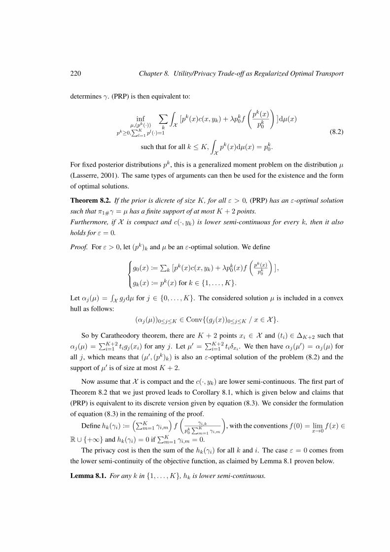
220 Chapter 8. Utility/Privacy Trade-off as Regularized Optimal Transport
determines γ. (PRP) is then equivalent to:
infµ,(pk(·))
pk≥0,∑K
l=1 pl(·)=1
∑k
∫X
[pk(x)c(x, yk) + λpk0f
(pk(x)pk0
) ]dµ(x)
such that for all k ≤ K,∫Xpk(x)dµ(x) = pk0.
(8.2)
For fixed posterior distributions pk, this is a generalized moment problem on the distribution µ
(Lasserre, 2001). The same types of arguments can then be used for the existence and the form
of optimal solutions.
Theorem 8.2. If the prior is dicrete of size K, for all ε > 0, (PRP) has an ε-optimal solution
such that π1#γ = µ has a finite support of at most K + 2 points.
Furthermore, if X is compact and c(·, yk) is lower semi-continuous for every k, then it also
holds for ε = 0.
Proof. For ε > 0, let (pk)k and µ be an ε-optimal solution. We defineg0(x) :=
∑k
[pk(x)c(x, yk) + λpk0(x)f
(pk(x)pk0
) ],
gk(x) := pk(x) for k ∈ 1, . . . ,K.
Let αj(µ) =∫X gjdµ for j ∈ 0, . . . ,K. The considered solution µ is included in a convex
hull as follows:
(αj(µ))0≤j≤K ∈ Conv(gj(x))0≤j≤K / x ∈ X.
So by Caratheodory theorem, there are K + 2 points xi ∈ X and (ti) ∈ ∆K+2 such that
αj(µ) =∑K+2i=1 tigj(xi) for any j. Let µ′ =
∑K+2i=1 tiδxi . We then have αj(µ′) = αj(µ) for
all j, which means that (µ′, (pk)k) is also an ε-optimal solution of the problem (8.2) and the
support of µ′ is of size at most K + 2.
Now assume that X is compact and the c(·, yk) are lower semi-continuous. The first part of
Theorem 8.2 that we just proved leads to Corollary 8.1, which is given below and claims that
(PRP) is equivalent to its discrete version given by equation (8.3). We consider the formulation
of equation (8.3) in the remaining of the proof.
Define hk(γi) :=(∑K
m=1 γi,m)f
(γi,k
pk0∑K
m=1 γi,m
), with the conventions f(0) = lim
x→0f(x) ∈
R ∪ +∞ and hk(γi) = 0 if∑Km=1 γi,m = 0.
The privacy cost is then the sum of the hk(γi) for all k and i. The case ε = 0 comes from
the lower semi-continuity of the objective function, as claimed by Lemma 8.1 proven below.
Lemma 8.1. For any k in 1, . . . ,K, hk is lower semi-continuous.
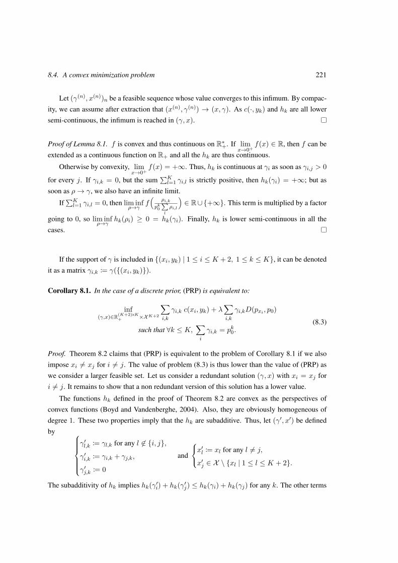
8.4. A convex minimization problem 221
Let (γ(n), x(n))n be a feasible sequence whose value converges to this infimum. By compac-
ity, we can assume after extraction that (x(n), γ(n)) → (x, γ). As c(·, yk) and hk are all lower
semi-continuous, the infimum is reached in (γ, x).
Proof of Lemma 8.1. f is convex and thus continuous on R∗+. If limx→0+
f(x) ∈ R, then f can be
extended as a continuous function on R+ and all the hk are thus continuous.
Otherwise by convexity, limx→0+
f(x) = +∞. Thus, hk is continuous at γi as soon as γi,j > 0
for every j. If γi,k = 0, but the sum∑Kl=1 γi,l is strictly positive, then hk(γi) = +∞; but as
soon as ρ→ γ, we also have an infinite limit.
If∑Kl=1 γi,l = 0, then lim inf
ρ→γf(
ρi,kpk0∑l
ρi,l
)∈ R∪+∞. This term is multiplied by a factor
going to 0, so lim infρ→γ
hk(ρi) ≥ 0 = hk(γi). Finally, hk is lower semi-continuous in all the
cases.
If the support of γ is included in (xi, yk) | 1 ≤ i ≤ K + 2, 1 ≤ k ≤ K, it can be denoted
it as a matrix γi,k := γ((xi, yk)).
Corollary 8.1. In the case of a discrete prior, (PRP) is equivalent to:
inf(γ,x)∈R(K+2)×K
+ ×XK+2
∑i,k
γi,k c(xi, yk) + λ∑i,k
γi,kD(pxi , p0)
such that ∀k ≤ K,∑i
γi,k = pk0.(8.3)
Proof. Theorem 8.2 claims that (PRP) is equivalent to the problem of Corollary 8.1 if we also
impose xi 6= xj for i 6= j. The value of problem (8.3) is thus lower than the value of (PRP) as
we consider a larger feasible set. Let us consider a redundant solution (γ, x) with xi = xj for
i 6= j. It remains to show that a non redundant version of this solution has a lower value.
The functions hk defined in the proof of Theorem 8.2 are convex as the perspectives of
convex functions (Boyd and Vandenberghe, 2004). Also, they are obviously homogeneous of
degree 1. These two properties imply that the hk are subadditive. Thus, let (γ′, x′) be defined
by γ′l,k := γl,k for any l 6∈ i, j,
γ′i,k := γi,k + γj,k,
γ′j,k := 0
and
x′l := xl for any l 6= j,
x′j ∈ X \ xl | 1 ≤ l ≤ K + 2.
The subadditivity of hk implies hk(γ′i) + hk(γ′j) ≤ hk(γi) + hk(γj) for any k. The other terms
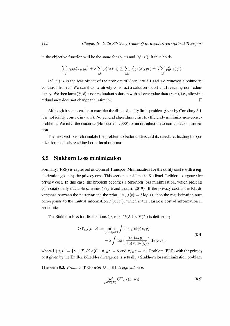
222 Chapter 8. Utility/Privacy Trade-off as Regularized Optimal Transport
in the objective function will be the same for (γ, x) and (γ′, x′). It thus holds
∑i,k
γi,kc(xi, yk) + λ∑i,k
pk0hk(γi) ≥∑i,k
γ′i,kc(x′i, yk) + λ∑i,k
pk0hk(γ′i).
(γ′, x′) is in the feasible set of the problem of Corollary 8.1 and we removed a redundant
condition from x. We can thus iteratively construct a solution (γ, x) until reaching non redun-
dancy. We then have (γ, x) a non redundant solution with a lower value than (γ, x), i.e., allowing
redundancy does not change the infimum.
Although it seems easier to consider the dimensionally finite problem given by Corollary 8.1,
it is not jointly convex in (γ, x). No general algorithms exist to efficiently minimize non-convex
problems. We refer the reader to (Horst et al., 2000) for an introduction to non-convex optimiza-
tion.
The next sections reformulate the problem to better understand its structure, leading to opti-
mization methods reaching better local minima.
8.5 Sinkhorn Loss minimization
Formally, (PRP) is expressed as Optimal Transport Minimization for the utility cost c with a reg-
ularization given by the privacy cost. This section considers the Kullback-Leibler divergence for
privacy cost. In this case, the problem becomes a Sinkhorn loss minimization, which presents
computationally tractable schemes (Peyré and Cuturi, 2019). If the privacy cost is the KL di-
vergence between the posterior and the prior, i.e., f(t) = t log(t), then the regularization term
corresponds to the mutual information I(X;Y ), which is the classical cost of information in
economics.
The Sinkhorn loss for distributions (µ, ν) ∈ P(X )× P(Y) is defined by
OTc,λ(µ, ν) := minγ∈Π(µ,ν)
∫c(x, y)dγ(x, y)
+ λ
∫log
( dγ(x, y)dµ(x)dν(y)
)dγ(x, y),
(8.4)
where Π(µ, ν) = γ ∈ P(X ×Y) | π1#γ = µ and π2#γ = ν. Problem (PRP) with the privacy
cost given by the Kullback-Leibler divergence is actually a Sinkhorn loss minimization problem.
Theorem 8.3. Problem (PRP) with D = KL is equivalent to
infµ∈P(X )
OTc,λ(µ, p0). (8.5)
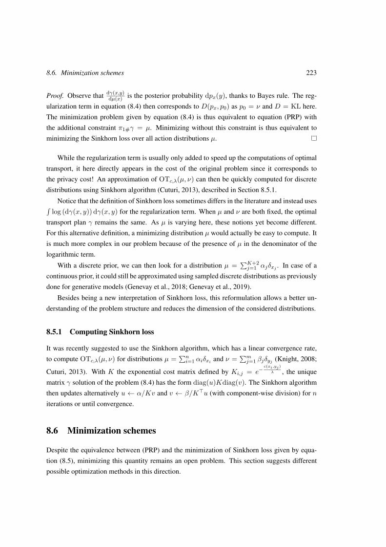
8.6. Minimization schemes 223
Proof. Observe that dγ(x,y)dµ(x) is the posterior probability dpx(y), thanks to Bayes rule. The reg-
ularization term in equation (8.4) then corresponds to D(px, p0) as p0 = ν and D = KL here.
The minimization problem given by equation (8.4) is thus equivalent to equation (PRP) with
the additional constraint π1#γ = µ. Minimizing without this constraint is thus equivalent to
minimizing the Sinkhorn loss over all action distributions µ.
While the regularization term is usually only added to speed up the computations of optimal
transport, it here directly appears in the cost of the original problem since it corresponds to
the privacy cost! An approximation of OTc,λ(µ, ν) can then be quickly computed for discrete
distributions using Sinkhorn algorithm (Cuturi, 2013), described in Section 8.5.1.
Notice that the definition of Sinkhorn loss sometimes differs in the literature and instead uses∫log (dγ(x, y)) dγ(x, y) for the regularization term. When µ and ν are both fixed, the optimal
transport plan γ remains the same. As µ is varying here, these notions yet become different.
For this alternative definition, a minimizing distribution µ would actually be easy to compute. It
is much more complex in our problem because of the presence of µ in the denominator of the
logarithmic term.
With a discrete prior, we can then look for a distribution µ =∑K+2j=1 αjδxj . In case of a
continuous prior, it could still be approximated using sampled discrete distributions as previously
done for generative models (Genevay et al., 2018; Genevay et al., 2019).
Besides being a new interpretation of Sinkhorn loss, this reformulation allows a better un-
derstanding of the problem structure and reduces the dimension of the considered distributions.
8.5.1 Computing Sinkhorn loss
It was recently suggested to use the Sinkhorn algorithm, which has a linear convergence rate,
to compute OTc,λ(µ, ν) for distributions µ =∑ni=1 αiδxi and ν =
∑mj=1 βjδyj (Knight, 2008;
Cuturi, 2013). With K the exponential cost matrix defined by Ki,j = e−c(xi,yj)
λ , the unique
matrix γ solution of the problem (8.4) has the form diag(u)Kdiag(v). The Sinkhorn algorithm
then updates alternatively u ← α/Kv and v ← β/K>u (with component-wise division) for n
iterations or until convergence.
8.6 Minimization schemes
Despite the equivalence between (PRP) and the minimization of Sinkhorn loss given by equa-
tion (8.5), minimizing this quantity remains an open problem. This section suggests different
possible optimization methods in this direction.
224 Chapter 8. Utility/Privacy Trade-off as Regularized Optimal Transport
8.6.1 Optimization methods
Convex minimization over a distribution set. Problems (PRP) and (8.5) are both of the form
minµ∈P(X )
J(µ), (8.6)
with J convex. Although solving such a problem is unknown in general, some methods are
possible in specific cases (see e.g., Chizat and Bach, 2018, for a short overview).
For polynomial costs, this problem can be solved using generalized moment approaches
(Lasserre, 2001), but the complexity explodes with the degree of the polynomial.
P(X ) is the convex hull of Dirac distributions on X , so Frank-Wolfe algorithm might be
a good choice (Jaggi, 2013), especially to guarantee sparsity of the returned distribution using
away-steps technique (Guélat and Marcotte, 1986; Clarkson, 2010). Unfortunately, the Franke-
Wolfe algorithm requires at each step to solve a subproblem, which is here equivalent to
arg maxx∈X
∑y∈Y
p0(y) exp(g(y)− c(x, y)
ε
),
where g depends on the previous optimization step. This problem is computationally intractable
for most cost functions, making Frank-Wolfe methods unadapted to our problem.
Non-convex minimization. Minimizing over the set of distributions remains solved only for
specific cases. The most common approach instead approximates problem (8.6) by discretizing
it as
minx∈Xmα∈∆m
J
(m∑i=1
αiδxi
). (8.7)
Although this dimensionally finite problem is not convex, recent literature has shown the
absence of spurious local minima for a large number of particles m (over-parameterization).
These results yet hold only under restrictive conditions on the loss function and problem struc-
ture (Li and Yuan, 2017; Soudry and Hoffer, 2017; Soltanolkotabi et al., 2018; Venturi et al.,
2018; Chizat and Bach, 2018), which are adapted to optimization with neural networks. None
of these conditions are satisfied here, making the benefit from over-parameterization uncertain.
The empirical results in Section 8.7.2 yet suggest that such a phenomenon might also hold in
our setting.
In general, reaching global optimality in non-convex minimization is intractable (Hendrix
and Boglárka, 2010; Sergeyev et al., 2013), so we only aim at computing local minima. In
practice, RMSProp and ADAM are often considered as the best algorithms in such cases, as
they tend to avoid bad local minima thanks to the use of specific momentums (Hinton et al.,
8.6. Minimization schemes 225
2012; Kingma and Ba, 2014). They yet remain little understood in theory (Reddi et al., 2019;
Zou et al., 2019).
Minimax formulation. Note that the dual formulation (Peyré and Cuturi, 2019, Proposition
4.4) of Equation (8.4) allows the following formulation of the optimization problem (8.5):
minµ∈P(X )
maxf∈C(X )g∈C(Y)
⟨µ, f
⟩+⟨p0, g
⟩− λ
⟨µ⊗ p0, exp ((f ⊕ g − c)/λ)
⟩, (8.8)
where⟨µ, f
⟩:=∫X f(x)dµ(x) for a distribution µ and a continuous function f on X , µ⊗ p0 is
the product distribution and f ⊕g(x, y) = f(x)+g(y). This corresponds to a minimax problem
of the form minx maxy ψ(x, y) where ψ(·, y) is convex for any y and ψ(x, ·) is concave for any
x. Such problems appear in many applications and have been extensively studied. We refer to
(Nedic and Ozdaglar, 2009; Chambolle and Pock, 2016; Thekumparampil et al., 2019; Lin et al.,
2020) for detailed surveys on the topic.
As we are considering the discretized problem (8.7), we are actually in the nonconvex-
concave setting where ψ is nonconvex on its first variable and concave on its second. Algorithms
with theoretical convergence rates to local minima have been studied in this specific setting
(Rafique et al., 2018; Lin et al., 2019; Nouiehed et al., 2019; Thekumparampil et al., 2019;
Lu et al., 2020; Ostrovskii et al., 2020; Lin et al., 2020). Most of them alternate (accelerated)
gradient descent on x and gradient ascent on y, while considering a regularized version ψε of ψ.
Their interests are mostly theoretical as ADAM and RMSProp on the first coordinate instead
of gradient descent should converge to better local minima in practice, similarly to nonconvex
minimization. In practice, they still provide good heuristics as shown in Section 8.7.2.
On minimizing Sinkhorn divergence. Ballu et al. (2020) recently proposed a method to solve
the minimization problem (8.5). Unfortunately, they consider discrete distributions and focus on
reducing the dependency in the size of their supports. More importantly, this method adds a
regularization term ηKL(µ, β) for some reference measure β and requires this regularizer to be
more significant than the one originally in the Sinkhorn loss, i.e., η ≥ λ. While this does not
add any trouble when considering regimes where both are close to 0, we here consider fixed λ,
potentially far from 0 as explained in Section 8.5. The scaling factor η thus cannot be negligible,
making this method unadapted to our case.
226 Chapter 8. Utility/Privacy Trade-off as Regularized Optimal Transport
8.6.2 Different algorithms
Using these previous formulations, we propose several algorithms to solve the optimization
problem (8.5), which are compared experimentally in Section 8.7.2. As explained above, we
consider the discrete but non-convex formulation:
minx∈Xmα∈∆m
OTc,λ
(m∑i=1
αiδxi , p0
). (8.9)
We first consider ADAM and RMSProp algorithms for this problem. Note that the gradient of
the Sinkhorn loss (Feydy et al., 2019) is given by∇OTc,λ(µ, ν) = (f, g), where f and g are the
solutions of the dual problem given by equation (8.8), i.e., (f, g) = λ(ln(u), ln(v)) where u and
v are the vectors computed by the Sinkhorn algorithm presented in Section 8.5.1. The gradient of
OTc,λ can then only be approximated, as it is the solution of an optimization problem. Luckily,
first order optimization methods can still be used with inexact gradients (Devolder et al., 2014).
Two approximations of the gradient are possible.
Analytic Differentiation: ∇OTc,λ(µ, ν) is approximated by (f (n), g(n)), which are the dual
variables obtained after n iterations of the Sinkhorn algorithm.
Automatic Differentiation: the gradient is computed via the chain rule over the successive op-
erations processed during the Sinkhorn algorithm.
These two methods have been recently compared by Ablin et al. (2020) and showed to roughly
perform similarly for the same computation time.
For each optimization step, the gradient∇OTc,λ is approximated by computing (u(k+1)t , v
(k+1)t )←
(α/Kv(k)t , β/K>u
(k+1)t ) for n iterates. However, if the distribution µt did not significantly
change since the last step, the gradient does not change too much as well. Instead of starting the
Sinkhorn algorithm from scratch (u(0)t = 111), we instead want to use the last optimization step
(u(0)t = u
(n)t−1) to converge faster. Note that this technique, which we call warm restart, cannot
be coupled with automatic differentiation as it would require nt backpropagation operations for
the optimization step t.
The iteration step (u, v)← (α/Kv, β/K>u) actually corresponds to a gradient ascent step
on (f, g) in the minimax formulation given by equation (8.8). The warm restart technique then
just corresponds to alternating optimization steps between the primal and dual variables, which
is classical in minimax optimization.
To summarize, here are the different features of the optimization scheme to compare in
Section 8.7.2.
8.7. Experiments and particular cases 227
Optimizer: the general used algorithm, i.e., ADAM, RMSProp or accelerated gradient descent
(AGD).
Differentiation: whether we use automatic or analytic differentiation.
Warm restart: whether we use the warm restart technique, which is only compatible with an-
alytic differentiation.
8.7 Experiments and particular cases
In this section, the case of linear utility cost is first considered and shown to have relations with
DC programming. The performances of different optimization schemes are then compared on a
simple example. Simulations based on the Sinkhorn scheme are then run for the real problem
of online repeated auctions. The code is publicly available at github.com/eboursier/
regularized_private_learning.
8.7.1 Linear utility cost
Section 8.4 described a general optimization scheme for (PRP) with a discrete type prior. Its
objective is to find local minima, for a dimensionally finite, non-convex problem, using classical
algorithms (Wright, 2015). However in some particular cases, better schemes are possible as
claimed in Sections 8.5 and 8.6 for the particular case of entropic regularization. In the case
of a linear utility with any privacy cost, it is related to DC programming (Horst et al., 2000).
A standard DC program is of the form minx∈X f(x) − g(x), where both f and g are convex
functions. Specific optimization schemes are then possible (Tao and An, 1997; Horst and Thoai,
1999; Horst et al., 2000). In the case of linear utility costs over a hyperrectangle, (PRP) can be
reformulated as a DC program stated in Theorem 8.4.
Theorem 8.4. IfX =d∏l=1
[al, bl] and c(x, y) = x>y, define φ(y)l := (bl−al)yl/2 and hk(γi) :=(∑Km=1 γi,m
)f( γi,k
pk0∑K
m=1 γi,m
). Then (PRP) is equivalent to the following DC program:
minγ∈R(K+2)×K
+
λ∑i,k
pk0hk(γi)−K+2∑i=1
∥∥∥∥∥K∑k=1
γi,kφ(yk)∥∥∥∥∥
1
,
such that for all k ≤ K,K+2∑i=1
γi,k = pk0.
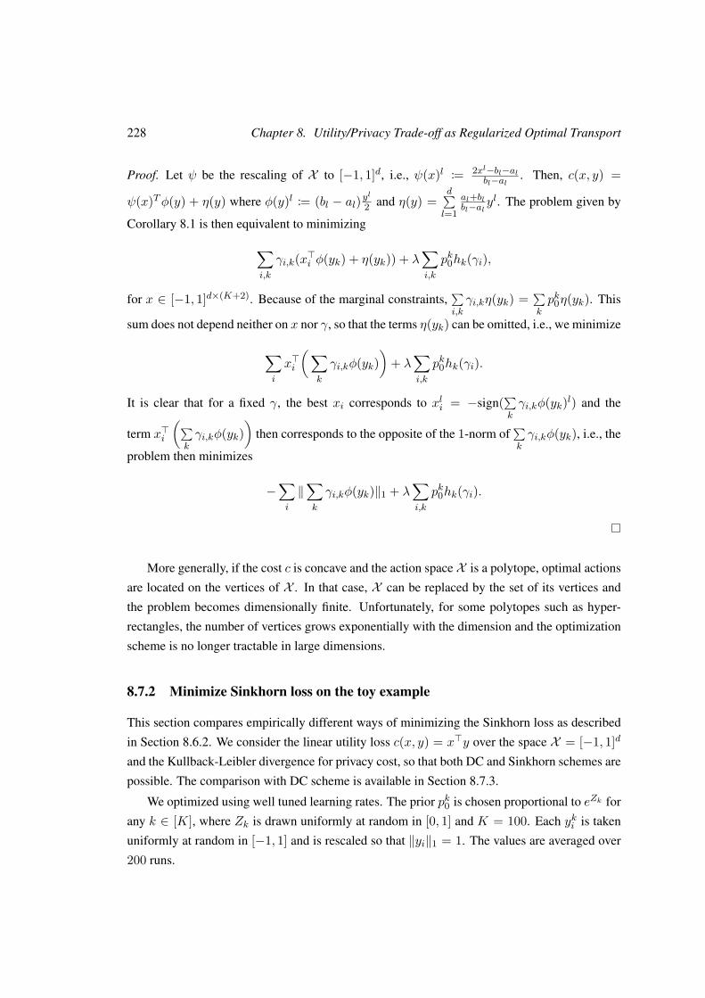
228 Chapter 8. Utility/Privacy Trade-off as Regularized Optimal Transport
Proof. Let ψ be the rescaling of X to [−1, 1]d, i.e., ψ(x)l := 2xl−bl−albl−al . Then, c(x, y) =
ψ(x)Tφ(y) + η(y) where φ(y)l := (bl − al)yl
2 and η(y) =d∑l=1
al+blbl−al y
l. The problem given by
Corollary 8.1 is then equivalent to minimizing
∑i,k
γi,k(x>i φ(yk) + η(yk)) + λ∑i,k
pk0hk(γi),
for x ∈ [−1, 1]d×(K+2). Because of the marginal constraints,∑i,kγi,kη(yk) =
∑kpk0η(yk). This
sum does not depend neither on x nor γ, so that the terms η(yk) can be omitted, i.e., we minimize
∑i
x>i
(∑k
γi,kφ(yk))
+ λ∑i,k
pk0hk(γi).
It is clear that for a fixed γ, the best xi corresponds to xli = −sign(∑kγi,kφ(yk)l) and the
term x>i
(∑kγi,kφ(yk)
)then corresponds to the opposite of the 1-norm of
∑kγi,kφ(yk), i.e., the
problem then minimizes
−∑i
‖∑k
γi,kφ(yk)‖1 + λ∑i,k
pk0hk(γi).
More generally, if the cost c is concave and the action space X is a polytope, optimal actions
are located on the vertices of X . In that case, X can be replaced by the set of its vertices and
the problem becomes dimensionally finite. Unfortunately, for some polytopes such as hyper-
rectangles, the number of vertices grows exponentially with the dimension and the optimization
scheme is no longer tractable in large dimensions.
8.7.2 Minimize Sinkhorn loss on the toy example
This section compares empirically different ways of minimizing the Sinkhorn loss as described
in Section 8.6.2. We consider the linear utility loss c(x, y) = x>y over the space X = [−1, 1]d
and the Kullback-Leibler divergence for privacy cost, so that both DC and Sinkhorn schemes are
possible. The comparison with DC scheme is available in Section 8.7.3.
We optimized using well tuned learning rates. The prior pk0 is chosen proportional to eZk for
any k ∈ [K], where Zk is drawn uniformly at random in [0, 1] and K = 100. Each yki is taken
uniformly at random in [−1, 1] and is rescaled so that ‖yi‖1 = 1. The values are averaged over
200 runs.
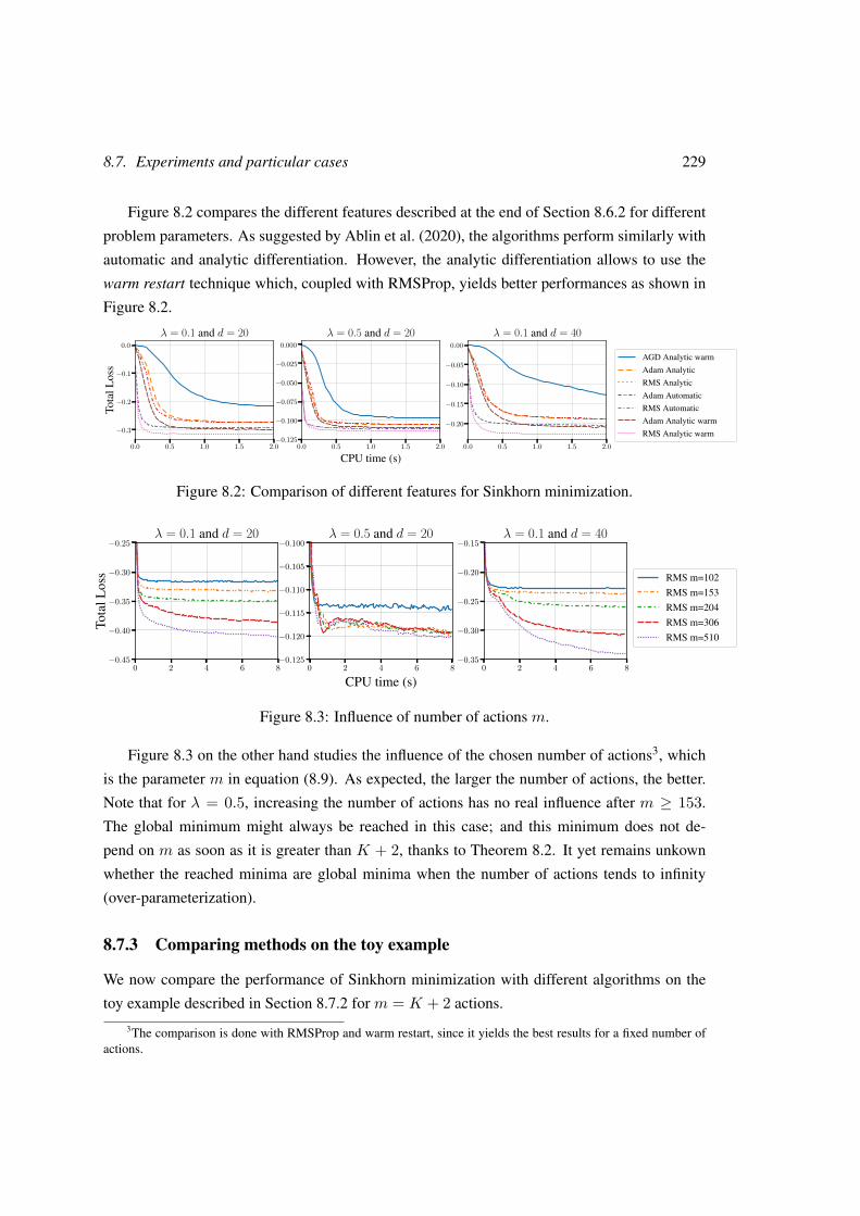
8.7. Experiments and particular cases 229
Figure 8.2 compares the different features described at the end of Section 8.6.2 for different
problem parameters. As suggested by Ablin et al. (2020), the algorithms perform similarly with
automatic and analytic differentiation. However, the analytic differentiation allows to use the
warm restart technique which, coupled with RMSProp, yields better performances as shown in
Figure 8.2.
0.0 0.5 1.0 1.5 2.0
−0.3
−0.2
−0.1
0.0
Tota
lLos
s
λ = 0.1 and d = 20
0.0 0.5 1.0 1.5 2.0
CPU time (s)
−0.125
−0.100
−0.075
−0.050
−0.025
0.000λ = 0.5 and d = 20
0.0 0.5 1.0 1.5 2.0
−0.20
−0.15
−0.10
−0.05
0.00λ = 0.1 and d = 40
AGD Analytic warmAdam AnalyticRMS AnalyticAdam AutomaticRMS AutomaticAdam Analytic warmRMS Analytic warm
Figure 8.2: Comparison of different features for Sinkhorn minimization.
0 2 4 6 8−0.45
−0.40
−0.35
−0.30
−0.25
Tota
lLos
s
λ = 0.1 and d = 20
0 2 4 6 8
CPU time (s)
−0.125
−0.120
−0.115
−0.110
−0.105
−0.100λ = 0.5 and d = 20
0 2 4 6 8−0.35
−0.30
−0.25
−0.20
−0.15λ = 0.1 and d = 40
RMS m=102RMS m=153RMS m=204RMS m=306RMS m=510
Figure 8.3: Influence of number of actions m.
Figure 8.3 on the other hand studies the influence of the chosen number of actions3, which
is the parameter m in equation (8.9). As expected, the larger the number of actions, the better.
Note that for λ = 0.5, increasing the number of actions has no real influence after m ≥ 153.
The global minimum might always be reached in this case; and this minimum does not de-
pend on m as soon as it is greater than K + 2, thanks to Theorem 8.2. It yet remains unkown
whether the reached minima are global minima when the number of actions tends to infinity
(over-parameterization).
8.7.3 Comparing methods on the toy example
We now compare the performance of Sinkhorn minimization with different algorithms on the
toy example described in Section 8.7.2 for m = K + 2 actions.3The comparison is done with RMSProp and warm restart, since it yields the best results for a fixed number of
actions.
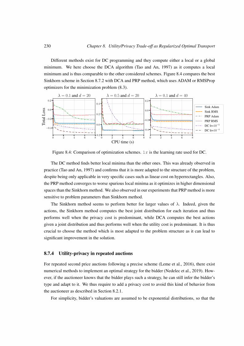
230 Chapter 8. Utility/Privacy Trade-off as Regularized Optimal Transport
Different methods exist for DC programming and they compute either a local or a global
minimum. We here choose the DCA algorithm (Tao and An, 1997) as it computes a local
minimum and is thus comparable to the other considered schemes. Figure 8.4 compares the best
Sinkhorn scheme in Section 8.7.2 with DCA and PRP method, which uses ADAM or RMSProp
optimizers for the minimization problem (8.3).
0 2 4 6 8
−0.4
−0.2
0.0
0.2
Tota
lLos
s
λ = 0.1 and d = 20
0 2 4 6 8
CPU time (s)
−0.2
0.0
0.2
0.4
λ = 0.5 and d = 20
0 2 4 6 8
−0.4
−0.2
0.0
0.2
λ = 0.1 and d = 40
Sink AdamSink RMSPRP AdamPRP RMSDC lr=10−5
DC lr=10−4
Figure 8.4: Comparison of optimization schemes. lr is the learning rate used for DC.
The DC method finds better local minima than the other ones. This was already observed in
practice (Tao and An, 1997) and confirms that it is more adapted to the structure of the problem,
despite being only applicable in very specific cases such as linear cost on hyperrectangles. Also,
the PRP method converges to worse spurious local minima as it optimizes in higher dimensional
spaces than the Sinkhorn method. We also observed in our experiments that PRP method is more
sensitive to problem parameters than Sinkhorn method.
The Sinkhorn method seems to perform better for larger values of λ. Indeed, given the
actions, the Sinkhorn method computes the best joint distribution for each iteration and thus
performs well when the privacy cost is predominant, while DCA computes the best actions
given a joint distribution and thus performs well when the utility cost is predominant. It is thus
crucial to choose the method which is most adapted to the problem structure as it can lead to
significant improvement in the solution.
8.7.4 Utility-privacy in repeated auctions
For repeated second price auctions following a precise scheme (Leme et al., 2016), there exist
numerical methods to implement an optimal strategy for the bidder (Nedelec et al., 2019). How-
ever, if the auctioneer knows that the bidder plays such a strategy, he can still infer the bidder’s
type and adapt to it. We thus require to add a privacy cost to avoid this kind of behavior from
the auctioneer as described in Section 8.2.1.
For simplicity, bidder’s valuations are assumed to be exponential distributions, so that the
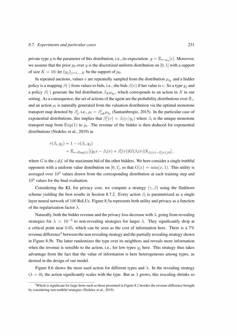
8.7. Experiments and particular cases 231
private type y is the parameter of this distribution, i.e., its expectation: y = Ev∼µy [v]. Moreover,
we assume that the prior p0 over y is the discretized uniform distribution on [0, 1] with a support
of size K = 10; let yjj=1,...,K be the support of p0.
In repeated auctions, values v are repeatedly sampled from the distribution µyj and a bidder
policy is a mapping β(·) from values to bids, i.e., she bids β(v) if her value is v. So a type yj and
a policy β(·) generate the bid distribution β#µyj , which corresponds to an action in X in our
setting. As a consequence, the set of actions of the agent are the probability distributions over R+
and an action ρi is naturally generated from the valuation distribution via the optimal monotone
transport map denoted by βij , i.e., ρi = βij#µyj (Santambrogio, 2015). In the particular case of
exponential distributions, this implies that βji (v) = βi(v/yj) where βi is the unique monotone
transport map from Exp(1) to ρi. The revenue of the bidder is then deduced for exponential
distributions (Nedelec et al., 2019) as
r(βi, yj) = 1− c(βi, yj)
= Ev∼Exp(1)[(yjv − βi(v) + β′i(v)
)G(βi(v)
)1βi(v)−β′i(v)≥0
],
whereG is the c.d.f. of the maximum bid of the other bidders. We here consider a single truthful
opponent with a uniform value distribution on [0, 1], so that G(x) = min(x, 1). This utility is
averaged over 103 values drawn from the corresponding distribution at each training step and
106 values for the final evaluation.
Considering the KL for privacy cost, we compute a strategy (γ, β) using the Sinkhorn
scheme yielding the best results in Section 8.7.2. Every action βi is parametrized as a single
layer neural network of 100 ReLUs. Figure 8.5a represents both utility and privacy as a function
of the regularization factor λ.
Naturally, both the bidder revenue and the privacy loss decrease with λ, going from revealing
strategies for λ ' 10−3 to non-revealing strategies for larger λ. They significantly drop at
a critical point near 0.05, which can be seen as the cost of information here. There is a 7%
revenue difference4 between the non revealing strategy and the partially revealing strategy shown
in Figure 8.5b. The latter randomizes the type over its neighbors and reveals more information
when the revenue is sensible to the action, i.e., for low types yj here. This strategy thus takes
advantage from the fact that the value of information is here heterogeneous among types, as
desired in the design of our model.
Figure 8.6 shows the most used action for different types and λ. In the revealing strategy
(λ = 0), the action significantly scales with the type. But as λ grows, this rescaling shrinks so
4Which is significant for large firms such as those presented in Figure 8.1 besides the revenue difference broughtby considering non truthful strategies (Nedelec et al., 2019).
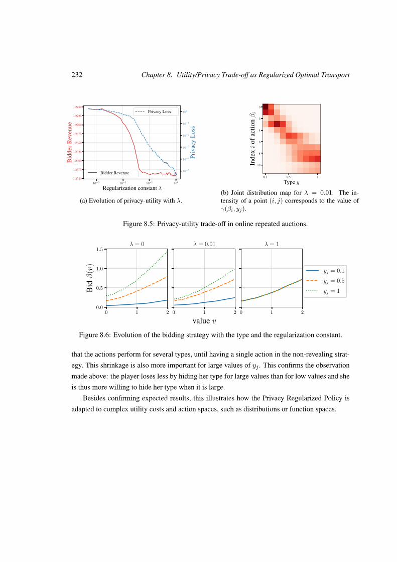
232 Chapter 8. Utility/Privacy Trade-off as Regularized Optimal Transport
10−3 10−2 10−1 100
Regularization constant λ
0.2550
0.2575
0.2600
0.2625
0.2650
0.2675
0.2700
0.2725
0.2750
Bid
derR
even
ue
Bidder Revenue 10−5
10−4
10−3
10−2
10−1
100
Priv
acy
Los
s
Privacy Loss
(a) Evolution of privacy-utility with λ.
0.1 0.5 1
Type y
0
2
4
6
8
10Inde
xi
ofac
tionβi
(b) Joint distribution map for λ = 0.01. The in-tensity of a point (i, j) corresponds to the value ofγ(βi, yj).
Figure 8.5: Privacy-utility trade-off in online repeated auctions.
0 1 20.0
0.5
1.0
1.5
Bidβ
(v)
λ = 0
0 1 2
value v
λ = 0.01
0 1 2
λ = 1
yj = 0.1yj = 0.5yj = 1
Figure 8.6: Evolution of the bidding strategy with the type and the regularization constant.
that the actions perform for several types, until having a single action in the non-revealing strat-
egy. This shrinkage is also more important for large values of yj . This confirms the observation
made above: the player loses less by hiding her type for large values than for low values and she
is thus more willing to hide her type when it is large.
Besides confirming expected results, this illustrates how the Privacy Regularized Policy is
adapted to complex utility costs and action spaces, such as distributions or function spaces.

Chapter 9
Social Learning in Non-StationaryEnvironments
Potential buyers of a product or service, before making their decisions, tend to read reviewswritten by previous consumers. We consider Bayesian consumers with heterogeneous pref-erences, who sequentially decide whether to buy an item of unknown quality, based onprevious buyers’ reviews. The quality is multi-dimensional and may occasionally vary overtime; the reviews are also multi-dimensional. In the simple uni-dimensional and static set-ting, beliefs about the quality are known to converge to its true value. This chapter extendsthis result in several ways. First, a multi-dimensional quality is considered, second, ratesof convergence are provided, third, a dynamical Markovian model with varying quality isstudied. In this dynamical setting the cost of learning is shown to be small.
9.1 Introduction . . . . . . . . . . . . . . . . . . . . . . . . . . . . . . . . . . . . 234
9.1.1 Main contribution . . . . . . . . . . . . . . . . . . . . . . . . . . . . . 235
9.1.2 Related literature . . . . . . . . . . . . . . . . . . . . . . . . . . . . . 235
9.1.3 Organization of the chapter . . . . . . . . . . . . . . . . . . . . . . . . 237
9.2 Model . . . . . . . . . . . . . . . . . . . . . . . . . . . . . . . . . . . . . . . 237
9.3 Stationary Environment . . . . . . . . . . . . . . . . . . . . . . . . . . . . . . 240
9.4 Dynamical Environment . . . . . . . . . . . . . . . . . . . . . . . . . . . . . 243
9.5 Naive Learners . . . . . . . . . . . . . . . . . . . . . . . . . . . . . . . . . . 249
9.A Omitted proofs . . . . . . . . . . . . . . . . . . . . . . . . . . . . . . . . . . 251
9.A.1 Proof of Lemma 9.1 . . . . . . . . . . . . . . . . . . . . . . . . . . . 251
9.A.2 Proof of the lower bound of Theorem 9.2 . . . . . . . . . . . . . . . . 252
9.A.3 Proof of Theorem 9.3 . . . . . . . . . . . . . . . . . . . . . . . . . . . 255
233
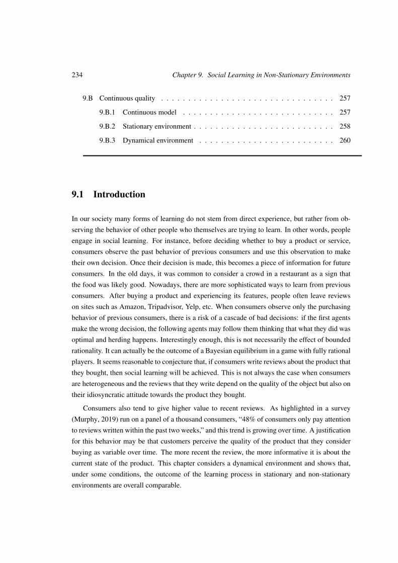
234 Chapter 9. Social Learning in Non-Stationary Environments
9.B Continuous quality . . . . . . . . . . . . . . . . . . . . . . . . . . . . . . . . 257
9.B.1 Continuous model . . . . . . . . . . . . . . . . . . . . . . . . . . . . 257
9.B.2 Stationary environment . . . . . . . . . . . . . . . . . . . . . . . . . . 258
9.B.3 Dynamical environment . . . . . . . . . . . . . . . . . . . . . . . . . 260
9.1 Introduction
In our society many forms of learning do not stem from direct experience, but rather from ob-
serving the behavior of other people who themselves are trying to learn. In other words, people
engage in social learning. For instance, before deciding whether to buy a product or service,
consumers observe the past behavior of previous consumers and use this observation to make
their own decision. Once their decision is made, this becomes a piece of information for future
consumers. In the old days, it was common to consider a crowd in a restaurant as a sign that
the food was likely good. Nowadays, there are more sophisticated ways to learn from previous
consumers. After buying a product and experiencing its features, people often leave reviews
on sites such as Amazon, Tripadvisor, Yelp, etc. When consumers observe only the purchasing
behavior of previous consumers, there is a risk of a cascade of bad decisions: if the first agents
make the wrong decision, the following agents may follow them thinking that what they did was
optimal and herding happens. Interestingly enough, this is not necessarily the effect of bounded
rationality. It can actually be the outcome of a Bayesian equilibrium in a game with fully rational
players. It seems reasonable to conjecture that, if consumers write reviews about the product that
they bought, then social learning will be achieved. This is not always the case when consumers
are heterogeneous and the reviews that they write depend on the quality of the object but also on
their idiosyncratic attitude towards the product they bought.
Consumers also tend to give higher value to recent reviews. As highlighted in a survey
(Murphy, 2019) run on a panel of a thousand consumers, “48% of consumers only pay attention
to reviews written within the past two weeks,” and this trend is growing over time. A justification
for this behavior may be that customers perceive the quality of the product that they consider
buying as variable over time. The more recent the review, the more informative it is about the
current state of the product. This chapter considers a dynamical environment and shows that,
under some conditions, the outcome of the learning process in stationary and non-stationary
environments are overall comparable.
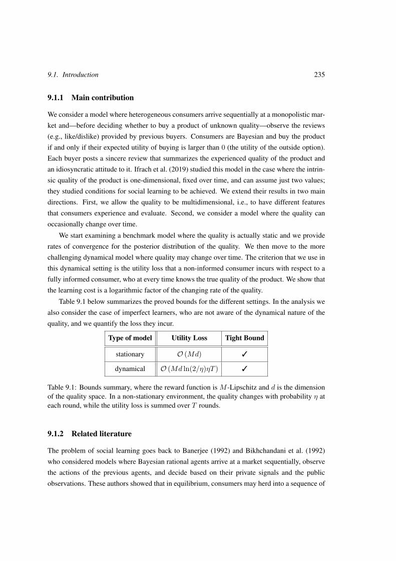
9.1. Introduction 235
9.1.1 Main contribution
We consider a model where heterogeneous consumers arrive sequentially at a monopolistic mar-
ket and—before deciding whether to buy a product of unknown quality—observe the reviews
(e.g., like/dislike) provided by previous buyers. Consumers are Bayesian and buy the product
if and only if their expected utility of buying is larger than 0 (the utility of the outside option).
Each buyer posts a sincere review that summarizes the experienced quality of the product and
an idiosyncratic attitude to it. Ifrach et al. (2019) studied this model in the case where the intrin-
sic quality of the product is one-dimensional, fixed over time, and can assume just two values;
they studied conditions for social learning to be achieved. We extend their results in two main
directions. First, we allow the quality to be multidimensional, i.e., to have different features
that consumers experience and evaluate. Second, we consider a model where the quality can
occasionally change over time.
We start examining a benchmark model where the quality is actually static and we provide
rates of convergence for the posterior distribution of the quality. We then move to the more
challenging dynamical model where quality may change over time. The criterion that we use in
this dynamical setting is the utility loss that a non-informed consumer incurs with respect to a
fully informed consumer, who at every time knows the true quality of the product. We show that
the learning cost is a logarithmic factor of the changing rate of the quality.
Table 9.1 below summarizes the proved bounds for the different settings. In the analysis we
also consider the case of imperfect learners, who are not aware of the dynamical nature of the
quality, and we quantify the loss they incur.
Type of model Utility Loss Tight Bound
stationary O (Md) 3
dynamical O (Md ln(2/η)ηT ) 3
Table 9.1: Bounds summary, where the reward function is M -Lipschitz and d is the dimensionof the quality space. In a non-stationary environment, the quality changes with probability η ateach round, while the utility loss is summed over T rounds.
9.1.2 Related literature
The problem of social learning goes back to Banerjee (1992) and Bikhchandani et al. (1992)
who considered models where Bayesian rational agents arrive at a market sequentially, observe
the actions of the previous agents, and decide based on their private signals and the public
observations. These authors showed that in equilibrium, consumers may herd into a sequence of
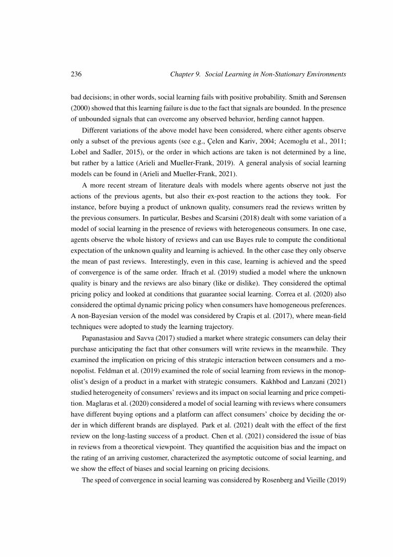
236 Chapter 9. Social Learning in Non-Stationary Environments
bad decisions; in other words, social learning fails with positive probability. Smith and Sørensen
(2000) showed that this learning failure is due to the fact that signals are bounded. In the presence
of unbounded signals that can overcome any observed behavior, herding cannot happen.
Different variations of the above model have been considered, where either agents observe
only a subset of the previous agents (see e.g., Çelen and Kariv, 2004; Acemoglu et al., 2011;
Lobel and Sadler, 2015), or the order in which actions are taken is not determined by a line,
but rather by a lattice (Arieli and Mueller-Frank, 2019). A general analysis of social learning
models can be found in (Arieli and Mueller-Frank, 2021).
A more recent stream of literature deals with models where agents observe not just the
actions of the previous agents, but also their ex-post reaction to the actions they took. For
instance, before buying a product of unknown quality, consumers read the reviews written by
the previous consumers. In particular, Besbes and Scarsini (2018) dealt with some variation of a
model of social learning in the presence of reviews with heterogeneous consumers. In one case,
agents observe the whole history of reviews and can use Bayes rule to compute the conditional
expectation of the unknown quality and learning is achieved. In the other case they only observe
the mean of past reviews. Interestingly, even in this case, learning is achieved and the speed
of convergence is of the same order. Ifrach et al. (2019) studied a model where the unknown
quality is binary and the reviews are also binary (like or dislike). They considered the optimal
pricing policy and looked at conditions that guarantee social learning. Correa et al. (2020) also
considered the optimal dynamic pricing policy when consumers have homogeneous preferences.
A non-Bayesian version of the model was considered by Crapis et al. (2017), where mean-field
techniques were adopted to study the learning trajectory.
Papanastasiou and Savva (2017) studied a market where strategic consumers can delay their
purchase anticipating the fact that other consumers will write reviews in the meanwhile. They
examined the implication on pricing of this strategic interaction between consumers and a mo-
nopolist. Feldman et al. (2019) examined the role of social learning from reviews in the monop-
olist’s design of a product in a market with strategic consumers. Kakhbod and Lanzani (2021)
studied heterogeneity of consumers’ reviews and its impact on social learning and price competi-
tion. Maglaras et al. (2020) considered a model of social learning with reviews where consumers
have different buying options and a platform can affect consumers’ choice by deciding the or-
der in which different brands are displayed. Park et al. (2021) dealt with the effect of the first
review on the long-lasting success of a product. Chen et al. (2021) considered the issue of bias
in reviews from a theoretical viewpoint. They quantified the acquisition bias and the impact on
the rating of an arriving customer, characterized the asymptotic outcome of social learning, and
we show the effect of biases and social learning on pricing decisions.
The speed of convergence in social learning was considered by Rosenberg and Vieille (2019)
9.2. Model 237
in models where only the actions of the previous agents are observed and by Acemoglu et al.
(2017) when reviews are present. This last paper is the closest to the spirit of this chapter.
Learning problems in non-stationary environment have been considered, for instance, by
Besbes et al. (2015) and Besbes et al. (2019) in a context where the function that is being learned
changes smoothly, rather than abruptly as in our model in Section 9.4.
9.1.3 Organization of the chapter
Section 9.2 introduces the model of social learning from consumer reviews. Section 9.3 studies
the stationary setting where the quality is fixed. Section 9.4 introduces the dynamical setting,
where the quality changes over time. Section 9.5 consider a model with naive consumers and
shows that knowledge of the dynamical structure is crucial for the consumer utility.
Section 9.A contains additional proofs and Section 9.B studies the continuous model where
the quality space Q is convex.
9.2 Model
We consider a model of social learning where consumers read reviews before making their pur-
chase decisions. A monopolist sells a product of unknown quality to consumers who arrive
sequentially at the market. The quality may vary over time, although variations are typically
rare. The quality of the product at time t is denoted by Qt and the set of possible qualities is
Q = 0, 1d. For a vector x, we denote by x(i) its i-th component, i.e., Q(i)t represents the i-th
feature of the product at time t and has a binary value (low or high).
The prior distribution of the quality at time 1 is π1. Consumers are indexed by the time of
their arrivals t ∈ N\0. They are heterogeneous and consumer t has an idiosyncratic preference
θt ∈ Θ for the product. This preference θt is private information. These preferences are assumed
to be i.i.d. according to some known distribution. In game-theoretic terms, θt could be seen as
the type of consumer t. The sequences of preferences θt and of qualities Qt are independent.
A consumer who buys the product posts a review in the form of a multi-dimensional nu-
merical grade. The symbol Zt denotes the review posted by consumer t. The notation Zt = ∗indicates that consumer t did not buy the product. We call Ht := Z1, . . . , Zt−1 the history
before the decision of consumer t. We setH1 := ∅.
Since the preferences are independent of the quality, a no-purchase decision does not carry
any information on the quality. As a consequence, the historyHt is informationally equivalent to
the reduced history Ht that includes only the reviews of the buyers up to t−1. This differentiates
this model from the classical social learning models, where consumers have private signals that
238 Chapter 9. Social Learning in Non-Stationary Environments
are correlated with the quality.
Based on the historyHt of past observations and her own preference θt, consumer t decides
whether to buy the product. In case of purchase, she receives the utility ut := r(Qt, θt) where r
is the reward function. A consumer who does not buy the product gets ut = 0.
Bayesian rationality is assumed, so consumer t buys the product if and only if her conditional
expected utility of purchasing is positive, that is, if and only if E[r(Qt, θt) | Ht, θt] > 0.
Consumer t then reviews the product by giving the feedback Zt = f(Qt, θt, εt) ∈ Z ⊂ Rd
where εt are i.i.d. variables independent from θt. Also, the feedback function is assumed to take
a finite number of values in Rd and to be of the form
f(Q, θ, ε) = (f (i)(Q(i), ε, θ))i=1,...,d .
In words, for each different featureQ(i) of the qualityQ, consumers provide a separate feedback.
Previous works (Acemoglu et al., 2017; Ifrach et al., 2019) consideredZ = 0, 1 as the reviews
were only the likes or dislikes of consumers. This model allows a more general and richer
feedback, such as ratings on a five-star scale for each feature, or even sparse feedback where
consumers do not necessarily review each feature.
In a model without noise εt, the learning process is much simpler, as already noted by Ifrach
et al. (2019). Indeed, in this case, a single negative review rules out many possibilities as it
means that the quality was overestimated. To depict a more interesting learning process, we
consider noise, which corresponds to variations caused by different factors, e.g., fluctuations in
the product quality or imperfect perception of the quality by the consumer.
In the following, πt denotes the posterior distribution of Qt given Ht and, for any i ∈ [d],π
(i)t (q(i)) = P[Q(i)
t = q(i) | Ht] is the i-th marginal of the posterior.
We also introduce the function G and its componentwise equivalent G(i), defined as
G(z, π, q) = P[Zt = z | πt = π,Qt = q], (9.1)
G(i)(z(i), π, q(i)) = P[Z(i)t = z(i) | πt = π,Q
(i)t = q(i)]. (9.2)
In the following, we also use the notations
G(z, π) = Eq∼π[G(z, π, q)], (9.3)
G(i)(z(i), π) = Eq∼π[G(i)(z(i), π, q(i))]. (9.4)
The following two assumptions will be used in the sequel.
Assumption 9.1 (Purchase guarantee). The reward function r is monotonic in each feature q(i)
and for any q ∈ Q, Pθt(r(q, θt) > 0
)> 0, i.e., there is always a fraction of consumers who buy
9.2. Model 239
the product.
Assumption 9.1 excludes situations where consumers stop buying if the expected quality
becomes low. Without this condition, social learning fails with positive probability (Acemoglu
et al., 2017; Ifrach et al., 2019).
Assumption 9.2 (Identifiability). For any i ∈ [d], any quality posterior π ∈ P(Q) and quality
q(i), we have G(i)( · , π, q(i)) > 0. Moreover, for q(i) 6= q′(i), there exists some z ∈ Z such that
G(i)(z(i), π, q(i)) 6= G(i)(z(i), π, q′(i)).
Assumption 9.2 is needed to distinguish different qualities based on past reviews. The posi-
tivity of G is required to avoid trivial situations. The case of G = 0 for some variables is similar
to the absence of noise εt, as a single observation can definitely rule out several possibilities.
An interesting choice of reward function is, for instance, r(Q, θ) = 〈Q, θt〉 where 〈 · , · 〉 is
the scalar product. In this case, θ(i)t is the weight that customer t gives to feature i of the service.
In practice, customers might also only focus on the best or worst aspects of the service,
meaning their reward might only depend on the maximal or minimal value of the Q(i)’s. The
ordered weighted averaging operators (Yager, 1988) model these behaviors. In an additive
model similar to the classical case in the literature, this leads to a reward function r(Q, θ) =∑ni=1w
(i)(Q+ θ)(σ(i)) where σ is a permutation such that (Q+ θ)(σ(i)) is the i-th largest com-
ponent of the vector (Q(i) + θ(i))i=1,...,d. If w(i) = 1/d for all i, this is just an average of all
features’ utilities. When w(1) = 1 and all other terms are 0, consumers are only interested in the
maximal utility among all features.
Much of the existing literature has focused on the following unidimensional setting
r(Q, θ) = Q+ θ − p,
f(Q, θ, ε) = sign (Q+ θ + ε− p) ,
where p is an exogenously fixed price. Since consumers review separately each feature of the
service, the feedback function is a direct extension of the above unidimensional setting. It is
then of the form
f (i)(Q(i), ε, θ) = sign(Q(i) + θ(i) + ε(i) − p(i)
), (9.5)
for some constant price p(i).
Having a sparse feedback is very common on platform reviews, where consumers only re-
view a few features. This case can be modeled by
f (i)(Q(i), ε, η, θ) = sign(Q(i) + θ(i) + ε(i) − p(i)
)ξ(i), (9.6)
240 Chapter 9. Social Learning in Non-Stationary Environments
with ε ∈ Rd and ξ ∈ 0, 1d. Although the noise vector is here given by the tuple (ε, ξ) instead
of ε alone, this remains a specific case of our model.
A multiplicative model can also be considered where the relevant quantity is Q(i)θ(i), rather
than Q(i) + θ(i). This model is very similar to the additive one when using a logarithmic trans-
formation.
9.3 Stationary Environment
As mentioned before, our aim is to consider a model where the quality of the product may oc-
casionally change over time. As a benchmark, we start considering the case where the quality
is constant: Qt = Q1 for all t ∈ N. We will leverage this case, when dealing with the dy-
namic model of variable quality. In the unidimensional case Q = 0, 1, Ifrach et al. (2019)
showed that the posterior almost surely converges to the true quality, and Acemoglu et al. (2017)
showed an asymptotic exponential convergence rate. Besides extending these results to the mul-
tidimensional model, this section shows anytime convergence rates of the posterior. The study
of convergence rates in social learning is just a recent concern (Acemoglu et al., 2017; Rosen-
berg and Vieille, 2019), despite being central to online learning (Bottou, 1999) and Bayesian
estimation (Ghosal et al., 2000). Moreover, convergence rates are of crucial interest when facing
a dynamical quality. The main goal of this section is thus to lay the foundation for the analysis
of Section 9.4.
The posterior update is obtained using Bayes’ rule for any q ∈ Q,
πt+1(q) = G (Zt, πt, q)G (Zt, πt)
πt(q). (9.7)
Theorem 9.1 below gives a convergence rate of the posterior to the true quality. Similarly to
Acemoglu et al. (2017, Theorem 2), it shows an exponential convergence rate. While their result
yields an asymptotic convergence rate, we provide an anytime, but slower, rate with similar as-
sumptions. We focus on anytime rates as they are highly relevant in the model with a dynamical,
evolving quality considered in Section 9.4.
Theorem 9.1. For q 6= q′, we have
E[πt+1(q′) | Q = q] ≤ exp(− tδ4
2γ2 + 4δ2
)1
maxi∈[d] π(i)1 (q(i))
,
where δ := mini∈[d],π∈P(Q)
∑z∈Z|G(i)(z(i), π, 1)−G(i)(z(i), π, 0)| (9.8)
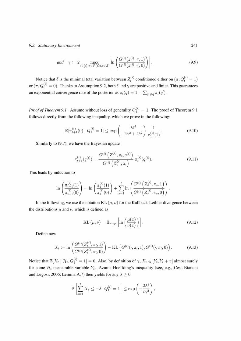
9.3. Stationary Environment 241
and γ := 2 maxi∈[d],π∈P(Q),z∈Z
∣∣∣∣∣ln(G(i)(z(i), π, 1)G(i)(z(i), π, 0)
)∣∣∣∣∣ . (9.9)
Notice that δ is the minimal total variation between Z(i)t conditioned either on (π,Q(i)
t = 1)or (π,Q(i)
t = 0). Thanks to Assumption 9.2, both δ and γ are positive and finite. This guarantees
an exponential convergence rate of the posterior as πt(q) = 1−∑q′ 6=q πt(q′).
Proof of Theorem 9.1. Assume without loss of generality Q(i)1 = 1. The proof of Theorem 9.1
follows directly from the following inequality, which we prove in the following:
E[π(i)t+1(0) | Q(i)
1 = 1] ≤ exp(− tδ4
2γ2 + 4δ2
)1
π(i)1 (1)
. (9.10)
Similarly to (9.7), we have the Bayesian update
π(i)t+1(q(i)) =
G(i)(Z
(i)t , πt, q
(i))
G(i)(Z
(i)t , πt
) π(i)t (q(i)). (9.11)
This leads by induction to
ln
π(i)t+1(1)π
(i)t+1(0)
= ln(π
(i)1 (1)π
(i)1 (0)
)+
t∑s=1
ln
G(i)(Z
(i)s , πs, 1
)G(i)
(Z
(i)s , πs, 0
) .
In the following, we use the notation KL (µ, ν) for the Kullback-Leibler divergence between
the distributions µ and ν, which is defined as
KL (µ, ν) = Ex∼µ[ln(µ(x)ν(x)
)]. (9.12)
Define now
Xt := ln(G(i)(Z(i)
t , πt, 1)G(i)(Z(i)
t , πt, 0)
)−KL
(G(i)(·, πt, 1), G(i)(·, πt, 0)
). (9.13)
Notice that E[Xt | Ht, Q(i)1 = 1] = 0. Also, by definition of γ, Xt ∈ [Yt, Yt + γ] almost surely
for some Ht-measurable variable Yt. Azuma-Hoeffding’s inequality (see, e.g., Cesa-Bianchi
and Lugosi, 2006, Lemma A.7) then yields for any λ ≥ 0:
P[
t∑s=1
Xs ≤ −λ∣∣∣Q(i)
1 = 1]≤ exp
(−2λ2
tγ2
),

242 Chapter 9. Social Learning in Non-Stationary Environments
which is equivalent to
P
π(i)t+1(0)π
(i)t+1(1)
≥ exp(λ−
t∑s=1
KL(G(i)(·, πs, 1), G(i)(·, πs, 0)
) )π(i)1 (0)π
(i)1 (1)
∣∣∣Q(i)1 = 1
≤ exp(−2λ2
tγ2
).
(9.14)
By Pinsker’s inequality (see, e.g., Tsybakov, 2009, Lemma 2.5), we have
KL(G(i)(·, πs, 1), G(i)(·, πs, 0)
)≥ δ2/2,
so Equation (9.14) becomes
P[π
(i)t+1(0) ≥ exp
(λ− tδ2(1, 0)
2)π(i)
1 (0)π
(i)1 (1)
∣∣∣Q(i)1 = 1
]≤ exp
(−2λ2
tγ2
),
where we used the fact that π(i)t+1(1) ≤ 1. This then yields
E[π(i)t+1(0) | Q(i)
1 = 1] ≤ exp(λ− tδ2
2
)π
(i)1 (0)π
(i)1 (1)
+ P[π
(i)t+1(0) ≥ exp
(λ− tδ2/2
)| Q(i)
1 = 1]
≤ exp(λ− tδ2
2
)π
(i)1 (0)π
(i)1 (1)
+ exp(−2λ2
tγ2
).
Let x = tγ2/4 and y = tδ2/2. Setting λ = −x+√
2xy + x2 equalizes the exponential terms:
E[π(i)t+1(0) | Q(i)
1 = 1] ≤ (1 + π(i)1 (0)π
(i)1 (1)
) exp(−x− y +
√x2 + 2xy
)
≤ 1π
(i)1 (1)
exp(− y2
2(x+ y)).
The second inequality is given by the convex inequality
√a−√a+ b ≤ − b
2√a+ b
, for a = x2 + 2xy and b = y2.
From the definitions of x and y, this yields
E[π(i)t+1(0) | Q(i)
1 = 1] ≤ 1π
(i)1 (1)
exp(− tδ4
2γ2 + 4δ2
).
We conclude by noting that π(i)t (q′(i)) ≥ πt(q′).
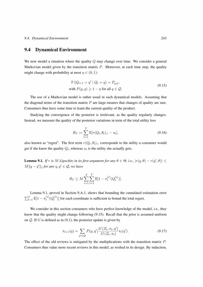
9.4. Dynamical Environment 243
9.4 Dynamical Environment
We now model a situation where the quality Q may change over time. We consider a general
Markovian model given by the transition matrix P . Moreover, at each time step, the quality
might change with probability at most η ∈ (0, 1):
P(Qt+1 = q′ | Qt = q
)= Pq,q′ ,
with P (q, q) ≥ 1− η for all q ∈ Q.(9.15)
The use of a Markovian model is rather usual in such dynamical models. Assuming that
the diagonal terms of the transition matrix P are large ensures that changes of quality are rare.
Consumers thus have some time to learn the current quality of the product.
Studying the convergence of the posterior is irrelevant, as the quality regularly changes.
Instead, we measure the quality of the posterior variations in term of the total utility loss
RT :=T∑t=1
E[r(Qt, θt)+ − ut], (9.16)
also known as “regret”. The first term r(Qt, θt)+ corresponds to the utility a consumer would
get if she knew the quality Qt, whereas ut is the utility she actually gets.
Lemma 9.1. If r is M -Lipschitz in its first argument for any θ ∈ Θ, i.e., |r(q, θ) − r(q′, θ)| ≤M‖q − q′‖1 for any q, q′ ∈ Q, we have
RT ≤Md∑i=1
T∑t=1
E[1− π(i)t (Q(i)
t )].
Lemma 9.1, proved in Section 9.A.1, shows that bounding the cumulated estimation error∑Tt=1 E[1− π(i)
t (Q(i)t )] for each coordinate is sufficient to bound the total regret.
We consider in this section consumers who have perfect knowledge of the model, i.e., they
know that the quality might change following (9.15). Recall that the prior is assumed uniform
on Q. If G is defined as in (9.1), the posterior update is given by
πt+1(q) =∑q′∈Q
P (q, q′)G (Zt, πt, q′)G (Zt, πt)
πt(q′). (9.17)
The effect of the old reviews is mitigated by the multiplications with the transition matrix P .
Consumers thus value more recent reviews in this model, as wished in its design. By induction,
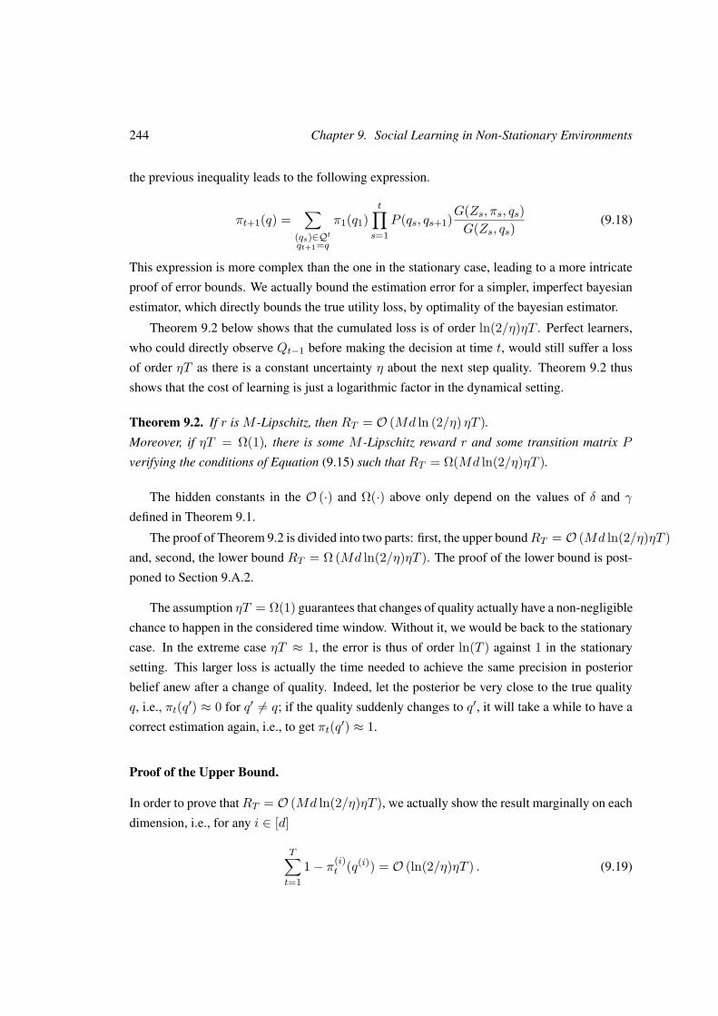
244 Chapter 9. Social Learning in Non-Stationary Environments
the previous inequality leads to the following expression.
πt+1(q) =∑
(qs)∈Qtqt+1=q
π1(q1)t∏
s=1P (qs, qs+1)G(Zs, πs, qs)
G(Zs, qs)(9.18)
This expression is more complex than the one in the stationary case, leading to a more intricate
proof of error bounds. We actually bound the estimation error for a simpler, imperfect bayesian
estimator, which directly bounds the true utility loss, by optimality of the bayesian estimator.
Theorem 9.2 below shows that the cumulated loss is of order ln(2/η)ηT . Perfect learners,
who could directly observe Qt−1 before making the decision at time t, would still suffer a loss
of order ηT as there is a constant uncertainty η about the next step quality. Theorem 9.2 thus
shows that the cost of learning is just a logarithmic factor in the dynamical setting.
Theorem 9.2. If r is M -Lipschitz, then RT = O (Md ln (2/η) ηT ).
Moreover, if ηT = Ω(1), there is some M -Lipschitz reward r and some transition matrix P
verifying the conditions of Equation (9.15) such that RT = Ω(Md ln(2/η)ηT ).
The hidden constants in the O (·) and Ω(·) above only depend on the values of δ and γ
defined in Theorem 9.1.
The proof of Theorem 9.2 is divided into two parts: first, the upper boundRT = O (Md ln(2/η)ηT )and, second, the lower bound RT = Ω (Md ln(2/η)ηT ). The proof of the lower bound is post-
poned to Section 9.A.2.
The assumption ηT = Ω(1) guarantees that changes of quality actually have a non-negligible
chance to happen in the considered time window. Without it, we would be back to the stationary
case. In the extreme case ηT ≈ 1, the error is thus of order ln(T ) against 1 in the stationary
setting. This larger loss is actually the time needed to achieve the same precision in posterior
belief anew after a change of quality. Indeed, let the posterior be very close to the true quality
q, i.e., πt(q′) ≈ 0 for q′ 6= q; if the quality suddenly changes to q′, it will take a while to have a
correct estimation again, i.e., to get πt(q′) ≈ 1.
Proof of the Upper Bound.
In order to prove thatRT = O (Md ln(2/η)ηT ), we actually show the result marginally on each
dimension, i.e., for any i ∈ [d]
T∑t=1
1− π(i)t (q(i)) = O (ln(2/η)ηT ) . (9.19)
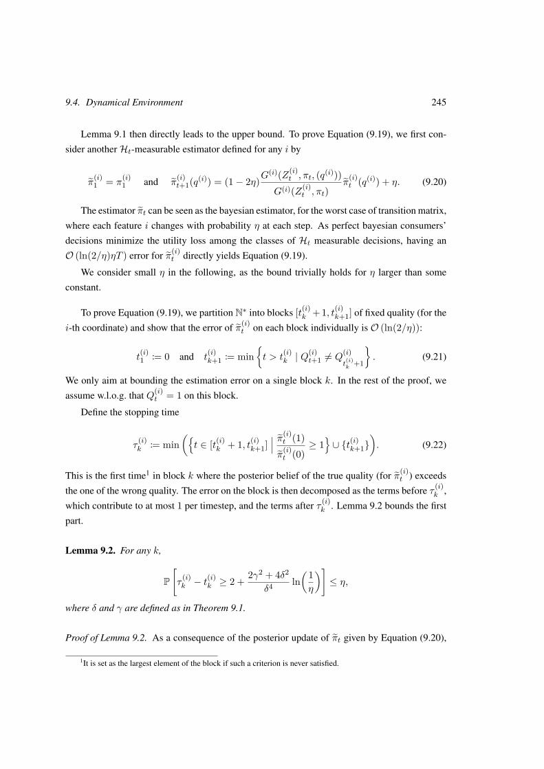
9.4. Dynamical Environment 245
Lemma 9.1 then directly leads to the upper bound. To prove Equation (9.19), we first con-
sider anotherHt-measurable estimator defined for any i by
π(i)1 = π
(i)1 and π
(i)t+1(q(i)) = (1− 2η)G
(i)(Z(i)t , πt, (q(i)))
G(i)(Z(i)t , πt)
π(i)t (q(i)) + η. (9.20)
The estimator πt can be seen as the bayesian estimator, for the worst case of transition matrix,
where each feature i changes with probability η at each step. As perfect bayesian consumers’
decisions minimize the utility loss among the classes of Ht measurable decisions, having an
O (ln(2/η)ηT ) error for π(i)t directly yields Equation (9.19).
We consider small η in the following, as the bound trivially holds for η larger than some
constant.
To prove Equation (9.19), we partition N∗ into blocks [t(i)k + 1, t(i)k+1] of fixed quality (for the
i-th coordinate) and show that the error of π(i)t on each block individually is O (ln(2/η)):
t(i)1 := 0 and t
(i)k+1 := min
t > t
(i)k | Q
(i)t+1 6= Q
(i)t(i)k
+1
. (9.21)
We only aim at bounding the estimation error on a single block k. In the rest of the proof, we
assume w.l.o.g. that Q(i)t = 1 on this block.
Define the stopping time
τ(i)k := min
(t ∈ [t(i)k + 1, t(i)k+1]
∣∣∣ π(i)t (1)π
(i)t (0)
≥ 1∪ t(i)k+1
). (9.22)
This is the first time1 in block k where the posterior belief of the true quality (for π(i)t ) exceeds
the one of the wrong quality. The error on the block is then decomposed as the terms before τ (i)k ,
which contribute to at most 1 per timestep, and the terms after τ (i)k . Lemma 9.2 bounds the first
part.
Lemma 9.2. For any k,
P[τ
(i)k − t
(i)k ≥ 2 + 2γ2 + 4δ2
δ4 ln(1η
)]≤ η,
where δ and γ are defined as in Theorem 9.1.
Proof of Lemma 9.2. As a consequence of the posterior update of πt given by Equation (9.20),
1It is set as the largest element of the block if such a criterion is never satisfied.
246 Chapter 9. Social Learning in Non-Stationary Environments
for t+ 1 ≤ τ (i)k ,
π(i)t+1(0) ≤ G(i)(Z(i)
t , πt, 0)G(Zt, πt)
πt(0) and π(i)t+1(1) ≥ G(i)(Z(i)
t , πt, 1)G(Zt, πt)
πt(1).
We then get by induction
π(i)t+1(0)π
(i)t+1(1)
≤ 1η
t∏s=t(i)
k+1
G(i)(Z(i)s , πs, 0)
G(i)(Z(i)s , πs, 1)
, (9.23)
as π(i)t(i)k
+1(1) ≥ η. For n =
⌈2γ2+4δ2
δ4 ln(
1η
)⌉, it has been shown in the proof of Theorem 9.1
that:
P
t(i)k
+n∏s=t(i)
k+1
G(Z(i)s , πs, 0)
G(Z(i)s , πs, 1)
> η∣∣∣ π
t(i)k
+1, ∀s ∈ [t(i)k + 1, t(i)k + n], Q(i)s = 1
≤ η.
Note that by definition of τ (i)k ,
π(i)
τ(i)k
(0)
π(i)
τ(i)k
(1)≤ 1. The above concentration inequality and (9.23) imply
that P[τ (i)k − t
(i)k ≥ n+ 1] ≤ η.
In Lemma 9.3 below we show that, past this stopping time τ (i)k , the quantity 1/π(i)
t (1) cannot
exceed some constant term in expectation.
Lemma 9.3. For any k ∈ N∗ and t ∈ [τ (i)k , t
(i)k+1],
E[
1π
(i)t (Q(i)
t )
∣∣∣ τ (i)k , (t(i)n )n
]≤ 2.
Proof of Lemma 9.3. By definition of G(i) and the posterior update, given by Equations (9.2)
and (9.20) respectively, we have
E
1π
(i)t+1(1)
∣∣∣ Q(i)t = 1,Ht
=∑
z(i):z∈Z
G(i)(z(i), π(i)t , 1)h
(G(i)(z(i), πt)
G(i)(z(i), πt, 1)π(i)t (1)
),
with h(x) = 1η + 1−2η
x
. (9.24)
Note that h is concave on R∗+, so by Jensen’s inequality:
E
1π
(i)t+1(1)
∣∣∣ Q(i)t = 1,Ht
≤ h( 1π
(i)t (1)
). (9.25)
9.4. Dynamical Environment 247
Lemma 9.3 then follows by induction
E
1π
(i)t+τ (i)
k+1
(1)
∣∣∣ τ (i)k ,∀s ∈ [τ (i)
k , t+ τ(i)k ], Q(i)
s = 1
≤ E
h 1π
(i)t+τ (i)
k
(1)
∣∣∣ τ (i)k ,∀s ∈ [τ (i)
k , t+ τ(i)k ], Q(i)
s = 1
≤ h
E 1π
(i)t+τ (i)
k
(1)
∣∣∣ τ (i)k ,∀s ∈ [τ (i)
k , t+ τ(i)k ], Q(i)
s = 1
≤ h (2) = 2.
The first inequality is a direct consequence of Equation (9.25), the second is Jensen’s inequal-
ity again, while the third one is obtained by induction using the fact that h is increasing and
π(i)τ
(i)k
(1) ≥ 12 .
Similarly to the proof of Theorem 9.1, Azuma-Hoeffding’s inequality on a single block leads to
E[t−1∏s=n
G(i)(Z(i)s , πs, 0)
G(i)(Z(i)s , πs, 1)
∣∣∣πn,∀s ∈ [n, t− 1], Q(i)s = 1
]≤ exp
(− (t− n)δ4
2γ2 + 4δ2
). (9.26)
Also, note that Equation (9.20) leads to
G(i)(Z(i)t , πt, 1)
G(i)(Z(i)t , πt)
≤π
(i)t+1(1)
(1− 2η)π(i)t (1)
.
By induction, we get
t−1∏s=n
G(i)(Z(i)s , πs, 1)
G(i)(Z(i)s , πs)
≤ 1π
(i)n (1)(1− 2η)t−n
. (9.27)
Multiplying the left hand side of (9.26) by the left hand side of (9.27), we obtain
E[t−1∏s=n
G(i)(Z(i)s , πs, 0)
G(i)(Z(i)s , πs)
∣∣∣ πn, ∀s ∈ [n, t− 1], Q(i)s = 1
]≤ (1− 2η)−(t−n)
π(i)n (1)
exp(− (t− n)δ4
2γ2 + 4δ2
).
(9.28)
248 Chapter 9. Social Learning in Non-Stationary Environments
Similarly to Equation (9.18), starting from n0 ≥ 1, for the i-th coordinate it can be shown that
π(i)t+1(q(i)) = (1− 2η)t−n0+1π(i)
n0 (q(i))t∏
s=n0
G(i)(Z
(i)s , πs, q
(i))
G(i)(Z
(i)s , πs
)+ η
t−n0∑s=0
(1− 2η)st∏
l=t−s+1
G(i)(Z(i)l , πl, q
(i))G(i)(Z(i)
l , πl).
DefineAtτ
(i)k
:=∀s ∈ [τ (i)
k , τ(i)k + t], Q(i)
s = 1
. Combining this formula with Equation (9.28),
we obtain
E[π
(i)τ
(i)k
+t(0) | H
τ(i)k
, Atτ
(i)k
]≤π
(i)τ
(i)k
(0)
π(i)τ
(i)k
(1)exp
(− tδ4
2γ2 + 4δ2
)
+ 2ηt−1∑s=0
E
1π
(i)τ
(i)k
+t−s(1)
∣∣∣Hτ
(i)k
, Atτ
(i)k
exp(− sδ4
2γ2 + 4δ2
).
Thanks to Lemma 9.3,
E
1π
(i)τ
(i)k
+t−s(1)
∣∣∣Hτ
(i)k
, Atτ
(i)k
≤ 2 andπ
(i)τ
(i)k
(0)
π(i)τ
(i)k
(1)≤ 1,
so that
E[π
(i)τ
(i)k
+t(0) | H
τ(i)k
, Atτ
(i)k
]≤ exp
(− tδ4
2γ2 + 4δ2
)+ 4η
t−1∑s=0
exp(− sδ4
2γ2 + 4δ2
)
≤ exp(− tδ4
2γ2 + 4δ2
)+ 4η
1− exp(− δ4
2γ2+4δ2
) . (9.29)
Finally, the estimation error for π(i)t incurred during the block k is at most
τ(i)k − t
(i)k +
t(i)k+1−t
(i)k−1∑
t=0
exp(− tδ4
2γ2 + 4δ2
)+ 4η
1− exp(− δ4
2γ2+4δ2
),
i.e., it is of order τ (i)k − t
(i)k + η(t(i)k+1 − t
(i)k ). Lemma 9.2 then yields
E[τ (i)k − t
(i)k | (tn)n] ≤ 2 + 2γ2 + 4δ2
δ4 ln(1η
)+ η(t(i)k+1 − t
(i)k ).
9.5. Naive Learners 249
Thus in expectation, given (tn)n, the estimation error of Q(i)t over the block k for πt is of
order ln(2/η) + η(t(i)k+1 − t(i)k ). Note that t(i)k+1 − t
(i)k is stochastically dominated by a geometric
distribution of parameter η. In expectation the number of blocks counted before T is thusO (ηT )and summing over all these blocks yields
T∑t=1
E[1− π(i)t (Q(i)
t )] = O (ln(2/η)ηT ) .
When summing over all coordinates, this implies that the regret incurred by the estimator πt is
of order O (Md ln(2/η)ηT ). Since the exact estimator πt minimizes the expected utility loss
among the class of allHt-measurable estimators, the upper bound follows.
Proof of the Lower Bound.
The proof of the lower bound is postponed to Section 9.A.2. The idea is that the posterior cannot
converge faster than exponentially on a single block. Thus, if the posterior converged in the last
block, e.g., πt(q′) ≈ η in a block of quality q, then it would require a time ln(2/η) before
πt(q′) ≥ 1/2 in the new block of quality q′, leading to a loss at least ln(2/η) on this block.
9.5 Naive Learners
In Section 9.4 we showed that learning occurs for Bayesian consumers who are perfectly aware
of the environment, and especially of its dynamical aspect. In some learning problems, Bayesian
learners can still have small regret, despite having an imperfect knowledge of the problem pa-
rameters or even ignoring some aspects of the problem.
This section shows that awareness of the problem’s dynamical structure is essential here. In
particular, naive learners incur a considerable utility loss.
In the following, we consider the setting described in Section 9.4 with naive learners, i.e.,
consumers who are unaware of possible quality changes over time. As a consequence, their
posterior distribution πnaivet follows the exact same update rule as in the stationary case:
πnaivet+1 (q) = G(Zt, πnaive
t , q)G(Zt, πnaive
t )πnaivet (q).
The regret for naive learners is then
T∑t=1
E[r(Qt, θt)+ − unaive
t
],
250 Chapter 9. Social Learning in Non-Stationary Environments
where unaivet = r(Qt, θt)1
∑q∈Q
πnaivet (q)r(q, θt) ≥ 0
.unaivet is the utility achieved by naive learners who make their decisions based on πnaive
t .
Theorem 9.3 below states that the utility loss for naive learners is non-negligible, i.e., of
order T , which displays the significance of taking into account the dynamical structure of the
problem in the learning process.
Theorem 9.3. If ηT = Ω(1), then there is some M -Lipschitz reward r and some transition
matrix P verifying the conditions given by Equation (9.15) such that
RnaiveT = Ω(MdT ).
The proof of Theorem 9.3 can be found in Section 9.A.3 and bears similarities with the proof
of the lower bound in Theorem 9.2. The posterior of naive learners converges quickly to the true
quality on a single block. Because of this, after a change of quality, it takes a long time before
the posterior belief of naive learners becomes accurate again with respect to the new quality.
Appendix
9.A Omitted proofs
This section contains detailed proofs of lemmas and theorems postponed to the Appendix.
9.A.1 Proof of Lemma 9.1
The inequality actually holds individually for each term of the sum when conditioned on πt, i.e.,
E[r(Qt, θt)+ − ut | πt] ≤ M∑di=1(1 − π(i)
t (Q(i)t )), which directly implies Lemma 9.1. By
definition, ut = r(Qt, θt)1(∑
q∈Q πt(q)r(q, θt) ≥ 0)
and so it comes
r(Qt, θt)+ − ut = r(Qt, θt)
1 (r(Qt, θt) ≥ 0)− 1
∑q∈Q
πt(q)r(q, θt) ≥ 0
= r(Qt, θt)
(1
r(Qt, θt) ≥ 0 ≥∑q∈Q
πt(q)r(q, θt)
− 1
∑q∈Q
πt(q)r(q, θt) ≥ 0 ≥ r(Qt, θt)
)
≤
∣∣∣∣∣∣r(Qt, θt)−∑q∈Q
πt(q)r(q, θt)
∣∣∣∣∣∣=
∣∣∣∣∣∣∑q∈Q
πt(q)(r(Qt, θt)− r(q, θt))
∣∣∣∣∣∣≤∑q∈Q
πt(q) |r(Qt, θt)− r(q, θt)|
≤M∑q∈Q
πt(q)‖Qt − q‖1
= Md∑i=1
(1− π(i)t (Q(i)
t )).
251
252 Chapter 9. Social Learning in Non-Stationary Environments
9.A.2 Proof of the lower bound of Theorem 9.2
In this proof we consider the following transition matrix:
P (q, q) = 1− η and P (q,111− q) = η,
i.e., all the features change simultaneously with probability η at each round. We also assume
that the prior is only split between the vectors 000 and 111, i.e., the features are either all 0 or all 1.
If we take the reward function r(q, θ) = M∑di=1 qi + θi, then the regret scales as
RT = Ω(M
d∑i=1
T∑t=1
E[1− π(i)t (Q(i)
t )])
= Ω(Md
T∑t=1
E[1− πt(Qt)]). (9.30)
In this model, we thus have the following posterior update
πt+1(111) = (1− 2η)G(Zt, πt,111)G(Zt, πt)
πt(111) + η. (9.31)
This proof uses a partitioning in blocks as follows
t1 := 0 and tk+1 := min t > tk | Qt+1 6= Qtk+1 . (9.32)
Consider the block k and assume w.l.o.g. that Qt = 111 for this block. Define the stopping
time
τk := min(t ∈ [tk + 1, tk+1]
∣∣∣ πt(111) ≥ 12∪ tk+1
), (9.33)
and similarly for τk+1 (with 000).
The estimation error incurred during blocks k and k+1 is at least (τk − tk + τk+1 − tk+1) /2.
Given the posterior update, πt+1(111) ≤ cπt(111) where c = 1 + maxπ,z G(z,π,111)G(z,π,000) . As a con-
sequence, τk+1 − tk+1 ≥ min(− ln(2πtk+1 (000))
ln(c) , tk+2 − tk+1
). Assume in the following that
tk+2 − tk+1 ≥ − ln(2η)ln(c) , so that we actually have τk+1 − tk+1 ≥ −
ln(2πtk+1 (0))ln(c) .
We now bound ln(πtk+1(000)) in expectation. By concavity of the logarithm,
E[ln(πtk+1(000)) | (tn)n, τk] ≤ ln(E[πtk+1(000) | (tn)n, τk]
).
Note that the estimator πt in the proof of the upper bound is similar to πt for the transition
9.A. Omitted proofs 253
matrix considered here. Equation (9.29) then yields
E[πtk+1(000) | (tn)n, τk] ≤ exp(−(tk+1 − τk)δ
4
2γ2 + 4δ2
)+ η
1− exp(− δ
4
2γ2+4δ2
) ,where
δ := minπ∈P(Q)
∑z∈Z|G(z, π,111)−G(z, π,000)| and γ := 2 max
π∈P(Q),z∈Z
∣∣∣∣ln(G(z, π,111)G(z, π,000)
)∣∣∣∣ .And so, with tk+2 − tk+1 ≥ − ln(η)
ln(c) ,
E[τk − tk + τk+1 − tk+1 | (tn)n, τk] ≥ τk − tk + Ω
− ln
exp(−(tk+1 − τk)δ
4
2γ2 + 4δ2
)+ η
1− exp(− δ
4
2γ2+4δ2
)
+
≥ τk − tk + Ω
((− ln (η)− 1
ηexp
(−(tk+1 − τk)δ
4
2γ2 + 4δ2
))+
).
Where we used the convex inequality − ln(x+ y) ≥ − ln(x)− y/x.
When looking at the variations of the right hand side with τk, it is minimized either when
τk = tk or when the second term is equal to 0, i.e., tk+1 − τk = Ω(ln(1/η)). Finally this yields
when tk+2 − tk+1 ≥ − ln(2η)ln(c) :
E[τk − tk + τk+1 − tk+1 | (tn)n] ≥ Ω(
min(
ln(1/η)− 1η
exp(−(tk+1 − tk)δ
4
2γ2 + 4δ2
),
ln(1/η) + tk+1 − tk)).
(9.34)
Case ηT ≥ 32. Recall that tk+1− tk are i.i.d. geometric variables of parameter η. Lemma 9.4
below provides some concentration bound for the sum of such variables. Its proof is given at the
end of the section.
Lemma 9.4. Denote by Y (n, p) the sum of n i.i.d. geometric variables of parameter p. We have
the following concentration bounds on Y (n, p):
1. For k ≤ 1 and kn/p ∈ N, P[Y (n, p) < kn/p] ≤ exp(− (1−1/k)2kn
1+1/k
).
2. For k ≥ 1 and kn/p ∈ N, P[Y (n, p) > kn/p] ≤ exp(− (1−1/k)2kn
2
).

254 Chapter 9. Social Learning in Non-Stationary Environments
Let β ∈ [14 ,
12 ] such that βηT ∈ 2N and note that 1 (tk+1 − tk ≥ x) follows a Bernoulli
distribution of parameter smaller than (1 − η)dxe. We then have the following concentration
bounds:
P
βηT∑k=1
tk+1 − tk > T
≤ exp(−(1− β)2ηT
2
)≤ exp
(−ηT8
)≤ e−4. (9.35)
and
P
βηT/2∑k=11
(t2k+1 − t2k ≥
1η
)1
(t2k+2 − t2k+1 ≥ −
ln(2η)ln(c)
)≤ βηT
4 (1− η)1η− ln(2η)
ln(c)
≤ exp
−βηT (1− η)1η− ln(2η)
ln(c)
16
.(9.36)
The first bound is a direct consequence of Lemma 9.4 while the second one is an application
of Chernoff bound to Bernoulli variables of parameter (1 − η)d1ηe−b ln(2η)
ln(c) c. Recall that we only
consider small η. We can thus assume that η is small enough so that 1η ≥ −
ln(2η)ln(c) . The second
bound then becomes:
P
βηT/2∑k=1
1
(t2k+1 − t2k ≥
1η
)1
(t2k+2 − t2k+1 ≥ −
ln(2η)ln(c)
)≤ βηT
4 (1− η)2η
≤ exp
−βηT (1− η)2η
16
.Note that for any x ∈ (0, 1
2), e−3 ≤ (1− x)2/x, so that the last inequality implies for η ≤ 12
P
βηT/2∑k=1
1
(t2k+1 − t2k ≥
1η
)1
(t2k+2 − t2k+1 ≥ −
ln(η)ln(c)
)≤ βηT
4 e−3
≤ exp(−βηTe
−3
16
)
≤ exp(−7e−3
8
).
Now note that e−4 + e−7e−3
8 < 1 so that neither the event in Equation (9.35) nor in Equa-
tion (9.36) hold with some constant probability. In that case, Equation (9.35) means that the βηT
first blocks fully count in the regret. Equation (9.36) implies that Equation (9.34) holds for at
least Ω(ηT ) pairs of blocks and for each of them, the incurred error is at least Ω(ln(1/η)). This
finally implies that LT = Ω(ln(1/η)ηT ) and similarly for the regret. We conclude by summing
over all the coordinates.
Case ηT ≤ 32. Since ηT = Ω(1), we can consider a constant c0 > 0 such that ηT > c0.
In that case, the desired bound can actually be obtained on the two first blocks only. Assume
9.A. Omitted proofs 255
w.l.o.g. for simplicity that T is a multiple of 4.
P (t1 − t0 ∈ [T/4, T/2] and t2 − t1 ∈ [T/4, T/2]) =((1− η)T/4 − (1− η)T/2
)2
= eT2 ln(1−η)(1− e
T4 ln(1−η))2
= e−ηT2 (1− e−ηT/2)2.
With a positive probability depending only on c0, the two first blocks are completed before
T , t1 − t0 ≥ T/4 and t2 − t1 ≥ T/4. Assuming w.l.o.g. that η is small enough so that
T/4 ≥ − ln(2η)ln(c) , Equation (9.34) then gives that the loss incurred during the two first blocks is
Ω (ln(1/η)). As ηT = O (1) in this specific case, this still leads to
T∑t=1
E[1− πt(Qt)] = Ω (ln(1/η)ηT ) .
This allows to conclude using Equation (9.30).
Proof of Lemma 9.4. Note that the probability that the sum of n i.i.d. geometric variables of pa-
rameter p are smaller than kn/p is exactly the probability that the sum of kn/p i.i.d. Bernoulli
variables are larger than n. We can then use the Chernoff bound on these kn/p Bernoulli vari-
ables. The same reasoning also leads to the second inequality.
9.A.3 Proof of Theorem 9.3
This proof uses the block partitioning given by Equation (9.32) and the same transition matrix
and reward as in Section 9.A.2. It relies on intermediate results given by Lemma 9.5. Its proof
can be found below.
Lemma 9.5. For any t ∈ [tk + 1, tk+1],
1. πnaivet (Qt) ≤ ct−tkπnaive
tk(Qt);
2. E[ln(πnaive
t (q)) | (tn)n, πnaivetk
, Qt 6= q]≤ −(t− tk) δ4
2γ2+4δ2 − ln(πnaivetk
(Qt));
3. P[
ln(πnaivet (q))−E
[ln(πnaive
t (q)) | (tn)n, πnaivetk
]≥ λγd
√t− tk|(tn)n, πnaive
tk
]≤ exp
(−2λ2);
where c = maxπ,z,q,q′ G(z,π,q)G(z,π,q) .
Consider two successive blocks k and k+1, where the quality is q on the block k and q′ on the
block k + 1. Similarly to the proof of Theorem 9.2, define τk+1 = min(t ∈ [tk+1 + 1, tk+2] |
πnaivet (q′) ≥ 1/2 ∪ tk+2
). We define τk similarly.
256 Chapter 9. Social Learning in Non-Stationary Environments
The first point of Lemma 9.5 implies that τk+1−tk+1 ≥ min(tk+2−tk+1,
− ln(2)−ln(πnaivetk+1
(q′))ln(c)
).
Moreover, thanks to the second and third points of Lemma 9.5, with probability at least
1− e−2λ2for some λ > 0,
− ln(πnaivetk+1 (q′)) ≥ (tk+1 − tk)
δ4
2γ2 + 4δ2 + ln(πnaivetk
(q))− λγd√tk+1 − tk. (9.37)
Either πnaivetk
(q) ≥ exp(−(tk+1 − tk) δ4
4γ2+8δ2
), in which case the two first terms in Equa-
tion (9.37) are larger than (tk+1 − tk) δ4
4γ2+8δ2 .
Otherwise, πnaivetk
(q) ≤ exp(−(tk+1 − tk) δ4
4γ2+8δ2
). Using the first point of Lemma 9.5,
this yields that for the − ln(2)ln(c) +(tk+1−tk) δ4
(4γ2+8δ2) ln(c) first steps of the block k, πnaivet (q) ≤ 1
2 ,
i.e., τk − tk ≥ − ln(2)ln(c) + (tk+1 − tk) δ4
(4γ2+8δ2) ln(c) .
So we can actually bound the error in expectation:
E[τk+1 − tk+1 + τk − tk|(tn)n] ≥(1− e−2λ2) min(tk+2 − tk+1,
δ4 (tk+1 − tk)(4γ2 + 8δ2) max(1, ln(c))
)
− ln(2) + λγd√tk+1 − tk
ln(c) .
(9.38)
Case η ≥ 32. Consider β ∈ [14 ,
12 ] such that βηT ∈ 2N∗. As tk+1 − tk are dominated by
geometric variables of parameter η, we can show similarly to Equations (9.35) and (9.36) in the
proof of Theorem 9.2 that
1. P[∑βηT
k=1 tk+1 − tk > T]≤ e−4;
2. P[∑βηT/2
k=1 1(t2k+1 − t2k ≥ 2
η
)1(t2k+2 − t2k+1 ≥ 2
η
)≤ βηT
4 (1− η/2)4η
]≤ exp
(−7e−3
8
).
Similarly to the proof of Theorem 9.2, the sum of these two probabilities is below 1, so that
none of these two events can happen with probability Ω(1). When it is the case, the first point
yields that the βηT first blocks totally count in the estimation error before T . The second point
implies, thanks to Equation (9.38), that the estimation loss is Ω(T ) in this case.
Case ηT ≤ 32. Since ηT = Ω(1), we can consider a constant c0 > 0 such that ηT >
c0. Similarly to the case ηT ≤ 32 in the proof of Theorem 9.2, we can show that with a
positive probability depending only on c0, the two first blocks are completed before T and
9.B. Continuous quality 257
min(t1 − t0, t2 − t1) ≥ T/4. In that case, Equation (9.38) yields that the estimation loss
incurred during the two first blocks is Ω(T ), which leads to a regret Ω(MdT ).
Proof of Lemma 9.5.
1) This is a direct consequence of the posterior update given by Equation (9.7).
2) Jensen’s inequality gives that
E[ln(πnaive
t (q)) | (tn)n, πnaivetk
]≤ ln
(E[πnaivet (q) | (tn)n, πnaive
tk
]).
Theorem 9.1 claims that
E[πnaivet (q) | (tn)n, πnaive
tk
]≤ exp
(−(t− tk)
δ4
2γ2 + 4δ2
)1
πnaivetk
(Qt),
leading to the second point.
3) Recall that ln(πnaivet (q)) = ln(πnaive
tk(q)) +
∑t−1s=tk ln
(G(Zs,πs,q)G(Zs,πs)
)and that ln
(G(Zs,πs,q)G(Zs,πs)
)∈
[Ys, Ys + γd] for some variable Ys. The third point is then a direct application of Azuma-
Hoeffding’s inequality as used in the proof of Theorem 9.1.
9.B Continuous quality
We consider in this section the continuous case whereQ is some continuous set and show that, in
the dynamic model described by Equation (9.15), the regret is upper bounded by O(Mη1/4T
)and lower bounded by Ω(Mη1/2T ) when the reward function is M -Lipschitz. Closing the gap
between these two bounds is left open for future work.
9.B.1 Continuous model
In the whole section, the quality spaceQ is a convex and compact subset of Rd. Assumption 9.1
is specific to the discrete model and we use an equivalent assumption in the continuous case.
Assumption 9.3 (Purchase guarantee, continuous case). The function r is non-decreasing in
each feature q(i) and there is some q ∈ Rd such that ∀i ∈ [d], q ∈ Q, q(i) ≤ q(i) and
Pθt(r(q, θt) > 0
)> 0.
In the continuous case, an additional assumption is required to get fast convergence of the
posterior.
258 Chapter 9. Social Learning in Non-Stationary Environments
Assumption 9.4 (Monotone feedback). For any i ∈ 1, . . . , d and πt ∈ P(Q), G(i)(z(i), πt, ·)defined by Equation (9.2) is continuously differentiable and strictly monotone in q(i) for some
z ∈ Z .
This assumption guarantees that for two different qualities, the distributions of observed
feedbacks are different enough. Note that Gi does not have to be strictly monotone in q(i) for
all z ∈ Z , but only for one of them. For instance in the sparse feedback model, the probability
of observing z(i) = ∗ indeed does not depend on the quality as it corresponds to the absence of
review. Requiring the monotonicity only for some zi is thus much weaker than for all of them.
9.B.2 Stationary environment
Consider as a warmup in this section the static case Qt = Q1 for all t ∈ N. The arguments from
Section 9.3 cannot be adapted to this case for two reasons. First, the pointwise convergence was
shown using the fact that the posterior was upper bounded by 1, but a similar bound does not
hold for density functions. Second, even the pointwise convergence of the posterior does not
give a good enough rate of convergence for the estimated quality. Instead, we first show the
existence of a “good” non-Bayesian estimator. The Bayes estimator will also have similar, if not
better, performances as it minimizes the Bayesian risk.
We first show the existence of a good non-Bayesian estimator. Define Lt(z) as the empirical
probability of observing the feedback z, i.e., Lt(z) = 1t
∑t−1s=1 1 (Zs = z). Also define for any
posterior π and quality q:
ψ(π, q) := (z 7→ G(z, π, q)) , (9.39)
whereG is defined by Equation (9.1). The function ψ(π, q) is simply the probability distribution
of the feedback, given the posterior π and the quality q.
Lemma 9.6. Under Assumptions 9.3 and 9.4,
E[∥∥∥ψ†t+1
(Lt+1
)−Q
∥∥∥2
2
]= O (1/t) ,
where
ψt+1( · ) := 1t
∑ts=1 ψ(πs, · )
and
ψ†t+1(Lt+1
):= arg min
Q∈Q‖Lt+1 − ψt+1(Q)‖22
= arg minQ∈Q
∑z∈Z
(Lt+1(z)− ψt+1(Q)(z))2.
9.B. Continuous quality 259
The † operator is a generalized inverse operator, i.e., f † is the composition of f−1 with the
projection on the image of f . For a bijective function, it is then exactly its inverse.
The arg min above is well defined by continuity of ψt+1 and compactness of Q. Assump-
tion 9.4 implies that ψt+1 is injective. Thanks to this, the function ψ†t+1 is well defined.
Here Lt+1 is the empirical distribution of the feedback. The function ψ†t+1 then returns the
quality that best fits this empirical distribution.
Proof. Note that Lt+1(z) = 1t
∑ts=1 1 (Zs = z), where E [1 (Zs = z) | Hs, Q] = G(z, πs, Q).
As we consider the variance of a sum of martingales, we have
E[(Lt+1(z)− ψt+1(Q)(z)
)2 ∣∣∣ Q] = 1t2
t∑s=1
Var(1 (Zs = z) | Q, πs).
From this, we deduce a convergence rate 1/t:
E[‖Lt+1 − ψt+1(Q)‖22
∣∣∣Q] ≤ 1t2
t∑s=1
∑z∈Z
Var(1 (Zs = z) | Q, πs)
≤ 1t2
t∑s=1
∑z∈Z
P(Zs = z | Q, πs) = 1t. (9.40)
As G(i) is strictly monotone in q(i) and continuously differentiable on Q for some z(i),
the absolute value of its derivative in q(i) is lower bounded by some positive constant. As a
consequence, for some λ > 0,
∀q, q′ ∈ Q, ‖q − q′‖ ≤ λ‖ψt+1(q)− ψt+1(q′)‖. (9.41)
For Q = ψ†t+1(Lt+1) = arg minQ∈Q ‖Lt+1 − ψt+1(Q)‖2, it follows
E[‖Q−Q‖22
∣∣∣Q] ≤ λE [‖ψt+1(Q)− ψt+1(Q)‖22∣∣∣Q]
≤ 2λE[‖Lt+1 − ψt+1(Q)‖22
∣∣∣Q]+ 2λE[‖Lt+1 − ψt+1(Q)‖22
∣∣∣Q]≤ 4λE
[‖Lt+1 − ψt+1(Q)‖22
∣∣∣Q] ≤ λ
t.
The third inequality is given by the definition of Q as a minimizer of the distance to Lt+1, and
Lemma 9.6 follows thanks to Equation (9.40).
In the sequel we use the notation Mt = E[Q | Ht]. Lemma 9.6 gives a non-Bayesian
estimator that converges to Q at rate 1/t in quadratic loss. Using arguments similar to Besbes
and Scarsini, 2018, this implies thatMta.s.−−→ Q, thanks to a result from Le Cam and Yang, 2000.
Theorem 9.4 yields a different result: Mt converges to Q at a rate 1/√t in average.
260 Chapter 9. Social Learning in Non-Stationary Environments
Theorem 9.4. Under Assumptions 9.3 and 9.4, then E[‖Mt+1 −Q‖1
]= O
(√d/t)
.
The hidden constant in the O (·) above depends only the parameter λ appearing in Equa-
tion (9.41), which depends on the functionsG(i). The above bound directly leads to aO(√
d/t)
regret when the reward is M -Lipschitz (for the 1-norm).
Note that the rate O(√
d/t)
is the best rate possible even if the reviews report exactly
Q + εt. Indeed, the best estimator in this case is the average quality 1t
∑s<t(Q + εs), which
behaves as a Gaussian variable with a variance of order 1/t by the central limit theorem on each
coordinate. The error E[‖Mt+1 −Q‖
]is then of the same order as the square root of the trace
of the covariance matrix of Mt+1, i.e.,√d/t.
Proof. A characterization of the Bayes estimator is that it minimizes the Bayesian mean square
error among allHt-measurable functions. In particular,
E[‖Mt+1 −Q‖22
]≤ E
[∥∥∥ψ†t+1(Lt+1
)−Q
∥∥∥2
2
].
Thanks to Lemma 9.6, this term is O (1/t) and Theorem 9.4 then follows by comparison of the
1 and 2-norms.
9.B.3 Dynamical environment
We now consider the dynamical setting given by Equation (9.15). The Markov chain is here
continuous, but the quality still has a probability to stay the same 1− η at each round. As in the
stationary case, we first expose a satisfying non-Bayesian estimator, implying similar bounds on
the posterior distribution.
In the stationary case, our non-Bayesian estimator comes from the empirical distribution of
the feedback. As highlighted by Equation (9.18), with a dynamical quality, recent reviews have
a larger weight in the posterior. This leads to the following adapted discounted estimator for
η1 ∈ (0, 1):
Lη1t (z) := η1
∑t−1s=1(1− η1)t−s−11 (Zs = z) . (9.42)
Lemma 9.7 below bounds the mean error for the estimator Lη1t .
Lemma 9.7. Under Assumptions 9.3 and 9.4, for η1 = √η,
T∑t=1
√E[∥∥∥Lη1
t (z)− ψt,η1(Qt)∥∥∥2
2
]= O
(η1/4T
),
9.B. Continuous quality 261
where
ψt,η1(Q)(z) := η1
t−1∑s=1
(1− η1)t−s−1G(z, πs, Q).
Proof. First fix the qualities (Qs)s and blocks (tn)n defined as in Equation (9.32). Note that
G(z, πt, Qt) is exactly the expectation of 1 (Zt = z) givenHt andQt. Similarly to the stationary
case, we have
E
(Lη1t (z)− η1
t−1∑s=1
(1− η1)t−s−1G(z, πs, Qs))2 ∣∣∣∣ (Qs)s
= η21
t−1∑s=1
(1− η1)2(t−s−1)Var(1 (Zs = z) | Qs).
When summing over all z ∈ Z , we get the following inequality
E[∥∥∥Lη1
t − η1
t−1∑s=1
(1− η1)t−s−1G(·, πs, Qs)∥∥∥2∣∣∣∣ (Qs)s
]≤ η2
11− (1− η1)2 ≤ η1. (9.43)
For t ∈ [ti + 1, ti+1], we can relate the expected value of Lη1t (z) to ψt,η1(Qt)(z):
(η1
t−1∑s=1
(1− η1)t−s−1G(z, πs, Qs)− ψt,η1(Qt)(z))2
= η21
( t−1∑s=1
(1− η1)t−s−1 (G(z, πs, Qs)−G(z, πs, Qt)))2
= η21
( ti∑s=1
(1− η1)t−s−1 (G(z, πs, Qs)−G(z, πs, Qt)))2
≤ (1− η1)2t−2(ti+1). (9.44)
The second equality holds because Qs = Qt for s > ti by definition of the blocks. In the last
inequality, we used the fact that G has values in [0, 1], besides comparing the partial sum with
(1− η1)t−(ti+1)/η1. This finally gives, for h(t) := max (t′ < t | Qt′ 6= Qt ∪ 0),
E[(η1
t−1∑s=1
(1− η1)t−s−1G(z, πs, Qs)− ψt,η1(Qt)(z))2 ∣∣∣ (Qs)s
]≤ (1− η1)2(t−h(t)−1).
(9.45)
When reversing the time, note that t−h(t)−1 is the minimum between a geometric variable
of parameter η and t− 1. It follows
E[(η1
t−1∑s=1
(1− η1)t−s−1G(z, πs, Qs)− ψt,η1(Qt)(z))2]≤ η
∞∑s=0
(1− η)s(1− η1)2s
≤ η
1− (1− η)(1− η1)2
262 Chapter 9. Social Learning in Non-Stationary Environments
≤ η
η + η1 − η1η. (9.46)
Noting that 2x2 + 2y2 ≥ (x+ y)2, we can now use Equations (9.43) and (9.46) to bound the
total error on a round:
E[(Lη1t (z)− ψt,η1(Qt)(z)
)2]≤ 2η1 + 2η
η + η1 − η1η.
The error on a single round is of order O(η1 + η
η+η1
)in average; and for η1 = √η, it is
then O(√η)
in average. Summing the square root of this term over all rounds finally yields
Lemma 9.7.
Theorem 9.5. If the reward is M -Lipschitz (for the 1-norm), the regret of Bayesian consumers
in the dynamical continuous case is bounded as RT = O(M√dη1/4T
)under Assumptions 9.3
and 9.4.
As in the stationary case, the hidden constant in the O (·) above depends only the parameter
λ appearing in Equation (9.41).
Proof of Theorem 9.5 . Similarly to the stationary setting, the error of the Bayesian estimator
can be bounded by the error of the non-Bayesian one since the former is the minimizer of the
quadratic loss among allHt-measurable functions:
E[∥∥E [Qt | Ht]−Qt
∥∥2] ≤ E[∥∥∥ψ†t,η1(Lη1
t )−Qt∥∥∥2]
.
Thanks to Assumption 9.4, ψt,η1 verifies Equation (9.41) for some constant λ > 0 independent
from η1 and T for any t ≥ 1η1
. As we consider ηT = Ω(1), the 1η1
first terms in the loss
are negligible compared η1/4T . The convergence rate is thus preserved when composing with
ψ†t,η1 . Theorem 9.5 then follows using Lemma 9.7 and Jensen’s inequality as in the proof of
Theorem 9.4.
In contrast to the discrete case, determining a tight bound in the continuous case remains
open for the dynamical setting. Note that the total error is of order at least M√dηT . Indeed,
in the stationary case, no estimator converges faster than a rate√d/t. As the length of a block
is around 1/η, the loss per block is thus Ω(√
d/η)
. Thanks to this, a tight bound should be
between M√dηT and M
√dη1/4T .
A reason for such a discrepancy between the discrete and continuous case might be that the
analysis is not tight enough. Especially, the considered non-Bayesian estimators might have a
much larger regret than the Bayesian estimator.
9.B. Continuous quality 263
On the other hand, reversing the posterior belief after a change of quality already takes a
considerable amount of time in the discrete case and causes a loss ln(1/η) against 1 in the
stationary case. Here as well, reversing this belief might take a larger time, causing a loss η−34
per block, against η−12 in the stationary case. Showing a tighter lower bound is yet much harder
than for the discrete case, as working directly on the Bayesian estimator is more intricate.
Lemma 9.7 uses the non-Bayesian estimator Lη1t with the parameter η1. Quite surprisingly,
√η seems to be the best choice for the parameter η1, despite η being the natural choice. Fig-
ure 9.1 below confirms this point empirically on a toy example. The code used for this ex-
periment can be found in the supplementary material. The experiment considers the classical
unidimensional setting with:
r(Q, θ) = Q+ θ,
f(Q, θ, ε) = sign(Q+ θ + ε).
Here, Q = [0, 1], η = 10−4 and θ and ε both have Gaussian distributions. The Markov Chain is
here given as follows Qt+1 = Qt with probability 1− η
Qt+1 = Xt+1 otherwise,
where (Xt) is an i.i.d. sequence of random variables drawn from the uniform distribution on
[0, 1].Computing the exact posterior Mt = E [Qt | Ht] is intractable, so we remedy this point by
assuming Mt = 1 all the time. This simplification does not affect the experiments run here as
ψt,η1 uses Mt only to determine the population of potential buyers.
A larger η1 allows to forget faster past reviews and thus gives a better adaptation after a
quality change. However, a larger η1 also yields a less accurate estimator in stationary phases.
The choice η2/3 seems to be the best trade-off in Figure 9.1. The optimal choice of η1 does
not only depend on η but also on the distributions of θ and ε. In the considered experiments, η is
thus not small enough to ignore these other dependencies. Figure 9.1 yet illustrates the trade-off
between small variance and fast adaptivity when tuning η1.
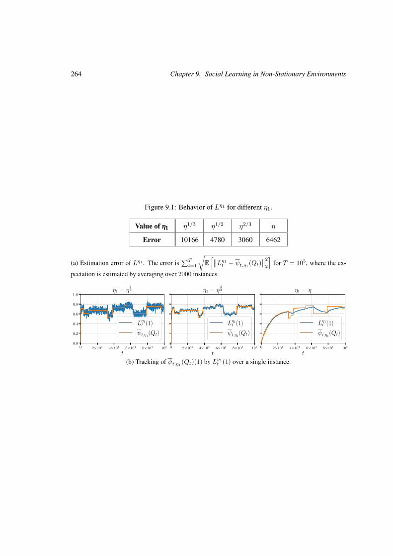
264 Chapter 9. Social Learning in Non-Stationary Environments
Figure 9.1: Behavior of Lη1 for different η1.
Value of η1η1η1 η1/3 η1/2 η2/3 η
Error 10166 4780 3060 6462
(a) Estimation error of Lη1 . The error is∑Tt=1
√E[∥∥Lη1
t − ψt,η1(Qt)∥∥2
2
]for T = 105, where the ex-
pectation is estimated by averaging over 2000 instances.
0 2×10⁴ 4×10⁴ 6×10⁴ 8×10⁴ 105
t
0.0
0.2
0.4
0.6
0.8
1.0η1 = η
12
Lη1t (1)
ψt,η1(Qt)
0 2×10⁴ 4×10⁴ 6×10⁴ 8×10⁴ 105
t
η1 = η23
Lη1t (1)
ψt,η1(Qt)
0 2×10⁴ 4×10⁴ 6×10⁴ 8×10⁴ 105
t
η1 = η
Lη1t (1)
ψt,η1(Qt)
(b) Tracking of ψt,η1(Qt)(1) by Lη1t (1) over a single instance.
Conclusion
This thesis considered several instances of interacting learning agents and studied how they
might behave to maximize either their earned individual reward in the case of selfish agents or
the total social welfare in the case of cooperative agents.
In the latter case, we showed that decentralized agents could still reach performances sim-
ilar to centralized algorithms, implying a negligible cost of decentralization. In particular, we
proposed algorithms comparable to centralized ones in multiplayer bandits using collision infor-
mation as a medium of communication between the players. In the homogeneous case, Chapter 4
proved that the optimal centralized performance is also reachable for decentralized agents. We
also proposed in Chapter 5 the first log(T )-regret algorithm in the heterogeneous setting. Simi-
larly, Chapter 7 proposed the first stable decentralized algorithm when the ratio between service
and arrival rates is larger than 1, which is also the criterion of stability for centralized algorithms.
The existence of decentralized strategies comparable to centralized algorithms might be due
to an oversimplification in the considered models. For example in multiplayer bandits, the pro-
posed algorithms use undesirable communication schemes in practice. Future work on these
topics should work on lifting unrealistic model assumptions to avoid such behaviors. Several of
these directions for multiplayer bandits were mentioned in Chapter 3 and include the following:
more limited feedback (no sensing), different collision models, non-stochasticity of the reward,
non-collaborative players or asynchronicity of the players.
Except for this last consideration, algorithms relying on similar communication schemes
also yield good performances in these harder models. For instance, the gap between no sensing
and collision sensing was recently almost closed (Huang et al., 2021). Also, Chapter 6 proposed
an algorithm robust to selfish players that still reach a regret comparable to the centralized case,
through the use of a Grim Trigger strategy. Assuming selfish players actually extended the gap
between homogeneous and heterogeneous setting, as the optimal allocation is no more reachable
and the existence of Grim Trigger strategies is only known with a limited level of heterogeneity.
We thus believe that the most crucial and oversimplifying assumption is the synchronicity of
the players. We propose in Chapter 4 a first log(T ) regret algorithm in a particular dynamic
265
266 Chapter 9. Social Learning in Non-Stationary Environments
setting, yet a lot remains to be found in either more general dynamic or asynchronous settings,
where players do not share common time slots. Our algorithms indeed heavily rely on this
synchronisation assumption to coordinate the communication schemes between the different
players, allowing to transmit messages between them perfectly.
In queuing systems, even selfish players have interest in cooperating, as the decentralized
strategy proposed in Chapter 7 is a correlated equilibrium of the patient game introduced by
Gaitonde and Tardos (2020b). Here again, the synchronisation assumption is widely used to
allow the queues to accurately estimate both the clearing probabilities of the servers and the
arrival rates of the other queues. While the model already presents some level of asynchronicity,
studying a more asynchronous and/or dynamic model also forms a main focus of future work
for this problem, for example through the use of adapted Glauber dynamics (see e.g., Shah and
Shin, 2012).
The other problems considered in this thesis raised different issues that also help to grasp
the different levels of interplay that might occur between multiple learning agents.
In Chapter 8, we proposed heuristics for balancing short term (greedily bidding) and long
term costs (concealing private information) in repeated online auctions. We formalized a new
utility-privacy trade-off problem to compute strategies revealing private information only if it
induces a significant increase in utility. For classical Bayesian costs, it benefits from recent ad-
vances in Optimal Transport. It yet leads to a non-convex minimization problem for which the
computation of global minima remains open. We believe that this work is a step towards the de-
sign of optimal utility vs. privacy trade-offs in economic mechanisms as well as for other appli-
cations. Its numerous connexions with recent topics of interest (optimization, optimal transport)
motivate a better understanding of them as future work.
Motivated by the behavior of consumers on review platforms, Chapter 9 was a first attempt
to use a change-point framework for social learning in online markets with reviews when the
qualities of a product vary over time. We provided a tight bound of the utility loss when the
quality space is 0, 1d. For more general quality spaces (e.g., continuous), determining the
incurred regret is a much harder problem. Many other directions also remain open for review
based markets. For instance, it would be interesting to study a model with a slowly drifting
quality, rather than abrupt changes. This work only focused on the consumer side, but the seller
can also adaptively set the price of the item. What is a good seller strategy in this case? The
selling platform can also design the format of the feedback given by the consumers. Determining
the format which allows the best possible convergence rate might also be of great interest in
practice. Considering perfect Bayesian consumers might be unrealistic. In reality, consumers
have limited computation capacity or can be risk averse, leading to different behaviors. Studying
9.B. Continuous quality 267
the effects of these limitations is also of great interest.
Finally, this thesis grasped only in a small part the kind of interactions that might happen
between learning agents. The observed behaviors highly depend on the considered model as
illustrated all along this thesis. Many questions then remain open and we believe that the ques-
tions mentioned above are among the most interesting and major questions to better understand
sequential learning in strategical environments.
Bibliography
[1] A. Abdulkadiroglu and T. Sönmez. “Random serial dictatorship and the core from ran-
dom endowments in house allocation problems”. In: Econometrica 66.3 (1998), pp. 689–
701.
[2] P. Ablin, G. Peyré, and T. Moreau. “Super-efficiency of automatic differentiation for
functions defined as a minimum”. In: arXiv preprint arXiv:2002.03722 (2020).
[3] D. Acemoglu, M. A. Dahleh, I. Lobel, and A. Ozdaglar. “Bayesian learning in social
networks”. In: Rev. Econ. Stud. 78.4 (2011), pp. 1201–1236.
[4] D. Acemoglu, A. Makhdoumi, A. Malekian, and A. Ozdaglar. “Fast and slow learning
from reviews”. Tech. rep. National Bureau of Economic Research, 2017.
[5] M. Adamczyk, P. Sankowski, and Q. Zhang. “Efficiency of truthful and symmetric
mechanisms in one-sided matching”. In: International Symposium on Algorithmic Game
Theory. Springer. 2014, pp. 13–24.
[6] R. Agrawal. “The continuum-armed bandit problem”. In: SIAM journal on control and
optimization 33.6 (1995), pp. 1926–1951.
[7] P. Alatur, K. Y. Levy, and A. Krause. “Multi-player bandits: The adversarial case”. In:
Journal of Machine Learning Research 21 (2020).
[8] K. Amin, A. Rostamizadeh, and U. Syed. “Learning prices for repeated auctions with
strategic buyers”. In: Advances in Neural Information Processing Systems. 2013, pp. 1169–
1177.
[9] K. Amin, A. Rostamizadeh, and U. Syed. “Repeated contextual auctions with strategic
buyers”. In: Advances in Neural Information Processing Systems. 2014, pp. 622–630.
[10] A. Anandkumar, N. Michael, A. K. Tang, and A. Swami. “Distributed Algorithms for
Learning and Cognitive Medium Access with Logarithmic Regret”. In: IEEE Journal on
Selected Areas in Communications 29.4 (2011), pp. 731–745.
268
Bibliography 269
[11] A. Anandkumar, N. Michael, and A. Tang. “Opportunistic spectrum access with multi-
ple users: Learning under competition”. In: 2010 Proceedings IEEE INFOCOM. IEEE.
2010, pp. 1–9.
[12] V. Anantharam, P. Varaiya, and J. Walrand. “Asymptotically efficient allocation rules
for the multiarmed bandit problem with multiple plays-Part I: I.I.D. rewards”. In: IEEE
Transactions on Automatic Control 32.11 (1987), pp. 968–976.
[13] V. Anantharam, P. Varaiya, and J. Walrand. “Asymptotically efficient allocation rules
for the multiarmed bandit problem with multiple plays-Part II: Markovian rewards”. In:
IEEE Transactions on Automatic Control 32.11 (1987), pp. 977–982.
[14] I. Arieli and M. Mueller-Frank. “A general analysis of sequential social learning”. In:
Math. Oper. Res. forthcoming (2021).
[15] I. Arieli and M. Mueller-Frank. “Multidimensional social learning”. In: Rev. Econ. Stud.
86.3 (2019), pp. 913–940.
[16] M. Arjovsky, S. Chintala, and L. Bottou. “Wasserstein generative adversarial networks”.
In: International Conference on Machine Learning. 2017, pp. 214–223.
[17] R. Arora, O. Dekel, and A. Tewari. “Online bandit learning against an adaptive adver-
sary: from regret to policy regret”. In: Proceedings of the 29th International Coference
on International Conference on Machine Learning. 2012, pp. 1747–1754.
[18] A. Attar, H. Tang, A. V. Vasilakos, F. R. Yu, and V. C. Leung. “A survey of security
challenges in cognitive radio networks: Solutions and future research directions”. In:
Proceedings of the IEEE 100.12 (2012), pp. 3172–3186.
[19] J. Audibert, S. Bubeck, and G. Lugosi. “Regret in Online Combinatorial Optimization”.
In: Math. Oper. Res. 39.1 (2014), pp. 31–45.
[20] P. Auer, N. Cesa-Bianchi, and P. Fischer. “Finite-time analysis of the multiarmed bandit
problem”. In: Machine learning 47.2-3 (2002), pp. 235–256.
[21] P. Auer, Y. Chen, P. Gajane, C.-W. Lee, H. Luo, R. Ortner, and C.-Y. Wei. “Achiev-
ing optimal dynamic regret for non-stationary bandits without prior information”. In:
Conference on Learning Theory. PMLR. 2019, pp. 159–163.
[22] P. Auer, N. Cesa-Bianchi, Y. Freund, and R. E. Schapire. “Gambling in a rigged casino:
The adversarial multi-armed bandit problem”. In: Proceedings of IEEE 36th Annual
Foundations of Computer Science. IEEE. 1995, pp. 322–331.
[23] P. Auer, N. Cesa-Bianchi, Y. Freund, and R. E. Schapire. “The nonstochastic multiarmed
bandit problem”. In: SIAM journal on computing 32.1 (2002), pp. 48–77.
270 Bibliography
[24] R. Aumann, M. Maschler, and R. Stearns. “Repeated games with incomplete informa-
tion”. MIT press, 1995.
[25] O. Avner and S. Mannor. “Concurrent bandits and cognitive radio networks”. In: Joint
European Conference on Machine Learning and Knowledge Discovery in Databases.
Springer. 2014, pp. 66–81.
[26] O. Avner and S. Mannor. “Learning to coordinate without communication in multi-user
multi-armed bandit problems”. In: arXiv preprint arXiv:1504.08167 (2015).
[27] O. Avner and S. Mannor. “Multi-user communication networks: A coordinated multi-
armed bandit approach”. In: IEEE/ACM Transactions on Networking 27.6 (2019), pp. 2192–
2207.
[28] B. Awerbuch and R. Kleinberg. “Competitive collaborative learning”. In: Journal of
Computer and System Sciences 74.8 (2008), pp. 1271–1288.
[29] R. Axelrod and W. D. Hamilton. “The evolution of cooperation”. In: science 211.4489
(1981), pp. 1390–1396.
[30] M. Ballu, Q. Berthet, and F. Bach. “Stochastic Optimization for Regularized Wasserstein
Estimators”. In: arXiv preprint arXiv:2002.08695 (2020).
[31] M. Bande and V. V. Veeravalli. “Multi-user multi-armed bandits for uncoordinated spec-
trum access”. In: 2019 International Conference on Computing, Networking and Com-
munications (ICNC). IEEE. 2019, pp. 653–657.
[32] M. Bande, A. Magesh, and V. V. Veeravalli. “Dynamic Spectrum Access using Stochas-
tic Multi-User Bandits”. In: arXiv preprint arXiv:2101.04388 (2021).
[33] A. V. Banerjee. “A simple model of herd behavior”. In: Quart. J. Econ. 107.3 (1992),
pp. 797–817.
[34] Y. Bar-On and Y. Mansour. “Individual regret in cooperative nonstochastic multi-armed
bandits”. In: arXiv preprint arXiv:1907.03346 (2019).
[35] S. Basu, K. A. Sankararaman, and A. Sankararaman. “Beyond log2(T ) Regret for De-
centralized Bandits in Matching Markets”. In: arXiv preprint arXiv:2103.07501 (2021).
[36] M. Bayati, N. Hamidi, R. Johari, and K. Khosravi. “Unreasonable Effectiveness of
Greedy Algorithms in Multi-Armed Bandit with Many Arms”. In: Advances in Neural
Information Processing Systems 33 (2020).
[37] J. Berger. “Schach-Jahrbuch fur 1899/1900 : fortsetzung des schach-jahrbuches fur 1892/93”.
In: Verlag von Veit (1899).
Bibliography 271
[38] Q. Berthet and V. Perchet. “Fast rates for bandit optimization with upper-confidence
Frank-Wolfe”. In: Advances in Neural Information Processing Systems. 2017, pp. 2225–
2234.
[39] D. P. Bertsekas. “Auction algorithms for network flow problems: A tutorial introduc-
tion”. In: Computational optimization and applications 1.1 (1992), pp. 7–66.
[40] O. Besbes and M. Scarsini. “On information distortions in online ratings”. In: Oper. Res.
66.3 (2018), pp. 597–610.
[41] O. Besbes, Y. Gur, and A. Zeevi. “Non-stationary stochastic optimization”. In: Oper.
Res. 63.5 (2015), pp. 1227–1244.
[42] O. Besbes, Y. Gur, and A. Zeevi. “Optimal exploration-exploitation in a multi-armed
bandit problem with non-stationary rewards”. In: Stoch. Syst. 9.4 (2019), pp. 319–337.
[43] L. Besson and E. Kaufmann. “Lower Bound for Multi-Player Bandits: Erratum for the
paper Multi-player bandits revisited”. 2019.
[44] L. Besson and E. Kaufmann. “Multi-Player Bandits Revisited”. In: Algorithmic Learn-
ing Theory. Lanzarote, Spain, 2018.
[45] L. Besson. “Multi-Players Bandit Algorithms for Internet of Things Networks”. PhD
thesis. CentraleSupélec, 2019.
[46] L. Besson and E. Kaufmann. “What Doubling Tricks Can and Can’t Do for Multi-Armed
Bandits”. In: arXiv.org:1803.06971 (2018).
[47] L. Besson, E. Kaufmann, O.-A. Maillard, and J. Seznec. “Efficient Change-Point Detec-
tion for Tackling Piecewise-Stationary Bandits”. In: (2020).
[48] S. Bikhchandani, D. Hirshleifer, and I. Welch. “A theory of fads, fashion, custom, and
cultural change as informational cascades”. In: J. Polit. Econ. 100.5 (1992), pp. 992–
1026.
[49] G. Birkhoff. “Tres observaciones sobre el algebra lineal”. In: Univ. Nac. Tucuman, Ser.
A 5 (1946), pp. 147–154.
[50] I. Bistritz and A. Leshem. “Distributed multi-player bandits-a game of thrones approach”.
In: Advances in Neural Information Processing Systems. 2018, pp. 7222–7232.
[51] I. Bistritz and A. Leshem. “Game of Thrones: Fully Distributed Learning for Multiplayer
Bandits”. In: Mathematics of Operations Research (2020).
[52] I. Bistritz, T. Z. Baharav, A. Leshem, and N. Bambos. “One for All and All for One:
Distributed Learning of Fair Allocations with Multi-player Bandits”. In: IEEE Journal
on Selected Areas in Information Theory (2021).
272 Bibliography
[53] A. Blum and Y. Monsour. “Learning, regret minimization, and equilibria”. In: Algorith-
mic Game Theory (2007).
[54] R. Bonnefoi, L. Besson, C. Moy, E. Kaufmann, and J. Palicot. “Multi-Armed Bandit
Learning in IoT Networks: Learning helps even in non-stationary settings”. In: Inter-
national Conference on Cognitive Radio Oriented Wireless Networks. Springer. 2017,
pp. 173–185.
[55] A. Borodin, J. Kleinberg, P. Raghavan, M. Sudan, and D. P. Williamson. “Adversar-
ial queueing theory”. In: Proceedings of the twenty-eighth annual ACM symposium on
Theory of computing. 1996, pp. 376–385.
[56] L. Bottou. “On-line learning and stochastic approximations”. In: On-Line Learning in
Neural Networks. Ed. by D. Saad. Publications of the Newton Institute. Cambridge Uni-
versity Press, 1999, pp. 9–42.
[57] F. Bourse, M. Minelli, M. Minihold, and P. Paillier. “Fast homomorphic evaluation of
deep discretized neural networks”. In: Annual International Cryptology Conference.
2018, pp. 483–512.
[58] E. Boursier and V. Perchet. “Selfish robustness and equilibria in multi-player bandits”.
In: Conference on Learning Theory. PMLR. 2020, pp. 530–581.
[59] E. Boursier and V. Perchet. “SIC-MMAB: Synchronisation Involves Communication
in Multiplayer Multi-Armed Bandits”. In: Advances in Neural Information Processing
Systems 32 (2019), pp. 12071–12080.
[60] E. Boursier and V. Perchet. “Utility/Privacy Trade-off through the lens of Optimal Trans-
port”. In: International Conference on Artificial Intelligence and Statistics. PMLR. 2020,
pp. 591–601.
[61] E. Boursier, E. Kaufmann, A. Mehrabian, and V. Perchet. “A Practical Algorithm for
Multiplayer Bandits when Arm Means Vary Among Players”. In: AISTATS 2020-23rd
International Conference on Artificial Intelligence and Statistics. 2020.
[62] E. Boursier, T. Garrec, V. Perchet, and M. Scarsini. “Making the most of your day: online
learning for optimal allocation of time”. In: arXiv preprint arXiv:2102.08087 (2021).
[63] E. Boursier, V. Perchet, and M. Scarsini. “Social Learning from Reviews in Non-Stationary
Environments”. In: arXiv preprint arXiv:2007.09996 (2020).
[64] T. Boyarski, A. Leshem, and V. Krishnamurthy. “Distributed learning in congested en-
vironments with partial information”. In: arXiv preprint arXiv:2103.15901 (2021).
Bibliography 273
[65] S. Boyd and L. Vandenberghe. “Convex optimization”. Cambridge university press,
2004.
[66] S. Brânzei and Y. Peres. “Multiplayer bandit learning, from competition to cooperation”.
In: arXiv preprint arXiv:1908.01135 (2019).
[67] S. Bubeck and N. Cesa-Bianchi. “Regret analysis of stochastic and nonstochastic multi-
armed bandit problems”. In: Foundations and Trends R© in Machine Learning 5.1 (2012),
pp. 1–122.
[68] S. Bubeck, T. Wang, and N. Viswanathan. “Multiple Identifications in Multi-Armed Ban-
dits”. In: International Conference on Machine Learning. 2013, pp. 258–265.
[69] S. Bubeck. “Convex optimization: Algorithms and complexity”. In: arXiv preprint arXiv:1405.4980
(2014).
[70] S. Bubeck and T. Budzinski. “Coordination without communication: optimal regret in
two players multi-armed bandits”. In: arXiv preprint arXiv:2002.07596 (2020).
[71] S. Bubeck, T. Budzinski, and M. Sellke. “Cooperative and Stochastic Multi-Player Multi-
Armed Bandit: Optimal Regret With Neither Communication Nor Collisions”. In: arXiv
preprint arXiv:2011.03896 (2020).
[72] S. Bubeck, Y. Li, Y. Peres, and M. Sellke. “Non-stochastic multi-player multi-armed
bandits: Optimal rate with collision information, sublinear without”. In: Conference on
Learning Theory. 2020, pp. 961–987.
[73] B. Çelen and S. Kariv. “Observational learning under imperfect information”. In: Games
Econom. Behav. 47.1 (2004), pp. 72–86.
[74] S. H. Cen and D. Shah. “Regret, stability, and fairness in matching markets with bandit
learners”. In: arXiv preprint arXiv:2102.06246 (2021).
[75] N. Cesa-Bianchi, T. Cesari, and V. Perchet. “Dynamic Pricing with Finitely Many Un-
known Valuations”. In: Algorithmic Learning Theory. 2019, pp. 247–273.
[76] N. Cesa-Bianchi and G. Lugosi. “Combinatorial bandits”. In: Journal of Computer and
System Sciences 78.5 (2012), pp. 1404–1422.
[77] N. Cesa-Bianchi and G. Lugosi. “Prediction, learning, and games”. Cambridge univer-
sity press, 2006.
[78] N. Cesa-Bianchi, T. Cesari, and C. Monteleoni. “Cooperative online learning: Keeping
your neighbors updated”. In: Algorithmic Learning Theory. PMLR. 2020, pp. 234–250.
[79] N. Cesa-Bianchi, C. Gentile, and Y. Mansour. “Delay and cooperation in nonstochastic
bandits”. In: The Journal of Machine Learning Research 20.1 (2019), pp. 613–650.
274 Bibliography
[80] A. Chambolle and T. Pock. “An introduction to continuous optimization for imaging”.
In: Acta Numerica 25 (2016), pp. 161–319.
[81] K. Chaudhuri, J. Imola, and A. Machanavajjhala. “Capacity bounded differential pri-
vacy”. In: Advances in Neural Information Processing Systems. 2019, pp. 3469–3478.
[82] N. Chen, A. Li, and K. Talluri. “Reviews and self-selection bias with operational impli-
cations”. In: Management Sci. forthcoming (2021).
[83] W. Chen, Y. Wang, and Y. Yuan. “Combinatorial multi-armed bandit: General framework
and applications”. In: International Conference on Machine Learning. 2013, pp. 151–
159.
[84] L. Chizat and F. Bach. “On the global convergence of gradient descent for over-parameterized
models using optimal transport”. In: Advances in neural information processing systems.
2018, pp. 3036–3046.
[85] K. L. Clarkson. “Coresets, sparse greedy approximation, and the Frank-Wolfe algo-
rithm”. In: ACM Transactions on Algorithms (TALG) 6.4 (2010), pp. 1–30.
[86] R. Combes, M. S. Talebi, A. Proutiere, and M. Lelarge. “Combinatorial bandits revis-
ited”. In: Proceedings of the 28th International Conference on Neural Information Pro-
cessing Systems-Volume 2. 2015, pp. 2116–2124.
[87] J. Correa, M. Mari, and A. Xia. “Dynamic pricing with Bayesian updates from online
reviews”. Tech. rep. 2020.
[88] N Courty, R. Flamary, and D. Tuia. “Domain adaptation with regularized optimal trans-
port”. In: Joint European Conference on Machine Learning and Knowledge Discovery
in Databases. 2014, pp. 274–289.
[89] D. Crapis, B. Ifrach, C. Maglaras, and M. Scarsini. “Monopoly pricing in the presence
of social learning”. In: Management Sci. 63.11 (2017), pp. 3586–3608.
[90] M. Cuturi. “Sinkhorn distances: Lightspeed computation of optimal transport”. In: Ad-
vances in Neural Information Processing Systems. 2013, pp. 2292–2300.
[91] S. J. Darak and M. K. Hanawal. “Multi-player multi-armed bandits for stable allocation
in heterogeneous ad-hoc networks”. In: IEEE Journal on Selected Areas in Communi-
cations 37.10 (2019), pp. 2350–2363.
[92] C. Daskalakis, P. W. Goldberg, and C. H. Papadimitriou. “The complexity of computing
a Nash equilibrium”. In: SIAM Journal on Computing 39.1 (2009), pp. 195–259.
[93] R. Degenne and V. Perchet. “Anytime optimal algorithms in stochastic multi-armed ban-
dits”. In: International Conference on Machine Learning. 2016, pp. 1587–1595.
Bibliography 275
[94] R. Degenne and V. Perchet. “Combinatorial semi-bandit with known covariance”. In:
Advances in Neural Information Processing Systems. 2016, pp. 2972–2980.
[95] R. Della Vecchia and T. Cesari. “An Efficient Algorithm for Cooperative Semi-Bandits”.
In: Algorithmic Learning Theory. PMLR. 2021, pp. 529–552.
[96] O. Devolder, F. Glineur, and Y. Nesterov. “First-order methods of smooth convex opti-
mization with inexact oracle”. In: Mathematical Programming 146.1-2 (2014), pp. 37–
75.
[97] C. Dwork. “Differential privacy”. In: Encyclopedia of Cryptography and Security (2011),
pp. 338–340.
[98] C. Dwork, F. McSherry, K. Nissim, and A. Smith. “Calibrating noise to sensitivity in
private data analysis”. In: Theory of cryptography conference. Springer. 2006, pp. 265–
284.
[99] R. Eilat, K. Eliaz, and X. Mu. “Optimal Privacy-Constrained Mechanisms”. Tech. rep.
C.E.P.R. Discussion Papers, 2019.
[100] M. Feldman, T. Koren, R. Livni, Y. Mansour, and A. Zohar. “Online pricing with strate-
gic and patient buyers”. In: Advances in Neural Information Processing Systems. 2016,
pp. 3864–3872.
[101] P. Feldman, Y. Papanastasiou, and E. Segev. “Social learning and the design of new
experience goods”. In: Management Sci. 65.4 (2019), pp. 1502–1519.
[102] J. Feydy, T. Séjourné, F.-X. Vialard, S. i. Amari, A. Trouve, and G. Peyré. “Interpolat-
ing between Optimal Transport and MMD using Sinkhorn Divergences”. In: The 22nd
International Conference on Artificial Intelligence and Statistics. 2019, pp. 2681–2690.
[103] J. W. Friedman. “A non-cooperative equilibrium for supergames”. In: The Review of
Economic Studies 38.1 (1971), pp. 1–12.
[104] C. Frogner, C. Zhang, H. Mobahi, M. Araya-Polo, and T. Poggio. “Learning with a
Wasserstein Loss”. In: Advances in Neural Information Processing Systems. 2015.
[105] D. Fudenberg and E. Maskin. “The folk theorem in repeated games with discounting
or with incomplete information”. In: A Long-Run Collaboration On Long-Run Games.
World Scientific, 2009, pp. 209–230.
[106] D. Fudenberg, F. Drew, D. K. Levine, and D. K. Levine. “The theory of learning in
games”. Vol. 2. MIT press, 1998.
[107] T. Gafni and K. Cohen. “Distributed Learning over Markovian Fading Channels for
Stable Spectrum Access”. In: arXiv preprint arXiv:2101.11292 (2021).
276 Bibliography
[108] Y. Gai, B. Krishnamachari, and R. Jain. “Combinatorial network optimization with un-
known variables: Multi-armed bandits with linear rewards and individual observations”.
In: IEEE/ACM Transactions on Networking 20.5 (2012), pp. 1466–1478.
[109] J. Gaitonde and E. Tardos. “Stability and Learning in Strategic Queuing Systems”. In:
arXiv preprint arXiv:2003.07009 (2020).
[110] J. Gaitonde and E. Tardos. “Virtues of Patience in Strategic Queuing Systems”. In: arXiv
preprint arXiv:2011.10205 (2020).
[111] A. Garhwal and P. P. Bhattacharya. “A survey on dynamic spectrum access techniques
for cognitive radio”. In: International Journal of Next-Generation Networks 3.4 (2011),
p. 15.
[112] A. Garivier and O. Cappé. “The KL-UCB algorithm for bounded stochastic bandits and
beyond”. In: Conference On Learning Theory. 2011, pp. 359–376.
[113] A. Genevay, G. Peyre, and M. Cuturi. “Learning Generative Models with Sinkhorn Di-
vergences”. In: International Conference on Artificial Intelligence and Statistics. 2018,
pp. 1608–1617.
[114] A. Genevay, L. Chizat, F. Bach, M. Cuturi, and G. Peyré. “Sample Complexity of
Sinkhorn divergences”. In: The 22nd International Conference on Artificial Intelligence
and Statistics. 2019, pp. 1574–1583.
[115] A. Genevay, M. Cuturi, G. Peyré, and F. Bach. “Stochastic optimization for large-scale
optimal transport”. In: Advances in Neural Information Processing Systems. 2016, pp. 3440–
3448.
[116] L. Georgiadis, M. J. Neely, and L. Tassiulas. “Resource allocation and cross-layer con-
trol in wireless networks”. Now Publishers Inc, 2006.
[117] S. Ghosal, J. K. Ghosh, and A. W. van der Vaart. “Convergence rates of posterior distri-
butions”. In: Ann. Statist. 28.2 (2000), pp. 500–531.
[118] R. Gilad-Bachrach, N. Dowlin, K. Laine, K. Lauter, M. Naehrig, and J. Wernsing. “Cryp-
tonets: Applying neural networks to encrypted data with high throughput and accuracy”.
In: International Conference on Machine Learning. 2016, pp. 201–210.
[119] N. Golrezaei, A. Javanmard, and V. Mirrokni. “Dynamic incentive-aware learning: Ro-
bust pricing in contextual auctions”. In: Advances in Neural Information Processing
Systems. 2019, pp. 9756–9766.
[120] J. Guélat and P. Marcotte. “Some comments on Wolfe’s ‘away step’”. In: Mathematical
Programming 35.1 (1986), pp. 110–119.
Bibliography 277
[121] S. Hart and A. Mas-Colell. “A simple adaptive procedure leading to correlated equilib-
rium”. In: Econometrica 68.5 (2000), pp. 1127–1150.
[122] E. Hendrix, G. Boglárka, et al. “Introduction to nonlinear and global optimization”.
Vol. 37. Springer, 2010.
[123] G. Hinton, N. Srivastava, and K. Swersky. “Neural networks for machine learning lec-
ture 6a overview of mini-batch gradient descent”. In: Cited on 14.8 (2012).
[124] W. Hoeffding. “Probability inequalities for sums of bounded random variables”. In:
Journal of the American Statistical Association 58 (1963), pp. 13–30.
[125] R. Horst and N. Thoai. “DC programming: overview”. In: Journal of Optimization The-
ory and Applications 103.1 (1999), pp. 1–43.
[126] R. Horst, P. Pardalos, and N. V. Thoai. “Introduction to global optimization”. Springer
Science & Business Media, 2000.
[127] W. Huang, R. Combes, and C. Trinh. “Towards Optimal Algorithms for Multi-Player
Bandits without Collision Sensing Information”. In: arXiv preprint arXiv:2103.13059
(2021).
[128] B. Ifrach, C. Maglaras, M. Scarsini, and A. Zseleva. “Bayesian social learning from
consumer reviews”. In: Oper. Res. 67.5 (2019), pp. 1209–1221.
[129] M. Jaggi. “Revisiting Frank-Wolfe: Projection-free sparse convex optimization”. In:
Proceedings of the 30th international conference on machine learning. 2013, pp. 427–
435.
[130] M. Jedor, J. Louëdec, and V. Perchet. “Be Greedy in Multi-Armed Bandits”. In: arXiv
preprint arXiv:2101.01086 (2021).
[131] L. Jiang and J. Walrand. “A distributed CSMA algorithm for throughput and utility maxi-
mization in wireless networks”. In: IEEE/ACM Transactions on Networking 18.3 (2009),
pp. 960–972.
[132] H. Joshi, R. Kumar, A. Yadav, and S. J. Darak. “Distributed algorithm for dynamic
spectrum access in infrastructure-less cognitive radio network”. In: 2018 IEEE Wireless
Communications and Networking Conference (WCNC). 2018, pp. 1–6.
[133] W. Jouini, D. Ernst, C. Moy, and J. Palicot. “Multi-armed bandit based policies for
cognitive radio’s decision making issues”. In: 2009 3rd International Conference on
Signals, Circuits and Systems (SCS). 2009.
[134] W. Jouini. “Contribution to learning and decision making under uncertainty for Cogni-
tive Radio.” PhD thesis. 2012.
278 Bibliography
[135] W. Jouini, D. Ernst, C. Moy, and J. Palicot. “Upper confidence bound based decision
making strategies and dynamic spectrum access”. In: 2010 IEEE International Confer-
ence on Communications. IEEE. 2010, pp. 1–5.
[136] A. Kakhbod and G. Lanzani. “Dynamic trading in product markets with heterogeneous
learning technologies”. Tech. rep. MIT, 2021.
[137] D. Kalathil, N. Nayyar, and R. Jain. “Decentralized learning for multiplayer multiarmed
bandits”. In: IEEE Transactions on Information Theory 60.4 (2014), pp. 2331–2345.
[138] E. Kaufmann, N. Korda, and R. Munos. “Thompson Sampling: An Asymptotically Op-
timal Finite Time Analysis”. In: Algorithmic Learning Theory (2012).
[139] D. Kingma and J. Ba. “Adam: A method for stochastic optimization”. In: arXiv preprint
arXiv:1412.6980 (2014).
[140] P. Knight. “The Sinkhorn–Knopp algorithm: convergence and applications”. In: SIAM
Journal on Matrix Analysis and Applications 30.1 (2008), pp. 261–275.
[141] J. Komiyama, J. Honda, and H. Nakagawa. “Optimal Regret Analysis of Thompson
Sampling in Stochastic Multi-armed Bandit Problem with Multiple Plays”. In: Interna-
tional Conference on Machine Learning. 2015, pp. 1152–1161.
[142] E. Koutsoupias and C. Papadimitriou. “Worst-case equilibria”. In: Annual Symposium
on Theoretical Aspects of Computer Science. Springer. 1999, pp. 404–413.
[143] S. Krishnasamy, R. Sen, R. Johari, and S. Shakkottai. “Regret of queueing bandits”. In:
CoRR, abs/1604.06377 (2016).
[144] R. Kumar, A. Yadav, S. J. Darak, and M. K. Hanawal. “Trekking based distributed al-
gorithm for opportunistic spectrum access in infrastructure-less network”. In: 2018 16th
International Symposium on Modeling and Optimization in Mobile, Ad Hoc, and Wire-
less Networks (WiOpt). 2018.
[145] R. Kumar, S. J. Darak, A. K. Sharma, and R. Tripathi. “Two-stage decision making
policy for opportunistic spectrum access and validation on USRP testbed”. In: Wireless
Networks 24.5 (2018), pp. 1509–1523.
[146] B. Kveton, Z. Wen, A. Ashkan, and C. Szepesvari. “Tight regret bounds for stochastic
combinatorial semi-bandits”. In: Artificial Intelligence and Statistics. 2015, pp. 535–
543.
[147] T. L. Lai and H. Robbins. “Asymptotically efficient adaptive allocation rules”. In: Ad-
vances in applied mathematics 6.1 (1985), pp. 4–22.
Bibliography 279
[148] P. Landgren, V. Srivastava, and N. E. Leonard. “On distributed cooperative decision-
making in multiarmed bandits”. In: 2016 European Control Conference (ECC). IEEE.
2016, pp. 243–248.
[149] J. Lasserre. “Global Optimization with Polynomials and the Problem of Moments”. In:
SIAM Journal on Optimization 11.3 (2001), pp. 796–817.
[150] T. Lattimore and C. Szepesvári. “Bandit algorithms”. In: preprint (2018), p. 28.
[151] L. Le Cam and G. L. Yang. “Asymptotics in Statistics”. Second. Springer-Verlag, New
York, 2000, pp. xiv+285.
[152] R. P. Leme, M. Pal, and S. Vassilvitskii. “A field guide to personalized reserve prices”.
In: Proceedings of the 25th international conference on world wide web. 2016, pp. 1093–
1102.
[153] Y. Li and Y. Yuan. “Convergence analysis of two-layer neural networks with relu activa-
tion”. In: Advances in neural information processing systems. 2017, pp. 597–607.
[154] T. Lin, C. Jin, and M. Jordan. “Near-optimal algorithms for minimax optimization”. In:
arXiv preprint arXiv:2002.02417 (2020).
[155] T. Lin, C. Jin, and M. Jordan. “On gradient descent ascent for nonconvex-concave min-
imax problems”. In: arXiv preprint arXiv:1906.00331 (2019).
[156] K. Liu and Q. Zhao. “Distributed Learning in Multi-Armed Bandit With Multiple Play-
ers”. In: IEEE Transactions on Signal Processing 58.11 (2010), pp. 5667–5681.
[157] K. Liu and Q. Zhao. “A restless bandit formulation of opportunistic access: Index-
ablity and index policy”. In: 2008 5th IEEE Annual Communications Society Conference
on Sensor, Mesh and Ad Hoc Communications and Networks Workshops. IEEE. 2008,
pp. 1–5.
[158] L. T. Liu, F. Ruan, H. Mania, and M. I. Jordan. “Bandit Learning in Decentralized Match-
ing Markets”. In: arXiv preprint arXiv:2012.07348 (2020).
[159] L. T. Liu, H. Mania, and M. Jordan. “Competing bandits in matching markets”. In: In-
ternational Conference on Artificial Intelligence and Statistics. PMLR. 2020, pp. 1618–
1628.
[160] I. Lobel and E. Sadler. “Information diffusion in networks through social learning”. In:
Theor. Econ. 10.3 (2015), pp. 807–851.
[161] S. Lu, I. Tsaknakis, M. Hong, and Y. Chen. “Hybrid block successive approximation
for one-sided non-convex min-max problems: algorithms and applications”. In: IEEE
Transactions on Signal Processing (2020).
280 Bibliography
[162] G. Lugosi and A. Mehrabian. “Multiplayer bandits without observing collision informa-
tion”. In: arXiv preprint arXiv:1808.08416 (2018).
[163] B. Mackowiak and M. Wiederholt. “Business cycle dynamics under rational inattention”.
In: The Review of Economic Studies 82.4 (2015), pp. 1502–1532.
[164] A. Magesh and V. Veeravalli. “Multi-player Multi-Armed Bandits with non-zero rewards
on collisions for uncoordinated spectrum access”. In: arXiv preprint arXiv:1910.09089
(2019).
[165] A. Magesh and V. V. Veeravalli. “Multi-User MABs with User Dependent Rewards for
Uncoordinated Spectrum Access”. In: 2019 53rd Asilomar Conference on Signals, Sys-
tems, and Computers. IEEE. 2019, pp. 969–972.
[166] C. Maglaras, M. Scarsini, and S. Vaccari. “Social learning from online reviews with
product choice”. Tech. rep. Columbia Business School Research Paper No. 18-17, 2020.
[167] J. R. Marden, H. P. Young, and L. Y. Pao. “Achieving pareto optimality through dis-
tributed learning”. In: SIAM Journal on Control and Optimization 52.5 (2014), pp. 2753–
2770.
[168] J. Marinho and E. Monteiro. “Cognitive radio: survey on communication protocols,
spectrum decision issues, and future research directions”. In: Wireless networks 18.2
(2012), pp. 147–164.
[169] A. W. Marshall, I. Olkin, and B. C. Arnold. “Inequalities: theory of majorization and its
applications”. Vol. 143. Springer, 1979.
[170] D. Martínez-Rubio, V. Kanade, and P. Rebeschini. “Decentralized Cooperative Stochas-
tic Bandits”. In: arXiv preprint arXiv:1810.04468 (2018).
[171] F. Matejka and A. McKay. “Rational inattention to discrete choices: A new foundation
for the multinomial logit model”. In: American Economic Review 105.1 (2015), pp. 272–
98.
[172] I. Mironov. “Rényi Differential Privacy”. In: Proceedings of 30th IEEE Computer Secu-
rity Foundations Symposium (CSF). 2017, pp. 263–275.
[173] J. Mitola and G. Q. Maguire. “Cognitive radio: making software radios more personal”.
In: IEEE Personal Communications 6.4 (1999), pp. 13–18.
[174] J. Munkres. “Algorithms for the assignment and transportation problems”. In: J. Soc.
Indust. Appl. Math. 5 (1957), pp. 32–38.
[175] R. Murphy. “Local Consumer Review Survey 2019”. In: BrightLocal (2019). URL: brightlocal.
com/research/local-consumer-review-survey.

Bibliography 281
[176] N. Nayyar, D. Kalathil, and R. Jain. “On regret-optimal learning in decentralized multi-
player multiarmed bandits”. In: IEEE Transactions on Control of Network Systems 5.1
(2016), pp. 597–606.
[177] T. Nedelec, N. E. Karoui, and V. Perchet. “Learning to bid in revenue-maximizing auc-
tions”. In: International Conference on Machine Learning. 2019, pp. 4781–4789.
[178] A. Nedic and A. Ozdaglar. “Subgradient methods for saddle-point problems”. In: Jour-
nal of optimization theory and applications 142.1 (2009), pp. 205–228.
[179] M. J. Neely, E. Modiano, and C.-P. Li. “Fairness and optimal stochastic control for het-
erogeneous networks”. In: IEEE/ACM Transactions On Networking 16.2 (2008), pp. 396–
409.
[180] M. Nouiehed, M. Sanjabi, T. Huang, J. Lee, and M. Razaviyayn. “Solving a class of
non-convex min-max games using iterative first order methods”. In: Advances in Neural
Information Processing Systems. 2019, pp. 14934–14942.
[181] D. Ostrovskii, A. Lowy, and M. Razaviyayn. “Efficient search of first-order nash equilib-
ria in nonconvex-concave smooth min-max problems”. In: arXiv preprint arXiv:2002.07919
(2020).
[182] Y. Papanastasiou and N. Savva. “Dynamic pricing in the presence of social learning and
strategic consumers”. In: Management Sci. 63.4 (2017), pp. 919–939.
[183] S. Park, W. Shin, and J. Xie. “The fateful first consumer review”. In: Marketing Sci. 40.3
(2021), pp. 481–507.
[184] R. Pemantle and J. S. Rosenthal. “Moment conditions for a sequence with negative drift
to be uniformly bounded in Lr”. In: Stochastic Processes and their Applications 82.1
(1999), pp. 143–155.
[185] V. Perchet and P. Rigollet. “The multi-armed bandit problem with covariates”. In: The
Annals of Statistics 41.2 (2013), pp. 693–721.
[186] V. Perchet, P. Rigollet, S. Chassang, and E. Snowberg. “Batched Bandit Problems”. In:
Proceedings of The 28th Conference on Learning Theory. 2015, pp. 1456–1456.
[187] V. Perchet. “Approachability, regret and calibration: Implications and equivalences”. In:
Journal of Dynamics & Games 1.2 (2014), p. 181.
[188] P. Perrault, E. Boursier, M. Valko, and V. Perchet. “Statistical efficiency of thompson
sampling for combinatorial semi-bandits”. In: Advances in Neural Information Process-
ing Systems 33 (2020).
282 Bibliography
[189] G. Peyré and M. Cuturi. “Computational optimal transport”. In: Foundations and Trends R©in Machine Learning 11.5-6 (2019), pp. 355–607.
[190] A. Proutiere and P. Wang. “An Optimal Algorithm in Multiplayer Multi-Armed Ban-
dits”. 2019.
[191] H. Rafique, M. Liu, Q. Lin, and T. Yang. “Non-convex min-max optimization: Provable
algorithms and applications in machine learning”. In: arXiv preprint arXiv:1810.02060
(2018).
[192] S. Reddi, S. Kale, and S. Kumar. “On the convergence of adam and beyond”. In: arXiv
preprint arXiv:1904.09237 (2019).
[193] J. Reed and B. Pierce. “Distance makes the types grow stronger: a calculus for differen-
tial privacy”. In: ACM Sigplan Notices. Vol. 45. 9. 2010, pp. 157–168.
[194] A. Rényi. “On measures of entropy and information”. In: Proceedings of the Fourth
Berkeley Symposium on Mathematical Statistics and Probability, Volume 1: Contribu-
tions to the Theory of Statistics. 1961.
[195] H. Robbins. “Some aspects of the sequential design of experiments”. In: Bulletin of the
American Mathematical Society 58.5 (1952), pp. 527–535.
[196] C. Robert, C. Moy, and H. Zhang. “Opportunistic Spectrum Access Learning Proof of
Concept”. In: SDR-WinnComm’14 (2014), p. 8.
[197] D. Rosenberg and N. Vieille. “On the efficiency of social learning”. In: Econometrica
87.6 (2019), pp. 2141–2168.
[198] J. Rosenski, O. Shamir, and L. Szlak. “Multi-player bandits–a musical chairs approach”.
In: International Conference on Machine Learning. 2016, pp. 155–163.
[199] T. Roughgarden. “Algorithmic game theory”. In: Communications of the ACM 53.7
(2010), pp. 78–86.
[200] T. Salimans, D. Metaxas, H. Zhang, and A. Radford. “Improving GANs using optimal
transport”. In: 6th International Conference on Learning Representations, ICLR 2018.
2018.
[201] A. Sankararaman, S. Basu, and K. A. Sankararaman. “Dominate or Delete: Decentral-
ized Competing Bandits with Uniform Valuation”. In: arXiv preprint arXiv:2006.15166
(2020).
[202] F. Santambrogio. “Optimal transport for applied mathematicians”. In: Birkäuser, NY 55
(2015), pp. 58–63.
Bibliography 283
[203] A. Sanyal, M. Kusner, A. Gascon, and V. Kanade. “TAPAS: Tricks to Accelerate (en-
crypted) Prediction As a Service”. In: International Conference on Machine Learning.
2018, pp. 4497–4506.
[204] S. Sawant, M. K. Hanawal, S. Darak, and R. Kumar. “Distributed learning algorithms for
coordination in a cognitive network in presence of jammers”. In: 2018 16th International
Symposium on Modeling and Optimization in Mobile, Ad Hoc, and Wireless Networks
(WiOpt). IEEE. 2018, pp. 1–8.
[205] S. Sawant, R. Kumar, M. K. Hanawal, and S. J. Darak. “Learning to Coordinate in a De-
centralized Cognitive Radio Network in Presence of Jammers”. In: IEEE Transactions
on Mobile Computing (2019).
[206] A. S. Schulz and N. E. S. Moses. “On the performance of user equilibria in traffic net-
works.” In: SODA. Vol. 3. 2003, pp. 86–87.
[207] F. Sentenac, E. Boursier, and V. Perchet. “Decentralized Learning in Online Queuing
Systems”. In: arXiv preprint arXiv:2106.04228 (2021).
[208] Y. Sergeyev, R. Strongin, and D. Lera. “Introduction to global optimization exploiting
space-filling curves”. Springer Science & Business Media, 2013.
[209] D. Shah and J. Shin. “Randomized scheduling algorithm for queueing networks”. In:
The Annals of Applied Probability 22.1 (2012), pp. 128–171.
[210] C. Shi and C. Shen. “On No-Sensing Adversarial Multi-player Multi-armed Bandits with
Collision Communications”. In: arXiv preprint arXiv:2011.01090 (2020).
[211] C. Shi, W. Xiong, C. Shen, and J. Yang. “Decentralized Multi-player Multi-armed Ban-
dits with No Collision Information”. In: arXiv preprint arXiv:2003.00162 (2020).
[212] J. F. Shortle, J. M. Thompson, D. Gross, and C. M. Harris. “Fundamentals of queueing
theory”. Vol. 399. John Wiley & Sons, 2018.
[213] C. Sims. “Implications of rational inattention”. In: Journal of monetary Economics 50.3
(2003), pp. 665–690.
[214] R. Sinkhorn. “Diagonal equivalence to matrices with prescribed row and column sums”.
In: The American Mathematical Monthly 74.4 (1967), pp. 402–405.
[215] A. Slivkins. “Introduction to multi-armed bandits”. In: arXiv preprint arXiv:1904.07272
(2019).
[216] G. Smith. “On the foundations of quantitative information flow”. In: International Con-
ference on Foundations of Software Science and Computational Structures. 2009, pp. 288–
302.
284 Bibliography
[217] L. Smith and P. Sørensen. “Pathological outcomes of observational learning”. In: Econo-
metrica 68.2 (2000), pp. 371–398.
[218] M. Soltanolkotabi, A. Javanmard, and J. Lee. “Theoretical insights into the optimization
landscape of over-parameterized shallow neural networks”. In: IEEE Transactions on
Information Theory 65.2 (2018), pp. 742–769.
[219] D. Soudry and E. Hoffer. “Exponentially vanishing sub-optimal local minima in multi-
layer neural networks”. In: arXiv preprint arXiv:1702.05777 (2017).
[220] L.-G. Svensson. “Strategy-proof allocation of indivisible goods”. In: Social Choice and
Welfare 16.4 (1999), pp. 557–567.
[221] B. Szorenyi, R. Busa-Fekete, I. Hegedus, R. Ormándi, M. Jelasity, and B. Kégl. “Gossip-
based distributed stochastic bandit algorithms”. In: International Conference on Ma-
chine Learning. 2013, pp. 19–27.
[222] P. Tao and L. An. “Convex analysis approach to DC programming: Theory, algorithms
and applications”. In: Acta mathematica vietnamica 22.1 (1997), pp. 289–355.
[223] L. Tassiulas and A. Ephremides. “Stability properties of constrained queueing systems
and scheduling policies for maximum throughput in multihop radio networks”. In: 29th
IEEE Conference on Decision and Control. IEEE. 1990, pp. 2130–2132.
[224] C. Tekin and M. Liu. “Online learning in decentralized multi-user spectrum access with
synchronized explorations”. In: MILCOM 2012-2012 IEEE Military Communications
Conference. IEEE. 2012, pp. 1–6.
[225] K. Thekumparampil, P. Jain, P. Netrapalli, and S. Oh. “Efficient algorithms for smooth
minimax optimization”. In: Advances in Neural Information Processing Systems. 2019,
pp. 12680–12691.
[226] W. R. Thompson. “On the Likelihood that one unknown probability exceeds another in
view of the evidence of two samples”. In: Biometrika 25.3-4 (1933), pp. 285–294.
[227] H. Tibrewal, S. Patchala, M. K. Hanawal, and S. J. Darak. “Distributed Learning and
Optimal Assignment in Multiplayer Heterogeneous Networks”. In: IEEE INFOCOM
2019. 2019, pp. 1693–1701.
[228] G. Tóth, Z. Hornák, and F. Vajda. “Measuring anonymity revisited”. In: Proceedings of
the Ninth Nordic Workshop on Secure IT Systems. 2004, pp. 85–90.
[229] A. B. Tsybakov. “Introduction to Nonparametric Estimation”. Springer, New York, 2009,
pp. xii+214.
Bibliography 285
[230] L. Venturi, A. Bandeira, and J. Bruna. “Spurious valleys in two-layer neural network
optimization landscapes”. In: arXiv preprint arXiv:1802.06384 (2018).
[231] A. Verma, M. K. Hanawal, and R. Vaze. “Distributed algorithms for efficient learning
and coordination in ad hoc networks”. In: 2019 International Symposium on Modeling
and Optimization in Mobile, Ad Hoc, and Wireless Networks (WiOPT). IEEE. 2019,
pp. 1–8.
[232] D. Vial, S. Shakkottai, and R Srikant. “Robust Multi-Agent Multi-Armed Bandits”. In:
arXiv preprint arXiv:2007.03812 (2020).
[233] C. Villani. “Optimal transport: old and new”. Vol. 338. Springer Science & Business
Media, 2008.
[234] M. J. Wainwright. “High-dimensional statistics: A non-asymptotic viewpoint”. Vol. 48.
Cambridge University Press, 2019.
[235] P.-A. Wang, A. Proutiere, K. Ariu, Y. Jedra, and A. Russo. “Optimal algorithms for
multiplayer multi-armed bandits”. In: International Conference on Artificial Intelligence
and Statistics. PMLR. 2020, pp. 4120–4129.
[236] Q. Wang, K. Ren, P. Ning, and S. Hu. “Jamming-resistant multiradio multichannel op-
portunistic spectrum access in cognitive radio networks”. In: IEEE Transactions on Ve-
hicular Technology 65.10 (2015), pp. 8331–8344.
[237] S. Wang and W. Chen. “Thompson Sampling for Combinatorial Semi-Bandits”. In: In-
ternational Conference on Machine Learning. 2018, pp. 5114–5122.
[238] L. Wei and V. Srivastava. “On Distributed Multi-Player Multiarmed Bandit Problems in
Abruptly Changing Environment”. In: 2018 IEEE Conference on Decision and Control
(CDC). IEEE. 2018, pp. 5783–5788.
[239] M. Woodroofe. “A one-armed bandit problem with a concomitant variable”. In: Journal
of the American Statistical Association 74.368 (1979), pp. 799–806.
[240] S. Wright. “Coordinate descent algorithms”. In: Mathematical Programming 151.1 (2015),
pp. 3–34.
[241] R. R. Yager. “On ordered weighted averaging aggregation operators in multicriteria de-
cisionmaking”. In: IEEE Transactions on systems, Man, and Cybernetics 18.1 (1988),
pp. 183–190.
[242] M.-J. Youssef, V. Veeravalli, J. Farah, and C. A. Nour. “Stochastic Multi-Player Multi-
Armed Bandits with Multiple Plays for Uncoordinated Spectrum Access”. In: PIMRC
2020: IEEE International Symposium on Personal, Indoor and Mobile Radio Commu-
nications. 2020.
[243] Q. Zhao and B. M. Sadler. “A survey of dynamic spectrum access”. In: IEEE signal
processing magazine 24.3 (2007), pp. 79–89.
[244] L. Zhou. “On a conjecture by Gale about one-sided matching problems”. In: Journal of
Economic Theory 52.1 (1990), pp. 123–135.
[245] F. Zou, L. Shen, Z. Jie, W. Zhang, and W. Liu. “A sufficient condition for convergences
of adam and rmsprop”. In: Proceedings of the IEEE conference on computer vision and
pattern recognition. 2019, pp. 11127–11135.
Titre: Apprentissage séquentiel dans un environnement stratégique
Mots clés: Apprentissage séquentiel, Bandits à plusieurs joueurs, Théorie des jeux, Jeux répétés
Résumé: En apprentissage séquentiel (ou jeuxrépétés), les données sont acquises et traitées à lavolée et un algorithme (ou stratégie) apprend à secomporter aussi bien que s’il avait pu observer l’étatde nature, par exemple les distributions des gains.Dans de nombreuses situations réelles, de tels agentsintelligents ne sont pas seuls et interagissent ou in-terfèrent avec d’autres. Ainsi, leurs décisions ontun impact direct sur les autres agents et indirecte-ment sur leurs propres gains à venir. Nous étudionsde quelle manière les algorithmes d’apprentissageséquentiel peuvent se comporter dans des environ-nements stratégiques quand ils sont confrontés àd’autres agents.
Cette thèse considère différents problèmes oùcertaines interactions entre des agents intelligents
apparaissent, pour lesquels nous proposes des algo-rithmes efficaces en termes de calcul avec de bonnesgaranties de performance (faible regret).
Lorsque les agents sont coopératifs, la difficultédu problème vient de son aspect décentralisé, étantdonné que les agents prennent leurs décisions ense basant seulement sur leurs propres observations.Dans ce cas, les algorithmes proposés non seule-ment coordonnent les agents afin d’éviter des inter-férences entre eux, mais ils utilisent également cesinterférences pour transférer de l’information entreles agents. Cela permet d’obtenir des performancescomparables aux meilleurs algorithmes centralisés.Avec des agents en concurrence, nous proposons desalgorithmes avec des garanties satisfaisantes, à la foisen terme de performance et de stratégie (ε-équilibrede Nash par exemple).
Title: Sequential Learning in a strategical environment
Keywords: Online Learning, Multiplayer bandits, Game Theory, Repeated Games
Abstract: In sequential learning (or repeatedgames), data is acquired and treated on the fly andan algorithm (or strategy) learns to behave as wellas if it got in hindsight the state of nature, e.g., dis-tributions of rewards. In many real life scenarios,learning agents are not alone and interact, or in-terfere, with many others. As a consequence, theirdecisions have an impact on the other and, by ex-tension, on the generating process of rewards. Weaim at studying how sequential learning algorithmsbehave in strategic environments, when facing andinterfering with each others. This thesis thus con-siders different problems, where some interactions
between learning agents arise and provides computa-tionally efficient algorithms with good performance(small regret) guarantees.
When agents are cooperative, the difficulty ofthe problem comes from its decentralized aspect, asthe different agents take decisions solely based ontheir observations. In this case, we propose algo-rithms that not only coordinate the agents to avoidnegative interference with each other, but also lever-age the interferences to transfer information betweenthe agents, thus reaching performances similar tocentralized algorithms. With competing agents, wepropose algorithms with both satisfying performanceand strategic (e.g., ε-Nash equilibria) guarantees.
Université Paris-SaclayEspace Technologique / Immeuble Discovery
Route de l’Orme aux Merisiers RD 128 / 91190 Saint-Aubin, France
Related Documents