Separation of Timescales in a Two-Layered Network

Separation of Timescales in a Two-Layered NetworkMaria Vlasiou∗, Jiheng Zhang†, Bert Zwart‡, Rob van der Mei‡

∗Department of Mathematics and Computer ScienceEindhoven University of Technology, P.O. Box 513, 5600 MB, Eindhoven, The Netherlands

Email: [email protected]†Department of Industrial Engineering and Logistics Management

Hong Kong University of Science and Technology, Hong Kong, S.A.R., ChinaEmail: [email protected]

‡Centrum Wiskunde & InformaticaScience Park 123, Amsterdam, The Netherlands

Email: (bert.zwart, mei)@cwi.nl

Abstract—We investigate a computer network consisting of twolayers occurring in, for example, application servers. The firstlayer incorporates the arrival of jobs at a network of multi-servernodes, which we model as a many-server Jackson network. At thesecond layer, active servers at these nodes act now as customerswho are served by a common CPU. Our main result shows aseparation of time scales in heavy traffic: the main source ofrandomness occurs at the (aggregate) CPU layer; the interactionsbetween different types of nodes at the other layer is shown toconverge to a fixed point at a faster time scale; this also yieldsa state-space collapse property. Apart from these fundamentalinsights, we also obtain an explicit approximation for the joint lawof the number of jobs in the system, which is provably accuratefor heavily loaded systems and performs numerically well formoderately loaded systems. The obtained results for the modelunder consideration can be applied to thread-pool dimensioningin application servers, while the technique seems applicable toother layered systems too.

I. INTRODUCTION

Communication networks need to support a growing di-versity and heterogeneity in applications. Examples are web-based multi-tiered system architectures, with a client tier toprovide an interface to end users, a business logic tier tocoordinate information retrieval and processing, and a data tierwith legacy systems to store and access customer data. In suchenvironments, different applications compete for access toshared infrastructure resources, both at the software level (e.g.,mutex and database locks, thread-pools) and at the hardwarelevel (e.g., bandwidth, processing power, disk access). Thus,the performance of such applications is determined by the in-terplay of software and hardware contention. For background,see [1]–[3].

In particular, in situations where web pages are created on-the-fly (think of making a reservation online), the benefitsof caching are limited and sizes of web pages are unknown,

The research of Maria Vlasiou and Jiheng Zhang is partly supported bytwo grants from the ‘Joint Research Scheme’ program, sponsored by theNetherlands Organization of Scientific Research (NWO) and the ResearchGrants Council of Hong Kong (RGC) through projects 649.000.005 and D-HK007/11T, respectively. The research of Bert Zwart is partly supported byan NWO VIDI grant and an IBM faculty award.

and there is usually ample core network bandwidth availableat reasonable prices. Consequently, the bottleneck in user-level performance can shift from the network interface to theapplication server, and implementing size-based schedulingpolicies becomes hard, contrary to the situation consideredin [4], [5].

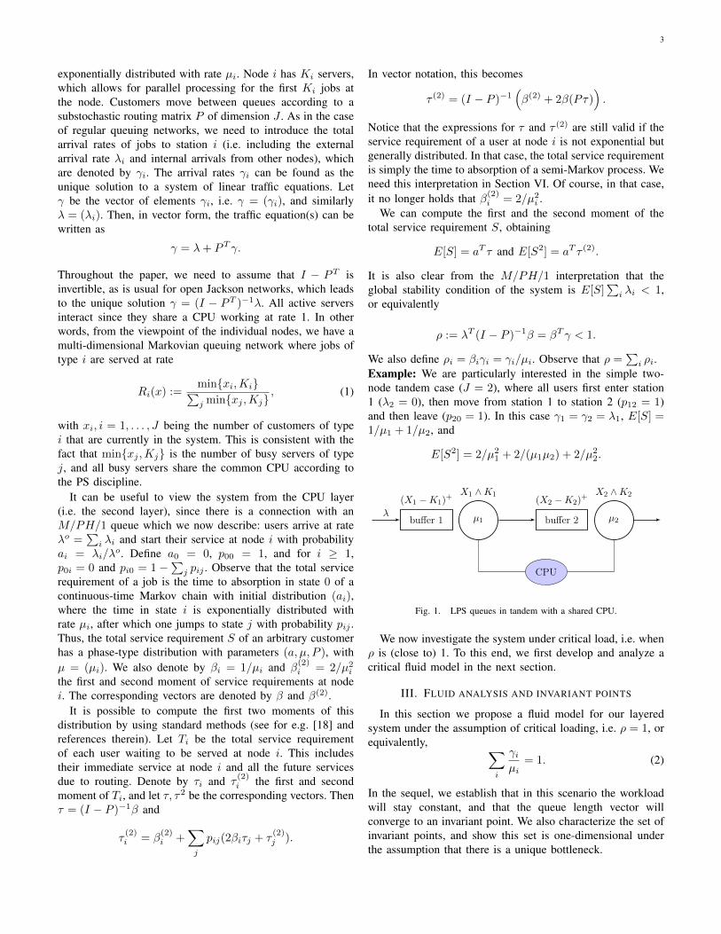
Application servers usually implement a number of thread-pools; a thread is software that can perform a specific type ofsub-transaction. Consider for example the web-server perfor-mance model proposed in [2]. Each HTTP request that requiresserver-side scripting (e.g., CGI or ASP scripts, or Java servlets)consists of two subsequent phases: a document-retrieval phase,and a script processing phase. To this end, the web serverimplements two thread-pools, one performing the first phaseof processing, and the other performing the second phase ofprocessing. The model consists of a tandem of two multi-server queues, where servers at queue 1 represent the phase-1threads, and the servers at queue 2 represent phase-2 threads.A particular feature of this model is that at all times the activethreads share a common Central Processing Unit (CPU) in aProcessor-Sharing (PS) fashion; cf. [6], [7]. Alternatively, onecan think of scheduling jobs in data centers, where differentparts of a job are taken care of by a different thread-pool.

Motivated by this, we study a relatively simple, but non-trivial two-layered network. An informal model descriptionis as follows. The first layer models the processing of jobsby a network of nodes. Each node consists of several serversand, therefore, it looks like a (generalized) Jackson networkconsisting of many-server queues. The servers in this networkact as customers in a second layer, in the sense that they areserved by a single CPU in a PS fashion. A detailed modeldescription is provided in Section II.

Variations of the above model have been investigated inseveral papers in the literature, but apart from stability analysis[6], a rigorous analysis of this layered network has beenlacking. The same can be said about other literature onlayered networks. Only a limited number of papers focuson the performance of multi-layered queuing networks. Afundamental paper is Rolia and Sevcik [8], who propose the

2

Method of Layers, i.e., a closed queuing-network based modelfor the responsiveness of client-server applications, explicitlytaking into account both software and hardware contention.Another fundamental contribution is presented by Woodsideet al. [9], who propose the so-called Stochastic RendezvousNetwork model to analyze the performance of applicationsoftware with client-server synchronization. The contributionspresented in [8] and [9] are often referred to as LayeredQueuing Models. A common drawback of multi-layered queu-ing models is that exact analysis is primarily restricted tospecial cases, and numerical algorithms are typically requiredto obtain performance measures of interest (see for example[9]). Although such methods are important, it is also valuableto look at layered systems from a more qualitative point ofview, which we do in this paper by considering the systemunder critical load.

The most simple example of the layered systems we con-sider is the case where the first layer consists of a single node.In this case, the model reduces to the so-called limited proces-sor sharing (LPS) queue. Recently, there has been considerableinterest in the analysis of LPS systems. Avi-Itzhak and Halfin[10] propose an approximation for the mean response time. Acomputational analysis based on matrix geometric methods isperformed in Zhang and Lipsky [11], [12]. Some stochasticordering results are derived in Nuyens and van der Weij[13]. Large deviation results are presented in Nair et al. [14],and these results are also applied to show that LPS providesrobust performance across a range of both heavy-tailed andlight-tailed job sizes, as it combines the attractive propertiesof a guaranteed service rate of FIFO and the possibility ofovertaking offered by PS.

The work on LPS that is most relevant for this studyis the work of Zhang, Dai and Zwart [15]–[17] who studythe stochastic processes that underlie the LPS queue in theheavy-traffic regime, i.e. an asymptotic regime where thetraffic intensity converges to 1. The setting is rather general,allowing the inter-arrival and service times to have generaldistributions. Fluid and diffusion limits are derived, leading toa heavy-traffic analysis of the steady-state distribution of LPS,showing that the approximation by Avi-Itzhak and Halfin [10]is asymptotically accurate in heavy traffic.

In the present paper, we perform an analysis similar to theone performed in [15]–[17]. Under the assumption that jobsizes are exponentially distributed, we expand the work in[15]–[17] from the single node case to networks. Moreover,based on our mathematical results, we propose an extensionto general job sizes.

We analyze the system as it approaches heavy traffic. Underthe assumption that there is a single bottleneck (an exactdefinition of bottleneck is given later), we derive explicitresults for the joint distribution of the number of jobs inthe system by proving a diffusion limit theorem. This limittheorem does not only yield explicit approximations but yieldsalso useful insights: if we look at the system from the CPUlayer, we can aggregate the whole system since the totalworkload acts as if we were dealing with a single server queue.

However, information regarding the interaction of several typesof customers at the other layer would then be lost. It turns out,nonetheless, that those interactions take place at a much fastertime scale in heavy traffic, and that the number of users of alltypes converge instantaneously to a piece-wise linear functionof the number of users at the bottleneck. This separation oftime scales property is shown to imply that in heavy traffic,the joint queue length vector can be written as a deterministicfunction of the total workload as seen from the CPU layer.Such a property is known as state-space collapse (SSC) in thestochastic network literature.

Thus, our methodological contribution is that it is possibleto rigorously establish a separation of time scales property inheavy traffic in an important class of layered networks, whichmakes these layered networks tractable. Although we focus onthe Markovian case, we believe that such properties hold moregenerally as well; we provide some physical and numericalarguments to support this claim. The result on separation oftime scales result essentially implies that the main source ofrandomness in heavy traffic can be observed at the CPU layer,thus making performance analysis much more tractable. Apartfrom supporting these claims by theorems, some numericalexperiments suggest that the resulting approximations performwell. The results in our paper may be useful to create designrules, for example to dimension thread-pools. Some first effortsusing heuristic approximations were proposed in [7].

The paper is organized as follows. We provide a detailedmodel description in Section II. In Section III we proposea fluid model for our two-layered system. We use this fluidmodel to analyze how users of different types interact if thesystem is in heavy traffic. In doing so, we construct a Lya-pounov function which we use to show that the user populationconverges uniformly to a fixed point that is uniquely definedthrough the total workload. The fluid model also helps under-stand which stations will be bottlenecks. Section IV containsour main results, namely a process limit theorem for thecustomer population process. A heavy-traffic approximationof the steady-state distribution of the customer population isproposed in Section V. Section VI presents an extension togeneral service times based on physical arguments, and somenumerical validation by comparing the proposed approxima-tions with simulation results. Concluding remarks can be foundin Section VII.

II. MODEL DESCRIPTION

The purpose of this section is to give a formal modeldescription. We adopt the convention that all vectors arecolumn vectors, and use aT to denote the transpose of avector or matrix. For two vectors x, y we denote xy to bethe vector consisting of elements xiyi. Furthermore, I is theidentity matrix, e is the vector consisting of 1’s, and ei is thevector whose ith element is 1 and the rest are all 0. Last,(x)+ = max{0, x} and a ∧ b = min{a, b}.

We consider a network with J nodes. Jobs arrive at nodei ∈ {1, . . . , J} according to a Poisson process with rate λi.Jobs have a random amount of service requirement, which is

3

exponentially distributed with rate µi. Node i has Ki servers,which allows for parallel processing for the first Ki jobs atthe node. Customers move between queues according to asubstochastic routing matrix P of dimension J . As in the caseof regular queuing networks, we need to introduce the totalarrival rates of jobs to station i (i.e. including the externalarrival rate λi and internal arrivals from other nodes), whichare denoted by γi. The arrival rates γi can be found as theunique solution to a system of linear traffic equations. Letγ be the vector of elements γi, i.e. γ = (γi), and similarlyλ = (λi). Then, in vector form, the traffic equation(s) can bewritten as

γ = λ+ PT γ.

Throughout the paper, we need to assume that I − PT isinvertible, as is usual for open Jackson networks, which leadsto the unique solution γ = (I − PT )−1λ. All active serversinteract since they share a CPU working at rate 1. In otherwords, from the viewpoint of the individual nodes, we have amulti-dimensional Markovian queuing network where jobs oftype i are served at rate

Ri(x) :=min{xi,Ki}∑j min{xj ,Kj}

, (1)

with xi, i = 1, . . . , J being the number of customers of typei that are currently in the system. This is consistent with thefact that min{xj ,Kj} is the number of busy servers of typej, and all busy servers share the common CPU according tothe PS discipline.

It can be useful to view the system from the CPU layer(i.e. the second layer), since there is a connection with anM/PH/1 queue which we now describe: users arrive at rateλo =

∑i λi and start their service at node i with probability

ai = λi/λo. Define a0 = 0, p00 = 1, and for i ≥ 1,

p0i = 0 and pi0 = 1−∑j pij . Observe that the total servicerequirement of a job is the time to absorption in state 0 of acontinuous-time Markov chain with initial distribution (ai),where the time in state i is exponentially distributed withrate µi, after which one jumps to state j with probability pij .Thus, the total service requirement S of an arbitrary customerhas a phase-type distribution with parameters (a, µ, P ), withµ = (µi). We also denote by βi = 1/µi and β

(2)i = 2/µ2

i

the first and second moment of service requirements at nodei. The corresponding vectors are denoted by β and β(2).

It is possible to compute the first two moments of thisdistribution by using standard methods (see for e.g. [18] andreferences therein). Let Ti be the total service requirementof each user waiting to be served at node i. This includestheir immediate service at node i and all the future servicesdue to routing. Denote by τi and τ

(2)i the first and second

moment of Ti, and let τ, τ2 be the corresponding vectors. Thenτ = (I − P )−1β and

τ(2)i = β

(2)i +

∑j

pij(2βiτj + τ(2)j ).

In vector notation, this becomes

τ (2) = (I − P )−1(β(2) + 2β(Pτ)

).

Notice that the expressions for τ and τ (2) are still valid if theservice requirement of a user at node i is not exponential butgenerally distributed. In that case, the total service requirementis simply the time to absorption of a semi-Markov process. Weneed this interpretation in Section VI. Of course, in that case,it no longer holds that β(2)

i = 2/µ2i .

We can compute the first and the second moment of thetotal service requirement S, obtaining

E[S] = aT τ and E[S2] = aT τ (2).

It is also clear from the M/PH/1 interpretation that theglobal stability condition of the system is E[S]

∑i λi < 1,

or equivalently

ρ := λT (I − P )−1β = βT γ < 1.

We also define ρi = βiγi = γi/µi. Observe that ρ =∑i ρi.

Example: We are particularly interested in the simple two-node tandem case (J = 2), where all users first enter station1 (λ2 = 0), then move from station 1 to station 2 (p12 = 1)and then leave (p20 = 1). In this case γ1 = γ2 = λ1, E[S] =1/µ1 + 1/µ2, and

E[S2] = 2/µ21 + 2/(µ1µ2) + 2/µ2

2.

Limited Resource Sharing of Tandem Queues

February 19, 2012

1 Model

buffer 1

(X1 � K1)+

� µ1

X1 ^ K1

buffer 2

(X2 � K2)+

µ2

X2 ^ K2

CPU

Figure 1.1: LPS queues in Tandem with a Shared CPU

1.1 Heavy Traffic Parameter Regime

Heavy traffic, as n ! 1,

�n ! �. (1.1)

Let

⇢n =�n(µ1 + µ2)

µ1µ2. (1.2)

We assume that

n(1 � ⇢n) ! ✓ > 0, as n ! 1. (1.3)

This implies that in the limit,

�(1

µ1+

1

µ2) = 1. (1.4)

2 Fluid Model

2.1 Definition of Fluid Model

For any x = (x1, x2), denote

R1(x) =x1 ^ K1

x1 ^ K1 + x2 ^ K2, R2(x) =

x2 ^ K1

x1 ^ K1 + x2 ^ K2. (2.1)

1

Fig. 1. LPS queues in tandem with a shared CPU.

We now investigate the system under critical load, i.e. whenρ is (close to) 1. To this end, we first develop and analyze acritical fluid model in the next section.

III. FLUID ANALYSIS AND INVARIANT POINTS

In this section we propose a fluid model for our layeredsystem under the assumption of critical loading, i.e. ρ = 1, orequivalently, ∑

i

γiµi

= 1. (2)

In the sequel, we establish that in this scenario the workloadwill stay constant, and that the queue length vector willconverge to an invariant point. We also characterize the set ofinvariant points, and show this set is one-dimensional underthe assumption that there is a unique bottleneck.

4

Our fluid model is defined by the following ordinary differ-ential equation (ODE):

X ′i(t) = λi − µiRi(X(t)) +

J∑j=1

pj,iµjRj(X(t)). (3)

Here, Rj(x) is defined in the same way as in the originalstochastic model, cf. (1). Moreover, Xi(t) can be interpretedas a fluid approximation of the number of jobs at time t, afteran appropriate normalization of time and space. We avoid atechnical discussion on fluid approximations and refer to [19]for background.

In particular, for our system it is possible to show thefollowing. Consider a sequence of ‘virtual’ systems indexedby n, where the number of servers at node i is equal tonKi (we call such systems virtual since there exists only one,rather than a sequence of real systems). The network structure,represented by the routing matrix P , and the service time ateach node is kept fixed. Let Xn

i (t) be the number of type ijobs at time t in the nth system. Then it can be shown that{Xn

i (nt)/n, t ≥ 0, i = 1, . . . , J} converges in the space offunctions to {Xi(t), t ≥ 0, i = 1, . . . , J}; see also [19]. Wewill not pursue a proof of this fluid limit result here, sinceit is not our main point. The fluid model we present has adifferent purpose: it serves as building block for developing aheavy-traffic approximation.

Regarding the scaling of the number of servers Ki to nKi,the skeptical reader should consider that this scaling eventuallyleads to tractable heavy-traffic approximations in the single-node case as shown in [15] and, more importantly, also inthe network case as shown later in this paper. In fact, lettingthe number of servers grow with n is the only way to keepthe probability of delay strictly between 0 and 1 in heavytraffic. For example, keeping the number of servers fixedwould lead to a delay probability of 1, which is not a veryuseful approximation for design purposes. In Section V, wecome back to this limiting procedure, and explain how we canutilize the limit of our sequence of ‘virtual’ systems to obtainperformance approximations for the actual system.

Getting back to the fluid model, we can write (3) into vectorform

X ′ = Ψ(X), (4)

where Ψ : [0,∞)J → RJ can be represented as

Ψ(x) = λ− µR(x) + PT (µR(x)), (5)

where R(x) is the vector with elementsRi(x) and µR(x)indicates a component-wise product, as before.

Theorem 1 (Existence and uniqueness). For any X(0) = x ∈RJ+, there exist a unique solution to the ODE (4).

Proof: It is clear that each Ri(x) is Lipschitz continuouson RJ+. So is the linear combination Ψ(x). The result followsfrom Theorem VI in Chapter 10 of [20].

Recall that the system is a work-conserving single-serverqueue when considered at the CPU layer. We now show

that this is also the case for our fluid model. We define theworkload for the fluid model as follows:

W (t) = βT (1− PT )−1X(t). (6)

Proposition 1. For each solution of (4), W (t) = W (0).

Proof: The proof follows from the computation of thederivative. From (4),

W ′(t) = βT (I − PT )−1X ′(t)

= βT (I − PT )−1(λ− µR(x) + PT (µR(x))

)= βT γ − βT (I − PT )−1(I − PT )µR(X(t))

= 1− βTµR(X(t)) = 1− 1 = 0,

where βT γ = 1 is due to critical loading and βTµR(x) =∑Ji=1Ri(x) = 1 by the definition of R(x) in (1).We now characterize the invariant manifold of the ODE,

which is the set of invariant points. A point x is invariant if

µiRi(x) = γi, i = 1, . . . , J. (7)

This definition of an invariant point is natural. To see this,observe that the right-hand side of (7) represents the total(arrival) rate into node i, while the left-hand side of (7) canbe interpreted as rate out of node i, as Ri(x) is the percentageof CPU dedicated to node i, thus representing the speed thatnode i works and µ−1i is the service requirement of a job atnode i.

A crucial notion in the study of invariant points is thenotion of bottleneck. It turns out that the following definitionis appropriate:

Definition 1 (Bottleneck). Node i is a bottleneck if i =arg minj

µjKjγj

.

In this paper, we focus on the case where there is a uniquebottleneck. Without loss of generality, we take node 1 as thebottleneck when we investigate the case of a general network;For convenience in numerical experiments and presentation,in the two-node tandem case we may sometimes take node 2as the bottleneck.

We will now describe the set of invariant points startingfrom the number of jobs at the bottleneck, i.e. x1. Thereare two cases: if x1 < K1 then it follows from (7) and thedefinition of Ri(x) that

µixi = γi∑j

xj .

Thus,∑j xj = µ1x1/γ1, so that µixi = γi

µ1x1

γ1.

In the second case, if x1 ≥ K1 then we can write

µixi = γiµ1K1

γ1. Thus, the set of invariant points, called the

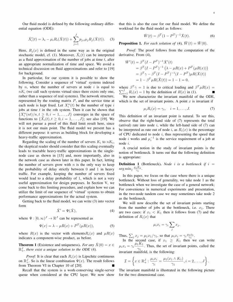
invariant manifold, is the following:

I =

{x ∈ RJ+ :

µixiγi

=µ1(x1 ∧K1)

γ1, i = 2, . . . , J

}.

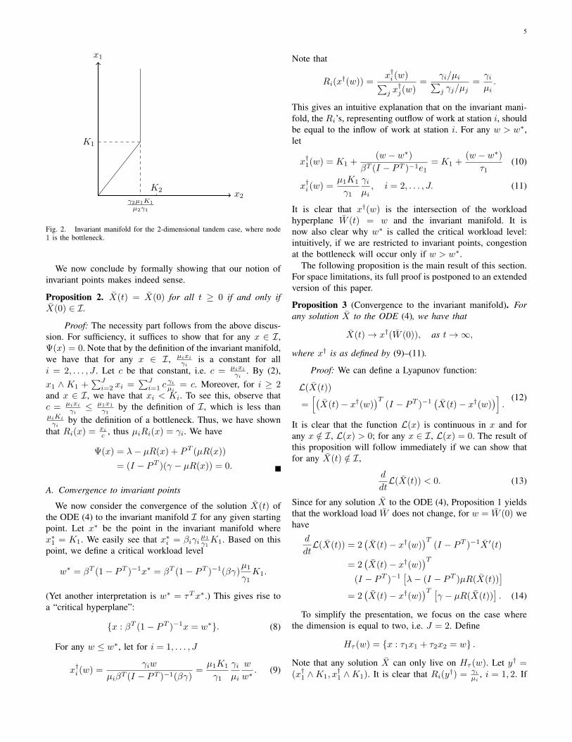
The invariant manifold is illustrated in the following picturefor the two dimensional case.

5

x1

x2

K1

γ2µ1K1

µ2γ1

K2

Fig. 2. Invariant manifold for the 2-dimensional tandem case, where node1 is the bottleneck.

We now conclude by formally showing that our notion ofinvariant points makes indeed sense.

Proposition 2. X(t) = X(0) for all t ≥ 0 if and only ifX(0) ∈ I.

Proof: The necessity part follows from the above discus-sion. For sufficiency, it suffices to show that for any x ∈ I,Ψ(x) = 0. Note that by the definition of the invariant manifold,we have that for any x ∈ I, µixi

γiis a constant for all

i = 2, . . . , J . Let c be that constant, i.e. c = µixiγi

. By (2),x1 ∧ K1 +

∑Ji=2 xi =

∑Ji=1 c

γiµi

= c. Moreover, for i ≥ 2and x ∈ I, we have that xi < Ki. To see this, observe thatc = µixi

γi≤ µ1x1

γ1by the definition of I, which is less than

µiKiγi

by the definition of a bottleneck. Thus, we have shownthat Ri(x) = xi

c , thus µiRi(x) = γi. We have

Ψ(x) = λ− µR(x) + PT (µR(x))

= (I − PT )(γ − µR(x)) = 0.

A. Convergence to invariant points

We now consider the convergence of the solution X(t) ofthe ODE (4) to the invariant manifold I for any given startingpoint. Let x∗ be the point in the invariant manifold wherex∗1 = K1. We easily see that x∗i = βiγi

µ1

γ1K1. Based on this

point, we define a critical workload level

w∗ = βT (1− PT )−1x∗ = βT (1− PT )−1(βγ)µ1

γ1K1.

(Yet another interpretation is w∗ = τTx∗.) This gives rise toa “critical hyperplane”:

{x : βT (1− PT )−1x = w∗}. (8)

For any w ≤ w∗, let for i = 1, . . . , J

x†i (w) =γiw

µiβT (I − PT )−1(βγ)=µ1K1

γ1

γiµi

w

w∗. (9)

Note that

Ri(x†(w)) =

x†i (w)∑j x†j(w)

=γi/µi∑j γj/µj

=γiµi.

This gives an intuitive explanation that on the invariant mani-fold, the Ri’s, representing outflow of work at station i, shouldbe equal to the inflow of work at station i. For any w > w∗,let

x†1(w) = K1 +(w − w∗)

βT (I − PT )−1e1= K1 +

(w − w∗)τ1

(10)

x†i (w) =µ1K1

γ1

γiµi, i = 2, . . . , J. (11)

It is clear that x†(w) is the intersection of the workloadhyperplane W (t) = w and the invariant manifold. It isnow also clear why w∗ is called the critical workload level:intuitively, if we are restricted to invariant points, congestionat the bottleneck will occur only if w > w∗.

The following proposition is the main result of this section.For space limitations, its full proof is postponed to an extendedversion of this paper.

Proposition 3 (Convergence to the invariant manifold). Forany solution X to the ODE (4), we have that

X(t)→ x†(W (0)), as t→∞,

where x† is as defined by (9)–(11).

Proof: We can define a Lyapunov function:

L(X(t))

=[(X(t)− x†(w)

)T(I − PT )−1

(X(t)− x†(w)

)].

(12)

It is clear that the function L(x) is continuous in x and forany x /∈ I, L(x) > 0; for any x ∈ I, L(x) = 0. The result ofthis proposition will follow immediately if we can show thatfor any X(t) /∈ I,

d

dtL(X(t)) < 0. (13)

Since for any solution X to the ODE (4), Proposition 1 yieldsthat the workload load W does not change, for w = W (0) wehave

d

dtL(X(t)) = 2

(X(t)− x†(w)

)T(I − PT )−1X ′(t)

= 2(X(t)− x†(w)

)T(I − PT )−1

[λ− (I − PT )µR(X(t))

]= 2

(X(t)− x†(w)

)T [γ − µR(X(t))

]. (14)

To simplify the presentation, we focus on the case wherethe dimension is equal to two, i.e. J = 2. Define

Hτ (w) = {x : τ1x1 + τ2x2 = w} .

Note that any solution X can only live on Hτ (w). Let y† =(x†1 ∧K1, x

†1 ∧K1). It is clear that Ri(y†) = γi

µi, i = 1, 2. If

6

X1(t) < x†1(w), then X2(t) > x†2(w), which follows from thefact that τ1, τ2 > 0. This implies that

X1(t) ∧K1 ≤ y†1, X2(t) ∧K2 ≥ y†2.

Notice that the above two inequalities can not be tight si-multaneously. Otherwise, X(t) would be equal to x†. Thus,R1(X) ≤ R1(x†(w)) and R2(X) ≥ R2(x†(w)) by thedefinition of Ri(·) in (1). Again, equality can not hold forboth. This implies that d

dtL(X(t)) < 0 according to (14). Thesame argument applies if X2(t) < x†2(w).

In the following section we show that, as ρ is close to 1, thefluid model is a good approximation of the queue length on atime scale of O(1/(1− ρ)). Since the diffusion time scale isof the order O(1/(1− ρ)2) it is tempting to conclude that theonly configurations of the customer populations that matter areconfigurations on the invariant manifold. These configurationsdepend on the workload w at the CPU, which then is expectedto be the driving force of randomness. The goal of the nextsection is to make this statement rigorous.

IV. STATE-SPACE COLLAPSE IN HEAVY TRAFFIC

We are now ready to develop a diffusion approximationfor the process describing the number of customers in thesystem, which we sometimes also refer to as the head-countprocess. Consider a sequence of such processes indexed by n.As n→∞, λn → λ. Let γn = (I − PT )−1λn, and

ρn = (γn)Tβ.

We assume that

ρn = 1− θ/n > 0, and Kni = Kin. (15)

(One way to achieve this is to set λni = λi(1− θ/n).) We areinterested in the limit of the diffusion scaled process

Xn(t) =1

nXn(n2t)

as n→∞, in which case the system approaches heavy traffic.It turns out that the choice Kn

i = Kin gives rise to a limitmodel in which the fraction of time the system is congestedis non-trivial (i.e. strictly between 0 and 1). For example, inthe single-node case, the results in [15] imply that the time-dependent delay probability P (Xn

1 (n2t) > Kn1 ), as well as

the stationary delay probability P (Xn1 (∞) > Kn

1 ), convergeto a quantity between 0 and 1. This enables one to obtain non-trivial and explicit approximations of the delay probability.

A starting point of our analysis is to recall the well-known(see e.g. [18]) heavy-traffic limit theorem for the workloadprocess at the CPU layer. Let Wn(t) = Wn(n2t)/n, t ≥ 0be the scaled workload process. Then Wn(·) converges to areflected Brownian motion (RBM) W ∗(·) with drift −θ andvariance σ2 = E(S)(1 + c2s) = E[S2]/E[S], where c2s =V ar(S)/E2(S). According to the calculation in Section II,σ2 = aT τ (2)/(aT τ).

Our main result is that Xn(t) converges to a process thatcan be described completely in terms of W ∗(t), using the

insights developed for the critical fluid model in the previoussection. To this end, define the map ∆ : R+ → RJ+ by

∆1(w) =w ∧ w∗w∗

K1 +(w − w∗)+

τ1, (16)

∆i(w) =w ∧ w∗w∗

µ1K1

γ1

γiµi, i = 2, . . . , J. (17)

This map is called lifting map, as it will be used to constructthe multi-dimensional limiting queue length process from theone-dimensional limiting workload process. In fact, our nextresult is a consequence of the fact that, in heavy traffic,Xn(t) ≈ ∆(Wn(t)), and making this statement rigorous isin fact a key ingredient of the proof, which is based onstate-space-collapse techniques as developed by Bramson [21].Again, the proof is omitted because of space limitations.

Theorem 2 (Diffusion limit). Suppose that Xn(0) = 0for all n. Then, the diffusion-scaled process Xn convergesweakly to the limit X∗ in heavy traffic. The limit X∗ can becharacterized as X∗(t) = ∆(W ∗(t)), i.e.

X∗1 (t) =W ∗(t) ∧ w∗

w∗K1 +

(W ∗(t)− w∗)+τ1

,

X∗i (t) =W ∗(t) ∧ w∗

w∗µ1K1

γ1

γiµi, i = 2, . . . , J.

Note the similarity of the lifting map and the quantitiesx†i (w) that are used to define the invariant points of the criticalfluid model. In fact, this is the key physical insight that justifiesthe title of this paper. Namely, fix t, take θ = 1, n = 1/(1−ρ)and recall that the workload fluctuates at the time scale of n2

as we set Wn(t) = Wn(n2t)/n. Hence, between time tn2

and tn2 + n the scaled workload hardly changes for n large.Namely, it will be approximately W ∗(t) throughout this time.During this time, by the convergence result of the fluid limitpresented in the previous section, 1

nXn(n2t + n) will have

converged to ∆(W ∗(t)). Thus, in heavy traffic, fluctuationsof the system at the layer of the individual servers occur ata much faster time scale than fluctuations at the CPU layer.If we wish to study fluctuations of the servers, we can keepthe total workload at the CPU layer fixed, and if we wishto study performance of the system on the time-scale of theCPU layer, we can assume that jobs at the servers live onthe invariant manifold; any deviations away from the invariantmanifold will have averaged out.

We believe that these physical insights are interesting, andmay also occur in other layered systems. In the next sections,we show how these insights lead to explicit and accurateapproximations of the layered system under consideration.

V. STEADY-STATE PERFORMANCE APPROXIMATIONS

In the previous section we have considered a sequence ofsystems approaching heavy traffic. The goal of the presentsection is to utilize Theorem 2 and obtain performance ap-proximations for the steady-state distribution for the originalsystem. The first step is to establish a heavy-traffic limit forthe sequence of steady-state distributions indexed by n. It is

7

well-known that the normalized steady-state workload of anM/G/1 queue in heavy traffic converges to an exponentiallydistributed random variable; i.e. if we consider the sequenceof systems introduced in the previous section, let Wn(∞) bethe steady-state workload in the nth system and Wn(∞) =1nW (∞), then

Wn(∞)⇒W ∗(∞),

where⇒ means convergence in distribution and W ∗(∞) is anexponentially distributed random variable with mean m = σ2

2θ ,by the classical steady-state analysis of RBM [18].

Since W ∗(∞) can also be seen as the limit (in distribution)of W ∗(t) as t → ∞, it is natural to expect that the heavy-traffic (n → ∞) and steady-state limits (t → ∞) can beinterchanged when considering Xn(t). It is possible to dothis in the same way as has been carried out in the single-node case [15]; detailed are omitted due to space limits. Wecan exploit this to derive a heavy-traffic limit theorem forXn(∞), which is a J-dimensional random vector denotingthe customer population in steady state in the nth system.Since ∆ is continuous, we have the following result by thecontinuous mapping theorem:

Xn(∞)⇒ X∗(∞) := ∆(W ∗(∞)).

Note that P(X∗i (∞) > x) = P (∆i(W∗(∞)) > x) .

Since the distribution of W ∗(∞) is explicit, as is themapping ∆, the above formula is explicit. Thus, we candevelop explicit approximations for the original system thatwill be accurate in heavy traffic.

Recall we called our sequence of systems indexed by n‘a sequence of virtual systems’. The total load in the nthvirtual system is ρn = 1 − θ/n and number of servers atnode i are Kn

i . In practice, one would like to get back tothe original system, so we need to determine which virtualsystem is appropriate. If we take θ = 1, then we should taken∗ = 1/(1 − ρ), which also implies that in the fluid modelthe number of active servers at node i should be equal to(1− ρ)Ki.

For our running example, the tandem network with 10 activeservers at the first node, 20 active servers at the second node,and a total system load of 0.8, then n = 5, and the relevantfluid model is the one where the number of active servers atthe first node equals 2 and at the second node 4.

In what follows, the quantities Ki represent the number ofservers at node i in the actual system. The critical workloadlevel w∗ can be rewritten as

w∗ = (1− ρ)∑j

ρjτjK1/ρ1.

The right-hand side can be simplified further using [18,Corollary III.5.3]:

w∗ = (1− ρ)∑j

ρjτjK1/ρ1 = (1− ρ)K1ρm/ρ1.

As W ∗ is exponential with mean m, the heavy-traffic approx-imation of the delay probability at the bottleneck becomes

P (W ∗ > w∗) = e−(1−ρ)K1ρρ1 ≈ ρK1

ρρ1 =: pd. (18)

In the second equation we used that e−(1−ρ) ≈ ρ to obtainan approximation more in line with the single-node approxi-mation proposed by [10]. Due to lack of space, we focus onone additional performance measure only, namely the expectedtotal response time (i.e. the sojourn time) E[V ] of an arbitraryjob which can be computed using Little’s law:

E[V ] = E[∑j

Xj ]/λo ≈ 1/λo

1− ρE[∑j

∆j(W∗)].

Straightforward computations, combined with the above ap-proximations, yield

E[∑j

∆j(W∗)] ≈ (1− pd) + pd

m

τ1.

It makes sense to multiply the right-hand side with ρ toobtain a result that is exact for the single-node case, andfrom a heavy-traffic point of view, (ρ ≈ 1) this still yieldsasymptotically accurate estimates. Putting everything together,our heavy-traffic approximation for E[V ] becomes

E[V ] ≈ E[S]

1− ρ

[(1− pd) + pd

m

τ1

]. (19)

In the single node case for exponential job sizes, we havethat m = E[S] = τ1 so our approximation indeed reducesto E[S]/(1 − ρ) which is the expected sojourn time in anM/M/1 queue. We now develop an extension valid for moregeneral service times combining the insights of the heavy-traffic analysis of our network model with available resultsfor the single node case.

VI. EXTENSION TO GENERAL JOB SIZES

For the single-node case, Poisson arrivals, and generalservice times, [10] proposed the approximation pd = ρK1 and

E[V ] = (1− pd)E[S]

1− ρ + pdm

1− ρ , (20)

where, as before m = E[S2]/(2E[S]). This approximationis exact for both FIFO (K1 = 1) and PS (K1 = ∞), and[15] shows the approximation is asymptotically exact in heavytraffic, using the same scaling procedure as in the presentpaper. Note further that for J = 1 we have that τ1 = E[S]and ρ1 = ρ so (19) and (20) coincide.

These considerations suggest that the approximation ofE[V ] given in (19) is still accurate for general service timesassuming station 1 is the single bottleneck and keeping ρK1

ρρ1 .

Proving this necessitates an extension of the measure-valuedframework in [17], which is beyond the scope of this paper.Instead, we validate our approximation with some simulationresults for the two-node tandem case.

Let βei = β(2)i /2βi be the mean residual service time of

a job at station i. For the two-node tandem case we haveγ1 = γ2 = λ1.

Since we fixed the topology of the network we will nolonger assume that node 1 is always the bottleneck. Observingthat pd ≈ ρρKi∗/ρi∗ if node i∗ is the bottleneck, we obtain

E[V ] ≈ E[S]

1− ρ

[(1− pd) + pdm

1

τi∗

].

8

TABLE ISIMULATION RESULTS

(β1, β2, c21, c22,K1,K2) approximation simulation

(1, 2, 4, 4, 3, 7) 10.24 10.41(1, 2, 4, 10, 4, 6) 11.37 10.71(1, 2, 10, 4, 4, 6) 10.77 10.57(1, 2, 10, 10, 4, 6) 11.58 10.87

(2, 1, 4, 4, 6, 4) 10.24 10.49(2, 1, 4, 10, 6, 4) 10.38 10.70(2, 1, 10, 4, 6, 4) 10.78 10.98(2, 1, 10, 10, 6, 4) 10.91 11.18(1, 10, 4, 4, 2, 8) 38.86 37.43(1, 10, 4, 10, 2, 8) 43.20 37.83(1, 10, 10, 4, 2, 8) 38.91 37.53

(1, 10, 10, 10, 2, 8) 43.24 37.97(10, 1, 4, 4, 8, 2) 38.52 38.88(10, 1, 4, 10, 8, 2) 38.56 39.11(10, 1, 10, 4, 8, 2) 42.46 40.77

(10, 1, 10, 10, 8, 2) 42.50 41.00

The constant m can be computed by noting that

m = E[S2]/(2E[S]) =ρ1ρ

(βe1 + β2) +ρ2ρβe2 .

We now present some numerical results for the case that bothservice times follow a hyper-exponential distribution. In allexamples, we focus on a moderately loaded system with ρ =0.7. We let the coefficient of variation of the service timesrange from 4 to 10 at both nodes (in fact we take the sameparameters as done in the experiment of [7]). Note that thesquared coefficient of variation c2i of the service time at nodei satisfies c2i = β

(2)i /β2

i − 1.Generally, the heavy-traffic approximations are quite accu-

rate, always within 15% of the outcome predicted by simu-lation, and in several cases the error is as small as 2%. Wefind that the results become less accurate if the coefficient ofvariation of the service time at the bottleneck is high. Similarconclusions can be drawn for higher values of the load andfor larger networks.

VII. CONCLUDING REMARKS

By establishing fluid and diffusion approximations of a two-layered queuing network, we have shown that, under criticalloading, different layers in the network operate at differenttime scales. From the macroscopic CPU viewpoint, the systembehaves as a simple one-server queue, which when criticallyloaded fluctuates at a time scale of O(1/(1−ρ)2). The networkdynamics at the other layer evolve at a faster time scaleO(1/(1 − ρ)), thus always reaching an invariant point as ifthe total workload at the CPU were constant.

We have established this result by introducing fluid anddiffusion approximation techniques to study layered networks.It is interesting to examine the potential of such techniques toanalyze other layered networks, such as those in [8], [9].

For our model, state-space collapse was established as aconsequence of the single bottleneck assumption. Driven bycuriosity, we are currently extending the analysis to multiplebottlenecks, although we note that the single bottleneck as-sumption will typically be an artefact of the fact that the buffersizes Ki need to be chosen as integers in implementations.

Another interesting topic is to allow for general job sizes,as well as time-varying arrival rates. Finally, we expect theresults to be directly useful to dimension thread-pools in webservers in a static fashion. The techniques in this paper arelikely to be useful for dynamic thread-pool dimensioning aswell, as the application of the techniques in this paper seemspromising to formulate tractable (Brownian) control problems.

REFERENCES

[1] W. van der Weij, S. Bhulai, and R. van der Mei, “Dynamic thread assign-ment in web server performance optimization,” Performance Evaluation,vol. 66, no. 6, pp. 301–310, 2009.

[2] R. van der Mei, R. Hariharan, and P. Reeser, “Web server performancemodeling,” Telecommunication Systems, vol. 16, pp. 361–378, 2001.

[3] V. Cardellini, E. Casalicchio, M. Colajanni, and P. Yu, “The state of theart in locally distributed web server systems,” ACM Computing Surveys,vol. 34, 2002.

[4] M. Crovella, R. Frangioso, and M. Harchol-Balter, “Connection schedul-ing in web servers,” in Proceedings USENIX symposium on InternetTechnologies and Systems, 1999.

[5] M. Harchol-Balter, B. Schroeder, N. Bansal, and N. Agrawal, “Srptscheduling for web servers,” Lecture Notes in Computer Science, vol.2221, pp. 11–21, 2001.

[6] M. Jonckheere, R. van der Mei, and W. van der Weij, “Rate stability andoutput rates in queueing networks with shared resources,” PerformanceEvaluation, vol. 67, no. 1, pp. 28–42, 2010.

[7] W. van der Weij, R. van der Mei, and B. G. F. Phillipson, “Optimalserver assignment in a two-layered tandem of multi-server queues,”in Proceedings 3rd International Working Conference on PerformanceModelling and Evaluation of Heterogeneous Networks (HETNETS),volume P01, Ilkley, England, July 2004.

[8] J. Rolia and K. Sevcik, “The method of layers,” IEEE Transactions onSoftware Engineering, vol. 21, pp. 689–699, 1995.

[9] C. Woodside, J. Neilson, D. Petriu, and S. Majumdar, “The stochasticrendezvous network model for the performance of synchronous client-server like distributed software,” IEEE Transactions on Computers,vol. 44, pp. 20–34, 1995.

[10] B. Avi-Itzhak and S. Halfin, “Expected response times in a non-symmetric time sharing queue with a limited number of service po-sitions,” in Proceedings of the 12th International Teletraffic Congress,Torino, 1988.

[11] F. Zhang and L. Lipsky, “Modelling restricted processor sharing,” inProc. of the 2006 Int’l Conf. on Parallel and Distributed ProcessingTechniques and Applications (PDPTA06), 2006.

[12] ——, “An analytical model for computer systems with non-exponentialservice times and memory thrashing overhead,” in Proc. of the 2007Int’l Conf. on Parallel and Distributed Processing Techniques andApplications (PDPTA07), 2007.

[13] M. Nuyens and W. van der Weij, “The limited processor sharing queue,”CWI, Amsterdam, Tech. Rep., 2007.

[14] J. Nair, A. Wierman, and B. Zwart, “Tail-robust scheduling via limitedprocessor sharing,” Performance Evaluation, 2010.

[15] J. Zhang and B. Zwart, “Steady state approximations of limited processorsharing queues in heavy traffic,” Queueing Syst., vol. 60, no. 3-4, pp.227–246, 2008.

[16] J. Zhang, J. G. Dai, and B. Zwart, “Law of Large Number Limits ofLimited Processor-Sharing Queues,” Math. Oper. Res., vol. 34, no. 4,pp. 937–970, 2009.

[17] ——, “Diffusion Limits of Limited Processor-Sharing Queues,” Ann.Appl. Probab., vol. 21, no. 2, pp. 745–799, 2011.

[18] S. Asmussen, Applied probability and queues, 2nd ed., ser. Applicationsof Mathematics (New York). New York: Springer-Verlag, 2003, vol. 51.

[19] A. Mandelbaum, W. A. Massey, and M. I. Reiman, “Strong approxima-tions for markovian service networks,” Queueing Syst., vol. 30, no. 1/2,pp. 149–201, 1998.

[20] W. Walter, Ordinary differential equations, ser. Graduate Texts inMathematics. New York: Springer-Verlag, 1998, vol. 182.

[21] M. Bramson, “State space collapse with application to heavy trafficlimits for multiclass queueing networks,” Queueing Syst., vol. 30, no.1-2, pp. 89–148, 1998.