Sentiment During Recessions

Sentiment during recessions∗

Diego Garcıa†

Kenan-Flagler Business School

University of North Carolina at Chapel Hill

March 2, 2010

Abstract

This paper studies the effect of sentiment on asset prices during the first half of the 20thcentury (1905-1958). As a proxy for sentiment, we use the fraction of positive and negativewords in two columns of financial news from the New York Times. The main finding ofthe paper is that, controlling for other well-known time-series patterns, news content helpspredict stock returns at the daily frequency, but only during recessions. A one standarddeviation shock to our news measure during recessions changes the conditional average returnon the DJIA by eleven basis points over one day.

JEL classification: G01, G14.Keywords: media content, stock returns, sentiment, recessions.

∗I would like to thank Craig Carroll, Riccardo Colacito, Jennifer Conrad, Alex Edmans, Joey Engelberg,Francesca Gino, Pab Jotikasthira, Oyvind Norli and Chris Roush for comments on an early draft, as well asseminar participants at UNC at Chapel-Hill. Special thanks to the CDLA staff, Kirill Fesenko, Fred Stipe, andparticularly Rita Van Duinen for their help in the optical character recognition stage of this project.†Diego Garcıa, Kenan-Flagler Business School, University of North Carolina at Chapel Hill, McColl Building,

C.B. 3490, Chapel Hill, NC, 27599-3490. Tel: 1-919-962-8404; Fax: 1-919-962-2068; Email:diego [email protected]; Webpage: http://www.unc.edu/∼garciadi

1 Introduction

Much interest in recent Economic and Finance research has been devoted to the role of

the media. Shiller (2000), for example, highlighted the potential role of the media in creating

asset bubbles and triggering market crashes. Tetlock (2007) convincingly argued that a simple

measure of sentiment, the number of negative words in the “Abreast of the market” column of

the Wall Street Journal, helps predict stock returns at the daily frequency from 1984 to 1999.

This paper contributes to this literature by studying the time series behavior of stock returns

and a sentiment variable constructed using financial news from the New York Times during the

early 20th century. This is a particularly interesting time period for research purposes for at

least two reasons: (i) it contains thirteen recessions (including the Great Depression), (ii) the

supply of news was much more concentrated (the only two media sources with regular coverage

of business news were the Wall Street Journal and the New York Times). We can thus take

advantage of the variation in the business cycle, and the content of a media outlet that was on

most investors’ desks every morning.

We build our proxy for sentiment using two columns from the New York Times,1 titled

“Financial Markets” and “Topics in Wall Street.” Both were published daily from 1905 to

1958, covering general financial news – from stock market performance to industry news and

macroeconomic events. Thus, they are natural candidates as gauges of the excitement and

agitation in US stock markets during the first half of the 20th century. We remark that these

columns were written in the afternoons, and investors would typically read them in the morning,

just prior to the opening of the market. Our sentiment measure is constructed aggregating

the number of positive and negative words in these columns, as defined in the dictionaries of

Loughran and McDonald (2009).

Our main result is to show that our sentiment variable predicts stock returns at the daily

frequency, after controlling for autocorrelation and other known determinants of stock returns.1Although the Wall Street Journal was already a respected business news outlet in the early 20th century,

as mentioned above, there is not an archive of its contents available for research purposes (as of 9/2009). Incontrast, the New York Times Historical Archive presents the complete contents of the New York Times goingback to 1851.

1

More interestingly, since our study includes roughly two thirds of the business cycles during the

20th century, the effect of our sentiment measure is concentrated during recessions. None of

our media based metrics meaningfully relate to stock returns during expansions, but they are

excellent predictors of asset prices during economic downturns. The magnitude of the effect is

sizable: a one standard deviation change in our sentiment measure move the conditional mean

of the Dow Jones Industrial Average (DJIA) by eleven basis points during recessions.

For the 1926-1958 period, for which cross-sectional data is available, we find that the effect

is particularly strong in small stocks. A one standard deviation movement in the sentiment

factor changes the next day average return of a small-stock portfolio by 18 basis points during

recessions. Further, the media measures can help predict the returns of the SMB portfolio.

The point estimates are large both in economic and statistical terms: a one standard-deviation

change to the sentiment factor during recessions moves the daily average return of the SMB

portfolio by 17 basis points. The effect is most pronounced during the Great Depression, but

also significant during the other recessions in our sample.

The news in our sample have a “tag-along” flavor: they essentially report on the previous

days events, giving mostly explanations about past asset price movements. In our dataset,

this comes to light in a strong predictability of the media content measure written on a given

afternoon, and the stock returns on that day. For example, a one standard deviation increase in

stock returns increases our positive news measure by a half standard deviation, and decreases

our negative news measure by a similar amount. Even though this feedback effect is strong

throughout our sample, it is more pronounced during expansions: news content is about 70%

more responsive to the same day stock returns during expansions than during recessions. This

is somewhat surprising, since the feedback from news to next day stock returns is concentrated

in recessions. Moreover, we find that our media content metrics vary significantly more within

business cycles than across recessions and expansions. Although there are more negative and

less positive words in economic downturns, these differences are a small fraction (< 20%) of the

unconditional standard deviation of positive and negative word counts.

The psychology literature has forcefully argued that emotions affect decision making, and

2

information processing in particular. For example, Tiedens and Linton (2001) show that emo-

tions elicit different reliance on heuristic versus systematic processing. The literature has also

found that the emotions of anxiety, hope and sadness are associated with a greater sense of

uncertainty (Smith and Ellsworth, 1985; Ortony, Clore, and Collins, 1988). Gino, Wood, and

Schweitzer (2009) show that anxiety makes agents more receptive to advice, even if this advice

is bad.2 This literature clearly shows that priming subjects into negative mood states changes

their decision making abilities. One can reasonably argue that in periods of expansion investors

feel happy and optimistic, whereas during recessions they feel fearful and anxious. The job

losses and the uncertainty over the future that investors experienced during the Great Depres-

sion must have put the population at large in negative mood states. Thus, we expect agents

to use different decision making rules, and, in particular, react differently to news, in recessions

than in expansions.

Our paper studies how the content of two financial columns of the New York Times newspaper

affect aggregate investor behavior. Although the above experimental studies from psychology

clearly establish that agents’ moods and emotions affect their individual behavior, it is the

nascent behavioral economics literature that has shown how such sentiment can move aggregate

quantities. For example, Hirshleifer and Shumway (2003) show how stock returns are affected by

the weather across the world, and Edmans, Garcıa, and Norli (2007) associate the outcomes of

sporting events, such as the World Cup, to drops in the stock markets when the country loses a

game (see Hirshleifer, 2001, for a survey on these topics). A critical theme from this literature is

the asymmetric effect of positive and negative events on outcomes, consistent with the prospect

theory of Kahneman and Tversky (1979). Akerlof and Shiller (2009), while discussing confidence

and the Michigan Consumer Sentiment Index, state that “we conceive of the link between changes

in confidence and changes in income as being especially large and critical when economies are

going into a downturn, but not so important at other times.” Both the existing empirical findings

in finance and the experimental evidence from psychology thus suggest that human behavior is2See Forgas (1991) for an excellent survey of the earlier literature, and Isen (1987), Bless, Clore, Schwarz,

Golisano, Rabe, and Wolk (1996), Forgas (1998), Park and Banaji (2000), Lerner and Keltner (2000), and Lernerand Keltner (2001) for more recent work.

3

significantly different in times of anxiety and fear versus periods of prosperity and tranquility,

which motivates our empirical analysis.

The paper contributes to the growing literature on the role and content of the media and its

effects on asset prices and investor behavior. Given data limitations, most of the literature has

studied the last twenty years, where news are available electronically in text format. Within our

sample period, Bow (1980) argues that there were no predictive signs in the media prior to the

1929 stock market crash.3 The closest paper to ours is Tetlock (2007), who studies a column

from the Wall Street Journal from 1984 to 1999. Our paper corroborates his main findings,

showing they are concentrated in economic downturns. Interestingly, we find that positive

words help predict stock returns, whereas his research showed only negative word counts had

predictive power. Since Tetlock (2007), the literature has examined the cross-section of stock

returns, other types of investor behavior, or news originating from sources other than media

outlets.4 The main advantage of our study is the ability to differentiate between recessionary

and expansionary periods, and thus how investor behavior differs in good and bad times. During

the first-half of the 20th century, business cycles were more frequent and severe, so our time

period is particularly well suited to study the effect of sentiment on asset prices in different

economic conditions. But there is another important difference between the last twenty years

and our sample period that makes our data very appealing: the supply of news was much

more concentrated during 1905-1958. The only other newspaper that contained wide coverage

of business news was the Wall Street Journal, so anyone investing in stocks would, almost

certainly, have read the columns that we study before the market opened each day.5

3See Griggs (1963) for a similar discussion in the context of the 1957-1958 recession. Norris and Bockelmann(2000) and Roush (2006) both have extensive discussions as to the role of the media prior to the Great Depression.Shiller (2000) discusses both the 1929 and the 1987 crashes in more detail.

4Standard databases of news start after 1980, so there is no much room for time-series research outside the1980-2008 window. The only other pure time-series analysis on a wide index is Larkin and Ryan (2008), who studythe effect of news feeds in intraday returns for the S&P500 index. For other related papers using text contentanalysis see Cutler, Poterba, and Summers (1989), Klibanoff, Lamont, and Wizman (1998), Chan (2003), Kaniel,Starks, and Vasudevan (2007), Schmitz (2007), Barber and Odean (2008), Gaa (2008), Tetlock, Saar-Tsechansky,and Macskassy (2008), Yuan (2008), Engelberg (2008), Fang and Peress (2009), Solomon (2009), Bhattacharya,Galpin, Yu, and Ray (2009).

5We should highlight that other mass communication channels were still in early development stages. Forexample, the first radio news program was broadcasted August 31, 1920 in Detroit, and radio news did not reachwide audiences until much later. Television did not become a staple commodity in US households until well intothe end of our sample period.

4

The paper is also related to the literature on investor sentiment (see Baker and Wurgler, 2007,

for a survey). Most of the sentiment indexes that have been suggested by other authors have

data requirements that restrict their implementation to the last forty years.6 As a consequence,

they are less likely to be able to take advantage of the frequency and severity of the business

cycle that the US experienced during the first half of the 20th century. Moreover, there is a

strong case to be made that markets have become fairly efficient over the last few decades, as

institutional investors and PhDs with quantitative backgrounds joined Wall Street. It seems

reasonable that the 1905-1958 US stock market was relatively less efficient, and thus a natural

place to study behavioral biases. Finally, another important advantage of our media based

measures is that they are available daily, and as such can be used in high-frequency studies.

The rest of the paper is structured as follows. Section 2 constructs the sentiment measures

we use in our study. In section 3 we analyze the feedback from stock returns to media content.

Section 4 presents the average returns on different indexes as a function of the previous days’ news

sentiment. Section 5 more formally studies the relationship between daily returns and sentiment

for the DJIA, whereas section 6 studies the results along the size cross-section. Section 7 looks

at the Great Depression and goes over other robustness checks. In section 8 we discuss the

relative merits of a sentiment hypothesis versus a purely rational one. Section 9 concludes.

2 The data

The paper uses three sources of data. The first is stock return information. We collect the

total return index for the Dow Jones Industrial average from Williamson (2008).7 The Dow

Jones Industrial index goes back to the turn of the 20th century, and thus allows us to have a

metric of US stock returns prior to the coverage in the more standard Center for Research in

Security Prices (CRSP), which started in 1926. We remark that during our period the Dow Jones

Industrial index was composed by as few as twelve securities in 1905, and increased to thirty6See Brown and Cliff (2004, 2005), Qiu and Welch (2006) and Lemmon and Portniaguina (2006) for some

recent research on sentiment measures and stock returns.7Historical data is available free of charge from http://www.djaverages.com/, including the total return for

the Dow Jones Industrial average, but as of the end of 2009 this source did not include Saturday data. For thisreason, we use the data on the DJIA from Williamson (2008), see http://www.measuringworth.org/DJA/.

5

starting in 1928. In section 6 we also study size-sorted portfolios from the CRSP database, for

which our sample is reduced to the time period 1926-1958. In particular, we construct an equally-

weighted average of the top three size decile portfolios, as provided via the Wharton Research

Data Services, which we shall refer to as the “big stock portfolio.” Similarly, we construct a

“small stock portfolio” using the three smallest size decile portfolios. We also construct a small-

minus-big portfolio (SMB from now on), which is long the small stock portfolio and short the

large stock portfolio. We let Rt denote the log-return on the different indexes of interest on date

t. Our second source of data, which contains business cycle information, is the NBER website

http://www.nber.org/cycles.html. The third source of data is the novel measure used in

this paper based on media content, which we describe next.

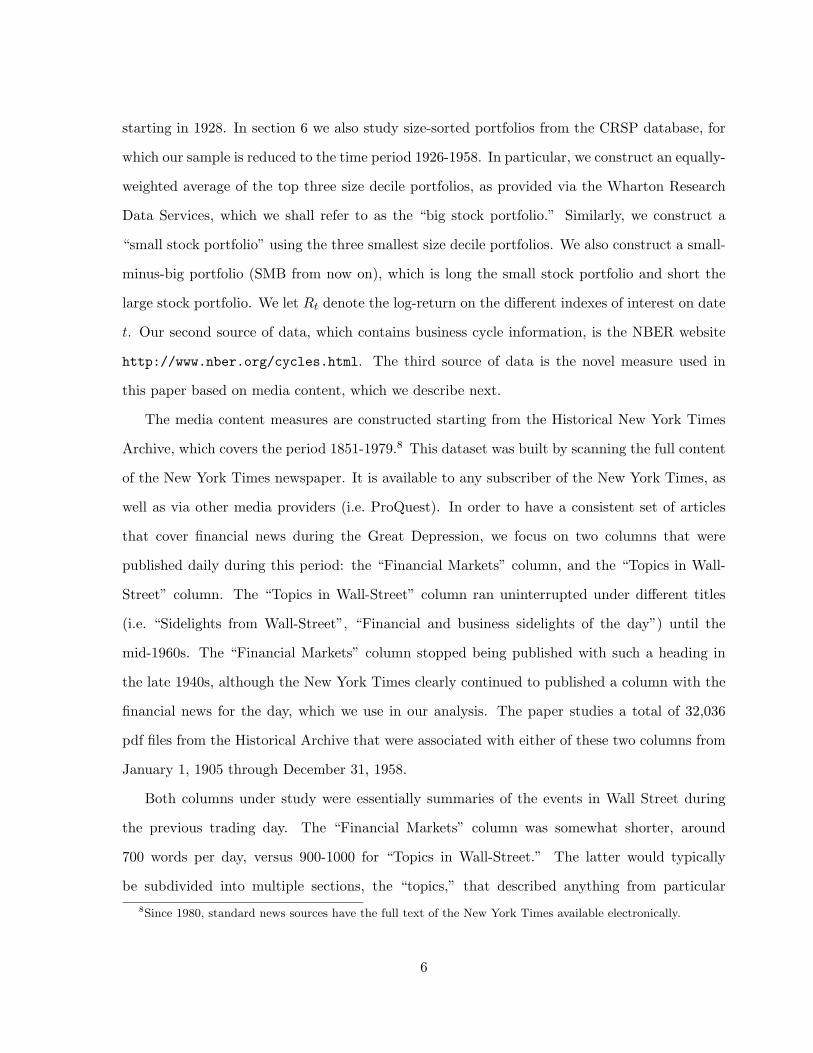
The media content measures are constructed starting from the Historical New York Times

Archive, which covers the period 1851-1979.8 This dataset was built by scanning the full content

of the New York Times newspaper. It is available to any subscriber of the New York Times, as

well as via other media providers (i.e. ProQuest). In order to have a consistent set of articles

that cover financial news during the Great Depression, we focus on two columns that were

published daily during this period: the “Financial Markets” column, and the “Topics in Wall-

Street” column. The “Topics in Wall-Street” column ran uninterrupted under different titles

(i.e. “Sidelights from Wall-Street”, “Financial and business sidelights of the day”) until the

mid-1960s. The “Financial Markets” column stopped being published with such a heading in

the late 1940s, although the New York Times clearly continued to published a column with the

financial news for the day, which we use in our analysis. The paper studies a total of 32,036

pdf files from the Historical Archive that were associated with either of these two columns from

January 1, 1905 through December 31, 1958.

Both columns under study were essentially summaries of the events in Wall Street during

the previous trading day. The “Financial Markets” column was somewhat shorter, around

700 words per day, versus 900-1000 for “Topics in Wall-Street.” The latter would typically

be subdivided into multiple sections, the “topics,” that described anything from particular8Since 1980, standard news sources have the full text of the New York Times available electronically.

6

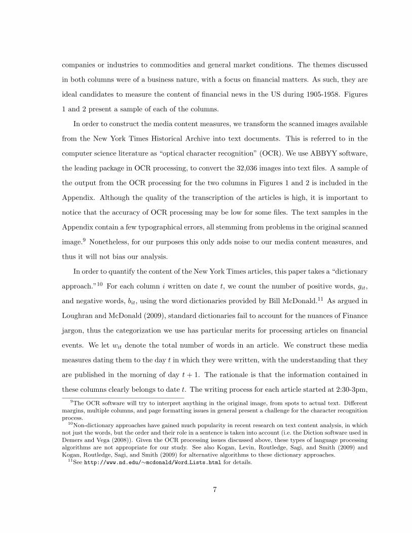
companies or industries to commodities and general market conditions. The themes discussed

in both columns were of a business nature, with a focus on financial matters. As such, they are

ideal candidates to measure the content of financial news in the US during 1905-1958. Figures

1 and 2 present a sample of each of the columns.

In order to construct the media content measures, we transform the scanned images available

from the New York Times Historical Archive into text documents. This is referred to in the

computer science literature as “optical character recognition” (OCR). We use ABBYY software,

the leading package in OCR processing, to convert the 32,036 images into text files. A sample of

the output from the OCR processing for the two columns in Figures 1 and 2 is included in the

Appendix. Although the quality of the transcription of the articles is high, it is important to

notice that the accuracy of OCR processing may be low for some files. The text samples in the

Appendix contain a few typographical errors, all stemming from problems in the original scanned

image.9 Nonetheless, for our purposes this only adds noise to our media content measures, and

thus it will not bias our analysis.

In order to quantify the content of the New York Times articles, this paper takes a “dictionary

approach.”10 For each column i written on date t, we count the number of positive words, git,

and negative words, bit, using the word dictionaries provided by Bill McDonald.11 As argued in

Loughran and McDonald (2009), standard dictionaries fail to account for the nuances of Finance

jargon, thus the categorization we use has particular merits for processing articles on financial

events. We let wit denote the total number of words in an article. We construct these media

measures dating them to the day t in which they were written, with the understanding that they

are published in the morning of day t + 1. The rationale is that the information contained in

these columns clearly belongs to date t. The writing process for each article started at 2:30-3pm,9The OCR software will try to interpret anything in the original image, from spots to actual text. Different

margins, multiple columns, and page formatting issues in general present a challenge for the character recognitionprocess.

10Non-dictionary approaches have gained much popularity in recent research on text content analysis, in whichnot just the words, but the order and their role in a sentence is taken into account (i.e. the Diction software used inDemers and Vega (2008)). Given the OCR processing issues discussed above, these types of language processingalgorithms are not appropriate for our study. See also Kogan, Levin, Routledge, Sagi, and Smith (2009) andKogan, Routledge, Sagi, and Smith (2009) for alternative algorithms to these dictionary approaches.

11See http://www.nd.edu/∼mcdonald/Word Lists.html for details.

7

typically just as the market was about to close, and the final copy was turned in to be edited

and typeset at around 5-6 pm.

We aggregate these media content measures to create a time-series that matches the Dow

Jones index return data available. The ultimate goal is to combine all the news that were

printed before the market opened, and then examine whether the content of such news, our

proxy for sentiment, can predict the following days’ stock returns. In essence, we are trying to

measure the content of the financial news on investors’ desks prior to the opening of the market.

During the period under consideration, the NYSE was open Monday through Saturday, with

the exception of national holidays. The two columns of the New York Times would be typically

published the day after the market closed, and they would discuss financial events related to

that day. For example, the Sunday edition would discuss Wall Street events from Saturday. On

some occasions, the New York Times would not print these columns on Sunday, but on Monday.

In order to aggregate the news, and not miss columns that appeared while the market was

not open, we average the measures of positive/negative content from articles that were written

since the market closed until the market next opens. When the market is open on consecutive

days, t and t+ 1, we define our daily measure of positive media content as Gt =∑

i git/∑

iwit,

where the summation is over all articles written in date t (given our news selection, there are

two such articles for the majority of our sample). Similarly, we construct our daily measure of

negative media content as Bt =∑

i bit/∑

iwit. In es-sense, we count the number of positive

and negative words in the financial news under consideration, and normalize them by the total

number of words. For non-consecutive market days we follow a similar approach, by averaging

all articles published from close to open. To be precise, consider two days t and t + h + 1

such that h > 0 and the market was closed h days, from t + 1 through t + h. We define the

positive media content measure as Gt =∑s=t+h

i,s=t gis/∑s=t+h

i,s=t wsh. We proceed analogously for

the negative media content variable and define Bt =∑s=t+h

i,s=t bis/∑s=t+h

i,s=t wsh. We define the

pessimism factor as the difference between the negative and positive media content measures,

i.e. Pt = Bt −Gt.

For consecutive trading dates, our media measures Gt and Bt are constructed using informa-

8

tion that was available as of the end of date t when the market is open on date t+1 (the bulk of

our sample). It is less clear whether market prices on date t reflected the information available

to the journalists writing the columns, as the deadline for turning in the article to the editor

was not until roughly 5-6pm, while the NYSE closed at 3pm during the period under study.12

We further remark that for non-consecutive trading dates, we use articles that may have been

written on days after date t, but prior to the market opening (i.e. in the case of holidays).

Thus, strictly speaking, the New York Times measures we use could contain information that

the market would not have as of the close of trade.

Table 1 presents sample statistics on our media measures. Panel A shows that, over the

whole sample period, the mean number of positive words in an article was 1.13%. Given a

typical “Financial Markets” column with 700 words, there were on average 7.9 positive words

in each article. The standard deviation of the positive words measure is 0.37%. The average

number of negative words over the whole sample is 1.88%, with a standard deviation of 0.59%.

The pessimism measure, as expected given the numbers just discussed, has a positive mean i.e. a

typical article has about 0.75% more negative than positive words. Panels B and C present the

sample statistics broken down by the business cycle. The average positive measure is slightly

higher during expansions, by five basis points. On the other hand, the average negative measure

is 13 basis points higher during recessions. The boxplots in Figure 3, which graphically illustrate

the content of the two bottom panels of Table 1, show that our negative and pessimism media

measures are different during recessions and booms, as one would expect. More importantly for

the purposes of our tests, there is a very large amount of variation within business cycles: the

volatility of the measures is an order of magnitude larger than the mean differences across the

business cycle.

For the rest of the paper we normalize our sentiment measures so they have a zero mean

and unit variance. This will allow us to interpret the regression coefficients in terms of one-

standard deviation shocks to the sentiment measures, thus making it easier to gauge the economic

magnitude of our results.12See http://www.nyse.com/about/newsevents/1176373643795.html for details.

9

3 Feedback from stock returns to media

We start studying the effect of the returns on the DJIA on the sentiment measures we

constructed. Clearly, one would expect to find such a linkage, since after all the “Financial

Markets” and “Topics of the Wall Street” columns discuss the performance on the market the

previous day. We estimate the following model:

Mt = (1−Dt) (λ1Rt + β1Ls(Rt) + γ1Ls(Mt)) +Dt (λ2Rt + β2Ls(Rt) + γ2Ls(Mt)) + ηXt + υt;

(1)

where Ls denotes an s-lag operator,13 Mt denotes one of our media measures, i.e. Mt = Gt in the

case of positive news, Mt = Bt in the case of negative news, and Mt = Bt−Gt in the case of our

pessimism factor. The variable Dt is a dummy variable taking on the value 1 if and only if date

t is during a recession The vector Xt denotes a set of exogenous variables, and υt is a zero-mean

error term with possibly time-varying volatility. The set of exogenous variables Xt includes a

constant term, day-of-the-week dummies, a dummy for whether date t belongs to a recession or

an expansion, as well as a dummy for the five days starting in Dec. 12th 1914. We estimate the

specification in (1) letting the lag operators have s = 4. We report heteroskedasticity robust

standard errors using the automatic lag selection suggested in Newey and West (1994).

Panel A from Table 2 presents the estimated λ1 and β1 coefficients from (1), which measure

the reaction of news content to stock returns during expansions. Stock returns are important

predictors of the media content variables, both the positive and the negative measures. As

expected, positive returns increase the number of positive words and decrease the number of

negative words, and as a consequence the pessimism measure. Given the daily standard deviation

of the DJIA over our whole sample period is 133 basis points, a one standard deviation increase

in stock returns increases the percentage of positive words on the articles written that day by

0.43 standard deviations, and decreases the negative words by 0.46 standard deviations. The

pessimism factor decreases by 0.57 standard deviations for a one standard deviation move in the

DJIA returns. The effect is also persistent – the second row of Panel C presents a formal F -test13For an arbitrary random process Yt, Ls(Yt) = {Yt−1, . . . , Yt−s}.

10

of the significance of the sum of the coefficients in lags one through four.

We remark that the effect we find is an order of magnitude larger than that reported in

Tetlock (2007), as we include a contemporaneous term in (2). The inclusion of such a term has

to do with the nature of the data: the columns in the New York Times were finished once the

market was closed, so it is rather natural to think that the market return on that day would

have an effect on the news content. Our empirical results show that indeed this is the case –

although lags one through four have an effect on our media measures, as in Tetlock (2007), the

return on the day the columns were written is the biggest determinant of the tone and content

used by journalists.

Panel B in Table 2 presents the effect during recessions. We see there is a smaller response

to stock returns in recessions than in expansions. The first row of Panel C shows that the

difference is statistically significant for all three media measures. The difference is economically

large: whereas a one-standard deviation increase to the DJIA during the whole sample period

raised the positive measure by 0.43 standard deviations, the effect during recessions is only 0.25

standard deviations. The magnitude for the negative words and the pessimism factor are similar.

Thus, it appears that journalists use more “signed words,” or “tag-along” more, when writing

about the day’s events in Wall Street during expansions than during recessions.

The analysis confirms that our media measures are related to the returns in the DJIA average

on the days the columns were written. It also shows that the journalists wrote differently in

expansions and recessions, as it concerns the number of positive and negative words that they

used while describing the day’s events. While the connection between the returns Rt and the

news written in the afternoon of date t is to be expected, the more interesting question is whether

such news help predict the returns Rt+1 on the following day, to which we now turn.

4 Preliminary results

Table 3 studies the relationship between stock returns and media content by dividing the

sample into subsets where the previous day news had “high” or “low” content. We implement

11

such classification by considering trading days where the news measures were in the top and

bottom quartile of the distribution. Namely, for each of our three measures on date t, we

subdivide the sample into two groups: all dates in the bottom quartile of the distribution, and

all dates in the top quartile. We then compute the averages of the following day’s return for

each of the four indexes we study.

Over our whole sample period, Panel A shows the average daily return in the DJIA was 1.6

basis points. On days preceded by news on the top-quartile of the positive measure, the average

return is 7.6 basis points, while it is −4.6 basis points on the days preceded by news on the

bottom-quartile of the positive news measure. The spread is larger for the negative measure,

which is presented in columns 4 and 5. On days preceded by news that contain more negative

words the average return is −4.8 basis points, whereas it is 10 basis points for days preceded by

few negative words. The spread is similar in magnitude for the pessimism measure.

The results for the large stock portfolio is presented in the second row of Panel A. We see

a similar pattern as for the DJIA, where high positive word counts are associated with higher

returns (10.1 basis points), and low positive word counts are followed by low stock returns (−5.8

basis points). The effect is also bigger for the negative measure, where the difference between

high/low negative content is over 20 basis points.

The small stock portfolio shows even more pronounced differences. Whereas the average

daily return on this portfolio was 4.1 basis points over the whole sample period, the returns on

days preceded by high pessimism were −29 basis points, while they were 30.1 basis points on

days where the pessimism measure was in the low quartile. Both the positive and the negative

sentiment measures contribute to this return spread, with the latter having a larger effect.

The last row of Panel A presents the results for the SMB portfolio. Over the whole sample

period, small stocks outperformed large stocks by 1 basis point. As expected given the larger

sensitivity of small stocks to our sentiment factor, we find that days with high pessimism content

have low returns, −18.8 basis points over the whole sample period, whereas days with low

pessimism have large positive returns, 13.5 basis points.

Panels B and C in Table 3 break down the analysis between recessions and expansions.

12

Clearly, during recessions the average returns on all indexes are significantly lower than during

expansions, −6.2 basis points versus 5.1 for the DJIA, as shown in the first column. As in

Panel A, we see that the DJIA returns are correlated with all sentiment measures. For example,

Panel B shows that days preceded with high positive news have average returns of 5.8 basis

points, whereas they are −15 basis points following low positive news. The spread is even larger

for the negative sentiment measure: −16.9 basis points versus 7.6 across the two quantiles.

More interestingly, the effect is much more pronounced in recessions than during expansions. In

expansionary periods, the returns on the DJIA following days with high negative counts is 2.2

basis points, whereas the average return is 10.7 on days with low negative counts. The difference

between these two averages is only 8.5 basis points, whereas it is over 24 basis points during

recessions.

The pattern just described for the DJIA holds for all other indexes. The small stock index has

particularly pronounced differences: during recessions the returns on days with high pessimism

is −56.5 basis points, whereas they are 37 basis points on days with low pessimism, a difference

of over 90 basis points. During expansions, the returns on days with high pessimism are −14.9

basis points, whereas with low pessimism the average return is 28.3 basis points, a difference of

43 basis points, less than half of the effect during recessions.

Although the evidence in Table 3 is suggestive of the predictability of stock returns using

the content of the news written on the previous days, it is possible that the columns may be

proxying for other variables that drive stock returns. For example, given that the news content

is related to the stock returns on the day the columns are written, as shown in Table 2, it

could be that we are simply picking up autocorrelation in stock returns. The rest of the paper

formally tests for the predictability of our sentiment variables controlling for other well-known

determinants of stock returns.

13

5 Sentiment and the DJIA

In order to analyze more formally the relationship between stock returns and news measures,

we postulate the following model for stock returns:

Rt = (1−Dt) (γ1Ls(Rt) + β1Ls(Mt)) +Dt (γ2Ls(Rt) + β2Ls(Mt)) + ηXt + εt; (2)

In the above specification, Mt denotes one of our media measures, i.e. Mt = Gt in the case of

positive news, Mt = Bt in the case of negative news, and Mt = Bt − Gt in the case of our

pessimism factor. The variable Dt is a dummy variable taking on the value 1 if and only if date

t is during a recession The vector Xt denotes a set of exogenous variables, and εt is a zero-mean

error term with possibly time-varying volatility. As the set of exogenous variables Xt we use a

constant term, day-of-the-week dummies, a dummy for whether date t belongs to a recession or

an expansion, as well as a dummy for the five days starting in Dec. 12th 1914.14 We estimate

the specification in (2) letting the lag operators have s = 5. We note that the system (1)-(2) is

not a VAR in a strict sense, since we postulate a contemporaneous term in (1). We estimate (2)

via OLS, and we report the usual heteroskedasticity robust standard errors using the automatic

lag selection suggested in Newey and West (1994).

Table 4 presents the estimates of the coefficients on the media variable Mt from (2). Panel

A includes the coefficient estimates β1, which measure the effect of media content on stock

returns during expansionary periods, roughly two thirds of our sample. There is little evidence of

predictability using the positive word counts, but the negative word counts, and as a consequence

the pessimism factor, do have significant coefficients. The magnitude of the effect is nonetheless

small – a one standard deviation change in the pessimism factor moves the DJIA by 2.9 basis

points.

Panel B presents the point estimates of β2, which measure the effect of our news measures on

stock returns during recessions. The point estimate on the positive news measure is 0.084 and

a t-statistic of 3.4. Thus, a one-standard deviation change in the counts of positive words from14Note that the NYSE closed due to the First World War from July 31st, 1914 until Dec. 12th, 1914.

14

the two columns of the New York Times increases the returns in the DJIA by 8.4 basis points

during recessions. The effect is both statistically and economically meaningful – positive word

counts have a much more important effect during recessions than during expansions. We note

that the fact that the positive word counts help predict stock returns is a novel result: Tetlock

(2007) focuses on negative word counts for most of his analysis due to the lack of predictability

using positive words (and other word categories).15

A similar pattern is observed for the negative and pessimism media measures. Whereas a

one standard deviation shock to the pessimism factor would move the DJIA by 2.9 basis points

during our whole sample, the effect would be 11 basis points during recessions. The effect

of the negative news metric is 2.6 basis points during expansions, and 7.8 basis points during

recessions. The first row of Panel C conducts a formal test of the differences in the coefficients in

Panels A and B, concluding that they are statistically different. More importantly, the economic

magnitude of the differences is large: the point estimates in Panel B are anywhere from three

to five times bigger than in Panel A.

By any measure, our sentiment proxies help predict stock returns the following day, with

similar magnitudes to those reported by Tetlock (2007) for our whole sample period, and sig-

nificantly larger during recessions. There is some evidence of return reversals in Panel A, as

the sum of the coefficients on lags t− 2 through t− 5 swamp the initial effect. The second row

in Panel C shows that the sum of these four lags is different than zero, in particular for the

pessimism factor (p-value of 1.6%). On the other hand, there is no evidence of return reversals

at all during recessions – the sum of the coefficients of lags two through five of any of the media

measures are negligible, and the F -test in the last row of Panel C shows that we cannot reject

the null hypothesis of no reversal during recessions. We conclude that sentiment has a larger

and more persistent effect on asset prices during economic downturns.

The skeptical reader may be concerned with the autocorrelation controls, in particular given

the clear relationship between the content of a column written on date t and the stock returns15As mentioned previously, our study uses the Loughran and McDonald (2009) word lists. Tetlock (2007) on

the other hand, uses the Harvard IV dictionary. In unreported analysis we show that our results are unchangedif we were to use this alternative dictionary.

15

on that date t. There is the possibility that including the five lags of returns L5(Rt) in (2)

may not be enough of a control, and our media measures simply pick up such autocorrelation,

which could be generated by market-microstructure phenomena. There is one empirical fact that

argues against this concern. During the 1905-1958 period, the autocorrelation of stock returns

was positive during expansions, with a leading coefficient on the other of 0.05, but virtually zero

during recessions.16 If we were picking up autocorrelation in returns, then our predictability

ought to be stronger during expansions than during recessions, clearly the opposite of what we

find.

We conclude this section by presenting two further robustness tests. The first addresses

the concern of running time-series regressions over a period of fifty years. Although we adjust

for heteroskedasticity in our standard errors, one could conjecture that regression coefficients

could change significantly, as US markets changed dramatically during the 1905-1958 period.

We estimate (2) separately each year during our sample, dropping the Dt variable. Figure 4

plots the estimates of the leading coefficients from our media variables for each year. Estimates

from the twelve years where at least eight months belonged to a recession are marked with a

red cross. Estimates from years where at most four months belonged to a recession are market

with blue dots. A dashed line gives the time-series average of the recessionary and expansionary

coefficients. The graph argues that the magnitude of the coefficients in Table 4 is unchanged

by this procedure. In the last panel of Figure 4 we see that the average effect is above 10 basis

points, and all twelve of the point estimates during recessions are negative. Although there is a

negative effect during expansions as well, it is an order of magnitude smaller.

Figure 5 gives a sense of the differences in magnitude by plotting a non-linear estimate of the

relationship between stock returns and our media measures. In particular, the graphs are lowess

plots of the residuals of a time-series regression as in (2) (dropping the media variables), and

each of our media variables. The solid line presents the estimates during expansions, whereas

the dashed line corresponds to recessions. The non-parametric estimates forcefully argue that

the effect of the media variables on stock returns is concentrated during recessions. It is also16The point estimates given in Table 1 of the Technical Appendix are very close to those that one would obtain

estimating (2) without any of the media variables.

16

interesting to note that the linear approximation is a decent one, particularly for the pessimism

factor. Overall, the data strongly supports the OLS evidence from Table 4.

6 Sentiment along the size cross-section

The behavioral literature argues small stocks are more susceptible to sentiment than large

stocks (Baker and Wurgler, 2007). In order to test whether this is indeed the case, we study

the returns on size-sorted portfolios from CRSP for the period 1926-1958. Although this cross-

sectional analysis includes twenty years less of data, it is worth noticing that it does encompass

the full Great Depression, which is of particular interest. The size of the sample, and thus the

power of the statistical tests in this section are roughly comparable to those in Tetlock (2007).

In particular, we study the large and small stock indexes defined in section 2, as well as the

SMB portfolio. The large stock index is comprised of the top three deciles in terms of market

capitalization, so although highly correlated with the DJIA discussed in the previous section, it

is a broader index of stocks. The SMB portfolio takes a long position in stocks in the bottom

three deciles in terms of market capitalization, and shorts the large stock index.

In order to formalize the statistical significance of the differences in returns reported in Table

3, we estimate (2) using as the dependent variable Rt the different size-sorted portfolios. The

point estimates in Table 5, which presents the results for the large stock portfolio, mirror those

from our previous section, even though the sample period is now smaller. The magnitude of

the point estimates is surprisingly close to those from Table 4: a one standard deviation shock

to the negative and pessimism measures move the large stock returns by −2.8 and −2.4 basis

points respectively. In contrast to Table 4, Panel A shows that over expansionary periods only

the negative factor is statistically significant at standard levels of confidence, with the positive

news measure having no predictive power at all.

Panel B presents the estimates that correspond to recessions. The point estimate for the

pessimism factor is −11.3 basis points during recessions (t-stat of −2.9), again an order of

magnitude larger than during expansions. The first row of Panel C shows that the difference

17

is statistically significant with a p-value of 4%. The same occurs for the negative and positive

metrics: both are statistically significant during recessions, but not during expansions. The

test for the difference reported in Panel C is particularly strong for the positive news measure

(p-value of 0.8%): whereas there is no predictability during expansions at all, a one-standard

deviation shock to the positive metric changes the conditional average return on the large stock

portfolio by more than ten basis points.

In terms of persistence, we again find some evidence of return reversals during expansions

- note how the coefficients in lags two through five have the opposite sign than the leading

coefficient in all the regressions. The second row in Panel C formalizes the statistical significance

of the sum of these coefficients for the positive and pessimism factors. As the last row of Panel

C shows, there is no evidence of return reversals during recessions at all. Thus we conclude

that the results from Table 4 hold for a broader large stock portfolio during the 1926-1958 time

period.

Table 6 presents the results for the small stock index. Under our hypothesis that sentiment

should have a bigger impact on small firms, which are more likely to be held by retail investors,

and after the preliminary analysis of Table 3, we expect the effects to be larger. Panel A shows

that indeed this is not the case during expansions, as the point estimates mimic those in Table

5. A one standard deviation move in the pessimism factor changes the returns in the small stock

index by only 3.1 basis points.

Panel B shows that the effect is concentrated in recessions. For the pessimism variable,

the point estimate is −18 basis points (t-stat −4.2) during recessions. The positive sentiment

variable becomes statistically significant during recessions, with a point estimate of 11.3 basis

points (t-stat 3.1), whereas it has no effect at all during expansions. The negative metric is also

only large in recessionary periods, −15 basis points (t-stat −3.8). As conjectured, the point

estimates for small firms are more pronounced. The previously documented patterns in terms

of return reversals hold for our sample of small stocks, as there is some evidence of reversals

during expansions but not during recessions.

Table 7 presents the results for the SMB portfolio, which takes a long position in small

18

stocks and a short position in large firms. This is a particularly attractive index to look at, since

the volatility of this portfolio is smaller than that of the previous indexes studied, due to the

positive correlation between large and small firm returns. Panel A shows that a one standard

deviation move in the positive, negative and pessimism factors change the SMB stock index by

5.7, −7.5 and −8.6 basis points respectively, more than two times the effect we uncovered for

the DJIA. It is interesting to note that the effect partially reverses over the following day, as the

coefficients on the second lag of all the media measures have the opposite sign than the first lag,

and they are all statistically significant. The second row of Panel C formalizes this statement,

as the p-values of an F -test on the sum of the coefficients in lags two through five are 5% or

better.

Panel B presents the analysis during recessions. As before, we find that the effect is signif-

icantly larger during recessions. For the pessimism variable, the point estimate is −17.4 basis

points (t-stat of −5.6) during recessions, more than twice its value during expansions. The point

estimates for the negative (positive) metric are −17.1 basis points (10) during recessions, again

more than twice their values during expansions. Although sentiment does drive the returns of

the SMB portfolio during expansions, it is a much more important determinant during reces-

sions. The p-value of a formal test of the difference of the effect of the pessimism factor across

the business cycle is below 1%, as shown in the first row of Panel C.

In terms of return reversals, we find very strong evidence of reversals during expansions, as

shown in the F -tests in the second row of Panel C. Actually, virtually half of the effect we report

in Panel A disappears by the second day. On the other hand, we find no evidence of reversals

during recessions – if anything we find evidence of continuations, note how all the coefficients in

the positive news measure are greater than zero for all lags. We conclude that the effect does

not revert at all during recessions, but prices do partially adjust during expansions.

The set of cross-sectional results are indirect evidence that the sentiment interpretation of

our results has more merits than an informational story. First, we should note that the firms

in the smallest size-decile are unlikely to be covered by the columns of the New York Times —

Fang and Peress (2009) show that there is significant concentration in terms of news coverage on

19

large and visible companies. It is possible to argue that small firms would be more susceptible to

information than large firms, which would explain the results in Table 6. For example, if access

to information would be harder for small firms, then an industry report or news on general

market conditions could possibly affect small firms to a greater extent. The evidence in Table 7

seems to contradict this, as we see that the media measure we construct have predictive power

on the SMB portfolio, which contradicts the hypothesis that small stocks’ returns are moving

when news arrive on large firms and/or an industry.

7 The Great Depression and robustness

The time period under study saw significant variation in the business cycle, in terms of

frequency and particularly the severity of economic crisis. With the exception of the Great

Depression, which covered almost four years, from August 1929 to March 1933, all other economic

downturns lasted less than two years, and some only a few months (i.e. the recession from August

1918 to March 1919). Thus it seems like a natural question to ask to what extent our previous

results may be stronger during the Great Depression. Another concern may be whether our

findings are driven by the high volatility that US markets suffered during the late 1920s and

early 1930s.

Table 8 repeats the analysis for recessions subdividing the data further into the Great De-

pression, which encompassed a total of 1064 trading days, and all other recessions, which added

up to 3831 trading days. The coefficient estimates in Panel A for the DJIA and large stock index

are smaller for the negative and pessimism factor, but larger for the positive news measure, as

compared to those from Panel B of Tables 4 and 5. On the other hand, the results for the small

stocks and the SMB portfolio are significantly larger during the Great Depression. The point

estimate for the pessimism variable is −26.6 and −27.7 basis points for small stocks and the

SMB portfolio respectively. Comparing these point estimates to those from Panel B, we see

that a large part of the effect we found in previous section is indeed coming from the Great

Depression. This said, the effects we have uncovered do not appear to be driven by the Great

20

Depression alone – the coefficients are all statistically significant in Panel B of Table 8, with

economic magnitudes similar to those reported in Tables 4–6.

Another potential problem with the design of the experiments under consideration lies in

the construction of our media measures when the markets were closed. Since we want to have

a valid column of the “Financial Markets” and/or the “Topics in Wall Street” for each trading

day, we include articles that may have been written during the weekend and/or holidays. To the

extent that there may be relevant information that journalists could include in their columns

while the market would be closed, it is possible that our study is contaminated by such inclusion.

Holidays aside, this is particularly important for articles written on Saturdays, as the market

closed at noon during the 1905-1958 period. Thus, it is possible that information that arrived

in the afternoon of Saturday drives our results.

In order to address this concern, Table 9 estimates the model discussed in section 5 restricting

the sample to consecutive trading days, i.e. dropping all Mondays or other days preceded by a

NYSE holiday. The news media measures are thus constructed using articles that were written

in the afternoon prior to the market opening. This alleviates the concern that the results would

be driven by new information being passed along to market participants after the market closed

via the articles in the New York Times.

The point estimates in both Panels A and B from Table 9 mirror those in previous tables.

Although the statistical significance drops slightly, due to the fact that we have roughly 17%

less observations, the magnitude and signs of all coefficients are very similar. The predictive

power of our news measures is concentrated during recessions, with one-day changes in stock

returns in the order of 9 basis points per one standard deviation change in the pessimism factor

for the DJIA and the large stock index, 16.8 for small stocks, and 19.6 for the SMB portfolio.

The effect is at most half the size during expansions.

In order to formalize the robustness of our results, the Technical Appendix to this paper

runs the analysis in Tables 4-7 using robust statistical techniques. In particular, the Technical

Appendix reports the estimates of β of the linear model (2) fitted by robust regression using

the M -estimator of Huber (1981). This technique was particularly developed to eliminate the

21

influence of outliers in a regression – a case of concern for our data set due to the high volatility of

stock returns during the Great Depression, as well as the long time-series. The results presented

in the Technical Appendix show that the estimates presented in Tables 4-7 survive such statistical

robustness test. The point estimates are virtually the same, and more importantly, all the

formal inference tests (difference of coefficients across the business cycle, reversals), yield the

same conclusions.

8 Discussion

The asymmetric response of stock returns to financial news across the business cycle is the

main finding of the paper. It is consistent with a story in which media content proxies for

investor sentiment (i.e. noise traders), and this sentiment is more salient during recessions. The

psychology literature discussed above suggests that such a reaction will be more pronounced

during periods of anxiety and fear, i.e. during economic downturns. Whereas we believe that

one of the key advantages of the media measures we construct is that they are unlikely to be

related to fundamental information not possessed by traders (see also Tetlock, 2007), a skeptical

reader may interpret the counts of positive and negative words from the New York Times as

information. The question of whether a purely rational story would be able to explain our results

is the focus of the next discussion.

If asset prices were to reflect all available information at all times, then there would be no

predictability in stock returns. It could be that journalist actually have information that is not

impounded in prices, and thus media content helps predict returns. A necessary condition for this

to be true is that the New York Times journalists gathered information that traders at the NYSE

did not have, virtually in the last few hours of trading – not a particularly plausible scenario. Our

findings across the business cycle would be consistent with information production by financial

intermediaries, in our case the New York Times journalists, giving more precise signals to traders

during recessions. Given our study design, nothing in the paper will conclusively argue against

either the pure sentiment or an information hypothesis. But the relative merits of such theories

22

to confront the data are clearly different.

The sentiment explanation seems to have more bite for multiple reasons. The two columns

we study would often describe the events in Wall Street as being driven by “sentiment.” John

Maynard Keynes, the most noted economist of his time, delivered his well known quote relating

human behavior to “animal spirits” during this time period. The end of our timeframe was still

decades away from the arrival of the efficient markets hypothesis and the more rigorous study

of Finance and Economics of today. If there is a time period when sentiment may have been

an important driver of asset prices, the early 20th century is the most natural candidate. Our

metrics for positive and negative news, simple word counts, are unlikely to be proxying for real

information, but rather for the tone of the articles being written in the New York Times. It

seems natural to interpret this tone as investor sentiment.

Moreover, if journalists were selling informative signals to traders, it is not clear why their

precision would increase during recessions. During economic downturns early in the 20th century

the press was hit particularly hard, as both subscriptions and advertising revenues were highly

pro-cyclical. For example, during the Great Depression the subscriptions to the Wall Street

Journal dropped from 52,000 to 28,000 (see p. 60 in Roush, 2006). It is unlikely that better

coverage of financial markets would accompany staff cuts.

Even if journalists were producing higher quality signals during recessions, it is also hard

to explain why there is virtually no predictability during expansions. Moreover, the effect is

particularly strong for small stocks, which are unlikely to be covered by the New York Times’

columns (Fang and Peress, 2009). A plausible reason for small firms to covary with media content

would be via spill-overs from information on industries and/or general market conditions. But

the critical finding of differential relationship along the business cycle would require small firms’

systematic risk to vary in particular ways from expansions to recessions.

There is clearly some purely rational story that may explain the joint time series behavior of

asset prices and our media content measures. The previous discussion, and that in the literature,

makes a simple sentiment story more plausible, but only further research in these topics will

clearly rule one explanation in favor of its alternative.

23

9 Conclusion

The paper proposes a crude measure of news content, and studies its relationship to stock

returns. Our main finding is that news content helps predict stock returns at the daily frequency,

but only during recessions. The most natural interpretation of our results is that investor sen-

timent has a particularly prominent effect during bad times. Although information production

by New York Times journalists could fluctuate through the business cycle, this alternative story

seems hard to reconcile with staff cuts during recessions. The fact that the predictability we un-

cover is concentrated on small stocks, which are unlikely to be covered by news, makes sentiment

the most likely explanation of our results.

The 1905-1958 period is particularly well suited to understand investor behavior, and partic-

ularly sentiment, during different parts of the business cycles. The uniqueness of the dataset we

use in this paper opens the door for other research questions. Whether there are lower-frequency

components to our sentiment measures is a natural avenue to explore, specially in connection

to economic growth figures and long-run stock returns. If sentiment does play a role in asset

pricing, it is much more likely that it had an effect back in the days of “bucket shops” and

“animal spirits” than in the more recent history.

24

References

Akerlof, G. A., and R. J. Shiller, 2009, Animal Spirits. Princeton University Press, Princeton.

Baker, M., and J. Wurgler, 2007, “Investor sentiment in the stock market,” Journa of EconomicPerspectives, 21, 129–151.

Barber, B., and T. Odean, 2008, “All that glitters: the effect of attention and news on thebuying behavior of individual and institutional investors,” Review of Financial Studies, 21(2),785–818.

Bhattacharya, U., N. Galpin, X. Yu, and R. Ray, 2009, “The role of the media in the internetIPO bubble,” Journal of Financial and Quantitative Analysis, forthcoming.

Bless, H., G. L. Clore, N. Schwarz, V. Golisano, C. Rabe, and M. Wolk, 1996, “Mood and theuse of scripts: does a happy mood really lead to mindlessness?,” Journal of Personality andSocial Psychology, 71(4), 665–679.

Bow, J., 1980, “The “Times’s” Financial Markets column in the period around the 1929 crash,”Journalism Quarterly, 57, 447–450.

Brown, G. W., and M. T. Cliff, 2004, “Investor sentiment and the near-term stock market,”Journal of Empirical Finance, 11, 1 – 27.

, 2005, “Investor Sentiment and Asset Valuation,” Journal of Business, 78(2), 405 – 440.

Chan, W. S., 2003, “Stock price reaction to news and no-news: drift and reversal after headlines,”Journal of Financial Economics, 70, 223–260.

Cutler, D. M., J. M. Poterba, and L. H. Summers, 1989, “What Moves Stock Prices?,” Journalof Portfolio Management, 15, 4–12.

Demers, E. A., and C. Vega, 2008, “Soft Information in Earnings Announcements: News orNoise?,” working paper, INSEAD.

Edmans, A., D. Garcıa, and Ø. Norli, 2007, “Sports sentiment and stock returns,” Journal ofFinance, 62, 1967–1998.

Engelberg, J., 2008, “Costly information processing: evidence from earnings announcements,”working paper, University of North Carolina.

Fang, L. H., and J. Peress, 2009, “Media coverage and the cross-section of stock returns,” Journalof Finance, forthcoming.

Forgas, J. P., 1991, Emotion and social judgments Pergamon Press, Oxford, chap. Affect andsocial judgments: An introductory review, pp. 3–29.

, 1998, “On being happy and mistaken: mood effects on the fundamental attributionerror,” Journal of Personality and Social Psychology, 75(2), 318–331.

25

Gaa, C., 2008, “Good news is no news: asymmetric inattention and the neglected firm effect,”working paper, University of British Columbia.

Gino, F., A. Wood, and M. E. Schweitzer, 2009, “How Anxiety Increases Advice-Taking (EvenWhen the Advice is Bad),” working paper, Wharton School of the University of Pennsylvania.

Griggs, H., 1963, “Newspaper performance in recession coverage,” Journalism Quarterly, 40,559–564.

Hirshleifer, D., 2001, “Investor psychology and asset pricing,” Journal of Finance, 61, 1533–1597.

Hirshleifer, D., and T. Shumway, 2003, “Good day sunshine: stock returns and the weather,”Journal of Finance, 58, 1009–1032.

Huber, P. J., 1981, Robust Statistics. Wiley.

Isen, A. M., 1987, “Positive affect, cognitive processes, and social behavior,” Advances in exper-imental social psychology, 20, 203–253.

Kahneman, D., and A. Tversky, 1979, “Prospect theory: an analysis of decision under risk,”Econometrica, 47, 263–292.

Kaniel, R., L. T. Starks, and V. Vasudevan, 2007, “Headlines and bottom lines: attention andlearning effects from media coverage of mutual funds,” working paper, University of Texas.

Klibanoff, P., O. Lamont, and T. Wizman, 1998, “Investor reaction to salient news in closed-endcountry funds,” Journal of Finance, 53(2), 673–699.

Kogan, S., D. Levin, B. R. Routledge, J. S. Sagi, and N. Smith, 2009, “Predicting risk fromfinancial reports with regression,” North American Association for Computational LinguisticsHuman Language Technologies Conference.

Kogan, S., B. R. Routledge, J. S. Sagi, and N. Smith, 2009, “Information Content of PublicFirm Disclosures and the Sarbanes-Oxley Act,” working paper, University of Texas at Austin.

Larkin, F., and C. Ryan, 2008, “Good news: using news feeds with genetic programming topredict stock prices,” Lecture Notes in Computer Science, 4971, 49–60.

Lemmon, M., and E. Portniaguina, 2006, “Consumer Confidence and Asset Prices: Some Em-pirical Evidence,” Review of Financial Studies, 19(4), 1499 – 1529.

Lerner, J. S., and D. Keltner, 2000, “Beyond valence: toward a model of emotion-specificinfluences on judgement and choice,” Cognition and emotion, 14(4), 473–493.

, 2001, “Fear, anger, and risk,” Journal of Personality and Social Psychology, 81(1),146–159.

Loughran, T., and B. McDonald, 2009, “When is a liability a liability?,” working paper, Uni-versity of Notre Dame.

Newey, W., and K. West, 1994, “Automatic lag selection in covariance matrix estimation,”Review of Economic Studies, 61, 631–653.

26

Norris, F., and C. Bockelmann, 2000, The New York Times — Century of Business. McGraw-Hill, New York City, New York.

Ortony, A., G. Clore, and A. Collins, 1988, The cognitive structure of emotions. CambridgeUniversity Press, Cambridge, England.

Park, J., and M. R. Banaji, 2000, “Mood and heuristics: the influence of happy and sad stateson sensitivity and bias in stereotyping,” Journal of Personality and Social Psychology, 78(6),1005–1023.

Qiu, L. X., and I. Welch, 2006, “Investor Sentiment Measures,” working paper, Brown University.

Roush, C., 2006, Profits and Losses. Marion Street Press, Oak Park, Illinois.

Schmitz, P., 2007, “Market and individual investors reactions to corporate news in the media,”working paper, University of Mannheim.

Shiller, R. J., 2000, Irrational Exuberance. Princeton University Press, Princeton.

Smith, C., and P. Ellsworth, 1985, “Patterns of cognitive appraisal in emotion,” Journal ofPersonality and Social Psychology, 48, 813–838.

Solomon, D., 2009, “Selective publicity and stock prices,” working paper, University of Chicago.

Tetlock, P. C., 2007, “Giving content to investor sentiment: the role of media in the stockmarket,” Journal of Finance, 62(3), 1139–1168.

Tetlock, P. C., M. Saar-Tsechansky, and S. Macskassy, 2008, “More than words: quantifyinglanguage to measure firms’ fundamentals,” Journal of Finance, 63(3), 1437–1467.

Tiedens, L. Z., and S. Linton, 2001, “Judgement under emotional certainty and uncertainty:the effects of specific emotions on information processing,” Journal of Personality and SocialPsychology, 81(6), 973–988.

Williamson, S. H., 2008, “Daily Closing Values of the DJA in the United States, 1885 to Present,”working paper, MeasuringWorth.

Yuan, Y., 2008, “Attention and trading,” working paper, University of Iowa.

27

Appendix

This Appendix presents the output of the opticalcharacter recognition on two random columns from theNew York Times. The first one is the “Financial Mar-kets” column from October 12th 1915, displayed in Fig-ure 1. The second is the “Topics in Wall Street” columnfrom June 25th, 1916, displayed in Figure 2. Positivewords, using the Loughran and McDonald (2009) dic-tionaries, are marked in italics, whereas negative wordsare marked in bold.

FINANCIAL MARKETSOct 12, 1915; pg. 14

Another Day of Great Activity, with Big Gains forthe Industrials.

Kxpcotalions that yesterday’s Stock Kxohan’ge ses-sion, sandwiched in be-hvirn two holidays, would seemuch less activity were quickly disappointed. Themarket opened very active and strong, anr] afu-r a smallreaction in the forenoon resumed its upward trend withalmost the same violence shown in the excited sessionsof last week. The list was again irregular, but by farthe larger number of stocks scored substantial gains andthe upward movement of some of the war issues, whichhad j been checked by banks and brokers who ’foiosawtrouble if the advance were not i held under control,was resumed with a great deal of visor. The most strik-ing gain among such issues was scored by Baldwin Loco-motive, which, after hang-infor several days around 113,returned yesterday to 127M>. closing at 12(i, with anet advance of 11 points. This secondary stage of ac-tivity for Baldwin was accompanied by fresh merger ru-mors, which do not appear to have any substantial basisIn fact. Even more active and relatively as strong wasWestirighouse. of which. more than WO.Udti shareschanged hands — up a range of .”’i points. It closedat J 13.*!. with a gain of points above Saturday’s close.The American Car & Foundry made n good recoveryto X.V-S. and gains of from to .” points were numer-ous. The motor issues returned to popularity, all threeclasses of Maxwell stock advancing on the expectationof pom c©kind of an announcement Wednesday of a planlooking to the payment of the accumulated dividend onthe first preferred. Studebaker advanced 2]< and Gen-eral Motors 1 point.

The rails retained some of their momentum fromlast week, and most of j the leaders sold at new highprices for : the. year. Xev.s of the note being preparedfor dispatch to tlreat Britain was received too late toaffect the market, if indeed uch news can have any ef-ifeet on the present temper of traders, and the list closedpretty clofc to the top.

j Some uneasiness was caused yesterday I by a newdevelopment of weakness in the foreign exchange mar-ket. Demand sterling, sold down to ?4.<<7% comparedwith the low price of Splits1.., on Saturday. The failureof the conclusion of the So”>”,0(10,000 Anglo-Frenchloan to help foreign exchange rates gave special interestto an important meeting of bankers held yesterday af-ternoon, which was addressed by Hr l-Zdward Holden,one of the visiting Commissioners.

28

TOPICS IN WALL STREETJune 25, 1916; pg E6

American munition Orders.Until yesterday the stock market gave no indica-

tion that the war stocks derived a chance of profit fromwar with Mexico. To speculators in these shares it wasin fact a matter of the keenest disappointment thatthey went down on war news. Over and over they haverepeated the question: ” What sort of a war stock isit that is depressed by a new war? ” Yesterday anadvance of 17 points in Bethlehem Steel held out a rayof hope and advances In most of the others on cover-ing by professionals strengthened hopes that the nextturn would be for the better. Officers of many of themunitions companies expected orders from the UnitedStates Government in the near future, but nowhere wasit believed that these orders would be placed at termspermitting as great profits as those obtained in some ofthe contracts with the Allies. **

The Extent of the Declines.From the high point of week before last to tbe low

point of last week, which was the low point of Friday’smarket, the average price of fifty representative stocksdeclined- 55.33 a share. These stocks included manyrailroad shares in which the declines were small com-pared with losses in some of the speculative industrials.Reading, which lost 8% points in this period, and Nor-folk & ”Western, with a loss of 5%, were the only railsto decline more than the 51-3-point average of the fifty.A score of industrials sustained greater losses and manyof these losses ran into double figures, among them be-ing: New York Air Brake, 11; Mexican Petroleum, 12%:Baldwin Locomotive, 13; United States Smelting, 13;Tennessee Copper, W/y, American Zinc, 14%; Willys-Overland, 16; Butte and Superior, 10%; United StatesIndustrial Alcohol, 2<% On the Curb Chevrolet Motorslost 46 points.

Sow Up, Now Down.It is interesting to note the change in sentiment

that sweeps over the floor of the Stock Exchange aftera pronounced rise, or sharp decline. Traders who havebeen bearish for weeks were turning bullish yesterdaymorning. They figured that the break which had beenneeded had been supplied, and that, therefore, stockswere a purchase again. ***

Tbe Mexican Fuetor.An old-time member eaid after the close that nei-

ther the Mexican war danger, nor the inadequacyof our war machinery, was really back of the slumpwhich took place last week. Those arguments wereadvanced to support the decline, but in his opinionthe break would have come had the Mexican situationcontinued unchanged. This man’s theory is that themarket had become badly congested with stocks, and

had to be cleaned out by a return to lower prices. Anumber of pools were carrying large amounts of stockwhich they had not been able to market, and there weresome large individual accounts that needed shaking out.The low prices made on Friday brought In a number offresh buyers, and If this trader’s theory works out themarket will develop a much better tone this week, re-gardless of developments across the border. When thelist grows stale’ nothing but a sharp setback will at-tract new money. That this market had become stalewas evidenced by its utter disregard of good news, suchas new and Increased dividends. <<**

No Extra Holiday.When the brokers gave up their expected extra hol-

iday before May 3p, they looked for an extra day pre-ceding the Fourth. The uncertainty of | the politicalsituation appears to have destroyed any chance of get-ting it. No petition has been circulated on the floor,and it is unlikely that the situation will clear in timeto allow the drafting of one before the next meeting ofGovernors. *>>*

Bonds) Have Idle Week.The bond market suffered along with stocks last

week, but without registering substantial declines. Bonds’were effected more through a let-down of buying thanfrom the liquidation of securities. Some of the banksand large dealers were reported as sellers of a consider-able amount of bonds which they had been carrying fora month or more, and on which they had good profits.If this actually did take place the offerings were rathereasily absorbed, and inquiries among bond men failedto show that there had been any urgent selling throughfear that the Mexican situation might wipe out profitsbefore they could be realized. The investment demandis believed to be widening, now that supplies from Eu-rope have begun to fall away, leaving room for otherofferings, and the bankers are inclined to think thatbusiness will pick up again with the coming of definitedevelopments south of the border.

29

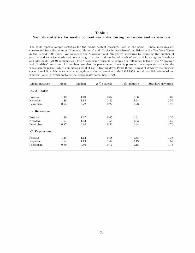
Table 1Sample statistics for media content variables during recessions and expansions

The table reports sample statistics for the media content measures used in the paper. These measures areconstructed from the columns “Financial Markets” and “Topics in Wall-Street” published in the New York Timesin the period 1905-1958. We construct the “Positive” and “Negative” measures by counting the number ofpositive and negative words and normalizing it by the total number of words of each article, using the Loughranand McDonald (2009) dictionaries. The “Pessimism” variable is simply the difference between the “Negative”and “Positive” measures. All numbers are given in percentages. Panel A presents the sample statistics for thewhole sample period, which comprises a total of 15616 trading days. Panel B and C break it down by the businesscycle. Panel B, which contains all trading days during a recession in the 1905-1958 period, has 4894 observations,whereas Panel C, which contains the expasionary dates, has 10722.

Media measure Mean Median 25% quantile 75% quantile Standard deviation

A. All dates

Positive 1.13 1.10 0.87 1.36 0.37Negative 1.88 1.83 1.46 2.24 0.59Pessimism 0.75 0.72 0.22 1.23 0.76

B. Recessions


C. Expansions


30

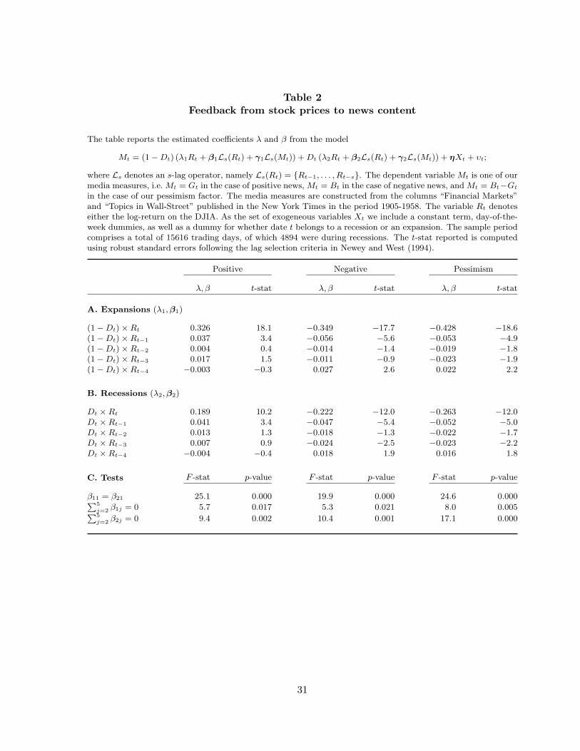
Table 2Feedback from stock prices to news content

The table reports the estimated coefficients λ and β from the model

Mt = (1−Dt) (λ1Rt + β1Ls(Rt) + γ1Ls(Mt)) +Dt (λ2Rt + β2Ls(Rt) + γ2Ls(Mt)) + ηXt + υt;

where Ls denotes an s-lag operator, namely Ls(Rt) = {Rt−1, . . . , Rt−s}. The dependent variable Mt is one of ourmedia measures, i.e. Mt = Gt in the case of positive news, Mt = Bt in the case of negative news, and Mt = Bt−Gt

in the case of our pessimism factor. The media measures are constructed from the columns “Financial Markets”and “Topics in Wall-Street” published in the New York Times in the period 1905-1958. The variable Rt denoteseither the log-return on the DJIA. As the set of exogeneous variables Xt we include a constant term, day-of-the-week dummies, as well as a dummy for whether date t belongs to a recession or an expansion. The sample periodcomprises a total of 15616 trading days, of which 4894 were during recessions. The t-stat reported is computedusing robust standard errors following the lag selection criteria in Newey and West (1994).

Positive Negative Pessimism

λ, β t-stat λ, β t-stat λ, β t-stat

A. Expansions (λ1,β1)

(1−Dt)×Rt 0.326 18.1 −0.349 −17.7 −0.428 −18.6(1−Dt)×Rt−1 0.037 3.4 −0.056 −5.6 −0.053 −4.9(1−Dt)×Rt−2 0.004 0.4 −0.014 −1.4 −0.019 −1.8(1−Dt)×Rt−3 0.017 1.5 −0.011 −0.9 −0.023 −1.9(1−Dt)×Rt−4 −0.003 −0.3 0.027 2.6 0.022 2.2

B. Recessions (λ2,β2)

Dt ×Rt 0.189 10.2 −0.222 −12.0 −0.263 −12.0Dt ×Rt−1 0.041 3.4 −0.047 −5.4 −0.052 −5.0Dt ×Rt−2 0.013 1.3 −0.018 −1.3 −0.022 −1.7Dt ×Rt−3 0.007 0.9 −0.024 −2.5 −0.023 −2.2Dt ×Rt−4 −0.004 −0.4 0.018 1.9 0.016 1.8

F -stat p-value F -stat p-value F -stat p-valueC. Tests

β11 = β21 25.1 0.000 19.9 0.000 24.6 0.000P5j=2 β1j = 0 5.7 0.017 5.3 0.021 8.0 0.005P5j=2 β2j = 0 9.4 0.002 10.4 0.001 17.1 0.000

31

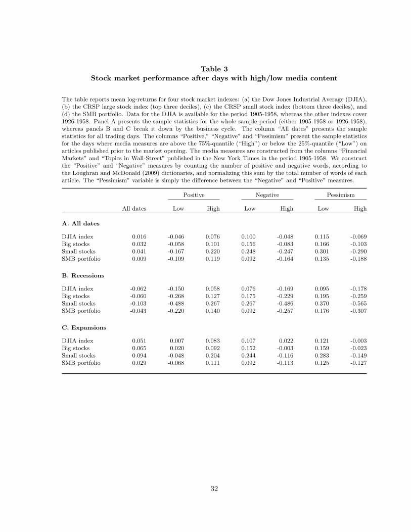
Table 3Stock market performance after days with high/low media content

The table reports mean log-returns for four stock market indexes: (a) the Dow Jones Industrial Average (DJIA),(b) the CRSP large stock index (top three deciles), (c) the CRSP small stock index (bottom three deciles), and(d) the SMB portfolio. Data for the DJIA is available for the period 1905-1958, whereas the other indexes cover1926-1958. Panel A presents the sample statistics for the whole sample period (either 1905-1958 or 1926-1958),whereas panels B and C break it down by the business cycle. The column “All dates” presents the samplestatistics for all trading days. The columns “Positive,” “Negative” and “Pessimism” present the sample statisticsfor the days where media measures are above the 75%-quantile (“High”) or below the 25%-quantile (“Low”) onarticles published prior to the market opening. The media measures are constructed from the columns “FinancialMarkets” and “Topics in Wall-Street” published in the New York Times in the period 1905-1958. We constructthe “Positive” and “Negative” measures by counting the number of positive and negative words, according tothe Loughran and McDonald (2009) dictionaries, and normalizing this sum by the total number of words of eacharticle. The “Pessimism” variable is simply the difference between the “Negative” and “Positive” measures.


All dates Low High Low High Low High

A. All dates

DJIA index 0.016 -0.046 0.076 0.100 -0.048 0.115 -0.069Big stocks 0.032 -0.058 0.101 0.156 -0.083 0.166 -0.103Small stocks 0.041 -0.167 0.220 0.248 -0.247 0.301 -0.290SMB portfolio 0.009 -0.109 0.119 0.092 -0.164 0.135 -0.188

B. Recessions

DJIA index -0.062 -0.150 0.058 0.076 -0.169 0.095 -0.178Big stocks -0.060 -0.268 0.127 0.175 -0.229 0.195 -0.259Small stocks -0.103 -0.488 0.267 0.267 -0.486 0.370 -0.565SMB portfolio -0.043 -0.220 0.140 0.092 -0.257 0.176 -0.307

C. Expansions

DJIA index 0.051 0.007 0.083 0.107 0.022 0.121 -0.003Big stocks 0.065 0.020 0.092 0.152 -0.003 0.159 -0.023Small stocks 0.094 -0.048 0.204 0.244 -0.116 0.283 -0.149SMB portfolio 0.029 -0.068 0.111 0.092 -0.113 0.125 -0.127

32

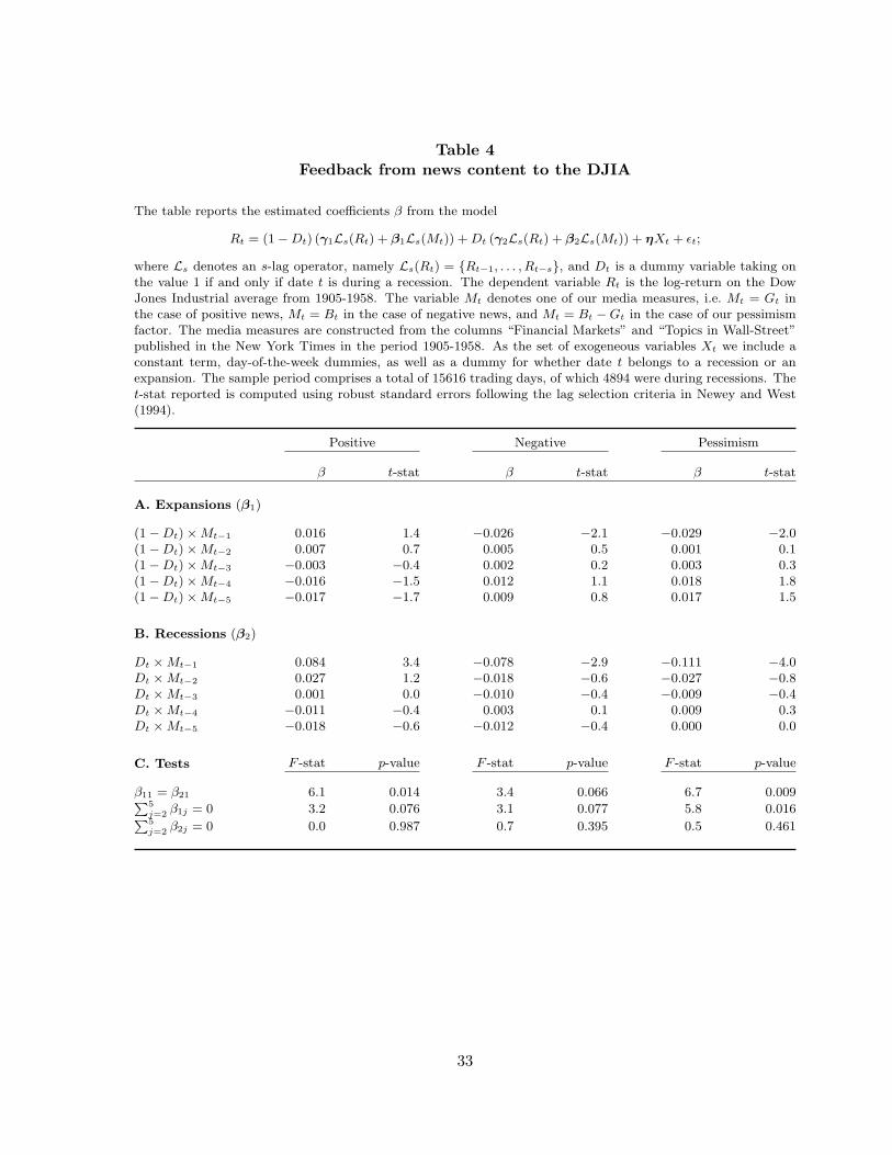
Table 4Feedback from news content to the DJIA

The table reports the estimated coefficients β from the model

Rt = (1−Dt) (γ1Ls(Rt) + β1Ls(Mt)) +Dt (γ2Ls(Rt) + β2Ls(Mt)) + ηXt + εt;

where Ls denotes an s-lag operator, namely Ls(Rt) = {Rt−1, . . . , Rt−s}, and Dt is a dummy variable taking onthe value 1 if and only if date t is during a recession. The dependent variable Rt is the log-return on the DowJones Industrial average from 1905-1958. The variable Mt denotes one of our media measures, i.e. Mt = Gt inthe case of positive news, Mt = Bt in the case of negative news, and Mt = Bt −Gt in the case of our pessimismfactor. The media measures are constructed from the columns “Financial Markets” and “Topics in Wall-Street”published in the New York Times in the period 1905-1958. As the set of exogeneous variables Xt we include aconstant term, day-of-the-week dummies, as well as a dummy for whether date t belongs to a recession or anexpansion. The sample period comprises a total of 15616 trading days, of which 4894 were during recessions. Thet-stat reported is computed using robust standard errors following the lag selection criteria in Newey and West(1994).


β t-stat β t-stat β t-stat

A. Expansions (β1)

(1−Dt)×Mt−1 0.016 1.4 −0.026 −2.1 −0.029 −2.0(1−Dt)×Mt−2 0.007 0.7 0.005 0.5 0.001 0.1(1−Dt)×Mt−3 −0.003 −0.4 0.002 0.2 0.003 0.3(1−Dt)×Mt−4 −0.016 −1.5 0.012 1.1 0.018 1.8(1−Dt)×Mt−5 −0.017 −1.7 0.009 0.8 0.017 1.5

B. Recessions (β2)

Dt ×Mt−1 0.084 3.4 −0.078 −2.9 −0.111 −4.0Dt ×Mt−2 0.027 1.2 −0.018 −0.6 −0.027 −0.8Dt ×Mt−3 0.001 0.0 −0.010 −0.4 −0.009 −0.4Dt ×Mt−4 −0.011 −0.4 0.003 0.1 0.009 0.3Dt ×Mt−5 −0.018 −0.6 −0.012 −0.4 0.000 0.0


β11 = β21 6.1 0.014 3.4 0.066 6.7 0.009P5j=2 β1j = 0 3.2 0.076 3.1 0.077 5.8 0.016P5j=2 β2j = 0 0.0 0.987 0.7 0.395 0.5 0.461

33

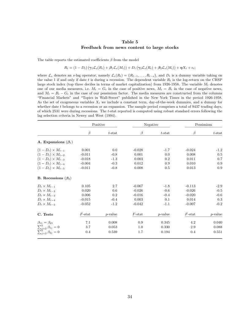
Table 5Feedback from news content to large stocks



where Ls denotes an s-lag operator, namely Ls(Rt) = {Rt−1, . . . , Rt−s}, and Dt is a dummy variable taking onthe value 1 if and only if date t is during a recession. The dependent variable Rt is the log-return on the CRSPlarge stock index (top three deciles in terms of market capitalization) from 1926-1958. The variable Mt denotesone of our media measures, i.e. Mt = Gt in the case of positive news, Mt = Bt in the case of negative news,and Mt = Bt − Gt in the case of our pessimism factor. The media measures are constructed from the columns“Financial Markets” and “Topics in Wall-Street” published in the New York Times in the period 1926-1958.As the set of exogeneous variables Xt we include a constant term, day-of-the-week dummies, and a dummy forwhether date t belongs to a recession or an expansion. The sample period comprises a total of 9437 trading days,of which 2531 were during recessions. The t-stat reported is computed using robust standard errors following thelag selection criteria in Newey and West (1994).



A. Expansions (β1)

(1−Dt)×Mt−1 0.001 0.0 -0.028 -1.7 -0.024 -1.2(1−Dt)×Mt−2 -0.011 -0.8 0.001 0.0 0.008 0.5(1−Dt)×Mt−3 -0.018 -1.3 0.003 0.2 0.011 0.7(1−Dt)×Mt−4 -0.004 -0.3 0.012 0.9 0.010 0.9(1−Dt)×Mt−5 -0.011 -0.8 0.008 0.5 0.013 0.9

B. Recessions (β2)

Dt ×Mt−1 0.105 2.7 -0.067 -1.8 -0.113 -2.9Dt ×Mt−2 0.020 0.6 -0.026 -0.6 -0.026 -0.5Dt ×Mt−3 0.006 0.2 -0.016 -0.4 -0.020 -0.6Dt ×Mt−4 -0.015 -0.4 0.003 0.1 0.014 0.3Dt ×Mt−5 -0.052 -1.2 -0.042 -1.1 -0.007 -0.2


β11 = β21 7.1 0.008 0.9 0.345 4.2 0.040P5j=2 β1j = 0 3.7 0.053 1.0 0.330 2.9 0.088P5j=2 β2j = 0 0.4 0.539 1.7 0.194 0.4 0.551

34

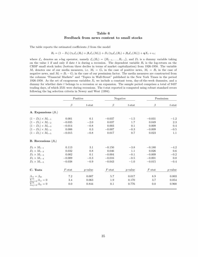
Table 6Feedback from news content to small stocks



where Ls denotes an s-lag operator, namely Ls(Rt) = {Rt−1, . . . , Rt−s}, and Dt is a dummy variable takingon the value 1 if and only if date t is during a recession. The dependent variable Rt is the log-return on theCRSP small stock index (bottom three deciles in terms of market capitalization) from 1926-1958. The variableMt denotes one of our media measures, i.e. Mt = Gt in the case of positive news, Mt = Bt in the case ofnegative news, and Mt = Bt −Gt in the case of our pessimism factor. The media measures are constructed fromthe columns “Financial Markets” and “Topics in Wall-Street” published in the New York Times in the period1926-1958. As the set of exogeneous variables Xt we include a constant term, day-of-the-week dummies, and adummy for whether date t belongs to a recession or an expansion. The sample period comprises a total of 9437trading days, of which 2531 were during recessions. The t-stat reported is computed using robust standard errorsfollowing the lag selection criteria in Newey and West (1994).



A. Expansions (β1)

(1−Dt)×Mt−1 0.001 0.1 −0.037 −1.5 −0.031 −1.2(1−Dt)×Mt−2 −0.035 −2.0 0.037 1.7 0.049 2.3(1−Dt)×Mt−3 −0.014 −0.8 0.003 0.1 0.009 0.4(1−Dt)×Mt−4 0.006 0.3 −0.007 −0.3 −0.009 −0.5(1−Dt)×Mt−5 −0.015 −0.8 0.017 0.7 0.023 1.1

B. Recessions (β2)

Dt ×Mt−1 0.113 3.1 −0.150 −3.8 −0.180 −4.2Dt ×Mt−2 0.032 0.8 0.046 1.1 0.026 0.6Dt ×Mt−3 0.002 0.1 −0.004 −0.1 −0.009 −0.2Dt ×Mt−4 −0.009 −0.3 −0.016 −0.5 −0.001 0.0Dt ×Mt−5 −0.038 −0.9 −0.043 −1.0 −0.015 −0.4


β11 = β21 7.2 0.007 5.7 0.017 8.9 0.003P5j=2 β1j = 0 3.4 0.063 1.9 0.170 3.7 0.054P5j=2 β2j = 0 0.0 0.844 0.1 0.776 0.0 0.968

35

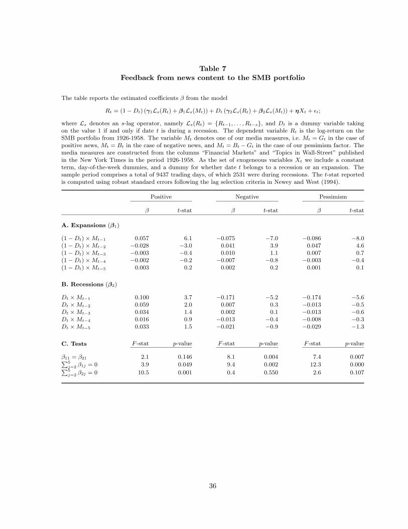
Table 7Feedback from news content to the SMB portfolio



where Ls denotes an s-lag operator, namely Ls(Rt) = {Rt−1, . . . , Rt−s}, and Dt is a dummy variable takingon the value 1 if and only if date t is during a recession. The dependent variable Rt is the log-return on theSMB portfolio from 1926-1958. The variable Mt denotes one of our media measures, i.e. Mt = Gt in the case ofpositive news, Mt = Bt in the case of negative news, and Mt = Bt −Gt in the case of our pessimism factor. Themedia measures are constructed from the columns “Financial Markets” and “Topics in Wall-Street” publishedin the New York Times in the period 1926-1958. As the set of exogeneous variables Xt we include a constantterm, day-of-the-week dummies, and a dummy for whether date t belongs to a recession or an expansion. Thesample period comprises a total of 9437 trading days, of which 2531 were during recessions. The t-stat reportedis computed using robust standard errors following the lag selection criteria in Newey and West (1994).



A. Expansions (β1)

(1−Dt)×Mt−1 0.057 6.1 −0.075 −7.0 −0.086 −8.0(1−Dt)×Mt−2 −0.028 −3.0 0.041 3.9 0.047 4.6(1−Dt)×Mt−3 −0.003 −0.4 0.010 1.1 0.007 0.7(1−Dt)×Mt−4 −0.002 −0.2 −0.007 −0.8 −0.003 −0.4(1−Dt)×Mt−5 0.003 0.2 0.002 0.2 0.001 0.1

B. Recessions (β2)

Dt ×Mt−1 0.100 3.7 −0.171 −5.2 −0.174 −5.6Dt ×Mt−2 0.059 2.0 0.007 0.3 −0.013 −0.5Dt ×Mt−3 0.034 1.4 0.002 0.1 −0.013 −0.6Dt ×Mt−4 0.016 0.9 −0.013 −0.4 −0.008 −0.3Dt ×Mt−5 0.033 1.5 −0.021 −0.9 −0.029 −1.3


β11 = β21 2.1 0.146 8.1 0.004 7.4 0.007P5j=2 β1j = 0 3.9 0.049 9.4 0.002 12.3 0.000P5j=2 β2j = 0 10.5 0.001 0.4 0.550 2.6 0.107

36

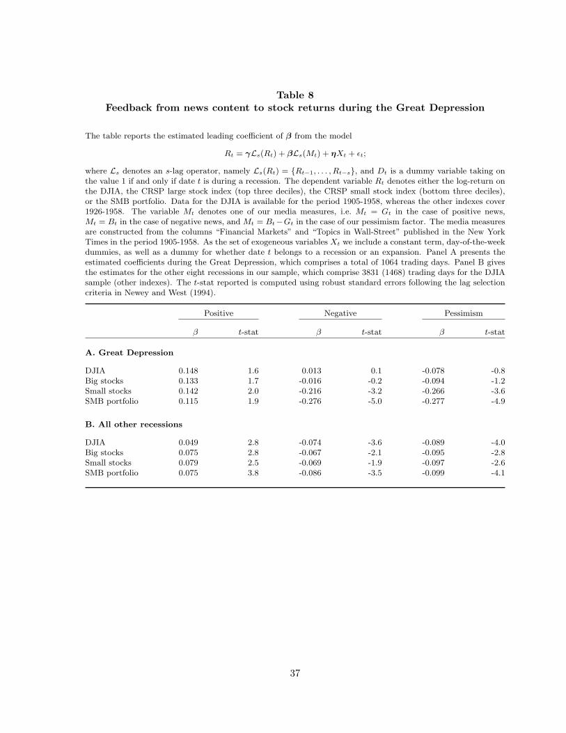
Table 8Feedback from news content to stock returns during the Great Depression

The table reports the estimated leading coefficient of β from the model

Rt = γLs(Rt) + βLs(Mt) + ηXt + εt;

where Ls denotes an s-lag operator, namely Ls(Rt) = {Rt−1, . . . , Rt−s}, and Dt is a dummy variable taking onthe value 1 if and only if date t is during a recession. The dependent variable Rt denotes either the log-return onthe DJIA, the CRSP large stock index (top three deciles), the CRSP small stock index (bottom three deciles),or the SMB portfolio. Data for the DJIA is available for the period 1905-1958, whereas the other indexes cover1926-1958. The variable Mt denotes one of our media measures, i.e. Mt = Gt in the case of positive news,Mt = Bt in the case of negative news, and Mt = Bt−Gt in the case of our pessimism factor. The media measuresare constructed from the columns “Financial Markets” and “Topics in Wall-Street” published in the New YorkTimes in the period 1905-1958. As the set of exogeneous variables Xt we include a constant term, day-of-the-weekdummies, as well as a dummy for whether date t belongs to a recession or an expansion. Panel A presents theestimated coefficients during the Great Depression, which comprises a total of 1064 trading days. Panel B givesthe estimates for the other eight recessions in our sample, which comprise 3831 (1468) trading days for the DJIAsample (other indexes). The t-stat reported is computed using robust standard errors following the lag selectioncriteria in Newey and West (1994).



A. Great Depression

DJIA 0.148 1.6 0.013 0.1 -0.078 -0.8Big stocks 0.133 1.7 -0.016 -0.2 -0.094 -1.2Small stocks 0.142 2.0 -0.216 -3.2 -0.266 -3.6SMB portfolio 0.115 1.9 -0.276 -5.0 -0.277 -4.9

B. All other recessions

DJIA 0.049 2.8 -0.074 -3.6 -0.089 -4.0Big stocks 0.075 2.8 -0.067 -2.1 -0.095 -2.8Small stocks 0.079 2.5 -0.069 -1.9 -0.097 -2.6SMB portfolio 0.075 3.8 -0.086 -3.5 -0.099 -4.1

37

Table 9Feedback from news content to stock returns on consecutive trading days

The table reports the estimated leading coefficients of β1 and β2 from the model


where Ls denotes an s-lag operator, namely Ls(Rt) = {Rt−1, . . . , Rt−s}, and Dt is a dummy variable taking onthe value 1 if and only if date t is during a recession. The dependent variable Rt denotes either the log-returnon the DJIA, the large stock index, the small stock index, or the small-minus-big portfolio. Data for the DJIA isavailable for the period 1905-1958, whereas the other indexes cover 1926-1958. The variable Mt denotes one of ourmedia measures, i.e. Mt = Gt in the case of positive news, Mt = Bt in the case of negative news, and Mt = Bt−Gt

in the case of our pessimism factor. The media measures are constructed from the columns “Financial Markets”and “Topics in Wall-Street” published in the New York Times in the period 1905-1958. As the set of exogeneousvariables Xt we include a constant term, day-of-the-week dummies, as well as a dummy for whether date t belongsto a recession or an expansion. Panel A presents the estimated coefficients for all trading dates t in our samplewhen the market was open at date t− 1 during expansionary periods, a total of 8551 (5484) trading days for theDJIA (other indexes). Panel B presents the results for consecutive trading days during recessions, a total of 3925(2023) trading days for the DJIA (other indexes). The t-stat reported is computed using robust standard errorsfollowing the lag selection criteria in Newey and West (1994).



A. Expansions (β11)


B. Recessions (β21)


38

Figure 1Financial Markets column published in the New York Times on October 12th, 1915.

39

Figure 2Topics in Wall Street colum published in the New York Times on June 25th, 1916.

40

●

●

●

●

●

●

●●

●●●

●

●

●●

●

●

●

●

●

●

●

●

●

●

●●●

●

●

●●●

●

●

●●

●

●

●

●

●

●

●

●

●●

●

●

●

●

●

●●

●

●

●

●●

●

●

●

●

●

●

●

●

●

●

●

●

●

●

●

●

●

●●

●●●

●●

●●●

●

●

●●

●●●●

●

●

●

●

●

●

●

●

●

●●

●●

●

●●●●●

●

●●

●

●

●

●

●

●

●●

●●

●

●

●

●

●●

●●

●

●

●

●●●

●

●●

●

●

●●

●

●●

●

●

●

●●

●●

●

●

●

●

●

●

●

●●

●

●

●

●

●

●

●●

●

●

●

●

●

●

●

●●

●

●

●

●

●

●●

●

●●

●

●

●

●

●●

●

●

●

●

●

●

●

●

●

●

●

●

●

●

●

●

●

●

●

●●

●

●

●

●

●●●

●

●

●●

●

●

●

●

●

●

●

●

●●

●

●●●●

●

●

●●

●

●

●

●

●●

●

●

●●

●

●

●

●

●

●

●

●

●

●

●●

●

●

●

●

●

●

●

●

●

●●●

●

●

●

●

●

●

●

●

●

●

●●●

●

●

●●

●

●

●

●

●

●

●

●

●●

●

●

●

●

●●

●

●●●

●

●●

●

●

●

●

●

●

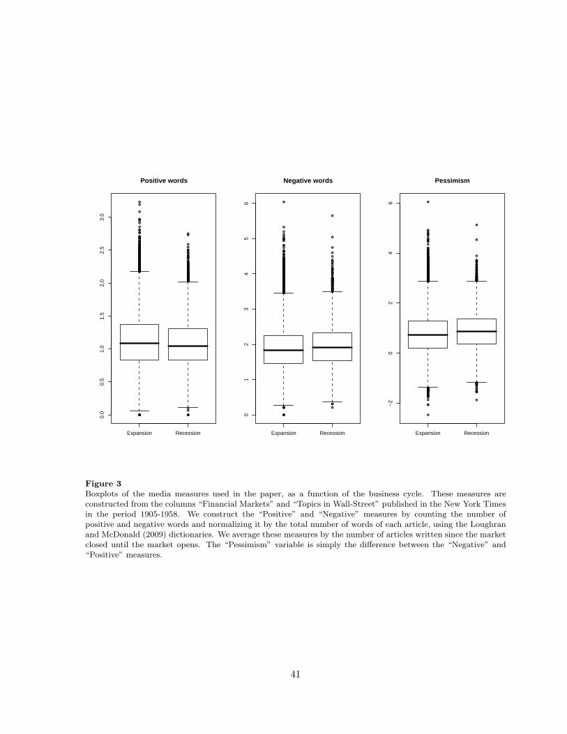
Expansion Recession

0.0

0.5

1.0

1.5

2.0

2.5

3.0

Positive words

●●

●

●

●

●

●●

●

●

●

●

●

●

●

●

●

●

●

●

●

●

●●

●

●

●●●●

●●

●

●

●●

●

●

●●

●●●●

●●

●●

●

●

●

●

●

●

●

●●

●

●

●

●●

●

●

●

●

●●

●

●

●

●

●

●

●

●

●

●

●

●●

●

●●

●●●

●

●

●

●

●

●

●

●

●●●

●

●

●

●

●●●

●

●

●●

●

●

●

●

●●

●

●

●

●

●

●

●

●

●

●

●●●

●

●●

●

●

●

●

●

●

●

●

●

●

●

●

●●●

●

●●

●

●

●

●

●

●

●

●

●●

●

●

●

●

●

●

●

●

●

●

●

●

●

●

●

●●

●

●

●

●

●

●

●

●

●

●

●●

●

●

●

●

●

●

●

●●

●

●

●

●●

●

●

●

●

●

●

●

●

●

●

●

●●

●

●

●

●●●

●

●

●

●

●

●●

●

●

●

●

●●

●

●

●

●

●

●

●

●

●

●

●

●●●

●

●

●

●

●

●

●●

●

●

●

●●

●

●

●

●●

●●

●

●●●

●

●

●

●●

●

●●●

●

●

●

●

●

●

●

●●

●

●

●

●

●

●

●

●

●

●

●

●

●

●

●

●

●●

●

●

●

●

●

●

●●

●

●

●

●

●●

●

●

●●

●

●

●

●

●●

●

●

●

●

●

●

●

●●

●●

●

●

●

●

●

●

●

●

●

●

●

●

●

●

●

●

●

●

●

●

●

●

●

●

●

●

●

●

●●

●

●

●

●

●

●

●

●

●

●

●

●

●

●

●

●●

●●●

●●

●●

●

●

●●

●

●●

●

●

Expansion Recession

01

23

45

6

Negative words

●

●●

●

●

●

●

●

●

●

●●

●

●

●

●

●

●

●●●●

●

●

●

●

●

●●

●

●

●

●●●

●

●●

●●

●

●

●

●

●●

●

●

●

●

●

●

●

●

●

●

●

●

●

●

●

●

●

●

●

●

●

●●

●●

●

●

●

●

●

●

●

●

●

●●●●

●

●

●

●

●●

●

●

●●

●

●●

●

●

●

●

●

●

●

●

●

●●

●

●●

●

●●

●

●

●

●

●

●

●

●

●

●

●

●

●

●

●

●

●

●

●

●

●

●

●●

●●

●

●●

●

●

●●

●●

●

●

●

●

●

●●

●

●

●

●

●

●

●●●●●

●

●

●

●

●

●

●●

●

●

●●

●

●

●

●

●

●

●

●

●

●

●

●

●●

●

●

●●

●●

●

●

●

●

●

●

●

●

●

●

●

●

●

●

●

●

●●

●

●

●

●

●

●●●

●

●

●●

●

●

●

●

●

●

●

●

●

●

●

●

●

●

●●

●

●

●

●

●

●●

●

●

●

●

●

●

●

●

●●

●

●

●

●

●

●

●

●

●

●

●

●

●

●

●

●●

●

●

●

●●

●

●

●

●

●

●

●

●

●●

●

●

●

●

●

●

●

●

●

●

●

●

●

●

●

●

●

●

●

●

●

●

●

●

●

●

●

●

●

●

●

●

●●●●

●●

●

●

●

●

●

●●

●●

●●●

●

●

●●

●

●

●

●

●

●

●

●

●●

●

●

Expansion Recession

−2

02

46

Pessimism

Figure 3Boxplots of the media measures used in the paper, as a function of the business cycle. These measures areconstructed from the columns “Financial Markets” and “Topics in Wall-Street” published in the New York Timesin the period 1905-1958. We construct the “Positive” and “Negative” measures by counting the number ofpositive and negative words and normalizing it by the total number of words of each article, using the Loughranand McDonald (2009) dictionaries. We average these measures by the number of articles written since the marketclosed until the market opens. The “Pessimism” variable is simply the difference between the “Negative” and“Positive” measures.

41

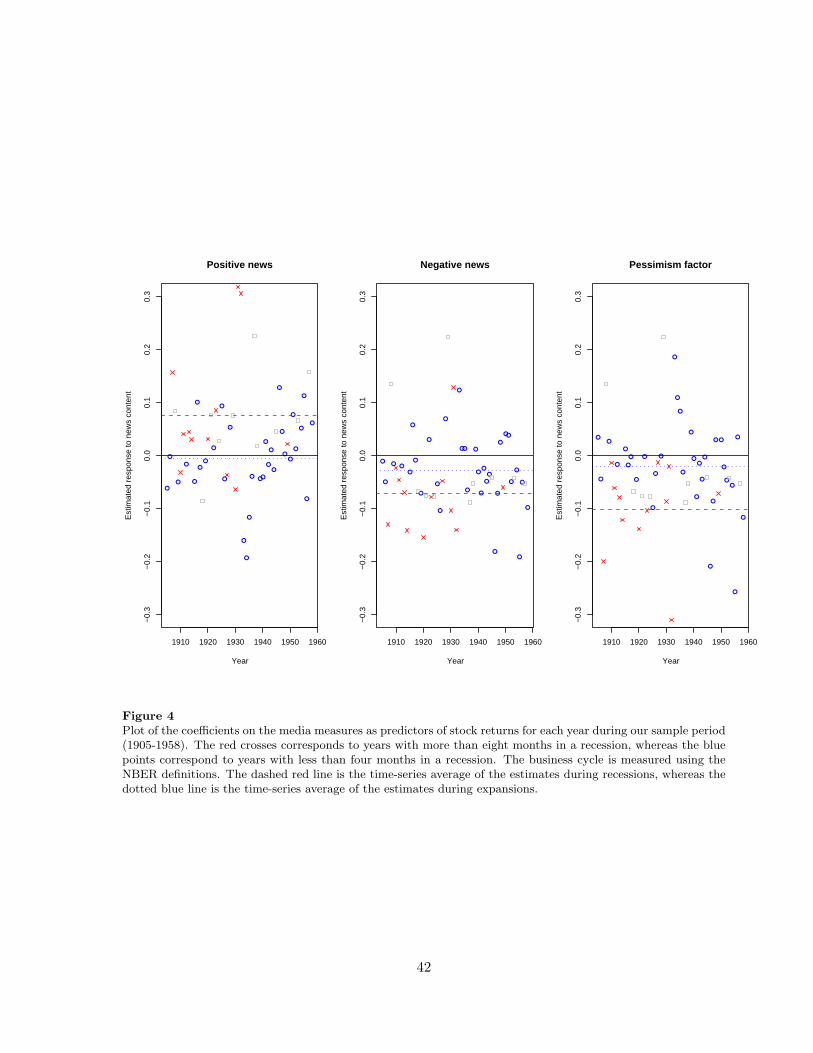
1910 1920 1930 1940 1950 1960

−0.

3−

0.2

−0.

10.

00.

10.

20.

3

Positive news

Year

Est

imat

ed r

espo

nse

to n

ews

cont

ent

●

●

●

●

●

●

●

●

●

●

●

●

●

●

●

● ●●

●

●

●

●

●

●

●●

●

●

●

●

●

●

1910 1920 1930 1940 1950 1960

−0.

3−

0.2

−0.

10.

00.

10.

20.

3

Negative news

Year

Est

imat

ed r

espo

nse

to n

ews

cont

ent

●

●

● ●

●

●

●

●

●

●

●

●

●

●●

●

●

●

●

●

●

●

●

●

●

●●

●

●

●

●

●

1910 1920 1930 1940 1950 1960

−0.

3−

0.2

−0.

10.

00.

10.

20.

3

Pessimism factor

Year

Est

imat

ed r

espo

nse

to n

ews

cont

ent

●

●

●

●

●

●

●

●

●

●

●

●

●

●

●

●

●

●

●

●

●

●

●

●

● ●

●

●●

●

●

●

Figure 4Plot of the coefficients on the media measures as predictors of stock returns for each year during our sample period(1905-1958). The red crosses corresponds to years with more than eight months in a recession, whereas the bluepoints correspond to years with less than four months in a recession. The business cycle is measured using theNBER definitions. The dashed red line is the time-series average of the estimates during recessions, whereas thedotted blue line is the time-series average of the estimates during expansions.

42

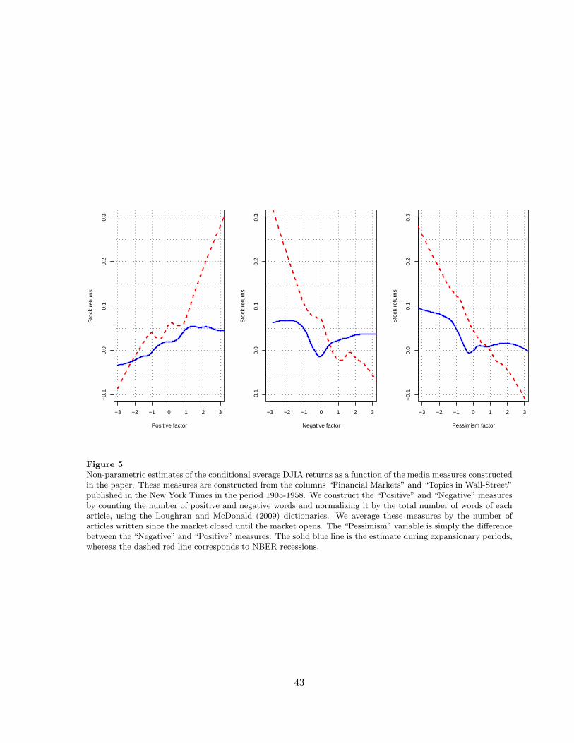
−3 −2 −1 0 1 2 3

−0.

10.

00.

10.

20.

3

Positive factor

Sto

ck r

etur

ns

−3 −2 −1 0 1 2 3

−0.

10.

00.

10.

20.

3

Negative factor

Sto

ck r

etur

ns

−3 −2 −1 0 1 2 3−

0.1

0.0

0.1

0.2

0.3

Pessimism factor

Sto

ck r

etur

ns

Figure 5Non-parametric estimates of the conditional average DJIA returns as a function of the media measures constructedin the paper. These measures are constructed from the columns “Financial Markets” and “Topics in Wall-Street”published in the New York Times in the period 1905-1958. We construct the “Positive” and “Negative” measuresby counting the number of positive and negative words and normalizing it by the total number of words of eacharticle, using the Loughran and McDonald (2009) dictionaries. We average these measures by the number ofarticles written since the market closed until the market opens. The “Pessimism” variable is simply the differencebetween the “Negative” and “Positive” measures. The solid blue line is the estimate during expansionary periods,whereas the dashed red line corresponds to NBER recessions.

43

Sentiment During Recessions

Documents