Sensory analysis via multi-block multivariate additive PLS splines

This article was downloaded by: [Pietro Amenta]On: 13 November 2012, At: 07:09Publisher: Taylor & FrancisInforma Ltd Registered in England and Wales Registered Number: 1072954 Registeredoffice: Mortimer House, 37-41 Mortimer Street, London W1T 3JH, UK

Journal of Applied StatisticsPublication details, including instructions for authors andsubscription information:http://www.tandfonline.com/loi/cjas20

Sensory analysis via multi-blockmultivariate additive PLS splinesRosaria Lombardo a , Pietro Amenta b , Myrtille Vivien c & RobertSabatier ca Department of Management, Accounting and QuantitativeMethods, Economics Faculty, Second University of Naples, Capua,CE, 81043, Italyb Department of Analysis of Economic and Social Systems,University of Sannio, Benevento, BN, 81024, Italyc Laboratoire de Physique Industrielle et Traitement del’Information, EA2415, Faculté de Pharmacie, 34093, MontpellierCedex 5, FranceVersion of record first published: 31 Aug 2011.

To cite this article: Rosaria Lombardo, Pietro Amenta, Myrtille Vivien & Robert Sabatier (2012):Sensory analysis via multi-block multivariate additive PLS splines, Journal of Applied Statistics,39:4, 731-743

To link to this article: http://dx.doi.org/10.1080/02664763.2011.611239

PLEASE SCROLL DOWN FOR ARTICLE

Full terms and conditions of use: http://www.tandfonline.com/page/terms-and-conditions

This article may be used for research, teaching, and private study purposes. Anysubstantial or systematic reproduction, redistribution, reselling, loan, sub-licensing,systematic supply, or distribution in any form to anyone is expressly forbidden.

The publisher does not give any warranty express or implied or make any representationthat the contents will be complete or accurate or up to date. The accuracy of anyinstructions, formulae, and drug doses should be independently verified with primarysources. The publisher shall not be liable for any loss, actions, claims, proceedings,demand, or costs or damages whatsoever or howsoever caused arising directly orindirectly in connection with or arising out of the use of this material.

Journal of Applied StatisticsVol. 39, No. 4, April 2012, 731–743

Sensory analysis via multi-block multivariateadditive PLS splines

Rosaria Lombardoa*, Pietro Amentab, Myrtille Vivienc and Robert Sabatierc

aDepartment of Management, Accounting and Quantitative Methods, Economics Faculty, SecondUniversity of Naples, Capua CE 81043, Italy; bDepartment of Analysis of Economic and Social Systems,University of Sannio, Benevento BN 81024, Italy; cLaboratoire de Physique Industrielle et Traitement de

l’Information, EA2415, Faculté de Pharmacie, 34093 Montpellier Cedex 5, France

(Received 13 November 2010; final version received 3 August 2011)

In the last decade, much effort has been spent on modelling dependence between sensory variables andchemical–physical ones, especially when observed at different occasions/spaces/times or if collected fromseveral groups (blocks) of variables. In this paper, we propose a nonlinear generalization of multi-blockpartial least squares with the inclusion of variable interactions. We show the performance of the methodon a known data set.

Keywords: multivariate additive partial least-squares splines; multi-block analysis; sensorial andchemical–physical variables

1. Introduction

Sensory evaluation is an important topic in the psychometrics literature. Of great interest is under-standing sensory phenomena from the chemical–physical characteristics of foods and studyingrelationships between sensory variables and hedonic variables or between instrumentals charac-teristics (chemical–physical variables) and hedonic judgements/preferences [17]. Psychologicalstudies also address sensory phenomena to quality perception of a person’s experience, as a con-sequence, different evaluations of expert people and/or consumers can be differently related withthe chemical–physical variables. Evaluating differences can be extremely useful to understandfood quality.

Usually, we face a large data set which can be split into several groups (blocks) of variables(collected as matrices of different dimension) where the rows are usually the same (products)but the columns are different, forming a so-called multi-block data set. When all the tables havetwo dimensions in common (rows and columns), the multi-block data set is called a three-waydata table (e.g. sensory profiling data are often collected as products by attributes/variables byjudges/consumers).

*Corresponding author. Email: [email protected]

ISSN 0266-4763 print/ISSN 1360-0532 online© 2012 Taylor & Francishttp://dx.doi.org/10.1080/02664763.2011.611239http://www.tandfonline.com

Dow

nloa

ded

by [

Piet

ro A

men

ta]

at 0

7:09

13

Nov

embe

r 20

12

732 R. Lombardo et al.

In the literature [16,27,28], numerous multi-block methods have been proposed to study sen-sory evaluations (e.g. generalized procrustes analysis [7], STATIS-ACT method [9], factorialmultiple analysis [5], and others [2,11,15,26]). Here, we point out multi-block regression meth-ods, based on partial least-squares (PLS) regression, which maximize a covariance criterion (e.g.[21,22, OMCIA–PLS], [21,23,26, GOMCIA–PLS] and [24, MUBRE]). In particular, we pro-pose a generalization of orthogonal multiple co-inertia analysis–PLS (OMCIA–PLS) [21,22] bynonlinear transformations of predictor variables. This new method, called OMCIA–multivariateadditive PLS spline (MAPLSS), analyses a multi-block response data set by a single data matrixof transformed predictors. When only linear relationships between variables exist, OMCIA–MAPLSS can be classified as linear OMCIA–PLS. Among several nonlinear approaches of PLS[1,4,8,10,18,29,30], we consider MAPLSS [13] as it allows to include interactions between predic-tor variables, which can be particularly useful when the predictors are chemical–physical variables.

This paper is divided into two sections. In Section 2, after a brief presentation of the back-ground methodologies, we illustrate OMCIA–MAPLSS, providing details of the computationalprocedure. The latter part (Section 3) is finally devoted to an application of this proposal on aknown coffee data set.

2. OMCIA via nonlinear PLS

In this section, we illustrate the main aspects of the OMCIA via MAPLSS. Before describingthe OMCIA–MAPLSS phases, we need to briefly summarize both OMCIA–PLS and MAPLSSmethods.

2.1 OMCIA–PLS

OMCIA–PLS [22] is a descriptive and a predictive method that explains a set of N matrices Yn

(i.e. a multi-block table) of responses by one matrix X (with I rows, J columns) [20] of predictors.In the special case, N = 1, OMCIA–PLS is coincident with the PLS regression of Yn on X.In general, OMCIA–PLS is a sequential multi-block PLS regression method, it can be viewed as

a projection of response variables Yn on latent structures, called the components, calculated withthe predictor matrix X. These components, t = Xa, are of maximum covariance with the linearcomponents of Yn, known as un =Ynbn. Indeed, the components are produced stepwise by themaximization of the squared covariance criterion sum:

∑Nn=1 cov2(t, un) = ∑

n(a′X′DYnbn)

2,over the eigenvectors a and bn, with norm unity constraints a′a = 1 and bn

′bn = 1, respectively,and metric defined by the diagonal matrix D (usually uniform metric).

It can be shown [21,22] that by adding an edge on the generic occasion n, we achieve bn, 1 asthe first eigenvector of Yn

′DXX′DYn, related to the largest eigenvector μn, 1 = cov2(t1, un, 1).Next, in turn, a1 is the first eigenvector of

∑n X′DYnY′

nDX associated with the largesteigenvalue λ1 = ∑

n cov2(t1, un) = ∑n μn,1.

Therefore, at the second step s = 2 of the stepwise iterative procedure, we compute the deflatedmatrices of the predictors and of the response variables in the following manner X(s=2) = P⊥

t1X

and Y(s=2)n = P⊥

t1Yn, where P⊥

t1= I − t1Dt′1/t′1Dt1 is the orthogonal projector operator.

After the deflation of all the matrices, thanks to the first component t1, a second set of com-ponents is obtained such that the squared covariance criterion sum between the deflated matricesis maximized, and so on. Finally, the two sets of the components ts and un, s (with s = 1, . . . A)are calculated. Notice that the components ts, s = 1, . . . , A, associated with the predictors are D-orthogonal, while the components un, s, s = 1, . . . A, linked to the responses are not D-orthogonal.In the literature usually, the component number, i.e. the model dimension A is set by the predictivesum of squares (PRESS) criterion.

Dow

nloa

ded

by [

Piet

ro A

men

ta]

at 0

7:09

13

Nov

embe

r 20

12

Journal of Applied Statistics 733

2.2 MAPLS via splines

The MAPLSS regression model [13] is a generalization of the PLS model involving multivariateadditive spline transformations, where each fitted response variables is a sum of transformationfunctions of both main and interaction effects of predictor variables. MAPLSS separately identifiesthe contributions of each variable and those associated with the different multivariate interactionsvia an ANOVA decomposition. For the sake of low-computational cost, the generalized crossvalidation (GCV) criterion [13] has been introduced in the model-building stage instead of theclassical PRESS.

MAPLSS can be also considered as a simple generalization of PLSS [3,4], where using theB-splines (basis splines) as transformation functions, not only the main predictor variables, butalso their interactions have been incorporated into the model. Spline functions S( · ) are piecewisepolynomials of degree d that join end to end on K points ξ 1, . . . , ξK , named the knots of a variablex(n × 1). x can be then coded into a basis of spline functions through the centred coding matrixB (n × r) whose generic element is Bl(x). Then, the transformation of x by the spline functionis S(x) = ∑r

l=1 βlBl(x), where β l is the regression spline coefficient. The dimension r dependson the degree d chosen for the splines and on the number K of internal knots that are used(r = 1 + d + K). In MAPLSS, each predictor (each column of X) is then coded into a B-splinebasis. The coding matrix B of X is then composed of the juxtaposed coding matrices of eachpredictor. Moreover, to capture bivariate interaction, the tensor product of two B-spline functionsis also used. Thus, a variable interaction will enter into the model by defining a new predictorin the design matrix. The computational price to be paid by MAPLSS through tensor productsof B-spline functions is tantamount proportional to expanding the column dimension of the newdesign matrix.

Let us consider x ∈ R2 and two sets of basis functions, B1

j (x1) for j = 1, . . . , r1 and B2

k (x2)

for k = 1, . . . , r2, for representing functions of coordinates x1 and x2, respectively. Then, ther1 × r2-dimensional tensor product basis defined by

Bj,k(x1, x2) = B1

j (x1)B2

k (x2)

allows to represent a bivariate interaction as a two-dimensional function

s1,2(x1, x2, β) =

r1∑

j=1

r2∑

k=1

βj,kBj,k(x1, x2).

The ANOVA spline decomposition with main and interaction effects is given by

y = s1(x1, β1) + s2(x

2, β2) + · · · + s1,2(x1, x2, β1,2) + · · · . (1)

To estimate the B-spline coefficients, the n × (r1 + r2 +· · · + r1r2 +· · · ) centred super-matrixB = [B1|B2|· · · |B1, 2|..], composed of more matrices depending on the number of main predictorsand on the number of the possible bivariate interactions, is included. The first two terms inEquation (1) are the coding matrices obtained by univariate B-spline transformations of x1 andx2, respectively. Furthermore, the columns of the block representing the first bivariate interaction,B1, 2, are coordinate-by-coordinate products of the columns of the two involved variables. Ingeneral, the interactions could involve more than two variables, but it is true that models withinteraction effects involving more than two variables become more difficult to interpret. Noticethat by, increasing the predictors and the interaction number, the column dimension of the designmatrix B grows exponentially fast.

After constructing the design matrix B, in MAPLSS, we estimate a sequence of centred anduncorrelated exploratory variables, i.e. the components (t1, . . . , tA). The number A of the retained

Dow

nloa

ded

by [

Piet

ro A

men

ta]

at 0

7:09

13

Nov

embe

r 20

12

734 R. Lombardo et al.

latent variables, called the model dimension, can be estimated by PRESS or GCV. However, thelatter criterion has been preferred in MAPLSS because of its lower computational cost. As alreadynoticed, MAPLSS is defined as the usual linear PLS regression of Yn onto the space spanned by thecentred coding matrix B (that is, MAPLSS(X,Y) ≡ PLS(B,Y)), which is of expanding dimensionwith respect to X. The drawback of MAPLSS is the larger computational cost than that of thePLS regression. For this reason, in MAPLSS, we propose an automatic selection of interactionsof order 1 only using the quick GCV, as the computational and interpretational price to be paidfor incorporating interactions of high degree increases with the number of predictors involved inthe analysis.

The selection of interactions implies forward/backward phases which produce a sequence ofmodels and estimate which one is the best, looking at a total criterion based on the GCV measure[12–14], which can be seen as a surrogate of the PRESS. The GCV criterion is given by

GCV(A, α) =∑q

j=1 ASRj (A)

[1 − α(A/n)]2, (2)

where ASRj (A) = 1/n‖Yj − Yj(A)‖2 is the average squared residuals for the response j mod-

elled with A components and α represents a penalty constant to be fixed. Empirically, in MAPLSS,one has to calibrate α to find values that give GCV (A, α) as close as possible to PRESS(A), theresulting values have been shown to vary between 0 and 3, usually. The value of α computed inPLS is typically used in the MAPLSS-building model stage. To avoid overfitting problems, welook for parsimonious models with the best values of the GCV(A, α) criterion. At the beginning ofthe forward phases only the main effects model are considered in the design matrix and the mainmodel is estimated. To evaluate the interaction terms individually, each interaction i is separatelyadded to the main effects, using the selection criterion

CRIT(A) = GCVm(A, α) − GCVm+i (A, α)

GCVm(A, α),

where m and m + i denote the models including the main effects and the main effects plus oneinteraction, respectively. When the dimension of the design matrix is not very high, we couldconsider a different formulation of this interaction evaluation criterion including the relativeincrease in the goodness-of-fit criterion, that is

CRIT(A) = R2m(A) − R2

m+i (A)

R2m(A)

+ GCVm(A, α) − GCVm+i (A, α)

GCVm(A, α).

Indeed, if the dimension of the design matrix is very high then the R2(A) index results close to 1,so in this case it will suffice to compute the interaction evaluation criterion by simply using thefirst expression of the selection criterion.

We eliminate the interaction term if CRIT(A) <ε, where ε is a fixed small constant term, andthen we order the accepted candidate interactions. At the end, we re-build the model including theaccepted bivariate interactions. Finally, in the backward phase, an automatic deleting procedurehas been used through the selection criterion, in order to prune the model with the lowest influenceANOVA terms (main or interaction effects).

2.3 OMCIA–MAPLSS

As already stated OMCIA–PLS regression can be viewed as a projection of the response vari-ables Yn (for n = 1, . . . , N) on the components calculated by the predictor matrix X, similarlythe OMCIA–MAPLSS regression can be viewed as a projection of the response variables Yn

Dow

nloa

ded

by [

Piet

ro A

men

ta]

at 0

7:09

13

Nov

embe

r 20

12

Journal of Applied Statistics 735

on the components, computed this time by the transformed predictor matrix X, which are ofmaximum squared covariance with the linear components of Yn. In the special case, N = 1,OMCIA–MAPLSS is coincident with the PLS regression of Yn on B.

Likewise in MAPLSS, all the J predictors are coded into a B-spline basis, getting J codingmatrices Bj, n × rj. Moreover, the interactions between predictors are taken into account bycomputing the tensor product of the corresponding coding matrices Bj.

OMCIA–MAPLSS consists then in using OMCIA–PLS to model the N block of responses Yn

by the coding matrix B = [B1|B2|· · · |BJ |B12|· · · ], where there are main and interaction effects.OMCIA–MAPLSS merges the basic computational aspects and properties of OMCIA–PLS andof MAPLSS, providing a nonlinear version of the former.

The first step of the method consists in computing the weight vectors that maximize the totalsquared covariance criterion, under the usual normalization constraints, given by the sum ofall covariance between block scores t = Ba, associated with the transformed predictors B, andun =Ynbn, associated with the response set Yn. Then, the squared covariance criterion sum isgiven by

∑Nn=1 cov2(t, un) = ∑

n(a′B′DYnbn)

2.Therefore, at the generic step s of OMCIA–MAPLSS, the weight vectors are computed by

maximizing the total squared covariance computed by the updated deflated matrices of the trans-formed predictors B(s−1) and of the responses Y(s−1)

n , setting at the beginning B(s=0) = B andY(s=0) =Y.

At the generic step s, the deflated matrices B(s−1) and Y(s−1)n , which are projected onto the

same space, are defined by B(s−1) = P⊥ts−1

B(s−2) and Y(s−1)n = P⊥

ts−1Y(s−2)

n , respectively. Likewisein OMCIA–PLS, the OMCIA–MAPLSS super-components ts are orthogonal while the super-components associated with the response blocks are not orthogonal.

Finally, likewise in MAPLSS, the GCV criterion has been preferred to be used in OMCIA–MAPLSS instead of the PRESS criterion, owing to a lower computational cost when the designmatrix is of a larger dimension.

3. Application on sensorial data

We now illustrate the capability of OMCIA–MAPLSS on a real-data example. OMCIA–MAPLSSregressions are based on a set of physical–chemical predictor variables and on seven sets ofsensory response variables given by a panel of judges composed of seven expert people. All theused methods have been programmed by the first and third authors in R� Language [19].

The data set is based on a well-known sensorial study [6,22]. This sensorial analysis has theobjective of studying the relationships between the sensorial properties of the coffee, given byan expert judge panel and the physical–chemical properties of the coffee. A sample of 13 coffeeshave been selected by considering three parameters: temperature, moisture–water proportion andgranulometry with three, two and three modalities, respectively. The sensorial properties have beenevaluated by 7 judges, by answering for each one of the 13 coffees the following 6 hedonisticquestions: quality of the perfume, intensity of the perfume, bitterness, acidity, aroma quality andaroma intensity. The scale of the sensorial properties was an ordinal five-point scale (1–5) withrespect to a reference sample (where 1 means that the reference sample is clearly better than theevaluated one and 5 means the evaluated sample is clearly better than the reference one). Thetwo data sets, therefore, are generated on the same statistical units, i.e. the coffees, on whichare measured the sensorial properties (response variables), and the physical–chemical properties(predictor variables) of the 13 coffees. For a deeper description of the data, see [6,22]. Finally,Table 1 reports the sensorial and physical–chemical properties and the used labels.

We can ask: are there differences among the seven sensory evaluations of the judges? What arethe causes of the difference? What are more reliable? What are the chemical–physical variables

Dow

nloa

ded

by [

Piet

ro A

men

ta]

at 0

7:09

13

Nov

embe

r 20

12

736 R. Lombardo et al.

Table 1. Sensorial and physical–chemical variables of the tables.

Sensorial variables Physical–chemical variables

Quality perfume PAC Dry extraction EXSIntensity perfume PAI Extraction rate TEEBitterness AME pH PHHAcidity ACI Acidity CIDAroma quality ARC Optic density (430 nm) DO4Aroma intensity ARI Optic density (510 nm) DO5

Conductivity CDTCaffeine CAFViscosity VISWater-holding capacity in the milling CPR

which affect more the sensory ones? To respond to all these questions, we perform OMCIA–MAPLSS. At first, we look at the predictor transformations and so at the choice of B-splineparameters, following the heuristic strategy of starting with a small degree and knot number andprogressively increasing the model complexity. As a result, the degree has been set equal to 1 and

Table 2. Comparing the GCV criteria for each judge (first dimension).

Judges

Total GCV 1 2 3 4 5 6 7

OMCIA–PLS 4.84 5.47 4.28 6.09 5.35 6.74 4.94OMCIA–MAPLSS 4.30 4.88 3.91 5.58 5.17 5.94 4.79

Table 3. Global and total GCV for each dimension.

GCV dim1 dim2 dim3 dim4 dim5 dim6

Judge 1 4.31 4.33 4.48 5.39 6.62 8.47Judge 2 4.89 5.05 5.48 5.91 7.22 9.16Judge 3 3.91 3.59 3.84 4.36 5.36 6.73Judge 4 5.58 5.82 5.52 6.37 8.16 11.03Judge 5 5.18 5.58 6.10 7.03 7.39 9.78Judge 6 5.94 4.96 5.19 6.51 7.48 9.51Judge 7 4.79 4.17 5.45 5.91 7.12 8.73

Global GCV 34.60 33.50 36.06 41.47 49.35 63.42

Table 4. Results of OMCIA–MAPLSS for the first step s = 1.

Judges

1 2 3 4 5 6 7

λ1 = 60.80 in OMCIA–PLSμn in OMCIA–PLS 10.83 8.25 13.77 5.79 9.23 1.63 11.28Variance un in OMCIA–PLS 3.12 2.58 3.14 2.09 2.33 2.01 2.59

λ1 = 95.23 in OMCIA–MAPLSSμn in OMCIA–MAPLSS 16.21 12.55 22.47 9.47 14.17 3.06 17.29Variance un in OMCIA–MAPLSS 3.11 2.67 3.18 2.09 2.34 2.04 2.61

Dow

nloa

ded

by [

Piet

ro A

men

ta]

at 0

7:09

13

Nov

embe

r 20

12

Journal of Applied Statistics 737

the number of knot to 1, for all predictors. As usual, all measured variables were scaled to be inthe (0, 1) range.

In order to compare the linear and nonlinear models, we compute the goodness of accuracyby the GCV criterion using a tuning parameter α in GCV equal to 1.3. This value of the tuningparameter has been obtained in the linear PLS model by calibrating the GCV value to be similarto the PRESS (as GCV is a surrogate of PRESS), after in the nonlinear models the same value ofthe parameter coefficient α is retained.

Passing from the linear model, OMCIA–PLS, to the nonlinear one, OMCIA–MAPLSS, theaccuracy of the final model is greatly improved with the values of the GCV being lower in eachtable (see Table 2 for the first dimension of the seven judges’ tables and Table 3 for all the otherdimensions). Furthermore, in Table 4, we compare the good performances of the nonlinear model

654321

35

40

45

50

55

60

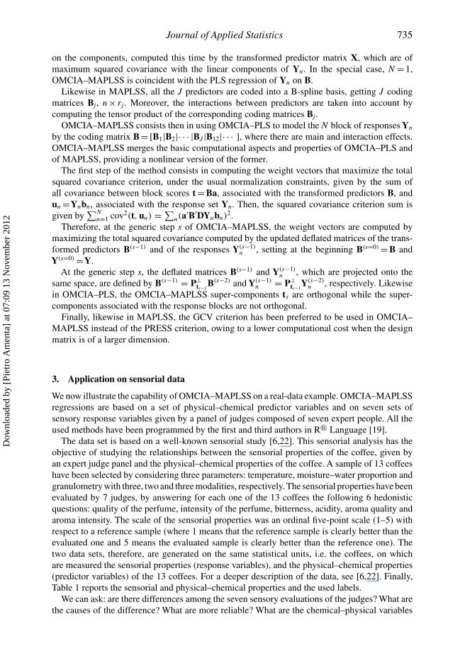
opt. Dim. 2, GCV = 33.4978 (alpha = 1.3)

Model Dim.

GC

V

Figure 1. Global GCV for OMCIA–MAPLSS.

0 5 10 15 20

0

1

2

3

4

5

6

Partial-squared covariances

axe 1

axe

2

1

2

34

56 7

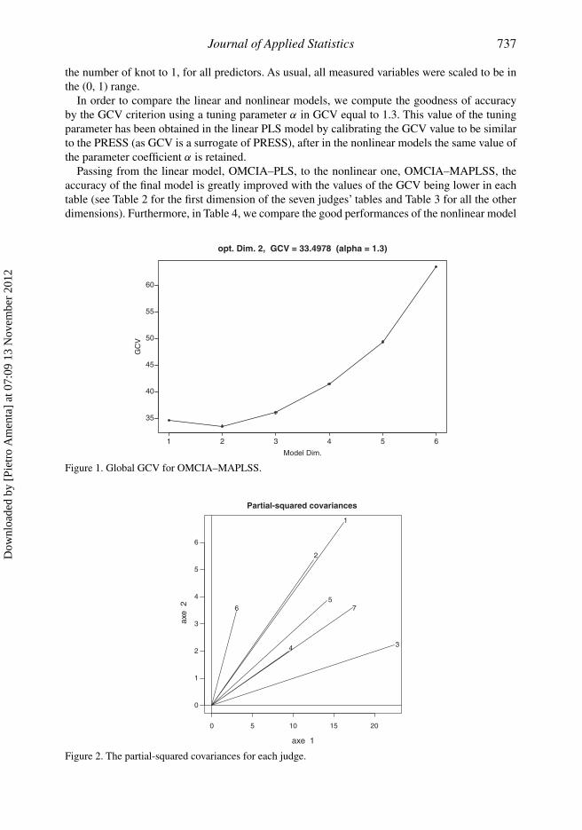
Figure 2. The partial-squared covariances for each judge.

Dow

nloa

ded

by [

Piet

ro A

men

ta]

at 0

7:09

13

Nov

embe

r 20

12

738 R. Lombardo et al.

with respect to the linear one, looking at the increased total criterion of the squared covariance,of the partial-squared covariance, of the variance of the components un, 1, in the first step s = 1 ofOMCIA–MAPLSS.

In OMCIA–MAPLSS after evaluating separately the 45 possible bivariate interactions by GCV,no interaction was included. In addition, by evaluating the global GCV achieved by the models(see Figure 1), the final number A of the retained component for OMCIA–MAPLSS was A = 2.In Table 3, we report the GCV values with respect to each judge’s table and model dimension.

In reality, the advantage of the GCV employed is that it can take more evidence in modernsensory analysis or in chemometrics when the number of descriptors of a product is increasinglylarge (for example, in the case of 40 predictors, we get 780 interactions to evaluate), as the quickGCV allows an easy automatic interaction selection.

Given that the sensory evaluations of the seven judges are different, we wonder what are thosemore predictable by the chemical–physical variables? Computing the partial covariances can helpto answer this question. The higher the covariance, the better the predictability of these sensory

−1.0 −0.5 0.0 0.5 1.0

−1.0

−0.5

0.0

0.5

1.0

(a) (b) (c)

(d) (e) (f)

(g) (h)

−1.0

−0.5

0.0

0.5

1.0

−1.0

−0.5

0.0

0.5

1.0

Correlation of Y1

t 1

t 2

PAC

PAI

AME

ACI

ARC

ARI

−1.0 −0.5 0.0 0.5 1.0

Correlation ofY2

t 1

t 2

PACPAIAME

ACI

ARCARI

−1.0 −0.5 0.0 0.5 1.0

Correlation ofY3

t 1

t 2

−1.0

−0.5

0.0

0.5

1.0

−1.0

−0.5

0.0

0.5

1.0

−1.0

−0.5

0.0

0.5

1.0

t 2

−1.0

−0.5

0.0

0.5

1.0

t 2

t 2 t 2

PACPAI

AMEACIARCARI

−1.0 −0.5 0.0 0.5 1.0

Correlation of Y4

t 1

PAC

PAI

AME

ACI

ARC

ARI

−1.0 −0.5 0.0 0.5 1.0

Correlation of Y5

t 1

PAC

PAI

AME

ACI

ARC

ARI

−1.0 −0.5 0.0 0.5 1.0

Correlation of Y6

t 1

PAC

PAI

AMEACI

ARCARI

−1.0 −0.5 0.0 0.5 1.0

Correlation of Y7

t 1

PACPAI

AME

ACI

ARC

ARI

−6 −4 −2 0 2 4

−4

−2

0

2

4

plot of the observations

axe 1

axe

2

Cafe1

Cafe2

Cafe3Cafe4

Cafe5

Cafe6

Cafe7

Cafe8Cafe9

Cafe10

Cafe11

Cafe12

Cafe13

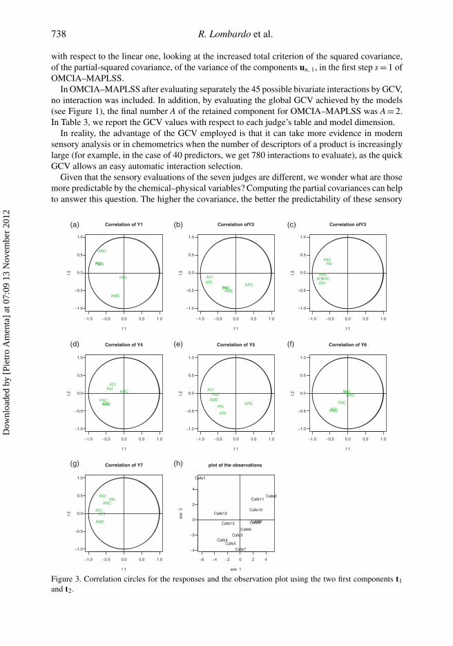
Figure 3. Correlation circles for the responses and the observation plot using the two first components t1and t2.

Dow

nloa

ded

by [

Piet

ro A

men

ta]

at 0

7:09

13

Nov

embe

r 20

12

Journal of Applied Statistics 739

DO4

DO5

EXS

CID

CDT

VIS

CAF

CPR

PHH

TEE

0.00 0.02 0.04 0.06 0.08 0.10

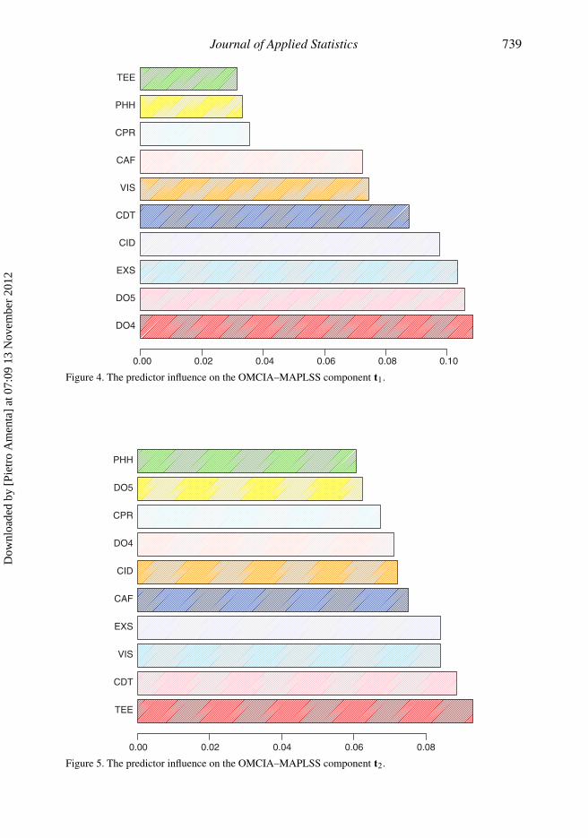
Figure 4. The predictor influence on the OMCIA–MAPLSS component t1.

TEE

CDT

VIS

EXS

CAF

CID

DO4

CPR

DO5

PHH

0.00 0.02 0.04 0.06 0.08

Figure 5. The predictor influence on the OMCIA–MAPLSS component t2.

Dow

nloa

ded

by [

Piet

ro A

men

ta]

at 0

7:09

13

Nov

embe

r 20

12

740 R. Lombardo et al.

evaluations. In Figure 2, we observe the partial-squared covariances, in particular it results thatthe judges 4 and 6 are different from the others, as their covariances are very low, thus the modelfor the judges 4 and 6 is not very representative. While the higher values of covariances concernthe judges 1, 2 and 3 that means the sensory evaluation (food quality perception) of the judges 1, 2and 3 can be well explained by the observed chemical–physical characteristics. Furthermore, thelow values of GCV in Table 3 assess in terms of accuracy the good performances of the modelsrelated to judges 1, 2 and 3 with respect to the others.

In Figure 3(a)–(g), we represent in a common space (compromise space), seven circles ofcorrelation, in which we represent the sensory variables for each judge. In Figure 3(h), we representthe units (coffees) in the common space.

Comparing those circles, we note the different association of the sensory responses with thefirst and the second axis. The responses in Figure 3(d)–(f) (concerning the judges 4 and 6) are lowcorrelated with the first and the second axis. In Figure 3(a)–(c), we notice the highest correlationsof almost all sensory variables with the first two components.

Looking at the observation plot, we clearly notice that the different position of Coffee1 andCoffee7, in particular Coffee7 is strictly associated with the second component. To recognizethe chemical–physical variables which characterize more the sensory variables, we look at thebar-plots of the predictor variables which influence the first two OMCIA–MAPLSS components.

Observe that the first component t1 is mainly related with the predictors DO4, DO5 and EXS,characterizing the differences between Coffee2, Coffee8, Coffee9 and Coffee1, Coffee12, Cof-fee13. The second component t2 is associated with the variables TEE, CDT and VIS, causing thedifferences between Coffee7, Coffee4, Coffee5 and Coffee1.

To explain the predictor influence on the common components, we represent graphically thecontributions of the ANOVA terms, in order to interpret the direct or inverse relationships of the

−1.5 −0.5 0.5 1.0 1.5 2.0

−0.06

−0.02

0.00

0.02

0.04

−0.06

−0.02

0.00

0.02

0.04

−0.06

−0.02

0.00

0.02

0.04

−0.06

−0.02

0.00

0.02

0.04

−0.06

−0.02

0.00

0.02

0.04

−0.06

−0.02

0.00

0.02

0.04

−0.06

−0.02

0.00

0.02

0.04

−0.06

−0.02

0.00

0.02

0.04

−0.06

−0.02

0.00

0.02

0.04

−0.06

−0.02

0.00

0.02

0.04

DO4

Cafe1

Cafe2

Cafe3

Cafe4

Cafe5

Cafe6

Cafe7

Cafe8

Cafe9

Cafe10Cafe11

Cafe12

Cafe13

−1.5 −0.5 0.0 0.5 1.0 1.5 2.0

DO5

Cafe1

Cafe2

Cafe3

Cafe4

Cafe5

Cafe6

Cafe7

Cafe8

Cafe9

Cafe10

Cafe11

Cafe12

Cafe13

−1.0 0.0 0.5 1.0 1.5 2.0

EXS

Cafe1

Cafe2

Cafe3

Cafe4Cafe5

Cafe6

Cafe7

Cafe8Cafe9

Cafe10

Cafe11

Cafe12

Cafe13

−1.0 0.0 0.5 1.0 1.5

CID

Cafe1

Cafe2

Cafe3

Cafe4Cafe5

Cafe6Cafe7

Cafe8

Cafe9

Cafe10

Cafe11

Cafe12

Cafe13

−1.5 −0.5 0.0 0.5 1.0 1.5

CDT

Cafe1

Cafe2

Cafe3

Cafe4Cafe5

Cafe68efaC 7efaC

Cafe9

Cafe10

Cafe11

Cafe12Cafe13

−1 0 1 2

VIS

Cafe1

Cafe2Cafe3

5efaC 4efaC

Cafe6

8efaC 7efaCCafe9

Cafe10

Cafe1131efaC 21efaC

−1.5 −0.5 0.0 0.5 1.0 1.5 2.0

CAF

Cafe1

Cafe2

Cafe3

Cafe4

Cafe5

Cafe6

8efaC 7efaC

Cafe9

Cafe10Cafe11

Cafe12

Cafe13

−2.5 −1.5 −0.5 0.5 1.0

CPR

Cafe1

Cafe2

Cafe3

Cafe4

Cafe5

Cafe6

8efaC 7efaC

Cafe9

Cafe10

Cafe11Cafe12Cafe13

−1 0 1 2

PHH

Cafe1

Cafe2

Cafe3

Cafe4Cafe5

Cafe6

Cafe7

Cafe801efaC 9efaC

Cafe11Cafe12

Cafe13

−1.5 −0.5 0.0 0.5 1.0 1.5

TEE

Cafe1Cafe2

Cafe3

Cafe4Cafe5

Cafe6

Cafe7

Cafe8Cafe9

Cafe10

Cafe11Cafe12Cafe13

(a) (b) (c) (d)

(e) (f)

(i) (j)

(g) (h)

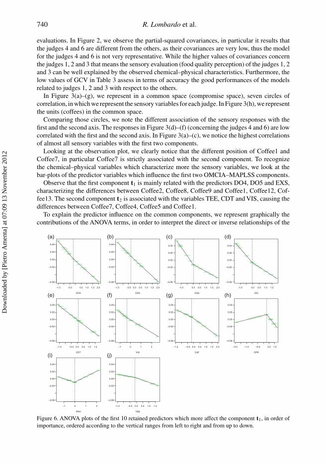
Figure 6. ANOVA plots of the first 10 retained predictors which more affect the component t1, in order ofimportance, ordered according to the vertical ranges from left to right and from up to down.

Dow

nloa

ded

by [

Piet

ro A

men

ta]

at 0

7:09

13

Nov

embe

r 20

12

Journal of Applied Statistics 741

−1.5 −0.5 0.0 0.5 1.0 1.5

−0.06

−0.02

0.00

0.02

0.04

−0.06

−0.02

0.00

0.02

0.04

−0.06

−0.02

0.00

0.02

0.04

−0.06

−0.02

0.00

0.02

0.04

−0.06

−0.02

0.00

0.02

0.04

−0.06

−0.02

0.00

0.02

0.04

−0.06

−0.02

0.00

0.02

0.04

−0.06

−0.02

0.00

0.02

0.04

−0.06

−0.02

0.00

0.02

0.04

−0.06

−0.02

0.00

0.02

0.04

TEE

Cafe1

Cafe2 Cafe3

Cafe4

Cafe5

Cafe6

Cafe7

Cafe8

Cafe9

Cafe10

Cafe11

Cafe12

Cafe13

−1.5 −0.5 0.0 0.5 1.0 1.5

CDT

Cafe1

Cafe2

Cafe3

Cafe4

Cafe5

Cafe6

8efaC 7efaC

Cafe9

Cafe10

Cafe11

Cafe12Cafe13

−1 0 1 2

VIS

Cafe1

Cafe2

Cafe3

5efaC 4efaC

Cafe6

8efaC 7efaC

Cafe9

Cafe10

Cafe11

31efaC 21efaC

−1.0 0.0 0.5 1.0 1.5 2.0

EXS

Cafe1Cafe2

Cafe3

Cafe4

Cafe5Cafe6

Cafe7

Cafe8Cafe9

Cafe10

Cafe11Cafe12

Cafe13

−1.5 −0.5 0.0 0.5 1.0 1.5 2.0

CAF

Cafe1

Cafe2Cafe3

Cafe4

Cafe5Cafe6

8efaC 7efaC

Cafe9

Cafe10

Cafe11Cafe12

Cafe13

−1.0 0.0 0.5 1.0 1.5

CID

Cafe1Cafe2

Cafe3

Cafe4

Cafe5

Cafe6Cafe7

Cafe8

Cafe9

Cafe10

Cafe11

Cafe12

Cafe13

−1.5 −0.5 0.5 1.0 1.5 2.0

DO4

Cafe1

Cafe2

Cafe3

Cafe4

Cafe5

Cafe6

Cafe7

Cafe8

Cafe9

Cafe10

Cafe11

Cafe12

Cafe13

−2.5 −1.5 −0.5 0.5 1.0

CPR

Cafe1

Cafe2

Cafe3

Cafe4

Cafe5

Cafe6

8efaC 7efaC

Cafe9

Cafe10

Cafe11

Cafe12Cafe13

−1.5 −0.5 0.0 0.5 1.0 1.5 2.0

DO5

Cafe1

Cafe2

Cafe3

Cafe4

Cafe5Cafe6

Cafe7

Cafe8

Cafe9

Cafe10

Cafe11Cafe12

Cafe13

−1 0 1 2

PHH

Cafe1

Cafe2

Cafe3

Cafe4

Cafe5

Cafe6

Cafe7

Cafe8

01efaC 9efaC

Cafe11

Cafe12

Cafe13

(a) (b) (c) (d)

(e) (f)

(i) (j)

(g) (h)

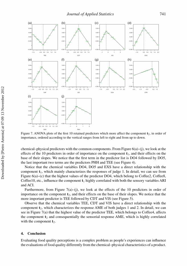
Figure 7. ANOVA plots of the first 10 retained predictors which more affect the component t2, in order ofimportance, ordered according to the vertical ranges from left to right and from up to down.

chemical–physical predictors with the common components. From Figure 6(a)–(j), we look at theeffects of the 10 predictors in order of importance on the component t1, and their effects on thebase of their slopes. We notice that the first term in the predictor list is DO4 followed by DO5,the last important two terms are the predictors PHH and TEE (see Figure 4).

Notice that the chemical variables DO4, DO5 and EXS have a direct relationship with thecomponent t1, which mainly characterizes the responses of judge 1. In detail, we can see fromFigure 6(a)–(c) that the highest values of the predictor DO4, which belong to Coffee2, Coffee8,Coffee10, etc., influence the component t1 highly correlated with both the sensory variables ARIand ACI.

Furthermore, from Figure 7(a)–(j), we look at the effects of the 10 predictors in order ofimportance on the component t2, and their effects on the base of their slopes. We notice that themore important predictor is TEE followed by CDT and VIS (see Figure 5).

Observe that the chemical variables TEE, CDT and VIS have a direct relationship with thecomponent t2, which characterizes the response AME of both judges 1 and 2. In detail, we cansee in Figure 7(a) that the highest value of the predictor TEE, which belongs to Coffee4, affectsthe component t2 and consequentially the sensorial response AME, which is highly correlatedwith the component t2.

4. Conclusion

Evaluating food quality perceptions is a complex problem as people’s experiences can influencethe evaluations of food quality differently from the chemical–physical characteristics of a product.

Dow

nloa

ded

by [

Piet

ro A

men

ta]

at 0

7:09

13

Nov

embe

r 20

12

742 R. Lombardo et al.

The study proposed in this work by OMCIA–MAPLSS has permitted to analyse the dependencerelationship between a three-way matrix of responses and a two-way table of predictor. We havetaken into account the differences among the judges (occasions), highlighting the judges’ evalu-ations as more reliable given the chemical–physical values. The method can be used not only tomake a choice among the best expert judges, but also to point out high-quality food. The non-linear approach, whose particular case is the linear one, has allowed to improve the goodness ofaccuracy of the model. Finally, future researches will consider some theoretical developmentsof the technique with the main aim to look for common space among the blocks of variables byTucker3 or PARAFAC models.

References

[1] M. Blanco, J. Coello, H. Iturriaga, S. Maspoch, and J. Pagès, NIR calibration in non-linear systems: Different PLSapproaches and artificial neural networks, Chemometr. Intell. Lab. Syst. 50 (2000), pp. 75–82.

[2] E.P.P. Derks, J.A. Westerhuis, A.K. Smilde, and B.M. King, An introduction to multi-block component analysis bymeans of a flavor language case study, Food Qual. Prefer. 14 (2003), pp. 497–506.

[3] J.F. Durand, Local polynomial additive regression through PLS and splines: PLSS, Chemometr. Intell. Lab. Syst. 58(2001), pp. 235–246.

[4] J.F. Durand and R. Sabatier, Additive splines for partial least squares regression, J. Amer. Statist. Assoc. 92 (1997),pp. 1546–1554.

[5] B. Escofier and J. Pagès, Multiple factor analysis (AFMULT package), Comput. Statist. Data Anal. 18 (1994),pp. 121–140.

[6] P.L. Gonzales, Analyse Statistique de données psycho-sensorielles, These de 3eme cycle, Universite Montpellier II,1982.

[7] J.C. Gower, Generalized procrustes analysis, Psychometrika 40 (1975), pp. 33–51.[8] F. Huon Kermadec, J.F. Durand, and R. Sabatier, Comparison between linear and nonlinear PLS methods to explain

overall liking from sensory characteristics, Food Qual. Prefer. 8 (1997), pp. 395–402.[9] C. Lavit,Y. Escoufier, R. Sabatier, and P. Traissac, The ACT (STATIS method), Comput. Statist. Data Anal. 18 (1994),

pp. 97–119.[10] R. Leardi, Genetic algorithms in chemometrics and chemistry: A review, J. Chemometr. 7 (2001), pp. 559–569.[11] S. Le Dien and J. Pagès, Hierarchical multiple factor analysis: Application to the comparison of sensory profiles,

Food Qual. Prefer. 14 (2003), pp. 397–403.[12] R. Lombardo, The analysis of sensory and chemical–physical variables via multivariate additive PLS splines, Food

Qual. Prefer. 22 (2011), pp. 714–724.[13] R. Lombardo, J.F. Durand, and R.D. Veaux, Building in multivariate additive partial least-squares splines via the

GCV criterion, J. Chemometr. 23 (2009), pp. 605–625.[14] R. Lombardo, J.F. Durand, and A. Faraj, Iterative design of experiments by non-linear PLS models. A case study:

The reservoir simulator data to forecast oil production, J. Classif. 23 (2011), pp. 113–125.[15] E. Morand and J. Pagès, Procrustes multiple factor analysis to analyse the overall perception of food products, Food

Qual. Prefer. 14 (2006), pp. 182–188.[16] K. Muteki and J.F. MacGregor, Multi-block PLS modeling for L-shape data structures with applications to mixture

modeling, Chemometr. Intell. Lab. Syst. 85 (2007), pp. 186–194.[17] E.M. Qannari, P. Courcoux, andA. Maunit, Analyse d’un ensemble de tableaux: Application aux données sensorielles

et de préférences, Actes des Vemes Journées Agro-Industrie et Méthodes Statistiques, Versaille, 1997.[18] S.J. Qin and T.J. McAvoy, Non-linear PLS modelling using neural networks, Comput. Chem. Eng. 16 (1992),

pp. 379–391.[19] R Development Core Team, R: A Language and Environment for Statistical Computing, R Foundation for Statistical

Computing, Vienna, Austria, 2004. Available at http://www.Rproject.org.[20] A.K. Smilde, J.A. Westerhuis, and R. Boqué, Multiway multiblock component and covariates regression models, J.

Chemometr. 14 (2000), pp. 301–331.[21] M. Vivien, Approches PLS Linéaires et Non-Linéaires Pour la Modélisation de Multi-Tableaux. Théorie et

Applications, These de 3eme cycle, University of Montpellier I, France, 2002.[22] M. Vivien and R. Sabatier, Une extension multi-tableaux de la régression PLS, Rev. Statist. Appl. 49 (2001),

pp. 31–54.[23] M. Vivien and R. Sabatier, Generalized orthogonal multiple co-inertia analysis(-PLS): New multiblock component

and regression methods, J. Chemometr. 17 (2003), pp. 287–301.

Dow

nloa

ded

by [

Piet

ro A

men

ta]

at 0

7:09

13

Nov

embe

r 20

12

Journal of Applied Statistics 743

[24] M. Vivien and R. Sabatier, MUBRE: An algorithm for multiblock regression. Application in sensory analysis,Proceedings of the 11th meeting of Chemometrics in Analytical Chemistry (CAC 2008), Vol. 3, Montpellier, France,30 June–4 July, 2008, pp. 85–89.

[25] M. Vivien and F. Sune, Two four-way multiblock methods used for comparing two consumer panels of children, FoodQual. Prefer. 20 (2009), pp. 472–481.

[26] M. Vivien, T. Verron, and R. Sabatier, Comparing and predicting sensory profiles from NIRS data: Use of theGOMCIA and GOMCIA-PLS multiblock methods, J. Chemometr. 19 (2005), pp. 162–170.

[27] J.A. Westerhuis and A.K. Smilde, Deflation in multiblock partial least squares, J. Chemometr. 15 (2001),pp. 485–493.

[28] J.A. Westerhuis, T. Kourti, and J.F. MacGregor, Analysis of multiblock and hierarchical PCA and PLS models, J.Chemometr. 12 (1998), pp. 301–321.

[29] S. Wold, Non-linear partial least squares modelling. II. Spline inner relation, Chemometr. Intell. Lab. Syst. 14(1992), pp. 71–84.

[30] S. Wold, N. Kettaneh-Wold, and B. Skagerberg, Non-linear PLS modelling, Chemometr. Intell. Lab. Syst. 7 (1989),pp. 53–65.

Dow

nloa

ded

by [

Piet

ro A

men

ta]

at 0

7:09

13

Nov

embe

r 20

12