ADDIS ABABA SCIENCE AND TECHNOLOGY UNIVERSITY SENSORLESS SPEED CONTROL OF PERMANENT MAGNET SYNCHRONOUS MOTOR USING MODEL REFERENCE ADAPTIVE SYSTEM A MASTER’S THESIS By AMARE TIGU ZEWUDIE DEPARTMENT OF ELECTRICAL AND COMPUTER ENGINEERING COLLAGE OF ELECTRICAL AND MECHANICAL ENGINEERING JUNE 2019

Welcome message from author
This document is posted to help you gain knowledge. Please leave a comment to let me know what you think about it! Share it to your friends and learn new things together.
Transcript

ADDIS ABABA SCIENCE AND TECHNOLOGY UNIVERSITY
SENSORLESS SPEED CONTROL OF PERMANENT
MAGNET SYNCHRONOUS MOTOR USING MODEL
REFERENCE ADAPTIVE SYSTEM
A MASTER’S THESIS
By
AMARE TIGU ZEWUDIE
DEPARTMENT OF ELECTRICAL AND COMPUTER
ENGINEERING
COLLAGE OF ELECTRICAL AND MECHANICAL
ENGINEERING
JUNE 2019

ADDIS ABABA SCIENCE AND TECHNOLOGY UNIVERSITY
SENSORLESS SPEED CONTROL OF PERMANENT
MAGNET SYNCHRONOUS MOTOR USING MODEL
REFERENCE ADAPTIVE SYSTEM
By
AMARE TIGU ZEWUDIE
A Thesis Submitted as a Partial Fulfilment of the Requirements for the Degree of Master of
Science in Electrical and Computer Engineering (Control and Instrumentation Engineering)
to
DEPARTMENT OF ELECTRICAL AND COMPUTER ENGINEERING
COLLAGE OF ELECTRICAL AND MECHANICAL ENGINEERING
JUNE 2019
ii
Approval
This is to certify that the thesis prepared by Mr.Amare Tigu Zewudie entitled “Sensorless
Speed control of Permanent Magnet Synchronous Motor Using Model Reference
Adaptive System” and submitted in fulfilment of the requirements for the Degree of Master
of Science complies with the regulations of the University and meets the accepted standards
with respect to originality and quality.
Approval by Board of Examiners
_______________ ___________ ____________
Chairman, Dept. Graduate Committee Signature Date
Dr.- Ing. Gebremichael Teame ___________ ____________
Advisor’s Name Signature Date
Beza Nekatibeb (PhD. Candidate) ___________ ____________
Co-Advisor’s Name Signature Date
______________ _____________ ___________
Internal Examiner Signature Date
______________ ____________ ___________
External Examiner Signature Date
_________________ _____________ __________
DGC chairperson Signature Date
__________________ _______________ ___________
Collage Dean/Associative Dean for GP Signature Date

iii
Declaration
I hereby declare that this thesis entitled “Sensorless Speed Control Of Permanent Magnet
Synchronous Motor Using Model Reference Adaptive System” is composed by myself,
with the guidance of my advisors, that the work contained herein is my own except where
explicitly stated otherwise in the text, and that this work has not been submitted, in whole or in
part, for any other degree, and all sources of materials used for the thesis have been fully
acknowledged.
Amare Tigu __________________ _________
Name Signature Date
Addis Ababa, Ethiopia June 2019
Place Date of Submission
This thesis has been submitted for examination with my approval as a university advisor.
Dr.- Ing. Gebremichael Teame ___________ _______
Advisor’s Name Signature Date
Beza Nekatibeb (PhD candidate) ____________ _______
Co-Advisor’s Name Signature Date

iv
Abstract
Nowadays many studies focusing on for the elimination of the speed and position sensors for
Field oriented control (FOC) based speed control of AC machines. It avoids the drawback of
the sensors such as, the required additional mounting space, decreasing the reliability in harsh
environments and increase the cost of the machines. In this work, sensorless speed control of
permanent magnet synchronous motor (PMSM) using model reference adaptive system
(MRAS) is proposed. Stator current based Model reference adaptive system is used to estimate
the speed of the motor and also the adaptation mechanism constructed by using Popov hyper
stability principle. The main idea here is that the reference model, which is the permanent
magnet synchronous motor (PMSM), d-q axis stator current output compared with the
adjustable model d-q axis current and their difference pass through adaptation method to
estimate the speed of the motor. In addition, model reference adaptive system (MRAC) with
Lyapunov stability adaptation mechanism is employed for speed control of machine which
decrease the dependence on system parameters significantly. This controller parameters are
tuned in such a way that the plant follows the reference model. The effectiveness of the
proposed system is tested through computer simulation. The software used to test the
effectiveness of the proposed system is MATLAB/Simulink. The system gives good
performance at loaded and no load conditions and hence it can work with different load torque
conditions and system parameter variation. The output of the proposed system compared with
the result of the system using conventional proportional and integral (PI) speed controller
shows better performance.
Key words
PMSM, FOC, Popov stability, Lyapunov stability, Stator Current Based MRAS,
Sensorless.

v
Acknowledgment
First and foremost I would like to thank the almighty God and his mother for helping me to
achieve my goal and to complete this thesis successfully. And then, I would like to thank
University of Gondar for giving the chance to study my master of degree and supporting me
financially.
I would like to expressing a sincere acknowledgement to my advisor, Dr.- Ing Gebremichael
Teame, for giving me the opportunity to research under his guidance and supervision. I
received motivation, comments, encouragement and continuous guidance from him during my
graduate studies. I also want to thanks Mr. Beza Nekatibeb (PhD candidate) for his technical
and professional supports.
Next, I want to thank all of my friends who aided me throughout my work. Also i would like
to express my sincere thanks and appreciation to Sntayehu Tesfaye and her grandmother
Yeshimebet for their indispensable encouragements they gave me.
Finally I want to thank my respected parents, Tigu Zewudie and Tihun Adgeh for their
continuous and valuable support throughout the time of my study.

vi
Contents
Approval ................................................................................................................................... ii
Declaration.............................................................................................................................. iii
Abstract .................................................................................................................................... iv
Acknowledgment ...................................................................................................................... v
List of Tables ........................................................................................................................ viii
List of Figures .......................................................................................................................... ix
List of Symbols ....................................................................................................................... xii
Chapter One ............................................................................................................................. 1
1. Introduction to Permanent Magnet Synchronous Motor (PMSM) ................................ 1
1.1 Background of the Study ............................................................................................... 1
1.2 Statement of the Problem .............................................................................................. 2
1.3 Objectives ........................................................................................................................ 3
1.3.1 General objective ..................................................................................................... 3
1.3.2 Specific Objectives ................................................................................................... 3
1.4 Scope and Limitation of the Thesis ............................................................................... 4
1.5 Methods ........................................................................................................................... 4
1.6 Thesis Organization ....................................................................................................... 6
Chapter two .............................................................................................................................. 7
2. Literature Review ................................................................................................................ 7
Chapter Three ........................................................................................................................ 12
3. Field Oriented Control and MRAS observer .................................................................. 12
3.1 Introduction .................................................................................................................. 12
3.2 Field Oriented Control (FOC) .................................................................................... 14
3.3 Transformations ........................................................................................................... 15
3.4 Mathematical Model of PMSM In d-q Frame of Reference .................................... 17
3.5 SVPWM for Inverter Fed PMSM............................................................................. 20
3.5.1 Principle of Space Vector PWM ........................................................................... 22
3.5.2 Implementation of Space Vector PWM ............................................................... 22
3.6 MRAS Observer Design for Speed Estimation of PMSM ...................................... 27

vii
3.6.1 Stator current based MRAS Observer Design for Speed Estimation............... 29
3.6.2 PI Parameter Adjustment of Speed estimator .................................................... 33
Chapter four ........................................................................................................................... 37
4. Speed and Current PI Controller design For PMSM ..................................................... 37
4.1 PID controller ............................................................................................................... 37
4.2 Current Controller Design .......................................................................................... 37
4.3 Speed Controller Design .............................................................................................. 41
4.3.1 Online Tuning of PI Speed Controller Gain with MRAC ................................. 43
4.3.2 MRAC based PI controller Design Method Using Lyapunov Stability Theory
.......................................................................................................................................... 44
Chapter Five ........................................................................................................................... 50
5. Simulation Result and Discussion .................................................................................... 50
5.1 Introduction .................................................................................................................. 50
5.2 Simulink Model of PMSM Drive System ................................................................... 50
5.3 Simulation Results ........................................................................................................ 53
5.3.1 Sensorless speed control simulation result .......................................................... 53
5.3.2 MRAC Speed Controller Simulation Result ....................................................... 64
Chapter six .............................................................................................................................. 66
6. Conclusion and recommendation ..................................................................................... 66
6.1 Conclusion ..................................................................................................................... 66
6.2 Recommendation .......................................................................................................... 67
References ............................................................................................................................... 68
Appendix ................................................................................................................................. 72

viii
List of Tables
Table 2. 1: Summery of literature review results ..................................................................... 10
Table 3. 1: Switching vectors, output phase voltages and output line to line voltages. .......... 21
Table 3. 2: Switching time calculation for the first sector ....................................................... 27
Table 5. 1: Performance comparison of PI and MRAS controller from Figure 5.19 .............. 65
Table A. 1: SPMSM Parameters .............................................................................................. 72
ix
List of Figures
Figure 1. 1: PMSM speed estimation method with Adaptive system ........................................ 5
Figure 1. 2 : Complete block diagram of sensorless FOC Controlled PMSM using MRAS .... 5
Figure 3. 1: Different PMSM rotor designs [20] ..................................................................... 12
Figure 3. 2 : Control method of PMSM ................................................................................... 13
Figure 3. 3: Transformations and Reference [26] .................................................................... 15
Figure 3. 4 : Forward Transformations [26] ............................................................................ 16
Figure 3. 5 : View of a three phase, two-pole PMSM [27] ...................................................... 17
Figure 3. 6 : Three Phase Inverter [2] ...................................................................................... 20
Figure 3. 7 : Basic switching vectors, sectors and a reference vector [2] ................................ 23
Figure 3. 8 : Voltage space vector and its components in a-b-c axis [25] ............................... 24
Figure 3. 9 : Reference voltage as a combination of adjacent vectors in sector I [25]. ........... 26
Figure 3. 10 : SVPWM switching pattern for the first sector [2] ............................................ 26
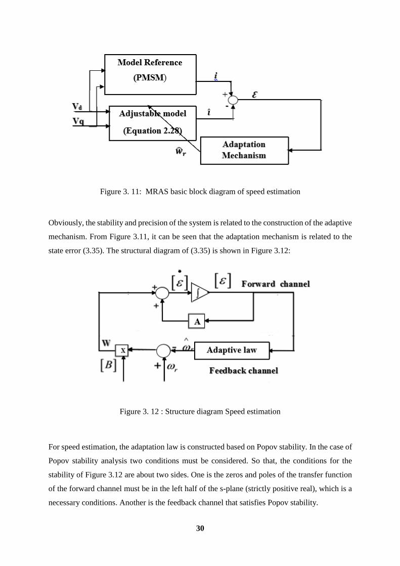
Figure 3. 11: MRAS basic block diagram of speed estimation .............................................. 30
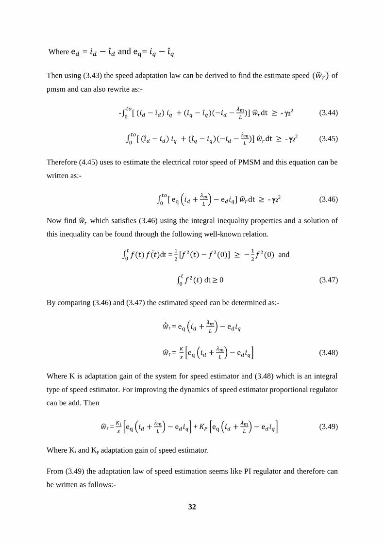
Figure 3. 12 : Structure diagram Speed estimation .................................................................. 30
Figure 3. 13 : MRAS structure diagram................................................................................... 33
Figure 3. 14: MRAS simplified structure diagram .................................................................. 34
Figure 3. 15: Root locus of closed loop adaptive control system ........................................... 36
Figure 4. 1: d –axis current closed loop transfer function with PI controller block diagram .. 38
Figure 4. 2 : q–axis current closed loop transfer function with PI controller block diagram .. 38
Figure 4. 3: Matlab Simulink block diagram of closed loop PI q-axis current controller ...... 40
Figure 4. 4: Open and Closed loop Step response of q-axis current ........................................ 41
Figure 4. 5: General structure of a typical MRAC scheme ...................................................... 44
Figure 4. 6: Matlab Simulink model for PI controller parameter adaptation using Lyapunove
stability. ................................................................................................................. 47
Figure 4. 7: Process and reference model speed step response output wave forms. ............... 48
Figure 4. 8: The difference of reference model and plant model response .............................. 48
Figure 4. 9 : Closed loop response of speed MRAC controller ............................................... 49
Figure 4. 10: The controlled signal U(t) .................................................................................. 49
Figure 5. 1: Complete Matlab/Simulink Model of the FOC based PMSM drive. ................... 50
Figure 5. 2 : PMSM Matlab Simulink model .......................................................................... 51
Figure 5. 3 : The overall speed and current controller representation in Matlab/Simulink. .... 51
x
Figure 5.4: Adjustable model and Adaptation mechanism of Speed estimation Matlab/Simulink
model. .................................................................................................................... 52
Figure 5. 5 : Complete Matlab/Simulink model of MRAS speed estimator. ........................... 52
Figure 5. 6 : Step input speed response with 2.4Nm load torque ............................................ 54
Figure 5. 7: Estimated and actual angle. ................................................................................. 54
Figure 5. 8 Rotor speed response with different a step input reference and load of 2.4 Nm ... 55
Figure 5. 9 : Square input signal rotor speed response with load of 2.4 Nm ........................... 55
Figure 5. 10: Load torque effect on MRAS based Speed estimator ....................................... 56
Figure 5. 11: The rotor speed response at 10 rad/sec step input signals without load. ............ 57
Figure 5. 12: Rotor speed responnse at 0 rad/sec step input signal without load .................... 57
Figure 5. 13: Step response of drive with speed reversal with load torque of 2.4 Nm. ........... 58
Figure 5. 14: Estimated and Actual speed response under parameter varations. ..................... 59
Figure 5. 15: Estimated and Actual angle under parameter variations. ................................... 59
Figure 5. 16: The estimated and actual d-q axis current. ......................................................... 60
Figure 5. 17: Proportionality of Te and q-axis current ........................................................... 61
Figure 5. 18: Three phase Current output motor wave form. .................................................. 61
Figure 5. 19: stator current and voltage when reference speed steps from 157 to 62 rad/sec at
t= 1s ....................................................................................................................... 62
Figure 5. 20 : Speed and torque response when reference speed steps from 157 t0 62 rad/sec at
t= 1s ....................................................................................................................... 62
Figure 5. 21: Speed and torque response when load torque steps from 0.5 to 2.4Nm at t=1 s.
............................................................................................................................... 63
Figure 5. 22: Stator current and voltages when load torque steps from 0.5 to 2.4Nm at t=1s. 63
Figure 5. 23: Speed response of PMSM using MRAC ............................................................ 64
Figure 5. 24: Comparison of PI and MRAC speed response ................................................... 65
xi
List of Abbreviations
FOC Filed Oriented Control
MRAS Model Reference Adaptive Control
IGBT Insulated Gate Bipolar Transistor
MTPA Maximum Torque per Ampere
SPMSM Surface Mounted Permanent Magnet Synchronous Motor
IPMSM Integrated Permanent Magnet Synchronous Motor
MRAC Model Reference Adaptive Controller
VSI Voltage Source Invertor
SVPWM Space Vector Pulse Width Modulation
PI Proportional Integral
MIT Massachusetts Institute of Technology
EMF Back Electromagnetic Force

xii
List of Symbols 𝑖𝑑 Direct axis current
𝑖𝑞 Quadrature axis current
𝑖̂𝑑 Estimated direct axis current
𝑖̂𝑞 Estimated quadrature axis current
𝑤𝑟 Electrical rotor speed
�̂�𝑟 Estimated electrical rotor speed
𝑤𝑚 Mechanical rotor speed
P Number of pole pairs
J Moment of Inertia
B Viscous friction
Te Electromagnetic torque
𝑇𝐿 Load torque
R Stator resistance
L Stator Inductance
λ𝑚 Permanent magnet flux
𝜃𝑟 Electrical rotor angle
𝜃𝑚 Mechanical angle
𝑉𝑑 Direct axis voltage
𝑉𝑞 Quadrature axis voltage
𝑒𝑑 Direct axis current error
𝑒𝑞 Quadrature axis current error
1
Chapter One
1. Introduction to Permanent Magnet Synchronous Motor (PMSM)
1.1 Background of the Study
Recently controlled AC drives have been extensively employed in various high performance
industrial application. This has been conventionally achieved by using DC drives with their
simple structure. AC machines are generally inexpensive, compact and robust with low
maintenance requirements compared to DC machines but require complex control [1].
However, recent advances in power electronics, control technique and signal processing have
led to significant development in AC drives. Permanent magnet synchronous motors (PMSM)
are AC machines, that increasingly replacing traditional DC motors in a wide range of
applications where a fast dynamic response is required [1].
A permanent magnet synchronous motor (PMSM) is an AC motors that uses permanent
magnets to produce the air gap magnetic field rather than using electromagnets. By the
replacement of electromagnets with permanent magnets the permanent magnet synchronous
motors had many advantage such as high efficiency, high torque to inertia ratio and efficient
heat dissipation and also makes it as smaller in size .The heat loss in the rotor of PMSM that
affects the machine operation is also negligible [2]. Because of the above mentioned
advantages this motor is extensively used in many applications such as electric vehicles,
robotics automation, hard disk drives etc. In PMSMs, the magnets can be placed in different
ways on the rotor. Depending on the placement they are classified as surface mounted
permanent magnet motor and interior permanent magnet synchronous motor. SPMSM is
simple to control and low cost of construction when it compared with IPMSM. But in the case
of IPMSM, it is better than that of SPMSM for high speed control application [3].
Depending on the distribution of stator winding the shape of the induced electromagnetic force
(EMF) in PMSM can be trapezoidal or sinusoidal shape. If the stator winding of PMSM
uniformly distributed as a circular form, it produces a sinusoidal EMF and it has less torque
ripples than trapezoidal induced EMF for speed control of PMSM [3]. The speed control of
PMSM can be achieved by using the scalar and vector control techniques or Field oriented
control technique (FOC). The problem with scalar control is that motor flux and torque in
general are coupled. This inherent coupling affects the response and makes the system prone

2
to instability for variable load condition. While in vector control both this are independently
controllable because of, the decoupled nature of flux and torque in this control strategy [2].
A mature and widely used control strategy for PMSMs is the FOC method. By using the vector
control technique separate exited DC motor like characteristics can be obtained from the
PMSM which are desirable for high performance operation .The basic idea with FOC is to
separately control the motor flux and torque. This is done by transforming the three fixed stator
currents, represented in a three-coordinate reference frame, into a rotating two coordinate
reference frame [1, 4]. The two current components are then controlled independently on each
other. The control output, that is the new motor voltage command, is then transformed back
and instructs the voltage inverter to produce the sinusoidal voltages that will be fed in to the
motor. This approach, FOC, makes the AC control behave like a DC control [4, 5].To do this,
the exact position of the rotor needs to be known using mechanical sensor. But by using
mechanical sensor to determine the information of the position of the rotor increases spacing,
weight and cost of the system and also it decreases the reliability of the system in the harsh
environment. To avoid such problem this thesis proposed that FOC based sensorless speed
control of PMSM drives. In addition to this, this thesis also consider adaptive control instead
of conventional PI speed control of PMSM.
1.2 Statement of the Problem
In sensorless speed control of permanent magnet synchronous motor, the rotor speed has been
estimated by various techniques. The simplest and popular methods are based on the back-
EMF and angular velocity of rotor flux. However, both the rotor flux and back-EMF methods
are less accurate due to the great sensitivity to motor parameter variation and also at low speed
condition it is difficult to estimate the speed of the drive due to the noise signal greater than the
estimated signal [7, 8]. Other method is based on extended Kalman filter, which is more robust
to the permanent magnet synchronous motor parameter changes but much more complicated
in practical realization and require complex mathematical analysis [13]. There are also signal
injection method and ANN based speed estimation of the drives. But in the case of signal
injection method it is difficult to estimate the speed at high speed conditions [16] and on the
other hand ANN based speed estimation, it is very complicated for practical realization and it
has also slow rate of adaptation time to estimate the speed of PMSM [17]. The solution for
rotor speed estimation is based on a stator current based MRAS principle approach has

3
advantages like simplicity, easy to implement, has direct physical interpretation and fast rate
of adaptation [18]. Stator current based model reference adaptive system can also estimate the
speed under the problem of parameter variation due to aging, un-model dynamics and
temperature effects even at low speed conditions. Therefore, stator current based MRAS can
estimate over a wide range of speed conditions of the drives.
The most common choices of the speed controller of PMSM is the so called conventional PI
compensator. Even though it has a simple structure and can offer a satisfactory performance in
a single operating condition [19], its performance affected under different operating conditions.
The main problem of this controller is the correct choice of the PI controller parameter gains
when the operating condition of the system is changed due to its internal and external factors
[2]. Therefore, an online tuning process must be performed to insure that the controller can
deal with the variations in the plant parameter using adaptive controller, which has good
response to model uncertainty and parameter change of the system.
1.3 Objectives
1.3.1 General objective
The main objective of this thesis is speed estimation and speed control of permanent magnet
synchronous motor (PMSM) using model reference adaptive system (MRAS).
1.3.2 Specific Objectives
To achieve the general objective, the specific objectives to accomplish are:
To study the characteristics and developing a mathematical model of permanent magnet
synchronous motor in d-q frame of reference for filed oriented control (FOC) design.
To design MRAS based on the nonlinear model of the permanent magnet synchronous
motor drive system.
To design adaptation mechanism to estimate the rotor speed of the motor.
To design control strategies for sensorless speed control of permanent magnet
synchronous motor.
To develop online tuning of speed controller PI parameters gain.
4
To simulate and test the sensorless speed control and it’s reference tracking of the
PMSM using Matlab/Simulink.
1.4 Scope and Limitation of the Thesis
This thesis is limited to design and simulation of the sensorless speed control of PMSM using
MRAS scheme and PI parameters of speed controller are tuned online using MRAC. It is also
consider only MTPA principle of PMSM speed control.
This thesis presents under the consideration of all magnetic flux distribution waveforms are
sinusoidal shape. Distribution of the current in the stator conductors are also assumed
sinusoidal to simplify the complex system dynamics and also considering ideal VSI.
The scope of thesis presents only a surface mounted permanent magnet synchronous motor
with a rated power of 0.75 Kwatt and rated torque of 2.4 Nm under variable load torque
conditions.
1.5 Methods
To accomplish speed estimation and speed control of PMSM the following methods have been
followed.
Mathematical modelling of the system for controller design and for determining
coupling effect dynamics of the system which is treated by feedforward decoupling
Designing a MRAC Speed Controller for the system based on performance
specification using Lyapunove stability theory.
Estimate rotor speed of PMSM based on stator current based MRAS using Popov
stability and PI adaptation mechanism.
Determine PI adaptation gain parameter using root locus analysis technique.
The proposed system result shown by using 2018a version of MTLAB/Simulink
software.
The MRAS speed observer scheme is illustrated in Figure 1.1 and also the complete sensorless
speed control of PMSM using MRAS is illustrated in Figure 1.2. The performance of the speed
controller and estimator tracing will be performed with under variable load condition, large
speed range, and under different reference input signals. The performance of the MRAC are

5
compared with that of PI controller, under parameter uncertainty. All the designing procedure
and simulation results are simulated by using Matlab software.
Figure 1. 1: PMSM speed estimation method with Adaptive system
Figure 1. 2 : Complete block diagram of sensorless FOC Controlled PMSM using MRAS
6
1.6 Thesis Organization
The thesis is organized as follows. Chapter one is the introduction and it is already discussed
and chapter two includes reviewing the literature to show the gaps and find the solution to it.
In chapter three detail description of FOC based speed control and the Mathematical model of
the PMSM as well as sensorless speed estimation of PMSM drive designed using MRAS is
considered. The fourth chapter describes current and speed controller design methods of the
system. The of speed PMSM controlled by using MRAC which makes robust to parameter
uncertainty due to internal and external factors and the d and q-axis current controlled by PI
controller. Chapter five provides simulation result and discussion of the proposed system.
Finally, conclusion and recommendations are drawn in chapter six.
7
Chapter two
2. Literature Review
Sensorless Speed control of PMSM drives has been a topic of interest for the last twenty years
and different articles have been published reporting different speed estimation and controller
design for such drives [2, 6].
In 2017 F. Genduso, R. Miceli, C. Rando and G. R. Galluzzo [7], “Back-EMF Sensorless
Control Algorithm for High Dynamics Performances PMSM” has been presented. The back-
EMF estimation method is probably the most common method for sensorless PMSM control.
It is simple and easy to calculate while still showing great performance at high speed control
applications, however, a well-known problem with this type of method is that the back-EMF
is dependent on the rotor speed. This means that at low speeds, the back-EMF is very small
and hence difficult to estimate correctly [8, 9]. Other mentioned disadvantages with the back-
EMF estimation method are the sensitivity against parameter uncertainties, measurement noise
and inverter irregularities [10]. The speed of the system is also controlled by PI controller which
is affected by the system parameter variation and makes it difficult to tune the controller
parameters [11] to increase the performance of the system. But this thesis proposed that by
using a stator current based model reference adaptive system (MRAS) to estimate the speed of
PMSM which is not sensitive to parameter variation and capable of estimating in wide range
of its speed unlike back EMF. The speed of the drive also controlled by adaptive control method
In 2016 J. K. J. Kang, B. H. B. Hu, H. L. H. Liu and G. X. G. Xu [12], presents “Sensorless
Control of Permanent Magnet Synchronous Motor Based on Extended Kalman Filter”.
Extended Kalman Filter is also another method used to estimate the rotor speed of PMSM. The
Kalman filter is a state observer which estimates the states of a dynamic linear system based
on least-square optimization. The key idea of the EKF is that it takes care of model inaccuracies
and measurement noise in a system by assuming them to be zero-mean white Gaussian noise
[12]. One drawback of this system is it only consider model inaccuracies of the estimation but
not about the speed controller performance. Another drawback of the EKF applications on a
speed estimation of PMSM is the high requirements on the processor. Since there are several
matrix multiplications, the EKF is computationally expensive and inefficient compared to
8
model reference adaptive system (MRAS) [13].This is makes, it difficult to implement on an
electrical drive if the processor used is not very high.
In 2016 J. Son and J. Lee, have presented “A High-Speed Sliding-Mode Observer for the
Sensorless Speed Control of a PMSM” [14]. This study proposes a sensorless speed control
strategy for a permanent-magnet synchronous motor (PMSM) based on a new sliding-mode
observer (SMO) which uses a sigmoidal function, instead of a discontinuous signum function,
as a switching function with variable boundary layers. Which is not use a low pass filter that
cases a time delay in a conventional sliding-mode observer (which uses a signum function).
The Sliding Mode Observer (SMO) is mostly used due to its simplicity. Since it is another form
of a back-EMF method, it has obvious problems of standstill and low speed estimation.
However, the SMO seems to perform better than most other back-EMF estimation methods
and the fact that it is not very complex (feasible) [10]. Even though the SMO is widely used
because of its robustness against parameter variations and disturbances, it cause high frequency
noise in the system dynamics due to the high frequency switching to the sliding surface. This
also introduces a constant error to the estimation. This phenomenon is called the chattering
effect and is a well-known disadvantage with the SMO estimation approach [4, 14]. On this
thesis such chattering effect can’t be appeared with model reference adaptive system based
speed estimation technique since it depends on the adaptation mechanism to minimise the error
which is the difference of the reference model and the process (PMSM) output. The author also
only considers the speed estimation method performance, but not about the speed controller
performance under system parameters are changed.
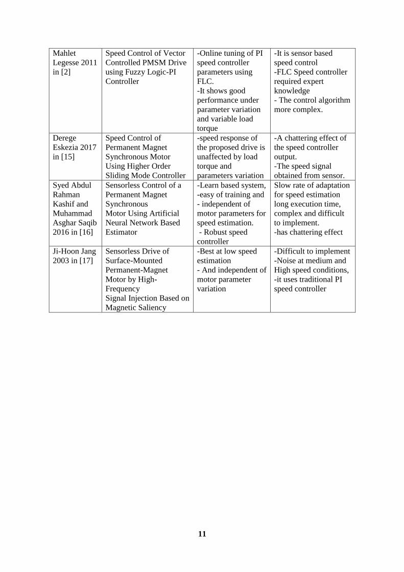
In 2011 Mahlet Legesse presents “Speed Control of Vector Controlled PMSM Drive using
Fuzzy Logic-PI Controller” [2]. In conventional PI speed controller the controller parameters
depends on the system parameters and its performance affected when the system parameter
change due to the internal and external conditions. To solve such problem it proposed that a
sensor based online tuning of PI speed controller parameters using fuzzy logic controller
approach for large speed range and under different load disturbance. But the speed sensor
increase the cost of the system and the controller performance increases with increasing the
fuzzy rules which makes the control algorithm more complex and also fuzzy logic controller
design required expert knowledge for system parameter change that makes controller design
difficult [11]. In this thesis a simple way of online tuning of PI gain for a sensorless speed
controller parameter using MRAC is proposed. In this thesis also solves the drawback of

9
mechanical sensor and also the controller parameters tuned based on the difference of the
performance specification of reference model and the desired model of the system. Since the
controller tuned based on the error of the two models, so that is simple to design and implement
[30].
In 2017 “Speed Control of Permanent Magnet Synchronous Motor Using Higher Order Sliding
Mode Controller” [15] was presented by D.Eskezia using a quasi-continuous higher order
sliding mode controller is designed for PMSM in order to regulate the desired reference speed
with robustness and minimized chattering effects. The speed response of the proposed drive is
unaffected by load torque and parameters variation. Furthermore, the developed controller has
good performance when the reference speed is changed. The main drawback of this system was
there exist still a chattering effect of the speed controller output even if it was minimized [15]
and also the speed and position information for FOC based control of PMSM drive was
obtained from using a mechanical sensor which also increases the cost of the system and
decrease the reliability of the system in harsh environment. In this thesis it is proposed to solve
such problem with stator current based MRAS speed estimator and MRAC speed controller.
In 2016 “Sensorless Control of PMSM Drive using Neural Network Observer” [16] was
presented by Syed Abdul Rahman Kashif and Muhammad Asghar Saqib. In this paper the
Neural network observer is designed to give the estimate of speed and position using direct and
quadrature current and voltage components. The proposed Neural Network Observer design
provides robust estimation of speed and offers advantage in terms of reduced mathematical
computations. It also provides using the SMC controller, the drive gives an improved
performance irrespective of the load variations. Even though the system gives good
performance under variable load condition and also the speed estimation is robust to parameter
uncertainty, it takes long processing time due to the neural network learning rate, very complex
and difficult to implement [11]. There is also a chattering problem on the speed controller
output due to the usage of SMC for the drives.
Ji-Hoon Jang in 2018 was presents “Sensorless Drive of Surface-Mounted Permanent-Magnet
Motor by High-Frequency Signal Injection Based on Magnetic Saliency” [17]. This paper
presents a new sensorless control method of a SPMSM using high-frequency voltage signal
10
injection method based on the high-frequency impedance difference. In the SPMSM, due to
the flux of the permanent magnet, the stator core around the q-axis winding is saturated. This
makes the magnetic saliency in the motor. This magnetic saliency has the information about
the rotor position. The high-frequency voltage signal is injected into the motor in order to detect
the magnetic saliency and estimate the rotor position. This sensorless control scheme makes it
possible to drive the SPMSM in the low-speed region including zero speed, even under heavy
load conditions and also the system is not sensitivity to parameter variation. The main
drawback of this method of sensorless drive control is that, it increase noise at medium and
high speed conditions and makes it difficult to estimate the speed of PMSM for high speed
control application. Another drawback of such system is also very difficult to implement [11]
due to very complex mathematical processing and signal analysis requirements.
To solve such problem this thesis proposed that the speed of PMSM drive is estimated by
MRAS observer and its PI speed controller parameters are tuned online using MRAC. A
senserless speed control of PMSM using MRAS does not require high performance processor
to implement it and has fast adaptation rate. The system speed controlled by MRAC gives good
response under parameter uncertainty of the PMSM drive.
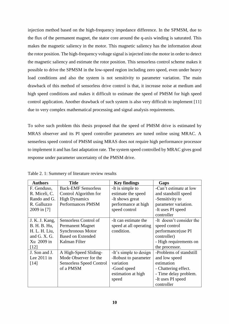
Table 2. 1: Summery of literature review results
Authors Title Key findings Gaps
F. Genduso,
R. Miceli, C.
Rando and G.
R. Galluzzo
2009 in [7]
Back-EMF Sensorless
Control Algorithm for
High Dynamics
Performances PMSM
-It is simple to
estimate the speed
-It shows great
performance at high
speed control
-Can’t estimate at low
and standstill speed
-Sensitivity to
parameter variation.
-It uses PI speed
controller
J. K. J. Kang,
B. H. B. Hu,
H. L. H. Liu,
and G. X. G.
Xu 2009 in
[12]
Sensorless Control of
Permanent Magnet
Synchronous Motor
Based on Extended
Kalman Filter
-It can estimate the
speed at all operating
condition.
-It doesn’t consider the
speed control
performance(use PI
controller)
- High requirements on
the processor.
J. Son and J.
Lee 2011 in
[14]
A High-Speed Sliding-
Mode Observer for the
Sensorless Speed Control
of a PMSM
-It’s simple to design
-Robust to parameter
variation
-Good speed
estimation at high
speed
-Problems of standstill
and low speed
estimation
- Chattering effect.
- Time delay problem.
-It uses PI speed
controller
11
Mahlet
Legesse 2011
in [2]
Speed Control of Vector
Controlled PMSM Drive
using Fuzzy Logic-PI
Controller
-Online tuning of PI
speed controller
parameters using
FLC.
-It shows good
performance under
parameter variation
and variable load
torque
-It is sensor based
speed control
-FLC Speed controller
required expert
knowledge
- The control algorithm
more complex.
Derege
Eskezia 2017
in [15]
Speed Control of
Permanent Magnet
Synchronous Motor
Using Higher Order
Sliding Mode Controller
-speed response of
the proposed drive is
unaffected by load
torque and
parameters variation
-A chattering effect of
the speed controller
output.
-The speed signal
obtained from sensor.
Syed Abdul
Rahman
Kashif and
Muhammad
Asghar Saqib
2016 in [16]
Sensorless Control of a
Permanent Magnet
Synchronous
Motor Using Artificial
Neural Network Based
Estimator
-Learn based system,
-easy of training and
- independent of
motor parameters for
speed estimation.
- Robust speed
controller
Slow rate of adaptation
for speed estimation
long execution time,
complex and difficult
to implement.
-has chattering effect
Ji-Hoon Jang
2003 in [17]
Sensorless Drive of
Surface-Mounted
Permanent-Magnet
Motor by High-
Frequency
Signal Injection Based on
Magnetic Saliency
-Best at low speed
estimation
- And independent of
motor parameter
variation
-Difficult to implement
-Noise at medium and
High speed conditions,
-it uses traditional PI
speed controller
12
Chapter Three
3. Field Oriented Control and MRAS observer
3.1 Introduction
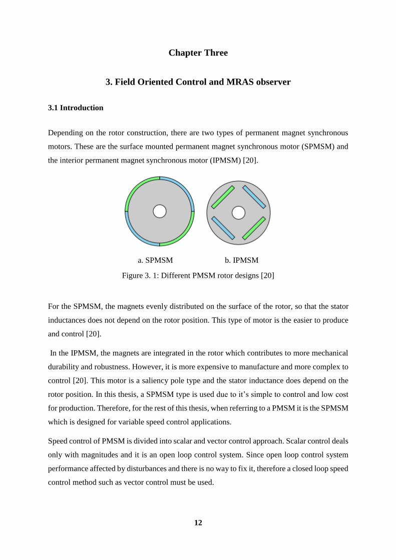
Depending on the rotor construction, there are two types of permanent magnet synchronous
motors. These are the surface mounted permanent magnet synchronous motor (SPMSM) and
the interior permanent magnet synchronous motor (IPMSM) [20].
a. SPMSM b. IPMSM
Figure 3. 1: Different PMSM rotor designs [20]
For the SPMSM, the magnets evenly distributed on the surface of the rotor, so that the stator
inductances does not depend on the rotor position. This type of motor is the easier to produce
and control [20].
In the IPMSM, the magnets are integrated in the rotor which contributes to more mechanical
durability and robustness. However, it is more expensive to manufacture and more complex to
control [20]. This motor is a saliency pole type and the stator inductance does depend on the
rotor position. In this thesis, a SPMSM type is used due to it’s simple to control and low cost
for production. Therefore, for the rest of this thesis, when referring to a PMSM it is the SPMSM
which is designed for variable speed control applications.
Speed control of PMSM is divided into scalar and vector control approach. Scalar control deals
only with magnitudes and it is an open loop control system. Since open loop control system
performance affected by disturbances and there is no way to fix it, therefore a closed loop speed
control method such as vector control must be used.

13
In vector control, magnitude and position of a controlled space vector is considered. These
relationships are valid even during transients which is essential for precise torque and speed
control [21, 22]. General block diagram of the control techniques of PMSM are shown in Figure
3.2.
Figure 3. 2 : Control method of PMSM
The problem with scalar control is that motor flux and torque are in general coupled. This
inherent coupling affects the response and makes the system prone to instability. However, the
vector control of PMSM allows a separate closed loop control for both the flux and torque of
the machines. Hence, it is possible to achieve a similar control structure to that of a separately
excited DC machine [2, 22, 23]. In vector control, two types of PMSM closed loop control
method. These are direct torque control (DTC) and filed oriented control (FOC).
The principle of Direct Torque Control (DTC) is to directly select voltage vectors based on the
difference between reference and actual value of torque and flux linkage in the hysteresis
comparators. Advantages of DTC are low complexity and sensitivity to motor parameter
change but shows poor in steady state performance since the crude voltage selection criteria
give rise to high ripple levels in stator current, flux linkage and torque [22, 24].
In order to achieve better dynamic performance, a more complex control scheme needs to be
applied to control the PMSM using field oriented control (FOC) to solve the problems in direct
torque control method.
14
3.2 Field Oriented Control (FOC)
With the mathematical processing power offered by the microcontrollers, advanced control
strategies can be implemented, in order to decouple the torque generation and the
magnetization functions in the PM motors. Such decoupled torque and magnetization control
is commonly called rotor flux oriented control, or simply FOC.
The vector control of currents and voltages results in control of the spatial orientation of the
electromagnetic fields in the machine and has led to the name field orientation. i.e. FOC usually
refers to controllers which maintain a 90ο electrical angle between rotor and stator field
components [22, 24, 25].
The FOC consists of controlling the stator currents represented by a vector. This control is
based on projection that transforms a three phase time and speed dependent model into a two
coordinate (d and q coordinates) time invariant model. These projections lead to a structure
similar to that of a DC machine control. FOC machines need two constants as input references:
the torque component (aligned with the q co-ordinate) and the flux component (aligned with d
co-ordinate). As FOC is simply based on projections, the control structure handles
instantaneous electrical quantities. This makes to have good accuracy in the transient and
steady state characteristics.
Thus, the advantages of FOC [2] are:
Transform of a complex and coupled AC model into a simple linear model.
Independent control of torque and flux is possible to achieve
Fast dynamic response and good transient and steady state performance.
High torque and low current at start up.
High Efficiency.
Wide speed range control through field weakening.
Because of the above advantages has mentioned, in this thesis has been considered FOC based
techniques of speed control of PMSM. FOC technique which involves converting the stationary
three reference frames in to rotating two reference frame where, the following tasks are
performed. [26]:
1. Stator reference frame (a, b, c) in which a, b, c are coplanar, at 120 degrees
to each other.

15
2. An orthogonal reference frame (α, β) in the same plane as the stator reference
frame in which the angle between the two axes is 90 degrees instead of 120
degrees. The alpha - axis is aligned with a-axis in the second frame.
3. Rotor reference frame (d, q), in which the d-axis is along the N and S poles or
along the flux vector of the rotor and the q-axis is at 90 degrees to the d-axis.
In Figure 3.3 shows the transformations done from the stator currents (i a, ib, ic) into the torque
producing and flux producing (i q, id) component.
(a) Three phase 120 reference (b) Two phase reference (c) Rotating reference frame
Figure 3. 3: Transformations and Reference [26]
Once the torque and flux producing components are controlled with the PI controller then the
controlled outputs, which are the voltages, are transformed back into the stator reference frame
using different transformations of voltages and currents.
3.3 Transformations
Transforming from a stator reference frame of a PMSM into a rotor reference frame is used
to get the time varying values of the motor parameters. In FOC, the components iq and id are
measured in the rotating reference frame. Hence the measured stator currents have to be
transformed from the three phase time variant stator reference frame to the two axis rotating d
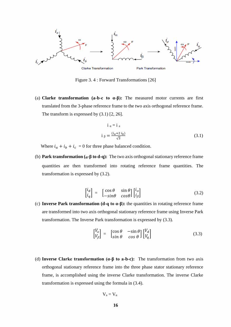
-q rotor reference frame. This can be done in two steps as shown in Figure 3.4.
16
Figure 3. 4 : Forward Transformations [26]
(a) Clarke transformation (a-b-c to α-β): The measured motor currents are first
translated from the 3-phase reference frame to the two axis orthogonal reference frame.
The transform is expressed by (3.1) [2, 26].
i α = i a
i β =(𝑖𝑎+2 𝑖𝑏)
√3 (3.1)
Where 𝑖𝑎 + 𝑖𝑏 + 𝑖𝑐 = 0 for three phase balanced condition.
(b) Park transformation (α-β to d-q): The two axis orthogonal stationary reference frame
quantities are then transformed into rotating reference frame quantities. The
transformation is expressed by (3.2).
[𝑖𝑑𝑖𝑞
] = [cos 𝜃 sin 𝜃−𝑠𝑖𝑛𝜃 𝑐𝑜𝑠𝜃
] [𝑖𝑖
] (3.2)
(c) Inverse Park transformation (d-q to α-β): the quantities in rotating reference frame
are transformed into two axis orthogonal stationary reference frame using Inverse Park
transformation. The Inverse Park transformation is expressed by (3.3).
[𝑉𝑉
] = [cos 𝜃 −sin 𝜃𝑠𝑖𝑛 𝜃 𝑐𝑜𝑠 𝜃
] [𝑉𝑑
𝑉𝑞] (3.3)
(d) Inverse Clarke transformation (α-β to a-b-c): The transformation from two axis
orthogonal stationary reference frame into the three phase stator stationary reference
frame, is accomplished using the inverse Clarke transformation. The inverse Clarke
transformation is expressed using the formula in (3.4).
Va = Vα

17
Vb = −Vα +√3Vβ
2 (3.4)
Vc = −Vα−√3Vβ
2
In FOC based PMSM speed control, the speed controller output is a quadrature axis (q-axis)
current which uses to a reference current for q-axis current controller. The d-axis and q-axis
current controller output also gives d-axis and q-axis controlled voltage. Therefore, for d and
q-axis current controller and speed controller design, the mathematical model of PMSM in d
and q-axis to be required.
3.4 Mathematical Model of PMSM In d-q Frame of Reference
In this thesis, surface mounted PMSM is considered for the study and the model discussed is
related to this system. SPMSM structure is presented in Figure 3.5 show a cross section of the
rotor and stator of a PMSM.
Figure 3. 5 : View of a three phase, two-pole PMSM [27]
For SMPM, the d and q components of the inductances are the same (Ld =Lq= L). As far as the
stator windings are wye-connected (with a neutral point) and supplied with balanced three

18
phase currents, the zero-axis components are neglected. The voltage equations for d and q axes
are: [27, 28].
Vd = R id + 𝑑𝜆𝑑
𝑑𝑡 – wr λq
Vq = R i q + 𝑑𝜆𝑞
𝑑𝑡 +wr λd ( 3 .5)
where λd = Lid +λm, λp = Liq, R the stator resistance, L the stator inductance, wr the rotor
electrical rotational speed and λm the permanent magnet flux.
When the value of λd and λq are substituted in (3.5) and rearranging, the following differential
equation is obtained.
𝑑𝑖𝑑
𝑑𝑡 = -
𝑅
𝐿𝑖𝑑+𝑤𝑟𝑖𝑞+
𝑉𝑑
𝐿
𝑑𝑖𝑞
𝑑𝑡 = -
𝑅
𝐿𝑖𝑞- 𝑤𝑟𝑖𝑑-𝑤𝑟
𝜆𝑚
𝐿 +
𝑉𝑑
𝐿 (3.6)
The electromagnetic torque of the machine can be expressed, in the d-q reference frame as:
Te = 3
2 p (λd iq –λq id)
Where λd = Ld id +λm and λq =Lq iq, then the electromagnetic torque becomes as:
Te = 3
2 p (λmiq – (Lq-Ld) iqid) (3.7)
In the case of SPMSM the d-axis and q-axis stator inductance are equal (a non-salient rotor),
the final expression of the electromagnetic torque equation become like in (3.8).
Te = 3
2 p λm iq (3.8)
This result is quite interesting for filed oriented control (FOC) due to independently controlling
of the torque producing current iq and flux producing current id. It shows that the only
component involved in torque production, in a PMSM without saliency is, the stator q-axis
current, therefore only Maximum Torque per Ampere (MTPA) control is possible rather than
filed weakening control for SPMSM.
Therefore for in all reference frame the electromechanical torque is:-
Ј 𝑑𝑤𝑚
𝑑𝑡 = Te-B𝑤𝑚-TL (3.9)
Where 𝑤𝑚 = 𝑑𝜃𝑚
𝑑𝑡 mechanical speed of the rotor, Ј is moment of inertia of the motor, B is
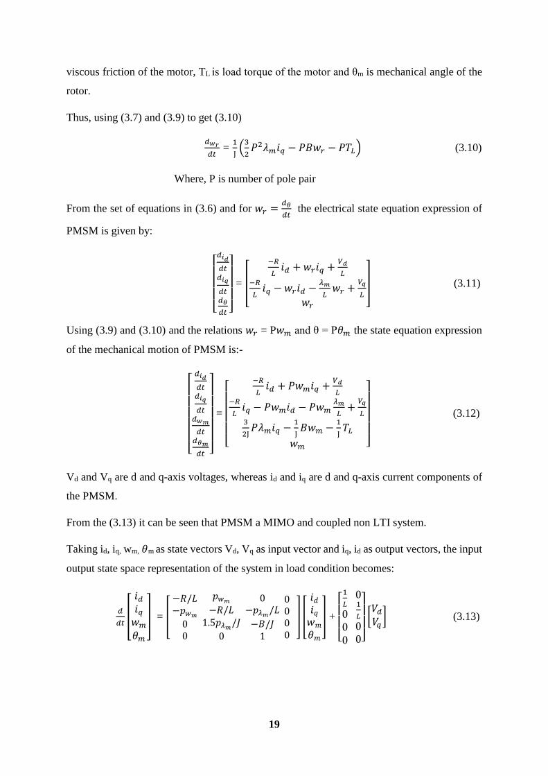
19
viscous friction of the motor, TL is load torque of the motor and θm is mechanical angle of the
rotor.
Thus, using (3.7) and (3.9) to get (3.10)
𝑑𝑤𝑟
𝑑𝑡 =
1
Ј(3
2𝑃2𝜆𝑚𝑖𝑞 − 𝑃𝐵𝑤𝑟 − 𝑃𝑇𝐿) (3.10)
Where, P is number of pole pair
From the set of equations in (3.6) and for 𝑤𝑟 =𝑑𝜃
𝑑𝑡 the electrical state equation expression of
PMSM is given by:
[ 𝑑𝑖𝑑
𝑑𝑡𝑑𝑖𝑞
𝑑𝑡𝑑𝜃
𝑑𝑡 ]
= [
−𝑅
𝐿𝑖𝑑 + 𝑤𝑟𝑖𝑞 +
𝑉𝑑
𝐿−𝑅
𝐿𝑖𝑞 − 𝑤𝑟𝑖𝑑 −
𝜆𝑚
𝐿𝑤𝑟 +
𝑉𝑞
𝐿𝑤𝑟
] (3.11)
Using (3.9) and (3.10) and the relations 𝑤𝑟 = P𝑤𝑚 and θ = P𝜃𝑚 the state equation expression
of the mechanical motion of PMSM is:-
[
𝑑𝑖𝑑
𝑑𝑡𝑑𝑖𝑞
𝑑𝑡𝑑𝑤𝑚
𝑑𝑡𝑑𝜃𝑚
𝑑𝑡 ]
=
[
−𝑅
𝐿𝑖𝑑 + 𝑃𝑤𝑚𝑖𝑞 +
𝑉𝑑
𝐿−𝑅
𝐿𝑖𝑞 − 𝑃𝑤𝑚𝑖𝑑 − 𝑃𝑤𝑚
𝜆𝑚
𝐿+
𝑉𝑞
𝐿3
2Ј𝑃𝜆𝑚𝑖𝑞 −
1
Ј𝐵𝑤𝑚 −
1
Ј𝑇𝐿
𝑤𝑚 ]
(3.12)
Vd and Vq are d and q-axis voltages, whereas id and iq are d and q-axis current components of
the PMSM.
From the (3.13) it can be seen that PMSM a MIMO and coupled non LTI system.
Taking id, iq, wm, 𝜃m as state vectors Vd, Vq as input vector and iq, id as output vectors, the input
output state space representation of the system in load condition becomes:
𝑑
𝑑𝑡[
𝑖𝑑𝑖𝑞𝑤𝑚
𝜃𝑚
] = [
−𝑅/𝐿−𝑝𝑤𝑚
00
𝑝𝑤𝑚
−𝑅/𝐿1.5𝑝𝜆𝑚
/𝐽
0
0−𝑝𝜆𝑚
/𝐿
−𝐵/𝐽1
0000
] [
𝑖𝑑𝑖𝑞𝑤𝑚
𝜃𝑚
] +
[ 1
𝐿
000
01
𝐿
00]
[𝑉𝑑
𝑉𝑞] (3.13)

20
The two phase voltage Vd and Vq in the rotor reference frame are then transformed into three
phase stator reference Va, Vb and Vc which acts as modulating voltage for the modulator which
uses the space vector pulse width modulation (SVPWM) scheme. The modulator output which
is in the form of pulses is used to drive the IGBT with anti-parallel diode acting as switches for
the conventional two level voltage source inverter (VSI).
3.5 SVPWM for Inverter Fed PMSM
The space vector pulse width modulation (SVPWM) method is an advanced computation-
intensive PWM method and is possibly the best method among the all PWM techniques for
variable frequency drive application [2, 6]. Because of its superior performance characteristics,
it has been finding wide spread application in recent years [2].
One of the major benefits of SVPWM is reduction of total harmonic distortion (THD) created
by the rapid switching inherent to this PWM algorithm and can have higher bus voltage
utilization [1, 2]. Legs of the three phase inverter are connected to the phases of the motor to
the positive and negative terminal of DC bus voltage as shown in Figure 3.6.
Figure 3. 6 : Three Phase Inverter [2]
The relationship between the switching variable vector [a b c]T and the line-to-line voltage
vector [Vab Vbc Vca]T of the three phase inverter [2] in Figure 3.6 is given by (3.14).

21
[
𝑉𝑎𝑏
𝑉𝑏𝑐
𝑉𝑐𝑎
] = 𝑉𝑑𝑐 [1 −1 00 1 −1
−1 0 1] [
abc] ( 3.14)
Where [a b c] is a vector representing the upper switches of the inverter. Their on and off state
determined based on the position of reference voltage and the two adjacent active vectors
dwelling time.
Also, the relationship between the switching variable vector [a b c]T and the phase voltage
vector [Va Vb Vc]T can be expressed below.
[
𝑉𝑎
𝑉𝑏
𝑉𝑐
] = 𝑉𝑑𝑐
3[
2 −1 −1−1 2 −1−1 −1 2
] [abc] (3.15)
The on and off states of the upper power devices are opposite to the lower one. So once the
states of the upper power transistors are determined, the states of lower one can be easily
determined. The eight switching vectors of the three upper power switches, output line to
neutral voltage (phase voltage), and output line-to-line voltages in terms of DC-link Vdc, are
given in Table 3.1
Table 3. 1: Switching vectors, output phase voltages and output line to line voltages.
Voltage
Vectors
Switching Vectors Line to neutral
Voltage
Line to line Voltage Vα Vβ
a B C Van Vbn Vcn Vab Vbc Vca
V0 0 0 0 0 0 0 0 0 0 0 0
V1 1 0 0 2/3 -1/3 -1/3 1 0 -1 2/3 0
V2 1 1 0 1/3 -1/3 -2/3 1 0 -1 1/3 1
√3
V3 0 1 0 -1/3 2/3 -1/3 -1 1 0 -1/3 1
√3
V4 0 1 1 -2/3 1/3 1/3 -1 0 1 -2/3 0
V5 0 0 1 -1/3 -1/3 2/3 0 -1 1 -1/3 -1
√3
V6 1 0 1 1/3 -2/3 1/3 1 -1 0 1/3 -1
√3
V7 1 1 1 0 0 0 0 0 0 0 0
(Note that the respective voltage should be multiplied by Vdc)

22
3.5.1 Principle of Space Vector PWM
Treats the sinusoidal voltage (reference voltage) as a constant amplitude vector
rotating at constant frequency.
This PWM technique approximates the reference voltage Vref by a combination
of the eight switching patterns (V0 to V7).
Coordinate transformation (a-b-c reference frame to the stationary α-β frame).
That is a three-phase voltage vector is transformed into a vector in the stationary
α-β coordinate frame represents the spatial vector sum of the three phase
voltage.
The vectors (V1 to V6) divide the plane into six sectors (each sector: 60 degrees).
Vref is generated by two adjacent non -zero vectors and two zero vectors.
3.5.2 Implementation of Space Vector PWM
To implement the space vector PWM, the voltage equations in the a-b-c reference frame must
be transformed into the stationary α-β reference frame that consists of the horizontal (α) and
vertical (β) axis, as a result, six non-zero vectors and two zero vectors are possible. Six nonzero
vectors V1 up to V6 shape the axis of a hexagonal as depicted in Figure 3.7, and feed electric
power to the load or DC link voltage is supplied to the load. The objective of space vector
PWM technique is to approximate the reference voltage vector Vref using the eight switching
patterns. One simple method of approximation is to generate the average output of the inverter
in a small period, Tz to be the same as that of Vref in the same period.
Consider that voltage phasor Vref is commanded. Its position is in between two switching
voltage vectors, say V1 and V2, and has a relative phase of α from V1, as shown in Figure 3.7.
The commanded voltage phasor can only be realized with the use of the neighboring switching
voltage vectors and in this case V1 and V2. Taking these switching vectors for a fraction of time
as it is not possible to take the fraction of them, and then combining them through the load
gives the desired command space voltage phasor.
23
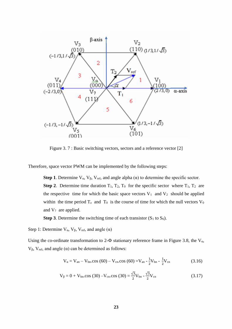
Figure 3. 7 : Basic switching vectors, sectors and a reference vector [2]
Therefore, space vector PWM can be implemented by the following steps:
Step 1. Determine Vα, Vβ, Vref, and angle alpha (α) to determine the specific sector.
Step 2. Determine time duration T1, T2, T0 for the specific sector where T1, T2 are
the respective time for which the basic space vectors V1 and V2 should be applied
within the time period Tz and T0 is the course of time for which the null vectors V0
and V7 are applied.
Step 3. Determine the switching time of each transistor (S1 to S6).
Step 1: Determine Vα, Vβ, Vref, and angle (α)
Using the co-ordinate transformation to 2-Ф stationary reference frame in Figure 3.8, the Vα,
Vβ, Vref, and angle (α) can be determined as follows:
Vα = Van – Vbn.cos (60) – Vcn.cos (60) =Van - 1
2Vbn -
1
2Vcn (3.16)
Vβ = 0 + Vbn.cos (30) –Vcn.cos (30) = √3
2Vbn -
√3
2Vcn (3.17)
24
Therefore, the above equations can be summarized in matrix form as follows.
[𝑉𝑉
] = [1 −
1
2−
1
2
0√3
2−
√3
2
] [Van
Vbn
Vcn
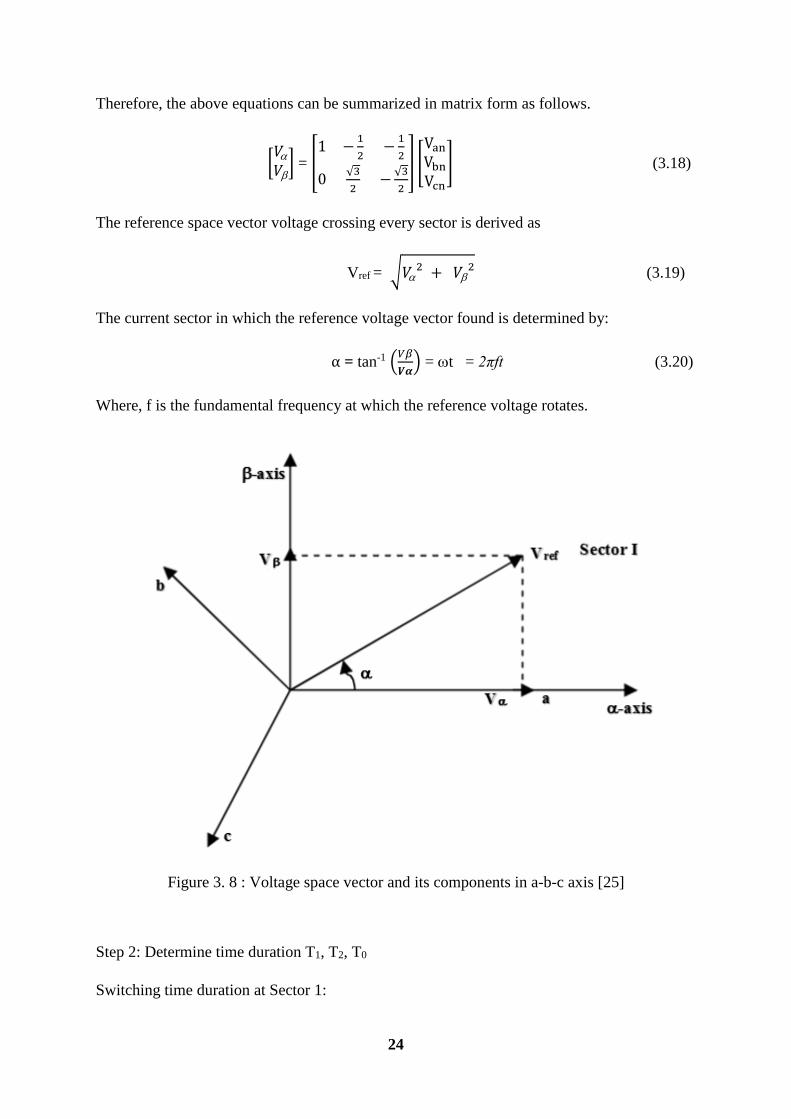
] (3.18)
The reference space vector voltage crossing every sector is derived as
Vref = √𝑉2 + 𝑉
2 (3.19)
The current sector in which the reference voltage vector found is determined by:
α = tan-1 (𝑉𝛽
𝑽𝜶) = t = 2πft (3.20)
Where, f is the fundamental frequency at which the reference voltage rotates.
Figure 3. 8 : Voltage space vector and its components in a-b-c axis [25]
Step 2: Determine time duration T1, T2, T0
Switching time duration at Sector 1:
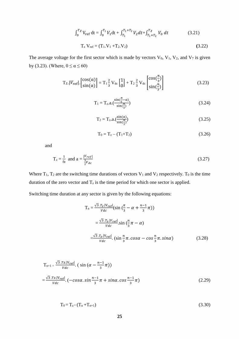
25
∫ Vref𝑇𝑍
0 dt = ∫ 𝑉1
𝑇1
0dt + ∫ 𝑉2𝑑𝑡
𝑇1+𝑇2
𝑇1+∫ 𝑉0 𝑑𝑡
𝑇𝑍
𝑇1+𝑇2 (3.21)
Tz Vref = (T1.V1 +T2.V2) (3.22)
The average voltage for the first sector which is made by vectors V0, V1, V2, and V7 is given
by (3.23). (Where, 0 ≤ α ≤ 60)
TZ.|𝑉ref|.[cos (α)sin (α)
] = T1 2
3 Vdc [
10] + T2
2
3 Vdc [
cos (π
3)
sin (π
3)] (3.23)
T1 = Tz.a.(sin (
π
3 −α)
sin (π
3)
) (3.24)
T2 = Tz.a.(sin (α)
sin (π
3)) (3.25)
T0 = Tz – (T1+T2) (3.26)
and
Tz = 1
fz and a =
|𝑉𝑟𝑒𝑓|3
2𝑉𝑑𝑐
(3.27)
Where T1, T2 are the switching time durations of vectors V1 and V2 respectively. T0 is the time
duration of the zero vector and Tz is the time period for which one sector is applied.
Switching time duration at any sector is given by the following equations:
Tn = √3 .𝑇𝑧.|Vref|
𝑉𝑑𝑐(sin (
𝜋
3− 𝛼 +
𝑛−1
3𝜋))
= √3 .𝑇𝑧.|𝑉ref|
𝑉𝑑𝑐.sin (
𝑛
3𝜋 − 𝛼)
=√3 .𝑇𝑧.|Vref|
𝑉𝑑𝑐. (sin
𝑛
3𝜋. 𝑐𝑜𝑠𝛼 − 𝑐𝑜𝑠
𝑛
3𝜋. 𝑠𝑖𝑛𝛼) (3.28)
Tn+1 = √3 .𝑇𝑧.|Vref|
𝑉𝑑𝑐. ( sin (𝛼 −
𝑛−1
3𝜋))
= √3 .𝑇𝑧.|Vref|
𝑉𝑑𝑐. (−𝑐𝑜𝑠𝛼. 𝑠𝑖𝑛
𝑛−1
3𝜋 + 𝑠𝑖𝑛𝛼. 𝑐𝑜𝑠
𝑛−1
3𝜋) (2.29)
T0 = Tz - (Tn +Tn+1) (3.30)

26
Where n = 1 through 6(sector 1 to 6) and 0 ≤ α ≤ 60
The method used to approximate the desired stator reference voltage with only eight possible
states of switches is to combine adjacent vectors of the reference voltage and to determine the
time of application of each adjacent vector as shown in Figure 3.9 for the first sector.
Figure 3. 9 : Reference voltage as a combination of adjacent vectors in sector I [25].
Step 3: Determine the switching time of each transistor (S1 to S6).
Figure 3. 10 : SVPWM switching pattern for the first sector [2]

27
Based on Figure 3.10, the switching time in the first sector is summarized in table 2.2
Table 3. 2 : Switching time calculation for the first sector
Sector Upper switch (S1,S2,S3) Lower switch (S2,S4,S6)
1 S1 = T1+T2+T0/2
S3 = T2+T0/2
S5 = T0/2
S2 = T0/2
S4 = T0/2+T1
S6 = T0/2+T1+T2
Other sector switching time can be calculated as the same principle as the first sector.
Field oriented control (FOC) require a position sensor for constantly monitoring the rotor speed
and rotor position. To avoid the drawback of using mechanical sensor for field oriented control,
a position and speed estimation method with model reference adaptive system (MRAS) is used
for sensorless FOC based speed control of PMSM.
3.6 MRAS Observer Design for Speed Estimation of PMSM
Sensorless speed control of PMSM can be performed by different methods, such as back
electromotive force (back EMF method), sliding mode observer, MRAS, Kalman filter, and
other sensorless scheme are also developed [28].
MRAS has the advantages of having simple algorithm and easy to implement in the digital
control system, and has the advantages of faster adaptation speed [18, 30]. This has been
proposed and applied to the PMSM sensorless control. There are two different models in
MRAS, one is the reference model and the other is the adjustable model. The deviation signal
of the output of the two models send to the adaptation mechanism, and then the output of the
adaptation mechanism are the estimated speed.
The problem of using MRAS to estimate the speed of PMSM is the construction of adaptive
law. When using Lyapunov stability method for construction of adaptation law, it is difficult
to find the Lyapunov function. But by using Popov stability for constructing the adaptive law
the problem is adjusting PI parameters of speed observer which simple and determined by the
root locus analysis method. The Popov stability principle is analysed through modern control
theory using strictly positive realness. The transfer function of the speed observer is constructed
in order to determine the PI adaptation gain of speed estimator. The PI regulator in the speed
estimator can be used as the adjustable link. This method of adaptation is simple and effective,
and avoid the complex algorithm of fuzzy adaptation [30].

28
In this thesis, stator current based MRAS is used for speed estimation of PMSM. The PMSM
itself used as the reference model and the q-axis and d-axis equations of stator current model
is used as adjustable model. To perform this, the stator voltage equation of the surface mounting
PMSM in d-q axis given as:
[Vd
Vq] = [
R +𝑑
𝑑𝑡Ld −wrLq
wrLd R+𝑑
𝑑𝑡Lq
] [idiq
] + [0
λmwr] (3.31)
Where Vd, Vq, id, iq are the stator voltage and current of the motor in the d-q axis and R, Ld, Lq
are the stator resistance and the inductance of the d-q axis, wr and λm are rotor electric angular
speed and flux respectively.
According to (3.31), the stator current state equation can be obtained.
𝑑
𝑑𝑡[idiq
] = [
−R
𝐿𝑑wr
−wr−R
𝐿𝑞
] [idiq
] + [
Vd
𝐿𝑑
Vq−λmwr
𝐿𝑞
] (3.32)
For surface mounting PMSM, Lq = Ld = L and PMSM use for reference model and the equation
(3.37) use for adjustable model. For speed estimation, R and L can be regarded as fixed values
so, the adjustable model for speed estimation can be given.
𝑑
𝑑𝑡[𝑖̂𝑑𝑖̂q
] = [
−𝑅
𝐿�̂�r
−�̂�r−R
L
] [𝑖̂d𝑖̂q
] + [
Vd
LVq−λm�̂�r
𝐿
] (3.33)
Where 𝑖̂𝑑 and 𝑖̂q the adjustable model stator current and �̂� the estimated electrical rotor speed.
After developing adjustable and reference models, the adaptation mechanism constructed by
Popov hyper stability theory. The adaptation mechanism is designed in a way to generate the
value of estimated speed used so as to minimize the error between the adjustable and reference
d − q axis stator current outputs. By adjusting the estimated rotational speed, the error between

29
the reference and the adjustable d − q axis stator currents is reduced. The error between the
adjustable model and reference model output d − q axis stator currents are defined as:
Defined state error:
𝑒𝑑 = 𝑖𝑑 - 𝑖̂𝑑 , 𝑒𝑞 = 𝑖𝑞 - 𝑖̂𝑞 (3.34)
The state error equation can be given by subtracting (3.33) from (3.32).
𝑑
𝑑𝑡[𝑒𝑑
𝑒𝑞] = [
−R
L�̂�r
−�̂�r−𝑅
L
] [𝑒𝑑
𝑒𝑞] + [
𝑖𝑞
−𝑖𝑑 −𝜆𝑚
𝐿
] (𝑤𝑟 − �̂�𝑟) (3.35)
This can be written in state space expression as:
𝑑
𝑑𝑡ε = A ε + Bu (3.36)
We can rewrite (3.36) to Popov standard stability form as
𝑑
𝑑𝑡ε = A ε + W
Where A = [
−R
L�̂�r
−�̂�r−R
L
] , W = [𝑖𝑞
−𝑖𝑑 −𝜆𝑚
𝐿
] (𝑤𝑟 − �̂�𝑟) and ε = [𝑒𝑑
𝑒𝑞]
3.6.1 Stator current based MRAS Observer Design for Speed Estimation
MRAS basic block diagram of speed estimation is shown in Figure 3.10. The PMSM in d-q
axis model used as a reference model and (3.33) used as adjustable model to estimate the speed
of PMSM drive.
30
Figure 3. 11: MRAS basic block diagram of speed estimation
Obviously, the stability and precision of the system is related to the construction of the adaptive
mechanism. From Figure 3.11, it can be seen that the adaptation mechanism is related to the
state error (3.35). The structural diagram of (3.35) is shown in Figure 3.12:
Figure 3. 12 : Structure diagram Speed estimation
For speed estimation, the adaptation law is constructed based on Popov stability. In the case of
Popov stability analysis two conditions must be considered. So that, the conditions for the
stability of Figure 3.12 are about two sides. One is the zeros and poles of the transfer function
of the forward channel must be in the left half of the s-plane (strictly positive real), which is a
necessary conditions. Another is the feedback channel that satisfies Popov stability.

31
For the first condition, the transfer function of forward channel can be deduced according to
modern control theory using state space expression. Its state space expression is:
𝜀̇ = A 𝜀 + u
Y = 𝜀 (3.37)
From this error state space expression it is possible to calculate the transfer function of the
forward channel by using the expression H(s) = C(Is − A)−1B as:
H(s) = s +
𝑅
𝐿
𝑠2+2𝑅
𝐿 s +(
𝑅
𝐿)2+ �̂�𝑟
2 (3.38)
From (3.38) it is clear that all of the poles and zeros of the transfer function H(s) are on the left
hand side of s-plane and also H (j) ≥0 for all values of (the forward path transfer function
is strictly positive real). Therefore the first necessary condition is satisfied and it is possible to
check the second condition of Popov hyper stability theory.
Secondly, the non-linear feedback (which includes the adaptation mechanism) must satisfies
the following Popov’s criterion for stability.
∫ ε𝑡0
0Twdt ≥ − o 2 (3.39)
Where to ≥ 0, o is a finite positive real constant, which is independent of 𝑡0.
Then substituting the value of ε = [𝑒d eq]T and W from (3.35) in to (3.39), the estimated speed
from Popov’s criterion for stability can be determined.
∫ {[ e𝑑 (𝑖𝑞 )] + [eq(−𝑖𝑑 −𝜆𝑚
𝐿)]}[𝑤𝑟 − �̂�𝑟] dt ≥
𝑡𝑜
0-o
2 (3.40)
It can also be decomposed in to two parts of (3.40) to find the adaptation law of speed estimator.
∫ [ e𝑑 (𝑖𝑞 )] + [eq (−𝑖𝑑 −𝜆𝑚
𝐿)]𝑤𝑟 dt − ∫ [ e𝑑 (𝑖𝑞 )] + [eq(−𝑖𝑑 −
𝜆𝑚
𝐿)] �̂�𝑟dt ≥
𝑡𝑜
0
𝑡𝑜
0-1
2 - 22
≥ -o2 (3.41)
From (3.41) the solution of integral inequality can be find individually as:-
∫ [ e𝑑 (𝑖𝑞 )] + [eq (−𝑖𝑑 −𝜆𝑚
𝐿)] 𝑤𝑟 dt
𝑡𝑜
0≥ -1
2 (3.42)
-∫ [ e𝑑 (𝑖𝑞 )] + [eq(−𝑖𝑑 −𝜆𝑚
𝐿)] �̂�𝑟dt ≥
𝑡𝑜
0- 2
2 (3.43)
32
Where e𝑑 = 𝑖𝑑 − �̂�𝑑 and eq= 𝑖𝑞 − �̂�𝑞
Then using (3.43) the speed adaptation law can be derived to find the estimate speed (�̂�𝑟) of
pmsm and can also rewrite as:-
-∫ [ (𝑖𝑑 − 𝑖̂𝑑) 𝑖𝑞 + (𝑖𝑞 − 𝑖̂𝑞)(−𝑖𝑑 −𝜆𝑚
𝐿)] �̂�𝑟dt ≥
𝑡𝑜
0- 2
2 (3.44)
∫ [ (𝑖̂𝑑 − 𝑖𝑑) 𝑖𝑞 + (𝑖̂𝑞 − 𝑖𝑞)(−𝑖𝑑 −𝜆𝑚
𝐿)] �̂�𝑟dt ≥
𝑡𝑜
0- 2
2 (3.45)
Therefore (4.45) uses to estimate the electrical rotor speed of PMSM and this equation can be
written as:-
∫ [ eq (𝑖𝑑 +𝜆𝑚
𝐿) − e𝑑𝑖𝑞] �̂�𝑟dt ≥
𝑡𝑜
0- 2
2 (3.46)
Now find �̂�𝑟 which satisfies (3.46) using the integral inequality properties and a solution of
this inequality can be found through the following well-known relation.
∫ 𝑓(𝑡)𝑡
0𝑓(𝑡)̇ dt =
1
2[𝑓2(𝑡) − 𝑓2(0)] ≥ −
1
2𝑓2(0) and
∫ 𝑓2(𝑡)𝑡
0 dt ≥ 0 (3.47)
By comparing (3.46) and (3.47) the estimated speed can be determined as:-
�̇̂�r = eq (𝑖𝑑 +𝜆𝑚
𝐿) − e𝑑𝑖𝑞
�̂�r = 𝐾
𝑠[eq (𝑖𝑑 +
𝜆𝑚
𝐿) − e𝑑𝑖𝑞] (3.48)
Where K is adaptation gain of the system for speed estimator and (3.48) which is an integral
type of speed estimator. For improving the dynamics of speed estimator proportional regulator
can be add. Then
�̂�r = 𝐾𝑖
𝑠[eq (𝑖𝑑 +
𝜆𝑚
𝐿) − e𝑑𝑖𝑞] + 𝐾𝑃 [eq (𝑖𝑑 +
𝜆𝑚
𝐿) − e𝑑𝑖𝑞] (3.49)
Where Ki and Kp adaptation gain of speed estimator.
From (3.49) the adaptation law of speed estimation seems like PI regulator and therefore can
be written as follows:-

33
�̂�𝑟 = A2 ε + ∫ A1ε𝑡𝑜
0 dt (3.50)
Where A1, A2 are non-linear function of ed, eq. Then search solutions to A1 and A2 such that
the equivalent feedback block verifies Popov’s criterion.
Then the observed rotor speed satisfies the following adaptation laws:
A1 = Ki [-iq 𝑒d +id 𝑒q + 𝜆𝑚
𝐿𝑠eq] (3.51)
A2 = Kp [-iq 𝑒d +id𝑒q + 𝜆𝑚
𝐿𝑠eq] (3.52)
Where Ki and Kp are the positive adaptation gains of the system.
The constant A1 and A2 substituted in (3.50), it can be shown that the observed rotor speed
satisfies the following adaptation laws:
�̂�𝑟 = A2 ε + 1
𝑆 A1ε (3.53)
�̂�𝑟 = Ki∫ (e𝑡𝑜
0 diq - eqid – eq 𝜆𝑚
𝐿𝑠) dt + Kp(𝑒diq - eqid – eq
𝜆𝑚
𝐿𝑠) + �̂�𝑟(0) ( 3.54)
3.6.2 PI Parameter Adjustment of Speed estimator
The adaptive law of the observer is constructed in 3.6.1, (3.54). So, the MRAS structure
diagram can be obtained in Figure 3.13.
Figure 3. 13 : MRAS structure diagram

34
The dotted line in Figure 3.13 is represented by the state space expression as follow:
ε ̇ = Aε + Bu
y =𝐵𝑇ε (3.55)
So, its transfer function is:
G(s) = (s+
𝑅
𝐿) (𝑖𝑞
2+(𝑖𝑑2+
𝜆𝑚
𝐿
2) )
𝑠2 + 2𝑅
𝐿 s +(
𝑅
𝐿)2 + �̂�𝑟
2 (3.56)
This transfer function show that, it has the same pole zero distribution as the forward transfer
function of (3.56). By further simplify the MRAS structure diagram of Figure 3.13, which is
easy to analysis for the adjustment of PI speed observer as:
Figure 3. 14: MRAS simplified structure diagram
So, this can be used to adjust the parameters of the PI regulator by using the root locus analysis
method for the simplified structure diagram of Figure 3.14, and make the system to achieve the
desired results. Because the value of id = 0 for maximum torque per Ampere (MTPA) control
strategy and iq are relatively small.so they can be neglected. This can get the open-loop transfer
function of system.
Gc(s) = 𝑘∗(s+
𝑅
𝐿 ) (s+Z)
𝑠3 + 2𝑅
𝐿 𝑠2 +((
𝑅
𝐿)2 + �̂�𝑟
2)s (3.57)
Where 𝑘∗ = Kp(𝜆𝑚
𝐿 )
2 and Z =
𝐾𝑖
𝐾𝑝

35
So, this can determine the value of k* and z to make the system to achieve the desired results,
thus determining the value of Ki and Kp.
The closed loop transfer function of the MRAS can be expressed as
𝑤𝑟
𝑤�̂� =
G(s)(𝐾𝑝𝑀𝑅𝐴𝑆+
𝐾𝑖𝑀𝑅𝐴𝑆𝑆
)
1+G(s)(𝐾𝑝𝑀𝑅𝐴𝑆+
𝐾𝑖𝑀𝑅𝐴𝑆𝑆
) (3.58)
The design of Kp and Ki is introduce to ensure stability, error tracking and robust operation.
The design criteria for this adaptive PI controller is done using root locus by using the transfer
function of the plant and set the time domain constraint. The constraint considered in this
design is percent of overshoot; settling time and rise time are less than 12%, less than 0.00792
second and less than 0.00155 second respectively.
The design of Ki and Kp is selected to ensure that all the poles and zeros are located in the left
hand side of s-plane and this allows for the required fast and stable response. The location of
closed loop transfer function poles characterizes the control system dynamics. Therefore, the
location of the PI controller zero (Z = 𝐾𝑖
𝐾𝑝 ) should be on the real axis to make sure that fast
dynamics response and take its value equal to 4 to 5 times greater than the open loop zeros of
the system G(s) in (3.56) to make it fast response.
Therefore, 𝐾𝑖
𝐾𝑝 is taken of 475 and from the root locus diagram of Gc(s) in (3.57) the maximum
possible gain of ‘k*’ should be obtained from the specifications of settling time, maximum
overshoot and rise times of the specification .In this case k* = 860.79 and using the relation k*
= Kp(𝜆𝑚
𝐿 )
2 then the value of Kp should become 1.22 and also Ki = 475*Kp = 579.5.
Using this controller gain parameters and substitute in (3.56), the stability of the estimator is
determined by root locus analysis methods. As seen in Figure 3.15, all the poles of the closed
loop transfer function of stator current based MRAS speed estimator lie in the left half of the
s-plane and therefore, the system has been stable in the operating point.

36
Figure 3. 15: Root locus of closed loop adaptive control system
In the stator current based MRAS speed estimation the voltages Vd and Vq are used as the input
for both adjustable and reference models. The output of reference model which is id and iq of
PMSM compared with the adjustable model output current which is 𝑖̂𝑑 and 𝑖̂𝑞 until the
deviation of them goes to zero by adjusting the adjustable model by the estimated speed. In this
case the estimated speed and actual speed of PMSM are equal.

37
Chapter four
4. Speed and Current PI Controller design For PMSM
4.1 PID controller
FOC based speed control of PMSM mainly consist of two loops the inner loop for current and
the outer loop for speed. The order of the loops is due to their response, how fast they can be
changed. This requires a current loop at least 10 times faster than the speed loop [2, 6] to avoid
the time delay in speed controller due to its cascaded control structure. The speed of the motor
and current loops can be controlled by using a PID controller.
PID controller has the optimum control dynamics including zero steady state error, fast
response (short rise time), no oscillations and higher stability. The necessity of using a
derivative gain component in addition to the PI controller is to eliminate the overshoot and the
oscillations occurring in the output response of the system.
Proportional (P) Term: The main usage of the P controller is to increase the response and to
decrease the steady state error of the system. As the proportional gain factor K increases, the
steady state error of the system decreases.
Integral (I) Term: it is mainly used to eliminate the steady state error.
Derivative (D) Term: D mode is designed to be proportional to the change of the output
variable to prevent the sudden changes occurring in the control output resulting from sudden
changes in the error signal.
PI controllers are quit common for ac machine drives, whereas the derivative action is sensitive
to measurement noise due to the high frequency voltage source inverter (VSI) and therefore
not necessary to use it, because it causes chattering effect on the controlled signal. Therefore
all the rotor speed, rotor flux and rotor torque are controlled by a separate PI module with
transfer function of KP + 𝐾𝑖
𝑠 , where Kp –is proportional gain and Ki –is integral gain.
4.2 Current Controller Design
For the design of PID-controllers it is necessary to know the closed loop transfer function. The
d-q axis current open loop transfer function from (3.6) can be obtained as:

38
𝑖𝑑
𝑉𝑑+𝑤𝑟 𝐿 𝑖𝑞 =
1
𝐿+𝑅 (4.1)
The block diagram of the closed loop transfer function with the PI controller in d-axis is shown
in Figure 4.1
Figure 4. 1: d –axis current closed loop transfer function with PI controller block diagram
Similarly as the d-axis current, the q-axis current open loop transfer function from (3.6) can
be:
𝑖𝑞
𝑉𝑞−𝑤𝑟(𝐿 𝑖𝑑+𝜆𝑚) =
1
𝐿+𝑅 (4.2)
The Block diagram of the closed loop transfer function with the PI controller in q-axis is shown
in Figure 4.2.
Figure 4. 2 : q–axis current closed loop transfer function with PI controller block diagram

39
From Figure 4.1 and Figure 4.2 r Liq and r (Lid +λm) block makes the closed loop transfer
function complicated respectively. For simplicity of PI controller parameter calculation, the r
Liq and r (Lid +λm) part of the equation is ignored by feed forward decoupling method. From
Figure 4.1 the overall transfer function between the flux component id and its reference idref is
as:
𝑖𝑑(𝑠)
𝑖𝑑 𝑟𝑒𝑓(𝑠) = 𝐾𝑝 𝑠+𝐾𝑖
𝐿 𝑠2+(𝐾𝑝+𝑅) 𝑠+𝐾𝑖 (4.3)
From Figure 4.2 the overall transfer function between the torque component iq and it’s reference
iqref is as:
𝑖𝑞(𝑠)
𝑖𝑞 𝑟𝑒𝑓(𝑠) =
𝐾𝑝 𝑠+𝐾𝑖
𝐿 𝑠2+(𝐾𝑝+𝑅) 𝑠+𝐾𝑖 (4.4)
The closed loop transfer function of (4.3) and (4.4) are the same due to Ld= Lq=L for surface
mounted PMSM. Therefore the design of q-axis current controller is sufficient to determine the
controller parameter of d-axis current controller.
By comparing the 2nd order closed loop system performance in (4.5) with (4.4) and (4.3), the
current controller gain values of Kp and Ki in terms of the motor parameters are found in (4.6)
and (4.7).
𝑛
2
𝑠2+2𝑛𝑠+𝑛2 (4.5)
Kp = 2n L-R (4.6)
Ki = 𝑛2 L (4.7)
Current Controller Design Specification
It is possible to consider in the design, the damping coefficient is selected to be 0.707 for
critical damping response and the natural frequency n is selected to determine the desired
closed-loop settling time, which also corresponds to the desired bandwidth of the closed-loop
system. The larger n is, the shorter the desired closed-loop settling time. It is also useful to
choose this parameter relative to the bandwidth of the open-loop system, which is R /L from
(4.3). Here, a normalized parameter 0 <𝛾 <1 is proposed to be used where the desired closed-
loop bandwidth is calculated [31] as:

40
n = 1
1−γ *
R
L (4.8)
With this type of formula, the parameter 𝛾 is often selected around 0.8 to give a satisfactory
performance, which is ωn value becomes five times the open loop bandwidth response [31].
Using (4.8) the damping coefficient and natural frequency are chosen to be:
=0.707 and n =714 rad/sec
Therefore, by using the specified value of undamped natural frequency and damping
coefficient, the current controller gain Kp and Ki can be determined using (4.6) and (4.7) with
R =0.43 and L =3.2mH of the motor parameters from Appendix A such that, Kp =5 and Ki
=1631.632. The overall transfer function of the q-axis current closed loop becomes:
𝑖𝑞(𝑠)
𝑖𝑞 𝑟𝑒𝑓(𝑠) =
1975 𝑠+355,937
𝑠2+2109.37 𝑆+355,937=
0.005 𝑠+1
0.0000028 𝑠2+0.006 𝑠+1 (4.9)
Figure 4. 3: Matlab Simulink block diagram of closed loop PI q-axis current controller
From Figure 4.4 it shows that, the q-axis current controller output response follows the
reference step input current with a rated current value of 4.3A. It indicates that, the output
response tracks the reference value within the current controller design specifications. Which
is the closed loop speed of response five times greater than open loop response. The d-axis
current controller response also the same as q-axis current controller response except that, its
reference input is set to zero value due to a MTPA speed control of PMSM.
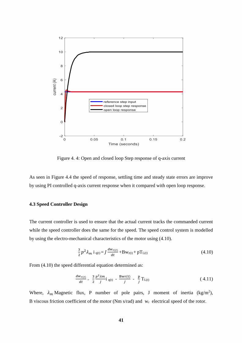
41
Figure 4. 4: Open and closed loop Step response of q-axis current
As seen in Figure 4.4 the speed of response, settling time and steady state errors are improve
by using PI controlled q-axis current response when it compared with open loop response.
4.3 Speed Controller Design
The current controller is used to ensure that the actual current tracks the commanded current
while the speed controller does the same for the speed. The speed control system is modelled
by using the electro-mechanical characteristics of the motor using (4.10).
3
2 𝑝2𝜆𝑚 i q(t) = 𝐽
𝑑𝑤𝑟(𝑡)
𝑑𝑡 +Bwr(t) + pTL(t) (4.10)
From (4.10) the speed differential equation determined as:
𝑑𝑤𝑟(𝑡)
𝑑𝑡 =
3
2 𝑝2𝜆𝑚
𝐽i q(t) -
Bwr(t)
𝐽 -
p
𝐽 TL(t) ( 4.11)
Where, 𝜆𝑚 Magnetic flux, P number of pole pairs, J moment of inertia (kg/m2),
B viscous friction coefficient of the motor (Nm s/rad) and wr electrical speed of the rotor.

42
Applying the Laplace transformation to get the relationship between the angular velocity and
the q- axis current.
( s + 𝐵
Ј)wr (s) =
3
2 𝑝2𝜆𝑚
Јiq(s) (4.12)
𝑤𝑟(𝑠)
𝑖𝑞(𝑠) =
3
2 𝑝2𝜆𝑚
Ј
s+ 𝐵
Ј
(4.13)
Now from the current PI controller designing using performance specification the transfer
function from the q-axis reference current to the actual q-axis current given by
𝑖𝑞(𝑠)
𝑖𝑞(𝑠)∗ =
(2𝜔𝑛 − 𝑅
𝐿) s+ 𝜔𝑛
2
𝑠2+2𝜔𝑛s +𝜔𝑛2
(4.14)
Substituting (4.14) transfer function in to (4.13), the relationship between the reference q-axis
current 𝑖𝑞(𝑠)∗ and the electrical speed wr(s) is given by:
𝑤𝑟(𝑠)
𝑖𝑞(𝑠)∗ = (
3
2 𝑝2𝜆𝑚
Ј
s + 𝐵
Ј
) ((2𝜔𝑛 −
𝑅
𝐿) s+ 𝜔𝑛
2
𝑠2+2𝜔𝑛s +𝜔𝑛2 ) (4.15)
If the natural frequency ωn chosen to be much greater than the mechanical relationship B
Ј, the
inner current-loop dynamics can be neglected, and the following first order model
approximation can be taken as:
𝑤𝑟(𝑠)
𝑖𝑞(𝑠)∗ ≈
3
2 𝑝2 𝜆𝑚
Ј
s + 𝐵
Ј
(4.16)
From (4.16) it shows that the electrical speed controller output gives the reference quadrature
current. Appling performance specification design technique like PI current controller using
(4.5), the speed PI controller parameters can be calculated as follows.
𝐾𝑝 = 2𝜔𝑛 −
𝐵
Ј
3
2 𝑝2𝜆𝑚
Ј
(4.17)
𝐾𝑖 = Ј𝜔𝑛
2
3
2 𝑝2𝜆𝑚
(4.18)
43
The band width of the outer-loop controller is benchmarked against the band width of the inner-
loop current controller system. It is recommended to choose the bandwidth of the outer-loop
system to be in the range of 5% to 10% of the bandwidth of the inner-loop control system [6,
29]. Therefore by using (4.17) and (4.18) with wn = 36 rad/s which is 5% of the inner loop
bandwidth and = 0.707 the controller parameters can be calculated as Kp = 0.045 and Ki =
1.143 values.
However, the above speed PI controller gain parameters are fixed values, when the system
parameters are changed due to internal and external factors or unmodelled dynamics of the
system its controller performances are degraded. To overcome such problem the controller gain
parameters must be tuned online using model reference adaptive controller (MRAC) based on
performance specification of the reference model.
4.3.1 Online Tuning of PI Speed Controller Gain with MRAC
The basic structure of a model reference adaptive control (MRAC) system is shown in the block
diagram in Figure 4.5.The reference model is chosen to generate the desired trajectory for the
plant output to follow. The tracking error represents the deviation of the plant output from the
desired trajectory. According to the tracking error, output of the controller and the output of
the plant, the adjustment mechanism automatically adjusts controller parameters so that the
behavior of the closed-loop control plant output closely follows that of reference model. The
structures of the reference model and the adaptive gains are chosen, which are based on the
requirements of control performance.
The adjustment mechanism of MRAC system constructed by a popular method for computing
the approximated sensitivity functions as so-called MIT rule. Using MIT rule to update the
controller parameters, the adjustment methods are sensitive to amplitude of input parameter
change and which affects the system performance and there is no way also to check the stability
of the system.
In order to improve the adjustment mechanism of controller parameters and to check the
stability of the system a Lyapunov stability method is used [32].
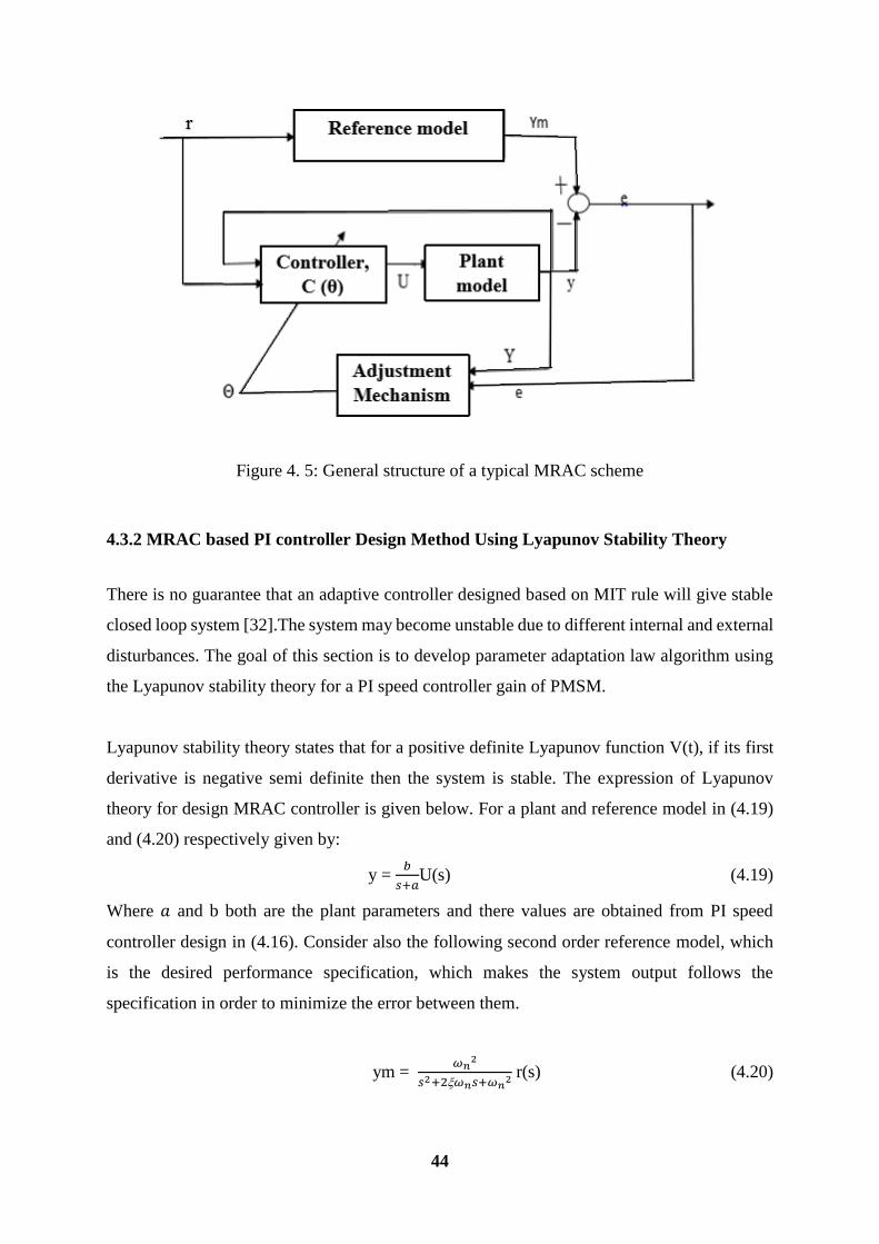
44
Figure 4. 5: General structure of a typical MRAC scheme
4.3.2 MRAC based PI controller Design Method Using Lyapunov Stability Theory
There is no guarantee that an adaptive controller designed based on MIT rule will give stable
closed loop system [32].The system may become unstable due to different internal and external
disturbances. The goal of this section is to develop parameter adaptation law algorithm using
the Lyapunov stability theory for a PI speed controller gain of PMSM.
Lyapunov stability theory states that for a positive definite Lyapunov function V(t), if its first
derivative is negative semi definite then the system is stable. The expression of Lyapunov
theory for design MRAC controller is given below. For a plant and reference model in (4.19)
and (4.20) respectively given by:
y = 𝑏
𝑠+𝑎U(s) (4.19)
Where 𝑎 and b both are the plant parameters and there values are obtained from PI speed
controller design in (4.16). Consider also the following second order reference model, which
is the desired performance specification, which makes the system output follows the
specification in order to minimize the error between them.
ym = 𝜔𝑛
2
𝑠2+2𝜔𝑛𝑠+𝜔𝑛2 r(s) (4.20)
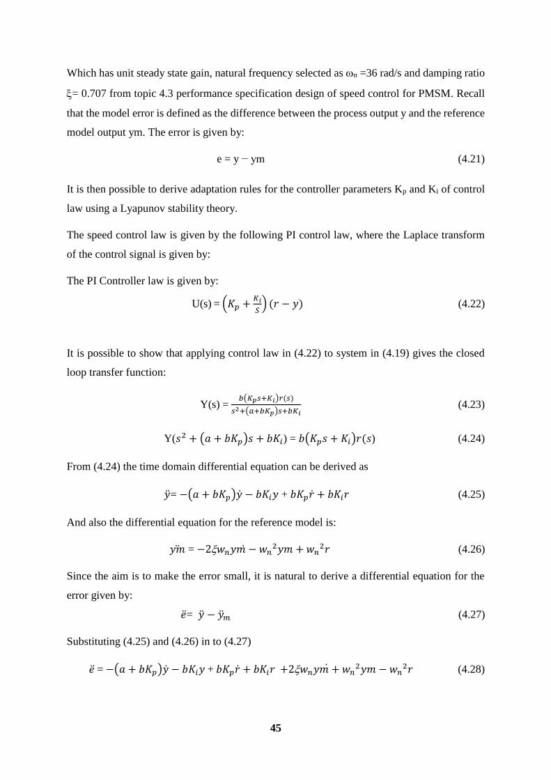
45
Which has unit steady state gain, natural frequency selected as n =36 rad/s and damping ratio
= 0.707 from topic 4.3 performance specification design of speed control for PMSM. Recall
that the model error is defined as the difference between the process output y and the reference
model output ym. The error is given by:
e = y − ym (4.21)
It is then possible to derive adaptation rules for the controller parameters Kp and Ki of control
law using a Lyapunov stability theory.
The speed control law is given by the following PI control law, where the Laplace transform
of the control signal is given by:
The PI Controller law is given by:
U(s) = (𝐾𝑝 +𝐾𝑖
𝑆) (𝑟 − 𝑦) (4.22)
It is possible to show that applying control law in (4.22) to system in (4.19) gives the closed
loop transfer function:
Y(s) = 𝑏(𝐾𝑝𝑠+𝐾𝑖)𝑟(𝑠)
𝑠2+(𝑎+𝑏𝐾𝑝)𝑠+𝑏𝐾𝑖 (4.23)
Y(𝑠2 + (𝑎 + 𝑏𝐾𝑝)𝑠 + 𝑏𝐾𝑖) = 𝑏(𝐾𝑝𝑠 + 𝐾𝑖)𝑟(𝑠) (4.24)
From (4.24) the time domain differential equation can be derived as
�̈�= −(𝑎 + 𝑏𝐾𝑝)�̇� − 𝑏𝐾𝑖𝑦 + 𝑏𝐾𝑝�̇� + 𝑏𝐾𝑖𝑟 (4.25)
And also the differential equation for the reference model is:
𝑦�̈� = −2𝑤𝑛𝑦𝑚 −̇ 𝑤𝑛2𝑦𝑚 + 𝑤𝑛
2𝑟 (4.26)
Since the aim is to make the error small, it is natural to derive a differential equation for the
error given by:
�̈�= �̈� − �̈�𝑚 (4.27)
Substituting (4.25) and (4.26) in to (4.27)
�̈� = −(𝑎 + 𝑏𝐾𝑝)�̇� − 𝑏𝐾𝑖𝑦 + 𝑏𝐾𝑝�̇� + 𝑏𝐾𝑖𝑟 +2𝑤𝑛𝑦𝑚 +̇ 𝑤𝑛2𝑦𝑚 − 𝑤𝑛
2𝑟 (4.28)

46
After some rearranging and adding 2𝑤𝑛�̇� − 2𝑤𝑛�̇� and 𝑤𝑛2𝑦 − 𝑤𝑛
2𝑦 to the above equation
gives
�̈� = −2𝑤𝑛(�̇� − 𝑦�̇�) + (−𝑎 − 𝑏𝐾𝑝 + 2𝑤𝑛)�̇� − 𝑤𝑛2(𝑦 − 𝑦𝑚) − (𝑏𝐾𝑖 − 𝑤𝑛
2)𝑦 +
𝑏𝐾𝑝�̇� + 𝑏𝐾𝑖𝑟 − 𝑤𝑛2r (4.29)
After simplifying of (4.29)
�̈�=−2𝑤𝑛�̇� − 𝑤𝑛2𝑒 − (𝑏𝐾𝑝 + 𝑎 − 2𝑤𝑛)(�̇� − �̇�) − (𝑏𝐾𝑖 − 𝑤𝑛
2)(𝑦 − 𝑟) − 𝑎�̇� + 2𝑤𝑛�̇�
. (4.30)
Now the next step is to select an appropriate positive definite Lyapunov function V(t). The
expression shown below can be taken as a positive definite Lyapunov function.
V(�̇�, 𝑒, 𝐾𝑝, 𝐾𝑖) = 1
2[�̇�2 + 𝑤𝑛
2𝑒2 +1
𝑏(𝑎 + 𝑏𝐾𝑝 − 2𝑤𝑛)
2+
1
𝑏(𝑏𝐾𝑖 − 𝑤𝑛
2)2] (4.31)
Where is any positive constant ≥ 0 .
Taking first derivative of the above equation with respect to time gives:
�̇� = �̇��̈� + 𝑤𝑛2𝑒�̇� +
1
(𝑏𝐾𝑝 + 𝑎 − 2𝑤𝑛)�̇�𝑝 +
1
(𝑏𝐾𝑖 − 𝑤𝑛
2)�̇�𝑖 (4.32)
Substituting (4.30), which is expression of derivative of error to (3.32) gives as:-
�̇� = −2𝑤𝑛�̇�2 +1
(𝑏𝐾𝑝 + 𝑎 − 2𝑤𝑛) (�̇�𝑝 − �̇�(�̇� − �̇�)) +
1
(𝑏𝐾𝑝 − 𝑤𝑛
2)(�̇�𝑖 − �̇�(𝑦 − 𝑟))
(4.33)
Now if the parameters are updated as:
�̇�𝑝 = �̇�(�̇� − �̇�), this implies 𝐾𝑝 = − 𝑆𝑒(𝑟 − 𝑦) (4.34)
and
�̇�𝑖 = �̇�(𝑦 − 𝑟), this implies 𝐾𝑖 = − 𝑒(𝑟 − 𝑦) (4.35)
Then
�̇�= −2𝑤𝑛�̇�2 (4.36)
This shows that first derivative of V is negative semi definite and implies that if the parameters
are updated as given in (4.34) and (4.35), the system will be stable.
Where is, the positive adaptation gain for MRAC design and selected by trey and error method
to get good system response.
A Matlab Simulink model representation of the adaptation scheme for online tuning of Kp and
Ki is depicted in Figure 4.6.
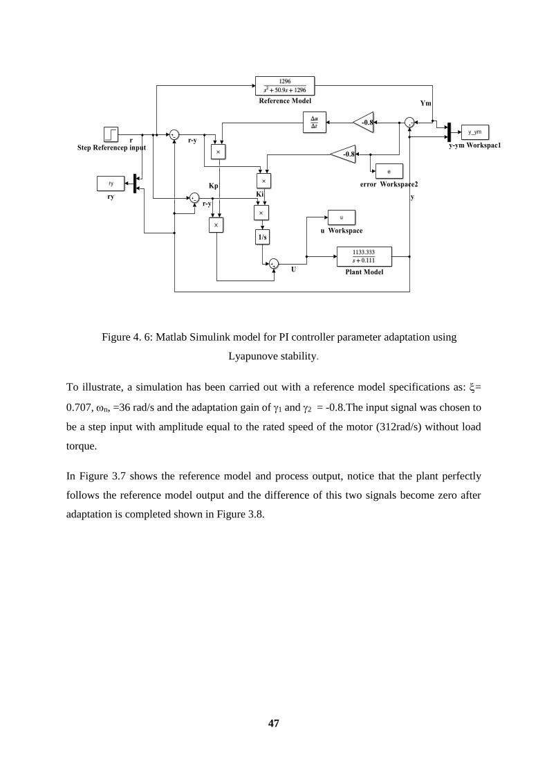
47
Figure 4. 6: Matlab Simulink model for PI controller parameter adaptation using
Lyapunove stability.
To illustrate, a simulation has been carried out with a reference model specifications as: =
0.707, n, =36 rad/s and the adaptation gain of 1 and 2 = -0.8.The input signal was chosen to
be a step input with amplitude equal to the rated speed of the motor (312rad/s) without load
torque.
In Figure 3.7 shows the reference model and process output, notice that the plant perfectly
follows the reference model output and the difference of this two signals become zero after
adaptation is completed shown in Figure 3.8.
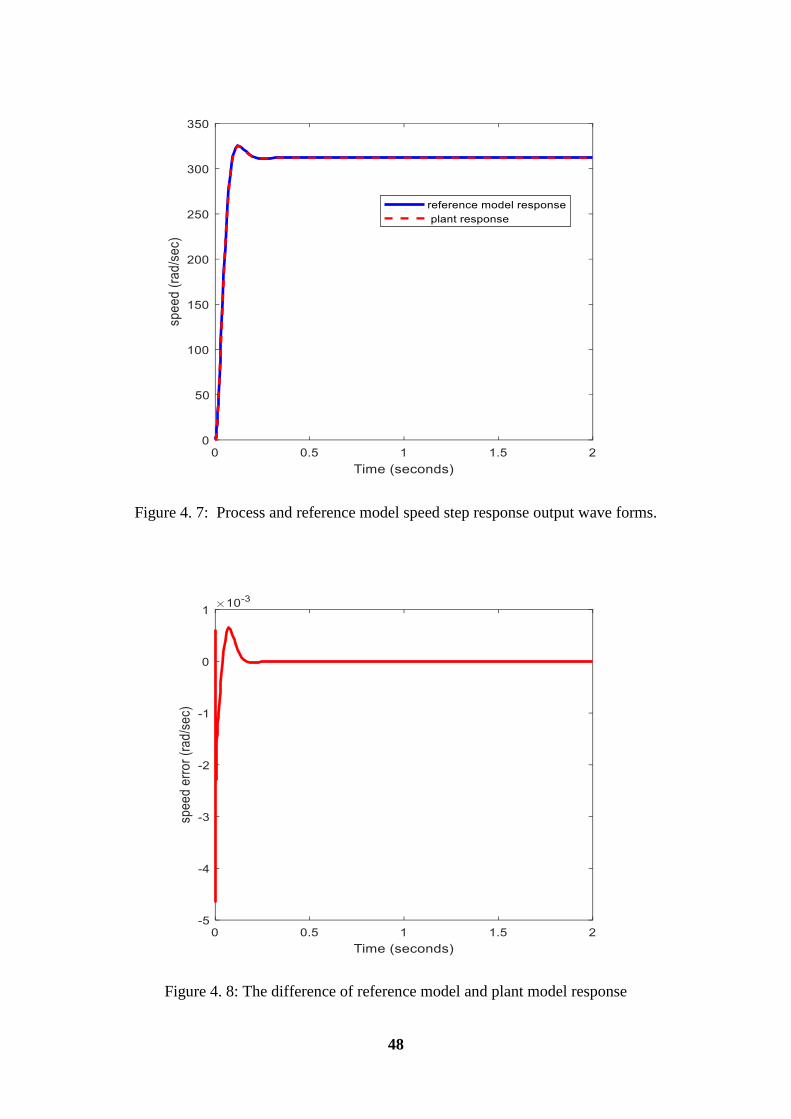
48
Figure 4. 7: Process and reference model speed step response output wave forms.
Figure 4. 8: The difference of reference model and plant model response

49
In the Figure 4.9 below shows using MRAC controller output response of the plant truck the
reference input when a step input is used with magnitude of 312 rad/sec and also the controlled
signal which is the input of the plant model goes to zero at steady state as shown in Figure 4.10
under no load condition.
Figure 4. 9 : Closed loop response of speed MRAC controller
Figure 4. 10: The controlled signal U(t)

50
Chapter Five
5 Simulation Result and Discussion
5.1 Introduction
This chapter of the thesis is concerned with the simulation results of FOC based closed loop
sensorless speed control of PMSM using model reference adaptive system with
Matlab/Simulink. The simulation result shows only the operation of PMSM below the base
speed and Maximum Torque per Ampere (MTPA) operation will be explained.
The parameters that is used for simulating the PMSM drive system placed in Appendix A of
table A.
5.2 Simulink Model of PMSM Drive System
The overall Matlab/Simulink model of the PMSM drive and Control system is shown in Figure
5.1. All the components of the real drive system are modelled to study the simulation result.
Figure 5. 1: Complete Matlab/Simulink Model of the FOC based PMSM drive.

51
Figure 5.2 shows Matlab Simulink block diagram PMSM in d-q frame of reference. The output
of we (electrical speed of the motor) and theta, in the model used for comparison purpose with
the estimated speed and angle outputs.
Figure 5. 2 : PMSM Matlab Simulink model
The PMSM speed controller with MRAC and its d-q axis PI current controllers with feed
forward voltage decoupling depicted in Figure 5.3. The output of voltage decoupling block is
used as the input of SVPWM by invers park transformations.
Figure 5. 3 : The overall speed and current controller representation in Matlab/Simulink.
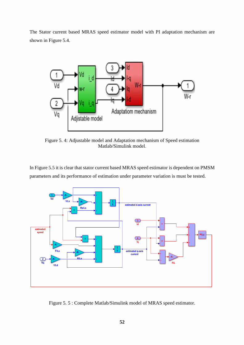
52
The Stator current based MRAS speed estimator model with PI adaptation mechanism are
shown in Figure 5.4.
Figure 5. 4: Adjustable model and Adaptation mechanism of Speed estimation
Matlab/Simulink model.
In Figure 5.5 it is clear that stator current based MRAS speed estimator is dependent on PMSM
parameters and its performance of estimation under parameter variation is must be tested.
Figure 5. 5 : Complete Matlab/Simulink model of MRAS speed estimator.
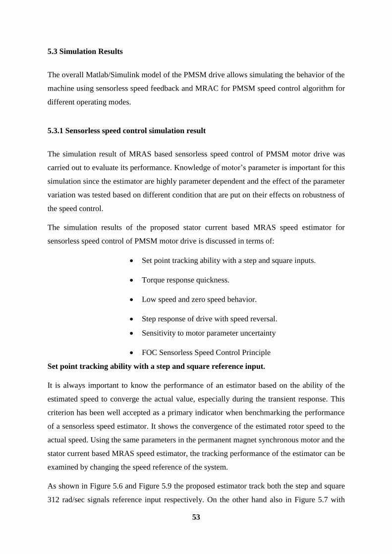
53
5.3 Simulation Results
The overall Matlab/Simulink model of the PMSM drive allows simulating the behavior of the
machine using sensorless speed feedback and MRAC for PMSM speed control algorithm for
different operating modes.
5.3.1 Sensorless speed control simulation result
The simulation result of MRAS based sensorless speed control of PMSM motor drive was
carried out to evaluate its performance. Knowledge of motor’s parameter is important for this
simulation since the estimator are highly parameter dependent and the effect of the parameter
variation was tested based on different condition that are put on their effects on robustness of
the speed control.
The simulation results of the proposed stator current based MRAS speed estimator for
sensorless speed control of PMSM motor drive is discussed in terms of:
Set point tracking ability with a step and square inputs.
Torque response quickness.
Low speed and zero speed behavior.
Step response of drive with speed reversal.
Sensitivity to motor parameter uncertainty
FOC Sensorless Speed Control Principle
Set point tracking ability with a step and square reference input.
It is always important to know the performance of an estimator based on the ability of the
estimated speed to converge the actual value, especially during the transient response. This
criterion has been well accepted as a primary indicator when benchmarking the performance
of a sensorless speed estimator. It shows the convergence of the estimated rotor speed to the
actual speed. Using the same parameters in the permanent magnet synchronous motor and the
stator current based MRAS speed estimator, the tracking performance of the estimator can be
examined by changing the speed reference of the system.
As shown in Figure 5.6 and Figure 5.9 the proposed estimator track both the step and square
312 rad/sec signals reference input respectively. On the other hand also in Figure 5.7 with

54
different reference step input, the estimated speed follows it. This shows the tracking
performance of the estimator and actual speed to the reference speed can be examined by
changing the reference of the system with the maximum steady state error of 0 % and good
transient performance with rise time less than 0.1 second. As shown in Figure 5.7 the estimated
angle perfectly follows with the actual angle with the maximum error of 0 degree from the step
input response of Figure 5.6.
Figure 5. 6 : Step input speed response with 2.4Nm load torque
Figure 5. 7: Estimated and actual angle.

55
Figure 5. 8 Rotor speed response with different a step input reference and load of 2.4 Nm
Figure 5. 9 : Square input signal rotor speed response with load of 2.4 Nm
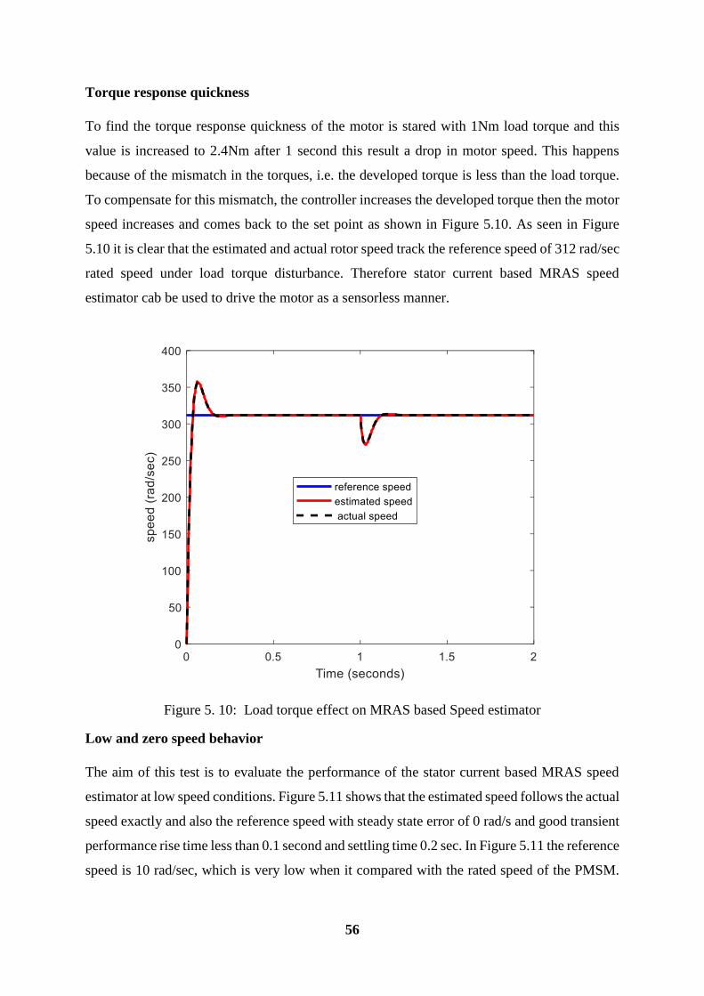
56
Torque response quickness
To find the torque response quickness of the motor is stared with 1Nm load torque and this
value is increased to 2.4Nm after 1 second this result a drop in motor speed. This happens
because of the mismatch in the torques, i.e. the developed torque is less than the load torque.
To compensate for this mismatch, the controller increases the developed torque then the motor
speed increases and comes back to the set point as shown in Figure 5.10. As seen in Figure
5.10 it is clear that the estimated and actual rotor speed track the reference speed of 312 rad/sec
rated speed under load torque disturbance. Therefore stator current based MRAS speed
estimator cab be used to drive the motor as a sensorless manner.
Figure 5. 10: Load torque effect on MRAS based Speed estimator
Low and zero speed behavior
The aim of this test is to evaluate the performance of the stator current based MRAS speed
estimator at low speed conditions. Figure 5.11 shows that the estimated speed follows the actual
speed exactly and also the reference speed with steady state error of 0 rad/s and good transient
performance rise time less than 0.1 second and settling time 0.2 sec. In Figure 5.11 the reference
speed is 10 rad/sec, which is very low when it compared with the rated speed of the PMSM.

57
Therefore the speed of the drive can be estimated over a wide range speed through very low
speed or zero speed to its rated speed (312 rad/sec) under the presence of load torque variation.
Figure 5. 11: The rotor speed response at 10 rad/sec step input signals without load.
In Figure 5.12 at the zero speed reference the estimated speed can be also zero. This means that
the system is stable at zero speed and continuous operation is possible.
Figure 5. 12: Rotor speed responnse at 0 rad/sec step input signal without load
58
Step response of drive with speed reversal
Figure 5.13 shows that simulation result for speed reversal in step input. The motor reference
speed is changed from -50rad/s to 100 rad/s at 1 second and again speed is set to 100 rad/s after
1 second. The result shows that the actual and estimated speed always track the reference speed
with good accuracy and transient response.
Figure 5. 13: Step response of drive with speed reversal with load torque of 2.4 Nm.
Parameter sensitivity
Since the MRAS based speed estimator for PMSM depends on motor parameters and therefore
the sensitivity to the motor parameters change should be tested for different reference speed.
It’s better to test the parameter change of the motor at the rated speed of the motor and below
rated speed of the motor.
To perform this the parameter R, L and λm can be increased by 50% from their nominal value
with a reference speed changed from 100 rad/s to 312 rad/s when loaded by 2.4 Nm. As shown
in Figure 5.14 the sensitivity to motor parameter changes of the sensorless MRAS speed
estimator is less sensitive to motor parameter variation. As shown in Figure 5.14 when the
motor parameters increased by 50% of their nominal value the estimated speed exactly follow
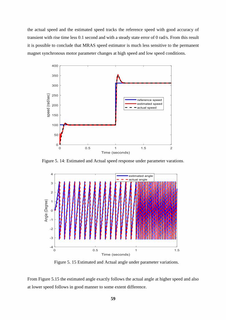
59
the actual speed and the estimated speed tracks the reference speed with good accuracy of
transient with rise time less 0.1 second and with a steady state error of 0 rad/s. From this result
it is possible to conclude that MRAS speed estimator is much less sensitive to the permanent
magnet synchronous motor parameter changes at high speed and low speed conditions.
Figure 5. 14: Estimated and Actual speed response under parameter varations.
Figure 5. 15 Estimated and Actual angle under parameter variations.
From Figure 5.15 the estimated angle exactly follows the actual angle at higher speed and also
at lower speed follows in good manner to some extent difference.
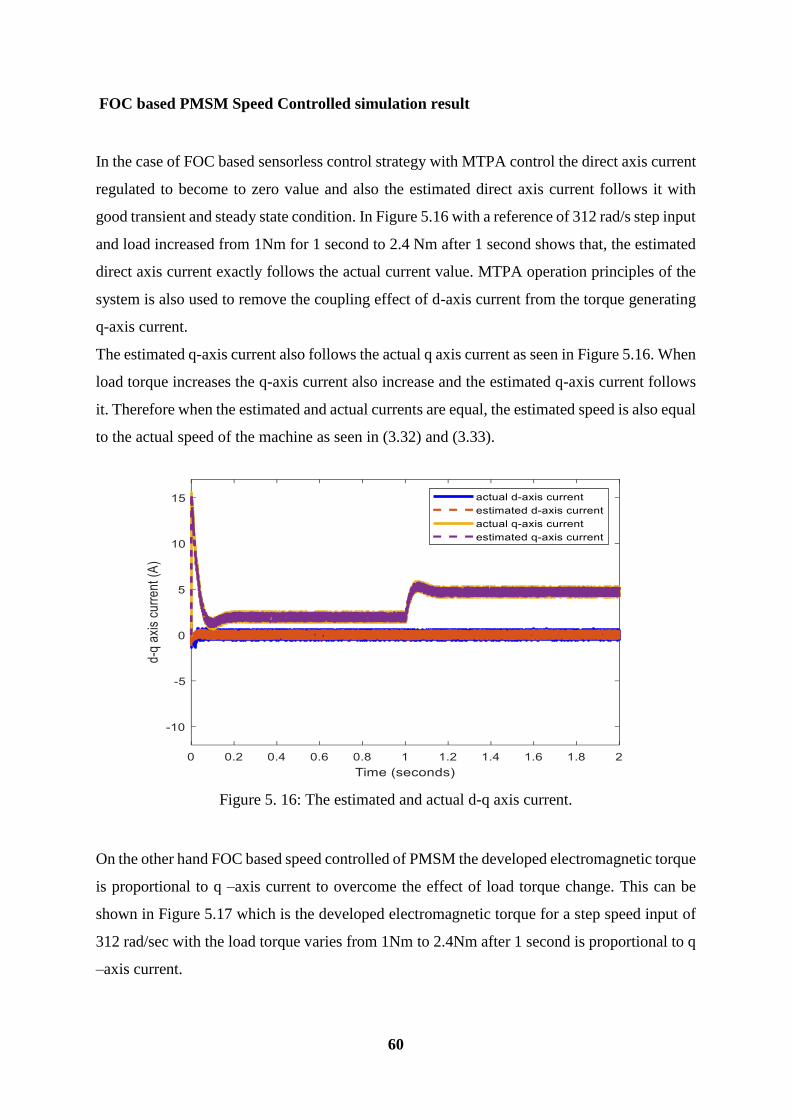
60
FOC based PMSM Speed Controlled simulation result
In the case of FOC based sensorless control strategy with MTPA control the direct axis current
regulated to become to zero value and also the estimated direct axis current follows it with
good transient and steady state condition. In Figure 5.16 with a reference of 312 rad/s step input
and load increased from 1Nm for 1 second to 2.4 Nm after 1 second shows that, the estimated
direct axis current exactly follows the actual current value. MTPA operation principles of the
system is also used to remove the coupling effect of d-axis current from the torque generating
q-axis current.
The estimated q-axis current also follows the actual q axis current as seen in Figure 5.16. When
load torque increases the q-axis current also increase and the estimated q-axis current follows
it. Therefore when the estimated and actual currents are equal, the estimated speed is also equal
to the actual speed of the machine as seen in (3.32) and (3.33).
Figure 5. 16: The estimated and actual d-q axis current.
On the other hand FOC based speed controlled of PMSM the developed electromagnetic torque
is proportional to q –axis current to overcome the effect of load torque change. This can be
shown in Figure 5.17 which is the developed electromagnetic torque for a step speed input of
312 rad/sec with the load torque varies from 1Nm to 2.4Nm after 1 second is proportional to q
–axis current.
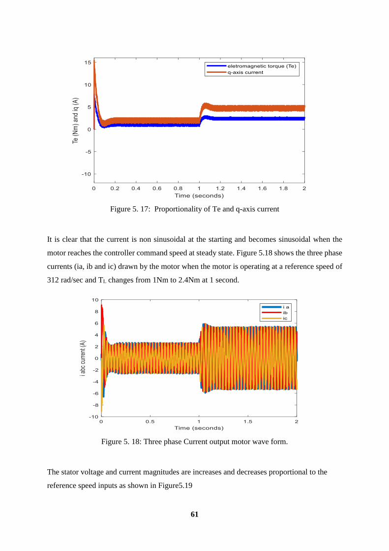
61
Figure 5. 17: Proportionality of Te and q-axis current
It is clear that the current is non sinusoidal at the starting and becomes sinusoidal when the
motor reaches the controller command speed at steady state. Figure 5.18 shows the three phase
currents (ia, ib and ic) drawn by the motor when the motor is operating at a reference speed of
312 rad/sec and TL changes from 1Nm to 2.4Nm at 1 second.
Figure 5. 18: Three phase Current output motor wave form.
The stator voltage and current magnitudes are increases and decreases proportional to the
reference speed inputs as shown in Figure5.19
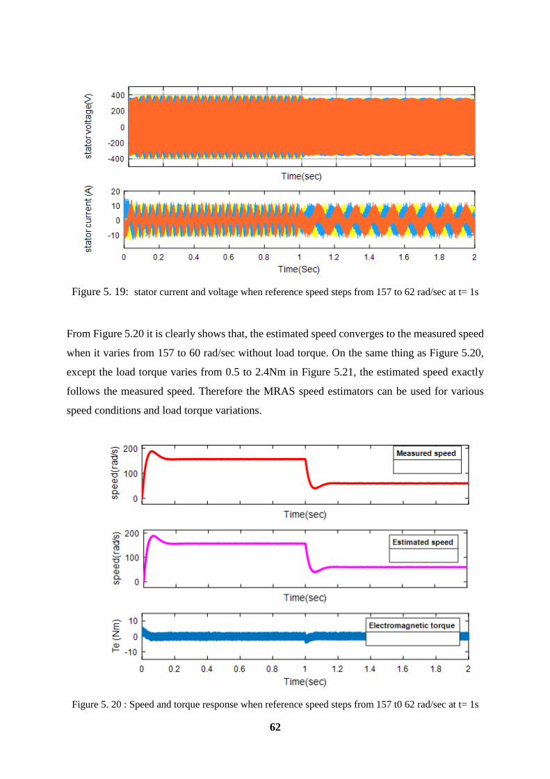
62
Figure 5. 19: stator current and voltage when reference speed steps from 157 to 62 rad/sec at t= 1s
From Figure 5.20 it is clearly shows that, the estimated speed converges to the measured speed
when it varies from 157 to 60 rad/sec without load torque. On the same thing as Figure 5.20,
except the load torque varies from 0.5 to 2.4Nm in Figure 5.21, the estimated speed exactly
follows the measured speed. Therefore the MRAS speed estimators can be used for various
speed conditions and load torque variations.
Figure 5. 20 : Speed and torque response when reference speed steps from 157 t0 62 rad/sec at t= 1s

63
Figure 5. 21: Speed and torque response when load torque steps from 0.5 to 2.4Nm at t=1 s.
In Figure 5.22 shows the variation of stator voltage and current when the load torque varies
from 0.5 to 2.4Nm rated torque.
Figure 5. 22: Stator current and voltages when load torque steps from 0.5 to 2.4Nm at t=1s

64
5.3.2 MRAC Speed Controller Simulation Result
The simulation results of the proposed MRAC type speed control of PMSM motor drive is
discussed in terms of:
Speed set point trucking performance.
Comparison of PI and MRAC speed controller.
Speed set point trucing performance
The proposed speed controller response tested under the performance specifications such as
rise time less than 0.1 second and stilling time less than 0.2 second with different load torque.
In Figure 5.23 shows that the output speed truck the reference speed of a step input magnitude
of 312 rad/sec under load torque changed from 1Nm to 2.4 Nm. It shows that the estimated and
actual speed tracks the reference input in the specified performance.
Figure 5. 23: Speed response of PMSM using MRAC
Comparison of PI and MRAC controller
Comparison of PI and MRAC controller performance under parameter variation due to the
internal and external factors of the system. Assuming that the PMSM parameters such that, its
resistance, inductance and magnetic flux value increased from its nominal value (in Appendix)
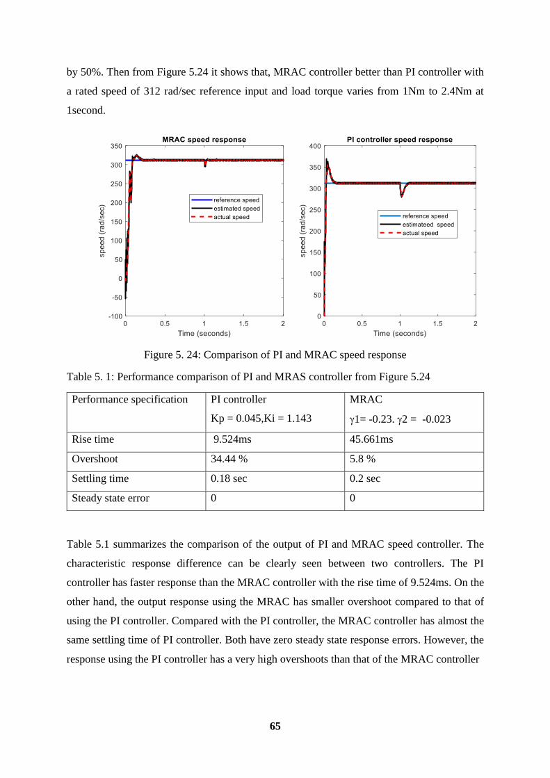
65
by 50%. Then from Figure 5.24 it shows that, MRAC controller better than PI controller with
a rated speed of 312 rad/sec reference input and load torque varies from 1Nm to 2.4Nm at
1second.
Figure 5. 24: Comparison of PI and MRAC speed response
Table 5. 1: Performance comparison of PI and MRAS controller from Figure 5.24
Performance specification PI controller
Kp = 0.045,Ki = 1.143
MRAC
1= -0.23. 2 = -0.023
Rise time 9.524ms 45.661ms
Overshoot 34.44 % 5.8 %
Settling time 0.18 sec 0.2 sec
Steady state error 0 0
Table 5.1 summarizes the comparison of the output of PI and MRAC speed controller. The
characteristic response difference can be clearly seen between two controllers. The PI
controller has faster response than the MRAC controller with the rise time of 9.524ms. On the
other hand, the output response using the MRAC has smaller overshoot compared to that of
using the PI controller. Compared with the PI controller, the MRAC controller has almost the
same settling time of PI controller. Both have zero steady state response errors. However, the
response using the PI controller has a very high overshoots than that of the MRAC controller

66
Chapter six
6. Conclusion and recommendation
6.1 Conclusion
In this thesis, the PMSM model is built according to the stator current d and q axis equations,
and the adaptive law of speed estimation is constructed according to the Popov hyper stability
methods. The design of stator current based MRAS speed estimator overcome the problem
due to mechanical speed sensor and parameter sensitivity for speed control of permanent
magnet synchronous motor has been studied.
For estimating the speed of PMSM the MRAS based observer is used to estimate the state of
𝑖̂𝑑 and 𝑖̂𝑞 current. This estimated states are determined from adjustable model of the observer.
When the reference model output and adjustable model output difference becomes zero, then
the estimated speed reaches its real value of the machine speed. The PI adaptation regulator is
used for the adaptation mechanism of speed estimator and the gain of PI parameters are
determined by using root locus analysis method. it has simple and fast adaptation rate than
other methods.
The simulation results shows that stator current based MRAS can estimate the rotor speed of
permanent magnet synchronous motor with good performance below the rated speed. As it is
shown from Figure 5.6, stator current based MRAS speed estimator estimate the rotor speed of
PMSM with a steady state error of 0 % and good transient response with rise time of less than
0.1 second and settling time 0.2 second has been achieved.
The performance of stator current based MRAS speed estimator was analysed in terms of speed
tracking capability, torque response quickness, low and zero speed behavior, step response of
drive with speed reversal and sensitivity to motor parameter uncertainty. The system gives
good performance at no load and loaded condition. Hence, it can work with different load
torque conditions and with parameters variation.
The robust controller under parameter variation for speed controller designed using MRAC
with Lyapunove stability. This controller response compared with conventional PI controller
response under parameter variations and it shows that MRAC decreases the over shoots and
has fast adaptation response than PI controller.

67
6.2 Recommendation
The adaptive PI controller for stator current based MRAS speed estimator which is used in this
thesis is designed based on the root locus analysis method. However, it needs to get the transfer
function of the system and determine PI parameter gain which makes the mathematical analysis
of the system complex. To overcome such difficulty of adaptation it is possible to use Fuzzy
logic nonlinear controller instead of classical PI controller, which is not require any
mathematical model and makes it simple. Therefore stator current based MRAS speed
estimator with FLC adaptation is recommended.
In addition to this, this thesis work only shows the effectiveness of the proposed system only
in MATLAB/Simulink computer simulation. But it is recommended that to show the
effectiveness again by implementing the real system for future works.
68
References
[1] F. Yusivar, N. Hidayat, R. Gunawan and A. Halim , "Implementation of Field Oriented
Control for Permanent Magnet Synchronous Motor," in Electrical Engineering and
Computer Science (ICEECS), IEEE, pp. 359-362, 2014.
[2] Mahlet Legesse, " Speed Control of Vector Controlled PMSM Drive using Fuzzy Logic-
PI Controller." thesis for the degree of Master of Science in Electrical and Computer
Engineering Addis Ababa Institute of Technology (AAiT), August, 2011.
[3] Chu, W.Q. Zhu and Q.Chen, "Simplified analytical optimization and comparison of
torque densities between electrically excited and permanent-magnet machines," IEEE
Trans, 2016.
[4] S. K. Kommuri, J. J. Rath, K. C. Veluvolu, M. Defoort, and S. Tatinati " Performance
comparison of sliding mode observers for back EMFs based speed estimation in PMSM,"
International Conference on Control in Automation and Systems (ICCAS), 2015.
[5] N. Li, Y. Ming, G. Xianguo and X. Dianguo " A Comparative Study of Model Predictive
Current Control and FOC for PMSM," in 17th International Conference on Electrical
Machines and Systems (ICEMS), IEEE., pp. 3143-3147, 2014.
[6] W.Lina "online Multi-parameter Identification for Surface mounted permanent magnet
synchronous motor," Transaction on chanina Electronic society, pp. 1656-1667, 2016.
[7] F. Genduso, R. Miceli, C. Rando and G. R. Galluzzo, "Back-EMF Sensorless Control
Algorithm for High Dynamics Performances PMSM," IEEE, vol. 13, no. 05, pp. 1342-
1349, 2009.
[8] L. An, D. Franck, and K. Hameyer, "Sensorless field oriented control using back-EMF
and flux observer for a surface mounted permanent magnet synchronous motor,"
International Journal of Applied Electromagnetics and Mechanics, vol. 45, no. 1-4, pp.
845-850, 2015.
69
[9] V. Nagarajan, M. Balaji and V. Kamaraj, "Back-Emf-Based Sensorless Field-Oriented
control of PMSM using Neural-network-based controller with start-up strategy,"
Advance in Intellegent systems and Computing, vol. 325, pp. 449-457, 2015.
[10] B. Nahid-Mobarakeh, F. Meibody-Tabar and F. M. Sargos, "Back EMF estimation based
sensorless control of PMSM: Robustness with respect to measurement errors and inverter
irregularities," in Industry Applications control, IEEE , vol. 34, no. 07, pp. 1231-1239,
2004.
[11] J. Beegum and Sema, " Comparision of Speed Control of PMSM with PI,PID and
Adaptive PID controllers," IRJET, vol. 43, no. 05, pp. 1656-1667, 2016.
[12] J. K. J. Kang, B. H. B. Hu, H. L. H. Liu and G. X. G. Xu, "Sensorless Control of
Permanent Magnet Synchronous Motor Based on Extended Kalman Filter," in 2009 IITA
International Conference on Services Science, Management and Engineering, pp. 571-
574, 2009.
[13] P. Borsje, T. F. Chan, Y. K. Wong and S. L. Ho, "A Comparative Study of Kalman
Filtering for Sensorless Control of a Permanent-Magnet Synchronous Motor Drive," in
Electric Machines and Drives, on International Conference ,IEEE, pp. 815-822, 2005.
[14] J. Son and J. Lee, "A High-Speed Sliding-Mode Observer for the Sensorless Speed
Control of a PMSM," IEEE Transactions On Industrial Electronics, vol. 58, no. 9, pp.
4069-4077, 2011.
[15] Derege Eskeza, "Speed control of permanent magnet synchronous motor using Higher
order Sliding mode cotroller ," Msc thesis for the degree of Masters of science in
electrical and computer Engineering Addis Abeba Institute of Technology (AAiT), 2017.
[16] Syed Abdul Rahman Kashif and Muhammad Asghar Saqib, "Sensorless Control of
PMSM Drive using Neural Network Observer," Electrical machines drive,Transaction
on IEEE, pp. 1526-1533, 2016.
[17] Ji-Hoon Jang ,“Sensorless Drive of Surface-Mounted Permanent-Magnet Motor by High-
Frequency Signal Injection Based on Magnetic Saliency," IEEE, vol. 36, no. 15, pp.
1723-1726, 2003.

70
[18] Q. Fang, D. Zhiquan and Q. Zhijian , " Method of Sensorless Vector Control for PMSM,"
Transactions of China Electrotechnical Society, Vol.22, No.10, 2007, pp.30-34., vol. 10,
no. 22, pp. 30-34, 2007.
[19] Mohamed I. Abu El- Sebah and Ghada A. Abdel Aziz , "High Performance Control of
Sensorless Permanent Magnet Synchronous Motor," transaction on IEEE, 2013.
[20] M. J. Grimble and M. A. Johnson, " Sensorless AC Electric Motor Control," Advance in
Industrial Control,IEEE, 2015.
[21] Dai Wenjin and Li Huiling, "Study of Direct Torque Control (DTC) system of a
Permanent Magnet synchronous Motor based on DSP," IEEE , in Electrical and machine
systems, 2001.
[22] D.W. Novonty and T.A. Lipo, " Vector control and dynamics of AC drives," in University
press, Oxford, 2002.
[23] S. Sumita, K. Tobari, S. Aoyagi, and D. Maeda, "A Simplified Sensorless Vector Control
Based on the Average of the DC Bus Current," in Conf. Rec., IEEE-IPEC, vol. 29, no.
14, pp. 3035-3040, 2010.
[24] Dai Wenjin and Li Huiling, "study of Direct Torque Control (DTC) system of a
Permanent Magnet synchronous Motor based on DSP," IEEE Electrical and machine
systems, 2001.
[25] Domenico Casadei, Fransesco Profumo, Giovanni Serra, Angelo Tani,, " Field Oriented
Control and Direct Torque control of two viable schemes for induction motors torque
control," IEEE Transactions on power Electronics, vol. 3, no. 06, pp. 219-227, 2017.
[26] www.microsemi.com/soc/company/contact/default.aspx. “, Microsemi., "Field Oriented
Control of Permanent Magnet Synchronous Motors User’s Guide”Microsemi.," 2019.
[27] Song Chi., "Position-sensorless control of permanent magnet synchronous machines
overwide speed range," ”.Thesis for the degree of Doctor, Department of Electrical and
Computer Engineering, Ohio State University, 2018.

71
[28] G. Xing, "Research on Rotor speed Identification Method for Permanent Magnet
Synchronous Motor Based on Improved Model Reference Adaptive System," Master
thesis: Hunan University , 2013.
[29] C. Yong, Z. Fu and L. Xia et al, "Online adaptive parameter identification of PMSM
based on the dead-time compensation," International Journal of Electronics, vol. 102,
no. 07, pp. 1132-1150, 2015.
[30] Z. Hongshuai, W. Ping and H. Bangcheng. "Rotor Position Measurement for High-speed
Permanent Magnet Synchronous Motors Based on Fuzzy PI MRAS." Proceedings of the
CSEE, vol. 12, no. 2, pp. 1889-1896, 2014.
[31] Liuping Wang , PID and pridictive control of electrical drives and power converters using
matlab simulink,, Singapore : John Wiley & Sons Pte. Ltd, 2015.
[32] K. J. Astrom and B. Wittenmark, Adaptive Control, NewYork City: Lund Institute of
Technology, 2008.
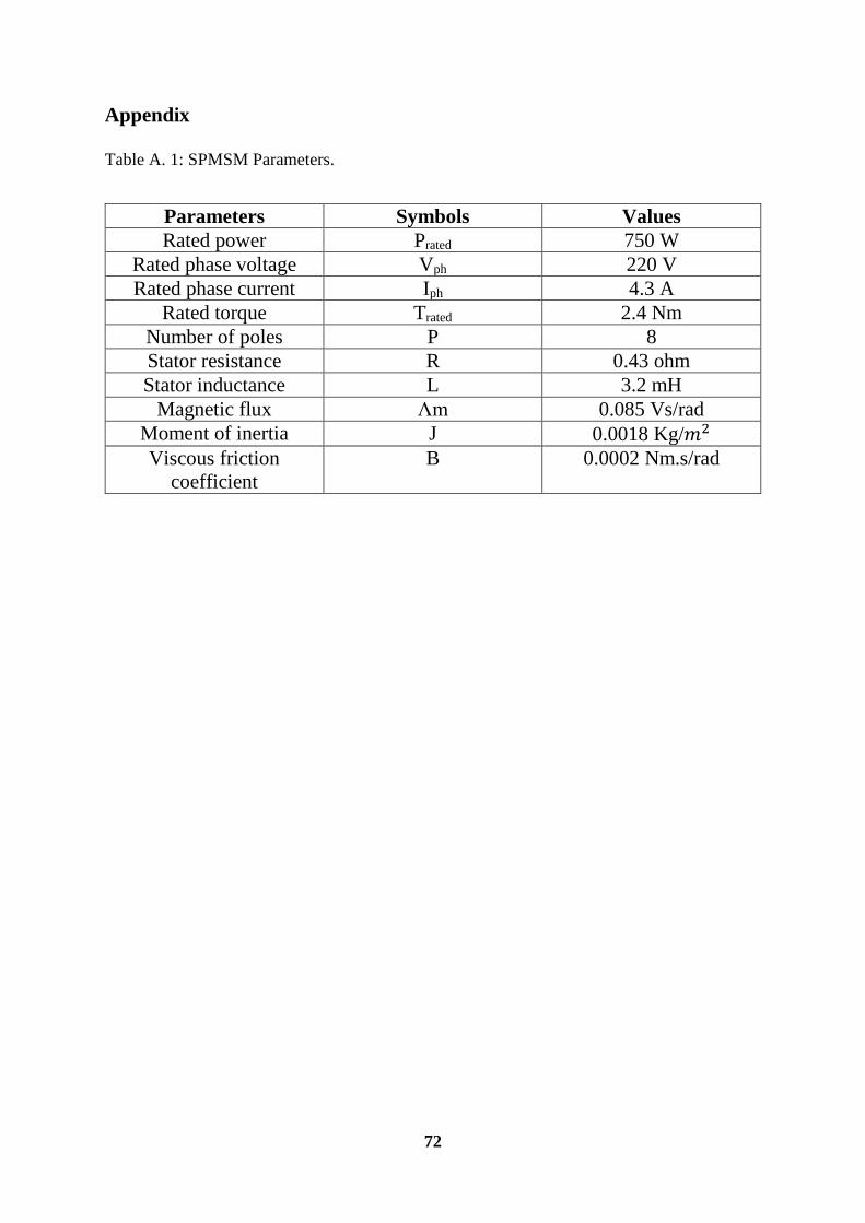
72
Appendix
Table A. 1: SPMSM Parameters.
Parameters Symbols Values
Rated power Prated 750 W
Rated phase voltage Vph 220 V
Rated phase current Iph 4.3 A
Rated torque Trated 2.4 Nm
Number of poles P 8
Stator resistance R 0.43 ohm
Stator inductance L 3.2 mH
Magnetic flux Λm 0.085 Vs/rad
Moment of inertia J 0.0018 Kg/𝑚2
Viscous friction
coefficient
B 0.0002 Nm.s/rad
Related Documents