Sensorless Induction Motor: High-Order Sliding-Mode Controller and Adaptive Interconnected Observer

3818 IEEE TRANSACTIONS ON INDUSTRIAL ELECTRONICS, VOL. 55, NO. 11, NOVEMBER 2008

Sensorless Induction Motor: High-OrderSliding-Mode Controller and Adaptive

Interconnected ObserverDramane Traoré, Franck Plestan, Member, IEEE, Alain Glumineau, Member, IEEE, and Jesus de Leon

Abstract—An adaptive interconnected observer and high-ordersliding-mode control of induction motors without mechanical sen-sors (speed sensor and load torque sensor) are proposed andexperimentally evaluated. The adaptive interconnected observerestimates fluxes, angular velocity, load torque, and stator resis-tance. Stability based on Lyapunov theory is proved to guaranteethe “observer–controller” stability.

Index Terms—High-order sliding mode (HOSM), inductionmotor (IM), observer, sensorless control.

I. INTRODUCTION

DUE TO COST reduction, mechanical speed sensorfragility, and sensor installation difficulty, sensorless in-

duction motor (IM) drives are becoming wide spread solutionsfor the next generation of commercial drives. Thus, the IMpresents a challenging control problem.

For direct field-oriented control (FOC) and variable structurecontrol of IM drives, speed knowledge is crucial. If sensors areused, the maintenance problem occurs. Consequently, duringthe last decade, there has been a considerable interest to developIM drives without mechanical sensors (sensorless). A major dif-ficulty is to ensure the robustness against parameter variationsas stator resistance for example [8].

The concepts and principles of sliding-mode (SM) controlapplied to electrical motors are introduced in [18]. The successof this type of control for electric drives is mainly due to itsdisturbance rejection, strong robustness, and simple implemen-tation, as shown by a large number of papers on sensorless IMdrives [11], [19] that use the standard approach of SM control.The specific problem of this standard approach is the chatteringeffect. In order to overcome this drawback and to improve thecontroller performances, an approach called “high-order slidingmode” (HOSM) algorithm has been proposed in order to keepthe main advantages of the standard SM control, the chatteringeffect being attenuated and high-order precision provided [13].

The rth-order SM controller with finite-time convergence hasbeen proposed in [10], [13], and [15]. In the sequel, the HOSM

Manuscript received January 15, 2008; revised July 18, 2008. First publishedAugust 19, 2008; current version published October 31, 2008.

D. Traoré, F. Plestan, and A. Glumineau are with the Institut deRecherche en Communications et en Cybernétique de Nantes, Ecole Centralede Nantes—CNRS, 44321 Nantes, France (e-mail: [email protected]).

J. de Leon is with the Universidad Autonóma de Nuevo León, San Nicolásde Los Garza 66540, Mexico.

Color versions of one or more of the figures in this paper are available onlineat http://ieeexplore.ieee.org.

Digital Object Identifier 10.1109/TIE.2008.2003368

speed-flux control is based on [15]: The latter proposes aneasy implementation and an a priori well-known convergencetime and is robust with respect to (w.r.t.) uncertainties anddisturbance.

In [4] and [9], it is shown that there is observability lost whenexcitation voltage frequency is zero and rotor speed is constant.Yet, in the literature, the sensorless algorithms are usually testedand evaluated at high and low speed [6], [14]. However, afew studies have highlighted this problem of unobservability.In [6], the “observer–controller” was tested on a “sensorlesscontrol benchmark.” The trajectories of this benchmark arechosen to evaluate the IM sensorless algorithm under conditionsof observability and unobservability. Unfortunately, when thereference value of the external load disturbance is greater than20% of the nominal value of the external load disturbance, theobserver–controller becomes unstable.

Since the observability properties are lost at very low speed,it is well known that it is impossible to reconstruct the stateof the IM that asymptotically converges to indistinguishabletrajectories [9]. However, under these trajectories, it is possibleto design an observer whose performances are acceptable evenif the asymptotic stability cannot be guaranteed. Thus, weneed a notion of stability that is more suitable than asymptoticstability; this is the practical stability [12]. The contributionsof this paper are an estimation of fluxes, speed, load torque,and stator resistance (critical parameter at very low speed), anHOSM speed-flux controller, the proof of practical stability ofthe closed loop system, and experimental tests on a significantsensorless control benchmark.

II. IM MODEL

The IM model is based on the motor equations in rotatingd- and q-axes and reads as⎡⎢⎢⎢⎢⎣isd

isq

φrd

φrq

Ω

⎤⎥⎥⎥⎥⎦ =

⎡⎢⎢⎢⎣

baφrd + bpΩφrq − γisd + ωsisq

baφrq − bpΩφrd − γisq − ωsisd

−aφrd + (ωs − pΩ)φrq + aMsrisd

−aφrq − (ωs − pΩ)φrd + aMsrisq

m(φrdisq − φrqisd) − cΩ − 1J Tl

⎤⎥⎥⎥⎦

+[m1 0 0 0 00 m1 0 0 0

]T [usd

usq

](1)

with isd, isq , φrd, φrq, usd, usq , Ω, Tl, and ωs are thestator currents, rotor fluxes, stator voltage inputs, angular

0278-0046/$25.00 © 2008 IEEE

TRAORÉ et al.: SENSORLESS IM: SLIDING-MODE CONTROLLER AND ADAPTIVE INTERCONNECTED OBSERVER 3819

speed, load torque, and stator frequency, respectively, (de-fined in Section V). The subscripts s and r refer to thestator and rotor, respectively. The parameters a, b, c, γ, σ,m, and m1 are defined as a = Rr/Lr, b = Msr/σLsLr, c =fv/J , γ = (L2

rRs +M2srRr)/σLsL

2r , σ = 1 − (M2

sr/LsLr),m = pMsr/JLr, and m1 = 1/σLs, respectively. Rs and Rr

are the resistances. Ls and Lr are the self-inductances, andMsr is the mutual inductance between the stator and rotorwindings. p is the number of pole-pair. J is the inertia ofthe system (motor and load), and fv is the viscous dampingcoefficient. Let γ1 be defined as γ1 = γ −m1Rs. ρ(ρ = ωs)and ωs are the angular position and speed, respectively, of thedq reference frame w.r.t. a fixed stator reference frame αβ,where the physical variables are defined.

III. ADAPTIVE INTERCONNECTED OBSERVER DESIGN

Assume that the load torque and stator resistance are slowlyvarying. Then, the dynamics of these two variables read as

Tl = 0 Rs = 0. (2)

Remark 1: The load torque is an unknown value variable;only its bound is available. The stator resistance changes withthe temperature. The load torque and stator resistance val-ues are assumed to be approximated by a piecewise constantfunction. �

Thus, the extended IM model [(1) and (2)] may be seen asthe interconnection between subsystems

Σ1

{X1 = A1(X2, y)X1 + g1(u, y,X2,X1) + ΦTl

y1 = C1X1(3)

Σ2

{X2 = A2(X1)X2 + g2(u, y,X1,X2)y2 = C2X2

(4)

A1(·) =

⎡⎣ 0 bpφrq −m1isd

−mφrq −c 00 0 0

⎤⎦

A2(·) =

⎡⎣−γ1 −bpΩ ab

0 −a −pΩ0 pΩ −a

⎤⎦

g1(·) =

⎡⎣−γ1isd + abφrd +m1usd + ωsisq

mφrdisq

0

⎤⎦

g2(·) =

⎡⎣−m1Rsisq − ωsisd +m1usq

ωsφrq + aMsrisd

−ωsφrd + aMsrisq

⎤⎦

Φ =

⎡⎣ 0− 1

J0

⎤⎦

C1 = C2 = [ 1 0 0 ] .

X1 = [ isd Ω Rs ]T and X2 = [ isq φrd φrq ]T are thestate vectors of (3) and (4), respectively, u = [usd usq ]T isthe input, and y = [ isd isq ]T is the output of the IM model.

Furthermore, the IM physical operation domain D is defined bythe set of values

D ={X ∈ R

7||φrd| ≤ Φmaxd , |φrq| ≤ Φmax

q , |isd| ≤ Imaxd ,

|isq| ≤ Imaxq , |Ω| ≤ Ωmax, |Tl| ≤ Tmax

l , |Rs| ≤ Rmaxs

}with X = [φrd φrq isd isq Ω Tl Rs ]T and Φmax

d ,Φmax

q , Imaxd , Imax

q , Ωmax, Tmaxl , and Rmax

s are the actualmaximum values for the fluxes, currents, speed, torque load,and stator resistance, respectively.

Remark 2: For systems (3) and (4), ωs is assumed to beknown. This assumption is necessary to build the intercon-nected observer but is not restrictive because ωs is provided bythe control law design (see more details in Section IV). �

Remark 3: The choice of subsystem variables has been madeto separate mechanical variables (Ω, Tl) from magnetic vari-ables (φrd, φrq). Another choice could be considered providedthat an observer could be designed. �

A. Observers Design

The adaptive interconnected observer developed in the sequelfor the sensorless IM is based on the interconnection betweenobservers using input persistence property [2] [which is linkedto observability properties of systems (3) and (4)]. The designof an observer for systems (3) and (4) is made through theseparate synthesis of the observer for each subsystem.

Assumption 1: The pairs (u,X2) and (u,X1) are persistentinputs for subsystems Σ1 and Σ2, respectively. �

Remark 4:

1) X2 and X1 are considered as inputs for subsystems (Σ1)and (Σ2), respectively.

2) When the IM is in the observable area, X2 and X1 satisfythe regularly persistent condition. Then, the asymptoticstability of the observer is guaranteed.

3) When the IM is in the unobservable area, X2 and X1

do not satisfy the regularly persistent condition. Then,the asymptotic stability of the observer is not guaranteed,whereas its practical stability is established (see in thesequel). �

Remark 5: A1(X2, y) is globally Lipschitz w.r.t.X2,A2(X1)is globally Lipschitz w.r.t. X1, and g2(u, y,X2,X1) is globallyLipschitz w.r.t. X2 and X1 and uniformly w.r.t. (u, y). �

Assumption 2: [7] g1(u, y,X2,X1) is globally Lipschitzw.r.t. X2 and X1 and uniform w.r.t. (u, y). �

Then, the interconnected observers for (3) and (4) read as

O1 :

⎧⎪⎪⎪⎪⎪⎪⎪⎪⎪⎪⎪⎪⎪⎪⎨⎪⎪⎪⎪⎪⎪⎪⎪⎪⎪⎪⎪⎪⎪⎩

Z1 = A1(Z2, y)Z1 + g1(u, y, Z2, Z1) + ΦTl

+(ΛS−1

3 ΛTCT1 + ΓS−1

1 CT1

)(y1 − y1)

+KCT2 (y2 − y2)

˙T l = S−1

3 ΛTCT1 (y1 − y1) +B1(Z2)(y2 − y2)

+B2(Z2)(y1 − y1)S1 = −θ1S1 −AT

1 (Z2, y)S1 − S1A1(Z2, y)+ CT

1 C1

S3 = −θ3S3 + ΛTCT1 C1Λ

Λ =(A1(Z2, y) − ΓS−1

1 CT1 C1

)Λ + Φ

y1 = C1Z1

(5)


O2 :

⎧⎪⎪⎪⎨⎪⎪⎪⎩Z2 = A2(Z1)Z2 + g2(u, y, Z1, Z2)

+ S−12 CT

2 (y2 − y2)S2 = −θ2S2 −AT

2 (Z1)S2

− S2A2(Z1) + CT2 C2

y2 = C2Z2

(6)

with Z1 = [ isd Ω Rs ]T and Z2 = [ isq φrd φrq ]Td arethe estimated state variables of Z1 and Z2, respectively. θ1, θ2,and θ3 are positive constants, S1 and S2 are symmetric positivedefinite matrices [2], S3(0) > 0, B1(Z2) = kmφrd, B2(Z2) =−kmφrq

K =

⎡⎣−kc1 0 0−kc2 0 0

0 0 0

⎤⎦ Γ =

⎡⎣ 1 0 0

0 1 00 0 α

⎤⎦

with k, kc1, kc2, α, and as positive constants.Remark 6: In (5), the term (B1(Z2)(y2 − y2) +

B2(Z2)(y1 − y1)) reads as

B1(Z2)(y2 − y2) +B2(Z2)(y1 − y1)

≡ k[m(φrdisq − φrqisd) −m(φrdisq − φrq isd)

]≡ k(Te − Te)

with Te and Te are the measured and estimated electromagnetictorques, respectively. �

Remark 7: From [2], the regularly persistent condition en-sures the tuning and the convergence of observers [(5)]. �

B. Stability Analysis of the ObserverUnder Uncertain Parameters

Under indistinguishable trajectories [9] (unobservable area),the asymptotic convergence of any observer cannot alwaysbe guaranteed because the observability properties are loston these trajectories. Then, in such cases, it is necessary toanalyze the stability of the observer–controller system. Thepractical stability notion [12] allows one to establish that thedynamics of the estimation error converge in a ballBr of radiusr (x ∈ Br ⇒ ‖x‖ ≤ r). If r → 0 at t→ ∞, then the classicalasymptotic stability is obtained.

1) Preliminary Results: This part is devoted to introducesome concepts and results of practical stability properties usingLyapunov-like functions and the theory of differential inequal-ities [12]. Define the following class of function W = {d1 ∈C[R+,R+] : d1(l) is strictly increasing in l and d1(l) → ∞ asl → ∞}. Let Br = {e ∈ R

7 : ‖e‖ ≤ r} where e = [ε1ε2, ε3]T.Consider the dynamical system

e = f(t, e) e(t0) = e0, t0 ≥ 0. (7)

System (7) is said to be as follows:

PS1) uniformly practically stable if, given (�1, �2)with 0 < �1 < �2, one has ‖e0‖ ≤ �1 ⇒ ‖e(t)‖ ≤ �2,∀t ≥ t0.

PS2) uniformly practically quasi-stable if, given �1 > 0,� > 0, T > 0, and ∀t0 ∈ R

+, one has ‖e0‖ ≤ �1 ⇒‖e(t)‖ ≤ �, ≥ t0 + T .

PS3) strongly uniformly practically stable, if PS1) andPS2) hold together.

Theorem 1: [12] Assume the following.

1) �1 and �2 are given such that 0 < �1 < �2.2) V ∈ C[R+ × R

n,R+], and V (t, e) is locally Lisp-schitzian in e.

3) for (t, e) ∈ R+ ×B�2 , d1(‖e‖) ≤ V (t, e) ≤ d2(‖e‖)

and

V (t, e) ≤ ℘ (t, V (t, e)) (8)

where d1, d2 ∈ W and ℘ ∈ C[R+2,R].4) d2(�1) < d1(�2) holds.

Then, the practical stability properties of

l = ℘(t, l) l(t0) = l0 ≥ 0 (9)

imply the corresponding practical stability properties ofsystem (7). �

Corollary 1: [12] In Theorem 1, if ℘(t, l) = −α1l + α2,with α1 and α2 > 0, it implies strong uniform practical stability[PS3)] of system (7). �

2) Stability Analysis: Consider now that the IM parametersare uncertainly bounded with well-known nominal values. Then

X1 =A1(X2, y)X1 + g1(u, y,X2,X1) + ΦTl

+ ΔA1(X2, y) + Δg1(u, y,X2,X1)

y1 =C1X1 (10)

X2 =A2(X1)X2 + g2(u, y,X1,X2)

+ ΔA2(X1) + Δg2(u, y,X1,X2)

y2 =C2X2 (11)

with ΔA1(·), ΔA2(·), Δg1(·), and Δg2(·) as the uncertainterms of A1(·), A2(·), g1(·), g2(·), respectively. Note that Rid

r ,Rid

s , M idsr , J id, Lid

s , and Lidr are the identified parameters.

Because of experimental conditions (for example, temperaturevariation and identification method imprecision), the identi-fied parameters are not exactly the real parameters of theIM. Then, one has b = bid + Δb, a = aid + Δa, c = cid + Δc,m = mid + Δm, m1 = mid

1 + Δm1, γ1 = γid1 + Δγ1, with

bid, aid, cid, mid, mid1 , γid

1 , Δb, Δa, Δc, Δm, Δm1, and Δγ1

as the identified values and uncertain values for b, a, c, m, m1,and γ1, respectively. It yields that the uncertain terms read as

ΔA1(·) =

⎡⎣ 0 Δb · pφrq −Δm1 · isd

−Δm · φrq −Δc 00 0 0

⎤⎦

Δg1(·) =

⎡⎣−Δγ1 · isd + Δab · φrd + Δm1 · usd + ωsisq

Δm · φrdisq

0

⎤⎦ .

ΔA2(·) and Δg2(·) can be written following a similar way.


Assumption 3: Considering the IM physical operation do-main D, assume that the uncertain terms are boundedsuch that there exist positive constants ρi > 0 (1 ≤ i ≤ 4)such that ‖ΔA1(X2, y)‖ ≤ ρ1, ‖ΔA2(X1)‖ ≤ ρ2, ‖Δg1(u, y,X2,X1)‖ ≤ ρ3, and ‖Δg2(u, y,X1,X2)‖ ≤ ρ4. �

Let the estimation errors be defined as

ε′1 = X1 − Z1 ε2 = X2 − Z2 ε3 = Tl − Tl. (12)

From (5) and (6), and (10) and (11), one gets

ε′1 =[A1(Z2, y) −ΛS−1

3 ΛTCT1 C1 − ΓS−1

1 CT1 C1

]ε′1

+ Φε3 −KCT2 C2ε2

+ [A1(X2, y) + ΔA1(X2, y) −A1(Z2, y)]X1

+ g1(u, y,X2,X1) + Δg1(u, y,X2,X1)

− g1(u, y, Z2, Z1) (13)

ε2 =[A2(Z1) − S−1

2 CT2 C2

]ε2

+ [A2(X1, y) + ΔA2(X1, y) −A2(Z1, y)]X2

+ g2(u, y,X1,X2) + Δg2(u, y,X1,X2)

− g2(u, y, Z1, Z2) (14)

ε3 = −S−13 ΛTCT

1 C1ε′1 −B1(Z2)C2ε2

−B2(Z2)C1ε′1. (15)

Following the same idea as in [20] and applying the transfor-mation ε1 = ε′1 − Λε3, it yields

ε1 = ε′1 − Λε3 − Λε3. (16)

By substituting (16) into (13)–(15), the estimation errordynamics are given by

ε1 =[A1(Z2, y) − ΓS−1

1 CT1 C1 +B21

]ε1

+ g1(u, y,X2,X1) + Δg1(u, y,X2,X1)

− g1(u, y, Z2, Z1) + (B12 −K ′)ε2 +B22ε3

+ [A1(X2, y) + ΔA1(X2, y) −A1(Z2, y)]X1

ε2 =[A2(Z1) − S−1

2 CT2 C2

]ε2

+ [A2(X1) + ΔA2(X1) −A2(Z1)]X2g2(u, y,X1,X2)

− g2(u, y, Z1, Z2) + Δg2(u, y,X1,X2)

ε3 = − [S−13 ΛTCT

1 C1Λ +B′2

]ε3

− [S−13 ΛTCT

1 C1 +B′′2

]ε1 −B′

1ε2 (17)

with B21 = ΛB2(Z2)C1, B12 = ΛB1(Z2)C2, B22 =ΛB2(Z2)C1Λ, B′

2 = B2(Z2)C1Λ, B′′2 = B2(Z2)C1, B′

1 =B1(Z2)C2, and K ′ = KCT

2 C2. Knowing that (u,X2) and(u,X1) are regular persistent inputs for subsystems (10) and(11), respectively, and Remark 7, then there exist t0 ≥ 0and real numbers ηmax

Si> 0, ηmin

Si> 0 which are independent

of θi such that V (t, εi) = εTi Siεi (1 ≤ i ≤ 3) and [2]

∀t ≥ t0 ηminSi

‖εi‖2 ≤ V (t, εi) ≤ ηmaxSi

‖εi‖2. (18)

Theorem 2: Consider the extended IM dynamic model (3)and (4) and assume that Assumptions 1–3 are satisfied. Bydesigning an adaptive interconnected observer (5) and (6), thestrongly uniform practical stability of estimation error dynam-ics [(17)] is established. �

Theorem 2 is proved in the Appendix.

IV. HIGH-ORDER SM CONTROL

Denote Ω∗ and φ∗ as the smooth bounded reference signalsfor the output variables, the speed Ω and the rotor flux modu-

lus√φ2

rd + φ2rq , respectively. Following the strategy of FOC

[3] (‖φrd‖ =√φ2

rd + φ2rq, φrq = 0), then the electromagnetic

torque

Te =pMsr

Lrφrdisq (19)

is proportional to the product of two state variables φrd and isq .From (19), it is observed that, by holding constant the magni-tude of the rotor flux, there is a linear relationship between thevariable isq and the speed dynamics.

Before carrying on the design of the controllers, the first stepconsists of estimating the stator frequency ωs. In the case of fluxoriented field, φrq ≡ 0 which gives ωs = pΩ + a(Msr/φrd)isq

[14]. In order to limit the effect of uncertainties on ωs estima-tion and to obtain φrq ≡ 0, one gets

ωs = pΩ + aMsr

φrd

isq − (isq − isq)

β1φrd

kωs(20)

with ωs as an estimated stator frequency, β1 = Msr/σLsLr,and kωs

> 0. The main control objective in the sequel is tocontrol the speed and flux of IM by using an HOSM controller.

A. HOSM Controller

1) Problem Formulation: Consider an uncertain nonlinearsystem

x = f(x) + g(x)u (21)

with x ∈ X ⊂ Rn as the state variable and u ∈ R as the input

control. For the sake of clarity, only a single input–single outputcase is considered in the sequel. Let σc(x, t) be the slidingvariable with a relative degree equal to r.

H1: The relative degree r of (21) w.r.t. σc is assumed tobe constant and known, and the associated zero dynamics arestable. �

The control objective is to fulfill the constraint σc(x, t) = 0in finite time and to keep it exactly by some feedback.

The rth-order SM control approach allows the finite timestabilization to zero of the sliding variable σc and its r − 1 firsttime derivatives by defining a suitable discontinuous controlfunction. Then, the output σc satisfies

σ(r)c = ϕ1(x, t) + ϕ2(x)u (22)

with ϕ2(x) = LgLr−1f σc and ϕ1(x) = Lr

fσc.


H2: The solutions are understood in the Filippov sense[5], and the system trajectories are supposed to be infinitelyextendible in time for any bounded Lebesgue measurableinput. �

H3: Functions ϕ1(x, t) and ϕ2(x) are bounded uncertainfunctions, and without loss of generality, let also the sign ofϕ2(x) be strictly positive. Thus, there exist positive constantsKm > 0, KM > 0, and C0 ≥ 0 such that 0 < Km < ϕ2(x) <KM and |ϕ1(x, t)| ≤ C0 for x ∈ X ⊂ R

n, X being a boundedopen subset of R

n within which the boundedness of the systemdynamics is ensured and t > 0. �

Then, the rth-order SM control of (21) w.r.t. the slidingvariable σc is equivalent to the finite time stabilization of

Zc1 = A11Zc1 +A12Zc2 Zc2 = ϕ1 + ϕ2u (23)

with Zc1 := [σc σc · · · σ(r−2)c ]T and Zc2 = σ

(r−1)c .

A11(r−1)×(r−1) and A12(r−1)×1 are such that Zc1 dynamics areread as linear Brunovsky form.

2) Controller Synthesis: The synthesis of an HOSM modecontroller for (21) consists of two steps:

1) design of the sliding manifold on which the systemevolves as early as t = 0;

2) design of the discontinuous control law u in order tomaintain the system trajectories on the sliding manifold.

Switching variable: Let S denote the switching variabledefined as

S = σ(r−1)c −F (r−1)(t) + λr−2

[σ(r−2)

c −F (r−2)(t)]

+ · · · + λ0 [σc(x, t) −F(t)] (24)

with λr−2, . . . , λ0 defined such that P (z) = z(r−1) +λr−2z

(r−2) + · · · + λ0 is a Hurwitz polynomial in thecomplex variable z. The function F(t) is a Cr one definedsuch that S(t = 0) = 0 and σ

(k)c (x(tf ), tf ) −F (k)(tf ) =

0 (0 ≤ k ≤ r − 1). Then, from the initial and final conditions,the problem consists of finding the function F(t) such that

σc,t=0 =F(0) σc,t=tF= F(tF ) = 0 σc,t=0 = F(0)

σc,t=tF= F(tF ) = 0, . . . , σ(r−1)

c,t=0 = F (r−1)(0)

σ(r−1)c,t=tF

=F (r−1)(tF ) = 0. (25)

A solution for F(t) reads as (1 ≤ j ≤ r) [15]

F(t) = KcTeFtσ(r−j)

c (0) (26)

with F being a 2r × 2r-dimensional stable matrix (strictlynegative eigenvalues) and T being a 2r × 1-dimensional vector.

H4: There exists an integer j such that σ(r−j)c (0) �= 0 and

bounded. �Lemma 1: Given Hypothesis H4 and tF > 0 bounded, there

exist a Hurwitz matrix F2r×2r and a matrix T2r×1 such thatmatrix K defined by (27), as shown at the bottom of the page,is invertible. �Kc is a 1 × 2r-dimensional gain matrix such that system (25)

is fulfilled. Then, one gets

Kc =[σ

(r−1)c (0) 0 σ

(r−2)c (0) 0 · · · σc(0) 0

] · K−1.(28)

Then, the switching variable S reads as

S =σ(r−1)c −KcTF

(r−1)eFtσ(r−j)c (0)

+ λr−2

[σ(r−2)

c −KcTF(r−2)eFtσ(r−j)

c (0)]

+ · · ·+ λ0

[σc(x, t) −KcTe

Ftσ(r−j)c (0)

]. (29)

H5: There exists a finite positive constant Θ > 0 such that(30), shown, at the bottom of the page is true.

The equation S = 0 describes the desired dynamicswhich satisfy the finite time stabilization of[σ(r−1)

c σ(r−2)c · · · σc ]T to zero. Then, the switching

manifold on which system (23) is forced to slide on via adiscontinuous control v is defined as

S = {x|S = 0}. (31)

Given (28), one gets S(t = 0) = 0: At the initial time, thesystem still evolves on the switching manifold which impliesthat there is no reaching phase.

Controller design: The attention is now focused on the de-sign of the discontinuous control law u which forces the systemtrajectories of (23) to slide on S in order to reach the origin infinite time and, then, to maintain the system at the origin.

Theorem 3 ([15]): Consider system (21) with a relativedegree r w.r.t. σc(x, t). Suppose that it is in minimum phasew.r.t. σc(x, t) and that hypotheses H1, H2, H3, and H4 arefulfilled. Let r be the SM order and tf (0 < tf <∞) thedesired convergence time. Let S ∈ IRn be defined by (29)with Kc being the single solution [(28)], and suppose thatassumption H5 is fulfilled. Then, let the control input u bedefined by u = −αcsign(S) with

αc ≥ C0 + Θ + η

Km. (32)

K =[F r−1Tσ

(r−j)c (0) F r−1eFtfT F r−2Tσ

(r−j)c (0) F r−2eFtfT · · · Tσ

(r−j)c (0) eFtfT

](27)

∣∣∣KcTFreFtσ(r−j)

c (0) − λr−2

[σ(r−1)

c −KcTFr−1eFtσ(r−j)

c (0)]− · · · − λ0

[σc(x, t) −KcTFe

Ftσ(r−j)c (0)

]∣∣∣ < Θ (30)


C0 and Km defined in assumption H3 and Θ defined by (30)lead to the establishment of an rth-order SM w.r.t. σc. Theconvergence time is tf .

Sketch of proof (Details in [15]): Condition (32) al-lows one to satisfy the η attractivity condition SS ≤ −η|S|,with η > 0.

B. Application to IM Control

As introduced before, the goal is to design a robust (w.r.t.uncertainties/disturbances) flux and speed controller. Define σφ

and σΩ, the sliding variables, as σφ = φrd − φ∗ and σΩ =Ω − Ω∗, respectively. From (3) and (4), the relative degree ofσφ and σΩ w.r.t. u equals 2 (r = 2), which implies that atleast a second-order SM controller is designed for the flux andspeed. In order to avoid the “chattering” effect and to improvethe robustness of the controller, according to previous design,third-order HOSM controllers are designed for the two outputs,which means that the discontinuous term is applied to σ(3)

φ andσ

(3)Ω through u. One has[

φ(2)rd

Ω(2)

]=[ϕα1(·)ϕα2(·)

]+ ϕβ(·)

[usd

usq

]. (33)

For flux oriented control φrq = 0, ϕα1 , ϕα2 , and ϕβ read as

ϕα1 = − aφrd + aMsr(baφrd − γisd + ωsisq)

ϕα2 =m[φrdisq + φrd(−bpΩφrd − γisq − ωsisd)

]− cΩ − Tl

J

ϕβ =[aMsrm1 0

0 mm1φrd

].

As there are uncertainties on several parameters, one sup-poses that the previous terms read as

ϕα1 =ϕNomα1 + Δϕα1

ϕα2 =ϕNomα2 + Δϕα2

ϕβ =ϕNomβ + Δϕβ (34)

such that ϕNomα1 , ϕNom

α2 , and ϕNomβ are the well-known nominal

terms, whereas Δϕα1, Δϕα2, and Δϕβ contain all the uncer-tainties due to parameter variations and disturbance. Supposethat these uncertainties are bounded. The control input u readsas [note that matrix ϕNom

β is invertible on the work domain(φrd �= 0)]1

[usd

usq

]= ϕNom−1

β

[−[ϕNom

α1

ϕNomα2

]+[νsd

νsq

]]. (35)

From (33)–(35), the switching variable dynamics read as[φ

(2)rd Ω(2)

]T = Ψα + Ψβ [ νsd νsq ]T .

1The interest of such a feedback is that it allows the minimization of the gainvalues of the control discontinuous function.

ϕNomα1

, ϕNomα1

, and ϕNomβ are bounded C1 functions in the

operation domain D of the IM which implies that Ψα and Ψβ

are uncertain bounded C1 functions. Then, one gets[σ

(3)φ

σ(3)Ω

]=Ψα+Ψβ

[νsd

νsq

]−[φ∗(3)

Ω∗(3)

]︸︷︷︸

ϕ1

+ Ψβ︸︷︷︸ϕ2

[νsd

νsq

]. (36)

The control law synthesis is made in two steps: the design ofthe switching variable and the discontinuous input.

Switching vector: From (29) and Theorem 3, the switch-ing vector reads as follows.

1) For t ≤ tF , Sφ = σ(2)φ − χφ and SΩ = σ

(2)Ω − χΩ with

χφ =KφF2eFtTσφ(0) − 2ζφωnφ

(σφ −KφFe

FtTσφ(0))

− ω2nφ

(σφ −Kφe

FtTσφ(0))

χΩ =KΩF2eFtTσΩ(0) − 2ζΩωnΩ

(σΩ −KΩFe

FtTσΩ(0))

− ω2nΩ

(σΩ −KΩe

FtTσΩ(0)).

2) For t > tF , Sφ = σ(2)φ + 2ζφωnφσφ + ω2

nφσφ and SΩ =

σ(2)Ω + 2ζΩωnΩσΩ + ω2

nΩσΩ with [Kφ, KΩ being derivedfrom (1)]

Kφ =[σ

(2)φ (0) 0 σφ(0) 0 σφ(0) 0

] · K−1φ

KΩ =[σ

(2)Ω (0) 0 σΩ(0) 0 σΩ(0) 0

] · K−1Ω .

Discontinuous input: The control discontinuous inputreads as

[ νsd νsq ]T = [−αφ.sign(Sφ) −αΩ.sign(SΩ) ]T . (37)

From (36), it yields

[ Sφ SΩ ]T = ϕ1 + ϕ2 · ν − [χφ χΩ ]T . (38)

By using the same method as Theorem 3, it yields that thereexist gains αφ and αΩ such that SφSφ ≤ −ηφ|Sφ| and SΩSΩ ≤−ηΩ|SΩ. Then, the convergence of the control is proved.

V. STABILITY ANALYSIS OF THE

OBSERVER–CONTROLLER SCHEME

Recalling that the main goal of this paper is to synthesize arobust sensorless control of IM, the speed and the flux are notmeasurable, and the load torque is considered as an unknowndisturbance. It yields that, in the control law, it is necessary toreplace speed and flux measurements and the stator resistanceby their estimated values. Then, the new sliding variablesare σφ = φrd − φ∗ and σΩ = Ω − Ω∗. The control input (35)reads as [

usd

usq

]= ϕNom−1

β

[−[ϕNom

α1

ϕNomα2

]+[νsd

νsq

]](39)

with ϕβ , ϕNomα1

, and ϕNomα2

as the estimated values [i.e., usingthe estimated values given by observer (5) and (6)] of ϕβ ,ϕNom

α1, and ϕNom

α2, respectively.


By using the same method as for the control design(33)–(35), the switching variable dynamics read as[

σ(3)

φ

σ(3)

Ω

]= ˙Ψα + ˙Ψβ

[νsd

νsq

]−[φ∗(3)

Ω∗(3)

]︸︷︷︸

ϕ1

+ Ψβ︸︷︷︸ϕ2

[νsd

νsq

](40)

with [ νsd νsq ]T = [−αφ.sign(Sφ) −αΩ.sign(SΩ) ]T.From (40) and the definition of switching vector, it yields[

Sφ SΩ

]T = ϕ1 + ϕ2 · ν −[χφ χΩ

]T. (41)

By using the same method as in Theorem 3, it yields thatthere exist gains αφ and αΩ such that SφSφ ≤ −ηφ|Sφ| and

SΩSΩ ≤ −ηΩ|SΩ|. Hence, the estimation and the tracking er-rors of the closed-loop system asymptotically converge. Now,the goal is to prove that φrd is different from zero as t tends to∞. Define εcomφ

= φ∗ − φrd, εobsφ= φrd − φrd, and φrd =

φ∗ − (εcomφ+ εobsφ

) with εcomφand εobsφ

as the flux track-

ing and estimation errors, respectively. The equation φrd = 0implies that φ∗ = εcomφ

+ εobsφ. From (38), one proves that

the tracking errors converge in the finite time, then εcomφ→

0 at t→ tF . Equation (51) is the solution of the estimationerror dynamics. By taking into account that φ∗ = 0.595 Wb,it follows that, if εobsφ

�= 0.595, then this implies φrd �= 0 atall t > 0.

Remark 8: When the control inputs are not persistent, the IMfollows indistinguishable trajectories. The practical stability isproved by using the same method as in [16]. �

VI. EXPERIMENTAL RESULTS

The previous control and observer are evaluated on an exper-imental setup [16]. The observer parameters are chosen as α =50, = 10, k = 0.16, kc1 = 250, kc2 = 0.5, kωs

= 60, θ1 =5000, θ2 = 7000, θ3 = 10e− 12 and allow the satisfaction ofconvergence conditions.

In order to optimize the behavior and the performances of themotor, two parameter tunings have been chosen: the first one toinduce the reaching of the motor flux and the second one toreject disturbance (such as load torque) and to ensure high levelaccuracy for the trajectory tracking. Then, the SM controllerparameters are chosen such that tF = 0.3 s and

1) t ≤ 5 s. ζφ = 0.35, ωnφ = 316 rad/s, αφ = 6.104, ζΩ =1.56, ωnΩ = 32 rad/s, and αΩ = 8.104.

2) t > 5 s. ζφ = 0.35, ωnφ = 447 rad/s, αφ = 15.104, ζΩ =0.7, ωnΩ = 200 rad/s, αΩ = 8.106.

Rotor speed and flux amplitude are provided by observers(5) and (6), whereas flux angle is provided by estimator (20).Stator resistance observer is initialized as Rs0 = 1.9 ohm.The initial value of φrd in the observer is φrd0 = 0.1. Theexperimental sampling time T equals 200 μs.

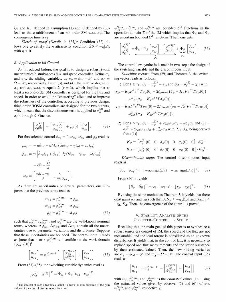
The aim of the first test (Fig. 1) is to show the predefinedconvergence time of the control laws for the motor as seenin Fig. 1 (top) for the measured and estimated speed: Theestimated speed reaches the measured speed at the convergencetime tF . Fig. 1 (middle) shows the desired and estimated flux.

Fig. 1. (Top) Measured speed Ω (radians) and its estimated counterpart(radians) versus time (seconds). (Middle) Reference flux (webers) and itsestimated counterpart (webers) versus time (seconds). (Bottom) Flux trackingerror (webers) versus time (seconds).

It can be viewed on Fig. 1 (bottom) that the flux tracking errorconverges to zero in the predefined convergence time tF .

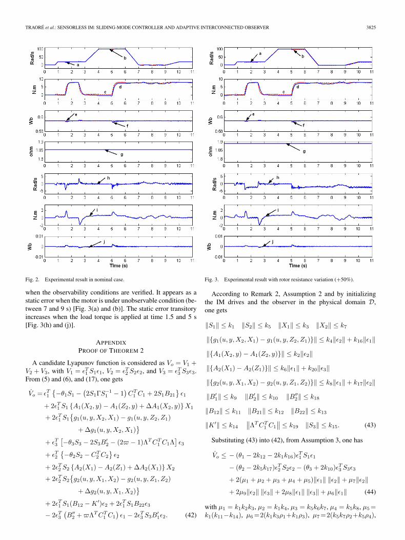
The experimental results2 of the nominal case with identifiedparameters (except stator resistance) are shown in Fig. 2. Thesefigures show the good performance of the complete systemobserver–controller in trajectory tracking and disturbance re-jection. The estimated motor speed [Fig. 2(b)] converges tothe measured speed [Fig. 2(a)] near and under conditions ofunobservability. The same conclusion is for estimated flux[Fig. 2(f)] w.r.t. reference flux [Fig. 2(e)]. The estimated loadtorque [Fig. 2(d)] converges to the measured load torque[Fig. 2(c)], under conditions of observability and at very lowfrequency (conditions of unobservability) (between 7 and 9 s).Nevertheless, it appears as a small static error when the motorspeed increases (between 4 and 6 s). The load torque is wellrejected except at the time when it is applied (Fig. 2(h) and (j)at time 1.5 and 5 s) and when it is removed (Fig. 2(h) and (j)at time 2.5 s). On Fig. 2(g), it can be viewed that the statorresistance estimation remains almost constant despite of thenoise and transient dynamics of the speed and load torque. Thistest shows the capability of the proposed controller to guaranteeflux and speed tracking of slowly varying speed reference withexcitation frequency close to zero (between 7 and 9 s).

The robustness of the observer–controller is confirmed by theresult obtained with rotor resistance variation (+50%) appliedto the observer and controller parameters (Fig. 3) (evaluationof robustness w.r.t. self-inductance variations has also beensuccessfully made). The increase of the rotor resistance valuedoes not affect the performance of the speed trajectory tracking,

2For each figure, each line is referred to as (a) and (c): measured speed andload torque; (e): reference flux; (b), (d), (f), and (g): estimated speed, loadtorque, flux, and stator resistance; and (h)–(j): speed, load torque, and fluxestimation error.


Fig. 2. Experimental result in nominal case.

when the observability conditions are verified. It appears as astatic error when the motor is under unobservable condition (be-tween 7 and 9 s) [Fig. 3(a) and (b)]. The static error transitoryincreases when the load torque is applied at time 1.5 and 5 s[Fig. 3(h) and (j)].

APPENDIX

PROOF OF THEOREM 2

A candidate Lyapunov function is considered as Vo = V1 +V2 + V3, with V1 = εT1 S1ε1, V2 = εT2 S2ε2, and V3 = εT3 S3ε3.From (5) and (6), and (17), one gets

Vo = εT1{−θ1S1 −

(2S1ΓS−1

1 − 1)CT

1 C1 + 2S1B21

}ε1

+ 2εT1 S1 {A1(X2, y) −A1(Z2, y) + ΔA1(X2, y)}X1

+ 2εT1 S1

{g1(u, y,X2,X1) − g1(u, y, Z2, Z1)

+ Δg1(u, y,X2,X1)}

+ εT3[−θ3S3 − 2S3B

′2 − (2 − 1)ΛTCT

1 C1Λ]ε3

+ εT2{−θ2S2 − CT

2 C2

}ε2

+ 2εT2 S2 {A2(X1) −A2(Z1) + ΔA2(X1)}X2

+ 2εT2 S2

{g2(u, y,X1,X2) − g2(u, y, Z1, Z2)

+ Δg2(u, y,X1,X2)}

+ 2εT1 S1(B12 −K ′)ε2 + 2εT1 S1B22ε3

− 2εT3(B′′

2 +ΛTCT1 C1

)ε1 − 2εT3 S3B

′1ε2. (42)

Fig. 3. Experimental result with rotor resistance variation (+50%).

According to Remark 2, Assumption 2 and by initializingthe IM drives and the observer in the physical domain D,one gets

‖S1‖ ≤ k1 ‖S2‖ ≤ k5 ‖X1‖ ≤ k3 ‖X2‖ ≤ k7

‖{g1(u, y,X2,X1) − g1(u, y, Z2, Z1)}‖ ≤ k4‖ε2‖ + k16‖ε1‖‖{A1(X2, y) −A1(Z2, y)}‖ ≤ k2‖ε2‖‖{A2(X1) −A2(Z1)}‖ ≤ k6‖ε1‖ + k20‖ε3‖‖{g2(u, y,X1,X2) − g2(u, y, Z1, Z2)}‖ ≤ k8‖ε1‖ + k17‖ε2‖‖B′

1‖ ≤ k9 ‖B′2‖ ≤ k10 ‖B′′

2‖ ≤ k18

‖B12‖ ≤ k11 ‖B21‖ ≤ k12 ‖B22‖ ≤ k13

‖K ′‖ ≤ k14

∥∥ΛTCT1 C1

∥∥ ≤ k19 ‖S3‖ ≤ k15. (43)

Substituting (43) into (42), from Assumption 3, one has

Vo ≤ − (θ1 − 2k12 − 2k1k16)εT1 S1ε1

− (θ2 − 2k5k17)εT2 S2ε2 − (θ3 + 2k10)εT3 S3ε3

+ 2(μ1 + μ2 + μ3 + μ4 + μ5)‖ε1‖ ‖ε2‖ + μ7‖ε2‖+ 2μ9‖ε2‖ ‖ε3‖ + 2μ8‖ε1‖ ‖ε3‖ + μ6‖ε1‖ (44)

with μ1 = k1k2k3, μ2 = k1k4, μ3 = k5k6k7, μ4 = k5k8, μ5 =k1(k11−k14), μ6 =2(k1k3ρ1+k1ρ3), μ7 =2(k5k7ρ2+k5ρ4),


μ8 = k1k13 − (k19 + k18), and μ9 = −k15k9 + k5k20k7.Then

Vo ≤ − (θ1 − 2k12 − 2k1k16)V1 − (θ2 − 2k5k17)V2

− (θ3 + 2k10)V3 + 2μ√V1

√V2 + μ7

√V2

+ 2μ9

√V2

√V3 + μ6

√V1 + 2μ8

√V1

√V3 (45)

with μ =∑5

j=0 μj , μj = (μj/√ηmin

S1

√ηmin

S2),

and j = 1, . . . , 5; μ8 = (μ8/√ηmin

S1

√ηmin

S3), μ9 =

(μ9/√ηmin

S2

√ηmin

S3), μ6 = (μ6/

√ηmin

S1), and μ7 =

(μ7/√ηmin

S2). Using the following inequalities:

√V1

√V2 ≤ ϕ1

2V1 +

12ϕ1

V2

√V1

√V3 ≤ ϕ2

2V1 +

12ϕ2

V3

√V2

√V3 ≤ ϕ3

2V2 +

12ϕ3

V3 ∀ϕi(i = 1, 2, 3) ∈]0, 1[

(46)

and substituting (46) into (45), one gets

Vo ≤ − (θ1 − 2k12 − 2k1k16 − μϕ1 − μ8ϕ2)V1

−(θ2 − 2k5k17 − μ

ϕ2− μ9ϕ3

)V2

−(θ3 + 2k10 − μ8

ϕ2− μ9

ϕ3

)V3 + μ6‖ε1‖ + μ7‖ε2‖

(47)

which gives

Vo ≤ − δ(V1 + V2 + V3) + μ(√V1 +

√V2)

≤ − δVo + μψ√Vo (48)

with δ = min(δ1, δ2, δ3) and μ = max(μ6, μ7), where δ1 =θ1 − 2k12 − 2k1k16 − μϕ1 − μ8ϕ2 > 0, δ2 = θ2 − 2k5k17 −(μ/ϕ2) − μ9ϕ3 > 0, δ3 =θ3+2k10−(μ8/ϕ2)−(μ9/ϕ3)>0,and ψ > 0 so that ψ

√V1 + V2 + V3 >

√V1 +

√V2. Next, de-

noting v = 2√Vo, it yields

v ≤ −δv + ψμ. (49)

From Theorem 1, one has ℘(t, l) = −δl + ψμ: (9) reads as

l = −δl + ψμ l(t0) = l0 ≥ 0. (50)

Its solution is given as

l(t) = l(t0)e−δ(t−t0) + r ·(1 − e−δ(t−t0)

)(51)

where r = (ψμ/δ) depends on parameter θi. In order to provethe strongly uniform practical stability (Corollary 1) of (50),

first, let us prove the uniform practical stability. Suppose thatl(t0) ≤ �1. From (51), one has

l(t) ≤ l(t0) + r ≤ �1 + r ≤ �2 (52)

so that l(t0) ≤ �1 implies that l(t) ≤ �2, ∀t ≥ t0. Accordingto PS1), (50) is uniformly practically stable. Let us provenow the uniform quasi-practical stability of (50). Suppose thatthere exist �1 > 0, � > 0, T > 0, l(t0) ≤ �1, and t ≥ t0 + T .Equation (51) is fulfilling

l(t) ≤ l(t0)e−δT + r ≤ �1e−δT + r ≤ � (53)

so that l(t0) ≤ �1 implies that l(t) ≤ �, ∀t ≥ t0 + T . Ac-cording to PS2), (50) is uniformly practically quasi-stable.Then, according to PS3), (50) is strongly uniformly prac-tically stable. In order to prove the strong uniform practi-cal stability of (17), check all the conditions of Theorem 1:It is clear that, from (52) and (53), �1 < �2, � < �2, Con-dition 1) of Theorem 1 is satisfied. By using (18), onehas ηmin‖e‖2 ≤ Vo(t, e) ≤ ηmax‖e‖2: Vo(t, e) is a Lyapunovfunction, locally Lipschitz in e, with ηmin = min{ηmin

Si, i =

1, 2, 3} and ηmax = max{ηmaxSi

, i = 1, 2, 3}. Taking d1(‖e‖) =ηmin‖e‖2, d2(‖e‖) = ηmax‖e‖2. Next, for (t, e) ∈ R+ ×B�2 ,d1(‖e‖) ≤ Vo(t, e) ≤ d2(‖e‖), and from (48), ℘(t, Vo(t, e)) =−δVo + μψ

√Vo. Then, conditions 2) and 3) are fulfilled.

On one hand, v(t0) ≤ �1 (because l(t0) ≤ �1) implies thatv(t) ≤ �2 (because l(t) ≤ �2), ∀t ≥ t0. Moreover, Vo(t, e) =(1/4)v(t)2. Then, it follows that v(t0) ≤ �1 which impliesthat ηmin‖e0‖2 < (1/4)�2

1. Hence, ‖e0‖ < (1/√

4ηmin)�1.On the other hand, (1/4)v(t)2 = Vo(t, e) = ηmax‖e(t)‖2 <(1/4)�2

2. Hence, ‖e(t)‖ < (1/√

4ηmax)�2. Consequently, 0 <(1/√

4ηmin)�1 < (1/√

4ηmax)�2. Writing the aforementionedinequality in the following form, we have ηmax

�21 < ηmin

�22,

which implies that d2(�1) < d1(�2). Finally, all conditions ofTheorem 1 hold which implies the strongly uniform practicalstability of (17).

REFERENCES

[1] G. Bartolini, A. Ferrara, and E. Usai, “Chattering avoidance by second-order sliding mode control,” IEEE Trans. Autom. Control, vol. 43, no. 2,pp. 241–246, Feb. 1998.

[2] G. Besançon and H. Hammouri, “Observer synthesis for a class of non-linear control systems,” Eur. J. Control, vol. 2, no. 3, pp. 176–192, 1996.

[3] F. Blaschke, “The principle of field orientation applied to the newtransvector closed-loop control system for rotating field machine,”Siemens Rev., vol. 93, pp. 217–220, 1972.

[4] C. Canudas de Wit, A. Youssef, J. P. Barbot, P. Martin, and F. Malrait,“Observability conditions of induction motors at low frequencies,” inProc. IEEE Conf. Decision Control, Sydney, Australia, 2000, pp. 2044–2049.

[5] A. F. Filippov, Differential Equations with Discontinuous Right-HandSide. Dordrecht, The Netherlands: Kluwer, 1988.

[6] M. Ghanes, J. de Leon, and A. Glumineau, “Novel controller for inductionmotor without mechanical sensor and experimental validation,” in Proc.IEEE Conf. Decision Control, San Diego, CA, 2006, pp. 4008–4013.

[7] M. Ghanes, J. De Leon, and A. Glumineau, “Observability studyand observer-based interconnected form for sensorless inductionmotor,” in Proc. IEEE Conf. Decision Control, San Diego, CA, 2006,pp. 1240–1245.

[8] J. Holtz, “Sensorless control of induction motor drives,” Proc. IEEE,vol. 90, no. 8, pp. 1359–1394, Aug. 2002.


[9] S. Ibarra-Rojas, J. Moreno, and G. Espinosa, “Global observability analy-sis of sensorless induction motors,” Automatica, vol. 40, no. 6, pp. 1079–1085, Jun. 2004.

[10] S. Laghrouche, F. Plestan, and A. Glumineau, “Practical higher ordersliding mode control: Optimal control based approach and applicationto electromechanical systems,” in Advances in Variable Structure andSliding Mode Control, vol. 334, C. Edwards, E. Fossas Colet, andL. Fridman, Eds. New York: Springer-Verlag, 2006.

[11] C. Lascu, I. Boldea, and F. Blaabbjerg, “Very-low-speed variable-structurecontrol of sensorless induction machine drives without signal injection,”IEEE Trans. Ind. Appl., vol. 41, no. 2, pp. 591–598, Mar./Apr. 2005.

[12] V. Laskhmikanthan, S. Leela, and A. A. Martynyuk, Practical Stability ofNonlinear Systems. Singapore: Word Scientific, 1990.

[13] A. Levant, “Universal single–input–single–output (SISO) sliding-modecontrollers with finite-time convergence,” IEEE Trans. Autom. Control,vol. 49, no. 9, pp. 1447–1451, Sep. 2001.

[14] M. Montanari and A. Tilli, “Sensorless control of induction motors basedon high-gain speed estimation and on-line stator resistance adaptation,” inProc. IEEE IECON, Paris, France, 2006, pp. 1263–1268.

[15] F. Plestan, A. Glumineau, and S. Laghrouche, “A new algorithm for high-order sliding mode control,” Int. J. Robust Nonlinear Control, vol. 18,no. 4/5, pp. 441–453, Mar. 2008.

[16] D. Traoré, D. de Léon, A. Glumineau, and L. Loron, “Speed sensorlessfield-oriented control of induction motor with interconnected observers:Experimental tests on low frequencies benchmark,” IET Control TheoryAppl., vol. 1, no. 6, pp. 1681–1692, Nov. 2007.

[17] D. Traoré, F. Plestan, A. Glumineau, and J. de Léon, “Sensorless inductionmotor: High-order sliding mode controller and adaptive interconnectedobserver,” in Proc. IFAC World Congr., Seoul, Korea, 2008.

[18] V. I. Utkin, “Sliding mode control design principles and applications toelectric drives,” IEEE Trans. Ind. Electron., vol. 40, no. 1, pp. 23–36,Feb. 1993.

[19] Y. Zhang, J. Changxi, and V. I. Utkin, “Sensorless sliding-mode control ofinduction motors,” IEEE Trans. Ind. Electron., vol. 47, no. 6, pp. 1286–1297, Dec. 2000.

[20] Q. Zhang, “Adaptive observers for multiple–input–multiple–output(MIMO) linear time-varying systems,” IEEE Trans. Autom. Control,vol. 47, no. 3, pp. 525–529, Mar. 2002.

Dramane Traoré received the B.S. degree in elec-trical engineering from Polytech’Nantes, Nantes,France. He is currently working toward the Ph.D.degree in the Institut de Recherche en Communica-tions et en Cybernétique de Nantes, Ecole Centralede Nantes—CNRS, Nantes.

His research interests include robust nonlinearcontrol (higher order sliding mode, backstepping,adaptive control, etc.), theoretical aspects of nonlin-ear observer design, and control of dc–ac motors.

Franck Plestan (M’00) received the Ph.D. degree inautomatic control from the Ecole Centrale de Nantes,Nantes, France, in 1995.

Since 2000, he has been an Assistant Professorwith the Institut de Recherche en Communicationset en Cybernétique de Nantes, Ecole Centrale deNantes—CNRS. His research interests include ro-bust nonlinear control (higher order sliding mode),theoretical aspects of nonlinear observer design,and control of electromechanical and mechanicalsystems (pneumatic actuators, biped robots, and

electrical motors).

Alain Glumineau (M’07) received the Ph.D. de-gree in automatic control from the Ecole NationaleSuperieure de Mecanique, Nantes, France, in 1981.

Since 1982, he has been with the Institut deRecherche en Communications et en Cybernétiquede Nantes (http://www.irccyn.ec-nantes.fr), EcoleCentrale de Nantes—CNRS, Nantes, as an AssociateProfessor and then Full Professor. He is an AssociateEditor of Control Engineering Practice. His cur-rent interests concern theoretical issues in nonlinearcontrol and observer design and their applications

mainly to electric and pneumatic systems.

Jesus de Leon received the Ph.D. degree in auto-matic control from Claude Bernard Lyon 1 Univer-sity, Villeurbanne, France, in 1992.

Since 1993, he has been a Professor of Electri-cal Engineering with the Universidad Autonóma deNuevo León, San Nicolás de Los Garza, Mexico.He is currently working on applications of controltheory, electrical machines, nonlinear observers, andpower systems.

Sensorless Induction Motor: High-Order Sliding-Mode Controller and Adaptive Interconnected Observer

Documents