Sensor Database: Querying Sensor Networks Yinghua Wu, Haiyong Xie

Welcome message from author
This document is posted to help you gain knowledge. Please leave a comment to let me know what you think about it! Share it to your friends and learn new things together.
Transcript
Sensor Database: Querying Sensor Networks
Yinghua Wu, Haiyong Xie
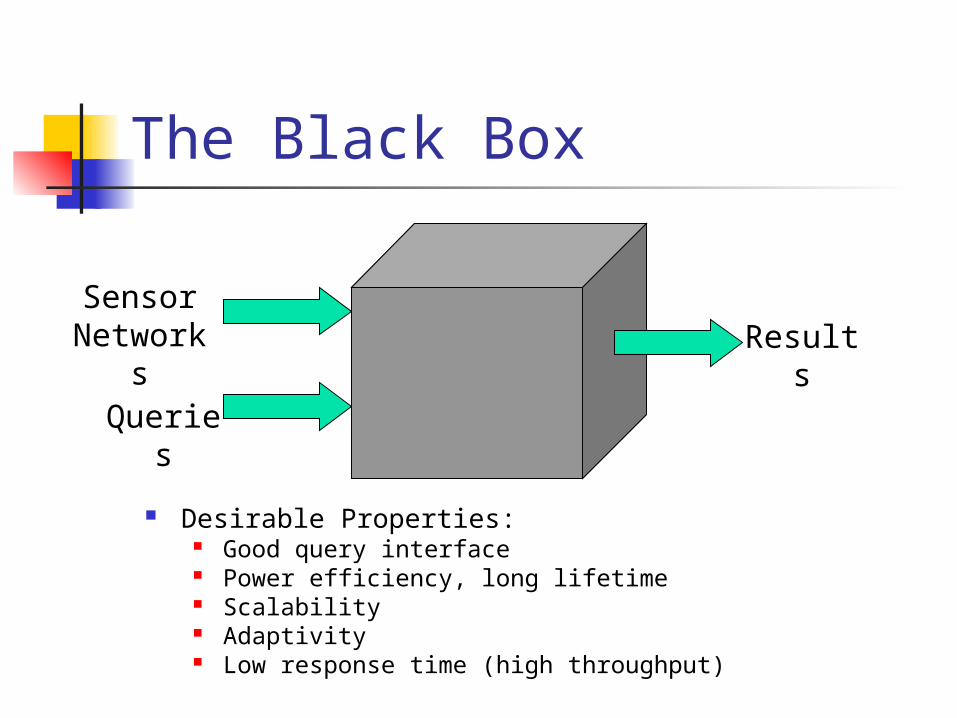
The Black Box
Sensor Network
sQuerie
s
Results
Desirable Properties: Good query interface Power efficiency, long lifetime Scalability Adaptivity Low response time (high throughput)

Outline
Background and motivation Acquisitional query optimization Continuously adaptive continuous
query optimization Summary Future work
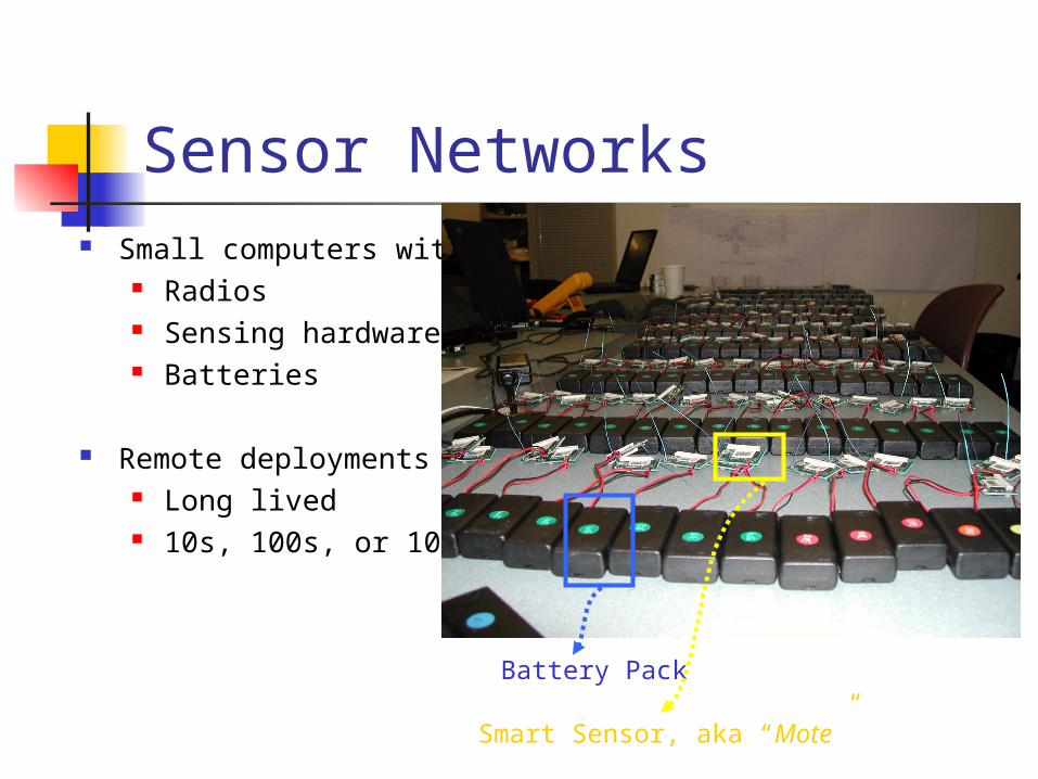
Sensor Networks Small computers with:
Radios Sensing hardware Batteries
Remote deployments Long lived 10s, 100s, or 1000s
Battery Pack
Smart Sensor, aka “Mote”

Mica Motes
4Mhz, 8 bit Atmel RISC uProc
40 kbit Radio
4 K RAM, 128 K Program Flash, 512 K Data Flash
AA battery pack
Based on TinyOS

Sensor Net Sample Apps
Traditional monitoring apparatus.
Earthquake monitoring in shake-test sites.
Vehicle detection: sensors along a road, collect data about passing vehicles.
Habitat Monitoring: Storm petrels on Great Duck Island, microclimates on James Reserve.
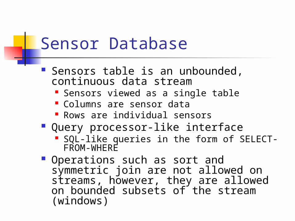
Sensor Database Sensors table is an unbounded,
continuous data stream Sensors viewed as a single table Columns are sensor data Rows are individual sensors
Query processor-like interface SQL-like queries in the form of SELECT-
FROM-WHERE Operations such as sort and symmetric
join are not allowed on streams, however, they are allowed on bounded subsets of the stream (windows)
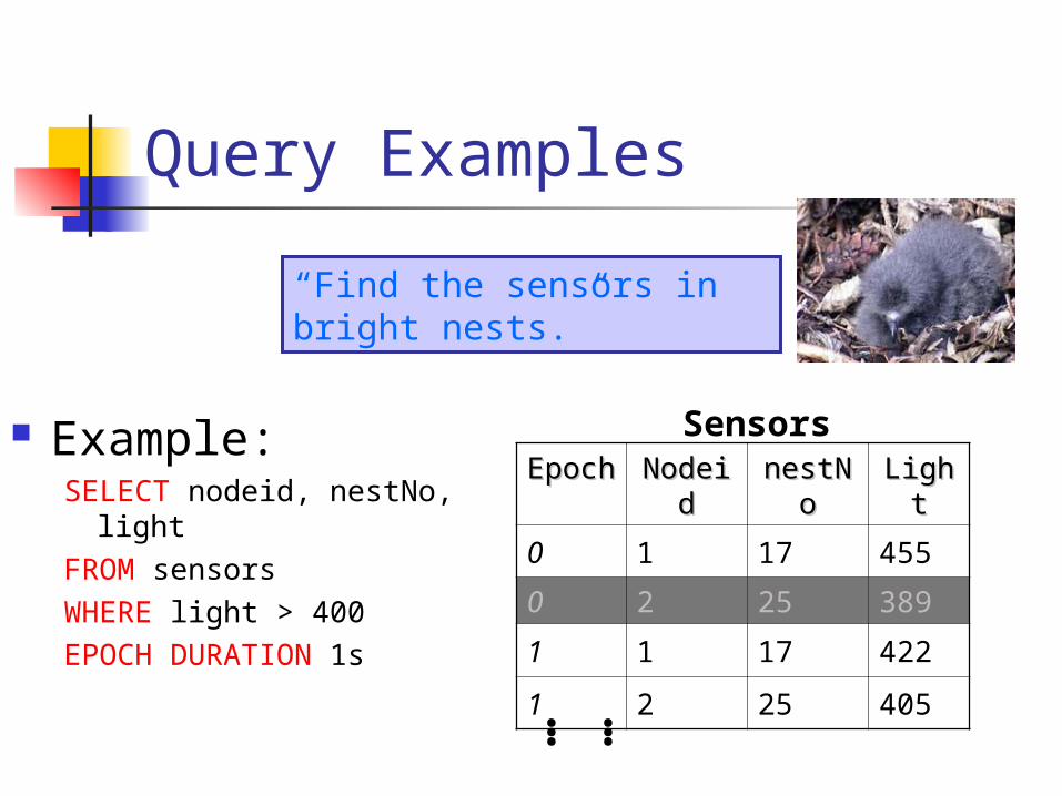
Query Examples
Example:SELECT nodeid, nestNo, lightFROM sensorsWHERE light > 400EPOCH DURATION 1s
EpocEpochh
NodeiNodeidd
nestNnestNoo
LightLight
0 1 17 455
0 2 25 389
1 1 17 422
1 2 25 405
Sensors
“Find the sensors in bright nests.”
……
Query Examples – cont’d
Epoch region CNT(…) AVG(…)
0 North 3 360
0 South 3 520
1 North 3 370
1 South 3 520
“Count the number occupied nests in each loud region of the island.”
SELECT region, CNT(occupied) AVG(sound)
FROM sensors
GROUP BY region
HAVING AVG(sound) > 200
EPOCH DURATION 10sRegions w/ AVG(sound) > 200
SELECT AVG(sound)
FROM sensors
EPOCH DURATION 10s
Continuous Query “Monitoring” queries look for recent
events in data streams; We confine our view to queries over ‘recent-history’
Only tuples currently entering the system Stored in in-memory data tables for time-
windowed joins between streams Long running, “standing queries”,
similar to trigger systems Installed; continuously produce results
until removed
Continuous Query - cont’d Closed world assumption does not hold
Could generate an infinite number of samples
Traditional system: data is provided a priori
Lots of queries, over the same data sources In-network processing Opportunity for work sharing! Global query optimization problem (hard) finding an optimal plan (adaptively)
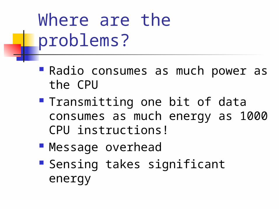
Where are the problems?
Radio consumes as much power as the CPU
Transmitting one bit of data consumes as much energy as 1000 CPU instructions!
Message overhead Sensing takes significant energy
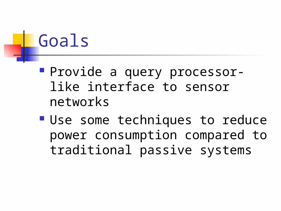
Goals
Provide a query processor-like interface to sensor networks
Use some techniques to reduce power consumption compared to traditional passive systems
Outline
Background and motivation Acquisitional query optimization Continuously adaptive continuous
query optimization Summary Future work

Acquisitional Query Processing Provide a query processor-like interface
to sensor networks Use Acquisitional techniques to reduce
power consumption compared to traditional passive systems
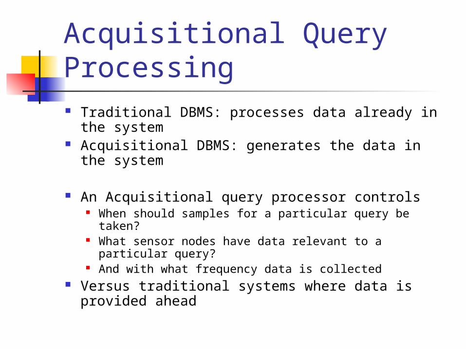
Acquisitional Query Processing Traditional DBMS: processes data already in the
system Acquisitional DBMS: generates the data in the
system
An Acquisitional query processor controls When should samples for a particular query be taken? What sensor nodes have data relevant to a particular
query? And with what frequency data is collected
Versus traditional systems where data is provided ahead

What’s the big deal? (revisit) Radio consumes as much power as the
CPU Transmitting one bit of data consumes
as much energy as 1000 CPU instructions!
Message sizes in TinyDB are by default 48 bytes
Sensing takes significant energy
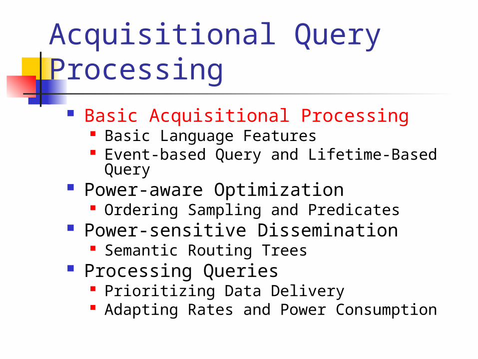
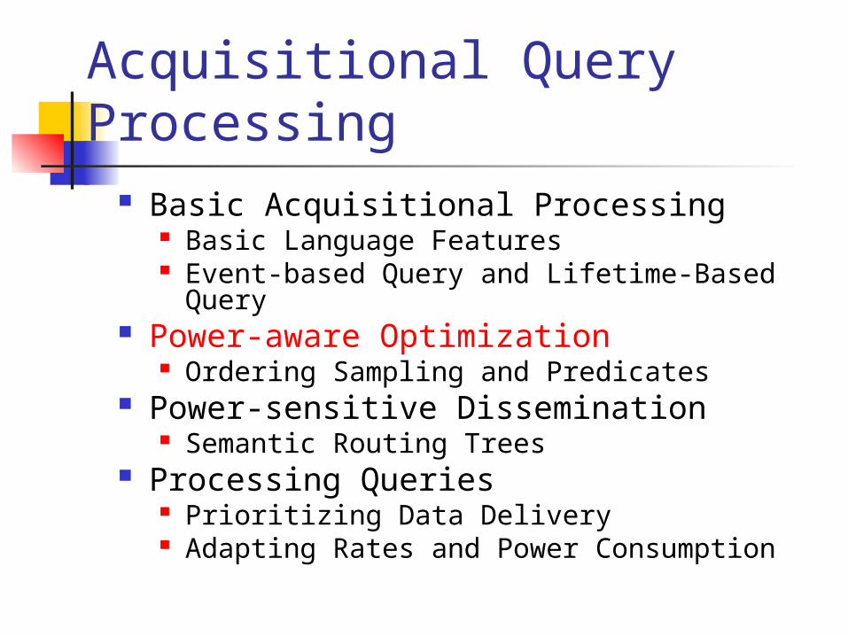
Acquisitional Query Processing
Basic Acquisitional Processing Basic Language Features Event-based Query and Lifetime-Based
Query Power-aware Optimization
Ordering Sampling and Predicates Power-sensitive Dissemination
Semantic Routing Trees Processing Queries
Prioritizing Data Delivery Adapting Rates and Power Consumption
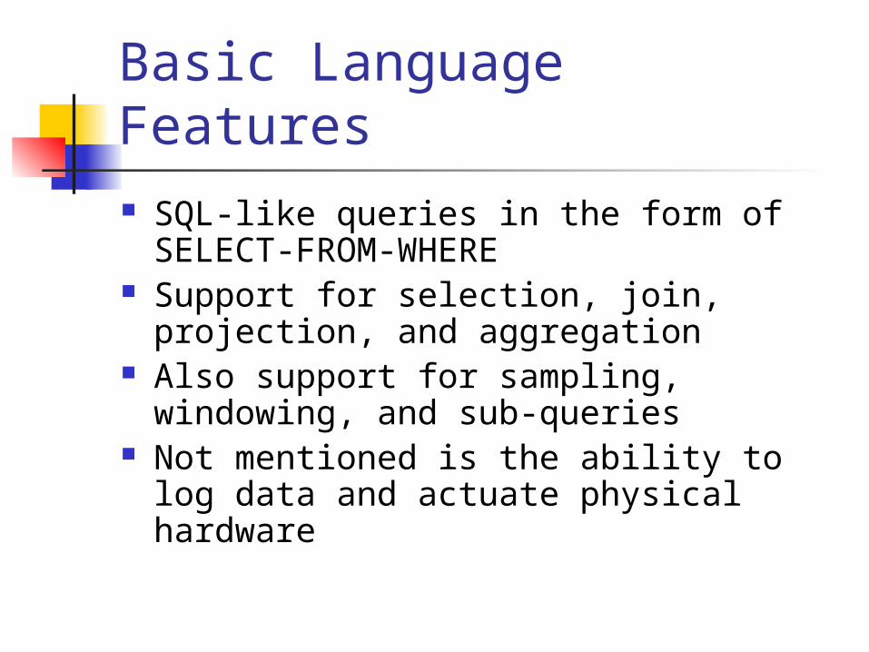
Basic Language Features SQL-like queries in the form of SELECT-
FROM-WHERE Support for selection, join, projection,
and aggregation Also support for sampling, windowing,
and sub-queries Not mentioned is the ability to log data
and actuate physical hardware
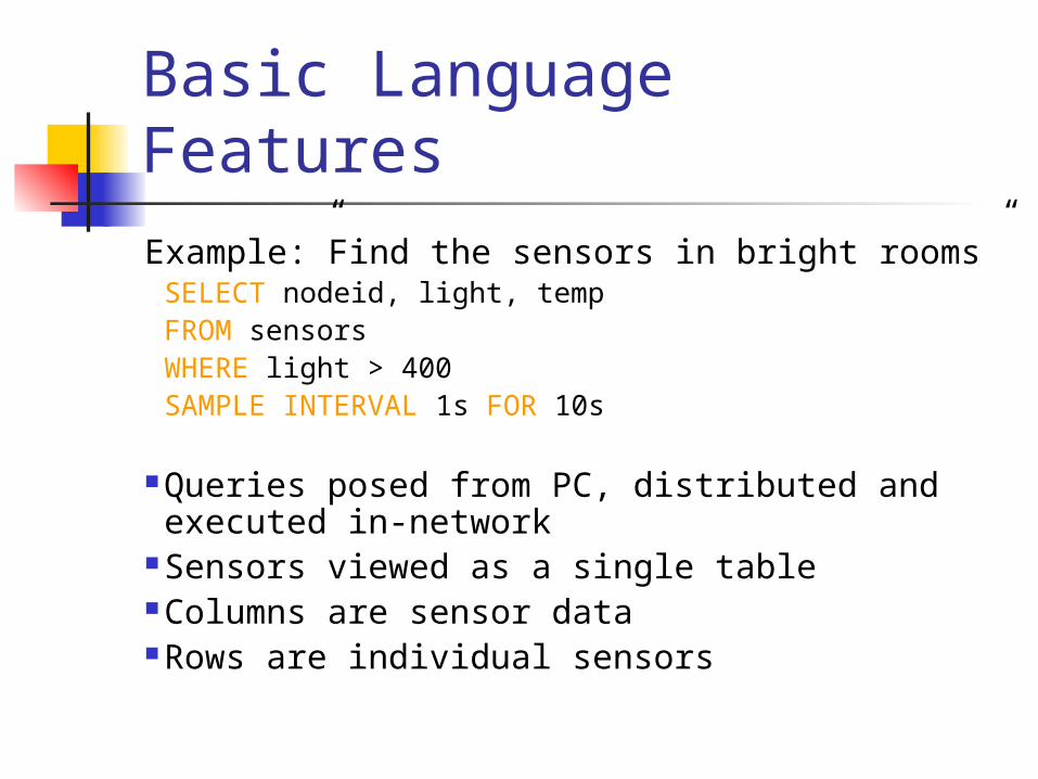
Basic Language FeaturesExample:”Find the sensors in bright rooms”
SELECT nodeid, light, tempFROM sensorsWHERE light > 400SAMPLE INTERVAL 1s FOR 10s
Queries posed from PC, distributed and executed in-network
Sensors viewed as a single tableColumns are sensor dataRows are individual sensors

Queries as a Stream Sensors table is an unbounded,
continuous data stream Operations such as sort and symmetric
join are not allowed on streams They are allowed on bounded subsets of
the stream (windows)

Windows Windows in TinyDB are fixed-size materialization points Materialization points can be used in queries
Example: “output a stream of counts indicating the number of recent light readings that were brighter than the current readings”CREATE
STORAGE POINT recentlight SIZE 8AS (SELECT nodeid, light FROM sensorsSAMPLE INTERVAL 10s)
SELECT COUNT(*)FROM sensors AS s, recentlight AS r1WHERE r.nodeid = s.nodeidAND s.light < r1.lightSAMPLE INTERVAL 10s
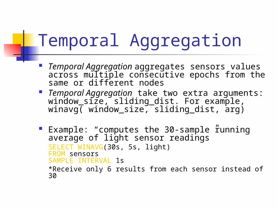
Temporal Aggregation Temporal Aggregation aggregates sensors
values across multiple consecutive epochs from the same or different nodes
Temporal Aggregation take two extra arguments: window_size, sliding_dist. For example, winavg( window_size, sliding_dist, arg)
Example: “computes the 30-sample running average of light sensor readings”
SELECT WINAVG(30s, 5s, light)FROM sensorsSAMPLE INTERVAL 1s
*Receive only 6 results from each sensor instead of 30
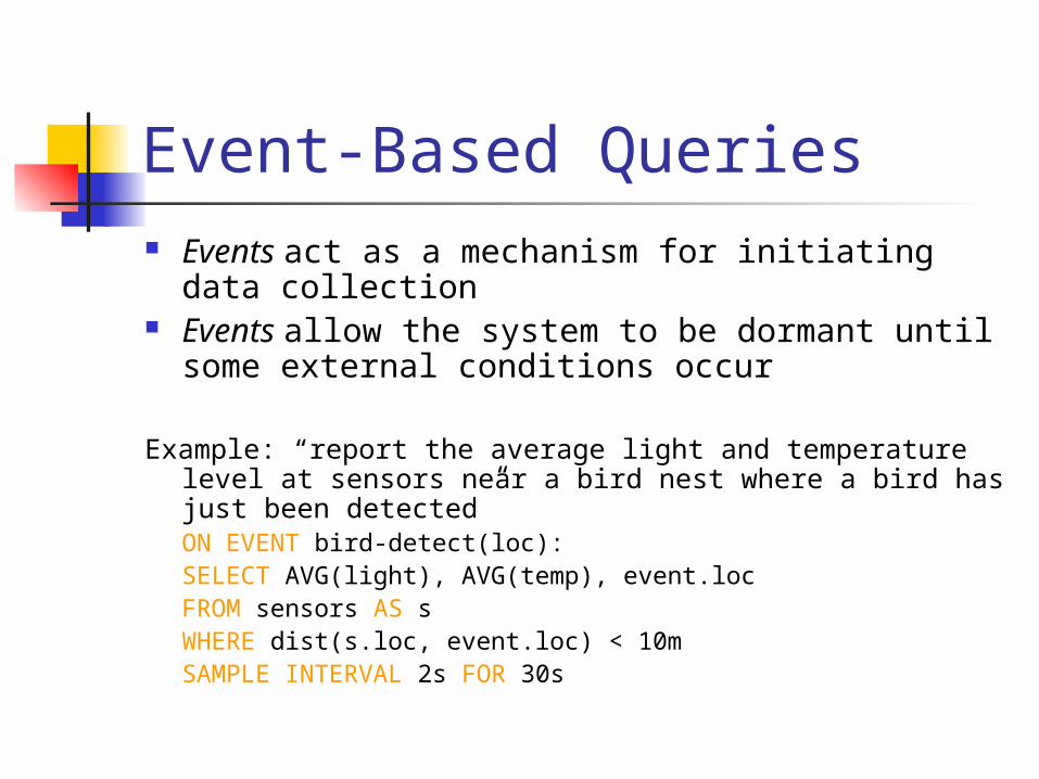
Event-Based Queries Events act as a mechanism for initiating data
collection Events allow the system to be dormant until
some external conditions occur
Example: “report the average light and temperature level at sensors near a bird nest where a bird has just been detected”ON EVENT bird-detect(loc):
SELECT AVG(light), AVG(temp), event.locFROM sensors AS sWHERE dist(s.loc, event.loc) < 10mSAMPLE INTERVAL 2s FOR 30s

Lifetime-Based Queries Lifetime is a much more intuitive way for
users to reason about power consumption To satisfy a lifetime clause, TinyDB
performs lifetime estimationT = ph / es
T: maximum transmission rate; ph: available power per hour; es: the energy to collect and transmit one sample
Example: “the network should run for at least 30 days”
SELECT nodeid, accelFROM sensorsLIFETIME 30 days
Acquisitional Query Processing
Basic Acquisitional Processing Basic Language Features Event-based Query and Lifetime-Based
Query Power-aware Optimization
Ordering Sampling and Predicates Power-sensitive Dissemination
Semantic Routing Trees Processing Queries
Prioritizing Data Delivery Adapting Rates and Power Consumption
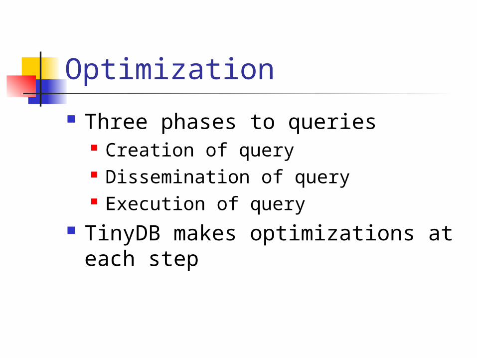
Optimization
Three phases to queries Creation of query Dissemination of query Execution of query
TinyDB makes optimizations at each step
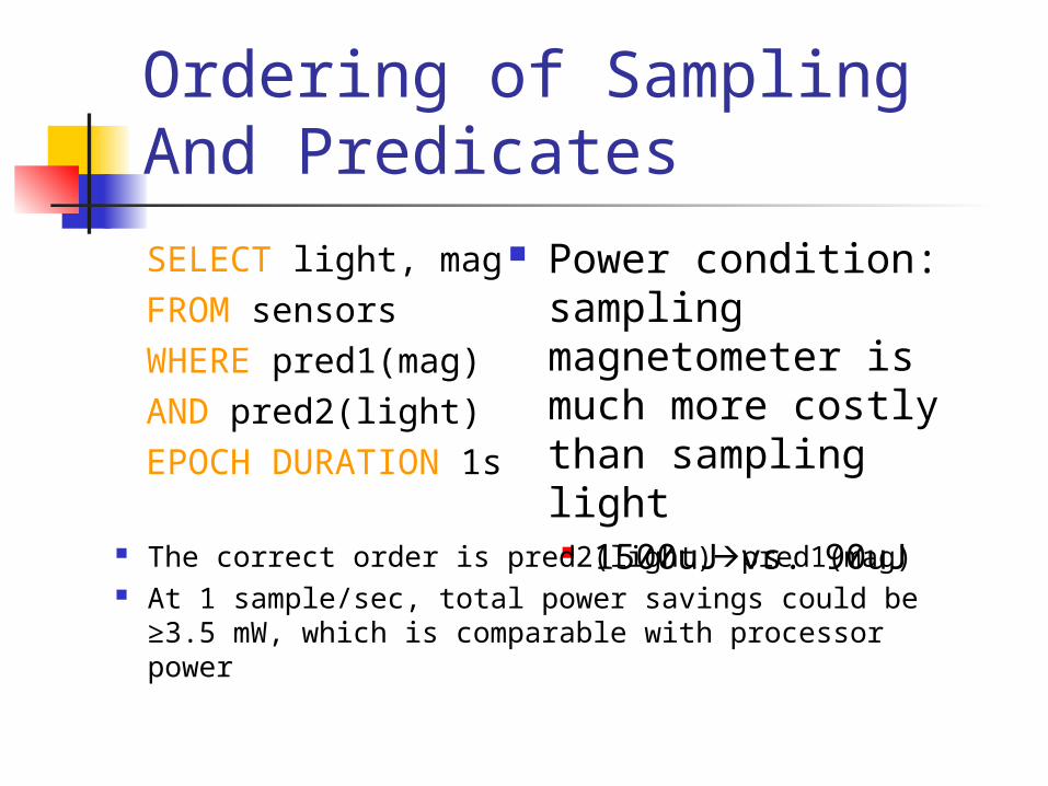
Ordering of Sampling And Predicates
SELECT light, magFROM sensorsWHERE pred1(mag)AND pred2(light)EPOCH DURATION 1s
Power condition:sampling magnetometer is much more costly than sampling light 1500uJ vs. 90uJ
The correct order is pred2(light)pred1(mag) At 1 sample/sec, total power savings could be
≥3.5 mW, which is comparable with processor power

For Aggregate Queries
The correct order is: Sample light, light>MAX? If so, sample mag, mag>X? Report light
SELECT WINMAX(light, 8s, 8s)
FROM sensors
WHERE mag>X
EPOCH DURATION 1s
Acquisitional Query Processing
Basic Acquisitional Processing Basic Language Features Event-based Query and Lifetime-Based
Query Power-aware Optimization
Ordering Sampling and Predicates Power-sensitive Dissemination
Semantic Routing Trees Processing Queries
Prioritizing Data Delivery Adapting Rates and Power Consumption

Semantic Routing Trees Co-acquisition: exploit correlations of
sensors to reduce data dissemination Queries are often constrained in a region Avoid sending queries to non-involved sensors
Rule: sensors that sample together route together
Build semantic routing trees (SRT) to reduce data dissemination SRT nodes choose parents based on semantic
properties as well as link quality

Semantic Routing Trees For node join, node picks parent whose
ancestor’s interval most overlap its descendants’ interval

Semantic Routing Trees
Parent nodes keep track of children’s value range
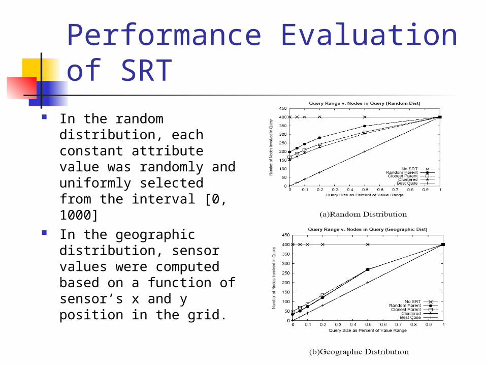
Performance Evaluation of SRT
In the random distribution, each constant attribute value was randomly and uniformly selected from the interval [0, 1000]
In the geographic distribution, sensor values were computed based on a function of sensor’s x and y position in the grid.

Acquisitional Query Processing
Basic Acquisitional Processing Basic Language Features Event-based Query and Lifetime-Based
Query Power-aware Optimization
Ordering Sampling and Predicates Power-sensitive Dissemination
Semantic Routing Trees Processing Queries
Prioritizing Data Delivery Adapting Rates and Power Consumption
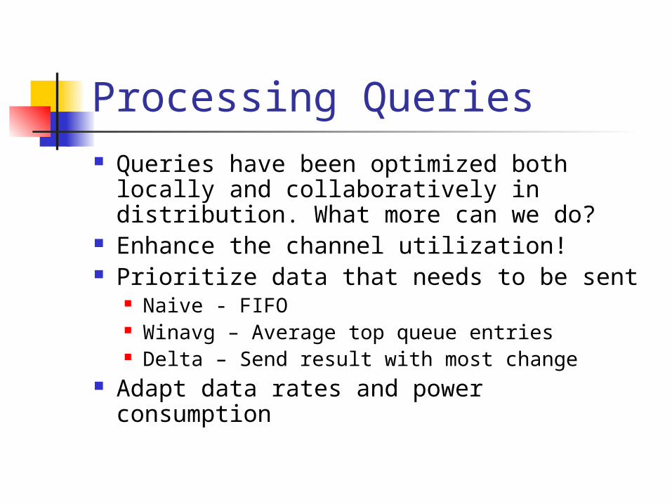
Processing Queries Queries have been optimized both
locally and collaboratively in distribution. What more can we do?
Enhance the channel utilization! Prioritize data that needs to be sent
Naive - FIFO Winavg – Average top queue entries Delta – Send result with most change
Adapt data rates and power consumption
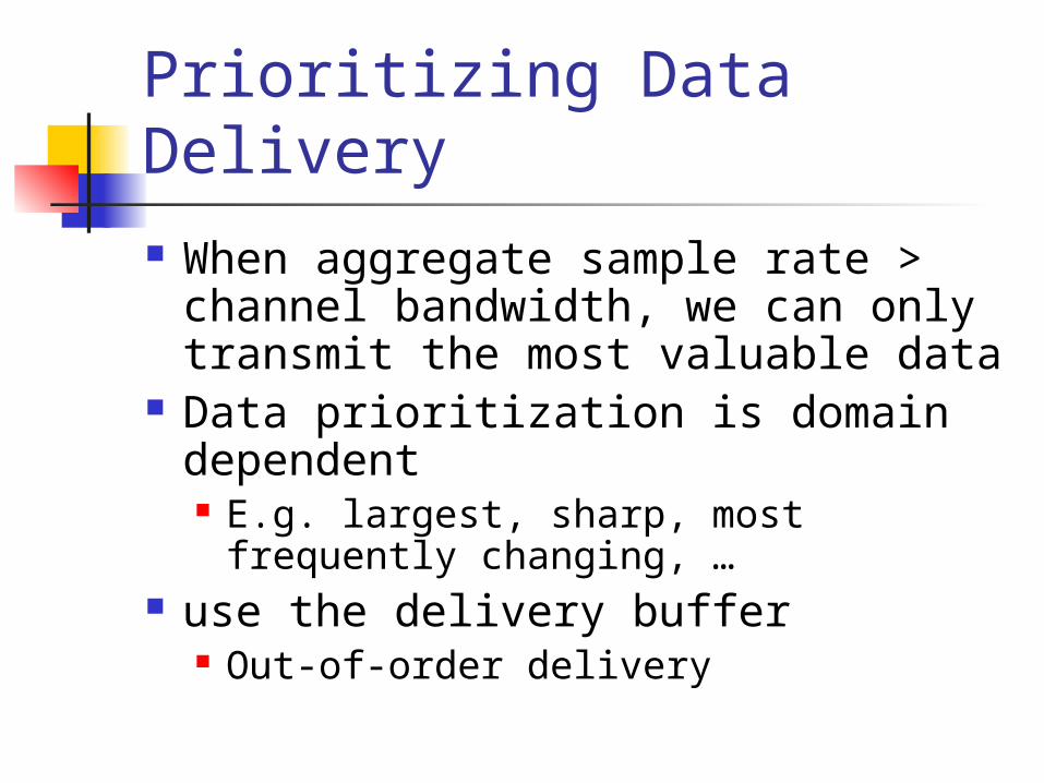
Prioritizing Data Delivery When aggregate sample rate >
channel bandwidth, we can only transmit the most valuable data
Data prioritization is domain dependent E.g. largest, sharp, most frequently
changing, … use the delivery buffer
Out-of-order delivery
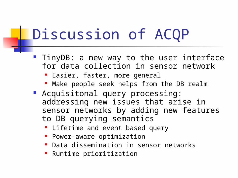
Discussion of ACQP TinyDB: a new way to the user interface for
data collection in sensor network Easier, faster, more general Make people seek helps from the DB realm
Acquisitonal query processing: addressing new issues that arise in sensor networks by adding new features to DB querying semantics
Lifetime and event based query Power-aware optimization Data dissemination in sensor networks Runtime prioritization
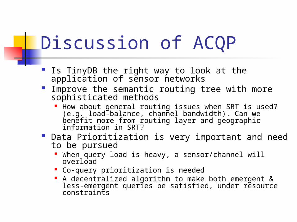
Discussion of ACQP Is TinyDB the right way to look at the application
of sensor networks Improve the semantic routing tree with more
sophisticated methods How about general routing issues when SRT is used?
(e.g. load-balance, channel bandwidth). Can we benefit more from routing layer and geographic information in SRT?
Data Prioritization is very important and need to be pursued
When query load is heavy, a sensor/channel will overload Co-query prioritization is needed A decentralized algorithm to make both emergent & less-
emergent queries be satisfied, under resource constraints
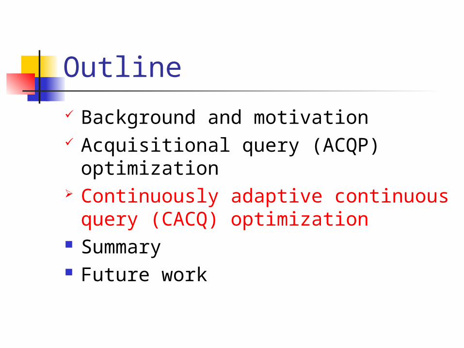
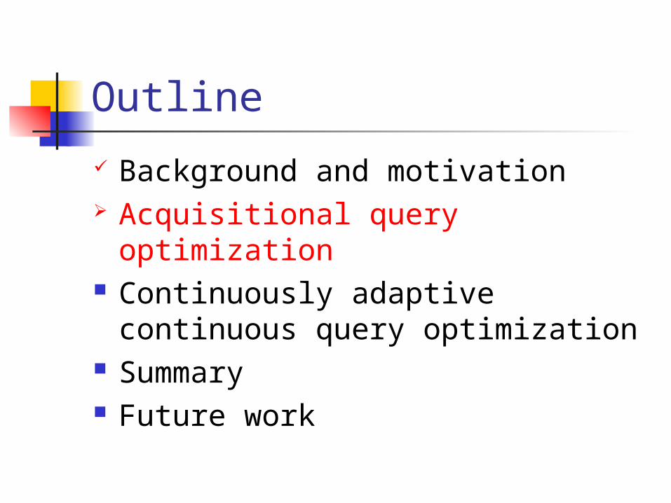
Outline
Background and motivation Acquisitional query (ACQP)
optimization Continuously adaptive continuous
query (CACQ) optimization Summary Future work
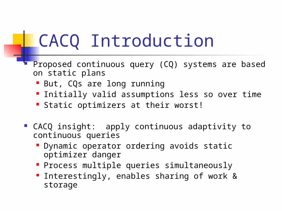
CACQ Introduction Proposed continuous query (CQ) systems are based
on static plans But, CQs are long running Initially valid assumptions less so over time Static optimizers at their worst!
CACQ insight: apply continuous adaptivity to continuous queries Dynamic operator ordering avoids static optimizer
danger Process multiple queries simultaneously Interestingly, enables sharing of work & storage
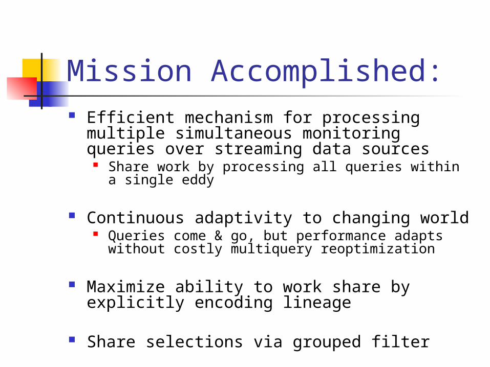
Mission Accomplished: Efficient mechanism for processing multiple
simultaneous monitoring queries over streaming data sources
Share work by processing all queries within a single eddy
Continuous adaptivity to changing world Queries come & go, but performance adapts without
costly multiquery reoptimization
Maximize ability to work share by explicitly encoding lineage
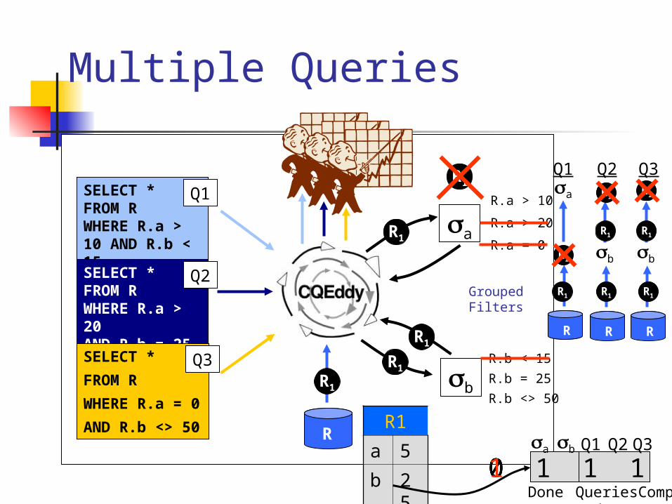
Share selections via grouped filter
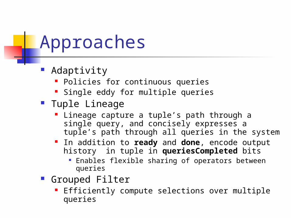
Approaches Adaptivity
Policies for continuous queries Single eddy for multiple queries
Tuple Lineage Lineage capture a tuple’s path through a single
query, and concisely expresses a tuple’s path through all queries in the system
In addition to ready and done, encode output history in tuple in queriesCompleted bits
Enables flexible sharing of operators between queries Grouped Filter
Efficiently compute selections over multiple queries
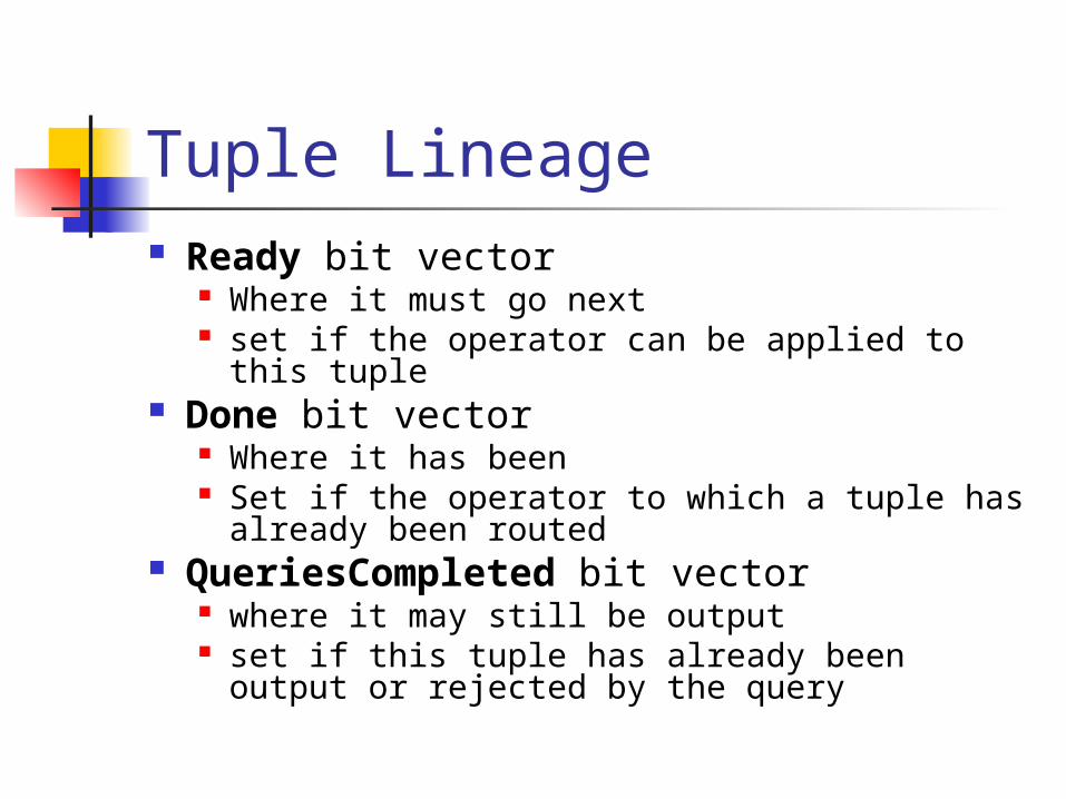
Tuple Lineage Ready bit vector
Where it must go next set if the operator can be applied to this tuple
Done bit vector Where it has been Set if the operator to which a tuple has
already been routed QueriesCompleted bit vector
where it may still be output set if this tuple has already been output or
rejected by the query
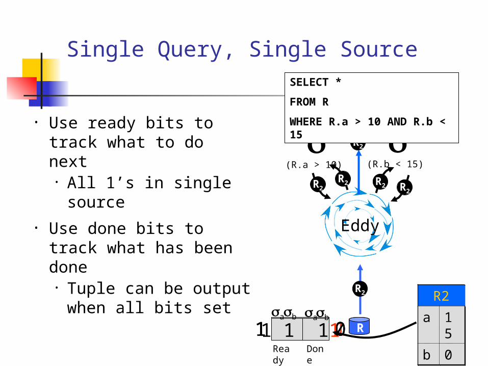
Single Query, Single Source
• Use ready bits to track what to do next• All 1’s in single
source• Use done bits to track
what has been done• Tuple can be output
when all bits set
R
(R.a > 10)
Eddy
(R.b < 15) R1
R1
R1
R1
a 5
b 25
R2
a 15
b 0
1 1 0 01 1 0 11 1 0 01 1 1 01 1 11Ready
Done
ab ab
R
(R.a > 10)
Eddy
(R.b < 15)
R2
R2R2R2 R2
R2
SELECT *
FROM R
WHERE R.a > 10 AND R.b < 15
a
b
R
a
b
R
a
b
R
Q1 Q2 Q3
Multiple Queries
R.a > 10
R.a > 20
R.a = 0
R.b < 15
R.b = 25
R.b <> 50b
a
R
R1
R1
R1
R1
R1
Grouped Filters
R1
a 5
b 25
SELECT *FROM RWHERE R.a > 10 AND R.b < 15
Q1
SELECT *FROM RWHERE R.a > 20AND R.b = 25
Q2
SELECT *
FROM R
WHERE R.a = 0
AND R.b <> 50
Q3
R1R1
R1 R1R1
R1R1
R1
0 0 0 0 00 0 1 0 00 1 1 0 00 1 1 1 11 1 1 1 1a b Q1 Q2Q3
Done
QueriesCompleted
a
b
R
a
b
R
a
b
R
Q1 Q2 Q3
Multiple Queries
R.a > 10
R.a > 20
R.a = 0
R.b < 15
R.b = 25
R.b <> 50b
a
R
R2
R2
R2
R2
R2
R2
Grouped Filters
R2
a 15
b 0
SELECT *FROM RWHERE R.a > 10 AND R.b < 15
Q1
SELECT *FROM RWHERE R.a > 20AND R.b = 25
Q2
SELECT *
FROM R
WHERE R.a = 0
AND R.b <> 50
Q3
0 0 0 0 0
b
a
R
b
a
R
b
a
R
Q1 Q2 Q3
R2 R2 R2
0 0 0 1 11 0 0 1 11 1 0 1 11 1 1 1 1a b Q1 Q2Q3
Done
QueriesCompleted
R1 R1
R2
Reorder Operators!
Outputting Tuples
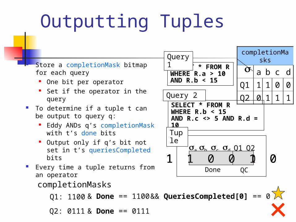
Store a completionMask bitmap for each query
One bit per operator Set if the operator in the query
To determine if a tuple t can be output to query q:
Eddy ANDs q’s completionMask with t’s done bits
Output only if q’s bit not set in t’s queriesCompleted bits
Every time a tuple returns from an operator
Q2: 0111
Q1: 1100 & Done == 1100
& Done == 0111
completionMasks&& QueriesCompleted[0] == 0
SELECT * FROM R WHERE R.a > 10 AND R.b < 15
Query 1
SELECT * FROM R WHERE R.b < 15 AND R.c <> 5 AND R.d = 10
Query 2
completionMasks
a b c d
Q1
1 1 0 0
Q2
0 1 1 1
Done
QC
a Q1 Q2b c d
Tuple
1 1 0 0 0 01 1 0 0 1 01 1 0 0 1 0
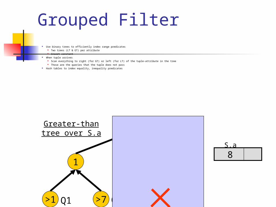
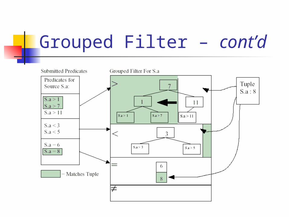
Grouped Filter Use binary trees to efficiently index range predicates
Two trees (LT & GT) per attribute Insert constant
When tuple arrives Scan everything to right (for GT) or left (for LT) of the tuple-attribute in the tree Those are the queries that the tuple does not pass
Hash tables to index equality, inequality predicates
Greater-than tree over S.a
8S.a
>11
7
1 11
>7>1 Q1 Q2 Q3
Grouped Filter – cont’d
Work Sharing via Tuple Lineage
A
B
C D
B
A
Data Stream S
s
sc
sBC
sD
sBD
Query 1
Query 2
Conventional Queries
s
s
sC
sCD
sCDB
CACQ - Adaptivity
A
CD
B
Data Stream S
A
C D
B
Data Stream S
Query 1
Query 2
Shared Subexpressions
sB
sAB sABReject?
sCDBA
s
Q1: SELECT * FROM s WHERE A, B, C Q2: SELECT * FROM s WHERE A, B, D
Intersection of CD goes through AB
an extra time!
AB must be
applied first!
Lineage (Queries
Completed) Enables
Any Ordering!
0 | 0QC
0 or 1 | 0QC
1 | 1QC0 or 1 | 0 or 1
QC
0 or 1 | 0 or 1QC
C D 0 or 1 | 0 or 1QC
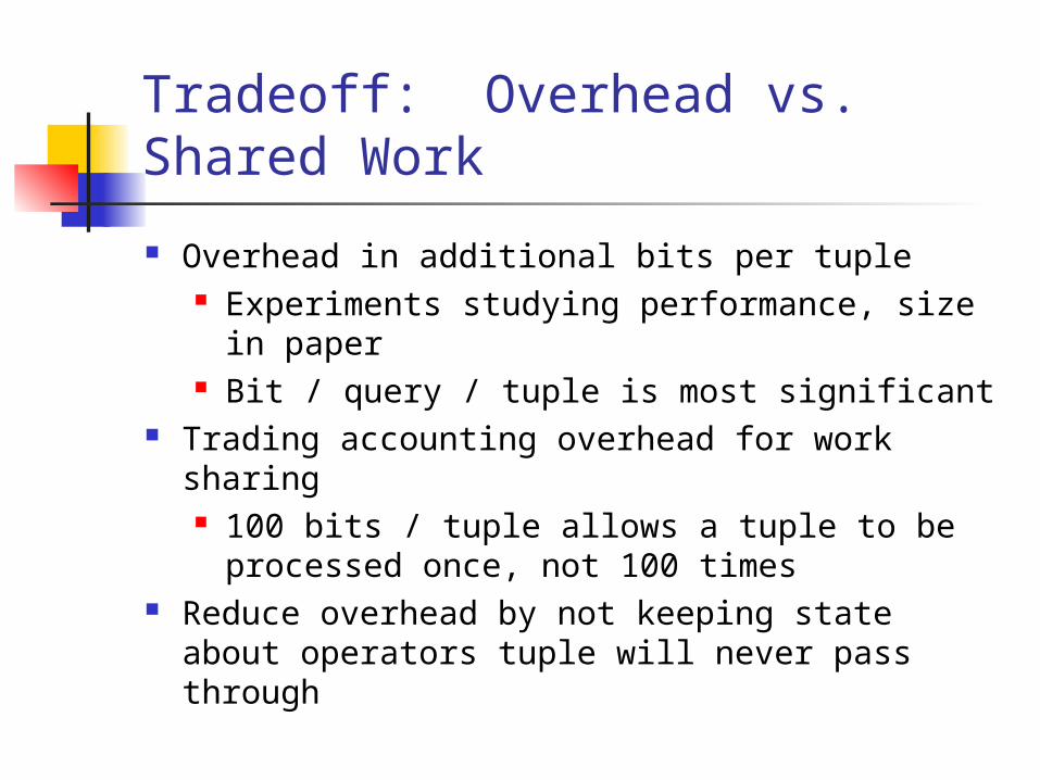
Tradeoff: Overhead vs. Shared Work
Overhead in additional bits per tuple Experiments studying performance, size in
paper Bit / query / tuple is most significant
Trading accounting overhead for work sharing 100 bits / tuple allows a tuple to be
processed once, not 100 times Reduce overhead by not keeping state about
operators tuple will never pass through

Evaluation Real Java implementation on top of Telegraph
QP 4,000 new lines of code in 75,000 line codebase
Server Platform Linux 2.4.10 Pentium III 733, 756 MB RAM
Queries posed from separate workstation Output suppressed
Lots of experiments in paper, just a few here
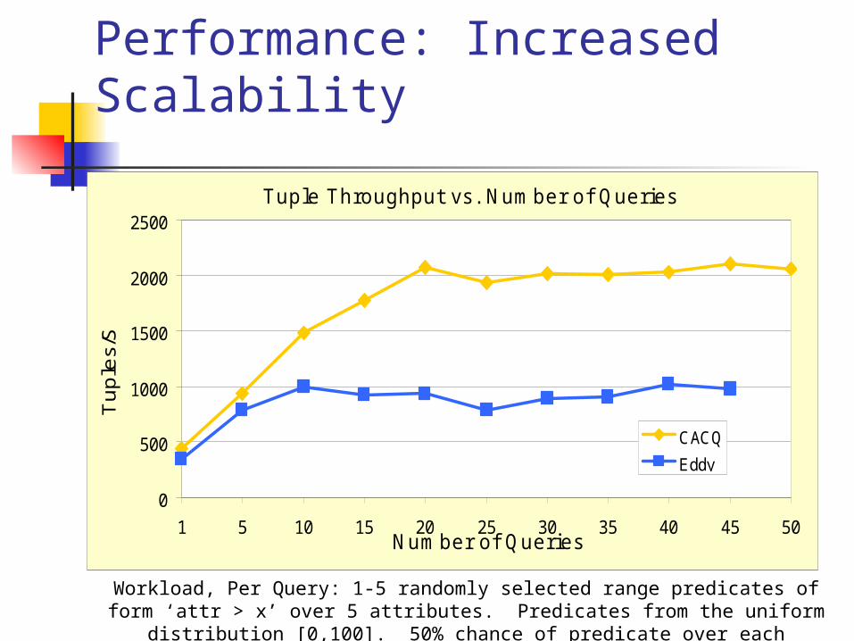
Performance: Increased Scalability
Tuple Throughput vs. Number of Queries
0
500
1000
1500
2000
2500
1 5 10 15 20 25 30 35 40 45 50Number of Queries
Tu
ple
s/S
CACQ
Eddy
Workload, Per Query: 1-5 randomly selected range predicates of form ‘attr > x’ over 5 attributes. Predicates from the uniform distribution [0,100]. 50%
chance of predicate over each attribute.
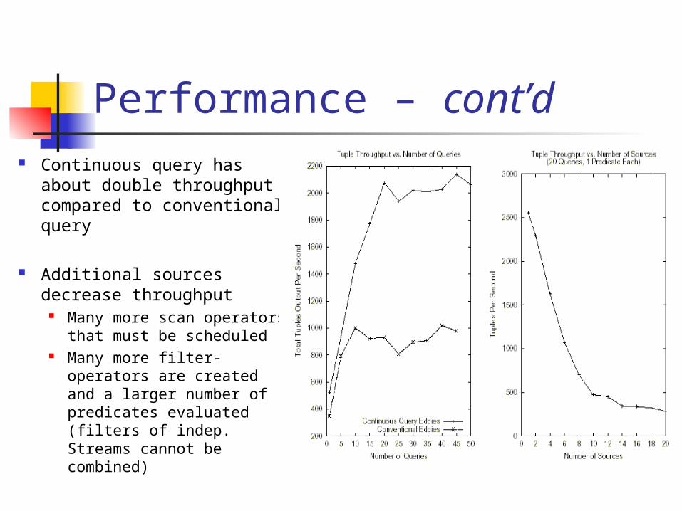
Performance – cont’d Continuous query has
about double throughput compared to conventional query
Additional sources decrease throughput
Many more scan operators that must be scheduled
Many more filter-operators are created and a larger number of predicates evaluated (filters of indep. Streams cannot be combined)
Outline
Background and motivation Acquisitional query (ACQP)
optimization Continuously adaptive continuous
query (CACQ) optimization Summary Future work
Summary: ACQP ACQP: controls when, where, and with
what frequency data is collected Question: Is this the best way (right way?)
to look at a sensor network?
Four related questions When should samples be taken? What sensors have relevant data? In what order should samples be taken? Is it worth it?
Summary: ACQP – cont’d How should the query be processed?
Sampling as a first class operation Event – join duality
How does the user control acquisition? Rates or lifetimes Event-based triggers
Which nodes have relevant data? Index-like data structures
Which samples should be transmitted? Prioritization, summary, and rate control

Summary: CACQ CACQ: sharing and adaptivity for high
performance monitoring queries over data streams
Features Adaptivity
Adapt to changing query workload without costly multi-query reoptimization
Work sharing via tuple lineage Without constraining the available plans
Computation sharing via grouped filter
Future Work Expressing lossiness Batching & query grouping Additional Operations
Joins Signal Processing
Integration with Streaming DBMS In-network vs. external operations
Heterogeneous Nodes and Operators Real Deployments
Related Documents


