Sensitivity analysis of rigid pavement design inputs using ...

Retrospective Theses and Dissertations Iowa State University Capstones, Theses andDissertations

1-1-2005

Sensitivity analysis of rigid pavement design inputsusing mechanistic-empirical pavement designguideAlper GucluIowa State University

Follow this and additional works at: https://lib.dr.iastate.edu/rtd

This Thesis is brought to you for free and open access by the Iowa State University Capstones, Theses and Dissertations at Iowa State University DigitalRepository. It has been accepted for inclusion in Retrospective Theses and Dissertations by an authorized administrator of Iowa State University DigitalRepository. For more information, please contact [email protected].

Recommended CitationGuclu, Alper, "Sensitivity analysis of rigid pavement design inputs using mechanistic-empirical pavement design guide" (2005).Retrospective Theses and Dissertations. 18791.https://lib.dr.iastate.edu/rtd/18791

Sensitivity analysis of rigid pavement design inputs using mechanistic-empirical pavement design guide

by

Alper Guclu

A thesis submitted to the graduate faculty

in partial fulfillment of the requirements for the degree of

MASTER OF SCIENCE

Major: Civil Engineering (Civil Engineering Materials)

Program of Study Committee: Halil Ceylan, Major Professor

Brian Coree Kejin Wang

Lester W. Schmerr, Jr.

Iowa State University

Ames, Iowa

2005

11

Graduate College Iowa State University

This is to certify that the master' s thesis of

Alper Guclu

has met the thesis requirements of Iowa State University

Signatures have been redacted for privacy

111

TABLE OF CONTENTS

LIST OF FIGURES ............................................................................................................. viii

LIST OF TABLES ............................................................................................................... xv

ABSTRACT ........................................................................................................................ .xvi

ACKNOWLEDGEMENTS ............................................................................................ xviii

CHAPTERl INTRODUCTION ..................................................................................... 1

(lJJ RESEARCH OBJECTIVE ................. . ....................... .... .............. ...... . ........ . ............ .. ...... 1

~ .2 BACKGROUND ... .. . . ..... ... . .. .. .. ..... .... ... .. .... .. .. .. .... . ..... .... . ... . .... .... . ............. ·············· ···· ··· 2

p GENERAL FEATURES AND SCOPE OF MEPDG .... . .. ............... .. . .. ... .. ... ... .. ..... ... . ...... .. .. 4

1.~ DESIGN APPROACH IN MEPDG DESIGN GUIDE .. . .. .... . . .. ......... . .. .. . .. .... .... .. ..... . ... .. . ... .. 5

!1.5' OVERVIEW OF CONCRETE PAVEMENT DESIGN M ETHODOLOGIES ... .... ... .............. .. .... 7

1.5.1 Empirical Pavement Design Methodologies ...... ....... ....... .... .... ....... ... ....... ... ... .. .... 7

1.5.2 Mechanistic-Empirical Pavement Design Methodologies .......... ........ ...... .... .. ...... 8

1.5.3 Advantages and Limitations of the Mechanistic-Empirical Design Approach. .. 12

1.6 SCOPE OF RESEARCH .... . .. ..... . . .. ... . .. .. ... . ... .. . ..... .... ... .... .. .... . .. .... ......... .. .. ................... 13

1.7 THESIS LAYOUT .. . . ... .... .. ......... ....... . .......... ......................... .. .. . . .... . . ..... ............... . .. .. . 14

1.8 REFERENCES ... ..... ......... ..... .. .... . ..... ........... .. ..... ....... .. .. ... . .......... . .. . . ... ...... ... ..... .... .. ... 15

CHAPTER2 CONCRETE PAVEMENT DESIGN METHODS AND

GUIDELINES ......................................................................................... 17

2.1 INTRODUCTION ..... .... .. .. . ... . ... ... . . ... ...... .... .. .. ... . . .. . .. ... . .... .. . . ... . .. ... .. .. ... ........ ...... ... ... ... 17

2.2 PAVEMENT D ESIGN METHODS .. .... . ... . ... .. ....... . . ... ...... .. . .. . .. . ....... . .. . ...................... .. ... 18

2. 2.1 Closed-form Formulas ... ...... ..... ... ... ...... ...... .... ... ...... .. .. .. ... .. ........ .. .. ... ...... .......... . 19

2.2.1.1 Goldbeck's Formula ......... .. ...... ...... ..... ... .. .. ..... ........ ... ..... ...... ... .. ... ......... ..... 19

lV

2.2.1.2 Westergaard Theory ........ ........ .... .. .. ....... ...... .. .. .... ......... ... ............... .... ...... .. 20

2.2.2 Influence Charts ..... ... .. .... .. ... ........ .. ... .. .... .......... .... ........... .. .. ... ........ ..... .. ... ....... ... 24

2.2. 3 Numerical Methods ...... ... ..... ......... ... ..... ... ... ....... .... ..... ..... ..... ....... .. ... ... ..... .. ... ... .. 25

2.2.3.1 ILLI-SLAB Finite Element Model ... ..... ............. ... ....... ... ...... .. ........ ... ... ..... 26

2.2.3.2 WESLIQUID and WESLA YER Finite Element Models .... ... .. ........ ...... .... 27

2.2.3.3 RISC Finite Element Model.. ... ..... ..... .... .... ............ ... ..... .. ... ... ...... ... ..... ....... 28

2.2.3.4 KENSLABS Finite Element Model.. .... .... ...... ..... ... ... ..... ..... ..................... .. 28

2.2.4 Road Tests .... .. ...... .. .. .. ........ ... ....... ... ... ....... ........... ... ..... .. ... .. ..... ... ...... .......... ... ..... 29

2.2.4.1 Maryland Road Test .......... ... .... ....... .... .. ...... ... ... .. .. ..... ..... ....... ..... ... .. ....... .... 29

2.2.4.2 AASHO Road Test ........ ...... ..... ........... ... ... ........ ...... ... ..... ... .. .. .......... ....... ... 30

2.2.4.2.1 Limitations ............ .... .......... ........ ....... ... ... ..... .. ... .... ... ... .. ..... ... .. ...... ......... 31

2.3 P AVEMENT D ESIGN G UIDES .. .. ... ... ..... .......... . . ... . . .. ..... ...... . .... ... . . . .. .. .... .... . .. .... .. . .. .. ... 32

2. 3. I AASHTO Design Guides for Pavement Structures ....... ... ..... ...... ......... ..... .... ...... 32

2.3.1.1 AASHTO Design Guide - 1986-1993 .. .. ... ... ....... ... ....... ... ..... .. ... .............. ... 33

2.3.1.2 Supplement to AASHTO Design Guide - 1998 .. ... ... ..... .. ..... .. .. ........ ...... .... 34

2.3.2 Portland Cement Association (PCA) Guidelines .. .. ............. ..... ........ ... ...... ... ... ... 35

2.3.3 Mechanistic-Empirical Pavement Design Methods ... ........ .. ....... ........ ..... ....... .... 36

2.3.4 Design Catalogs ......... .... ....... ... .. ... ... ...... ... .... ... .... ... .. ... ....... .. ..... ..... ... .... ...... ...... . 37

2.3.5 Other Methods ...... .... ...... ...... ...... ........... .. .... ........ .. .... .... ..... ... .......... ... ............ .... 37

2.4 REFERENCES ... .... .. .. .. . .. . .. ... . .. .. . .. .. . .. .. ... ... ... .... .. . .. ... . .. . ... ... .. .... .. .. . .. . .... . ... . .. . .. ... .. . .. .. .. 38

CHAPTER3 INPUT PARAMETERS FOR THE MECHANISTIC-EMPIRICAL

PAVEMENT DESIGN GUIDE ............................................................. 43

3.1 INTRODUCTION .. .. . .. .. . .. . ........ . .. . ... . .. .. .... . ..... . .. . ... . . ... .... . . .. .. . . .. . .... . .. .. ..... ..... ... .. .... .. .. .. 43

3.2 D ESIGN INPUTS ... .... ... . ..... . . .. .. . .. .. ... ....... . ..... . .. . ... . . .. .. ... .. .... . .. . . ..... . .. ......... . . ... ... . . .. .. ... 44

3. 2. I General Inputs .. .... .. ...... ...... .... ........ ... .... .... .... ... ........ .... ... .... ... .... ... .. ... .... ........... . 44

3.2.2 Traffic_ Module .......... .... .... .. .. ...... ...... .... .. .. ......... ............... ...... ... ........... .. : .. ... ... ... 45

3 .2.2. 1 Traffic Characterizations Sources .. ... ...... ......... .. .... ... ... .. ....... .. .... .... .... .... .... 45

3.2.2.1.1 Weight-In-Motion (WIM) Data ...... .... ... ........ ............ .... ....... .. .. ..... ... ... ... 46

3.2.2.1.2 Automatic Vehicle Classification (AVC) Data ........... ... .... ............. .. .. .. .. 46

v

3 .2.2.1.3 Vehicle Counts ............................................. ..... ...................................... 46

3.2.2.1.4 Traffic Forecasting and Trip Generation Models ................................... 47

3 .2.2.2 Traffic Characterization Inputs ................. .................................................. 4 7

3.2.2.2.1 Traffic volume ........................................................................................ 48

3 .2.2.2.1.1 Two-Way Annual Average Daily Truck Traffic (AADTT) ........... 48

3 .2.2.2.1.2 Number of Lanes in the Design Direction ........... ..... ..... ................. 49

3.2.2.2.1.3 Percent Trucks in Design Direction ....................... .................... .... 49

3 .2.2.2.1.4 Percent Trucks in Design Lane .............................. ..... ... ..... .. ........ . 49

3.2.2.2.1.5 Vehicle Operational Speed ............ .......... ............... ..... ........ .. ....... .. 50

3 .2.2.2.2 Traffic Volume Adjustment Factors ....................................................... 51

3.2.2.2.2.1 Monthly Adjustment Factors .......................................................... 51

3.2.2.2.2.2 Vehicle Class Distribution ............................................ .................. 52

3.2.2.2.2.3 Truck Hourly Distribution Factors ........................... ............ ......... . 53

3 .2.2.2.2.4 Traffic Growth Factors ................................................................... 54

3.2.2.2.3 Axle Load Distribution Factors .............................................................. 54

3.2.2.2.4 General Traffic Inputs ................... .................. .. .......... .. ........ ........... .. ..... 55

3.2.2.2.4.1 Lateral Traffic Wander ........................................................... .. ..... . 55

3.2.2.2.4.2 Number of Axle Types per Truck Class ......................................... 56

3.2.2.2.4.3 Axle Configuration ......................................................................... 56

3 .2.2.2.4.4 Wheelbase ...................................................................................... 57

3.2.3 Climate Module .... ...... ....................... ...... ............... ..... .... .. .. ...... .. ...... .... .... ... ...... . 58

3.2.4 Materials Module ..... ........... ..... ........ ..... .... ....... .. .... .. .. ...... .. ...... ..... ...... ... ... .......... 59

3.2.4.1 Portland Cement Concrete .......................................................................... 61

3.2.4.1.1 Strength Parameters for PCC Materials .................................................. 61

3 .2.4.1.1.1 Modulus of Elasticity ..................................................................... 61

3.2.4.1.1.2 Flexural Strength of PCC Materials ............................................... 64

3.2.4.1.2 General Input Parameters ........................................................................ 65

3.2.4.1.2.1 Poisson's Ratio of PCC Materials ................................................... 66

3.2.4.1.2.2 Unit Weight of PCC Materials ............................................ .. ......... 66

3 .2.4.1.3 PCC Mix Design Inputs ....................... ................................................... 67

Vl

3.2.4.1.4 PCC Thermal Design Inputs ....... ..... ........ .................................... ...... ..... 68

3.2.4.1.4.1 PCC Coefficient of Thermal Expansion ....... ...... ........ ........ ..... .... .. . 68

3.2.4.2 Unbound Granular and Subgrade Materials .......... ........ .. ..... .... ...... ... ......... 70

3.2.4.2.1 Non Linear Material Characterization Models ....... ... ... ...... .............. ...... 72

3.3 REFERENCES ... ... .... .. .. ........ .. ... .............. ..... ........... .......... ............. .. ...... ... ..... .. .. ... ..... 75

CHAPTER 4: SENSITIVITY ANALYSIS OF RIGID PAVEMENTS MODULE

DESIGN INPUT PARAMETERS ......................................................... 76

4.1 INTRODUCTION ...... ....... ... ..... .... ... .... .... .... ......... .... .. ..... .... ...... .... ..... ......................... 76

4.2 DATA COLLECTION ......... .......... ... ........ .......... ..... .................. ..... .... ...... .. .... ........ ..... . 77

4.2.1 PCC-1 ..... .... ... ................ ..... ........ ..... ..... .......... .... .. .. .... ..... ..... .. .. .... ....... .. ...... ...... . 79

4.1 .1.1 Traffic ...... .... .. ....... .......... ... ................. ...... .... ............................. ... ... ...... ..... 79

4.1.1.2 Climate ........ ... ... .. .. ... ...... ................ .. ... ......... ... ...... ....... ...... ....... .... ..... ........ . 79

4.1.1.3 Structure ................. .... .................... ..... ..... ..... ........ ... ..... ..... ..... ...... .... ... ...... . 80

4.2.2 PCC-2 ..... ...... ....... .......... .... ...... ................... ...... .. ... .. .... ..... ...... ... .. ... .... ... .. ..... ...... 83

4.1 .1.4 Traffic .. ....................... .... .......... ... ............ ...... ... .. ..... .. ... ...... ... ....... .. ..... ..... .. 83

4.1 .1.5 Climate .... ...... .. ........ ......... ..... ...... ...... ......... ... .. .. ........ ........ ..... ... ...... .... ........ 83

4.1.1.6 Structure ...... ...... ........ ... ... ......... .......... ..... .... .. .. ........ .... ...... ..... ................... .. 84

4.3 MEPDG ANALYSES OF SELECTED SITES .... ................ ......... ..... .... ....... ... .. ..... .. ...... .. 87

4.4 SENSITIVITY ANALYSIS OF MEPDG .... ........... ..... ...... .... ........ .. ... ... ..... .. ....... .... ...... .. 88

4. 4. 1 Overview ... ... ... .. .... ............... ........ ..... ........ .... ...... .... ... ............. ... .................... ..... 88

4. 4. 2 Sensitivity Analysis ... ..... ..... .... .......... ...... ..... ..... ....... ... ..... ........ ......... ..... ... .... .. ... .. 91

4.4.2.1 Summary of Sensitivity Results for Faulting ... ... ........... ... ..... .... ..... .......... .. 99

4.4.2.2 Summary of Sensitivity Results for Transverse Cracking ............ ............ 101

4.4.2.3 Summary of Sensitivity Results for Smoothness .... .... ..... ...... ........... .. .... .. 103

4.5 REFERENCES ..... .. .... ... .... .............. .. ... .............. .... .. ..... ... ... ..... ....... ....... .... ......... .... .. 105

Vll

CHAPTER 5: SUMMARY AND CONCLUSIONS ................................................... 107

5.1 OVERVIEW ..... . ......................... . . .... .................... ...... .. ............. .......... . .. ........... .. .. ... 107

5.2 CONCLUSIONS .... ........................................................ ........................... ................. 108

5.3 RECOMMENDATIONS ............... . ..... ...................................................................... . .. 112

5.4 FUTURE RESEARCH .......... ... .... . .. . .. .. ............. ..... .. . ... ... ......... ... . .... ..... . .... .. . ...... . ... .. .. 11 2

APPENDIX A ACCOMPANYING CD-ROM AND SYSTEM REQUIREMENTS ... . 114

APPENDIX A GRAPHS FOR SENSITIVITY ANALYSIS OF JPCP DESIGN

INPUTS .. ............ ..... .... .................... ....... ........................ ..... .... ..... .... ...... . CD

Figure 1.1

Figure 1.2

Figure 2.1

Figure 2.2

Figure 2.3

Figure 3.1

Figure 3.2

Figure 3.3

Figure 3.4

Figure 4.1

Figure 4.2

Figure 4.3

Figure 4.4

Figure 4.5

Figure 4.6

Figure 4.7

Figure 4.8

Figure 4.9

Figure 4.10

Figure A.I

Figure A.2

Figure A.3

Figure A.4

Vlll

LIST OF FIGURES

Mechanistic-empirical procedure flowchart ...... .... ................................. .......... 9

Calibration of transverse cracking based on percent slabs cracked vs . fatigue

damage on 196 field sections .......................................................................... 11

Goldbeck's formula ... ..... ........................... ..... .. ..... ....... .. ... ..... .............. .. ......... 20

Westergaard corner loading ............ ........ ........................................................ 21

Westergaard different loading locations ..................................... ......... ........... 22

Mechanistic-empirical pavement design guide inputs diagram ........ .. ..... ... .... 44

Screenshot of MEPDG software for traffic characterization inputs ............... 4 7

Illustrations and definitions of the vehicle classes used for collecting

traffic data that are needed for design purposes ..... ..... ....... ............ ... ... ... .... .. . 53

Screenshot of climatic module of the MEPDG software .. ......... ............... ...... 59

Locations of two selected rigid pavement sites in Iowa ... .... .... ................. ..... 78

PCC-1 : L TTP information .............................................................................. 82

PCC-2: LTTP information .. .... ..................................................... .. .. ..... ... .... ... 86

Comparison of MEPDG results with PMIS data on pavement smoothness ... 87

The selected climatic locations for sensitivity analysis ............................ ...... 91

Faulting for different curl/warp effective temperature difference (built-in) ... 92

Cracking for different curl/warp effective temperature difference (built-in). 93

IRI for different curl/warp effective temperature difference (built-in) .... ....... 93

Cracking for different joint spacing at different pavement thicknesses .... ..... 94

Smoothness for different joint spacing at different pavement thicknesses ..... 94

Faulting for different curl/warp effective temperature difference ......... ....... 115

Cracking for different curl/warp effective temperature difference ............... 116

IRI for different curl/warp effective temperature difference ........................ 117

Faulting for different joint spacings ...................................................... ... ..... 118

Figure A.5

Figure A.6

Figure A.7

Figure A.8

Figure A.9

Figure A.10

Figure A.11

Figure A.12

Figure A.13

Figure A.14

Figure A.15

Figure A.16

Figure A.17

Figure A.18

Figure A.19

Figure A.20

Figure A.21

Figure A.22

Figure A.23

Figure A.24

Figure A.25

Figure A.26

Figure A.27

Figure A.28

Figure A.29

Figure A.30

Figure A.31

Figure A.32

Figure A.33

Figure A.34

IX

Cracking for different joint spacings ... ........ .......... ............ ... ............. .... .. ... .. 119

IRI for different joint spacings ...... ................... .......... .................... ........... .... 120

Faulting for different sealant types ................... ...... .... ..................... ........ ..... 121

Cracking for different sealant types ..... .................. ..... ........... ................... .... 122

IRI for different sealant types ... ... ....... ........................ ....... .... ..... .................. 123

Faulting for different dowel diameters .................... ..... ........ .... .................. .. 124

Cracking for different dowel diameters ................... ................ ........ ...... .. ..... 125

IRI for different dowel diameters ................... ..... ... ...................................... 126

Faulting for different dowel spacings ........... ..... ............... ............................ 127

Cracking for different dowel spacings ...................... ..... .... ..... ...................... 128

IRI for different dowel spacings ............................ ......................... ....... ....... 129

Faulting for different edge support .. ..... ....... .. ........ ........................ .... .... ....... 130

Cracking for different edge support....................... ... ......... ........................... 13 1

IRI for different edge support .................. .... .............. ... ....... ......................... 132

Faulting for different PCC-Base interface .................................... ........... ..... 133

Cracking for different PCC-Base interface ............... ... ... .............................. 134

IRI for different PCC-Base interface .............. .................................. ..... ....... 135

Faulting for different erodibility index ......... ... ..... .. .... ... ............................... 136

Cracking for different erodibility index ....................... ....... ... ...... .... .... ...... .. . 13 7

IRI for different erodibility index ............... ............................. ....... .............. 138

Faulting for different surface shortwave absorptivity ................................... 139

Cracking for different surface shortwave absorptivity ................................. 140

IRI for different surface shortwave absorptivity ........................................... 141

Faulting for different infiltration of surface water .... ............... ... ... ......... ...... 14 2

Cracking for different infiltration of surface water. ...................................... 14 3

IRI for different infiltration of surface water ..... .. ........ ............ ..... ................ 144

Faulting for different PCC layer thicknesses ..... .... ... ... ...... ......... ....... ... ..... ... 145

Cracking for different PCC layer thicknesses ............. ..... .............. ............... 146

IRI for different PCC layer thickness ...................... ..... ... ........ ..................... 14 7

Faulting for different unit weight.. ................................ ... ... .... ....... ............... 148

Figure A.35

Figure A.36

Figure A.37

Figure A.38

Figure A.39

Figure A.40

Figure A.41

Figure A.42

Figure A.43

Figure A.44

Figure A.45

Figure A.46

Figure A.47

Figure A.48

Figure A.49

Figure A.50

Figure A.51

Figure A.52

Figure A.53

Figure A.54

Figure A.55

Figure A.56

Figure A.57

Figure A.58

Figure A.59

Figure A.60

Figure A.61

Figure A.62

Figure A.63

Figure A.64

x

Cracking for different unit weight ... ......... .................................................... 149

IRI for different unit weight .. ....................... ....... .... ....... ..... ......... ........... .. .... 150

Faulting for different poisson's ratio ............. .......... ................. .... ................. 151

Cracking for different poisson's ratio ...... ........... ..... ..... ..... .. .. ..... .. ............. .... 152

IRI for different poisson's ratio ................. ...... ..... ... .................... ................. . 153

Faulting for different coefficient of thermal expansion .... .................... ..... .. . 154

Cracking for different coefficient of thermal expansion ....... ..... .. .. ........ ...... . 15 5

IRI for different coefficient of thermal expansion ................ ........................ 156

Faulting for different thermal conductivity ..... ........ .............. ..... .. ................ . 157

Cracking for different thermal conductivity .... ....... .. ....... ..... ... ... ........... ... ... . 158

IRI for different thermal conductivity .... ..... .. .......... ..... .... .. .. ................. ... ... .. 159

Faulting for different heat capacity ............. .................................................. 160

Cracking for different heat capacity ........ ....... ........ ................... .......... ......... 161

IRI for different heat capacity ............... ....... .... ... ..... ... .... .. ............................ 162

Faulting for different cement type ............. .... ......... .. .......... .. .............. ...... .... 163

Cracking for different cement type .......... ........ ....... .. ..... ..... .. .... ... .......... ... ... . 164

IRI for different cement type ....................... .... .. ..... .. .. .............. ... ......... .... .... 165

Faulting for different cement content ........ .... .. .. ................................... .... .... 166

Cracking for different cement content .................... ......... .. .. ... ..... ..... ........ .... 167

IRI for different cement content ...... .. ........... ... ....... ............. ... .... .. ...... .. .... .... 168

Faulting for different water/cement ratio .... ... .. .. .................. .. ....................... 169

Cracking for different water/cement ratio .... .. .. .. ... ... .. .... ............................. .. 170

IRI for different water/cement ratio .... ..... .... .... ........ ............ .. ....................... 171

Faulting for different aggregate type ....... ...... ............................................... 172

Cracking for different aggregate type ..... ......... ........................ ... .......... ........ 1 73

IRI for different aggregate type ...... .... ............. .............. ... ... ........ ..... ...... ...... 174

Faulting for different PCC set temperature ...... ............................ ........... ...... 175

Cracking for different PCC set temperature .... ....................................... ...... 176

IRI for different PCC set temperature ...... ..... ..... .... ........... ................ .... ........ 177

Faulting for different ultimate shrinkage at 40 % R.H ... .. ....... ......... ..... ... .... 178

Figure A.65

Figure A.66

Figure A.67

Figure A.68

Figure A.69

Figure A.70

Figure A.71

Figure A.72

Figure A.73

Figure A.74

Figure A.75

Figure A.76

Figure A.77

Figure A.78

Figure A.79

Figure A.80

Figure A.81

Figure A.82

Figure A.83

Figure A.84

Figure A.85

Figure A.86

Figure A.87

Figure A.88

Figure A.89

Figure A.90

Figure A.91

Xl

Cracking for different ultimate shrinkage at 40 % R.H . ... .. ......... ......... .. .... .. 1 79

IRI for different ultimate shrinkage at 40 % R.H ....... ............................... ... 180

Faulting for different reversible shrinkage ... .. ... ......... ... ..... ... ..... ........ ...... ... . 181

Cracking for different reversible shrinkage ..... .............. ...... .... ..... ....... ... .... .. 182

IRI for different reversible shrinkage .... ... ........ ....... .... .. ... ... ..... ....... ... .. .. .... .. 183

Faulting for different time to develop 50 % of ultimate shrinkage ......... .... .. 184

Cracking for different time to develop 50 % of ultimate shrinkage .... ... ... ... 185

IRI for different time to develop 50 % of ultimate shrinkage ....................... 186

Faulting for different curing method ... .... ............ .. ...... .. ..... ... .... ........ ............ 187

Cracking for different curing method ........................... .... ...... ... .... .. .. ...... ..... 188

IRI for different curing method ....... ..... .. ... .... ..... ...... ..... ..... ....... ... .... ... ...... .... 189

Faulting for different 28-day PCC modulus of rupture ..... ... .... ................ ... . 190

Cracking for different 28-day PCC modulus of rupture ..... .. .. ............... .... ... 191

IRI for different 28-day PCC modulus of rupture ... ... .. .. .. .. .. .... ....... .. ...... .. ... 192

Faulting for different 28-day PCC compressive strength .......... .. ........ ......... 193

Cracking for different 28-day PCC compressive strength ... ... ..... .............. ... 194

IRI for different 28-day PCC compressive strength .. ........ ...... .. .. ......... .... .... 195

Faulting for different climates .... ... .... ... ... ........ ........ ....... .... .... .. ... ..... .. ....... ... 196

Cracking for different climates ....... ......... ..... ........................... .... .......... ....... 197

IRI for different climates .... ...... ........ .. ....... .............. ... .. .. ... ....... ..... ......... .. .... 198

Cracking for different joint spacing at different pavement thicknesses .. ... .. 199

Bottom-up cracking for different joint spacing at different pavement

thicknesses ... ........................ .... ...... ................. ... ..... .. ... ...... ........................... 200

Top-down cracking for different joint spacing at different pavement

thicknesses ... ...... ................ ... .......... .......... ................. ... .... ... ... ..... ......... .... .... 201

Smoothness for different joint spacing at different pavement thicknesses ... 202

Smoothness for different joint spacing at different pavement thicknesses

with specified reliability (R= 90 %) ........ ..... ................................................ 203

Faulting for different joint spacing at different pavement thicknesses .... ..... 204

Cracking for different joint spacing at different pavement thicknesses ....... 205

Figure A.92

Figure A.93

Figure A.94

Figure A.95

Figure A.96

Figure A.97

Figure A.98

Figure A.99

XU

Bottom-up cracking for different joint spacing at different pavement

thicknesses ................................................. .... ................. .. ... .. ......... .............. 206

Top-down cracking for different joint spacing at different pavement

thicknesses ........................................... ...... ...... ............ .............. .. ............... .. 207

Smoothness for different joint spacing at different pavement thicknesses ... 208

Smoothness for different joint spacing at different pavement thicknesses

at specified reliability (R= 90 %) ........................................ .. ....... ....... .......... 209

Faulting for different joint spacing at different pavement thicknesses ... ...... 210

Cracking for different pavement ages at different dowel diameters ....... .... .. 211

Cumulative damage for different pavement ages at different dowel

diameters ..... ... ...... ....... ..... ... ...... ............ ... ... ........................... ..... .... .. ....... .. .. . 212

Smoothness for different pavement ages at different dowel diameters ... ... .. 213

Figure A. l 00 Smoothness for different pavement ages at different dowel diameters

at specified reliability (R = 90 % ) .................................................................. 214

Figure A.101 Faulting for different pavement ages at different dowel diameters ... ........... 215

Figure A. l 02 Cracking for different joint spacing at different design lives ...... .. ........ ....... 216

Figure A.103 Bottom-up cracking for different joint spacing at different design lives ...... 217

Figure A. I 04 Top-down cracking for different joint spacing at different design lives .. .... 218

Figure A.105 Smoothness for different joint spacing at different design lives .............. ..... 219

Figure A.106 Smoothness for different joint spacing at different design lives

at specified reliability (R = 90 % ) ......................... ..................... .. ............. ..... 220

Figure A.l 07 Faulting for different joint spacing at different design lives ..... .. .................. 221

Figure A.108 Cracking for different time of construction at different design lives ............ 222

Figure A.109 Bottom-up cracking for different time of construction at different design

lives ... .... ... ........ .. .. ..... ... ... ...... ..... .............. ...... ..... ...... .. ........ ..... ... ... ............... 223

Figure A.110 Top-down cracking for different time of construction at different design

lives ........... .. ................ ..... ... ... ..... ... ....... .... .. .. ... ... .......... ... .. ... ... ...... ... .... ... ..... 224

Figure A.111 Smoothness for different time of construction at different design lives ....... 225

Figure A.11 2 Faulting for different time of construction at different design lives ..... .... .. .. 226

Figure A.113 Cracking for different AADTT at different design lives ... ........ ... .. .... .......... 227

Xlll

Figure A.114 Bottom-up cracking for different AADTT at different design lives ... ......... . 228

Figure A.115 Top-down cracking for different AADTT at different design lives ............ . 229

Figure A.116 Smoothness for different AADTT at different design lives ..... ............... ...... 230

Figure A.117 Smoothness at specified reliability for different AADTT at different

design lives .. ............................................................... ........ .. ....... ....... ........... 231

Figure A.118 Faulting for different AADTT at different design lives ...... ......................... . 232

Figure A.119 Cracking for different coefficient of thermal expansion at different

design lives ... .. .... ..... ......... ........ .. ................ ... ............ ...... .................. .... ........ 233

Figure A.120 Bottom-up cracking for different coefficient of thermal expansion at

different design lives ................................................................ ....... ..... ........ . 234

Figure A.121 Top-down cracking for different coefficient of thermal expansion at

different design lives ............. .... .... ... ........ .......... .......................... .. ............... 23 5

Figure A.122 Smoothness for different coefficient of thermal expansion at different

design lives ........................ ......................... ....... ........................................... . 236

Figure A.123 Smoothness at specified reliability for different coefficient of thermal

expansion at different design lives .................. .... .. ....................... ...... .. ......... 237

Figure A.124 Faulting for different coefficient of thermal expansion at different

design lives .................................................................................................... 238

Figure A.125 Cracking for different pavement thickness at different design lives ............ 239

Figure A.126 Smoothness for different pavement thickness at different design lives ........ 240

Figure A.127 Smoothness at specified reliability for different pavement thickness

at different design lives ................................................... .. ................ ..... .... ... 241

Figure A.128 Faulting for different pavement thickness at different design lives .............. 242

Figure A.129 Cracking for different joint spacing at different pavement thicknesses ....... 243

Figure A.130 Bottom-up cracking for different joint spacing at different pavement

thicknesses ....... ................................... ..... ...... ............... .... .. ........ .. .. .............. 244

Figure A.131 Top-down cracking for different joint spacing at different pavement

thicknesses ....... .. ........................................................................................... 245

Figure A.132 Smoothness for different joint spacing at different pavement thicknesses .. . 246

XIV

Figure A.13 3 Smoothness at specified reliability for different joint spacing at

different pavement thicknesses ............. .. ...... ... ......................... ....... .... ......... 24 7

Figure A.134 Faulting for different joint spacing at different pavement thicknesses ......... 248

Figure A.135 Cracking for different mean wheel-path at different traffic wander

standard deviation ... ..... ............................ ...... .......... .......... ........................... 249

Figure A.136 Bottom-up cracking for different mean wheel-path at different

traffic wander standard deviation ....... ........... .. ................... ... ... ... ................ .. 250

Figure A.137 Top-down cracking for different mean wheel-path at different

traffic wander standard deviation ......................... .............. .......... .... .... .... ..... 251

Figure A.138 Smoothness for different mean wheel-path at different traffic

wander standard deviation ............................................................................ 252

Figure A.139 Smoothness at specified reliability for different mean wheel-path

at different traffic wander standard deviation .... ..... ............... .... ..... ... ........... 253

Figure A.140 Faulting for different mean wheel-path at different traffic wander

standard deviation ....... ........ ......... ................ .. .. ..... .... .. .. ............ ......... .. ... .... .. 254

Table 3.1

Table 3.2

Table 3.3

Table 3.4

Table 3.5

Table 3.6

Table 3.7

Table 3.8

Table 3.9

Table 3.10

Table 4.1

Table 4.2

Table 4.3

Table 4.4

Table 4.5

Table 4.6

Table 4.7

Table 4.8

Table 4.9

Table 4.10

Table 4.11

Table 4.12

Table 4.13

Table 4.1 4

Table 4.15

Table 4.16

xv

LIST OF TABLES

Material types used in the MEPDG ............ ........ ........................................... 60

Required input data for modulus of elasticity at level 1 ....................... ........ .. 62

Required input data for modulus of elasticity at level 2 ............... .. ........... .. .. 63

Required input data for modulus of elasticity at level 3 ........ .. .. ..................... 64

Modulus of rupture estimation for different level of inputs .. .... ... .. ...... .......... 65

Typical poisson's ratio values for PCC materials. .. ...................... ...... ........... 66

Unit weight estimation of PCC materials .... ... ............... ................................ 67

Typical ranges for common PCC components ............... .. .. .. ................ .... .. ... 69

General correlations to find MR .. .... ..... ..... ...... .. ................... .......................... 73

Typical modulus values for different soils ...... .. .............. .. ....... ..... ............ ...... 7 4

General information on two selected rigid pavement sites ....... .. ................. .. . 78

PCC-1: Location information .................... ....... .... ... ........ ............. ......... ......... 80

PCC-1 : Pavement information .................. ........................ .. .. .. ......... ............... 81

PCC-1 : Climate information .... ... ......... ...... ............ .... ... ..... ... .... .......... ...... ...... 81

PCC-1: Traffic information ....................................................................... .. .... 81

PCC-2: Location information ...... ............. .. .. .............. .. ...... .. .................... .. .... 84

PCC-2: Pavement information .... ......................... ........... .... .. ... ...... ........... ..... . 85

PCC-2: Climate information ................. ....... .............. ... ...... .. .......................... 85

PCC-1: Traffic information ........ ........... ... .. ......... ................ ............................ 85

Comparison of MEPDG results and PMIS data ............................................. 88

Summary of standard input parameters for sensitivity analyses ........ ...... ....... 89

Summary of sensitivity scales ............................................. ........................... . 95

Summary of results of sensitivity analysis for rigid pavements ...... ... ....... .... . 96

Summary of sensitivity level of input parameters for faulting of JPCP ....... 100

Summary of sensitivity level of input parameters for transverse

cracking of JPCP .... ........ ... .. ............ .... ... ....... .............. .... ..... .. .. ... .. .......... .. .. .. 102

Summary of sensitivity level of input parameters for smoothness of JPCP. 104

XVI

ABSTRACT

Pavement design procedures, available in the literature, do not fully take advantage of

mechanistic concepts, which make them heavily rely on empirical approaches. Because of

the heavy dependence on empirical procedures, the existing design methodologies do not

capture the actual behavior of Portland cement concrete (PCC) pavements. However, reliance

on empirical solutions can be reduced by introducing mechanistic- empirical methods, which

is now adopted in the newly released mechanistic-empirical pavement design guide

(MEPDG). This new design procedure incorporates a wide range of input parameters

associated with the mechanics of rigid pavements. To compare the sensitivity of these

various input parameters on the performance of concrete pavements, two jointed plain

concrete pavement (JPCP) sites were selected in Iowa. These two sections are also part of the

Long Term Pavement Performance (LTPP) program where a long history of pavement

performance data exists. Data obtained from the Iowa Department of Transportation (Iowa

DOT) Pavement Management Information System (PMIS) and L TPP database were used to

form two standard pavement sections for the comprehensive sensitivity analyses. The

sensitivity analyses were conducted using the MEPDG software to study the effects of design

input parameters on pavement performance of faulting, transverse cracking, and smoothness.

Based on the sensitivity results, ranking of the rigid pavement input parameters were

established and categorized from most sensitive to insensitive to help pavement design

engineers to identify the level of importance of each input parameter. The curl/warp

effective temperature difference (built-in curling and warping of the slabs) and PCC thermal

xvii

properties are found to be the most sensitive input parameters. Based on the comprehensive

sensitivity analyses, the idea of developing an expert system was introduced to help the

pavement design engineers identify the input parameters that they can modify to satisfy the

predetermined pavement performance criteria. Predicted pavement distresses using the

MEPDG software for the two Iowa rigid pavement sites were compared against the measured

pavement distresses obtained from the Iowa DOT's PMIS and comparison results are

discussed in this study.

xviii

ACKNOWLEDGEMENTS

I would like to thank my advisor, Dr. Halil Ceylan, for providing me with the opportunity to

work on this project and for his guidance throughout both this research and my graduate

studies. Dr. Brian Coree, is greatly appreciated for his assistance and periodical discussions

on my research. Thanks are also expressed to the support and comments of other committee

members, Dr. Kejin Wang and Dr. Lester Schmerr. Mr. Chris Brakke and Mr. Ben Behnami

from Iowa DOT both of whom provided the required data and assistance during this study

also deserve sincere thanks.

The research described in this thesis was funded by Iowa Highway Research Board and Iowa

Department of Transportation (Iowa DOT) both of which are gratefully acknowledged.

Special thanks are due to my family, for their love, patience, and support. The last but not

least, I would like to thank my friends for their encouragement; suggestions, and support.

1.1 Research Objective

CHAPTERl

INTRODUCTION

The objective of this research was to identify the sensitivity of input parameters needed for

designing the jointed plain concrete pavements (JPCPs) used in the newly released

mechanistic-empirical pavement design guide (MEPDG) (a.k.a. NCHRP Project 1-37A

Mechanistic-Empirical Pavement Design Guide for Design of New and Rehabilitated

Pavement Structures). The findings of this study will guide the state department of

transportations (DOTs) to determine which input parameters have either the most or the least

effect on the predicted pavement distresses of transverse cracking, faulting and smoothness.

In this chapter, the development of mechanistic-empirical pavement design procedures in

American Association of State Highway and Transportation Officials (AASHTO) guidelines

and an overview of concrete pavements is presented.

2

1.2 Background

Three types of concrete pavements are commonly used; (1) jointed plain concrete pavement

(JPCP), (2) jointed reinforced concrete pavement (JRCP), and (3) continuously reinforced

concrete pavement (CRCP).

JPCP has transverse joints spaced less than 5m apart and does not have reinforcing steel in

the slab. According to a performance survey, Nussbaum and Lokken [1.1] recommended

maximum joint spacings of 6m for doweled joints. JPCP can contain steel dowel bars and

tie-bars across transverse joints and longitudinal joints, respectively.

JRCP has transverse joints spaced about 9-12m apart and contains steel reinforcement in the

slab. Steel reinforcement in the form of wired mesh is designed to increase the structural

capacity of the slab. Dowel bars and tie-bars are also used at all transverse and longitudinal

joints, respectively.

CRCP does not have transverse joints and contains more steel reiq.forcement than JRCP. The

high steel content influences the formation of the transverse cracks in close distances [1 .2].

Transverse reinforcing steel is often used.

According to a 1999 survey, at least 70% of the state highway agencies in the United States

used JPCP. About 20% of the states used JRCP, and about 6 or 7 state highway agencies

3

built CRCP, most notably on high-volume, urban roadways. In this study the analysis of

JPCP sections under MEPDG software was discussed.

The historical development of mechanistic-empirical (M-E) pavement design procedures in

the AASHTO guides goes back to the 1986 AASHTO Design Guide. In the 1986 AASHTO

guide for pavement structures, M-E design procedure was firstly defined as the calibration of

mechanistic models with observations of performance, i.e. empirical correlations. It was also

stated that in a multi-layered pavement system, analytic methods were the numerical

calculations of the pavement responses when subjected to external loads or the effects of

temperature or moisture. Then, assuming that pavements can be modeled as a multi-layered

elastic or visco-elastic structure on an elastic or visco-elastic foundation, the stress, strain, or

deflection could be calculated at any point within or below the pavement structure.

Mechanistic procedures are referred to for the ability to translate the analytical calculations

of the pavement responses to physical distress such as cracking or rutting (pavement

performance). However, pavement performances are subjective to a number of factors, that

cannot be exactly modeled by mechanistic methods. It is, therefore, necessary to incorporate

empirical pavement performance models with mechanistic models. Thus, in the 1986

AASHTO Guide, the procedure is defined conceptually as a mechanistic-empirical pavement

design procedure. [1.3]

The AASHTO pavement design guides [1.3-5] used empirical methods, which are valid for

specific environmental, material, and loading conditions. In order to develop a design

procedure without these limitations, the development of M-E design procedures was

4

promoted by the AASHTO Joint Task Force on Pavements (JTFP). AASHTO JTFP

recommended the research should be initiated for the later versions of the AASHTO design

guides. Then, the National Cooperative Highway Research Project (NCHRP) Project 1-26

[l.6-9] was the first NCHRP project to be sponsored. After that, the second phase ofNCHRP

1-26 started and was completed in 1992 with its two volumes of final reports showing the

guidelines for the data input stage of the procedures [1.1 O]. Finally, at the conclusion of a

workshop held in March 1996 in Irvine, California, JTFP concluded a long-term project for

the development of a design guide based as fully as possible on mechanistic principles. This

guide is titled The NCHRP Project l-37A mechanistic-empirical design guide for design of

new and rehabilitated pavement structures [l.11].

1.3 General Features and Scope of MEPDG

The main objective of the MEPDG was to provide a pavement design guide based on

mechanistic-empirical design procedures for new and rehabilitated pavement systems, and a

user-friendly software and documentation. With the help of the software, the designers would

have the control to design and the flexibility to consider various features. For the design, not

only were the site conditions but also the construction conditions were considered. Moreover,

the MEPDG is in a format that provides the development of existing mechanistic-empirical

pavement design procedures in connection with trucking, materials, construction, computers,

and so on. [l.11]

5

1.4 Design Approach in MEPDG Design Guide

Reliability and rehabilitation design issues were updated by incorporating mechanistic

approaches in relation to the 1986 and 1993 AASHTO guides and were broadened to include

rehabilitation considerations not included in AASHTO guides. In the design approach, one

must first consider the design inputs and analysis strategies. Design inputs are materials

characterization, traffic data input, and the climate using the Enhanced Integrated Climatic

Model (EICM). Next, the structural performance analysis must be considered, which is based

on trial and error, beginning with standard trials obtained from agencies. Then, with initial

estimates of some values, the pavement section is analyzed using the distress models. The

outputs are the expected amount of distress and smoothness over time. Until satisfactory

results are obtained, iterative approach continues. In summary, the following considerations

are included in the MEPDG [ 1.11]:

• Traffic

• Climate

• Material properties (Subgrade/foundation, base, granular base)

• Existing pavement condition

• Construction factors

• Sub drainage

• Shoulder design

• Rehabilitation treatments and strategies

• New pavement and rehabilitation options

• Pavement performance (key distresses and smoothness)

6

• Design reliability

• Life cycle costs

Another aspect of the MEPDG is the hierarchical approach to the design inputs, which is not

found in either AASHTO design guides or any other design guides. With this approach, the

inputs are separated into three levels.

Level 1: Inputs provide a high level of accuracy. Level 1 inputs are used in cases of

pavements with heavy traffic. These inputs require laboratory testing, field-testing (such as

dynamic modulus testing of hot mix asphalt concrete), and non-destructive deflection testing.

In addition, they require more tests and sources than other types.

Level 2: Inputs provide an intermediate level of accuracy, and would be considered the

closest to the typical procedures applied in the AASHTO design guides. This level of inputs

could be used when there is not enough equipment or testing programs. The required data are

estimated through the correlations. These values could be provided from the agencies.

Level 3: Inputs provide the lowest accuracy and this level might be used for pavement with

low volumes of traffic. The input values are mostly taken from the default values that are

based on seasonal averages or the basic correlations.

A combination of the three input levels can also be used. However, regardless of the input

level(s) used, the design procedure and the distress models are the same.

7

1.5 Overview of Concrete Pavement Design Methodologies

1.5.1 Empirical Pavement Design Methodologies

Empirical methods are based on experience. As more experiences were added throughout the

years concerning the development of pavement thickness design, several methods have been

developed by agencies. A commonly known empirical method is the AASHTO method. It is

based on the results of the American Association of State Highway Officials (AASHO) road

test conducted in Ottawa, Illinois, in the late 1950s and early 1960s. The first interim design

guide based on the AASHO method was published in 1961 and revised in 1972 and 1981 . In

1986, results of the NCHRP Project 20-7 /24 recommended that the guide be expanded and

revised. After the 1986 AASHTO design guide was finished, it was last revised in 1993.

After the AASHO road test, the pavement serviceability-performance concept, an

outstanding feature, was developed for the thickness design. Serviceability is the ability to

serve traffic in its existing conditions [ 1.11]. Present Serviceability Index (PSI) is one

method to find serviceability condition. PSI is the condition index based on pavement

roughness and distresses, such as rutting, cracking, and patching [ 1.11]. Designs are based on

the empirical equations that are produced with PSI after the AASHO road test.

The shortcomings of empirical methods based on the AASHO road test are as follows:

• It is only valid for the same environmental, material, and loading conditions.

8

• Traffic values are no longer the same as those of the AASHO road test. (including

axle loads and configurations, tire pressures, tire types, and volumes).

• In the road test only one type of subgrade soil is used.

• The rehabilitation of existing pavements is not addressed in the road test, and the

AASHTO guide does not have a globally validated scheme for this.

1.5.2 Mechanistic-Empirical Pavement Design Methodologies

Before the new MEPDG guide was released, some industry groups [1.13-1.14] and highway

agencies had already established mechanistic-empirical procedures, including Illinois [1.12].

The mechanistic-empirical design approach is a very sophisticated and reliable method of

design. The complexity of the mechanistic-empirical procedure comes from use of finite

element models for pavement system analysis, especially in the analysis of comers and joints

on rigid pavements. Although the analyses are complex, the use of computers makes the

design easier. Especially, the MEPDG's user-friendly software makes the analysis easier.

Another aspect of the new MEPDG is that it does not provide a design thickness at the end of

pavement analysis; instead, it provides the pavement performance throughout its design life.

Therefore, MEPDG is a performance prediction tool more than an analysis tool. The design

thickness can be predicted by modifying design inputs and obtaining the best performance

with an iterative procedure.

9

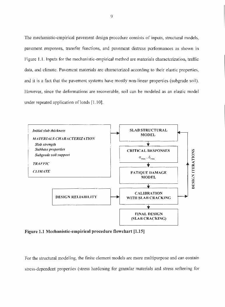
The mechanistic-empirical pavement design procedure consists of inputs, structural models,

pavement responses, transfer functions, and pavement distress performances as shown in

Figure 1.1. Inputs for the mechanistic-empirical method are materials characterization, traffic .

data, and climate. Pavement materials are characterized according to their elastic properties,

and it is a fact that the pavement systems have mostly non-linear properties (subgrade soil).

However, since the deformations are recoverable, soil can be modeled as an elastic model

under repeated application of loads [ 1.10].

Initial slab thickness SLAB STRUCTURAL I+--~ MODEL MATERIALS CHARACTERIZA T/ON

Slab strength ... Subbase properties CRITICAL RESPONSES Subgrade soil support

crmax ' 0max

TRAFFIC .. .4 ..

CLIMATE FATIQUE DAMAGE MODEL

.. CALIBRATION

DESIGN RELIABILITY r--+ WITH SLAB CRACKING ___.

+ FINAL DESIGN

(SLAB CRACKING)

Figure 1.1 Mechanistic-empirical procedure flowchart (1.15)

For the structural modeling, the finite element models are more multipurpose and can contain

stress-dependent properties (stress hardening for granular materials and stress softening for

10

fine-grained soils). The finite element models can also include failure criteria (such as the

Mohr-Coulomb model in ILLI-PA VE). Stress dependent finite element programs (such as

ILLI-PAVE, MICH-PA VE, and Texas ILLI-PAVE) and elastic layer programs (such as

BISAR, WESLEA, JULEA, CHEVRON, ELSYM 5, CIRCL Y) are recommended for

flexible pavements. [ 1.15]

The empirical aspect of the mechanistic-empirical pavement design process is the transfer

functions. They relate the pavement responses to the pavement distress models. For instance,

in MEPDG, the transfer function for the percentage of slabs with transverse cracks in a given

traffic lane is used as the measure of transverse cracking, and is predicted using the following

model for both bottom-up and top-down cracking [l.11] :

CRK= l 1 + FD -16s

Where,

CRK =predicted amount of bottom-up or top-down cracking (fraction)

FD= fatigue damage

Model Statistics:

R2 = 0.86

N = 522 observations

SEE = 5 .4 percent

11

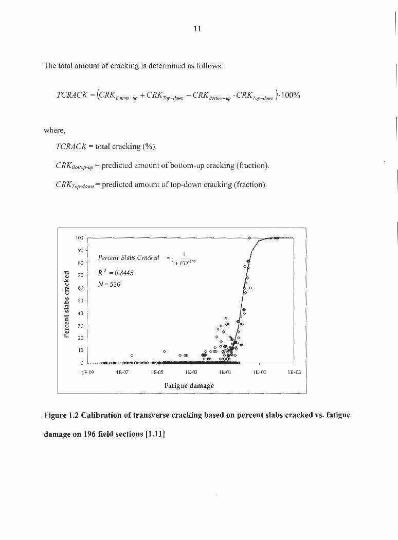
The total amount of cracking is determined as follows:

TCRACK = (CRKBottom-up + CRKTop-down -CRKBottom-up · CRKTop-down )· 100%

where,

TCRACK =total cracking(%).

CRKsoaop-up =predicted amount of bottom-up cracking (fraction).

CRKrop-down = predicted amount of top-down cracking (fraction).

100

90

Percent Slabs Cracked 80 I+ FD-16s

"O 70 R 2 = 0.8445 Q)

~ N=520 u

!ti 60 i... u ti)

50 ,.Q !ti -ti) 40 ..... s:: Q)

30 u i... Q)

p... 20

10 ¢ ¢ ¢ «>

0

lE-09 lE-07 lE-05 lE-03 lE-01 lE+Ol 1E+03

Fatigue damage

Figure 1.2 Calibration of transverse cracking based on percent slabs cracked vs. fatigue

damage on 196 field sections (1.11]

12

The equation assumes that a slab may crack from either bottom-up or top-down, but not both.

The JPCP transverse cracking model was calibrated based on performance of 196 field

sections located in 24 States (see Figure 1.2). The calibration sections consist of LTPP GPS-

3 and SPS-2 sections and 36 sections from the FHWA study Performance of Concrete

Pavements.

The failure mechanism is defined as the distress of the pavement systems. In order to fail,

transfer functions relate the critical responses to these failures. After relating these, an

iterative design process is applied to find the thickness of the pavement.

1.5.3 Advantages and Limitations of the Mechanistic-Empirical Design Approach

The advantages of the MEPDG can be summarized as follows [1.11]:

• New loading conditions can be evaluated (such as axle configurations, damaging

effects of increased loadings, high tire pressures)

• Better use of available materials can be estimated. For example, the use of

stabilized materials in both rigid and flexible pavements can be simulated to

predict future performances

• More reliable design (not over design or under-designed)

• Rehabilitation concept is addressed

• Seasonal effects such as thaw weakening can be included in the performance

estimates

1"' . .)

• Long-term affects can be included in the analysis

• Different sub-grades can be used to estimate performances

• Aging effects can be evaluated such as asphalt hardens with time, which, m

return, affects both fatigue cracking and rutting

The limitations are below:

• Computational complexity due to structural models for pavements (such as finite

element models) which requires the need of computers

• Inadequate knowledge about the design procedure

• Inexperienced personnel

• Weakness in the transfer functions

1.6 Scope of Research

Considering the current state of MEPDG, the research presented in this thesis focused on the

following areas:

1. Development of sensitivity levels for inputs of rigid pavement design module of

MEPDG for each pavement performance criteria using MEPDG software.

2. Development of set of recommendations for implementation plan in Iowa.

14

1. 7 Thesis Layout

This thesis contains five chapters. Following an introduction in this chapter for concrete

pavements and mechanistic-empirical design methodology, Chapter 2 provides a literature

review of concrete pavement analysis methods, road tests and existing design guidelines

developed for rigid pavement design.

Chapter 3 presents the design inputs used in the MEPDG with extensive review of traffic,

climate, and material input parameters. Data collection, description of the sites and input

parameters used in the sensitivity analyses are presented in Chapter 4. The summary of

results is also presented in Chapter 4. The research findings, conclusions and

recommendations are given in Chapter 5.

In the attached CD-ROM, Appendix A is located. Appendix A provides the plots for the

sensitivity analyses of JPCP design inputs for each pavement performance.

15

1.8 References

[1.1] Nussbaum, P.J., and E. C. Lokken, 1978, Portland Cement Concrete Pavements,

Performance Related to Design - Construction-Maintenance, Report No. FHWA-TS-78-

202, Prepared by PCA for Federal Highway Administration

[1.2] Huang, Yang H., Pavement Analysis and Design, 2nd Edition, Pearson Education,

Inc. , 2004

[1.3] AASHTO, Interim Guide for the Design of Pavement Structures. American

Association of State Highway and Transportation Officials, 1972

[1.4] AASHTO, Guide for the Design of Pavement Structures. American Association of

State Highway and Transportation Officials, 1986

[1.5] AASHTO, Guide for the Design of Pavement Structures. American Association of

State Highway and Transportation Officials, 1993

[1.6] Calibrated Mechanistic Structural Analysis Procedure for Pavement, volume 1.

NCHRP Project 1-26, Final Report, Phase 1. TRB, National Research Council,

Washington, D.C., 1990

[1.7] Calibrated Mechanistic Structural Analysis Procedure for Pavement, volume 2.

NCHRP Project 1-26, Final Report, Phase 1. TRB, National Research Council,

Washington, D.C., 1990

[1.8] Calibrated Mechanistic Structural Analysis Procedure for Pavement, volume 1.

NCHRP Project 1-26, Final Report, Phase 2. TRB, National Research Council,

Washington, D.C., 1992

16

[1.9] Calibrated Mechanistic Structural Analysis Procedure for Pavement, volume 2.

NCHRP Project 1-26, Final Report, Phase 2. TRB, National Research Council,

Washington, D.C., 1992

[l.10] Masada, T., Sargand, S. M., Abdalla, B., and Figueroa J.L. Material Properties For

Implementation Of Mechanistic-Empirical (M-E) Pavement Design Procedures. Report.

Ohio Transportation Research Program, 2004

[l.11] NCHRP, MEPDG Design Guide, NCHRP Project l-37A, Final Report, TRB,

National Research Council, Washington, D.C, 2004

[l.12] Mechanistic Pavement Design, Supplement to Section 7 of the Illinois Department of

the Transportation Design Manual, Springfield, Aug. 1989

[l.13] Shell Pavement Design Manual- Asphalt Pavements and Overlays for Road Traffic.

Shell International Petroleum Company, Ltd., London, England, 1978

[l.14] Thickness Design - Asphalt Pavements for Highways and streets, Manual Series MS-

1 Asphalt Institute, Lexington, KY., 1991

[l.15] Thompson, M.R., Mechanistic- Empirical Flexible Pavement Design: An Overview.

In Transportation Research Record, 1998

17

CHAPTER2

CONCRETE PAVEMENT DESIGN METHODS AND

GUIDELINES

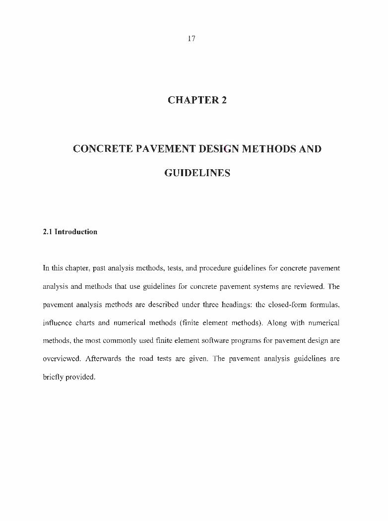
2.1 Introduction

In this chapter, past analysis methods, tests, and procedure guidelines for concrete pavement

analysis and methods that use guidelines for concrete pavement systems are reviewed. The

pavement analysis methods are described under three headings: the closed-form formulas,

influence charts and numerical methods (finite element methods). Along with numerical

methods, the most commonly used finite element software programs for pavement design are

overviewed. Afterwards the road tests are given. The pavement analysis guidelines are

briefly provided.

18

2.2 Pavement Design Methods

Test roads, research, analytical studies, and, most importantly, the observed performance of

pavements in service served as the basis for concrete pavement design practices [2.1].

The first PCC pavement was built in Bellefontaine in Ohio, 1891 by the father of PCC

pavements, George Bartholomev. The first controlled evaluation of concrete pavement

performance was conducted in 1909. The Public Works Department of Detroit (Michigan)

conducted what was probably the first pavement test track. Based on this study, Wayne

County, Michigan paved Woodward A venue with concrete - making it the first mile of rural

concrete in the United States.

Pavement design methods are based on the flexural stress and the findings of test road

sections. Flexural stress is the major design factor for concrete pavements. In early road tests,

such as the Bates road tests (1912 - 1923) and Pittsburg road tests (1921 - 1922), simple

equations relating pavement thickness to traffic loading emerged. These were the beginnings

of so-called "mechanistic-empirical" design procedures (mechanistic - based on computed

pavement response; empirical - calibrated to observe pavement performance) [2.1]. As the

other road tests were conducted more complex solutions were discovered and presented as

influence charts for pavement design. Afterwards, with the introduction of the computer,

numerical methods such as finite element methods for pavement design were developed.

Thus, three methods can be used to determine the stresses and deflections in concrete

pavements: closed-form formulas, influence charts, and numerical methods.

19

2.2.1 Closed-form Formulas

Closed-form formulas are the analytical solutions for determining the stresses and deflections

of rigid pavement systems. The well-known formulas and assumptions are presented below.

2.2.1.1 Goldbeck's Formula

In 1919, Goldbeck [2.2] developed the earliest formula for use in concrete pavement design.

The same equation was applied by Older [2.3] in the Bates road test. Goldbeck's assumption

of the pavement system as a simple cantilever beam with a load concentrated at the corner

yielded his simple equation: for a given concentrated load of P, a cross section at a distance x

from the corner, the bending moment of Px and the width of section is 2x (see Figure 2.1).

When the subgrade support is neglected and the slab is considered as cantilever beam,

Goldbeck' s equation for stresses is as follows:

where,

crc = stress due to corner loading

P = concentrated load

h = thickness

x = distance from the corner

Px 3P ac = _!_(2x)h2 = h2

6

20

/

/ sec E-E .E

max. stress

Figure 2.1 Goldbeck's formula [2.4)

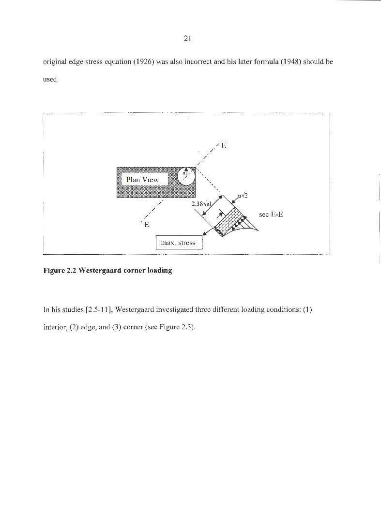
2.2.1.2 Westergaard Theory

Harold Westergaard [2.5] developed closed-form analytical equations for the determination

of stresses and deflections in concrete pavements. His equations can be applied only to large

slabs on a Winkler (or liquid) foundation loaded with a single-wheel load with a circular,

semicircular, elliptical, or semi elliptical contact area (see Figure 2.2). A Winkler foundation

is characterized by a series of springs attached to the plate. Westergaard published his first

equations in 1926, and published his in-depth studies and revised equations in 1927, 1929,

1933, 1939, 1943, and finally in 1948. He published new derived equations in 1948. In 1985,

Ioannides et al. [2.12] demonstrated that Westergaard' s several equations were erroneous,

and provided the correct forms of the equations. Moreover, it was determined that the

21

original edge stress equation (1926) was also incorrect and his later formula (1948) should be

used.

/

/

max. stress

Figure 2.2 Westergaard corner loading

' ' '

/

' ' ' ' ' '

sec E-E

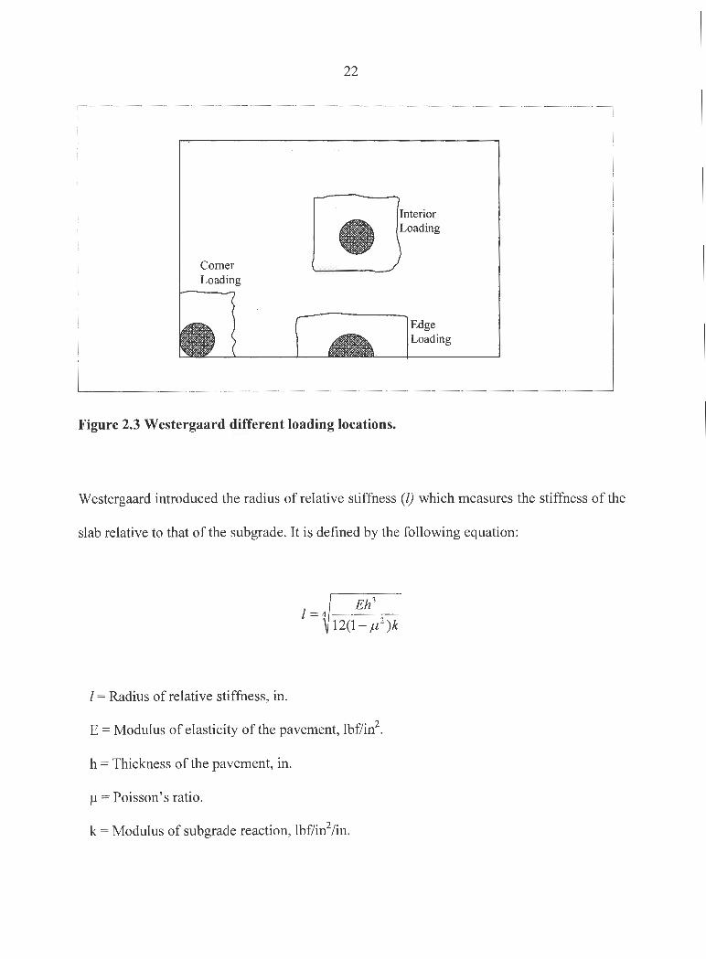
In his studies [2.5-11] , Westergaard investigated three different loading conditions: (1)

interior, (2) edge, and (3) corner (see Figure 2.3).

Comer Loading

22

Figure 2.3 Westergaard different loading locations.

Interior Loading

Edge Loading

Westergaard introduced the radius of relative stiffness (l) which measures the stiffness of the

slab relative to that of the subgrade. It is defined by the following equation:

l = Radius of relative stiffness, in.

Eh 3 f= 4 - ---

12(1- µ 2 )k

E = Modulus of elasticity of the pavement, lbf/in2.

h = Thickness of the pavement, in.

µ = Poisson' s ratio.

k = Modulus of subgrade reaction, lbf/in2/in.

23

For the development of his theory, Westergaard used following assumptions:

• The concrete slab is acting as a homogeneous, isotropic elastic solid in equilibrium.

• The slab cross section is uniform.

• There are no shear or frictional forces .

• There are no in-plane forces.

• The neutral axis is located at the mid-depth of the slab.

• Plain strain assumption is applied.

• Shear deformations are small and can be ignored.

• The slab is considered infinite for the center loading condition and semi-infinite for

the edge loading condition.

• The slab is placed on a Winkler foundation in which the subgrade is represented as

discrete springs beneath the slab.

• The loads at the interior and the comer of the slab are distributed uniformly over a

circular area of contact, whereas the load at the edge of the slab is distributed

uniformly over a semicircular area of contact.

There are also several limitations to this theory listed as follows:

• Only deformations and stresses at interior, edge, and comer locations can be

calculated.

• Shear and frictional forces on the slab surface may actually be quite considerable.

• The Winkler foundation only extends to the edge of the slab. In reality, support is

provided by the surrounding sub-base and subgrade.

24

• The theory assumes that the slab is fully supported. However, voids or discontinuity

exist beneath the slab.

• Load transfer between joints or cracks is not considered in the stress or deflection

calculations.

2.2.2 Influence Charts

Based on Pickett and Ray 's Analysis [2.13] in 1951 influence charts for determining the

stress and deflections in concrete pavements are developed. Pickett and Ray used

Westergaard's theory and developed theoretical solutions for concrete slabs on an elastic half

space and used these solutions in their charts for determining stresses for edge and interior

loading conditions. The use of the charts involves the original configuration of contact area

which is not the circular area but the original tire imprints. The total number of blocks

counted under the contact area related to the estimation of the stress and deflection of the

concrete pavement under that wheel load. These charts were used by the Portland Cement

Association (PCA) for pavement design in 1966. After Pickett and Badaruddin [2.14] a

simple influence chart based on solid foundations was developed.

25

2.2.3 Numerical Methods

Closed-form equations and influ nee charts assume that the slab and subgrade are in full

contact. Due to their simplicity, closed-form equations and influence charts were used to

develop simple equations by Westergaard and other researchers at first. However, because of

the temperature curling and pumping and moisture warping, the slab and subgrade are

usually not in full contact [2.4]. Thus this assumption is unrealistic and does not represent the

actual soil behavior. Later, with the development of computer technology, more realistic

models could be numerically represented. With the advances in computers, new pavement

design methods have been developed for partial contact of the subgrade layer.

Hudson and Matlock [2.15] used a discrete element method to describe the subgrade as a

combination of elastic joints, rigid bars, and torsional bars representing subgrade as dense

liquid. Cheung and Zienkiewic · [2.16] developed finite element methods for analyzing

pavements on elastic foundations. Finite element method solutions were used to convert the

pavement systems into small elements that are connected with structural nodes. The stress

and deflections calculated at each nodes resulted is overcoming the previous models

limitations. Furthermore, Huang and Wang [2.17-18] applied finite element methods on the

jointed slabs on liquid foundations. In 1978 Tabatabaie [2.19] developed the ILLI-SLAB

program. ILLI-SLAB is a finite element program using 2D thin plate elements for the

analysis of pavements. Chou [2.20] developed finite element programs called WESLIQUID

and WESLA YER for the analysis of the liquid and layered foundations, respectively. RISC,

KENSLAB and KENLA YER were the other finite elements methods using 2D thin plate

26

elements. Recently Chen et al. [2.21} and General Accounting Office in 1997 both have

used the 3D finite element modeling for pavement design. Although there are many

advantages of using a 3D finite element, due to the computational difficulties and complex

modeling problems, they are not adopted for pavement analysis. Commonly used ILLI­

SLAB, WELIQUID and WESLA YER, RISC and KENSLABS finite element computer

programs are described as fo llows.

2.2.3.1 ILLI-SLAB Finite Element Model

The most widely used and verified 2D thin plate finite element program, the ILLI-SLAB,

was developed at the University of Illinois in the late 1970' s for the structural analysis of

jointed concrete slabs consisting of one or two layers, with either smooth interface or

complete bonding between layers. The model was based on the classical theory medium thick

elastic plate on top of a Winkler foundation in its original version. Later the model was

revised and improved through several research studies. These studies resulted in the addition

of different subgrade models [2.22-23] and in the addition of added capability of linear and

non-linear temperature loadings of multi slab layered pavements [2.24] . The program can

handle up to 10 slabs in each direction, with joints treated as rectangular elements with zero

width. The capabilities of the ILLI-SLAB provide several options for analyzing the following

pavement design models:

• Multiple axle loads in any configuration, and axles in any location on the slab

27

• Jointed plain concrete pavements with longitudinal and transverse cracks with

different Load transfer efficiencies (L TE)

• Variable concrete slabs, subgrade supports

• A linear temperature gradient in uniformly thick slabs

• Concrete shoulders with or without tie bars.

2.2.3.2 WESLIQUID and WESLA YER Finite Element Models

In collaboration with Huang and Chou (2.20] developed the WESLIQUID and WESLA YER

in 1981 at Waterways Experiment Station. The WESLIQUID finite element computer

program was developed for the analysis of concrete pavements subjected to the multiple­

wheel loads and temperature gradients. WESLA YER, on the other hand, was developed for

the computation of state of the stress in a rigid supported on an elastic solid or layered elastic

foundation. WESLA YER's method of solution is very similar to the WESLIQUID.

WESLIQUID model employs a Winkler foundation, whereas the foundation is considered to

be layered in WESLA YER which is more realistic when layers of base and sub-base exist

above the subgrade. Multiple slabs and two layer systems with bonded or un-bonded

interfaces can be analyzed by WESLIQUID. Slab thicknesses and subgrade moduli may vary

from node to node. Curling analysis can be performed under a linear temperature distribution

through the thickness of a one or two layer system in both models.

28

2.2.3.3 RISC Finite Element Model

RISC finite element program was developed in 1983 by Majidzadeh et al. [2.25] as a part of

a mechanistic design procedure for rigid pavements. It is based on coupling of a finite

element slab on top of a multilayer elastic solid foundation where the slab is represented by

thin shell elements. Pavement materials were modeled as linearly elastic, and environmental

effects were also considered through the AASHTO regional factor by modifying traffic.

RISC is capable of analyzing various rigid pavement sections with various thicknesses and

various base, sub-base, and subgrade.

2.2.3.4 KENSLABS Finite Element Model

KENSLABS was developed by Huang [2.26} at the University of Kentucky. It can analyze

nine slabs with shear and moment transfer across the joints. The program can model slabs on

liquid, solid, or layered foundations. It can analyze two layers and slab thickness can vary

from node to node or from slab to slab. The unique feature of the program is its ability to

perform a damage analysis with up to 24 seasonal periods per year.

29

2.2.4 Road Tests

The mid 1940s was the start of a new era for pavement design methodologies based on the

large scale road tests. The design methods were developed from the observed performance of

the pavements under controlled conditions during the road tests. Pavement engineers had the

chance for a better understanding of pavement performance under different conditions. All

road tests were supervised by the Highway Research Board with the assistance of universities

and other trade associations. A few of the more pertinent findings of such test roads which

have led or will lead to changes in pavement design include (1) the Maryland road test for

rigid pavements, (2) the WASHO road test for flexible pavements, and (3) the AASHO road

test for both rigid and flexible pavements. The Maryland road test and AASHO road test

were presented in brief, and then the limitations of AASHO test were discussed.

2.2.4.1 Maryland Road Test

The Maryland road test was conducted in 1950 on a 1.1 mile section of US 301 located

approximately 9 miles south of La Plata, Maryland. The aim of this road test was to

determine the relative effects of four different axle loadings using two vehicle types on a

specific concrete pavement design [2.27]. The loads employed were 18,000 pounds and

22,400 pounds on single axles, and 32,000 pounds and 44,000 pounds on tandem axles.

These loadings were selected to represent conditions of expected future values on these

roads. The major findings indicated that the pumping was the major distress for the

30

pavements on fine-grained soils. The stresses formed on the slab were increased extremely

and caused rupture on the slab after pumping occurred.

2.2.4.2 AASHO Road Test

The AASHO road test was the last of the major road tests in the United States, conducted

from 1958 to 1960 near Ottawa, Illinois about 80 miles southwest of Chicago [2 .28]. The aim

of this road test was to identify the relationship between the number of repetition of specified

axle loads with different magnitudes and arrangements and pavement thickness. This road

test involved both rigid and flexible pavements. Planning the project began about 1950, the

site was selected in 1954; construction was carried between 1956 and 1958. Testing began in

October 1958 and ended 1960 and data analysis and final reporting were completed in 1962.

In all, the test road contained six loops, each with two lanes. Single-axle loadings ranged

from 2,000 to 30,000 lb; tandems from 24,000 to 48,000 lb. Field testing and measurement,

laboratory work, and analysis of data made use of the most modern equipment and statistical

methods. The final reports totaled more than 1600 pages. One of the important findings of

the AASHO road test was that the engineers developed the concept of "serviceability ratings"

which the smoothness and ride-ability of the various pavement sections were keyed.

31

2.2.4.2.1 Limitations

The AAS HO road test was the most comprehensive of the road tests, yet it was still limited to

the influence of only the environment of Central Illinois, the roadbed soil of Central Illinois,

and the materials of Central Illinois which were used to construct the pavement sections. One

immediate concern was to develop expanded criteria which would allow different conditions

and materials to be considered in the design process. Components of the design procedure

requiring local verification include:

• Climate

• Soil properties

• Material properties

The basic principles established and validated by the road test still serve as the basis for a

large number of performance-based design procedures being used in the United States today.

The AASHTO interim guide design for rigid and flexible pavement, Corps of Engineers,

Louisiana, Utah, and Kentucky designs are among a large family of pavement design

techniques which were primarily developed on the basis of field performance taken from the

road test. Their popularity indicates the usefulness of the data collected on the road test.

32

2.3 Pavement Design Guides

The most widely used procedure for design of concrete pavements is specified in the Guide

for Design of Pavement Structures published in 1986 and 1993 by the American Association

of State Highway and Transportation Officials (AASHTO) [2.29-30]. The 1993 version

differs from the 1986 version only in the overlay design chapter. Only a few states use the

1972 AASHO Interim Guide procedure [2.31] or the Portland Cement Association (PCA)

procedure [2.32] or their own empirical or mechanistic-empirical procedure, or a design

catalog.

2.3.1 AASHTO Design Guides for Pavement Structures

Based on the Results of AASHO road tests an empirical pavement design guide, the 1972

AASHO Interim guide, was published. Basically, the number of axle load applications are

used as a function of the slab thickness, axle type (single or tandem) and weight, and terminal

serviceability. This original model applies only to the designs, traffic conditions, climate,

subgrade, and materials of the AASHO road test. In later versions, it has been extended to

make possible the estimation of allowable axle load applications to a given terminal

serviceability level for conditions of concrete strength, subgrade k-value, and concrete E

different than those of the AASHO road test. The AASHTO design methodology has also

been extended to accommodate the conversion of mixed axle loads to equivalent 80-kN (18-

kip) equivalent single axle loads (ESALs) through the use of load equivalency factors. The

33

loss of serviceability that corresponds to a predicted number of axle load applications does

not include any contribution of faulting to pavement roughness because the AASHO road test

experienced substantial loss of support. The design loss of serviceability is assumed to be

entirely due to slab cracking.

2.3.1.1 AASHTO Design Guide-1986-1993

Due to the limitations of the 1972 interim Design Guide, extensive revisions were made to

include more fundamental concepts (some recommended in mechanistic approaches) and

extend the applicability of the design procedure. These revisions include:

1. Replacement of soil support value and the modulus of subgrade reaction with the

modulus of resilience for both flexible and rigid pavements.

2. The inclusion of design reliability.

3. The use of resilient Modulus testing to select layer coefficients for flexible

pavements.

4. Drainage has been included through recognition of the impact of drainage on

performance and suitable adjustments to material properties.

5. Improved environmental design has been included for frost heave, swelling soils,

and thaw weakening.

6. Load transfer can be designed for in rigid pavements.

34

7. Life-cycle cost information has been included for use in evaluating alternate

designs.

Other items in the design guide which have been added or expanded include rehabilitation,

pavement management, load equivalency factors, traffic considerations, and low volume road

design.

2.3.1.2 Supplement to AASHTO Design Guide-1998

The revised AASHTO design model for concrete pavements presented in the 1998

Supplement to the AASHTO Guide (2.33] was developed under NCHRP Project 1-30 [2.34]

and field-validated by analysis of the GPS-3, GPS-4, and GPS-5 (JPCP, JRCP, and CRCP)

sections in the Long-Term Pavement Performance (LTPP) studies [2.35].

The purpose of the NCHRP Project 1-30 study was to evaluate and improve the AASHTO

Guide's characterization of subgrade and base support. The original AASHO empirical

model was calibrated to the springtime k-value measured in plate load tests on the granular

base, whereas the 1986 Guide's method for determining the design k-value was based on a

seasonally adjusted annual average k-value. A key recommendation of the 1-30 study was

that, subgrade model under rigid pavement design module should be characterized by the

seasonally adjusted annual average static elastic values. The 1998 AASHTO Supplement

presents guidelines for determination of an appropriate design k-value on the basis of plate

35

be.aring tests, correlations with soil types andyroperties, CBR, or deflections measured on in­

service pavements. It is recommended in the 1998 AASHTO Supplement that both the

beneficial and detrimental effects of a granular or treated base and the computation of slab

stress in response to load as well as temperature and moisture gradients should be considered.

2.3.2 Portland Cement Association (PCA) Guidelines

The PCA procedure was developed using the results of finite element analyses of stresses

induced in concrete pavements by joint, edge, and comer loading. The PCA procedure, like

the 1986-1993 AASHTO procedure, employs the "composite IC' concept in which the design

k is a function of the subgrade soil k, base thickness, and base type (granular or cement

treated). The pavement design procedure has control criteria with respect to two potential

failure modes: fatigue and erosion.

The fatigue analysis incorporates the assumption that approximately 6% of all truck loads

will pass sufficiently close to the slab edge to produce a significant tensile stress. The fatigue

model was changed to eliminate a discontinuity in the high load levels in the current PCA

procedure. The erosion analysis quantifies the rate of work with which a slab comer is

deflected by a wheel load as a function of the slab thickness, foundation k-value, and

estimated pressure at the slab-foundation interface. An additional safety factor can be applied

to the axle load levels used in the fatigue and erosion analyses to account for the more

significant consequences of error in traffic prediction for higher-volume facilities. An

36

adequate thickness is one for which the sum of the contributions of all axle load levels to

fatigue and erosion damage is less than 100%.

2.3.3 Mechanistic-Empirical Pavement Design Methods

Mechanistic pavement design procedures are based on mechanics of materials equations that

relate an input to pavement response such as stress, strain or deformation (see chapter 1 ).

Laboratory testing is often included to provide relationship between loadings and failure.

Empirical design methods (see chapter 1) typically relate observed field performance to

design variables, such as a road test. Mechanistic-empirical design approaches combine the

theory and physical testing with the observed performance to design the pavement structure.

The basis of a mechanistic-empirical design procedure is to analytical calculation of the

stress or strain and transfer these mechanistic stress, strain to the pavement responses using

transfer functions to predict distresses resulting from the response. Transfer functions can be

developed from laboratory test data or they can be based on observed performance data

collected in the field. As more distress survey data becomes available, theoretical models

may be more accurately calibrated to represent observed performance models. Calibration

with field performance is a necessity for accurate designs as theory alone has not proven

sufficient to design pavements realistically.

37

2.3.4 Design Catalogs

A design catalog does not present a thickness design procedure by itself. It is a format for

recommended thicknesses and other design details. A design catalog for both flexible and

rigid pavements in the United States was developed under NCHRP Project 1-32 [2.40] .

2.3.5 Other Methods

Other concrete pavement design methods are rangmg from empirical methods to

mechanistic-empirical methods. Most notable among the mechanistic-empirical methods are

the zero-maintenance design procedure [2.36-37] and the NCHRP Project 1-26 procedure

[2.38-39].

38

2.4 References

[2.1] http: //www.pavement.com/PavTech/ AbtConc/History/Evolution.html, "Evaluation of

Concrete Road Design in the United States" American Concrete Pavement Association,

2001

[2.2] Goldbeck, A.T., 1919" Thickness of Concrete Slabs" Public Roads, pp. 34-38

[2.3] Older, C. 1924, "Highway Research in Illinois" Transactions, ASCE, Vol. 12, No. 2,

pp. 124-130

[2.4] Huang, Y. H., "Pavement Analysis and Design ", 2nd Edition, Pearson Education,

Inc. 2004

[2.5] Westergaard, H. M. 1926a, "Analysis of Stresses in Concrete Pavement Due to

Variations ofTemperature" Proceedings, Highway Research board, Vol. 6. pp 201-215

[2.6] Westergaard, H. M. 1926b, "Stresses in Concrete Pavements Computed by

Theoretical Analysis" Public Roads, Vol. 7. pp 25-35

[2.7] Westergaard, H. M. 1927, "Theory of Concrete Pavement Design" Proceedings,

Highway Research board, Part 1. pp 175-181

[2.8] Westergaard, H.M. 1933. "Analytical Tools for Judging Results of Structural Tests of

Concrete Pavements" Public Roads, Vol.14, No.I 0, pp. 185-188

[2.9] Westergaard, H.M., 1939. "Stresses in Concrete Runways of Airports" Proceedings,

Highway Research Board, Vol.19, pp 197-202

[2.10] Westergaard, H.M., 1943 . "Stress Concentrations in Plates Loaded over Small

Areas" Transactions, ASCE, Vol. I 08, pp. 831-856

39

[2.11] Westergaard, H.M., 1948. "New Formulas for Stresses in Concrete Pavements of

Airfields" Transactions, ASCE, Vol. 113, pp.425-444

[2.12] Ioannides, A. M., M. R. Thompson, and E. J. Barenberg, 1985. "Westergaard

Solutions Reconsidered'' Transportation Research Record 1043, pp. 13-23,

Transportation Research Board

[2.13] Pickett, G.K. Ray 1951, "Influence Charts for Concrete Pavement" Transactions

ASCE, Vol. 116, pp. 49-73

[2.14] Pickett, G., S. Badaruddin 1956, "Influence Chart for Bending of a semi-infinite

Pavement Slab" Proceedings, Ninth International Congress on Applied Mechanics, Vol.

6, pp. 396-402

[2.15] Hudson, W. R., H. Mattlock, 1966, "Analysis of Discontinuous Orthotropic Pavement

Slabs Subjected to Combined Loads" Highway Research Record 131 , pp. 1-48, Highway

Research Board.

[2.16] Cheung, Y. K., 0. C., Zienkiewicz, 1965 "Plates and Tanks on Elastic Foundations­

An Application of Finite Element Method' International Journal of Solids and Structures,

Vol. 1, pp 451-461

[2.17] Huang Y. H., S. T., Wang, 1973, "Finite Element Analysis of Concrete Slabs and Its

Implications for Rigid Pavement Design " Highway Research Record 466, pp. 55-69,

Highway Research Board

[2.18) Huang Y. H., S. T., Wang, 1974, "Finite Element Analysis of Rigid Pavements with

Partial Subgrade Contact" Transportation Research Record 485, pp. 39-54,

Transportation Research Board

40

[2.19] Tabatabaie, A.M., 1978 "Structural Analysis of Concrete Pavement Joints" Ph. D.

Thesis, University of Illinois, Urbana-Champaign

[2.20] Chou, Y.T., 1981. "Structural Analysis Computer Programs for Rigid

Multicomponent Pavement Structures with Discontinuities- WESLJQUJD and

WESLAYER" Technical Report GL-81-6, Reports 1,2, and 3, U.S. Army Engineer

Waterways Experiment Station

[2.21] Chen, D. H. Z., Musharraf, J. Laguros, Alan Soltani, 1995, "Assessment of Computer

Programs for Analysis of Flexible Pavement Structure" Transportation Research Record

1482, pp. 123-133, Transportation Research Board

[2.22] Ioannides, A. M., 1984. "Analysis of Slabs-On-Grade for a variety of Loading and

Support Conditions" Ph. D. Thesis, University of Illinois, Urbana-Charp.paign

[2.23] Khazanovich, L., Ioannides, A. M., 1993. "Finite Element Analysis of Slabs-On­

Grade Using Higher Order Subgrade Models" Proceedings of 1993 Airfield Pavement

Committee Conference, American Society of Civil Engineers, New York

[2.24] Korovesis, G. T., 1990. "Analysis of Slabs-On-Grade Systems Subjected to Wheel and

Temperature Loadings" Ph.D. Thesis, University of Illinois, Urbana-Champaign

[2.25] Majidzadeh, K. J. , Ilves, G. J. , Sklyut, H., 1984, "Mechanistic Design of Rigid

Pavements, Vol. I, Development of the Design Procedures" Report No. FHWA-RD-86-

124, Vol. 2, "Design and Implementation Manual" Report No. FHWA-RD-86-235,

Federal Highway Administration

[2.26] Huang Y. H., 1985, "A Computer Package for Structural Analysis of Concrete

Pavements" Proceedings, 3rd International Conference on Concrete Pavement Design and

Rehabilitation, pp. 295-307, Purdue University

41

[2.27] HRB, 1952, "Final Report on Road Test One MD" Highway Research Board

[2.28] HRB, 1962, "The AASHO Road Test" Highway Research Board

[2.29] AASHTO, "Guide for Design of Pavement Structures. American Association of State

Highway and Transportation Officials, Washington, D.C., 1986

[2.30] AASHTO, "Guide for Design of Pavement Structures. American Association of State

Highway and Transportation Officials, Washington, D.C., 1993

[2. 31] AASHTO, "Interim Guide for Design of Pavement Structures". American

Association of State Highway Officials, Washington, D.C., 1972

[2.32] PCA, "Thickness Design/or Concrete Highway and Street Pavements ". EB109.01P.

Portland Cement Association, Skokie, Ill., 1984

[2.33] AASHTO, "Supplement to the AASHTO Guide for Design of Pavement Structures,

Part II- Rigid Pavement Design and Rigid Pavement Joint Design". American

Association of State Highway and Transportation Officials, Washington, D.C., 1998

[2.34] Darter, M. I., K. T. Hall, and C. M. Kuo. NCHRP Report 372: "Support Under

Portland Cement Concrete Pavements ". TRB, National Research Council, Washington,

D.C., 1997

[2.35] Hall, K. T., M. I. Darter, T. E. Hoerner, and L. Khazanovich. "LTPP Data Analysis

Phase I: Validation of Guidelines for k Value Selection and Concrete Pavement

Performance Prediction." Report FHWA-RD-96-168. FHWA, U.S. Department of

Transportation, 1997

[2.36] Darter, M. I. "Design of Zero-Maintenance Plain Jointed Concrete Pavement,

Volume I- Development of Design Procedure." Report FHWA-RD-77-111. FHWA,

U.S. Department of Transportation, 1977

42

[2.37] Darter, M. I., and E. J. Barenberg. "Design of Zero-Maintenance Plain Jointed

Concrete Pavement, Volume 2- Design Manual. " Report FHWA-RD-77-112. FHWA,

U.S. Department of Transportation, 1977

[2.38] Barenberg, E. J., and M. R. Thompson. "Calibrated Mechanistic Structural Analysis

Procedures for Pavements." NCHRP Project 1-26. TRB, National Research Council,

Washington, D.C., 1992

[2.39] Salsilli, R. A., E. J. Barenberg, and M. I. Darter. "Calibrated Mechanistic Design

Procedure to Prevent Transverse Cracking of Jointed Plain Concrete Pavements." In

Proceedings, Fifth International Conference on Concrete Pavement Design and

Rehabilitation, Purdue University, West Lafayette, Ind., 1993

[2.40] Darter, M. I., H. L. Von Quintus, Y. J. Jiang, E. B. Owusu - Antwi, and B. M

Killingsworth. "Catalog of Recommended Design Features " (CD-ROM). NCHRP

Project 1-32. TRB, National Research Council, Washington, D.C., 1997

43

CHAPTER3

INPUT PARAMETERS FOR THE MECHANISTIC­

EMPIRICAL PAVEMENT DESIGN GUIDE

3.1 Introduction

Many design methods do not consider the effect of different climatic locations and material

characteristics. This is due to the limited conditions of the AASHO road test in terms of one

climate, and one soil condition. In this chapter, the major rigid pavement design input

parameters of the mechanical-empirical pavement design guide (MEPDG) are discussed in

detail. The rigid pavement design inputs are described under three major categories: (1)

Traffic, (2) Climate, and (3) Material inputs. Another aspect of the MEPDG described in this

chapter is the hierarchical approach to the design inputs, which is not found in the AASHTO

design guides. With this approach, the inputs are separated into three levels as stated in

MEPDG [3 .1] .

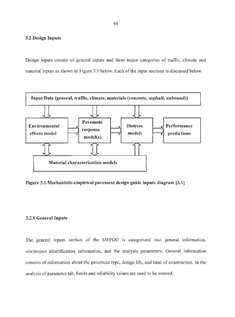
44

3.2 Design Inputs

Design inputs consist of general inputs and three major categories of traffic, climate and

material inputs as shown in Figure 3.1 below. Each of the input sections is discussed below.

Input Data (general, traffic, climate, materials (concrete, asphalt, unbound))

.. 7' .. ~ ........ 7'

Pavement Environmental ~ ~ Distress ~ Performance

effects model -----v response

models predictions model(s)

r--v r--v

...::"'"~ ...::"'" ...::"'"~

'-7 .. Material characterization models

Figure 3.1 Mechanistic-empirical pavement design guide inputs diagram [3.1)

3.2.1 General Inputs

The general inputs section of the MEPDG 1s categorized into general information,

site/project identification information, and the analysis parameters. General information

consists of information about the pavement type, design life, and time of construction. In the

analysis of parameter tab, limits and reliability values are need to be entered.

45

3.2.2 Traffic Module

Traffic data is one of the most essential aspects of pavement design. Traffic data required by

the MEPDG are in agreement with the Traffic Monitoring Guide (I'MG). The traffic loads

applied to pavement during its design life and the frequency of vehicle loads is calculated by

using the traffic data. The equivalent single axle load (ESAL) used in the different versions

of the AASHTO Guide for Pavement Design is not applicable in the MEPDG. MEPDG

outputs the accumulated amount of heavy traffic on a monthly basis for the magnitude of

truck traffic loadings in the design lane [3 .1] .

3.2.2.1 Traffic Characterizations Sources

Traffic data is collected by three different methods: (1) weigh-in-motion (WIM), (2)

automatic vehicle classification (A VC), and (3) vehicle counts. This data can be augmented

by traffic estimates computed using traffic forecasting and trip generation models. Following

are the main sources of traffic data that are typically used for the traffic characterization in

theMEPDG.

46

3.2.2.1.1 Weight-In-Motion (WIM) Data

WIM data, providing traffic data over a period of time, includes:

• Vehicle type and the number

• Speed

• Axle weights and gross weight

• Axle spacing

3.2.2.1.2 Automatic Vehicle Classification (AVC) Data

A VC data includes the number and types of vehicles counted over a period of time. A VC

data is used to determine the normalized truck class distribution. A VC data can be Level 1 to

3 depending on where the data is collected.

3.2.2.1.3 Vehicle Counts

Vehicle counts are a count of the total number of vehicles categorized by passenger vehicles,

buses, and trucks over a period of time. Vehicle counts are used when detailed truck traffic

data are unavailable. Thus, it can be either input level 2 or level 3 based on the specific

location (site-specific, regional/statewide, or national) where data is collected.

47

3.2.2.1.4 Traffic Forecasting and Trip Generation Models

Traffic forecasting and trip generation models can be used for estimation of Level 1 or Level

2 type of data used in the MEPDG depending on their calibration of site-specific or

regional/statewide data.

3.2.2.2 Traffic Characterization Inputs

Four basic types of traffic data are required for pavement structural design: (1 ) Traffic

volume, (2) Traffic volume adjustment factors, (3) Axle load distribution factors, and (4)

General traffic inputs (see Figure 3.2).

Trame 613

Design Life [years): j2s , ~

Percent of trucks in design lane 1%)?· jso.o

·fl Edit I Axle load distribution factor: .. [SJ Ed/ I General Traffic Inputs ~

Traffic G rowlh ;: I compound, 4%

./ DK X Cancel

-160 __ _

Figure 3.2 Screenshot of MEPDG software for traffic characterization inputs

48

3.2.2.2.1 Traffic volume

The base year for the traffic inputs is defined as the first calendar year that the roadway

segment under design is opened to traffic. The following base year information is required:

• Two-way annual average daily truck traffic (AADTT).

• Number of lanes in the design direction.

• Percent trucks in design direction.

• Percent trucks in design lane.

• Vehicle (truck) operational speed.

3.2.2.2.1.1 Two-Way Annual Average Daily Truck Traffic (AADTT)

The total number of heavy vehicles of classes 4 to 13 in the traffic stream passing a point or

segment of a road in both directions during a 24-hour period is called two-way annual

average daily truck traffic (AADTT). It is commonly obtained simply by dividing the total

number of truck traffic of the given time period by the number of days in that time period.

Base year AADTT is defined as Level 1, 2 or 3. The input level is based on the level of the

sources (WIM, AVC, Vehicle Counts, or Traffic forecasting and trip generation models).

Local experience is also considered as Level 3 data.

49

3.2.2.2.1.2 Number of Lanes in the Design Direction

The number of lanes in the design direction is determined from design specifications and

represents the total number of lanes in one direction.

3.2.2.2.1.3 Percent Trucks in Design Direction

This design input defines the percentage of trucks in the design direction. The directional

distribution factor (DDF) can be used to calculate the difference in the different directions. It

is usually assumed to be 50% when traffic is given in two directions; however, this is not

always the case. The MEPDG software provides a default value (Level 3) of 55% for

interstate-type facilities computed using traffic data from the LTPP database [3 .2-3]. The

levels of input for percent trucks in design direction are defined Level 1 through 3 depending

on the level of DDF determined from traffic source levels.

3.2.2.2.1.4 Percent Trucks in Design Lane

Percent trucks in the design lane, or truck lane distribution factor (LDF), accounts for the

distribution of truck traffic between the lanes in one direction. For two-lane, two-way

highways (one lane in one direction), this factor is 1.0 because all truck traffic in any one

direction must use the same lane. For multiple lanes in one direction, it depends on the

50

AADTT and other geometric and site-specific conditions. The level of input for LDF is

based on the source data. [3 .1]

The default (Level 3) values recommended for use based on the LDF for the most common

type of truck (vehicle class 9 trucks) is as follows:

• Single-lane roadways in one direction, LDF = 1.00.

• Two-lane roadways in one direction, LDF = 0.90.

• Three-lane roadways in one direction, LDF = 0.60.

• Four-lane roadways in one direction, LDF =0.45.

3.2.2.2.1.5 Vehicle Operational Speed

The average vehicle speed in the MEPDG is given as 60 mph, but this value can be modified

to reflect local conditions. A description of a detailed methodology used for determining

operational speeds can be found in the Transportation Research Board Highway Capacity

Manual or AASHTO's A Policy on Geometric Design of Highways and Streets (often called

the "Green Book") [3 .4-5].

51

3.2.2.2.2 Traffic Volume Adjustment Factors

The following truck-traffic volume adjustment factors are required for traffic

characterization:

• Monthly adjustment.

• Vehicle class distribution.

• Hourly truck distribution.

• Traffic growth factors.

3.2.2.2.2.1 Monthly Adjustment Factors

Truck traffic monthly adjustment factors are the percentage of the annual truck traffic for a

given truck class in a specific month. Monthly adjustment factors (MAF) can be calculated

regardless of the source of the data (WIM, A VC, vehicle count, and so on), each for different

types of highways as follows [3 .1]:

• For the given traffic data (24-hour of continuous data collection), determine the

total number of trucks (in a given class) for each 24-hour period. If data were not

collected for the entire 24-hour period, the measured daily truck traffic should be

adjusted to be representative of a 24-hour period.

• Using representative daily data collected for the different months within a year,

determine the average daily truck traffic for each month in the year.

• Sum up the average daily truck traffic for each month for the entire year.

52

• Calculate the monthly adjustment factors by dividing the average daily truck

traffic for each month by summing the average daily truck traffic for each month

for the entire year and multiplying it by 12 as given below:

MAF = AADT'F; * 12 I ]2

LAADT'F; i= l

Where,

monthly adjustment factor for month i

AADTTi AADTT for month i

The sum of the MAF of all months must equal 12. Pavement designs can be sensitive to

MAF. If no information is available, it is recommended that designers assume an even or

equal distribution (i.e ., 1.0 for all months for all vehicle classes).

3.2.2.2.2.2 Vehicle Class Distribution

The data obtained from such AVC, WIM, and vehicle counts are used to obtain vehicle

classification. Figure 3.3 shows the standard vehicle classes that have been used for FHWA

and LTPP [3.2-3].

53

FHWA VEHICLE CLASSIFICATIONS 1 XoLorcyc1es 2 p,., ,~nq~r Car ' 3rvo Atle. i Tir< S 1 n~l• 1 Bes es

\.,"11t ,.

~ ~ ~~ B 5 1'vo .1 t l t> . 6 Tl rt! St nq l c 6 Three Atl< 51n1 1< U:t1ls 7 Tour or no re Arl e 51n~ l c 8 rour or ~., , J.t h 5tnql•

j..., !t1!: er .. · ~·

La ES woo-~ ~ 6 ~ ~ 0 ~@r@~ © . ~rr- .1.oJ 9 rive t t te S1nqle Trailers 10 S'it Ct' ?So re Ad t Sl ·i'ql e T r• i ltH'l 11 rtve o r Lt'$1 Atlr: f.'.:lt: ..- TC'A l le r s

I ~ ( I~ I Jf!a .0019 (Old . (Q (0)-Z) C' . 0 12 511 lcle n~ l Lt-7r~t lec~

t3-, - Se te n or l'ro re >.. r te t1 u lL1·"'ira1l r rs

[ JC ~ H ~ co o-oa 6CfQ

Figure 3.3 Illustrations and definitions of the vehicle classes used for collecting traffic

data that are needed for design purposes [3.1].

3.2.2.2.2.3 Truck Hourly Distribution Factors

The hourly distribution factors (HDF) represent the percentage of the traffic within each hour

of the day. The sum of the percent of daily truck traffic per time increment must add up to

100 percent.

54

3.2.2.2.2.4 Traffic Growth Factors

Traffic growth factors represent the future estimates of the traffic data. The MEPDG software

allows users to use three different traffic growth functions to compute the growth or decay in

truck traffic over time (forecasting truck traffic). The three functions provided to estimate

future truck traffic volumes are presented as follows:

Where;

AADTTx = 1.0 * AADTT8 y (No growth)

AADTTx = GR* AGE+ AADTT8 y (Linear growth)

AADTTx = ADTT8 y * (GR) AGE (Compound growth)

AADTT x = Annual average daily truck traffic at age X

GR= Traffic growth rate

AADTT sv = Base year annual average daily truck traffic

3.2.2.2.3 Axle Load Distribution Factors

The axle load distribution factors basically correspond to the percentage of the total axle

applications within each load interval for a specific axle type (single, tandem, tridem, and

55

quad) and vehicle class (classes 4 through 13). The load intervals for each axle type are

provided below [3 .1] :

• Single axles - 3,000 lb to 40,000 lb at 1,000-lb intervals.

• Tandem axles - 6,000 lb to 80,000 lb at 2,000-lb intervals.

• Tridem and quad axles - 12,000 lb to 102,000 lb at 3,000-lb intervals.

3.2.2.2.4 General Traffic Inputs

General traffic inputs can be summarized as follows:

• Lateral traffic wander

• Number of axle types per truck class

• Axle configuration

• Wheel base

3.2.2.2.4.1 Lateral Traffic Wander

Traffic wander effect is defined with 3 inputs: (1) Mean wheel location, (2) Traffic wander

standard deviation, and (3) Design lane width. The Mean wheel location is the distance from

the outer edge of the wheel to the pavement marking. 18 inch of recommended default value

is provided with the MEPDG software. Traffic wander standard deviation is the statistic

56

describing how tightly the lateral traffic wander is clustered around the mean wheel location.

A default (Level 3) mean truck traffic wander standard deviation of 10 inches is provided in

the MEPDG software. This is recommended if more accurate information is not available.

Design lane width is the parameter that refers to the actual traffic lane width, as defined by

the distance between the lane markings on either side of the design lane. It is a design factor

and may or may not equal the slab width. The default value for standard-width lanes is 12 ft.

[3.1]

3.2.2.2.4.2 Number of Axle Types per Truck Class

This input represents the average number of axles for each truck class (class 4 -13) for each

axle type (single, tandem, tridem, and quad). The inputs at different levels are based on the

traffic source data.

3.2.2.2.4.3 Axle Configuration

A series of data elements are needed to describe the configurations of the typical tire and axle

loads that would be applied to the roadway because computed pavement responses are

generally sensitive to both wheel locations and the interaction between the various wheels on

a given axle. These data elements can be obtained directly from manufacturers databases or

57

measured directly in the field. Typical values are provided for each of the following

elements; however, site-specific values may be used, if available.

• Average axle-width - the distance between two outside edges of an axle. For

typical trucks, 8.5 ft may be assumed for axle width.

• Dual tire spacing - the distance between centers of a dual tire. Typical dual tire

spacing for trucks is 12 in.

• Axle spacing - the distance between the two consecutive axles of a tandem,

tridem, or quad. The average axle spacing is 51.6 inches for tandem and 49.2

inches for tridem and quad axles.

3.2.2.2.4.4 Wheelbase

Vehicles wheelbase can be obtained directly from manufacturer ' s database or measured in

the field. Typical values are provided for the average axle spacing and percent of trucks are

provided as follows [3 .1]:

• Average axle spacing (ft) - short, medium, or long. The recommended values are

12, 15, and 18 ft for short, medium, and long axle spacing, respectively.

• Percent of trucks in class 8 - 13 with the short, medium, and long axle spacing -

use even distribution (e.g., 33, 33 , and 34% for short, medium, and long axles,

respectively), unless more accurate information is available.

58

3.2.3 Climate Module

The environmental effects on pavements and pavements' reaction to the environmental

conditions have an important effect on the design of rigid pavements. The required

parameters can be defined as internal and external inputs. The external inputs are

precipitation, temperature, freeze-thaw cycles, and depth of water table. The pavement

reactions such as the susceptibility of the pavement materials to moisture and freeze-thaw

damage, and drainability and infiltration properties of pavement layers are called internal

inputs. These required input parameters are created through a sophisticated climatic modeling

tool called the Enhanced Integrated Climatic Model (EICM). The necessary climate inputs

are the climatic locations. There are already large numbers of defined locations in the

MEPDG but also using latitude and longitude, the climatic data can be generated by

extrapolating nearby weather stations (see Figure 3.4). MEPDG software provided 15

climatic weather stations for Iowa including Ames, Des Moines, Iowa City. The program

reads hourly climatic information during the analysis stage. The climate file contains the

sunrise time, sunset time and radiation for each day of the design life period. In addition, for

each 24-hour period in each day of the design life, the temperature, rainfall, air speed,

sunshine, and depth of ground water table are also listed in the climate file. With this

information, the EICM computes and predicts the following information for pavement layers:

temperature, resilient modulus adjustment factors, pore water pressure, water content, frost

and thaw depths, frost heave, and drainage performance.

59

Environment/ Cl1matlc 0£!

Current climatic. data file:

Gen er ate new climatic data file

Cancel

r- . Latitude {degrees.minutes)

j '. \ :.,j,ongitude (degrees.minutes)

"r- Elevation (ft)

r

Figure 3.4 Screenshot of climatic module of the MEPDG software

3.2.4 Materials Module

The major categorical system developed for the M-E Pavement Design Guide is presented in

Table 3 .1. Six major material groups have been developed: asphalt materials, PCC materials,

cementitiously or chemically stabilized materials, non-stabilized granular materials, subgrade

soils, and bedrock.

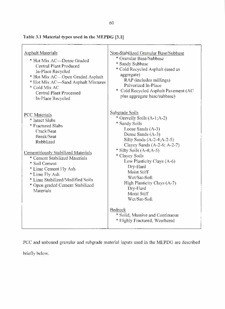
60

Table 3.1 Material types used in the MEPDG [3.1)

Asphalt Materials Non-Stabilized Granular Base/Subbase

* Hot Mix AC-Dense Graded * Granular Base/Subbase

Central Plant Produced * Sandy Subbase

In-Place Recycled *Cold Recycled Asphalt (used as

* Hot Mix AC- Open Graded Asphalt aggregate)

*Hot Mix AC-Sand Asphalt Mixtures RAP (includes millings)

*Cold Mix AC Pulverized In-Place

Central Plant Processed * Cold Recycled Asphalt Pavement (AC

In-Place Recycled plus aggregate base/sub base)

PCC Materials Subgrade Soils

* Intact Slabs * Gravelly Soils (A-1 ;A-2)

* Fractured Slabs * Sandy Soils

Crack/Seat Loose Sands (A-3)

Break/Seat Dense Sands (A-3)

Rubblized Silty Sands (A-2-4;A-2-5) Clayey Sands (A-2-6; A-2-7)

Cementitiously Stabilized Materials * Silty Soils (A-4;A-5)

* Cement Stabilized Materials * Clayey Soils

* Soil Cement Low Plasticity Clays (A-6)

*Lime Cement Fly Ash Dry-Hard

* Lime Fly Ash Moist Stiff

* Lime Stabilized/Modified Soils Wet/Sat-Soft

* Open graded Cement Stabilized High Plasticity Clays (A-7)

Materials Dry-Hard Moist Stiff Wet/Sat-Soft

Bedrock * Solid, Massive and Continuous *Highly Fractured, Weathered

PCC and unbound granular and subgrade material inputs used in the MEPDG are described

briefly below.

61

3.2.4.1 Portland Cement Concrete

PCC inputs of MEPDG are gathered under 4 headings: strength inputs, general inputs, mix

design inputs, and thermal inputs. These parameters will be explained in detail.

3.2.4.1.1 Strength Parameters for PCC Materials

Modulus of elasticity and flexural strength of PCC materials are the main strength parameters

used in the MEPDG software. The detailed information for the calculation of these inputs is

given next.

3.2.4.1.1.1 Modulus of Elasticity

The ratio of stress to strain in the elastic range of a stress-strain curve for a given concrete

mixture defines its modulus of elasticity [3 .6]. The PCC modulus of elasticity is influenced

significantly by mix design parameters and mode of testing. The mixture parameters that

most strongly influence elastic modulus include ratio of water to cementitious materials, and

relative proportions of paste and aggregate. For each hierarchical level of inputs the

procedure of estimating PCC elasticity modulus (Ee) differs as below.

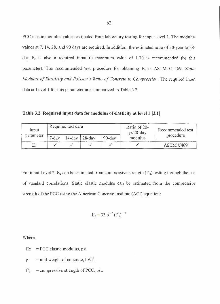
62

PCC elastic modulus values estimated from laboratory testing for input level 1. The modulus

values at 7, 14, 28, and 90 days are required. In addition, the estimated ratio of 20-year to 28-

day Ee is also a required input (a maximum value of 1.20 is recommended for this

parameter). The recommended test procedure for obtaining Ee is ASTM C 469, Static

Modulus of Elasticity and Poisson's Ratio of Concrete in Compression. The required input

data at Level 1 for this parameter are summarized in Table 3.2.

Table 3.2 Required input data for modulus of elasticity at level 1 [3.1]

Input Required test data Ratio of20-

Recommended test yr/28-day

parameter 7-day 14-day 28-day 90-day modulus procedure

Ee ./ ./ ./ ./ ./ ASTMC469

For input Level 2, Ee can be estimated from compressive strength (f e) testing through the use

of standard correlations. Static elastic modulus can be estimated from the compressive

strength of the PCC using the American Concrete Institute (ACI) equation:

Ee= 33 p 3/2 (f' e) 1/2

Where,

Ee = PCC elastic modulus, psi.

p = unit weight of concrete, lb/ft3.

f' c = compressive strength of PCC, psi.

63

Input compressive strength results at 7, 14, 28, and 90 days and the estimated ratio of 20-year

to 28-day compressive strength are required. Testing should be performed in accordance

with AASHTO T 22, compressive strength of cylindrical concrete specimens. Table 3.3

summarizes the recommended procedures and required input data at Level 2.

Table 3.3 Required input data for modulus of elasticity at level 2 [3.1]

Input Required test data Ratio of 20-

Recommended yr/28-day

parameter 7-day 14-day 28-day 90-day strength

test procedure

Compressive strength

./ ./ ./ ./ ./ AASHTOT22

Estimating PCC Elastic Modulus at Input Level based on a single point (28-day) estimate of

the concrete strength (either modulus of rupture (MR) or f' c) using strength gain equations:

STRRA TIO= 1.0 + 0.12*log10 (AGE/0.0767) - 0.01566*[log 10 (AGE/0.0767)] 2

MR= 9.5 (fc) o.s (MR and f c in psi)

Where,

STRRATIO strength ratio of MR at a given age to MR at 28 days .

AGE . .

specimen age m years.

64

Additionally, if the 28-day Ee is known for the project mixtures, it can also be input to better

define the strength-modulus correlation. Table 3 .4 summarizes the recommended input data

at Level 3.

Table 3.4 Required input data for modulus of elasticity at level 3 [3.1]

Input parameter 28-day value Recommended test procedure

Flexural Strength ./ AASHTO T97 or from records

Compressive ./ AASHTO T22 or from strength records

Optional - to be entered with ASTM C469 or from

Elastic modulus either the flexural or records

compressive strength inputs

3.2.4.1.1.2 Flexural Strength of PCC Materials

The flexural strength, often termed modulus of rupture (MR), can be defined as the

maximum tensile stress at rupture at the bottom of a simply supported concrete beam during

a flexural test with third point loading [3 .1] . Like all measures of PCC strength, the modulus

of rupture is strongly influenced by mix design parameters. Table 3.5 summarizes the

required input data for different input levels for modulus of rupture estimation.

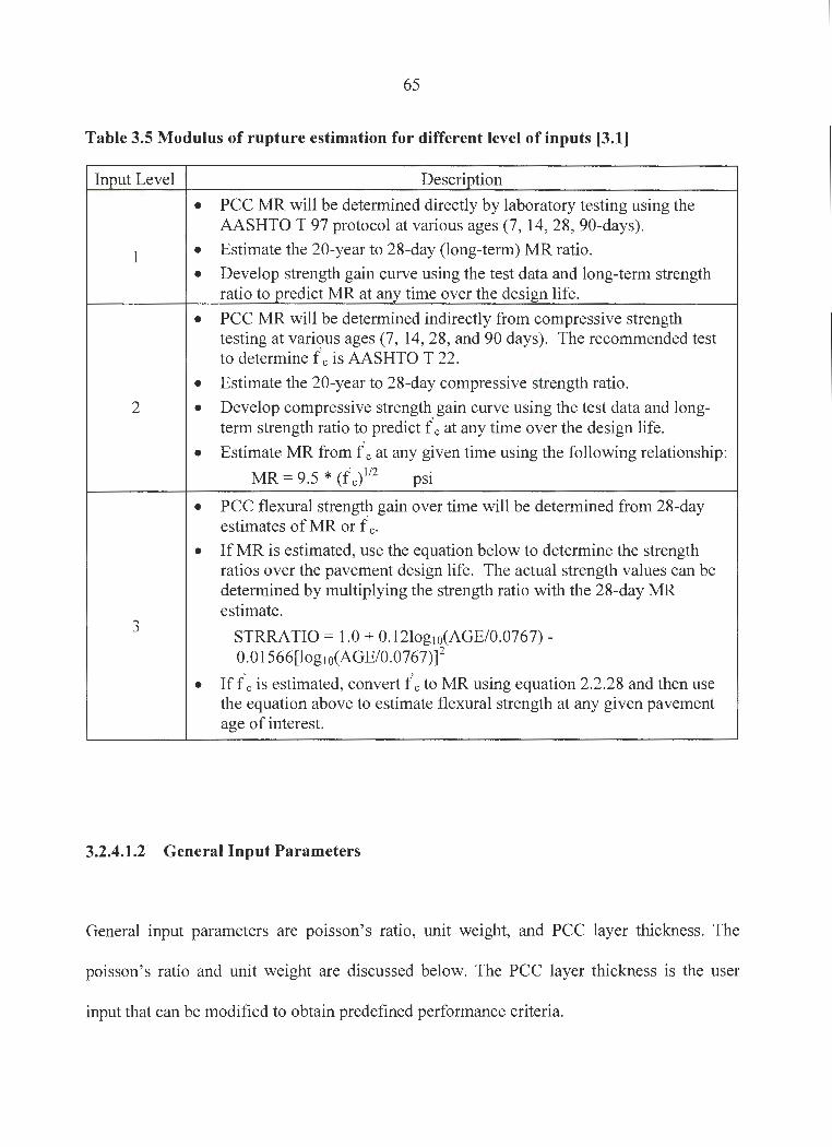
65

Table 3.5 Modulus of rupture estimation for different level of inputs [3.1]

Input Level Description

• PCC MR will be determined directly by laboratory testing using the AASHTO T 97 protocol at various ages (7, 14, 28, 90-days).

1 • Estimate the 20-year to 28-day (long-term) MR ratio .

• Develop strength gain curve using the test data and long-term strength ratio to predict MR at any time over the design life.

• PCC MR will be determined indirectly from compressive strength testing at various ages (7, 14, 28, and 90 days). The recommended test to determine f c is AASHTO T 22.

• Estimate the 20-year to 28-day compressive strength ratio .

2 • Develop compressive strength gain curve using the test data and long-term strength ratio to predict f c at any time over the design life.

• Estimate MR from f c at any given time using the following relationship:

MR = 9.5 * (f c) 112 psi

• PCC flexural strength gain over time will be determined from 28-day estimates of MR or f c·

• If MR is estimated, use the equation below to determine the strength ratios over the pavement design life. The actual strength values can be determined by multiplying the strength ratio with the 28-day MR estimate.

3 STRRATIO = 1.0 + 0.12log10(AGE/0.0767)-0.01566[log1o(AGE/0.0767)]2

• If f c is estimated, convert f c to MR using equation 2.2.28 and then use the equation above to estimate flexural strength at any given pavement age of interest.

3.2.4.1.2 General Input Parameters

General input parameters are poisson's ratio, unit weight, and PCC layer thickness. The

poisson's ratio and unit weight are discussed below. The PCC layer thickness is the user

input that can be modified to obtain predefined performance criteria.

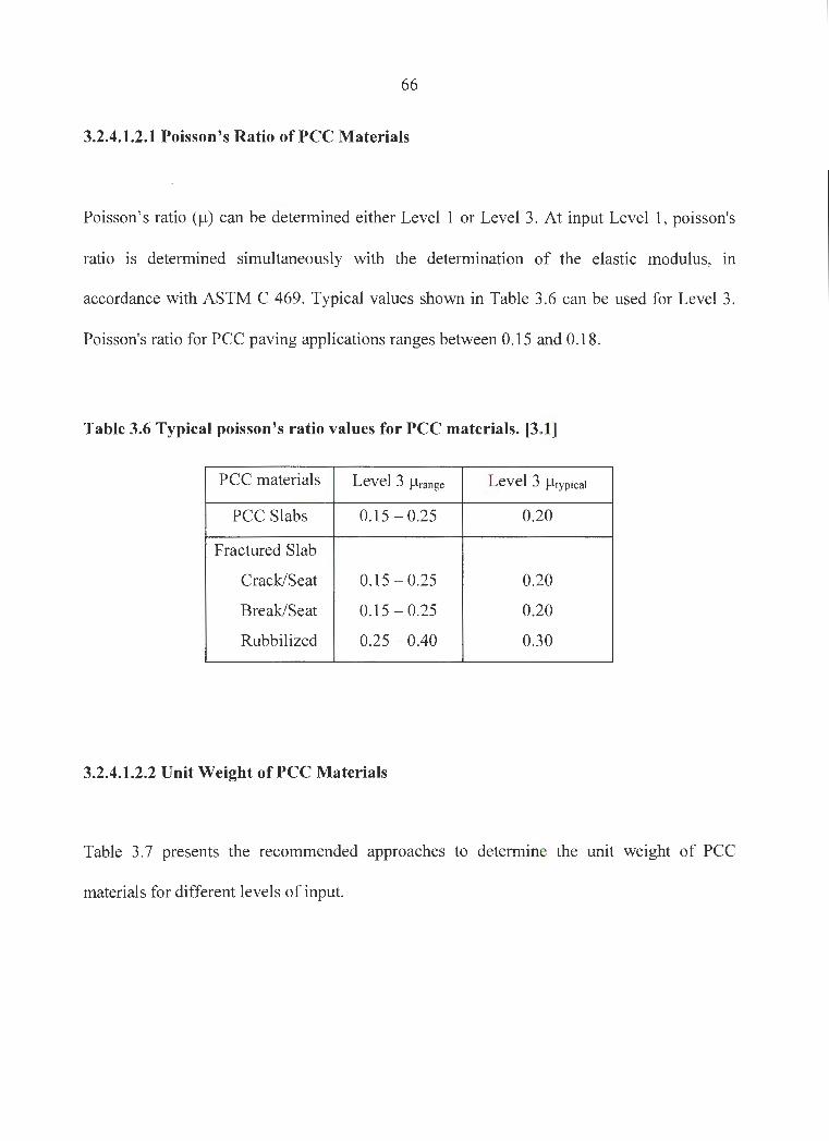
66

3.2.4.1.2.1 Poisson's Ratio of PCC Materials

Poisson's ratio(µ) can be determined either Level 1 or Level 3. At input Level 1, poisson's

ratio is determined simultaneously with the determination of the elastic modulus, in

accordance with ASTM C 469. Typical values shown in Table 3.6 can be used for Level 3.

Poisson's ratio for PCC paving applications ranges between 0.15 and 0.18.

Table 3.6 Typical poisson's ratio values for PCC materials. (3.1)

PCC materials Level 3 µrange Level 3 µtypical

PCC Slabs 0.15-0.25 0.20

Fractured Slab

Crack/Seat 0.15-0.25 0.20

Break/Seat 0.15 - 0.25 0.20

Rubbilized 0.25 - 0.40 0.30

3.2.4.1.2.2 Unit Weight of PCC Materials

Table 3. 7 presents the recommended approaches to determine the unit weight of PCC

materials for different levels of input.

67

Table 3.7 Unit weight estimation of PCC materials [3.1]

Material Input group Level Description

category

• Estimate value from testing performed in accordance with

1 AASHTO T 121 -Mass per Cubic Meter (Cubic Foot), Yield, and Air Content (Gravimetric) of Concrete

2 • Not applicable . PCC

• User selects design values based upon agency historical data

3 or from typical values shown below:

Typical range for normal weight concrete: 140 to 160 lb/ft3

3.2.4.1.3 PCC Mix Design Inputs

Mix design inputs are summarized as follows:

• Cement type

• Cementitious material content

• Water/cement ratio

• Aggregate type

• PCC zero-set temperature

• Shrinkage

o Ultimate shrinkage strain, micro-strain units.

o Time required to develop 50 percent of the ultimate shrinkage strain

o Anticipated amount of reversible shrinkage

o Curing method

68

Shrinkage can cause significant curling and warping in PCC slabs resulting in pavement

cracking.

3.2.4.1.4 PCC Thermal Design Inputs

PCC thermal conductivity, heat capacity, and the coefficient of thermal expansion are the

required thermal properties of the PCC layer. The level 1 and 2 values for PCC thermal

conductivity and heat capacity is estimated using laboratory testing in accordance with

ASTM E 1952 and ASTM D 2766 respectively. For level 3 the recommended values for

former ranges from 1.0 to 1.5 Btu/ (ft) (hr) (°F), and latter ranges from 0.2 to 0.28 Btu/ (lb)

(°F). The PCC coefficient of thermal expansion is discussed in detail below.

3.2.4.1.4.1 PCC Coefficient of Thermal Expansion

The coefficient of thermal expansion ( apcc) is defined as the change in unit length per degree

of temperature change. When the a rec is known, the unrestrained change in length produced

by a given change in temperature can be calculated as (3 .1]:

~L = arcc ~TL

Where,

~L = change in unit length of PCC due to a temperature change of~ T.

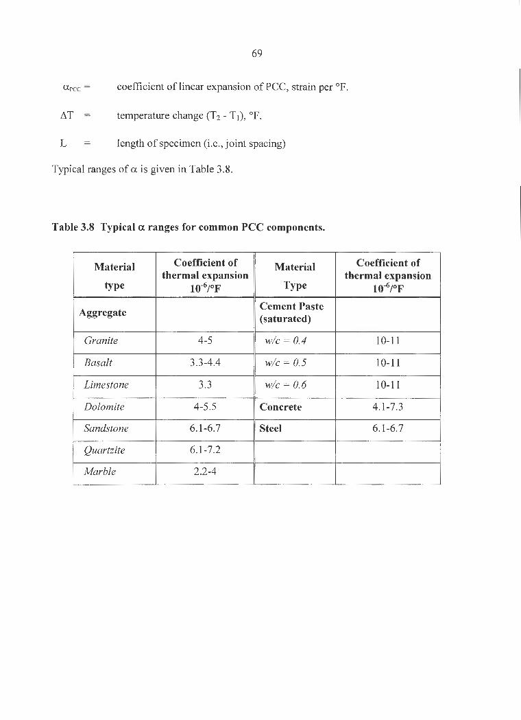
69

Urcc = coefficient of linear expansion of PCC, strain per °F.

~T temperature change (T2 - T1) , °F.

L length of specimen (i.e., joint spacing)

Typical ranges of a is given in Table 3.8.

Table 3.8 Typical a. ranges for common PCC components.

Material Coefficient of Material Coefficient of thermal expansion thermal expansion

type 10-6/°F Type 10-6/°F

Aggregate Cement Paste (saturated)

Granite 4-5 w/c = 0.4 10-11

Basalt 3.3-4.4 w/c = 0.5 10-11

Limestone 3.3 w/c = 0.6 10-11

Dolomite 4-5 .5 Concrete 4.1 -7.3

Sandstone 6.1-6.7 Steel 6.1-6.7

Quartzite 6.1-7.2

Marble 2.2-4

70

3.2.4.2 Unbound Granular and Subgrade Materials

Unbound granular materials and subgrade materials are chosen according to the unified soil

classification (USC) and AASHTO classification of soils in the MEPDG. The AASHTO soil

classification is explained in the specifications as the test AASHTO M 145 "The

Classification of Soils and Soil-Aggregate Mixtures for Highway Construction Purposes."

AASHTO soil classification uses the particle-size distributions and consistency limits

(Atterberg limits) to classify the soils. AASHTO soil classification is based on the portion of

unbound granular and subgrade materials that is smaller than 3-in diameter. The AASHTO

classification system identifies two material types:

~ Granular materials (i.e., materials having 35% or less, by weight, particles smaller

than 0.0029-in in diameter).

~ Silt-clay materials (i.e., materials having more than 35% , by weight, particles smaller

than 0.0029-in in diameter).

These two divisions are further subdivided into 7 main group classifications (i.e., A-1 though

A-7). The group and subgroup classifications are based on estimated or measured grain-size

distribution and on liquid limit and plasticity index values.

The USC system is explained in the test standard ASTM D2487, "Standard Method for

Classification of Soils for Engineering Purposes." The USC system identifies three major soil

divisions:

71

• Coarse-grained soils (i.e., materials having less than 50%, by weight, particles

smaller than 0.0029-in in diameter).

• Fine-grained soils (i.e., materials having 50% or more, by weight, particles

smaller than 0.0029-in in diameter).

• Highly organic soils (materials that demonstrate certain organic characteristics).

These divisions are further subdivided into basic soil groups. The major soil divisions and

basic soil groups are determined on the basis of estimated or measured values for grain-size

distribution and Atterberg limits. ASTM D 2487 shows the criteria chart used for classifying

soil in the USC system and the basic soil groups of the system. For this design procedure,

unbound granular materials are defined using the AASHTO classification system and are the

materials that fall within the specifications for soil groups A-1 to A-3. Sub grade materials are

defined using both the AASHTO and USC and cover the entire range of soil classifications

available under both systems.

Resilient modulus, MR, is required for the pavement response model used in the MEPDG as

well as poisson's ratio, µ. Those materials are used for the computation of the stress

dependent stiffness of unbound granular materials, subgrade materials, and bedrock materials

under moving loads. Resilient modulus is defined as the ratio of the repeated deviator axial

stress to the recoverable axial strain. They are used to characterize layer behavior when

subjected to stresses. Unbound materials display stress-dependent properties (i.e., granular

materials generally are "stress hardening" and show an increase in modulus with an increase

72

m stress while fine-grained soils generally are "stress softening" and display a modulus

decrease with increased stress).

3.2.4.2.1 Non Linear Material Characterization Models

In pavement design the repeated moving traffic loads are one of the most important factors to

be considered. Under repeated loading, most of the deformations are recoverable and thus

considered elastic. The resilient modulus (Mr) is then defined as the elastic stiffness of the

pavement materials for analysis of repeated traffic loads. In the MEPDG following nonlinear

model is used to characterize the resilient modulus of unbound bases, sub-bases, and sub-

grades.

Where;

Mr = resilient modulus

8 = bulk stress= cr1 + cr2 + cr3

cr 1 = major principal stress

cr2 = intermediate principal stress= cr3 for MR Test on cylindrical specimen

cr3 = minor principal stress/confining pressure

1 ~ 2 2 2 'toct = octahedral shear stress = - ( cr 1 - cr 2) + ( cr 1 - cr 3) + ( cr 2 - cr 3) 3

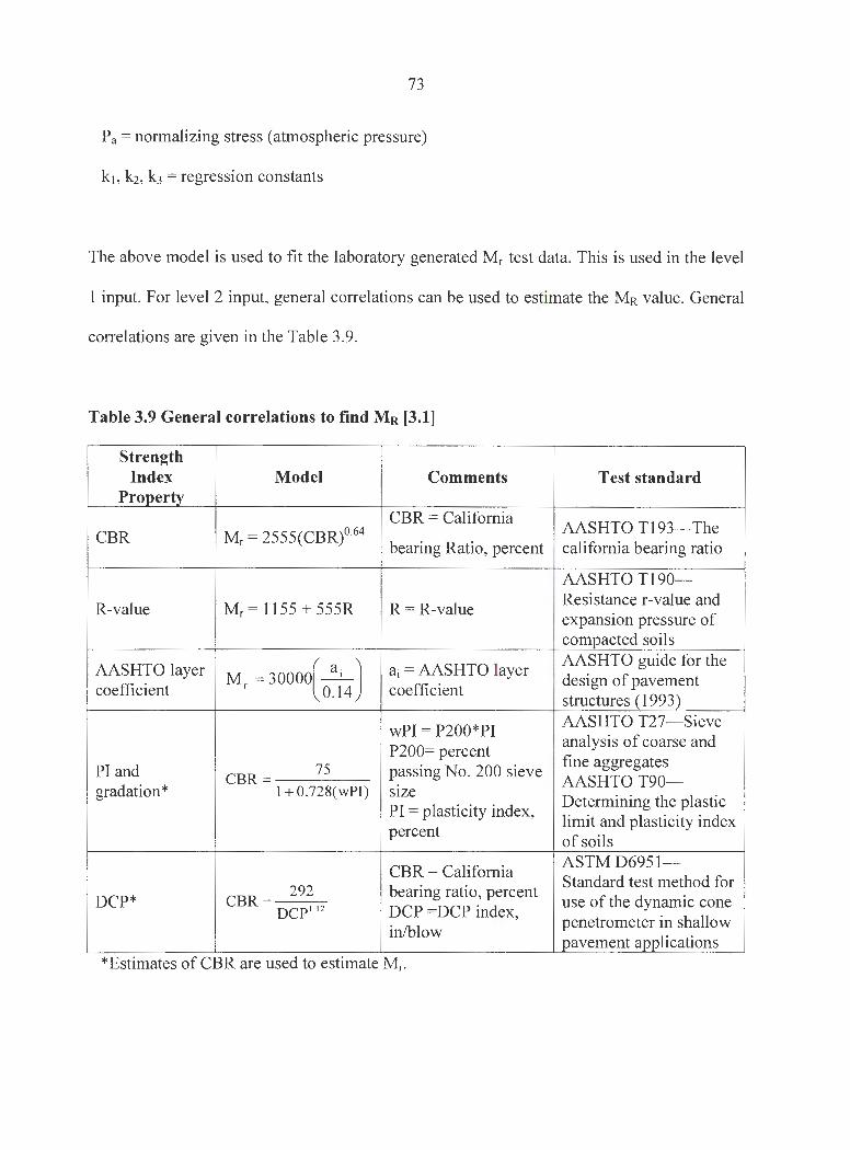
73

Pa = normalizing stress (atmospheric pressure)

k1, k1, k3 = regression constants

The above model is used to fit the laboratory generated Mr test data. This is used in the level

1 input. For level 2 input, general correlations can be used to estimate the MR value. General

correlations are given in the Table 3.9.

Table 3.9 General correlations to find MR [3.1]

Strength Index Model Comments Test standard

Property CBR = California

AASHTO Tl 93- The CBR Mr = 2555(CBR)0·64

bearing Ratio, percent california bearing ratio

AASHTO Tl90-

R-value Mr = 1155 + 555R R = R-value Resistance r-value and expansion pressure of compacted soils

AASHTO layer M r = 30000( ~) ai = AASHTO layer

AASHTO guide for the

coefficient coefficient design of pavement

0.14 structures (1993)

wPI = P200*PI AASHTO T27- Sieve

P200= percent analysis of coarse and fine aggregates

PI and CBR= 75 passing No. 200 sieve

AASHTOT90-gradation* 1+ 0.728(wPI) size

Determining the plastic PI = plasticity index,

limit and plasticity index percent

of soils

CBR = California ASTM D6951-

292 bearing ratio, percent Standard test method for

DCP* CBR= DCP 1 12 DCP =DCP index,

use of the dynamic cone

in/blow penetrometer in shallow pavement applications

*Estimates of CBR are used to estimate Mr.

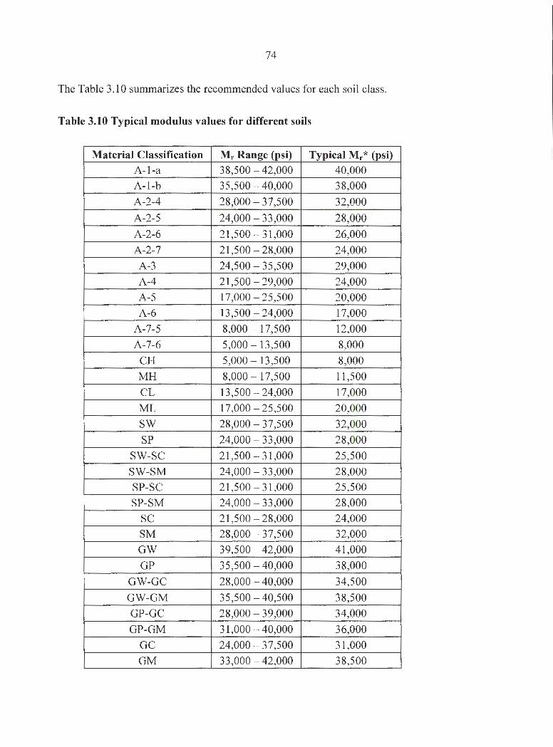
74

The Table 3.10 summarizes the recommended values for each soil class.

Table 3.10 Typical modulus values for different soils

Material Classification Mr Range (psi) Typical Mr* (psi) A-1-a 38,500 - 42,000 40,000

A-1-b 35,500 - 40,000 38,000

A-2-4 28,000 - 37,500 32,000

A-2-5 24,000 - 33,000 28,000

A-2-6 21 ,500 - 31 ,000 26,000

A-2-7 21,500 - 28,000 24,000

A-3 24,500 - 35,500 29,000

A-4 21 ,500- 29,000 24,000

A-5 17,000 - 25,500 20,000

A-6 13,500 - 24,000 17,000

A-7-5 8,000 - 17,500 12,000

A-7-6 5,000 - 13,500 8,000

CH 5,000 - 13,500 8,000

MH 8,000 - 17,500 11,500

CL 13,500 - 24,000 17,000

ML 17,000 - 25,500 20,000

SW 28,000 - 37,500 32,000

SP 24,000 - 33 ,000 28,000

SW-SC 21 ,500 -31,000 25,500

SW-SM 24,000 - 33,000 28,000

SP-SC 21,500 - 31,000 25,500

SP-SM 24,000 - 33,000 28,000

SC 21 ,500 - 28,000 24,000

SM 28,000 - 37,500 32,000

GW 39,500 - 42,000 41,000

GP 35,500 - 40,000 38,000

GW-GC 28,000 - 40,000 34,500

GW-GM 35,500 - 40,500 38,500

GP-GC 28,000 - 39,000 34,000

GP-GM 31,000 - 40,000 36,000

GC 24,000 - 37,500 31 ,000

GM 33,000 - 42,000 38,500

75

3.3 References

[3.1) MEPDG Design Guide, NCHRP Project 1-37A, Final Report, TRB, National

Research Council, Washington, D.C, 2004

[3.2) Federal Highway Administration. Guide to LTPP Traffic Data Collection and

Processing (2001). FHWA, Washington, DC.

[3.3) ERES Consultants (2001). DataPave Software (version 3.0). Federal Highway

Administration, Washington, D.C.

[3.4] TRB, Highway Capacity Manual (1985), Special Report 209, Transportation

Research Board, Washington, D.C.

[3.5] AASHTO, A Policy on Geometric Design of Highways and Streets (1990), American

Association of State Highway and Transportation Officials, Washington, D.C.

[3.6) Kosmataka, S. H., B. Kerkhoff, and W.C. Panarese. Design and Control of Concrete

Mixtures, EBOO 1, 14th Edition, Portland Cement Association, Skokie, Illinois, USA, 2002

76

CHAPTER4

SENSITIVITY ANALYSIS OF RIGID PAVEMENTS MODULE

DESIGN INPUT PARAMETERS

4.1 Introduction

The main focus of this chapter was to identify the sensitivity of input parameters needed for

designing jointed plain concrete pavements used in the mechanistic-empirical pavement

design guide (MEPDG). To study the sensitivity of the large number of input parameters on

the predicted pavement distresses, two rigid pavement sections were selected from the Iowa

Department of Transportation (Iowa DOT) Pavement Management Information System

(PMIS). A history of pavement deflection testing, material testing, traffic, and other related

data were also available in the L TPP database. Several hundred sensitivity runs were

conducted using the MEPDG software to study the selected rigid pavement sites extensively.

For unknown input parameters needed to run the MEPDG software, the nationally calibrated

default values were used. Sensitivity analyses were conducted on a standard pavement

section formed from two JPCP sites to study the effects on pavement performance in terms of

77

faulting, transverse cracking, and smoothness. Based on the sensitivity analysis of the rigid

pavement (Portland cement concrete) input parameters, a sensitivity chart were determined

and presented from the most sensitive to insensitive to help the pavement design engineers

identify the level of importance of each input parameter. A comparison on predicted

pavement smoothens for two Iowa sites using the MEPDG software and the measured

pavement distresses values from DOT are presented.

4.2 Data Collection

The very first part of this project was the extensive data collection. From the Iowa

Department of Transportation (Iowa DOT) Pavement Management Information System

(PMIS) two rigid pavement sections were selected which were also a part of the Long Term

Pavement Performance (L TPP) program. A history of pavement deflection testing, material

testing, traffic, and other related data were available in the L TPP database. These two

sections were named as PCC-1 and PCC-2 (see Table 4.1 and Figure 4.1). Detailed

information for these two sites is given in the following headings:

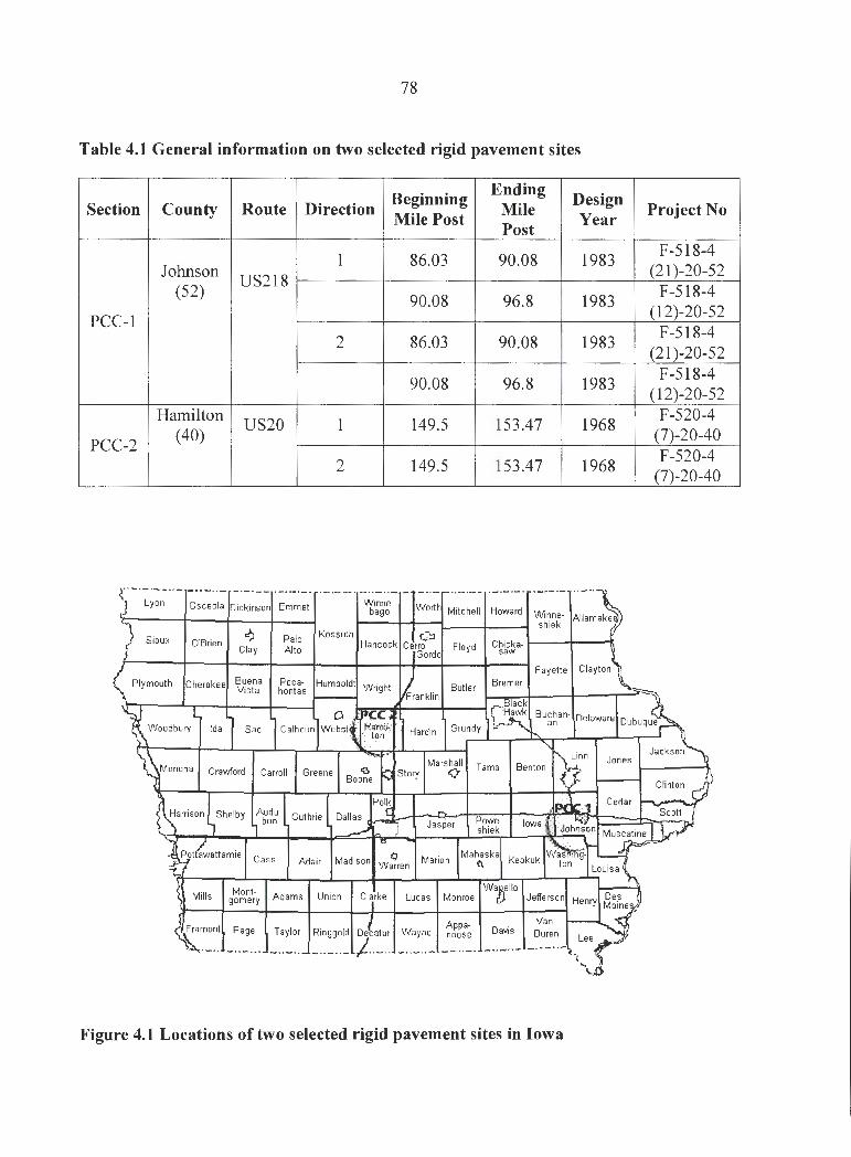
78

Table 4.1 General information on two selected rigid pavement sites

Ending Beginning

Section County Route Direction Mile Post Mile

Johnson (52)

US218

PCC-1

Hamilton US20

(40) PCC-2

·· - ·-·-- ·· - -··- ·· - -·- ·-- ·- ·- ·-· Lyon

Sioux

Osceola Dickinson Emmet

~ Palo O'Brien Clay Alto

Buena Poca-Vista honta s

Ida Sac

Crawford Carroll

Cass

Mont­gomery

Page

Adams

Taylor

Post

1 86.03 90.08

90.08 96.8

2 86.03 90.08

90.08 96.8

1 149.5 153.47

2 149.5 153.47

Winne-bago Worth Mitchell Howard

Ko ssuth 0 Hancock Cerro Floyd Chick a-

Gordo saw

Humboldt Wright Butler

Hardin Grundy

Marshall Tama Q

Powe-Jasper shiek

Union Lucas Wa11,ello

Monroe [)

Davis Appa-

Ringgold Decatur Wayne noose

-· ·-· ·- )---·· -··-··- __ ... _. - ··- ·· - -··- ···-

Figure 4.1 Locations of two selected rigid pavement sites in Iowa

Design Year

1983

1983

1983

1983

1968

1968

Project No

F-518-4 (21)-20-52

F-518-4 (12)-20-52

F-518-4 (21)-20-52

F-518-4 (12)-20-52

F-520-4 (7)-20-40 F-520-4

(7)-20-40

79

4.2.1 PCC-1

PCC-1, located on US-218 near Johnson County, Iowa, was constructed in 1983. The test

section was in the northbound direction, and designated between 86.03 and 90.08 miles of

US-218. A complete listing of information obtained is summarized in the Tables 4.2, 4.3, 4.4

and 4.5; and Figure 4.2 shows the summary of general information from LTPP data.

4.2.1.1 Traffic

The traffic records provided by the Iowa Department of Transportation indicated that, in

1983, the pavement carried a two-way average daily traffic (ADT) of 2,500 vehicles per day,

including heavy trucks. In 2002, it was estimated as 3,590 vehicles per day, including 540

vehicles of truck traffic.

4.2.1.2 Climate

This section of US-218 is located in the wet-freeze environmental region. This area has a

freezing index of 466.88, and receives 930.58 mm of rainfall annually. The latitude and

longitudes are given as 41.57 and 91.55 degrees respectively.

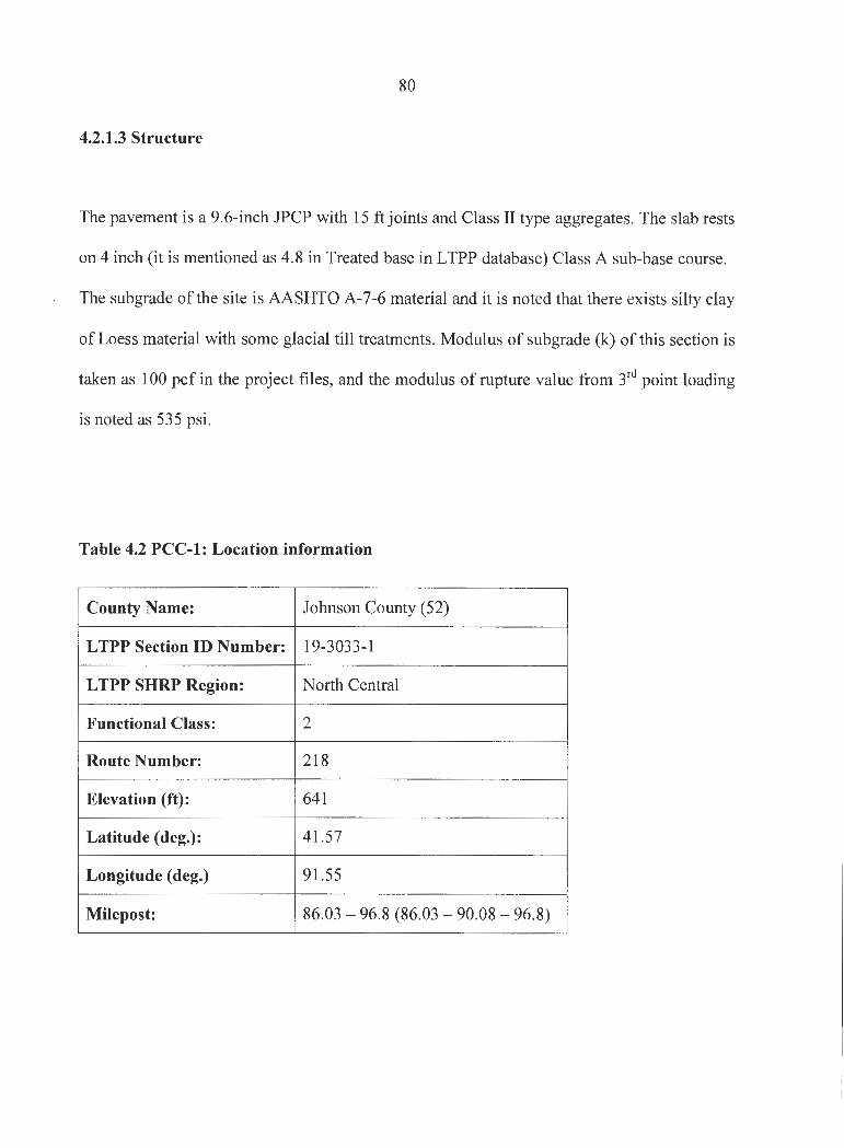
80

4.2.1.3 Structure

The pavement is a 9.6-inch JPCP with 15 ft joints and Class II type aggregates. The slab rests

on 4 inch (it is mentioned as 4.8 in Treated base in LTPP database) Class A sub-base course.

The subgrade of the site is AASHTO A-7-6 material and it is noted that there exists silty clay

of Loess material with some glacial till treatments. Modulus of subgrade (k) of this section is

taken as 100 pcf in the project files, and the modulus of rupture value from 3rd point loading

is noted as 535 psi .

Table 4.2 PCC-1: Location information

County Name: Johnson County (52)

LTPP Section ID Number: 19-3033-1

L TPP SHRP Region: North Central

Functional Class: 2

Route Number: 218

Elevation (ft): 641

Latitude (deg.): 41.57

Longitude (deg.) 91.55

Milepost: 86.03 - 96.8 (86.03 - 90.08 - 96.8)

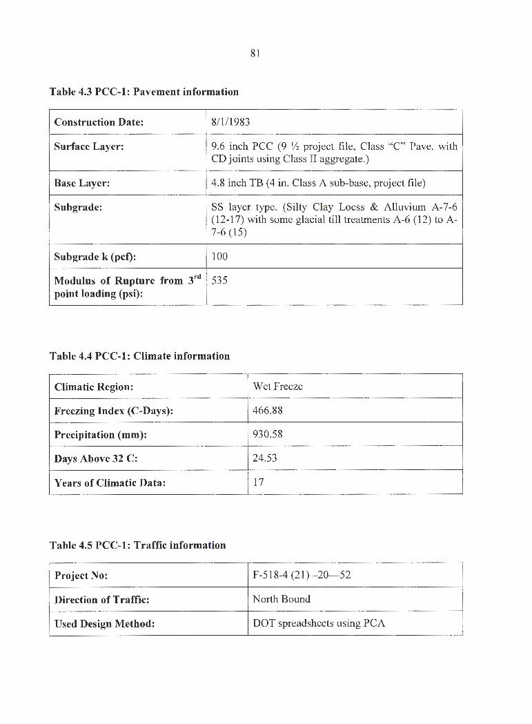
81

Table 4.3 PCC-1: Pavement information

Construction Date: 81111983

Surface Layer: 9.6 inch PCC (9 Yi project file, Class "C" Pave. with CD joints using Class II aggregate.)

Base Layer: 4.8 inch TB (4 in. Class A sub-base, project file)

Subgrade: SS layer type. (Silty Clay Loess & Alluvium A-7-6 (12-17) with some glacial till treatments A-6 (12) to A-7-6 (15)

Subgrade k (pct): 100

Modulus of Rupture from 3rd 535 point loading (psi):

Table 4.4 PCC-1: Climate information

Climatic Region: Wet Freeze

Freezing Index (C-Days): 466.88

Precipitation (mm): 930.58

Days Above 32 C: 24.53

Years of Climatic Data: 17

Table 4.5 PCC-1: Traffic information

Project No: F-518-4 (21)-20- 52

Direction of Traffic: North Bound

Used Design Method: DOT spreadsheets using PCA

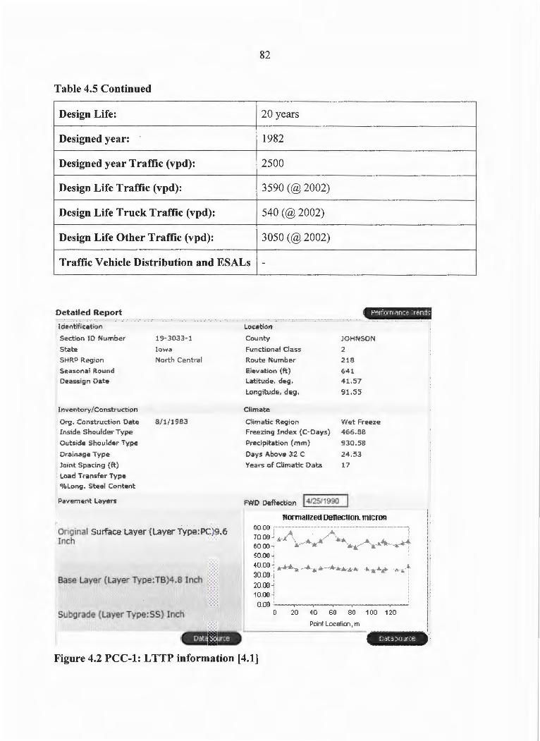
82

Table 4.5 Continued

Design Life: 20 years

Designed year: 1982

Designed year Traffic (vpd): 2500

Design Life Traffic (vpd): 3590 (@ 2002)

Design Life Truck Traffic (vpd): 540 (@2002)

Design Life Other Traffic (vpd): 3050 (@ 2002)

Traffic Vehicle Distribution and ESALs -

Detailed Report

Identification

Section ID Number

' State

SHRP Region

, Seasonal Roun d

'j Deas:sign Date

, lnverrtory/Canst rudtion

:, Org,. Construction Date

i Ins :ide Shoulde r Type

Outside Shoulder Type

Drainagoe Type

Joint Spacing (ft)

Load Transfer Type

Iowa

Noli:h Centra I

B/l/19S3

Original Surface Layer (Layer Type:PC)9.6 Inch

Data source

Location

County

Fun ctional Class

Route Numbe r

Elevation (~)

Latitude, deg,

Lo ngitude , deg.

Climate

Climatic Reg icn

Freezing Index ( C-Days)

PN!dpitation {mm)

Days ,ll.bove 32. C

Years o f Climatic Data

JOHNSON

2

2 18

641

41.57

91.55

Wet Freeze

466.BB

930. SB

24.53

17

rmrmallzed oenecnon, micron 00.00

7000 " 6000 ~

50,00

40.00

30.00 20.00 1000

000 ~"-·-,----..-----r--"••""'"--~ .. ·-"--,.-"""~ 0 20 4 0 60 80 1 00 1 20

Pcin1 Loca1im, m

Figure 4.2 PCC-1: LTTP information [4.1]

83

4.2.2 PCC-2

PCC-2, located on US-20 near Hamilton County, Iowa, was constructed in 1968. The test

section was west-bound in the north central LTPP SHRP region, and designated between

149.5 and 153.47 miles of US-20. A complete listing of information obtained is summarized

in the Tables 4.6, 4.7, 4.8 and 4.9; and Figure 4.3 shows the summary of general information

from L TPP data.

4.2.2.1 Traffic

In 1968, the pavement carried a two-way average daily traffic (ADT) of 3, 160 vehicles per

day, including heavy trucks. In 2002, it was 5,610 vehicles per day, including 840 vehicles of

truck traffic.

4.2.2.2 Climate

This section of US-20 is located in the wet-freeze environmental region. This area has a

freezing index of 763.69, and receives 861.74 mm of rainfall annually. The latitude and

longitudes are given as 42.46 and 93.59 degrees respectively.

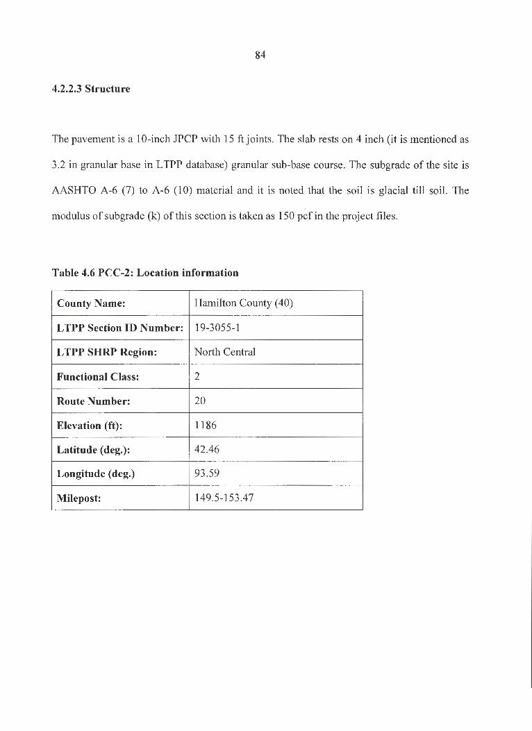
84

4.2.2.3 Structure

The pavement is a 10-inch JPCP with 15 ft joints. The slab rests on 4 inch (it is mentioned as

3 .2 in granular base in L TPP database) granular sub-base course. The sub grade of the site is

AASHTO A-6 (7) to A-6 (10) material and it is noted that the soil is glacial till soil. The

modulus of subgrade (k) of this section is taken as 150 pcf in the project files.

Table 4.6 PCC-2: Location information

County Name: Hamilton County ( 40)

LTPP Section ID Number: 19-3055-1

LTPP SHRP Region: North Central

Functional Class: 2

Route Number: 20

Elevation (ft): 1186

Latitude (deg.): 42.46

Longitude (deg.) 93 .59

Milepost: 149.5-153.47

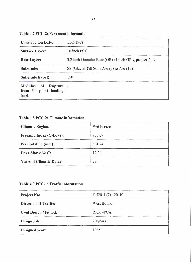
85

Table 4.7 PCC-2: Pavement information

Construction Date: 11 /2/1968

Surface Layer: 10 inch PCC

Base Layer: 3.2 inch Granular Base (GB) (4 inch GSB, project file)

Subgrade: SS (Glacial Till Soils A-6 (7) to A-6 (10)

Subgrade k (pcf): 150

Modulus of Rupture -from 3rd point loading (psi):

Table 4.8 PCC-2: Climate information

Climatic Region: Wet Freeze

Freezing Index (C-Days): 763.69

Precipitation (mm): 861.74

Days Above 32 C: 12.24

Years of Climatic Data: 29

Table 4.9 PCC-1: Traffic information

Project No: F-520-4 (7) -20-40

Direction of Traffic: West Bound

Used Design Method: Rigid-PCA

Design Life: 20 years

Designed year: 1965

86

Table 4.9 Continued

Designed year Traffic (vpd): 3160

Design Life Traffic (vpd): 5610 (@1985)

Design Life Truck Traffic (vpd): 840 (@1985)

Design Life Other Traffic (vpd): 4770 (@1985)

Traffic Vehicle Distribution and ESALs -

Deta:i led Rep ort !P=="'?""==,,,=====-'o=====•o""===,=o==c====='"'"'"'"c,:°"'""-'""== ~~ -·--www-·-' ,~ Identification

Section ID Num be r

" State SHiRP Region

Sea.5oJlal Round

!i Dea .ssign Date

\I l ~ Ii 11 Ir Inventory/Const ructio n H ii Org. Construction Date 11 II Inside, Shoulde1- Type

;; Outside Shoulder Type

Dra inage Type d II Joint Spacing ( ft}

II Load Transfer Ty·pe

II •tolon g . Steel Content

Ii Pavemen t Layer s ii !J I!

19-3055-t

lovia

No 1th Ce ntral

1 1/1/1968

::o riginal Surface layer (layer Type: PC}lO "Inch q

II ll llBase layer (layer ~ype:GB)3, . .2 Inch

Ii !!s ubgrade (LayerType:SS) Inch

l oca t ion

County

Functional Class

Route Number

Elevation (ft)

Lat itude,, deg .

Lo ngit ude, deg.

Cli!mate

HAMI LTON

2

20

11&6

42.46

93.59

Climati-c Region Wet Freeze

Freezing Index (C-Days) 763 .69

Precipit ation {mm) 8 6 1.74

Da·rs .Above 32 C

Yea r s of Climatk Data

12.24

29

FWD Deflection J ,7113.fi989 . L r

Norrnanzect oenectlori, micron

'l CO ,OO - ra<AAAdlr "1<-&-A.tr'~·-..-.&--,,o.~.k 00,00 ,

ED.DO

40 ,00 - A

2() ,00

0,00 '---~--~---~-~---,-' 0 20 40 GO OJ 1 CO 1 20 140

Poirt Loca1ion, rn

Figure 4.3 PCC-2: LTTP information [4.1)

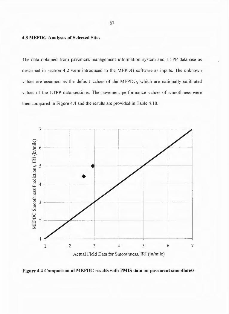
87

4.3 MEPDG Analyses of Selected Sites

The data obtained from pavement management information system and L TPP database as

described in section 4.2 were introduced to the MEPDG software as inputs. The unknown

values are assumed as the default values of the MEPDG, which are nationally calibrated

values of the L TPP data sections. The pavement performance values of smoothness were

then compared in Figure 4.4 and the results are provided in Table 4.10.

7

,,......_ ~ .......

~ 6 ....... ...__,

02 ........ (/)~ 5 i::: 0 ....... ....... • u :..a ())

4 I-;

A.. (/) (/) ())

.§ ....... 0 3 0 -

E r/).

d Cl

2 A.. i:.r.:l ~

1 2 3 4 5 6 7

Actual Field Data for Smoothness, IRJ (in/mile)

Figure 4.4 Comparison of MEPDG results with PMIS data on pavement smoothness

88

Table 4.10 Comparison of MEPDG results and PMIS data

IRI (in/mile) PMIS MEPDG

PCC-1 Johnson(52) 2.57 4.43

PCC-2 Hamilton ( 40) 2.94 4.99

4.4 Sensitivity Analysis of MEPDG

4.4.1 Overview

Sensitivity analyses were carried out on a representative pavement section to examine the

effect of each input or inputs groups of two on pavement performance by using the MEPDG

software and the design inputs. The standard input parameters for the representative

pavement section of the Iowa highway system was determined by using the inputs similar to

the properties of two PCC sections described in section 4.2 and were introduced considering

Iowa conditions. A detailed summary of input parameters is given in Table 4.11.

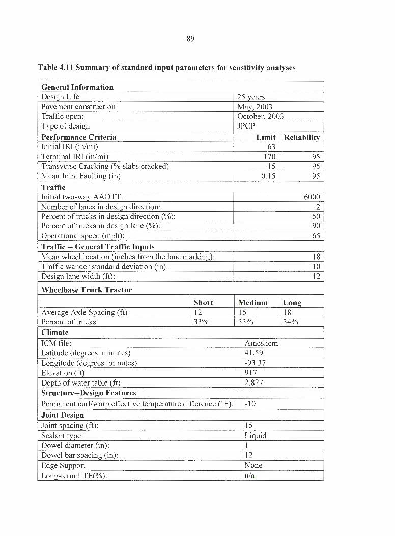
89

Table 4.11 Summary of standard input parameters for sensitivity analyses

General Information Design Life 25 years Pavement construction: May, 2003 Traffic open: October, 2003 Type of design JPCP Performance Criteria Limit Reliability Initial IRI (in/mi) 63 Terminal IRI (in/mi) 170 95 Transverse Cracking (% slabs cracked) 15 95 Mean Joint Faulting (in) 0.15 95

Traffic Initial two-way AADTT: 6000 Number of lanes in design direction: 2 Percent of trucks in design direction(%): 50 Percent of trucks in design lane(%): 90 Operational speed (mph): 65 Traffic -- General Traffic Inputs Mean wheel location (inches from the lane marking): 18 Traffic wander standard deviation (in): 10 Design lane width (ft): 12

Wheelbase Truck Tractor

Short Medium Lon~ Average Axle Spacing (ft) 12 15 18 Percent of trucks 33% 33% 34% Climate ICM file : Ames.icm Latitude (degrees. minutes) 41.59 Longitude (degrees. minutes) -93.37 Elevation (ft) 917 Depth of water table (ft) 2.827 Structure--Design Features

Permanent curl/warp effective temperature difference (°F): -10

Joint Design Joint spacing (ft): 15 Sealant type: Liquid Dowel diameter (in): 1 Dowel bar spacing (in): 12 Edge Support None Long-term LIE(%): n/a

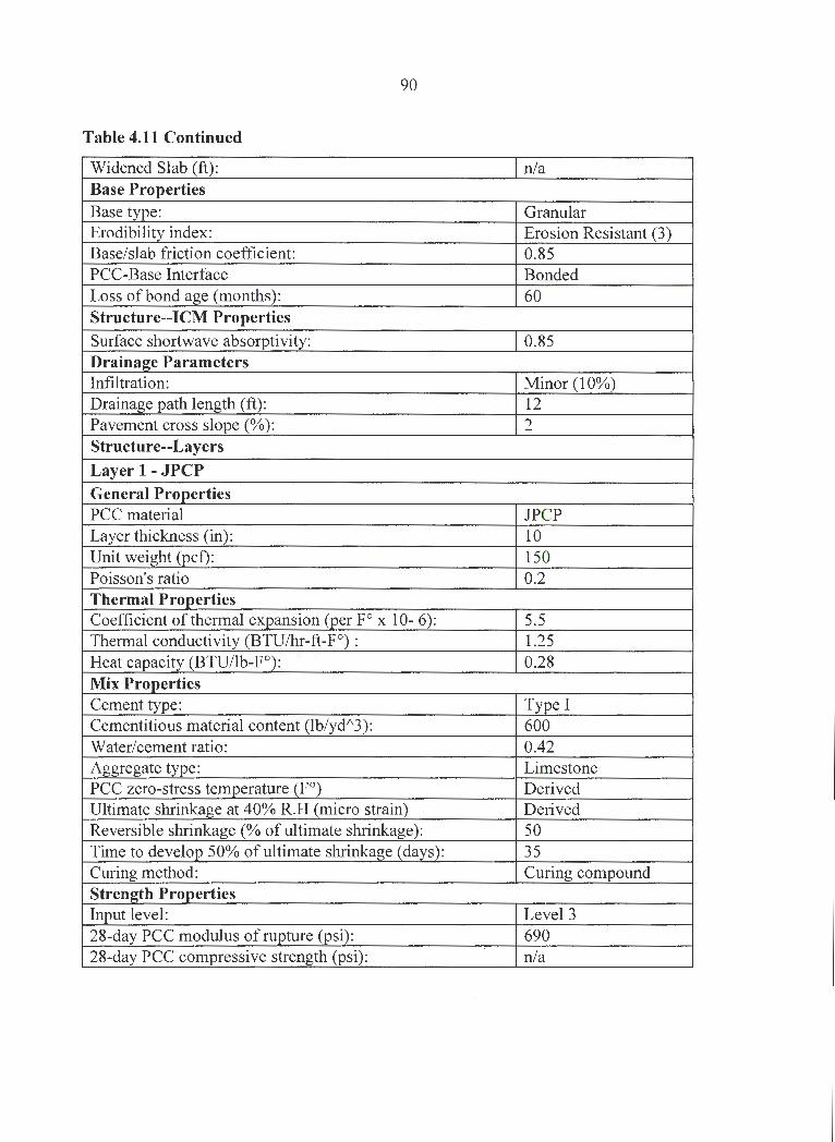
90

Table 4.11 Continued

Widened Slab (ft) : n/a Base Properties Base type: Granular Erodibility index: Erosion Resistant (3) Base/slab friction coefficient: 0.85 PCC-Base Interface Bonded Loss of bond age (months): 60 Structure--ICM Properties Surface shortwave absorptivity: 0.85 Drainage Parameters Infiltration: Minor (10%) Drainage path length (ft): 12 Pavement cross slope(%): 2 Structure--Layers

Layer 1 - JPCP General Properties PCC material JPCP Layer thickness (in): 10 Unit weight (pcf): 150 Poisson's ratio 0.2 Thermal Properties Coefficient of thermal expansion (per F0 x 10- 6): 5.5 Thermal conductivity (BTU/hr-ft-F 0 ) : 1.25 Heat capacity (BTU/lb-F 0 ): 0.28 Mix Properties Cement type: Type I Cementitious material content (lb/yd/\3): 600 Water/cement ratio: 0.42 Aggregate type: Limestone PCC zero-stress temperature (F 0 ) Derived Ultimate shrinkage at 40% R.H (micro strain) Derived Reversible shrinkage(% of ultimate shrinkage): 50 Time to develop 50% of ultimate shrinkage (days): 35 Curing method: Curing compound Strength Properties Input level: Level 3 28-day PCC modulus of rupture (psi): 690 28-day PCC compressive strength (psi): n/a

91

4.4.2 Sensitivity Analysis

The representative pavement section was analyzed with MEPDG software. Then, varying

one input parameter within its ranges and holding other parameters constant in the model,

several analyses were carried out. Pavement distresses throughout the design life for each

input file were plotted. The goal of this analysis was to perform the individual effects of each

input parameter on the critical pavement performance using the MEPDG software. It should

be noted that the climatic condition reflects Iowa's climate data, and as a variable, the

climate input, is considered in or around the Iowa. The chosen weather stations are located in

Figure 4.5.

· ""-·-·-- · ·- - .. ·-··- - · - ·-- ·--"- ' "7.'¥ · ·-·-.. ·-· -·-- -··- - _ .. ,_. · ·-·-- ·- ·- ·-~ Lyon

Sioux

Osceola Dickinson Emmet, Winne-bago Worth Mitchell Howard

O'Brien ~ Clay

Buena Vista

Ida Sac

Crawford

Palo Alto

Kossuth 0 Hancock Cerro Floyd Chicka-

Gordo saw

~con~~~ Humboldt Wright Butler

0 Calhoun Webster Hf~i l- Hardin Gru,....nd_y....1.....--.-.i.::..orr-'---.-__.-r-_,

Marshall 0 Tama

shiek Jasper Powe-

Adams Union Wa11,ello

Lucas Monroe V

Taylor Ringgold Wayne

Kirksville, MO

Appa­noose Davis

Iowa

Figure 4.5 The selected climatic locations for sensitivity analysis

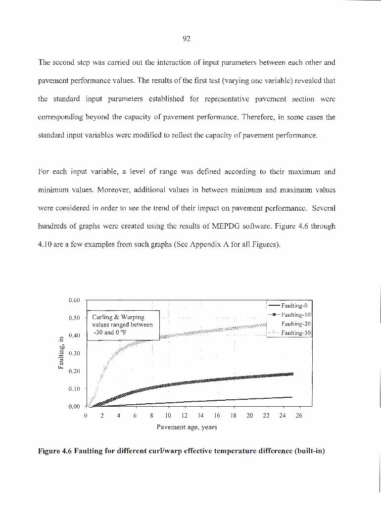
92

The second step was carried out the interaction of input parameters between each other and

pavement performance values. The results of the first test (varying one variable) revealed that

the standard input parameters established for representative pavement section were

corresponding beyond the capacity of pavement performance. Therefore, in some cases the

standard input variables were modified to reflect the capacity of pavement performance.

For each input variable, a level of range was defined according to their maximum and

minimum values. Moreover, additional values in between minimum and maximum values

were considered in order to see the trend of their impact on pavement performance. Several

hundreds of graphs were created using the results of MEPDG software. Figure 4.6 through

4.10 are a few examples from such graphs (See Appendix A for all Figures).

0.60

0.50

.5 0.40

bi\ :B 0.30 ~ ro

i:.i.. 0.20

0.10

0.00

0

Curling & Warping values ranged between -30 and 0 °F

2 4 6 8

- Faulting-0

-- Faulting-IO

L--~-~~b-~~m-::~.~ l x ::~::::~~~

l 0 12 14 16 18 20 22 24 26

Pavement age, years

Figure 4.6 Faulting for different curl/warp effective temperature difference (built-in)

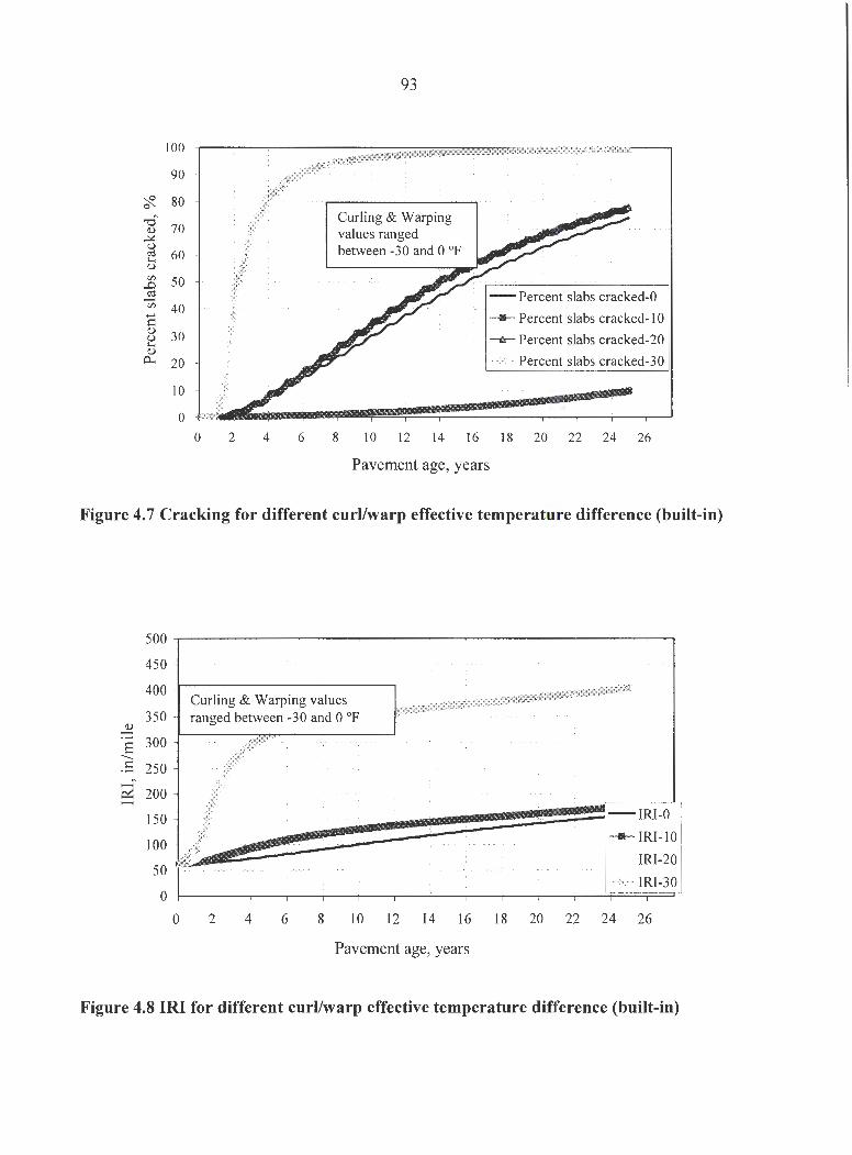
100

90

~ 80 "O 70 Q)

-'<: (.) <'3 60 ..... (.)

Cll 50 ..D ~ Cll 40 ...... c:: Q)

30 (.) ..... Q)

0... 20

10

0

0 2 4 6

93

Curling & Warping values ranged between -30 and 0 °f

---- Percent slabs cracked- I 0

__,..._Percent slabs cracked-20

->+-- Percent slabs cracked-30

8 10 12 14 16 18 20 22 24 26

Pavement age, years

Figure 4.7 Cracking for different curl/warp effective temperature difference (built-in)

500

450

400

350 ~

300 s --.s 250 ..... ~ 200 .....

150

100

50

0

0

Curling & Warping values ranged between -30 and 0 °f

-IRl-0

---- IRI-10

IRJ-20

··~·>f- !Rl-30

2 4 6 8 10 12 14 16 18 20 22 24 26

Pavement age, years

Figure 4.8 IRI for different curl/warp effective temperature difference (built-in)

100

90

80 "O (!)

70 ~ (.) ro .... 60 u (fJ

.£J 50 ..:::! VJ -i:: 40 (!) (.)

30 .... (!)

0... 20

10

0

94

Design Life: 20 years PCC (JPCP) 8-12 in. GB (Crushed Gravel)

3.2 in . SM (E=32,000) AADTT: 8,000

Wet-Freeze Doweled (D= I in.)

-+-h=8 #-----.!'~-----------<

- h=9

__________ __,~----~---#'----,,f"--------------1- -h=IO

~h=ll

+--------:::::llll!J--.,,.""-----"'1'--_,,,,,.'--------------i---h= l 2

12 14 16 18 20

Joint Spacing (ft)

Figure 4.9 Cracking for different joint spacing at different pavement thicknesses

300

280

260

240 ,-.., ~ 220 '§ !:: 200 :..:::,

g; 180

140

120

100

-lll-h=9 .~~=---~~;;;;;;----~~~----1 _ -h= IO

,.__.....,,=----------- ------ -1 ""'*""'h= l I

---h= l 2

12 14 16 18 Joint Spacing (ft)

3.2 in. SM (E=32,000) AADTI: 8,000

Wet-Freeze Doweled (D= I in.)

20

Figure 4.10 Smoothness for different joint spacing at different pavement thicknesses

95

The obtained plots were visually inspected. The evaluation was made according to the

pavement performance value and the amount of change in the pavement performance value

due to changing input variable. It can be seen that the results obtained were sensitive in

different scales, so the scales shown in Table 4.12 were developed for a better understanding

of the effects of input parameters.

Table 4.12 Summary of sensitivity scales

Extreme Sensitivity Very Sensitive Sensitive

LS Low Sensitivity I Insensitive

Table 4.13 compares the sensitivity values extracted from all of the plots given in Appendix

A. Table 4.13 also shows the input scale for sensitivity for each pavement performance and

also their hierarchical input level used in the MEPDG software.

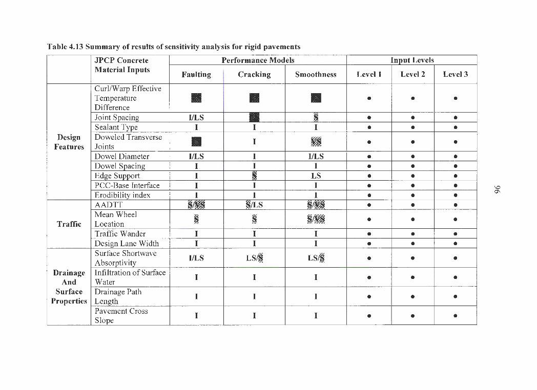
Table 4.13 Summary of results of sensitivity analysis for rigid pavements

JPCP Concrete Performance Models Material Inputs

Faulting Cracking Smoothness

Curl/Warp Effective Temperature • • • Difference Joint Spacing I/LS I Sealant Type I I I

Design Doweled Transverse • I II Features Joints Dowel Diameter I/LS I I/LS Dowel Spacing I I I Edge Support I I LS PCC-Base Interface I I I Erodibility index I I I AADTT - ')LS Mean Wheel I I HI Traffic Location

- ''<-»·

Traffic Wander I I I Design Lane Width I I I Surface Shortwave

I/LS LS/I LS/I Absorptivity Drainage Infiltration of Surface

I I I And Water

Surface Drainage Path I I I Properties Length

Pavement Cross I I I

Slope

Input Levels

Level 1 Level 2

• •

• • . • •

• • • • • • • • • • • • • • • • • • • • • •

• • • •

• •

Level 3

•

• • • • • • • • • • • • •

•

• •

'-0 O'\

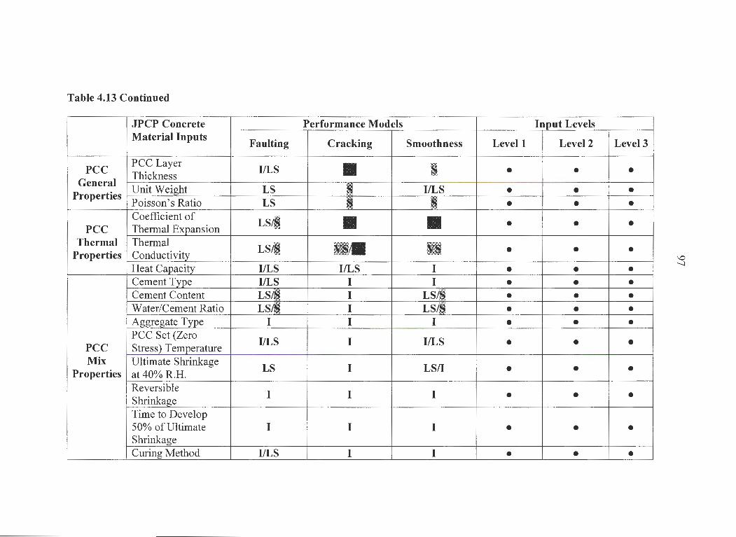
Table 4.13 Continued

JPCP Concrete Material Inputs

Faulting

PCC PCC Layer

I/LS Thickness

General Unit Weight LS Properties Poisson's Ratio LS Coefficient of

LS/I PCC Thermal Expansion Thermal Thermal

LS/I Properties Conductivity Heat Capacity I/LS Cement Type I/LS Cement Content LS!~ Water/Cement Ratio LS/~ Aggregate Type I PCC Set (Zero

I/LS PCC Stress) Temperature Mix Ultimate Shrinkage

LS Properties at40%R.H. Reversible

I Shrinkage Time to Develop 50% of Ultimate I Shrinkage Curing Method I/LS

Performance Models

Cracking Smoothness

• 9 I I/LS

I I

• • m• ~ I/LS I

I I I LS/S I LS/S I I

I I/LS

I LS/I

I I

I I

I I

Input Levels

Level 1 Level 2

• • • • • • • • • • • • • • • • • • • • • • • • • •

• • • •

Level 3

• • • • • • • • • • • •

•

•

•

\0 -....l

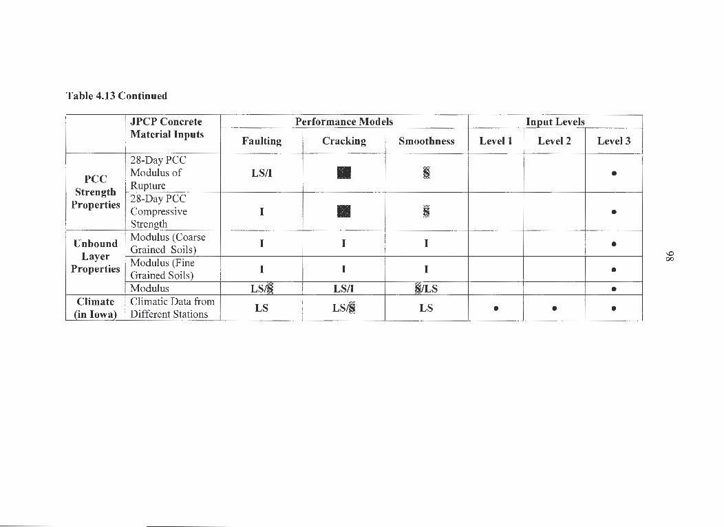
Table 4.13 Continued

JPCP Concrete Material Inputs

Faulting

28-Day PCC

PCC Modulus of LS/I

Strength Rupture 28-Day PCC

Properties Compressive I Strength

Unbound Modulus (Coarse

I Layer

Grained Soils) Modulus (Fine

Properties Grained Soils)

I

Modulus LS/I Climate Climatic Data from

LS (in Iowa) Different Stations

Performance Models

Cracking Smoothness

• I

• B

I I

I I

LS/I ~/LS

LSt LS

Input Levels

Level 1 Level 2

• •

Level 3

•

•

• • • •

'-0 00

99

Results for each pavement performance model can be summarized based on faulting,

transverse cracking, and smoothness as follows:

4.4.2.1 Summary of Sensitivity Results for Faulting

Faulting is an important pavement performance criterion and has a negative effect on ride

quality. It is defined as the differential elevation across the joint and is a result of heavy axle

loads, insufficient load transfer between adjacent slabs, free moisture beneath the pavement,

and erosion of the supporting base or subgrade material from beneath the slab [4.2]. Usually

the approach slab is higher than the leave slab due to pumping, the most common faulting

mechanism. Faulting is noticeable when the average faulting in the pavement section reaches

about 2.5 mm (0.1 inch). When the average faulting reaches 4 mm (0.15 in), diamond

grinding or other rehabilitation measures should be considered [ 4.3]. Significant joint

faulting has a major impact on the life cycle costs of the pavement in terms of rehabilitation

and vehicle operating costs.

The following Table 4.14 summarizes the sensitivity scales of the parameters for the faulting

performance of JPCP. In the table, the sensitivity of inputs are given under three columns -

extreme sensitivity, sensitive to very sensitive, and low sensitive to insensitive.

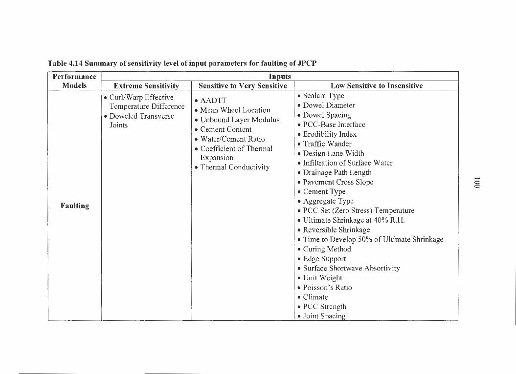
Table 4.14 Summary of sensitivity level of input parameters for faulting of JPCP

Performance Inputs Models Extreme Sensitivity Sensitive to Very Sensitive Low Sensitive to Insensitive

•Curl/Warp Effective • AADTT • Sealant Type

Temperature Difference • Mean Wheel Location • Dowel Diameter

• Doweled Transverse • Unbound Layer Modulus • Dowel Spacing

Joints • PCC-Base Interface • Cement Content

• Erodibility Index • Water/Cement Ratio • Coefficient of Thermal

• Traffic Wander

Expansion • Design Lane Width

•Thermal Conductivity • Infiltration of Surface Water • Drainage Path Length • Pavement Cross Slope • Cement Type

Faulting • Aggregate Type • PCC Set (Zero Stress) Temperature • Ultimate Shrinkage at 40% R.H. • Reversible Shrinkage •Time to Develop 50% of Ultimate Shrinkage • Curing Method • Edge Support • Surface Shortwave Absortivity •Unit Weight • Poisson's Ratio •Climate • PCC Strength • Joint Spacing

......... 0 0

101

4.4.2.2 Summary of Sensitivity Results for Transverse Cracking

Transverse cracking is the key structural failure distress for JPCP. These cracks are usually

caused by a combination of heavy load repetitions and stresses due to temperature gradient,

moisture gradient, and drying shrinkage [ 4.4]. As transverse cracking in JPCP increases,

further cracking forms. This may lead to the replacement of the whole slab. Slab replacement

is costly and can lead to early rehabilitation of the pavement as more occurs. Because

transverse cracking is the primary structural design criterion, there should not be many of

these occurring in regular projects. However, the AASHTO design guides does not provide a

procedure for directly checking a pavement design for transverse cracking, and the guides do

not provide adequate recommendations. [4.5]

Table 4.15 summarizes the sensitivity levels of input parameters for the transverse cracking

of JPCP. The sensitivity of inputs is summarized under three columns - extreme sensitivity,

sensitive to very sensitive and low sensitive to insensitive.

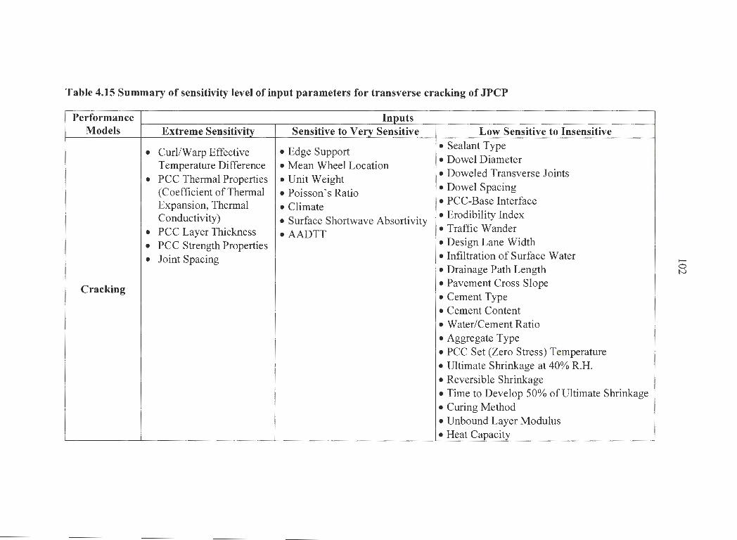
Table 4.15 Summary of sensitivity level of input parameters for transverse cracking of JPCP

Performance Inputs Models Extreme Sensitivity Sensitive to Very Sensitive Low Sensitive to Insensitive

• Curl/Warp Effective •Edge Support • Sealant Type

Temperature Difference • Mean Wheel Location • Dowel Diameter

• PCC Thermal Properties •Unit Weight • Doweled Transverse Joints

(Coefficieqt of Thermal • Poisson' s Ratio • Dowel Spacing

Expansion, Thermal •Climate • PCC-Base Interface

Conductivity) • Surface Shortwave Absortivity • Erodibility Index

• PCC Layer Thickness • AADTT •Traffic Wander

• PCC Strength Properties • Design Lane Width

• Joint Spacing • Infiltration of Surface Water • Drainage Path Length

Cracking • Pavement Cross Slope • Cement Type • Cement Content • Water/Cement Ratio • Aggregate Type • PCC Set (Zero Stress) Temperature • Ultimate Shrinkage at 40% R.H. • Reversible Shrinkage • Time to Develop 50% of Ultimate Shrinkage • Curing Method • Unbound Layer Modulus • Heat Capacity

........ 0 N

103

4.4.2.3 Summary of Sensitivity Results for Smoothness

Smoothness is an extremely important characteristic of a pavement's performance.

Smoothness is also referred to as "roughness". Pavement smoothness greatly affects ride

quality, safety, and vehicle operation speed costs which are very important to the traveling

public. Sayers and Gillespie [4.6-9] define road roughness as the variation in surface

elevation that induces traversing vehicles. Roughness is caused by surface irregularities.

Surface irregularities either are built into a pavement during construction or develop after

construction due to traffic, climatic, and other factors [ 4.10]. One measure of the pavement

roughness provided in the L TPP data base is the international roughness index (IRI),

established in 1986 by the World Bank. IRI is calculated from the longitudinal road profile

and is reported in units of inches/mile or meters/kilometer. IRI has been shown to correlate

with the present serviceability rating (PSR), which is a subjective user rating of the existing

ride quality of the pavement [ 4.11]. The sensitivity results of the MEPDG compare the

sensitivity of input parameters that significantly affect JPCP smoothness as measured by IRI.

Table 4.16 summarizes the input parameters that affect the smoothness of the JPCP pavement

with its sensitivity level.

Table 4.16 Summary of sensitivity level of input parameters for smoothness of JPCP

Performance Inputs Models Extreme Sensitivity Sensitive to Very Sensitive Low Sensitive to Insensitive

• Doweled Transverse Joints • Sealant Type • Curl/Warp Effective • AADTT • Dowel Diameter

Temperature Difference • Mean Wheel Location • Dowel Spacing • PCC Thermal Properties • Joint Spacing • PCC-Base Interface

(Coefficient of Thermal • PCC Layer Thickness • Erodibility Index Expansion, Thermal

• PCC Strength Properties • Traffic Wander Conductivity)

• Poisson' s Ratio • Design Lane Width

• Surface Shortwave Absortivity • Infiltration of Surface Water

• Unbound Layer Modulus • Drainage Path Length

• Cement Content • Pavement Cross Slope Smoothness • Water/Cement Ratio • Cement Type

• Aggregate Type • PCC Set (Zero Stress) Temperature • Ultimate Shrinkage at 40% R.H. • Reversible Shrinkage • Time to Develop 50% of Ultimate

Shrinkage • Curing Method • Edge Support • Climate • Unit Weight

......... 0 ~

105

4.5 References

[4.1] http: //www.datapave.com , Federal Highway Administration, Long Term Pavement

Performance (L TPP) data, Release 18, July 2004

[4.2] Simpson, et al. (1993). "Sensitivity Analyses for Selected Pavement Distresses"

SHRP-P-393. Washington DC: National Research Council.

[4.3] Rao, S., H. T. Yu, L. Khazanovich, M. I. Darter, and J. W. Mack. 1999. "Longevity of

Diamond-Ground Concrete Pavements" Transportation Research Record 1684.

Transportation Research Board of the National Academies.

[4.4] Huang, Y. H. ,"Pavement Analysis and Design", 2°d Edition, Pearson Education, Inc.

'2004

[4.5] Yu, T.H., M.I. Darter, K.D. Smith, J. Jiang, and L. Khazanovich. (1996).

"Performance of Concrete Pavements: Volume III-Improving Concrete Pavement

Performance", FHWA-RD-95-111, Federal Highway Administration, 1996

[ 4.6] M. W. Sayers and S. M. Karamihas, "The Little Book of Profiling", UMTRI, 1995,

85p

[4.7] M. W. Sayers, "On the Calculation of !RI from Longitudinal Road Profile."

Transportation Research Record 1501, Transportation Research Board, National

Research Council, Washington, D.C., 1995, pp. 1-12

[4.8] T. D. Gillespie, "Everything You Always Wanted to Know about the !RI, but Were

Afraid to Ask!" Presented at the Road Profile Users Group Meeting, Lincoln, Nebraska,

September 22-24, 1992

106

[4.9] M. W. Sayers, T. D. Gillespie, and C. A. V. Queiroz, "International Experiment to

Establish Correlations and Standard Calibration Methods for Road Roughness

Measurements." World Bank Teclmical Paper No. 45, the World Bank, Washington DC,

January 1986

[ 4.1 O] L. Khazanovich, M. Darter, R. Bartlett, and T. McPeak. (1998) "Common

Characteristics of Good and Poorly Performing PCC Pavements" FHWA-RD-97-131 ,

Federal Highway Administration, 1998

[ 4.11] Al-Omari, B. and M. I. Darter, (1995). "Effect on Pavement Deterioration Types on

!RI and Rehabilitation " Transportation Research Record No. 1505. Washington DC:

Transportation Research Board

107

CHAPTERS

SUMMARY AND CONCLUSIONS

5.1 Overview

Mechanistic-Empirical Pavement Design Guide (MEPDG) is based on mechanistic-empirical

design procedures and also known as the NCHRP Project l-37A Mechanistic-Empirical

Pavement Design Guide for Design of New and Rehabilitated Pavement Structures. MEPDG

includes (1) a guide for mechanistic-empirical design and analysis, (2) companion software

with documentation and user manual, and (3) an extensive series of supporting technical

documentation. The key improvements that have been included in the MEPDG that make it

superior to the 1993 AASHTO Guide are: (1) the use of mechanistic-empirical pavement

design procedures, (2) the implementation of performance prediction of transverse cracking,

faulting, and smoothness for jointed plain concrete pavements, (3) the addition of climatic

inputs, ( 4) better characterization of traffic loading inputs, (5) more sophisticated structural

modeling capabilities, and (6) the ability to model real-world changes in material properties.

In short, mechanistic-empirical pavement design procedure is one that uses the principles of

108

both engmeermg mechanics and field verification to come up with a design process.

Mechanistic methods are used to predict pavement responses and their performance is

predicted based on performance data collected from "real world" pavements. Due to the

complexity of its design procedure, it also has more inputs with its hierarchical approach to

the design inputs .

This thesis presents the results of sensitivity investigation on input parameters of rigid

modules of the MEPDG. First, a comprehensive literature review addressing the design

methods and guidelines of concrete pavements was prepared. Consequently, an overview of

the rigid pavement design inputs (traffic, climate, and material inputs) of the MEPDG was

completed. Next, the analysis of two selected JPCP sections was performed with the user­

friendly MEPDG software. The MEPDG results were compared with available actual

pavement field data. Then, using the MEPDG software, the sensitivity of rigid module input

parameters of the MEPDG was investigated. Using a sensitivity scale, the effects of inputs

parameters on pavement performance were summarized. Conclusions drawn from the study

and recommendation for future research are presented below.

5.2 Conclusions

The following conclusions were drawn as a result of the sensitivity analyses described in

Chapter 4 (see Table 4.13-16):

109

.,/ The extremely sensitive input parameters for transverse cracking are found as:

• Curl/warp effective temperature difference (built-in)

• Coefficient of thermal expansion

• Thermal conductivity

• PCC layer thickness

• PCC strength properties, and

• Joint spacing

In addition, the sensitive to very sensitive input parameters for transverse cracking

are:

• Edge support

• Mean wheel location (traffic wander)

• Unit weight

• Poisson's ratio

• Climate

• Surface shortwave absortivity, and

• Annual average daily truck traffic (AADTT)

Other examined parameters are found as less sensitive to insensitive .

.,/ The extremely sensitive input parameters for faulting are:

• Curl/warp effective temperature difference (built-in)

• Doweled transverse joints (load transfer mechanism, doweled or un-doweled)

The sensitive to very sensitive input parameters for faulting are:

• Coefficient of thermal expansion

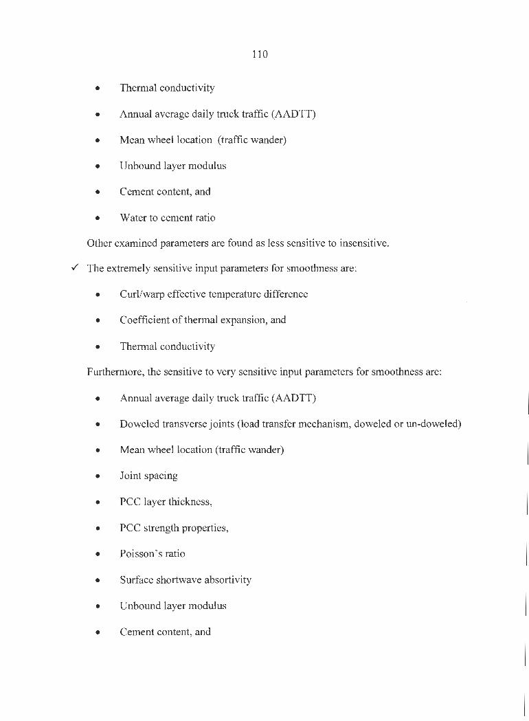
110

• Thermal conductivity

• Annual average daily truck traffic (AADTT)

• Mean wheel location (traffic wander)

• Unbound layer modulus

• Cement content, and

• Water to cement ratio

Other examined parameters are found as less sensitive to insensitive .

../ The extremely sensitive input parameters for smoothness are:

• Curl/warp effective temperature difference

• Coefficient of thermal expansion, and

• Thermal conductivity

Furthermore, the sensitive to very sensitive input parameters for smoothness are:

• Annual average daily truck traffic (AADTT)

• Doweled transverse joints (load transfer mechanism, doweled or un-doweled)

• Mean wheel location (traffic wander)

• Joint spacing

• PCC layer thickness,

• PCC strength properties,

• Poisson' s ratio

• Surface shortwave absortivity

• Unbound layer modulus

• Cement content, and

111

• Water to cement ratio

Other examined parameters are found as less sensitive to insensitive .

./ The Curl/warp effective temperature difference, coefficient of thermal expansion, and

thermal conductivity come out to be the most critical design input parameters that

affect each performance criteria. Since these input parameters can not be modified,

accurate values should be input into the model. The sensitivity of the model to these

parameters is extremely high; therefore, pavement performance outputs can vary

significantly. Thus, extreme attention should be given to determine input data for

these particular parameters. If necessary, material test(s) should be carried out to

determine the magnitude of these parameters. Otherwise the accuracy of the predicted

pavement distresses differs significantly .

./ Among of the extremely sensitive and sensitive to very sensitive parameters, the

pavement design engineer can only modify; PCC layer thickness, doweled transverse

joints, and joint spacing. PCC strength properties is also modifiable provided that

pavement design specifications are met.

./ For pavement smoothness, comparison of the MEPDG analysis and actual field data

of the two selected JPCP sites indicated that the use of MEPDG needs to be calibrated

for Iowa suggesting that the accuracy of the actual field data is questionable .

./ Since the available field data for transverse cracking in pavement management

information system are in different units then those used in the MPEDG, it is

recommended that the units of MPEDG should be correlated to the actual field data.

112

5.3 Recommendations

Based on observations made throughout this study, the following recommendations are

made:

./ A training program for pavement design engineers with an emphasis on which design

input parameters to change or to enter with high precision should be implemented .

./ The existing pavement design guides such as 1993 AASHTO Design Guide do not

provide performance prediction of pavements. With the new design approach that

includes the use of mechanistic-empirical pavement design procedures and prediction

of performance models, in-depth knowledge about use of design inputs is required

and establishment of an expert system is recommended. An expert system will help

pavement design engineers to determine the critical rigid pavement design inputs that

should be modified and not modified for rigid pavement design and the use of correct

hierarchical level of each design input.

./ Implementation of laboratory testing, field-testing, and non-destructive deflection

testing should be started for all design input parameters. Priority should be given to

extremely sensitive input parameters.

5.4 Future Research

./ For local calibration, Iowa DOT should select further sites for different climatic

locations, traffic loadings, and material characteristics representing Iowa highway and

113

roads. A detailed comparison on pavement distresses of the MEPDG analysis and the

actual field data of these sites should be carried out. It is also of paramount

importance to collect detailed accurate field data .

../ The correlation between the PMIS data and the MEPDG performance models should

be further investigated for a better comparison of the MEPDG results, such that units

should be converted.

114

APPENDIX A

ACCOMPANYING CD-ROM AND

SYSTEM REQUIREMENTS

Appendix A is located in CD-ROM, and contains series of graphs for sensitivity analysis of

JPCP design inputs constituting the standard pavement section and data used in the analysis

presented in Chapter 4 of the text.

System requirements for CD: IBM PC or 100% compatibles; Windows 95 or higher; 32 MB

RAM; hard disk (1 GB minimum); Microsoft Word 2000 or higher.