Struct Multidisc Optim (2011) 44:797–814 DOI 10.1007/s00158-011-0665-4 INDUSTRIAL APPLICATION Sensitivity analysis of optimum solutions by updating active constraints: application in aircraft structural design Aitor Baldomir · Santiago Hernandez · Jacobo Diaz · Arturo Fontan Received: 7 April 2010 / Revised: 7 March 2011 / Accepted: 19 April 2011 / Published online: 3 June 2011 c Springer-Verlag 2011 Abstract Often the parameters considered as constants in an optimization problem have some uncertainty and it is interesting to know how the optimum solution is modified when these values are changed. The only way to continue having the optimal solution is to perform a new optimiza- tion loop, but this may require a high computational effort if the optimization problem is large. However, there are sev- eral procedures to obtain the new optimal design, based on getting the sensitivities of design variables and objective function with respect to a fixed parameter. Most of these methods require obtaining second derivatives which has a significant computational cost. This paper uses the feasible direction-based technique updating the active constraints to obtain the approximate optimum design. This proce- dure only requires the first derivatives and it is noted that the updating set of active constraints improves the result, making possible a greater fixed parameter variation. This methodology is applied to an example of very common structural optimization problems in technical literature and to a real aircraft structure. Keywords Aircraft · Feasible direction · Sensitivity · Optimum design 1 Introduction During the structural design process, the designer often needs to modify some fixed parameter values such as A. Baldomir (B ) · S. Hernandez · J. Diaz · A. Fontan Structural Mechanics Group, School of Civil Engineering, University of La Coruña, La Coruña, Spain e-mail: [email protected] geometrical dimensions, material properties, stress or strain limits, etc. These modifications can always be incorpo- rated into the structure and we can verify if the limit states are satisfied or not. If a design of a structure comes from an optimization process, the optimum solution depends on those fixed parameters, and a modification in any of them will cause changes in the final optimal solution. From the experience of structural optimization in aeronautical engineering, these modifications occur often, even in the advanced design stages. When there is a change in any fixed parameter, we have two options: solve the optimization problem again or obtain an approximate optimum solution. The latter option is considered in this research work. Given a design problem composed by a set of fixed parameters p = ( p 1 , p 2 ,. . . ,p k ) and another set of design variables X, structural optimization can be defined as the procedure for identifying the value of X that provides the best result for an objective function F (X,p), subject to a number of constraints. In mathematical form: min F (X, p) (1) subject to g j (X, p) ≤ 0 j = 1, ..., m (2) where m is the total number of constraints. Therefore, the optimum design is X ∗ = X ∗ (p). Often in real design situations, a parameter p ⊂ p does not have the scheduled value, so the parameter p becomes p + p. Some situations where this occurs are changes in load values or material properties, decisions about the final geometry of some structural elements or variations in stress or strain limits.

Welcome message from author
This document is posted to help you gain knowledge. Please leave a comment to let me know what you think about it! Share it to your friends and learn new things together.
Transcript

Struct Multidisc Optim (2011) 44:797–814DOI 10.1007/s00158-011-0665-4
INDUSTRIAL APPLICATION
Sensitivity analysis of optimum solutions by updating activeconstraints: application in aircraft structural design
Aitor Baldomir · Santiago Hernandez · Jacobo Diaz ·Arturo Fontan
Received: 7 April 2010 / Revised: 7 March 2011 / Accepted: 19 April 2011 / Published online: 3 June 2011c© Springer-Verlag 2011
Abstract Often the parameters considered as constants inan optimization problem have some uncertainty and it isinteresting to know how the optimum solution is modifiedwhen these values are changed. The only way to continuehaving the optimal solution is to perform a new optimiza-tion loop, but this may require a high computational effortif the optimization problem is large. However, there are sev-eral procedures to obtain the new optimal design, based ongetting the sensitivities of design variables and objectivefunction with respect to a fixed parameter. Most of thesemethods require obtaining second derivatives which has asignificant computational cost. This paper uses the feasibledirection-based technique updating the active constraintsto obtain the approximate optimum design. This proce-dure only requires the first derivatives and it is noted thatthe updating set of active constraints improves the result,making possible a greater fixed parameter variation. Thismethodology is applied to an example of very commonstructural optimization problems in technical literature andto a real aircraft structure.
Keywords Aircraft · Feasible direction · Sensitivity ·Optimum design
1 Introduction
During the structural design process, the designer oftenneeds to modify some fixed parameter values such as
A. Baldomir (B) · S. Hernandez · J. Diaz · A. FontanStructural Mechanics Group, School of Civil Engineering,University of La Coruña, La Coruña, Spaine-mail: [email protected]
geometrical dimensions, material properties, stress or strainlimits, etc. These modifications can always be incorpo-rated into the structure and we can verify if the limit statesare satisfied or not. If a design of a structure comes froman optimization process, the optimum solution depends onthose fixed parameters, and a modification in any of themwill cause changes in the final optimal solution. Fromthe experience of structural optimization in aeronauticalengineering, these modifications occur often, even in theadvanced design stages.
When there is a change in any fixed parameter, wehave two options: solve the optimization problem again orobtain an approximate optimum solution. The latter optionis considered in this research work.
Given a design problem composed by a set of fixedparameters p = (p1, p2,. . . ,pk) and another set of designvariables X, structural optimization can be defined as theprocedure for identifying the value of X that provides thebest result for an objective function F(X,p), subject to anumber of constraints. In mathematical form:
min F (X, p) (1)
subject to
g j (X, p) ≤ 0 j = 1, ..., m (2)
where m is the total number of constraints.Therefore, the optimum design is X∗ = X∗(p). Often in
real design situations, a parameter p ⊂ p does not havethe scheduled value, so the parameter p becomes p + �p.
Some situations where this occurs are changes in load valuesor material properties, decisions about the final geometryof some structural elements or variations in stress or strainlimits.

798 A. Baldomir et al.
These circumstances affect the optimum solution; there-fore a new optimization procedure needs to be carried out.While this can be easily done for small size problems, it canbe cumbersome for large structural models.
On the other hand, changes in the value of these param-eters may not be excessive; hence the designer can rightlythink that the information of the previous problem should beof some use.
In that case, an alternative approach can be performedwith some advantages. This technique consists of obtain-ing design variable sensitivities and the objective functionsensitivity with respect to the modified parameter. If thesesensitivities are known, we can get an approximate value ofF and X when a parameter p has a variation of �p as:
F̃ = F∗ + ∂ F
∂p· �p
x̃i = x∗i + ∂xi
∂p· �p i = 1, ..., n (3)
where n is the number of design variables.The first two methods to obtain these sensitivities were
developed by Sobieszczanski-Sobieski et al. (1982). Theprocedure in both methods is to derive the expressions ofthe extreme conditions with respect to the parameter p andsolve the resulting linear system of equations. The first oneis based on the differentiation of the Kuhn-Tucker condi-tions and the second one consists of the differentiation ofthe extremum condition of a penalty function with respectto the parameter.
A different approach for getting the sensitivities ofthe optimum solution was performed by Vanderplaats andYoshida (1985). In this technique, the sensitivity is obtainedusing the feasible directions concept (Zoutendijk 1960) inthat it searches the maximum improvement of the objec-tive function when the parameter becomes a new designvariable.
In order to implement both methods, the input dataneeded are the optimum design, the gradient of constraintsand the gradient of the objective function for a given valueof the parameter p. Depending on the type of algorithm usedfor optimization, second order derivatives constraints andthe second derivatives of objective function in the optimumdesign are available (Haftka et al. 1990; Vanderplaats 2001).
With these input data, either of the two techniques men-tioned above can be formulated, obtaining an approximatesolution with a low computational effort.
However, the work done by Sobieszczanski-Sobieski, aswell as that by Vanderplaats, make clear that the formu-lations are valid when the set of active constraints do notchange (Barthelemy and Sobieszczanski-Sobieski 1983a, b).As noted in this paper, the set of active constraints canchange for small parameter variations.
There are sophisticated methods (Rakowska et al. 1991)to determine the changes in the set of active constraintswhen the parameter is modified. The effectiveness of thesemethods has been proven but requires a high computationalcost. Other studies performed in the topology optimizationfield (Guo and Cheng 2000) have used Sobieszczanski-Sobieski’s method, getting good results when the set ofactive constraints does not change. That research concludesthat Rakowska’s method can be used to track the activeconstrains, but it will require a high computational effort.
A contribution of this research is to obtain a methodol-ogy that allows tracking the set of active constraints with alow computational effort. This research enhances a method-ology for obtaining approximate optimal solutions basedon Vanderplaats’ method by updating active constraints.The reason for using the approach based on the search forfeasible directions is that this method only requires the cal-culation of the first derivatives of constraints and objectivefunction.
Another contribution of this research is the application ofthis approach to real aircraft structures using finite elementmodels with bar and shell elements. Also this methodologyis applied to parameter variations of very different natures.
2 Sensitivity analysis of parameters by feasibledirections approach
The feasible directions approach starts with the definitionof an expanded design space, where the parameter p isconsidered as a new design variable xn+1 = p. The aimis the modification of the design variables to achieve themaximum improvement of the design when the parameterchanges. This problem may be formulated as the searchfor the forward direction S of the design variables thatminimizes the objective function F .
min ∇F(X∗)T · S (4)
subject to
∇g j(X∗)T · S ≤ 0 j ∈ J (5)
ST · S ≤ 1 (6)
where J is the set of active constraints at the optimumdesign, resulting after solving problem (1–2).
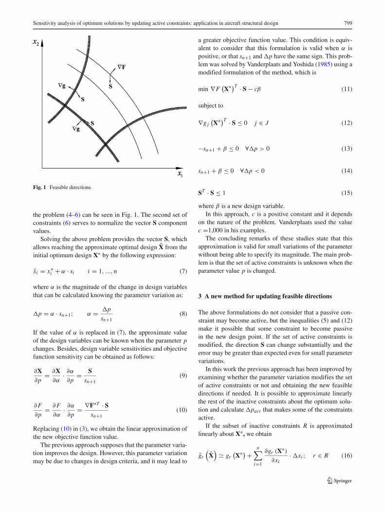
It is intended that the angle between ∇F and S is asobtuse as possible to minimize F as shown in Fig. 1.Besides, the new design point X̃ cannot be outside of thedesign region, which means that the angle between S andthe active constraint gradients should also be obtuse. Theseconstraints are expressed in (5) and a graphical scheme of
Sensitivity analysis of optimum solutions by updating active constraints: application in aircraft structural design 799
Fig. 1 Feasible directions
the problem (4–6) can be seen in Fig. 1. The second set ofconstraints (6) serves to normalize the vector S componentvalues.
Solving the above problem provides the vector S, whichallows reaching the approximate optimal design X̃ from theinitial optimum design X∗ by the following expression:
x̃i = x∗i + α · si i = 1, ..., n (7)
where α is the magnitude of the change in design variablesthat can be calculated knowing the parameter variation as:
�p = α · sn+1; α = �p
sn+1(8)
If the value of α is replaced in (7), the approximate valueof the design variables can be known when the parameter pchanges. Besides, design variable sensitivities and objectivefunction sensitivity can be obtained as follows:
∂X∂p
= ∂X∂α
· ∂α
∂p= S
sn+1(9)
∂ F
∂p= ∂ F
∂α· ∂α
∂p= ∇F∗T · S
sn+1(10)
Replacing (10) in (3), we obtain the linear approximation ofthe new objective function value.
The previous approach supposes that the parameter varia-tion improves the design. However, this parameter variationmay be due to changes in design criteria, and it may lead to
a greater objective function value. This condition is equiv-alent to consider that this formulation is valid when α ispositive, or that sn+1 and �p have the same sign. This prob-lem was solved by Vanderplaats and Yoshida (1985) using amodified formulation of the method, which is
min ∇F(X∗)T · S − cβ (11)
subject to
∇g j(X∗)T · S ≤ 0 j ∈ J (12)
−sn+1 + β ≤ 0 ∀�p > 0 (13)
sn+1 + β ≤ 0 ∀�p < 0 (14)
ST · S ≤ 1 (15)
where β is a new design variable.In this approach, c is a positive constant and it depends
on the nature of the problem. Vanderplaats used the valuec =1,000 in his examples.
The concluding remarks of these studies state that thisapproximation is valid for small variations of the parameterwithout being able to specify its magnitude. The main prob-lem is that the set of active constraints is unknown when theparameter value p is changed.
3 A new method for updating feasible directions
The above formulations do not consider that a passive con-straint may become active, but the inequalities (5) and (12)make it possible that some constraint to become passivein the new design point. If the set of active constraints ismodified, the direction S can change substantially and theerror may be greater than expected even for small parametervariations.
In this work the previous approach has been improved byexamining whether the parameter variation modifies the setof active constraints or not and obtaining the new feasibledirections if needed. It is possible to approximate linearlythe rest of the inactive constraints about the optimum solu-tion and calculate �pact that makes some of the constraintsactive.
If the subset of inactive constraints R is approximatedlinearly about X∗, we obtain
g̃r
(X̃
) gr
(X∗) +
n∑
i=1
∂gr (X∗)∂xi
· �xi ; r ∈ R (16)

800 A. Baldomir et al.
Imposing that these constraints become active
g̃r
(X̃
) gr
(X∗) +
n∑
i=1
∂gr (X∗)∂xi
· �xi = 0 r ∈ R (17)
On the other hand, (7) can be written as
�xi = α · si (18)
and replacing the values of �xi in the expression (17), weobtain the expressions
gr(X∗) + αr ·
n∑
i=1
∂gr (X∗)∂xi
· si = 0;
αr = −gr (X∗)n∑
i=1
∂gr (X∗)∂xi
· si
r ∈ R (19)
Thus, there is an equation for each value of r and oneunknown for each value of r . The smallest value of αr isnamed αact and provides the maximum parameter variationwithout activating any other constraint, which is:
�pact = αact · sn+1 (20)
Fig. 2 Flowchart to obtain the approximate optimum solution byupdating active constraints
In the case that �pact > �p, it is not necessary to updatethe set of active constraints, but if �pact < �p, it will benecessary to update this set. The next step is to recalculate anew feasible direction by solving the problem (4–6) or (11–15) but from the new approximate solution X̃act obtained byapplying (7) with α = αact . This step requires the calcula-tion of the gradients of design constraints and the gradientof the objective function in X̃act . The flowchart that showsthis methodology appears in Fig. 2.
The technique explained obtains a value of �pact bylinearizing each inactive constraint at the optimum andchoosing the smallest value of �p. This rule guarantees theattenuation of the effect of linearizing the constraints. Thequantification of this impact can be evaluated by compari-son between approximate and optimum solutions presentedto the application examples.
This methodology only needs the first derivatives of theobjective function and constraints, unlike what happensin the other methods. Moreover, the resulting optimiza-tion problem, for obtaining feasible directions, requires alow computational effort, since the functions involved areexplicit and the problem is linear with the exception of thelast constraint.
4 Application examples
4.1 Ten-bar truss structure
This example is a widely known problem in the field ofstructural optimization (Berke and Khot 1974; Kirsch 1981;Haftka et al. 1990). It is a ten-bar structure with two verti-cal loads of value Q =1 kN as can be seen in Fig. 3. Linearelastic material behaviour has been considered with Young’smodulus of value E =210,000 MPa and normal stress limitwas set to 250 MPa.
Fig. 3 Ten-bar truss structure. Dimensions in metres

Sensitivity analysis of optimum solutions by updating active constraints: application in aircraft structural design 801
Table 1 Results of optimum design for different values of p
xi p = 0.01 p = 0.015 p = 0.02 p = 0.03
x1 28.672 18.966 14.350 9.332
x2 0.100 0.100 0.100 0.100
x3 21.944 15.212 10.847 8.003
x4 14.651 9.859 7.270 4.632
x5 0.100 0.100 0.100 0.100
x6 0.100 0.100 0.100 0.100
x7 7.290 6.083 5.534 5.661
x8 19.711 12.745 9.913 6.557
x9 20.738 13.919 10.293 6.552
x10 0.100 0.100 0.100 0.100
The optimization problem is to minimize the structuralvolume and the design variables are the cross sectional areasxi of each bar. Stress constraints and displacement con-straints have been considered in the optimization problemthat it can be defined as follows:
min F =∑
xi · li (21)
subject to
xi ≥ 0.1 i = 1, ..., 10 (22)
−250 ≤ σi ≤ 250 i = 1, ..., 10 (23)
−w5 ≤ wmáx (24)
where σ i is the normal stress and w5 is the vertical displace-ment of node 5.
The parameter chosen is the maximum allowed verticaldisplacement in node 5, p = wmax .
First, optimal solutions with four different values of theparameter p = wmax have been obtained by solving theproblem defined in (21–24) and numerical results are shownin Table 1.
Then, parameter variations of 10%, 25% and 50% havebeen performed to get the optimum design X∗ and theapproximate solution X̃ by using the feasible direction tech-nique. These results are shown in Tables 2, 4 and 6 wherethe error in the objective function is also specified. Thiserror is 1.8% for a parameter variation of 10%, while fora parameter variation of 25% and 50%, the error increasesup to 11% and 30% respectively. It is important to notethat the initial value of the parameter, which in this caseis the maximum displacement allowed in node 5,p = wmax ,is a determinant factor to get good results. Thus, for 25%(Table 4) of parameter variation, the approximate value issufficiently accurate when the initial value is p = 0.02 cm,but if the initial value of the parameter is p = 0.03 cm,the error is much larger. The explanation remains on theset of active constraints which—considering some differentinitial values of p—does not change up to a very largeparameter variation. Nevertheless, for other initial valuesof p, a smaller change of the parameter modifies the set ofactive constraints leading to major errors of the approximatesolution.
Not only objective function error should be checked inapproximate results, but also the value of constraints. Theseresults are presented in Tables 3, 5 and 7 where the valueof constraint and violation ratio are provided. The violationratio is calculated as the relative error between the structuralresponse value and the limit constraint value. The maximumconstraint violation is 1.1% for �p = 10% but this valueincreases significantly for larger parameter variations.
Table 2 Real and approximateoptima for �p = 10% with fourinitial values of the parameter p
p + �p = 0.011 p + �p = 0.0165 p + �p = 0.022 p + �p = 0.033
Variable X∗ X̃ X∗ X̃ X∗ X̃ X∗ X̃
x1 26.006 27.357 17.181 17.989 13.179 13.614 8.318 8.695
x2 0.100 0.100 0.100 0.100 0.100 0.100 0.100 0.100
x3 20.112 20.699 13.955 14.317 9.422 10.099 8.044 7.998
x4 13.354 13.363 8.990 8.916 6.544 6.531 4.121 3.982
x5 0.100 0.450 0.100 0.321 0.100 0.347 0.100 0.212
x6 0.100 0.100 0.100 0.100 0.100 0.100 0.100 0.100
x7 7.018 6.023 5.778 5.180 5.542 5.223 5.720 5.654
x8 17.791 17.809 11.483 11.307 9.300 8.879 5.834 5.686
x9 18.898 18.916 12.705 12.585 9.259 9.248 5.833 5.633
x10 0.100 0.100 0.100 0.100 0.100 0.100 0.100 0.100
F 43,820.5 44,159.4 29,860.4 29,879.1 22,920.0 23,024.1 16,384.6 16,283.1
Error F (%) – 0.8 – 0.1 – 0.4 – −0.6

802 A. Baldomir et al.
Table 3 Constraint feasibility for approximate solutions (�p = 10%)
p + �p = 0.011 p + �p = 0.0165 p + �p = 0.022 p + �p = 0.033
Violation ratio Violation ratio Violation ratio Violation ratio
σ 1 7.73E-03 0.000 1.16E-02 0.000 1.52E-02 0.000 2.29E-02 0.000
σ 2 −5.85E-04 0.000 1.75E-03 0.000 5.19E-03 0.000 1.47E-02 0.000
σ 3 −9.11E-03 0.000 −1.34E-02 0.000 −1.91E-02 0.000 −2.51E-02 0.004
σ 4 −7.49E-03 0.000 −1.12E-02 0.000 −1.52E-02 0.000 −2.47E-02 0.000
σ 5 2.53E-02 0.011 2.52E-02 0.006 2.06E-02 0.000 3.25E-03 0.000
σ 6 −5.85E-04 0.000 1.75E-03 0.000 5.19E-03 0.000 1.47E-02 0.000
σ 7 2.08E-02 0.000 2.51E-02 0.006 2.53E-02 0.011 2.52E-02 0.008
σ 8 −8.85E-03 0.000 −1.35E-02 0.000 −1.70E-02 0.000 −2.47E-02 0.000
σ 9 7.48E-03 0.000 1.12E-02 0.000 1.52E-02 0.000 2.47E-02 0.000
σ 10 8.28E-04 0.000 −2.48E-03 0.000 −7.35E-03 0.000 −2.08E-02 0.000
w5 −1.11E-02 0.009 −1.67E-02 0.009 −2.21E-02 0.006 −3.33E-02 0.010
Table 4 Real and approximate optima for �p = 25% with four initial values of the parameter p
p + �p = 0.0125 p + �p = 0.0188 p + �p = 0.025 p + �p = 0.0375
Variable X* X̃ X* X̃ X* X̃ X* X̃
x1 22.829 25.384 15.191 16.177 11.573 12.511 7.938 7.740
x2 0.100 0.100 0.100 0.100 0.100 0.100 0.100 0.100
x3 17.919 18.832 12.010 12.423 8.301 8.976 8.062 7.991
x4 11.775 11.431 7.853 7.071 5.743 5.423 3.938 3.007
x5 0.100 0.976 0.100 0.100 0.100 0.718 0.100 0.381
x6 0.100 0.100 0.100 0.100 0.100 0.100 0.100 0.100
x7 6.640 4.122 5.531 2.139 5.572 4.757 5.745 5.644
x8 15.509 14.955 10.270 8.801 8.153 7.330 5.569 4.379
x9 16.664 16.184 11.093 9.974 8.128 7.681 5.569 4.253
x10 0.100 0.100 0.100 0.100 0.100 0.100 0.100 0.100
F 38,827.3 38,458.9 26,470.4 29,435.6 20,506.3 20,132.6 15,931.8 14,273.7
Error F (%) – −0.9 – 11.2 – −1.8 – −10.4
Table 5 Constraint feasibility for approximate solutions (�p = 25%)
p + �p = 0.0125 p + �p = 0.0188 p + �p = 0.025 p + �p = 0.0375
Violation ratio Violation ratio Violation ratio Violation ratio
σ 1 8.92E-03 0.000 1.30E-02 0.000 1.68E-02 0.000 2.52E-02 0.007
σ 2 −1.52E-04 0.000 −9.08E-03 0.000 8.19E-03 0.000 2.19E-02 0.000
σ 3 −9.22E-03 0.000 −1.53E-02 0.000 −2.12E-02 0.000 −2.57E-02 0.027
σ 4 −8.75E-03 0.000 −1.43E-02 0.000 −1.83E-02 0.000 −3.25E-02 0.301
σ 5 2.70E-02 0.079 8.67E-02 2.469 1.53E-02 0.000 −7.97E-03 0.000
σ 6 −1.52E-04 0.000 −9.08E-03 0.000 8.19E-03 0.000 2.19E-02 0.000
σ 7 2.53E-02 0.011 5.98E-02 1.391 2.67E-02 0.068 2.64E-02 0.055
σ 8 −1.19E-02 0.000 −1.76E-02 0.000 −2.13E-02 0.000 −3.06E-02 0.224
σ 9 8.74E-03 0.000 1.43E-02 0.000 1.83E-02 0.000 3.25E-02 0.301
σ 10 2.15E-04 0.000 1.28E-02 0.000 −1.16E-02 0.000 −3.09E-02 0.237
w5 −1.32E-02 0.058 −2.05E-02 0.088 −2.61E-02 0.043 −4.03E-02 0.073

Sensitivity analysis of optimum solutions by updating active constraints: application in aircraft structural design 803
Table 6 Real and approximateoptima for �p = 50% with fourinitial values of the parameter p
p + �p = 0.015 p + �p = 0.0225 p + �p = 0.0375 p + �p = 0.045
Variable X* X̃ X* X̃ X* X̃ X* X̃
x1 18.966 22.096 12.880 13.388 7.938 8.394 7.938 6.148
x2 0.100 0.100 0.100 0.100 0.100 0.100 0.100 0.100
x3 15.212 15.720 9.219 9.634 8.062 5.019 8.062 7.979
x4 9.859 8.211 6.395 4.282 3.938 2.540 3.938 1.381
x5 0.100 1.851 0.100 0.100 0.100 1.005 0.100 0.661
x6 0.100 0.100 0.100 0.100 0.100 0.100 0.100 0.100
x7 6.083 0.954 5.547 0.100 5.745 4.675 5.745 5.627
x8 12.745 10.199 9.086 4.857 5.569 3.707 5.569 2.201
x9 13.919 11.630 9.049 6.029 5.569 3.598 5.569 1.955
x10 0.100 0.100 0.100 0.100 0.100 0.100 0.100 0.100
F 32,684.2 28,958.1 22,473.7 15,581.6 15,931.8 12,326.0 15,931.8 10,924.9
Error F (%) – −11.4 – −30.7 – −22.6 – −31.4
Table 7 Constraint feasibility for approximate solutions (�p = 50%)
p + �p = 0.015 p + �p = 0.0225 p + �p = 0.0375 p + �p = 0.045
Violation ratio Violation ratio Violation ratio Violation ratio
σ 1 1.22E-02 0.000 2.05E-02 0.000 2.37E-02 0.000 2.83E-02 0.132
σ 2 −2.69E-04 0.000 −1.14E-01 3.542 2.35E-02 0.000 4.93E-02 0.973
σ 3 −8.27E-03 0.000 −1.31E-02 0.000 −4.00E-02 0.600 −2.83E-02 0.133
σ 4 −1.22E-02 0.000 −2.60E-02 0.040 −3.84E-02 0.538 −6.88E-02 1.754
σ 5 3.78E-02 0.512 6.27E-01 24.060 1.56E-03 0.000 −3.18E-02 0.273
σ 6 −2.69E-04 0.000 −1.14E-01 3.542 2.35E-02 0.000 4.93E-02 0.973
σ 7 4.45E-02 0.778 3.68E-01 13.705 3.05E-02 0.220 3.17E-02 0.266
σ 8 −2.36E-02 0.000 −5.07E-02 1.027 −3.78E-02 0.514 −4.76E-02 0.903
σ 9 1.22E-02 0.000 2.61E-02 0.045 3.84E-02 0.535 6.88E-02 1.751
σ 10 3.81E-04 0.000 1.61E-01 5.423 −3.33E-02 0.331 −6.98E-02 1.791
w5 −1.99E-02 0.330 −4.00E-02 0.780 −4.77E-02 0.273 −6.62E-02 0.472
Table 8 Real and approximateoptima for �p = 10% trackingconstraints with four initialvalues of the parameter p
p + �p = 0.011 p + �p = 0.0165 p + �p = 0.022 p + �p = 0.033
Variable X* X̃ X* X̃ X* X̃ X* X̃
x1 26.006 27.357 17.181 17.989 13.179 13.614 8.318 8.695
x2 0.100 0.100 0.100 0.100 0.100 0.100 0.100 0.100
x3 20.112 20.699 13.955 14.317 9.422 10.099 8.044 7.998
x4 13.354 13.363 8.990 8.916 6.544 6.531 4.121 3.982
x5 0.100 0.450 0.100 0.321 0.100 0.347 0.100 0.212
x6 0.100 0.100 0.100 0.100 0.100 0.100 0.100 0.100
x7 7.018 6.023 5.778 5.180 5.542 5.223 5.720 5.654
x8 17.791 17.809 11.483 11.307 9.300 8.879 5.834 5.686
x9 18.898 18.916 12.705 12.585 9.259 9.248 5.833 5.633
x10 0.100 0.100 0.100 0.100 0.100 0.100 0.100 0.100
F 43,820.6 44,159.5 29,860.409 29,879.1 22,920.0 23,024.1 16,384.6 16,283.1
Error F (%) – 0.8 – 0.1 – 0.4 – −0.6
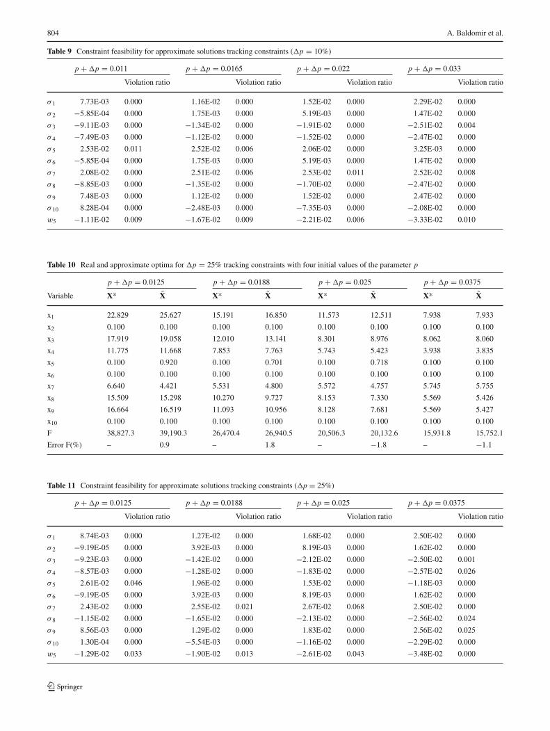
804 A. Baldomir et al.
Table 9 Constraint feasibility for approximate solutions tracking constraints (�p = 10%)
p + �p = 0.011 p + �p = 0.0165 p + �p = 0.022 p + �p = 0.033
Violation ratio Violation ratio Violation ratio Violation ratio
σ 1 7.73E-03 0.000 1.16E-02 0.000 1.52E-02 0.000 2.29E-02 0.000
σ 2 −5.85E-04 0.000 1.75E-03 0.000 5.19E-03 0.000 1.47E-02 0.000
σ 3 −9.11E-03 0.000 −1.34E-02 0.000 −1.91E-02 0.000 −2.51E-02 0.004
σ 4 −7.49E-03 0.000 −1.12E-02 0.000 −1.52E-02 0.000 −2.47E-02 0.000
σ 5 2.53E-02 0.011 2.52E-02 0.006 2.06E-02 0.000 3.25E-03 0.000
σ 6 −5.85E-04 0.000 1.75E-03 0.000 5.19E-03 0.000 1.47E-02 0.000
σ 7 2.08E-02 0.000 2.51E-02 0.006 2.53E-02 0.011 2.52E-02 0.008
σ 8 −8.85E-03 0.000 −1.35E-02 0.000 −1.70E-02 0.000 −2.47E-02 0.000
σ 9 7.48E-03 0.000 1.12E-02 0.000 1.52E-02 0.000 2.47E-02 0.000
σ 10 8.28E-04 0.000 −2.48E-03 0.000 −7.35E-03 0.000 −2.08E-02 0.000
w5 −1.11E-02 0.009 −1.67E-02 0.009 −2.21E-02 0.006 −3.33E-02 0.010
Table 10 Real and approximate optima for �p = 25% tracking constraints with four initial values of the parameter p
p + �p = 0.0125 p + �p = 0.0188 p + �p = 0.025 p + �p = 0.0375
Variable X* X̃ X* X̃ X* X̃ X* X̃
x1 22.829 25.627 15.191 16.850 11.573 12.511 7.938 7.933
x2 0.100 0.100 0.100 0.100 0.100 0.100 0.100 0.100
x3 17.919 19.058 12.010 13.141 8.301 8.976 8.062 8.060
x4 11.775 11.668 7.853 7.763 5.743 5.423 3.938 3.835
x5 0.100 0.920 0.100 0.701 0.100 0.718 0.100 0.100
x6 0.100 0.100 0.100 0.100 0.100 0.100 0.100 0.100
x7 6.640 4.421 5.531 4.800 5.572 4.757 5.745 5.755
x8 15.509 15.298 10.270 9.727 8.153 7.330 5.569 5.426
x9 16.664 16.519 11.093 10.956 8.128 7.681 5.569 5.427
x10 0.100 0.100 0.100 0.100 0.100 0.100 0.100 0.100
F 38,827.3 39,190.3 26,470.4 26,940.5 20,506.3 20,132.6 15,931.8 15,752.1
Error F(%) – 0.9 – 1.8 – −1.8 – −1.1
Table 11 Constraint feasibility for approximate solutions tracking constraints (�p = 25%)
p + �p = 0.0125 p + �p = 0.0188 p + �p = 0.025 p + �p = 0.0375
Violation ratio Violation ratio Violation ratio Violation ratio
σ 1 8.74E-03 0.000 1.27E-02 0.000 1.68E-02 0.000 2.50E-02 0.000
σ 2 −9.19E-05 0.000 3.92E-03 0.000 8.19E-03 0.000 1.62E-02 0.000
σ 3 −9.23E-03 0.000 −1.42E-02 0.000 −2.12E-02 0.000 −2.50E-02 0.001
σ 4 −8.57E-03 0.000 −1.28E-02 0.000 −1.83E-02 0.000 −2.57E-02 0.026
σ 5 2.61E-02 0.046 1.96E-02 0.000 1.53E-02 0.000 −1.18E-03 0.000
σ 6 −9.19E-05 0.000 3.92E-03 0.000 8.19E-03 0.000 1.62E-02 0.000
σ 7 2.43E-02 0.000 2.55E-02 0.021 2.67E-02 0.068 2.50E-02 0.000
σ 8 −1.15E-02 0.000 −1.65E-02 0.000 −2.13E-02 0.000 −2.56E-02 0.024
σ 9 8.56E-03 0.000 1.29E-02 0.000 1.83E-02 0.000 2.56E-02 0.025
σ 10 1.30E-04 0.000 −5.54E-03 0.000 −1.16E-02 0.000 −2.29E-02 0.000
w5 −1.29E-02 0.033 −1.90E-02 0.013 −2.61E-02 0.043 −3.48E-02 0.000

Sensitivity analysis of optimum solutions by updating active constraints: application in aircraft structural design 805
Table 12 Real and approximate optima for �p = 50% tracking constraints with four initial values of the parameter p
p + �p = 0.015 p + �p = 0.0225 p + �p = 0.0375 p + �p = 0.045
Variable X* X̃ X* X̃ X* X̃ X* X̃
x1 18.966 23.521 12.880 14.871 7.938 7.932 7.938 7.933
x2 0.100 0.100 0.100 0.100 0.100 0.100 0.100 0.100
x3 15.212 16.873 9.219 11.106 8.062 8.057 8.062 8.060
x4 9.859 9.531 6.395 5.764 3.938 3.939 3.938 3.835
x5 0.100 1.546 0.100 1.363 0.100 0.100 0.100 0.100
x6 0.100 0.100 0.100 0.100 0.100 0.100 0.100 0.100
x7 6.083 3.781 5.547 4.069 5.745 5.718 5.745 5.755
x8 12.745 12.430 9.086 6.977 5.569 5.572 5.569 5.426
x9 13.919 13.496 9.049 8.128 5.569 5.535 5.569 5.427
x10 0.100 0.100 0.100 0.100 0.100 0.100 0.100 0.100
F 32,684.2 33,776.4 22,473.7 21,802.5 15,931.8 15,898.6 15,931.8 15,752.1
Error F (%) – 3.3 – −3.0 – −0.2 – −1.1
On the other hand, the improved methodology reflectedin the flowchart of Fig. 2 has been applied to this example,obtaining the results presented in Tables 8, 10 and 12.
It can be seen that for a 10% parameter variation, theresults are identical to those obtained without updatingactive constraints. The reason is that this variation of theparameter does not change the set of active constraints.However, for a parameter variation of 25% the maximumobjective function error decreases from 11% to 2% withoutupdating active constraints while this error is reduced from30% to 3% when updating them.
Similar to the previous case, we have checked the con-straint values of approximate designs and these results areshown in Tables 9, 11 and 13. In the first case (Table 9)the results are identical to those in Table 3, since there isno change in the set of active constraints. For �p = 25%the maximum violation ratio is reduced very much, going
from 247% to 6.8%, and for �p = 50% from 2,400%to 16%.
4.2 Aircraft fuselage panel
4.2.1 Model def inition
The example presented here is a curved panel correspondingto a cylindrical fuselage portion of an aircraft. The geome-try of the model is defined in Fig. 4 and it is composed ofthree structural elements: the skin or external surface of themodel, the stringers or longitudinal stiffeners and frames ortransversal stiffeners.
The longitudinal panel dimension is 1,450 mm and thecurved edge length is 580 mm, with a radius of curvatureof value r =1,500 mm. The separation between stiffeners
Table 13 Constraint feasibility for approximate solutions tracking constraints (�p = 50%)
p + �p = 0.015 p + �p = 0.0225 p + �p = 0.0375 p + �p = 0.045
Violation ratio Violation ratio Violation ratio Violation ratio
σ 1 9.87E-03 0.000 1.46E-02 0.000 2.50E-02 0.001 2.50E-02 0.000
σ 2 2.18E-03 0.000 8.08E-03 0.000 1.55E-02 0.000 1.62E-02 0.000
σ 3 −9.95E-03 0.000 −1.65E-02 0.000 −2.50E-02 0.001 −2.50E-02 0.001
σ 4 −1.05E-02 0.000 −1.72E-02 0.000 −2.50E-02 0.000 −2.57E-02 0.026
σ 5 2.09E-02 0.000 1.27E-02 0.000 2.31E-04 0.000 −1.18E-03 0.000
σ 6 2.18E-03 0.000 8.08E-03 0.000 1.55E-02 0.000 1.62E-02 0.000
σ 7 2.54E-02 0.017 2.90E-02 0.160 2.51E-02 0.004 2.50E-02 0.000
σ 8 −1.50E-02 0.000 −2.36E-02 0.000 −2.50E-02 0.000 −2.56E-02 0.024
σ 9 1.05E-02 0.000 1.73E-02 0.000 2.52E-02 0.006 2.56E-02 0.025
σ 10 −3.08E-03 0.000 −1.14E-02 0.000 −2.20E-02 0.000 −2.29E-02 0.000
w5 −1.56E-02 0.041 −2.48E-02 0.102 −3.43E-02 0.000 −3.48E-02 0.000

806 A. Baldomir et al.
Fig. 4 Geometric model. Dimensions in millimetres
is indicated in Fig. 4 and their cross section is a Z-shapegeometry with internal dimensions provided in Fig. 5.
A finite element model shown in Fig. 6 having 8,442degrees of freedom has been performed in Abaqus/CAEv6.9-2 and it served to obtain the structural responses inorder to verify if the design is valid or not. At the skin,four node shell elements type S4R (Abaqus/CAE 2008)have been used considering a thickness of 1.5 mm. Atthe stringers, three node bar elements B31 (Abaqus/CAE2008) have been used. According to the Sun’s (2006)specifications, the material used was aluminium typeAL2024-T3 for the skin and aluminium type AL7075-T6 forthe stiffeners with mechanics properties shown in Table 14.
Boundary conditions are established along the edges ofthe panel. Firstly, all displacements and rotations are con-strained for one of the short edges. Secondly, remaining
Fig. 5 Stiffener cross sections. Frames (left) and stringers (right).Dimensions in millimetres
Fig. 6 Finite element mesh and boundary conditions
edges are defined as follows: constraining the normal dis-placement with respect to the plane defined by the fourpanel corners and constraining all rotations.
A shear buckling analysis of the panel has been per-formed considering the load specified in Fig. 7. A unitload has been applied so that the eigenvalue obtained isdirectly the critical buckling load. Besides, a static analysishas been performed with geometric non-linearity includinglarge-displacement formulation for a load case of internalpressure in the fuselage. In this case a maximum pressurevalue of 0.0621 MPa was considered, as presented in thepaper by Rouse et al. (1997).
4.2.2 Optimization problem and numerical results
Before obtaining the sensitivity analysis of the optimalsolution, it is necessary to formulate and solve the initialoptimization problem.
The design variables considered were the skin thick-ness and the geometric dimensions and thickness of thecross section members of the stiffeners. Table 15 lists thedesign variables, indicating the initial values and upper andlower limits. These design variables are shown graphicallyin Fig. 8.
Table 14 Mechanical properties of the material
Property
E σ u σ Y ρ
Material GPa υ MPa MPa g/cm3
Aluminum
2024-T3 72 0.33 449 324 2.78
7075-T6 71 0.33 538 490 2.78
σ u tensile ultimate stress, σ Y tensile yield stress

Sensitivity analysis of optimum solutions by updating active constraints: application in aircraft structural design 807
Fig. 7 Load case for buckling analysis
The first set of constraints is the lateral limits of designvariables specified in Table 15.
The second type of constraints bounds some of theresponses obtained in the Abaqus structural model for thestatic analysis and buckling analysis. Specifically, the abso-lute value for principal strains, in the skin elements, is lim-ited to 0.004 for the case of internal pressure load, accordingto the reference paper (Rouse et al. 1997). For bucklinganalysis, a lower bound on the buckling load factor has beenintroduced as λ > λmin where λmin = 125. Furthermore aconstraint on the buckling analysis has been incorporatedin order to limit the displacement of the stiffeners to 5%of the maximum panel displacement. This constraint pre-vents global panel buckling and guarantees that the bucklingoccurs between two stiffeners. Figure 9 shows the globalbuckling mode compared to the local buckling mode if thisconstraint is entered.
The last set of constraints introduced to the optimiza-tion problem limits the slenderness of each member thatcomposes the cross section of stiffeners. This preventsthe occurrence of local buckling in the aluminium profilesin Z.
Fig. 8 Design variables. Frame (left), stringer (right) and skin(bottom)
To establish the bounds of slenderness, we refer to therecommendations of Eurocode 9 (2007) for projects of alu-minium structures. This document specifies a classificationof cross sections in four types: Class 1, Class 2, Class 3 andClass 4. We have accepted that no section reaches the plasticmoment, and according to that specified in the Eurocode 9,these sections are of type Class 3.
The slenderness parameter β defined in the document is
β = b
t(25)
where b is the length of the member and t is the thickness.This parameter must satisfy the constraint β2 ≤ β ≤ β3
according to the values given in Table 16, which is extractedfrom Eurocode 9.
Table 15 Design variables
Initial value and lateral limits.Values in millimetres
Variable Description Min. Initial Max.
Pe Thickness of skin 0.4 1.5 3
T1 Length of lower flange in frame cross section 5 25 50
T2 Length of upper flange in frame cross section 5 15 50
TA Web height of frame cross section 20 60 100
TB Lip height of frame cross section 1 8 20
Te Thickness of members that compose the frame cross section 0.5 2 5
L1 Length of lower flange in stringer cross section 5 22 50
L2 Length of upper flange in stringer cross section 5 15 50
LA Web height of stringer cross section 10 25 50
LB Lip height of stringer cross section 1 6 20
Le Thickness of members that compose the stringer cross section 0.5 2 5

808 A. Baldomir et al.
Fig. 9 Global buckling of panel(left). Local buckling of panel(right)
The ε value can be obtained from the material yieldstrength of stiffeners, which in this case is AL7075-T6aluminium type, and this value is provided in Table 14.Applying the formula given in Table 16, the value ε = 0.714is obtained.
The Eurocode 9 identifies two types of members in across section depending on whether the ends are braced ornot. Outer elements are those having a free edge and theother braced and inner elements are those with both endsbraced.
With respect to material characteristics, it is noted thatthis type of aluminium has a thermal treatment (Armao2000) and welding is not used in the placement of thestiffeners to avoid corrosion in the area of application. Withthese data it is possible to define the slenderness constraintson the stiffeners as follows:
1. Web buckling constraint
The web of the cross section is braced at both ends, thereforeit is considered as inner element, and observing Table 16 weobtain the values β=16ε and β3 = 22ε. Recalling that ε =0.714, we obtain the constraints:
11.423≤β ≤15.714 ⇒
⎧⎪⎨
⎪⎩
11.423≤ L A
Le≤15.714
11.423≤ T A
T e≤15.714
(26)
where LA, Le, TA and Te are the design variables specifiedin Fig. 8. The buckling mode that we want to avoid is shownin Fig. 10.
2. Upper flange buckling constraint
Similarly to the previous case as an inner element, the valuesof the constraints are the same, but applied to other designvariables:
11.423≤β ≤15.714 ⇒
⎧⎪⎨
⎪⎩
11.423≤ L1
Le≤15.714
11.423≤ T 1
T e≤15.714
(27)
where L1, Le, T 1 and Te are the design variables specifiedin Fig. 8, and the buckling mode that we want to avoid isshown in Fig. 11.
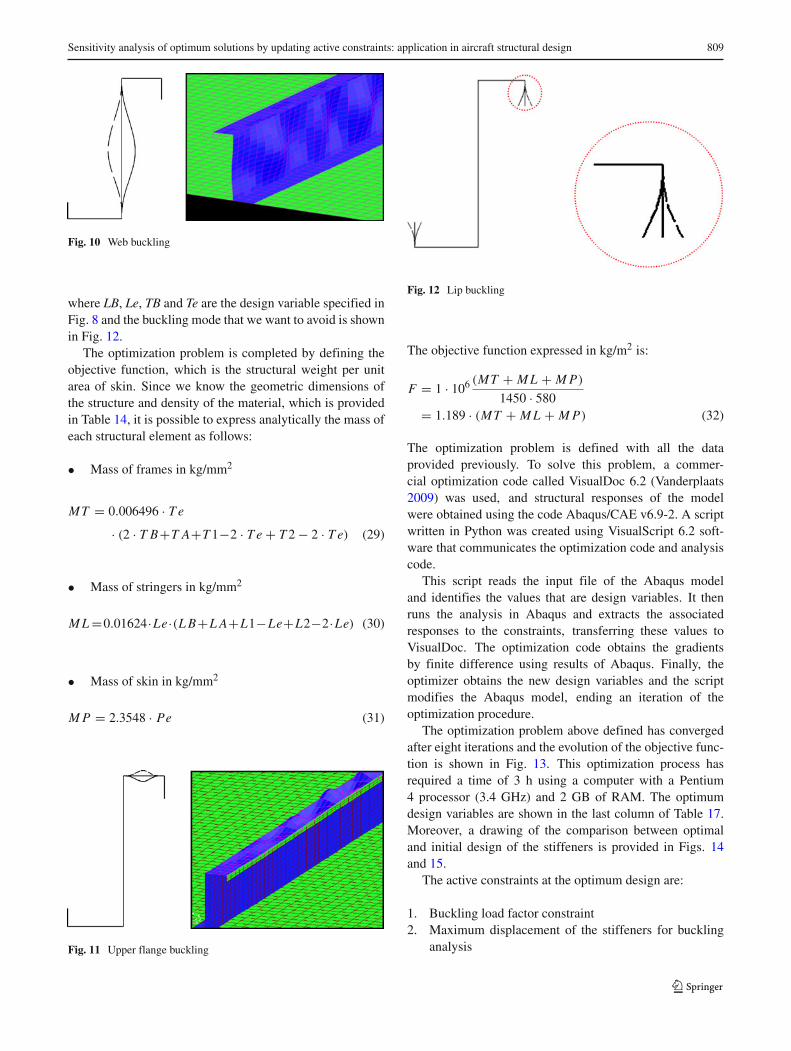
3. Lip buckling constraints
This member is braced only at one end so it is consideredas an outer element, and the data obtained for this case areβ2 = 4.5ε, β3 = 5ε, leading to the following constraints:
3.214≤β ≤3.571 ⇒
⎧⎪⎨
⎪⎩
3.214≤ L B
Le≤3.571
3.214≤ T B
T e≤3.571
(28)
Table 16 Slenderness parameters extracted from Eurocode 9
Element β1 β2 β3
W/thermal W/thermal WO/thermal W/thermal W/thermal WO/thermal W/thermal W/thermal WO/thermal
treatment, treatment treatment, treatment, treatment treatment, treatment, treatment treatment,
WO/welding welding, welding WO/welding welding, welding WO/welding welding, welding
WO/welding WO/welding WO/welding
WO/treatment WO/treatment WO/treatment
Outer 3ε 2.5ε 2ε 4.5ε 4ε 3ε 6ε 5ε 4ε
Inner 11ε 9ε 7ε 16ε 13ε 11ε 22ε 18ε 15ε
ε = (250/f0)1/2 with f0 in N/mm2
Sensitivity analysis of optimum solutions by updating active constraints: application in aircraft structural design 809
Fig. 10 Web buckling
where LB, Le, TB and Te are the design variable specified inFig. 8 and the buckling mode that we want to avoid is shownin Fig. 12.
The optimization problem is completed by defining theobjective function, which is the structural weight per unitarea of skin. Since we know the geometric dimensions ofthe structure and density of the material, which is providedin Table 14, it is possible to express analytically the mass ofeach structural element as follows:
• Mass of frames in kg/mm2
MT = 0.006496 · T e
· (2 · T B+T A+T 1−2 · T e + T 2 − 2 · T e) (29)
• Mass of stringers in kg/mm2
M L =0.01624·Le·(L B+L A+L1−Le+L2−2·Le) (30)
• Mass of skin in kg/mm2
M P = 2.3548 · Pe (31)
Fig. 11 Upper flange buckling
Fig. 12 Lip buckling
The objective function expressed in kg/m2 is:
F = 1 · 106 (MT + M L + M P)
1450 · 580= 1.189 · (MT + M L + M P) (32)
The optimization problem is defined with all the dataprovided previously. To solve this problem, a commer-cial optimization code called VisualDoc 6.2 (Vanderplaats2009) was used, and structural responses of the modelwere obtained using the code Abaqus/CAE v6.9-2. A scriptwritten in Python was created using VisualScript 6.2 soft-ware that communicates the optimization code and analysiscode.
This script reads the input file of the Abaqus modeland identifies the values that are design variables. It thenruns the analysis in Abaqus and extracts the associatedresponses to the constraints, transferring these values toVisualDoc. The optimization code obtains the gradientsby finite difference using results of Abaqus. Finally, theoptimizer obtains the new design variables and the scriptmodifies the Abaqus model, ending an iteration of theoptimization procedure.
The optimization problem above defined has convergedafter eight iterations and the evolution of the objective func-tion is shown in Fig. 13. This optimization process hasrequired a time of 3 h using a computer with a Pentium4 processor (3.4 GHz) and 2 GB of RAM. The optimumdesign variables are shown in the last column of Table 17.Moreover, a drawing of the comparison between optimaland initial design of the stiffeners is provided in Figs. 14and 15.
The active constraints at the optimum design are:
1. Buckling load factor constraint2. Maximum displacement of the stiffeners for buckling
analysis

810 A. Baldomir et al.
Fig. 13 Objective functionhistory
3. Maximum strain in the skin for internal pressure4. Web buckling in frames and stringers5. Lip buckling in stringers6. Lower limit of the variable T1
Figure 16 shows the buckling mode of the structure for theoptimal values of design variables. The buckling mode forthe optimal solution appears for a value of λ = 125.02 andbuckling instability occurs locally between two stiffeners,verifying that there is no global buckling.
4.3 Sensitivity analysis and linear approximationof the optimal solution
The optimal solution of the above problem is the startingpoint for implementing the methodology explained in thisresearch. Two fixed parameters have been considered: theminimum value of buckling load factor λmin , whose valuein the optimization problem is λmin = 125 and the radius ofcurvature of the panel, whose initial value is r= 1,500 mm.
The input data to obtain the approximate optimumdesign using the previous methodology are the set of activeconstraints, already provided before and the gradients of
Table 17 Optimum design
Variable Initial Optimum
Pe 1.5 1.7
T1 25 5.0
T2 15 9.7
TA 60 22.2
TB 8 2.7
Te 2 1.4
L1 22 5.2
L2 15 21.1
LA 25 21.7
LB 6 4.9
Le 2 1.4
Dimensions in millimetres
constraints and gradient of the objective function. In thiscase all these data are a by-product of the optimizationmethod itself, and therefore it is not necessary to obtainthem again. To update all active constraints and implementthe flow diagram of Fig. 2 it will be necessary to calculategradients in the new approximate designs. These values areobtained by finite differences.
The approximate optimum solutions presented belowhave been obtained with the same computer and the com-puting time has not exceeded 4 min in any case.
p = λmin (�p = −10%)
The first approximate optimal solution is performed consid-ering a 10% reduction in the parameter p = λmin , from avalue of λmin = 125 to λmin = 112.5.
Initially, we seek an approximate optimum solution byobtaining only once the feasible direction S for the totalvariation of parameter. The problem (4–6) has been formu-lated and solved for this example, obtaining the S vector,which contains the 12 direction components associated toeach design variable when the parameter p is modified. Theresulting solution was:
S = [−.003, 0, .3108, .0643, −.5599, .0041, .0411,
−.0324, −.0452, −.0075, −.0021, −.7622]
Knowing the parameter variation and applying the expres-sions (7–8), the new approximate optimum solution can bedetermined. Table 18 shows this result for p = λmin =112.5 (�p = −10%) and also provides the optimal solutionof the original optimization problem for the same parametervalue.
The new design has an approximate weight per unitarea of panel very similar to the optimum design, differingonly by 1.3%. However, the approximate design is invalidbecause the design variable TB has a negative value, whichis not an appropriate value for a geometric dimension. Theresulting value of the objective function is invalid becauseone term is subtracting mass, which makes no sense. Nev-ertheless, this part of the cross section does not contribute

Sensitivity analysis of optimum solutions by updating active constraints: application in aircraft structural design 811
Fig. 14 Initial design of theframes (left in black colour),optimum design (right in greencolour) and a comparisonbetween both designs (centre)
much in the mass of the structure and hence an error in thatvariable has almost no effect on the total mass.
This circumstance shows that 10% variation of theparameter cannot be done in only one step by solving theoptimization problem (4–6). It will be necessary to updateall active constraints and regain the vector S, according tothe new methodology presented in the flowchart of Fig. 2.Applying this procedure, the previous approximation isvalid up to a parameter value p =122.72 (�p = −1.8%),point at which the constraint of minimal value for the vari-able TB is activated. At this point, it is necessary to solve theproblem (11–15) again and the result obtained is the next:
S = [−.0036, 0, .2464, −.0661, 0, −.0042, .0215,
−.0326, −.0246, −.0141, −.0043, −.9657]
Then, it was verified that no other constraint becomes activefor the remainder of the parameter variation. The value ofthe approximate solution is given in Table 18.
This result is better, since the error in the objective func-tion is reduced to 0.25%. In this case the design is feasible,
contrary to what happened in the previous case, leading tothe conclusion that this new approach is efficient.
p = λmin (�p = −25%)
The next variation on the parameter p = λmin is a reduc-tion of 25%, from λmin = 125 to λmin = 93.75. Again,if the approximation of the optimal solution is done with asingle evaluation of vector S, obtained for the point corre-sponding to λmin = 125, the results would lead to an invaliddesign with much larger errors. Therefore, the approxima-tion of the optimal solution has been obtained by updatingthe active constraints, and it has been found that for aparameter value λmin = 108.62 (�p = −13.1%) anotherconstraint becomes active, which in this case is the lowerlimit of the variable SL1. Once again, the vector S needs tobe update a this new point, resulting:
S = [−.0039, 0, .2770, −.0844, 0, −.0054, 0, −.0333,
−.0462, −.0077, −.0022, −.9554]
Fig. 15 Initial design of thestiffeners (left in black colour),optimum design (right in greencolour) and a comparisonbetween both designs (centre)
812 A. Baldomir et al.
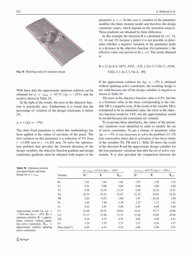
Fig. 16 Buckling mode for optimum design
With these data the approximate optimum solution can beobtained for p = λmin = 93.75 (�p = −25%) and theresult is shown in Table 18.
In the light of the results, the error in the objective func-tion is practically zero. Furthermore it is found that thepercentage of violation of the design constraints is below2%.
p = r (�p = −5%)
The other fixed parameter to which this methodology hasbeen applied is the radius of curvature of the panel. Thefirst variation on this parameter is a reduction of 5% fromr =1,500 mm to r =1,425 mm. To solve the optimiza-tion problem that provides the forward direction of thedesign variables, the objective function gradient and designconstraints gradients must be obtained with respect to the
parameter p = r . In this case a variation of the parametermodifies the finite element model and therefore the designconstraint values, which depend on the structural analysis.These gradients are obtained by finite difference.
In this example the direction S is calculated by (11, 12,13, 14 and 15) because a priori it is not possible to deter-mine whether a negative variation of the parameter leadsto a decrease in the objective function. For parameter c theeffective value was proven to be c =1. The result obtainedis:
S = [1.2e-4, 0, .0473, .0191, -.135, 1.23e-3, 7.42e-3, -.0156,
5.82e-3, 1.3e-3, 3.74e-4, -.99]
If the approximate solution for �p = −5% is obtainedwithout updating active constraints, the resulting design isnot valid because one of the design variables is negative asshown in Table 19.
The error in the objective function value is 0.5%, but thisis a fictitious value as the mass corresponding to the vari-able TB is a negative term. If the result of the variable TB isconsidered to be its minimum value, the error in the objec-tive function would be 3.8%, but the approximation wouldbe invalid because the constraints are violated.
To overcome these drawbacks, the values of the param-eter variations were identified in order to modify the setof active constraints. To get a change of parameter value�p = −5%, it was necessary to solve the problem (11–15)four consecutive times due to activation of the lower limitsof the variables TA, TB and L1. Table 20 shows the resultof the direction S and the approximate design variables forthe four parameter variations that alter the set of active con-straints. It is also provided the comparison between the
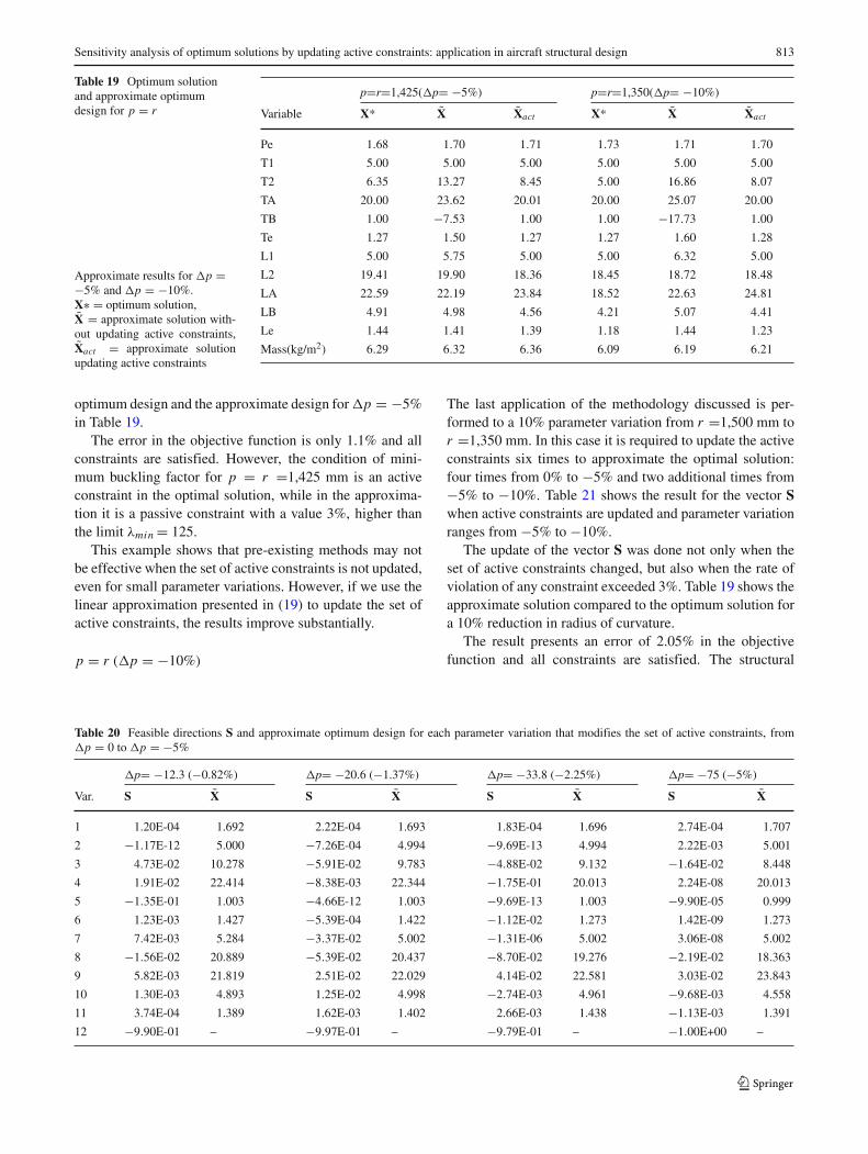
Table 18 Optimum solutionand approximate optimumdesign for p = λmin
Approximate results for �p =− 10% and �p = −25%. X∗ =optimum solution, X̃ = approx-imate solution without updat-ing active constraints, X̃act =approximate solution updatingactive constraints
p= λmin =112.5 (�p= −10%) p= λmin =93.75 (�p = −25%)
Variable X* X̃ X̃act X* X̃ X̃act
Pe 1.62 1.64 1.64 1.53 1.58 1.55
T1 5.01 5.00 5.00 5.00 5.00 5.00
T2 9.58 14.79 13.23 9.49 22.44 13.51
TA 22.55 23.23 21.67 21.32 24.84 22.26
TB 2.84 −6.51 1.00 1.87 −20.26 1.00
Te 1.44 1.48 1.38 1.37 1.57 1.42
L1 5.02 5.87 5.09 6.49 6.89 5.00
L2 21.06 20.55 20.64 18.43 19.77 19.86
LA 21.13 21.00 21.35 21.48 19.85 20.58
LB 4.78 4.75 4.70 4.02 4.59 4.51
Le 1.34 1.35 1.33 1.37 0.54 1.27
Mass (kg/m2) 6.20 6.12 6.22 5.86 4.99 5.87
Sensitivity analysis of optimum solutions by updating active constraints: application in aircraft structural design 813
Table 19 Optimum solutionand approximate optimumdesign for p = r
Approximate results for �p =−5% and �p = −10%.X∗ = optimum solution,X̃ = approximate solution with-out updating active constraints,X̃act = approximate solutionupdating active constraints
p=r=1,425(�p= −5%) p=r=1,350(�p= −10%)
Variable X* X̃ X̃act X* X̃ X̃act
Pe 1.68 1.70 1.71 1.73 1.71 1.70
T1 5.00 5.00 5.00 5.00 5.00 5.00
T2 6.35 13.27 8.45 5.00 16.86 8.07
TA 20.00 23.62 20.01 20.00 25.07 20.00
TB 1.00 −7.53 1.00 1.00 −17.73 1.00
Te 1.27 1.50 1.27 1.27 1.60 1.28
L1 5.00 5.75 5.00 5.00 6.32 5.00
L2 19.41 19.90 18.36 18.45 18.72 18.48
LA 22.59 22.19 23.84 18.52 22.63 24.81
LB 4.91 4.98 4.56 4.21 5.07 4.41
Le 1.44 1.41 1.39 1.18 1.44 1.23
Mass(kg/m2) 6.29 6.32 6.36 6.09 6.19 6.21
optimum design and the approximate design for �p = −5%in Table 19.
The error in the objective function is only 1.1% and allconstraints are satisfied. However, the condition of mini-mum buckling factor for p = r =1,425 mm is an activeconstraint in the optimal solution, while in the approxima-tion it is a passive constraint with a value 3%, higher thanthe limit λmin = 125.
This example shows that pre-existing methods may notbe effective when the set of active constraints is not updated,even for small parameter variations. However, if we use thelinear approximation presented in (19) to update the set ofactive constraints, the results improve substantially.
p = r (�p = −10%)
The last application of the methodology discussed is per-formed to a 10% parameter variation from r =1,500 mm tor =1,350 mm. In this case it is required to update the activeconstraints six times to approximate the optimal solution:four times from 0% to −5% and two additional times from−5% to −10%. Table 21 shows the result for the vector Swhen active constraints are updated and parameter variationranges from −5% to −10%.
The update of the vector S was done not only when theset of active constraints changed, but also when the rate ofviolation of any constraint exceeded 3%. Table 19 shows theapproximate solution compared to the optimum solution fora 10% reduction in radius of curvature.
The result presents an error of 2.05% in the objectivefunction and all constraints are satisfied. The structural
Table 20 Feasible directions S and approximate optimum design for each parameter variation that modifies the set of active constraints, from�p = 0 to �p = −5%
�p= −12.3 (−0.82%) �p= −20.6 (−1.37%) �p= −33.8 (−2.25%) �p= −75 (−5%)
Var. S X̃ S X̃ S X̃ S X̃
1 1.20E-04 1.692 2.22E-04 1.693 1.83E-04 1.696 2.74E-04 1.707
2 −1.17E-12 5.000 −7.26E-04 4.994 −9.69E-13 4.994 2.22E-03 5.001
3 4.73E-02 10.278 −5.91E-02 9.783 −4.88E-02 9.132 −1.64E-02 8.448
4 1.91E-02 22.414 −8.38E-03 22.344 −1.75E-01 20.013 2.24E-08 20.013
5 −1.35E-01 1.003 −4.66E-12 1.003 −9.69E-13 1.003 −9.90E-05 0.999
6 1.23E-03 1.427 −5.39E-04 1.422 −1.12E-02 1.273 1.42E-09 1.273
7 7.42E-03 5.284 −3.37E-02 5.002 −1.31E-06 5.002 3.06E-08 5.002
8 −1.56E-02 20.889 −5.39E-02 20.437 −8.70E-02 19.276 −2.19E-02 18.363
9 5.82E-03 21.819 2.51E-02 22.029 4.14E-02 22.581 3.03E-02 23.843
10 1.30E-03 4.893 1.25E-02 4.998 −2.74E-03 4.961 −9.68E-03 4.558
11 3.74E-04 1.389 1.62E-03 1.402 2.66E-03 1.438 −1.13E-03 1.391
12 −9.90E-01 – −9.97E-01 – −9.79E-01 – −1.00E+00 –

814 A. Baldomir et al.
Table 21 Feasible directions S and approximate optimum design foreach parameter variation that modifies the set of active constraints,from �p = −5% to �p = −10%
�p= −115 (−7.67%) �p= −150 (−10%)
Var. S X̃ S X̃
1 −2.20E-04 1.698 −2.07E-05 1.698
2 1.50E-03 5.000 1.31E-03 5.000
3 −7.55E-03 8.143 −2.05E-03 8.070
4 1.69E-03 20.000 2.12E-03 20.000
5 4.23E-10 1.000 2.95E-14 1.000
6 1.07E-04 1.277 1.18E-04 1.281
7 1.36E-07 5.000 1.07E-02 5.000
8 3.20E-03 18.493 −4.75E-04 18.476
9 −4.45E-03 23.663 3.23E-02 24.806
10 8.49E-03 4.901 −1.40E-02 4.407
11 −4.96E-04 1.371 −4.00E-03 1.229
12 −9.98E-01 – −9.98E-01 –
analysis with the approximate optimum design was carriedout and a buckling load factor of λ = 126.88 was obtained,which is very close to the value of active constraint that isλmin = 125. The displacements of stiffeners were extractedfor buckling analysis obtaining a maximum value of 4.8%with respect to the maximum value of the panel, whichmeets the above limitation of 5%.
5 Conclusions
When there is uncertainty or inaccuracy in some fixedparameter for an optimization problem, it is desirable tohave methods to avoid the need to carry out a new optimiza-tion process, providing an approximate optimum result.
The feasible direction-based technique, where only firstorder derivatives are involved, has provided sufficientapproximation to optimal when the set of active constraintsdoes not change. If the set of active constraints changes theapproximation of the solution may not be good, even forsmall variations of the parameters.
The main contribution of this paper is to convert the fea-sible direction-based technique into an iterative process thatupdates the set of active constraints because of changesin the parameter value. This methodology improves theaccuracy of the optimum approximation, making possi-ble greater parameter variations. Regarding the applicationexamples it can be said that the pre-existing referencesworked only with very simple structures and in this case the
methodology has been applied to a real aircraft structure.Numerical results of two examples show that the error
found is small compared with the optimal solution obtainedby performing a new optimization loop, even for largeparameter variations.
The comparison between the results obtained updatingand without updating active constraints is presented in sev-eral tables for both examples. It can be observed that theerror is significantly reduced when applying this methodol-ogy, concluding that this approach is advantageous.
Acknowledgements The research leading to these results hasreceived funding from the European Community’s Seventh Frame-work Programme FP7/2007-2013 under grant agreement n◦ 213371(MAAXIMUS—www.maaximus.eu).
Also, the Dutch National Aerospace Laboratory (NRL) is acknowl-edged for providing the finite element model of the panel.
References
Abaqus/CAE Inc (2008) Abaqus/CAE v6.9-2 User’s ManualArmao F (2000) On aluminium welding. MetalForming
MagazineBarthelemy JFM, Sobieszczanski-Sobieski J (1983a) Optimum
sensitivity derivatives nonlinear programming. AIAA J 21(6):913–915
Barthelemy JFM, Sobieszczanski-Sobieski J (1983b) Extrapola-tion of optimum design based on sensitivity derivatives. AIAA J21(5):797–799
Berke L, Khot NS (1974) Use of optimally criteria methods for largescale systems. AGARD-LS-70
Eurocode 9 (2007) Design of all aluminium structures, Part 1-1:General Common rules. BS EN 1999-1-1
Guo X, Cheng GD (2000) An extrapolation approach for the solu-tion of singular optima. Structural Multidisciplinary Optimization,19:255–262, Springer-Verlag
Haftka RT, Gürdal Z, Kamat MP (1990) Elements of structural opti-mization, Second Revised Edition. Kluwer Academic Publishers
Kirsch U (1981) Optimum structural design. McGraw-Hill, IncRakowska J, Haftka RT, Watson LT (1991) An active set algorithm
for tracing parameterized optima. Struct Optim 3:29–44Rouse M, Ambur DR, Bodine J, Dopker B (1997) Evaluation of a
composite sandwich fuselage side panel with damage and subjectedto internal pressure. NASA Tech Memo 110309
Sobieszczanski-Sobieski J, Barthelemy JFM, Riley KM (1982) Sen-sitivity of optimum solutions of problem parameters. AIAA J20(9):1291–1299
Sun CT (2006) Mechanics of aircraft structures, 2nd edn. WileyVanderplaats GN (2001) Numerical optimization techniques for
engineering design. Vanderplaats Research & Development, Inc.Colorado Springs
Vanderplaats GN, Yoshida H (1985) Efficient calculation of optimumdesign sensitivity. AIAA J 23(11):1798–1803
Vanderplaats Research & Development, Inc (2009) VisualDoc 6.2User’s Manual. http://www.vrand.com
Zoutendijk G (1960) Methods of feasible directions. Elsevier,Amsterdam
Related Documents