Sensitivity Analysis of Kernel Estimates: Implications in Nonlinear Physiological System Identification

Annals of Biomedical Engineering,Vol. 26, pp. 488–501, 1998 0090-6964/98 $10.501 .00Printed in the USA. All rights reserved. Copyright © 1998 Biomedical Engineering Society

Sensitivity Analysis of Kernel Estimates: Implications in NonlinearPhysiological System Identification

DAVID T. WESTWICK, BELA SUKI, AND KENNETH R. LUTCHEN

Department of Biomedical Engineering, Boston University, Boston, MA

(Received 18 December 1996; accepted 26 November 1997)

sti-s,us

e ofm

ysisfica

ofonfiedictiona-de

d tonsi-mu-kertheom-eseianiantpu

ce,tory

ds.

thaelym-behei-

thed

iann isly

lemm-heyo be

lslyonas

nd

ngsingerrai-

ataingerye

ems,

na-

n-hich

ntsing

io-os-

Abstract—Many techniques have been developed for the emation of the Volterra/Wiener kernels of nonlinear systemand have found extensive application in the study of variophysiological systems. To date, however, we are not awarmethods for estimating the reliability of these kernels frosingle data records. In this study, we develop a formal analof variance for least-squares based nonlinear system identition algorithms. Expressions are developed for the variancethe estimated kernel coefficients and are used to place cdence bounds around both kernel estimates and output prtions. Specific bounds are developed for two such identificaalgorithms: Korenberg’s fast orthogonal algorithm and the Lguerre expansion technique. Simulations, employing a morepresentative of the peripheral auditory system, are usevalidate the theoretical derivations, and to explore their setivity to assumptions regarding the system and data. The silations show excellent agreement between the variances ofnel coefficients and output predictions as estimated fromresults of a single trial compared to the same quantities cputed from an ensemble of 1000 Monte Carlo runs. Thtechniques were validated with white and nonwhite Gaussinputs and with white Gaussian and nonwhite non-Gaussmeasurement noise on the output, provided that the ounoise source was independent of the test input. ©1998 Bio-medical Engineering Society.@S0090-6964~98!01503-3#

Keywords—Least squares regression, Analysis of varianLaguerre expansion, Orthogonal algorithm, Peripheral audisystem model.

INTRODUCTION

Lee and Schetzen19 provided the first practical methofor the nonparametric identification of nonlinear systemHowever, their method was based on the assumptionthe system under study was being excited by an infinitlong, white Gaussian input. Thus, applications were liited to systems where this ideal input could at leastapproximated experimentally. As a result, most of tinitial applications of nonlinear identification were d

Address correspondence to David T. Westwick, Department of Bmedical Engineering, Boston University, 44 Cummington Street, Bton, MA 02215. Electronic mail: [email protected]

488

-

--

l

-

t

t

rected at the early stages of visual processing inretina ~for reviews of this literature see Marmarelis anMarmarelis23 and Sakuranaga25!.

The need for a long duration, nearly white Gaussinput can be bypassed if a least-squares regressioused in the identification. This innovation was originalsuggested by Amorocho and Brandstetter,1 who notedthat this approach generated a least-squares probwhich was computationally intractable, using the coputers of the day, with even modest data records. Tsuggested that, since the kernels could be expected tsmooth ~in their application!, the size of the estimationproblem could be reduced dramatically if the kernewere expanded using a small number of relativesmooth functions, and chose to expand their kernelsthe basis of discrete Laguerre filters. This approach wfirst used in a physiological context by Watanabe aStark.27

Recently, possibly due to the explosion in computipower, there has been a resurgence of interest in uexact least-squares methods to estimate Wiener/Voltkernels. Korenberg12,13,17estimated the kernel values drectly, as done by the Lee–Schetzen19 technique, butperformed an exact orthogonalization over the drecords, an approach equivalent to solving the underlyleast-squares regression using a QR factorization. A vefficient implementation of this procedure, which htermed the fast orthogonal algorithm,12,13 was also devel-oped, and has been applied to various sensory systsuch as the catfish retina,18 the visual cortex in the cat,8

the locust photoreceptor10 and the cockroach tactilespine.9

Exact orthogonalization can also be used in combition with an expansion onto an arbitrary basis,12 as dem-onstrated in simulation, in Ref. 16. In addition, Koreberg suggested an orthogonal search technique wwould start with a variety of potential basis elements12.Proceeding iteratively, the set of potential basis elemewould be searched for the most significant remainelement, which would then be added to the model.

oftial-forallyhethetheena

.ntsedw-ichtinginther-

re-senhe

glopnd

idenli-winit-eueeyinmedso

athe

ofea

ceay

ls,

bea

e-

reo-

setheFs.lta

tly

se

-

tothe

489Sensitivity Analysis of Kernel Estimates

Marmarelis21 expanded the kernels on the basisdiscrete Laguerre functions, as was done in the inileast-squares techniques,1,27 and solved the ensuing regression explicitly. He developed a heuristic methoddetermining the value of the decay parameter, usudenoteda, which controls the shape and extent of tbasis elements, given the expected memory length ofsystem and the desired number of basis functions inexpansion. This approach has been used to study rautoregulation in rats,5,6,22 by fitting first- through third-order kernels between renal blood pressure and flow

The physiological insight gained by these experimeshould be tempered by the reliability of the estimatkernels, and of the quantities derived from them. Hoever, we are not aware of any studies to date whpropose a general and rigorous approach for evaluathe reliability of these kernel estimates. Typically,papers developing new algorithms, the smoothness ofkernels estimated from a single simulation trial, peformed with noise in the output measurement, is psented as evidence of the robustness of the propotechnique.1,13,14,21While such anecdotal evidence is oftepersuasive, it does not provide any indication of treliability of the technique, or of how it will behavegiven data from a particular experimental protocol.

In this study, we will exploit the theory surroundinstatistical analysis of least-squares estimation to deveexpressions for the variance of kernel coefficients aoutput predictions generated by least-squares basedtification techniques. While these methods will be appcable regardless of the selected expansion basis, weapply them to two common choices: a series of udelays~discrete deltas!, as employed in the fast orthogonal algorithm~FOA!,12,13 and a bank of discrete Laguerrfilters used by the Laguerre expansion techniq~LET!.1,21,27 We will show how these bounds can bused to separate features which are due to the underlsystem, and hence worthy of further investigation, frothose which are likely to be statistical errors introducby the identification technique. Furthermore, we will alshow how these bounds can be used to asses theequacy of the chosen modeling technique, refineanalysis, and thereby create improved models.

THEORY

System identification embodies the constructionmathematical models of dynamic systems based on msurements of their inputs and outputs.20 The system un-der investigation is driven by an input,u(t), and pro-duces an output signal,y(t). While the input is assumedto be under the control of the investigator, and henexactly known, the output must be measured, and m

l

d

-

ll

g

d-

-

contain noise,v(t). Thus, based on the available signau(t) and z(t)5y(t)1v(t), the goal is to construct amodel of the unknown system.

System Models

In this paper, we will assume that the system canrepresented by a finite Volterra series. Thus, givenfinite model order,q, and memory length,R, we repre-sent the system output as:12

y~ t !5 (n50

q H (t150

R21

¯ (tn50

R21

kn~t1 ,...,tn!

3 u~ t2t1! . . . u~ t2tn!J . ~1!

Any finite Volterra series model can also be reprsented by a Wiener–Bose model,4,14 shown in Fig. 1,consisting of a bank of linear filters whose outputs acombined and transformed by a multiple-input polynmial. In general, the impulse response functions~IRFs!of the L filters in the filter bank,hi(t) 1< i<L, arechosen prior to the identification. The Wiener–Bomodel can then be thought of as the expansion ofsystem’s kernels onto a basis formed by the filter IRCommon choices for this basis include delayed depulses12,13 and Laguerre filters.1,21,27 In practice, the ker-nels may be expanded on any basis which is sufficiengeneral.12

If xi(t) denotes the output at timet of the i th filter inthe filter bank, then the output of the Wiener–Bomodel is given by

y~ t !5c~0!1(i 51

L

ci~1!xi~ t !1(

i 51

L

(j 51

i

ci , j~2!xi~ t !xj~ t !1 . . . ,

~2!

where theci 1 , . . . ,i n(n) are the coefficients of the multiple

input polynomial nonlinearity. The superscript refersthe order of polynomial term, and the subscripts label

FIGURE 1. Block diagram of a Wiener–Bose model.

.thes.

r-rst

ists

a

res

lshn-

a

490 WESTWICK, SUKI, AND LUTCHEN

particular filter outputs included in the polynomial termThere is a straightforward relationship between

Wiener–Bose model, and the finite Volterra serieGiven the coefficients,ci 1 , . . . ,i n

(n) , and the impulse re-

sponses,hi(t), the Volterra kernels can easily be geneated from the Wiener–Bose model. For example, the fithree Volterra kernels are given by21

k05c~0!, ~3!

k1~t!5(i 51

L

ci~1!hi~t!, ~4!

k2~t1 ,t2!5(i 51

L

ci ,i~2!hi~t1!hi~t2!

1(i 51

L

(j 51

i 21 ci , j~2!

2@hi~t1!hj~t2!1hj~t1!hi~t2!#.

~5!

-

-ffi-

t,

ef-

If the filters, hi(t), are specifieda priori, then themodel is completely specified by the order,q, of thepolynomial and the values of its coefficients,ci 1 , . . . ,i n

(n)

for 0<n<q. Thus, the system identification problemreduced to the estimation of the polynomial coefficienfrom records of input–output data.

Least-Squares Based Identification

Because the output of the Wiener–Bose model islinear function of the polynomial coefficients,c(n), theymay be estimated using a single least-squaregression.1,27 First the input,u(t), is filtered by each ofthe filters in the bank, resulting in the signax1(t), . . . ,xL(t). From these linear filter outputs, eacof the terms in the polynomial nonlinearity can be geerated and collected in anN3M matrix, X, with Nequal to the length of the data record andM!N equal tothe number of model parameters. For example, ifsecond-order polynomial is used,X would contain:1

X5F 1 x1~1! . . . xL~1! x12~1! x1~1!x2~1! . . . xL

2~1!

1 x1~2! . . . xL~2! x12~2! x1~2!x2~2! . . . xL

2~2!

] ] ] ] ] ]

1 x1~N! . . . xL~N! x12~N! x1~N!x2~N! . . . xL

2~N!

G . ~6!

ob-

,

els.the

tel

st,re,

tesin

the

Now Eq. ~2! can be written as a matrix equation:1

y5Xb, ~7!

where theM31 vectorb contains the polynomial coefficients

bT5@c~0! c1~1! . . . cL

~1! c1,1~2! c1,2

~2! . . . cL,L~2!

#.

~8!

Using Eq. ~7!, the nonlinear system identification problem can be formulated as the estimation of the coecient vector,b, given the regressor matrix,X ~which isderived from the input!, and the noise corrupted outpuz. If y is the output of the estimated system,y5Xb,then we wish to choose the vector of polynomial coficients, b, to minimize the mean squared error,

(t51

N

@z~ t !2 y~ t !#2.

The solution to this linear least-squares estimation prlem is given by:2

b5~XTX!21XTz. ~9!

Once the least-squares estimate,b, has been computedthe kernels can be generated using Eqs.~3!–~5!.

As noted earlier, the IRFs,h1(t) . . . hL(t), form theexpansion basis which is used to represent the kernThus, if a series of discrete Laguerre filters was used,least-squares regression given by Eq.~9! would beequivalent to the LET. Similarly, if a series of discredeltas were used, Eq.~9! would produce results identicato the FOA, but with far greater computational cosince the FOA exploits the resulting lagged structuand the straightforward application of Eq.~9! does not.Clearly, other choices of basis are also possible.12

Variance of Estimated Coefficients,b

The statistical properties of least-squares estimahave been extensively studied, and are summarizedRef. 2. If the system can be exactly represented byselected class of models so thaty5Xb, and the output

-t oeffithe

ese,-ef.

is

ffi-foray

pute

o

need

vesionndnel

f-

ts,f

erre-

ere-

t,ffi-

om

on-x-ay

es


measurements,z(t)5y(t)1v(t), are corrupted by an additive zero-mean noise process which is independenthe input, then the least-squares estimate of the cocients, b, is unbiased and has covariance given byM3M matrix:2

Cb5~XTX!21XTE@vvT#X~XTX!21. ~10!

Direct evaluation of~10! is not usually possible, sincthe covariance matrix of the measurement noiE@vvT#, is an N3N matrix and is not generally available. If the measurement noise is white, then from R2, E@vvT#5sv

2I , wheresv2 is the variance ofv(t), and

I is an identity matrix. Furthermore,

sv25

1

N2M (t51

N

@z~ t !2 y~ t !#2, ~11!

whereM , which is the number of model parameters,an unbiased estimate of the noise variance,sv

2 . ThusCb

is reduced to:2

Cb5sv2~XTX!21. ~12!

Variance of Kernel Estimates and Model PredictedOutput

Given the covariance matrix of the estimated coecients, we may also estimate the covariance matrixany function of these coefficients. In particular, we mcompute the variance~and in principle covariance! of thekernel values, and of the model output to any given insignal u(t), both of which are linear functions of thestimated coefficients. LetgPRM, whereM is the num-ber of model parameters, and consider the variancegTb. Then2

Var~gTb !5gTCbg. ~13!

More generally, ifgPRM3n so thatgTb is a linearndimensional function ofb, then the n3n covariancematrix of gTb is given by Eq.~13!. Thus, Eq.~13! canbe used to estimate the variance of any of the kervalues, or that of output predictions due to the identifimodel.2

Kernel Estimates. Once the expansion coefficients habeen estimated, regardless of the choice of expanbasis, Eqs.~4! and ~5! are used to generate the first- asecond-order kernel estimates. For the first-order kerwe can rewrite~4! as a matrix equation so that

f-

f

l

,

k1~ j !5@0 h1~ j ! . . . hL~ j ! 0 . . . 0#b

5~g j~1!!Tb ~14!

so that k1( j ) is a linear function of the estimated coeficients. The subscripts and superscripts applied tog areanalogous to those used for the polynomial coefficienci 1 , . . . ,i n

(n) . From Eq. ~13!, we see that the variance o

k1( j ) is given by

Var@ k1~ j !#5~g j~1!!TCbg j

~1! . ~15!

Similarly, Eq. ~5! is used to generate the second-ordkernel estimate from the expansion coefficients. Bycasting Eq.~5! as a matrix equation, we can use Eq.~13!to estimate the variance of the (i , j )th kernel value byselecting the linear function (g i , j

(2))Tb as

k2~ i , j !5F0 . . . 0 h1~ i !h1~ j !

31

2@h1~ i !h2~ j !1h1~ j !h2~ i !#

3 . . . hL~ i !hL~ j !G b5~g i , j~2!!Tb.

Variance of Model Output Predictions.Implicit in Eqs.~13! and ~7! is the notion that there will be a variancassociated with any given point in a model output pdiction due to the variance in the coefficientsb. Letu(t) be an input to the model, and letX be the result ofapplying Eq.~6! to u(t). Then, from Eq.~7!, the pre-dicted output,y (b,t), is given by

y ~ b !5Xb.

Thus using Eq.~13! the covariance of the model outpuwhich is due to the variance associated with the coecient estimates, is given by

XCbX T. ~16!

The variance of the model output can be obtained frthe diagonal of this covariance matrix.

Nonwhite, Non-Gaussian Measurement Noise

In many practical applications, the measurements ctain noise which is neither Gaussian nor white. For eample, in physiological experiments measurements mbe corrupted by noise from a wide variety of sourc

Ince

tics

areas

ese-ionsedits

MA

ted

oisean

n

ro-ual

lasillueemthehndys-

lyablealsure

re-en-inlat-la-

ise-

,assingrd-ts.p-m-no-els.ri-ti-ry

heee


including ECG, EMG, power lines, and thermal noise.this section, we will develop estimates of the covarianmatrix for the coefficients which donot require the as-sumption of white Gaussian residuals.

We start by observing that Eq.~10! depends on thecovariance matrix and not on any higher-order statisof the noise. SinceE@vvT# is anN3N matrix, its directinclusion in Eq.~10! would be impractical for all but theshortest of data sets. However, efficient techniquesavailable2 if the measurement noise can be modeledeither a moving average~MA ! or auto-regressive~AR!process. While the computational manipulations of thalgorithms depend on the MA~or AR! process parameters, their effect is to include the noise auto-correlatinto the calculation. Thus, these methods can be uregardless of the nature of the noise, provided thatauto-correlation can be adequately generated by a~or AR! model.

Initially, we assume that the measurement noise,v(t),is generated by a moving average process:

v~ t !5n~ t !1(i 51

K

ain~ t2 i !, ~17!

wheren(t) is a white sequence with variancesv2 . Then,

it can be shown that the covariance of the estimacoefficients becomes2

Cb5sv2~XTX!21ZTZ~XTX!21, ~18!

whereZ is a matrix given by

Z~ i , j !5 (n50

K

X~ i 1n, j !an . ~19!

As mentioned above, the actual measurement nneed not be derived from an MA process. The use ofMA model is simply a computational manipulatiowhich allows the efficient evaluation ofXTE@vvT#X. Weneed only find a MA process which generates the apppriate covariance matrix for the noise, whatever its actsource.

Modeling Error

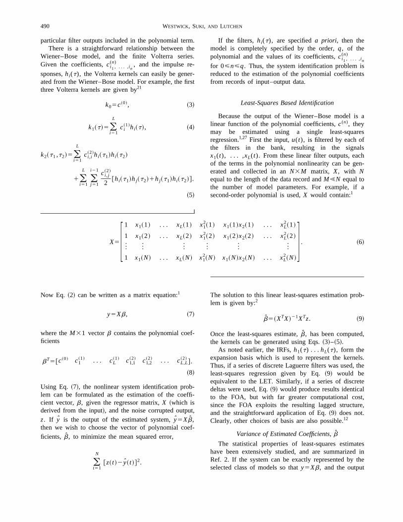
If the true system cannot be represented by the cof models used in the identification, modeling errors wresult. There will be energy in the residuals which is dto the input acting on the unmodeled parts of the systConsider the schematic presented in Fig. 2, in whichsystem is explicitly divided into a modelable part, whicis within the model class used in the identification, aan unmodelable part, which contains the rest of the s

,

s

.

tem. In this schematic, the modeling errors,v(t), aregenerated by the input acting on the lower block.

Clearly, in this scenario, the modeling errors will onbe Gaussian if the input is Gaussian and the unmodelsystem is linear. Similarly, the spectrum of the residuwill depend on both the input spectrum and on the natof the unmodelable system. Thus,v(t) will almost cer-tainly be nonwhite and non-Gaussian. Unlike measument noise, however, modeling errors are not indepdent of the input, violating one of the key assumptionsthe theoretical development. The consequences of vioing this assumption will be demonstrated in the Simutions section, below.

SIMULATIONS

In this section, we will apply our sensitivity analysto simulation results obtained from a model of the pripheral auditory system. Pfeiffer24 proposed a modelcomprising a static nonlinearity separating two band-pfilters, and showed that it was capable of generattwo-tone suppression. No speculation was given regaing the physiological analogs of the model componen

Swerup26 suggested that the first band-pass filter reresented the frequency selectivity of the basilar mebrane, and that the nonlinearity, a second-order polymial in his model, approximated the half-wavrectification thought to be performed by the hair celThis model was used to study the effects of using vaous stimuli in identification experiments aimed at esmating linearized properties of the peripheral auditosystem. Subsequently, Korenberg13 used simulated datafrom this model to demonstrate the superiority of tFOA over the earlier cross-correlation approach of Land Schetzen.19

FIGURE 2. Block diagram of the identification problem in-cluding modeling errors. The ‘‘true system’’ consists of ev-erything enclosed in the dashed box. That which can berepresented by the class of models used in the identificationis contained in the box labeled ‘‘Modelable System.’’ Therest of the system, the unmodelable part, produces the‘‘model errors,’’ v „t …. In general, the measured output, z„t …may contain either noise, modeling errors, or both.

bnr-

n-

e-illti-n

-illl-tsr-

ll

-ur

eles.ndsuf

pu-imu-p

ertis-

om-

r-oftputputre,ble

nd

enout-iseari-tes

00tes

st-. AtAof

esderdic-

00e

essA

el,en-

nd--thely.le

lot-hethesedsulte-


Parameters describing the linear and nonlinear susystems are given in Table 1. These were used to geerate the theoretical first- and second-order Volterra kenels of this system, which are shown in Fig. 3.

Simulations were performed under three sets of coditions:

~1! White Gaussian input, with white Gaussian measurment noise added to the output. These results wdemonstrate the performance of the uncertainty esmates under ideal conditions. Only the uncertainty ithe kernel values will be presented.

~2! Nonwhite Gaussian input, with white Gaussian measurement noise added to the output. Here we wpresent results for the uncertainty in both kernel vaues and output predictions, and examine the effecwhich the input spectrum has on the model uncetainty.

~3! Nonwhite Gaussian input, with nonwhite, non-Gaussian residuals. In these simulations, we wievaluate the utility of including the MA residualmodel in the sensitivity analysis. In addition, we willinvestigate the effects of modeling errors on the uncertainty of the estimates, and on the accuracy of osingle-trial predictions of that uncertainty.

Two issues were investigated. First, we compared thvariances of kernel coefficients estimated from singtrials to those obtained from an ensemble of simulationThus, for each test, a 1000 trial Monte Carlo simulatiowas conducted. For each trial, new input, output, annoise sequences were generated. Kernels were then emated between the input and the noise corrupted outpusing LET and FOA. Sums of kernel estimates, and o

FIGURE 3. First- and second-Volterra kernels of the simu-lated system.

TABLE 1. Parameter values for the test LNL system.

Linear blocks

poles z50.488560.3062izeros z50,0.7877

Static nonlinearity

y5x1x2

--

ti-t

their squares, were accumulated allowing for the comtation of ensemble means and variances once the slation was completed. In addition, the bootstraalgorithm7 was applied to the ensemble of first-ordkernels to estimate the variance of the ensemble statics. The ensemble standard deviations were then cpared to the single run predictions@based on Eq.~13!#obtained from the last trial in the simulation.

In cases~2! and ~3!, we also considered the uncetainty of output predictions, both in-sample and outsample. In these simulations, we generated the oudue to each identified model, using both the test inand an independent, white, Gaussian input. As befowe compared the variance computed from the ensemof trials to that predicted from a single trial.

Detailed descriptions of the individual simulations atheir results are presented below.

White Input, White Measurement Noise

In the first set of simulations, the system was drivby 1000 point white Gaussian noise sequences. Theput was corrupted by 10 dB of white Gaussian nowhich was independent of the input. The ensemble vances of both first- and second-order kernel estimaobtained by LET and FOA were computed from a 10trial Monte Carlo simulation and compared to estimafrom single trials.

Figure 4 shows the standard deviation of the firorder kernel estimates produced by both techniqueszero lag, the standard deviation of the LET and FOkernel estimates corresponded to 2.06% and 2.25%the kernel values, respectively. Clearly, both techniquproduced excellent first-order kernel estimates unthese conditions. In both cases, the theoretical pretions, obtained from a single trial using Eq.~13!, agreedwell with the ensemble statistics obtained from the 10trial Monte Carlo simulation, as is evident given thbootstrap estimates~shown as error bars! of the uncer-tainty in the ensemble estimate of the underlying procvariance. Note that the standard deviation of the FOkernel estimate is virtually constant across the kernwhereas the uncertainty in the LET estimate is conctrated near 0 lag.

Similar results are presented in Fig. 5 for the secoorder kernel estimates. At~0,0! lag, the ensemble standard deviations correspond to 1.67% and 1.76% oftrue kernel value for the LET and FOA, respectiveThe single trial prediction and Monte Carlo ensembresult for the second-order FOA kernel estimate are pted in panels A and B of Fig. 5, respectively. Note tnear constant level of variance associated with all ofoff-diagonal points in kernel estimates, and the increauncertainty of the diagonal. Panel C, the ensemble reand D, the single trial prediction show the standard d

yr-elilo

e

n

e

ll.dl

.

o

ns


viation of the second-order kernel estimate produced bthe LET. As in the first-order kernel estimate, the uncetainty is concentrated near the origin. As the distancfrom the origin is increased, the variance of the kernecoefficients decreases. Thus, the kernel estimates wappear to be very smooth on the periphery, regardlessthe degree of uncertainty near the origin.

FIGURE 4. Standard deviation of first-order kernel estimates.Single trial predictions and Monte-Carlo ensemble „1000trial … results are plotted for both the fast orthogonal algo-rithm and Laguerre expansion technique. Error bars on theensemble results show bootstrap estimates of one standarddeviation.

FIGURE 5. Standard deviation of second-order kernel esti-mates: „A… fast-orthogonal algorithm, standard deviation ofensemble of kernel estimates, „B… fast-orthogonal algorithm,prediction based on single trial, „C… Laguerre expansiontechnique, ensemble standard deviation, „D… Laguerre expan-sion, single trial prediction.

lf

Nonwhite Input, White Measurement Noise

Since least-squares identification methods such as thLET and FOA do not require a white Gaussian input, werepeated the previous simulations using an input whichwas filtered by a fourth-order Butterworth low-pass filterwith a normalized cut-off frequency of 0.8. This corre-sponds to a reasonably gentle filtering, and produced ainput which was effectively white over the bandwidth ofthe system. Even this relatively gentle filtering had anoticeable effect on the estimation variance.

Comparing Figs. 4 and 6, we see that there was asmall but noticeable increase in the variance of both theLET and FOA estimates of the first-order kernel near itsorigin. Indeed, at 0 lag, the relative errors were 2.56%and 3.43% for the LET and FOA, respectively. Note thevirtually exact agreement between the predictions andthe ensemble statistics. It is also evident that the variancof the FOA estimates is no longer constant, as it waswhen the input was white, but there is a substantiaincrease in the uncertainty near the center of the kerneSimilar comparisons can be made between Figures 5 an7, which show the results for the second-order kerneestimates.

As described earlier, the uncertainty in the outputpredictions was also investigated under these conditionsFor each trial in the Monte Carlo simulation, the identi-fied model was used to predict the system response ttwo signals: the original input used in the identificationand an independent new sequence of white Gaussianoise. The variance of each of these output predictionwas then computed from the ensemble of trials, and

FIGURE 6. Standard deviation of first-order kernel estimates.Single trial predictions and Monte Carlo ensemble „1000trial … results are plotted for both the fast orthogonal algo-rithm and Laguerre expansion technique. Input was low-passfiltered Gaussian noise.

lts

thm-

toereeotetemnot

theoveper-ut.ch9%inizeely

theed

asengthe


compared to the predictions given by Eq.~16!, using theresults from a single trial. Figure 8 shows the resufrom the ‘‘in sample’’ prediction using LET. From theupper panel, which shows the ensemble results andtheoretical prediction, it is evident that the variance coputed from a single data record@Eq. ~16!# provided anexcellent prediction of the model output variance duethe uncertainty in the estimated coefficients. The lowpanel shows the noiseless system output plotted betw99% confidence bounds on the predicted output. Nthat the solid line, which represents the noiseless sysoutput, stays between the two dotted lines but iscentered between them.

Figure 9 shows the same quantities, except thatmodel was used to predict the system response to a nsequence of white Gaussian noise. Again, the uppanel shows that Eq.~16! provided an excellent prediction of the degree of uncertainty in the model outpThis is further supported by the lower panel, whishows the system output plotted between the 9bounds on the prediction. Note the large fluctuationsthe distance between bounds, or alternatively in the sof the standard deviation, as compared to the relativconstant uncertainty in the in-sample prediction~Fig. 8!.This is probably due to the spectral differences intwo inputs: the system was identified using a colorinput, but the cross-validation was performed usingwhite Gaussian input. Thus, there were features prein the cross-validation input, but not in the traininsample, which are responsible for the large peaks inoutput uncertainty.

FIGURE 7. Standard deviation of second-order kernel esti-mates using a low-pass filtered Gaussian noise input: „A…

fast-orthogonal algorithm, standard deviation of ensemble ofkernel estimates, „B… fast-orthogonal algorithm, predictionbased on single trial, C … Laguerre expansion technique, en-semble standard deviation, „D… Laguerre expansion, singletrial prediction.

e

n

l

t

Modeling Errors and other Nonwhite, Non-GaussianNoise Sources

Equations ~17!–~19! present a modification to ourvariance estimators which allows for nonwhite, non-

FIGURE 8. Standard deviation of the model output for in-sample predictions. The upper panel shows the standarddeviation of the ensemble of model outputs from the MonteCarlo simulation „solid line … as well as the standard devia-tion prediction based on the results of a single trial „dottedline …. The lower panel shows the noiseless system outputplotted between 99% confidence bounds on the model out-put.

FIGURE 9. Standard deviation of the model output for cross-validation predictions. The upper panel shows the standarddeviation of the ensemble of model outputs from the MonteCarlo simulation „solid line … as well as the standard devia-tion prediction based on the results of a single trial „dottedline …. The lower panel shows the noiseless system outputplotted between 99% confidence bounds on the model out-put. In this case, the input was a white noise sequencewhich was not used during the identification.

lopin

on-obs,

hentlynte

alssteenalso-thee-thethe

atathe

g aperd-

totheerelds.ea-as

op-as

parwocortedpued

-rerlly

for-orse aent

rst-ua-theen

s

e

e

,

-


Gaussian residuals. Here, the relevance of this devement is investigated using a series of simulationswhich the system output was corrupted by colored, nGaussian sequences. Single-trial predictions weretained from Eq.~12!, which presumes white residualand then compared to those calculated using Eq.~18!,which incorporates a MA model of the residuals into tvariance estimator. Both predictions were subsequecompared to ensemble results obtained from the MoCarlo simulation.

Two sources of nonwhite, non-Gaussian residuwere considered. In the first case, the residuals consiof nonwhite measurement noise which was independof the test input. In the second instance, the residustill nonwhite, were due to modeling errors, i.e., compnents in the system which could not be modeled byclass of models included in the identification. Neverthless, the two simulations were designed such thatstatistical properties of the measurement noise and ofmodeling errors would be as similar as possible.

To create modeling errors, we first generated dusing the second-order model, as before. However,identification was performed under the~incorrect! as-sumption that the system was linear~i.e., the polynomialused in the Laguerre expansion was limited to havinsingle zero order term and eight linear terms, onefilter in the bank!. Hence, the contribution of the seconorder kernel produced nonzero residuals strictly duemodeling error. In the scheme presented in Fig. 2,system’s first-order kernel would fall within the upp‘‘modelable’’ block, whereas its second-order kernwould be in the ‘‘unmodelable’’ block. Its output woultherefore be considered as ‘‘noise’’ or modeling error

Our next task was to create additive, nonwhite, msurement noise which, unlike the modeling errors, windependent of the test input, but whose statistical prerties were as close to those of the modeling errorspossible. Here the test system consisted of the linearof the auditory model, a cascade comprising the tlinear subsystems. The measurement noise, whichrupted the output of this linear system, was generafrom a Gaussian sequence, independent of the test inbut which had the same spectrum. This was transformby an LNL system15 consisting of the two identical bandpass filters, used previously, separated by a squaThus, the initial noise sequence, which was statisticaidentical to the test input, underwent the same transmations as those which produced the modeling errcreating a sequence whose statistics were the samthose of the modeling errors, but which was independof the test input.

Figure 10 compares the standard deviation of the fiorder kernels, estimated using LET, in these two sittions. The left panel shows the results obtained whenmodel was first-order and corrupted by an independ

-

-

dt,

t

-

t,

.

,s

t

noise sequence, as described above. The solid line showthe standard deviation of the ensemble of kernel esti-mates. The dashed line, which fits this almost exactly, isthe prediction based on a single trial incorporating a MAmodel @i.e., Eq. ~18!# of the residual auto-correlation tocompensate for the nonwhite, non-Gaussian nature of thresiduals. The dotted line is the result obtained under theassumption that the residuals were [email protected]., Eq.~12!#.At low lags, this prediction is inferior to that generatedusing the MA model, especially given the bootstrapestimates7 of the variability in the ensemble standarddeviation. This represents a case in which it is importantto incorporate the second-order statistics of the residualsinto the variance prediction.

The right hand panel shows the results obtained whenmodeling error was incorporated into the simulation. Inthis case, neither of the single trial estimates predictedthe standard deviation of the first-order kernel estimatefor lags less than 4. The estimator based on the MAresidual model outperformed that which assumed whiteresiduals. Both estimators missed the first two peaks inthe kernel variance. These fluctuations in the ensemblestandard deviation appear to be significant, since they armuch larger than the estimated standard deviation in theensemble statistic, shown as error bars in Fig 10. Thuswe have an example where the effects of modeling errorscannot be completely accounted for by the estimatorsdeveloped in this paper.

Figure 11 shows the standard deviation of the modeloutput under both conditions. The upper panel shows theresults obtained with an independent noise sequence. Under these conditions, the estimator based on Eq.~18!,which includes the MA model of the residuals, accu-rately predicts the uncertainty in the model output. Thelower panel shows the results obtained with modelingerrors. Note how the single-trial estimate follows theslow variations in the output uncertainty, but misses

FIGURE 10. Standard deviation of first-order kernel esti-mates using LET. The panel on the left shows the resultsobtained when the output of the first-order kernel of the testsystem was corrupted with noise generated by filtering anindependent sequence with the its second-order kernel. Thepanel on the right shows the results obtained when the testsystem was identified as a linear system, i.e., the output ofthe second-order kernel produced modeling errors.

-n

fslr-

th-

rese

oftaesps

nd

ypeed-ns

re-ewory

di-withd toin-effi-ave

lltemb-

eshesri-

els,ss-

edlses,heits

5,asuternd-reher ofels-er-

red

iteofintysti-

eigs.the

ure-oisethence


most of the fine structure. Also note that it almost universally under-predicts the ensemble standard deviatio

DISCUSSION

The LET and FOA, each based on the solution olinear least-squares problems, have found extensive uin the mathematical modeling of nonlinear physiologicasystems. In this study, the theory surrounding the uncetainty in least-squares estimates was used to predictvariance of both kernel coefficients and output predictions computed by these algorithms. Simulations weused to establish the accuracy and limitations of thesingle-trial variance estimates.

This study is the first which permits the assessmentthe uncertainty in estimated kernels from single darecords. As such, future applications of least-squarbased identification algorithms can use these develoments to predict the accuracy of their kernel estimateand output predictions, whatever basis is used to expathe kernels.

Choice of Test System

The purpose of the simulations presented in this studwas to asses the accuracy of the theoretical develoments, under a variety of conditions, and to test thsensitivity of our analysis to certain assumptions madabout the data. While examples using both the LET anFOA are included in this study, they should not be interpreted as exhaustive, or even unbiased, comparisobetween these algorithms. In these simulations the sy

FIGURE 11. Standard deviation model predictions from afirst-order model. The upper panel shows the results ob-tained when the system output was corrupted by the outputof a second-order kernel driven by an independent noisesequence. The lower panel shows the results due to model-ing errors.

.

e

e

-

-

s-

tem had smooth kernels, as evident in Fig. 3, and thefore could be accurately represented using relatively fLaguerre filters, as compared to the system memlength ~9 vs 17!. Thus, application of the LET involvedsolving a much smaller, and sometimes better contioned, least-squares regression than was the casethe FOA. These apparent advantages can be expectevanish as the number of Laguerre basis functionscreases. For systems which cannot be representedciently using the Laguerre basis, such as those that h‘‘jagged’’ kernels, the number of Laguerre filters wibecome comparable to the memory length of the sysso that the size and conditioning of the estimation prolems underlying the two kernel identification procedurwill also be comparable. As a result, the two approacwill also produce comparable levels of estimation vaance, as demonstrated in the Appendix.

Note that the smoothness of the test system’s kerndid not effect the simulations presented by Korenberg13

which compared the FOA to the Lee and Schetzen crocorrelation technique.19 Since both approaches expandthe kernels on the same basis, a set of delayed imputhe underlying estimation problem was identical. Tsuperiority demonstrated by the FOA was due toinclusion of an exact least-squares solution.

Accuracy and Limitations

The first set of simulations, presented in Figs. 4 andwere conducted under ideal conditions: the system wdriven by a white Gaussian input, and had its outpcorrupted with 10 dB of white Gaussian noise. Undthese conditions, the variances of both first- and secoorder kernels estimated by both LET and FOA wepredicted accurately from the results of single trials. Tmagnitudes of the standard deviations were an ordemagnitude less than those of the theoretical kern~shown in Fig. 3! indicating that both algorithms produced extremely reliable estimates of the system’s knels under these conditions.

The second set of simulations employed a coloinput. As a result, the Hessian~i.e., XTX) was no longerdiagonal for either algorithm, as it had been in the whinput case. While this deterioration in the conditioningthe least-squares problem was evident in the uncertaassociated with the estimated kernels, the variance emates based on single trials remained reliable.

Finally, we examined the effect of nonidealities in thmeasurement noise. The simulations presented in F10 and 11 show that the predictions obtained fromMA noise [email protected]., Eq.~18!#, accurately predicted theuncertainty caused by nonwhite, non-Gaussian measment noise. Thus, under nonwhite measurement nconditions estimates of the second-order statistics ofmeasurement noise must be incorporated in the varia

rear

sti-urebede

re-d-in-

sn-orceis

sti-d-

sedelly,ed

lterIn

heo-sis

ticm

l.hatd-

,rnees’’el,

theandling

de-. If

p-hew-es-atae

ber

n,edhe

willtheiseach

r-eheel,

nts.el

edses.Fs,ua-tialnsginearandtedelydr-

lastn the

seET


prediction. Figure 10 demonstrated that inadequatesults occur under these conditions when the residualsincorrectly assumed to be white Gaussian noise.

Modeling Errors

Figures 10 and 11 also show that the variance emates can be biased by modeling error, which will occif the system being identified is not strictly within thclass of models being used. This condition can oftendetected using the high-order correlation based movalidity tests proposed by Billings and Voon,3 as was thecase in this study~not shown!.

When modeling errors are present, part of the psumed ‘‘measurement noise’’ is really from these moeling errors, and is therefore not independent of theput. As a result, Eq.~18! fails. Note that the residualemployed in the two simulations were statistically idetical, except with regards to their dependence on,independence from, the input. The failure of the varianestimates to predict the results of modeling errorspotentially dangerous, since it may result in an overemation of a model’s reliability. The problems surrouning these errors, however, are not easily resolved.

In the framework established by the Wiener–Bomodel of Fig. 1, there are two potential sources of moerror: the filter bank and the static nonlinearity. Clearif the system has dynamics which are not containwithin the subspace spanned by the IRFs in the fibank, these will not be included in the identification.Korenberg’s orthogonal techniques,13 this situationwould arise if the memory length,R, was chosen lessthan the memory length of the true system. In tLET,1,21,27 this type of error could arise due to inapprpriate choices of either the number of Laguerre bafunctions,L, or the decay parameter,a.

The other potential source of model error is the stanonlinearity, which is represented by a polynomial. FroEqs. ~3!–~5!, it is clear that thenth order kernel isgenerated by thenth degree terms in the polynomiaThus, if the system has kernels of order higher than tof the highest degree included in the polynomial, moeling errors will result.

Zhanget al.28 also showed, albeit only for the FOAthat modeling errors can cause both bias in the keestimates, and random fluctuations which add to thetimation variance. They considered both ‘‘filter bankerrors, by truncating the memory length of the modand ‘‘nonlinearity’’ errors, by reducing the maximumkernel order. They demonstrated, at least withinscope of their simulations, that the nature of the biasestimation variance depended on the type of modeerror.

One possible approach to this issue would be tovelop expressions specific to various modeling errors

-e

l

l-

the type of modeling error was known, the simplest aproach would be to include the missing terms in tidentification, bypassing the problem altogether. Hoever, this may lead to a model which includes an excsive number of parameters, given the amount of davailable. Thus, it may still be worthwhile to determinwhether the~known! modeling error will increase theestimation variance more than the increase in the numof parameters.

Even if the nature of the modeling error is knowpredicting its effect on the variance of the estimatcoefficients is made difficult by the dependence of tmodeling errors on the test input. The simplification,

E@~XTX!21XT~vvT!X~XTX!21#

5~XTX!21XTE@vvT#X~XTX!21,

which is the final step in the derivation of Eq.~10!, isonly valid when the errors,v, are independent of theinput, u(t), and therefore the regressors,X. If this is notthe case, the covariance of the estimated coefficientsbe a function of the high-order correlations betweenerrors and the input, which in turn depend on the precnature of the modeling errors. Thus, a general approdoes not appear to be possible.

Distribution of Kernel Variance

From the first two sets of simulations~Figs. 4 and 5!it is apparent that the uncertainty is distributed diffeently by the FOA and LET. When the input is white, thuncertainty in FOA estimates is nearly constant, with texception of the diagonal of the second-order kernwhich has a higher variance than the surrounding poiWith the exception of the diagonal points, each kernvalue depends on a single regression coefficient.

In the LET, however, the uncertainty is concentratnear zero lag, and decays to zero as the lag increaThis is due mainly to the shapes of the Laguerre IReach of which include one or more peaks and flucttions near zero lag followed by a smooth exponendecay. The lower order filters have fewer fluctuationear the origin, and start their decay closer to the orithan do the higher-order filters. Thus, kernel values nthe origin are affected by each of the regressors,therefore have a relatively high uncertainty associawith them. Points on the periphery depend on relativfew basis elements~only those which have not decayeto zero!, and therefore have a relatively small uncetainty. This becomes more extreme when even thebasis element has decayed to near zero, and results ismooth shape of LET kernel estimates.

It is interesting to note that, at least in the white noisimulations, the maximum variance present in the L

sti-ETels

adh-gsing

ofallytheer-r oreto

sti-

i-htems aIfbees

r-ent

rareereff-

eliedtem

sedsistedut–il-for

eluld

esis,rre

the

beia-

derp-a

elingso-

ug-n

isbe

sultser,

om-rs.

er-to

onaltated

v-nc-n-bein-ti-

sti-redentndof

S-of

peruseall

restthe

rep-ns.ted,

Itsas


kernels was comparable to that found in the FOA emates. This was the case despite the fact that the Lmodels had far fewer parameters than the FOA kern~55 vs 171!. Thus, even though the LET estimates hmuch lower variance away from the origin, the two tecniques had similar uncertainty over the first few lawhich, at least in this example, contained the interestkernel values.

When nonwhite inputs were used, the varianceFOA kernel estimates increased dramatically, especinear the center of the kernels. While the variance ofLET kernels also increased, the distribution of unctainty appeared to remain constant. The larger numbeparameters identified by the FOA resulted in a mopoorly conditioned estimation problem, as comparedthe LET, and hence to the higher variance in the emated kernel coefficients.

Implications in Physiological System Identification

The ultimate objective in biomedical and physiologcal applications of system identification is to gain insiginto the function and mechanisms underlying the systin question. The analysis presented in this paper hanumber of potential applications within this paradigm.the kernel variance estimates are examined, it maypossible to separate those regions or features in thetimated kernels which are worthy of further consideation from those which are likely due to measuremnoise.

Second, this analysis may be applied to the structutests used to differentiate among block structured repsentations. For example, if a Hammerstein structure wbeing considered, rather than simply requiring all odiagonal elements to be zero,11 we would require thatnone of the off-diagonal elements besignificantlydiffer-ent from zero, given the statistical framework of thsensitivity analysis. This approach could also be appto the tests used to determine whether or not a sysmay have a Wiener LN11 or LNL structure.15

Perhaps most significantly, this analysis can be uin the evaluation of experimental protocols and analymethods. Consider the specific example, albeit simulapresented in this paper. Assume that only the inpoutput data from the colored input experiment is avaable. By examining the standard deviation predictedthe first-order kernel estimated using FOA~shown inFig. 6! its maximum is approximately 15% of the kernpeak. Thus, a 99% bound on the estimation error wobe approximately 38% of the kernel peak~i.e., 2.6 timesthe deviation!.

If this level of uncertainty is not acceptable, onmight try expanding the kernels on an incomplete basuch as a small number of suitably chosen Laguefilters.1,21,27 If the system can be represented using

f

-

l-

,

reduced basis, the robustness of the estimates willimproved. In this example, the maximum standard devtion present in the Laguerre expansion of the first-orkernel, identified using the colored noise input, is aproximately 3.03% of kernel peak corresponding to99% error bound of 7.89% of the maximum kernvalue. In principal, any other basis, such as the decayexponentials, sinusoids or exponentially decaying sinuids suggested by Korenberg and Hunter,16 could also beused. Alternately, the orthogonal search procedure sgested by Korenberg12 could be used to select betweeseveral different basis expansions. Whatever basistested, estimates of the resulting uncertainty couldused to evaluate its performance, and compare the reto those achieved using different expansions. Howevcare must be taken to ensure that the use of an incplete basis does not result in significant modeling erro

Summary

In this study, we developed estimates of the unctainty in kernel coefficients and output predictions duethe Laguerre expansion technique and the fast orthogalgorithm, which could be computed from a single darecord. The accuracy of this approach was demonstrausing Monte Carlo simulations. By incorporating a moing average model of the residual auto-correlation fution into the uncertainty calculations, the effects of nowhite, non-Gaussian measurement noise couldpredicted accurately, provided the noise source wasdependent of the input. Modeling errors are problemacal, since they produce residuals which are not statically independent of the input, an assumption requiby our estimators of model uncertainty. The developmof specialized methods for detecting modeling errors aestimating the severity of their effects is a subjectongoing research.

ACKNOWLEDGMENTS

This research was supported by NSF Grant No. BE9711259, NIH Grant No. HL50515, and the CollegeEngineering, Boston University.

APPENDIX

The simulations presented in the body of the pacan be expected to be biased in favor of the LET becathe test system could be modeled using a relatively smnumber of Laguerre basis elements. Here, in the inteof balance, we present the opposite extreme, wherekernels are so jagged that they cannot possibly beresented using a small number of Laguerre functioThe system’s second-order kernel, a randomly generasymmetric, 17 by 17 point array, is shown in Fig. 12.first-order kernel was also randomly generated, and w

-tel.

th

17eentyee

h

ed

deronrialthe

ofntyory

in-es.

n-–

el

ems.

,e-aly-

Z.el-ds.

lingh-

ti-de

ar

earep-el-,

ofas-

es,of

r-

nonal

nel


similarly jagged. To maintain consistency with the previous simulations, the system was scaled so that its ouput, when stimulated by the nonwhite test input, had thsame variance as that of the peripheral auditory mode

A 1000 trial Monte Carlo simulation was used tocompute the uncertainty in the kernels estimated by boLET and FOA. Unlike the previous simulations, whereonly nine basis elements were used, the LET requiredLaguerre filters to produce unbiased estimates of thkernels. Restricting the memory length of the Laguerrbasis to 17 samples resulted in a set of basis elemewhich were very similar to the delayed impulses used bthe FOA. Thus, the estimation problems solved by thtwo algorithms were essentially the same. However, thrunning time of the LET far exceeded that of the FOAsince the LET does not use any of the acceleration tec

FIGURE 12. Second-order kernel of the ‘‘jagged’’ system.Both this and the first-order kernel, which is similarly jagged,were randomly generated.

FIGURE 13. Standard deviation of second-order kernel esti-mates using the jagged test system with a low-pass filteredGaussian noise input. Fast-orthogonal algorithm, „A… stan-dard deviation of ensemble of kernel estimates, „B… predic-tion based on single trial. Laguerre expansion technique „17basis functions …, „C… ensemble standard deviation, „D… singletrial prediction.

-

s

-

niques present in the FOA, which depend on the laggstructure of the underlying regression matrix.

Figure 13 shows the uncertainty in the second-orkernel estimates produced by both identificatischemes. As in the previous simulations, the single-testimates, shown on the right, accurately predictedensemble results. Furthermore, note the high degreesimilarity between these results and the uncertaipresent in the FOA estimates of the peripheral auditmodel shown in Fig. 7. Similar results~not shown! wereobtained with the first-order kernel estimates.

REFERENCES

1 Amorocho, J., and A. Brandstetter. Determination of nonlear functional response functions in rainfall runoff processWater Resour. Res.7:1087–1101, 1971.

2Beck, J. V., and K. J. Arnold. Parameter Estimation in Egineering and Science. New York: Wiley, 1977, pp. 213333.

3Billings, S. A., and W. S. F. Voon. Correlation based modvalidity tests for non-linear models.Int. J. Control 44:235–244, 1986.

4Boyd, S., and L. O. Chua. Fading memory and the problof approximating nonlinear operators with Volterra serieIEEE Trans. Circuits Syst.CAS-32:1150–1161, 1985.

5Chon, K. H., Y. M. Chen, V. Z. Marmarelis, D. J. Marshand N. H. Holstein-Rathlou. Detection of interactions btween myogenic and TGF mechanisms using nonlinear ansis. Am. J. Physiol.267:F160–F173, 1994.

6Chon, K. H., N.-H. Holstein-Rathlou, D. J. Marsh, and V.Marmarelis. Parametric and nonparametric nonlinear moding of renal autoregulation dynamics. In: Advanced Methoof Physiological System Modeling, Vol. 3, edited by V. ZMarmarelis. New York: Plenum, 1994, pp. 195–210.

7Efron, B. The Jackknife, the Bootstrap and Other ResampPlans. Philadelphia: Society for Industrial and Applied Matematics, 1982, pp. 29–35.

8Emerson, R. C., M. J. Korenberg, and M. C. Citron. Idenfication of complex-cell intensive nonlinearities in a cascamodel of cat visual cortex.Biol. Cybern.66:291–300, 1992.

9French, A. S., and M. J. Korenberg. Disection of a nonlinecascade model for sensory encoding.Ann. Biomed. Eng.19:473–484, 1991.

10French, A. S., A. E. C. Pece, and M. J. Korenberg. Nonlinmodels of transduction and adaptation in Locust photorectors. In: Advanced Methods of Physiological System Moding, Vol. 2, edited by V. Z. Marmarelis. New York: Plenum1989, pp. 81–95.

11Hunter, I. W., and M. J. Korenberg. The identificationnonlinear biological systems: Wiener and Hammerstein ccade models.Biol. Cybern.55:135–144, 1986.

12Korenberg, M. J. Functional expansions, parallel cascadand nonlinear difference equations. In: Advanced MethodsPhysiological System Modeling, Vol. 1, edited by V. Z. Mamarelis. New York: Plenum, 1987, pp. 221–240.

13Korenberg, M. J. Identifying nonlinear difference equatioand functional expansion representations: The fast orthogalgorithm. Ann. Biomed. Eng.16:123–142, 1988.

14Korenberg, M. J. Parallel cascade identification and kerestimation for nonlinear systems.Ann. Biomed. Eng.19:429–455, 1991.

of

of

ofes.

ofta-.ner

e-

-

,u-

i-

earns.

the

ar

n.on


15Korenberg, M. J., and I. W. Hunter. The identificationnonlinear biological systems: LNL cascade models.Biol. Cy-bern. 55:125–134, 1986.

16Korenberg, M. J., and I. W. Hunter. The identificationnonlinear biological systems: Wiener kernel approaches.Ann.Biomed. Eng.18:629–654, 1990.

17Korenberg, M. J., and I. W. Hunter. The identificationnonlinear biological systems: Volterra kernel approachAnn. Biomed. Eng.24:250–268, 1996.

18Korenberg, M. J., H. M. Sakai, and K.-I. Naka. Dissectionthe neuron network in the catfish inner retina. III interpretion of spike kernels.J. Neurophysiol.61:1110–1120, 1989

19Lee Y. W., and M. Schetzen. Measurement of the Wiekernels of a non-linear system by cross-correlation.Int. J.Control 2:237–254, 1965.

20Ljung, L. System Identification: Theory for the User. Englwood Cliffs: Prentice-Hall, 1987, pp. 434–456.

21Marmarelis, V. Z. Identification of nonlinear biological systems using Laguerre expansions of kernels.Ann. Biomed.Eng. 21:573–589, 1993.

22Marmarelis, V. Z., K. H. Chon, Y. M. Chen, D. J. Marshand N. H. Holstein-Rathlou. Nonlinear analysis of renal atoregulation under broadband forcing conditions.Ann.Biomed. Eng.21:591–603, 1993.

23Marmarelis, P. Z., and V. Z. Marmarelis. Analysis of Physological Systems. New York: Plenum, 1978, pp. 1–487.

24Pfeiffer, R. R. A model for two-tone inhibition of singlecochlear nerve fibres.J. Acoust. Soc. Am.48:1373–1378,1970.

25Sakuranaga, M., S. Sato, E. Hida, and K-I. Naka. Nonlinanalysis: mathematical theory and biological applicatioCRC Crit. Rev. Biomed. Eng.14:127–184, 1986.

26Swerup, C. On the choice of noise for the analysis ofperipheral auditory system.Biol. Cybern.29:97–104, 1978.

27Watanabe, A., and L. Stark. Kernel method for nonlineanalysis: identification of a biological control system.Math.Biosci. 27:99–108, 1975.

28Zhang, Q., B. Suki, D. T. Westwick, and K. R. LutcheFactors affecting Volterra kernel estimation: Emphasislung tissue viscoelasticity.Ann. Biomed. Eng.26:103–116.

Sensitivity Analysis of Kernel Estimates: Implications in Nonlinear Physiological System Identification

Documents