Sensitivity analysis of distributed erosion models: Framework

Sensitivity analysis of distributed erosion models:Framework

B. Cheviron,1 S. J. Gumiere,1 Y. Le Bissonnais,1 R. Moussa,1 and D. Raclot2

Received 7 March 2009; revised 9 December 2009; accepted 21 January 2010; published 4 August 2010.

[1] We introduce the (P, R, p) procedure for analysis of distributed erosion models,evaluating separate sensitivities to input fluxes (precipitations P), to the propensity ofsoil to surface flow (runoff conditions R), and to specific erosion properties (descriptiveparameters p). For genericity and easier comparisons between models, superparametersof equivalent slope and equivalent erodibility are assembled from innate descriptiveparameters: parameterization is reduced to four coded integers that are arguments of thesoil loss function. Directional sensitivities are calculated in a deterministic way, associatedwith any selected displacement in parameter space. In this multistage and risk‐orientatedprocedure, special emphasis is placed on trajectories from best‐case toward worst‐casescenarios, involving one‐at‐a‐time variations and Latin Hypercube samples. Sensitivitymaps are produced in the superparameter plane, tracing risk isovalues and estimatingthe relative importance of the equivalent parameters and of their spatial distributions.

Citation: Cheviron, B., S. J. Gumiere, Y. Le Bissonnais, R. Moussa, and D. Raclot (2010), Sensitivity analysis of distributederosion models: Framework, Water Resour. Res., 46, W08508, doi:10.1029/2009WR007950.

1. Introduction and Scope

[2] New insights on the topic of climate change urgeresearch on erosion, especially in regions that have been iden-tified as vulnerable to sharpened or more frequent naturalevents. Although different concepts appear in models pertain-ing to different scales, all water erosion models addresspotential damages caused by rain and runoff. Soil loss resultsare nevertheless conditioned by slopes and by soil erodibilityencountered along flow paths. Regarding phenomenologyand parameter requirements, erosion models integrate spe-cific processes, one step further in complexity but far lessstudied than the hydrological descriptions on which theynecessarily rely and strongly depend. Sensitivity analysisconducted on erosion models lack an explicit and genericframework to estimate the relative importance of hydrolog-ical and erosion factors or categories of factors. To remedythis flaw, we propose an adaptable guideline resorting tointelligent selection of parameters.[3] Hydrological parameters cited as crucial to soil losses

are the saturated hydraulic conductivity of surface layers inWEPP [Nearing et al., 1990], LISEM [De Roo et al., 1996] andEUROSEM [Veihe and Quinton, 2000], friction coefficientsresponsible for flow retardation in PSEM‐2D [Nord andEsteves, 2005] or net capillary drive [Veihe and Quinton,2000] in small‐scale physics based models. At mediumscales, sensitivity to runoff and antecedent rain are used inSTREAM [Cerdan et al., 2002] to qualify the influence ofhydrological factors. At larger scales, surface crusting andpercentage of vegetation cover control the effect of input

fluxes on soil losses in PESERA [Gobin et al., 2004; Kirkbyet al., 2008], while MESALES [Le Bissonnais et al., 2002]resorts to surface crusting and land use as indicators ofrunoff conditions. Parameter sets associated with optimumtransmission of input fluxes render soils more prone tosimulated erosion, but particle detachment still dependson values of a different set of specific erosion parameters.For example, key erosion parameters are soil erodibility inMESALES and PESERA, sensitivity to diffuse erosion andsoil cohesion in STREAM, sediment size in EUROSEM,soil cohesion and rill erodibility in PSEM‐2D and again rillerodibility in LISEM.[4] Only partial sensitivity results are available in litera-

ture on erosion models, for the relative importance ofhydrological and specific erosion parameters has not beentested yet. The consensus is that models are more sensitiveto hydrological conditions than to specific erosion para-meters, but Gumiere et al. [2009] suggested that reportedsensitivity indexes may be influenced by test configurations,almost always involving strong input fluxes. Investigationprocedures combining widely varied rain intensities, runoffconditions and erosion parameters are therefore needed andwere included in the present study.[5] In a unified description, a causal link exists between

the input flux, precipitations P, the transmitted flux, obtainedfrom runoff conditions R, and the resulting soil loss, cal-culated from specific erosion properties p. A three‐category(P, R, p) sensitivity analysis procedure seems thereforepossible and appropriate for most erosion models, its effec-tiveness being to discriminate between the effects of “con-trol” hydrological factors (P, R) and “descriptive” erosionparameters (p). Focusing on erosion processes, one maywish to estimate the sensitivity to parameters of the p cat-egory for varied (P, R) combinations representing as manywater excess conditions.

1UMR LISAH, INRA, IRD, SupAgro, Montpellier, France.2UMR LISAH, IRD, SupAgro, Tunis, Tunisia.

Copyright 2010 by the American Geophysical Union.0043‐1397/10/2009WR007950

WATER RESOURCES RESEARCH, VOL. 46, W08508, doi:10.1029/2009WR007950, 2010

W08508 1 of 13

http://dx.doi.org/10.1029/2009WR007950

[6] To meet the claimed objectives at a satisfying levelof genericity, the framework has to include the maximumpossible variety of situations in terms of P, R and p valuesor combinations of these values. The (P, R, p) frame-work should certainly refer to literature to (1) exploit at bestthe identified structural similarities between very differenthydrology‐erosion models, to ensure a wide applicabilityof the procedure; (2) define its position in the world ofsensitivity analysis as a deterministic multilocal procedureresorting to a combination of methods to gain sensitivityresults from selected parameter arrangements; (3) prove itsusefulness in erosion modeling, through specific and justi-fied choices for sensitivity measurement and representa-tion, relying on common calculation devices; and (4) placeemphasis on simple tests to measure the sensitivity of anerosion model to spatial distributions of its descriptiveparameters.

1.1. Position Regarding Hydrology‐Erosion Models

[7] Sufficient complexity of underlying hydrological mod-els is a prerequisite to accurate erosion modeling, at the riskof degraded performances due to overparameterization [Beven,1989], especially for models involving spatially distributedparameters [Beven, 1993]. Additional uncertainties arise whenonly few measured data are available, increasing equifinalitythus weakening the physical meaning of parameters, asdiscussed by de Marsily [1994] and then Beven et al. [2001]from a theoretical point of view. While intended to describea wide set of often nonobservable events, the construction ofa model is a deterministic process that relies on a limitedseries of scenarios and choices. It requires a minima iden-tification of the flowchart and slopes of the system, plusknowledge about the nature and range of intensity of itsdriving mechanisms at the nominal scale of the model. Theexistence of scale effects [Blöschl and Sivapalan, 1995] andthe lack of well‐established rules to perform scale aggrega-tions [Sivapalan, 2003] both question the compatibility ofdifferent models when reaching the limit between differentscales [Blöschl, 2001].[8] Owing to the interdependence with hydrology [Merritt

et al., 2003] and to intrinsic strong measurement errors[Nearing et al., 1999; Nearing, 2000], several obstaclesprevent high‐performance erosion modeling and in situevaluation of the models [Boardman, 2006]. As a majorconcern regarding land management, Jetten et al. [1999,2003] pointed out poor predictions of the spatial pattern ofsoil losses. They also reported the scale dependence ofcomputed soil loss to the resolution grid used, but sug-gested that precision could be gained from an adequateconfinement of phenomena in certain cells [Jetten et al.,2005].[9] All mentioned elements plead in favor of a deter-

ministic procedure involving a reduced number of descrip-tive parameters, whose values would be distributed on afixed topology and tested under the widest expected rangeof precipitation intensities. The number of cells in the dis-cretization grid should be high enough to induce noticeabledistribution effects through clearly contrasted parametricconfigurations. On the other hand, the number of cells shouldbe small enough to induce few equifinalities and facilitateinterpretation. To decrease the number of erosion parameterswithout disregarding specificities of each model or losing

generality, one may constitute groups of parameters, thusreducing the parameterization to the two necessary compo-nents of any erosion model, the “equivalent slope” and“equivalent erodibility.” The former superparameter shouldthus integrate all relief or Digital Elevation Model infor-mation. The latter should bear information relative to rill[Knapen et al., 2007] and interrill erodibility [Gumiereet al., 2009] as a whole or separately dealt with [Bryan,1976; Wischmeier and Smith, 1978; Bryan, 2000; Sheridanet al., 2000], as in physics‐based models where distinctparameter sets may be used to constitute an “equivalent rillerodibility” and an “equivalent interrill erodibility.” What-ever their nominal scales, the described procedure places allmodels on the same starting line before the final stage ofsensitivity analysis begins, which is an indirect way ofstudying scale issues: searching for sensitivity trends asso-ciated with the nominal scales of models under examination.

1.2. Position Regarding Sensitivity Analysis Practices

[10] Regarding sensitivity analysis practices [Saltelli etal., 2000; Frey and Patil, 2002; Pappenberger et al., 2008],the (P, R, p) framework is a multistage procedure combiningone‐at‐a‐time (OAT) variations and Latin Hypercube sam-pling techniques [McKay et al., 1979]. It performs a partialscreening of the parameter space which originates in themethod exposed by Morris [1991], adapted by van Griensvenet al. [2006], also used by Mulungu and Munishi [2007] andthen renewed and improved by Campolongo et al. [2007].The advantages of using combined methods as a surrogateto their respective limitations have been advocated byKleijnen and Helton [1999] and Frey and Patil [2002].[11] Our scope is to obtain sensitivity estimations near

certain nodes in the parameter space, for selected realiza-tions of (P, R, ps, pe), where ps and pe account for hypercubecombinations of p values forming the superparameters ofequivalent slope and equivalent erodibility. Relevant valuesof the equivalent parameters are sorted after initial one‐at‐a‐time variations in the individual p parameters, then varia-tions in values of the equivalent parameters are tested together(hypercubes) or separately (one at a time) for differentvalues of (P, R). From its construction and roles played by(P, R) on one side, (ps, pe) on the other side, our procedurefalls in the multilocal rather than in the global sensitivityanalysis classification.[12] Deterministic and local sensitivity information is

sought, so we leave aside the intensive but “blind” MonteCarlo screenings [Sieber and Uhlenbrook, 2005] or variance‐based sensitivity estimations [Hier‐Majumder et al., 2006;Tang et al., 2007; Castaings et al., 2007] eventually resortingto Sobol [1993] algorithms or conducted with the FourierAmplitude Sensitivity Test [Helton, 1993; Crosetto andTarantola, 2001]. These discarded methods yield statisticalresults and perform well in verifications of model struc-ture when no prior knowledge on the models is available.On the contrary, the (P, R, p) framework is progressivelyexecuted from successive sensitivity results inferringprivileged scenarios. As explained by Saltelli et al. [2004]and Pappenberger et al. [2008], sensitivity results may alsodepend on the way the analysis method is formulated.Hypothesis of uniform distribution of parameter values sim-ilar to these formulated by Beven and Binley [1992] arenevertheless expected to reduce discrepancies between results

CHEVIRON ET AL.: SENSITIVITY ANALYSIS OF DISTRIBUTED EROSION MODELS W08508W08508

2 of 13

of the deterministic and probabilistic methods, judging fromstudies conducted in other research domains [Mitchell andCampbell, 2001; Kamboj et al., 2005].

1.3. Position Regarding Sensitivity Measure andRepresentation

[13] The choice of a sensitivity measure is constrained bythat of a sensitivity analysis procedure. Local deterministicschemes incline to intuitive definitions of sensitivity [Lions,1968], relying on first‐order Taylor developments, i.e., thelinear hypothesis. These first‐order local sensitivities [Saltelliet al., 2000] simply approximate sensitivity as the propor-tionality between output and input variation, in absolute orrelative form. This measure was termed “elementary effect”by Morris [1991]. It applies for displacements in parameterspace involving variations in a single parameter or in two atonce [Campolongo and Braddock, 1999], provided inputvariations are not too narrow, causing roundoff or “divideby zero” errors, or not too big, breaking the linear hypoth-esis when confronted to nonlinear behavior of the model.[14] When two or more parameters are varied at the same

time, it becomes a challenge to identify the individualcontribution of each parameter to the output variation. Theclassical probabilistic answer in global (nonpoint) methodsis to measure linear and higher‐order sensitivities as themean elementary effect and its standard deviation. The latterestimates correlations and interactions between parameters,providing the nondiagonal values in sensitivity matrixes[see, e.g., Ronen, 1988]. But as stated by Saltelli et al. [2004]and Ionescu‐Bujor and Cacuci [2004], the identificationof high‐order effects is doubtful unless additional assump-tions are available regarding pairs of nonindependent para-meters. A convincing example is given by Knight andShiono [1996] scrutating complex interactions between para-meters associated with channel and floodplain friction.

[15] In the (P, R, p) procedure, deterministic and multi-local sensitivity calculations are possible, starting from thenodes of interest in parameter space. Additional assumptionsare also available to indicate relevant directions for thesemultiple calculations, including combined parameter varia-tions toward best‐case or worst‐case scenarios. The under-lying concept and calculation device is that of the Gâteauxdirectional derivatives [Gâteaux, 1913]. It pertains in anal-ysis of nonlinear discrete systems [Cacuci, 1981, 2003] andgeneralizes the concept of elementary effect to any dis-placement in parameter space.

1.4. Sensitivity to Spatial Distributions of Parameters

[16] Again, the purpose here is not to test the sensitivityof a model to every spatial distribution of its descriptiveparameters or superparameters, ignoring previous knowl-edge on the model behavior [Lilburne and Tarantola, 2009].The analysis rather involves a limited number of verydifferent and contrasted spatial distributions of parametervalues, associated with expected noticeable effects on thesoil loss results. The sensitivity to spatial distributions is theemergent property here, whereas other deterministic tech-niques are listed in the work by Turanyi and Rabitz [2000],yielding so‐called “distributed sensitivities.” As any spatialdistribution can be seen as a disturbance of spatial homo-geneity, the natural sensitivity measure should make refer-ence to the result obtained in a spatially homogeneousconfiguration.[17] We propose here a sensitivity analysis framework

relying on a multistage procedure especially designed fordistributed erosion models. This procedure discriminatesbetween sensitivity effects due to hydrological factors andspecific erosion properties. It resorts to deterministic mul-tilocal sensitivity calculations in which erosion parametersare tested one at a time or many at a time for a wide set ofcombined rain intensities and runoff conditions. A combi-nation of sensitivity analysis techniques is used but thispaper does not aim at any theoretical novelty. We ratherfocus on easy‐to‐apply sensitivity measures allowing com-parisons between models pertaining at different scales andappealing to different concepts. Emphasis is placed on theestimation of the sensitivity of a model to spatial distribu-tions of its parameters, which is calculated and illustratedfrom selected contrasted configurations. All tests were per-formed on the OpenFluid (L. I. S. A. H. Laboratory, UMRINRA‐IRD‐SupAgro, Montpellier, France, 2009; availableat http://www.umr‐lisah.fr/openfluid) platform, a softwareenvironment for modeling fluxes in landscapes.

2. Materials and Methods

2.1. Virtual Catchment

[18] In the (P, R, p) procedure, the virtual catchment isthe topographical entity on which soil loss and sensitivitycalculations are performed. Its principal features are shownin Figure 1. Its topology is fixed. Flow paths F1 to F5 stayunaffected by the driving rain conditions and are the onlyconnectivity lines between cells in the catchment, regardinghydrological and sedimentological processes. If not bridgedby a flow line, two adjacent cells have no interactions. Forsimplicity, all cells are arbitrarily represented by squaresbut their length and width may vary, if distance to the

Figure 1. Layout and connectivity in the virtual catchmentbetween surface units numbered 1 to 9. The one‐way down-stream hydrological and sedimentological connectivity isindicated by flow lines numbered F1 to F5.


3 of 13

drainage line or streamwise distance has to be introduced tofit requirements of a given model. Conversely, the surfacearea of the elements should be kept constant, in accordancewith the nominal spatial scale of the model.[19] Only spatially homogeneous values of the hydro-

logical factors accounting for precipitations P and runoffconditions R are considered here. Asymmetry is thus pro-vided by the flow network. This very simple nine‐cell set-ting introduces differences between the five equivalentupstream cells (1, 2, 3, 6, 9) and higher‐order cells (4, 5,8, 7), sorted here by increasing numbers of drained cells.Five different levels of flow aggregation exist thus in thevirtual catchment, tested for multiple pairs of hydrolog-ical conditions (P, R). A wide data set of local (cell) andglobal (virtual catchment) soil loss results is thus created.It spans over the entire phenomenological range of themodel, from very weak erosion in upstream cells under lowwater excess conditions to very strong erosion in down-stream cells under high water excess conditions.[20] The same number of data set entries could have been

obtained from a more complicated flowchart involving ahigher number of cells and less pairs of (P, R) values, butwould have represented a different variety in situations. Wepreferred testing more (P, R) values on a reduced 3 × 3setting for graphical simplicity and to better analyze thecontribution of interrill (or diffuse) erosion. When separatelycomputed in a model, interrill erosion does not depend onflow aggregations but is governed by local rain intensity,thus is better studied when considering more P values.[21] The advantages of more complex flow networks a

priori remains that of more diverse patterns of flow aggrega-tions or embranchments, occurring at more varied positionsalong the linear network, this time concerning rill (linear)erosion. But even with the simple 3 × 3 setting, the virtualcatchment partly remedies the expected drawbacks: flowaggregations are made in two different manners, eitherstreamwise (1 → 4) or by embranchments (2&3 → 5,5&6&9 → 8, 4&8 → 7). The (P, R, p) procedure tests the

way a model performs these aggregations at different flowstrengths, depending on their position in the network andon the imposed (P, R) values.[22] As we focus on the role played by specific erosion

parameters, both spatially homogeneous and distributedconfigurations of the descriptive parameters p are tested. Inthe former case, asymmetry is only due to the flowchart,five different and increasing soil loss results are expected atthe outlet of cells (1, 4, 5, 8, 7), involving four aggrega-tions, for any pair of (P, R) values. In the latter case, het-erogeneity in values of p between cells is superimposed toasymmetry created by the flowchart.

2.2. Classification of the Parameters

[23] The (P, R, p) procedure distinguishes between theP, R and p categories on phenomenological criteria. Inputfluxes given as rain intensities are termed “precipitations”and placed in the P category. Parameters describing slopeor taking part in the definition of an equivalent erodibilityfall in the p category. The remaining parameters, neitherdirectly related to erosion processes nor being input fluxes,are termed “runoff conditions,” coded R. Though this def-inition aims at unambiguously discriminating between Rand p parameters, it is adaptable to specificities of anymodel. A general strategy regarding parameterization of allcompared models is nevertheless intended and desirable. Iffor example a given parameter switches from the p to the Rcategory when testing a different model, the correspondingsensitivity is recorded as a sensitivity to R and not anymoreto p values, which complicates comparative analyses.[24] As parameters are dispatched into three independent

categories without interactions, these categories may be seenin Figure 2 as orthogonal axis bearing values of P, R and p.The gradation along each axis is made of unit increments:the range of variation for “real” P, R and p values is reducedto a certain number of segments of unit length. As referencesto a central point in parameter space are made, an oddnumber of values should preferentially be used in eachcategory, finding the same number of values on both sidesof the central position on each axis. Depending on allow-ances of each model or on user‐defined options a differentnumber of P and R conditions may be tested, but furthersteps in the procedure impose the same number of valuesfor all parameters in the p category. The (P, R, p) proce-dure requires at least three values for P and R but needs atleast five for p. Three values for P and R represent low,median and high precipitation intensities or runoff condi-tions, for which at least five p values are needed to drawpossible inflexions in the model response.[25] In an event‐based erosion model, one may thus have

five rain intensities corresponding to precipitations of 20,35, 50, 65 and 80 mm h−1 coded 1, 2, 3, 4 and 5 as P values.In a large‐scale model, if rain intensities appear as a monthlyaverage with a given standard deviation and additionalinformation on the number of rainy days, the user mustcreate undoubtedly “increasing” P conditions. This opera-tion requires a minimum knowledge of the model as well asclear modeling objectives. The simplest way to achieve thechoice in P values is to freeze all R and p values beforetesting combinations of parameters intended to form the Pvalues, then to sort these P values by increasing calculatedsoil losses.

Figure 2. Model responseM in the first stage of the (P, R, p)procedure. Unit increments separate consecutive values ofP, R, and p on each axis.


4 of 13

[26] The problem is similar in the definition of runoffconditions. Let us consider for illustration a process‐basedmodel where runoff is governed by the saturated hydraulicconductivity Ks and initial water content �i of the topsoillayers. If three values are available for each, the naturalchoice to form R values is to combine Ks and �i in increas-ingly favorable runoff conditions R = 1 (Ks max, �i min),R = 2 (Ks median, �i median) and R = 3 (Ks min, �i max).

2.3. Spatial Distributions of the Parameters

[27] Parameters of the p category should not raise defi-nition issues, as they are tested for themselves though invarious spatial patterns, either homogeneous (A) or distrib-uted (B). In A configurations, the tested parameter has thesame value in all cells and at least five levels of values areneeded: five is the minimum to correctly draw the form ofthe model response in one‐at‐a‐time variations.[28] When designing B configurations, we opted for a

limited number of contrasted configurations, in terms ofspatial distributions and parameter values involved, as canbe seen in Figure 3. Several arguments explain this choice:(1) the deterministic logic followed throughout this studyappeals to a small number of easily identifiable cases andresults; (2) only limited‐precision data are available inhydrology or erosion science, pleading for tests involvingcontrasted data that could be related to field conditions; and(3) these sensitivity tests do not aim at complete examina-tion of a model but rather at identifying its behavior in themore or less risky situations present among the proposedheterogenous settings.[29] For comparison purposes between homogeneous and

distributed settings, configuration B1 was chosen identicalto the median A case: when compared to B1, other B con-figurations could also be compared to any of the A cases.

We then imposed three very different and simple patterns:(1) the first subfamily of B configurations includes B2 to B5and simulates a gradation of values by stripes, involvingonly the minimal, median and maximal values among theeleven allowed values; (2) the second subfamily includes B6to B9 where a stripe of maximal values is placed betweentwo stripes of minimal values or vice versa; and (3) the lastsubfamily (B10, B11) proposes gradations of valuesapproximately superimposed to the flowchart.

2.4. Resolution Scheme

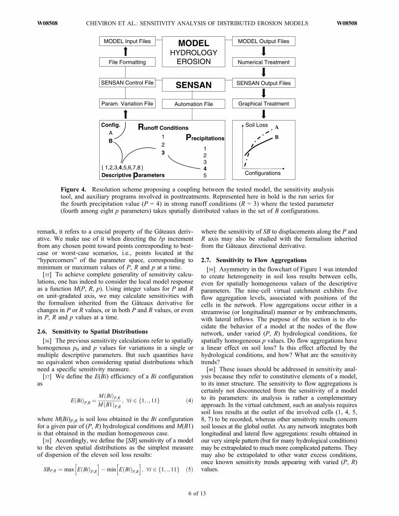
[30] The predefined parametric configurations can beprocessed in the model under control of the SENSAN[Doherty, 2004] sensitivity analysis tool as depicted inFigure 4. A line in the parameter variation file contains alluser‐defined values of the tested descriptive parameter in thenine cells of the virtual catchment, as well as indications ofthe P and R values. Consequently, the parameter variationfiles has as many lines as the number of parametric con-figurations to be tested. Once numerical and graphicalposttreatments have been completed and the parametervariation file has been entirely read, SENSAN’s executionnormally terminates. To keep it running on several param-eter files in a row, i.e., for each descriptive parameter, weused additional automation scripts.

2.5. Sensitivity Calculations

[31] When considering a single parameter, the intuitivedefinition of sensitivity is a first‐order approximation:

M pð Þ �M p0ð Þ ¼ @M

@pjp0 p� p0ð Þ ¼ S p� p0ð Þ ð1Þ

where M(p) is the output obtained from a certain p param-eter value, M(p0) is the output obtained from the p0 startingparameter value. S is the local sensitivity of the model,accounting for the derivative of M(p) with respect to p andcalculated at p0. In this formulation, S is implicitly constanton [p0, p], which questions the relevant size of the [p0, p]interval, especially for models associated with local non-linear behaviors or threshold effects.[32] According to the previous developments:

M pð ÞP;R �M p0ð ÞP;R ¼ SP;R �pð Þ ð2Þ

where model outputs and the associated sensitivity calcu-lation hold for the given (P, R) values and for any (suffi-ciently small) dp = p − p0 displacement in parameter spaceinvolving one or more descriptive parameters.[33] Using unit increments as gradations of the axis of

p values and only taking discrete values of p as multiplesof the unit increments, SP,R is de facto estimated as anapproximate Gâteaux directional derivative [Gâteaux, 1913;Cacuci, 2003; Behmardi and Nayeri, 2008]:

SP;R ¼ M p0 þ ��pð ÞP;R �M p0ð ÞP;R�

ð3Þ

where l is a (sufficiently small) real number and dp has notto be small anymore, provided p0 + dp is a point still insideor at least on the boundaries of the parameter space.[34] In such conditions, SP,R should be termed “sensi-

tivity at p0 in the direction of dp.” More than a formal

Figure 3. Spatially distributed B configurations used intesting specific erosion parameters. Light, medium, and darkgray cells receive values associated with minimum, median,and maximum soil loss, respectively.


5 of 13

remark, it refers to a crucial property of the Gâteaux deriv-ative. We make use of it when directing the dp incrementfrom any chosen point toward points corresponding to best‐case or worst‐case scenarios, i.e., points located at the“hypercorners” of the parameter space, corresponding tominimum or maximum values of P, R and p at a time.[35] To achieve complete generality of sensitivity calcu-

lations, one has indeed to consider the local model responseas a function M(P, R, p). Using integer values for P and Ron unit‐gradated axis, we may calculate sensitivities withthe formalism inherited from the Gâteaux derivative forchanges in P or R values, or in both P and R values, or evenin P, R and p values at a time.

2.6. Sensitivity to Spatial Distributions

[36] The previous sensitivity calculations refer to spatiallyhomogenous p0 and p values for variations in a single ormultiple descriptive parameters. But such quantities haveno equivalent when considering spatial distributions whichneed a specific sensitivity measure.[37] We define the E(Bi) efficiency of a Bi configuration

as

E Bið ÞP;R ¼M Bið ÞP;RM B1ð ÞP;R

; 8i 2 f1; :; 11g ð4Þ

where M(Bi)P,R is soil loss obtained in the Bi configurationfor a given pair of (P, R) hydrological conditions and M(B1)is that obtained in the median homogeneous case.[38] Accordingly, we define the [SB] sensitivity of a model

to the eleven spatial distributions as the simplest measureof dispersion of the eleven soil loss results:

SBP;R ¼ max E Bið ÞP;Rh i

�min E Bið ÞP;Rh i

; 8i 2 f1; :; 11g ð5Þ

where the sensitivity of SB to displacements along the P andR axis may also be studied with the formalism inheritedfrom the Gâteaux directional derivative.

2.7. Sensitivity to Flow Aggregations

[39] Asymmetry in the flowchart of Figure 1 was intendedto create heterogeneity in soil loss results between cells,even for spatially homogeneous values of the descriptiveparameters. The nine‐cell virtual catchment exhibits fiveflow aggregation levels, associated with positions of thecells in the network. Flow aggregations occur either in astreamwise (or longitudinal) manner or by embranchments,with lateral inflows. The purpose of this section is to elu-cidate the behavior of a model at the nodes of the flownetwork, under varied (P, R) hydrological conditions, forspatially homogeneous p values. Do flow aggregations havea linear effect on soil loss? Is this effect affected by thehydrological conditions, and how? What are the sensitivitytrends?[40] These issues should be addressed in sensitivity anal-

ysis because they refer to constitutive elements of a model,to its inner structure. The sensitivity to flow aggregations iscertainly not disconnected from the sensitivity of a modelto its parameters: its analysis is rather a complementaryapproach. In the virtual catchment, such an analysis requiressoil loss results at the outlet of the involved cells (1, 4, 5,8, 7) to be recorded, whereas other sensitivity results concernsoil losses at the global outlet. As any network integrates bothlongitudinal and lateral flow aggregations: results obtained inour very simple pattern (but for many hydrological conditions)may be extrapolated to much more complicated patterns. Theymay also be extrapolated to other water excess conditions,once known sensitivity trends appearing with varied (P, R)values.

Figure 4. Resolution scheme proposing a coupling between the tested model, the sensitivity analysistool, and auxiliary programs involved in posttreatments. Represented here in bold is the run series forthe fourth precipitation value (P = 4) in strong runoff conditions (R = 3) where the tested parameter(fourth among eight p parameters) takes spatially distributed values in the set of B configurations.


6 of 13

[41] The model response is M(P, R, p) and we considerhere the spatially homogeneous case for hydrological con-ditions (P, R) and all descriptive parameters contained in p.Changing variables, we introduce M(X, p) where X is anunknown function X(P, R) representing the amount of waterflowing out of a given cell. Consequently, X depends onlocal (P, R) values in a cell as well as on the inflow providedby immediate upstream cells. X can therefore be expressedas a function of the local runoff x and the incomingupstream flow y. With these notations X becomes X(x, y).[42] For illustration, let us describe flow aggregation

between cells 1 and 4.[43] 1. For example, soil loss at the outlet of cell 1 is

M(X1, p) with indicial notation X1(x1, y1) for local cell values.But no incoming upstream flow y1 must be considered ascell 1 itself is an upstream cell. We may thus express soilloss at the outlet of cell 1 as M(x1, p).[44] 2. Passing downstream to the next cell, soil loss at the

outlet of cell 4 is M(X4, p), with X4(x4, y4) and y4 = x1. Wemay now write M(x4, x1, p). Introducing dx = x4 − x1, we usethe equivalent expression M(dx, p) which relates soil loss atthe outlet of cell 4 to the streamwise flow aggregation dxbetween cells 1 and 4.[45] 3. It is then possible to test the sensitivity of this

quantity to different levels of P, R and p by comparingM(dx, p) with dM = M(X4, p) − M(X1, p). The same calcu-lation pertains for lateral aggregations.

2.8. Stages of the Procedure

2.8.1. Objectives[46] This section deals with construction of the multi-

stage (P, R, p) procedure, describing a progressive andorientated exploration of parameter space. A combination ofOAT and LH sampling methods is applied, which reducesthe parameterization to superparameters accounting for

equivalent slope (ps) and equivalent erodibility (pe). Theseessential components of any erosion model are then testedindividually and together to yield final sensitivity resultsprone to graphical representation. The following paragraphsenumerate the stages of the procedure for spatially homo-geneous configurations of the descriptive p parameters. Alast item indicates adaptations to the case of spatially dis-tributed p values.2.8.2. Preliminary Stage[47] The already‐described preliminary stage is the clas-

sification of fluxes and parameters into the independent P, Rand p categories. A further subdivision of the p categoryis needed for models that distinguish between linear (rill)and diffuse (interrill) erosion processes, before building theequivalent erodibility from the “equivalent linear erodibil-ity” and “equivalent diffuse erodibility.” If a parameteris called in both erosion processes, the best solution when-ever possible is to separately test its values in both pro-cesses under two different names. When no distinction existsbetween linear and diffuse erosion, for example in regional‐scale models, the procedure simply aims at building anequivalent erodibility.2.8.3. Individual One‐at‐a‐Time Tests[48] Figure 5 depicts the situation where candidate descrip-

tive parameters of the model are erodibility, rooting depthand soil texture. OAT tests are performed on each of themunder three combinations of P and R values, namely theless, median and most prone to soil loss. These tests involveat least five parameter values covering the entire nominalrange of variation. Useful representations of the results are“spider diagrams” plotting the relative output variation iny ordinate versus the relative input variation in x ordinate,the center of the diagram being the (0, 0) reference point.When testing a parameter, all others are held at their refer-ence (median) values.

Figure 5. Candidate p parameters are extracted from the innate parameterization of the model, testedone at a time (section 2.8.3) under indicated precipitation P and runoff R conditions, and then sortedby increasing soil loss order in as many values of the superparameter pe termed equivalent erodibility.


7 of 13

[49] If the model is proven to be insensitive to a candidateparameter under varied hydrological conditions, this param-eter is excluded from the procedure. We discard the prob-lematic though improbable case where a parameter has noinfluence if tested alone but a strong influence if tested incorrelation with some other parameters. The choice wemake here is coherent with the fact that prior knowledge isavailable on tested models. Moreover, such problematicbehaviors should have been removed or smoothened duringconstruction of the models.[50] If the model is sensitive to a candidate parameter, the

sign of the sensitivity is checked for: is it a positive one, anincrease in parameter value causing an increase in modelresponse, or a negative one? For parameters showing anegative sensitivity, the list of values is re‐sorted in oppositeorder, so that progressing inside this list finally givesincreasing soil loss values. In the chosen example, erod-ibility values are certainly already sorted in the right order,whereas rooting depth values probably need re‐sorting. Thetrend is a priori uncertain for soil texture values and mayeven depend on (P, R) conditions.2.8.4. Rules to Form Superparameters[51] In the next step, superparameters are formed by

assembling values of each of the retained candidate para-meters into increasing pe values. Figure 5 shows five testedvalues coded 1 to 5 for erodibility (e1 to e5), rooting depth(r1 to r5) and soil texture (t1 to t5). In addition, soil texturewas supposed here to have a positive sensitivity. Then fivecombinations of values are available to form the equivalenterodibility, which are (e1, r5, t1), (e2, r4, t2), (e3, r3, t3),(e4, r2, t4) and (e5, r1, t5) in increasing soil loss order.Depending on specificities of the models, at least two super-parameters are built: equivalent slope (ps) and equivalenterodibility (pe). The latter is subdivided into equivalentlinear erodibility and equivalent diffuse erodibility only indetailed models.

[52] Through options retained in the construction of super-parameters, the procedure follows an imaginary line betweenbest‐case and worst‐case scenarios. This strategy of an ori-entated exploration must be related to what is expectedfrom erosion models: identifying risky situations or changesin parameter values leading to progressively more riskysituations. Consequently a similar but enriched approach ismaintained in exploration of superparameter space, wheretrajectories are still centered on the best‐case–worst‐case axis.2.8.5. Exploration of Superparameter Space[53] Shown in Figure 6 is the coverage of superparameter

space from values of the equivalent slope ps and equivalenterodibility pe. The minimum grid of five by five values ispresented in the background. Two types of explorations areclearly visible, involving OAT displacements between blackcircles and Latin Hypercube (LH) samples between whitecircles. The first diagonal is the axis linking the best‐case tothe worst‐case scenarios, for any given (P, R) conditions.The second diagonal is a transverse axis of lesser impor-tance but whose points are needed to complete sensitivitymaps in the (ps, pe) plane.[54] All sensitivity calculations resort to equation (3). The

default algorithms perform sensitivity calculations betweentwo successive points on the OAT or LH axis. They couldbe easily extended to displacements between any two circlesbut were found sufficient to obtain relevant sensitivityinformation in the (ps, pe) plane. As the general expressionfor soil loss is M(P, R, ps, pe), local sensitivity results areavailable for variations in P, R, ps, pe and for any displace-ment involving one or more arguments of the M function.2.8.6. Adaptations for Spatially DistributedConfigurations[55] Figure 7 is the adaptation of Figure 5 to the case of

spatially distributed parameters. Each one of the candidatedescriptive parameters takes the eleven spatial distributionsof Figure 3. All configurations are then sorted by increasingefficiencies relative to the reference configuration B1. In thisexample, the least “productive” configuration (in terms ofcalculated soil loss) for e is B3 and the most productive isB8. B1 is near the beginning of the list, which means thatmany spatially distributed configurations yield more soilloss than the median homogeneous case. Depending onmodels and hydrological conditions, the position of B1 inthe list may drastically vary between simulations.[56] Gathering results for all descriptive parameters, Be

values are assembled exactly like pe values. If B3, B6 andB9 are the least productive configurations for e, r and trespectively, then Be1 is the combination (eB3, rB6, tB9)representing the lesser risk among tested spatial distributionsof the superparameter pe. At the other end of the list, in thefictitious situation of Figure 7 the higher risk Be11 isreached when parameters e, r and t take the B8, B5 and B6patterns, respectively. The logic is still to draw the line frombest‐case to worst‐case scenarios, for each of the super-parameters ps and pe, then for both.[57] Figure 8 is the adaptation of Figure 6 and describes

how Bs and Be values associated with ps and pe are arrangedinto OAT and LH samples. In the suggested exploration ofsuperparameter space, Be6 plays the role of the median pe3value in Figure 6. Again, the diagonal of primary interestjoins the (Bs1, Be1) and (Bs11, Be11) points at the lower leftand upper right of the (Bs, Be) plane. Directional sensitivitycalculations along OAT and LH axis allow comparisons

Figure 6. Exploration of superparameter space involvingone‐at‐a‐time (OAT, black circles) and Latin Hypercube(LH, white circles) displacements in values of the equivalentslope ps and equivalent erodibility pe. Best‐case and worst‐case scenarios are the less and most risky situations regard-ing erosion, respectively.


8 of 13

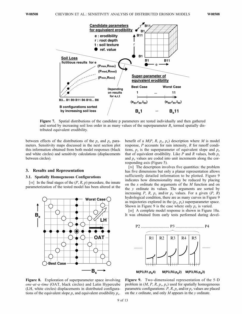
between effects of the distributions of the ps and pe para-meters. Sensitivity maps discussed in the next section plotthis information obtained from both model responses (blackand white circles) and sensitivity calculations (displacementsbetween circles).

3. Results and Representation

3.1. Spatially Homogeneous Configurations

[58] In the final stages of the (P, R, p) procedure, the innateparameterization of the tested model has been altered at the

benefit of a M(P, R, ps, pe) description where M is modelresponse, P accounts for rain intensity, R for runoff condi-tions, ps is the superparameter of equivalent slope and pethat of equivalent erodibility. Like P and R values, both psand pe values are coded into unit increments along the cor-responding axis (Figure 5).[59] The description involves five quantities: the problem

has five dimensions but only a planar representation allowssufficiently detailed information to be plotted. Figure 9indicates how dimensionality may be reduced by placingon the x ordinate the arguments of the M function and onthe y ordinate its values. The arguments are sorted byincreasing P, R, ps and/or pe values. For a given (P, R)hydrological condition, there are as many curves in Figure 9as trajectories explored in the (ps, pe) superparameter space.Shown in Figure 9 is the case where only pe is varied.[60] A complete model response is shown in Figure 10a.

It was obtained from early tests performed during devel-

Figure 7. Spatial distributions of the candidate p parameters are tested individually and then gatheredand sorted by increasing soil loss order in as many values of the superparameter Be termed spatially dis-tributed equivalent erodibility.

Figure 8. Exploration of superparameter space involvingone‐at‐a‐time (OAT, black circles) and Latin Hypercube(LH, white circles) displacements in distributed configura-tions of the equivalent slope ps and equivalent erodibility pe.

Figure 9. Two‐dimensional representation of the 5‐Dproblem in (M, P, R, ps, pe) used for spatially homogeneousparametric configurations: P, R, ps and/or pe values are placedon the x ordinate, and only M appears in the y ordinate.


9 of 13

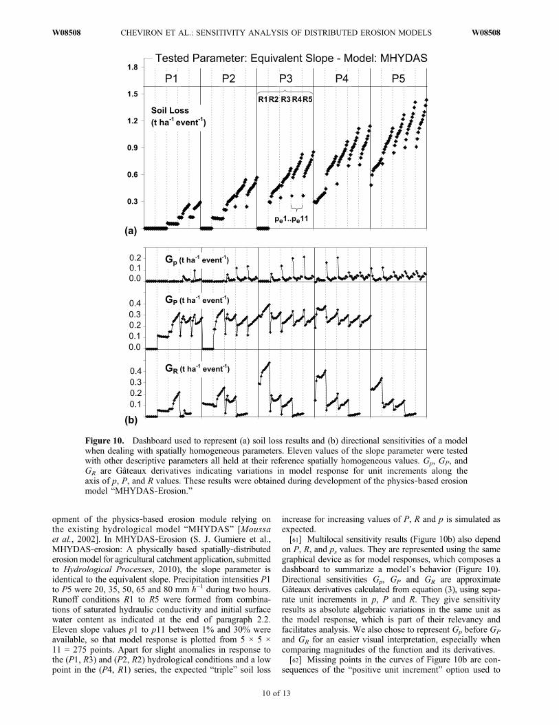
opment of the physics‐based erosion module relying onthe existing hydrological model “MHYDAS” [Moussaet al., 2002]. In MHYDAS‐Erosion (S. J. Gumiere et al.,MHYDAS‐erosion: A physically based spatially‐distributederosionmodel for agricultural catchment application, submittedto Hydrological Processes, 2010), the slope parameter isidentical to the equivalent slope. Precipitation intensities P1to P5 were 20, 35, 50, 65 and 80 mm h−1 during two hours.Runoff conditions R1 to R5 were formed from combina-tions of saturated hydraulic conductivity and initial surfacewater content as indicated at the end of paragraph 2.2.Eleven slope values p1 to p11 between 1% and 30% wereavailable, so that model response is plotted from 5 × 5 ×11 = 275 points. Apart for slight anomalies in response tothe (P1, R3) and (P2, R2) hydrological conditions and a lowpoint in the (P4, R1) series, the expected “triple” soil loss

increase for increasing values of P, R and p is simulated asexpected.[61] Multilocal sensitivity results (Figure 10b) also depend

on P, R, and ps values. They are represented using the samegraphical device as for model responses, which composes adashboard to summarize a model’s behavior (Figure 10).Directional sensitivities Gp, GP and GR are approximateGâteaux derivatives calculated from equation (3), using sepa-rate unit increments in p, P and R. They give sensitivityresults as absolute algebraic variations in the same unit asthe model response, which is part of their relevancy andfacilitates analysis. We also chose to represent Gp before GP

and GR for an easier visual interpretation, especially whencomparing magnitudes of the function and its derivatives.[62] Missing points in the curves of Figure 10b are con-

sequences of the “positive unit increment” option used to

Figure 10. Dashboard used to represent (a) soil loss results and (b) directional sensitivities of a modelwhen dealing with spatially homogeneous parameters. Eleven values of the slope parameter were testedwith other descriptive parameters all held at their reference spatially homogeneous values. Gp, GP, andGR are Gâteaux derivatives indicating variations in model response for unit increments along theaxis of p, P, and R values. These results were obtained during development of the physics‐based erosionmodel “MHYDAS‐Erosion.”


10 of 13

calculate sensitivities. For example, sensitivity results GP(P,R, p) represented in the P4 column address variations fromM(P4, R, p) to M(P5, R, p) and no such results are given forvariations from P5 to P6 because P6 does not exist. Thesame applies here when values p = 10 and R = 4 are reached.[63] Sensitivity results show here noticeably high points

in the Gp curve corresponding to transitions between thefirst (1%) and second (3%) slope values which resulted inthreshold effects, more pronounced for median (P, R) valuesnear the middle of the curve. The GP curve rises withincreasing (P, R) conditions then stabilizes, indicating anear‐linear effect of P values for high water excess condi-tions. The sensitivity to an increase in runoff conditions issomewhat different. Whatever the P value, GR stronglydecreases when R is increased, the effect being again morepronounced for median P values.

3.2. Spatially Distributed Configurations

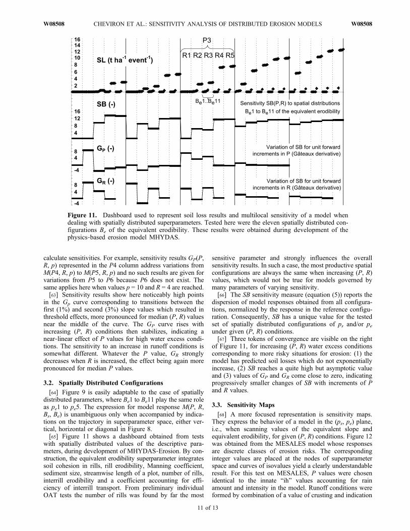
[64] Figure 9 is easily adaptable to the case of spatiallydistributed parameters, where Be1 to Be11 play the same roleas pe1 to pe5. The expression for model response M(P, R,Bs, Be) is unambiguous only when accompanied by indica-tions on the trajectory in superparameter space, either ver-tical, horizontal or diagonal in Figure 8.[65] Figure 11 shows a dashboard obtained from tests

with spatially distributed values of the descriptive para-meters, during development of MHYDAS‐Erosion. By con-struction, the equivalent erodibility superparameter integratessoil cohesion in rills, rill erodibility, Manning coefficient,sediment size, streamwise length of a plot, number of rills,interrill erodibility and a coefficient accounting for effi-ciency of interrill transport. From preliminary individualOAT tests the number of rills was found by far the most

sensitive parameter and strongly influences the overallsensitivity results. In such a case, the most productive spatialconfigurations are always the same when increasing (P, R)values, which would not be true for models governed bymany parameters of varying sensitivity.[66] The SB sensitivity measure (equation (5)) reports the

dispersion of model responses obtained from all configura-tions, normalized by the response in the reference configu-ration. Consequently, SB has a unique value for the testedset of spatially distributed configurations of ps and/or peunder given (P, R) conditions.[67] Three tokens of convergence are visible on the right

of Figure 11, for increasing (P, R) water excess conditionscorresponding to more risky situations for erosion: (1) themodel has predicted soil losses which do not exponentiallyincrease, (2) SB reaches a quite high but asymptotic valueand (3) values of GP and GR come close to zero, indicatingprogressively smaller changes of SB with increments of Pand R values.

3.3. Sensitivity Maps

[68] A more focused representation is sensitivity maps.They express the behavior of a model in the (ps, pe) plane,i.e., when scanning values of the equivalent slope andequivalent erodibility, for given (P, R) conditions. Figure 12was obtained from the MESALES model whose responsesare discrete classes of erosion risks. The correspondinginteger values are placed at the nodes of superparameterspace and curves of isovalues yield a clearly understandableresult. For this test on MESALES, P values were chosenidentical to the innate “ih” values accounting for rainamount and intensity in the model. Runoff conditions wereformed by combination of a value of crusting and indication

Figure 11. Dashboard used to represent soil loss results and multilocal sensitivity of a model whendealing with spatially distributed superparameters. Tested here were the eleven spatially distributed con-figurations Be of the equivalent erodibility. These results were obtained during development of thephysics‐based erosion model MHYDAS.


11 of 13

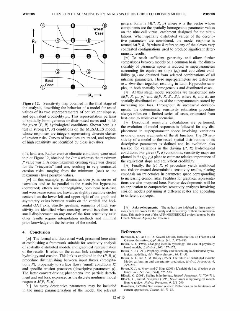
of a land use. Rather erosive climatic conditions were usedto plot Figure 12, obtained for P = 4 whereas the maximumP value was 5. A near‐maximum crusting value was chosenfor the “vineyards” land use, resulting in very contrastederosion risks, ranging from the minimum (one) to themaximum (five) possible values.[69] In this example, pe dominates over ps as curves of

isovalues tend to be parallel to the x axis but hypercube(combined) effects are nonnegligible, both near best‐caseand worst‐case scenarios. Isovalues slightly resemble circlescentered on the lower left and upper right of the graph andasymmetry exists between results on the vertical and hori-zontal OAT axis. Strictly speaking, segments of high sen-sitivity are identified when crossing several isovalues in asmall displacement on any one of the four sensitivity axis:other results require interpolation methods and minimalprior knowledge on the behavior of the model.

4. Conclusion

[70] The formal and theoretical work presented here aimsat establishing a framework suitable for sensitivity analysisof spatially distributed models and graphical representationof the results. It relies on the causal link existing betweenhydrology and erosion. This link is exploited in the (P, R, p)procedure distinguishing between input fluxes (precipita-tions P), propensity to surface flows (runoff conditions R)and specific erosion processes (descriptive parameters p).The latter convert driving phenomena into particle detach-ment and soil loss, expressed as the discrete nonlinear modelresponse M(P, R, p).[71] As many descriptive parameters may be included

in the innate parameterization of the model, the relevant

general form is M(P, R, p) where p is the vector whosecomponents are the spatially homogenous parameter valueson the nine‐cell virtual catchment designed for the simu-lations. When spatially distributed values of the descrip-tive parameters are considered, the model response istermed M(P, R, B) where B refers to any of the eleven verycontrasted configurations used to produce significant deter-ministic results.[72] To reach sufficient genericity and allow further

comparisons between models on a common basis, the dimen-sionality of parameter space is reduced as superparametersaccounting for equivalent slope (ps) and equivalent erod-ibility (pe) are obtained from selected combinations of allintrinsic parameters. These superparameters are tested oneat a time then together, resulting in Latin Hypercube sam-ples, in both spatially homogeneous and distributed cases.[73] At this stage, model responses are transformed into

M(P, R, ps, pe) and M(P, R, Bs, Be), where Bs and Be arespatially distributed values of the superparameters sorted byincreasing soil loss. Throughout its successive develop-ments, the deterministic sensitivity estimation procedurealways relies on a limited series of cases, orientated frombest‐case to worst‐case scenarios.[74] Directional sensitivity calculations are performed:

the evolution of model responses is followed for any dis-placement in superparameter space involving variationsin one or more arguments of the M function. The SB sen-sitivity of a model to the tested spatial distributions of itsdescriptive parameters is defined and its evolution alsotracked for variations in the driving (P, R) hydrologicalconditions. For given (P, R) conditions, sensitivity maps areplotted in the (ps, pe) plane to estimate relative importance ofthe equivalent slope and equivalent erodibility.[75] Finally, the (P, R, p) procedure yields multilocal

and risk‐orientated deterministic sensitivity results, placingemphasis on trajectories in parameter space correspondingto increasing erosion risks. Facilities for graphical representa-tions are also proposed here. Further developments will bean application to comparative sensitivity analyses involvingerosion models pertaining at different scales and appealingto different concepts.

[76] Acknowledgments. The authors are indebted to three anony-mous peer reviewers for the quality and exhaustivity of their recommenda-tions. This study is part of the ANR‐MESOEROS21 project, granted by theFrench National Agency for Research.

ReferencesBehmardi, D., and E. D. Nayeri (2008), Introduction of Fréchet andGâteaux derivative, Appl. Math. Sci., 2, 975–980.

Beven, K. J. (1989), Changing ideas in hydrology: The case of physicallybased models, J. Hydrol., 105, 157–172.

Beven, K. J. (1993), Prophecy, reality and uncertainty in distributed hydro-logical modelling, Adv. Water Resour., 16, 41–51.

Beven, K. J., and A. M. Binley (1992), The future of distributed models:Model calibration and uncertainty prediction, Hydrol. Processes, 6,279–298.

Beven, K. J., A. Musy, and C. Higy (2001), L’unicité de lieu, d’action et detemps, Rev. Sci. Eau, 14(4), 525–533.

Blöschl, G. (2001), Scaling in hydrology, Hydrol. Processes, 15, 709–711.Blöschl, G., and M. Sivapalan (1995), Scale issues in hydrological model-ling: A review, Hydrol. Processes, 9, 251–290.

Boardman, J. (2006), Soil erosion science: Reflections on the limitations ofcurrent approaches, Catena, 68, 73–86.

Figure 12. Sensitivity map obtained in the final stage ofthe analysis, describing the behavior of a model for testedvalues of its two superparameters of equivalent slope psand equivalent erodibility pe. This representation pertainsto spatially homogeneous or distributed cases and holdsfor given (P, R) hydrological conditions. Shown here is atest in strong (P, R) conditions on the MESALES model,whose responses are integers representing discrete classesof erosion risks. Curves of isovalues are traced, and regionsof high sensitivity are identified by close isovalues.


12 of 13

Bryan, R. B. (1976), Considerations on soil erodibility indices and sheet-wash, Catena, 3, 99–111.

Bryan, R. B. (2000), Soil erodibility and processes of water erosion on hill-slope, Geomorphology, 1, 385–415.

Cacuci, D. G. (1981), Sensitivity theory for non‐linear systems. I. Non‐linear functional analysis approach, J. Math. Phys., 22, 2794–2802.

Cacuci, D. G. (2003), Sensitivity and Uncertainty Analysis, vol. 1, Theory,Chapman and Hall, Boca Raton, Fla.

Campolongo, F., and R. Braddock (1999), Sensitivity analysis of theIMAGE Greenhouse model, Environ. Modell. Software, 14, 275–282.

Campolongo, F., J. Cariboni, and A. Saltelli (2007), An effective screeningdesign for sensitivity analysis of large models, Environ. Modell. Soft-ware, 22(10), 1509–1518.

Castaings, W., D. Dartus, F.‐X. Le Dimet, and G.‐M. Saulnier (2007), Sen-sitivity analysis and parameter estimation for the distributed modelingof infiltration excess overland flow, Hydrol. Earth Syst. Sci. Discuss.,4, 363–405.

Cerdan, O., Y. Le Bissonnais, A. Couturier, and N. Saby (2002), Modellinginterrill erosion in small cultivated catchments, Hydrol. Processes, 16,3215–3226.

Crosetto, M., and S. Tarantola (2001), Uncertainty and sensitivity analysis:Tools for GIS‐based model implementation, Int. J. Geogr. Info. Sci.,15(5), 415–437.

de Marsily, G. (1994), Quelques réflexions sur l’utilisation des modèles enhydrologie, Rev. Sci. Eau, 7(3), 219–234.

De Roo, A. P. J., R. J. E. Offermans, and N. H. D. T. Cremers (1996),LISEM: A single‐event, physically based hydrological and soil erosionmodel for drainage basins. II: Sensitivity analysis, validation and appli-cation, Hydrol. Processes, 10, 1119–1126.

Doherty, J. (2004), PEST: Model‐Independent Parameter Estimation—User Manual, Watermark Numer. Comput., Brisbane, Qld., Australia.

Frey, H. C., and S. R. Patil (2002), Identification and review of sensitivityanalysis methods, Risk Anal., 22(3), 553–578.

Gâteaux, R. (1913), Sur les fonctionnelles continues et les fonctionnellesanalytiques, C. R. Hebd. Seances Acad. Sci., 157, 325–327.

Gobin, A., R. J. A. Jones, M. Kirkby, P. Campling, C. Kosmas, G. Govers,and A. R. Gentile (2004), Pan‐European assessment and monitoring ofsoil erosion by water, Environ. Sci. Policy, 7, 25–38.

Gumiere, S. J., Y. Le Bissonnais, and D. Raclot (2009), Soil resistance tointerrill erosion: Model parameterization and sensitivity, Catena, 77,274–284.

Helton, J. C. (1993), Uncertainty and sensitivity analysis techniques for usein performance assessment for radioactive waste disposal, Reliab. Eng.Syst. Safety, 42, 327–367.

Hier‐Majumder, C. A., B. J. Travis, E. Belanger, G. Richard, A. P. Vincent,and D. A. Yuen (2006), Efficient sensitivity analysis for flow and trans-port in the Earth’s crust and mantle, Geophys. J. Int., 166, 907–922.

Ionescu‐Bujor, M., and D. G. Cacuci (2004), A comparative review of sen-sitivity and uncertainty analysis of large‐scale systems. I. Deterministicmethods, Nucl. Sci. Eng., 147(3), 189–203.

Jetten, V., A. de Roo, and D. Favis‐Mortlock (1999), Evaluation of field‐scale and catchment‐scale soil erosion models, Catena, 37, 521–541.

Jetten, V., G. Govers, and R. Hessel (2003), Erosion models: Quality ofspatial predictions, Hydrol. Processes, 17, 887–900.

Jetten, V., J. Boiffin, and A. de Roo (2005), Defining monitoring strategiesfor runoff and erosion studies in agricultural catchments: A simulationapproach, Eur. J. Soil Sci., 47, 579–592.

Kamboj, S., J.‐J. Cheng, and C. Yu (2005), Deterministic vs. probabilisticanalyses to identify sensitive parameters in dose assessment usingRESRAD, Health Phys., 88(5), suppl. 2, 104–109.

Kirkby, M. J., B. J. Irvine, R. J. A. Jones, G. Govers, and PESERA team(2008), The PESERA coarse scale erosion model for Europe. I.—Modelrationale and implementation, Eur. J. Soil Sci., 59, 1293–1306.

Kleijnen, J. P. C., and J. C. Helton (1999), Statistical analysis of scatter-plots to identify important factors in large‐scale simulations. 2: Robust-ness of techniques, Reliab. Eng. Syst. Safety, 65, 187–197.

Knapen, A., J. Poesen, G. Govers, G. Gyssels, and J. Nachtergaele (2007),Resistance of soils to concentrated flow erosion: A review, Earth Sci.Rev., 80, 75–109.

Knight, D. W., and K. Shiono (1996), Channel and floodplain hydraulics,in Floodplain Processes, edited by M. G. Anderson, D. E. Walling, andP. D. Bates, pp. 139–182, John Wiley, New York.

Le Bissonnais, Y., C. Montier, J. Jamagne, J. Daroussin, and D. King(2002), Mapping erosion risk for cultivated soil in France, Catena, 46,207–220.

Lilburne, L., and S. Tarantola (2009), Sensitivity analysis of spatial models,Int. J. Geogr. Info. Sci., 23(2), 151–168.

Lions, J. L. (1968), Contrôle Optimal des Systèmes Gouvernés par desÉquations aux Dérivées Partielles, Gauthier‐Villars, Paris.

McKay, M. D., R. J. Beckman, and W. J. Conover (1979), A comparison ofthree methods for selecting values of input variables in the analysis ofoutput from a computer code, Technometrics, 21, 239–245.

Merritt, W. S., R. A. Letcher, and A. J. Jakeman (2003), A review of ero-sion and sediment transport models, Environ. Modell. Software, 18,761–799.

Mitchell, M., and C. Campbell (2001), Probabilistic exposure assessment ofoperator and residential exposure: A Canadian regulatory perspective,Ann. Occup. Hyg., 45, 43–47.

Morris, M. D. (1991), Factorial sampling plans for preliminary computa-tional experiments, Technometrics, 33, 161–174.

Moussa, R., M. Voltz, and P. Andrieux (2002), Effects of the spatial orga-nization of agricultural management on the hydrological behaviour of afarmed catchment during flood events, Hydrol. Processes, 16, 393–412.

Mulungu, D. M. M., and S. E. Munishi (2007), Simiyu River catchmentparameterization using SWAT model, Phys. Chem. Earth, 32, 1032–1039.

Nearing, M. A. (2000), Evaluating soil erosion models using measured plotdata: Accounting for variability in the data, Earth Surf. Processes Land-forms, 25, 1035–1043.

Nearing, M. A., L. Deer‐Ascough, and J. M. Laflen (1990), Sensitivityanalysis of the WEPP hillslope profile erosion modelTrans. ASAE, 33,839–849.

Nearing, M. A., G. Govers, and L. D. Norton (1999), Variability in soilerosion data from replicated plots, Soil Sci. Soc. Am. J., 63, 1829–1835.

Nord, G., and M. Esteves (2005), PSEM_2D: A physically based model oferosion processes at the plot scale, Water Resour. Res., 41, W08407,doi:10.1029/2004WR003690.

Pappenberger, F., K. J. Beven, M. Ratto, and P. Matgen (2008), Multi‐method global sensitivity analysis of flood inundation models, Adv.Water Resour., 31, 1–14.

Ronen, Y. (1988), The role of uncertainties, in Uncertainty Analysis, pp. 1–40,CRC Press, Boca Raton, Fla.

Saltelli, A., K. Chan, and E. M. Scott (2000), Sensitivity Analysis, JohnWiley, New York.

Saltelli, A., S. Tarantola, F. Campolongo, and M. Ratto (2004), SensitivityAnalysis in Practice: A Guide to Assessing Scientific Models, JohnWiley, Hoboken, N. J.

Sheridan, G. J., H. B. So, R. J. Loch, and C. M. Walker (2000), Estimationof erosion model erodibility parameters from media properties, Aust. J.Soil Res., 38, 256–284.

Sieber, A., and S. Uhlenbrook (2005), Sensitivity analyses of a distributedcatchment model to verify the model structure, J. Hydrol., 310, 216–235.

Sivapalan, M. (2003), Process complexity at hillslope scale, process sim-plicity at the watershed scale: Is there a connection?, Hydrol. Processes,17, 1037–1041.

Sobol, I. M. (1993), Sensitivity estimates for nonlinear mathematicalmodels, Math. Modell. Comput. Exp., 1, 407–417.

Tang, Y., P. Reed, K. van Werkhoven, and T. Wagener (2007), Advancingthe identification and evaluation of distributed rainfall‐runoff modelsusing global sensitivity analysis, Water Resour. Res., 43, W06415,doi:10.1029/2006WR005813.

Turanyi, T., and H. Rabitz (2000), Local methods and their applications,in Sensitivity Analysis, edited by A. Saltelli, K. Chan, and E. M. Scott,pp. 367–383, John Wiley, New York.

van Griensven, A., T. Meixner, S. Grunwald, T. Bishop, M. Diluzio, andR. Srinivasan (2006), A global sensitivity analysis tool for the para-meters of multi‐variable catchment models, J. Hydrol., 324, 10–23.

Veihe, A., and J. Quinton (2000), Sensitivity analysis of EUROSEM usingMonte Carlo simulation: I. Hydrological, soil and vegetation parameters,Hydrol. Processes, 14, 915–926.

Wischmeier, W. H., and D. D. Smith (1978), Agricultural Handbook,vol. 537, Predicting Rainfall Erosion Losses, U.S. Dep. of Agric.,Washington, D. C.

B. Cheviron, S. J. Gumiere, Y. Le Bissonnais, and R. Moussa, UMRLISAH, INRA, IRD, SupAgro, 2 place Viala, F‐34060 Montpellier,France. ([email protected]; [email protected];[email protected]; [email protected])D. Raclot, UMR LISAH, IRD, SupAgro, 5 impasse Chehrazade, 1004

Tunis, Tunisia. ([email protected])


13 of 13

Sensitivity analysis of distributed erosion models: Framework

Documents